Introduction to Statistics -- STAT 200 -- Briercrest College
577
Introduction to Statistics -- STAT 200 -- Briercrest College -- Version 2017 Revision A Collection edited by: Claude Laflamme Content authors: Claude Laflamme, Svitlana Pshenychna, OpenStax, Joshua Emmanuel, Colleen Ball, and OpenStax Business Statistics Based on: Business Statistics -- STA200 -- Briercrest College -- Version 2017 Revision A <http://legacy.cnx.org/content/col11969/1.10>. Online: <https://legacy.cnx.org/content/col12102/1.7> This selection and arrangement of content as a collection is copyrighted by Claude Laflamme. Creative Commons Attribution License 4.0 http://creativecommons.org/licenses/by/4.0/ Collection structure revised: 2018/03/22 PDF Generated: 2021/08/31 12:39:38 For copyright and attribution information for the modules contained in this collection, see the "Attributions" section at the end of the collection. 1
-
Upload
khangminh22 -
Category
Documents
-
view
0 -
download
0
Transcript of Introduction to Statistics -- STAT 200 -- Briercrest College

Introduction to Statistics -- STAT 200 --Briercrest College -- Version 2017Revision ACollection edited by: Claude LaflammeContent authors: Claude Laflamme, Svitlana Pshenychna, OpenStax, Joshua Emmanuel, Colleen Ball, andOpenStax Business StatisticsBased on: Business Statistics -- STA200 -- Briercrest College -- Version 2017 Revision A<http://legacy.cnx.org/content/col11969/1.10>.Online: <https://legacy.cnx.org/content/col12102/1.7>This selection and arrangement of content as a collection is copyrighted by Claude Laflamme.Creative Commons Attribution License 4.0 http://creativecommons.org/licenses/by/4.0/Collection structure revised: 2018/03/22PDF Generated: 2021/08/31 12:39:38For copyright and attribution information for the modules contained in this collection, see the "Attributions"section at the end of the collection.
1

2
This OpenStax book is available for free at https://legacy.cnx.org/content/col12102/1.7

Table of Contents
Preface -- STAT 200 -- Briecrest College -- Version 2017RevA . . . . . . . . . . . . . . . . . . . . . 1Chapter 1: Sampling and Data . . . . . . . . . . . . . . . . . . . . . . . . . . . . . . . . . . . . . . 3
1.1 Definitions of Statistics, Probability, and Key Terms . . . . . . . . . . . . . . . . . . . . . . . 31.2 Data, Sampling, and Variation in Data and Sampling . . . . . . . . . . . . . . . . . . . . . . 71.3 Levels of Measurement . . . . . . . . . . . . . . . . . . . . . . . . . . . . . . . . . . . . 191.4 Experimental Design and Ethics . . . . . . . . . . . . . . . . . . . . . . . . . . . . . . . . 27
Chapter 2: Descriptive Statistics . . . . . . . . . . . . . . . . . . . . . . . . . . . . . . . . . . . 432.1 Frequency Distributions and Graphs - (Base Version - Lyryx Learning) . . . . . . . . . . . . 442.2 Measures of the Location of the Data - (Base Version - Lyryx Learning) . . . . . . . . . . . 532.3 Measures of the Center of the Data . . . . . . . . . . . . . . . . . . . . . . . . . . . . . . 612.4 Sigma Notation and Calculating the Arithmetic Mean . . . . . . . . . . . . . . . . . . . . . 642.5 Skewness and the Mean, Median, and Mode . . . . . . . . . . . . . . . . . . . . . . . . . 652.6 Measures of the Spread of the Data - (Base Version - Lyryx Learning) . . . . . . . . . . . . 67
Chapter 3: Probability Topics . . . . . . . . . . . . . . . . . . . . . . . . . . . . . . . . . . . . . 1033.1 Terminology . . . . . . . . . . . . . . . . . . . . . . . . . . . . . . . . . . . . . . . . . . 1033.2 Independent and Mutually Exclusive Events . . . . . . . . . . . . . . . . . . . . . . . . . . 1083.3 Two Basic Rules of Probability . . . . . . . . . . . . . . . . . . . . . . . . . . . . . . . . . 1163.4 Contingency Tables and Probability Trees . . . . . . . . . . . . . . . . . . . . . . . . . . . 1213.5 Principles of Counting - (Base Version - Lyryx Learning) . . . . . . . . . . . . . . . . . . . 132
Chapter 4: Discrete Random Variables . . . . . . . . . . . . . . . . . . . . . . . . . . . . . . . . 1574.1 Hypergeometric Distribution . . . . . . . . . . . . . . . . . . . . . . . . . . . . . . . . . . 1594.2 Binomial Distribution - (Base Version - Lyryx Learning) . . . . . . . . . . . . . . . . . . . . 1604.3 Geometric Distribution . . . . . . . . . . . . . . . . . . . . . . . . . . . . . . . . . . . . . 1654.4 Poisson Distribution . . . . . . . . . . . . . . . . . . . . . . . . . . . . . . . . . . . . . . 170
Chapter 5: Continuous Random Variables . . . . . . . . . . . . . . . . . . . . . . . . . . . . . . 1975.1 Properties of Continuous Probability Density Functions . . . . . . . . . . . . . . . . . . . . 1985.2 The Uniform Distribution . . . . . . . . . . . . . . . . . . . . . . . . . . . . . . . . . . . . 2025.3 The Exponential Distribution . . . . . . . . . . . . . . . . . . . . . . . . . . . . . . . . . . 205
Chapter 6: The Normal Distribution . . . . . . . . . . . . . . . . . . . . . . . . . . . . . . . . . . 2356.1 The Standard Normal Distribution - (Base Version - Lyryx Learning) . . . . . . . . . . . . . 2366.2 Using the Normal Distribution - (Base Version - Lyryx Learning) . . . . . . . . . . . . . . . 242
Chapter 7: The Central Limit Theorem . . . . . . . . . . . . . . . . . . . . . . . . . . . . . . . . 2677.1 The Central Limit Theorem for Sample Means - (Base Version - Lyryx Learning) . . . . . . . 2687.2 Exploring the Central Limit Theorem - (Base Version - Lyryx Learning) . . . . . . . . . . . . 270
Chapter 8: Confidence Intervals . . . . . . . . . . . . . . . . . . . . . . . . . . . . . . . . . . . . 2858.1 A Confidence Interval for a Population Standard Deviation, Known or Large Sample Size . . 2868.2 A Confidence Interval for a Population Standard Deviation Unknown, Small Sample Case . . 2958.3 A Confidence Interval for A Population Proportion . . . . . . . . . . . . . . . . . . . . . . . 2998.4 Calculating the Sample Size n: Continuous and Binary Random Variables . . . . . . . . . . 303
Chapter 9: Hypothesis Testing with One Sample . . . . . . . . . . . . . . . . . . . . . . . . . . . 3339.1 Null and Alternative Hypotheses . . . . . . . . . . . . . . . . . . . . . . . . . . . . . . . . 3349.2 Outcomes and the Type I and Type II Errors . . . . . . . . . . . . . . . . . . . . . . . . . . 3359.3 Distribution Needed for Hypothesis Testing . . . . . . . . . . . . . . . . . . . . . . . . . . 3389.4 Full Hypothesis Test Examples - (Base Version - Lyryx Learning) . . . . . . . . . . . . . . . 3449.5 Rare Events, the Sample, Decision and Conclusion . . . . . . . . . . . . . . . . . . . . . . 353
Chapter 10: Hypothesis Testing with Two Samples . . . . . . . . . . . . . . . . . . . . . . . . . 37310.1 Comparing Two Independent Population Means . . . . . . . . . . . . . . . . . . . . . . . 37410.2 Comparing Two Independent Population Proportions . . . . . . . . . . . . . . . . . . . . 38110.3 Two Population Means with Known Standard Deviations . . . . . . . . . . . . . . . . . . 38410.4 Matched or Paired Samples . . . . . . . . . . . . . . . . . . . . . . . . . . . . . . . . . 387
Chapter 11: The Chi-Square Distribution . . . . . . . . . . . . . . . . . . . . . . . . . . . . . . . 41711.1 Facts About the Chi-Square Distribution . . . . . . . . . . . . . . . . . . . . . . . . . . . 41811.2 Test of a Single Variance . . . . . . . . . . . . . . . . . . . . . . . . . . . . . . . . . . . 41811.3 Goodness-of-Fit Test . . . . . . . . . . . . . . . . . . . . . . . . . . . . . . . . . . . . . 42211.4 Test of Independence . . . . . . . . . . . . . . . . . . . . . . . . . . . . . . . . . . . . . 42911.5 Test for Homogeneity . . . . . . . . . . . . . . . . . . . . . . . . . . . . . . . . . . . . . 43411.6 Comparison of the Chi-Square Tests . . . . . . . . . . . . . . . . . . . . . . . . . . . . . 437

Chapter 12: F Distribution and One-Way ANOVA . . . . . . . . . . . . . . . . . . . . . . . . . . . 46512.1 Test of Two Variances . . . . . . . . . . . . . . . . . . . . . . . . . . . . . . . . . . . . . 46512.2 One-Way ANOVA . . . . . . . . . . . . . . . . . . . . . . . . . . . . . . . . . . . . . . . 46912.3 The F Distribution and the F-Ratio . . . . . . . . . . . . . . . . . . . . . . . . . . . . . . 46912.4 Facts About the F Distribution . . . . . . . . . . . . . . . . . . . . . . . . . . . . . . . . 479
Chapter 13: Linear Regression and Correlation . . . . . . . . . . . . . . . . . . . . . . . . . . . 50313.1 The Correlation Coefficient r - (Base Version - Lyryx Learning) . . . . . . . . . . . . . . . 50413.2 Testing the Significance of the Correlation Coefficient - (Base Version - Lyryx Learning) . . 50713.3 Linear Equations - (Base Version - Lyryx Learning) . . . . . . . . . . . . . . . . . . . . . 50813.4 The Regression Equation - (Base Version - Lyryx Learning) . . . . . . . . . . . . . . . . . 51013.5 Predicting with a Regression Equation - (Base Version - Lyryx Learning) . . . . . . . . . . 51613.6 How to Use Excel for Regression Analysis - (Base Version - Lyryx Learning) . . . . . . . . 51913.7 Regression Analysis with the BAII Plus Calculator . . . . . . . . . . . . . . . . . . . . . . 526
Appendix A: Statistical Tables . . . . . . . . . . . . . . . . . . . . . . . . . . . . . . . . . . . . . 531Appendix B: Mathematical Phrases, Symbols, and Formulas . . . . . . . . . . . . . . . . . . . . 551Index . . . . . . . . . . . . . . . . . . . . . . . . . . . . . . . . . . . . . . . . . . . . . . . . . . . 559
This OpenStax book is available for free at https://legacy.cnx.org/content/col12102/1.7

PREFACE -- STAT 200 -- BRIECRESTCOLLEGE -- VERSION 2017REVA
About Business StatisticsBusiness Statistics is designed for the one-semester, introduction to statistics course and is geared toward students majoringin fields other than math or engineering, and this adaptation of the original Introductory Statistics text has been donespecifically for the course STA200 at Briecrest College. This text assumes students have been exposed to intermediatealgebra, and it focuses on the applications of statistical knowledge rather than the theory behind it.
The foundation of this textbook is Collaborative Statistics, by Barbara Illowsky and Susan Dean. Additional topics,examples, and ample opportunities for practice have been added to each chapter. The development choices for this textbookwere made with the guidance of many faculty members who are deeply involved in teaching this course. These choices ledto innovations in art, terminology, and practical applications, all with a goal of increasing relevance and accessibility forstudents. We strove to make the discipline meaningful, so that students can draw from it a working knowledge that willenrich their future studies and help them make sense of the world around them.
Coverage and Scope
Chapter 1 Sampling and DataChapter 2 Descriptive StatisticsChapter 3 Probability TopicsChapter 4 Discrete Random VariablesChapter 5 Continuous Random VariablesChapter 6 The Normal DistributionChapter 7 The Central Limit TheoremChapter 8 Confidence IntervalsChapter 9 Hypothesis Testing with One SampleChapter 10 Hypothesis Testing with Two SamplesChapter 11 The Chi-Square DistributionChapter 12 F Distribution and One-Way ANOVAChapter 13 Linear Regression and Correlation
Pedagogical Foundation and Features• Examples are placed strategically throughout the text to show students the step-by-step process of interpreting and
solving statistical problems. To keep the text relevant for students, the examples are drawn from a broad spectrum ofpractical topics; these include examples about college life and learning, health and medicine, retail and business, andsports and entertainment.
• Practice, Homework, and Bringing It Together problems give the students problems at various degrees of difficultywhile also including real-world scenarios to engage students.
About Our TeamOriginal Authors
Barbara Illowsky De Anza College
Susan Dean De Anza College
Humber College Contributors
Dr. Svitlana Pshenychna Professor of Mathematics and Statistics, Humber College
Colleen Ball Professor of Mathematics and Statistics, Humber College
Joshua Emmanuel Professor of Mathematics and Statistics, Humber College
Preface 1

University of Oklahoma Contributors
Alexander Holmes Regent's Professor of Economics University of Oklahoma
Kevin Hadley Analyst, Federal Reserve Bank of Kansas City
Mathew Price Research Assistant, University of Oklahoma
2 Preface
This OpenStax book is available for free at https://legacy.cnx.org/content/col12102/1.7
1 | SAMPLING AND DATA
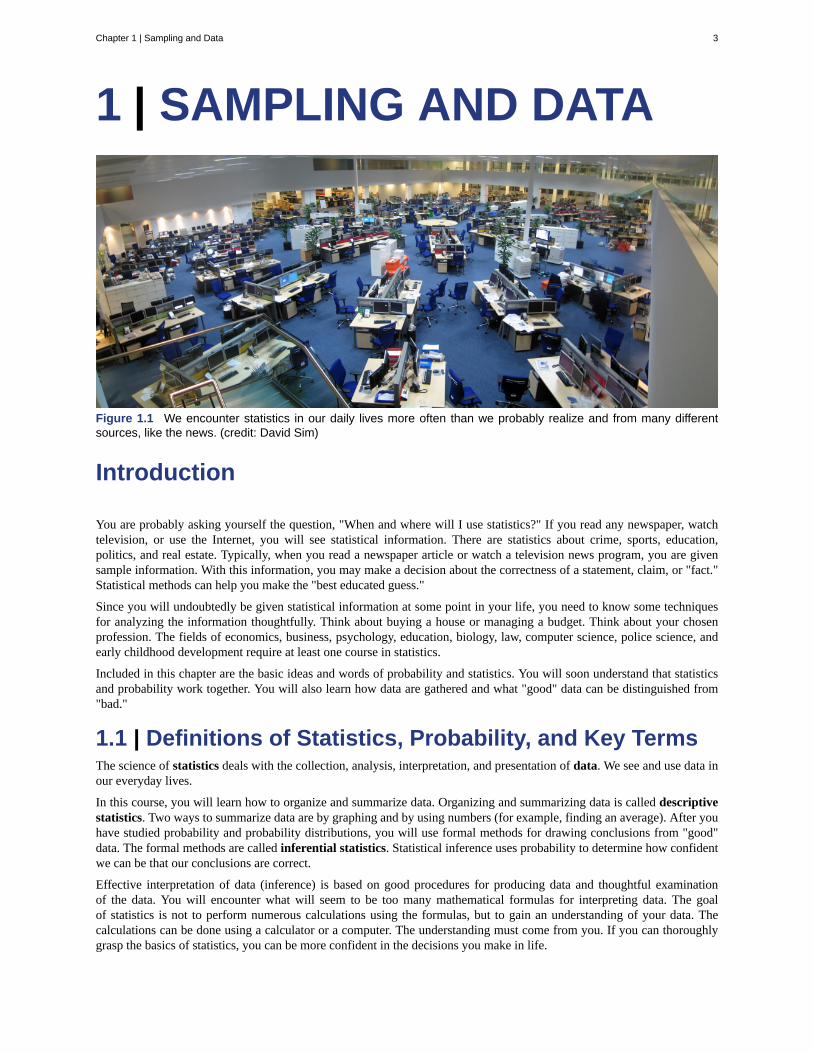
Figure 1.1 We encounter statistics in our daily lives more often than we probably realize and from many differentsources, like the news. (credit: David Sim)
Introduction
You are probably asking yourself the question, "When and where will I use statistics?" If you read any newspaper, watchtelevision, or use the Internet, you will see statistical information. There are statistics about crime, sports, education,politics, and real estate. Typically, when you read a newspaper article or watch a television news program, you are givensample information. With this information, you may make a decision about the correctness of a statement, claim, or "fact."Statistical methods can help you make the "best educated guess."
Since you will undoubtedly be given statistical information at some point in your life, you need to know some techniquesfor analyzing the information thoughtfully. Think about buying a house or managing a budget. Think about your chosenprofession. The fields of economics, business, psychology, education, biology, law, computer science, police science, andearly childhood development require at least one course in statistics.
Included in this chapter are the basic ideas and words of probability and statistics. You will soon understand that statisticsand probability work together. You will also learn how data are gathered and what "good" data can be distinguished from"bad."
1.1 | Definitions of Statistics, Probability, and Key TermsThe science of statistics deals with the collection, analysis, interpretation, and presentation of data. We see and use data inour everyday lives.
In this course, you will learn how to organize and summarize data. Organizing and summarizing data is called descriptivestatistics. Two ways to summarize data are by graphing and by using numbers (for example, finding an average). After youhave studied probability and probability distributions, you will use formal methods for drawing conclusions from "good"data. The formal methods are called inferential statistics. Statistical inference uses probability to determine how confidentwe can be that our conclusions are correct.
Effective interpretation of data (inference) is based on good procedures for producing data and thoughtful examinationof the data. You will encounter what will seem to be too many mathematical formulas for interpreting data. The goalof statistics is not to perform numerous calculations using the formulas, but to gain an understanding of your data. Thecalculations can be done using a calculator or a computer. The understanding must come from you. If you can thoroughlygrasp the basics of statistics, you can be more confident in the decisions you make in life.
Chapter 1 | Sampling and Data 3

ProbabilityProbability is a mathematical tool used to study randomness. It deals with the chance (the likelihood) of an event occurring.For example, if you toss a fair coin four times, the outcomes may not be two heads and two tails. However, if you tossthe same coin 4,000 times, the outcomes will be close to half heads and half tails. The expected theoretical probability of
heads in any one toss is 12 or 0.5. Even though the outcomes of a few repetitions are uncertain, there is a regular pattern
of outcomes when there are many repetitions. After reading about the English statistician Karl Pearson who tossed a coin24,000 times with a result of 12,012 heads, one of the authors tossed a coin 2,000 times. The results were 996 heads. The
fraction 9962000 is equal to 0.498 which is very close to 0.5, the expected probability.
The theory of probability began with the study of games of chance such as poker. Predictions take the form of probabilities.To predict the likelihood of an earthquake, of rain, or whether you will get an A in this course, we use probabilities. Doctorsuse probability to determine the chance of a vaccination causing the disease the vaccination is supposed to prevent. Astockbroker uses probability to determine the rate of return on a client's investments. You might use probability to decide tobuy a lottery ticket or not. In your study of statistics, you will use the power of mathematics through probability calculationsto analyze and interpret your data.
Key TermsIn statistics, we generally want to study a population. You can think of a population as a collection of persons, things, orobjects under study. To study the population, we select a sample. The idea of sampling is to select a portion (or subset)of the larger population and study that portion (the sample) to gain information about the population. Data are the result ofsampling from a population.
Because it takes a lot of time and money to examine an entire population, sampling is a very practical technique. If youwished to compute the overall grade point average at your school, it would make sense to select a sample of students whoattend the school. The data collected from the sample would be the students' grade point averages. In presidential elections,opinion poll samples of 1,000–2,000 people are taken. The opinion poll is supposed to represent the views of the peoplein the entire country. Manufacturers of canned carbonated drinks take samples to determine if a 16 ounce can contains 16ounces of carbonated drink.
From the sample data, we can calculate a statistic. A statistic is a number that represents a property of the sample. Forexample, if we consider one math class to be a sample of the population of all math classes, then the average number ofpoints earned by students in that one math class at the end of the term is an example of a statistic. The statistic is an estimateof a population parameter, in this case the mean. A parameter is a numerical characteristic of the whole population thatcan be estimated by a statistic. Since we considered all math classes to be the population, then the average number of pointsearned per student over all the math classes is an example of a parameter.
One of the main concerns in the field of statistics is how accurately a statistic estimates a parameter. The accuracy reallydepends on how well the sample represents the population. The sample must contain the characteristics of the populationin order to be a representative sample. We are interested in both the sample statistic and the population parameter ininferential statistics. In a later chapter, we will use the sample statistic to test the validity of the established populationparameter.
A variable, or random variable, usually notated by capital letters such as X and Y, is a characteristic or measurement thatcan be determined for each member of a population. Variables may be numerical or categorical. Numerical variablestake on values with equal units such as weight in pounds and time in hours. Categorical variables place the person orthing into a category. If we let X equal the number of points earned by one math student at the end of a term, then X is anumerical variable. If we let Y be a person's party affiliation, then some examples of Y include Republican, Democrat, andIndependent. Y is a categorical variable. We could do some math with values of X (calculate the average number of pointsearned, for example), but it makes no sense to do math with values of Y (calculating an average party affiliation makes nosense).
Data are the actual values of the variable. They may be numbers or they may be words. Datum is a single value.
Two words that come up often in statistics are mean and proportion. If you were to take three exams in your math classesand obtain scores of 86, 75, and 92, you would calculate your mean score by adding the three exam scores and dividing bythree (your mean score would be 84.3 to one decimal place). If, in your math class, there are 40 students and 22 are men
and 18 are women, then the proportion of men students is 2240 and the proportion of women students is 18
40 . Mean and
proportion are discussed in more detail in later chapters.
4 Chapter 1 | Sampling and Data
This OpenStax book is available for free at https://legacy.cnx.org/content/col12102/1.7
NOTE
The words " mean" and " average" are often used interchangeably. The substitution of one word for the other iscommon practice. The technical term is "arithmetic mean," and "average" is technically a center location. However, inpractice among non-statisticians, "average" is commonly accepted for "arithmetic mean."
Example 1.1
Determine what the key terms refer to in the following study. We want to know the average (mean) amountof money first year college students spend at ABC College on school supplies that do not include books. Werandomly surveyed 100 first year students at the college. Three of those students spent $150, $200, and $225,respectively.
Solution 1.1
The population is all first year students attending ABC College this term.
The sample could be all students enrolled in one section of a beginning statistics course at ABC College (althoughthis sample may not represent the entire population).
The parameter is the average (mean) amount of money spent (excluding books) by first year college students atABC College this term: the population mean.
The statistic is the average (mean) amount of money spent (excluding books) by first year college students in thesample.
The variable could be the amount of money spent (excluding books) by one first year student. Let X = the amountof money spent (excluding books) by one first year student attending ABC College.
The data are the dollar amounts spent by the first year students. Examples of the data are $150, $200, and $225.
1.1 Determine what the key terms refer to in the following study. We want to know the average (mean) amount ofmoney spent on school uniforms each year by families with children at Knoll Academy. We randomly survey 100families with children in the school. Three of the families spent $65, $75, and $95, respectively.
Example 1.2
Determine what the key terms refer to in the following study.
A study was conducted at a local college to analyze the average cumulative GPA’s of students who graduated lastyear. Fill in the letter of the phrase that best describes each of the items below.
1. Population ____ 2. Statistic ____ 3. Parameter ____ 4. Sample ____ 5. Variable ____ 6. Data ____
a. all students who attended the college last year
b. the cumulative GPA of one student who graduated from the college last year
c. 3.65, 2.80, 1.50, 3.90
d. a group of students who graduated from the college last year, randomly selected
e. the average cumulative GPA of students who graduated from the college last year
f. all students who graduated from the college last year
g. the average cumulative GPA of students in the study who graduated from the college last year
Chapter 1 | Sampling and Data 5

Solution 1.21. f; 2. g; 3. e; 4. d; 5. b; 6. c
Example 1.3
Determine what the key terms refer to in the following study.
As part of a study designed to test the safety of automobiles, the National Transportation Safety Board collectedand reviewed data about the effects of an automobile crash on test dummies. Here is the criterion they used:
Speed at which cars crashed Location of “drive” (i.e. dummies)
35 miles/hour Front Seat
Table 1.1
Cars with dummies in the front seats were crashed into a wall at a speed of 35 miles per hour. We want to knowthe proportion of dummies in the driver’s seat that would have had head injuries, if they had been actual drivers.We start with a simple random sample of 75 cars.
Solution 1.3
The population is all cars containing dummies in the front seat.
The sample is the 75 cars, selected by a simple random sample.
The parameter is the proportion of driver dummies (if they had been real people) who would have suffered headinjuries in the population.
The statistic is proportion of driver dummies (if they had been real people) who would have suffered head injuriesin the sample.
The variable X = whether a dummy (if it had been a real person) would have suffered head injuries.
The data are either: yes, had head injury, or no, did not.
Example 1.4
Determine what the key terms refer to in the following study.
An insurance company would like to determine the proportion of all medical doctors who have been involved inone or more malpractice lawsuits. The company selects 500 doctors at random from a professional directory anddetermines the number in the sample who have been involved in a malpractice lawsuit.
Solution 1.4
The population is all medical doctors listed in the professional directory.
The parameter is the proportion of medical doctors who have been involved in one or more malpractice suits inthe population.
The sample is the 500 doctors selected at random from the professional directory.
The statistic is the proportion of medical doctors who have been involved in one or more malpractice suits in thesample.
The variable X = whether an individual doctor has been involved in a malpractice suit.
The data are either: yes, was involved in one or more malpractice lawsuits, or no, was not.
6 Chapter 1 | Sampling and Data
This OpenStax book is available for free at https://legacy.cnx.org/content/col12102/1.7
1.2 | Data, Sampling, and Variation in Data and SamplingData may come from a population or from a sample. Lowercase letters like x or y generally are used to represent data
values. Most data can be put into the following categories:
• Qualitative
• Quantitative
Qualitative data are the result of categorizing or describing attributes of a population. Qualitative data are also oftencalled categorical data. Hair color, blood type, ethnic group, the car a person drives, and the street a person lives on areexamples of qualitative(categorical) data. Qualitative(categorical) data are generally described by words or letters. Forinstance, hair color might be black, dark brown, light brown, blonde, gray, or red. Blood type might be AB+, O-, or B+.Researchers often prefer to use quantitative data over qualitative(categorical) data because it lends itself more easily tomathematical analysis. For example, it does not make sense to find an average hair color or blood type.
Quantitative data are always numbers. Quantitative data are the result of counting or measuring attributes of a population.Amount of money, pulse rate, weight, number of people living in your town, and number of students who take statistics areexamples of quantitative data. Quantitative data may be either discrete or continuous.
All data that are the result of counting are called quantitative discrete data. These data take on only certain numericalvalues. If you count the number of phone calls you receive for each day of the week, you might get values such as zero, one,two, or three.
Data that are not only made up of counting numbers, but that may include fractions, decimals, or irrational numbers, arecalled quantitative continuous data. Continuous data are often the results of measurements like lengths, weights, or times.A list of the lengths in minutes for all the phone calls that you make in a week, with numbers like 2.4, 7.5, or 11.0, wouldbe quantitative continuous data.
Example 1.5 Data Sample of Quantitative Discrete Data
The data are the number of books students carry in their backpacks. You sample five students. Two students carrythree books, one student carries four books, one student carries two books, and one student carries one book. Thenumbers of books (three, four, two, and one) are the quantitative discrete data.
1.5 The data are the number of machines in a gym. You sample five gyms. One gym has 12 machines, one gym has15 machines, one gym has ten machines, one gym has 22 machines, and the other gym has 20 machines. What type ofdata is this?
Example 1.6 Data Sample of Quantitative Continuous Data
The data are the weights of backpacks with books in them. You sample the same five students. The weights (inpounds) of their backpacks are 6.2, 7, 6.8, 9.1, 4.3. Notice that backpacks carrying three books can have differentweights. Weights are quantitative continuous data.
1.6 The data are the areas of lawns in square feet. You sample five houses. The areas of the lawns are 144 sq. feet,160 sq. feet, 190 sq. feet, 180 sq. feet, and 210 sq. feet. What type of data is this?
Chapter 1 | Sampling and Data 7
Example 1.7
You go to the supermarket and purchase three cans of soup (19 ounces tomato bisque, 14.1 ounces lentil, and 19ounces Italian wedding), two packages of nuts (walnuts and peanuts), four different kinds of vegetable (broccoli,cauliflower, spinach, and carrots), and two desserts (16 ounces pistachio ice cream and 32 ounces chocolate chipcookies).
Name data sets that are quantitative discrete, quantitative continuous, and qualitative(categorical).
Solution 1.7
One Possible Solution:
• The three cans of soup, two packages of nuts, four kinds of vegetables and two desserts are quantitativediscrete data because you count them.
• The weights of the soups (19 ounces, 14.1 ounces, 19 ounces) are quantitative continuous data because youmeasure weights as precisely as possible.
• Types of soups, nuts, vegetables and desserts are qualitative(categorical) data because they are categorical.
Try to identify additional data sets in this example.
Example 1.8
The data are the colors of backpacks. Again, you sample the same five students. One student has a red backpack,two students have black backpacks, one student has a green backpack, and one student has a gray backpack. Thecolors red, black, black, green, and gray are qualitative(categorical) data.
1.8 The data are the colors of houses. You sample five houses. The colors of the houses are white, yellow, white, red,and white. What type of data is this?
NOTE
You may collect data as numbers and report it categorically. For example, the quiz scores for each student are recordedthroughout the term. At the end of the term, the quiz scores are reported as A, B, C, D, or F.
Example 1.9
Work collaboratively to determine the correct data type (quantitative or qualitative). Indicate whether quantitativedata are continuous or discrete. Hint: Data that are discrete often start with the words "the number of."
a. the number of pairs of shoes you own
b. the type of car you drive
c. the distance from your home to the nearest grocery store
d. the number of classes you take per school year
e. the type of calculator you use
f. weights of sumo wrestlers
8 Chapter 1 | Sampling and Data
This OpenStax book is available for free at https://legacy.cnx.org/content/col12102/1.7

g. number of correct answers on a quiz
h. IQ scores (This may cause some discussion.)
Solution 1.9Items a, d, and g are quantitative discrete; items c, f, and h are quantitative continuous; items b and e arequalitative, or categorical.
1.9 Determine the correct data type (quantitative or qualitative) for the number of cars in a parking lot. Indicatewhether quantitative data are continuous or discrete.
Example 1.10
A statistics professor collects information about the classification of her students as freshmen, sophomores,juniors, or seniors. The data she collects are summarized in the pie chart Figure 1.1. What type of data does thisgraph show?
Figure 1.2
Solution 1.10This pie chart shows the students in each year, which is qualitative (or categorical) data.
1.10 The registrar at State University keeps records of the number of credit hours students complete each semester.The data he collects are summarized in the histogram. The class boundaries are 10 to less than 13, 13 to less than 16,16 to less than 19, 19 to less than 22, and 22 to less than 25.
Chapter 1 | Sampling and Data 9
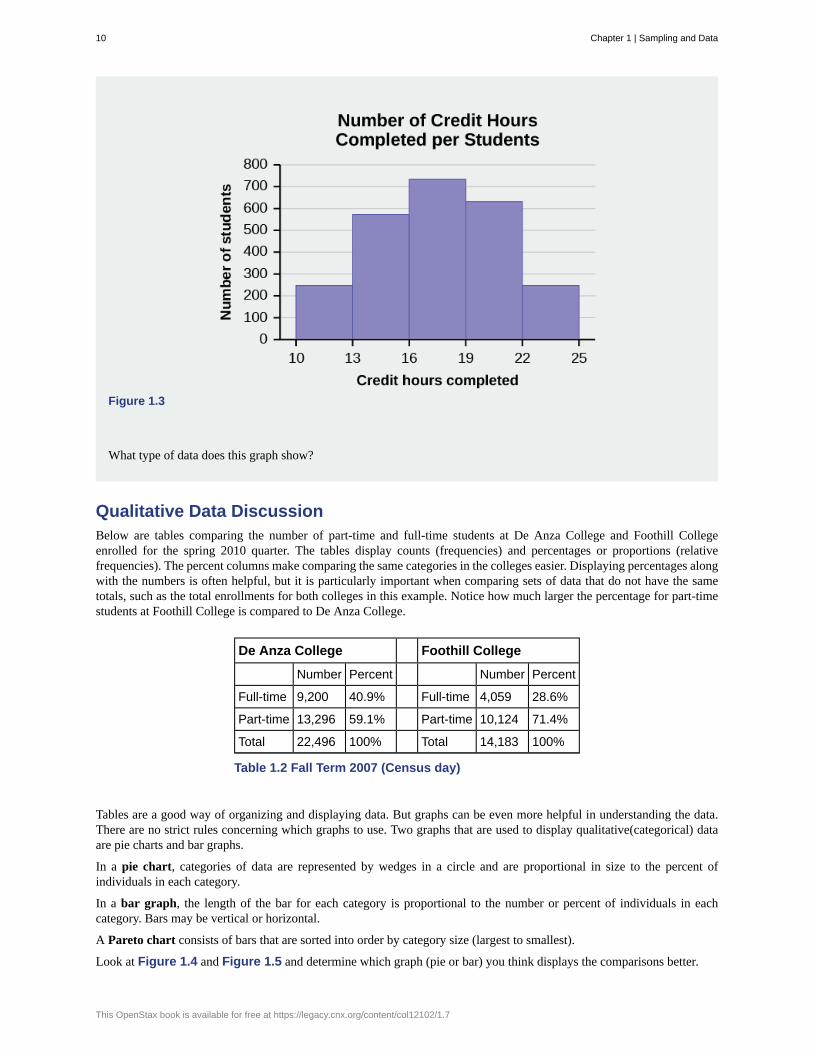
Figure 1.3
What type of data does this graph show?
Qualitative Data DiscussionBelow are tables comparing the number of part-time and full-time students at De Anza College and Foothill Collegeenrolled for the spring 2010 quarter. The tables display counts (frequencies) and percentages or proportions (relativefrequencies). The percent columns make comparing the same categories in the colleges easier. Displaying percentages alongwith the numbers is often helpful, but it is particularly important when comparing sets of data that do not have the sametotals, such as the total enrollments for both colleges in this example. Notice how much larger the percentage for part-timestudents at Foothill College is compared to De Anza College.
De Anza College Foothill College
Number Percent Number Percent
Full-time 9,200 40.9% Full-time 4,059 28.6%
Part-time 13,296 59.1% Part-time 10,124 71.4%
Total 22,496 100% Total 14,183 100%
Table 1.2 Fall Term 2007 (Census day)
Tables are a good way of organizing and displaying data. But graphs can be even more helpful in understanding the data.There are no strict rules concerning which graphs to use. Two graphs that are used to display qualitative(categorical) dataare pie charts and bar graphs.
In a pie chart, categories of data are represented by wedges in a circle and are proportional in size to the percent ofindividuals in each category.
In a bar graph, the length of the bar for each category is proportional to the number or percent of individuals in eachcategory. Bars may be vertical or horizontal.
A Pareto chart consists of bars that are sorted into order by category size (largest to smallest).
Look at Figure 1.4 and Figure 1.5 and determine which graph (pie or bar) you think displays the comparisons better.
10 Chapter 1 | Sampling and Data
This OpenStax book is available for free at https://legacy.cnx.org/content/col12102/1.7

It is a good idea to look at a variety of graphs to see which is the most helpful in displaying the data. We might makedifferent choices of what we think is the “best” graph depending on the data and the context. Our choice also depends onwhat we are using the data for.
(a) (b)Figure 1.4
Figure 1.5
Percentages That Add to More (or Less) Than 100%
Sometimes percentages add up to be more than 100% (or less than 100%). In the graph, the percentages add to more than100% because students can be in more than one category. A bar graph is appropriate to compare the relative size of thecategories. A pie chart cannot be used. It also could not be used if the percentages added to less than 100%.
Characteristic/category Percent
Full-time students 40.9%
Students who intend to transfer to a 4-year educational institution 48.6%
Table 1.3 De Anza College Spring 2010
Chapter 1 | Sampling and Data 11
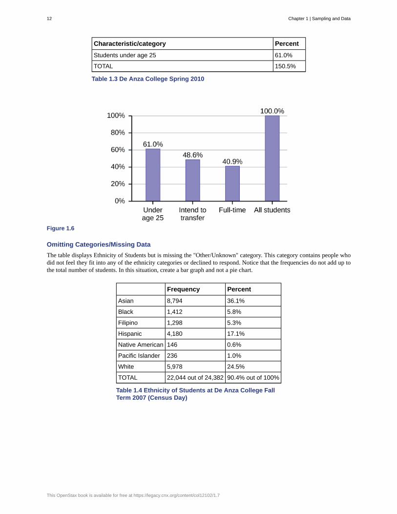
Characteristic/category Percent
Students under age 25 61.0%
TOTAL 150.5%
Table 1.3 De Anza College Spring 2010
Figure 1.6
Omitting Categories/Missing Data
The table displays Ethnicity of Students but is missing the "Other/Unknown" category. This category contains people whodid not feel they fit into any of the ethnicity categories or declined to respond. Notice that the frequencies do not add up tothe total number of students. In this situation, create a bar graph and not a pie chart.
Frequency Percent
Asian 8,794 36.1%
Black 1,412 5.8%
Filipino 1,298 5.3%
Hispanic 4,180 17.1%
Native American 146 0.6%
Pacific Islander 236 1.0%
White 5,978 24.5%
TOTAL 22,044 out of 24,382 90.4% out of 100%
Table 1.4 Ethnicity of Students at De Anza College FallTerm 2007 (Census Day)
12 Chapter 1 | Sampling and Data
This OpenStax book is available for free at https://legacy.cnx.org/content/col12102/1.7

Figure 1.7
The following graph is the same as the previous graph but the “Other/Unknown” percent (9.6%) has been included. The“Other/Unknown” category is large compared to some of the other categories (Native American, 0.6%, Pacific Islander1.0%). This is important to know when we think about what the data are telling us.
This particular bar graph in Figure 1.8 can be difficult to understand visually. The graph in Figure 1.9 is a Pareto chart.The Pareto chart has the bars sorted from largest to smallest and is easier to read and interpret.
Figure 1.8 Bar Graph with Other/Unknown Category
Chapter 1 | Sampling and Data 13
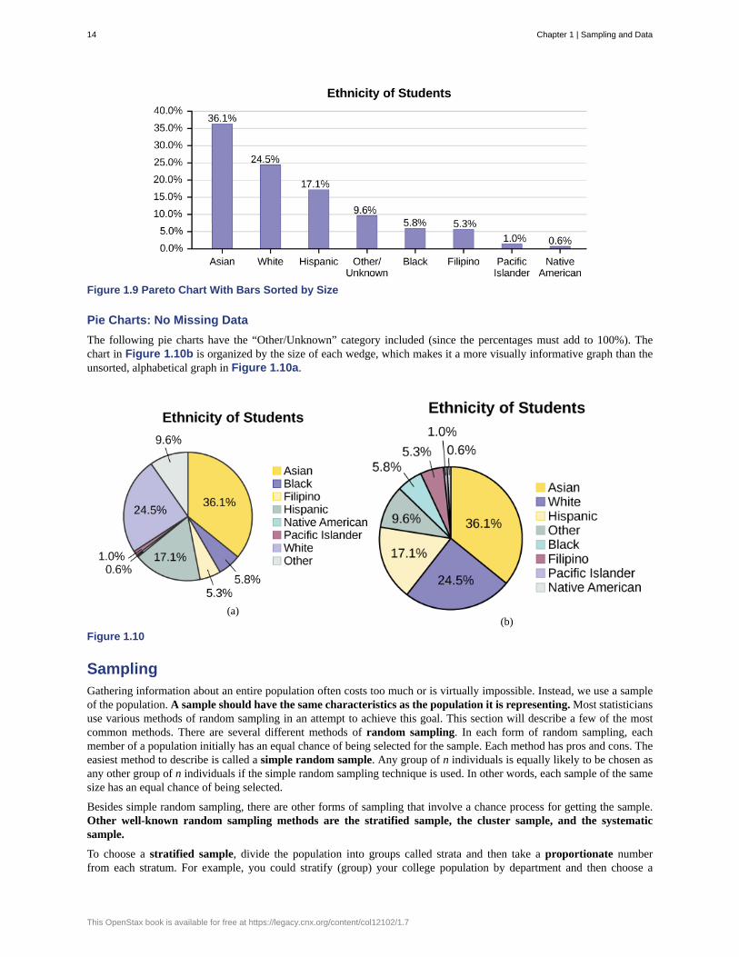
Figure 1.9 Pareto Chart With Bars Sorted by Size
Pie Charts: No Missing Data
The following pie charts have the “Other/Unknown” category included (since the percentages must add to 100%). Thechart in Figure 1.10b is organized by the size of each wedge, which makes it a more visually informative graph than theunsorted, alphabetical graph in Figure 1.10a.
(a)(b)
Figure 1.10
SamplingGathering information about an entire population often costs too much or is virtually impossible. Instead, we use a sampleof the population. A sample should have the same characteristics as the population it is representing. Most statisticiansuse various methods of random sampling in an attempt to achieve this goal. This section will describe a few of the mostcommon methods. There are several different methods of random sampling. In each form of random sampling, eachmember of a population initially has an equal chance of being selected for the sample. Each method has pros and cons. Theeasiest method to describe is called a simple random sample. Any group of n individuals is equally likely to be chosen asany other group of n individuals if the simple random sampling technique is used. In other words, each sample of the samesize has an equal chance of being selected.
Besides simple random sampling, there are other forms of sampling that involve a chance process for getting the sample.Other well-known random sampling methods are the stratified sample, the cluster sample, and the systematicsample.
To choose a stratified sample, divide the population into groups called strata and then take a proportionate numberfrom each stratum. For example, you could stratify (group) your college population by department and then choose a
14 Chapter 1 | Sampling and Data
This OpenStax book is available for free at https://legacy.cnx.org/content/col12102/1.7

proportionate simple random sample from each stratum (each department) to get a stratified random sample. To choosea simple random sample from each department, number each member of the first department, number each member ofthe second department, and do the same for the remaining departments. Then use simple random sampling to chooseproportionate numbers from the first department and do the same for each of the remaining departments. Those numberspicked from the first department, picked from the second department, and so on represent the members who make up thestratified sample.
To choose a cluster sample, divide the population into clusters (groups) and then randomly select some of the clusters.All the members from these clusters are in the cluster sample. For example, if you randomly sample four departmentsfrom your college population, the four departments make up the cluster sample. Divide your college faculty by department.The departments are the clusters. Number each department, and then choose four different numbers using simple randomsampling. All members of the four departments with those numbers are the cluster sample.
To choose a systematic sample, randomly select a starting point and take every nth piece of data from a listing of thepopulation. For example, suppose you have to do a phone survey. Your phone book contains 20,000 residence listings. Youmust choose 400 names for the sample. Number the population 1–20,000 and then use a simple random sample to pick anumber that represents the first name in the sample. Then choose every fiftieth name thereafter until you have a total of 400names (you might have to go back to the beginning of your phone list). Systematic sampling is frequently chosen becauseit is a simple method.
A type of sampling that is non-random is convenience sampling. Convenience sampling involves using results that arereadily available. For example, a computer software store conducts a marketing study by interviewing potential customerswho happen to be in the store browsing through the available software. The results of convenience sampling may be verygood in some cases and highly biased (favor certain outcomes) in others.
Sampling data should be done very carefully. Collecting data carelessly can have devastating results. Surveys mailed tohouseholds and then returned may be very biased (they may favor a certain group). It is better for the person conducting thesurvey to select the sample respondents.
True random sampling is done with replacement. That is, once a member is picked, that member goes back into thepopulation and thus may be chosen more than once. However for practical reasons, in most populations, simple randomsampling is done without replacement. Surveys are typically done without replacement. That is, a member of thepopulation may be chosen only once. Most samples are taken from large populations and the sample tends to be small incomparison to the population. Since this is the case, sampling without replacement is approximately the same as samplingwith replacement because the chance of picking the same individual more than once with replacement is very low.
In a college population of 10,000 people, suppose you want to pick a sample of 1,000 randomly for a survey. For anyparticular sample of 1,000, if you are sampling with replacement,
• the chance of picking the first person is 1,000 out of 10,000 (0.1000);
• the chance of picking a different second person for this sample is 999 out of 10,000 (0.0999);
• the chance of picking the same person again is 1 out of 10,000 (very low).
If you are sampling without replacement,
• the chance of picking the first person for any particular sample is 1000 out of 10,000 (0.1000);
• the chance of picking a different second person is 999 out of 9,999 (0.0999);
• you do not replace the first person before picking the next person.
Compare the fractions 999/10,000 and 999/9,999. For accuracy, carry the decimal answers to four decimal places. To fourdecimal places, these numbers are equivalent (0.0999).
Sampling without replacement instead of sampling with replacement becomes a mathematical issue only when thepopulation is small. For example, if the population is 25 people, the sample is ten, and you are sampling with replacementfor any particular sample, then the chance of picking the first person is ten out of 25, and the chance of picking a differentsecond person is nine out of 25 (you replace the first person).
If you sample without replacement, then the chance of picking the first person is ten out of 25, and then the chance ofpicking the second person (who is different) is nine out of 24 (you do not replace the first person).
Compare the fractions 9/25 and 9/24. To four decimal places, 9/25 = 0.3600 and 9/24 = 0.3750. To four decimal places,these numbers are not equivalent.
When you analyze data, it is important to be aware of sampling errors and nonsampling errors. The actual process ofsampling causes sampling errors. For example, the sample may not be large enough. Factors not related to the sampling
Chapter 1 | Sampling and Data 15

process cause nonsampling errors. A defective counting device can cause a nonsampling error.
In reality, a sample will never be exactly representative of the population so there will always be some sampling error. As arule, the larger the sample, the smaller the sampling error.
In statistics, a sampling bias is created when a sample is collected from a population and some members of the populationare not as likely to be chosen as others (remember, each member of the population should have an equally likely chance ofbeing chosen). When a sampling bias happens, there can be incorrect conclusions drawn about the population that is beingstudied.
Critical Evaluation
We need to evaluate the statistical studies we read about critically and analyze them before accepting the results of thestudies. Common problems to be aware of include
• Problems with samples: A sample must be representative of the population. A sample that is not representative of thepopulation is biased. Biased samples that are not representative of the population give results that are inaccurate andnot valid.
• Self-selected samples: Responses only by people who choose to respond, such as call-in surveys, are often unreliable.
• Sample size issues: Samples that are too small may be unreliable. Larger samples are better, if possible. In somesituations, having small samples is unavoidable and can still be used to draw conclusions. Examples: crash testing carsor medical testing for rare conditions
• Undue influence: collecting data or asking questions in a way that influences the response
• Non-response or refusal of subject to participate: The collected responses may no longer be representative of thepopulation. Often, people with strong positive or negative opinions may answer surveys, which can affect the results.
• Causality: A relationship between two variables does not mean that one causes the other to occur. They may be related(correlated) because of their relationship through a different variable.
• Self-funded or self-interest studies: A study performed by a person or organization in order to support their claim. Isthe study impartial? Read the study carefully to evaluate the work. Do not automatically assume that the study is good,but do not automatically assume the study is bad either. Evaluate it on its merits and the work done.
• Misleading use of data: improperly displayed graphs, incomplete data, or lack of context
• Confounding: When the effects of multiple factors on a response cannot be separated. Confounding makes it difficultor impossible to draw valid conclusions about the effect of each factor.
Example 1.11
A study is done to determine the average tuition that San Jose State undergraduate students pay per semester.Each student in the following samples is asked how much tuition he or she paid for the Fall semester. What is thetype of sampling in each case?
a. A sample of 100 undergraduate San Jose State students is taken by organizing the students’ names byclassification (freshman, sophomore, junior, or senior), and then selecting 25 students from each.
b. A random number generator is used to select a student from the alphabetical listing of all undergraduatestudents in the Fall semester. Starting with that student, every 50th student is chosen until 75 students areincluded in the sample.
c. A completely random method is used to select 75 students. Each undergraduate student in the fall semesterhas the same probability of being chosen at any stage of the sampling process.
d. The freshman, sophomore, junior, and senior years are numbered one, two, three, and four, respectively.A random number generator is used to pick two of those years. All students in those two years are in thesample.
e. An administrative assistant is asked to stand in front of the library one Wednesday and to ask the first 100undergraduate students he encounters what they paid for tuition the Fall semester. Those 100 students arethe sample.
16 Chapter 1 | Sampling and Data
This OpenStax book is available for free at https://legacy.cnx.org/content/col12102/1.7

Solution 1.11a. stratified; b. systematic; c. simple random; d. cluster; e. convenience
Example 1.12
Determine the type of sampling used (simple random, stratified, systematic, cluster, or convenience).
a. A soccer coach selects six players from a group of boys aged eight to ten, seven players from a group ofboys aged 11 to 12, and three players from a group of boys aged 13 to 14 to form a recreational soccer team.
b. A pollster interviews all human resource personnel in five different high tech companies.
c. A high school educational researcher interviews 50 high school female teachers and 50 high school maleteachers.
d. A medical researcher interviews every third cancer patient from a list of cancer patients at a local hospital.
e. A high school counselor uses a computer to generate 50 random numbers and then picks students whosenames correspond to the numbers.
f. A student interviews classmates in his algebra class to determine how many pairs of jeans a student owns,on the average.
Solution 1.12a. stratified; b. cluster; c. stratified; d. systematic; e. simple random; f.convenience
If we were to examine two samples representing the same population, even if we used random sampling methods for thesamples, they would not be exactly the same. Just as there is variation in data, there is variation in samples. As you becomeaccustomed to sampling, the variability will begin to seem natural.
Example 1.13
Suppose ABC College has 10,000 part-time students (the population). We are interested in the average amount ofmoney a part-time student spends on books in the fall term. Asking all 10,000 students is an almost impossibletask.
Suppose we take two different samples.
First, we use convenience sampling and survey ten students from a first term organic chemistry class. Many ofthese students are taking first term calculus in addition to the organic chemistry class. The amount of money theyspend on books is as follows:
$128; $87; $173; $116; $130; $204; $147; $189; $93; $153
The second sample is taken using a list of senior citizens who take P.E. classes and taking every fifth senior citizenon the list, for a total of ten senior citizens. They spend:
$50; $40; $36; $15; $50; $100; $40; $53; $22; $22
It is unlikely that any student is in both samples.
a. Do you think that either of these samples is representative of (or is characteristic of) the entire 10,000 part-timestudent population?
Solution 1.13a. No. The first sample probably consists of science-oriented students. Besides the chemistry course, some ofthem are also taking first-term calculus. Books for these classes tend to be expensive. Most of these students are,more than likely, paying more than the average part-time student for their books. The second sample is a group ofsenior citizens who are, more than likely, taking courses for health and interest. The amount of money they spendon books is probably much less than the average parttime student. Both samples are biased. Also, in both cases,
Chapter 1 | Sampling and Data 17
not all students have a chance to be in either sample.
b. Since these samples are not representative of the entire population, is it wise to use the results to describe theentire population?
Solution 1.13b. No. For these samples, each member of the population did not have an equally likely chance of being chosen.
Now, suppose we take a third sample. We choose ten different part-time students from the disciplines ofchemistry, math, English, psychology, sociology, history, nursing, physical education, art, and early childhooddevelopment. (We assume that these are the only disciplines in which part-time students at ABC College areenrolled and that an equal number of part-time students are enrolled in each of the disciplines.) Each student ischosen using simple random sampling. Using a calculator, random numbers are generated and a student froma particular discipline is selected if he or she has a corresponding number. The students spend the followingamounts:
$180; $50; $150; $85; $260; $75; $180; $200; $200; $150
c. Is the sample biased?
Solution 1.13c. The sample is unbiased, but a larger sample would be recommended to increase the likelihood that the samplewill be close to representative of the population. However, for a biased sampling technique, even a large sampleruns the risk of not being representative of the population.
Students often ask if it is "good enough" to take a sample, instead of surveying the entire population. If the surveyis done well, the answer is yes.
1.13 A local radio station has a fan base of 20,000 listeners. The station wants to know if its audience would prefermore music or more talk shows. Asking all 20,000 listeners is an almost impossible task.
The station uses convenience sampling and surveys the first 200 people they meet at one of the station’s music concertevents. 24 people said they’d prefer more talk shows, and 176 people said they’d prefer more music.
Do you think that this sample is representative of (or is characteristic of) the entire 20,000 listener population?
Variation in DataVariation is present in any set of data. For example, 16-ounce cans of beverage may contain more or less than 16 ounces ofliquid. In one study, eight 16 ounce cans were measured and produced the following amount (in ounces) of beverage:
15.8; 16.1; 15.2; 14.8; 15.8; 15.9; 16.0; 15.5
Measurements of the amount of beverage in a 16-ounce can may vary because different people make the measurements orbecause the exact amount, 16 ounces of liquid, was not put into the cans. Manufacturers regularly run tests to determine ifthe amount of beverage in a 16-ounce can falls within the desired range.
Be aware that as you take data, your data may vary somewhat from the data someone else is taking for the same purpose.This is completely natural. However, if two or more of you are taking the same data and get very different results, it is timefor you and the others to reevaluate your data-taking methods and your accuracy.
Variation in SamplesIt was mentioned previously that two or more samples from the same population, taken randomly, and having close tothe same characteristics of the population will likely be different from each other. Suppose Doreen and Jung both decideto study the average amount of time students at their college sleep each night. Doreen and Jung each take samples of 500students. Doreen uses systematic sampling and Jung uses cluster sampling. Doreen's sample will be different from Jung'ssample. Even if Doreen and Jung used the same sampling method, in all likelihood their samples would be different. Neither
18 Chapter 1 | Sampling and Data
This OpenStax book is available for free at https://legacy.cnx.org/content/col12102/1.7
would be wrong, however.
Think about what contributes to making Doreen’s and Jung’s samples different.
If Doreen and Jung took larger samples (i.e. the number of data values is increased), their sample results (the averageamount of time a student sleeps) might be closer to the actual population average. But still, their samples would be, in alllikelihood, different from each other. This variability in samples cannot be stressed enough.
Size of a Sample
The size of a sample (often called the number of observations, usually given the symbol n) is important. The examples youhave seen in this book so far have been small. Samples of only a few hundred observations, or even smaller, are sufficientfor many purposes. In polling, samples that are from 1,200 to 1,500 observations are considered large enough and goodenough if the survey is random and is well done. Later we will find that even much smaller sample sizes will give very goodresults. You will learn why when you study confidence intervals.
Be aware that many large samples are biased. For example, call-in surveys are invariably biased, because people choose torespond or not.
1.3 | Levels of MeasurementOnce you have a set of data, you will need to organize it so that you can analyze how frequently each datum occurs in theset. However, when calculating the frequency, you may need to round your answers so that they are as precise as possible.
Levels of MeasurementThe way a set of data is measured is called its level of measurement. Correct statistical procedures depend on a researcherbeing familiar with levels of measurement. Not every statistical operation can be used with every set of data. Data can beclassified into four levels of measurement. They are (from lowest to highest level):
• Nominal scale level
• Ordinal scale level
• Interval scale level
• Ratio scale level
Data that is measured using a nominal scale is qualitative (categorical). Categories, colors, names, labels and favoritefoods along with yes or no responses are examples of nominal level data. Nominal scale data are not ordered. For example,trying to classify people according to their favorite food does not make any sense. Putting pizza first and sushi second is notmeaningful.
Smartphone companies are another example of nominal scale data. The data are the names of the companies that makesmartphones, but there is no agreed upon order of these brands, even though people may have personal preferences. Nominalscale data cannot be used in calculations.
Data that is measured using an ordinal scale is similar to nominal scale data but there is a big difference. The ordinal scaledata can be ordered. An example of ordinal scale data is a list of the top five national parks in the United States. The topfive national parks in the United States can be ranked from one to five but we cannot measure differences between the data.
Another example of using the ordinal scale is a cruise survey where the responses to questions about the cruise are“excellent,” “good,” “satisfactory,” and “unsatisfactory.” These responses are ordered from the most desired response to theleast desired. But the differences between two pieces of data cannot be measured. Like the nominal scale data, ordinal scaledata cannot be used in calculations.
Data that is measured using the interval scale is similar to ordinal level data because it has a definite ordering but thereis a difference between data. The differences between interval scale data can be measured though the data does not have astarting point.
Temperature scales like Celsius (C) and Fahrenheit (F) are measured by using the interval scale. In both temperaturemeasurements, 40° is equal to 100° minus 60°. Differences make sense. But 0 degrees does not because, in both scales, 0 isnot the absolute lowest temperature. Temperatures like -10° F and -15° C exist and are colder than 0.
Interval level data can be used in calculations, but one type of comparison cannot be done. 80° C is not four times as hot as20° C (nor is 80° F four times as hot as 20° F). There is no meaning to the ratio of 80 to 20 (or four to one).
Data that is measured using the ratio scale takes care of the ratio problem and gives you the most information. Ratio scaledata is like interval scale data, but it has a 0 point and ratios can be calculated. For example, four multiple choice statistics
Chapter 1 | Sampling and Data 19

final exam scores are 80, 68, 20 and 92 (out of a possible 100 points). The exams are machine-graded.
The data can be put in order from lowest to highest: 20, 68, 80, 92.
The differences between the data have meaning. The score 92 is more than the score 68 by 24 points. Ratios can becalculated. The smallest score is 0. So 80 is four times 20. The score of 80 is four times better than the score of 20.
FrequencyTwenty students were asked how many hours they worked per day. Their responses, in hours, are as follows: 5; 6; 3; 3; 2;4; 7; 5; 2; 3; 5; 6; 5; 4; 4; 3; 5; 2; 5; 3.
Table 1.5 lists the different data values in ascending order and their frequencies.
Data value Frequency
2 3
3 5
4 3
5 6
6 2
7 1
Table 1.5 Frequency Tableof Student Work Hours
A frequency is the number of times a value of the data occurs. According to Table 1.5, there are three students who worktwo hours, five students who work three hours, and so on. The sum of the values in the frequency column, 20, representsthe total number of students included in the sample.
A relative frequency is the ratio (fraction or proportion) of the number of times a value of the data occurs in the set of alloutcomes to the total number of outcomes. To find the relative frequencies, divide each frequency by the total number ofstudents in the sample–in this case, 20. Relative frequencies can be written as fractions, percents, or decimals.
Data value Frequency Relative frequency
2 3320 or 0.15
3 5520 or 0.25
4 3320 or 0.15
5 6620 or 0.30
6 2220 or 0.10
7 1120 or 0.05
Table 1.6 Frequency Table of Student Work Hourswith Relative Frequencies
The sum of the values in the relative frequency column of Table 1.6 is 2020 , or 1.
Cumulative relative frequency is the accumulation of the previous relative frequencies. To find the cumulative relative
20 Chapter 1 | Sampling and Data
This OpenStax book is available for free at https://legacy.cnx.org/content/col12102/1.7
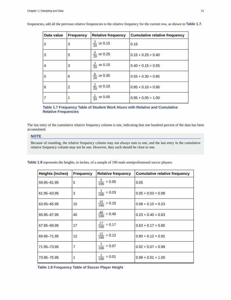
frequencies, add all the previous relative frequencies to the relative frequency for the current row, as shown in Table 1.7.
Data value Frequency Relative frequency Cumulative relative frequency
2 3320 or 0.15 0.15
3 5520 or 0.25 0.15 + 0.25 = 0.40
4 3320 or 0.15 0.40 + 0.15 = 0.55
5 6620 or 0.30 0.55 + 0.30 = 0.85
6 2220 or 0.10 0.85 + 0.10 = 0.95
7 1120 or 0.05 0.95 + 0.05 = 1.00
Table 1.7 Frequency Table of Student Work Hours with Relative and CumulativeRelative Frequencies
The last entry of the cumulative relative frequency column is one, indicating that one hundred percent of the data has beenaccumulated.
NOTE
Because of rounding, the relative frequency column may not always sum to one, and the last entry in the cumulativerelative frequency column may not be one. However, they each should be close to one.
Table 1.8 represents the heights, in inches, of a sample of 100 male semiprofessional soccer players.
Heights (inches) Frequency Relative frequency Cumulative relative frequency
59.95–61.95 55
100 = 0.05 0.05
61.95–63.95 33
100 = 0.03 0.05 + 0.03 = 0.08
63.95–65.95 1515100 = 0.15 0.08 + 0.15 = 0.23
65.95–67.95 4040100 = 0.40 0.23 + 0.40 = 0.63
67.95–69.95 1717100 = 0.17 0.63 + 0.17 = 0.80
69.95–71.95 1212100 = 0.12 0.80 + 0.12 = 0.92
71.95–73.95 77
100 = 0.07 0.92 + 0.07 = 0.99
73.95–75.95 11
100 = 0.01 0.99 + 0.01 = 1.00
Table 1.8 Frequency Table of Soccer Player Height
Chapter 1 | Sampling and Data 21
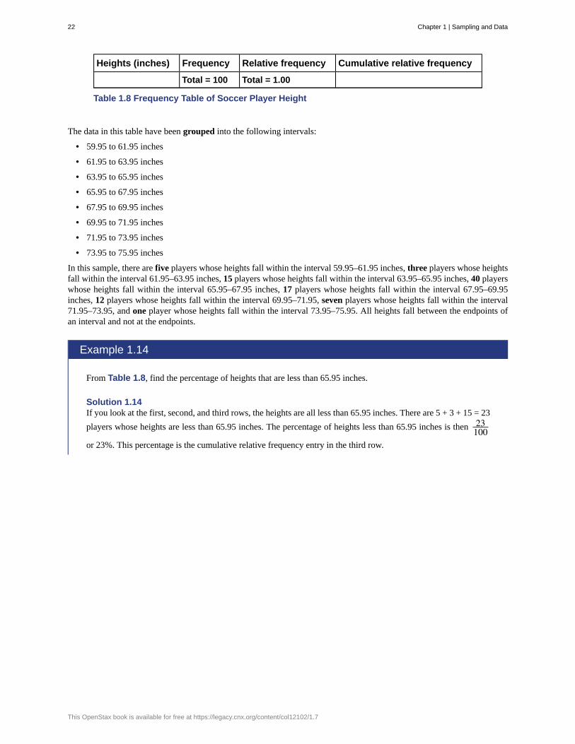
Heights (inches) Frequency Relative frequency Cumulative relative frequency
Total = 100 Total = 1.00
Table 1.8 Frequency Table of Soccer Player Height
The data in this table have been grouped into the following intervals:
• 59.95 to 61.95 inches
• 61.95 to 63.95 inches
• 63.95 to 65.95 inches
• 65.95 to 67.95 inches
• 67.95 to 69.95 inches
• 69.95 to 71.95 inches
• 71.95 to 73.95 inches
• 73.95 to 75.95 inches
In this sample, there are five players whose heights fall within the interval 59.95–61.95 inches, three players whose heightsfall within the interval 61.95–63.95 inches, 15 players whose heights fall within the interval 63.95–65.95 inches, 40 playerswhose heights fall within the interval 65.95–67.95 inches, 17 players whose heights fall within the interval 67.95–69.95inches, 12 players whose heights fall within the interval 69.95–71.95, seven players whose heights fall within the interval71.95–73.95, and one player whose heights fall within the interval 73.95–75.95. All heights fall between the endpoints ofan interval and not at the endpoints.
Example 1.14
From Table 1.8, find the percentage of heights that are less than 65.95 inches.
Solution 1.14If you look at the first, second, and third rows, the heights are all less than 65.95 inches. There are 5 + 3 + 15 = 23
players whose heights are less than 65.95 inches. The percentage of heights less than 65.95 inches is then 23100
or 23%. This percentage is the cumulative relative frequency entry in the third row.
22 Chapter 1 | Sampling and Data
This OpenStax book is available for free at https://legacy.cnx.org/content/col12102/1.7
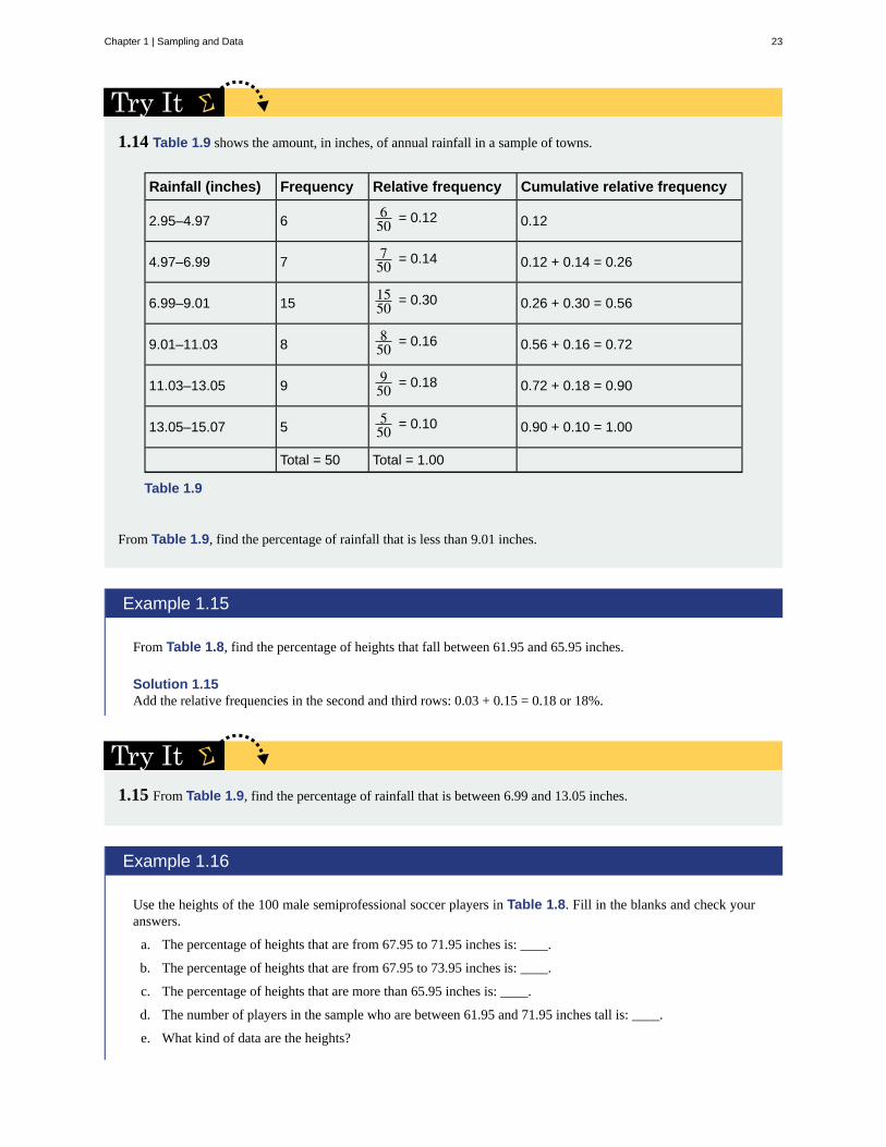
1.14 Table 1.9 shows the amount, in inches, of annual rainfall in a sample of towns.
Rainfall (inches) Frequency Relative frequency Cumulative relative frequency
2.95–4.97 6650 = 0.12 0.12
4.97–6.99 7750 = 0.14 0.12 + 0.14 = 0.26
6.99–9.01 151550 = 0.30 0.26 + 0.30 = 0.56
9.01–11.03 8850 = 0.16 0.56 + 0.16 = 0.72
11.03–13.05 9950 = 0.18 0.72 + 0.18 = 0.90
13.05–15.07 5550 = 0.10 0.90 + 0.10 = 1.00
Total = 50 Total = 1.00
Table 1.9
From Table 1.9, find the percentage of rainfall that is less than 9.01 inches.
Example 1.15
From Table 1.8, find the percentage of heights that fall between 61.95 and 65.95 inches.
Solution 1.15Add the relative frequencies in the second and third rows: 0.03 + 0.15 = 0.18 or 18%.
1.15 From Table 1.9, find the percentage of rainfall that is between 6.99 and 13.05 inches.
Example 1.16
Use the heights of the 100 male semiprofessional soccer players in Table 1.8. Fill in the blanks and check youranswers.
a. The percentage of heights that are from 67.95 to 71.95 inches is: ____.
b. The percentage of heights that are from 67.95 to 73.95 inches is: ____.
c. The percentage of heights that are more than 65.95 inches is: ____.
d. The number of players in the sample who are between 61.95 and 71.95 inches tall is: ____.
e. What kind of data are the heights?
Chapter 1 | Sampling and Data 23

f. Describe how you could gather this data (the heights) so that the data are characteristic of all malesemiprofessional soccer players.
Remember, you count frequencies. To find the relative frequency, divide the frequency by the total number ofdata values. To find the cumulative relative frequency, add all of the previous relative frequencies to the relativefrequency for the current row.
Solution 1.16a. 29%
b. 36%
c. 77%
d. 87
e. quantitative continuous
f. get rosters from each team and choose a simple random sample from each
Example 1.17
Nineteen people were asked how many miles, to the nearest mile, they commute to work each day. The data areas follows: 2; 5; 7; 3; 2; 10; 18; 15; 20; 7; 10; 18; 5; 12; 13; 12; 4; 5; 10. Table 1.10 was produced:
Data Frequency Relative frequency Cumulative relative frequency
3 3319 0.1579
4 1119 0.2105
5 3319 0.1579
7 2219 0.2632
10 3419 0.4737
12 2219 0.7895
13 1119 0.8421
15 1119 0.8948
18 1119 0.9474
20 1119 1.0000
Table 1.10 Frequency of Commuting Distances
a. Is the table correct? If it is not correct, what is wrong?
b. True or False: Three percent of the people surveyed commute three miles. If the statement is not correct,what should it be? If the table is incorrect, make the corrections.
24 Chapter 1 | Sampling and Data
This OpenStax book is available for free at https://legacy.cnx.org/content/col12102/1.7

c. What fraction of the people surveyed commute five or seven miles?
d. What fraction of the people surveyed commute 12 miles or more? Less than 12 miles? Between five and 13miles (not including five and 13 miles)?
Solution 1.17a. No. The frequency column sums to 18, not 19. Not all cumulative relative frequencies are correct.
b. False. The frequency for three miles should be one; for two miles (left out), two. The cumulative relativefrequency column should read: 0.1052, 0.1579, 0.2105, 0.3684, 0.4737, 0.6316, 0.7368, 0.7895, 0.8421,0.9474, 1.0000.
c. 519
d. 719 , 12
19 , 719
1.17 Table 1.9 represents the amount, in inches, of annual rainfall in a sample of towns. What fraction of townssurveyed get between 11.03 and 13.05 inches of rainfall each year?
Example 1.18
Table 1.11 contains the total number of deaths worldwide as a result of earthquakes for the period from 2000 to2012.
Year Total number of deaths
2000 231
2001 21,357
2002 11,685
2003 33,819
2004 228,802
2005 88,003
2006 6,605
2007 712
2008 88,011
2009 1,790
2010 320,120
2011 21,953
2012 768
Total 823,856
Table 1.11
Chapter 1 | Sampling and Data 25
Answer the following questions.
a. What is the frequency of deaths measured from 2006 through 2009?
b. What percentage of deaths occurred after 2009?
c. What is the relative frequency of deaths that occurred in 2003 or earlier?
d. What is the percentage of deaths that occurred in 2004?
e. What kind of data are the numbers of deaths?
f. The Richter scale is used to quantify the energy produced by an earthquake. Examples of Richter scalenumbers are 2.3, 4.0, 6.1, and 7.0. What kind of data are these numbers?
Solution 1.18a. 97,118 (11.8%)
b. 41.6%
c. 67,092/823,356 or 0.081 or 8.1 %
d. 27.8%
e. Quantitative discrete
f. Quantitative continuous
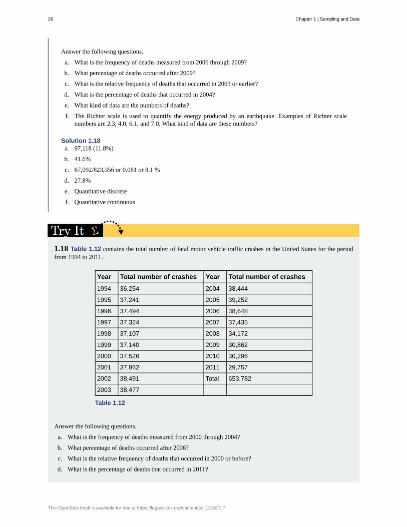
1.18 Table 1.12 contains the total number of fatal motor vehicle traffic crashes in the United States for the periodfrom 1994 to 2011.
Year Total number of crashes Year Total number of crashes
1994 36,254 2004 38,444
1995 37,241 2005 39,252
1996 37,494 2006 38,648
1997 37,324 2007 37,435
1998 37,107 2008 34,172
1999 37,140 2009 30,862
2000 37,526 2010 30,296
2001 37,862 2011 29,757
2002 38,491 Total 653,782
2003 38,477
Table 1.12
Answer the following questions.
a. What is the frequency of deaths measured from 2000 through 2004?
b. What percentage of deaths occurred after 2006?
c. What is the relative frequency of deaths that occurred in 2000 or before?
d. What is the percentage of deaths that occurred in 2011?
26 Chapter 1 | Sampling and Data
This OpenStax book is available for free at https://legacy.cnx.org/content/col12102/1.7

e. What is the cumulative relative frequency for 2006? Explain what this number tells you about the data.
1.4 | Experimental Design and EthicsDoes aspirin reduce the risk of heart attacks? Is one brand of fertilizer more effective at growing roses than another?Is fatigue as dangerous to a driver as the influence of alcohol? Questions like these are answered using randomizedexperiments. In this module, you will learn important aspects of experimental design. Proper study design ensures theproduction of reliable, accurate data.
The purpose of an experiment is to investigate the relationship between two variables. When one variable causes changein another, we call the first variable the independent variable or explanatory variable. The affected variable is calledthe dependent variable or response variable: stimulus, response. In a randomized experiment, the researcher manipulatesvalues of the explanatory variable and measures the resulting changes in the response variable. The different values of theexplanatory variable are called treatments. An experimental unit is a single object or individual to be measured.
You want to investigate the effectiveness of vitamin E in preventing disease. You recruit a group of subjects and ask themif they regularly take vitamin E. You notice that the subjects who take vitamin E exhibit better health on average thanthose who do not. Does this prove that vitamin E is effective in disease prevention? It does not. There are many differencesbetween the two groups compared in addition to vitamin E consumption. People who take vitamin E regularly often takeother steps to improve their health: exercise, diet, other vitamin supplements, choosing not to smoke. Any one of thesefactors could be influencing health. As described, this study does not prove that vitamin E is the key to disease prevention.
Additional variables that can cloud a study are called lurking variables. In order to prove that the explanatory variable iscausing a change in the response variable, it is necessary to isolate the explanatory variable. The researcher must design herexperiment in such a way that there is only one difference between groups being compared: the planned treatments. This isaccomplished by the random assignment of experimental units to treatment groups. When subjects are assigned treatmentsrandomly, all of the potential lurking variables are spread equally among the groups. At this point the only differencebetween groups is the one imposed by the researcher. Different outcomes measured in the response variable, therefore, mustbe a direct result of the different treatments. In this way, an experiment can prove a cause-and-effect connection betweenthe explanatory and response variables.
The power of suggestion can have an important influence on the outcome of an experiment. Studies have shown that theexpectation of the study participant can be as important as the actual medication. In one study of performance-enhancingdrugs, researchers noted:
Results showed that believing one had taken the substance resulted in [performance] times almost as fast as those associatedwith consuming the drug itself. In contrast, taking the drug without knowledge yielded no significant performanceincrement. (McClung, M. Collins, D. “Because I know it will!”: placebo effects of an ergogenic aid on athletic performance.Journal of Sport & Exercise Psychology. 2007 Jun. 29(3):382-94. Web. April 30, 2013.)
When participation in a study prompts a physical response from a participant, it is difficult to isolate the effects of theexplanatory variable. To counter the power of suggestion, researchers set aside one treatment group as a control group.This group is given a placebo treatment–a treatment that cannot influence the response variable. The control group helpsresearchers balance the effects of being in an experiment with the effects of the active treatments. Of course, if you areparticipating in a study and you know that you are receiving a pill which contains no actual medication, then the power ofsuggestion is no longer a factor. Blinding in a randomized experiment preserves the power of suggestion. When a personinvolved in a research study is blinded, he does not know who is receiving the active treatment(s) and who is receivingthe placebo treatment. A double-blind experiment is one in which both the subjects and the researchers involved with thesubjects are blinded.
Example 1.19
The Smell & Taste Treatment and Research Foundation conducted a study to investigate whether smell canaffect learning. Subjects completed mazes multiple times while wearing masks. They completed the pencil andpaper mazes three times wearing floral-scented masks, and three times with unscented masks. Participants wereassigned at random to wear the floral mask during the first three trials or during the last three trials. For eachtrial, researchers recorded the time it took to complete the maze and the subject’s impression of the mask’s scent:
Chapter 1 | Sampling and Data 27

positive, negative, or neutral.
a. Describe the explanatory and response variables in this study.
b. What are the treatments?
c. Identify any lurking variables that could interfere with this study.
d. Is it possible to use blinding in this study?
Solution 1.19a. The explanatory variable is scent, and the response variable is the time it takes to complete the maze.
b. There are two treatments: a floral-scented mask and an unscented mask.
c. All subjects experienced both treatments. The order of treatments was randomly assigned so there were nodifferences between the treatment groups. Random assignment eliminates the problem of lurking variables.
d. Subjects will clearly know whether they can smell flowers or not, so subjects cannot be blinded in this study.Researchers timing the mazes can be blinded, though. The researcher who is observing a subject will notknow which mask is being worn.
28 Chapter 1 | Sampling and Data
This OpenStax book is available for free at https://legacy.cnx.org/content/col12102/1.7

Average
Blinding
Categorical Variable
Cluster Sampling
Continuous Random Variable
Control Group
Convenience Sampling
Cumulative Relative Frequency
Data
Discrete Random Variable
Double-blinding
Experimental Unit
Explanatory Variable
Frequency
Informed Consent
Institutional Review Board
Lurking Variable
Mathematical Models
Nonsampling Error
Numerical Variable
Observational Study
Parameter
Placebo
KEY TERMSalso called mean or arithmetic mean; a number that describes the central tendency of the data
not telling participants which treatment a subject is receiving
variables that take on values that are names or labels
a method for selecting a random sample and dividing the population into groups (clusters); usesimple random sampling to select a set of clusters. Every individual in the chosen clusters is included in the sample.
a random variable (RV) whose outcomes are measured; the height of trees in theforest is a continuous RV.
a group in a randomized experiment that receives an inactive treatment but is otherwise managedexactly as the other groups
a nonrandom method of selecting a sample; this method selects individuals that are easilyaccessible and may result in biased data.
The term applies to an ordered set of observations from smallest to largest. Thecumulative relative frequency is the sum of the relative frequencies for all values that are less than or equal to thegiven value.
a set of observations (a set of possible outcomes); most data can be put into two groups: qualitative (an attributewhose value is indicated by a label) or quantitative (an attribute whose value is indicated by a number).Quantitative data can be separated into two subgroups: discrete and continuous. Data is discrete if it is the result ofcounting (such as the number of students of a given ethnic group in a class or the number of books on a shelf). Datais continuous if it is the result of measuring (such as distance traveled or weight of luggage)
a random variable (RV) whose outcomes are counted
the act of blinding both the subjects of an experiment and the researchers who work with the subjects
any individual or object to be measured
the independent variable in an experiment; the value controlled by researchers
the number of times a value of the data occurs
Any human subject in a research study must be cognizant of any risks or costs associated with thestudy. The subject has the right to know the nature of the treatments included in the study, their potential risks, andtheir potential benefits. Consent must be given freely by an informed, fit participant.
a committee tasked with oversight of research programs that involve human subjects
a variable that has an effect on a study even though it is neither an explanatory variable nor aresponse variable
a description of a phenomenon using mathematical concepts, such as equations, inequalities,distributions, etc.
an issue that affects the reliability of sampling data other than natural variation; it includes avariety of human errors including poor study design, biased sampling methods, inaccurate information provided bystudy participants, data entry errors, and poor analysis.
variables that take on values that are indicated by numbers
a study in which the independent variable is not manipulated by the researcher
a number that is used to represent a population characteristic and that generally cannot be determined easily
an inactive treatment that has no real effect on the explanatory variable
Chapter 1 | Sampling and Data 29

Population
Probability
Proportion
Qualitative Data
Quantitative Data
Random Assignment
Random Sampling
Relative Frequency
Representative Sample
Response Variable
Sample
Sampling Bias
Sampling Error
Sampling with Replacement
Sampling without Replacement
Simple Random Sampling
Statistic
Statistical Models
Stratified Sampling
Survey
Systematic Sampling
Treatments
Variable
all individuals, objects, or measurements whose properties are being studied
a number between zero and one, inclusive, that gives the likelihood that a specific event will occur
the number of successes divided by the total number in the sample
See Data.
See Data.
the act of organizing experimental units into treatment groups using random methods
a method of selecting a sample that gives every member of the population an equal chance ofbeing selected.
the ratio of the number of times a value of the data occurs in the set of all outcomes to the numberof all outcomes to the total number of outcomes
a subset of the population that has the same characteristics as the population
the dependent variable in an experiment; the value that is measured for change at the end of anexperiment
a subset of the population studied
not all members of the population are equally likely to be selected
the natural variation that results from selecting a sample to represent a larger population; this variationdecreases as the sample size increases, so selecting larger samples reduces sampling error.
Once a member of the population is selected for inclusion in a sample, that member isreturned to the population for the selection of the next individual.
A member of the population may be chosen for inclusion in a sample only once. Ifchosen, the member is not returned to the population before the next selection.
a straightforward method for selecting a random sample; give each member of thepopulation a number. Use a random number generator to select a set of labels. These randomly selected labelsidentify the members of your sample.
a numerical characteristic of the sample; a statistic estimates the corresponding population parameter.
a description of a phenomenon using probability distributions that describe the expected behaviorof the phenomenon and the variability in the expected observations.
a method for selecting a random sample used to ensure that subgroups of the population arerepresented adequately; divide the population into groups (strata). Use simple random sampling to identify aproportionate number of individuals from each stratum.
a study in which data is collected as reported by individuals.
a method for selecting a random sample; list the members of the population. Use simplerandom sampling to select a starting point in the population. Let k = (number of individuals in thepopulation)/(number of individuals needed in the sample). Choose every kth individual in the list starting with theone that was randomly selected. If necessary, return to the beginning of the population list to complete your sample.
different values or components of the explanatory variable applied in an experiment
a characteristic of interest for each person or object in a population
30 Chapter 1 | Sampling and Data
This OpenStax book is available for free at https://legacy.cnx.org/content/col12102/1.7
CHAPTER REVIEW
1.1 Definitions of Statistics, Probability, and Key TermsThe mathematical theory of statistics is easier to learn when you know the language. This module presents important termsthat will be used throughout the text.
1.2 Data, Sampling, and Variation in Data and SamplingData are individual items of information that come from a population or sample. Data may be classified as qualitative(categorical), quantitative continuous, or quantitative discrete.
Because it is not practical to measure the entire population in a study, researchers use samples to represent the population.A random sample is a representative group from the population chosen by using a method that gives each individual in thepopulation an equal chance of being included in the sample. Random sampling methods include simple random sampling,stratified sampling, cluster sampling, and systematic sampling. Convenience sampling is a nonrandom method of choosinga sample that often produces biased data.
Samples that contain different individuals result in different data. This is true even when the samples are well-chosen andrepresentative of the population. When properly selected, larger samples model the population more closely than smallersamples. There are many different potential problems that can affect the reliability of a sample. Statistical data needs to becritically analyzed, not simply accepted.
1.3 Levels of MeasurementSome calculations generate numbers that are artificially precise. It is not necessary to report a value to eight decimal placeswhen the measures that generated that value were only accurate to the nearest tenth. Round off your final answer to onemore decimal place than was present in the original data. This means that if you have data measured to the nearest tenth ofa unit, report the final statistic to the nearest hundredth.
In addition to rounding your answers, you can measure your data using the following four levels of measurement.
• Nominal scale level: data that cannot be ordered nor can it be used in calculations
• Ordinal scale level: data that can be ordered; the differences cannot be measured
• Interval scale level: data with a definite ordering but no starting point; the differences can be measured, but there isno such thing as a ratio.
• Ratio scale level: data with a starting point that can be ordered; the differences have meaning and ratios can becalculated.
When organizing data, it is important to know how many times a value appears. How many statistics students study fivehours or more for an exam? What percent of families on our block own two pets? Frequency, relative frequency, andcumulative relative frequency are measures that answer questions like these.
1.4 Experimental Design and EthicsA poorly designed study will not produce reliable data. There are certain key components that must be included in everyexperiment. To eliminate lurking variables, subjects must be assigned randomly to different treatment groups. One of thegroups must act as a control group, demonstrating what happens when the active treatment is not applied. Participants inthe control group receive a placebo treatment that looks exactly like the active treatments but cannot influence the responsevariable. To preserve the integrity of the placebo, both researchers and subjects may be blinded. When a study is designedproperly, the only difference between treatment groups is the one imposed by the researcher. Therefore, when groupsrespond differently to different treatments, the difference must be due to the influence of the explanatory variable.
“An ethics problem arises when you are considering an action that benefits you or some cause you support, hurts or reducesbenefits to others, and violates some rule.” (Andrew Gelman, “Open Data and Open Methods,” Ethics and Statistics,http://www.stat.columbia.edu/~gelman/research/published/ChanceEthics1.pdf (accessed May 1, 2013).) Ethical violationsin statistics are not always easy to spot. Professional associations and federal agencies post guidelines for proper conduct. Itis important that you learn basic statistical procedures so that you can recognize proper data analysis.
Chapter 1 | Sampling and Data 31
HOMEWORK
1.1 Definitions of Statistics, Probability, and Key Terms
For each of the following eight exercises, identify: a. the population, b. the sample, c. the parameter, d. the statistic, e. thevariable, and f. the data. Give examples where appropriate.
1. A fitness center is interested in the mean amount of time a client exercises in the center each week.
2. Ski resorts are interested in the mean age that children take their first ski and snowboard lessons. They need thisinformation to plan their ski classes optimally.
3. A cardiologist is interested in the mean recovery period of her patients who have had heart attacks.
4. Insurance companies are interested in the mean health costs each year of their clients, so that they can determine the costsof health insurance.
5. A politician is interested in the proportion of voters in his district who think he is doing a good job.
6. A marriage counselor is interested in the proportion of clients she counsels who stay married.
7. Political pollsters may be interested in the proportion of people who will vote for a particular cause.
8. A marketing company is interested in the proportion of people who will buy a particular product.
Use the following information to answer the next three exercises: A Lake Tahoe Community College instructor is interestedin the mean number of days Lake Tahoe Community College math students are absent from class during a quarter.
9. What is the population she is interested in?a. all Lake Tahoe Community College studentsb. all Lake Tahoe Community College English studentsc. all Lake Tahoe Community College students in her classesd. all Lake Tahoe Community College math students
10. Consider the following:
X = number of days a Lake Tahoe Community College math student is absent
In this case, X is an example of a:
a. variable.b. population.c. statistic.d. data.
11. The instructor’s sample produces a mean number of days absent of 3.5 days. This value is an example of a:a. parameter.b. data.c. statistic.d. variable.
1.2 Data, Sampling, and Variation in Data and Sampling
For the following exercises, identify the type of data that would be used to describe a response (quantitative discrete,quantitative continuous, or qualitative), and give an example of the data.
12. number of tickets sold to a concert
13. percent of body fat
14. favorite baseball team
15. time in line to buy groceries
16. number of students enrolled at Evergreen Valley College
17. most-watched television show
18. brand of toothpaste
32 Chapter 1 | Sampling and Data
This OpenStax book is available for free at https://legacy.cnx.org/content/col12102/1.7
19. distance to the closest movie theatre
20. age of executives in Fortune 500 companies
21. number of competing computer spreadsheet software packages
Use the following information to answer the next two exercises: A study was done to determine the age, number of timesper week, and the duration (amount of time) of resident use of a local park in San Jose. The first house in the neighborhoodaround the park was selected randomly and then every 8th house in the neighborhood around the park was interviewed.
22. “Number of times per week” is what type of data?a. qualitative (categorical)b. quantitative discretec. quantitative continuous
23. “Duration (amount of time)” is what type of data?a. qualitative (categorical)b. quantitative discretec. quantitative continuous
24. Airline companies are interested in the consistency of the number of babies on each flight, so that they have adequatesafety equipment. Suppose an airline conducts a survey. Over Thanksgiving weekend, it surveys six flights from Boston toSalt Lake City to determine the number of babies on the flights. It determines the amount of safety equipment needed bythe result of that study.
a. Using complete sentences, list three things wrong with the way the survey was conducted.b. Using complete sentences, list three ways that you would improve the survey if it were to be repeated.
25. Suppose you want to determine the mean number of students per statistics class in your state. Describe a possiblesampling method in three to five complete sentences. Make the description detailed.
26. Suppose you want to determine the mean number of cans of soda drunk each month by students in their twenties at yourschool. Describe a possible sampling method in three to five complete sentences. Make the description detailed.
27. List some practical difficulties involved in getting accurate results from a telephone survey.
28. List some practical difficulties involved in getting accurate results from a mailed survey.
29. With your classmates, brainstorm some ways you could overcome these problems if you needed to conduct a phone ormail survey.
30. The instructor takes her sample by gathering data on five randomly selected students from each Lake Tahoe CommunityCollege math class. The type of sampling she used is
a. cluster samplingb. stratified samplingc. simple random samplingd. convenience sampling
31. A study was done to determine the age, number of times per week, and the duration (amount of time) of residents usinga local park in San Jose. The first house in the neighborhood around the park was selected randomly and then every eighthhouse in the neighborhood around the park was interviewed. The sampling method was:
a. simple randomb. systematicc. stratifiedd. cluster
Chapter 1 | Sampling and Data 33

32. Name the sampling method used in each of the following situations:a. A woman in the airport is handing out questionnaires to travelers asking them to evaluate the airport’s service.
She does not ask travelers who are hurrying through the airport with their hands full of luggage, but instead asksall travelers who are sitting near gates and not taking naps while they wait.
b. A teacher wants to know if her students are doing homework, so she randomly selects rows two and five and thencalls on all students in row two and all students in row five to present the solutions to homework problems to theclass.
c. The marketing manager for an electronics chain store wants information about the ages of its customers. Overthe next two weeks, at each store location, 100 randomly selected customers are given questionnaires to fill outasking for information about age, as well as about other variables of interest.
d. The librarian at a public library wants to determine what proportion of the library users are children. The librarianhas a tally sheet on which she marks whether books are checked out by an adult or a child. She records this datafor every fourth patron who checks out books.
e. A political party wants to know the reaction of voters to a debate between the candidates. The day after the debate,the party’s polling staff calls 1,200 randomly selected phone numbers. If a registered voter answers the phone oris available to come to the phone, that registered voter is asked whom he or she intends to vote for and whetherthe debate changed his or her opinion of the candidates.
33. A “random survey” was conducted of 3,274 people of the “microprocessor generation” (people born since 1971, theyear the microprocessor was invented). It was reported that 48% of those individuals surveyed stated that if they had $2,000to spend, they would use it for computer equipment. Also, 66% of those surveyed considered themselves relatively savvycomputer users.
a. Do you consider the sample size large enough for a study of this type? Why or why not?b. Based on your “gut feeling,” do you believe the percents accurately reflect the U.S. population for those
individuals born since 1971? If not, do you think the percents of the population are actually higher or lower thanthe sample statistics? Why?Additional information: The survey, reported by Intel Corporation, was filled out by individuals who visited theLos Angeles Convention Center to see the Smithsonian Institute's road show called “America’s Smithsonian.”
c. With this additional information, do you feel that all demographic and ethnic groups were equally represented atthe event? Why or why not?
d. With the additional information, comment on how accurately you think the sample statistics reflect the populationparameters.
34. The Well-Being Index is a survey that follows trends of U.S. residents on a regular basis. There are six areas ofhealth and wellness covered in the survey: Life Evaluation, Emotional Health, Physical Health, Healthy Behavior, WorkEnvironment, and Basic Access. Some of the questions used to measure the Index are listed below.
Identify the type of data obtained from each question used in this survey: qualitative(categorical), quantitative discrete, orquantitative continuous.
a. Do you have any health problems that prevent you from doing any of the things people your age can normally do?b. During the past 30 days, for about how many days did poor health keep you from doing your usual activities?c. In the last seven days, on how many days did you exercise for 30 minutes or more?d. Do you have health insurance coverage?
35. In advance of the 1936 Presidential Election, a magazine titled Literary Digest released the results of an opinionpoll predicting that the republican candidate Alf Landon would win by a large margin. The magazine sent post cardsto approximately 10,000,000 prospective voters. These prospective voters were selected from the subscription list of themagazine, from automobile registration lists, from phone lists, and from club membership lists. Approximately 2,300,000people returned the postcards.
a. Think about the state of the United States in 1936. Explain why a sample chosen from magazine subscription lists,automobile registration lists, phone books, and club membership lists was not representative of the population ofthe United States at that time.
b. What effect does the low response rate have on the reliability of the sample?c. Are these problems examples of sampling error or nonsampling error?d. During the same year, George Gallup conducted his own poll of 30,000 prospective voters. These researchers used
a method they called "quota sampling" to obtain survey answers from specific subsets of the population. Quotasampling is an example of which sampling method described in this module?
34 Chapter 1 | Sampling and Data
This OpenStax book is available for free at https://legacy.cnx.org/content/col12102/1.7

36. Crime-related and demographic statistics for 47 US states in 1960 were collected from government agencies, includingthe FBI's Uniform Crime Report. One analysis of this data found a strong connection between education and crimeindicating that higher levels of education in a community correspond to higher crime rates.
Which of the potential problems with samples discussed in Section 1.2 could explain this connection?
37. YouPolls is a website that allows anyone to create and respond to polls. One question posted April 15 asks:
“Do you feel happy paying your taxes when members of the Obama administration are allowed to ignore their taxliabilities?” (lastbaldeagle. 2013. On Tax Day, House to Call for Firing Federal Workers Who Owe Back Taxes. Opinionpoll posted online at: http://www.youpolls.com/details.aspx?id=12328 (accessed May 1, 2013).)
As of April 25, 11 people responded to this question. Each participant answered “NO!”
Which of the potential problems with samples discussed in this module could explain this connection?
38. A scholarly article about response rates begins with the following quote:
“Declining contact and cooperation rates in random digit dial (RDD) national telephone surveys raise serious concerns aboutthe validity of estimates drawn from such research.” (Scott Keeter et al., “Gauging the Impact of Growing Nonresponseon Estimates from a National RDD Telephone Survey,” Public Opinion Quarterly 70 no. 5 (2006),http://poq.oxfordjournals.org/content/70/5/759.full (http://poq.oxfordjournals.org/content/70/5/759.full)(accessed May 1, 2013).)
The Pew Research Center for People and the Press admits:
“The percentage of people we interview – out of all we try to interview – has been declining over the past decade or more.”(Frequently Asked Questions, Pew Research Center for the People & the Press, http://www.people-press.org/methodology/frequently-asked-questions/#dont-you-have-trouble-getting-people-to-answer-your-polls (accessed May 1, 2013).)
a. What are some reasons for the decline in response rate over the past decade?b. Explain why researchers are concerned with the impact of the declining response rate on public opinion polls.
1.3 Levels of Measurement
39. Fifty part-time students were asked how many courses they were taking this term. The (incomplete) results are shownbelow:
# of courses Frequency Relative frequency Cumulative relative frequency
1 30 0.6
2 15
3
Table 1.13 Part-time Student Course Loads
a. Fill in the blanks in Table 1.13.b. What percent of students take exactly two courses?c. What percent of students take one or two courses?
Chapter 1 | Sampling and Data 35

40. Sixty adults with gum disease were asked the number of times per week they used to floss before their diagnosis. The(incomplete) results are shown in Table 1.14.
# flossing per week Frequency Relative frequency Cumulative relative frequency
0 27 0.4500
1 18
3 0.9333
6 3 0.0500
7 1 0.0167
Table 1.14 Flossing Frequency for Adults with Gum Disease
a. Fill in the blanks in Table 1.14.b. What percent of adults flossed six times per week?c. What percent flossed at most three times per week?
41. Nineteen immigrants to the U.S were asked how many years, to the nearest year, they have lived in the U.S. The dataare as follows: 2; 5; 7; 2; 2; 10; 20; 15; 0; 7; 0; 20; 5; 12; 15; 12; 4; 5; 10.
Table 1.15 was produced.
Data Frequency Relative frequency Cumulative relative frequency
0 2219 0.1053
2 3319 0.2632
4 1119 0.3158
5 3319 0.4737
7 2219 0.5789
10 2219 0.6842
12 2219 0.7895
15 1119 0.8421
20 1119 1.0000
Table 1.15 Frequency of Immigrant Survey Responses
a. Fix the errors in Table 1.15. Also, explain how someone might have arrived at the incorrect number(s).b. Explain what is wrong with this statement: “47 percent of the people surveyed have lived in the U.S. for 5 years.”c. Fix the statement in b to make it correct.d. What fraction of the people surveyed have lived in the U.S. five or seven years?e. What fraction of the people surveyed have lived in the U.S. at most 12 years?f. What fraction of the people surveyed have lived in the U.S. fewer than 12 years?g. What fraction of the people surveyed have lived in the U.S. from five to 20 years, inclusive?
36 Chapter 1 | Sampling and Data
This OpenStax book is available for free at https://legacy.cnx.org/content/col12102/1.7

42. How much time does it take to travel to work? Table 1.16 shows the mean commute time by state for workers at least16 years old who are not working at home. Find the mean travel time, and round off the answer properly.
24.0 24.3 25.9 18.9 27.5 17.9 21.8 20.9 16.7 27.3
18.2 24.7 20.0 22.6 23.9 18.0 31.4 22.3 24.0 25.5
24.7 24.6 28.1 24.9 22.6 23.6 23.4 25.7 24.8 25.5
21.2 25.7 23.1 23.0 23.9 26.0 16.3 23.1 21.4 21.5
27.0 27.0 18.6 31.7 23.3 30.1 22.9 23.3 21.7 18.6
Table 1.16
43. Forbes magazine published data on the best small firms in 2012. These were firms which had been publicly traded forat least a year, have a stock price of at least $5 per share, and have reported annual revenue between $5 million and $1billion. Table 1.17 shows the ages of the chief executive officers for the first 60 ranked firms.
Age Frequency Relative frequency Cumulative relative frequency
40–44 3
45–49 11
50–54 13
55–59 16
60–64 10
65–69 6
70–74 1
Table 1.17
a. What is the frequency for CEO ages between 54 and 65?b. What percentage of CEOs are 65 years or older?c. What is the relative frequency of ages under 50?d. What is the cumulative relative frequency for CEOs younger than 55?e. Which graph shows the relative frequency and which shows the cumulative relative frequency?
Figure 1.11
Use the following information to answer the next two exercises: Table 1.18 contains data on hurricanes that have made
Chapter 1 | Sampling and Data 37

direct hits on the U.S. Between 1851 and 2004. A hurricane is given a strength category rating based on the minimum windspeed generated by the storm.
Category Number of direct hits Relative frequency Cumulative frequency
1 109 0.3993 0.3993
2 72 0.2637 0.6630
3 71 0.2601
4 18 0.9890
5 3 0.0110 1.0000
Total = 273
Table 1.18 Frequency of Hurricane Direct Hits
44. What is the relative frequency of direct hits that were category 4 hurricanes?a. 0.0768b. 0.0659c. 0.2601d. Not enough information to calculate
45. What is the relative frequency of direct hits that were AT MOST a category 3 storm?a. 0.3480b. 0.9231c. 0.2601d. 0.3370
REFERENCES
1.1 Definitions of Statistics, Probability, and Key Terms
The Data and Story Library, http://lib.stat.cmu.edu/DASL/Stories/CrashTestDummies.html (accessed May 1, 2013).
1.2 Data, Sampling, and Variation in Data and Sampling
Gallup-Healthways Well-Being Index. http://www.well-beingindex.com/default.asp (accessed May 1, 2013).
Gallup-Healthways Well-Being Index. http://www.well-beingindex.com/methodology.asp (accessed May 1, 2013).
Gallup-Healthways Well-Being Index. http://www.gallup.com/poll/146822/gallup-healthways-index-questions.aspx(accessed May 1, 2013).
Data from http://www.bookofodds.com/Relationships-Society/Articles/A0374-How-George-Gallup-Picked-the-President
Dominic Lusinchi, “’President’ Landon and the 1936 Literary Digest Poll: Were Automobile and Telephone Owners toBlame?” Social Science History 36, no. 1: 23-54 (2012), http://ssh.dukejournals.org/content/36/1/23.abstract (accessed May1, 2013).
“The Literary Digest Poll,” Virtual Laboratories in Probability and Statistics http://www.math.uah.edu/stat/data/LiteraryDigest.html (accessed May 1, 2013).
“Gallup Presidential Election Trial-Heat Trends, 1936–2008,” Gallup Politics http://www.gallup.com/poll/110548/gallup-presidential-election-trialheat-trends-19362004.aspx#4 (accessed May 1, 2013).
The Data and Story Library, http://lib.stat.cmu.edu/DASL/Datafiles/USCrime.html (accessed May 1, 2013).
LBCC Distance Learning (DL) program data in 2010-2011, http://de.lbcc.edu/reports/2010-11/future/highlights.html#focus(accessed May 1, 2013).
Data from San Jose Mercury News
38 Chapter 1 | Sampling and Data
This OpenStax book is available for free at https://legacy.cnx.org/content/col12102/1.7
1.3 Levels of Measurement
“State & County QuickFacts,” U.S. Census Bureau. http://quickfacts.census.gov/qfd/download_data.html (accessed May 1,2013).
“State & County QuickFacts: Quick, easy access to facts about people, business, and geography,” U.S. Census Bureau.http://quickfacts.census.gov/qfd/index.html (accessed May 1, 2013).
“Table 5: Direct hits by mainland United States Hurricanes (1851-2004),” National Hurricane Center,http://www.nhc.noaa.gov/gifs/table5.gif (accessed May 1, 2013).
“Levels of Measurement,” http://infinity.cos.edu/faculty/woodbury/stats/tutorial/Data_Levels.htm (accessed May 1, 2013).
Courtney Taylor, “Levels of Measurement,” about.com, http://statistics.about.com/od/HelpandTutorials/a/Levels-Of-Measurement.htm (accessed May 1, 2013).
David Lane. “Levels of Measurement,” Connexions, http://cnx.org/content/m10809/latest/ (accessed May 1, 2013).
1.4 Experimental Design and Ethics
“Vitamin E and Health,” Nutrition Source, Harvard School of Public Health, http://www.hsph.harvard.edu/nutritionsource/vitamin-e/ (accessed May 1, 2013).
Stan Reents. “Don’t Underestimate the Power of Suggestion,” athleteinme.com, http://www.athleteinme.com/ArticleView.aspx?id=1053 (accessed May 1, 2013).
Ankita Mehta. “Daily Dose of Aspiring Helps Reduce Heart Attacks: Study,” International Business Times, July 21, 2011.Also available online at http://www.ibtimes.com/daily-dose-aspirin-helps-reduce-heart-attacks-study-300443 (accessedMay 1, 2013).
The Data and Story Library, http://lib.stat.cmu.edu/DASL/Stories/ScentsandLearning.html (accessed May 1, 2013).
M.L. Jackson et al., “Cognitive Components of Simulated Driving Performance: Sleep Loss effect and Predictors,” AccidentAnalysis and Prevention Journal, Jan no. 50 (2013), http://www.ncbi.nlm.nih.gov/pubmed/22721550 (accessed May 1,2013).
“Earthquake Information by Year,” U.S. Geological Survey. http://earthquake.usgs.gov/earthquakes/eqarchives/year/(accessed May 1, 2013).
“Fatality Analysis Report Systems (FARS) Encyclopedia,” National Highway Traffic and Safety Administration.http://www-fars.nhtsa.dot.gov/Main/index.aspx (accessed May 1, 2013).
Data from www.businessweek.com (accessed May 1, 2013).
Data from www.forbes.com (accessed May 1, 2013).
“America’s Best Small Companies,” http://www.forbes.com/best-small-companies/list/ (accessed May 1, 2013).
U.S. Department of Health and Human Services, Code of Federal Regulations Title 45 Public Welfare Department of Healthand Human Services Part 46 Protection of Human Subjects revised January 15, 2009. Section 46.111:Criteria for IRBApproval of Research.
“April 2013 Air Travel Consumer Report,” U.S. Department of Transportation, April 11 (2013), http://www.dot.gov/airconsumer/april-2013-air-travel-consumer-report (accessed May 1, 2013).
Lori Alden, “Statistics can be Misleading,” econoclass.com, http://www.econoclass.com/misleadingstats.html (accessedMay 1, 2013).
Maria de los A. Medina, “Ethics in Statistics,” Based on “Building an Ethics Module for Business, Science, and EngineeringStudents” by Jose A. Cruz-Cruz and William Frey, Connexions, http://cnx.org/content/m15555/latest/ (accessed May 1,2013).
SOLUTIONS
2a. all children who take ski or snowboard lessons
Chapter 1 | Sampling and Data 39

b. a group of these children
c. the population mean age of children who take their first snowboard lesson
d. the sample mean age of children who take their first snowboard lesson
e. X = the age of one child who takes his or her first ski or snowboard lesson
f. values for X, such as 3, 7, and so on
4a. the clients of the insurance companies
b. a group of the clients
c. the mean health costs of the clients
d. the mean health costs of the sample
e. X = the health costs of one client
f. values for X, such as 34, 9, 82, and so on
6a. all the clients of this counselor
b. a group of clients of this marriage counselor
c. the proportion of all her clients who stay married
d. the proportion of the sample of the counselor’s clients who stay married
e. X = the number of couples who stay married
f. yes, no
8a. all people (maybe in a certain geographic area, such as the United States)
b. a group of the people
c. the proportion of all people who will buy the product
d. the proportion of the sample who will buy the product
e. X = the number of people who will buy it
f. buy, not buy
10 a
12 quantitative discrete, 150
14 qualitative, Oakland A’s
16 quantitative discrete, 11,234 students
18 qualitative, Crest
20 quantitative continuous, 47.3 years
22 b
24a. The survey was conducted using six similar flights.
The survey would not be a true representation of the entire population of air travelers.Conducting the survey on a holiday weekend will not produce representative results.
b. Conduct the survey during different times of the year.Conduct the survey using flights to and from various locations.Conduct the survey on different days of the week.
26 Answers will vary. Sample Answer: You could use a systematic sampling method. Stop the tenth person as they leaveone of the buildings on campus at 9:50 in the morning. Then stop the tenth person as they leave a different building on
40 Chapter 1 | Sampling and Data
This OpenStax book is available for free at https://legacy.cnx.org/content/col12102/1.7

campus at 1:50 in the afternoon.
28 Answers will vary. Sample Answer: Many people will not respond to mail surveys. If they do respond to the surveys,you can’t be sure who is responding. In addition, mailing lists can be incomplete.
30 b
32 convenience; cluster; stratified ; systematic; simple random
34a. qualitative(categorical)
b. quantitative discrete
c. quantitative discrete
d. qualitative(categorical)
36 Causality: The fact that two variables are related does not guarantee that one variable is influencing the other. Wecannot assume that crime rate impacts education level or that education level impacts crime rate. Confounding: There aremany factors that define a community other than education level and crime rate. Communities with high crime rates andhigh education levels may have other lurking variables that distinguish them from communities with lower crime ratesand lower education levels. Because we cannot isolate these variables of interest, we cannot draw valid conclusions aboutthe connection between education and crime. Possible lurking variables include police expenditures, unemployment levels,region, average age, and size.
38a. Possible reasons: increased use of caller id, decreased use of landlines, increased use of private numbers, voice mail,
privacy managers, hectic nature of personal schedules, decreased willingness to be interviewed
b. When a large number of people refuse to participate, then the sample may not have the same characteristics of thepopulation. Perhaps the majority of people willing to participate are doing so because they feel strongly about thesubject of the survey.
40a.
# flossing per week Frequency Relative frequency Cumulative relative frequency
0 27 0.4500 0.4500
1 18 0.3000 0.7500
3 11 0.1833 0.9333
6 3 0.0500 0.9833
7 1 0.0167 1
Table 1.19
b. 5.00%
c. 93.33%
42 The sum of the travel times is 1,173.1. Divide the sum by 50 to calculate the mean value: 23.462. Because each state’stravel time was measured to the nearest tenth, round this calculation to the nearest hundredth: 23.46.
44 b
Chapter 1 | Sampling and Data 41

42 Chapter 1 | Sampling and Data
This OpenStax book is available for free at https://legacy.cnx.org/content/col12102/1.7

2 | DESCRIPTIVESTATISTICS
Figure 2.1 When you have large amounts of data, you will need to organize it in a way that makes sense. Theseballots from an election are rolled together with similar ballots to keep them organized. (credit: William Greeson)
Introduction
Once you have collected data, what will you do with it? Data can be described and presented in many different formats. Forexample, suppose you are interested in buying a house in a particular area. You may have no clue about the house prices, soyou might ask your real estate agent to give you a sample data set of prices. Looking at all the prices in the sample often isoverwhelming. A better way might be to look at the median price and the variation of prices. The median and variation arejust two ways that you will learn to describe data. Your agent might also provide you with a graph of the data.
In this chapter, you will study numerical and graphical ways to describe and display your data. This area of statistics is called"Descriptive Statistics." You will learn how to calculate, and even more importantly, how to interpret these measurementsand graphs.
A statistical graph is a tool that helps you learn about the shape or distribution of a sample or a population. A graph can bea more effective way of presenting data than a mass of numbers because we can see where data clusters and where there areonly a few data values. Newspapers and the Internet use graphs to show trends and to enable readers to compare facts andfigures quickly. Statisticians often graph data first to get a picture of the data. Then, more formal tools may be applied.
Some of the types of graphs that are used to summarize and organize data are the dot plot, the bar graph, the histogram, thestem-and-leaf plot, the frequency polygon (a type of broken line graph), the pie chart, and the box plot. In this chapter, we
Chapter 2 | Descriptive Statistics 43

will briefly look at stem-and-leaf plots, line graphs, and bar graphs, as well as frequency polygons, and time series graphs.Our emphasis will be on histograms and box plots.
2.1 | Frequency Distributions and Graphs - (Base Version
- Lyryx Learning)FREQUENCY DISTRIBUTIONS OF DATAA frequency distribution lists categories (or intervals) and the number of times each occurs (frequency).A relative frequency distribution lists categories (or intervals) and the proportion of times each occurs.
Relative Frequency = class f requencytotal f requency = f
n
Frequency Distribution for Qualitative Data
Example 2.1 Letter Grades
The letter grades in a statistics class are given as follows (raw data):
C C A A C A A A B C A F C D D B A C B B
A A D C A C C B B B D D D C B C C C F C
Table 2.1 Letter Grades for 40 statistics students
Construct a frequency distribution table.Construct a relative frequency distribution table.
a) How many students scored a B or better?b) What percent of students scored a D?c) What proportion of students scored a C or worse?
Solution
The following is a frequency distribution table that helps summarize the data in Table 2.1 above.
Grade Number of Students, f
A 10
B 8
C 14
D 6
F 2
Total n = 40
Table 2.2 Frequency distribution ofthe grades
44 Chapter 2 | Descriptive Statistics
This OpenStax book is available for free at https://legacy.cnx.org/content/col12102/1.7

Grade Frequency Relative Frequency
A 10 10/40 = 25%
B 8 8/40 = 20%
C 14 14/40 = 35%
D 6 6/40 = 15%
F 2 2/40 = 5%
Total n = 40 100%
Table 2.3 Relative Frequency Distribution ofLetter Grades
a) 18 students scored a B or higher. (A or B)b) 15% scored a D.c) 55% scored a C or worse.
Graphical Representation of Qualitative Data
Bar Chart - consists of rectangular bars showing the frequencies of each category of a distribution. The bar chart for thefrequency distribution in Table 2.2 is seen below:
Figure 2.2 Bar Chart for Letter Grades
Pie Chart - a circle divided into sections reflecting the percentage of frequencies in each category of the distribution. ThePie Chart for Table 2.3 is seen below.
Chapter 2 | Descriptive Statistics 45

Figure 2.3 Pie Chart for Letter Grades
Frequency Distribution for Quantitative Data
Example 2.2 Age of Patients
The following are ages of the 25 patients on the 6th floor of a hospital. Construct a frequency distribution and arelative frequency distribution for these data: 12, 21, 51, 53, 26, 21, 21, 38, 55, 52, 38, 37, 40, 13, 38, 55, 31, 54,48, 49, 54, 42, 56, 26, 54.
Age Class Frequency Relative Frequency
10 to under 20 2 2/25 = 8%
20 to under 30 5 5/25 = 20%
30 to under 40 5 5/25 = 20%
40 to under 50 4 4/25 = 16%
50 to under 60 9 9/25 = 36%
Total n = 25 100%
Table 2.4
The numbers 10, 20, 30, 40, 50 are lower limits.The numbers 20, 30, 40, 50, 60 are upper limits.The difference between two consecutive lower (or upper) limits is called Class Width.
46 Chapter 2 | Descriptive Statistics
This OpenStax book is available for free at https://legacy.cnx.org/content/col12102/1.7
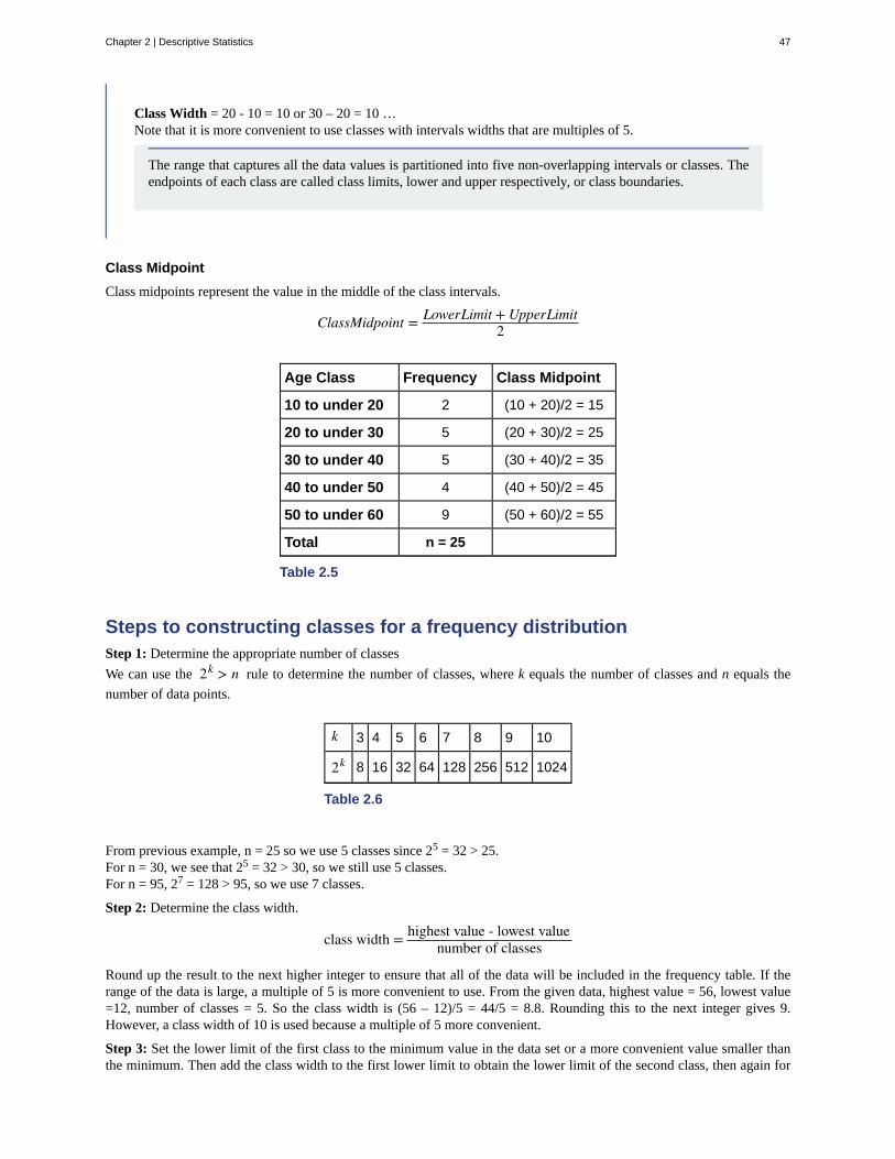
Class Width = 20 - 10 = 10 or 30 – 20 = 10 …Note that it is more convenient to use classes with intervals widths that are multiples of 5.
The range that captures all the data values is partitioned into five non-overlapping intervals or classes. Theendpoints of each class are called class limits, lower and upper respectively, or class boundaries.
Class Midpoint
Class midpoints represent the value in the middle of the class intervals.
ClassMidpoint = LowerLimit + UpperLimit2
Age Class Frequency Class Midpoint
10 to under 20 2 (10 + 20)/2 = 15
20 to under 30 5 (20 + 30)/2 = 25
30 to under 40 5 (30 + 40)/2 = 35
40 to under 50 4 (40 + 50)/2 = 45
50 to under 60 9 (50 + 60)/2 = 55
Total n = 25
Table 2.5
Steps to constructing classes for a frequency distributionStep 1: Determine the appropriate number of classes
We can use the 2k > n rule to determine the number of classes, where k equals the number of classes and n equals the
number of data points.
k 3 4 5 6 7 8 9 10
2k 8 16 32 64 128 256 512 1024
Table 2.6
From previous example, n = 25 so we use 5 classes since 25 = 32 > 25.For n = 30, we see that 25 = 32 > 30, so we still use 5 classes.For n = 95, 27 = 128 > 95, so we use 7 classes.
Step 2: Determine the class width.
class width = highest value - lowest valuenumber of classes
Round up the result to the next higher integer to ensure that all of the data will be included in the frequency table. If therange of the data is large, a multiple of 5 is more convenient to use. From the given data, highest value = 56, lowest value=12, number of classes = 5. So the class width is (56 – 12)/5 = 44/5 = 8.8. Rounding this to the next integer gives 9.However, a class width of 10 is used because a multiple of 5 more convenient.
Step 3: Set the lower limit of the first class to the minimum value in the data set or a more convenient value smaller thanthe minimum. Then add the class width to the first lower limit to obtain the lower limit of the second class, then again for
Chapter 2 | Descriptive Statistics 47

the third, and so on. The upper limits are now obvious.
Example 2.3 Years of Service
The following data represents the years of service of a sample of management employees:
35, 28, 32, 33.5, 31, 33, 34, 32, 30, 23.5, 16, 23, 19, 35, 21, 26, 31.5, 11.5, 28, 37.528, 22, 19, 23, 29, 29, 28, 19, 13, 15, 12, 30, 15, 15, 26, 20, 15, 19.5, 22, 32
Use the steps described above to construct a frequency distribution for the data.
Solution
Step 1: Finding the number of classes.From the given data, n = 40. We use the 2k > n ruleSince 25= 32 < 40 and 26 = 64 > 40, we use 6 classes.
Step 2: Finding the class widthHighest value = 37.5Lowest Value = 11.5Number of classes = 6
class width = 37.5 − 11.56 = 4.33 ≈ 5 (rounded up to a convenient value)
Step 3: Construct the tableMinimum value = 11.5 → Convenient Lower Limit of first class = 10.Since the class width is 5, we have the following frequency distribution table.
Years Frequency
10 to under 15 4
15 to under 20 8
20 to under 25 7
25 to under 30 8
30 to under 35 10
35 to under 40 3
Total 40
Table 2.7
Graphical Representation of Quantitative DataHISTOGRAM: A histogram is a graph that displays interval data by using adjacent vertical bars to represent thefrequencies. There are no spaces between the bars of a histogram unless a class frequency is zero. The frequency histogramfor the Age data in Table 2.4 is shown below.
48 Chapter 2 | Descriptive Statistics
This OpenStax book is available for free at https://legacy.cnx.org/content/col12102/1.7

Figure 2.4
FREQUENCY POLYGON: a line plot of class frequencies against their respective class midpoints. The frequencypolygon for the Age data in Table 2.4 is shown below.
Figure 2.5
Cumulative Frequency DistributionA cumulative frequency distribution shows the number (or percent) of observations that are less than or equal to eachclass interval. The cumulative frequency for each interval is the sum of the frequencies for that class and all previous classes.The following table shows the cumulative frequencies and relative cumulative frequencies for the Age data in Table 2.4.
Chapter 2 | Descriptive Statistics 49

Class Interval Frequency Cumulative Frequency Cumulative Relative Frequency
10 to under 20 2 2 2/25 = 8%
20 to under 30 5 5 + 2 = 7 7/25 = 28%
30 to under 40 5 5 + 7 = 12 12/25 = 48%
40 to under 50 4 4 + 12 = 16 16/25 = 64%
50 to under 60 9 9 + 16 = 25 25/25 = 100%
Total n = 25
Table 2.8
The table shows that 28% of the patients are under 30 years old while 64% are under 50 years old.
Cumulative Frequency Graph (Ogive)
An Ogive (pronounced oh-jive) is a graphical representation of a cumulative frequency distribution. On an ogive,cumulative frequencies are plotted against class upper limits. The ogive for the preceding table is shown below.
Figure 2.6
It can be seen on the ogive that about 40% of the patients are under 35 years old.
ReferencesNHL 2015-2016 Standings (League). Available online at https://www.nhl.com/standings (accessed September 2, 2016).
Homework
Exercise 2.1 : Lost Games
Canadian teams in the NHL performed poorly during the 2015-2016 season. No Canadian team made the playoffs thatseason. The bar graph below shows the number of regulation losses each team had.
50 Chapter 2 | Descriptive Statistics
This OpenStax book is available for free at https://legacy.cnx.org/content/col12102/1.7

Figure 2.7
a) Which team lost the highest number of games in regulation?b) Which team lost the least number of games in regulation?c) How many games were lost in total by the teams?d) What is the relative frequency of the games lost by Calgary?e) Which of the Canadian teams performed best during the 2015-2016 season?
Solutiona) Edmontonb) Ottawac) 42+39+38+38+40+35+43 = 275d) 40/275 = 14.55%e) Ottawa
Exercise 2.2 : Music Type
Some psychologists believe that the type of music you enjoy listening to tells a lot about your personality. The followingpie chart shows the music preference of students at a postsecondary institution.
Chapter 2 | Descriptive Statistics 51
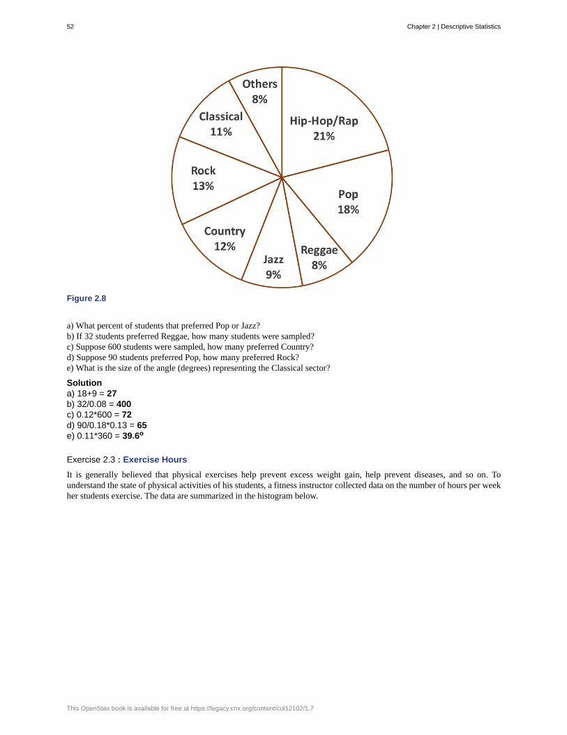
Figure 2.8
a) What percent of students that preferred Pop or Jazz?b) If 32 students preferred Reggae, how many students were sampled?c) Suppose 600 students were sampled, how many preferred Country?d) Suppose 90 students preferred Pop, how many preferred Rock?e) What is the size of the angle (degrees) representing the Classical sector?
Solutiona) 18+9 = 27b) 32/0.08 = 400c) 0.12*600 = 72d) 90/0.18*0.13 = 65e) 0.11*360 = 39.6o
Exercise 2.3 : Exercise Hours
It is generally believed that physical exercises help prevent excess weight gain, help prevent diseases, and so on. Tounderstand the state of physical activities of his students, a fitness instructor collected data on the number of hours per weekher students exercise. The data are summarized in the histogram below.
52 Chapter 2 | Descriptive Statistics
This OpenStax book is available for free at https://legacy.cnx.org/content/col12102/1.7

Figure 2.9
a) The fitness instructor collected data from how many students?b) How many class intervals were used?c) Based on the 2k rule, are the number of classes appropriate? Explain.d) What is the width of each class interval?e) How many students exercise for less than 4 hours per week?f) What percent of the students exercise between 4 and 10 hours per week?g) What is the class midpoint for those that exercise from 6 to under 8 hours?
Solutiona) 18+15+22+13+10+8+4 = 90b) 7c) Yes. 27 = 128 > 90d) 2e) 18+15 = 33f) (22+13+10)/90 = 50%g) (6 + 8)/2 = 7 hours
2.2 | Measures of the Location of the Data - (Base Version
- Lyryx Learning)PercentilesPercentiles divide ordered data into hundredths. That is, 100 equal parts. There are 99 percentiles, which we denote byP1, P2, P3, … , P99 . To score in the 90th percentile of an exam does not mean that you received 90% on a test. It means
that 90% of test scores are less than your score and 10% of the test scores are greater than your test score.
Percentiles are useful for comparing values. For this reason, universities and colleges use percentiles extensively. Oneinstance in which colleges and universities use percentiles is when SAT results are used to determine a minimum testingscore that will be used as an acceptance factor. For example, suppose Duke accepts SAT scores at or above the 75th
percentile. That translates into a score of at least 1220.
Percentiles are mostly used with very large populations. Therefore, if you were to say that 90% of the test scores areless (and not the same or less) than your score, it would be acceptable because removing one particular data value is not
Chapter 2 | Descriptive Statistics 53
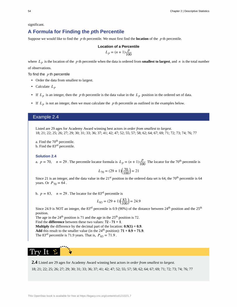
significant.
A Formula for Finding the pth PercentileSuppose we would like to find the p th percentile. We must first find the location of the p th percentile.
Location of a Percentile
L p = (n + 1) p100
where L p is the location of the p th percentile when the data is ordered from smallest to largest, and n is the total number
of observations.
To find the p th percentile
• Order the data from smallest to largest.
• Calculate L p
• If L p is an integer, then the p th percentile is the data value in the L p position in the ordered set of data.
• If L p is not an integer, then we must calculate the p th percentile as outlined in the examples below.
Example 2.4
Listed are 29 ages for Academy Award winning best actors in order from smallest to largest.18; 21; 22; 25; 26; 27; 29; 30; 31; 33; 36; 37; 41; 42; 47; 52; 55; 57; 58; 62; 64; 67; 69; 71; 72; 73; 74; 76; 77
a. Find the 70th percentile.b. Find the 83rd percentile.
Solution 2.4
a. p = 70, n = 29 . The percentile locator formula is L p = (n + 1) p100 The locator for the 70th percentile is
L70 = (29 + 1)⎛⎝ 70100⎞⎠ = 21
Since 21 is an integer, and the data value in the 21st position in the ordered data set is 64, the 70th percentile is 64years. Or P70 = 64 .
b. p = 83, n = 29 . The locator for the 83rd percentile is
L83 = (29 + 1)⎛⎝ 83100⎞⎠ = 24.9
Since 24.9 is NOT an integer, the 83rd percentile is 0.9 (90%) of the distance between 24th position and the 25th
position.The age in the 24th position is 71 and the age in the 25th position is 72.Find the difference between these two values: 72 - 71 = 1.Multiply the difference by the decimal part of the location: 0.9(1) = 0.9.Add this result to the smaller value (in the 24th position): 71 + 0.9 = 71.9.The 83rd percentile is 71.9 years. That is, P83 = 71.9 .
2.4 Listed are 29 ages for Academy Award winning best actors in order from smallest to largest.
18; 21; 22; 25; 26; 27; 29; 30; 31; 33; 36; 37; 41; 42; 47; 52; 55; 57; 58; 62; 64; 67; 69; 71; 72; 73; 74; 76; 77
54 Chapter 2 | Descriptive Statistics
This OpenStax book is available for free at https://legacy.cnx.org/content/col12102/1.7

a. Calculate the 20th percentile.b. Calculate the 55th percentile.
Quartiles
Quartiles are special percentiles. The first quartile, Q1, is the same as the 25th percentile, and the third quartile, Q3, is thesame as the 75th percentile. The median, M, is called both the second quartile, Q2, and the 50th percentile.
To calculate quartiles, the data must be ordered from smallest to largest. Quartiles divide ordered data into four equal parts.
The median is a number that measures the "center" of the data. You can think of the median as the "middle value," butit does not actually have to be one of the observed values. It is a number that separates ordered data into halves. Half thevalues are the same number or smaller than the median, and half the values are the same number or larger. For example,consider the following data.1; 11.5; 6; 7.2; 4; 8; 9; 10; 6.8; 8.3; 2; 2; 10; 1Ordered from smallest to largest:1; 1; 2; 2; 4; 6; 6.8; 7.2; 8; 8.3; 9; 10; 10; 11.5
Since there are 14 observations, the median is between the seventh value, 6.8, and the eighth value, 7.2. To find the median,add the two values together and divide by two.
Median = Q2 = 6.8 + 7.22 = 7
The median or second quartile is seven. Half of the values are smaller than seven and half of the values are larger thanseven.
To find the first quartile, we use our location of a percentile formula. The first quartile Q1 = P25 , so we find L25 .
L25 = (14 + 1)⎛⎝ 25100⎞⎠ = 3.75
The first quartile falls between the 3rd and 4th sorted values. The 3rd value is 2 and the 4th value is also 2. Since these are thesame value, we do not need to perform any calculations.The first quartile Q1 = 2 .
The third quartile Q3 = P75 , so we find L75 .
L75 = (14 + 1)⎛⎝ 75100⎞⎠ = 11.25
The first quartile is therefore between the 11th and 12th sorted values. The 11th value is 9 and the 12th value is 10.The distance between the 11th and 12th values is 10 − 9 = 1 .
0.25 of the distance is 0.25(1) = 0.25 .
The third quartile Q3 = 9.25 .
The interquartile range IQR is a number that indicates the spread of the middle half or the middle 50% of the data. It
is the difference between the third quartile Q3 , and the first quartile Q1 . From the preceding example, Q1 = 2 and
Q3 = 9.25 .
Therefore,
IQR = Q3 - Q1 = 9.25 - 2 = 7.25
The range of the middle 50% of the values is 7.25.
Example 2.5
For the following 13 real estate prices, find the quartiles and calculate the IQR.389,950; 230,500; 158,000; 479,000; 639,000; 114,950; 5,500,000; 387,000; 659,000; 529,000; 575,000;
Chapter 2 | Descriptive Statistics 55
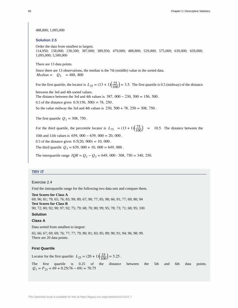
488,800; 1,095,000
Solution 2.5
Order the data from smallest to largest.114,950; 158,000; 230,500; 387,000; 389,950; 479,000; 488,800; 529,000; 575,000; 639,000; 659,000;1,095,000; 5,500,000
There are 13 data points.
Since there are 13 observations, the median is the 7th (middle) value in the sorted data.Median = Q2 = 488, 800
For the first quartile, the locator is L25 = (13 + 1)⎛⎝ 25100⎞⎠ = 3.5. The first quartile is 0.5 (midway) of the distance
between the 3rd and 4th sorted values.The distance between the 3rd and 4th values is 387, 000 − 230, 500 = 156, 500 .
0.5 of the distance gives 0.5(156, 500) = 78, 250 .
So the value midway the 3rd and 4th values is 230, 500 + 78, 250 = 308, 750 .
The first quartile Q1 = 308, 750 .
For the third quartile, the percentile locator is L75 = (13 + 1)⎛⎝ 75100⎞⎠ = 10.5. The distance between the
10th and 11th values is 659, 000 − 639, 000 = 20, 000 .
0.5 of the distance gives 0.5(20, 000) = 10, 000 .
The third quartile Q3 = 639, 000 + 10, 000 = 649, 000 .
The interquartile range IQR = Q1 − Q3 = 649, 000 - 308, 750 = 340, 250.
TRY IT
Exercise 2.4
Find the interquartile range for the following two data sets and compare them.
Test Scores for Class A69; 96; 81; 79; 65; 76; 83; 99; 89; 67; 90; 77; 85; 98; 66; 91; 77; 69; 80; 94Test Scores for Class B90; 72; 80; 92; 90; 97; 92; 75; 79; 68; 70; 80; 99; 95; 78; 73; 71; 68; 95; 100
Solution
Class A
Data sorted from smallest to largest:
65; 66; 67; 69; 69; 76; 77; 77; 79; 80; 81; 83; 85; 89; 90; 91; 94; 96; 98; 99.There are 20 data points.
First Quartile
Locator for the first quartile: L25 = (20 + 1)⎛⎝ 25100⎞⎠ = 5.25 .
The first quartile is 0.25 of the distance between the 5th and 6th data points.Q1 = P25 = 69 + 0.25(76 − 69) = 70.75
56 Chapter 2 | Descriptive Statistics
This OpenStax book is available for free at https://legacy.cnx.org/content/col12102/1.7
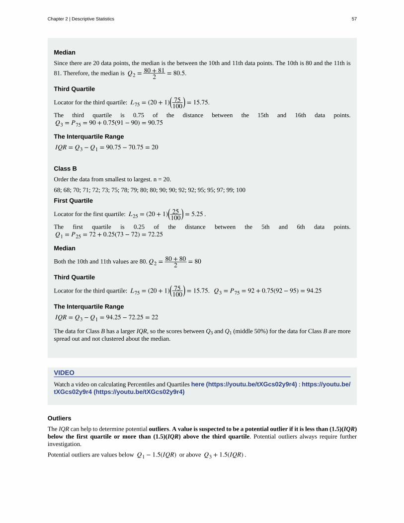
Median
Since there are 20 data points, the median is the between the 10th and 11th data points. The 10th is 80 and the 11th is
81. Therefore, the median is Q2 = 80 + 812 = 80.5.
Third Quartile
Locator for the third quartile: L75 = (20 + 1)⎛⎝ 75100⎞⎠ = 15.75.
The third quartile is 0.75 of the distance between the 15th and 16th data points.Q3 = P75 = 90 + 0.75(91 − 90) = 90.75
The Interquartile Range
IQR = Q3 − Q1 = 90.75 − 70.75 = 20
Class B
Order the data from smallest to largest. n = 20.
68; 68; 70; 71; 72; 73; 75; 78; 79; 80; 80; 90; 90; 92; 92; 95; 95; 97; 99; 100
First Quartile
Locator for the first quartile: L25 = (20 + 1)⎛⎝ 25100⎞⎠ = 5.25 .
The first quartile is 0.25 of the distance between the 5th and 6th data points.Q1 = P25 = 72 + 0.25(73 − 72) = 72.25
Median
Both the 10th and 11th values are 80. Q2 = 80 + 802 = 80
Third Quartile
Locator for the third quartile: L75 = (20 + 1)⎛⎝ 75100⎞⎠ = 15.75. Q3 = P75 = 92 + 0.75(92 − 95) = 94.25
The Interquartile Range
IQR = Q3 − Q1 = 94.25 − 72.25 = 22
The data for Class B has a larger IQR, so the scores between Q3 and Q1 (middle 50%) for the data for Class B are morespread out and not clustered about the median.
VIDEO
Watch a video on calculating Percentiles and Quartiles here (https://youtu.be/tXGcs02y9r4) : https://youtu.be/tXGcs02y9r4 (https://youtu.be/tXGcs02y9r4)
Outliers
The IQR can help to determine potential outliers. A value is suspected to be a potential outlier if it is less than (1.5)(IQR)below the first quartile or more than (1.5)(IQR) above the third quartile. Potential outliers always require furtherinvestigation.
Potential outliers are values below Q1 − 1.5(IQR) or above Q3 + 1.5(IQR) .
Chapter 2 | Descriptive Statistics 57

NOTE
A potential outlier is a data point that is significantly different from the other data points. These special data pointsmay be errors or some kind of abnormality or they may be a key to understanding the data.
Example 2.6
Calculate the IQR and determine if there are potential outliers for the following 11 scores.20 ; 6 ; 15 ; 10 ; 45 ; 18 ; 25 ; 22 ; 19 ; 37 ; 13
Solution 2.6
Order the data from smallest to largest.6 ; 10 ; 13 ; 15 ; 18 ; 19 ; 20 ; 22 ; 25 ; 37 ; 45
L25 = (11 + 1)⎛⎝ 25100⎞⎠ = 3rd ⎯⎯⎯⎯⎯⎯⎯⎯⎯⎯⎯⎯⎯⎯⎯⎯⎯⎯⎯⎯⎯⎯⎯ Q1 = 13
L75 = (11 + 1)⎛⎝ 75100⎞⎠ = 9th ⎯⎯⎯⎯⎯⎯⎯⎯⎯⎯⎯⎯⎯⎯⎯⎯⎯⎯⎯⎯⎯⎯⎯ Q3 = 25
IQR = Q3 − Q1 = 25 − 13 = 12
1.5(IQR) = 1.5×12 = 18
Q1 − 1.5(IQR) = 13 − 18 = − 5
Q3 + 1.5(IQR) = 25 + 18 = 43
No score is less than –5. However, 45 is more than 43. Therefore, 45 is a potential outlier.
Interpreting Percentiles, Quartiles, and MedianA percentile indicates the relative standing of a data value when data are sorted into numerical order from smallest to largest.Percentages of data values are less than or equal to the pth percentile. For example, 15% of data values are less than or equalto the 15th percentile.
• Low percentiles always correspond to lower data values.
• High percentiles always correspond to higher data values.
A percentile may or may not correspond to a value judgment about whether it is "good" or "bad." The interpretation ofwhether a certain percentile is "good" or "bad" depends on the context of the situation to which the data applies. In somesituations, a low percentile would be considered "good;" in other contexts a high percentile might be considered "good". Inmany situations, there is no value judgment that applies.
Understanding how to interpret percentiles properly is important not only when describing data, but also when calculatingprobabilities in later chapters of this text.
GUIDELINE
When writing the interpretation of a percentile in the context of the given data, the sentence should contain thefollowing information.
• information about the context of the situation being considered
• the data value (value of the variable) that represents the percentile
• the percent of individuals or items with data values below the percentile
• the percent of individuals or items with data values above the percentile.
58 Chapter 2 | Descriptive Statistics
This OpenStax book is available for free at https://legacy.cnx.org/content/col12102/1.7

Example 2.7
On a timed math test, the first quartile for time it took to finish the exam was 35 minutes. Interpret the first quartilein the context of this situation.
Solution 2.7• Twenty-five percent of students finished the exam under 35 minutes.
• Seventy-five percent of students finished the exam in over 35 minutes.
• A low percentile could be considered good, as finishing more quickly on a timed exam is desirable. (If youtake too long, you might not be able to finish.)
Example 2.8
On a 20 question math test, the 70th percentile for number of correct answers was 16. Interpret the 70th percentilein the context of this situation.
Solution 2.8• Seventy percent of students answered less than 16 questions correctly.
• Thirty percent of students answered more than 16 questions correctly.
• A higher percentile could be considered good, as answering more questions correctly is desirable.
2.8 On a 60 point written assignment, the 80th percentile for the number of points earned was 49. Interpret the 80th
percentile in the context of this situation.
Example 2.9
At a community college, it was found that the 30th percentile of credit units that students are enrolled for is sevenunits. Interpret the 30th percentile in the context of this situation.
Solution 2.9• Thirty percent of students are enrolled in seven or fewer credit units.
• Seventy percent of students are enrolled in seven or more credit units.
• In this example, there is no "good" or "bad" value judgment associated with a higher or lower percentile.Students attend community college for varied reasons and needs, and their course load varies according totheir needs.
Boxplot and the 5-Number SummaryA boxplot is a graphical display, based on quartiles, that helps picture the distribution of a data set. The following valuesare needed to construct a box plot. They are also referred to as the 5-number summary .
1. Minimum value (lowest value)
2. First quartile (Q1)
3. Median (Q2)
Chapter 2 | Descriptive Statistics 59

4. Third quartile (Q3)
5. Maximum value (highest value)
A boxplot divides data into quartiles (see figure below). It consists of a rectangle in the middle, bounded on the left (bottom)by the first quartile (Q1), and on the right (top) by the third quartile (Q3). A vertical line is also drawn within the boxrepresenting the median. Two horizontal lines, called whiskers, extend from the bottom and top of the box. The bottomwhisker extends from Q1 to the smallest non-outlier in the data set, and the top whisker extends from Q3 to the largest non-outlier. Outliers (if they exist) are plotted separately as points (or asteriks) on the chart.
Figure 2.10 Boxplot
Example 2.10
Sharpe Middle School is applying for a grant that will be used to add fitness equipment to the gym. The principalsurveyed 15 anonymous students to determine how many minutes a day the students spend exercising. Thenumber of exercise minutes from the 15 anonymous students are shown below.
50 ; 10 ; 45 ; 90 ; 0 ; 100 ; 20 ; 30 ; 30 ; 40 ; 0 ; 60 ; 120 ; 70 ; 30
Determine the 5-number summary and construct a boxplot for the data.
Solution 2.10Min = 0
L25 = (15 + 1)⎛⎝ 25100⎞⎠ = 4th ⎯⎯⎯⎯⎯⎯⎯⎯⎯⎯⎯⎯⎯⎯⎯⎯⎯⎯⎯⎯⎯⎯⎯ Q1 = 20
Median = 40
L75 = (15 + 1)⎛⎝ 75100⎞⎠ = 12th ⎯⎯⎯⎯⎯⎯⎯⎯⎯⎯⎯⎯⎯⎯⎯⎯⎯⎯⎯⎯⎯⎯⎯ Q3 = 70
Max = 120
Figure 2.11 Boxplot for Exercise Minutes Data
Since 75% of the students exercise for 70 minutes or less daily, and since the IQR is 50 minutes (70 – 20 = 50),
60 Chapter 2 | Descriptive Statistics
This OpenStax book is available for free at https://legacy.cnx.org/content/col12102/1.7

we know that half of the students surveyed exercise between 20 minutes and 70 minutes daily. This seems areasonable amount of time spent exercising, so the principal would be justified in purchasing the new equipment.
2.3 | Measures of the Center of the DataThe "center" of a data set is also a way of describing location. The two most widely used measures of the "center" of thedata are the mean (average) and the median. To calculate the mean weight of 50 people, add the 50 weights together anddivide by 50. Technically this is the arithmetic mean. We will discuss the geometric mean later. To find the median weightof the 50 people, order the data and find the number that splits the data into two equal parts meaning an equal number ofobservations on each side. The weight of 25 people are below this weight and 25 people are heavier than this weight. Themedian is generally a better measure of the center when there are extreme values or outliers because it is not affected by theprecise numerical values of the outliers. The mean is the most common measure of the center.
NOTE
The words “mean” and “average” are often used interchangeably. The substitution of one word for the other iscommon practice. The technical term is “arithmetic mean” and “average” is technically a center location. Formally,the arithmetic mean is called the first moment of the distribution by mathematicians. However, in practice among non-statisticians, “average" is commonly accepted for “arithmetic mean.”
When each value in the data set is not unique, the mean can be calculated by multiplying each distinct value by its frequencyand then dividing the sum by the total number of data values. The letter used to represent the sample mean is an x with abar over it (pronounced “x bar”): x– .
The Greek letter μ (pronounced "mew") represents the population mean. One of the requirements for the sample mean tobe a good estimate of the population mean is for the sample taken to be truly random.
To see that both ways of calculating the mean are the same, consider the sample:1; 1; 1; 2; 2; 3; 4; 4; 4; 4; 4
x– = 1 + 1 + 1 + 2 + 2 + 3 + 4 + 4 + 4 + 4 + 411 = 2.7
x– = 3(1) + 2(2) + 1(3) + 5(4)11 = 2.7
In the second calculation, the frequencies are 3, 2, 1, and 5.
You can quickly find the location of the median by using the expression n + 12 .
The letter n is the total number of data values in the sample. If n is an odd number, the median is the middle value ofthe ordered data (ordered smallest to largest). If n is an even number, the median is equal to the two middle values addedtogether and divided by two after the data has been ordered. For example, if the total number of data values is 97, thenn + 1
2 = 97 + 12 = 49. The median is the 49th value in the ordered data. If the total number of data values is 100, then
n + 12 = 100 + 1
2 = 50.5. The median occurs midway between the 50th and 51st values. The location of the median and
the value of the median are not the same. The upper case letter M is often used to represent the median. The next exampleillustrates the location of the median and the value of the median.
Example 2.11
AIDS data indicating the number of months a patient with AIDS lives after taking a new antibody drug are asfollows (smallest to largest):3; 4; 8; 8; 10; 11; 12; 13; 14; 15; 15; 16; 16; 17; 17; 18; 21; 22; 22; 24; 24; 25; 26; 26; 27; 27; 29; 29; 31; 32; 33;33; 34; 34; 35; 37; 40; 44; 44; 47;
Chapter 2 | Descriptive Statistics 61

Calculate the mean and the median.
Solution 2.11
The calculation for the mean is:
x– = [3 + 4 + (8)(2) + 10 + 11 + 12 + 13 + 14 + (15)(2) + (16)(2) + ... + 35 + 37 + 40 + (44)(2) + 47]40 = 23.6
To find the median, M, first use the formula for the location. The location is:n + 1
2 = 40 + 12 = 20.5
Starting at the smallest value, the median is located between the 20th and 21st values (the two 24s):3; 4; 8; 8; 10; 11; 12; 13; 14; 15; 15; 16; 16; 17; 17; 18; 21; 22; 22; 24; 24; 25; 26; 26; 27; 27; 29; 29; 31; 32; 33;33; 34; 34; 35; 37; 40; 44; 44; 47;
M = 24 + 242 = 24
Example 2.12
Suppose that in a small town of 50 people, one person earns $5,000,000 per year and the other 49 each earn$30,000. Which is the better measure of the "center": the mean or the median?
Solution 2.12
x– = 5, 000, 000 + 49(30, 000)50 = 129,400
M = 30,000
(There are 49 people who earn $30,000 and one person who earns $5,000,000.)
The median is a better measure of the "center" than the mean because 49 of the values are 30,000 and one is5,000,000. The 5,000,000 is an outlier. The 30,000 gives us a better sense of the middle of the data.
Another measure of the center is the mode. The mode is the most frequent value. There can be more than one mode in adata set as long as those values have the same frequency and that frequency is the highest. A data set with two modes iscalled bimodal.
Example 2.13
Statistics exam scores for 20 students are as follows:
50; 53; 59; 59; 63; 63; 72; 72; 72; 72; 72; 76; 78; 81; 83; 84; 84; 84; 90; 93
Find the mode.
Solution 2.13The most frequent score is 72, which occurs five times. Mode = 72.
Example 2.14
Five real estate exam scores are 430, 430, 480, 480, 495. The data set is bimodal because the scores 430 and 480each occur twice.
62 Chapter 2 | Descriptive Statistics
This OpenStax book is available for free at https://legacy.cnx.org/content/col12102/1.7

When is the mode the best measure of the "center"? Consider a weight loss program that advertises a mean weightloss of six pounds the first week of the program. The mode might indicate that most people lose two pounds thefirst week, making the program less appealing.
NOTE
The mode can be calculated for qualitative data as well as for quantitative data. For example, if the data setis: red, red, red, green, green, yellow, purple, black, blue, the mode is red.
Calculating the Arithmetic Mean of Grouped Frequency TablesWhen only grouped data is available, you do not know the individual data values (we only know intervals and intervalfrequencies); therefore, you cannot compute an exact mean for the data set. What we must do is estimate the actual meanby calculating the mean of a frequency table. A frequency table is a data representation in which grouped data is displayedalong with the corresponding frequencies. To calculate the mean from a grouped frequency table we can apply the basic
definition of mean: mean = data sumnumber o f data values We simply need to modify the definition to fit within the restrictions
of a frequency table.
Since we do not know the individual data values we can instead find the midpoint of each interval. The midpoint
islower boundary + upper boundary
2 . We can now modify the mean definition to be
Mean o f Frequency Table =∑ fm
∑ fwhere f = the frequency of the interval and m = the midpoint of the interval.
Example 2.15
A frequency table displaying professor Blount’s last statistic test is shown. Find the best estimate of the classmean.
Grade interval Number of students
50–56.5 1
56.5–62.5 0
62.5–68.5 4
68.5–74.5 4
74.5–80.5 2
80.5–86.5 3
86.5–92.5 4
92.5–98.5 1
Table 2.9
Solution 2.15• Find the midpoints for all intervals
Chapter 2 | Descriptive Statistics 63

Grade interval Midpoint
50–56.5 53.25
56.5–62.5 59.5
62.5–68.5 65.5
68.5–74.5 71.5
74.5–80.5 77.5
80.5–86.5 83.5
86.5–92.5 89.5
92.5–98.5 95.5
Table 2.10
• Calculate the sum of the product of each interval frequency and midpoint. ∑ fm
53.25(1) + 59.5(0) + 65.5(4) + 71.5(4) + 77.5(2) + 83.5(3) + 89.5(4) + 95.5(1) = 1460.25
• μ =∑ fm
∑ f= 1460.25
19 = 76.86
2.15 Maris conducted a study on the effect that playing video games has on memory recall. As part of her study, shecompiled the following data:
Hours teenagers spend on video games Number of teenagers
0–3.5 3
3.5–7.5 7
7.5–11.5 12
11.5–15.5 7
15.5–19.5 9
Table 2.11
What is the best estimate for the mean number of hours spent playing video games?
2.4 | Sigma Notation and Calculating the Arithmetic MeanFormula for Population Mean
() μ = 1N ∑i = 1
Nxi
64 Chapter 2 | Descriptive Statistics
This OpenStax book is available for free at https://legacy.cnx.org/content/col12102/1.7

Formula for Sample Mean
() x– = 1n ∑i = 1
nxi
This unit is here to remind you of material that you once studied and said at the time “I am sure that I will never need this!”
Here are the formulas for a population mean and the sample mean. The Greek letter μ is the symbol for the populationmean and x– is the symbol for the sample mean. Both formulas have a mathematical symbol that tells us how to make
the calculations. It is called Sigma notation because the symbol is the Greek capital letter sigma: Σ. Like all mathematicalsymbols it tells us what to do: just as the plus sign tells us to add and the x tells us to multiply. These are called mathematicaloperators. The Σ symbol tells us to add a specific list of numbers.
Let’s say we have a sample of animals from the local animal shelter and we are interested in their average age. If we listeach value, or observation, in a column, you can give each one an index number. The first number will be number 1 and thesecond number 2 and so on.
Animal Age
1 9
2 1
3 8.5
4 10.5
5 10
6 8.5
7 12
8 8
9 1
10 9.5
Table 2.12
Each observation represents a particular animal in the sample. Purr is animal number one and is a 9 year old cat, Toto isanimal number 2 and is a 1 year old puppy and so on.
To calculate the mean we are told by the formula to add up all these numbers, ages in this case, and then divide the sum by10, the total number of animals in the sample.
Animal number one, the cat Purr, is designated as X1, animal number 2, Toto, is designated as X2 and so on through Dundeewho is animal number 10 and is designated as X10.
The i in the formula tells us which of the observations to add together. In this case it is X1 through X10 which is all of them.We know which ones to add by the indexing notation, the i = 1 and the n or capital N for the population. For this examplethe indexing notation would be i = 1 and because it is a sample we use a small n on the top of the Σ which would be 10.
The standard deviation requires the same mathematical operator and so it would be helpful to recall this knowledge fromyour past.
The sum of the ages is found to be 78 and dividing by 10 gives us the sample mean age as 7.8 years.
2.5 | Skewness and the Mean, Median, and ModeConsider the following data set.4; 5; 6; 6; 6; 7; 7; 7; 7; 7; 7; 8; 8; 8; 9; 10
This data set can be represented by following histogram. Each interval has width one, and each value is located in the middleof an interval.
Chapter 2 | Descriptive Statistics 65

Figure 2.12
The histogram displays a symmetrical distribution of data. A distribution is symmetrical if a vertical line can be drawn atsome point in the histogram such that the shape to the left and the right of the vertical line are mirror images of each other.The mean, the median, and the mode are each seven for these data. In a perfectly symmetrical distribution, the meanand the median are the same. This example has one mode (unimodal), and the mode is the same as the mean and median.In a symmetrical distribution that has two modes (bimodal), the two modes would be different from the mean and median.
The histogram for the data: 4; 5; 6; 6; 6; 7; 7; 7; 7; 8 shown in Figure 2.12 is not symmetrical. The right-hand side seems"chopped off" compared to the left side. A distribution of this type is called skewed to the left because it is pulled out tothe left. We can formally measure the skewness of a distribution just as we can mathematically measure the center weight
of the data or its general "speadness". The mathematical formula for skewness is: a3 = ∑⎛⎝xi − x¯ ⎞⎠
3
ns3 . The greater the
deviation from zero indicates a greater degree of skewness. If the skewness is negative then the distribution is skewed leftas in Figure 2.13. A positive measure of skewness indicates right skewness such as Figure 2.14.
Figure 2.13
The mean is 6.3, the median is 6.5, and the mode is seven. Notice that the mean is less than the median, and they areboth less than the mode. The mean and the median both reflect the skewing, but the mean reflects it more so.
The histogram for the data: 6; 7; 7; 7; 7; 8; 8; 8; 9; 10 shown in Figure 2.13, is also not symmetrical. It is skewed to theright.
66 Chapter 2 | Descriptive Statistics
This OpenStax book is available for free at https://legacy.cnx.org/content/col12102/1.7

Figure 2.14
The mean is 7.7, the median is 7.5, and the mode is seven. Of the three statistics, the mean is the largest, while the modeis the smallest. Again, the mean reflects the skewing the most.
To summarize, generally if the distribution of data is skewed to the left, the mean is less than the median, which is often lessthan the mode. If the distribution of data is skewed to the right, the mode is often less than the median, which is less thanthe mean.
As with the mean, median and mode, and as we will see shortly, the variance, there are mathematical formulas that give usprecise measures of these characteristics of the distribution of the data. Again looking at the formula for skewness we seethat this is a relationship between the mean of the data and the individual observations cubed.
a3 = ∑⎛⎝xi − x¯ ⎞⎠
3
ns3
where s is the sample standard deviation of the data, Xi , and x¯ is the arithmetic mean and n is the sample size.
Formally the arithmetic mean is known as the first moment of the distribution. The second moment we will see is thevariance, and skewness is the third moment. The variance measures the squared differences of the data from the mean andskewness measures the cubed differences of the data from the mean. While a variance can never be a negative number,the measure of skewness can and this is how we determine if the data are skewed right of left. The skewness for a normaldistribution is zero, and any symmetric data should have skewness near zero. Negative values for the skewness indicatedata that are skewed left and positive values for the skewness indicate data that are skewed right. By skewed left, we meanthat the left tail is long relative to the right tail. Similarly, skewed right means that the right tail is long relative to the lefttail. The skewness characterizes the degree of asymmetry of a distribution around its mean. While the mean and standarddeviation are dimensional quantities (this is why we will take the square root of the variance ) that is, have the same unitsas the measured quantities Xi , the skewness is conventionally defined in such a way as to make it nondimensional. It is a
pure number that characterizes only the shape of the distribution. A positive value of skewness signifies a distribution withan asymmetric tail extending out towards more positive X and a negative value signifies a distribution whose tail extendsout towards more negative X. A zero measure of skewness will indicate a symmetrical distribution.
Skewness and symmetry become important when we discuss probability distributions in later chapters.
2.6 | Measures of the Spread of the Data - (Base Version -
Lyryx Learning)An important characteristic of any set of data is the variation in the data. In some data sets, the data values are concentratedclosely near the mean; in other data sets, the data values are more widely spread out from the mean. There are several waysto measure variation. Three commonly used measures of variation are the range, the variance and the standard deviation
Chapter 2 | Descriptive Statistics 67
.
The RangeThe range is the simplest measure of variation. The range measures the difference between the highest and lowest values ina data set.
Range = Highest Value - Lowest Value
Example 2.16 Workout Times
Find the range of the following workout times (mins): 13.3, 21.1, 12.1, 25.5, 28.9, 26, 16.8, 13.6, 27.6, 15.4, 18.4
Solution
Highest Value = 28.9Lowest Value = 12.1Range = 28.9 - 12.1 = 16.8
While the range gives us some idea of how spread out the data is, it tells us nothing about how data is dispersed within therange, whether it is compact or spread out or clustered around certain values.
The standard deviation is a more common measure of variation that takes all of the data points into consideration.
The Standard DeviationThe standard deviation is a number that measures how far data values are from their mean.
The standard deviation:• provides a numerical measure of the overall amount of variation in a data set, and
• can be used to determine whether a particular data value is close to or far from the mean.
The standard deviation provides a measure of the overall variation in a data set
The standard deviation is small when the data are all concentrated close to the mean, exhibiting little variation or spread.The standard deviation is larger when the data values are more spread out from the mean, exhibiting more variation.Thestandard deviation is always non-negative.
Suppose that we are studying the amount of time customers wait in line at the checkout at supermarket A and supermarketB. The average wait time at both supermarkets is five minutes. At supermarket A, the standard deviation for the wait time istwo minutes; at supermarket B. The standard deviation for the wait time is four minutes.
Because supermarket B has a higher standard deviation, we know that there is more variation in the wait times atsupermarket B. Overall, wait times at supermarket B are more spread out from the average; wait times at supermarket A aremore concentrated near the average.
Calculating the Standard Deviation
If x is a number, then the difference "x – mean" is called its deviation. In a data set, there are as many deviations as thereare items in the data set. The deviations are used to calculate the standard deviation. If the numbers belong to a population,in symbols a deviation is x – μ. For sample data, in symbols a deviation is x – x– .
The procedure to calculate the standard deviation depends on whether the numbers are the entire population or are datafrom a sample. The calculations are similar, but not identical. Therefore the symbol used to represent the standard deviationdepends on whether it is calculated from a population or a sample. The lower case letter s represents the sample standard
deviation and the Greek letter σ (sigma, lower case) represents the population standard deviation. If the sample has thesame characteristics as the population, then s should be a good estimate of σ.
To calculate the standard deviation, we need to calculate the variance first. The variance is the average of the squares
of the deviations (the x – x– values for a sample, or the x – μ values for a population). The symbol σ2 represents the
population variance; the population standard deviation σ is the square root of the population variance. The symbol s2
represents the sample variance; the sample standard deviation s is the square root of the sample variance. You can think ofthe standard deviation as a special average of the deviations.
68 Chapter 2 | Descriptive Statistics
This OpenStax book is available for free at https://legacy.cnx.org/content/col12102/1.7
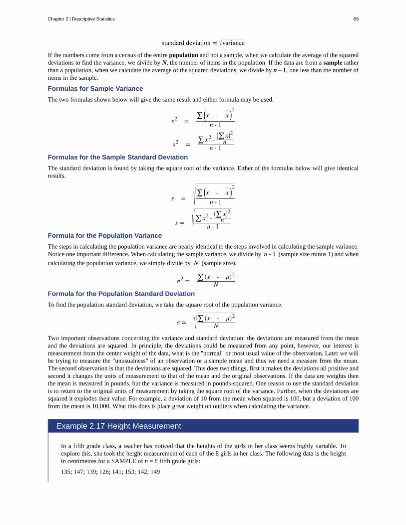
standard deviation = variance
If the numbers come from a census of the entire population and not a sample, when we calculate the average of the squareddeviations to find the variance, we divide by N, the number of items in the population. If the data are from a sample ratherthan a population, when we calculate the average of the squared deviations, we divide by n – 1, one less than the number ofitems in the sample.
Formulas for Sample Variance
The two formulas shown below will give the same result and either formula may be used.
s2 = ∑ ⎛⎝x - x¯ ⎞⎠
2
n - 1
s2 = ∑ x2 -
⎛⎝∑ x⎞⎠2n
n - 1Formulas for the Sample Standard Deviation
The standard deviation is found by taking the square root of the variance. Either of the formulas below will give identicalresults.
s = ∑ ⎛⎝x - x¯ ⎞⎠
2
n - 1
s = ∑ x2 -
⎛⎝∑ x⎞⎠2n
n - 1Formula for the Population Variance
The steps in calculating the population variance are nearly identical to the steps involved in calculating the sample variance.Notice one important difference. When calculating the sample variance, we divide by n - 1 (sample size minus 1) and when
calculating the population variance, we simply divide by N (sample size).
σ2 = ∑ (x - μ)2
NFormula for the Population Standard Deviation
To find the population standard deviation, we take the square root of the population variance.
σ = ∑ (x - μ)2
N
Two important observations concerning the variance and standard deviation: the deviations are measured from the meanand the deviations are squared. In principle, the deviations could be measured from any point, however, our interest ismeasurement from the center weight of the data, what is the "normal" or most usual value of the observation. Later we willbe trying to measure the "unusualness" of an observation or a sample mean and thus we need a measure from the mean.The second observation is that the deviations are squared. This does two things, first it makes the deviations all positive andsecond it changes the units of measurement to that of the mean and the original observations. If the data are weights thenthe mean is measured in pounds, but the variance is measured in pounds-squared. One reason to use the standard deviationis to return to the original units of measurement by taking the square root of the variance. Further, when the deviations aresquared it explodes their value. For example, a deviation of 10 from the mean when squared is 100, but a deviation of 100from the mean is 10,000. What this does is place great weight on outliers when calculating the variance.
Example 2.17 Height Measurement
In a fifth grade class, a teacher has noticed that the heights of the girls in her class seems highly variable. Toexplore this, she took the height measurement of each of the 8 girls in her class. The following data is the heightin centimetres for a SAMPLE of n = 8 fifth grade girls:
135; 147; 139; 126; 141; 153; 142; 149
Chapter 2 | Descriptive Statistics 69

x¯ = 135 + 147 + 139 + 126 + 141 + 153 + 142 + 1498 = 141.5
The average height is 141.5 cm.
The variance may be calculated by using a table. Then the standard deviation is calculated by taking the squareroot of the variance. We will explain the parts of the table after calculating s.
x x - x ⎛⎝x - x⎞⎠
2
135 135-141.5 = -6.5 (-6.5)2 = 42.25
147 147-141.5 = 5.5 (5.5)2 = 30.25
139 139 - 141.5 = -2.5 (-2.5)2 = 6.25
126 126 - 141.5 = -15.5 (-15.5)2 = 240.25
141 141 - 141.5 = -0.5 (-0.5)2 = 0.25
153 153 - 141.5 = 11.5 (11.5)2 = 132.25
142 142 - 141.5 = 0.5 (0.5)2 = 0.25
149 149 - 141.5 = 7.5 (7.5)2 = 56.25
Total 508
Table 2.13
The sample variance, s2, is equal to the sum of the last column (508) divided by the total number of data valuesminus one (8 - 1):
s2 = 5088 − 1 = 72.57142857
The sample variance is 72.57 cm2, rounded to 2 decimal places.
The sample standard deviation s is equal to the square root of the sample variance:
s = 72.57142857 = 8.5189,
The sample standard deviation, rounded to 2 decimal places, is 8.52 cm.
Here is a video (https://youtu.be/lLLud8kfm1M) on how to use the BA II Plus calculator to obtain the mean,standard deviation, and variance.
Explanation of the standard deviation calculation shown in the table
The deviations show how spread out the data are about the mean. The data value 135 is farther from the mean than is thedata value 141 which is indicated by the deviations -6.5 and -0.5. A positive deviation occurs when the data value is greaterthan the mean, whereas a negative deviation occurs when the data value is less than the mean. If you add the deviations,the sum is always zero. (In the example above, there are n = 8 deviations.) So you cannot simply add the deviations toget the spread of the data. By squaring the deviations, you make them positive numbers, and the sum will also be positive.The variance, then, is the average squared deviation. By squaring the deviations we are placing an extreme penalty onobservations that are far from the mean; these observations get greater weight in the calculations of the variance. We will seelater on that the variance (standard deviation) plays the critical role in determining our conclusions in inferential statistics.We can begin now by using the standard deviation as a measure of "unusualness." "How did you do on the test?" "Terrific!Two standard deviations above the mean." This, we will see, is an unusually good exam grade.
The variance is a squared measure and does not have the same units as the data. Taking the square root solves the problem.The standard deviation measures the spread in the same units as the data.
Notice that instead of dividing by n = 8, the calculation divided by n – 1 = 8 – 1 = 7 because the data is a sample. Forthe sample variance, we divide by the sample size minus one (n – 1). Why not divide by n? The answer has to do with
70 Chapter 2 | Descriptive Statistics
This OpenStax book is available for free at https://legacy.cnx.org/content/col12102/1.7

the population variance. The sample variance is an estimate of the population variance. This estimate requires us to usean estimate of the population mean rather than the actual population mean. Based on the theoretical mathematics that liesbehind these calculations, dividing by (n – 1) gives a better estimate of the population variance.
The standard deviation, s or σ, is either zero or larger than zero. When the standard deviation is zero, there is no spread; thatis, the all the data values are equal to each other. The standard deviation is small when the data are all concentrated close tothe mean, and is larger when the data values show more variation from the mean. When the standard deviation is a lot largerthan zero, the data values are very spread out about the mean; outliers can make s or σ very large.
Chapter 2 | Descriptive Statistics 71

Example 2.18 Prof Tan Le's Class
72 Chapter 2 | Descriptive Statistics
This OpenStax book is available for free at https://legacy.cnx.org/content/col12102/1.7

Use the following data (final exam scores) from Prof. Tan Le's summer statistics class:
42, 56, 63, 67, 68, 68, 69, 69, 72, 73, 74, 78, 80, 83, 88, 88, 88, 90, 92, 94, 94, 94, 94, 96, 100
a. Create a chart containing the data, frequencies, relative frequencies, and cumulative relative frequencies to2 decimal places.
b. Calculate the following to one decimal place:
i. The sample mean
ii. The median
iii. The mode
iv. The range
v. The sample variance
vi. The sample standard deviation
vii. The first quartile
viii. The third quartile
ix. IQR
Solution 2.18a. See Table 2.13
b. i. The sample mean = 79.2
ii. The median = 79
iii. The mode = 94
iv. The range = 58
v. The sample variance = 209.6
vi. The sample standard deviation = 14.5
vii. The first quartile = 68.5
viii. The third quartile = 93
ix. IQR = 93 – 68.5 = 24.5
Data Frequency Relative Frequency Cumulative Relative Frequency
42 1 0.04 0.04
56 1 0.04 0.08
63 1 0.04 0.12
67 1 0.04 0.16
68 2 0.08 0.24
69 2 0.08 0.32
72 1 0.04 0.36
73 1 0.04 0.4
74 1 0.04 0.44
78 1 0.04 0.48
Total 25 1 ---
Chapter 2 | Descriptive Statistics 73
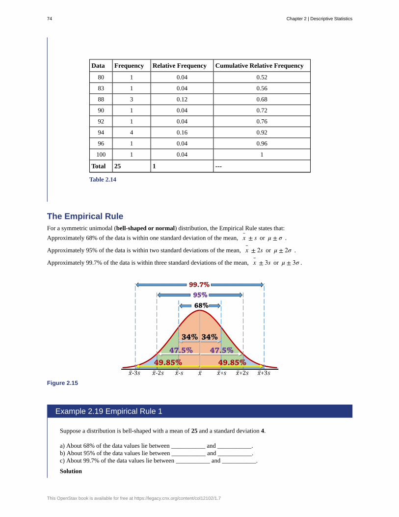
Data Frequency Relative Frequency Cumulative Relative Frequency
80 1 0.04 0.52
83 1 0.04 0.56
88 3 0.12 0.68
90 1 0.04 0.72
92 1 0.04 0.76
94 4 0.16 0.92
96 1 0.04 0.96
100 1 0.04 1
Total 25 1 ---
Table 2.14
The Empirical RuleFor a symmetric unimodal (bell-shaped or normal) distribution, the Empirical Rule states that:
Approximately 68% of the data is within one standard deviation of the mean, x ± s or μ ± σ .
Approximately 95% of the data is within two standard deviations of the mean, x ± 2s or μ ± 2σ .
Approximately 99.7% of the data is within three standard deviations of the mean, x ± 3s or μ ± 3σ .
Figure 2.15
Example 2.19 Empirical Rule 1
Suppose a distribution is bell-shaped with a mean of 25 and a standard deviation 4.
a) About 68% of the data values lie between ___________ and ___________.b) About 95% of the data values lie between ___________ and ___________.c) About 99.7% of the data values lie between ___________ and ___________.
Solution
74 Chapter 2 | Descriptive Statistics
This OpenStax book is available for free at https://legacy.cnx.org/content/col12102/1.7
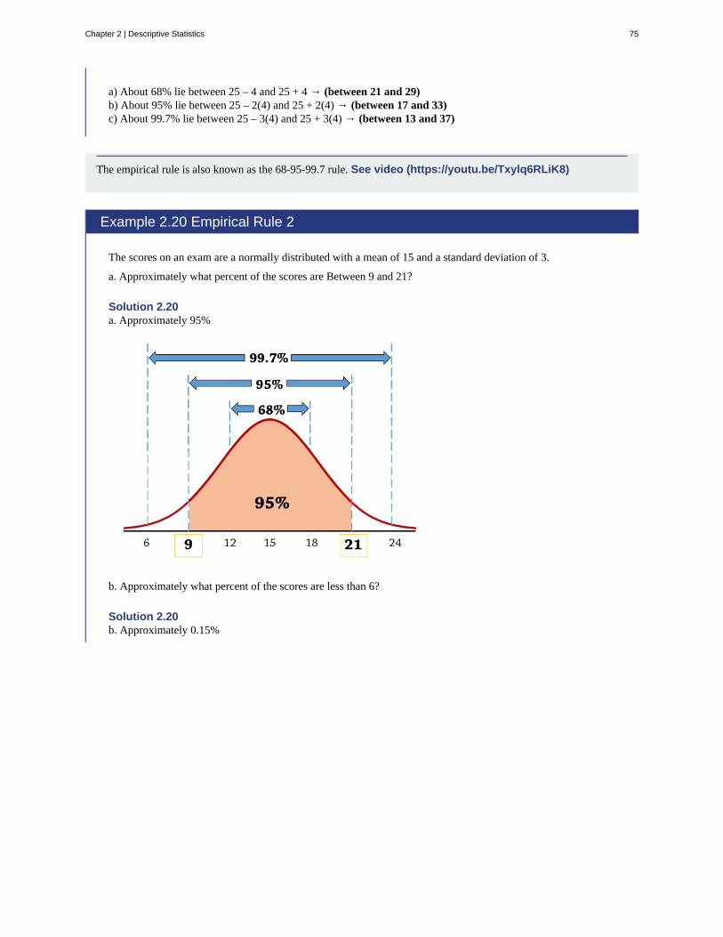
a) About 68% lie between 25 – 4 and 25 + 4 → (between 21 and 29)b) About 95% lie between 25 – 2(4) and 25 + 2(4) → (between 17 and 33)c) About 99.7% lie between 25 – 3(4) and 25 + 3(4) → (between 13 and 37)
The empirical rule is also known as the 68-95-99.7 rule. See video (https://youtu.be/Txylq6RLiK8)
Example 2.20 Empirical Rule 2
The scores on an exam are a normally distributed with a mean of 15 and a standard deviation of 3.
a. Approximately what percent of the scores are Between 9 and 21?
Solution 2.20a. Approximately 95%
b. Approximately what percent of the scores are less than 6?
Solution 2.20b. Approximately 0.15%
Chapter 2 | Descriptive Statistics 75
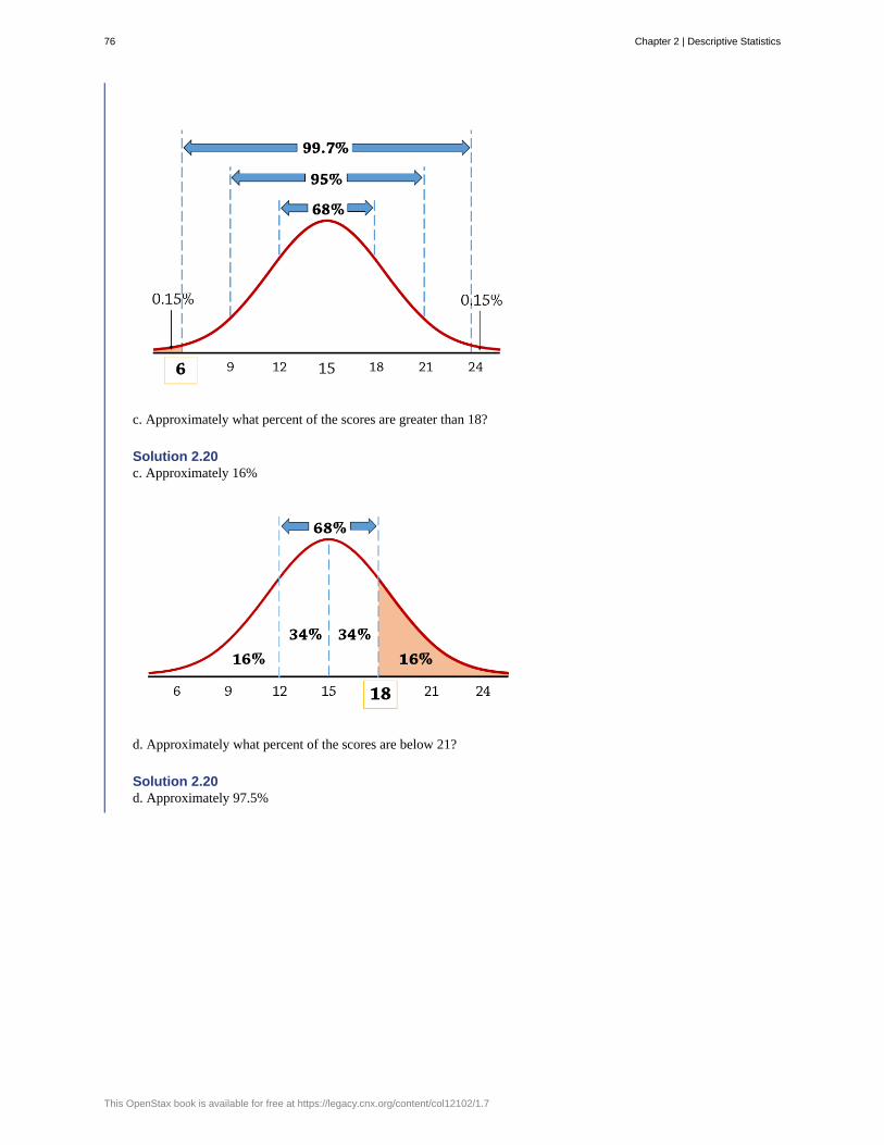
c. Approximately what percent of the scores are greater than 18?
Solution 2.20c. Approximately 16%
d. Approximately what percent of the scores are below 21?
Solution 2.20d. Approximately 97.5%
76 Chapter 2 | Descriptive Statistics
This OpenStax book is available for free at https://legacy.cnx.org/content/col12102/1.7

e. Approximately what percent of the scores are between 12 and 24?
Solution 2.20e. Approximately 83.85%
Coefficient of VariationAnother useful way to compare distributions besides simple comparisons of means or standard deviations is to adjust fordifferences in the scale of the data being measured. Quite simply, a large variation in data with a large mean is different thanthe same variation in data with a small mean. To adjust for the scale of the underlying data the Coefficient of Variation (CV)has been developed. Mathematically:
Sample Coefficient of VariationCV = s
x¯
Population Coefficient of VariationCV = σ
μ
We can see that this measures the variability of the underlying data as a percentage of the mean value; the center weight ofthe data set. This measure is useful in comparing risk where an adjustment is warranted because of differences in scale of
Chapter 2 | Descriptive Statistics 77

two data sets. In effect, the scale is changed to common scale, percentage differences and allows direct comparison of thetwo or more magnitudes of variation of different data sets.
Example 2.21 Pete and Ahmed
Two students, Pete and Ahmed, from different colleges, wanted to find out whose school has a higher GPAvariability. They both agree that too much variability in GPAs is bad and want to know whose school isperforming better in that respect. Here is a summary of data from their schools.
Standard Deviation of GPA Mean GPA
Pete’s school 9.0 78
Ahmed’s school 8.6 70
Table 2.15
Solution
We compute and compare the coefficient of variation for each school.
Pete's School: CV = 9.078 = 0.115 or 11.5%
Ahmed's School: CV = 8.670 = 0.123 or 12.3%
Although the standard deviation is higher for Pete’s school, Ahmed’s school has more GPA variability relative tothe mean.
78 Chapter 2 | Descriptive Statistics
This OpenStax book is available for free at https://legacy.cnx.org/content/col12102/1.7
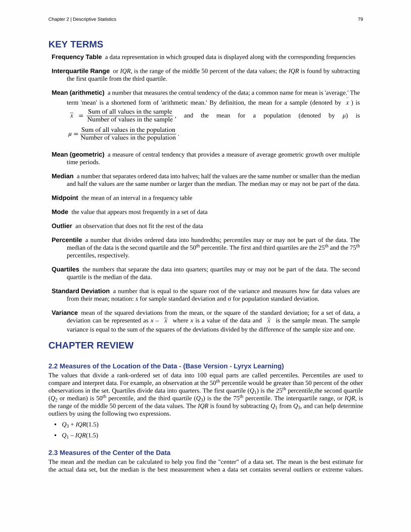
Frequency Table
Interquartile Range
Mean (arithmetic)
Mean (geometric)
Median
Midpoint
Mode
Outlier
Percentile
Quartiles
Standard Deviation
Variance
KEY TERMSa data representation in which grouped data is displayed along with the corresponding frequencies
or IQR, is the range of the middle 50 percent of the data values; the IQR is found by subtractingthe first quartile from the third quartile.
a number that measures the central tendency of the data; a common name for mean is 'average.' The
term 'mean' is a shortened form of 'arithmetic mean.' By definition, the mean for a sample (denoted by x¯ ) is
x– = Sum of all values in the sampleNumber of values in the sample , and the mean for a population (denoted by μ) is
μ = Sum of all values in the populationNumber of values in the population .
a measure of central tendency that provides a measure of average geometric growth over multipletime periods.
a number that separates ordered data into halves; half the values are the same number or smaller than the medianand half the values are the same number or larger than the median. The median may or may not be part of the data.
the mean of an interval in a frequency table
the value that appears most frequently in a set of data
an observation that does not fit the rest of the data
a number that divides ordered data into hundredths; percentiles may or may not be part of the data. Themedian of the data is the second quartile and the 50th percentile. The first and third quartiles are the 25th and the 75th
percentiles, respectively.
the numbers that separate the data into quarters; quartiles may or may not be part of the data. The secondquartile is the median of the data.
a number that is equal to the square root of the variance and measures how far data values arefrom their mean; notation: s for sample standard deviation and σ for population standard deviation.
mean of the squared deviations from the mean, or the square of the standard deviation; for a set of data, adeviation can be represented as x – x– where x is a value of the data and x– is the sample mean. The sample
variance is equal to the sum of the squares of the deviations divided by the difference of the sample size and one.
CHAPTER REVIEW
2.2 Measures of the Location of the Data - (Base Version - Lyryx Learning)The values that divide a rank-ordered set of data into 100 equal parts are called percentiles. Percentiles are used tocompare and interpret data. For example, an observation at the 50th percentile would be greater than 50 percent of the otherobeservations in the set. Quartiles divide data into quarters. The first quartile (Q1) is the 25th percentile,the second quartile(Q2 or median) is 50th percentile, and the third quartile (Q3) is the the 75th percentile. The interquartile range, or IQR, isthe range of the middle 50 percent of the data values. The IQR is found by subtracting Q1 from Q3, and can help determineoutliers by using the following two expressions.
• Q3 + IQR(1.5)
• Q1 – IQR(1.5)
2.3 Measures of the Center of the DataThe mean and the median can be calculated to help you find the "center" of a data set. The mean is the best estimate forthe actual data set, but the median is the best measurement when a data set contains several outliers or extreme values.
Chapter 2 | Descriptive Statistics 79

The mode will tell you the most frequently occurring datum (or data) in your data set. The mean, median, and mode areextremely helpful when you need to analyze your data, but if your data set consists of ranges which lack specific values, themean may seem impossible to calculate. However, the mean can be approximated if you add the lower boundary with theupper boundary and divide by two to find the midpoint of each interval. Multiply each midpoint by the number of valuesfound in the corresponding range. Divide the sum of these values by the total number of data values in the set.
2.5 Skewness and the Mean, Median, and ModeLooking at the distribution of data can reveal a lot about the relationship between the mean, the median, and the mode.There are three types of distributions. A left (or negative) skewed distribution has a shape like Figure 2.13. A right (orpositive) skewed distribution has a shape like Figure 2.14. A symmetrical distribution looks like Figure 2.12.
2.6 Measures of the Spread of the Data - (Base Version - Lyryx Learning)The standard deviation can help you calculate the spread of data. There are different equations to use if are calculating thestandard deviation of a sample or of a population.
• The Standard Deviation allows us to compare individual data or classes to the data set mean numerically.
• s =∑ (x − x– )2
n − 1 is the formula for calculating the standard deviation of a sample. To calculate the standard
deviation of a population, we would use the population mean, μ, and the formula σ =∑ (x − μ)2
N .
FORMULA REVIEW
2.2 Measures of the Location of the Data - (BaseVersion - Lyryx Learning)
L p = (n + 1) p100
where Lp = the ranking or position of a data value,
p = the pth percentile,
n = total number of data
2.3 Measures of the Center of the Data
μ =∑ fm
∑ fWhere f = interval frequencies and m =
interval midpoints.
The arithmetic mean for a sample (denoted by x¯ ) is
x– = Sum of all values in the sampleNumber of values in the sample
The arithmetic mean for a population (denoted by μ) is
μ = Sum of all values in the populationNumber of values in the population
2.5 Skewness and the Mean, Median, and Mode
Formula for skewness: a3 = ∑⎛⎝xi − x¯ ⎞⎠
3
ns3
Formula for Coefficient of Variation:
CV = sx¯
· 100 conditioned upon x¯ ≠ 0
2.6 Measures of the Spread of the Data - (BaseVersion - Lyryx Learning)
Formulas for Sample Standard Deviation
s = Σ(x − x– )2
n − 1 or s =
⎛⎝⎜∑ x2
⎞⎠⎟ -⎛⎝∑ x⎞⎠2n
n - 1 For the
sample standard deviation, the denominator is n - 1, that isthe sample size - 1.
Formulas for Population Standard Deviation
σ = Σ(x − μ)2
N For the population standard
deviation, the denominator is N, the number of items in thepopulation.
80 Chapter 2 | Descriptive Statistics
This OpenStax book is available for free at https://legacy.cnx.org/content/col12102/1.7

PRACTICE
2.2 Measures of the Location of the Data - (Base Version - Lyryx Learning)
5. Listed are 29 ages for Academy Award winning best actors in order from smallest to largest.
18; 21; 22; 25; 26; 27; 29; 30; 31; 33; 36; 37; 41; 42; 47; 52; 55; 57; 58; 62; 64; 67; 69; 71; 72; 73; 74; 76; 77
a. Find the 40th percentile.b. Find the 78th percentile.
6. Listed are 32 ages for Academy Award winning best actors in order from smallest to largest.
18; 18; 21; 22; 25; 26; 27; 29; 30; 31; 31; 33; 36; 37; 37; 41; 42; 47; 52; 55; 57; 58; 62; 64; 67; 69; 71; 72; 73; 74; 76; 77
a. Find the percentile of 37.b. Find the percentile of 72.
7. Jesse was ranked 37th in his graduating class of 180 students. At what percentile is Jesse’s ranking?
8.a. For runners in a race, a low time means a faster run. The winners in a race have the shortest running times. Is it
more desirable to have a finish time with a high or a low percentile when running a race?b. The 20th percentile of run times in a particular race is 5.2 minutes. Write a sentence interpreting the 20th percentile
in the context of the situation.c. A bicyclist in the 90th percentile of a bicycle race completed the race in 1 hour and 12 minutes. Is he among
the fastest or slowest cyclists in the race? Write a sentence interpreting the 90th percentile in the context of thesituation.
9.a. For runners in a race, a higher speed means a faster run. Is it more desirable to have a speed with a high or a low
percentile when running a race?b. The 40th percentile of speeds in a particular race is 7.5 miles per hour. Write a sentence interpreting the 40th
percentile in the context of the situation.
10. On an exam, would it be more desirable to earn a grade with a high or low percentile? Explain.
11. Mina is waiting in line at the Department of Motor Vehicles (DMV). Her wait time of 32 minutes is the 85th percentileof wait times. Is that good or bad? Write a sentence interpreting the 85th percentile in the context of this situation.
12. In a survey collecting data about the salaries earned by recent college graduates, Li found that her salary was in the 78th
percentile. Should Li be pleased or upset by this result? Explain.
13. In a study collecting data about the repair costs of damage to automobiles in a certain type of crash tests, a certain modelof car had $1,700 in damage and was in the 90th percentile. Should the manufacturer and the consumer be pleased or upsetby this result? Explain and write a sentence that interprets the 90th percentile in the context of this problem.
14. The University of California has two criteria used to set admission standards for freshman to be admitted to a collegein the UC system:
a. Students' GPAs and scores on standardized tests (SATs and ACTs) are entered into a formula that calculates an"admissions index" score. The admissions index score is used to set eligibility standards intended to meet the goalof admitting the top 12% of high school students in the state. In this context, what percentile does the top 12%represent?
b. Students whose GPAs are at or above the 96th percentile of all students at their high school are eligible (calledeligible in the local context), even if they are not in the top 12% of all students in the state. What percentage ofstudents from each high school are "eligible in the local context"?
15. Suppose that you are buying a house. You and your realtor have determined that the most expensive house you canafford is the 34th percentile. The 34th percentile of housing prices is $240,000 in the town you want to move to. In this town,can you afford 34% of the houses or 66% of the houses?
Chapter 2 | Descriptive Statistics 81
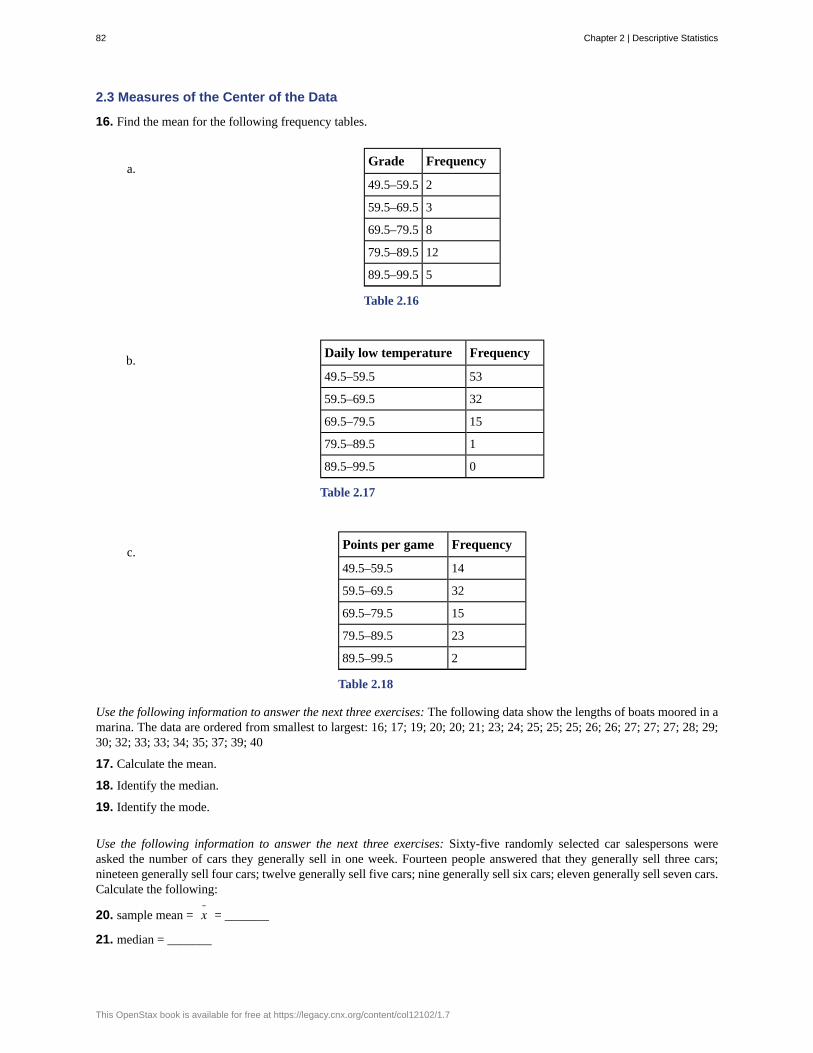
2.3 Measures of the Center of the Data
16. Find the mean for the following frequency tables.
a.Grade Frequency
49.5–59.5 2
59.5–69.5 3
69.5–79.5 8
79.5–89.5 12
89.5–99.5 5
Table 2.16
b.Daily low temperature Frequency
49.5–59.5 53
59.5–69.5 32
69.5–79.5 15
79.5–89.5 1
89.5–99.5 0
Table 2.17
c.Points per game Frequency
49.5–59.5 14
59.5–69.5 32
69.5–79.5 15
79.5–89.5 23
89.5–99.5 2
Table 2.18
Use the following information to answer the next three exercises: The following data show the lengths of boats moored in amarina. The data are ordered from smallest to largest: 16; 17; 19; 20; 20; 21; 23; 24; 25; 25; 25; 26; 26; 27; 27; 27; 28; 29;30; 32; 33; 33; 34; 35; 37; 39; 40
17. Calculate the mean.
18. Identify the median.
19. Identify the mode.
Use the following information to answer the next three exercises: Sixty-five randomly selected car salespersons wereasked the number of cars they generally sell in one week. Fourteen people answered that they generally sell three cars;nineteen generally sell four cars; twelve generally sell five cars; nine generally sell six cars; eleven generally sell seven cars.Calculate the following:
20. sample mean = x¯ = _______
21. median = _______
82 Chapter 2 | Descriptive Statistics
This OpenStax book is available for free at https://legacy.cnx.org/content/col12102/1.7

22. mode = _______
2.4 Sigma Notation and Calculating the Arithmetic Mean
23. A group of 10 children are on a scavenger hunt to find different color rocks. The results are shown in the Table 2.19below. The column on the right shows the number of colors of rocks each child has. What is the mean number of rocks?
Child Rock colors
1 5
2 5
3 6
4 2
5 4
6 3
7 7
8 2
9 1
10 10
Table 2.19
24. A group of children are measured to determine the average height of the group. The results are in Table 2.20 below.What is the mean height of the group to the nearest hundredth of an inch?
Child Height in inches
Adam 45.21
Betty 39.45
Charlie 43.78
Donna 48.76
Earl 37.39
Fran 39.90
George 45.56
Heather 46.24
Table 2.20
Chapter 2 | Descriptive Statistics 83
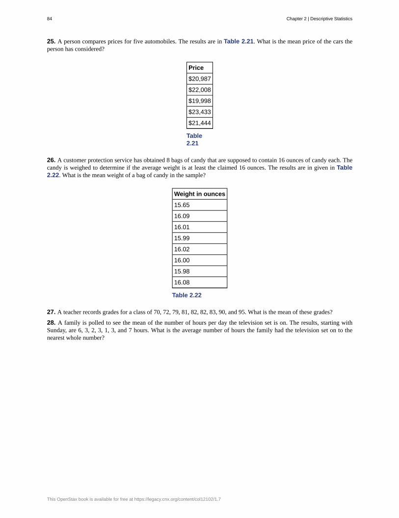
25. A person compares prices for five automobiles. The results are in Table 2.21. What is the mean price of the cars theperson has considered?
Price
$20,987
$22,008
$19,998
$23,433
$21,444
Table2.21
26. A customer protection service has obtained 8 bags of candy that are supposed to contain 16 ounces of candy each. Thecandy is weighed to determine if the average weight is at least the claimed 16 ounces. The results are in given in Table2.22. What is the mean weight of a bag of candy in the sample?
Weight in ounces
15.65
16.09
16.01
15.99
16.02
16.00
15.98
16.08
Table 2.22
27. A teacher records grades for a class of 70, 72, 79, 81, 82, 82, 83, 90, and 95. What is the mean of these grades?
28. A family is polled to see the mean of the number of hours per day the television set is on. The results, starting withSunday, are 6, 3, 2, 3, 1, 3, and 7 hours. What is the average number of hours the family had the television set on to thenearest whole number?
84 Chapter 2 | Descriptive Statistics
This OpenStax book is available for free at https://legacy.cnx.org/content/col12102/1.7

29. A city received the following rainfall for a recent year. What is the mean number of inches of rainfall the city receivedmonthly, to the nearest hundredth of an inch? Use Table 2.23.
Month Rainfall in inches
January 2.21
February 3.12
March 4.11
April 2.09
May 0.99
June 1.08
July 2.99
August 0.08
September 0.52
October 1.89
November 2.00
December 3.06
Table 2.23
30. A football team scored the following points in its first 8 games of the new season. Starting at game 1 and in order thescores are 14, 14, 24, 21, 7, 0, 38, and 28. What is the mean number of points the team scored in these eight games?
2.5 Skewness and the Mean, Median, and ModeUse the following information to answer the next three exercises: State whether the data are symmetrical, skewed to the left,or skewed to the right.
31. 1; 1; 1; 2; 2; 2; 2; 3; 3; 3; 3; 3; 3; 3; 3; 4; 4; 4; 5; 5
32. 16; 17; 19; 22; 22; 22; 22; 22; 23
33. 87; 87; 87; 87; 87; 88; 89; 89; 90; 91
34. When the data are skewed left, what is the typical relationship between the mean and median?
35. When the data are symmetrical, what is the typical relationship between the mean and median?
36. What word describes a distribution that has two modes?
Chapter 2 | Descriptive Statistics 85

37. Describe the shape of this distribution.
Figure 2.16
38. Describe the relationship between the mode and the median of this distribution.
Figure 2.17
39. Describe the relationship between the mean and the median of this distribution.
Figure 2.18
86 Chapter 2 | Descriptive Statistics
This OpenStax book is available for free at https://legacy.cnx.org/content/col12102/1.7

40. Describe the shape of this distribution.
Figure 2.19
41. Describe the relationship between the mode and the median of this distribution.
Figure 2.20
42. Are the mean and the median the exact same in this distribution? Why or why not?
Figure 2.21
Chapter 2 | Descriptive Statistics 87
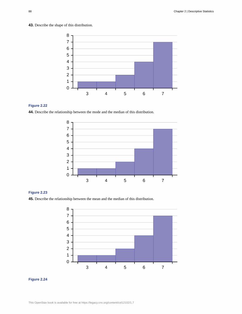
43. Describe the shape of this distribution.
Figure 2.22
44. Describe the relationship between the mode and the median of this distribution.
Figure 2.23
45. Describe the relationship between the mean and the median of this distribution.
Figure 2.24
88 Chapter 2 | Descriptive Statistics
This OpenStax book is available for free at https://legacy.cnx.org/content/col12102/1.7

46. The mean and median for the data are the same.
3; 4; 5; 5; 6; 6; 6; 6; 7; 7; 7; 7; 7; 7; 7
Is the data perfectly symmetrical? Why or why not?
47. Which is the greatest, the mean, the mode, or the median of the data set?
11; 11; 12; 12; 12; 12; 13; 15; 17; 22; 22; 22
48. Which is the least, the mean, the mode, and the median of the data set?
56; 56; 56; 58; 59; 60; 62; 64; 64; 65; 67
49. Of the three measures, which tends to reflect skewing the most, the mean, the mode, or the median? Why?
50. In a perfectly symmetrical distribution, when would the mode be different from the mean and median?
2.6 Measures of the Spread of the Data - (Base Version - Lyryx Learning)Use the following information to answer the next two exercises: The following data are the distances between 20 retail storesand a large distribution center. The distances are in miles.29; 37; 38; 40; 58; 67; 68; 69; 76; 86; 87; 95; 96; 96; 99; 106; 112; 127; 145; 150
51. Use a calculator or computer to find the standard deviation and round to the nearest tenth.
HOMEWORK
2.2 Measures of the Location of the Data - (Base Version - Lyryx Learning)
52. The median age for U.S. blacks currently is 30.9 years; for U.S. whites it is 42.3 years.a. Based upon this information, give two reasons why the black median age could be lower than the white median
age.b. Does the lower median age for blacks necessarily mean that blacks die younger than whites? Why or why not?c. How might it be possible for blacks and whites to die at approximately the same age, but for the median age for
whites to be higher?
Chapter 2 | Descriptive Statistics 89
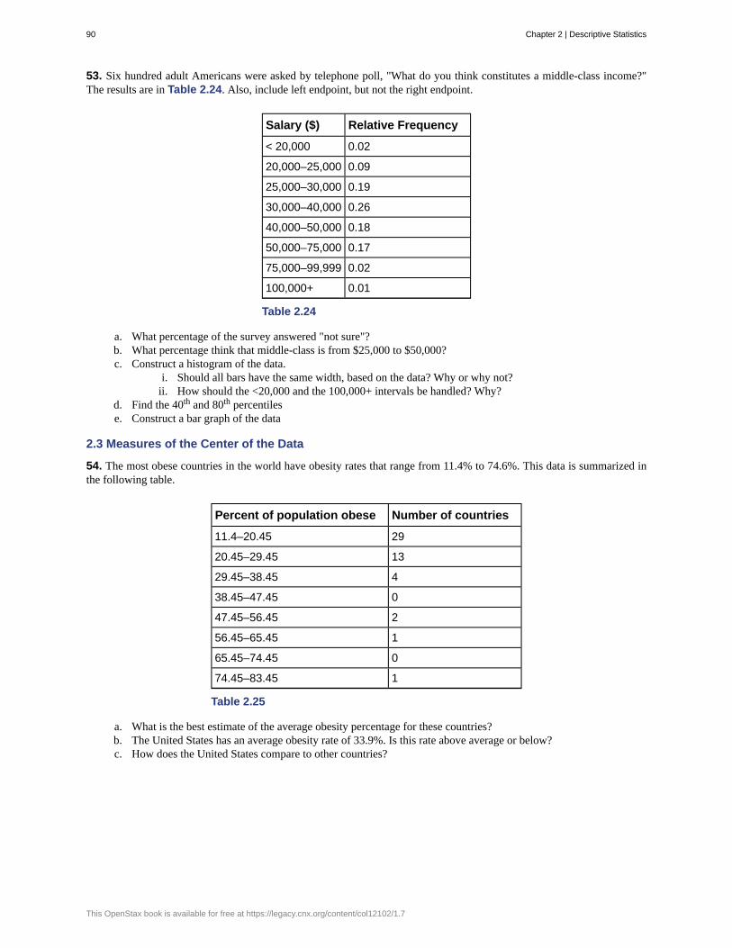
53. Six hundred adult Americans were asked by telephone poll, "What do you think constitutes a middle-class income?"The results are in Table 2.24. Also, include left endpoint, but not the right endpoint.
Salary ($) Relative Frequency
< 20,000 0.02
20,000–25,000 0.09
25,000–30,000 0.19
30,000–40,000 0.26
40,000–50,000 0.18
50,000–75,000 0.17
75,000–99,999 0.02
100,000+ 0.01
Table 2.24
a. What percentage of the survey answered "not sure"?b. What percentage think that middle-class is from $25,000 to $50,000?c. Construct a histogram of the data.
i. Should all bars have the same width, based on the data? Why or why not?ii. How should the <20,000 and the 100,000+ intervals be handled? Why?
d. Find the 40th and 80th percentilese. Construct a bar graph of the data
2.3 Measures of the Center of the Data
54. The most obese countries in the world have obesity rates that range from 11.4% to 74.6%. This data is summarized inthe following table.
Percent of population obese Number of countries
11.4–20.45 29
20.45–29.45 13
29.45–38.45 4
38.45–47.45 0
47.45–56.45 2
56.45–65.45 1
65.45–74.45 0
74.45–83.45 1
Table 2.25
a. What is the best estimate of the average obesity percentage for these countries?b. The United States has an average obesity rate of 33.9%. Is this rate above average or below?c. How does the United States compare to other countries?
90 Chapter 2 | Descriptive Statistics
This OpenStax book is available for free at https://legacy.cnx.org/content/col12102/1.7

55. Table 2.26 gives the percent of children under five considered to be underweight. What is the best estimate for themean percentage of underweight children?
Percent of underweight children Number of countries
16–21.45 23
21.45–26.9 4
26.9–32.35 9
32.35–37.8 7
37.8–43.25 6
43.25–48.7 1
Table 2.26
2.4 Sigma Notation and Calculating the Arithmetic Mean
56. A sample of 10 prices is chosen from a population of 100 similar items. The values obtained from the sample, and thevalues for the population, are given in Table 2.27 and Table 2.28 respectively.
a. Is the mean of the sample within $1 of the population mean?b. What is the difference in the sample and population means?
Prices of the sample
$21
$23
$21
$24
$22
$22
$25
$21
$20
$24
Table 2.27
Prices of the population Frequency
$20 20
$21 35
$22 15
$23 10
$24 18
$25 2
Table 2.28
Chapter 2 | Descriptive Statistics 91

57. A standardized test is given to ten people at the beginning of the school year with the results given in Table 2.29 below.At the end of the year the same people were again tested.
a. What is the average improvement?b. Does it matter if the means are subtracted, or if the individual values are subtracted?
Student Beginning score Ending score
1 1100 1120
2 980 1030
3 1200 1208
4 998 1000
5 893 948
6 1015 1030
7 1217 1224
8 1232 1245
9 967 988
10 988 997
Table 2.29
58. A small class of 7 students has a mean grade of 82 on a test. If six of the grades are 80, 82,86, 90, 90, and 95, what isthe other grade?
59. A class of 20 students has a mean grade of 80 on a test. Nineteen of the students has a mean grade between 79 and 82,inclusive.
a. What is the lowest possible grade of the other student?b. What is the highest possible grade of the other student?
60. If the mean of 20 prices is $10.39, and 5 of the items with a mean of $10.99 are sampled, what is the mean of the other15 prices?
2.5 Skewness and the Mean, Median, and Mode
61. The median age of the U.S. population in 1980 was 30.0 years. In 1991, the median age was 33.1 years.a. What does it mean for the median age to rise?b. Give two reasons why the median age could rise.c. For the median age to rise, is the actual number of children less in 1991 than it was in 1980? Why or why not?
2.6 Measures of the Spread of the Data - (Base Version - Lyryx Learning)
Use the following information to answer the next nine exercises: The population parameters below describe the full-timeequivalent number of students (FTES) each year at Lake Tahoe Community College from 1976–1977 through 2004–2005.
• μ = 1000 FTES
• median = 1,014 FTES
• σ = 474 FTES
• first quartile = 528.5 FTES
• third quartile = 1,447.5 FTES
• n = 29 years
62. A sample of 11 years is taken. About how many are expected to have a FTES of 1014 or above? Explain how youdetermined your answer.
92 Chapter 2 | Descriptive Statistics
This OpenStax book is available for free at https://legacy.cnx.org/content/col12102/1.7
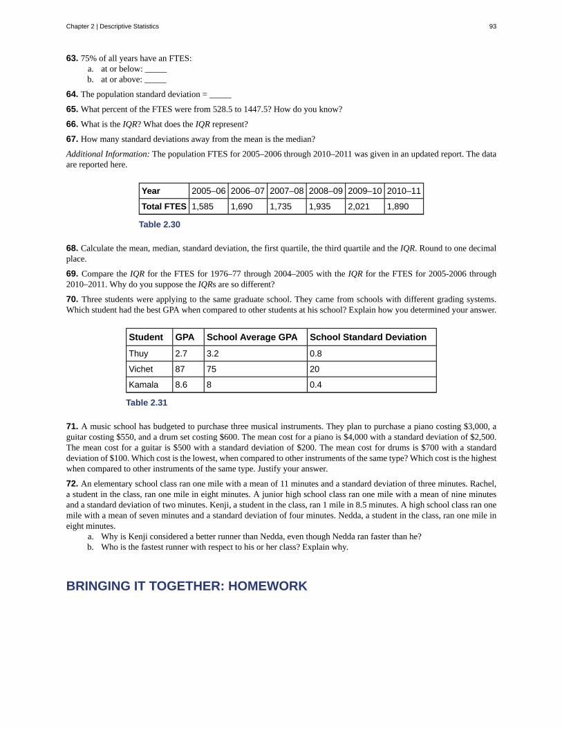
63. 75% of all years have an FTES:a. at or below: _____b. at or above: _____
64. The population standard deviation = _____
65. What percent of the FTES were from 528.5 to 1447.5? How do you know?
66. What is the IQR? What does the IQR represent?
67. How many standard deviations away from the mean is the median?
Additional Information: The population FTES for 2005–2006 through 2010–2011 was given in an updated report. The dataare reported here.
Year 2005–06 2006–07 2007–08 2008–09 2009–10 2010–11
Total FTES 1,585 1,690 1,735 1,935 2,021 1,890
Table 2.30
68. Calculate the mean, median, standard deviation, the first quartile, the third quartile and the IQR. Round to one decimalplace.
69. Compare the IQR for the FTES for 1976–77 through 2004–2005 with the IQR for the FTES for 2005-2006 through2010–2011. Why do you suppose the IQRs are so different?
70. Three students were applying to the same graduate school. They came from schools with different grading systems.Which student had the best GPA when compared to other students at his school? Explain how you determined your answer.
Student GPA School Average GPA School Standard Deviation
Thuy 2.7 3.2 0.8
Vichet 87 75 20
Kamala 8.6 8 0.4
Table 2.31
71. A music school has budgeted to purchase three musical instruments. They plan to purchase a piano costing $3,000, aguitar costing $550, and a drum set costing $600. The mean cost for a piano is $4,000 with a standard deviation of $2,500.The mean cost for a guitar is $500 with a standard deviation of $200. The mean cost for drums is $700 with a standarddeviation of $100. Which cost is the lowest, when compared to other instruments of the same type? Which cost is the highestwhen compared to other instruments of the same type. Justify your answer.
72. An elementary school class ran one mile with a mean of 11 minutes and a standard deviation of three minutes. Rachel,a student in the class, ran one mile in eight minutes. A junior high school class ran one mile with a mean of nine minutesand a standard deviation of two minutes. Kenji, a student in the class, ran 1 mile in 8.5 minutes. A high school class ran onemile with a mean of seven minutes and a standard deviation of four minutes. Nedda, a student in the class, ran one mile ineight minutes.
a. Why is Kenji considered a better runner than Nedda, even though Nedda ran faster than he?b. Who is the fastest runner with respect to his or her class? Explain why.
BRINGING IT TOGETHER: HOMEWORK
Chapter 2 | Descriptive Statistics 93
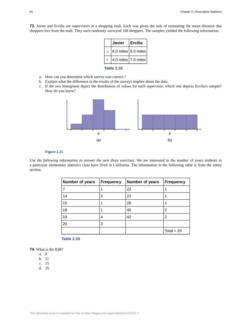
73. Javier and Ercilia are supervisors at a shopping mall. Each was given the task of estimating the mean distance thatshoppers live from the mall. They each randomly surveyed 100 shoppers. The samples yielded the following information.
Javier Ercilia
x¯ 6.0 miles 6.0 miles
s 4.0 miles 7.0 miles
Table 2.32
a. How can you determine which survey was correct ?b. Explain what the difference in the results of the surveys implies about the data.c. If the two histograms depict the distribution of values for each supervisor, which one depicts Ercilia's sample?
How do you know?
Figure 2.25
Use the following information to answer the next three exercises: We are interested in the number of years students ina particular elementary statistics class have lived in California. The information in the following table is from the entiresection.
Number of years Frequency Number of years Frequency
7 1 22 1
14 3 23 1
15 1 26 1
18 1 40 2
19 4 42 2
20 3
Total = 20
Table 2.33
74. What is the IQR?a. 8b. 11c. 15d. 35
94 Chapter 2 | Descriptive Statistics
This OpenStax book is available for free at https://legacy.cnx.org/content/col12102/1.7

75. What is the mode?a. 19b. 19.5c. 14 and 20d. 22.65
76. Is this a sample or the entire population?a. sampleb. entire populationc. neither
77. Twenty-five randomly selected students were asked the number of movies they watched the previous week. The resultsare as follows:
# of movies Frequency
0 5
1 9
2 6
3 4
4 1
Table 2.34
a. Find the sample mean x¯ .
b. Find the approximate sample standard deviation, s.
78. Forty randomly selected students were asked the number of pairs of sneakers they owned. Let X = the number of pairsof sneakers owned. The results are as follows:
X Frequency
1 2
2 5
3 8
4 12
5 12
6 0
7 1
Table 2.35
a. Find the sample mean x¯
b. Find the sample standard deviation, sc. Construct a histogram of the data.d. Complete the columns of the chart.e. Find the first quartile.f. Find the median.g. Find the third quartile.h. What percent of the students owned at least five pairs?i. Find the 40th percentile.j. Find the 90th percentile.k. Construct a line graph of the datal. Construct a stemplot of the data
Chapter 2 | Descriptive Statistics 95

79. Following are the published weights (in pounds) of all of the team members of the San Francisco 49ers from a previousyear.
177; 205; 210; 210; 232; 205; 185; 185; 178; 210; 206; 212; 184; 174; 185; 242; 188; 212; 215; 247; 241; 223; 220; 260;245; 259; 278; 270; 280; 295; 275; 285; 290; 272; 273; 280; 285; 286; 200; 215; 185; 230; 250; 241; 190; 260; 250; 302;265; 290; 276; 228; 265
a. Organize the data from smallest to largest value.b. Find the median.c. Find the first quartile.d. Find the third quartile.e. The middle 50% of the weights are from _______ to _______.f. If our population were all professional football players, would the above data be a sample of weights or the
population of weights? Why?g. If our population included every team member who ever played for the San Francisco 49ers, would the above data
be a sample of weights or the population of weights? Why?h. Assume the population was the San Francisco 49ers. Find:
i. the population mean, μ.ii. the population standard deviation, σ.
iii. the weight that is two standard deviations below the mean.iv. When Steve Young, quarterback, played football, he weighed 205 pounds. How many standard
deviations above or below the mean was he?
i. That same year, the mean weight for the Dallas Cowboys was 240.08 pounds with a standard deviation of 44.38pounds. Emmit Smith weighed in at 209 pounds. With respect to his team, who was lighter, Smith or Young? Howdid you determine your answer?
80. One hundred teachers attended a seminar on mathematical problem solving. The attitudes of a representative sampleof 12 of the teachers were measured before and after the seminar. A positive number for change in attitude indicates that ateacher's attitude toward math became more positive. The 12 change scores are as follows:
3; 8; –1; 2; 0; 5; –3; 1; –1; 6; 5; –2
a. What is the mean change score?b. What is the standard deviation for this population?c. What is the median change score?d. Find the change score that is 2.2 standard deviations below the mean.
81. Refer to Figure 2.26 determine which of the following are true and which are false. Explain your solution to each partin complete sentences.
Figure 2.26a. The medians for both graphs are the same.b. We cannot determine if any of the means for both graphs is different.c. The standard deviation for graph b is larger than the standard deviation for graph a.d. We cannot determine if any of the third quartiles for both graphs is different.
96 Chapter 2 | Descriptive Statistics
This OpenStax book is available for free at https://legacy.cnx.org/content/col12102/1.7

82. In a recent issue of the IEEE Spectrum, 84 engineering conferences were announced. Four conferences lasted two days.Thirty-six lasted three days. Eighteen lasted four days. Nineteen lasted five days. Four lasted six days. One lasted sevendays. One lasted eight days. One lasted nine days. Let X = the length (in days) of an engineering conference.
a. Organize the data in a chart.b. Find the median, the first quartile, and the third quartile.c. Find the 65th percentile.d. Find the 10th percentile.e. The middle 50% of the conferences last from _______ days to _______ days.f. Calculate the sample mean of days of engineering conferences.g. Calculate the sample standard deviation of days of engineering conferences.h. Find the mode.i. If you were planning an engineering conference, which would you choose as the length of the conference: mean;
median; or mode? Explain why you made that choice.j. Give two reasons why you think that three to five days seem to be popular lengths of engineering conferences.
Use the following information to answer the next two exercises. X = the number of days per week that 100 clients use aparticular exercise facility.
x Frequency
0 3
1 12
2 33
3 28
4 11
5 9
6 4
Table 2.36
83. The 80th percentile is _____a. 5b. 80c. 3d. 4
84. The number that is 1.5 standard deviations BELOW the mean is approximately _____a. 0.7b. 4.8c. –2.8d. Cannot be determined
Chapter 2 | Descriptive Statistics 97
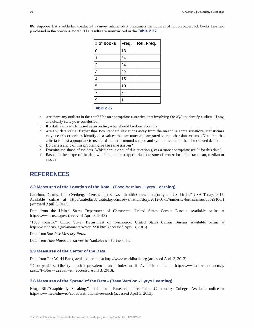
85. Suppose that a publisher conducted a survey asking adult consumers the number of fiction paperback books they hadpurchased in the previous month. The results are summarized in the Table 2.37.
# of books Freq. Rel. Freq.
0 18
1 24
2 24
3 22
4 15
5 10
7 5
9 1
Table 2.37
a. Are there any outliers in the data? Use an appropriate numerical test involving the IQR to identify outliers, if any,and clearly state your conclusion.
b. If a data value is identified as an outlier, what should be done about it?c. Are any data values further than two standard deviations away from the mean? In some situations, statisticians
may use this criteria to identify data values that are unusual, compared to the other data values. (Note that thiscriteria is most appropriate to use for data that is mound-shaped and symmetric, rather than for skewed data.)
d. Do parts a and c of this problem give the same answer?e. Examine the shape of the data. Which part, a or c, of this question gives a more appropriate result for this data?f. Based on the shape of the data which is the most appropriate measure of center for this data: mean, median or
mode?
REFERENCES
2.2 Measures of the Location of the Data - (Base Version - Lyryx Learning)
Cauchon, Dennis, Paul Overberg. “Census data shows minorities now a majority of U.S. births.” USA Today, 2012.Available online at http://usatoday30.usatoday.com/news/nation/story/2012-05-17/minority-birthscensus/55029100/1(accessed April 3, 2013).
Data from the United States Department of Commerce: United States Census Bureau. Available online athttp://www.census.gov/ (accessed April 3, 2013).
“1990 Census.” United States Department of Commerce: United States Census Bureau. Available online athttp://www.census.gov/main/www/cen1990.html (accessed April 3, 2013).
Data from San Jose Mercury News.
Data from Time Magazine; survey by Yankelovich Partners, Inc.
2.3 Measures of the Center of the Data
Data from The World Bank, available online at http://www.worldbank.org (accessed April 3, 2013).
“Demographics: Obesity – adult prevalence rate.” Indexmundi. Available online at http://www.indexmundi.com/g/r.aspx?t=50&v=2228&l=en (accessed April 3, 2013).
2.6 Measures of the Spread of the Data - (Base Version - Lyryx Learning)
King, Bill.“Graphically Speaking.” Institutional Research, Lake Tahoe Community College. Available online athttp://www.ltcc.edu/web/about/institutional-research (accessed April 3, 2013).
98 Chapter 2 | Descriptive Statistics
This OpenStax book is available for free at https://legacy.cnx.org/content/col12102/1.7

SOLUTIONS
5a. The 40th percentile is 37 years.
b. The 78th percentile is 69.8 years.
7 Jesse graduated 37th out of a class of 180 students. This puts Jesse at spot 144 counting from the lowest grade.
144 = ⎛⎝180 + 1⎞⎠⎛⎝p
100⎞⎠p = 144(100)
181 p = 79.56
Jesse’s rank of 37 puts him at approximately the 80th percentile.
9a. For runners in a race it is more desirable to have a high percentile for speed. A high percentile means a higher speed
which is faster.
b. 40% of runners ran at speeds of 7.5 miles per hour or less (slower). 60% of runners ran at speeds of 7.5 miles per houror more (faster).
11 When waiting in line at the DMV, the 85th percentile would be a long wait time compared to the other people waiting.85% of people had shorter wait times than Mina. In this context, Mina would prefer a wait time corresponding to a lowerpercentile. 85% of people at the DMV waited 32 minutes or less. 15% of people at the DMV waited 32 minutes or longer.
13 The manufacturer and the consumer would be upset. This is a large repair cost for the damages, compared to the othercars in the sample. INTERPRETATION: 90% of the crash tested cars had damage repair costs of $1700 or less; only 10%had damage repair costs of $1700 or more.
15 You can afford 34% of houses. 66% of the houses are too expensive for your budget. INTERPRETATION: 34% ofhouses cost $240,000 or less. 66% of houses cost $240,000 or more.
17 Mean: 16 + 17 + 19 + 20 + 20 + 21 + 23 + 24 + 25 + 25 + 25 + 26 + 26 + 27 + 27 + 27 + 28 + 29 + 30 + 32 + 33 + 33
+ 34 + 35 + 37 + 39 + 40 = 738; 73827 = 27.33
19 The most frequent lengths are 25 and 27, which occur three times. Mode = 25, 27
21 4
24 39.48 in.
25 $21,574
26 15.98 ounces
27 81.56
28 4 hours
29 2.01 inches
30 18.25
31 The data are symmetrical. The median is 3 and the mean is 2.85. They are close, and the mode lies close to the middleof the data, so the data are symmetrical.
33 The data are skewed right. The median is 87.5 and the mean is 88.2. Even though they are close, the mode lies to theleft of the middle of the data, and there are many more instances of 87 than any other number, so the data are skewed right.
35 When the data are symmetrical, the mean and median are close or the same.
37 The distribution is skewed right because it looks pulled out to the right.
39 The mean is 4.1 and is slightly greater than the median, which is four.
41 The mode and the median are the same. In this case, they are both five.
43 The distribution is skewed left because it looks pulled out to the left.
45 The mean and the median are both six.
47 The mode is 12, the median is 12.5, and the mean is 15.1. The mean is the largest.
Chapter 2 | Descriptive Statistics 99
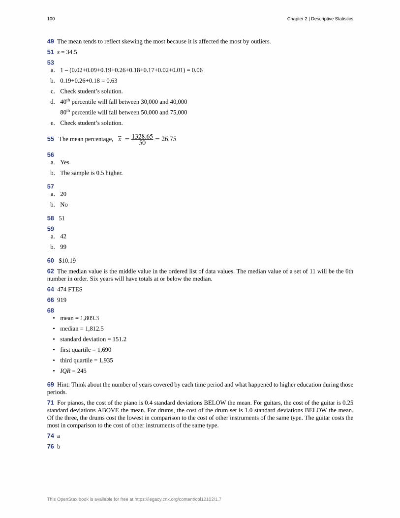
49 The mean tends to reflect skewing the most because it is affected the most by outliers.
51 s = 34.5
53a. 1 – (0.02+0.09+0.19+0.26+0.18+0.17+0.02+0.01) = 0.06
b. 0.19+0.26+0.18 = 0.63
c. Check student’s solution.
d. 40th percentile will fall between 30,000 and 40,000
80th percentile will fall between 50,000 and 75,000
e. Check student’s solution.
55 The mean percentage, x– = 1328.6550 = 26.75
56a. Yes
b. The sample is 0.5 higher.
57a. 20
b. No
58 51
59a. 42
b. 99
60 $10.19
62 The median value is the middle value in the ordered list of data values. The median value of a set of 11 will be the 6thnumber in order. Six years will have totals at or below the median.
64 474 FTES
66 919
68• mean = 1,809.3
• median = 1,812.5
• standard deviation = 151.2
• first quartile = 1,690
• third quartile = 1,935
• IQR = 245
69 Hint: Think about the number of years covered by each time period and what happened to higher education during thoseperiods.
71 For pianos, the cost of the piano is 0.4 standard deviations BELOW the mean. For guitars, the cost of the guitar is 0.25standard deviations ABOVE the mean. For drums, the cost of the drum set is 1.0 standard deviations BELOW the mean.Of the three, the drums cost the lowest in comparison to the cost of other instruments of the same type. The guitar costs themost in comparison to the cost of other instruments of the same type.
74 a
76 b
100 Chapter 2 | Descriptive Statistics
This OpenStax book is available for free at https://legacy.cnx.org/content/col12102/1.7

77a. 1.48
b. 1.12
79a. 174; 177; 178; 184; 185; 185; 185; 185; 188; 190; 200; 205; 205; 206; 210; 210; 210; 212; 212; 215; 215; 220; 223;
228; 230; 232; 241; 241; 242; 245; 247; 250; 250; 259; 260; 260; 265; 265; 270; 272; 273; 275; 276; 278; 280; 280;285; 285; 286; 290; 290; 295; 302
b. 241
c. 205.5
d. 272.5
e. 205.5, 272.5
f. sample
g. population
h. i. 236.34
ii. 37.50
iii. 161.34
iv. 0.84 std. dev. below the mean
i. Young
81a. True
b. True
c. True
d. False
84 a
Chapter 2 | Descriptive Statistics 101

102 Chapter 2 | Descriptive Statistics
This OpenStax book is available for free at https://legacy.cnx.org/content/col12102/1.7

3 | PROBABILITY TOPICS
Figure 3.1 Meteor showers are rare, but the probability of them occurring can be calculated. (credit: Navicore/flickr)
Introduction
It is often necessary to "guess" about the outcome of an event in order to make a decision. Politicians study polls to guesstheir likelihood of winning an election. Teachers choose a particular course of study based on what they think students cancomprehend. Doctors choose the treatments needed for various diseases based on their assessment of likely results. Youmay have visited a casino where people play games chosen because of the belief that the likelihood of winning is good. Youmay have chosen your course of study based on the probable availability of jobs.
You have, more than likely, used probability. In fact, you probably have an intuitive sense of probability. Probability dealswith the chance of an event occurring. Whenever you weigh the odds of whether or not to do your homework or to studyfor an exam, you are using probability. In this chapter, you will learn how to solve probability problems using a systematicapproach.
3.1 | TerminologyProbability is a measure that is associated with how certain we are of outcomes of a particular experiment or activity.An experiment is a planned operation carried out under controlled conditions. If the result is not predetermined, then theexperiment is said to be a chance experiment. Flipping one fair coin twice is an example of an experiment.
A result of an experiment is called an outcome. The sample space of an experiment is the set of all possible outcomes.Three ways to represent a sample space are: to list the possible outcomes, to create a tree diagram, or to create a Venndiagram. The uppercase letter S is used to denote the sample space. For example, if you flip one fair coin, S = {H, T} whereH = heads and T = tails are the outcomes.
An event is any combination of outcomes. Upper case letters like A and B represent events. For example, if the experimentis to flip one fair coin, event A might be getting at most one head. The probability of an event A is written P(A).
The probability of any outcome is the long-term relative frequency of that outcome. Probabilities are between zero andone, inclusive (that is, zero and one and all numbers between these values). P(A) = 0 means the event A can never happen.P(A) = 1 means the event A always happens. P(A) = 0.5 means the event A is equally likely to occur or not to occur. Forexample, if you flip one fair coin repeatedly (from 20 to 2,000 to 20,000 times) the relative frequency of heads approaches0.5 (the probability of heads).
Equally likely means that each outcome of an experiment occurs with equal probability. For example, if you toss a fair,
Chapter 3 | Probability Topics 103

six-sided die, each face (1, 2, 3, 4, 5, or 6) is as likely to occur as any other face. If you toss a fair coin, a Head (H) and aTail (T) are equally likely to occur. If you randomly guess the answer to a true/false question on an exam, you are equallylikely to select a correct answer or an incorrect answer.
To calculate the probability of an event A when all outcomes in the sample space are equally likely, count the numberof outcomes for event A and divide by the total number of outcomes in the sample space. For example, if you toss a fairdime and a fair nickel, the sample space is {HH, TH, HT, TT} where T = tails and H = heads. The sample space has four
outcomes. A = getting one head. There are two outcomes that meet this condition {HT, TH}, so P(A) = 24 = 0.5.
Suppose you roll one fair six-sided die, with the numbers {1, 2, 3, 4, 5, 6} on its faces. Let event E = rolling a number that
is at least five. There are two outcomes {5, 6}. P(E) = 26 . If you were to roll the die only a few times, you would not be
surprised if your observed results did not match the probability. If you were to roll the die a very large number of times, you
would expect that, overall, 26 of the rolls would result in an outcome of "at least five". You would not expect exactly 2
6 .
The long-term relative frequency of obtaining this result would approach the theoretical probability of 26 as the number of
repetitions grows larger and larger.
This important characteristic of probability experiments is known as the law of large numbers which states that as thenumber of repetitions of an experiment is increased, the relative frequency obtained in the experiment tends to becomecloser and closer to the theoretical probability. Even though the outcomes do not happen according to any set pattern ororder, overall, the long-term observed relative frequency will approach the theoretical probability. (The word empirical isoften used instead of the word observed.)
It is important to realize that in many situations, the outcomes are not equally likely. A coin or die may be unfair, or biased.Two math professors in Europe had their statistics students test the Belgian one Euro coin and discovered that in 250 trials,a head was obtained 56% of the time and a tail was obtained 44% of the time. The data seem to show that the coin is not afair coin; more repetitions would be helpful to draw a more accurate conclusion about such bias. Some dice may be biased.Look at the dice in a game you have at home; the spots on each face are usually small holes carved out and then painted tomake the spots visible. Your dice may or may not be biased; it is possible that the outcomes may be affected by the slightweight differences due to the different numbers of holes in the faces. Gambling casinos make a lot of money depending onoutcomes from rolling dice, so casino dice are made differently to eliminate bias. Casino dice have flat faces; the holes arecompletely filled with paint having the same density as the material that the dice are made out of so that each face is equallylikely to occur. Later we will learn techniques to use to work with probabilities for events that are not equally likely.
" ∪ " Event: The Union
An outcome is in the event A ∪ B if the outcome is in A or is in B or is in both A and B. For example, let A = {1, 2, 3, 4,
5} and B = {4, 5, 6, 7, 8}. A ∪ B = {1, 2, 3, 4, 5, 6, 7, 8}. Notice that 4 and 5 are NOT listed twice.
" ∩ " Event: The Intersection
An outcome is in the event A ∩ B if the outcome is in both A and B at the same time. For example, let A and B be {1, 2,
3, 4, 5} and {4, 5, 6, 7, 8}, respectively. Then A ∩ B = {4, 5}.
The complement of event A is denoted A′ (read "A prime"). A′ consists of all outcomes that are NOT in A. Notice that P(A)
+ P(A′) = 1. For example, let S = {1, 2, 3, 4, 5, 6} and let A = {1, 2, 3, 4}. Then, A′ = {5, 6}. P(A) = 46 , P(A′) = 2
6 , and
P(A) + P(A′) = 46 + 2
6 = 1
The conditional probability of A given B is written P(A | B). P(A | B) is the probability that event A will occur given that the
event B has already occurred. A conditional reduces the sample space. We calculate the probability of A from the reduced
sample space B. The formula to calculate P(A | B) is P(A | B) =P(A ∩ B)P(B) where P(B) is greater than zero.
For example, suppose we toss one fair, six-sided die. The sample space S = {1, 2, 3, 4, 5, 6}. Let A = face is 2 or 3 and B =face is even (2, 4, 6). To calculate P(A | B), we count the number of outcomes 2 or 3 in the sample space B = {2, 4, 6}. Then
we divide that by the number of outcomes B (rather than S).
104 Chapter 3 | Probability Topics
This OpenStax book is available for free at https://legacy.cnx.org/content/col12102/1.7

We get the same result by using the formula. Remember that S has six outcomes.
P(A | B) =P(A ∩ B)P(B) =
(the number of outcomes that are 2 or 3 and even inS)6
(the number of outcomes that are even inS)6
=1636
= 13
Odds
The odds of an event presents the probability as a ratio of success to failure. This is common in various gambling formats.Mathematically, the odds of an event can be defined as:
P(A)1 − P(A)
where P(A) is the probability of success and of course 1 − P(A) is the probability of failure. Odds are always quoted as"numerator to denominator," e.g. 2 to 1. Here the probability of winning is twice that of losing; thus, the probability ofwinning is 0.66. A probability of winning of 0.60 would generate odds in favor of winning of 3 to 2. While the calculationof odds can be useful in gambling venues in determining payoff amounts, it is not helpful for understanding probability orstatistical theory.
Understanding Terminology and Symbols
It is important to read each problem carefully to think about and understand what the events are. Understanding the wordingis the first very important step in solving probability problems. Reread the problem several times if necessary. Clearlyidentify the event of interest. Determine whether there is a condition stated in the wording that would indicate that theprobability is conditional; carefully identify the condition, if any.
Example 3.1
The sample space S is the whole numbers starting at one and less than 20.
a. S = _____________________________Let event A = the even numbers and event B = numbers greater than 13.
b. A = _____________________, B = _____________________
c. P(A) = _____________, P(B) = ________________
d. A ∩ B = ____________________, A OR B = ________________
e. P(A ∩ B) = _________, P(A ∪ B) = _____________
f. A′ = _____________, P(A′) = _____________
g. P(A) + P(A′) = ____________
h. P(A | B) = ___________, P(B | A) = _____________; are the probabilities equal?
Solution 3.1a. S = {1, 2, 3, 4, 5, 6, 7, 8, 9, 10, 11, 12, 13, 14, 15, 16, 17, 18, 19}
b. A = {2, 4, 6, 8, 10, 12, 14, 16, 18}, B = {14, 15, 16, 17, 18, 19}
c. P(A) = 919 , P(B) = 6
19
d. A ∩ B = {14,16,18}, A OR B = {2, 4, 6, 8, 10, 12, 14, 15, 16, 17, 18, 19}
e. P(A ∩ B) = 319 , P(A ∪ B) = 12
19
f. A′ = 1, 3, 5, 7, 9, 11, 13, 15, 17, 19; P(A′) = 1019
g. P(A) + P(A′) = 1 ( 919 + 10
19 = 1)
Chapter 3 | Probability Topics 105

h. P(A | B) =P(A ∩ B)P(B) = 3
6 , P(B | A) =P(A ∩ B)P(A) = 3
9 , No
3.1 The sample space S is all the ordered pairs of two whole numbers, the first from one to three and the second fromone to four (Example: (1, 4)).
a. S = _____________________________
Let event A = the sum is even and event B = the first number is prime.
b. A = _____________________, B = _____________________
c. P(A) = _____________, P(B) = ________________
d. A ∩ B = ____________________, A ∪ B = ________________
e. P(A ∩ B) = _________, P(A ∪ B) = _____________
f. B′ = _____________, P(B′) = _____________
g. P(A) + P(A′) = ____________
h. P(A | B) = ___________, P(B | A) = _____________; are the probabilities equal?
Example 3.2
A fair, six-sided die is rolled. Describe the sample space S, identify each of the following events with a subset ofS and compute its probability (an outcome is the number of dots that show up).
a. Event T = the outcome is two.
b. Event A = the outcome is an even number.
c. Event B = the outcome is less than four.
d. The complement of A.
e. A | B
f. B | A
g. A ∩ B
h. A ∪ B
i. A ∪ B′
j. Event N = the outcome is a prime number.
k. Event I = the outcome is seven.
Solution 3.2
a. T = {2}, P(T) = 16
b. A = {2, 4, 6}, P(A) = 12
106 Chapter 3 | Probability Topics
This OpenStax book is available for free at https://legacy.cnx.org/content/col12102/1.7

c. B = {1, 2, 3}, P(B) = 12
d. A′ = {1, 3, 5}, P(A′) = 12
e. A | B = {2}, P(A | B) = 13
f. B | A = {2}, P(B | A) = 13
g. A ∩ B = {2}, P(A ∩ B) = 16
h. A ∪ B = {1, 2, 3, 4, 6}, P(A ∪ B) = 56
i. A ∪ B′ = {2, 4, 5, 6}, P(A ∪ B′) = 23
j. N = {2, 3, 5}, P(N) = 12
k. A six-sided die does not have seven dots. P(7) = 0.
Example 3.3
Table 3.1 describes the distribution of a random sample S of 100 individuals, organized by gender and whetherthey are right- or left-handed.
Right-handed Left-handed
Males 43 9
Females 44 4
Table 3.1
Let’s denote the events M = the subject is male, F = the subject is female, R = the subject is right-handed, L = thesubject is left-handed. Compute the following probabilities:
a. P(M)
b. P(F)
c. P(R)
d. P(L)
e. P(M ∩ R)
f. P(F ∩ L)
g. P(M ∪ F)
h. P(M ∪ R)
i. P(F ∪ L)
j. P(M')
k. P(R | M)
Chapter 3 | Probability Topics 107

l. P(F | L)
m. P(L | F)
Solution 3.3a. P(M) = 0.52
b. P(F) = 0.48
c. P(R) = 0.87
d. P(L) = 0.13
e. P(M ∩ R) = 0.43
f. P(F ∩ L) = 0.04
g. P(M ∪ F) = 1
h. P(M ∪ R) = 0.96
i. P(F ∪ L) = 0.57
j. P(M') = 0.48
k. P(R | M) = 0.8269 (rounded to four decimal places)
l. P(F | L) = 0.3077 (rounded to four decimal places)
m. P(L | F) = 0.0833
3.2 | Independent and Mutually Exclusive EventsIndependent and mutually exclusive do not mean the same thing.
Independent EventsTwo events are independent if one of the following are true:
• P(A|B) = P(A)
• P(B|A) = P(B)
• P(A ∩ B) = P(A)P(B)
Two events A and B are independent if the knowledge that one occurred does not affect the chance the other occurs. Forexample, the outcomes of two roles of a fair die are independent events. The outcome of the first roll does not change theprobability for the outcome of the second roll. To show two events are independent, you must show only one of the aboveconditions. If two events are NOT independent, then we say that they are dependent.
Sampling may be done with replacement or without replacement.
• With replacement: If each member of a population is replaced after it is picked, then that member has the possibilityof being chosen more than once. When sampling is done with replacement, then events are considered to beindependent, meaning the result of the first pick will not change the probabilities for the second pick.
• Without replacement: When sampling is done without replacement, each member of a population may be chosenonly once. In this case, the probabilities for the second pick are affected by the result of the first pick. The events areconsidered to be dependent or not independent.
If it is not known whether A and B are independent or dependent, assume they are dependent until you can showotherwise.
108 Chapter 3 | Probability Topics
This OpenStax book is available for free at https://legacy.cnx.org/content/col12102/1.7

Example 3.4
You have a fair, well-shuffled deck of 52 cards. It consists of four suits. The suits are clubs, diamonds, hearts andspades. There are 13 cards in each suit consisting of 1, 2, 3, 4, 5, 6, 7, 8, 9, 10, J (jack), Q (queen), K (king) ofthat suit.
a. Sampling with replacement:Suppose you pick three cards with replacement. The first card you pick out of the 52 cards is the Q of spades. Youput this card back, reshuffle the cards and pick a second card from the 52-card deck. It is the ten of clubs. Youput this card back, reshuffle the cards and pick a third card from the 52-card deck. This time, the card is the Q ofspades again. Your picks are {Q of spades, ten of clubs, Q of spades}. You have picked the Q of spades twice.You pick each card from the 52-card deck.
b. Sampling without replacement:Suppose you pick three cards without replacement. The first card you pick out of the 52 cards is the K of hearts.You put this card aside and pick the second card from the 51 cards remaining in the deck. It is the three ofdiamonds. You put this card aside and pick the third card from the remaining 50 cards in the deck. The third cardis the J of spades. Your picks are {K of hearts, three of diamonds, J of spades}. Because you have picked thecards without replacement, you cannot pick the same card twice. The probability of picking the three of diamondsis called a conditional probability because it is conditioned on what was picked first. This is true also of theprobability of picking the J of spades. The probability of picking the J of spades is actually conditioned on boththe previous picks.
3.4 You have a fair, well-shuffled deck of 52 cards. It consists of four suits. The suits are clubs, diamonds, hearts andspades. There are 13 cards in each suit consisting of 1, 2, 3, 4, 5, 6, 7, 8, 9, 10, J (jack), Q (queen), K (king) of that suit.Three cards are picked at random.
a. Suppose you know that the picked cards are Q of spades, K of hearts and Q of spades. Can you decide if thesampling was with or without replacement?
b. Suppose you know that the picked cards are Q of spades, K of hearts, and J of spades. Can you decide if thesampling was with or without replacement?
Example 3.5
You have a fair, well-shuffled deck of 52 cards. It consists of four suits. The suits are clubs, diamonds, hearts, andspades. There are 13 cards in each suit consisting of 1, 2, 3, 4, 5, 6, 7, 8, 9, 10, J (jack), Q (queen), and K (king)of that suit. S = spades, H = Hearts, D = Diamonds, C = Clubs.
a. Suppose you pick four cards, but do not put any cards back into the deck. Your cards are QS, 1D, 1C, QD.
b. Suppose you pick four cards and put each card back before you pick the next card. Your cards are KH, 7D,6D, KH.
Which of a. or b. did you sample with replacement and which did you sample without replacement?
Solution 3.5
a. Without replacement; b. With replacement
Chapter 3 | Probability Topics 109
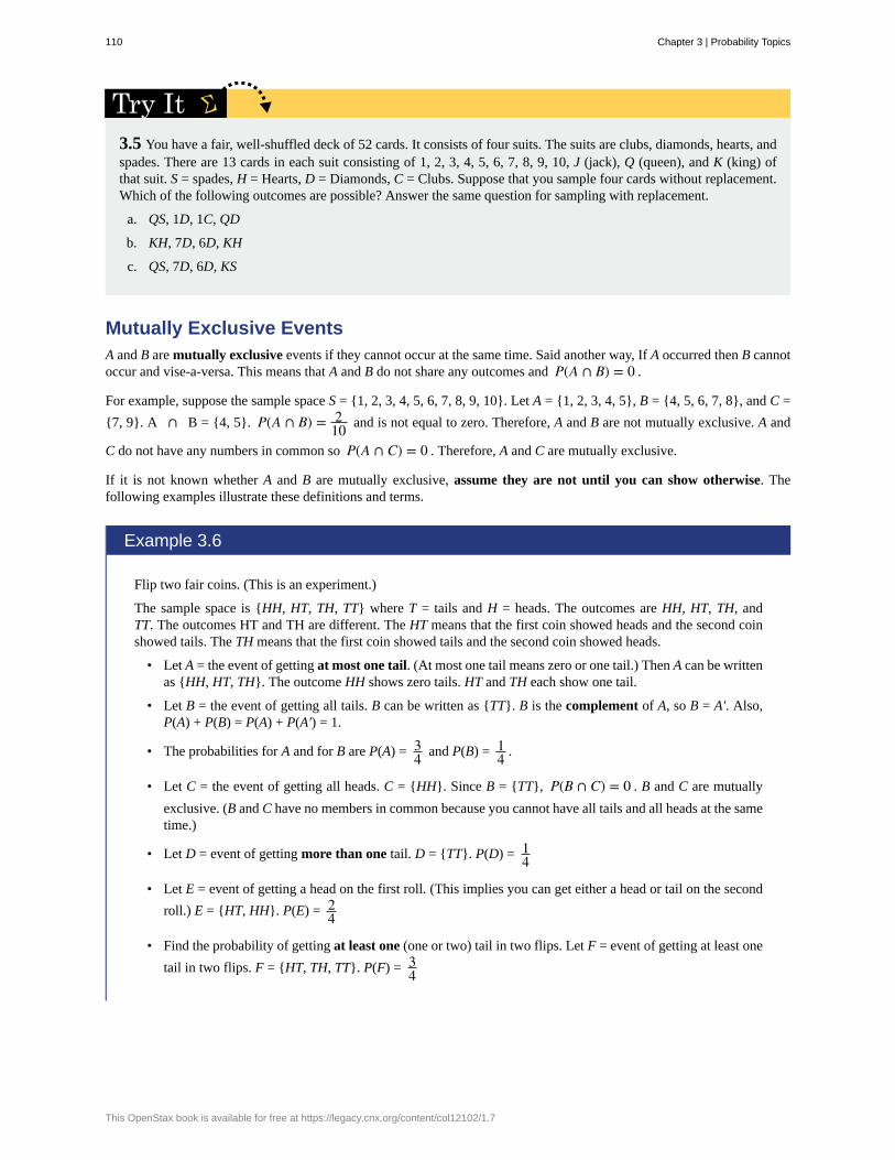
3.5 You have a fair, well-shuffled deck of 52 cards. It consists of four suits. The suits are clubs, diamonds, hearts, andspades. There are 13 cards in each suit consisting of 1, 2, 3, 4, 5, 6, 7, 8, 9, 10, J (jack), Q (queen), and K (king) ofthat suit. S = spades, H = Hearts, D = Diamonds, C = Clubs. Suppose that you sample four cards without replacement.Which of the following outcomes are possible? Answer the same question for sampling with replacement.
a. QS, 1D, 1C, QD
b. KH, 7D, 6D, KH
c. QS, 7D, 6D, KS
Mutually Exclusive EventsA and B are mutually exclusive events if they cannot occur at the same time. Said another way, If A occurred then B cannotoccur and vise-a-versa. This means that A and B do not share any outcomes and P(A ∩ B) = 0 .
For example, suppose the sample space S = {1, 2, 3, 4, 5, 6, 7, 8, 9, 10}. Let A = {1, 2, 3, 4, 5}, B = {4, 5, 6, 7, 8}, and C =
{7, 9}. A ∩ B = {4, 5}. P(A ∩ B) = 210 and is not equal to zero. Therefore, A and B are not mutually exclusive. A and
C do not have any numbers in common so P(A ∩ C) = 0 . Therefore, A and C are mutually exclusive.
If it is not known whether A and B are mutually exclusive, assume they are not until you can show otherwise. Thefollowing examples illustrate these definitions and terms.
Example 3.6
Flip two fair coins. (This is an experiment.)
The sample space is {HH, HT, TH, TT} where T = tails and H = heads. The outcomes are HH, HT, TH, andTT. The outcomes HT and TH are different. The HT means that the first coin showed heads and the second coinshowed tails. The TH means that the first coin showed tails and the second coin showed heads.
• Let A = the event of getting at most one tail. (At most one tail means zero or one tail.) Then A can be writtenas {HH, HT, TH}. The outcome HH shows zero tails. HT and TH each show one tail.
• Let B = the event of getting all tails. B can be written as {TT}. B is the complement of A, so B = A′. Also,P(A) + P(B) = P(A) + P(A′) = 1.
• The probabilities for A and for B are P(A) = 34 and P(B) = 1
4 .
• Let C = the event of getting all heads. C = {HH}. Since B = {TT}, P(B ∩ C) = 0 . B and C are mutually
exclusive. (B and C have no members in common because you cannot have all tails and all heads at the sametime.)
• Let D = event of getting more than one tail. D = {TT}. P(D) = 14
• Let E = event of getting a head on the first roll. (This implies you can get either a head or tail on the second
roll.) E = {HT, HH}. P(E) = 24
• Find the probability of getting at least one (one or two) tail in two flips. Let F = event of getting at least one
tail in two flips. F = {HT, TH, TT}. P(F) = 34
110 Chapter 3 | Probability Topics
This OpenStax book is available for free at https://legacy.cnx.org/content/col12102/1.7

3.6 Draw two cards from a standard 52-card deck with replacement. Find the probability of getting at least one blackcard.
Example 3.7
Flip two fair coins. Find the probabilities of the events.
a. Let F = the event of getting at most one tail (zero or one tail).
b. Let G = the event of getting two faces that are the same.
c. Let H = the event of getting a head on the first flip followed by a head or tail on the second flip.
d. Are F and G mutually exclusive?
e. Let J = the event of getting all tails. Are J and H mutually exclusive?
Solution 3.7
Look at the sample space in Example 3.6.
a. Zero (0) or one (1) tails occur when the outcomes HH, TH, HT show up. P(F) = 34
b. Two faces are the same if HH or TT show up. P(G) = 24
c. A head on the first flip followed by a head or tail on the second flip occurs when HH or HT show up. P(H)
= 24
d. F and G share HH so P(F ∩ G) is not equal to zero (0). F and G are not mutually exclusive.
e. Getting all tails occurs when tails shows up on both coins (TT). H’s outcomes are HH and HT.
J and H have nothing in common so P(J ∩ H) = 0. J and H are mutually exclusive.
3.7 A box has two balls, one white and one red. We select one ball, put it back in the box, and select a second ball(sampling with replacement). Find the probability of the following events:
a. Let F = the event of getting the white ball twice.
b. Let G = the event of getting two balls of different colors.
c. Let H = the event of getting white on the first pick.
d. Are F and G mutually exclusive?
e. Are G and H mutually exclusive?
Example 3.8
Roll one fair, six-sided die. The sample space is {1, 2, 3, 4, 5, 6}. Let event A = a face is odd. Then A = {1, 3, 5}.Let event B = a face is even. Then B = {2, 4, 6}.
Chapter 3 | Probability Topics 111
• Find the complement of A, A′. The complement of A, A′, is B because A and B together make up the sample
space. P(A) + P(B) = P(A) + P(A′) = 1. Also, P(A) = 36 and P(B) = 3
6 .
• Let event C = odd faces larger than two. Then C = {3, 5}. Let event D = all even faces smaller than five.Then D = {2, 4}. P(C ∩ D) = 0 because you cannot have an odd and even face at the same time. Therefore,
C and D are mutually exclusive events.
• Let event E = all faces less than five. E = {1, 2, 3, 4}.
Are C and E mutually exclusive events? (Answer yes or no.) Why or why not?
Solution 3.8
No. C = {3, 5} and E = {1, 2, 3, 4}. P⎛⎝C ∩ E⎞⎠ = 16 . To be mutually exclusive, P(C ∩ E) must be zero.
• Find P(C|A) . This is a conditional probability. Recall that the event C is {3, 5} and event A is {1, 3, 5}. To
find P(C|A) , find the probability of C using the sample space A. You have reduced the sample space from
the original sample space {1, 2, 3, 4, 5, 6} to {1, 3, 5}. So, P⎛⎝C|A⎞⎠ = 23 .
3.8 Let event A = learning Spanish. Let event B = learning German. Then A ∩ B = learning Spanish and German.
Suppose P(A) = 0.4 and P(B) = 0.2 . P(A ∩ B) = 0.08 . Are events A and B independent? Hint: You must show
ONE of the following:
• P(A|B) = P(A)
• P(B|A) = P(B)
• P(A ∩ B) = P(A)P(B)
Example 3.9
Let event G = taking a math class. Let event H = taking a science class. Then, G ∩ H = taking a math class and
a science class. Suppose P(G) = 0.6, P(H) = 0.5 , and P(G ∩ H) = 0.3. Are G and H independent?
If G and H are independent, then you must show ONE of the following:
• P(G|H) = P(G)
• P(H|G) = P(H)
• P(G ∩ H) = P(G)P(H)
NOTE
The choice you make depends on the information you have. You could choose any of the methods herebecause you have the necessary information.
a. Show that P(G|H) = P(G) .
112 Chapter 3 | Probability Topics
This OpenStax book is available for free at https://legacy.cnx.org/content/col12102/1.7

Solution 3.9
P⎛⎝G|H⎞⎠ = P(G ∩H)P(H) = 0.3
0.5 = 0.6 = P⎛⎝G⎞⎠
b. Show P(G ∩ H) = P(G)P(H) .
Solution 3.9P⎛⎝G⎞⎠P⎛⎝H⎞⎠ = ⎛
⎝0.6⎞⎠(0.5⎞⎠ = 0.3 = P⎛⎝G ∩ H⎞⎠
Since G and H are independent, knowing that a person is taking a science class does not change the chance thathe or she is taking a math class. If the two events had not been independent (that is, they are dependent) thenknowing that a person is taking a science class would change the chance he or she is taking math. For practice,show that P(H|G) = P(H) to show that G and H are independent events.
3.9 In a bag, there are six red marbles and four green marbles. The red marbles are marked with the numbers 1, 2, 3,4, 5, and 6. The green marbles are marked with the numbers 1, 2, 3, and 4.
• R = a red marble
• G = a green marble
• O = an odd-numbered marble
• The sample space is S = {R1, R2, R3, R4, R5, R6, G1, G2, G3, G4}.
S has ten outcomes. What is P(G ∩ O) ?
Example 3.10
Let event C = taking an English class. Let event D = taking a speech class.
Suppose P(C) = 0.75 , P(D) = 0.3 , P(C|D) = 0.75 and P(C ∩ D) = 0.225 .
Justify your answers to the following questions numerically.
a. Are C and D independent?
b. Are C and D mutually exclusive?
c. What is P(D|C) ?
Solution 3.10a. Yes, because P(C|D) = P(C) .
b. No, because P(C ∩ D) is not equal to zero.
c. P⎛⎝D|C⎞⎠ = P(C ∩ D)P(C) = 0.225
0.75 = 0.3
Chapter 3 | Probability Topics 113

3.10 A student goes to the library. Let events B = the student checks out a book and D = the student checks out aDVD. Suppose that P(B) = 0.40 , P(D) = 0.30 and P(B ∩ D) = 0.20 .
a. Find P(B|D) .
b. Find P(D|B) .
c. Are B and D independent?
d. Are B and D mutually exclusive?
Example 3.11
In a box there are three red cards and five blue cards. The red cards are marked with the numbers 1, 2, and 3, andthe blue cards are marked with the numbers 1, 2, 3, 4, and 5. The cards are well-shuffled. You reach into the box(you cannot see into it) and draw one card.
Let R = red card is drawn, B = blue card is drawn, E = even-numbered card is drawn.
The sample space S = R1, R2, R3, B1, B2, B3, B4, B5. S has eight outcomes.
• P⎛⎝R⎞⎠ = 3
8.P⎛⎝B⎞⎠ = 5
8.P⎛⎝R ∩ B⎞⎠ = 0 . (You cannot draw one card that is both red and blue.)
• P⎛⎝E⎞⎠ = 3
8 . (There are three even-numbered cards, R2, B2, and B4.)
• P(E|B) = 25 . (There are five blue cards: B1, B2, B3, B4, and B5. Out of the blue cards, there are two even
cards; B2 and B4.)
• P(B|E) = 23 . (There are three even-numbered cards: R2, B2, and B4. Out of the even-numbered cards, to
are blue; B2 and B4.)
• The events R and B are mutually exclusive because P(R ∩ B) = 0 .
• Let G = card with a number greater than 3. G = {B4, B5}. P⎛⎝G⎞⎠ = 2
8 . Let H = blue card numbered between
one and four, inclusive. H = {B1, B2, B3, B4}. P(G|H) = 14 . (The only card in H that has a number greater
than three is B4.) Since 28 = 1
4 , P(G) = P(G|H) , which means that G and H are independent.
3.11 In a basketball arena,
• 70% of the fans are rooting for the home team.
• 25% of the fans are wearing blue.
• 20% of the fans are wearing blue and are rooting for the away team.
• Of the fans rooting for the away team, 67% are wearing blue.
Let A be the event that a fan is rooting for the away team.Let B be the event that a fan is wearing blue.
114 Chapter 3 | Probability Topics
This OpenStax book is available for free at https://legacy.cnx.org/content/col12102/1.7
Are the events of rooting for the away team and wearing blue independent? Are they mutually exclusive?
Example 3.12
In a particular college class, 60% of the students are female. Fifty percent of all students in the class have longhair. Forty-five percent of the students are female and have long hair. Of the female students, 75% have long hair.Let F be the event that a student is female. Let L be the event that a student has long hair. One student is pickedrandomly. Are the events of being female and having long hair independent?
• The following probabilities are given in this example:
• P(F)=0.60; P(L)=0.50
• P(F ∩ L) = 0.45
• P(L|F) = 0.75
NOTE
The choice you make depends on the information you have. You could use the first or last condition onthe list for this example. You do not know P(F|L) yet, so you cannot use the second condition.
Check whether P(F ∩ L) = P(F)P(L) . We are given that P(F ∩ L) = 0.45 , but
P(F)P(L) = (0.60)(0.50) = 0.30 . The events of being female and having long hair are not independent because
P(F ∩ L) does not equal P(F)P(L) .
Check whether P(L|F) equals P(L) . We are given that P(L|F) = 0.75 , but P(L) = 0.50 ; they are not equal.
The events of being female and having long hair are not independent.
Interpretation of Results
The events of being female and having long hair are not independent; knowing that a student is female changesthe probability that a student has long hair.
3.12 Mark is deciding which route to take to work. His choices are I = the Interstate and F = Fifth Street.
• P(I) = 0.44 and P(F) = 0.56
• P(I ∩ F) = 0 because Mark will take only one route to work.
What is the probability of P(I ∪ F) ?
Example 3.13
a. Toss one fair coin (the coin has two sides, H and T). The outcomes are ________. Count the outcomes. Thereare ____ outcomes.
b. Toss one fair, six-sided die (the die has 1, 2, 3, 4, 5 or 6 dots on a side). The outcomes are________________. Count the outcomes. There are ___ outcomes.
c. Multiply the two numbers of outcomes. The answer is _______.
Chapter 3 | Probability Topics 115

d. If you flip one fair coin and follow it with the toss of one fair, six-sided die, the answer to c is the number ofoutcomes (size of the sample space). What are the outcomes? (Hint: Two of the outcomes are H1 and T6.)
e. Event A = heads (H) on the coin followed by an even number (2, 4, 6) on the die.A = {_________________}. Find P(A).
f. Event B = heads on the coin followed by a three on the die. B = {________}. Find P(B).
g. Are A and B mutually exclusive? (Hint: What is P(A ∩ B) ? If P(A ∩ B) = 0 , then A and B are mutually
exclusive.)
h. Are A and B independent? (Hint: Is P(A ∩ B) = P(A)P(B) ? If P(A ∩ B) = P(A)P(B) , then A and B are
independent. If not, then they are dependent).
Solution 3.13a. H and T; 2
b. 1, 2, 3, 4, 5, 6; 6
c. 2(6) = 12
d. T1, T2, T3, T4, T5, T6, H1, H2, H3, H4, H5, H6
e. A = {H2, H4, H6}; P(A) = 312
f. B = {H3}; P(B) = 112
g. Yes, because P(A ∩ B) = 0
h. P⎛⎝A ∩ B⎞⎠ = 0.P⎛⎝A⎞⎠P⎛⎝B⎞⎠ = ( 3
12).P⎛⎝A ∩ B⎞⎠does not equalP⎛⎝A⎞⎠P⎛⎝B⎞⎠, soAandBare dependent.
3.13 A box has two balls, one white and one red. We select one ball, put it back in the box, and select a second ball(sampling with replacement). Let T be the event of getting the white ball twice, F the event of picking the white ballfirst, S the event of picking the white ball in the second drawing.
a. Compute P(T) .
b. Compute P(T |F) .
c. Are T and F independent?.
d. Are F and S mutually exclusive?
e. Are F and S independent?
3.3 | Two Basic Rules of ProbabilityWhen calculating probability, there are two rules to consider when determining if two events are independent or dependentand if they are mutually exclusive or not.
The Multiplication RuleIf A and B are two events defined on a sample space, then: P(A ∩ B) = P(B)P(A|B) . We can think of the intersection
symbol as substituting for the word "and".
This rule may also be written as: P⎛⎝A|B⎞⎠ = P(A ∩ B)P(B)
116 Chapter 3 | Probability Topics
This OpenStax book is available for free at https://legacy.cnx.org/content/col12102/1.7
This equation is read as the probability of A given B equals the probability of A and B divided by the probability of B.
If A and B are independent, then P(A|B) = P(A) . Then P(A ∩ B) = P(A|B)P(B) becomes P(A ∩ B) = P(A)(B)because the P(A|B) = P(A) if A and B are independent.
One easy way to remember the multiplication rule is that the word "and" means that the event has to satisfy two conditions.For example the name drawn from the class roster is to be both a female and a sophomore. It is harder to satisfy twoconditions than only one and of course when we multiply fractions the result is always smaller. This reflects the increasingdifficulty of satisfying two conditions.
The Addition RuleIf A and B are defined on a sample space, then: P(A ∪ B) = P(A) + P(B) - P(A ∩ B) . We can think of the union symbol
substituting for the word "or". The reason we subtract the intersection of A and B is to keep from double counting elementsthat are in both A and B.
If A and B are mutually exclusive, then P(A ∩ B) = 0 . Then P(A ∪ B) = P(A) + P(B) - P(A ∩ B) becomes
P(A ∪ B) = P(A) + P(B) .
Example 3.14
Klaus is trying to choose where to go on vacation. His two choices are: A = New Zealand and B = Alaska
• Klaus can only afford one vacation. The probability that he chooses A is P(A) = 0.6 and the probability thathe chooses B is P(B) = 0.35.
• P(A ∩ B) = 0 because Klaus can only afford to take one vacation
• Therefore, the probability that he chooses either New Zealand or Alaska isP(A ∪ B) = P(A) + P(B) = 0.6 + 0.35 = 0.95 . Note that the probability that he does not choose to go
anywhere on vacation must be 0.05.
Example 3.15
Carlos plays college soccer. He makes a goal 65% of the time he shoots. Carlos is going to attempt two goals in arow in the next game. A = the event Carlos is successful on his first attempt. P(A) = 0.65. B = the event Carlos issuccessful on his second attempt. P(B) = 0.65. Carlos tends to shoot in streaks. The probability that he makes thesecond goal | that he made the first goal is 0.90.
a. What is the probability that he makes both goals?
b. What is the probability that Carlos makes either the first goal or the second goal?
c. Are A and B independent?
d. Are A and B mutually exclusive?
Solution 3.15a. a. The problem is asking you to find P(A ∩ B) = P(B ∩ A) . Since P(B | A) = 0.90: P(B ∩ A) = P(B | A)
P(A) = (0.90)(0.65) = 0.585
Carlos makes the first and second goals with probability 0.585.
b. b. The problem is asking you to find P(A ∪ B).
P(A ∪ B) = P(A) + P(B) - P(A ∩ B) = 0.65 + 0.65 - 0.585 = 0.715
Carlos makes either the first goal or the second goal with probability 0.715.
Chapter 3 | Probability Topics 117

c. c. No, they are not, because P(B ∩ A) = 0.585.
P(B)P(A) = (0.65)(0.65) = 0.423
0.423 ≠ 0.585 = P(B ∩ A)
So, P(B ∩ A) is not equal to P(B)P(A).
d. d. No, they are not because P(A ∩ B) = 0.585.
To be mutually exclusive, P(A ∩ B) must equal zero.
3.15 Helen plays basketball. For free throws, she makes the shot 75% of the time. Helen must now attempt two freethrows. C = the event that Helen makes the first shot. P(C) = 0.75. D = the event Helen makes the second shot. P(D)= 0.75. The probability that Helen makes the second free throw given that she made the first is 0.85. What is theprobability that Helen makes both free throws?
Example 3.16
A community swim team has 150 members. Seventy-five of the members are advanced swimmers. Forty-seven of the members are intermediate swimmers. The remainder are novice swimmers. Forty of the advancedswimmers practice four times a week. Thirty of the intermediate swimmers practice four times a week. Ten ofthe novice swimmers practice four times a week. Suppose one member of the swim team is chosen randomly.
a. What is the probability that the member is a novice swimmer?
b. What is the probability that the member practices four times a week?
c. What is the probability that the member is an advanced swimmer and practices four times a week?
d. What is the probability that a member is an advanced swimmer and an intermediate swimmer? Are being anadvanced swimmer and an intermediate swimmer mutually exclusive? Why or why not?
e. Are being a novice swimmer and practicing four times a week independent events? Why or why not?
Solution 3.16
a. 28150
b. 80150
c. 40150
d. P(advanced ∩ intermediate) = 0, so these are mutually exclusive events. A swimmer cannot be an
advanced swimmer and an intermediate swimmer at the same time.
e. No, these are not independent events.P(novice ∩ practices four times per week) = 0.0667
P(novice)P(practices four times per week) = 0.09960.0667 ≠ 0.0996
118 Chapter 3 | Probability Topics
This OpenStax book is available for free at https://legacy.cnx.org/content/col12102/1.7
3.16 A school has 200 seniors of whom 140 will be going to college next year. Forty will be going directly to work.The remainder are taking a gap year. Fifty of the seniors going to college play sports. Thirty of the seniors goingdirectly to work play sports. Five of the seniors taking a gap year play sports. What is the probability that a senior istaking a gap year?
Example 3.17
Felicity attends Modesto JC in Modesto, CA. The probability that Felicity enrolls in a math class is 0.2 and theprobability that she enrolls in a speech class is 0.65. The probability that she enrolls in a math class | that she
enrolls in speech class is 0.25.
Let: M = math class, S = speech class, M | S = math given speech
a. What is the probability that Felicity enrolls in math and speech?Find P(M ∩ S) = P(M | S)P(S).
b. What is the probability that Felicity enrolls in math or speech classes?Find P(M ∪ S) = P(M) + P(S) - P(M ∩ S).
c. Are M and S independent? Is P(M | S) = P(M)?
d. Are M and S mutually exclusive? Is P(M ∩ S) = 0?
Solution 3.17a. 0.1625, b. 0.6875, c. No, d. No
3.17 A student goes to the library. Let events B = the student checks out a book and D = the student check out a DVD.Suppose that P(B) = 0.40, P(D) = 0.30 and P(D | B) = 0.5.
a. Find P(B ∩ D).
b. Find P(B ∪ D).
Example 3.18
Studies show that about one woman in seven (approximately 14.3%) who live to be 90 will develop breast cancer.Suppose that of those women who develop breast cancer, a test is negative 2% of the time. Also suppose that inthe general population of women, the test for breast cancer is negative about 85% of the time. Let B = womandevelops breast cancer and let N = tests negative. Suppose one woman is selected at random.
a. What is the probability that the woman develops breast cancer? What is the probability that woman testsnegative?
b. Given that the woman has breast cancer, what is the probability that she tests negative?
c. What is the probability that the woman has breast cancer AND tests negative?
d. What is the probability that the woman has breast cancer or tests negative?
e. Are having breast cancer and testing negative independent events?
Chapter 3 | Probability Topics 119

f. Are having breast cancer and testing negative mutually exclusive?
Solution 3.18a. P(B) = 0.143; P(N) = 0.85
b. P(N | B) = 0.02
c. P(B ∩ N) = P(B)P(N | B) = (0.143)(0.02) = 0.0029
d. P(B ∪ N) = P(B) + P(N) - P(B ∩ N) = 0.143 + 0.85 - 0.0029 = 0.9901
e. No. P(N) = 0.85; P(N | B) = 0.02. So, P(N | B) does not equal P(N).
f. No. P(B ∩ N) = 0.0029. For B and N to be mutually exclusive, P(B ∩ N) must be zero.
3.18 A school has 200 seniors of whom 140 will be going to college next year. Forty will be going directly to work.The remainder are taking a gap year. Fifty of the seniors going to college play sports. Thirty of the seniors goingdirectly to work play sports. Five of the seniors taking a gap year play sports. What is the probability that a senior isgoing to college and plays sports?
Example 3.19
Refer to the information in Example 3.18. P = tests positive.
a. Given that a woman develops breast cancer, what is the probability that she tests positive. Find P(P | B) = 1
- P(N | B).
b. What is the probability that a woman develops breast cancer and tests positive. Find P(B ∩ P) = P(P |B)P(B).
c. What is the probability that a woman does not develop breast cancer. Find P(B′) = 1 - P(B).
d. What is the probability that a woman tests positive for breast cancer. Find P(P) = 1 - P(N).
Solution 3.19a. 0.98; b. 0.1401; c. 0.857; d. 0.15
3.19 A student goes to the library. Let events B = the student checks out a book and D = the student checks out aDVD. Suppose that P(B) = 0.40, P(D) = 0.30 and P(D | B) = 0.5.
a. Find P(B′).
b. Find P(D ∩ B).
c. Find P(B | D).
d. Find P(D ∩ B′).
e. Find P(D | B′).
120 Chapter 3 | Probability Topics
This OpenStax book is available for free at https://legacy.cnx.org/content/col12102/1.7

3.4 | Contingency Tables and Probability TreesContingency TablesA contingency table provides a way of portraying data that can facilitate calculating probabilities. The table helps indetermining conditional probabilities quite easily. The table displays sample values in relation to two different variables thatmay be dependent or contingent on one another. Later on, we will use contingency tables again, but in another manner.
Example 3.20
Suppose a study of speeding violations and drivers who use cell phones produced the following fictional data:
Speeding violation in thelast year
No speeding violation in thelast year
Total
Uses cell phone while driving 25 280 305
Does not use cell phone whiledriving
45 405 450
Total 70 685 755
Table 3.2
The total number of people in the sample is 755. The row totals are 305 and 450. The column totals are 70 and685. Notice that 305 + 450 = 755 and 70 + 685 = 755.
Calculate the following probabilities using the table.
a. Find P(Driver is a cell phone user).
b. Find P(Driver had no violation in the last year).
c. Find P(Driver had no violation in the last year ∩ was a cell phone user).
d. Find P(Driver is a cell phone user ∪ driver had no violation in the last year).
e. Find P(Driver is a cell phone user | driver had a violation in the last year).
f. Find P(Driver had no violation last year | driver was not a cell phone user)
Solution 3.20
a.number of cell phone users
total number in study = 305755
b. number that had no violationtotal number in study = 685
755
c. 280755
d. ⎛⎝305755 + 685
755⎞⎠ − 280
755 = 710755
e. 2570 (The sample space is reduced to the number of drivers who had a violation.)
f. 405450 (The sample space is reduced to the number of drivers who were not cell phone users.)
Chapter 3 | Probability Topics 121

3.20 Table 3.3 shows the number of athletes who stretch before exercising and how many had injuries within thepast year.
Injury in last year No injury in last year Total
Stretches 55 295 350
Does not stretch 231 219 450
Total 286 514 800
Table 3.3
a. What is P(athlete stretches before exercising)?
b. What is P(athlete stretches before exercising | no injury in the last year)?
Example 3.21
Table 3.4 shows a random sample of 100 hikers and the areas of hiking they prefer.
Sex The coastline Near lakes and streams On mountain peaks Total
Female 18 16 ___ 45
Male ___ ___ 14 55
Total ___ 41 ___ ___
Table 3.4 Hiking Area Preference
a. Complete the table.
Solution 3.21a.
Sex The coastline Near lakes and streams On mountain peaks Total
Female 18 16 11 45
Male 16 25 14 55
Total 34 41 25 100
Table 3.5 Hiking Area Preference
b. Are the events "being female" and "preferring the coastline" independent events?
Let F = being female and let C = preferring the coastline.
1. Find P(F ∩ C) .
2. Find P(F)P(C)
Are these two numbers the same? If they are, then F and C are independent. If they are not, then F and C are not
122 Chapter 3 | Probability Topics
This OpenStax book is available for free at https://legacy.cnx.org/content/col12102/1.7

independent.
Solution 3.21
b.
1. P⎛⎝F ∩ C⎞⎠ = 18100 = 0.18
2. P(F)P(C) = ⎛⎝ 45100⎞⎠⎛⎝ 34100⎞⎠ = (0.45)(0.34) = 0.153
P(F ∩ C) ≠ P(F)P(C), so the events F and C are not independent.
c. Find the probability that a person is male given that the person prefers hiking near lakes and streams. Let M =being male, and let L = prefers hiking near lakes and streams.
1. What word tells you this is a conditional?
2. Fill in the blanks and calculate the probability: P(___ | ___) = ___.
3. Is the sample space for this problem all 100 hikers? If not, what is it?
Solution 3.21c.
1. The word 'given' tells you that this is a conditional.
2. P(M | L) = 2541
3. No, the sample space for this problem is the 41 hikers who prefer lakes and streams.
d. Find the probability that a person is female or prefers hiking on mountain peaks. Let F = being female, and letP = prefers mountain peaks.
1. Find P(F).
2. Find P(P).
3. Find P(F ∩ P) .
4. Find P(F ∪ P) .
Solution 3.21d.
1. P(F) = 45100
2. P(P) = 25100
3. P(F ∩ P) = 11100
4. P(F ∪ P) = 45100 + 25
100 - 11100 = 59
100
Chapter 3 | Probability Topics 123

3.21 Table 3.6 shows a random sample of 200 cyclists and the routes they prefer. Let M = males and H = hilly path.
Gender Lake path Hilly path Wooded path Total
Female 45 38 27 110
Male 26 52 12 90
Total 71 90 39 200
Table 3.6
a. Out of the males, what is the probability that the cyclist prefers a hilly path?
b. Are the events “being male” and “preferring the hilly path” independent events?
Example 3.22
Muddy Mouse lives in a cage with three doors. If Muddy goes out the first door, the probability that he gets caught
by Alissa the cat is 15 and the probability he is not caught is 4
5 . If he goes out the second door, the probability he
gets caught by Alissa is 14 and the probability he is not caught is 3
4 . The probability that Alissa catches Muddy
coming out of the third door is 12 and the probability she does not catch Muddy is 1
2 . It is equally likely that
Muddy will choose any of the three doors so the probability of choosing each door is 13 .
Caught or not Door one Door two Door three Total
Caught115
112
16 ____
Not caught415
312
16 ____
Total ____ ____ ____ 1
Table 3.7 Door Choice
• The first entry 115 = ⎛⎝15
⎞⎠⎛⎝13⎞⎠ is P⎛⎝Door One ∩ Caught⎞⎠
• The entry 415 = ⎛⎝45
⎞⎠⎛⎝13⎞⎠ is P⎛⎝Door One ∩ Not Caught⎞⎠
Verify the remaining entries.
a. Complete the probability contingency table. Calculate the entries for the totals. Verify that the lower-rightcorner entry is 1.
Solution 3.22a.
124 Chapter 3 | Probability Topics
This OpenStax book is available for free at https://legacy.cnx.org/content/col12102/1.7

Caught or not Door one Door two Door three Total
Caught115
112
16
1960
Not caught415
312
16
4160
Total515
412
26 1
Table 3.8 Door Choice
b. What is the probability that Alissa does not catch Muddy?
Solution 3.22
b. 4160
c. What is the probability that Muddy chooses Door One ∪ Door Two given that Muddy is caught by Alissa?
Solution 3.22
c. 919
Example 3.23
Table 3.9 contains the number of crimes per 100,000 inhabitants from 2008 to 2011 in the U.S.
Year Robbery Burglary Rape Vehicle Total
2008 145.7 732.1 29.7 314.7
2009 133.1 717.7 29.1 259.2
2010 119.3 701 27.7 239.1
2011 113.7 702.2 26.8 229.6
Total
Table 3.9 United States Crime Index Rates Per 100,000Inhabitants 2008–2011
TOTAL each column and each row. Total data = 4,520.7
a. Find P⎛⎝2009 ∩ Robbery⎞⎠ .
b. Find P⎛⎝2010 ∩ Burglary⎞⎠ .
c. Find P⎛⎝2010 ∪ Burglary⎞⎠ .
d. Find P(2011 | Rape).
e. Find P(Vehicle | 2008).
Chapter 3 | Probability Topics 125
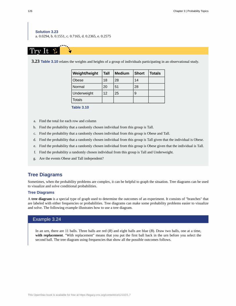
Solution 3.23a. 0.0294, b. 0.1551, c. 0.7165, d. 0.2365, e. 0.2575
3.23 Table 3.10 relates the weights and heights of a group of individuals participating in an observational study.
Weight/height Tall Medium Short Totals
Obese 18 28 14
Normal 20 51 28
Underweight 12 25 9
Totals
Table 3.10
a. Find the total for each row and column
b. Find the probability that a randomly chosen individual from this group is Tall.
c. Find the probability that a randomly chosen individual from this group is Obese and Tall.
d. Find the probability that a randomly chosen individual from this group is Tall given that the individual is Obese.
e. Find the probability that a randomly chosen individual from this group is Obese given that the individual is Tall.
f. Find the probability a randomly chosen individual from this group is Tall and Underweight.
g. Are the events Obese and Tall independent?
Tree DiagramsSometimes, when the probability problems are complex, it can be helpful to graph the situation. Tree diagrams can be usedto visualize and solve conditional probabilities.
Tree Diagrams
A tree diagram is a special type of graph used to determine the outcomes of an experiment. It consists of "branches" thatare labeled with either frequencies or probabilities. Tree diagrams can make some probability problems easier to visualizeand solve. The following example illustrates how to use a tree diagram.
Example 3.24
In an urn, there are 11 balls. Three balls are red (R) and eight balls are blue (B). Draw two balls, one at a time,with replacement. "With replacement" means that you put the first ball back in the urn before you select thesecond ball. The tree diagram using frequencies that show all the possible outcomes follows.
126 Chapter 3 | Probability Topics
This OpenStax book is available for free at https://legacy.cnx.org/content/col12102/1.7

Figure 3.2 Total = 64 + 24 + 24 + 9 = 121
The first set of branches represents the first draw. The second set of branches represents the second draw. Each ofthe outcomes is distinct. In fact, we can list each red ball as R1, R2, and R3 and each blue ball as B1, B2, B3, B4,B5, B6, B7, and B8. Then the nine RR outcomes can be written as:
R1R1; R1R2; R1R3; R2R1; R2R2; R2R3; R3R1; R3R2; R3R3
The other outcomes are similar.
There are a total of 11 balls in the urn. Draw two balls, one at a time, with replacement. There are 11(11) = 121outcomes, the size of the sample space.
a. List the 24 BR outcomes: B1R1, B1R2, B1R3, ...
Solution 3.24a. B1R1; B1R2; B1R3; B2R1; B2R2; B2R3; B3R1; B3R2; B3R3; B4R1; B4R2; B4R3; B5R1; B5R2; B5R3; B6R1;B6R2; B6R3; B7R1; B7R2; B7R3; B8R1; B8R2; B8R3
b. Using the tree diagram, calculate P(RR).
Solution 3.24
b. P(RR) = ⎛⎝ 311⎞⎠⎛⎝ 311⎞⎠ = 9
121
c. Using the tree diagram, calculate P(RB ∪ BR) .
Solution 3.24
c. P(RB ∪ BR) = ⎛⎝ 311⎞⎠⎛⎝ 811⎞⎠ + ⎛⎝ 8
11⎞⎠⎛⎝ 311⎞⎠ = 48
121
d. Using the tree diagram, calculate P(R on 1st draw ∩ B on 2nd draw) .
Solution 3.24
d. P(R on 1st draw ∩ B on 2nd draw) = ⎛⎝ 311⎞⎠⎛⎝ 811⎞⎠ = 24
121
e. Using the tree diagram, calculate P(R on 2nd draw | B on 1st draw).
Chapter 3 | Probability Topics 127
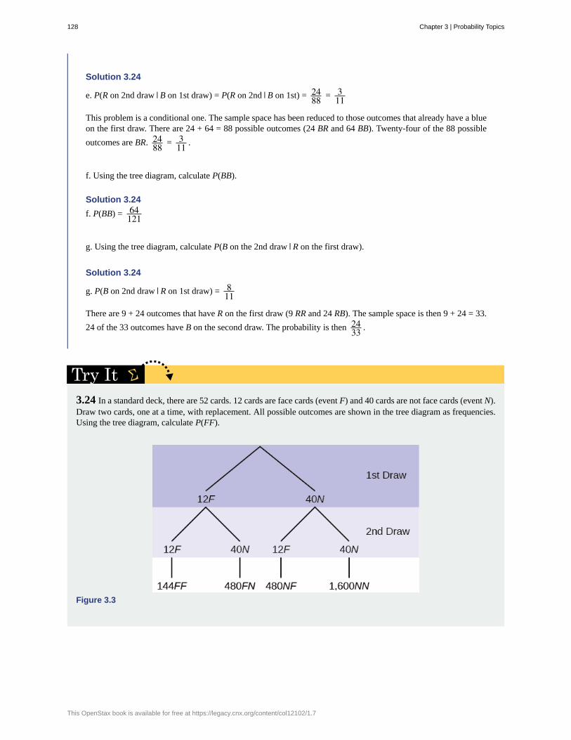
Solution 3.24
e. P(R on 2nd draw | B on 1st draw) = P(R on 2nd | B on 1st) = 2488 = 3
11
This problem is a conditional one. The sample space has been reduced to those outcomes that already have a blueon the first draw. There are 24 + 64 = 88 possible outcomes (24 BR and 64 BB). Twenty-four of the 88 possible
outcomes are BR. 2488 = 3
11 .
f. Using the tree diagram, calculate P(BB).
Solution 3.24
f. P(BB) = 64121
g. Using the tree diagram, calculate P(B on the 2nd draw | R on the first draw).
Solution 3.24
g. P(B on 2nd draw | R on 1st draw) = 811
There are 9 + 24 outcomes that have R on the first draw (9 RR and 24 RB). The sample space is then 9 + 24 = 33.
24 of the 33 outcomes have B on the second draw. The probability is then 2433 .
3.24 In a standard deck, there are 52 cards. 12 cards are face cards (event F) and 40 cards are not face cards (event N).Draw two cards, one at a time, with replacement. All possible outcomes are shown in the tree diagram as frequencies.Using the tree diagram, calculate P(FF).
Figure 3.3
128 Chapter 3 | Probability Topics
This OpenStax book is available for free at https://legacy.cnx.org/content/col12102/1.7

Example 3.25
An urn has three red marbles and eight blue marbles in it. Draw two marbles, one at a time, this time withoutreplacement, from the urn. "Without replacement" means that you do not put the first ball back before youselect the second marble. Following is a tree diagram for this situation. The branches are labeled with probabilitiesinstead of frequencies. The numbers at the ends of the branches are calculated by multiplying the numbers on the
two corresponding branches, for example, ⎛⎝ 311⎞⎠⎛⎝ 210⎞⎠ = 6
110 .
Figure 3.4 Total = 56 + 24 + 24 + 6110 = 110
110 = 1
NOTE
If you draw a red on the first draw from the three red possibilities, there are two red marbles left to draw onthe second draw. You do not put back or replace the first marble after you have drawn it. You draw withoutreplacement, so that on the second draw there are ten marbles left in the urn.
Calculate the following probabilities using the tree diagram.
a. P(RR) = ________
Solution 3.25
a. P(RR) = ⎛⎝ 311⎞⎠⎛⎝ 210⎞⎠ = 6
110
b. Fill in the blanks:
P(RB ∪ BR) = ⎛⎝ 311⎞⎠⎛⎝ 810⎞⎠ + (___)(___) = 48
110
Chapter 3 | Probability Topics 129

Solution 3.25
b. P(RB ∪ BR) = ⎛⎝ 311⎞⎠⎛⎝ 810⎞⎠ + ⎛⎝ 8
11⎞⎠⎛⎝ 310⎞⎠ = 48
110
c. P(R on 2nd | B on 1st) =
Solution 3.25
c. P(R on 2nd | B on 1st) = 310
d. Fill in the blanks.
P(R on 1st ∩ B on 2nd) = (___)(___) = 24110
Solution 3.25
d. P(R on 1st ∩ B on 2nd) = ⎛⎝ 311⎞⎠⎛⎝ 810⎞⎠ = 24
110
e. Find P(BB).
Solution 3.25
e. P(BB) = ⎛⎝ 811⎞⎠⎛⎝ 710⎞⎠
f. Find P(B on 2nd | R on 1st).
Solution 3.25
f. Using the tree diagram, P(B on 2nd | R on 1st) = P(R | B) = 810 .
If we are using probabilities, we can label the tree in the following general way.
• P(R | R) here means P(R on 2nd | R on 1st)
• P(B | R) here means P(B on 2nd | R on 1st)
• P(R | B) here means P(R on 2nd | B on 1st)
• P(B | B) here means P(B on 2nd | B on 1st)
130 Chapter 3 | Probability Topics
This OpenStax book is available for free at https://legacy.cnx.org/content/col12102/1.7

3.25 In a standard deck, there are 52 cards. Twelve cards are face cards (F) and 40 cards are not face cards (N). Drawtwo cards, one at a time, without replacement. The tree diagram is labeled with all possible probabilities.
Figure 3.5
a. Find P(FN ∪ NF) .
b. Find P(N | F).
c. Find P(at most one face card).Hint: "At most one face card" means zero or one face card.
d. Find P(at least on face card).Hint: "At least one face card" means one or two face cards.
Example 3.26
A litter of kittens available for adoption at the Humane Society has four tabby kittens and five black kittens. Afamily comes in and randomly selects two kittens (without replacement) for adoption.
Chapter 3 | Probability Topics 131
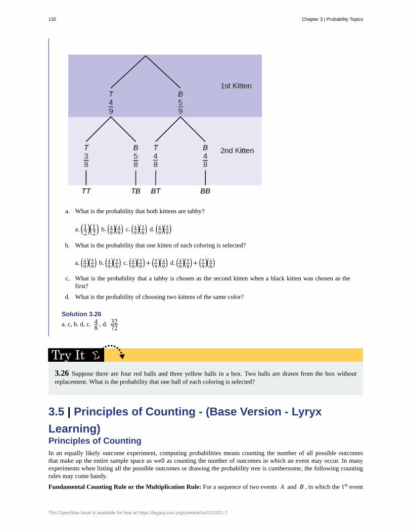
a. What is the probability that both kittens are tabby?
a. ⎛⎝12⎞⎠⎛⎝12⎞⎠ b. ⎛⎝49
⎞⎠⎛⎝49⎞⎠ c. ⎛⎝49
⎞⎠⎛⎝38⎞⎠ d. ⎛⎝49
⎞⎠⎛⎝59⎞⎠
b. What is the probability that one kitten of each coloring is selected?
a. ⎛⎝49⎞⎠⎛⎝59⎞⎠ b. ⎛⎝49
⎞⎠⎛⎝58⎞⎠ c. ⎛⎝49
⎞⎠⎛⎝59⎞⎠+⎛⎝59⎞⎠⎛⎝49⎞⎠ d. ⎛⎝49
⎞⎠⎛⎝58⎞⎠+⎛⎝59⎞⎠⎛⎝48⎞⎠
c. What is the probability that a tabby is chosen as the second kitten when a black kitten was chosen as thefirst?
d. What is the probability of choosing two kittens of the same color?
Solution 3.26
a. c, b. d, c. 48 , d. 32
72
3.26 Suppose there are four red balls and three yellow balls in a box. Two balls are drawn from the box withoutreplacement. What is the probability that one ball of each coloring is selected?
3.5 | Principles of Counting - (Base Version - Lyryx
Learning)Principles of CountingIn an equally likely outcome experiment, computing probabilities means counting the number of all possible outcomesthat make up the entire sample space as well as counting the number of outcomes in which an event may occur. In manyexperiments when listing all the possible outcomes or drawing the probability tree is cumbersome, the following countingrules may come handy.
Fundamental Counting Rule or the Multiplication Rule: For a sequence of two events A and B , in which the 1st event
132 Chapter 3 | Probability Topics
This OpenStax book is available for free at https://legacy.cnx.org/content/col12102/1.7

A can occur in m ways and the 2nd event B can occur in n ways, the events together can occur a total of m×n ways.
To use this counting rule, think of each choice as a slot, or position, to fill.
Example 1 An experiment consists of tossing a fair coin twice and recording the side that lands face-up on each toss. Howmany combinations of heads and tails is possible?
Solution The number of combinations is
2 (number or choices for the 1st toss) x 2 (number or choices for the 2nd toss)= 4.
Notation:
• We write N(S) for the total number of outcomes (size of a sample space).
• N(A) denotes the number of outcomes in event A .
Example 2 An experiment consists of tossing a fair coin once and then rolling a fair six-sided die and recording the sidesthat land face up. Find the size of the sample space N(S) . Illustrate your answer by drawing a probability tree diagram.
Solution The size of the sample space is N(S) = 2×6 = 12 .
The fundamental principle of counting may be extended to any number of ordered independent events.
Example 3 A bank summer associate outfit consists of a pair of pants, a shirt, and a tie. Suppose he can choose from amongfour pairs of pants, six shirts, and three ties. How many different outfits are possible?
Solution Using the counting principle, there are N(S) = 4×6×3 = 72 outfits.
Example 4 (Traveling Salesmen problem) A franchise supervisor must visit eight different locations around the country.She can visit them in any order, but wishes to find the most convenient sequence. How many sequences are possible?
Solution We think of each location as a slot that can be filled with a number of choices:
Number of choices available 8 7 6 5 4 3 2 1
Location 1st 2nd 3rd 4th 5th 6th 7th 8th
Table 3.11
Then, by extended multiplication rule, the total number of sequences is
8×7×6×5×4×3×2×1 = 8!
The notation (above read "eight factorial") is a shorthand for the product of all the integers from 1 to 8.
Factorial Notation:
n ! = 1×2×3×4× ⋯ ×(n - 1)×n0! = 1 1! = 1
Factorial Rule:
A collection of n different items can be arranged in n ! different ways.
Example 5 In how many ways the letters of the word "MATH" can be arranged?
Solution The word contains four different items. It can thus be arranged in 4! = 24 ways.
Note: Factorial calculations (for relatively small numbers) can be done using the factorial key on the calculator.
Permutations
The word permutation means an arrangement or a sequence and implies that the ORDER of items is IMPORTANT.
Example 6 Given three letters A B C, how many different arrangements are possible?
Solution By the factorial rule there are 3! = 6 ways to arrange three different letters:
ABC CAB BCA ACB CBA BAC,
forming six different sequences as long as ORDER matters.
Chapter 3 | Probability Topics 133
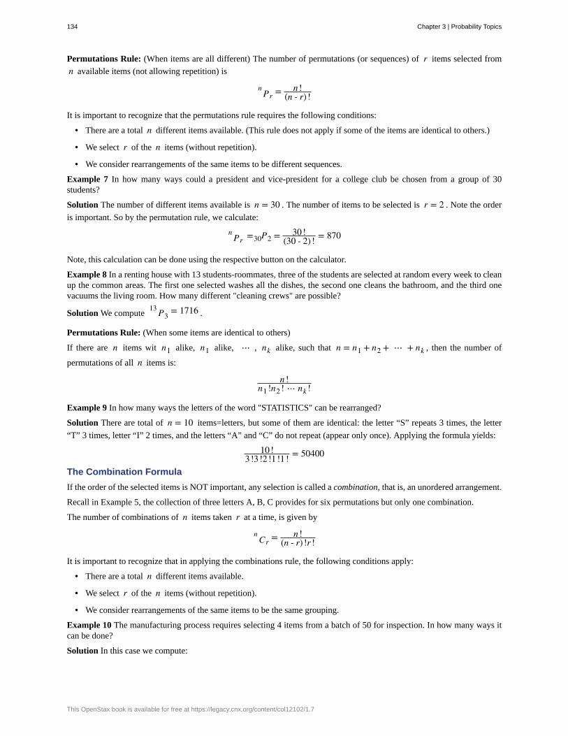
Permutations Rule: (When items are all different) The number of permutations (or sequences) of r items selected from
n available items (not allowing repetition) is
nPr = n !
(n - r) !
It is important to recognize that the permutations rule requires the following conditions:
• There are a total n different items available. (This rule does not apply if some of the items are identical to others.)
• We select r of the n items (without repetition).
• We consider rearrangements of the same items to be different sequences.
Example 7 In how many ways could a president and vice-president for a college club be chosen from a group of 30students?
Solution The number of different items available is n = 30 . The number of items to be selected is r = 2 . Note the order
is important. So by the permutation rule, we calculate:
nPr =30P2 = 30!
(30 - 2) ! = 870
Note, this calculation can be done using the respective button on the calculator.
Example 8 In a renting house with 13 students-roommates, three of the students are selected at random every week to cleanup the common areas. The first one selected washes all the dishes, the second one cleans the bathroom, and the third onevacuums the living room. How many different "cleaning crews" are possible?
Solution We compute13P3
= 1716 .
Permutations Rule: (When some items are identical to others)
If there are n items wit n1 alike, n1 alike, ⋯ , nk alike, such that n = n1 + n2 + ⋯ + nk , then the number of
permutations of all n items is:
n !n1 !n2 ! ⋯ nk !
Example 9 In how many ways the letters of the word "STATISTICS" can be rearranged?
Solution There are total of n = 10 items=letters, but some of them are identical: the letter “S” repeats 3 times, the letter
“T” 3 times, letter “I” 2 times, and the letters “A” and “C” do not repeat (appear only once). Applying the formula yields:
10!3!3!2!1!1! = 50400
The Combination Formula
If the order of the selected items is NOT important, any selection is called a combination, that is, an unordered arrangement.
Recall in Example 5, the collection of three letters A, B, C provides for six permutations but only one combination.
The number of combinations of n items taken r at a time, is given by
nCr = n !
(n - r) !r !
It is important to recognize that in applying the combinations rule, the following conditions apply:
• There are a total n different items available.
• We select r of the n items (without repetition).
• We consider rearrangements of the same items to be the same grouping.
Example 10 The manufacturing process requires selecting 4 items from a batch of 50 for inspection. In how many ways itcan be done?
Solution In this case we compute:
134 Chapter 3 | Probability Topics
This OpenStax book is available for free at https://legacy.cnx.org/content/col12102/1.7
nCr =50C4 = 50!
(50 - 4) !4! = 50×49×48×4724 = 230, 300
Note that 50! is already a huge number in your calculator, but doing a simplification first yields a much easier calculation.
Example 10. How many sets of 12 questions for an online quiz can be chosen from a pool of 23 questions?
Solution We compute:
nCr =23C12 = 23!
(23 - 12)!12! = 1, 352, 078
Using a Spreadsheet for Calculations
The common spreadsheets (LibreOffice (free), Microsoft Excel,..) offer common functions, inclduing a permutationfunction with the syntax PERMUT(n, r) and combination function with the syntax COMBIN(n, r) . The built-in
factorial function is used as FACT(n) .
Example 11 Using a spreadsheet we obtain:
Counting Rule Excel Formula Example Excel Input
Factorial = FACT(number) 8! = 40320 = FACT(8)
Permutation = PERMUT(number, numberchosen) 7P3= 210 = PERMUT(7, 3)
Combination = COMBIN(number, numberchosen) 12C4= 495 = COMBIN(12, 4)
Table 3.12
Homework
Exercise 3.1
How many blood types are possible in total if blood can be Rh+ or Rh- and belong to one of four blood groups A, B, AB,O?
Solution8
Exercise 3.2
A marketing consultant typically tailors her sales scripts to the target audience. For these purposes the potential consumersare divided by gender (male, female), by age (into 5 groups) and by the level of household income (into 3 groups). Howmany different scripts are necessary to prepare?
Solution30
Exercise 3.3
If a monkey typed four strokes on a keyboard and each stroke was a different letter of the alphabet, what is the probabilitythat the monkey typed the word "MATH"?
Solution1/358800
Exercise 3.4
There are staff cutbacks in the department. There are five people eligible to stay on staff, but only three positions that canbe maintained. In how many ways can the three positions be filled? Assume that the position ranks are different.
SolutionP = 60
Chapter 3 | Probability Topics 135
Exercise 3.5
a) Alice has 15 favorite songs to choose from. If she needs 7 songs in a specific order to choose for her half hour workout,how many different playlists are possible?b) Sobia, Alice's friend, likes the same 15 songs and uses iTunes shuffle, which randomly selects songs from the list, tomake her 7 song workout playlist. How many different playlists are possible for Sobia?
Solutiona) 32,432,400b) 6,435
Exercise 3.6
A baby is given the letters O, T, O, T, N, R, O. Find the probability that he spells the word “TORONTO” on the first try.
Solution1/420
Exercise 3.7
Assume that boys and girls are equally likely to be born for a specific couple.a) Find the probability that a couple with three children will have exactly two boys.b) Find the probability that a couple with 8 children will have exactly 5 boys and 3 girls.
Solutiona) 3/8b) 56/256
Exercise 3.8
A telephone number consists of seven digits, the first three representing the exchange. How many different telephonenumbers are possible within the 647 exchange?
Solution
104 = 10000
Exercise 3.9
There are six vacancies in an office: four for technical support and two for marketing analysts. Find the number of waysof filling the vacancies if after the first round of interviews 15 people were selected for technical support positions, and 10people were selected for marketing analysts' positions.
Solution15C4 ×10C2 = 61, 425
Exercise 3.10
The access code for a home security system consists of four digits from 0, 1, 2, 3, 4, 5, 6, 7, 8, 9. How many access codesare possible ifa) each digit can be used only once and not repeated?b) each digit can be repeated?c) each digit cannot be repeated and the first digit must be 1, 2, or 3?d) each digit can be repeated but the first digit cannot be 1,2, or 3?e) only a group of 4 numbers is required (rearrangements do not matter)?
Solutiona) 10×9×8×7 = 5, 040
b) 104 = 10, 000
c) 3×9×8×7 = 1, 512
136 Chapter 3 | Probability Topics
This OpenStax book is available for free at https://legacy.cnx.org/content/col12102/1.7

d) 7×10×10×10 = 7, 000
e)10C4
= 210 .
Chapter 3 | Probability Topics 137

Conditional Probability
Contingency Table
Dependent Events
Equally Likely
Event
Experiment
Independent Events
Mutually Exclusive
Outcome
Probability
Sample Space
Sampling with Replacement
Sampling without Replacement
The Complement Event
The Conditional Probability of A | B
The Intersection: the ∩ Event
The Union: the ∪ Event
Tree Diagram
KEY TERMSthe likelihood that an event will occur given that another event has already occurred
the method of displaying a frequency distribution as a table with rows and columns to show howtwo variables may be dependent (contingent) upon each other; the table provides an easy way to calculateconditional probabilities.
If two events are NOT independent, then we say that they are dependent.
Each outcome of an experiment has the same probability.
a subset of the set of all outcomes of an experiment; the set of all outcomes of an experiment is called a samplespace and is usually denoted by S. An event is an arbitrary subset in S. It can contain one outcome, two outcomes,no outcomes (empty subset), the entire sample space, and the like. Standard notations for events are capital letterssuch as A, B, C, and so on.
a planned activity carried out under controlled conditions
The occurrence of one event has no effect on the probability of the occurrence of another event.Events A and B are independent if one of the following is true:
1. P(A|B) = P(A)
2. P(B|A) = P(B)
3. P(A ∩ B) = P(A)P(B)
Two events are mutually exclusive if the probability that they both happen at the same time iszero. If events A and B are mutually exclusive, then P(A ∩ B) = 0.
a particular result of an experiment
a number between zero and one, inclusive, that gives the likelihood that a specific event will occur; thefoundation of statistics is given by the following 3 axioms (by A.N. Kolmogorov, 1930’s): Let S denote the samplespace and A and B are two events in S. Then:
• 0 ≤ P(A) ≤ 1
• If A and B are any two mutually exclusive events, then P(A ∪ B) = P(A) + P(B).
• P(S) = 1
the set of all possible outcomes of an experiment
If each member of a population is replaced after it is picked, then that member has thepossibility of being chosen more than once.
When sampling is done without replacement, each member of a population may bechosen only once.
The complement of event A consists of all outcomes that are NOT in A.
P(A | B) is the probability that event A will occur given that the event B has
already occurred.
An outcome is in the event A ∩ B if the outcome is in both A ∩ B at the same
time.
An outcome is in the event A ∪ B if the outcome is in A or is in B or is in both A and B.
the useful visual representation of a sample space and events in the form of a “tree” with branchesmarked by possible outcomes together with associated probabilities (frequencies, relative frequencies)
138 Chapter 3 | Probability Topics
This OpenStax book is available for free at https://legacy.cnx.org/content/col12102/1.7
CHAPTER REVIEW
3.1 TerminologyIn this module we learned the basic terminology of probability. The set of all possible outcomes of an experiment is calledthe sample space. Events are subsets of the sample space, and they are assigned a probability that is a number between zeroand one, inclusive.
3.2 Independent and Mutually Exclusive EventsTwo events A and B are independent if the knowledge that one occurred does not affect the chance the other occurs. If twoevents are not independent, then we say that they are dependent.
In sampling with replacement, each member of a population is replaced after it is picked, so that member has the possibilityof being chosen more than once, and the events are considered to be independent. In sampling without replacement, eachmember of a population may be chosen only once, and the events are considered not to be independent. When events do notshare outcomes, they are mutually exclusive of each other.
3.3 Two Basic Rules of ProbabilityThe multiplication rule and the addition rule are used for computing the probability of A and B, as well as the probability ofA or B for two given events A, B defined on the sample space. In sampling with replacement each member of a population isreplaced after it is picked, so that member has the possibility of being chosen more than once, and the events are consideredto be independent. In sampling without replacement, each member of a population may be chosen only once, and theevents are considered to be not independent. The events A and B are mutually exclusive events when they do not have anyoutcomes in common.
3.4 Contingency Tables and Probability TreesThere are several tools you can use to help organize and sort data when calculating probabilities. Contingency tables helpdisplay data and are particularly useful when calculating probabilities that have multiple dependent variables.
A tree diagram use branches to show the different outcomes of experiments and makes complex probability questions easyto visualize.
FORMULA REVIEW
3.1 Terminology
A and B are events
P(S) = 1 where S is the sample space
0 ≤ P(A) ≤ 1
P(A | B) =P(A ∩ B)P(B)
3.2 Independent and Mutually Exclusive Events
If A and B are independent, P(A ∩ B) = P(A)P(B),P(A|B) = P(A) and P(B|A) = P(B).
If A and B are mutually exclusive,
P(A ∪ B) = P(A) + P(B) and P(A ∩ B) = 0.
3.3 Two Basic Rules of Probability
The multiplication rule: P(A ∩ B) = P(A | B)P(B)
The addition rule: P(A ∪ B) = P(A) + P(B) - P(A ∩B)
PRACTICE
Chapter 3 | Probability Topics 139

3.1 Terminology
11. In a particular college class, there are male and female students. Some students have long hair and some students haveshort hair. Write the symbols for the probabilities of the events for parts a through j. (Note that you cannot find numericalanswers here. You were not given enough information to find any probability values yet; concentrate on understanding thesymbols.)
• Let F be the event that a student is female.• Let M be the event that a student is male.• Let S be the event that a student has short hair.• Let L be the event that a student has long hair.
a. The probability that a student does not have long hair.b. The probability that a student is male or has short hair.c. The probability that a student is a female and has long hair.d. The probability that a student is male, given that the student has long hair.e. The probability that a student has long hair, given that the student is male.f. Of all the female students, the probability that a student has short hair.g. Of all students with long hair, the probability that a student is female.h. The probability that a student is female or has long hair.i. The probability that a randomly selected student is a male student with short hair.j. The probability that a student is female.
Use the following information to answer the next four exercises. A box is filled with several party favors. It contains 12hats, 15 noisemakers, ten finger traps, and five bags of confetti. One party favor is chosen from the box at random.Let H = the event of getting a hat.Let N = the event of getting a noisemaker.Let F = the event of getting a finger trap.Let C = the event of getting a bag of confetti.
12. Find P(H).
13. Find P(N).
14. Find P(F).
15. Find P(C).
Use the following information to answer the next six exercises. A jar of 150 jelly beans contains 22 red jelly beans, 38yellow, 20 green, 28 purple, 26 blue, and the rest are orange. One jelly bean is chosen from the box at random.Let B = the event of getting a blue jelly beanLet G = the event of getting a green jelly bean.Let O = the event of getting an orange jelly bean.Let P = the event of getting a purple jelly bean.Let R = the event of getting a red jelly bean.Let Y = the event of getting a yellow jelly bean.
16. Find P(B).
17. Find P(G).
18. Find P(P).
19. Find P(R).
20. Find P(Y).
21. Find P(O).
Use the following information to answer the next six exercises. There are 23 countries in North America, 12 countries inSouth America, 47 countries in Europe, 44 countries in Asia, 54 countries in Africa, and 14 in Oceania (Pacific Oceanregion).Let A = the event that a country is in Asia.Let E = the event that a country is in Europe.Let F = the event that a country is in Africa.
140 Chapter 3 | Probability Topics
This OpenStax book is available for free at https://legacy.cnx.org/content/col12102/1.7

Let N = the event that a country is in North America.Let O = the event that a country is in Oceania.Let S = the event that a country is in South America.
22. Find P(A).
23. Find P(E).
24. Find P(F).
25. Find P(N).
26. Find P(O).
27. Find P(S).
28. What is the probability of drawing a red card in a standard deck of 52 cards?
29. What is the probability of drawing a club in a standard deck of 52 cards?
30. What is the probability of rolling an even number of dots with a fair, six-sided die numbered one through six?
31. What is the probability of rolling a prime number of dots with a fair, six-sided die numbered one through six?
Use the following information to answer the next two exercises. You see a game at a local fair. You have to throw a dart at acolor wheel. Each section on the color wheel is equal in area.
Figure 3.6
Let B = the event of landing on blue.Let R = the event of landing on red.Let G = the event of landing on green.Let Y = the event of landing on yellow.
32. If you land on Y, you get the biggest prize. Find P(Y).
33. If you land on red, you don’t get a prize. What is P(R)?
Use the following information to answer the next ten exercises. On a baseball team, there are infielders and outfielders.Some players are great hitters, and some players are not great hitters.Let I = the event that a player in an infielder.Let O = the event that a player is an outfielder.Let H = the event that a player is a great hitter.Let N = the event that a player is not a great hitter.
Chapter 3 | Probability Topics 141

34. Write the symbols for the probability that a player is not an outfielder.
35. Write the symbols for the probability that a player is an outfielder or is a great hitter.
36. Write the symbols for the probability that a player is an infielder and is not a great hitter.
37. Write the symbols for the probability that a player is a great hitter, given that the player is an infielder.
38. Write the symbols for the probability that a player is an infielder, given that the player is a great hitter.
39. Write the symbols for the probability that of all the outfielders, a player is not a great hitter.
40. Write the symbols for the probability that of all the great hitters, a player is an outfielder.
41. Write the symbols for the probability that a player is an infielder or is not a great hitter.
42. Write the symbols for the probability that a player is an outfielder and is a great hitter.
43. Write the symbols for the probability that a player is an infielder.
44. What is the word for the set of all possible outcomes?
45. What is conditional probability?
46. A shelf holds 12 books. Eight are fiction and the rest are nonfiction. Each is a different book with a unique title. Thefiction books are numbered one to eight. The nonfiction books are numbered one to four. Randomly select one bookLet F = event that book is fictionLet N = event that book is nonfictionWhat is the sample space?
47. What is the sum of the probabilities of an event and its complement?
Use the following information to answer the next two exercises. You are rolling a fair, six-sided number cube. Let E = theevent that it lands on an even number. Let M = the event that it lands on a multiple of three.
48. What does P(E | M) mean in words?
49. What does P(E ∪ M) mean in words?
3.2 Independent and Mutually Exclusive Events
50. E and F are mutually exclusive events. P(E) = 0.4; P(F) = 0.5. Find P⎛⎝E ∣ F⎞⎠.
51. J and K are independent events. P(J|K) = 0.3. Find P(J).
52. U and V are mutually exclusive events. P(U) = 0.26; P(V) = 0.37. Find:a. P(U ∩ V) =b. P(U|V) =c. P(U ∪ V) =
53. Q and R are independent events. P(Q) = 0.4 and P⎛⎝Q ∩ R⎞⎠ = 0.1. Find P(R).
3.3 Two Basic Rules of ProbabilityUse the following information to answer the next ten exercises. Forty-eight percent of all Californians registered votersprefer life in prison without parole over the death penalty for a person convicted of first degree murder. Among LatinoCalifornia registered voters, 55% prefer life in prison without parole over the death penalty for a person convicted of firstdegree murder. 37.6% of all Californians are Latino.
In this problem, let:
• C = Californians (registered voters) preferring life in prison without parole over the death penalty for a personconvicted of first degree murder.
• L = Latino Californians
Suppose that one Californian is randomly selected.
54. Find P(C).
142 Chapter 3 | Probability Topics
This OpenStax book is available for free at https://legacy.cnx.org/content/col12102/1.7

55. Find P(L).
56. Find P(C | L).
57. In words, what is C | L?
58. Find P(L ∩ C).
59. In words, what is L ∩ C?
60. Are L and C independent events? Show why or why not.
61. Find P(L ∪ C).
62. In words, what is L ∪ C?
63. Are L and C mutually exclusive events? Show why or why not.
HOMEWORK
3.1 Terminology
64.
Figure 3.7 The graph in Figure 3.7 displays the sample sizes and percentages of people in different age and gendergroups who were polled concerning their approval of Mayor Ford’s actions in office. The total number in the sample of allthe age groups is 1,045.
a. Define three events in the graph.b. Describe in words what the entry 40 means.c. Describe in words the complement of the entry in question 2.d. Describe in words what the entry 30 means.e. Out of the males and females, what percent are males?f. Out of the females, what percent disapprove of Mayor Ford?g. Out of all the age groups, what percent approve of Mayor Ford?h. Find P(Approve | Male).
i. Out of the age groups, what percent are more than 44 years old?j. Find P(Approve | Age < 35).
65. Explain what is wrong with the following statements. Use complete sentences.a. If there is a 60% chance of rain on Saturday and a 70% chance of rain on Sunday, then there is a 130% chance of
rain over the weekend.b. The probability that a baseball player hits a home run is greater than the probability that he gets a successful hit.
Chapter 3 | Probability Topics 143
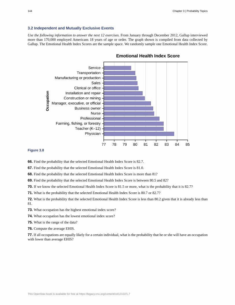
3.2 Independent and Mutually Exclusive Events
Use the following information to answer the next 12 exercises. From January through December 2012, Gallup interviewedmore than 170,000 employed Americans 18 years of age or order. The graph shown is compiled from data collected byGallup. The Emotional Health Index Scores are the sample space. We randomly sample one Emotional Health Index Score.
Figure 3.8
66. Find the probability that the selected Emotional Health Index Score is 82.7.
67. Find the probability that the selected Emotional Health Index Score is 81.0.
68. Find the probability that the selected Emotional Health Index Score is more than 81?
69. Find the probability that the selected Emotional Health Index Score is between 80.5 and 82?
70. If we know the selected Emotional Health Index Score is 81.5 or more, what is the probability that it is 82.7?
71. What is the probability that the selected Emotional Health Index Score is 80.7 or 82.7?
72. What is the probability that the selected Emotional Health Index Score is less than 80.2 given that it is already less than81.
73. What occupation has the highest emotional index score?
74. What occupation has the lowest emotional index score?
75. What is the range of the data?
76. Compute the average EHIS.
77. If all occupations are equally likely for a certain individual, what is the probability that he or she will have an occupationwith lower than average EHIS?
144 Chapter 3 | Probability Topics
This OpenStax book is available for free at https://legacy.cnx.org/content/col12102/1.7

3.3 Two Basic Rules of Probability
78. On February 28, 2013, a Field Poll Survey reported that 61% of California registered voters approved of allowing twopeople of the same gender to marry and have regular marriage laws apply to them. Among 18 to 39 year olds (Californiaregistered voters), the approval rating was 78%. Six in ten California registered voters said that the upcoming SupremeCourt’s ruling about the constitutionality of California’s Proposition 8 was either very or somewhat important to them. Outof those CA registered voters who support same-sex marriage, 75% say the ruling is important to them.
In this problem, let:
• C = California registered voters who support same-sex marriage.• B = California registered voters who say the Supreme Court’s ruling about the constitutionality of California’s
Proposition 8 is very or somewhat important to them• A = California registered voters who are 18 to 39 years old.
a. Find P(C).b. Find P(B).c. Find P(C | A).
d. Find P(B|C).e. In words, what is C | A?
f. In words, what is B | C?
g. Find P(C ∩ B).
h. In words, what is C ∩ B?
i. Find P(C ∪ B).
j. Are C and B mutually exclusive events? Show why or why not.
79. After Rob Ford, the mayor of Toronto, announced his plans to cut budget costs in late 2011, the Forum Research polled1,046 people to measure the mayor’s popularity. Everyone polled expressed either approval or disapproval. These are theresults their poll produced:
• In early 2011, 60 percent of the population approved of Mayor Ford’s actions in office.• In mid-2011, 57 percent of the population approved of his actions.• In late 2011, the percentage of popular approval was measured at 42 percent.
a. What is the sample size for this study?b. What proportion in the poll disapproved of Mayor Ford, according to the results from late 2011?c. How many people polled responded that they approved of Mayor Ford in late 2011?d. What is the probability that a person supported Mayor Ford, based on the data collected in mid-2011?e. What is the probability that a person supported Mayor Ford, based on the data collected in early 2011?
Use the following information to answer the next three exercises. The casino game, roulette, allows the gambler to bet onthe probability of a ball, which spins in the roulette wheel, landing on a particular color, number, or range of numbers. Thetable used to place bets contains of 38 numbers, and each number is assigned to a color and a range.
Chapter 3 | Probability Topics 145

Figure 3.9 (credit: film8ker/wikibooks)
80.a. List the sample space of the 38 possible outcomes in roulette.b. You bet on red. Find P(red).c. You bet on -1st 12- (1st Dozen). Find P(-1st 12-).d. You bet on an even number. Find P(even number).e. Is getting an odd number the complement of getting an even number? Why?f. Find two mutually exclusive events.g. Are the events Even and 1st Dozen independent?
81. Compute the probability of winning the following types of bets:a. Betting on two lines that touch each other on the table as in 1-2-3-4-5-6b. Betting on three numbers in a line, as in 1-2-3c. Betting on one numberd. Betting on four numbers that touch each other to form a square, as in 10-11-13-14e. Betting on two numbers that touch each other on the table, as in 10-11 or 10-13f. Betting on 0-00-1-2-3g. Betting on 0-1-2; or 0-00-2; or 00-2-3
82. Compute the probability of winning the following types of bets:a. Betting on a colorb. Betting on one of the dozen groupsc. Betting on the range of numbers from 1 to 18d. Betting on the range of numbers 19–36e. Betting on one of the columnsf. Betting on an even or odd number (excluding zero)
83. Suppose that you have eight cards. Five are green and three are yellow. The five green cards are numbered 1, 2, 3, 4,and 5. The three yellow cards are numbered 1, 2, and 3. The cards are well shuffled. You randomly draw one card.
• G = card drawn is green• E = card drawn is even-numbered
a. List the sample space.b. P(G) = _____c. P(G | E) = _____
d. P(G ∩ E) = _____
e. P(G ∪ E) = _____
f. Are G and E mutually exclusive? Justify your answer numerically.
146 Chapter 3 | Probability Topics
This OpenStax book is available for free at https://legacy.cnx.org/content/col12102/1.7

84. Roll two fair dice separately. Each die has six faces.a. List the sample space.b. Let A be the event that either a three or four is rolled first, followed by an even number. Find P(A).c. Let B be the event that the sum of the two rolls is at most seven. Find P(B).d. In words, explain what “P(A | B)” represents. Find P(A | B).
e. Are A and B mutually exclusive events? Explain your answer in one to three complete sentences, includingnumerical justification.
f. Are A and B independent events? Explain your answer in one to three complete sentences, including numericaljustification.
85. A special deck of cards has ten cards. Four are green, three are blue, and three are red. When a card is picked, its colorof it is recorded. An experiment consists of first picking a card and then tossing a coin.
a. List the sample space.b. Let A be the event that a blue card is picked first, followed by landing a head on the coin toss. Find P(A).c. Let B be the event that a red or green is picked, followed by landing a head on the coin toss. Are the events A and
B mutually exclusive? Explain your answer in one to three complete sentences, including numerical justification.d. Let C be the event that a red or blue is picked, followed by landing a head on the coin toss. Are the events A and
C mutually exclusive? Explain your answer in one to three complete sentences, including numerical justification.
86. An experiment consists of first rolling a die and then tossing a coin.a. List the sample space.b. Let A be the event that either a three or a four is rolled first, followed by landing a head on the coin toss. Find
P(A).c. Let B be the event that the first and second tosses land on heads. Are the events A and B mutually exclusive?
Explain your answer in one to three complete sentences, including numerical justification.
87. An experiment consists of tossing a nickel, a dime, and a quarter. Of interest is the side the coin lands on.a. List the sample space.b. Let A be the event that there are at least two tails. Find P(A).c. Let B be the event that the first and second tosses land on heads. Are the events A and B mutually exclusive?
Explain your answer in one to three complete sentences, including justification.
88. Consider the following scenario:Let P(C) = 0.4.Let P(D) = 0.5.Let P(C | D) = 0.6.
a. Find P(C ∩ D).
b. Are C and D mutually exclusive? Why or why not?c. Are C and D independent events? Why or why not?d. Find P(C ∪ D).
e. Find P(D | C).
89. Y and Z are independent events.a. Rewrite the basic Addition Rule P(Y ∪ Z) = P(Y) + P(Z) - P(Y ∩ Z) using the information that Y and Z are
independent events.b. Use the rewritten rule to find P(Z) if P(Y ∪ Z) = 0.71 and P(Y) = 0.42.
90. G and H are mutually exclusive events. P(G) = 0.5 P(H) = 0.3a. Explain why the following statement MUST be false: P(H | G) = 0.4.
b. Find P(H ∪ G).
c. Are G and H independent or dependent events? Explain in a complete sentence.
Chapter 3 | Probability Topics 147
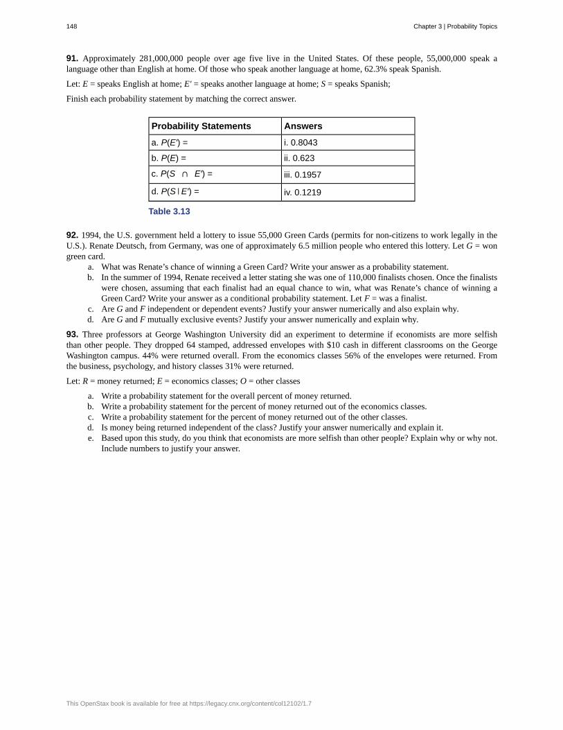
91. Approximately 281,000,000 people over age five live in the United States. Of these people, 55,000,000 speak alanguage other than English at home. Of those who speak another language at home, 62.3% speak Spanish.
Let: E = speaks English at home; E′ = speaks another language at home; S = speaks Spanish;
Finish each probability statement by matching the correct answer.
Probability Statements Answers
a. P(E′) = i. 0.8043
b. P(E) = ii. 0.623
c. P(S ∩ E′) = iii. 0.1957
d. P(S | E′) = iv. 0.1219
Table 3.13
92. 1994, the U.S. government held a lottery to issue 55,000 Green Cards (permits for non-citizens to work legally in theU.S.). Renate Deutsch, from Germany, was one of approximately 6.5 million people who entered this lottery. Let G = wongreen card.
a. What was Renate’s chance of winning a Green Card? Write your answer as a probability statement.b. In the summer of 1994, Renate received a letter stating she was one of 110,000 finalists chosen. Once the finalists
were chosen, assuming that each finalist had an equal chance to win, what was Renate’s chance of winning aGreen Card? Write your answer as a conditional probability statement. Let F = was a finalist.
c. Are G and F independent or dependent events? Justify your answer numerically and also explain why.d. Are G and F mutually exclusive events? Justify your answer numerically and explain why.
93. Three professors at George Washington University did an experiment to determine if economists are more selfishthan other people. They dropped 64 stamped, addressed envelopes with $10 cash in different classrooms on the GeorgeWashington campus. 44% were returned overall. From the economics classes 56% of the envelopes were returned. Fromthe business, psychology, and history classes 31% were returned.
Let: R = money returned; E = economics classes; O = other classes
a. Write a probability statement for the overall percent of money returned.b. Write a probability statement for the percent of money returned out of the economics classes.c. Write a probability statement for the percent of money returned out of the other classes.d. Is money being returned independent of the class? Justify your answer numerically and explain it.e. Based upon this study, do you think that economists are more selfish than other people? Explain why or why not.
Include numbers to justify your answer.
148 Chapter 3 | Probability Topics
This OpenStax book is available for free at https://legacy.cnx.org/content/col12102/1.7
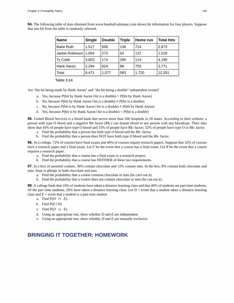
94. The following table of data obtained from www.baseball-almanac.com shows hit information for four players. Supposethat one hit from the table is randomly selected.
Name Single Double Triple Home run Total hits
Babe Ruth 1,517 506 136 714 2,873
Jackie Robinson 1,054 273 54 137 1,518
Ty Cobb 3,603 174 295 114 4,189
Hank Aaron 2,294 624 98 755 3,771
Total 8,471 1,577 583 1,720 12,351
Table 3.14
Are "the hit being made by Hank Aaron" and "the hit being a double" independent events?
a. Yes, because P(hit by Hank Aaron | hit is a double) = P(hit by Hank Aaron)
b. No, because P(hit by Hank Aaron | hit is a double) ≠ P(hit is a double)
c. No, because P(hit is by Hank Aaron | hit is a double) ≠ P(hit by Hank Aaron)
d. Yes, because P(hit is by Hank Aaron | hit is a double) = P(hit is a double)
95. United Blood Services is a blood bank that serves more than 500 hospitals in 18 states. According to their website, aperson with type O blood and a negative Rh factor (Rh-) can donate blood to any person with any bloodtype. Their datashow that 43% of people have type O blood and 15% of people have Rh- factor; 52% of people have type O or Rh- factor.
a. Find the probability that a person has both type O blood and the Rh- factor.b. Find the probability that a person does NOT have both type O blood and the Rh- factor.
96. At a college, 72% of courses have final exams and 46% of courses require research papers. Suppose that 32% of courseshave a research paper and a final exam. Let F be the event that a course has a final exam. Let R be the event that a courserequires a research paper.
a. Find the probability that a course has a final exam or a research project.b. Find the probability that a course has NEITHER of these two requirements.
97. In a box of assorted cookies, 36% contain chocolate and 12% contain nuts. In the box, 8% contain both chocolate andnuts. Sean is allergic to both chocolate and nuts.
a. Find the probability that a cookie contains chocolate or nuts (he can't eat it).b. Find the probability that a cookie does not contain chocolate or nuts (he can eat it).
98. A college finds that 10% of students have taken a distance learning class and that 40% of students are part time students.Of the part time students, 20% have taken a distance learning class. Let D = event that a student takes a distance learningclass and E = event that a student is a part time student
a. Find P(D ∩ E).
b. Find P(E | D).
c. Find P(D ∪ E).
d. Using an appropriate test, show whether D and E are independent.e. Using an appropriate test, show whether D and E are mutually exclusive.
BRINGING IT TOGETHER: HOMEWORK
Chapter 3 | Probability Topics 149

99. A previous year, the weights of the members of the San Francisco 49ers and the Dallas Cowboys were published inthe San Jose Mercury News. The factual data are compiled into Table 3.15.
Shirt # ≤ 210 211–250 251–290 290≤
1–33 21 5 0 0
34–66 6 18 7 4
66–99 6 12 22 5
Table 3.15
For the following, suppose that you randomly select one player from the 49ers or Cowboys.
If having a shirt number from one to 33 and weighing at most 210 pounds were independent events, then what should betrue about P(Shirt# 1–33|≤ 210 pounds)?
100. The probability that a male develops some form of cancer in his lifetime is 0.4567. The probability that a male has atleast one false positive test result (meaning the test comes back for cancer when the man does not have it) is 0.51. Some ofthe following questions do not have enough information for you to answer them. Write “not enough information” for thoseanswers. Let C = a man develops cancer in his lifetime and P = man has at least one false positive.
a. P(C) = ______
b. P(P|C) = ______
c. P(P|C') = ______
d. If a test comes up positive, based upon numerical values, can you assume that man has cancer? Justify numericallyand explain why or why not.
101. Given events G and H: P(G) = 0.43; P(H) = 0.26; P(H ∩ G) = 0.14
a. Find P(H ∪ G).b. Find the probability of the complement of event (H ∩ G).c. Find the probability of the complement of event (H ∪ G).
102. Given events J and K : P(J) = 0.18; P(K) = 0.37; P(J ∪ K) = 0.45a. Find P(J ∩ K).b. Find the probability of the complement of event (J ∩ K).c. Find the probability of the complement of event (J ∩ K).
REFERENCES
3.1 Terminology
“Countries List by Continent.” Worldatlas, 2013. Available online at http://www.worldatlas.com/cntycont.htm (accessedMay 2, 2013).
3.2 Independent and Mutually Exclusive Events
Lopez, Shane, Preety Sidhu. “U.S. Teachers Love Their Lives, but Struggle in the Workplace.” Gallup Wellbeing, 2013.http://www.gallup.com/poll/161516/teachers-love-lives-struggle-workplace.aspx (accessed May 2, 2013).
Data from Gallup. Available online at www.gallup.com/ (accessed May 2, 2013).
3.3 Two Basic Rules of Probability
DiCamillo, Mark, Mervin Field. “The File Poll.” Field Research Corporation. Available online at http://www.field.com/fieldpollonline/subscribers/Rls2443.pdf (accessed May 2, 2013).
150 Chapter 3 | Probability Topics
This OpenStax book is available for free at https://legacy.cnx.org/content/col12102/1.7

Rider, David, “Ford support plummeting, poll suggests,” The Star, September 14, 2011. Available online athttp://www.thestar.com/news/gta/2011/09/14/ford_support_plummeting_poll_suggests.html (accessed May 2, 2013).
“Mayor’s Approval Down.” News Release by Forum Research Inc. Available online at http://www.forumresearch.com/forms/News Archives/News Releases/74209_TO_Issues_-_Mayoral_Approval_%28Forum_Research%29%2820130320%29.pdf (accessed May 2, 2013).
“Roulette.” Wikipedia. Available online at http://en.wikipedia.org/wiki/Roulette (accessed May 2, 2013).
Shin, Hyon B., Robert A. Kominski. “Language Use in the United States: 2007.” United States Census Bureau. Availableonline at http://www.census.gov/hhes/socdemo/language/data/acs/ACS-12.pdf (accessed May 2, 2013).
Data from the Baseball-Almanac, 2013. Available online at www.baseball-almanac.com (accessed May 2, 2013).
Data from U.S. Census Bureau.
Data from the Wall Street Journal.
Data from The Roper Center: Public Opinion Archives at the University of Connecticut. Available online athttp://www.ropercenter.uconn.edu/ (accessed May 2, 2013).
Data from Field Research Corporation. Available online at www.field.com/fieldpollonline (accessed May 2,2 013).
3.4 Contingency Tables and Probability Trees
“Blood Types.” American Red Cross, 2013. Available online at http://www.redcrossblood.org/learn-about-blood/blood-types (accessed May 3, 2013).
Data from the National Center for Health Statistics, part of the United States Department of Health and Human Services.
Data from United States Senate. Available online at www.senate.gov (accessed May 2, 2013).
“Human Blood Types.” Unite Blood Services, 2011. Available online at http://www.unitedbloodservices.org/learnMore.aspx (accessed May 2, 2013).
Haiman, Christopher A., Daniel O. Stram, Lynn R. Wilkens, Malcolm C. Pike, Laurence N. Kolonel, Brien E. Henderson,and Loīc Le Marchand. “Ethnic and Racial Differences in the Smoking-Related Risk of Lung Cancer.” The New EnglandJournal of Medicine, 2013. Available online at http://www.nejm.org/doi/full/10.1056/NEJMoa033250 (accessed May 2,2013).
Samuel, T. M. “Strange Facts about RH Negative Blood.” eHow Health, 2013. Available online at http://www.ehow.com/facts_5552003_strange-rh-negative-blood.html (accessed May 2, 2013).
“United States: Uniform Crime Report – State Statistics from 1960–2011.” The Disaster Center. Available online athttp://www.disastercenter.com/crime/ (accessed May 2, 2013).
Data from Clara County Public H.D.
Data from the American Cancer Society.
Data from The Data and Story Library, 1996. Available online at http://lib.stat.cmu.edu/DASL/ (accessed May 2, 2013).
Data from the Federal Highway Administration, part of the United States Department of Transportation.
Data from the United States Census Bureau, part of the United States Department of Commerce.
Data from USA Today.
“Environment.” The World Bank, 2013. Available online at http://data.worldbank.org/topic/environment (accessed May 2,2013).
“Search for Datasets.” Roper Center: Public Opinion Archives, University of Connecticut., 2013. Available online athttps://ropercenter.cornell.edu/?s=Search+for+Datasets (accessed February 6, 2019).
SOLUTIONS
11a. P(L′) = P(S)
Chapter 3 | Probability Topics 151

b. P(M ∪ S)
c. P(F ∩ L)
d. P(M | L)
e. P(L | M)
f. P(S | F)
g. P(F | L)
h. P(F ∪ L)
i. P(M ∩ S)
j. P(F)
13 P(N) = 1542 = 5
14 = 0.36
15 P(C) = 542 = 0.12
17 P(G) = 20150 = 2
15 = 0.13
19 P(R) = 22150 = 11
75 = 0.15
21 P(O) = 150 - 22 - 38 - 20 - 28 - 26150 = 16
150 = 875 = 0.11
23 P(E) = 47194 = 0.24
25 P(N) = 23194 = 0.12
27 P(S) = 12194 = 6
97 = 0.06
29 1352 = 1
4 = 0.25
31 36 = 1
2 = 0.5
33 P(R) = 48 = 0.5
35 P(O ∪ H)
37 P(H | I)
39 P(N | O)
41 P(I ∪ N)
43 P(I)
45 The likelihood that an event will occur given that another event has already occurred.
47 1
49 the probability of landing on an even number or a multiple of three
51 P(J) = 0.3
53 P(Q ∩ R) = P(Q)P(R) 0.1 = (0.4)P(R) P(R) = 0.25
152 Chapter 3 | Probability Topics
This OpenStax book is available for free at https://legacy.cnx.org/content/col12102/1.7

55 0.376
57 C | L means, given the person chosen is a Latino Californian, the person is a registered voter who prefers life in prison
without parole for a person convicted of first degree murder.
59 L ∩ C is the event that the person chosen is a Latino California registered voter who prefers life without parole over
the death penalty for a person convicted of first degree murder.
61 0.6492
63 No, because P(L ∩ C) does not equal 0.
65a. You can't calculate the joint probability knowing the probability of both events occurring, which is not in the
information given; the probabilities should be multiplied, not added; and probability is never greater than 100%
b. A home run by definition is a successful hit, so he has to have at least as many successful hits as home runs.
67 0
69 0.3571
71 0.2142
73 Physician (83.7)
75 83.7 − 79.6 = 4.1
77 P(Occupation < 81.3) = 0.5
79a. The Forum Research surveyed 1,046 Torontonians.
b. 58%
c. 42% of 1,046 = 439 (rounding to the nearest integer)
d. 0.57
e. 0.60.
81
a. P(Betting on two line that touch each other on the table) = 638
b. P(Betting on three numbers in a line) = 338
c. P(Betting on one number) = 138
d. P(Betting on four number that touch each other to form a square) = 438
e. P(Betting on two number that touch each other on the table ) = 238
f. P(Betting on 0-00-1-2-3) = 538
g. P(Betting on 0-1-2; or 0-00-2; or 00-2-3) = 338
83a. {G1, G2, G3, G4, G5, Y1, Y2, Y3}
b. 58
c. 23
Chapter 3 | Probability Topics 153
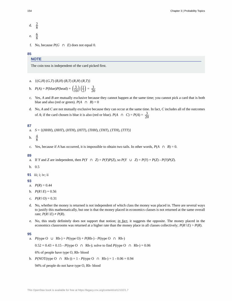
d. 28
e. 68
f. No, because P(G ∩ E) does not equal 0.
85
NOTE
The coin toss is independent of the card picked first.
a. {(G,H) (G,T) (B,H) (B,T) (R,H) (R,T)}
b. P(A) = P(blue)P(head) = ⎛⎝ 310⎞⎠⎛⎝12⎞⎠ = 3
20
c. Yes, A and B are mutually exclusive because they cannot happen at the same time; you cannot pick a card that is bothblue and also (red or green). P(A ∩ B) = 0
d. No, A and C are not mutually exclusive because they can occur at the same time. In fact, C includes all of the outcomes
of A; if the card chosen is blue it is also (red or blue). P(A ∩ C) = P(A) = 320
87a. S = {(HHH), (HHT), (HTH), (HTT), (THH), (THT), (TTH), (TTT)}
b. 48
c. Yes, because if A has occurred, it is impossible to obtain two tails. In other words, P(A ∩ B) = 0.
89a. If Y and Z are independent, then P(Y ∩ Z) = P(Y)P(Z), so P(Y ∪ Z) = P(Y) + P(Z) - P(Y)P(Z).
b. 0.5
91 iii; i; iv; ii
93a. P(R) = 0.44
b. P(R | E) = 0.56
c. P(R | O) = 0.31
d. No, whether the money is returned is not independent of which class the money was placed in. There are several waysto justify this mathematically, but one is that the money placed in economics classes is not returned at the same overallrate; P(R | E) ≠ P(R).
e. No, this study definitely does not support that notion; in fact, it suggests the opposite. The money placed in theeconomics classrooms was returned at a higher rate than the money place in all classes collectively; P(R | E) > P(R).
95a. P(type O ∪ Rh-) = P(type O) + P(Rh-) - P(type O ∩ Rh-)
0.52 = 0.43 + 0.15 - P(type O ∩ Rh-); solve to find P(type O ∩ Rh-) = 0.06
6% of people have type O, Rh- blood
b. P(NOT(type O ∩ Rh-)) = 1 - P(type O ∩ Rh-) = 1 - 0.06 = 0.94
94% of people do not have type O, Rh- blood
154 Chapter 3 | Probability Topics
This OpenStax book is available for free at https://legacy.cnx.org/content/col12102/1.7

97a. Let C = be the event that the cookie contains chocolate. Let N = the event that the cookie contains nuts.
b. P(C ∪ N) = P(C) + P(N) - P(C ∩ N) = 0.36 + 0.12 - 0.08 = 0.40
c. P(NEITHER chocolate NOR nuts) = 1 - P(C ∪ N) = 1 - 0.40 = 0.60
100a. P(C) = 0.4567
b. not enough information
c. not enough information
d. No, because over half (0.51) of men have at least one false positive text
102a. (J ∪ K) = P( J ) + P(K) − P(J ∩ K); 0.45 = 0.18 + 0.37 − P(J ∩ K); solve to find P(J ∩ K) = 0.10
b. P(NOT(J ∩ K)) = 1 − P(J ∩ K) = 1 − 0.10 = 0.90
c. P(NOT(J ∪ K)) = 1 − P(J ∪ K) = 1 − 0.45 = 0.55
Chapter 3 | Probability Topics 155

156 Chapter 3 | Probability Topics
This OpenStax book is available for free at https://legacy.cnx.org/content/col12102/1.7

4 | DISCRETE RANDOMVARIABLES
Figure 4.1 You can use probability and discrete random variables to calculate the likelihood of lightning striking theground five times during a half-hour thunderstorm. (Credit: Leszek Leszczynski)
Introduction
A student takes a ten-question, true-false quiz. Because the student had such a busy schedule, he or she could not study andguesses randomly at each answer. What is the probability of the student passing the test with at least a 70%?
Small companies might be interested in the number of long-distance phone calls their employees make during the peak timeof the day. Suppose the historical average is 20 calls. What is the probability that the employees make more than 20 long-distance phone calls during the peak time?
These two examples illustrate two different types of probability problems involving discrete random variables. Recall thatdiscrete data are data that you can count, that is, the random variable can only take on whole number values. A randomvariable describes the outcomes of a statistical experiment in words. The values of a random variable can vary with eachrepetition of an experiment, often called a trial.
Random Variable NotationThe upper case letter X denotes a random variable. Lower case letters like x or y denote the value of a random variable. If Xis a random variable, then X is written in words, and x is given as a number.
For example, let X = the number of heads you get when you toss three fair coins. The sample space for the toss of three faircoins is TTT; THH; HTH; HHT; HTT; THT; TTH; HHH. Then, x = 0, 1, 2, 3. X is in words and x is a number. Notice thatfor this example, the x values are countable outcomes. Because you can count the possible values as whole numbers that Xcan take on and the outcomes are random (the x values 0, 1, 2, 3), X is a discrete random variable.
Chapter 4 | Discrete Random Variables 157

Probability Density Functions (PDF) for a Random VariableA probability density function or probability distribution function has two characteristics:
1. Each probability is between zero and one, inclusive.
2. The sum of the probabilities is one.
A probability density function is a mathematical formula that calculates probabilities for specific types of events, whatwe have been calling experiments. There is a sort of magic to a probability density function (Pdf) partially because thesame formula often describes very different types of events. For example, the binomial Pdf will calculate probabilities forflipping coins, yes/no questions on an exam, opinions of voters in an up or down opinion poll, indeed any binary event.Other probability density functions will provide probabilities for the time until a part will fail, when a customer will arriveat the turnpike booth, the number of telephone calls arriving at a central switchboard, the growth rate of a bacterium, and onand on. There are whole families of probability density functions that are used in a wide variety of applications, includingmedicine, business and finance, physics and engineering, among others.
For our needs here we will concentrate on only a few probability density functions as we develop the tools of inferentialstatistics.
Counting Formulas and the Combinational FormulaTo repeat, the probability of event A , P(A), is simply the number of ways the experiment will result in A, relative to thetotal number of possible outcomes of the experiment.
As an equation this is:
() P(A) = number of ways to get ATotal number of possible outcomes
When we looked at the sample space for flipping 3 coins we could easily write the full sample space and thus could easilycount the number of events that met our desired result, e.g. x = 1 , where X is the random variable defined as the number ofheads.
As we have larger numbers of items in the sample space, such as a full deck of 52 cards, the ability to write out the samplespace becomes impossible.
We see that probabilities are nothing more than counting the events in each group we are interested in and dividing by thenumber of elements in the universe, or sample space. This is easy enough if we are counting sophomores in a Stat class,but in more complicated cases listing all the possible outcomes may take a life time. There are, for example, 36 possibleoutcomes from throwing just two six-sided dice where the random variable is the sum of the number of spots on the up-facing sides. If there were four dice then the total number of possible outcomes would become 1,296. There are more than2.5 MILLION possible 5 card poker hands in a standard deck of 52 cards. Obviously keeping track of all these possibilitiesand counting them to get at a single probability would be tedious at best.
An alternative to listing the complete sample space and counting the number of elements we are interested in, is to skip thestep of listing the sample space, and simply figuring out the number of elements in it and doing the appropriate division. Ifwe are after a probability we really do not need to see each and every element in the sample space, we only need to knowhow many elements are there. Counting formulas were invented to do just this. They tell us the number of unordered subsetsof a certain size that can be created from a set of unique elements. By unordered it is meant that, for example, when dealingcards, it does not matter if you got {ace, ace, ace, ace, king} or {king, ace, ace, ace, ace} or {ace, king, ace, ace, ace} andso on. Each of these subsets are the same because they each have 4 aces and one king.
Combinational Formula
⎛⎝nx⎞⎠ = nCx = n !
x !(n - x) !
This is the formula that tells the number of unique unordered subsets of size x that can be created from n unique elements.The formula is read “n combinatorial x”. Sometimes it is read as “n choose x." The exclamation point "!" is called a factorialand tells us to take all the numbers from 1 through the number before the ! and multiply them together thus 4! is 1·2·3·4=24.By definition 0! = 1. The formula is called the Combinatorial Formula. It is also called the Binomial Coefficient, for reasonsthat will be clear shortly. While this mathematical concept was understood long before 1653, Blaise Pascal is given majorcredit for his proof that he published in that year. Further, he developed a generalized method of calculating the values forcombinatorials known to us as the Pascal Triangle. Pascal was one of the geniuses of an era of extraordinary intellectualadvancement which included the work of Galileo, Rene Descartes, Isaac Newton, William Shakespeare and the refinementof the scientific method, the very rationale for the topic of this text.
158 Chapter 4 | Discrete Random Variables
This OpenStax book is available for free at https://legacy.cnx.org/content/col12102/1.7

Let’s find the hard way the total number of combinations of the four aces in a deck of cards if we were going to take themtwo at a time. The sample space would be:
S={Spade,Heart),(Spade, Diamond),(Spade,Club), (Diamond,Club),(Heart,Diamond),(Heart,Club)}
There are 6 combinations; formally, six unique unordered subsets of size 2 that can be created from 4 unique elements. Touse the combinatorial formula we would solve the formula as follows:
()⎛⎝42⎞⎠ = 4!
(4 - 2) !2! = 4 · 3 · 2 · 12 · 1 · 2 · 1 = 6
If we wanted to know the number of unique 5 card poker hands that could be created from a 52 card deck we simplycompute:
()⎛⎝52
5⎞⎠
where 52 is the total number of unique elements from which we are drawing and 5 is the size group we are putting theminto.
With the combinatorial formula we can count the number of elements in a sample space without having to write each oneof them down, truly a lifetime's work for just the number of 5 card hands from a deck of 52 cards. We can now apply thistool to a very important probability density function, the hypergeometric distribution.
Remember, a probability density function computes probabilities for us. We simply put the appropriate numbers in theformula and we get the probability of specific events. However, for these formulas to work they must be applied only tocases for which they were designed.
4.1 | Hypergeometric DistributionThe simplest probability density function is the hypergeometric. This is the most basic one because it is created bycombining our knowledge of probabilities from Venn diagrams, the addition and multiplication rules, and the combinatorialcounting formula.
To find the number of ways to get 2 aces from the four in the deck we computed:
()⎛⎝42⎞⎠ = 4!
2!(4 - 2) ! = 6
And if we did not care what else we had in our hand for the other three cards we would compute:
()⎛⎝48
3⎞⎠ = 48!
3!45! = 17,296
Putting this together, we can compute the probability of getting exactly two aces in a 5 card poker hand as:
⎛⎝42⎞⎠⎛⎝48
3⎞⎠
⎛⎝52
5⎞⎠
= .0399
This solution is really just the probability distribution known as the Hypergeometric. The generalized formula is:
() h(x) =⎛⎝Ax⎞⎠⎛⎝N - An - x⎞⎠
⎛⎝Nn⎞⎠
where x = the number we are interested in coming from the group with A objects.
h(x) is the probability of x successes, in n attempts, when A successes (aces in this case) are in a population that contains Nelements. The hypergeometric distribution is an example of a discrete probability distribution because there is no possibilityof partial success, that is, there can be no poker hands with 2 1/2 aces. Said another way, a discrete random variable hasto be a whole, or counting, number only. This probability distribution works in cases where the probability of a successchanges with each draw. Another way of saying this is that the events are NOT independent. In using a deck of cards, weare sampling WITHOUT replacement. If we put each card back after it was drawn then the hypergeometric distribution bean inappropriate Pdf.
For the hypergeometric to work,
Chapter 4 | Discrete Random Variables 159

1. the population must be dividable into two and only two independent subsets (aces and non-aces in our example). Therandom variable X = the number of items from the group of interest.
2. the experiment must have changing probabilities of success with each experiment (the fact that cards are not replacedafter the draw in our example makes this true in this case). Another way to say this is that you sample withoutreplacement and therefore each pick is not independent.
3. the random variable must be discrete, rather than continuous.
Example 4.1
A candy dish contains 30 jelly beans and 20 gumdrops. Ten candies are picked at random. What is the probabilitythat 5 of the 10 are gumdrops? The two groups are jelly beans and gumdrops. Since the probability question asksfor the probability of picking gumdrops, the group of interest (first group A in the formula) is gumdrops. Thesize of the group of interest (first group) is 30. The size of the second group is 20. The size of the sample is 10(jelly beans or gumdrops). Let X = the number of gumdrops in the sample of 10. X takes on the values x = 0, 1,2, ..., 10. a. What is the probability statement written mathematically? b. What is the hypergeometric probabilitydensity function written out to solve this problem? c. What is the answer to the question "What is the probabilityof drawing 5 gumdrops in 10 picks from the dish?"
Solution 4.1a. P(x = 5)
b. P(x = 5) =
⎛⎝5
30⎞⎠⎛⎝5
20⎞⎠
⎛⎝10
50⎞⎠
c. P(x = 5) = 0.215
4.1 A bag contains letter tiles. Forty-four of the tiles are vowels, and 56 are consonants. Seven tiles are picked atrandom. You want to know the probability that four of the seven tiles are vowels. What is the group of interest, the sizeof the group of interest, and the size of the sample?
4.2 | Binomial Distribution - (Base Version - Lyryx
Learning)A binomial process is any case where there are only two possibilities in any one trial, called successes and failures. It getsits name from the binary number system where all numbers are reduced to either 1's or 0's, which is the basis for computertechnology and CD music recordings.
Binomial Probability Formula
P(x) = C · px · qn - x where C = n !x !(n - x) !
P(x) is the probability of x successes in n trials when the probability of a success in ANY ONE TRIAL is p and the
probability of failure is q = 1 - p .
We can see now why the combinatorial formula is also called the binomial coefficient because it reappears here again inthe binomial probability function. For the binomial formula to work, the probability of a success in any one trial must bethe same from trial to trial, or in other words, the outcomes of each trial must be independent. Flipping a coin is a binomialprocess because the probability of getting a head in one flip does not depend upon what has happened in PREVIOUS flips.
160 Chapter 4 | Discrete Random Variables
This OpenStax book is available for free at https://legacy.cnx.org/content/col12102/1.7

Just like a set of data, the binomial probability distribution has a mean and a standard deviation given by the formulas:
μ = npσ = npq
Here are four characteristics of a binomial experiment.
1. There are a fixed number of trials. Think of trials as repetitions of an experiment. The letter n denotes the number oftrials.
2. The random variable X, number of successes, is discrete.
3. There are only two possible outcomes, called "success" and "failure," for each trial. The letter p denotes the probabilityof a success on one trial, and q denotes the probability of a failure on one trial. p + q = 1.
4. The n trials are independent and are repeated using identical conditions. Think of this as drawing WITH replacement.Because the n trials are independent, the outcome of one trial does not help in predicting the outcome of another trial.Another way of saying this is that for each individual trial, the probability, p, of a success and probability, q, of afailure remain the same. For example, randomly guessing at a true-false statistics question has only two outcomes.If a success is guessing correctly, then a failure is guessing incorrectly. Suppose Joe always guesses correctly on anystatistics true-false question with probability p = 0.6. Then, q = 0.4. This means that for every true-false statisticsquestion Joe answers, his probability of success (p = 0.6) and his probability of failure (q = 0.4) remain the same.
The outcomes of a binomial experiment fit a binomial probability distribution. The random variable X = the number ofsuccesses obtained in the n independent trials.
Any experiment that has characteristics three and four and where n = 1 is called a Bernoulli Trial (named after JacobBernoulli who, in the late 1600s, studied them extensively). A binomial experiment takes place when the number ofsuccesses is counted in one or more Bernoulli Trials.
Example 4.2
Suppose you play a game that you can only either win or lose. The probability that you win any game is 55%, andthe probability that you lose is 45%. Each game you play is independent. If you play the game 20 times, write thefunction that describes the probability that you win 15 of the 20 times.
• Here, if you define X as the number of wins, then X takes on the values 0, 1, 2, 3, ..., 20.
• The probability of a success is p = 0.55.
• The probability of a failure is q = 0.45.
• The number of trials is n = 20.
• The probability question can be stated mathematically as P(X = 15).
Example 4.3
A fair coin is flipped 15 times. Each flip is independent. What is the probability of getting more than ten heads?Let X = the number of heads in 15 flips of the fair coin. X takes on the values 0, 1, 2, 3, ..., 15. Since the coin isfair, p = 0.5 and q = 0.5. The number of trials is n = 15. State the probability question mathematically.
Solution 4.3P(X > 10)
Example 4.4
Approximately 70% of statistics students do their homework in time for it to be collected and graded. Eachstudent does homework independently. In a statistics class of 50 students, what is the probability that at least 40
Chapter 4 | Discrete Random Variables 161

will do their homework on time? Students are selected randomly.
a. This is a binomial problem because there is only a success or a __________, there are a fixed number of trials,and the probability of a success is 0.70 for each trial.
Solution 4.4a. failure
b. If we are interested in the number of students who do their homework on time, then how do we define X?
Solution 4.4b. X = the number of statistics students who do their homework on time
c. What values does X take on?
Solution 4.4c. 0, 1, 2, …, 50
d. What is a "failure," in words?
Solution 4.4
d. Failure is defined as a student who does not complete his or her homework on time.
The probability of a success is p = 0.70. The number of trials is n = 50.
e. If p + q = 1, then what is q?
Solution 4.4e. q = 0.30
f. The words "at least" translate as what kind of inequality for the probability question P(x ____ 40).
Solution 4.4f. greater than or equal to (≥)The probability question is P(x ≥ 40).
Example 4.5
In 2014, a study on Gender differences in the financial knowledge of Canadians revealed that only about15% of women correctly answered some key financial literacy questions related to interest, inflation and riskdiversification. In a sample of 20 women, what is the probability that
a. five answered correctly?
b. none answered correctly?
c. at least one answered correctly?
Solution 4.5p = 0.15, q = 0.85, n = 20
a. P(X = 5) = C×0.155×0.85(20 - 5) = 15504×0.000076×0.087354 = 0.1028
162 Chapter 4 | Discrete Random Variables
This OpenStax book is available for free at https://legacy.cnx.org/content/col12102/1.7
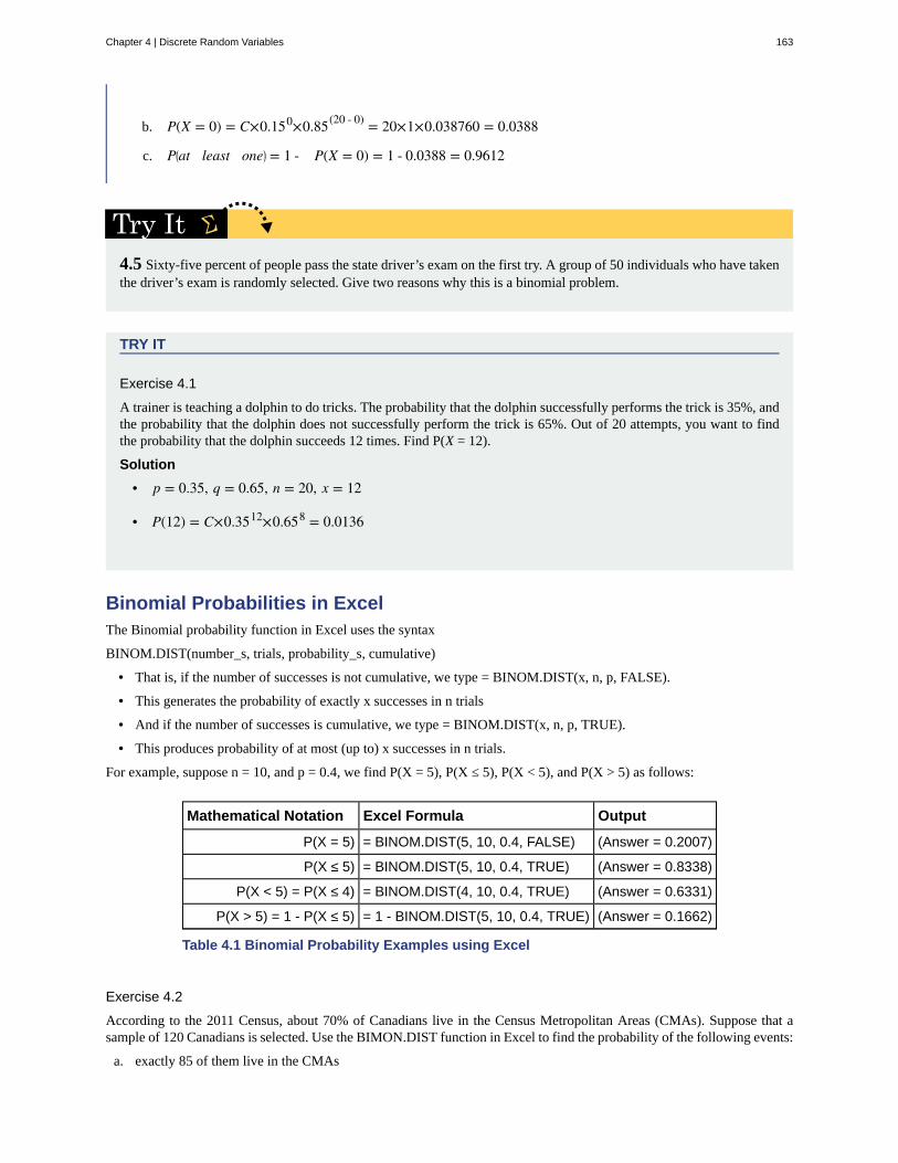
b. P(X = 0) = C×0.150×0.85(20 - 0) = 20×1×0.038760 = 0.0388
c. P⎛⎝at least one⎞⎠ = 1 - P(X = 0) = 1 - 0.0388 = 0.9612
4.5 Sixty-five percent of people pass the state driver’s exam on the first try. A group of 50 individuals who have takenthe driver’s exam is randomly selected. Give two reasons why this is a binomial problem.
TRY IT
Exercise 4.1
A trainer is teaching a dolphin to do tricks. The probability that the dolphin successfully performs the trick is 35%, andthe probability that the dolphin does not successfully perform the trick is 65%. Out of 20 attempts, you want to findthe probability that the dolphin succeeds 12 times. Find P(X = 12).
Solution
• p = 0.35, q = 0.65, n = 20, x = 12
• P(12) = C×0.3512×0.658 = 0.0136
Binomial Probabilities in ExcelThe Binomial probability function in Excel uses the syntax
BINOM.DIST(number_s, trials, probability_s, cumulative)
• That is, if the number of successes is not cumulative, we type = BINOM.DIST(x, n, p, FALSE).
• This generates the probability of exactly x successes in n trials
• And if the number of successes is cumulative, we type = BINOM.DIST(x, n, p, TRUE).
• This produces probability of at most (up to) x successes in n trials.
For example, suppose n = 10, and p = 0.4, we find P(X = 5), P(X ≤ 5), P(X < 5), and P(X > 5) as follows:
Mathematical Notation Excel Formula Output
P(X = 5) = BINOM.DIST(5, 10, 0.4, FALSE) (Answer = 0.2007)
P(X ≤ 5) = BINOM.DIST(5, 10, 0.4, TRUE) (Answer = 0.8338)
P(X < 5) = P(X ≤ 4) = BINOM.DIST(4, 10, 0.4, TRUE) (Answer = 0.6331)
P(X > 5) = 1 - P(X ≤ 5) = 1 - BINOM.DIST(5, 10, 0.4, TRUE) (Answer = 0.1662)
Table 4.1 Binomial Probability Examples using Excel
Exercise 4.2
According to the 2011 Census, about 70% of Canadians live in the Census Metropolitan Areas (CMAs). Suppose that asample of 120 Canadians is selected. Use the BIMON.DIST function in Excel to find the probability of the following events:
a. exactly 85 of them live in the CMAs
Chapter 4 | Discrete Random Variables 163

b. 85 or fewer live in the CMAs
c. less than 90 live in the CMAs
d. more than 90 live in the CMAs
e. at least 90 in the CMAs
Solutiona. P(X = 85) = BINOM.DIST(85, 120, 0.7, FALSE) (Answer = 0.0783)
b. P(X ≤ 85) = BINOM.DIST(85, 120, 0.7, TRUE) (Answer = 0.6127)
c. P(X < 90) = P(X ≤ 89) = BINOM.DIST(89, 120, 0.7, TRUE) (Answer = 0.8641)
d. P(X > 90) = 1 - P(X ≤ 90) = 1 - BINOM.DIST(90, 120, 0.7, TRUE) (Answer = 0.0959)
e. P(X ≥ 90) = 1 - P(X ≤ 89) = 1 - BINOM.DIST(89, 120, 0.7, TRUE) (Answer = 0.1359)
Binomial Probability TablesBinomial probabilities can also be obtained easily from Binomial probability tables as provided in the Appendix. The figurebelow is an excerpt from the Binomial Table for n = 5. Note that this table provides the probability for individual x (success)values.
For example, for n = 5 and p = 0.7, we see readily from the table thatP(X = 3) = 0.3087, P(X = 4) = 0.3602, and P(X = 5) = 0.1681.
Figure 4.2 Binomial Probabilities for n = 5 Binomial Probabilities for n = 5
Example 4.6
Suppose 80% of eBay purchases from China successfully arrive in Canada. A customer recently ordered 12 items.Use the binomial tables to find the probability that
a. exactly 10 of them will successfully arrive?
b. 8 or 9 will successfully arrive?
c. at least 10 will successfully arrive?
d. More than 6 but less than 10 will arrive?
Solution 4.6Using the Binomial Probability tables (n = 12, p = 0.8):
a. P(X = 10) = 0.2835
b. P(X = 8 or 9) = P(8)+P(9) = 0.1329 + 0.2362 = 0.3961
c. P(X ≥ 10) = P(10) + P(11) + P(12) = 0.2835 + 0.2062 + 0.0687 = 0.5584
d. P(6 < X < 10) = P(7 ≤ X ≤ 9) = P(7)+P(8)+P(9) = 0.0532 + 0.1329 + 0.2362 = 0.4223
164 Chapter 4 | Discrete Random Variables
This OpenStax book is available for free at https://legacy.cnx.org/content/col12102/1.7

Figure 4.3 Binomial Probabilities for n = 12 Binomial Probabilities for n = 12
4.6 During the 2016 regular NBA season, DeAndre Jordan of the Los Angeles Clippers had the highest field goalcompletion rate in the league. DeAndre scored with 70% of his shots. Suppose you choose a random sample of 80shots made by DeAndre during the 2016 season.
a. How many field shots would you expect DeAndre to score?
b. What is the standard deviation of shots scored.
c. Find the probability that DeAndre scored with 60 of these shots.
d. Find the probability that DeAndre scored with more than 50 of these shots. Hint: use Excel.
4.3 | Geometric DistributionThe geometric probability density function builds upon what we have learned from the binomial distribution. In this casethe experiment continues until either a success or a failure occurs rather than for a set number of trials. There are three maincharacteristics of a geometric experiment.
1. There are one or more Bernoulli trials with all failures except the last one, which is a success. In other words, you keeprepeating what you are doing until the first success. Then you stop. For example, you throw a dart at a bullseye untilyou hit the bullseye. The first time you hit the bullseye is a "success" so you stop throwing the dart. It might take sixtries until you hit the bullseye. You can think of the trials as failure, failure, failure, failure, failure, success, STOP.
2. In theory, the number of trials could go on forever.
3. The probability, p, of a success and the probability, q, of a failure is the same for each trial. p + q = 1 and q = 1 − p.
For example, the probability of rolling a three when you throw one fair die is 16 . This is true no matter how many
times you roll the die. Suppose you want to know the probability of getting the first three on the fifth roll. On rolls
one through four, you do not get a face with a three. The probability for each of the rolls is q = 56 , the probability of a
failure. The probability of getting a three on the fifth roll is ⎛⎝56⎞⎠⎛⎝56⎞⎠⎛⎝56⎞⎠⎛⎝56⎞⎠⎛⎝16⎞⎠ = 0.0804
4. X = the number of independent trials until the first success.
Chapter 4 | Discrete Random Variables 165

Example 4.7
You play a game of chance that you can either win or lose (there are no other possibilities) until you lose. Yourprobability of losing is p = 0.57. What is the probability that it takes five games until you lose? Let X = the numberof games you play until you lose (includes the losing game). Then X takes on the values 1, 2, 3, ... (could go onindefinitely). The probability question is P(x = 5).
4.7 You throw darts at a board until you hit the center area. Your probability of hitting the center area is p = 0.17. Youwant to find the probability that it takes eight throws until you hit the center. What values does X take on?
Example 4.8
A safety engineer feels that 35% of all industrial accidents in her plant are caused by failure of employees tofollow instructions. She decides to look at the accident reports (selected randomly and replaced in the pile afterreading) until she finds one that shows an accident caused by failure of employees to follow instructions. Onaverage, how many reports would the safety engineer expect to look at until she finds a report showing anaccident caused by employee failure to follow instructions? What is the probability that the safety engineer willhave to examine at least three reports until she finds a report showing an accident caused by employee failure tofollow instructions?
Let X = the number of accidents the safety engineer must examine until she finds a report showing an accidentcaused by employee failure to follow instructions. X takes on the values 1, 2, 3, .... The first question asks youto find the expected value or the mean. The second question asks you to find P(x ≥ 3). ("At least" translates to a"greater than or equal to" symbol).
4.8 An instructor feels that 15% of students get below a C on their final exam. She decides to look at final exams(selected randomly and replaced in the pile after reading) until she finds one that shows a grade below a C. We want toknow the probability that the instructor will have to examine at least ten exams until she finds one with a grade belowa C. What is the probability question stated mathematically?
Example 4.9
Suppose that you are looking for a student at your college who lives within five miles of you. You know that 55%of the 25,000 students do live within five miles of you. You randomly contact students from the college until onesays he or she lives within five miles of you. What is the probability that you need to contact four people?
This is a geometric problem because you may have a number of failures before you have the one success youdesire. Also, the probability of a success stays approximately the same each time you ask a student if he or shelives within five miles of you. There is no definite number of trials (number of times you ask a student).
a. Let X = the number of ____________ you must ask ____________ one says yes.
Solution 4.9a. Let X = the number of students you must ask until one says yes.
166 Chapter 4 | Discrete Random Variables
This OpenStax book is available for free at https://legacy.cnx.org/content/col12102/1.7

b. What values does X take on?
Solution 4.9b. 1, 2, 3, …, (total number of students)
c. What are p and q?
Solution 4.9c. p = 0.55; q = 0.45
d. The probability question is P(_______).
Solution 4.9d. P(x = 4)
Notation for the Geometric: G = Geometric Probability Distribution FunctionX ~ G(p)
Read this as "X is a random variable with a geometric distribution." The parameter is p; p = the probability of a successfor each trial.
The Geometric Pdf tells us the probability that the first occurrence of success requires x number of independent trials, eachwith success probability p. If the probability of success on each trial is p, then the probability that the xth trial (out of xtrials) is the first success is:
() P⎛⎝X = x⎞⎠ = ⎛⎝1 - p⎞⎠x - 1p
for x = 1, 2, 3, ....The expected value of X, the mean of this distribution, is 1/p. This tells us how many trials we have to expect until we getthe first success including in the count the trial that results in success. The above form of the Geometric distribution is usedfor modeling the number of trials until the first success. The number of trials includes the one that is a success: x = all trialsincluding the one that is a success. This can be seen in the form of the formula. If X = number of trials including the success,then we must multiply the probability of failure, (1-p), times the number of failures, that is X-1.
By contrast, the following form of the geometric distribution is used for modeling number of failures until the first success:
() P⎛⎝X = x⎞⎠ = ⎛⎝1 - p⎞⎠xp
for x = 0, 1, 2, 3, ....In this case the trial that is a success is not counted as a trial in the formula: x = number of failures. The expected value,
mean, of this distribution is μ =⎛⎝1 − p⎞⎠
p . This tells us how many failures to expect before we have a success. In either case,
the sequence of probabilities is a geometric sequence.
Example 4.10
Assume that the probability of a defective computer component is 0.02. Components are randomly selected. Findthe probability that the first defect is caused by the seventh component tested. How many components do youexpect to test until one is found to be defective?
Let X = the number of computer components tested until the first defect is found.
X takes on the values 1, 2, 3, ... where p = 0.02. X ~ G(0.02)
Find P(x = 7). Answer: P(x = 7) = (1 - 0.02)7-1 × 0.02 = 0.0177.
Chapter 4 | Discrete Random Variables 167

The probability that the seventh component is the first defect is 0.0177.
The graph of X ~ G(0.02) is:
Figure 4.4
The y-axis contains the probability of x, where X = the number of computer components tested. Notice that theprobabilities decline by a common increment. This increment is the same ratio between each number and is calleda geometric progression and thus the name for this probability density function.
The number of components that you would expect to test until you find the first defective component is the mean,μ = 50 .
The formula for the mean for the random variable defined as number of failures until first success is μ = 1p =
10.02 = 50
See Example 4.11 for an example where the geometric random variable is defined as number of trials untilfirst success. The expected value of this formula for the geometric will be different from this version of thedistribution.
The formula for the variance is σ2 = ⎛⎝1p⎞⎠⎛⎝1p − 1⎞⎠ = ⎛⎝ 1
0.02⎞⎠⎛⎝ 10.02 − 1⎞⎠ = 2,450
The standard deviation is σ = ⎛⎝1p⎞⎠⎛⎝1p − 1⎞⎠ = ⎛
⎝ 10.02⎞⎠⎛⎝ 10.02 − 1⎞⎠ = 49.5
Example 4.11
The lifetime risk of developing pancreatic cancer is about one in 78 (1.28%). Let X = the number of people youask before one says he or she has pancreatic cancer. The random variable X in this case includes only the numberof trials that were failures and does not count the trial that was a success in finding a person who had the disease.The appropriate formula for this random variable is the second one presented above. Then X is a discrete random
variable with a geometric distribution: X ~ G ⎛⎝ 178⎞⎠ or X ~ G(0.0128).
a. What is the probability of that you ask 9 people before one says he or she has pancreatic cancer? This isasking, what is the probability that you ask 9 people unsuccessfully and the tenth person is a success?
b. What is the probability that you must ask 20 people?
168 Chapter 4 | Discrete Random Variables
This OpenStax book is available for free at https://legacy.cnx.org/content/col12102/1.7
c. Find the (i) mean and (ii) standard deviation of X.
Solution 4.11a. P(x = 9) = (1 - 0.0128)9 · 0.0128 = 0.0114
b. P(x = 20) = (1 - 0.0128)19 · 0.0128 =0.01
c. i. Mean = μ =⎛⎝1 − p⎞⎠
p = (1 − 0.0128)0.0128 = 77.12
ii. Standard Deviation = σ =1 − pp2 = 1 − 0.0128
0.01282 ≈ 77.62
4.11 The literacy rate for a nation measures the proportion of people age 15 and over who can read and write. Theliteracy rate for women in The United Colonies of Independence is 12%. Let X = the number of women you ask untilone says that she is literate.
a. What is the probability distribution of X?
b. What is the probability that you ask five women before one says she is literate?
c. What is the probability that you must ask ten women?
Example 4.12
A baseball player has a batting average of 0.320. This is the general probability that he gets a hit each time he isat bat.
What is the probability that he gets his first hit in the third trip to bat?
Solution 4.12P (x=3) = (1-0.32)3-1 × .32 = 0.1480
In this case the sequence is failure, failure success.
How many trips to bat do you expect the hitter to need before getting a hit?
Solution 4.12
μ = 1p = 1
0.320 = 3.125 ≈ 3
This is simply the expected value of successes and therefore the mean of the distribution.
Example 4.13
There is an 80% chance that a Dalmatian dog has 13 black spots. You go to a dog show and count the spots onDalmatians. What is the probability that you will review the spots on 3 dogs before you find one that has 13 blackspots?
Solution 4.13P(x=3) = (1 - 0.80)3 × 0.80 = 0.0064
Chapter 4 | Discrete Random Variables 169
4.4 | Poisson DistributionAnother useful probability distribution is the Poisson distribution, or waiting time distribution. This distribution is used todetermine how many checkout clerks are needed to keep the waiting time in line to specified levels, how may telephonelines are needed to keep the system from overloading, and many other practical applications. A modification of the Poisson,the Pascal, invented nearly four centuries ago, is used today by telecommunications companies worldwide for load factors,satellite hookup levels and Internet capacity problems. The distribution gets its name from Simeon Poisson who presentedit in 1837 as an extension of the binomial distribution which we will see can be estimated with the Poisson.
There are two main characteristics of a Poisson experiment.
1. The Poisson probability distribution gives the probability of a number of events occurring in a fixed interval of timeor space if these events happen with a known average rate.
2. The events are independently of the time since the last event. For example, a book editor might be interested in thenumber of words spelled incorrectly in a particular book. It might be that, on the average, there are five words spelledincorrectly in 100 pages. The interval is the 100 pages and it is assumed that there is no relationship between whenmisspellings occur.
3. The random variable X = the number of occurrences in the interval of interest.
Example 4.14
A bank expects to receive six bad checks per day, on average. What is the probability of the bank getting fewerthan five bad checks on any given day? Of interest is the number of checks the bank receives in one day, so thetime interval of interest is one day. Let X = the number of bad checks the bank receives in one day. If the bankexpects to receive six bad checks per day then the average is six checks per day. Write a mathematical statementfor the probability question.
Solution 4.14P(x < 5)
Example 4.15
You notice that a news reporter says "uh," on average, two times per broadcast. What is the probability that thenews reporter says "uh" more than two times per broadcast.
This is a Poisson problem because you are interested in knowing the number of times the news reporter says "uh"during a broadcast.
a. What is the interval of interest?
Solution 4.15a. one broadcast measured in minutes
b. What is the average number of times the news reporter says "uh" during one broadcast?
Solution 4.15b. 2
c. Let X = ____________. What values does X take on?
Solution 4.15c. Let X = the number of times the news reporter says "uh" during one broadcast.x = 0, 1, 2, 3, ...
170 Chapter 4 | Discrete Random Variables
This OpenStax book is available for free at https://legacy.cnx.org/content/col12102/1.7
d. The probability question is P(______).
Solution 4.15d. P(x > 2)
Notation for the Poisson: P = Poisson Probability Distribution FunctionX ~ P(μ)
Read this as "X is a random variable with a Poisson distribution." The parameter is μ (or λ); μ (or λ) = the mean for theinterval of interest. The mean is the number of occurrences that occur on average during the interval period.
The formula for computing probabilities that are from a Poisson process is:
() P(x) = μx e-μ
x !
where P(X) is the probability of X successes, μ is the expected number of successes based upon historical data, e is thenatural logarithm approximately equal to 2.718, and X is the number of successes per unit, usually per unit of time.
In order to use the Poisson distribution, certain assumptions must hold. These are: the probability of a success, μ, isunchanged within the interval, there cannot be simultaneous successes within the interval, and finally, that the probabilityof a success among intervals is independent, the same assumption of the binomial distribution.
In a way, the Poisson distribution can be thought of as a clever way to convert a continuous random variable, usuallytime, into a discrete random variable by breaking up time into discrete independent intervals. This way of thinking aboutthe Poisson helps us understand why it can be used to estimate the probability for the discrete random variable from thebinomial distribution. The Poisson is asking for the probability of a number of successes during a period of time while thebinomial is asking for the probability of a certain number of successes for a given number of trials.
Example 4.16
Leah's answering machine receives about six telephone calls between 8 a.m. and 10 a.m. What is the probabilitythat Leah receives more than one call in the next 15 minutes?
Let X = the number of calls Leah receives in 15 minutes. (The interval of interest is 15 minutes or 14 hour.)
x = 0, 1, 2, 3, ...
If Leah receives, on the average, six telephone calls in two hours, and there are eight 15 minute intervals in twohours, then Leah receives
⎛⎝18⎞⎠ (6) = 0.75 calls in 15 minutes, on average. So, μ = 0.75 for this problem.
X ~ P(0.75)
Find P(x > 1). P(x > 1) = 0.1734
Probability that Leah receives more than one telephone call in the next 15 minutes is about 0.1734.
The graph of X ~ P(0.75) is:
Chapter 4 | Discrete Random Variables 171
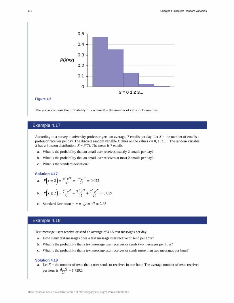
Figure 4.5
The y-axis contains the probability of x where X = the number of calls in 15 minutes.
Example 4.17
According to a survey a university professor gets, on average, 7 emails per day. Let X = the number of emails aprofessor receives per day. The discrete random variable X takes on the values x = 0, 1, 2 …. The random variableX has a Poisson distribution: X ~ P(7). The mean is 7 emails.
a. What is the probability that an email user receives exactly 2 emails per day?
b. What is the probability that an email user receives at most 2 emails per day?
c. What is the standard deviation?
Solution 4.17
a. P⎛⎝x = 2⎞⎠ = μx e-μ
x! = 72 e-7
2! = 0.022
b. P⎛⎝x ≤ 2⎞⎠ = 70 e-7
0! + 71 e-7
1! + 72 e-7
2! = 0.029
c. Standard Deviation = σ = μ = 7 ≈ 2.65
Example 4.18
Text message users receive or send an average of 41.5 text messages per day.
a. How many text messages does a text message user receive or send per hour?
b. What is the probability that a text message user receives or sends two messages per hour?
c. What is the probability that a text message user receives or sends more than two messages per hour?
Solution 4.18a. Let X = the number of texts that a user sends or receives in one hour. The average number of texts received
per hour is 41.524 ≈ 1.7292.
172 Chapter 4 | Discrete Random Variables
This OpenStax book is available for free at https://legacy.cnx.org/content/col12102/1.7
b. P⎛⎝x = 2⎞⎠ = μx e-μ
x! = 1.7292 e-1.729
2! = 0.265
c. P⎛⎝x > 2⎞⎠ = 1 - P⎛⎝x ≤ 2⎞⎠ = 1 - ⎡⎣70 e-7
0! + 71 e-7
1! + 72 e-7
2!⎤⎦ = 0.250
Example 4.19
On May 13, 2013, starting at 4:30 PM, the probability of low seismic activity for the next 48 hours in Alaskawas reported as about 1.02%. Use this information for the next 200 days to find the probability that there will below seismic activity in ten of the next 200 days. Use both the binomial and Poisson distributions to calculate theprobabilities. Are they close?
Solution 4.19
Let X = the number of days with low seismic activity.
Using the binomial distribution:
• P⎛⎝x = 10⎞⎠ = 200!10!(200 - 10)!×.010210×.9898190 = 0.000039
Using the Poisson distribution:
• Calculate μ = np = 200(0.0102) ≈ 2.04
• P⎛⎝x = 10⎞⎠ = μx e-μ
x! = 2.0410 e-2.04
10! = 0.000045
We expect the approximation to be good because n is large (greater than 20) and p is small (less than 0.05). Theresults are close—both probabilities reported are almost 0.
Estimating the Binomial Distribution with the Poisson DistributionWe found before that the binomial distribution provided an approximation for the hypergeometric distribution. Now wefind that the Poisson distribution can provide an approximation for the binomial. We say that the binomial distributionapproaches the Poisson. The binomial distribution approaches the Poisson distribution is as n gets larger and p is small suchthat np becomes a constant value. There are several rules of thumb for when one can say they will use a Poisson to estimatea binomial. One suggests that np, the mean of the binomial, should be less than 25. Another author suggests that it shouldbe less than 7. And another, noting that the mean and variance of the Poisson are both the same, suggests that np and npq,the mean and variance of the binomial, should be greater than 5. There is no one broadly accepted rule of thumb for whenone can use the Poisson to estimate the binomial.
As we move through these probability distributions we are getting to more sophisticated distributions that, in a sense,contain the less sophisticated distributions within them. This proposition has been proven by mathematicians. This gets usto the highest level of sophistication in the next probability distribution which can be used as an approximation to all ofthose that we have discussed so far. This is the normal distribution.
Example 4.20
A survey of 500 seniors in the Price Business School yields the following information. 75% go straight to workafter graduation. 15% go on to work on their MBA. 9% stay to get a minor in another program. 1% go on to get aMaster's in Finance.
What is the probability that more than 2 seniors go to graduate school for their Master's in finance?
Chapter 4 | Discrete Random Variables 173

Solution 4.20
This is clearly a binomial probability distribution problem. The choices are binary when we define the results as"Graduate School in Finance" versus "all other options." The random variable is discrete, and the events are, wecould assume, independent. Solving as a binomial problem, we have:
Binomial Solution
n · p = 500 · 0.01 = 5 = µ
P(0) = 500!0!(500 − 0)!0.010(1 − 0.01)500−0
= 0.00657
P(1) = 500!1!(500 − 1)!0.011(1 − 0.01)500−1
= 0.03318
P(2) = 500!2!(500 − 2)!0.012(1 − 0.01)500−2
= 0.08363
Adding all 3 together = 0.12339
1 − 0.12339 = 0.87661
Poisson approximation
n · p = 500 · 0.01 = 5 = μ
n · p · (1 − p) = 500 · 0.01 · ⎛⎝0.99⎞⎠ ≈ 5 = σ2 = μ
P(X) = e−np(np)xx ! =
⎧⎩⎨P(0) = e−5 · 50
0!⎫⎭⎬+⎧⎩⎨P(1) = e−5 · 51
1!⎫⎭⎬+⎧⎩⎨P(2) = e−5 · 52
2!⎫⎭⎬
0.0067 + 0.0337 + 0.0842 = 0.12471 − 0.1247 = 0.8753
An approximation that is off by 1 one thousandth is certainly an acceptable approximation.
174 Chapter 4 | Discrete Random Variables
This OpenStax book is available for free at https://legacy.cnx.org/content/col12102/1.7

Bernoulli Trials
Binomial Experiment
Binomial Probability Distribution
Geometric Distribution
Geometric Experiment
Hypergeometric Experiment
Hypergeometric Probability
Poisson Probability Distribution
KEY TERMSan experiment with the following characteristics:
1. There are only two possible outcomes called “success” and “failure” for each trial.
2. The probability p of a success is the same for any trial (so the probability q = 1 − p of a failure is the same forany trial).
a statistical experiment that satisfies the following three conditions:
1. There are a fixed number of trials, n.
2. There are only two possible outcomes, called "success" and, "failure," for each trial. The letter p denotes theprobability of a success on one trial, and q denotes the probability of a failure on one trial.
3. The n trials are independent and are repeated using identical conditions.
a discrete random variable (RV) that arises from Bernoulli trials; there are a fixednumber, n, of independent trials. “Independent” means that the result of any trial (for example, trial one) does notaffect the results of the following trials, and all trials are conducted under the same conditions. Under thesecircumstances the binomial RV X is defined as the number of successes in n trials. The mean is μ = np and thestandard deviation is σ = npq . The probability of exactly x successes in n trials is P(x) = C · px · qn - x
a discrete random variable (RV) that arises from the Bernoulli trials; the trials are repeateduntil the first success. The geometric variable X is defined as the number of trials until the first success. The mean is
μ = 1p and the standard deviation is σ = 1
p⎛⎝1p − 1⎞⎠ . The probability of exactly x failures before the first success is
given by the formula: P(X = x) = p(1 – p)x – 1 where one wants to know probability for the number of trials until thefirst success: the xth trail is the first success.An alternative formulation of the geometric distribution asks the question: what is the probability of x failures untilthe first success? In this formulation the trial that resulted in the first success is not counted. The formula for thispresentation of the geometric is: P(X = x) = p(1 − p)x
The expected value in this form of the geometric distribution is μ = 1 − pp
The easiest way to keep these two forms of the geometric distribution straight is to remember that p is theprobability of success and (1−p) is the probability of failure. In the formula the exponents simply count the numberof successes and number of failures of the desired outcome of the experiment. Of course the sum of these twonumbers must add to the number of trials in the experiment.
a statistical experiment with the following properties:
1. There are one or more Bernoulli trials with all failures except the last one, which is a success.
2. In theory, the number of trials could go on forever. There must be at least one trial.
3. The probability, p, of a success and the probability, q, of a failure do not change from trial to trial.
a statistical experiment with the following properties:
1. You take samples from two groups.
2. You are concerned with a group of interest, called the first group.
3. You sample without replacement from the combined groups.
4. Each pick is not independent, since sampling is without replacement.
a discrete random variable (RV) that is characterized by:
1. A fixed number of trials.
2. The probability of success is not the same from trial to trial.
We sample from two groups of items when we are interested in only one group. X is defined as the number ofsuccesses out of the total number of items chosen.
a discrete random variable (RV) that counts the number of times a certain event
Chapter 4 | Discrete Random Variables 175
Probability Distribution Function (PDF)
Random Variable (RV)
will occur in a specific interval; characteristics of the variable:
• The probability that the event occurs in a given interval is the same for all intervals.
• The events occur with a known mean and independently of the time since the last event.
The distribution is defined by the mean μ of the event in the interval. The mean is μ = np. The standard deviation
is σ = μ . The probability of having exactly x successes in r trials is P(x) = μx e-μ
x ! . The Poisson distribution is
often used to approximate the binomial distribution, when n is “large” and p is “small” (a general rule is that npshould be greater than or equal to 25 and p should be less than or equal to 0.01).
a mathematical description of a discrete random variable (RV), giveneither in the form of an equation (formula) or in the form of a table listing all the possible outcomes of anexperiment and the probability associated with each outcome.
a characteristic of interest in a population being studied; common notation for variables areupper case Latin letters X, Y, Z,...; common notation for a specific value from the domain (set of all possible valuesof a variable) are lower case Latin letters x, y, and z. For example, if X is the number of children in a family, then xrepresents a specific integer 0, 1, 2, 3,.... Variables in statistics differ from variables in intermediate algebra in thetwo following ways.
• The domain of the random variable (RV) is not necessarily a numerical set; the domain may be expressed inwords; for example, if X = hair color then the domain is {black, blond, gray, green, orange}.
• We can tell what specific value x the random variable X takes only after performing the experiment.
CHAPTER REVIEW
4.0 IntroductionThe characteristics of a probability distribution or density function (PDF) are as follows:
1. Each probability is between zero and one, inclusive (inclusive means to include zero and one).
2. The sum of the probabilities is one.
4.1 Hypergeometric DistributionThe combinatorial formula can provide the number of unique subsets of size x that can be created from n unique objects to
help us calculate probabilities. The combinatorial formula is ⎛⎝nx⎞⎠ = nCx = n !
x !(n - x) !
A hypergeometric experiment is a statistical experiment with the following properties:
1. You take samples from two groups.
2. You are concerned with a group of interest, called the first group.
3. You sample without replacement from the combined groups.
4. Each pick is not independent, since sampling is without replacement.
The outcomes of a hypergeometric experiment fit a hypergeometric probability distribution. The random variable X = the
number of items from the group of interest. h(x) =⎛⎝Ax⎞⎠⎛⎝N - An - x⎞⎠
⎛⎝Nn⎞⎠
.
4.2 Binomial Distribution - (Base Version - Lyryx Learning)A statistical experiment can be classified as a binomial experiment if the following conditions are met:
1. There are a fixed number of trials, n.
2. There are only two possible outcomes, called "success" and, "failure" for each trial. The letter p denotes theprobability of a success on one trial and q denotes the probability of a failure on one trial.
176 Chapter 4 | Discrete Random Variables
This OpenStax book is available for free at https://legacy.cnx.org/content/col12102/1.7

3. The n trials are independent and are repeated using identical conditions.
The outcomes of a binomial experiment fit a binomial probability distribution. The random variable X = the number ofsuccesses obtained in the n independent trials. The mean of X can be calculated using the formula μ = np, and the standarddeviation is given by the formula σ = npq .
The formula for the Binomial probability density function is
P(x) = C · px · q(n - x)
4.3 Geometric DistributionThere are three characteristics of a geometric experiment:
1. There are one or more Bernoulli trials with all failures except the last one, which is a success.
2. In theory, the number of trials could go on forever. There must be at least one trial.
3. The probability, p, of a success and the probability, q, of a failure are the same for each trial.
In a geometric experiment, define the discrete random variable X as the number of independent trials until the first success.We say that X has a geometric distribution and write X ~ G(p) where p is the probability of success in a single trial.
The mean of the geometric distribution X ~ G(p) is μ = 1 / p where x = number of trials until first success for the formula
P(X = x) = (1 - p)x - 1 p where the number of trials is up and including the first success.
An alternative formulation of the geometric distribution asks the question: what is the probability of x failures until the firstsuccess? In this formulation the trial that resulted in the first success is not counted. The formula for this presentation of thegeometric is:
P(X = x) = p(1 − p)x
The expected value in this form of the geometric distribution is
() μ = 1 − pp
The easiest way to keep these two forms of the geometric distribution straight is to remember that p is the probability ofsuccess and (1−p) is the probability of failure. In the formula the exponents simply count the number of successes andnumber of failures of the desired outcome of the experiment. Of course the sum of these two numbers must add to thenumber of trials in the experiment.
4.4 Poisson DistributionA Poisson probability distribution of a discrete random variable gives the probability of a number of events occurring ina fixed interval of time or space, if these events happen at a known average rate and independently of the time since the lastevent. The Poisson distribution may be used to approximate the binomial, if the probability of success is "small" (less thanor equal to 0.01) and the number of trials is "large" (greater than or equal to 25). Other rules of thumb are also suggestedby different authors, but all recognize that the Poisson distribution is the limiting distribution of the binomial as n increasesand p approaches zero.
The formula for computing probabilities that are from a Poisson process is:
() P(x) = μx e-μ
x !
where P(X) is the probability of successes, μ (pronounced mu) is the expected number of successes, e is the naturallogarithm approximately equal to 2.718, and X is the number of successes per unit, usually per unit of time.
Chapter 4 | Discrete Random Variables 177
FORMULA REVIEW
4.1 Hypergeometric Distribution
h(x) =⎛⎝Ax⎞⎠⎛⎝N - An - x⎞⎠
⎛⎝Nn⎞⎠
4.2 Binomial Distribution - (Base Version - LyryxLearning)
X ~ B(n, p) means that the discrete random variable Xhas a binomial probability distribution with n trials andprobability of success p.
X = the number of successes in n independent trials
n = the number of independent trials
X takes on the values x = 0, 1, 2, 3, ..., n
p = the probability of a success for any trial
q = the probability of a failure for any trial
p + q = 1
q = 1 – p
The mean of X is μ = np. The standard deviation of X is σ =npq .
P(x) = C · px · q(n - x)
where P(X) is the probability of X successes in n trialswhen the probability of a success in ANY ONE TRIAL isp.
4.3 Geometric Distribution
P(X = x) = p(1 − p)x − 1
X ~ G(p) means that the discrete random variable X hasa geometric probability distribution with probability ofsuccess in a single trial p.
X = the number of independent trials until the first success
X takes on the values x = 1, 2, 3, ...
p = the probability of a success for any trial
q = the probability of a failure for any trial p + q = 1q = 1 – p
The mean is μ = 1p .
The standard deviation is σ =1 – pp2 = 1
p⎛⎝1p − 1⎞⎠ .
4.4 Poisson Distribution
X ~ P(μ) means that X has a Poisson probability distributionwhere X = the number of occurrences in the interval ofinterest.
X takes on the values x = 0, 1, 2, 3, ...
The mean μ or λ is typically given.
The variance is σ2 = μ, and the standard deviation isσ = μ .
When P(μ) is used to approximate a binomial distribution,μ = np where n represents the number of independent trialsand p represents the probability of success in a single trial.
() P(x) = μx e-μ
x !
PRACTICE
4.0 IntroductionUse the following information to answer the next five exercises: A company wants to evaluate its attrition rate, in otherwords, how long new hires stay with the company. Over the years, they have established the following probabilitydistribution.
Let X = the number of years a new hire will stay with the company.
Let P(x) = the probability that a new hire will stay with the company x years.
178 Chapter 4 | Discrete Random Variables
This OpenStax book is available for free at https://legacy.cnx.org/content/col12102/1.7

3. Complete Table 4.2 using the data provided.
x P(x)
0 0.12
1 0.18
2 0.30
3 0.15
4
5 0.10
6 0.05
Table 4.2
4. P(x = 4) = _______
5. P(x ≥ 5) = _______
6. On average, how long would you expect a new hire to stay with the company?
7. What does the column “P(x)” sum to?
Use the following information to answer the next six exercises: A baker is deciding how many batches of muffins to make tosell in his bakery. He wants to make enough to sell every one and no fewer. Through observation, the baker has establisheda probability distribution.
x P(x)
1 0.15
2 0.35
3 0.40
4 0.10
Table 4.3
8. Define the random variable X.
9. What is the probability the baker will sell more than one batch? P(x > 1) = _______
10. What is the probability the baker will sell exactly one batch? P(x = 1) = _______
11. On average, how many batches should the baker make?
Use the following information to answer the next four exercises: Ellen has music practice three days a week. She practicesfor all of the three days 85% of the time, two days 8% of the time, one day 4% of the time, and no days 3% of the time. Oneweek is selected at random.
12. Define the random variable X.
13. Construct a probability distribution table for the data.
14. We know that for a probability distribution function to be discrete, it must have two characteristics. One is that the sumof the probabilities is one. What is the other characteristic?
Use the following information to answer the next five exercises: Javier volunteers in community events each month. Hedoes not do more than five events in a month. He attends exactly five events 35% of the time, four events 25% of the time,
Chapter 4 | Discrete Random Variables 179
three events 20% of the time, two events 10% of the time, one event 5% of the time, and no events 5% of the time.
15. Define the random variable X.
16. What values does x take on?
17. Construct a PDF table.
18. Find the probability that Javier volunteers for less than three events each month. P(x < 3) = _______
19. Find the probability that Javier volunteers for at least one event each month. P(x > 0) = _______
4.1 Hypergeometric DistributionUse the following information to answer the next five exercises: Suppose that a group of statistics students is divided intotwo groups: business majors and non-business majors. There are 16 business majors in the group and seven non-businessmajors in the group. A random sample of nine students is taken. We are interested in the number of business majors in thesample.
20. In words, define the random variable X.
21. What values does X take on?
4.2 Binomial Distribution - (Base Version - Lyryx Learning)Use the following information to answer the next eight exercises: The Higher Education Research Institute at UCLAcollected data from 203,967 incoming first-time, full-time freshmen from 270 four-year colleges and universities in the U.S.71.3% of those students replied that, yes, they believe that same-sex couples should have the right to legal marital status.Suppose that you randomly pick eight first-time, full-time freshmen from the survey. You are interested in the number thatbelieves that same sex-couples should have the right to legal marital status.
22. In words, define the random variable X.
23. X ~ _____(_____,_____)
24. What values does the random variable X take on?
25. Construct the probability distribution function (PDF).
x P(x)
Table 4.4
26. On average (μ), how many would you expect to answer yes?
27. What is the standard deviation (σ)?
28. What is the probability that at most five of the freshmen reply “yes”?
29. What is the probability that at least two of the freshmen reply “yes”?
4.3 Geometric DistributionUse the following information to answer the next six exercises: The Higher Education Research Institute at UCLA collected
180 Chapter 4 | Discrete Random Variables
This OpenStax book is available for free at https://legacy.cnx.org/content/col12102/1.7
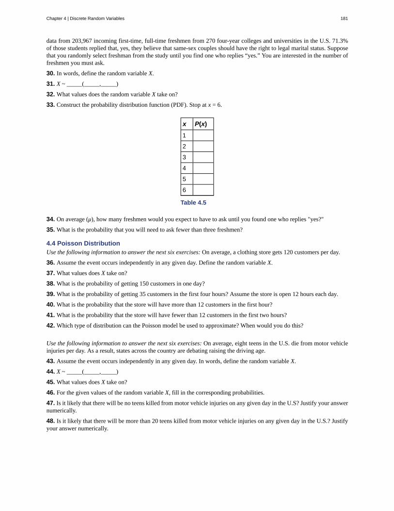
data from 203,967 incoming first-time, full-time freshmen from 270 four-year colleges and universities in the U.S. 71.3%of those students replied that, yes, they believe that same-sex couples should have the right to legal marital status. Supposethat you randomly select freshman from the study until you find one who replies “yes.” You are interested in the number offreshmen you must ask.
30. In words, define the random variable X.
31. X ~ _____(_____,_____)
32. What values does the random variable X take on?
33. Construct the probability distribution function (PDF). Stop at x = 6.
x P(x)
1
2
3
4
5
6
Table 4.5
34. On average (μ), how many freshmen would you expect to have to ask until you found one who replies "yes?"
35. What is the probability that you will need to ask fewer than three freshmen?
4.4 Poisson DistributionUse the following information to answer the next six exercises: On average, a clothing store gets 120 customers per day.
36. Assume the event occurs independently in any given day. Define the random variable X.
37. What values does X take on?
38. What is the probability of getting 150 customers in one day?
39. What is the probability of getting 35 customers in the first four hours? Assume the store is open 12 hours each day.
40. What is the probability that the store will have more than 12 customers in the first hour?
41. What is the probability that the store will have fewer than 12 customers in the first two hours?
42. Which type of distribution can the Poisson model be used to approximate? When would you do this?
Use the following information to answer the next six exercises: On average, eight teens in the U.S. die from motor vehicleinjuries per day. As a result, states across the country are debating raising the driving age.
43. Assume the event occurs independently in any given day. In words, define the random variable X.
44. X ~ _____(_____,_____)
45. What values does X take on?
46. For the given values of the random variable X, fill in the corresponding probabilities.
47. Is it likely that there will be no teens killed from motor vehicle injuries on any given day in the U.S? Justify your answernumerically.
48. Is it likely that there will be more than 20 teens killed from motor vehicle injuries on any given day in the U.S.? Justifyyour answer numerically.
Chapter 4 | Discrete Random Variables 181
HOMEWORK
4.1 Hypergeometric Distribution
49. A group of Martial Arts students is planning on participating in an upcoming demonstration. Six are students of TaeKwon Do; seven are students of Shotokan Karate. Suppose that eight students are randomly picked to be in the firstdemonstration. We are interested in the number of Shotokan Karate students in that first demonstration.
a. In words, define the random variable X.b. List the values that X may take on.c. How many Shotokan Karate students do we expect to be in that first demonstration?
50. In one of its Spring catalogs, L.L. Bean® advertised footwear on 29 of its 192 catalog pages. Suppose we randomlysurvey 20 pages. We are interested in the number of pages that advertise footwear. Each page may be picked at most once.
a. In words, define the random variable X.b. List the values that X may take on.c. How many pages do you expect to advertise footwear on them?d. Calculate the standard deviation.
51. Suppose that a technology task force is being formed to study technology awareness among instructors. Assume thatten people will be randomly chosen to be on the committee from a group of 28 volunteers, 20 who are technically proficientand eight who are not. We are interested in the number on the committee who are not technically proficient.
a. In words, define the random variable X.b. List the values that X may take on.c. How many instructors do you expect on the committee who are not technically proficient?d. Find the probability that at least five on the committee are not technically proficient.e. Find the probability that at most three on the committee are not technically proficient.
52. Suppose that nine Massachusetts athletes are scheduled to appear at a charity benefit. The nine are randomly chosenfrom eight volunteers from the Boston Celtics and four volunteers from the New England Patriots. We are interested in thenumber of Patriots picked.
a. In words, define the random variable X.b. List the values that X may take on.c. Are you choosing the nine athletes with or without replacement?
53. A bridge hand is defined as 13 cards selected at random and without replacement from a deck of 52 cards. In a standarddeck of cards, there are 13 cards from each suit: hearts, spades, clubs, and diamonds. What is the probability of being dealta hand that does not contain a heart?
a. What is the group of interest?b. How many are in the group of interest?c. How many are in the other group?d. Let X = _________. What values does X take on?e. The probability question is P(_______).f. Find the probability in question.g. Find the (i) mean and (ii) standard deviation of X.
4.2 Binomial Distribution - (Base Version - Lyryx Learning)
54. According to a recent article the average number of babies born with significant hearing loss (deafness) is approximatelytwo per 1,000 babies in a healthy baby nursery. The number climbs to an average of 30 per 1,000 babies in an intensive carenursery.
Suppose that 1,000 babies from healthy baby nurseries were randomly surveyed. Find the probability that exactly two babieswere born deaf.
Use the following information to answer the next four exercises. Recently, a nurse commented that when a patient calls themedical advice line claiming to have the flu, the chance that he or she truly has the flu (and not just a nasty cold) is onlyabout 4%. Of the next 25 patients calling in claiming to have the flu, we are interested in how many actually have the flu.
55. Define the random variable and list its possible values.
56. State the distribution of X.
57. Find the probability that at least four of the 25 patients actually have the flu.
182 Chapter 4 | Discrete Random Variables
This OpenStax book is available for free at https://legacy.cnx.org/content/col12102/1.7

58. On average, for every 25 patients calling in, how many do you expect to have the flu?
59. People visiting video rental stores often rent more than one DVD at a time. The probability distribution for DVD rentalsper customer at Video To Go is given Table 4.6. There is five-video limit per customer at this store, so nobody ever rentsmore than five DVDs.
x P(x)
0 0.03
1 0.50
2 0.24
3
4 0.07
5 0.04
Table 4.6
a. Describe the random variable X in words.b. Find the probability that a customer rents three DVDs.c. Find the probability that a customer rents at least four DVDs.d. Find the probability that a customer rents at most two DVDs.
60. A school newspaper reporter decides to randomly survey 12 students to see if they will attend Tet (Vietnamese NewYear) festivities this year. Based on past years, she knows that 18% of students attend Tet festivities. We are interested inthe number of students who will attend the festivities.
a. In words, define the random variable X.b. List the values that X may take on.c. Give the distribution of X. X ~ _____(_____,_____)d. How many of the 12 students do we expect to attend the festivities?e. Find the probability that at most four students will attend.f. Find the probability that more than two students will attend.
Use the following information to answer the next two exercises: The probability that the San Jose Sharks will win any givengame is 0.3694 based on a 13-year win history of 382 wins out of 1,034 games played (as of a certain date). An upcomingmonthly schedule contains 12 games.
61. The expected number of wins for that upcoming month is:a. 1.67b. 12
c. 3821043
d. 4.43
Let X = the number of games won in that upcoming month.
62. What is the probability that the San Jose Sharks win six games in that upcoming month?a. 0.1476b. 0.2336c. 0.7664d. 0.8903
63. What is the probability that the San Jose Sharks win at least five games in that upcoming montha. 0.3694b. 0.5266c. 0.4734d. 0.2305
64. A student takes a ten-question true-false quiz, but did not study and randomly guesses each answer. Find the probabilitythat the student passes the quiz with a grade of at least 70% of the questions correct.
Chapter 4 | Discrete Random Variables 183

65. A student takes a 32-question multiple-choice exam, but did not study and randomly guesses each answer. Each questionhas three possible choices for the answer. Find the probability that the student guesses more than 75% of the questionscorrectly.
66. Six different colored dice are rolled. Of interest is the number of dice that show a one.a. In words, define the random variable X.b. List the values that X may take on.c. On average, how many dice would you expect to show a one?d. Find the probability that all six dice show a one.e. Is it more likely that three or that four dice will show a one? Use numbers to justify your answer numerically.
67. More than 96 percent of the very largest colleges and universities (more than 15,000 total enrollments) have some onlineofferings. Suppose you randomly pick 13 such institutions. We are interested in the number that offer distance learningcourses.
a. In words, define the random variable X.b. List the values that X may take on.c. Give the distribution of X. X ~ _____(_____,_____)d. On average, how many schools would you expect to offer such courses?e. Find the probability that at most ten offer such courses.f. Is it more likely that 12 or that 13 will offer such courses? Use numbers to justify your answer numerically and
answer in a complete sentence.
68. Suppose that about 85% of graduating students attend their graduation. A group of 22 graduating students is randomlychosen.
a. In words, define the random variable X.b. List the values that X may take on.c. Give the distribution of X. X ~ _____(_____,_____)d. How many are expected to attend their graduation?e. Find the probability that 17 or 18 attend.f. Based on numerical values, would you be surprised if all 22 attended graduation? Justify your answer numerically.
69. At The Fencing Center, 60% of the fencers use the foil as their main weapon. We randomly survey 25 fencers at TheFencing Center. We are interested in the number of fencers who do not use the foil as their main weapon.
a. In words, define the random variable X.b. List the values that X may take on.c. Give the distribution of X. X ~ _____(_____,_____)d. How many are expected to not to use the foil as their main weapon?e. Find the probability that six do not use the foil as their main weapon.f. Based on numerical values, would you be surprised if all 25 did not use foil as their main weapon? Justify your
answer numerically.
70. Approximately 8% of students at a local high school participate in after-school sports all four years of high school. Agroup of 60 seniors is randomly chosen. Of interest is the number who participated in after-school sports all four years ofhigh school.
a. In words, define the random variable X.b. List the values that X may take on.c. Give the distribution of X. X ~ _____(_____,_____)d. How many seniors are expected to have participated in after-school sports all four years of high school?e. Based on numerical values, would you be surprised if none of the seniors participated in after-school sports all
four years of high school? Justify your answer numerically.f. Based upon numerical values, is it more likely that four or that five of the seniors participated in after-school
sports all four years of high school? Justify your answer numerically.
71. The chance of an IRS audit for a tax return with over $25,000 in income is about 2% per year. We are interested in theexpected number of audits a person with that income has in a 20-year period. Assume each year is independent.
a. In words, define the random variable X.b. List the values that X may take on.c. Give the distribution of X. X ~ _____(_____,_____)d. How many audits are expected in a 20-year period?e. Find the probability that a person is not audited at all.f. Find the probability that a person is audited more than twice.
184 Chapter 4 | Discrete Random Variables
This OpenStax book is available for free at https://legacy.cnx.org/content/col12102/1.7

72. It has been estimated that only about 30% of California residents have adequate earthquake supplies. Suppose yourandomly survey 11 California residents. We are interested in the number who have adequate earthquake supplies.
a. In words, define the random variable X.b. List the values that X may take on.c. Give the distribution of X. X ~ _____(_____,_____)d. What is the probability that at least eight have adequate earthquake supplies?e. Is it more likely that none or that all of the residents surveyed will have adequate earthquake supplies? Why?f. How many residents do you expect will have adequate earthquake supplies?
73. There are two similar games played for Chinese New Year and Vietnamese New Year. In the Chinese version, fair dicewith numbers 1, 2, 3, 4, 5, and 6 are used, along with a board with those numbers. In the Vietnamese version, fair dice withpictures of a gourd, fish, rooster, crab, crayfish, and deer are used. The board has those six objects on it, also. We will playwith bets being $1. The player places a bet on a number or object. The “house” rolls three dice. If none of the dice show thenumber or object that was bet, the house keeps the $1 bet. If one of the dice shows the number or object bet (and the othertwo do not show it), the player gets back his or her $1 bet, plus $1 profit. If two of the dice show the number or object bet(and the third die does not show it), the player gets back his or her $1 bet, plus $2 profit. If all three dice show the numberor object bet, the player gets back his or her $1 bet, plus $3 profit. Let X = number of matches and Y = profit per game.
a. In words, define the random variable X.b. List the values that X may take on.c. List the values that Y may take on. Then, construct one PDF table that includes both X and Y and their
probabilities.d. Calculate the average expected matches over the long run of playing this game for the player.e. Calculate the average expected earnings over the long run of playing this game for the player.f. Determine who has the advantage, the player or the house.
74. According to The World Bank, only 9% of the population of Uganda had access to electricity as of 2009. Suppose werandomly sample 150 people in Uganda. Let X = the number of people who have access to electricity.
a. What is the probability distribution for X?b. Using the formulas, calculate the mean and standard deviation of X.c. Find the probability that 15 people in the sample have access to electricity.d. Find the probability that at most ten people in the sample have access to electricity.e. Find the probability that more than 25 people in the sample have access to electricity.
75. The literacy rate for a nation measures the proportion of people age 15 and over that can read and write. The literacyrate in Afghanistan is 28.1%. Suppose you choose 15 people in Afghanistan at random. Let X = the number of people whoare literate.
a. Sketch a graph of the probability distribution of X.b. Using the formulas, calculate the (i) mean and (ii) standard deviation of X.c. Find the probability that more than five people in the sample are literate. Is it is more likely that three people or
four people are literate.
4.3 Geometric Distribution
76. A consumer looking to buy a used red Miata car will call dealerships until she finds a dealership that carries the car. Sheestimates the probability that any independent dealership will have the car will be 28%. We are interested in the number ofdealerships she must call.
a. In words, define the random variable X.b. List the values that X may take on.c. Give the distribution of X. X ~ _____(_____,_____)d. On average, how many dealerships would we expect her to have to call until she finds one that has the car?e. Find the probability that she must call at most four dealerships.f. Find the probability that she must call three or four dealerships.
Chapter 4 | Discrete Random Variables 185
77. Suppose that the probability that an adult in America will watch the Super Bowl is 40%. Each person is consideredindependent. We are interested in the number of adults in America we must survey until we find one who will watch theSuper Bowl.
a. In words, define the random variable X.b. List the values that X may take on.c. Give the distribution of X. X ~ _____(_____,_____)d. How many adults in America do you expect to survey until you find one who will watch the Super Bowl?e. Find the probability that you must ask seven people.f. Find the probability that you must ask three or four people.
78. It has been estimated that only about 30% of California residents have adequate earthquake supplies. Suppose weare interested in the number of California residents we must survey until we find a resident who does not have adequateearthquake supplies.
a. In words, define the random variable X.b. List the values that X may take on.c. Give the distribution of X. X ~ _____(_____,_____)d. What is the probability that we must survey just one or two residents until we find a California resident who does
not have adequate earthquake supplies?e. What is the probability that we must survey at least three California residents until we find a California resident
who does not have adequate earthquake supplies?f. How many California residents do you expect to need to survey until you find a California resident who does not
have adequate earthquake supplies?g. How many California residents do you expect to need to survey until you find a California resident who does
have adequate earthquake supplies?
79. In one of its Spring catalogs, L.L. Bean® advertised footwear on 29 of its 192 catalog pages. Suppose we randomlysurvey 20 pages. We are interested in the number of pages that advertise footwear. Each page may be picked more thanonce.
a. In words, define the random variable X.b. List the values that X may take on.c. Give the distribution of X. X ~ _____(_____,_____)d. How many pages do you expect to advertise footwear on them?e. Is it probable that all twenty will advertise footwear on them? Why or why not?f. What is the probability that fewer than ten will advertise footwear on them?g. Reminder: A page may be picked more than once. We are interested in the number of pages that we must
randomly survey until we find one that has footwear advertised on it. Define the random variable X and give itsdistribution.
h. What is the probability that you only need to survey at most three pages in order to find one that advertisesfootwear on it?
i. How many pages do you expect to need to survey in order to find one that advertises footwear?
80. Suppose that you are performing the probability experiment of rolling one fair six-sided die. Let F be the event ofrolling a four or a five. You are interested in how many times you need to roll the die in order to obtain the first four or fiveas the outcome.
• p = probability of success (event F occurs)• q = probability of failure (event F does not occur)
a. Write the description of the random variable X.b. What are the values that X can take on?c. Find the values of p and q.d. Find the probability that the first occurrence of event F (rolling a four or five) is on the second trial.
81. Ellen has music practice three days a week. She practices for all of the three days 85% of the time, two days 8% of thetime, one day 4% of the time, and no days 3% of the time. One week is selected at random. What values does X take on?
186 Chapter 4 | Discrete Random Variables
This OpenStax book is available for free at https://legacy.cnx.org/content/col12102/1.7

82. The World Bank records the prevalence of HIV in countries around the world. According to their data, “Prevalence ofHIV refers to the percentage of people ages 15 to 49 who are infected with HIV.”[1] In South Africa, the prevalence of HIVis 17.3%. Let X = the number of people you test until you find a person infected with HIV.
a. Sketch a graph of the distribution of the discrete random variable X.b. What is the probability that you must test 30 people to find one with HIV?c. What is the probability that you must ask ten people?d. Find the (i) mean and (ii) standard deviation of the distribution of X.
83. According to a recent Pew Research poll, 75% of millennials (people born between 1981 and 1995) have a profile ona social networking site. Let X = the number of millennials you ask until you find a person without a profile on a socialnetworking site.
a. Describe the distribution of X.b. Find the (i) mean and (ii) standard deviation of X.c. What is the probability that you must ask ten people to find one person without a social networking site?d. What is the probability that you must ask 20 people to find one person without a social networking site?e. What is the probability that you must ask at most five people?
4.4 Poisson Distribution
84. The switchboard in a Minneapolis law office gets an average of 5.5 incoming phone calls during the noon hour onMondays. Experience shows that the existing staff can handle up to six calls in an hour. Let X = the number of calls receivedat noon.
a. Find the mean and standard deviation of X.b. What is the probability that the office receives at most six calls at noon on Monday?c. Find the probability that the law office receives six calls at noon. What does this mean to the law office staff who
get, on average, 5.5 incoming phone calls at noon?d. What is the probability that the office receives more than eight calls at noon?
85. The maternity ward at Dr. Jose Fabella Memorial Hospital in Manila in the Philippines is one of the busiest in the worldwith an average of 60 births per day. Let X = the number of births in an hour.
a. Find the mean and standard deviation of X.b. Sketch a graph of the probability distribution of X.c. What is the probability that the maternity ward will deliver three babies in one hour?d. What is the probability that the maternity ward will deliver at most three babies in one hour?e. What is the probability that the maternity ward will deliver more than five babies in one hour?
86. A manufacturer of Christmas tree light bulbs knows that 3% of its bulbs are defective. Find the probability that a stringof 100 lights contains at most four defective bulbs using both the binomial and Poisson distributions.
87. The average number of children a Japanese woman has in her lifetime is 1.37. Suppose that one Japanese woman israndomly chosen.
a. In words, define the random variable X.b. List the values that X may take on.c. Find the probability that she has no children.d. Find the probability that she has fewer children than the Japanese average.e. Find the probability that she has more children than the Japanese average.
88. The average number of children a Spanish woman has in her lifetime is 1.47. Suppose that one Spanish woman israndomly chosen.
a. In words, define the Random Variable X.b. List the values that X may take on.c. Find the probability that she has no children.d. Find the probability that she has fewer children than the Spanish average.e. Find the probability that she has more children than the Spanish average .
1. ”Prevalence of HIV, total (% of populations ages 15-49),” The World Bank, 2013. Available online athttp://data.worldbank.org/indicator/SH.DYN.AIDS.ZS?order=wbapi_data_value_2011+wbapi_data_value+wbapi_data_value-last&sort=desc (accessed May15, 2013).
Chapter 4 | Discrete Random Variables 187

89. Fertile, female cats produce an average of three litters per year. Suppose that one fertile, female cat is randomly chosen.In one year, find the probability she produces:
a. In words, define the random variable X.b. List the values that X may take on.c. Give the distribution of X. X ~ _______d. Find the probability that she has no litters in one year.e. Find the probability that she has at least two litters in one year.f. Find the probability that she has exactly three litters in one year.
90. The chance of having an extra fortune in a fortune cookie is about 3%. Given a bag of 144 fortune cookies, we areinterested in the number of cookies with an extra fortune. Two distributions may be used to solve this problem, but only useone distribution to solve the problem.
a. In words, define the random variable X.b. List the values that X may take on.c. How many cookies do we expect to have an extra fortune?d. Find the probability that none of the cookies have an extra fortune.e. Find the probability that more than three have an extra fortune.f. As n increases, what happens involving the probabilities using the two distributions? Explain in complete
sentences.
91. According to the South Carolina Department of Mental Health web site, for every 200 U.S. women, the average numberwho suffer from anorexia is one. Out of a randomly chosen group of 600 U.S. women determine the following.
a. In words, define the random variable X.b. List the values that X may take on.c. Give the distribution ofX. X ~ _____(_____,_____)d. How many are expected to suffer from anorexia?e. Find the probability that no one suffers from anorexia.f. Find the probability that more than four suffer from anorexia.
92. The chance of an IRS audit for a tax return with over $25,000 in income is about 2% per year. Suppose that 100 peoplewith tax returns over $25,000 are randomly picked. We are interested in the number of people audited in one year. Use aPoisson distribution to answer the following questions.
a. In words, define the random variable X.b. List the values that X may take on.c. How many are expected to be audited?d. Find the probability that no one was audited.e. Find the probability that at least three were audited.
93. Approximately 8% of students at a local high school participate in after-school sports all four years of high school. Agroup of 60 seniors is randomly chosen. Of interest is the number that participated in after-school sports all four years ofhigh school.
a. In words, define the random variable X.b. List the values that X may take on.c. How many seniors are expected to have participated in after-school sports all four years of high school?d. Based on numerical values, would you be surprised if none of the seniors participated in after-school sports all
four years of high school? Justify your answer numerically.e. Based on numerical values, is it more likely that four or that five of the seniors participated in after-school sports
all four years of high school? Justify your answer numerically.
94. On average, Pierre, an amateur chef, drops three pieces of egg shell into every two cake batters he makes. Suppose thatyou buy one of his cakes.
a. In words, define the random variable X.b. List the values that X may take on.c. On average, how many pieces of egg shell do you expect to be in the cake?d. What is the probability that there will not be any pieces of egg shell in the cake?e. Let’s say that you buy one of Pierre’s cakes each week for six weeks. What is the probability that there will not
be any egg shell in any of the cakes?f. Based upon the average given for Pierre, is it possible for there to be seven pieces of shell in the cake? Why?
Use the following information to answer the next two exercises: The average number of times per week that Mrs. Plum’scats wake her up at night because they want to play is ten. We are interested in the number of times her cats wake her up
188 Chapter 4 | Discrete Random Variables
This OpenStax book is available for free at https://legacy.cnx.org/content/col12102/1.7

each week.
95. In words, the random variable X = _________________a. the number of times Mrs. Plum’s cats wake her up each week.b. the number of times Mrs. Plum’s cats wake her up each hour.c. the number of times Mrs. Plum’s cats wake her up each night.d. the number of times Mrs. Plum’s cats wake her up.
96. Find the probability that her cats will wake her up no more than five times next week.a. 0.5000b. 0.9329c. 0.0378d. 0.0671
REFERENCES
4.2 Binomial Distribution - (Base Version - Lyryx Learning)
“Access to electricity (% of population),” The World Bank, 2013. Available online at http://data.worldbank.org/indicator/EG.ELC.ACCS.ZS?order=wbapi_data_value_2009%20wbapi_data_value%20wbapi_data_value-first&sort=asc (accessedMay 15, 2015).
“Distance Education.” Wikipedia. Available online at http://en.wikipedia.org/wiki/Distance_education (accessed May 15,2013).
“NBA Statistics – 2016,” ESPN NBA, 2016. Available online at http://espn.go.com/nba/statistics/_/seasontype/2 (accessedJune 1, 2016).
Newport, Frank. “Americans Still Enjoy Saving Rather than Spending: Few demographic differences seen in these viewsother than by income,” GALLUP® Economy, 2013. Available online at http://www.gallup.com/poll/162368/americans-enjoy-saving-rather-spending.aspx (accessed May 15, 2013).
Pryor, John H., Linda DeAngelo, Laura Palucki Blake, Sylvia Hurtado, Serge Tran. The American Freshman: NationalNorms Fall 2011. Los Angeles: Cooperative Institutional Research Program at the Higher Education Research Instituteat UCLA, 2011. Also available online at http://heri.ucla.edu/PDFs/pubs/TFS/Norms/Monographs/TheAmericanFreshman2011.pdf (accessed May 15, 2013).
“The World FactBook,” Central Intelligence Agency. Available online at https://www.cia.gov/library/publications/the-world-factbook/geos/af.html (accessed May 15, 2013).
“What are the key statistics about pancreatic cancer?” American Cancer Society, 2013. Available online athttp://www.cancer.org/cancer/pancreaticcancer/detailedguide/pancreatic-cancer-key-statistics (accessed May 15, 2013).
“The Canadian Population in 2011: Population Counts and Growth” Statistics Canada, 2016. Available online athttps://www12.statcan.gc.ca/census-recensement/2011/as-sa/98-310-x/98-310-x2011001-eng.cfm (accessed June 2, 2016).
4.3 Geometric Distribution
“Millennials: A Portrait of Generation Next,” PewResearchCenter. Available online at http://www.pewsocialtrends.org/files/2010/10/millennials-confident-connected-open-to-change.pdf (accessed May 15, 2013).
“Millennials: Confident. Connected. Open to Change.” Executive Summary by PewResearch Social & DemographicTrends, 2013. Available online at http://www.pewsocialtrends.org/2010/02/24/millennials-confident-connected-open-to-change/ (accessed May 15, 2013).
“Prevalence of HIV, total (% of populations ages 15-49),” The World Bank, 2013. Available online athttp://data.worldbank.org/indicator/SH.DYN.AIDS.ZS?order=wbapi_data_value_2011+wbapi_data_value+wbapi_data_value-last&sort=desc (accessed May15, 2013).
Pryor, John H., Linda DeAngelo, Laura Palucki Blake, Sylvia Hurtado, Serge Tran. The American Freshman: NationalNorms Fall 2011. Los Angeles: Cooperative Institutional Research Program at the Higher Education Research Instituteat UCLA, 2011. Also available online at http://heri.ucla.edu/PDFs/pubs/TFS/Norms/Monographs/
Chapter 4 | Discrete Random Variables 189

TheAmericanFreshman2011.pdf (accessed May 15, 2013).
“Summary of the National Risk and Vulnerability Assessment 2007/8: A profile of Afghanistan,” The European Union andICON-Institute. Available online at http://ec.europa.eu/europeaid/where/asia/documents/afgh_brochure_summary_en.pdf(accessed May 15, 2013).
“The World FactBook,” Central Intelligence Agency. Available online at https://www.cia.gov/library/publications/the-world-factbook/geos/af.html (accessed May 15, 2013).
“UNICEF reports on Female Literacy Centers in Afghanistan established to teach women and girls basic resading [sic]and writing skills,” UNICEF Television. Video available online at http://www.unicefusa.org/assets/video/afghan-female-literacy-centers.html (accessed May 15, 2013).
4.4 Poisson Distribution
“ATL Fact Sheet,” Department of Aviation at the Hartsfield-Jackson Atlanta International Airport, 2013. Available onlineat http://www.atl.com/about-atl/atl-factsheet/ (accessed February 6, 2019).
Center for Disease Control and Prevention. “Teen Drivers: Fact Sheet,” Injury Prevention & Control: Motor Vehicle Safety,October 2, 2012. Available online at http://www.cdc.gov/Motorvehiclesafety/Teen_Drivers/teendrivers_factsheet.html(accessed May 15, 2013).
“Children and Childrearing,” Ministry of Health, Labour, and Welfare. Available online at http://www.mhlw.go.jp/english/policy/children/children-childrearing/index.html (accessed May 15, 2013).
“Eating Disorder Statistics,” South Carolina Department of Mental Health, 2006. Available online at http://www.state.sc.us/dmh/anorexia/statistics.htm (accessed May 15, 2013).
“Giving Birth in Manila: The maternity ward at the Dr Jose Fabella Memorial Hospital in Manila, the busiest in thePhilippines, where there is an average of 60 births a day,” theguardian, 2013. Available online athttp://www.theguardian.com/world/gallery/2011/jun/08/philippines-health#/?picture=375471900&index=2 (accessed May15, 2013).
“How Americans Use Text Messaging,” Pew Internet, 2013. Available online at http://pewinternet.org/Reports/2011/Cell-Phone-Texting-2011/Main-Report.aspx (accessed May 15, 2013).
Lenhart, Amanda. “Teens, Smartphones & Testing: Texting volume is up while the frequency of voice calling is down.About one in four teens say they own smartphones,” Pew Internet, 2012. Available online athttp://www.pewinternet.org/~/media/Files/Reports/2012/PIP_Teens_Smartphones_and_Texting.pdf (accessed May 15,2013).
“One born every minute: the maternity unit where mothers are THREE to a bed,” MailOnline. Available online athttp://www.dailymail.co.uk/news/article-2001422/Busiest-maternity-ward-planet-averages-60-babies-day-mothers-bed.html (accessed May 15, 2013).
Vanderkam, Laura. “Stop Checking Your Email, Now.” CNNMoney, 2013. Available online athttp://management.fortune.cnn.com/2012/10/08/stop-checking-your-email-now/ (accessed May 15, 2013).
“World Earthquakes: Live Earthquake News and Highlights,” World Earthquakes, 2012. http://www.world-earthquakes.com/index.php?option=ethq_prediction (accessed May 15, 2013).
190 Chapter 4 | Discrete Random Variables
This OpenStax book is available for free at https://legacy.cnx.org/content/col12102/1.7

SOLUTIONS
3
x P(x)
0 0.12
1 0.18
2 0.30
3 0.15
4 0.10
5 0.10
6 0.05
Table 4.7
5 0.10 + 0.05 = 0.15
7 1
9 0.35 + 0.40 + 0.10 = 0.85
11 1(0.15) + 2(0.35) + 3(0.40) + 4(0.10) = 0.15 + 0.70 + 1.20 + 0.40 = 2.45
13
x P(x)
0 0.03
1 0.04
2 0.08
3 0.85
Table 4.8
15 Let X = the number of events Javier volunteers for each month.
Chapter 4 | Discrete Random Variables 191

17
x P(x)
0 0.05
1 0.05
2 0.10
3 0.20
4 0.25
5 0.35
Table 4.9
19 1 – 0.05 = 0.95
20 X = the number of business majors in the sample.
21 2, 3, 4, 5, 6, 7, 8, 9
22 X = the number that reply “yes”
24 0, 1, 2, 3, 4, 5, 6, 7, 8
26 5.7
28 0.4151
30 X = the number of freshmen selected from the study until one replied "yes" that same-sex couples should have the rightto legal marital status.
32 1,2,…
34 1.4
37 0, 1, 2, 3, 4, …
39 0.0485
41 0.0214
43 X = the number of U.S. teens who die from motor vehicle injuries per day.
45 0, 1, 2, 3, 4, ...
47 No
50a. X = the number of pages that advertise footwear
b. 0, 1, 2, 3, ..., 20
c. 3.03
d. 1.5197
52a. X = the number of Patriots picked
b. 0, 1, 2, 3, 4
c. Without replacement
55 X = the number of patients calling in claiming to have the flu, who actually have the flu. X = 0, 1, 2, ...25
57 0.0165
192 Chapter 4 | Discrete Random Variables
This OpenStax book is available for free at https://legacy.cnx.org/content/col12102/1.7
59a. X = the number of DVDs a Video to Go customer rents
b. 0.12
c. 0.11
d. 0.77
61 d. 4.43
63 c
65• X = number of questions answered correctly
• X ~ B ⎛⎝32, 13⎞⎠
• We are interested in MORE THAN 75% of 32 questions correct. 75% of 32 is 24. We want to find P(x > 24). Theevent "more than 24" is the complement of "less than or equal to 24."
• P(x > 24) = 0
• The probability of getting more than 75% of the 32 questions correct when randomly guessing is very small andpractically zero.
67a. X = the number of college and universities that offer online offerings.
b. 0, 1, 2, …, 13
c. X ~ B(13, 0.96)
d. 12.48
e. 0.0135
f. P(x = 12) = 0.3186 P(x = 13) = 0.5882 More likely to get 13.
69a. X = the number of fencers who do not use the foil as their main weapon
b. 0, 1, 2, 3,... 25
c. X ~ B(25,0.40)
d. 10
e. 0.0442
f. The probability that all 25 not use the foil is almost zero. Therefore, it would be very surprising.
71a. X = the number of audits in a 20-year period
b. 0, 1, 2, …, 20
c. X ~ B(20, 0.02)
d. 0.4
e. 0.6676
f. 0.0071
731. X = the number of matches
2. 0, 1, 2, 3
3. In dollars: −1, 1, 2, 3
Chapter 4 | Discrete Random Variables 193

4. 12
5. The answer is −0.0787. You lose about eight cents, on average, per game.
6. The house has the advantage.
75a. X ~ B(15, 0.281)
Figure 4.6
b. i. Mean = μ = np = 15(0.281) = 4.215
ii. Standard Deviation = σ = npq = 15(0.281)(0.719) = 1.7409
c. P(x > 5)=1 – 0.7754 = 0.2246P(x = 3) = 0.1927P(x = 4) = 0.2259It is more likely that four people are literate that three people are.
77a. X = the number of adults in America who are surveyed until one says he or she will watch the Super Bowl.
b. X ~ G(0.40)
c. 2.5
d. 0.0187
e. 0.2304
79a. X = the number of pages that advertise footwear
b. X takes on the values 0, 1, 2, ..., 20
c. X ~ B(20, 29192 )
d. 3.02
e. No
f. 0.9997
g. X = the number of pages we must survey until we find one that advertises footwear. X ~ G( 29192 )
194 Chapter 4 | Discrete Random Variables
This OpenStax book is available for free at https://legacy.cnx.org/content/col12102/1.7

h. 0.3881
i. 6.6207 pages
81 0, 1, 2, and 3
83a. X ~ G(0.25)
b. i. Mean = μ = 1p = 1
0.25 = 4
ii. Standard Deviation = σ =1 − pp2 = 1 − 0.25
0.252 ≈ 3.4641
c. P(x = 10) = 0.0188
d. P(x = 20) = 0.0011
e. P(x ≤ 5) = 0.7627
84a. X ~ P(5.5); μ = 5.5; σ = 5.5 ≈ 2.3452
b. P(x ≤ 6) ≈ 0.6860
c. There is a 15.7% probability that the law staff will receive more calls than they can handle.
d. P(x > 8) = 1 – P(x ≤ 8) ≈ 1 – 0.8944 = 0.1056
86 Let X = the number of defective bulbs in a string. Using the Poisson distribution:• μ = np = 100(0.03) = 3
• X ~ P(3)
• P(x ≤ 4) ≈ 0.8153
Using the binomial distribution:• X ~ B(100, 0.03)
• P(x ≤ 4) = 0.8179
The Poisson approximation is very good—the difference between the probabilities is only 0.0026.
88a. X = the number of children for a Spanish woman
b. 0, 1, 2, 3,...
c. 0.2299
d. 0.5679
e. 0.4321
90a. X = the number of fortune cookies that have an extra fortune
b. 0, 1, 2, 3,... 144
c. 4.32
d. 0.0124 or 0.0133
e. 0.6300 or 0.6264
f. As n gets larger, the probabilities get closer together.
92a. X = the number of people audited in one year
b. 0, 1, 2, ..., 100
Chapter 4 | Discrete Random Variables 195
c. 2
d. 0.1353
e. 0.3233
94a. X = the number of shell pieces in one cake
b. 0, 1, 2, 3,...
c. 1.5
d. 0.2231
e. 0.0001
f. Yes
96 d
196 Chapter 4 | Discrete Random Variables
This OpenStax book is available for free at https://legacy.cnx.org/content/col12102/1.7

5 | CONTINUOUS RANDOMVARIABLES
Figure 5.1 The heights of these radish plants are continuous random variables. (Credit: Rev Stan)
Introduction
Continuous random variables have many applications. Baseball batting averages, IQ scores, the length of time a longdistance telephone call lasts, the amount of money a person carries, the length of time a computer chip lasts, rates of returnfrom an investment, and SAT scores are just a few. The field of reliability depends on a variety of continuous randomvariables, as do all areas of risk analysis.
NOTE
The values of discrete and continuous random variables can be ambiguous. For example, if X is equal to the numberof miles (to the nearest mile) you drive to work, then X is a discrete random variable. You count the miles. If X isthe distance you drive to work, then you measure values of X and X is a continuous random variable. For a secondexample, if X is equal to the number of books in a backpack, then X is a discrete random variable. If X is the weight ofa book, then X is a continuous random variable because weights are measured. How the random variable is defined isvery important.
Chapter 5 | Continuous Random Variables 197
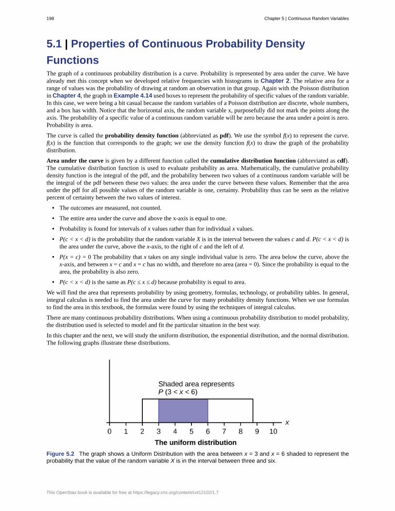
5.1 | Properties of Continuous Probability Density
FunctionsThe graph of a continuous probability distribution is a curve. Probability is represented by area under the curve. We havealready met this concept when we developed relative frequencies with histograms in Chapter 2. The relative area for arange of values was the probability of drawing at random an observation in that group. Again with the Poisson distributionin Chapter 4, the graph in Example 4.14 used boxes to represent the probability of specific values of the random variable.In this case, we were being a bit casual because the random variables of a Poisson distribution are discrete, whole numbers,and a box has width. Notice that the horizontal axis, the random variable x, purposefully did not mark the points along theaxis. The probability of a specific value of a continuous random variable will be zero because the area under a point is zero.Probability is area.
The curve is called the probability density function (abbreviated as pdf). We use the symbol f(x) to represent the curve.f(x) is the function that corresponds to the graph; we use the density function f(x) to draw the graph of the probabilitydistribution.
Area under the curve is given by a different function called the cumulative distribution function (abbreviated as cdf).The cumulative distribution function is used to evaluate probability as area. Mathematically, the cumulative probabilitydensity function is the integral of the pdf, and the probability between two values of a continuous random variable will bethe integral of the pdf between these two values: the area under the curve between these values. Remember that the areaunder the pdf for all possible values of the random variable is one, certainty. Probability thus can be seen as the relativepercent of certainty between the two values of interest.
• The outcomes are measured, not counted.
• The entire area under the curve and above the x-axis is equal to one.
• Probability is found for intervals of x values rather than for individual x values.
• P(c < x < d) is the probability that the random variable X is in the interval between the values c and d. P(c < x < d) isthe area under the curve, above the x-axis, to the right of c and the left of d.
• P(x = c) = 0 The probability that x takes on any single individual value is zero. The area below the curve, above thex-axis, and between x = c and x = c has no width, and therefore no area (area = 0). Since the probability is equal to thearea, the probability is also zero.
• P(c < x < d) is the same as P(c ≤ x ≤ d) because probability is equal to area.
We will find the area that represents probability by using geometry, formulas, technology, or probability tables. In general,integral calculus is needed to find the area under the curve for many probability density functions. When we use formulasto find the area in this textbook, the formulas were found by using the techniques of integral calculus.
There are many continuous probability distributions. When using a continuous probability distribution to model probability,the distribution used is selected to model and fit the particular situation in the best way.
In this chapter and the next, we will study the uniform distribution, the exponential distribution, and the normal distribution.The following graphs illustrate these distributions.
Figure 5.2 The graph shows a Uniform Distribution with the area between x = 3 and x = 6 shaded to represent theprobability that the value of the random variable X is in the interval between three and six.
198 Chapter 5 | Continuous Random Variables
This OpenStax book is available for free at https://legacy.cnx.org/content/col12102/1.7

Figure 5.3 The graph shows an Exponential Distribution with the area between x = 2 and x = 4 shaded to representthe probability that the value of the random variable X is in the interval between two and four.
Figure 5.4 The graph shows the Standard Normal Distribution with the area between x = 1 and x = 2 shaded torepresent the probability that the value of the random variable X is in the interval between one and two.
For continuous probability distributions, PROBABILITY = AREA.
Example 5.1
Consider the function f(x) = 120 for 0 ≤ x ≤ 20. x = a real number. The graph of f(x) = 1
20 is a horizontal line.
However, since 0 ≤ x ≤ 20, f(x) is restricted to the portion between x = 0 and x = 20, inclusive.
Figure 5.5
f(x) = 120 for 0 ≤ x ≤ 20.
Chapter 5 | Continuous Random Variables 199

The graph of f(x) = 120 is a horizontal line segment when 0 ≤ x ≤ 20.
The area between f(x) = 120 where 0 ≤ x ≤ 20 and the x-axis is the area of a rectangle with base = 20 and height
= 120 .
AREA = 20⎛⎝ 120⎞⎠ = 1
Suppose we want to find the area between f(x) = 120 and the x-axis where 0 < x < 2.
Figure 5.6
AREA = (2 – 0)⎛⎝ 120⎞⎠ = 0.1
(2 – 0) = 2 = base of a rectangle
REMINDER
area of a rectangle = (base)(height).
The area corresponds to a probability. The probability that x is between zero and two is 0.1, which can be writtenmathematically as P(0 < x < 2) = P(x < 2) = 0.1.
Suppose we want to find the area between f(x) = 120 and the x-axis where 4 < x < 15.
200 Chapter 5 | Continuous Random Variables
This OpenStax book is available for free at https://legacy.cnx.org/content/col12102/1.7
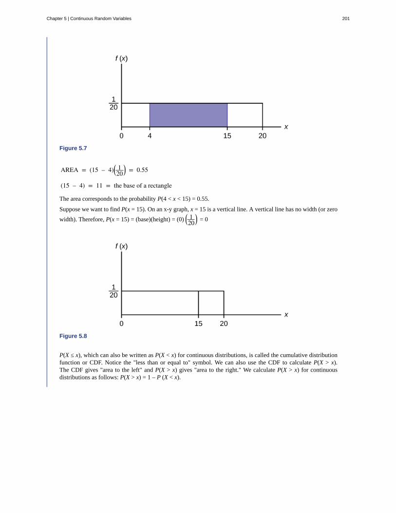
Figure 5.7
AREA = (15 – 4)⎛⎝ 120⎞⎠ = 0.55
(15 – 4) = 11 = the base of a rectangle
The area corresponds to the probability P(4 < x < 15) = 0.55.
Suppose we want to find P(x = 15). On an x-y graph, x = 15 is a vertical line. A vertical line has no width (or zero
width). Therefore, P(x = 15) = (base)(height) = (0) ⎛⎝ 120⎞⎠ = 0
Figure 5.8
P(X ≤ x), which can also be written as P(X < x) for continuous distributions, is called the cumulative distributionfunction or CDF. Notice the "less than or equal to" symbol. We can also use the CDF to calculate P(X > x).The CDF gives "area to the left" and P(X > x) gives "area to the right." We calculate P(X > x) for continuousdistributions as follows: P(X > x) = 1 – P (X < x).
Chapter 5 | Continuous Random Variables 201

Figure 5.9
Label the graph with f(x) and x. Scale the x and y axes with the maximum x and y values. f(x) = 120 , 0 ≤ x ≤ 20.
To calculate the probability that x is between two values, look at the following graph. Shade the region between x= 2.3 and x = 12.7. Then calculate the shaded area of a rectangle.
Figure 5.10
P(2.3 < x < 12.7) = (base)(height) = (12.7 − 2.3)⎛⎝ 120⎞⎠ = 0.52
5.1 Consider the function f(x) = 18 for 0 ≤ x ≤ 8. Draw the graph of f(x) and find P(2.5 < x < 7.5).
5.2 | The Uniform DistributionThe uniform distribution is a continuous probability distribution and is concerned with events that are equally likely tooccur. When working out problems that have a uniform distribution, be careful to note if the data is inclusive or exclusiveof endpoints.
The mathematical statement of the uniform distribution is
f(x) = 1b − a for a ≤ x ≤ b
202 Chapter 5 | Continuous Random Variables
This OpenStax book is available for free at https://legacy.cnx.org/content/col12102/1.7

where a = the lowest value of x and b = the highest value of x.
Formulas for the theoretical mean and standard deviation are
μ = a + b2 and σ = (b − a)2
12
5.1 The data that follow are the number of passengers on 35 different charter fishing boats. The sample mean = 7.9 andthe sample standard deviation = 4.33. The data follow a uniform distribution where all values between and includingzero and 14 are equally likely. State the values of a and b. Write the distribution in proper notation, and calculate thetheoretical mean and standard deviation.
1 12 4 10 4 14 11
7 11 4 13 2 4 6
3 10 0 12 6 9 10
5 13 4 10 14 12 11
6 10 11 0 11 13 2
Table 5.1
Example 5.2
The amount of time, in minutes, that a person must wait for a bus is uniformly distributed between zero and 15minutes, inclusive.
a. What is the probability that a person waits fewer than 12.5 minutes?
Solution 5.2
a. Let X = the number of minutes a person must wait for a bus. a = 0 and b = 15. X ~ U(0, 15). Write the probability
density function. f (x) = 115 − 0 = 1
15 for 0 ≤ x ≤ 15.
Find P (x < 12.5). Draw a graph.
P(x < k) = (base)(height) = (12.5 - 0)⎛⎝ 115⎞⎠ = 0.8333
The probability a person waits less than 12.5 minutes is 0.8333.
Chapter 5 | Continuous Random Variables 203
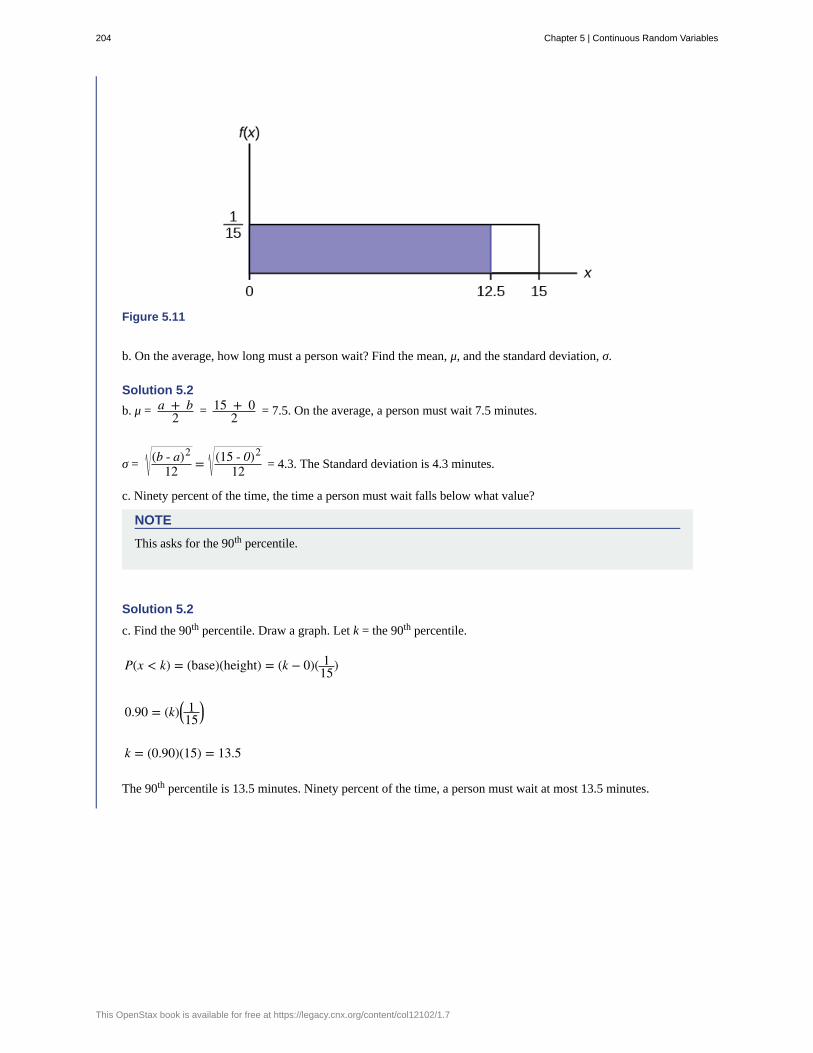
Figure 5.11
b. On the average, how long must a person wait? Find the mean, μ, and the standard deviation, σ.
Solution 5.2
b. μ = a + b2 = 15 + 0
2 = 7.5. On the average, a person must wait 7.5 minutes.
σ =(b - a)2
12 = (15 - 0)2
12 = 4.3. The Standard deviation is 4.3 minutes.
c. Ninety percent of the time, the time a person must wait falls below what value?
NOTE
This asks for the 90th percentile.
Solution 5.2
c. Find the 90th percentile. Draw a graph. Let k = the 90th percentile.
P(x < k) = (base)(height) = (k − 0)( 115)
0.90 = (k)⎛⎝ 115⎞⎠
k = (0.90)(15) = 13.5
The 90th percentile is 13.5 minutes. Ninety percent of the time, a person must wait at most 13.5 minutes.
204 Chapter 5 | Continuous Random Variables
This OpenStax book is available for free at https://legacy.cnx.org/content/col12102/1.7

Figure 5.12
5.2 The total duration of baseball games in the major league in the 2011 season is uniformly distributed between 447hours and 521 hours inclusive.
a. Find a and b and describe what they represent.
b. Write the distribution.
c. Find the mean and the standard deviation.
d. What is the probability that the duration of games for a team for the 2011 season is between 480 and 500 hours?
5.3 | The Exponential DistributionThe exponential distribution is often concerned with the amount of time until some specific event occurs. For example,the amount of time (beginning now) until an earthquake occurs has an exponential distribution. Other examples include thelength of time, in minutes, of long distance business telephone calls, and the amount of time, in months, a car battery lasts. Itcan be shown, too, that the value of the change that you have in your pocket or purse approximately follows an exponentialdistribution.
Values for an exponential random variable occur in the following way. There are fewer large values and more small values.For example, marketing studies have shown that the amount of money customers spend in one trip to the supermarketfollows an exponential distribution. There are more people who spend small amounts of money and fewer people who spendlarge amounts of money.
Exponential distributions are commonly used in calculations of product reliability, or the length of time a product lasts.
The random variable for the exponential distribution is continuous and often measures a passage of time, although it canbe used in other applications. Typical questions may be, “what is the probability that some event will occur within the nextx hours or days, or what is the probability that some event will occur between x1 hours and x2 hours, or what is the
probability that the event will take more than x1 hours to perform?” In short, the random variable X equals (a) the time
between events or (b) the passage of time to complete an action, e.g. wait on a customer. The probability density function isgiven by:
f (x) = 1μe
− 1μx
where μ is the historical average waiting time, and has a mean and standard deviation of 1/μ.
An alternative form of the exponential distribution formula recognizes what is often called the decay factor. The decay factor
Chapter 5 | Continuous Random Variables 205

simply measures how rapidly the probability of an event declines as the random variable X increases. When the notationusing the decay parameter m is used, the probability density function is presented as:
f (x) = me−mx
where m = 1μ
In order to calculate probabilities for specific probability density functions, the cumulative density function is used. Thecumulative density function (cdf) is simply the integral of the pdf and is:
F(x) = ∫0
∞ ⎡
⎣⎢⎢1μe
- xμ⎤
⎦⎥⎥ = 1 - e
- xμ
Example 5.3
Let X = amount of time (in minutes) a postal clerk spends with a customer. The time is known from historical datato have an average amount of time equal to four minutes.
It is given that μ = 4 minutes, that is, the average time the clerk spends with a customer is 4 minutes. Rememberthat we are still doing probability and thus we have to be told the population parameters such as the mean. Todo any calculations, we need to know the mean of the distribution: the historical time to provide a service, forexample. Knowing the historical mean allows the calculation of the decay parameter, m.
m = 1μ . Therefore, m = 1
4 = 0.25 .
When the notation used the decay parameter, m, the probability density function is presented as
f (x) = me−mx , which is simply the original formula with m substituted for 1μ , or f (x) = 1
μe− 1μx
.
To calculate probabilities for an exponential probability density function, we need to use the cumulative densityfunction. As shown below, the curve for the cumulative density function is:
f(x) = 0.25e–0.25x where x is at least zero and m = 0.25.
For example, f(5) = 0.25e(-0.25)(5) = 0.072. In other words, the function has a value of .072 when x = 5.
The graph is as follows:
Figure 5.13
Notice the graph is a declining curve. When x = 0,
f(x) = 0.25e(−0.25)(0) = (0.25)(1) = 0.25 = m. The maximum value on the y-axis is always m, one divided by themean.
206 Chapter 5 | Continuous Random Variables
This OpenStax book is available for free at https://legacy.cnx.org/content/col12102/1.7

5.3 The amount of time spouses shop for anniversary cards can be modeled by an exponential distribution with theaverage amount of time equal to eight minutes. Write the distribution, state the probability density function, and graphthe distribution.
Example 5.4
a. Using the information in Example 5.3, find the probability that a clerk spends four to five minutes with arandomly selected customer.
Solution 5.4
a. Find P(4 < x < 5).The cumulative distribution function (CDF) gives the area to the left.P(x < x) = 1 – e–mx
P(x < 5) = 1 – e(–0.25)(5) = 0.7135 and P(x < 4) = 1 – e(–0.25)(4) = 0.6321P(4 < x < 5)= 0.7135 – 0.6321 = 0.0814
Figure 5.14
5.4 The number of days ahead travelers purchase their airline tickets can be modeled by an exponential distributionwith the average amount of time equal to 15 days. Find the probability that a traveler will purchase a ticket fewer thanten days in advance. How many days do half of all travelers wait?
Example 5.5
On the average, a certain computer part lasts ten years. The length of time the computer part lasts is exponentiallydistributed.
a. What is the probability that a computer part lasts more than 7 years?
Solution 5.5a. Let x = the amount of time (in years) a computer part lasts.
Chapter 5 | Continuous Random Variables 207
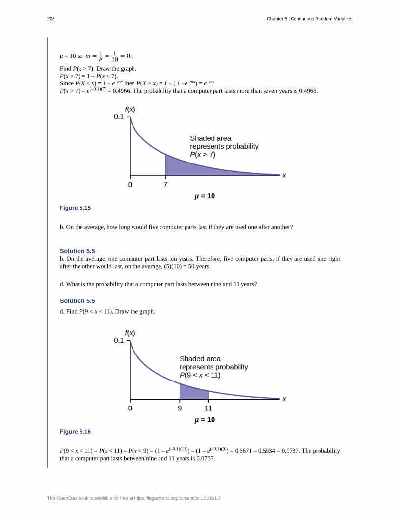
μ = 10 so m = 1μ = 1
10 = 0.1
Find P(x > 7). Draw the graph.P(x > 7) = 1 – P(x < 7).Since P(X < x) = 1 – e–mx then P(X > x) = 1 – ( 1 –e–mx) = e–mx
P(x > 7) = e(–0.1)(7) = 0.4966. The probability that a computer part lasts more than seven years is 0.4966.
Figure 5.15
b. On the average, how long would five computer parts last if they are used one after another?
Solution 5.5b. On the average, one computer part lasts ten years. Therefore, five computer parts, if they are used one rightafter the other would last, on the average, (5)(10) = 50 years.
d. What is the probability that a computer part lasts between nine and 11 years?
Solution 5.5
d. Find P(9 < x < 11). Draw the graph.
Figure 5.16
P(9 < x < 11) = P(x < 11) – P(x < 9) = (1 – e(–0.1)(11)) – (1 – e(–0.1)(9)) = 0.6671 – 0.5934 = 0.0737. The probabilitythat a computer part lasts between nine and 11 years is 0.0737.
208 Chapter 5 | Continuous Random Variables
This OpenStax book is available for free at https://legacy.cnx.org/content/col12102/1.7

5.5 On average, a pair of running shoes can last 18 months if used every day. The length of time running shoes last isexponentially distributed. What is the probability that a pair of running shoes last more than 15 months? On average,how long would six pairs of running shoes last if they are used one after the other? Eighty percent of running shoeslast at most how long if used every day?
Example 5.6
Suppose that the length of a phone call, in minutes, is an exponential random variable with decay parameter 112
. The decay p[parameter is another way to view 1/λ. If another person arrives at a public telephone just beforeyou, find the probability that you will have to wait more than five minutes. Let X = the length of a phone call, inminutes.
What is m, μ, and σ? The probability that you must wait more than five minutes is _______ .
Solution 5.6
• m = 112
• μ = 12
• σ = 12
P(x > 5) = 0.6592
Example 5.7
The time spent waiting between events is often modeled using the exponential distribution. For example, supposethat an average of 30 customers per hour arrive at a store and the time between arrivals is exponentiallydistributed.
a. On average, how many minutes elapse between two successive arrivals?
b. When the store first opens, how long on average does it take for three customers to arrive?
c. After a customer arrives, find the probability that it takes less than one minute for the next customer toarrive.
d. After a customer arrives, find the probability that it takes more than five minutes for the next customer toarrive.
e. Is an exponential distribution reasonable for this situation?
Solution 5.7a. Since we expect 30 customers to arrive per hour (60 minutes), we expect on average one customer to arrive
every two minutes on average.
b. Since one customer arrives every two minutes on average, it will take six minutes on average for threecustomers to arrive.
c. Let X = the time between arrivals, in minutes. By part a, μ = 2, so m = 12 = 0.5.
The cumulative distribution function is P(X < x) = 1 – e(-0.5)(x)
Therefore P(X < 1) = 1 – e(–0.5)(1) = 0.3935.
Chapter 5 | Continuous Random Variables 209

Figure 5.17
d. P(X > 5) = 1 – P(X < 5) = 1 – (1 – e(-0.5)(5)) = e–2.5 ≈ 0.0821.
Figure 5.18
e. This model assumes that a single customer arrives at a time, which may not be reasonable since peoplemight shop in groups, leading to several customers arriving at the same time. It also assumes that the flowof customers does not change throughout the day, which is not valid if some times of the day are busier thanothers.
Memorylessness of the Exponential DistributionRecall that the amount of time between customers for the postal clerk discussed earlier is exponentially distributed witha mean of two minutes. Suppose that five minutes have elapsed since the last customer arrived. Since an unusually longamount of time has now elapsed, it would seem to be more likely for a customer to arrive within the next minute. With theexponential distribution, this is not the case–the additional time spent waiting for the next customer does not depend on howmuch time has already elapsed since the last customer. This is referred to as the memoryless property. The exponential andgeometric probability density functions are the only probability functions that have the memoryless property. Specifically,the memoryless property says that
P (X > r + t | X > r) = P (X > t) for all r ≥ 0 and t ≥ 0
For example, if five minutes have elapsed since the last customer arrived, then the probability that more than one minutewill elapse before the next customer arrives is computed by using r = 5 and t = 1 in the foregoing equation.
210 Chapter 5 | Continuous Random Variables
This OpenStax book is available for free at https://legacy.cnx.org/content/col12102/1.7
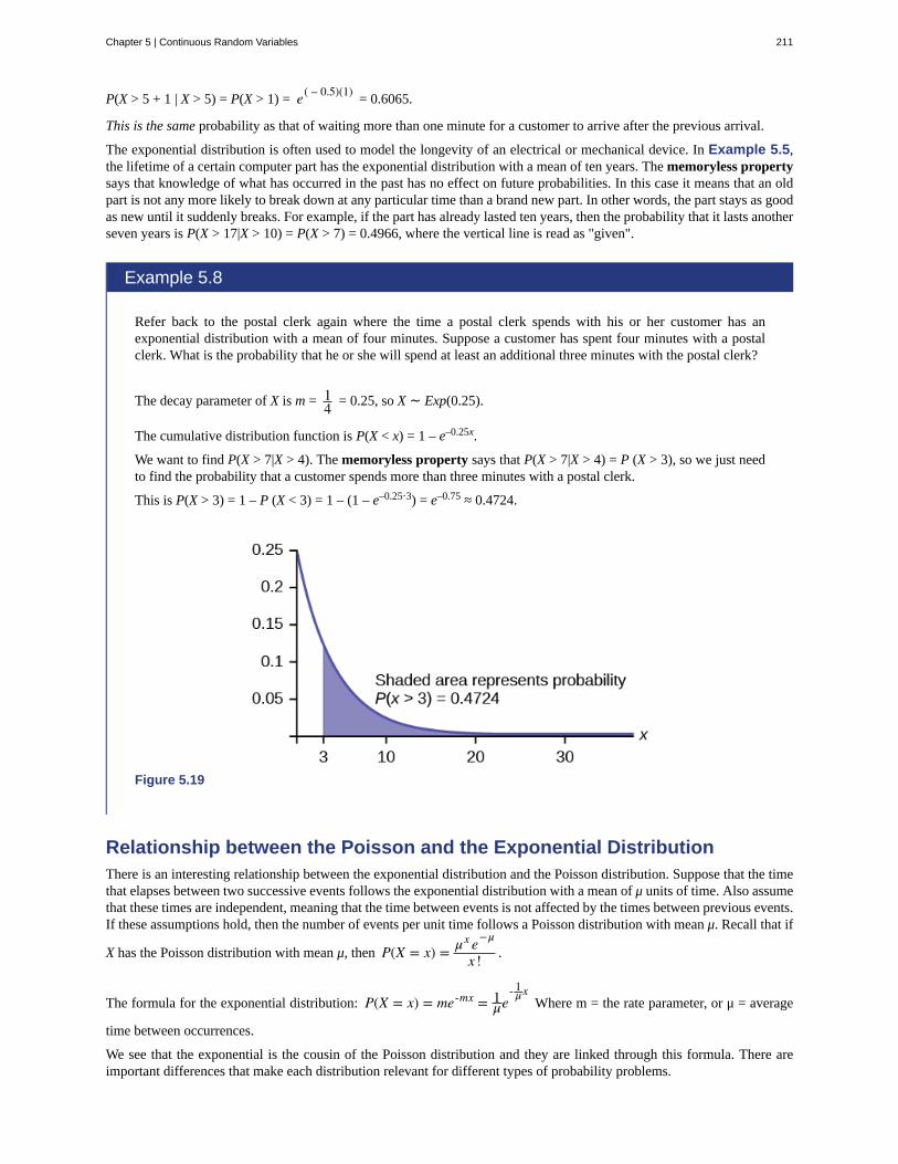
P(X > 5 + 1 | X > 5) = P(X > 1) = e( – 0.5)(1)= 0.6065.
This is the same probability as that of waiting more than one minute for a customer to arrive after the previous arrival.
The exponential distribution is often used to model the longevity of an electrical or mechanical device. In Example 5.5,the lifetime of a certain computer part has the exponential distribution with a mean of ten years. The memoryless propertysays that knowledge of what has occurred in the past has no effect on future probabilities. In this case it means that an oldpart is not any more likely to break down at any particular time than a brand new part. In other words, the part stays as goodas new until it suddenly breaks. For example, if the part has already lasted ten years, then the probability that it lasts anotherseven years is P(X > 17|X > 10) = P(X > 7) = 0.4966, where the vertical line is read as "given".
Example 5.8
Refer back to the postal clerk again where the time a postal clerk spends with his or her customer has anexponential distribution with a mean of four minutes. Suppose a customer has spent four minutes with a postalclerk. What is the probability that he or she will spend at least an additional three minutes with the postal clerk?
The decay parameter of X is m = 14 = 0.25, so X ∼ Exp(0.25).
The cumulative distribution function is P(X < x) = 1 – e–0.25x.
We want to find P(X > 7|X > 4). The memoryless property says that P(X > 7|X > 4) = P (X > 3), so we just needto find the probability that a customer spends more than three minutes with a postal clerk.
This is P(X > 3) = 1 – P (X < 3) = 1 – (1 – e–0.25⋅3) = e–0.75 ≈ 0.4724.
Figure 5.19
Relationship between the Poisson and the Exponential DistributionThere is an interesting relationship between the exponential distribution and the Poisson distribution. Suppose that the timethat elapses between two successive events follows the exponential distribution with a mean of μ units of time. Also assumethat these times are independent, meaning that the time between events is not affected by the times between previous events.If these assumptions hold, then the number of events per unit time follows a Poisson distribution with mean μ. Recall that if
X has the Poisson distribution with mean μ, then P(X = x) = μx e−μ
x ! .
The formula for the exponential distribution: P(X = x) = me-mx = 1μe
- 1μx
Where m = the rate parameter, or μ = average
time between occurrences.
We see that the exponential is the cousin of the Poisson distribution and they are linked through this formula. There areimportant differences that make each distribution relevant for different types of probability problems.
Chapter 5 | Continuous Random Variables 211
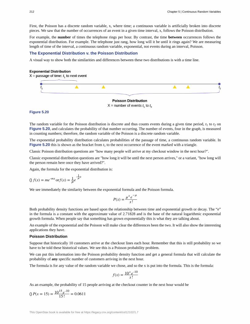
First, the Poisson has a discrete random variable, x, where time; a continuous variable is artificially broken into discretepieces. We saw that the number of occurrences of an event in a given time interval, x, follows the Poisson distribution.
For example, the number of times the telephone rings per hour. By contrast, the time between occurrences follows theexponential distribution. For example. The telephone just rang, how long will it be until it rings again? We are measuringlength of time of the interval, a continuous random variable, exponential, not events during an interval, Poisson.
The Exponential Distribution v. the Poisson Distribution
A visual way to show both the similarities and differences between these two distributions is with a time line.
Figure 5.20
The random variable for the Poisson distribution is discrete and thus counts events during a given time period, t1 to t2 onFigure 5.20, and calculates the probability of that number occurring. The number of events, four in the graph, is measuredin counting numbers; therefore, the random variable of the Poisson is a discrete random variable.
The exponential probability distribution calculates probabilities of the passage of time, a continuous random variable. InFigure 5.20 this is shown as the bracket from t1 to the next occurrence of the event marked with a triangle.
Classic Poisson distribution questions are "how many people will arrive at my checkout window in the next hour?".
Classic exponential distribution questions are "how long it will be until the next person arrives," or a variant, "how long willthe person remain here once they have arrived?".
Again, the formula for the exponential distribution is:
() f (x) = me-mx or f (x) = 1μe
- 1μx
We see immediately the similarity between the exponential formula and the Poisson formula.
P(x) = μx e−μ
x !
Both probability density functions are based upon the relationship between time and exponential growth or decay. The “e”in the formula is a constant with the approximate value of 2.71828 and is the base of the natural logarithmic exponentialgrowth formula. When people say that something has grown exponentially this is what they are talking about.
An example of the exponential and the Poisson will make clear the differences been the two. It will also show the interestingapplications they have.
Poisson Distribution
Suppose that historically 10 customers arrive at the checkout lines each hour. Remember that this is still probability so wehave to be told these historical values. We see this is a Poisson probability problem.
We can put this information into the Poisson probability density function and get a general formula that will calculate theprobability of any specific number of customers arriving in the next hour.
The formula is for any value of the random variable we chose, and so the x is put into the formula. This is the formula:
f (x) = 10x e-10
x !
As an example, the probability of 15 people arriving at the checkout counter in the next hour would be
() P(x = 15) = 1015 e-10
15! = 0.0611
212 Chapter 5 | Continuous Random Variables
This OpenStax book is available for free at https://legacy.cnx.org/content/col12102/1.7

Here we have inserted x = 15 and calculated the probability that in the next hour 15 people will arrive is .061.
Exponential Distribution
If we keep the same historical facts that 10 customers arrive each hour, but we now are interested in the service time aperson spends at the counter, then we would use the exponential distribution. The exponential probability function for anyvalue of x, the random variable, for this particular checkout counter historical data is:
() f (x) = 1.1e
-x.1 = 10e-10x
To calculate µ, the historical average service time, we simply divide the number of people that arrive per hour, 10 , into thetime period, one hour, and have µ = 0.1. Historically, people spend 0.1 of an hour at the checkout counter, or 6 minutes.This explains the .1 in the formula.
There is a natural confusion with µ in both the Poisson and exponential formulas. They have different meanings, althoughthey have the same symbol. The mean of the exponential is one divided by the mean of the Poisson. If you are given thehistorical number of arrivals you have the mean of the Poisson. If you are given an historical length of time between eventsyou have the mean of an exponential.
Continuing with our example at the checkout clerk; if we wanted to know the probability that a person would spend 9minutes or less checking out, then we use this formula. First, we convert to the same time units which are parts of onehour. Nine minutes is 0.15 of one hour. Next we note that we are asking for a range of values. This is always the case for acontinuous random variable. We write the probability question as:
p⎛⎝x ≤ 9⎞⎠ = 1 - 10e-10x
We can now put the numbers into the formula and we have our result.
() p(x = .15) = 1 - 10e-10(.15) = 0.7769
The probability that a customer will spend 9 minutes or less checking out is 0.7769.
We see that we have a high probability of getting out in less than nine minutes and a tiny probability of having 15 customersarriving in the next hour.
Chapter 5 | Continuous Random Variables 213

Conditional Probability
decay parameter
Exponential Distribution
memoryless property
Poisson distribution
Uniform Distribution
KEY TERMSthe likelihood that an event will occur given that another event has already occurred.
The decay parameter describes the rate at which probabilities decay to zero for increasing values ofx. It is the value m in the probability density function f(x) = me(-mx) of an exponential random variable. It is also
equal to m = 1μ , where μ is the mean of the random variable.
a continuous random variable (RV) that appears when we are interested in the intervals oftime between some random events, for example, the length of time between emergency arrivals at a hospital. The
mean is μ = 1m and the standard deviation is σ = 1
m . The probability density function is f (x) = me-mx or
f (x) = 1μe
- 1μx
, x ≥ 0 and the cumulative distribution function is P(X ≤ x) = 1 - e−mx or P(X ≤ x) = 1 - e− 1μx
.
For an exponential random variable X, the memoryless property is the statement thatknowledge of what has occurred in the past has no effect on future probabilities. This means that the probability thatX exceeds x + t, given that it has exceeded x, is the same as the probability that X would exceed t if we had noknowledge about it. In symbols we say that P(X > x + t|X > x) = P(X > t).
If there is a known average of μ events occurring per unit time, and these events are independentof each other, then the number of events X occurring in one unit of time has the Poisson distribution. The probability
of x events occurring in one unit time is equal to P(X = x) = μx e−μ
x ! .
a continuous random variable (RV) that has equally likely outcomes over the domain, a < x < b;it is often referred as the rectangular distribution because the graph of the pdf has the form of a rectangle. The
mean is μ = a + b2 and the standard deviation is σ = (b − a)2
12 . The probability density function is f(x) = 1b − a
for a < x < b or a ≤ x ≤ b. The cumulative distribution is P(X ≤ x) = x − ab − a .
CHAPTER REVIEW
5.1 Properties of Continuous Probability Density FunctionsThe probability density function (pdf) is used to describe probabilities for continuous random variables. The area under thedensity curve between two points corresponds to the probability that the variable falls between those two values. In otherwords, the area under the density curve between points a and b is equal to P(a < x < b). The cumulative distribution function(cdf) gives the probability as an area. If X is a continuous random variable, the probability density function (pdf), f(x), isused to draw the graph of the probability distribution. The total area under the graph of f(x) is one. The area under the graphof f(x) and between values a and b gives the probability P(a < x < b).
Figure 5.21
214 Chapter 5 | Continuous Random Variables
This OpenStax book is available for free at https://legacy.cnx.org/content/col12102/1.7

The cumulative distribution function (cdf) of X is defined by P (X ≤ x). It is a function of x that gives the probability thatthe random variable is less than or equal to x.
5.2 The Uniform DistributionIf X has a uniform distribution where a < x < b or a ≤ x ≤ b, then X takes on values between a and b (may include a and
b). All values x are equally likely. We write X ∼ U(a, b). The mean of X is μ = a + b2 . The standard deviation of X is
σ = (b − a)2
12 . The probability density function of X is f (x) = 1b − a for a ≤ x ≤ b. The cumulative distribution function
of X is P(X ≤ x) = x − ab − a . X is continuous.
Figure 5.22
The probability P(c < X < d) may be found by computing the area under f(x), between c and d. Since the corresponding areais a rectangle, the area may be found simply by multiplying the width and the height.
5.3 The Exponential Distribution
If X has an exponential distribution with mean μ, then the decay parameter is m = 1μ . The probability density function
of X is f(x) = me-mx (or equivalently f (x) = 1μe
− x / μ. The cumulative distribution function of X is P(X ≤ x) = 1 – e–mx.
FORMULA REVIEW
5.1 Properties of Continuous ProbabilityDensity Functions
Probability density function (pdf) f(x):
• f(x) ≥ 0
• The total area under the curve f(x) is one.
Cumulative distribution function (cdf): P(X ≤ x)
5.2 The Uniform Distribution
X = a real number between a and b (in some instances, Xcan take on the values a and b). a = smallest X; b = largestX
X ~ U (a, b)
The mean is μ = a + b2
The standard deviation is σ = (b – a)2
12
Probability density function: f (x) = 1b − a for
a ≤ X ≤ b
Area to the Left of x: P(X < x) = (x – a) ⎛⎝ 1b − a
⎞⎠
Area to the Right of x: P(X > x) = (b – x) ⎛⎝ 1b − a
⎞⎠
Area Between c and d: P(c < x < d) = (base)(height) = (d
Chapter 5 | Continuous Random Variables 215
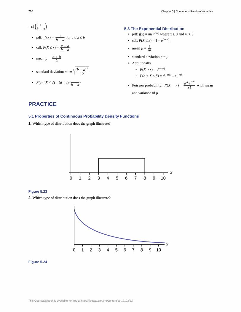
– c) ⎛⎝ 1b − a
⎞⎠
• pdf: f (x) = 1b − a for a ≤ x ≤ b
• cdf: P(X ≤ x) = x − ab − a
• mean µ = a + b2
• standard deviation σ = (b − a)2
12
• P(c < X < d) = (d – c) ( 1b – a)
5.3 The Exponential Distribution• pdf: f(x) = me(–mx) where x ≥ 0 and m > 0
• cdf: P(X ≤ x) = 1 – e(–mx)
• mean µ = 1m
• standard deviation σ = µ
• Additionally
◦ P(X > x) = e(–mx)
◦ P(a < X < b) = e(–ma) – e(–mb)
• Poisson probability: P(X = x) = μx e−μ
x ! with mean
and variance of μ
PRACTICE
5.1 Properties of Continuous Probability Density Functions
1. Which type of distribution does the graph illustrate?
Figure 5.23
2. Which type of distribution does the graph illustrate?
Figure 5.24
216 Chapter 5 | Continuous Random Variables
This OpenStax book is available for free at https://legacy.cnx.org/content/col12102/1.7

3. Which type of distribution does the graph illustrate?
Figure 5.25
4. What does the shaded area represent? P(___< x < ___)
Figure 5.26
5. What does the shaded area represent? P(___< x < ___)
Figure 5.27
6. For a continuous probability distribution, 0 ≤ x ≤ 15. What is P(x > 15)?
7. What is the area under f(x) if the function is a continuous probability density function?
8. For a continuous probability distribution, 0 ≤ x ≤ 10. What is P(x = 7)?
9. A continuous probability function is restricted to the portion between x = 0 and 7. What is P(x = 10)?
10. f(x) for a continuous probability function is 15 , and the function is restricted to 0 ≤ x ≤ 5. What is P(x < 0)?
11. f(x), a continuous probability function, is equal to 112 , and the function is restricted to 0 ≤ x ≤ 12. What is P (0 < x <
12)?
Chapter 5 | Continuous Random Variables 217

12. Find the probability that x falls in the shaded area.
Figure 5.28
13. Find the probability that x falls in the shaded area.
Figure 5.29
14. Find the probability that x falls in the shaded area.
Figure 5.30
15. f(x), a continuous probability function, is equal to 13 and the function is restricted to 1 ≤ x ≤ 4. Describe P⎛⎝x > 3
2⎞⎠.
5.2 The Uniform DistributionUse the following information to answer the next ten questions. The data that follow are the square footage (in 1,000 feetsquared) of 28 homes.
218 Chapter 5 | Continuous Random Variables
This OpenStax book is available for free at https://legacy.cnx.org/content/col12102/1.7
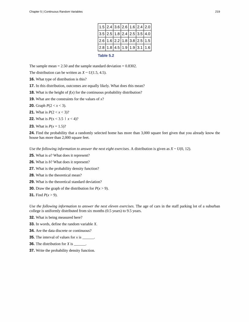
1.5 2.4 3.6 2.6 1.6 2.4 2.0
3.5 2.5 1.8 2.4 2.5 3.5 4.0
2.6 1.6 2.2 1.8 3.8 2.5 1.5
2.8 1.8 4.5 1.9 1.9 3.1 1.6
Table 5.2
The sample mean = 2.50 and the sample standard deviation = 0.8302.
The distribution can be written as X ~ U(1.5, 4.5).
16. What type of distribution is this?
17. In this distribution, outcomes are equally likely. What does this mean?
18. What is the height of f(x) for the continuous probability distribution?
19. What are the constraints for the values of x?
20. Graph P(2 < x < 3).
21. What is P(2 < x < 3)?
22. What is P(x < 3.5 | x < 4)?
23. What is P(x = 1.5)?
24. Find the probability that a randomly selected home has more than 3,000 square feet given that you already know thehouse has more than 2,000 square feet.
Use the following information to answer the next eight exercises. A distribution is given as X ~ U(0, 12).
25. What is a? What does it represent?
26. What is b? What does it represent?
27. What is the probability density function?
28. What is the theoretical mean?
29. What is the theoretical standard deviation?
30. Draw the graph of the distribution for P(x > 9).
31. Find P(x > 9).
Use the following information to answer the next eleven exercises. The age of cars in the staff parking lot of a suburbancollege is uniformly distributed from six months (0.5 years) to 9.5 years.
32. What is being measured here?
33. In words, define the random variable X.
34. Are the data discrete or continuous?
35. The interval of values for x is ______.
36. The distribution for X is ______.
37. Write the probability density function.
Chapter 5 | Continuous Random Variables 219

38. Graph the probability distribution.a. Sketch the graph of the probability distribution.
Figure 5.31b. Identify the following values:
i. Lowest value for x– : _______
ii. Highest value for x– : _______
iii. Height of the rectangle: _______iv. Label for x-axis (words): _______v. Label for y-axis (words): _______
39. Find the average age of the cars in the lot.
40. Find the probability that a randomly chosen car in the lot was less than four years old.a. Sketch the graph, and shade the area of interest.
Figure 5.32b. Find the probability. P(x < 4) = _______
220 Chapter 5 | Continuous Random Variables
This OpenStax book is available for free at https://legacy.cnx.org/content/col12102/1.7
41. Considering only the cars less than 7.5 years old, find the probability that a randomly chosen car in the lot was less thanfour years old.
a. Sketch the graph, shade the area of interest.
Figure 5.33b. Find the probability. P(x < 4 | x < 7.5) = _______
42. What has changed in the previous two problems that made the solutions different?
43. Find the third quartile of ages of cars in the lot. This means you will have to find the value such that 34 , or 75%, of the
cars are at most (less than or equal to) that age.a. Sketch the graph, and shade the area of interest.
Figure 5.34b. Find the value k such that P(x < k) = 0.75.c. The third quartile is _______
5.3 The Exponential DistributionUse the following information to answer the next ten exercises. A customer service representative must spend differentamounts of time with each customer to resolve various concerns. The amount of time spent with each customer can bemodeled by the following distribution: X ~ Exp(0.2)
44. What type of distribution is this?
45. Are outcomes equally likely in this distribution? Why or why not?
46. What is m? What does it represent?
47. What is the mean?
48. What is the standard deviation?
Chapter 5 | Continuous Random Variables 221

49. State the probability density function.
50. Graph the distribution.
51. Find P(2 < x < 10).
52. Find P(x > 6).
53. Find the 70th percentile.
Use the following information to answer the next seven exercises. A distribution is given as X ~ Exp(0.75).
54. What is m?
55. What is the probability density function?
56. What is the cumulative distribution function?
57. Draw the distribution.
58. Find P(x < 4).
59. Find the 30th percentile.
60. Find the median.
61. Which is larger, the mean or the median?
Use the following information to answer the next 16 exercises. Carbon-14 is a radioactive element with a half-life of about5,730 years. Carbon-14 is said to decay exponentially. The decay rate is 0.000121. We start with one gram of carbon-14.We are interested in the time (years) it takes to decay carbon-14.
62. What is being measured here?
63. Are the data discrete or continuous?
64. In words, define the random variable X.
65. What is the decay rate (m)?
66. The distribution for X is ______.
67. Find the amount (percent of one gram) of carbon-14 lasting less than 5,730 years. This means, find P(x < 5,730).a. Sketch the graph, and shade the area of interest.
Figure 5.35b. Find the probability. P(x < 5,730) = __________
222 Chapter 5 | Continuous Random Variables
This OpenStax book is available for free at https://legacy.cnx.org/content/col12102/1.7

68. Find the percentage of carbon-14 lasting longer than 10,000 years.a. Sketch the graph, and shade the area of interest.
Figure 5.36b. Find the probability. P(x > 10,000) = ________
69. Thirty percent (30%) of carbon-14 will decay within how many years?a. Sketch the graph, and shade the area of interest.
Figure 5.37b. Find the value k such that P(x < k) = 0.30.
HOMEWORK
5.1 Properties of Continuous Probability Density Functions
For each probability and percentile problem, draw the picture.
70. Consider the following experiment. You are one of 100 people enlisted to take part in a study to determine the percentof nurses in America with an R.N. (registered nurse) degree. You ask nurses if they have an R.N. degree. The nursesanswer “yes” or “no.” You then calculate the percentage of nurses with an R.N. degree. You give that percentage to yoursupervisor.
a. What part of the experiment will yield discrete data?b. What part of the experiment will yield continuous data?
71. When age is rounded to the nearest year, do the data stay continuous, or do they become discrete? Why?
Chapter 5 | Continuous Random Variables 223

5.2 The Uniform Distribution
For each probability and percentile problem, draw the picture.
72. Births are approximately uniformly distributed between the 52 weeks of the year. They can be said to follow a uniformdistribution from one to 53 (spread of 52 weeks).
a. Graph the probability distribution.b. f(x) = _________c. μ = _________d. σ = _________e. Find the probability that a person is born at the exact moment week 19 starts. That is, find P(x = 19) = _________f. P(2 < x < 31) = _________g. Find the probability that a person is born after week 40.h. P(12 < x | x < 28) = _________
73. A random number generator picks a number from one to nine in a uniform manner.a. Graph the probability distribution.b. f(x) = _________c. μ = _________d. σ = _________e. P(3.5 < x < 7.25) = _________f. P(x > 5.67)g. P(x > 5 | x > 3) = _________
74. According to a study by Dr. John McDougall of his live-in weight loss program at St. Helena Hospital, the people whofollow his program lose between six and 15 pounds a month until they approach trim body weight. Let’s suppose that theweight loss is uniformly distributed. We are interested in the weight loss of a randomly selected individual following theprogram for one month.
a. Define the random variable. X = _________b. Graph the probability distribution.c. f(x) = _________d. μ = _________e. σ = _________f. Find the probability that the individual lost more than ten pounds in a month.g. Suppose it is known that the individual lost more than ten pounds in a month. Find the probability that he lost less
than 12 pounds in the month.h. P(7 < x < 13 | x > 9) = __________. State this in a probability question, similarly to parts g and h, draw the
picture, and find the probability.
75. A subway train on the Red Line arrives every eight minutes during rush hour. We are interested in the length of time acommuter must wait for a train to arrive. The time follows a uniform distribution.
a. Define the random variable. X = _______b. Graph the probability distribution.c. f(x) = _______d. μ = _______e. σ = _______f. Find the probability that the commuter waits less than one minute.g. Find the probability that the commuter waits between three and four minutes.
76. The age of a first grader on September 1 at Garden Elementary School is uniformly distributed from 5.8 to 6.8 years.We randomly select one first grader from the class.
a. Define the random variable. X = _________b. Graph the probability distribution.c. f(x) = _________d. μ = _________e. σ = _________f. Find the probability that she is over 6.5 years old.g. Find the probability that she is between four and six years old.
Use the following information to answer the next three exercises. The Sky Train from the terminal to the rental–car and
224 Chapter 5 | Continuous Random Variables
This OpenStax book is available for free at https://legacy.cnx.org/content/col12102/1.7

long–term parking center is supposed to arrive every eight minutes. The waiting times for the train are known to follow auniform distribution.
77. What is the average waiting time (in minutes)?a. zerob. twoc. threed. four
78. The probability of waiting more than seven minutes given a person has waited more than four minutes is?a. 0.125b. 0.25c. 0.5d. 0.75
79. The time (in minutes) until the next bus departs a major bus depot follows a distribution with f(x) = 120 where x goes
from 25 to 45 minutes.a. Define the random variable. X = ________b. Graph the probability distribution.c. The distribution is ______________ (name of distribution). It is _____________ (discrete or continuous).d. μ = ________e. σ = ________f. Find the probability that the time is at most 30 minutes. Sketch and label a graph of the distribution. Shade the
area of interest. Write the answer in a probability statement.g. Find the probability that the time is between 30 and 40 minutes. Sketch and label a graph of the distribution.
Shade the area of interest. Write the answer in a probability statement.h. P(25 < x < 55) = _________. State this in a probability statement, similarly to parts g and h, draw the picture, and
find the probability.
80. Suppose that the value of a stock varies each day from $16 to $25 with a uniform distribution.a. Find the probability that the value of the stock is more than $19.b. Find the probability that the value of the stock is between $19 and $22.c. Given that the stock is greater than $18, find the probability that the stock is more than $21.
81. A fireworks show is designed so that the time between fireworks is between one and five seconds, and follows a uniformdistribution.
a. Find the average time between fireworks.b. Find probability that the time between fireworks is greater than four seconds.
82. The number of miles driven by a truck driver falls between 300 and 700, and follows a uniform distribution.a. Find the probability that the truck driver goes more than 650 miles in a day.b. Find the probability that the truck drivers goes between 400 and 650 miles in a day.
5.3 The Exponential Distribution
83. Suppose that the length of long distance phone calls, measured in minutes, is known to have an exponential distributionwith the average length of a call equal to eight minutes.
a. Define the random variable. X = ________________.b. Is X continuous or discrete?c. μ = ________d. σ = ________e. Draw a graph of the probability distribution. Label the axes.f. Find the probability that a phone call lasts less than nine minutes.g. Find the probability that a phone call lasts more than nine minutes.h. Find the probability that a phone call lasts between seven and nine minutes.i. If 25 phone calls are made one after another, on average, what would you expect the total to be? Why?
Chapter 5 | Continuous Random Variables 225
84. Suppose that the useful life of a particular car battery, measured in months, decays with parameter 0.025. We areinterested in the life of the battery.
a. Define the random variable. X = _________________________________.b. Is X continuous or discrete?c. On average, how long would you expect one car battery to last?d. On average, how long would you expect nine car batteries to last, if they are used one after another?e. Find the probability that a car battery lasts more than 36 months.f. Seventy percent of the batteries last at least how long?
85. The percent of persons (ages five and older) in each state who speak a language at home other than English isapproximately exponentially distributed with a mean of 9.848. Suppose we randomly pick a state.
a. Define the random variable. X = _________________________________.b. Is X continuous or discrete?c. μ = ________d. σ = ________e. Draw a graph of the probability distribution. Label the axes.f. Find the probability that the percent is less than 12.g. Find the probability that the percent is between eight and 14.h. The percent of all individuals living in the United States who speak a language at home other than English is 13.8.
i. Why is this number different from 9.848%?ii. What would make this number higher than 9.848%?
86. The time (in years) after reaching age 60 that it takes an individual to retire is approximately exponentially distributedwith a mean of about five years. Suppose we randomly pick one retired individual. We are interested in the time after age60 to retirement.
a. Define the random variable. X = _________________________________.b. Is X continuous or discrete?c. μ = ________d. σ = ________e. Draw a graph of the probability distribution. Label the axes.f. Find the probability that the person retired after age 70.g. Do more people retire before age 65 or after age 65?h. In a room of 1,000 people over age 80, how many do you expect will NOT have retired yet?
87. The cost of all maintenance for a car during its first year is approximately exponentially distributed with a mean of$150.
a. Define the random variable. X = _________________________________.b. μ = ________c. σ = ________d. Draw a graph of the probability distribution. Label the axes.e. Find the probability that a car required over $300 for maintenance during its first year.
Use the following information to answer the next three exercises. The average lifetime of a certain new cell phone is threeyears. The manufacturer will replace any cell phone failing within two years of the date of purchase. The lifetime of thesecell phones is known to follow an exponential distribution.
88. The decay rate is:a. 0.3333b. 0.5000c. 2d. 3
89. What is the probability that a phone will fail within two years of the date of purchase?a. 0.8647b. 0.4866c. 0.2212d. 0.9997
226 Chapter 5 | Continuous Random Variables
This OpenStax book is available for free at https://legacy.cnx.org/content/col12102/1.7
90. What is the median lifetime of these phones (in years)?a. 0.1941b. 1.3863c. 2.0794d. 5.5452
91. At a 911 call center, calls come in at an average rate of one call every two minutes. Assume that the time that elapsesfrom one call to the next has the exponential distribution.
a. On average, how much time occurs between five consecutive calls?b. Find the probability that after a call is received, it takes more than three minutes for the next call to occur.c. Ninety-percent of all calls occur within how many minutes of the previous call?d. Suppose that two minutes have elapsed since the last call. Find the probability that the next call will occur within
the next minute.e. Find the probability that less than 20 calls occur within an hour.
92. In major league baseball, a no-hitter is a game in which a pitcher, or pitchers, doesn't give up any hits throughoutthe game. No-hitters occur at a rate of about three per season. Assume that the duration of time between no-hitters isexponential.
a. What is the probability that an entire season elapses with a single no-hitter?b. If an entire season elapses without any no-hitters, what is the probability that there are no no-hitters in the
following season?c. What is the probability that there are more than 3 no-hitters in a single season?
93. During the years 1998–2012, a total of 29 earthquakes of magnitude greater than 6.5 have occurred in Papua NewGuinea. Assume that the time spent waiting between earthquakes is exponential.
a. What is the probability that the next earthquake occurs within the next three months?b. Given that six months has passed without an earthquake in Papua New Guinea, what is the probability that the
next three months will be free of earthquakes?c. What is the probability of zero earthquakes occurring in 2014?d. What is the probability that at least two earthquakes will occur in 2014?
94. According to the American Red Cross, about one out of nine people in the U.S. have Type B blood. Suppose the bloodtypes of people arriving at a blood drive are independent. In this case, the number of Type B blood types that arrive roughlyfollows the Poisson distribution.
a. If 100 people arrive, how many on average would be expected to have Type B blood?b. What is the probability that over 10 people out of these 100 have type B blood?c. What is the probability that more than 20 people arrive before a person with type B blood is found?
95. A web site experiences traffic during normal working hours at a rate of 12 visits per hour. Assume that the durationbetween visits has the exponential distribution.
a. Find the probability that the duration between two successive visits to the web site is more than ten minutes.b. The top 25% of durations between visits are at least how long?c. Suppose that 20 minutes have passed since the last visit to the web site. What is the probability that the next visit
will occur within the next 5 minutes?d. Find the probability that less than 7 visits occur within a one-hour period.
96. At an urgent care facility, patients arrive at an average rate of one patient every seven minutes. Assume that the durationbetween arrivals is exponentially distributed.
a. Find the probability that the time between two successive visits to the urgent care facility is less than 2 minutes.b. Find the probability that the time between two successive visits to the urgent care facility is more than 15 minutes.c. If 10 minutes have passed since the last arrival, what is the probability that the next person will arrive within the
next five minutes?d. Find the probability that more than eight patients arrive during a half-hour period.
REFERENCES
5.2 The Uniform Distribution
McDougall, John A. The McDougall Program for Maximum Weight Loss. Plume, 1995.
Chapter 5 | Continuous Random Variables 227
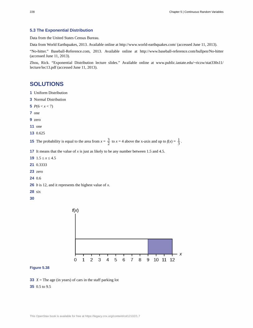
5.3 The Exponential Distribution
Data from the United States Census Bureau.
Data from World Earthquakes, 2013. Available online at http://www.world-earthquakes.com/ (accessed June 11, 2013).
“No-hitter.” Baseball-Reference.com, 2013. Available online at http://www.baseball-reference.com/bullpen/No-hitter(accessed June 11, 2013).
Zhou, Rick. “Exponential Distribution lecture slides.” Available online at www.public.iastate.edu/~riczw/stat330s11/lecture/lec13.pdf (accessed June 11, 2013).
SOLUTIONS
1 Uniform Distribution
3 Normal Distribution
5 P(6 < x < 7)
7 one
9 zero
11 one
13 0.625
15 The probability is equal to the area from x = 32 to x = 4 above the x-axis and up to f(x) = 1
3 .
17 It means that the value of x is just as likely to be any number between 1.5 and 4.5.
19 1.5 ≤ x ≤ 4.5
21 0.3333
23 zero
24 0.6
26 b is 12, and it represents the highest value of x.
28 six
30
Figure 5.38
33 X = The age (in years) of cars in the staff parking lot
35 0.5 to 9.5
228 Chapter 5 | Continuous Random Variables
This OpenStax book is available for free at https://legacy.cnx.org/content/col12102/1.7

37 f(x) = 19 where x is between 0.5 and 9.5, inclusive.
39 μ = 5
41a. Check student’s solution.
b. 3.57
43a. Check student's solution.
b. k = 7.25
c. 7.25
45 No, outcomes are not equally likely. In this distribution, more people require a little bit of time, and fewer people requirea lot of time, so it is more likely that someone will require less time.
47 five
49 f(x) = 0.2e-0.2x
51 0.5350
53 6.02
55 f(x) = 0.75e-0.75x
57
Figure 5.39
59 0.4756
61 The mean is larger. The mean is 1m = 1
0.75 ≈ 1.33 , which is greater than 0.9242.
63 continuous
65 m = 0.000121
67a. Check student's solution
b. P(x < 5,730) = 0.5001
69a. Check student's solution.
b. k = 2947.73
Chapter 5 | Continuous Random Variables 229

71 Age is a measurement, regardless of the accuracy used.
73a. Check student’s solution.
b. f (x) = 18 where 1 ≤ x ≤ 9
c. five
d. 2.3
e. 1532
f. 333800
g. 23
75a. X represents the length of time a commuter must wait for a train to arrive on the Red Line.
b. Graph the probability distribution.
c. f (x) = 18 where 0 ≤ x ≤ 8
d. four
e. 2.31
f. 18
g. 18
77 d
78 b
80
a. The probability density function of X is 125 − 16 = 1
9 .
P(X > 19) = (25 – 19) ⎛⎝19⎞⎠ = 6
9 = 23 .
Figure 5.40
b. P(19 < X < 22) = (22 – 19) ⎛⎝19⎞⎠ = 3
9 = 13 .
230 Chapter 5 | Continuous Random Variables
This OpenStax book is available for free at https://legacy.cnx.org/content/col12102/1.7

Figure 5.41
c. This is a conditional probability question. P(x > 21 | x > 18). You can do this two ways:
◦ Draw the graph where a is now 18 and b is still 25. The height is 1(25 − 18) = 1
7
So, P(x > 21 | x > 18) = (25 – 21) ⎛⎝17⎞⎠ = 4/7.
◦ Use the formula: P(x > 21 | x > 18) =P(x > 21 ∩ x > 18)
P(x > 18)
=P(x > 21)P(x > 18) =
(25 − 21)(25 − 18) = 4
7 .
82
a. P(X > 650) = 700 − 650700 − 300 = 50
400 = 18 = 0.125.
b. P(400 < X < 650) = 650 − 400700 − 300 = 250
400 = 0.625
84a. X = the useful life of a particular car battery, measured in months.
b. X is continuous.
c. 40 months
d. 360 months
e. 0.4066
f. 14.27
86a. X = the time (in years) after reaching age 60 that it takes an individual to retire
b. X is continuous.
c. five
d. five
e. Check student’s solution.
f. 0.1353
g. before
h. 18.3
88 a
90 c
Chapter 5 | Continuous Random Variables 231
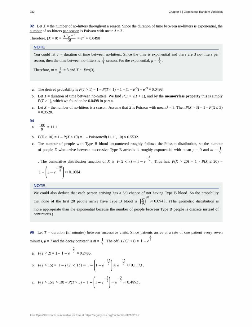
92 Let X = the number of no-hitters throughout a season. Since the duration of time between no-hitters is exponential, thenumber of no-hitters per season is Poisson with mean λ = 3.
Therefore, (X = 0) = 30 e – 3
0! = e–3 ≈ 0.0498
NOTE
You could let T = duration of time between no-hitters. Since the time is exponential and there are 3 no-hitters per
season, then the time between no-hitters is 13 season. For the exponential, µ = 1
3 .
Therefore, m = 1μ = 3 and T ∼ Exp(3).
a. The desired probability is P(T > 1) = 1 – P(T < 1) = 1 – (1 – e–3) = e–3 ≈ 0.0498.
b. Let T = duration of time between no-hitters. We find P(T > 2|T > 1), and by the memoryless property this is simplyP(T > 1), which we found to be 0.0498 in part a.
c. Let X = the number of no-hitters is a season. Assume that X is Poisson with mean λ = 3. Then P(X > 3) = 1 – P(X ≤ 3)= 0.3528.
94
a. 1009 = 11.11
b. P(X > 10) = 1 – P(X ≤ 10) = 1 – Poissoncdf(11.11, 10) ≈ 0.5532.
c. The number of people with Type B blood encountered roughly follows the Poisson distribution, so the number
of people X who arrive between successive Type B arrivals is roughly exponential with mean μ = 9 and m = 19
. The cumulative distribution function of X is P(X < x) = 1 − e− x
9 . Thus hus, P(X > 20) = 1 - P(X ≤ 20) =
1 −⎛⎝⎜1 − e
− 209⎞⎠⎟ ≈ 0.1084.
NOTE
We could also deduce that each person arriving has a 8/9 chance of not having Type B blood. So the probability
that none of the first 20 people arrive have Type B blood is ⎛⎝89⎞⎠
20≈ 0.0948 . (The geometric distribution is
more appropriate than the exponential because the number of people between Type B people is discrete instead ofcontinuous.)
96 Let T = duration (in minutes) between successive visits. Since patients arrive at a rate of one patient every seven
minutes, μ = 7 and the decay constant is m = 17 . The cdf is P(T < t) = 1 − e
t7
a. P(T < 2) = 1 - 1 − e− 2
7 ≈ 0.2485.
b. P(T > 15) = 1 − P(T < 15) = 1 −⎛⎝⎜1 − e
− 157⎞⎠⎟ ≈ e
− 157 ≈ 0.1173 .
c. P(T > 15|T > 10) = P(T > 5) = 1 −⎛⎝⎜1 − e
− 57⎞⎠⎟ = e
− 57 ≈ 0.4895 .
232 Chapter 5 | Continuous Random Variables
This OpenStax book is available for free at https://legacy.cnx.org/content/col12102/1.7

d. Let X = # of patients arriving during a half-hour period. Then X has the Poisson distribution with a mean of 307 , X ∼
Poisson ⎛⎝307⎞⎠ . Find P(X > 8) = 1 – P(X ≤ 8) ≈ 0.0311.
Chapter 5 | Continuous Random Variables 233

234 Chapter 5 | Continuous Random Variables
This OpenStax book is available for free at https://legacy.cnx.org/content/col12102/1.7

6 | THE NORMALDISTRIBUTION
Figure 6.1 If you ask enough people about their shoe size, you will find that your graphed data is shaped like a bellcurve and can be described as normally distributed. (credit: Ömer Ünlϋ)
Introduction
The normal, a continuous distribution, is the most important of all the distributions. It is widely used and even more widelyabused. Its graph is bell-shaped. You see the bell curve in almost all disciplines. Some of these include psychology, business,economics, the sciences, nursing, and, of course, mathematics. Some of your instructors may use the normal distribution tohelp determine your grade. Most IQ scores are normally distributed. Often real-estate prices fit a normal distribution. Thenormal distribution is extremely important, but it cannot be applied to everything in the real world.
In this chapter, you will study the normal distribution, the standard normal distribution, and applications associated withthem.
The normal distribution has two parameters (two numerical descriptive measures), the mean (μ) and the standard deviation(σ). If X is a quantity to be measured that has a normal distribution with mean (μ) and standard deviation (σ), we designatethis by writing
Chapter 6 | The Normal Distribution 235

Figure 6.2
The probability density function is a rather complicated function. Do not memorize it. It is not necessary.
f (x) = 1σ ⋅ 2 ⋅ π
⋅ e− 1
2 ⋅ ⎛⎝x − μσ⎞⎠2
The cumulative distribution function is P(X < x). It is calculated either by a calculator or a computer, or it is looked up in atable.
The curve is symmetrical about a vertical line drawn through the mean, μ. The mean is the same as the median, which is thesame as the mode, because the graph is symmetric about μ. As the notation indicates, the normal distribution depends onlyon the mean and the standard deviation. Since the area under the curve must equal one, a change in the standard deviation,σ, causes a change in the shape of the curve; the curve becomes fatter and wider or skinnier and taller depending on σ.A change in μ causes the graph to shift to the left or right. This means there are an infinite number of normal probabilitydistributions. One of special interest is called the standard normal distribution.
6.1 | The Standard Normal Distribution - (Base Version -
Lyryx Learning)The standard normal distribution is a normal distribution of standardized values called z-scores. A z-score is measuredin units of the standard deviation. For example, if the mean of a normal distribution is five and the standard deviation istwo, the value 11 is three standard deviations above (or to the right of) the mean. The calculation is as follows:
z = x - μσ = 11 - 5
2 = 3
The mean for the standard normal distribution is zero, and the standard deviation is one. That is, Z ~ N(0, 1). The value xcomes from a normal distribution with mean μ and standard deviation σ.
Z-ScoresIf X is a normally distributed random variable and X ~ N(μ, σ), then the z-score is:
z = x - μσ
The z-score tells you how many standard deviations the value x is above (to the right of) or below (to the left of) themean, μ. Values of x that are larger than the mean have positive z-scores, and values of x that are smaller than the meanhave negative z-scores. If x equals the mean, then x has a z-score of zero.
Example 6.1
Suppose X ~ N(5, 6). This means that x is a normally distributed random variable with mean μ = 5 and standard
236 Chapter 6 | The Normal Distribution
This OpenStax book is available for free at https://legacy.cnx.org/content/col12102/1.7

deviation σ = 6. Suppose x = 17. Then:
z = x - μσ = 17 - 5
6 = 2
This means that x = 17 is two standard deviations (2σ) above (or to the right) of the mean μ = 5. The standarddeviation is σ = 6.
Now suppose x = 1. Then:
z = 1 - 56 ≈ – 0.67
This means that x = 1 is 0.67 standard deviations below (or to the left) of the mean μ = 5.
Summarizing, when z is positive, x is above or to the right of μ. And when z is negative, x is to the left of or belowμ. Or, when z is positive, x is greater than μ, and when z is negative x is less than μ.
6.1 What is the z-score of x, when x = 7.5 and X ~ N(12,3)?
Example 6.2
Some doctors believe that a person can lose five pounds, on the average, in a month by reducing his or her fatintake and by exercising consistently. Suppose weight loss has a normal distribution. Let X = the amount of weightlost(in pounds) by a person in a month. Use a standard deviation of two pounds. X ~ N(5, 2). Fill in the blanks.
a. Suppose a person lost ten pounds in a month. The z-score when x = 10 pounds is z = _______ . This z-scoretells you that x = 10 is ________ standard deviations to the ________ (right or left) of the mean which is ______.
Solution 6.2a.
z = 10 - 52 = 2.5
z-score tells you that x = 10 is 2.5 standard deviations to the right of the mean which is five.
b. Suppose a person gained three pounds (a negative weight loss). Then z = __________. This z-score tells youthat x = –3 is ________ standard deviations to the __________ (right or left) of the mean.
Solution 6.2b.
z = -3 – 52 = -4
This z-score tells you that x = –3 is four standard deviations to the left of the mean.
Suppose the random variables X1 and X2 have the following normal distributions: X1 ~ N(5, 6) and X2 ~ N(2, 1).
If x1 = 17, z = x1 − μσ = 17 − 5
2 = 2 (μ = 5, σ = 6)
If x2 = 4, z = x2 − μσ = 4 − 2
1 = 2 (μ = 2, σ = 1)
Chapter 6 | The Normal Distribution 237

Therefore, x1 = 17 and x2 = 4 are both two (of their own) standard deviations to the right of their respective means.
The z-score allows us to compare data that are scaled differently. To understand the concept, suppose X1 ~ N(5, 6)represents weight gains for one group of people who are trying to gain weight and X1 ~ N(2, 1) measures the weight gain fora second group of people. A negative weight gain would be a weight loss. Since x2 = 17 and x2 = 4 are each two standarddeviations to the right of their means, they represent the same standardized weight gain relative to their means.
6.2 Fill in the blanks.
Jerome averages 16 points a game with a standard deviation of four points. X ~ N(16,4). Suppose Jerome scores tenpoints in a game. The z–score when x = 10 is _____. This score tells you that x = 10 is _____ standard deviations tothe ______(right or left) of the mean which is ______.
The Empirical Rule
If X is a random variable and has a normal distribution with mean µ and standard deviation σ, then the Empirical Rule saysthe following:
• About 68% of the x values lie between –1σ and +1σ of the mean µ (within one standard deviation of the mean).
• About 95% of the x values lie between –2σ and +2σ of the mean µ (within two standard deviations of the mean).
• About 99.7% of the x values lie between –3σ and +3σ of the mean µ (within three standard deviations of the mean).Notice that almost all the x values lie within three standard deviations of the mean.
• The z-scores for +1σ and –1σ are +1 and –1, respectively.
• The z-scores for +2σ and –2σ are +2 and –2, respectively.
• The z-scores for +3σ and –3σ are +3 and –3 respectively.
The empirical rule is also known as the 68-95-99.7 rule. See video (https://youtu.be/Txylq6RLiK8)
Figure 6.3
Example 6.3
The mean height of 15 to 18-year-old males from Chile from 2009 to 2010 was 170 cm with a standard deviationof 6.28 cm. Male heights are known to follow a normal distribution. Let X = the height of a 15 to 18-year-oldmale from Chile in 2009 to 2010. Then X ~ N(170, 6.28).
238 Chapter 6 | The Normal Distribution
This OpenStax book is available for free at https://legacy.cnx.org/content/col12102/1.7

Suppose a 15 to 18-year-old male from Chile was 168 cm tall from 2009 to 2010. The z-score when x = 168 cmis z = _______. This z-score tells you that x = 168 is ________ standard deviations to the ________ (right or left)of the mean which is _____ .
Solution 6.3–0.32, 0.32, left, 170
z = x - μσ = 168 - 170
6.28 = - 0.32
6.3 In 2012, 1,664,479 students took the SAT exam. The distribution of scores in the verbal section of the SAT had amean µ = 496 and a standard deviation σ = 114. Let X = a SAT exam verbal section score in 2012. Then X ~ N(496,114).
Find the z-scores for x1 = 325 and x2 = 366. Interpret each z-score. What can you say about x1 = 325 and x2 = 366?
Example 6.4
Suppose x has a normal distribution with mean 50 and standard deviation 6.
• About 68% of the x values lie between –1σ = (–1)(6) = –6 and 1σ = (1)(6) = 6 of the mean (50). The values50 – 6 = 44 and 50 + 6 = 56 are within one standard deviation of the mean (50). The z-scores are –1 and +1for 44 and 56, respectively.
• About 95% of the x values lie between –2σ = (–2)(6) = –12 and 2σ = (2)(6) = 12 of the mean (50). Thevalues 50 – 12 = 38 and 50 + 12 = 62 are within two standard deviations of the mean (50). The z-scores are–2 and +2 for 38 and 62, respectively.
• About 99.7% of the x values lie between –3σ = (–3)(6) = –18 and 3σ = (3)(6) = 18 of the mean (50). Thevalues 50 – 18 = 32 and 50 + 18 = 68 are within three standard deviations of the mean (50). The z-scores are–3 and +3 for 32 and 68, respectively.
6.4 Suppose X has a normal distribution with mean 25 and standard deviation five. Between what values of x do 68%of the values lie?
Example 6.5
From 1984 to 1985, the mean height of 15 to 18-year-old males from Chile was 172.36 cm, and the standarddeviation was 6.34 cm. Let X = the height of 15 to 18-year-old males in 1984 to 1985. Then X ~ N(172.36, 6.34).
a. About 68% of the x values lie between ___________ and ___________. The z-scores are ______ and______, respectively.
b. About 95% of the x values lie between ___________ and ___________. The z-scores are ______ and______, respectively.
c. About 99.7% of the x values lie between ___________ and ___________. The z-scores are ______ and______, respectively.
Chapter 6 | The Normal Distribution 239

Solution 6.5a. About 68% of the values lie between 166.02 and 178.7. The z-scores are –1 and 1.
b. About 95% of the values lie between 159.68 and 185.04. The z-scores are –2 and 2.
c. About 99.7% of the values lie between 153.34 and 191.38. The z-scores are –3 and 3.
6.5 The scores on a college entrance exam have an approximate normal distribution with mean, µ = 52 points and astandard deviation, σ = 11 points.
a. About 68% of the scores lie between ___________ and ___________. The z-scores are ______ and ______,respectively.
b. About 95% of the scores lie between ___________ and ___________. The z-scores are ______ and ______,respectively.
c. About 99.7% of the scores lie between ___________ and ___________. The z-scores are ______ and ______,respectively.
Example 6.6
Suppose a normal distribution has a mean score of 15 and a standard deviation of 3. That is X ~ (15, 3).
a. Approximately what percent of the scores are Between 9 and 21?
Solution 6.6a. Approximately 95%
Figure 6.4
b. Approximately what percent of the scores are less than 6?
Solution 6.6b. Approximately 0.15%
240 Chapter 6 | The Normal Distribution
This OpenStax book is available for free at https://legacy.cnx.org/content/col12102/1.7

Figure 6.5
c. Approximately what percent of the scores are greater than 18?
Solution 6.6c. Approximately 16%
Figure 6.6
d. Approximately what percent of the scores are below 21?
Solution 6.6d. Approximately 97.5%
Chapter 6 | The Normal Distribution 241
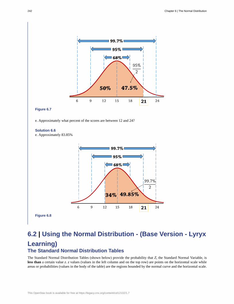
Figure 6.7
e. Approximately what percent of the scores are between 12 and 24?
Solution 6.6e. Approximately 83.85%
Figure 6.8
6.2 | Using the Normal Distribution - (Base Version - Lyryx
Learning)The Standard Normal Distribution TablesThe Standard Normal Distribution Tables (shown below) provide the probability that Z, the Standard Normal Variable, isless than a certain value z. z values (values in the left column and on the top row) are points on the horizontal scale whileareas or probabilities (values in the body of the table) are the regions bounded by the normal curve and the horizontal scale.
242 Chapter 6 | The Normal Distribution
This OpenStax book is available for free at https://legacy.cnx.org/content/col12102/1.7

Figure 6.9 Table of Standard Normal Probabilities for Negative z-scores Table of Standard Normal Probabilities
Chapter 6 | The Normal Distribution 243

for Negative z-scores. Table entries are "less than" areas.
244 Chapter 6 | The Normal Distribution
This OpenStax book is available for free at https://legacy.cnx.org/content/col12102/1.7

Figure 6.10 Table of Standard Normal Probabilities for Positive z-scores Table of Standard Normal Probabilities
Chapter 6 | The Normal Distribution 245

for Positive z-scores. Table entries are "less than" areas.
The shaded area in the following graph indicates the area to the left of z1. This area is represented by the probability P(z <z1).
Figure 6.11
P(z < z1) = Area to the left of the vertical line through z1.P(z > z1) = 1 – P(z < z1) = Area to the right of the vertical line through z1.P(z < z1) is the same as P(z ≤ z1) and P(z > z1) is the same as P(z ≥ z1) for continuous distributions.
To locate the area less than z = 1.43 on the table, for example, locate the row for 1.4 and the column for 0.03 (Figure6.12). The intersection of the row and column gives 0.9236. Hence P(z < 1.43) = 0.9236. Consequently, P(z > 1.43) = 1 -P(z <1.43) = 1 - 0.9236 = 0.0764.
Figure 6.12
Calculations of Probabilities
Example 6.7
Use the standard normal tables to find the following areas/probabilities:
a. Area to the left of z = 1.36: P(z < 1.36)
Solution 6.7a. P(z < 1.36) = 0.9131
b. Area to the left of z = -0.60: P(z < − 0.60)
Solution 6.7b. P(z < − 0.60) = 0.2743
c. Area to the right of z = 1.47: P(z > 1.47)
246 Chapter 6 | The Normal Distribution
This OpenStax book is available for free at https://legacy.cnx.org/content/col12102/1.7

Solution 6.7c. P(z > 1.47) = 1 − P(z < 1.47) = 1 − 0.9292 = 0.0708
d. Area to the right of z = -0.33: P(z > − 0.33) .
Solution 6.7d. P(z > − 0.33) = 1 − P(z < − 0.33) = 1 − 0.3707 = 0.6293
e. Area between z = -2.16 and z = 0.45: P(−2.16 < z < − 0.33)
Solution 6.7e. P(−2.16 < z < − 0.33) = P(z < 0.45) − P(z < − 2.16) = 0.6736 − 0.0154 = 0.6582
f. Area between z = 1.13 and z = 3.10: P(1.13 < z < 3.10)
Solution 6.7f. P(1.13 < z < 3.10) = P(z < 3.10) − P(z < 1.13) = 0.9990 − 0.8708 = 0.1282
Example 6.8
The final exam scores in a statistics class were normally distributed with a mean of 63 and a standard deviationof 5.
a. Find the probability that a randomly selected student scored less than 65 on the exam.
Solution 6.8
a. Let X = score on the final exam. X ~ N(63, 5) where μ = 63 and σ = 5. We begin by calculating the z-score for65, using the formula
z = x - μσ .
For x = 65, the corresponding z-score is
z = 65 - 635 = 0.4
From the z-tables, the area corresponding to z = 0.40 is 0.6554. That is,
P(x < 65) = P(z < 0.40) = 0.6554
Figure 6.13
The probability that any student selected at random scores less than 65 is 0.6554.Interpretation: About 65.54% of students who took the test scored below 65.
b. Find the probability that a randomly selected student scored more than 57 on the exam.
Chapter 6 | The Normal Distribution 247
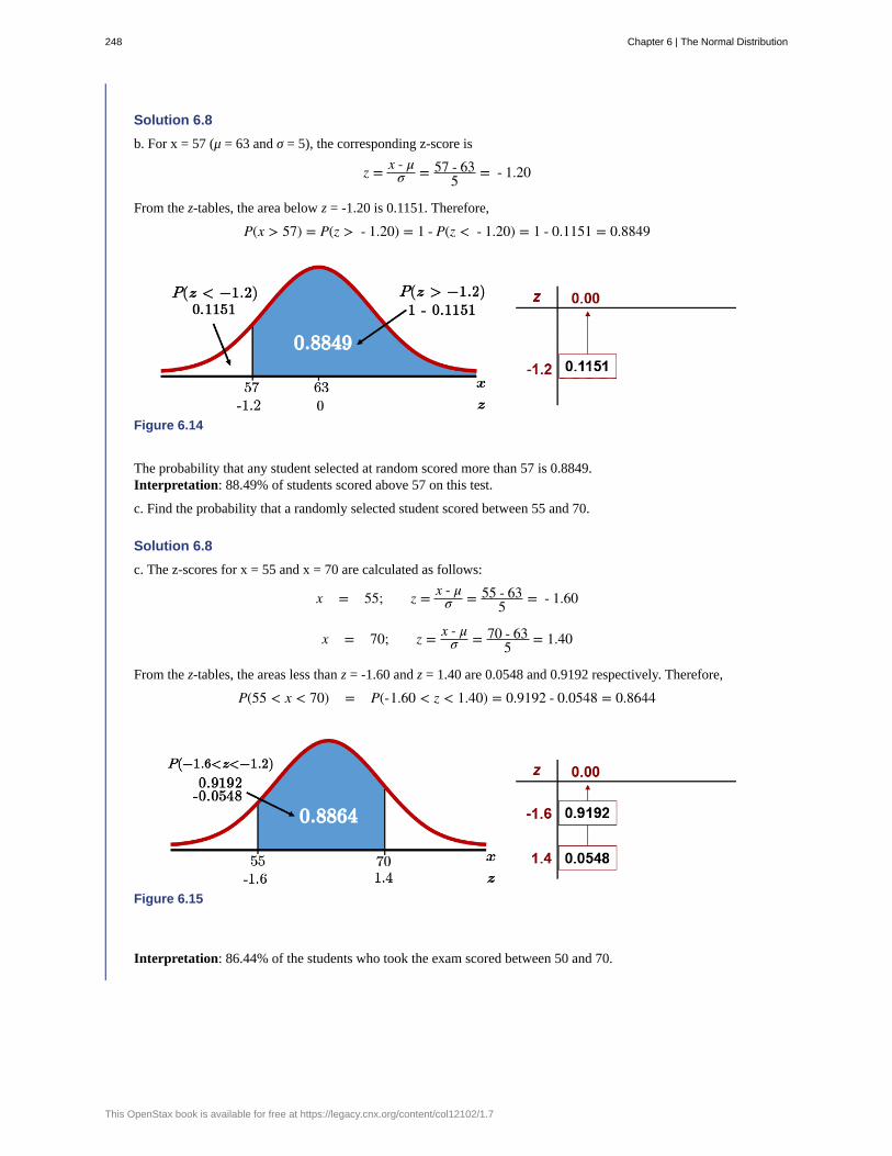
Solution 6.8
b. For x = 57 (μ = 63 and σ = 5), the corresponding z-score is
z = x - μσ = 57 - 63
5 = - 1.20
From the z-tables, the area below z = -1.20 is 0.1151. Therefore,
P(x > 57) = P(z > - 1.20) = 1 - P(z < - 1.20) = 1 - 0.1151 = 0.8849
Figure 6.14
The probability that any student selected at random scored more than 57 is 0.8849.Interpretation: 88.49% of students scored above 57 on this test.
c. Find the probability that a randomly selected student scored between 55 and 70.
Solution 6.8
c. The z-scores for x = 55 and x = 70 are calculated as follows:
x = 55; z = x - μσ = 55 - 63
5 = - 1.60
x = 70; z = x - μσ = 70 - 63
5 = 1.40
From the z-tables, the areas less than z = -1.60 and z = 1.40 are 0.0548 and 0.9192 respectively. Therefore,
P(55 < x < 70) = P(-1.60 < z < 1.40) = 0.9192 - 0.0548 = 0.8644
Figure 6.15
Interpretation: 86.44% of the students who took the exam scored between 50 and 70.
248 Chapter 6 | The Normal Distribution
This OpenStax book is available for free at https://legacy.cnx.org/content/col12102/1.7
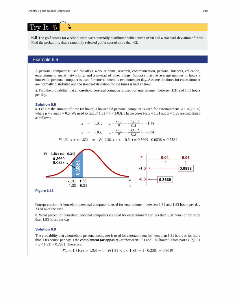
6.8 The golf scores for a school team were normally distributed with a mean of 68 and a standard deviation of three.Find the probability that a randomly selected golfer scored more than 63.
Example 6.9
A personal computer is used for office work at home, research, communication, personal finances, education,entertainment, social networking, and a myriad of other things. Suppose that the average number of hours ahousehold personal computer is used for entertainment is two hours per day. Assume the times for entertainmentare normally distributed and the standard deviation for the times is half an hour.
a. Find the probability that a household personal computer is used for entertainment between 1.31 and 1.83 hoursper day.
Solution 6.9a. Let X = the amount of time (in hours) a household personal computer is used for entertainment. X ~ N(2, 0.5)where μ = 2 and σ = 0.5. We need to find P(1.31 < x < 1.83). The z-scores for x = 1.31 and x = 1.83 are calculatedas follows:
x = 1.31; z = x - μσ = 1.31 - 2
0.5 = - 1.38
x = 1.83; z = x - μσ = 1.83 - 2
0.5 = - 0.34
P(1.31 < x < 1.83) = P(-1.38 < z < - 0.34) = 0.3669 - 0.0838 = 0.2381
Figure 6.16
Interpretation: A household personal computer is used for entertainment between 1.31 and 1.83 hours per day23.81% of the time.
b. What percent of household personal computers are used for entertainment for less than 1.31 hours or for morethan 1.83 hours per day.
Solution 6.9
The probability that a household personal computer is used for entertainment for “less than 1.31 hours or for morethan 1.83 hours” per day is the complement (or opposite) of “between 1.31 and 1.83 hours”. From part a), P(1.31< x < 1.83) = 0.2381. Therefore,
P(x < 1.31orx > 1.83) = 1 – P(1.31 < x < 1.83) = 1 - 0.2381 = 0.7619
Chapter 6 | The Normal Distribution 249

Figure 6.17
Interpretation: 76.19% of household personal computers are used for entertainment for less than 1.31 hours orfor more than 1.83 hours per day
6.9 The golf scores for a school team were normally distributed with a mean of 68 and a standard deviation of three.Find the probability that a golfer scored between 64 and 70.
Calculating ScoresWe are sometimes faced with the problem of finding a score (z or x), rather than probability (or area). That is, we areprovided with the probability (or area) in a region and are required to find the corresponding z-score and/or x value. Thisreverse lookup process is shown in the following examples.
Example 6.10
a. Find the value of z1 in the figure below. The area to the left of z1 is 0.0485 or P(z < z1) = 0.0485 .
Figure 6.18
Solution 6.10a. The area less than z1 is 0.0485. Since this area is less than 0.5, it can be found on the negative z-score table.Looking 0.0485 up in the area section of the z-table, we see that the corresponding z-score is -1.66.
250 Chapter 6 | The Normal Distribution
This OpenStax book is available for free at https://legacy.cnx.org/content/col12102/1.7
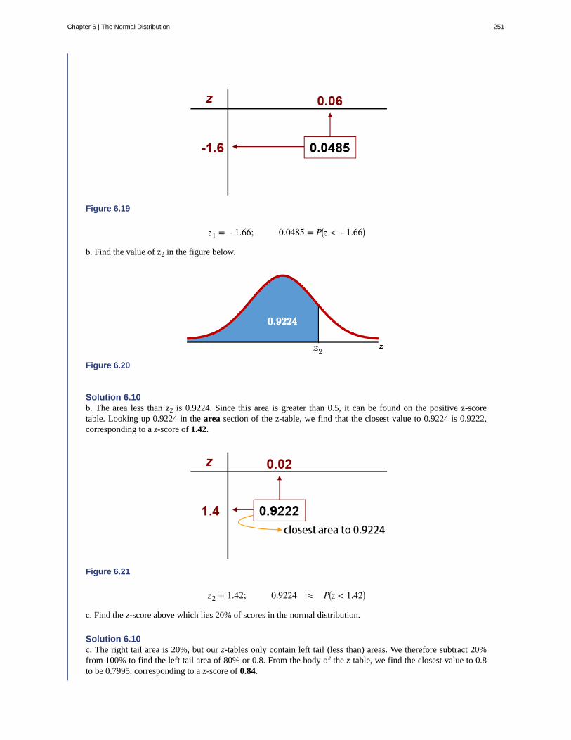
Figure 6.19
z1 = - 1.66; 0.0485 = P⎛⎝z < - 1.66⎞⎠
b. Find the value of z2 in the figure below.
Figure 6.20
Solution 6.10b. The area less than z2 is 0.9224. Since this area is greater than 0.5, it can be found on the positive z-scoretable. Looking up 0.9224 in the area section of the z-table, we find that the closest value to 0.9224 is 0.9222,corresponding to a z-score of 1.42.
Figure 6.21
z2 = 1.42; 0.9224 ≈ P⎛⎝z < 1.42⎞⎠
c. Find the z-score above which lies 20% of scores in the normal distribution.
Solution 6.10c. The right tail area is 20%, but our z-tables only contain left tail (less than) areas. We therefore subtract 20%from 100% to find the left tail area of 80% or 0.8. From the body of the z-table, we find the closest value to 0.8to be 0.7995, corresponding to a z-score of 0.84.
Chapter 6 | The Normal Distribution 251

Figure 6.22
P(z > 0.84) ≈ 0.2
d. Find b such that P(z > b) = 0. 9121
Solution 6.10d. P(z > b) = 0. 9121 implies that the area to the right of b is 0.9121. Since this area is on the right, and the normaltables we have only provide areas on the left, we subtract 0.9121 from 1, so that the "less than area" is 0.0879.The closest area in the table is 0.0885, corresponding to a z-score is -1.35.
Figure 6.23
b = - 1.35; P(z > - 1.35) ≈ 0.9121
Calculating x-values
Starting with the z-formula, we can solve for x as follows:
z = x − μσ ⇒ zσ = x − μ μ + zσ = x
x = μ + zσ
Example 6.11
Suppose the highway fuel consumption of cars sold in a city follows a normal distribution with a mean of 8.7 L/100km and a standard deviation of 2.5 L/100km.
a. What fuel consumption rate represents the third quartile?
Solution 6.11a. Let X = car fuel consumption. X ~ N(8.7, 2.5) where μ = 8.7 and σ = 2.5. The area below the 3rd quartile (75thpercentile) is 0.75. Since we already have μ and σ, we simply need to find the z-score corresponding to the lowerarea of 0.75 in the table. The closest area to 0.75 in the standard normal table is 0.7486 and this corresponds to z= 0.67. Therefore,
252 Chapter 6 | The Normal Distribution
This OpenStax book is available for free at https://legacy.cnx.org/content/col12102/1.7

z = x - μσ becomes 0.67 = x - 8.7
2.50.67(2.5) = x − 8.7 ⇒ x = 8.7 + 0.67(2.5) = 10.375
Or we can simply use the x transformation formula obtained earlier:x = μ + zσ = 8.7 + 0.67⎛⎝2.5⎞⎠ = 10.375
Figure 6.24
The fuel consumption rate representing the third quartile is 10.375 L/100km.
b. Determine the fuel consumption rate above which 90% of the cars will fall.
Solution 6.11b. If the fuel consumption rate has 90% higher than it, then it has 10% lower. We then search for the closestz-score to 0.1. The closest area to 0.1 is 0.1003, corresponding to a z-score of -1.28. Therefore,
x = μ + zσ = 8.7 - 1.28⎛⎝2.5⎞⎠ = 5.5
Figure 6.25
The fuel consumption rate above which 90% of the cars will fall is 5.5L/100km. This is the 10th percentile rate.That is, only 10% of the cars have consumption rate of 5.5L/km or better.
c. What is the fuel consumption rate of the least efficient 20% of the cars?
Solution 6.11c. The least efficient 20% of the cars will have the worst fuel consumption rates, and thus the highest 20% L/100km values. As a result, the required rate will separate the top 20% of the rates from bottom 80%. Searchingfor the closest area to 0.8 we find 0.7995 which corresponds to a z-score of 0.84. The required consumption rateis
x = μ + zσ = 8.7 + 0.84⎛⎝2.5⎞⎠ = 10.8
Chapter 6 | The Normal Distribution 253
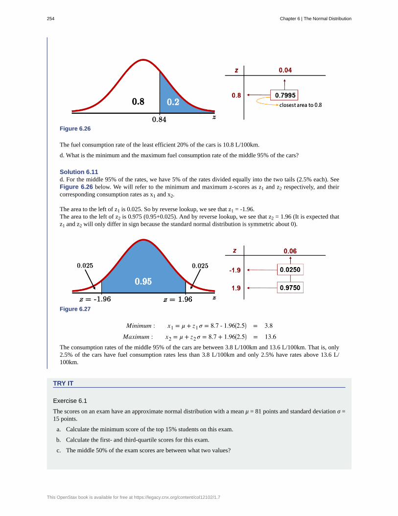
Figure 6.26
The fuel consumption rate of the least efficient 20% of the cars is 10.8 L/100km.
d. What is the minimum and the maximum fuel consumption rate of the middle 95% of the cars?
Solution 6.11d. For the middle 95% of the rates, we have 5% of the rates divided equally into the two tails (2.5% each). SeeFigure 6.26 below. We will refer to the minimum and maximum z-scores as z1 and z2 respectively, and theircorresponding consumption rates as x1 and x2.
The area to the left of z1 is 0.025. So by reverse lookup, we see that z1 = -1.96.The area to the left of z2 is 0.975 (0.95+0.025). And by reverse lookup, we see that z2 = 1.96 (It is expected thatz1 and z2 will only differ in sign because the standard normal distribution is symmetric about 0).
Figure 6.27
Minimum : x1 = μ + z1 σ = 8.7 - 1.96⎛⎝2.5⎞⎠ = 3.8
Maximum : x2 = μ + z2 σ = 8.7 + 1.96⎛⎝2.5⎞⎠ = 13.6The consumption rates of the middle 95% of the cars are between 3.8 L/100km and 13.6 L/100km. That is, only2.5% of the cars have fuel consumption rates less than 3.8 L/100km and only 2.5% have rates above 13.6 L/100km.
TRY IT
Exercise 6.1
The scores on an exam have an approximate normal distribution with a mean μ = 81 points and standard deviation σ =15 points.
a. Calculate the minimum score of the top 15% students on this exam.
b. Calculate the first- and third-quartile scores for this exam.
c. The middle 50% of the exam scores are between what two values?
254 Chapter 6 | The Normal Distribution
This OpenStax book is available for free at https://legacy.cnx.org/content/col12102/1.7
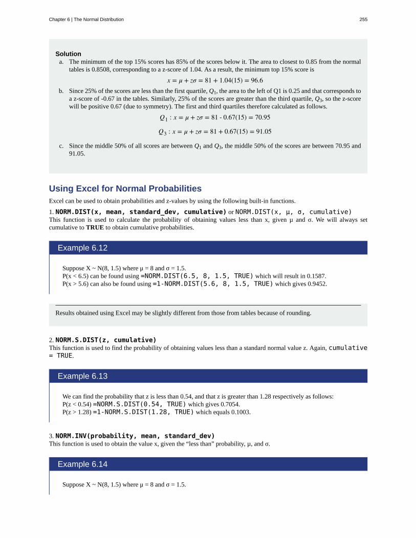
Solutiona. The minimum of the top 15% scores has 85% of the scores below it. The area to closest to 0.85 from the normal
tables is 0.8508, corresponding to a z-score of 1.04. As a result, the minimum top 15% score is
x = μ + zσ = 81 + 1.04(15) = 96.6b. Since 25% of the scores are less than the first quartile, Q1, the area to the left of Q1 is 0.25 and that corresponds to
a z-score of -0.67 in the tables. Similarly, 25% of the scores are greater than the third quartile, Q3, so the z-scorewill be positive 0.67 (due to symmetry). The first and third quartiles therefore calculated as follows.
Q1 : x = μ + zσ = 81 - 0.67(15) = 70.95
Q3 : x = μ + zσ = 81 + 0.67(15) = 91.05
c. Since the middle 50% of all scores are between Q1 and Q3, the middle 50% of the scores are between 70.95 and91.05.
Using Excel for Normal ProbabilitiesExcel can be used to obtain probabilities and z-values by using the following built-in functions.
1. NORM.DIST(x, mean, standard_dev, cumulative) or NORM.DIST(x, µ, σ, cumulative)This function is used to calculate the probability of obtaining values less than x, given µ and σ. We will always setcumulative to TRUE to obtain cumulative probabilities.
Example 6.12
Suppose X ~ N(8, 1.5) where μ = 8 and σ = 1.5.P(x < 6.5) can be found using =NORM.DIST(6.5, 8, 1.5, TRUE) which will result in 0.1587.P(x > 5.6) can also be found using =1-NORM.DIST(5.6, 8, 1.5, TRUE) which gives 0.9452.
Results obtained using Excel may be slightly different from those from tables because of rounding.
2. NORM.S.DIST(z, cumulative)This function is used to find the probability of obtaining values less than a standard normal value z. Again, cumulative= TRUE.
Example 6.13
We can find the probability that z is less than 0.54, and that z is greater than 1.28 respectively as follows:P(z < 0.54) =NORM.S.DIST(0.54, TRUE) which gives 0.7054.P(z > 1.28) =1-NORM.S.DIST(1.28, TRUE) which equals 0.1003.
3. NORM.INV(probability, mean, standard_dev)This function is used to obtain the value x, given the “less than” probability, µ, and σ.
Example 6.14
Suppose X ~ N(8, 1.5) where μ = 8 and σ = 1.5.
Chapter 6 | The Normal Distribution 255

Then the score corresponding to the 10th percentile can be obtained by =NORM.INV(0.1, 8, 1.5) = 6.08.The minimum score of the top 30% of the scores can also be obtained by =NORM.INV(1-0.3, 8, 1.5) =8.79.
4. NORM.S.INV(probability)This function is used to obtain a standard normal score z corresponding to a specified “less than” probability.
Example 6.15
The z-score corresponding to the 37th percentile can be obtained by =NORM.S.INV(0.37) = -0.33The z-score that has 7.5% of the area above it can be obtained by =NORM.S.INV(1-0.075) = 1.44
256 Chapter 6 | The Normal Distribution
This OpenStax book is available for free at https://legacy.cnx.org/content/col12102/1.7
Normal Distribution
Standard Normal Distribution
z-score
KEY TERMS
a continuous random variable (RV) with pdf f(x) = 1σ 2π
e
– (x – μ)2σ2
2
, where μ is the mean of
the distribution and σ is the standard deviation; notation: X ~ N(μ, σ). If μ = 0 and σ = 1, the RV, Z, is called thestandard normal distribution.
a continuous random variable (RV) X ~ N(0, 1); when X follows the standard normaldistribution, it is often noted as Z ~ N(0, 1).
the linear transformation of the form z =x – μ
σ ; if this transformation is applied to any normal distribution X ~
N(μ, σ) the result is the standard normal distribution Z ~ N(0,1). If this transformation is applied to any specificvalue x of the RV with mean μ and standard deviation σ, the result is called the z-score of x. The z-score allows us tocompare data that are normally distributed but scaled differently.
CHAPTER REVIEW
6.1 The Standard Normal Distribution - (Base Version - Lyryx Learning)A z-score is a standardized value. Its distribution is the standard normal, Z ~ N(0, 1). The mean of the z-scores is zero andthe standard deviation is one. If z is the z-score for a value x from the normal distribution N(µ, σ) then z tells you how manystandard deviations x is above (greater than) or below (less than) µ.
6.2 Using the Normal Distribution - (Base Version - Lyryx Learning)The normal distribution, which is continuous, is the most important of all the probability distributions. Its graph is bell-shaped. This bell-shaped curve is used in almost all disciplines. Since it is a continuous distribution, the total area underthe curve is one. The parameters of the normal are the mean µ and the standard deviation σ. A special normal distribution,called the standard normal distribution is the distribution of z-scores. Its mean is zero, and its standard deviation is one.
FORMULA REVIEW
6.0 Introduction -- Normal Distribution - (BaseVersion - Lyryx Learning)
X ∼ N(μ, σ)
μ = the mean; σ = the standard deviation
6.1 The Standard Normal Distribution - (BaseVersion - Lyryx Learning)
Z ~ N(0, 1)
z = a standardized value (z-score)
mean = 0; standard deviation = 1
To find the Kth percentile of X when the z-scores is known:k = μ + (z)σ
z-score: z =x – μσ
Z = the random variable for z-scores
Z ~ N(0, 1)
6.2 Using the Normal Distribution - (BaseVersion - Lyryx Learning)
Normal Distribution: X ~ N(µ, σ) where µ is the mean andσ is the standard deviation.
Standard Normal Distribution: Z ~ N(0, 1).
Formula for calculating z-socres: z = x - μσ
Formula for finding x: x = μ + zσ
PRACTICE
Chapter 6 | The Normal Distribution 257

6.1 The Standard Normal Distribution - (Base Version - Lyryx Learning)
2. A bottle of water contains 12.05 fluid ounces with a standard deviation of 0.01 ounces. Define the random variable X inwords. X = ____________.
3. A normal distribution has a mean of 61 and a standard deviation of 15. What is the median?
4. X ~ N(1, 2)
σ = _______
5. A company manufactures rubber balls. The mean diameter of a ball is 12 cm with a standard deviation of 0.2 cm. Definethe random variable X in words. X = ______________.
6. X ~ N(–4, 1)
What is the median?
7. X ~ N(3, 5)
σ = _______
8. X ~ N(–2, 1)
μ = _______
9. What does a z-score measure?
10. What does standardizing a normal distribution do to the mean?
11. Is X ~ N(0, 1) a standardized normal distribution? Why or why not?
12. What is the z-score of x = 12, if it is two standard deviations to the right of the mean?
13. What is the z-score of x = 9, if it is 1.5 standard deviations to the left of the mean?
14. What is the z-score of x = –2, if it is 2.78 standard deviations to the right of the mean?
15. What is the z-score of x = 7, if it is 0.133 standard deviations to the left of the mean?
16. Suppose X ~ N(2, 6). What value of x has a z-score of three?
17. Suppose X ~ N(8, 1). What value of x has a z-score of –2.25?
18. Suppose X ~ N(9, 5). What value of x has a z-score of –0.5?
19. Suppose X ~ N(2, 3). What value of x has a z-score of –0.67?
20. Suppose X ~ N(4, 2). What value of x is 1.5 standard deviations to the left of the mean?
21. Suppose X ~ N(4, 2). What value of x is two standard deviations to the right of the mean?
22. Suppose X ~ N(8, 9). What value of x is 0.67 standard deviations to the left of the mean?
23. Suppose X ~ N(–1, 2). What is the z-score of x = 2?
24. Suppose X ~ N(12, 6). What is the z-score of x = 2?
25. Suppose X ~ N(9, 3). What is the z-score of x = 9?
26. Suppose a normal distribution has a mean of six and a standard deviation of 1.5. What is the z-score of x = 5.5?
27. In a normal distribution, x = 5 and z = –1.25. This tells you that x = 5 is ____ standard deviations to the ____ (right orleft) of the mean.
28. In a normal distribution, x = 3 and z = 0.67. This tells you that x = 3 is ____ standard deviations to the ____ (right orleft) of the mean.
29. In a normal distribution, x = –2 and z = 6. This tells you that x = –2 is ____ standard deviations to the ____ (right orleft) of the mean.
30. In a normal distribution, x = –5 and z = –3.14. This tells you that x = –5 is ____ standard deviations to the ____ (rightor left) of the mean.
31. In a normal distribution, x = 6 and z = –1.7. This tells you that x = 6 is ____ standard deviations to the ____ (right orleft) of the mean.
258 Chapter 6 | The Normal Distribution
This OpenStax book is available for free at https://legacy.cnx.org/content/col12102/1.7

32. About what percent of x values from a normal distribution lie within one standard deviation (left and right) of the meanof that distribution?
33. About what percent of the x values from a normal distribution lie within two standard deviations (left and right) of themean of that distribution?
34. About what percent of x values lie between the second and third standard deviations (both sides)?
35. Suppose X ~ N(15, 3). Between what x values does 68.27% of the data lie? The range of x values is centered at the meanof the distribution (i.e., 15).
36. Suppose X ~ N(–3, 1). Between what x values does 95.45% of the data lie? The range of x values is centered at the meanof the distribution(i.e., –3).
37. Suppose X ~ N(–3, 1). Between what x values does 34.14% of the data lie?
38. About what percent of x values lie between the mean and three standard deviations?
39. About what percent of x values lie between the mean and one standard deviation?
40. About what percent of x values lie between the first and second standard deviations from the mean (both sides)?
41. About what percent of x values lie betwween the first and third standard deviations(both sides)?Use the following information to answer the next two exercises: The life of Sunshine CD players is normally distributedwith mean of 4.1 years and a standard deviation of 1.3 years. A CD player is guaranteed for three years. We are interestedin the length of time a CD player lasts.
42. Define the random variable X in words. X = _______________.
43. X ~ _____(_____,_____)
6.2 Using the Normal Distribution - (Base Version - Lyryx Learning)
44. How would you represent the area to the left of one in a probability statement?
Figure 6.28
45. What is the area to the right of one?
Figure 6.29
46. Is P(x < 1) equal to P(x ≤ 1)? Why?
Chapter 6 | The Normal Distribution 259

47. How would you represent the area to the left of three in a probability statement?
Figure 6.30
48. What is the area to the right of three?
Figure 6.31
49. If the area to the left of x in a normal distribution is 0.123, what is the area to the right of x?
50. If the area to the right of x in a normal distribution is 0.543, what is the area to the left of x?Use the following information to answer the next four exercises:
X ~ N(54, 8)
51. Find the probability that x > 56.
52. Find the probability that x < 30.
53. Find the 80th percentile.
54. Find the 60th percentile.
55. X ~ N(6, 2)
Find the probability that x is between three and nine.
56. X ~ N(–3, 4)
Find the probability that x is between one and four.
57. X ~ N(4, 5)
Find the maximum of x in the bottom quartile.
HOMEWORK
6.1 The Standard Normal Distribution - (Base Version - Lyryx Learning)
Use the following information to answer the next two exercises: The patient recovery time from a particular surgicalprocedure is normally distributed with a mean of 5.3 days and a standard deviation of 2.1 days.
260 Chapter 6 | The Normal Distribution
This OpenStax book is available for free at https://legacy.cnx.org/content/col12102/1.7
58. What is the median recovery time?a. 2.7b. 5.3c. 7.4d. 2.1
59. What is the z-score for a patient who takes ten days to recover?a. 1.5b. 0.2c. 2.2d. 7.3
60. The length of time to find it takes to find a parking space at 9 A.M. follows a normal distribution with a mean of fiveminutes and a standard deviation of two minutes. If the mean is significantly greater than the standard deviation, which ofthe following statements is true?
I. The data cannot follow the uniform distribution.II. The data cannot follow the exponential distribution..
III. The data cannot follow the normal distribution.a. I onlyb. II onlyc. III onlyd. I, II, and III
61. The heights of the 430 National Basketball Association players were listed on team rosters at the start of the 2005–2006season. The heights of basketball players have an approximate normal distribution with mean, µ = 79 inches and a standarddeviation, σ = 3.89 inches. For each of the following heights, calculate the z-score and interpret it using complete sentences.
a. 77 inchesb. 85 inchesc. If an NBA player reported his height had a z-score of 3.5, would you believe him? Explain your answer.
62. The systolic blood pressure (given in millimeters) of males has an approximately normal distribution with mean µ =125 and standard deviation σ = 14. Systolic blood pressure for males follows a normal distribution.
a. Calculate the z-scores for the male systolic blood pressures 100 and 150 millimeters.b. If a male friend of yours said he thought his systolic blood pressure was 2.5 standard deviations below the mean,
but that he believed his blood pressure was between 100 and 150 millimeters, what would you say to him?
63. Kyle’s doctor told him that the z-score for his systolic blood pressure is 1.75. Which of the following is the bestinterpretation of this standardized score? The systolic blood pressure (given in millimeters) of males has an approximatelynormal distribution with mean µ = 125 and standard deviation σ = 14. If X = a systolic blood pressure score then X ~ N (125,14).
a. Which answer(s) is/are correct?i. Kyle’s systolic blood pressure is 175.
ii. Kyle’s systolic blood pressure is 1.75 times the average blood pressure of men his age.iii. Kyle’s systolic blood pressure is 1.75 above the average systolic blood pressure of men his age.iv. Kyles’s systolic blood pressure is 1.75 standard deviations above the average systolic blood pressure for
men.b. Calculate Kyle’s blood pressure.
64. Height and weight are two measurements used to track a child’s development. The World Health Organization measureschild development by comparing the weights of children who are the same height and the same gender. In 2009, weights forall 80 cm girls in the reference population had a mean µ = 10.2 kg and standard deviation σ = 0.8 kg. Weights are normallydistributed. X ~ N(10.2, 0.8). Calculate the z-scores that correspond to the following weights and interpret them.
a. 11 kgb. 7.9 kgc. 12.2 kg
Chapter 6 | The Normal Distribution 261
65. In 2005, 1,475,623 students heading to college took the SAT. The distribution of scores in the math section of the SATfollows a normal distribution with mean µ = 520 and standard deviation σ = 115.
a. Calculate the z-score for an SAT score of 720. Interpret it using a complete sentence.b. What math SAT score is 1.5 standard deviations above the mean? What can you say about this SAT score?c. For 2012, the SAT math test had a mean of 514 and standard deviation 117. The ACT math test is an alternate to
the SAT and is approximately normally distributed with mean 21 and standard deviation 5.3. If one person tookthe SAT math test and scored 700 and a second person took the ACT math test and scored 30, who did better withrespect to the test they took?
6.2 Using the Normal Distribution - (Base Version - Lyryx Learning)
Use the following information to answer the next two exercises: The patient recovery time from a particular surgicalprocedure is normally distributed with a mean of 5.3 days and a standard deviation of 2.1 days.
66. What is the probability of spending more than two days in recovery?a. 0.0580b. 0.8447c. 0.0553d. 0.9420
67. The 90th percentile for recovery times is?a. 8.89b. 7.07c. 7.99d. 4.32
Use the following information to answer the next three exercises: The length of time it takes to find a parking space at 9A.M. follows a normal distribution with a mean of five minutes and a standard deviation of two minutes.
68. Based upon the given information and numerically justified, would you be surprised if it took less than one minute tofind a parking space?
a. Yesb. Noc. Unable to determine
69. Find the probability that it takes at least eight minutes to find a parking space.a. 0.0001b. 0.9270c. 0.1862d. 0.0668
70. Seventy percent of the time, it takes more than how many minutes to find a parking space?a. 1.24b. 2.41c. 3.95d. 6.05
71. According to a study done by De Anza students, the height for Asian adult males is normally distributed with an averageof 66 inches and a standard deviation of 2.5 inches. Suppose one Asian adult male is randomly chosen. Let X = height ofthe individual.
a. X ~ _____(_____,_____)b. Find the probability that the person is between 65 and 69 inches. Include a sketch of the graph, and write a
probability statement.c. Would you expect to meet many Asian adult males over 72 inches? Explain why or why not, and justify your
answer numerically.d. The middle 40% of heights fall between what two values? Sketch the graph, and write the probability statement.
262 Chapter 6 | The Normal Distribution
This OpenStax book is available for free at https://legacy.cnx.org/content/col12102/1.7
72. IQ is normally distributed with a mean of 100 and a standard deviation of 15. Suppose one individual is randomlychosen. Let X = IQ of an individual.
a. X ~ _____(_____,_____)b. Find the probability that the person has an IQ greater than 120. Include a sketch of the graph, and write a
probability statement.c. MENSA is an organization whose members have the top 2% of all IQs. Find the minimum IQ needed to qualify
for the MENSA organization. Sketch the graph, and write the probability statement.d. The middle 50% of IQs fall between what two values? Sketch the graph and write the probability statement.
73. The percent of fat calories that a person in America consumes each day is normally distributed with a mean of about 36and a standard deviation of 10. Suppose that one individual is randomly chosen. Let X = percent of fat calories.
a. X ~ _____(_____,_____)b. Find the probability that the percent of fat calories a person consumes is more than 40. Graph the situation. Shade
in the area to be determined.c. Find the maximum number for the lower quarter of percent of fat calories. Sketch the graph and write the
probability statement.
74. Suppose that the distance of fly balls hit to the outfield (in baseball) is normally distributed with a mean of 250 feet anda standard deviation of 50 feet.
a. If X = distance in feet for a fly ball, then X ~ _____(_____,_____)b. If one fly ball is randomly chosen from this distribution, what is the probability that this ball traveled fewer than
220 feet? Sketch the graph. Scale the horizontal axis X. Shade the region corresponding to the probability. Findthe probability.
c. Find the 80th percentile of the distribution of fly balls. Sketch the graph, and write the probability statement.
75. In China, four-year-olds average three hours a day unsupervised. Most of the unsupervised children live in rural areas,considered safe. Suppose that the standard deviation is 1.5 hours and the amount of time spent alone is normally distributed.We randomly select one Chinese four-year-old living in a rural area. We are interested in the amount of time the child spendsalone per day.
a. In words, define the random variable X.b. X ~ _____(_____,_____)c. Find the probability that the child spends less than one hour per day unsupervised. Sketch the graph, and write the
probability statement.d. What percent of the children spend over ten hours per day unsupervised?e. Seventy percent of the children spend at least how long per day unsupervised?
76. In the 1992 presidential election, Alaska’s 40 election districts averaged 1,956.8 votes per district for President Clinton.The standard deviation was 572.3. (There are only 40 election districts in Alaska.) The distribution of the votes per districtfor President Clinton was bell-shaped. Let X = number of votes for President Clinton for an election district.
a. State the approximate distribution of X.b. Is 1,956.8 a population mean or a sample mean? How do you know?c. Find the probability that a randomly selected district had fewer than 1,600 votes for President Clinton. Sketch the
graph and write the probability statement.d. Find the probability that a randomly selected district had between 1,800 and 2,000 votes for President Clinton.e. Find the third quartile for votes for President Clinton.
77. Suppose that the duration of a particular type of criminal trial is known to be normally distributed with a mean of 21days and a standard deviation of seven days.
a. In words, define the random variable X.b. X ~ _____(_____,_____)c. If one of the trials is randomly chosen, find the probability that it lasted at least 24 days. Sketch the graph and
write the probability statement.d. Sixty percent of all trials of this type are completed within how many days?
Chapter 6 | The Normal Distribution 263
78. Terri Vogel, an amateur motorcycle racer, averages 129.71 seconds per 2.5 mile lap (in a seven-lap race) with a standarddeviation of 2.28 seconds. The distribution of her race times is normally distributed. We are interested in one of herrandomly selected laps.
a. In words, define the random variable X.b. X ~ _____(_____,_____)c. Find the percent of her laps that are completed in less than 130 seconds.d. The fastest 3% of her laps are under _____.e. The middle 80% of her laps are from _______ seconds to _______ seconds.
79. Suppose that Ricardo and Anita attend different colleges. Ricardo’s GPA is the same as the average GPA at his school.Anita’s GPA is 0.70 standard deviations above her school average. In complete sentences, explain why each of the followingstatements may be false.
a. Ricardo’s actual GPA is lower than Anita’s actual GPA.b. Ricardo is not passing because his z-score is zero.c. Anita is in the 70th percentile of students at her college.
80. An expert witness for a paternity lawsuit testifies that the length of a pregnancy is normally distributed with a mean of280 days and a standard deviation of 13 days. An alleged father was out of the country from 240 to 306 days before thebirth of the child, so the pregnancy would have been less than 240 days or more than 306 days long if he was the father.The birth was uncomplicated, and the child needed no medical intervention. What is the probability that he was NOT thefather? What is the probability that he could be the father? Calculate the z-scores first, and then use those to calculate theprobability.
81. Facebook provides a variety of statistics on its Web site that detail the growth and popularity of the site.
On average, 28 percent of 18 to 34 year olds check their Facebook profiles before getting out of bed in the morning. Supposethis percentage follows a normal distribution with a standard deviation of five percent.
a. Find the probability that the percent of 18 to 34-year-olds who check Facebook before getting out of bed in themorning is at least 30.
b. Find the 95th percentile, and express it in a sentence.
REFERENCES
6.1 The Standard Normal Distribution - (Base Version - Lyryx Learning)
“Blood Pressure of Males and Females.” StatCruch, 2013. Available online at http://www.statcrunch.com/5.0/viewreport.php?reportid=11960 (accessed Sep 2, 2016).
“The Use of Epidemiological Tools in Conflict-affected populations: Open-access educational resources for policy-makers:Calculation of z-scores.” London School of Hygiene and Tropical Medicine, 2009. Available online athttp://conflict.lshtm.ac.uk/page_125.htm (accessed Sep 2, 2016).
“2012 College-Bound Seniors Total Group Profile Report.” CollegeBoard, 2012. Available online athttp://media.collegeboard.com/digitalServices/pdf/research/TotalGroup-2012.pdf (accessed Sep 2, 2016).
“Digest of Education Statistics: ACT score average and standard deviations by sex and race/ethnicity and percentage ofACT test takers, by selected composite score ranges and planned fields of study: Selected years, 1995 through 2009.”National Center for Education Statistics. Available online at http://nces.ed.gov/programs/digest/d09/tables/dt09_147.asp(accessed Sep 2, 2016).
“List of stadiums by capacity.” Wikipedia. Available online at https://en.wikipedia.org/wiki/List_of_stadiums_by_capacity(accessed Sep 2, 2016).
Data from the National Basketball Association. Available online at www.nba.com (accessed May 14, 2013).
6.2 Using the Normal Distribution - (Base Version - Lyryx Learning)
“Naegele’s rule.” Wikipedia. Available online at http://en.wikipedia.org/wiki/Naegele's_rule (accessed June 23, 2016).
“403: NUMMI.” Chicago Public Media & Ira Glass, 2013. Available online at http://www.thisamericanlife.org/radio-archives/episode/403/nummi (accessed June 23, 2016).
264 Chapter 6 | The Normal Distribution
This OpenStax book is available for free at https://legacy.cnx.org/content/col12102/1.7
“Facebook Statistics.” Statistics Brain. Available online at http://www.statisticbrain.com/facebook-statistics/(June 23,2016).
SOLUTIONS
2 ounces of water in a bottle
4 2
6 –4
8 –2
10 The mean becomes zero.
12 z = 2
14 z = 2.78
16 x = 20
18 x = 6.5
20 x = 1
22 x = 1.97
24 z = –1.67
26 z ≈ –0.33
28 0.67, right
30 3.14, left
32 about 68%
34 about 4%
36 between –5 and –1
38 about 50%
40 about 27%
42 The lifetime of a Sunshine CD player measured in years.
44 P(x < 1)
46 Yes, because they are the same in a continuous distribution: P(x = 1) = 0
48 1 – P(x < 3) or P(x > 3)
50 1 – 0.543 = 0.457
52 0.0013
54 56.03
56 0.1186
59 c
61a. Use the z-score formula. z = –0.5141. The height of 77 inches is 0.5141 standard deviations below the mean. An NBA
player whose height is 77 inches is shorter than average.
b. Use the z-score formula. z = 1.5424. The height 85 inches is 1.5424 standard deviations above the mean. An NBAplayer whose height is 85 inches is taller than average.
c. Height = 79 + 3.5(3.89) = 90.67 inches, which is over 7.7 feet tall. There are very few NBA players this tall so theanswer is no, not likely.
Chapter 6 | The Normal Distribution 265

63a. iv
b. Kyle’s blood pressure is equal to 125 + (1.75)(14) = 149.5.
65 Let X = an SAT math score and Y = an ACT math score.
a. X = 720 720 – 52015 = 1.74 The exam score of 720 is 1.74 standard deviations above the mean of 520.
b. z = 1.5The math SAT score is 520 + 1.5(115) ≈ 692.5. The exam score of 692.5 is 1.5 standard deviations above the mean of520.
c.X – μ
σ = 700 – 514117 ≈ 1.59, the z-score for the SAT.
Y – μσ = 30 – 21
5.3 ≈ 1.70, the z-scores for the ACT. With respect
to the test they took, the person who took the ACT did better (has the higher z-score).
67 c
69 d
71a. X ~ N(66, 2.5)
b. 0.5404
c. No, the probability that an Asian male is over 72 inches tall is 0.0082
73a. X ~ N(36, 10)
b. The probability that a person consumes more than 40% of their calories as fat is 0.3446.
c. Approximately 25% of people consume less than 29.26% of their calories as fat.
75a. X = number of hours that a Chinese four-year-old in a rural area is unsupervised during the day.
b. X ~ N(3, 1.5)
c. The probability that the child spends less than one hour a day unsupervised is 0.0918.
d. The probability that a child spends over ten hours a day unsupervised is less than 0.0001.
e. 2.21 hours
77a. X = the distribution of the number of days a particular type of criminal trial will take
b. X ~ N(21, 7)
c. The probability that a randomly selected trial will last more than 24 days is 0.3336.
d. 22.77
266 Chapter 6 | The Normal Distribution
This OpenStax book is available for free at https://legacy.cnx.org/content/col12102/1.7

7 | THE CENTRAL LIMITTHEOREM
Figure 7.1 If you want to figure out the distribution of the change people carry in their pockets, using the centrallimit theorem and assuming your sample is large enough, you will find that the distribution is normal and bell-shaped.(credit: John Lodder)
Introduction
Why are we so concerned with means? Two reasons are: they give us a middle ground for comparison, and they are easy
to calculate. It also seems reasonable to use the mean of a sample, x¯ , drawn from the population to estimate and make
inferences about the population mean μ . In this chapter, you will study sample means and their relationships to the sample
size and the parameters of the underlying population as described by the central limit theorem.
The central limit theorem (CLT for short) is one of the most powerful and useful ideas in all of statistics. The central limittheorem is concerned with drawing finite samples size n from a population X with a known mean, μ, and a known standard
deviation, σ. The conclusion is that if we collect samples of size n with a "large enough n," calculate each sample's mean,and create a histogram of those means, then the resulting histogram will tend to have an approximate normal distribution.
The astounding result is that it does not matter what the distribution of the original population is, or whetheryou even need to know it. The important fact is that the distribution of sample means tend to follow the normaldistribution.
The size of the sample, n, that is required in order to be "large enough" depends on the original population from which the
Chapter 7 | The Central Limit Theorem 267
samples are drawn (the sample size should be at least 30, n ≥ 30 , or the data should come from a normal distribution). If
the original population is non-normal(bi-modal or highly skewed), then more observations are needed for the distributionof the sample mean to be approximately normal. Sampling is done with replacement in the theoretical model.
7.1 | The Central Limit Theorem for Sample Means - (Base
Version - Lyryx Learning)The Sampling Distribution of the Sample Mean
The sampling distribution is a theoretical probability distribution. It is created by taking repeatedly samples of size n from
a population. Each sample mean is then treated as an individual score of this new distribution, the sampling distribution.
The sampling distribution of the sample mean is represented by a continuous random variable X¯
. This distribution is related
to n , the sample size, and to the parameters of the original population X , mean μ and standard deviation σ .
Properties of the Sample Mean
For each value of n , the mean of the sampling distribution of X¯
is the mean of the original population; that is,
μX¯ = μ
The standard deviation (SD) of the sampling distribution of X¯
is smaller than the standard deviation σ of the original
population; and is called the standard error of the mean (SE); that is,
σ X = σn
Reasons to Sample and Significance of the Sampling Distribution
The reasons that one samples a population are obvious. The time and expense of checking every invoice to determine itsvalidity or every shipment to see if it contains all the items may well exceed the cost of errors in billing or shipping. Forsome products, sampling would require destroying them.
This raises an important question; just which sample was drawn. Even if the samples were randomly drawn, there aretheoretically an almost infinite number of samples. With just 100 items, there are more than 75 million unique samples ofsize five (n = 5) that can be drawn. Of the 75 million, then, which one did you get? Moreover, sample means can vary
from each other and from the population mean. This sampling variability is unavoidable and is called sampling error.More formally, sampling error is the difference between a sample statistic and its corresponding population parameter. The
recognition that any sample mean is a score from the probability distribution of the sample mean, X¯
, can be used for
estimating the true value of the population mean μ . The tool that connects the sampling distribution of sample means and
the original population is formulated in the central limit theorem.
Figure 7.2 graphically displays this very important proposition.
268 Chapter 7 | The Central Limit Theorem
This OpenStax book is available for free at https://legacy.cnx.org/content/col12102/1.7

Figure 7.2
Notice that the horizontal axis in the top panel is labeled X. These are the individual scores of the original population. Thisis the unknown distribution of the population values. The graph is purposefully drawn all squiggly to show that it does notmatter just how odd ball it really is. Remember, we will never know what this distribution looks like.
The horizontal axis in bottom panel is labeled X–
. Each score on this distribution is a sample mean. All these sample means
x¯ were calculated from individual samples with the same sample size. The X–
sampling distribution contains all of the
sample mean values from all the possible samples drawn randomly from the original population. Observe that the shape ofthis distribution is approximately normal, and the mean μ
X¯ is the same as μ .
To put it more formally:
Central Limit Theorem (CLT)
As n , the sample size, increases, the sampling distribution of the sample mean approaches a normal distribution. The larger
the sample size, the more closely the sampling distribution of X¯
will resemble the normal distribution. More specifically:
• If the original population is distributed normally, then the distribution of X¯
is exactly normal for any sample size.
• If the original population in non-normal, then the distribution of X¯
can be approximated reasonably well by a normal
distribution if n ≥ 30 . The approximation gets better as n increases.
• The mean of X¯
is equal to the mean of the original population: μX¯ = μ
Chapter 7 | The Central Limit Theorem 269

• The standard deviation of X¯
is calculated as σX¯ = σ
n .
Applying the Central Limit Theorem for Means
The practical significance of the CLT is that now we can compute probabilities for drawing a sample mean, x– , in just the
same way as we did for drawing specific scores, x . The standardizing formula has to be amended to recognize that the
mean and standard deviation of the original population have to be replaced with the mean and standard deviation of thesampling distribution. The new standardizing formula is
Z =x − μ Xσ X
= x − μσn
Notice that μ X in the first formula has been changed to simply μ in the second version. This formula will be used to
provide estimates of the unknown population parameter μ .
Here is a brief video on Sampling Distribution of the Sample Mean (https://youtu.be/hqiMcHqlZ4s) .
Example 1
A normally distributed population has a mean of 40 and a standard deviation of 12. What does the CLT say about thesampling distribution of the mean if samples of size 100 are drawn from this population?
Solution. Since the population is normal, the the sampling distribution of the mean is exactly normal with
X ∼ N⎛⎝40, 12100⎞⎠ or X ∼ N(40, 1.2) . That is, the mean of the sampling distribution μ X or μ is 40 and the
standard deviation σ X (the standard error of the mean) is 1.2.
Example 2
A normal population has a mean of 75 and a standard deviation of 5. A sample of 40 scores is drawn from this population.Find the probability that the sample mean is:
a. Less than 74.
b. Greater than 77.
Solution.The sampling distribution of the sample mean X¯
is exactly normal: X ∼ N⎛⎝75, 540⎞⎠ or N(75, 0.790569)
. We keep more than 4 decimal places to ensure the accuracy of further calculations.
a. P⎛⎝ x < 74⎞⎠ = P⎛⎝z < 74 − 750.790569
⎞⎠ = P(z < − 1.26) = 0.1038.
b. P⎛⎝ x > 77⎞⎠ = P⎛⎝z > 77 − 750.790569
⎞⎠ = P(z > 2.53) = 1 − 0.9943 = 0.0057.
7.2 | Exploring the Central Limit Theorem - (Base Version
- Lyryx Learning)Examples of the Central Limit TheoremLaw of Large Numbers
The law of large numbers says that if you take samples of larger and larger size from any population, then the mean of thesampling distribution, μ x– tends to get closer and closer to the true population mean, μ. From the central limit theorem,
we know that as n gets larger and larger, the sample means follow a normal distribution. The larger n gets, the smaller thestandard deviation of the sampling distribution gets. (Remember that the standard deviation for the sampling distribution of
X–
is σn .) This means that the sample mean x– must be closer to the population mean μ as n increases. We can say that μ
is the value that the sample means approach as n gets larger. The central limit theorem illustrates the law of large numbers.
270 Chapter 7 | The Central Limit Theorem
This OpenStax book is available for free at https://legacy.cnx.org/content/col12102/1.7

This concept is so important and plays such a critical role in what follows it deserves to be developed further. Indeed, thereare two critical issues that flow from the Central Limit Theorem and the application of the Law of Large numbers to it.These are
1. The sampling distribution of the sample mean is normally distributed regardless of the underlying distribution of thepopulation observations and
2. standard deviation of the sampling distribution decreases as the size of the samples that were used to calculate themeans for the sampling distribution increases.
Taking these in order. It would seem counterintuitive that the population may have any distribution and the distributionof means coming from it would still be normally distributed. With the use of computers, experiments can be simulatedthat show the process by which the sampling distribution changes as the sample size is increased. These simulations showvisually the results of the mathematical proof of the Central Limit Theorem.
Here are three examples of very different population distributions and the evolution of the sampling distribution to a normaldistribution as the sample size increases. The top panel in these cases represents the histogram for the original data. Thethree panels show the histograms for 1,000 randomly drawn samples for different sample sizes: n=10, n= 25 and n=50. Asthe sample size increases, and the number of samples taken remains constant, the distribution of the 1,000 sample meansbecomes closer to the smooth line that represents the normal distribution.
Figure 7.3 is for a normal distribution of individual observations and we would expect the sampling distribution toconverge on the normal quickly. The results show this and show that even at a very small sample size the distribution isclose to the normal distribution.
Chapter 7 | The Central Limit Theorem 271

272 Chapter 7 | The Central Limit Theorem
This OpenStax book is available for free at https://legacy.cnx.org/content/col12102/1.7

Figure 7.3
Figure 7.4 is a uniform distribution which, a bit amazingly, quickly approached the normal distribution even with only asample of 10.
Chapter 7 | The Central Limit Theorem 273

274 Chapter 7 | The Central Limit Theorem
This OpenStax book is available for free at https://legacy.cnx.org/content/col12102/1.7

Figure 7.4
Figure 7.5 is a skewed distribution. This last one could be an exponential, geometric, or binomial with a small probabilityof success creating the skew in the distribution. For skewed distributions our intuition would say that this will take largersample sizes to move to a normal distribution and indeed that is what we observe from the simulation. Nevertheless, at asample size of 50, not considered a very large sample, the distribution of sample means has very decidedly gained the shapeof the normal distribution.
Chapter 7 | The Central Limit Theorem 275
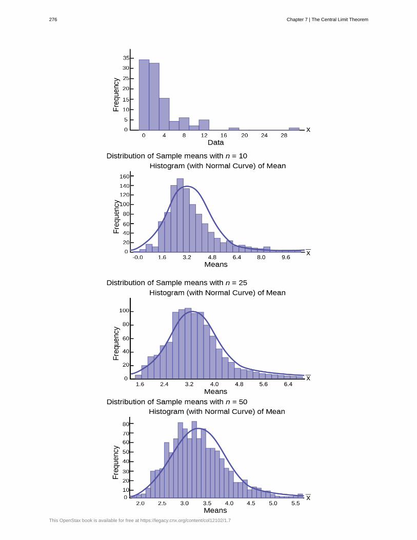
276 Chapter 7 | The Central Limit Theorem
This OpenStax book is available for free at https://legacy.cnx.org/content/col12102/1.7
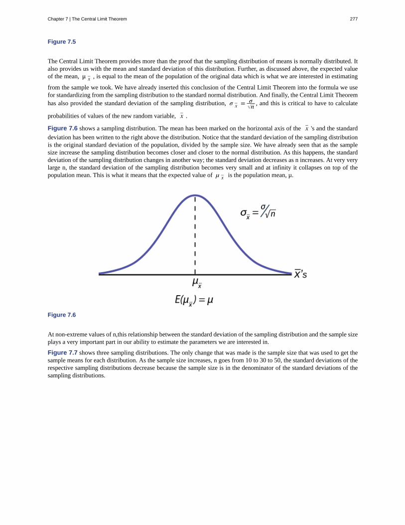
Figure 7.5
The Central Limit Theorem provides more than the proof that the sampling distribution of means is normally distributed. Italso provides us with the mean and standard deviation of this distribution. Further, as discussed above, the expected valueof the mean, μ x– , is equal to the mean of the population of the original data which is what we are interested in estimating
from the sample we took. We have already inserted this conclusion of the Central Limit Theorem into the formula we usefor standardizing from the sampling distribution to the standard normal distribution. And finally, the Central Limit Theoremhas also provided the standard deviation of the sampling distribution, σ x– = σ
n , and this is critical to have to calculate
probabilities of values of the new random variable, x– .
Figure 7.6 shows a sampling distribution. The mean has been marked on the horizontal axis of the x– 's and the standard
deviation has been written to the right above the distribution. Notice that the standard deviation of the sampling distributionis the original standard deviation of the population, divided by the sample size. We have already seen that as the samplesize increase the sampling distribution becomes closer and closer to the normal distribution. As this happens, the standarddeviation of the sampling distribution changes in another way; the standard deviation decreases as n increases. At very verylarge n, the standard deviation of the sampling distribution becomes very small and at infinity it collapses on top of thepopulation mean. This is what it means that the expected value of µ x– is the population mean, µ.
Figure 7.6
At non-extreme values of n,this relationship between the standard deviation of the sampling distribution and the sample sizeplays a very important part in our ability to estimate the parameters we are interested in.
Figure 7.7 shows three sampling distributions. The only change that was made is the sample size that was used to get thesample means for each distribution. As the sample size increases, n goes from 10 to 30 to 50, the standard deviations of therespective sampling distributions decrease because the sample size is in the denominator of the standard deviations of thesampling distributions.
Chapter 7 | The Central Limit Theorem 277
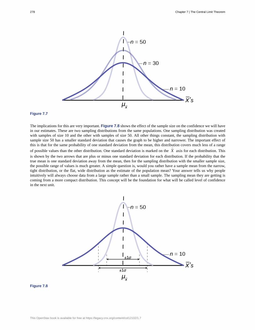
Figure 7.7
The implications for this are very important. Figure 7.8 shows the effect of the sample size on the confidence we will havein our estimates. These are two sampling distributions from the same populations. One sampling distribution was createdwith samples of size 10 and the other with samples of size 50. All other things constant, the sampling distribution withsample size 50 has a smaller standard deviation that causes the graph to be higher and narrower. The important effect ofthis is that for the same probability of one standard deviation from the mean, this distribution covers much less of a range
of possible values than the other distribution. One standard deviation is marked on the X–
axis for each distribution. This
is shown by the two arrows that are plus or minus one standard deviation for each distribution. If the probability that thetrue mean is one standard deviation away from the mean, then for the sampling distribution with the smaller sample size,the possible range of values is much greater. A simple question is, would you rather have a sample mean from the narrow,tight distribution, or the flat, wide distribution as the estimate of the population mean? Your answer tells us why peopleintuitively will always choose data from a large sample rather than a small sample. The sampling mean they are getting iscoming from a more compact distribution. This concept will be the foundation for what will be called level of confidencein the next unit.
Figure 7.8
278 Chapter 7 | The Central Limit Theorem
This OpenStax book is available for free at https://legacy.cnx.org/content/col12102/1.7
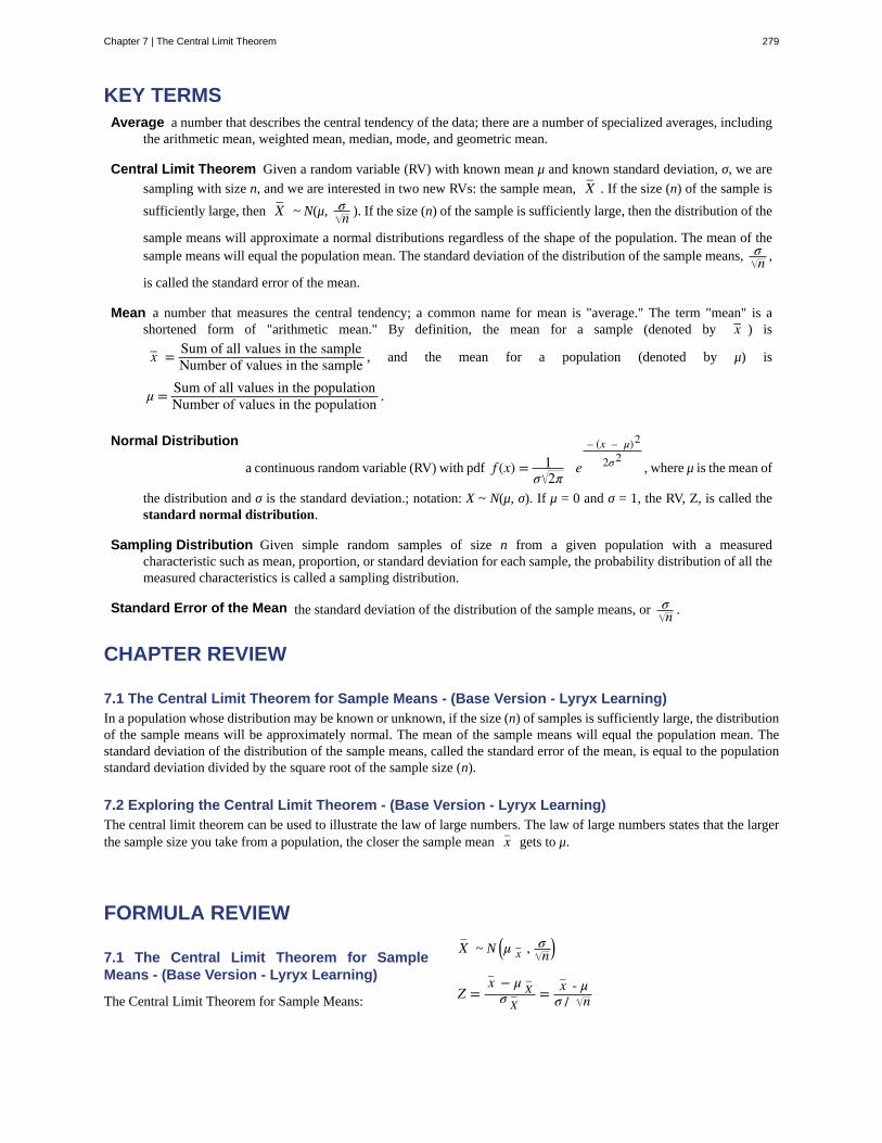
Average
Central Limit Theorem
Mean
Normal Distribution
Sampling Distribution
Standard Error of the Mean
KEY TERMSa number that describes the central tendency of the data; there are a number of specialized averages, including
the arithmetic mean, weighted mean, median, mode, and geometric mean.
Given a random variable (RV) with known mean μ and known standard deviation, σ, we are
sampling with size n, and we are interested in two new RVs: the sample mean, X– . If the size (n) of the sample is
sufficiently large, then X– ~ N(μ, σn ). If the size (n) of the sample is sufficiently large, then the distribution of the
sample means will approximate a normal distributions regardless of the shape of the population. The mean of thesample means will equal the population mean. The standard deviation of the distribution of the sample means, σ
n ,
is called the standard error of the mean.
a number that measures the central tendency; a common name for mean is "average." The term "mean" is ashortened form of "arithmetic mean." By definition, the mean for a sample (denoted by x– ) is
x– = Sum of all values in the sampleNumber of values in the sample , and the mean for a population (denoted by μ) is
μ = Sum of all values in the populationNumber of values in the population .
a continuous random variable (RV) with pdf f (x) = 1σ 2π
e
– (x – μ)2
2σ2, where μ is the mean of
the distribution and σ is the standard deviation.; notation: X ~ N(μ, σ). If μ = 0 and σ = 1, the RV, Z, is called thestandard normal distribution.
Given simple random samples of size n from a given population with a measuredcharacteristic such as mean, proportion, or standard deviation for each sample, the probability distribution of all themeasured characteristics is called a sampling distribution.
the standard deviation of the distribution of the sample means, or σn .
CHAPTER REVIEW
7.1 The Central Limit Theorem for Sample Means - (Base Version - Lyryx Learning)In a population whose distribution may be known or unknown, if the size (n) of samples is sufficiently large, the distributionof the sample means will be approximately normal. The mean of the sample means will equal the population mean. Thestandard deviation of the distribution of the sample means, called the standard error of the mean, is equal to the populationstandard deviation divided by the square root of the sample size (n).
7.2 Exploring the Central Limit Theorem - (Base Version - Lyryx Learning)The central limit theorem can be used to illustrate the law of large numbers. The law of large numbers states that the largerthe sample size you take from a population, the closer the sample mean x– gets to μ.
FORMULA REVIEW
7.1 The Central Limit Theorem for SampleMeans - (Base Version - Lyryx Learning)
The Central Limit Theorem for Sample Means:
X–
~ N ⎛⎝μ x– , σn⎞⎠
Z =x– − μ X
–σ X
– = x– - μσ / n
Chapter 7 | The Central Limit Theorem 279
The mean of X¯
: μX¯ = μ
The standard deviation of X¯
is σX¯ = σ
n and is called the
standard error of the mean.
PRACTICE
7.2 Exploring the Central Limit Theorem - (Base Version - Lyryx Learning)Use the following information to answer the next ten exercises: A manufacturer produces 25-pound lifting weights. Thelowest actual weight is 24 pounds, and the highest is 26 pounds. Each weight is equally likely so the distribution of weightsis uniform. A sample of 100 weights is taken.
1.a. What is the distribution for the weights of one 25-pound lifting weight? What is the mean and standard deivation?b. What is the distribution for the mean weight of 100 25-pound lifting weights?c. Find the probability that the mean actual weight for the 100 weights is less than 24.9.
2. Draw the graph from Exercise 7.1
3. Find the probability that the mean actual weight for the 100 weights is greater than 25.2.
4. Draw the graph from Exercise 7.3
5. Find the 90th percentile for the mean weight for the 100 weights.
6. Draw the graph from Exercise 7.5
7.a. What is the distribution for the sum of the weights of 100 25-pound lifting weights?b. Find P(Σx < 2,450).
8. Draw the graph from Exercise 7.7
9. Find the 90th percentile for the total weight of the 100 weights.
10. Draw the graph from Exercise 7.9
Use the following information to answer the next five exercises: The length of time a particular smartphone's battery lastsfollows an exponential distribution with a mean of ten months. A sample of 64 of these smartphones is taken.
11.a. What is the standard deviation?b. What is the parameter m?
12. What is the distribution for the length of time one battery lasts?
13. What is the distribution for the mean length of time 64 batteries last?
14. What is the distribution for the total length of time 64 batteries last?
15. Find the probability that the sample mean is between seven and 11.
16. Find the 80th percentile for the total length of time 64 batteries last.
17. Find the IQR for the mean amount of time 64 batteries last.
18. Find the middle 80% for the total amount of time 64 batteries last.
Use the following information to answer the next eight exercises: A uniform distribution has a minimum of six and amaximum of ten. A sample of 50 is taken.
19. Find P(Σx > 420).
20. Find the 90th percentile for the sums.
21. Find the 15th percentile for the sums.
280 Chapter 7 | The Central Limit Theorem
This OpenStax book is available for free at https://legacy.cnx.org/content/col12102/1.7

22. Find the first quartile for the sums.
23. Find the third quartile for the sums.
24. Find the 80th percentile for the sums.
HOMEWORK
7.1 The Central Limit Theorem for Sample Means - (Base Version - Lyryx Learning)
25. A sample of 16 observations is drawn from a normal population with the mean of 1000 and standard deviation of 200.Find the following.
a. P⎛⎝x¯ < 960⎞⎠ .
b. P⎛⎝x¯ > 1100⎞⎠ .
26. The length of time it takes to find a parking space at Humber at 9 am follows a normal distribution with a mean of 7.6minutes and a standard deviation of 0.8 minutes. One day at 9 am you randomly ask 16 students who just parked their carsto report the time it took them to find parking. What is the probability that the mean time sampled students spent lookingfor parking is less than 8 minutes?
27. ABC Credit.Cards.com research team claims that the average credit card debts carried by Canadians follows adistribution with a mean of $3745 and a standard deviation of $1310. What is the probability that in a random sample of100 credit card holders, the mean credit card debt is between $3600 and $4000?
28. Suppose that the distance of fly balls hit to the outfield (in baseball) is normally distributed with a mean of 250 feet anda standard deviation of 50 feet. We randomly sample 49 fly balls.
a. If X– = average distance in feet for 49 fly balls, then X– ~ _______(_______,_______)
b. What is the probability that the 49 balls traveled an average of less than 240 feet? Sketch the graph. Scale the
horizontal axis for X– . Shade the region corresponding to the probability. Find the probability.
29. According to the Internal Revenue Service, the average length of time for an individual to complete (keep records for,learn, prepare, copy, assemble, and send) IRS Form 1040 is 10.53 hours (without any attached schedules). The distributionis unknown. Let us assume that the standard deviation is two hours. Suppose we randomly sample 36 taxpayers.
a. In words, Χ = _____________
b. In words, X– = _____________
c. X– ~ _____(_____,_____)
d. Would you be surprised if the 36 taxpayers finished their Form 1040s in an average of more than 12 hours?Explain why or why not in complete sentences.
e. Would you be surprised if one taxpayer finished his or her Form 1040 in more than 12 hours? In a completesentence, explain why.
30. Suppose that a category of world-class runners are known to run a marathon (26 miles) in an average of 145 minutes
with a standard deviation of 14 minutes. Consider 49 of the races. Let X– the average of the 49 races.
a. X– ~ _____(_____,_____)
b. Find the probability that the runner will average between 142 and 146 minutes in these 49 marathons.
31. Determine which of the following are true and which are false. Then, in complete sentences, justify your answers.
a. When the sample size is large, the mean of X– is approximately equal to the mean of Χ.
b. When the sample size is large, X– is approximately normally distributed.
c. When the sample size is large, the standard deviation of X– is approximately the same as the standard deviation
of Χ.
Chapter 7 | The Central Limit Theorem 281
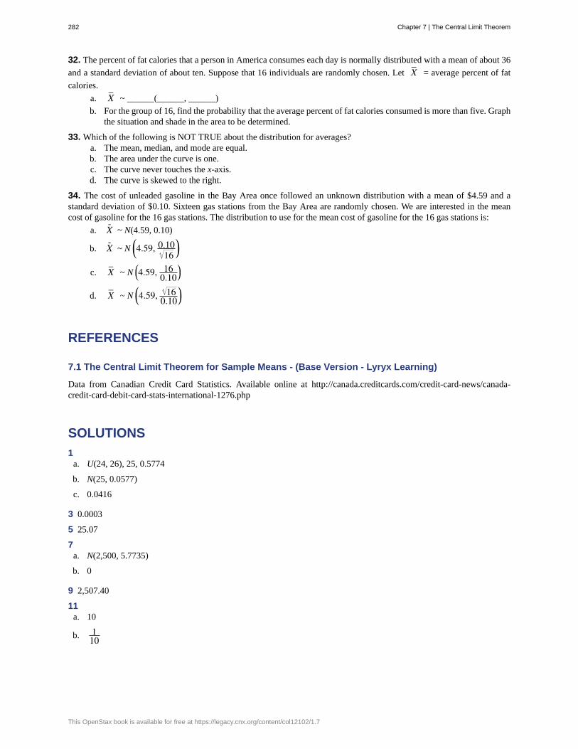
32. The percent of fat calories that a person in America consumes each day is normally distributed with a mean of about 36
and a standard deviation of about ten. Suppose that 16 individuals are randomly chosen. Let X– = average percent of fat
calories.
a. X– ~ ______(______, ______)
b. For the group of 16, find the probability that the average percent of fat calories consumed is more than five. Graphthe situation and shade in the area to be determined.
33. Which of the following is NOT TRUE about the distribution for averages?a. The mean, median, and mode are equal.b. The area under the curve is one.c. The curve never touches the x-axis.d. The curve is skewed to the right.
34. The cost of unleaded gasoline in the Bay Area once followed an unknown distribution with a mean of $4.59 and astandard deviation of $0.10. Sixteen gas stations from the Bay Area are randomly chosen. We are interested in the meancost of gasoline for the 16 gas stations. The distribution to use for the mean cost of gasoline for the 16 gas stations is:
a. X- ~ N(4.59, 0.10)
b. X- ~ N⎛⎝4.59, 0.10
16⎞⎠
c. X– ~ N ⎛⎝4.59, 160.10⎞⎠
d. X– ~ N⎛⎝4.59, 16
0.10⎞⎠
REFERENCES
7.1 The Central Limit Theorem for Sample Means - (Base Version - Lyryx Learning)
Data from Canadian Credit Card Statistics. Available online at http://canada.creditcards.com/credit-card-news/canada-credit-card-debit-card-stats-international-1276.php
SOLUTIONS
1a. U(24, 26), 25, 0.5774
b. N(25, 0.0577)
c. 0.0416
3 0.0003
5 25.07
7a. N(2,500, 5.7735)
b. 0
9 2,507.40
11a. 10
b. 110
282 Chapter 7 | The Central Limit Theorem
This OpenStax book is available for free at https://legacy.cnx.org/content/col12102/1.7
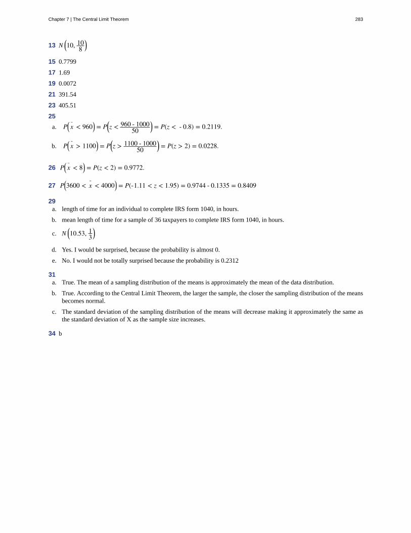
13 N ⎛⎝10, 108⎞⎠
15 0.7799
17 1.69
19 0.0072
21 391.54
23 405.51
25
a. P⎛⎝x¯ < 960⎞⎠ = P⎛⎝z < 960 - 1000
50⎞⎠ = P(z < - 0.8) = 0.2119.
b. P⎛⎝x¯ > 1100⎞⎠ = P⎛⎝z > 1100 - 1000
50⎞⎠ = P(z > 2) = 0.0228.
26 P⎛⎝x¯ < 8⎞⎠ = P(z < 2) = 0.9772.
27 P⎛⎝3600 < x¯ < 4000⎞⎠ = P(-1.11 < z < 1.95) = 0.9744 - 0.1335 = 0.8409
29a. length of time for an individual to complete IRS form 1040, in hours.
b. mean length of time for a sample of 36 taxpayers to complete IRS form 1040, in hours.
c. N ⎛⎝10.53, 13⎞⎠
d. Yes. I would be surprised, because the probability is almost 0.
e. No. I would not be totally surprised because the probability is 0.2312
31a. True. The mean of a sampling distribution of the means is approximately the mean of the data distribution.
b. True. According to the Central Limit Theorem, the larger the sample, the closer the sampling distribution of the meansbecomes normal.
c. The standard deviation of the sampling distribution of the means will decrease making it approximately the same asthe standard deviation of X as the sample size increases.
34 b
Chapter 7 | The Central Limit Theorem 283

284 Chapter 7 | The Central Limit Theorem
This OpenStax book is available for free at https://legacy.cnx.org/content/col12102/1.7

8 | CONFIDENCEINTERVALS
Figure 8.1 Have you ever wondered what the average number of M&Ms in a bag at the grocery store is? You canuse confidence intervals to answer this question. (credit: comedy_nose/flickr)
Introduction
Suppose you were trying to determine the mean rent of a two-bedroom apartment in your town. You might look in theclassified section of the newspaper, write down several rents listed, and average them together. You would have obtaineda point estimate of the true mean. If you are trying to determine the percentage of times you make a basket when shootinga basketball, you might count the number of shots you make and divide that by the number of shots you attempted. In thiscase, you would have obtained a point estimate for the true proportion the parameter p in the binomial probability densityfunction.
We use sample data to make generalizations about an unknown population. This part of statistics is called inferentialstatistics. The sample data help us to make an estimate of a population parameter. We realize that the point estimate ismost likely not the exact value of the population parameter, but close to it. After calculating point estimates, we constructinterval estimates, called confidence intervals. What statistics provides us beyond a simple average, or point estimate, is anestimate to which we can attach a probability of accuracy, what we will call a confidence level. We make inferences with aknown level of probability.
In this chapter, you will learn to construct and interpret confidence intervals. You will also learn a new distribution,the Student's-t, and how it is used with these intervals. Throughout the chapter, it is important to keep in mind that theconfidence interval is a random variable. It is the population parameter that is fixed.
Chapter 8 | Confidence Intervals 285

If you worked in the marketing department of an entertainment company, you might be interested in the mean number ofsongs a consumer downloads a month from iTunes. If so, you could conduct a survey and calculate the sample mean, x– ,
and the sample standard deviation, s. You would use x– to estimate the population mean and s to estimate the population
standard deviation. The sample mean, x– , is the point estimate for the population mean, μ. The sample standard deviation,
s, is the point estimate for the population standard deviation, σ.
x– and s are each called a statistic.
A confidence interval is another type of estimate but, instead of being just one number, it is an interval of numbers. Theinterval of numbers is a range of values calculated from a given set of sample data. The confidence interval is likely toinclude the unknown population parameter.
Suppose, for the iTunes example, we do not know the population mean μ, but we do know that the population standarddeviation is σ = 1 and our sample size is 100. Then, by the central limit theorem, the standard deviation of the samplingdistribution of the sample means is
σn = 1
100= 0.1 .
The empirical rule, which applies to the normal distribution, says that in approximately 95% of the samples, the samplemean, x– , will be within two standard deviations of the population mean μ. For our iTunes example, two standard
deviations is (2)(0.1) = 0.2. The sample mean x– is likely to be within 0.2 units of μ.
Because x- is within 0.2 units of μ, which is unknown, then μ is likely to be within 0.2 units of x– with 95% probability.
The population mean μ is contained in an interval whose lower number is calculated by taking the sample mean andsubtracting two standard deviations (2)(0.1) and whose upper number is calculated by taking the sample mean and addingtwo standard deviations. In other words, μ is between x– − 0.2 and x– + 0.2 in 95% of all the samples.
For the iTunes example, suppose that a sample produced a sample mean x– = 2 . Then with 95% probability the unknown
population mean μ is between
x– − 0.2 = 2 − 0.2 = 1.8 and x– + 0.2 = 2 + 0.2 = 2.2
We say that we are 95% confident that the unknown population mean number of songs downloaded from iTunes per monthis between 1.8 and 2.2. The 95% confidence interval is (1.8, 2.2). Please note that we talked in terms of 95% confidenceusing the empirical rule. The empirical rule for two standard deviations is only approximately 95% of the probabilityunder the normal distribution. To be precise, two standard deviations under a normal distribution is actually 95.44% of theprobability. To calculate the exact 95% confidence level we would use 1.96 standard deviations.
The 95% confidence interval implies two possibilities. Either the interval (1.8, 2.2) contains the true mean μ, or our sampleproduced an x– that is not within 0.2 units of the true mean μ. The second possibility happens for only 5% of all the
samples (95% minus 100% = 5%).
Remember that a confidence interval is created for an unknown population parameter like the population mean, μ.
For the confidence interval for a mean the formula would be:
μ = X–
± Zασn
Or written another way as:
X–
− Zα σn ≤ μ ≤ X
–+ Zα σ
n
Where X–
is the sample mean. Zα is determined by the level of confidence desired by the analyst, and σn is the standard
deviation of the sampling distribution for means given to us by the Central Limit Theorem.
8.1 | A Confidence Interval for a Population Standard
Deviation, Known or Large Sample SizeA confidence interval for a population mean, when the population standard deviation is known based on the conclusion ofthe Central Limit Theorem that the sampling distribution of the sample means follow an approximately normal distribution.
286 Chapter 8 | Confidence Intervals
This OpenStax book is available for free at https://legacy.cnx.org/content/col12102/1.7
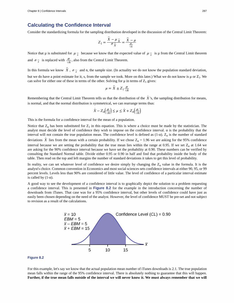
Calculating the Confidence IntervalConsider the standardizing formula for the sampling distribution developed in the discussion of the Central Limit Theorem:
Z1 =X−
− μ X−
σ X− = X
−− μσn
Notice that µ is substituted for µ x− because we know that the expected value of µ x− is µ from the Central Limit theorem
and σ x− is replaced with σn , also from the Central Limit Theorem.
In this formula we know X−
, σ x− and n, the sample size. (In actuality we do not know the population standard deviation,
but we do have a point estimate for it, s, from the sample we took. More on this later.) What we do not know is μ or Z1. Wecan solve for either one of these in terms of the other. Solving for μ in terms of Z1 gives:
μ = X−
± Z1σn
Remembering that the Central Limit Theorem tells us that the distribution of the X-
's, the sampling distribution for means,
is normal, and that the normal distribution is symmetrical, we can rearrange terms thus:
X-
− Zα⎛⎝ σn⎞⎠ ≤ μ ≤ X
-+ Zα⎛⎝ σn⎞⎠
This is the formula for a confidence interval for the mean of a population.
Notice that Zα has been substituted for Z1 in this equation. This is where a choice must be made by the statistician. Theanalyst must decide the level of confidence they wish to impose on the confidence interval. α is the probability that theinterval will not contain the true population mean. The confidence level is defined as (1-α). Zα is the number of standard
deviations X-
lies from the mean with a certain probability. If we chose Zα = 1.96 we are asking for the 95% confidence
interval because we are setting the probability that the true mean lies within the range at 0.95. If we set Zα at 1.64 weare asking for the 90% confidence interval because we have set the probability at 0.90. These numbers can be verified byconsulting the Standard Normal table. Divide either 0.95 or 0.90 in half and find that probability inside the body of thetable. Then read on the top and left margins the number of standard deviations it takes to get this level of probability.
In reality, we can set whatever level of confidence we desire simply by changing the Zα value in the formula. It is theanalyst's choice. Common convention in Economics and most social sciences sets confidence intervals at either 90, 95, or 99percent levels. Levels less than 90% are considered of little value. The level of confidence of a particular interval estimateis called by (1-α).
A good way to see the development of a confidence interval is to graphically depict the solution to a problem requestinga confidence interval. This is presented in Figure 8.2 for the example in the introduction concerning the number ofdownloads from iTunes. That case was for a 95% confidence interval, but other levels of confidence could have just aseasily been chosen depending on the need of the analyst. However, the level of confidence MUST be pre-set and not subjectto revision as a result of the calculations.
Figure 8.2
For this example, let's say we know that the actual population mean number of iTunes downloads is 2.1. The true populationmean falls within the range of the 95% confidence interval. There is absolutely nothing to guarantee that this will happen.Further, if the true mean falls outside of the interval we will never know it. We must always remember that we will
Chapter 8 | Confidence Intervals 287
never ever know the true mean. Statistics simply allows us, with a given level of probability (confidence), to say that thetrue mean is within the range calculated. This is what was called in the introduction, the "level of ignorance admitted".
Changing the Confidence Level or Sample SizeHere again is the formula for a confidence interval for an unknown population mean assuming we know the populationstandard deviation:
X-
− Zα⎛⎝ σn⎞⎠ ≤ μ ≤ X
-+ Zα⎛⎝ σn⎞⎠
It is clear that the confidence interval is driven by two things, the chosen level of confidence, Zα , and the standard deviation
of the sampling distribution. The Standard deviation of the sampling distribution is further affected by two things, thestandard deviation of the population and the sample size we chose for our data. Here we wish to examine the effects of eachof the choices we have made on the calculated confidence interval, the confidence level and the sample size.
For a moment we should ask just what we desire in a confidence interval. Our goal was to estimate the population meanfrom a sample. We have forsaken the hope that we will ever find the true population mean, and population standarddeviation for that matter, for any case except where we have an extremely small population and the cost of gathering thedata of interest is very small. In all other cases we must rely on samples. With the Central Limit Theorem we have the toolsto provide a meaningful confidence interval with a given level of confidence, meaning a known probability of being wrong.By meaningful confidence interval we mean one that is useful. Imagine that you are asked for a confidence interval for theages of your classmates. You have taken a sample and find a mean of 19.8 years. You wish to be very confident so youreport an interval between 9.8 years and 29.8 years. This interval would certainly contain the true population mean and havea very high confidence level. However, it hardly qualifies as meaningful. The very best confidence interval is narrow whilehaving high confidence. There is a natural tension between these two goals. The higher the level of confidence the widerthe confidence interval as the case of the students' ages above. We can see this tension in the equation for the confidenceinterval.
μ = x_ ± Zα⎛⎝ σn⎞⎠
The confidence interval will increase in width as Zα increases, Zα increases as the level of confidence increases. There
is a tradeoff between the level of confidence and the width of the interval. Now let's look at the formula again and wesee that the sample size also plays an important role in the width of the confidence interval. The sample size, n , shows
up in the denominator of the standard deviation of the sampling distribution. As the sample size increases, the standarddeviation of the sampling distribution decreases and thus the width of the confidence interval, while holding constantthe level of confidence. This relationship was demonstrated in m54537 (https://legacy.cnx.org/content/m54537/latest/#fs-id8850305) . Again we see the importance of having large samples for our analysis although we then face asecond constraint, the cost of gathering data.
Calculating the Confidence Interval: An Alternative ApproachAnother way to approach confidence intervals is through the use of something called the Error Bound. The Error Bound getsits name from the recognition that it provides the boundary of the interval derived from the standard error of the samplingdistribution. In the equations above it is seen that the interval is simply the estimated mean, sample mean, plus or minussomething. That something is the Error Bound and is driven by the probability we desire to maintain in our estimate, Zα, times the standard deviation of the sampling distribution. The Error Bound for a mean is given the name, Error BoundMean, or EBM.
To construct a confidence interval for a single unknown population mean μ, where the population standard deviation isknown, we need x- as an estimate for μ and we need the margin of error. Here, the margin of error (EBM) is called the error
bound for a population mean (abbreviated EBM). The sample mean x- is the point estimate of the unknown population
mean μ.
The confidence interval estimate will have the form:
(point estimate - error bound, point estimate + error bound) or, in symbols,( x- – EBM, x- +EBM )
The mathematical formula for this confidence interval is:
X-
− Zα⎛⎝ σn⎞⎠ ≤ μ ≤ X
-+ Zα⎛⎝ σn⎞⎠
The margin of error (EBM) depends on the confidence level (abbreviated CL). The confidence level is often considered the
288 Chapter 8 | Confidence Intervals
This OpenStax book is available for free at https://legacy.cnx.org/content/col12102/1.7

probability that the calculated confidence interval estimate will contain the true population parameter. However, it is moreaccurate to state that the confidence level is the percent of confidence intervals that contain the true population parameterwhen repeated samples are taken. Most often, it is the choice of the person constructing the confidence interval to choose aconfidence level of 90% or higher because that person wants to be reasonably certain of his or her conclusions.
There is another probability called alpha (α). α is related to the confidence level, CL. α is the probability that the intervaldoes not contain the unknown population parameter.Mathematically, 1 - α = CL.
A confidence interval for a population mean with a known standard deviation is based on the fact that the samplingdistribution of the sample means follow an approximately normal distribution. Suppose that our sample has a mean of x- =
10, and we have constructed the 90% confidence interval (5, 15) where EBM = 5.
To get a 90% confidence interval, we must include the central 90% of the probability of the normal distribution. If weinclude the central 90%, we leave out a total of α = 10% in both tails, or 5% in each tail, of the normal distribution.
Figure 8.3
To capture the central 90%, we must go out 1.645 standard deviations on either side of the calculated sample mean. Thevalue 1.645 is the z-score from a standard normal probability distribution that puts an area of 0.90 in the center, an area of0.05 in the far left tail, and an area of 0.05 in the far right tail.
It is important that the standard deviation used must be appropriate for the parameter we are estimating, so in this sectionwe need to use the standard deviation that applies to the sampling distribution for means which we studied with the CentralLimit Theorem and is, σ
n .
Calculating the Confidence Interval Using EBM
To construct a confidence interval estimate for an unknown population mean, we need data from a random sample. Thesteps to construct and interpret the confidence interval are:
• Calculate the sample mean x- from the sample data. Remember, in this section we know the population standard
deviation σ.
• Find the z-score from the standard normal table that corresponds to the confidence level desired.
• Calculate the error bound EBM.
• Construct the confidence interval.
• Write a sentence that interprets the estimate in the context of the situation in the problem.
We will first examine each step in more detail, and then illustrate the process with some examples.
Finding the z-score for the Stated Confidence Level
When we know the population standard deviation σ, we use a standard normal distribution to calculate the error boundEBM and construct the confidence interval. We need to find the value of z that puts an area equal to the confidence level (indecimal form) in the middle of the standard normal distribution Z ~ N(0, 1).
The confidence level, CL, is the area in the middle of the standard normal distribution. CL = 1 – α, so α is the area that issplit equally between the two tails. Each of the tails contains an area equal to α
2 .
The z-score that has an area to the right of α2 is denoted by Zα
2.
Chapter 8 | Confidence Intervals 289
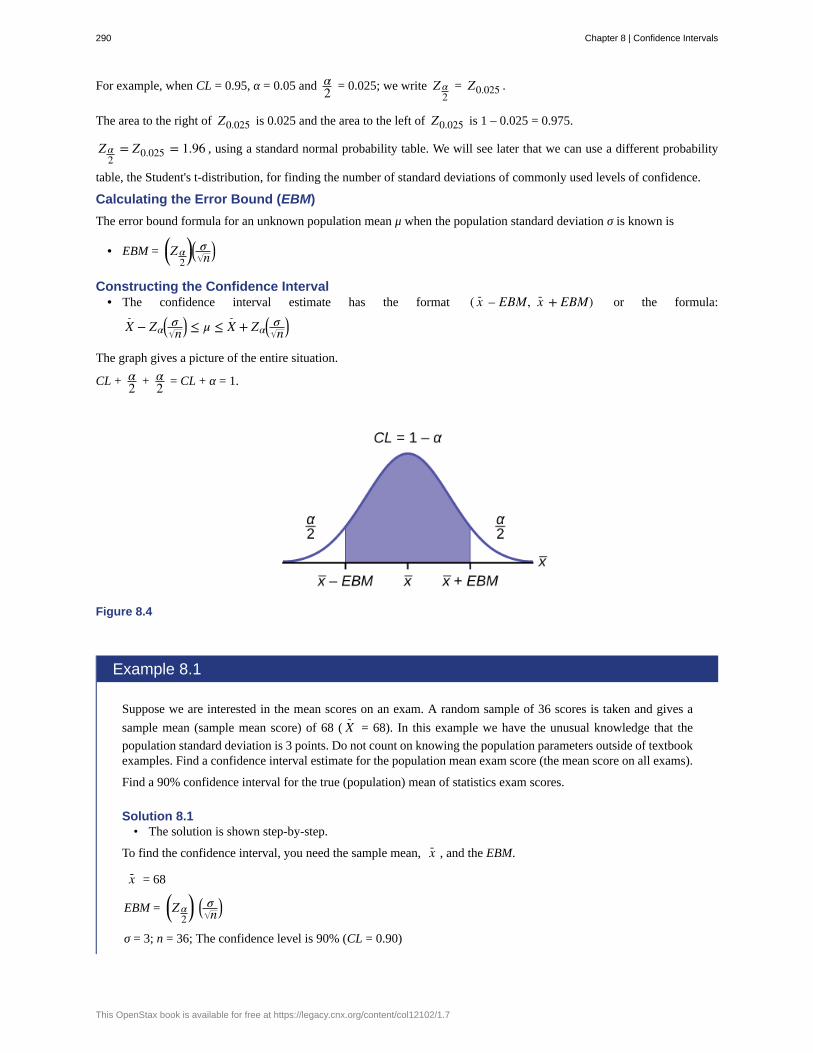
For example, when CL = 0.95, α = 0.05 and α2 = 0.025; we write Zα
2= Z0.025 .
The area to the right of Z0.025 is 0.025 and the area to the left of Z0.025 is 1 – 0.025 = 0.975.
Zα2
= Z0.025 = 1.96 , using a standard normal probability table. We will see later that we can use a different probability
table, the Student's t-distribution, for finding the number of standard deviations of commonly used levels of confidence.
Calculating the Error Bound (EBM)
The error bound formula for an unknown population mean μ when the population standard deviation σ is known is
• EBM =⎛⎝Zα
2
⎞⎠⎛⎝ σn⎞⎠
Constructing the Confidence Interval• The confidence interval estimate has the format ( x- – EBM, x- + EBM) or the formula:
X-
− Zα⎛⎝ σn⎞⎠ ≤ μ ≤ X
-+ Zα⎛⎝ σn⎞⎠
The graph gives a picture of the entire situation.
CL + α2 + α
2 = CL + α = 1.
Figure 8.4
Example 8.1
Suppose we are interested in the mean scores on an exam. A random sample of 36 scores is taken and gives a
sample mean (sample mean score) of 68 ( X-
= 68). In this example we have the unusual knowledge that the
population standard deviation is 3 points. Do not count on knowing the population parameters outside of textbookexamples. Find a confidence interval estimate for the population mean exam score (the mean score on all exams).
Find a 90% confidence interval for the true (population) mean of statistics exam scores.
Solution 8.1• The solution is shown step-by-step.
To find the confidence interval, you need the sample mean, x- , and the EBM.
x- = 68
EBM =⎛⎝Zα
2
⎞⎠ ⎛⎝ σn⎞⎠
σ = 3; n = 36; The confidence level is 90% (CL = 0.90)
290 Chapter 8 | Confidence Intervals
This OpenStax book is available for free at https://legacy.cnx.org/content/col12102/1.7
CL = 0.90 so α = 1 – CL = 1 – 0.90 = 0.10
α2 = 0.05 Zα
2= z0.05
The area to the right of Z0.05 is 0.05 and the area to the left of Z0.05 is 1 – 0.05 = 0.95.
Zα2
= Z0.05 = 1.645
This can be found using a computer, or using a probability table for the standard normal distribution. Because thecommon levels of confidence in the social sciences are 90%, 95% and 99% it will not be long until you becomefamiliar with the numbers , 1.645, 1.96, and 2.56
EBM = (1.645)⎛⎝ 3
36⎞⎠ = 0.8225
x- - EBM = 68 - 0.8225 = 67.1775
x- + EBM = 68 + 0.8225 = 68.8225
The 90% confidence interval is (67.1775, 68.8225).
Interpretation
We estimate with 90% confidence that the true population mean exam score for all statistics students is between67.18 and 68.82.
Example 8.2
Suppose we change the original problem in Example 8.1 by using a 95% confidence level. Find a 95%confidence interval for the true (population) mean statistics exam score.
Chapter 8 | Confidence Intervals 291
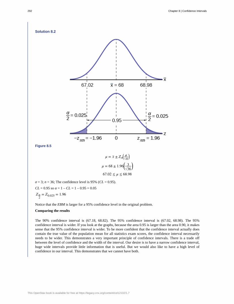
Solution 8.2
Figure 8.5
μ = x_ ± Zα⎛⎝ σn⎞⎠
μ = 68 ± 1.96⎛⎝ 336⎞⎠
67.02 ≤ μ ≤ 68.98
σ = 3; n = 36; The confidence level is 95% (CL = 0.95).
CL = 0.95 so α = 1 – CL = 1 – 0.95 = 0.05
Zα2
= Z0.025 = 1.96
Notice that the EBM is larger for a 95% confidence level in the original problem.
Comparing the results
The 90% confidence interval is (67.18, 68.82). The 95% confidence interval is (67.02, 68.98). The 95%confidence interval is wider. If you look at the graphs, because the area 0.95 is larger than the area 0.90, it makessense that the 95% confidence interval is wider. To be more confident that the confidence interval actually doescontain the true value of the population mean for all statistics exam scores, the confidence interval necessarilyneeds to be wider. This demonstrates a very important principle of confidence intervals. There is a trade offbetween the level of confidence and the width of the interval. Our desire is to have a narrow confidence interval,huge wide intervals provide little information that is useful. But we would also like to have a high level ofconfidence in our interval. This demonstrates that we cannot have both.
292 Chapter 8 | Confidence Intervals
This OpenStax book is available for free at https://legacy.cnx.org/content/col12102/1.7

Figure 8.6
Summary: Effect of Changing the Confidence Level• Increasing the confidence level makes the confidence interval wider.
• Decreasing the confidence level makes the confidence interval narrower.
And again here is the formula for a confidence interval for an unknown mean assuming we have the populationstandard deviation:
X-
− Zα⎛⎝ σn⎞⎠ ≤ μ ≤ X
-+ Zα⎛⎝ σn⎞⎠
The standard deviation of the sampling distribution was provided by the Central Limit Theorem as σn . While
we infrequently get to choose the sample size it plays an important role in the confidence interval. Because thesample size is in the denominator of the equation, as n increases it causes the standard deviation of the sampling
distribution to idecrease and thus the width of the confidence interval to decrease. We have met this before as wereviewed the effects of sample size on the Central Limit Theorem. There we saw that as n increases the sampling
distribution narrows until in the limit it collapses on the true population mean.
Example 8.3
Suppose we change the original problem in Example 8.1 to see what happens to the confidence interval if thesample size is changed.
Leave everything the same except the sample size. Use the original 90% confidence level. What happens to theconfidence interval if we increase the sample size and use n = 100 instead of n = 36? What happens if we decreasethe sample size to n = 25 instead of n = 36?
Solution 8.3
μ = x_ ± Zα⎛⎝ σn⎞⎠
μ = 68 ± 1.645⎛⎝ 3100⎞⎠
67.5065 ≤ μ ≤ 68.4935If we increase the sample size n to 100, we decrease the width of the confidence interval relative to the originalsample size of 36 observations.
Solution 8.3
μ = x_ ± Zα⎛⎝ σn⎞⎠
μ = 68 ± 1.645⎛⎝ 325⎞⎠
Chapter 8 | Confidence Intervals 293

67.013 ≤ μ ≤ 68.987If we decrease the sample size n to 25, we increase the width of the confidence interval by comparison to theoriginal sample size of 36 observations.
Summary: Effect of Changing the Sample Size• Increasing the sample size makes the confidence interval narrower.
• Decreasing the sample size makes the confidence interval wider.
We have already seen this effect when we reviewed the effects of changing the size of the sample, n, on the Central LimitTheorem. See m54537 (https://legacy.cnx.org/content/m54537/latest/#fs-id1171528778810) to see this effect.Before we saw that as the sample size increased the standard deviation of the sampling distribution decreases. This was whywe choose the sample mean from a large sample as compared to a small sample, all other things held constant.
Thus far we assumed that we knew the population standard deviation. This will virtually never be the case. We will have thesample standard deviation, s, however. This is a point estimate for the population standard deviation and can be substitutedinto the formula for confidence intervals for a mean under certain circumstances. We just saw the effect the sample sizehas on the width of confidence interval and the impact on the sampling distribution for our discussion of the Central LimitTheorem. We can invoke this to substitute the point estimate for the standard deviation if the sample size is large "enough".Simulation studies indicate that 30 observations or more will be sufficient to eliminate any meaningful bias in the estimatedconfidence interval.
Example 8.4
Spring break can be a very expensive holiday. A sample of 80 students is surveyed, and the average amount spentby students on travel and beverages is $593.84. The sample standard deviation is approximately $369.34.
Construct a 92% confidence interval for the population mean amount of money spent by spring breakers.
Solution 8.4
We begin with the confidence interval for a mean. We use the formula for a mean because the random variable isdollars spent and this is a continuous random variable. The point estimate for the population standard deviation,s, has been substituted for the true population standard deviation because with 80 observations there is no concernfor bias in the estimate of the confidence interval.
μ = x¯ ± ⎡⎣Z(a /2)sn⎤⎦
Substituting the values into the formula, we have:
μ = 593.84 ± ⎡⎣1.75369.3480⎤⎦
Z(a / 2) is found on the standard normal table by looking up 0.46 in the body of the table and finding the number
of standard deviations on the side and top of the table; 1.75. The solution for the interval is thus:
μ = 593.84 ± 72.2636 = ⎛⎝521.57, 666.10⎞⎠
$ 521.58 ≤ μ ≤ $ 666.10
294 Chapter 8 | Confidence Intervals
This OpenStax book is available for free at https://legacy.cnx.org/content/col12102/1.7

Figure 8.7
Formula ReviewThe general form for a confidence interval for a single population mean, known standard deviation, normal distribution is
given by X-
− Zα⎛⎝ σn⎞⎠ ≤ μ ≤ X
-+ Zα⎛⎝ σn⎞⎠ This formula is used when the population standard deviation is known.
CL = confidence level, or the proportion of confidence intervals created that are expected to contain the true populationparameter
α = 1 – CL = the proportion of confidence intervals that will not contain the population parameter
zα2
= the z-score with the property that the area to the right of the z-score is ∝2 this is the z-score used in the calculation
of "EBM where α = 1 – CL.
8.2 | A Confidence Interval for a Population Standard
Deviation Unknown, Small Sample CaseIn practice, we rarely know the population standard deviation. In the past, when the sample size was large, this did notpresent a problem to statisticians. They used the sample standard deviation s as an estimate for σ and proceeded as before tocalculate a confidence interval with close enough results. This is what we did in Example 8.4 above. The point estimatefor the standard deviation, s, was substituted in the formula for the confidence interval for the population standard deviation.In this case there 80 observation well above the suggested 30 observations to eliminate any bias from a small sample.However, statisticians ran into problems when the sample size was small. A small sample size caused inaccuracies in theconfidence interval.
William S. Goset (1876–1937) of the Guinness brewery in Dublin, Ireland ran into this problem. His experiments with hopsand barley produced very few samples. Just replacing σ with s did not produce accurate results when he tried to calculatea confidence interval. He realized that he could not use a normal distribution for the calculation; he found that the actualdistribution depends on the sample size. This problem led him to "discover" what is called the Student's t-distribution.
Chapter 8 | Confidence Intervals 295
The name comes from the fact that Gosset wrote under the pen name "A Student."
Up until the mid-1970s, some statisticians used the normal distribution approximation for large sample sizes and used theStudent's t-distribution only for sample sizes of at most 30 observations.
If you draw a simple random sample of size n from a population with mean μ and unknown population standard deviation
σ and calculate the t-score t =x- – μ⎛⎝ sn⎞⎠
, then the t-scores follow a Student's t-distribution with n – 1 degrees of freedom.
The t-score has the same interpretation as the z-score. It measures how far in standard deviation units x- is from its mean
μ. For each sample size n, there is a different Student's t-distribution.
The degrees of freedom, n – 1, come from the calculation of the sample standard deviation s. Remember when we firstcalculated a sample standard deviation we divided the sum of the squared deviations by n − 1, but we used n deviations(x – x- values) to calculate s. Because the sum of the deviations is zero, we can find the last deviation once we know the
other n – 1 deviations. The other n – 1 deviations can change or vary freely. We call the number n – 1 the degrees offreedom (df) in recognition that one is lost in the calculations. The effect of losing a degree of freedom is that the t-valueincreases and the confidence interval increases in width.
Properties of the Student's t-Distribution• The graph for the Student's t-distribution is similar to the standard normal curve and at infinite degrees of freedom it
is the normal distribution. You can confirm this by reading the bottom line at infinite degrees of freedom for a familiarlevel of confidence, e.g. at column 0.05, 95% level of confidence, we find the t-value of 1.96 at infinite degrees offreedom.
• The mean for the Student's t-distribution is zero and the distribution is symmetric about zero, again like the standardnormal distribution.
• The Student's t-distribution has more probability in its tails than the standard normal distribution because the spread ofthe t-distribution is greater than the spread of the standard normal. So the graph of the Student's t-distribution will bethicker in the tails and shorter in the center than the graph of the standard normal distribution.
• The exact shape of the Student's t-distribution depends on the degrees of freedom. As the degrees of freedom increases,the graph of Student's t-distribution becomes more like the graph of the standard normal distribution.
• The underlying population of individual observations is assumed to be normally distributed with unknown populationmean μ and unknown population standard deviation σ. This assumption comes from the Central Limit theorem because
the individual observations in this case are the x¯ s of the sampling distribution. The size of the underlying population
is generally not relevant unless it is very small. If it is normal then the assumption is met and doesn't need discussion.
A probability table for the Student's t-distribution is used to calculate t-values at various commonly-used levels ofconfidence. The table gives t-scores that correspond to the confidence level (column) and degrees of freedom (row). Whenusing a t-table, note that some tables are formatted to show the confidence level in the column headings, while the columnheadings in some tables may show only corresponding area in one or both tails. Notice that at the bottom the table will showthe t-value for infinite degrees of freedom. Mathematically, as the degrees of freedom increase, the t-distribution approachesthe standard normal distribution. You can find familiar Z-values by looking in the relevant alpha column and reading valuein the last row.
A Student's t table (See Appendix A) gives t-scores given the degrees of freedom and the right-tailed probability.
The Student's t-distribution has one of the most desirable properties of the normal: it is symmetrical. What the Student'st-distribution does is spread out the horizontal axis so it takes a larger number of standard deviations to capture the sameamount of probability. In reality there are an infinite number of Student's t-distributions, one for each adjustment to thesample size. As the sample size increases, the Student's t-distribution become more and more like the normal distribution.When the sample size reaches 30 the normal distribution is usually substituted for the Student's t because they are so muchalike. This relationship between the Student's t-distribution and the normal distribution is shown in Figure 8.8.
296 Chapter 8 | Confidence Intervals
This OpenStax book is available for free at https://legacy.cnx.org/content/col12102/1.7
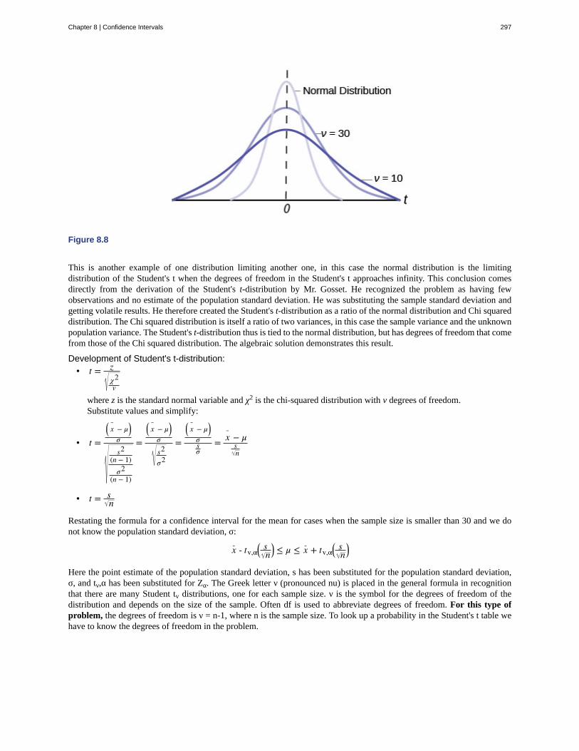
Figure 8.8
This is another example of one distribution limiting another one, in this case the normal distribution is the limitingdistribution of the Student's t when the degrees of freedom in the Student's t approaches infinity. This conclusion comesdirectly from the derivation of the Student's t-distribution by Mr. Gosset. He recognized the problem as having fewobservations and no estimate of the population standard deviation. He was substituting the sample standard deviation andgetting volatile results. He therefore created the Student's t-distribution as a ratio of the normal distribution and Chi squareddistribution. The Chi squared distribution is itself a ratio of two variances, in this case the sample variance and the unknownpopulation variance. The Student's t-distribution thus is tied to the normal distribution, but has degrees of freedom that comefrom those of the Chi squared distribution. The algebraic solution demonstrates this result.
Development of Student's t-distribution:• t = z
χ2v
where z is the standard normal variable and χ2 is the chi-squared distribution with v degrees of freedom.Substitute values and simplify:
• t =
⎛⎝ x − μ⎞⎠
σs2
(n − 1)σ2
(n − 1)
=
⎛⎝ x − μ⎞⎠
σs2
σ2
=
⎛⎝ x − μ⎞⎠
σsσ
= x¯ − μsn
• t = sn
Restating the formula for a confidence interval for the mean for cases when the sample size is smaller than 30 and we donot know the population standard deviation, σ:
x- - tv,α⎛⎝ sn⎞⎠ ≤ μ ≤ x- + tv,α
⎛⎝ sn⎞⎠
Here the point estimate of the population standard deviation, s has been substituted for the population standard deviation,σ, and tν,α has been substituted for Zα. The Greek letter ν (pronounced nu) is placed in the general formula in recognitionthat there are many Student tv distributions, one for each sample size. ν is the symbol for the degrees of freedom of thedistribution and depends on the size of the sample. Often df is used to abbreviate degrees of freedom. For this type ofproblem, the degrees of freedom is ν = n-1, where n is the sample size. To look up a probability in the Student's t table wehave to know the degrees of freedom in the problem.
Chapter 8 | Confidence Intervals 297

Example 8.5
The average earnings per share (EPS) for 10 industrial stocks randomly selected from those listed on the Dow-
Jones Industrial Average was found to be X-
= 1.85 with a standard deviation of s=0.395. Calculate a 99%
confidence interval for the average EPS of all the industrials listed on the DJIA.
x- - tv,α⎛⎝ sn⎞⎠ ≤ μ ≤ x- + tv,α
⎛⎝ sn⎞⎠
Solution 8.5
To help visualize the process of calculating a confident interval we draw the appropriate distribution for theproblem. In this case this is the Student’s t because we do not know the population standard deviation and thesample is small, less than 30.
Figure 8.9
To find the appropriate t-value requires two pieces of information, the level of confidence desired and the degreesof freedom. The question asked for a 99% confidence level. On the graph this is shown where (1-α) , the levelof confidence , is in the unshaded area. The tails, thus, have .005 probability each, α/2. The degrees of freedomfor this type of problem is n-1= 9. From the Student’s t table, at the row marked 9 and column marked .005, isthe number of standard deviations to capture 99% of the probability, 3.2498. These are then placed on the graphremembering that the Student’s t is symmetrical and so the t-value is both plus or minus on each side of the mean.
Inserting these values into the formula gives the result. These values can be placed on the graph to see the
relationship between the distribution of the sample means, X-
's and the Student’s t-distribution.
μ = X-
± tα/2,df=n-1sn = 1.851 ± 3.24980.395
10= 1.8551 ± 0.406
1.445 ≤ μ ≤ 2.257
We state the formal conclusion as :
298 Chapter 8 | Confidence Intervals
This OpenStax book is available for free at https://legacy.cnx.org/content/col12102/1.7
With 99% confidence level, the average EPS of all the industries listed at DJIA is from $1.44 to $2.26.
8.5 You do a study of hypnotherapy to determine how effective it is in increasing the number of hours of sleep subjectsget each night. You measure hours of sleep for 12 subjects with the following results. Construct a 95% confidenceinterval for the mean number of hours slept for the population (assumed normal) from which you took the data.
8.2; 9.1; 7.7; 8.6; 6.9; 11.2; 10.1; 9.9; 8.9; 9.2; 7.5; 10.5
8.3 | A Confidence Interval for A Population ProportionDuring an election year, we see articles in the newspaper that state confidence intervals in terms of proportions orpercentages. For example, a poll for a particular candidate running for president might show that the candidate has 40%of the vote within three percentage points (if the sample is large enough). Often, election polls are calculated with 95%confidence, so, the pollsters would be 95% confident that the true proportion of voters who favored the candidate would bebetween 0.37 and 0.43.
Investors in the stock market are interested in the true proportion of stocks that go up and down each week. Businesses thatsell personal computers are interested in the proportion of households in the United States that own personal computers.Confidence intervals can be calculated for the true proportion of stocks that go up or down each week and for the trueproportion of households in the United States that own personal computers.
The procedure to find the confidence interval for a population proportion is similar to that for the population mean, but theformulas are a bit different although conceptually identical. While the formulas are different, they are based upon the samemathematical foundation given to us by the Central Limit Theorem. Because of this we will see the same basic format usingthe same three pieces of information: the sample value of the parameter in question, the standard deviation of the relevantsampling distribution, and the number of standard deviations we need to have the confidence in our estimate that we desire.
How do you know you are dealing with a proportion problem? First, the underlying distribution has a binary randomvariable and therefore is a binomial distribution. (There is no mention of a mean or average.) If X is a binomial randomvariable, then X ~ B(n, p) where n is the number of trials and p is the probability of a success. To form a sample proportion,take X, the random variable for the number of successes and divide it by n, the number of trials (or the sample size). Therandom variable P′ (read "P prime") is the sample proportion,
P′ = Xn
(Sometimes the random variable is denoted as P , read "P hat".)
p′ = the estimated proportion of successes or sample proportion of successes (p′ is a point estimate for p, the truepopulation proportion, and thus q is the probability of a failure in any one trial.)
x = the number of successes in the sample
n = the size of the sample
The formula for the confidence interval for a population proportion follows the same format as that for an estimate of apopulation mean. Remembering the sampling distribution for the proportion from Chapter 7 (https://legacy.cnx.org/content/m54530/latest/) , the standard deviation was found to be:
σp' = p⎛⎝1 − p⎞⎠n
The confidence interval for a population proportion, therefore, becomes:
p = p′ ± ⎡⎣Z⎛⎝a2⎞⎠p′⎛⎝1 − p′⎞⎠
n⎤⎦
Chapter 8 | Confidence Intervals 299
Z⎛⎝a2⎞⎠
is set according to our desired degree of confidence andp′⎛⎝1 − p′⎞⎠
n is the standard deviation of the sampling
distribution.
The sample proportions p′ and q′ are estimates of the unknown population proportions p and q. The estimatedproportions p′ and q′ are used because p and q are not known.
Remember that as p moves further from 0.5 the binomial distribution becomes less symmetrical. Because we are estimatingthe binomial with the symmetrical normal distribution the further away from symmetrical the binomial becomes the lessconfidence we have in the estimate.
This conclusion can be demonstrated through the following analysis. Proportions are based upon the binomial probabilitydistribution. The possible outcomes are binary, either “success” or “failure”. This gives rise to a proportion, meaning thepercentage of the outcomes that are “successes”. It was shown that the binomial distribution could be fully understood if weknew only the probability of a success in any one trial, called p. The mean and the standard deviation of the binomial werefound to be:
μ = npσ = npq
It was also shown that the binomial could be estimated by the normal distribution if BOTH np AND nq were greater than 5.From the discussion above, it was found that the standardizing formula for the binomial distribution is:
Z = p' - p⎛⎝pqn⎞⎠
which is nothing more than a restatement of the general standardizing formula with appropriate substitutions for μ andσ from the binomial. We can use the standard normal distribution, the reason Z is in the equation, because the normaldistribution is the limiting distribution of the binomial. This is another example of the Central Limit Theorem. Wehave already seen that the sampling distribution of means is normally distributed. Recall the extended discussion inChapter 7 (https://legacy.cnx.org/content/m54530/latest/) concerning the sampling distribution of proportions andthe conclusions of the Central Limit Theorem.
We can now manipulate this formula in just the same way we did for finding the confidence intervals for a mean, but to findthe confidence interval for the binomial population parameter, p.
p' - Zαp'q'n ≤ p ≤ p' + Zα
p'q'n
Where p′ = x/n, the point estimate of p taken from the sample. Notice that p′ has replaced p in the formula. This is becausewe do not know p, indeed, this is just what we are trying to estimate.
Unfortunately, there is no correction factor for cases where the sample size is small so np′ and nq' must always be greaterthan 5 to develop an interval estimate for p.
Example 8.6
Suppose that a market research firm is hired to estimate the percent of adults living in a large city who have cellphones. Five hundred randomly selected adult residents in this city are surveyed to determine whether they havecell phones. Of the 500 people sampled, 421 responded yes - they own cell phones. Using a 95% confidence level,compute a confidence interval estimate for the true proportion of adult residents of this city who have cell phones.
Solution 8.6• The solution step-by-step.
Let X = the number of people in the sample who have cell phones. X is binomial: the random variable is binary,people either have a cell phone or they do not.
To calculate the confidence interval, we must find p′, q′.
n = 500
x = the number of successes in the sample = 421
300 Chapter 8 | Confidence Intervals
This OpenStax book is available for free at https://legacy.cnx.org/content/col12102/1.7

p′ = xn = 421
500 = 0.842
p′ = 0.842 is the sample proportion; this is the point estimate of the population proportion.
q′ = 1 – p′ = 1 – 0.842 = 0.158
Since the requested confidence level is CL = 0.95, then α = 1 – CL = 1 – 0.95 = 0.05 ⎛⎝α2⎞⎠ = 0.025.
Then zα2
= z0.025 = 1.96
This can be found using the Standard Normal probability table in Appendix A. This can also be found in thestudents t table at the 0.025 column and infinity degrees of freedom because at infinite degrees of freedom thestudents t-distribution becomes the standard normal distribution, Z.
The confidence interval for the true binomial population proportion is
() p' - Zαp'q'n ≤ p ≤ p' + Zα
p'q'n
() Substituting in the values from above we find the confidence interval is : 0.810 ≤ p ≤ 0.874
Interpretation
We estimate with 95% confidence that between 81% and 87.4% of all adult residents of this city have cell phones.
Explanation of 95% Confidence Level
Ninety-five percent of the confidence intervals constructed in this way would contain the true value for thepopulation proportion of all adult residents of this city who have cell phones.
8.6 Suppose 250 randomly selected people are surveyed to determine if they own a tablet. Of the 250 surveyed, 98reported owning a tablet. Using a 95% confidence level, compute a confidence interval estimate for the true proportionof people who own tablets.
Example 8.7
The Dundee Dog Training School has a larger than average proportion of clients who compete in competitiveprofessional events. A confidence interval for the population proportion of dogs that compete in professionalevents from 150 different training schools is constructed. The lower limit is determined to be 0.08 and the upperlimit is determined to be 0.16. Determine the level of confidence used to construct the interval of the populationproportion of dogs that compete in professional events.
Solution 8.7
We begin with the formula for a confidence interval for a proportion because the random variable is binary; eitherthe client competes in professional competitive dog events or they don't.
p = p′ ± ⎡⎣Z⎛⎝a2⎞⎠p′⎛⎝1 − p′⎞⎠
n⎤⎦
Next we find the sample proportion:
Chapter 8 | Confidence Intervals 301
p′ = 0.08 + 0.162 = 0.12
The ± that makes up the confidence interval is thus 0.04; 0.12 + 0.04 = 0.16 and 0.12 − 0.04 = 0.08, the boundariesof the confidence interval. Finally, we solve for Z.
⎡⎣Z ⋅ 0.12(1 − 0.12)
150⎤⎦ = 0.04 , therefore Z = 1.51
And then look up the probability for 1.51 standard deviations on the standard normal table.
p⎛⎝Z = 1.51⎞⎠ = 0.4345 , p⎛⎝Z⎞⎠ ⋅ 2 = 0.8690 or 86.90 % .
Example 8.8
A financial officer for a company wants to estimate the percent of accounts receivable that are more than 30days overdue. He surveys 500 accounts and finds that 300 are more than 30 days overdue. Compute a 90%confidence interval for the true percent of accounts receivable that are more than 30 days overdue, and interpretthe confidence interval.
Solution 8.8• The solution is step-by-step:
x = 300 and n = 500
p′ = xn = 300
500 = 0.600
q′ = 1 - p′ = 1 - 0.600 = 0.400
Since confidence level = 0.90, then α = 1 – confidence level = (1 – 0.90) = 0.10 ⎛⎝α2⎞⎠ = 0.05
Zα2
= Z0.05 = 1.645
This Z-value can be found using a standard normal probability table. The student's t-table can also be used byentering the table at the 0.05 column and reading at the line for infinite degrees of freedom. The t-distribution isthe normal distribution at infinite degrees of freedom. This is a handy trick to remember in finding Z-values forcommonly used levels of confidence. We use this formula for a confidence interval for a proportion:
p' - Zαp'q'n ≤ p ≤ p' + Zα
p'q'n
Substituting in the values from above we find the confidence interval for the true binomial population proportionis 0.564 ≤ p ≤ 0.636
Interpretation• We estimate with 90% confidence that the true percent of all accounts receivable overdue 30 days is between
56.4% and 63.6%.
• Alternate Wording: We estimate with 90% confidence that between 56.4% and 63.6% of ALL accounts areoverdue 30 days.
Explanation of 90% Confidence Level
Ninety percent of all confidence intervals constructed in this way contain the true value for the population percentof accounts receivable that are overdue 30 days.
302 Chapter 8 | Confidence Intervals
This OpenStax book is available for free at https://legacy.cnx.org/content/col12102/1.7
8.8 A student polls his school to see if students in the school district are for or against the new legislation regardingschool uniforms. She surveys 600 students and finds that 480 are against the new legislation.
a. Compute a 90% confidence interval for the true percent of students who are against the new legislation, and interpretthe confidence interval.
b. In a sample of 300 students, 68% said they own an iPod and a smart phone. Compute a 97% confidence interval forthe true percent of students who own an iPod and a smartphone.
8.4 | Calculating the Sample Size n: Continuous and
Binary Random VariablesContinuous Random Variables
Usually we have no control over the sample size of a data set. However, if we are able to set the sample size, as in caseswhere we are taking a survey, it is very helpful to know just how large it should be to provide the most information.Sampling can be very costly in both time and product. Simple telephone surveys will cost approximately $30.00 each, forexample, and some sampling requires the destruction of the product.
If we go back to our standardizing formula for the sampling distribution for means, we can see that it is possible to solve it
for n. If we do this we have ⎛⎝X–
- μ⎞⎠ in the denominator.
n = Zα2 σ2
⎛⎝X
–- μ⎞⎠
2 = Zα2 σ2
e2
Because we have not taken a sample yet we do not know any of the variables in the formula except that we can set Zα to thelevel of confidence we desire just as we did when determining confidence intervals. If we set a predetermined acceptable
error, or tolerance, for the difference between X–
and μ, called e in the formula, we are much further in solving for the
sample size n. We still do not know the population standard deviation, σ. In practice, a pre-survey is usually done whichallows for fine tuning the questionnaire and will give a sample standard deviation that can be used. In other cases, previousinformation from other surveys may be used for σ in the formula. While crude, this method of determining the samplesize may help in reducing cost significantly. It will be the actual data gathered that determines the inferences about thepopulation, so caution in the sample size is appropriate calling for high levels of confidence and small sampling errors.
Binary Random Variables
What was done in cases when looking for the mean of a distribution can also be done when sampling to determine thepopulation parameter p for proportions. Manipulation of the standardizing formula for proportions gives:
n = Zα2 pqe2
where e = (p′-p), and is the acceptable sampling error, or tolerance, for this application. This will be measured in percentagepoints.
In this case the very object of our search is in the formula, p, and of course q because q =1-p. This result occurs becausethe binomial distribution is a one parameter distribution. If we know p then we know the mean and the standard deviation.Therefore, p shows up in the standard deviation of the sampling distribution which is where we got this formula. If, in anabundance of caution, we substitute 0.5 for p we will draw the largest required sample size that will provide the level ofconfidence specified by Zα and the tolerance we have selected. This is true because of all combinations of two fractionsthat add to one, the largest multiple is when each is 0.5. Without any other information concerning the population parameterp, this is the common practice. This may result in oversampling, but certainly not under sampling, thus, this is a cautiousapproach.
There is an interesting trade-off between the level of confidence and the sample size that shows up here when considering
Chapter 8 | Confidence Intervals 303

the cost of sampling. Table 8.1 shows the appropriate sample size at different levels of confidence and different level ofthe acceptable error, or tolerance.
Required sample size (90%) Required sample size (95%) Tolerance level
1691 2401 2%
752 1067 3%
271 384 5%
68 96 10%
Table 8.1
This table is designed to show the maximum sample size required at different levels of confidence given an assumed p= 0.5and q=0.5 as discussed above.
The acceptable error, called tolerance in the table, is measured in plus or minus values from the actual proportion. Forexample, an acceptable error of 5% means that if the sample proportion was found to be 26 percent, the conclusion would bethat the actual population proportion is between 21 and 31 percent with a 90 percent level of confidence if a sample of 271had been taken. Likewise, if the acceptable error was set at 2%, then the population proportion would be between 24 and 28percent with a 90 percent level of confidence, but would require that the sample size be increased from 271 to 1,691. If wewished a higher level of confidence, we would require a larger sample size. Moving from a 90 percent level of confidenceto a 95 percent level at a plus or minus 5% tolerance requires changing the sample size from 271 to 384. A very commonsample size often seen reported in political surveys is 384. With the survey results it is frequently stated that the results aregood to a plus or minus 5% level of “accuracy”.
Example 8.9
Suppose a mobile phone company wants to determine the current percentage of customers aged 50+ who usetext messaging on their cell phones. How many customers aged 50+ should the company survey in order to be90% confident that the estimated (sample) proportion is within three percentage points of the true populationproportion of customers aged 50+ who use text messaging on their cell phones.
Solution 8.9
From the problem, we know that the acceptable error, e, is 0.03 (3%=0.03) and zα2
z0.05 = 1.645 because the
confidence level is 90%. The acceptable error, e, is the difference between the actual population proportion p, andthe sample proportion we expect to get from the sample.
However, in order to find n, we need to know the estimated (sample) proportion p′. Remember that q′ = 1 –p′. But, we do not know p′ yet. Since we multiply p′ and q′ together, we make them both equal to 0.5 becausep′q′ = (0.5)(0.5) = 0.25 results in the largest possible product. (Try other products: (0.6)(0.4) = 0.24; (0.3)(0.7)= 0.21; (0.2)(0.8) = 0.16 and so on). The largest possible product gives us the largest n. This gives us a largeenough sample so that we can be 90% confident that we are within three percentage points of the true populationproportion. To calculate the sample size n, use the formula and make the substitutions.
n = z2 p′q′e2 gives n = 1.6452(0.5)(0.5)
0.032 = 751.7
Round the answer to the next higher value. The sample size should be 752 cell phone customers aged 50+ in orderto be 90% confident that the estimated (sample) proportion is within three percentage points of the true populationproportion of all customers aged 50+ who use text messaging on their cell phones.
304 Chapter 8 | Confidence Intervals
This OpenStax book is available for free at https://legacy.cnx.org/content/col12102/1.7

8.9 Suppose an internet marketing company wants to determine the current percentage of customers who click on adson their smartphones. How many customers should the company survey in order to be 90% confident that the estimatedproportion is within five percentage points of the true population proportion of customers who click on ads on theirsmartphones?
Chapter 8 | Confidence Intervals 305
Binomial Distribution
Confidence Interval (CI)
Confidence Level (CL)
Degrees of Freedom (df)
Error Bound for a Population Mean (EBM)
Error Bound for a Population Proportion (EBP)
Inferential Statistics
Normal Distribution
Parameter
Point Estimate
Standard Deviation
Student's t-Distribution
KEY TERMSa discrete random variable (RV) which arises from Bernoulli trials; there are a fixed number, n,
of independent trials. “Independent” means that the result of any trial (for example, trial 1) does not affect theresults of the following trials, and all trials are conducted under the same conditions. Under these circumstances thebinomial RV X is defined as the number of successes in n trials. The notation is: X~B(n,p). The mean is μ = np and
the standard deviation is σ = npq . The probability of exactly x successes in n trials is P⎛⎝X = x⎞⎠ = ⎛⎝nx⎞⎠ px qn − x
.
an interval estimate for an unknown population parameter. This depends on:
• the desired confidence level,
• information that is known about the distribution (for example, known standard deviation),
• the sample and its size.
the percent expression for the probability that the confidence interval contains the truepopulation parameter; for example, if the CL = 90%, then in 90 out of 100 samples the interval estimate will enclosethe true population parameter.
the number of objects in a sample that are free to vary
the margin of error; depends on the confidence level, sample size, andknown or estimated population standard deviation.
the margin of error; depends on the confidence level, the samplesize, and the estimated (from the sample) proportion of successes.
also called statistical inference or inductive statistics; this facet of statistics deals with estimatinga population parameter based on a sample statistic. For example, if four out of the 100 calculators sampled aredefective we might infer that four percent of the production is defective.
a continuous random variable (RV) with pdf f (x) = 1σ 2π
e– (x – μ)2 / 2σ2
, where μ is the mean
of the distribution and σ is the standard deviation, notation: X ~ N(μ,σ). If μ = 0 and σ = 1, the RV is called thestandard normal distribution.
a numerical characteristic of a population
a single number computed from a sample and used to estimate a population parameter
a number that is equal to the square root of the variance and measures how far data values arefrom their mean; notation: s for sample standard deviation and σ for population standard deviation
investigated and reported by William S. Gossett in 1908 and published under the pseudonymStudent; the major characteristics of this random variable (RV) are:
• It is continuous and assumes any real values.
• The pdf is symmetrical about its mean of zero.
• It approaches the standard normal distribution as n get larger.
• There is a "family" of t–distributions: each representative of the family is completely defined by the numberof degrees of freedom, which depends upon the application for which the t is being used.
CHAPTER REVIEW
8.2 A Confidence Interval for a Population Standard Deviation Unknown, Small Sample CaseIn many cases, the researcher does not know the population standard deviation, σ, of the measure being studied. In these
306 Chapter 8 | Confidence Intervals
This OpenStax book is available for free at https://legacy.cnx.org/content/col12102/1.7

cases, it is common to use the sample standard deviation, s, as an estimate of σ. The normal distribution creates accurateconfidence intervals when σ is known, but it is not as accurate when s is used as an estimate. In this case, the Student’st-distribution is much better. Define a t-score using the following formula:
t = x- - μsn
The t-score follows the Student’s t-distribution with n – 1 degrees of freedom. The confidence interval under this
distribution is calculated with x- ± ⎛⎝tα2⎞⎠ sn where tα
2is the t-score with area to the right equal to α
2 , s is the sample
standard deviation, and n is the sample size. Use a table, calculator, or computer to find tα2
for a given α.
8.3 A Confidence Interval for A Population ProportionSome statistical measures, like many survey questions, measure qualitative rather than quantitative data. In this case, thepopulation parameter being estimated is a proportion. It is possible to create a confidence interval for the true populationproportion following procedures similar to those used in creating confidence intervals for population means. The formulasare slightly different, but they follow the same reasoning.
Let p′ represent the sample proportion, x/n, where x represents the number of successes and n represents the sample size.Let q′ = 1 – p′. Then the confidence interval for a population proportion is given by the following formula:
p' - Zαp'q'n ≤ p ≤ p' + Zα
p'q'n
8.4 Calculating the Sample Size n: Continuous and Binary Random VariablesSometimes researchers know in advance that they want to estimate a population mean within a specific margin of error fora given level of confidence. In that case, solve the relevant confidence interval formula for n to discover the size of thesample that is needed to achieve this goal:
n = Zα2 σ2
⎛⎝x- - μ⎞⎠2
If the random variable is binary then the formula for the appropriate sample size to maintain a particular level of confidencewith a specific tolerance level is given by
n = Zα2 pqe2
FORMULA REVIEW
8.2 A Confidence Interval for a PopulationStandard Deviation Unknown, Small SampleCase
s = the standard deviation of sample values.
t = x- − μsn
is the formula for the t-score which measures
how far away a measure is from the population mean in theStudent’s t-distribution
df = n - 1; the degrees of freedom for a Student’s t-distribution where n represents the size of the sample
T~tdf the random variable, T, has a Student’s t-distributionwith df degrees of freedom
The general form for a confidence interval for a singlemean, population standard deviation unknown, and samplesize less than 30 Student's t is given by:
x- - tv,α⎛⎝ sn⎞⎠ ≤ μ ≤ x- + tv,α
⎛⎝ sn⎞⎠
8.3 A Confidence Interval for A PopulationProportion
p′= xn where x represents the number of successes in a
sample and n represents the sample size. The variable p′ isthe sample proportion and serves as the point estimate forthe true population proportion.
q′ = 1 – p′
Chapter 8 | Confidence Intervals 307

The variable p′ has a binomial distribution that can beapproximated with the normal distribution shown here. Theconfidence interval for the true population proportion isgiven by the formula:
p' - Zαp'q'n ≤ p ≤ p' + Zα
p'q'n
n = Zα
22 p′q′
e2 provides the number of observations
needed to sample to estimate the population proportion,p, with confidence 1 - α and margin of error e. Where e= the acceptable difference between the actual populationproportion and the sample proportion.
8.4 Calculating the Sample Size n: Continuousand Binary Random Variables
n = Z2 σ2⎛⎝x- - μ⎞⎠2
= the formula used to determine the sample
size (n) needed to achieve a desired margin of error at agiven level of confidence for a continuous random variable
n = Zα2 pqe2 = the formula used to determine the sample
size if the random variable is binary
PRACTICE
8.2 A Confidence Interval for a Population Standard Deviation Unknown, Small Sample CaseUse the following information to answer the next five exercises. A hospital is trying to cut down on emergency room waittimes. It is interested in the amount of time patients must wait before being called back to be examined. An investigationcommittee randomly surveyed 70 patients. The sample mean was 1.5 hours with a sample standard deviation of 0.5 hours.
1. Identify the following:a. x- =_______
b. sx =_______
c. n =_______d. n – 1 =_______
2. Define the random variables X and X- in words.
3. Which distribution should you use for this problem?
4. Construct a 95% confidence interval for the population mean time spent waiting. State the confidence interval, sketch thegraph, and calculate the error bound.
5. Explain in complete sentences what the confidence interval means.
Use the following information to answer the next six exercises: One hundred eight Americans were surveyed to determinethe number of hours they spend watching television each month. It was revealed that they watched an average of 151 hourseach month with a standard deviation of 32 hours. Assume that the underlying population distribution is normal.
6. Identify the following:a. x- =_______
b. sx =_______
c. n =_______d. n – 1 =_______
7. Define the random variable X in words.
8. Define the random variable X- in words.
9. Which distribution should you use for this problem?
10. Construct a 99% confidence interval for the population mean hours spent watching television per month. (a) State theconfidence interval, (b) sketch the graph, and (c) calculate the error bound.
11. Why would the error bound change if the confidence level were lowered to 95%?
Use the following information to answer the next 13 exercises: The data in Table 8.2 are the result of a random survey of 39
308 Chapter 8 | Confidence Intervals
This OpenStax book is available for free at https://legacy.cnx.org/content/col12102/1.7

national flags (with replacement between picks) from various countries. We are interested in finding a confidence intervalfor the true mean number of colors on a national flag. Let X = the number of colors on a national flag.
X Freq.
1 1
2 7
3 18
4 7
5 6
Table 8.2
12. Calculate the following:a. x- =______
b. sx =______
c. n =______
13. Define the random variable X- in words.
14. What is x- estimating?
15. Is σx known?
16. As a result of your answer to Exercise 8.15, state the exact distribution to use when calculating the confidenceinterval.
Construct a 95% confidence interval for the true mean number of colors on national flags.
17. How much area is in both tails (combined)?
18. How much area is in each tail?
19. Calculate the following:a. lower limitb. upper limitc. error bound
20. The 95% confidence interval is_____.
21. Fill in the blanks on the graph with the areas, the upper and lower limits of the Confidence Interval and the samplemean.
Figure 8.10
22. In one complete sentence, explain what the interval means.
Chapter 8 | Confidence Intervals 309
23. Using the same x- , sx , and level of confidence, suppose that n were 69 instead of 39. Would the error bound become
larger or smaller? How do you know?
24. Using the same x- , sx , and n = 39, how would the error bound change if the confidence level were reduced to 90%?
Why?
8.3 A Confidence Interval for A Population ProportionUse the following information to answer the next two exercises: Marketing companies are interested in knowing thepopulation percent of women who make the majority of household purchasing decisions.
25. When designing a study to determine this population proportion, what is the minimum number you would need tosurvey to be 90% confident that the population proportion is estimated to within 0.05?
26. If it were later determined that it was important to be more than 90% confident and a new survey were commissioned,how would it affect the minimum number you need to survey? Why?
Use the following information to answer the next five exercises: Suppose the marketing company did do a survey. Theyrandomly surveyed 200 households and found that in 120 of them, the woman made the majority of the purchasingdecisions. We are interested in the population proportion of households where women make the majority of the purchasingdecisions.
27. Identify the following:a. x = ______b. n = ______c. p′ = ______
28. Define the random variables X and P′ in words.
29. Which distribution should you use for this problem?
30. Construct a 95% confidence interval for the population proportion of households where the women make the majorityof the purchasing decisions. State the confidence interval, sketch the graph, and calculate the error bound.
31. List two difficulties the company might have in obtaining random results, if this survey were done by email.
Use the following information to answer the next five exercises: Of 1,050 randomly selected adults, 360 identifiedthemselves as manual laborers, 280 identified themselves as non-manual wage earners, 250 identified themselves as mid-level managers, and 160 identified themselves as executives. In the survey, 82% of manual laborers preferred trucks, 62%of non-manual wage earners preferred trucks, 54% of mid-level managers preferred trucks, and 26% of executives preferredtrucks.
32. We are interested in finding the 95% confidence interval for the percent of executives who prefer trucks. Define randomvariables X and P′ in words.
33. Which distribution should you use for this problem?
34. Construct a 95% confidence interval. State the confidence interval, sketch the graph, and calculate the error bound.
35. Suppose we want to lower the sampling error. What is one way to accomplish that?
36. The sampling error given in the survey is ±2%. Explain what the ±2% means.
Use the following information to answer the next five exercises: A poll of 1,200 voters asked what the most significant issuewas in the upcoming election. Sixty-five percent answered the economy. We are interested in the population proportion ofvoters who feel the economy is the most important.
37. Define the random variable X in words.
38. Define the random variable P′ in words.
39. Which distribution should you use for this problem?
40. Construct a 90% confidence interval, and state the confidence interval and the error bound.
41. What would happen to the confidence interval if the level of confidence were 95%?
310 Chapter 8 | Confidence Intervals
This OpenStax book is available for free at https://legacy.cnx.org/content/col12102/1.7
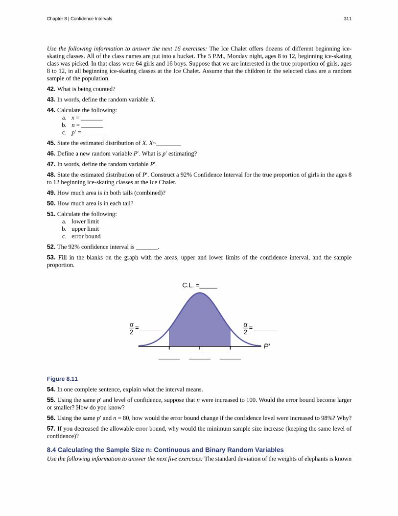
Use the following information to answer the next 16 exercises: The Ice Chalet offers dozens of different beginning ice-skating classes. All of the class names are put into a bucket. The 5 P.M., Monday night, ages 8 to 12, beginning ice-skatingclass was picked. In that class were 64 girls and 16 boys. Suppose that we are interested in the true proportion of girls, ages8 to 12, in all beginning ice-skating classes at the Ice Chalet. Assume that the children in the selected class are a randomsample of the population.
42. What is being counted?
43. In words, define the random variable X.
44. Calculate the following:a. x = _______b. n = _______c. p′ = _______
45. State the estimated distribution of X. X~________
46. Define a new random variable P′. What is p′ estimating?
47. In words, define the random variable P′.
48. State the estimated distribution of P′. Construct a 92% Confidence Interval for the true proportion of girls in the ages 8to 12 beginning ice-skating classes at the Ice Chalet.
49. How much area is in both tails (combined)?
50. How much area is in each tail?
51. Calculate the following:a. lower limitb. upper limitc. error bound
52. The 92% confidence interval is _______.
53. Fill in the blanks on the graph with the areas, upper and lower limits of the confidence interval, and the sampleproportion.
Figure 8.11
54. In one complete sentence, explain what the interval means.
55. Using the same p′ and level of confidence, suppose that n were increased to 100. Would the error bound become largeror smaller? How do you know?
56. Using the same p′ and n = 80, how would the error bound change if the confidence level were increased to 98%? Why?
57. If you decreased the allowable error bound, why would the minimum sample size increase (keeping the same level ofconfidence)?
8.4 Calculating the Sample Size n: Continuous and Binary Random VariablesUse the following information to answer the next five exercises: The standard deviation of the weights of elephants is known
Chapter 8 | Confidence Intervals 311
to be approximately 15 pounds. We wish to construct a 95% confidence interval for the mean weight of newborn elephantcalves. Fifty newborn elephants are weighed. The sample mean is 244 pounds. The sample standard deviation is 11 pounds.
58. Identify the following:a. x- = _____
b. σ = _____c. n = _____
59. In words, define the random variables X and X- .
60. Which distribution should you use for this problem?
61. Construct a 95% confidence interval for the population mean weight of newborn elephants. State the confidenceinterval, sketch the graph, and calculate the error bound.
62. What will happen to the confidence interval obtained, if 500 newborn elephants are weighed instead of 50? Why?
Use the following information to answer the next seven exercises: The U.S. Census Bureau conducts a study to determinethe time needed to complete the short form. The Bureau surveys 200 people. The sample mean is 8.2 minutes. There is aknown standard deviation of 2.2 minutes. The population distribution is assumed to be normal.
63. Identify the following:a. x- = _____
b. σ = _____c. n = _____
64. In words, define the random variables X and X- .
65. Which distribution should you use for this problem?
66. Construct a 90% confidence interval for the population mean time to complete the forms. State the confidence interval,sketch the graph, and calculate the error bound.
67. If the Census wants to increase its level of confidence and keep the error bound the same by taking another survey, whatchanges should it make?
68. If the Census did another survey, kept the error bound the same, and surveyed only 50 people instead of 200, whatwould happen to the level of confidence? Why?
69. Suppose the Census needed to be 98% confident of the population mean length of time. Would the Census have tosurvey more people? Why or why not?
Use the following information to answer the next ten exercises: A sample of 20 heads of lettuce was selected. Assume thatthe population distribution of head weight is normal. The weight of each head of lettuce was then recorded. The mean weightwas 2.2 pounds with a standard deviation of 0.1 pounds. The population standard deviation is known to be 0.2 pounds.
70. Identify the following:a. x- = ______
b. σ = ______c. n = ______
71. In words, define the random variable X.
72. In words, define the random variable X- .
73. Which distribution should you use for this problem?
74. Construct a 90% confidence interval for the population mean weight of the heads of lettuce. State the confidenceinterval, sketch the graph, and calculate the error bound.
75. Construct a 95% confidence interval for the population mean weight of the heads of lettuce. State the confidenceinterval, sketch the graph, and calculate the error bound.
76. In complete sentences, explain why the confidence interval in Exercise 8.74 is larger than in Exercise 8.75.
77. In complete sentences, give an interpretation of what the interval in Exercise 8.75 means.
312 Chapter 8 | Confidence Intervals
This OpenStax book is available for free at https://legacy.cnx.org/content/col12102/1.7
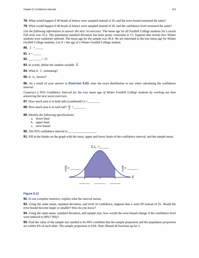
78. What would happen if 40 heads of lettuce were sampled instead of 20, and the error bound remained the same?
79. What would happen if 40 heads of lettuce were sampled instead of 20, and the confidence level remained the same?
Use the following information to answer the next 14 exercises: The mean age for all Foothill College students for a recentFall term was 33.2. The population standard deviation has been pretty consistent at 15. Suppose that twenty-five Winterstudents were randomly selected. The mean age for the sample was 30.4. We are interested in the true mean age for WinterFoothill College students. Let X = the age of a Winter Foothill College student.
80. x- = _____
81. n = _____
82. ________ = 15
83. In words, define the random variable X- .
84. What is x- estimating?
85. Is σx known?
86. As a result of your answer to Exercise 8.83, state the exact distribution to use when calculating the confidenceinterval.
Construct a 95% Confidence Interval for the true mean age of Winter Foothill College students by working out thenanswering the next seven exercises.
87. How much area is in both tails (combined)? α =________
88. How much area is in each tail? α2 =________
89. Identify the following specifications:a. lower limitb. upper limitc. error bound
90. The 95% confidence interval is:__________________.
91. Fill in the blanks on the graph with the areas, upper and lower limits of the confidence interval, and the sample mean.
Figure 8.12
92. In one complete sentence, explain what the interval means.
93. Using the same mean, standard deviation, and level of confidence, suppose that n were 69 instead of 25. Would theerror bound become larger or smaller? How do you know?
94. Using the same mean, standard deviation, and sample size, how would the error bound change if the confidence levelwere reduced to 90%? Why?
95. Find the value of the sample size needed to be 90% confident that the sample proportion and the population proportionare within 4% of each other. The sample proportion is 0.60. Note: Round all fractions up for n.
Chapter 8 | Confidence Intervals 313
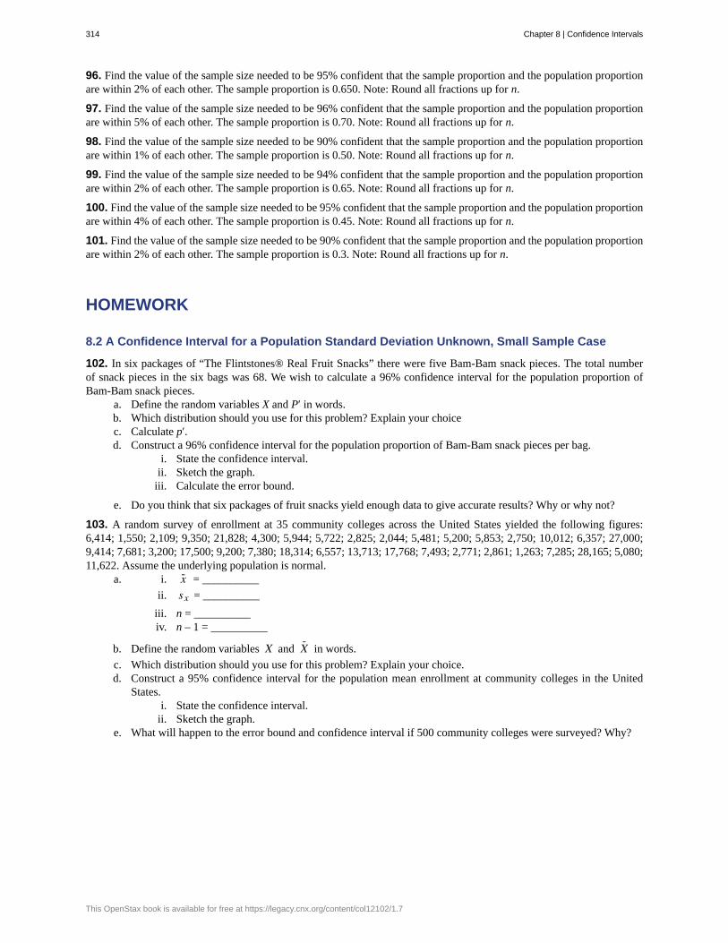
96. Find the value of the sample size needed to be 95% confident that the sample proportion and the population proportionare within 2% of each other. The sample proportion is 0.650. Note: Round all fractions up for n.
97. Find the value of the sample size needed to be 96% confident that the sample proportion and the population proportionare within 5% of each other. The sample proportion is 0.70. Note: Round all fractions up for n.
98. Find the value of the sample size needed to be 90% confident that the sample proportion and the population proportionare within 1% of each other. The sample proportion is 0.50. Note: Round all fractions up for n.
99. Find the value of the sample size needed to be 94% confident that the sample proportion and the population proportionare within 2% of each other. The sample proportion is 0.65. Note: Round all fractions up for n.
100. Find the value of the sample size needed to be 95% confident that the sample proportion and the population proportionare within 4% of each other. The sample proportion is 0.45. Note: Round all fractions up for n.
101. Find the value of the sample size needed to be 90% confident that the sample proportion and the population proportionare within 2% of each other. The sample proportion is 0.3. Note: Round all fractions up for n.
HOMEWORK
8.2 A Confidence Interval for a Population Standard Deviation Unknown, Small Sample Case
102. In six packages of “The Flintstones® Real Fruit Snacks” there were five Bam-Bam snack pieces. The total numberof snack pieces in the six bags was 68. We wish to calculate a 96% confidence interval for the population proportion ofBam-Bam snack pieces.
a. Define the random variables X and P′ in words.b. Which distribution should you use for this problem? Explain your choicec. Calculate p′.d. Construct a 96% confidence interval for the population proportion of Bam-Bam snack pieces per bag.
i. State the confidence interval.ii. Sketch the graph.
iii. Calculate the error bound.
e. Do you think that six packages of fruit snacks yield enough data to give accurate results? Why or why not?
103. A random survey of enrollment at 35 community colleges across the United States yielded the following figures:6,414; 1,550; 2,109; 9,350; 21,828; 4,300; 5,944; 5,722; 2,825; 2,044; 5,481; 5,200; 5,853; 2,750; 10,012; 6,357; 27,000;9,414; 7,681; 3,200; 17,500; 9,200; 7,380; 18,314; 6,557; 13,713; 17,768; 7,493; 2,771; 2,861; 1,263; 7,285; 28,165; 5,080;11,622. Assume the underlying population is normal.
a. i. x- = __________
ii. sx = __________
iii. n = __________iv. n – 1 = __________
b. Define the random variables X and X- in words.
c. Which distribution should you use for this problem? Explain your choice.d. Construct a 95% confidence interval for the population mean enrollment at community colleges in the United
States.i. State the confidence interval.
ii. Sketch the graph.e. What will happen to the error bound and confidence interval if 500 community colleges were surveyed? Why?
314 Chapter 8 | Confidence Intervals
This OpenStax book is available for free at https://legacy.cnx.org/content/col12102/1.7

104. Suppose that a committee is studying whether or not there is waste of time in our judicial system. It is interested inthe mean amount of time individuals waste at the courthouse waiting to be called for jury duty. The committee randomlysurveyed 81 people who recently served as jurors. The sample mean wait time was eight hours with a sample standarddeviation of four hours.
a. i. x- = __________
ii. sx = __________
iii. n = __________iv. n – 1 = __________
b. Define the random variables X and X- in words.
c. Which distribution should you use for this problem? Explain your choice.d. Construct a 95% confidence interval for the population mean time wasted.
i. State the confidence interval.ii. Sketch the graph.
e. Explain in a complete sentence what the confidence interval means.
105. A pharmaceutical company makes tranquilizers. It is assumed that the distribution for the length of time they last isapproximately normal. Researchers in a hospital used the drug on a random sample of nine patients. The effective period ofthe tranquilizer for each patient (in hours) was as follows: 2.7; 2.8; 3.0; 2.3; 2.3; 2.2; 2.8; 2.1; and 2.4.
a. i. x- = __________
ii. sx = __________
iii. n = __________iv. n – 1 = __________
b. Define the random variable X in words.
c. Define the random variable X- in words.
d. Which distribution should you use for this problem? Explain your choice.e. Construct a 95% confidence interval for the population mean length of time.
i. State the confidence interval.ii. Sketch the graph.
f. What does it mean to be “95% confident” in this problem?
106. Suppose that 14 children, who were learning to ride two-wheel bikes, were surveyed to determine how long they hadto use training wheels. It was revealed that they used them an average of six months with a sample standard deviation ofthree months. Assume that the underlying population distribution is normal.
a. i. x- = __________
ii. sx = __________
iii. n = __________iv. n – 1 = __________
b. Define the random variable X in words.
c. Define the random variable X- in words.
d. Which distribution should you use for this problem? Explain your choice.e. Construct a 99% confidence interval for the population mean length of time using training wheels.
i. State the confidence interval.ii. Sketch the graph.
f. Why would the error bound change if the confidence level were lowered to 90%?
Chapter 8 | Confidence Intervals 315
107. The Federal Election Commission (FEC) collects information about campaign contributions and disbursements forcandidates and political committees each election cycle. A political action committee (PAC) is a committee formed to raisemoney for candidates and campaigns. A Leadership PAC is a PAC formed by a federal politician (senator or representative)to raise money to help other candidates’ campaigns.
The FEC has reported financial information for 556 Leadership PACs that operating during the 2011–2012 election cycle.The following table shows the total receipts during this cycle for a random selection of 30 Leadership PACs.
$46,500.00 $0 $40,966.50 $105,887.20 $5,175.00
$29,050.00 $19,500.00 $181,557.20 $31,500.00 $149,970.80
$2,555,363.20 $12,025.00 $409,000.00 $60,521.70 $18,000.00
$61,810.20 $76,530.80 $119,459.20 $0 $63,520.00
$6,500.00 $502,578.00 $705,061.10 $708,258.90 $135,810.00
$2,000.00 $2,000.00 $0 $1,287,933.80 $219,148.30
Table 8.3
x- = $251, 854.23
s = $521, 130.41
Use this sample data to construct a 95% confidence interval for the mean amount of money raised by all Leadership PACsduring the 2011–2012 election cycle. Use the Student's t-distribution.
108. Forbes magazine published data on the best small firms in 2012. These were firms that had been publicly traded for atleast a year, have a stock price of at least $5 per share, and have reported annual revenue between $5 million and $1 billion.The Table 8.4 shows the ages of the corporate CEOs for a random sample of these firms.
48 58 51 61 56
59 74 63 53 50
59 60 60 57 46
55 63 57 47 55
57 43 61 62 49
67 67 55 55 49
Table 8.4
Use this sample data to construct a 90% confidence interval for the mean age of CEO’s for these top small firms. Use theStudent's t-distribution.
109. Unoccupied seats on flights cause airlines to lose revenue. Suppose a large airline wants to estimate its mean numberof unoccupied seats per flight over the past year. To accomplish this, the records of 225 flights are randomly selected and thenumber of unoccupied seats is noted for each of the sampled flights. The sample mean is 11.6 seats and the sample standarddeviation is 4.1 seats.
a. i. x- = __________
ii. sx = __________
iii. n = __________iv. n-1 = __________
b. Define the random variables X and X- in words.
c. Which distribution should you use for this problem? Explain your choice.d. Construct a 92% confidence interval for the population mean number of unoccupied seats per flight.
i. State the confidence interval.ii. Sketch the graph.
316 Chapter 8 | Confidence Intervals
This OpenStax book is available for free at https://legacy.cnx.org/content/col12102/1.7

110. In a recent sample of 84 used car sales costs, the sample mean was $6,425 with a standard deviation of $3,156. Assumethe underlying distribution is approximately normal.
a. Which distribution should you use for this problem? Explain your choice.
b. Define the random variable X- in words.
c. Construct a 95% confidence interval for the population mean cost of a used car.i. State the confidence interval.
ii. Sketch the graph.d. Explain what a “95% confidence interval” means for this study.
111. Six different national brands of chocolate chip cookies were randomly selected at the supermarket. The grams of fatper serving are as follows: 8; 8; 10; 7; 9; 9. Assume the underlying distribution is approximately normal.
a. Construct a 90% confidence interval for the population mean grams of fat per serving of chocolate chip cookiessold in supermarkets.
i. State the confidence interval.ii. Sketch the graph.
b. If you wanted a smaller error bound while keeping the same level of confidence, what should have been changedin the study before it was done?
c. Go to the store and record the grams of fat per serving of six brands of chocolate chip cookies.d. Calculate the mean.e. Is the mean within the interval you calculated in part a? Did you expect it to be? Why or why not?
112. A survey of the mean number of cents off that coupons give was conducted by randomly surveying one coupon perpage from the coupon sections of a recent San Jose Mercury News. The following data were collected: 20¢; 75¢; 50¢; 65¢;30¢; 55¢; 40¢; 40¢; 30¢; 55¢; $1.50; 40¢; 65¢; 40¢. Assume the underlying distribution is approximately normal.
a. i. x- = __________
ii. sx = __________
iii. n = __________iv. n-1 = __________
b. Define the random variables X and X- in words.
c. Which distribution should you use for this problem? Explain your choice.d. Construct a 95% confidence interval for the population mean worth of coupons.
i. State the confidence interval.ii. Sketch the graph.
e. If many random samples were taken of size 14, what percent of the confidence intervals constructed shouldcontain the population mean worth of coupons? Explain why.
Use the following information to answer the next two exercises: A quality control specialist for a restaurant chain takes arandom sample of size 12 to check the amount of soda served in the 16 oz. serving size. The sample mean is 13.30 with asample standard deviation of 1.55. Assume the underlying population is normally distributed.
113. Find the 95% Confidence Interval for the true population mean for the amount of soda served.a. (12.42, 14.18)b. (12.32, 14.29)c. (12.50, 14.10)d. Impossible to determine
8.3 A Confidence Interval for A Population Proportion
114. Insurance companies are interested in knowing the population percent of drivers who always buckle up before ridingin a car.
a. When designing a study to determine this population proportion, what is the minimum number you would needto survey to be 95% confident that the population proportion is estimated to within 0.03?
b. If it were later determined that it was important to be more than 95% confident and a new survey wascommissioned, how would that affect the minimum number you would need to survey? Why?
Chapter 8 | Confidence Intervals 317

115. Suppose that the insurance companies did do a survey. They randomly surveyed 400 drivers and found that 320claimed they always buckle up. We are interested in the population proportion of drivers who claim they always buckle up.
a. i. x = __________ii. n = __________
iii. p′ = __________b. Define the random variables X and P′, in words.c. Which distribution should you use for this problem? Explain your choice.d. Construct a 95% confidence interval for the population proportion who claim they always buckle up.
i. State the confidence interval.ii. Sketch the graph.
e. If this survey were done by telephone, list three difficulties the companies might have in obtaining random results.
116. According to a recent survey of 1,200 people, 61% feel that the president is doing an acceptable job. We are interestedin the population proportion of people who feel the president is doing an acceptable job.
a. Define the random variables X and P′ in words.b. Which distribution should you use for this problem? Explain your choice.c. Construct a 90% confidence interval for the population proportion of people who feel the president is doing an
acceptable job.i. State the confidence interval.
ii. Sketch the graph.
117. An article regarding interracial dating and marriage recently appeared in the Washington Post. Of the 1,709 randomlyselected adults, 315 identified themselves as Latino, 323 identified themselves as Black, 254 identified themselves as Asian,and 779 identified themselves as White. In this survey, 86% of Blacks said that they would welcome a White person intotheir families. Among Asians, 77% would welcome a White person into their families, 71% would welcome a Latino, and66% would welcome a Black person.
a. We are interested in finding the 95% confidence interval for the percent of all Black adults who would welcomea White person into their families. Define the random variables X and P′, in words.
b. Which distribution should you use for this problem? Explain your choice.c. Construct a 95% confidence interval.
i. State the confidence interval.ii. Sketch the graph.
118. Refer to the information in Exercise 8.117.a. Construct three 95% confidence intervals.
i. percent of all Asians who would welcome a White person into their families.ii. percent of all Asians who would welcome a Latino into their families.
iii. percent of all Asians who would welcome a Black person into their families.
b. Even though the three point estimates are different, do any of the confidence intervals overlap? Which?c. For any intervals that do overlap, in words, what does this imply about the significance of the differences in the
true proportions?d. For any intervals that do not overlap, in words, what does this imply about the significance of the differences in
the true proportions?
119. Stanford University conducted a study of whether running is healthy for men and women over age 50. During thefirst eight years of the study, 1.5% of the 451 members of the 50-Plus Fitness Association died. We are interested in theproportion of people over 50 who ran and died in the same eight-year period.
a. Define the random variables X and P′ in words.b. Which distribution should you use for this problem? Explain your choice.c. Construct a 97% confidence interval for the population proportion of people over 50 who ran and died in the same
eight–year period.i. State the confidence interval.
ii. Sketch the graph.d. Explain what a “97% confidence interval” means for this study.
318 Chapter 8 | Confidence Intervals
This OpenStax book is available for free at https://legacy.cnx.org/content/col12102/1.7
120. A telephone poll of 1,000 adult Americans was reported in an issue of Time Magazine. One of the questions askedwas “What is the main problem facing the country?” Twenty percent answered “crime.” We are interested in the populationproportion of adult Americans who feel that crime is the main problem.
a. Define the random variables X and P′ in words.b. Which distribution should you use for this problem? Explain your choice.c. Construct a 95% confidence interval for the population proportion of adult Americans who feel that crime is the
main problem.i. State the confidence interval.
ii. Sketch the graph.d. Suppose we want to lower the sampling error. What is one way to accomplish that?e. The sampling error given by Yankelovich Partners, Inc. (which conducted the poll) is ±3%. In one to three
complete sentences, explain what the ±3% represents.
121. Refer to Exercise 8.120. Another question in the poll was “[How much are] you worried about the quality ofeducation in our schools?” Sixty-three percent responded “a lot”. We are interested in the population proportion of adultAmericans who are worried a lot about the quality of education in our schools.
a. Define the random variables X and P′ in words.b. Which distribution should you use for this problem? Explain your choice.c. Construct a 95% confidence interval for the population proportion of adult Americans who are worried a lot about
the quality of education in our schools.i. State the confidence interval.
ii. Sketch the graph.d. The sampling error given by Yankelovich Partners, Inc. (which conducted the poll) is ±3%. In one to three
complete sentences, explain what the ±3% represents.
Use the following information to answer the next three exercises: According to a Field Poll, 79% of California adults (actualresults are 400 out of 506 surveyed) feel that “education and our schools” is one of the top issues facing California. We wishto construct a 90% confidence interval for the true proportion of California adults who feel that education and the schoolsis one of the top issues facing California.
122. A point estimate for the true population proportion is:a. 0.90b. 1.27c. 0.79d. 400
123. A 90% confidence interval for the population proportion is _______.a. (0.761, 0.820)b. (0.125, 0.188)c. (0.755, 0.826)d. (0.130, 0.183)
Use the following information to answer the next two exercises: Five hundred and eleven (511) homes in a certainsouthern California community are randomly surveyed to determine if they meet minimal earthquake preparednessrecommendations. One hundred seventy-three (173) of the homes surveyed met the minimum recommendations forearthquake preparedness, and 338 did not.
124. Find the confidence interval at the 90% Confidence Level for the true population proportion of southern Californiacommunity homes meeting at least the minimum recommendations for earthquake preparedness.
a. (0.2975, 0.3796)b. (0.6270, 0.6959)c. (0.3041, 0.3730)d. (0.6204, 0.7025)
125. The point estimate for the population proportion of homes that do not meet the minimum recommendations forearthquake preparedness is ______.
a. 0.6614b. 0.3386c. 173d. 338
Chapter 8 | Confidence Intervals 319

126. On May 23, 2013, Gallup reported that of the 1,005 people surveyed, 76% of U.S. workers believe that they willcontinue working past retirement age. The confidence level for this study was reported at 95% with a ±3% margin of error.
a. Determine the estimated proportion from the sample.b. Determine the sample size.c. Identify CL and α.d. Calculate the error bound based on the information provided.e. Compare the error bound in part d to the margin of error reported by Gallup. Explain any differences between the
values.f. Create a confidence interval for the results of this study.g. A reporter is covering the release of this study for a local news station. How should she explain the confidence
interval to her audience?
127. A national survey of 1,000 adults was conducted on May 13, 2013 by Rasmussen Reports. It concluded with 95%confidence that 49% to 55% of Americans believe that big-time college sports programs corrupt the process of highereducation.
a. Find the point estimate and the error bound for this confidence interval.b. Can we (with 95% confidence) conclude that more than half of all American adults believe this?c. Use the point estimate from part a and n = 1,000 to calculate a 75% confidence interval for the proportion of
American adults that believe that major college sports programs corrupt higher education.d. Can we (with 75% confidence) conclude that at least half of all American adults believe this?
128. Public Policy Polling recently conducted a survey asking adults across the U.S. about music preferences. When asked,80 of the 571 participants admitted that they have illegally downloaded music.
a. Create a 99% confidence interval for the true proportion of American adults who have illegally downloadedmusic.
b. This survey was conducted through automated telephone interviews on May 6 and 7, 2013. The error bound of thesurvey compensates for sampling error, or natural variability among samples. List some factors that could affectthe survey’s outcome that are not covered by the margin of error.
c. Without performing any calculations, describe how the confidence interval would change if the confidence levelchanged from 99% to 90%.
129. You plan to conduct a survey on your college campus to learn about the political awareness of students. You wantto estimate the true proportion of college students on your campus who voted in the 2012 presidential election with 95%confidence and a margin of error no greater than five percent. How many students must you interview?
8.4 Calculating the Sample Size n: Continuous and Binary Random Variables
130. Among various ethnic groups, the standard deviation of heights is known to be approximately three inches. We wishto construct a 95% confidence interval for the mean height of male Swedes. Forty-eight male Swedes are surveyed. Thesample mean is 71 inches. The sample standard deviation is 2.8 inches.
a. i. x- =________
ii. σ =________iii. n =________
b. In words, define the random variables X and X- .
c. Which distribution should you use for this problem? Explain your choice.d. Construct a 95% confidence interval for the population mean height of male Swedes.
i. State the confidence interval.ii. Sketch the graph.
e. What will happen to the level of confidence obtained if 1,000 male Swedes are surveyed instead of 48? Why?
131. Announcements for 84 upcoming engineering conferences were randomly picked from a stack of IEEE Spectrummagazines. The mean length of the conferences was 3.94 days, with a standard deviation of 1.28 days. Assume theunderlying population is normal.
a. In words, define the random variables X and X- .
b. Which distribution should you use for this problem? Explain your choice.c. Construct a 95% confidence interval for the population mean length of engineering conferences.
i. State the confidence interval.ii. Sketch the graph.
320 Chapter 8 | Confidence Intervals
This OpenStax book is available for free at https://legacy.cnx.org/content/col12102/1.7

132. Suppose that an accounting firm does a study to determine the time needed to complete one person’s tax forms. Itrandomly surveys 100 people. The sample mean is 23.6 hours. There is a known standard deviation of 7.0 hours. Thepopulation distribution is assumed to be normal.
a. i. x- =________
ii. σ =________iii. n =________
b. In words, define the random variables X and X- .
c. Which distribution should you use for this problem? Explain your choice.d. Construct a 90% confidence interval for the population mean time to complete the tax forms.
i. State the confidence interval.ii. Sketch the graph.
e. If the firm wished to increase its level of confidence and keep the error bound the same by taking another survey,what changes should it make?
f. If the firm did another survey, kept the error bound the same, and only surveyed 49 people, what would happen tothe level of confidence? Why?
g. Suppose that the firm decided that it needed to be at least 96% confident of the population mean length of time towithin one hour. How would the number of people the firm surveys change? Why?
133. A sample of 16 small bags of the same brand of candies was selected. Assume that the population distribution of bagweights is normal. The weight of each bag was then recorded. The mean weight was two ounces with a standard deviationof 0.12 ounces. The population standard deviation is known to be 0.1 ounce.
a. i. x- =________
ii. σ =________iii. sx =________
b. In words, define the random variable X.
c. In words, define the random variable X- .
d. Which distribution should you use for this problem? Explain your choice.e. Construct a 90% confidence interval for the population mean weight of the candies.
i. State the confidence interval.ii. Sketch the graph.
f. Construct a 98% confidence interval for the population mean weight of the candies.i. State the confidence interval.
ii. Sketch the graph.iii. Calculate the error bound.
g. In complete sentences, explain why the confidence interval in part f is larger than the confidence interval in parte.
h. In complete sentences, give an interpretation of what the interval in part f means.
134. A camp director is interested in the mean number of letters each child sends during his or her camp session. Thepopulation standard deviation is known to be 2.5. A survey of 20 campers is taken. The mean from the sample is 7.9 with asample standard deviation of 2.8.
a. i. x- =________
ii. σ =________iii. n =________
b. Define the random variables X and X- in words.
c. Which distribution should you use for this problem? Explain your choice.d. Construct a 90% confidence interval for the population mean number of letters campers send home.
i. State the confidence interval.ii. Sketch the graph.
e. What will happen to the error bound and confidence interval if 500 campers are surveyed? Why?
Chapter 8 | Confidence Intervals 321

135. What is meant by the term “90% confident” when constructing a confidence interval for a mean?a. If we took repeated samples, approximately 90% of the samples would produce the same confidence interval.b. If we took repeated samples, approximately 90% of the confidence intervals calculated from those samples would
contain the sample mean.c. If we took repeated samples, approximately 90% of the confidence intervals calculated from those samples would
contain the true value of the population mean.d. If we took repeated samples, the sample mean would equal the population mean in approximately 90% of the
samples.
136. The Federal Election Commission collects information about campaign contributions and disbursements forcandidates and political committees each election cycle. During the 2012 campaign season, there were 1,619 candidates forthe House of Representatives across the United States who received contributions from individuals. Table 8.5 shows thetotal receipts from individuals for a random selection of 40 House candidates rounded to the nearest $100. The standarddeviation for this data to the nearest hundred is σ = $909,200.
$3,600 $1,243,900 $10,900 $385,200 $581,500
$7,400 $2,900 $400 $3,714,500 $632,500
$391,000 $467,400 $56,800 $5,800 $405,200
$733,200 $8,000 $468,700 $75,200 $41,000
$13,300 $9,500 $953,800 $1,113,500 $1,109,300
$353,900 $986,100 $88,600 $378,200 $13,200
$3,800 $745,100 $5,800 $3,072,100 $1,626,700
$512,900 $2,309,200 $6,600 $202,400 $15,800
Table 8.5
a. Find the point estimate for the population mean.b. Using 95% confidence, calculate the error bound.c. Create a 95% confidence interval for the mean total individual contributions.d. Interpret the confidence interval in the context of the problem.
137. The American Community Survey (ACS), part of the United States Census Bureau, conducts a yearly census similarto the one taken every ten years, but with a smaller percentage of participants. The most recent survey estimates with 90%confidence that the mean household income in the U.S. falls between $69,720 and $69,922. Find the point estimate for meanU.S. household income and the error bound for mean U.S. household income.
138. The average height of young adult males has a normal distribution with standard deviation of 2.5 inches. You want toestimate the mean height of students at your college or university to within one inch with 93% confidence. How many malestudents must you measure?
139. If the confidence interval is change to a higher probability, would this cause a lower, or a higher, minimum samplesize?
140. If the tolerance is reduced by half, how would this affect the minimum sample size?
141. If the value of p is reduced, would this necessarily reduce the sample size needed?
142. Is it acceptable to use a higher sample size than the one calculated byz2 pqe2 ?
143. A company has been running an assembly line with 97.42%% of the products made being acceptable. Then, a criticalpiece broke down. After the repairs the decision was made to see if the number of defective products made was still closeenough to the long standing production quality. Samples of 500 pieces were selected at random, and the defective rate wasfound to be 0.025%.
a. Is this sample size adequate to claim the company is checking within the 90% confidence interval?b. The 95% confidence interval?
322 Chapter 8 | Confidence Intervals
This OpenStax book is available for free at https://legacy.cnx.org/content/col12102/1.7

REFERENCES
8.1 A Confidence Interval for a Population Standard Deviation, Known or Large Sample Size
“American Fact Finder.” U.S. Census Bureau. Available online at http://factfinder2.census.gov/faces/nav/jsf/pages/searchresults.xhtml?refresh=t (accessed July 2, 2013).
“Disclosure Data Catalog: Candidate Summary Report 2012.” U.S. Federal Election Commission. Available online athttp://www.fec.gov/data/index.jsp (accessed July 2, 2013).
“Headcount Enrollment Trends by Student Demographics Ten-Year Fall Trends to Most Recently Completed Fall.”Foothill De Anza Community College District. Available online at http://research.fhda.edu/factbook/FH_Demo_Trends/FoothillDemographicTrends.htm (accessed September 30,2013).
Kuczmarski, Robert J., Cynthia L. Ogden, Shumei S. Guo, Laurence M. Grummer-Strawn, Katherine M. Flegal, Zuguo Mei,Rong Wei, Lester R. Curtin, Alex F. Roche, Clifford L. Johnson. “2000 CDC Growth Charts for the United States: Methodsand Development.” Centers for Disease Control and Prevention. Available online at http://www.cdc.gov/growthcharts/2000growthchart-us.pdf (accessed July 2, 2013).
La, Lynn, Kent German. "Cell Phone Radiation Levels." c|net part of CBX Interactive Inc. Available online athttp://reviews.cnet.com/cell-phone-radiation-levels/ (accessed July 2, 2013).
“Mean Income in the Past 12 Months (in 2011 Inflation-Adjusted Dollars): 2011 American Community Survey 1-YearEstimates.” American Fact Finder, U.S. Census Bureau. Available online at http://factfinder2.census.gov/faces/tableservices/jsf/pages/productview.xhtml?pid=ACS_11_1YR_S1902&prodType=table (accessed July 2, 2013).
“Metadata Description of Candidate Summary File.” U.S. Federal Election Commission. Available online athttp://www.fec.gov/finance/disclosure/metadata/metadataforcandidatesummary.shtml (accessed July 2, 2013).
“National Health and Nutrition Examination Survey.” Centers for Disease Control and Prevention. Available online athttp://www.cdc.gov/nchs/nhanes.htm (accessed July 2, 2013).
8.2 A Confidence Interval for a Population Standard Deviation Unknown, Small Sample Case
“America’s Best Small Companies.” Forbes, 2013. Available online at http://www.forbes.com/best-small-companies/list/(accessed July 2, 2013).
Data from Microsoft Bookshelf.
Data from http://www.businessweek.com/.
Data from http://www.forbes.com/.
“Disclosure Data Catalog: Leadership PAC and Sponsors Report, 2012.” Federal Election Commission. Available online athttp://www.fec.gov/data/index.jsp (accessed July 2,2013).
“Human Toxome Project: Mapping the Pollution in People.” Environmental Working Group. Available online athttp://www.ewg.org/sites/humantoxome/participants/participant-group.php?group=in+utero%2Fnewborn (accessed July 2,2013).
“Metadata Description of Leadership PAC List.” Federal Election Commission. Available online at http://www.fec.gov/finance/disclosure/metadata/metadataLeadershipPacList.shtml (accessed July 2, 2013).
8.3 A Confidence Interval for A Population Proportion
Jensen, Tom. “Democrats, Republicans Divided on Opinion of Music Icons.” Public Policy Polling. Available online athttp://www.publicpolicypolling.com/Day2MusicPoll.pdf (accessed July 2, 2013).
Madden, Mary, Amanda Lenhart, Sandra Coresi, Urs Gasser, Maeve Duggan, Aaron Smith, and Meredith Beaton. “Teens,Social Media, and Privacy.” PewInternet, 2013. Available online at http://www.pewinternet.org/Reports/2013/Teens-Social-Media-And-Privacy.aspx (accessed July 2, 2013).
Prince Survey Research Associates International. “2013 Teen and Privacy Management Survey.” Pew Research Center:Internet and American Life Project. Available online at http://www.pewinternet.org/~/media//Files/Questionnaire/2013/Methods%20and%20Questions_Teens%20and%20Social%20Media.pdf (accessed July 2, 2013).
Chapter 8 | Confidence Intervals 323

Saad, Lydia. “Three in Four U.S. Workers Plan to Work Pas Retirement Age: Slightly more say they will do this bychoice rather than necessity.” Gallup® Economy, 2013. Available online at http://www.gallup.com/poll/162758/three-four-workers-plan-work-past-retirement-age.aspx (accessed July 2, 2013).
The Field Poll. Available online at http://field.com/fieldpollonline/subscribers/ (accessed July 2, 2013).
Zogby. “New SUNYIT/Zogby Analytics Poll: Few Americans Worry about Emergency Situations Occurring in TheirCommunity; Only one in three have an Emergency Plan; 70% Support Infrastructure ‘Investment’ for National Security.”Zogby Analytics, 2013. Available online at http://www.zogbyanalytics.com/news/299-americans-neither-worried-nor-prepared-in-case-of-a-disaster-sunyit-zogby-analytics-poll (accessed July 2, 2013).
“52% Say Big-Time College Athletics Corrupt Education Process.” Rasmussen Reports, 2013. Available online athttp://www.rasmussenreports.com/public_content/lifestyle/sports/may_2013/52_say_big_time_college_athletics_corrupt_education_process (accessed July 2, 2013).
SOLUTIONS
2 X is the number of hours a patient waits in the emergency room before being called back to be examined. X- is the mean
wait time of 70 patients in the emergency room.
4 CI: (1.3808, 1.6192)
Figure 8.13
EBM = 0.12
6a. x- = 151
b. sx = 32
c. n = 108
d. n – 1 = 107
8 X- is the mean number of hours spent watching television per month from a sample of 108 Americans.
10 CI: (142.92, 159.08)
324 Chapter 8 | Confidence Intervals
This OpenStax book is available for free at https://legacy.cnx.org/content/col12102/1.7

Figure 8.14
EBM = 8.08
12a. 3.26
b. 1.02
c. 39
14 μ
16 t38
18 0.025
20 (2.93, 3.59)
22 We are 95% confident that the true mean number of colors for national flags is between 2.93 colors and 3.59 colors.
23 The error bound would become EBM = 0.245. This error bound decreases because as sample sizes increase, variabilitydecreases and we need less interval length to capture the true mean.
26 The sample size needed would increase. As the confidence level increases, α decreases and z⎛⎝a2⎞⎠
increases. To
maintain the same error bound, the size of the sample needs to increase.
28 X is the number of “successes” where the woman makes the majority of the purchasing decisions for the household. P′ isthe percentage of households sampled where the woman makes the majority of the purchasing decisions for the household.
30 CI: (0.5321, 0.6679)
Figure 8.15
EBM: 0.0679
32 X is the number of “successes” where an executive prefers a truck. P′ is the percentage of executives sampled whoprefer a truck.
Chapter 8 | Confidence Intervals 325
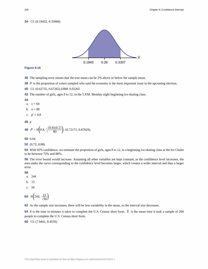
34 CI: (0.19432, 0.33068)
Figure 8.16
36 The sampling error means that the true mean can be 2% above or below the sample mean.
38 P′ is the proportion of voters sampled who said the economy is the most important issue in the upcoming election.
40 CI: (0.62735, 0.67265) EBM: 0.02265
42 The number of girls, ages 8 to 12, in the 5 P.M. Monday night beginning ice-skating class.
44a. x = 64
b. n = 80
c. p′ = 0.8
46 p
48 P′~N⎛⎝0.8, (0.8)(0.2)80⎞⎠ . (0.72171, 0.87829).
50 0.04
52 (0.72; 0.88)
54 With 92% confidence, we estimate the proportion of girls, ages 8 to 12, in a beginning ice-skating class at the Ice Chaletto be between 72% and 88%.
56 The error bound would increase. Assuming all other variables are kept constant, as the confidence level increases, thearea under the curve corresponding to the confidence level becomes larger, which creates a wider interval and thus a largererror.
58a. 244
b. 15
c. 50
60 N⎛⎝244, 1550⎞⎠
62 As the sample size increases, there will be less variability in the mean, so the interval size decreases.
64 X is the time in minutes it takes to complete the U.S. Census short form. X- is the mean time it took a sample of 200
people to complete the U.S. Census short form.
66 CI: (7.9441, 8.4559)
326 Chapter 8 | Confidence Intervals
This OpenStax book is available for free at https://legacy.cnx.org/content/col12102/1.7

Figure 8.17
68 The level of confidence would decrease because decreasing n makes the confidence interval wider, so at the same errorbound, the confidence level decreases.
70a. x- = 2.2
b. σ = 0.2
c. n = 20
72 X- is the mean weight of a sample of 20 heads of lettuce.
74 EBM = 0.07CI: (2.1264, 2.2736)
Figure 8.18
76 The interval is greater because the level of confidence increased. If the only change made in the analysis is a change inconfidence level, then all we are doing is changing how much area is being calculated for the normal distribution. Therefore,a larger confidence level results in larger areas and larger intervals.
78 The confidence level would increase.
80 30.4
82 σ
84 μ
86 normal
88 0.025
90 (24.52,36.28)
92 We are 95% confident that the true mean age for Winger Foothill College students is between 24.52 and 36.28.
Chapter 8 | Confidence Intervals 327
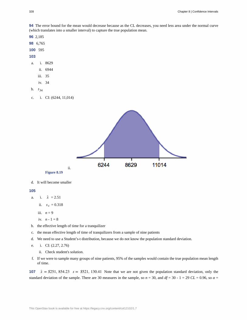
94 The error bound for the mean would decrease because as the CL decreases, you need less area under the normal curve(which translates into a smaller interval) to capture the true population mean.
96 2,185
98 6,765
100 595
103
a. i. 8629
ii. 6944
iii. 35
iv. 34
b. t34
c. i. CI: (6244, 11,014)
ii.Figure 8.19
d. It will become smaller
105
a. i. x- = 2.51
ii. sx = 0.318
iii. n = 9
iv. n - 1 = 8
b. the effective length of time for a tranquilizer
c. the mean effective length of time of tranquilizers from a sample of nine patients
d. We need to use a Student’s-t distribution, because we do not know the population standard deviation.
e. i. CI: (2.27, 2.76)
ii. Check student's solution.
f. If we were to sample many groups of nine patients, 95% of the samples would contain the true population mean lengthof time.
107 x- = $251, 854.23 s = $521, 130.41 Note that we are not given the population standard deviation, only the
standard deviation of the sample. There are 30 measures in the sample, so n = 30, and df = 30 - 1 = 29 CL = 0.96, so α =
328 Chapter 8 | Confidence Intervals
This OpenStax book is available for free at https://legacy.cnx.org/content/col12102/1.7

1 - CL = 1 - 0.96 = 0.04 α2 = 0.02tα
2= t0.02 = 2.150 EBM = tα
2⎛⎝ sn⎞⎠ = 2.150⎛⎝521, 130.41
30⎞⎠ ~ $204, 561.66 x- -
EBM = $251,854.23 - $204,561.66 = $47,292.57 x- + EBM = $251,854.23+ $204,561.66 = $456,415.89 We estimate with
96% confidence that the mean amount of money raised by all Leadership PACs during the 2011–2012 election cycle liesbetween $47,292.57 and $456,415.89.
109
a. i. x- = 11.6
ii. sx = 4.1
iii. n = 225
iv. n - 1 = 224
b. X is the number of unoccupied seats on a single flight. X- is the mean number of unoccupied seats from a sample of
225 flights.
c. We will use a Student’s-t distribution, because we do not know the population standard deviation.
d. i. CI: (11.12 , 12.08)
ii. Check student's solution.
111
a. i. CI: (7.64 , 9.36)
ii.Figure 8.20
b. The sample should have been increased.
c. Answers will vary.
d. Answers will vary.
e. Answers will vary.
113 b
114a. 1,068
b. The sample size would need to be increased since the critical value increases as the confidence level increases.
116a. X = the number of people who feel that the president is doing an acceptable job;
P′ = the proportion of people in a sample who feel that the president is doing an acceptable job.
b. N⎛⎝0.61, (0.61)(0.39)1200
⎞⎠
c. i. CI: (0.59, 0.63)
Chapter 8 | Confidence Intervals 329

ii. Check student’s solution
118
a. i. (0.72, 0.82)
ii. (0.65, 0.76)
iii. (0.60, 0.72)
b. Yes, the intervals (0.72, 0.82) and (0.65, 0.76) overlap, and the intervals (0.65, 0.76) and (0.60, 0.72) overlap.
c. We can say that there does not appear to be a significant difference between the proportion of Asian adults who saythat their families would welcome a White person into their families and the proportion of Asian adults who say thattheir families would welcome a Latino person into their families.
d. We can say that there is a significant difference between the proportion of Asian adults who say that their familieswould welcome a White person into their families and the proportion of Asian adults who say that their families wouldwelcome a Black person into their families.
120a. X = the number of adult Americans who feel that crime is the main problem; P′ = the proportion of adult Americans
who feel that crime is the main problem
b. Since we are estimating a proportion, given P′ = 0.2 and n = 1000, the distribution we should use is
N⎛⎝0.2, (0.2)(0.8)1000
⎞⎠ .
c. i. CI: (0.18, 0.22)
ii. Check student’s solution.
d. One way to lower the sampling error is to increase the sample size.
e. The stated “± 3%” represents the maximum error bound. This means that those doing the study are reporting amaximum error of 3%. Thus, they estimate the percentage of adult Americans who feel that crime is the main problemto be between 18% and 22%.
122 c
125 a
127
a. p′ =(0.55 + 0.49)
2 = 0.52; EBP = 0.55 - 0.52 = 0.03
b. No, the confidence interval includes values less than or equal to 0.50. It is possible that less than half of the populationbelieve this.
c. CL = 0.75, so α = 1 – 0.75 = 0.25 and α2 = 0.125 zα
2= 1.150 . (The area to the right of this z is 0.125, so the area to
the left is 1 – 0.125 = 0.875.)
EBP = (1.150) 0.52(0.48)1, 000 ≈ 0.018
(p′ - EBP, p′ + EBP) = (0.52 – 0.018, 0.52 + 0.018) = (0.502, 0.538)
d. Yes – this interval does not fall less than 0.50 so we can conclude that at least half of all American adults believe thatmajor sports programs corrupt education – but we do so with only 75% confidence.
130
a. i. 71
ii. 2.8
iii. 48
b. X is the height of a male Swede, and x_ is the mean height from a sample of 48 male Swedes.
330 Chapter 8 | Confidence Intervals
This OpenStax book is available for free at https://legacy.cnx.org/content/col12102/1.7

c. Normal. We know the standard deviation for the population, and the sample size is greater than 30.
d. i. CI: (70.151, 71.85)
ii.Figure 8.21
e. The confidence interval will decrease in size, because the sample size increased. Recall, when all factors remainunchanged, an increase in sample size decreases variability. Thus, we do not need as large an interval to capture thetrue population mean.
132
a. i. x- = 23.6
ii. σ = 7
iii. n = 100
b. X is the time needed to complete an individual tax form. X- is the mean time to complete tax forms from a sample of
100 customers.
c. N⎛⎝23.6, 7100⎞⎠ because we know sigma.
d. i. (22.228, 24.972)
ii.Figure 8.22
e. It will need to change the sample size. The firm needs to determine what the confidence level should be, then applythe error bound formula to determine the necessary sample size.
Chapter 8 | Confidence Intervals 331

f. The confidence level would increase as a result of a larger interval. Smaller sample sizes result in more variability. Tocapture the true population mean, we need to have a larger interval.
g. According to the error bound formula, the firm needs to survey 206 people. Since we increase the confidence level,we need to increase either our error bound or the sample size.
134
a. i. 7.9
ii. 2.5
iii. 20
b. X is the number of letters a single camper will send home. X-
is the mean number of letters sent home from a sample
of 20 campers.
c. N 7.9⎛⎝2.520⎞⎠
d. i. CI: (6.98, 8.82)
ii.Figure 8.23
e. The error bound and confidence interval will decrease.
136a. x- = $568,873
b. CL = 0.95 α = 1 – 0.95 = 0.05 zα2
= 1.96
EBM = z0.025σn = 1.96 909200
40= $281,764
c. x- − EBM = 568,873 − 281,764 = 287,109
x- + EBM = 568,873 + 281,764 = 850,637
d. We estimate with 95% confidence that the mean amount of contributions received from all individuals by Housecandidates is between $287,109 and $850,637.
139 Higher
140 It would increase to four times the prior value.
141 No, It could have no affect if it were to change to 1 – p, for example. If it gets closer to 0.5 the minimum sample sizewould increase.
142 Yes
143a. No
b. No
332 Chapter 8 | Confidence Intervals
This OpenStax book is available for free at https://legacy.cnx.org/content/col12102/1.7

9 | HYPOTHESIS TESTINGWITH ONE SAMPLE
Figure 9.1 You can use a hypothesis test to decide if a dog breeder’s claim that every Dalmatian has 35 spots isstatistically sound. (Credit: Robert Neff)
Introduction
Now we are down to the bread and butter work of the statistician: developing and testing hypotheses. It is important toput this material in a broader context so that the method by which a hypothesis is formed is understood completely. Usingtextbook examples often clouds the real source of statistical hypotheses.
Statistical testing is part of a much larger process known as the scientific method. This method was developed more thantwo centuries ago as the accepted way that new knowledge could be created. Until then, and unfortunately even today,among some, "knowledge" could be created simply by some authority saying something was so, ipso dicta. Superstition andconspiracy theories were (are?) accepted uncritically.
The scientific method, briefly, states that only by following a careful and specific process can some assertion be includedin the accepted body of knowledge. This process begins with a set of assumptions upon which a theory, sometimes called amodel, is built. This theory, if it has any validity, will lead to predictions; what we call hypotheses.
As an example, in Microeconomics the theory of consumer choice begins with certain assumption concerning human
Chapter 9 | Hypothesis Testing with One Sample 333

behavior. From these assumptions a theory of how consumers make choices using indifference curves and the budget line.This theory gave rise to a very important prediction, namely, that there was an inverse relationship between price andquantity demanded. This relationship was known as the demand curve. The negative slope of the demand curve is reallyjust a prediction, or a hypothesis, that can be tested with statistical tools.
Unless hundreds and hundreds of statistical tests of this hypothesis had not confirmed this relationship, the so-called Lawof Demand would have been discarded years ago. This is the role of statistics, to test the hypotheses of various theories todetermine if they should be admitted into the accepted body of knowledge; how we understand our world. Once admitted,however, they may be later discarded if new theories come along that make better predictions.
Not long ago two scientists claimed that they could get more energy out of a process than was put in. This caused atremendous stir for obvious reasons. They were on the cover of Time and were offered extravagant sums to bring theirresearch work to private industry and any number of universities. It was not long until their work was subjected to therigorous tests of the scientific method and found to be a failure. No other lab could replicate their findings. Consequentlythey have sunk into obscurity and their theory discarded. It may surface again when someone can pass the tests of thehypotheses required by the scientific method, but until then it is just a curiosity. Many pure frauds have been attempted overtime, but most have been found out by applying the process of the scientific method.
This discussion is meant to show just where in this process statistics falls. Statistics and statisticians are not necessarily inthe business of developing theories, but in the business of testing others' theories. Hypotheses come from these theoriesbased upon an explicit set of assumptions and sound logic. The hypothesis comes first, before any data are gathered. Datado not create hypotheses; they are used to test them. If we bear this in mind as we study this section the process of formingand testing hypotheses will make more sense.
One job of a statistician is to make statistical inferences about populations based on samples taken from the population.Confidence intervals are one way to estimate a population parameter. Another way to make a statistical inference is tomake a decision about the value of a specific parameter. For instance, a car dealer advertises that its new small truck gets35 miles per gallon, on average. A tutoring service claims that its method of tutoring helps 90% of its students get an A ora B. A company says that women managers in their company earn an average of $60,000 per year.
A statistician will make a decision about these claims. This process is called " hypothesis testing." A hypothesis testinvolves collecting data from a sample and evaluating the data. Then, the statistician makes a decision as to whether or notthere is sufficient evidence, based upon analyses of the data, to reject the null hypothesis.
In this chapter, you will conduct hypothesis tests on single means and single proportions. You will also learn about the errorsassociated with these tests.
9.1 | Null and Alternative HypothesesThe actual test begins by considering two hypotheses. They are called the null hypothesis and the alternative hypothesis.These hypotheses contain opposing viewpoints.
H0: The null hypothesis: It is a statement of no difference between the variables–they are not related. This can often beconsidered the status quo and as a result if you cannot accept the null it requires some action.
Ha: The alternative hypothesis: It is a claim about the population that is contradictory to H0 and what we conclude whenwe cannot accept H0. This is usually what the researcher is trying to prove. The alternative hypothesis is the contender andmust win with significant evidence to overthrow the status quo. This concept is sometimes referred to the tyranny of thestatus quo because as we will see later, to overthrow the null hypothesis takes usually 90 or greater confidence that this isthe proper decision.
Since the null and alternative hypotheses are contradictory, you must examine evidence to decide if you have enoughevidence to reject the null hypothesis or not. The evidence is in the form of sample data.
After you have determined which hypothesis the sample supports, you make a decision. There are two options for adecision. They are "cannot accept H0" if the sample information favors the alternative hypothesis or "do not reject H0" or"decline to reject H0" if the sample information is insufficient to reject the null hypothesis. These conclusions are all basedupon a level of probability, a significance level, that is set my the analyst.
Table 9.1 presents the various hypotheses in the relevant pairs. For example, if the null hypothesis is equal to some value,the alternative has to be not equal to that value.
334 Chapter 9 | Hypothesis Testing with One Sample
This OpenStax book is available for free at https://legacy.cnx.org/content/col12102/1.7
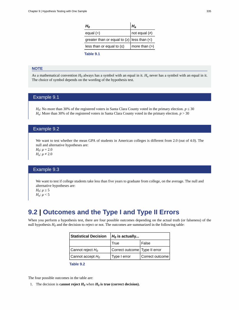
H0 Ha
equal (=) not equal (≠)
greater than or equal to (≥) less than (<)
less than or equal to (≤) more than (>)
Table 9.1
NOTE
As a mathematical convention H0 always has a symbol with an equal in it. Ha never has a symbol with an equal in it.The choice of symbol depends on the wording of the hypothesis test.
Example 9.1
H0: No more than 30% of the registered voters in Santa Clara County voted in the primary election. p ≤ 30Ha: More than 30% of the registered voters in Santa Clara County voted in the primary election. p > 30
Example 9.2
We want to test whether the mean GPA of students in American colleges is different from 2.0 (out of 4.0). Thenull and alternative hypotheses are:H0: μ = 2.0Ha: μ ≠ 2.0
Example 9.3
We want to test if college students take less than five years to graduate from college, on the average. The null andalternative hypotheses are:H0: μ ≥ 5Ha: μ < 5
9.2 | Outcomes and the Type I and Type II ErrorsWhen you perform a hypothesis test, there are four possible outcomes depending on the actual truth (or falseness) of thenull hypothesis H0 and the decision to reject or not. The outcomes are summarized in the following table:
Statistical Decision H0 is actually...
True False
Cannot reject H0 Correct outcome Type II error
Cannot accept H0 Type I error Correct outcome
Table 9.2
The four possible outcomes in the table are:
1. The decision is cannot reject H0 when H0 is true (correct decision).
Chapter 9 | Hypothesis Testing with One Sample 335

2. The decision is cannot accept H0 when H0 is true (incorrect decision known as a Type I error). This case is describedas "rejecting a good null". As we will see later, it is this type of error that we will guard against by setting theprobability of making such an error. The goal is to NOT take an action that is an error.
3. The decision is cannot reject H0 when, in fact, H0 is false (incorrect decision known as a Type II error). This iscalled "accepting a false null". In this situation you have allowed the status quo to remain in force when it should beoverturned. As we will see, the null hypothesis has the advantage in competition with the alternative.
4. The decision is cannot accept H0 when H0 is false (correct decision).
Each of the errors occurs with a particular probability. The Greek letters α and β represent the probabilities.
α = probability of a Type I error = P(Type I error) = probability of rejecting the null hypothesis when the null hypothesisis true: rejecting a good null.
β = probability of a Type II error = P(Type II error) = probability of not rejecting the null hypothesis when the nullhypothesis is false. (1 − β) is called the Power of the Test.
α and β should be as small as possible because they are probabilities of errors.
Statistics allows us to set the probability that we are making a Type I error. The probability of making a Type I error isα. Recall that the confidence intervals in the last unit were set by choosing a value called Zα (or tα) and the alpha valuedetermined the confidence level of the estimate because it was the probability of the interval failing to capture the true mean(or proportion parameter p). This alpha and that one are the same.
The easiest way to see the relationship between the alpha error and the level of confidence is with the following figure.
Figure 9.2
In the center of Figure 9.2 is a normally distributed sampling distribution marked H0. This is a sampling distribution of
X–
and by the Central Limit Theorem it is normally distributed. The distribution in the center is marked H0 and represents
the distribution for the null hypotheses H0: µ = 100. This is the value that is being tested. The formal statements of the nulland alternative hypotheses are listed below the figure.
The distributions on either side of the H0 distribution represent distributions that would be true if H0 is false, under thealternative hypothesis listed as Ha. We do not know which is true, and will never know. There are, in fact, an infinitenumber of distributions from which the data could have been drawn if Ha is true, but only two of them are on Figure 9.2representing all of the others.
To test a hypothesis we take a sample from the population and determine if it could have come from the hypothesizeddistribution with an acceptable level of significance. This level of significance is the alpha error and is marked on Figure9.2 as the shaded areas in each tail of the H0 distribution. (Each area is actually α/2 because the distribution is symmetricaland the alternative hypothesis allows for the possibility for the value to be either greater than or less than the hypothesizedvalue--called a two-tailed test).
If the sample mean marked as X–
1 is in the tail of the distribution of H0, we conclude that the probability that it could have
come from the H0 distribution is less than alpha. We consequently state, "the null hypothesis cannot be accepted with (α)
level of significance". The truth may be that this X–
1 did come from the H0 distribution, but from out in the tail. If this is
so then we have falsely rejected a true null hypothesis and have made a Type I error. What statistics has done is provide an
336 Chapter 9 | Hypothesis Testing with One Sample
This OpenStax book is available for free at https://legacy.cnx.org/content/col12102/1.7
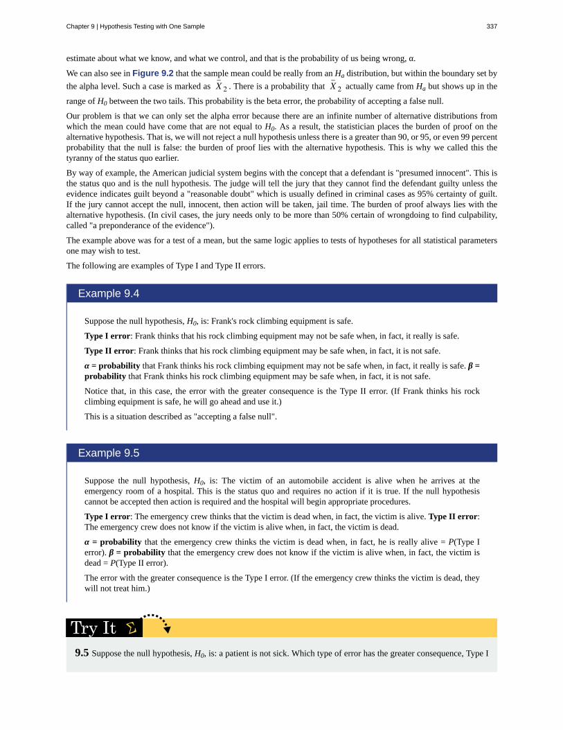
estimate about what we know, and what we control, and that is the probability of us being wrong, α.
We can also see in Figure 9.2 that the sample mean could be really from an Ha distribution, but within the boundary set by
the alpha level. Such a case is marked as X–
2 . There is a probability that X–
2 actually came from Ha but shows up in the
range of H0 between the two tails. This probability is the beta error, the probability of accepting a false null.
Our problem is that we can only set the alpha error because there are an infinite number of alternative distributions fromwhich the mean could have come that are not equal to H0. As a result, the statistician places the burden of proof on thealternative hypothesis. That is, we will not reject a null hypothesis unless there is a greater than 90, or 95, or even 99 percentprobability that the null is false: the burden of proof lies with the alternative hypothesis. This is why we called this thetyranny of the status quo earlier.
By way of example, the American judicial system begins with the concept that a defendant is "presumed innocent". This isthe status quo and is the null hypothesis. The judge will tell the jury that they cannot find the defendant guilty unless theevidence indicates guilt beyond a "reasonable doubt" which is usually defined in criminal cases as 95% certainty of guilt.If the jury cannot accept the null, innocent, then action will be taken, jail time. The burden of proof always lies with thealternative hypothesis. (In civil cases, the jury needs only to be more than 50% certain of wrongdoing to find culpability,called "a preponderance of the evidence").
The example above was for a test of a mean, but the same logic applies to tests of hypotheses for all statistical parametersone may wish to test.
The following are examples of Type I and Type II errors.
Example 9.4
Suppose the null hypothesis, H0, is: Frank's rock climbing equipment is safe.
Type I error: Frank thinks that his rock climbing equipment may not be safe when, in fact, it really is safe.
Type II error: Frank thinks that his rock climbing equipment may be safe when, in fact, it is not safe.
α = probability that Frank thinks his rock climbing equipment may not be safe when, in fact, it really is safe. β =probability that Frank thinks his rock climbing equipment may be safe when, in fact, it is not safe.
Notice that, in this case, the error with the greater consequence is the Type II error. (If Frank thinks his rockclimbing equipment is safe, he will go ahead and use it.)
This is a situation described as "accepting a false null".
Example 9.5
Suppose the null hypothesis, H0, is: The victim of an automobile accident is alive when he arrives at theemergency room of a hospital. This is the status quo and requires no action if it is true. If the null hypothesiscannot be accepted then action is required and the hospital will begin appropriate procedures.
Type I error: The emergency crew thinks that the victim is dead when, in fact, the victim is alive. Type II error:The emergency crew does not know if the victim is alive when, in fact, the victim is dead.
α = probability that the emergency crew thinks the victim is dead when, in fact, he is really alive = P(Type Ierror). β = probability that the emergency crew does not know if the victim is alive when, in fact, the victim isdead = P(Type II error).
The error with the greater consequence is the Type I error. (If the emergency crew thinks the victim is dead, theywill not treat him.)
9.5 Suppose the null hypothesis, H0, is: a patient is not sick. Which type of error has the greater consequence, Type I
Chapter 9 | Hypothesis Testing with One Sample 337

or Type II?
Example 9.6
It’s a Boy Genetic Labs claim to be able to increase the likelihood that a pregnancy will result in a boy beingborn. Statisticians want to test the claim. Suppose that the null hypothesis, H0, is: It’s a Boy Genetic Labs has noeffect on gender outcome. The status quo is that the claim is false. The burden of proof always falls to the personmaking the claim, in this case the Genetics Lab.
Type I error: This results when a true null hypothesis is rejected. In the context of this scenario, we would statethat we believe that It’s a Boy Genetic Labs influences the gender outcome, when in fact it has no effect. Theprobability of this error occurring is denoted by the Greek letter alpha, α.
Type II error: This results when we fail to reject a false null hypothesis. In context, we would state that It’s aBoy Genetic Labs does not influence the gender outcome of a pregnancy when, in fact, it does. The probabilityof this error occurring is denoted by the Greek letter beta, β.
The error of greater consequence would be the Type I error since couples would use the It’s a Boy Genetic Labsproduct in hopes of increasing the chances of having a boy.
9.6 “Red tide” is a bloom of poison-producing algae–a few different species of a class of plankton calleddinoflagellates. When the weather and water conditions cause these blooms, shellfish such as clams living in the areadevelop dangerous levels of a paralysis-inducing toxin. In Massachusetts, the Division of Marine Fisheries (DMF)monitors levels of the toxin in shellfish by regular sampling of shellfish along the coastline. If the mean level of toxinin clams exceeds 800 μg (micrograms) of toxin per kg of clam meat in any area, clam harvesting is banned there untilthe bloom is over and levels of toxin in clams subside. Describe both a Type I and a Type II error in this context, andstate which error has the greater consequence.
Example 9.7
A certain experimental drug claims a cure rate of at least 75% for males with prostate cancer. Describe both theType I and Type II errors in context. Which error is the more serious?
Type I: A cancer patient believes the cure rate for the drug is less than 75% when it actually is at least 75%.
Type II: A cancer patient believes the experimental drug has at least a 75% cure rate when it has a cure rate thatis less than 75%.
In this scenario, the Type II error contains the more severe consequence. If a patient believes the drug works atleast 75% of the time, this most likely will influence the patient’s (and doctor’s) choice about whether to use thedrug as a treatment option.
9.3 | Distribution Needed for Hypothesis TestingEarlier, we discussed sampling distributions. Particular distributions are associated with hypothesis testing.We will performhypotheses tests of a population mean using a normal distribution or a Student's t-distribution. (Remember, use a Student'st-distribution when the population standard deviation is unknown and the sample size is small, where small is considered tobe less than 30 observations.) We perform tests of a population proportion using a normal distribution when we can assumethat the distribution is normally distributed. We consider this to be true if the sample proportion, p ' , times the sample
size is greater than 5 and 1- p ' times the sample size is also greater than 5. This is the same rule of thumb we used when
338 Chapter 9 | Hypothesis Testing with One Sample
This OpenStax book is available for free at https://legacy.cnx.org/content/col12102/1.7

developing the formula for the confidence interval for a population proportion.
Hypothesis Test for the MeanGoing back to the standardizing formula we can derive the test statistic for testing hypotheses concerning means.
Zc = x– - μ0σ / n
The standardizing formula cannot be solved as it is because we do not have μ, the population mean. However, if wesubstitute in the hypothesized value of the mean, μ0 in the formula as above, we can compute a Z value. This is the teststatistic for a test of hypothesis for a mean and is presented in Figure 9.3. We interpret this Z value as the associated
probability that a sample with a sample mean of X–
could have come from a distribution with a population mean of H0 and
we call this Z value Zc for “calculated”. Figure 9.3 and Figure 9.4 show this process.
Figure 9.3
In Figure 9.3 two of the three possible outcomes are presented. X–
1 and X–
3 are in the tails of the hypothesized
distribution of H0. Notice that the horizontal axis in the top panel is labeled X–
's. This is the same theoretical distribution of
X–
's, the sampling distribution, that the Central Limit Theorem tells us is normally distributed. This is why we can draw it
with this shape. The horizontal axis of the bottom panel is labeled Z and is the standard normal distribution. Zα2
and -Zα2
,
called the critical values, are marked on the bottom panel as the Z values associated with the probability the analyst has setas the level of significance in the test, (α). The probabilities in the tails of both panels are, therefore, the same.
Notice that for each X–
there is an associated Zc, called the calculated Z, that comes from solving the equation above. This
calculated Z is nothing more than the number of standard deviations that the hypothesized mean is from the sample mean.
Chapter 9 | Hypothesis Testing with One Sample 339

If the sample mean falls "too many" standard deviations from the hypothesized mean we conclude that the sample meancould not have come from the distribution with the hypothesized mean, given our pre-set required level of significance.It could have come from H0, but it is deemed just too unlikely. In Figure 9.3 both X
_1 and X
_3 are in the tails of the
distribution. They are deemed "too far" from the hypothesized value of the mean given the chosen level of alpha. If in factthis sample mean it did come from H0, but from in the tail, we have made a Type I error: we have rejected a good null. Ouronly real comfort is that we know the probability of making such an error, α, and we can control the size of α.
Figure 9.4 shows the third possibility for the location of the sample mean, x_ . Here the sample mean is within the two
critical values. That is, within the probability of (1-α) and we cannot reject the null hypothesis.
Figure 9.4
This gives us the decision rule for testing a hypothesis for a two-tailed test:
Decision rule: two-tail test
If |Zc| < Zα2
: then do not REJECT H0
If |Zc| > Zα2
: then REJECT H0
Table 9.3
This rule will always be the same no matter what hypothesis we are testing or what formulas we are using to make thetest. The only change will be to change the Zc to the appropriate symbol for the test statistic for the parameter beingtested. Stating the decision rule another way: if the sample mean is unlikely to have come from the distribution with the
340 Chapter 9 | Hypothesis Testing with One Sample
This OpenStax book is available for free at https://legacy.cnx.org/content/col12102/1.7

hypothesized mean we cannot accept the null hypothesis. Here we define "unlikely" as having a probability less than alphaof occurring.
P-Value ApproachAn alternative decision rule can be developed by calculating the probability that a sample mean could be found that wouldgive a test statistic larger than the test statistic found from the current sample data assuming that the null hypothesis is true.Here the notion of "likely" and "unlikely" is defined by the probability of drawing a sample with a mean from a populationwith the hypothesized mean that is either larger or smaller than that found in the sample data. Simply stated, the p-valueapproach compares the desired significance level, α, to the p-value which is the probability of drawing a sample meanfurther from the hypothesized value than the actual sample mean. A large p-value calculated from the data indicates that weshould not reject the null hypothesis. The smaller the p-value, the more unlikely the outcome, and the stronger the evidenceis against the null hypothesis. We would reject the null hypothesis if the evidence is strongly against it. The relationshipbetween the decision rule of comparing the calculated test statistics, Zc, and the Critical Value, Zα , and using the p-valuecan be seen in Figure 9.5.
Figure 9.5
The calculated value of the test statistic is Zc in this example and is marked on the bottom graph of the standard normaldistribution because it is a Z value. In this case the calculated value is in the tail and thus we cannot accept the null
hypothesis, the associated X–
is just too unusually large to believe that it came from the distribution with a mean of µ0 with
a significance level of α.
If we use the p-value decision rule we need one more step. We need to find in the standard normal table the probabilityassociated with the calculated test statistic, Zc. We then compare that to the α associated with our selected level ofconfidence. In Figure 9.5 we see that the p-value is less than α and therefore we cannot accept the null. We know thatthe p-value is less than α because the area under the p-value is smaller than α/2. It is important to note that two researchersdrawing randomly from the same population may find two different P-values from their samples. This occurs because theP-value is calculated as the probability in the tail beyond the sample mean assuming that the null hypothesis is correct.Because the sample means will in all likelihood be different this will create two different P-values. Nevertheless, theconclusions as to the null hypothesis should be different with only the level of probability of α.
Here is a systematic way to make a decision of whether you cannot accept or cannot reject a null hypothesis if using the
Chapter 9 | Hypothesis Testing with One Sample 341

p-value and a preset or preconceived α (the " significance level"). A preset α is the probability of a Type I error (rejectingthe null hypothesis when the null hypothesis is true). It may or may not be given to you at the beginning of the problem. Inany case, the value of α is the decision of the analyst. When you make a decision to reject or not reject H0, do as follows:
• If α > p-value, cannot accept H0. The results of the sample data are significant. There is sufficient evidence to concludethat H0 is an incorrect belief and that the alternative hypothesis, Ha, may be correct.
• If α ≤ p-value, cannot reject H0. The results of the sample data are not significant. There is not sufficient evidence toconclude that the alternative hypothesis, Ha, may be correct. In this case the status quo stands.
• When you "cannot reject H0", it does not mean that you should believe that H0 is true. It simply means that the sampledata have failed to provide sufficient evidence to cast serious doubt about the truthfulness of H0. Remember that thenull is the status quo and it takes high probability to overthrow the status quo. This bias in favor of the null hypothesisis what gives rise to the statement "tyranny of the status quo" when discussing hypothesis testing and the scientificmethod.
Both decision rules will result in the same decision and it is a matter of preference which one is used.
One and Two-tailed TestsThe discussion of Figure 9.3-Figure 9.5 was based on the null and alternative hypothesis presented in Figure 9.3. Thiswas called a two-tailed test because the alternative hypothesis allowed that the mean could have come from a populationwhich was either larger or smaller than the hypothesized mean in the null hypothesis. This could be seen by the statementof the alternative hypothesis as μ ≠ 100, in this example.
It may be that the analyst has no concern about the value being "too" high or "too" low from the hypothesized value. If thisis the case, it becomes a one-tailed test and all of the alpha probability is placed in just one tail and not split into α/2 as inthe above case of a two-tailed test. Any test of a claim will be a one-tailed test. For example, a car manufacturer claims thattheir Model 17B provides gas mileage of greater than 25 miles per gallon. The null and alternative hypothesis would be:
H0: µ ≤ 25Ha: µ > 25
The claim would be in the alternative hypothesis. The burden of proof in hypothesis testing is carried in the alternative. Thisis because failing to reject the null, the status quo, must be accomplished with 90 or 95 percent confidence that it cannot bemaintained. Said another way, we want to have only a 5 or 10 percent probability of making a Type I error, rejecting a goodnull; overthrowing the status quo.
This is a one-tailed test and all of the alpha probability is placed in just one tail and not split into α/2 as in the above case ofa two-tailed test.
Figure 9.6 shows the two possible cases and the form of the null and alternative hypothesis that give rise to them.
342 Chapter 9 | Hypothesis Testing with One Sample
This OpenStax book is available for free at https://legacy.cnx.org/content/col12102/1.7
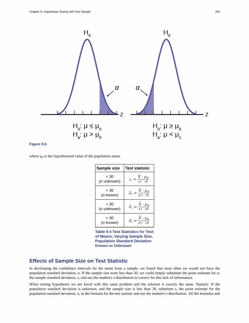
Figure 9.6
where μ0 is the hypothesized value of the population mean.
Sample size Test statistic
< 30(σ unknown) tc = X
–- μ0
s / n
< 30(σ known) Zc = X
–- μ0
σ / n
> 30(σ unknown) Zc = X
–- μ0
s / n
> 30(σ known) Zc = X
–- μ0
σ / n
Table 9.4 Test Statistics for Testof Means, Varying Sample Size,Population Standard DeviationKnown or Unknown
Effects of Sample Size on Test StatisticIn developing the confidence intervals for the mean from a sample, we found that most often we would not have thepopulation standard deviation, σ. If the sample size were less than 30, we could simply substitute the point estimate for σ,the sample standard deviation, s, and use the student's t-distribution to correct for this lack of information.
When testing hypotheses we are faced with this same problem and the solution is exactly the same. Namely: If thepopulation standard deviation is unknown, and the sample size is less than 30, substitute s, the point estimate for thepopulation standard deviation, σ, in the formula for the test statistic and use the student's t-distribution. All the formulas and
Chapter 9 | Hypothesis Testing with One Sample 343
figures above are unchanged except for this substitution and changing the Z distribution to the student's t-distribution onthe graph. Remember that the student's t-distribution can only be computed knowing the proper degrees of freedom for theproblem. In this case, the degrees of freedom is computed as before with confidence intervals: df = (n-1). The calculatedt-value is compared to the t-value associated with the pre-set level of confidence required in the test, tα, df found in thestudent's t tables. If we do not know σ, but the sample size is 30 or more, we simply substitute s for σ and use the normaldistribution.
Table 9.4 summarizes these rules.
A Systematic Approach for Testing A HypothesisA systematic approach to hypothesis testing follows the following steps and in this order. This template will work for allhypotheses that you will ever test.
• Set up the null and alternative hypothesis. This is typically the hardest part of the process. Here the question beingasked is reviewed. What parameter is being tested, a mean, a proportion, differences in means, etc. Is this a one-tailedtest or two-tailed test?
• Decide the level of significance required for this particular case and determine the critical value. These can be foundin the appropriate statistical table. The levels of confidence typical for businesses are 80, 90, 95, 98, and 99. However,the level of significance is a policy decision and should be based upon the risk of making a Type I error, rejecting agood null. Consider the consequences of making a Type I error.
Next, on the basis of the hypotheses and sample size, select the appropriate test statistic and find the relevant criticalvalue: Zα, tα, etc. Drawing the relevant probability distribution and marking the critical value is always big help. Besure to match the graph with the hypothesis, especially if it is a one-tailed test.
• Take a sample(s) and calculate the relevant parameters: sample mean, standard deviation, or proportion. Using theformula for the test statistic from above in step 2, now calculate the test statistic for this particular case using theparameters you have just calculated.
• Compare the calculated test statistic and the critical value. Marking these on the graph will give a good visual pictureof the situation. There are now only two situations:
a. The test statistic is in the tail: Cannot Accept the null, the probability that this sample mean (proportion) camefrom the hypothesized distribution is too small to believe that it is the real home of these sample data.
b. The test statistic is not in the tail: Cannot Reject the null, the sample data are compatible with the hypothesizedpopulation parameter.
• Reach a conclusion. It is best to articulate the conclusion two different ways. First a formal statistical conclusion suchas “With a 5 % level of significance we cannot accept the null hypotheses that the population mean is equal to XX(units of measurement)”. The second statement of the conclusion is less formal and states the action, or lack of action,required. If the formal conclusion was that above, then the informal one might be, “The machine is broken and weneed to shut it down and call for repairs”.
All hypotheses tested will go through this same process. The only changes are the relevant formulas and those aredetermined by the hypothesis required to answer the original question.
9.4 | Full Hypothesis Test Examples - (Base Version -
Lyryx Learning)Tests on Means
Example 9.8
Jeffrey, as an eight-year old, established a mean time of 16.43 seconds for swimming the 25-yard freestyle, witha standard deviation of 0.8 seconds. His dad, Frank, thought that Jeffrey could swim the 25-yard freestyle fasterusing goggles. Frank bought Jeffrey a new pair of expensive goggles and timed Jeffrey for 15 25-yard freestyleswims. For the 15 swims, Jeffrey's mean time was 16 seconds. Frank thought that the goggles helped Jeffreyto swim faster than the 16.43 seconds. Conduct a hypothesis test using a preset α = 0.05.
344 Chapter 9 | Hypothesis Testing with One Sample
This OpenStax book is available for free at https://legacy.cnx.org/content/col12102/1.7
Solution 9.8
Set up the Hypothesis Test:
Since the problem is about a mean, this is a test of a single population mean.
Set the null and alternative hypothesis:
In this case there is an implied challenge or claim. This is that the goggles will reduce the swimming time. Theeffect of this is to set the hypothesis as a one-tailed test. The claim will always be in the alternative hypothesisbecause the burden of proof always lies with the alternative. Remember that the status quo must be defeated witha high degree of confidence, in this case 95 % confidence. The null and alternative hypotheses are thus:
H0: μ ≥ 16.43 Ha: μ < 16.43
For Jeffrey to swim faster, his time will be less than 16.43 seconds. The "<" tells you this is left-tailed.
Determine the distribution needed:
Random variable: X¯
= the mean time to swim the 25-yard freestyle.
Distribution for the test statistic:
The sample size is less than 30 and we do not know the population standard deviation so this is a t-test. and the
proper formula is: tc = X-
- μ0s / n
μ0 = 16.43 comes from H0 and not the data. X-
= 16. s = 0.8, and n = 15.
Our step 2, setting the level of significance, has already been determined by the problem, .05 for a 95 %significance level. It is worth thinking about the meaning of this choice. The Type I error is to conclude thatJeffrey swims the 25-yard freestyle, on average, in less than 16.43 seconds when, in fact, he actually swims the25-yard freestyle, on average, in 16.43 seconds. (Reject the null hypothesis when the null hypothesis is true.) Forthis case the only concern with a Type I error would seem to be that Jeffery’s dad may fail to bet on his son’svictory because he does not have appropriate confidence in the effect of the goggles.
To find the critical value we need to select the appropriate test statistic. We have concluded that this is a t-test onthe basis of the sample size and that we are interested in a population mean. We can now draw the graph of thet-distribution and mark the critical value. For this problem the degrees of freedom are n-1, or 14. Looking up 14degrees of freedom at the 0.05 column of the t-table we find 1.761. This is the critical value and we can put thison our graph.
Step 3 is the calculation of the test statistic using the formula we have selected. We find that the calculated teststatistic is 2.08, meaning that the sample mean is 2.08 standard deviations away from the hypothesized mean of16.43.
tc = x- - μ0sn
= 16 - 16.43.815
= -2.08
Chapter 9 | Hypothesis Testing with One Sample 345

Figure 9.7
Step 4 has us compare the test statistic and the critical value and mark these on the graph. We see that the test statistic is inthe tail and thus we move to step 4 and reach a conclusion. The probability that an average time of 16 minutes could comefrom a distribution with a population mean of 16.43 minutes is too unlikely for us to accept the null hypothesis. We cannotaccept the null.
Step 5 has us state our conclusions first formally and then less formally. A formal conclusion would be stated as: “Witha 95% level of significance we cannot accept the null hypothesis that the swimming time with goggles comes from adistribution with a population mean time of 16.43 minutes.” Less formally, “With 95% significance we believe that thegoggles improves swimming speed”
If we wished to use the p-value system of reaching a conclusion we would calculate the statistic and take the additional stepto find the probability of being 2.08 standard deviations from the mean on a t-distribution. This value is .0281. Comparingthis to the α-level of .05 we see that we cannot accept the null. The p-value has been put on the graph as the shaded areabeyond -2.08 and it shows that it is smaller than the hatched area which is the alpha level of 0.05. Both methods reach thesame conclusion that we cannot accept the null hypothesis.
9.8 The mean throwing distance of a football for Marco, a high school freshman quarterback, is 40 yards, with astandard deviation of two yards. The team coach tells Marco to adjust his grip to get more distance. The coach recordsthe distances for 20 throws. For the 20 throws, Marco’s mean distance was 45 yards. The coach thought the differentgrip helped Marco throw farther than 40 yards. Conduct a hypothesis test using a preset α = 0.05. Assume the throw
346 Chapter 9 | Hypothesis Testing with One Sample
This OpenStax book is available for free at https://legacy.cnx.org/content/col12102/1.7
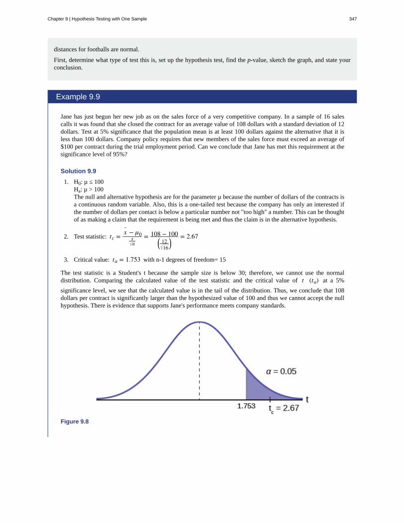
distances for footballs are normal.
First, determine what type of test this is, set up the hypothesis test, find the p-value, sketch the graph, and state yourconclusion.
Example 9.9
Jane has just begun her new job as on the sales force of a very competitive company. In a sample of 16 salescalls it was found that she closed the contract for an average value of 108 dollars with a standard deviation of 12dollars. Test at 5% significance that the population mean is at least 100 dollars against the alternative that it isless than 100 dollars. Company policy requires that new members of the sales force must exceed an average of$100 per contract during the trial employment period. Can we conclude that Jane has met this requirement at thesignificance level of 95%?
Solution 9.9
1. H0: µ ≤ 100Ha: µ > 100The null and alternative hypothesis are for the parameter µ because the number of dollars of the contracts isa continuous random variable. Also, this is a one-tailed test because the company has only an interested ifthe number of dollars per contact is below a particular number not "too high" a number. This can be thoughtof as making a claim that the requirement is being met and thus the claim is in the alternative hypothesis.
2. Test statistic: tc = x¯ − µ0sn
= 108 − 100⎛⎝ 12
16⎞⎠
= 2.67
3. Critical value: ta = 1.753 with n-1 degrees of freedom= 15
The test statistic is a Student's t because the sample size is below 30; therefore, we cannot use the normaldistribution. Comparing the calculated value of the test statistic and the critical value of t (ta) at a 5%
significance level, we see that the calculated value is in the tail of the distribution. Thus, we conclude that 108dollars per contract is significantly larger than the hypothesized value of 100 and thus we cannot accept the nullhypothesis. There is evidence that supports Jane's performance meets company standards.
Figure 9.8
Chapter 9 | Hypothesis Testing with One Sample 347

9.9 It is believed that a stock price for a particular company will grow at a rate of $5 per week with a standarddeviation of $1. An investor believes the stock won’t grow as quickly. The changes in stock price is recorded forten weeks and are as follows: $4, $3, $2, $3, $1, $7, $2, $1, $1, $2. Perform a hypothesis test using a 5% level ofsignificance. State the null and alternative hypotheses, state your conclusion, and identify the Type I errors.
Example 9.10
A manufacturer of salad dressings uses machines to dispense liquid ingredients into bottles that move alonga filling line. The machine that dispenses salad dressings is working properly when 8 ounces are dispensed.Suppose that the average amount dispensed in a particular sample of 35 bottles is 7.91 ounces with a variance of
0.03 ounces squared, s2 . Is there evidence that the machine should be stopped and production wait for repairs?
The lost production from a shutdown is potentially so great that management feels that the level of significancein the analysis should be 99%.
Again we will follow the steps in our analysis of this problem.
Solution 9.10
STEP 1: Set the Null and Alternative Hypothesis. The random variable is the quantity of fluid placed in thebottles. This is a continuous random variable and the parameter we are interested in is the mean. Our hypothesistherefore is about the mean. In this case we are concerned that the machine is not filling properly. From what weare told it does not matter if the machine is over-filling or under-filling, both seem to be an equally bad error. Thistells us that this is a two-tailed test: if the machine is malfunctioning it will be shutdown regardless if it is fromover-filling or under-filling. The null and alternative hypotheses are thus:
H0 : μ = 8Ha : μ ≠ 8
STEP 2: Decide the level of significance and draw the graph showing the critical value.
This problem has already set the level of significance at 99%. The decision seems an appropriate one and showsthe thought process when setting the significance level. Management wants to be very certain, as certain asprobability will allow, that they are not shutting down a machine that is not in need of repair. To draw thedistribution and the critical value, we need to know which distribution to use. Because this is a continuous randomvariable and we are interested in the mean, and the sample size is greater than 30, the appropriate distribution isthe normal distribution and the relevant critical value is 2.575 from the normal table or the t-table at 0.005 columnand infinite degrees of freedom. We draw the graph and mark these points.
348 Chapter 9 | Hypothesis Testing with One Sample
This OpenStax book is available for free at https://legacy.cnx.org/content/col12102/1.7
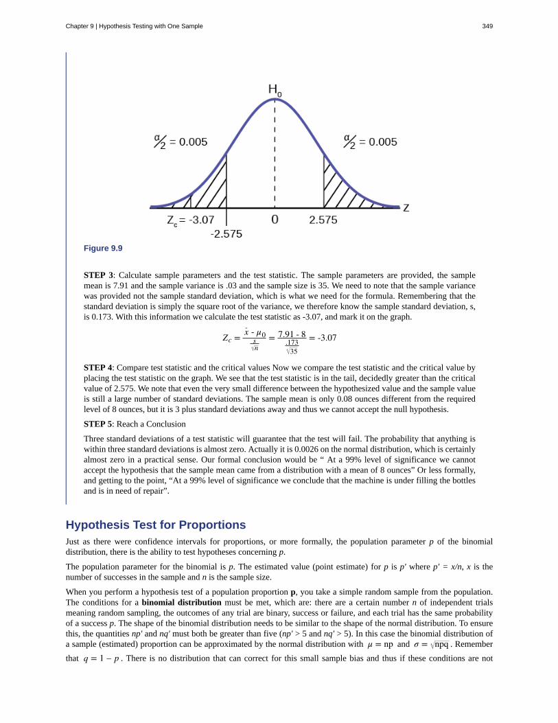
Figure 9.9
STEP 3: Calculate sample parameters and the test statistic. The sample parameters are provided, the samplemean is 7.91 and the sample variance is .03 and the sample size is 35. We need to note that the sample variancewas provided not the sample standard deviation, which is what we need for the formula. Remembering that thestandard deviation is simply the square root of the variance, we therefore know the sample standard deviation, s,is 0.173. With this information we calculate the test statistic as -3.07, and mark it on the graph.
Zc = x- - μ0sn
= 7.91 - 8.173
35
= -3.07
STEP 4: Compare test statistic and the critical values Now we compare the test statistic and the critical value byplacing the test statistic on the graph. We see that the test statistic is in the tail, decidedly greater than the criticalvalue of 2.575. We note that even the very small difference between the hypothesized value and the sample valueis still a large number of standard deviations. The sample mean is only 0.08 ounces different from the requiredlevel of 8 ounces, but it is 3 plus standard deviations away and thus we cannot accept the null hypothesis.
STEP 5: Reach a Conclusion
Three standard deviations of a test statistic will guarantee that the test will fail. The probability that anything iswithin three standard deviations is almost zero. Actually it is 0.0026 on the normal distribution, which is certainlyalmost zero in a practical sense. Our formal conclusion would be “ At a 99% level of significance we cannotaccept the hypothesis that the sample mean came from a distribution with a mean of 8 ounces” Or less formally,and getting to the point, “At a 99% level of significance we conclude that the machine is under filling the bottlesand is in need of repair”.
Hypothesis Test for ProportionsJust as there were confidence intervals for proportions, or more formally, the population parameter p of the binomialdistribution, there is the ability to test hypotheses concerning p.
The population parameter for the binomial is p. The estimated value (point estimate) for p is p′ where p′ = x/n, x is thenumber of successes in the sample and n is the sample size.
When you perform a hypothesis test of a population proportion p, you take a simple random sample from the population.The conditions for a binomial distribution must be met, which are: there are a certain number n of independent trialsmeaning random sampling, the outcomes of any trial are binary, success or failure, and each trial has the same probabilityof a success p. The shape of the binomial distribution needs to be similar to the shape of the normal distribution. To ensurethis, the quantities np′ and nq′ must both be greater than five (np′ > 5 and nq′ > 5). In this case the binomial distribution ofa sample (estimated) proportion can be approximated by the normal distribution with μ = np and σ = npq . Remember
that q = 1 – p . There is no distribution that can correct for this small sample bias and thus if these conditions are not
Chapter 9 | Hypothesis Testing with One Sample 349

met we simply cannot test the hypothesis with the data available at that time. We met this condition when we first wereestimating confidence intervals for p.
Again, we begin with the standardizing formula modified because this is the distribution of a binomial.
Z = p' - ppqn
Substituting p0 , the hypothesized value of p, we have:
Zc = p' - p0p0q0n
This is the test statistic for testing hypothesized values of p, where the null and alternative hypotheses take one of thefollowing forms:
Two-Tailed Test One-Tailed Test One-Tailed Test
H0: p = p0 H0: p ≤ p0 H0: p ≥ p0
Ha: p ≠ p0 Ha: p > p0 Ha: p < p0
Table 9.5
The decision rule stated above applies here also: if the calculated value of Zc shows that the sample proportion is "too many"standard deviations from the hypothesized proportion, the null hypothesis cannot be accepted. The decision as to what is"too many" is pre-determined by the analyst depending on the level of significance required in the test.
Example 9.11
The mortgage department of a large bank is interested in the nature of loans of first-time borrowers. Thisinformation will be used to tailor their marketing strategy. They believe that 50% of first-time borrowers take outsmaller loans than other borrowers. They perform a hypothesis test to determine if the percentage is the same ordifferent from 50%. They sample 100 first-time borrowers and find 53 of these loans are smaller that the otherborrowers. For the hypothesis test, they choose a 5% level of significance.
Solution 9.11
STEP 1: Set the null and alternative hypothesis.
H0: p = 0.50 Ha: p ≠ 0.50
The words "is the same or different from" tell you this is a two-tailed test. The Type I and Type II errors are asfollows: The Type I error is to conclude that the proportion of borrowers is different from 50% when, in fact, theproportion is actually 50%. (Reject the null hypothesis when the null hypothesis is true). The Type II error is thereis not enough evidence to conclude that the proportion of first time borrowers differs from 50% when, in fact, theproportion does differ from 50%. (You fail to reject the null hypothesis when the null hypothesis is false.)
STEP 2: Decide the level of significance and draw the graph showing the critical value
The level of significance has been set by the problem at the 95% level. Because this is two-tailed test one-half ofthe alpha value will be in the upper tail and one-half in the lower tail as shown on the graph. The critical valuefor the normal distribution at the 95% level of confidence is 1.96. This can easily be found on the student’s t-table at the very bottom at infinite degrees of freedom remembering that at infinity the t-distribution is the normaldistribution. Of course the value can also be found on the normal table but you have go looking for one-half of 95(0.475) inside the body of the table and then read out to the sides and top for the number of standard deviations.
350 Chapter 9 | Hypothesis Testing with One Sample
This OpenStax book is available for free at https://legacy.cnx.org/content/col12102/1.7

Figure 9.10
STEP 3: Calculate the sample parameters and critical value of the test statistic.
The test statistic is a normal distribution, Z, for testing proportions and is:
Z = p' - p0p0q0n
= .53 - .50.5(.5)100
= 0.60
For this case, the sample of 100 found 53 first-time borrowers were different from other borrowers. The sampleproportion, p′ = 53/100= 0.53 The test question, therefore, is : “Is 0.53 significantly different from .50?” Puttingthese values into the formula for the test statistic we find that 0.53 is only 0.60 standard deviations away from .50.This is barely off of the mean of the standard normal distribution of zero. There is virtually no difference fromthe sample proportion and the hypothesized proportion in terms of standard deviations.
STEP 4: Compare the test statistic and the critical value.
The calculated value is well within the critical values of ± 1.96 standard deviations and thus we cannot reject thenull hypothesis. To reject the null hypothesis we need significant evident of difference between the hypothesizedvalue and the sample value. In this case the sample value is very nearly the same as the hypothesized valuemeasured in terms of standard deviations.
STEP 5: Reach a conclusion
The formal conclusion would be “At a 95% level of significance we cannot reject the null hypothesis that50% of first-time borrowers have the same size loans as other borrowers”. Less formally we would say that“There is no evidence that one-half of first-time borrowers are significantly different in loan size from otherborrowers”. Notice the length to which the conclusion goes to include all of the conditions that are attached tothe conclusion. Statisticians for all the criticism they receive, are careful to be very specific even when this seemstrivial. Statisticians cannot say more than they know and the data constrain the conclusion to be within the metesand bounds of the data.
9.11 A teacher believes that 85% of students in the class will want to go on a field trip to the local zoo. She performsa hypothesis test to determine if the percentage is the same or different from 85%. The teacher samples 50 students and39 reply that they would want to go to the zoo. For the hypothesis test, use a 1% level of significance.
Chapter 9 | Hypothesis Testing with One Sample 351

Example 9.12
Suppose a consumer group suspects that the proportion of households that have three or more cell phones is 30%.A cell phone company has reason to believe that the proportion is not 30%. Before they start a big advertisingcampaign, they conduct a hypothesis test. Their marketing people survey 150 households with the result that 43of the households have three or more cell phones.
Solution 9.12
Here is an abbreviate version of the system to solve hypothesis tests applied to a test on a proportions.
H0 : p = 0.3Ha : p ≠ 0.3n = 150
p' = xn = 43
150 = 0.287
Zc = p' - p0p0q0n
= 0.287 - 0.3.3(.7)150
= 0.347
Figure 9.11
Example 9.13
The National Institute of Standards and Technology provides exact data on conductivity properties of materials.Following are conductivity measurements for 11 randomly selected pieces of a particular type of glass.
1.11; 1.07; 1.11; 1.07; 1.12; 1.08; .98; .98 1.02; .95; .95Is there convincing evidence that the average conductivity of this type of glass is greater than one? Use asignificance level of 0.05.
Solution 9.13Let’s follow a four-step process to answer this statistical question.
1. State the Question: We need to determine if, at a 0.05 significance level, the average conductivity of the
352 Chapter 9 | Hypothesis Testing with One Sample
This OpenStax book is available for free at https://legacy.cnx.org/content/col12102/1.7
selected glass is greater than one. Our hypotheses will be
a. H0: μ ≤ 1
b. Ha: μ > 1
2. Plan: We are testing a sample mean without a known population standard deviation with less than 30observations. Therefore, we need to use a Student's-t distribution. Assume the underlying population isnormal.
3. Do the calculations and draw the graph.
4. State the Conclusions: We cannot accept the null hypothesis. It is reasonable to state that the data supportsthe claim that the average conductivity level is greater than one.
Example 9.14
In a study of 420,019 cell phone users, 172 of the subjects developed brain cancer. Test the claim that cell phoneusers developed brain cancer at a greater rate than that for non-cell phone users (the rate of brain cancer fornon-cell phone users is 0.0340%). Since this is a critical issue, use a 0.005 significance level. Explain why thesignificance level should be so low in terms of a Type I error.
Solution 9.141. We need to conduct a hypothesis test on the claimed cancer rate. Our hypotheses will be
a. H0: p ≤ 0.00034
b. Ha: p > 0.00034
If we commit a Type I error, we are essentially accepting a false claim. Since the claim describes cancer-causing environments, we want to minimize the chances of incorrectly identifying causes of cancer.
2. We will be testing a sample proportion with x = 172 and n = 420,019. The sample is sufficiently largebecause we have np' = 420,019(0.00034) = 142.8, nq' = 420,019(0.99966) = 419,876.2, two independentoutcomes, and a fixed probability of success p' = 0.00034. Thus we will be able to generalize our results tothe population.
9.5 | Rare Events, the Sample, Decision and ConclusionEstablishing the type of distribution, sample size, and known or unknown standard deviation can help you figure out howto go about a hypothesis test. However, there are several other factors you should consider when working out a hypothesistest.
Rare EventsSuppose you make an assumption about a property of the population (this assumption is the null hypothesis). Then yougather sample data randomly. If the sample has properties that would be very unlikely to occur if the assumption is true,then you would conclude that your assumption about the population is probably incorrect. (Remember that your assumptionis just an assumption—it is not a fact and it may or may not be true. But your sample data are real and the data are showingyou a fact that seems to contradict your assumption.)
For example, Didi and Ali are at a birthday party of a very wealthy friend. They hurry to be first in line to grab a prize froma tall basket that they cannot see inside because they will be blindfolded. There are 200 plastic bubbles in the basket andDidi and Ali have been told that there is only one with a $100 bill. Didi is the first person to reach into the basket and pull
out a bubble. Her bubble contains a $100 bill. The probability of this happening is 1200 = 0.005. Because this is so unlikely,
Ali is hoping that what the two of them were told is wrong and there are more $100 bills in the basket. A "rare event" hasoccurred (Didi getting the $100 bill) so Ali doubts the assumption about only one $100 bill being in the basket.
Chapter 9 | Hypothesis Testing with One Sample 353
Binomial Distribution
Central Limit Theorem
Confidence Interval (CI)
Critical Value
Hypothesis
Hypothesis Testing
Level of Significance of the Test
Normal Distribution
Standard Deviation
Student's t-Distribution
Test Statistic
KEY TERMSa discrete random variable (RV) that arises from Bernoulli trials. There are a fixed number, n,
of independent trials. “Independent” means that the result of any trial (for example, trial 1) does not affect theresults of the following trials, and all trials are conducted under the same conditions. Under these circumstances thebinomial RV Χ is defined as the number of successes in n trials. The notation is: X ~ B(n, p) μ = np and the standard
deviation is σ = npq . The probability of exactly x successes in n trials is P(X = x) = ⎛⎝nx⎞⎠px qn − x .
Given a random variable (RV) with known mean μ and known standard deviation σ. We are
sampling with size n and we are interested in two new RVs - the sample mean, X . If the size n of the sample is
sufficiently large, then X ~N⎛⎝μ, σn⎞⎠ . If the size n of the sample is sufficiently large, then the distribution of the
sample means will approximate a normal distribution regardless of the shape of the population. The expected valueof the mean of the sample means will equal the population mean. The standard deviation of the distribution of thesample means, σ
n , is called the standard error of the mean.
an interval estimate for an unknown population parameter. This depends on:
• The desired confidence level.
• Information that is known about the distribution (for example, known standard deviation).
• The sample and its size.
The t or Z value set by the researcher that measures the probability of a Type I error, α.
a statement about the value of a population parameter, in case of two hypotheses, the statement assumed tobe true is called the null hypothesis (notation H0) and the contradictory statement is called the alternative hypothesis(notation Ha).
Based on sample evidence, a procedure for determining whether the hypothesis stated is areasonable statement and should not be rejected, or is unreasonable and should be rejected.
probability of a Type I error (reject the null hypothesis when it is true). Notation:α. In hypothesis testing, the Level of Significance is called the preconceived α or the preset α. The Confidence levelis (1-α).
a continuous random variable (RV) with pdf f (x) = 1σ 2π
e
−(x − μ)2
2σ2, where μ is the mean of
the distribution, and σ is the standard deviation, notation: X ~ N(μ, σ). If μ = 0 and σ = 1, the RV is called thestandard normal distribution.
a number that is equal to the square root of the variance and measures how far data values arefrom their mean; notation: s for sample standard deviation and σ for population standard deviation.
investigated and reported by William S. Gossett in 1908 and published under the pseudonymStudent. The major characteristics of the random variable (RV) are:
• It is continuous and assumes any real values.
• The pdf is symmetrical about its mean of zero. However, it is more spread out and flatter at the apex than thenormal distribution.
• It approaches the standard normal distribution as n gets larger.
• There is a "family" of t-distributions: every representative of the family is completely defined by the numberof degrees of freedom which is one less than the number of data items.
The formula that counts the number of standard deviations on the relevant distribution that estimatedparameter is away from the hypothesized value.
354 Chapter 9 | Hypothesis Testing with One Sample
This OpenStax book is available for free at https://legacy.cnx.org/content/col12102/1.7

Type I Error
Type II Error
The decision is to reject the null hypothesis when, in fact, the null hypothesis is true.
The decision is not to reject the null hypothesis when, in fact, the null hypothesis is false.
CHAPTER REVIEW
9.1 Null and Alternative HypothesesIn a hypothesis test, sample data is evaluated in order to arrive at a decision about some type of claim. If certain conditionsabout the sample are satisfied, then the claim can be evaluated for a population. In a hypothesis test, we:
1. Evaluate the null hypothesis, typically denoted with H0. The null is not rejected unless the hypothesis test showsotherwise. The null statement must always contain some form of equality (=, ≤ or ≥)
2. Always write the alternative hypothesis, typically denoted with Ha or H1, using not equal, less than or greaterthan symbols, i.e., (≠, <, or > ).
3. If we reject the null hypothesis, then we can assume there is enough evidence to support the alternative hypothesis.
4. Never state that a claim is proven true or false. Keep in mind the underlying fact that hypothesis testing is basedon probability laws; therefore, we can talk only in terms of non-absolute certainties.
9.2 Outcomes and the Type I and Type II ErrorsIn every hypothesis test, the outcomes are dependent on a correct interpretation of the data. Incorrect calculations ormisunderstood summary statistics can yield errors that affect the results. A Type I error occurs when a true null hypothesisis rejected. A Type II error occurs when a false null hypothesis is not rejected.
The probabilities of these errors are denoted by the Greek letters α and β, for a Type I and a Type II error respectively. Thepower of the test, 1 – β, quantifies the likelihood that a test will yield the correct result of a true alternative hypothesis beingaccepted. A high power is desirable.
9.3 Distribution Needed for Hypothesis TestingIn order for a hypothesis test’s results to be generalized to a population, certain requirements must be satisfied.
When testing for a single population mean:
1. A Student's t-test should be used if the data come from a simple, random sample and the population isapproximately normally distributed, or the sample size is large, with an unknown standard deviation.
2. The normal test will work if the data come from a simple, random sample and the population is approximatelynormally distributed, or the sample size is large.
When testing a single population proportion use a normal test for a single population proportion if the data comes from asimple, random sample, fill the requirements for a binomial distribution, and the mean number of success and the meannumber of failures satisfy the conditions: np > 5 and nq > 5 where n is the sample size, p is the probability of a success, andq is the probability of a failure.
9.4 Full Hypothesis Test Examples - (Base Version - Lyryx Learning)The hypothesis test itself has an established process. This can be summarized as follows:
1. Determine H0 and Ha. Remember, they are contradictory.
2. Determine the random variable.
3. Determine the distribution for the test.
4. Draw a graph and calculate the test statistic.
5. Compare the calculated test statistic with the Z critical value determined by the level of significance required bythe test and make a decision (cannot reject H0 or cannot accept H0), and write a clear conclusion using Englishsentences.
9.5 Rare Events, the Sample, Decision and ConclusionWhen the probability of an event occurring is low, and it happens, it is called a rare event. Rare events are important to
Chapter 9 | Hypothesis Testing with One Sample 355

consider in hypothesis testing because they can inform your willingness not to reject or to reject a null hypothesis. To test anull hypothesis, find the p-value for the sample data and graph the results.
FORMULA REVIEW
9.3 Distribution Needed for Hypothesis Testing
Sample size Test statistic
< 30(σ unknown) tc = X
–- μ0
s / n
< 30(σ known) Zc = X
–- μ0
σ / n
Table 9.6 Test Statistics for Testof Means, Varying Sample Size,Population Known or Unknown
Sample size Test statistic
> 30(σ unknown) Zc = X
–- μ0
s / n
> 30(σ known) Zc = X
–- μ0
σ / n
Table 9.6 Test Statistics for Testof Means, Varying Sample Size,Population Known or Unknown
PRACTICE
9.1 Null and Alternative Hypotheses
1. You are testing that the mean speed of your cable Internet connection is more than three Megabits per second. What isthe random variable? Describe in words.
2. You are testing that the mean speed of your cable Internet connection is more than three Megabits per second. State thenull and alternative hypotheses.
3. The American family has an average of two children. What is the random variable? Describe in words.
4. The mean entry level salary of an employee at a company is $58,000. You believe it is higher for IT professionals in thecompany. State the null and alternative hypotheses.
5. A sociologist claims the probability that a person picked at random in Times Square in New York City is visiting the areais 0.83. You want to test to see if the proportion is actually less. What is the random variable? Describe in words.
6. A sociologist claims the probability that a person picked at random in Times Square in New York City is visiting the areais 0.83. You want to test to see if the claim is correct. State the null and alternative hypotheses.
7. In a population of fish, approximately 42% are female. A test is conducted to see if, in fact, the proportion is less. Statethe null and alternative hypotheses.
8. Suppose that a recent article stated that the mean time spent in jail by a first–time convicted burglar is 2.5 years. A studywas then done to see if the mean time has increased in the new century. A random sample of 26 first-time convicted burglarsin a recent year was picked. The mean length of time in jail from the survey was 3 years with a standard deviation of 1.8years. Suppose that it is somehow known that the population standard deviation is 1.5. If you were conducting a hypothesistest to determine if the mean length of jail time has increased, what would the null and alternative hypotheses be? Thedistribution of the population is normal.
a. H0: ________b. Ha: ________
9. A random survey of 75 death row inmates revealed that the mean length of time on death row is 17.4 years with astandard deviation of 6.3 years. If you were conducting a hypothesis test to determine if the population mean time on deathrow could likely be 15 years, what would the null and alternative hypotheses be?
a. H0: __________b. Ha: __________
356 Chapter 9 | Hypothesis Testing with One Sample
This OpenStax book is available for free at https://legacy.cnx.org/content/col12102/1.7

10. The National Institute of Mental Health published an article stating that in any one-year period, approximately 9.5percent of American adults suffer from depression or a depressive illness. Suppose that in a survey of 100 people in a certaintown, seven of them suffered from depression or a depressive illness. If you were conducting a hypothesis test to determineif the true proportion of people in that town suffering from depression or a depressive illness is lower than the percent in thegeneral adult American population, what would the null and alternative hypotheses be?
a. H0: ________b. Ha: ________
9.2 Outcomes and the Type I and Type II Errors
11. The mean price of mid-sized cars in a region is $32,000. A test is conducted to see if the claim is true. State the Type Iand Type II errors in complete sentences.
12. A sleeping bag is tested to withstand temperatures of –15 °F. You think the bag cannot stand temperatures that low.State the Type I and Type II errors in complete sentences.
13. For Exercise 9.12, what are α and β in words?
14. In words, describe 1 – β For Exercise 9.12.
15. A group of doctors is deciding whether or not to perform an operation. Suppose the null hypothesis, H0, is: the surgicalprocedure will go well. State the Type I and Type II errors in complete sentences.
16. A group of doctors is deciding whether or not to perform an operation. Suppose the null hypothesis, H0, is: the surgicalprocedure will go well. Which is the error with the greater consequence?
17. The power of a test is 0.981. What is the probability of a Type II error?
18. A group of divers is exploring an old sunken ship. Suppose the null hypothesis, H0, is: the sunken ship does not containburied treasure. State the Type I and Type II errors in complete sentences.
19. A microbiologist is testing a water sample for E-coli. Suppose the null hypothesis, H0, is: the sample does not contain E-coli. The probability that the sample does not contain E-coli, but the microbiologist thinks it does is 0.012. The probabilitythat the sample does contain E-coli, but the microbiologist thinks it does not is 0.002. What is the power of this test?
20. A microbiologist is testing a water sample for E-coli. Suppose the null hypothesis, H0, is: the sample contains E-coli.Which is the error with the greater consequence?
9.3 Distribution Needed for Hypothesis Testing
21. Which two distributions can you use for hypothesis testing for this chapter?
22. Which distribution do you use when you are testing a population mean and the population standard deviation is known?Assume sample size is large. Assume a normal distribution with n ≥ 30.
23. Which distribution do you use when the standard deviation is not known and you are testing one population mean?Assume a normal distribution, with n ≥ 30.
24. A population mean is 13. The sample mean is 12.8, and the sample standard deviation is two. The sample size is 20.What distribution should you use to perform a hypothesis test? Assume the underlying population is normal.
25. A population has a mean is 25 and a standard deviation of five. The sample mean is 24, and the sample size is 108.What distribution should you use to perform a hypothesis test?
26. It is thought that 42% of respondents in a taste test would prefer Brand A. In a particular test of 100 people, 39%preferred Brand A. What distribution should you use to perform a hypothesis test?
27. You are performing a hypothesis test of a single population mean using a Student’s t-distribution. What must youassume about the distribution of the data?
28. You are performing a hypothesis test of a single population mean using a Student’s t-distribution. The data are not froma simple random sample. Can you accurately perform the hypothesis test?
29. You are performing a hypothesis test of a single population proportion. What must be true about the quantities of npand nq?
30. You are performing a hypothesis test of a single population proportion. You find out that np is less than five. What mustyou do to be able to perform a valid hypothesis test?
Chapter 9 | Hypothesis Testing with One Sample 357

31. You are performing a hypothesis test of a single population proportion. The data come from which distribution?
9.4 Full Hypothesis Test Examples - (Base Version - Lyryx Learning)
32. Assume H0: μ = 9 and Ha: μ < 9. Is this a left-tailed, right-tailed, or two-tailed test?
33. Assume H0: μ ≤ 6 and Ha: μ > 6. Is this a left-tailed, right-tailed, or two-tailed test?
34. Assume H0: p = 0.25 and Ha: p ≠ 0.25. Is this a left-tailed, right-tailed, or two-tailed test?
35. Draw the general graph of a left-tailed test.
36. Draw the graph of a two-tailed test.
37. A bottle of water is labeled as containing 16 fluid ounces of water. You believe it is less than that. What type of testwould you use?
38. Your friend claims that his mean golf score is 63. You want to show that it is higher than that. What type of test wouldyou use?
39. A bathroom scale claims to be able to identify correctly any weight within a pound. You think that it cannot be thataccurate. What type of test would you use?
40. You flip a coin and record whether it shows heads or tails. You know the probability of getting heads is 50%, but youthink it is less for this particular coin. What type of test would you use?
41. If the alternative hypothesis has a not equals ( ≠ ) symbol, you know to use which type of test?
42. Assume the null hypothesis states that the mean is at least 18. Is this a left-tailed, right-tailed, or two-tailed test?
43. Assume the null hypothesis states that the mean is at most 12. Is this a left-tailed, right-tailed, or two-tailed test?
44. Assume the null hypothesis states that the mean is equal to 88. The alternative hypothesis states that the mean is notequal to 88. Is this a left-tailed, right-tailed, or two-tailed test?
9.5 Rare Events, the Sample, Decision and Conclusion
45. When do you reject the null hypothesis?
46. The probability of winning the grand prize at a particular carnival game is 0.005. Is the outcome of winning very likelyor very unlikely?
47. The probability of winning the grand prize at a particular carnival game is 0.005. Michele wins the grand prize. Is thisconsidered a rare or common event? Why?
48. It is believed that the mean height of high school students who play basketball on the school team is 73 inches with astandard deviation of 1.8 inches. A random sample of 40 players is chosen. The sample mean was 71 inches, and the samplestandard deviation was 1.5 years. Do the data support the claim that the mean height is less than 73 inches? The p-value isalmost zero. State the null and alternative hypotheses and interpret the p-value.
49. The mean age of graduate students at a University is at most 31 y ears with a standard deviation of two years. A randomsample of 15 graduate students is taken. The sample mean is 32 years and the sample standard deviation is three years.Are the data significant at the 1% level? The p-value is 0.0264. State the null and alternative hypotheses and interpret thep-value.
358 Chapter 9 | Hypothesis Testing with One Sample
This OpenStax book is available for free at https://legacy.cnx.org/content/col12102/1.7

50. Does the shaded region represent a low or a high p-value compared to a level of significance of 1%?
Figure 9.12
51. What should you do when α > p-value?
52. What should you do if α = p-value?
53. If you do not reject the null hypothesis, then it must be true. Is this statement correct? State why or why not in completesentences.Use the following information to answer the next seven exercises: Suppose that a recent article stated that the mean timespent in jail by a first-time convicted burglar is 2.5 years. A study was then done to see if the mean time has increased inthe new century. A random sample of 26 first-time convicted burglars in a recent year was picked. The mean length of timein jail from the survey was three years with a standard deviation of 1.8 years. Suppose that it is somehow known that thepopulation standard deviation is 1.5. Conduct a hypothesis test to determine if the mean length of jail time has increased.Assume the distribution of the jail times is approximately normal.
54. Is this a test of means or proportions?
55. What symbol represents the random variable for this test?
56. In words, define the random variable for this test.
57. Is the population standard deviation known and, if so, what is it?
58. Calculate the following:
a. x _______
b. σ _______c. sx _______d. n _______
59. Since both σ and sx are given, which should be used? In one to two complete sentences, explain why.
60. State the distribution to use for the hypothesis test.
Chapter 9 | Hypothesis Testing with One Sample 359

61. A random survey of 75 death row inmates revealed that the mean length of time on death row is 17.4 years with astandard deviation of 6.3 years. Conduct a hypothesis test to determine if the population mean time on death row couldlikely be 15 years.
a. Is this a test of one mean or proportion?b. State the null and alternative hypotheses.
H0: ____________________ Ha : ____________________c. Is this a right-tailed, left-tailed, or two-tailed test?d. What symbol represents the random variable for this test?e. In words, define the random variable for this test.f. Is the population standard deviation known and, if so, what is it?g. Calculate the following:
i. x = _____________
ii. s = ____________iii. n = ____________
h. Which test should be used?i. State the distribution to use for the hypothesis test.j. Find the p-value.k. At a pre-conceived α = 0.05, what is your:
i. Decision:ii. Reason for the decision:
iii. Conclusion (write out in a complete sentence):
HOMEWORK
9.1 Null and Alternative Hypotheses
62. Some of the following statements refer to the null hypothesis, some to the alternate hypothesis.
State the null hypothesis, H0, and the alternative hypothesis. Ha, in terms of the appropriate parameter (μ or p).
a. The mean number of years Americans work before retiring is 34.b. At most 60% of Americans vote in presidential elections.c. The mean starting salary for San Jose State University graduates is at least $100,000 per year.d. Twenty-nine percent of high school seniors get drunk each month.e. Fewer than 5% of adults ride the bus to work in Los Angeles.f. The mean number of cars a person owns in her lifetime is not more than ten.g. About half of Americans prefer to live away from cities, given the choice.h. Europeans have a mean paid vacation each year of six weeks.i. The chance of developing breast cancer is under 11% for women.j. Private universities' mean tuition cost is more than $20,000 per year.
63. Over the past few decades, public health officials have examined the link between weight concerns and teen girls'smoking. Researchers surveyed a group of 273 randomly selected teen girls living in Massachusetts (between 12 and 15years old). After four years the girls were surveyed again. Sixty-three said they smoked to stay thin. Is there good evidencethat more than thirty percent of the teen girls smoke to stay thin? The alternative hypothesis is:
a. p < 0.30b. p ≤ 0.30c. p ≥ 0.30d. p > 0.30
64. A statistics instructor believes that fewer than 20% of Evergreen Valley College (EVC) students attended the openingnight midnight showing of the latest Harry Potter movie. She surveys 84 of her students and finds that 11 attended themidnight showing. An appropriate alternative hypothesis is:
a. p = 0.20b. p > 0.20c. p < 0.20d. p ≤ 0.20
360 Chapter 9 | Hypothesis Testing with One Sample
This OpenStax book is available for free at https://legacy.cnx.org/content/col12102/1.7
65. Previously, an organization reported that teenagers spent 4.5 hours per week, on average, on the phone. The organizationthinks that, currently, the mean is higher. Fifteen randomly chosen teenagers were asked how many hours per week theyspend on the phone. The sample mean was 4.75 hours with a sample standard deviation of 2.0. Conduct a hypothesis test.The null and alternative hypotheses are:
a. Ho: x = 4.5, Ha : x > 4.5
b. Ho: μ ≥ 4.5, Ha: μ < 4.5c. Ho: μ = 4.75, Ha: μ > 4.75d. Ho: μ = 4.5, Ha: μ > 4.5
9.2 Outcomes and the Type I and Type II Errors
66. State the Type I and Type II errors in complete sentences given the following statements.a. The mean number of years Americans work before retiring is 34.b. At most 60% of Americans vote in presidential elections.c. The mean starting salary for San Jose State University graduates is at least $100,000 per year.d. Twenty-nine percent of high school seniors get drunk each month.e. Fewer than 5% of adults ride the bus to work in Los Angeles.f. The mean number of cars a person owns in his or her lifetime is not more than ten.g. About half of Americans prefer to live away from cities, given the choice.h. Europeans have a mean paid vacation each year of six weeks.i. The chance of developing breast cancer is under 11% for women.j. Private universities mean tuition cost is more than $20,000 per year.
67. For statements a-j in Exercise 9.109, answer the following in complete sentences.a. State a consequence of committing a Type I error.b. State a consequence of committing a Type II error.
68. When a new drug is created, the pharmaceutical company must subject it to testing before receiving the necessarypermission from the Food and Drug Administration (FDA) to market the drug. Suppose the null hypothesis is “the drug isunsafe.” What is the Type II Error?
a. To conclude the drug is safe when in, fact, it is unsafe.b. Not to conclude the drug is safe when, in fact, it is safe.c. To conclude the drug is safe when, in fact, it is safe.d. Not to conclude the drug is unsafe when, in fact, it is unsafe.
69. A statistics instructor believes that fewer than 20% of Evergreen Valley College (EVC) students attended the openingmidnight showing of the latest Harry Potter movie. She surveys 84 of her students and finds that 11 of them attended themidnight showing. The Type I error is to conclude that the percent of EVC students who attended is ________.
a. at least 20%, when in fact, it is less than 20%.b. 20%, when in fact, it is 20%.c. less than 20%, when in fact, it is at least 20%.d. less than 20%, when in fact, it is less than 20%.
70. It is believed that Lake Tahoe Community College (LTCC) Intermediate Algebra students get less than seven hours ofsleep per night, on average. A survey of 22 LTCC Intermediate Algebra students generated a mean of 7.24 hours with astandard deviation of 1.93 hours. At a level of significance of 5%, do LTCC Intermediate Algebra students get less thanseven hours of sleep per night, on average?
The Type II error is not to reject that the mean number of hours of sleep LTCC students get per night is at least seven when,in fact, the mean number of hours
a. is more than seven hours.b. is at most seven hours.c. is at least seven hours.d. is less than seven hours.
Chapter 9 | Hypothesis Testing with One Sample 361
71. Previously, an organization reported that teenagers spent 4.5 hours per week, on average, on the phone. The organizationthinks that, currently, the mean is higher. Fifteen randomly chosen teenagers were asked how many hours per week theyspend on the phone. The sample mean was 4.75 hours with a sample standard deviation of 2.0. Conduct a hypothesis test,the Type I error is:
a. to conclude that the current mean hours per week is higher than 4.5, when in fact, it is higherb. to conclude that the current mean hours per week is higher than 4.5, when in fact, it is the samec. to conclude that the mean hours per week currently is 4.5, when in fact, it is higherd. to conclude that the mean hours per week currently is no higher than 4.5, when in fact, it is not higher
9.3 Distribution Needed for Hypothesis Testing
72. It is believed that Lake Tahoe Community College (LTCC) Intermediate Algebra students get less than seven hours ofsleep per night, on average. A survey of 22 LTCC Intermediate Algebra students generated a mean of 7.24 hours with astandard deviation of 1.93 hours. At a level of significance of 5%, do LTCC Intermediate Algebra students get less than
seven hours of sleep per night, on average? The distribution to be used for this test is X– ~ ________________
a. N(7.24, 1.9322
)
b. N(7.24, 1.93)c. t22d. t21
9.4 Full Hypothesis Test Examples - (Base Version - Lyryx Learning)
73. A particular brand of tires claims that its deluxe tire averages at least 50,000 miles before it needs to be replaced. Frompast studies of this tire, the standard deviation is known to be 8,000. A survey of owners of that tire design is conducted.From the 28 tires surveyed, the mean lifespan was 46,500 miles with a standard deviation of 9,800 miles. Using alpha =0.05, is the data highly inconsistent with the claim?
74. From generation to generation, the mean age when smokers first start to smoke varies. However, the standard deviationof that age remains constant of around 2.1 years. A survey of 40 smokers of this generation was done to see if the meanstarting age is at least 19. The sample mean was 18.1 with a sample standard deviation of 1.3. Do the data support the claimat the 5% level?
75. The cost of a daily newspaper varies from city to city. However, the variation among prices remains steady with astandard deviation of 20¢. A study was done to test the claim that the mean cost of a daily newspaper is $1.00. Twelve costsyield a mean cost of 95¢ with a standard deviation of 18¢. Do the data support the claim at the 1% level?
76. An article in the San Jose Mercury News stated that students in the California state university system take 4.5 years, onaverage, to finish their undergraduate degrees. Suppose you believe that the mean time is longer. You conduct a survey of49 students and obtain a sample mean of 5.1 with a sample standard deviation of 1.2. Do the data support your claim at the1% level?
77. The mean number of sick days an employee takes per year is believed to be about ten. Members of a personneldepartment do not believe this figure. They randomly survey eight employees. The number of sick days they took for thepast year are as follows: 12; 4; 15; 3; 11; 8; 6; 8. Let x = the number of sick days they took for the past year. Should thepersonnel team believe that the mean number is ten?
78. In 1955, Life Magazine reported that the 25 year-old mother of three worked, on average, an 80 hour week. Recently,many groups have been studying whether or not the women's movement has, in fact, resulted in an increase in the averagework week for women (combining employment and at-home work). Suppose a study was done to determine if the meanwork week has increased. 81 women were surveyed with the following results. The sample mean was 83; the samplestandard deviation was ten. Does it appear that the mean work week has increased for women at the 5% level?
79. Your statistics instructor claims that 60 percent of the students who take her Elementary Statistics class go through lifefeeling more enriched. For some reason that she can't quite figure out, most people don't believe her. You decide to checkthis out on your own. You randomly survey 64 of her past Elementary Statistics students and find that 34 feel more enrichedas a result of her class. Now, what do you think?
80. A Nissan Motor Corporation advertisement read, “The average man’s I.Q. is 107. The average brown trout’s I.Q. is 4.So why can’t man catch brown trout?” Suppose you believe that the brown trout’s mean I.Q. is greater than four. You catch12 brown trout. A fish psychologist determines the I.Q.s as follows: 5; 4; 7; 3; 6; 4; 5; 3; 6; 3; 8; 5. Conduct a hypothesistest of your belief.
362 Chapter 9 | Hypothesis Testing with One Sample
This OpenStax book is available for free at https://legacy.cnx.org/content/col12102/1.7
81. Refer to Exercise 9.119. Conduct a hypothesis test to see if your decision and conclusion would change if your beliefwere that the brown trout’s mean I.Q. is not four.
82. According to an article in Newsweek, the natural ratio of girls to boys is 100:105. In China, the birth ratio is 100: 114(46.7% girls). Suppose you don’t believe the reported figures of the percent of girls born in China. You conduct a study.In this study, you count the number of girls and boys born in 150 randomly chosen recent births. There are 60 girls and 90boys born of the 150. Based on your study, do you believe that the percent of girls born in China is 46.7?
83. A poll done for Newsweek found that 13% of Americans have seen or sensed the presence of an angel. A contingentdoubts that the percent is really that high. It conducts its own survey. Out of 76 Americans surveyed, only two had seenor sensed the presence of an angel. As a result of the contingent’s survey, would you agree with the Newsweek poll? Incomplete sentences, also give three reasons why the two polls might give different results.
84. The mean work week for engineers in a start-up company is believed to be about 60 hours. A newly hired engineerhopes that it’s shorter. She asks ten engineering friends in start-ups for the lengths of their mean work weeks. Based on theresults that follow, should she count on the mean work week to be shorter than 60 hours?
Data (length of mean work week): 70; 45; 55; 60; 65; 55; 55; 60; 50; 55.
85. Sixty-eight percent of online courses taught at community colleges nationwide were taught by full-time faculty. Totest if 68% also represents California’s percent for full-time faculty teaching the online classes, Long Beach City College(LBCC) in California, was randomly selected for comparison. In the same year, 34 of the 44 online courses LBCC offeredwere taught by full-time faculty. Conduct a hypothesis test to determine if 68% represents California. NOTE: For moreaccurate results, use more California community colleges and this past year's data.
86. According to an article in Bloomberg Businessweek, New York City's most recent adult smoking rate is 14%. Supposethat a survey is conducted to determine this year’s rate. Nine out of 70 randomly chosen N.Y. City residents reply that theysmoke. Conduct a hypothesis test to determine if the rate is still 14% or if it has decreased.
87. The mean age of De Anza College students in a previous term was 26.6 years old. An instructor thinks the mean agefor online students is older than 26.6. She randomly surveys 56 online students and finds that the sample mean is 29.4 witha standard deviation of 2.1. Conduct a hypothesis test.
88. Registered nurses earned an average annual salary of $69,110. For that same year, a survey was conducted of 41California registered nurses to determine if the annual salary is higher than $69,110 for California nurses. The sampleaverage was $71,121 with a sample standard deviation of $7,489. Conduct a hypothesis test.
89. La Leche League International reports that the mean age of weaning a child from breastfeeding is age four to fiveworldwide. In America, most nursing mothers wean their children much earlier. Suppose a random survey is conducted of21 U.S. mothers who recently weaned their children. The mean weaning age was nine months (3/4 year) with a standarddeviation of 4 months. Conduct a hypothesis test to determine if the mean weaning age in the U.S. is less than four yearsold.
90. Over the past few decades, public health officials have examined the link between weight concerns and teen girls'smoking. Researchers surveyed a group of 273 randomly selected teen girls living in Massachusetts (between 12 and 15years old). After four years the girls were surveyed again. Sixty-three said they smoked to stay thin. Is there good evidencethat more than thirty percent of the teen girls smoke to stay thin?After conducting the test, your decision and conclusion are
a. Reject H0: There is sufficient evidence to conclude that more than 30% of teen girls smoke to stay thin.b. Do not reject H0: There is not sufficient evidence to conclude that less than 30% of teen girls smoke to stay thin.c. Do not reject H0: There is not sufficient evidence to conclude that more than 30% of teen girls smoke to stay thin.d. Reject H0: There is sufficient evidence to conclude that less than 30% of teen girls smoke to stay thin.
Chapter 9 | Hypothesis Testing with One Sample 363
91. A statistics instructor believes that fewer than 20% of Evergreen Valley College (EVC) students attended the openingnight midnight showing of the latest Harry Potter movie. She surveys 84 of her students and finds that 11 of them attendedthe midnight showing.At a 1% level of significance, an appropriate conclusion is:
a. There is insufficient evidence to conclude that the percent of EVC students who attended the midnight showingof Harry Potter is less than 20%.
b. There is sufficient evidence to conclude that the percent of EVC students who attended the midnight showing ofHarry Potter is more than 20%.
c. There is sufficient evidence to conclude that the percent of EVC students who attended the midnight showing ofHarry Potter is less than 20%.
d. There is insufficient evidence to conclude that the percent of EVC students who attended the midnight showingof Harry Potter is at least 20%.
92. Previously, an organization reported that teenagers spent 4.5 hours per week, on average, on the phone. The organizationthinks that, currently, the mean is higher. Fifteen randomly chosen teenagers were asked how many hours per week theyspend on the phone. The sample mean was 4.75 hours with a sample standard deviation of 2.0. Conduct a hypothesis test.
At a significance level of a = 0.05, what is the correct conclusion?a. There is enough evidence to conclude that the mean number of hours is more than 4.75b. There is enough evidence to conclude that the mean number of hours is more than 4.5c. There is not enough evidence to conclude that the mean number of hours is more than 4.5d. There is not enough evidence to conclude that the mean number of hours is more than 4.75
Instructions: For the following ten exercises,Hypothesis testing: For the following ten exercises, answer each question.
a. State the null and alternate hypothesis.
b. State the p-value.
c. State alpha.
d. What is your decision?
e. Write a conclusion.
f. Answer any other questions asked in the problem.
93. According to the Center for Disease Control website, in 2011 at least 18% of high school students have smoked acigarette. An Introduction to Statistics class in Davies County, KY conducted a hypothesis test at the local high school (amedium sized–approximately 1,200 students–small city demographic) to determine if the local high school’s percentagewas lower. One hundred fifty students were chosen at random and surveyed. Of the 150 students surveyed, 82 havesmoked. Use a significance level of 0.05 and using appropriate statistical evidence, conduct a hypothesis test and state theconclusions.
94. A recent survey in the N.Y. Times Almanac indicated that 48.8% of families own stock. A broker wanted to determineif this survey could be valid. He surveyed a random sample of 250 families and found that 142 owned some type of stock.At the 0.05 significance level, can the survey be considered to be accurate?
95. Driver error can be listed as the cause of approximately 54% of all fatal auto accidents, according to the AmericanAutomobile Association. Thirty randomly selected fatal accidents are examined, and it is determined that 14 were causedby driver error. Using α = 0.05, is the AAA proportion accurate?
96. The US Department of Energy reported that 51.7% of homes were heated by natural gas. A random sample of 221homes in Kentucky found that 115 were heated by natural gas. Does the evidence support the claim for Kentucky at the α =0.05 level in Kentucky? Are the results applicable across the country? Why?
97. For Americans using library services, the American Library Association claims that at most 67% of patrons borrowbooks. The library director in Owensboro, Kentucky feels this is not true, so she asked a local college statistic class toconduct a survey. The class randomly selected 100 patrons and found that 82 borrowed books. Did the class demonstratethat the percentage was higher in Owensboro, KY? Use α = 0.01 level of significance. What is the possible proportion ofpatrons that do borrow books from the Owensboro Library?
364 Chapter 9 | Hypothesis Testing with One Sample
This OpenStax book is available for free at https://legacy.cnx.org/content/col12102/1.7
98. The Weather Underground reported that the mean amount of summer rainfall for the northeastern US is at least 11.52inches. Ten cities in the northeast are randomly selected and the mean rainfall amount is calculated to be 7.42 inches witha standard deviation of 1.3 inches. At the α = 0.05 level, can it be concluded that the mean rainfall was below the reportedaverage? What if α = 0.01? Assume the amount of summer rainfall follows a normal distribution.
99. A survey in the N.Y. Times Almanac finds the mean commute time (one way) is 25.4 minutes for the 15 largest UScities. The Austin, TX chamber of commerce feels that Austin’s commute time is less and wants to publicize this fact. Themean for 25 randomly selected commuters is 22.1 minutes with a standard deviation of 5.3 minutes. At the α = 0.10 level,is the Austin, TX commute significantly less than the mean commute time for the 15 largest US cities?
100. A report by the Gallup Poll found that a woman visits her doctor, on average, at most 5.8 times each year. A randomsample of 20 women results in these yearly visit totals
3; 2; 1; 3; 7; 2; 9; 4; 6; 6; 8; 0; 5; 6; 4; 2; 1; 3; 4; 1At the α = 0.05 level can it be concluded that the sample mean is higher than 5.8 visits per year?
101. According to the N.Y. Times Almanac the mean family size in the U.S. is 3.18. A sample of a college math classresulted in the following family sizes:5; 4; 5; 4; 4; 3; 6; 4; 3; 3; 5; 5; 6; 3; 3; 2; 7; 4; 5; 2; 2; 2; 3; 2At α = 0.05 level, is the class’ mean family size greater than the national average? Does the Almanac result remain valid?Why?
102. The student academic group on a college campus claims that freshman students study at least 2.5 hours per day, onaverage. One Introduction to Statistics class was skeptical. The class took a random sample of 30 freshman students andfound a mean study time of 137 minutes with a standard deviation of 45 minutes. At α = 0.01 level, is the student academicgroup’s claim correct?
9.5 Rare Events, the Sample, Decision and Conclusion
103. The National Institute of Mental Health published an article stating that in any one-year period, approximately 9.5percent of American adults suffer from depression or a depressive illness. Suppose that in a survey of 100 people in a certaintown, seven of them suffered from depression or a depressive illness. Conduct a hypothesis test to determine if the trueproportion of people in that town suffering from depression or a depressive illness is lower than the percent in the generaladult American population.
a. Is this a test of one mean or proportion?b. State the null and alternative hypotheses.
H0: ____________________ Ha: ____________________c. Is this a right-tailed, left-tailed, or two-tailed test?d. What symbol represents the random variable for this test?e. In words, define the random variable for this test.f. Calculate the following:
i. x = ________________ii. n = ________________
iii. p′ = _____________
g. Calculate σx = __________. Show the formula set-up.h. State the distribution to use for the hypothesis test.i. Find the p-value.j. At a pre-conceived α = 0.05, what is your:
i. Decision:ii. Reason for the decision:
iii. Conclusion (write out in a complete sentence):
REFERENCES
9.1 Null and Alternative Hypotheses
Data from the National Institute of Mental Health. Available online at http://www.nimh.nih.gov/publicat/depression.cfm.
Chapter 9 | Hypothesis Testing with One Sample 365

9.4 Full Hypothesis Test Examples - (Base Version - Lyryx Learning)
Data from Amit Schitai. Director of Instructional Technology and Distance Learning. LBCC.
Data from Bloomberg Businessweek. Available online at http://www.businessweek.com/news/2011- 09-15/nyc-smoking-rate-falls-to-record-low-of-14-bloomberg-says.html.
Data from energy.gov. Available online at http://energy.gov (accessed June 27. 2013).
Data from Gallup®. Available online at www.gallup.com (accessed June 27, 2013).
Data from Growing by Degrees by Allen and Seaman.
Data from La Leche League International. Available online at http://www.lalecheleague.org/Law/BAFeb01.html.
Data from the American Automobile Association. Available online at www.aaa.com (accessed June 27, 2013).
Data from the American Library Association. Available online at www.ala.org (accessed June 27, 2013).
Data from the Bureau of Labor Statistics. Available online at http://www.bls.gov/oes/current/oes291111.htm.
Data from the Centers for Disease Control and Prevention. Available online at www.cdc.gov (accessed June 27, 2013)
Data from the U.S. Census Bureau, available online at http://quickfacts.census.gov/qfd/states/00000.html (accessed June27, 2013).
Data from the United States Census Bureau. Available online at http://www.census.gov/hhes/socdemo/language/.
Data from Toastmasters International. Available online at http://toastmasters.org/artisan/detail.asp?CategoryID=1&SubCategoryID=10&ArticleID=429&Page=1.
Data from Weather Underground. Available online at www.wunderground.com (accessed June 27, 2013).
Federal Bureau of Investigations. “Uniform Crime Reports and Index of Crime in Daviess in the State of Kentuckyenforced by Daviess County from 1985 to 2005.” Available online at http://www.disastercenter.com/kentucky/crime/3868.htm (accessed June 27, 2013).
“Foothill-De Anza Community College District.” De Anza College, Winter 2006. Available online athttp://research.fhda.edu/factbook/DAdemofs/Fact_sheet_da_2006w.pdf.
Johansen, C., J. Boice, Jr., J. McLaughlin, J. Olsen. “Cellular Telephones and Cancer—a Nationwide Cohort Studyin Denmark.” Institute of Cancer Epidemiology and the Danish Cancer Society, 93(3):203-7. Available online athttp://www.ncbi.nlm.nih.gov/pubmed/11158188 (accessed June 27, 2013).
Rape, Abuse & Incest National Network. “How often does sexual assault occur?” RAINN, 2009. Available online athttp://www.rainn.org/get-information/statistics/frequency-of-sexual-assault (accessed June 27, 2013).
SOLUTIONS
1 The random variable is the mean Internet speed in Megabits per second.
3 The random variable is the mean number of children an American family has.
5 The random variable is the proportion of people picked at random in Times Square visiting the city.
7a. H0: p = 0.42
b. Ha: p < 0.42
9a. H0: μ = 15
b. Ha: μ ≠ 15
11 Type I: The mean price of mid-sized cars is $32,000, but we conclude that it is not $32,000. Type II: The mean price ofmid-sized cars is not $32,000, but we conclude that it is $32,000.
13 α = the probability that you think the bag cannot withstand -15 degrees F, when in fact it can β = the probability that
366 Chapter 9 | Hypothesis Testing with One Sample
This OpenStax book is available for free at https://legacy.cnx.org/content/col12102/1.7

you think the bag can withstand -15 degrees F, when in fact it cannot
15 Type I: The procedure will go well, but the doctors think it will not. Type II: The procedure will not go well, but thedoctors think it will.
17 0.019
19 0.998
21 A normal distribution or a Student’s t-distribution
23 Use a Student’s t-distribution
25 a normal distribution for a single population mean
27 It must be approximately normally distributed.
29 They must both be greater than five.
31 binomial distribution
32 This is a left-tailed test.
34 This is a two-tailed test.
36
Figure 9.13
38 a right-tailed test
40 a left-tailed test
42 This is a left-tailed test.
44 This is a two-tailed test.
46 The outcome of winning is very unlikely.
48 H0: μ > = 73Ha: μ < 73The p-value is almost zero, which means there is sufficient data to conclude that the mean height of high school studentswho play basketball on the school team is less than 73 inches at the 5% level. The data do support the claim.
50 The shaded region shows a low p-value.
52 Do not reject H0.
54 means
56 the mean time spent in jail for 26 first time convicted burglars
58a. 3
b. 1.5
c. 1.8
d. 26
Chapter 9 | Hypothesis Testing with One Sample 367

60 X ~N⎛⎝2.5, 1.526⎞⎠
62a. H0: μ = 34; Ha: μ ≠ 34
b. H0: p ≤ 0.60; Ha: p > 0.60
c. H0: μ ≥ 100,000; Ha: μ < 100,000
d. H0: p = 0.29; Ha: p ≠ 0.29
e. H0: p = 0.05; Ha: p < 0.05
f. H0: μ ≤ 10; Ha: μ > 10
g. H0: p = 0.50; Ha: p ≠ 0.50
h. H0: μ = 6; Ha: μ ≠ 6
i. H0: p ≥ 0.11; Ha: p < 0.11
j. H0: μ ≤ 20,000; Ha: μ > 20,000
64 c
66a. Type I error: We conclude that the mean is not 34 years, when it really is 34 years. Type II error: We conclude that the
mean is 34 years, when in fact it really is not 34 years.
b. Type I error: We conclude that more than 60% of Americans vote in presidential elections, when the actual percentageis at most 60%.Type II error: We conclude that at most 60% of Americans vote in presidential elections when, in fact,more than 60% do.
c. Type I error: We conclude that the mean starting salary is less than $100,000, when it really is at least $100,000. TypeII error: We conclude that the mean starting salary is at least $100,000 when, in fact, it is less than $100,000.
d. Type I error: We conclude that the proportion of high school seniors who get drunk each month is not 29%, when itreally is 29%. Type II error: We conclude that the proportion of high school seniors who get drunk each month is 29%when, in fact, it is not 29%.
e. Type I error: We conclude that fewer than 5% of adults ride the bus to work in Los Angeles, when the percentage thatdo is really 5% or more. Type II error: We conclude that 5% or more adults ride the bus to work in Los Angeles when,in fact, fewer that 5% do.
f. Type I error: We conclude that the mean number of cars a person owns in his or her lifetime is more than 10, whenin reality it is not more than 10. Type II error: We conclude that the mean number of cars a person owns in his or herlifetime is not more than 10 when, in fact, it is more than 10.
g. Type I error: We conclude that the proportion of Americans who prefer to live away from cities is not about half,though the actual proportion is about half. Type II error: We conclude that the proportion of Americans who prefer tolive away from cities is half when, in fact, it is not half.
h. Type I error: We conclude that the duration of paid vacations each year for Europeans is not six weeks, when in factit is six weeks. Type II error: We conclude that the duration of paid vacations each year for Europeans is six weekswhen, in fact, it is not.
i. Type I error: We conclude that the proportion is less than 11%, when it is really at least 11%. Type II error: Weconclude that the proportion of women who develop breast cancer is at least 11%, when in fact it is less than 11%.
j. Type I error: We conclude that the average tuition cost at private universities is more than $20,000, though in realityit is at most $20,000. Type II error: We conclude that the average tuition cost at private universities is at most $20,000when, in fact, it is more than $20,000.
68 b
70 d
72 d
368 Chapter 9 | Hypothesis Testing with One Sample
This OpenStax book is available for free at https://legacy.cnx.org/content/col12102/1.7
73a. H0: μ ≥ 50,000
b. Ha: μ < 50,000
c. Let X = the average lifespan of a brand of tires.
d. normal distribution
e. z = -2.315
f. p-value = 0.0103
g. Check student’s solution.
h. i. alpha: 0.05
ii. Decision: Reject the null hypothesis.
iii. Reason for decision: The p-value is less than 0.05.
iv. Conclusion: There is sufficient evidence to conclude that the mean lifespan of the tires is less than 50,000 miles.
i. (43,537, 49,463)
75a. H0: μ = $1.00
b. Ha: μ ≠ $1.00
c. Let X = the average cost of a daily newspaper.
d. normal distribution
e. z = –0.866
f. p-value = 0.3865
g. Check student’s solution.
h. i. Alpha: 0.01
ii. Decision: Do not reject the null hypothesis.
iii. Reason for decision: The p-value is greater than 0.01.
iv. Conclusion: There is sufficient evidence to support the claim that the mean cost of daily papers is $1. The meancost could be $1.
i. ($0.84, $1.06)
77a. H0: μ = 10
b. Ha: μ ≠ 10
c. Let X the mean number of sick days an employee takes per year.
d. Student’s t-distribution
e. t = –1.12
f. p-value = 0.300
g. Check student’s solution.
h. i. Alpha: 0.05
ii. Decision: Do not reject the null hypothesis.
iii. Reason for decision: The p-value is greater than 0.05.
iv. Conclusion: At the 5% significance level, there is insufficient evidence to conclude that the mean number of sickdays is not ten.
Chapter 9 | Hypothesis Testing with One Sample 369

i. (4.9443, 11.806)
79a. H0: p ≥ 0.6
b. Ha: p < 0.6
c. Let P′ = the proportion of students who feel more enriched as a result of taking Elementary Statistics.
d. normal for a single proportion
e. 1.12
f. p-value = 0.1308
g. Check student’s solution.
h. i. Alpha: 0.05
ii. Decision: Do not reject the null hypothesis.
iii. Reason for decision: The p-value is greater than 0.05.
iv. Conclusion: There is insufficient evidence to conclude that less than 60 percent of her students feel moreenriched.
i. Confidence Interval: (0.409, 0.654)The “plus-4s” confidence interval is (0.411, 0.648)
81a. H0: μ = 4
b. Ha: μ ≠ 4
c. Let X the average I.Q. of a set of brown trout.
d. two-tailed Student's t-test
e. t = 1.95
f. p-value = 0.076
g. Check student’s solution.
h. i. Alpha: 0.05
ii. Decision: Reject the null hypothesis.
iii. Reason for decision: The p-value is greater than 0.05
iv. Conclusion: There is insufficient evidence to conclude that the average IQ of brown trout is not four.
i. (3.8865,5.9468)
83a. H0: p ≥ 0.13
b. Ha: p < 0.13
c. Let P′ = the proportion of Americans who have seen or sensed angels
d. normal for a single proportion
e. –2.688
f. p-value = 0.0036
g. Check student’s solution.
h. i. alpha: 0.05
ii. Decision: Reject the null hypothesis.
iii. Reason for decision: The p-value is less than 0.05.
370 Chapter 9 | Hypothesis Testing with One Sample
This OpenStax book is available for free at https://legacy.cnx.org/content/col12102/1.7
iv. Conclusion: There is sufficient evidence to conclude that the percentage of Americans who have seen or sensedan angel is less than 13%.
i. (0, 0.0623).The“plus-4s” confidence interval is (0.0022, 0.0978)
86a. H0: p = 0.14
b. Ha: p < 0.14
c. Let P′ = the proportion of NYC residents that smoke.
d. normal for a single proportion
e. –0.2756
f. p-value = 0.3914
g. Check student’s solution.
h. i. alpha: 0.05
ii. Decision: Do not reject the null hypothesis.
iii. Reason for decision: The p-value is greater than 0.05.
iv. At the 5% significance level, there is insufficient evidence to conclude that the proportion of NYC residents whosmoke is less than 0.14.
i. Confidence Interval: (0.0502, 0.2070): The “plus-4s” confidence interval (see chapter 8) is (0.0676, 0.2297).
88a. H0: μ = 69,110
b. Ha: μ > 69,110
c. Let X = the mean salary in dollars for California registered nurses.
d. Student's t-distribution
e. t = 1.719
f. p-value: 0.0466
g. Check student’s solution.
h. i. Alpha: 0.05
ii. Decision: Reject the null hypothesis.
iii. Reason for decision: The p-value is less than 0.05.
iv. Conclusion: At the 5% significance level, there is sufficient evidence to conclude that the mean salary ofCalifornia registered nurses exceeds $69,110.
i. ($68,757, $73,485)
90 c
92 c
94a. H0: p = 0.488 Ha: p ≠ 0.488
b. p-value = 0.0114
c. alpha = 0.05
d. Reject the null hypothesis.
e. At the 5% level of significance, there is enough evidence to conclude that 48.8% of families own stocks.
f. The survey does not appear to be accurate.
Chapter 9 | Hypothesis Testing with One Sample 371
96a. H0: p = 0.517 Ha: p ≠ 0.517
b. p-value = 0.9203.
c. alpha = 0.05.
d. Do not reject the null hypothesis.
e. At the 5% significance level, there is not enough evidence to conclude that the proportion of homes in Kentucky thatare heated by natural gas is 0.517.
f. However, we cannot generalize this result to the entire nation. First, the sample’s population is only the state ofKentucky. Second, it is reasonable to assume that homes in the extreme north and south will have extreme high usageand low usage, respectively. We would need to expand our sample base to include these possibilities if we wanted togeneralize this claim to the entire nation.
98a. H0: µ ≥ 11.52 Ha: µ < 11.52
b. p-value = 0.000002 which is almost 0.
c. alpha = 0.05.
d. Reject the null hypothesis.
e. At the 5% significance level, there is enough evidence to conclude that the mean amount of summer rain in thenortheaster US is less than 11.52 inches, on average.
f. We would make the same conclusion if alpha was 1% because the p-value is almost 0.
100a. H0: µ ≤ 5.8 Ha: µ > 5.8
b. p-value = 0.9987
c. alpha = 0.05
d. Do not reject the null hypothesis.
e. At the 5% level of significance, there is not enough evidence to conclude that a woman visits her doctor, on average,more than 5.8 times a year.
102a. H0: µ ≥ 150 Ha: µ < 150
b. p-value = 0.0622
c. alpha = 0.01
d. Do not reject the null hypothesis.
e. At the 1% significance level, there is not enough evidence to conclude that freshmen students study less than 2.5 hoursper day, on average.
f. The student academic group’s claim appears to be correct.
372 Chapter 9 | Hypothesis Testing with One Sample
This OpenStax book is available for free at https://legacy.cnx.org/content/col12102/1.7

10 | HYPOTHESISTESTING WITH TWOSAMPLES
Figure 10.1 If you want to test a claim that involves two groups (the types of breakfasts eaten east and west of theMississippi River) you can use a slightly different technique when conducting a hypothesis test. (credit: Chloe Lim)
Introduction
Studies often compare two groups. For example, researchers are interested in the effect aspirin has in preventing heartattacks. Over the last few years, newspapers and magazines have reported various aspirin studies involving two groups.Typically, one group is given aspirin and the other group is given a placebo. Then, the heart attack rate is studied overseveral years.
There are other situations that deal with the comparison of two groups. For example, studies compare various diet andexercise programs. Politicians compare the proportion of individuals from different income brackets who might vote forthem. Students are interested in whether SAT or GRE preparatory courses really help raise their scores. Many businessapplications require comparing two groups. It may be the investment returns of two different investment strategies, or thedifferences in production efficiency of different management styles.
To compare two means or two proportions, you work with two groups. The groups are classified either as independent ormatched pairs. Independent groups consist of two samples that are independent, that is, sample values selected from one
Chapter 10 | Hypothesis Testing with Two Samples 373
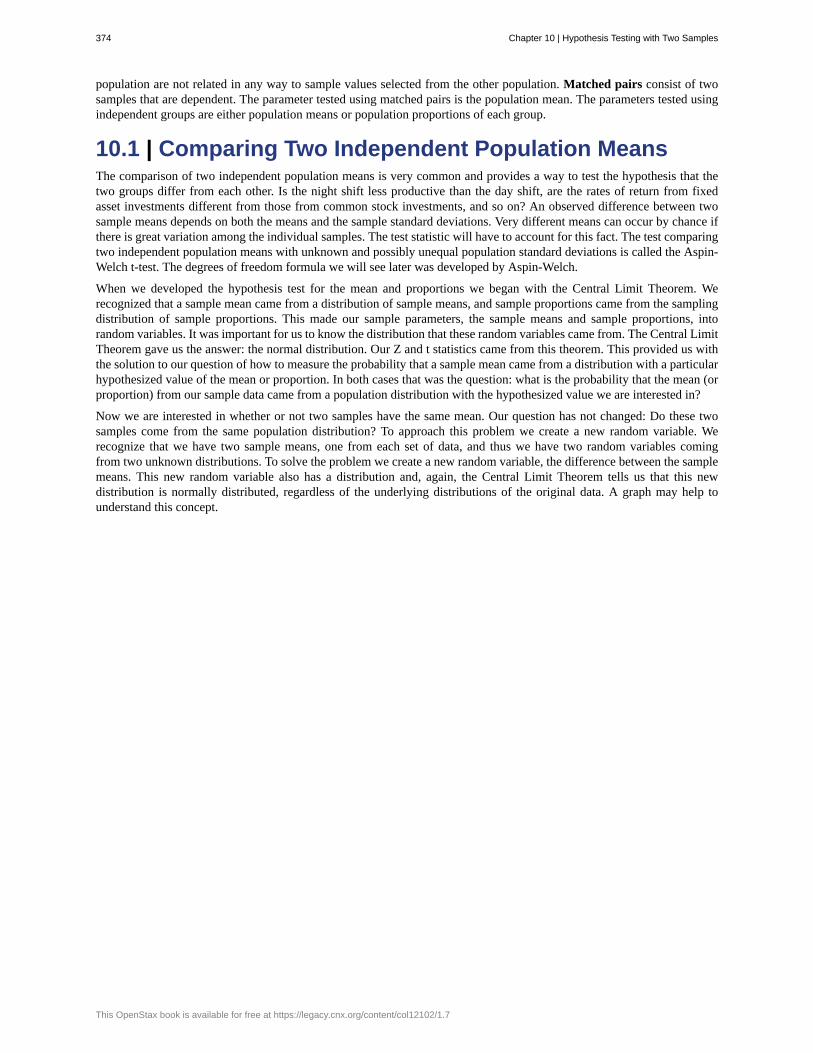
population are not related in any way to sample values selected from the other population. Matched pairs consist of twosamples that are dependent. The parameter tested using matched pairs is the population mean. The parameters tested usingindependent groups are either population means or population proportions of each group.
10.1 | Comparing Two Independent Population MeansThe comparison of two independent population means is very common and provides a way to test the hypothesis that thetwo groups differ from each other. Is the night shift less productive than the day shift, are the rates of return from fixedasset investments different from those from common stock investments, and so on? An observed difference between twosample means depends on both the means and the sample standard deviations. Very different means can occur by chance ifthere is great variation among the individual samples. The test statistic will have to account for this fact. The test comparingtwo independent population means with unknown and possibly unequal population standard deviations is called the Aspin-Welch t-test. The degrees of freedom formula we will see later was developed by Aspin-Welch.
When we developed the hypothesis test for the mean and proportions we began with the Central Limit Theorem. Werecognized that a sample mean came from a distribution of sample means, and sample proportions came from the samplingdistribution of sample proportions. This made our sample parameters, the sample means and sample proportions, intorandom variables. It was important for us to know the distribution that these random variables came from. The Central LimitTheorem gave us the answer: the normal distribution. Our Z and t statistics came from this theorem. This provided us withthe solution to our question of how to measure the probability that a sample mean came from a distribution with a particularhypothesized value of the mean or proportion. In both cases that was the question: what is the probability that the mean (orproportion) from our sample data came from a population distribution with the hypothesized value we are interested in?
Now we are interested in whether or not two samples have the same mean. Our question has not changed: Do these twosamples come from the same population distribution? To approach this problem we create a new random variable. Werecognize that we have two sample means, one from each set of data, and thus we have two random variables comingfrom two unknown distributions. To solve the problem we create a new random variable, the difference between the samplemeans. This new random variable also has a distribution and, again, the Central Limit Theorem tells us that this newdistribution is normally distributed, regardless of the underlying distributions of the original data. A graph may help tounderstand this concept.
374 Chapter 10 | Hypothesis Testing with Two Samples
This OpenStax book is available for free at https://legacy.cnx.org/content/col12102/1.7
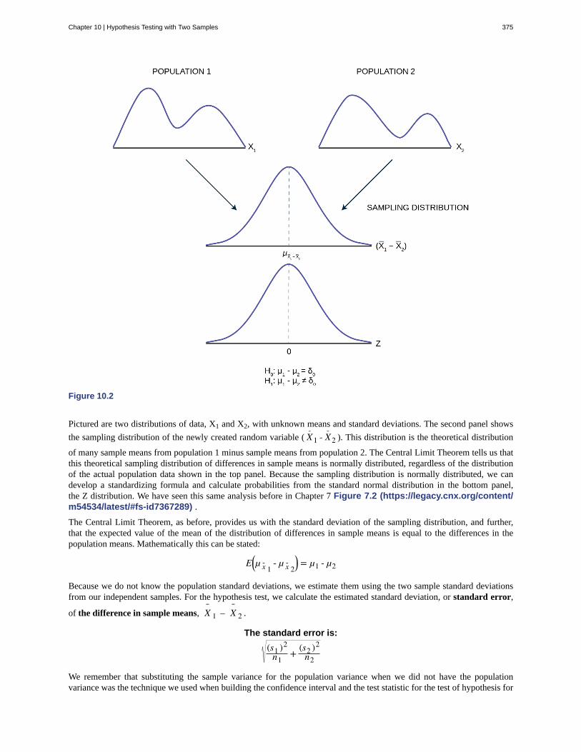
Figure 10.2
Pictured are two distributions of data, X1 and X2, with unknown means and standard deviations. The second panel shows
the sampling distribution of the newly created random variable ( X-
1 - X-
2 ). This distribution is the theoretical distribution
of many sample means from population 1 minus sample means from population 2. The Central Limit Theorem tells us thatthis theoretical sampling distribution of differences in sample means is normally distributed, regardless of the distributionof the actual population data shown in the top panel. Because the sampling distribution is normally distributed, we candevelop a standardizing formula and calculate probabilities from the standard normal distribution in the bottom panel,the Z distribution. We have seen this same analysis before in Chapter 7 Figure 7.2 (https://legacy.cnx.org/content/m54534/latest/#fs-id7367289) .
The Central Limit Theorem, as before, provides us with the standard deviation of the sampling distribution, and further,that the expected value of the mean of the distribution of differences in sample means is equal to the differences in thepopulation means. Mathematically this can be stated:
E⎛⎝µ x- 1- µ x- 2
⎞⎠ = µ1 - µ2
Because we do not know the population standard deviations, we estimate them using the two sample standard deviationsfrom our independent samples. For the hypothesis test, we calculate the estimated standard deviation, or standard error,
of the difference in sample means, X 1 – X 2 .
The standard error is:
(s1 )2
n1+ (s2 )2
n2
We remember that substituting the sample variance for the population variance when we did not have the populationvariance was the technique we used when building the confidence interval and the test statistic for the test of hypothesis for
Chapter 10 | Hypothesis Testing with Two Samples 375

a single mean back in Confidence Intervals and Hypothesis Testing with One Sample. The test statistic (t-score)is calculated as follows:
() tc = ( x 1 – x 2 ) – δ0(s1 )2n1 + (s2 )2
n2
where:• s1 and s2, the sample standard deviations, are estimates of σ1 and σ2, respectively and
• σ1 and σ2 are the unknown population standard deviations.
• x 1 and x 2 are the sample means. μ1 and μ2 are the unknown population means.
The number of degrees of freedom (df) requires a somewhat complicated calculation. The df are not always a wholenumber. The test statistic above is approximated by the Student's t-distribution with df as follows:
The standard error is:
d f =
⎛⎝⎜ (s1)2
n1 + (s2)2n2
⎞⎠⎟
2
⎛⎝ 1n1 – 1⎞⎠⎛⎝⎜ (s1)2
n1
⎞⎠⎟
2
+ ⎛⎝ 1n2 – 1⎞⎠⎛⎝⎜ (s2)2
n2
⎞⎠⎟
2
When both sample sizes n1 and n2 are 30 or larger, the Student's t approximation is very good. If each sample has more than30 observations then the degrees of freedom can be calculated as n1 + n2 - 2.
The format of the sampling distribution, differences in sample means, specifies that the format of the null and alternativehypothesis is:
H0 : µ1 - µ2 = δ0
Ha : µ1 - µ2 ≠ δ0
where δ0 is the hypothesized difference between the two means. If the question is simply “is there any difference betweenthe means?” then δ0 = 0 and the null and alternative hypotheses becomes:
H0 : µ1 = µ2
Ha : µ1 ≠ µ2
An example of when δ0 might not be zero is when the comparison of the two groups requires a specific difference forthe decision to be meaningful. Imagine that you are making a capital investment. You are considering changing from yourcurrent model machine to another. You measure the productivity of your machines by the speed they produce the product.It may be that a contender to replace the old model is faster in terms of product throughput, but is also more expensive. Thesecond machine may also have more maintenance costs, setup costs, etc. The null hypothesis would be set up so that thenew machine would have to be better than the old one by enough to cover these extra costs in terms of speed and cost ofproduction. This form of the null and alternative hypothesis shows how valuable this particular hypothesis test can be. Formost of our work we will be testing simple hypotheses asking if there is any difference between the two distribution means.
Example 10.1 Independent groups
The Kona Iki Corporation produces coconut milk. They take coconuts and extract the milk inside by drilling ahole and pouring the milk into a vat for processing. They have both a day shift (called the B shift) and a nightshift (called the G shift) to do this part of the process. They would like to know if the day shift and the night shiftare equally efficient in processing the coconuts. A study is done sampling 9 shifts of the G shift and 16 shifts ofthe B shift. The results of the number of hours required to process 100 pounds of coconuts is presented in Table10.1. A study is done and data are collected, resulting in the data in Table 10.1.
376 Chapter 10 | Hypothesis Testing with Two Samples
This OpenStax book is available for free at https://legacy.cnx.org/content/col12102/1.7

SampleSize
Average Number of Hours to Process 100 Pounds ofCoconuts
Sample StandardDeviation
GShift
9 2 0.866
BShift
16 3.2 1.00
Table 10.1
Is there a difference in the mean amount of time for each shift to process 100 pounds of coconuts? Test at the 5%level of significance.
Solution 10.1
The population standard deviations are not known and cannot be assumed to equal each other. Let g be thesubscript for the G Shift and b be the subscript for the B Shift. Then, μg is the population mean for G Shift and μbis the population mean for B Shift. This is a test of two independent groups, two population means.
Random variable: X g − X b = difference in the sample mean amount of time between the G Shift and the B
Shift takes to process the coconuts.H0: μg = μb H0: μg – μb = 0Ha: μg ≠ μb Ha: μg – μb ≠ 0The words "the same" tell you H0 has an "=". Since there are no other words to indicate Ha, is either faster orslower. This is a two tailed test.
Distribution for the test: Use tdf where df is calculated using the df formula for independent groups, twopopulation means above. Using a calculator, df is approximately 18.8462.
Graph:
Chapter 10 | Hypothesis Testing with Two Samples 377

Figure 10.3
() tc =⎛⎝X
-1 − X
-2⎞⎠− δ0
S12
n1 +S2
2n2
= -3.01
We next find the critical value on the t-table using the degrees of freedom from above. The critical value, 2.093,is found in the .025 column, this is α/2, at 19 degrees of freedom. (The convention is to round up the degreesof freedom to make the conclusion more conservative.) Next we calculate the test statistic and mark this on thet-distribution graph.
Make a decision: Since the calculated t-value is in the tail we cannot accept the null hypothesis that there is nodifference between the two groups. The means are different.
The graph has included the sampling distribution of the differences in the sample means to show how the t-distribution aligns with the sampling distribution data. We see in the top panel that the calculated difference in thetwo means is -1.2 and the bottom panel shows that this is 3.01 standard deviations from the mean. Typically we donot need to show the sampling distribution graph and can rely on the graph of the test statistic, the t-distributionin this case, to reach our conclusion.
Conclusion: At the 5% level of significance, the sample data show there is sufficient evidence to conclude thatthe mean number of hours that the G Shift takes to process 100 pounds of coconuts is different from the B Shift(mean number of hours for the B Shift is greater than the mean number of hours for the G Shift).
378 Chapter 10 | Hypothesis Testing with Two Samples
This OpenStax book is available for free at https://legacy.cnx.org/content/col12102/1.7

NOTE
When the sum of the sample sizes is larger than 30 (n1 + n2 > 30) you can use the normal distribution to approximatethe Student's t.
Example 10.2
A study is done to determine if Company A retains its workers longer than Company B. It is believed thatCompany A has a higher retention than Company B. The study finds that in a sample of 11 workers at CompanyA their average time with the company is four years with a standard deviation of 1.5 years. A sample of 9 workersat Company B finds that the average time with the company was 3.5 years with a standard deviation of 1 year.Test this proposition at the 1% level of significance.
a. Is this a test of two means or two proportions?
Solution 10.2a. two means because time is a continuous random variable.
b. Are the populations standard deviations known or unknown?
Solution 10.2b. unknown
c. Which distribution do you use to perform the test?
Solution 10.2c. Student's t
d. What is the random variable?
Solution 10.2
d. X A - X B
e. What are the null and alternate hypotheses?
Solution 10.2e.
• Ho : μA ≤ μB
• Ha : μA > μB
f. Is this test right-, left-, or two-tailed?
Solution 10.2f. right one-tailed test
Chapter 10 | Hypothesis Testing with Two Samples 379
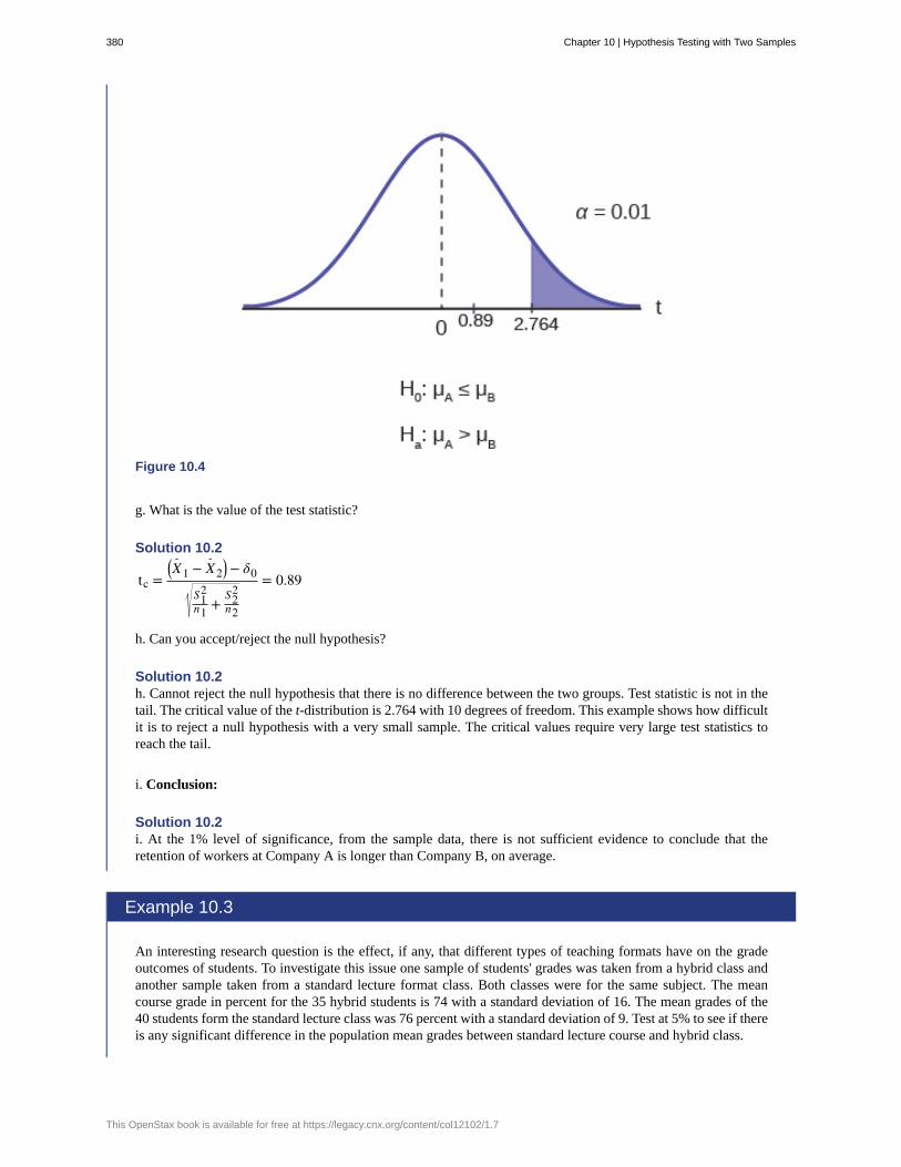
Figure 10.4
g. What is the value of the test statistic?
Solution 10.2
tc =⎛⎝X
-1 − X
-2⎞⎠− δ0
S12
n1 +S2
2n2
= 0.89
h. Can you accept/reject the null hypothesis?
Solution 10.2h. Cannot reject the null hypothesis that there is no difference between the two groups. Test statistic is not in thetail. The critical value of the t-distribution is 2.764 with 10 degrees of freedom. This example shows how difficultit is to reject a null hypothesis with a very small sample. The critical values require very large test statistics toreach the tail.
i. Conclusion:
Solution 10.2i. At the 1% level of significance, from the sample data, there is not sufficient evidence to conclude that theretention of workers at Company A is longer than Company B, on average.
Example 10.3
An interesting research question is the effect, if any, that different types of teaching formats have on the gradeoutcomes of students. To investigate this issue one sample of students' grades was taken from a hybrid class andanother sample taken from a standard lecture format class. Both classes were for the same subject. The meancourse grade in percent for the 35 hybrid students is 74 with a standard deviation of 16. The mean grades of the40 students form the standard lecture class was 76 percent with a standard deviation of 9. Test at 5% to see if thereis any significant difference in the population mean grades between standard lecture course and hybrid class.
380 Chapter 10 | Hypothesis Testing with Two Samples
This OpenStax book is available for free at https://legacy.cnx.org/content/col12102/1.7

Solution 10.3
We begin by noting that we have two groups, students from a hybrid class and students from a standard lectureformat class. We also note that the random variable, what we are interested in, is students' grades, a continuousrandom variable. We could have asked the research question in a different way and had a binary random variable.For example, we could have studied the percentage of students with a failing grade, or with an A grade. Both ofthese would be binary and thus a test of proportions and not a test of means as is the case here. Finally, there is nopresumption as to which format might lead to higher grades so the hypothesis is stated as a two-tailed test.
H0: µ1 = µ2Ha: µ1 ≠ µ2
As would virtually always be the case, we do not know the population variances of the two distributions and thusour test statistic is:
tc =⎛⎝x
¯1 − x¯ 2
⎞⎠− δ0
s2n1 + s2
n2
= (74 − 76) − 016235 + 92
40
= −0.65
To determine the critical value of the Student's t we need the degrees of freedom. For this case we use: df = n1+ n2 - 2 = 35 + 40 -2 = 73. This is large enough to consider it the normal distribution thus ta/2 = 1.96. Again asalways we determine if the calculated value is in the tail determined by the critical value. In this case we do noteven need to look up the critical value: the calculated value of the difference in these two average grades is noteven one standard deviation apart. Certainly not in the tail.
Conclusion: Cannot reject the null at α=5%. Therefore, evidence does not exist to prove that the grades inhybrid and standard classes differ.
10.2 | Comparing Two Independent Population
ProportionsWhen conducting a hypothesis test that compares two independent population proportions, the following characteristicsshould be present:
1. The two independent samples are random samples that are independent.
2. The number of successes is at least five, and the number of failures is at least five, for each of the samples.
3. Growing literature states that the population must be at least ten or even perhaps 20 times the size of the sample. Thiskeeps each population from being over-sampled and causing biased results.
Comparing two proportions, like comparing two means, is common. If two estimated proportions are different, it may bedue to a difference in the populations or it may be due to chance in the sampling. A hypothesis test can help determine if adifference in the estimated proportions reflects a difference in the two population proportions.
Like the case of differences in sample means, we construct a sampling distribution for differences in sample proportions:⎛⎝pA
' - pB' ⎞⎠where pA
' = X AnA
and pB' = X B
nBare the sample proportions for the two sets of data in question. XA and XB
are the number of successes in each sample group respectively, and nA and nB are the respective sample sizes from the twogroups. Again we go the Central Limit theorem to find the distribution of this sampling distribution for the differences insample proportions. And again we find that this sampling distribution, like the ones past, are normally distributed as provedby the Central Limit Theorem, as seen in Figure 10.5 .
Chapter 10 | Hypothesis Testing with Two Samples 381
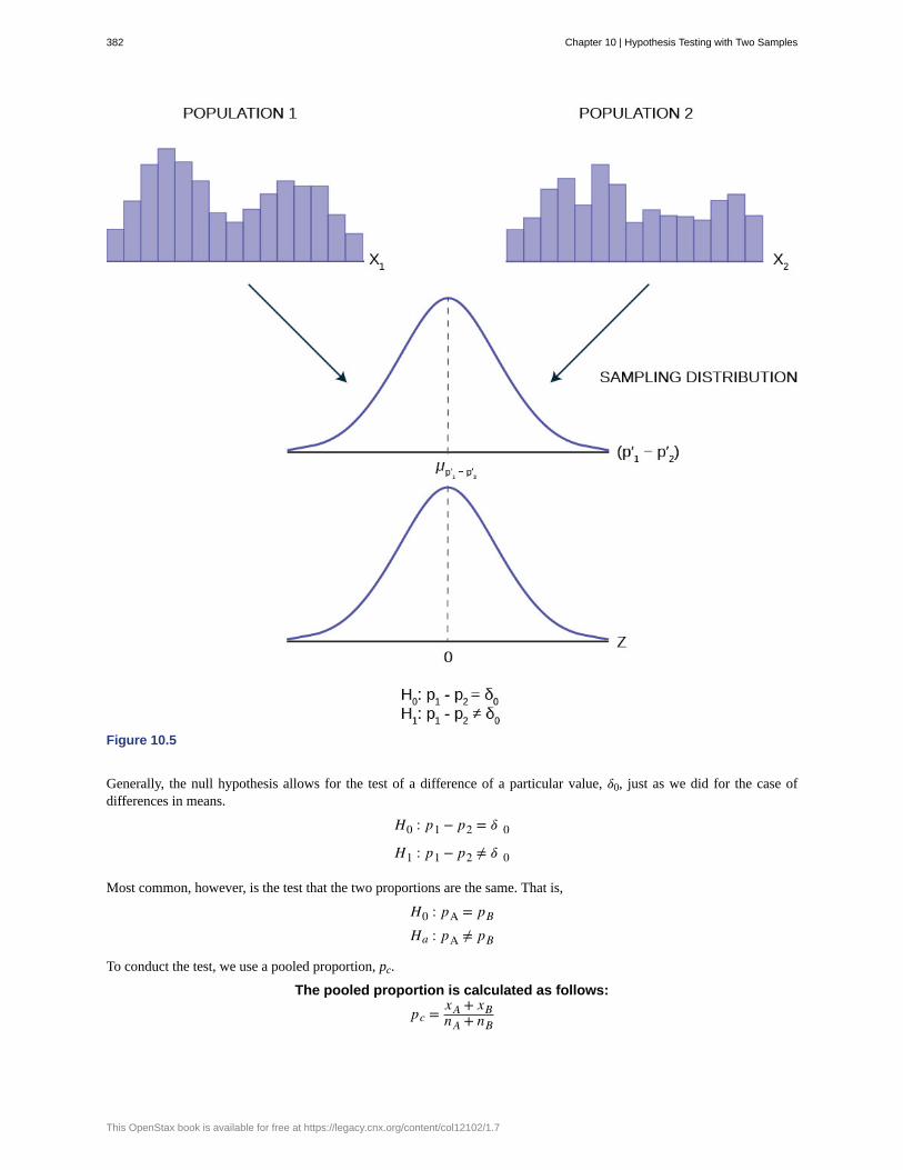
Figure 10.5
Generally, the null hypothesis allows for the test of a difference of a particular value, 𝛿0, just as we did for the case ofdifferences in means.
H0 : p1 − p2 = 𝛿 0
H1 : p1 − p2 ≠ 𝛿 0
Most common, however, is the test that the two proportions are the same. That is,
H0 : pA = pBHa : pA ≠ pB
To conduct the test, we use a pooled proportion, pc.
The pooled proportion is calculated as follows:
pc = xA + xBnA + nB
382 Chapter 10 | Hypothesis Testing with Two Samples
This OpenStax book is available for free at https://legacy.cnx.org/content/col12102/1.7

The test statistic (z-score) is:
Zc =(pA′ − pB′ ) − δ0
pc(1 − pc)( 1nA
+ 1nB)
where δ0 is the hypothesized differences between the two proportions and pc is the pooled variance from the formula above.
Example 10.4
A bank has recently acquired a new branch and thus has customers in this new territory. They are interested inthe default rate in their new territory. They wish to test the hypothesis that the default rate is different from theircurrent customer base. They sample 200 files in area A, their current customers, and find that 20 have defaulted.In area B, the new customers, another sample of 200 files shows 12 have defaulted on their loans. At a 10% levelof significance can we say that the default rates are the same or different?
Solution 10.4
This is a test of proportions. We know this because the underlying random variable is binary, default or notdefault. Further, we know it is a test of differences in proportions because we have two sample groups, the currentcustomer base and the newly acquired customer base. Let A and B be the subscripts for the two customer groups.Then pA and pB are the two population proportions we wish to test.
Random Variable:
P′A – P′B = difference in the proportions of customers who defaulted in the two groups.
H0 : pA = pB
Ha : pA ≠ pB
The words "is a difference" tell you the test is two-tailed.
Distribution for the test: Since this is a test of two binomial population proportions, the distribution is normal:
pc = xA + xBnA + nB
= 20 + 12200 + 200 = 0.08 1 – pc = 0.92
(p′A – p′B) = 0.04 follows an approximate normal distribution.
Estimated proportion for group A: p′A = xAnA = 20
200 = 0.1
Estimated proportion for group B: p′B = xBnB = 12
200 = 0.06
The estimated difference between the two groups is : p′A – p′B = 0.1 – 0.06 = 0.04.
Chapter 10 | Hypothesis Testing with Two Samples 383
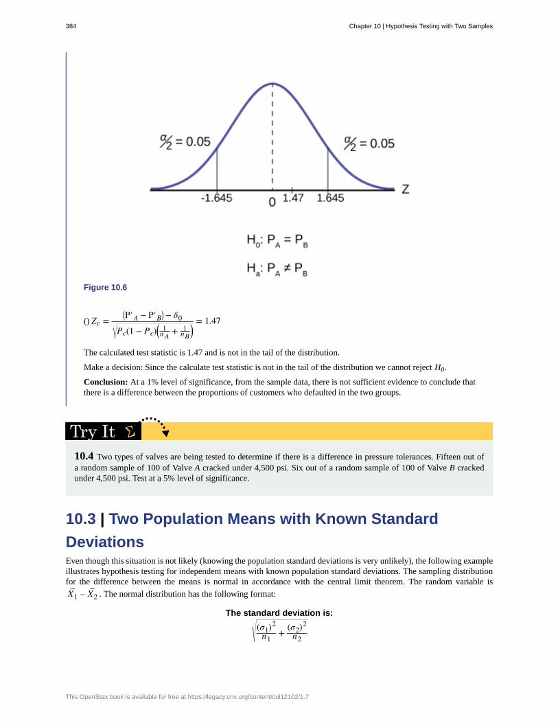
Figure 10.6
() Zc =⎛⎝P′A − P′B
⎞⎠− δ0
Pc(1 − Pc)⎛⎝ 1nA
+ 1nB⎞⎠
= 1.47
The calculated test statistic is 1.47 and is not in the tail of the distribution.
Make a decision: Since the calculate test statistic is not in the tail of the distribution we cannot reject H0.
Conclusion: At a 1% level of significance, from the sample data, there is not sufficient evidence to conclude thatthere is a difference between the proportions of customers who defaulted in the two groups.
10.4 Two types of valves are being tested to determine if there is a difference in pressure tolerances. Fifteen out ofa random sample of 100 of Valve A cracked under 4,500 psi. Six out of a random sample of 100 of Valve B crackedunder 4,500 psi. Test at a 5% level of significance.
10.3 | Two Population Means with Known Standard
DeviationsEven though this situation is not likely (knowing the population standard deviations is very unlikely), the following exampleillustrates hypothesis testing for independent means with known population standard deviations. The sampling distributionfor the difference between the means is normal in accordance with the central limit theorem. The random variable is
X1– – X2
–. The normal distribution has the following format:
The standard deviation is:
(σ1)2
n1+ (σ2)2
n2
384 Chapter 10 | Hypothesis Testing with Two Samples
This OpenStax book is available for free at https://legacy.cnx.org/content/col12102/1.7

The test statistic (z-score) is:
Zc = ( x– 1 – x– 2) – δ0(σ1)2n1 + (σ2)2
n2
Example 10.5
Independent groups, population standard deviations known: The mean lasting time of two competing floorwaxes is to be compared. Twenty floors are randomly assigned to test each wax. Both populations have a normaldistributions. The data are recorded in Table 10.2.
Wax Sample mean number of months floor wax lasts Population standard deviation
1 3 0.33
2 2.9 0.36
Table 10.2
Does the data indicate that wax 1 is more effective than wax 2? Test at a 5% level of significance.
Solution 10.5
This is a test of two independent groups, two population means, population standard deviations known.
Random Variable: X– 1 – X– 2 = difference in the mean number of months the competing floor waxes last.
H0 : μ1 ≤ μ2
Ha : μ1 > μ2
The words "is more effective" says that wax 1 lasts longer than wax 2, on average. "Longer" is a “>” symboland goes into Ha. Therefore, this is a right-tailed test.
Distribution for the test: The population standard deviations are known so the distribution is normal. Using theformula for the test statistic we find the calculated value for the problem.
Zc =⎛⎝μ1 - μ2
⎞⎠ - δ0
σ12
n1 +σ2
2n2
= 0.1
Chapter 10 | Hypothesis Testing with Two Samples 385

Figure 10.7
The estimated difference between he two means is : X– 1 – X– 2 = 3 – 2.9 = 0.1
Compare calculated value and critical value and Zα: We mark the calculated value on the graph and find thecalculated value is not in the tail therefore we cannot reject the null hypothesis.
Make a decision: the calculated value of the test statistic is not in the tail, therefore you cannot reject H0.
Conclusion: At the 5% level of significance, from the sample data, there is not sufficient evidence to concludethat the mean time wax 1 lasts is longer (wax 1 is more effective) than the mean time wax 2 lasts.
10.5 The means of the number of revolutions per minute of two competing engines are to be compared. Thirty enginesare randomly assigned to be tested. Both populations have normal distributions. Table 10.3 shows the result. Do thedata indicate that Engine 2 has higher RPM than Engine 1? Test at a 5% level of significance.
Engine Sample mean number of RPM Population standard deviation
1 1,500 50
2 1,600 60
Table 10.3
Example 10.6
An interested citizen wanted to know if Democratic U. S. senators are older than Republican U.S. senators, onaverage. On May 26 2013, the mean age of 30 randomly selected Republican Senators was 61 years 247 daysold (61.675 years) with a standard deviation of 10.17 years. The mean age of 30 randomly selected Democraticsenators was 61 years 257 days old (61.704 years) with a standard deviation of 9.55 years.
386 Chapter 10 | Hypothesis Testing with Two Samples
This OpenStax book is available for free at https://legacy.cnx.org/content/col12102/1.7

Do the data indicate that Democratic senators are older than Republican senators, on average? Test at a 5% levelof significance.
Solution 10.6
This is a test of two independent groups, two population means. The population standard deviations are unknown,but the sum of the sample sizes is 30 + 30 = 60, which is greater than 30, so we can use the normal approximationto the Student’s-t distribution. Subscripts: 1: Democratic senators 2: Republican senators
Random variable: X– 1 – X– 2 = difference in the mean age of Democratic and Republican U.S. senators.
H0 : μ1 ≤ μ2 H0 : μ1 - μ2 ≤ 0
Ha : μ1 > μ2 Ha : μ1 - μ2 > 0
The words "older than" translates as a “>” symbol and goes into Ha. Therefore, this is a right-tailed test.
Figure 10.8
Make a decision: The p-value is larger than 5%, therefore we cannot reject the null hypothesis. By calculatingthe test statistic we would find that the test statistic does not fall in the tail, therefore we cannot reject the nullhypothesis. We reach the same conclusion using either method of a making this statistical decision.
Conclusion: At the 5% level of significance, from the sample data, there is not sufficient evidence to concludethat the mean age of Democratic senators is greater than the mean age of the Republican senators.
10.4 | Matched or Paired SamplesIn most cases of economic or business data we have little or no control over the process of how the data are gathered. In thissense the data are not the result of a planned controlled experiment. In some cases, however, we can develop data that arepart of a controlled experiment. This situation occurs frequently in quality control situations. Imagine that the productionrates of two machines built to the same design, but at different manufacturing plants, are being tested for differences insome production metric such as speed of output or meeting some production specification such as strength of the product.The test is the same in format to what we have been testing, but here we can have matched pairs for which we can test if
Chapter 10 | Hypothesis Testing with Two Samples 387

differences exist. Each observation has its matched pair against which differences are calculated. First, the differences inthe metric to be tested between the two lists of observations must be calculated, and this is typically labeled with the letter
"d." Then, the average of these matched differences, X¯d is calculated as is its standard deviation, Sd. We expect that the
standard deviation of the differences of the matched pairs will be smaller than unmatched pairs because presumably fewerdifferences should exist because of the correlation between the two groups.
When using a hypothesis test for matched or paired samples, the following characteristics may be present:
1. Simple random sampling is used.
2. Sample sizes are often small.
3. Two measurements (samples) are drawn from the same pair of individuals or objects.
4. Differences are calculated from the matched or paired samples.
5. The differences form the sample that is used for the hypothesis test.
6. Either the matched pairs have differences that come from a population that is normal or the number of differences issufficiently large so that distribution of the sample mean of differences is approximately normal.
In a hypothesis test for matched or paired samples, subjects are matched in pairs and differences are calculated. Thedifferences are the data. The population mean for the differences, μd, is then tested using a Student's-t test for a singlepopulation mean with n – 1 degrees of freedom, where n is the number of differences, that is, the number of pairs not thenumber of observations.
The null and alternative hypotheses for this test are:H0 : µd = 0Ha : µd ≠ 0
The test statistic is:
tc = x– d − μd⎛⎝sdn⎞⎠
Example 10.7
A company has developed a training program for its entering employees because they have become concernedwith the results of the six-month employee review. They hope that the training program can result in better six-month reviews. Each trainee constitutes a “pair”, the entering score the employee received when first enteringthe firm and the score given at the six-month review. The difference in the two scores were calculated for eachemployee and the means for before and after the training program was calculated. The sample mean before thetraining program was 20.4 and the sample mean after the training program was 23.9. The standard deviation ofthe differences in the two scores across the 20 employees was 3.8 points. Test at the 10% significance level thenull hypothesis that the two population means are equal against the alternative that the training program helpsimprove the employees’ scores.
Solution 10.7The first step is to identify this as a two sample case: before the training and after the training. This differentiatesthis problem from simple one sample issues. Second, we determine that the two samples are "paired." Eachobservation in the first sample has a paired observation in the second sample. This information tells us that thenull and alternative hypotheses should be:
H0 : µd ≤ 0Ha : µd > 0
This form reflects the implied claim that the training course improves scores; the test is one-tailed and the claimis in the alternative hypothesis. Because the experiment was conducted as a matched paired sample rather thansimply taking scores from people who took the training course those who didn't, we use the matched pair teststatistic:
388 Chapter 10 | Hypothesis Testing with Two Samples
This OpenStax book is available for free at https://legacy.cnx.org/content/col12102/1.7
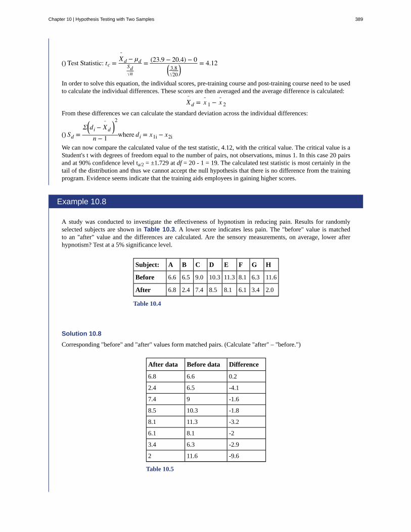
() Test Statistic: tc = X¯d − µdSdn
= (23.9 − 20.4) − 0⎛⎝3.8
20⎞⎠
= 4.12
In order to solve this equation, the individual scores, pre-training course and post-training course need to be usedto calculate the individual differences. These scores are then averaged and the average difference is calculated:
X¯d = x¯ 1 − x¯ 2
From these differences we can calculate the standard deviation across the individual differences:
() Sd =Σ⎛⎝di − X
¯d⎞⎠
2
n − 1 where di = x1i − x2i
We can now compare the calculated value of the test statistic, 4.12, with the critical value. The critical value is aStudent's t with degrees of freedom equal to the number of pairs, not observations, minus 1. In this case 20 pairsand at 90% confidence level ta/2 = ±1.729 at df = 20 - 1 = 19. The calculated test statistic is most certainly in thetail of the distribution and thus we cannot accept the null hypothesis that there is no difference from the trainingprogram. Evidence seems indicate that the training aids employees in gaining higher scores.
Example 10.8
A study was conducted to investigate the effectiveness of hypnotism in reducing pain. Results for randomlyselected subjects are shown in Table 10.3. A lower score indicates less pain. The "before" value is matchedto an "after" value and the differences are calculated. Are the sensory measurements, on average, lower afterhypnotism? Test at a 5% significance level.
Subject: A B C D E F G H
Before 6.6 6.5 9.0 10.3 11.3 8.1 6.3 11.6
After 6.8 2.4 7.4 8.5 8.1 6.1 3.4 2.0
Table 10.4
Solution 10.8
Corresponding "before" and "after" values form matched pairs. (Calculate "after" – "before.")
After data Before data Difference
6.8 6.6 0.2
2.4 6.5 -4.1
7.4 9 -1.6
8.5 10.3 -1.8
8.1 11.3 -3.2
6.1 8.1 -2
3.4 6.3 -2.9
2 11.6 -9.6
Table 10.5
Chapter 10 | Hypothesis Testing with Two Samples 389
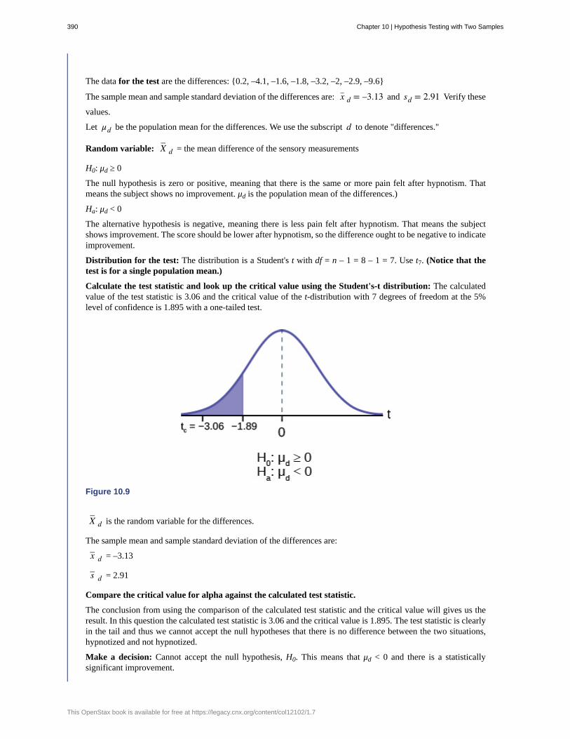
The data for the test are the differences: {0.2, –4.1, –1.6, –1.8, –3.2, –2, –2.9, –9.6}
The sample mean and sample standard deviation of the differences are: x– d = –3.13 and sd = 2.91 Verify these
values.
Let μd be the population mean for the differences. We use the subscript d to denote "differences."
Random variable: X– d = the mean difference of the sensory measurements
H0: μd ≥ 0
The null hypothesis is zero or positive, meaning that there is the same or more pain felt after hypnotism. Thatmeans the subject shows no improvement. μd is the population mean of the differences.)
Ha: μd < 0
The alternative hypothesis is negative, meaning there is less pain felt after hypnotism. That means the subjectshows improvement. The score should be lower after hypnotism, so the difference ought to be negative to indicateimprovement.
Distribution for the test: The distribution is a Student's t with df = n – 1 = 8 – 1 = 7. Use t7. (Notice that thetest is for a single population mean.)
Calculate the test statistic and look up the critical value using the Student's-t distribution: The calculatedvalue of the test statistic is 3.06 and the critical value of the t-distribution with 7 degrees of freedom at the 5%level of confidence is 1.895 with a one-tailed test.
Figure 10.9
X– d is the random variable for the differences.
The sample mean and sample standard deviation of the differences are:
x– d = –3.13
s– d = 2.91
Compare the critical value for alpha against the calculated test statistic.
The conclusion from using the comparison of the calculated test statistic and the critical value will gives us theresult. In this question the calculated test statistic is 3.06 and the critical value is 1.895. The test statistic is clearlyin the tail and thus we cannot accept the null hypotheses that there is no difference between the two situations,hypnotized and not hypnotized.
Make a decision: Cannot accept the null hypothesis, H0. This means that μd < 0 and there is a statisticallysignificant improvement.
390 Chapter 10 | Hypothesis Testing with Two Samples
This OpenStax book is available for free at https://legacy.cnx.org/content/col12102/1.7
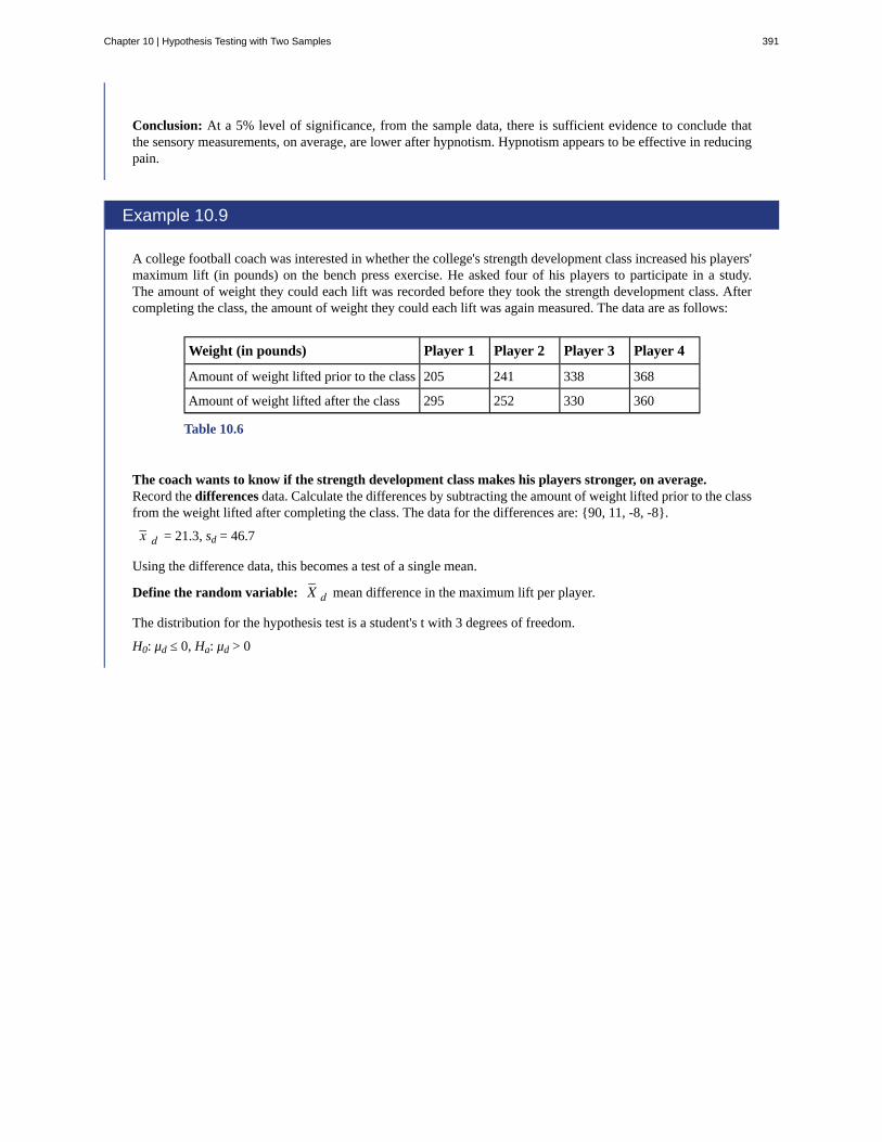
Conclusion: At a 5% level of significance, from the sample data, there is sufficient evidence to conclude thatthe sensory measurements, on average, are lower after hypnotism. Hypnotism appears to be effective in reducingpain.
Example 10.9
A college football coach was interested in whether the college's strength development class increased his players'maximum lift (in pounds) on the bench press exercise. He asked four of his players to participate in a study.The amount of weight they could each lift was recorded before they took the strength development class. Aftercompleting the class, the amount of weight they could each lift was again measured. The data are as follows:
Weight (in pounds) Player 1 Player 2 Player 3 Player 4
Amount of weight lifted prior to the class 205 241 338 368
Amount of weight lifted after the class 295 252 330 360
Table 10.6
The coach wants to know if the strength development class makes his players stronger, on average.Record the differences data. Calculate the differences by subtracting the amount of weight lifted prior to the classfrom the weight lifted after completing the class. The data for the differences are: {90, 11, -8, -8}.
x– d = 21.3, sd = 46.7
Using the difference data, this becomes a test of a single mean.
Define the random variable: X– d mean difference in the maximum lift per player.
The distribution for the hypothesis test is a student's t with 3 degrees of freedom.
H0: μd ≤ 0, Ha: μd > 0
Chapter 10 | Hypothesis Testing with Two Samples 391

Figure 10.10
Calculate the test statistic look up the critical value: Critical value of the test statistic is 0.91. The critical valueof the student's t at 5% level of significance and 3 degrees of freedom is 2.353.
Decision: If the level of significance is 5%, we cannot reject the null hypothesis, because the calculated value ofthe test statistic is not in the tail.
What is the conclusion?
At a 5% level of significance, from the sample data, there is not sufficient evidence to conclude that the strengthdevelopment class helped to make the players stronger, on average.
392 Chapter 10 | Hypothesis Testing with Two Samples
This OpenStax book is available for free at https://legacy.cnx.org/content/col12102/1.7

Cohen’s d
Independent Groups
Matched Pairs
Pooled Variance
KEY TERMSa measure of effect size based on the differences between two means. If d is between 0 and 0.2 then the effect
is small. If d approaches is 0.5, then the effect is medium, and if d approaches 0.8, then it is a large effect.
two samples that are selected from two populations, and the values from one population are notrelated in any way to the values from the other population.
two samples that are dependent. Differences between a before and after scenario are tested by testingone population mean of differences.
a weighted average of two variances that can then be used when calculating standard error.
CHAPTER REVIEW
10.1 Comparing Two Independent Population MeansTwo population means from independent samples where the population standard deviations are not known
• Random Variable: X– 1 − X– 2 = the difference of the sampling means
• Distribution: Student's t-distribution with degrees of freedom (variances not pooled)
10.2 Comparing Two Independent Population ProportionsTest of two population proportions from independent samples.
• Random variable: p'A – p'B = difference between the two estimated proportions
• Distribution: normal distribution
10.3 Two Population Means with Known Standard DeviationsA hypothesis test of two population means from independent samples where the population standard deviations are knownwill have these characteristics:
• Random variable: X– 1 − X– 2 = the difference of the means
• Distribution: normal distribution
10.4 Matched or Paired SamplesA hypothesis test for matched or paired samples (t-test) has these characteristics:
• Test the differences by subtracting one measurement from the other measurement
• Random Variable: x– d = mean of the differences
• Distribution: Student’s-t distribution with n – 1 degrees of freedom
• If the number of differences is small (less than 30), the differences must follow a normal distribution.
• Two samples are drawn from the same set of objects.
• Samples are dependent.
FORMULA REVIEW
Chapter 10 | Hypothesis Testing with Two Samples 393

10.1 Comparing Two Independent PopulationMeans
Standard error: SE =(s1)2
n1+ (s2)2
n2
Test statistic (t-score): tc =( x 1 − x 2) − δ0
(s1)2n1 + (s2)2
n2
Degrees of freedom:
d f =
⎛⎝⎜ (s1)2
n1 + (s2)2n2
⎞⎠⎟
2
⎛⎝ 1n1 − 1⎞⎠⎛⎝⎜ (s1)2
n1
⎞⎠⎟
2
+ ⎛⎝ 1n2 − 1⎞⎠⎛⎝⎜ (s2)2
n2
⎞⎠⎟
2
where:
s1 and s2 are the sample standard deviations, and n1 and
n2 are the sample sizes.
x 1 and x 2 are the sample means.
10.2 Comparing Two Independent PopulationProportions
Pooled Proportion: pc =xA + xBnA + nB
Test Statistic (z-score): Zc = (p′ A − p′ B)
pc(1 − pc)⎛⎝ 1nA
+ 1nB⎞⎠
where
pA' and pB
' are the sample proportions, pA and pB are
the population proportions,
Pc is the pooled proportion, and nA and nB are the samplesizes.
10.3 Two Population Means with KnownStandard Deviations
Test Statistic (z-score):
Zc = ( x– 1 − x– 2) − δ0(σ1)2n1 + (σ2)2
n2
where:σ1 and σ2 are the known population standard deviations.
n1 and n2 are the sample sizes. x– 1 and x– 2 are the
sample means. μ1 and μ2 are the population means.
10.4 Matched or Paired Samples
Test Statistic (t-score): tc =x– d − μd⎛⎝sdn⎞⎠
where:
x– d is the mean of the sample differences. μd is the mean
of the population differences. sd is the sample standarddeviation of the differences. n is the sample size.
PRACTICE
10.1 Comparing Two Independent Population MeansUse the following information to answer the next 15 exercises: Indicate if the hypothesis test is for
a. independent group means, population standard deviations, and/or variances known
b. independent group means, population standard deviations, and/or variances unknown
c. matched or paired samples
d. single mean
e. two proportions
f. single proportion
1. It is believed that 70% of males pass their drivers test in the first attempt, while 65% of females pass the test in the firstattempt. Of interest is whether the proportions are in fact equal.
2. A new laundry detergent is tested on consumers. Of interest is the proportion of consumers who prefer the new brandover the leading competitor. A study is done to test this.
3. A new windshield treatment claims to repel water more effectively. Ten windshields are tested by simulating rain withoutthe new treatment. The same windshields are then treated, and the experiment is run again. A hypothesis test is conducted.
394 Chapter 10 | Hypothesis Testing with Two Samples
This OpenStax book is available for free at https://legacy.cnx.org/content/col12102/1.7

4. The known standard deviation in salary for all mid-level professionals in the financial industry is $11,000. Company Aand Company B are in the financial industry. Suppose samples are taken of mid-level professionals from Company A andfrom Company B. The sample mean salary for mid-level professionals in Company A is $80,000. The sample mean salaryfor mid-level professionals in Company B is $96,000. Company A and Company B management want to know if their mid-level professionals are paid differently, on average.
5. The average worker in Germany gets eight weeks of paid vacation.
6. According to a television commercial, 80% of dentists agree that Ultrafresh toothpaste is the best on the market.
7. It is believed that the average grade on an English essay in a particular school system for females is higher than for males.A random sample of 31 females had a mean score of 82 with a standard deviation of three, and a random sample of 25 maleshad a mean score of 76 with a standard deviation of four.
8. The league mean batting average is 0.280 with a known standard deviation of 0.06. The Rattlers and the Vikings belongto the league. The mean batting average for a sample of eight Rattlers is 0.210, and the mean batting average for a sampleof eight Vikings is 0.260. There are 24 players on the Rattlers and 19 players on the Vikings. Are the batting averages of theRattlers and Vikings statistically different?
9. In a random sample of 100 forests in the United States, 56 were coniferous or contained conifers. In a random sample of80 forests in Mexico, 40 were coniferous or contained conifers. Is the proportion of conifers in the United States statisticallymore than the proportion of conifers in Mexico?
10. A new medicine is said to help improve sleep. Eight subjects are picked at random and given the medicine. The meanshours slept for each person were recorded before starting the medication and after.
11. It is thought that teenagers sleep more than adults on average. A study is done to verify this. A sample of 16 teenagershas a mean of 8.9 hours slept and a standard deviation of 1.2. A sample of 12 adults has a mean of 6.9 hours slept and astandard deviation of 0.6.
12. Varsity athletes practice five times a week, on average.
13. A sample of 12 in-state graduate school programs at school A has a mean tuition of $64,000 with a standard deviation of$8,000. At school B, a sample of 16 in-state graduate programs has a mean of $80,000 with a standard deviation of $6,000.On average, are the mean tuitions different?
14. A new WiFi range booster is being offered to consumers. A researcher tests the native range of 12 different routersunder the same conditions. The ranges are recorded. Then the researcher uses the new WiFi range booster and records thenew ranges. Does the new WiFi range booster do a better job?
15. A high school principal claims that 30% of student athletes drive themselves to school, while 4% of non-athletes drivethemselves to school. In a sample of 20 student athletes, 45% drive themselves to school. In a sample of 35 non-athletestudents, 6% drive themselves to school. Is the percent of student athletes who drive themselves to school more than thepercent of nonathletes?
Use the following information to answer the next three exercises: A study is done to determine which of two soft drinkshas more sugar. There are 13 cans of Beverage A in a sample and six cans of Beverage B. The mean amount of sugar inBeverage A is 36 grams with a standard deviation of 0.6 grams. The mean amount of sugar in Beverage B is 38 grams witha standard deviation of 0.8 grams. The researchers believe that Beverage B has more sugar than Beverage A, on average.Both populations have normal distributions.
16. Are standard deviations known or unknown?
17. What is the random variable?
18. Is this a one-tailed or two-tailed test?
Use the following information to answer the next 12 exercises: The U.S. Center for Disease Control reports that the meanlife expectancy was 47.6 years for White people born in 1900 and 33.0 years for non-White people. Suppose that yourandomly survey death records for people born in 1900 in a certain county. Of the 124 Whites, the mean life span was 45.3years with a standard deviation of 12.7 years. Of the 82 non-Whites, the mean life span was 34.1 years with a standarddeviation of 15.6 years. Conduct a hypothesis test to see if the mean life spans in the county were the same for White andnon-White people.
19. Is this a test of means or proportions?
Chapter 10 | Hypothesis Testing with Two Samples 395

20. State the null and alternative hypotheses.a. H0: __________b. Ha: __________
21. Is this a right-tailed, left-tailed, or two-tailed test?
22. In symbols, what is the random variable of interest for this test?
23. In words, define the random variable of interest for this test.
24. Which distribution (normal or Student's t) would you use for this hypothesis test?
25. Explain why you chose the distribution you did for Exercise 10.24.
26. Calculate the test statistic.
27. Sketch a graph of the situation. Label the horizontal axis. Mark the hypothesized difference and the sample difference.Shade the area corresponding to the p-value.
28. At a pre-conceived α = 0.05, what is your:a. Decision:b. Reason for the decision:c. Conclusion (write out in a complete sentence):
29. Does it appear that the means are the same? Why or why not?
10.2 Comparing Two Independent Population ProportionsUse the following information for the next five exercises. Two types of phone operating system are being tested to determineif there is a difference in the proportions of system failures (crashes). Fifteen out of a random sample of 150 phones withOS1 had system failures within the first eight hours of operation. Nine out of another random sample of 150 phones withOS2 had system failures within the first eight hours of operation. OS2 is believed to be more stable (have fewer crashes)than OS1.
30. Is this a test of means or proportions?
31. What is the random variable?
32. State the null and alternative hypotheses.
33. What can you conclude about the two operating systems?
Use the following information to answer the next twelve exercises. In the recent Census, three percent of the U.S. populationreported being of two or more races. However, the percent varies tremendously from state to state. Suppose that two randomsurveys are conducted. In the first random survey, out of 1,000 North Dakotans, only nine people reported being of two ormore races. In the second random survey, out of 500 Nevadans, 17 people reported being of two or more races. Conducta hypothesis test to determine if the population percents are the same for the two states or if the percent for Nevada isstatistically higher than for North Dakota.
34. Is this a test of means or proportions?
35. State the null and alternative hypotheses.a. H0: _________b. Ha: _________
36. Is this a right-tailed, left-tailed, or two-tailed test? How do you know?
37. What is the random variable of interest for this test?
38. In words, define the random variable for this test.
39. Which distribution (normal or Student's t) would you use for this hypothesis test?
40. Explain why you chose the distribution you did for the Exercise 10.56.
41. Calculate the test statistic.
42. At a pre-conceived α = 0.05, what is your:a. Decision:b. Reason for the decision:c. Conclusion (write out in a complete sentence):
396 Chapter 10 | Hypothesis Testing with Two Samples
This OpenStax book is available for free at https://legacy.cnx.org/content/col12102/1.7
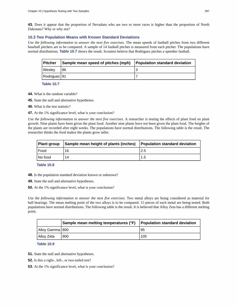
43. Does it appear that the proportion of Nevadans who are two or more races is higher than the proportion of NorthDakotans? Why or why not?
10.3 Two Population Means with Known Standard DeviationsUse the following information to answer the next five exercises. The mean speeds of fastball pitches from two differentbaseball pitchers are to be compared. A sample of 14 fastball pitches is measured from each pitcher. The populations havenormal distributions. Table 10.7 shows the result. Scouters believe that Rodriguez pitches a speedier fastball.
Pitcher Sample mean speed of pitches (mph) Population standard deviation
Wesley 86 3
Rodriguez 91 7
Table 10.7
44. What is the random variable?
45. State the null and alternative hypotheses.
46. What is the test statistic?
47. At the 1% significance level, what is your conclusion?
Use the following information to answer the next five exercises. A researcher is testing the effects of plant food on plantgrowth. Nine plants have been given the plant food. Another nine plants have not been given the plant food. The heights ofthe plants are recorded after eight weeks. The populations have normal distributions. The following table is the result. Theresearcher thinks the food makes the plants grow taller.
Plant group Sample mean height of plants (inches) Population standard deviation
Food 16 2.5
No food 14 1.5
Table 10.8
48. Is the population standard deviation known or unknown?
49. State the null and alternative hypotheses.
50. At the 1% significance level, what is your conclusion?
Use the following information to answer the next five exercises. Two metal alloys are being considered as material forball bearings. The mean melting point of the two alloys is to be compared. 15 pieces of each metal are being tested. Bothpopulations have normal distributions. The following table is the result. It is believed that Alloy Zeta has a different meltingpoint.
Sample mean melting temperatures (°F) Population standard deviation
Alloy Gamma 800 95
Alloy Zeta 900 105
Table 10.9
51. State the null and alternative hypotheses.
52. Is this a right-, left-, or two-tailed test?
53. At the 1% significance level, what is your conclusion?
Chapter 10 | Hypothesis Testing with Two Samples 397
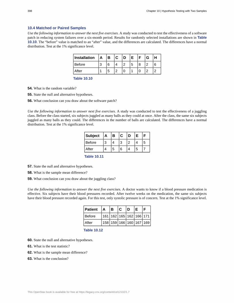
10.4 Matched or Paired SamplesUse the following information to answer the next five exercises. A study was conducted to test the effectiveness of a softwarepatch in reducing system failures over a six-month period. Results for randomly selected installations are shown in Table10.10. The “before” value is matched to an “after” value, and the differences are calculated. The differences have a normaldistribution. Test at the 1% significance level.
Installation A B C D E F G H
Before 3 6 4 2 5 8 2 6
After 1 5 2 0 1 0 2 2
Table 10.10
54. What is the random variable?
55. State the null and alternative hypotheses.
56. What conclusion can you draw about the software patch?
Use the following information to answer next five exercises. A study was conducted to test the effectiveness of a jugglingclass. Before the class started, six subjects juggled as many balls as they could at once. After the class, the same six subjectsjuggled as many balls as they could. The differences in the number of balls are calculated. The differences have a normaldistribution. Test at the 1% significance level.
Subject A B C D E F
Before 3 4 3 2 4 5
After 4 5 6 4 5 7
Table 10.11
57. State the null and alternative hypotheses.
58. What is the sample mean difference?
59. What conclusion can you draw about the juggling class?
Use the following information to answer the next five exercises. A doctor wants to know if a blood pressure medication iseffective. Six subjects have their blood pressures recorded. After twelve weeks on the medication, the same six subjectshave their blood pressure recorded again. For this test, only systolic pressure is of concern. Test at the 1% significance level.
Patient A B C D E F
Before 161 162 165 162 166 171
After 158 159 166 160 167 169
Table 10.12
60. State the null and alternative hypotheses.
61. What is the test statistic?
62. What is the sample mean difference?
63. What is the conclusion?
398 Chapter 10 | Hypothesis Testing with Two Samples
This OpenStax book is available for free at https://legacy.cnx.org/content/col12102/1.7

HOMEWORK
10.1 Comparing Two Independent Population Means
64. The mean number of English courses taken in a two–year time period by male and female college students is believedto be about the same. An experiment is conducted and data are collected from 29 males and 16 females. The males took anaverage of three English courses with a standard deviation of 0.8. The females took an average of four English courses witha standard deviation of 1.0. Are the means statistically the same?
65. A student at a four-year college claims that mean enrollment at four–year colleges is higher than at two–year collegesin the United States. Two surveys are conducted. Of the 35 two–year colleges surveyed, the mean enrollment was 5,068with a standard deviation of 4,777. Of the 35 four-year colleges surveyed, the mean enrollment was 5,466 with a standarddeviation of 8,191.
66. At Rachel’s 11th birthday party, eight girls were timed to see how long (in seconds) they could hold their breath in arelaxed position. After a two-minute rest, they timed themselves while jumping. The girls thought that the mean differencebetween their jumping and relaxed times would be zero. Test their hypothesis.
Relaxed time (seconds) Jumping time (seconds)
26 21
47 40
30 28
22 21
23 25
45 43
37 35
29 32
Table 10.13
67. Mean entry-level salaries for college graduates with mechanical engineering degrees and electrical engineering degreesare believed to be approximately the same. A recruiting office thinks that the mean mechanical engineering salary isactually lower than the mean electrical engineering salary. The recruiting office randomly surveys 50 entry level mechanicalengineers and 60 entry level electrical engineers. Their mean salaries were $46,100 and $46,700, respectively. Theirstandard deviations were $3,450 and $4,210, respectively. Conduct a hypothesis test to determine if you agree that the meanentry-level mechanical engineering salary is lower than the mean entry-level electrical engineering salary.
68. Marketing companies have collected data implying that teenage girls use more ring tones on their cellular phones thanteenage boys do. In one particular study of 40 randomly chosen teenage girls and boys (20 of each) with cellular phones,the mean number of ring tones for the girls was 3.2 with a standard deviation of 1.5. The mean for the boys was 1.7 witha standard deviation of 0.8. Conduct a hypothesis test to determine if the means are approximately the same or if the girls’mean is higher than the boys’ mean.
Use the information from Data Sets in Appendix A: Statistical Tables to answer the next four exercises.
69. Using the data from Lap 1 only, conduct a hypothesis test to determine if the mean time for completing a lap in races isthe same as it is in practices.
70. Repeat the test in Exercise 10.69, but use Lap 5 data this time.
71. Repeat the test in Exercise 10.69, but this time combine the data from Laps 1 and 5.
72. In two to three complete sentences, explain in detail how you might use Terri Vogel’s data to answer the followingquestion. “Does Terri Vogel drive faster in races than she does in practices?”
Use the following information to answer the next two exercises. The Eastern and Western Major League Soccer conferenceshave a new Reserve Division that allows new players to develop their skills. Data for a randomly picked date showed the
Chapter 10 | Hypothesis Testing with Two Samples 399
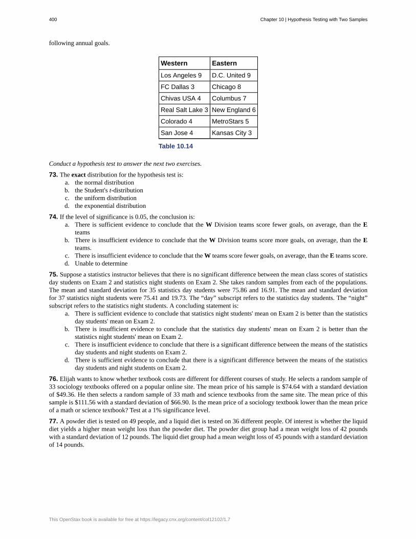
following annual goals.
Western Eastern
Los Angeles 9 D.C. United 9
FC Dallas 3 Chicago 8
Chivas USA 4 Columbus 7
Real Salt Lake 3 New England 6
Colorado 4 MetroStars 5
San Jose 4 Kansas City 3
Table 10.14
Conduct a hypothesis test to answer the next two exercises.
73. The exact distribution for the hypothesis test is:a. the normal distributionb. the Student's t-distributionc. the uniform distributiond. the exponential distribution
74. If the level of significance is 0.05, the conclusion is:a. There is sufficient evidence to conclude that the W Division teams score fewer goals, on average, than the E
teamsb. There is insufficient evidence to conclude that the W Division teams score more goals, on average, than the E
teams.c. There is insufficient evidence to conclude that the W teams score fewer goals, on average, than the E teams score.d. Unable to determine
75. Suppose a statistics instructor believes that there is no significant difference between the mean class scores of statisticsday students on Exam 2 and statistics night students on Exam 2. She takes random samples from each of the populations.The mean and standard deviation for 35 statistics day students were 75.86 and 16.91. The mean and standard deviationfor 37 statistics night students were 75.41 and 19.73. The “day” subscript refers to the statistics day students. The “night”subscript refers to the statistics night students. A concluding statement is:
a. There is sufficient evidence to conclude that statistics night students' mean on Exam 2 is better than the statisticsday students' mean on Exam 2.
b. There is insufficient evidence to conclude that the statistics day students' mean on Exam 2 is better than thestatistics night students' mean on Exam 2.
c. There is insufficient evidence to conclude that there is a significant difference between the means of the statisticsday students and night students on Exam 2.
d. There is sufficient evidence to conclude that there is a significant difference between the means of the statisticsday students and night students on Exam 2.
76. Elijah wants to know whether textbook costs are different for different courses of study. He selects a random sample of33 sociology textbooks offered on a popular online site. The mean price of his sample is $74.64 with a standard deviationof $49.36. He then selects a random sample of 33 math and science textbooks from the same site. The mean price of thissample is $111.56 with a standard deviation of $66.90. Is the mean price of a sociology textbook lower than the mean priceof a math or science textbook? Test at a 1% significance level.
77. A powder diet is tested on 49 people, and a liquid diet is tested on 36 different people. Of interest is whether the liquiddiet yields a higher mean weight loss than the powder diet. The powder diet group had a mean weight loss of 42 poundswith a standard deviation of 12 pounds. The liquid diet group had a mean weight loss of 45 pounds with a standard deviationof 14 pounds.
400 Chapter 10 | Hypothesis Testing with Two Samples
This OpenStax book is available for free at https://legacy.cnx.org/content/col12102/1.7

78. Suppose a statistics instructor believes that there is no significant difference between the mean class scores of statisticsday students on Exam 2 and statistics night students on Exam 2. She takes random samples from each of the populations.The mean and standard deviation for 35 statistics day students were 75.86 and 16.91, respectively. The mean and standarddeviation for 37 statistics night students were 75.41 and 19.73. The “day” subscript refers to the statistics day students. The“night” subscript refers to the statistics night students. An appropriate alternative hypothesis for the hypothesis test is:
a. μday > μnightb. μday < μnightc. μday = μnightd. μday ≠ μnight
10.2 Comparing Two Independent Population Proportions
79. A recent drug survey showed an increase in the use of drugs and alcohol among local high school seniors as compared tothe national percent. Suppose that a survey of 100 local seniors and 100 national seniors is conducted to see if the proportionof drug and alcohol use is higher locally than nationally. Locally, 65 seniors reported using drugs or alcohol within the pastmonth, while 60 national seniors reported using them.
80. We are interested in whether the proportions of female suicide victims for ages 15 to 24 are the same for White andthe Black people in the United States. We randomly pick one year, 1992, to compare the races. The number of suicidesestimated in the United States in 1992 for White females is 4,930. Five hundred eighty were aged 15 to 24. The estimate forBlack females is 330. Forty were aged 15 to 24. We will let female suicide victims be our population.
81. Elizabeth Mjelde, an art history professor, was interested in whether the value from the Golden Ratio formula,⎛⎝larger + smaller dimension
larger dimension⎞⎠ was the same in the Whitney Exhibit for works from 1900 to 1919 as for works from 1920
to 1942. Thirty-seven early works were sampled, averaging 1.74 with a standard deviation of 0.11. Sixty-five of the laterworks were sampled, averaging 1.746 with a standard deviation of 0.1064. Do you think that there is a significant differencein the Golden Ratio calculation?
82. A recent year was randomly picked from 1985 to the present. In that year, there were 2,051 Hispanic students at CabrilloCollege out of a total of 12,328 students. At Lake Tahoe College, there were 321 Hispanic students out of a total of 2,441students. In general, do you think that the percent of Hispanic students at the two colleges is basically the same or different?
Use the following information to answer the next three exercises. Neuroinvasive West Nile virus is a severe disease thataffects a person’s nervous system . It is spread by the Culex species of mosquito. In the United States in 2010 there were629 reported cases of neuroinvasive West Nile virus out of a total of 1,021 reported cases and there were 486 neuroinvasivereported cases out of a total of 712 cases reported in 2011. Is the 2011 proportion of neuroinvasive West Nile virus casesmore than the 2010 proportion of neuroinvasive West Nile virus cases? Using a 1% level of significance, conduct anappropriate hypothesis test.
• “2011” subscript: 2011 group.
• “2010” subscript: 2010 group
83. This is:a. a test of two proportionsb. a test of two independent meansc. a test of a single meand. a test of matched pairs.
84. An appropriate null hypothesis is:a. p2011 ≤ p2010b. p2011 ≥ p2010c. μ2011 ≤ μ2010d. p2011 > p2010
85. Researchers conducted a study to find out if there is a difference in the use of eReaders by different age groups.Randomly selected participants were divided into two age groups. In the 16- to 29-year-old group, 7% of the 628 surveyeduse eReaders, while 11% of the 2,309 participants 30 years old and older use eReaders.
Chapter 10 | Hypothesis Testing with Two Samples 401
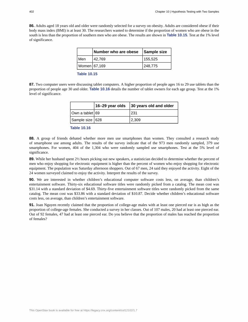
86. Adults aged 18 years old and older were randomly selected for a survey on obesity. Adults are considered obese if theirbody mass index (BMI) is at least 30. The researchers wanted to determine if the proportion of women who are obese in thesouth is less than the proportion of southern men who are obese. The results are shown in Table 10.15. Test at the 1% levelof significance.
Number who are obese Sample size
Men 42,769 155,525
Women 67,169 248,775
Table 10.15
87. Two computer users were discussing tablet computers. A higher proportion of people ages 16 to 29 use tablets than theproportion of people age 30 and older. Table 10.16 details the number of tablet owners for each age group. Test at the 1%level of significance.
16–29 year olds 30 years old and older
Own a tablet 69 231
Sample size 628 2,309
Table 10.16
88. A group of friends debated whether more men use smartphones than women. They consulted a research studyof smartphone use among adults. The results of the survey indicate that of the 973 men randomly sampled, 379 usesmartphones. For women, 404 of the 1,304 who were randomly sampled use smartphones. Test at the 5% level ofsignificance.
89. While her husband spent 2½ hours picking out new speakers, a statistician decided to determine whether the percent ofmen who enjoy shopping for electronic equipment is higher than the percent of women who enjoy shopping for electronicequipment. The population was Saturday afternoon shoppers. Out of 67 men, 24 said they enjoyed the activity. Eight of the24 women surveyed claimed to enjoy the activity. Interpret the results of the survey.
90. We are interested in whether children’s educational computer software costs less, on average, than children’sentertainment software. Thirty-six educational software titles were randomly picked from a catalog. The mean cost was$31.14 with a standard deviation of $4.69. Thirty-five entertainment software titles were randomly picked from the samecatalog. The mean cost was $33.86 with a standard deviation of $10.87. Decide whether children’s educational softwarecosts less, on average, than children’s entertainment software.
91. Joan Nguyen recently claimed that the proportion of college-age males with at least one pierced ear is as high as theproportion of college-age females. She conducted a survey in her classes. Out of 107 males, 20 had at least one pierced ear.Out of 92 females, 47 had at least one pierced ear. Do you believe that the proportion of males has reached the proportionof females?
402 Chapter 10 | Hypothesis Testing with Two Samples
This OpenStax book is available for free at https://legacy.cnx.org/content/col12102/1.7

92. "To Breakfast or Not to Breakfast?" by Richard Ayore
In the American society, birthdays are one of those days that everyone looks forward to. People of different ages and peergroups gather to mark the 18th, 20th, …, birthdays. During this time, one looks back to see what he or she has achieved forthe past year and also focuses ahead for more to come.
If, by any chance, I am invited to one of these parties, my experience is always different. Instead of dancing around withmy friends while the music is booming, I get carried away by memories of my family back home in Kenya. I remember thegood times I had with my brothers and sister while we did our daily routine.
Every morning, I remember we went to the shamba (garden) to weed our crops. I remember one day arguing with mybrother as to why he always remained behind just to join us an hour later. In his defense, he said that he preferred waitingfor breakfast before he came to weed. He said, “This is why I always work more hours than you guys!”
And so, to prove him wrong or right, we decided to give it a try. One day we went to work as usual without breakfast,and recorded the time we could work before getting tired and stopping. On the next day, we all ate breakfast before goingto work. We recorded how long we worked again before getting tired and stopping. Of interest was our mean increase inwork time. Though not sure, my brother insisted that it was more than two hours. Using the data in Table 10.17, solve ourproblem.
Work hours with breakfast Work hours without breakfast
8 6
7 5
9 5
5 4
9 7
8 7
10 7
7 5
6 6
9 5
Table 10.17
10.3 Two Population Means with Known Standard Deviations
NOTE
If you are using a Student's t-distribution for one of the following homework problems, including for paired data, youmay assume that the underlying population is normally distributed. (When using these tests in a real situation, youmust first prove that assumption, however.)
93. A study is done to determine if students in the California state university system take longer to graduate, on average,than students enrolled in private universities. One hundred students from both the California state university system andprivate universities are surveyed. Suppose that from years of research, it is known that the population standard deviationsare 1.5811 years and 1 year, respectively. The following data are collected. The California state university system studentstook on average 4.5 years with a standard deviation of 0.8. The private university students took on average 4.1 years with astandard deviation of 0.3.
Chapter 10 | Hypothesis Testing with Two Samples 403
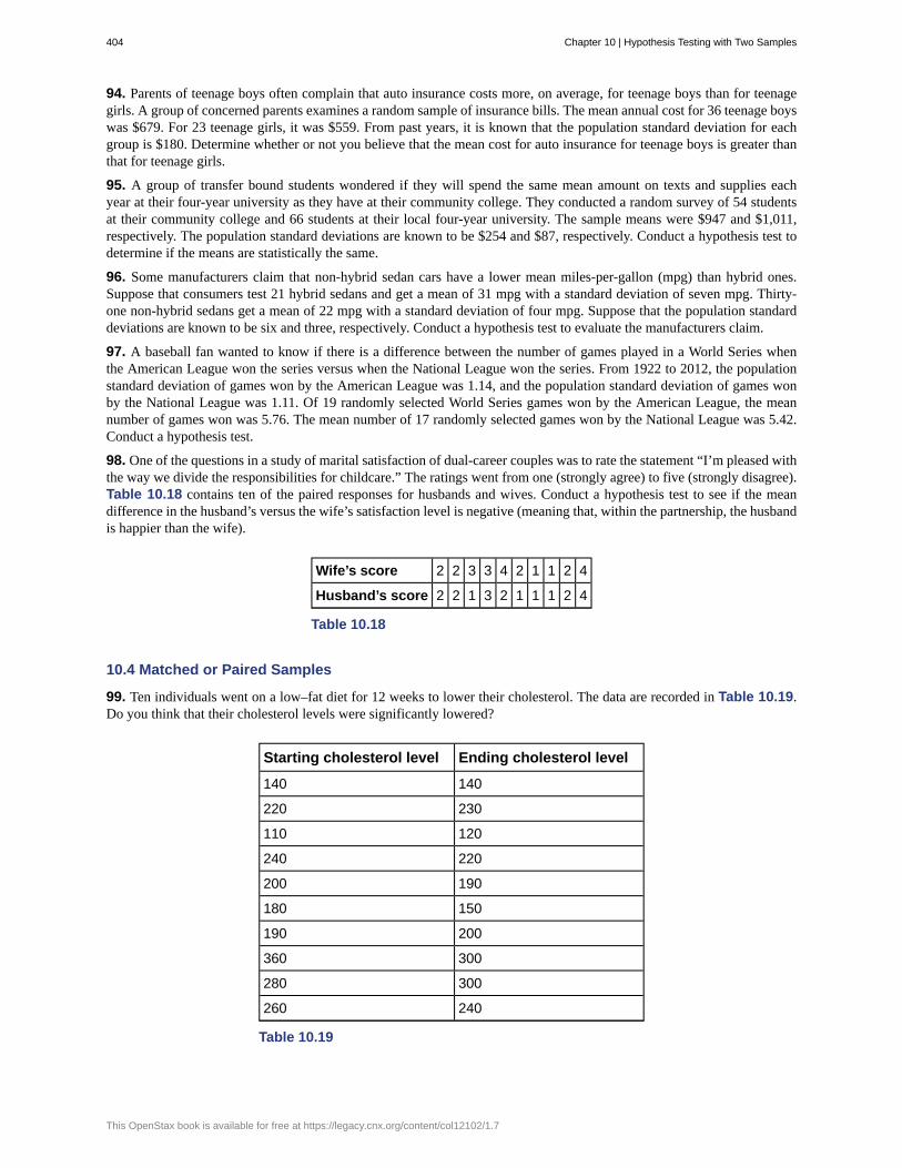
94. Parents of teenage boys often complain that auto insurance costs more, on average, for teenage boys than for teenagegirls. A group of concerned parents examines a random sample of insurance bills. The mean annual cost for 36 teenage boyswas $679. For 23 teenage girls, it was $559. From past years, it is known that the population standard deviation for eachgroup is $180. Determine whether or not you believe that the mean cost for auto insurance for teenage boys is greater thanthat for teenage girls.
95. A group of transfer bound students wondered if they will spend the same mean amount on texts and supplies eachyear at their four-year university as they have at their community college. They conducted a random survey of 54 studentsat their community college and 66 students at their local four-year university. The sample means were $947 and $1,011,respectively. The population standard deviations are known to be $254 and $87, respectively. Conduct a hypothesis test todetermine if the means are statistically the same.
96. Some manufacturers claim that non-hybrid sedan cars have a lower mean miles-per-gallon (mpg) than hybrid ones.Suppose that consumers test 21 hybrid sedans and get a mean of 31 mpg with a standard deviation of seven mpg. Thirty-one non-hybrid sedans get a mean of 22 mpg with a standard deviation of four mpg. Suppose that the population standarddeviations are known to be six and three, respectively. Conduct a hypothesis test to evaluate the manufacturers claim.
97. A baseball fan wanted to know if there is a difference between the number of games played in a World Series whenthe American League won the series versus when the National League won the series. From 1922 to 2012, the populationstandard deviation of games won by the American League was 1.14, and the population standard deviation of games wonby the National League was 1.11. Of 19 randomly selected World Series games won by the American League, the meannumber of games won was 5.76. The mean number of 17 randomly selected games won by the National League was 5.42.Conduct a hypothesis test.
98. One of the questions in a study of marital satisfaction of dual-career couples was to rate the statement “I’m pleased withthe way we divide the responsibilities for childcare.” The ratings went from one (strongly agree) to five (strongly disagree).Table 10.18 contains ten of the paired responses for husbands and wives. Conduct a hypothesis test to see if the meandifference in the husband’s versus the wife’s satisfaction level is negative (meaning that, within the partnership, the husbandis happier than the wife).
Wife’s score 2 2 3 3 4 2 1 1 2 4
Husband’s score 2 2 1 3 2 1 1 1 2 4
Table 10.18
10.4 Matched or Paired Samples
99. Ten individuals went on a low–fat diet for 12 weeks to lower their cholesterol. The data are recorded in Table 10.19.Do you think that their cholesterol levels were significantly lowered?
Starting cholesterol level Ending cholesterol level
140 140
220 230
110 120
240 220
200 190
180 150
190 200
360 300
280 300
260 240
Table 10.19
404 Chapter 10 | Hypothesis Testing with Two Samples
This OpenStax book is available for free at https://legacy.cnx.org/content/col12102/1.7

Use the following information to answer the next two exercises. A new AIDS prevention drug was tried on a group of 224HIV positive patients. Forty-five patients developed AIDS after four years. In a control group of 224 HIV positive patients,68 developed AIDS after four years. We want to test whether the method of treatment reduces the proportion of patients thatdevelop AIDS after four years or if the proportions of the treated group and the untreated group stay the same.
Let the subscript t = treated patient and ut = untreated patient.
100. The appropriate hypotheses are:a. H0: pt < put and Ha: pt ≥ putb. H0: pt ≤ put and Ha: pt > putc. H0: pt = put and Ha: pt ≠ putd. H0: pt = put and Ha: pt < put
Use the following information to answer the next two exercises. An experiment is conducted to show that blood pressurecan be consciously reduced in people trained in a “biofeedback exercise program.” Six subjects were randomly selectedand blood pressure measurements were recorded before and after the training. The difference between blood pressures wascalculated (after - before) producing the following results: x– d = −10.2 sd = 8.4. Using the data, test the hypothesis that the
blood pressure has decreased after the training.
101. The distribution for the test is:a. t5b. t6c. N(−10.2, 8.4)
d. N(−10.2, 8.46
)
102. A golf instructor is interested in determining if her new technique for improving players’ golf scores is effective. Shetakes four new students. She records their 18-hole scores before learning the technique and then after having taken her class.She conducts a hypothesis test. The data are as follows.
Player 1 Player 2 Player 3 Player 4
Mean score before class 83 78 93 87
Mean score after class 80 80 86 86
Table 10.20
The correct decision is:
a. Reject H0.b. Do not reject the H0.
Chapter 10 | Hypothesis Testing with Two Samples 405
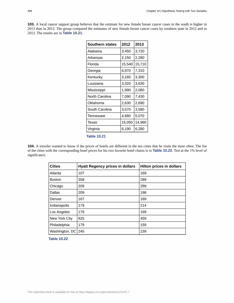
103. A local cancer support group believes that the estimate for new female breast cancer cases in the south is higher in2013 than in 2012. The group compared the estimates of new female breast cancer cases by southern state in 2012 and in2013. The results are in Table 10.21.
Southern states 2012 2013
Alabama 3,450 3,720
Arkansas 2,150 2,280
Florida 15,540 15,710
Georgia 6,970 7,310
Kentucky 3,160 3,300
Louisiana 3,320 3,630
Mississippi 1,990 2,080
North Carolina 7,090 7,430
Oklahoma 2,630 2,690
South Carolina 3,570 3,580
Tennessee 4,680 5,070
Texas 15,050 14,980
Virginia 6,190 6,280
Table 10.21
104. A traveler wanted to know if the prices of hotels are different in the ten cities that he visits the most often. The listof the cities with the corresponding hotel prices for his two favorite hotel chains is in Table 10.22. Test at the 1% level ofsignificance.
Cities Hyatt Regency prices in dollars Hilton prices in dollars
Atlanta 107 169
Boston 358 289
Chicago 209 299
Dallas 209 198
Denver 167 169
Indianapolis 179 214
Los Angeles 179 169
New York City 625 459
Philadelphia 179 159
Washington, DC 245 239
Table 10.22
406 Chapter 10 | Hypothesis Testing with Two Samples
This OpenStax book is available for free at https://legacy.cnx.org/content/col12102/1.7

105. A politician asked his staff to determine whether the underemployment rate in the northeast decreased from 2011 to2012. The results are in Table 10.23.
Northeastern states 2011 2012
Connecticut 17.3 16.4
Delaware 17.4 13.7
Maine 19.3 16.1
Maryland 16.0 15.5
Massachusetts 17.6 18.2
New Hampshire 15.4 13.5
New Jersey 19.2 18.7
New York 18.5 18.7
Ohio 18.2 18.8
Pennsylvania 16.5 16.9
Rhode Island 20.7 22.4
Vermont 14.7 12.3
West Virginia 15.5 17.3
Table 10.23
BRINGING IT TOGETHER: HOMEWORK
Use the following information to answer the next ten exercises. indicate which of the following choices best identifies thehypothesis test.
a. independent group means, population standard deviations and/or variances known
b. independent group means, population standard deviations and/or variances unknown
c. matched or paired samples
d. single mean
e. two proportions
f. single proportion
106. A powder diet is tested on 49 people, and a liquid diet is tested on 36 different people. The population standarddeviations are two pounds and three pounds, respectively. Of interest is whether the liquid diet yields a higher mean weightloss than the powder diet.
107. A new chocolate bar is taste-tested on consumers. Of interest is whether the proportion of children who like the newchocolate bar is greater than the proportion of adults who like it.
108. The mean number of English courses taken in a two–year time period by male and female college students is believedto be about the same. An experiment is conducted and data are collected from nine males and 16 females.
109. A football league reported that the mean number of touchdowns per game was five. A study is done to determine ifthe mean number of touchdowns has decreased.
Chapter 10 | Hypothesis Testing with Two Samples 407

110. A study is done to determine if students in the California state university system take longer to graduate thanstudents enrolled in private universities. One hundred students from both the California state university system and privateuniversities are surveyed. From years of research, it is known that the population standard deviations are 1.5811 years andone year, respectively.
111. According to a YWCA Rape Crisis Center newsletter, 75% of rape victims know their attackers. A study is done toverify this.
112. According to a recent study, U.S. companies have a mean maternity-leave of six weeks.
113. A recent drug survey showed an increase in use of drugs and alcohol among local high school students as compared tothe national percent. Suppose that a survey of 100 local youths and 100 national youths is conducted to see if the proportionof drug and alcohol use is higher locally than nationally.
114. A new SAT study course is tested on 12 individuals. Pre-course and post-course scores are recorded. Of interest is themean increase in SAT scores. The following data are collected:
Pre-course score Post-course score
1 300
960 920
1010 1100
840 880
1100 1070
1250 1320
860 860
1330 1370
790 770
990 1040
1110 1200
740 850
Table 10.24
115. University of Michigan researchers reported in the Journal of the National Cancer Institute that quitting smoking isespecially beneficial for those under age 49. In this American Cancer Society study, the risk (probability) of dying of lungcancer was about the same as for those who had never smoked.
408 Chapter 10 | Hypothesis Testing with Two Samples
This OpenStax book is available for free at https://legacy.cnx.org/content/col12102/1.7

116. Lesley E. Tan investigated the relationship between left-handedness vs. right-handedness and motor competence inpreschool children. Random samples of 41 left-handed preschool children and 41 right-handed preschool children weregiven several tests of motor skills to determine if there is evidence of a difference between the children based on thisexperiment. The experiment produced the means and standard deviations shown Table 10.25. Determine the appropriatetest and best distribution to use for that test.
Left-handed Right-handed
Sample size 41 41
Sample mean 97.5 98.1
Sample standard deviation 17.5 19.2
Table 10.25
a. Two independent means, normal distributionb. Two independent means, Student’s-t distributionc. Matched or paired samples, Student’s-t distributiond. Two population proportions, normal distribution
117. A golf instructor is interested in determining if her new technique for improving players’ golf scores is effective. Shetakes four (4) new students. She records their 18-hole scores before learning the technique and then after having taken herclass. She conducts a hypothesis test. The data are as Table 10.26.
Player 1 Player 2 Player 3 Player 4
Mean score before class 83 78 93 87
Mean score after class 80 80 86 86
Table 10.26
This is:
a. a test of two independent means.b. a test of two proportions.c. a test of a single mean.d. a test of a single proportion.
REFERENCES
10.1 Comparing Two Independent Population Means
Data from Graduating Engineer + Computer Careers. Available online at http://www.graduatingengineer.com
Data from Microsoft Bookshelf.
Data from the United States Senate website, available online at www.Senate.gov (accessed June 17, 2013).
“List of current United States Senators by Age.” Wikipedia. Available online at http://en.wikipedia.org/wiki/List_of_current_United_States_Senators_by_age (accessed June 17, 2013).
“Sectoring by Industry Groups.” Nasdaq. Available online at http://www.nasdaq.com/markets/barchart-sectors.aspx?page=sectors&base=industry (accessed June 17, 2013).
“Strip Clubs: Where Prostitution and Trafficking Happen.” Prostitution Research and Education, 2013. Available online atwww.prostitutionresearch.com/ProsViolPosttrauStress.html (accessed June 17, 2013).
“World Series History.” Baseball-Almanac, 2013. Available online at http://www.baseball-almanac.com/ws/wsmenu.shtml(accessed June 17, 2013).
Chapter 10 | Hypothesis Testing with Two Samples 409

10.2 Comparing Two Independent Population Proportions
Data from Educational Resources, December catalog.
Data from Hilton Hotels. Available online at http://www.hilton.com (accessed June 17, 2013).
Data from Hyatt Hotels. Available online at http://hyatt.com (accessed June 17, 2013).
Data from Statistics, United States Department of Health and Human Services.
Data from Whitney Exhibit on loan to San Jose Museum of Art.
Data from the American Cancer Society. Available online at http://www.cancer.org/index (accessed June 17, 2013).
Data from the Chancellor’s Office, California Community Colleges, November 1994.
“State of the States.” Gallup, 2013. Available online at http://www.gallup.com/poll/125066/State-States.aspx?ref=interactive (accessed June 17, 2013).
“West Nile Virus.” Centers for Disease Control and Prevention. Available online at http://www.cdc.gov/ncidod/dvbid/westnile/index.htm (accessed June 17, 2013).
10.3 Two Population Means with Known Standard Deviations
Data from the United States Census Bureau. Available online at http://www.census.gov/prod/cen2010/briefs/c2010br-02.pdf
Hinduja, Sameer. “Sexting Research and Gender Differences.” Cyberbullying Research Center, 2013. Available online athttp://cyberbullying.us/blog/sexting-research-and-gender-differences/ (accessed June 17, 2013).
“Smart Phone Users, By the Numbers.” Visually, 2013. Available online at http://visual.ly/smart-phone-users-numbers(accessed June 17, 2013).
Smith, Aaron. “35% of American adults own a Smartphone.” Pew Internet, 2013. Available online athttp://www.pewinternet.org/~/media/Files/Reports/2011/PIP_Smartphones.pdf (accessed June 17, 2013).
“State-Specific Prevalence of Obesity AmongAduls—Unites States, 2007.” MMWR, CDC. Available online athttp://www.cdc.gov/mmwr/preview/mmwrhtml/mm5728a1.htm (accessed June 17, 2013).
“Texas Crime Rates 1960–1012.” FBI, Uniform Crime Reports, 2013. Available online at: http://www.disastercenter.com/crime/txcrime.htm (accessed June 17, 2013).
SOLUTIONS
1 two proportions
3 matched or paired samples
5 single mean
7 independent group means, population standard deviations and/or variances unknown
9 two proportions
11 independent group means, population standard deviations and/or variances unknown
13 independent group means, population standard deviations and/or variances unknown
15 two proportions
17 The random variable is the difference between the mean amounts of sugar in the two soft drinks.
19 means
21 two-tailed
23 the difference between the mean life spans of White and non-White people
25 This is a comparison of two population means with unknown population standard deviations.
27 Check student’s solution.
410 Chapter 10 | Hypothesis Testing with Two Samples
This OpenStax book is available for free at https://legacy.cnx.org/content/col12102/1.7

28a. Cannot accept the null hypothesis
b. p-value < 0.05
c. There is not enough evidence at the 5% level of significance to support the claim that life expectancy in the 1900s isdifferent between White and non-White people.
31 P′OS1 – P′OS2 = difference in the proportions of phones that had system failures within the first eight hours of operationwith OS1 and OS2.
34 proportions
36 right-tailed
38 The random variable is the difference in proportions (percents) of the populations that are of two or more races inNevada and North Dakota.
40 Our sample sizes are much greater than five each, so we use the normal for two proportions distribution for thishypothesis test.
42a. Cannot accept the null hypothesis.
b. p-value < alpha
c. At the 5% significance level, there is sufficient evidence to conclude that the proportion (percent) of the populationthat is of two or more races in Nevada is statistically higher than that in North Dakota.
44 The difference in mean speeds of the fastball pitches of the two pitchers
46 –2.46
47 At the 1% significance level, we can reject the null hypothesis. There is sufficient data to conclude that the mean speedof Rodriguez’s fastball is faster than Wesley’s.
49 Subscripts: 1 = Food, 2 = No FoodH0 : μ1 ≤ μ2
Ha : μ1 > μ2
51 Subscripts: 1 = Gamma, 2 = ZetaH0 : μ1 = μ2
Ha : μ1 ≠ μ2
53 There is sufficient evidence so we cannot accept the null hypothesis. The data support that the melting point for AlloyZeta is different from the melting point of Alloy Gamma.
54 the mean difference of the system failures
56 With a p-value 0.0067, we can cannot accept the null hypothesis. There is enough evidence to support that the softwarepatch is effective in reducing the number of system failures.
60 H0: μd ≥ 0 Ha: μd < 0
63 We decline to reject the null hypothesis. There is not sufficient evidence to support that the medication is effective.
65 Subscripts: 1: two-year colleges; 2: four-year collegesa. H0 : μ1 ≥ μ2
b. Ha : μ1 < μ2
c. X 1 – X 2 is the difference between the mean enrollments of the two-year colleges and the four-year colleges.
d. Student’s-t
e. test statistic: -0.2480
f. p-value: 0.4019
Chapter 10 | Hypothesis Testing with Two Samples 411
g. Check student’s solution.
h. i. Alpha: 0.05
ii. Decision: Cannot reject
iii. Reason for Decision: p-value > alpha
iv. Conclusion: At the 5% significance level, there is sufficient evidence to conclude that the mean enrollment atfour-year colleges is higher than at two-year colleges.
67 Subscripts: 1: mechanical engineering; 2: electrical engineeringa. H0 : μ1 ≥ μ2
b. Ha : μ1 < μ2
c. X 1 − X 2 is the difference between the mean entry level salaries of mechanical engineers and electrical engineers.
d. t108
e. test statistic: t = –0.82
f. p-value: 0.2061
g. Check student’s solution.
h. i. Alpha: 0.05
ii. Decision: Cannot reject the null hypothesis.
iii. Reason for Decision: p-value > alpha
iv. Conclusion: At the 5% significance level, there is insufficient evidence to conclude that the mean entry-levelsalaries of mechanical engineers is lower than that of electrical engineers.
69a. H0 : μ1 = μ2
b. Ha : μ1 ≠ μ2
c. X 1 − X 2 is the difference between the mean times for completing a lap in races and in practices.
d. t20.32
e. test statistic: –4.70
f. p-value: 0.0001
g. Check student’s solution.
h. i. Alpha: 0.05
ii. Decision: Cannot accept the null hypothesis.
iii. Reason for Decision: p-value < alpha
iv. Conclusion: At the 5% significance level, there is sufficient evidence to conclude that the mean time forcompleting a lap in races is different from that in practices.
71a. H0 : μ1 = μ2
b. Ha : μ1 ≠ μ2
c. is the difference between the mean times for completing a lap in races and in practices.
d. t40.94
e. test statistic: –5.08
412 Chapter 10 | Hypothesis Testing with Two Samples
This OpenStax book is available for free at https://legacy.cnx.org/content/col12102/1.7
f. p-value: zero
g. Check student’s solution.
h. i. Alpha: 0.05
ii. Decision: Cannot accept the null hypothesis.
iii. Reason for Decision: p-value < alpha
iv. Conclusion: At the 5% significance level, there is sufficient evidence to conclude that the mean time forcompleting a lap in races is different from that in practices.
74 c
76 Test: two independent sample means, population standard deviations unknown. μ1 = the mean price of a sociology
text on the selected site. μ2 = the mean price of a math/science text on the selected site. Random variable: X1 - X1
= the difference in the sample mean textbook price between sociology texts and math/science texts. Hypotheses:H0 : μ1 - μ2 = 0, Ha : μ1 - μ2 < μ2 which can be expressed as
H0s : μ1 - μ2, Ha μ1 < μ2 . Distribution for the test: Use td f ; because each sample has more than 30
observations, d f = n1 + n2 - 2 = 33 + 33 - 2 = 64 . Estimate the critical value on the t -table using the nearest available
degrees of freedom, 60. The critical value, 2.660, is found in the .0005 column. Calculate the test statistic:
tc =⎛⎝X
¯1 - X
¯2⎞⎠ - 0
s12
n2+ s2
2
n2
= (74.64 - 111.56) - 049.362
33 + 66.902
33
= - 2.55 . Using a calculator with tc = - 2.55 and d f = 64 , the left-tailed
p -value: Decision: Reject H0 . Conclusion: At the 1% level of significance, from the sample data, there is sufficient
evidence to conclude that the mean price of sociology textbooks is less than the mean price of textbooks for math/science.
78 d
80a. H0: PW = PB
b. Ha: PW ≠ PB
c. The random variable is the difference in the proportions of White and Black suicide victims, aged 15 to 24.
d. normal for two proportions
e. test statistic: –0.1944
f. p-value: 0.8458
g. Check student’s solution.
h. i. Alpha: 0.05
ii. Decision: Cannot accept the null hypothesis.
iii. Reason for decision: p-value > alpha
iv. Conclusion: At the 5% significance level, there is insufficient evidence to conclude that the proportions of Whiteand Black female suicide victims, aged 15 to 24, are different.
82 Subscripts: 1 = Cabrillo College, 2 = Lake Tahoe Collegea. H0 : p1 = p2
b. Ha : p1 ≠ p2
c. The random variable is the difference between the proportions of Hispanic students at Cabrillo College and Lake TahoeCollege.
d. normal for two proportions
Chapter 10 | Hypothesis Testing with Two Samples 413

e. test statistic: 4.29
f. p-value: 0.00002
g. Check student’s solution.
h. i. Alpha: 0.05
ii. Decision: Cannot accept the null hypothesis.
iii. Reason for decision: p-value < alpha
iv. Conclusion: There is sufficient evidence to conclude that the proportions of Hispanic students at Cabrillo Collegeand Lake Tahoe College are different.
84 a
85 Test: two independent sample proportions. Random variable: p′1 - p′2 Distribution:H0 : p1 = p2
Ha : p1 ≠ p2 The proportion of eReader users is different for the 16- to 29-year-old users from that of the 30 and older
users. Graph: two-tailed
87 Test: two independent sample proportions Random variable: p′1 − p′2 Distribution: H0 : p1 = p2
Ha : p1 > p2 A higher proportion of tablet owners are aged 16 to 29 years old than are 30 years old and older. Graph:
right-tailed Do not reject the H0. Conclusion: At the 1% level of significance, from the sample data, there is not sufficientevidence to conclude that a higher proportion of tablet owners are aged 16 to 29 years old than are 30 years old and older.
89 Subscripts: 1: men; 2: womena. H0 : p1 ≤ p2
b. Ha : p1 > p2
c. P′1 − P′2 is the difference between the proportions of men and women who enjoy shopping for electronic equipment.
d. normal for two proportions
e. test statistic: 0.22
f. p-value: 0.4133
g. Check student’s solution.
h. i. Alpha: 0.05
ii. Decision: Cannot reject the null hypothesis.
iii. Reason for Decision: p-value > alpha
iv. Conclusion: At the 5% significance level, there is insufficient evidence to conclude that the proportion of menwho enjoy shopping for electronic equipment is more than the proportion of women.
91a. H0 : p1 = p2
b. Ha : p1 ≠ p2
c. P′1 − P′2 is the difference between the proportions of men and women that have at least one pierced ear.
d. normal for two proportions
e. test statistic: –4.82
f. p-value: zero
g. Check student’s solution.
h. i. Alpha: 0.05
ii. Decision: Cannot accept the null hypothesis.
414 Chapter 10 | Hypothesis Testing with Two Samples
This OpenStax book is available for free at https://legacy.cnx.org/content/col12102/1.7

iii. Reason for Decision: p-value < alpha
iv. Conclusion: At the 5% significance level, there is sufficient evidence to conclude that the proportions of malesand females with at least one pierced ear is different.
92a. H0: µd = 0
b. Ha: µd > 0
c. The random variable Xd is the mean difference in work times on days when eating breakfast and on days when noteating breakfast.
d. t9
e. test statistic: 4.8963
f. p-value: 0.0004
g. Check student’s solution.
h. i. Alpha: 0.05
ii. Decision: Cannot accept the null hypothesis.
iii. Reason for Decision: p-value < alpha
iv. Conclusion: At the 5% level of significance, there is sufficient evidence to conclude that the mean difference inwork times on days when eating breakfast and on days when not eating breakfast has increased.
94 Subscripts: 1 = boys, 2 = girlsa. H0 : μ1 ≤ μ2
b. Ha : μ1 > μ2
c. The random variable is the difference in the mean auto insurance costs for boys and girls.
d. normal
e. test statistic: z = 2.50
f. p-value: 0.0062
g. Check student’s solution.
h. i. Alpha: 0.05
ii. Decision: Cannot accept the null hypothesis.
iii. Reason for Decision: p-value < alpha
iv. Conclusion: At the 5% significance level, there is sufficient evidence to conclude that the mean cost of autoinsurance for teenage boys is greater than that for girls.
96 Subscripts: 1 = non-hybrid sedans, 2 = hybrid sedansa. H0 : μ1 ≥ μ2
b. Ha : μ1 < μ2
c. The random variable is the difference in the mean miles per gallon of non-hybrid sedans and hybrid sedans.
d. normal
e. test statistic: 6.36
f. p-value: 0
g. Check student’s solution.
h. i. Alpha: 0.05
ii. Decision: Cannot accept the null hypothesis.
Chapter 10 | Hypothesis Testing with Two Samples 415

iii. Reason for decision: p-value < alpha
iv. Conclusion: At the 5% significance level, there is sufficient evidence to conclude that the mean miles per gallonof non-hybrid sedans is less than that of hybrid sedans.
98a. H0: µd = 0
b. Ha: µd < 0
c. The random variable Xd is the average difference between husband’s and wife’s satisfaction level.
d. t9
e. test statistic: t = –1.86
f. p-value: 0.0479
g. Check student’s solution
h. i. Alpha: 0.05
ii. Decision: Cannot accept the null hypothesis, but run another test.
iii. Reason for Decision: p-value < alpha
iv. Conclusion: This is a weak test because alpha and the p-value are close. However, there is insufficient evidenceto conclude that the mean difference is negative.
99 p-value = 0.1494 At the 5% significance level, there is insufficient evidence to conclude that the medication loweredcholesterol levels after 12 weeks.
103 Test: two matched pairs or paired samples (t-test) Random variable: X– d Distribution: t12 H0: μd = 0 Ha: μd > 0 The
mean of the differences of new female breast cancer cases in the south between 2013 and 2012 is greater than zero. Theestimate for new female breast cancer cases in the south is higher in 2013 than in 2012. Graph: right-tailed p-value: 0.0004Decision: Cannot accept H0 Conclusion: At the 5% level of significance, from the sample data, there is sufficient evidenceto conclude that there was a higher estimate of new female breast cancer cases in 2013 than in 2012.
105 Test: matched or paired samples (t-test) Difference data: {–0.9, –3.7, –3.2, –0.5, 0.6, –1.9, –0.5, 0.2, 0.6, 0.4, 1.7, –2.4,
1.8} Random Variable: X– d Distribution: H0: μd = 0 Ha: μd < 0 The mean of the differences of the rate of underemployment
in the northeastern states between 2012 and 2011 is less than zero. The underemployment rate went down from 2011 to2012. Graph: left-tailed. Decision: Cannot reject H0. Conclusion: At the 5% level of significance, from the sample data,there is not sufficient evidence to conclude that there was a decrease in the underemployment rates of the northeastern statesfrom 2011 to 2012.
107 e
109 d
111 f
113 e
115 f
117 a
416 Chapter 10 | Hypothesis Testing with Two Samples
This OpenStax book is available for free at https://legacy.cnx.org/content/col12102/1.7

11 | THE CHI-SQUAREDISTRIBUTION
Figure 11.1 The chi-square distribution can be used to find relationships between two things, like grocery prices atdifferent stores. (credit: Pete/flickr)
Introduction
Have you ever wondered if lottery winning numbers were evenly distributed or if some numbers occurred with a greaterfrequency? How about if the types of movies people preferred were different across different age groups? What about if acoffee machine was dispensing approximately the same amount of coffee each time? You could answer these questions byconducting a hypothesis test.
You will now study a new distribution, one that is used to determine the answers to such questions. This distribution iscalled the chi-square distribution.
In this chapter, you will learn the three major applications of the chi-square distribution:
1. the goodness-of-fit test, which determines if data fit a particular distribution, such as in the lottery example
2. the test of independence, which determines if events are independent, such as in the movie example
3. the test of a single variance, which tests variability, such as in the coffee example
Chapter 11 | The Chi-Square Distribution 417

11.1 | Facts About the Chi-Square DistributionThe notation for the chi-square distribution is:
χ ∼ χd f2
where df = degrees of freedom which depends on how chi-square is being used. (If you want to practice calculating chi-square probabilities then use df = n - 1. The degrees of freedom for the three major uses are each calculated differently.)
For the χ2 distribution, the population mean is μ = df and the population standard deviation is σ = 2(d f ) .
The random variable is shown as χ2.
The random variable for a chi-square distribution with k degrees of freedom is the sum of k independent, squared standardnormal variables.
χ2 = (Z1)2 + (Z2)2 + ... + (Zk)2
1. The curve is nonsymmetrical and skewed to the right.
2. There is a different chi-square curve for each df.
Figure 11.2
3. The test statistic for any test is always greater than or equal to zero.
4. When df > 90, the chi-square curve approximates the normal distribution. For X ~ χ1,0002 the mean, μ = df = 1,000
and the standard deviation, σ = 2(1,000) = 44.7. Therefore, X ~ N(1,000, 44.7), approximately.
5. The mean, μ, is located just to the right of the peak.
11.2 | Test of a Single VarianceThus far our interest has been exclusively on the population parameter μ or it's counterpart in the binomial, p. Surely themean of a population is the most critical piece of information to have, but in some cases we are interested in the variabilityof the outcomes of some distribution. In almost all production processes quality is measured not only by how closely themachine matches the target, but also the variability of the process. If one were filling bags with potato chips not only wouldthere be interest in the average weight of the bag, but also how much variation there was in the weights. No one wants to beassured that the average weight is accurate when their bag has no chips. Electricity voltage may meet some average level,but great variability, spikes, can cause serious damage to electrical machines, especially computers. I would not only liketo have a high mean grade in my classes, but also low variation about this mean. In short, statistical tests concerning thevariance of a distribution have great value and many applications.
A test of a single variance assumes that the underlying distribution is normal. The null and alternative hypotheses arestated in terms of the population variance. The test statistic is:
χc2 =⎛⎝n - 1⎞⎠s2
σ02
418 Chapter 11 | The Chi-Square Distribution
This OpenStax book is available for free at https://legacy.cnx.org/content/col12102/1.7

where:
• n = the total number of observations in the sample data
• s2 = sample variance
• σ02 = hypothesized value of the population variance
• H0 : σ2 = σ02
• Ha : σ2 ≠ σ02
You may think of s as the random variable in this test. The number of degrees of freedom is df = n - 1. A test of a singlevariance may be right-tailed, left-tailed, or two-tailed. Example 11.1 will show you how to set up the null and alternativehypotheses. The null and alternative hypotheses contain statements about the population variance.
Example 11.1
Math instructors are not only interested in how their students do on exams, on average, but how the exam scoresvary. To many instructors, the variance (or standard deviation) may be more important than the average.
Suppose a math instructor believes that the standard deviation for his final exam is five points. One of his beststudents thinks otherwise. The student claims that the standard deviation is more than five points. If the studentwere to conduct a hypothesis test, what would the null and alternative hypotheses be?
Solution 11.1
Even though we are given the population standard deviation, we can set up the test using the population varianceas follows.
• H0: σ2 ≤ 52
• Ha: σ2 > 52
11.1 A SCUBA instructor wants to record the collective depths each of his students' dives during their checkout. He isinterested in how the depths vary, even though everyone should have been at the same depth. He believes the standarddeviation is three feet. His assistant thinks the standard deviation is less than three feet. If the instructor were to conducta test, what would the null and alternative hypotheses be?
Example 11.2
With individual lines at its various windows, a post office finds that the standard deviation for waiting times forcustomers on Friday afternoon is 7.2 minutes. The post office experiments with a single, main waiting line andfinds that for a random sample of 25 customers, the waiting times for customers have a standard deviation of 3.5minutes on a Friday afternoon.
With a significance level of 5%, test the claim that a single line causes lower variation among waiting timesfor customers.
Solution 11.2
Since the claim is that a single line causes less variation, this is a test of a single variance. The parameter is thepopulation variance, σ2.
Random Variable: The sample standard deviation, s, is the random variable. Let s = standard deviation for the
Chapter 11 | The Chi-Square Distribution 419

waiting times.
• H0: σ2 ≥ 7.22
• Ha: σ2 < 7.22
The word "less" tells you this is a left-tailed test.
Distribution for the test: χ242 , where:
• n = the number of customers sampled
• df = n – 1 = 25 – 1 = 24
Calculate the test statistic:
χc2 = (n − 1)s2
σ2 = (25 − 1)(3.5)2
7.22 = 5.67
where n = 25, s = 3.5, and σ = 7.2.
Figure 11.3
The graph of the Chi-square shows the distribution and marks the critical value with 24 degrees of freedom at95% level of confidence, α = 0.05, 13.85. The critical value of 13.85 came from the Chi squared table which isread very much like the students t table. The difference is that the students t-distribution is symmetrical and theChi squared distribution is not. At the top of the Chi squared table we see not only the familiar 0.05, 0.10, etc.but also 0.95, 0.975, etc. These are the columns used to find the left hand critical value. The graph also marksthe calculated χ2 test statistic of 5.67. Comparing the test statistic with the critical value, as we have done with allother hypothesis tests, we reach the conclusion.
Make a decision: Because the calculated test statistic is in the tail we cannot accept H0. This means that youreject σ2 ≥ 7.22. In other words, you do not think the variation in waiting times is 7.2 minutes or more; you thinkthe variation in waiting times is less.
Conclusion: At a 5% level of significance, from the data, there is sufficient evidence to conclude that a singleline causes a lower variation among the waiting times or with a single line, the customer waiting times vary lessthan 7.2 minutes.
420 Chapter 11 | The Chi-Square Distribution
This OpenStax book is available for free at https://legacy.cnx.org/content/col12102/1.7
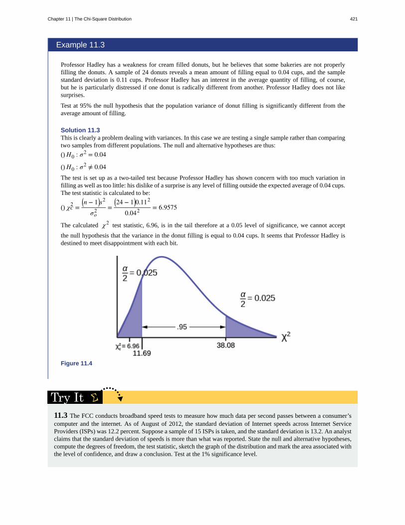
Example 11.3
Professor Hadley has a weakness for cream filled donuts, but he believes that some bakeries are not properlyfilling the donuts. A sample of 24 donuts reveals a mean amount of filling equal to 0.04 cups, and the samplestandard deviation is 0.11 cups. Professor Hadley has an interest in the average quantity of filling, of course,but he is particularly distressed if one donut is radically different from another. Professor Hadley does not likesurprises.
Test at 95% the null hypothesis that the population variance of donut filling is significantly different from theaverage amount of filling.
Solution 11.3This is clearly a problem dealing with variances. In this case we are testing a single sample rather than comparingtwo samples from different populations. The null and alternative hypotheses are thus:
() H0 : σ2 = 0.04
() H0 : σ2 ≠ 0.04The test is set up as a two-tailed test because Professor Hadley has shown concern with too much variation infilling as well as too little: his dislike of a surprise is any level of filling outside the expected average of 0.04 cups.The test statistic is calculated to be:
() χc2 =⎛⎝n − 1⎞⎠s2
σo2=⎛⎝24 − 1⎞⎠0.112
0.042 = 6.9575
The calculated χ2 test statistic, 6.96, is in the tail therefore at a 0.05 level of significance, we cannot accept
the null hypothesis that the variance in the donut filling is equal to 0.04 cups. It seems that Professor Hadley isdestined to meet disappointment with each bit.
Figure 11.4
11.3 The FCC conducts broadband speed tests to measure how much data per second passes between a consumer’scomputer and the internet. As of August of 2012, the standard deviation of Internet speeds across Internet ServiceProviders (ISPs) was 12.2 percent. Suppose a sample of 15 ISPs is taken, and the standard deviation is 13.2. An analystclaims that the standard deviation of speeds is more than what was reported. State the null and alternative hypotheses,compute the degrees of freedom, the test statistic, sketch the graph of the distribution and mark the area associated withthe level of confidence, and draw a conclusion. Test at the 1% significance level.
Chapter 11 | The Chi-Square Distribution 421

11.3 | Goodness-of-Fit TestIn this type of hypothesis test, you determine whether the data "fit" a particular distribution or not. For example, you maysuspect your unknown data fit a binomial distribution. You use a chi-square test (meaning the distribution for the hypothesistest is chi-square) to determine if there is a fit or not. The null and the alternative hypotheses for this test may be writtenin sentences or may be stated as equations or inequalities.
The test statistic for a goodness-of-fit test is:
Σk
(O − E)2
E
where:
• O = observed values (data)
• E = expected values (from theory)
• k = the number of different data cells or categories
The observed values are the data values and the expected values are the values you would expect to get if the null
hypothesis were true. There are n terms of the form(O − E)2
E .
The number of degrees of freedom is df = (number of categories – 1).
The goodness-of-fit test is almost always right-tailed. If the observed values and the corresponding expected values arenot close to each other, then the test statistic can get very large and will be way out in the right tail of the chi-square curve.
NOTE
The number of expected values inside each cell needs to be at least five in order to use this test.
Example 11.4
Absenteeism of college students from math classes is a major concern to math instructors because missing classappears to increase the drop rate. Suppose that a study was done to determine if the actual student absenteeismrate follows faculty perception. The faculty expected that a group of 100 students would miss class according toTable 11.1.
Number of absences per term Expected number of students
0–2 50
3–5 30
6–8 12
9–11 6
12+ 2
Table 11.1
A random survey across all mathematics courses was then done to determine the actual number (observed) ofabsences in a course. The chart in Table 11.2 displays the results of that survey.
422 Chapter 11 | The Chi-Square Distribution
This OpenStax book is available for free at https://legacy.cnx.org/content/col12102/1.7
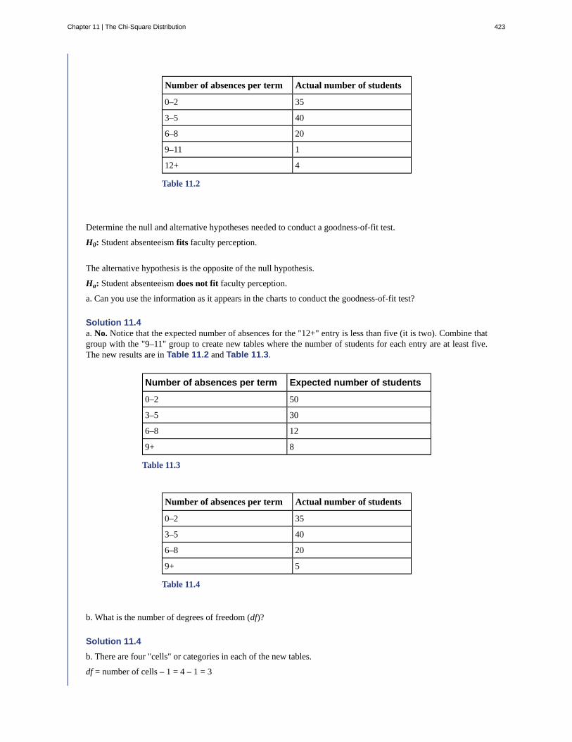
Number of absences per term Actual number of students
0–2 35
3–5 40
6–8 20
9–11 1
12+ 4
Table 11.2
Determine the null and alternative hypotheses needed to conduct a goodness-of-fit test.
H0: Student absenteeism fits faculty perception.
The alternative hypothesis is the opposite of the null hypothesis.
Ha: Student absenteeism does not fit faculty perception.
a. Can you use the information as it appears in the charts to conduct the goodness-of-fit test?
Solution 11.4a. No. Notice that the expected number of absences for the "12+" entry is less than five (it is two). Combine thatgroup with the "9–11" group to create new tables where the number of students for each entry are at least five.The new results are in Table 11.2 and Table 11.3.
Number of absences per term Expected number of students
0–2 50
3–5 30
6–8 12
9+ 8
Table 11.3
Number of absences per term Actual number of students
0–2 35
3–5 40
6–8 20
9+ 5
Table 11.4
b. What is the number of degrees of freedom (df)?
Solution 11.4
b. There are four "cells" or categories in each of the new tables.
df = number of cells – 1 = 4 – 1 = 3
Chapter 11 | The Chi-Square Distribution 423

11.4 A factory manager needs to understand how many products are defective versus how many are produced. Thenumber of expected defects is listed in Table 11.5.
Number produced Number defective
0–100 5
101–200 6
201–300 7
301–400 8
401–500 10
Table 11.5
A random sample was taken to determine the actual number of defects. Table 11.6 shows the results of the survey.
Number produced Number defective
0–100 5
101–200 7
201–300 8
301–400 9
401–500 11
Table 11.6
State the null and alternative hypotheses needed to conduct a goodness-of-fit test, and state the degrees of freedom.
Example 11.5
Employers want to know which days of the week employees are absent in a five-day work week. Most employerswould like to believe that employees are absent equally during the week. Suppose a random sample of 60managers were asked on which day of the week they had the highest number of employee absences. The resultswere distributed as in Table 11.6. For the population of employees, do the days for the highest number ofabsences occur with equal frequencies during a five-day work week? Test at a 5% significance level.
Monday Tuesday Wednesday Thursday Friday
Number of absences 15 12 9 9 15
Table 11.7 Day of the Week Employees were Most Absent
Solution 11.5
The null and alternative hypotheses are:
• H0: The absent days occur with equal frequencies, that is, they fit a uniform distribution.
424 Chapter 11 | The Chi-Square Distribution
This OpenStax book is available for free at https://legacy.cnx.org/content/col12102/1.7

• Ha: The absent days occur with unequal frequencies, that is, they do not fit a uniform distribution.
If the absent days occur with equal frequencies, then, out of 60 absent days (the total in the sample: 15 + 12 + 9+ 9 + 15 = 60), there would be 12 absences on Monday, 12 on Tuesday, 12 on Wednesday, 12 on Thursday, and12 on Friday. These numbers are the expected (E) values. The values in the table are the observed (O) values ordata.
This time, calculate the χ2 test statistic by hand. Make a chart with the following headings and fill in the columns:
• Expected (E) values (12, 12, 12, 12, 12)
• Observed (O) values (15, 12, 9, 9, 15)
• (O – E)
• (O – E)2
•(O – E)2
E
Now add (sum) the last column. The sum is three. This is the χ2 test statistic.
The calculated test statistics is 3 and the critical value of the χ2 distribution at 4 degrees of freedom the 0.05 levelof confidence is 9.48. This value is found in the χ2 table at the 0.05 column on the degrees of freedom row 4.
The degrees of freedom are the number of cells – 1 = 5 – 1 = 4
Next, complete a graph like the following one with the proper labeling and shading. (You should shade the righttail.)
Figure 11.5
χc2 = Σk
(O − E)2
E = 3
The decision is not to reject the null hypothesis because the calculated value of the test statistic is not in the tailof the distribution.
Conclusion: At a 5% level of significance, from the sample data, there is not sufficient evidence to conclude thatthe absent days do not occur with equal frequencies.
11.5 Teachers want to know which night each week their students are doing most of their homework. Most teachersthink that students do homework equally throughout the week. Suppose a random sample of 56 students were asked on
Chapter 11 | The Chi-Square Distribution 425

which night of the week they did the most homework. The results were distributed as in Table 11.8.
Sunday Monday Tuesday Wednesday Thursday Friday Saturday
Number ofstudents
11 8 10 7 10 5 5
Table 11.8
From the population of students, do the nights for the highest number of students doing the majority of their homeworkoccur with equal frequencies during a week? What type of hypothesis test should you use?
Example 11.6
One study indicates that the number of televisions that American families have is distributed (this is the givendistribution for the American population) as in Table 11.9.
Number of Televisions Percent
0 10
1 16
2 55
3 11
4+ 8
Table 11.9
The table contains expected (E) percents.
A random sample of 600 families in the far western United States resulted in the data in Table 11.10.
Number of Televisions Frequency
0 66
1 119
2 340
3 60
4+ 15
Total = 600
Table 11.10
The table contains observed (O) frequency values.
At the 1% significance level, does it appear that the distribution "number of televisions" of far western UnitedStates families is different from the distribution for the American population as a whole?
426 Chapter 11 | The Chi-Square Distribution
This OpenStax book is available for free at https://legacy.cnx.org/content/col12102/1.7

Solution 11.6
This problem asks you to test whether the far western United States families distribution fits the distribution ofthe American families. This test is always right-tailed.
The first table contains expected percentages. To get expected (E) frequencies, multiply the percentage by 600.The expected frequencies are shown in Table 11.10.
Number of televisions Percent Expected frequency
0 10 (0.10)(600) = 60
1 16 (0.16)(600) = 96
2 55 (0.55)(600) = 330
3 11 (0.11)(600) = 66
over 3 8 (0.08)(600) = 48
Table 11.11
Therefore, the expected frequencies are 60, 96, 330, 66, and 48.
H0: The "number of televisions" distribution of far western United States families is the same as the "number oftelevisions" distribution of the American population.
Ha: The "number of televisions" distribution of far western United States families is different from the "numberof televisions" distribution of the American population.
Distribution for the test: χ42 where df = (the number of cells) – 1 = 5 – 1 = 4.
Calculate the test statistic: χ2 = 29.65
Graph:
Figure 11.6
The graph of the Chi-square shows the distribution and marks the critical value with four degrees of freedom at99% level of confidence, α = .01, 13.277. The graph also marks the calculated chi squared test statistic of 29.65.Comparing the test statistic with the critical value, as we have done with all other hypothesis tests, we reach theconclusion.
Chapter 11 | The Chi-Square Distribution 427

Make a decision: Because the test statistic is in the tail of the distribution we cannot accept the null hypothesis.
This means you reject the belief that the distribution for the far western states is the same as that of the Americanpopulation as a whole.
Conclusion: At the 1% significance level, from the data, there is sufficient evidence to conclude that the"number of televisions" distribution for the far western United States is different from the "number of televisions"distribution for the American population as a whole.
11.6 The expected percentage of the number of pets students have in their homes is distributed (this is the givendistribution for the student population of the United States) as in Table 11.12.
Number of pets Percent
0 18
1 25
2 30
3 18
4+ 9
Table 11.12
A random sample of 1,000 students from the Eastern United States resulted in the data in Table 11.13.
Number of pets Frequency
0 210
1 240
2 320
3 140
4+ 90
Table 11.13
At the 1% significance level, does it appear that the distribution “number of pets” of students in the Eastern UnitedStates is different from the distribution for the United States student population as a whole?
Example 11.7
Suppose you flip two coins 100 times. The results are 20 HH, 27 HT, 30 TH, and 23 TT. Are the coins fair? Testat a 5% significance level.
Solution 11.7
This problem can be set up as a goodness-of-fit problem. The sample space for flipping two fair coins is {HH, HT,
428 Chapter 11 | The Chi-Square Distribution
This OpenStax book is available for free at https://legacy.cnx.org/content/col12102/1.7
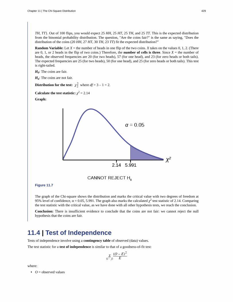
TH, TT}. Out of 100 flips, you would expect 25 HH, 25 HT, 25 TH, and 25 TT. This is the expected distributionfrom the binomial probability distribution. The question, "Are the coins fair?" is the same as saying, "Does thedistribution of the coins (20 HH, 27 HT, 30 TH, 23 TT) fit the expected distribution?"
Random Variable: Let X = the number of heads in one flip of the two coins. X takes on the values 0, 1, 2. (Thereare 0, 1, or 2 heads in the flip of two coins.) Therefore, the number of cells is three. Since X = the number ofheads, the observed frequencies are 20 (for two heads), 57 (for one head), and 23 (for zero heads or both tails).The expected frequencies are 25 (for two heads), 50 (for one head), and 25 (for zero heads or both tails). This testis right-tailed.
H0: The coins are fair.
Ha: The coins are not fair.
Distribution for the test: χ22 where df = 3 – 1 = 2.
Calculate the test statistic: χ2 = 2.14
Graph:
Figure 11.7
The graph of the Chi-square shows the distribution and marks the critical value with two degrees of freedom at95% level of confidence, α = 0.05, 5.991. The graph also marks the calculated χ2 test statistic of 2.14. Comparingthe test statistic with the critical value, as we have done with all other hypothesis tests, we reach the conclusion.
Conclusion: There is insufficient evidence to conclude that the coins are not fair: we cannot reject the nullhypothesis that the coins are fair.
11.4 | Test of IndependenceTests of independence involve using a contingency table of observed (data) values.
The test statistic for a test of independence is similar to that of a goodness-of-fit test:
Σ(i ⋅ j)
(O – E)2
E
where:
• O = observed values
Chapter 11 | The Chi-Square Distribution 429

• E = expected values
• i = the number of rows in the table
• j = the number of columns in the table
There are i ⋅ j terms of the form(O – E)2
E .
A test of independence determines whether two factors are independent or not. You first encountered the termindependence in Section 3.2 earlier. As a review, consider the following example.
NOTE
The expected value inside each cell needs to be at least five in order for you to use this test.
Example 11.8
Suppose A = a speeding violation in the last year and B = a cell phone user while driving. If A and B areindependent then P(A ∩ B) = P(A)P(B). A ∩ B is the event that a driver received a speeding violation last
year and also used a cell phone while driving. Suppose, in a study of drivers who received speeding violationsin the last year, and who used cell phone while driving, that 755 people were surveyed. Out of the 755, 70 had aspeeding violation and 685 did not; 305 used cell phones while driving and 450 did not.
Let y = expected number of drivers who used a cell phone while driving and received speeding violations.
If A and B are independent, then P(A ∩ B) = P(A)P(B). By substitution,
y755 = ⎛⎝ 70
755⎞⎠⎛⎝305755⎞⎠
Solve for y: y =(70)(305)
755 = 28.3
About 28 people from the sample are expected to use cell phones while driving and to receive speeding violations.
In a test of independence, we state the null and alternative hypotheses in words. Since the contingency tableconsists of two factors, the null hypothesis states that the factors are independent and the alternative hypothesisstates that they are not independent (dependent). If we do a test of independence using the example, then thenull hypothesis is:
H0 : Being a cell phone user while driving and receiving a speeding violation are independent events; in other
words, they have no effect on each other.
If the null hypothesis were true, we would expect about 28 people to use cell phones while driving and to receivea speeding violation.
The test of independence is always right-tailed because of the calculation of the test statistic. If the expectedand observed values are not close together, then the test statistic is very large and way out in the right tail of thechi-square curve, as it is in a goodness-of-fit.
The number of degrees of freedom for the test of independence is:
df = (number of columns - 1)(number of rows - 1)
The following formula calculates the expected number (E):
E = (row total)(column total)total number surveyed
430 Chapter 11 | The Chi-Square Distribution
This OpenStax book is available for free at https://legacy.cnx.org/content/col12102/1.7

11.8 A sample of 300 students is taken. Of the students surveyed, 50 were music students, while 250 were not. Ninety-seven of the 300 surveyed were on the honor roll, while 203 were not. If we assume being a music student and beingon the honor roll are independent events, what is the expected number of music students who are also on the honorroll?
Example 11.9
A volunteer group, provides from one to nine hours each week with disabled senior citizens. The program recruitsamong community college students, four-year college students, and nonstudents. In Table 11.14 is a sample ofthe adult volunteers and the number of hours they volunteer per week.
Type of volunteer 1–3 Hours 4–6 Hours 7–9 Hours Row total
Community college students 111 96 48 255
Four-year college students 96 133 61 290
Nonstudents 91 150 53 294
Column total 298 379 162 839
Table 11.14 Number of Hours Worked Per Week by Volunteer Type (Observed) Thetable contains observed (O) values (data).
Is the number of hours volunteered independent of the type of volunteer?
Solution 11.9
The observed table and the question at the end of the problem, "Is the number of hours volunteered independentof the type of volunteer?" tell you this is a test of independence. The two factors are number of hoursvolunteered and type of volunteer. This test is always right-tailed.
H0: The number of hours volunteered is independent of the type of volunteer.
Ha: The number of hours volunteered is dependent on the type of volunteer.
The expected results are in Table 11.14.
Type of volunteer 1-3 Hours 4-6 Hours 7-9 Hours
Community college students 90.57 115.19 49.24
Four-year college students 103.00 131.00 56.00
Nonstudents 104.42 132.81 56.77
Table 11.15 Number of Hours Worked Per Week by Volunteer Type(Expected) The table contains expected (E) values (data).
For example, the calculation for the expected frequency for the top left cell is
E = (row total)(column total)total number surveyed = (255)(298)
839 = 90.57
Calculate the test statistic: χ2 = 12.99 (calculator or computer)
Chapter 11 | The Chi-Square Distribution 431

Distribution for the test: χ42
df = (3 columns – 1)(3 rows – 1) = (2)(2) = 4
Graph:
Figure 11.8
The graph of the Chi-square shows the distribution and marks the critical value with four degrees of freedom
at 95% level of confidence, α = 0.05, 9.488. The graph also marks the calculated χc2 test statistic of 12.99.
Comparing the test statistic with the critical value, as we have done with all other hypothesis tests, we reach theconclusion.
Make a decision: Because the calculated test statistic is in the tail we cannot accept H0. This means that thefactors are not independent.
Conclusion: At a 5% level of significance, from the data, there is sufficient evidence to conclude that the numberof hours volunteered and the type of volunteer are dependent on one another.
For the example in Table 11.14, if there had been another type of volunteer, teenagers, what would the degreesof freedom be?
432 Chapter 11 | The Chi-Square Distribution
This OpenStax book is available for free at https://legacy.cnx.org/content/col12102/1.7
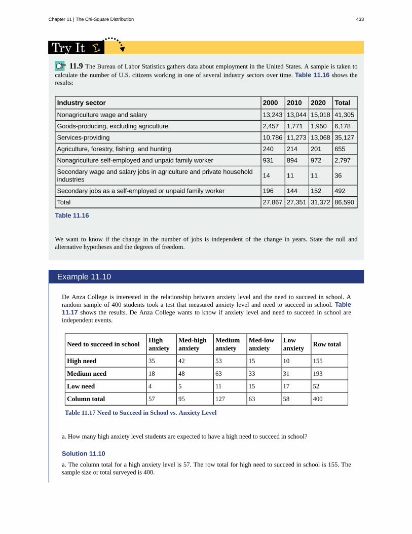
11.9 The Bureau of Labor Statistics gathers data about employment in the United States. A sample is taken tocalculate the number of U.S. citizens working in one of several industry sectors over time. Table 11.16 shows theresults:
Industry sector 2000 2010 2020 Total
Nonagriculture wage and salary 13,243 13,044 15,018 41,305
Goods-producing, excluding agriculture 2,457 1,771 1,950 6,178
Services-providing 10,786 11,273 13,068 35,127
Agriculture, forestry, fishing, and hunting 240 214 201 655
Nonagriculture self-employed and unpaid family worker 931 894 972 2,797
Secondary wage and salary jobs in agriculture and private householdindustries
14 11 11 36
Secondary jobs as a self-employed or unpaid family worker 196 144 152 492
Total 27,867 27,351 31,372 86,590
Table 11.16
We want to know if the change in the number of jobs is independent of the change in years. State the null andalternative hypotheses and the degrees of freedom.
Example 11.10
De Anza College is interested in the relationship between anxiety level and the need to succeed in school. Arandom sample of 400 students took a test that measured anxiety level and need to succeed in school. Table11.17 shows the results. De Anza College wants to know if anxiety level and need to succeed in school areindependent events.
Need to succeed in schoolHighanxiety
Med-highanxiety
Mediumanxiety
Med-lowanxiety
Lowanxiety
Row total
High need 35 42 53 15 10 155
Medium need 18 48 63 33 31 193
Low need 4 5 11 15 17 52
Column total 57 95 127 63 58 400
Table 11.17 Need to Succeed in School vs. Anxiety Level
a. How many high anxiety level students are expected to have a high need to succeed in school?
Solution 11.10
a. The column total for a high anxiety level is 57. The row total for high need to succeed in school is 155. Thesample size or total surveyed is 400.
Chapter 11 | The Chi-Square Distribution 433

E = (row total)(column total)total surveyed = 155 ⋅ 57
400 = 22.09
The expected number of students who have a high anxiety level and a high need to succeed in school is about 22.
b. If the two variables are independent, how many students do you expect to have a low need to succeed in schooland a med-low level of anxiety?
Solution 11.10b. The column total for a med-low anxiety level is 63. The row total for a low need to succeed in school is 52.The sample size or total surveyed is 400.
c. E = (row total)(column total)total surveyed = ________
Solution 11.10
c. E = (row total)(column total)total surveyed = 8.19
d. The expected number of students who have a med-low anxiety level and a low need to succeed in school isabout ________.
Solution 11.10d. 8
11.5 | Test for HomogeneityThe goodness–of–fit test can be used to decide whether a population fits a given distribution, but it will not suffice to decidewhether two populations follow the same unknown distribution. A different test, called the test for homogeneity, can beused to draw a conclusion about whether two populations have the same distribution. To calculate the test statistic for a testfor homogeneity, follow the same procedure as with the test of independence.
NOTE
The expected value inside each cell needs to be at least five in order for you to use this test.
Hypotheses
H0: The distributions of the two populations are the same.
Ha: The distributions of the two populations are not the same.
Test Statistic
Use a χ2 test statistic. It is computed in the same way as the test for independence.
Degrees of Freedom (df)
df = number of columns - 1
Requirements
All values in the table must be greater than or equal to five.
Common Uses
Comparing two populations. For example: men vs. women, before vs. after, east vs. west. The variable is categorical withmore than two possible response values.
434 Chapter 11 | The Chi-Square Distribution
This OpenStax book is available for free at https://legacy.cnx.org/content/col12102/1.7

Example 11.11
Do male and female college students have the same distribution of living arrangements? Use a level ofsignificance of 0.05. Suppose that 250 randomly selected male college students and 300 randomly selectedfemale college students were asked about their living arrangements: dormitory, apartment, with parents, other.The results are shown in Table 11.17. Do male and female college students have the same distribution of livingarrangements?
Dormitory Apartment With Parents Other
Males 72 84 49 45
Females 91 86 88 35
Table 11.18 Distribution of living arrangements forcollege males and college females
Solution 11.11
H0: The distribution of living arrangements for male college students is the same as the distribution of livingarrangements for female college students.
Ha: The distribution of living arrangements for male college students is not the same as the distribution of livingarrangements for female college students.
Degrees of Freedom (df):df = number of columns – 1 = 4 – 1 = 3
Distribution for the test: χ32
Calculate the test statistic: χc2 = 10.129
Figure 11.9
The graph of the Chi-square shows the distribution and marks the critical value with three degrees of freedom
Chapter 11 | The Chi-Square Distribution 435

at 95% level of confidence, α = 0.05, 7.815. The graph also marks the calculated χ2 test statistic of 10.129.Comparing the test statistic with the critical value, as we have done with all other hypothesis tests, we reach theconclusion.
Make a decision: Because the calculated test statistic is in the tail we cannot accept H0. This means that thedistributions are not the same.
Conclusion: At a 5% level of significance, from the data, there is sufficient evidence to conclude that thedistributions of living arrangements for male and female college students are not the same.
Notice that the conclusion is only that the distributions are not the same. We cannot use the test for homogeneityto draw any conclusions about how they differ.
11.11 Do families and singles have the same distribution of cars? Use a level of significance of 0.05. Suppose that 100randomly selected families and 200 randomly selected singles were asked what type of car they drove: sport, sedan,hatchback, truck, van/SUV. The results are shown in Table 11.19. Do families and singles have the same distributionof cars? Test at a level of significance of 0.05.
Sport Sedan Hatchback Truck Van/SUV
Family 5 15 35 17 28
Single 45 65 37 46 7
Table 11.19
11.11 Ivy League schools receive many applications, but only some can be accepted. At the schools listed inTable 11.20, two types of applications are accepted: regular and early decision.
Application type accepted Brown Columbia Cornell Dartmouth Penn Yale
Regular 2,115 1,792 5,306 1,734 2,685 1,245
Early decision 577 627 1,228 444 1,195 761
Table 11.20
We want to know if the number of regular applications accepted follows the same distribution as the number of earlyapplications accepted. State the null and alternative hypotheses, the degrees of freedom and the test statistic, sketchthe graph of the χ2 distribution and show the critical value and the calculated value of the test statistic, and draw aconclusion about the test of homogeneity.
436 Chapter 11 | The Chi-Square Distribution
This OpenStax book is available for free at https://legacy.cnx.org/content/col12102/1.7

11.6 | Comparison of the Chi-Square TestsAbove the χ2 test statistic was used in three different circumstances. The following bulleted list is a summary of which χ2
test is the appropriate one to use in different circumstances.
• Goodness-of-Fit: Use the goodness-of-fit test to decide whether a population with an unknown distribution "fits" aknown distribution. In this case there will be a single qualitative survey question or a single outcome of an experimentfrom a single population. Goodness-of-Fit is typically used to see if the population is uniform (all outcomes occurwith equal frequency), the population is normal, or the population is the same as another population with a knowndistribution. The null and alternative hypotheses are:H0: The population fits the given distribution.Ha: The population does not fit the given distribution.
• Independence: Use the test for independence to decide whether two variables (factors) are independent or dependent.In this case there will be two qualitative survey questions or experiments and a contingency table will be constructed.The goal is to see if the two variables are unrelated (independent) or related (dependent). The null and alternativehypotheses are:H0: The two variables (factors) are independent.Ha: The two variables (factors) are dependent.
• Homogeneity: Use the test for homogeneity to decide if two populations with unknown distributions have the samedistribution as each other. In this case there will be a single qualitative survey question or experiment given to twodifferent populations. The null and alternative hypotheses are:H0: The two populations follow the same distribution.Ha: The two populations have different distributions.
Chapter 11 | The Chi-Square Distribution 437

Contingency Table
Goodness-of-Fit
Test for Homogeneity
Test of Independence
KEY TERMSa table that displays sample values for two different factors that may be dependent or contingent
on one another; it facilitates determining conditional probabilities.
a hypothesis test that compares expected and observed values in order to look for significantdifferences within one non-parametric variable. The degrees of freedom used equals the (number of categories – 1).
a test used to draw a conclusion about whether two populations have the same distribution. Thedegrees of freedom used equals the (number of columns – 1).
a hypothesis test that compares expected and observed values for contingency tables in orderto test for independence between two variables. The degrees of freedom used equals the (number of columns – 1)multiplied by the (number of rows – 1).
CHAPTER REVIEW
11.1 Facts About the Chi-Square DistributionThe chi-square distribution is a useful tool for assessment in a series of problem categories. These problem categoriesinclude primarily (i) whether a data set fits a particular distribution, (ii) whether the distributions of two populations are thesame, (iii) whether two events might be independent, and (iv) whether there is a different variability than expected within apopulation.
An important parameter in a chi-square distribution is the degrees of freedom df in a given problem. The random variablein the chi-square distribution is the sum of squares of df standard normal variables, which must be independent. The keycharacteristics of the chi-square distribution also depend directly on the degrees of freedom.
The chi-square distribution curve is skewed to the right, and its shape depends on the degrees of freedom df. For df > 90,the curve approximates the normal distribution. Test statistics based on the chi-square distribution are always greater thanor equal to zero. Such application tests are almost always right-tailed tests.
11.2 Test of a Single VarianceTo test variability, use the chi-square test of a single variance. The test may be left-, right-, or two-tailed, and its hypothesesare always expressed in terms of the variance (or standard deviation).
11.3 Goodness-of-Fit TestTo assess whether a data set fits a specific distribution, you can apply the goodness-of-fit hypothesis test that uses thechi-square distribution. The null hypothesis for this test states that the data come from the assumed distribution. The testcompares observed values against the values you would expect to have if your data followed the assumed distribution. Thetest is almost always right-tailed. Each observation or cell category must have an expected value of at least five.
11.4 Test of IndependenceTo assess whether two factors are independent or not, you can apply the test of independence that uses the chi-squaredistribution. The null hypothesis for this test states that the two factors are independent. The test compares observed valuesto expected values. The test is right-tailed. Each observation or cell category must have an expected value of at least 5.
11.5 Test for HomogeneityTo assess whether two data sets are derived from the same distribution—which need not be known, you can apply the testfor homogeneity that uses the chi-square distribution. The null hypothesis for this test states that the populations of the twodata sets come from the same distribution. The test compares the observed values against the expected values if the twopopulations followed the same distribution. The test is right-tailed. Each observation or cell category must have an expectedvalue of at least five.
11.6 Comparison of the Chi-Square TestsThe goodness-of-fit test is typically used to determine if data fits a particular distribution. The test of independence makesuse of a contingency table to determine the independence of two factors. The test for homogeneity determines whether two
438 Chapter 11 | The Chi-Square Distribution
This OpenStax book is available for free at https://legacy.cnx.org/content/col12102/1.7
populations come from the same distribution, even if this distribution is unknown.
FORMULA REVIEW
11.1 Facts About the Chi-Square Distribution
χ2 = (Z1)2 + (Z2)2 + … (Zdf)2 chi-square distribution random
variable
μχ2 = df chi-square distribution population mean
σ χ2 = 2⎛⎝d f ⎞⎠ Chi-Square distribution population standard
deviation
11.2 Test of a Single Variance
χ2 = (n − 1)s2
σ02 Test of a single variance statistic where:
n: sample sizes: sample standard deviationσ0 : hypothesized value of the population standard
deviation
df = n – 1 Degrees of freedom
Test of a Single Variance• Use the test to determine variation.
• The degrees of freedom is the number of samples – 1.
• The test statistic is(n – 1)s2
σ02 , where n = sample size,
s2 = sample variance, and σ2 = population variance.
• The test may be left-, right-, or two-tailed.
11.3 Goodness-of-Fit Test
∑k
(O − E)2
E goodness-of-fit test statistic where:
O: observed valuesE: expected values
k: number of different data cells or categories
df = k − 1 degrees of freedom
11.4 Test of Independence
Test of Independence• The number of degrees of freedom is equal to (number
of columns - 1)(number of rows - 1).
• The test statistic is ∑i ⋅ j
(O − E)2
E where O =
observed values, E = expected values, i = the numberof rows in the table, and j = the number of columns inthe table.
• If the null hypothesis is true, the expected number
E = (row total)(column total)total surveyed .
11.5 Test for Homogeneity
∑i ⋅ j
(O − E)2
E Homogeneity test statistic where: O =
observed valuesE = expected valuesi = number of rows in data contingency tablej = number of columns in data contingency table
df = (i −1)(j −1) Degrees of freedom
PRACTICE
11.1 Facts About the Chi-Square Distribution
1. If the number of degrees of freedom for a chi-square distribution is 25, what is the population mean and standarddeviation?
2. If df > 90, the distribution is _____________. If df = 15, the distribution is ________________.
3. When does the chi-square curve approximate a normal distribution?
4. Where is μ located on a chi-square curve?
Chapter 11 | The Chi-Square Distribution 439
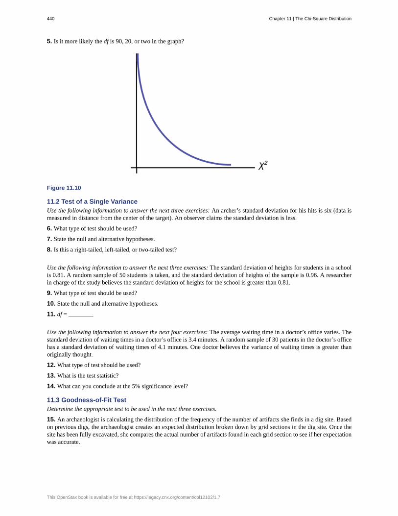
5. Is it more likely the df is 90, 20, or two in the graph?
Figure 11.10
11.2 Test of a Single VarianceUse the following information to answer the next three exercises: An archer’s standard deviation for his hits is six (data ismeasured in distance from the center of the target). An observer claims the standard deviation is less.
6. What type of test should be used?
7. State the null and alternative hypotheses.
8. Is this a right-tailed, left-tailed, or two-tailed test?
Use the following information to answer the next three exercises: The standard deviation of heights for students in a schoolis 0.81. A random sample of 50 students is taken, and the standard deviation of heights of the sample is 0.96. A researcherin charge of the study believes the standard deviation of heights for the school is greater than 0.81.
9. What type of test should be used?
10. State the null and alternative hypotheses.
11. df = ________
Use the following information to answer the next four exercises: The average waiting time in a doctor’s office varies. Thestandard deviation of waiting times in a doctor’s office is 3.4 minutes. A random sample of 30 patients in the doctor’s officehas a standard deviation of waiting times of 4.1 minutes. One doctor believes the variance of waiting times is greater thanoriginally thought.
12. What type of test should be used?
13. What is the test statistic?
14. What can you conclude at the 5% significance level?
11.3 Goodness-of-Fit TestDetermine the appropriate test to be used in the next three exercises.
15. An archaeologist is calculating the distribution of the frequency of the number of artifacts she finds in a dig site. Basedon previous digs, the archaeologist creates an expected distribution broken down by grid sections in the dig site. Once thesite has been fully excavated, she compares the actual number of artifacts found in each grid section to see if her expectationwas accurate.
440 Chapter 11 | The Chi-Square Distribution
This OpenStax book is available for free at https://legacy.cnx.org/content/col12102/1.7
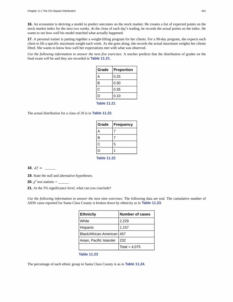
16. An economist is deriving a model to predict outcomes on the stock market. He creates a list of expected points on thestock market index for the next two weeks. At the close of each day’s trading, he records the actual points on the index. Hewants to see how well his model matched what actually happened.
17. A personal trainer is putting together a weight-lifting program for her clients. For a 90-day program, she expects eachclient to lift a specific maximum weight each week. As she goes along, she records the actual maximum weights her clientslifted. She wants to know how well her expectations met with what was observed.
Use the following information to answer the next five exercises: A teacher predicts that the distribution of grades on thefinal exam will be and they are recorded in Table 11.21.
Grade Proportion
A 0.25
B 0.30
C 0.35
D 0.10
Table 11.21
The actual distribution for a class of 20 is in Table 11.22.
Grade Frequency
A 7
B 7
C 5
D 1
Table 11.22
18. d f = ______
19. State the null and alternative hypotheses.
20. χ2 test statistic = ______
21. At the 5% significance level, what can you conclude?
Use the following information to answer the next nine exercises: The following data are real. The cumulative number ofAIDS cases reported for Santa Clara County is broken down by ethnicity as in Table 11.23.
Ethnicity Number of cases
White 2,229
Hispanic 1,157
Black/African-American 457
Asian, Pacific Islander 232
Total = 4,075
Table 11.23
The percentage of each ethnic group in Santa Clara County is as in Table 11.24.
Chapter 11 | The Chi-Square Distribution 441

EthnicityPercentage of total countypopulation
Number expected (round to twodecimal places)
White 42.9% 1748.18
Hispanic 26.7%
Black/African-American
2.6%
Asian, PacificIslander
27.8%
Total = 100%
Table 11.24
22. If the ethnicities of AIDS victims followed the ethnicities of the total county population, fill in the expected number ofcases per ethnic group.Perform a goodness-of-fit test to determine whether the occurrence of AIDS cases follows the ethnicities of the generalpopulation of Santa Clara County.
23. H0: _______
24. Ha: _______
25. Is this a right-tailed, left-tailed, or two-tailed test?
26. degrees of freedom = _______
27. χ2 test statistic = _______
28. Graph the situation. Label and scale the horizontal axis. Mark the mean and test statistic. Shade in the regioncorresponding to the confidence level.
Figure 11.11
Let α = 0.05
Decision: ________________
Reason for the Decision: ________________
Conclusion (write out in complete sentences): ________________
29. Does it appear that the pattern of AIDS cases in Santa Clara County corresponds to the distribution of ethnic groups inthis county? Why or why not?
11.4 Test of IndependenceDetermine the appropriate test to be used in the next three exercises.
442 Chapter 11 | The Chi-Square Distribution
This OpenStax book is available for free at https://legacy.cnx.org/content/col12102/1.7
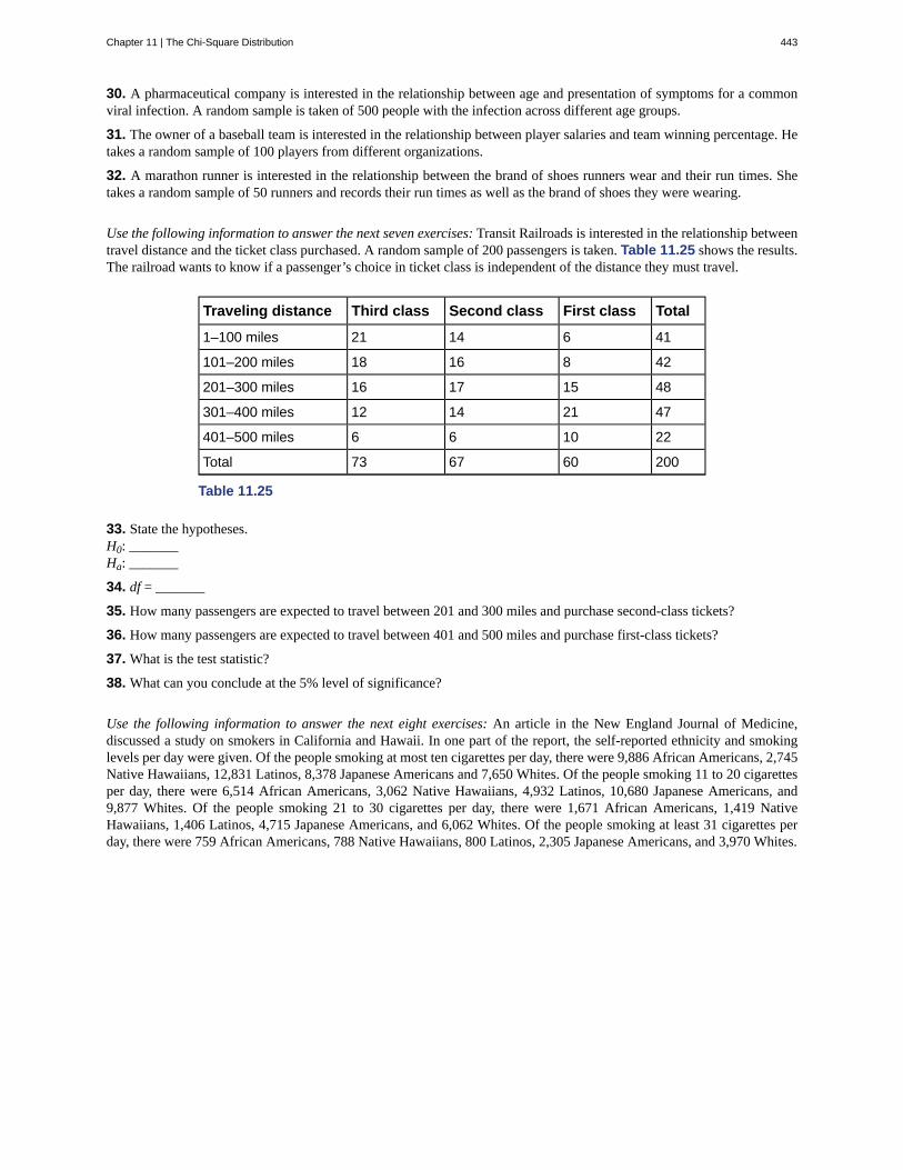
30. A pharmaceutical company is interested in the relationship between age and presentation of symptoms for a commonviral infection. A random sample is taken of 500 people with the infection across different age groups.
31. The owner of a baseball team is interested in the relationship between player salaries and team winning percentage. Hetakes a random sample of 100 players from different organizations.
32. A marathon runner is interested in the relationship between the brand of shoes runners wear and their run times. Shetakes a random sample of 50 runners and records their run times as well as the brand of shoes they were wearing.
Use the following information to answer the next seven exercises: Transit Railroads is interested in the relationship betweentravel distance and the ticket class purchased. A random sample of 200 passengers is taken. Table 11.25 shows the results.The railroad wants to know if a passenger’s choice in ticket class is independent of the distance they must travel.
Traveling distance Third class Second class First class Total
1–100 miles 21 14 6 41
101–200 miles 18 16 8 42
201–300 miles 16 17 15 48
301–400 miles 12 14 21 47
401–500 miles 6 6 10 22
Total 73 67 60 200
Table 11.25
33. State the hypotheses.H0: _______Ha: _______
34. df = _______
35. How many passengers are expected to travel between 201 and 300 miles and purchase second-class tickets?
36. How many passengers are expected to travel between 401 and 500 miles and purchase first-class tickets?
37. What is the test statistic?
38. What can you conclude at the 5% level of significance?
Use the following information to answer the next eight exercises: An article in the New England Journal of Medicine,discussed a study on smokers in California and Hawaii. In one part of the report, the self-reported ethnicity and smokinglevels per day were given. Of the people smoking at most ten cigarettes per day, there were 9,886 African Americans, 2,745Native Hawaiians, 12,831 Latinos, 8,378 Japanese Americans and 7,650 Whites. Of the people smoking 11 to 20 cigarettesper day, there were 6,514 African Americans, 3,062 Native Hawaiians, 4,932 Latinos, 10,680 Japanese Americans, and9,877 Whites. Of the people smoking 21 to 30 cigarettes per day, there were 1,671 African Americans, 1,419 NativeHawaiians, 1,406 Latinos, 4,715 Japanese Americans, and 6,062 Whites. Of the people smoking at least 31 cigarettes perday, there were 759 African Americans, 788 Native Hawaiians, 800 Latinos, 2,305 Japanese Americans, and 3,970 Whites.
Chapter 11 | The Chi-Square Distribution 443

39. Complete the table.
Smoking levelper day
AfricanAmerican
NativeHawaiian
LatinoJapaneseAmericans
White Totals
1-10
11-20
21-30
31+
Totals
Table 11.26 Smoking Levels by Ethnicity (Observed)
40. State the hypotheses.H0: _______Ha: _______
41. Enter expected values in Table 11.26. Round to two decimal places.
Calculate the following values:
42. df = _______
43. χ2 test statistic = ______
44. Is this a right-tailed, left-tailed, or two-tailed test? Explain why.
45. Graph the situation. Label and scale the horizontal axis. Mark the mean and test statistic. Shade in the regioncorresponding to the confidence level.
Figure 11.12
State the decision and conclusion (in a complete sentence) for the following preconceived levels of α.
46. α = 0.05a. Decision: ___________________b. Reason for the decision: ___________________c. Conclusion (write out in a complete sentence): ___________________
47. α = 0.01a. Decision: ___________________b. Reason for the decision: ___________________c. Conclusion (write out in a complete sentence): ___________________
444 Chapter 11 | The Chi-Square Distribution
This OpenStax book is available for free at https://legacy.cnx.org/content/col12102/1.7

11.5 Test for Homogeneity
48. A math teacher wants to see if two of her classes have the same distribution of test scores. What test should she use?
49. What are the null and alternative hypotheses for Exercise 11.48?
50. A market researcher wants to see if two different stores have the same distribution of sales throughout the year. Whattype of test should he use?
51. A meteorologist wants to know if East and West Australia have the same distribution of storms. What type of test shouldshe use?
52. What condition must be met to use the test for homogeneity?Use the following information to answer the next five exercises: Do private practice doctors and hospital doctors have thesame distribution of working hours? Suppose that a sample of 100 private practice doctors and 150 hospital doctors areselected at random and asked about the number of hours a week they work. The results are shown in Table 11.27.
20–30 30–40 40–50 50–60
Private practice 16 40 38 6
Hospital 8 44 59 39
Table 11.27
53. State the null and alternative hypotheses.
54. df = _______
55. What is the test statistic?
56. What can you conclude at the 5% significance level?
11.6 Comparison of the Chi-Square Tests
57. Which test do you use to decide whether an observed distribution is the same as an expected distribution?
58. What is the null hypothesis for the type of test from Exercise 11.57?
59. Which test would you use to decide whether two factors have a relationship?
60. Which test would you use to decide if two populations have the same distribution?
61. How are tests of independence similar to tests for homogeneity?
62. How are tests of independence different from tests for homogeneity?
HOMEWORK
11.1 Facts About the Chi-Square Distribution
Decide whether the following statements are true or false.
63. As the number of degrees of freedom increases, the graph of the chi-square distribution looks more and moresymmetrical.
64. The standard deviation of the chi-square distribution is twice the mean.
65. The mean and the median of the chi-square distribution are the same if df = 24.
11.2 Test of a Single Variance
Use the following information to answer the next twelve exercises: Suppose an airline claims that its flights are consistentlyon time with an average delay of at most 15 minutes. It claims that the average delay is so consistent that the variance is nomore than 150 minutes. Doubting the consistency part of the claim, a disgruntled traveler calculates the delays for his next
Chapter 11 | The Chi-Square Distribution 445
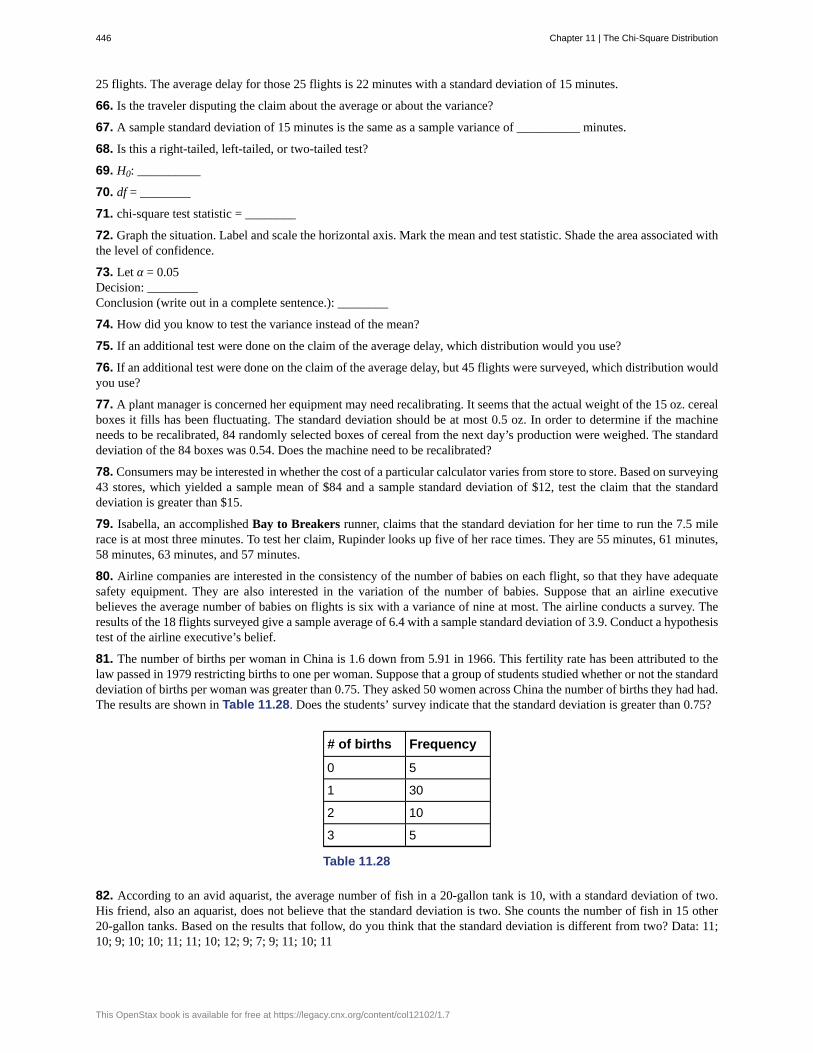
25 flights. The average delay for those 25 flights is 22 minutes with a standard deviation of 15 minutes.
66. Is the traveler disputing the claim about the average or about the variance?
67. A sample standard deviation of 15 minutes is the same as a sample variance of __________ minutes.
68. Is this a right-tailed, left-tailed, or two-tailed test?
69. H0: __________
70. df = ________
71. chi-square test statistic = ________
72. Graph the situation. Label and scale the horizontal axis. Mark the mean and test statistic. Shade the area associated withthe level of confidence.
73. Let α = 0.05Decision: ________Conclusion (write out in a complete sentence.): ________
74. How did you know to test the variance instead of the mean?
75. If an additional test were done on the claim of the average delay, which distribution would you use?
76. If an additional test were done on the claim of the average delay, but 45 flights were surveyed, which distribution wouldyou use?
77. A plant manager is concerned her equipment may need recalibrating. It seems that the actual weight of the 15 oz. cerealboxes it fills has been fluctuating. The standard deviation should be at most 0.5 oz. In order to determine if the machineneeds to be recalibrated, 84 randomly selected boxes of cereal from the next day’s production were weighed. The standarddeviation of the 84 boxes was 0.54. Does the machine need to be recalibrated?
78. Consumers may be interested in whether the cost of a particular calculator varies from store to store. Based on surveying43 stores, which yielded a sample mean of $84 and a sample standard deviation of $12, test the claim that the standarddeviation is greater than $15.
79. Isabella, an accomplished Bay to Breakers runner, claims that the standard deviation for her time to run the 7.5 milerace is at most three minutes. To test her claim, Rupinder looks up five of her race times. They are 55 minutes, 61 minutes,58 minutes, 63 minutes, and 57 minutes.
80. Airline companies are interested in the consistency of the number of babies on each flight, so that they have adequatesafety equipment. They are also interested in the variation of the number of babies. Suppose that an airline executivebelieves the average number of babies on flights is six with a variance of nine at most. The airline conducts a survey. Theresults of the 18 flights surveyed give a sample average of 6.4 with a sample standard deviation of 3.9. Conduct a hypothesistest of the airline executive’s belief.
81. The number of births per woman in China is 1.6 down from 5.91 in 1966. This fertility rate has been attributed to thelaw passed in 1979 restricting births to one per woman. Suppose that a group of students studied whether or not the standarddeviation of births per woman was greater than 0.75. They asked 50 women across China the number of births they had had.The results are shown in Table 11.28. Does the students’ survey indicate that the standard deviation is greater than 0.75?
# of births Frequency
0 5
1 30
2 10
3 5
Table 11.28
82. According to an avid aquarist, the average number of fish in a 20-gallon tank is 10, with a standard deviation of two.His friend, also an aquarist, does not believe that the standard deviation is two. She counts the number of fish in 15 other20-gallon tanks. Based on the results that follow, do you think that the standard deviation is different from two? Data: 11;10; 9; 10; 10; 11; 11; 10; 12; 9; 7; 9; 11; 10; 11
446 Chapter 11 | The Chi-Square Distribution
This OpenStax book is available for free at https://legacy.cnx.org/content/col12102/1.7

83. The manager of "Frenchies" is concerned that patrons are not consistently receiving the same amount of French frieswith each order. The chef claims that the standard deviation for a ten-ounce order of fries is at most 1.5 oz., but the managerthinks that it may be higher. He randomly weighs 49 orders of fries, which yields a mean of 11 oz. and a standard deviationof two oz.
84. You want to buy a specific computer. A sales representative of the manufacturer claims that retail stores sell thiscomputer at an average price of $1,249 with a very narrow standard deviation of $25. You find a website that has aprice comparison for the same computer at a series of stores as follows: $1,299; $1,229.99; $1,193.08; $1,279; $1,224.95;$1,229.99; $1,269.95; $1,249. Can you argue that pricing has a larger standard deviation than claimed by the manufacturer?Use the 5% significance level. As a potential buyer, what would be the practical conclusion from your analysis?
85. A company packages apples by weight. One of the weight grades is Class A apples. Class A apples have a mean weightof 150 g, and there is a maximum allowed weight tolerance of 5% above or below the mean for apples in the same consumerpackage. A batch of apples is selected to be included in a Class A apple package. Given the following apple weights of thebatch, does the fruit comply with the Class A grade weight tolerance requirements. Conduct an appropriate hypothesis test.
(a) at the 5% significance level
(b) at the 1% significance level
Weights in selected apple batch (in grams): 158; 167; 149; 169; 164; 139; 154; 150; 157; 171; 152; 161; 141; 166; 172;
11.3 Goodness-of-Fit Test
86. A six-sided die is rolled 120 times. Fill in the expected frequency column. Then, conduct a hypothesis test to determineif the die is fair. The data in Table 11.29 are the result of the 120 rolls.
Face value Frequency Expected frequency
1 15
2 29
3 16
4 15
5 30
6 15
Table 11.29
Chapter 11 | The Chi-Square Distribution 447
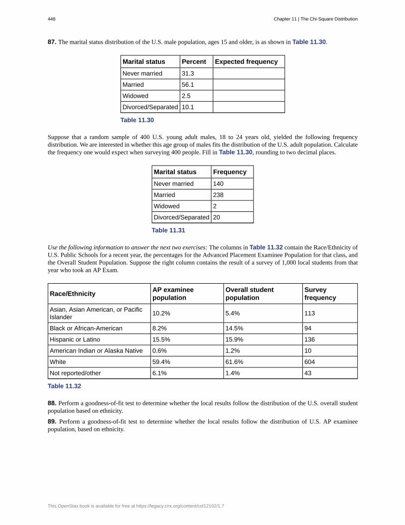
87. The marital status distribution of the U.S. male population, ages 15 and older, is as shown in Table 11.30.
Marital status Percent Expected frequency
Never married 31.3
Married 56.1
Widowed 2.5
Divorced/Separated 10.1
Table 11.30
Suppose that a random sample of 400 U.S. young adult males, 18 to 24 years old, yielded the following frequencydistribution. We are interested in whether this age group of males fits the distribution of the U.S. adult population. Calculatethe frequency one would expect when surveying 400 people. Fill in Table 11.30, rounding to two decimal places.
Marital status Frequency
Never married 140
Married 238
Widowed 2
Divorced/Separated 20
Table 11.31
Use the following information to answer the next two exercises: The columns in Table 11.32 contain the Race/Ethnicity ofU.S. Public Schools for a recent year, the percentages for the Advanced Placement Examinee Population for that class, andthe Overall Student Population. Suppose the right column contains the result of a survey of 1,000 local students from thatyear who took an AP Exam.
Race/EthnicityAP examineepopulation
Overall studentpopulation
Surveyfrequency
Asian, Asian American, or PacificIslander
10.2% 5.4% 113
Black or African-American 8.2% 14.5% 94
Hispanic or Latino 15.5% 15.9% 136
American Indian or Alaska Native 0.6% 1.2% 10
White 59.4% 61.6% 604
Not reported/other 6.1% 1.4% 43
Table 11.32
88. Perform a goodness-of-fit test to determine whether the local results follow the distribution of the U.S. overall studentpopulation based on ethnicity.
89. Perform a goodness-of-fit test to determine whether the local results follow the distribution of U.S. AP examineepopulation, based on ethnicity.
448 Chapter 11 | The Chi-Square Distribution
This OpenStax book is available for free at https://legacy.cnx.org/content/col12102/1.7

90. The City of South Lake Tahoe, CA, has an Asian population of 1,419 people, out of a total population of 23,609.Suppose that a survey of 1,419 self-reported Asians in the Manhattan, NY, area yielded the data in Table 11.33. Conduct agoodness-of-fit test to determine if the self-reported sub-groups of Asians in the Manhattan area fit that of the Lake Tahoearea.
Race Lake Tahoe frequency Manhattan frequency
Asian Indian 131 174
Chinese 118 557
Filipino 1,045 518
Japanese 80 54
Korean 12 29
Vietnamese 9 21
Other 24 66
Table 11.33
Use the following information to answer the next two exercises: UCLA conducted a survey of more than 263,000 collegefreshmen from 385 colleges in fall 2005. The results of students' expected majors by gender were reported in The Chronicleof Higher Education (2/2/2006). Suppose a survey of 5,000 graduating females and 5,000 graduating males was done as afollow-up last year to determine what their actual majors were. The results are shown in the tables for Exercise 11.91 andExercise 11.92. The second column in each table does not add to 100% because of rounding.
91. Conduct a goodness-of-fit test to determine if the actual college majors of graduating females fit the distribution of theirexpected majors.
Major Women - expected major Women - actual major
Arts & Humanities 14.0% 670
Biological Sciences 8.4% 410
Business 13.1% 685
Education 13.0% 650
Engineering 2.6% 145
Physical Sciences 2.6% 125
Professional 18.9% 975
Social Sciences 13.0% 605
Technical 0.4% 15
Other 5.8% 300
Undecided 8.0% 420
Table 11.34
Chapter 11 | The Chi-Square Distribution 449
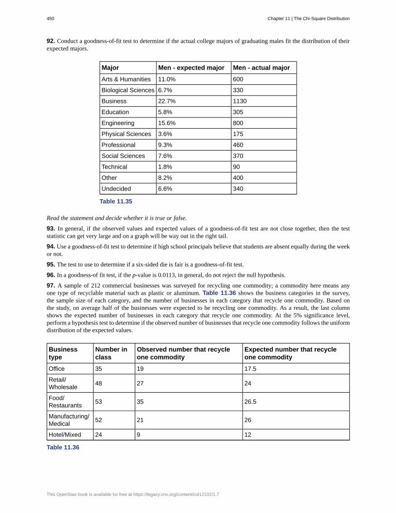
92. Conduct a goodness-of-fit test to determine if the actual college majors of graduating males fit the distribution of theirexpected majors.
Major Men - expected major Men - actual major
Arts & Humanities 11.0% 600
Biological Sciences 6.7% 330
Business 22.7% 1130
Education 5.8% 305
Engineering 15.6% 800
Physical Sciences 3.6% 175
Professional 9.3% 460
Social Sciences 7.6% 370
Technical 1.8% 90
Other 8.2% 400
Undecided 6.6% 340
Table 11.35
Read the statement and decide whether it is true or false.
93. In general, if the observed values and expected values of a goodness-of-fit test are not close together, then the teststatistic can get very large and on a graph will be way out in the right tail.
94. Use a goodness-of-fit test to determine if high school principals believe that students are absent equally during the weekor not.
95. The test to use to determine if a six-sided die is fair is a goodness-of-fit test.
96. In a goodness-of fit test, if the p-value is 0.0113, in general, do not reject the null hypothesis.
97. A sample of 212 commercial businesses was surveyed for recycling one commodity; a commodity here means anyone type of recyclable material such as plastic or aluminum. Table 11.36 shows the business categories in the survey,the sample size of each category, and the number of businesses in each category that recycle one commodity. Based onthe study, on average half of the businesses were expected to be recycling one commodity. As a result, the last columnshows the expected number of businesses in each category that recycle one commodity. At the 5% significance level,perform a hypothesis test to determine if the observed number of businesses that recycle one commodity follows the uniformdistribution of the expected values.
Businesstype
Number inclass
Observed number that recycleone commodity
Expected number that recycleone commodity
Office 35 19 17.5
Retail/Wholesale
48 27 24
Food/Restaurants
53 35 26.5
Manufacturing/Medical
52 21 26
Hotel/Mixed 24 9 12
Table 11.36
450 Chapter 11 | The Chi-Square Distribution
This OpenStax book is available for free at https://legacy.cnx.org/content/col12102/1.7

98. Table 11.37 contains information from a survey among 499 participants classified according to their age groups. Thesecond column shows the percentage of obese people per age class among the study participants. The last column comesfrom a different study at the national level that shows the corresponding percentages of obese people in the same ageclasses in the USA. Perform a hypothesis test at the 5% significance level to determine whether the survey participants area representative sample of the USA obese population.
Age class (years) Obese (percentage) Expected USA average (percentage)
20–30 75.0 32.6
31–40 26.5 32.6
41–50 13.6 36.6
51–60 21.9 36.6
61–70 21.0 39.7
Table 11.37
11.4 Test of Independence
99. A recent debate about where in the United States skiers believe the skiing is best prompted the following survey. Testto see if the best ski area is independent of the level of the skier.
U.S. ski area Beginner Intermediate Advanced
Tahoe 20 30 40
Utah 10 30 60
Colorado 10 40 50
Table 11.38
100. Car manufacturers are interested in whether there is a relationship between the size of car an individual drives and thenumber of people in the driver’s family (that is, whether car size and family size are independent). To test this, suppose that800 car owners were randomly surveyed with the results in Table 11.39. Conduct a test of independence.
Family Size Sub & Compact Mid-size Full-size Van & Truck
1 20 35 40 35
2 20 50 70 80
3–4 20 50 100 90
5+ 20 30 70 70
Table 11.39
Chapter 11 | The Chi-Square Distribution 451
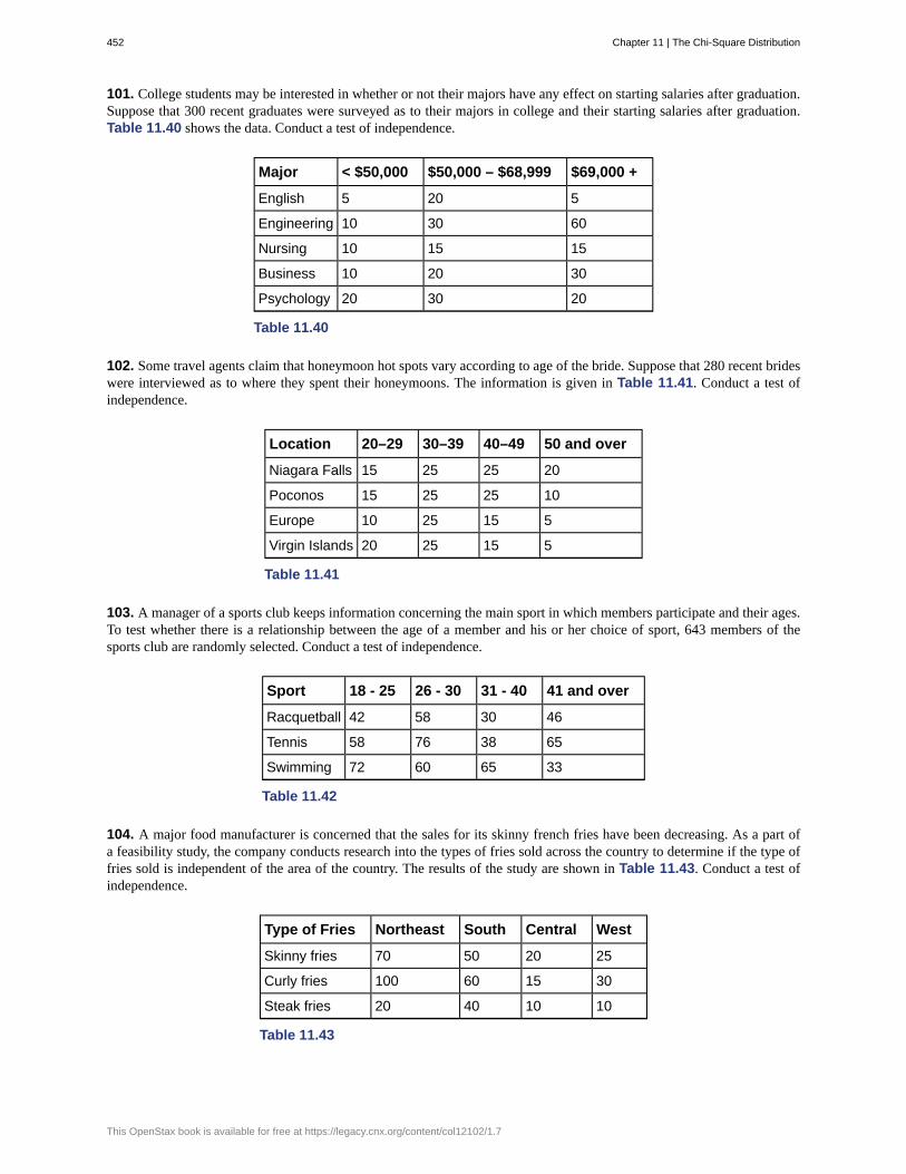
101. College students may be interested in whether or not their majors have any effect on starting salaries after graduation.Suppose that 300 recent graduates were surveyed as to their majors in college and their starting salaries after graduation.Table 11.40 shows the data. Conduct a test of independence.
Major < $50,000 $50,000 – $68,999 $69,000 +
English 5 20 5
Engineering 10 30 60
Nursing 10 15 15
Business 10 20 30
Psychology 20 30 20
Table 11.40
102. Some travel agents claim that honeymoon hot spots vary according to age of the bride. Suppose that 280 recent brideswere interviewed as to where they spent their honeymoons. The information is given in Table 11.41. Conduct a test ofindependence.
Location 20–29 30–39 40–49 50 and over
Niagara Falls 15 25 25 20
Poconos 15 25 25 10
Europe 10 25 15 5
Virgin Islands 20 25 15 5
Table 11.41
103. A manager of a sports club keeps information concerning the main sport in which members participate and their ages.To test whether there is a relationship between the age of a member and his or her choice of sport, 643 members of thesports club are randomly selected. Conduct a test of independence.
Sport 18 - 25 26 - 30 31 - 40 41 and over
Racquetball 42 58 30 46
Tennis 58 76 38 65
Swimming 72 60 65 33
Table 11.42
104. A major food manufacturer is concerned that the sales for its skinny french fries have been decreasing. As a part ofa feasibility study, the company conducts research into the types of fries sold across the country to determine if the type offries sold is independent of the area of the country. The results of the study are shown in Table 11.43. Conduct a test ofindependence.
Type of Fries Northeast South Central West
Skinny fries 70 50 20 25
Curly fries 100 60 15 30
Steak fries 20 40 10 10
Table 11.43
452 Chapter 11 | The Chi-Square Distribution
This OpenStax book is available for free at https://legacy.cnx.org/content/col12102/1.7

105. According to Dan Lenard, an independent insurance agent in the Buffalo, N.Y. area, the following is a breakdown ofthe amount of life insurance purchased by males in the following age groups. He is interested in whether the age of the maleand the amount of life insurance purchased are independent events. Conduct a test for independence.
Age of males None < $200,000 $200,000–$400,000 $401,001–$1,000,000 $1,000,001+
20–29 40 15 40 0 5
30–39 35 5 20 20 10
40–49 20 0 30 0 30
50+ 40 30 15 15 10
Table 11.44
106. Suppose that 600 thirty-year-olds were surveyed to determine whether or not there is a relationship between the levelof education an individual has and salary. Conduct a test of independence.
Annual salaryNot a high schoolgraduate
High schoolgraduate
Collegegraduate
Masters ordoctorate
< $30,000 15 25 10 5
$30,000–$40,000 20 40 70 30
$40,000–$50,000 10 20 40 55
$50,000–$60,000 5 10 20 60
$60,000+ 0 5 10 150
Table 11.45
Read the statement and decide whether it is true or false.
107. The number of degrees of freedom for a test of independence is equal to the sample size minus one.
108. The test for independence uses tables of observed and expected data values.
109. The test to use when determining if the college or university a student chooses to attend is related to his or hersocioeconomic status is a test for independence.
110. In a test of independence, the expected number is equal to the row total multiplied by the column total divided by thetotal surveyed.
111. An ice cream maker performs a nationwide survey about favorite flavors of ice cream in different geographic areasof the U.S. Based on Table 11.46, do the numbers suggest that geographic location is independent of favorite ice creamflavors? Test at the 5% significance level.
U.S. region/Flavor
Strawberry Chocolate VanillaRockyroad
Mintchocolatechip
PistachioRowtotal
West 12 21 22 19 15 8 97
Midwest 10 32 22 11 15 6 96
East 8 31 27 8 15 7 96
South 15 28 30 8 15 6 102
Column total 45 112 101 46 60 27 391
Table 11.46
Chapter 11 | The Chi-Square Distribution 453

112. Table 11.47 provides a recent survey of the youngest online entrepreneurs whose net worth is estimated at onemillion dollars or more. Their ages range from 17 to 30. Each cell in the table illustrates the number of entrepreneurswho correspond to the specific age group and their net worth. Are the ages and net worth independent? Perform a test ofindependence at the 5% significance level.
Age group\ Net worth value (in millions of US dollars) 1–5 6–24 ≥25 Row total
17–25 8 7 5 20
26–30 6 5 9 20
Column total 14 12 14 40
Table 11.47
113. A 2013 poll in California surveyed people about taxing sugar-sweetened beverages. The results are presented in Table11.48, and are classified by ethnic group and response type. Are the poll responses independent of the participants’ ethnicgroup? Conduct a test of independence at the 5% significance level.
Opinion/Ethnicity
Asian-American
White/Non-Hispanic
African-American
LatinoRowtotal
Against tax 48 433 41 160 682
In favor of tax 54 234 24 147 459
No opinion 16 43 16 19 94
Column total 118 710 81 326 1235
Table 11.48
11.5 Test for Homogeneity
114. A psychologist is interested in testing whether there is a difference in the distribution of personality types for businessmajors and social science majors. The results of the study are shown in Table 11.49. Conduct a test of homogeneity. Testat a 5% level of significance.
Open Conscientious Extrovert Agreeable Neurotic
Business 41 52 46 61 58
Social Science 72 75 63 80 65
Table 11.49
115. Do men and women select different breakfasts? The breakfasts ordered by randomly selected men and women at apopular breakfast place is shown in Table 11.50. Conduct a test for homogeneity at a 5% level of significance.
French toast Pancakes Waffles Omelettes
Men 47 35 28 53
Women 65 59 55 60
Table 11.50
454 Chapter 11 | The Chi-Square Distribution
This OpenStax book is available for free at https://legacy.cnx.org/content/col12102/1.7

116. A fisherman is interested in whether the distribution of fish caught in Green Valley Lake is the same as the distributionof fish caught in Echo Lake. Of the 191 randomly selected fish caught in Green Valley Lake, 105 were rainbow trout, 27were other trout, 35 were bass, and 24 were catfish. Of the 293 randomly selected fish caught in Echo Lake, 115 wererainbow trout, 58 were other trout, 67 were bass, and 53 were catfish. Perform a test for homogeneity at a 5% level ofsignificance.
117. In 2007, the United States had 1.5 million homeschooled students, according to the U.S. National Center for EducationStatistics. In Table 11.51 you can see that parents decide to homeschool their children for different reasons, and somereasons are ranked by parents as more important than others. According to the survey results shown in the table, is thedistribution of applicable reasons the same as the distribution of the most important reason? Provide your assessment at the5% significance level. Did you expect the result you obtained?
Reasons forHomeschooling
Applicable reason (inthousands ofrespondents)
Most important reason(in thousands ofrespondents)
Rowtotal
Concern about theenvironment of other schools
1,321 309 1,630
Dissatisfaction with academicinstruction at other schools
1,096 258 1,354
To provide religious or moralinstruction
1,257 540 1,797
Child has special needs, otherthan physical or mental
315 55 370
Nontraditional approach tochild’s education
984 99 1,083
Other reasons (e.g., finances,travel, family time, etc.)
485 216 701
Column total 5,458 1,477 6,935
Table 11.51
118. When looking at energy consumption, we are often interested in detecting trends over time and how they correlateamong different countries. The information in Table 11.52 shows the average energy use (in units of kg of oil equivalentper capita) in the USA and the joint European Union countries (EU) for the six-year period 2005 to 2010. Do the energy usevalues in these two areas come from the same distribution? Perform the analysis at the 5% significance level.
Year European Union United States Row total
2010 3,413 7,164 10,557
2009 3,302 7,057 10,359
2008 3,505 7,488 10,993
2007 3,537 7,758 11,295
2006 3,595 7,697 11,292
2005 3,613 7,847 11,460
Column total 20,965 45,011 65,976
Table 11.52
Chapter 11 | The Chi-Square Distribution 455

119. The Insurance Institute for Highway Safety collects safety information about all types of cars every year, and publishesa report of Top Safety Picks among all cars, makes, and models. Table 11.53 presents the number of Top Safety Picks insix car categories for the two years 2009 and 2013. Analyze the table data to conclude whether the distribution of cars thatearned the Top Safety Picks safety award has remained the same between 2009 and 2013. Derive your results at the 5%significance level.
Year \ Cartype
SmallMid-size
LargeSmallSUV
Mid-sizeSUV
LargeSUV
Rowtotal
2009 12 22 10 10 27 6 87
2013 31 30 19 11 29 4 124
Column total 43 52 29 21 56 10 211
Table 11.53
11.6 Comparison of the Chi-Square Tests
120. Is there a difference between the distribution of community college statistics students and the distribution of universitystatistics students in what technology they use on their homework? Of some randomly selected community college students,43 used a computer, 102 used a calculator with built in statistics functions, and 65 used a table from the textbook. Of somerandomly selected university students, 28 used a computer, 33 used a calculator with built in statistics functions, and 40used a table from the textbook. Conduct an appropriate hypothesis test using a 0.05 level of significance.
Read the statement and decide whether it is true or false.
121. If df = 2, the chi-square distribution has a shape that reminds us of the exponential.
BRINGING IT TOGETHER: HOMEWORK
122.a. Explain why a goodness-of-fit test and a test of independence are generally right-tailed tests.b. If you did a left-tailed test, what would you be testing?
REFERENCES
11.1 Facts About the Chi-Square Distribution
Data from Parade Magazine.
“HIV/AIDS Epidemiology Santa Clara County.”Santa Clara County Public Health Department, May 2011.
11.2 Test of a Single Variance
“AppleInsider Price Guides.” Apple Insider, 2013. Available online at http://appleinsider.com/mac_price_guide (accessedMay 14, 2013).
Data from the World Bank, June 5, 2012.
11.3 Goodness-of-Fit Test
Data from the U.S. Census Bureau
Data from the College Board. Available online at http://www.collegeboard.com.
Data from the U.S. Census Bureau, Current Population Reports.
Ma, Y., E.R. Bertone, E.J. Stanek III, G.W. Reed, J.R. Hebert, N.L. Cohen, P.A. Merriam, I.S. Ockene, “Association
456 Chapter 11 | The Chi-Square Distribution
This OpenStax book is available for free at https://legacy.cnx.org/content/col12102/1.7

between Eating Patterns and Obesity in a Free-living US Adult Population.” American Journal of Epidemiology volume158, no. 1, pages 85-92.
Ogden, Cynthia L., Margaret D. Carroll, Brian K. Kit, Katherine M. Flegal, “Prevalence of Obesity in the United States,2009–2010.” NCHS Data Brief no. 82, January 2012. Available online at http://www.cdc.gov/nchs/data/databriefs/db82.pdf(accessed May 24, 2013).
Stevens, Barbara J., “Multi-family and Commercial Solid Waste and Recycling Survey.” Arlington Count, VA. Availableonline at http://www.arlingtonva.us/departments/EnvironmentalServices/SW/file84429.pdf (accessed May 24,2013).
11.4 Test of Independence
DiCamilo, Mark, Mervin Field, “Most Californians See a Direct Linkage between Obesity and Sugary Sodas. Two inThree Voters Support Taxing Sugar-Sweetened Beverages If Proceeds are Tied to Improving School Nutrition and PhysicalActivity Programs.” The Field Poll, released Feb. 14, 2013. Available online at http://field.com/fieldpollonline/subscribers/Rls2436.pdf (accessed May 24, 2013).
Harris Interactive, “Favorite Flavor of Ice Cream.” Available online at http://www.statisticbrain.com/favorite-flavor-of-ice-cream (accessed May 24, 2013)
“Youngest Online Entrepreneurs List.” Available online at http://www.statisticbrain.com/youngest-online-entrepreneur-list(accessed May 24, 2013).
11.5 Test for Homogeneity
Data from the Insurance Institute for Highway Safety, 2013. Available online at www.iihs.org/iihs/ratings (accessed May24, 2013).
“Energy use (kg of oil equivalent per capita).” The World Bank, 2013. Available online at http://data.worldbank.org/indicator/EG.USE.PCAP.KG.OE/countries (accessed May 24, 2013).
“Parent and Family Involvement Survey of 2007 National Household Education Survey Program (NHES),” U.S.Department of Education, National Center for Education Statistics. Available online at http://nces.ed.gov/pubsearch/pubsinfo.asp?pubid=2009030 (accessed May 24, 2013).
“Parent and Family Involvement Survey of 2007 National Household Education Survey Program (NHES),” U.S.Department of Education, National Center for Education Statistics. Available online at http://nces.ed.gov/pubs2009/2009030_sup.pdf (accessed May 24, 2013).
SOLUTIONS
1 mean = 25 and standard deviation = 7.0711
3 when the number of degrees of freedom is greater than 90
5 df = 2
6 a test of a single variance
8 a left-tailed test
10 H0: σ2 = 0.812; Ha: σ2 > 0.812
12 a test of a single variance
16 a goodness-of-fit test
18 3
20 2.04
21 We decline to reject the null hypothesis. There is not enough evidence to suggest that the observed test scores aresignificantly different from the expected test scores.
23 H0: the distribution of AIDS cases follows the ethnicities of the general population of Santa Clara County.
25 right-tailed
Chapter 11 | The Chi-Square Distribution 457
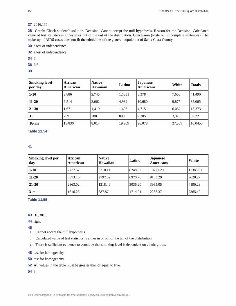
27 2016.136
28 Graph: Check student’s solution. Decision: Cannot accept the null hypothesis. Reason for the Decision: Calculatedvalue of test statistics is either in or out of the tail of the distribution. Conclusion (write out in complete sentences): Themake-up of AIDS cases does not fit the ethnicities of the general population of Santa Clara County.
30 a test of independence
32 a test of independence
34 8
36 6.6
39
Smoking levelper day
AfricanAmerican
NativeHawaiian
LatinoJapaneseAmericans
White Totals
1-10 9,886 2,745 12,831 8,378 7,650 41,490
11-20 6,514 3,062 4,932 10,680 9,877 35,065
21-30 1,671 1,419 1,406 4,715 6,062 15,273
31+ 759 788 800 2,305 3,970 8,622
Totals 18,830 8,014 19,969 26,078 27,559 10,0450
Table 11.54
41
Smoking level perday
AfricanAmerican
NativeHawaiian
LatinoJapaneseAmericans
White
1-10 7777.57 3310.11 8248.02 10771.29 11383.01
11-20 6573.16 2797.52 6970.76 9103.29 9620.27
21-30 2863.02 1218.49 3036.20 3965.05 4190.23
31+ 1616.25 687.87 1714.01 2238.37 2365.49
Table 11.55
43 10,301.8
44 right
46a. Cannot accept the null hypothesis.
b. Calculated value of test statistics is either in or out of the tail of the distribution.
c. There is sufficient evidence to conclude that smoking level is dependent on ethnic group.
48 test for homogeneity
50 test for homogeneity
52 All values in the table must be greater than or equal to five.
54 3
458 Chapter 11 | The Chi-Square Distribution
This OpenStax book is available for free at https://legacy.cnx.org/content/col12102/1.7

57 a goodness-of-fit test
59 a test for independence
61 Answers will vary. Sample answer: Tests of independence and tests for homogeneity both calculate the test statistic the
same way ∑(i j)
(O - E)2
E . In addition, all values must be greater than or equal to five.
63 true
65 false
67 225
69 H0: σ2 ≤ 150
71 36
72 Check student’s solution.
74 The claim is that the variance is no more than 150 minutes.
76 a Student's t- or normal distribution
78a. H0: σ = 15
b. Ha: σ > 15
c. df = 42
d. chi-square with df = 42
e. test statistic = 26.88
f. Check student’s solution.
g. i. Alpha = 0.05
ii. Decision: Cannot reject null hypothesis.
iii. Reason for decision: Calculated value of test statistics is either in or out of the tail of the distribution.
iv. Conclusion: There is insufficient evidence to conclude that the standard deviation is greater than 15.
80a. H0: σ ≤ 3
b. Ha: σ > 3
c. df = 17
d. chi-square distribution with df = 17
e. test statistic = 28.73
f. Check student’s solution.
g. i. Alpha: 0.05
ii. Decision: Cannot accept the null hypothesis.
iii. Reason for decision: Calculated value of test statistics is either in or out of the tail of the distribution.
iv. Conclusion: There is sufficient evidence to conclude that the standard deviation is greater than three.
82a. H0: σ = 2
b. Ha: σ ≠ 2
c. df = 14
d. chi-square distribution with df = 14
Chapter 11 | The Chi-Square Distribution 459
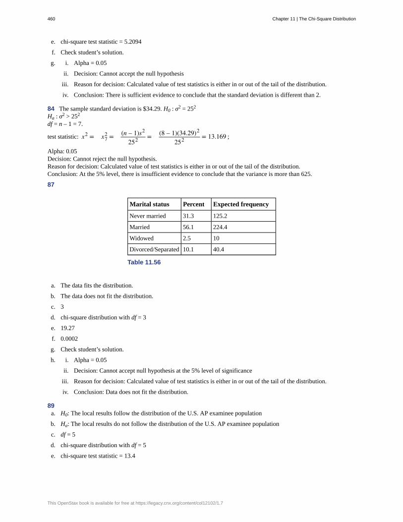
e. chi-square test statistic = 5.2094
f. Check student’s solution.
g. i. Alpha = 0.05
ii. Decision: Cannot accept the null hypothesis
iii. Reason for decision: Calculated value of test statistics is either in or out of the tail of the distribution.
iv. Conclusion: There is sufficient evidence to conclude that the standard deviation is different than 2.
84 The sample standard deviation is $34.29. H0 : σ2 = 252
Ha : σ2 > 252
df = n – 1 = 7.
test statistic: x2 = x72 = (n – 1)s2
252 = (8 – 1)(34.29)2
252 = 13.169 ;
Alpha: 0.05Decision: Cannot reject the null hypothesis.Reason for decision: Calculated value of test statistics is either in or out of the tail of the distribution.Conclusion: At the 5% level, there is insufficient evidence to conclude that the variance is more than 625.
87
Marital status Percent Expected frequency
Never married 31.3 125.2
Married 56.1 224.4
Widowed 2.5 10
Divorced/Separated 10.1 40.4
Table 11.56
a. The data fits the distribution.
b. The data does not fit the distribution.
c. 3
d. chi-square distribution with df = 3
e. 19.27
f. 0.0002
g. Check student’s solution.
h. i. Alpha = 0.05
ii. Decision: Cannot accept null hypothesis at the 5% level of significance
iii. Reason for decision: Calculated value of test statistics is either in or out of the tail of the distribution.
iv. Conclusion: Data does not fit the distribution.
89a. H0: The local results follow the distribution of the U.S. AP examinee population
b. Ha: The local results do not follow the distribution of the U.S. AP examinee population
c. df = 5
d. chi-square distribution with df = 5
e. chi-square test statistic = 13.4
460 Chapter 11 | The Chi-Square Distribution
This OpenStax book is available for free at https://legacy.cnx.org/content/col12102/1.7
f. Check student’s solution.
g. i. Alpha = 0.05
ii. Decision: Cannot accept null when a = 0.05
iii. Reason for Decision: Calculated value of test statistics is either in or out of the tail of the distribution.
iv. Conclusion: Local data do not fit the AP Examinee Distribution.
v. Decision: Do not reject null when a = 0.01
vi. Conclusion: There is insufficient evidence to conclude that local data do not follow the distribution of the U.S.AP examinee distribution.
91a. H0: The actual college majors of graduating females fit the distribution of their expected majors
b. Ha: The actual college majors of graduating females do not fit the distribution of their expected majors
c. df = 10
d. chi-square distribution with df = 10
e. test statistic = 11.48
f. Check student’s solution.
g. i. Alpha = 0.05
ii. Decision: Cannot reject null when a = 0.05 and a = 0.01
iii. Reason for decision: Calculated value of test statistics is either in or out of the tail of the distribution.
iv. Conclusion: There is insufficient evidence to conclude that the distribution of actual college majors of graduatingfemales fits the distribution of their expected majors.
94 true
96 false
98a. H0: Surveyed obese fit the distribution of expected obese
b. Ha: Surveyed obese do not fit the distribution of expected obese
c. df = 4
d. chi-square distribution with df = 4
e. test statistic = 54.01
f. Check student’s solution.
g. i. Alpha: 0.05
ii. Decision: Cannot accept the null hypothesis.
iii. Reason for decision: Calculated value of test statistics is either in or out of the tail of the distribution.
iv. Conclusion: At the 5% level of significance, from the data, there is sufficient evidence to conclude that thesurveyed obese do not fit the distribution of expected obese.
100a. H0: Car size is independent of family size.
b. Ha: Car size is dependent on family size.
c. df = 9
d. chi-square distribution with df = 9
e. test statistic = 15.8284
f. Check student’s solution.g.
Chapter 11 | The Chi-Square Distribution 461

i. Alpha: 0.05
ii. Decision: Cannot reject the null hypothesis.
iii. Reason for decision: Calculated value of test statistics is either in or out of the tail of the distribution.
iv. Conclusion: At the 5% significance level, there is insufficient evidence to conclude that car size and family sizeare dependent.
102a. H0: Honeymoon locations are independent of bride’s age.
b. Ha: Honeymoon locations are dependent on bride’s age.
c. df = 9
d. chi-square distribution with df = 9
e. test statistic = 15.7027
f. Check student’s solution.
g. i. Alpha: 0.05
ii. Decision: Cannot reject the null hypothesis.
iii. Reason for decision: Calculated value of test statistics is either in or out of the tail of the distribution.
iv. Conclusion: At the 5% significance level, there is insufficient evidence to conclude that honeymoon location andbride age are dependent.
104a. H0: The types of fries sold are independent of the location.
b. Ha: The types of fries sold are dependent on the location.
c. df = 6
d. chi-square distribution with df = 6
e. test statistic =18.8369
f. Check student’s solution.
g. i. Alpha: 0.05
ii. Decision: Cannot accept the null hypothesis.
iii. Reason for decision: Calculated value of test statistics is either in or out of the tail of the distribution.
iv. Conclusion: At the 5% significance level, There is sufficient evidence that types of fries and location aredependent.
106a. H0: Salary is independent of level of education.
b. Ha: Salary is dependent on level of education.
c. df = 12
d. chi-square distribution with df = 12
e. test statistic = 255.7704
f. Check student’s solution.
g. Alpha: 0.05
Decision: Cannot accept the null hypothesis.
Reason for decision: Calculated value of test statistics is either in or out of the tail of the distribution.
Conclusion: At the 5% significance level, there is sufficient evidence to conclude that salary and level of education aredependent.
462 Chapter 11 | The Chi-Square Distribution
This OpenStax book is available for free at https://legacy.cnx.org/content/col12102/1.7
108 true
110 true
112a. H0: Age is independent of the youngest online entrepreneurs’ net worth.
b. Ha: Age is dependent on the net worth of the youngest online entrepreneurs.
c. df = 2
d. chi-square distribution with df = 2
e. test statistic = 1.76
f. Check student’s solution.
g. i. Alpha: 0.05
ii. Decision: Cannot reject the null hypothesis.
iii. Reason for decision: Calculated value of test statistics is either in or out of the tail of the distribution.
iv. Conclusion: At the 5% significance level, there is insufficient evidence to conclude that age and net worth for theyoungest online entrepreneurs are dependent.
114a. H0: The distribution for personality types is the same for both majors
b. Ha: The distribution for personality types is not the same for both majors
c. df = 4
d. chi-square with df = 4
e. test statistic = 3.01
f. Check student’s solution.
g. i. Alpha: 0.05
ii. Decision: Cannot reject the null hypothesis.
iii. Reason for decision: Calculated value of test statistics is either in or out of the tail of the distribution.
iv. Conclusion: There is insufficient evidence to conclude that the distribution of personality types is different forbusiness and social science majors.
116a. H0: The distribution for fish caught is the same in Green Valley Lake and in Echo Lake.
b. Ha: The distribution for fish caught is not the same in Green Valley Lake and in Echo Lake.
c. 3
d. chi-square with df = 3
e. 11.75
f. Check student’s solution.
g. i. Alpha: 0.05
ii. Decision: Cannot accept the null hypothesis.
iii. Reason for decision: Calculated value of test statistics is either in or out of the tail of the distribution.
iv. Conclusion: There is evidence to conclude that the distribution of fish caught is different in Green Valley Lakeand in Echo Lake
118a. H0: The distribution of average energy use in the USA is the same as in Europe between 2005 and 2010.
b. Ha: The distribution of average energy use in the USA is not the same as in Europe between 2005 and 2010.
Chapter 11 | The Chi-Square Distribution 463

c. df = 4
d. chi-square with df = 4
e. test statistic = 2.7434
f. Check student’s solution.
g. i. Alpha: 0.05
ii. Decision: Cannot reject the null hypothesis.
iii. Reason for decision: Calculated value of test statistics is either in or out of the tail of the distribution.
iv. Conclusion: At the 5% significance level, there is insufficient evidence to conclude that the average energy usevalues in the US and EU are not derived from different distributions for the period from 2005 to 2010.
120a. H0: The distribution for technology use is the same for community college students and university students.
b. Ha: The distribution for technology use is not the same for community college students and university students.
c. 2
d. chi-square with df = 2
e. 7.05
f. p-value = 0.0294
g. Check student’s solution.
h. i. Alpha: 0.05
ii. Decision: Cannot accept the null hypothesis.
iii. Reason for decision: p-value < alpha
iv. Conclusion: There is sufficient evidence to conclude that the distribution of technology use for statisticshomework is not the same for statistics students at community colleges and at universities.
122a. The test statistic is always positive and if the expected and observed values are not close together, the test statistic is
large and the null hypothesis will be rejected.
b. Testing to see if the data fits the distribution “too well” or is too perfect.
464 Chapter 11 | The Chi-Square Distribution
This OpenStax book is available for free at https://legacy.cnx.org/content/col12102/1.7

12 | F DISTRIBUTION ANDONE-WAY ANOVA
Figure 12.1 One-way ANOVA is used to measure information from several groups.
Introduction
Many statistical applications in psychology, social science, business administration, and the natural sciences involve severalgroups. For example, an environmentalist is interested in knowing if the average amount of pollution varies in severalbodies of water. A sociologist is interested in knowing if the amount of income a person earns varies according to his or herupbringing. A consumer looking for a new car might compare the average gas mileage of several models.
For hypothesis tests comparing averages among more than two groups, statisticians have developed a method called"Analysis of Variance" (abbreviated ANOVA). In this chapter, you will study the simplest form of ANOVA called singlefactor or one-way ANOVA. You will also study the F distribution, used for one-way ANOVA, and the test for differencesbetween two variances. This is just a very brief overview of one-way ANOVA. One-Way ANOVA, as it is presented here,relies heavily on a calculator or computer.
12.1 | Test of Two VariancesThis chapter introduces a new probability density function, the F distribution. This distribution is used for many applications
Chapter 12 | F Distribution and One-Way ANOVA 465

including ANOVA and for testing equality across multiple means. We begin with the F distribution and the test of hypothesisof differences in variances. It is often desirable to compare two variances rather than two averages. For instance, collegeadministrators would like two college professors grading exams to have the same variation in their grading. In order fora lid to fit a container, the variation in the lid and the container should be approximately the same. A supermarket mightbe interested in the variability of check-out times for two checkers. In finance, the variance is a measure of risk and thusan interesting question would be to test the hypothesis that two different investment portfolios have the same variance, thevolatility.
In order to perform a F test of two variances, it is important that the following are true:
1. The populations from which the two samples are drawn are approximately normally distributed.
2. The two populations are independent of each other.
Unlike most other hypothesis tests in this book, the F test for equality of two variances is very sensitive to deviations fromnormality. If the two distributions are not normal, or close, the test can give a biased result for the test statistic.
Suppose we sample randomly from two independent normal populations. Let σ12 and σ2
2 be the unknown population
variances and s12 and s2
2 be the sample variances. Let the sample sizes be n1 and n2. Since we are interested in comparing
the two sample variances, we use the F ratio:
F =
⎡⎣⎢s1
2
σ12
⎤⎦⎥
⎡⎣⎢s2
2
σ22
⎤⎦⎥
F has the distribution F ~ F(n1 – 1, n2 – 1)
where n1 – 1 are the degrees of freedom for the numerator and n2 – 1 are the degrees of freedom for the denominator.
If the null hypothesis is σ12 = σ2
2 , then the F Ratio, test statistic, becomes Fc =
⎡⎣⎢s1
2
σ12
⎤⎦⎥
⎡⎣⎢s2
2
σ22
⎤⎦⎥
= s12
s22
The various forms of the hypotheses tested are:
Two-Tailed Test One-Tailed Test One-Tailed Test
H0: σ12 = σ2
2 H0: σ12 ≤ σ2
2 H0: σ12 ≥ σ2
2
H1: σ12 ≠ σ2
2 H1: σ12 > σ2
2 H1: σ12 < σ2
2
Table 12.1
A more general form of the null and alternative hypothesis for a two tailed test would be :
H0 : σ12
σ22 = δ0
Ha : σ12
σ22 ≠ δ0
Where if δ0 = 1 it is a simple test of the hypothesis that the two variances are equal. This form of the hypothesis does havethe benefit of allowing for tests that are more than for simple differences and can accommodate tests for specific differencesas we did for differences in means and differences in proportions. This form of the hypothesis also shows the relationshipbetween the F distribution and the χ2 : the F is a ratio of two chi squared distributions a distribution we saw in the lastchapter. This is helpful in determining the degrees of freedom of the resultant F distribution.
466 Chapter 12 | F Distribution and One-Way ANOVA
This OpenStax book is available for free at https://legacy.cnx.org/content/col12102/1.7

If the two populations have equal variances, then s12 and s2
2 are close in value and the test statistic, Fc = s12
s22 is close to
one. But if the two population variances are very different, s12 and s2
2 tend to be very different, too. Choosing s12 as the
larger sample variance causes the ratios1
2
s22 to be greater than one. If s1
2 and s22 are far apart, then Fc = s1
2
s22 is a large
number.
Therefore, if F is close to one, the evidence favors the null hypothesis (the two population variances are equal). But if F ismuch larger than one, then the evidence is against the null hypothesis. In essence, we are asking if the calculated F statistic,test statistic, is significantly different from one.
To determine the critical points we have to find Fα,df1,df2. See Appendix A for the F table. This F table has values for variouslevels of significance from 0.1 to 0.001 designated as "p" in the first column. To find the critical value choose the desiredsignificance level and follow down and across to find the critical value at the intersection of the two different degrees offreedom. The F distribution has two different degrees of freedom, one associated with the numerator, df1, and one associatedwith the denominator, df2 and to complicate matters the F distribution is not symmetrical and changes the degree of skewnessas the degrees of freedom change. The degrees of freedom in the numerator is n1-1, where n1 is the sample size for group1, and the degrees of freedom in the denominator is n2-1, where n2 is the sample size for group 2. Fα,df1,df2 will give thecritical value on the upper end of the F distribution.
To find the critical value for the lower end of the distribution, reverse the degrees of freedom and divide the F-value fromthe table into one.
• Upper tail critical value : Fα,df1,df2
• Lower tail critical value : 1/Fα,df2,df1
When the calculated value of F is between the critical values, not in the tail, we cannot reject the null hypothesis that thetwo variances came from a population with the same variance. If the calculated F-value is in either tail we cannot accept thenull hypothesis just as we have been doing for all of the previous tests of hypothesis.
An alternative way of finding the critical values of the F distribution makes the use of the F-table easier. We note in theF-table that all the values of F are greater than one therefore the critical F value for the left hand tail will always be lessthan one because to find the critical value on the left tail we divide an F value into the number one as shown above. We alsonote that if the sample variance in the numerator of the test statistic is larger than the sample variance in the denominator,the resulting F value will be greater than one. The shorthand method for this test is thus to be sure that the larger of the twosample variances is placed in the numerator to calculate the test statistic. This will mean that only the right hand tail criticalvalue will have to be found in the F-table.
Example 12.1
Two college instructors are interested in whether or not there is any variation in the way they grade math exams.They each grade the same set of 10 exams. The first instructor's grades have a variance of 52.3. The secondinstructor's grades have a variance of 89.9. Test the claim that the first instructor's variance is smaller. (In mostcolleges, it is desirable for the variances of exam grades to be nearly the same among instructors.) The level ofsignificance is 10%.
Solution 12.1
Let 1 and 2 be the subscripts that indicate the first and second instructor, respectively.
n1 = n2 = 10.
H0: σ12 ≥ σ2
2 and Ha: σ12 < σ2
2
Calculate the test statistic: By the null hypothesis (σ12 ≥ σ2
2 ) , the F statistic is:
Fc = s22
s12 = 89.9
52.3 = 1.719
Chapter 12 | F Distribution and One-Way ANOVA 467

Critical value for the test: F9,9 = 5.35 where n1 – 1 = 9 and n2 – 1 = 9.
Figure 12.2
Make a decision: Since the calculated F value is not in the tail we cannot reject H0.
Conclusion: With a 10% level of significance, from the data, there is insufficient evidence to conclude that thevariance in grades for the first instructor is smaller.
12.1 The New York Choral Society divides male singers up into four categories from highest voices to lowest: Tenor1,Tenor2, Bass1, Bass2. In the table are heights of the men in the Tenor1 and Bass2 groups. One suspects that taller menwill have lower voices, and that the variance of height may go up with the lower voices as well. Do we have goodevidence that the variance of the heights of singers in each of these two groups (Tenor1 and Bass2) are different?
Tenor1 Bass 2 Tenor 1 Bass 2 Tenor 1 Bass 2
69 72 67 72 68 67
72 75 70 74 67 70
71 67 65 70 64 70
66 75 72 66 69
76 74 70 68 72
74 72 68 75 71
71 72 64 68 74
66 74 73 70 75
68 72 66 72
Table 12.2
468 Chapter 12 | F Distribution and One-Way ANOVA
This OpenStax book is available for free at https://legacy.cnx.org/content/col12102/1.7
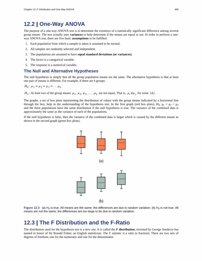
12.2 | One-Way ANOVAThe purpose of a one-way ANOVA test is to determine the existence of a statistically significant difference among severalgroup means. The test actually uses variances to help determine if the means are equal or not. In order to perform a one-way ANOVA test, there are five basic assumptions to be fulfilled:
1. Each population from which a sample is taken is assumed to be normal.
2. All samples are randomly selected and independent.
3. The populations are assumed to have equal standard deviations (or variances).
4. The factor is a categorical variable.
5. The response is a numerical variable.
The Null and Alternative HypothesesThe null hypothesis is simply that all the group population means are the same. The alternative hypothesis is that at leastone pair of means is different. For example, if there are k groups:
H0 : μ1 = μ2 = μ3 = . . .μk
Ha : At least two of the group means μ1, μ2, μ3, . . . ,μk are not equal. That is, μi≠μ j for some i≠ j .
The graphs, a set of box plots representing the distribution of values with the group means indicated by a horizontal linethrough the box, help in the understanding of the hypothesis test. In the first graph (red box plots), H0: μ1 = μ2 = μ3and the three populations have the same distribution if the null hypothesis is true. The variance of the combined data isapproximately the same as the variance of each of the populations.
If the null hypothesis is false, then the variance of the combined data is larger which is caused by the different means asshown in the second graph (green box plots).
Figure 12.3 (a) H0 is true. All means are the same; the differences are due to random variation. (b) H0 is not true. Allmeans are not the same; the differences are too large to be due to random variation.
12.3 | The F Distribution and the F-RatioThe distribution used for the hypothesis test is a new one. It is called the F distribution, invented by George Snedecor butnamed in honor of Sir Ronald Fisher, an English statistician. The F statistic is a ratio (a fraction). There are two sets ofdegrees of freedom; one for the numerator and one for the denominator.
Chapter 12 | F Distribution and One-Way ANOVA 469
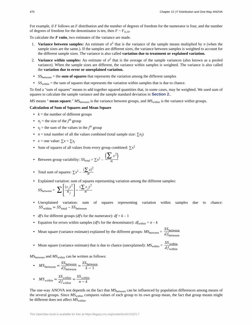
For example, if F follows an F distribution and the number of degrees of freedom for the numerator is four, and the numberof degrees of freedom for the denominator is ten, then F ~ F4,10.
To calculate the F ratio, two estimates of the variance are made.
1. Variance between samples: An estimate of σ2 that is the variance of the sample means multiplied by n (when thesample sizes are the same.). If the samples are different sizes, the variance between samples is weighted to account forthe different sample sizes. The variance is also called variation due to treatment or explained variation.
2. Variance within samples: An estimate of σ2 that is the average of the sample variances (also known as a pooledvariance). When the sample sizes are different, the variance within samples is weighted. The variance is also calledthe variation due to error or unexplained variation.
• SSbetween = the sum of squares that represents the variation among the different samples
• SSwithin = the sum of squares that represents the variation within samples that is due to chance.
To find a "sum of squares" means to add together squared quantities that, in some cases, may be weighted. We used sum ofsquares to calculate the sample variance and the sample standard deviation in Section 2..
MS means " mean square." MSbetween is the variance between groups, and MSwithin is the variance within groups.
Calculation of Sum of Squares and Mean Square
• k = the number of different groups
• nj = the size of the jth group
• sj = the sum of the values in the jth group
• n = total number of all the values combined (total sample size: ∑nj)
• x = one value: ∑x = ∑sj
• Sum of squares of all values from every group combined: ∑x2
• Between group variability: SStotal = ∑x2 –
⎛⎝∑ x2⎞⎠
n
• Total sum of squares: ∑x2 –⎛⎝∑ x⎞⎠2n
• Explained variation: sum of squares representing variation among the different samples:
SSbetween = ∑⎡⎣⎢(s j)
2
n j
⎤⎦⎥− (∑ s j)
2
n
• Unexplained variation: sum of squares representing variation within samples due to chance:SSwithin = SStotal – SSbetween
• df's for different groups (df's for the numerator): df = k – 1
• Equation for errors within samples (df's for the denominator): dfwithin = n – k
• Mean square (variance estimate) explained by the different groups: MSbetween =SSbetweend fbetween
• Mean square (variance estimate) that is due to chance (unexplained): MSwithin =SSwithind fwithin
MSbetween and MSwithin can be written as follows:
• MSbetween = SSbetweend fbetween
= SSbetweenk − 1
• MSwithin = SSwithind fwithin
= SSwithinn − k
The one-way ANOVA test depends on the fact that MSbetween can be influenced by population differences among means ofthe several groups. Since MSwithin compares values of each group to its own group mean, the fact that group means mightbe different does not affect MSwithin.
470 Chapter 12 | F Distribution and One-Way ANOVA
This OpenStax book is available for free at https://legacy.cnx.org/content/col12102/1.7

The null hypothesis says that all groups are samples from populations having the same normal distribution. The alternatehypothesis says that at least two of the sample groups come from populations with different normal distributions. If the nullhypothesis is true, MSbetween and MSwithin should both estimate the same value.
NOTE
The null hypothesis says that all the group population means are equal. The hypothesis of equal means implies thatthe populations have the same normal distribution, because it is assumed that the populations are normal and that theyhave equal variances.
F-Ratio or F Statistic
F = MSbetweenMSwithin
If MSbetween and MSwithin estimate the same value (following the belief that H0 is true), then the F-ratio should beapproximately equal to one. Mostly, just sampling errors would contribute to variations away from one. As it turns out,MSbetween consists of the population variance plus a variance produced from the differences between the samples. MSwithinis an estimate of the population variance. Since variances are always positive, if the null hypothesis is false, MSbetween willgenerally be larger than MSwithin.Then the F-ratio will be larger than one. However, if the population effect is small, it is notunlikely that MSwithin will be larger in a given sample.
The foregoing calculations were done with groups of different sizes. If the groups are the same size, the calculations simplifysomewhat and the F-ratio can be written as:
F-Ratio Formula when the groups are the same size
F = n ⋅ s x–2
s2pooled
where ...• n = the sample size
• dfnumerator = k – 1
• dfdenominator = n – k
• s2 pooled = the mean of the sample variances (pooled variance)
• s x–2 = the variance of the sample means
Data are typically put into a table for easy viewing. One-Way ANOVA results are often displayed in this manner bycomputer software.
Source ofvariation
Sum ofsquares (SS)
Degrees offreedom (df)
Mean square (MS) F
Factor(Between)
SS(Factor) k – 1MS(Factor) =SS(Factor)/(k – 1)
F =MS(Factor)/MS(Error)
Error(Within)
SS(Error) n – kMS(Error) =SS(Error)/(n – k)
Total SS(Total) n – 1
Table 12.3
Example 12.2
Three different diet plans are to be tested for mean weight loss. The entries in the table are the weight losses forthe different plans. The one-way ANOVA results are shown in Table 12.4.
Chapter 12 | F Distribution and One-Way ANOVA 471
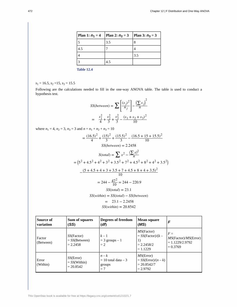
Plan 1: n1 = 4 Plan 2: n2 = 3 Plan 3: n3 = 3
5 3.5 8
4.5 7 4
4 3.5
3 4.5
Table 12.4
s1 = 16.5, s2 =15, s3 = 15.5
Following are the calculations needed to fill in the one-way ANOVA table. The table is used to conduct ahypothesis test.
SS(between) = ∑⎡⎣⎢(s j)
2
n j
⎤⎦⎥−⎛⎝∑ s j
⎞⎠2
n
= s1
2
4 +s2
2
3 +s3
2
3 − (s1 + s2 + s3)2
10
where n1 = 4, n2 = 3, n3 = 3 and n = n1 + n2 + n3 = 10
= (16.5)2
4 + (15)2
3 + (15.5)2
3 − (16.5 + 15 + 15.5)2
10SS(between) = 2.2458
S(total) = ∑ x2 −⎛⎝∑ x⎞⎠2n
= ⎛⎝52 + 4.52 + 42 + 32 + 3.52 + 72 + 4.52 + 82 + 42 + 3.52⎞⎠
−(5 + 4.5 + 4 + 3 + 3.5 + 7 + 4.5 + 8 + 4 + 3.5)2
10
= 244 − 472
10 = 244 − 220.9
SS(total) = 23.1SS(within) = SS(total) − SS(between)
= 23.1 − 2.2458SS(within) = 20.8542
Source ofvariation
Sum of squares(SS)
Degrees of freedom(df)
Mean square(MS)
F
Factor(Between)
SS(Factor)= SS(Between)= 2.2458
k – 1= 3 groups – 1= 2
MS(Factor)= SS(Factor)/(k –1)= 2.2458/2= 1.1229
F =MS(Factor)/MS(Error)= 1.1229/2.9792= 0.3769
Error(Within)
SS(Error)= SS(Within)= 20.8542
n – k= 10 total data – 3groups= 7
MS(Error)= SS(Error)/(n – k)= 20.8542/7= 2.9792
472 Chapter 12 | F Distribution and One-Way ANOVA
This OpenStax book is available for free at https://legacy.cnx.org/content/col12102/1.7

Source ofvariation
Sum of squares(SS)
Degrees of freedom(df)
Mean square(MS)
F
TotalSS(Total)= 2.2458 + 20.8542= 23.1
n – 1= 10 total data – 1= 9
Table 12.5
12.2 As part of an experiment to see how different types of soil cover would affect slicing tomato production,Marist College students grew tomato plants under different soil cover conditions. Groups of three plants each had oneof the following treatments
• bare soil
• a commercial ground cover
• black plastic
• straw
• compost
All plants grew under the same conditions and were the same variety. Students recorded the weight (in grams) oftomatoes produced by each of the n = 15 plants:
Bare: n1 = 3 Ground Cover: n2 = 3 Plastic: n3 = 3 Straw: n4 = 3 Compost: n5 = 3
2,625 5,348 6,583 7,285 6,277
2,997 5,682 8,560 6,897 7,818
4,915 5,482 3,830 9,230 8,677
Table 12.6
Create the one-way ANOVA table.
The one-way ANOVA hypothesis test is always right-tailed because larger F-values are way out in the right tail of theF-distribution curve and tend to make us reject H0.
Example 12.3
Let’s return to the slicing tomato exercise in Try It. The means of the tomato yields under the five mulchingconditions are represented by μ1, μ2, μ3, μ4, μ5. We will conduct a hypothesis test to determine if all meansare the same or at least one is different. Using a significance level of 5%, test the null hypothesis that there isno difference in mean yields among the five groups against the alternative hypothesis that at least one mean isdifferent from the rest.
Chapter 12 | F Distribution and One-Way ANOVA 473

Solution 12.3
The null and alternative hypotheses are:
H0: μ1 = μ2 = μ3 = μ4 = μ5
Ha: μi ≠ μj some i ≠ j
The one-way ANOVA results are shown in Table 12.6
Source ofvariation
Sum ofsquares (SS)
Degrees offreedom (df)
Mean square (MS) F
Factor(Between)
36,648,561 5 – 1 = 436,648,561
4 = 9,162,140 9,162,1402,044,672.6 = 4.4810
Error (Within) 20,446,726 15 – 5 = 1020,446,726
10 = 2,044,672.6
Total 57,095,287 15 – 1 = 14
Table 12.7
Distribution for the test: F4,10
df(num) = 5 – 1 = 4
df(denom) = 15 – 5 = 10
Test statistic: F = 4.4810
Figure 12.4
Probability Statement: p-value = P(F > 4.481) = 0.0248.
Compare α and the p-value: α = 0.05, p-value = 0.0248
Make a decision: Since α > p-value, we cannot accept H0.
Conclusion: At the 5% significance level, we have reasonably strong evidence that differences in mean yields forslicing tomato plants grown under different mulching conditions are unlikely to be due to chance alone. We mayconclude that at least some of mulches led to different mean yields.
474 Chapter 12 | F Distribution and One-Way ANOVA
This OpenStax book is available for free at https://legacy.cnx.org/content/col12102/1.7
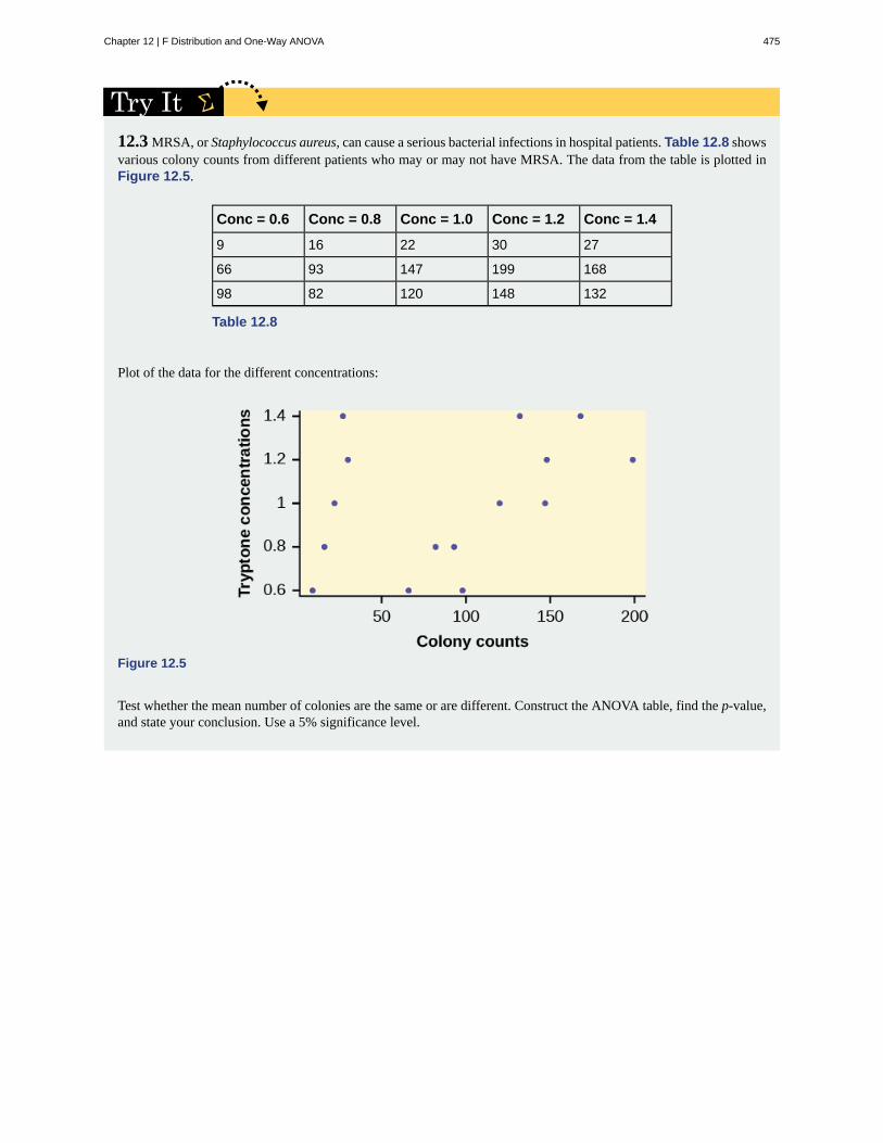
12.3 MRSA, or Staphylococcus aureus, can cause a serious bacterial infections in hospital patients. Table 12.8 showsvarious colony counts from different patients who may or may not have MRSA. The data from the table is plotted inFigure 12.5.
Conc = 0.6 Conc = 0.8 Conc = 1.0 Conc = 1.2 Conc = 1.4
9 16 22 30 27
66 93 147 199 168
98 82 120 148 132
Table 12.8
Plot of the data for the different concentrations:
Figure 12.5
Test whether the mean number of colonies are the same or are different. Construct the ANOVA table, find the p-value,and state your conclusion. Use a 5% significance level.
Chapter 12 | F Distribution and One-Way ANOVA 475

Example 12.4
Four sororities took a random sample of sisters regarding their grade means for the past term. The results areshown in Table 12.9.
Sorority 1 Sorority 2 Sorority 3 Sorority 4
2.17 2.63 2.63 3.79
1.85 1.77 3.78 3.45
2.83 3.25 4.00 3.08
1.69 1.86 2.55 2.26
3.33 2.21 2.45 3.18
Table 12.9 Mean grades for four sororities
Using a significance level of 1%, is there a difference in mean grades among the sororities?
Solution 12.4
Let μ1, μ2, μ3, μ4 be the population means of the sororities. Remember that the null hypothesis claims that thesorority groups are from the same normal distribution. The alternate hypothesis says that at least two of thesorority groups come from populations with different normal distributions. Notice that the four sample sizes areeach five.
NOTE
This is an example of a balanced design, because each factor (i.e., sorority) has the same number ofobservations.
H0: μ1 = μ2 = μ3 = μ4
Ha: Not all of the means μ1, μ2, μ3, μ4 are equal.
Distribution for the test: F3,16
where k = 4 groups and n = 20 samples in total
df(num)= k – 1 = 4 – 1 = 3
df(denom) = n – k = 20 – 4 = 16
Calculate the test statistic: F = 2.23
Graph:
476 Chapter 12 | F Distribution and One-Way ANOVA
This OpenStax book is available for free at https://legacy.cnx.org/content/col12102/1.7

Figure 12.6
Probability statement: p-value = P(F > 2.23) = 0.1241
Compare α and the p-value: α = 0.01p-value = 0.1241α < p-value
Make a decision: Since α < p-value, you cannot reject H0.
Conclusion: There is not sufficient evidence to conclude that there is a difference among the mean grades for thesororities.
12.4 Four sports teams took a random sample of players regarding their GPAs for the last year. The results are shownin Table 12.10.
Basketball Baseball Hockey Lacrosse
3.6 2.1 4.0 2.0
2.9 2.6 2.0 3.6
2.5 3.9 2.6 3.9
3.3 3.1 3.2 2.7
3.8 3.4 3.2 2.5
Table 12.10 GPAs for four sports teams
Use a significance level of 5%, and determine if there is a difference in GPA among the teams.
Example 12.5
A fourth grade class is studying the environment. One of the assignments is to grow bean plants in different soils.Tommy chose to grow his bean plants in soil found outside his classroom mixed with dryer lint. Tara chose to
Chapter 12 | F Distribution and One-Way ANOVA 477

grow her bean plants in potting soil bought at the local nursery. Nick chose to grow his bean plants in soil fromhis mother's garden. No chemicals were used on the plants, only water. They were grown inside the classroomnext to a large window. Each child grew five plants. At the end of the growing period, each plant was measured,producing the data (in inches) in Table 12.11.
Tommy's plants Tara's plants Nick's plants
24 25 23
21 31 27
23 23 22
30 20 30
23 28 20
Table 12.11
Does it appear that the three media in which the bean plants were grown produce the same mean height? Test at a3% level of significance.
Solution 12.5
This time, we will perform the calculations that lead to the F' statistic. Notice that each group has the same
number of plants, so we will use the formula F' =n ⋅ s x–
2
s2pooled
.
First, calculate the sample mean and sample variance of each group.
Tommy's plants Tara's plants Nick's plants
Sample mean 24.2 25.4 24.4
Sample variance 11.7 18.3 16.3
Table 12.12
Next, calculate the variance of the three group means (Calculate the variance of 24.2, 25.4, and 24.4). Variance
of the group means = 0.413 = s x–2
Then MSbetween = ns x–2 = (5)(0.413) where n = 5 is the sample size (number of plants each child grew).
Calculate the mean of the three sample variances (Calculate the mean of 11.7, 18.3, and 16.3). Mean of thesample variances = 15.433 = s2 pooled
Then MSwithin = s2pooled = 15.433.
The F statistic (or F ratio) is F = MSbetweenMSwithin
= ns x–2
s2pooled
= (5)(0.413)15.433 = 0.134
The dfs for the numerator = the number of groups – 1 = 3 – 1 = 2.
The dfs for the denominator = the total number of samples – the number of groups = 15 – 3 = 12
The distribution for the test is F2,12 and the F statistic is F = 0.134
The p-value is P(F > 0.134) = 0.8759.
Decision: Since α = 0.03 and the p-value = 0.8759, then you cannot reject H0. (Why?)
478 Chapter 12 | F Distribution and One-Way ANOVA
This OpenStax book is available for free at https://legacy.cnx.org/content/col12102/1.7
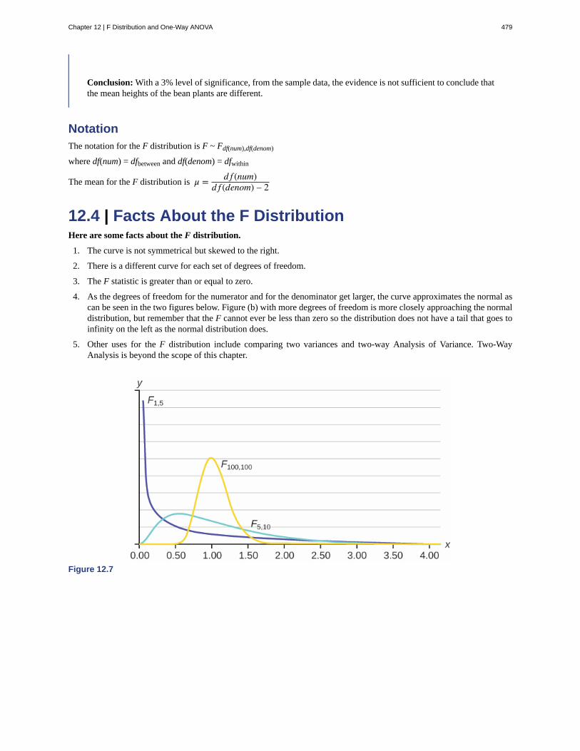
Conclusion: With a 3% level of significance, from the sample data, the evidence is not sufficient to conclude thatthe mean heights of the bean plants are different.
NotationThe notation for the F distribution is F ~ Fdf(num),df(denom)
where df(num) = dfbetween and df(denom) = dfwithin
The mean for the F distribution is μ = d f (num)d f (denom) – 2
12.4 | Facts About the F DistributionHere are some facts about the F distribution.
1. The curve is not symmetrical but skewed to the right.
2. There is a different curve for each set of degrees of freedom.
3. The F statistic is greater than or equal to zero.
4. As the degrees of freedom for the numerator and for the denominator get larger, the curve approximates the normal ascan be seen in the two figures below. Figure (b) with more degrees of freedom is more closely approaching the normaldistribution, but remember that the F cannot ever be less than zero so the distribution does not have a tail that goes toinfinity on the left as the normal distribution does.
5. Other uses for the F distribution include comparing two variances and two-way Analysis of Variance. Two-WayAnalysis is beyond the scope of this chapter.
Figure 12.7
Chapter 12 | F Distribution and One-Way ANOVA 479
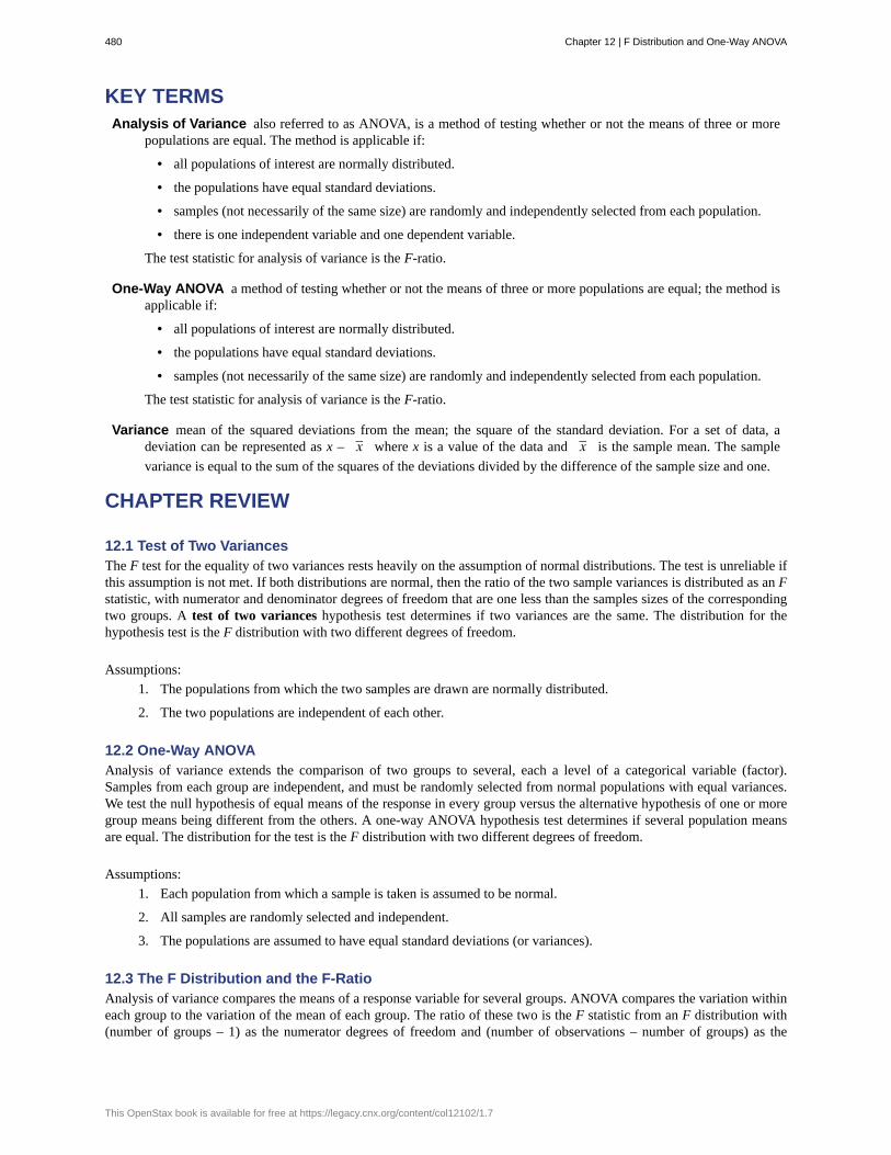
Analysis of Variance
One-Way ANOVA
Variance
KEY TERMSalso referred to as ANOVA, is a method of testing whether or not the means of three or more
populations are equal. The method is applicable if:
• all populations of interest are normally distributed.
• the populations have equal standard deviations.
• samples (not necessarily of the same size) are randomly and independently selected from each population.
• there is one independent variable and one dependent variable.
The test statistic for analysis of variance is the F-ratio.
a method of testing whether or not the means of three or more populations are equal; the method isapplicable if:
• all populations of interest are normally distributed.
• the populations have equal standard deviations.
• samples (not necessarily of the same size) are randomly and independently selected from each population.
The test statistic for analysis of variance is the F-ratio.
mean of the squared deviations from the mean; the square of the standard deviation. For a set of data, adeviation can be represented as x – x– where x is a value of the data and x– is the sample mean. The sample
variance is equal to the sum of the squares of the deviations divided by the difference of the sample size and one.
CHAPTER REVIEW
12.1 Test of Two VariancesThe F test for the equality of two variances rests heavily on the assumption of normal distributions. The test is unreliable ifthis assumption is not met. If both distributions are normal, then the ratio of the two sample variances is distributed as an Fstatistic, with numerator and denominator degrees of freedom that are one less than the samples sizes of the correspondingtwo groups. A test of two variances hypothesis test determines if two variances are the same. The distribution for thehypothesis test is the F distribution with two different degrees of freedom.
Assumptions:
1. The populations from which the two samples are drawn are normally distributed.
2. The two populations are independent of each other.
12.2 One-Way ANOVAAnalysis of variance extends the comparison of two groups to several, each a level of a categorical variable (factor).Samples from each group are independent, and must be randomly selected from normal populations with equal variances.We test the null hypothesis of equal means of the response in every group versus the alternative hypothesis of one or moregroup means being different from the others. A one-way ANOVA hypothesis test determines if several population meansare equal. The distribution for the test is the F distribution with two different degrees of freedom.
Assumptions:
1. Each population from which a sample is taken is assumed to be normal.
2. All samples are randomly selected and independent.
3. The populations are assumed to have equal standard deviations (or variances).
12.3 The F Distribution and the F-RatioAnalysis of variance compares the means of a response variable for several groups. ANOVA compares the variation withineach group to the variation of the mean of each group. The ratio of these two is the F statistic from an F distribution with(number of groups – 1) as the numerator degrees of freedom and (number of observations – number of groups) as the
480 Chapter 12 | F Distribution and One-Way ANOVA
This OpenStax book is available for free at https://legacy.cnx.org/content/col12102/1.7

denominator degrees of freedom. These statistics are summarized in the ANOVA table.
12.4 Facts About the F DistributionThe graph of the F distribution is always positive and skewed right, though the shape can be mounded or exponentialdepending on the combination of numerator and denominator degrees of freedom. The F statistic is the ratio of a measureof the variation in the group means to a similar measure of the variation within the groups. If the null hypothesis is correct,then the numerator should be small compared to the denominator. A small F statistic will result, and the area under the Fcurve to the right will be large, representing a large p-value. When the null hypothesis of equal group means is incorrect,then the numerator should be large compared to the denominator, giving a large F statistic and a small area (small p-value)to the right of the statistic under the F curve.
When the data have unequal group sizes (unbalanced data), then techniques from Section 12.3 need to be used for handcalculations. In the case of balanced data (the groups are the same size) however, simplified calculations based on groupmeans and variances may be used. In practice, of course, software is usually employed in the analysis. As in any analysis,graphs of various sorts should be used in conjunction with numerical techniques. Always look at your data!
FORMULA REVIEW
12.1 Test of Two Variances
H0 :σ1
2
σ22 = δ0
Ha :σ1
2
σ22 ≠ δ0
if δ0=1 then
H0 : σ12 = σ2
2
Ha : σ12 ≠ σ2
Test statistic is :
Fc =S1
2
S22
12.3 The F Distribution and the F-Ratio
SSbetween = ∑⎡⎣⎢(s j)
2
n j
⎤⎦⎥−⎛⎝∑ s j
⎞⎠2
n
SStotal = ∑ x2 −⎛⎝∑ x⎞⎠
2
n
SSwithin = SStotal − SSbetween
dfbetween = df(num) = k – 1
dfwithin = df(denom) = n – k
MSbetween =SSbetweend fbetween
MSwithin =SSwithind fwithin
F =MSbetweenMSwithin
• k = the number of groups
• nj = the size of the jth group
• sj = the sum of the values in the jth group
• n = the total number of all values (observations)combined
• x = one value (one observation) from the data
• s x–2 = the variance of the sample means
• s2pooled = the mean of the sample variances (pooled
variance)
PRACTICE
12.1 Test of Two VariancesUse the following information to answer the next two exercises. There are two assumptions that must be true in order toperform an F test of two variances.
1. Name one assumption that must be true.
2. What is the other assumption that must be true?
Chapter 12 | F Distribution and One-Way ANOVA 481

Use the following information to answer the next five exercises. Two coworkers commute from the same building. They areinterested in whether or not there is any variation in the time it takes them to drive to work. They each record their times for20 commutes. The first worker’s times have a variance of 12.1. The second worker’s times have a variance of 16.9. The firstworker thinks that he is more consistent with his commute times. Test the claim at the 10% level. Assume that commutetimes are normally distributed.
3. State the null and alternative hypotheses.
4. What is s1 in this problem?
5. What is s2 in this problem?
6. What is n?
7. What is the F statistic?
8. What is the critical value?
9. Is the claim accurate?
Use the following information to answer the next four exercises. Two students are interested in whether or not there isvariation in their test scores for math class. There are 15 total math tests they have taken so far. The first student’s gradeshave a standard deviation of 38.1. The second student’s grades have a standard deviation of 22.5. The second student thinkshis scores are more consistent.
10. State the null and alternative hypotheses.
11. What is the F Statistic?
12. What is the critical value?
13. At the 5% significance level, do we reject the null hypothesis?
Use the following information to answer the next three exercises. Two cyclists are comparing the variances of their overallpaces going uphill. Each cyclist records his or her speeds going up 35 hills. The first cyclist has a variance of 23.8 andthe second cyclist has a variance of 32.1. The cyclists want to see if their variances are the same or different. Assume thatcommute times are normally distributed.
14. State the null and alternative hypotheses.
15. What is the F Statistic?
16. At the 5% significance level, what can we say about the cyclists’ variances?
12.2 One-Way ANOVAUse the following information to answer the next five exercises. There are five basic assumptions that must be fulfilled inorder to perform a one-way ANOVA test. What are they?
17. Write one assumption.
18. Write another assumption.
19. Write a third assumption.
20. Write a fourth assumption.
12.3 The F Distribution and the F-RatioUse the following information to answer the next eight exercises. Groups of men from three different areas of the countryare to be tested for mean weight. The entries in Table 12.13 are the weights for the different groups.
Group 1 Group 2 Group 3
216 202 170
Table 12.13
482 Chapter 12 | F Distribution and One-Way ANOVA
This OpenStax book is available for free at https://legacy.cnx.org/content/col12102/1.7

Group 1 Group 2 Group 3
198 213 165
240 284 182
187 228 197
176 210 201
Table 12.13
21. What is the Sum of Squares Factor?
22. What is the Sum of Squares Error?
23. What is the df for the numerator?
24. What is the df for the denominator?
25. What is the Mean Square Factor?
26. What is the Mean Square Error?
27. What is the F statistic?
Use the following information to answer the next eight exercises. Girls from four different soccer teams are to be tested formean goals scored per game. The entries in Table 12.14 are the goals per game for the different teams.
Team 1 Team 2 Team 3 Team 4
1 2 0 3
2 3 1 4
0 2 1 4
3 4 0 3
2 4 0 2
Table 12.14
28. What is SSbetween?
29. What is the df for the numerator?
30. What is MSbetween?
31. What is SSwithin?
32. What is the df for the denominator?
33. What is MSwithin?
34. What is the F statistic?
35. Judging by the F statistic, do you think it is likely or unlikely that you will reject the null hypothesis?
12.4 Facts About the F Distribution
36. An F statistic can have what values?
37. What happens to the curves as the degrees of freedom for the numerator and the denominator get larger?Use the following information to answer the next seven exercise. Four basketball teams took a random sample of playersregarding how high each player can jump (in inches). The results are shown in Table 12.15.
Chapter 12 | F Distribution and One-Way ANOVA 483

Team 1 Team 2 Team 3 Team 4 Team 5
36 32 48 38 41
42 35 50 44 39
51 38 39 46 40
Table 12.15
38. What is the df(num)?
39. What is the df(denom)?
40. What are the Sum of Squares and Mean Squares Factors?
41. What are the Sum of Squares and Mean Squares Errors?
42. What is the F statistic?
43. What is the p-value?
44. At the 5% significance level, is there a difference in the mean jump heights among the teams?
Use the following information to answer the next seven exercises. A video game developer is testing a new game on threedifferent groups. Each group represents a different target market for the game. The developer collects scores from a randomsample from each group. The results are shown in Table 12.16
Group A Group B Group C
101 151 101
108 149 109
98 160 198
107 112 186
111 126 160
Table 12.16
45. What is the df(num)?
46. What is the df(denom)?
47. What are the SSbetween and MSbetween?
48. What are the SSwithin and MSwithin?
49. What is the F Statistic?
50. What is the p-value?
51. At the 10% significance level, are the scores among the different groups different?
Use the following information to answer the next three exercises. Suppose a group is interested in determining whetherteenagers obtain their drivers licenses at approximately the same average age across the country. Suppose that the followingdata are randomly collected from five teenagers in each region of the country. The numbers represent the age at whichteenagers obtained their drivers licenses.
Northeast South West Central East
16.3 16.9 16.4 16.2 17.1
Table 12.17
484 Chapter 12 | F Distribution and One-Way ANOVA
This OpenStax book is available for free at https://legacy.cnx.org/content/col12102/1.7
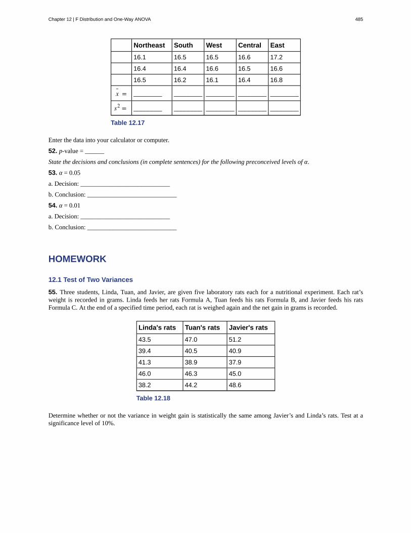
Northeast South West Central East
16.1 16.5 16.5 16.6 17.2
16.4 16.4 16.6 16.5 16.6
16.5 16.2 16.1 16.4 16.8
x = ________ ________ ________ ________ ________
s2 = ________ ________ ________ ________ ________
Table 12.17
Enter the data into your calculator or computer.
52. p-value = ______
State the decisions and conclusions (in complete sentences) for the following preconceived levels of α.
53. α = 0.05
a. Decision: ____________________________
b. Conclusion: ____________________________
54. α = 0.01
a. Decision: ____________________________
b. Conclusion: ____________________________
HOMEWORK
12.1 Test of Two Variances
55. Three students, Linda, Tuan, and Javier, are given five laboratory rats each for a nutritional experiment. Each rat’sweight is recorded in grams. Linda feeds her rats Formula A, Tuan feeds his rats Formula B, and Javier feeds his ratsFormula C. At the end of a specified time period, each rat is weighed again and the net gain in grams is recorded.
Linda's rats Tuan's rats Javier's rats
43.5 47.0 51.2
39.4 40.5 40.9
41.3 38.9 37.9
46.0 46.3 45.0
38.2 44.2 48.6
Table 12.18
Determine whether or not the variance in weight gain is statistically the same among Javier’s and Linda’s rats. Test at asignificance level of 10%.
Chapter 12 | F Distribution and One-Way ANOVA 485

56. A grassroots group opposed to a proposed increase in the gas tax claimed that the increase would hurt working-classpeople the most, since they commute the farthest to work. Suppose that the group randomly surveyed 24 individuals andasked them their daily one-way commuting mileage. The results are as follows.
Working-class Professional (middle incomes) Professional (wealthy)
17.8 16.5 8.5
26.7 17.4 6.3
49.4 22.0 4.6
9.4 7.4 12.6
65.4 9.4 11.0
47.1 2.1 28.6
19.5 6.4 15.4
51.2 13.9 9.3
Table 12.19
Determine whether or not the variance in mileage driven is statistically the same among the working class and professional(middle income) groups. Use a 5% significance level.
Use the following information to answer the next two exercises. The following table lists the number of pages in fourdifferent types of magazines.
Home decorating News Health Computer
172 87 82 104
286 94 153 136
163 123 87 98
205 106 103 207
197 101 96 146
Table 12.20
57. Which two magazine types do you think have the same variance in length?
58. Which two magazine types do you think have different variances in length?
486 Chapter 12 | F Distribution and One-Way ANOVA
This OpenStax book is available for free at https://legacy.cnx.org/content/col12102/1.7

59. Is the variance for the amount of money, in dollars, that shoppers spend on Saturdays at the mall the same as the variancefor the amount of money that shoppers spend on Sundays at the mall? Suppose that the Table 12.21 shows the results of astudy.
Saturday Sunday Saturday Sunday
75 44 62 137
18 58 0 82
150 61 124 39
94 19 50 127
62 99 31 141
73 60 118 73
89
Table 12.21
60. Are the variances for incomes on the East Coast and the West Coast the same? Suppose that Table 12.22 showsthe results of a study. Income is shown in thousands of dollars. Assume that both distributions are normal. Use a level ofsignificance of 0.05.
East West
38 71
47 126
30 42
82 51
75 44
52 90
115 88
67
Table 12.22
Chapter 12 | F Distribution and One-Way ANOVA 487

61. Thirty men in college were taught a method of finger tapping. They were randomly assigned to three groups of ten,with each receiving one of three doses of caffeine: 0 mg, 100 mg, 200 mg. This is approximately the amount in no, one, ortwo cups of coffee. Two hours after ingesting the caffeine, the men had the rate of finger tapping per minute recorded. Theexperiment was double blind, so neither the recorders nor the students knew which group they were in. Does caffeine affectthe rate of tapping, and if so how?
Here are the data:
0 mg 100 mg 200 mg 0 mg 100 mg 200 mg
242 248 246 245 246 248
244 245 250 248 247 252
247 248 248 248 250 250
242 247 246 244 246 248
246 243 245 242 244 250
Table 12.23
62. King Manuel I, Komnenus ruled the Byzantine Empire from Constantinople (Istanbul) during the years 1145 to 1180A.D. The empire was very powerful during his reign, but declined significantly afterwards. Coins minted during his erawere found in Cyprus, an island in the eastern Mediterranean Sea. Nine coins were from his first coinage, seven from thesecond, four from the third, and seven from a fourth. These spanned most of his reign. We have data on the silver contentof the coins:
First coinage Second coinage Third coinage Fourth coinage
5.9 6.9 4.9 5.3
6.8 9.0 5.5 5.6
6.4 6.6 4.6 5.5
7.0 8.1 4.5 5.1
6.6 9.3 6.2
7.7 9.2 5.8
7.2 8.6 5.8
6.9
6.2
Table 12.24
Did the silver content of the coins change over the course of Manuel’s reign?
Here are the means and variances of each coinage. The data are unbalanced.
First Second Third Fourth
Mean 6.7444 8.2429 4.875 5.6143
Variance 0.2953 1.2095 0.2025 0.1314
Table 12.25
488 Chapter 12 | F Distribution and One-Way ANOVA
This OpenStax book is available for free at https://legacy.cnx.org/content/col12102/1.7

63. The American League and the National League of Major League Baseball are each divided into three divisions: East,Central, and West. Many years, fans talk about some divisions being stronger (having better teams) than other divisions.This may have consequences for the postseason. For instance, in 2012 Tampa Bay won 90 games and did not play in thepostseason, while Detroit won only 88 and did play in the postseason. This may have been an oddity, but is there goodevidence that in the 2012 season, the American League divisions were significantly different in overall records? Use thefollowing data to test whether the mean number of wins per team in the three American League divisions were the same ornot. Note that the data are not balanced, as two divisions had five teams, while one had only four.
Division Team Wins
East NY Yankees 95
East Baltimore 93
East Tampa Bay 90
East Toronto 73
East Boston 69
Table 12.26
Division Team Wins
Central Detroit 88
Central Chicago Sox 85
Central Kansas City 72
Central Cleveland 68
Central Minnesota 66
Table 12.27
Division Team Wins
West Oakland 94
West Texas 93
West LA Angels 89
West Seattle 75
Table 12.28
Chapter 12 | F Distribution and One-Way ANOVA 489

12.2 One-Way ANOVA
64. Three different traffic routes are tested for mean driving time. The entries in the Table 12.29 are the driving times inminutes on the three different routes.
Route 1 Route 2 Route 3
30 27 16
32 29 41
27 28 22
35 36 31
Table 12.29
State SSbetween, SSwithin, and the F statistic.
65. Suppose a group is interested in determining whether teenagers obtain their drivers licenses at approximately the sameaverage age across the country. Suppose that the following data are randomly collected from five teenagers in each regionof the country. The numbers represent the age at which teenagers obtained their drivers licenses.
Northeast South West Central East
16.3 16.9 16.4 16.2 17.1
16.1 16.5 16.5 16.6 17.2
16.4 16.4 16.6 16.5 16.6
16.5 16.2 16.1 16.4 16.8
x– = ________ ________ ________ ________ ________
s2 = ________ ________ ________ ________ ________
Table 12.30
State the hypotheses.
H0: ____________
Ha: ____________
12.3 The F Distribution and the F-Ratio
Use the following information to answer the next three exercises. Suppose a group is interested in determining whetherteenagers obtain their drivers licenses at approximately the same average age across the country. Suppose that the followingdata are randomly collected from five teenagers in each region of the country. The numbers represent the age at whichteenagers obtained their drivers licenses.
Northeast South West Central East
16.3 16.9 16.4 16.2 17.1
16.1 16.5 16.5 16.6 17.2
16.4 16.4 16.6 16.5 16.6
16.5 16.2 16.1 16.4 16.8
Table 12.31
490 Chapter 12 | F Distribution and One-Way ANOVA
This OpenStax book is available for free at https://legacy.cnx.org/content/col12102/1.7

Northeast South West Central East
x– = ________ ________ ________ ________ ________
s2 = ________ ________ ________ ________ ________
Table 12.31
H0: µ1 = µ2 = µ3 = µ4 = µ5
Hα: At least any two of the group means µ1, µ2, …, µ5 are not equal.
66. degrees of freedom – numerator: df(num) = _________
67. degrees of freedom – denominator: df(denom) = ________
68. F statistic = ________
12.4 Facts About the F Distribution
69. Three students, Linda, Tuan, and Javier, are given five laboratory rats each for a nutritional experiment. Each rat'sweight is recorded in grams. Linda feeds her rats Formula A, Tuan feeds his rats Formula B, and Javier feeds his ratsFormula C. At the end of a specified time period, each rat is weighed again, and the net gain in grams is recorded. Using asignificance level of 10%, test the hypothesis that the three formulas produce the same mean weight gain.
Linda's rats Tuan's rats Javier's rats
43.5 47.0 51.2
39.4 40.5 40.9
41.3 38.9 37.9
46.0 46.3 45.0
38.2 44.2 48.6
Table 12.32 Weights of Student Lab Rats
70. A grassroots group opposed to a proposed increase in the gas tax claimed that the increase would hurt working-classpeople the most, since they commute the farthest to work. Suppose that the group randomly surveyed 24 individuals andasked them their daily one-way commuting mileage. The results are in Table 12.33. Using a 5% significance level, testthe hypothesis that the three mean commuting mileages are the same.
Working-class Professional (middle incomes) Professional (wealthy)
17.8 16.5 8.5
26.7 17.4 6.3
49.4 22.0 4.6
9.4 7.4 12.6
65.4 9.4 11.0
47.1 2.1 28.6
19.5 6.4 15.4
51.2 13.9 9.3
Table 12.33
Use the following information to answer the next two exercises. Table 12.34 lists the number of pages in four different
Chapter 12 | F Distribution and One-Way ANOVA 491

types of magazines.
Home decorating News Health Computer
172 87 82 104
286 94 153 136
163 123 87 98
205 106 103 207
197 101 96 146
Table 12.34
71. Using a significance level of 5%, test the hypothesis that the four magazine types have the same mean length.
72. Eliminate one magazine type that you now feel has a mean length different from the others. Redo the hypothesis test,testing that the remaining three means are statistically the same. Use a new solution sheet. Based on this test, are the meanlengths for the remaining three magazines statistically the same?
73. A researcher wants to know if the mean times (in minutes) that people watch their favorite news station are the same.Suppose that Table 12.35 shows the results of a study.
CNN FOX Local
45 15 72
12 43 37
18 68 56
38 50 60
23 31 51
35 22
Table 12.35
Assume that all distributions are normal, the four population standard deviations are approximately the same, and the datawere collected independently and randomly. Use a level of significance of 0.05.
492 Chapter 12 | F Distribution and One-Way ANOVA
This OpenStax book is available for free at https://legacy.cnx.org/content/col12102/1.7
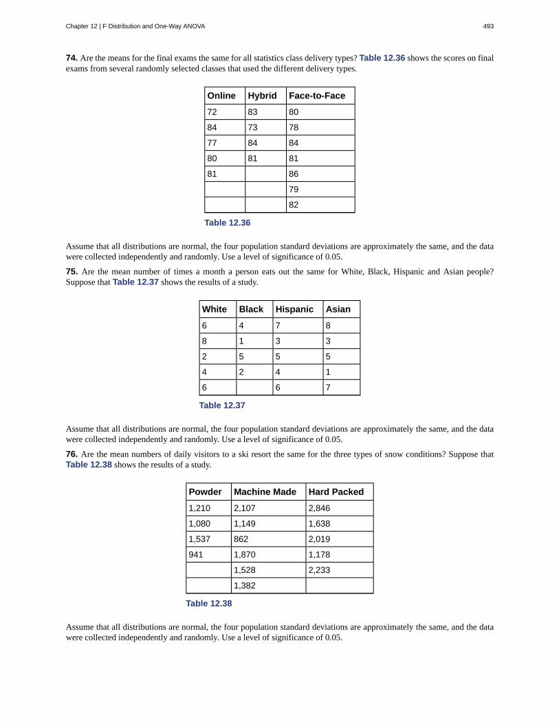
74. Are the means for the final exams the same for all statistics class delivery types? Table 12.36 shows the scores on finalexams from several randomly selected classes that used the different delivery types.
Online Hybrid Face-to-Face
72 83 80
84 73 78
77 84 84
80 81 81
81 86
79
82
Table 12.36
Assume that all distributions are normal, the four population standard deviations are approximately the same, and the datawere collected independently and randomly. Use a level of significance of 0.05.
75. Are the mean number of times a month a person eats out the same for White, Black, Hispanic and Asian people?Suppose that Table 12.37 shows the results of a study.
White Black Hispanic Asian
6 4 7 8
8 1 3 3
2 5 5 5
4 2 4 1
6 6 7
Table 12.37
Assume that all distributions are normal, the four population standard deviations are approximately the same, and the datawere collected independently and randomly. Use a level of significance of 0.05.
76. Are the mean numbers of daily visitors to a ski resort the same for the three types of snow conditions? Suppose thatTable 12.38 shows the results of a study.
Powder Machine Made Hard Packed
1,210 2,107 2,846
1,080 1,149 1,638
1,537 862 2,019
941 1,870 1,178
1,528 2,233
1,382
Table 12.38
Assume that all distributions are normal, the four population standard deviations are approximately the same, and the datawere collected independently and randomly. Use a level of significance of 0.05.
Chapter 12 | F Distribution and One-Way ANOVA 493
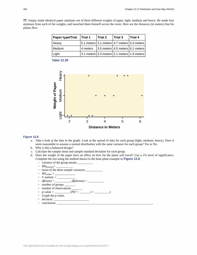
77. Sanjay made identical paper airplanes out of three different weights of paper, light, medium and heavy. He made fourairplanes from each of the weights, and launched them himself across the room. Here are the distances (in meters) that hisplanes flew.
Paper type/Trial Trial 1 Trial 2 Trial 3 Trial 4
Heavy 5.1 meters 3.1 meters 4.7 meters 5.3 meters
Medium 4 meters 3.5 meters 4.5 meters 6.1 meters
Light 3.1 meters 3.3 meters 2.1 meters 1.9 meters
Table 12.39
Figure 12.8a. Take a look at the data in the graph. Look at the spread of data for each group (light, medium, heavy). Does it
seem reasonable to assume a normal distribution with the same variance for each group? Yes or No.b. Why is this a balanced design?c. Calculate the sample mean and sample standard deviation for each group.d. Does the weight of the paper have an effect on how far the plane will travel? Use a 1% level of significance.
Complete the test using the method shown in the bean plant example in Figure 12.8.◦ variance of the group means __________◦ MSbetween= ___________◦ mean of the three sample variances ___________◦ MSwithin = _____________◦ F statistic = ____________◦ df(num) = __________, df(denom) = ___________◦ number of groups _______◦ number of observations _______◦ p-value = __________ (P(F > _______) = __________)◦ Graph the p-value.◦ decision: _______________________◦ conclusion: _______________________________________________________________
494 Chapter 12 | F Distribution and One-Way ANOVA
This OpenStax book is available for free at https://legacy.cnx.org/content/col12102/1.7
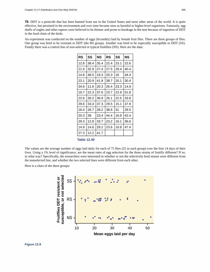
78. DDT is a pesticide that has been banned from use in the United States and most other areas of the world. It is quiteeffective, but persisted in the environment and over time became seen as harmful to higher-level organisms. Famously, eggshells of eagles and other raptors were believed to be thinner and prone to breakage in the nest because of ingestion of DDTin the food chain of the birds.
An experiment was conducted on the number of eggs (fecundity) laid by female fruit flies. There are three groups of flies.One group was bred to be resistant to DDT (the RS group). Another was bred to be especially susceptible to DDT (SS).Finally there was a control line of non-selected or typical fruitflies (NS). Here are the data:
RS SS NS RS SS NS
12.8 38.4 35.4 22.4 23.1 22.6
21.6 32.9 27.4 27.5 29.4 40.4
14.8 48.5 19.3 20.3 16 34.4
23.1 20.9 41.8 38.7 20.1 30.4
34.6 11.6 20.3 26.4 23.3 14.9
19.7 22.3 37.6 23.7 22.9 51.8
22.6 30.2 36.9 26.1 22.5 33.8
29.6 33.4 37.3 29.5 15.1 37.9
16.4 26.7 28.2 38.6 31 29.5
20.3 39 23.4 44.4 16.9 42.4
29.3 12.8 33.7 23.2 16.1 36.6
14.9 14.6 29.2 23.6 10.8 47.4
27.3 12.2 41.7
Table 12.40
The values are the average number of eggs laid daily for each of 75 flies (25 in each group) over the first 14 days of theirlives. Using a 1% level of significance, are the mean rates of egg selection for the three strains of fruitfly different? If so,in what way? Specifically, the researchers were interested in whether or not the selectively bred strains were different fromthe nonselected line, and whether the two selected lines were different from each other.
Here is a chart of the three groups:
Figure 12.9
Chapter 12 | F Distribution and One-Way ANOVA 495

79. The data shown is the recorded body temperatures of 130 subjects as estimated from available histograms.
Traditionally we are taught that the normal human body temperature is 98.6 F. This is not quite correct for everyone. Arethe mean temperatures among the four groups different?
Calculate 95% confidence intervals for the mean body temperature in each group and comment about the confidenceintervals.
FL FH ML MH FL FH ML MH
96.4 96.8 96.3 96.9 98.4 98.6 98.1 98.6
96.7 97.7 96.7 97 98.7 98.6 98.1 98.6
97.2 97.8 97.1 97.1 98.7 98.6 98.2 98.7
97.2 97.9 97.2 97.1 98.7 98.7 98.2 98.8
97.4 98 97.3 97.4 98.7 98.7 98.2 98.8
97.6 98 97.4 97.5 98.8 98.8 98.2 98.8
97.7 98 97.4 97.6 98.8 98.8 98.3 98.9
97.8 98 97.4 97.7 98.8 98.8 98.4 99
97.8 98.1 97.5 97.8 98.8 98.9 98.4 99
97.9 98.3 97.6 97.9 99.2 99 98.5 99
97.9 98.3 97.6 98 99.3 99 98.5 99.2
98 98.3 97.8 98 99.1 98.6 99.5
98.2 98.4 97.8 98 99.1 98.6
98.2 98.4 97.8 98.3 99.2 98.7
98.2 98.4 97.9 98.4 99.4 99.1
98.2 98.4 98 98.4 99.9 99.3
98.2 98.5 98 98.6 100 99.4
98.2 98.6 98 98.6 100.8
Table 12.41
REFERENCES
12.1 Test of Two Variances
“MLB Vs. Division Standings – 2012.” Available online at http://espn.go.com/mlb/standings/_/year/2012/type/vs-division/order/true.
12.3 The F Distribution and the F-Ratio
Tomato Data, Marist College School of Science (unpublished student research)
12.4 Facts About the F Distribution
Data from a fourth grade classroom in 1994 in a private K – 12 school in San Jose, CA.
Hand, D.J., F. Daly, A.D. Lunn, K.J. McConway, and E. Ostrowski. A Handbook of Small Datasets: Data for FruitflyFecundity. London: Chapman & Hall, 1994.
496 Chapter 12 | F Distribution and One-Way ANOVA
This OpenStax book is available for free at https://legacy.cnx.org/content/col12102/1.7
Hand, D.J., F. Daly, A.D. Lunn, K.J. McConway, and E. Ostrowski. A Handbook of Small Datasets. London: Chapman &Hall, 1994, pg. 50.
Hand, D.J., F. Daly, A.D. Lunn, K.J. McConway, and E. Ostrowski. A Handbook of Small Datasets. London: Chapman &Hall, 1994, pg. 118.
“MLB Standings – 2012.” Available online at http://espn.go.com/mlb/standings/_/year/2012.
Mackowiak, P. A., Wasserman, S. S., and Levine, M. M. (1992), "A Critical Appraisal of 98.6 Degrees F, the Upper Limit ofthe Normal Body Temperature, and Other Legacies of Carl Reinhold August Wunderlich," Journal of the American MedicalAssociation, 268, 1578-1580.
SOLUTIONS
1 The populations from which the two samples are drawn are normally distributed.
3 H0 : σ1 = σ2 Ha : σ1 < σ2 or H0: σ12 = σ2
2 Ha: σ12 < σ2
2
5 4.11
7 0.7159
9 No, at the 10% level of significance, we cannot reject the null hypothesis and state that the data do not show that thevariation in drive times for the first worker is less than the variation in drive times for the second worker.
11 2.8674
13 Cannot accept the null hypothesis. There is enough evidence to say that the variance of the grades for the first studentis higher than the variance in the grades for the second student.
15 0.7414
17 Each population from which a sample is taken is assumed to be normal.
19 The populations are assumed to have equal standard deviations (or variances).
21 4,939.2
23 2
25 2,469.6
27 3.7416
29 3
31 13.2
33 0.825
35 Because a one-way ANOVA test is always right-tailed, a high F statistic corresponds to a low p-value, so it is likely thatwe cannot accept the null hypothesis.
37 The curves approximate the normal distribution.
39 ten
41 SS = 237.33; MS = 23.73
43 0.1614
45 two
47 SS = 5,700.4; MS = 2,850.2
49 3.6101
51 Yes, there is enough evidence to show that the scores among the groups are statistically significant at the 10% level.
55
a. H0 : σ12 = σ2
2
Chapter 12 | F Distribution and One-Way ANOVA 497

b. Ha : σ12 ≠ σ1
2
c. df(num) = 4; df(denom) = 4
d. F4, 4
e. 3.00
f. Check student's solution.
g. Decision: Cannot reject the null hypothesis; Conclusion: There is insufficient evidence to conclude that the variancesare different.
58 The answers may vary. Sample answer: Home decorating magazines and news magazines have different variances.
60
a. H0: = σ12 = σ2
2
b. Ha: σ12 ≠ σ1
2
c. df(n) = 7, df(d) = 6
d. F7,6
e. 0.8117
f. 0.7825
g. Check student’s solution.
h. i. Alpha: 0.05
ii. Decision: Cannot reject the null hypothesis.
iii. Reason for decision: calculated test statistics is not in the tail of the distribution
iv. Conclusion: There is not sufficient evidence to conclude that the variances are different.
62 Here is a strip chart of the silver content of the coins:
Figure 12.10
While there are differences in spread, it is not unreasonable to use ANOVA techniques. Here is the completed ANOVAtable:
498 Chapter 12 | F Distribution and One-Way ANOVA
This OpenStax book is available for free at https://legacy.cnx.org/content/col12102/1.7

Source of variation Sum of squares (SS) Degrees of freedom (df) Mean square (MS) F
Factor (Between) 37.748 4 – 1 = 3 12.5825 26.272
Error (Within) 11.015 27 – 4 = 23 0.4789
Total 48.763 27 – 1 = 26
Table 12.42
P(F > 26.272) = 0; Cannot accept the null hypothesis for any alpha. There is sufficient evidence to conclude that the meansilver content among the four coinages are different. From the strip chart, it appears that the first and second coinages hadhigher silver contents than the third and fourth.
63 Here is a stripchart of the number of wins for the 14 teams in the AL for the 2012 season.
Figure 12.11
While the spread seems similar, there may be some question about the normality of the data, given the wide gaps in themiddle near the 0.500 mark of 82 games (teams play 162 games each season in MLB). However, one-way ANOVA isrobust. Here is the ANOVA table for the data:
Source of variation Sum of squares (SS) Degrees of freedom (df) Mean square (MS) F
Factor (Between) 344.16 3 – 1 = 2 172.08
Error (Within) 1,219.55 14 – 3 = 11 110.87 1.5521
Total 1,563.71 14 – 1 = 13
Table 12.43
P(F > 1.5521) = 0.2548Since the p-value is so large, there is not good evidence against the null hypothesis of equal means. We cannot reject thenull hypothesis. Thus, for 2012, there is not any have any good evidence of a significant difference in mean number of winsbetween the divisions of the American League.
64 SSbetween = 26SSwithin = 441F = 0.2653
67 df(denom) = 15
Chapter 12 | F Distribution and One-Way ANOVA 499

69a. H0: µL = µT = µJ
b. Ha: at least any two of the means are different
c. df(num) = 2; df(denom) = 12
d. F distribution
e. 0.67
f. 0.5305
g. Check student’s solution.
h. Decision:Cannot reject null hypothesis; Conclusion: There is insufficient evidence to conclude that the means aredifferent.
72a. Ha: µc = µn = µh
b. At least any two of the magazines have different mean lengths.
c. df(num) = 2, df(denom) = 12
d. F distribution
e. F = 15.28
f. p-value = 0.001
g. Check student’s solution.
h. i. Alpha: 0.05
ii. Decision: Cannot accept the null hypothesis.
iii. Reason for decision: p-value < alpha
iv. Conclusion: There is sufficient evidence to conclude that the mean lengths of the magazines are different.
74a. H0: μo = μh = μf
b. At least two of the means are different.
c. df(n) = 2, df(d) = 13
d. F2,13
e. 0.64
f. 0.5437
g. Check student’s solution.
h. i. Alpha: 0.05
ii. Decision: Cannot reject the null hypothesis.
iii. Reason for decision: p-value > alpha
iv. Conclusion: The mean scores of different class delivery are not different.
76a. H0: μp = μm = μh
b. At least any two of the means are different.
c. df(n) = 2, df(d) = 12
d. F2,12
e. 3.13
f. 0.0807
500 Chapter 12 | F Distribution and One-Way ANOVA
This OpenStax book is available for free at https://legacy.cnx.org/content/col12102/1.7

g. Check student’s solution.
h. i. Alpha: 0.05
ii. Decision: Cannot reject the null hypothesis.
iii. Reason for decision: p-value > alpha
iv. Conclusion: There is not sufficient evidence to conclude that the mean numbers of daily visitors are different.
78 The data appear normally distributed from the chart and of similar spread. There do not appear to be any seriousoutliers, so we may proceed with our ANOVA calculations, to see if we have good evidence of a difference between thethree groups. H0 : µ1 = µ2 = µ3 ; Ha : µi ≠ ; some i ≠ j Define μ1, μ2, μ3, as the population mean number of eggs laid
by the three groups of fruit flies. F statistic = 8.6657; p-value = 0.0004
Figure 12.12
Decision: Since the p-value is less than the level of significance of 0.01, we reject the null hypothesis. Conclusion: Wehave good evidence that the average number of eggs laid during the first 14 days of life for these three strains of fruitflies aredifferent. Interestingly, if you perform a two sample t-test to compare the RS and NS groups they are significantly different(p = 0.0013). Similarly, SS and NS are significantly different (p = 0.0006). However, the two selected groups, RS and SSare not significantly different (p = 0.5176). Thus we appear to have good evidence that selection either for resistance orfor susceptibility involves a reduced rate of egg production (for these specific strains) as compared to flies that were notselected for resistance or susceptibility to DDT. Here, genetic selection has apparently involved a loss of fecundity.
Chapter 12 | F Distribution and One-Way ANOVA 501

502 Chapter 12 | F Distribution and One-Way ANOVA
This OpenStax book is available for free at https://legacy.cnx.org/content/col12102/1.7

13 | LINEAR REGRESSIONAND CORRELATION
Figure 13.1 Linear regression and correlation can help you determine if an auto mechanic’s salary is related to hiswork experience. (credit: Joshua Rothhaas)
Introduction
Professionals often want to know how two or more numeric variables are related. For example, is there a relationshipbetween the grade on the second math exam a student takes and the grade on the final exam? If there is a relationship, whatis the relationship and how strong is it?
In another example, your income may be determined by your education, your profession, your years of experience, and yourability, or your gender or color. The amount you pay a repair person for labor is often determined by an initial amount plusan hourly fee.
These examples may or may not be tied to a model, meaning that some theory suggested that a relationship exists. Thislink between a cause and an effect, often referred to as a model, is the foundation of the scientific method and is the coreof how we determine what we believe about how the world works. Beginning with a theory and developing a model of thetheoretical relationship should result in a prediction, what we have called a hypothesis earlier. Now the hypothesis concernsa full set of relationships. As an example, in Economics the model of consumer choice discussed earlier is based uponassumptions concerning human behavior: a desire to maximize something called utility, knowledge about the benefits ofone product over another, likes and dislikes, referred to generally as preferences, and so on. These combined to give us thedemand curve. From that we have the prediction that as prices rise the quantity demanded will fall. Economics has modelsconcerning the relationship between what prices are charged for goods and the market structure in which the firm operates,
Chapter 13 | Linear Regression and Correlation 503

monopoly verse competition, for example. Models for who would be most likely to be chosen for an on-the-job trainingposition, the impacts of Federal Reserve policy changes and the growth of the economy and on and on.
Models are not unique to Economics, even within the social sciences. In political science, for example, there are models thatpredict behavior of bureaucrats to various changes in circumstances based upon assumptions of the goals of the bureaucrats.There are models of political behavior dealing with strategic decision making both for international relations and domesticpolitics.
The so-called hard sciences are, of course, the source of the scientific method as they tried through the centuries to explainthe confusing world around us. Some early models today make us laugh; spontaneous generation of life for example. Theseearly models are seen today as not much more than the foundational myths we developed to help us bring some sense oforder to what seemed chaos.
The foundation of all model building is the perhaps arrogant statement that we know what caused the result we see. Thisis embodied in the simple mathematical statement of the functional form that y = f(x). The response, Y, is caused by thestimulus, X. Every model will eventually come to this final place and it will be here that the theory will live or die. Will thedata support this hypothesis? If so then fine, we shall believe this version of the world until a better theory comes to replaceit. This is the process by which we moved from flat earth to round earth, from earth-center solar system to sun-center solarsystem, and on and on.
The scientific method does not confirm a theory for all time: it does not prove “truth”. All theories are subject to reviewand may be overturned. These are lessons we learned as we first developed the concept of the hypothesis test earlier in thisbook. Here, as we begin this section, these concepts deserve review because the tool we will develop here is the cornerstoneof the scientific method and the stakes are higher. Full theories will rise or fall because of this statistical tool; regression andthe more advanced versions call econometrics.
In this chapter we will begin with correlation, the investigation of relationships among variables that may or may not befounded on a cause and effect model. The variables simply move in the same, or opposite, direction. That is to say, theydo not move randomly. Correlation provides a measure of the degree to which this is true. From there we develop a tool tomeasure cause and effect relationships; regression analysis. We will be able to formulate models and tests to determine ifthey are statistically sound. If they are found to be so, then we can use them to make predictions: if as a matter of policy wechanged the value of this variable what would happen to this other variable? If we imposed a gasoline tax of 20 cents perlitre how would that effect the carbon emissions, sales of Hummers/Hybrids, use of mass transit, etc.? The ability to provideanswers to these types of questions is the value of regression as both a tool to help us understand our world and to makethoughtful policy decisions.
13.1 | The Correlation Coefficient r - (Base Version - Lyryx
Learning)As we begin this section we note that the type of data we will be working with has changed. Perhaps unnoticed, all the datawe have been using is for a single variable. It may be from two samples, but it is still a univariate variable. The type of datadescribed in the examples above and for any model of cause and effect is bivariate data — "bi" for two variables. In reality,statisticians use multivariate data, meaning many variables.
For example, a researcher might be interested in the consumption habits of individuals. For a particular period of time theycould gather the price paid for a certain item, amount purchased, and income of many individual people. They could theninvestigate the relationship between the variables.
Relationship between variables
Beginning with a set of data with two independent variables we ask the question: are these related? One way to visuallyanswer this question is to create a scatter plot of the data. We could not do that before when we were doing descriptivestatistics because those data were univariate. Now we have bivariate data so we can plot in two dimensions. Threedimensions are possible on a flat piece of paper, but become very hard to fully conceptualize. Of course, more than threedimensions cannot be graphed although the relationships can be measured mathematically.
Example of the relationship between two variables
A professor is interested in investigating whether there is a relationship between the number of hours of sleep a student getsthe night before a test, and their grade on the test. She collects information from 10 students:
504 Chapter 13 | Linear Regression and Correlation
This OpenStax book is available for free at https://legacy.cnx.org/content/col12102/1.7

Hours slept 7 4 9 5 8 6 10 7 5 8
Test grade (%) 65 45 85 62 71 68 91 87 58 75
Table 13.1
By plotting the data in a scatter diagram, we can start to examine the relationship between the two variables.
Figure 13.2
Dependent and Independent Variables
When examining the relationship between two or more variables, we will have one dependent variable and one or moreindependent variables. We investigate how the dependent variable changes as the independent variable (or variables)change. If we observe a relationship between the dependent and independent variables, we can make predictions about thedependent variable based upon the independent variable(s).
In the example above, the dependent variable is the test grade, because we are examining how the test grade varies as thehours of sleep varies. The hours slept is the independent variable.
On a scatter diagram showing the relationship between two variables, the independent variable is plotted on the x axis andthe dependent variable is plotted on the y axis.
Coefficient of Correlation, r
To provide mathematical precision to the measurement of what we see we use the correlation coefficient. The correlationtells us something about the co-movement of two variables, but nothing about why this movement occurred. Formally,correlation analysis assumes that both variables being analyzed are independent variables. This means that neither onecauses the movement in the other. Further, it means that neither variable is dependent on the other, or for that matter, on anyother variable. Even with these limitations, correlation analysis can yield some interesting results.
The correlation coefficient, ρ (pronounced rho), is the mathematical statistic for a population that provides us with ameasurement of the strength of a linear relationship between the two variables. For a sample of data, the statistic, r ,
developed by Karl Pearson in the early 1900s, is an estimate of the population correlation and, for two variables, x and y, isdefined mathematically as:
r = n∑ xy - ⎛⎝∑ x⎞⎠⎛⎝∑ y⎞⎠⎡⎣n⎛⎝∑ x2⎞⎠ -
⎛⎝∑ x⎞⎠
2⎤⎦⎡⎣n⎛⎝∑ y2⎞⎠ -
⎛⎝∑ y⎞⎠
2⎤⎦
where n is the number of observations, and x and y represent the values of the individual observations.
The correlation coefficient r ranges in value from -1 to 1.
In practice all correlation and regression analysis will be provided through computer software designed for these purposes.Anything more than perhaps one-half a dozen observations creates immense computational problems. It was because of thisfact that correlation, and even more so, regression, were not widely used research tools until after the advent of “computingmachines”. Now the computing power required to analyze data using regression packages is deemed almost trivial bycomparison to just a decade ago.
Visualization of correlation coefficient with scatter diagrams
To visualize any linear relationship that may exist review the plot of a scatter diagrams of the standardized data. Figure
Chapter 13 | Linear Regression and Correlation 505
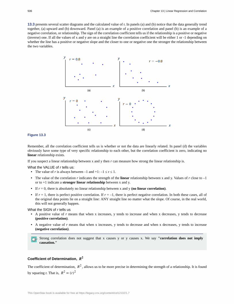
13.3 presents several scatter diagrams and the calculated value of r. In panels (a) and (b) notice that the data generally trendtogether, (a) upward and (b) downward. Panel (a) is an example of a positive correlation and panel (b) is an example of anegative correlation, or relationship. The sign of the correlation coefficient tells us if the relationship is a positive or negative(inverse) one. If all the values of x and y are on a straight line the correlation coefficient will be either 1 or -1 depending onwhether the line has a positive or negative slope and the closer to one or negative one the stronger the relationship betweenthe two variables.
Figure 13.3
Remember, all the correlation coefficient tells us is whether or not the data are linearly related. In panel (d) the variablesobviously have some type of very specific relationship to each other, but the correlation coefficient is zero, indicating nolinear relationship exists.
If you suspect a linear relationship between x and y then r can measure how strong the linear relationship is.
What the VALUE of r tells us:• The value of r is always between –1 and +1: –1 ≤ r ≤ 1.
• The value of the correlation r indicates the strength of the linear relationship between x and y. Values of r close to –1or to +1 indicate a stronger linear relationship between x and y.
• If r = 0, there is absolutely no linear relationship between x and y (no linear correlation).
• If r = 1, there is perfect positive correlation. If r = –1, there is perfect negative correlation. In both these cases, all ofthe original data points lie on a straight line: ANY straight line no matter what the slope. Of course, in the real world,this will not generally happen.
What the SIGN of r tells us• A positive value of r means that when x increases, y tends to increase and when x decreases, y tends to decrease
(positive correlation).
• A negative value of r means that when x increases, y tends to decrease and when x decreases, y tends to increase(negative correlation).
Strong correlation does not suggest that x causes y or y causes x. We say "correlation does not implycausation."
Coefficient of Determination, R2
The coefficient of determination, R2 , allows us to be more precise in determining the strength of a relationship. It is found
by squaring r. That is, R2 = (r)2
506 Chapter 13 | Linear Regression and Correlation
This OpenStax book is available for free at https://legacy.cnx.org/content/col12102/1.7
The coefficient of determination measures the amount of variation in the dependent variable, y, that is explained by thevariation in the independent variable, x.
Example 13.1 Coefficient of Determination
Suppose the coefficient of correlation between two variables, x and y, is r = - 0.85 .
Interpret the meaning of the coefficient of correlation.
Solution 13.1 r = - 0.85 indicates a strong, negative relationship between the independent and dependent variables.
Find the coefficient of determination and interpret its meaning.
Solution 13.1
Coefficient of Determination R2 = ⎛⎝-0.85⎞⎠2
= 0.7225
This tells us that 72.25% of the variation in the dependent variable, y, is explained by the variation in theindependent variable, x.
13.2 | Testing the Significance of the Correlation
Coefficient - (Base Version - Lyryx Learning)The correlation coefficient, r, tells us about the strength and direction of the linear relationship between X1 and X2.
The sample data are used to compute r, the correlation coefficient for the sample. If we had data for the entire population, wecould find the population correlation coefficient. But because we have only sample data, we cannot calculate the populationcorrelation coefficient. The sample correlation coefficient, r, is our estimate of the unknown population correlationcoefficient.
ρ = population correlation coefficient (unknown)r = sample correlation coefficient (known; calculated from sample data)
The hypothesis test lets us decide whether the value of the population correlation coefficient ρ is "close to zero" or"significantly different from zero". We decide this based on the sample correlation coefficient r and the sample size n.
If the test concludes that the correlation coefficient is significantly different from zero, we say that the correlationcoefficient is "significant."
• Conclusion: There is sufficient evidence to conclude that there is a significant linear relationship between X1 and X2because the correlation coefficient is significantly different from zero.
• What the conclusion means: There is a significant linear relationship X1 and X2. If the test concludes that thecorrelation coefficient is not significantly different from zero (it is close to zero), we say that correlation coefficient is"not significant".
If the test concludes that the correlation coefficient is not significantly different from zero (it is close to zero), we saythat correlation coefficient is "not significant".
Performing the Hypothesis Test• Null Hypothesis: H0: ρ = 0
• Alternate Hypothesis: Ha: ρ ≠ 0
What the Hypotheses Mean in Words• Null Hypothesis H0: The population correlation coefficient IS NOT significantly different from zero. There IS NOT
a significant linear relationship (correlation) between X1 and X2 in the population.
• Alternate Hypothesis Ha: The population correlation coefficient is significantly different from zero. There is asignificant linear relationship (correlation) between X1 and X2 in the population.
Chapter 13 | Linear Regression and Correlation 507
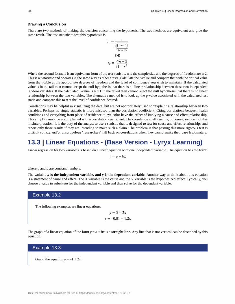
Drawing a Conclusion
There are two methods of making the decision concerning the hypothesis. The two methods are equivalent and give thesame result. The test statistic to test this hypothesis is:
tc = r⎛⎝1 − r2⎞⎠(n − 2)
OR
tc = r n − 21 − r2
Where the second formula is an equivalent form of the test statistic, n is the sample size and the degrees of freedom are n-2.This is a t-statistic and operates in the same way as other t tests. Calculate the t-value and compare that with the critical valuefrom the t-table at the appropriate degrees of freedom and the level of confidence you wish to maintain. If the calculatedvalue is in the tail then cannot accept the null hypothesis that there is no linear relationship between these two independentrandom variables. If the calculated t-value is NOT in the tailed then cannot reject the null hypothesis that there is no linearrelationship between the two variables. The alternative method is to look up the p-value associated with the calculated teststatic and compare this to α at the level of confidence desired.
Correlations may be helpful in visualizing the data, but are not appropriately used to "explain" a relationship between twovariables. Perhaps no single statistic is more misused than the correlation coefficient. Citing correlations between healthconditions and everything from place of residence to eye color have the effect of implying a cause and effect relationship.This simply cannot be accomplished with a correlation coefficient. The correlation coefficient is, of course, innocent of thismisinterpretation. It is the duty of the analyst to use a statistic that is designed to test for cause and effect relationships andreport only those results if they are intending to make such a claim. The problem is that passing this more rigorous test isdifficult so lazy and/or unscrupulous "researchers" fall back on correlations when they cannot make their case legitimately.
13.3 | Linear Equations - (Base Version - Lyryx Learning)Linear regression for two variables is based on a linear equation with one independent variable. The equation has the form:
y = a + bx
where a and b are constant numbers.
The variable x is the independent variable, and y is the dependent variable. Another way to think about this equationis a statement of cause and effect. The X variable is the cause and the Y variable is the hypothesized effect. Typically, youchoose a value to substitute for the independent variable and then solve for the dependent variable.
Example 13.2
The following examples are linear equations.
y = 3 + 2xy = –0.01 + 1.2x
The graph of a linear equation of the form y = a + bx is a straight line. Any line that is not vertical can be described by thisequation.
Example 13.3
Graph the equation y = –1 + 2x.
508 Chapter 13 | Linear Regression and Correlation
This OpenStax book is available for free at https://legacy.cnx.org/content/col12102/1.7
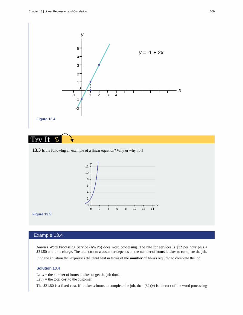
Figure 13.4
13.3 Is the following an example of a linear equation? Why or why not?
Figure 13.5
Example 13.4
Aaron's Word Processing Service (AWPS) does word processing. The rate for services is $32 per hour plus a$31.50 one-time charge. The total cost to a customer depends on the number of hours it takes to complete the job.
Find the equation that expresses the total cost in terms of the number of hours required to complete the job.
Solution 13.4
Let x = the number of hours it takes to get the job done.Let y = the total cost to the customer.
The $31.50 is a fixed cost. If it takes x hours to complete the job, then (32)(x) is the cost of the word processing
Chapter 13 | Linear Regression and Correlation 509

only. The total cost is: y = 31.50 + 32x
Slope and Y-Intercept of a Linear EquationFor the linear equation y = a + bx, b = slope and a = y-intercept. From algebra recall that the slope is a number that describesthe steepness of a line, and the y-intercept is the y coordinate of the point (0, a) where the line crosses the y-axis.
Figure 13.6 Three possible graphs of y = a + bx. (a) If b > 0, the line slopes upward to the right. (b) If b = 0, the lineis horizontal. (c) If b < 0, the line slopes downward to the right.
Example 13.5
Svetlana tutors to make extra money for college. For each tutoring session, she charges a one-time fee of $25plus $15 per hour of tutoring. A linear equation that expresses the total amount of money Svetlana earns for eachsession she tutors is y = 25 + 15x.
What are the independent and dependent variables? What is the y-intercept and what is the slope? Interpret themusing complete sentences.
Solution 13.5
The independent variable (x) is the number of hours Svetlana tutors each session. The dependent variable (y) isthe amount, in dollars, Svetlana earns for each session.
The y-intercept is 25 (a = 25). At the start of the tutoring session, Svetlana charges a one-time fee of $25 (this iswhen x = 0). The slope is 15 (b = 15). For each session, Svetlana earns $15 for each hour she tutors.
13.4 | The Regression Equation - (Base Version - Lyryx
Learning)Regression analysis is a statistical technique that can test the hypothesis that a variable is dependent upon one or more othervariables. Further, regression analysis can provide an estimate of the magnitude of the impact of a change in one variableon another. This last feature, of course, is all important in predicting future values.
Regression analysis is based upon a functional relationship among variables and further, assumes that the relationship islinear. When the relationship among variables is not linear, special techniques are required. These techniques will not bediscussed here.
The linear regression equation for two variables is as follows:
y^ = a + bx
where y^ is the predicted value of y for a given x value, a is the y - intercept, b is the slope of the line, and x is any
value of the independent variable.
The formula for the slope b is:
510 Chapter 13 | Linear Regression and Correlation
This OpenStax book is available for free at https://legacy.cnx.org/content/col12102/1.7

b = n⎛⎝∑ xy⎞⎠ - ⎛⎝∑ x⎞⎠⎛⎝∑ y⎞⎠
n⎛⎝∑ x2⎞⎠ - ⎛⎝∑ x⎞⎠2
The formula for the y - intercept a is:
a = ∑ yn - b∑ x
n
Figure 13.7 presents the regression problem in the form of a scatter plot graph of the data set where it is hypothesized thaty is dependent upon the single independent variable x .
Figure 13.7
In Figure 13.7 , the line that has been graphed through the points is the graph of the regression equation. For this data, theregression equation is the line that best fits the data when plotted on a scatter diagram. Notice that some points are abovethe line and some points are below the line. The line has been chosen such that that the sum of the squares of the verticaldistances from each point to the line is minimized.
Consider a basic relationship from Macroeconomic Principle, the consumption function. This theoretical relationship statesthat as a person's income rises, their consumption rises, but by a smaller amount than the rise in income. We can explorethis relationship through regression analysis. In Figure 13.8 below, y is consumption and x is income. The regression
problem is, first, to establish that this relationship exists, and second, to determine the impact of a change in income on aperson's consumption.
Figure 13.8
Each "dot" in Figure 13.8 represents the consumption and income of different individuals at some point in time.
The regression problem comes down to determining which straight line would best represent the data in Figure 13.9.Regression analysis is sometimes called "least squares" analysis because the method of determining which line best "fits"
Chapter 13 | Linear Regression and Correlation 511
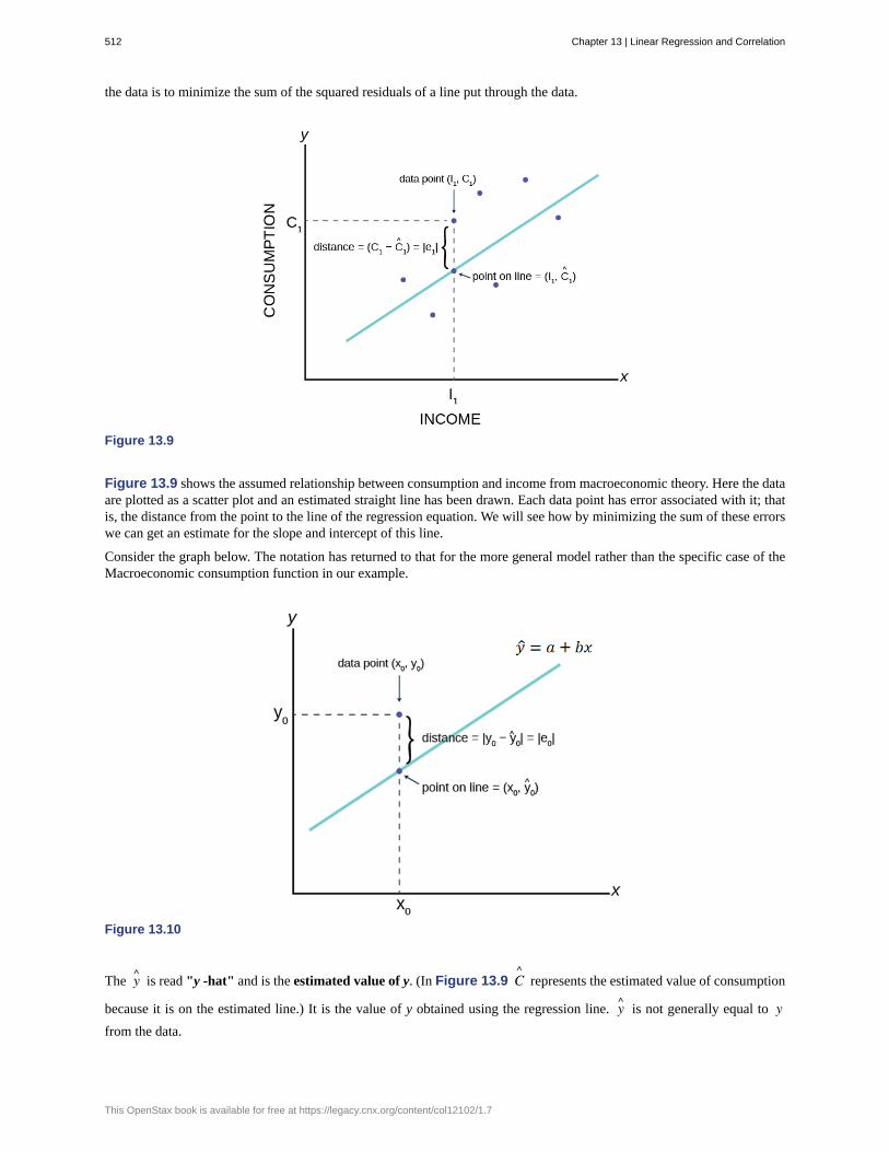
the data is to minimize the sum of the squared residuals of a line put through the data.
Figure 13.9
Figure 13.9 shows the assumed relationship between consumption and income from macroeconomic theory. Here the dataare plotted as a scatter plot and an estimated straight line has been drawn. Each data point has error associated with it; thatis, the distance from the point to the line of the regression equation. We will see how by minimizing the sum of these errorswe can get an estimate for the slope and intercept of this line.
Consider the graph below. The notation has returned to that for the more general model rather than the specific case of theMacroeconomic consumption function in our example.
Figure 13.10
The y^ is read "y -hat" and is the estimated value of y. (In Figure 13.9 C^
represents the estimated value of consumption
because it is on the estimated line.) It is the value of y obtained using the regression line. y^ is not generally equal to yfrom the data.
512 Chapter 13 | Linear Regression and Correlation
This OpenStax book is available for free at https://legacy.cnx.org/content/col12102/1.7
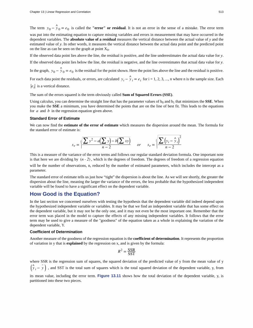
The term y0 − y 0 = e0 is called the "error" or residual. It is not an error in the sense of a mistake. The error term
was put into the estimating equation to capture missing variables and errors in measurement that may have occurred in thedependent variables. The absolute value of a residual measures the vertical distance between the actual value of y and theestimated value of y. In other words, it measures the vertical distance between the actual data point and the predicted pointon the line as can be seen on the graph at point X0.
If the observed data point lies above the line, the residual is positive, and the line underestimates the actual data value for y.
If the observed data point lies below the line, the residual is negative, and the line overestimates that actual data value for y.
In the graph, y0 − y 0 = e0 is the residual for the point shown. Here the point lies above the line and the residual is positive.
For each data point the residuals, or errors, are calculated yi − y i = ei for i = 1, 2, 3, ..., n where n is the sample size. Each
|ei| is a vertical distance.
The sum of the errors squared is the term obviously called Sum of Squared Errors (SSE).
Using calculus, you can determine the straight line that has the parameter values of b0 and b1 that minimizes the SSE. Whenyou make the SSE a minimum, you have determined the points that are on the line of best fit. This leads to the equationsfor a and b in the regression equation given above.
Standard Error of Estimate
We can now find the estimate of the error of estimate which measures the dispersion around the mean. The formula forthe standard error of estimate is:
se =∑ y2 − a⎛⎝∑ y⎞⎠− b⎛⎝∑ xy⎞⎠
n − 2 or se =∑ ⎛⎝yi − y i
⎞⎠
2
n − 2
This is a measure of the variance of the error terms and follows our regular standard deviation formula. One important noteis that here we are dividing by (n - 2) , which is the degrees of freedom. The degrees of freedom of a regression equation
will be the number of observations, n, reduced by the number of estimated parameters, which includes the intercept as aparameter.
The standard error of estimate tells us just how “tight” the dispersion is about the line. As we will see shortly, the greater thedispersion about the line, meaning the larger the variance of the errors, the less probable that the hypothesized independentvariable will be found to have a significant effect on the dependent variable.
How Good is the Equation?In the last section we concerned ourselves with testing the hypothesis that the dependent variable did indeed depend uponthe hypothesized independent variable or variables. It may be that we find an independent variable that has some effect onthe dependent variable, but it may not be the only one, and it may not even be the most important one. Remember that theerror term was placed in the model to capture the effects of any missing independent variables. It follows that the errorterm may be used to give a measure of the "goodness" of the equation taken as a whole in explaining the variation of thedependent variable, Y.
Coefficient of Determination
Another measure of the goodness of the regression equation is the coefficient of determination. It represents the proportionof variation in y that is explained by the regression on x, and is given by the formula:
R2 = SSRSST
where SSR is the regression sum of squares, the squared deviation of the predicted value of y from the mean value of y⎛⎝ y i − y ⎞⎠ , and SST is the total sum of squares which is the total squared deviation of the dependent variable, y, from
its mean value, including the error term. Figure 13.11 shows how the total deviation of the dependent variable, y, ispartitioned into these two pieces.
Chapter 13 | Linear Regression and Correlation 513
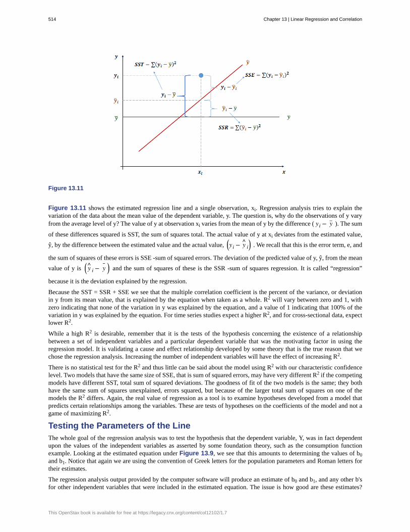
Figure 13.11
Figure 13.11 shows the estimated regression line and a single observation, xi. Regression analysis tries to explain thevariation of the data about the mean value of the dependent variable, y. The question is, why do the observations of y varyfrom the average level of y? The value of y at observation xi varies from the mean of y by the difference ( yi − y– ). The sum
of these differences squared is SST, the sum of squares total. The actual value of y at xi deviates from the estimated value,
ŷ, by the difference between the estimated value and the actual value, ⎛⎝yi − y i⎞⎠ . We recall that this is the error term, e, and
the sum of squares of these errors is SSE -sum of squared errors. The deviation of the predicted value of y, ŷ, from the mean
value of y is ⎛⎝ y i − y ⎞⎠ and the sum of squares of these is the SSR -sum of squares regression. It is called “regression”
because it is the deviation explained by the regression.
Because the SST = SSR + SSE we see that the multiple correlation coefficient is the percent of the variance, or deviationin y from its mean value, that is explained by the equation when taken as a whole. R2 will vary between zero and 1, withzero indicating that none of the variation in y was explained by the equation, and a value of 1 indicating that 100% of thevariation in y was explained by the equation. For time series studies expect a higher R2, and for cross-sectional data, expectlower R2.
While a high R2 is desirable, remember that it is the tests of the hypothesis concerning the existence of a relationshipbetween a set of independent variables and a particular dependent variable that was the motivating factor in using theregression model. It is validating a cause and effect relationship developed by some theory that is the true reason that wechose the regression analysis. Increasing the number of independent variables will have the effect of increasing R2.
There is no statistical test for the R2 and thus little can be said about the model using R2 with our characteristic confidencelevel. Two models that have the same size of SSE, that is sum of squared errors, may have very different R2 if the competingmodels have different SST, total sum of squared deviations. The goodness of fit of the two models is the same; they bothhave the same sum of squares unexplained, errors squared, but because of the larger total sum of squares on one of themodels the R2 differs. Again, the real value of regression as a tool is to examine hypotheses developed from a model thatpredicts certain relationships among the variables. These are tests of hypotheses on the coefficients of the model and not agame of maximizing R2.
Testing the Parameters of the LineThe whole goal of the regression analysis was to test the hypothesis that the dependent variable, Y, was in fact dependentupon the values of the independent variables as asserted by some foundation theory, such as the consumption functionexample. Looking at the estimated equation under Figure 13.9, we see that this amounts to determining the values of b0and b1. Notice that again we are using the convention of Greek letters for the population parameters and Roman letters fortheir estimates.
The regression analysis output provided by the computer software will produce an estimate of b0 and b1, and any other b'sfor other independent variables that were included in the estimated equation. The issue is how good are these estimates?
514 Chapter 13 | Linear Regression and Correlation
This OpenStax book is available for free at https://legacy.cnx.org/content/col12102/1.7

In order to test a hypothesis concerning any estimate, we have found that we need to know the underlying samplingdistribution. It should come as no surprise at his stage in the course that the answer is going to be the normal distribution.This can be seen by remembering the assumption that the error term in the population, ε, is normally distributed. If the errorterm is normally distributed and the variance of the estimates of the equation parameters, b0 and b1, are determined by thevariance of the error term, it follows that the variances of the parameter estimates are also normally distributed. And indeedthis is just the case.
We can see this by the creation of the test statistic for the test of hypothesis for the slope parameter, β1 in our consumptionfunction equation. To test whether or not Y does indeed depend upon X, or in our example, that consumption depends uponincome, we need only test the hypothesis that β1 equals zero. This hypothesis would be stated formally as:
H0 : β1 = 0Ha : β1 ≠ 0
If we cannot reject the null hypothesis, we must conclude that our theory has no validity. If we cannot reject the nullhypothesis that β1 = 0 then b1, the coefficient of Income, is zero and zero times anything is zero. Therefore the effect ofIncome on Consumption is zero. There is no relationship as our theory had suggested.
Notice that we have set up the presumption, the null hypothesis, as "no relationship". This puts the burden of proof on thealternative hypothesis. In other words, if we are to validate our claim of finding a relationship, we must do so with a levelof confidence greater than 90, 95, or 99 percent. The status quo is ignorance, no relationship exists, and to be able to makethe claim that we have actually added to our body of knowledge we must do so with significant probability of being correct.John Maynard Keynes got it right and thus was born Keynesian economics starting with this basic concept in 1936.
The test statistic for this test comes directly from our old friend the standardizing formula:
tc = b1 − β1Sb1
where b1 is the estimated value of the slope of the regression line, β1 is the hypothesized value of beta, in this case zero, andSb1
is the standard deviation of the estimate of b1. In this case we are asking how many standard deviations is the estimated
slope away from the hypothesized slope. This is exactly the same question we asked before with respect to a hypothesisabout a mean: how many standard deviations is the estimated mean, the sample mean, from the hypothesized mean?
The test statistic is written as a student's t distribution, but if the sample size is larger enough so that the degrees of freedomare greater than 30 we may again use the normal distribution. To see why we can use the student's t or normal distributionwe have only to look at Sb1
,the formula for the standard deviation of the estimate of b1:
Sb1= Se2
⎛⎝xi − x–⎞⎠2
or
Sb1= Se2⎛⎝n − 1⎞⎠Sx2
Where Se is the estimate of the error variance and S2x is the variance of x values of the coefficient of the independent
variable being tested.
We see that Se, the estimate of the error variance, is part of the computation. Because the estimate of the error varianceis based on the assumption of normality of the error terms, we can conclude that the sampling distribution of the beta's, thecoefficients of our hypothesized regression line, are also normally distributed.
One last note concerns the degrees of freedom of the test statistic. Previously we subtracted 1 from the sample size todetermine the degrees of freedom in a student's t problem. Here we must subtract one degree of freedom for each parameterestimated in the equation. For the example of the consumption function we lose 2 degrees of freedom, one for b0 , the
intercept, and one for b1, the slope of the consumption function. If we were estimating an equation with three independentvariables, we would lose 4 degrees of freedom: three for the independent variables and one more for the intercept.
The decision rule for acceptance or rejection of the null hypothesis follows exactly the same form as in all our previous testof hypothesis. Namely, if the calculated value of t (or Z) falls into the tails of the distribution, where the tails are defined byα ,the required confidence in the test, we cannot accept the null hypothesis. If on the other hand, the calculated value of the
Chapter 13 | Linear Regression and Correlation 515
test statistic is within the critical region, we cannot reject the null hypothesis.
If we conclude that we cannot accept the null hypothesis, we are able to state with (1 - α) level of confidence that the slope
of the line is given by b1. This is an extremely important conclusion. Regression analysis not only allows us to test if acause and effect relationship exists, we can also determine the magnitude of that relationship, if one is found to exist. It isthis feature of regression analysis that makes it so valuable. If models can be developed that have statistical validity, we arethen able to simulate the effects of changes in variables that may be under our control with some degree of probability , ofcourse. For example, if advertising is demonstrated to effect sales, we can determine the effects of changing the advertisingbudget and decide if the increased sales are worth the added expense.
13.5 | Predicting with a Regression Equation - (Base
Version - Lyryx Learning)One important value of an estimated regression equation is its ability to predict the effects on for a given value of y of a
change in one or more values of the independent variables.
The regression equation allows us to estimate the value of y for a given value of x .
y^ = a + bx
Example 13.6
In an attempt to predict the final exam score using the the third test (where x is the third test score, and y is the
final exam score) the following regression equation was obtained: y^ = − 173.51 + 4.83x
Suppose you want to estimate, or predict, the mean final exam score of statistics students who received 73 on thethird test. The exam scores (x-values) range from 65 to 75. Since 73 is between the x-values 65 and 75, we feelcomfortable to substitute x = 73 into the equation. Then:
y = − 173.51 + 4.83(73) = 179.08
We predict that statistics students who earn a grade of 73 on the third test will earn a grade of 179.08 on the finalexam, on average.
a. What would you predict the final exam score to be for a student who scored a 66 on the third test?
Solution 13.6a. 145.27
b. Suppose the third test scores (x-values) range from 65 to 75, can you predict the final exam score for a studentwho scored a 90 on the third test?
Solution 13.6b. The x values in the data are between 65 and 75. Ninety is outside of the domain of the observed x values in thedata (independent variable), so you cannot reliably predict the final exam score for this student. (Even though itis possible to enter 90 into the equation for x and calculate a corresponding y value, the y value that you get willhave a confidence interval that may not be meaningful.)
To understand really how unreliable the prediction can be outside of the observed x values observed in the data,make the substitution x = 90 into the equation.
y^ = –173.51 + 4.83⎛⎝90⎞⎠ = 261.19
The final-exam score is predicted to be 261.19. The largest the final-exam score can be is 200.
516 Chapter 13 | Linear Regression and Correlation
This OpenStax book is available for free at https://legacy.cnx.org/content/col12102/1.7

NOTE
The process of predicting inside of the observed x values observed in the data is called interpolation. Theprocess of predicting outside of the observed x values observed in the data is called extrapolation.
Exercise 13.1
Data are collected on the relationship between the number of hours per week practicing a musical instrument andscores on a math test.
The line of best fit is y^ = 72.5 + 2.8x ,
where x represents the time spent studying in hours, and ŷ represents the predicted score on the math test as a percent.What would you predict the score on a math test would be for a student who practices a musical instrument for fivehours a week?
Solution
y^ = 72.5 + 2.8⎛⎝5⎞⎠ = 86.5
We would expect a score of 86.5%.
Confidence about the predicted value y
Remember that point estimates do not carry a particular level of probability, or level of confidence, because points haveno “width” above which there is an area to measure. This was why we developed confidence intervals for the mean andproportion earlier. The same concern arises here also. There are actually two different approaches to the issue of developingestimates of changes in the independent variable, or variables, on the dependent variable. The first approach wishes tomeasure the expected mean value of y from a specific change in the value of x: this specific value implies that expectedvalue. Here the question is: what is the mean impact on y that would result from multiple hypothetical experiments on y atthis specific value of x. Remember that there is a variance around the estimated parameter of x and thus each experimentwill result in a bit of a different estimate of the value of y.
The second approach to estimate the effect of a specific value of x on y treats the event as a single experiment: you choosex and multiply it times the coefficient and that provides a single estimate of y. Because this approach acts as if there were asingle experiment the variance that exists in the parameter estimate is larger than the variance associated with the expectedvalue approach.
The conclusion is that we have two different ways to predict the effect of values of the independent variable(s) on thedependent variable and thus we have two different intervals. Both are correct answers to the question being asked, but thereare two different questions. To avoid confusion, the first case where we are asking for the expected value of the mean of theestimated y, is called a confidence interval as we have named this concept before. The second case, where we are askingfor the estimate of the impact on the dependent variable y of a single experiment using a value of x, is called the predictioninterval. The test statistics for these two interval measures within which the estimated value of y will fall are:
Confidence Interval for Expected Value of Mean Value of y for x=xp
y ± tα / 2 se
⎛
⎝⎜⎜⎜ 1n +⎛⎝x p − x ⎞⎠
2
(n − 1)sx
2
⎞
⎠⎟⎟⎟
Chapter 13 | Linear Regression and Correlation 517

Prediction Interval for an Individual y for x = xp
y ± tα / 2 se
⎛
⎝⎜⎜⎜
1 + 1n +⎛⎝x p − x ⎞⎠
2
(n − 1)sx
2
⎞
⎠⎟⎟⎟
Where se is the standard deviation of the error term and sx is the standard deviation of the x variable.
The mathematical computations of these two test statistics are complex. Various computer regression software packagesprovide programs within the regression functions to provide answers to inquires of estimated predicted values of y givenvarious values chosen for the x variable(s). It is important to know just which interval is being tested in the computerpackage because the difference in the size of the standard deviations will change the size of the interval estimated. This isshown in Figure 13.12.
Figure 13.12 Prediction and confidence intervals for regression equation; 95% confidence level.
Figure 13.12 shows visually the difference the standard deviation makes in the size of the estimated intervals. Theconfidence interval, measuring the expected value of the dependent variable, is smaller than the prediction interval for thesame level of confidence. The expected value method assumes that the experiment is conducted multiple times rather thanjust once as in the other method. The logic here is similar, although not identical, to that discussed when developing therelationship between the sample size and the confidence interval using the Central Limit Theorem. There, as the number ofexperiments increased, the distribution narrowed and the confidence interval became tighter around the expected value ofthe mean.
It is also important to note that the intervals around a point estimate are highly dependent upon the range of data used toestimate the equation regardless of which approach is being used for prediction. Remember that all regression equations gothrough the point of means, that is, the mean value of y and the mean values of all independent variables in the equation.As the value of x chosen to estimate the associated value of y is further from the point of means the width of the estimatedinterval around the point estimate increases. Choosing values of x beyond the range of the data used to estimate the equationpossess even greater danger of creating estimates with little use; very large intervals, and risk of error. Figure 13.13 showsthis relationship.
518 Chapter 13 | Linear Regression and Correlation
This OpenStax book is available for free at https://legacy.cnx.org/content/col12102/1.7
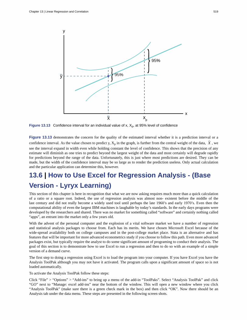
Figure 13.13 Confidence interval for an individual value of x, Xp, at 95% level of confidence
Figure 13.13 demonstrates the concern for the quality of the estimated interval whether it is a prediction interval or a
confidence interval. As the value chosen to predict y, Xp in the graph, is further from the central weight of the data, X–
, we
see the interval expand in width even while holding constant the level of confidence. This shows that the precision of anyestimate will diminish as one tries to predict beyond the largest weight of the data and most certainly will degrade rapidlyfor predictions beyond the range of the data. Unfortunately, this is just where most predictions are desired. They can bemade, but the width of the confidence interval may be so large as to render the prediction useless. Only actual calculationand the particular application can determine this, however.
13.6 | How to Use Excel for Regression Analysis - (Base
Version - Lyryx Learning)This section of this chapter is here in recognition that what we are now asking requires much more than a quick calculationof a ratio or a square root. Indeed, the use of regression analysis was almost non- existent before the middle of thelast century and did not really become a widely used tool until perhaps the late 1960’s and early 1970’s. Even then thecomputational ability of even the largest IBM machines is laughable by today’s standards. In the early days programs weredeveloped by the researchers and shared. There was no market for something called “software” and certainly nothing called“apps”, an entrant into the market only a few years old.
With the advent of the personal computer and the explosion of a vital software market we have a number of regressionand statistical analysis packages to choose from. Each has its merits. We have chosen Microsoft Excel because of thewide-spread availability both on college campuses and in the post-college market place. Stata is an alternative and hasfeatures that will be important for more advanced econometrics study if you choose to follow this path. Even more advancedpackages exist, but typically require the analyst to do some significant amount of programing to conduct their analysis. Thegoal of this section is to demonstrate how to use Excel to run a regression and then to do so with an example of a simpleversion of a demand curve.
The first step to doing a regression using Excel is to load the program into your computer. If you have Excel you have theAnalysis ToolPak although you may not have it activated. The program calls upon a significant amount of space so is notloaded automatically.
To activate the Analysis ToolPak follow these steps:
Click “File” > “Options” > “Add-ins” to bring up a menu of the add-in “ToolPaks”. Select “Analysis ToolPak” and click“GO” next to “Manage: excel add-ins” near the bottom of the window. This will open a new window where you click“Analysis ToolPak” (make sure there is a green check mark in the box) and then click “OK”. Now there should be anAnalysis tab under the data menu. These steps are presented in the following screen shots.
Chapter 13 | Linear Regression and Correlation 519
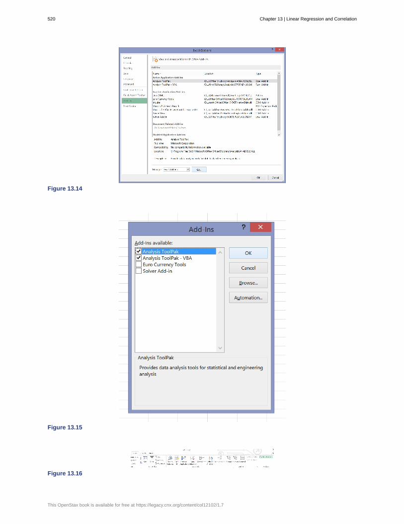
Figure 13.14
Figure 13.15
Figure 13.16
520 Chapter 13 | Linear Regression and Correlation
This OpenStax book is available for free at https://legacy.cnx.org/content/col12102/1.7
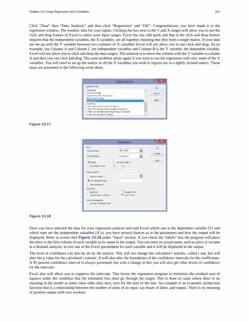
Click “Data” then “Data Analysis” and then click “Regression” and “OK”. Congratulations, you have made it to theregression window. The window asks for your inputs. Clicking the box next to the Y and X ranges will allow you to use theclick and drag feature of Excel to select your input ranges. Excel has one odd quirk and that is the click and drop featurerequires that the independent variables, the X variables, are all together, meaning that they form a single matrix. If your dataare set up with the Y variable between two columns of X variables Excel will not allow you to use click and drag. As anexample, say Column A and Column C are independent variables and Column B is the Y variable, the dependent variable.Excel will not allow you to click and drop the data ranges. The solution is to move the column with the Y variable to columnA and then you can click and drag. The same problem arises again if you want to run the regression with only some of the Xvariables. You will need to set up the matrix so all the X variables you wish to regress are in a tightly formed matrix. Thesesteps are presented in the following scene shots.
Figure 13.17
Figure 13.18
Once you have selected the data for your regression analysis and told Excel which one is the dependent variable (Y) andwhich ones are the independent valuables (X‘s), you have several choices as to the parameters and how the output will bedisplayed. Refer to screen shot Figure 13.18 under “Input” section. If you check the “labels” box the program will placethe entry in the first column of each variable as its name in the output. You can enter an actual name, such as price or incomein a demand analysis, in row one of the Excel spreadsheet for each variable and it will be displayed in the output.
The level of confidence can also be set by the analyst. This will not change the calculated t statistic, called t stat, but willalter the p value for the calculated t statistic. It will also alter the boundaries of the confidence intervals for the coefficients.A 95 percent confidence interval is always presented, but with a change in this you will also get other levels of confidencefor the intervals.
Excel also will allow you to suppress the intercept. This forces the regression program to minimize the residual sum ofsquares under the condition that the estimated line must go through the origin. This is done in cases where there is nomeaning in the model at some value other than zero, zero for the start of the line. An example is an economic productionfunction that is a relationship between the number of units of an input, say hours of labor, and output. There is no meaningof positive output with zero workers.
Chapter 13 | Linear Regression and Correlation 521
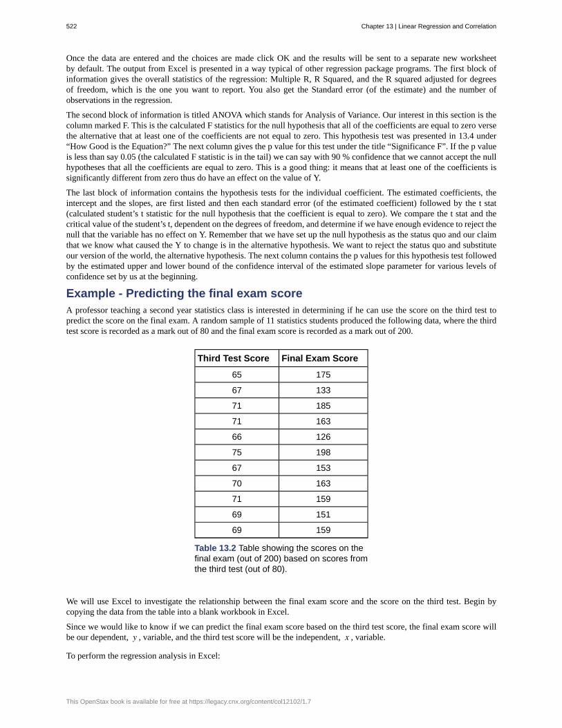
Once the data are entered and the choices are made click OK and the results will be sent to a separate new worksheetby default. The output from Excel is presented in a way typical of other regression package programs. The first block ofinformation gives the overall statistics of the regression: Multiple R, R Squared, and the R squared adjusted for degreesof freedom, which is the one you want to report. You also get the Standard error (of the estimate) and the number ofobservations in the regression.
The second block of information is titled ANOVA which stands for Analysis of Variance. Our interest in this section is thecolumn marked F. This is the calculated F statistics for the null hypothesis that all of the coefficients are equal to zero versethe alternative that at least one of the coefficients are not equal to zero. This hypothesis test was presented in 13.4 under“How Good is the Equation?” The next column gives the p value for this test under the title “Significance F”. If the p valueis less than say 0.05 (the calculated F statistic is in the tail) we can say with 90 % confidence that we cannot accept the nullhypotheses that all the coefficients are equal to zero. This is a good thing: it means that at least one of the coefficients issignificantly different from zero thus do have an effect on the value of Y.
The last block of information contains the hypothesis tests for the individual coefficient. The estimated coefficients, theintercept and the slopes, are first listed and then each standard error (of the estimated coefficient) followed by the t stat(calculated student’s t statistic for the null hypothesis that the coefficient is equal to zero). We compare the t stat and thecritical value of the student’s t, dependent on the degrees of freedom, and determine if we have enough evidence to reject thenull that the variable has no effect on Y. Remember that we have set up the null hypothesis as the status quo and our claimthat we know what caused the Y to change is in the alternative hypothesis. We want to reject the status quo and substituteour version of the world, the alternative hypothesis. The next column contains the p values for this hypothesis test followedby the estimated upper and lower bound of the confidence interval of the estimated slope parameter for various levels ofconfidence set by us at the beginning.
Example - Predicting the final exam scoreA professor teaching a second year statistics class is interested in determining if he can use the score on the third test topredict the score on the final exam. A random sample of 11 statistics students produced the following data, where the thirdtest score is recorded as a mark out of 80 and the final exam score is recorded as a mark out of 200.
Third Test Score Final Exam Score
65 175
67 133
71 185
71 163
66 126
75 198
67 153
70 163
71 159
69 151
69 159
Table 13.2 Table showing the scores on thefinal exam (out of 200) based on scores fromthe third test (out of 80).
We will use Excel to investigate the relationship between the final exam score and the score on the third test. Begin bycopying the data from the table into a blank workbook in Excel.
Since we would like to know if we can predict the final exam score based on the third test score, the final exam score willbe our dependent, y , variable, and the third test score will be the independent, x , variable.
To perform the regression analysis in Excel:
522 Chapter 13 | Linear Regression and Correlation
This OpenStax book is available for free at https://legacy.cnx.org/content/col12102/1.7

1) Ensure that your data is entered in columns in Excel. Then, navigate to Data, Data Analysis, Regression. Press OK.
2) Input your Y Range and X Range (careful of order!). Press OK.
If you have included the headings in the data,check off the "labels" box.
Figure 13.19
Your output will appear in a separate Excel tab and will look like this:
Figure 13.20
This gives us several pieces of important information.
Chapter 13 | Linear Regression and Correlation 523

First, let's focus on the "Coefficients" column.
The "Intercept" coefficient gives us the y -intecept, which is a from the regression equation.
The "Third test score" coefficient tells us the coefficient in front of the x variable, which is b from the regression equation.
Using the above output, the regression equation that relations the final exam score to the third test score is
y = - 173.513 + 4.827x
Now, look at "Multiple R" from the output. This output gives us the coefficient of correlation, r . Excel will always give
a positive value for "Multiple R". To decide if r is positive or negative, we look at the slope of the line. In this case, our
slope ( b = 4.827 ) is positive, which means that r is also positive. If the b were a negative number, r would be negative.
In our example,
r = 0.663
This indicates that there is a moderate, positive relationship between the score on the final exam and the score on the thirdtest.
We also see R Square in the output. In this example,
R2 = 0.440
telling us that 44.0% of the variation in final exam score is due to the variation in the third test score.
Estimating the Demand for Bricks - A Multiple Regression ExampleHere is an example of using the Excel program to run a regression for a particular specific case: estimating the demandfor bricks. These data can be found in the provided Excel file. Begin by downloading these data into an Excel spreadsheet.Because of the quirky way Excel allows the data to be entered into the regression package it is best to have the independentvariables, price of bricks and income next to each other as it is here.
Once your data are entered into the spreadsheet it is always good to look at the data. Examine the range, the means and thestandard deviations. Use your understanding of descriptive statistics from the very first part of this course. In large data setsyou will not be able to “scan” the data. The Analysis ToolPac makes it easy to get the range, mean and standard deviations.You can also quickly get correlations among the variables. Examine for outliers. In this example if you had a year where theprice of bricks was $9.00 or $2.00 we should be suspicious. These values are several standard deviations from the mean andthus have a very low probability of coming from this distribution. Review the history. Did something happen? Was here alabor strike, change in import fees, something that makes these unusual conditions? Do not take the data without question.There may have been a typo somewhere, who knows without review.
The data gathered was determined by the model that is being tested. This should always be the case. One is not doinginferential statistics by throwing a mountain of data into a computer and asking the machine for a theory. Theory first,tests follow. In this case the theory of consumer demand posits that the quantity of a good demanded is inversely relatedto its price and is positively related to income. These data are national average prices and income is the nation’s per capitaincome. Consumption is national demand for bricks. These are time series data; we are tracking the brick market for theUnited States from 1982-2010.
We are trying to create a demand curve, which we know from economic theory shows how variables effect how much ofa good gets consumed. We expect to see a negative relationship between price and quantity, i.e. as price increases thenquantity demanded decreases. Similarly, we expect to see a positive relationship between income and quantity demanded.We expect these results because that is what is predicted by a hundred years of economic theory and research. Essentiallywe are testing this century-old hypothesis. Quantity demanded will be our Y variable, and Income and Price will be our twoX variables.
Go to the regression window, enter the data and select 95% confidence level and click “OK”. You can include the labels inthe input range but be sure to click the “labels” box on the main regression page if you do.
The output should show up automatically on a new worksheet.
524 Chapter 13 | Linear Regression and Correlation
This OpenStax book is available for free at https://legacy.cnx.org/content/col12102/1.7

Figure 13.21
Titled as “Summary of Output”, the R-Square is the strength of the correlation between Y and X1 and X2 taken as a group.Our R-square, adjusted for degrees of freedom, of 0.699 means that 70% of the variation in Y, demand for bricks, canbe explained by variations in X1 and X2, Price and Income. Considering that bricks are an input in construction, omittedvariables that are related to construction might explain the other 30% of the variation. This is a possible research topic.
Looking at the third panel of output we can write the equation as:
Y = b0 + b1 X1 + b2 X2 + e
where b0 is the intercept, b1 is the estimated coefficient on price, and b2 is the estimated coefficient on income and e is theerror term. The equation is written in Roman letters indicating that these are the estimated values and not the populationparameters, β’s.
Our estimated equation is:
Tons of Bricks = 91.73 − 3.22(Price) + 0.0000167(Income)
In other words, increasing the price by one dollar will lead to a 3.22-ton reduction in bricks purchased. Similarly, increasingper capita national income by one thousand dollars will lead to a 0.0167 ton increase in bricks consumed. This should makeintuitive sense from economic theory, as price increases lead to less quantity demanded as people substitute away frombricks as a building material. As income increases the quantity demanded increases as people build more houses and officebuildings and need more bricks. It is important to have a theory first that predicts the significance or at least the directionof the coefficients. Without a theory to test, this research tool is not much more helpful than the correlation coefficient welearned about earlier.
We cannot stop there. We need to first check whether our coefficients are statistically significant from zero. We set up ahypothesis of:
H0 : β1 = 0Ha : β1 ≠ 0
for both coefficients. Recall from earlier that we will not be able to definitively say that our estimated b1 is the actual realpopulation β1 , but rather that with 1-α % confidence we cannot reject the null hypothesis that our calculated b1 is the trueβ1 significantly different from zero. The analyst is making a claim that the price causes an impact on quantity demanded.The claim is therefore in the alternative hypothesis. It will take a very small probability, 0.05 in this case, of being wrong,to overthrow the null hypothesis, the status quo, that β= 0. In all regression hypothesis tests the claim is in the alternativeand the claim is that the theory has found a variable that has a significant impact on the Y variable.
The test statistic follows the standardizing formula:
tc = b1 − β0Sb1
The computer calculates this test statistic and presents it as “t stat”. You can find this value to the right of the standard errorof the coefficient estimate. To reach a conclusion we compare this test statistic with the critical value of the student’s t atdegrees of freedom n-2-1 = 16, and alpha=0.025 (95% confidence for a two-tailed test). Our t stat for b1 is -3.54 which isgreater than 2.12 (the value you looked up in the t table), so we cannot accept our null hypothesis of no effect. We concludethat Price has a significant effect on Y because the calculated t value is in the tail. You can conduct the same test for b2.This time the calculated t statistic of the coefficient for the per capita income is not in the tail; t stat of 0.145. A t stat of0.145 says that the estimated coefficient is only a very small number of standard deviations away from zero. We cannotreject the null hypothesis of no relationship; with these data we do not find that per capita income has a significant effect on
Chapter 13 | Linear Regression and Correlation 525

the demand for bricks.
These tests tell us whether or not an individual coefficient is significantly different from zero, but does not address theoverall quality of the model. We have seen that the R squared adjusted for degrees of freedom indicates this model withthese two variable explains 70% of the variation in quantity of bricks demanded. We can also conduct a second test of themodel taken as a whole. This is the F test presented in section 13.4 of this chapter. Because this is a multiple regression(more than one X), we use the F-test to determine if our coefficients collectively affect Y. The hypothesis is:
H0 : β1 = β2 = 0Ha : "at least one of theβi is not equal to 0"
Under the ANOVA section of the output we find the calculated F statistic for this hypothesis. For this example the F statisticis 21.9. Again, comparing the calculated F statistic with the critical value given our desired level of confidence and thedegrees of freedom will allow us to reach a conclusion. The critical value can be found in an F Table knowing that we have(n-3)=16 degrees of freedom and setting α/2 = 0.025 (95% confidence). The critical value is determined to be 2.12 andtherefore we cannot accept the null hypotheses because the calculated F is in the tail. By not being able to accept the nullhypotheses we conclude that this specification of this model has validity because at least one of the estimated coefficientsis significantly different from zero. Since F-calculated is greater than F-critical, we can reject H0, meaning that X1 and X2together has a significant effect on Y.
An alternative way to reach this conclusion is to use the p-value comparison rule. The p-value is the area in the tail, giventhe calculated F statistic. In essence, the computer is finding the F value in the table for us. Under “significance F” is thisprobability. For this example it is calculated to be 2.6 x 10⁻⁵, or 2.6 then moving the decimal five places to the left. (.000026)This is an almost infinitesimal level of probability and is certainly less than our alpha level at 95% confidence. Again weconcluded that we cannot accept the null hypothesis.
The development of computing machinery and the software useful for academic and business research has made it possibleto answer questions that just a few years ago we could not even formulate. Data is available in electronic format and canbe moved into place for analysis in ways and at speeds that were unimaginable a decade ago. The sheer magnitude of datasets that can today be used for research and analysis gives us a higher quality of results than in days past. Even with onlyan Excel spreadsheet we can conduct very high level research. This section gives you the tools to conduct some of this veryinteresting research with the only limit being your imagination.
13.7 | Regression Analysis with the BAII Plus CalculatorThe following video posted on YouTube by Professor Joshua Emmanuel demonstrates how to find the correlation andregression coefficients of the regression equation using the BAII Plus calculator:https://www.youtube.com/watch?v=NVc3RZHyzaA (https://www.youtube.com/watch?v=NVc3RZHyzaA)
Table 13.3 shows the data set referenced in the video. You may wish to follow along with your own calculator as youwatch the video and work through the steps listed below.
x y
5 10
9 35
13 30
7 15
Table13.3
Here are the steps that are outlined in the video:1. Clear any old data
Press 2nd→Data, then 2nd→Clr Work
2. Enter your dataPress 2nd→Data- Your first x value will go in X01- Type it in and press enter
526 Chapter 13 | Linear Regression and Correlation
This OpenStax book is available for free at https://legacy.cnx.org/content/col12102/1.7
- Press the ↓ arrow- You will see Y01. Enter the first y value and press enter- Repeat until all data has been entered- Press ↑ and ↓ arrows to review your data
3. Choose your calculation methodWe would like the calculator to say LIN. If it does not, we will change it to this mode.Press 2nd→Stat and then press 2nd→Set repeatedly until you see LIN
4. View the outputWhile you are in the LIN STAT mode - Press ↑ and ↓ arrows to view the output
- You will see n, a, b, r, ΣX, ΣX2, ΣY , ΣY 2, ΣXY , along with other information
Regression coefficients, a and b
The regression equation is given by y^ = a + bx . The coefficients a and b can be read directly from the calculator. In this
example, a = - 0.571 and b = 2.714 . Thus, the regression equation is y^ = - 0.571 + 2.714x .
Coefficient of correlation, r
The coefficient of correlation, r , can be read directly from the calculator. In our example, the coefficient of correlation,
r = 0.7789 .
Finding the coefficient of determination, R2
To find the coefficient of determination, simply square the r value. If r = 0.7789 , then R2 = 0.6067 .
Chapter 13 | Linear Regression and Correlation 527
a is the symbol for the Y-Intercept
b is the symbol for Slope
Bivariate
Linear
Multivariate
R2 – Coefficient of Determination
r – Correlation Coefficient
Residual or “error”
Sum of Squared Errors (SSE)
X – the independent variable
Y – the dependent variable
KEY TERMSSometimes written as b0 , because when writing the theoretical linear model
β0 is used to represent a coefficient for a population.
The word coefficient will be used regularly for the slope, because it is a number that willalways be next to the letter “x.” It will be written as b1 when a sample is used, and β1 will be used with a
population or when writing the theoretical linear model.
two variables are present in the model where one is the “cause” or independent variable and the other is the“effect” of dependent variable.
a model that takes data and regresses it into a straight line equation.
a system or model where more than one independent variable is being used to predict an outcome. Therecan only ever be one dependent variable, but there is no limit to the number of independent variables.
This is a number between 0 and 1 that represents the percentage variation of thedependent variable that can be explained by the variation in the independent
variable. Sometimes calculated by the equation R2 = SSRSST where SSR is the “Sum of Squares Regression” and
SST is the “Sum of Squares Total.”
A number between −1 and 1 that represents the strength and direction of the relationshipbetween “X” and “Y.” The value for “r” will equal 1 or −1 only if all the plotted points
form a perfectly straight line.
the value calculated from subtracting y0 − y^ 0 = e0 . The absolute value of a residual measures
the vertical distance between the actual value of y and the estimated value of y that appears on the best-fit line.
the calculated value from adding up all the squared residual terms. The hope is thatthis value is very small when creating a model.
This will sometimes be referred to as the “predictor” variable, because these valueswere measured in order to determine what possible outcomes could be predicted.
Also, using the letter “y” represents actual values while y^ represents predicted or
estimated values. Predicted values will come from plugging in observed “x” values into a linear model.
CHAPTER REVIEW
13.3 Linear Equations - (Base Version - Lyryx Learning)The most basic type of association is a linear association. This type of relationship can be defined algebraically by theequations used, numerically with actual or predicted data values, or graphically from a plotted curve. (Lines are classifiedas straight curves.) Algebraically, a linear equation typically takes the form y = mx + b, where m and b are constants, x isthe independent variable, y is the dependent variable. In a statistical context, a linear equation is written in the form y = a +bx, where a and b are the constants. This form is used to help readers distinguish the statistical context from the algebraiccontext. In the equation y = a + bx, the constant b that multiplies the x variable (b is called a coefficient) is called the slope.The slope describes the rate of change between the independent and dependent variables; in other words, the rate of changedescribes the change that occurs in the dependent variable as the independent variable is changed. In the equation y = a +bx, the constant a is called as the y-intercept. Graphically, the y-intercept is the y coordinate of the point where the graph ofthe line crosses the y axis. At this point x = 0.
The slope of a line is a value that describes the rate of change between the independent and dependent variables. The slopetells us how the dependent variable (y) changes for every one unit increase in the independent (x) variable, on average. They-intercept is used to describe the dependent variable when the independent variable equals zero. Graphically, the slope is
528 Chapter 13 | Linear Regression and Correlation
This OpenStax book is available for free at https://legacy.cnx.org/content/col12102/1.7

represented by three line types in elementary statistics.
13.4 The Regression Equation - (Base Version - Lyryx Learning)It is hoped that this discussion of regression analysis has demonstrated the tremendous potential value it has as a tool fortesting models and helping to better understand the world around us. The regression model has its limitations, especially therequirement that the underlying relationship be approximately linear.
SOLUTIONS
Chapter 13 | Linear Regression and Correlation 529

530 Chapter 13 | Linear Regression and Correlation
This OpenStax book is available for free at https://legacy.cnx.org/content/col12102/1.7

APPENDIX A:
STATISTICAL TABLESF Distribution
Figure A1 Table entry for p is the critical value F* with probability p lying to its right.
Degrees of freedom in the numerator
Degrees of freedomin the denominator
p 1 2 3 4 5 6 7 8 9
.100 39.86 49.50 53.59 55.83 57.24 58.20 58.91 59.44 59.86
.050 161.45 199.50 215.71 224.58 230.16 233.99 236.77 238.88 240.54
.025 647.79 799.50 864.16 899.58 921.85 937.11 948.22 956.66 963.28
.010 4052.2 4999.5 5403.4 5624.6 5763.6 5859.0 5928.4 5981.1 6022.5
1
.001 405284 500000 540379 562500 576405 585937 592873 598144 602284
.100 8.53 9.00 9.16 9.24 9.29 9.33 9.35 9.37 9.38
.050 18.51 19.00 19.16 19.25 19.30 19.33 19.35 19.37 19.38
.025 38.51 39.00 39.17 39.25 39.30 39.33 39.36 39.37 39.39
.010 98.50 99.00 99.17 99.25 99.30 99.33 99.36 99.37 99.39
2
.001 998.50 999.00 999.17 999.25 999.30 999.33 999.36 999.37 999.39
.100 5.54 5.46 5.39 5.34 5.31 5.28 5.27 5.25 5.24
.050 10.13 9.55 9.28 9.12 9.01 8.94 8.89 8.85 8.813
.025 17.44 16.04 15.44 15.10 14.88 14.73 14.62 14.54 14.47
Table A1 F critical values
Appendix A 531

Degrees of freedom in the numerator
.010 34.12 30.82 29.46 28.71 28.24 27.91 27.67 27.49 27.35
.001 167.03 148.50 141.11 137.10 134.58 132.85 131.58 130.62 129.86
.100 4.54 4.32 4.19 4.11 4.05 4.01 3.98 3.95 3.94
.050 7.71 6.94 6.59 6.39 6.26 6.16 6.09 6.04 6.00
.025 12.22 10.65 9.98 9.60 9.36 9.20 9.07 8.98 8.90
.010 21.20 18.00 16.69 15.98 15.52 15.21 14.98 14.80 14.66
4
.001 74.14 61.25 56.18 53.44 51.71 50.53 49.66 49.00 48.47
.100 4.06 3.78 3.62 3.52 3.45 3.40 3.37 3.34 3.32
.050 6.61 5.79 5.41 5.19 5.05 4.95 4.88 4.82 4.77
.025 10.01 8.43 7.76 7.39 7.15 6.98 6.85 6.76 6.68
.010 16.26 13.27 12.06 11.39 10.97 10.67 10.46 10.29 10.16
5
.001 47.18 37.12 33.20 31.09 29.75 28.83 28.16 27.65 27.24
.100 3.78 3.46 3.29 3.18 3.11 3.05 3.01 2.98 2.96
.050 5.99 5.14 4.76 4.53 4.39 4.28 4.21 4.15 4.10
.025 8.81 7.26 6.60 6.23 5.99 5.82 5.70 5.60 5.52
.010 13.75 10.92 9.78 9.15 8.75 8.47 8.26 8.10 7.98
6
.001 35.51 27.00 23.70 21.92 20.80 20.03 19.46 19.03 18.69
.100 3.59 3.26 3.07 2.96 2.88 2.83 2.78 2.75 2.72
.050 5.59 4.74 4.35 4.12 3.97 3.87 3.79 3.73 3.68
.025 8.07 6.54 5.89 5.52 5.29 5.12 4.99 4.90 4.82
.010 12.25 9.55 8.45 7.85 7.46 7.19 6.99 6.84 6.72
7
.001 29.25 21.69 18.77 17.20 16.21 15.52 15.02 14.63 14.33
Table A1 F critical values
Degrees of freedom in the numerator
Degrees offreedomin thedenominator
p 10 12 15 20 25 30 40 50 60 120 1000
.100 60.19 60.71 61.22 61.74 62.05 62.26 62.53 62.69 62.79 63.06 63.30
.050 241.88 243.91 245.95 248.01 249.26 250.10 251.14 251.77 252.20 253.25 254.19
.025 968.63 976.71 984.87 993.10 998.08 1001.4 1005.6 1008.1 1009.8 1014.0 1017.7
.010 6055.8 6106.3 6157.3 6208.7 6239.8 6260.6 6286.8 6302.5 6313.0 6339.4 6362.7
1
.001 605621 610668 615764 620908 624017 626099 628712 630285 631337 633972 636301
.100 9.39 9.41 9.42 9.44 9.45 9.46 9.47 9.47 9.47 9.48 9.49
.050 19.40 19.41 19.43 19.45 19.46 19.46 19.47 19.48 19.48 19.49 19.492
.025 39.40 39.41 39.43 39.45 39.46 39.46 39.47 39.48 39.48 39.49 39.50
Table A2 F critical values (continued)
532 Appendix A
This OpenStax book is available for free at https://legacy.cnx.org/content/col12102/1.7
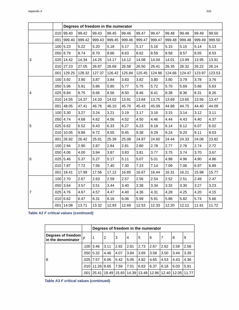
Degrees of freedom in the numerator
.010 99.40 99.42 99.43 99.45 99.46 99.47 99.47 99.48 99.48 99.49 99.50
.001 999.40 999.42 999.43 999.45 999.46 999.47 999.47 999.48 999.48 999.49 999.50
.100 5.23 5.22 5.20 5.18 5.17 5.17 5.16 5.15 5.15 5.14 5.13
.050 8.79 8.74 8.70 8.66 8.63 8.62 8.59 8.58 8.57 8.55 8.53
.025 14.42 14.34 14.25 14.17 14.12 14.08 14.04 14.01 13.99 13.95 13.91
.010 27.23 27.05 26.87 26.69 26.58 26.50 26.41 26.35 26.32 26.22 26.14
3
.001 129.25 128.32 127.37 126.42 125.84 125.45 124.96 124.66 124.47 123.97 123.53
.100 3.92 3.90 3.87 3.84 3.83 3.82 3.80 3.80 3.79 3.78 3.76
.050 5.96 5.91 5.86 5.80 5.77 5.75 5.72 5.70 5.69 5.66 5.63
.025 8.84 8.75 8.66 8.56 8.50 8.46 8.41 8.38 8.36 8.31 8.26
.010 14.55 14.37 14.20 14.02 13.91 13.84 13.75 13.69 13.65 13.56 13.47
4
.001 48.05 47.41 46.76 46.10 45.70 45.43 45.09 44.88 44.75 44.40 44.09
.100 3.30 3.27 3.24 3.21 3.19 3.17 3.16 3.15 3.14 3.12 3.11
.050 4.74 4.68 4.62 4.56 4.52 4.50 4.46 4.44 4.43 4.40 4.37
.025 6.62 6.52 6.43 6.33 6.27 6.23 6.18 6.14 6.12 6.07 6.02
.010 10.05 9.89 9.72 9.55 9.45 9.38 9.29 9.24 9.20 9.11 9.03
5
.001 26.92 26.42 25.91 25.39 25.08 24.87 24.60 24.44 24.33 24.06 23.82
.100 2.94 2.90 2.87 2.84 2.81 2.80 2.78 2.77 2.76 2.74 2.72
.050 4.06 4.00 3.94 3.87 3.83 3.81 3.77 3.75 3.74 3.70 3.67
.025 5.46 5.37 5.27 5.17 5.11 5.07 5.01 4.98 4.96 4.90 4.86
.010 7.87 7.72 7.56 7.40 7.30 7.23 7.14 7.09 7.06 6.97 6.89
6
.001 18.41 17.99 17.56 17.12 16.85 16.67 16.44 16.31 16.21 15.98 15.77
.100 2.70 2.67 2.63 2.59 2.57 2.56 2.54 2.52 2.51 2.49 2.47
.050 3.64 3.57 3.51 3.44 3.40 3.38 3.34 3.32 3.30 3.27 3.23
.025 4.76 4.67 4.57 4.47 4.40 4.36 4.31 4.28 4.25 4.20 4.15
.010 6.62 6.47 6.31 6.16 6.06 5.99 5.91 5.86 5.82 5.74 5.66
7
.001 14.08 13.71 13.32 12.93 12.69 12.53 12.33 12.20 12.12 11.91 11.72
Table A2 F critical values (continued)
Degrees of freedom in the numerator
Degrees of freedomin the denominator
p 1 2 3 4 5 6 7 8 9
.100 3.46 3.11 2.92 2.81 2.73 2.67 2.62 2.59 2.56
.050 5.32 4.46 4.07 3.84 3.69 3.58 3.50 3.44 3.39
.025 7.57 6.06 5.42 5.05 4.82 4.65 4.53 4.43 4.36
.010 11.26 8.65 7.59 7.01 6.63 6.37 6.18 6.03 5.91
8
.001 25.41 18.49 15.83 14.39 13.48 12.86 12.40 12.05 11.77
Table A3 F critical values (continued)
Appendix A 533
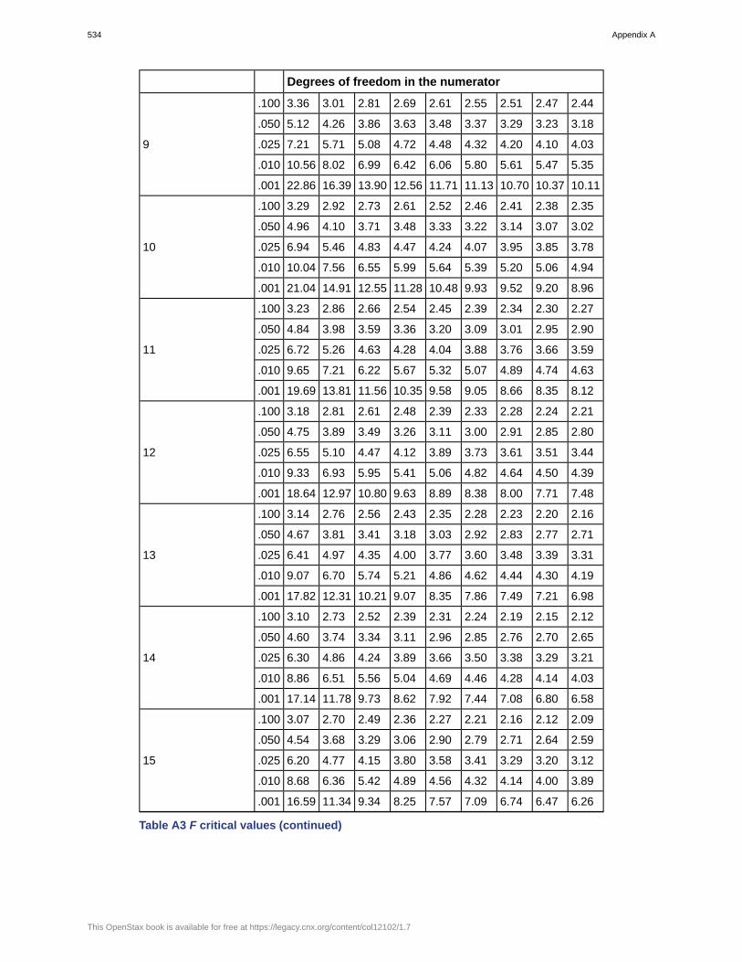
Degrees of freedom in the numerator
.100 3.36 3.01 2.81 2.69 2.61 2.55 2.51 2.47 2.44
.050 5.12 4.26 3.86 3.63 3.48 3.37 3.29 3.23 3.18
.025 7.21 5.71 5.08 4.72 4.48 4.32 4.20 4.10 4.03
.010 10.56 8.02 6.99 6.42 6.06 5.80 5.61 5.47 5.35
9
.001 22.86 16.39 13.90 12.56 11.71 11.13 10.70 10.37 10.11
.100 3.29 2.92 2.73 2.61 2.52 2.46 2.41 2.38 2.35
.050 4.96 4.10 3.71 3.48 3.33 3.22 3.14 3.07 3.02
.025 6.94 5.46 4.83 4.47 4.24 4.07 3.95 3.85 3.78
.010 10.04 7.56 6.55 5.99 5.64 5.39 5.20 5.06 4.94
10
.001 21.04 14.91 12.55 11.28 10.48 9.93 9.52 9.20 8.96
.100 3.23 2.86 2.66 2.54 2.45 2.39 2.34 2.30 2.27
.050 4.84 3.98 3.59 3.36 3.20 3.09 3.01 2.95 2.90
.025 6.72 5.26 4.63 4.28 4.04 3.88 3.76 3.66 3.59
.010 9.65 7.21 6.22 5.67 5.32 5.07 4.89 4.74 4.63
11
.001 19.69 13.81 11.56 10.35 9.58 9.05 8.66 8.35 8.12
.100 3.18 2.81 2.61 2.48 2.39 2.33 2.28 2.24 2.21
.050 4.75 3.89 3.49 3.26 3.11 3.00 2.91 2.85 2.80
.025 6.55 5.10 4.47 4.12 3.89 3.73 3.61 3.51 3.44
.010 9.33 6.93 5.95 5.41 5.06 4.82 4.64 4.50 4.39
12
.001 18.64 12.97 10.80 9.63 8.89 8.38 8.00 7.71 7.48
.100 3.14 2.76 2.56 2.43 2.35 2.28 2.23 2.20 2.16
.050 4.67 3.81 3.41 3.18 3.03 2.92 2.83 2.77 2.71
.025 6.41 4.97 4.35 4.00 3.77 3.60 3.48 3.39 3.31
.010 9.07 6.70 5.74 5.21 4.86 4.62 4.44 4.30 4.19
13
.001 17.82 12.31 10.21 9.07 8.35 7.86 7.49 7.21 6.98
.100 3.10 2.73 2.52 2.39 2.31 2.24 2.19 2.15 2.12
.050 4.60 3.74 3.34 3.11 2.96 2.85 2.76 2.70 2.65
.025 6.30 4.86 4.24 3.89 3.66 3.50 3.38 3.29 3.21
.010 8.86 6.51 5.56 5.04 4.69 4.46 4.28 4.14 4.03
14
.001 17.14 11.78 9.73 8.62 7.92 7.44 7.08 6.80 6.58
.100 3.07 2.70 2.49 2.36 2.27 2.21 2.16 2.12 2.09
.050 4.54 3.68 3.29 3.06 2.90 2.79 2.71 2.64 2.59
.025 6.20 4.77 4.15 3.80 3.58 3.41 3.29 3.20 3.12
.010 8.68 6.36 5.42 4.89 4.56 4.32 4.14 4.00 3.89
15
.001 16.59 11.34 9.34 8.25 7.57 7.09 6.74 6.47 6.26
Table A3 F critical values (continued)
534 Appendix A
This OpenStax book is available for free at https://legacy.cnx.org/content/col12102/1.7
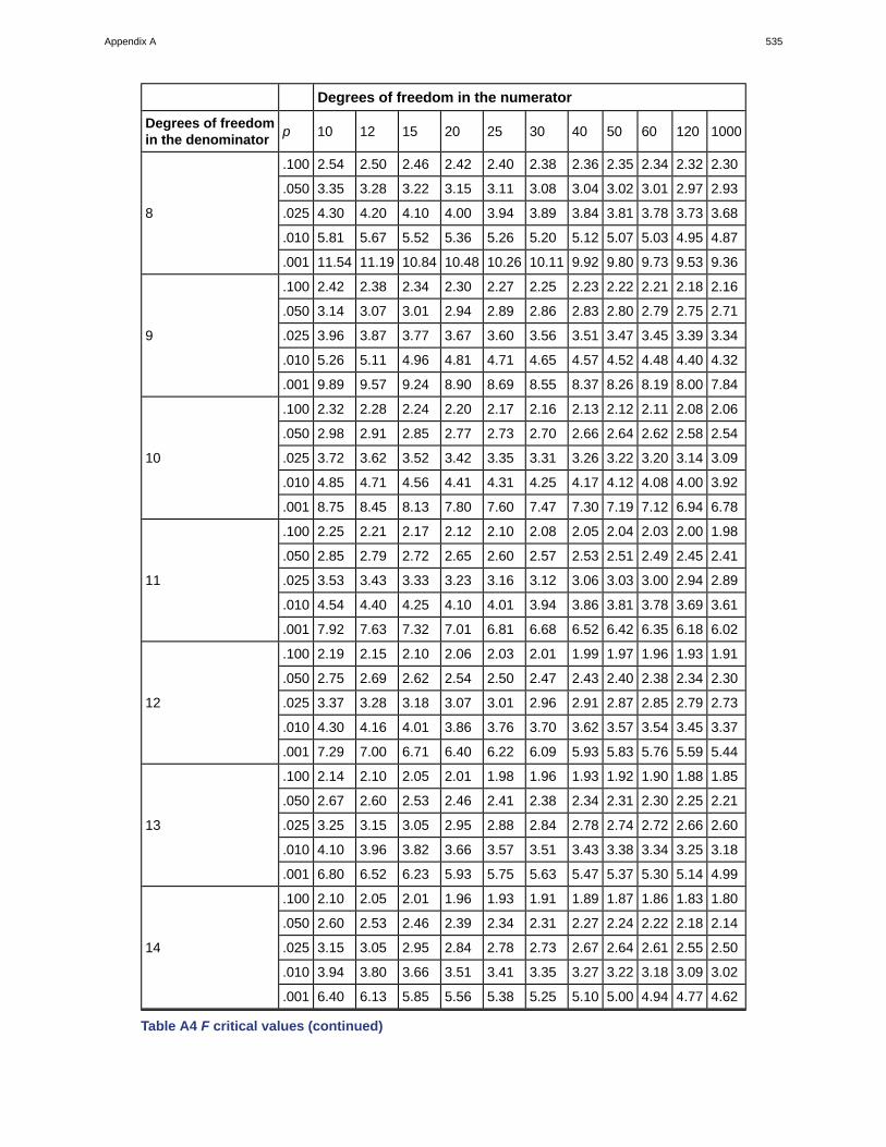
Degrees of freedom in the numerator
Degrees of freedomin the denominator
p 10 12 15 20 25 30 40 50 60 120 1000
.100 2.54 2.50 2.46 2.42 2.40 2.38 2.36 2.35 2.34 2.32 2.30
.050 3.35 3.28 3.22 3.15 3.11 3.08 3.04 3.02 3.01 2.97 2.93
.025 4.30 4.20 4.10 4.00 3.94 3.89 3.84 3.81 3.78 3.73 3.68
.010 5.81 5.67 5.52 5.36 5.26 5.20 5.12 5.07 5.03 4.95 4.87
8
.001 11.54 11.19 10.84 10.48 10.26 10.11 9.92 9.80 9.73 9.53 9.36
.100 2.42 2.38 2.34 2.30 2.27 2.25 2.23 2.22 2.21 2.18 2.16
.050 3.14 3.07 3.01 2.94 2.89 2.86 2.83 2.80 2.79 2.75 2.71
.025 3.96 3.87 3.77 3.67 3.60 3.56 3.51 3.47 3.45 3.39 3.34
.010 5.26 5.11 4.96 4.81 4.71 4.65 4.57 4.52 4.48 4.40 4.32
9
.001 9.89 9.57 9.24 8.90 8.69 8.55 8.37 8.26 8.19 8.00 7.84
.100 2.32 2.28 2.24 2.20 2.17 2.16 2.13 2.12 2.11 2.08 2.06
.050 2.98 2.91 2.85 2.77 2.73 2.70 2.66 2.64 2.62 2.58 2.54
.025 3.72 3.62 3.52 3.42 3.35 3.31 3.26 3.22 3.20 3.14 3.09
.010 4.85 4.71 4.56 4.41 4.31 4.25 4.17 4.12 4.08 4.00 3.92
10
.001 8.75 8.45 8.13 7.80 7.60 7.47 7.30 7.19 7.12 6.94 6.78
.100 2.25 2.21 2.17 2.12 2.10 2.08 2.05 2.04 2.03 2.00 1.98
.050 2.85 2.79 2.72 2.65 2.60 2.57 2.53 2.51 2.49 2.45 2.41
.025 3.53 3.43 3.33 3.23 3.16 3.12 3.06 3.03 3.00 2.94 2.89
.010 4.54 4.40 4.25 4.10 4.01 3.94 3.86 3.81 3.78 3.69 3.61
11
.001 7.92 7.63 7.32 7.01 6.81 6.68 6.52 6.42 6.35 6.18 6.02
.100 2.19 2.15 2.10 2.06 2.03 2.01 1.99 1.97 1.96 1.93 1.91
.050 2.75 2.69 2.62 2.54 2.50 2.47 2.43 2.40 2.38 2.34 2.30
.025 3.37 3.28 3.18 3.07 3.01 2.96 2.91 2.87 2.85 2.79 2.73
.010 4.30 4.16 4.01 3.86 3.76 3.70 3.62 3.57 3.54 3.45 3.37
12
.001 7.29 7.00 6.71 6.40 6.22 6.09 5.93 5.83 5.76 5.59 5.44
.100 2.14 2.10 2.05 2.01 1.98 1.96 1.93 1.92 1.90 1.88 1.85
.050 2.67 2.60 2.53 2.46 2.41 2.38 2.34 2.31 2.30 2.25 2.21
.025 3.25 3.15 3.05 2.95 2.88 2.84 2.78 2.74 2.72 2.66 2.60
.010 4.10 3.96 3.82 3.66 3.57 3.51 3.43 3.38 3.34 3.25 3.18
13
.001 6.80 6.52 6.23 5.93 5.75 5.63 5.47 5.37 5.30 5.14 4.99
.100 2.10 2.05 2.01 1.96 1.93 1.91 1.89 1.87 1.86 1.83 1.80
.050 2.60 2.53 2.46 2.39 2.34 2.31 2.27 2.24 2.22 2.18 2.14
.025 3.15 3.05 2.95 2.84 2.78 2.73 2.67 2.64 2.61 2.55 2.50
.010 3.94 3.80 3.66 3.51 3.41 3.35 3.27 3.22 3.18 3.09 3.02
14
.001 6.40 6.13 5.85 5.56 5.38 5.25 5.10 5.00 4.94 4.77 4.62
Table A4 F critical values (continued)
Appendix A 535

Degrees of freedom in the numerator
.100 2.06 2.02 1.97 1.92 1.89 1.87 1.85 1.83 1.82 1.79 1.76
.050 2.54 2.48 2.40 2.33 2.28 2.25 2.20 2.18 2.16 2.11 2.07
.025 3.06 2.96 2.86 2.76 2.69 2.64 2.59 2.55 2.52 2.46 2.40
.010 3.80 3.67 3.52 3.37 3.28 3.21 3.13 3.08 3.05 2.96 2.88
15
.001 6.08 5.81 5.54 5.25 5.07 4.95 4.80 4.70 4.64 4.47 4.33
Table A4 F critical values (continued)
Degrees of freedom in the numerator
Degrees of freedomin the denominator
p 1 2 3 4 5 6 7 8 9
.100 3.05 2.67 2.46 2.33 2.24 2.18 2.13 2.09 2.06
.050 4.49 3.63 3.24 3.01 2.85 2.74 2.66 2.59 2.54
.025 6.12 4.69 4.08 3.73 3.50 3.34 3.22 3.12 3.05
.010 8.53 6.23 5.29 4.77 4.44 4.20 4.03 3.89 3.78
16
.001 16.12 10.97 9.01 7.94 7.27 6.80 6.46 6.19 5.98
.100 3.03 2.64 2.44 2.31 2.22 2.15 2.10 2.06 2.03
.050 4.45 3.59 3.20 2.96 2.81 2.70 2.61 2.55 2.49
.025 6.04 4.62 4.01 3.66 3.44 3.28 3.16 3.06 2.98
.010 8.40 6.11 5.19 4.67 4.34 4.10 3.93 3.79 3.68
17
.001 15.72 10.66 8.73 7.68 7.02 6.56 6.22 5.96 5.75
.100 3.01 2.62 2.42 2.29 2.20 2.13 2.08 2.04 2.00
.050 4.41 3.55 3.16 2.93 2.77 2.66 2.58 2.51 2.46
.025 5.98 4.56 3.95 3.61 3.38 3.22 3.10 3.01 2.93
.010 8.29 6.01 5.09 4.58 4.25 4.01 3.84 3.71 3.60
18
.001 15.38 10.39 8.49 7.46 6.81 6.35 6.02 5.76 5.56
.100 3.36 3.01 2.81 2.69 2.61 2.55 2.51 2.47 2.44
.050 5.12 4.26 3.86 3.63 3.48 3.37 3.29 3.23 3.18
.025 7.21 5.71 5.08 4.72 4.48 4.32 4.20 4.10 4.03
.010 10.56 8.02 6.99 6.42 6.06 5.80 5.61 5.47 5.35
19
.001 22.86 16.39 13.90 12.56 11.71 11.13 10.70 10.37 10.11
.100 2.97 2.59 2.38 2.25 2.16 2.09 2.04 2.00 1.96
.050 4.35 3.49 3.10 2.87 2.71 2.60 2.51 2.45 2.39
.025 5.87 4.46 3.86 3.51 3.29 3.13 3.01 2.91 2.84
.010 8.10 5.85 4.94 4.43 4.10 3.87 3.70 3.56 3.46
20
.001 14.82 9.95 8.10 7.10 6.46 6.02 5.69 5.44 5.24
.100 2.96 2.57 2.36 2.23 2.14 2.08 2.02 1.98 1.9521
.050 4.32 3.47 3.07 2.84 2.68 2.57 2.49 2.42 2.37
Table A5 F critical values (continued)
536 Appendix A
This OpenStax book is available for free at https://legacy.cnx.org/content/col12102/1.7
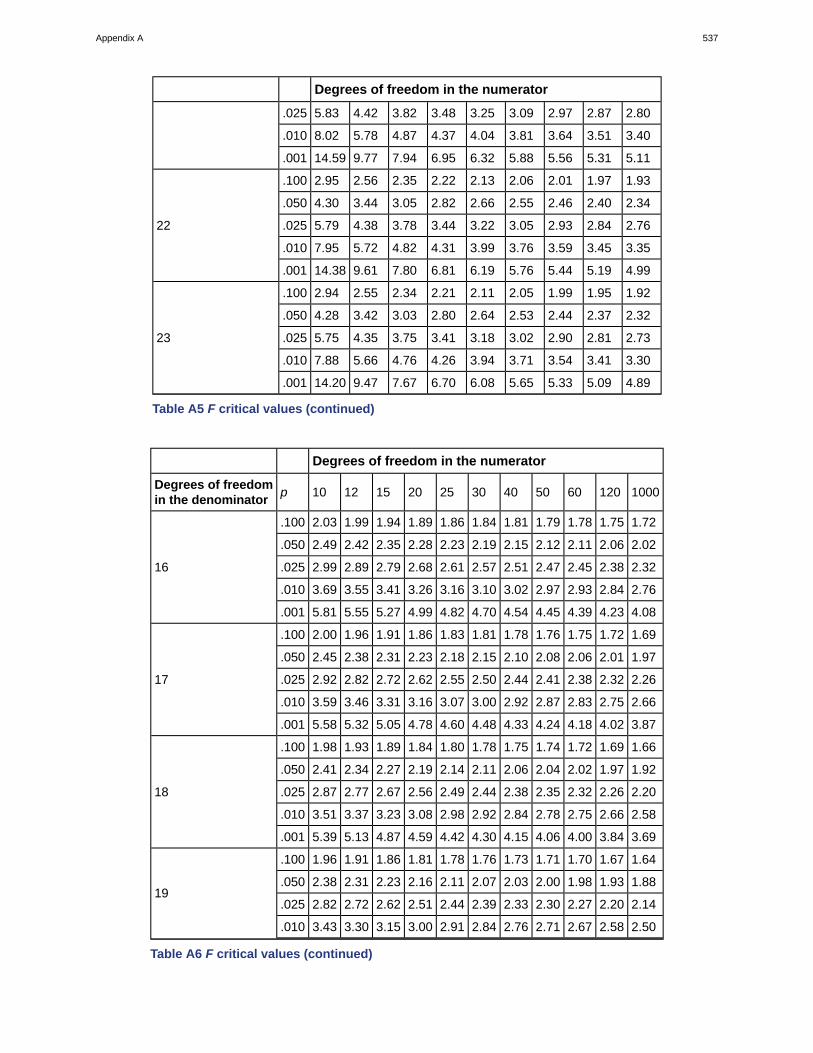
Degrees of freedom in the numerator
.025 5.83 4.42 3.82 3.48 3.25 3.09 2.97 2.87 2.80
.010 8.02 5.78 4.87 4.37 4.04 3.81 3.64 3.51 3.40
.001 14.59 9.77 7.94 6.95 6.32 5.88 5.56 5.31 5.11
.100 2.95 2.56 2.35 2.22 2.13 2.06 2.01 1.97 1.93
.050 4.30 3.44 3.05 2.82 2.66 2.55 2.46 2.40 2.34
.025 5.79 4.38 3.78 3.44 3.22 3.05 2.93 2.84 2.76
.010 7.95 5.72 4.82 4.31 3.99 3.76 3.59 3.45 3.35
22
.001 14.38 9.61 7.80 6.81 6.19 5.76 5.44 5.19 4.99
.100 2.94 2.55 2.34 2.21 2.11 2.05 1.99 1.95 1.92
.050 4.28 3.42 3.03 2.80 2.64 2.53 2.44 2.37 2.32
.025 5.75 4.35 3.75 3.41 3.18 3.02 2.90 2.81 2.73
.010 7.88 5.66 4.76 4.26 3.94 3.71 3.54 3.41 3.30
23
.001 14.20 9.47 7.67 6.70 6.08 5.65 5.33 5.09 4.89
Table A5 F critical values (continued)
Degrees of freedom in the numerator
Degrees of freedomin the denominator
p 10 12 15 20 25 30 40 50 60 120 1000
.100 2.03 1.99 1.94 1.89 1.86 1.84 1.81 1.79 1.78 1.75 1.72
.050 2.49 2.42 2.35 2.28 2.23 2.19 2.15 2.12 2.11 2.06 2.02
.025 2.99 2.89 2.79 2.68 2.61 2.57 2.51 2.47 2.45 2.38 2.32
.010 3.69 3.55 3.41 3.26 3.16 3.10 3.02 2.97 2.93 2.84 2.76
16
.001 5.81 5.55 5.27 4.99 4.82 4.70 4.54 4.45 4.39 4.23 4.08
.100 2.00 1.96 1.91 1.86 1.83 1.81 1.78 1.76 1.75 1.72 1.69
.050 2.45 2.38 2.31 2.23 2.18 2.15 2.10 2.08 2.06 2.01 1.97
.025 2.92 2.82 2.72 2.62 2.55 2.50 2.44 2.41 2.38 2.32 2.26
.010 3.59 3.46 3.31 3.16 3.07 3.00 2.92 2.87 2.83 2.75 2.66
17
.001 5.58 5.32 5.05 4.78 4.60 4.48 4.33 4.24 4.18 4.02 3.87
.100 1.98 1.93 1.89 1.84 1.80 1.78 1.75 1.74 1.72 1.69 1.66
.050 2.41 2.34 2.27 2.19 2.14 2.11 2.06 2.04 2.02 1.97 1.92
.025 2.87 2.77 2.67 2.56 2.49 2.44 2.38 2.35 2.32 2.26 2.20
.010 3.51 3.37 3.23 3.08 2.98 2.92 2.84 2.78 2.75 2.66 2.58
18
.001 5.39 5.13 4.87 4.59 4.42 4.30 4.15 4.06 4.00 3.84 3.69
.100 1.96 1.91 1.86 1.81 1.78 1.76 1.73 1.71 1.70 1.67 1.64
.050 2.38 2.31 2.23 2.16 2.11 2.07 2.03 2.00 1.98 1.93 1.88
.025 2.82 2.72 2.62 2.51 2.44 2.39 2.33 2.30 2.27 2.20 2.1419
.010 3.43 3.30 3.15 3.00 2.91 2.84 2.76 2.71 2.67 2.58 2.50
Table A6 F critical values (continued)
Appendix A 537
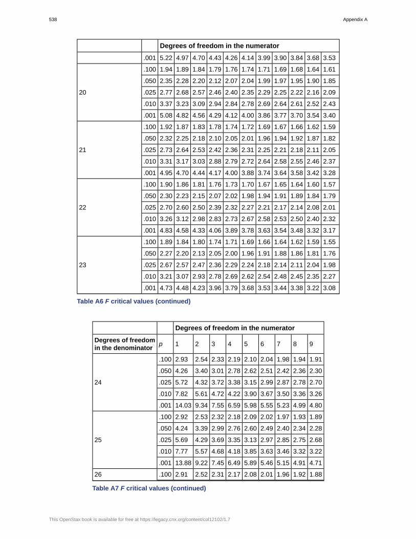
Degrees of freedom in the numerator
.001 5.22 4.97 4.70 4.43 4.26 4.14 3.99 3.90 3.84 3.68 3.53
.100 1.94 1.89 1.84 1.79 1.76 1.74 1.71 1.69 1.68 1.64 1.61
.050 2.35 2.28 2.20 2.12 2.07 2.04 1.99 1.97 1.95 1.90 1.85
.025 2.77 2.68 2.57 2.46 2.40 2.35 2.29 2.25 2.22 2.16 2.09
.010 3.37 3.23 3.09 2.94 2.84 2.78 2.69 2.64 2.61 2.52 2.43
20
.001 5.08 4.82 4.56 4.29 4.12 4.00 3.86 3.77 3.70 3.54 3.40
.100 1.92 1.87 1.83 1.78 1.74 1.72 1.69 1.67 1.66 1.62 1.59
.050 2.32 2.25 2.18 2.10 2.05 2.01 1.96 1.94 1.92 1.87 1.82
.025 2.73 2.64 2.53 2.42 2.36 2.31 2.25 2.21 2.18 2.11 2.05
.010 3.31 3.17 3.03 2.88 2.79 2.72 2.64 2.58 2.55 2.46 2.37
21
.001 4.95 4.70 4.44 4.17 4.00 3.88 3.74 3.64 3.58 3.42 3.28
.100 1.90 1.86 1.81 1.76 1.73 1.70 1.67 1.65 1.64 1.60 1.57
.050 2.30 2.23 2.15 2.07 2.02 1.98 1.94 1.91 1.89 1.84 1.79
.025 2.70 2.60 2.50 2.39 2.32 2.27 2.21 2.17 2.14 2.08 2.01
.010 3.26 3.12 2.98 2.83 2.73 2.67 2.58 2.53 2.50 2.40 2.32
22
.001 4.83 4.58 4.33 4.06 3.89 3.78 3.63 3.54 3.48 3.32 3.17
.100 1.89 1.84 1.80 1.74 1.71 1.69 1.66 1.64 1.62 1.59 1.55
.050 2.27 2.20 2.13 2.05 2.00 1.96 1.91 1.88 1.86 1.81 1.76
.025 2.67 2.57 2.47 2.36 2.29 2.24 2.18 2.14 2.11 2.04 1.98
.010 3.21 3.07 2.93 2.78 2.69 2.62 2.54 2.48 2.45 2.35 2.27
23
.001 4.73 4.48 4.23 3.96 3.79 3.68 3.53 3.44 3.38 3.22 3.08
Table A6 F critical values (continued)
Degrees of freedom in the numerator
Degrees of freedomin the denominator
p 1 2 3 4 5 6 7 8 9
.100 2.93 2.54 2.33 2.19 2.10 2.04 1.98 1.94 1.91
.050 4.26 3.40 3.01 2.78 2.62 2.51 2.42 2.36 2.30
.025 5.72 4.32 3.72 3.38 3.15 2.99 2.87 2.78 2.70
.010 7.82 5.61 4.72 4.22 3.90 3.67 3.50 3.36 3.26
24
.001 14.03 9.34 7.55 6.59 5.98 5.55 5.23 4.99 4.80
.100 2.92 2.53 2.32 2.18 2.09 2.02 1.97 1.93 1.89
.050 4.24 3.39 2.99 2.76 2.60 2.49 2.40 2.34 2.28
.025 5.69 4.29 3.69 3.35 3.13 2.97 2.85 2.75 2.68
.010 7.77 5.57 4.68 4.18 3.85 3.63 3.46 3.32 3.22
25
.001 13.88 9.22 7.45 6.49 5.89 5.46 5.15 4.91 4.71
26 .100 2.91 2.52 2.31 2.17 2.08 2.01 1.96 1.92 1.88
Table A7 F critical values (continued)
538 Appendix A
This OpenStax book is available for free at https://legacy.cnx.org/content/col12102/1.7

Degrees of freedom in the numerator
.050 4.23 3.37 2.98 2.74 2.59 2.47 2.39 2.32 2.27
.025 5.66 4.27 3.67 3.33 3.10 2.94 2.82 2.73 2.65
.010 7.72 5.53 4.64 4.14 3.82 3.59 3.42 3.29 3.18
.001 13.74 9.12 7.36 6.41 5.80 5.38 5.07 4.83 4.64
.100 2.90 2.51 2.30 2.17 2.07 2.00 1.95 1.91 1.87
.050 4.21 3.35 2.96 2.73 2.57 2.46 2.37 2.31 2.25
.025 5.63 4.24 3.65 3.31 3.08 2.92 2.80 2.71 2.63
.010 7.68 5.49 4.60 4.11 3.78 3.56 3.39 3.26 3.15
27
.001 13.61 9.02 7.27 6.33 5.73 5.31 5.00 4.76 4.57
.100 2.89 2.50 2.29 2.16 2.06 2.00 1.94 1.90 1.87
.050 4.20 3.34 2.95 2.71 2.56 2.45 2.36 2.29 2.24
.025 5.61 4.22 3.63 3.29 3.06 2.90 2.78 2.69 2.61
.010 7.64 5.45 4.57 4.07 3.75 3.53 3.36 3.23 3.12
28
.001 13.50 8.93 7.19 6.25 5.66 5.24 4.93 4.69 4.50
.100 2.89 2.50 2.28 2.15 2.06 1.99 1.93 1.89 1.86
.050 4.18 3.33 2.93 2.70 2.55 2.43 2.35 2.28 2.22
.025 5.59 4.20 3.61 3.27 3.04 2.88 2.76 2.67 2.59
.010 7.60 5.42 4.54 4.04 3.73 3.50 3.33 3.20 3.09
29
.001 13.39 8.85 7.12 6.19 5.59 5.18 4.87 4.64 4.45
.100 2.88 2.49 2.28 2.14 2.05 1.98 1.93 1.88 1.85
.050 4.17 3.32 2.92 2.69 2.53 2.42 2.33 2.27 2.21
.025 5.57 4.18 3.59 3.25 3.03 2.87 2.75 2.65 2.57
.010 7.56 5.39 4.51 4.02 3.70 3.47 3.30 3.17 3.07
30
.001 13.29 8.77 7.05 6.12 5.53 5.12 4.82 4.58 4.39
.100 2.84 2.44 2.23 2.09 2.00 1.93 1.87 1.83 1.79
.050 4.08 3.23 2.84 2.61 2.45 2.34 2.25 2.18 2.12
.025 5.42 4.05 3.46 3.13 2.90 2.74 2.62 2.53 2.45
.010 7.31 5.18 4.31 3.83 3.51 3.29 3.12 2.99 2.89
40
.001 12.61 8.25 6.59 5.70 5.13 4.73 4.44 4.21 4.02
Table A7 F critical values (continued)
Degrees of freedom in the numerator
Degrees of freedomin the denominator
p 10 12 15 20 25 30 40 50 60 120 1000
.100 1.88 1.83 1.78 1.73 1.70 1.67 1.64 1.62 1.61 1.57 1.54
.050 2.25 2.18 2.11 2.03 1.97 1.94 1.89 1.86 1.84 1.79 1.7424
.025 2.64 2.54 2.44 2.33 2.26 2.21 2.15 2.11 2.08 2.01 1.94
Table A8 F critical values (continued)
Appendix A 539
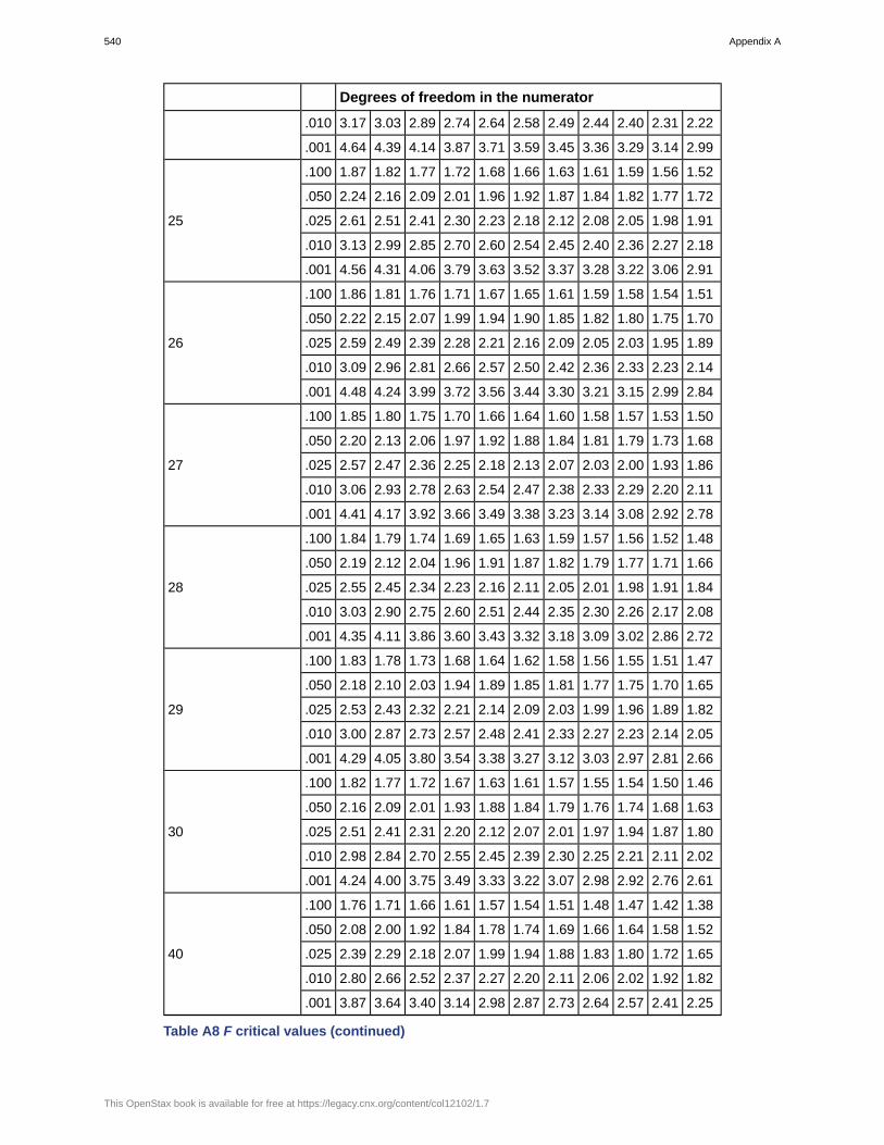
Degrees of freedom in the numerator
.010 3.17 3.03 2.89 2.74 2.64 2.58 2.49 2.44 2.40 2.31 2.22
.001 4.64 4.39 4.14 3.87 3.71 3.59 3.45 3.36 3.29 3.14 2.99
.100 1.87 1.82 1.77 1.72 1.68 1.66 1.63 1.61 1.59 1.56 1.52
.050 2.24 2.16 2.09 2.01 1.96 1.92 1.87 1.84 1.82 1.77 1.72
.025 2.61 2.51 2.41 2.30 2.23 2.18 2.12 2.08 2.05 1.98 1.91
.010 3.13 2.99 2.85 2.70 2.60 2.54 2.45 2.40 2.36 2.27 2.18
25
.001 4.56 4.31 4.06 3.79 3.63 3.52 3.37 3.28 3.22 3.06 2.91
.100 1.86 1.81 1.76 1.71 1.67 1.65 1.61 1.59 1.58 1.54 1.51
.050 2.22 2.15 2.07 1.99 1.94 1.90 1.85 1.82 1.80 1.75 1.70
.025 2.59 2.49 2.39 2.28 2.21 2.16 2.09 2.05 2.03 1.95 1.89
.010 3.09 2.96 2.81 2.66 2.57 2.50 2.42 2.36 2.33 2.23 2.14
26
.001 4.48 4.24 3.99 3.72 3.56 3.44 3.30 3.21 3.15 2.99 2.84
.100 1.85 1.80 1.75 1.70 1.66 1.64 1.60 1.58 1.57 1.53 1.50
.050 2.20 2.13 2.06 1.97 1.92 1.88 1.84 1.81 1.79 1.73 1.68
.025 2.57 2.47 2.36 2.25 2.18 2.13 2.07 2.03 2.00 1.93 1.86
.010 3.06 2.93 2.78 2.63 2.54 2.47 2.38 2.33 2.29 2.20 2.11
27
.001 4.41 4.17 3.92 3.66 3.49 3.38 3.23 3.14 3.08 2.92 2.78
.100 1.84 1.79 1.74 1.69 1.65 1.63 1.59 1.57 1.56 1.52 1.48
.050 2.19 2.12 2.04 1.96 1.91 1.87 1.82 1.79 1.77 1.71 1.66
.025 2.55 2.45 2.34 2.23 2.16 2.11 2.05 2.01 1.98 1.91 1.84
.010 3.03 2.90 2.75 2.60 2.51 2.44 2.35 2.30 2.26 2.17 2.08
28
.001 4.35 4.11 3.86 3.60 3.43 3.32 3.18 3.09 3.02 2.86 2.72
.100 1.83 1.78 1.73 1.68 1.64 1.62 1.58 1.56 1.55 1.51 1.47
.050 2.18 2.10 2.03 1.94 1.89 1.85 1.81 1.77 1.75 1.70 1.65
.025 2.53 2.43 2.32 2.21 2.14 2.09 2.03 1.99 1.96 1.89 1.82
.010 3.00 2.87 2.73 2.57 2.48 2.41 2.33 2.27 2.23 2.14 2.05
29
.001 4.29 4.05 3.80 3.54 3.38 3.27 3.12 3.03 2.97 2.81 2.66
.100 1.82 1.77 1.72 1.67 1.63 1.61 1.57 1.55 1.54 1.50 1.46
.050 2.16 2.09 2.01 1.93 1.88 1.84 1.79 1.76 1.74 1.68 1.63
.025 2.51 2.41 2.31 2.20 2.12 2.07 2.01 1.97 1.94 1.87 1.80
.010 2.98 2.84 2.70 2.55 2.45 2.39 2.30 2.25 2.21 2.11 2.02
30
.001 4.24 4.00 3.75 3.49 3.33 3.22 3.07 2.98 2.92 2.76 2.61
.100 1.76 1.71 1.66 1.61 1.57 1.54 1.51 1.48 1.47 1.42 1.38
.050 2.08 2.00 1.92 1.84 1.78 1.74 1.69 1.66 1.64 1.58 1.52
.025 2.39 2.29 2.18 2.07 1.99 1.94 1.88 1.83 1.80 1.72 1.65
.010 2.80 2.66 2.52 2.37 2.27 2.20 2.11 2.06 2.02 1.92 1.82
40
.001 3.87 3.64 3.40 3.14 2.98 2.87 2.73 2.64 2.57 2.41 2.25
Table A8 F critical values (continued)
540 Appendix A
This OpenStax book is available for free at https://legacy.cnx.org/content/col12102/1.7

Degrees of freedom in the numerator
Degrees of freedomin the denominator
p 1 2 3 4 5 6 7 8 9
.100 2.81 2.41 2.20 2.06 1.97 1.90 1.84 1.80 1.76
.050 4.03 3.18 2.79 2.56 2.40 2.29 2.20 2.13 2.07
.025 5.34 3.97 3.39 3.05 2.83 2.67 2.55 2.46 2.38
.010 7.17 5.06 4.20 3.72 3.41 3.19 3.02 2.89 2.78
50
.001 12.22 7.96 6.34 5.46 4.90 4.51 4.22 4.00 3.82
.100 2.79 2.39 2.18 2.04 1.95 1.87 1.82 1.77 1.74
.050 4.00 3.15 2.76 2.53 2.37 2.25 2.17 2.10 2.04
.025 5.29 3.93 3.34 3.01 2.79 2.63 2.51 2.41 2.33
.010 7.08 4.98 4.13 3.65 3.34 3.12 2.95 2.82 2.72
60
.001 11.97 7.77 6.17 5.31 4.76 4.37 4.09 3.86 3.69
.100 2.76 2.36 2.14 2.00 1.91 1.83 1.78 1.73 1.69
.050 3.94 3.09 2.70 2.46 2.31 2.19 2.10 2.03 1.97
.025 5.18 3.83 3.25 2.92 2.70 2.54 2.42 2.32 2.24
.010 6.90 4.82 3.98 3.51 3.21 2.99 2.82 2.69 2.59
100
.001 11.50 7.41 5.86 5.02 4.48 4.11 3.83 3.61 3.44
.100 2.73 2.33 2.11 1.97 1.88 1.80 1.75 1.70 1.66
.050 3.89 3.04 2.65 2.42 2.26 2.14 2.06 1.98 1.93
.025 5.10 3.76 3.18 2.85 2.63 2.47 2.35 2.26 2.18
.010 6.76 4.71 3.88 3.41 3.11 2.89 2.73 2.60 2.50
200
.001 11.15 7.15 5.63 4.81 4.29 3.92 3.65 3.43 3.26
.100 2.71 2.31 2.09 1.95 1.85 1.78 1.72 1.68 1.64
.050 3.85 3.00 2.61 2.38 2.22 2.11 2.02 1.95 1.89
.025 5.04 3.70 3.13 2.80 2.58 2.42 2.30 2.20 2.13
.010 6.66 4.63 3.80 3.34 3.04 2.82 2.66 2.53 2.43
1000
.001 10.89 6.96 5.46 4.65 4.14 3.78 3.51 3.30 3.13
Table A9 F critical values (continued)
Degrees of freedom in the numerator
Degrees of freedomin the denominator
p 10 12 15 20 25 30 40 50 60 120 1000
.100 1.73 1.68 1.63 1.57 1.53 1.50 1.46 1.44 1.42 1.38 1.33
.050 2.03 1.95 1.87 1.78 1.73 1.69 1.63 1.60 1.58 1.51 1.45
.025 2.32 2.22 2.11 1.99 1.92 1.87 1.80 1.75 1.72 1.64 1.56
.010 2.70 2.56 2.42 2.27 2.17 2.10 2.01 1.95 1.91 1.80 1.70
50
.001 3.67 3.44 3.20 2.95 2.79 2.68 2.53 2.44 2.38 2.21 2.05
Table A10 F critical values (continued)
Appendix A 541

Degrees of freedom in the numerator
.100 1.71 1.66 1.60 1.54 1.50 1.48 1.44 1.41 1.40 1.35 1.30
.050 1.99 1.92 1.84 1.75 1.69 1.65 1.59 1.56 1.53 1.47 1.40
.025 2.27 2.17 2.06 1.94 1.87 1.82 1.74 1.70 1.67 1.58 1.49
.010 2.63 2.50 2.35 2.20 2.10 2.03 1.94 1.88 1.84 1.73 1.62
60
.001 3.54 3.32 3.08 2.83 2.67 2.55 2.41 2.32 2.25 2.08 1.92
.100 1.66 1.61 1.56 1.49 1.45 1.42 1.38 1.35 1.34 1.28 1.22
.050 1.93 1.85 1.77 1.68 1.62 1.57 1.52 1.48 1.45 1.38 1.30
.025 2.18 2.08 1.97 1.85 1.77 1.71 1.64 1.59 1.56 1.46 1.36
.010 2.50 2.37 2.22 2.07 1.97 1.89 1.80 1.74 1.69 1.57 1.45
100
.001 3.30 3.07 2.84 2.59 2.43 2.32 2.17 2.08 2.01 1.83 1.64
.100 1.63 1.58 1.52 1.46 1.41 1.38 1.34 1.31 1.29 1.23 1.16
.050 1.88 1.80 1.72 1.62 1.56 1.52 1.46 1.41 1.39 1.30 1.21
.025 2.11 2.01 1.90 1.78 1.70 1.64 1.56 1.51 1.47 1.37 1.25
.010 2.41 2.27 2.13 1.97 1.87 1.79 1.69 1.63 1.58 1.45 1.30
200
.001 3.12 2.90 2.67 2.42 2.26 2.15 2.00 1.90 1.83 1.64 1.43
.100 1.61 1.55 1.49 1.43 1.38 1.35 1.30 1.27 1.25 1.18 1.08
.050 1.84 1.76 1.68 1.58 1.52 1.47 1.41 1.36 1.33 1.24 1.11
.025 2.06 1.96 1.85 1.72 1.64 1.58 1.50 1.45 1.41 1.29 1.13
.010 2.34 2.20 2.06 1.90 1.79 1.72 1.61 1.54 1.50 1.35 1.16
1000
.001 2.99 2.77 2.54 2.30 2.14 2.02 1.87 1.77 1.69 1.49 1.22
Table A10 F critical values (continued)
Numerical entries represent the probability that a standard normal random variable is between 0 and z where z = x − μσ .
Figure A2
542 Appendix A
This OpenStax book is available for free at https://legacy.cnx.org/content/col12102/1.7

Standard Normal Probability Distribution: Z Table
z 0.00 0.01 0.02 0.03 0.04 0.05 0.06 0.07 0.08 0.09
0.0 0.0000 0.0040 0.0080 0.0120 0.0160 0.0199 0.0239 0.0279 0.0319 0.0359
0.1 0.0398 0.0438 0.0478 0.0517 0.0557 0.0596 0.0636 0.0675 0.0714 0.0753
0.2 0.0793 0.0832 0.0871 0.0910 0.0948 0.0987 0.1026 0.1064 0.1103 0.1141
0.3 0.1179 0.1217 0.1255 0.1293 0.1331 0.1368 0.1406 0.1443 0.1480 0.1517
0.4 0.1554 0.1591 0.1628 0.1664 0.1700 0.1736 0.1772 0.1808 0.1844 0.1879
0.5 0.1915 0.1950 0.1985 0.2019 0.2054 0.2088 0.2123 0.2157 0.2190 0.2224
0.6 0.2257 0.2291 0.2324 0.2357 0.2389 0.2422 0.2454 0.2486 0.2517 0.2549
0.7 0.2580 0.2611 0.2642 0.2673 0.2704 0.2734 0.2764 0.2794 0.2823 0.2852
0.8 0.2881 0.2910 0.2939 0.2967 0.2995 0.3023 0.3051 0.3078 0.3106 0.3133
0.9 0.3159 0.3186 0.3212 0.3238 0.3264 0.3289 0.3315 0.3340 0.3365 0.3389
1.0 0.3413 0.3438 0.3461 0.3485 0.3508 0.3531 0.3554 0.3577 0.3599 0.3621
1.1 0.3643 0.3665 0.3686 0.3708 0.3729 0.3749 0.3770 0.3790 0.3810 0.3830
1.2 0.3849 0.3869 0.3888 0.3907 0.3925 0.3944 0.3962 0.3980 0.3997 0.4015
1.3 0.4032 0.4049 0.4066 0.4082 0.4099 0.4115 0.4131 0.4147 0.4162 0.4177
1.4 0.4192 0.4207 0.4222 0.4236 0.4251 0.4265 0.4279 0.4292 0.4306 0.4319
1.5 0.4332 0.4345 0.4357 0.4370 0.4382 0.4394 0.4406 0.4418 0.4429 0.4441
1.6 0.4452 0.4463 0.4474 0.4484 0.4495 0.4505 0.4515 0.4525 0.4535 0.4545
1.7 0.4554 0.4564 0.4573 0.4582 0.4591 0.4599 0.4608 0.4616 0.4625 0.4633
1.8 0.4641 0.4649 0.4656 0.4664 0.4671 0.4678 0.4686 0.4693 0.4699 0.4706
1.9 0.4713 0.4719 0.4726 0.4732 0.4738 0.4744 0.4750 0.4756 0.4761 0.4767
2.0 0.4772 0.4778 0.4783 0.4788 0.4793 0.4798 0.4803 0.4808 0.4812 0.4817
2.1 0.4821 0.4826 0.4830 0.4834 0.4838 0.4842 0.4846 0.4850 0.4854 0.4857
2.2 0.4861 0.4864 0.4868 0.4871 0.4875 0.4878 0.4881 0.4884 0.4887 0.4890
2.3 0.4893 0.4896 0.4898 0.4901 0.4904 0.4906 0.4909 0.4911 0.4913 0.4916
2.4 0.4918 0.4920 0.4922 0.4925 0.4927 0.4929 0.4931 0.4932 0.4934 0.4936
2.5 0.4938 0.4940 0.4941 0.4943 0.4945 0.4946 0.4948 0.4949 0.4951 0.4952
2.6 0.4953 0.4955 0.4956 0.4957 0.4959 0.4960 0.4961 0.4962 0.4963 0.4964
2.7 0.4965 0.4966 0.4967 0.4968 0.4969 0.4970 0.4971 0.4972 0.4973 0.4974
2.8 0.4974 0.4975 0.4976 0.4977 0.4977 0.4978 0.4979 0.4979 0.4980 0.4981
2.9 0.4981 0.4982 0.4982 0.4983 0.4984 0.4984 0.4985 0.4985 0.4986 0.4986
3.0 0.4987 0.4987 0.4987 0.4988 0.4988 0.4989 0.4989 0.4989 0.4990 0.4990
3.1 0.4990 0.4991 0.4991 0.4991 0.4992 0.4992 0.4992 0.4992 0.4993 0.4993
3.2 0.4993 0.4993 0.4994 0.4994 0.4994 0.4994 0.4994 0.4995 0.4995 0.4995
3.3 0.4995 0.4995 0.4995 0.4996 0.4996 0.4996 0.4996 0.4996 0.4996 0.4997
3.4 0.4997 0.4997 0.4997 0.4997 0.4997 0.4997 0.4997 0.4997 0.4997 0.4998
Table A11 Standard Normal Distribution
Appendix A 543

Student's t Distribution
Figure A3 Upper critical values of Student's t Distribution with v Degrees of Freedom
For selected probabilities, a, the table shows the values tv,a such that P(tv > tv,a) = a, where tv is a Student’s t random variablewith v degrees of freedom. For example, the probability is .10 that a Student’s t random variable with 10 degrees of freedomexceeds 1.372.
v 0.10 0.05 0.025 0.01 0.005 0.001
1 3.078 6.314 12.706 31.821 63.657 318.313
2 1.886 2.920 4.303 6.965 9.925 22.327
3 1.638 2.353 3.182 4.541 5.841 10.215
4 1.533 2.132 2.776 3.747 4.604 7.173
5 1.476 2.015 2.571 3.365 4.032 5.893
6 1.440 1.943 2.447 3.143 3.707 5.208
7 1.415 1.895 2.365 2.998 3.499 4.782
8 1.397 1.860 2.306 2.896 3.355 4.499
9 1.383 1.833 2.262 2.821 3.250 4.296
10 1.372 1.812 2.228 2.764 3.169 4.143
11 1.363 1.796 2.201 2.718 3.106 4.024
12 1.356 1.782 2.179 2.681 3.055 3.929
13 1.350 1.771 2.160 2.650 3.012 3.852
14 1.345 1.761 2.145 2.624 2.977 3.787
15 1.341 1.753 2.131 2.602 2.947 3.733
16 1.337 1.746 2.120 2.583 2.921 3.686
17 1.333 1.740 2.110 2.567 2.898 3.646
18 1.330 1.734 2.101 2.552 2.878 3.610
Table A12 Probability of Exceeding the CriticalValue NIST/SEMATECH e-Handbook of StatisticalMethods, http://www.itl.nist.gov/div898/handbook/,September 2011.
544 Appendix A
This OpenStax book is available for free at https://legacy.cnx.org/content/col12102/1.7

v 0.10 0.05 0.025 0.01 0.005 0.001
19 1.328 1.729 2.093 2.539 2.861 3.579
20 1.325 1.725 2.086 2.528 2.845 3.552
21 1.323 1.721 2.080 2.518 2.831 3.527
22 1.321 1.717 2.074 2.508 2.819 3.505
23 1.319 1.714 2.069 2.500 2.807 3.485
24 1.318 1.711 2.064 2.492 2.797 3.467
25 1.316 1.708 2.060 2.485 2.787 3.450
26 1.315 1.706* 2.056 2.479 2.779 3.435
27 1.314 1.703 2.052 2.473 2.771 3.421
28 1.313 1.701 2.048 2.467 2.763 3.408
29 1.311 1.699 2.045 2.462 2.756 3.396
30 1.310 1.697 2.042 2.457 2.750 3.385
40 1.303 1.684 2.021 2.423 2.704 3.307
60 1.296 1.671 2.000 2.390 2.660 3.232
100 1.290 1.660 1.984 2.364 2.626 3.174
∞ 1.282 1.645 1.960 2.326 2.576 3.090
Table A12 Probability of Exceeding the CriticalValue NIST/SEMATECH e-Handbook of StatisticalMethods, http://www.itl.nist.gov/div898/handbook/,September 2011.
Figure A4
Appendix A 545

χ2 Probability Distribution
df 0.995 0.990 0.975 0.950 0.900 0.100 0.050 0.025 0.010 0.005
1 0.000 0.000 0.001 0.004 0.016 2.706 3.841 5.024 6.635 7.879
2 0.010 0.020 0.051 0.103 0.211 4.605 5.991 7.378 9.210 10.597
3 0.072 0.115 0.216 0.352 0.584 6.251 7.815 9.348 11.345 12.838
4 0.207 0.297 0.484 0.711 1.064 7.779 9.488 11.143 13.277 14.860
5 0.412 0.554 0.831 1.145 1.610 9.236 11.070 12.833 15.086 16.750
6 0.676 0.872 1.237 1.635 2.204 10.645 12.592 14.449 16.812 18.548
7 0.989 1.239 1.690 2.167 2.833 12.017 14.067 16.013 18.475 20.278
8 1.344 1.646 2.180 2.733 3.490 13.362 15.507 17.535 20.090 21.955
9 1.735 2.088 2.700 3.325 4.168 14.684 16.919 19.023 21.666 23.589
10 2.156 2.558 3.247 3.940 4.865 15.987 18.307 20.483 23.209 25.188
11 2.603 3.053 3.816 4.575 5.578 17.275 19.675 21.920 24.725 26.757
12 3.074 3.571 4.404 5.226 6.304 18.549 21.026 23.337 26.217 28.300
13 3.565 4.107 5.009 5.892 7.042 19.812 22.362 24.736 27.688 29.819
14 4.075 4.660 5.629 6.571 7.790 21.064 23.685 26.119 29.141 31.319
15 4.601 5.229 6.262 7.261 8.547 22.307 24.996 27.488 30.578 32.801
16 5.142 5.812 6.908 7.962 9.312 23.542 26.296 28.845 32.000 34.267
17 5.697 6.408 7.564 8.672 10.085 24.769 27.587 30.191 33.409 35.718
18 6.265 7.015 8.231 9.390 10.865 25.989 28.869 31.526 34.805 37.156
19 6.844 7.633 8.907 10.117 11.651 27.204 30.144 32.852 36.191 38.582
20 7.434 8.260 9.591 10.851 12.443 28.412 31.410 34.170 37.566 39.997
21 8.034 8.897 10.283 11.591 13.240 29.615 32.671 35.479 38.932 41.401
22 8.643 9.542 10.982 12.338 14.041 30.813 33.924 36.781 40.289 42.796
23 9.260 10.196 11.689 13.091 14.848 32.007 35.172 38.076 41.638 44.181
24 9.886 10.856 12.401 13.848 15.659 33.196 36.415 39.364 42.980 45.559
25 10.520 11.524 13.120 14.611 16.473 34.382 37.652 40.646 44.314 46.928
26 11.160 12.198 13.844 15.379 17.292 35.563 38.885 41.923 45.642 48.290
27 11.808 12.879 14.573 16.151 18.114 36.741 40.113 43.195 46.963 49.645
28 12.461 13.565 15.308 16.928 18.939 37.916 41.337 44.461 48.278 50.993
29 13.121 14.256 16.047 17.708 19.768 39.087 42.557 45.722 49.588 52.336
30 13.787 14.953 16.791 18.493 20.599 40.256 43.773 46.979 50.892 53.672
40 20.707 22.164 24.433 26.509 29.051 51.805 55.758 59.342 63.691 66.766
50 27.991 29.707 32.357 34.764 37.689 63.167 67.505 71.420 76.154 79.490
60 35.534 37.485 40.482 43.188 46.459 74.397 79.082 83.298 88.379 91.952
70 43.275 45.442 48.758 51.739 55.329 85.527 90.531 95.023 100.425 104.215
Table A13 Area to the Right of the Critical Value of χ2
546 Appendix A
This OpenStax book is available for free at https://legacy.cnx.org/content/col12102/1.7

df 0.995 0.990 0.975 0.950 0.900 0.100 0.050 0.025 0.010 0.005
80 51.172 53.540 57.153 60.391 64.278 96.578 101.879 106.629 112.329 116.321
90 59.196 61.754 65.647 69.126 73.291 107.565 113.145 118.136 124.116 128.299
100 67.328 70.065 74.222 77.929 82.358 118.498 124.342 129.561 135.807 140.169
Table A13 Area to the Right of the Critical Value of χ2
Data SetsLap TimesThe following tables provide lap times from Terri Vogel's log book. Times are recorded in seconds for 2.5-mile lapscompleted in a series of races and practice runs.
Lap 1 Lap 2 Lap 3 Lap 4 Lap 5 Lap 6 Lap 7
Race 1 135 130 131 132 130 131 133
Race 2 134 131 131 129 128 128 129
Race 3 129 128 127 127 130 127 129
Race 4 125 125 126 125 124 125 125
Race 5 133 132 132 132 131 130 132
Race 6 130 130 130 129 129 130 129
Race 7 132 131 133 131 134 134 131
Race 8 127 128 127 130 128 126 128
Race 9 132 130 127 128 126 127 124
Race 10 135 131 131 132 130 131 130
Race 11 132 131 132 131 130 129 129
Race 12 134 130 130 130 131 130 130
Race 13 128 127 128 128 128 129 128
Race 14 132 131 131 131 132 130 130
Race 15 136 129 129 129 129 129 129
Race 16 129 129 129 128 128 129 129
Race 17 134 131 132 131 132 132 132
Race 18 129 129 130 130 133 133 127
Race 19 130 129 129 129 129 129 128
Race 20 131 128 130 128 129 130 130
Table A14 Race Lap Times (in seconds)
Appendix A 547
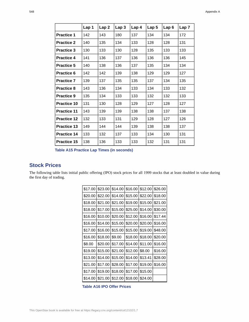
Lap 1 Lap 2 Lap 3 Lap 4 Lap 5 Lap 6 Lap 7
Practice 1 142 143 180 137 134 134 172
Practice 2 140 135 134 133 128 128 131
Practice 3 130 133 130 128 135 133 133
Practice 4 141 136 137 136 136 136 145
Practice 5 140 138 136 137 135 134 134
Practice 6 142 142 139 138 129 129 127
Practice 7 139 137 135 135 137 134 135
Practice 8 143 136 134 133 134 133 132
Practice 9 135 134 133 133 132 132 133
Practice 10 131 130 128 129 127 128 127
Practice 11 143 139 139 138 138 137 138
Practice 12 132 133 131 129 128 127 126
Practice 13 149 144 144 139 138 138 137
Practice 14 133 132 137 133 134 130 131
Practice 15 138 136 133 133 132 131 131
Table A15 Practice Lap Times (in seconds)
Stock PricesThe following table lists initial public offering (IPO) stock prices for all 1999 stocks that at least doubled in value duringthe first day of trading.
$17.00 $23.00 $14.00 $16.00 $12.00 $26.00
$20.00 $22.00 $14.00 $15.00 $22.00 $18.00
$18.00 $21.00 $21.00 $19.00 $15.00 $21.00
$18.00 $17.00 $15.00 $25.00 $14.00 $30.00
$16.00 $10.00 $20.00 $12.00 $16.00 $17.44
$16.00 $14.00 $15.00 $20.00 $20.00 $16.00
$17.00 $16.00 $15.00 $15.00 $19.00 $48.00
$16.00 $18.00 $9.00 $18.00 $18.00 $20.00
$8.00 $20.00 $17.00 $14.00 $11.00 $16.00
$19.00 $15.00 $21.00 $12.00 $8.00 $16.00
$13.00 $14.00 $15.00 $14.00 $13.41 $28.00
$21.00 $17.00 $28.00 $17.00 $19.00 $16.00
$17.00 $19.00 $18.00 $17.00 $15.00
$14.00 $21.00 $12.00 $18.00 $24.00
Table A16 IPO Offer Prices
548 Appendix A
This OpenStax book is available for free at https://legacy.cnx.org/content/col12102/1.7

$15.00 $23.00 $14.00 $16.00 $12.00
$24.00 $20.00 $14.00 $14.00 $15.00
$14.00 $19.00 $16.00 $38.00 $20.00
$24.00 $16.00 $8.00 $18.00 $17.00
$16.00 $15.00 $7.00 $19.00 $12.00
$8.00 $23.00 $12.00 $18.00 $20.00
$21.00 $34.00 $16.00 $26.00 $14.00
Table A16 IPO Offer Prices
ReferencesData compiled by Jay R. Ritter of University of Florida using data from Securities Data Co. and Bloomberg.
Appendix A 549

550 Appendix A
This OpenStax book is available for free at https://legacy.cnx.org/content/col12102/1.7

APPENDIX B:MATHEMATICALPHRASES, SYMBOLS,
AND FORMULASEnglish Phrases Written Mathematically
When the English says: Interpret this as:
X is at least 4. X ≥ 4
The minimum of X is 4. X ≥ 4
X is no less than 4. X ≥ 4
X is greater than or equal to 4. X ≥ 4
X is at most 4. X ≤ 4
The maximum of X is 4. X ≤ 4
X is no more than 4. X ≤ 4
X is less than or equal to 4. X ≤ 4
X does not exceed 4. X ≤ 4
X is greater than 4. X > 4
X is more than 4. X > 4
X exceeds 4. X > 4
X is less than 4. X < 4
There are fewer X than 4. X < 4
X is 4. X = 4
X is equal to 4. X = 4
X is the same as 4. X = 4
X is not 4. X ≠ 4
X is not equal to 4. X ≠ 4
X is not the same as 4. X ≠ 4
X is different than 4. X ≠ 4
Table B1
Appendix B 551
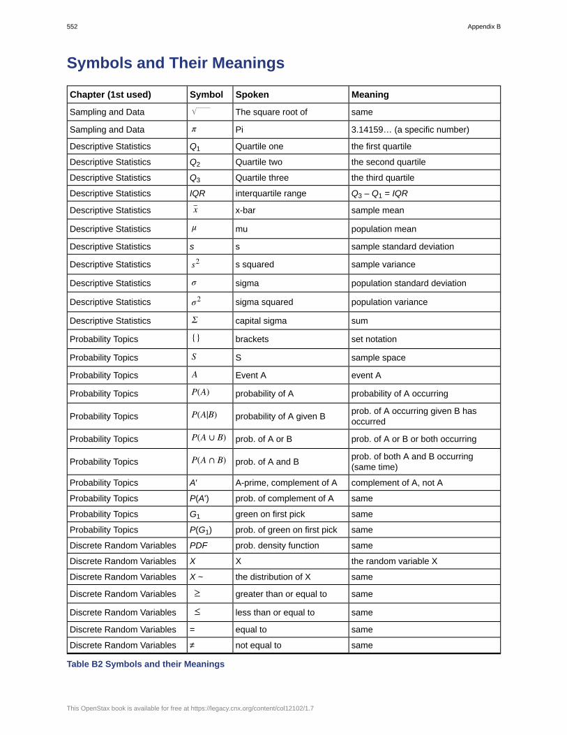
Symbols and Their Meanings
Chapter (1st used) Symbol Spoken Meaning
Sampling and Data The square root of same
Sampling and Data π Pi 3.14159… (a specific number)
Descriptive Statistics Q1 Quartile one the first quartile
Descriptive Statistics Q2 Quartile two the second quartile
Descriptive Statistics Q3 Quartile three the third quartile
Descriptive Statistics IQR interquartile range Q3 – Q1 = IQR
Descriptive Statistics x– x-bar sample mean
Descriptive Statistics μ mu population mean
Descriptive Statistics s s sample standard deviation
Descriptive Statistics s2 s squared sample variance
Descriptive Statistics σ sigma population standard deviation
Descriptive Statistics σ2 sigma squared population variance
Descriptive Statistics Σ capital sigma sum
Probability Topics {} brackets set notation
Probability Topics S S sample space
Probability Topics A Event A event A
Probability Topics P(A) probability of A probability of A occurring
Probability Topics P(A|B) probability of A given Bprob. of A occurring given B hasoccurred
Probability Topics P(A ∪ B) prob. of A or B prob. of A or B or both occurring
Probability Topics P(A ∩ B) prob. of A and Bprob. of both A and B occurring(same time)
Probability Topics A′ A-prime, complement of A complement of A, not A
Probability Topics P(A') prob. of complement of A same
Probability Topics G1 green on first pick same
Probability Topics P(G1) prob. of green on first pick same
Discrete Random Variables PDF prob. density function same
Discrete Random Variables X X the random variable X
Discrete Random Variables X ~ the distribution of X same
Discrete Random Variables ≥ greater than or equal to same
Discrete Random Variables ≤ less than or equal to same
Discrete Random Variables = equal to same
Discrete Random Variables ≠ not equal to same
Table B2 Symbols and their Meanings
552 Appendix B
This OpenStax book is available for free at https://legacy.cnx.org/content/col12102/1.7

Chapter (1st used) Symbol Spoken Meaning
Continuous RandomVariables
f(x) f of x function of x
Continuous RandomVariables
pdf prob. density function same
Continuous RandomVariables
U uniform distribution same
Continuous RandomVariables
Exp exponential distribution same
Continuous RandomVariables
f(x) = f of x equals same
Continuous RandomVariables
m m decay rate (for exp. dist.)
The Normal Distribution N normal distribution same
The Normal Distribution z z-score same
The Normal Distribution Z standard normal dist. same
The Central Limit Theorem X– X-bar the random variable X-bar
The Central Limit Theorem μ x– mean of X-bars the average of X-bars
The Central Limit Theorem σ x– standard deviation of X-bars same
Confidence Intervals CL confidence level same
Confidence Intervals CI confidence interval same
Confidence Intervals EBM error bound for a mean same
Confidence Intervals EBP error bound for a proportion same
Confidence Intervals t Student's t-distribution same
Confidence Intervals df degrees of freedom same
Confidence Intervals tα2
student t with α/2 area inright tail
same
Confidence Intervals p′ p-prime sample proportion of success
Confidence Intervals q′ q-prime sample proportion of failure
Hypothesis Testing H0 H-naught, H-sub 0 null hypothesis
Hypothesis Testing Ha H-a, H-sub a alternate hypothesis
Hypothesis Testing H1 H-1, H-sub 1 alternate hypothesis
Hypothesis Testing α alpha probability of Type I error
Hypothesis Testing β beta probability of Type II error
Hypothesis Testing X1–
– X2 X1-bar minus X2-bar difference in sample means
Hypothesis Testing μ1 − μ2 mu-1 minus mu-2 difference in population means
Hypothesis Testing P′1 − P′2 P1-prime minus P2-prime difference in sample proportions
Table B2 Symbols and their Meanings
Appendix B 553

Chapter (1st used) Symbol Spoken Meaning
Hypothesis Testing p1 − p2 p1 minus p2 difference in population proportions
Chi-Square Distribution Χ2 Ky-square Chi-square
Chi-Square Distribution O Observed Observed frequency
Chi-Square Distribution E Expected Expected frequency
Linear Regression andCorrelation
y = a + bx y equals a plus b-x equation of a straight line
Linear Regression andCorrelation
y^ y-hat estimated value of y
Linear Regression andCorrelation
r sample correlationcoefficient
same
Linear Regression andCorrelation
ε error term for a regressionline
same
Linear Regression andCorrelation
SSE Sum of Squared Errors same
F-Distribution and ANOVA F F-ratio F-ratio
Table B2 Symbols and their Meanings
Formulas
Symbols you must know
Population Sample
N Size n
μ Mean x_
σ2 Variance s2
σ Standard deviation s
p Proportion p′
Single data set formulae
Population Sample
μ = E(x) = 1N ∑i = 1
N(xi) Arithmetic mean x– = 1
n ∑i = 1
n(xi)
Geometric mean x~ =⎛⎝⎜∏i = 1
n
Xi
⎞⎠⎟
1n
Q3 = 3(n + 1)4 , Q1 = (n + 1)
4Inter-quartile rangeIQR = Q3 − Q1
Q3 = 3(n + 1)4 , Q1 = (n + 1)
4
Table B3
554 Appendix B
This OpenStax book is available for free at https://legacy.cnx.org/content/col12102/1.7

σ2 = 1N ∑i = 1
N(xi − μ)2 Variance s2 = 1
n ∑i = 1
n⎛⎝xi − x_ ⎞⎠2
Single data set formulae
Population Sample
μ = E(x) = 1N ∑i = 1
N⎛⎝mi · fi
⎞⎠ Arithmetic mean x– = 1
n ∑i = 1
n⎛⎝mi · fi
⎞⎠
Geometric mean x~ =⎛⎝⎜∏i = 1
n
Xi
⎞⎠⎟
1n
σ2 = 1N ∑i = 1
N(mi − μ)2 · fi Variance s2 = 1
n ∑i = 1
n⎛⎝mi − x_ ⎞⎠2 · fi
CV = σμ · 100 Coefficient of variation CV = s
x_ · 100
Table B3
Basic probability rules
P(A ∩ B) = P(A|B) ·P(B) Multiplication rule
P(A ∪ B) = P(A) + P(B) − P(A ∩ B) Addition rule
P(A ∩ B) = P(A) ·P(B) or P(A|B) = P(A) Independence test
Hypergeometric distribution formulae
nCx = ⎛⎝nx⎞⎠ = n !
x !(n − x) ! Combinatorial equation
P(x) =⎛⎝Ax⎞⎠⎛⎝N − An − x
⎞⎠
⎛⎝Nn⎞⎠
Probability equation
E⎛⎝X⎞⎠ = μ = np Mean
σ2 = ⎛⎝N − nN − 1
⎞⎠np(q) Variance
Binomial distribution formulae
P(x) = n !x !(n − x) !p
x (q)n − xProbability density function
E⎛⎝X⎞⎠ = μ = np Arithmetic mean
σ2 = np⎛⎝q⎞⎠ Variance
Geometric distribution formulae
P(X = x) = (1 − p)x − 1(p) Probability when xis the first success.
Probability when x is the number
of failures before first successP(X = x) = (1 − p)x(p)
Table B4
Appendix B 555

μ = 1p Mean Mean μ = 1 − p
p
σ2 =⎛⎝1 − p⎞⎠p2 Variance Variance σ2 =
⎛⎝1 − p⎞⎠p2
Poisson distribution formulae
P(x) = e−μ μxx ! Probability equation
E(X) = μ Mean
σ2 = μ Variance
Uniform distribution formulae
f (x) = 1b − a for a ≤ x ≤ b PDF
E(X) = μ = a + b2 Mean
σ2 = (b − a)2
12 Variance
Exponential distribution formulae
P(X ≤ x) = 1 − e−mxCumulative probability
E(X) = μ = 1m or m = 1
μ Mean and decay factor
σ2 = 1m2 = μ2
Variance
Table B4
The following page of formulae requires the use of the " Z ", " t ", " χ 2 " or " F " tables.
Z = x − μσ Z-transformation for normal distribution
Z = x − np′np′(q′) Normal approximation to the binomial
Probability (ignoressubscripts)
Hypothesis testing
Confidence intervals[bracketed symbols equal margin of error]
(subscripts denote locations on respective distribution tables)
Zc = x– - μ0σn
Interval for the population mean when sigma is known
x– ± ⎡⎣Z(α / 2)σn⎤⎦
Zc = x– - μ0sn
Interval for the population mean when sigma is unknown but n > 30
x– ± ⎡⎣Z(α / 2)sn⎤⎦
tc = x– - μ0sn
Interval for the population mean when sigma is unknown but n < 30
x– ± ⎡⎣t(n − 1), (α / 2)sn⎤⎦
Table B5
556 Appendix B
This OpenStax book is available for free at https://legacy.cnx.org/content/col12102/1.7
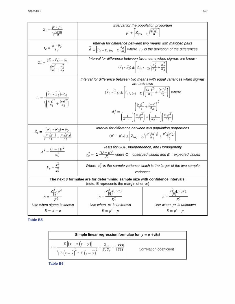
Zc = p′ - p0p0 q0n
Interval for the population proportion
p′ ± ⎡⎣Z(α / 2)p′q′n⎤⎦
tc = d–
- δ0sd
Interval for difference between two means with matched pairs
d–
± ⎡⎣t(n − 1), (α / 2)sdn⎤⎦ where sd is the deviation of the differences
Zc = (x1– - x2
– ) − δ0σ1
2n1 +
σ22
n2
Interval for difference between two means when sigmas are known
(x1– - x2
– ) ±⎡⎣⎢Z(α / 2)
σ12
n1+σ2
2
n2
⎤⎦⎥
tc =⎛⎝x
¯1 - x¯ 2
⎞⎠ - δ0
⎛⎝⎜ (s1)2
n1 + (s2)2n2
⎞⎠⎟
Interval for difference between two means with equal variances when sigmasare unknown
( x¯ 1 - x¯ 2) ±⎡⎣⎢td f , (α / 2)
⎛⎝⎜(s1)2
n1+ (s2)2
n2
⎞⎠⎟⎤⎦⎥ where
d f =
⎛⎝⎜ (s1)2
n1 + (s2)2n2
⎞⎠⎟
2
⎛⎝⎜ 1n1 − 1
⎞⎠⎟⎛⎝⎜ (s1)2
n1
⎞⎠⎟ +⎛⎝⎜ 1n2 − 1
⎞⎠⎟⎛⎝⎜ (s2)2
n2
⎞⎠⎟
Zc =⎛⎝p′1 - p′2
⎞⎠− δ0
p′1⎛⎝q′1
⎞⎠
n1 + p′2⎛⎝q′2
⎞⎠
n2
Interval for difference between two population proportions
(p′1 - p′2) ±⎡⎣⎢Z(α / 2)
p′1⎛⎝q′1
⎞⎠
n1+ p′2
⎛⎝q′2
⎞⎠
n2
⎤⎦⎥
χc2 = (n − 1)s2
σ02
Tests for GOF, Independence, and Homogeneity
χc2 = Σ (O − E)2
E where O = observed values and E = expected values
Fc =s1
2
s22
Where s12 is the sample variance which is the larger of the two sample
variances
The next 3 formulae are for determining sample size with confidence intervals.(note: E represents the margin of error)
n =Z⎛⎝a2⎞⎠
2 σ2
E2
Use when sigma is known
E = x¯ − μ
n =Z⎛⎝a2⎞⎠
2 (0.25)
E2
Use when p′ is unknown
E = p′ − p
n =Z⎛⎝a2⎞⎠
2 [p′(q′)]
E2
Use when p′ is unknown
E = p′ − p
Table B5
Simple linear regression formulae for y = a + b⎛⎝x⎞⎠
r =Σ ⎡⎣⎛⎝x − x¯ ⎞⎠
⎛⎝y − y¯ ⎞⎠
⎤⎦
Σ ⎛⎝x − x¯ ⎞⎠2
* Σ ⎛⎝y − y¯ ⎞⎠2
=SxySx Sy
= SSRSST Correlation coefficient
Table B6
Appendix B 557
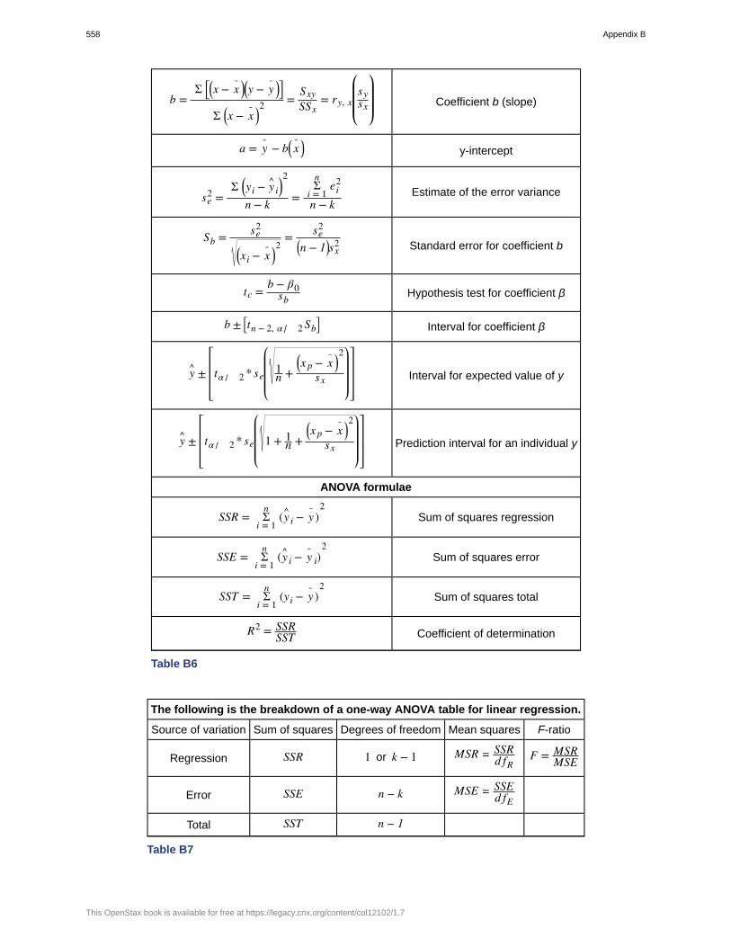
b =Σ ⎡⎣⎛⎝x − x¯ ⎞⎠
⎛⎝y − y¯ ⎞⎠
⎤⎦
Σ ⎛⎝x − x¯ ⎞⎠2 =
SxySSx
= ry, x
⎛
⎝⎜⎜sysx
⎞
⎠⎟⎟
Coefficient b (slope)
a = y¯ − b⎛⎝x¯ ⎞⎠ y-intercept
se2 =Σ ⎛⎝yi − y^ i
⎞⎠2
n − k =Σ
i = 1
nei
2
n − kEstimate of the error variance
Sb = se2
⎛⎝xi − x¯ ⎞⎠
2= se2⎛⎝n − 1⎞⎠sx2 Standard error for coefficient b
tc = b − β0sb Hypothesis test for coefficient β
b ± ⎡⎣tn − 2, α / 2Sb⎤⎦ Interval for coefficient β
y^ ±
⎡
⎣⎢⎢⎢tα / 2 * se
⎛
⎝⎜⎜⎜ 1
n +⎛⎝x p − x¯ ⎞⎠
2
sx
⎞
⎠⎟⎟⎟⎤
⎦⎥⎥⎥
Interval for expected value of y
y^ ±
⎡
⎣⎢⎢⎢tα / 2 * se
⎛
⎝⎜⎜⎜
1 + 1n +⎛⎝x p − x¯ ⎞⎠
2
sx
⎞
⎠⎟⎟⎟⎤
⎦⎥⎥⎥
Prediction interval for an individual y
ANOVA formulae
SSR = Σi = 1
n(y^ i − y¯ )
2Sum of squares regression
SSE = Σi = 1
n(y^ i − y¯ i)
2Sum of squares error
SST = Σi = 1
n(yi − y¯ )
2Sum of squares total
R2 = SSRSST Coefficient of determination
Table B6
The following is the breakdown of a one-way ANOVA table for linear regression.
Source of variation Sum of squares Degrees of freedom Mean squares F-ratio
Regression SSR 1 or k − 1 MSR = SSRd fR
F = MSRMSE
Error SSE n − k MSE = SSEd fE
Total SST n − 1
Table B7
558 Appendix B
This OpenStax book is available for free at https://legacy.cnx.org/content/col12102/1.7

INDEXSymbols5-number summary, 59
Aa is the symbol for the Y-Intercept, 528alternative hypothesis, 334, 342Analysis of Variance, 480Area to the left, 246Area to the right, 246assumption, 353average, 5Average, 29, 279
Bb is the symbol for Slope, 528balanced design, 476bar graph, 10Bernoulli Trial, 161Bernoulli Trials, 175binomial distribution, 299, 349Binomial Distribution, 306, 354Binomial Experiment, 175binomial probability distribution,161Binomial Probability Distribution,175bivariate, 504Bivariate, 528Blinding, 27, 29boxplot, 59
CCategorical Variable, 29Categorical variables, 4central limit theorem, 267Central Limit Theorem, 279, 354chi-square distribution, 418Cluster Sampling, 29coefficient of determination, 513Cohen’s d, 393complement, 104conditional probability, 104Conditional Probability, 138, 214confidence interval, 286, 295,517Confidence Interval (CI), 306,354confidence intervals, 299Confidence intervals, 334confidence level, 288Confidence Level (CL), 306contingency table, 121, 429Contingency Table, 138, 438
continuous, 7Continuous Random Variable,29control group, 27Control Group, 29Convenience Sampling, 29Critical Value, 354critical values, 339cumulative distribution function(CDF), 207Cumulative relative frequency,20Cumulative Relative Frequency,29
Ddata, 3Data, 4, 29decay parameter, 214degrees of freedom, 296Degrees of Freedom (df), 306degrees of freedom (df), 376Dependent Events, 138dependent variable, 27, 30descriptive statistics, 3discrete, 7Discrete Random Variable, 29double-blind experiment, 27Double-blinding, 29
EEmpirical Rule, 238empirical rule, 286equal standard deviations, 469Equally likely, 103Equally Likely, 138Error Bound for a PopulationMean (EBM), 306Error Bound for a PopulationProportion (EBP), 306Error Bound Mean, 288estimate of the error of estimate,513event, 103Event, 138expected mean, 517expected value, 517expected values, 422experiment, 103Experiment, 138experimental unit, 27Experimental Unit, 29explanatory variable, 27Explanatory Variable, 29exponential distribution, 205Exponential Distribution, 214extrapolation, 517
FF distribution, 469F ratio, 470fair, 103frequency, 20Frequency, 29Frequency Table, 79
Ggeometric distribution, 167Geometric Distribution, 175Geometric Experiment, 175Goodness-of-Fit, 438goodness-of-fit test, 422
HHours slept, 505hypergeometric experiment, 176Hypergeometric Experiment,175Hypergeometric Probability, 175hypotheses, 334Hypothesis, 354hypothesis test, 355hypothesis testing, 334Hypothesis Testing, 354
Iindependent, 108, 117Independent Events, 138Independent groups, 373Independent Groups, 393independent variable, 27, 29inferential statistics, 3, 285Inferential Statistics, 306Informed Consent, 29Institutional Review Board, 29interpolation, 517Interquartile Range, 79interval scale, 19
Llaw of large numbers, 104, 270level of measurement, 19Level of Significance of the Test, 354Linear, 528long-term relative frequency,103Lurking Variable, 29lurking variables, 27
Mmatched pairs, 373Matched Pairs, 393Mathematical Models, 29mean, 4, 5, 61
Index 559
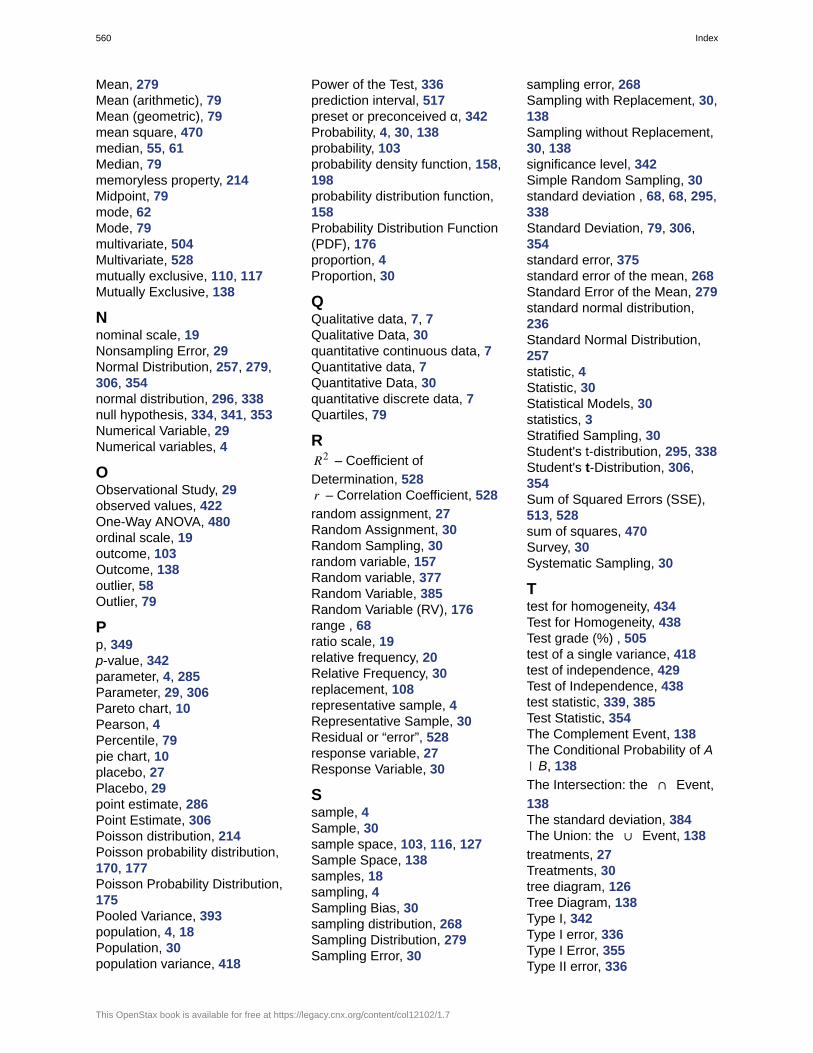
Mean, 279Mean (arithmetic), 79Mean (geometric), 79mean square, 470median, 55, 61Median, 79memoryless property, 214Midpoint, 79mode, 62Mode, 79multivariate, 504Multivariate, 528mutually exclusive, 110, 117Mutually Exclusive, 138
Nnominal scale, 19Nonsampling Error, 29Normal Distribution, 257, 279,306, 354normal distribution, 296, 338null hypothesis, 334, 341, 353Numerical Variable, 29Numerical variables, 4
OObservational Study, 29observed values, 422One-Way ANOVA, 480ordinal scale, 19outcome, 103Outcome, 138outlier, 58Outlier, 79
Pp, 349p-value, 342parameter, 4, 285Parameter, 29, 306Pareto chart, 10Pearson, 4Percentile, 79pie chart, 10placebo, 27Placebo, 29point estimate, 286Point Estimate, 306Poisson distribution, 214Poisson probability distribution,170, 177Poisson Probability Distribution,175Pooled Variance, 393population, 4, 18Population, 30population variance, 418
Power of the Test, 336prediction interval, 517preset or preconceived α, 342Probability, 4, 30, 138probability, 103probability density function, 158,198probability distribution function,158Probability Distribution Function(PDF), 176proportion, 4Proportion, 30
QQualitative data, 7, 7Qualitative Data, 30quantitative continuous data, 7Quantitative data, 7Quantitative Data, 30quantitative discrete data, 7Quartiles, 79
RR2 – Coefficient of
Determination, 528r – Correlation Coefficient, 528
random assignment, 27Random Assignment, 30Random Sampling, 30random variable, 157Random variable, 377Random Variable, 385Random Variable (RV), 176range , 68ratio scale, 19relative frequency, 20Relative Frequency, 30replacement, 108representative sample, 4Representative Sample, 30Residual or “error”, 528response variable, 27Response Variable, 30
Ssample, 4Sample, 30sample space, 103, 116, 127Sample Space, 138samples, 18sampling, 4Sampling Bias, 30sampling distribution, 268Sampling Distribution, 279Sampling Error, 30
sampling error, 268Sampling with Replacement, 30,138Sampling without Replacement,30, 138significance level, 342Simple Random Sampling, 30standard deviation , 68, 68, 295,338Standard Deviation, 79, 306,354standard error, 375standard error of the mean, 268Standard Error of the Mean, 279standard normal distribution,236Standard Normal Distribution,257statistic, 4Statistic, 30Statistical Models, 30statistics, 3Stratified Sampling, 30Student's t-distribution, 295, 338Student's t-Distribution, 306,354Sum of Squared Errors (SSE),513, 528sum of squares, 470Survey, 30Systematic Sampling, 30
Ttest for homogeneity, 434Test for Homogeneity, 438Test grade (%) , 505test of a single variance, 418test of independence, 429Test of Independence, 438test statistic, 339, 385Test Statistic, 354The Complement Event, 138The Conditional Probability of A| B, 138
The Intersection: the ∩ Event,
138The standard deviation, 384The Union: the ∪ Event, 138
treatments, 27Treatments, 30tree diagram, 126Tree Diagram, 138Type I, 342Type I error, 336Type I Error, 355Type II error, 336
560 Index
This OpenStax book is available for free at https://legacy.cnx.org/content/col12102/1.7
Type II Error, 355
Uunfair, 104Uniform Distribution, 214
Vvariable, 4Variable, 30variance, 68Variance, 79, 480Variance between samples, 470Variance within samples, 470variances, 469Variation, 18
XX – the independent variable,528
YY – the dependent variable, 528
Zz-score, 257, 296z-scores, 236
Index 561

562 Index
This OpenStax book is available for free at https://legacy.cnx.org/content/col12102/1.7
ATTRIBUTIONSCollection: Introduction to Statistics -- STAT 200 -- Briercrest College -- Version 2017 Revision AEdited by: Claude LaflammeEdited by: Claude Laflamme and Claude LaflammeURL: https://legacy.cnx.org/content/col12102/1.7/Copyright: Claude LaflammeLicense: http://creativecommons.org/licenses/by/4.0/Based on: Business Statistics -- STA200 -- Briercrest College -- Version 2017 Revision A <http://legacy.cnx.org/content/col11969/1.10> arranged by Claude Laflamme.
Module: Preface -- STA200 -- Briecrest College -- Version 2017RevAUsed here as: Preface -- STAT 200 -- Briecrest College -- Version 2017RevABy: Claude LaflammeURL: https://legacy.cnx.org/content/m63543/1.1/Copyright: Claude LaflammeLicense: http://creativecommons.org/licenses/by/4.0/Based on: Preface -- BSTA 200 -- Humber College -- Version 2016RevA <http://legacy.cnx.org/content/m62552/1.4> by Claude Laflammeand Svitlana Pshenychna.
Module: IntroductionBy: OpenStaxURL: https://legacy.cnx.org/content/m54035/1.5/Copyright: Rice UniversityLicense: http://creativecommons.org/licenses/by/4.0/Based on: Introduction <http://legacy.cnx.org/content/m46913/1.11> by OpenStax.
Module: Definitions of Statistics, Probability, and Key TermsBy: OpenStaxURL: https://legacy.cnx.org/content/m54033/1.8/Copyright: Rice UniversityLicense: http://creativecommons.org/licenses/by/4.0/Based on: Definitions of Statistics, Probability, and Key Terms <http://legacy.cnx.org/content/m46909/1.6> byOpenStax.
Module: Data, Sampling, and Variation in Data and SamplingBy: OpenStaxURL: https://legacy.cnx.org/content/m54036/1.15/Copyright: Rice UniversityLicense: http://creativecommons.org/licenses/by/4.0/Based on: Data, Sampling, and Variation in Data and Sampling <http://legacy.cnx.org/content/m46885/1.12> byOpenStax.
Module: Levels of MeasurementBy: OpenStaxURL: https://legacy.cnx.org/content/m54038/1.8/Copyright: Rice UniversityLicense: http://creativecommons.org/licenses/by/4.0/Based on: Frequency, Frequency Tables, and Levels of Measurement <http://legacy.cnx.org/content/m46882/1.10>by OpenStax.
Module: Experimental Design and EthicsBy: OpenStaxURL: https://legacy.cnx.org/content/m54056/1.6/Copyright: Rice UniversityLicense: http://creativecommons.org/licenses/by/4.0/Based on: Experimental Design and Ethics <http://legacy.cnx.org/content/m46919/1.8> by OpenStax.
Index 563

Module: IntroductionBy: OpenStaxURL: https://legacy.cnx.org/content/m53786/1.2/Copyright: Rice UniversityLicense: http://creativecommons.org/licenses/by/4.0/Based on: Introduction <http://legacy.cnx.org/content/m46925/1.5> by OpenStax.
Module: Frequency Distributions and Graphs - (Base Version - Lyryx Learning)By: Claude LaflammeURL: https://legacy.cnx.org/content/m65597/1.2/Copyright: Claude LaflammeLicense: http://creativecommons.org/licenses/by/4.0/Based on: Frequency Distributions and Graphs - Version 2016RevA - Lyryx Learning <http://legacy.cnx.org/content/m62672/1.2> by Joshua Emmanuel, Colleen Ball, Claude Laflamme, and Svitlana Pshenychna.
Module: Measures of the Location of the Data - (Base Version - Lyryx Learning)By: Claude LaflammeURL: https://legacy.cnx.org/content/m65609/1.2/Copyright: Claude LaflammeLicense: http://creativecommons.org/licenses/by/4.0/Based on: Measures of the Location of the Data - BSTA 200 -- Humber College -- Version 2016RevA<http://legacy.cnx.org/content/m62377/1.1> by Claude Laflamme, Svitlana Pshenychna, Joshua Emmanuel, andColleen Ball.
Module: Measures of the Center of the DataBy: OpenStaxURL: https://legacy.cnx.org/content/m53802/1.22/Copyright: Rice UniversityLicense: http://creativecommons.org/licenses/by/4.0/Based on: Measures of the Center of the Data <http://legacy.cnx.org/content/m46928/1.6> by OpenStax.
Module: Sigma Notation and Calculating the Arithmetic MeanBy: OpenStaxURL: https://legacy.cnx.org/content/m53799/1.14/Copyright: Rice UniversityLicense: http://creativecommons.org/licenses/by/4.0/
Module: Skewness and the Mean, Median, and ModeBy: OpenStaxURL: https://legacy.cnx.org/content/m53804/1.19/Copyright: Rice UniversityLicense: http://creativecommons.org/licenses/by/4.0/Based on: Skewness and the Mean, Median, and Mode <http://legacy.cnx.org/content/m46931/1.3> by OpenStax.
Module: Measures of the Spread of the Data - (Base Version - Lyryx Learning)By: Claude LaflammeURL: https://legacy.cnx.org/content/m65611/1.2/Copyright: Claude LaflammeLicense: http://creativecommons.org/licenses/by/4.0/Based on: Measures of the Spread of the Data -- BSTA 200 -- Humber College -- Version 2016 RevA<http://legacy.cnx.org/content/m62671/1.3> by Claude Laflamme, Joshua Emmanuel, Colleen Ball, and SvitlanaPshenychna.
Module: IntroductionBy: OpenStaxURL: https://legacy.cnx.org/content/m54216/1.2/Copyright: Rice UniversityLicense: http://creativecommons.org/licenses/by/4.0/Based on: Introduction <http://legacy.cnx.org/content/m46938/1.7> by OpenStax.
564 Index
This OpenStax book is available for free at https://legacy.cnx.org/content/col12102/1.7

Module: TerminologyBy: OpenStaxURL: https://legacy.cnx.org/content/m54218/1.14/Copyright: Rice UniversityLicense: http://creativecommons.org/licenses/by/4.0/Based on: Terminology <http://legacy.cnx.org/content/m46942/1.5> by OpenStax.
Module: Independent and Mutually Exclusive EventsBy: OpenStaxURL: https://legacy.cnx.org/content/m54219/1.8/Copyright: Rice UniversityLicense: http://creativecommons.org/licenses/by/4.0/Based on: Independent and Mutually Exclusive Events <http://legacy.cnx.org/content/m46948/1.5> by OpenStax.
Module: Two Basic Rules of ProbabilityBy: OpenStaxURL: https://legacy.cnx.org/content/m54220/1.11/Copyright: Rice UniversityLicense: http://creativecommons.org/licenses/by/4.0/Based on: Two Basic Rules of Probability <http://legacy.cnx.org/content/m46947/1.4> by OpenStax.
Module: Contingency Tables and Probability TreesBy: OpenStaxURL: https://legacy.cnx.org/content/m54259/1.12/Copyright: Rice UniversityLicense: http://creativecommons.org/licenses/by/4.0/Based on: Tree and Venn Diagrams <http://legacy.cnx.org/content/m46944/1.6> by OpenStax.
Module: Principles of Counting - (Base Version - Lyryx Learning)By: Claude LaflammeURL: https://legacy.cnx.org/content/m65630/1.2/Copyright: Claude LaflammeLicense: http://creativecommons.org/licenses/by/4.0/Based on: Principles of Counting - Humber College -Version 2016RevA <http://legacy.cnx.org/content/m62099/1.3> by Claude Laflamme, Svitlana Pshenychna, Joshua Emmanuel, and Colleen Ball.
Module: IntroductionBy: OpenStaxURL: https://legacy.cnx.org/content/m54262/1.15/Copyright: Rice UniversityLicense: http://creativecommons.org/licenses/by/4.0/Based on: Introduction <http://legacy.cnx.org/content/m46955/1.5> by OpenStax.
Module: Hypergeometric DistributionBy: OpenStaxURL: https://legacy.cnx.org/content/m54393/1.21/Copyright: Rice UniversityLicense: http://creativecommons.org/licenses/by/4.0/Based on: Hypergeometric Distribution <http://legacy.cnx.org/content/m46964/1.6> by OpenStax.
Module: Binomial Distribution - (Base Version - Lyryx Learning)By: Claude LaflammeURL: https://legacy.cnx.org/content/m65598/1.2/Copyright: Claude LaflammeLicense: http://creativecommons.org/licenses/by/4.0/Based on: Binomial Distribution - BSTA 200 -- Humber College -- Version 2016RevA <http://legacy.cnx.org/content/m62026/1.1> by Claude Laflamme, Svitlana Pshenychna, Joshua Emmanuel, and Colleen Ball.
Module: Geometric Distribution
Index 565

By: OpenStaxURL: https://legacy.cnx.org/content/m54422/1.18/Copyright: Rice UniversityLicense: http://creativecommons.org/licenses/by/4.0/Based on: Geometric Distribution <http://legacy.cnx.org/content/m46953/1.5> by OpenStax.
Module: Poisson DistributionBy: OpenStaxURL: https://legacy.cnx.org/content/m54398/1.16/Copyright: Rice UniversityLicense: http://creativecommons.org/licenses/by/4.0/Based on: Poisson Distribution <http://legacy.cnx.org/content/m46961/1.5> by OpenStax.
Module: IntroductionBy: OpenStaxURL: https://legacy.cnx.org/content/m54469/1.4/Copyright: Rice UniversityLicense: http://creativecommons.org/licenses/by/4.0/Based on: Introduction <http://legacy.cnx.org/content/m46967/1.5> by OpenStax.
Module: Properties of Continuous Probability Density FunctionsBy: OpenStaxURL: https://legacy.cnx.org/content/m54471/1.15/Copyright: Rice UniversityLicense: http://creativecommons.org/licenses/by/4.0/Based on: Continuous Probability Functions <http://legacy.cnx.org/content/m46965/1.4> by OpenStax.
Module: The Uniform DistributionBy: OpenStaxURL: https://legacy.cnx.org/content/m54473/1.9/Copyright: Rice UniversityLicense: http://creativecommons.org/licenses/by/4.0/Based on: The Uniform Distribution <http://legacy.cnx.org/content/m46972/1.4> by OpenStax.
Module: The Exponential DistributionBy: OpenStaxURL: https://legacy.cnx.org/content/m54480/1.32/Copyright: Rice UniversityLicense: http://creativecommons.org/licenses/by/4.0/Based on: The Exponential Distribution <http://legacy.cnx.org/content/m46969/1.6> by OpenStax.
Module: Introduction -- Normal Distribution - (Base Version - Lyryx Learning)By: Claude LaflammeURL: https://legacy.cnx.org/content/m65606/1.2/Copyright: Claude LaflammeLicense: http://creativecommons.org/licenses/by/4.0/Based on: Introduction -- Normal Distribution -- BSTA 200 -- Humber College -- Version 2016RevA<http://legacy.cnx.org/content/m62556/1.1> by Claude Laflamme, Svitlana Pshenychna, and Joshua Emmanuel.
Module: The Standard Normal Distribution - (Base Version - Lyryx Learning)By: Claude LaflammeURL: https://legacy.cnx.org/content/m65628/1.2/Copyright: Claude LaflammeLicense: http://creativecommons.org/licenses/by/4.0/Based on: The Standard Normal Distribution -- BSTA 200 -- Humber College -- Version 2016RevA<http://legacy.cnx.org/content/m62554/1.2> by Claude Laflamme, Svitlana Pshenychna, and Joshua Emmanuel.
Module: Using the Normal Distribution - (Base Version - Lyryx Learning)By: Claude Laflamme
566 Index
This OpenStax book is available for free at https://legacy.cnx.org/content/col12102/1.7

URL: https://legacy.cnx.org/content/m65629/1.2/Copyright: Claude LaflammeLicense: http://creativecommons.org/licenses/by/4.0/Based on: Using the Normal Distribution -- BSTA 200 -- Humber College -- Version 2016RevA <http://legacy.cnx.org/content/m62555/1.2> by Claude Laflamme, Svitlana Pshenychna, and Joshua Emmanuel.
Module: Introduction -- Central Limit Theorem - (Base Version - Lyryx Learning)By: Claude LaflammeURL: https://legacy.cnx.org/content/m65601/1.2/Copyright: Claude LaflammeLicense: http://creativecommons.org/licenses/by/4.0/Based on: Introduction -- Central Limit Theorem -- BSTA 200 -- Humber College -- Version 2016RevA<http://legacy.cnx.org/content/m62124/1.2> by Claude Laflamme, Joshua Emmanuel, Colleen Ball, and SvitlanaPshenychna.
Module: The Central Limit Theorem for Sample Means - (Base Version - Lyryx Learning)By: Claude LaflammeURL: https://legacy.cnx.org/content/m65622/1.2/Copyright: Claude LaflammeLicense: http://creativecommons.org/licenses/by/4.0/Based on: The Central Limit Theorem for Sample Means -- BSTA 200 -- Humber College -- Version 2016RevA<http://legacy.cnx.org/content/m62530/1.1> by Claude Laflamme, Svitlana Pshenychna, Joshua Emmanuel, andColleen Ball.
Module: Exploring the Central Limit Theorem - (Base Version - Lyryx Learning)By: Claude LaflammeURL: https://legacy.cnx.org/content/m65599/1.2/Copyright: Claude LaflammeLicense: http://creativecommons.org/licenses/by/4.0/Based on: Exploring the Central Limit Theorem -- BSTA 200 -- Humber College -- Version 2016RevA<http://legacy.cnx.org/content/m62529/1.1> by Claude Laflamme, Svitlana Pshenychna, Joshua Emmanuel, andColleen Ball.
Module: IntroductionBy: OpenStaxURL: https://legacy.cnx.org/content/m55460/1.8/Copyright: Rice UniversityLicense: http://creativecommons.org/licenses/by/4.0/Based on: Introduction <http://legacy.cnx.org/content/m47008/1.4> by OpenStax.
Module: A Confidence Interval for a Population Standard Deviation, Known or Large Sample SizeBy: OpenStaxURL: https://legacy.cnx.org/content/m55461/1.27/Copyright: Rice UniversityLicense: http://creativecommons.org/licenses/by/4.0/Based on: A Single Population Mean using the Normal Distribution <http://legacy.cnx.org/content/m47002/1.9> byOpenStax.
Module: A Confidence Interval for a Population Standard Deviation Unknown, Small Sample CaseBy: OpenStaxURL: https://legacy.cnx.org/content/m55462/1.40/Copyright: Rice UniversityLicense: http://creativecommons.org/licenses/by/4.0/Based on: A Single Population Mean using the Student t Distribution <http://legacy.cnx.org/content/m47001/1.7>by OpenStax.
Module: A Confidence Interval for A Population ProportionBy: OpenStaxURL: https://legacy.cnx.org/content/m55463/1.22/
Index 567

Copyright: Rice UniversityLicense: http://creativecommons.org/licenses/by/4.0/Based on: A Population Proportion <http://legacy.cnx.org/content/m46999/1.7> by OpenStax.
Module: Calculating the Sample Size n: Continuous and Binary Random VariablesBy: OpenStaxURL: https://legacy.cnx.org/content/m56644/1.20/Copyright: Rice UniversityLicense: http://creativecommons.org/licenses/by/4.0/
Module: IntroductionBy: OpenStaxURL: https://legacy.cnx.org/content/m55603/1.7/Copyright: Rice UniversityLicense: http://creativecommons.org/licenses/by/4.0/
Module: Null and Alternative HypothesesBy: OpenStaxURL: https://legacy.cnx.org/content/m55606/1.10/Copyright: Rice UniversityLicense: http://creativecommons.org/licenses/by/4.0/
Module: Outcomes and the Type I and Type II ErrorsBy: OpenStaxURL: https://legacy.cnx.org/content/m55607/1.16/Copyright: Rice UniversityLicense: http://creativecommons.org/licenses/by/4.0/
Module: Distribution Needed for Hypothesis TestingBy: OpenStaxURL: https://legacy.cnx.org/content/m55608/1.21/Copyright: Rice UniversityLicense: http://creativecommons.org/licenses/by/4.0/
Module: Full Hypothesis Test Examples - (Base Version - Lyryx Learning)By: Claude LaflammeURL: https://legacy.cnx.org/content/m66754/1.1/Copyright: Claude LaflammeLicense: http://creativecommons.org/licenses/by/4.0/Based on: Full Hypothesis Test Examples <http://legacy.cnx.org/content/m55610/1.27> by OpenStax.
Module: Rare Events, the Sample, Decision and ConclusionBy: OpenStax Business StatisticsURL: https://legacy.cnx.org/content/m55611/1.2/Copyright: OpenStax Business StatisticsLicense: http://creativecommons.org/licenses/by/4.0/Based on: Rare Events, the Sample, Decision and Conclusion <http://legacy.cnx.org/content/m47044/1.4> byOpenStax.
Module: IntroductionBy: OpenStaxURL: https://legacy.cnx.org/content/m55613/1.6/Copyright: Rice UniversityLicense: http://creativecommons.org/licenses/by/4.0/Based on: Introduction <http://legacy.cnx.org/content/m47057/1.5> by OpenStax.
Module: Comparing Two Independent Population MeansBy: OpenStax Business StatisticsURL: https://legacy.cnx.org/content/m55671/1.33/
568 Index
This OpenStax book is available for free at https://legacy.cnx.org/content/col12102/1.7

Copyright: OpenStax Business StatisticsLicense: http://creativecommons.org/licenses/by/4.0/Based on: Two Population Means with Unknown Standard Deviations <http://legacy.cnx.org/content/m47050/1.8>by OpenStax.
Module: Comparing Two Independent Population ProportionsBy: OpenStaxURL: https://legacy.cnx.org/content/m55672/1.31/Copyright: Rice UniversityLicense: http://creativecommons.org/licenses/by/4.0/Based on: Comparing Two Independent Population Proportions <http://legacy.cnx.org/content/m47060/1.7> byOpenStax.
Module: Two Population Means with Known Standard DeviationsBy: OpenStaxURL: https://legacy.cnx.org/content/m55673/1.21/Copyright: Rice UniversityLicense: http://creativecommons.org/licenses/by/4.0/Based on: Two Population Means with Known Standard Deviations <http://legacy.cnx.org/content/m47061/1.5> byOpenStax.
Module: Matched or Paired SamplesBy: OpenStaxURL: https://legacy.cnx.org/content/m55674/1.20/Copyright: Rice UniversityLicense: http://creativecommons.org/licenses/by/4.0/Based on: Matched or Paired Samples <http://legacy.cnx.org/content/m47045/1.8> by OpenStax.
Module: IntroductionBy: OpenStaxURL: https://legacy.cnx.org/content/m55691/1.3/Copyright: Rice UniversityLicense: http://creativecommons.org/licenses/by/4.0/
Module: Facts About the Chi-Square DistributionBy: OpenStaxURL: https://legacy.cnx.org/content/m55693/1.5/Copyright: Rice UniversityLicense: http://creativecommons.org/licenses/by/4.0/Based on: Facts About the Chi-Square Distribution <http://legacy.cnx.org/content/m47062/1.5> by OpenStax.
Module: Test of a Single VarianceBy: OpenStaxURL: https://legacy.cnx.org/content/m55694/1.21/Copyright: Rice UniversityLicense: http://creativecommons.org/licenses/by/4.0/Based on: Test of a Single Variance <http://legacy.cnx.org/content/m47085/1.6> by OpenStax.
Module: Goodness-of-Fit TestBy: OpenStaxURL: https://legacy.cnx.org/content/m55696/1.19/Copyright: Rice UniversityLicense: http://creativecommons.org/licenses/by/4.0/Based on: Goodness-of-Fit Test <http://legacy.cnx.org/content/m47064/1.5> by OpenStax.
Module: Test of IndependenceBy: OpenStaxURL: https://legacy.cnx.org/content/m55697/1.19/Copyright: Rice University
Index 569

License: http://creativecommons.org/licenses/by/4.0/Based on: Test of Independence <http://legacy.cnx.org/content/m47077/1.6> by OpenStax.
Module: Test for HomogeneityBy: OpenStaxURL: https://legacy.cnx.org/content/m55698/1.12/Copyright: Rice UniversityLicense: http://creativecommons.org/licenses/by/4.0/Based on: Test for Homogeneity <http://legacy.cnx.org/content/m47091/1.5> by OpenStax.
Module: Comparison of the Chi-Square TestsBy: OpenStaxURL: https://legacy.cnx.org/content/m55700/1.6/Copyright: Rice UniversityLicense: http://creativecommons.org/licenses/by/4.0/
Module: IntroductionBy: OpenStaxURL: https://legacy.cnx.org/content/m55702/1.5/Copyright: Rice UniversityLicense: http://creativecommons.org/licenses/by/4.0/Based on: Introduction <http://legacy.cnx.org/content/m47121/1.2> by OpenStax.
Module: Test of Two VariancesBy: OpenStaxURL: https://legacy.cnx.org/content/m55703/1.25/Copyright: Rice UniversityLicense: http://creativecommons.org/licenses/by/4.0/Based on: Test of Two Variances <http://legacy.cnx.org/content/m47125/1.5> by OpenStax.
Module: One-Way ANOVABy: OpenStaxURL: https://legacy.cnx.org/content/m55706/1.9/Copyright: Rice UniversityLicense: http://creativecommons.org/licenses/by/4.0/Based on: One-Way ANOVA <http://legacy.cnx.org/content/m47124/1.2> by OpenStax.
Module: The F Distribution and the F-RatioBy: OpenStaxURL: https://legacy.cnx.org/content/m55712/1.18/Copyright: Rice UniversityLicense: http://creativecommons.org/licenses/by/4.0/
Module: Facts About the F DistributionBy: OpenStaxURL: https://legacy.cnx.org/content/m55704/1.25/Copyright: Rice UniversityLicense: http://creativecommons.org/licenses/by/4.0/Based on: Facts About the F Distribution <http://legacy.cnx.org/content/m47119/1.4> by OpenStax.
Module: Introduction -- Linear Regression and Correlation - (Base Version - Lyryx Learning)By: Claude LaflammeURL: https://legacy.cnx.org/content/m65602/1.2/Copyright: Claude LaflammeLicense: http://creativecommons.org/licenses/by/4.0/Based on: Introduction -- Linear Regression and Correlation -- BSTA 200 -- Humber College -- Version 2016RevA<http://legacy.cnx.org/content/m62531/1.1> by Claude Laflamme, Colleen Ball, Joshua Emmanuel, and SvitlanaPshenychna.
570 Index
This OpenStax book is available for free at https://legacy.cnx.org/content/col12102/1.7

Module: The Correlation Coefficient r - (Base Version - Lyryx Learning)By: Claude LaflammeURL: https://legacy.cnx.org/content/m65631/1.2/Copyright: Claude LaflammeLicense: http://creativecommons.org/licenses/by/4.0/Based on: The Correlation Coefficient r -- BSTA 200 -- Humber College -- Version 2016RevA <http://legacy.cnx.org/content/m62019/1.1> by Claude Laflamme, Svitlana Pshenychna, Joshua Emmanuel, and Colleen Ball.
Module: Testing the Significance of the Correlation Coefficient - (Base Version - Lyryx Learning)By: Claude LaflammeURL: https://legacy.cnx.org/content/m65620/1.2/Copyright: Claude LaflammeLicense: http://creativecommons.org/licenses/by/4.0/Based on: Testing the Significance of the Correlation Coefficient -- BSTA 200 -- Humber College -- Version 2016RevA<http://legacy.cnx.org/content/m62027/1.1> by Claude Laflamme, Svitlana Pshenychna, Joshua Emmanuel, andColleen Ball.
Module: Linear Equations - (Base Version - Lyryx Learning)By: Claude LaflammeURL: https://legacy.cnx.org/content/m65608/1.2/Copyright: Claude LaflammeLicense: http://creativecommons.org/licenses/by/4.0/Based on: Linear Equations -- BSTA 200 -- Humber College -- Version 2016RevA <http://legacy.cnx.org/content/m62020/1.1> by Claude Laflamme, Svitlana Pshenychna, Joshua Emmanuel, and Colleen Ball.
Module: The Regression Equation - (Base Version - Lyryx Learning)By: Claude LaflammeURL: https://legacy.cnx.org/content/m65627/1.2/Copyright: Claude LaflammeLicense: http://creativecommons.org/licenses/by/4.0/Based on: The Regression Equation -- BSTA 200 -- Humber College -- Version 2016RevA <http://legacy.cnx.org/content/m62022/1.1> by Claude Laflamme, Svitlana Pshenychna, Joshua Emmanuel, and Colleen Ball.
Module: Predicting with a Regression Equation - (Base Version - Lyryx Learning)By: Claude LaflammeURL: https://legacy.cnx.org/content/m65612/1.2/Copyright: Claude LaflammeLicense: http://creativecommons.org/licenses/by/4.0/Based on: Predicting with a Regression Equation -- BSTA 200 -- Humber College -- Version 2016RevA<http://legacy.cnx.org/content/m62023/1.1> by Claude Laflamme, Svitlana Pshenychna, Joshua Emmanuel, andColleen Ball.
Module: How to Use Excel for Regression Analysis - (Base Version - Lyryx Learning)By: Claude LaflammeURL: https://legacy.cnx.org/content/m65600/1.2/Copyright: Claude LaflammeLicense: http://creativecommons.org/licenses/by/4.0/Based on: How to Use Excel for Regression Analysis -- BSTA 200 -- Humber College -- Version 2016RevA<http://legacy.cnx.org/content/m62025/1.1> by Claude Laflamme, Svitlana Pshenychna, Joshua Emmanuel, andColleen Ball.
Module: Regression Analysis with the BAII Plus CalculatorBy: Colleen Ball, Joshua Emmanuel, and Svitlana PshenychnaURL: https://legacy.cnx.org/content/m62013/1.1/Copyright: Colleen Ball, Joshua Emmanuel, and Svitlana PshenychnaLicense: http://creativecommons.org/licenses/by/4.0/
Module: Statistical TablesBy: OpenStax
Index 571

URL: https://legacy.cnx.org/content/m56641/1.18/Copyright: Rice UniversityLicense: http://creativecommons.org/licenses/by/4.0/Based on: Appendix H: Tables <http://legacy.cnx.org/content/m47875/1.7> by OpenStax.
Module: Mathematical Phrases, Symbols, and FormulasBy: OpenStaxURL: https://legacy.cnx.org/content/m56640/1.17/Copyright: Rice UniversityLicense: http://creativecommons.org/licenses/by/4.0/Based on: Appendix F: Mathematical Phrases, Symbols, and Formulas <http://legacy.cnx.org/content/m47891/1.4>by OpenStax.
572 Index
This OpenStax book is available for free at https://legacy.cnx.org/content/col12102/1.7

ABOUT CONNEXIONSSince 1999, Connexions has been pioneering a global system where anyone can create course materials and make them fullyaccessible and easily reusable free of charge. We are a Web-based authoring, teaching and learning environment open to anyoneinterested in education, including students, teachers, professors and lifelong learners. We connect ideas and facilitate educationalcommunities. Connexions's modular, interactive courses are in use worldwide by universities, community colleges, K-12 schools,distance learners, and lifelong learners. Connexions materials are in many languages, including English, Spanish, Chinese,Japanese, Italian, Vietnamese, French, Portuguese, and Thai.
Index 573