und Raumfahrt eV Continuous Quantum Mechanics of Single ...
192
DE05FA302 Deutsches Zentrum für Luft- und Raumfahrt e.V. Forschungsbericht 2004-32 Continuous Quantum Mechanics of Single Particles in Closed and Quasi-Closed Systems: Parts I and II Michael Brieger Institute of Technical Physics Stuttgart DLR
-
Upload
khangminh22 -
Category
Documents
-
view
1 -
download
0
Transcript of und Raumfahrt eV Continuous Quantum Mechanics of Single ...

DE05FA302
Deutsches Zentrumfür Luft- und Raumfahrt e.V.
Forschungsbericht 2004-32
Continuous Quantum Mechanics ofSingle Particles in Closed andQuasi-Closed Systems: Parts I and II
Michael Brieger
Institute of Technical PhysicsStuttgart
DLR

Herausgeber
TelefonTelefax
Deutsches Zentrumfür Luft- und Raumfahrt e.V.Bibliotheks- undInformationswesenD-51170 KölnPorz-WahnheideLinder HöheD-51147 Köln
(0 22 03) 6 01-32 01(0 22 03)6 01-47 47
Als Manuskript gedruckt.Abdruck oder sonstige Verwendungnur nach Absprache mit dem DLR gestattet.
ISSN 1434-8454

quantum mechanics, Schrödinger's time-dependent equation, energy representation, classicallyillustrative description, examples, complete spontaneous transition process without QED
M.BRIEGER
Institut für Technische Physik des DLR, Stuttgart
Continuous Quantum Mechanics in Closed and Quasi-Closed Single-Particle Systems
DLR-Forschungsbericht 2004-32, 2004, 179 pages, 4 figs., 205 refs., 36,00 €
the established statistical interpretation of quantum mechanics never envisioned our today's ability tohandle and investigate single particles in trap devices. After scrutinizing the development of quantummechanics, we point out that Schrödinger's equation establishes an energy representation, whichobtains the energy eigenvalues as extrema of the energy curve or on the energy hypersurface,respectively. We also strongly emphasize its never exhausted capability of accounting in classicalterms and full detail for the dynamics of single particles in closed systems. This is demonstrated forseveral familiar examples. They show that the eigensolutions to Schrödinger's equation must notblindly be identified with physically stationary states. The gained insight into the true dynamics allowsto describe, without involving QED, the time evolution of a complete spontaneous transition as beingdriven by unbalanced internal dynamics. This mechanism relies on the fact that perfect balances areonly possible in the exact extrema of the total energy and that any deviation, which is characterizedby nonstationary states, makes multipole moments oscillate and emit electromagnetic radiation.
Quantenmechanik, zeitabhängige Schrödinger-Gleichung, Energiedarstellung, klassisch anschaulicheBeschreibung, Beispiele, vollständiger spontaner Übergangsprozess ohne Quantenelektrodynamik
(Publiziert in englischer Sprache)
M. BRIEGER
Institut für Technische Physik des DLR, Stuttgart
Stetige Quantenmechanik in geschlossenen und quasi-geschlossenen Ein-Teilchen-Systemen
DLR-Forschungsbericht2004-32,2004, 179 Seiten, 4 Bilder, 205Literaturstellen, 36.00 6" zzgl. MwSt.Die etablierte statistische Interpretation der Quantenmechanik hat nie unsere heutige Fähigkeit fürmöglich gehalten, einzelne Teilchen in Fallenanordnungen zu halten und zu untersuchen. Ausgehendvon einer kritischen Analyse der Entwicklung der Quantenmechanik wird darauf hingewiesen, dass dieSchrödinger-Gleichung einer Energiedarstellung gleichkommt, deren Eigenwerte sich als Extremalpunkteder Energiekurve bzw. auf ihrer Hyperfläche herausstellen. Ferner werden ihre nie ausgeschöpftenMöglichkeiten hervorgehoben, in abgeschlossenen Systemen der Dynamik von Einzelteilchen im Detailund „klassisch" anschaulich Rechnung zu tragen. Dies wird anhand mehrerer bekannter Beispieledemonstriert. Dabei zeigt sich, dass die Lösungen der Schrödinger-Gleichung nicht automatisch auchphysikalisch stationäre Zustände repräsentieren. Der dabei gewonnene Einblick in die tatsächlicheDynamik erlaubt ohne Rückgriff auf die Quantenelektrodynamik die Zeitentwicklung eines vollständigenspontanen Übergangs zu beschreiben, und zwar als angetrieben durch die fehlende Balance derinneren Dynamik. Der Mechanismus beruht auf der Tatsache, dass eine perfekte Balance nur in denexakten Extremalpunkten möglich ist. Jede Abweichung führt daher zu nichtstationären Zuständen, diesich durch oszillierende Multipolmomente auszeichnen und so ursächlich für die Emission vonelektromagnetischer Strahlung werden.


Deutsches Zentrumfür Luft- und Raumfahrt e.V.
Forschungsbericht 2004-32
Continuous Quantum Mechanics ofSingle Particles in Closed andQuasi-Closed Systems: Parts I and II
Michael Brieger
Institute of Technical PhysicsStuttgart
179 Pages4 Figures
205 References


Continuous Quantum Mechanics ofSingle Particles in Closed and Quasi-Closed Systems: Parts I and II
Deutsches Zentrumfür Luft- und Raumfahrt e.V.

»DE021362834J
Abstract
The established statistical interpretation of quantum mechanics never envisioned ourtoday's ability to handle and investigate single particles in trap devices. After scruti-nizing the development of quantum mechanics, we point out that Schrödinger's equa-tion establishes an energy representation, which obtains the energy eigenvalues as ex-trema of the energy curve or on the energy hypersurface, respectively. We also stronglyemphasize its never exhausted capability of accounting in classical terms and full detailfor the dynamics of single particles in closed systems. This is demonstrated for sev-eral familiar examples. They show that the eigensolutions to Schrödinger's equationmust not blindly be identified with physically stationary states. The gained insight intothe true dynamics allows to describe, without involving QED, the time evolution ofa complete spontaneous transition as being driven by unbalanced internal dynamics.This mechanism relies on the fact that perfect balances are only possible in the exactextrema of the total energy and that any deviation, which is characterized by nonsta-tionary states, makes multipole moments oscillate and emit electromagnetic radiation.

Zusammenfassung
Die etablierte statistische Interpretation der Quantenmechanik hat nie unsere heutigeFähigkeit für möglich gehalten, einzelne Teilchen in Fallenanordnungen zu halten undzu untersuchen. Ausgehend von einer kritischen Analyse der Entwicklung der Quan-tenmechanik wird darauf hingewiesen, dass die Schrödinger-Gleichung einer Energie-darstellung gleichkommt, deren Eigenwerte sich als Extremalpunkte der Energiekurvebzw. auf ihrer Hyperfläche herausstellen. Ferner werden ihre nie ausgeschöpftenMöglichkeiten hervorgehoben, in abgeschlossenen Systemen der Dynamik von Einzel-teilchen im Detail und "klassisch" anschaulich Rechnung zu tragen. Dies wird an-hand mehrerer bekannter Beispiele demonstriert. Dabei zeigt sich, dass die Lösungender Schrödinger-Gleichung nicht automatisch auch physikalisch stationäre Zuständerepräsentieren. Der dabei gewonnene Einblick in die tatsächliche Dynamik erlaubtohne Rückgriff auf die Quantenelektrodynamik die Zeitentwicklung eines vollständi-gen spontanen Übergangs zu beschreiben, und zwar als angetrieben durch die fehlendeBalance der inneren Dynamik. Der Mechanismus beruht auf der Tatsache, dass eineperfekte Balance nur in den exakten Extremalpunkten möglich ist. Jede Abweichungführt daher zu nichtstationären Zuständen, die sich durch oszillierende Multipolmo-mente auszeichnen und so zur Ursache für die Emission von elektromagnetischer Strah-lung werden.


Contents
1 Introduction 1
2 Part I: The discrepancy between the established interpretation and . . . 3
2.1 How it all began 6
2.2 Our objective 20
2.3 The examples 24
2.4 Theory of multiply periodic motions 27
2.4.1 The relationship between the principles of classical and quantummechanics 27
2.4.2 The role of nonstationary states 39
2.5 The consequences of a pure energy representation 42
2.5.1 Free particles 43
2.5.2 Bound one-particle systems 53
2.6 The linear harmonic oscillator 54
2.6.1 The algebraic description of the linear harmonic oscillator . . . . 57
2.6.2 General expectation values of properties not relevant to the totalenergy 59
2.6.3 General expectation values of properties relevant to the total energy 64
2.6.4 The question of equally spaced energy eigenvalues 68
2.6.5 The role of the linear harmonic oscillator in the quantization of
the electromagnetic field 70
2.6.6 The linear harmonic oscillator and the correspondence principle . . 73
2.6.7 The linear harmonic oscillator and the uncertainty relations . . . 78
2.6.8 ([x,p.r]) = ih as a result of continuous action 82
2.7 The two-dimensional isotropic harmonic oscillator 89
2.7.1 General expectation value of properties relevant to the total energy 92
2.7.2 Dynamics determined by angular momentum 95
2.7.3 Dynamics without angular momentum 1012.7.4 General expectation values of properties not relevant to the total
energy 102
vii

2.8 The Kepler problem 105
2.8.1 The multiply periodic exchange of energy as a special feature ofthe Kepler problem 109
2.8.2 Multiply periodic oscillations of the radial variable 115
2.8.3 General expectation values of properties not relevant to the totalenergy 120
2.9 Discussion of the behavior of the examples 124
2.9.1 Stationary and nonstationary states with angular momentum . . 124
2.9.2 Stationary states without angular momentum 127
2.9.3 General considerations 129
3 Part II: The time dependence of spontaneous multipole transitions 131
3.1 The mechanical origin of spontaneous transitions in two-level systems . 135
3.1.1 The mathematical implementation . 137
3.2 The dynamical theory of complete transitions in single particles withtwo-level systems 139
3.2.1 The two-level model 139
3.2.2 The self-sustained transition mechanism 144
3.2.3 The dynamical origin of the transition probability 149
3.3 A comparison between the present and the QED results 159
3.3.1 A critical look back in history 159
3.3.2 General aspects of the present results 161
3.3.3 General aspects of the QED results 163
3.3.4 Comparison of special features and behavior beyond QED . . . . 165
3.3.5 Particle-like behavior at very short wavelengths 167
4 Conclusion 169
4.1 Acknowledgments 170

1 Introduction
From the very beginning, the interpretation of quantum mechanics had to cope withsome puzzling aspects of its results. Whatever the respective viewpoint, for instancewith regard to the measurement problem, seemingly apparent remedy at one pointcreated new unintelligible consequences at another. So, the issue became rather a mat-ter of belief than knowledge. Nevertheless, since decades the statistical interpretationis established as something like a mainstream interpretation.In Part I, we shall first review how the final establishment of this interpretation wasstrongly influenced by the strong personalities of its numerous early proponents de-spite the fact that Schrödinger's acknowledged achievements would have allowed tofavor less radical assumptions. In this context, however, we shall have to expose thateven Schrödinger was not able to escape the prevalent Zeitgeist because he did not rec-ognize how much of the intrinsic dynamics the solutions to his equation are capableof describing in classical terms if used in conjunction with the principle of superposi-tion. Picking up the threads where and how it all began, we shall only investigate thedynamical behavior of closed single-particle systems. Accordingly, all our conclusionswill only hold for such systems, which conserve their once gained total energy for alltimes and, as a consequence, have to be described by time-independent Hamiltonians.It is the main intention of this report to show that such Hamiltonians entail solutionsto Schrödinger's equation that determine in full causality the time evolution of a singleparticle's unperturbed dynamics in accord with familiar classical perceptions by givingconcrete ideas of what the particle is doing when left by itself in different potential en-vironments. Although all our results, thus, will not allow to account for any measuringinterference from outside and, therefore, may rightfully be termed as experimentallynot or only indirectly verifiable, their proximity to if not identity with well-known clas-sical results will permit, nonetheless, conclusions that otherwise would not be possibleor only speculations. This way, they will show that single microscopic particles behavethe same way as macroscopic ones do.
By allowing for a quasi-closed system, which is only a little bit leaky, these conclusionswill permit us to present in Part II a strikingly simple theory of the complete time evo-lution of a spontaneous transition in a two-level system. This theory is solely based onthe inner dynamics of the source and, therefore, need not involve the vacuum fluctua-tions of the electromagnetic field as the prime driving mechanism. Despite its simplic-ity it can account for all features of such an individual event like the unpredictabilityof its occurrence, the Lorentzian line shape of the emitted radiation, and the potentialfor particle-like properties of the photon at short wavelengths. Moreover, our theorywill prove capable of even explaining the exponential decay of the radiation emittedby an ensemble of excited like particles.

Continuous quantum mechanics... Parts I and II
Before getting started we want to address a delicate point that touches on ethics inscience: Although our treatise will include a quite critical analysis of the present inter-pretation of quantum mechanics it is not our intention to blame anyone for anything.If our expositions should give rise to this impression we regret it and apologize be-forehand. This work is just an attempt to convince people that the present view onquantum mechanics is too narrow and, therefore, fails to let its classical features comeinto sight. But, in some way, this is also a personal and, therefore, subjective view, ofcourse, and, maybe, we ourselves do not know any better.However, if we take re-search literally as search here, search there and over again, thequest for truth especially in the microscopic world to which we have no direct accessthrough our senses is always something that resembles more an erratic random walkthan a straight line. But, of course, especially textbooks must not follow each erroneouskink but have to expose what since has settled and become the mainstream perception.On the other hand, just because of the lamented lack of direct evidence, we feel thatit would be very advantageous to our general understanding of the microworld if thealleged total breach with classical behavior could be shown to only exist as a result ofunrecognized and, therefore, not exhausted capabilities of both Schrodinger's equationand the principle of superposition. This is what we are about to take up the cudgelsfor.
We conclude the introduction with a technical remark: We shall use page-specifyingreferences in the form of [ref. number, p(p)pcige number(s)]. As we try to make as manysuch references as possible, the running text would sometimes get clogged with longstrings of such references. In order to avoid these occurrences we prefer to providethese citations in footnotes.As for the numerous textbooks cited, their choice is quite accidental because their se-lection was only a matter of their availability on the shelves of the university libraryand, so, apart from dealing with the respective matter, does not mean anything.

2 Part I: The discrepancy between theestablished interpretation and thecapabilities of Schrödinger's equation
Despite common roots, quantum mechanics is deemed ever since quite different fromclassical mechanics in particular and classical physics in general1. Founded on a seem-ingly firm and consistent axiomatic framework, it is held to have proven capable ofexplaining any classically inexplicable effect like the stability and line spectra of atomsand molecules, the tunneling of a particles through the potential barrier of disintegrat-ing heavy nuclei, superfluidity, superconductivity, and so forth, to name only somefew impressive achievements.Given all its successes, it is rightfully called mankind's most important theoretical ed-ifice. But, as the objects of its investigations are not accessible to human senses - in-dividually, they cannot be seen, smelt or felt, and the way of how their properties aredetermined can interfere with what actually is the object of the measurement - resultsof measurements cannot be interpreted as straightforwardly as it is possible in classi-cal physics by direct evidence: Their interpretation always depends, sometimes more,sometimes less, on what perception or model they are supposed to confirm. This alsoholds for the view on dualism that makes the appearance of wave or particle-like be-havior dependent on the properties of the measuring apparatus2. As a consequence,the interpretation of the results is neither unambiguous, nor is it, as the measurementproblem3 proves, free of paradoxes if the agreed-upon rules are applied with ultimateconsequence: Because of defying describability by Schrödinger's equation4 two of themajor issues were and partly still are the conceptions5 of "quantum jumps" and ofan instantaneous "collapse" or reduction6 of the state vector upon measurement, thelatter, however, only until the less abrupt process of environmentally induced decoher-ence was brought into play7. The introduction of such a process is the result of thecognition that a time-independent Hamiltonian makes Schrödinger's linear and deter-
1 [1, p580], [2, pP879-880], [3, pp557-558], [4, ppl72,195,197], [5, p641], [6, chapl], [7, p283]2 [7, p285]i[8,Pp222ff]4 [7, p283], [9-13]5 [1,p582), [U,pl48], [15,pp614,617,619,645],[l6,pp502,504], [17-29], [30,pp95,97], [31,ppU6,153], [32,
P836]6 [7, p285], [8, ppm-114,222], [33, p220], [34, pp350ff), [35, pp65,370ff], [36, plOl], [37]7 [38]
Continuous quantum mechanics ... Parts I and II
ministic equation8 only applicable to closed systems9.Decoherence has become a subject of intense research10 since about two decades. Itexplains the probabilistic outcome of a measurement, which formerly used to be re-lated to an instantaneous "collapse" upon measurement, by involving the presence ofthe environment in open systems. The conception of decoherence is primarily meantto make intelligible the loss of quantum correlations in macroscopic systems as due tothe enormous number of, in general, uncontrollable degrees of freedom. This percep-tion implies that such correlations exist between spatially separated pieces of the wavepacket11, i.e., between different particles in an ensemble, as it is deemed to be describedby the nondiagonal parts of the density matrix. Decoherence is then made responsiblefor the destruction of the quantum coherence by eliminating the off-diagonal terms12.
Equally at odds with the properties of Schrödinger's equation is the long alleged in-determinacy, i.e., the absence of causality13 in the dynamics of individual particles. Butnot only these properties of Schrödinger's equation may raise doubts: Another reasondefinitely is that neither the notion of instantaneous "quantum jumps" nor of instanta-neous "collapse" is reconcilable with the inherent inertia of a particle with finite massunless one is willing to give up the principle of inertia as de Broglie14 was.
Bohr's role
From the very beginning and throughout the years, Bohr was and remained one of thekey players in quantum mechanics. This is probably owed to his convincing person-ality, which endowed him with so much influence and lasting impact on the develop-ment of quantum mechanics. For this reason, we shall keep a closer eye on him. Inthis context, it is interesting to note that after the publication of his first revolutionaryarticles10 he gave himself a break for several years as far as major contributions areconcerned. An article meant for publication in the April 1916 issue of the London, Ed-inburgh, and Dublin Philosophical Magazine was withdrawn in the last minute andonly published six years later as an authorized German translation16. In this paper,he had tried to summarize the development of quantum mechanics and to clarify hispoints of view but withdrew it when, while at Manchester, he belatedly got informedof Sommerfeld's treatises17. The reason for this withdrawal was that he wanted to alsoinclude an evaluation of Sommerfeld's results. This contribution also seems to be theone where he touched upon his ideas about the correspondence principle18 for the firsttime but without naming it as such.In this context it is also worth noting that without being dubbed this way, the origin
8 [7, p285]9 [38, pp36,37]
l0cf., e.g., [38-40]11 [38,p41]12 [38, p42]13 [1, pp580,585,587,589], [4, pl97], [15, pp645-646,648], [41, p866], [42, p804], [43, p241], [44]14 [45]15 [46-50]16 [51]17 [51, pIV]18 [51, ppl33-134]

2. Part I: The discrepancy between the established interpretation and... 5
of "quantum jump" usually attributed to Bohr, actually dates back to Planck's hypoth-esis19 of "quantum emission" according to which "emission, other than absorption,does not occur continuously but only at certain points in time, then, however, all ofa sudden and intermittent". In this context, Planck further assumed "that an oscilla-tor can only emit energy at those points in time when its oscillation energy has justreached an integer multiple of the energy quantum e = hv. Whether it then reallyemits or increases its oscillation energy by further absorption, is to be left to accident".Some pages further, he repeated20 "while the absorption of radiation by an oscillatoroccurs totally continuously in a way that its energy increases steadily and constantly,the following law holds for emission: The oscillator emits after irregular time intervalsand according to the laws of chance, but always only at such a point in time when itsoscillation energy just equals an integer multiple n of the elementary quantum e = hv.Then, however, it emits all of its oscillation energy ne". He thus has laid the groundsfor a statistical interpretation, at least of the emission process, which later culminatesin the term "transition probability".While the conception of "quantum jumps" as an abrupt, instantaneous change from onestationary state to another21 is still lingering on22, partly in terms of an experimen-tally stimulated revival23 that24 "verifies the correctness of the theoretical picture ofindividual systems undergoing quantum jumps" and, thereby, Bohr's point of view25,partly with a shift toward a less dynamics-denying meaning26 after it had been re-alized that systems can also exist in so-called coherent superpositions of states27, theexclusiveness of the claim that only properties of stationary states are observable stillstands firm. Until the introduction of decoherence28 this exclusiveness claim was the rea-son for demanding that any state vector instantaneously "collapse" into the respectiveeigenfunction of that state29 whose observable properties happen to be the result of themeasurement. This demand is now deemed to be mitigated by the process of decoher-ence. This new conception applies to open quantum systems and sees the "collapse" asa continuous process30 that permanently takes place as a result of the interaction withthe environment and in which the decoherence rate is the faster the bigger the mass ofthe system31.
Although most of the classically unintelligible ideas now seem to have been acceptedon the basis of seemingly convincing experimental evidence, the hardly verifiable "col-lapse"32 remained an issue ever since despite the fact that its observation has been
19 [14, ppU8-H9]20 [14, pl55]21 [1, p582], [15, pp614,617,619,645], [16, pp502,504], [17, pp661,664], [30, pp95,97], [31, ppl46,153], [32,
p836]22 [18-29]23 [18-23]24 [29, p262]25 [29, p265]26 [27-29]27 [27], [28, pp363-364]28 [38]29 [8, ppll3-114,222]30 [39, pl516]31 [38p42]32 [8, ppU3-114,222]

Continuous quantum mechanics ... Parts I and II
claimed about 20 years ago in conjunction with the alleged observation33 of "quantumjumps".There have been many attempts to overcome this drawback, be it the many-worldsinterpretation34, be it the idea of an involvement of the experimentalist's conscious-ness35 as expressed, for instance, by Heisenberg's 1927 statement36 that "the trajectoryonly comes into being through our observation" or be it the assumption37 of "hiddenvariables" to name only some of the most prominent ones. None of them has led toan intelligible and, thereby, convincing resolution to this problem. To the contrary,they have created epistemological problems of their own like, in the latter case, for in-stance, "action at a distance", i.e., nonlocality38 of interactions in many-body systems.But although hidden variables theories are considered "dead" by some researchers39
who consider these theories to have experimentally been proven not to be in compli-ance with Bell's inequalities40 while others do not share this opinion41, the question ofdecoherence as caused by environmentally induced superselection rules42 is still a hottopic.
However, as we shall only be considering closed and quasi-closed single-particle sys-tems, our investigations of such idealized cases will neither be affected by Bell's in-equalities, which only apply to correlations between at least two particles, nor by deco-herence because any interaction with the environment is excluded for closed systems.
2.1 How it all began
Thus, in the quest for truth and knowledge many conceptions have been put forward.In order to understand how it all came about and, especially, to grasp the spirit of theage that during last century's mid 20's led to the far-reaching conclusions, which areinfluencing our world view to this very day, we have to go back in history and take acloser look at the very beginnings of quantum mechanics:Obviously, the origin of many unintelligible problems is directly related to Planck'stheory43 and its extension in terms of Bohr's postulates44, which Bohr had put forwardin an attempt to explain the hydrogen spectrum: While in his first article45 he still hadmodestly stated "that the dynamical equilibrium of the systems in the stationary statescan be discussed by help of the ordinary (i.e., classical) mechanics, while the passing
33 [18, p2797]34 [7, p285], [52]35 [7,p286], [8, p2Z3], [53,54]36 [4, p 185]37 [7, pP291-293], [8, ppl08-109,170-172], [55-57] , [58, pl52]38 [57, pp813-814], [59, p25]39 [60]*> [61]41 [62]42 [40], [63], [64]43 [14, ppl48-U9,155], [65,66] , [67, p530]44 [31, pll8], [46, pp4,5,7,15], [47, p478], [49, p510], [50, pp396,398], [68, plO4], [69, p426], [70, p230], [71,
p3], [72, pp71-72], [73, pp787-788]45 [46, p7]

2. Part I: The discrepancy between the established interpretation and... 7
of the systems between stationary states cannot be treated on that basis", he later46
became more assertive "that the dynamical equilibrium of the systems in stationarystates is governed by the ordinary laws of mechanics, while these laws do not hold forthe transition from one state to another".In spite of not knowing how to treat transitions, he had - at least in the beginning - avery clear, though classical perception of what is going on in stationary states, namely,that they represent situations of dynamical balance47 that are predetermined by theneed for circular orbits with integer multiples of a basic angular momentum48. Andit is remarkable that for transitions and the concomitant emission or absorption of ra-diation he repeatedly used in these papers the formulation that this happens "duringthe passing of the system between stationary states" or similar49 possibly indicatingthat originally he might not have had in mind a discontinuous behavior, although inquoting50 the principal assumptions of Planck's theory "that the energy of vibratingelectrical particles cannot be transferred into radiation, and vice versa, in the contin-uous way assumed in the ordinary electrodynamics, but only in finite quanta of theamount hu ..." he acknowledged for the first time that transitions might have to beconsidered discontinuous events as he later51 always did by also referring52 to Planck.
Almost a decade later, though before the advent of Schrödinger's equation, he hadchanged his mind not only with regard to transitions in which he now saw real discon-tinuities53 even in terms of interruptions of the regular dynamics34 that make a detaileddescription of emission and absorption impossible55. This opinion of his was sharedby most of his contemporaries56. They also followed him with regard to his changedstandpoint concerning the nature of stationary states when he reformulated57 his firstpostulate "according to which there are certain special states of the atom in which it canexist without emission of radiation although the particles perform accelerated motionsrelative to each other" despite the admitted fact that this is in contradiction to classicalelectrodynamics58. He further assumed "that these so-called stationary states possess apeculiar stability of such a kind that it is impossible to add energy to or extract energyfrom the atom other than through a process that transforms the atom into another ofthese states". Accordingly, with "peculiar" becoming his favorite characterization59 ofstationary states, his new conviction60 further stated "that an atom possesses a numberof distinguished states, the so-called stationary states, which are supposed to possess
46 [50, p396]47 [47, p478]48 [46, pp4,15], [47, p477], [49, p510], [50, p396]49 [46, ppll,13,14,16], [49, pp507,508]50 [49, pp506-507+footnote]51 [1 , pp580,584], [31 , ppU7,146,152,153,15?,163], [51 , pl33\, [68, plO5], [69, p4Z4]52 [51, pl24]53 [51 , ppl24,133], [69, p424], [71 , p2]54 [31 , pl52]55 [31 , pU8], [51 , ppVI,VII,Xin,133,139], [68, plO4], [69, p426], [70, p230], [71, p3\, [72, pp71-72], [73,
pp787-788]56 [43, P241];[67, p529], [90, pp84,85,90]57[74,p3]58 [70, P230]59 [31 , ppll8,148), [70, p230], [71 , p3]60 [31, ppU8,139], [72, pp71-72], [73, pp787-788]

Continuous quantum mechanics ... Parts I and II
a remarkable (peculiar61) stability, for which no interpretation can be derived from the con-cepts of classical electrodynamics. This stability comes to light in the circumstance thatany change of the state of the atom must consist of a complete process of transitionfrom one of these stationary state to another" and, so, expressed in a similar way whathe had uttered earlier62.When he first put forward his postulate it seems to have been born out of a generalcontemporary opinion because he continued in his first paper63: "...for it is knownthat the ordinary mechanics cannot have an absolute validity, but will only hold incalculations of certain mean values of the motion of the electrons. ... in the calculationsof the dynamical equilibrium in a stationary state ... we need not distinguish betweenthe actual motions and their mean values". This statement is obviously the origin of thenotion that expectation values have to represent mean values. Whether this concernsa statistical or a time-averaged mean value will be of pivotal importance to this treatise.
Bohr's postulates were considered a total breach with the familiar and illustrativeterms of classical physics64. Although first met with irritation as expressed, e.g., byH. A. Lorentz's remark65 made in his address on the occasion of the 1923 Jubilee Cel-ebration of the Societe Franchise de Physique that "we do not understand Planck'shypothesis concerning oscillators nor the exclusion of nonstationary orbits, and we donot understand, how, after all, according to Bohr's theory, light is produced", thepostulates, nevertheless, eventually became commonly accepted66 and later even ax-iomatically ennobled doctrines. Ever since, especially because of the second part ofabove quoted postulate, atomic and subatomic particles are deemed to have an ob-servable and describable existence67 only in stationary states, i.e., when in the eigen-states of the respective Hamilton operator H. The foundation of this conception waslaid by above statement, which makes it easy to understand how supportive it wasand still is in context with the statistical interpretation68, which is built on the appli-cability of the principle of superposition to the solutions of Schrödinger's equation:If an operator A, which represents the property A, commutes with H it has the sameset of eigenfunctions </>,: and, therefore, obeys an eigenvalue equation Aipt — aftpi ofthe same kind. As a consequence, only when in an eigenstate such a property fulfills(A2), = (?i;;|.4
2|0,) = a] = {^i\A\tpi)2 = (A)] and can therefore, in statistical terms, becalled precisely observable or measurable because its mean-square deviation vanishesidentically for the respective stationary state: ((AA)2)i = (A2)^ - (A)2 = 0. Or putanother way, as the eigenvalues correspond to the result of a principal-axis transfor-mation, the probable error69 disappears.This already indicates that many ideas have contributed to the consolidation of thisconception, so we shall go through them one by one in the following: Our startingpoint will be the original notion that the dynamics in these particles allow them to stay
61 [31, ppU8,148]62 [75, ppl,4]63 [46, p7]64 [76, p989]65 [77, pl55]66cf., e.g., [78, p43]67 [51, ppl24,150\, [79, p722]68 [58, pP168-169], [80, pp46,51], [81, p359]69 [4, ppl81,182,196], [76, pp991\

2. Part I: The discrepancy between the established interpretation and... 9
in a stationary state until they make an instantaneous and, therefore, discontinuous"quantum jump" to another one70. The assumed discontinuity is a consequence of thefact that since Planck's discovery71 the energy is deemed only capable of discontinuouschanges72. As these are predominantly effected by light quanta hut, the photons areimagined as indivisible tiny bits of radiative energy73.Such a jump usually occurs spontaneously but may also be caused by a perturbation.However, as the theory can neither provide any information about the instant of timewhen it happens74 nor how it happens, no predictions are possible in this respect. Allwhat can be known is that spontaneous jumps occur statistically75 with a related transi-tion probability76. As a result, the particles are said to actually exist77 only in stationarystates.Belief in Planck's original conception78 led to Bohr's firm conviction that this new the-ory accordingly had to be regarded as a "discontinuum" theory79. This conviction wasshared by most of his contemporaries80 engaged in the development of modern quan-tum theory. As a consequence, they expected such a theory to be fundamentally dif-ferent from anything known in classical physics although only some blurred contourswere visible then.No wonder that Heisenberg was met with undivided agreement when he proposedthe necessity of a search for new kinematic and mechanic relations81, which shouldonly concentrate on observables, i.e.,, properties, which he considered measurable, likeenergies, frequencies, and transition probabilities and not care about descriptivenessor even try to explain the dynamics in individual particles82. The finding that matri-ces83 and q-numbersM do not commute was celebrated as a first important achievementin that search. Especially the fact that this applies to the matrix representations of thecanonically conjugate variables of space and momentum xpx — pxx = ih was welcomedas a natural and more stringent condition of quantization85 than Bohr's postulates86.
Another strong stimulus in this development was Ritz's experimentally found but thenpuzzling combination law of spectroscopy, which is the essence of Bohr's second pos-tulate87. Obviously influenced by Planck88 but going further in its accounting for ex-
70 [1, p582], [14, pl48], [15, pp614,617,619,645], [16, pp502,504], [17-29], [30, pp95,97], [31, ppl46,153], [32,p836]
71 [14, ppU8,162], [65, pp556,561]72 [1, p580], [5, p62Z], [16, pp502,504], [51, pl24], [69, p424], [71, pl\73 [67, P529)74 [5, p622], [16, p504]75 [14, ppl49,155]76 [30, p99], [80, pp283-285], [82, pUO]77 [51, ppl24,150]78 [14, ppl48-149,162], [65, pp556,561]79 [51, ppl24,133], [69, p424]80 [2-5,15-17,76,83-86]81 [2,3,5,76,83,85,86]82 [2, p880]83 [2], [83]84 [86]85 [3, p562], [6, P87], [83, pp871,876)86 [31 ,46-50,70,71 ], [72, pp71 -72], [73, pp787-788]87 [31, pl39], [46, p8], [47, p487], [49, p507], [50, p396], [70, p230], [71, p3], [72, p72], [73, p788]88 [14, pp89,146]

10 Continuous quantum mechanics... Parts I and II
perimental evidence, this postulate demands that any emission and absorption of ra-diation correspond to a complete transition89 between stationary states and, therefore,only occur with the monochromatic resonance frequency90 that is given by the differenceof the energies between two stationary states divided by Planck's constant.This experimental evidence puzzled Bohr, Heisenberg, Dirac, and their contempo-raries91 very much: On the one hand, Bohr92 considered monochromatic frequenciesemitted in transitions between stationary states to be a stringent necessity for being incompliance with his perception that a continuous change of energy during the tran-sition would entail a concomitant continuous change93 of the emitted frequency. Al-though the feature of monochromaticity, if Fourier's theorem is applied, totally contra-dicts94 instantaneous "quantum jumps", he felt forced to assume such a process for thejust given reason.On the other hand, and this seems to be the most important reason for their puzzle-ment, him and his followers were used to associate multiply periodic motions onlywith Fourier series95, a scheme successfully applied to, e.g., the overtone eigenfrequen-cies of a clamped string. But Bohr's second postulate quite obviously did not fit intothat scheme. Expressed somewhat helplessly by the statement96 that "this (transition)frequency has no simple connection with the motion of the particles in an atom" and97
that "quantum theory is the attempt to overcome difficulties in the application of usualmechanics and electrodynamics to atomic systems" they could not imagine physicalcircumstances that would allow to relate the frequencies observed in atomic spectraand postulated by Bohr's frequency condition98, to any actual multiply periodic mo-tion of the electric dipole moment.In this context it is worth mentioning that the only quantum mechanical model whosefrequency spectrum fully corresponds to that of the clamped string, is the later foundcase of a particle in a square well with infinitely high walls99.But Bohr soon realized that Balmer's empirically found formula of which he was ableto explain for the first time the composition of the Rydberg constant in terms of fun-damental physical constants100, asymptotically, i.e., for very high principal quantumnumbers, produces transition frequencies that approach an equally spaced, Fourier-like frequency comb101. This finding was highly welcomed, as, in his view, it providedthe long sought connection with the classical motion of particles102.In a Coulomb potential, this behavior is a consequence of the fact that in regions of
89 [75, ppl,4]90 [51, ppVl,Xl,U3,135,151\, [68, ppW4,105], [69, pp424,426], [75, ppl,5]91 [2, p879], [4, pl85], [6, pi], [15, p617], [46, ppl3-14], [69, p430], [70, pp230,231], [76, p990]92 [51, ppVI,Xl,133,135,151], [68, ppl04,105], [69, pp424,426], [75, ppl,5]93 [46, pp4,7], [69, p428]94 [1 , p582], [14, pl48], [15, pp614,617,619,645], [16, pp502,504], [31, ppl46,153], [32, p836]95 [1, p585], [3, p558], [4, pl85], [15, pp614,617], [31, ppl20,143-144], [46, ppl4,16], [51, ppXI,133,135], [69,
p429,430], [70, pp230,231], [76, p990]96 [70, p230]97 [51 , P123]98 [31, pl39], [46, p8], [47, p487], [49, p507], [50, p396], [51, ppl23,135], [70, p230], [71, p3]99 [80, Pp38-39], [87, pp88-91])
m [7, p293], [46, pp5,8,14], [49, p509], [50, pp397,400], [69, pp428,430], [70, p237]101 [31, pl43], [51, ppVlI,VIU,XlXUl,XlV,XVl,XVU,133,135], [69, pp429-430]102 [31, pp!20,143], [51, pp!35,151], [69, pp429-430]
2. Part I: The discrepancy between the established interpretation and... 11
almost macroscopic radii this potential can piecewise be linearly approximated. Bohrinterpreted this finding as an indication of an asymptotic transition to classical behav-ior and henceforth made it a criterion, the so-called correspondence principle103 that anyquantum theory should comply with in order to find the correct stationary states outof infinitely many classically possible states104.
Equally, with h being a very small number, it has been reasoned105 that commutativityis only slightly violated so that in the limit h —> 0 the classical expressions should be ob-tained106. In this sense, it was seen as a confirmation of the consistency of Heisenberg'snew theory that this applies to the commutator relation xpx — pxx = ih between thematrices that represent the position coordinate and its canonically conjugate momen-tum107.The "discontinuum" approach was strongly opposed by Schrödinger108. On groundsof his famous linear partial differential equation in space and time he saw continuity andcausality generally saved. In that he was only partially supported by Dirac109, namely,only in so far as a stationary state's evolution with time between preparation and mea-surement is concerned when the system is left undisturbed. Today, the extension ofthis feature of Schrödinger's equation to arbitrary state vectors is undisputed110. Ad-ditionally, compliance with the prerequisite of a closed system for this period of time,this is what makes stationary states at all possible. "But only them!" was the generallyshared opinion because, according to a somewhat extended later version of Bohr's firstpostulate111, any disturbance must lead to a lasting change of the dynamics and, so, hasto result in a complete transition from the initial into another stationary state.The transitions were seen112 as interruptions of the regular motion and associated withradiative processes in a system originally assumed as closed. Despite Schrödinger'sobjections, the proponents of a "discontinuum" theory had no doubts about theirstand113. They denounced Schrödinger's view as quasi-classical114 or distracting115 inspite of acknowledging116 the independently proven equivalence117 of the diametri-cally opposite approaches by Heisenberg and Schrödinger. They even hailed his equa-tion as more fundamental118, more comprehensive119, and more practical120 than the
103 [31, ppU2,145ff], [51 , ppVn,Vin,XI,XIIl,XIVrXVU,133-134], [69, pp429ff], [70, pp231,234], [71, p5], [72,pp73-74], [73, p789], [88, p250]
104 [15, pp614,616,622], [31, ppl45ff], [72, pp73-74], [73, p789]105 [15, p622]106 [3, p562], [15, p622]107 [3, p562], [15, p622], [83, pp871,876]108 [9, p375], [11, p735], [90, p89]m[6,pp4,108]110 [33, p236], [38, p36], [60, pl254]111 [31, ppll8,139], [70, p230], [72, pp71-72], [73, pp787-788], [75, ppl,4]112 [31, pl52]113 [1, p580], [15, p615], [16, p506], [76, pp989,990,992], [90, p90]114 [15, pp615,637,641+footnote2]115 [4, pl96+footnotel]116 [15, pp615,640], [86, p662]117 [8, ppl5-18,101], [11], [89, p726]118 [41, p864], [89, p726]119 [42, p826]120 [15, p641], [42, p826], [90, p89]

12 Continuous quantum mechanics ... Parts I and II
calculation with quadratic matrices of infinite dimension121 or with q-numbers122 butdid not accept the resultant consequences with regard to its classical virtues of deter-minacy and causality in general.To the contrary, accepting Schrödinger's theory as only appropriate for the descriptionof the stationary states, Born exploited it in respect of the applicability of the princi-ple of superposition in a study of the collision problem123. He did so on the basis ofSchrödinger's time-independent equation by putting special emphasis on the asymp-totic behavior of aperiodic systems that he assumed to move, sufficiently long beforeand after the collision, like free particles as a stationary current of incoming and out-going plane waves, respectively, the latter of which include the reflected ones, and theamplitudes of the incoming ones determine those of all outgoing ones.
As he could not discover in the results any fingerprints of the individual atoms124 thatcould have changed his attitude toward the "discontinuum" question, Born introducedhis probability interpretation125 according to which the absolute squares of the mixing co-efficients are designating the probability that the system is in the respective stationarystate and only in this one in accord with Bohr's theory126.First hesitatingly, he uttered his opinion127 that determinacy and causality should begiven up in the atomic realm. Later128, he became more assertive and convinced thatthe motion of individual particles follows statistical laws while causality only holdsfor the probability or, in other words129, that the probability is deterministic while thebehavior of a single particle is not.This view is apparently being supported by the fact that Schrödinger's time-dependentequations for both the regular wave function ip and its complex conjugate %f can easilybe combined to obtain a continuity equation divS + |£ = 0 if P = tp*ijj is interpreted asthe position probability density and S = ^ ( 0 * Vi'-i/>Vi'*) as the pertinent probabilitycurrent density130. As there is nothing but Schrödinger's time-dependent equationinvolved, this relation also holds for any state vector \I/(r, it) = ^na„.</)n(r) exp(-i^t)that is a solution to this time-dependent equation, i.e., for any linear combination of itstime-dependent eigensolutions %bn(r, t) = <Pn(r) exp(— ij^-t).
So, abandoning the principle of causality for the elementary processes, the Laws of Na-ture have since been considered131 to be of a purely statistical kind in the microcosmosin the sense132 "that if the experiment is repeated a large number of times, each partic-ular result will be obtained in a definite fraction of the total number of times, so thatthere is a definite probability of its being obtained". This statement conforms to how the
121 [83, p860]122 [86]123 [41,42]124 [41, p866]125 [8, ppl02,107-109], [41,42]125 [91, ppl 70-171]127 [41, p866]128 [42, p804]129 [43, p241]130 [33, pp238-239], [58, pl21], [80, p26]131 [1, p585], [4, ppl77,179], [8, pplO9,172-17'3]n2

2. Part I: The discrepancy between the established interpretation and... 13
expectation value of an operator Ö was also understood by Schrödinger133, namely, asthe average value obtained after an unlimited number of repeated measurements onan always identically prepared system: (O) = {^(r,t)\O\^(r,t)} = J2n \
an\2On where\an\
2 denotes the probability that the eigenvalue On is being obtained in a single mea-surement. That this relation actually refers to a time average in a single system ratherthan to an ensemble average will be shown below in conjunction with our definitionof the general expectation value and further on supported by our examples.In this context, it has to be remembered that the probability interpretation sees in0*(r)0n(r)dr the probability of finding the particle at the location r in a volume el-ement of size dr when it is in the state labeled n and that, accordingly, the eigen-value On = ((j)n(r)\O\^n{T)) — /0*(r)CVn(r)dr is something like the respective space-averaged value of the property represented by the operator O. Thus, the probabilityinterpretation understands the expectation value as the ensemble average of individu-ally space-averaged values.In his view on causality Born was followed by his colleagues in the "discontinuum"community134. So, while praising135 Schrödinger's achievement but also belittling136
his theory as a welcome mathematical supplement to Heisenberg's matrix mechanics,Schrödinger's opponents prevailed over him in the struggle of opinions137, it seems,first by the sheer number of highly acclaimed members in the "discontinuum" com-munity and later by further, seemingly supportive findings to be addressed a coupleof lines below.But Schrödinger remained always more than skeptical despite his defeat138. Later, hebecame the most outspoken opponent139 of discontinuity. But he fared like the prophetin the desert. In the long run, it seems, it was not only the number of his opponentsbut especially their multiply Nobel-Prize-awarded findings and their concomitantlyenhanced authority that made their conviction find its way into the still prevalent andaccepted axiom alluded to above. It demands in accordance with the "discontinuum"claim of Bohr's first postulate that, whatever dynamical state of the system the statevector is describing, the only possible results of a measurement of an observable Ö beone of its eigenvalues140 On as we have elaborated on in the beginning. And, admit-tedly, as we shall show in Part II, with low time resolution they really are the only ones,indeed.
Amidst this struggle, Einstein took a seemingly undecided stand: In the same issue ofthe same journal where Born141 and Jordan142 justified their ideas about the necessityto abandon causality in the atomic realm, Einstein wrote an article143 on the occasion of
133 [92, p296)134 [1 , p585], [4, pl97), [8, pplO8-W9], [44], [90, pplll,116]135 [4, pl96, footnote 1]136 [15, pp615,639-642]137 [44, pi 07]138 [ 9 4 _ 9 6 ]139 [90, pp92-94], [97]140 [8, pplO5,U5-116], [33, p215], [34, P103], [35, pp63ff], [36, pp99,101], [57, p805], [58, Ppl68-169], [80,
p46), [98, P64]141 [43]142 [15,44]MS [ 9 3 ]

14 Continuous quantum mechanics... Parts I and II
Newton's 200th day of death. There, it seems, he indirectly expressed his true feelingsabout this matter by first eloquently honoring and praising Newton's achievementsin formulating causality-implying differential laws. Finally, he concluded his articlewith the statement144 "who would dare to decide today whether causality and dif-ferential laws should be definitely abandoned". Interestingly enough, it was Einsteinwho originally introduced the notion of the observability145 of theoretically predictablephenomena as the only necessity a theory should be capable of complying with. But helater denounced and even rejected this idea quite harshly146. Equally did he never ac-cept that the quantum theory should have a principally statistical character. He wouldquit any discussion with his famous147 "God does not throw dice".However, it was not only the probability interpretation148 that effected the well-knownoutcome. Following Born's publication, it was, most importantly and most of all, theformulation of the uncertainty relations by Heisenberg149 that served as the ultimate jus-tification for a statistical interpretation^5®. In many examples like the 7-ray microscopesuggested by Drude151, Heisenberg152 repeatedly underscored that the uncertainty re-lations only become important in the case of a simultaneous determination of the valuesof canonically conjugate variables, i.e., in a simultaneous measurement. By the way, itis interesting to note that shortly before Heisenberg's publication Dirac made a remarkpointing in the same direction153.But as Heisenberg had derived the uncertainty relations on the basis of a Fourier trans-formation of a Gaussian wave packet154 these relations were soon deemed a conse-quence of the assumed complementary wave nature of material particles introduced byde Broglie105 and, thus, an inherent feature even of any particle's unobserved dynam-ics156. In spite of originally not envisioning such an interpretation, Heisenberg referredto it in his paper in a note added at proof157 as being suggested by Bohr who thereinsaw a confirmation of his contemplations about the complementarity principle158. ButHeisenberg strongly welcomed159 it as providing deeper insight because, from the verybeginning, he considered the uncertainty relations an inherent part of the theory and adirect consequence of the noncommutativity of the matrices representing the canoni-cally conjugate variables. He concluded that this result, in general, would make anyobservation of individual dynamic properties impossible. And this not only because itwould not permit to obtain an exact knowledge of the presence, i.e., the determinationof initial conditions, so that one could not expect to be able to make precise predictions
144 [93 , p276]145 [90 , pp42,80]146 [90, pp80,84,85]147 [90 , pp99,101]148 [7, pp283,285], [ 4 1 - 4 4 ] , [85, p674]149 [4, ppl75,180], [84, pp9-14]150 [4, ppl97], [8, ppl02,107-109]151 [90, p98]152 [4, pl74], [84, ppl5-35]153 [5, p623]154 [4, P180], [99 , P269], [100, pp337-339]155 [101]156 [ 1 , pp580,581,582,587], [7, p283], [99 , p258]157 [4, ppl97-198]158 [1], [90,pp95,98,116,130,133,136,138,139]159 [4, ppl73,175,180]

2. Part I: The discrepancy between the established interpretation and... 15
for the future160. Thus, lacking the prerequisites for the applicability of the causal lawas one of the consequences, he saw161 the invalidity of the causal law ascertained andconcluded for the quantum theory an inherently statistical character, which, not onlyin his view, results from fundamental uncertainties of all observations of microscopicspecies.
So, he recommended162 that one should no longer try to find ways of how to calcu-late, for instance, basically unobservable electron orbits, or, as Dirac163 put it in follow-ing Heisenberg's opinion164, "science is concerned only with observable things" and165
"what cannot be investigated by experiment, should be regarded as outside the do-main of science". Instead, one should concentrate on establishing relations betweentruly observable properties as, according to Heisenberg's conviction, only representedby diagonal matrices166.Since Schrödinger's discovery167, as explained on page 13, the elements of theses ma-trices consist of an integral over all space with the product of the absolute square of hiswave function and the respective operator in between as integrand. As the probabilityinterpretation sees in the wave function's absolute square the local probability densityof finding the particle in a volume element at the specified location, the diagonal ma-trix element, i.e., the eigenvalue, is interpreted as a spatial mean value of the particle'sproperty represented by the operator.Because of complying with Bohr's first postulate168 and, maybe even more importantly,because of being precisely measurable as shown on page 8 above, these eigenvaluesform the basis for the statistical interpretation, which accordingly defines the expecta-tion values in terms of weighted sums of diagonal matrix elements and understandsthem as statistical mean values169, i.e., as ensemble averages170 how they emerge froma series of infinitely many independent measurements and whose mean square devi-ations171, as shown above, only vanish for the eigenvalues, i.e., for the elements of adiagonal matrix172.
However, as we shall show below, the same result, namely, in terms of a weightedsum of diagonal matrix elements can also be obtained as the time average of the generalexpectation value describing a dynamical property of a single particle.On the other hand, spinning the original thread further, if two observables cannotshare the same eigenfunctions because of not commuting, the product of their meansquare deviations can directly be related to the square of their commutator as a lower
160 [4, pl97]161 [4, pl97)162 [76, p990]163 [6, p3]164 [90, pp41,77]165 [6, p6]166 [4, pi81], [6, pp69,74], [58, ppl68-169], [80, pp46-47], [85, p652]167 [ 9 ]
168 [ 3 1 , 4 6 - 5 0 , 7 0 , 7 1 ] , [72, pp71-72], [73, pp787-788]169 [33, pZZ7], [58, pl23], [80, p27], [81 , p359], [92, p296]170 [102, p3]171 [33, p230], [58, p219], [80, p60], [92, p297], [103]172 [6, p69], [8, pl63], [36, p45]

16 Continuous quantum mechanics ... Parts I and II
bound173. To be given on page 81 below, this is the general form of the uncertainty re-lations how it was early presumed by Heisenberg. But it must be emphasized that thisis an intimate feature of the statistical interpretation, which equally stands or falls withit. Taken as a justification for the exclusiveness of above-mentioned axiomatic claim,this only leaves room for ensembles as quantum mechanically describable statisticalentities174.Despite their originally clear-cut restriction to measurements the uncertainty relationshave been interpreted as generally preventing any deterministic behavior of individ-ual particles as a consequence of their assumed wave nature175. This becomes mostobvious in the widespread explanation that relates the existence of a zero-point energyin a quantum mechanical linear harmonic oscillator to the uncertainty relations176. Thereason will be given below in context with our exposition of this very important and,therefore, frequently treated model. However, as long as any probing manipulationfrom outside is not incorporated in the Hamilton operator, the system is being de-scribed how it evolves due to its own dynamics. This will be demonstrated not onlyfor the linear harmonic oscillator but for all our examples.
Belief in the uncertainty-related indeterminacy, which Bohr expressed in his comple-mentarity principle177 as a consequence of the wave-particle conception178 introduced byde Broglie179 for the properties of individual particles, seem to be the reason that therehave scarcely been any attempts to mathematically describe the individual behaviorand thereby understand how much of a classical dynamic feature could possibly berecognized in the data despite this seemingly intrinsic lack of verifiability. Instead oftrying to establish a direct link between the individual dynamics and the parametersobtained as the result of a measurement like, e.g., the frequency of the emitted radia-tion, any theoretical effort directed toward the description of the dynamics of individualparticles beyond stationary states was and obviously still is considered not to be acces-sible theoretically180 and, thus, axiomatically excluded. Instead, it had been decidedto rely on an indeterministic statistical interpretation181, although this denies causalityfor the individual behavior and is in contradiction to the properties of Schrodinger'sequation. This self-imposed restraint has confined the possibilities of quantum me-chanics per definitionem to only the description of what are deemed measurable phe-nomena in stationary states without looking beyond and asking how they come aboutalthough the possibility of how to cope with the questions has early been recognizedin principle182. Thus, with the sight exclusively focused on eigenvalues and, thereby,the concomitant eigenvectors, this is like trying to describe classical mechanics by onlyusing the unit vectors of Euclidean space, i.e., without their linear combinations.
173 [33, p287], [81 , p364], [92, pp298-299], [103], [104, pl8]174 [15, p646], [32, pp810-811,812], [34, pplOOff], [35, pp33ff], [80, pp47,51], [81 , pp360-361], [92, p296], [102,
175 [7, pp283,285], [99, p258]176cf., e.g., [80, p69], [102, p20], [105, ppl70-171], [106, p50]177 [1], [90, Pp95,98,U6,130,133,136,138,139]178 [7, P285]179 [101]180 [29, p257]181 [A,ppl77,179]182 [6, pp4,W8]

2. Part I: The discrepancy between the established interpretation and... 17
All this happened despite early further hints like Ehrenfest's theorem183 that general ex-pectation values do reproduce classical relations (on pages 33 through 36 of subsection2.4.1, Eqs. (2.13) through (2.17), it will become clear what we mean by the term gen-eral expectation value). But these hints were not given the attention they should havedeserved because the minds of the key players were obviously too much preoccupiedwith the notion that expectation values have to be regarded as statistical mean values184.
In this sense, the same state vector $ of a pure state185 (cf. below) is required to repre-sent each and every particle in an ensemble, provided it had identically been preparedin the beginning186. This state vector results from the application of the principle ofsuperposition as a consequence of the linearity of Schrödinger's equation187 and thelinear independence of its eigensolutions if they belong to different eigenvalues as aresult of a boundary value problem.The aspect of the principle of superposition that different stationary quantum statesshould be occupied simultaneously has caused some irritation188 in the past, which isrelated189 to "stationary states only" and "only one occupied at a time". As we shallsee later this irritation is rooted in the fact that the solutions to Schrödinger's equation,the eigenstates, are always being identified with physically stationary states.The way out of this dilemma was directed by the probability interpretation, whichtermed the state vector a set of potentially occupied eigenstates190 by ascribing to the ab-solute squares \an\
2 = |(<AnK')l2 °f the mixing coefficients the probability for obtainingthe respective eigenvalue in a measurement. Clinging to above-mentioned "stationary-states-only" dogma this is deemed to be most easily verifiable for an ensemble of iden-tically prepared physical systems each of which, as a consequence, is in the same purestate and, therefore, described by the same state vector. Following above-mentioneddefinition of an observable O, which only allows for diagonal matrices and, thereby,sees no need for considering the time dependence of the wave functions, its expecta-tion value191 (<I>| <D\ty) = J2n \
an\2On in respect of this state vector192 decomposes into asum of weighted eigenvalues On whose weights are given by the absolute squares ofthe mixing coefficients an/ which generate the state vector ty = Y^,n
a»^» from the lin-early independent eigenfunctions 4>n according to the principle of superposition. Thus,if the observable Ö is measured in each system of the ensemble the eigenvalue On issupposed to be obtained with a percentage193 of |an|
2. Accordingly, the expectationvalue {<J/| O\^) is held194 to be the average value of the observable represented by theoperator O.
Since, as part of the exclusiveness of said axiom, a measurement of an observable can183 [33, pp242,314,507], [35, plO2], [58, p220], [80, pp29-30], [102, p6], [106, pU3], [107]184 [33, p227], [42, P806], [58, pl23], [80, PZ7], [81 , P359], [92, P296], [103]185 [6, ppl2-18], [30, p94], [34, ppl00-101,342ff], [35, p37], [58, p205], [80, ppl61,164,166,378], [81 , p360],
[105, p601], [108, p65], [109, pl88], [110, pp74-77]186 [95, p826]187 [9-13]188 [6, pl2]189 [79, p722]190 [111, p722]191 [6, p46]192 [35, p50], [36, pW2], [42, p806], [80, p378], [81 , p359], [98, pp66,67], [110, p77]193 [35, p51)194 [87, p74]
18 Continuous quantum mechanics... Parts I and II
yield a result with certainty if and only if any particle so described is in an eigenstate195
when being measured, the state vector describing the ensemble prior to measurementhas to instantaneously "collapse", at the instant of measurement, into the eigenfunc-tion196 (pn associated with the eigenvalue On of the particle being measured. Althoughthe introduction of environmentally induced decoherence avoids the instantaneous "col-lapse" at the instant of measurement by reducing the state vector exponentially ona decoherence time scale to the desired pointer basis197 prior to that instant with thehelp from the environment, the outcome of the measurement is not changed. As theso-called decoherence time is inversely proportional to the mass198 of the consideredsystem, it makes the quantum correlations quickly disappear preferentially in macro-scopic systems.
As the condition of normalization demands J2n la«l2 = 1' tn*s ^act *s being considered
to additionally support the interpretation that the absolute squares of the mixing co-efficients \an\
2 represent the probabilities199 of obtaining the related eigenvalues On. Italso is the reason why the state vector is often being called an expectation catalog200 ofpossible results of a measurement and explains, as outlined above, why the statisticalinterpretation understands the expectation value as a statistical mean value201, whichan observable property of an ensemble202 obtains after many measurements.A recent attempt203 to illustrate the "collapse" uses the concept of a continuous stochas-tic time evolution of the state vector to reproduce the ensemble averages of a dissipa-tive master equation and finds that the state vector wanders around random-walk-likein its Hubert space until it settles in one of the eigenstates according to the relatedstatistical weight. This happens so quickly that it looks like a quantum jump.At this point, we may summarize the preceding part as follows: The current percep-tion of the measurement process identifies the expectation value with the ensemble av-erage204 and sees it as a purely statistical quantity2tb, i.e., as a random variable, which isthe result of many measurements that individually obtain the possible value On withprobability206 \an\
2 provided that this value is an eigenvalue of an operator O, whichrepresents an "observable" property because it commutes with the Hamiltonian. Then,because of above-shown fact that the mean-square deviation of such an "observable"property vanishes for the eigenstates207, the individual measurement obtains the pos-sible value On with absolute accuracy. Based on the exclusiveness of said axiom whoseorigin is Bohr's first postulate, the whole scheme can only work if the individual mea-suring process is either accompanied by an instantaneous "collapse" of the state vectorinto the respective eigenfunction or, in a mitigated continuous way, if the reduction
195 [8, pW5], [36, p45], [57], [58, ppl68-169], [80, pp46-47], [98, p64]196 [8, ppU3-114,222]197 [39, pl523]198 [38, P41]199 [8, plO3), [30, p94], [42, p803]200 [7, pZ85), [34, pp344ff], [95, Pp823-825], [96, p844]201 [33, p227), [58, pl23], [80, p27], [81 , p359], [92, P297], [103]202 [102, P3]203 [29, pP263,266]204 [102, P3]2115 [58, pl23], [80, p27], [81, p364], [92, p296]206 [8, plO3], [30, p94], [42, p803], [81, p359]207 [8, ppl63ff], [36, p45], [58, ppl68-169], [80, p46]

2. Part I: The discrepancy between the established interpretation and... 19
of the state vector occurs prior to the measurement by decoherence208 as a result of anever-present interaction with the surrounding environment. Thereby, one is seeminglymaking sure that the result of the individual measurement is obtained with the highestcertainty possible. All this goes back to Heisenberg's demand209 that the exclusive taskof quantum mechanics be to only provide formal relations between the results of ob-servations, i.e., measurements. The restrictiveness of this demand is a consequence ofhis uncertainty relations210 which, from his point of view, fully justify the assumptionof a discontinuous, statistical behavior for individual particles.An example in this regard, introduced by Heisenberg211 as a theory of directly ob-servable quantities, is the S-matrix formalism of elementary particle physics212, whichregards the scattering matrix as a black box. All one knows about it is that it con-tains something like a switching device with probabilistic settings. The probabilisticswitches are related to the off-diagonal elements of the scattering matrix. These arecalled the transition probability amplitudes213 because their absolute squares deter-mine the transition probabilities into the different exit channels of the considered re-action. Thus, for a projectile initially prepared in the remote past and a given targetor scattering center, one only asks for the asymptotic probabilities of certain scatter-ing events in the remote future. This is based on the assumption that the asymptoticbehavior of the wave function is observable214.However successful and appropriate this black-box approach may be for the analysis of scatter-ing data in general, in the single-particle case this conception amounts to shrinking away fromproblems and to a self-dictated retreat to a phenomenological description of nature that gets sat-isfaction from only matching the patterns of the observed phenomena but otherwise must notask how and why they come about nor even try to explain the underlying mechanisms in detailalthough it has been recognized that this is possible in principle215. As a general attitude,unfortunately, refrain from looking beyond the self-imposed axiomatic blockade hasbeen passed on for generations. But we shall prove that the solutions to Schrödinger'sequation are capable not only of making this "look beyond" possible but of also ex-plaining very complicated types of dynamical behavior in single particles that are leftundisturbed.
Raising no concerns among the advocates of discontinuity and indeterminacy, of course,the identification of the expectation value with a statistical mean value buys credit thisway at the expense of the fact that Schrödinger's equation216 can neither217 describe"quantum jumps" nor218 any kind of "collapse" or reduction of the state vector. Thereasons being, first, that this equation is a linear partial differential equation in spaceand time. All these properties spell out determinacy and causality219, at least between
208 [38]209 [2, p880], [3, p557), [4, pl97], [76, p990]210 [4]211 [112]212 [113]213 [113, P6]214 [112, p515]215 [6, pp4,108]216 [ 9 _ 1 3 ]217 [1, p582), [15, pp614,617,619,645), [16, pp502,504], [17, pp661,664], [31, ppl46,153]218 [8, ppU3-114,222]219 [7, p285]

20 Continuous quantum mechanics... Parts I and II
measurements as Dirac220 conceded, thus making it a synonym not only for the wavefunction's continuity for either type of variable but also a synonym for any property'scontinuity represented by it during periods of undisturbed evolution. The second rea-son is that these periods extend indefinitely for closed systems.In an attempt to bridge the gap and reconcile both opposing views, Bohr221 introducedthe conception of complementarity by assuming a wave-particle duality as an intrinsicfeature of all natural phenomena. Which of the two sides of the "coin" would show upas dominating a phenomenon, would only depend, in his view, on the kind of the mea-suring apparatus222. A favorable, maybe even intended side-effect of this conceptionalso was that it allowed to alleviate the dynamical problems related to the concept223
of "quantum jumps".
2.2 Our objective
Independent of the epistemological problem related to duality, we shall devise a rig-orous analytical method of how to use the extant quantum mechanical tools for de-scribing the intrinsic dynamics of closed single-particle systems in a rather classical waywithout being forced to account for possible wave properties224. That this is possibleresults from the fact that the matrix elements always involve an integration over allspace. The method is self-evident and straightforward. Its basics were early recog-nized by Bohr225 but not pursued.
Here, in Part I, it will exclusively be applied to closed systems. Thus, it will not be askedhow the system has gained its energy but only how it evolves in time all by itself inaccord with this energy content. Therefore, we shall not be plagued by the questionsof "collapse" and decoherence. While the latter approach tries to reconcile so-called"quantum interference phenomena" held to be characteristic of the quantum behaviorof ensembles in the microcosmos due to the assumed wave properties, with the "regu-lar" macroscopic behavior described by classical physics where such correlations arenot observed, our impetus makes us pursue the opposite direction by trying to revealas much classicality as possible in the behavior of closed single-particle quantum sys-tems. This will enable us to demonstrate that "quantum interference phenomena" arenot related to ensembles but are expressing dynamical features related to the internaldynamics in closed single particle systems.Closed systems represent model cases that usually cannot live up to reality and, so,would make the whole undertaking look like a purely academic exercise unless itwould turn out that the closed systems's behavior can be described in classical termseven as a result of a rigorously quantum mechanical treatment. Then the knowledgeabout their undisturbed dynamics could facilitate the understanding of their behaviorenormously given the fact that individually they act beyond human perceptibility. But
220 [6,pp4,108]221 [1], [90, pp95,98,116,130,133l136,138,139\222 [7, p285]223 [1, p58Z], [14, pl48], [15, pp614,617,619,645], [16, pp502,504], [17-29], [30, pp95,97], [31, ppl46,153], [32,
p836]224 [6, p3]225 [1, p587]

2. Part I: The discrepancy between the established interpretation and... 21
if we knew that when left all by themselves they behave classically even under a quan-tum mechanical description we could avoid wrong conclusions when they are allowedto weakly interact with the environment. This will be dealt with in Part II for the caseof spontaneous transitions.By the way it should be remembered in this context that classical physics equallymakes use of such idealizations: For instance, the harmonic oscillator, a device withoutfriction, is such a case that is treated as a closed system.It is the main intention of this treatise to show that even a purely quantum mechanicaltreatment of the problems allows the closed system's time evolution to be describedin a continuous, deterministic, and, indeed, almost classical manner. This is a fortunatecircumstance because it allows us to know from classical analogy what the particlereally would be doing when isolated from the rest of the world. And if the influence ofthe real environment would prove marginal in given cases the better for us. Especiallyfor closed systems, the originally denied fact of continuously describable behavior willreveal any property's potential continuity, including the energy's! This may soundstrange for a theory that is supposed to deliver only quantized features, especially forthe energy whose quantized eigenvalues are among the first things to be obtained froma solution to Schrödinger's equation if the Hamiltonian is independent of time.The method gives up the exclusiveness of said axiom and no longer considers the ex-pectation values to be ensemble averages226 but, by fully including the time depen-dence of the eigenfunctions, to be describing time-dependent properties of individualparticles. Then, continuity and causality227, indeed, can display their genuine charac-ter beyond stationary states as a natural consequence of the properties of a linear differ-ential equation with boundary conditions like Schrödinger's time-dependent equationfor binding potentials. These properties include the applicability of the superpositionprinciple by showing that the eigenstates, if related to dynamically real stationary situ-ations, are embedded like point islands in a sea of infinitely many nonstationary statesor, using Schrödinger's picture228, that the principle of superposition bridges the gapbetween the stationary states by admitting intermediate states. But, remaining in ourmore illustrative picture, we have to emphasize that as long as the Hamiltonian is in-dependent of time and, so, describes a closed system, i.e., as long as there is no changeof energy that has to be taken into account for the particle, there are no currents in thatsea that could make the system float from one island to another or between them.
Continuity comes about very naturally even for the energy if we simply let us beguided by the properties of Schrödinger's equation: As it complies with the require-ment for the applicability of the principle of superposition according to which, in prin-ciple, any linear combination of the eigenfunctions is also a solution to this equation,every such solution could possibly represent one of infinitely many different dynam-ical situations. This is how continuity of the properties is established via the continu-ously possible choice of the mixing coefficients. All these choices are subjected to thecondition of normalization. Among them are those for which just one of the mixingcoefficient happens to equal exactly unity. Then, all others have to be zero in the nor-malized state vector. These special choices generate the stationary states, which may
226 [102, p3]227 [6, pp4,108]228 [97, pU4]

22 Continuous quantum mechanics ... Parts I and II
represent real physical situations of dynamical balance in the same way as originallyenvisioned by Bohr229. However, stationary states are only possible in closed systems.When dealing with such systems, we already mentioned that we do not care abouthow it acquired its energy but take it as it is. Notwithstanding the fact that, strictlyspeaking, closed atomic systems are not accessible to observation in principle230, thequestionable axiom claims observability only for the stationary states and reveals aninconsistency this way unless the system's closure is not so strictly meant. Then, how-ever, we may ask despite the overwhelming authority of our patriarchs who decidedotherwise, why should the observability of the continuous spectrum of all possible sit-uations, which are expressed in the general expectation values by the infinitely manypossible linear combinations of the eigenfunctions, be confined to only the discreteones of the eigenvalues, although, as we shall show, they may not even represent realphysical situations? Only because of otherwise not being stationary?
From the very beginning of quantum mechanics, this viewpoint did matter very muchbecause only the stationary states seemed to warrant that classically inexplicable sta-bility against electromagnetic decay231. Among all the other things outlined above,this led to the strong conviction among the early proponents of quantum theory232 thatonly a "discontinuum" theory is appropriate for the description of the microworld.There is also another inconsistency, which concerns the definition of the state vector ofa pure state as a representation of an ensemble of identically prepared particles22'3' and notas an expression for a dynamical situation in a single particle: If even the outcome ofa measurement on an ensemble of identically prepared particles is a probabilistic onefor observable properties, how should we ever be able to prepare such an ensemble asthe preparation process itself necessarily includes measurements? Not to mention theuncertainty relations, which make it, basically and in principle, impossible to achievethis goal. The situation does not get any better, if one relaxes the requirement by onlydemanding similarly prepared individual particles234.Thus, doubts235 were and are still justified by what has been outlined above and willbe repeated here: These doubts derive from the independently proven equivalence236
of the two seemingly incompatible approaches, Heisenberg's matrix mechanics237 andSchrödinger's wave mechanics238, an equivalence, which has been seen not only asmathematically established239 and even as a mathematical identity240, but also acknowl-edged Schrödinger's as the more comprehensive241 one for above given reasons242.Thus, to this very day, the question still remains to be answered: Why should only
229 [46, pp4,7,15], [47, p478]230 [ 1 , p586], [79, pp722-723], [88, pp245,254], [99, p259]231 [31 , ppll8,148], [46, pp3-4,7], [70, pp229,230], [71 , p3], [72, pp71-72], [73, pp787-788], [78, p44]232 [4,15,31,41^4,46-50,70,71,84]233 [35, p37], [95, p826]234 [81 , pP360-361]235 [9-13,94-97,114]236[8,ppl5-18,101],[H], [89]237 [2,3,83]238 [ 9 _ 1 3 ]
239 [86, P662]240 [11, p735], [89, p726]241 [41 , p864]242 [8, p240,remarkl9]

2. Part I: The discrepancy between the established interpretation and... 23
those results of Schrödinger's more comprehensive continuum theory be kept thatmatch the elements of Heisenberg's diagonalized matrices, i.e., the point spectrum ofthe stationary states and the other, the nonstationary ones be discarded as physicallynot observable?Basing our considerations on purely mathematical properties, we shall resolve thisparadoxical situation by showing that only the complete dynamical picture is capableof easily explaining more than only the stability of stationary states that puzzled re-searchers243 so much at the beginning of the 20'th century. This is possible because onlythe nonstationary states are associated with oscillating electromagnetic multipoles thatradiate244 while these states, depending on the magnitude of the multipole moments,are more or less quickly being passed through in radiative transitions. But measure-ments of transient phenomena depend on the available time resolution and, of course,only the physically stationary states never pose problems in this respect.Giving up the exclusiveness of the contestable axiom, we shall follow Ehrenfest245
by applying the principle of superposition to the rigorous solutions of Schrödinger'sequation246. The proximity of the behavior of general expectation values to classicalmechanics is well known247. So, there is actually nothing basically new except that weshall reveal the classical properties in a way hitherto not deemed possible. This is a re-sult of our very consequent exploitation of all features of the principle of superpositionin respect of the state vectors of pure states and related general expectation values. Themost important one of these features, which is the key to a truly dynamical descrip-tion, is the inclusion of the time dependence of the eigensolutions to Schrödinger'stime-dependent equation! The necessity of this inclusion cannot be overemphasizedalthough it should be taken for granted! Only this inclusion will make us easily un-derstand that the resultant time dependence of the state vector allows general expecta-tion values to describe dynamical situations, which are representative of nonstationarystates in a single particle and do not refer to an ensemble.
Using their properties, we shall show with the help of some fundamental examples thatnonstationary states are physically real although their energies lie in regions, whichperturbation theory248 claims for virtual intermediate states. Moreover, we shall showthat in nonstationary states the general expectation values behave classically in everyconceivable respect while stationary states, indeed, may represent extraordinary situ-ations of dynamical balance like those envisioned by Bohr249 from the very beginning.As their stability depends on a dynamical balance, it can easily be destroyed by evena small perturbation or it may even not have fully been achieved at all, as will bemade clear in Part II. However, as long as radiative transitions can be neglected andthe particle regarded to be in a closed system, which is only possible if the particle'sHamiltonian is independent of time and, therefore, can only describe its unperturbeddynamics, any dynamical situation, stationary or not, is energetically stable.
243 [31, ppU8,148], [70, p230], [71, p3], [72, pp71-72], [73, pp787-788], [78, p44]244 [1, p586]245 [33, pp242,314,507], [35, P102], [58, p220], [80, pp29-30], [102, p6], [106, p!13), [107]246
247 [33, pp240-250]246 [82, pl40], [115, pl96]249 [46, p7\, [47, p478], [49, p510], [51, ppl25,126,129,151]

24 Continuous quantum mechanics ... Parts I and II
2.3 The examples
For demonstrating our view, we shall use the well-known examples of the motion ofa single point mass in, first, a constant potential, second and third, a harmonic oscil-lator potential of both one and two dimensions and then, fourth, its behavior in theatomic Kepler problem. The reason for the choice of these examples is obvious: Theyare among the few ones for which rigorous analytical solutions to Schrödinger's equa-tion exist. So few their numbers, they will show, though, that belief in the validityof said axiom's exclusiveness is only justified in the case of a free particle, but that inall other cases it has prevented generations of physicists from looking farther beyondeigenvalues than possible with perturbation techniques when the time dependence ofthe wave functions is usually first made use of and first order time-dependent pertur-bation theory250 serves as the means of choice to establish the transition probability251.
In the early days of quantum mechanics, the linear harmonic oscillator, besides theother examples mentioned, was one of the physical models dealt with most by thepioneers252 of quantum mechanics. For our purposes, the harmonic oscillator is anextremely well-suited model case as there is hardly anything else conceivable thatseems to confirm so convincingly the deep division between classical and quantummechanics: From a classical point of view, the notion is beyond imagination that a lin-ear harmonic oscillator is supposed to be stationary most of the time despite a nonzerototal energy. Then, it is said to only be allowed to occupy one rung at a time of aladder of equally spaced energy eigenvalues, those represented by the so-called sta-tionary states253. Like for a ladder, the lowest rung is above the ground, i.e., representsa nonzero energy, the so-called "zero-point" energy while classically the only knownstationary situation consists of the point mass sitting at the bottom of the potentialwithout kinetic energy254. Due to the "zero-point" energy, this is quantum mechani-cally forbidden. Within the frame of the statistical interpretation, this is considered aconsequence of the uncertainty relations255.
Thus, everything seems different in a quantum mechanical harmonic oscillator: Per-ceptible action with the frequency a>o is supposed to only take place when, under emis-sion or absorption of an energy quantum hujo , the point mass "jumps" down or up,respectively, from one rung to the next, i.e., from one stationary state to the respectiveneighboring one236 or as Weyl257 put it: "... unable to alter its energy continuouslysince it (Planck's oscillator) can only emit or absorb these fixed quanta of energy, ... itwill consequently spring to and fro on the rungs of its energy ladder,... ". This concep-tion of instantaneous action is equally incompatible with Schrödinger's equation andwas heavily opposed by him258. Additionally, the notion of instantaneous "jumps"cannot be reconciled with the inertia of particles with a finite mass unless one follows
250 [30, p94], [86, p675], [114], [116, p248]251 [30, pp95,97], [80, pp28Z-Z85], [82, ppl38-140], [86, p676], [91, ppl73]252 [2, p889], [10, p514], [78, pp54-60], [89, p7Z4], [117, pl85]253 [118, p5]254 [33, p505]255 [4], [84, pp9-14]256 [29, p2S7], [118, p5]257 [78, p43]258 [ 9 7 ]

2. Part I: The discrepancy between the established interpretation and... 25
de Broglie259 and is willing to give up the principle of inertia.In 1924, when Bohr and his co-authors260 admitted "that the interpretation of atomicphenomena does not involve a description of the mechanism of the discontinuous pro-cesses, which in the quantum theory of spectra are designated as transitions betweenstationary states of the atom", the only way out seemed to them the retreat to the inter-pretation that these "jumps" occur with a certain transition probability261 (see below).Since then, this concept has persisted262. It sees the transition probability as dependingon the absolute square of the respective off-diagonal matrix element, usually called thetransition matrix element. If the transition is a spontaneous electromagnetic one, forinstance a dipole transition, the transition probability additionally depends on u%, thetransition frequency cubed. But, according to the established interpretation, this is allwe can ever know about a transition because it is still considered true what Bohr eversince263 and again with his co-authors264 restated in 1924, namely, that "the ordinarylaw of electrodynamics ... do not allow us to describe the details of the mechanism un-derlying the process of transition between the various stationary states. At the presentstate of science it seems necessary, as regards the occurrence of transition processes,to content ourselves with considerations of probability" as introduced by Einstein265
in his deduction of Planck's law of blackbody radiation266. When they considered267
"the properties of the field originating from a single atom" in a transition, "as far asthey are connected with the capacity of interference of light from one and the samesource", they gave a vague idea of how they understood the term "instantaneous" bydemanding that "the constitution of this field must not be sought in the peculiarities ofthe transition processes themselves, the duration of which we shall assume at any rate notto be large compared with the period of the corresponding harmonic component in the motionof the atom". Having based their considerations on the idea268 "that a given atom ina certain stationary state communicates continually with other atoms through a time-spatial mechanism which is virtually equivalent with the field of radiation", they putthemselves on a wrong track by continuing269 that "an upper limit on the capacityof interference, however, will clearly be given by the mean time interval in which theatom remains in the stationary state representing the initial state of the transition underconsideration" and270 that "the lengths of the individual wave trains (are) terminatedby the transition processes", which they deemed discontinuous271. Irrespective of thefact that the latter remarks contradict Bohr's own statement272 that "no emission takesplace in stationary states", we shall prove in Part II that the opposite is true in everyrespect.
259 [45]260 [72, p69], [73, p785]261 [30,p99], [i\,pUll [119]262 [80, pp283-285], [82, ppl75ff), [115, pl79], [120, p354], [121 , pZ07]263 [31 , p l l 8 ] , [51 , ppVl,VU,XUI,133,139], [68, plO4], [69, p426], [70, p230], [71, p3]264 [72, p72\, [73 , P788]265 [119, pl23]266 [14, pl62] [65, p561), [66, p698]267 [72, p78], [73, p794]268 [72, pp74-75], [73, p790]269 [72, p79], [73, p794]270 [72, p79], [73, p795]271 [73, p797]272 [70, p230]

26 Continuous quantum mechanics ... Parts I and II
Later, the uncertainty relations273 were regarded as the inherent cause for nondeter-ministic behavior of single systems274 and, so, as corroborating the interpretation oftransitions as unpredictable, discontinuous events, which match the photon hypothe-sis275 but, accordingly, have no appropriately describable time evolution of their own,as mentioned above. This notion has obviously not changed much since. As a conse-quence, the transition probability still serves as a measure of the instant of time whensomething of this kind may happen, and for comparing different transitions.This axiomatically demanded switching off and on of states or particles, which doesnot care about the intrinsic physical mechanism but only formally accounts for experi-mental evidence and, thus, underscores the phenomenological character of the presentinterpretation, is also expressed by the annihilation and creation operators, respec-tively, used in quantum electrodynamics (QED)276 and second quantization. The latteris highly appreciated in solid state theory277.Therefore, by invoking the correspondence principle, textbooks278 take pains to con-vince students that, as a main feature of the intrinsically oscillatory nature of the quan-tum mechanical harmonic oscillator, its distribution of the position probability densityin stationary states is approaching the classical one only for increasingly higher andhigher quantum numbers: Given by |0n(r)|
2, this distribution resembles some sort ofstanding wave. And in fact, among others279 the Zeitgeist seduced even Schrödinger280
to see it this way, although the wave function itself has no physical meaning. But hav-ing become a common notion of this historical origin, which focuses on wave proper-ties281 and probability282, this distribution is still being viewed as a standing wave283,which has its outermost parts with highest probability density leaking out beyond theclassical turning points. For increasing quantum numbers, the approach of the u-likeshape of classical behavior is inferred from the growth of the outermost density peaksand the concomitantly diminishing relative amount of leakage. Because of the normal-ization, this growth takes place at the expense of the inner density peaks and has beeninterpreted as a natural tribute to the longer time spent in the vicinity of the turningpoints than in other parts where the kinetic energy is significantly greater than zero.We shall equally base our considerations on the rigorous solutions to Schrödinger'sequation. But by appropriately making use of the quantum mechanical tools, weshall prove that all classical features of the dynamics can be reproduced without be-ing hindered by uncertainty relations, neither in the cases of the linear and the two-dimensional isotropic harmonic oscillator nor in the case of the quantum mechanicalKepler problem. This is a consequence of the fact that we shall only be considering
273 [4^ [8 4 / ppg.j^274 [7, pp283,285]275 [72,p71],[73,p787],[U9]276 [33, pp484,498,617], [58, p434], [82, p62], [115, ppl29,133], [120, pp94,95], [121, pp38,39], [122, p254],
[123, pl5]277 [122, pp457ff], [123, ppl5-16,18,23], [124, pp297ff], [125, pp408ff]278cf, e.g., [33, pp501-502], [35, ppl43-145], [80, pp72ff], [98, plO2], [102, pp23-24], [105, ppl75-177], [106,
p54], [126, pp376-377], [127, pp36-37], [128, p203]279 [ 4 1 , p 8 6 4 ] , [ 6 7 , p 5 2 9 ] , [ 7 8 , p59]280 [9, p373], [90, p89]281 [6, P3]282 [41,42]283 [129, pi 641]

2. Part I: The discrepancy between the established interpretation and... 27
closed systems in Part I. By their very definition, closed systems are free from externalintrusions.In conjunction with the linear harmonic oscillator we shall also show that the conclu-sions inferred from the uncertainty relations only hold within the restrictions of thestatistical interpretation, which assumes that only diagonal matrix elements representprecisely measurable properties and that a statistical root-mean-square law applies tothe deviations brought about by the ensemble's being represented by a state vector,i.e., if its constituents are not in the same eigenstate when being measured. Addition-ally, however, the general expectation values of the bilinear operator combinations xpx
and pxx will be shown to be nonstationary each but to combine in the commutatorin the well-known time-independent way only because of oscillating with the sameperiodic time dependence about a mirrored imaginary stationary value while in theanti-commutator they are related to a quasi-classical type of time-dependent behaviorearly foreseen by Heisenberg284.Moreover, we shall be able to explain for any type of harmonic oscillator why theyhave equally spaced energy eigenvalues: Without the questionable axiom, the reasoncould easily have been recognized to be of a purely mathematical origin for the linearmodes of motion while for the circular modes in a two-dimensional isotropic harmonicoscillator the fact is responsible that the angular momentum must equal integer multi-ples of h. In this case, the resultant eigenstates are also physically stationary. The sameholds for the Kepler problem, where the scheme of physically stationary states equallydepends on circular orbits, which pertain to well defined multiples of h for the respec-tive angular momenta. This is also the main hypothesis that Bohr put forward in hisearly papers285 and the key reason, as we shall see, for what is usually called "the quan-tization of energy" in binding potentials that afford angular momenta. Its importancewas recognized from the very beginning286.
2.4 Theory of multiply periodic motions
Before tackling the concrete problems, we shall shortly review the main principles ofclassical mechanics and their relation to quantum mechanics in order to better under-stand how close their relationship really is and that nothing justifies the assumptionof a deep division between both. It is merely two basically different approaches thatmatter for how things are being dealt with: A force approach in the classical case andan energy approach in the quantum mechanical case.
2.4.1 The relationship between the principles of classical and quan-tum mechanics
In classical mechanics, equations of motion for systems of N point masses, which arenot allowed to move freely but are subjected to a number of, say, n constraints, can
284 [2, p884]285 [46, pl5], [47, p477], [50, p396]286 [46, pl5], [50, pp396-397]

28 Continuous quantum mechanics ... Parts I and II
be deduced from two principles, d'Alembert's and Hamilton's more advanced one:The first one, d'Alembert's, establishes via virtual displacements, i.e., via the virtualwork done by the constraining forces, a balance between the internal and inertial forcespresent in the constrained system of point masses. Made up of vectors, i.e., quantitiescharacterized by directions in space, this balance directly gives rise to the equations ofmotion for each vector component the solutions to which allow to predict, dependingon the constraining and the initial conditions, the particles's traces in phase space. Inorder to overcome cognition-narrowing peculiarities of special coordinate systems, theintroduction of/= 3N - n generalized coordinates, which incorporate the n constrainingconditions and, thus, truly represent the/ degrees of freedom, transforms d'Alembert'sprinciple of virtual displacements into Lagrange's equations of the second kind
d_ dL{qk,qk,t) _ dL(qk,qk,t) =Q
dt dq'k dqk
They form a set of/ partial differential equations for Lagrange's function L(qklqk,t),which depends on the/ generalized coordinates qk (k = 2,2,...,/), their associated/ gen-eralized velocities qk, and, possibly, explicitly on time t. For conservative forces, La-grange's function is independent of time and given by L(qk,qk) = T(qk,qk) - V{qk),i.e., the difference between the kinetic energy T{qk, qk) and the potential energy V(qk).Then, Eq. (2.1) is just another way of expressing the definition of the components of aconservative force.
In formal mathematical terms, Lagrange's equations of the second kind are identical toEuler's differential equation the solution to which makes its integral over a given in-terval an extremum. As such, Lagrange's function automatically is part of the solutionto Hamilton's principle of least action
6 [2L(qk,qk,t)dt = 0. (2.2)
Taking it a step further, the introduction of Hamilton's function H(pk, qk, t) = J2kL{qk,q'k,t) with the canonically conjugate momentum pk as a further, particle-relatedindependent variable uses Lagrange's equations of the second kind to obtain the canon-ical equations of mechanics
dH{pk:qk) . dH(pk,qk)Qk = ^ , Pk = ~ • (2-3)
dpk dqk
Also called Hamilton's equations, they represent the simplest general form the equa-tions of motion can be brought into. Once Hamilton's function is known, for instanceas being independent of time, the components of velocity and force can directly beobtained from it by a simple respective differentiation.
Using Hamilton's equations, the time derivative of any function F(pk,qk,t) that de-pends on the / generalized coordinates and momenta as well as, potentially, also ex-plicitly on time can be expressed as
dF{pk,qk,t) =dF(pk,qk,t) f |dt dt I ' J v ' '

2. Part I: The discrepancy between the established interpretation and... 29
where taking advantage of Eq. (2.3) has led to the expression
^ ) x dH(pk,qk) {25)
dF{pk,qkj) ÖH(pk, qk)~ X
dqk
which is called Poisson's bracket. Upon replacement of the arbitrary function F(pk, qk, t)by Hamilton's function H(pk, qk: t), Eqs. (2.4) and (2.5) make clear that Hamilton's func-tion is a constant of the motion, provided it does not explicitly depend on time. Then,the definitions of Hamilton's and Lagrange's functions for conservative systems, i.e.,H{Pk-, qk-1) = Ysk'PkQk - L(qk, qk: t) and L{qk, qk) = T(qk, qk) - V(qk), manifest that thisconstant equals E = T + V, the total energy of such systems because J2k pkqk = 2T.
A further step uses a canonical transformation to generate the Hamilton-Jacobi partialdifferential equation
H (qk, ~)=E (2.6)
where the action function S is the generator of this transformation.
Inspired287 by de Broglie's wave conception288, Schrödinger skillfully related the ac-tion function to his wave function \l> via its logarithm289, and by using Hamilton'svariational principle to make the integral over all space of the quadratic form of * anextremum, he obtained his famous equation for the special case of the Kepler prob-lem290 because he was aiming at putting the explanation of the hydrogen spectrumon a mathematically more solid basis, i.e., without having to resort to postulates likeBohr's. The same time-independent equation was also derived by Eckart291 who, how-ever, started from entirely different considerations, namely, by simply translating or-dinary classical equations into operator notation. This also included Hamilton's equa-tions292, a step that already the work of Born, Jordan, and Heisenberg293 had suggested.Beyond that, Eckart additionally made the straightforward extension to an arbitraryconservative potential294, while Schrödinger in a later communication generalized thetime-independent first version to the time-dependent final one295.
Eckart's way of deducing Schrödinger's equation further adds to the doubts aboutthe alleged division between classical and quantum mechanics. To the contrary, giventhis undeniably intimate relationship, it is not astonishing that above statements madein conjunction with Eq. (2.5) about energy conservation also hold true in quantummechanics296 if the Hamilton operator H, which has to be substituted for Hamilton'sfunction, equally does not explicitly depend on time. This is a consequence of the
287 [9, P372]288 [ 1 0 1 ]
289 [9, p361], [32, p809]290 [9, p36Z]291 [89, p720]292 [89, p713\293 [3, pp563,573,574], [83, p869]294 [89, p722]295 [13, ^222]296 [3, p564]

30 Continuous quantum mechanics ... Parts I and II
equivalence between the classical Eqs. (2.3) through (2.5) and their quantum mechan-ical counterparts297, which makes sure that, for instance, the Virial theorem of classicalmechanics also holds true in quantum mechanics for the time averages in general andnot only for the stationary states298 as the current interpretation makes believe. Theintimate relationship also expresses itself, e.g., in the Heisenberg picture299, by the op-erator equivalent300 of Eq. (2.4)
4 4 + j0.H} (2.7)dt dt ih V \
where the arbitrary function F(pk,qk,t) has been replaced by the operator Ö. It isobvious from Eq. (2.7) that the commutator relation -)-[C9, H] is equivalent to Poisson'sbracket301 of Eq. (2.5). This is so not only because of formally fitting in but also insubstantial terms as the replacement of the operator O by the Hamilton operator Hmakes this term vanish in the same way. On the other hand, if the operator Ö has thesame eigenfunctions as the Hamiltonian, it commutes with H and equally does notexplicitly depend on time if H does not. As a result, it is a constant of the motion as well.Only then, the established interpretation regards it to represent an observable property ofthe investigated system because its eigenvalues can precisely be measured for reasonsmentioned on page 8 above. This eigenvalue behavior is connected to the fact that insaid case of the Hamiltonian's independence of time the time dependence of the wavefunction f/'(r, t) in Schrödinger's time-dependent equation
Hiiv,t) = ihjiP(rA) (2.8)
can be separated from the spatial part
Hr,t) = d)(r)e-t%t . (2.9)
Even four years after its discovery, this result kept leading to some irritation302: "Onegets the impression that, based on this result, one cannot speak about something hap-pening in the system but just only about its state".
Yet, it is important to note that the dependence on all other coordinates is contained in(p(r) and that these coordinates do not depend on time. For a dynamical system, this isonly possible if the time dependence is periodical and all the other variables representtime averages, about which the oscillations occur in nonstationary states. This is themain feature of a theory that is inherently suited for the description of multiply peri-odic motions as will be shown below. For stationary states, however, these oscillationshave to die out.
For bound systems, the above separation procedure gives rise to a set of eigenvalueequations for the energy
H0n{v) = En<j>n[r) (2.10)297 [85, pp648-651], [89, pp712-713\298 [3, p577], [33, p505], [35, ppl44], [36, pl55], [80, pl80], [98, plO3], [126, pp235,379]299 [3, p563], [6, ppm-113], [33, pp312-314], [35, p85], [58, pp314-316\, [80, ppl70-171]3ll0cf., e.g., [80, pl71\, [83, p867], [85, p651]3(11 [6, pp84ff], [85, P648]302 [79, p722]

2. Part I: The discrepancy between the established interpretation and... 31
because of the boundary conditions required to be met for the wave function's be-ing square-integrable over all space: regularity at the origin and vanishing at infinity.Meant to confine the particle to the potential, this makes the individual solutions tothe spatial part, the so-called eigenfunctions <f)n(r), turn out to be mutually orthogo-nal. This way, they are not only linearly independent of each other but also represent acomplete orthonormal set. As a consequence of the linearity of the Schrödinger's equa-tion and the completeness as well as the orthonormality of its eigensolutions 0n(r), theprinciple of superposition303 can be applied. It makes any linear combination of theeigenfunctions 0„(r) a solution to Eq. (2.10). Resulting from the applicability of thisprinciple, the eigenfunctions are considered the unit vectors of the so-called Hubertspace304 and, therefore, analogous to the Cartesian unit vectors of ordinary Euclideanspace, which can be linearly combined to match any vector in ordinary space. Thishas made the theory of Hubert space305 one of the most fundamental mathematicalfoundations of quantum mechanics. Thus, due to this formal mathematical analogywith the representation of vectors in ordinary Euclidean space, the resultant vector inHubert space, i.e., the most general wave function, is usually called a state vector306.Since above-listed properties are not changed when the individual time dependencesare attached according to Eq. (2.9), not only the spatial eigenfunctions <pn(r) but also thecomplete eigensolutions ^n(r, t) permit a straightforward application of the principleof superposition307. So, other than in the case of the Cartesian unit vectors, the indi-vidual time dependences of the basis vectors make the Hubert space a dynamical onewith the result that it is always the complete set of eigenfunctions ^„.(r. t), which hasto be available for composing any state vector that is supposed to represent any gen-eral dynamic situation. Unfortunately, the usual definition of the state vector does notstress the inclusion of the time dependence explicitly. But as we shall be dealing withdynamical situations in dynamical systems, we shall always do so. This will prove toplay a pivotal role in our treatise!
The commonly encountered lack of accounting for the time dependence seems to havebeen influenced by Bohr's view308 that "in the conception of stationary states we are... concerned with a characteristic application of the quantum postulate. By its verynature, this conception means a complete renunciation as regards a time description" and309
"... the term stationaiy states ... demands ... a total renunciation of a time description."And he is wrong, as we shall show with most of our examples, when he states310 "assoon as we are really concerned with a time problem, however, the consideration of astrictly closed system is excluded".Eq. (2.10) demonstrates very clearly that Schrödinger's equation is a representation ofthe considered system's total energy. This is the decisive difference between the quan-tum formulation and the classical ones: Although d'Alembert's principle, for instance,
303 [6, ppl5-18], [34, pplOO-103], [108, pp56,65], [109, pl88], [130, p45), [131, p39]304 [130]305 [130]306 [6, ppU-18], [30, p94], [34, ppl00-101,342ff], [35, p37], [80, pl63], [105, p601), [108, p65], [109, pl88],
[110, pp74-77]307 [30, p94], [91, pi 69]308 [1, p587]309 [88, pZ54]310 [1, p588]

32 Continuous quantum mechanics ... Parts I and II
equally is based on an energetic footing because it requires the minimization of thevirtual work, it does so by only varying the virtual displacements but not the compo-nents of the forces. Equally its more advanced successors, be it Lagrange's equationsof the second kind or be it Hamilton's equations, are more or less, as we have pointedout above, disguised representations of the components of the forces in conservativesystems.By contrast and as mentioned, Schrödinger's equation, is a genuine energy represen-tation of these systems. For bound ones, as explained above, its solutions supply acomplete set of orthonormal eigenfunctions tpn{r, t) and related energy eigenvalues.So, according to the superposition principle, any wave function constructed from anyof the possible linear combinations of the complete eigenfunctions ipn(r,t) must alsoreflect the property of representing the total energy. Simultaneously, any such state vectorrepresents a possible dynamical state of the system. Even if this state is not stationary itmust not be confused with a perturbed one because the state vector is only represent-ing the dynamics that are going on in a closed system. The energy curve that resultsfrom the variability of the mixing coefficients has extrema at the eigenvalues311 . Thisfact will be exploited in Part II.
For reasons related to and in the sense of the established interpretation, the most gen-eral wave function is also called a state vector of a pure state if each and every particle inan ensemble had identically been prepared in the beginning such that the probable con-tributions of each eigenstate from a complete set of commutative operators are knownfrom the preparation process with certainty312. Then, one is said to have maximalknowledge about the ensemble313.
Contrary to the ordinary Euclidean space, however, the Hubert space is not only adynamical one but also an individual one although it may have infinitely many di-mensions. The reason being that its basis vectors are intimately related to the gener-ating Hamilton operator to which they are solutions. Therefore, a given Hubert spaceextends, in the first place, only as far as necessary for permitting to describe the dy-namics of everything that the given Hamilton operator demands in terms of an energyrepresentation, but nothing more. As a result, even the eigenfunctions, i.e., the unit vec-tors of the problem, may individually represent special dynamic situations containedin and possible for the respective Hamilton operator as we shall show. These situa-tions are characterized by the fact that different contributions to the total energy havestopped exchanging energy and, instead, have become independent of time, i.e., sta-tionary. Unfortunately, as the example of the linear harmonic oscillator will show, thisbehavior is not an exclusive feature of physically real situations.Thus, in accord with the eigenvectors-generating Hamiltonian of Eq. (2.10) (and onlythis way!), the application of the principle of superposition can generate any state vec-tor that is capable of representing any dynamical situation in the closed system thatconforms to the properties of this Hamiltonian. Using Schrödinger representation314
throughout the rest of this treatise, we find the state vector moving315 in the Hubert311 [130, p345]312 [35, p34\, [131, p38], [132, p350]313 [35, P57\, [58, p204], [110, p75], [131, p38]314 [6, pill], [35, p84], [58, pp312-3U], [80, ppl68-170]315 [6, pill]

2. Part I: The discrepancy between the established interpretation and... 33
space that is spanned by the mutually orthonormalized eigenfunctions related to theHamiltonian316 in Eq. (2.10)
#(r, t) = J2 a«0n(r, t) = J2 fl>»(r) e"' ̂ ' . (2.11)
Before proceeding, we want to mention that by exploiting the Hamilton operator'sstipulated independence of time, we can express this fact by separation of variablesand subsequent formal integration317 of Eq. (2.8) given on page 30 as
#(r,<) = e-'^l'-to)^(r,to) . (2.12)
This amounts to a unitary transformation318, which transforms the time-independentstate vector \I/(r, to) at the initial time t0 into the time-dependent one ^(r, t) at any latertime. Thus, the operator exp[—^7i(t - to)] obviously contains all the information onthe inherent time evolution of any state vector \I/(r, t) of the undisturbed system onceit is known at f.o and, hence, also on the intrinsic dynamics of the system as far as it isaccessible by an energy representation. It is exactly this information that all our exampleswill unfold not only in general but also specifically.
It is important to be aware of the fact that degeneracy is a possible and often evennecessary intrinsic feature of an energy representation. Only degeneracy makes sure, forinstance in the case of spherical symmetry, that there is orientational equivalence: Afterseparation, the uniform angular dependence of the Hamiltonian enters the radial partonly in terms of an additional, spherically symmetric potential, the centrifugal barrierwith the square of the angular momentum operator. This way, all those 21 + 1 spatialorientations, which form the set of the mutually orthonormal orientational parts of theeigenvectors in terms of the spherical harmonics319, are rendered energetically equiv-alent. Expressing, as in classical mechanics, the fact that in a field-free environmentthe energy is independent of the orientation of the system, this degeneracy is neces-sary to allow to continuously describe any of the angular momentum's actual spatialorientations by linear combinations of the spherical harmonics. Without affecting thesystem's energy in any way, this especially includes all possible polar orientations ofthe angular momentum. In the next subsection below, we shall discuss in more detailfurther consequences of such an energy representation.
Using the bra and ket notation320 as a shorthand for the integration over all space ofthe state vectors <3>*(r, £), ty(r,t), and an operator O(v,t), we understand the generalexpectation value of this operator in the basis of H as given by321
1 ^ ! O\0n) (2.13)
316 [30, P94], [33, p246), [99, pZ62], [114, p957]317cf., e.g., [80, pl69]318 [6, pill], [35, p84], [58, pp315], [80, ppl62,170]319 [104, pp21,24], [133, pl8], [134, p5], [135, pl55]3W[6,ppl6-22]321 [33, p249]

34 Continuous quantum mechanics ... Parts I and II
where the time dependence of each eigensolution ipn(r,t) = 0„(r)exp(—i^i) willprove to be the essential dynamical feature. Accordingly, the total time derivative ofthe general expectation value reads
d(O)dt
(2.14)
From the way of how Eq. (2.14) has been obtained it is clear that this equation hasdynamical solutions only for those not explicitly time-dependent operators that do notcommute with the Hamiltonian because only then their off-diagonal matrix elementscan be nonzero. It supplies the foundation on which Ehrenfest's theorem322 is built.While Heisenberg and his contemporaries323, as elaborated on above, were almost ob-sessed with attributing discontinuities to the behavior of properties represented byoperators with nonvanishing commutators, this feature, as Eq. (2.14) indicates and weshall show in detail with our examples, will prove, in fact, to be a necessity for the so-lutions's to Schrödinger's equation being capable of describing in an almost classicalway the continuous behavior of single particles in closed systems.That this does not involve uncertainties will be explained on page 81 in conjunctionwith Eq. (2.88) there. Although it is quite long since it is not at issue anymore thatbetween measurements there is no indeterminacy in the time evolution of quantumsystems324, the unreflected use of Eq. (2.88) may be seen to be the reason why thedefiniteness of the time-independent Hamiltonian in terms of the well-defined totalenergy that it represents is considered to cause a total indeterminacy of the operator Ö,thereby leaving only room for constants of the motion that are in accordance with the"eigenstates-only" axiom.But contrary to this notion, Eq. (2.14) also confirms another feature of a closed system,namely, that if an operator commutes with the Hamiltonian because it represents aproperty that is a real constant of the motion, it does so independently of the actualdynamical situation and retains this characteristic feature no matter what state the sys-tem is in, stationary or nonstationary. This constancy holds at any time and for anydynamical situation, not only for the eigenstates related to a,, = Snj. But these arethe only ones that the questionable axiom admits as observables. So, if the operatorÖ commutes with H, it has the same eigenfunctions and, thus, its matrix elementscan only be diagonal, (0m| O\<pn) = 6m,nOn, no matter what energy the state vector isrepresenting. As a result, the relation of Eq. (2.13) is reduced to a time-independentweighted sum of eigenvalues (^| O\^) = Y^n \an\
2On. This, of course, also holds forthe Hamiltonian: (vl/| H\^) = Yln \an\2En is always the total energy. This fact revealsthat the "collapse" demanded by the statistical interpretation violates the principle ofthe conservation of energy. Our treatment, however, is not at odds with this principle
322 [33, p242], [35, plO2], [36, pl39], [58, p218], [80, pp29-30], [102, p6], [106, pll3), [107]323 [3, p562], [15, p622], [83, pp871,876]324 [33, p236], [38, p36], [60, pl253]
2. Part I: The discrepancy between the established interpretation and... 35
as above relation holds true not only if the particle is in a nonstationary state when allmixing coefficients have to obey 0 < \an\ < 1 because of the condition of normalizationYn la»l2 = 1' but a^so if it is in *ne fth stationary state, which renders on = 5nj, and thecondition of normalization is automatically being complied with.Even more importantly though actually to be taken for granted, Eq. (2.14) proves thatany state vector integrates its equation of motion given on page 30 by Eq. (2.7), nomatter whether it represents a stationary or a nonstationary dynamical situation. Es-pecially in our case here where we require all operators not to explicitly depend ontime, this is a very important aspect of our derivation, which is not so evident from theusual way325 that uses only the definition of the expectation value like on the left handside of Eq. (2.13), differentiates it piece by piece with respect to time, and replaces thetime derivatives of the wave function by virtue of Schrödinger's time-dependent equa-tion. This can all be done without specifying the kind of wave function explicitly. Here,however, it becomes absolutely clear that only the state vector is capable of bringingout the dynamical behavior of real properties even though they do not commute withthe Hamiltonian.How a particle's feature behaves in the actual dynamic situation depends on the prop-erties of the operator representing this "observable". The quotation marks are usedhere to indicate that we have a classical perception of the particle's properties with re-gard to their unperturbed time evolution as far as the latter are expressed by "generalexpectation values", and how, accordingly, we understand this designation.Under the stipulated conditions, as indicated, also operators O must exist that do notcommute with H at all because they represent properties that must never become sta-tionary in a dynamical system. As a consequence, either all their diagonal matrix ele-ments vanish identically and only their off-diagonal ones differ from zero or this com-mutator gives rise to an always time-dependent expectation value. In the first case,properties represented by such operators can never have nonzero stationary valuesbecause, as expressed by vanishing time averages, they have to keep changing peri-odically about their origin even in stationary situations. The reason being that theircontinuous action plays a vital role in making these situations dynamically possibleand maintaining them. Provided the eigenfunctions have a definite parity, the oddoperators of the Cartesian position components and, thereby, of the electric dipole mo-ment belong this first kind, but only in a confining potential. In the second case, to thecontrary, which, e.g., applies to a free particle, its position coordinate is such a vari-able that has to continuously and linearly change with time because it has to expressits endlessly ongoing uniform motion. Therefore, its wave function must not have adefinite parity.
On the other hand, there may also be operators that have nonzero diagonal as wellas off-diagonal matrix elements like, e.g., the magnetic dipole moment or the radialvariable in the Kepler problem. The magnetic dipole moment has this property becauseit is always associated with a nonzero angular momentum.For the state vector, i.e., the linear combination of potentially all eigenfunctions, theparity argument does not hold any longer. But, as will be shown below, parity deter-mines, along with the selection rules, not only the individual values of the diagonal
325 [33, p241], [35, p73], [36, pl38], [58, p210], [102, P5], [106, plU]
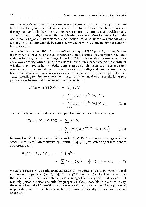
36 Continuous quantum mechanics ... Parts I and II
matrix elements and thereby the time average about which the property of the par-ticle that is being represented by the general expectation value oscillates in a nonsta-tionary state and whether there is a nonzero one for a stationary state. Additionallyand most importantly, however, this combination also determines by the indices of thenonzero-off-diagonal matrix elements the frequencies of possibly simultaneous oscil-lations. This will immediately become clear when we work out the inherent oscillatorybehavior next.In this context we note that both summations in Eq. (2.13) on page 33, no matter howfar they run, always cover the same range of indices because they pertain to the samestate vector as given, e.g. on page 33 by Eq. (2.11). This is also the reason why weare always dealing with quadratic matrices in quantum mechanics, independently ofwhether they have finite or infinite dimensions, and why there is always the samenumber of off-diagonal elements on either side of the diagonal. As a consequence,both summations occurring in a general expectation value can always be split into threeparts according to whether m = n. m > n or m < n where the sums in the latter twoparts always have equal numbers of off-diagonal terms
(2-15)
For a self-adjoint or at least Hermitian operator, this can be contracted to give
(2.16)
because hermiticity makes the third sum in Eq. (2.15) the complex conjugate of thesecond sum there. Alternatively, by rewriting Eq. (2.16) we can bring it into a moreappropriate form
S (uVnt + An,n) (2.17)
where the phase 3m, n results from the angle in the complex plane between the realand imaginary parts of a*nan(0m| O\(pn). Eqs. (2.16) and (2.17) make it very clear thatthe hermiticity of the matrix elements is a stringent necessity for the description ofmultiply periodic motions as only this property makes it possible to invert, so-to-say,the effect of so-called "transition matrix elements" and thereby meet the requirementof periodic motions that the system has to return periodically to previous dynamicsituations.

2. Part I: The discrepancy between the established interpretation and... 37
Before proceeding, one word about the way of how the time dependence of the generalexpectation value has above been written as (O(t)): At first glance, this notation mayappear misleading as it seems to contradict our stipulation that we are only dealingwith not explicitly time-dependent operators. As the time dependence only comesabout for the general expectation value we should actually follow other authors326 andwrite (O)(t) instead. But as this looks a kind of weird and also does not make theindication of time averaging any easier or look better we shall stick to our originalnotation but have to keep in mind that the time dependence exclusively pertains to thegeneral expectation value as a result of the state vector's dependence on time.
For a time-independent Hamiltonian, Eqs. (2.16) and (2.17) clearly demonstrate thatSchrödinger's time-dependent equation and its solutions establish the foundation fora theory of such multiply periodic motions that cannot be decomposed into simpleFourier series because the frequencies depend on the potential in which the particlemoves and, so, have to be determined individually from the solutions to the pertinentHamiltonian. Unfortunately, the wave conception along with the probability interpre-tation have misleadingly associated the time-dependent part with quantum interfer-ence effects (see below). These interferences are also deemed to not only make thedifference between the predictions of quantum mechanics and hidden variables theo-ries but also to be the reason for nonclassical behavior of quantum probabilities andresponsible for quantum correlations327 between different parts of the ensemble.At this point it is important to emphasize that the system is a closed one for a time-independent Hamiltonian and that these multiply periodic motions describe the con-sidered system's internal dynamics, which evolve with time all by themselves accord-ing to what is predetermined by its Hamiltonian. Hence, its dynamical situation, sta-tionary or not, never changes as long as its total energy does not. Then, in compliancewith the principle of superposition, the system would also exist with total energiesthat lie between the stationary states, i.e., in one of its many unperturbed nonstationarydynamical situations, which are also stable if a change of energy is excluded. Such sit-uations would then be dubbed nonstationary and described by the state vector \I>(r, t)as given on page 33 by Eq. (2.11) with all \an\ < 1 and constant.
Focusing on328 "eigenstates only" and, therefore, missing to consider the time depen-dence, the present statistical interpretation misunderstands the first line in Eq.(2.16) asan ensemble average329 and calls it the expectation value of the operator O that shouldbe obtained as the result of measurements on a large number of similarly preparedidentical systems330. If, however, the time dependence is taken into account, there can-not be any doubt that this term has to be understood as the time average of O for a singleparticle. While in the case of a large number of measurements on identically preparedidentical single particles the expected result is independent of whether we see it thisway or the other, the difference becomes important in the single event: Involving anunpredictable and unintelligible "collapse" of the state vector into one of the eigenvec-tors331 as a consequence of the questionable axiom, the established interpretation de-
326cf., e.g., [33, p249]327 [60, ppl254,1255]328 [79, p722\329 [102, p3]330 [6, p46], [36, plO2], [42, p806], [80, p378], [81, p361], [98, pp66,67]331 [6, ppl3,36], [8, ppU3-114,222], [33, p220], [34, pp350ff], [35, pp65,370ff], [36, plOl]

38 Continuous quantum mechanics ... Parts I and II
mands that always only one of the eigenvalues On be measured at a time, the chance ofobtaining just this one332 being |an|
2. To the contrary, our understanding of Eqs. (2.16)and (2.17), which includes the time dependence, does not have to assume a "collapse"because it sees Yln \o-n\2On in a very natural way as the time average of the property rep-resented by O when the system is in a nonstationary state. This time average is alwaysthere as the stationary part of the multiply periodic motion. At the instant of measure-ment, it may, however, be altered by the contribution from its time-dependent part inaccord with the instantaneous phase of the latter. All this will irrefutably be proven bythe concrete examples to be given below.It is obvious from Eqs. (2.16) and (2.17) on page 36, respectively, that in nonstation-ary states the time dependence of the general expectation value consists of a superpo-sition of periodic oscillations with frequencies uim<n = j-(Em - En). Complying withBohr's frequency condition333, these are the true eigenfrequencies33'4 the particle's motioncan be decomposed into. Unfortunately, this was not recognized in the past and evenSchrödinger has contributed to the interpretational troubles: Caught in the conceptionof wave behavior from the very beginning, he kept interpreting the time-independentspatial part of the eigenfunctions of the stationary states as expressing proper vibra-tions335 in terms of standing waves336 and the eigenenergies as equivalents of the eigen-frequencies of these proper vibrations. Accordingly, he regarded the emission frequen-cies as being equal to the differences of what he considered to be the eigenfrequencies337.Expressly he wrote338 even 26 years after his discovery. "The achievement of wavemechanics was that ... the 'stationary states' of Bohr's theory take the role of propervibrations and their discrete 'energy levels' the role of the proper frequencies of theseproper vibrations;... Moreover, the radiated frequencies ... equal the differences of theproper frequencies; . . ."
Which of the eigenfrequencies (in our terms) are active depends on the nondiagonalmatrix elements of the operator, i.e., on the selection rules339, and on which of the in-finitely many combinations of the mixing coefficients a*man are actually realized. Theirnumber depends on all the eigenstates with nonzero mixing coefficients that also con-tribute to the particle's total energy in a nonstationary state. But all active oscilla-tions take place simultaneously, although with potentially strongly differing ampli-tudes. But simultaneousness and strongly differing amplitudes, as Schrödinger re-marked340, do not contradict experience as the clamped string proves whose multiplyperiodic motion can be decomposed into a simple Fourier series, which consists ofone fundamental frequency and its integer multiples as overtones the latter of whichhave significantly smaller amplitudes. Along this line Schrödinger later doubted341
the existence of secondary radiation predicted by the dispersion theory of Kramers332 [6, pp73,74], [33, p217], [36, plO2], [42, p806], [80, p378), [98, p67]333 [31, pl39], [46, p8], [47, p487], [49, p507], [50, p396], [70, p230], [71, p3]334 [33, pZ49]335 [1, pP586,587], [9, pP372-373], [41, p864], [88, p253], [97, ppll4,122], [114, pP961-962]336 [9, p373\, [90, p89]337 [9, p374\, [90, p89], [97, pU4], [114, p962]338 [97, plU]339 [33, p249]340 [9, p375]341 [13, p375]
2. Part I: The discrepancy between the established interpretation and... 39
and Heisenberg342. But his notion of simultaneously active proper vibrations did notfind Born's appreciation343, who saw it in contradiction to Bohr's accepted theory. Con-sistently with this view, he insisted on dealing with atomic systems that occupy onlyone stationary state at a time344. In this he was absolutely right, as we shall prove, ifhe had meant this literally for physically stationary states. But Schrödinger's remarkunknowingly referred to the nonstationary states, and there simultaneousness, as willbe explained below and also in another communication345, is a necessary prerequisitefor describing complex periodic spatial motions. Contrary to the classically known ex-ample mentioned, the "atomic" types of such motions depend on the potential and,so, have their individual frequency patterns, which have to be obtained from the solu-tions to Schrödinger's equation. For these and above-given reasons, these patterns aredifferent from an equally spaced frequency comb as represented by a simple Fourierseries.Independently of Schrödinger's or anyone else's viewpoint, i.e., whether or not onewants to attribute standing-wave properties to the spatial eigenfunctions or their ab-solute squares, it is important to point out here again that this does not matter at allfor Eqs. (2.16) and (2.17) on page 36, respectively, as all types of matrix elements in thegeneral expectation value always involve an integration over all space.
If, as stipulated, the Hamiltonian does not explicitly depend on time, the general oscil-latory behavior of the eigenfunctions, as expressed on page 30 by Eq. (2.9), is a directconsequence of the form of Schrödinger's equation and the separability of space andtime variables resulting from it: After the periodic time dependence has been sepa-rated off by factorizing the wave function into a product of individually only time andspace-dependent functions, the remaining spatial part can only represent a time aver-age because after separation it can no longer depend on time. Thus, in the first place,Schrödinger's time-dependent equation has the inherent capability of describing mul-tiply periodic motions.
As the /cth eigenvalue is produced by demanding an — 8U: k all simultaneous oscilla-tions have ceased for an eigenstate, i.e., in a stationary state all properties are truly in-dependent of time. But they are only observable if their time average is different fromzero. As a consequence, Eqs. (2.16) and (2.17) make it very clear that the axiomaticclaim of only eigenvalues's having observable properties makes one miss the most es-sential part of the dynamics. Moreover, as the example of the linear harmonic oscillatorwill show, it may even lead to wrong conclusions with regard to what346 "stationarystates" constitute physically.
2.4.2 The role of nonstationary states
To this very day, one aspect of quantum mechanics, in our view, has found only in-consistent and confusing consideration because it is obviously biased by the exclusive-ness claim of the questionable axiom: As expressed by the general state vector, this
342 [136]343 [91, ppl 69-170]344 [91, pi 70]345 [137]346 [118, p5]

40 Continuous quantum mechanics ... Parts I and II
is the dynamical role of the nonstationary states. Their properties are only somewhathalf-heartedly and misleadingly being addressed when the state vector is called347 "acompletely coherent superposition of basis states" because this designation is usuallyused only for a special case of ensemble preparation, namely, when all members of theensemble are in the same pure state. In the general statistical case when there is onlyincomplete information about the state of the ensemble the system can appropriatelybe described by a density operator348, which represents a kind of average operator349.Its diagonal matrix elements represent the probabilities, or rather the average probabil-ities350, of finding the respective basis states realized in the ensemble351. Accordingly,they are also called the populations352 of the respective eigenstates. Its off-diagonal ma-trix elements, on the other hand, which are associated with oscillatory time depen-dences in accord with Bohr's frequency condition353, are often called coherences354 andseen as expressing quantum correlations355 between different groups in the ensemblebecause they are deemed to only occur between populated states356. If they do notcancel out each other357 the coherences are held responsible for quantum interferencephenomena and used, for instance, for the explanation of transient phenomena likequantum beats358.
This type of beating is observable, for instance, after the simultaneous excitation of anarrow multiplet state in an ensemble. This can be effected, e.g., in atoms by beam-foilexcitation359 or in molecules360 with a short laser pulse (Ar « nsec). The beating showsup as a modulation that is superimposed on the re-emitted but decaying fluorescence.Although the modulation frequencies have been identified as representing the respec-tive multiplet splittings no link has been established yet to mechanical properties ofthe emitting species. To the contrary, preoccupied with wave properties of particlesin mind, physicists have interpreted quantum beats as quantum interference effects361.Accordingly, benefiting from this biased wave conception, Young's famous double slitexperiment362 is usually being alluded to as a paradigm.This optical analogy has also been invoked for the explanation of the level-crossingeffect363. Although not a transient effect, it has equally been termed a quantum me-chanical interference effect364. It occurs as a bump in the intensity of the resonantlyscattered light when two magnetic sublevels whose magnetic quantum numbers differ
347 [ 131 , p49]348 [33 , pp295-304], [58, p331], [ 1 3 1 , p41]349 [33 , p297\350 [33 , p303]351 [80, p379], [105, p603], [ 131 , p42]352 [33, p303]353 [31 , pl39], [46, p8], [47, P487], [49, P507], [50, p396], [70, P230], [ 71 , P3]354 [33, p303], [ 131 , p48]355 [38, p38]356 [33 , p304]357 [33 , p303]358 [ 121 , P17], [ 131 , pp46-47,133-138], [138, pP256,260]359cf, e.g. , [139]360 [240-143]361 [ 1 2 1 , pl7], [ 1 3 1 , p47], [138 , pp256,260]362 [144, pl61], [145, ppl03-105], [146, pp7,43,73]363 [ i 4 7 _ i 4 9 ] ; [150, p82\364 [148,149], [150, pp74,82]

2. Part I: The discrepancy between the established interpretation and... 41
by either |Am| = 2 or |Am| = 1, cross at a certain strength of the linearly scanned uni-form magnetic field which the atoms are exposed to while they scatter resonant lightusually produced incoherently by a hollow cathode lamp365.But our exploitation of the properties of the nonstationary states strongly indicate, in-deed, that, on the one hand, the level-crossing effect has its origin in the fact that, e.g.,in the Larmor precession of the total magnetic moment the frequencies correspondingto two of its transverse components, which are counter-rotating and have | Am| = 2, be-come equal for the "crossing" field strength. Generating a linear oscillation this way, itsamplitude is the sum of the amplitudes of the counter-rotating and simultaneously in-phase oscillating components366. Thus, while the level-crossing effect seems to be trulygenerated by each individual atom as the incoherent continuous excitation suggests,the quantum beat in atoms367, on the other hand, can be shown to be an ensemble phe-nomenon in which fine, hyperfine, Stark or Zeeman oscillations368, respectively, thatoccur in each individual member of the decaying ensemble are synchronized by theimpulsive excitation process.Be it beam-foil or pulsed-laser excitation, the effect of the impulsive excitation processis two-fold: First, if the spectral width of the excitation process, i.e., the lack of sharp-ness of the excitation energy, is of the order of the level splitting nonstationary statesare being excited that lie energetically between the stationary levels. These states, aswill be shown by the examples, represent dynamical situations with inner oscillationsthat are performed with the frequency equivalent of the level splitting. Concomitantly,second, however, the Fourier transform of the spectral width, the duration of the ex-citation, is significantly shorter than the period of the inner oscillation. This way itsynchronizes the individual oscillations in the members of the ensemble and, so, cor-relates their internal motions.In beam-foil experiments, which can be described very well by the time evolution ofthe density matrix369, the beating and decay can be observed continuously by monitor-ing the fluorescence at varying distances down-stream from the foil370. On the otherhand, with pulsed-laser excitation of, e.g., molecules the technique of delayed coin-cidence may be employed in which the exciting laser pulse triggers a time-to-pulse-height converter which is only stopped upon the detection of the first fluorescencephoton371. Although many molecules are simultaneously excited, this is equivalent toactually experimenting with only one molecule at a time and, therefore, the procedurehas to be repeated over and over again until a continuous beating signal has been ac-cumulated. As we are dealing with single particles in this case there are no correlationswith other particles that could be made responsible for the beating. This demonstratesthat the beat signal is composed of, so-to-say, snapshots of the internal dynamics in in-dividual molecules. Arranged in due time sequence, these snapshots combine to givethe movie of the internal oscillation.Common to both methods is that the observed particles travel in vacuum: In beam-foil
365 [151,152]366
367 [139]368 [153]369 [154, p948]370 [139, p263]371 [140-143]

42 Continuous quantum mechanics ... Parts I and II
spectroscopy accelerated and collimated beams of velocity-selected ions impinge onthe foil and partly emerge down-stream from the foil as highly excited atomic speciesthat suffered only little loss of kinetic energy. Their number is determined by theenergy-dependent cross sections for electron capture.In the case of the referred-to Stark-quantum-beats experiments on molecules372, thespecies were prepared in situ either in an isentropic expansion from a nozzle andshaped to a jet beam by a skimmer before excitation or they left from an effusive sourceinto vacuum.The reason for letting the species travel freely in vacuum is to minimize collision-induced deco-herence by the environment.
Although justifiable in the case of quantum beats, the mixing coefficients are kept be-ing called probability amplitudes, thus alluding to ensembles and to the exclusivenessclaim of "eigenstates only" in a measurement. Without this claim everything wouldbecome quite easy and strikingly obvious: All directly and indirectly observable prop-erties are represented by general expectation values of respective operators as on page 36in Eqs. (2.16) and (2.17), respectively. This includes their oscillatory time behavior,which enables us to directly or indirectly infer the particle's unperturbed dynamics.This can be accomplished, for instance, via the determination of the frequency of thespontaneously emitted radiation provided the instantaneous loss of energy can be con-sidered sufficiently small. In this case, as will be shown in Part II below, it is only thenonstationary states through which we can learn what the particle is doing, for exam-ple, by detecting the radiation it can only emit while traversing the energetic regionof the nonstationary states because only these show oscillatory behavior. As a mat-ter of fact, it is only the transient nonstationary states to which we owe our knowl-edge about the stationary states by virtue of the measured transition frequencies. Forthe nonstationary states, the validity of Bohr's and his co-authors's classical assump-tion373 that "atoms (,which) contain electrified particles (,) ... can perform harmonicoscillations round positions of stable equilibrium and ... will exchange energy andmomentum with the radiation field according to the classical laws of electrodynam-ics" will be demonstrated to also hold approximately in the quantum-mechanical case,at least for a two-level model. The reservation "approximately" is necessary becausethe equilibrium is not absolutely stable but assumed to change "slowly" with time.Here, "slowly" means that the change takes long compared to the periods of the multi-frequency motion.
2.5 The consequences of a pure energy representation
The general expectation values, as Eqs. (2.16) and (2.17) show on page 36, respectively,have to be obtained with an adequate state vector in order to integrate the equation ofmotion for that operator as shown by Eq. (2.14) on page 34. For this to be the case, thestate vector must not only be composed of the eigenvectors of the Hamiltonian pertain-ing to the problem but also include the respective time dependences of the eigenfunctions.This is what makes our expectation values general because each of the possible state
372 [140-143]373 [72,pp70-71],[73,p786]

2. Part I: The discrepancy between the established interpretation and... 43
vectors then describes one of the infinitely many possible dynamical situations thatcan be obtained from exactly one of the infinitely many possible linear combinationsof all eigenfunctions. In principle, this may include linear combinations to which someeigenfunctions cannot contribute because their mixing coefficients are zero. If somelinear combinations lead to the same total energy (H) — Yln \an\2En the representeddynamical situations are energetically degenerate.In general, a dynamical situation may be characterized by the number of eigenfre-quencies involved and active, the amplitudes of the respective oscillations, and by thetime-averaged value about which the oscillations take place in accord with the relatedtotal energy. So, all these features not only depend on the eigenfunctions, which are thesolutions to Schrödinger's equation, of course, but also on the mixing coefficients. Ifthe Hamiltonian is independent of time and does not include the coupling to other sys-tems, Schrödinger's partial differential equation represents the total energy of a singleparticle's motion in space and time. Then, as we have outlined above, the so-describedsystem constitutes a closed one because its total energy is conserved. This may includethe particle itself if inner degrees of freedom play a role. In order to expressly keep itthis way we do not consider transitions, neither at this point nor for the entire Part I.The eigenfunctions and all their possible linear combinations must not only reflect allproperties that contribute to the respective total energy of the particle in appropriateenergetic terms but, at the same time, they must also express this as functions of spaceand time, the latter, however, always in an oscillatory manner as a tribute to the formof Schrödinger's equation. Of course, the eigenfunctions can and have to do that onlyfor contributions that they had actually solved Schrödinger's equation for, i.e., theycan only represent and account for what is included in the Hamiltonian. But in or-der to be able to do that, the eigenfunctions and any of their linear combinations mustalways comprise all possible configurations in ordinary space as well as all possibleorientations of any angular momentum for which the particle possesses the same to-tal energy. As a consequence, the higher the spatial symmetry the more energeticallyequivalent orientations and spatial configurations have to be covered. Thus, degen-eracy is an inherent feature. This is a consequence of the scalar nature of the energyand how an energy representation has to account for it. Another outstanding, though in-herently dynamic feature of an energy representation, which will be shown to generallyhold true for bound systems in nonstationary states, is the multiply periodic exchangeamong different contributions to the total energy. This exchange, which is typical ofnonstationary states, makes sure that the total energy always remains constant.
2.5.1 Free particles
As a first example, we consider the features that an energy representation has to sup-ply for a free particle. Although, in its ultimate consequence, this is an abstract case,which denies reality, it is nevertheless worth being looked into: The free particle's po-sition cannot be of any concern for an energy representation because neither its potentialenergy nor, concomitantly, its kinetic energy depend on it. So, if we choose, for sim-plicity's sake, V(r) = 0 everywhere, the particle's kinetic energy is identical to its totalenergy. Thus, all that matters for an energy representation is the magnitude of the par-ticle's momentum, and it is totally unimportant to the total energy where it is and in

44 Continuous quantum mechanics ... Parts I and II
which direction it is moving because it finds the same conditions everywhere. Hence,for a particle with any given momentum, both its direction and location in space arewithout any effect on its total energy. Being infinitely degenerate in this regard, theseproperties can and even must be left absolutely indeterminate by an energy representa-tion.
As we are dealing here only with time-independent Hamiltonians, we are describ-ing closed systems whose total energy must be a constant per definitionem. In the freeparticle's case., as here chosen, the constant total energy coincides with the kinetic en-ergy. Therefore, each individual particle can only have this one energy once and for all.Hence, the putative energy continuum only makes sure that, in principle, the wholerange of nonrelativistic energies is initially available for the particle. But this continuumis accessible only once, i.e., at the very beginning when the initial conditions determinethe particle's energy, and never again thereafter. And as the particle's position does notmatter at all, it need not be determined and the preparation of its initial momentum canbe accomplished to any desired accuracy even under the restrictions of the uncertaintyrelations. So, whatever value the particle's momentum happened to have been givenin the remote past, individually, the free particle always remains in the one and onlydynamical state it initially occupied. There, it has to stay forever because there is noth-ing that could ever change its dynamical parameters. Thus, an individual free particleonly exists in one stationary state, and this is its only eigenstate out of a continuum ofinfinitely many possible ones.
Additionally, as there is nothing in a force-free environment that could ever changethe particle's momentum, it is an intrinsic feature of a free particle's behavior that thisproperty must be a constant of the motion374. As a result, its momentum should com-mute with the Hamiltonian, e.g., [px, H] — 0, and it should, accordingly, have the sameeigenfunctions. Thus, the properties of having the same eigenfunctions for both energyand momentum with eigenvalues independent of position and time are indispensablecriteria to be met by any free particle's wave function. Additionally, it has to expressthe fact that the free particle can only move linearly.
Thus, what is to be expected can easily be stated and the solution to the problem onthe basis of Schrödinger's equation is straightforward and equally easy to achieve. Theapparent easiness makes this problem a favorite subject that almost any textbook375
would not want to miss out. However, so easy the solution, so problematic it couldbe from a mathematical point of view if we would expect too much from it. We shallcomment on its mathematical and physical properties in due time. But there is onegeneral aspect of the properties of Schrödinger's equation that should be elucidatedright away: This is its inherent capability to preferentially describe multiply periodicmotions in smooth binding potentials.
As a result, it is easy to understand that for a free particle, which has to move uni-formly in the infinitely extended space of constant potential energy, this situation mustbe representedby a wave function that, due to this property of Schrödinger's equation, isnot only oscillatory in time but, at the same time, must also be able to account spatiallyfor all of above-listed features: Under these conditions, this can only be accomplishedby a traveling monochromatic plane wave, which extends in one of the infinitely many
374 [36,̂ 242]375cf., e.g., [33, pp22,64], [35, p27], [99, p267], [105, p57], [126, P33], [128, p55]

2. Part I: The discrepancy between the established interpretation and... 45
possible directions of propagation from — oo to +oc with an infinitely wide phase frontand any additional arbitrary phase.But this representation alone does not justify the conclusion that the particle has waveproperties although this is generally being assumed376. However highly attractive andseducing the apparent wave properties may seem with regard to the principle of super-position, its application is not only questionable but even mathematically prohibitedbecause the solutions to this problem, as we shall show, do not admit the principle ofsuperposition. But this apparent shortcoming is not devastating because this propertyis physically neither reasonable nor necessary as we have expounded above.For simplicity's sake and because we can choose the orientation of our coordinate sys-tem however it pleases us, we decide to have the particle's direction of motion, forinstance, parallel to the x direction. Then, Schrödinger's equation for a free particle inan environment of vanishing potential energy reads
n2 d2p dip-2^J^ = %n-dJ- ( 2 J 8 )
Not caring about the normalization constant for the time being, we obtain the follow-ing solutions377
rj}±{x,t)=e±i(<kx^!^l+^ (2.19)
In these wave functions, k is the wave number, m the particle's mass, and <fi an arbitraryphase. Noting that the arbitrariness of this phase additionally underscores the unim-portance of the particle's position, we shall continue by setting 0 = 0. Furthermore, wenote that both wave functions are intimately and identically related to the separationconstant E = ~^-. This is the energy eigenvalue, which can take on any nonrelativisticvalue. Of course, the dependence of the two basic wave functions on the position co-ordinate x and time has to reflect the properties of traveling waves, which propagateoppositely. But these features do not matter for any total energy.
As for the demanded vanishing of the commutator between the momentum opera-tor px and the Hamiltonian, the result of the application of this operator to the wavefunction of Eq. (2.19)
P*1>±(x,t) = - 2 M 2 Ü = ±hky±(x,t) . (2.20)I OX
tells us through Eq. (2.20) not only that it is also an eigenfunction of the momentum378,indeed, but also that the particle is moving uniformly with the constant momentum hkeither to the right or to the left and independently of location and time.The statistical interpretation sees compliance with above-stated criteria especially inthe fact that the wave functions of Eq. (2.19) give rise to a position probability density\ib±(x,t)\2 that is constant in time and everywhere379. But although these wave func-tions do conform with all physical requirements listed above this fact already puts thefinger on the mathematically sore spot if we have unreflected expectations: The wave
376 [6, p3]377 [105, P57], [109, p26), [126, p33]378 [105, p57], [109, p31]379 [33, p22] , [35, p27]

46 Continuous quantum mechanics ... Parts I and II
functions of Eq. (2.19) with their continuous dependence on k do not span a Hubertspace because in the rigorous mathematical sense they are neither square-integrable380
for identical nor orthogonal for different wave numbers k and k1. Although the corre-sponding integral ^ /+~exp[±i(fc'-fc)z]d.T =» £ lim«,̂ «, sin°,(^° = 6{k'-k) is practi-cally identical to the definition of the 6 function381 it does not exist in itself382 becausethe limiting process can only be carried out successfully when the 5 function is be-ing integrated over in the presence of an arbitrary function. Unfortunately, this fact issometimes handled less rigorously when the integral is directly identified with the 6function. Then, the whole procedure is called normalization on the 6 function383.
The lack of orthonormalizability destroys the applicability of the principle of super-position. This is the price that has to be paid for the fact that despite the momentumoperator's not being self-adjoint but only Hermitian384 real eigenvalues are being ob-tained. But as we have explained above, there is no physical need for using the superpo-sition principle as a means of enforcing square-integrability and, thereby, localizationbecause a prerequisite for a real necessity of square integrability is that the particle bespatially confined and thereby localizable. As already discussed at length above, thisis not the case here and, therefore, this property neither need nor can be supplied bythe solutions to an energy representation. Reversing the argument, however, we couldtake the absence of square integrability as an indication or even fingerprint that a freeparticle inherently cannot be localizable because of lack of spatial confinement.Despite this fact it has been argued385 that the wave functions of Eq. (2.19) do notrepresent any physically reasonable state of the particle because with their absolutesquare being constant these monochromatic plane-wave solutions fail to be square-integrable386 and, so, do not comply with the axiomatically demanded properties thatin quantum mechanics the description of a physical system has to be accomplished interms of the elements of a separable complex Hubert space associated with the physicalsystem387 and that every observable is represented by a linear self-adjoint operator thatacts in the respective Hubert space388.So, as the particle must be somewhere because even the universe is deemed to be finite,this argument has been used to justify the application of the principle of superpositionas the only way to overcome this deficiency389. Thus, if we would not be aware ofthe shortcomings related to above-mentioned lack of rigor and blindly follow this ar-gument, the results of Eq. (2.19) would seem to constitute a limiting situation of aninherent Fourier transformation for the pair of canonically conjugate variables of posi-tion and momentum whose vectors are pointing in the chosen direction. For this pair,it would seem as if there were a S-type spectrum in momentum space and a white spec-
380 [105, pp58-59,136]381 [6, pp58-60]382 [82, pp66-7J]383 [58, pl83\, [80, p55], [126, pp570-571]384 [155, pl903]385 [33, p23]386 [58, pill]387 [35, P37]388 [35, p40]389 [33, p23]

2. Part I: The discrepancy between the established interpretation and... 47
trum in ordinary space390. And, indeed, if there were no time dependence in Eq. (2.19)the spatial dependence of the wave function on exp (±ikx) would suggests that any su-perposition of the eigenfunctions in terms of an integral over all momenta hk rangingfrom k = — oo to k = +oo would mathematically be identical to a Fourier transforma-tion391. This may have contributed to assume the same392 for the eigenfunctions ofEq. (2.19)
/ c{k)e+iykx-^i) dk (2.21)
although only Schrödinger's time-independent equation also admits this interpretation.So, it is not astonishing that there is a shortcoming: In spite of remaining a solution toEq. (2.18) for the integrand it has lost the property of being a simultaneous eigenfunc-tion of the momentum operator.
Accordingly, unreflected and unchecked reliance in the applicability of the principle ofsuperposition along with the belief in wave properties393 as a natural result of whichwave packets could be generated would seduce us to generally apply the seeminglyinherent Fourier-type transformation behavior. In the special case of a linear superpo-sition that takes the form of a Gaussian momentum distribution, a Fourier transforma-tion would also produce a Gaussian distribution in ordinary space but with a widththat is complementary to the other one in the sense that, e.g., Ax Apa. = h. This isexactly the way how Heisenberg derived his uncertainty relations394.
Guided by de Broglie's wave conception395, particularly Bohr396 related the movingparticle to a wave packet because he saw in wave properties the ultimate reason forthe uncertainty relations as an inherent dynamical property. Although Heisenberg397
was aware of the statistical significance of de Broglie waves and equally advocated398
the statistical interpretation of quantum mechanics, he originally favored the expla-nation that the uncertainty relations only come into play at the instant when, e.g., anelectron's position is being determined experimentally399. Then, they provide an illus-trative elucidation for the noncommutativity400 of [x,px] = ih, which in his opinionwas the reason for discontinuities401 that occur in the behavior of particles at such in-stances. All his examples and Gedankenexperimente402 are pointing in this direction.Finally, however, he seems to have been convinced to see it Bohr's way403.
This concept is accepted ever since404 and, so, is reproduced in most textbooks405. It390 [33 , P27]391 [130, p293]392cf., e .g . , [33 , p22], [35 , p27], [99, p267], [128 , p55]393 [6, p3]394 [4, pl80], [84, ppl2-14]395 [101]39b[l,pp581-582]397 [4, pl76+footnote 1]398 [4,ppl76-177]399 [4, p i 75]400 [4, pi 75]401 [4, ppl76-177]402 [84, ppl5-35]403 [4, pl97, note added at proof]404 [6, pp3,121ff], [7, p285], [99, p263], [156, ppl74-177]4 0 5cf . ,e .g . , [33, pp22-28], [35, pp27-29], [128, pp55-59]

48 Continuous quantum mechanics... Parts I and II
becomes most visible when the existence of a zero-point energy in a quantum mechan-ical linear harmonic oscillator is related to the uncertainty relations406 Yet, it has to bepointed out that here the conclusions have been drawn under the tacit assumption thatthe application of the principle of superposition really makes sense physically.
In the case of a free particle, the applicability of the principle of superposition must bequestioned for above-given reasons. In order to substantiate this claim we shall takesome closer looks: Already in the one-dimensional case, the superposition of the twobasic solutions of Eq. (2.19), one plane wave propagating to the right and one to theleft, respectively, spell trouble if done without checking the physical consequences: Theresultant wave function
*(x,t) = cie+i(kx-!£t) +c2e-i(kx+h£t) (2.22)
may also be written as
ty{x, t) = e"*^' \(c-[ + c2) coskx + i(cx - c2) sin kx\ . (2.23)
Along with the locally modulated absolute square
\V{x,t)\2 = \Cl\2 + \c2\
2 + 2^{clc*2ei2kx} (2.24)
this clearly shows that the wave function of Eq. (2.22) represents a standing wave and,therefore, can no longer be an eigenfunction of the particle's momentum
(2.25)
although it should because of having to reflect its being a constant of the motion. Thisdiscrepancy is a consequence of the fact that an individual particle cannot move ei-ther way simultaneously. But as an energy representation is directionally insensitive,Eqs. (2.22) and (2.23) nonetheless are solutions to Eq. (2.18) on page 45 and, thereforerepresent eigenfunctions of the energy with the eigenvalue E = %^- in seeming ac-cordance with the superposition principle. So, there is only one way to reconcile allfeatures with each other: This is to demand k = 0, i.e., that the particle be at rest wher-ever it may be. But, with the wave function's being constant, this is just the trivialsolution to Eq. (2.18).
Contrary to that and without checking the result of the action of the momentum oper-ator on that wave function, the failure of not accounting for the time dependence hasled to wrongly infer407 from the absolute square of the wave function in Eq. (2.24) that,on the basis of the statistical interpretation, this is describing the chances |ci|2 or |c2|
2,respectively, of finding the particle moving to the right or to the left.
If we would not further doubt the general applicability of the principle of superposi-tion our findings so far would only suggest excluding the superposition of counter-propagating waves with the same wave number. Hence, a general kind of one-sidedsuperposition would have the lower bound —oo replaced by zero in Eq. (2.21) in orderto have, e.g., all waves traveling to the right.
406cfv e.g., [80, p69], [102, P20], [105, pP170-171], [106, p50]407 [157, pl5Z]

2. Part I: The discrepancy between the established interpretation and... 49
As indicated above, a favored momentum distribution is the Gaussian one (with thelower bound extended to —oo: cf.408). Then,
where
The odd analytic function409
a(t) =
dt
(2.26)
(2.27)
(2.28)
is directly related to the error function410 by Erf(z) = \^/ir <&{z). For x real, it has theproperty411 limx_^+oc $(x) = 1 and although this limit is only reached asymptoticallythe monotonous rise is fast412 so that $(a; = 1.3) « 0.93.It is apparent from Eq. (2.26) that the assumption of a Gaussian momentum distri-bution leads to a moving Gaussian peak in ordinary space even without involving aFourier transformation. Due to the form of the wave function, the unreflected appli-cation of the principle of superposition would correspond to such a transformation,indeed, if we would have extended the lower bound of the integral in Eq. (2.21) to — ooas well as of those in the first and second line of Eq. (2.26). Being the eye-catchingdominant feature, the Gaussian peak travels with the group velocity vg = ^ andspreads out with time due to the time dependence of a(t). This becomes most appar-ent if we write this time dependence out explicitly (with the lower bound extended to-oo: cf.413)
(2.29)
For sufficiently large a, i.e., for a very narrow initial momentum distribution aboutko 3> 0, we could have extended, without seriously contradicting Eq. (2.21), the lower
408 [33, p64], [99, p267], [128, p57]409 [158, p26]410 [158, pp26-27], [159, pl47]411 [158, p26]412 [158, p27]413 [33, p64], [99, P267], [128, p57]
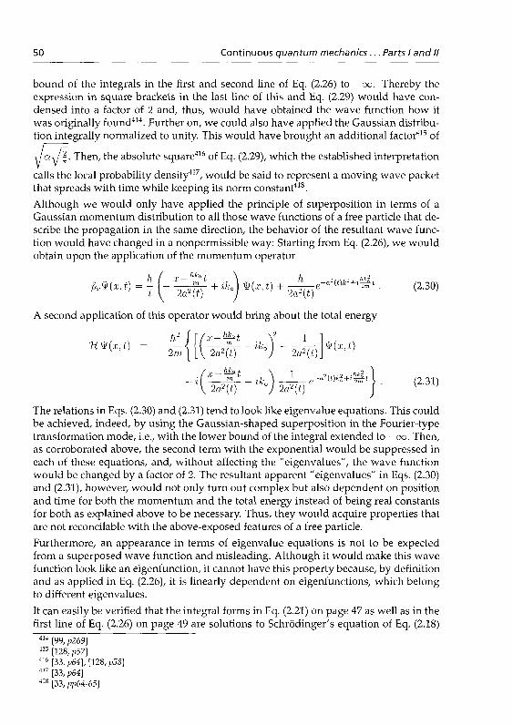
50 Continuous quantum mechanics ... Parts I and II
bound of the integrals in the first and second line of Eq. (2.26) to —oo. Thereby theexpression in square brackets in the last line of this and Eq. (2.29) would have con-densed into a factor of 2 and, thus, would have obtained the wave function how itwas originally found414. Further on, we could also have applied the Gaussian distribu-tion integrally normalized to unity. This would have brought an additional factor415 of
K Then, the absolute square416 of Eq. (2.29), which the established interpretation
calls the local probability density417, would be said to represent a moving wave packetthat spreads with time while keeping its norm constant418.Although we would only have applied the principle of superposition in terms of aGaussian momentum distribution to all those wave functions of a free particle that de-scribe the propagation in the same direction, the behavior of the resultant wave func-tion would have changed in a nonpermissible way: Starting from Eq. (2.26), we wouldobtain upon the application of the momentum operator
*•»<*•() = 7 (" W + lk) *<*• ° + ^Wf'mki+''4' • (Z30)
A second application of this operator would bring about the total energy
The relations in Eqs. (2.30) and (2.31) tend to look like eigenvalue equations. This couldbe achieved, indeed, by using the Gaussian-shaped superposition in the Fourier-typetransformation mode, i.e., with the lower bound of the integral extended to —oo. Then,as corroborated above, the second term with the exponential would be suppressed ineach of these equations, and, without affecting the "eigenvalues", the wave functionwould be changed by a factor of 2. The resultant apparent "eigenvalues" in Eqs. (2.30)and (2.31), however, would not only turn out complex but also dependent on positionand time for both the momentum and the total energy instead of being real constantsfor both as explained above to be necessary. Thus, they would acquire properties thatare not reconcilable with the above-exposed features of a free particle.Furthermore, an appearance in terms of eigenvalue equations is not to be expectedfrom a superposed wave function and misleading. Although it would make this wavefunction look like an eigenfunction, it cannot have this property because, by definitionand as applied in Eq. (2.26), it is linearly dependent on eigenfunctions, which belongto different eigenvalues.It can easily be verified that the integral forms in Eq. (2.21) on page 47 as well as in thefirst line of Eq. (2.26) on page 49 are solutions to Schrödinger's equation of Eq. (2.18)
414 [99, p269]415 [128, p57]416 [33, p64], [128, p58]417 [33, p64]418 [33, pp64-65]

2. Part I: The discrepancy between the established interpretation and... 51
on page 45. This property is preserved, of course, in the integration process419 as acomparison of Eq. (2.31) with the following one clearly demonstrates
which is obtained from Eq. (2.29) under observation of Eq. (2.27).Despite this property, any dependence of the total energy on position and/or time,as in Eq. (2.31), is absolutely irreconcilable with the time-independent Hamiltonianwe started out with. This literally has to lead to a separation constant in the sense ofthe word, there is no way around! Even though the formation of the general expecta-tion values of the momentum and the Hamiltonian by multiplication of Eqs. (2.30) and(2.31), respectively, with the complex conjugate wave function of Eqs. (2.29) and subse-quent integration over the position coordinate x from — oo to +oo, would eliminate thespace dependence, it nevertheless would leave the resultant expectation values depen-dent on time. But, as pointed out above, both expectation values must be independentof time. So, although mathematically correct, these results are totally unacceptable for aclosed physical system.How did this deficiency sneak in? The most obvious formal reason is the introductionof the quadratic supplement, which allowed the step from the first line to the secondone in Eq. (2.26) on page 49. While one part of the "zero" that is added to the argumentof the exponential in order to transform the integration variable is absorbed in the inte-grand and, so, disappears as a consequence of the integration, the other part survivesbecause it is independent of the integration variable. This is the part that is responsiblefor the trouble in the first place.
But the deeper reason lies in the fact that the wave function of Eq. (2.29), as demon-strated by Eqs. (2.31) and (2.32), satisfies Schrödinger's equation in a inappropriateway by making belief to be representing an eigenfunction: For this really to be thecase, the correct way is predetermined by the Hamiltonian's stipulated independenceof time. As a consequence, a separation of variables must be possible with the effectthat the "eigenvalues" on the right-hand sides of Eqs. (2.30) and (2.31), respectively,should be identical to the separation constant and not equal to a function that is depen-dent on both space and time. In any case, the lost properties could only be recoveredif the width of the wave packet in momentum space would become vanishingly smallby making a —> oo and thereby reproducing, according to Eq. (2.29), the original "one-way" wave function of Eq. (2.19) given on page 45. This demonstrates the exclusive-ness of the original eigenfunctions.What is the physical reason that the principle of superposition obviously fails when afree particle's wave function is represented by a Gaussian-shaped pulse that is movingin ordinary space? The answer has already been given above: In response to the factthat it is not needed at all, neither in momentum space nor in ordinary space, the wavefunctions of Eq. (2.19) on page 45 do not admit the application of this principle becausethey are not orthonormalizable..
419 [99, p269)

52 Continuous quantum mechanics... Parts I and II
The need for the principle of superposition only arises in binding potentials when thepossibly multiply periodic exchange has to be accounted for that occurs between thekinetic and potential energy only in nonstationary states. Then, as will be shown be-low, it provides the basis for the general validity of the Virial theorem.
However, for the sake of apparent consistency, different methods have been devised toartificially make the free particle's wave function square-integrable: The normalizationwith the help of Dirac's S function420 has already been mentioned. Another one, e.g., isthe normalization in a cubic box421. With periodic boundary conditions at the walls ofthe box the components of the wave vector are restrictred to the values422 k{ = 27m,/Lwhere L is the length of the edges. By aligning the cubes three-dimensionally the freespace can be completely filled. The choice of periodic boundary conditions admitstraveling as well as standing waves. This is achieved by demanding the same valueand slope of the wave function at the wall between adjacent cubes. As the basic boxcan be made arbitrarily large, the differences between the discrete wave vectors can bemade arbirarily small. In this sense, it is always assumed that the limit L —> oo is takenat the end of the calculation423.
Complementary to the fact that a free particle's momentum must be a constant of themotion we also have the fact that its position must not wherever that may be. ApplyingEq. (2.14) of page 34 with either type of the wave functions of Eq. (2.19) on page 45 andintegrating with respect to time, we find
fik(x(t)) = ±—t (ip±(x, t)\ip±(x: t)) (2.33)
where (-ip± (x, t)\ 4>±{x, t)) has deliberately been left standing in order to indicate inde-pendently of any normalization scheme that the nonlocalizability of the free particleis owed to the fact that knowledge about its position cannot be provided by an energyrepresentation. To finally make the point we are after, Eq. (2.33) clearly shows that thenoncommutativity of [x,7i] ^ 0, which brings about the velocity ± ^ , is directly re-lated to the particle's having to keep on moving uniformly all the time. Therefore, itsposition cannot be a constant of the motion. This also explains why the nonvanishingcommutator [x, px] ^ 0 is a must for a free particle.
As a matter of fact, the free particle problem is the only case to which the exclusive-ness of the questionable axiom fully applies. For the same reason, off-diagonal matrixelements do not exist in this case. These are only needed, as we shall see below, for thedescription of multiply periodic motions, which can only occur, of course, in bindingpotentials with a smooth and continuous dependence on the position variable. In suchpotentials, the usual mode of motion always involves a periodic exchange betweenthe particle's kinetic and potential energy. Concomitantly, this also always impliesperiodically changing accelerations and decelerations because the particle experiencesspatially changing parts of the potential and, so, feels periodically changing forces. Forbeing capable of covering all dynamical situations of this nonstationary behavior of asingle particle the formalism has to resort to the principle of superposition. This willbecome clear below when we shall discuss the really dynamic examples.
420 [58, p270], [80, p55], [126, pp570-571]421 [80, p54], [87, pp88-90], [126, pp571-573]422 [80, P54]423 3, p54]

2. Part I: The discrepancy between the established interpretation and... 53
So, any attempt to apply the principle of superposition to the basic free-particle solu-tions violates dynamic essentials by ignoring that a single free particle can only possessone direction and one magnitude of its momentum. Moreover, the resultant localizationis not in compliance with what an energy representation is actually capable of deliveringin this case: As the peak of the respective Gaussian defines the most probable momen-tum and position, respectively, a dependence between energy and location is beingintroduced through the back door that is not justified at all as it is way beyond thecapability of an energy representation.
But if we would interpret the wave function of Eqs. (2.26) and (2.29) on page 49, respec-tively, as representing an ensemble of noninteracting particles that has been preparedat t = 0 with numbers in each momentum interval h(k, dk) according to the narrowGaussian momentum distribution around ko, the initial localization and the spreadingwith time of the ensemble's wave packet424 could easily be understood: Simply dueto the different velocities of its constituents, there is an inherent tendency to restore atotally delocalized situation.In order to make the connection with the statistical interpretation more apparent thisspreading is often derived under the assumption that the behavior of the position andmomentum variables is governed by the uncertainty relations and, so, is a statisticalone with respective root-mean-square deviations425 that determine the widths of therespective Gaussian distributions. Then, even the statistical interpretation would al-low this spreading to be understood without resorting to wave properties: If in thebeginning neither momentum nor location are sharply defined, i.e., without knowingtheir exact values, we can state that the farther the cannon ball flies the more likely itis that it will miss a target of given size and position.In passing we should mention that the wave conception works quite well for quasi-freeparticles, e.g., for the description of the delocalized electrons in the conduction band ofmetals where the energy bands in the periodic potential result from the dependence ofthe electron energy on k2 and its "reflections" at the boundaries of the Brillouin zonedue to Bragg reflection and Born's theorem426. But owing to genuine delocalization, noFourier-type behavior has to be inferred for ordinary space.
2.5.2 Bound one-particle systems
The remainder of Part I will deal with bound one-particle systems. As well-known ex-amples, it will comprise the quantum mechanical treatment of the harmonic oscillatorin one and two dimensions as well as of the Kepler problem. Before we go into detailswe want to address some general consequences pertaining to their energy representation.
As we have already seen in conjunction with the free-particle case, an energy represen-tation does not care about directions in space that are energetically equivalent. Underthe same premise it does not care about orientations in space either, provided no pref-erential direction is imposed on this space, e.g., by a static electromagnetic field. In
424 [58, pp218-222], [80, p64]425 [33, pp230-231], [35, pp52-53], [58, p222], [80, pp60-64], [81, p364], [92, pp297-299], [100, pp337-339],
[103], [135, p96\426 [122, pp42,47ff], [125, pp48ff], [160, pp246,252ff], [161, ppl33ff]

54 Continuous quantum mechanics ... Parts I and II
other words, this careless attitude is only possible if different spatial orientations of,e.g., the angular momentum, are energetically degenerate. Spherical symmetry is aprerequisite for this to be possible for angular momenta and implies the feasibility ofa separation of the angular dependence from the radial one. This is what we shall en-counter in the case of the two-dimensional isotropic harmonic oscillator and the Keplerproblem.Thus, in the general spherical case, the angular parts of the solutions to Schrödinger'sequation must equally reflect the energy representation of this equation by being energet-ically degenerate with regard to orientation for reasons mentioned on page 33 above incontext with the state vector. This allows them to comprise for any given angular mo-mentum in terms of mutually orthonormal parts of the eigenfunctions all those linearlyindependent spatial orientations as basis vectors that permit to construct from linearsuperpositions any arbitrary spatial orientation of the particle's angular momentumthat belongs to the same energy. This is the reason why here, analogous to the classicalcase, the operator of the angular momentum occurs squared in Schrödinger's equationand, thus, makes its eigenvalues enter the radial part of this equation in terms of acentrifugal barrier either as ^^ß for the two-dimensional isotropic harmonic oscillator
or as h 2 ^2 in the Kepler problem, in any case, however, independently of the actual
orientation of the angular momentum involved.So, apart from the usual separation of space and time variables, which establishes aperiodic behavior for the time dependence of the motion, periodicity of also the angu-lar motion is the additional feature that entails the separability of radial and angularvariables under rotational and spherical symmetry. As after separation, in principle,the respective variables have to be totally independent of each other, separability in-herently implies that an averaging process must be possible as an intrinsic feature ofthe motion: For a multiply periodic time dependence the remaining space dependencecan only be the time average, while after the separation of radial and angular variables,in the same way, the remaining radial part is an angular average as encountered, e.g.,in a centrifugal barrier.The limitations of our method in respect of analytical rigor are easy to see: The prob-lem must be analytically solvable in full rigor in order to obtain all basis vectors ofthe respective Hubert space. But despite these limitations it is especially the verifiabil-ity and transparency of analytical solutions that can convince and thereby open newhorizons for a better understanding of a realm of physics that even many renownedphysicists427, in following our patriarchs, deem not fully comprehensible for funda-mental reasons related to the uncertainty relations.
2.6 The linear harmonic oscillator
Taking the linear harmonic oscillator as our next example, we shall calculate the generalexpectation values of some of its most obvious properties. Before getting started, weshortly review, for the reader's convenience, the main steps how they were originally
427cf., e.g., [162, pl-1], [163, pl29]

2. Part I: The discrepancy between the established interpretation and... 55
taken428 but which may also be found in most textbooks429.
By introducing the dimensionless variable £ = ax with a2 = 7~ and the parameterA = ^ where in both relations the eigenfrequency uQ — J ~ derives from the squareroot of the ratio of the constant of the restoring force k over the mass m of the pointmass while E its total energy, the spatial part of Schrödinger's equation for the linearharmonic oscillator can be transformed430 into
+ (A - eno = o. (2.34)uc,~
In order to obtain the correct asymptotic behavior, the wave function is factorized431
into u(£) = H(£) exp(-l^). This changes432 Eq. (2.34) into
H"(0 - 2H'(0 + (A - l)H(O = 0 . (2.35)
An ansatz with a power expansion for #(£) leads to a recursion relation that makesthe need apparent to terminate the power series at some exponent n in order not tospoil the asymptotic behavior, the second boundary condition. The first one, regular-ity at the origin, is met by the ansatz itself. The termination is achieved by confiningthe parameter A in the recursion relation for the expansion coefficients to the discrete,integer values An — 2n + 1 with n = 0, 1, 2,... . This is the condition of quantization,which generates the spectrum of discrete, equidistant energy eigenvalues because thenabove-mentioned relation between A and the total energy delivers En = huo(n + \). Atthe same time, An = 2n + 1 transforms Eq. (2.35) into the differential equation for Her-mite polynomials433
H"n(0 - 2E'n{i) + 2nHn(0 = 0 . (2.36)
These polynomials are defined in — oo < £ < +co and have the form434
//•n^) = (_l)ne€2_^Le-€2 (2.37)
for integer n > 0. Rendering the eigenfunctions orthonormalizable, they comply433
with
= 8m,n 2" n ! ^ . (2.38)
Some of their recursion relations436 are very helpful in calculating matrix elements
1(f), (2.39a)
, (239b)(2.39c)
428 [10, p514]429cf., e.g., [33, pp483ff], [35, ppUlff], [36, pp66ff], [78, pp54-60], [80, pp66ff], [98, pp99ff], [102, ppl9ff],
[105, ppl66ff], [106, pp48ff], [126, pp364ff], [127, pp33ff], [128, ppl96ff]430 [10, p515], [35, pU2], [36, p66), [102, ppl9,100], [128, pl97]431 [35, pl42), [78, p57]4 3 2 [ 1 0 2 , p l 9 ]433 [78, p57], [102, p2l], [158, plOl], [159, p292]434 [78, p57], [102, p22], [158, p2O2], [159, pl93]435 [78, p57], [102, pZ2], [158, p202]4 3 6 [ 7 8 , p 5 g ] , [158,p202]

56 Continuous quantum mechanics ... Parts I and II
where Eq. (2.39a) assisted in obtaining the final result of Eq. (2.39c) from the differenti-ation of Eq. (2.37) in Eq. (2.39b). For all terms to be contributing, n > 1 is needed. Butobviously, all relations of Eq. (2.39) also hold for n = 0 as can be easily verified withthe help of Eq. (2.37). The rearranged form437 of Eq. (2.39a)
£Hn(0 = ±Hn+l(0 + nH^iO (2.40)
is important not only to the calculation of the matrix element of the position coordinateitself but also of powers thereof: If we multiply this relation with £ and again applyit on the right hand side to each of the newly generated products of £ with the twoHermite polynomials of different order, we arrive at
eHn(0 = \Hn+2(O + \(2n + 1) Hn(O + n(n - 1) Hn-2(O (2.41)
with n > 2 if all terms are to contribute. Inserting the rearranged relation of Eq. (2.39a)into Eq. (2.39b), we obtain, after a minor rearrangement of the latter, yet another one
K(O - €#n(0 = ~Hn+1(O + nHn^(a . (2.42)
where all terms only contribute if n > 1.
Accounting for the normalization constant according to the orthogonality relation ofEq. (2.38) and the factorization introduced past Eq. (2.34), the eigenfunctions of thelinear harmonic oscillator read438
(bn{x) = N^x) Hn(ax) e~iJ^ , (2.43a)
= N^Hn(0e~^ (2.43b)
with439
wS {2M)
where the superscript (x) indicates that the normalization constant pertains to thespace variable x because of the appearance of a under the root. Now, it is easy toverify that the multiplication of Eq. (2.42) by exp( —1£2) represents the first derivativeof the eigenfunction <pn(^(x)) with respect to £.
Before moving further away from the analytical eigenfunctions, it seems appropriateto consider the relations that have obviously contributed to the justification of the in-terpretation that deems the zero-point energy a consequence of the uncertainty princi-ple440: As this energy pertains to the quantum number n = 0, the prevalent axiomaticrules call upon the eigenfunction 0o(x) to take responsibility. And in following Born'sprobability concept441, it does so in a seemingly nicely fitting way by demonstratingthat it gives rise to a Gaussian position density distribution | (Po{x)\2 = ^= exp [—(ax)2}
437cf. [106, p52]438 [10, p514], [35, ppU3], [98, plOO], [102, pp22,101], [120, p93], [164, pZ05]439 [102, p22]440 [165, pP78-79]441 [41,42]

2. Part I: The discrepancy between the established interpretation and... 57
because, as the definition of the Hermite polynomials in Eq. (2.37) shows, HQ(ax) — 1.This finding has been taken as evidence that a wave packet oscillates in the groundstate. Together with the eigenfunction expressed in terms of the momentum ratherthan the excursion, which is obtained from a Fourier transformation in the contestableway outlined in context with the discussion of the free particle and equally producesa Gaussian momentum density distribution for n — 0, this way, i.e., by attributing aphysical meaning to | (j>n(x)\2, the above-described original derivation of Heisenberg'suncertainty relations is being reproduced.
2.6.1 The algebraic description of the linear harmonic oscillator
In this context, it may be of interest that an important feature442 can be worked outfrom linear combinations of the Hermitian operators x and px for which the above-mentioned first derivative comes into play:
~1 \ 1 / A \
(2.45a)
(2.45b)
where £ = ax with a2 = '-^ assisted in obtaining the far right hand side. As ä / äf, itis obvious that the newly introduced operators are neither self-adjoint nor Hermitian.Inversion443 of these relations makes the Hermitian operators x and px appear as linearcombinations of a and a)
(2.46a)
P., = t^'-^^-a,) (2.46b)
Using the commutator relation [x, px] = ih, it takes little to arrive at444 [a, of] = 1.
Having Eq. (2.42) and Eq. (2.40), the rearranged form of Eq. (2.39a), handy and recallingwhat we mentioned at the end of the preceding paragraph, we have
^<M£(z)) = JVw[-ii/n+1(0 + n J V i ( 0 V £ , (2-47a)
(2.47b)
and obtain445 from Eq. (2.45) with the help of Eq. (2.44)
ä<bn(x) = \/nd>n-i(x) , (2.48a)
a^n{x) = Vn+14>n+l(x) . (2.48b)442 [33, p489], [35, pl45], [102, p25], [123, pl5]443 [102, p26], [123, pl8]444 [102, p26]445 [33, pp489-494], [35, pU6), [102, p25]

58 Continuous quantum mechanics... Parts I and II
The action of the stepping operators d and ot is to lower or raise, respectively, the eigen-function by one rung. For reasons of how they are deemed to act as phenomenologicaloff/on operators, they are often called, respectively, annihilation (or destruction) andcreation operators. They play a very important role in QED446 and second quantiza-tion447.Independently of what can be inferred from Eq. (2.48a), the combination of the rela-tions of Eq. (2.47) in terms of a0o(^) doubtlessly states that a4>0(x) = 0. Notwith-standing this fact, äcpo(x) does not belong to the spectrum of eigenfunctions of theHamiltonian. This will be shown next.It is quite easy to see from Eqs. (2.34) and (2.45) on pages 55 and 57, respectively, thatthe product d̂ d can be made part of the Hamiltonian and, when compared with theenergy eigenvalue, deserves to be called number
H <pn = hujo ( d f d + - ) <bn = huo (n + - ) </>n . (2.49)
or Fock operator448. Hence, the number operator J\f = a)a has the eigenvalues n =0,1 ,2 ,3 , . . . , which, per definitionem, are never negative449. If we apply the numberoperator to the state äcj)n and take advantage of the commutator [d, d*] = 1, it is easy toshow450 that
N(a<j>n) = (dd.f - l)(ä0„) = ä(Af - 1) <j>n = (n - l)(a0n) . (2.50)
Thus, as M must be. positive definite, ä<pn is an eigenfunction of the number operatorand, thereby, of the Hamiltonian, provided n > 1. This was to be expected because any4>n is an eigenfunction as long as n > 0. But as a consequence of the fact that a lowesteigenfunction 0O exists, d0o does not belong to the spectrum of eigenfunctions of theHamiltonian.
Although the annihilation and creation operators allow to move step by step and either wayfrom one spatial eigenfunction to the next neighboring one, the result of this action does notbelong to the spectrum of solutions to Schrödinger's time-dependent equation: As is clearlyvisible in Eq. (2.45), these operators are defined to only affect the spatial part of theeigenfunction and, thus, leave the time-dependent part untouched. After their ap-plication, the spatial part of the wave function may refer, e.g., to the energy eigen-value Ej while the time-dependent part is still associated with, say, Em. Accordingly,while the Hamiltonian's acting on the spatial part of an eigenfunction proportional to 4>jwould produce the eigenvalue Ej, the first time derivative of this very same eigenfunc-tion would supply the nonmatching eigenvalue Em. This mismatch is a consequencethat only Schrödinger's time-independent equation has been considered. Although thisequation was the first one discovered by Schrödinger451 the general one is his time-dependent one because, as has been shown on page 30 by Eqs. (2.9) and (2.10), the
446 [33, pp484,498,617], [58, p434], [82, p6Z], [115, ppl29,133], [116, ^ 2 6 0 , 2 6 2 , 2 6 2 ] , [120, pp94,95], [121,pp38,39]
447 [122, pp457ff], [123, ppl5-16,18,23], [124, pp297ff], [125, pp408ff]448 [35, pl46], [102, p26], [120, p96], [121 , pp9ff], [122, p458], [123, p26 ] , [124, pp298,316], [125, p409]449 [35, pl46]450 [35, pl46], [122, p458]451 [9, p362]

2. Part I: The discrepancy between the established interpretation and... 59
time-independent one is only obtained as a result of space-time separation. This ac-tion first only supplies a separation constant, which after the solution of the resultanteigenvalue equation has to be identified with the energy eigenvalue.
Despite the deficiency of not being a solution to Schrödinger's time-dependent equation,it does not entail detrimental consequences: This is related to the singular property ofthe linear harmonic oscillator's having only one eigenfrequency. As a result, the har-monic oscillator admits the classical features of its dynamic properties even in operatorequations that can be attained by purely algebraic methods: Based on the definitionsin Eq. (2.45) on page 57 and with the help of the number operator in conjunction with
[a, a*] = 1, the commutator between x and H obtains [x, H] = ih^J^^-fä - a) = ^and, so, gives Eq. (2.7) on page 30 the form
hx,H} = ^ = ^-. (2.51)in m at
Equally, as we obtain for the commutator \px, H] = ~ihuilm^/^~(ä^ + ä) — —ihulmx,
Eq. (2.7) is turned into
2 . _ 1 , . n,, _ dpx _ d2x
Equating the far left part with the far right part, we can immediately deduce in opera-tor form the classical equation of motion for the harmonic oscillator
§ = - ^ . (2.53)The lesson to be learned from Eqs. (2.51) and (2.53) for the linear harmonic oscillatoris that operator relations do express the underlying basic classical laws that determinethe motion in the closed system. But as operators they cannot express how the actualmotion is being performed. This, however, is possible with the general expectationvalues as will be shown by Eqs. (2.57), (2.62), and (2.99) on pages 60, 62, and 84 below,respectively.
2.6.2 General expectation values of properties not relevant to the to-tal energy
Before getting started we want to mention that all ensuing matrix elements can equallywell and even more easily be obtained by following the above-explained purely alge-braic path. For pedagogic reasons, however, especially because the integration overall space remains truly visible, we shall follow the analytic form. There, we have allrelations handy that we need to calculate the matrix elements relevant to the generalexpectation values of the considered properties.
The general expectation value of the position coordinate
We begin with the position coordinate of which we should not expect that an energyrepresentation can fully account for its behavior by any linear combination of eigen-functions because the eigenfunctions represent the total energy and, therefore as part

60 Continuous quantum mechanics ... Parts I and II
of it, rather (x2) than (x). The matrix element of the position coordinate reads
(d>m(x)\x\0n(x)) =j\r(x) !\r(
(2.54)
Taking advantage on page 55 of the second form of Eq. (2.39a) and rearranging thenormalization constants in order to meet the needs of the Hermite polynomials of dif-ferent order introduced by application of Eq. (2.39a), we obtain with the orthogonalityrelation of Eq. (2.38) on page 55 and consistent with Eqs. (2.46a) and (2.48) on page 57,respectively,
>m(x)\ x\<j>n{x)) = -Oi
(2.55)
With respect to Eqs. (2.16) and (2.17) on page 36, respectively, the fact that there are onlyoff-diagonal matrix elements shows that for a linear harmonic oscillator the excursioncan never have a nonzero stationary value in an energy representation: The "zero-point"energy does not allow the oscillator to ever stop oscillating.These matrix elements may be found in the original papers452 as well as in almost anytextbook4^3 dealing with the subject, but, unfortunately, seldom what they effect wheninserted into Eq. (2.16) or (2.17) on page 36, respectively.However, before doing so, we should become aware of the following: Although thematrix elements of Eq. (2.55) look asymmetrical in respect of the same initial state, wehave to keep in mind that in the step from Eq. (2.15) to Eq. (2.16) on page 36 we tookadvantage of the fact that we are always dealing with Hermitian matrices of any squaredimension whose off-diagonal elements are related by (m\O\n) = (n|O|m)* and, so,occur in equal numbers. Here, the matrix elements are real. Thus, the matrix is even
symmetric: {(pn+\{x)\ x\(j)n{x)) = {(pn(x)\x\<pn+i(x)) = ^y1^- Inserted, this obtainsfrom Eq. (2.15) on page 36
(2.56)
and shows that the second line is the complex conjugate of the first one. ConfirmingEq. (2.16), it produces two times the real part
(2.57)
452 [30, p96], [83, p878], [89, p725], [117, pl85]453cf., e.g., [33, p499], [36, Pp68,152], [78, pp59-60,84], [80, p72], [98, plO5], [102, p25], [105, pl74], [106,
p55), [128, p200], [129, pi642]

2. Part I: The discrepancy between the established interpretation and... 61
This result is equivalent to the classical one454, which may be written as
x(t) = Acosu0t - B sin ujot . (2.58)
Describing the same behavior, the outcome of an early quantum mechanical deduc-tion405 that investigated the motion of a Gaussian wave packet found the wave packet'scenter to move periodically in the familiar classical way and wondered about not see-ing any trace of quantization456.Contrary to Schrödinger's assumption457, comparison of Eq. (2.58) with the way ofhow Eq. (2.57) came about shows that not the energy eigenvalues but, as explainedon page 36 in conjunction with Eqs. (2.16) and (2.17), their differences determine theeigenfrequencies of a system in accord with Bohr's frequency condition458. It also re-veals that our choice of how the state vector should be composed of the linearly in-dependent eigenfunctions includes a decision about the initial conditions and therebythe amplitude of the oscillation. In this sense, the sum over the quantum numbers ofthe so-called transition matrix elements in Eq. (2.55) seem to determine, so-to-say, howmany rungs of the ladder the oscillator climbs up stepwise in the potential during aquarter-period. But, as we may assume for the time being, these steps could, at least inprinciple, individually be reduced or even left out by the arbitrarily and continuouslyselectable mixing coefficients an, which then accordingly affect the factors $R{a*+1on}and ö{a*+1an}, respectively. Then, only the sums of nonzero contributions in Eq. (2.57)would be responsible for the resultant amplitude. We shall come back to this point laterand take a closer look at it.The study of Schrödinger's early papers reveals that in the beginning he himself, un-fortunately, was unable to escape the prevailing Zeitgeist in the community accordingto which only stationary states were deemed to reflect reality. So, he saw, as mentioned,the actual oscillation in the absolute square of the eigenfunction in terms of a standingwave459 although he later also tried to relate the corresponding energy eigenvalue to anamplitude460 by using the classical relation. But finding no effect of the classical turn-ing point on the course of the related eigenfunction, he dismissed this sharply definedpoint as insignificant for the eigenfunction and kept sticking to the standing-wave in-terpretation by calling the eigenfunctions the amplitudes of the proper vibrations461.Much later462, though, appreciating the possibilities of the superposition principle, hehad changed his mind upon realizing that this principle "completely does away withthe prerogative of the stationary states".
454 [33, p508], [36, p466], [58, p444]455 [100, pp350-352]456 [100, p351)457 [9, p374], [97, pplU,122], [114, pp961-962), [166]458 [31, P139], [46, P8], [47, P487], [49, P507], [50, p396], [70, P230], [71, p3]459 [9, p373], [41 , p864), [67, p529], [90, p89]460 [10, p516]461 [166, p665]462 [97, plU]

62 Continuous quantum mechanics ... Parts I and II
The general expectation value of the canonically conjugate momentum
Now, turning to the momentum and being aware of the fact that the same argumentsapply as for the operator x, we can proceed similarly. Since the spatial derivative in
is equal to Eq. (2.42) on page 56 times exp( —|£2)/ the application of the orthogonalityrelation463 Eq. (2.38) on page 55 makes the matrix element become464
ha—
i(2.60)
This is consistent with Eqs. (2.46b) and (2.48) on page 57. Due to purely imaginarymatrix elements the Hermitian matrix is anti-symmetric, because hermiticity calls for
((t)n+i(x)\px\(f)n(x)) = (^„(.T)|px|0n+1(x))' = ihaJzp. So, we obtain
(Px{t)) =
(2.61)
Again, the second line is the complex conjugate of the first one. But this time, theexpression in square brackets is twice the imaginary part times i. Using the definitionof Q given on page 55 in order to make the appearance comparable to Eq. (2.57) in thecorrect sense, we end up with
(2.62)+ cosujot
which exactly corresponds465 to what we are used to see classically, namely, that thecomponent of a particle's momentum in x direction can always be deduced from thisposition coordinate by first obtaining its velocity from differentiating x with respect totime and then multiplying the result with its mass. This finding of a full correspon-dence with classical behavior is convincingly corroborated on page 59 also by the pureoperator relation of Eq. (2.51), which was attained by applying purely algebraic meansin terms of creation and annihilation operators.
Despite the fact that this corresponds exactly to what Ehrenfest466 deduced in very gen-eral terms for the relation between the general expectation values of these canonically
m[158,pl02]464cf., e.g., [33, p499], [78, pp60,84], [98, plO5], [102, p24], [106, p51], [128, p200]465 [33, p508], [36, p466], [58, p444]466 [33, pp242,3U,507], [35, plO2], [58, p220], [80, ppZ9-30], [102, p6], [106, pll3], [107, p456]

2. Part I: The discrepancy between the established interpretation and... 63
conjugate variables by only using Schrödinger's time-dependent equation, this resultis not accepted: With the notion of the expectation value as an ensemble average467
with a mean square deviation468 in mind and guided by the picture of a spreadingwave packet, it has been argued469 by obviously alluding to the cases dealt with inref.470, that not only this equivalence but also Ehrenfest's theorem471 in general only holdtrue for Hamiltonians that are polynomials of the second degree at most in respectof the canonically conjugate coordinates of position and momentum like for the freeparticle, the linear harmonic oscillator, and a charged particle in a constant electric ormagnetic field472. This would make the harmonic oscillator one of the exceptional casesof congruence between classical and quantum mechanics. But, as the Kepler problemwill demonstrate below, this is not an exception and, therefore, the resultant conclusiona consequence of and only valid under the applied interpretation.As to the physics of the harmonic oscillator, Eq. (2.57) on page 60 and Eq. (2.62) onpage 62 nicely show that the periodic time dependences of both variables must be180 degrees out of phase. So, it is evident, indeed, that in nonstationary states thegeneral expectation values represent the dynamical behavior of a single harmonic oscil-lator in a similar way as well-known classically while, as mentioned in subsection 2.3,the widely used resort to the correspondence principle can only provide a faint ideaof an equivalence to this actual behavior. Moreover, refuting the established convic-tion and without having to involve473 "hidden variables" in any way, the solutions toSchrödinger's equation seem to prove capable, indeed, of describing a particle's tracein phase space in the same familiar way as known from classical mechanics. How-ever, there are some restrictions related to the energy representation that prevent thisfrom happening for small quantum numbers in a similar way. These restrictions willbe addressed later in section 2.6.6 below when we explain the difference between xand px on the one hand and x2 as well as px
2 on the other. Apart from these restric-tions, not only this finding has consequences of epistemological importance, but alsoall our further examples will cast doubt on the long standing notion474 that indetermi-nacy and not causality rules the microworld. A pillar of the statistical interpretation475,this seeming indeterminacy is rooted in the uncertainty relation476 along with the beliefthat only eigenstates represent physical reality477. And indeed, if the properties of themicroworld, which are deemed to deserve the characterization "observable", are seenso restrictively, those of the linear harmonic oscillator seem to confirm the establishedconviction. But in view of the uncertainty relation478 and another feature, which willbe addressed in section 2.6.8 below, it is important to point out in this context that thetime-dependent general expectation values of both the spatial x component in Eq. (2.57)
467 [58, pl23], [80, p27], [81 , p360], [98, pp66-67], [102, p3]468 [33, p230], [36, p412], [58, pp216-220], [80, p60], [81 , p364], [92, p297], [103]469 [58, pp220,444-448]470 [100]471 [33, pP242,314,507], [35, plO2], [58, p220], [80, p29], [107]472 [58, pp217,220]473 [7, pp291-293], [8, pplO8-W9,170-172], [ 55 -57 ,59 ]474 [1 , pp580,585], [8, ppl72-173], [4, pl79]475
476 [4], [84, pp9-14]477 [31 , ppU8-U9], [72, pp71-72], [73, pp787-788], [118, P5]
[4], [84, pp9-14]

64 Continuous quantum mechanics ... Parts I and II
on page 60 and its canonically conjugate momentum px in Eq. (2.62) on page 62 reflectone and the same nonstationary dynamical situation without being affected by the un-certainty relation in any way. As mentioned, this is a consequence of the fact that, bytheir very definition, closed systems are free from external intrusions. We shall comeback to this point again.As in the form of Eqs. (2.57) and (2.62) on pages 60 and 62, respectively, neither theposition coordinate nor the associated momentum are relevant to the total energy, thereduction of the state vector to one of the eigenfunctions, say, 4>k(x) by demanding an =5n^ produces {x(t))k = (px(t))k — 0. Naively and spontaneously, we could interpretthis in two ways: First, as producing the time averages of Eqs. (2.57) and (2.62) or,second, as producing the only stationary state which is classically possible. The lattercase, however, would neither comply with the energy of the lowest state whose zero-point energy is said to be a consequence of the uncertainty relations479, as explainedabove, nor could it hold for any energy the state vector is supposed to represent ingeneral. But more importantly, such a scenario would not be in accord with the factthat both x and px do not commute with the Hamiltonian and, therefore, must neverbecome constants of the motion. For this to be always true, the existence of a zero-pointenergy is indispensable.
Why "stationary states480" are only a formal mathematical construct for a linear har-monic oscillator that is necessary for the description of its dynamical behavior butwithout any physical relevance will be explained on pages 68 - 70 in subsection 2.6.4below.Another point is important and, therefore, worth noting: Usually, because of appear-ing in the transition probability, the nondiagonal matrix elements of the excursion aretreated as potentially giving rise to a transition involving an exchange of energy be-tween the constituents of a coupled system, e.g., in a spontaneous emission processwhere the radiation field gains energy at the expense of the emitting atom. In ourtreatment, however, which, for the time being, we have confined to a single closed sys-tem, the nondiagonal matrix elements simply serve as links, so-to-say, which connectthe different segments that make up the final oscillation amplitude, and, thus, are notcapable of causing any changes of the oscillator's total energy as long as the system isa closed one. In this case, they only serve to make the periodic exchange of kinetic andpotential energy possible within the system in a well-known classical way. This willbecome very clear when we deal with the energy next.
2.6.3 General expectation values of properties relevant to the totalenergy
Mattering for the potential and kinetic energy, the squares of both the position coor-dinate and its conjugate momentum, respectively, are the properties to be considerednext.
479 [4], [84, pp9-14]48(1 [118, P5]

2. Part I: The discrepancy between the established interpretation and... 65
The general expectation value of the square of the position coordinate
We begin with the general expectation value of the square of the position coordinate
• < * m - v n
(2.63)
Taking advantage of Eq. (2.41) on page 56 but otherwise following the procedures de-scribed above, we obtain481
(2.64)
The matrix elements's being real turns the Hermitian matrix symmetric. Thus, the
off-diagonal elements read {6n+2{x)\ x2\(pn(x)} = ((/)n{x)\x2\<pn+2(x)} = v ( n+^"+ 2 ) m \n_
sertion into Eq. (2.15) on page 36 then yields
(2.65)
Again, it is evident that the third line in Eq. (2.65) is the complex conjugate of the firstone. Then, if we include the factor \mJl and make use of the definition a2 = ^—f weobtain the general expectation value of the potential energy as
cos 2to0 2)
- sin 2uot Y 5s{a„+2an j \J{n + !)(??, +2)
(2.66)
where the last sum multiplied by the factor in front of the square bracket is nothing but2 SJa"l2 j^»' -̂e-' ̂ a ^ *he total energy in the closed system.
481 [102, p25], [106, p55], [129, pl642]

66 Continuous quantum mechanics ... Parts I and II
The general expectation value of the square of the canonically conjugate momentum
The general expectation value of the square of the momentum's x component is easilyobtained from Eq. (2.66) if we use Schrödinger's equation in the form of Eq. (2.34) givenon page 55
d£2
r + oo
7-oc
Equivalent to Eq. (2.63), the kinetic energy only needs the help of the following rela-tions: Eq. (2.38) on page 55, the relation An = |^- = 2n + 1, the definition a2 = m^L,and Eq. (2.64). Then
2m,COS 2tüot 2_\ ^ 1 an+2an \ \/{n + l ) ( n + 2)
L )i=0
— sin 2iüot71 = 0
„ / 1 \
(2.68)
where, again, the last sum equals half the total energy. Also note that the time depen-dence is inverted.
Classically, we would have obtained from Eq. (2.58) of page 60 and the pertainingmomentum
1 ^-rnJlx2(t) = H cos2^'0£x (A2 — B2) — sin2^oix 2AB + (/l2 + ß2) , (2.69a)2 4 L J '
o s 2 Ü J o t x tA 2 -B 2 ) -sm2üü o tx2AB-(Ä 2 + B2)] . (2.69b)2m 4 L v ' v >\
Again, in total congruence with the classical case of Eq. (2.69), we find in Eqs. (2.66)and (2.68) for nonstationary states the same periodic exchange of energy between thegeneral expectation values of the potential and kinetic energy, respectively.
Equivalent to \mujl(A2 + B2) of the classical case, this exchange takes place about thecommon time average | ^2n \an\
2En with 2UJO, twice the eigenfrequency, because theoscillator goes through a turning point twice in a period. Moreover, on time average,the general expectation values of both contributing energies have an equal share inthe total energy whatever its value. This way, they comply with the Virial theorem forany total energy in full accordance with classical mechanics and not only for that ofthe stationary states as the questionable axiom482 makes believe. But, of course, if thetheorem holds for the time averages in nonstationary states, it must hold for stationarystates anyway.
However, this general statement only proves true for physically stationary states, whichare related to situations of dynamical balance. Such states do neither exist in a classical
482 [3, p577], [33, p505], [35, ppU4], [36, pl55], [80, pl80), [98, pW3], [126, ppZ35,379]
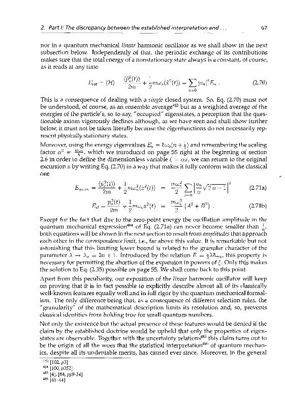
2. Part I: The discrepancy between the established interpretation and... 67
nor in a quantum mechanical linear harmonic oscillator as we shall show in the nextsubsection below. Independently of that, the periodic exchange of its contributionsmakes sure that the total energy of a nonstationary state always is a constant, of course,as it reads at any time
Eiot = (H) = ^ ^ + lmuJo(x2(t)) = J2 Wn\2En . (2.70)
n=0
This is a consequence of dealing with a single closed system. So, Eq. (2.70) must notbe understood, of course, as an ensemble average483 but as a weighted average of theenergies of the particle's, so-to-say, "occupied" eigenstates, a perception that the ques-tionable axiom vigorously declines although, as we have seen and shall show furtherbelow, it must not be taken literally because the eigenfunctions do not necessarily rep-resent physically stationary states.Moreover, using the energy eigenvalues En = hujo(n + |) and remembering the scalingfactor a2 = rDjB-, which we introduced on page 55 right at the beginning of section2.6 in order to define the dimensionless variable £ = ax, we can return to the originalexcursion x by writing Eq. (2.70) in a way that makes it fully conform with the classical
(2.71.)
Ed = ^ T + I™**® = ^(A2 + ß2) . (2.71b)
Except for the fact that due to the zero-point energy the oscillation amplitude in thequantum mechanical expression484 of Eq. (2.71a) can never become smaller than ^,both equations will be shown in the next section to result from amplitudes that approacheach other in the correspondence limit, i.e., far above this value. It is remarkable but notastonishing that this limiting lower bound is related to the granular character of theparameter A —> \n = 2n + 1. Introduced by the relation E = ^\hu>o, this property isnecessary for permitting the abortion of the expansion in powers of £. Only this makesthe solution to Eq. (2.35) possible on page 55. We shall come back to this point.
Apart from this peculiarity, our exposition of the linear harmonic oscillator will keepon proving that it is in fact possible to explicitly describe almost all of its classicallywell-known features equally well and in full rigor by the quantum mechanical formal-ism. The only difference being that, as a consequence of different selection rules, the"granularity" of the mathematical description limits its resolution and, so, preventsclassical identities from holding true for small quantum numbers.Not only the existence but the actual presence of these features would be denied if theclaim by the established doctrine would be upheld that only the properties of eigen-states are observable. Together with the uncertainty relations485 this claim turns out tobe the origin of all the woes that the statistical interpretation486 of quantum mechan-ics, despite all its undeniable merits, has caused ever since. Moreover, in the general
483 [102, p3]484 [100, p352]

68 Continuous quantum mechanics... Parts I and II
context of our deduction it has become very clear that in the case of a single point massmoving in a linear harmonic potential it is the stationary states487 that do not make anysense for several reasons to be addressed below and that, accordingly we must notrelate the absolutely squared mixing coefficients to probabilities although this seemsto be also supported by the condition of normalization: If the conception and conse-quences of above-mentioned axiom were also to hold for single particles, any mea-surement would force the state vector to "collapse" and thus change the energy of thesystem in an unpredictable way. Thus dooming any effort, each measurement wouldjust be a deed of gambling.
2.6.4 The question of equally spaced energy eigenvalues
There is, in our view, a fact of utmost importance that has been overlooked ever since:This fact is rooted in Eqs. (2.16) and (2.17) on page 36, respectively. It suggests thatin a linear harmonic oscillator the evenly spaced energies of the eigenstates should notbe understood as having any physical meaning of their own. The reason being thatthey only emerge from a purely mathematical necessity, which is directly related to theformalism: As can be easily seen on pages 60 through 66 from how some equationscame about, specifically, Eqs. (2.56), (2.57), (2.62), (2.66) as well as (2.68) and (2.70),the equal spacing of the eigenstates is required in conjunction with the relevant selec-tion rules expressed by Eq. (2.55) on page 60, Eq. (2.60) on page 62, and Eq. (2.64) onpage 65 in order to make sure that, whatever the energy and the concomitant ampli-tude, the oscillation of any property always proceeds with one and the same relatedfrequency because the harmonic oscillator does have only one eigenfrequency, indeed.In a mathematical formalism that is built on producing seemingly quantized energiesin the first place, this peculiarity of the harmonic potential can only be properly takeninto account by eigenenergies with a constant difference. This is how a theory of inher-ently multiply periodic motions manages to describe a periodic motion that is characterized byonly a single frequency.
From a classical point of view, both the eigenstates and their vicinity are problematic inthe linear harmonic oscillator with regard to a physical interpretation in classical terms:In the eigenstates, the Virial theorem confronts us with the contradictory situation thatthere is potential and kinetic energy but no oscillation, which could provide the peri-odic exchange between both as an indication of its ongoing dynamic behavior. On theother hand, the absence of any oscillation is the feature required to be complied with bya physically stationary state. However, in the linear harmonic oscillator's case it appearsthat there is only oscillation in the energetic neighborhood of the so-called stationarystates but its amplitude may be far too small to be able to explain the resultant energies.
A way out of this dilemma may be found in the fact that the summations involvedin the formalism are not unique. For instance, by choosing normalized mixing coeffi-cients with identical absolute squares |an_A,.|2 = • • • = |an_!|2 = |an|2 = |an+1 |2 = • • • =|an+fc|2 = T r̂rj (with n — k > 0 and k > 1), which are symmetrically arranged around\an\
2, we can exploit the energy's linear dependence on the quantum number accordingto Eqs. (2.66), (2.68), and (2.70) on pages 65 through 67, respectively, and exactly repro-duce the total energy En = hwo(n + | ) of the "eigenstate" labeled n but nonetheless
487 [118, p5]

2. Part I: The discrepancy between the established interpretation and... 69
have the oscillator in a nonstationary state performing an oscillation with an ampli-tude that is appropriate at least asymptotically as we shall see below in conjunctionwith the application of the correspondence principle. Of course, independently of thespecial labeling, any odd number of nonzero mixing coefficients of the same kind willhave the same result. Equally, the same also holds true for any series of normalizedmixing coefficients with the same modulus that extends without omissions from n — 0to -a = M. However, in order to really describe a nonstationary state, we have to beaware of the selection rules for the energy as applied in Eq. (2.64) on page 65. Theyprompt us to impose the restriction on M that it be an even integer, i.e., M = 2N. Mak-ing use of the condition of normalization, this gives rise to the following constant totalenergy of the nonstationary state
(2.72)
For the comparison between Eqs. (2.71a) and (2.71b) on page 67 this means that in thiscase
o / i \A + B - c? v 2 ; • ( 2 7 3 )
This is exactly the relation that Schrödinger488 deduced for the A'th eigenvalue from theclassical relation Eq. (2.71b) between the amplitude and the square root of the energy.However, focusing on the eigenfunction and because of not seeing any impact of therelated classical turning point on the course of the eigenfunction along the directionof excursion, he judged that such a definite value of the maximal linear excursion isinsignificant for the respective eigenfunction and kept sticking to the standing-waveinterpretation by calling the eigenfunctions the amplitudes of the proper vibrations489,as mentioned.
Nonetheless, this result clearly confirms the classical fact that the energy (here its non-stationary "eigenvalue") directly determines the amplitude of a linear harmonic oscillator(here of a quantum mechanical one) and, so, demonstrates that the oscillator is reallydoing what it is known for. As a consequence, the eigensolutions must not be identifiedunreflectedly ivith physically stationary situations. Another example of this kind will begiven on page 125.
But at a superficial first glance, any quantum mechanical amplitude seems to only beable to change its energy discontinuously490 and thus, other than classically possible.In this case, it is effecting, in compliance with Planck's hypothesis491, that a change ofenergy can only occur stepwise492 in amounts of TIUJO. This way and without affecting
488[10,p526]489 [166, p665]4911 [118, P5]491 [14, ppl48,162], [65, pp561,556], [66, p698]492 [118, p5]

70 Continuous quantum mechanics ... Parts I and II
the dynamical properties, the quantization of a linear harmonic oscillator would onlyimpose granularity on the corresponding classical amplitude. But it has to be kept inmind that this result is a consequence of just one of infinitely many, at least mathemat-ically possible choices of the mixing coefficients.In Part II, it will be shown that we can take advantage of these continuously possiblechoices also physically: There, it will be demonstrated that the continuous variabilityof the mixing coefficients allows for describing spontaneous transitions as continuousprocesses that are driven in a self-sustained manner only by the nonstationary innerdynamics and without the need for involving the vacuum fluctuations of the electro-magnetic field.
2.6.5 The role of the linear harmonic oscillator in the quantization ofthe electromagnetic field
There is another point of interest we already touched upon on page 60 by using theword "seldom" when we were about to reach Eq. (2.56). This word refers to a lessobvious, very quantum-like looking but in respect of the final result in Eq. (2.57) above,fully equivalent way of deduction493. It relates, as shown by Eq. (2.48) on page 57, thesquare roots in Eqs. (2.55) and (2.60) on pages 60 and 62, respectively, to the actionof creation and annihilation operators. As mentioned there, the introduction494 of therelations a)\n) = \/n + 1 \n + 1) and a\n) = y/n\n — 1), respectively, is a procedurethat especially the quantization of the free electromagnetic field495 and the formalismof second quantization496 heavily rely on. But these theoretical fields never make useof in the sense of Eqs. (2.56) and (2.61) on pages 60 and 62, respectively.
In QED, for example, the importance of the linear harmonic oscillator to the quantiza-tion of the free electromagnetic field derives from the fact that the homogeneous waveequation for the vector potential can be separated into a spatial and a temporal part497
both of which have oscillatory solutions: While the spatial part takes on the form ofa homogeneous Helmholtz wave equation498 of which the formal equivalence withSchrödinger's time-independent equation has allowed the latter to be also called waveequation, the time-dependent part is the related time equivalent, i.e., the well-knownequation of a classical linear harmonic oscillator as obtained from d'Alembert's prin-ciple. How intimately both parts are related with each other has also been shown onpage 59 by Eq. (2.53). It manifests that it is possible to generate the oscillator's classicaltime-dependent equation of motion with only the assistance of the creation and anni-hilation operators and their commutator relation by using the general equation of mo-tion of Eq. (2.7) on page 30 for the operators that act in Schrödinger's time-independentequation.If the generalized momentum p — ^A in the electromagnetic field with vector po-
493 [33, p508], [36, pp464-466], [58, pp443-444]494 [33, pp484,498,617], [35, pl46], [36, pl51], [58, pp436], [98, plO9], [105, p222]495 [115, ppl32,134], [116, pp260,261,262], [120, pp93-95], [121, pplO,12,38-39]496 [122, pp457ff], [123, ppl5-16,18,23], [124, pp297ff], [125, pp408ff]497 [82, P39], [167, p32]498 [167, p32), [168, pp243,425]

2. Part I: The discrepancy between the established interpretation and... 71
tential A is introduced into Schrödinger's nonrelativistic Hamiltonian499 it gives riseto a small perturbative, first-order coupling term500, which in Coulomb gauge501 fortransverse fields is proportional502 to the scalar product (A • p) and leads to the elec-tric503 and magnetic dipole operators in the lowest of the multipole orders 2l. Withthe vector potential A expressed in terms of modified creation and annihilation op-erators504, the generalized field part of the respective nondiagonal matrix elements inthe transition probability505 indicates by Eq. (2.55) on page 60 how in terms of thenumber or Fock state representation506 of the electromagnetic field the photon num-ber nk in the mode with the frequency uok would have changed once the transitionwould have taken place507: In a simple single-mode absorption process, it is low-ered by one due to the action of the annihilation operator hk \n,\,..., rij, nk, m,...) =y/nk~!«!,..., Uj. nk-\, ni,...) on the multimode wave function of the field508 while inan emission process of the same kind it is raised by one due to the action of the creationoperator509 a\ |rax,..., n,-, nk, n/,...) = \/nk + 1 |r?a,..., n.j, nk + 1, nh ...). Apart fromthe fact that for linear processes the harmonic model only permits the photon numberto be increased or diminished by unity at a time, thereby confirming Bohr's perceptionthat transitions in a linear harmonic oscillator are only possible between neighboring,in his view510 "stationary states", it is especially the additional one under the squareroot, which seems to endow only the general action of the creation operator with nevervanishing transition matrix elements even in the case of the photon vacuum511 whenall photon numbers are zero, ri\ = • • • = n3• = nk = n\ = • • • = 0. This property has beeninterpreted as the fact-establishing evidence that only QED is capable of accountingfor spontaneous emission. This phenomenon describes transitions that occur despitethe absence of any stimulating photon, i.e., even in the photon vacuum.
Spontaneous transitions were once considered to be induced by a virtual radiationfield, which was invented by Bohr, Kramers, and Slater512 as a means to make a per-manent communication between the atoms possible. But nowadays the notion is thatsuch transitions are driven by the fluctuations of the photon vacuum513. These fluc-tuations are said to be always present as a result of the residual energy density514 re-lated to the zero-point energy of the electromagnetic field. So, the QED explanation ofspontaneous transitions relies fully on the asymmetric action of the creation and theannihilation operators with regard to y/n + 1 and y/n, respectively.
In this context, however, it is important to recognize that this is contrary to what we499 [80, pi 77]500 [30, p88]501 [80, pp399,523]502 [30, p92], [34, p297], [80, ppl?'8-179,398], [82, pp43,125], [121, ppU7-U8], [124, p313]503 [115, p43], [120, P84], [121, ppU8-149]504 [82, Pp62-63], [115, p!35]505 [30, pp95,97]506 [120, p96], [121, pp9ff], [124, pp298,316]507 [30, pp95-96], [116, p260]~M[U6,pp261,262]509 [33, p617], [116, pp261r262], [121, pl2], [122, p459], [124, p298], [125, p410]510 [118, p5]511 [33, pP616,618], [115, pl34], [116, pp260,261,262+footnote-265], [120, p344], [121, p39]5U[72,p75],[73,p791]513 [33, p619], [120, p345], [121, pll], [124, p317]5U [116, p265]
72 Continuous quantum mechanics... Parts I and II
see on pages 60 and 62 in Eqs. (2.57) and (2.62), respectively, and what is additionallyunderscored by Eq. (2.53) on page 59, namely, that this asymmetry is only a seem-ing one, which is necessary for the matrix elements's hermiticity. Unfortunately notseen this way, the asymmetry has been pushed further by extending the action of theannihilation operator to below the range allowed by the respective matrix element inEq. (2.55) on page 60. This extension was achieved515 by exploiting that d| 0) = 0, asmentioned on page 57 in context with Eq. (2.48). Although this is not an operator rela-tion, it looks reasonable because there is nothing in a vacuum that could be destroyedor annihilated516.
The apparent lack of symmetry was even welcomed as a suitable means to explain,apart from induced emission and absorption, especially spontaneous emission517, whichis deemed to have no classical analog. Moreover, the asymmetry seems to fit the suc-cessive actions of, first, the annihilation and then, second, the creation operator as theyappear combined in the number operator018 M = ä^ä. But as the application of a to | 0)would generate the "nothing" in terms of a\ 0) = 0 and the subsequent application of df
is not defined, only their joint action in the number operator tfä is permitted becauseonly this operator appears in the Hamiltonian as a consequence of the commutator re-lation [a,(V] = 1 deduced519 from [q,p] = ih. Thus, only the number operator is partof the energy representation whereas, as we have shown on page 58 in Eq. (2.50), d| 0) isneither an eigenstate of the Hamiltonian nor a state at all. As a consequence, it cannotbe part of a Hermitian matrix element. But only these do matter.
Additionally, if | 0) is already supposed to represent the vacuum state with zero-pointenergy \huo, what energy is to be assigned to the "nothing" named a\ 0)? Accordingto how the annihilation operator acts "nothing" should energetically be below the vac-uum. Thus, taken literally, "nothing" should not be able to have any energy. But thiswould contradict the existence of the zero-point energy as the lowest one possible. Asa consequence, a\ 0} should not be considered to represent anything physically real.
Following this questionable path of the established perception, it is interesting to notethat the quantization of the free electromagnetic field interprets the nth eigenstate ofthe linear harmonic oscillator representing the field mode with eigenfrequency uo ascontaining n photons with the energy hu>o each520 in accordance with the action of thenumber operator521 ä.̂ ä„. on the eigenstate \n). As this formalism treats each eigen-state | n) on the same footing by giving all of them equal weight it is clear that thecorresponding amplitude of the truly oscillating electromagnetic field, as expressed bythe respective field strength, must be obtained from a state vector with identical mixingcoefficients. This is exactly the assumption that led to Eq. (2.72) on page 69. Accord-ingly, as expressed by Eq. (2.73) there, N photons in the field are equivalent to the fieldstrength squared of the field mode that is truly oscillating with the frequency mo andhas an energy density determined by hwo(N + \). According to Eq. (2.72), this energydensity is given by the general expectation value of the Hamiltonian as obtained from a
515 [6, pl38], [33, p618], [35, pU6], [115, pl31], [120, p95], [121, p9]516 [169, p63]517 [135, p82]518 [6, pl36], [33, p490], [35, pU6], [115, pl34], [120, p96], [121, plO]519 [6,pl36], [33, p489,617], [35, p i 4 5 ] , [ 1 1 5 , p l 2 9 ] , [120, p94], [121, p9], [122, p458], [124,p299], [125, p409]520 [115, pl34], [120, p96], [121 , plO]521 [33, p490\, [115, pl32], [120, p96], [121, plO]

2. Part I: The discrepancy between the established interpretation and... 73
state vector with identical mixing coefficients running up without omissions from n = 0to 2A". Thus, the number of photons in a field mode turns out to be just a measure ofthe field strength in that mode and speaking of multiphoton interactions a synonymfor nonlinear interactions between matter and radiation due to a correspondingly highfield strength in the electromagnetic wave. While providing a clear idea of the oscilla-tion amplitude in truly classical terms this way, the energy representation is not capableof delivering any information about the phase of the field mode.As can be inferred from the preceding paragraphs, the current interpretation defines aphoton in the nth mode of the electromagnetic field as its indivisible unit of energy522
Tiujn by always assuming a complete transition from one stationary state to another. Thisimpression is held to be confirmed not only by Planck's perception523 that "at high fre-quencies radiative energy shrinks spatially and concentrates in single space points,which move like corpuscles and, therefore, are called light quanta". Most obviously,this visualization is strongly influenced by Einstein524. But our impression is even be-coming certain upon Planck's expressly stating525 "that... a new, totally different kindof fluctuations additionally comes about the statistics of which can only be explainedby the existence of discrete atoms of energy of the size of a light quantum".As a consequence of the principle of energy conservation, any complete exchange ofenergy, e.g., between an atom and the radiation field in a single-photon process, is thussaid to only be possible by this amount. This would imply an instantaneous change bytwo rungs in the sums in the first and second line of Eq. (2.72). However, taking a closersecond look at this equation, we realize that if the mixing coefficients would be allowedto continuously change with time while maintaining their condition of normalizationaccording to an(t)/^/J2n \an{t)\2, the change of energy during the transition processwould take a finite nonzero period of time. This is what we shall see in Part II below.There, we shall show that, contrary to the still prevailing notion526 that "it is not possi-ble to imagine that we would follow the exact time evolution of spontaneous emissionwith any physical tool known", it is possible, indeed, at least for a two-level system, totheoretically describe the full dynamical time evolution of spontaneous transitions asbeing driven by the inner dynamics of the source in the first place, i.e., without havingto involve the vacuum fluctuations of a quantized electromagnetic field as the activedriving mechanism or even the quantization of this field at all.
2.6.6 The linear harmonic oscillator and the correspondence principle
So, except for the lowest state, we can safely discard the "stationary states" as not beingphysically relevant in the case of a linear harmonic oscillator. This is in contradiction toBohr's first postulate527 and the questionable axiom. Unreflected belief in it has misledinto taking the eigensolutions for real528 as physically stationary states even in a linear
522 [14, pP148-149], [65, p561], [66, p698], [78, p43], [119]523 [67, pp529-530]524 [119, ppl22,123]525 [67, p530]526 [29, p265]527 [31,46,50,70,71]528 [118, p5)

74 Continuous quantum mechanics ... Parts I and II
harmonic oscillator and accepting stationary states as something totally different529
from what is predicted by classical mechanics. Our other examples, however, willdemonstrate that for higher dimensions stationary states may indeed have a physicalsignificance in terms of representing situations of dynamical balance.Although this is quite comforting it does not resolve the mystery about the zero-pointenergy associated with the lowest eigenstate because there above-indicated methodsfail. The key to the resolution of this problem may lie, as mentioned before, in theenergy representation leading on page 55 to Eq. (2.34) and in the fact that in the coursefrom there to Eq. (2.36) it was necessary for the solution to this differential equation torestrict the parameter A to the never vanishing discrete values An = 2n + 1. Even moreimportantly, however, such a minimal energy seems to be necessary for sustainingthe property that both x and px must never commute with the Hamiltonian under anycircumstances because as long as there is energy in the system they cannot becomeconstants of the motion. This is different from a free particle for which px must be aconstant of the motion while x must not.
Despite all the obvious similarity with classical behavior - if the seemingly discon-tinuous changes of the amplitude and the question of the zero-point energy are leftaside - there is another significant difference for small quantum numbers that is re-lated to the selection rules as indicated above. This difference is rooted in the fact thatSchrödinger's equation as well as necessarily all of its solutions represent the total energy.Here, the contributions to the total energy are only related to (x2^)) and (px(t)) but notto (x(t)) and {px{t)). Therefore, while classically, e.g., x2 can directly be obtained fromx by squaring, this simple procedure does not hold for the respective general expecta-tion values if the quantum numbers are small. As made apparent by the respectivemixing coefficients, this is owed to the fact that different selection rules dominate thecalculation of these properties. This is expressed on pages 60 and 62 by Eqs. (2.55) and(2.60) for (x(t)) and (px(t)), respectively, on the one hand and on page 65 by Eq. (2.64)for both (x2(t)) and (px(t)) on the other. Thus, these properties do not involve all com-ponents of the same general state vector equally but rather, so-to-say, only differentsubvectors because different components do not contribute. This has the same effectas if they were missing and, thus, as if in Hubert space the spatial motion would berepresented by a periodic change among two separate pairs of state vectors that aresomewhat different.Why this is the case may be explained as follows: Being at the heart of the principle ofsuperposition, the real and imaginary parts of each of the mixing coefficients can takeon, in principle, any value in the interval (0,1) provided they all comply with the gen-eral condition of normalization J2n l
a«l2 = 1- Accordingly, each state vector representsa different dynamical situation. Neighboring state vectors are similar but not identi-cal. As a result, they span the Hubert space continuously, thus covering a continuousspectrum of dynamical situations. For this reason, above-mentioned subvectors spansubspaces that do not fully overlap for small quantum numbers and only tend to do sofor great ones when the differences become negligibly small. Thus, being not identicalfor small quantum numbers, they represent independent dynamical situations of theirown and, as a consequence, effect different dynamical features, which are similar but,under these circumstances, cannot be made identical by squaring.
529 [33, p508]

2. Part I: The discrepancy between the established interpretation and... 75
This action and some minor rearrangement obtains from Eq. (2.57) of page 60
»I, '(x(t))2 =
Equally, Eq. (2.62) supplies from page 62
(Px{t))2 = — mhujo< cos 2u)ot ) (- $
- sin 2ujot ^ ^ 2 ^{<nm=0 n=0
. (2.75)
When compared with Eqs. (2.66) and (2.68) of pages 65 and 667 respectively, Eqs. (2.74)and (2.75) have the same time dependence but, nonetheless, are not identical for smallquantum numbers. In the correspondence limit, however, they do merge. The asymp-totically dwindling importance of the difference of the selection rules plays a decisiverole in this behavior. This will be shown next.Under inclusion of the scaling factor a from page 55 together with Eqs. (2.57) and (2.58)from pages 60 and 61, respectively, as manifested by Eqs. (2.74) and (2.75), the compar-ison of the quantum mechanical amplitudes in Eqs. (2.66) and (2.68) on pages 65 and66, respectively, with the classical amplitudes in Eqs. (2.69a) and (2.69b) on the latterpage shows that for an identical asymptotic behavior the quantum mechanical amplitudesought to fulfill the following conditions
A = (2.76a)
(2.76b)
B = -

76 Continuous quantum mechanics ... Parts I and II
AB = —, J2 \a'r71 = 0
.ra=0("+ 2) (2.78a)
(2.78b)
i.e./that in the correspondence limit the respective expressions labeled a) should becomeequal to the respective expressions labeled b). For instance, pertaining exclusively tothe comparison between Eqs. (2.66), (2.68) of pages 65, 66, respectively, on the one handand (2.69a), (2.69b) on the other, Eq. (2.78) expresses the demand that in the correspon-dence limit
.71 = 0
(2.79)
Like the former Eqs. (2.76) and (2.77) this latter one represents a condition for the choiceof the mixing coefficients. In order to investigate whether and how this condition canbe met under the correspondence principle, i.e., for n > 2, and, e.g., identical mixingcoefficients, we assume, because of the summations, the following strings of vanishingand nonvanishing mixing coefficients, respectively, ao = ax = a2 = a3 = • • • = am>2 =0 a n d a m + ] = a m + 2 = a m + 3 = a m + 3 = ••• = a m + k = E+i& w h e r e , f o r o b v i o u s
reasons, k > 2. Mixing coefficients with greater indices are equally assumed to be zero.Under these circumstances, Eq. (2.79) transforms into
m + k m + k
The sum on the right hand side of Eq. (2.80) can readily be calculated
m + k /m+k m
n=m+\ \n=l n=l
(2.81)
Accordingly, the squares of Eqs. (2.76a) and (2.76b), respectively, whose asymptoticbehavior is next to be investigated become approximately equal to
(2.82a)
(2.82b)

2. Part I: The discrepancy between the established interpretation and... 11
The squared sum on the right hand side of Eq. (2.82b) reads
2
\/n\ = ( Vm + 1 + y/m+2 + \/m + 3 H h Vm + k-1 + Vm + k
= (m+1) + (m + 2) + (m + 3) + h (m + fc-1) + (m. + k)
/* "N
(2.83)
Obviously, the second line in Eq. (2.83) equals mA- + §(/c + 1) = |(2m + k + 1). A lowerbound for the rest is certainly found by substituting everywhere m + j: —> m, wherej = 1, 2, 3 , . . . , k while an upper bound is obtained by the replacement m + j —> m + k.Then
k2 ( 1 - k2
— \2m + k + H —2 V k
k'2m + k + 1 +
(1 - (2.84)
Thus, for k ;» 1 flnrf, at the same time, ?ri 3> A-, the right hand side of Eq. (2.82b) isobviously converging to the expression of Eq. (2.82a). As this applies to the squares,the conclusion is even more justified for their roots so that we can state that iden-tity between the quantum mechanical and the classical expressions for the amplitudesand the related time-averaged value of the respective energy contributions is beingapproached in the correspondence limit for equal mixing coefficients. Following theintended guideline given by the correspondence principle5310, we can also state that achange of amplitude occurs according to the steps provided by the off-diagonal ma-trix elements alone.
It is in the sense of the continuous span of the Hubert space that the continuity of thesum of weighted energy eigenvalues in terms the absolute squares of the mixing coef-ficients indicates that nonstationary states not only can be chosen to continuously fillthe energetic gaps between the eigenvalues but, as corroborated above, they can alsobe prepared to even match the eigenenergies of the linear harmonic oscillator. As longas any kind of loss of energy, e.g., through emission of radiation, is not incorporatedin the Hamiltonian only dynamical situations can be described that are characterized,according to Eq. (2.70) of page 67, by a fixed amount of the total energy. Hence, per-taining to a closed system, these situations are energetically stable but dynamically notstationary.While nonstationary states can now easily be understood as representing dynamicalsituations in classically well-known terms, it is the stationary states especially of thelinear harmonic oscillator that do not fit in the familiar classical picture: While in caseslike the two-dimensional Isotropie oscillator and the Kepler problem to be dealt withbelow the eigenstates with angular momentum have a physical meaning in classical
53(1 [15, pp6U,616,62Z], [31, ppU2,U5ff], [51, ppVII,VIlI,Xl,XIII,XIV,XVII,133-134], [69, pp429ff], [70,pp231,234], [71, p5], [72, pp73-74], [73, p789], [88, p250]

78 Continuous quantum mechanics... Parts I and II
terms, namely, as representing exceptional dynamic situations, which only occur dueto a dynamical balance and, so, explain very naturally the concomitant cessation of theexchange between kinetic and potential energy as well as the absence of periodic ac-celerations and decelerations, something similar cannot be recognized in the behaviorof a linear harmonic oscillator.
From a classical point of view, this would be very reasonable because such a balancedoes not exist classically, and, so, would confirm this classical feature. But if the ax-iomatic claim531 of "eigenstates only" would have to be taken literally in a totally ex-clusive form, it would confront us with the following situation: Without detectableexchange, both the kinetic and potential energy have to contribute the same constantamount ~(n + |) to the total energy. If one would try to find a physical meaningbeyond their functional mathematical importance addressed above one would have toresort to the kind of speculation that the present interpretation suggests on the basis ofthe wave conception: In stationary states, the point mass does not periodically followthe contour of the potential, but, for an unknown reason and in an unobservable andnonclassical manner, is miraculously bouncing back and forth at constant height in thepotential. For this bouncing to be a stationary one, it must do so as a standing wave532.But this is the kind of mystery we really do not want to promote.
Unfortunately, the lowest total energy quantum mechanically possible in a linear har-monic oscillator is of this mysterious kind. But apart from seeing the need for its sus-taining the property this way that both x and px should never become constants ofthe motion because of not commuting with the Hamiltonian, we have no idea as yetof how to reasonably explain in classical terms, if at all possible, the physical meaningof the zero-point energy now that we have seen that even for small quantum num-bers the solutions to Schrödinger's equation for the linear harmonic oscillator do notsupport the assumption of a nondeterministic behavior that could be justified by theuncertainty relations533. And why should only the lowest energy range be stricken thisway? But as repeatedly indicated in this context, the nonzero lower bound for the en-ergy seems to be associated with the necessity to uphold the noncommutativity of bothx and px with V. under all conditions. As such, it would be a consequence of an energyrepresentation that is related to granularity. In this sense, the lower energy bound mightnot represent a physical limit.
2.6.7 The linear harmonic oscillator and the uncertainty relations
The properties of stationary states in a linear harmonic oscillator remain a mystery onlyif we squeeze ourselves into the axiomatic straight]acket. Then we find our situationeven exacerbated by the fact that one of the main pillars of the established statisticalinterpretation534, the already-mentioned and much acclaimed uncertainty relation535
between the space variable x and its canonically conjugate momentum px, is used toexplain the zero-point energy pertaining to the lowest quantum number n = 0. Ac-
531 [79, p722], [91, pl70]532 [9, p373], [41 , p864], [67, p529], [78, p59], [90, p89], [129, pl641]533 [4], [84, pp9-14]534 [7, pp283,285]535 [4], [84, pp9-14]

2. Part I: The discrepancy between the established interpretation and... 79
cording to the accepted statistical interpretation536 and as a consequence of Bohr's firstpostulate537 the statistical mean value of a property when the system is in a certain stateis given by the expectation value formed with the state vector of that state but without con-sidering the time-dependent off-diagonal parts. This definition effects, as explained,that the mean-square deviation (AC)2 = (Ö2) — (Ö)2 always only vanishes for the "ob-servables" O of an ensemble, i.e., when the dynamical state of the system correspondsto an eigenstate. Then, these properties's values are represented by the elements of therespective diagonal matrices.
The same definition is often also used in the derivation of the uncertainty relation forthe linear harmonic oscillator: As for a stationary state k, in general, the mixing coef-ficients reduce to an = 8n,k, the mean square deviations of the relevant variables, asobtained in accord with the established interpretation on pages 65, 66, and 75, respec-tively, from Eqs. (2.66), (2.68), (2.74), and (2.75), are given by538,
(2.85a)
(2.85b)
Taking the square root of each of these expressions and multiplying the results, weobtain what is commonly held to confirm the well-known uncertainty relations539 andto explain the zero-point energy540
= h (k + 0 . (2.86)
This result, however, is not astonishing in view of the fact that in deducing it onlystationary states had been admitted as physically relevant. This perception is basedon early convictions541, not to say beliefs, but not knowledge that quantum mechan-ics is a "discontinuum" theory for the individual particle and a statistical one for theensemble. Only as such, it automatically entails the statistical root-mean-square law542.
The uncertainty relations were seen by Heisenberg543 as a direct consequence of thenoncommutativity of pxx — xpx = j when the real variables x and px are representedby matrices. Conceived for matrix multiplication prior to the advent of Schrödinger'sequation544, this relation was then appreciated as the basic condition of quantization545
and seen as a confirmation of the conception of a "discontinuum" theory. The later ver-ification546, however, that Schrödinger's equation comprises Heisenberg's approach
536 [7, pp283,285]537 [31 , pU8], [46, p7], [50, p396], [70, p230]538 [33, p503], [126, pp377-378]539cf., e.g., [33, p504], [35, pU4], [36, p465], [58, p446], [98, plO3], [121 , p52], [126, p376]540 [80, p69], [105, ppl70-171], [106, p50], [126, p378]541 [1-6,8,16,17,31,41-44,46-50,70,71,76,83-86]542 [16], [35, pp52-53], [58, pl33], [80, p60], [81 , p364], [92, p297), [100, pp337-339], [103], [135, p96]543 [4, pi 75]544
545 [3, p562], [83, pp871,876]546 [11], [89]

80 Continuous quantum mechanics ... Parts I and II
in a more fundamental way547 did not succeed in changing the broadly shared "dis-continuum" belief as outlined above. To the contrary, the possibility of deducing theuncertainty relations not only from wave-packet properties but also on the basis of astatistical root-mean-square behavior548 seems to have been considered proof of thisassumption.
Starting from the expressions for the respective root-mean-square deviations,whichimply independent statistical events, the apparently most accepted derivation of theposition-momentum uncertainty relation549 states that the product of the root-mean-square deviations of these canonically conjugate variables has a lower bound of | .This result is obtained without involving any further properties like a dependence onquantum numbers. Thus, it is quite obvious in this context that the uncertainty relationdeduced this way in Eq. (2.86) for the linear harmonic oscillator violates the correspon-dence principle, which demands that classical behavior be approached for very highquantum numbers. Although h is very small it is nonetheless finite. Hence, for k —> oothe uncertainty product in Eq. (2.86) becomes appreciable instead of vanishing.
This deficiency could be overcome by formally taking the root-mean-square law liter-ally as an order to combine on pages 65, 66, and 75, respectively, the time averages ofthe general nonstationary forms given by Eqs. (2.66) and (2.74) on the one hand andEqs. (2.68) and (2.75) on the other. With the time averages indicated by the index t, thiswould obtain
' (2.87)
For stationary states in the formal sense of the questionable axiom, a,, = Sn,k andEq. (2.86) would be reproduced. But, as explained above, the same total energy for aneigenstate can also be attributed to a nonstationary state in compliance with classicalbehavior. Moreover, from Eqs. (2.82) through (2.84) we know that the equivalences be-tween Eqs. (2.76a) and (2.76b) as well as between Eqs. (2.77a) and (2.77b) on page 75 dohold in the correspondence limit. If inserted into Eq. (2.87) and used in this sense, theywould make above expression vanish for very high quantum numbers. This demon-strates that in the correspondence limit the motion is truly deterministic in the classicalsense by effecting, e.g., (x(t))2 —> (x2(t)). The fact, however, that Eq. (2.87) does notvanish for small quantum numbers must not lead to the wrong conclusion that there isindeterminacy on the quantum level. To the contrary, the single particle's motion is nota statistical random walk but deterministic despite the seemingly existent uncertaintiesfor small quantum numbers. But what looks like uncertainties must not be interpretedas such because, on the one hand, as we have explained above, they result from the factthat in an impermissible way different dynamical situations are being compared eachbf which is dictated by different off-diagonal matrix elements due to different selectionrules and thereby different effective state vectors. On the other hand, it could also beexplained as a result of the finite resolution that the mathemathematical tools suffer
547 [41, p864], [89, p726]548 [35, pp52-53], [58, ppl33-135], [80, pp60-61], [81, p364], [92, p297], [100, pp337-339], [103], [135, p96]549 [33, pp230-231], [58, pl34], [92, pp297-299], [100, pp337-339], [103], [135, p96]

2. Part I: The discrepancy between the established interpretation and... 81
from at low quantum numbers due to the granularity of the energy representation. But,as we have seen above, the difference of the selection rules is essential for providingthe correct frequencies: UJ0 for the linear excursion and the related momentum, 2UJO forthe exchange of kinetic and potential energy.For this reason, we have avoided here to equate the first line in Eq. (2.87) to AxApx
in order to indicate that the root-mean-square law is not applicable and that, in thisregard, Eq. (2.87) does not make any sense. But if the general claim would be justifiedit ought to apply to any kind of dynamical situation, especially if, as will be shownbelow, the general expectation value ([.r,px.]) = ih holds for any state vector, i.e., ingeneral.
The most general form of the uncertainty relations is equally based on purely statisticalconsiderations that matter for a measurement. It is derived by virtue of the Schwartzinequality and relates the product of the mean square deviations, which determines theproduct of the variances of the measured mean values (A) and (B), to their commutatorrelation by550
)((AB)2) > (2.88)
It is important to be aware of the fact that this relation only holds if the different proper-ties, which both operators represent independently, are simultaneously being subjectedto a measurement551 and if at least one of them is susceptible to variances. This is gen-erally true in a measurement on canonically conjugate operators when the state vectorundergoes an unpredictable modification552. Thus, in general, this uncertainty productcould only become effective in the case of a simultaneous measurement of the proper-ties represented by the operators A and B.But Eq. (2.88) does not hold at all for a closed system because it is not being interferedwith per definitionem but left alone to evolve in time all by itself. As has been pointedout on page 8 and in conjunction with Eq. (2.14) on page 34 this is the case especially fora time-independent Hamiltonian because it represents the total energy as a constant ofthe motion of the closed system. This constancy is independent of the actual dynamicalsituation that the total energy determines. As a consequence, the conclusions that havebeen drawn in conjunction with Eq. (2.14) hold true because no lack of determinacycan be inferred for the general expectation value of an operator that therefore can actdeterministically in a closed system although it does not commute with the system'stime-independent Hamiltonian.In this sense will the next section show that the first-found commutator relation be-tween the position coordinate and its canonically conjugate momentum, which wasthe stimulus for Heisenberg's invention of his original uncertainty relation553, does notadmit any discontinuities in the time evolution of a closed system, a property thatHeisenberg554 always associated the commutator relation with and that he saw clearlyand, in his view, irrefutably explained by the uncertainty relations.
550 [33, ^ 2 8 7 ] , [35, Pp53-54], [58, p300], [81 , p364], [92, ppZ98-299], [103] , [104, pl8], [126, / jp225-226] , [128 ,pp280-282]
551 [33, pp234,236], [60, pl254]552 [33, p236]553
554

82 Continuous quantum mechanics... Parts I and II
2.6.8 {[x, px\) = ih as a result of continuous action
In this context, it is interesting to look into what the operator combinations xpx andpxx effect separately. Combined in the commutator relation xpx — pxx — ih, they wereconsidered by Born, Heisenberg555, and Dirac536 the ultimate condition of quantiza-tion for matrix mechanics and q-numbers and the key relation for what they deemedthe new, discontinuous kinematics. [x,px] = ih is also the relation, which especiallyBorn and Jordan557 based all their conclusions on and which in Heisenberg's view wasphysically explained and justified beyond doubt by his deduction of the uncertaintyrelations558. This is contrasted by the contradictory fact that Schrödinger559 as well asindependently Eckart560 could easily reproduce the commutator relation by introduc-ing spatial partial differentials for the respective components of the momentum. And,in fact, their deductions are surely representative of a continuum theory and were seenby Eckart in a note added with proof561 as even more fundamental than matrix me-chanics.
The general expectation value of the operator combination xpx
We begin with the calculation of the general expectation value of the operator combi-nation xpx. When making the step from Eq. (2.59) to Eq. (2.60) on page 62 we usedEq. (2.42) of page 56 to obtain the latter. We repeat this step explicitly and make it ourstarting point
Px0n(x) = ih N& a -ifn+i(0 - nHn_i(C) \ e~ * • (2-89)
Multiplication with x demands that the recursion relation of Eq. (2.39a) on page 55 beapplied in the rearranged form of Eq. (2.40) on page 56. The result is
n(0 ~ nin - l)#n-2(0 \e~** . (2.90)
Application of Eq. (2.38) on page 55 leads to matrix elements similar to those of Eq. (2.64)on page 65 but purely imaginary
r i .(6m(x)\ xpx\cpn(x)) = ih dm,n+2 - V (n + ! ) ( « + 2)
(2.91)
This makes {4>n+2{x)\ xpx\(j)n{x)) = (d>n(x)\ xpx\4)n+2(x))* = jy/(n + l ) (n + 2) the onlymatrix elements involved due to hermiticity. Accordingly, insertion into Eq. (2.15) on
555 [3,83]556 [85]557 [83, p871]558 [4], [84, pplZ-14]559 [11, P737]560 [89, pp712,719]561 [89, p7Z6)
2. Part I: The discrepancy between the established interpretation and... 83
page 36 yields (for clarity's sake, we use here the notation we originally dismissed onpage 37 for esthetical reasons)
(xpx){t) = ih 2)
n=o
(2.92)
Here the sum in the second line obviously is the condition of normalization. With thesame arguments used on page 65 in the step from Eq. (2.65) to Eq. (2.66) but beingaware of the fact that this time twice the imaginary part times i is being obtained, wecan transform this into
(xpx)(t) = -h
sin 2u>ot {n 2)
h(2.93)
With a stationary imaginary part, this general expectation value does not oscillate aboutanything observable.
The general expectation value of the operator combination pxx
Next, we calculate the general expectation value of pxx. We proceed like before onpage 60 in that we explicitly specify the step from Eq. (2.54) to Eq. (2.55) with the helpof the rearranged form of Eq. (2.39a), which is given on page 55 by Eq. (2.40)
I fi I ,2
' (2-94)
Application of px to this expression and use of Eq. (2.42) from page 56 lead to
* , (2.95)
which is very similar to Eq. (2.90). The only difference is a change of sign for the middleterm |#n(£). Therefore, we can directly jump to the counterpart of Eq. (2.93) by onlychanging the respective sign
(pxx)(t) = -h COS 2üJot 2)
sin 2ujot 2)
.h(2.96)

84 Continuous quantum mechanics ... Parts I and II
Thus, for the general expectation value of the commutator between x and px, the dif-ference of Eqs. (2.93) and (2.96) supplies, as expected, the well-known commutatorrelation
<[£, Px}-) = ifi , (2-97)
which here, however, is proven to hold for any state vector, i.e., for any dynamicalsituation in a linear harmonic oscillator. But it can do so only because the periodicexchange between the general expectation values of xpx and pxx with twice the eigen-frequency drops out in this combination leaving only twice the stationary imaginarypart in compliance with the fact that px is only a Hermitian but not a self-adjoint oper-ator562. As Schrödinger563 already remarked in 1930, the commutator of two Hermitianoperators is nothing else but twice the imaginary part of their product564 according toAB = \{AB+BA) + \{AB-BA) = \{\A.B)+ + [A.B)-). As such, it does not representan observable property.
But this is only one side of the coin: Little attention has been paid in this context to thereal part of this product. It is Hermitian and made up of the other combination, onehalf of the anti-commutator565, which we have indicated by the (+) index. Guided bythe classical relation that
we find for the sum of Eqs. (2.93) and (2.96) and in view of Eq. (2.66) on page 65
1 - cos2oUn=0
+ sin 2 o ; o ^ y ^ J Q * + 2 q n 1^(7?. + l ) (n + 2)n=0
«*2««»
Corroborating this relation, the same result can be obtained in operator form by purelyalgebraic means, namely, by applying creation and annihilation operators. Using theirdefinitions in Eq. (2.45) on page 57, their commutator relation [a, af]- = 1/ and thenumber operator as the essential part in the Hamiltonian, we obtain for the commuta-tor [x2, H]- = -^(f l 1^ - aa) and, hence, from Eq. (2.7) on page 28
^x\H\. = ^(at&t -aa) = ^[x:px]+ = ±3* • (2.100)
All this is in full accordance with what Heisenberg566, before the advent of Schrödinger'swave mechanics, already suggested for the first time derivative of an expression likeftv
2 = vft + ftv. Physically, Eqs. (2.99) and (2.100) are directly related to the tempo-ral change of the potential energy, which would be obtained by multiplication with u%
562 [155, pl903]563 [92, p297]564ct, e.g., [58, p256]565 [92, P297]566 [2, p884]

2. Part I: The discrepancy between the established interpretation and... 85
and \rrvJl, respectively. Then, Eqs. (2.99) and (2.100) would be fully consistent with theclassical expression obtained from differentiating Eq. (2.69a) on page 66 with respectto time
— -mulx2(t) = - ^ p - [sin2u>0* x (A2 - B2) + cos2o;0* x 2AB\ (2.101)
because with regard to the factor in front of the square bracket we have to be awareof the fact that ^ X n̂ ̂ {an+2an} V'(" + 1)(« + 2) corresponds to A2 — B'2 according toEqs. (2.76a) and (2.77a) on page 75 while ^ £ n Q{a*1+2an} \/(n + l)(n + 2) correspondsto AB according to Eq. (2.78b) on page 76.The so described temporal change is taking place during the periodic exchange withthe kinetic energy. As the deduction of the relation in Eq. (2.99) involves the same sub-vectors that are relevant for the exchange of potential and kinetic energy in the linearharmonic oscillator, it vanishes for those states, which historically were called "sta-tionary", and, thus, escapes the established interpretation. But, as we have shownabove, there is no mandatory need to follow Bohr's postulate in the case of the linearharmonic oscillator and associate with the eigenstates something physically stationarythat contradicts classical experience.This is another strong indication that an essential classical feature would be missed ifonly so-called "stationary" states were considered to represent physical reality. More-over, as the relation of Eq. (2.99), which, in principle, is observable but only holds fornonstationary states, is eye to eye with that of Eq. (2.97) on page 84, which is constantbut not real and, therefore, not observable although it is deemed to matter only for the"stationary states", the question arises why should uncertainty relations, if at all, non-deterministically influence only the behavior of "stationary states"? Additionally andeven more importantly, as observability is the key feature at the center of the estab-lished interpretation, how should one understand that something unobservable couldever have become so important to the interpretation of the theory? In really physicallystationary states, as we shall prove in our next examples, also canonically conjugatevariables may have well defined values in accord with their intrinsic dynamics. So,why should the uncertainty relations hold at all when it comes to describing the dy-namics of particles that are not perturbed by measurements567? Only because, in prin-ciple, something like that could possibly happen? The alleged wave nature, as a matterof fact, cannot be held responsible!
While Schrödinger's approach568 clearly is a continuous one, Heisenberg's was bornout of his conviction that nature behaves discontinuously on very small scales569. Inthis he is still being followed by the vast majority of physicists. So, to Schrödinger'slasting chagrin his findings were only accepted as appropriate for describing the con-tinuous but steady-state dynamics in stationary states, the rest is held unintelligible570.Indicative for this general attitude is the fact that time dependence is still being consid-ered a result of a perturbation571. The application of the interaction representation572
567 [6, pp4,108]568 [ 9 _ 1 3 ]
569 [4, pl73], [76, pP989,993,994]57(1 [162, pl-1], [163, pl29]571 [30, p94], [86, p675], [114], [116, p248]572 [33, p347], [80, ppl72,281]

86 Continuous quantum mechanics ... Parts I and II
is the most obvious sign in this case. It attributes the state vector's change with timeto the action of a unitarily transformed perturbation Hamiltonian. Therefore, onlyHeisenberg's approach, which, in his and his followers's view, happened to coincidewith Schrödinger's for the eigenstates573, is deemed to meet the general demand fornew kinematics574 in the description of microscopic particles. While in the late 1920sthe struggle of opinions575 was still in full swing about whether a continuum theoryor a "discontinuum" one is appropriate, Heisenberg gave the debate, as we have de-scribed above, the decisive turn by putting forward his meanwhile well-known uncer-tainty relations576. However, in all his original examples and Gedankenexperimente577
like the 7-ray microscope, which he gave to promote his ideas and make them plausi-ble, he was always talking about localization and observation.
These are terms that only become important in a measurement process but do not re-late to the particle's unperturbed intrinsic dynamics. As long as the physics of the ap-plied probing device, i.e., the interaction Hamiltonian with the measuring apparatus,is not fully incorporated, the mathematical description of the particle can only reflectits intrinsic dynamics, which it follows even if a special environment like a static elec-tromagnetic field has been generated for the investigation. Accordingly, nothing canbe predicted that is beyond the scope of the applied Hamiltonian. Heisenberg knewabout this and underscored the necessity of a complete Hamiltonian already in theopening sentence of the first section of his revolutionary article578. But with only a cou-ple of pieces of the puzzle available, it is indicative of the general confusion about howand where to continue the quest for truth and knowledge that even more than one yearafter Schrödinger's discovery Heisenberg drew his far-reaching conclusion and estab-lished the uncertainty principle579 without explicitly incorporating the measurementprocess in an appropriately extended Hamiltonian. He did so convinced of a "dis-continuum" theory and obviously saw in the uncertainty principle the only plausibleexplanation for the nonvanishing commutator relation between the space coordinatesand their canonically conjugate momenta. In this he was backed by Bohr's580 comple-mentarity principle of wave-particle duality581, which considers the particle's allegedwave properties to be the reason for an intrinsically not exactly definable dynamicalbehavior582. Thereby, the way was paved for results like that of Eq. (2.86) on page 79.But intuitively, there is no doubt that the uncertainty relations certainly do apply toany measurement that tries to verify the internal dynamics directly.A "discontinuum" theory that is built on the simultaneous unobservability of the par-ticle's canonically conjugate coordinates by giving their nonvanishing commutator re-lation key importance, misses the main features of Schrödinger's equation. The reasonbeing, as we have already corroborated in detail above in context with the free parti-cle, that the use of the Hamilton operator implies an energy representation: In our case,
573 [ n ]
574 [4, ppl73,195]575 [4, p i 72]576 [4], [84, pp9-14]577 [84, pP15-35]57S[4,pl74]579 [4], [84, pp9-14]580 [1, pp580,581,58Z,587], [90, pp95,98,116,130,133,136,138,139]581 [15, p642], [67, p531], [76, p994]582 [6, pp3,lll\, [7, pp285,293], [76, p994]

2. Part I: The discrepancy between the established interpretation and... 87
this concerns the operators x2 and fil in the first place and, on an equal level, also thebilinear operator combinations xpx and pxx, but not the single ones x and px. Our state-ment made above about the uncertainty principle is supported by the fact that espe-cially those solutions to Schrödinger's equation, which cover nonstationary situationsof the intrinsic dynamics in a classically well-known way even in coincidence with theenergy eigenvalues of the so-called eigenstates, do not supply any indication what-so-ever that the dynamics of a particle, which moves in a one-dimensional harmonicpotential and is not being interfered with from outside, evolve other than continuouslyand in a well describable, causal way even when not in a stationary state as it has beenclaimed for this to be possible583. Thus, the quantum formalism is capable, indeed, ofrepresenting even the behavior of particles in the microcosmos as deterministic. Thisis not astonishing because, by their very definition, closed systems are free from exter-nal intrusions. Contradicting the statistical interpretation's demand584 that "one maynot, under any circumstances, attribute simultaneously to the quantum particle a rig-orously precise position and a rigorously precise momentum" in an indirect way, thisrefutes the existence of self-imposed uncertainty relations in the intrinsic dynamics ofsingle particles, indeed. Even the aspect of possible wave properties585, which wasbrought into the debate by Bohr586 in a move to extend Heisenberg's ideas to the realmof complementary properties587, does not matter at all as the matrix elements alwaysinvolve an integration over all space.At this point, we should again bring to our minds that the quantum mechanical linearharmonic oscillator is the model of choice for the quantization of the free electromag-netic field588. There, the existence of the zero-point energy has been interpreted as aresidual energy density of the respective mode in the electromagnetic field with, ac-cordingly, finite squares of the related field strengths while these field strengths them-selves, which are zero-averaging, are the essential reason for vacuum fluctuations589.As explained above, these are held responsible, e.g., for spontaneous transitions590 andthe Lamb shift591.
In retrospect, it is quite clear that neither the operators, which represent the relevantreal variables, nor the wave function, nor the combination operator times wave functionalone constitute something physically meaningful. Especially in conjunction with theconception that only stationary states have a physical reality, even their combination interms of matrix elements, if looked at as isolated quantities, which classify the diagonalones as observable properties592 and the off-diagonal ones as responsible for transitionprobabilities593, fail to give an idea of the whole physical picture and thus lead to pre-mature conclusions. The whole story, as also the further examples will show, is onlybeing told if they are combined in the general expectation value according to Eqs. (2.16)
583 [6, pp4,108]584 [58, pl33]585 [4, ppl97-198], [6, p3], [76, pp992,994]586 [1, pp580,581,582,587], [90, pp95,98,116,130,133,136,138,139)587 [7, Pp285,Z93], [15, p642], [67, p531], [76, p994]588 [82,115,120,121]589 [33, pP618-619], [120, p345], [121, pp2,ll-12]590 [82, ppl77ff), [120, pp347ff], [121 , ppll,206ff], [124, p317]591 [33, P619], [121, ppl2ff], [170]5n[4,pl81], [76,p991]593 [76, p990]

88 Continuous quantum mechanics... Parts I and II
and (2.17) on page 36, respectively. There the off-diagonal matrix elements determine,together with the mixing coefficients, the individual amplitudes of an, in most cases,multiply periodic motion while the weighted sum of the diagonal ones determines thetime-averaged value about which this motion is taking place. So, in the special case ofthe linear harmonic oscillator, the off-diagonal matrix elements play, so-to-say, the roleof pace makers in the sense that their active numbers decide on how far the excur-sion can periodically reach out although the total energy may coincide with what thequestionable axiom makes one call an energy eigenvalue of a stationary state594 andexclusively claims as physical reality.
This raises the general question: Which of the mathematical results can be consideredas physically real when all can only be verified indirectly? As regards the general puz-zlement about how to explain the early experimental results in atomic physics, ourpatriarchs permitted themselves to call everything into question, including the prin-ciple of the conservation of energy and momentum what Bohr595 contemplated for awhile as being only statistically met. The result is known: Convinced of having to dealwith something - depending on the viewpoint - quite to totally different from classicalmechanics096, our patriarchs tended to accept any classically inexplicable conception ifonly it could theoretically reproduce experimental findings, i.e., the observed phenom-ena. The only restriction they would accept was that the asymptotic results shouldcomply with the correspondence principle597. Once this condition was met, they felt safeon the quantum level and believed in the physical reality of the results as the examplesof the "stationary states" of a linear harmonic oscillator598 and its "zero-point" energyshow. Applied to quantum electrodynamics, the latter feature599 has been used, asmentioned, to identify the vacuum fluctuations600 of the electromagnetic field as thecause of spontaneous emission601 and the Lamb shift602.In this context we have to emphasize that the introduction of the correspondence principlewas a more or less desperate attempt to establish a connection between the observedatomic frequencies and the motion of the bound electron, and be it only in the limit ofvery high quantum numbers. At least in this limit, it was deemed possible to relate thegeneration of electromagnetic radiation to the accelerated motion of charged particles.At the point in time when Bohr introduced this principle he could not know any betterbecause suitable mathematical tools had not been discovered yet. This only happened10 years later with the discovery of Schrödinger's equation and the related applicabil-ity of the principle of superposition, but the capabilities of the new tools remainedwidely unrecognized. Especially our examples of higher dimensions like the two-dimensional isotropic harmonic oscillator and the Kepler problem will prove suitedto exploit these capabilities independently of the magnitude of any quantum number.
594 [118, p5]595 [72, pp76-77,84], [73, pp792-793,800]596 [2, pp879-880], [3, pp557,558], [4, ppl73,177,195], [5, p621], [76, p990], [83, p858], [85, p462], [86, p661]597 [15, pp614,616,622], [31, ppl42,145ff], [51, ppVII,VIII,XI,XIII,XIV,XVII,133-134], [69, pp429ff], [70,
pp231,234\, [71 , p5], [72, pp73-74], [73, p789], [88, p250]598 [118, p5\599 [116, p265]600 [33, pp618-619], [120, p345], [121, pp2,ll-12]601 [82, ppl77ff], [120, pp347ff], [121, pp206ff], [124, p317]602 [33, p619], [121, ppl2ff\, [170]

2. Part I: The discrepancy between the established interpretation and... 89
In order to answer at least the question raised in conjunction with the simultaneousvanishing of the general expectation values of position and canonically conjugate mo-mentum for the so-called eigenstates as a result of the general vanishing of any of theirdiagonal matrix elements, and to avoid running into inconsistencies, we feel after allwhat we have expounded so far and what is still to come that this vanishing should beinterpreted as due to time averaging and as a general feature of those of the particle'sdynamical variables that cannot stop oscillating even if, as will be shown below, thetotal energy really corresponds to a physically stationary state. Although missing thegeneral point, this vanishing of {x(t))n — 0 for "stationary states" has correctly alsobeen interpreted603 as the mean displacement when the particle oscillates symmetri-cally about its equilibrium point at x = 0. But this interpretation sees correspondencewith the classical oscillator only as far as the average behavior goes and expressly em-phasizes the discrete nature of the energy eigenvalues as the only ones allowed forthe particle604. For a linear harmonic oscillator, however, as has been explained above,neither "stationary states" nor their energy eigenvalues have any physical relevance oftheir own beyond their making possible the establishment of the characteristic singleeigenfrequency of the oscillator.As for stationary states in classically real and physical terms, how at least those withangular momentum can easily be understood as representing situations of dynamicalbalance in the same way as originally anticipated by Bohr605, will be shown in our nextexamples. They will also corroborate above argument that the general nonexistenceof certain variables's diagonal matrix elements is an unambiguous indication of thedynamical necessity that these variables have to keep on oscillating even in physicallystationary states because it is only their never ending oscillation that makes the exis-tence of such dynamical balances possible. This is also the reason why they must neverbecome constants of the motion.
2.7 The two-dimensional isotropic harmonic oscillator
The model case of the two-dimensional isotropic harmonic oscillator with angular mo-mentum finds its most important physical realization in the dynamics of the transversemotion that a charged particle performs in a uniform magnetic field606. There, the phys-ically real stationary states are known as the Landau levels. From the way of how theLorentz force acts it is clear that these levels always represent stationary states withangular momentum.
We begin again by sketching the derivation of the spatial eigenfunctions. In polarcoordinates, Schrödinger's time-independent equation reads for the two-dimensionalisotropic oscillator607
2 r or r2 öS1 2603 [129, pi642]604 [129, pl642]605 [46, pp4,7,15], [47, p478], [48, p858], [49, p510), [50, pp396-397,398]61)6 [33, pp750ff], [128, pP349,459-462], [171, pp456-458]607 [36, pl45]
90 Continuous quantum mechanics ... Parts I and II
where the occurrence of the azimuthal angle d> made us change the denomination ofthe time-independent part of the wave function. The separation of the angular fromthe radial part supplies
cI>A/(c6) = - L e ' A / « \ (2.103)\J I'K
If M = 0, ±1. ±2. ± 3 , . . . , <&M{4>) is unique and obeys the orthogonality relation
/ $*M, (<j>) $ M (0 ) d® = 5M., M • (2.104)Jo
As the sign of M only decides on whether the particle orbits the symmetry axis clock-wise or counterclockwise, respectively and, so, determines a motion it cannot performboth ways simultaneously, we do not suffer any loss of generality if we confine ourconsiderations to the positive values: M > 0. Independently of this stipulation, thisleaves for the radial part
m O ^ ^ ) m = 0 . (2.105,dr2 r dr Ar2
The substitutions k2 — ^ß and 7 = rn^s- as well as multiplication of Eq. (2.105) withyjr transforms R(r) into F(r) = y/rR{r) and changes Eq. (2.105) into
( r ) = 0. (2.106)
Regularity at the origin and correct asymptotic behavior at infinity are achieved bymaking the cinsatz F(r) = rM+^ e~ir2G(r). This transforms Eq. (2.106) into
) = 0. ,2,07,
The change to the dimensionless variable C, = yr2 brings Eq. (2.107) into the form of aconfluent hypergeometric differential equation608, which is related to that of a Laguerrepolynomial609
M + l) G(C) = O. (2.108)47 J
As in the linear case, the demand of square-integrability requires the recursion relation,which results from a power expansion for G(Q, to be aborted at some power jV =0, 1, 2, 3 , . . . , thus forcing the expression in square brackets to equal -N
-(M + l ) - — = -N, (2.109)2V ' 47 ' v '
Thereby, again, a discrete spec t rum of energy eigenvalues is be ing p roduced
En = huo(2N + M + l) = hiüo(n + 1) . (2.110)608 [158, p276], [172, p248]609 [172, P268]

2. Part I: The discrepancy between the established interpretation and... 91
It is clear from n = 2JV + M that the principal quantum number n must be equal toor greater than the azimuthal quantum number M: n > M; in the latter case by aneven natural number. The condition of quantization in Eq. (2.109) turns the differentialequation of Eq. (2.108) into that for a Laguerre polynomial610 of order Ar.
N Lu{c) = o _ {2m)
Based on the generating function6
the Laguerre polynomials derive from612
If we stipulate Ltl(z) = 0, application of Eq. (2.113) shows that the following recursionrelations613 also hold for k — 0. Then, they can help to calculate matrix elements forany natural number k > 0
l{z): (2.114a)
(2.114b)
(2.114c)(2.114d)
In our case where z — £ and a = M are real with M > — 1, the Laguerre polynomialsare orthogonal and their orthogonality relation614 reads
TzL*~{z)
= (fc + l)J
= kLftz)-
- ~zLk-\
= Lkiz) ~
-(k
= öm,„. j — . (2.115)
In the second line use has been made of the particularly here concerning property ofthe Gamma function615 that F(l + a) = aT(a), which translates for natural numbersa = M = 0, 1,2,... into T(l + M) = M!As a result of the preceding, the radial eigenfunctions are obtained as
(2-116)
m [158, p98], [159, pl88]611 [158, p98], [159, pl89]6 1 2 [158, p98], [159, pl88]6 1 3 [158, p98], [159, pP189-190]6 1 4 [158, plOO]6 1 5 [158, p4], [172, pi]

92 Continuous quantum mechanics ... Parts I and II
where the normalization constant for the "r" version is
(n-M\V 2 )
while for the "("" version with Q as integration variable the factor 2^M+l in the radicandwould have to be replaced by unity in compliance with Eq. (2.115).
2.7.1 General expectation value of properties relevant to the total en-ergy
For the convenience of the greater proximity to the relevant statements in the precedingsections dealing with the linear harmonic oscillator, we now start with the calculationof the general expectation values of the contributions to the total energy of the two-dimensional isotropic harmonic oscillator. Being a necessary reqisite, the state vector isnow reading
n
J2Y ,Me-'^'Än,M(r)$A/(^) , (2.118)
The general expectation value of the potential energy
With no angular dependence of the potential energy V(r) = ^mulr2 = \TiujoC,{r) itsgeneral expectation value becomes, according to Eq. (2.16) of page 36 and with the helpof Eqs. (2.104) and Eq. (2.110) of page 90
n
(V(r, t)) = ywo2^^^;a;, iAfan,Me l""o(n '-n)'(Hn',w(r)|r2|ÄII,w(r)> • (2.119)n'=0 n=0 M=0
With adaptation of the normalization constants to the alternative variable ( = yr2, thematrix element in Eq. (2.119) can be transformed into
(Rn'.M(r)\f2\Rn,M{r)) = I Rn>,M(r)r2Rn.M{r)rdr•k)
rMQC7 Jo
= ±-(Rn,,M(0\(\Rn,M(0). (2.120)
Using the recursion relation of Eq. (2.114a) and the orthogonality relation of Eq. (2.115),we obtain for this matrix element
(2.121)

2. Part I: The discrepancy between the established interpretation and... 93
Again, with all matrix elements's being real, the Hermitian matrix becomes symmetric:(Rn+2,M(r)\f2\RntAI(r)} = (Rn,M(r)\f2\Rn+^M(r)) = -±^/(n + 2r-AP where werecall that 7 = rB^s-. Then, insertion into Eq. (2.119) yields
= HT [ " e + i W E E <+2. A/ <V A/ 5„=o M=0
< M «7.4-2, M 2 V(n + 2)2 -
n=0 A/=0
Again, we obtain the second line as the complex conjugate of the first one and arrivefor the general expectation value of the potential energy at
- COS 2uot
„=o M=0
+ sin 2u>ot J2 E 9{<+2, M °n, M } \/(« + 2)2 -n=0 A</=0
(2-123)
The general expectation value of the kinetic energy
We now turn to the kinetic energy. As part of its determination, according to Eq. (2.105)on page 90, we have to calculate the second radial derivative of the wave function ofEq. (2.116). The resultant expression can strongly be simplified by rearranging it suchas to reproduce the differential equation of Eq. (2.111) on page 91 as part of it. Then, ina somewhat mixed notation for space reasons
+M(M - 1) rM-2 Lt^iO } • (2-124)
The part with the first radial derivative reads
~Rn, M(r) = N%M e - ^ {(M r^-2 - yrM) L^ (C) + 2-yrM ±L"->, (C)} • (2.125)
Both add to give
94 Continuous quantum mechanics ... Parts I and II
so that the application of the operator of the radial kinetic energy to the radial wavefunction of Eq. (2.116) on page 91 yields with the help of 7 = 7Jj^
C](2.127)
Using for the expression in square brackets the orthogonality relation of Eq. (2.115)on page 91 with the constant part 2(n + 1) and the step on page 92 from Eq. (2.120)to Eq. (2.121) with the part linear in (, just as we did in the linear case for arrivingat Eq. (2.68) on page 66, we finally achieve the following expression for the matrixelements of the radial kinetic energy
2)2 -
(2.128)
Comparison with the expression in braces in Eqs. (2.121) shows that both only differ bythe sign of the off-diagonal matrix elements. So, the same arguments, which justifiedthe step from Eq. (2.122) to Eq. (2.123), obtain for the general expectation value of theradial kinetic energy
{Hkin(t)) = -Y\ + COS 2wot J2 J2 ^{<+2, M «n, M } V fa + 2)2 - M2
L n=0 A/=0
n.=0 M=0
Q"n,M\ y1 ~r *•) \ • \L.\./iJ)
n=0 M=0 -•
We underscore the fact that Eqs. (2.123) and (2.129) hold generally, i.e., for the casewith as well as without angular momentum and for any total energy. As for the linearcase in Eqs. (2.66), (2.68), and (2.69) on pages 65 and 66, respectively, we again see theclassically well-known periodic exchange of energy between the kinetic and the poten-tial contributions to the total energy. This necessarily involves periodically changingaccelerations and decelerations. The exchange tells us that the particle is really doingwhat we expect, namely, to be periodically moving about in the potential. It takes placefor either contribution about the same time-averaged value |/lwo Y1„,J2M I0«,i\i\2fa• + 1)and, so, proves again the validity of the Virial theorem for the time averages of the gen-eral quantum mechanical case and not only for the eigenstates616 as expressed by onlydiagonal matrix elements. In the two-dimensional case as well, the exchange occurswith twice the eigenfrequency, of course. But other than in the linear case, here theadditional degree of freedom effects that this frequency is the feature of two very dif-ferent types of nonstationary dynamical behavior. One of these is characterized by anangular momentum that corresponds to the respective total energy.
616 [3, p577], [33, p505], [35, ppl44], [36, pl55], [80, pl80], [98, plO3], [126, pp235,379]

2. Part I: The discrepancy between the established interpretation and... 95
2.7.2 Dynamics determined by angular momentum
Although this angular momentum is a constant of the motion because Cz always com-mutes with H, its modulus is not necessarily an integer multiple of ft. in the generalcase of a nonstationary state
(Cz) = (V(r,<t>,t)\Cz\V{r,<fi,t))
n'=0 n=0 A/'=0 M=0
M . (2.130)
The different behavior in nonstationary situations with angular momentum has its ori-gin in the shape of the effective radial potential. It reads
\ ^ (2.131)
and makes clear that its shape most strongly depends on whether or not the particle'smotion in a stationary state is characterized by a nonzero angular momentum (Cz) =ft.M and how big it is, i.e., on whether there exits a stronger or weaker centrifugalbarrier or none.
Why is this important to stationary states in the first place? The answer is as follows:After separation of the radial from the angular part the eigenvalues ft'2M2 of the lat-ter determine the separation constant, which both parts have in common. So, whenit is combined with the regular harmonic potential of the radial part in the step fromEq. (2.102) to Eq. (2.105) on page 90, the separation constant gives rise to the effectivepotential of Eq. (2.131), which, accordingly, is characterized by a definite angular mo-mentum out of a set of eigenvalues. This way, as early foreseen by Bohr617 in classicalterms, the solutions to the radial part of the Hamiltonian are sought under the premisethat a predetermined set of possible angular momenta be accounted for. But as thesesolutions lead to the energy eigenvalues, they also have to anticipate, as a prerequisiteso-to-say, that the result has to represent stationary situations. Thus, the challenge is:Find the energy of a stationary dynamical situation when the eigenvalue of the relatedangular momentum must equal an integer multiple of ft.. A death rider in a barrel, oneof those familiar circus attractions, would have to meet the same challenge if told togenerate a definite angular momentum. As a result, these stationary situations onlyexist for those angular momenta that determine the centrifugal barrier in the radialpart of the Hamiltonian.
Hence, when in a nonstationary state, the point mass moves in the rotational paraboloidwith a nonzero angular momentum (Cz) = ft, J2n ZTM la». M\2M that need not be an in-teger multiple of ft. The frequency 2CJO of the energy exchange then does not originatefrom the particle's radially diving through the origin back and forth twice in one periodlike in the case of the linear radial motion when M = 0, i.e., without angular momen-tum. This is not possible because, as a consequence of the orbiting motion about the
617 [46, pl5], [47, p477], [50, P396]

96 Continuous quantum mechanics ... Parts I and II
symmetry axis of the potential, the centrifugal barrier repels it from the region near theorigin. So, in this case, as we shall see in Fig. 2.1 below, the doubled eigenfrequency israther a result of the shape of the effective radial potential.
As far as physically stationary states in general are concerned, any oscillation-relatedexchange of energy and the concomitant accelerations and decelerations have to stopwhenever the system is in a dynamical equilibrium characterized by, say, k, M'. Thisrequires a71, M — Sn^kdM,M'- Only then, as a result, potential and kinetic energy havean equal and constant share of ^hujo(k + 1) in the total energy independent of timewhile, as we have explained on pages 93 and 94 in conjunction with Eqs. (2.123) and(2.129), respectively, in nonstationary states it is only the time average, which both typesof energy share in equal amounts in accord with the Virial theorem.
Here, for a two-dimensional isotropic harmonic potential, the mystery of what a sta-tionary state means in classically physical terms can quite easily be resolved: For sta-tionary states with angular momentum, this implies a constant radius: Extracted fromEq. (2.123) on page 93, the general expectation value of the radius squared is given by
(f 2(0> = ~«=n A/=O
sin 2cuot Y, E *{<+2, M °». ** } V(" + 2)2 -n-O M=0
and obviously includes radial oscillations in the general case. For a stationary statelabeled k, this reduces to the constant value just mentioned
(f2>* = —(fc + 1). (2.133)
N = 0 as above makes k = M > 1 and Eq. (2.133) describes a constant radius relatedto the angular momentum TiM
(f2)fc=M = -^_(A/ + l) , (2.134)TWJ
which is in accord with the related potential energy. As a consequence of that, anyradial momentum must vanish.
The constancy of the radius is the result of a dynamical balance between the centripetaland the centrifugal forces. This easily explains the necessary absence of both the radialoscillations and the concomitant accelerations and decelerations because the particlenow travels on the equipotential line in the minimum of the effective potential. It iseasy to see that this really has to be the case: Classically, the total energy of the generalsituation is given by
Elot = \mt2 + 2 ^ j + \mu2o r
2 . (2.135)
For circular orbits, i.e., without any radial change with time, which means withoutradial momentum, the effective potential of Eq. (2.131) is equal to the classical total

2. Part I: The discrepancy between the established interpretation and... 97
energy of Eq. (2.135) if we identify, as above, the angular momentum with L = hM.Differentiating this total energy with respect to r, we find that the minimum of the totalenergy and, thereby, of the effective potential in Eq. (2.131) is obtained for the radius
rLn = z^-M , (2.136)
which simply expresses the radius of the uniform circular motion by the classical def-inition of the related angular momentum L = mr^ninu)o — hM. This minimum des-ignates the location where the repulsive and attractive potential curves cross. There,either curve contributes the same amount to the effective potential's value at this point.As this value equally represents the total energy, the crossing point between the re-pulsive centrifugal curve and the attractive harmonic potential curve reveals itself thisway as the geometrical manifestation of the Virial theorem for circular orbits.
Moving on the bottom of this circular valley, the particle can no longer probe spatialchanges of the potential because it now travels along the equipotential line in the mini-mum of the potential. As a consequence, it has stopped exchanging periodically kineticand potential energy. This is exactly what we can deduce from Eqs. (2.123) and (2.129)on pages 93 and 94, respectively, for the physically stationary states. Concomitantly, theperiodic accelerations and decelerations have stopped. As a result, the kinetic energycan now be only rotational, i.e., of the purely angular kind. This is exactly what is beingexpressed by Eq. (2.136) and what makes the angular motion on this circle strictly uni-form and the point mass move around without being accelerated in any way. Thereby,it meets all criteria that are abstractly demanded for a stationary state618. Therefore,even if the particle would bear a charge the lack of accelerations would prevent it fromradiating and thereby losing energy619 even in an open system.
Thus, only a perfectly circular orbit coincident with the minimum of the related effec-tive potential here provides the stability against radiative energy losses that Bohr620 didnot see but successfully tried to enforce with his postulates. In hindsight, though, it isquite disturbing that he later wondered so much about these orbits621 as representinga classically inexplicable situation although he originally ventured out with a clearlyclassical perception of exactly this kind622. Maybe, he had impressed himself too muchwith the notion that the electron should spiral into the nucleus once the interactionwith the electromagnetic field had been admitted623 "in which case the electron will nolonger describe stationary orbits". But, admittedly, the cessation of any accelerationcan much more easily be recognized in an energy representation in terms of a vanishingof the energy exchange between the kinetic and potential contributions.
However, if the condition of balance would only be slightly violated, there would be aradial oscillation however small its amplitude might be initially, which would make acharged open system begin to radiate energy. Thus, although the total energy woulddeviate only little from its stationary eigenvalue and the oscillation amplitude wouldbe correspondingly small, the system would be prone to make a spontaneous radiative
618 [33, pp246-247]619 [30, p93], [31 , pUO], [168, pp665ff]620 [31 , pU5], [46, ppl-4], [50, p396], [51 , ppXI,XUI,123,124,139], [69, p424], [70, p229]621 [31 , ppll8,148], [50, p396], [70, p230], [71 , p3], [72, pp71-72], [73, pp787-788]622 [46, pp4,7,15], [47, p478], [48, p858], [49, p510], [50, pp396-397,398]623 [46, pp3-4]

98 Continuous quantum mechanics ... Parts I and II
transition. But it may take some time until it really would be able to do so. Why andhow this initially small amplitude grows to a maximum and then tends toward zeroagain will be explained in detail in Part II.The quantum mechanical result of Eq. (2.134) on page 96 has to be compared withthe classical value of Eq. (2.136). This comparison reveals a discrepancy: While theresultant classical value for the total energy is Veff(rmin) = hu!oM, the total quantummechanical energy according to Eq. (2.110) on page 90, is given by Ek=M — hujo(M + 1)and differs by one unit h of the angular momentum. Obviously, Eq. (2.134), thoughseemingly equivalent, only becomes equal to the classically obtained radius of the ef-fective potential's minimum in Eq. (2.136) when the correspondence limit is approachedfor A / » 1.
What might be the reason for this discrepancy? The idea of an intrinsic angular mo-mentum of one unit ft, which is being suggested by the direct equivalence between theradius and the classically related angular momentum, must be dismissed because sucha feature should also show up in the centrifugal barrier. But it does not.The most accepted alternative relates the additional energy in Eq. (2.110) on page 90 tothe zero-point energy, which lifts the dynamically available energy range to all valuesabove the minimal value hujo.Another alternative explanation, which we are in favor of, is related to the correspon-dence behavior as an immanent feature of an energy representation, which aims at gettingthe energies right in the first place. It does so by terminating the exchange of energyfor the stationary states. Energywise, this is the feature to be complied with when theparticle really travels on the equipotential line in the minimum of that valley. Thisimportant behavior, however, is achieved at the expense of the limited resolution, so-to-say of the quantum mechanical describability of other variables, which makes itimpossible especially at small quantum numbers to represent other features equallywell.Apart from their stable, perfectly circular orbits, another feature of the stationary stateswith angular momentum is that their energies, as given on page 90 by the eigenvaluesof Eq. (2.110), depend linearly on the angular momentum. That they do so also clas-sically will be shown next. In order to corroborate this finding and thereby make iteasily understood why the total energy depends linearly on the angular momentum,let us take a closer look: This energy, of course, has to be the minimum of the effec-tive potential in order to make sure that the dynamical situation of the orbiting pointmass really is a stable circular one, that is, without radial oscillations and, thereby, sta-tionary] Even classically, the energy of this minimum depends linearly on the angularmomentum: When a point mass moves in a circular orbit with radius rmvn, the relatedangular momentum is given by Lmin = mrllin6 = mr2
minu0. With L2mn = m2r*ninujl
inserted into Eq. (2.135) on page 96, the kinetic energy T = 2m™j" , which is purelyangular for a circular motion, turns out to equal the potential energy V — ^mrfninu)%in compliance with the Virial theorem T = 2 ™j" = ^"^m/n '̂o = ^ and, so> producesEtot,min = Ti'f'min^l = uoLmin. This also holds true for any integer multiple M of thissmallest angular momentum Lmin: For being able to move with an integer multiple Mof Lmin in the same potential and with the same angular frequency, the particle has tooccupy an orbit with the greater radius rM — \fMrmin: L = mr^ujo — MLmin. This

2. Part I: The discrepancy between the established interpretation and... 99
is only possible, of course, on a correspondingly higher level of the potential energy.Accordingly, the related total energies are given in terms of equally spaced multiplesof Elot,min: EtouM = -MuJoLmin — MEtoumin- This is what also happens quantummechanically: On page 90, the application of the operator Cz = f^ to the angulareigenfunction of Eq. (2.103) can only produce an integer multiple of h for the angularmomentum: £ 2 $ M = TIM$M- SO, it is fully consistent with the classical case that an-gular momenta of this kind define equally spaced total energies and that, accordingly,for N = 0 as before the general expectation value of the total energy of a stationarystate (Etot)M = hujo{M + 1) is fully in line with the classical expression if the questionof the significance of the zero-point energy is left aside. For obvious reasons, the zero-point energy becomes negligible in the correspondence limit, i.e., for M —»oo. So, we canconclude that whenever the point mass or particle is in a stationary state with angularmomentum, it circles the symmetry axis on the bottom of the quantum-mechanicallycorrected effective potential.This proves again that the solutions to Schrödinger's equation permit to describe theparticle's motion in simple classical terms even for the stationary states, at least forthose with angular momentum, and this in the same way as originally envisioned byBohr624. Now, it is easy to understand why physically stationary states usually repre-sent situations of dynamical balance625. Here, these balances are, as expounded, pre-determined by the need for circular orbits with integer multiples of a basic angularmomentum626. Such a balance would not be possible without deterministic behavior.This is clearly manifested by the cessation of the energy exchange and the concomitantabsence of radial oscillations as well as the termination of periodic accelerations anddeceleration that go along with them. Thus, for this type of stationary states, deter-ministic behavior is an indispensable prerequisite although the uncertainty relations627
would allow for a definite angular momentum even if the particle's dynamics wereinherently affected. The reason being that an angular momentum results from a vec-tor product, which is known for not containing bilinear products of the canonicallyconjugated variables Xi and pXr.
Returning to nonstationary states with angular momentum, we can obtain an idea ofwhat the radial oscillations look like in real space despite the use of an energy rep-resentation in the right hand side of Fig. 2.1. For this purpose the potential energyhas been projected on the inner surface of an open cone in order to linearly reproducethe equidistant stationary potential energies of the eigenstates in terms of concentricequidistant circles the radii of which differ by \huo. Representing the factor (n +1) inthe potential energy of Eq. (2.123) on page 93, the even numbers 2, 4. 6, which ascendfrom the center outward and refer to the three dotted circles, give the potential ener-gies in the cone for the eigenstates with (iV = 0. M = 1) for n +1 = 2; (N = 0, M = 3)and (N = 1, M = 1) for n +1 = 4; (N = 0, M = 5), (JV = 1, M = 3), and (N = 2, M = 1)for n+1 = 6. In this context, we have to remember that the principal quantum num-ber is given by n — 2N + M. Accordingly, the four solid circles, which would haveto be labeled by the respective ascending odd integers, do so for the energies of theeigenstates with (N = 0, M = 0) for n + 1 = 1, (N = 0, M = 2) and (N = 1, M = 0)
624 [46, pp4,7,15], [47, p478], [48, p858], [49, p510], [50, pp396-397,398]625 [47, p478]626 [46, pl5], [47, p477], [50, p396]627 [4]

100 Continuous quantum mechanics ... Parts I and II
60
330
10 12potential energy <V(t)>
Figure 2.1: Left part: The effective potential for (Cz) = 2h. Right part: The periodic timedependence of the potential energy when the two-dimensional isotropic oscillator is in anonstationary state. The energy is projected onto the inner surface of an open cone inorder to linearly reproduce the eigenvalues of the potential energy as concentric circles.
for n+ 1 = 3, further with (N = 0, M = 4), (N = 1, M = 2), and (N = 2, M = 0)for n +1 = 5. Finally, the outermost one marks the eigenvalue for n +1 = 7 with(JV = 0, M = 6),(N=1, M = 4),{N = 2, M = 2), and (JV = 3, M = 0). The complex mixingcoefficients an%M — (^{«•«.M} + ^{^M}), which lead to the depicted shape of thenonstationary "orbit" as marked by the closed, heavy solid curve in the right part, are
The right hand side of the figure displays the dynamical course of the potential en-ergy. It can easily be recognized that in nonstationary states the point mass does notperform an orbiting circular motion but moves on a closed curve with a symmetrical,waist-dominated shape. This curve even intersects the circular orbits that representthe potential energy of nearby stationary states because, as can be inferred from theindices of the mixing coefficients, it is characterized by a mixture of angular momentawith the positive azimuthal quantum numbers M = 1 and M — 3, which, accordingto Eq. (2.130) on page 95, add to give (Cz) = 2.07 h. As manifested by the waist, thismotion involves a periodic exchange of potential and kinetic energy with twice theeigenfrequency: The waist marks the locations of minimal potential energy, i.e., thosetwo points in the effective potential where the point mass has climbed up the repulsivecentrifugal barrier to the current top. From there, it moves downhill toward the bottomof the circular valley, i.e., toward the minimum of the effective potential, and then againuphill on the opposite slope, which is almost solely effected by the outer paraboloid.This illustrates the periodic accelerations and decelerations, respectively, that are onlypresent in nonstationary states. It should also be noted that not so much the generalshape of the closed curve but its final form and orientation are directly determined bythe initial choice of the mixing coefficients and, so, by the initial conditions.

2. Part I: The discrepancy between the established interpretation and... 101
2.7.3 Dynamics without angular momentum
The case of M — 0 gives rise to a totally different dynamical behavior because, asEq. (2.131) clearly shows on page 95, there is nothing that could prevent a particlefrom linearly oscillating through the origin along any radial line in the x — y plane. Tomake this clearly understood will be our next task.
According to Eqs. (2.103), (2.116), and (2.117) on pages 90, 91, and 92, respectively, thetime-independent part of the eigenfunctions reads for M = 0
2 JbffY)? ) yA.yo/)
where n — 2A\ For what follows it is important to note that for identical dynamicparameters the factors, which made the arguments dimensionless for the linear andthe two-dimensional isotropic harmonic oscillator, respectively, are related by a2 = 7.
In the following we shall first consider a system that is made up of two independentparts, namely, two linear harmonic oscillators that have identical dynamic parametersbut vibrate independently along the Cartesian x and y axes, respectively. The eigen-function of the combined system is then given by the product of the independent indi-vidual eigenfunctions of Eq. (2.43a) on page 56 and the energy eigenvalue by the sumof the individual eigenvalues according to Eq. (2.110) of page 90
(2.138a)E n . m = hujo(n + m + l ) . (2.138b)
This energy eigenvalue also determines the time behavior of the wave function ofEq. (2.138a) in the same sense as in Eq. (2.9) on page 30.
Next, by choosing a special linear combination of the eigenfunctions of Eq. (2.138a),we can correlate both linear motions in a special way
(2.139)
where J\f is the normalization constant. We note that, according to Eq. (2.138b), thiswave function belongs to the energy eigenvalue EN = hwo(2N +1). Moreover, the sumin Eq. (2.139) can directly be expressed628 by the Laguerre polynomial in Eq. (2.137)
\H2k{^x) H2N-2k(s/jy) = (-l)A'Ar!L°v(7 [x2 + y2]) . (2.140)\ a /
k=0
So, as r2 = x2 + y2, it is not astonishing that the wave function of Eq. (2.139), whichdescribes a linear motion in a two-dimensional Cartesian harmonic oscillator, is also,according to Eq. (2.140), an eigenfunction of the two-dimensional isotropic harmonicoscillator when, in compliance with Eq. (2.110) on page 90 and Eq. (2.137) here, re-spectively, a purely radial motion with energy "eigenvalues" EN = hu>0(2N + 1) is
628 [159, ppl 88,195]

102 Continuous quantum mechanics ... Parts I and II
performed. This value results from the fact that each degree of freedom bears the sameenergy Eß — E% = hu)o(N + | ) . The quotation marks are meant to be understood inthe sense of all what has been said in conjunction with the linear harmonic oscillator.The congruence between both representations is perfect for the lowest state even with-out the application of Eq. (2.140). The reason being that according to Eq. (2.37)629 onpage 55 and Eq. (2.113)630 on page 91, respectively, H0(z) = 1 and L%(z) = 1, the latterholding for any a. Hence, the wave function of the ground state has the same Gaussianshape as discussed on page 58 for the linear harmonic oscillator in the paragraph pastEq. (2.50).Thus, all what has been said in the various subsections of section 2.6 dealing with thelinear harmonic oscillator also applies here to all the nonstationary states without angu-lar momentum, i.e., those characterized by M = 0 and called S states. As these statescannot have any angular preference in an energy representation, all radial orientationsare equally probable in the x — y plane. This makes their energies infinitely degener-ate from an angular point of view. As a consequence for an ensemble containing asufficiently large number of particles, it also gives rise to a uniform, disk-like angulardistribution as the most probable one. Like in the case of the linear harmonic oscillator,the equivalence includes the nonstationary energetic counterparts with n > 1 of whatwere there, in formal mathematical terms, called the stationary states zvithout physicalrelevance. It is quite obvious that all these conclusions also apply to the S states of theisotropic three-dimensional oscillator.Next, we want to look into what the quantum mechanical formalism can tell us aboutthe motion in the x—y plane in the case of a two-dimensional isotropic harmonic oscil-lator whose potential extends in the +z direction. But we should not expect to obtaina spatial one-to-one image of the curve described above in Fig. 2.1 because x and y arenot relevant to the energy.
2.7.4 General expectation values of properties not relevant to the to-tal energy
For that purpose we shall now calculate the general expectation values of the x and ycoordinates
x = r c o s 0 = - (e+i<t> + e-**) , (2.141a)
y = rs in0= — (e+i4> - e'^) . (2.141b)
These relations imply that we shall be dealing with orbital motions. Their angulardependence changes the angular eigenfunctions of Eq. (2.103) on page 90 in the statevector of Eq. (2.118) on page 92 and, thus, introduces angular matrix elements into theirgeneral expectation values. Due to the orthogonality relation of Eq. (2.104), these matrixelements differ from zero only for the selection rules that they define, which, in thiscase, are AM = ±1. Then, they supply in a first step, e.g., for the general expectation
629 [158, plOZ], [159, pl93]530 [158, plOO], [159, pl88]

2. Part I: The discrepancy between the established interpretation and... 103
value of the x coordinatei "
/ tm\ = A y ^ y y ^ a * , anMel^n'-n]L{Rnl M Ar)\f\Rn M{r))n'-0 n=0 A/=0
+ \ E E E <'.«-i «-Me'*(n'-n)({ß„',M-i(r)| r|Än,M(r)) . (2.142)n'=0 n,=0 A/=0
In a second step, the radial matrix elements can be calculated with the help of therecursion relation of Eq. (2.114d), the normalization constant of Eq. (2.117), and theorthogonality relation of Eq. (2.115), all on page 91. Then they read
, (2.143a)
(2.143b)
Being real and, thus, turning their Hermitian matrix into a symmetric one, the matrixelements find their transposed Hermitian counterparts crosswise: The first term ofEq. (2.143a) in the second term of Eq. (2.143b) and the first term of Eq. (2.143b) in thesecond term of Eq. (2.143a)
{Rn+LM+l(r)\f\Rn,M(r)} = (Rn,M(r)\ r\Rn+hM+1(r)} = + j " ' + ^ + 2 , (2.144a)
(Rn+hM-r(r)\r\Rn,M(r)) = (RnMr)\r\Rn+i,M-i(r)) = -J" ^ + 2 . (2.144b)
Insertion into Eq. (2.142) under observance of Eq. (2.110) on page 90 then yields
n=0A/=0
n + M + 2,M-I\I ^1 I a«, A/
+ e~^_ y " / ^ n+M + 2 _ ̂ ^ ^ n-M + 2 \ , ^ (2 M 5 )2 n=0 M=0 \ "+ V 2 7 " V 2° /
Again, we realize that the second line is the complex conjugate of the first one. Accord-ingly, the sum of both lines is twice the real part of the expression
t n-M + 2\ \n+l,M-i\ 7> O n , A / >
V Z1 j Jn+M+2 t n-M + 2\ \
^ an+l,M-l\ ^ " an,A/M2.* I V ^ / J
— sin<n=0 A-/=0
For the general expectation value of the y coordinate we have to start from
= k E E E <', A/+I G-. A'/e"°(n'"n)<(Rn>,M+i(r)I f\Rn,M(r)>n'=0 ra=0 A/=0
1 n
- — V ^ V < ' A-/-1 a« AfeiWo(n'-n)t(i?n, M - I M I r\Rn MM> (2.147)n'=0 n-0 A/=0

104 Continuous quantum mechanics... Parts I and II
and obtain after insertion of the matrix elements of Eq. (2.144)
a* A/ . (2.148)
Again, the second line is the complex conjugate of the first one. But this time, twice theimaginary part times i is obtained owing to the difference of both lines
n=0M=0 IV V A1 V
' " " ^ ]ön,A^(2.149)n=0A/=0 IA v ~ ' V ^ ' /
With (x(t)) of Eq. (2.146) and (y(t)) of Eq. (2.149) oscillating with fixed phases the tra-jectory in the x-y plane is a circle. For displaying a radial oscillation, however, it wouldhave to be an ellipse. But for the same reasons, which are related to the different selec-tion rules and have been expounded in conjunction with the linear harmonic oscillator,this is not a one-to-one projection of a trace in the open potential-energy cone similarto the one depicted in Fig. 2.1.As we stipulated to only consider angular momenta with M > 0, the directions ofrevolution are positive, i.e., clockwise when looked along the positive z direction, andin accordance with to where the angular momenta have to point for M > 0.More importantly, however, here it becomes evident that our former interpretation ofthe vanishing of (.r(0)fc=M = (y(t))k=M = 0 for stationary states with angular momen-tum as representing a time average is correct because it results from the necessity thatthese variables have to keep on oscillating particularly in stationary states with angularmomentum. But owing to the fact, as explained above, that the point mass has to moveon a circular orbit in this case they have to do so symmetrically about their common ori-gin and, so, give rise to vanishing time averages. This is their only time-independentfeature they can contribute to the characteristics of a stationary state.This is just what a dynamical balance is all about: Some properties can become inde-pendent of time, but others have to keep on going in a special way in order to makethis balance possible. This is why properties like, e.g., x and px here, must never com-mute with the Hamiltonian and become constants of the motion because otherwisethey could not provide the necessary dynamical balance. Hence, this is exactly howthe Cartesian components of position and momentum have to behave when the two-dimensional isotropic harmonic oscillator is in a physically stationary state with angularmomentum.But, as shown in subsection 2.7.3, it also holds when this oscillator is in an S stateand oscillating along any radial direction because it is for the same reason that thevanishing of {x(t))n — (px{t))n = 0 also applies to the excursion and the momentumof the linear harmonic oscillator. In either case, it reflects for any constant energy thesteady state of a permanently vibrating undamped oscillator.

2. Part I: The discrepancy between the established interpretation and... 105
2.8 The Kepler problem
As in the preceding examples, we keep sketching the derivation of the eigenfunctions.Among the first things to be obtained along that way are the eigenvalues. In sphericalrelative coordinates, Schrödinger's time-independent equation reads631
rA*) = 0 (2.150)2/ir2 dr \ dr J 2[ir2 r
where the operator of the orbital angular momentum is given by632
09) sm ö d
The separation of the angular dependence from the radial one supplies for the for-mer633 the following eigenvalue equation
(2.152a)
Additionally,we have634
CzY^m{e,(b) = hmYlttn(d,(f>) . (2.152b)
where the Y^m{9,4>) are the spherical harmonics635. As the integer component has tocomply with \m\ < I, there are 21 + 1 of these mutually orthonormal angular and en-ergetically degenerate basis vectors for the same I, which can be used in linear com-binations to describe any spatial orientation of the related angular momentum withquantum number I. Moreover, they are also orthonormal636 to any angular basis vectorrepresenting a different angular momentum /'
/ Y,*m{9, 0) Y^m,{6, <p) sin 9dOd<p = 5U> 5m,m, . (2.153)o Jo
Linear combinations of these angular basis vectors, as they occur, for example, in a statevector, are capable of representing any spatial orientation of any angular momentum.
With the eigenvalue of Eq. (2.152a) inserted into Eq. (2.150) we obtain for the radialpart637
\{r) = 0 , (2.154)
(2,55)
r2 r dr
which can be simplified by the transformation R(r) = ^ to give
h?\ r 2/ir2
631 [80, p90], [102, p27], [135, ppl86-187]632 [80, p77], [102, p27], [104, pU], [133, pl8], [135, pl53]633 [102, p30]634 [102, p30], [135, pl53]635 [104, ppZl,24], [133, pl8], [134, p5), [135, pl55]636 [104, P21], [133, pl9], [134, p6)637 [9, p363), [128, p404]

106 Continuous quantum mechanics... Parts I and II
After the introduction of the dimensionless variable p = cxr and the parameter A =?£§£ where - a 2 = ^ Eq. (2.155) takes on the form638
dp2
An ansatz of the form u(p) — pl+1e~p/2L(p), which makes sure that the solution is wellbehaved, i.e., regular in the origin and vanishing for p —» oo, transforms Eq. (2.156)into639
^ [ ] ^ [ ] 0 . (2.157)Provided the parameter A is confined to the integer values640 A = N + 1+ 1 = n > 1,Eq. (2.157) is the differential equation for the Laguerre polynomial641 L2'+1(p) of orderA" = 0, 1, 2, . . . similar to the one already encountered on page 91 in Eq. (2.111) assolution to the two-dimensional isotropic oscillator. As in former cases, the restrictivecondition on A expresses the necessity of aborting an expansion in powers of p. Thishas automatically been built into our ansatz by incorporating L(p) in order not to spoilthe asymptotic behavior. From this condition it is clear that n > I + 1. And as before,this restriction effects the quantization of the energy eigenvalues by first rendering
2 Zan = (2.158)
na0
and then
h n ~ 8 A * ^ ~ 2aon2~ 2h2 n2 ^ ^
where ao = - ^ is the equivalent of the Bohr radius for the reduced mass p. We notethat Eq. (2.158) will imply an individual radial scaling factor for the argument of eachsolution. Thus, the radial wave function of an eigenstate labeled n, I reads
Rnj(r) = an Nn<i pln e-p«l2L2^lx{pn) . (2.160)
Unfortunately, the Laguerre polynomials are not uniquely defined in the literature642.This leads to different normalization constants. We shall follow the definition643, whichwe already stated on page 91 in Eq. (2.113) and which also Schrödinger used644,
2 -twhere the expression in parentheses is a binomial coefficient. In our case a• — 21 + 1,m = n — l — 1, and z = pn. The calculation of the radial normalization constant can thenproceed as follows: Suitably written, the form of the normalization integral
1=-- Rll{r)r2dr = N l l - p2'+1 e~"L^Up) P ^ - I ( P ) dp (2.162)JO &n JQ
638 [135, pl87]639 [80, p91], [128, p404]640 [80, p92]641 [158, p98], [159, pl88]642cf., e.g. , [58, p416], [80, p93], [135, pl89]643 [158, p98], [159, pl88]644 [9, p369]

2. Part I: The discrepancy between the established interpretation and... 107
suggests the application of the recursion relation Eq. (2.114a) from page 91. As a resultof this action, only the middle term can contribute a factor In to the orthogonalityrelation of Eq. (2.115) on page 91. This then supplies for above normalization integral
> [L^Upfdp = 2n j ^ ~ (2.163)o ( n — i — L ) \
Combining Eqs. (2.162) and (2.163), we obtain for the normalization constant
^ < ! ! = L l £ ] (2.164)n2 (n + l)!
As mentioned, each radial eigenfunction has an individual radial scaling factor. Thisposes no problem for the calculation of the diagonal matrix elements but makes it morecomplicated for the off-diagonal ones. Nevertheless, all matrix elements of arbitrarypowers of the radial variable can be calculated on a general footing if the definitionof the Laguerre polynomial of Eq. (2.161) is used, which gives it in terms of its powerexpansion645. In our case, with Eq. (2.158) in mind, this is
fc=O
For calculating a most general radial matrix element like
/•oo
(Rn> i'(r)\rp\Rni(r)) = Rn, ,,(r) Rn t(r)rp+2dr (2.166)Jo
the exponential in the radial eigenfunction of Eq. (2.160) makes it necessary that, inorder to obtain a common integration variable, the radial variable be transformed into
X = 7, r (2.167)
With everything necessary inserted the matrix element of Eq. (2.166) becomes
/ R (r\\ rP\ R (r\ \ nl'+I-
k\q\ (n + n ) \ n'-l'-l-k A n-l-l-q
/•oox / e-X xl'+l+2+p+k+q ^ _
Jo
Making use ofroc
/ = N ! , (2.169)
[158, p98], [159, pl88]

108 Continuous quantum mechanics ... Parts I and II
we finally arrive at
(Rn> i'(r)\fp\ Rn i(r)/o \P (n')l+[+p nl' + 1+p l(ri-l'-l) I (71-1-1) I
(~2)fc+" ("T*A: ( n' + V(k\q\ {n' + n)k+i\ n'-l'-l-k J\ n-l-l-q
x{l' + l + 2 + p + k + q)\ . (2.170)
Noting that no kind of radial matrix elements is excluded by selection rules, we nowhave everything handy we might need to calculate the general expectation values ofrelevant properties.Combining the angular and radial eigenfunctions the state vector reads
71-1 +/
*(r, 9, 0 ; t) = Y^ 5Z X an.Lm e~i§^1 RnJ{r) YLm(9, cp) . (2.171)n=\ 1=0 m=-l
As for the general expectation value of any operator O(r) with only a radial depen-dence, the orthonormality of the spherical harmonics in Eq. (2.153) on page 105 effectsthe Kronecker 8i>j, 8m^m and, so, reduces the ensuing expression to
7J.-1 + /
^ E E E E <',i,man,i,m e-'r"J^l(^j{r)\O(r)\RnJ(r)) . (2.172)n' = l n=\ 1=0 m=-l
The stipulated orientational independence of the operator O(T) also effects that thefixed angular momentum and its fixed spatial orientation as represented by the statevector of Eq. (2.171) and there expressed by the weighted summations over all rele-vant basis angular momenta / and their relevant basis components m, also holds forthe respective general expectation value of Eq. (2.172). This means for (r(t)) that, for in-stance, this angular momentum determines the spatial orientation of the orbital planein which (r(t)) lies.As the radial matrix elements are real, the application of Eq. (2.16) supplies frompage 36
= E E E \an,Lm\2(RnJ(r)\O(r)\RnJ(r)) (2.173)n=l 1=0 m=-l
n-1 +/
+ 2 E E E {̂ M7i'>n=l /=0 m=-l
n-1 +/
ri>n=l 1=0 77i=-/
where uv,n = y,(En' ~ En). This is a typical example of a multiply periodic time depen-dence. Which and how many of the eigenfrequencies ujn>_n are simultaneously activedepends on the mixing coefficients an.i.m and, thereby, as we shall see next, on theenergy.

2. Part I: The discrepancy between the established interpretation and... 109
2.8.1 The multiply periodic exchange of energy as a special featureof the Kepler problem
The exchange between kinetic and potential energy takes place through multiply peri-odic radial oscillations, as we shall see. We begin with the calculation of how the radialpart of the operator of the kinetic energy in Eq. (2.154) on page 105 acts on the radialeigenfunction of Eq. (2.160) given on page 106:
d r dpn
= al NnJ e-
Accordingly,
1*^M = a3 Nnie-P^ (^ipi-2 _ pi-^ + 2^1 JL) L^UPn) (2-175)
and
d2RnJ(r) 2d2Rn.l(pn)
dr* a" dpi
= al NnJ p<-2 e - ^ ["/(/ - 1) - lPn + ̂ (2.176)
Operating the whole radial part of the kinetic Hamiltonian, as given on page 105 byEq. (2.154), on the radial eigenfunction, we can simplify the resultant expression byusing the differential equation of Eq. (2.157) given on page 106. Then we obtain withthe help of Eq. (2.158) given on the same page
2 2 d Z(Z +
The same action yields for the potential energy
Ze'2V(r) RnJ(r) = anRnJ(r) (2.178)
Pn
and shows, with Eqs. (2.158) and (2.159) of page 106, respectively, in mind, that thesum of Eqs. (2.177) and (2.178) yields the eigenvalue equation for the total energy, ofcourse
k,,n + V(r)] RnJ{r) = -^-anRn>l{r) = ~^^RnAr) • (2-179)
Because of the orthonormality of the radial eigenfunctions for even differently scalingarguments the constant first part in Eq. (2.177) contributes fully to the stationary part

110 Continuous quantum mechanics ... Parts I and II
and its diagonal matrix elements can readily be obtained from Eq. (2.163) on page 107,while the radial matrix elements contributed by the second part646 result from applyingEq. (2.170) of page 108. According to Eq. (2.173), this makes the general expectationvalue of the kinetic energy read
(nut)} =n=l /=0 m.=-l
k>n=l 1—0 m=-ln-1 +1
- 2
k>n=\ 1-0 m=-l
„ 2
where the radial off-diagonal matrix elements of the electron's Coulomb interactionwith the nucleus may be calculated, of course, with the help of Eq. (2.170) on page 108and ujk.n = j-(Ek - En) from the energy eigenvalues En = -^f^ given on page 106 byEq. (2.159). 'The general expectation value of the electron's potential energy then obtains
n=l /=0 m=-l
2EEE (*Ark>n=l 1=0 m=-l
E E E (Rk,i(r)n=l /=0 m=-l
f
Ze2
allmanj,:mj cos ujk,nt
Directly related to the form of the Coulomb potential, Eqs. (2.180) and (2.181) herefeature a multiply periodic exchange of energy between the parts contributing to thetotal energy. As a standard feature of bound systems with smooth potentials, thisexchange is accompanied by continuously changing accelerations and decelerations,respectively.
It is important to keep in mind that for obtaining the general expectation value of thepotential and the radial kinetic energy, respectively, we have made use of the fact thatthe angular dependence does not change. Although not expressed explicitly, this isequivalent to tacitly taking advantage of the orthogonality of the spherical harmonicsin terms of the Kronecker symbols 6i>j5m>tm. As a consequence, and this we are see-ing here in Eqs. (2.180) and (2.181), the exchange of energy occurs only through radialoscillations.Assisted by Eq. (2.159) of page 106, these equations manifest once more the validity ofthe Virial theorem for the time averages647 in general
n=l /=0 m=-lM6cf. for the diagonal one, e.g., [58, p484], [128, p407], [135, pl94]647 [46, pp21,24], [47, p480]

2. Part I: The discrepancy between the established interpretation and... 111
i.e., for those of stationary as well as of nonstationary states and not, as claimed648,only for the former, which can involve only single diagonal matrix elements. Theeigenvalues of stationary states labeled n', I', m' are only produced649 when | an,/,m|2 =ön,n' öi,i' öm,m'- But, of course, if valid for the time averages of nonstationary states theVirial theorem is valid for the stationary states anyway. So, Eq. (2.182) determines in anycase and at any time each contribution's time-averaged share in the total energy
Etoi = (Hkinit))n=\ 1=0 m=-l
where the equivalence on the far right hand side is a consequence of the Virial theo-rem650. As we are dealing with a closed system, it is clear that the total energy must bea constant at any time and for any dynamical situation considered.Similar to Eq. (2.130) on page 95, this also holds true for the z component and thesquared modulus of the angular momentum involved
{£,) = {V{r,d,<f>;t)\£z\V(r,6,<t>:t))ra-l +/
> 2 , (2.184a)7i=i ;=o ? » = - ;
(C2) = <#(r,0,<M)|n - l +1
n = l 1=0 m=-l
because these features always commute with the Hamiltonian.Linear combinations of angular momentum eigenfunctions with different orientationsnot only of the same angular momentum but also in combinations with other ones arevery helpful when it comes to getting an understanding of the spatial orientation ofOrbitals in molecules and crystals651 like the tetrahedral one for sp3. Due to ligand fieldsplitting and the resultant symmetry breaking these linear combinations are station-ary and not degenerate any more. This method of approximation is known as linearcombination of atomic Orbitals (LCAO).At this point it is appropriate to repeat and extend a remark that we have similarlymade in conjunction with the two-dimensional isotropic oscillator: Here, it is the gen-eral eigenvalue Ti2l(l + 1) of the angular momentum operator squared that acts as theseparation constant and enters the differential equation of the radial part as numeratorin the centrifugal barrier. Therefore, we have to be aware of the fact that the determina-tion of the radial eigenfunctions and of the eigenvalues of the total energy is attainedunder the implicit premise that, in accord with the degeneracy of the eigenvalue, sta-tionary states are only possible for the respective set of definite angular momenta. Thisis in compliance with what Bohr652 underscored from the very beginning, namely, that
648 [3, p577], [33, p505], [35, ppl44], [36, pl55], [80, pl80], [98, plO3], [126, p332]649 [128, p407], [135, p i 94}650 [49, p510], [50, p400], [51 , pl29]651 [33, pp842-855), [173, pp495,535-536,539,548-549], [174, ppl24,193,203-211]652 [46, ppl5,23], [47, pp477,478], [48, p858], [49, p510], [50, p396]

112 Continuous quantum mechanics ... Parts I and II
the existence of stationary states is intimately related to integer multiples of a basicangular momentum of unit h.If nonzero and related to charged particles, these angular momenta are always associ-ated with respective magnetic moments. This makes clear that any stationary state withangular momentum must also have a respective stationary magnetic moment. In thisrespect, the parity argument, which results from the spherical symmetry and, thus, re-quires each total eigenfunction ipn,i,m(r, 0, (p; t) = Rnj{r)Y^m(9, <f>) exp ( — ̂ Ent) to havea definite parity, is accounting for this need in appropriate mathematical terms.Equally obvious as found in conjunction with Eq. (2.134) on page 96 and below for thetwo-dimensional isotropic harmonic oscillator with angular momentum, Eqs. (2.180)and (2.181) on page 110 manifest that the multiply periodic energy exchange, which ispurely radial, comes to a standstill whenever the system is in a stationary state. Thenthe potential as well as the kinetic energy are constant, and periodic accelerations anddecelerations do not occur any longer. The concomitant constancy of the radial variableimplies a circular orbit, which must be related to a definite angular momentum. Inthis case, the particle moves on the equipotential line in the minimum of the effectivepotential instead of periodically probing radial changes of the potential. In the sameway as for the two-dimensional isotropic harmonic oscillator with angular momentum,this explains that the particle's motion is now free of accelerations and decelerationsand, therefore, uniform. It also corresponds exactly to what is obtained classically.
This is not astonishing in view of what we already stated in subsection 2.4.1 with re-gard to the close relationship between classical and quantum mechanics. Not to men-tion that Bohr himself started his revolutionary conception with the fundamental as-sumption that classical mechanics holds for the description of stationary states653 whenhe applied Planck's quantum theory604 to the constitution of atomic systems. In hispostulates, circular orbits and the related angular momenta in terms of integer multi-ples of h played a central role as inherent features of stationary states655. Here, this isconfirmed beyond any doubts through the strict application of the quantum mechani-cal tools.Later, however, and for no easily identifiable reasons, Bohr shifted his opinion withregard to the originally right-away understandable stability of the stationary states:While in the beginning he always wrote656 "... we have assumed that the motion ofthe particles in the stationary states of the system can be determined by help of ordi-nary mechanics" or similar657, he then reformulated658 his first postulate "according towhich there are certain special states of the atom in which it can exist without emissionof radiation although the particles perform accelerated motions relative to each other".He further assumed "that these so-called stationary states possess a peculiar stability ofsuch a kind that it is impossible to add energy to or extract energy from the atom otherthan through a process that transforms the atom into another of these states". Fromthen on, as mentioned above, peculiar stability became his favorite characterization of
653 [46, p7], [49, p5W], [50, p396], [70, p230]654 [14,65-67]655 [46, pp4,15,23], [47, p478], [48, p858], [49, p5W], [50, pp396,398]656 [49, p510]657 [46, p7], [47, p478], [48, p858], [50, p396], [51, ppVl,124,151], [69, p427]658 [74, P3]

2. Part I: The discrepancy between the established interpretation and... 113
stationary states659.In bound systems, degeneracy is not a privilege of quantum mechanics. The classicalKepler problem for a pure — £ potential between two point-like particles already findsthat all elliptical orbits with the same semimajor axis a have the same total energy660
E — — ̂ independently of their orbital angular momenta and the spatial orientationsof the latter. For the same semimajor axis, these angular momenta L only determine,equally independently of their spatial orientations, the numerical eccentricity661 e =A 1 + ^| |r = J l — ^ of their generating orbits (// is the reduced mass). Determining
the semiminor axis according to b = ay/\ - e2, this eccentricity can vary between e = 0for circular orbits, which are centered on the origin of the potential, and e = 1 for eithera parabola as a nonbinding trajectory with E = 0 because a —> oc, or for L — 0 whenthe attracting particles plunge radially into each other.In between these limits, i.e., when 0 < e < 1, the classical orbits are ellipses, alongwhich there is always a periodic exchange between the kinetic and the potential en-ergy, i.e., among the contributions to the constant total energy. Such an exchange ischaracteristic of nonstationary situations and always involves a periodic spatial prob-ing of the potential, which unavoidably implies above-mentioned periodic accelera-tions and decelerations and, so, in the atomic case, gives rise to spontaneous emissionof radiation662.
It is obvious that circular orbits are only obtained for L = y/fiaC. This is exactlythe angular momentum pertinent to the minimum of the effective potential Vejf(r) =- 7 + 5̂ 2 when r = rmin — a. In this case, the total energy is equal to the latter, i.e.,E — [Veff(r)}min — Veff(a) = - £ , because the radial part of the kinetic energy |//r2
vanishes due to the absence of radial changes with time, leaving only the constant an-gular part ^ 2 / which acts as a centrifugal barrier. The vanishing of radial oscillationsis a consequence of a dynamical balance or equilibrium between centripetal and cen-trifugal forces663. The result is a uniform angular motion with a constant radius, whichmarks the equipotential line along the minimum of the potential valley. Dynamically,this circular motion represents a stationary state of the system!Thus, even classically, circular orbits are stable against radiative energy losses, in-deed. This is exactly what Bohr664 originally seems to have had in mind, and it alsoholds for all circular orbits with angular momenta that are associated with integermultiples of a basic angular momentum Lo as Bohr anticipated from the very be-ginning665. Given by Ln = nLo = n^fiaoC, they imply greater radii666 rn = n2ao.The energies of the stationary states pertaining to these angular momenta then varyas667 En — [Veff(rn)\min — Veff(n
2a0) = — 2^;- If there is another set of angular mo-menta L'u = vL\ = v\J\ia,\C, which builds up on another basic radius a\ such that
659 [31 , ppll8,148], [70, p230], [71 , p3]660 [46, p3], [49, p508], [175, p85]661 [176, pl9]662 [30, p93], [31, pUO], [168, pp665ff]663 [47, p478]664 [46, pp4,15], [47, p478], [49, p510], [50, pp396,398]665 [46, pl5], [47, p477], [50, p396]656 [46, p5], [49, pp508,509i [50, p400), [70, pp237,Z45)667 [46, pp5,8], [49, pp508,509], [50, p400], [70, p237]

114 Continuous quantum mechanics ... Parts I and II
En+\ — — 2(r,.-H)2ao = ~2^h~i = E"' t n e energies of the second set of circular orbits are
degenerate with those of the first set, but shifted by one rung. This can be continuedfor a third set with En+2 = -2(n+2)2ao = Eu+i = -2(„+(i)ga1
= E™ = " S S a n d s o f o r t h 'accordingly.Generally, although the following statement does not hold literally for small quantumnumbers / of the angular momentum as it would if the factor in the centrifugal barrierwould be I2 instead of /(/ +1), we can state that the energy eigenvalues of the stationarystates with angular momentum of both the two-dimensional harmonic oscillator andthe spinless electron in the hydrogen atom, whether expressed quantum mechanicallyor classically, are predetermined in the respective potential by the angular momen-tum's restriction to integer multiples of one or more basic angular momenta. So, theformalism brings together what belongs together in an early foreseen way668.As a consequence, in the quantum-mechanical Kepler problem as well, circular orbitsare equally the main feature of physically stationary states with angular momentum.Removing the veil of myth from the important case of the hydrogen atom withoutthe electron's spin being taken into account in the same way as already expoundedabove in conjunction with the two-dimensional harmonic oscillator, these circular or-bits equally explain the stability of this kind of stationary states against radiative decay.Because of its importance, we repeat the reasoning once more: As these orbits repre-sent situations of dynamical balance between the centripetal and the centrifugal forces,which implies the absence of radial accelerations, positive or negative, the electron'smotion is purely angular and uniform. But without any accelerations there is no rea-son for Bremsstrahlung669 that could make it radiate and lose energy670 or, put anotherway, without any temporal changes of the magnitude of the electric dipole moment theatom lacks the prerequisite for a Hertzian dipole to radiate671. This reason for the ex-traordinary stability of stationary states has early been anticipated by Bohr672. It alsoexplains why there is no measurable electric dipole moment for a stationary state withangular momentum: The dipole rotates uniformly without changing its magnitude.So, it cannot generate a nonzero time average.This is clearly not the case when the atom is in a nonstationary state. Then, providedthe closed system is only a little bit leaky and the instantaneous radiative loss of en-ergy is accordingly small, it would give rise to a spontaneous transition scenario, whichwould make only the composition of the mixing coefficients in the condition of normal-ization change slowly with time toward compositions with lower energy and, thereby,would leave the intrinsic dynamics practically unaffected.
On the basis of this scenario, as will be demonstrated in Part II, it is quite easy toshow for a two-level system that a dynamical description of the time evolution of acomplete spontaneous transition is possible without having to involve the quantizationof the electromagnetic field. Permitting deeper insight, this description sees the in-ner dynamics in nonstationary states as the main reason that spontaneously drives atransition nonlinearly through their energetic realm. It can account not only for the
668 [46, P15], [47, p477), [50, P396]" [168, pp708ff]
670 [30, p93], [31 , pUO], [168, pp665ff]671 [168, pp4Wff]672 [46, pp4,7,15], [47, p478], [48, p858], [49, p510), [50, pp396-397,398]

2. Part I: The discrepancy between the established interpretation and... 115
Lorentzian line shape as a consequence of the finite duration of the spontaneous tran-sition process but is also able to explain why, on the one hand, the individual instant ofthe transition cannot be predicted although it can explain, on the other hand, why thisinstant occurs with the well-known transition probability and why the power radiatedby an ensemble of excited atoms of the same kind, i.e., the intensity of the emitted line,decreases exponentially with time in accord with this transition probability.The time interval during which the emission takes place in a transition was once con-sidered by Bohr and others so serious a problem673 that the difficulties encountered inresolving it raised doubts about whether the interaction between radiation and mat-ter could ever be described in a really causal space-time-like way. Expressly, Bohrand his co-authors wrote674: "Although the correspondence principle makes it possi-ble through the estimation of probabilities of transition to draw conclusions about themean time which an atom remains in a given stationary state, great difficulties havebeen involved in the problem of the time interval in which emission of radiation con-nected with the transition takes place. In fact,..., the latter difficulty has strengthenedthe doubt, ... , whether the detailed interpretation of the interaction between matterand radiation can be given at all in terms of a causal description in space and time ofthe kind hitherto used of the interpretation of natural phenomena". These difficultiesroot in the photon concept introduced by Einstein675. It attributes, based on the comple-mentarity principle of wave-particle duality676, both wave and corpuscular propertiesto light. In Part II we shall also demonstrate that our dynamical description of thetransition process is capable of even accounting for the corpuscular feature, indeed,provided the transition is fast and energetic enough.
As mentioned above on page 110, Eqs. (2.180) and (2.181) show very clearly that fornonstationary states there is, depending on the energy and, concomitantly, on howmany eigenfrequencies are active, a multiply periodic exchange going on between thekinetic and the potential energy. Apart from the cross-products of the mixing coeffi-cients, the amount of this exchange strongly depends on how the integration over theeigenfunctions in general determines the values of the matrix elements and therebyinfluences the oscillation amplitudes. In this context, it is appropriate to point outagain that the sheer presence of this integration over all space makes clear that it istotally unimportant to the general expectation value whether or not the eigenfunctionsand their absolute squares are held to have properties of standing waves. So, it is purespeculation when this integration is interpreted as a spatial average of a switching overfrom one standing wave character of the radial eigenfunction to another.
2.8.2 Multiply periodic oscillations of the radial variable
Another interesting subject that corroborates above statements and, therefore, is worthbeing looked into is the time dependence of the radial variable itself. As only theradial variable is being dealt with, this implies that the angular dependence does notchange and that, accordingly, the orthonormality of the spherical harmonics supplies
673 [72, p74], [73, p790]674 [73, p790]675 [119, ppl2Z,123]676 [1, pp580,581,582,587], [7, pp285,293], [15, p642], [67, p531], [76, p994], [90, pp98,116]

116 Continuous quantum mechanics ... Parts I and II
the same selection rules öi<jöm>^m as for the contributions to the total energy. As aconsequence, and this makes it especially interesting, the general expectation value ofthe radial variable will turn out as physically real as said contributions to the totalenergy although it fails to commute with the Hamilton operator in the same way asdoes, e.g., the potential energy, the reason being that usually both are not stationarybecause of [P,H]=p[2rp~lj-r + (p+l)rp"2]g.
The general expectation value of the radial variable could be easily obtained by justcombining Eq. (2.173) of page 108 for p — 1 with Eq. (2.170) on the same page. But inorder to obtain at least the diagonal matrix elements in closed form we shall proceedas follows: Starting with
(RnAr)\ f\RnAr)) = ^ r ^ 1 e-^L^UPn) PI^UP») dp* , (2.185)an JO
we see that Eq. (2.185) has been written in a way that suggests twice the successiveapplication of the recursion relation given on page 91 by Eq. (2.114a). In general termsit then reads
z2Ll{z) = [m + \){m + 2) Lam+2{z) - 2(m + l)(2m + 2 +a) La
m+l(z)
+ Urn + l)(m + 1 + a) + (2m + 1 + a)2 + m(m + a)] L° (z)
- 2(m + a)(2m + a) L^_y(z) + (m + a)(m - 1 + a) L^_2(z) (2.186)
with 777 > 2 if all terms are to contribute. As m = n — l — 1 and a = 21 + 1, exploitation ofthe orthogonality relation in Eq. (2.115) on page 91 along with Eqs. (2.158) and (2.164)on pages 106 and 107, respectively, then obtains for the diagonal matrix element of theradial variable677
(B.nj(r)\r\Rnj(r)) = ^[zn2- 1(1 + 1)] . (2.187)
Now, we are ready for writing down the general expectation value of the radial variable
<*(*)> = + £ £ £ l « » . i . m l 2 | | [ 3 n 2 - W + l)] (2-188)n.=l 1=0 m=-l
•n-1 +1
+ 2 Yl 5Z Yl <ßfe.'(r)|^|Än,/(r))k>n=i /=0 »7i=-/
n -1 +(
- 2 Y, H H <ß^KO|'iÄn,,/(r))A->n=l /=0 m=-l
As expounded above for a nonzero angular momentum, the general expectation valueof the radial variable describes a multiply periodic motion that is confined to the or-bital plane determined by the angular momentum of Eq. (2.184) given on page 111 inaccord with the state vector of Eq. (2.171) on page 108. As there are no components ex-cluded from this state vector due to selection rules, it displays the same nonstationarydynamical situation that also holds for the contributions to the total energy. Hence, itis equally obvious as for the potential energy that in nonstationary states the general
677 [58, p419\, [128, p407], [135, pl94]

2. Part I: The discrepancy between the established interpretation and... 117
expectation value of the radial variable always oscillates with all active frequenciessimultaneously while for physically stationary states it becomes constant and takes onthe value given by Eq. (2.187).For the deductions in Part II it is important to recall Eq. (2.17) of page 36 and note that theamplitudes of the simultaneous radial oscillations zuith the respective frequencies are directlygiven by twice the respective nondiagonal matrix element times the product of the nonzeromixing coefficients of the eigenstates, or better, basis vectors involved. So, the products ofthe nonzero mixing coefficients determine both the active frequencies and the related actualamplitudes. Why this is important becomes immediately obvious when we calculate,with Eq. (2.17) of page 36 in mind, the radial accelerations
A->n=l /=0 m=-l
(2.189)As, for the time being, we are still dealing with a closed system, this result can onlyaccount for the radial accelerations that matter in a nonstationary state for a given andconstant amount of the total energy as well as of the total angular momentum. Thereason being that, as r = sjx2 + y2 + z2 has no orientational dependence, the generalexpectation value of the radial variable can only reflect what happens in the orbitalplane for a given angular momentum. Therefore, Eq. (2.189) cannot account for thechange of the angular momentum that necessarily has to go along with transitions dueto selection rules. As a consequence, Fig. 2.2 below can only serve as an illustration ofwhat may happen during a transition. In this sense, Eq. (2.189) may be taken as a snapshot at time t of the accelerations that may similarly occur during a transition. Then,according to Larmor's formula678, after absolutely squaring and time averaging overthe fast oscillations with frequencies av/',n/ the obtained expression would be propor-tional to the instantaneously emitted power, differing only in the matrix elements fromthe correct ones that additionally are nondiagonal in respect of the angular momentainvolved. In this sense, transitions will be dealt with in Part II. The main assumptionthere is that the loss of energy occurs so slowly that the dynamics remain essentiallyintact during the spontaneous transition and that, therefore, only the composition of thestate vector is allowed to change in a transition. This means that the mixing coefficientsbecome dependent on time only during this process.In this respect, the Cartesian components could do much better because what actuallymatters in an energy representation is the dipole energy e r • E that would have to beadded to the Hamiltonian where r is the position vector with Cartesian components(re, y, z) and E is the vector of the electric field strength in the emitted radiation. Thus,above result is self-explanatory only in so far as it makes clear that spontaneous radia-tive transitions have to involve the nonstationary states because they obviously are theessence of the transition probability. The presence of the cross-product of the mixingcoefficients as part of the actual oscillation amplitude will be the most important fea-ture for the dynamical description of spontaneous transitions to be dealt with in Part II.
On the other hand, as mentioned, Eq. (2.189) also makes clear that the radial acceler-ations only vanish for the physically stationary states. Then, both the radial variableand the potential energy become constant, thereby implying circular orbits for physi-
678 [30, p93], [31, pl40], [168, p665], [177, pl86]
118 Continuous quantum mechanics ... Parts I and II
cally stationary states with angular momentum. What it entails with regard to the spe-cial stability against radiative loss of energy has already been concluded above frommore indirect evidence in conjunction with the constancy of the energies. But, here,Eq (2.189) makes it doubtlessly apparent.In this context, it may be interesting to note that the stationary radius, as given byEq. (2.187), can be related to something well-known classically: As already mentionedabove in conjunction with the energy, the radius of the minimum of the effective poten-tial, which only makes a circular orbit possible, is directly related to the angular mo-mentum, here by rmin =
h l^P = ^ao 1(1 + 1). Classically, as we have shown above, thisradius should also determine the energy. But if we equate the radial dependence of theeffective potential to its eigenvalue, which coincides with the total energy En — — £a
en2
in this case, and solve for the radial variable we obtain rn /. ± = -|o0 n2 1 ± Jl — *•* >
i.e., the radii where the energy level intersects the curve of the effective potential679.Hence, it is only the arithmetic mean of these values f„j = ^aon
2 that determinesthe eigenvalue of the potential's general expectation value: (V(t))n = -§^2 = —ijr--As always I < n — 1, but for very large quantum numbers and macroscopic angularmomenta n2 — lmax(lmax + l) + lmax+1 ~ ^max(̂ max+l)/ i-e-/ n2 —> K^+l) w e understandthat in approaching the correspondence limit rnj.± —> fnj —> rmin. This can also be seenin above relation for the intersection radii where the square root in the expression en-closed by square brackets tends toward zero under the circumstances of correspondencebehavior. Then it is only a matter of appropriately splitting the expression between n2
and 1(1+ 1) to see that in the correspondence limit the eigenvalue of the radial variable inEq. (2.187) behaves like (RnJ(r)\f\Rnj(r)) = ±ao [3n2 - 1(1 + 1)] -> \a0 1(1 + 1) = rmin.As indicated, the reason for this correspondence behavior is to be seen in the fact that forsmall quantum numbers n2 ^ I2.
Here, we encounter the same difficulties as on page 98 for the two-dimensional isotropicharmonic oscillator. But although the Kepler problem does not know anything about azero-point energy there is a lowest possible energy eigenvalue as well even for point-like particles. So, we are tempted to ascribe the discrepancy to the lack of computa-tional resolution that seems to be rooted in the difference of the matrix elements for rand ,̂ which especially shows up for small quantum numbers. As explained in section2.6.6, this interpretation is based on the surmise that the solutions of an energy repre-sentation here will correctly represent £ rather than r although there is no change of thestate vector involved that could be traced to different selection rules.
Fig. 2.2 illustrates for the fixed angular momentum / = 1 and Z = 1 how the generalexpectation value of the radial variable can move about in nonstationary and stationarystates without changing the angular momentum. Thus, the figure does not representwhat happens during a transition.In the left part, our state vector is composed of only the lowest two eigenstates that ad-mit / = 1, i.e., those with n = 2, 3. In the right part, it is then extended to comprise alsothe next higher one with n — 4. As the spatial orientation does not matter in Eq. (2.188)on page 116, we choose in the first case the numbers a2p = -4=(2-H) and a3p = -4(1 +i)as the only nonzero mixing coefficients anjtm = (3?{anijm} + i^{anj,m}). They allow
679 [128, p4U], [135, pl93]

2. Part I: The discrepancy between the established interpretation and... 119
120 60 f=l 60
210 330
240 300
270
radial variable <r(t)> [a.u.]
330
240
radial variable <r(t)> [a.u.]
Figure 2.2: Kepler problem: The time dependence of the radial variable in a nonstation-ary state with the constant angular momentum 1 = 1. As a consequence, the traces donot represent the trajectories pursued during a transition. Left part: The available en-ergy is somewhat below the first excited eigenstate and allows only for the single radialoscillation frequency w3,2 = ^{E3p - E2p). Right part: The available energy is somewhatbelow the second excited eigenstate and allows for the three radial oscillation frequen-cies u;3i2 = Ti(E3p - Ezp)> W4,2 = j-{EAp - E2p), and w4,3 = \{Eip ~ E^P)- T h e s o l i d c i r c l es
indicate the radii of the circular orbits for the stationary states. These are only occupiedif the energy equals the respective eigenvalues (cf. text for further details).
only the oscillation frequency w3,2 = ä| §^- Together with the off-diagonal radial ma-trix element (R3p(r)\ f\R2p(r)) = —1.769472 ao they lead to the eccentric, closed orbit inthe left part of Fig. 2.2. The solid concentric circles in both parts of the figure pertain tothe stationary states with n = 2. 3, 4 and denote the radii of their circular orbits. Theirvalues are given as the multiples |[3n2 -1(1 + 1)] of the Bohr radius ao and read 5, 12.5,and 23, respectively.When extending the number of states, we have to readjust the condition of normal-ization, which makes the following mixing coefficients pertain to the right part ofFig. 2.2: a2p = ^=(2 + i), a3p = -^-(1 + i), and a4p = ^=(1 + z2). The admission
of a third state now gives rise to two further oscillation frequencies: 04,2 = YQ^JU^
and o;4,3 = ^ f^ • These frequencies are represented in the right part relative to thefirst frequency as w,u = 1-35 w3:2 and u;4,3 = 0.35 w3,2. Apart from the mixing coeffi-cients, their effect is additionally weighted by the off-diagonal radial matrix elements{Rip(r)\f\R2p(r)) = -0.740323 a0 and {R4p(r)\ f\R3p(r)) = -3.761240 o0, respectively.In this context, it is necessary to point out that the traces in Fig. 2.2 do not represent theorbital course that the electron takes during a spontaneous electric dipole (El) transi-tion because Eq. (2.188) on page 116 cannot account for the change of the orbital angularmomentum. But in view of how this feature is handled on page 111 by Eq. (2.184), theydo give a snapshot-like impression of what is happening during a transition.

120 Continuous quantum mechanics ... Parts I and II
2.8.3 General expectation values of properties not relevant to the to-tal energy
Like in the case of the two-dimensional isotropic harmonic oscillator it makes sense inview of El transitions to also look into the behavior of the general expectation valuesof the Cartesian components of the position coordinate. In so doing, we shall take
advantage of the properties of the spherical tensor operators680 fq = J^ rYiq{6, 0),which are related to said components by681 f±1 = ^ ^ ( ^ ± w) a n d r0 = z. With thestate vector of Eq. (2.171) on page 108 their general expectation values become
(rq(t)) = ( * ( r , 6, <f>;t)\fq\*{r, 6,<j>;t)) (2.190)
The radial integral has already been given in general terms on page 108 by Eq. (2.170)and the angular integral over three spherical harmonics in the last line is well known682
/ I Ylm,(0,<t>)Yv,q{ß,<t>)YLm{ß,<l>)sva.6d0d<t>= (2.191)'o Jo
0 0 0 J\ -m' q m
The expressions in parentheses are the so-called 3-j symbols683. They are related to theClebsch-Gordan or vector-coupling coefficients684. Their dynamical meaning will berevealed in another communication685.The first 3-j symbol vanishes identically unless the sum of all angular momenta in theupper row is even686. This imposes the selection rules /' = l,± 1 on the magnitude of theangular momentum of what, with transitions in mind from an "eigenstates-only" pointof view, usually is called the "final" state. The second 3-j symbol in Eq. (2.191) vanishesunless the sum of the components in its lower row vanishes687 and, so, imposes anotherset of selection rules, this time on the angular momentum's component m! = m + q inthe so-called "final" state and, thereby, on its orientation. Thus, in a first step we obtain
680 [104, pp69,124], [133, p67]681 [104, pp69,124], [133, p67\682 [104, pp21,63], [134, p66]683 [104, p46], [133, p39], [134, p60]684 [104, Pp37-52,75], [133, pp30,136], [134, p60]685 [ 1 3 7 ]
686 [104, pp50,125], [134, p63]687[134,p62]

2. Part I: The discrepancy between the established interpretation and... 121
for above angular integral688
7 V , (2.192)Jo Jo
As the 3-j symbols have been tabulated for the cases when at least one of the angu-lar momenta is small689 (< 2), any one concerning here can be looked up and easilyevaluated with the help of their properties690.The operators r±\ are not Hermitian, but their linear combinations in terms of theCartesian x and y components are: x = -75(̂ -1 — f+\), y = 75(^-1 + 7"+i)- So, thefollowing angular parts only matter, first, for the general expectation value of the xcomponent
f (2.193a)
Yllm,(d,(f))Y1.+1(ß,cP)YLm(e,(p)sm0dedö\' 1
+ 3)(2/ + l) ' - < < — " - y (2/ + l ) ( 2 / - l )
and, second, for the general expectation value of the y component
phi r (^ riV~\ / Yi\ m'^^Wh-i^^Wi^miO,^) sin 9 de dd (2.193b)
+ I f Yllm,{6,(f))Yh+1(e,(p)Yltm(9,(i>)smededJ =Jo Jo J
i
The results for the angular matrix elements of the .x component turn out real, thoseof the ?/ component purely imaginary. Thus, in the first case the Hermitian matrix issymmetric while in the second case it is anti-symmetric. The first matrix elements in
688 [104, pP50,125), [134, p63]689 [104, P125], [133, p36], [134, pp64-65]690 [104, pp46-47], [133, p37], [134, p61]

122 Continuous quantum mechanics... Parts I and II
the first line of either result take us from /, m to / +1, m—1 and the second ones from/+1, m—1 again back to /, m. Something similar happens in the respective second lineswhere we are taken from /, m to /+1, m+1 and then from /+1, m+1 back again to /, m.This scenario applies, e.g., to an excitation process from the S ground state to the firstexcited P state but also in emission, for instance, from a higher P state into the first Dstate. With opposite changes in energy the change of the orbital angular momentumwould be the other way around. All these features originate from the property of thematrix elements's being Hermitian
<^„',/+i,m-i(r, 9, d>)\ £| W,m(r\ 9, 0)) = (ipn,i,m(r, 9, <f>)\ .*|^„M+i,m_i(r, 9, <t>)) (2.194a)
4(2/ + 3)(2/ + l) ', 9, d)\x\iL>nJim(r, 9, <j>)) = (i>n,i,m(r, 6, <f>)\ x|V„',/+i,m +i(r, 6, (f>)) (2.194b)
4(2/ + 3)(2/ + l) :
r,9,<f>)\y\vl)nXm(r,9,<}>)) = (ipn,i,m(r, 9, <j>)\ y\i>n<j+i,m-i(r, 9, 6))* (2.194c)
= ? ( Ä n V + K r ) | r | ^ K r ) ) y / ^ | i | ^ ^ ,
r,O,<j))\y\ipnj!m{r,0,(j))) = (^„,/,m(T.Ö,0)|y|i/;n/i/+1,m+i(r,(9,0))* (2.194d)
4(2/ + 3)(2/ + l) 'With the inclusion of the oscillatory exponentials and the potentially complex mixingcoefficients the distribution of the signs of the matrix elements in Eq. (2.193a) obtainsthe general expectation value of the x component as twice the real part like in Eq. (2.146)on page 103 while the distribution of the signs of the matrix elements in Eq. (2.193b)obtains the general expectation value of the y component as i times twice the imaginarypart like on page 104 in Eq. (2.149). Thus,
n - l m=+l
n'=0 n-0 1=0 m = -l
m+
n - l m=+l
- E E E E sinu;n.,nt(Rn>j+l(r)\f\Rnj(r)) (2.195).'=0 n=0 /=0 m=-l
3)(2/

2. Part I: The discrepancy between the established interpretation and... 123
and
n— 1 m=+/
(y(t))= -TJ.'=O n=0 1=0 m = -l
X(I - m + l)(l - m + 2)
(2/ + 3)(2/ + l)
=0 n=0 /=0 m = -
3)(2/
E sina;,n^i(ßnM+1(r)|r|Ä,M(r)) (2.196)
3)(2/
m + 2)(2/ + 3)(2/ + l)
Due to equal amplitudes and only opposite phase relations, each frequency componentin the general expectation values (x(t)) and (y(t)) alone would describe a circular mo-tion. Provided this motion would be centered on the origin and not on one of the foci,the circles would represent the projection onto the x—y plane of a tilted elliptical orbitalmotion if the inclination of the orbital plane about the minor axis would be such thatthe projection onto the x — y plane of the major axis would equal the minor axis. Then,the motion in the actual orbiting plane would also be showing a radial oscillation. Thiscorresponds to what we have seen for the two-dimensional isotropic harmonic oscil-lator on page 103 in context with Eqs. (2.146) and (2.149). But here, there is anotherindependent feature: If we would watch from above (z > 0) and compare the termswith the same amplitude factors, which are led by $l{an>j+i,m.-ian,i.n).} a nd related toAm = m' — m = — 1, we would see that (x(t)) and (y(t)) combine in the x — y planeto produce a clockwise circular motion. The same holds true for the amplitude factorsled by ^s{a*n, l+lm_yanj^m}, only that this part is positively phase-shifted by f relativeto the former one. Similarly, the terms with the same amplitude factors, which are ledby 9?{a*/ m m+1ara>/,m} and related to Am = m! — m = +1, describe a counterclockwiserotation that equally lags by | behind the one characterized by ^{a*, /+1 m + 1an j j m}.In a field-free environment, both directions of revolution are energetically equivalent.But, of course, any electron can only move in one direction at a time. As Eqs. (2.195)and (2.196) represent a situation that is very close to what occurs during a transition itis clear that the circular polarization observed in a direction parallel to the z directionis directly related to the electron's direction of revolution in the x—y plane.
Another feature of an inclined orbital plane pertaining to a three-dimensional case isthat the electron's motion if looked at perpendicularly to that direction gives rise to anobservation of mutally orthogonal linear polarizations parallel and perpendicular tothe z direction. The perpendicular one is related to the motion in the x — y plane, theparallel one to that along the z direction. So, we also have to consider what happensin the z direction. Since z = f0 is the third spherical tensor component, the angular

124 Continuous quantum mechanics ... Parts I and II
matrix elements can be readily obtained from Eq. (2.192) on page 121
I (2.197)
(2/ + 3)(2Z + l) •
Hermiticity makes the behavior correspond to that of the x component. So, we obtain
n'=0 rc=0 (=0 m=-l
(2/ + 3)(2/ + l)
- E E E E ^n,nt(Rn,J+l(r)\f\RnAr)) (2.198)n'=0 n=0 /=0 m=-/
(/ - m + l)(/ + m + 1)(2/ + 3)(2/ + l)
Like the projection onto the x — y plane the presence of the same oscillations along thez direction indicates in the same way that the orbital plane is tilted relative to the x — yplane. Which way azimuthally cannot be said because it does not matter energetically.But one thing can be said, namely, that the mixing coefficients <v,(+i.m+i/ anv+i,m-i/and an'j+itm must all be equal because its is the same motion that is being projectedsimultaneously onto the x—y plane and onto the z direction. So, the mixing coefficientsmust not depend on the magnetic quantum number in the field-free case. For thesame reason, it is also evident that the emission of El radiation both perpendicularand parallel to the z direction, but with linear polarizations parallel and perpendicularto it in the first case and with circular polarization of one or the other handedness in thesecond case must occur simultaneously because of originating from the same motion.
2.9 Discussion of the behavior of the examples
2.9.1 Stationary and nonstationary states with angular momentum
All our examples for binding potentials confirm in detail the physical essence of Eqs.(2.16) and (2.17) on page 36, namely, that the general expectation values describe multi-ply'periodic motions in a well-known classical way. Especially the harmonic oscillatorin both one and two dimensions as well as the physically equally important Keplerproblem demonstrate that it is the nonstationary states in the first place where the gen-eral expectation values of the contributing energies can truly reflect the familiar classi-cal behavior in a deterministic and continuous way. All this is achieved without anyadditional assumptions like hidden variables691 by just following the directions of the
691 [7, pp291-293], [8, ppl08-109,170-172], [55-57]

2. Part I: The discrepancy between the established interpretation and ... 125
principle of superposition. In the case of the two-dimensional isotropic oscillator andthe Kepler problem it is the stationary states with angular momentum that find a sim-ple and illustrative explanation as representing situations of dynamical balance in thesame way as originally anticipated by Bohr692.This also holds for another example693 that cannot be presented here for space reasonsbecause it is on the verge of analytical tractability and correspondingly long due to verybulky expressions. This is a result of the fact that the expansion of the wave functionin a known finite set of four basis vectors necessitates for the solution of Schrödinger'stime-dependent equation the solution of a four-dimensional system of coupled lineardifferential equations of first order for the expansion coefficients. So, here, we shall atleast give a short mention next.This example, which describes the coupling dynamics of two angular momenta ofmagnitude \h each in an arbitrarily oriented magnetic field694, shows that the methodof identifying observable properties with general expectation values is capable of de-livering rigorous results even in far more complicated cases. A special advantage ofthis case is that due to the completely broken symmetry provided by the arbitrarinessof the field orientation, there is no degeneracy-related ambiguity with regard to spatialorientations. As a consequence and owing to the fact that in the presence of an exter-nal magnetic field the coupling magnetic moments enter the Hamiltonian linearly interms of their dipole energies with the external field, we are able to directly explain thedynamics of the total magnetic moment in full detail even in an energy representation:
First, the energy eigenvalues in the field are independent of its orientation and thereare eigenstates for any field orientation. But this does not mean that they representphysically stationary states for any orientation: The total magnetic moment can onlybecome stationary, i.e., be in a state of dynamical balance, if internal and field-imposedexternal torques compensate each other. This is only possible if two conditions are met:The particle-related axis of quantization must coincide with the field direction and,simultaneously, the coupling angle has to have the correct value. How this conditionis being complied with by field-dependent coupling angles is expressed by the field-dependent course of the energy eigenvalues, the most sensitive contribution to whichin this regard is the energy of the angular momentum coupling. Without an externalfield695 the coupling angle is directly determined by the Clebsch-Gordan coefficients696.
This example is another demonstration that the solutions to Schrödinger's equation, like for thelinear harmonic oscillator, do not automatically represent physically stationary states.
Second, similar to the Kepler case just expounded, all observable emission frequencies,intensities, and polarizations as a function of the external field can directly be linked tothe total magnetic moment's spatial motion as a result of how this motion decomposesinto partial ones when the considered atom, e.g., silver, is in a nonstationary hyper-fine state of its electronic ground state. The general motion consists of a basic Larmorprecession about the field direction superimposed on which is a multi-frequency os-cillation of the coupling angle that affects the longitudinal as well as the transverse
692 [46, pp4,7,15], [47, p478], [48, p858], [49, p510], [50, pp396-397,398\693
695 [137]696 [104, pp37-52,75], [133, pp30,136], [134, p60]

126 Continuous quantum mechanics ... Parts I and II
components of the total magnetic moment. As a fingerprint of this specific motion,this is the reason for the, in general possible, simultaneous presence of all eigenfre-quencies of the system and all types of polarizations but with varying, field-dependentintensities, which may start from zero and increase with the field or tend toward zerofor high field strengths.In this context, third, the results explain in a similar way as discussed on page 122 inconnection with Eqs. (2.195) and (2.196) why in magnetic dipole (Ml) transitions withAMF = ±1, respectively, light with the same frequencies is emitted not only circularlypolarized along the field direction but also linearly polarized with the magnetic vec-tor perpendicular to the field direction into any direction perpendicular to it while inAMF = 0 transitions light with another frequency is emitted linearly polarized withthe magnetic vector parallel to the field direction but into all directions perpendicularto it: The reason being that in the investigated case of silver, the spatial oscillationsof the coupling angle decompose for the total magnetic moment into one longitudinallinear oscillation parallel to the field direction, which takes place with the eigenfre-quency related to AMF — 0, and four rotating transverse ones perpendicular to it,which proceed with the eigenfrequencies related to AMF = ±1. Three of these latterones, namely, those with AMF — -1 have the same direction of rotation while thefourth with AMF = +1 has the opposite direction of rotation. This is the mechanicalorigin of the handedness of the different circular polarizations as they can be observedin the radiation emitted along the field direction.
In doublet systems with at least a value of Ih for the orbital angular momentum, it isalso the mechanical origin of the so-called level-crossings effect. It occurs at a certainfield strength B\ for which two oppositely rotating transverse components with, e.g.,| AMF\ = 2 have the same frequency because two of the three levels involved cross sot h a t u ^ i ) = £[£i(Bi) - £,-(£i)] = uk,j(
Bi) = Td^iBi) - Ej(B{)] because E^B,) =Ek{B\). As a result, the two counterrotating transverse components add to give onelinearly oscillating transverse component at this field strength Bx.
Here, additionally, fourth, the field-dependent magnitude of the oscillating compo-nents of the total magnetic moment that are associated with the respective eigenfre-quencies determines as a function of the external field which of the emitted lines arethe strong ESR lines and which the weak NMR lines. In this context, it turns out thatthe coupling persists however strong the external field may be and that the notion ofindependent spin flips is a misconception because the longitudinal and some trans-verse oscillations die out at high field while others do not.
Last but not least, fifth, the flexibility of the coupling joint also gives rise to a hithertounknown type of magnetizability, which is only present in nonstationary states butshould nonetheless be observable. This observability is confined to medium magneticfield strengths because it tends toward zero for higher ones.Thus, even more convincingly than the two-dimensional isotropic harmonic oscilla-tor and the Kepler problem dealt with above, this example demonstrates that onlythe nonstationary states are actually capable of communicating what is going on in-ternally by emitting radiation with the characteristic frequencies, polarizations, andintensities. It also shows for a much more complicated case that new insight can begained. All this proves wrong the notion that physically only properties matter that

2. Part I: The discrepancy between the established interpretation and... 127
can be represented by stationary states and, therefore, deserve to be called697 "observ-able" and "measurable". To the contrary, the stringent restrictions of this view haveprevented generations of physicists from recognizing that stationary states, if physi-cally permissible, are only exceptional situations of dynamical balance. These are thefew situations when the system is really mute and cannot communicate because noneof its multipole moments is oscillating and, so, periodically changing its magnitude. Theresultant stability against radiative decay has here been shown to be directly related tothe circular orbits in a two-dimensional isotropic oscillator potential as well as in thethree-dimensional spherical Kepler problem.
2.9.2 Stationary states without angular momentum
To show something similar is not possible for stationary states without angular mo-mentum, the so-called S states. Contrary to the states with angular momentum, whichfeature a continuous and illustrative transition from nonstationary orbits with radialoscillations to stationary circular ones without while the related angular momentumchanges concomitantly, the S states are of a totally different kind because they neces-sitate a different type of motion: For the two-dimensional isotropic harmonic oscil-lator, they represent linear oscillations along any radial direction in the x — y plane.Like those of a linear harmonic oscillator, they can never become stationary in a re-ally physical sense. This conclusion can be drawn from the fact that there exists, asshown in subsection 2.7.3, a superposition of independent linear oscillation modes ofa two-dimensional anisotropic harmonic oscillator that permits a transition to a radialoscillation in an isotropic one.Something equivalent does not exist for the Kepler problem because it is a sphericalproblem per se with a singularity of the potential at the origin. As a consequence, anypoint-like bound particle (E < 0) performing a purely radial motion in a pure Coulombpotential would get swallowed sooner or later by this potential's singularity and nevercome back. Thus, any kind of periodic radial motion associated with S states likein the case of the two-dimensional isotropic harmonic oscillator should actually notbe possible. This may also be one of the reasons why the nonlinear dependence onthe principal quantum number makes it impossible to find a superposition of eigen-functions that would allow to reproduce a "stationary eigenvalue" for a nonstationarysituation. This was one of the key findings for the linear harmonic oscillator, which alsoapplies to the S states of a two-dimensional isotropic harmonic oscillator.But surely, without angular momentum, as Eqs. (2.150) and (2.152a) show on page 105,the particle's motion in the Kepler problem as well must be purely radial in any spatialdirection. And due to698 YOtO(9,0) = ~r^ a^ radial directions are equally probable. Thecurrent probability interpretation takes advantage of this fact by attributing sphericalsymmetry to S states for ensembles as a whole. However, as a pure Coulomb poten-tial has this unphysical singularity in its center reality can better be approximated ifwe adopt the model used to describe the isotopic line shifts of medium and heavy el-ements: Apart from the general mass effect699, which is due to the varying reduced
697 [58, ppl 68-169], [80, p47]698 [104, pl24], [133, ppl9,145]699[178,p222]

128 Continuous quantum mechanics ... Parts I and II
masses and affects all levels by changing the "relative Rydberg constant", it is the vol-ume effect700 that predominantly and almost exclusively affects S states: It visualizesthe nucleus as a uniformly charged sphere with an attractive parabolic potential forthe electron inside, which is joined at the surface of the nucleus to the Coulomb poten-tial outside in a continuously differentiable way. In such a combined potential, whichmodifies the general Coulomb potential in only a minute central part, multiply peri-odic radial oscillations are possible for s electrons, indeed. The involvement of manyfrequencies in even such a spatially linear motion results from the form of the Coulombpotential whose becoming the shallower the farther out the particle moves can only beaccounted for dynamically by adding components with lower and lower frequenciesto its periodic motion. This is necessary because any radial motion with a fixed energybecomes the slower the farther it reaches out into regions where the Coulomb potentialgets increasingly flatter. This explains why in Eq. (2.187) on page 116 the time-averagedvalue of the radial variable becomes bigger also for / = 0.
But here as well, there is nothing in an S state that could deserve to be called sta-tionary because of representing a dynamical balance. Equally, there seems to be noth-ing that would be suited to explain why especially the l.s or 2,s states in hydrogenand hydrogen-like ions, which have to keep on oscillating radially all the time, shouldnot radiatively lose energy because of the periodic accelerations and decelerations in-volved in their motion.
The answer might possibly be found in what we have learned so far from the cases withangular momentum: As soon as a stationary state constitutes a dynamical balance thetime average of any linear component of the circular motion vanishes, demonstratingthis way a dynamical necessity that makes this kind of balance possible. This happensalthough the linear component of the uniform circular motion seems to indicate periodicaccelerations and decelerations which, of course, are not encountered in the actualmotion. The essential point in this context is that the vanishing time average of anylinear component's motion is a consequence of the fact that this motion has becomesymmetrically periodic about the origin.This is not the case when the system is in a nonstationary state with angular momen-tum: As a glance at the effective potential shows it is always strongly anharmonic, be theKepler one or that for the isotropic harmonic oscillator in the left part of Fig. 2.1. Thisasymmetry leads to an effective time-averaged radial displacement from the value thatholds for a stationary state. In the Kepler case, this is obvious in Eq. (2.188) on page 116.As a result, the nonstationary states provide a nonzero electric dipole moment that cancouple to the electromagnetic field, so-to-say, dc-like and independently of its oscil-lations. However, as will be shown in Part II, this dipole moment exists only for theduration of the transition and then is slowly but nonlinearly varying.A nonzero time-averaged electric dipole moment is not possible in a "stationary" S statebecause its permanently on-going radial oscillation is always symmetrical about itsorigin, whatever the shape of the spherical potential. Something similar happens inmolecular physics for a peculiar case: The dipole moment as a function of the internu-clear distance in the first electronically excited ,4 lT,+ state of 'LiH has a zero-crossover,which becomes effective almost identically in the vibrational level v' = 5. There, upontime averaging, the electric dipole moment experienced during one half of the vibra-
7(111 [178, pZ28]

2. Part I: The discrepancy between the established interpretation and ... 129
tional period is almost canceled out by the opposite one experienced during the otherhalf period. Accordingly small is the Stark splitting in this vibrational level for a rovi-brational state with f = 1 from which a dipole moment of only 0.089(14) Debye hasbeen deduced701 in excellent agreement with theoretical predictions. From this behav-ior, namely that despite a nonsymmetrical vibration the course of the dipole momentfunction nevertheless makes the time average almost vanish, and the known stabilityagainst radiative decay of the Is and 2s states in hydrogen we may conclude that theirbeing "stationary" and their concomitant inability to decay radiatively results from thevanishing of the time-averaged electric dipole moment here caused by the symmetry oftheir persistent radial oscillations.
2.9.3 General considerations
All our examples kept dealing with the intrinsic dynamics of isolated systems. De-scribed by time-independent Hamiltonians, they represent closed systems with a con-served total energy, no matter what the dynamical situation. This energy is determinedby the weighted sum of energy eigenvalues with the weights's being given by the ab-solute squares of the mixing coefficients. The same applies to any time-independentpart (which may prove observable) of any multiply periodic property, which, as a con-sequence, may also become stationary in a situation of dynamical balance. Thus, theway of how the condition of normalization is composed of the absolute squares of themixing coefficients makes it responsible for the respective total energy and the poten-tially measurable time averages of potentially observable multiply periodic properties.At this point, it is almost mandatory to emphasize the fact again that if nothing se-vere happens to each dynamical system in the measuring process that would changethe current time average of its properties, the final result of a measurement would befound independently of whether we follow the statistical interpretation and considerthe weighted sum of a property's eigenvalues as a consequence of individual "col-lapses" of the state vector of an ensemble of identically prepared particles or take itas the time average of this multiply periodic property after a great number of identi-cally prepared particles has individually been measured without the need to assumethe "collapse" of their state vector. Such a conclusion would also hold for the processof decoherence702 in which the interaction with the environment prior to the measuringprocess is assumed to make the individual members in the ensemble "collapse" intoone of the possible eigenstates in accord with the related probabilities. Thereby, it is as-sumed that these coincide with the pointer states703 of the apparatus so that the resultis not changed by the measurement itself.
Although the multiply periodic motions in all presented examples cannot be verifiedexperimentally without actually involving the uncertainty principle by actively dis-turbing the particle's dynamics after they had settled according the initial setting ofthe conserved total energy, it is comforting to know that there is a clear message: Aslong as the Hamiltonian is independent of time the described system is a closed one,which evolves with time according to its intrinsic dynamics, and whose quantum me-
701 [142,143]702 [38]703 [38, pi523]

130 Continuous quantum mechanics ... Parts I and II
chemical description confirms its classical dynamic properties equally well, at least as far as itis possible for an energy representation. Apart from degeneracies, varying settings makethe concomitant compositions of the state vector capable of continuously covering allenergies and other potentially observable properties. But as long as the system is notallowed to communicate its inner state, e.g., by voluntarily giving up part of its energyin terms of spontaneously emitted radiation, a passive observer cannot tell what is go-ing on in the system. However, for enabling him to attain this knowledge, we have torelax the closure condition in such a way that any voluntary temporal change of thetotal energy has to take place so slowly that it keeps the system quasi-closed by onlyaffecting the system's energy after a great many cycles of the multiply periodic motionbut not the intrinsic dynamics themselves. Then, the passive observer can get a lot ofgenuine information about the system and its dynamics like frequency, polarization,and intensity, and this without actively disturbing it during the emission process.
This is all the more true the farther the distance between source and observer. If we takethis distance to astronomical scales like five billion light years, the earth's evolutionwas not yet complete, and no one could have foreseen at that time that there wouldeventually be intelligent human beings that some day would be able to measure thisradiation. So, the measuring process could not have interfered with the source processnor could the latter have been influenced be the observer's consciousness704. Bothprocesses are totally decoupled in astronomical observations. This casts doubts onthe demand that in a quantum mechanical measurement source, photon, and detectoralways have to be considered as one quantum mechanical system705.
Under the premises of the described case, the system remains in the subspace of thegeneral Hubert space. This subspace is defined by its initial energy. A slow change ofenergy can then be taken as going along with a temporal change of how the persistentcondition of normalization is composed of the absolute squares of the mixing coeffi-cients. Starting from a totally different perception, this is also the line along which thetime-dependent perturbation theory706 tries to pursue the time evolution of a systemwhen a perturbation forces it out of an initially assumed stationary state. This percep-tion follows the "stationary-states-only" axiom according to which the system occupiesa stationary state until the occurrence of a perturbation changes the dynamical situa-tion. Tracing the reason for the ensuing time dependence of the wave function exclu-sively to the perturbation Hamiltonian707, this is what the interaction representation708
has in mind. But as this time dependence is the result of a unitary transformation thatalso endows the transformed interaction Hamiltonian with a time dependence thismay be the reason that the departure from a seemingly time-independent behavior instationary states is considered to be connected with a time-dependent perturbation.The transition probability is one of the important first order results obtained this way709.Part II will go far beyond this result and give a simple example of how the time evolu-tion of the mixing coefficients can be determined in the case of a complete spontaneoustransition between two isolated levels.
704 [7, p286], [8, p223], [53,54]705 [58, pl59]706 [30, P94], [86, p675], [114], [116, p248]707 [30, p94], [86, p675], [114], [116, p248]708 [58, pp321-322], [80, ppl71-172]
[30, p99], [80, pp282-285], [82, ppl38ff], [120, pp73ff]

3 Part II: The time dependence ofspontaneous multipole transitions
Although the present doctrine deems it impossible for fundamental reasons, we shallpresent in this part a simple, dynamically consistent model for the time evolution ofa complete spontaneous multipole transition between two isolated eigenstates that rep-resent physically stationary states. This model applies, e.g., in a field-free environmentto magnetic dipole transitions between the hyperfine-structure levels in the electronicground states of hydrogen and silver. Based on the persistent validity of the conditionof normalization as expressed by a parameter angle, it fully exploits the principle ofsuperposition with the help of this feature. For this to work, we have to assume thatthe emission process is only marginally perturbing the source dynamics. For this tohold true the change of the total energy must occur so slowly that it does not seriouslyaffect the instantaneous dynamics.By identifying the source dynamics in nonstationary states as the driving force be-hind spontaneous emission processes, the model features a self-sustained mechanismof well-defined duration. This mechanism, which is totally independent of the quan-tization of the electromagnetic field and, in principle, also of the vacuum fluctuations,rests on the balance between the classical, but QFJD-adapted expression for the time-averaged, instantaneously emitted power and the temporal change of the atomic totalenergy. It supplies a nonlinear differential equation of first order for the parameter an-gle's change with time whose instantaneous value determines the respective dynami-cal state of the system during a transition. The exact solution for the time dependenceof the parameter angle can quite naturally explain why, on the one hand, the intensityemitted by an ensemble of like atoms after impulsive excitation as well as repeatedtrials on a single atom follows an exponential decay law with the well-known meanlifetime although, on the other hand, the emission does not occur at a constant rateand the instant of the individual event is unpredictable. The finite duration of the tran-sition process turns out to be proportional to the reciprocal of the transition probabilityand, under favorable initial conditions, associated with a Lorentzian spectral intensitydistribution. However, looking only into what is happening in the source and not in-cluding the back-action of the generated electromagnetic fields nor the influence of thevacuum fluctuations on the dynamics, this model can only serve as a promising firststep toward a comprehensive dynamical description of spontaneous transitions.
For general axiomatic reasons, mentioned in section 2.3, a visualization of how theprocess of spontaneous emission proceeds dynamically in a single atomic or molecularradiation source is deemed impossible. If nevertheless attempted, the results are vagueand confusing because of inconsistencies and opposing conceptions: On the one hand,
131

132 Continuous quantum mechanics ... Parts I and II
there is the classical picture, which portrays the emitting atom or molecule, respec-tively, in its simplest emission mode as a damped Hertzian oscillator1, which loses itsenergy at a constant rate2 with the effect that its emission decays exponentially. Thisidea seems to be corroborated quantum electrodynamically by the Weisskopf-Wignerapproximation3.
However, the current probability interpretation claims this result also as an ensem-ble average because it obtains a decaying exponential for the upper state's amplitudesquared4 and, so, equally assumes the spontaneous loss of energy to be occurring ata constant rate. Accordingly, the QED probability of finding the ensemble radiating ismaximal immediately after excitation.
Both the experimentally confirmed exponential decay of the emitted intensity and thewell-known fact that the Fourier transform of a damped oscillation gives rise to aLorentzian line shape for the emitted spectral intensity distribution5 seem to supporteither perception. This may have contributed to the longevity of this visualization.But if we investigate the process more closely on the individual level, nothing fits, aswe shall see, and some early approaches even have a built-in birth defect, so-to-say:Based on the attractive fact of this seemingly desirable Fourier-transform behavior,they assume an exponential decay from the very beginning6 and deduce the rate con-stant from this ansatz7. But for obtaining the Lorentzian-shaped spectral intensity dis-tribution they have to assume times that are very long compared to the lifetime8. Eventhen, the original Wigner-Weisskopf approximation gives rise to a slightly asymmetricline shape, which consists of a superposition of a Lorentzian and a small dispersion-shaped profile9.In contradiction to that, the simplest QED description of the spontaneous emissionprocess as effected by a single-mode one-photon creation operator10 would imply aninfinitely long, strictly monochromatic wave train. Although this would be in com-pliance with Bohr's demand11 it could only be generated by an endlessly and inex-haustibly oscillating source and, too bad, would violate the quantum condition huj.
Moreover, the dynamical aspect of an exponentially decaying individual source12 woulddemand that at an unforeseeable instant of time there be so strong a perturbation by afluctuation of the photon vacuum that the dipole all of a sudden is pushed from zeroto maximal amplitude and starts oscillating with a constant decay rate while a shortblink before, as mandatory for any stationary state, everything was calm and quietbecause of its time-independent properties. Such a scenario would require fierce ac-tion by "nothing". Additionally, as the vacuum fluctuations occur statistically not only
1 [82, p32], [120, pll], [121, p248], [136, p683], [179, p54]2 [177, pl86], [180, p57], [181, p88]3 [82, pl82], [120, p354], [121, p208], [179, pp62,66]4 [82, pl82], [120, p354], [121, p207]5 [82, p33], [179, p54]6 [30, p98], [179, p62]7 [30, p99], [179, p66]8 [30, p99], [179, p66]9 [179, p66]
1U [82, pp62,176], [116, pp260,261,262], [120, p315], [121, pl98]11 [51, ppVI,Xl,133,135,151], [68, ppl04,105], [69, pp424,426], [75, ppl,5]12 [121, p208]

3. Part II: The time dependence of spontaneous multipole transitions 133
with regard to site but also with regard to strength, this scenario would also raise thequestion of whether there is a threshold for successfully triggering a spontaneous tran-sition and, if so, how in view of an individual exponential decay with the mean lifetimethe decay of an excited ensemble then would have to be characterized because the rateequation at a constant rate makes the temporal change dependent on the number stillpresent.
Conversely, as a consequence of the axiom that an atom or molecule can only occupyone eigenstate at a time, the old "quantum jump" hypothesis13 maintains, now evenbolstered by seemingly experimental evidence14, that a spontaneous transition con-sists of an unpredictable dwell-time in the stationary state and an ensuing instanta-neous transition. But such an instantaneous jump would have to be accompanied bythe emission of white light, i.e., a large number of photons of any energy. Moreover,unless one is willing to follow de Broglie15 and give up the principle of inertia, thequestion has not been answered yet how an instantaneous transition could be recon-ciled with the dynamics of the system that have to account for the finite inertial massof the electron.Nonetheless, the quantum-jump hypothesis has experienced a renaissance about twodecades ago, especially since the interpretation of experiments on single ions in a trap16
has claimed the results to represent the experimental demonstration of this concept17,and, so, has revitalized it in an adapted form, which also accounts for coherence18.But apart from the differences, dynamically all concepts are irreconcilable with theelectron's nonzero inertial mass.Although we shall start from a totally different point of view, the results of our ap-proach will turn out, independently and inadvertently, to be similar in some respectsboth in interpretation and content to those of the neoclassical theory of emission de-veloped by Jaynes and co-workers19 during last century's '60s. By fully including thenonstationary dynamics, we shall develop a simple model that, for any strengths of ini-tial perturbations, naturally accounts for the inherent inertia of any multipole radiationsource and meets its dynamical requirements throughout the duration of a spontaneoustransition. This goes far beyond the established concept, which, by starting from a sta-tionary state, only seeks to find a perception of the general transition dynamics from aperturbative approach. As a result, it can only cover the very beginning of a transition.This leaves the stationary properties inherently dominant.
Also contrary to the established notion in both semiclassical theory20 and QED, herethis process is not viewed as only made possible by the combined action of the vac-uum fluctuations and the radiation reaction field21, but, in a very "classical" fashion,by auto-oscillating multipole moments that are energized by the lack of balance char-acteristic of nonstationary states as described by the examples given in Part I or, e.g.,
13 [1, p582], [14, pl48], [15, pp614,617,619,645], [16, pp502,504), [17, pp661,664], [31, ppl46,153], [32, p836]14 [18, ^2797,2798], [20, ppl696,1698], [21, ppl699,1702]15 [45]16 [18-22,182]17 [18, ^2797,2798], [20, ppl696,1698], [21, ppl699,1702]18 [23,28,29]19 [183-185], [186, p97]2Q[187,p36]21 [188,189]

134 Continuous quantum mechanics... Parts I and II
between internal and/or external torques as in the case of the Ml transition betweenhyperfine levels22 mentioned on page 125 above. Making the unperturbed source dy-namics the primary cause for spontaneous transitions, our view is supported not onlyby the smallness of the Lamb shift23, the long duration of the transition process com-pared to the period of oscillation, and the concomitant prevalence of the unperturbedtransition frequency, but especially by the fact that, as explained on pages 122, 123,and 124, respectively, in conjunction with Eqs. (2.195), (2.196), and (2.198) and alsoto be proven in another communication24 for the magnetic moment in the electronicground state of silver, all observable features of the emitted radiation may unambigu-ously be traced to respective motions of components of the multipole moments in thesource. The prevailing dominance of these characteristic features indicates that the in-stantaneous dynamics of the source are practically left unperturbed by the emissionprocess and that the source dynamics themselves are responsible for the spontaneousemission of the respective electromagnetic multipole field in a very "classical" sense.As a result, the persistence of these dynamical features makes it at all possible to as-cribe fingerprint character to atomic or molecular fluorescence.
Although we shall confine ourselves to only considering the source dynamics, we shallnevertheless be able to conclude from their time-dependent behavior what the relatedproperties of the spontaneously emitted radiation will be, at least as far as major fea-tures are concerned. Our findings will manifest that the spontaneous decay of the up-per state's amplitude squared is not exponential for an individual atom. But as we shallonly be looking into the source dynamics, we shall neither be able to appropriatelytake into account the back-action of the self-generated field strengths on the sourcedynamics nor the influence of the ever-present vacuum fluctuations.For explaining such details, neoclassical theory had already taken some steps in thisdirection25 by treating the electromagnetic field classically. As we have shown in con-junction with the linear harmonic oscillator this is not so bad at all. For a full account,however, we would have to directly and consistently calculate, among other things,how, e.g., in the case of electric multipole transitions, the field strengths of the emittedradiation are generated by the charge and current densities and how they back-act onthem in the near-field region. Many efforts of a fully quantized kind have been un-dertaken in this direction26. With respect to the generating process, our results will begiving some hinds. And despite our model's simplicity, it will convincingly prove thatspontaneous transitions are possible without involving the fluctuations of the photonvacuum if only we would be willing to give up the general claim of the questionedaxiom. Then, it might represent a first step toward a more detailed and comprehensivedynamical description of the transition process in general.Despite some recognizable similarities between this work and the neoclassical theory27,our approach is different in that it is confined to only looking into a self-sustainedmechanism, which allows the source dynamics to drive a spontaneous transition. Thus,it does not suffer from the deficiencies that prevented the neoclassical theory from en-
22 [137]23 [170]24 [137]25 [183-185] , [186, p97]26cf., e.g., [190] a n d re fe rences t he r e in27 [183-185] , [186, P97]

3. Part II: The time dependence of spontaneous multipole transitions 135
joying a lasting acceptance. Nevertheless, we shall point out where both theories comeclose to each other and where they disagree on essentials. We do this because we sharemany of the views that its authors outlined in the introductions to their papers. Inparticular are we convinced that too much emphasis has been put on so-called "sta-tionary" properties in the past. Our main objections refer to the fact that the statevector of a pure state is not accepted as describing a nonstationary dynamical situationin a single unperturbed system. To prove this was the main intention of the first part.
Instead, the state vector has widely been misunderstood as a sum of projections ontothe eigenvectors in the sense that the absolute squares of the respective mixing co-efficients represent a catalog28 of probabilities for observable properties. This is themalaise of the current probability interpretation of these absolute squares. Directlytraceable to the terminology of the "state vector" in Hubert space, it seduces into try-ing to explain dynamical properties from only the knowledge of the stationary oneswithout duly involving the time dependence of the eigenvectors. Then, as the eigen-vectors can provide only one aspect of the general dynamics, it is basically impossibleto generalize from only this knowledge.Even time-dependent perturbation theory, depending on its order, can only explorethe dynamics in the closer or farther vicinity of the eigenstates, respectively. There,however, the stationary properties remain inherently dominant. So, actually nothingcomprehensive can be learned this way about the full dynamics.The opposite is true: Only if we know the full dynamics we can specify the condi-tions under which a system may become physically stationary. This has been demon-strated by the examples in Part I of which especially that of the linear harmonic oscilla-tor shows that eigensolutions do not automatically and stringently represent physicallystationary states. As mentioned on page 125, this will also be proven in another com-munication29. All examples show that physically stationary states constitute dynam-ically extraordinary situations of balance. Only this way, they confirm the disputedaxiom that an individual atom can only be in one physically stationary state at a time.
3.1 The mechanical origin of spontaneous transitions intwo-level systems
QED supplies a recipe30 for how to calculate the probability of spontaneous transitionsfrom the combination of the atomic transition matrix elements and the matrix elementof the photon creation operator31, which was introduced in Eq. (2.45) of page 57 incontext with the linear harmonic oscillator as part of the quantization of the free elec-tromagnetic field and shown in Eq. (2.48) on the same page how it acts. However,this probability only allows predictions about the very beginning of the transition pro-cess32 but not about how it proceeds further on. By contrast, our proposed mechanismwill do just this. Moreover, it will turn out to be an inherent and fundamental prop-
28 [7, p285], [34, pp344ff], [95, pp823-825], [96, p844]29 [137]30 [115, pp51,179], [120,354], [121, p207]31 [82, pp56,62], [115, ppl34,199,207], [116, Pp260,261,262-265], [120, 95], [121, plO]32 [82, P139]

136 Continuous quantum mechanics... Parts I and II
erty of any nonrelativistic quantum mechanical radiation source as it is only basedon Schrödinger's equation, the principle of superposition, and the classically knownand QED-confirmed fact that oscillating multipole moments generate electromagneticradiation. This corresponds to the neoclassical view, which is strongly supported byour findings in Eqs. (2.17), (2.146), (2.149), (2.188), (2.189), (2.195), (2.196), and (2.198)on pages 36, 103, 104, 116, 117, 122, 123, and 124, respectively, of Part I here and else-where33. These findings confirm that for an atom in a nonstationary state all features ofthe emitted radiation like frequencies, line strengths, linear, and circular polarizations(including handedness) can directly be related to the motions of the components of theatom's electric and magnetic moment, respectively, in a general way and not only in thecorrespondence limit. This relation has been searched for desperately but unsuccessfullyby our patriarchs34.
As we have shown in Part I, nonstationary states represent dynamical out-of-balancesituations that are always associated with oscillatory nondiagonal properties like theelectromagnetic multipole moments. The radiation-generating multipole oscillations,which are only present during transitions and, in our scenario, will be described ingeneral terms, have different mechanical origins for different kinds of multipoles: Forinstance, as the Kepler problem shows, a lack of balance between the centripetal andcentrifugal forces makes the atomic electron perform radial oscillations in the effec-tive potential. Its concomitantly oscillating El moment effects the radiative loss of en-ergy that changes the electron's orbit and, thereby, its orbital angular momentum. Onthe other hand, in magnetic fields, Ml transitions within fine-structure or hyperfine-structure manyfolds are caused by oscillations of the coupling angle between the cou-pling magnetic moments of the associated angular momenta35. This auto-oscillationis driven by the unbalanced torques that the coupling angular momenta mutually ex-ert on each other. In this case, which applies to nonstationary dynamical situations ofthe spin-orbit or magnetic hyperfine interaction, a lack of balance between the torquespresent in the system makes the resultant total magnetic moment oscillate.So, in the real world where the system is not a closed one, once the atom is out ofbalance, i.e., in a nonstationary state, the concomitantly present multipole oscillationswill give rise to a radiative loss of energy. Thereby, the nonstationary atomic situationsbecome energetically unstable and cause spontaneous transitions into lower states. Pro-vided this loss of energy is so slow that the original dynamics are only marginally af-fected, it is safe to assume that this only makes the mixing coefficients additionallydependent on time while the eigenfunctions, which form the basis for expressing thedynamics, may be kept how they had originally been obtained. In this approximation,as we shall show below for a simple two-dimensional model, a dynamical descriptionis possible for what Bohr always demanded36, namely, a complete transition process.By observing the emitted light, we witness this "going through nonstationary states"with measurable success. But in the beginning and at the end of a transition whenthe vicinity to an initial or final stationary state, respectively, determines the atomicdynamics, this state may be termed quasi-stationary because, as our results will show,
33 [137]34 [1, p585], [3, p558], [4, pl85), [15, pp614,617], [31, ppl20,143-144], [46, ppl4,16], [51, ppXI,133,135], [69,
p429,430], [70, pp230,231], [72, p69], [73, p787], [76, p990]35 [137]36 [31, ppU8,139], [70, p230], [72, pp71-72], [73, pp787-788], [75, ppl,4]

3. Part II: The time dependence of spontaneous multipole transitions 137
the time evolution gives a transition the slower a start or end the closer the system isto an eigenstate and so allows it to stay in the neighborhood of these states for muchlonger periods of time than in the majority of the continuously distributed nonsta-tionary states that it is passing through in a transition more or less swiftly. This makesquasi-stationary states equally prominent because they permit a comparably easy mea-surement of their properties. But these measurements will have to bear some spreadof data, of course, that corresponds to a time-energy uncertainty.In this context, it is not astonishing that the very limited time resolution until last cen-tury's late '60s, which endowed experimental detectors with strongly time-averagingcharacteristics (in the early days of spectroscopy, photographic plates in spectrographsused to need exposure times of hours), has been enhancing the seeming prominenceof stationary and quasi-stationary properties ever since and thereby supporting theaxiom that only properties of stationary states are measurable.Opposed to the established one, as explained above, our interpretation also holds for asingle particle because it explains a general expectation value not as an ensemble aver-age but as a generally observable dynamical property provided the time resolution ishigh enough37. Upon measurement, as a consequence, this meaning does not imply theneed for an either-or-decision with the concomitant "collapse" of the wave function.Instead, if the time resolution is insufficient, it reflects after sufficiently many mea-surements the time-averaged properties of the system as represented by the actual statevector at the instant of measurement. Accordingly, depending on the actual state ofthe system, the quasi-stationary properties, as expressed on page 36 in Eq. (2.17) by thetime-independent weighted sum over eigenvalues, are then either dominated by thequalities of one of the eigenstates when the system is still close to it and oscillating withsmall, only slowly varying amplitudes or, when far away from any eigenstate in themidst of a transition and oscillating with maximal amplitude, a rapidly changing mixof the properties of those states most involved. This change, as we shall prove below,is rapid only when compared with what is happening in the vicinity of eigenstates.When compared with the oscillation periods, it has, according to the prerequisites ofour approximation, to be so slow that it is practically stationary on such time scales.
3.1.1 The mathematical implementation
So, the philosophy that we shall be pursuing is quite simple: The fundamental solu-tions to the linear Schrödinger equation provide a complete set of orthonormal eigen-functions. Any linear combination of these solutions represents a possible dynamicalsituation of any individual system. This is at the heart of the principle of superposition.With emphasis on any linear combination, it is clear that, though for closed systemsonly a parametric sense, any general expectation value, as in Eq. (2.17) of page 36, isa continuous function of all the complex products a*xan of all possible values of themixing coefficients that comply with the condition of normalization J2n l
a«l2 — 1-As stipulated, the spontaneous changes of the dynamical situation will be assumed tooccur so slowly that the instantaneous dynamics are virtually left unaffected. This willallow for dealing with the system as a quasi-closed one and, thus, to keep the original
37 [137]

138 Continuous quantum mechanics... Parts I and II
eigenfunctions and matrix elements, which are actually related to a time-independentHamiltonian. As a consequence, the change will only be reflected by mixing coeffi-cients that change with time in the same way as anticipated by the time-dependentperturbation theory from the very beginning.With this philosophy much more insight into the dynamics in general is possible38.Since we keep dealing with the same system, these changes must not violate the con-dition of normalization at any time. So, ^ n |a„(£)[2 = 1 should be persistently valid.This corresponds to a conservation of the sum of the absolutely squared mixing coeffi-cients |an(i)|
2 but not of the original total energy. It takes this sum as what it is in thefirst place, namely, simply as a persistent condition of normalization that holds for anindividual system at any time. Accordingly, a respective linear combination of eigen-functions as in Eq. (2.11) on page 33, but with slowly varying, time-dependent mixingcoefficients, is assumed to represent a related dynamical state of the almost unperturbedsystem while it is performing a spontaneous transition. During this transition, the in-stantaneous time-averaged "stationary" properties would be expressed by the generalexpectation values as given on page 36 of Part I by Eqs. (2.16) and (2.17).
Thus, depending on the number of coefficients |an(£)| < 1, which have to be consid-ered in a complete set as making up the respective initial dynamical situation with theconcomitant total energy, each n-tuple of the mixing coefficients marks a point on thesurface of an n-dimensional sphere of unit radius for any possible dynamical situation.This dynamical situation is characterized by the simultaneous oscillation with all eigen-frequencies of the system that are possible under the given circumstances and allowedby the selection rules39 as we have shown in Part I above and shall do so elsewhere40.If in spontaneous emission events this situation is slowly changing (as compared withthe longest oscillation period), i.e., without significantly altering the instantaneous dy-namics, this point will move on the energetic topography related that sphere along apath that follows the steepest local gradients possible for the initial direction as de-termined by the initial conditions. At the eigenstates, this topography either showssolitary local saddle points for singlet states or groups of them in structured plateausfor multiplets. These saddle points have a minimum in the direction of the eigenvector4>n for which \an\ = 1 if seen from higher energies, but they are maxima in the direc-tions of eigenvectors with lower energies. The lowest state of them all, i.e., the groundstate, will be an unambiguous minimum, of course.In some special cases, the system may preferentially be moving between those specialpoints, which are pinpointing the location of the eigenvectors </>„. On such occasions,a decay consists of successive, i.e., cascading transitions. Featuring a; = 5^n, onlythese locations are associated with eigenvalues, the "locally" extreme values of theenergy41. Thus, even if initially in an eigenstate, only a small kick in the right directionis sufficient to bring the system out of balance and allow the internal dynamics totake over and provide the means for an appropriate release of energy. This makes thesystem "voluntarily" move along one of these paths, which always point "down-hill"energetically during the spontaneous transition process. This will turn out to be the
38 [137]39 [33, p249]40 [137]41 [130, p345]

3. Part II: The time dependence of spontaneous multipole transitions 139
essence of spontaneous decay. As we shall only be dealing with a single system, itsstate vector will be that of a pure state42. This is the same starting point used for theatomic part in the neoclassical theory43.
3.2 The dynamical theory of complete transitions in sin-gle particles with two-level systems
It is along these lines that we shall be exploiting the most essential property of the prin-ciple of superposition, namely, that, once the system is slightly open, the variability ofthe mixing coefficients makes any general expectation value a truly continuous functionof these coefficients. For demonstrating this property, we start with the general expec-tation value of the Hamilton operator. It reads, as we already mentioned in Part I onpages 34 and 36 in conjunction with Eqs. (2.14) and (2.15), respectively,
(3.1)
As the an are assumed to change with time in a transition, this is the instantaneoustotal atomic energy. This also holds true for any "observable" property representedby an operator A that commutes with Ji. But amidst a transition, as a consequence,their expectation values cannot constitute extreme values as the eigenvalues do44. Ifall |an(i)|
2 < 1 and the time-resolving power of the apparatus is insufficient, the fasterthe an(t) change with time the less accurately the so-called "observables" can be deter-mined during a transition. So contrary to the eigenvalues of the stationary eigenstates,no observable property represented by A can exactly be known for such a dynamicalsituation if the time resolution is insufficient. Here and further on, when speaking ofstationary states, we always mean physically stationary states.
For making this point very clear, we shall restrict our considerations henceforth to thesimplest case, i.e., to a two-dimensional subspace of the general Hubert space45. Thisapplies to the 2p — Is El transition with Am = 0 in the atomic Kepler problem dealtwith in subsection 2.8 and to the precession states with MF = 0 in the hyperfine structureof hydrogen or silver in a field-free environment46.
3.2.1 The two-level model
In what follows we shall investigate what happens after the system has energeticallybeen brought into or, better, very close to, e.g., its first excited state, which is a physicallystationary one, of course. When then left by itself, all that can happen is that the system
42 [105, p601], [108, p65], [131, pp37-39]43 [185], [186, pp97,102]44 [130, p345]45 [130]46 [137]
140 Continuous quantum mechanics ... Parts I and II
may eventually make a spontaneous transition into its ground state. Thus, only theeigenvectors of two states, <pj for the first excited one and 4>k for the ground state, canbe involved, and we have to take in Eq. (2.11) on page 33
an — aiön,i . where /' = j , k . (3.2)
As a consequence of the condition of normalization, here the two coefficients a, haveto describe points on a unit circle. Accordingly, the need to always meet the conditionof normalization can automatically be complied with in this two-dimensional case byintroducing for the moduli of both mixing coefficients a dependence on one parame-ter angle a via the basic trigonometric functions. Related to the built-in normalizationcondition, a favorable side effect is that the seeming dependence on two parameters forthe moduli can simultaneously be reduced to only one independent variable. Respec-tive complex phases ß may be chosen to account for the coefficients's possibly beingcomplex or having different relative signs
cij = coscte"^ , ak = sinaelßk . (3.3)
We choose for a the interval -TT < a < +TT. After insertion of Eq. (3.3) into Eq. (3.1)and use of Ek sin2« = Ek{\ - cos2 a) in the latter, we obtain for the general expectationvalue of the reduced total energy
f^=rf.. (3.4)
It looks like a continuous function of the parameter angle a. For a closed system, how-ever, i.e., without loss of energy, a would not change. With our choice in Eq. (3.3),a = ± n | generates the the eigenstates, that is for n = 0, 2 the upper eigenstate fy withenergy eigenvalue Ej, while for n = 1 the lower one 4>k with energy eigenvalue Ek isproduced. Apparently, the orthonormality of the stationary eigenstates corresponds to| Act | = | and their general energy expectation values are related to extrema as neces-sary47 and as predicted on page 32. Since everything needed happens i n — | < c t < + |we can confine the parameter angle to this interval.
When not representing an eigenstate but an unperturbed general dynamical situation,the nonstationary most general wave function, i.e., the state vector of Eq. (2.11) onpage 33 with Eq. (3.3) inserted, reads
ty(t) = (/. ie- l '(^ t-^)cosa + ^e- ' (^ t - / 3 *)s ina . (3.5)
If a T̂ 0, ± | , the associated general expectation value of the total reduced energy issomewhere between the eigenvalues in accord with Eq. (3.4).The established interpretation would demand that COS2Q represent the probability ofmeasuring the properties of the upper eigenstate pj with energy Ej. In the case of asingle particle, however, this would force us to assume that the missing energy E,- sin2ais supplied by the measuring device upon "collapse" of the wave function. But sincesuch a device usually operates from its ground state, such a "collapse" could not occurbecause of being energetically prohibited.
47 [130, p345]
3. Part II: The time dependence of spontaneous multipole transitions 141
Next, we shall prove for the two-dimensional case that the nonstationary most generalwave function of Eq. (2.11) on page 33 describes the system during a transition. For anelectromagnetic one, be MP the z component of a 2l multipole operator, electric ormagnetic. We shall only be considering the z component in order to be able to keepthe mathematical dimension of the problem as low as possible. But, as Eqs. (2.13) and(2.15) through (2.17) indicate on pages 33 and 36, respectively, it generally holds truefor any such dimension. Here, it applies to the real examples mentioned. Then, thestate vector of Eq. (2.11) on page 33 provides the following expression for the generalexpectation value of this operator
[fa\M^l)\fa)sm2a:-i-A3)
| Mil)\ (pj)e- i(E2^Ekt-Aß)] sin a cos a , (3.6)
where A/3 = ßj - ßk. The significance of the diagonal part has already been discussedexhaustingly in conjunction with the examples given in Part I. Since the z component ofany multipole operator is always Hermitian, we can write the transition matrix elementas
<& I Mil)\ <t>j) = \(fa | M o( / ) | <f>j)\ e + ^ (0 . (3.7)
Insertion of Eq. (3.7) into Eq. (3.6) only affects the oscillatory part, and we obtain, ac-cording to Eq. (2.17) of page 36, for the general expectation value of the multipole mo-ment's z component
^o(l)| 0fe> (3.8)
2sinctcosa |(fa | M®\ 63)| c o s \ j 7 Ek t - Aß - 7
Obviously, complex mixing coefficients and transition matrix elements only cause aphase shift of the oscillation. Here, we have to emphasize that the general expecta-tion value in Eq. (3.8) was formed with the unperturbed state vector of Eq. (3.5). Asexpressed by the oscillatory part in Eq. (3.8), it represents any possible nonstationary,but energetically stable state as long as a 7̂ 0, ± | and constant because the system isclosed. The oscillation frequency Ujtk = jr (Ej — Ek) naturally complies with Bohr'sfrequency condition48. As explained in Part I, it defines the eigenfrequencies of theatom49. It is obvious from Eq. (2.17) on page 36 that the oscillations in nonstationarystates usually are multi-mode and, thus, possibly simultaneously occurring fingerprintsof the source. In simple cases, like the hyperfine coupling in doublet ground statesof atoms like hydrogen or silver in the presence of an arbitrarily oriented magneticfield, these multi-frequency oscillations of the total magnetic moment can be proven50
to originate, as mentioned on pagel25 of Part I, from a superposition of its Larmor pre-cession and internal oscillations of its coupling angle. In this case, these oscillations arepowered by unbalanced internal and external torques, which not only the interacting
48 [31, pl39], [46, p8], [47, p487], [49, p507], [50, p396], [70, p230], [71, p3], [72, p72], [73, p788]49 [33, p249]50 [137]

142 Continuous quantum mechanics... Parts I and II
electronic and nuclear spins mutually inflict on each other but so also does the externalfield. Even in a field-free environment, the motion of the total magnetic moment onlyreduces to a longitudinal single-mode oscillation with the frequency equivalent of thehyperfine splitting and corresponds to a AMF = 0 transition in this then only two-dimensional case. This oscillation persists unless a balance of the internal torques isestablished for coupling angles that are defined by the Clebsch-Gordan coefficients51.In line with the neoclassical theory52 is the fact that oscillating transition multipoles au-tomatically invoke the classical picture of radiating ones and so provide a spontaneousloss mechanism, which changes the composition of the state vector by changing a withtime. The confirmation of this loss mechanism by QED and its relative slowness is thefoundation our model is built on. But, surely, without any loss mechanism, the systemwould stay in any nonstationary situation for an indefinite period of time.
An essential result of our model will be a time-consuming spontaneous emission pro-cess during which the oscillation is self-sustained. Although the duration of substantialemission is well definable, the complete transition takes infinitely long. As is to be ex-pected from a transition between the two eigenstates with energies Ej and Ek, this com-plete duration of the oscillatory source process will be consistent with the release of theenergy quantum Ej — Ek = hu>j,k. But the finite duration of substantial emission willautomatically imply the emission of a wave packet of finite length for each single-frequencymechanical oscillation mode. As a consequence, the "photons" created in these elemen-tary processes, cannot be single-mode53 although the generative processes are becausethey proceed with the eigenfrequencies of the system and, accordingly, release the en-ergy hujj,k, which was wrongly54 associated with that of a single-mode photon.We further note on page 141 that 2 sin a cos a = sin 2a in Eq. (3.8). The significanceof this expression is twofold: First, it represents a dynamical amplitude factor of theoscillation because we shall find a = a(t) during a transition. Second, it expresses howthe general expectation value of the atom's reduced total energy given on page 140 byEq. (3.4) changes as a function of a because it is the negative derivative of cos2«.The behavior of both the dynamical oscillation amplitude sin 2a and of the general ex-pectation value of the reduced energy cos2« as a function of a is illustrated in Fig. 3.1.With this figure at hand, it is worth pointing out again the equivalence between Eqs.(3.1) and (3.4) on pages 139/140, on the one hand, and the stationary part of Eq. (3.8)given on page 141, on the other. Thus, while COS2Q represents the time average of thegeneral expectation value of any of the upper state's properties in reduced form (!) sin 2Qappears only together with an oscillatory off-diagonal part of a respective operator.Hence, under a persistent condition of normalization in two dimensions, the curves inFig. 3.1 represent the moduli of the only weight factors that are possible for diagonal andoff-diagonal properties, respectively. These the source must take on for respective dy-namical situations because this two-dimensional subspace remains the only one avail-able during the spontaneous transition considered under the stipulated provisions. So,these curves are the essence of the principle of superposition and generally hold truefor an energetically two-dimensional system, be it closed or leaky.
51 [137]52 [184, pl257]53 [121, pZ8]54 [51, ppVI,XI,133,135,151], [68, ppl04,105], [69, pp424,426], [75, ppl,5]

3. Part II: The time dependence of spontaneous multipole transitions 143
sin2a
0.5 1.5a [rad]
Figure 3.1: Plot of the general expectation value of the reduced energy COS2Q and anyobservable alike as well as of the dynamical amplitude factor sin 2a of the oscillatory partof the multipole moment as a function of the parameter angle a.
Beyond this purely mathematical fact, however, it is obvious from Fig. 3.1 that for dy-namical reasons the oscillatory part of any multipole moment vanishes identically fora = 0, ±f, i.e., whenever the system is exactly in one of the two stationary statesinvolved here. Otherwise, there would and could not be physically stationary states.Hence, when truly in such a state, there cannot be any oscillating multipole momentwhose action could make the system radiate and lose energy. As we have repeatedlypointed out in Part I in conjunction with the examples involving angular momenta,this is the prime reason for what Bohr once thought to be the classically inexplicablestability of atoms55. It complies with what we already know since Eqs. (2.16) and (2.17)of page 36, namely, that physically stationary states are only made possible by the con-comitant vanishing of any oscillatory part as in Eq. (3.8) on page 141.
Here, however, we learn that this vanishing is related to quite steep zero-crossovers. Asthese points are an intimate part of above-mentioned situations of dynamical balance,they, so-to-say, intrinsically meet the prerequisite for stability against radiative decay.But, as the zero-crossovers of sin 2a occur at the points of steepest slope, the excitedstate's dependence on one of these points makes its balance extremely delicate. So, as isapparent from Fig. 3.1, physically stationary states only mark singular points in the wholedynamical range that is open to the system. This confirms our earlier remark thateigenstates have exceptional properties in that the zero-crossovers make us understandthat such situations of dynamical balance are hard to match especially for the excitedstates. Hence, it would be rather unlikely to always be able to prepare an excitedsystem exactly in the considered upper eigenstate, i.e., only with a(t — 0) = 0. But weshall show below that it is sufficient to prepare it with a(t = 0) ^ 0 in the vicinity of thatexact eigenstate and still have a quasi-stationary behavior despite the fact that sin 2Q'Snot being identically zero causes a residual oscillation amplitude, which prevents the
55 [31, pp!18,148], [70, p230], [71, p3], [72, pp71-72], [73, pp787-788], [78, p44]

144 Continuous quantum mechanics... Parts I and II
system from being fully stationary. The relative stability of even such situations isdirectly related to the extremal character of the energy eigenvalues56, which makessure for the excited state that in the beginning the very small initial amplitude of theoscillation has only little effect on the system's energy because, according to Eq. (3.4)on page 140 and Fig. 3.1 on page 143, in the vicinity of the maximum there is onlyvery little energy that can be given away per unit of time. In the long run, however,even an initially small radiative loss of energy due to a beginning emission with centerfrequency ^ *. will have an effect.
As long as only spontaneous transitions between bound states are concerned, the struc-tural change is rather small. Provided this is really the case and the emission processaffects the instantaneous source dynamics only little throughout its duration, the dy-namics will stay close to their respective unperturbed regime, and the dynamical stateof the system can be represented at any time by a time-dependent superposition of theunperturbed eigenfunctions. This is the assumption we have made and consider tobe justified not only by the smallness of the Lamb shift57, which makes sure that theprevalence of the unperturbed eigenfrequency UJ^ k is maintained and shows up as thetransition frequency, but also by the very long duration of the transition process com-pared with the period of the oscillation. The latter argument becomes all the truer theslower the transition. Then, the curves in Fig. 3.1 will remain valid, at least in firstapproximation.
On the other hand, similar curves would hold true, if we would have solved the prob-lem under inclusion of the radiative corrections as effected by the vacuum fluctuations.Then, in Eq. (3.4) on page 140, the atomic energy eigenvalues of the upper and lowereigenstates would include the respective Lamb shifts58 and the atomic state vector ofEq. (3.5) could be identified as the one obtained for the complete problem. The reactionfield then could only influence the system during the transition, in the El case, e.g., bya self-inflicted dynamical Stark effect. But as a Lamb shift, in the first place, is exper-imentally perceived as a small shift of the respective transition frequency, one shouldalso consider the possibility that the vacuum fluctuations may not at all or at least notalone be responsible for this shift or part of it but also above-mentioned reaction field.This would be worth considering especially in cases like the one to which the discoveryof this effect is owed, namely, where only one of two energetically degenerate statescan strongly decay.
3.2.2 The self-sustained transition mechanism
In any case, what makes a spontaneous transition a self-sustained dynamical processcan directly be read from Fig. 3.1: Any radiative loss of energy in the excited statemakes the dynamical situation of even an only slightly open system move to the right,i.e., toward greater parameter angles a. Though initially only very slowly, this processcauses the dynamical amplitude factor sin 2a to grow. As it has its maximal slope at thezero-crossovers, i.e., also for the a of the upper exact eigenstate, and as this maximalslope is practically constant in the vicinity of the zero-crossovers, the initial growth of
56 [130, p345]57 [170]58 [170]

3. Part II: The time dependence of spontaneous multipole transitions 145
the dynamical amplitude factor is linear. In a classical description, the emitted power isproportional to the square of the total amplitude factor of the oscillatory component ofthe multipole moment59. A linear increase of the oscillation amplitude then makes theemitted power grow quadratically. This is also how the atom's total energy decreasesin the vicinity of the excited eigenstate. So, due to the twofold significance of sin 2a,the increase of the parameter angle a also makes sure that the atomic energy is simul-taneously reaching regions of steeper slope where a correspondingly higher amount ofenergy can be radiated per unit of time. Hence, in a kind of self-amplifying dynamicalfeedback process the atom is radiating a continuously increasing amount of power un-til it has reached the maximum at a = ±\. There, the general expectation value of itstotal energy is exactly halfway between the eigenvalues, and both the dynamical am-plitude factor sin 2a and the slope of the general energy expectation value are maximalas a function of a. Thus, at this point, the atom emits with maximal power. In the fur-ther course of the transition, i.e., with \a\ increasing beyond J, the amount of radiatedpower decreases again. For the same reason that caused the slow start-up behavior inthe beginning, the lower exact eigenstate is approached only asymptotically.
When speaking of eigenstates further on, we shall really mean the exact physical onesassociated with an extreme value of the energy and a zero-crossover of the dynamicaloscillation amplitude for any transition multipole.For quantifying this transition scenario, we need to establish a power balance be-tween the loss rate of the general expectation value of the instantaneous atomic en-ergy given on page 140 by Eq. (3.3) and the time-averaged power radiated (time av-eraging is meant to take place over as many oscillation periods as possible withoutsubstantial change of sin2a(t)). For the power, we had referred to the classical ex-pression in above scenario. In the most important and, thus, most treated case of anoscillating dipole with moment po the instantaneously emitted time-averaged classi-cal power reads60 W^ = ^p2uA in compliance with Larmor's formula61. Compar-ison with the QED expression62
WQID = -^\{k\P\j)\2ujA or in terms of the transitionprobability63 A,-* = ^-3\{k\P\j)\2u;lk as64 W^ED = Afkh^k shows that, accordingto the correspondence principle^5, both results conform under the replacement recipep2 = (Mi l ) f => 4 \{dk | M„(1) | <f>j)\2 = 4 \{k\P\j)\2, i.e., if the squared oscillation ampli-tude of the classical dipole moment is substituted by four times the absolute square ofthe atomic transition matrix element for the dipole operator66. Inclusion67 of the timeaveraging over the single oscillation frequency reduces the substitution factor to two.It is important to note that the replacement procedure, which makes both expressionsequivalent, implies that the QED result takes the classical dipole-emission pattern forgranted or, at least, that the integration in the far-field region over the full solid angle
59 [168, pp412,413,415], [176,p484]60 [82, p25], [168, pp412,413], [175, p318], [176, p484)61 [30, p93], [31, pUO], [168, p665], [177, pl86)62[6,ppl78,245],[82,pl78]63 [115, pl79], [120, p354], [121, p207), [181, P91]64 [134, pp202-203,222], [136, p683], [181, p88]65 [134, p221]66 [134, pp203,222], [181, pp89,91]67 [82,pp25,178]
146 Continuous quantum mechanics... Parts I and II
supplies the same factor. Only then, the recipe can work. The first implication is con-trary to what Einstein demanded in his deduction of Planck's formula of blackbodyradiation68, "that we can only arrive at a theory without contradictions if we under-stand the elementary processes (of emission) as totally directional events" and69 that"emission of spherical waves does not exist".In view of Eq. (2.17) on page 36 and all equivalent expressions of Part I, but especiallywith reference to Eq. (2.189) on page 117 and Eq. (3.8) on page 141 above, the replace-ment recipe is not astonishing because it would reflect a one-to-one equivalence70 ifthe cross-products of the mixing coefficients had not to be taken into account as well.Unfortunately, failing to account for these cross-products this is what the QED resultis based on. But while the classical result can assume that the dipole is oscillating witha constant amplitude because the emission of electromagnetic radiation can be main-tained at a coiistant rate by feeding the dipole antenna from a suitable power source,this assumption is not possible for an atomic source that has only a limited amount ofenergy available after impulsive excitation. Nonetheless, the QED treatment followsthe concept that the spontaneous transition process also proceeds at a constant rategiven by the transition probability per unit time A^\. So, the correspondence betweenthe classical and the QED result only makes sense if the latter refers to an ensembledespite the fact that Wo = Akhi0j^ has also been referred to a single atom71. Onlyfor ensembles, this is a reasonable expression for the emitted power72 because of theepistemological difficulties discussed above for this process in single particles.
In our case, the same replacement would not embrace the total amplitude, but wouldignore the square of the dynamical amplitude factor sina cosa. As this is changing non-linearly in the transition, the individual emission process cannot proceed at a constantrate. As a consequence of Eq. (3.8) given on page 141, we have to modify the substitu-tion of the square of the classical dipole moment by multiplying \((f)k | MP | (pj)\2 with4 sin2 a- cos2« instead of only with 4. So, following the correspondence principle73 and gen-eralizing to arbitrary multipole order at the same time, we have to replace the classicalaverage power of the emitted multipole radiation74 by
l (3.9)Eq. (3.9) is identical for / = 1 to Eq. (4) of ref. [191] (there, a factor of 4 is missingthat would account for the complex conjugate of Eq. (2), ibid.). In Eq. (3.9), a(/) is thenumerical factor given above for I = 1 that also bears the additionally necessary units.Its value is essentially obtained from integrating Poynting's time-averaged vector inthe radiation zone over a sufficiently large sphere surrounding the multipole radiationsource in its center. So, this factor is determined by the angular distribution of theemitted radiation only in terms of an average over the full solid angle. Classically, e.g.,
68 [14, pl62], [65, p561], n a m e l y [119, ppl22,123]69 [119, pl27]70 [181, p89]71 [136, p683]72 [134, p222], [181, p88]7 3 [134 ,p222 ]74 [82, ppl78,180], [129, pl880], [168, pp4U,413,415], [181, pp98-99]
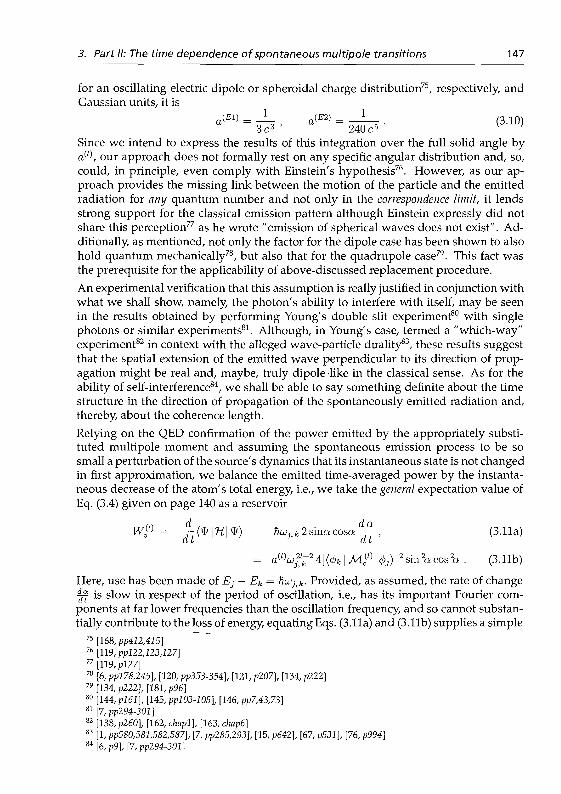
3. Part II: The time dependence of spontaneous multipole transitions 147
for an oscillating electric dipole or spheroidal charge distribution75, respectively, andGaussian units, it is
a(E1) - 6 • a<£2) = 2 3 b • <3-10»Since we intend to express the results of this integration over the full solid angle byaw, our approach does not formally rest on any specific angular distribution and, so,could, in principle, even comply with Einstein's hypothesis76. However, as our ap-proach provides the missing link between the motion of the particle and the emittedradiation for any quantum number and not only in the correspondence limit, it lendsstrong support for the classical emission pattern although Einstein expressly did notshare this perception77 as he wrote "emission of spherical waves does not exist". Ad-ditionally, as mentioned, not only the factor for the dipole case has been shown to alsohold quantum mechanically78, but also that for the quadrupole case79. This fact wasthe prerequisite for the applicability of above-discussed replacement procedure.An experimental verification that this assumption is really justified in conjunction withwhat we shall show, namely, the photon's ability to interfere with itself, may be seenin the results obtained by performing Young's double slit experiment80 with singlephotons or similar experiments81. Although, in Young's case, termed a "which-way"experiment82 in context with the alleged wave-particle duality83, these results suggestthat the spatial extension of the emitted wave perpendicular to its direction of prop-agation might be real and, maybe, truly dipole-like in the classical sense. As for theability of self-interference84, we shall be able to say something definite about the timestructure in the direction of propagation of the spontaneously emitted radiation and,thereby, about the coherence length.Relying on the QED confirmation of the power emitted by the appropriately substi-tuted multipole moment and assuming the spontaneous emission process to be sosmall a perturbation of the source's dynamics that its instantaneous state is not changedin first approximation, we balance the emitted time-averaged power by the instanta-neous decrease of the atom's total energy, i.e., we take the general expectation value ofEq. (3.4) given on page 140 as a reservoir
W® = - Y (* \H\ *) = Tnwj,k 2 sinct cosct ̂ , (3.11a)
= a^ujfj2 4| (<pk | M«] | 4>j) | 2 sin 2a cos 2a . (3.11b)
Here, use has been made of Ej — Ek — hu>j<k. Provided, as assumed, the rate of change^y is slow in respect of the period of oscillation, i.e., has its important Fourier com-ponents at far lower frequencies than the oscillation frequency, and so cannot substan-tially contribute to the loss of energy, equating Eqs. (3.11a) and (3.11b) supplies a simple
75 [168, pp412,415]76 [119, ppl22,123,127]77 [119, pl27]78 [6, ppl78,245], [120, pp353-354), [121, p207], [134, p222]79 [134, p222], [181, p96]80 [144, pl61], [145, pplO3-W5], [146, pp7,43,73]81 [7,pp294-301]82 [138, p260], [162, chapl], [163, chap6]83 [1, pp580,581,582,587], [7, pp285,293], [15, p642], [67, p531], [76, p994]84[6,p9],[7,pp294-301]

148 Continuous quantum mechanics... Parts I and II
nonlinear differential equation of first order for the change with time of the parameterangle a(t)
^ ^ (3.12a)
where„(0
^ V 4 1 ^ 1 ^ 0 ' ^ ' 2 ^ 1 (3-12b)represents the well-known QED transition probability per unit time for AM = 0 transi-tions85 in a generalized form comprising El and Ml as well as E2 transitions.Eq. (3.12a) is a nonlinear differential equation of first order that can easily be integratedafter separation of variables because rfln(tana) = s[n^osa • Before doing so we have torecall that for simplicity's sake we stipulated to only deal with the z component ofthe dipole moment. This, however, does not take into account that, e.g., in El tran-sitions, the motion of the electron, according to Eqs. (2.195), (2.196), and (2.198) onpages 122,123, and 124, respectively, has not only this oscillatory component along thez direction but simultaneously also follows a circular trace in the x — y plane, whichthe electron performs either clockwise or counterclockwise, which way is usually notknown. Equally unknown is usually the spatial orientation as expressed by the mag-netic quantum number m unless the state has designedly been prepared by polarizedexcitation. If not, we may sum the square of the orientational parts of the matrix ele-ments, as given by the squares of Eq. (2.192) on page 121, over all m for both directionsof revolution and then average. The result is that the actual decay rate is twice as large,and we attain for the exponential form of the result
a(t) = a r c t a n [ t a n a{t = 0)e A%11 . (3.13)
Here, the notation a(t — 0) has deliberately been chosen for the initial value of theparameter angle in order to emphasize that for a(t — 0) = 0 the process of spontaneousemission described above could never get started. Thus, without a perturbation thatwould change such a situation into one where a(t = 0) ^ 0, the system would stay inthe upper exact eigenstate for an infinitely long period of time.
This finding is exactly what Bohr might have had in mind with his first postulate86
when he demanded87 that "an atomic system can permanently only exist in a certainnumber of stationary states".
This result is also fully in compliance with the uncertainty relation between energy andtime: As all preceding examples with angular momentum have shown in Part I, even ifnot confined to a closed system and spontaneous transitions were possible, the atomicenergy would not change for truly stationary eigenstates. Without perturbations, as aconsequence, any exact eigenstate should have an infinitely long lifetime.
In this context, we should mention that the same statement about the infinite lifetimeof an exact eigenstate was also deduced from the results of the neoclassical theory88 and
85 [6, ppl78,245], [82, pl78], [115, pl79], [120, p354], [121, p207], [181, pp91,96]86 [31, pll8], [46, pp4,5,7,15], [47, p478], [49, p510], [50, pp396,398], [68, plO4], [69, p426], [70, p230], [71,
p3], [72, pp71-72], [73, pp787-788]87 [51, ppl23,124]88 [185, pill], [186, plOO]
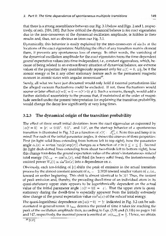
3. Part II: The time dependence of spontaneous multipole transitions 149
that there is a strong resemblance between our Fig. 3.2 below and Figs. 2 and 1, respec-tively, of refs. [184,185]. But how critical the dynamical balance is for exact eigenstatesdue to the zero-crossovers of the dynamical oscillation amplitude, is hidden in theirresults and, thus, not as obvious as from our Fig. 3.1.Dynamically, this behavior is easily explained by the zero-crossovers of sin 2a at thelocations of the exact eigenstates: Nullifying the effect of any transition matrix elementthere, it prevents any spontaneous loss of energy. In other words, the vanishing ofthe dynamical oscillation amplitude for the exact eigenstates turns the time-dependentgeneral expectation values into time-independent, i.e., constant eigenvalues, which, be-cause of being related to an extraordinary situation of dynamical balance, are extremevalues of the properties they unambiguously represent only for a(t) = 0, ± | , be it theatomic energy or be it any other stationary feature such as the permanent magneticmoment in atomic states with angular momentum89.
Surely, all what we have just discussed would only hold if external perturbations likethe alleged vacuum fluctuations could be excluded. If not, these fluctuations wouldsooner or later effect a(t — 0) = 0 —> a(t>0) / 0. Such a scenario, though, would add afurther statistical uncertainty to the process that, if maintained at the order of magni-tude needed under the present interpretation for explaining the transition probability,would change the decay law significantly at very long times.
3.2.3 The dynamical origin of the transition probability
The effect of three small initial deviations from the exact eigenvalue as expressed by\a(t — 0)| = |e| = 0.01°. 0.1°, and 1.0°, on the start-up behavior of a spontaneoustransition is illustrated in Fig. 3.2 as a function of x(t) — A^k t. Note this and keep it inmind! For each of the initial parameter angles, it shows the courses of three properties:First (in light solid lines extending from bottom left to top right), how the parameterangle as(x) — arctan[tan |e| exp(z)] changes as a function of x in 0 < x < f. Second(in light dash-dotted lines extending from about two-thirds left to bottom right), howthis change translates the general expectation value of the atom's instantaneous reducedtotal energy (H)red = cos2ae(x), and third (in heavy solid lines), the instantaneouslyemitted power Wo(t) oc sin22a(z) into a dependence on x.
Obviously, each ten-folding of |e| shifts the peak of emission in the actual transitionprocess by the almost constant amount of xo = —2.3026 toward smaller values of x, i.e.,toward an earlier beginning. This shift is almost identical to In 10 ! Thus, the instantof peak emission and, thereby, the preceding dwell-time of an individual atom in itsquasi-stationary upper state appears to be logarithmically dependent on the actualvalue of the initial parameter angle | a(t = 0)| = | e |. That the upper state is quasi-stationary during the dwell-time is especially apparent from the initially extremelyslow change of the general expectation value cos2a(.T) of the reduced total energy.The quasi-logarithmic dependence on | a(t = 0)| = \e\ indicated in Fig. 3.2 can be sub-stantiated in general terms: If tmax denotes the period of time it takes for reaching thepeak of the oscillation amplitude then, according to Eqs. (3.9) and (3.11b) on pages 146and 147, respectively, the maximal power is emitted at | a(tmax)\ = | . Hence, we obtain
89 [137]

150 Continuous quantum mechanics... Parts I and II
<x(t=O) | = | 8 | : 1.0° o.r 0.01c
1.4
1.2
i
0.8
0.6
0.4
0.2
| . |
/
. aE(x) [rad]
cos2aP(x)
sin22aJx)
6 7x
10 11 12 13 14
(i)Figure 3.2: Time evolution of a spontaneous transition process as a function of x = A\'ktfor the initial parameter angles |a( i = 0)| = |e| = 0.01°, 0.1°, and 1.0° (cf. text). Light solidlines: change of the parameter angle a£(x) = arctan[tan|e|exp(x)]. Dash-dotted lines:change of the general expectation value of the reduced total energy {H)red = cos2as(x).Heavy solid lines: change of the instantaneously emitted power Wo '(x) oc sin22a£(x).
from Eq. (3.13) on page 148 for | a(t = 0)\ < f
tan|a(* = 0)| = (3.14)
Here, it becomes apparent how strongly the instant of peak emission depends on| a(t = 0)\. Since tan | a(t — 0)\ can be approximated linearly over a wide range of initialparameter angles (even for a = 0.5 rad the deviation is only +9.26%), the logarithmicdependence is well established for the interesting range of initial parameter angles:In tan | a{t = 0)| « In \a(t = 0)\ = - Afk tmax. So, independently of whether a{t = 0) ispositive or negative, the probability exp {—-^pk tmax) that a single atom radiates at tmax
with maximum power90 and thereby indicates that it is amidst its emission process,is directly determined by how close its initial energy Ej cos2a(t = 0) + Ek sin
2o;(t = 0)was to the upper state's exact energy eigenvalue Ej as an unambiguous feature of aphysically stationary state.There is no doubt that without knowledge of the individual value of the initial pa-rameter angle a(t = 0) in Eqs. (3.13) and (3.14), respectively, we can neither predictthe dwell-time for the individual atom nor the related value of tmax, at which timethe dynamical situation of the emitting atom is characterized by a maximal oscillationamplitude and a concomitant maximal release of power. Only if we observe a great
90 [18, p2798]

3. Part II: The time dependence of spontaneous multipole transitions 151
number of transitions will it be possible for us to say something about the transitionprobability. But instead of observing sequentially a great number of transitions in asingle particle we may find it easier to observe the decay of the fluorescence of a bulkof excited like atoms.
Then, there can also be no doubt that in the vicinity of the maximum of the generalenergy expectation value, which marks, in the proper sense, the energy eigenvalue ofthe upper exact eigenstate for a = 0, all small initial parameter angles a(t = 0) ^ 0are equally probable because there cos2a(i = 0) « 1. This can be exploited when abulk of atoms is instantaneously excited by a process with finite energy bandwidth.The equal probability for all parameter angles in this small interval may be expressedby a uniform population density per radian n. Therefore, we may assume that in adelayed coincidence experiment on a bulk any such narrow angle interval da will bepopulated with dN = nda atoms in accord with its width da. This would total anumber of N — 2n\ a(t — 0) | in the angle interval between 0 and | a(t — 0)| on either sideof the maximum. If the uniformly populated region would extend up to an equallysmall maximal parameter angle | ao(t = 0)\ then, accordingly, the total number of atomsoriginally excited at t = 0, would be
No = 2n\ao(t = 0 ) \ . (3.15)
Related to this maximal initial parameter angle ao(t = 0) is, according to Eq. (3.14), theshortest period of time t°max after a 5-like excitation at t = 0, which has to elapse beforeany individually emitted radiation reaches maximal amplitude. This is the time whenthe bulk sample is emitting with maximal amplitude for the first time.
Using Eq. (3.15) and the linear approximation to tanct(t = 0) mentioned in conjunctionwith Eq. (3.14), we can express the uniform population density per radian as
2n = JVoe/V£*c« . (3.16)
Under the given circumstances, the time i^ax is determined by atoms that the excitationprocess happened to have placed on the outskirts of the populated parameter-angleinterval. Having the greatest initial parameter angle, these atoms are the first onesin the excited bulk to come into full swing after t°max has elapsed. Then radiation isemanating from them with maximal amplitude. At later times, tmax > t°max, whenthe still populated parameter-angle interval extends only up to a smaller parameterangle \a(t = 0)| < \ao(t = 0)|, a total number of N = 2n\a(t = 0)| atoms has notyet or is just reaching that stage. Taking advantage in Eq. (3.14) of the fact that here(tan | a(t = 0)\) « J a(t — 0)\ and inserting Eq. (3.16), this number can be expressed by
JV = J V o e - ^ ' (3.17)
where here t — tmax — t°max now designates the time after t°max. This relation also holdstrue at any distance from the emitting atom because the equal shifts by the time-of-flight T to the detector drop out.
This is a very interesting result. Although, without knowledge of the individual valueof a(t = 0) 7̂ 0, it is impossible to predict the instant when in the course of its tran-sition the individual atom will be reaching the stage of peak emission, we obtain the

152 Continuous quantum mechanics... Parts I and II
familiar law of exponential decay for bulk experiments with only the statistically easy-to-justify assumption that in the close vicinity of the maximum of the general energyexpectation value the total population of the upper state is uniformly spread out over acertain small interval of initial parameter angles and thereby energies. At least in firstapproximation, this is a safe assumption for an impulsive excitation process that is notenergy selective like a ̂ -function but has a certain bandwidth.In this context, however, the need arises for a careful scrutiny of the deviations exper-imentally observed at the very beginning of the exponential decay. Such an investi-gation should help to decide on whether their origin, usually interpreted as pile-upeffect, really is an electronic artefact or whether they express the breakdown of the as-sumption that the population density per radian extends truly uniformly over the totalinterval of occupied initial parameter angles.
It is well-known that an exponential decay, like Beer's law, is usually obtained fromstatistical considerations that lead to a rate equation according to which the temporaldecline of the excited species is proportional to the number still present: -~^ — A^kN.This proportionality is provided by the constant transition rate. But our way lets useasily understand that there is also a different, dynamical side to this feature: In ourscenario, the decay of the upper state's bulk population proceeds by erosion of therange of occupied initial parameter angles a(t = 0) ^ 0 from the outer edge inward,i.e., by first eating off atoms with the greatest initial parameter angle ao(t = 0) ^ 0,then successively those with smaller and smaller ones. As, according to Eq. (3.14) onpage 150, the coming into full swing is the faster the greater the nonvanishing initialparameter angle a(t — 0) ^ 0, initially many more excited atoms of the bulk make atransition per unit time than later when it takes longer to reach that stage. Althoughthis contradicts transitions at a constant rate, it is here the constancy of the number ofatoms per angle interval, which is available for transitions at the respective instant oftime, that together with a varying "transition rate" gives rise to the exponential decayof bulk samples as observed, e.g., in beam-foil excitation experiments91 where the du-ration of the very short excitation process, the passage through the foil, is well definedbut the excitation energy is not. Thus, how in compliance with the uncertainty relationthe individual uncertainty in a(t = 0) and the related initial energy deviation leads toan individual dwell-time, the continuous spread of the individual initial general expec-tation values of the energy leads to an overall mean lifetime for the bulk population.
Our results confirm the statement in the article by Stroud and Jaynes92 that "it does notrequire an atom to emit an exponentially damped wave train in order to observe an ex-ponential decay of the fluorescence, since the total radiation will fall off exponentially,whatever the shape of the basic spontaneous emission pulse, provided only that thenumber of emitting atoms falls off exponentially".
Repeated trials on single particles
The applicability of our theory, however, is not limited to the description of bulk be-havior, indeed. It also applies, as already indicated above, to repeated trials on sin-
91 [192]92 [185, pi 07}

3. Part II: The time dependence of spontaneous multipole transitions 153
gle particles, e.g., single ions isolated in a trap93. A wealth of experiments has beendevoted to this subject but we shall focus here on the first one94 performed on a sin-gle Ba+ ion in a radio-frequency trap95: In this experiment, which, for the time be-ing, will be described in terms of the currently accepted interpretation, a weak line at455.4 nm filtered from an incoherent hollow cathode lamp and connecting the states65251/2 — Qp2P3/2 occasionally causes dark periods in the continuously monitored flu-orescence from the lower laser-pumped transition 6s2Si/2 - Qp2P\/2 (493.4nm), whichis also used to laser-cool the ion by slight red-detuning. The second, simultaneouslylaser-pumped upper transition 6p2Pi/2 - 5d2D3/2 (649.9nm) prevents the electron fromgetting lost into the low-lying metastable 5d D3/2 state. So, with the hollow cathodelamp blocked, fluorescence emanates continuously from the monitored line. But withthe weak line active, dark periods are observed once in a while when due to branchingin the 6p 2P3/2 state the electron has made a transition into the second metastable state5d 2D5/2 and then is really not available for the pumping cycle, at least not for a certainperiod of time. These dark periods have been attributed96 to "electron shelving" inthe metastable state, which lasts until the electron makes a "quantum jump"97 into the6s 2S\/2 ground state through an E2 transition at 1.762 /mi. (Comment: The "stationary-states-only" doctrine of the current interpretation obviously imposes the notion thatthe electron stays in the metastable eigenstate without changing its dynamical param-eters until it makes a sudden transition into the ground state after, on time average, amean lifetime r = (A2J 6s)"1 in accord with the E2 transition probability). By measuringa large, statistically relevant number of durations of the dark periods a mean lifetime of32 ± 5 ,s was determined for the metastable state. Prior to this first experimental verifi-cation, but a decade after having been proposed98, quite some effort had been put intotreating the effect theoretically by various quantum-statistical techniques99.
Contrary to these intricate treatments, however, the duration of the dark periods canmuch more easily be explained with the help of Eq. (3.13) given on page 148. As ex-plained above, the scenario assumes100 that on some occasions the electron in the ionis excited by the weak line from the ground state to the 6p2P3/2 state and that thisstate's spontaneous decay then happens to follow a cascade-like path on the ener-getic topography explained above where the fast first step consists of the El transition6p2P3/2 — 5d 2D5/2. After that the electron finds itself close by the saddle plateau of themetastable 5d 2D5/2 state. If we start our clock with the beginning of the very weak and,therefore, long lasting quadrupole oscillation, i.e., with the electron's "arrival", so-to-say, in the close vicinity of the metastable state after the fast oscillation of the precedingEl transition has died out, the ensuing dark period manifests a dynamical situation,which is characterized by the absence of the oscillation mode at the frequency of thelaser-cooled 6s 2S\/2 — 6p 2Pj/2 transition that would allow to drive the electron back tothe excited 6p 2P\/2 state.
93 [18-22,182]94 [18]93 [193, p534] a n d re fe rences t h e r e i n96 [ 1 8 ]
97 [18-23]98 [ 1 9 4 ]
99 [195-199]100 [ l g ]

154 Continuous quantum mechanics ... Parts I and II
By the way, the excitation into the excited Qp2P^/2 state by the weak line presumablygets a chance only because of a temporary phase mismatch between the electron's mo-tion in the ion and the strong pump field, which is most probably caused by the micro-motion of the ion as a whole in the trap or phase jumps in the radiation of the pumplaser. So, the dark periods actually start with this excitation process. However, as notonly the dwell-time in the excited 6p2P3/2 state but also the ensuing transition timeinto the metastable hd 2Db/2 state are negligibly short compared to what is happeningin this latter state and during its decay, we may safely attribute the duration of the darkperiods to only what is going on in conjunction with the E2 transition.
In the experiment, the E2 photon is not detected. The conclusion of its emission isindirectly stated by the recurrence of the fluorescence that is being monitored. Thismeans that the duration of the dark period is a measure for the time its takes the ion toget ready for the next excitation on the monitored transition. Inversion of Eq. (3.13) onpage 148 obtains for tD, the duration of a dark period
tan a(t = 0)tan a(tu)
'ID (3.18)
Here, contrary to the "shelving" scenario, which is based on the quantum-jump hy-pothesis101, our's is a continuous one: According to the transition dynamics describedabove and depicted in Fig. 3.2, tD comprises the dwell-time, which, due to an unpre-dictable a(t = 0), is varying statistically from event to event, and a fixed period oftime that is determined by the finite duration of the actual transition to be defined onpage 156 below. But the return to the ground state is to be seen in a wider sense in thatit need not be the exact eigenstate because of the finite spectral width of the excitinglaser radiation. This means that at the end of the E2 transition 5d2Db/2 - 6s2Sl/2, theelectron is arriving at a parameter angle a(to), pertinent to that transition and closeto | , which brings it back into the vicinity of the exact ground state in terms of ampli-tude. Then, it is prone to again fall prey to the exciting pump laser light at 493.4 nm.According to Eq. (3.18), this parameter angle need not be the same in each event as itis the ratio of the tangent of the initial parameter angle a(t = 0) over that of the for-mer one that causes varying periods of tD. But statistically the main contribution tothe variation of tD comes from the variation of a(t — 0), of course. Extraction of thetransition probability of Eq. (3.18) from measurement data is particularly easy whenthe transition is forbidden, i.e., slow and the periods tu correspondingly long.Common to the treatment of both the bulk case and repeated trials on an individual ionis the tacit assumption that the occupation of different small initial parameter anglesa(t — 0) always occurs with equal probability. The only difference being, that for thebulk this occupation is scanned in a single sweep because the | a(t = 0)\ of the individ-ual atoms are continuously distributed with a uniform population density per radian nover the range 0 < | a(t = 0)\ < \ ao(t = 0)\ while for the single ion only after sufficientlymany repeated trials statistics have added up the different event-related individualoccupations to mimic such a uniform population density.
101 [I,p582], [U,pU8], [15,pp6U,617,619,645],[16,pp50Z,504], [17-29], [30,pp95,97], [31,ppl46,153], [32,p836]

3. Part II: The time dependence of spontaneous multipole transitions 155
The emitted energy
According to Eqs. (3.9), (3.11), and (3.13) on pages 146 through 148, the power of theemitted radiation time-averaged over the fast oscillation with ujjik is proportional
oc sin2 J2axctan [tana(i = 0) e ^ ' l j (3.19)
to at any instant t. Eq. (3.19) determines the temporal envelope of the emitted wavepacket as depicted in Fig. 3.2 by the heavy solid curves. Taking the emitted power asgiven on page 147 by Eq. (3.11) and integrating over time
c roc 1
W«\t)dt = huj^k / sin2a— dt (3.20)Jo d''
j , k cos2 a(t — 0) - cos2a(t —> oc) .
we obtain the total energy emitted in the course of the transition. Resulting in anexpression that was to be expected from Eq. (3.4) on page 140, this energy is veryclose to htu'j^k, of course, provided a(t = 0) is sufficiently small so that cos2a(t = 0) m1, and the transition can unperturbedly proceed for long enough a time. This lattercondition has been indicated in Eq. (3.20) by writing cos2a(£ —> 00) instead of cos2f = 0.Thus, hu!j: k is only obtained in the case that Bohr102 called a complete transition from onestationary state to another. As matter of fact, a complete transition will rather be theexception than the rule given the necessity for the absence of perturbations during avery long period of time.By the way, the same result would have been obtained, of course, if we had startedwith time integrating Eq. (3.19) on page 155 in conjunction with Eq. (3.13) of page 148and substituted dt by the expression that follows from the differential equation givenby Eq. (3.12a) on page 148.Eq. (3.20) resolves the conundrum that puzzled Bohr103 and others since Planck's dis-covery104 of the energy quantum hu> and that also led to the disturbing notion of dis-continuities in the microworld: According to Bohr's understanding of classical electro-dynamics105, the frequency of the emitted radiation should increase during a transitionin accordance with the loss of the atomic energy and the concomitant acceleration ofthe electron when it, in his view, spirals into more tightly bound orbits. This way ofrelating the origin of the frequencies in the emitted radiation to periodic features of theelectron's motion was in disagreement with the experimental evidence of line spectra.On the other hand, the accepted fact of Planck's relation106 on which Bohr had builthis second postulate107 left no room for this kind of classical perception because it de-manded the emission of monochromatic light. Although Bohr was not able to explainthe reason for the seeming inadequacy of the classical description108, he was in good
102 [31, ppll8,139], [70, p230], [72, pp71-72], [73, pp787-788], [75, ppl,4]103 [69, p426]104 [14, ppU8-U9], [65, pp556,561]105 [46, pp4,7], [69, p428]106 [14, pP148-U9,155], [65, PP556,561]107 [31, pl39], [46, p8], [47, p487], [49, p507], [50, p396], [70, p230], [71, P3], [72, p72], [73, p788]108 [31, pp!51-152], [46, pp2,19], [49, p509], [50, p398], [70, p230], [71, pp2,3], [72, pp71-72], [73, p788]

156 Continuous quantum mechanics... Parts I and II
company with regard to both the rejection of classical electrodynamics109 as well as thepromotion of the monochromaticity question110 when he felt forced to assume111 "instriking contrast to this theory that the transition is always followed by an emission ofmonochromatic radiation the frequency of which is determined simply from the differ-ence of the energy in the two states"112. Convinced113 that " quantum theory has to beunderstood as an attempt to overcome certain characteristic difficulties in the applica-tion to atomic systems of the usual mechanics and electrodynamics" and in followingPlanck114, he repeatedly concluded115 that the assumption of transitions between sta-tionary states in atomic systems automatically entails discontinuities116 that make adetailed description of emission and absorption impossible117 and that the intimaterelationship of his frequency condition with Planck's assumption of energy quanta im-poses that the emitted radiation be monochromatic1™. In both questions, he followedPlanck119 and found his approval120.
The duration of the transition and the spectral intensity distribution of the emittedradiation
Next, we shall define the duration of the transition: For this purpose, we use Eq. (3.14)from page 150 and insert it into Eq. (3.13) on page 148. This yields
(3.21)
We define the duration of the transition by the full-width-at-half-maximum (FWHM)of the power emitted as a function of time according to Eq. (3.19). With this definition,we obtain for the time span of substantial emission
A T = 2 t[/2 — tmax = 2
which corresponds to a coherence length of
A, = c AT = 2 c
In (tan | '^ (3.22)
In ( tan ?](3.23)
Aj!k
and deviates from the usual definition121 Ac = ^ by a factor of 1.586 (cf. Eq. (3.26)).1119 [U, ppl47,148]110 [14, pp89,146]111 [68, ppl04,105]112 [51, ppVI,XI,133,135,151], [68, ppl04,105], [69, pp424,426], [75, ppl,5]m[5\,ppl22,139]114 [14, ppl47,148-149,155], [65, pp556,561]115 [51, p224]116 [51, ppl24,133], [69, p424], [71, p2]117 [31, pllS], [51, ppVI,133], [68, p204], [69, p426], [70, p230], [71, p3], [72, pp71-72], [73, pp787-788]118 [51, ppVI,XI,133,135,151], [68, ppl04,105], [69, pP424,426], [75, p/7l,5]119 [14, pp89,146,147,148], [51, ppl24,133]120 [67]121 [7, p294]

3. Part II: The time dependence of spontaneous multipole transitions 157
Like the mean lifetime of the bulk, the duration of the transition in each individual atomis also proportional to the reciprocal of the well-known transition probability per unittime. However, it is important to note that the duration of an unperturbed transition isthe same for all individual systems, no matter how long the individual d well-time in theupper state. Therefore, the ensuing spectral line width, which will be dealt with next,can only be a consequence of the identical finite duration of the individual transitions.
Although we keep looking at only the source dynamics, we may assume, as we did incontext with Eq. (3.19), that the original time dependence of the unperturbed dynamicsprevails and that, therefore, apart from finer details, the time dependence of the emit-ted field strengths is determined by that of the source in the first place. As mentioned,this view is supported and justifiable by the smallness of, e.g., the Lamb shift122 and theconcomitant prevalence of the unperturbed oscillation frequency during the transition.Then, according to Eq. (3.8) on page 141, the time-dependent part of the field strengthsmay be taken as proportional to sin 2a(t) COSWJ,^. With the help of Eq. (3.12a) given onpage 148, the abbreviation a(t = 0) = e, and the assumption of an unperturbed transi-tion, the Fourier transformation of the field strength results in the following recursionformula
/ sin2n+12a(t)eiQtdt =
= t sin*"1 2e ^—-3 sin**1 2e cos 2 e ( 2 w + 1 ) ^ y
[ ]2
I poo
+ - — ') J'*J / sh^n+^+12a(t)eiQtdt (3.24)
where uo = to ± a;Jifc. Applied iteratively, Eq. (3.24) yields/•oo
/ sm2a(t)eiatdt =Jo
i sin 2e ^= < 1+ sin22e ^ 4 ^ — (3.25)
K i ) 1 K )
- sin 2e cos 2e
+ sin'2ET ; W-^ ; r +
[170]

158 Continuous quantum mechanics... Parts I and II
Upon absolutely squaring and with cos22£ = 1 — sin22£, this obtains for the spectralintensity distribution
sin22e(3.26)
3 sin42e+ — x
3-A
12 sin62e
( wV -2
2 / \2
Given the high frequencies involved, only terms with u — UJ — UJ^ k can substantiallycontribute. The line shape is practically purely Lorentzian as long as e is small enough.For larger values as, e.g., induced by heavy collisions, a homogeneous line broadeningis predicted. Under the assumptions made, it is, e.g., 0.89% for e = 0.5°.
As the Fourier transformation in Eq. (3.26) takes us from the time to the frequencydomain, the factor sin22e in front of the pure Lorentzian part represents a measureof how often per unit time a transition can take place and, therefore, depends on theindividual dwell-time parameter e.
For sufficiently small e, the almost ideally Lorentzian line profile of Eq. (3.26) mani-fests that our theory does not suffer from one of the main deficiencies123 the neoclas-sical theory had to cope with by obtaining a hyperbolic secant squared124 rather thana Lorentzian. Moreover, Eqs. (3.17), (3.20), and (3.26) on pages 151, 155, and 158, re-spectively, manifest that our model meets the basic quantum mechanical requirementsto be complied with in transitions. It proves that the natural line width is a dynami-cal feature that results from the identical finite duration of the transition processes inindividual atoms and, therefore, has nothing to do with an ensemble's level width,which is explained here as originating from the uniform occupation of a finite range ofc's. Thus, a seemingly finite level width is effective only for an ensemble and then re-sponsible for the mean lifetime. Both features, though, are connected by the transitionprobability given on page 148 by Eq. (3.12b).
There are other, physically very important aspects of our findings: One is that theyshed new light on what is usually called radiation damping. With the Fourier trans-form of the model of a damped oscillator in mind125, the natural line width is commonlyattributed to a constant decay rate, which is seen126 as a result the reaction field has onthe motion of the particle. Here, however, we learn that a decay mechanism exists forthe individual particle that is independent of such influences, at least in first approxi-mation, and only determined by the finite duration of the transition process.
123 [186, plOO]124 [185]125 [82, pp32-33]126 [83, p887]

3. Part II: The time dependence of spontaneous multipole transitions 159
Another one is that each single photon as demanded by Dirac127 and to be concludedfrom Eqs. (3.23) and (3.26) on pages 156 and 158, respectively, has the capability ofinterfering with itself. Experimental confirmations have been claimed128 but there arealso voices129 opposing this claim.
3.3 A comparison between the present and the QED re-sults
3.3.1 A critical look back in history
With a bold intuitive vision, Bohr130 had been able to deduce the existence of station-ary states lüith angular momentum from purely classical mechanics. Nevertheless, hecould not stop wondering about their "peculiar" stability131 because, from his pointof view, the charged particles in hydrogen perform accelerated motions even when instationary states132. This should exclude any energetic stability. Therefore, his persis-tent astonishment might be rooted in the fact that from the very beginning and for noapparent reasons, he seems to have mentally blocked his way to cognition by alwayswrongly concluding, in spite of knowing to be in contradiction133, that the commonlaws of electrodynamics do not apply134. Moreover, in his view, the radiative loss ofenergy should be accompanied by an increase of the emitted frequency135. Such a fea-ture would make the emission of sharp lines impossible.In an attempt to overcome these inconsistencies, he had formulated his postulates. Al-though he kept hoping136 that the difficulties in conjunction with transitions could beresolved some day and struggled hard in this respect he never succeeded in develop-ing a perception of how transitions could be described in detail. Finally, he becameconvinced137 that no detailed description of the transition process is possible in princi-ple. In this Bohr was followed by his contemporaries, and it was taken for granted thattransitions had generally to be considered discontinuous events138.
In this context, we should remember, however, that Bohr conceived his theory wellbefore the advent of Schrödinger's equation. Although he kept searching until longafter Schrödinger's discovery he could not find a general connection between his fre-quency condition and the periodic motions of the particles that is valid for all quantum
127 [6, p9], [7, p294]n8[7,pp296-301]129 [200, P37]130 [31 , pll8], [46, pp4,5,7,15), [47, p478], [49, p510), [50, pp396,398), [68, pW4], [69, p426], [70, p230], [71 ,
p3], [72, pp71-72], [73, pp787-788]131 [31, ppU8,148l [70, p230], [71 , p3]132 [74, P3]133 [70, p230]134 [46, pp2,3-4,7,16,19], [49, p509], [50, p396], [51, ppVl-VU,Xl,Xlll,123,124,133}, [68, ppl04,105], [69,
pp424,427,429], [70, p228], [72, pp71-72], [73, pp787-788], [74, pp2-3]135 [46, pp3-4)136 [46, pp2,7], [49, p509], [50, pp396,398]137 [31, pU8], [46, p7], [49, pp508-509], [51, pVI], [68, plO4], [69, p426], [70, p230], [71, p3], [72, pP71-
72], [73, pp787-788]U8[15,pp614,617],[76,p989]

160 Continuous quantum mechanics... Parts I and II
numbers and not only in the correspondence limit. But in retrospect, it is all too easy tospell out the reason for Bohr's failure in this respect: Like his contemporaries, he hadclung to the notions they were used to and to the mathematical tools at their disposal,namely, that multiply periodic motions allegedly can only be decomposed into the fre-quencies supplied by Fourier series. As it turns out now, those tools are not adequate,the right ones had either not been developed yet or, as it happened even after the de-velopment of Schrödinger's equation, have not been recognized as such and what theircapabilities. The reason for this general "blindness" may lie, in our view, in the coin-cidence that the form of the "wave functions" seems to fully corroborate de Broglie'sconcept139 of wave properties. This concept, as we have explained on page 29 of Part I,had inspired Schrödinger140 to the formulation of his equation and, so, because of hissuccess, he never had doubts about it. And if it was not him to doubt whoever elseshould have done so?
So, the infeasibility to match reality to the now obsolete claim that any periodic motioncan be decomposed into its harmonics141 as well as the inability to imagine eigenfre-quencies beyond the scope of Fourier's theorem142 and to realize that the invalidityof this claim is caused by the inapplicability of Fourier's theorem led Bohr to prema-turely conclude that the usual laws of electrodynamics are not generally applicable tothe microworld143. This conclusion is related to the fact that only in the transition tothe macroworld such a connection seemed possible because all he could find was thatin the asymptotic limit of high quantum numbers the transition frequencies betweenneighboring Rydberg states in hydrogen and the alkalis approach a Fourier-like combof equally spaced frequencies. Happy to see the painstakingly sought connection atleast asymptotically, he introduced his correspondence principlelii.Contrary to what Bohr repeatedly insisted on in following Planck145, namely, that theemission process is discontinuous because of the assumption of being accompanied bymonochromatic radiation146, we have proven here that neither the first nor this secondassumption are compelling ones, but that the opposite is true, namely, that transitionsare continuous processes, indeed, and that the emitted radiation consists of a wavepacket. Despite the fixed eigenfrequency of the source, this latter feature is owed tothe finite duration the source can observably be active on this frequency. However, thesystem is only prone to make a spontaneous transition into a lower state if a(t = 0) ^ 0,for instance, due to a perturbation like a collision or, more probably, simply because ofnot matching the upper exact eigenstate in the excitation process.As a much more subtle, though ubiquitous type of perturbation the fluctuations of thephoton vacuum may have their share in preventing any atom from ever being able tosettle in an exact eigenstate. This, however, would require that these fluctuations are
139 [101]140 [9, p372]141 [31 , ppl20,143-144], [46, pl4], [69, p430], [70, pp230,231], [71 , p5], [72, pp71-72], [73, pp787-788]142 [46, ppl3-14], [51 , ppXI,133,135], [69, p430], [70, pp231,234], [75, pi]143 [46, pp2,3-4,7,16,19], [49, p509], [50, p396], [51 , ppVI-VII,XI,XUI,123,124,133], [68, ppl04,105], [69,
pp424,427,429], [70, p228], [74, pp2-3], [75, pi]144 [31 , ppl42,145ff], [51 , ppVll,Vm,Xl,Xni,XlV,XVU,133-134], [69, pp429ff], [70, pp231,234], [71, p5], [72,
pp73-74], [73, p789], [88, p250]145 [14, ppl48-149,155], [51 , ppl24,133]146 [51 , ppVl,XI,133,135,151], [68, pp!04,105], [69, pp424,426], [75, ppl,5]
3, Part II: The time dependence of spontaneous multipole transitions 161
present at any time and any place and not only occasionally occurring statistical eventsas assumed for the explanation of the transition probability.As we have shown for time-independent Hamiltonians both in general terms in Eqs.(2.16) and (2.17) of page 36, respectively, as well as more specifically with our exam-ples, our findings clearly manifest that Schrödinger's time-dependent equation and itssolutions establish the foundation for a theory of such multiply periodic motions thatcannot be decomposed into simple Fourier series because the eigenfrequencies of thesystem have to be determined individually from the solutions to the pertinent Hamil-tonian, i.e., in accordance with the respective potential. These eigenfrequencies onlybecome visible when the principle of superposition is applied in terms of the generalexpectation values. Then they allow to describe a single particle's motion in an appro-priate way and how this motion, provided the concomitant loss of energy is limitedto minute amounts per unit of time, can generate electromagnetic radiation only whenthe system is in nonstationary states.In a Coulomb potential and for very high quantum numbers, this description includesthe asymptotic Fourier-like behavior that inspired Bohr147 to formulate the correspon-dence principle. But now that we have found its roots we may safely call it obsolete.
3.3.2 General aspects of the present results
The finite duration of the transition process in Eq. (3.22) of page 156 is a tribute to thenecessity that dynamical systems with finite inertial masses need a finite amount oftime for rearranging. Surprisingly enough, our findings confirm Bohr's quantum jumphypothesis148 in a dynamically adjusted way by embracing a shorter or longer periodof relatively little change, the dwell-time, and a constant period of strong change, the"jump time" in Bohr's view, so-to-say, which determines the duration of the transitionindependently of the preceding dwell-time. As x — A^kt in Fig. 3.2 on page 150, thisconfirmation even tends to become asymptotically perfect because in the time domain,as can be understood from this figure, the changes of ae(x(t)) and (Ji)red = cos2ae(x(t))with time are the more step-like and, concomitantly, Wo\t) oc sin22ae(x(t)) the moreneedle-like, i.e., the more instantaneous, the higher the transition probability Aj k. Thisway, as a matter of fact, our results not only settle the controversy149 between Bohr andSchrödinger over the issue of "quantum jumps" by equally confirming Schrödinger'sview who insisted on a continuous process. They finally also answer Einstein's callupon Heisenberg made in a personal conversation150: "So, if your theory is right, youwill have to tell me some day what the atom is doing when it transits from one station-ary state to another under emission of light".
As shown on pagel58 by Eq. (3.26), a finite emission process automatically introducesa multi-mode wave packet, which, in the direction of propagation, is a relatively local-ized superposition of modes that moves with the velocity of light151. Being composed
147 [31, ppU2,U5ff], [51, ppVIl,VIII,XI,XIII,XIV,XVIU33-134], [69, pp429ff], [70, pp231,234], [71, p5), [72,pp73-74], [73, p789], [75, p2], [88, p250]
148 [1 , p582], [31, ppl46,153], [49, p507]149 [90, pp92-94]150 [90, p85]151 [121, P28)

162 Continuous quantum mechanics... Parts I and II
of a large number of appropriately weighted modes, this lump of radiation energy car-ries away an energy close to hu)j,k> provided the source can start its emission in theclose vicinity of the upper eigenstate and remains unperturbed during the whole pro-cess as assumed for Eq. (3.20) on page 155. However, as we have explained above, thereare good dynamical reasons that emission processes may predominantly take place be-tween quasi-stationary states and, so, not consume all of the the seemingly availabletotal atomic energy fiojj^. But the center frequency uij^ of the emitted radiation is al-ways an unmistakable fingerprint of the source because it directly reflects one of themechanical eigenfrequencies the particle's motion is composed of. Notwithstandingthis fact, the energy balance we used in Eq. (3.11) of page 147 makes sure that the totalenergy of the total system (atom + radiation field) is conserved at any time.
So far, the definition of the photon has been based on the concept that it carries onlythe full single-mode quantum Ti u)jy k when it is being released monochromatically in anelementary transition between stationary states with the respective single frequencyaccording to Bohr's second postulate152. So, if we wish to keep associating the photonwith the elementary emission process, we may still characterize it by its center fre-quency Wj, A: but have to be aware of the fact that it is a lump of multi-mode radiativeenergy that usually contains somewhat less than huij<k.
It is well-known that the term mean lifetime153 is defined by the relation T~1 = ^2k A^k
when transitions into more than one lower state are possible and all polarizations in-cluded. The coefficients for spontaneous emission A- \ together with those for stim-ulated emission and absorption were introduced by Einstein154 in his derivation ofPlanck's formula describing the blackbody radiation in thermal equilibrium.
Actually, these terms were defined as probabilities per unit of time for the occurrenceof the respective events and meant to hold for individual atoms or molecules, i.e., forindividual systems in general. With regard to Aj k, Einstein expressly remarked153 that"it is not necessary to assume that this event (a spontaneous transition) does not taketime; its duration must only be negligible compared to the period of time the moleculespends in stationary states". In this respect, our findings confirm his perception.
The condition of thermal equilibrium for all equivalent species in a bulk sample canthen be expressed by demanding that the relevant equations balance each other and sobecome stationary156. If only spontaneous transitions were considered157 (this wouldnot correspond to thermal equilibrium), the rate equation for the population of theupper state would lead to an exponential decay of this population at a rate of A-\.This may be another reason why its reciprocal is called the mean lifetime158.
However, we have demonstrated on page 151 in conjunction with Eq. (3.17) how ina bulk this average property of many excited, almost identically prepared particlesunfolds as being dynamically rooted. As has been explained there, this is mainly a
152 [31, pl39], [46, p8], [47, p487], [49, p507], [50, p396], [70, p230], [71 , p3], [72, p72], [73, p788]153 [179, p54], [181, p80]154 [119, pl23]155 [119, P123]156 [119, pl24], [181, P80]157 [181, p80]158 [121, p208], [179, P54]

3. Part II: The time dependence of spontaneous multipole transitions 163
consequence of how an erosion process of the bulk population makes the individualspontaneous transition processes get started in a well defined time sequence for thedifferent classes of initial occupations. As the instant of decay is not predictable foran individual atom because it is determined by an unknown value of a(t) ^ 0 whoseeffect has been dealt with on page 154 in context with Eq. (3.18) and depicted in Fig. 3.2on page 150, this shows that a continuous exponential decay can only be the feature ofa pure bulk. However, as we have pointed out in the introduction to Part II, an in-appropriate use of the reciprocal of the constant decay rate has also applied the term"lifetime" to the elementary event in a single atom or molecule159. Such inconsistenciesdo not plague our approach, and we do not have to resort to dynamically and statis-tically unsatisfactory models for explaining the mean lifetime and the Lorentzian lineshape of the spectral intensity distribution.Summarizing what we did so far, we have substituted in Eq. (3.9) on page 146 the clas-sical multipole moment by an effective transition matrix element, which includes thedynamical oscillation amplitude sin2a(t). It reproduces on page 151 in Eq. (3.17) theexponential decay of an ensemble with a rate of A\. We have justified the substitu-tion not only by how the classical and the QED results for A^\ compare160 but also andespecially by how all our results in Part I suggest it, especially Eq. (2.189) on page 117.
3.3.3 General aspects of the QED results
An approach with a field-quantized electromagnetic propagator161, which reaches be-yond established ones, stresses the spatial localization of the light emitted by a single-electron atom. Starting from QED and aiming at a better understanding of the elec-trodynamics in the near-field zone of the atom and, thereby, at the back-action of thefield, it addresses the spatial confinement problem and establishes an explicit expres-sion for the relation between the self-field part of the transverse electric field opera-tor and the atomic current density operator. The time dynamics of the self-field arefound to only depend on the time evolution of the atomic flip operator (cf. Eq. (64) inref. [190]) indicating that the field strength follows the time dependence of the source.We have employed this "classical" concept for obtaining the spectral intensity distri-bution by absolutely squaring the Fourier transform of the slowly time-dependent partin Eq. (3.8) given on page 141.
The subject of spontaneous emission has been a challenge to many authors and, so, hasseen many approaches162. All QED calculations start with embracing both source andEl field in quantized form and follow the Weisskopf-Wigner approximation163, whichoriginally anticipated for the amplitude of the excited state an exponentially decayingsolution164. Though differing in the details of the way pursued especially in avoidingany such anticipation, later QED calculations165 take proper account of the fact that in
159 [121, p208]160 [6, pl78], [82, pl78], [115, pp51,179], [120, p354], [121, p207], [134, p203], [181, pP89,91]161
162cf., e.g., [120, pp347ff], [121, pp206ff], and the comparing review of ref. [186]163 [82, pi 82], [179], [186, p9]lM[179,p62]165cf., e.g., refs. [120, pp347-354] and [121, pp206-208]

164 Continuous quantum mechanics... Parts I and II
free space the atom interacts with a continuum of modes in order to allow for the fi-nite line width. Using the multimode rotating-wave approximation, they arrive at thesame linear differential-integral equation for the excited state's amplitude166, whichexpresses its temporal change at time t as a function of its history up to this time. Anapproximate solution, which rests on the assumption of a slowly varying state am-plitude, turns this linear differential-integral equation into a simple linear differentialone. When integrated, it describes an exponential decay of the upper state's absolutelysquared amplitude in terms of the well-known constant El transition probability perunit time A^ as given on page 148 by Eq. (3.12b) [from page 147 the left expressionof Eq. (3.10) has been inserted], and so confirms the ansatz in the original paper167.This result is also obtained by a semiclassical approach168. But while there the upperstate's absolutely squared amplitude is expressly understood as an ensemble average,the QED result is referred169 to as holding for the individual atom.In order to obtain from this result the line shape, i.e., the frequency distribution ofthe modes contributing to the final state of the field, the solution for the exponentiallydecaying initial amplitude, despite its approximate character, is substituted in the inte-gral equation that connects the amplitude of the final state at time t with the amplitudeof the initial state at all previous times170 by equally making the final state's ampli-tude a function of the history of the initial state's one. Insertion of the approximatesolution and subsequent integration results in a linear superposition of single-photonstates for the field part of the state vector after the emission, which has different wavevectors associated with them. Despite the restrictions imposed by the approximationon the result with regard to the time span of its validity, it is assumed that it is stillvalid sufficiently long after the emission171 in order to make possible that it can yieldthe necessary Lorentzian intensity distribution172 upon absolutely squaring.If equivalent to the finite duration of the elementary emission process we find, it shouldpertain to a single atom. However, if, despite such references173, the appearance ofthe reciprocal lifetime in the exponential of the upper state's amplitude squared is toindicate that it holds at any time, the result can only pertain to an ensemble. As a con-sequence, the only conclusion, which can be drawn from the QED expression, is thatthe Lorentzian line shape results from the superposition of the many individual tran-sition events in the bulk, which are seen as being associated with the creation operatorfor, i.e., the emission of, strictly single-mode photons. Attributing implicitly an infinitecoherence length due to total monochromaticity, such a photon definition neither is rec-oncilable with the release of a finite amount of energy, as occurring for each individualsystem in the transition between its states of well defined energy differences, nor witha concomitant finite duration of the transition however this may be defined174. Theseconceptually fundamental problems are not encountered in our approach.
166 [120, p354], [121, p207]167 [179, p62]168 [187, p37]169 [120, P355], [121, p208]170cf., e.g., [121, pp207,208]171 [121, P208]172 [82, p284] , [186, p22]173 [120, p355), [121, p208]1 7 4 For s o m e a spec t s of h o w to def ine the p h o t o n , a lso see ref. [120, p315].

3. Part II: The time dependence of spontaneous multipole transitions 165
3.3.4 Comparison of special features and behavior beyond QED
Behavior shortly after excitation
At this point, it is appropriate to compare the QED behavior with the one of our find-ings and uproot the inconsistencies: If the QED result for the upper state's absolutelysquared amplitude is understood as an ensemble average, it literally represents the in-stantaneous population of that state in the sense of Eq. (3.17) given on page 151. If,however, in contradiction to the established notion but in its terminology, we wouldassume an individual meaning, i.e., that the upper state's absolutely squared ampli-tude is expressing the probability of finding a single atom still in the upper state, itwould be directly comparable with our's.
In our case, the upper state's amplitude has been defined on page 140 by the left ex-pression in Eq. (3.3). Accordingly, its absolute square can be transformed into
W (3'27)With / —*• El in mind, insertion of Eq. (3.13) from page 148 and some restructuringyield
\cj{t)\2 = cos2a(t)
= mC ° S Q JÜ- • (3.28)
cosh Ayk t - cos2a(t = 0) sinh A(-[k t
As for the individual decay behavior, in our case the same exponential as for the QED
result only holds for such a time span after t = 0, for which, depending on A)'k, the ex-
pression in the denominator is still very close to unity, i.e., to the minimum of cosh At k t
and the zero-crossover of sinh Af^k t. There
Cj{t)|2 ta cos2a{t = 0) e~A^"l = \ c_,-(0)[ 2 e ~ A & l . (3.29)
Holding for A\'\ t <£i 1, this is exactly the time domain of the QED result175. Hence,being only an approximation to Eqs. (3.27) and (3.28), Eq. (3.29) proves that our modelcomprises the Weisskopf-Wigner approximation176, which thus is shown to cover onlythe very beginning of the transition.
At later but still short times after t = 0, the denominator in Eq. (3.28) becomes increas-ingly less than unity for small a(t = 0) because the hyperbolic sine rises faster there thanthe hyperbolic cosine. This effects a slower decay than initially indicated by Eq. (3.29)as is also noticeable in Fig. 3.2 on page 150 from how little the energy changes in thatrange. This demonstrates that our theory goes far beyond the QED result.
For an easier understanding of the initial change of energy, we insert Eq. (3.12a) frompage 148 into the second line of Eq. (3.11) on page 147 by taking into account the factor
175 [82, ppl39,168]176 [82, Ppl82-184], [120, pp351-354], [121, pp206-208], [179]

166 Continuous quantum mechanics... Parts I and II
of two discussed there and then make use of the equivalence between the first andsecond line
- ^ ( 0 W * > - Ek) = {Ej - Ek)±Afksm*2a(t) . (3.30)
As long as the slow start-up behavior keeps the slowly increasing parameter angle inthe vicinity of the small initial deviation, i.e., a(t) ~ a(t = 0) = e, the system is quasi-stationary and its energy remains very close to that of the upper exact eigenstate, sothat AEjtk = (^\TC\^) - Ek remains almost equal to Ej - Ek = &E°k. This is alsoobvious from Fig. 3.2. Hence, equivalent to a time-dependent perturbation approach,this yields
-^«U%*&Udt. (3.31)
Upon integration and because of Eq. (3.4) given on page 140, we obtain for small times
|Cj-(*)|2 = cos^t) = ^ « e-M^*)> . (3.32)
This expression demonstrates that the individual dwell-time {\A^\sm22e)~l heavilydepends on the initial parameter angle a(t — 0) = e in the same way as found inEq. (3.26) on page 158. This angle determines the duration of the initially flat, quasi-linear decrease of the energy by making the linear term dominate the power expan-sion of the exponential in this time regime. There, the oscillation amplitude is still verysmall. As a result, radiating only very faintly, the system displays quasi-stationaryrather than transient properties. As a consequence, time intervals like the dwell-timecan neither contribute much to the emitted total energy nor dominate the spectral pro-file. But they allow the atom to display quasi-stationary properties. On the other hand,the period of time, which is independent of the individual dwell-time parameter e andhas been defined on page 156 by Eq. (3.22) as the duration of the transition, sees thefiercest of oscillations. Together with Eq. (3.26) on page 158 this is another strong rea-son for holding the finite duration of the individual transition responsible for the lineshape and not the mean lifetime of the bulk.
Behavior amidst the transition and at the end
For an investigation into the behavior of | Cj(t)\2 in the neighborhood of the transitionpeak at tmaxr the use of Eq. (3.27) together with Eq. (3.21) from page 156 provides theappropriate form
| c3{t)\2 = cos2a(*) = 2 J (tt . • (3-33)
Apart from the factor of 2 in the argument, this relation is identical to Eq. (20a) ofref. [184] even in respect of the constant of integration. Because of maximum slopeat the inflection point at tmax, expansion of Eq. (3.33) up to the linear term is fullysufficient there and supplies
\ \ % \ (3.34)

3. Part II: The time dependence of spontaneous multipole transitions 167
This is the time regime in the middle of the transition where the duration of the transi-tion has been defined. There, the transition progresses linearly and the meaning of A k
as transition probability per unit time becomes misleading because A^\ is truly deter-mining the velocity of this progress in this regime. But we can avoid any confusion byexpressing A^\ with the help of Eq. (3.22) on page 156 by the duration AT
ij i \i 2 •'• i / i " " \ ^ ''max , ~ or-\
Cj(t « tmax)\ « - - In (tan - ) . (3.35)2 AT
At later times, when the hyperbolic functions already are dominated by the exponen-tial with the positive argument, i.e., for A^\ t » 1 or, equivalently, t > tmax, Eqs. (3.33)and (3.28), respectively, transform into
| c,.(* -» oo)|2 = e-2^1*(*-'•»«) = cot2a(£ = 0) e-2A^ . (3.36)
This is the region in Fig. 3.2 where cos2ct(£) is already approaching the lower eigenstateand the transition is almost complete. There, the final decay rate of the upper state'samplitude squared is twice as large as in the beginning. This is necessary because ithas to cope with the very large factor in front of it.
3.3.5 Particle-like behavior at very short wavelengths
The localization of the emitted energy in respect of the direction of propagation willbe the key issue of the following discussion: Any transition process is the slower thelower the frequency. Its concomitantly longer duration effects the emission of a longerand, thus, more monochromatic wave train, provided the transition can proceed un-perturbedly. On the other hand, the more deeply states are bound, the more the energydifferences between stationary states increase and, thereby, the transition frequenciesujj^k- As a result, the duration, e.g., of an El transition, is drastically shortened be-cause of w3
fc contained in the denominator of Eq. (3.22) on page 156. The very strongincrease of this factor in the transition probability of Eq. (3.12b) on page 148 is only par-tially counteracted by the reduction of the value of the transition matrix element dueto a diminishing overlap between the combining wave functions. For giving an idea ofthe orders of magnitude involved, we shall illustrate this in nonrelativistic hydrogenicapproximation for the Ka line of any element: Neglecting spin and relativistic correc-tions, we choose as a representative atomic El transition matrix element the one thatcan be obtained from Eq. (2.198) on page 124 with the help of Eq. (2.170) on page 108.
It reads {<j)\s\ero\ 02p) = §I\A f̂1- Obviously, it decreases as Z~l, while the energydifference E2p — Eis = \RyZ2 increases as Z2. As a result of Eq. (3.12b) in conjunctionwith the left part of Eq. (3.10) given on pages 148 and 147, respectively, the transitionprobability scales as Z\ A{^\8 = 6.27 x 10⁸ • ZAs~\ and, following Eq. (3.22) as givenon page 156, the transition time as Z~A: AT = 2.81 x 10"9 • Z~4s. As this is the timespan of substantial emission, the emitted energy corresponds to an average power ofapproximately WiEl) = 5.81 x 1(T10 • Z6 W. So, already the 16 keV radiation emitted ina single Ka transition by Zr+39 has a total average power of about 2.05 W. At the highesttransition energies of about 100 keV emitted in atomic physics by hydrogen-like ions
168 Continuous quantum mechanics ... Parts I and II
of the heaviest elements (Z ~ 100), a single Ka transition only lasts about 2.81 x 10~17s,and so releases a power pulse of about 581 W with a correspondingly high electric fieldstrength. Even in this case, the duration of the transition is still some 694 times longerthan the period of the oscillation. However, as the wavelength in this regime becomesequal to the radius of the 2p orbital, the electric dipole approximation breaks downand our description can only provide an estimate for an order of magnitude. Withthese restraints in mind, the coherence length of the emitted wave packet, accordingto Eq. (3.23) on page 156, becomes extremely short at these frequencies as it scales asAc = 0.843 x Z~4 m. For our order-of-magnitude example, this would be only 8.43 nmfor Z — 100. Such a short pulse of extremely high intensity can act on an electron moreparticle- than wave-like in the direction of propagation. So, in the high energy regime,even particle-like behavior could be explained on the basis of wave properties by onlyconsidering what happens in the source. This would resolve, at least for light, the co-nundrum about the wave-particle duality that Bohr once put forward in terms of hiscomplementarity principle^77 in order to reconcile seemingly incompatible phenomena.Not only was he followed in this by his contemporaries178 but to this very day it is stillbeing considered179 to hold.
Nowadays, this should not any longer be a perception beyond imagination becauseit has become a practical technological application, indeed: The use of state-of-the-artfemtosecond laser pulses180 even in the terawatt regime is becoming common placein industrial material processing that applies, e.g., laser ablation in micro- and nano-machining as an extremely precise tool for drilling and shaping181, not to mention thefascinating new physics this application is benefiting from182.The generation of these very short laser pulses can be classically explained by thephase-locked superposition of a great many quasi-monochromatic, i.e., practically in-finitely extended traveling waves, which are present in the laser resonator as longi-tudinal modes and add constructively always after half a round-trip-time in accordwith the length of the linear laser resonator while they interfere destructively in be-tween. As a result, the phenomenon may be visualized as a short pulse bouncingback and forth between the resonator mirrors. The greater the spectral width of thegain medium the more longitudinal modes fit into the resonator because of being ableto oscillate above threshold, and the higher the electric field strength in the pulse.(The quasi-monochromaticity of the equally spaced longitudinal modes, which whenphase-locked superpose to obtain the the very short pulses, suggests, of course, to in-terpret each pulse in terms of a salvo containing many kinds of different photons withdifferent energies h(ujo + nAw) where the number in each kind is determined by thegain profile).
177 [1 , pp580,581,582,587], [7, pp285,293], [15, p642], [67, p531], [76, p994], [90, pp95,98,116,130,133,136,138,139]
178 [15, p642], [67, p531], [76, p994]179 [7, pP285,294]mcL, e.g., [201], [202]181 cf., e.g., [203], [204]182 [205]

4 Conclusion
Starting from basic aspects of the dynamics, our theory developed in Part II is not onlyable to account for all observable features related to spontaneous transitions but it canalso describe this process in full detail. This makes it possible to equally represent theobserved phenomena theoretically and explain also why they occur the way they do.Despite its simplicity and although deemed impossible to this very day it provides adeeper insight into the dynamics of photon creation this way.The underlying theory of the intrinsic dynamics has been presented in Part I by justputting the pieces together that actually were known since last century's late 20s, atleast. This is done by simply following the principle of superposition and strictly ob-serving to include the time dependence in the state vector. It has allowed us to demon-strate in Part I on rigorously quantum mechanical grounds that for closed systemsthe most probable realm of the unperturbed most general wave functions of a singlesystem, i.e., of the state vectors of pure states in general, is the regime between theeigenstates. There, the system is in nonstationary states, which feature simultaneousoscillations on all those eigenfrequencies that are in accordance with the respectiveconstant total energy of the closed system.
This view has been exploited and applied by a plausible new approach to spontaneoustransitions, whose essential ingredients are justified by QED. Focusing on the sourcedynamics, a power balance between the temporal change of the system's instantaneoustotal energy and the power radiated shows that during a spontaneous emission pro-cess the nonstationary regime is being passed through nonlinearly due to an inherent,self-sustained dynamical mechanism that makes any multipole moment oscillate and,thus, radiate energy. This always happens unless the system is in an exact eigenstate,which is characterized by a dynamical balance and, so, represents a physically station-ary state. However, as such situations of dynamical balance are extraordinary and,so, hard to prepare the system's general behavior after preparation in an excited stateshould rather be characterized as close-to-balance or quasi-stationary and, so, as beingprone to spontaneous transitions. Once started, such transitions are self-driven anddo not need the assistance of the vacuum fluctuations or the reaction field1. These areassumed to be small perturbations that affect the transition process only little, and soallow the unperturbed nonstationary dynamics to prevail. The smallness of the Lambshift2 together with the long duration of the transition compared to the period of oscil-lation make the unperturbed oscillation frequency recognizable as a dominant featureand so justify the assumption of this prevalence.
1 [188,189]2 [170]
169

170 Continuous quantum mechanics... Parts I and II
The time profile of the transition process allows of a well defined duration and alsogives rise to an almost ideal Lorentzian line shape for the emitted spectral intensitydistribution if the initial energy is sufficiently close to an eigenvalue. Although theindividual dwell-time in the excited state cannot be predicted, a bulk of excited iden-tical systems as well as repeated trials on a single system have been shown to followan exponential decay law with the well-known mean lifetime. The underlying ero-sion process of the excited population provides a simple dynamical explanation of theenergy-time uncertainty relation.
A further result is that in interactions with matter, depending on the power releasedand, thereby, on the duration of the transition, the lump of radiative energy called pho-ton will act wave-like when created in a slow transition as a quasi-monochromaticwave with a correspondingly long coherence length but may also act particle-like whenoriginating from a very fast one with a concomitantly ultrashort coherence length.
A last word
Before concluding we want to put our criticism into perspective: Imagine we had livedat the turn of the 19th to the 20th century and into the first decades of the latter whenall the breathtaking new theories were put forth that changed our world view so dra-matically and sustainably: first Planck's quantum theory, then Einstein's special andgeneral theory of relativity and Bohr's atomic model, thereafter de Broglie's wave con-cept that prompted Schrödinger to his successful wave equation, Heisenberg's uncer-tainty relations, and so forth. Could we dare to contend that we would have been ableto escape the Zeitgeist that generated a mood of acceptance for anything how far be-yond human comprehension and intelligibility it ever might have been if only it couldbe verified experimentally, or the other way around, seemingly explain experimentalevidence? Honestly, the answer should be "no" especially if we have to face the factthat the new theories stimulated so many new ideas to be released and whirr aboutthat it was hard to separate the wheat from the chaff. With nothing being really set-tled the quest for knowledge and understanding obviously became replaced, at least inpart, by getting accustomed to the unintelligible. This attitude found its expression inHeisenberg's well-known demand that theoretical efforts be only concentrated on thedescription of the measurable properties of experimental phenomena. This acceptedattitude has certainly proven beneficial to the theoretical development of high energyand elementary particle physics. So, we expressly want to confine our criticism to whatwe feel secure about, the nonrelativistic behavior of single particles in closed systems.
4.1 Acknowledgments
We are especially grateful to Professor H. Opower, former head of the Institute ofTechnical Physics, for his persistent encouragement and support. We also thank hissuccessor Professor W. Bohn for condoning the completion of this report. Critical andsometimes controversial discussions with Professor H. Opower, Dr. B. Hüttner, andDr. G. Spindler helped to clarify the matter and are highly appreciated. We also thankProfessor H. Paul for bringing to our attention the work on neoclassical theory.
Bibliography
[1] N. Bohr, Nature 121, 580 (1928).
[2] W. Heisenberg, Z. Phys. 33, 879 (1925).
[3] M. Born, W. Heisenberg, and P. Jordan, Z. Phys. 35, 557 (1926).
[4] W. Heisenberg, Z. Phys. 43,172 (1927).
[5] P. A. M. Dirac, Proc. Roy. Soc. London A113, 621 (1927).
[6] P. A. M. Dirac, The Principles of Quantum Mechanics, 4th rev. ed. (Oxford Univer-sity Press, Oxford, repr. 1982).
[7] F. M. Pipkin, Atomic Physics Tests of the Basic Concepts in Quantum Mechanics in:Advances in Atomic and Molecular Physics Vol. 14,281; D. R. Bates and B. Bedersoneds. (Academic Press, New York, 1978).
[8] J. von Neumann, Mathematische Grundlagen der Quantenmechanik 1st ed.(Springer, Berlin, 1932, reprint. 1968).
[9] E. Schrödinger, Ann. Physik 79, 361 (1926).
[10] E. Schrödinger, Ann. Physik 79, 489 (1926).
[11] E. Schrödinger, Ann. Physik 79, 734 (1926).
[12] E. Schrödinger, Ann. Physik 80, 437 (1926).
[13] E. Schrödinger, Ann. Physik 81,109 (1926).
[14] M. Planck, Vorlesungen über die Theorie der Wärmestrahlung, 2. Aufl. (VerlagJ. A. Barth/Leipzig, 1913).
[15] P. Jordan, Naturwiss. 15, 614 (1927); ibid., 636 (1927).
[16] W. Heisenberg, Z. Phys. 40, 501 (1927).
[17] P. Jordan, Z. Phys. 40, 661 (1927).
[18] W. Nagourney, J. Sandberg, and H. Dehmelt, Phys. Rev. Lett. 56, 2797 (1986).
[19] Th. Sauter, R. Blatt, W. Neuhauser, and P. E. Toschek, Opt. Commun. 60, 287(1986).
171

172 Continuous quantum mechanics ... Parts I and II
[20] Th. Sauter, W. Neuhauser, R. Blatt and P. E. Toschek, Phys. Rev. Lett. 57, 1696(1986).
[21] J. C. Bergquist, R. G. Hulet, W. M. Itano and D. J. Wineland, Phys. Rev. Lett. 57,1699 (1986).
[22] W. M. Itano, J. C. Bergquist, R. G. Hulet, and D. J. Wineland, Phys. Rev. Lett. 59,2732 (1987).
[23] R. Blatt and P. Zoller, Eur. J. Phys. 9, 250 (1988).
[24] S. Reynaud, J. Dalibard, and C. Cohen-Tannoudji, IEEE J. Quant. Electron. 24,1395 (1988).
[25] M. Lewenstein and J. Javanainen, IEEE J. Quant. Electron. 24,1403 (1988).
[26] G. S. Agarwal, S. V. Lawande, and R. d'Souza, IEEE J. Quant. Electron. 24, 1413(1988).
[27] R. J. Cook, Physica Scripta T21, 49 (1988).
[28] R. J. Cook in Progress in Optics Vol. XXVIII, ed. E. Wolf (Elsevier Science PubL,Amsterdam, 1990).
[29] S. Stenholm and M. Wilkens, Contemp. Phys. 38,257 (1997).
[30] E. Fermi, Rev. Mod. Phys. 4, 87 (1932).
[31] N. Bohr, Z. Phys. 13,117 (1923).
[32] P. Jordan, Z. Phys. 40, 809 (1927).
[33] C. Cohen-Tannoudji, B. Diu, and R Laloe, Quantum Mechanics Vol. I (J. Wiley &Sons, New York and Hermann, Paris, 1977).
[34] H. C. Ohanian, Principles ofQuajitum Mechanics (Prentice Hall, Englewood CliffsNJ, 1990).
[35] A. Galindo and P. Pascual, Quantum Mechanics, Vol. I (Springer, Berlin, 1990).
[36] J.-L. Basdevant and J. Dalibard, Quantum Mechanics, (Springer, Berlin, 2002).
[37] M. Cini and M. Serva, in Quantum Theory ivithout Reduction, edited by M. Ciniand J.-M. Levy-Leblond (Adam Hilger, Bristol, 1990).
[38] W. H. Zurek, Phys. Today 44, 36 (Oct. 1991).
[39] W. H. Zurek, Phys. Rev. D 24,1516 (1981).
[40] W. H. Zurek, Phys. Rev. D 26,1862 (1982).
[41] M. Born, Z. Phys. 37, 863 (1926).
[42] M. Born, Z. Phys. 38, 803 (1926).

BIBLIOGRAPHY 173
[43] M. Born, Naturwiss. 15, 238 (1927).
[44] P. Jordan, Naturwiss. 15,105 (1927).
[45] L. de Broglie, Nature 112, 540 (1923).
[46] N. Bohr, Phil. Mag. 26,1 (1913).
[47] N. Bohr, Phil. Mag. 26, 476 (1913).
[48] N. Bohr, Phil. Mag. 26, 857 (1913).
[49] N. Bohr, Phil. Mag. 27, 506 (1914).
[50] N. Bohr, Phil. Mag. 30, 394 (1915).
[51] N. Bohr, Abhandlungen über Atombau (authorized German translation of workpublished 1913-1916) (F. Vieweg & Sohn, Braunschweig, 1921).
[52] H. Everett, Rev. Mod. Phys. 29, 454 (1957).
[53] E. Wigner, Am. J. Phys. 31, 6 (1963).
[54] A. Shimony, Am. J. Phys. 31, 755 (1963).
[55] D. Böhm, Phys. Rev. 85,166 (1952).
[56] D. Böhm, Phys. Rev. 85,180 (1952).
[57] N. D. Mermin, Rev. Mod. Phys. 65, 803 (1993).
[58] A. Messiah, Quantum Mechanics, Vol. I (North-Holland Publishing, Amsterdam,1965).
[59] P. R. Holland, The Quantum Theory of Motion (Cambridge University Press, Cam-bridge, 1993).
[60] F. Rohrlich, Science 221,1251 (1983).
[61] J. S. Bell, Physics 1,195 (1965).
[62] D. Dürr, Bohmsche Mechanik als Grundlage der Quantenmechanik (Springer, Berlin,2001).
[63] W. H. Zurek, Physica Scripta T76,186 (1988).
[64] W. T. Strunz, G. Alber, and F. Haake, J. Physik (DPG) 11, 47 (2002).
[65] M. Planck, Ann. Physik 4, 553 (1901).
[66] M. Planck, Physikalische Abhandlungen und Vorträge Bd. 1 (Vieweg & Sohn, Braun-schweig, 1958).
[67] M. Planck, Naturwiss. 15, 529 (1927).

174 Continuous quantum mechanics ... Parts I and II
[68] N. Bohr, Nature 107,104 (1921).
[69] N. Bohr, Z. Phys. 2, 423 (1920).
[70] N. Bohr, Ann. Physik 71, 228 (1923).
[71] N. Bohr, Naturwiss. 14,1 (1926).
[72] N. Bohr, H. A. Kramers, and J. C. Slater, Z. Phys. 24, 69 (1924).
[73] N. Bohr, H. A. Kramers, and J. C. Slater, Phil. Mag. 47, 785 (1924).
[74] N. Bohr, Z. Phys. 9,1 (1922).
[75] N. Bohr, Z. Phys. 6,1 (1921).
[76] W. Heisenberg, Naturwiss. 14, 989 (1926).
[77] M. Jammer, The Conceptual Development of Quantum Mechanics, (McGraw-Hill,New York, 1966).
[78] H. Weyl, The Theory of Groups and Quantum Mechanics (Dover, New York, 1931).
[79] E. Madelung, Z. Phys. 62, 721 (1930).
[80] L. I. Schiff, Quantum Mechanics (McGraw-Hill, New York, 1981).
[81] L. E. Ballentine, Rev. Mod. Phys. 62, 358 (1970).
[82] W. Heitler, The Quantum Theory of Radiation 3rd ed (Oxford University Press, Ox-ford, 1957).
[83] M. Born and P. Jordan, Z. Phys. 34, 858 (1925).
[84] W. Heisenberg, Physikalische Prinzipien der Quantentheorie (S. Hirzel Verlag,Leipzig, 1930).
[85] P. A. M. Dirac, Proc. Roy. Soc. London 109, 642 (1925).
[86] P. A. M. Dirac, Proc. Roy. Soc. London A112, 661 (1926).
[87] A. Th. Fromhold Jr., Quantum Mechanics for Applied Physics and Engineering(Dover, New York, 1981).
[88] N. Bohr, Naturwiss. 16, 245 (1928).
[89] C. Eckart, Phys. Rev. 28, 711 (1926).
[90] W. Heisenberg, Der Teil und das Ganze (in German) 2nd ed. (dtv, München, 1975).
[91] M. Born, Z. Phys. 40,167 (1926).
[92] E. Schrödinger, Preuss. Akad. Wiss. Berlin, Phys.-Math. Kl., Sitz.-Ber. June 19,p296 (1930).

BIBLIOGRAPHY 175
[93] A. Einstein, Naturwiss. 15, 273 (1927).
[94] E. Schrödinger, Naturwiss. 23, 807 (1935).
[95] E. Schrödinger, Naturwiss. 23, 823 (1935).
[96] E. Schrödinger, Naturwiss. 23, 844 (1935).
[97] E. Schrödinger, Br. J. Philos. Sei. 3,109; ibid. 233 (1952).
[98] V. K. Thankappan, Quantum Mechanics 2nd ed. (J. Wiley & Sons, New York, 1993).
[99] C. G. Darwin, Proc. Roy. Soc. London 117, 258 (1927).
[100] E. H. Kennard, Z. Phys. 44, 326 (1927).
[101] L. de Broglie, Ann. de Physique 3, 22 (1925).
[102] A. Yariv, Quantum Electronics 3rd ed. (J. Wiley & Sons, New York, 1989).
[103] H. P. Robertson, Phys. Rev. 34,163 (1929).
[104] A. R. Edmonds, Angular Momentum in Quantum Mechanics (Princeton UniversityPress, Princeton NJ, 1957).
[105] B. H. Bransden and C. J. Joachain, Introduction to Quantum Mechanics (LongmanScientific & Technical, Harlow, 1989).
[106] A. Yariv, An Introduction to Theory and Applications of Quantum Mechanics (J. Wiley& Sons, New York, 1982).
[107] P. Ehrenfest, Z. Phys. 45, 455 (1927).
[108] G. Sposito, An Introduction to Quantum Physics (J. Wiley & Sons, New York, 1970).
[109] P. J. E. Peebles, Quantum Mechanics (Princeton University Press, Princeton, 1992).
[110] U. Fano, Rev. Mod. Phys. 29, 74 (1957).
[Ill] E. Madelung, Z. Phys. 62, 721 (1930).
[112] W. Heisenberg, Z. Phys. 120, 513, 673 (1943).
[113] A. O. Barut, The Theory of the Scattering Matrix (MacMillan Co., New York, 1967).
[114] E. Schrödinger, Ann. Physik 83, 956 (1927).
[115] R. Loudon, The Quantum Theory of Light 2nd ed (Clarendon Press, Oxford, 1983).
[116] P. A. M. Dirac, Proc. Roy. Soc. London A114,243 (1927).
176 Continuous quantum mechanics ... Parts I and II
[117] M. Born and N. Wiener, Z. Phys. 36,174 (1926).
[118] N. Bohr, Z. Phys. 6,1 (1921).
[119] A. Einstein, Phys. Zeitschr. 18,121 (1917).
[120] P. Meystre and M. Sargent III, Elements of Quantum Optics (Springer, Berlin, 1990).
[121] M. O. Scully and M. S. Zubairy, Quantum Optics (Cambridge University Press,Cambridge, 1997).
[122] O. Madelung, Introduction to Solid State Theory, 2nd print. (Springer, Berlin, 1981).
[123] C. Kittel, Quantum Theory of Solids, 4th print. (J. Wiley & Sons, New York, 1967).
[124] R. H. Landau, Quantum Mechanics II, 2nd ed. (J. Wiley & Sons, New York, 1996).
[125] W. A. Harrison, Solid State Theory (Dover, New York, 1979).
[126] A. Das and A. C. Melissinos, Quantum Mechanics, a Modern Introduction (Gordon& Breach Science Publishers, New York, 1986).
[127] A. I. M. Rae, Quantum Mechanics, 3rd ed. (IOP Publishing, Bristol, 1992).
[128] R. W. Robinett, Quantum Mechanics (Oxford University Press, Oxford, 1997).
[129] P. M. Morse and H. Feshbach, Methods of Theoretical Physics Part II (McGraw-Hill,New York, 1953).
[130] R. Courant and D. Hubert, Methoden der mathematischen Physik (in German), 4thed. (Springer, Berlin, 1993).
[131] K. Blum, Density Matrix Theory and Applications (Plenum Press, New York, 1981).
[132] F. Schwabl, Quantenmechanik (in German) 4th ed (Springer, Berlin, 1993).
[133] D. M. Brink and G. R. Satchler, Angular Momentum (Clarendon Press,Oxford,1968).
[134] I. I. Sobel'man, Atomic Spectra and Radiative Transfer, 2nd ed. (Springer, Berlin,1992).
[135] U. E. Condon and H. Odaba§i, Atomic Structure (Cambridge University Press,Cambridge, 1980).
[136] H. A. Kramers and W. Heisenberg, Z. Phys. 31, 681 (1925).
[137] M. Brieger, to be published.
[138] S. Haroche, Quantum Beats and Time-Resolved Spectroscopy in: Topics in AppliedPhysics Vol. 13, 253; K. Shimoda ed. (Springer, Berlin, 1976).

BIBLIOGRAPHY 177
[139] H. J. Andrä, Physica Scripta T9, 257 (1974).
[140] M. Brieger, A. Hese, A. Renn, and A. Sodeik, Chem. Phys. Lett. 76, 465 (1980).
[141] M. Brieger, A. Hese, A. Renn, and A. Sodeik, Chem. Phys. Lett. 78,153 (1981).
[142] M. Brieger, A. Renn, A. Sodeik, and A. Hese, Chem. Phys. 75,1 (1983).
[143] M. Brieger, Chem. Phys. 89, 275 (1984).
[144] F. G. Smith, Optics, repr. 1982 (J. Wiley & Sons, New York, 1971).
[145] L. Levi, Applied Optics, Vol. 1 (J. Wiley & Sons, New York, 1968).
[146] W. H. Steel, Interferometry, 2nd ed. (Cambridge University Press, Cambridge,1983).
[147] G. Breit, Rev. Mod. Phys. 5, 91 (1933).
[148] F. D. Colegrove, P. A. Franken, R. R. Lewis, and R. H. Sands, Phys. Rev. Lett. 3,420 (1959).
[149] P. A. Franken, Phys. Rev. 121, 508 (1961).
[150] B. Budick, Optical Pumping Methods in Atomic Spectroscopy, in Adv. At. Mol. Phys.,Vol. 3, eds. D. R. Bates and I. Estermann (Academic Press, New York, 1967).
[151] M. Brieger and P. Zimmermann, Zeitschr. f. Naturforschg. A22, 2001 (1967).
[152] M. Brieger, H. Bucka, A. Reichelt and P. Zimmermann, Zeitschr. f. Naturforschg.A24, 903 (1969).
[153] M. Brieger, to be published.
[154] H. G. Berry, J. L. Subtil and M. Carre, J. Physique 33, 947 (1972).
[155] F. Gieres, Rep. Prog. Phys. 63,1893 (2000).
[156] E. C. Kemble, Rev. Mod. Phys. 1,157 (1929).
[157] R. Shankar, Principles of Quantum Mechanics, 2nd ed. (Plenum Press, New York,1994).
[158] Jahnke-Emde-Lösch, Tables of Higher Functions 7th ed. (B. G. Teubner, Stuttgart,1966).
[159] Bateman Manuscript Project, Higher Transcendental Functions Vol. II, ed.A. Erdelyi (McGraw-Hill, New York, 1953).
[160] G. Burns, Solid State Physics (Academic Press, Orlando FL, 1985).
[161] N. W. Ashcroft and N. D. Mermin, Solid State Physics intl. ed. (W. B. Saunders,Orlando FL, 1976).

178 Continuous quantum mechanics... Parts I and II
[162] R. P. Feynman, R. B. Leighton, and M. Sands, The Feynman Lectures on Physics Vol.Ill (Addison-Wesley, Reading MA, 1969).
[163] R. P. Feynman, The Character of Physical Law (M. I. T. Press, Cambridge MA, 1967).
[164] F. London, Z. Phys. 40,193 (1926).
[165] G. Herzberg, Spectra of Diatomic Molecules 2nd ed. (van Nostrand, New York,1950).
[166] E. Schrödinger, Naturwiss. 14, 664 (1926).
[167] W. Vogel, D.-G. Welsch, and S. Wallentowitz Quantum Optics - an Introduction,2nd ed. (Wiley-VCH Verlag, Berlin, 2001).
[168] J. D. Jackson, Classical Electrodynamics, 3rd ed. (J. Wiley & Sons, New, York, 1999).
[169] R. J. Glauber in Quantum Optics, S. M. Kay and A. Maitland eds. (Academic Press,London, 1970).
[170] W. E. Lamb Jr and R. C. Retherford, Phys. Rev. 72, 241 (1947).
[171] L. D. Landau and E. M. Lifshitz, Quantum Mechanics I (English translation) (Perg-amon Press, New York, 1977).
[172] Bateman Manuscript Project, Higher Transcendental Functions Vol. I, ed. A. Erdelyi(McGraw-Hill, New York, 1953).
[173] W. J. Moore, Physical Chemistry, 4th ed. (Longmans, London, 1963).
[174] M. Alonso and E. J. Finn, Fundamental University Physics, Vol.Ill Quantum andStatistical Physics (Addison-Wesley, Reading MA, 1968, repr. 1976).
[175] G. Joos, Lehrbuch der Theoretischen Physik (in German), 10th ed. (Akadem. Ver-lagsanstalt, Leipzig, 1959).
[176] W. Weizel, Lehrbuch der Theoretischen Physik (in German) Vol I (Springer-Verlag,Berlin, 1955).
[177] D. Meschede, Optics, Light arid Lasers (Wiley-VHC, Weinheim, 2004).
[178] 1.1. Sobel'man, Introduction to the Theory of Atomic Spectra (Pergamon Press, Ox-ford, 1972).
[179] V. Weisskopf and E. Wigner, Z. Phys. 63, 54 (1930).
[180] D. Böhm, Quantum Theory (Prentice-Hall, Englewood Cliffs NJ, 1951; repr. 1989by Dover).
[181] E. U. Condon and G. H. Shortley, The Theory of Atomic Spectra (Cambridge Uni-versity Press, Cambridge, 1935 repr. 1970).

BIBLIOGRAPHY 179
[182] N. Yu, W. Nagourney, and H. Dehmelt, Phys. Rev. Lett. 78, 4898 (1997).
[183] E. T. Jaynes and F. W. Cummings, Proc. IEEE 51, 89 (1963).
[184] M. D. Crisp and E. T. Jaynes, Phys. Rev. 179,1253 (1969).
[185] C. R. Stroud and E. T. Jaynes, Phys. Rev. A 1,106 (1970).
[186] G. S. Agarwal, in Springer Tracts in Modern Physics edited by G. Höhler (Springer-Verlag, Berlin, 1974), Vol. 70.
[187] G. W. Series, Phys. Rep. 43,1 (1978).
[188] P. W. Milonni, Phys. Rep. 25,1 (1976).
[189] P. W. Milonni, Am. J. Phys. 52, 340 (1984).
[190] O. Keller, Phys. Rev. A 58, 3407 (1998).
[191] R. K. Nesbet, Phys. Rev. Lett. 27, 553 (1971).
[192] B. Becker and H. J. Andrä, Nucl. Instr. Methods B9, 650 (1985).
[193] W. Paul, Rev. Mod. Phys. 62, 531 (1990).
[194] H. Dehmelt, Bull. Am. Phys. Soc. 20, 60 (1975).
[195] R. J. Cook and H. J. Kimble, Phys. Rev. Lett. 54,1023 (1985).
[196] C. Cohen-Tannoudji and J. Dalibard, Europhys. Lett. 1, 441 (1986).
[197] J. Javanainen, Phys. Rev. A 33, 2121 (1986).
[198] R T. Arecchi, A. Schenzle, R. G. DeVoe, K. Jungmann, and R. G. Brewer, Phys.Rev. A 33, 212 (1986).
[199] A. Schenzle, R. G. DeVoe, and R. G. Brewer, Phys. Rev. A 33, 2127 (1986).
[200] R. Y. Chiao, P. G. Kwiat, and A. M. Steinberg, Optical tests of quantum mechanics inAdv. At. Mol. & Opt. Phys. Vol. 34, eds. B. Bedersen and H. Walther (AcademicPress, New York, 1994).
[201] S. A. Akhmanov, V. A. Vysloukh, and A. S. Chirkin, Optics of Femtosecond LaserPulses (American Institute of Physics, New York, 1992).
[202] J.-C. Diels and W. Rudolph, Ultrashort Laser Pulse Phenomena (Academic Press,New York, 1996).
[203] G. Chryssolouris, Laser Machining, Theory and Practice (Springer, New York, 1991).
[204] D. Bäuerle, Laser Processing and Chemistry, 3rd ed. (Springer, Berlin, 2000).
[205] B. Hüttner, J. Phys. Cond. Matt. 10, 6121 (1998); J. Phys. Cond. Matt. 11, 6757(1999); J. Phys. Cond. Matt. 14, 6689 (2000).

ISSN 1434-8454
ISRN DLR-FB-2004-32