Entropy-satisfying relaxation method with large time-steps

for Euler IBVPs

F. Coquel∗†, Q. L. Nguyen‡, M. Postel∗† and Q. H. Tran‡§

December 31, 2007

Abstract

This paper could have been given the title: “How to positively and implicitly solveEuler equations using only linear scalar advections.” The new relaxation method wepropose is able to solve Euler-like systems —as well as initial and boundary valueproblems— with real state laws at very low cost, using a hybrid explicit-implicit timeintegration associated with the Arbitrary Lagrangian-Eulerian formalism. Further-more, it enjoys many desirable properties, such as: (i) the preservation of positivityfor densities; (ii) the guarantee of min-max principle for mass fractions; (iii) the sat-isfaction of entropy inequality, under an expressible bound on the CFL ratio. Thedesign of this optimal time-step, which takes into account data not only from theinner domain but also from the boundary conditions, is the main novel feature weemphasize on.

Keywords

Euler equations, multiphase flow, initial boundary value problems, explicit-implicit,relaxation methods, Lagrange-projection, entropy-satisfying, positivity-preserving

1 Introduction

The numerical simulation of compressible fluid flows governed by Euler-like equations hasbeen the subject of extensive researches for several decades [18,19,24,33]. This contribu-tion is concerned with 1-D initial and boundary value problems (IBVPs) within a hybridexplicit-implicit time integration. Although the present work primarily comes within thescope of multiphase flows in pipelines [27, 30], the numerical method we propose extendswell beyond it.

In industrial applications, the possibility of using large time-steps via an implicit timeintegration is an essential requirement to bring down the computational cost to an accept-able level. The price to be paid for such a CPU saving is the difficulty to ensure positivitytheoretically at large time-steps, although the supposedly greater amount of numericaldissipation plays in our favor. In the area of implicit methods for Euler equations, itseems that we have positive, entropic but still costly schemes [23] on one side, and on the

∗UPMC Univ Paris 06, UMR 7598, Laboratoire Jacques-Louis Lions, F-75005, Paris, France†CNRS, UMR 7598, Laboratoire Jacques-Louis Lions, F-75005, Paris, France‡Departement Mathematiques Appliquees, Institut Francais du Petrole, 1 et 4 avenue de Bois-Preau,

92852 Rueil-Malmaison Cedex, France§Corresponding author: Q-Huy.Tran@ifp.fr, phone +33 1 47 52 74 22, fax +33 1 47 52 70 22

1

opposite side, efficient but more “risky” ones [8, 28,36]. The aim of this paper is to showthat we can simultaneously achieve low cost and preserve positivity, while maintainingsome degree of accuracy on slow waves, at least for the flow regimes described below.

In the flow regimes under consideration, there co-exist two kinds of waves that areclearly separated by their characteristic speeds: fast acoustic waves and slow kinematicwaves. From the petroleum engineer’s standpoint, however, only the kinematic ones are ofinterest since they represent mass transportation. Therefore, the wisdom is to find someway to make the time integration implicit with respect to fast waves (to keep the time-stepreasonably large), while remaining explicit with respect to slow waves (to maintain accu-racy). Such an attempt toward a hybrid explicit-implicit scheme in Eulerian coordinateshas been made by Masella et al. [26], followed by Faille and Heintze [17], in the frameworkof VFRoe methods. The idea is to forcibly alter the “Roe-matrix” (or more exactly, itsVFRoe version) by canceling its slow components. This do-it-yourself trick is exact forlinear systems, but for nonlinear systems, it is a mere heuristic, even if it turns out to workfine in most cases. Anyhow, it was reused for relaxation methods by Baudin et al. [4].Let us also mention the work by Evje and Flatten [16]. Unfortunately, little can be saidregarding the positivity of such methods.

There is another way, nevertheless, to build up such a selectively implicit scheme,and amazingly, this second way is based upon a theoretical tool that had been createdfor quite a different purpose. The Arbitrary Lagrangian-Eulerian (ALE) formalism wasintroduced [20] to allow for computations over a moving mesh. It consists of two steps: (i)the Lagrange step, in which physical phenomena, except for the displacement of particles,are taken into account; (ii) the convection step, during which the quantities are remappedaccordingly. When applied to a motionless grid, the two steps most naturally split thewaves into two families: fast acoustic waves for the Lagrange step, and slow kinematicwaves for the convection step (also called projection step or remap step). Consequently,all we have to do is to compute the Lagrange step by an implicit scheme, while carryingout the convection step by an explicit scheme.

As a matter of fact, this alternative explicit-implicit approach has already been imple-mented for years in KIVA [1,21], a code for 3-D reactive flows, but without the motivationrelated to the separation of waves. In KIVA, there is no way to ensure positivity either.The time-step for the Lagrange step is assessed by some rule of thumb, whereas in theconvection step, the current time-step has to be divided into smaller sub-cycles in orderto comply with the CFL condition associated with explicit transport.

Our claim is that, in the 1-D case, it is possible to recover all of the good properties viaan a priori estimate of the time-step. This estimate is the happy outcome of a completetheory including existence, uniqueness, positivity, entropy for the IBVP at the continu-ous and discrete levels. The key to the success is relaxation [22, 25, 29], the benefits ofwhich are manifold. First, it is well-known [3,7,10,11] that explicit relaxation schemes canbe easily made positivity-preserving. Second, relaxation provides us with a PDE inter-pretation, from which a correct treatment for boundary conditions can be derived in theframework proposed by Dubois and LeFloch [15]. Finally, as will be shown in §3, it reducesthe Lagrange step to a set of two symmetric scalar linear advection equations, coupledthrough boundary conditions. For this two-advection system, there can be put forwarda short-cut solution procedure and a quick but almost optimal estimate for L∞-bounds.Thus, considering that the remap step also boils down to several independent linear scalaradvections, it is not unfair to say that we have managed to solve Euler equations by meansof linear scalar advections only!

2

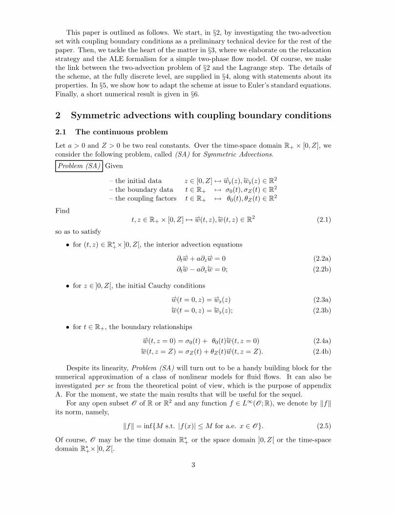
This paper is outlined as follows. We start, in §2, by investigating the two-advectionset with coupling boundary conditions as a preliminary technical device for the rest of thepaper. Then, we tackle the heart of the matter in §3, where we elaborate on the relaxationstrategy and the ALE formalism for a simple two-phase flow model. Of course, we makethe link between the two-advection problem of §2 and the Lagrange step. The details ofthe scheme, at the fully discrete level, are supplied in §4, along with statements about itsproperties. In §5, we show how to adapt the scheme at issue to Euler’s standard equations.Finally, a short numerical result is given in §6.

2 Symmetric advections with coupling boundary conditions

2.1 The continuous problem

Let a > 0 and Z > 0 be two real constants. Over the time-space domain R+ × [0, Z], weconsider the following problem, called (SA) for Symmetric Advections.

Problem (SA) Given

– the initial data z ∈ [0, Z] 7→ w(z),w(z) ∈ R

2

– the boundary data t ∈ R+ 7→ σ0(t), σZ(t) ∈ R2

– the coupling factors t ∈ R+ 7→ θ0(t), θZ(t) ∈ R2

Findt, z ∈ R+ × [0, Z] 7→ w(t, z),w(t, z) ∈ R

2 (2.1)

so as to satisfy

• for (t, z) ∈ R∗+× ]0, Z[, the interior advection equations

∂tw + a∂z

w = 0 (2.2a)

∂tw − a∂z

w = 0; (2.2b)

• for z ∈ ]0, Z[, the initial Cauchy conditions

w(t = 0, z) = w(z) (2.3a)w(t = 0, z) = w(z); (2.3b)

• for t ∈ R+, the boundary relationships

w(t, z = 0) = σ0(t) + θ0(t)w(t, z = 0) (2.4a)

w(t, z = Z) = σZ(t) + θZ(t)w(t, z = Z). (2.4b)

Despite its linearity, Problem (SA) will turn out to be a handy building block for thenumerical approximation of a class of nonlinear models for fluid flows. It can also beinvestigated per se from the theoretical point of view, which is the purpose of appendixA. For the moment, we state the main results that will be useful for the sequel.

For any open subset O of R or R2 and any function f ∈ L∞(O; R), we denote by ‖f‖

its norm, namely,

‖f‖ = infM s.t. |f(x)| ≤M for a.e. x ∈ O. (2.5)

Of course, O may be the time domain R∗+ or the space domain ]0, Z[ or the time-space

domain R∗+× ]0, Z[.

3

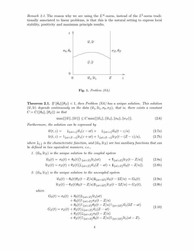
Remark 2.1. The reason why we are using the L∞-norm, instead of the L2-norm tradi-tionally associated to linear problems, is that this is the natural setting to express localstability, positivity and maximum principle results.

00 Z zw,

w

t

σ0, θ0 σZ , θZ

w,w

ϕ,ϕ

Fig. 1. Problem (SA).

Theorem 2.1. If ‖θ0‖‖θZ‖ < 1, then Problem (SA) has a unique solution. This solution(w,w) depends continuously on the data (w,

w, σ0, σZ), that is, there exists a constantC = C(‖θ0‖, ‖θZ‖) so that

max‖w‖, ‖w‖ ≤ Cmax‖w‖, ‖w‖, ‖σ0‖, ‖σZ‖. (2.6)

Furthermore, the solution can be expressed by

w(t, z) = 1at<zw(z − at) + 1at>z

w0(t− z/a) (2.7a)

w(t, z) = 1at<Z−zw(z + at) + 1at>Z−z

wZ(t− (Z − z)/a), (2.7b)

where 1. is the characteristic function, and (w0,wZ) are two auxiliary functions that can

be defined in two equivalent manners, i.e.,

1. (w0,wZ) is the unique solution to the coupled system

w0(t) = σ0(t) + θ0(t)[1at<Zw(at) + 1at>Z

wZ(t− Z/a)] (2.8a)

wZ(t) = σZ(t) + θZ(t)[1at<Zw(Z − at) + 1at>Z

w0(t− Z/a)]; (2.8b)

2. (w0,wZ) is the unique solution to the uncoupled system

w0(t)− θ0(t)θZ(t− Z/a)1at>2Zw0(t− 2Z/a) = G0(t) (2.9a)

wZ(t)− θZ(t)θ0(t− Z/a)1at>2ZwZ(t− 2Z/a) = GZ(t), (2.9b)

where

G0(t) = σ0(t) + θ0(t)1at<Zw(at)

+ θ0(t)1at>ZσZ(t− Z/a)

+ θ0(t)1at>ZθZ(t− Z/a)1at<2Zw(2Z − at)

GZ(t) = σZ(t) + θZ(t)1at<Zw(Z − at)

+ θZ(t)1at>Zσ0(t− Z/a)

+ θZ(t)1at>Zθ0(t− Z/a)1at<2Zw(at− Z).

(2.10)

4

Proof See Appendix A. 2

The auxiliary functions w0 and wZ are none other than the incoming values w(t, z = 0)and w(t, z = Z). As for1at<Z

w(at) + 1at>ZwZ(t− Z/a) and 1at<Z

w(at) + 1at>Zw0(t− Z/a)

in (2.8), they actually represent the outgoing values w(t, z = 0) and w(t, z = Z).Another result is the min-max principle below, that can be considered as a refined

version of the estimate (2.6). Its purpose is to compare solutions at two close time valuest and t+ ∆t.

Proposition 2.1. If 0 < ∆t < Z/a, then

1. The functions (w0,wZ) introduced in Theorem 2.1 and representing incoming bound-ary values are enclosed by

m0(t;∆t) ≤ w0(t′) ≤

M0(t;∆t) (2.11a)

mZ(t;∆t) ≤ wZ(t′) ≤MZ(t;∆t), (2.11b)

for t′ ∈ [t, t+ ∆t], where

M0(t;∆t) = max

t1∈[t,t+∆t]σ0(t1) +θ0(t1)w(t, a(t1 − t))

m0(t;∆t) = mint1∈[t,t+∆t]

σ0(t1) +θ0(t1)w(t, a(t1 − t))

MZ(t;∆t) = max

t1∈[t,t+∆t]σZ(t1)+θZ(t1)w(t, Z − a(t1 − t))

mZ(t;∆t) = mint1∈[t,t+∆t]

σZ(t1)+θZ(t1)w(t, Z − a(t1 − t)).

(2.12)

2. The solution functions (w,w) at time t+ ∆t are enclosed by

m∆t(t, z) ≤ w(t+ ∆t, z) ≤M∆t(t, z) (2.13a)

m∆t(t, z) ≤ w(t+ ∆t, z) ≤M∆t(t, z), (2.13b)

where

M∆t(t, z) = max

M0(t;∆t), 〈

M 〉(t, z)

M∆t(t, z) = max

MZ(t;∆t), 〈

M 〉(t, z)

m∆t(t, z) = minm0(t;∆t), 〈m 〉(t, z) m∆t(t, z) = minmZ(t;∆t), 〈m 〉(t, z)

with〈M〉(t, z) = max

z′∈[0,z]

w(t, z′) 〈M〉(t, z) = max

z′∈[z,Z]

w(t, z′)

〈m〉(t, z) = minz′∈[0,z]

w(t, z′) 〈m〉(t, z) = minz′∈[z,Z]

w(t, z′).(2.14)

Proof The first part is a consequence of (2.8), in the right-hand sides of which we havereplaced (w(.),

w(.)) by (w(t, .),w(t, .)) and t by ∆t in the brackets. This is tantamountto considering the solution at time t as initial data and to looking ahead for a small timeinterval ∆t. Since a∆t < Z, the terms containing 1a∆t>Z drop out and we easily get(2.12).

As for the second part, we go along the same lines to deduce (2.14) from (2.7), butthis time the initial data and the boundary data have been taken into account. 2

5

The bounds for w(t+ ∆t, z) depend only on what lies on the left of z, while those forw(t + ∆t, z) depend only on what lies on the right of z. The coupling between w and wis achieved, in reality, via the bounds on w0 and wZ , as evidenced by (2.12). In (2.14),it would have been more optimal to restrict the dependence domains to [z − a∆, z] and[z, z + a∆t], but what we have in mind is to prepare the ground for a parallelism betweenthe continuous and the discrete problems.

2.2 The discrete problem

The space domain [0, Z] is divided into N cells of variable lengths ∆zi so that∑N

i=1 ∆zi =Z. To each cell ]zi−1/2, zi+1/2[ we associate ψi representing an approximation of ψ(zi). Weadd to this grid two fictitious points, located at i = 0 and i = N + 1 in order to cope withboundary conditions. However, the discrete norm

‖ψ‖ = max1≤i≤N

|ψi| (2.15)

is taken over inner points. Let ∆t > 0 be a time-step. The superscript n will denote thetime level tn, while n♯ will denote the time level tn♯ = tn + ∆t. The problem below ismeant to be a discrete version of the continuous Problem (SA).

Problem (SA)nN Given, for 0 ≤ i ≤ N + 1,

wni ,

wni ∈ R× R, σn

0 , σnZ ∈ R× R, θn

0 , θnZ ∈ R× R. (2.16)

Findwn♯

i ,wn♯

i ∈ R× R so as to satisfy (2.17)

• the implicit scheme for interior points 1 ≤ i ≤ N , i.e.,

wn♯i −

wni

∆t+ a

wn♯i −

wn♯i−1

∆zi= 0 (2.18a)

wn♯i −

wni

∆t− a

wn♯i+1 −

wn♯i

∆zi= 0; (2.18b)

• the boundary relationships for the two fictitious points, i.e.,

wn♯0 = σn

0 + θn0wn♯

0 (2.19a)

wn♯N+1 = σn

Z + θnZwn♯

N+1; (2.19b)

• the Neumann relationships for outgoing waves, i.e.,

wn♯0 = wn♯

1 (2.20a)

wn♯N+1 = wn♯

N . (2.20b)

The reason why we choose to work with an implicit scheme such as (2.18) has been men-tioned: in applications, (w,w) will correspond to fast acoustic waves. In (2.19), which isa discrete version of (2.4), the data (σ0, σZ , θ0, θZ) have been frozen to time n to makethe presentation easier. Note that the conditions are imposed at the centers of the ficti-tious cells, not at the edges of the physical domain. The Neumann relationships (2.20)correspond to a wave-cancellation strategy adapted from Dubois and LeFloch [15].

6

Definition 2.1. Let us introduce

• the local acoustic CFL ratios

µi =a∆t

∆zi, (2.21)

• the local apparent propagation factor

ei =µi

1 + µi, (2.22)

• the global cumulated propagation factors

Eℓk =

Πℓ

j=kej if k ≤ ℓ

1 if k > ℓ.(2.23)

Although µi is allowed to be larger than 1, ei and Eℓk can never exceed or equal 1. The

name “apparent propagation factor” comes from the following observation. Rewriting theinner equations (2.18) under the form

(1 + µi)wn♯

i − µiwn♯

i−1 = wni (2.24a)

(1 + µi)wn♯i − µi

wn♯i+1 = wn

i , (2.24b)

we can deduce that

wn♯i = ei

wn♯i−1 + (1− ei)

wni (2.25a)

wn♯i = eiw

n♯i+1 + (1− ei)w

ni . (2.25b)

In the above convex combinations, the factor ei accounts for the influence of the upwindcell (i.e., i− 1 for wi and i+ 1 for wi) in the updated values at i.

Theorem 2.2. If θn0 θ

nZ < 1, then Problem (SA)nN is well-posed, in the sense that it

has a unique solution. This solution (wn♯i ,

wn♯i ) depends continuously on the initial data

(wni ,

wni , σ

n0 , σ

nZ), that is, there exists a constant C = C(θn

0 , θnZ), independent of ∆t, so that

max‖wn♯‖, ‖wn♯‖ ≤ Cmax‖wn‖, ‖wn‖, |σn0 |, |σ

nZ |. (2.26)

Furthermore, the solution can be given by

wn♯i =

∑ik=1 (Ei

k+1 −Eik)

wnk + Ei

1wn♯

0 (2.27a)

wn♯j =

∑Nℓ=j (Eℓ−1

j − Eℓj)wn

ℓ + ENjwn♯

N+1 (2.27b)

for 0 ≤ i ≤ N , 1 ≤ j ≤ N + 1, where the boundary values (wn♯0 ,

wn♯N+1) can be defined in

two equivalent manners, i.e.,

1. (wn♯0 ,

wn♯N+1) is the unique solution to the coupled system

wn♯0 = σn

0 + θn0 [

∑Nℓ=1 (Eℓ−1

1 − Eℓ1)wn

ℓ + EN1wn♯

N+1] (2.28a)

wn♯N+1 = σn

Z + θnZ [

∑Nk=1 (EN

k+1 − ENk )wn

k + EN1wn♯

0 ]; (2.28b)

7

2. (wn♯0 ,

wn♯N+1) is the unique solution to the uncoupled system

[1− θn0 θ

nZ(EN

1 )2]wn♯0 = σn

0 +θn0

∑Nℓ=1 (Eℓ−1

1 − Eℓ1)wn

ℓ (2.29a)

+θn0E

N1 [σn

Z + θnZ

∑Nk=1(E

Nk+1 − E

Nk )wn

k ]

[1− θn0 θ

nZ(EN

1 )2]wn♯N+1 = σn

Z+θnZ

∑Nk=1 (EN

k+1 − ENk )wn

k (2.29b)

+θnZE

N1 [σn

0 + θn0

∑Nℓ=1(E

ℓ−11 − Eℓ

1)wn

ℓ ].

It is worthwhile to ponder over the formal analogy between this Theorem and Theorem2.1, by contemplating (2.27)–(2.29) vs. (2.7)–(2.9). Note that the assumption θn

0 θnZ < 1

at the discrete level is weaker than the condition ‖θ0‖‖θZ‖ < 1 at the continuous level. Asin the continuous case, there is a refined min-max estimate. For θ ∈ R and (wk)1≤k≤N ,we define the upper-bound

M(θ,w) =

θ max1≤k≤N

wk if θ ≥ 0

−θ min1≤k≤N

wk if θ < 0,(2.30)

and the lower-bound

m(θ,w) =

θ min1≤k≤N

wk if θ ≥ 0

−θ max1≤k≤N

wk if θ < 0.(2.31)

Proposition 2.2. If θn0 θ

nZ < 1, then for all ∆t > 0,

1. The values of fictitious points (w0,wZ) introduced in Theorem 2.1 and representingincoming waves are enclosed by

mn♯0 ≤

wn♯0 ≤

Mn♯

0 and mn♯N+1 ≤

wn♯N+1 ≤

Mn♯

N+1 (2.32)

mn♯0 = min

ξ∈[0,1]

σn0 + θn

0σnZξ +m(θn

0 θnZ ,

wn)ξ(1− ξ) +m(θn0 ,

wn)(1− ξ)

1− θn0 θ

nZξ

2

Mn♯

0 = maxξ∈[0,1]

σn0 + θn

0σnZξ +M(θn

0 θnZ ,

wn)ξ(1− ξ) +M(θn0 ,

wn)(1 − ξ)

1− θn0 θ

nZξ

2

mn♯N+1 = min

ξ∈[0,1]

σnZ + θn

Zσn0 ξ +m(θn

0 θnZ ,

wn)ξ(1− ξ) +m(θnZ ,

wn)(1− ξ)

1− θn0 θ

nZξ

2

Mn♯

N+1 = maxξ∈[0,1]

σnZ + θn

Zσn0 ξ +M(θn

0 θnZ ,

wn)ξ(1 − ξ) +M(θnZ ,

wn)(1− ξ)

1− θn0 θ

nZξ

2.

(2.33)

2. The values of inner points 1 ≤ i, j ≤ N are enclosed by

mn♯i ≤

wn♯i ≤

Mn♯

i and mn♯j ≤

wn♯j ≤

Mn♯

j , (2.34)

with Mn♯

i = maxMn♯

0 , 〈M〉ni

Mn♯

j = maxMn♯

N+1, 〈M〉nj

mn♯i = min mn♯

0 , 〈m〉ni

mn♯j = min mn♯

N+1, 〈m〉nj ,

and〈M〉ni = max

1≤k≤i

wnk 〈

M〉nj = max

j≤ℓ≤N

wnℓ

〈m〉ni = min1≤k≤i

wnk 〈m〉nj = min

j≤ℓ≤N

wnℓ .

(2.35)

8

Formal connections could be made between this Proposition and Proposition 2.1, byscrutinizing (2.32)–(2.35) vs. (2.11)–(2.14). The bounds supplied by (2.32)–(2.35) alsohave a practical purpose: they will indeed be used for the numerical computation of someoptimal CFL ratios in the upcoming Euler problems.

Continuous dependence of (wn♯,wn♯) with respect to (σn0 , σ

nZ ,

wn,wn), as stated inTheorem 2.2 and improved in Proposition 2.2, can be interpreted as a stability property.In the case of Problem (SA)n

N , however, there is an additional stability property via energyinequalities.

Theorem 2.3. For any strictly convex function (w,w) ∈ R2 7→ S (w,w) ∈ R that is of

the formS (w,w) = S(w) + S(w), (2.36)

in which w ∈ R 7→ S(w) ∈ R is strictly convex function, the implicit scheme (2.18) ofProblem (SA)nN satisfies the implicit local energy dissipation inequality

S (wn♯i ,

wn♯i )−S (wn

i ,wn

i )

∆t+

H (wn♯i ,

wn♯i+1)−H (wn♯

i−1,wn♯

i )

∆zi≤ 0, (2.37)

for 1 ≤ i ≤ N , where H (w,w) = a[S(w)− S(w)] is the consistent energy-flux.

We recall that for smooth solutions of the continuous Problem (SA), combining (2.2a)and (2.2b) leads to the equality

∂tS (w,w) + ∂zH (w,w) = 0, (2.38)

provided that S is smooth itself. The fact that this additional conservation law has aninequality counterpart at the discrete level is a major asset for the stability of a scheme.

Remark 2.2. More general energies can be considered for S , but the form (2.36) will sufficeto our forthcoming purpose.

Proof of Theorem 2.2

Uniqueness and existence. Suppose wn♯0 is known. Then, by (2.25a), we have wn♯

1 =

e1wn♯0 + (1− e1)w

n1 . By induction on 1 ≤ i ≤ N , we carry out a left-to-right sweeping

wn♯i = Ei

1wn♯

0 +∑i

k=1(Eik+1 − E

ik)wn

k . (2.39)

Specifying i = N in (2.39), combining with (2.20b) and using (2.19b), we have

wn♯N+1 = σn

Z + θnZ [

∑Nℓ=1(E

Nk+1 − E

Nk )wn

ℓ + EN1wn♯

0 ]. (2.40)

In a similar fashion, if wn♯N+1 were known, we can derive

wn♯j = EN

jwn♯

N+1 +∑N

ℓ=j(Eℓ−1j − Eℓ

j)wn

ℓ (2.41)

for 1 ≤ j ≤ N , then

wn♯0 = σn

0 + θn0 [

∑Nℓ=1(E

ℓ−11 − Eℓ

1)wn

ℓ + EN1wn♯

N+1]. (2.42)

The system (2.39), (2.41) coincides exactly with (2.27), while (2.42), (2.40) appears tobe exactly (2.28). A little more algebra shows the equivalence between (2.28) and (2.29).

9

Note that if θn0 θ

nZ < 1, since EN

1 < 1, the bracket 1− θn0 θ

nZ(EN

1 )2 remains always positive.

Continuous dependence. Equation (2.29a) gives rise to the abrupt upper-bound

|wn♯0 | ≤ C0 max|σn

0 |, |σnZ |, ‖

wn‖, ‖wn‖, (2.43)

with

[1− θn0 θ

nZ(EN

1 )2]C0 = 1+ |θn0 |

∑Nℓ=1(E

ℓ−11 − Eℓ

1)

+ |θn0 |E

N1 + |θn

0 ||θnZ |E

N1

∑Nℓ=1(E

ik+1 − E

ik).

(2.44)

Indeed, note that on one hand Eℓ−11 − Eℓ

1 ≥ 0 and Eik+1 − E

ik ≥ 0. On the other hand,

the sums are telescoping, i.e.,∑N

ℓ=1(Eℓ−11 − Eℓ

1) =∑N

k=1(ENk+1 − E

Nk ) = 1− EN

1 . (2.45)

As a result,

C0 = C0(EN1 ) =

1 + |θn0 |(1− E

N1 ) + |θn

0 |EN1 + |θn

0 ||θnZ |E

N1 (1− EN

1 )

1− θn0 θ

nZ(EN

1 )2. (2.46)

To get rid of ∆t (through EN1 ) in C0, we can upper-bound it by ‖C0‖ = maxξ∈[0,1]C0(ξ),

which is finite because C0(ξ) is a continuous function of ξ ∈ [0, 1]. In a similar way, wecan show that

|wn♯N+1| ≤ ‖CN+1‖max|σn

0 |, |σnZ |, ‖

wn‖, ‖wn‖ (2.47)

for some constant ‖CN+1‖, which depends on (θn0 , θ

nZ) but not on ∆t. This enables us to

writemax|wn♯

0 |, |wn♯

N+1| ≤ C(θn0 , θ

nZ)max|σn

0 |, |σnZ |, ‖

wn‖, ‖wn‖, (2.48)

with C(θn0 , θ

nZ) = max(‖C0‖, ‖CN+1‖). As for points inside the domain, from the first

equation of (2.27), we have

|wn♯i | ≤ [Ei

1 +∑i

k=1(Eik+1 − E

ik)]max|wn♯

0 |, ‖wn‖ = max|wn♯

0 |, ‖wn‖ (2.49)

for all 1 ≤ i ≤ N , so that ‖wn♯‖ is bounded by the right-hand side of (2.48) too. Thesame conclusion holds true for ‖wn♯‖. 2

Proof of Proposition 2.2 The first part is a straightforward consequence of formulae(2.29). The second part is based on (2.27). 2

Proof of Theorem 2.3 From the convex combinations (2.25), we infer that

S(wn♯i ) ≤ eiS(wn♯

i−1) + (1− ei)S(wni ) (2.50a)

S(wn♯i ) ≤ eiS(wn♯

i+1) + (1− ei)S(wni ), (2.50b)

insofar as S is a convex function. Using the definition (2.22) of ei, we cast (2.50) into

(1 + µi)S(wn♯i )− µiS(wn♯

i−1) ≤ S(wni ) (2.51a)

(1 + µi)S(wn♯i )− µiS(wn♯

i+1) ≤ S(wni ). (2.51b)

Using the definition (2.21) of µi, we go back to the discretized form

S(wn♯i )− S(wn

i )

∆t+ a

S(wn♯i )− S(wn♯

i−1)

∆zi≤ 0 (2.52a)

S(wn♯i )− S(wn

i )

∆t− a

S(wn♯i+1)− S(wn♯

i )

∆zi≤ 0. (2.52b)

To complete the proof, we add (2.52a) and (2.52b) together. 2

10

2.3 Practical procedures

On the grounds of computational efficiency, we recommend the following solution proce-dure, to be implemented in place of explicit formulae (2.27)–(2.29). The basic idea restson the following observation.

Lemma 2.1. The mapping wn♯0 7→ F (wn♯

0 ) defined by the diagram

F (wn♯0 ) |wn♯

0

(2.25a)−−−−→ wn♯

1

(2.25a)−−−−→ . . . wn♯

i . . .(2.25a)−−−−→ wn♯

N

(2.20b)−−−−→ wn♯

N+1

(2.19a)

xy(2.19b)

wn♯0 ←−−−−

(2.20a)

wn♯1 ←−−−−

(2.25b). . . wn♯

i . . . ←−−−−(2.25b)

wn♯N ←−−−−

(2.25b)

wn♯N+1

is an affine function, whose derivative is equal to θn0 θ

nZ(EN

1 )2.

Proof Each elementary step of the diagram is an affine operation, therefore, the overallprocess is an affine function. In the left-to-right propagation using (2.25a), the cumulated

factor by which the variable wn♯0 is multiplied is EN

1 . The outlet condition (2.19b) multi-plies it by θn

Z . In the right-to-left propagation using (2.25b), the cumulated factor is alsoEN

1 . The inlet condition (2.19a) multiplies the variable by θn0 . 2

Of course, the expected value for wn♯0 is a fixed point of F . The fact that F (w0) =

θn0 θ

nZ(EN

1 )2w0 + β naturally suggests a two-step procedure:

1. We first set wn♯0 = 0 and apply the sweep process described in the diagram in order

to compute β = F (0).

2. We deduce the correct value for wn♯0 by

wn♯0 =

β

1− θn0 θ

nZ(EN

1 )2. (2.53)

Once this value is known, a second sweep loop is performed in order to assign thecorrect values to every other points in the computational domain.

Note that, because of linearity, the existence of a unique fixed point for F only requiresθn0 θ

nZ(EN

1 )2 6= 1, which is implied by θn0 θ

nZ < 1, instead of the contracting property

|θn0 θ

nZ(EN

1 )2| < 1, for which one would have to impose |θn0 ||θ

nZ | < 1.

Finally, we wish to point out a handy recipe for the practical computation of thebounds (2.33). The following result is valid only when θ = θn

0 θnZ < 0, but this will be

sufficient for our applications.

Lemma 2.2. For a given θ < 0, the extremal values of the function

f(ξ) =Aξ2 +Bξ + C

1− θξ2, ξ ∈ [0, 1] (2.54)

are given by

minξ∈[0,1]

f(ξ) = 1B≥0f(0) + 1B<0f(min(ξ⋆, 1)) (2.55a)

maxξ∈[0,1]

f(ξ) = 1B≥0f(1) + 1B<0 maxf(0), f(1) (2.55b)

11

where ξ⋆ only needs to be defined for when B < 0 by

ξ⋆ =−(A+ θC) +

√(A+ θC)2 − θB2

θB. (2.56)

Proof The proof is based on a discussion about the roots of the derivative

f ′(ξ) =θBξ2 + 2(A+ θC)ξ +B

(1− θξ2)2. (2.57)

We leave it to the readers. 2

3 Two-phase flow model: the continuous problem

3.1 The original problem

In this section, we deal with a hydrodynamic model built from a smooth enough inter-nal energy function (τ, Y ) ∈ R

∗+ × [0, 1] 7→ ε(τ, Y ) ∈ R+ with the following properties

motivated by the framework for compressible fluids proposed by Weyl [35]:

(a) ε> 0; (b) ετ < 0; (c) εττ > 0;(d) ετττ < 0; (e) εττεY Y > (ετY )2.

(3.1)

From the internal energy ε, we define

the pressure P (τ, Y ) = −ετ (τ, Y ); (3.2a)

the sound speed c(τ, Y ) = τ√εττ (τ, Y ) = τ

√−Pτ (τ, Y ). (3.2b)

Conditions (3.1c), (3.1e) express the fact that ε is strictly convex with respect to (τ, Y ).From the standpoint of physics, τ is meant to be a specific volume, that is, the inverse ofsome density ρ, while Y is meant to be a mass-fraction. For a prescribed internal energyε, we state the following IBVP for a fluid model within the phase space

ΩU = U = (ρY, ρ, ρu) ∈ R3 | ρ > 0, u ∈ R and Y ∈ [0, 1], (3.3)

where u denotes the velocity.

Problem (TP) Given

– the initial data x ∈ [0,X] 7→ U(x) ∈ ΩU

– the inlet data t ∈ R+ 7→ q0(t), g0(t) ∈ R2+

– the outlet data t ∈ R+ 7→ pX(t), YX(t) ∈ R+ × [0, 1]

FindU : (t, x) ∈ R

+ × [0,X] 7→ U(t, x) ∈ ΩU (3.4)

so as to satisfy in the usual sense of distributions

• for (t, x) ∈ R∗+× ]0,X[, the system of conservation laws

∂t(ρY ) + ∂x(ρYu) = 0 (3.5a)

∂t(ρ) + ∂x(ρu) = 0 (3.5b)

∂t(ρu) + ∂x(ρu2 + p) = 0, (3.5c)

with p = P

(1

ρ,ρY

ρ

), where P is the pressure defined in (3.2a);

12

• for (t, x) ∈ R∗+× ]0,X[, the energy inequality

∂tρE(U) + ∂xρEu+ pu(U) ≤ 0, (3.6)

with

ρE(U) =1

2

(ρu)2

ρ+ ρε

(1

ρ,ρY

ρ

); (3.7)

• for x ∈ ]0,X[, the initial Cauchy conditions

ρ(t = 0, x) = ρ(x), u(t = 0, x) = u(x), Y (t = 0, x) = Y(x); (3.8)

• for t ∈ R+, the boundary relationships

ρu(t, x = 0) = q0(t) if u(t, 0) > −c(ρ−1(t, 0), Y (t, 0)) (3.9a)

ρYu(t, x = 0) = g0(t) if u(t, 0) > 0 (3.9b)

p(t, x = X) = pX(t) if u(t,X) < c(ρ−1(t,X), Y (t,X)) (3.9c)

Y (t, x = X) = YX(t) if u(t,X) < 0, (3.9d)

where c is the sound speed defined in (3.2b).

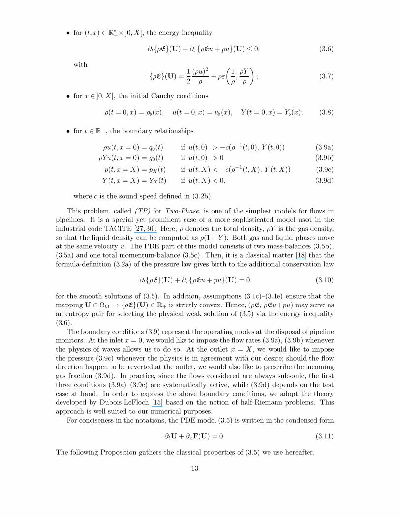
This problem, called (TP) for Two-Phase, is one of the simplest models for flows inpipelines. It is a special yet prominent case of a more sophisticated model used in theindustrial code TACITE [27,30]. Here, ρ denotes the total density, ρY is the gas density,so that the liquid density can be computed as ρ(1− Y ). Both gas and liquid phases moveat the same velocity u. The PDE part of this model consists of two mass-balances (3.5b),(3.5a) and one total momentum-balance (3.5c). Then, it is a classical matter [18] that theformula-definition (3.2a) of the pressure law gives birth to the additional conservation law

∂tρE(U) + ∂xρEu+ pu(U) = 0 (3.10)

for the smooth solutions of (3.5). In addition, assumptions (3.1c)–(3.1e) ensure that themapping U ∈ ΩU → ρE(U) ∈ R+ is strictly convex. Hence, (ρE, ρEu+pu) may serve asan entropy pair for selecting the physical weak solution of (3.5) via the energy inequality(3.6).

The boundary conditions (3.9) represent the operating modes at the disposal of pipelinemonitors. At the inlet x = 0, we would like to impose the flow rates (3.9a), (3.9b) wheneverthe physics of waves allows us to do so. At the outlet x = X, we would like to imposethe pressure (3.9c) whenever the physics is in agreement with our desire; should the flowdirection happen to be reverted at the outlet, we would also like to prescribe the incominggas fraction (3.9d). In practice, since the flows considered are always subsonic, the firstthree conditions (3.9a)–(3.9c) are systematically active, while (3.9d) depends on the testcase at hand. In order to express the above boundary conditions, we adopt the theorydeveloped by Dubois-LeFloch [15] based on the notion of half-Riemann problems. Thisapproach is well-suited to our numerical purposes.

For conciseness in the notations, the PDE model (3.5) is written in the condensed form

∂tU + ∂xF(U) = 0. (3.11)

The following Proposition gathers the classical properties of (3.5) we use hereafter.

13

Proposition 3.1. The system (3.5) is hyperbolic over ΩU, i.e., for any state U ∈ ΩU,the Jacobian matrix ∇UF(U) is has real eigenvalues

u− c(U) < u < u+ c(U) (3.12)

and is R-diagonalizable. The two extreme fields are genuinely nonlinear while the inter-mediate one is linearly degenerate.

Furthermore, the mapping U ∈ ΩU → ρE(U) ∈ R+ is strictly convex.

Proof The calculations are very classical and can be found in [18] for instance. Let usjust recall that hyperbolicity is due to (3.1c), genuine nonlinearity of the extreme fields isdue to (3.1d), the additional law (3.10) follows from (3.2a) and strict convexity of ρE isdue to (3.1c), (3.1e). 2

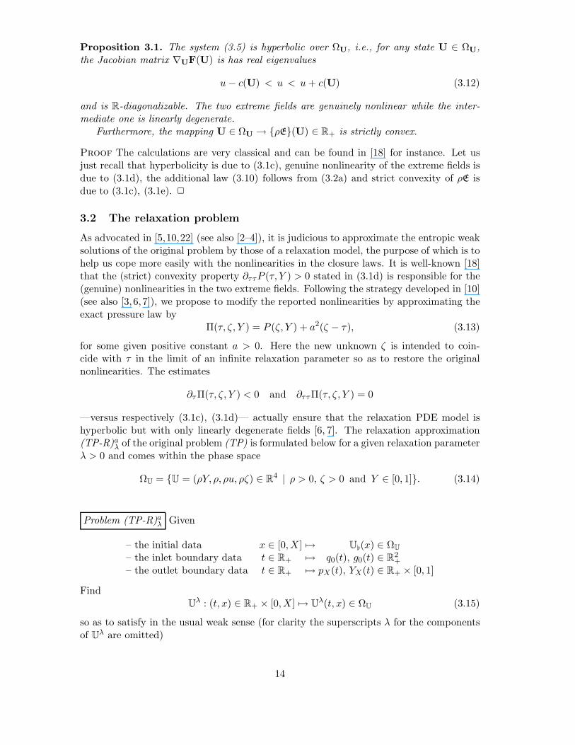
3.2 The relaxation problem

As advocated in [5,10,22] (see also [2–4]), it is judicious to approximate the entropic weaksolutions of the original problem by those of a relaxation model, the purpose of which is tohelp us cope more easily with the nonlinearities in the closure laws. It is well-known [18]that the (strict) convexity property ∂ττP (τ, Y ) > 0 stated in (3.1d) is responsible for the(genuine) nonlinearities in the two extreme fields. Following the strategy developed in [10](see also [3, 6, 7]), we propose to modify the reported nonlinearities by approximating theexact pressure law by

Π(τ, ζ, Y ) = P (ζ, Y ) + a2(ζ − τ), (3.13)

for some given positive constant a > 0. Here the new unknown ζ is intended to coin-cide with τ in the limit of an infinite relaxation parameter so as to restore the originalnonlinearities. The estimates

∂τΠ(τ, ζ, Y ) < 0 and ∂ττΠ(τ, ζ, Y ) = 0

—versus respectively (3.1c), (3.1d)— actually ensure that the relaxation PDE model ishyperbolic but with only linearly degenerate fields [6, 7]. The relaxation approximation(TP-R)a

λ of the original problem (TP) is formulated below for a given relaxation parameterλ > 0 and comes within the phase space

ΩU = U = (ρY, ρ, ρu, ρζ) ∈ R4 | ρ > 0, ζ > 0 and Y ∈ [0, 1]. (3.14)

Problem (TP-R)aλ Given

– the initial data x ∈ [0,X] 7→ U(x) ∈ ΩU

– the inlet boundary data t ∈ R+ 7→ q0(t), g0(t) ∈ R2+

– the outlet boundary data t ∈ R+ 7→ pX(t), YX(t) ∈ R+ × [0, 1]

FindU

λ : (t, x) ∈ R+ × [0,X] 7→ Uλ(t, x) ∈ ΩU (3.15)

so as to satisfy in the usual weak sense (for clarity the superscripts λ for the componentsof U

λ are omitted)

14

• for (t, x) ∈ R∗+× ]0,X[, the system of conservation laws

∂t(ρY ) + ∂x(ρYu) = 0 (3.16a)

∂t(ρ) + ∂x(ρu) = 0 (3.16b)

∂t(ρu) + ∂x(ρu2 + Π(τ, ζ, Y )) = 0 (3.16c)

∂t(ρζ) + ∂x(ρζu) = λρ[τ − ζ]; (3.16d)

• for (t, x) ∈ R∗+× ]0,X[, the energy inequality

∂tρE (Uλ) + ∂xρEu+ Πu(Uλ) ≤ 0, (3.17)

with

ρE (Uλ) =1

2

(ρu)2

ρ+ ρε

(ρζ

ρ,ρY

ρ

)+

ρ

2a2

[Π2 − P 2

(ρζ

ρ,ρY

ρ

)]; (3.18)

• for x ∈ ]0,X[, the initial Cauchy conditions

ρ(t = 0, x) = ρ(x), u(t = 0, x) = u(x), (3.19a)

Y (t = 0, x) = Y(x), ζ(t = 0, x) = ζ(x); (3.19b)

• for t ∈ R+, the boundary relationships

ρu(t, x = 0) = q0(t) if u(t, 0) > −aτ(t, 0) (3.20a)

ρYu(t, x = 0) = g0(t) if u(t, 0) > 0 (3.20b)

Π(t, x = X) = pX(t) if u(t,X) < aτ(t,X) (3.20c)

Y (t, x = X) = YX(t) if u(t,X) < 0. (3.20d)

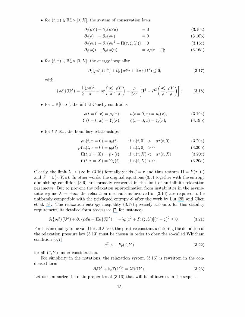
Clearly, the limit λ→ +∞ in (3.16) formally yields ζ = τ and thus restores Π = P (τ, Y )and E = E(τ, Y, u). In other words, the original equations (3.5) together with the entropydiminishing condition (3.6) are formally recovered in the limit of an infinite relaxationparameter. But to prevent the relaxation approximation from instabilities in the asymp-totic regime λ → +∞, the relaxation mechanisms involved in (3.16) are required to beuniformly compatible with the privileged entropy E after the work by Liu [25] and Chenet al. [9]. The relaxation entropy inequality (3.17) precisely accounts for this stabilityrequirement, its detailed form reads (see [7] for instance)

∂tρE (Uλ) + ∂xρEu+ Πu(Uλ) = −λρ[a2 + Pτ (ζ, Y )](τ − ζ)2 ≤ 0. (3.21)

For this inequality to be valid for all λ > 0, the positive constant a entering the definition ofthe relaxation pressure law (3.13) must be chosen in order to obey the so-called Whithamcondition [6, 7]

a2 > −Pτ (ζ, Y ) (3.22)

for all (ζ, Y ) under consideration.For simplicity in the notations, the relaxation system (3.16) is rewritten in the con-

densed form∂tU

λ + ∂xF(Uλ) = λR(Uλ). (3.23)

Let us summarize the main properties of (3.16) that will be of interest in the sequel.

15

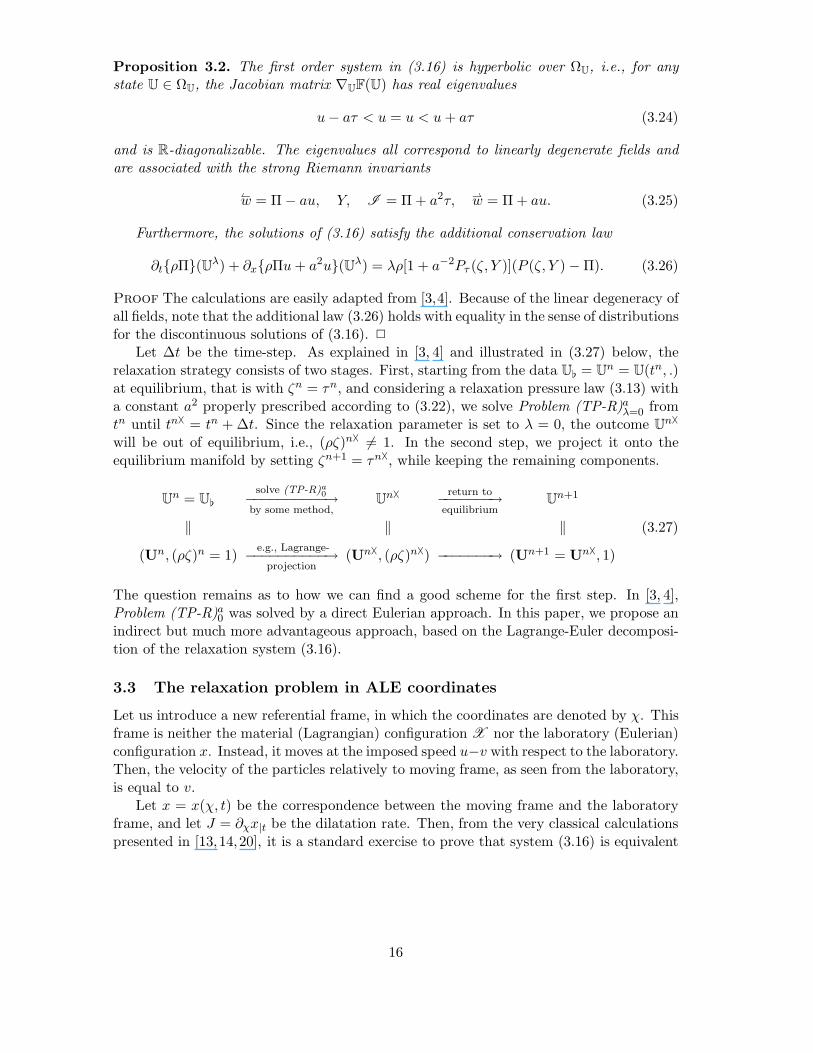
Proposition 3.2. The first order system in (3.16) is hyperbolic over ΩU, i.e., for anystate U ∈ ΩU, the Jacobian matrix ∇UF(U) has real eigenvalues

u− aτ < u = u < u+ aτ (3.24)

and is R-diagonalizable. The eigenvalues all correspond to linearly degenerate fields andare associated with the strong Riemann invariants

w = Π− au, Y, I = Π + a2τ, w = Π + au. (3.25)

Furthermore, the solutions of (3.16) satisfy the additional conservation law

∂tρΠ(Uλ) + ∂xρΠu+ a2u(Uλ) = λρ[1 + a−2Pτ (ζ, Y )](P (ζ, Y )−Π). (3.26)

Proof The calculations are easily adapted from [3,4]. Because of the linear degeneracy ofall fields, note that the additional law (3.26) holds with equality in the sense of distributionsfor the discontinuous solutions of (3.16). 2

Let ∆t be the time-step. As explained in [3, 4] and illustrated in (3.27) below, therelaxation strategy consists of two stages. First, starting from the data U = U

n = U(tn, .)at equilibrium, that is with ζn = τn, and considering a relaxation pressure law (3.13) witha constant a2 properly prescribed according to (3.22), we solve Problem (TP-R)a

λ=0 fromtn until tn" = tn + ∆t. Since the relaxation parameter is set to λ = 0, the outcome U

n"

will be out of equilibrium, i.e., (ρζ)n" 6= 1. In the second step, we project it onto theequilibrium manifold by setting ζn+1 = τn", while keeping the remaining components.

Un = U

solve (TP-R)a0−−−−−−−−−−→

by some method,U

n" return to−−−−−−−→equilibrium

Un+1

‖ ‖ ‖

(Un, (ρζ)n = 1)e.g., Lagrange-−−−−−−−−−−→

projection(Un", (ρζ)n") −−−−−−−→ (Un+1 = Un", 1)

(3.27)

The question remains as to how we can find a good scheme for the first step. In [3, 4],Problem (TP-R)a

0 was solved by a direct Eulerian approach. In this paper, we propose anindirect but much more advantageous approach, based on the Lagrange-Euler decomposi-tion of the relaxation system (3.16).

3.3 The relaxation problem in ALE coordinates

Let us introduce a new referential frame, in which the coordinates are denoted by χ. Thisframe is neither the material (Lagrangian) configuration X nor the laboratory (Eulerian)configuration x. Instead, it moves at the imposed speed u−v with respect to the laboratory.Then, the velocity of the particles relatively to moving frame, as seen from the laboratory,is equal to v.

Let x = x(χ, t) be the correspondence between the moving frame and the laboratoryframe, and let J = ∂χx|t be the dilatation rate. Then, from the very classical calculationspresented in [13,14,20], it is a standard exercise to prove that system (3.16) is equivalent

16

to

∂t(J) + ∂χ(v) − ∂χ(u) = 0 (3.28a)

∂t(ρYJ) + ∂χ(ρYv) = 0 (3.28b)

∂t(ρJ) + ∂χ(ρv) = 0 (3.28c)

∂t(ρuJ) + ∂χ(ρuv) + ∂χ(Π) = 0 (3.28d)

∂t(ρζJ) + ∂χ(ρζv)︸ ︷︷ ︸ ︸ ︷︷ ︸ = λρJ(τ − ζ). (3.28e)

projection Lagrange

From the standpoint of physics, the formulation (3.28) most naturally separates fast acous-tic waves from slow kinematic waves. Therefore, the basic idea of Arbitrary Lagrangian-Eulerian (ALE) approaches is to perform a splitting of (3.28), as indicated above, withina time-step ∆t. The Lagrange-projection method that we are going to detail is a specialcase of ALE, in which v is well-chosen so as to fall back on Eulerian coordinates after thetwo steps, namely, to secure Jn" = 1:

(Jn = 1,Un)Lagrange−−−−−→ (Jn♯,Un♯)

projection−−−−−−→ (Jn" = 1,Un"). (3.29)

3.3.1 Lagrange step

In the Lagrange step, which takes into account only acoustic effects due to the pressure,the PDE system to be solved reads

∂t(J) − ∂χ(u) = 0 (3.30a)

∂t(ρYJ) = 0 (3.30b)

∂t(ρJ) = 0 (3.30c)

∂t(ρuJ) + ∂χ(Π) = 0 (3.30d)

∂t(ρζJ) = λρJ(τ − ζ). (3.30e)

This system is equipped with the initial data (J,U) = (Jn = 1,Un) and a suitablymodified version of the boundary conditions (3.20), namely,

(a) ρu(t, χ = 0) = q0(t); (c) Π(t, χ = X) = pX(t);(b) ρYu(t, χ = 0) = g0(t); (d) Y (t, χ = X) = YX(t).

(3.31)

The good news is that when λ = 0, it is possible to solve (3.30)–(3.31) by means ofProblem (SA). In other words, we can reduce the Lagrange step to the problem of twosymmetric advections with coupling boundary conditions.

Theorem 3.1. Let m = ρ = ρn > 0 be the initial density. Define

z =

∫ χ

0m(κ) dκ and Z =

∫ X

0m(κ) dκ. (3.32)

Then, the Lagrange step (3.30)–(3.31) with λ = 0 is equivalent to

• the PDE system

(a) ∂tY = 0; (c) ∂tw + a∂z

w = 0;(b) ∂tI = 0; (d) ∂t

w − a∂zw = 0,

(3.33)

where Y and (w,w,I ) = (Π + au,Π − au,Π + a2τ), already introduced in (3.25),are to be considered as functions of (t, z) ∈ [tn, tn+1]× [0, Z];

17

• and the boundary conditions

(a) Y (t, z = 0) = g0(t)/q0(t); (b) w(t, z = 0) =σ0(t) + θ0(t)w(t, z = 0);(c) Y (t, z = Z)=YX(t); (d) w(t, z = Z)=σZ(t) + θZ(t)w(t, z = Z),

(3.34)

where

σ0(t) =2I(0)q0(t)

1 + q0(t)/a, θ0(t) =

1− q0(t)/a

1 + q0(t)/a, (3.35a)

σZ(t) = 2pX(t), θZ(t) = −1. (3.35b)

Proof Equation (3.30c) implies that m = ρJ is a function of χ alone, and it coincideswith its initial value, i.e., m = ρJ = ρn. Factoring m out of the time derivatives in theremaining equations of (3.30), dividing each equation by m > 0, and using dz = m(χ)dχ,we end up with

(a) ∂tY = 0; (c) ∂tτ − ∂zu = 0;(b) ∂tζ = 0; (d) ∂tu+ ∂zΠ = 0.

(3.36)

where we remind that Π = P (ζ, Y ) + a2(ζ − τ). This system, in which z appears as theLagrangian mass-coordinate [34], can be shown to be hyperbolic with eigenvalues ±a and0 (double), all of them being linearly degenerate fields. Hence, it is equivalent to

∂tτ − ∂zu = 0 (3.37a)

∂tY = 0 (3.37b)

∂tu + ∂zΠ = 0 (3.37c)

∂tΠ + a2∂zu = 0, (3.37d)

from which (3.33) follows. On the other hand, the boundary conditions (3.31) can berewritten as

(a) Y (t, z = 0) = g0(t)/q0(t); (b) u(t, z = 0) = q0(t)τ(t, z = 0);(c) Y (t, z = Z) = YX(t); (d) Π(t, z = Z) = pX(t).

(3.38)

Substituting the inverse transformation

Π = 12 (w + w), u = 1

2a(w − w), τ = 12a2 [2I − (w + w)] (3.39)

into (3.38) and invoking I (t, z = 0) = I(0) yield (3.34)–(3.35). 2

3.3.2 Projection step

The outcome of the fast Lagrange step, designated by (Jn♯,Un♯) in (3.29), is now the inputdata for the slow projection step. The latter amounts to solving

∂t(J) + ∂χ(v) = 0 (3.40a)

∂t(ρYJ) + ∂χ(ρYv) = 0 (3.40b)

∂t(ρJ) + ∂χ(ρv) = 0 (3.40c)

∂t(ρuJ) + ∂χ(ρuv) = 0 (3.40d)

∂t(ρζJ) + ∂χ(ρζv) = 0. (3.40e)

18

where v is a given velocity field. Comparing the evolution equations (3.40a) and (3.30a)for J , we see that in order for J to go back to its initial value 1, we have to take v = u.For the moment, it is not obvious as to how we can achieve this, but things will becomemore convincing at the fully discrete level. Anyhow, taking v = u for granted and writingthe system (3.40) under the condensed form

∂t(J) + ∂χ(u) = 0 (3.41a)

∂t(UJ) + ∂χ(Uu) = 0, (3.41b)

we can combine the equations to obtain component-wise advection equation

∂tU +u

J∂xU = 0. (3.42)

Thus, the projection step is merely a remap of the variables contained in U.

4 Two-phase flow model: the numerical scheme

The link made by Theorem 3.1 between the Lagrange step and Problem (SA) opens thepossibility for us to apply the scheme considered in Problem (SA)nN .

4.1 Updating formulae

We divide the domain [0,X] into N cells [xj−1/2, xj+1/2] of size ∆x = X/N . The innercells are numbered from 1 to N . We also define two ghost cells labeled 0 and N + 1.

4.1.1 For the Lagrange step

At the beginning of each time step n → n♯, the variables χ and x coincide each, so thatwe can identify them. Since all data, including ρn, are assumed to be piecewise constant,the local step-size of the mass-coordinate z is

∆zi = ρni ∆x. (4.1)

To update (w,w) in (3.33)–(3.34), we use formulae (2.18)–(2.20). Updating (Y,I )inside the domain is trivial, since ∂tY = ∂tI = 0. As for (Y,I ) at the boundaries, weneed to specify two more conditions at each ghost cell, as indicated in (4.3a) and (4.4a)below. Note that

– the “wave-cancellation” conditions for I are justified by the fact that the I -wave,artificially created by the relaxation model, has no real physical meaning;

– the “mass-fraction” conditions for Y do not conflict with the evolution equation∂tY = 0, since the latter is valid only for inner points.

In summary, the comprehensive set of equations for the Lagrange step is

19

• For 1 ≤ i ≤ N

Y n♯i − Y

ni

∆t= 0 (4.2a)

In♯i −I n

i

∆t= 0 (4.2b)

wn♯i −

wni

∆t+ a

wn♯i −

wn♯i−1

∆zi= 0 (4.2c)

wn♯i −

wni

∆t− a

wn♯i+1 −

wn♯i

∆zi= 0. (4.2d)

• For i = 0

Y n♯0 = gn

0 /qn0 , I

n♯0 = I

n♯1 , (4.3a)

wn♯0 = wn♯

1 ,wn♯

0 = σn0 + θn

0wn♯

0 (4.3b)

with σn0 =

2qn0 /a

1 + qn0 /a

In1 and θn

0 =1− qn

0 /a

1 + qn0 /a

;

• For i = N + 1

Y n♯N+1 = Y n

X , In♯N+1 = I

n♯N , (4.4a)

wn♯N+1 = wn♯

N ,wn♯

N+1 = σnZ + θn

Zwn♯

N+1 (4.4b)

with σnZ = 2pn

X and θnZ = −1.

To gain more insight into this scheme, it is helpful to rewrite it in terms of the originalvariables. A little algebra shows that (4.2) is equivalent to

ρni

Y n♯i − Y

ni

∆t= 0 (4.5a)

ρni

τn♯i − τ

ni

∆t−

un♯i+1/2 − u

n♯i−1/2

∆x= 0 (4.5b)

ρni

un♯i − u

ni

∆t+

Πn♯i+1/2 − Πn♯

i−1/2

∆x= 0 (4.5c)

ρni

ζn♯i − ζ

ni

∆t= 0 (4.5d)

where

Πn♯i+1/2 = 1

2(Πn♯j + Πn♯

j+1)−a2 (un♯

j+1 − un♯j ) (4.6a)

un♯i+1/2 = 1

2(un♯j + un♯

j+1) −12a(Πn♯

j+1 −Πn♯j ) (4.6b)

turn out to be the pressure and the velocity of the solution to the Riemann problemassociated with (3.37) at the interface i+ 1/2. Straightforward calculations show that wecan replace (4.5d) by

ρni

Πn♯j −Πn

j

∆t+ a2

un♯i+1/2

− un♯i−1/2

∆x= 0 (4.7)

20

so as to be able to work with Π as a fully-fledged variable. Since Jni = 1, equation (4.5b)

can still be interpreted as

Jn♯i − J

ni

∆t−un♯

i+1/2 − un♯i−1/2

∆x= 0, (4.8)

which is the discrete version of (3.30a). Following the widely adopted terminology incontinuum mechanics (see [12] for a mathematical presentation), we shall refer to (4.8) as

Piola’s identity. If, in (4.5), we replace (4.5b) with (ρJ)n♯i = ρn

i , then the new system canbe condensed under the conservative form

(UJ)n♯i − (UJ)ni

∆t+

An♯i+1/2 − A

n♯i−1/2

∆x= 0, (4.9)

where An♯i+1/2 = (0, 0, Πn♯

i+1/2, 0) denotes the acoustic part of the flux. For later use, we

write An♯i+1/2 = (0, 0, Πn♯

i+1/2).

Remark 4.1. In the pure Eulerian setting of [4] and within the frame of an implicit timeintegration, Baudin et al. strongly recommended to handle the discrete version of therelaxation equation (3.16d) in the limit λ → +∞. Here and by contrast, the proposedsolution procedure seems to rely on the choice λ = 0 as advocated by formulae (3.33).Let us however stress that no contradiction arises with [4]. Had we discretized the lastequation (3.30e) by the consistent approximation

ρni

ζn♯i − ζ

ni

∆t= λρn

i (τni − ζ

n♯i ), (4.10)

then for any λ ≥ 0 we would end up with the expected value (4.5d)

ζn♯i = τn

i (4.11)

because at time n, the variable ζ is at equilibrium, i.e., ζni = τn

i . This algebraic miracleoccurs solely in Lagrangian coordinates.

4.1.2 For the projection step

Piola’s identity (4.8) clearly shows that, at the discrete level, we have to use the velocity

field vi+1/2 = un♯i+1/2, defined at the interfaces, to remap the variables. More concretely,

we have to discretize (3.41) by

Jn"

i − Jn♯i

∆t+

un♯i+1/2 − u

n♯i−1/2

∆x= 0 (4.12a)

(UJ)n"

i − (UJ)n♯i

∆t+

(Uu)n♯i+1/2 − (Uu)n♯

i−1/2

∆x= 0, (4.12b)

the product (Uu)n♯i+1/2 being upwinded as

(Uu)n♯i+1/2 = U

n♯i (un♯

i+1/2)+ + U

n♯i+1(u

n♯i+1/2)

−, (4.13)

21

where u+ (respectively u−) stands for the positive (resp. negative) part of u. Note that

Πn♯i+1/2 and un♯

i+1/2 are byproducts of the Lagrange step and can be computed as

Πn♯i+1/2 = 1

2(wn♯i + wn♯

i+1), un♯i+1/2 = 1

2a(wn♯i −

wn♯i+1). (4.14)

To better understand this projection step, let us multiply (4.8) by Un♯i and add it to

(4.12b). Arguing that Jn" = 1, according to (4.12a), we have after some cancellations

Un"

i − Un♯i

∆t+ (un♯

i−1/2)+ U

n♯i − U

n♯i−1

∆x+ (un♯

i+1/2)− U

n♯i+1 − U

n♯i

∆x= 0. (4.15)

Undoubtedly, this is a first-order explicit discretization of (3.42), in which J has beennevertheless “implicited” to Jn". Introduce the algebraic CFL ratios

λi+1/2 =un♯

i+1/2∆t

∆x(4.16)

based on the transport velocities. Then, equation (4.15) becomes

Un"

i = λ+i−1/2U

n♯i−1 + (1− λ+

i−1/2 + λ−i+1/2)Un♯i − λ

−i+1/2U

n♯i+1, (4.17)

and we see that CFL-like conditions can be imposed on ∆t so that the right-hand side of(4.17) be a convex combination. This is the goal of the next subsection.

4.2 Positivity, stability and energy properties

The novelty we wish to put forward, as far as the proposed scheme is concerned, lies inthe guarantee of positivity, stability and energy dissipation, as stated in the followingTheorem.

Theorem 4.1. The overall scheme (3.27), (3.29) enjoys the following properties:

1. It can be put under a locally conservative form

Un+1i −Un

i

∆t+

Fn♯i+1/2 − F

n♯i−1/2

∆x= 0 (4.18)

with Fn♯i+1/2 = U

n♯i (un♯

i+1/2)+ + U

n♯i+1(u

n♯i+1/2)

− + An♯i+1/2.

2. Under the CFL constraint

∆t

∆x<

2a

max1≤i≤N

(M

n♯

i −mn♯

i+1)+ − (mn♯

i −M

n♯

i+1)− , (4.19)

where the variousM,

M,m,m’s, defined by (2.33)–(2.34) of Proposition 2.2, are

explicitly computable from data at time n and do not depend on ∆t, we have

ρn+1i > 0 and Y n+1

i ∈ [0, 1]. (4.20)

3. Under the CFL restriction (4.19), there holds the min-max principle

minY ni−1, Y

ni , Y

ni+1 ≤ Y

n+1i ≤ maxY n

i−1, Yni , Y

ni+1. (4.21)

22

4. Under the CFL restriction (4.19) and the Whitham-like condition

a2 > maxi∈1,...,N

maxσ∈[0,1]

−Pτ (στni + (1− σ)τn♯

i , Y ni ), (4.22)

we have the discrete energy inequality

ρE(Un+1i )− ρE(Un

i )

∆t+

(ρEu+ Πu)n♯i+1/2 − (ρEu+ Πu)n♯

i−1/2

∆x≤ 0, (4.23)

which is consistent with (3.6).

5. Stationary contact discontinuities are exactly preserved.

To our knowledge, the stability results that we state and that are valid for a timeimplicit approximation of the solutions of the Euler’s IBVP, seem to be new. This is whyTheorem 4.1 deserves our attention. Anticipating the proof, the derivation of the CFLrestriction (4.19) directly results when enforcing for validity the estimate

∆t

∆x[(un♯

i−1/2)+ − (un♯

i+1/2)−] < 1, (4.24)

which is nothing but a CFL condition based on the intermediate wave velocity u. Letus recall that the proposed scheme is time-explicit with respect to this wave so that theabove condition is expected. Numerical benchmarks strongly support that the estimate(4.19) actually provides a sharp lower-bound of the time step ∆t dictated by the “exact”condition (4.24).

Let us also briefly comment on the Whitham-like condition (4.22) by stressing out thatit formally reads the same as the one derived in a fully time explicit setting [6]. In thisrespect, the sharp version (4.22) of the Whitham condition (3.22) is quite natural. Finally,the exact capture of steady contact discontinuities is known to be an accuracy propertyof central importance in a growing number of applications.

We now turn to the proof of the above statements. The derivation of the energyinequality (4.23) relies on the following preliminary result.

Lemma 4.1. For all ∆t > 0 and under the Whitham-like condition (4.22), the solutionof the Lagrange step satisfies the energy inequality

ρni

E(Un♯i )− E(Un

i )

∆t+

(Πu)n♯i+1/2 − (Πu)n♯

i−1/2

∆x≤ 0, (4.25)

where E is defined in (3.7), and (Πn♯i+1/2

, un♯i+1/2

) by (4.14).

Observe that the proposed discrete inequality is nothing but a consistent approximationof the energy inequality (3.6) expressed in Lagrangian coordinates

∂t(ρEJ) + ∂χ(Pu) ≤ 0. (4.26)

Proof of Theorem 4.1

Locally conservative form. Adding (4.9) and (4.12b) together, we get

Un"

i − Uni

∆t+

Fn♯i+1/2

− Fn♯i−1/2

∆x= 0, (4.27)

23

with Fn♯i+1/2 = U

n♯i (un♯

i+1/2)+ + U

n♯i+1(u

n♯i+1/2)

− + An♯i+1/2. Extract the first three components

of (4.27) to have (4.18).

Positivity for density and gas mass-fraction. Since (ρJ)n♯i = ρn

i , we have ρn♯i > 0 as soon

as Jn♯i > 0. By virtue of Piola’s identity (4.8), we have to ask for

∆t

∆x[un♯

i−1/2 − un♯i+1/2] < 1. (4.28)

From (4.17), we see that the estimate ρn♯i > 0 implies ρn"

i > 0 as soon as the combinationin the right-hand side is convex. It suffices that 1− λ+

i−1/2 + λ−i+1/2 > 0, that is,

∆t

∆x[(un♯

i−1/2)+ − (un♯

i+1/2)−] < 1. (4.29)

Obviously, (4.29) is stronger than (4.28), therefore we just have to focus on (4.29). Thanksto (4.14) and to Proposition 2.2, we have

12a(mn♯

j −M

n♯

j+1) ≤ un♯i+1/2 ≤

12a(

M

n♯

j −mn♯

j+1). (4.30)

Consequently,

(un♯i−1/2)

+ − (un♯i+1/2)

− ≤ 12a [(

M

n♯

j−1 −mn♯

j )+ − (mn♯j −

M

n♯

j+1)−], (4.31)

hence the sufficient condition (4.19) to ensure ρn"

i = ρn+1i > 0.

Min-max principle. In (4.17), we subtract the second equation, multiplied by any constantA, to the first one to obtain

ρn"

j (Y n"

j −A) = λ+i−1/2

ρn♯j−1(Y

n♯j−1 −A)− λ−

i+1/2ρn♯

j+1(Yn♯j+1 −A) (4.32)

+ [1− λ+i−1/2 + λ−i+1/2]ρ

n♯j (Y n♯

j −A). (4.33)

Again, Y n♯ = Y n. Selecting A = maxY ni−1, Y

ni , Y

ni+1, then A = minY n

i−1, Yni , Y

ni+1, and

discussing about the signs, we obtain (4.21). The property Y n+1i ∈ [0, 1] follows directly.

Energy inequality. Leaving out the last component of (4.17), we are allowed to write

Un+1i = Un"

i = λ+i−1/2U

n♯i−1 + (1− λ+

i−1/2 + λ−i+1/2)Un♯i − λ

−i+1/2U

n♯i+1, (4.34)

which is a convex combination under constraint (4.19). By Jensen’s inequality, applied tothe convex function U 7→ ρE(U), we infer

(ρE)n+1i ≤ λ+

i−1/2(ρE)n♯i−1 + [1− λ+

i−1/2 + λ−i+1/2](ρE)n♯i − λ

−i+1/2(ρE)n♯

i+1. (4.35)

However, by construction

1− λ+i−1/2 + λ−i+1/2 = Jn♯

i + (λ−i−1/2 − λ+i+1/2). (4.36)

As a result, the inequality (4.35) becomes

(ρE)n+1i ≤ ρn

i En♯i −

∆t

∆x[(ρEu)n♯

i+1/2 − (ρEu)n♯i−1/2], (4.37)

24

again with the notation

(ρEu)n♯i+1/2 = (ρE)n♯

i (un♯i+1/2)

+ + (ρE)n♯i+1(u

n♯i+1/2)

− (4.38)

for the upwinded product. Now, according to Lemma 4.1,

ρni E

n♯i ≤ (ρE)ni −

∆t

∆x[(Πu)n♯

i+1/2 − (Πu)n♯i−1/2]. (4.39)

Inserting (4.39) into the right-hand sides of (4.37) leads to (4.23).

Preservation of steady contact discontinuities. The equivalent form (4.5)–(4.6) clearlyyields from a stationary contact discontinuity (say, at time n)

ρni , un

i = 0, Pni = P ⋆, i ∈ 1, ..., N,

the Lagrangian updated values

ρn♯i = ρn

i , un♯i = 0, Pn♯

i = P ⋆, i ∈ 1, ..., N,

namely un♯i+1/2 = 0 and Πn♯

i+1/2 = P ⋆ so that the Eulerian projection step ends up with

(ρY )n+1i = (ρY )ni , ρn+1

i = ρni , (ρu)n+1

i = 0. (4.40)

In other words, steady contact discontinuities are exactly preserved. 2

Proof of Lemma 4.1 Let us use Theorem 2.3 with S(w) =w2

4a2in order to get

Sn♯i −S n

i

∆t+

Hn♯

i+1/2 −Hn♯

i−1/2

ρni ∆x

≤ 0, (4.41)

with (after some manipulations)

Sni = 1

2 [u2 + (Π/a)2]ni , Sn♯i = 1

2 [u2 + (Π/a)2]n♯i , H

n♯i+1/2 = (Πu)n♯

i+1/2. (4.42)

Since S = E− ε+ 12 (Π/a)2, equation (4.41) can be cast into

ρni

En♯i − E

ni

∆t+

(Πu)n♯i+1/2 − (Πu)n♯

i−1/2

∆x≤ ρn

i Rn♯i , (4.43)

where

Rn♯i = εn♯

i − εni −

1

2a2[(Πn♯

j )2 − (Πnj )2] (4.44)

and εn♯i = ε(τn♯

i , Y n♯i ) = ε(τn♯

i , Y ni ). Since the relaxation system is brought back to equi-

librium at each time step, we have Πnj = P (τn

j , Ynj ) = Pn

j . Therefore, we can rewrite theprevious equation as

Rn♯i = εn♯

i − εni −

1

a2Pn

i (Πn♯j − P

ni )−

1

2a2(Πn♯

i − Pni )2. (4.45)

Because ζn♯i = τn

i , as pointed out in (4.11), we have

Πn♯j − P

nj = −a2(τn♯

j − τnj ) (4.46)

25

in order to transform (4.45) into

Rn♯i = εn♯

i − εni + Pn

i (τn♯i − τ

ni )− 1

2a2(τn♯

i − τni )2. (4.47)

Recalling the Taylor expansion with integral remainder

ε(τn♯i , Y n

i )− ε(τni , Y

ni )− ∂τε(τ

ni , Y

ni )(τn♯

i − τni ) =

∫ τn♯j

τnj

∂ττε(ς, Yni )(τn♯

i − ς) dς, (4.48)

we can easily derive

Rn♯i = (τn♯

i − τni )2

∫ 1

0[∂ττε(στ

ni + (1− σ)τn♯

i , Y ni )− a2](1− σ) dσ. (4.49)

In view of the formula-definition (3.2a) for the exact pressure law, Rn♯i ≤ 0 if a2 is chosen

sufficiently large according to the Whitham-like condition (4.22). 2

5 Euler’s standard single-phase model: an easy extension

5.1 The continuous problem

This section deals with the Euler equations for real compressible materials modeled by asmooth enough internal energy (τ, s) ∈ R

∗+×R+ 7→ ε(τ, s) ∈ R+ satisfying Weyl’s general

assumptions [35]

(a) ε> 0; (b) ετ < 0; (c) εττ > 0;(d) ετττ < 0; (e) εττεss> (ετs)

2; (f) εs< 0.(5.1)

From the internal energy ε, we define

the pressure P (τ, s) = −ετ (τ, s) (5.2a)

the sound speed c(τ, s) = τ√εττ (τ, s) = τ

√−Pτ (τ, s) (5.2b)

the temperature Θ(τ, s) = −εs(τ, s). (5.2c)

Here, τ still denotes the specific volume while s stands for the specific entropy of a givencompressible material. Comparing (5.1) to (3.1) via the formal identification s ≡ Y , wesee that the requirements for Problem (EU) are slightly stronger than those for Problem(TP): here we have to introduce the notion of temperature and to require it to be positivevia (5.1f). The reported strict monotonicity property enables us to define

(τ, ε) 7→ s(τ, ε) as the inverse function of (τ, s) 7→ ε(τ, s). (5.3)

Moreover, the fact of utmost importance of that this inverse function s is decreasing withrespect to ε, since

sε = 1/εs = −1/Θ < 0. (5.4)

To use notations from thermodynamics, we have dε = −Pdτ − Θds. An internal energyε being prescribed, we state the following IBVP over the natural phase space

ΩV = V = (ρE, ρ, ρu) ∈ R3 | ρ > 0, u ∈ R, ε = E− 1

2u2 > 0. (5.5)

Problem (EU) Given

26

– the initial data x ∈ [0,X] 7→ V(x) ∈ ΩV

– the inlet data t ∈ R+ 7→ q0(t), Θ0(t) ∈ R2+

– the outlet data t ∈ R+ 7→ pX(t) ∈ R+

FindV : (t, x) ∈ R+ × [0,X] 7→ V(t, x) ∈ ΩV (5.6)

so as to satisfy in the weak sense

• for (t, x) ∈ R∗+× ]0,X[, the system of conservation laws

∂t(ρE) + ∂x(ρEu+ pu) = 0 (5.7a)

∂t(ρ) + ∂x(ρu) = 0 (5.7b)

∂t(ρu) + ∂x(ρu2 + p) = 0, (5.7c)

with p = P (ρ−1, s), where P is the pressure defined in (5.2a), and s is computed by(5.3), using ε = E− 1

2u2. We have intentionally put the energy balance (5.7a) in the

first row in order to compare (5.7) with (3.5) ;

• for (t, x) ∈ R∗+× ]0,X[, the entropy inequality

∂tρs(V) + ∂xρsu(V) ≤ 0; (5.8)

• for x ∈ ]0,X[, the initial Cauchy conditions

ρ(t = 0, x) = ρ(x), u(t = 0, x) = u(x), E(t = 0, x) = E(x); (5.9)

• for t ∈ R+, the boundary relationships

ρu(t, x = 0) = q0(t) if u(t, 0) > −c(ρ−1(t, 0), s(t, 0)) (5.10a)

Θ(t, x = 0) = Θ0(t) if u(t, 0) > 0 (5.10b)

p(t, x = X) = pX(t) if u(t,X) < c(ρ−1(t,X), s(t,X)) (5.10c)

where c is the sound speed defined in (5.2b).

This problem is the usual Euler model for single-phase flows. As is well-known [18], smoothsolutions of (5.7) obeys the additional conservation law

∂tρs(V) + ∂xρsu(V) = 0, (5.11)

while discontinuous solutions of (5.7) are selected according to the entropy inequality (5.8).As for the boundary conditions (5.10), they are inspired from real-life operating modes.To shorten the notations, the PDE system (5.7) is given the clear condensed form

∂tV + ∂xG(V) = 0. (5.12)

In order to recapitulate the main properties in use hereafter, we state

Proposition 5.1. The system (5.7) is hyperbolic over ΩV, i.e., for any state V ∈ ΩV,the Jacobian matrix ∇VG(V) has real eigenvalues

u− c(V) < u < u+ c(V), (5.13)

and is R-diagonalizable. The two extreme fields are genuinely nonlinear, while the inter-mediate one is linearly degenerate.

Furthermore, the mapping V ∈ ΩV → ρs(V) ∈ R is strictly convex.

27

Proof See [18] for the details. 2

We design the evolution strategy in two steps, after an idea introduced in [10]. First,we replace the energy-balance equation (5.7a) in the PDE system by the entropy-balanceequation (5.8), with the equality sign, namely we consider weak solutions of the followingauxiliary hyperbolic system

∂t(ρs) + ∂x(ρs) = 0 (5.14a)

∂t(ρ) + ∂x(ρu) = 0 (5.14b)

∂t(ρu) + ∂x(ρu2 + p) = 0, (5.14c)

selected according to the natural energy inequality

∂tρE(ρ, ρu, ρs) + ∂x(ρE + p)u(ρ, ρu, ρs) ≤ 0. (5.15)

Classical considerations [18] indeed prove the strict convexity of the mapping (ρ, ρu, ρs)→ρE(ρ, ρu, ρs) from assumptions (5.1a), (5.1c), (5.1e). In other words, this mappingnatural yields an entropy for discriminating the physically relevant discontinuous solutionsof (5.14).

By the formal identification Y ≡ s, we are brought back to Problem (TP). After solvingthe new Problem (TP) (5.7) thanks to the relaxation/Lagrange-projection method pro-posed earlier, we obtain Un‡ = (ρs, ρ, ρu)n‡ with a discrete analog of the energy inequality(5.15), that we rewrite in a semi-discrete form to shorten the notations

ρE(ρn‡, (ρu)n‡, (ρs)n‡) ≤ (ρE)n −∆t∂x(ρEu+ Πu)n♯. (5.16)

In order to enforce for validity the mandatory conservation of the total energy at time(n + 1), we set (ρE)n+1 = (ρE)n − ∆t∂x(ρEu + Πu)n♯, while keeping unchanged theupdated values of the density and momentum. In other words, we choose ρn+1 = ρn‡ and(ρu)n+1 = (ρu)n‡. The procedure is depicted in the following diagram. The reason whythis process does guarantee the entropy decay

(ρs)n+1 ≡ ρs(ρn+1, (ρu)n+1, (ρE)n+1) ≤ (ρs)n‡ = (ρs)n −∆t∂x(ρsu)n♯,

and hence the consistency with the expected entropy inequality (5.8) will be elaboratedon in the next subsection.

Vn = (ρE, ρ, ρu)n Vn+1 = (ρE, ρ, ρu)n+1 ⇒ (ρs)n+1 ≤ (ρs)n‡y E,s

xswap

Un = (ρs, ρ, ρu)nPb. (TP )−−−−−−→with Y ≡s

Un‡ = (ρs, ρ, ρu)n‡ ⇒ (ρE)n‡ ≤ (ρE)n+1

(5.17)

Remark 5.1. In comparison with Problem (TP), there is a subtle difference regardingboundary conditions. In §3, we imposed the gas flow rate ρY (t, x = 0) at the inlet,from which we deduced the incoming fraction Y (t, x = 0). Here, we have the temperatureΘ(t, x = 0) instead. By inverting the mapping s 7→ Θ(τ, s) at fixed τ (which is possiblethanks to the estimate Θs = −εss < 0 due to the strict convexity assumptions (5.1c)–(5.1e) of the mapping (τ, s) → ε(τ, s)), we obtain s(t, x = 0) as a function of τ(t, x = 0)and Θ0(t). Since τ is decoupled from s in the scheme, this enables us to do as if s(t, x = 0)were known. At the outlet, we choose to let s(t, x = X) unspecified in agreement with theusual applications according to which the velocity is expected to keep the constant signu(t,X) > 0.

28

5.2 The discrete scheme

The step Un → Un‡ in (5.17) is of course performed via the scheme (3.27), (3.29), whichconsists of the two steps

Un Lagrange−−−−−→ Un♯ projection

−−−−−−→ Un‡ (5.18)

Arguing again about the formal identification Y ≡ s, the formulae for the Lagrange stepresult mutatis-mutandis from (4.2)–(4.4), namely, they read

• For 1 ≤ i ≤ N

sn♯i − s

ni

∆t= 0 (5.19a)

In♯i −I n

i

∆t= 0 (5.19b)

wn♯i −

wni

∆t+ a

wn♯i −

wn♯i−1

∆zi= 0 (5.19c)

wn♯i −

wni

∆t− a

wn♯i+1 −

wn♯i

∆zi= 0. (5.19d)

• For i = 0

sn♯0 = S(τn♯

0 ,Θn0 ), I

n♯0 = I

n♯1 , (5.20a)

wn♯0 = wn♯

1 ,wn♯

0 = σn0 + θn

0wn♯

0 (5.20b)

with σn0 =

2qn0 /a

1 + qn0 /a

In1 and θn

0 =1− qn

0 /a

1 + qn0 /a

;

• For i = N + 1

sn♯N+1 = sn

X , In♯N+1 = I

n♯N , (5.21a)

wn♯N+1 = wn♯

N ,wn♯

N+1 = σnZ + θn

Zwn♯

N+1 (5.21b)

with σnZ = 2pn

X and θnZ = −1.

In (5.20), the function Θ 7→ S(τ,Θ) is the inverse of the temperature function s 7→ Θ(τ, s)with respect to s, at fixed τ . The first argument in S is taken either at time n or at timen♯. This is not a difficulty in itself, since in view of the structure of the equations, thespecific volume τn♯

0 can be obtained before and independently of sn♯0 . In this Lagrange

step, the relaxation parameter a is assumed to satisfy a Whitham condition similar to(3.22), that is

a2 > −Pτ (ζ, s) (5.22)

for all (ζ, s) under consideration.

Once (s,I ,w,w)n♯i has been converted to (U, ρζ)n♯

i = (ρs, ρ, ρu, ρζ)n♯i , the projection

step is applied according to (4.12)–(4.14). Because we are interested only in the first threecomponents, we rewrite this step as

(UJ)n‡i − (UJ)n♯i

∆t+

(Uu)n♯i+1/2

− (Uu)n♯i−1/2

∆x= 0, (5.23)

29

the product (Uu)n♯i+1/2 being upwinded as (Uu)n♯

i+1/2 = Un♯i (un♯

i+1/2)+ + U

n♯i+1(u

n♯i+1/2)

−,

with un♯i+1/2 = 1

2a(wn♯i −

wn♯i+1). So far, we have

(ρs)n‡i = (ρs)ni −∆t

∆x[(ρsu)n♯

i+1/2 − (ρsu)n♯i−1/2] (5.24a)

(ρE)n‡i ≤ (ρE)ni −∆t

∆x[(ρEu+ Πu)n♯

i+1/2 − (ρEu+ Πu)n♯i−1/2] (5.24b)

for all 1 ≤ i ≤ N . The first equation is, by construction, the update value for (ρs)n‡i ,whereas the second equation is the energy property of Theorem 4.1. Now, the “swap”step consists in ruling that

(ρE)n+1i = (ρE)ni −

∆t

∆x[(ρEu+ Πu)n♯

i+1/2 − (ρEu+ Πu)n♯i−1/2] (5.25a)

(ρ)n+1i = (ρ)n‡i (5.25b)

(ρu)n+1i = (ρu)n‡i (5.25c)

from which we deduce

(ρs)n+1i = ρn+1

i s(τn+1i , εn+1

i ) = ρn+1i s(τn+1

i ,En+1i − 1

2(un+1i )2). (5.26)

Theorem 5.1. The overall scheme (5.17), (5.18) enjoys the following properties:

1. It can be put under a locally conservative form

Vn+1i −Vn

i

∆t+

Gn♯i+1/2 −G

n♯i−1/2

∆x= 0 (5.27)

withG

n♯i+1/2 = V

n♯i (un♯

i+1/2)+ + V

n♯i+1(u

n♯i+1/2)

− + Bn♯i+1/2 (5.28)

and Bn♯i+1/2 = (Πn♯

i+1/2un♯i+1/2, 0, Π

n♯i+1/2).

2. Under the CFL constraint

∆t

∆x<

2a

max1≤i≤N

(M

n♯

i −mn♯

i+1)+ − (mn♯

i −M

n♯

i+1)− , (5.29)

whereM,

M,m,m are defined by (2.33)–(2.34) of Proposition 2.2, we have

ρn+1i > 0 and εn+1

i > 0. (5.30)

3. Under the CFL condition (5.29), there holds the max principle

sn+1i ≤ maxsn

i−1, sni , s

ni+1. (5.31)

4. Under the CFL condition (5.29), and the Whitham-like condition

a2 > maxi∈1,...,N

maxσ∈[0,1]

−Pτ (στni + (1− σ)τn♯

i , sni ), (5.32)

we have the entropy inequality

ρs(Vn+1i )− ρs(Vn

i )

∆t+

(ρsu)n♯i+1/2 − (ρsu)n♯

i−1/2

∆x≤ 0. (5.33)

30

5. Stationary contact discontinuities are exactly preserved.

Proof The locally conservative form is obvious. The positivity of the density followsexactly the same steps as those developed in the previous section and gives rise to theCFL restriction (5.29). If we are able to prove that

εn+1i ≥ εn‡i and sn+1

i ≤ sn‡i , (5.34)

then the remaining claims will follow suit, because

• by assumption (5.1a), εn‡i = ε(τn‡i , sn‡

i ) > 0

• by the min-max principle (4.21), sn‡i ≤ maxsn

i−1, sni , s

ni+1

• by definition, (ρs)n‡i = (ρs)ni −∆t∆x [(ρsu)n♯

i+1/2 − (ρsu)n♯i−1/2].

To derive (5.34), we first note that from (5.24a) and (5.25b), we have (ρE)n+1i ≥ (ρE)n‡i ,

whenceE

n+1i ≥ E

n‡i (5.35)

because ρn+1i = ρn‡

i . Since E = 12u

2 + ε and un+1i = un‡

i , we infer that εn+1i ≥ εn‡i . Now,

as already pointed out in (5.4), s is decreasing with respect to ε at fixed τ . Therefore,

sn+1i = s(τn+1

i , εn+1i ) ≤ s(τn+1

i , εn‡i ) = s(τn‡i , εn‡i ) = sn‡

i , (5.36)

which completes the proof. 2

6 Numerical application

In order to illustrate the numerical scheme presented in section 4 we run a test case withboundary conditions mimicking a real operating situation. A mixture of gas and oil isinjected into a pipeline for 200 seconds. Then the oil flow is stopped so that in 50 secondsthe gas mass-fraction rises to its limit value 1. The two curves in panel (a) of Figure 6display the gas mass-fraction monitored at the inlet and outlet of the pipe. The pressureat the outlet is kept constant throughout the experiment.

For simplicity, the constant a is chosen according to the following rough version of theWhitham condition (3.22)

a2 = max1≤i≤N

−Pτ (τni , Y

ni ). (6.1)

Panel (b) in Figure 6 displays the time-step used during the simulation and computedaccording the estimate (4.19) of Theorem 4.1, along with the actual theoretical time-step (4.24) computed in an a posteriori manner. The example shows that our time-stepestimate is actually fairly close to the optimal one, while ensuring the desired min-maxprinciple on physical quantities.

31

(a)

0

0.5

1

0 1000 2000 3000

Y

t

inlet

outlet

(b)

0

1

2

0 1000 2000 3000

∆ t

t

estim

best

Fig. 2. Gas mass-fraction and time step evolution with time

7 Concluding remarks

Throughout this paper, we have opted for an axiomatic layout to introduce the variousproblems considered. This compact presentation allows us to highlight the role of theboundary conditions and to put them on an equal footing with the PDE’s for the innerdomain and the initial data.

For the sake of clarity, the transformation of the Lagrange step into two symmetricadvection equations has been performed via the invariants w = Π + av and w = Π −av involving the main variables. Actually, at the discrete level, there is an alternativeformulation that makes use of the time variations

δ(.) = (.)n♯ − (.)n. (7.1)

This incremental formulation comes in handier when we want to discretize the boundaryconditions (2.4) on the basis of the values of (σ0, σZ) at time n♯ instead of time n. It isalso of great help when we wish to extend the new explicit-implicit method to a quasisecond-order approximation. In this case, it is still possible to apply the same philosophyin order to find an optimal time-step that preserves positivity, even though the entropyinequality cannot be ascertained.

Works are currently in progress in order to extend the method to more general andrealistic two-phase flow systems, in which the gas mass balance reads

∂t(ρY ) + ∂x(ρYu− σ) = 0, (7.2)

where σ = σ(ρ, Y, u) represents a hydrodynamic closure law [3,4].

Acknowledgments

This work was supported by the Ministere de la Recherche under grant ERT-22052274:Simulation avancee du transport des hydrocarbures and by the Institut Francais du Petrole.

References

[1] A. A. Amsden, P. J. O’Rourke, and T. D. Butler, KIVA-II: A computer program forchemically reactive flows with sprays, Report LA-11560-MS, Los Alamos National Laboratory,1989.

32

[2] N. Andrianov, F. Coquel, M. Postel, and Q. H. Tran, A relaxation multiresolutionscheme for accelerating realistic two-phase flows calculations in pipelines, Int. J. Numer. Meth.Fluids, 54 (2007), pp. 207–236.

[3] M. Baudin, C. Berthon, F. Coquel, R. Masson, and Q. H. Tran, A relaxation methodfor two-phase flow models with hydrodynamic closure law, Numer. Math., 99 (2005), pp. 411–440.

[4] M. Baudin, F. Coquel, and Q. H. Tran, A semi-implicit relaxation scheme for modelingtwo-phase flow in a pipeline, SIAM J. Sci. Comput., 27 (2005), pp. 914–936.

[5] F. Bouchut, Entropy satisfying flux vector splittings and kinetic BGK models, Numer. Math.,94 (2003), pp. 623–672.

[6] , Nonlinear stability of finite volume methods for hyperbolic conservation laws, and well-balanced schemes for sources, Frontiers in Mathematics, Birkhauser, 2004.

[7] C. Chalons and F. Coquel, Navier-Stokes equations with several independent pressurelaws and explicit predictor-corrector schemes, Numer. Math., 101 (2005), pp. 451–478.

[8] J. J. Chattot and S. Mallet, A “box-scheme” for the Euler equations, in NonlinearHyperbolic Problems, C. Carasso, P. A. Raviart, and D. Serre, eds., vol. 1270 of LectureNotes in Mathematics, Berlin, 1987, Springer-Verlag, pp. 82–102.

[9] G. Q. Chen, C. D. Levermore, and T. P. Liu, Hyperbolic conservation laws with stiffrelaxation terms and entropy, Comm. Pure Appl. Math., 47 (1994), pp. 787–830.

[10] F. Coquel, E. Godlewski, B. Perthame, A. In, and P. Rascle, Some new Godunovand relaxation methods for two-phase flow problems, in Godunov methods: Theory and Ap-plications, E. Toro, ed., Proceedings of the International Conference on Godunov methods inOxford, 1999, New York, 2001, Kluwer Academic/Plenum Publishers, pp. 179–188.

[11] F. Coquel and B. Perthame, Relaxation of energy and approximate Riemann solvers forgeneral pressure laws in fluid dynamics, SIAM J. Numer. Anal., 35 (1998), pp. 2223–2249.

[12] C. Dafermos, Hyperbolic Conservation Laws in Continuum Physics, vol. 325 of Grundlehrender mathematischen Wissenschaften, Springer-Verlag, Berlin, 2000.

[13] B. Despres and C. Mazeran, Lagrangian gas dynamics in two-dimensions and Lagrangiansystems, Arch. Ration. Mech. Anal., 178 (2005), pp. 327–372.

[14] J. Donea, A. Huerta, J. P. Ponthot, and A. Rodrıguez-Ferran, Arbitrary Lagragian-Eulerian methods, in Encyclopedia of Computational Mechanics, E. Stein, R. de Borst, andT. Hughes, eds., vol. 1, John Wiley & Sons, 2004, ch. 14, pp. 413–437.

[15] F. Dubois and P. LeFloch, Boundary conditions for nonlinear hyperbolic systems of con-servation laws, J. Diff. Eq., 71 (1988), pp. 93–122.

[16] S. Evje and T. Flatten, Weakly implicit numerical schemes for a two-fluid model, SIAMJ. Sci. Comput., 26 (2005), pp. 1449–1484.

[17] I. Faille and E. Heintze, A rough finite volume scheme for modeling two phase flow in apipeline, Computers and Fluids, 28 (1999), pp. 213–241.

[18] E. Godlewski and P. A. Raviart, Numerical Approximation of Hyperbolic Systems ofConservation Laws, vol. 118 of Applied Mathematical Sciences, Springer-Verlag, New York,1996.

[19] C. Hirsch, Numerical Computation of Internal and External Flows, Vol. I & II, Wiley Seriesin Numerical Methods in Engineering, John Wiley and Sons, New York, 1990.

[20] C. W. Hirt, A. A. Amsden, and J. L. Cook, An arbitrary Lagrangian-Eulerian computingmethod for all flow speeds, J. Comput. Phys., 14 (1974), pp. 227–253.

33

[21] M. J. Holst, Notes on the KIVA-II software and chemically reactive fluid mechanics, ReportUCRL-ID-112019, Lawrence Livermore National Laboratory, California, 1992.

[22] S. Jin and Z. P. Xin, The relaxation schemes for systems of conservation laws in arbitraryspace dimension, Comm. Pure Appl. Math., 48 (1995), pp. 235–276.

[23] C. Johnson and A. Szepessy, On the convergence of a finite element method for a nonlinearhyperbolic conservation law, Math. Comp., 49 (1987), pp. 427–444.

[24] R. J. LeVeque, Numerical Methods for Conservation Laws, Lectures in Mathematics, ETHZurich, Birkhauser Verlag, Berlin, 1992.

[25] T. P. Liu, Hyperbolic conservation laws with relaxation, Comm. Math. Phys., 108 (1987),pp. 153–175.

[26] J. M. Masella, I. Faille, and T. Gallouet, On an approximate Godunov scheme, Int.J. Comput. Fluid Dynam., 12 (1999), pp. 133–149.

[27] J. M. Masella, Q. H. Tran, D. Ferre, and C. Pauchon, Transient simulation oftwo-phase flows in pipes, Int. J. Multiph. Flow, 24 (1998), pp. 739–755.

[28] W. A. Mulder and B. van Leer, Experiments with implicit upwind methods for the Eulerequations, J. Comput. Phys., 59 (1985), pp. 232–246.

[29] R. Natalini, Convergence to equilibrium for the relaxation approximations of conservationlaws, Comm. Pure Appl. Math., 49 (1996), pp. 1–30.

[30] C. Pauchon, H. Dhulesia, G. Binh-Cirlot, and J. Fabre, TACITE: A transient tool formultiphase pipeline and well simulation, SPE Annual Technical Conference and Exhibition,New Orleans, September 1994, 1994. SPE Paper 28545.

[31] D. L. Russell, Controllability and stabilizability theory for linear partial differential equa-tions: recent progress and open questions, SIAM Review, 20 (1978), pp. 639–739.

[32] J. Smoller, Shock Waves and Reaction-Diffusion Equations, vol. 258 of Grundlehren dermathematischen Wissenschaften, Springer-Verlag, New York, 1994.

[33] E. F. Toro, Riemann Solvers and Numerical Methods for Fluid Dynamics: A PracticalIntroduction, Springer-Verlag, Berlin, 1997.

[34] D. H. Wagner, Equivalence of the Euler and Lagrangian equations of gas dynamics for weaksolutions, J. Diff. Eq., 68 (1987), pp. 118–136.

[35] H. Weyl, Shock waves in arbitrary fluids, Comm. Pure Appl. Math, 2 (1949), pp. 103–122.

[36] H. C. Yee, R. F. Warming, and A. Harten, Implicit Total Variation Diminishing schemesfor steady-state calculations, J. Comput. Phys., 57 (1985), pp. 327–360.

A Functional framework for Problem (SA)

At first sight, Problem (SA) seems to have the flavor of a “classics”, and one might suspectthat it has been already investigated in the literature. However, a more careful look revealsthat the coupling of boundary conditions through (2.4), in which (θ0, θZ) depend on timet, could be a new feature. The only reference we have been able to find that contains asimilar two-advection system is a review by Russell [31], in which only a subcase of Problem(SA) is considered. On the other hand, the functional framework usually associated withlinear problems involves L2-spaces, as is the case in Russell’s paper. However, in viewof the application of Problem (SA) to the approximation of Problem (TP) and Problem(EU), what we really need are L∞-norms, as already explained in §2.1.

34

We use the L∞-norm defined by (2.5) and the notations of §2.1. We shall also writeL∞ ∩ C1(O ; R) for L∞(O ; R) ∩ C1(O ; R), equipped with the same norm. Finally, forshort-hand convenience, we write R

+Z = R

+× [0, Z]. The set of C1-functions ϕ(t, z) whosesupports are compact and included in R

+Z is denoted by C 1

0 (R+Z ).

We are going to work out a weak formulation for Problem (SA).

Definition A.1. Given

– the initial data w,w ∈ L∞([0, Z]; R)× L∞([0, Z]; R), (A.1a)

– the boundary data σ0, σZ ∈ L∞(R+; R)× L∞(R+; R), (A.1b)

– the coupling factors θ0, θZ ∈ L∞ ∩ C1(R+; R)× L∞ ∩ C1(R+; R), (A.1c)

the pairw,w ∈ L∞(R+

Z ; R)× L∞(R+Z ; R) (A.2)

is said to be a weak solution to Problem (SA) if, for any pair of test functions (ϕ,ϕ) ∈C 1

0 (R+Z )× C 1

0 (R+Z ) subject to

ϕ(t, 0) = θ0(t)ϕ(t, 0) and ϕ(t, Z) = θZ(t)ϕ(t, Z) for all t > 0, (A.3)

we have

0 =

∫∫

R+

Z

w(∂tϕ+ a∂z

ϕ) dt dz +

∫∫

R+

Z

w(∂tϕ− a∂z

ϕ) dt dz

+

∫

[0,Z]

w(z)ϕ(0, z) dz +

∫

[0,Z]

w(z)ϕ(0, z) dz

+

∫

R+

aσ0(t)ϕ(t, 0) dt +

∫

R+

aσZ(t)ϕ(t, Z) dt.

(A.4)

It can be checked that under the assumptions (A.1)–(A.2), all integrals involved in(A.4) are well-defined. This weak formulation comes from standard techniques [18]. Wefirst suppose (w,w) to be a classical solution. Multiplying (2.2a) by ϕ, (2.2b) by ϕ,integrating by parts then adding them together, we replace the initial data by (2.3) andmake use of (2.4) to get rid of the boundary terms. The constraints (A.3) on test functions(ϕ,ϕ) reflect the fact that (w,w) see each other through boundary conditions. The subsetof C 1

0 (R+Z )× C 1

0 (R+Z ) containing pairs of test functions satisfying (A.3) is not empty.

This weak formulation allows us to clarify Theorem 2.1 and to tackle with the proof.

Theorem A.1. If ‖θ0‖‖θZ‖ < 1, then Problem (SA) is well-posed, in the sense that ithas a unique weak solution depending continuously on the data. All other statementsof Theorem 2.1 hold true. Furthermore, the auxiliary functions (w0,wZ) both belong toL∞(R+; R).

In order to prove Theorem A.1, we need three preliminary results. The first two aretechnical devices for existence, while the last one is the cornerstone for uniqueness.

Lemma A.1. Let T > 0 and let α, g be two functions in L∞(R+; R). If ‖α‖ < 1, thenthe functional equation

w(t)− α(t)1t>Tw(t− T ) = g(t) (A.5)

admits a unique solution w ∈ L∞(R+; R). This solution depends continuously on the datag, and we have

‖w‖ ≤1

1− ‖α‖‖g‖. (A.6)

35

Proof Let us first assume existence and try to find out a formula for w. For t < T ,it is plain that w(t) = g(t). For t > T let d = ⌊t/T ⌋, so that 0 ≤ t − dT < T , andw(t− dT ) = g(t− dT ). Then, combining the equalities

w(t) = α(t) w(t− T ) + g(t)w(t− T ) = α(t− T ) w(t− 2T ) + g(t− T )w(t− 2T ) = α(t− 2T ) w(t− 3T ) + g(t− 2T ). . . = . . .w(t− (d− 1)T ) = α(t− (d− 1)T ) w(t− dT ) + g(t− (d− 1)T )

(A.7)

we end up with

w(t) = g(t) +

d∑

r=1

α(t)α(t − T ) . . . α(t− (r − 1)T )g(t − rT ). (A.8)

This ensures uniqueness. Conversely, we can readily check that

w(t) = g(t) +

⌊t/T ⌋∑

r=1

α(t)α(t − T ) . . . α(t− (r − 1)T )g(t − rT ) (A.9)

is indeed a solution to (A.5), the latter formula being valid for any t ≥ 0. From (A.9), itfollows that

|w(t)| ≤ ‖g‖(1 +

⌊t/T ⌋∑

r=1

|α(t)α(t − T ) . . . α(t− (r − 1)T )|) ≤ ‖g‖(1 +

⌊t/T ⌋∑

r=1

‖α‖r) (A.10)

so that if ‖α‖ < 1, we have w ∈ L∞(R+; R) and the desired estimate (A.6). 2

Lemma A.2. The two systems (2.8) and (2.9) are equivalent. If ‖θ0‖‖θZ‖ < 1, then theyhave the same unique solution (w0,wZ), which depends continuously on the data.

Proof We first prove well-posedness for (2.9). This is done by applying Lemma A.1 twice.The first time, with

T = 2Z/a, w(t) = w0(t), α(t) = θ0(t)θZ(t− Z/a), g(t) = G0(t), (A.11)

we get existence, uniqueness and continuous dependence for w0. In this case,

‖w0‖ ≤1

1− ‖θ0‖‖θZ‖(‖σ0‖+ ‖θ0‖max‖w‖, ‖σZ‖+ ‖θZ‖‖w‖). (A.12)

The second time, with

T = 2Z/a, w(t) = wZ(t), α(t) = θZ(t)θ0(t− Z/a), g(t) = GZ(t), (A.13)

we get existence, uniqueness and continuous dependence for wZ . In this case,

‖wZ‖ ≤1

1− ‖θ0‖‖θZ‖(‖σZ‖+ ‖θZ‖max‖w‖, ‖σ0‖+ ‖θ0‖‖w‖). (A.14)

Let us write (2.8b) at time t − Z/a, and plug the expression for wZ(t − Z/a) into(2.8a). We then obtain (2.9a). A similar elimination enables us to deduce (2.9b) from(2.8). Thus, (2.8)⇒ (2.9).

36

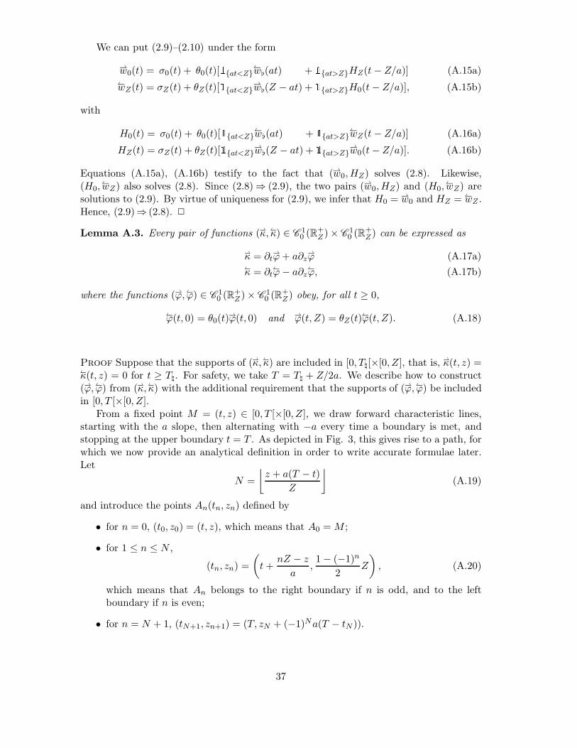
We can put (2.9)–(2.10) under the form

w0(t) = σ0(t) + θ0(t)[1at<Zw(at) + 1at>ZHZ(t− Z/a)] (A.15a)

wZ(t) = σZ(t) + θZ(t)[1at<Zw(Z − at) + 1at>ZH0(t− Z/a)], (A.15b)

with

H0(t) = σ0(t) + θ0(t)[1at<Zw(at) + 1at>Z

wZ(t− Z/a)] (A.16a)

HZ(t) = σZ(t) + θZ(t)[1at<Zw(Z − at) + 1at>Z

w0(t− Z/a)]. (A.16b)

Equations (A.15a), (A.16b) testify to the fact that (w0,HZ) solves (2.8). Likewise,(H0,wZ) also solves (2.8). Since (2.8)⇒ (2.9), the two pairs (w0,HZ) and (H0,wZ) aresolutions to (2.9). By virtue of uniqueness for (2.9), we infer that H0 = w0 and HZ = wZ .Hence, (2.9)⇒ (2.8). 2

Lemma A.3. Every pair of functions (κ,κ) ∈ C 10 (R+

Z )× C 10 (R+

Z ) can be expressed as

κ = ∂tϕ+ a∂z

ϕ (A.17a)κ = ∂t

ϕ− a∂zϕ, (A.17b)

where the functions (ϕ,ϕ) ∈ C 10 (R+

Z )× C 10 (R+

Z ) obey, for all t ≥ 0,

ϕ(t, 0) = θ0(t)ϕ(t, 0) and ϕ(t, Z) = θZ(t)ϕ(t, Z). (A.18)

Proof Suppose that the supports of (κ,κ) are included in [0, T[×[0, Z], that is, κ(t, z) =κ(t, z) = 0 for t ≥ T. For safety, we take T = T + Z/2a. We describe how to construct(ϕ,ϕ) from (κ,κ) with the additional requirement that the supports of (ϕ,ϕ) be includedin [0, T [×[0, Z].

From a fixed point M = (t, z) ∈ [0, T [×[0, Z], we draw forward characteristic lines,starting with the a slope, then alternating with −a every time a boundary is met, andstopping at the upper boundary t = T . As depicted in Fig. 3, this gives rise to a path, forwhich we now provide an analytical definition in order to write accurate formulae later.Let

N =

⌊z + a(T − t)

Z

⌋(A.19)

and introduce the points An(tn, zn) defined by

• for n = 0, (t0, z0) = (t, z), which means that A0 = M ;

• for 1 ≤ n ≤ N ,

(tn, zn) =

(t+

nZ − z

a,1− (−1)n

2Z

), (A.20)

which means that An belongs to the right boundary if n is odd, and to the leftboundary if n is even;

• for n = N + 1, (tN+1, zn+1) = (T, zN + (−1)Na(T − tN )).

37

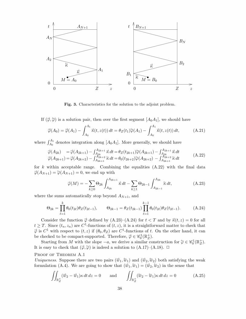
z00

t

z00

t

A1

AN

AN+1 BN+1

BN

B1

B2

A2

• •

κ

κ

M = A0

κ

κM = B0

Z Z

Fig. 3. Characteristics for the solution to the adjoint problem.

If (ϕ,ϕ) is a solution pair, then over the first segment [A0A1], we should have

ϕ(A0) = ϕ(A1)−

∫ A1

A0

κ(t, z(t)) dt = θZ(t1)ϕ(A1)−

∫ A1

A0

κ(t, z(t)) dt, (A.21)

where∫ A1

A0denotes integration along [A0A1]. More generally, we should have

ϕ(A2k) =ϕ(A2k+1)−∫ A2k+1

A2k

κdt= θZ(t2k+1)ϕ(A2k+1)−

∫ A2k+1

A2k

κ dtϕ(A2k+1)=ϕ(A2k+2)−

∫ A2k+2

A2k+1

κdt= θ0(t2k+2)ϕ(A2k+2) −

∫ A2k+2

A2k+1

κ dt(A.22)

for k within acceptable range. Combining the equalities (A.22) with the final dataϕ(AN+1) = ϕ(AN+1) = 0, we end up with

ϕ(M) = −∑

k≥0

Θ2k

∫ A2k+1

A2k

κdt−∑

k≥1

Θ2k−1

∫ A2k

A2k−1

κ dt, (A.23)

where the sums automatically stop beyond AN+1, and

Θ2k =k∏

ℓ=1

θ0(t2ℓ)θZ(t2ℓ−1), Θ2k−1 = θZ(t2k−1)k−1∏

ℓ=1

θ0(t2ℓ)θZ(t2ℓ−1). (A.24)

Consider the function ϕ defined by (A.23)–(A.24) for t < T and by κ(t, z) = 0 for allt ≥ T . Since (tn, zn) are C1-functions of (t, z), it is a straightforward matter to check thatϕ is C1 with respect to (t, z) if (θ0, θZ) are C1-functions of t. On the other hand, it canbe checked to be compact-supported. Therefore, ϕ ∈ C 1

0 (R+Z ).

Starting from M with the slope −a, we derive a similar construction for ϕ ∈ C 10 (R+

Z ).It is easy to check that (ϕ,ϕ) is indeed a solution to (A.17)–(A.18). 2

Proof of Theorem A.1

Uniqueness. Suppose there are two pairs (w1,w1) and (w2,

w2) both satisfying the weakformulation (A.4). We are going to show that (w1,

w1) = (w2,w2) in the sense that

∫∫

R+

Z

(w2 − w1)κdt dz = 0 and

∫∫

R+

Z

(w2 − w1)κdt dz = 0 (A.25)

38

for all κ ∈ C 10 (R+

Z ). We resort to a nonlinear version of Holmgren’s technique [32] andconsider the adjoint problem (A.17)–(A.18) for a given pair (κ,κ) ∈ C 1

0 (R+Z ) × C 1

0 (R+Z ).

According to Lemma A.3, this problem has a solution (ϕ,ϕ) ∈ C 10 (R+

Z )×C 10 (R+

Z ). Specify-ing this solution pair as test functions and writing the weak formulation (A.4) for (w1,w1)and (w2,w2), then subtracting, we get

0 =

∫∫

R+

Z

(w2 − w1)(∂tϕ+ a∂z

ϕ) dt dz +

∫∫

R+

Z

(w2 −w1)(∂tϕ− a∂z

ϕ) dt dz, (A.26)

which implies

0 =

∫∫

R+

Z

(w2 − w1)κ dt dz +

∫∫

R+

Z

(w2 − w1)κ dt dz. (A.27)

To reach claim (A.25), we set (κ,κ) = (κ, 0), then (κ,κ) = (0, κ).

Existence and continuous dependence. The aim of the game is to plug the candidatefunctions (w,w), defined by (2.7)–(2.8), into the right-hand side of the weak formulation(A.4) and to check that it vanishes. The calculations are somewhat cumbersome, becauseof the many changes of variables to be carried out for the double integrals. We just sketchout the intermediate steps, leaving the details to the reader.

First, using (2.7) and cutting the integration domain into subdomains, we have

∫∫R

+

Z

w(∂tϕ+ a∂z

ϕ) dt dz+∫ Z0

w(z)ϕ(0, z) dz +

∫R+ aw0(t)ϕ(t, 0) dt

=∫ Z0

w(z)ϕ(Z−z

a , Z) dz+∫

R+ aw0(t)ϕ(t+ Z

a , Z) dt∫∫R

+

Z

w(∂tϕ− a∂z

ϕ) dt dz+∫ Z0

w(z)ϕ(0, z) dz +

∫R+ awZ(t)ϕ(t, Z) dt

=∫ Z0

w(z)ϕ( z

a , 0) dz +∫

R+ awZ(t)ϕ(t+ Za , 0) dt

(A.28)

Invoking (2.8), taking advantage of (A.3), making appropriate changes of variables andinvoking (2.8) once again leads us to the conclusion that the right-hand side of (A.4) isequal to 0.

It remains to check that (w,w) are L∞-functions. From (2.7) and from the L∞-assumptions made on (w,

w), it is obvious that we simply need to check that the auxiliaryfunctions (w0,wZ) are L∞-functions. From (2.9)–(2.10) and by Lemma A.1, it can be seenthat this can be ensured as soon as ‖θ0‖‖θZ‖ < 1. Finally, from the estimates (A.12)–(A.13), it is not difficult to infer that

max‖w0‖, ‖wZ‖ ≤(1 + ‖θ0‖)(1 + ‖θZ‖)

1− ‖θ0‖‖θZ‖max‖w‖, ‖

w‖, ‖σ0‖, ‖σZ‖. (A.29)

Recalling (2.7) again and arguing that the constant in (A.29) is greater than 1, we arriveat (2.6). 2

39