Relaxation Schemes for Nonlinear Kinetic Equations

RELAXATION SCHEMES FOR NONLINEAR KINETIC EQUATIONS∗

E. GABETTA† , L. PARESCHI‡ , AND G. TOSCANI†

SIAM J. NUMER. ANAL. c© 1997 Society for Industrial and Applied MathematicsVol. 34, No. 6, pp. 2168–2194, December 1997 005

Abstract. A class of numerical schemes for nonlinear kinetic equations of Boltzmann type isdescribed. Following Wild’s approach, the solution is represented as a power series with parameterdepending exponentially on the Knudsen number. This permits us to derive accurate and stabletime discretizations for all ranges of the mean free path. These schemes preserve the main physicalproperties: positivity, conservation of mass, momentum, and energy. Moreover, for some particularmodels, the entropy property is also shown to hold.

Key words. Boltzmann equation, fluid dynamic limit, Wild sum

AMS subject classifications. 35L65, 65C20, 76P05, 82C40

PII. S0036142995287768

1. Introduction. Numerical resolution methods for the Boltzmann equationplay an important role in practical and theoretical analysis of the time evolution of ararefied gas. The widely used and best-known of these methods is the direct simulationMonte Carlo method due to Bird [4]. After Bird’s algorithm, more sophisticatedmethods related to the Boltzmann equation have been proposed, either based on arandom particle approximation [2], [19], [23] or, more recently, fully deterministic[24], [30]. Most of them take into account the fact that the kinetic equations to besolved involve both convection and interactions between particles. Consequently, theschemes rely on an approximation to the solution where the free molecular streamingand the relaxation to equilibrium are dealt with in two separate steps.

In effect, it is expected that the solution to the collision step will approach thesteady state quite rapidly, i.e., on the scale of time between collisions. On the otherhand, streaming produces a change of density on a much longer time scale. Thus,there should be a separation between the time scales on which collisions and streamingoccur. From a physical point of view, the collisions, occurring at each point in thephysical space, rapidly drive the local velocity distribution very close to the localMaxwellian, conserving the local density, bulk velocity, and energy, before streaminghas time to have any appreciable influence. After this short time, the streamingbecomes relatively significant, the effect of the collisions being small near the localequilibrium.

For the above reasons it becomes clear that any plausible approximation to thecollision process must bring the nonequilibrium data near the local Maxwellian. Thecharacteristic length scale of the relaxation is the mean free path between collisions,which we can identify as the Knudsen number. The limit of large relaxation rate(or small Knudsen number) is usually referred to as the fluid dynamic limit andcharacterizes the passage from a kinetic description of fluid mechanics to a macroscopicdescription, given, except near shock waves and boundary layers, by the Euler orNavier–Stokes equations.

∗Received by the editors June 14, 1995; accepted for publication (in revised form) April 3, 1996.This paper has been written within the activities of the National Council for Researches (CNR),Project “Applicazioni della Matematica per la Tecnologia e la Societa.”

http://www.siam.org/journals/sinum/34-6/28776.html†Universita di Pavia, Dipartimento di Matematica, Via Abbiategrasso 215, 27100 Pavia, Italy

([email protected], [email protected]).‡Universita di Ferrara, Dipartimento di Matematica, Via Machiavelli 35, 44100 Ferrara, Italy

([email protected]).

2168

RELAXATION SCHEMES FOR NONLINEAR KINETIC EQUATIONS 2169

The fluid dynamic limit is a challenge for numerical methods, because in thisregime the relaxation term becomes stiff. In most methods based on finite volumes,finite elements, or finite differences, the time step, in order to get positivity of theapproximated solution, has to be chosen proportional to the mean free path, a con-dition that makes these schemes unusable near the fluid regime. On the other hand,random particle methods need so many particles near the fluid regime that they arenot competitive.

To get unconditionally stable schemes, when the number of involved equations (invelocities) is finite and small, it is natural to use implicit or semi-implicit methods forthe collision part [9]. When more realistic models, like the full Boltzmann equation,are considered, this treatment is no longer possible, and it appears extremely difficultto construct approximations to the collision step that are well posed for any regimeand that preserve the usual conservation laws.

Moreover, as observed by Caflisch, Jin, and Russo [9], this problem is not merely anumerical stability problem. In fact, stable numerical discretizations may still producespurious solutions [25], [26]. Numerical experience shows that a sufficient conditionfor the correct behavior of the scheme near the fluid regime is that the numerical fluiddynamic limit should be a good discretization of the model Euler equations. This isguaranteed if in this limit the collision scheme projects into the local Maxwellian atevery time step.

A well-posed first-order discretization (in space and time) for any regime has re-cently been proposed by Perthame and Coron [12] for the Bhatnagar–Gross–Krook(BGK) model of the Boltzmann equation. Roughly speaking, in [12] the approxima-tion to the relaxation is given by a convex combination of the initial values and of thecorresponding local Maxwellian. This simultaneously gives positivity, conservation ofmass, momentum, and energy, and an entropy property independent of the mean freepath. As we will explain in the following paragraphs, the method presented here canbe considered an extension of the previous idea to general nonlinear Boltzmann-typeequations.

To summarize, the main features of a numerical approximation to the collisiondynamic that is in accord with the physical picture would be:

• well-posedness of the collision step for arbitrary values of the mean free path;• preservation of the main physical quantities: mass, momentum, energy, and

(whenever possible) entropy principle.• correct fluid dynamic limit, i.e., in this limit the numerical approximation is in

good agreement with the Euler equations.We propose, in this paper, a time discretization of the relaxation process that

satisfies the aforementioned requirements. The starting point is to represent thesolution in a power series of mean values of successive iterations of a bilinear operator,as introduced by Wild [32] to express the solution to the homogeneous Boltzmannequation for Maxwell pseudomolecules. The main feature of this representation isthat the weights in the arithmetic mean depend on the exponential of the Knudsennumber instead of the inverse of it, as usual. The schemes we derive clearly work for alldiscrete velocity models of the Boltzmann equation that possess the correct number ofcollision invariants; in addition, they apply to the full Boltzmann equation for Maxwellkernels, a model for which the Wild sum is the exact solution to the problem, and tomore general kernels which satisfy numerically essential cut-off hypotheses.

To conclude this introduction, we note that although we develop the schemes inthe kinetic background, the method can easily be generalized to a much wider classof hyperbolic systems with nonlinear stiff relaxation terms [9], [20], [25], [26].

2170 E. GABETTA, L. PARESCHI, AND G. TOSCANI

2. The setting. In kinetic theory the time evolution of a rarefied gas in a vesselis governed by the Boltzmann equation [11]

(2.1)

∂f

∂t+ v · ∇xf =

1

ǫJ(f, f), t ≥ 0,

f(x, v, t = 0) = f0(x, v), (x, v) ∈ Λ × R3,

γ+f(x, v, t) = Kγ−f(x, v, t), (x, v, t) ∈ E+,

where f = f(x, v, t) is the one particle distribution function of the molecules of therarefied gas at time t and ǫ is the Knudsen number proportional to the mean freepath between collisions. In (2.1), Λ is a bounded spatial domain of R3, to whichthe gas under consideration is confined. The boundary ∂Λ is assumed to have a unitinner normal n(x) at almost every x ∈ ∂Λ. The last relation in (2.1) is concerned withboundary conditions, K is a linear integral operator, and γ±f denote the traces of f on

E± ={

(x, v, t) ∈ ∂Λ × R3 × (0, T ) : ±v · n(x) > 0}

.

The bilinear collision operator J(f, f) describes the binary collisions of the particles,

J(f, f)(x, v, t)

(2.2) =

∫

R3×S2

β

(

q · σ

|q|, |q|

)

[f(x, v1, t)f(x,w1, t) − f(x, v, t)f(x,w, t)] dw dσ.

In the above expression, σ is a unit vector, so that dσ is an element of the areaof the surface of the unit sphere S2 in R3. Moreover, q = v − w is the relativevelocity, whereas (v1, w1) represent the postcollisional velocities associated with theprecollisional velocities (v, w) and the collision parameter σ,

(2.3) v1 =1

2(v + w + |q|σ), w1 =

1

2(v + w − |q|σ).

We have conservation of momentum and energy in every collision,

(2.4) v1 + w1 = v + w, v21 + w2

1 = v2 + w2.

As already mentioned in the introduction, from a formal point of view we expect thatin the limit ǫ → 0 the local mass density, momentum, and temperature

(2.5)

ρ(x, t) =

∫

R3

f(x, v, t) dv,

ρu(x, t) =

∫

R3

vf(x, v, t) dv,

T (x, t) =1

3ρ

∫

R3

[v − u(x, t)]2f(x, v, t) dv,

converge to a solution of compressible Euler equations

(2.6)

∂ρ

∂t+ div(ρu) = 0,

∂ρu

∂t+ div(ρu× u) + grad(p) = 0,

∂E

∂t+ div(Eu+ pu) = 0,

p = ρT, E =3

2ρT +

1

2ρu2.

Rigorous results in this direction can be found in [11].


As we will see below, the discretization we propose preserves this characteristic,becoming, as ǫ → 0, a stable numerical scheme for (2.6).

2.1. Splitting of the time scales. The initial-boundary value problem for theBoltzmann equation described in (2.1) will be approached by means of a splitting intime of the free molecular flow and relaxation due to collisions.

To this end, we rewrite equation (2.1) in the form

(2.7)∂f

∂t= Sf + Rf,

where

(2.8) S = −v · ∇x

and R is given by the nonlinear collision operator on the right-hand side of (2.1).Thus, in order to compute the solution, we can solve the coupled equations

(2.9)∂f

∂t= Sf,

∂f

∂t= Rf

and apply Trotter’s formula

(2.10) et(S+R) = limN→∞

(

etN Se

tN R

)N

.

The method is said to be convergent if Trotter’s formula (2.10) holds when S and Rare the aforementioned operators.

In further detail, for any N > 0 and 0 ≤ n < N , we denote for a fixed t > 0

∆t =t

N, tn = n∆t.

Then, two sequences fn+1/2 and fn+1 of piecewise continuous functions are definedon [tn, tn+1] by induction on n. Now, let f0 be the initial density and suppose thatthe functions fn approximating the solution at tn have been constructed. Then, theapproximation functions fn+1/2 and fn+1 are obtained in two steps. On the timeinterval [tn, tn+1], first we solve the transport phase

(2.11)

∂fn+1/2

∂t= Sfn+1/2,

fn+1/2(x, v, t = tn) = fn(x, v),

and then, denoting by fn+1/2(x, v) = fn+1/2(x, v, tn+1), the collision phase

(2.12)

∂fn+1

∂t= Rfn+1,

fn+1(x, v, t = tn) = fn+1/2(x, v).

Finally, we define

(2.13) fn+1(x, v) = fn+1(x, v, tn+1).

The method yields approximate solutions and in particular permits the separate treat-ment of the two subproblems (2.11)–(2.12).


Remark 2.1. Some recent results showed that the splitting can be used in a con-structive way to get existence and uniqueness of a local solution to kinetic equations.This has been proved for the planar Broadwell model in a square box in [31]. Morerecently, a proof of weak convergence of the splitting towards the DiPerna–Lions [14]solution of the Boltzmann equation has been obtained in [13].

In the following sections, we are interested in developing a numerical approxi-mation to the relaxation process (2.12) which is uniformly stable with ǫ. For theapproximation of (2.11), which goes beyond our purpose, we refer to the large classof numerical methods for multidimensional systems of conservation laws (see, forexample, [8], [22], [27], [29]). In section 5, for simplicity, we will consider some one-dimensional schemes.

3. Approximation of the relaxation. In the collision step described in theprevious section, we are going to study, for each x ∈ Λ, in the time interval [tn, tn+1]the spatially homogeneous problem

(3.1)

∂fn+1

∂t=

1

ǫJ(fn+1, fn+1),

fn+1(x, v, t = tn) = fn+1/2(x, v).

Here, the x-variable acts as a parameter, and it will be omitted in the rest of the paper.During the evolution process described by (3.1), the local mass density, momentum,and energy do not vary with time, and hence we can write

(3.2) ρn+1(t) = ρn+1/2, un+1(t) = un+1/2, Tn+1(t) = Tn+1/2.

3.1. Series solutions. The solution to the Cauchy problem for (3.1) can besought in the form of a power series

(3.3) fn+1(v, t) =

∞∑

k=0

(t− tn)kf (k)(v), f (0)(v) = fn+1/2(v),

where, substituting (3.3) into (3.1), we obtain for the functions f (k) the recurrentformula

(3.4) f (k+1)(v) =1

k + 1

k∑

h=0

1

ǫJ(f (h), f (k−h)), k = 0, 1, . . . .

As one can easily observe, this representation is unusable for our numerical purposesbecause it becomes meaningless in the stiff region (ǫ ≪ 1) of (3.1). In particular,truncating expression (3.3) beyond the first-order term, we get the classical Eulerformula. We point out that power series expansion of the type (3.5)–(3.6) can beconsidered as the limit result of iteration processes applied to the integral form ofproblem (3.1).

Let us consider instead of (3.1) a differential system of the type

(3.5)

df

dt=

1

ǫ[P (f, f) − µf ] ,

f(v, t = 0) = f0(v),

where µ 6= 0 is a constant and P a bilinear operator.


Wild [32] solved equation (3.5) in the case of Maxwell pseudomolecules, but hismethod can be applied under more a general hypothesis on P . Following Wild’sapproach, the solution to (3.5) can be expressed, formally, as an arithmetic mean,with weight changing exponentially with time, of sequences of convolution iterates ofP .

Let us replace the time variable t and the required function f = f(v, t) using theequations

(3.6) t′ = (1 − e−µt/ǫ), F (v, t′) = f(v, t)eµt/ǫ.

Then F is easily shown to satisfy

(3.7)

dF

dt′=

1

µP (F, F ), 0 < t′ < 1,

F (v, t′ = 0) = f0(v).

Now, problem (3.7) has the same structure as (3.1), and hence the solution can beexpanded in the form of a power series in t′:

(3.8) F (v, t′) =

∞∑

k=0

t′kf (k)(v), f (0)(v) = f0(v),

where the functions f (k) are given by the recurrent formula

(3.9) f (k+1)(v) =1

k + 1

k∑

h=0

1

µP (f (h), f (k−h)), k = 0, 1, . . . .

Reverting to the old notation, we obtain the following formal representation of thesolution to the Cauchy problem (3.5):

(3.10) f(v, t) = e−µt/ǫ∞∑

k=0

(

1 − e−µt/ǫ)k

f (k)(v).

It is remarkable that in [17], by assuming only certain quadratic properties on P , theuniform convergence of series (3.10) with respect to t has been proved.

Remark 3.1. The solution to (3.5) can be expressed in a similar form provided Pis an n-linear operator (n ≥ 2). In this situation, system (3.5) reads

(3.11)

df

dt=

1

ǫ[Pn(f, . . . , f) − µf ] ,

f(v, t = 0) = f0(v).

By replacing the time variable t and the function f = f(v, t) using relations

t′ = (1 − e−µ(n−1)t/ǫ), F (v, t′) = f(v, t)eµt/ǫ.

Similarly, we obtain

f(v, t) = e−µ(n−1)t/ǫ∞∑

k=0

(

1 − e−µ(n−1)t/ǫ)k

f (k)(v),


which is, for k = 0, 1, . . . ,

f (k+1)(v) =1

k + 1

∑

h1+···+hn=k

1

(n− 1)µPn(f (h1), . . . , f (hn)).

The following general result holds [21].THEOREM 3.1. Let B be a Banach space and let P : Bn → B, n ≥ 2, be an

n-linear operator satisfying the inequality

(3.12) ‖P (g1, . . . , gn)‖ ≤ CP ‖g1‖ · · · ‖gn‖ ∀ gi ∈ B.

We define

(3.13) g(x, t) = e−t∞∑

k=0

bk

(

1 − e−(n−1)t)k

g(k)(x),

where for k = 0, 1, . . . ,

(3.14) g(k+1)(x) =1

k + 1

∑

h1+···+hn=k

bh1· · · bhn

(n− 1)bkPn(g(h1), . . . , g(hn)),

and the numbers bk are the coefficients in the Taylor’s expansion of

(1 − x)1

1−n =

∞∑

k=0

bkxk.

Let

t0 =1

(1 − n)ln(1 − C−1

P ‖f0‖1−n)

and

t1 =

1

(1 − n)ln(1 − C−1

P ‖f0‖1−n),

∞,

C−1P ‖f0‖

1−n < 1,

C−1P ‖f0‖

1−n ≥ 1.

Then, (3.13) is uniformly convergent on compact subsets of ]t0, t1[ and is the unique

solution to problem

(3.15)

dg

dt= P (g, . . . , g) − g,

g(x, t = 0) = g0(x).

Remark 3.2. Let τ = µt/ǫ; then the system (3.11), and so (3.5), take the form(3.15), where now the n-linear operator is P/µ.

In all the kinetic equations we will consider in the next paragraphs, we haveµ = ‖f0‖L1

and n = 2. Thus, choosing B = L1(R3),

‖P (g1, g2)

µ‖L1

≤1

µ‖g1‖1‖g2‖L1

,

and condition (3.12) is satisfied with CP = 1/µ. Therefore, the initial value problemhas a unique solution in the time interval [0,∞[ independently on ǫ.


3.2. Numerical schemes. We describe in this section the numerical approxi-mation to problem (3.5). First we state the following lemma.

LEMMA 3.1.(a) Let P be a nonnegative bilinear operator such that

(3.16)

∫

R3

P (f, f)

1vv2

dv = µ

∫

R3

f

1vv2

dv

where µ 6= 0 is a constant. Then the coefficients f (k) defined by (3.14) are nonnegative

and satisfy, ∀k > 0,

(3.17)

∫

R3

f (k)

1vv2

dv =

∫

R3

f (0)

1vv2

dv.

(b) If for p = 0, 1 we have

(3.18) f (p+1) = f (p), P (f (p), f (p)) = µf (p),

then f (q) = f (p) ∀q ≥ p.The proof is a simple exercise, and we leave it to the reader.Moreover, a simple modification of the Toeplitz theorem will be useful [28].LEMMA 3.2. Let {cnk}n,k≥0 be a double sequence of real, nonnegative numbers

which satisfy the following conditions:

(3.19)

∞∑

k=0

cnk = 1 ∀n, limn→∞

cnk = 0 ∀k.

If {hk}k≥0 is a convergent sequence of elements of a Banach space B, then the sequence

gn =

∞∑

k=0

cnkhk

is well defined ∀n, {gn}n≥0 is convergent, and

limn→∞

gn = limk→∞

hk.

Suppose the sequence{

f (k)}

k≥0defined by (3.9) is convergent. Then (3.10) is

well defined for any value of the mean free path, and moreover, by Lemma 3.2, if wedenote by

(3.20) f∞(v) = limk→∞

f (k),

we have

(3.21) limt→∞

f(v, t) = f∞(v),

with f∞(v) being the local equilibrium.Thus, for m > 1, we can introduce the following class of numerical schemes for

the approximation of problem (3.5) in the time interval [tn, tn+1]:

(3.22) fn+1(v) = (1 − τ(∆t, ǫ))

m∑

k=0

τ(∆t, ǫ)kf (k)(v) + τ(∆t, ǫ)m+1f∞(v),

where τ(∆t, ǫ) = 1 − exp {−(µ∆t)/ǫ} and the terms f (k) are defined by (3.9).


THEOREM 3.2. The time discretization defined by (3.22) is such that

(i) If supk>m{|f (k) − f∞|} ≤ C for a constant C = C(v), then it is at least an

m-order approximation (in µ∆t/ǫ) of (3.10). Moreover,

|f(v, t) − fn+1(v)| ≤ C τ(∆t, ǫ)m+1.

(ii) When (3.16) holds then total mass, momentum, and energy are preserved.

(iii) If P is a nonnegative operator then fn+1(v) is nonnegative independently of

the value of ǫ.(iv) For any m,n ≥ 0 we have

limǫ/∆t→0

fn+1(v) = f∞(v).

Moreover, with the same assumptions as (i), the following holds:

|fn+1(v) − f∞(v)| ≤ C [1 − τ(∆t, ǫ)m+1].

Proof. Property (i) is a simple consequence of

|f(v, t) − fn+1(v)| = (1 − τ(∆t, ǫ))

∞∑

k=m+1

τ(∆t, ǫ)k|f (k)(v) − f∞(v)|

≤ C (1 − τ(∆t, ǫ))

∞∑

k=m+1

τ(∆t, ǫ)k

= C τ(∆t, ǫ)m+1 ≤ C min

{

1,

(

µ∆t

ǫ

)m+1}

∀m, n.

Applying Lemma 3.1, the conservation properties (ii) are just deduced from

(1 − τ(∆t, ǫ))

m∑

k=0

τ(∆t, ǫ)k + τ(∆t, ǫ)m+1 = 1.

The nonnegativity (iii) is clear since, by Lemma 3.1, f (k) are nonnegative ∀k and0 ≤ τ(∆t, ǫ) ≤ 1 ∀∆t, ǫ.

Finally, relations (iv) are readily checked by noting that

limǫ/∆t→0

τ(∆t, ǫ) = 1 ∀m,

and

|fn+1(v) − f∞(v)| = (1 − τ(∆t, ǫ))

m∑

k=0

τ(∆t, ǫ)k|f (k)(v) − f∞(v)|

≤ C (1 − τ(∆t, ǫ))

m∑

k=0

τ(∆t, ǫ)k

= C [1 − τ(∆t, ǫ)m+1] ∀m, n.

Remark 3.3. Before considering some applications of the previous approximationsto various kinetic equations we point out that:

• Property (i) implies that the number Ne of evaluation of the bilinear operatorP , which in general is the most expansive part of the computation, is related to theorder m of the schemes by Ne =

∑mp=1 p. As we will see, more accurate error estimates

are linked to the structure of the bilinear operator P . In particular, the accuracy ofthe schemes is related to the rate of convergence of the sequence f (k) towards f (∞).

• Property (iii) states that the numerical schemes are unconditionally stable.• Properties (ii) and (iv) are enough to guarantee that the method has a correct

numerical behavior near the fluid regime.


4. Applications.

4.1. Discrete velocity models. The discrete velocity models of the Boltzmannequation supply a clarifying example of the application of (3.22). The discrete kinetictheory [16] is concerned with the analysis of systems of gas particles with a finite setof selected velocities, and provides a useful substitute for the Boltzmann equation,in terms of a system of hyperbolic equations with relaxation. The general model iswritten in the form

(4.1)

∂fi

∂t+ vi · ∇fi =

1

ǫ[Gi(f , f) − fiLi(f)] ,

fi(x, t = 0) = ϕi(x), i = 1, 2, . . . , r,

where V = {vi, i = 1, 2, . . . , r} is the set of the admissible velocities and

f(x, t) = {f1(x, t), . . . , fr(x, t)}

is the r-components vector whose ith component represents the density of the particleswith velocity vi in the position x ∈ R3 at time t. In system (4.1) the gain term Gi

and the loss term Li, i = 1, 2, . . . , r, are defined through the expressions

(4.2) Gi(f , f)(x, t) =

r∑

j,k,l=0

Aklijfk(x, t)fl(x, t),

(4.3) Li(f)(x, t) =

r∑

j,k,l=0

Aijklfj(x, t) .

The quantities Aklij are nonnegative constants, linked to the probability that two

particles with velocities vi and vj collide and come out of the collision with velocitiesvk and vl.

Because of symmetry properties, due to the particular choice of the allowed ve-locities, some of these models possess a number of collision invariants greater thanthe usual one [16]. In these cases, there is no possibility to define a unique equilib-rium state with the same moments of the initial density. For this reason, from nowon, it is intended that we will refer only to regular discrete models, namely to mod-els that have only the usual conserved quantities: mass, momentum, and energy. Acharacterization of the regular models is due to Cercignani [10].

Let us define

(4.4) A = maxi,j

r∑

k,l=0

Aijkl.

Then we have, for i = 1, 2, . . . , r,

Gi(f , f) − fiLi(f) =

r∑

j,k,l=0

Aklijfkfl −

r∑

j,k,l=0

Aijklfifj

=

r∑

j,k,l=0

Aklijfkfl +

r∑

j=0

A−

r∑

k,l=0

Aijkl

fifj −Afi

r∑

j=0

fj ,

where the coefficients A−∑r

k,l=0Aijkl are nonnegative as a consequence of (4.4).


Thus, with the previous notations, the relaxation step can be written in theequivalent form

(4.5)

∂fn+1i

∂t=

1

ǫ

[

Ri(fn+1, fn+1) −Aρn+1fn+1

i

]

,

fn+1i (t = tn) = f

n+1/2i , i = 1, 2, . . . , r,

where the mass ρn+1 =∑

i fn+1i remains constant during the evolution, and Ri is the

positive bilinear operator

Ri(f ,g)(t)

(4.6) =

r∑

j,k,l=0

Aklijfk(t)gl(t) +

A−

r∑

k,l=0

Aijkl

fi(t)gj(t)

.

The solution to equation (4.5) will be approximated by the m-order scheme fori = 1, 2, . . . , r:

(4.7)

fn+1i = (1 − τ(∆t, ǫ))

m∑

k=0

(τ(∆t, ǫ))kf

(k)i + τ(∆t, ǫ)m+1Mi(f

n+1/2),

f(k+1)i =

1

k + 1

k∑

h=0

1

ρn+1/2Ri(f

(h), f (k−h)), f(0)i = f

n+1/2i ,

where τ(∆t, ǫ) = 1 − exp{

−(Aρn+1/2∆t)/ǫ}

and Mi(f) is the ith component of thelocal Maxwellian with the same moments as f .

It is interesting to note that the coefficients f (k) in (4.7) can be computed directlyby recursion using (4.6). Thus, contrary to the continuous Boltzmann equation, fordiscrete velocity models the implementation of the schemes does not need furtherapproximations. Obviously, due to the increasing of the computational cost, high-order schemes (m ≥ 2) are of practical interest when the number of velocities is smallor in one-dimensional situations. On the other hand, except for some simple models,an accurate evaluation of the local Maxwellian requires a proper numerical method.

4.1.1. Maxwellian state. As in classical kinetic theory, it is well known thatamong all velocity distributions corresponding to given macroscopic variables, thedensities fi of the associated Maxwellian state are those for which the discrete Boltz-mann H-function

(4.8) H =

r∑

i=1

fi log(fi)

is minimum.By introducing the space of summational invariants

(4.9) Ψ(V ) ={

ψ : V → R s.t. Aklij (ψ(vi) + ψ(vj) − ψ(vk) − ψ(vl)) = 0

}

,

the Maxwellian state is characterized by the fact that log(f) belongs to Ψ(V ). Asalready observed, in the general situation, this space can be larger than expected, i.e.,the space spanned by (1, v, v2). For regular models this does not occur, and hence


there are q ≤ 5 coefficients ci, i = 1, . . . , q, depending on the mass, momentum, andenergy of the initial data such that

M(f) = exp

{

q∑

i=1

ciφi

}

,

where{

φi ∈ V, i = 1, . . . , q}

is a basis of Ψ(V ).Using a different basis one gets the usual expressions for the Maxwellian densities

(4.10) Mi(f) = a exp{

−(vi − b)2/c)}

whose parameters a,b, c depend on mass, mean velocity, and temperature of the initialdata

(4.11) ρ =

r∑

i=1

Mi(f), u =1

ρ

r∑

i=1

Mi(f)vi, T =1

3

[

1

ρ

r∑

i=1

Mi(f)v2i − u2

]

.

Clearly, it is difficult to obtain analytically the expression of Mi(f) as a function ofthe macroscopic variables ρ,u, T .

The simplest way to get an explicit approximation of the Maxwellian densities isgiven by [18]

(4.12) Mi(f) =ρ exp

{

−(vi − u)2/2T}

∑qh=1 exp {−(vh − u)2/2T}

.

This approximated solution satisfies exactly the first of (4.11), whereas the remainingrelations become exact as the number of velocities approaches infinity. Thus (4.12)is acceptable only for very large values of r. More accurate equilibrium state can beobtained solving numerically the system of nonlinear equations (4.10)–(4.11) with astandard iterative method using (4.12) as initial estimate of the solution.

4.1.2. Broadwell model. The connection of the present approximation withprevious ones will now be analyzed for the planar Broadwell model. This model is thesimplest discrete velocity model with the correct number of collision invariants (massand momentum) and represents a prototype of hyperbolic system with relaxation.For this reason the development of specific numerical methods has been consideredby several authors [5], [9], [15].

Particles can move with only four velocities, directed along the axes of an orthog-onal reference frame, and only head-on collisions are permitted. The system of fourequations is

(4.13)

∂f1∂t

+ v∂f1∂x

=1

ǫ(f2f4 − f1f3),

∂f2∂t

+ v∂f2∂y

=1

ǫ(f1f3 − f2f4),

∂f3∂t

− v∂f3∂x

=1

ǫ(f2f4 − f1f3),

∂f4∂t

− v∂f4∂y

=1

ǫ(f1f3 − f2f4).

Since in this case the constant A defined by (4.4) is equal to 1, the relaxationprocess linked to (4.13) takes the form

(4.14)∂fn+1

i

∂t=

1

ǫ

[

Ri(fn+1, fn+1) − ρn+1fn+1

i

]

, i = 1, 2, 3, 4,


where, using the compact notation fn+1k = fn+1

l , if k ≡ l mod 4,

Ri(fn+1, fn+1) = (fn+1

i + fn+1i+1 )(fn+1

i + fn+1i+3 ).

A simple calculation shows that the local Maxwellian with the same moments asfn+1 is given by

(4.15) Mi(fn+1) =

1

ρn+1Ri(f

n+1, fn+1).

The first term in (4.7) satisfies f(1)i = Mi(f

n+1); thus by virtue of Lemma 3.1(b) theWild sum comes at once into the exact solution and all schemes for m ≥ 1 are equalto the exact solution in the time interval [tn, tn+1]:

(4.16) fn+1i = e−ρn+1∆t/ǫf

n+1/2i +

(

1 − e−ρn+1∆t/ǫ)

Mi(fn+1/2), i = 1, 2, 3, 4.

It is clear that (4.16) satisfies the conservation of mass, momentum, and entropy prin-ciple, since the aforementioned approximated solution is nothing else than a convexcombination of the initial values and of the local Maxwellian.

As usual, implicit schemes, generating nonnegative approximations at any regime,can be obtained from (4.16) by substituting e−(ρ∆t)/ǫ with 1/[1+(ρ∆t)/ǫ] at the firstorder or with [1 − (ρ∆t)/2ǫ]/[1 + (ρ∆t)/2ǫ] at the second order. We point out thatonly the first-order scheme possesses the correct fluid dynamic limit.

The first-order approximation has been used in [31] to obtain a constructive proofof local existence and uniqueness of a solution to the plane Broadwell model in a squarebox, by means of the splitting of the equations. More recently, the same approximationto the relaxation step for Broadwell has been used in [9] to get an unconditionallystable second-order splitting scheme with a correct description of the fluid regime.

A splitting of the plane Broadwell model, in which the relaxation step has beensolved directly on (4.16), has been employed in [5] to investigate the asymptoticbehavior of the solution towards a steady state for small values of the mean free path.

Remark 4.1. To end this section let us recall that by virtue of (4.14)–(4.15) theplanar Broadwell model has the same structure of the BGK model of the Boltzmannequation, and thus for this model, we get

fn+1(v) = e−ρn+1∆t/ǫfn+1/2(v) +(

1 − e−ρn+1∆t/ǫ)

M(fn+1/2)(v)

with M now being the local Maxwellian with the same moments as f . We remarkthat in [12] the authors, in order to produce a numerical way to pass from kineticequations to compressible Euler equations, developed a stable discretization valid forarbitrary values of the mean free path based on the previous approximation to therelaxation step.

4.2. Maxwell models. Maxwell pseudomolecules clearly represent the natural,but not the simplest, situation in which expansion (3.10) can be fruitfully employedto get an approximation to the relaxation dynamics for the Boltzmann equation. Insuch a gas model, particles interact with a collision rate β = β( q·σ

|g| ) depending only

on the scattering angle and not on the energies of the colliding molecules. Thus, itis immediate to see that the conservation of density leads to a simplification of thestructure of problem (3.1) which takes the form

(4.17)

∂fn+1

∂t=

1

ǫ

[

Q(fn+1, fn+1) − βρn+1fn+1]

,

fn+1(v, t = tn) = fn+1/2(v),


where

(4.18) Q(f, g)(v, t) =

∫

R3×S2

β

(

q · σ

|q|

)

f(v1, t)g(w1, t) dwdσ

and

β =

∫

S2

β

(

q · σ

|q|

)

dσ .

Applying the Wild method to problem (4.17), we obtain the following represen-tation of the solution:

(4.19) fn+1(v, t) = e−(βρn+1t)/ǫ∞∑

k=0

(

1 − e−(βρn+1t)/ǫ)k

f (k)(v)

with, for k ≥ 1,

(4.20) f (k+1)(v) =1

k + 1

n∑

h=0

1

βρQ(f (h), f (k−h))(v), f (0)(v) = fn+1/2(v).

It is a simple exercise to verify that the coefficients f (k)(v), k ≥ 1, have the samemass, bulk velocity, and temperature of f (0)(v). In particular, this implies that theCauchy problem (4.17) is well posed in L∞ with weight 1 + v2.

Note that the coefficients of expansion (4.19) include numerous five-fold integralslike (4.18). Thus, except for one-dimensional situations, the most interesting schemefor practical applications is that for m = 1.

We get the first-order approximation to the solution by substituting f (k), k ≥ 2,with the local Maxwellian. With the notations of section 2, the first-order schemereads

fn+1(v) =

(

1 − τ(∆t, ǫ)fn+1/2(v)

(4.21) +(1 − τ(∆t, ǫ))τ(∆t, ǫ)1

βρQ(fn+1/2, fn+1/2) + τ(∆t, ǫ)

)2

M(fn+1/2)(v),


−(βρn+1/2∆t)/ǫ}

, and we denote by

(4.22) M(f)(v) =ρ

(2πT )3/2exp

{

(v − V )2

2T

}

the local Maxwellian with the same moments as f(v).Since we are interested in the time integration, we remark that in order to solve

system (4.21) numerically, we need a velocity discretization for the evaluation of (4.18)and (4.22). Thus, depending on the numerical method used for the five-fold integral,both deterministic and stochastic, we get different approximations of the solution to(4.17).

As predicted by Theorem 3.1, by the properties of Q, it is clear that fn+1 iswell defined independently on the Knudsen number and has the same density, meanvelocity, and temperature of fn+1/2. It would certainly be interesting to verify thevalidity of the entropy condition, but the question is open in its generality.


4.2.1. Planar case. A positive answer can be found for some simpler situations,like the planar case. In a recent paper [6], in fact, a sufficient condition has beenderived for a convex functional Γ to satisfy the inequality

(4.23) Γ

[

1

βρQ(f, f)

]

≤ Γ(f).

For the Boltzmann H-function

H(f) =

∫

R2

f(v) log f(v) dv,

inequality (4.23) is a consequence of the exponential power inequality by Shannon [6].Thus, by convexity, we obtain

H(fn+1) ≤ (1 − τ(∆t, ǫ))H(fn+1/2)

+(1 − τ(∆t, ǫ))τ(∆t, ǫ)H

[

1

βρQ(fn+1/2, fn+1/2)

]

+ τ(∆t, ǫ)2H[M(fn+1/2)]

≤ (1 − τ(∆t, ǫ)2)H(fn+1/2) + τ(∆t, ǫ)2H[M(fn+1/2)] ≤ H(fn+1/2),

proving a total entropy estimate. The recursivity relation (4.20) permits us to extendthe entropy property to m > 1.

The Maxwell gas in the plane is interesting because of the propagation of regu-larity. In fact, in [6] another convex functional satisfying (4.23) was discovered. Thisfunctional, known as the Linnik functional, is defined by

(4.24) L(f) = 4

∫

R2

(

∇√

f(v))2

dv.

In analogy with the Boltzmann H-functional, given a function f(v) with finite mass,momentum, and energy, the Linnik functional is such that L(f) ≥ L[M(f)]. Thus,by the same argument we used to derive the entropy estimate, we get

L(fn+1) ≤ L(fn+1/2).

Since mass is conserved and

‖√

f‖H1 = ρ1/2 +1

2L(f)1/2,

it follows that

(4.25) ‖√

fn+1(·)‖H1 ≤ ‖√

fn+1/2(·)‖H1 .

By means of classical Sobolev embeddings it is possible in this case to get errorestimates in sup-norm.

4.3. Boltzmann equation with a general kernel. In this section we dealwith a possible extension of the method to the Boltzmann equation with a collisionkernel that satisfies the boundedness condition

(4.26)

∫

S2

β

(

q · σ

|q|, q

)

dσ ≤ C.


This condition seems to be essential for convergence proofs of simulation methods tothe solution to the full Boltzmann equation. An exhaustive discussion on this pointfor Nambu’s scheme can be found in [3]. From a physical point of view, (4.26) meansthat β will have to be truncated in almost all cases of practical interest. From anumerical point of view, the situation is less dramatic. In effect, what we are lookingfor is a well-posed approximation to the relaxation step (3.1) for the full Boltzmannequation. After [1], it is well known that the solution to the spatially homogeneousproblem exists and is unique for almost all general kernels with cut-off, providedsufficiently many moments exist initially. This means that, when condition (4.26) isnot satisfied with the position

(4.27) βr

(

q · σ

|q|, q

)

= min

{

β

(

q · σ

|q|, q

)

, r

}

,

the solutions{

fn+1r (x, t)

}

r≥1to the problems

(4.28)

∂fn+1

∂t=

1

ǫJr(f

n+1, fn+1),

fn+1(v, t = tn) = fn+1/2(v)

obtained by replacing β with βr converge, as r goes to infinity, towards the uniquesolution to the original problem. Hence, for a general collision kernel with cut-off, byfurther cutting the kernel to satisfy (4.27), we get a problem whose solution, at leastfor large r, is a reasonable approximation to the true problem.

Thus, for a fixed r, let us consider instead of (3.1) the relaxation problem

(4.29)

∂fn+1

∂t=

1

ǫ

[

Qr(fn+1, fn+1) − fn+1Sr(f

n+1)]

,

fn+1(v, t = tn) = fn+1/2(v),

where

(4.30) Qr(f, f)(v, t) =

∫

R3×S2

βr

(

q · σ

|q|, |q|

)

f(v1, t)f(w1, t) dwdσ

and

(4.31) Sr(f)(v, t) =

∫

R3×S2

βr

(

q · σ

|q|, |q|

)

f(w, t) dwdσ .

Because of definition (4.27),

Sr(f)(v, t) ≤ 4πrρ.

Therefore, if we define

Rr(f, g)(v)

(4.32) = Qr(f, g)(v) +

∫

R3×S2

[

r − βr

(

q · σ

|q|, |q|

)]

f(v)g(w) dwdσ,


Rr(f, g) is a nonnegative bilinear operator, and the relaxation part can be rewrittenin the form

(4.33)

∂fn+1

∂t=

1

ǫ

[

Rr(fn+1, fn+1) − 4πrρn+1fn+1

]

,

fn+1(v, t = tn) = fn+1/2(v),

which is of the type (3.5). Thus the solution fr to (4.33) can be represented in the formof a Wild sum like (4.19)–(4.20) with β = 4πr. We can easily extend to this situationthe considerations of the previous section. In particular, as for the Maxwellian case,the first-order scheme is the main interesting one and reads

fn+1r (v) =

(

1 − τ(∆t, ǫ)fn+1/2r (v)

(4.34)

+(1 − τ(∆t, ǫ))τ(∆t, ǫ)1

4πrρRr(f

n+1/2r , fn+1/2

r ) + τ(∆t, ǫ)

)2

M(fn+1/2r )(v) ,


−(4πrρn+1/2∆t)/ǫ}

.Hence fn+1

r defined by (4.34) is well defined independently of the Knudsen num-ber, it has the correct moments, and it converges towards the correct fluid-dynamiclimit. No proofs of the entropy principle are presently available.

5. Implementation and numerical tests. As already observed, the imple-mentation of the schemes is dependent on the different choices of the relaxation op-erator P . In particular, the applications to the full Boltzmann equation are strictlyrelated to the integration rule used for the evaluation of the collision operator. In thiscase, except for one-dimensional problems (in velocity), the most interesting schemesare the first-order ones. Numerical results in this direction for the homogeneousBoltzmann equation in two dimensions can be found in [24]. On the contrary, for thediscrete velocity models of the Boltzmann equation, the computation of the schemescan be performed directly by recursivity without further approximations. For thereason given above, the tests we have performed refer to some discrete models of theBoltzmann equation at different regimes.

5.1. Relaxation of some nonlinear models. The purpose of this section isto show, through some practical examples, how different structures of the relaxationterms lead to different computable algorithms, and that the numerical schemes areunconditionally stable and work with uniform accuracy with respect of ǫ.

Example 1. Carleman model. The Carleman model of the Boltzmann equationdescribes a set of particles moving with velocity ±1 along the x-axis. The relaxationprocess reads

(5.1)

∂f1∂t

=1

ǫ(f2

2 − f21 ),

∂f2∂t

=1

ǫ(f2

1 − f22 ),

where f1(t) and f2(t) are the density functions of the particles traveling with velocity+1,−1.


0 1 2 3 4

0

0.1

0.2

0.3

0.4

0.5

0.6

0.7

0.8

0.9

1

FIG. 1. Coefficients f(k)1 (◦) and f

(k)2 (∗) for Carleman model.

Due to mass conservation, ρ = f1 + f2, system (5.1) can be rewritten in theequivalent form

(5.2)

∂f1∂t

+ρ

ǫf1 =

1

ǫ(f2

2 + f2f1) =ρ

ǫf2,

∂f2∂t

+ρ

ǫf2 =

1

ǫ(f2

1 + f1f2) =ρ

ǫf1.

It is easy to check that the local Maxwellian is given by f∞1 = f∞

2 = ρ/2 and that

all terms f(k)i , k > 1, in the Wild representation of the solution to the initial value

problem for (5.2) are equal to the local Maxwellian. Figure 1 shows the behavior of

the sequences f(k)1 , f

(k)2 for ρ = 1.0 and f

(0)1 − f

(0)2 = −0.5.

Thus, by making use of the notations introduced in the previous sections, all theschemes for m ≥ 1, similarly to the plane Broadwell model situation, provide theexact solution to (5.2) in the time interval [tn, tn+1]

(5.3) fn+1i =

1

2

[

ρn+1/2 + (−1)i+1e−2(ρn+1/2∆t)(fn+1/21 − f

n+1/22 )

]

, i = 1, 2.

Example 2. Broadwell models. Here we consider the relaxation process for a setof modified one-dimensional Broadwell models defined by

(5.4)

∂f1∂t

=1

ǫ(f2

3 − f1f2),

∂f2∂t

=1

ǫ(f2

3 − f1f2),

∂f3∂t

=1

αǫ(f1f2 − f2

3 ),


with f1, f2, and f3 now being the density of particles with velocity 1,−1, 0, respec-tively. The parameter α, such that α ≥ 1 is an integer, is proportional to the numberof particle densities moving with zero velocity. In particular, for α = 1, (5.4) is noth-ing but the reduced four velocity Broadwell model we have analyzed in section 4.1,whereas for α = 2, it corresponds to the reduced six velocity Broadwell model. Thespace of the collision invariant has dimension q = 2 corresponding to conservation ofmass and mean velocity

ρ = f1 + f2 + 2αf3, ρu = f1 − f2.

From the conservation of mass we can write (5.4) in the form

(5.5)

∂f1∂t

+ρ

ǫf1 =

1

ǫ(f2

1 + f23 + 2αf1f3),

∂f2∂t

+ρ

ǫf2 =

1

ǫ(f2

2 + f23 + 2αf2f3),

∂f3∂t

+ρ

ǫf3 =

1

αǫ(f2

3 (2α2 − 1) + f1f2 + αf1f3 + αf2f3).

Clearly, if α = 1, it is possible to linearize system (5.5), and hence the schemes coincideonce more with the exact solution (4.16). On the contrary, for α > 1, system (5.5)preserves the nonlinearity and thus represents an interesting test case.

The Maxwellian state is characterized by two constants a and b such that

(5.6) M1 = a exp{b}, M2 = a exp{−b}, M3 = a.

In particular, it is possible to get the analytic expression of a and b as a function ofρ and u:

(5.7) a =ρ(1 − e)

2α, b = log

[

(1 − e)

α(e− u)

]

,

where e = e(u) is given by

(5.8)

e =1

2(1 + u2), α = 1,

e =1

(α2 − 1)

(

α√

α2u2 + 1 − u2 − 1)

, α > 1.

By noting with Ri(f , f)/ǫ, i = 1, 2, 3, the right-hand side of equations (5.5), the systemhas the same structure as (4.5) with A = 1, and hence the general m-order scheme isgiven by (4.7) with r = 3.

The numerical computations refer to the initial nonequilibrium data characterizedby relations (5.6)–(5.7) but not (5.8) with

(5.9) ρ = 1.0, u = 0.1, e = 0.5.

In all computations we used a fixed ∆t = 0.1.

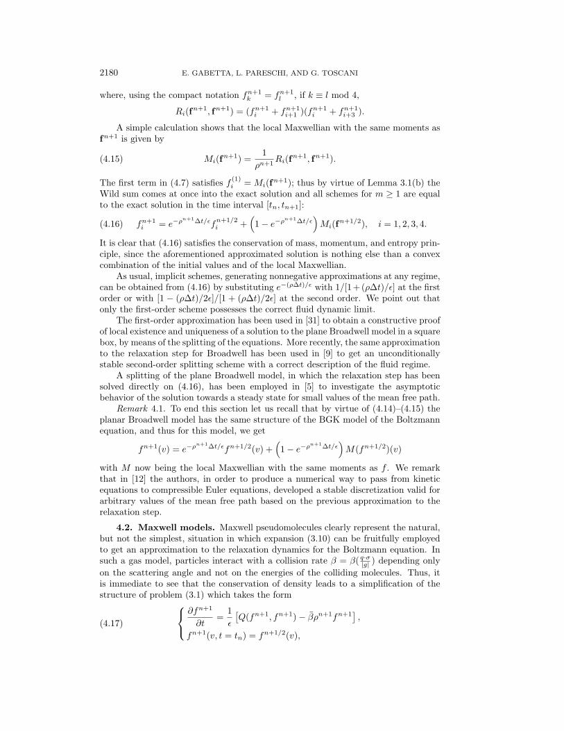
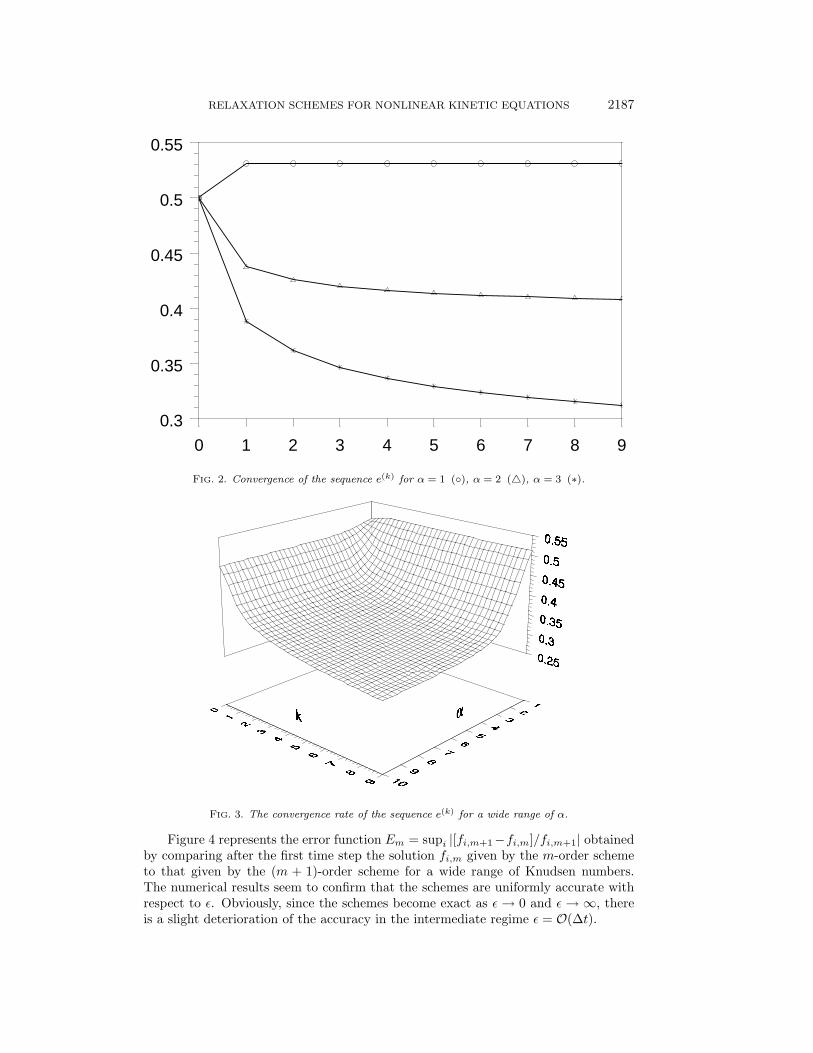
Figures 2 and 3 show the convergence of the sequence e(k) = f(k)1 + f

(k)2 towards

the Maxwellian state for different values of α. It is remarkable that, in the nonlinearsituation, after a fast convergence rate of low-order terms, the asymptotic convergencerate becomes extremely slow.


0 1 2 3 4 5 6 7 8 9

0.3

0.35

0.4

0.45

0.5

0.55

FIG. 2. Convergence of the sequence e(k) for α = 1 (◦), α = 2 (△), α = 3 (∗).

FIG. 3. The convergence rate of the sequence e(k) for a wide range of α.

Figure 4 represents the error function Em = supi |[fi,m+1−fi,m]/fi,m+1| obtainedby comparing after the first time step the solution fi,m given by the m-order schemeto that given by the (m + 1)-order scheme for a wide range of Knudsen numbers.The numerical results seem to confirm that the schemes are uniformly accurate withrespect to ǫ. Obviously, since the schemes become exact as ǫ → 0 and ǫ → ∞, thereis a slight deterioration of the accuracy in the intermediate regime ǫ = O(∆t).


0.000 0.001 0.010 0.100 1.000 10.000 100.000

0.000

0.002

0.004

0.006

0.008

0.010

0.012

0.014

0.016

0.018

0.020

FIG. 4. Relative error Em with ∆t = 0.1 for m = 1 (×), m = 2 (◦), m = 3 (⋄), m = 4 (∗).

FIG. 5. Relaxation process for α = 2 versus ǫ.

Finally, in Figure 5, we present the trend towards equilibrium of the BoltzmannH-function in time for α = 2 at different regimes. Since different schemes give essentiallythe same results, we have shown only the first-order one. It is clear that the relaxationtime is proportional to the Knudsen number. Numerical computations for other initialdata confirmed the qualitative behavior described by Figures 1–5.

5.2. Shock wave profiles. The previous kinetic models can be used to showthe influence of small Knudsen number on the structure of shock waves.


The spatial dependent situation reads

(5.10)

∂f1∂t

+∂f1∂x

=1

ǫ(f2

3 − f1f2),

∂f2∂t

−∂f2∂x

=1

ǫ(f2

3 − f1f2),

∂f3∂t

=1

αǫ(f1f2 − f2

3 ).

After the splitting of (5.10) we need a numerical scheme for solving the transportphase for f1 and f2. Because we are dealing with a hyperbolic system it is naturalto use upwind schemes. In our numerical experiments we considered the first-orderupwind scheme with uniform mesh spacing ∆x in the spatial grid points xi given by

(5.11) fn+1/2j (xi) = fn

j (xi) + η[fnj (xi+ij ) − fn

j (xi)], j = 1, 2

and its second-order TVD (total variation diminishing) extension [22]

(5.12)f

n+1/2j (xi) =fn

j (xi) + η[fnj (xi+ij ) − fn

j (xi)]−

ijη(1 − η)

2[Fn

j (xi+ij )∆x− Fnj (xi)∆x], j = 1, 2,

where η = ∆t/∆x, ij = (−1)j ,

Fj(xi) =[fj(xi−j+2) − fj(xi−j+1)]

∆xφ(θj(xi)), θj(xi) =

[

fj(xi) − fj(xi−1)

fj(xi+1) − fj(xi)

]ij

,

and φ is the particular slope-limiter function. In particular, we test two different slopelimiters, the “superbee” limiter of Roe,

φRS(θ) = max{0,min{1, 2θ},min(θ, 2)},

and Van Leer’s limiter function,

φV L(θ) = (|θ| + θ)/(1 + |θ|).

The initial data is characterized by two local Maxwellians with mass and velocity

(5.13)ρ, u, x ≤ 0,

ρ, u, x > 0,

where the macroscopic quantities ρ, u are computed in terms of ρ, u from the classicalRankine–Hugoniot relations.

The test case we consider is the infinite Mach number shock wave problem forα = 2 characterized by

ρ = 4.0, u = 0; ρ = 1.0, u = 1.0.

In this situation, corresponding to a shock wave traveling with speed s = 1/3, theproblem can be solved exactly [7]:

(5.14) ρ(x, t) =4 + eξ/ǫ

1 + eξ/ǫ, u(x, t) =

eξ/ǫ

1 + eξ/ǫ,

where ξ = [3x− t]/2.


-1.00 -0.90 -0.80 -0.70 -0.60 -0.50 -0.40 -0.30 -0.20 -0.10 0.00

-0.50

0.00

0.50

1.00

1.50

2.00

2.50

3.00

3.50

4.00

4.50

FIG. 6. Numerical solution for the shock wave problem of ρ (◦) and u (⊗) for the first-order

scheme with η = 0.5.

-1.00 -0.90 -0.80 -0.70 -0.60 -0.50 -0.40 -0.30 -0.20 -0.10 0.00

-0.50

0.00

0.50

1.00

1.50

2.00

2.50

3.00

3.50

4.00

4.50

FIG. 7. Numerical solution for the shock wave problem of ρ (◦) and u (⊗) for the first-order

scheme with η = 1.0.

In Figures 6, 7, 8, and 9 we compare with the exact solution the computed densityand mean velocity profiles of the first- and second-order splitting schemes (transportand collision) for different values of ǫ. All the graphs refer to a fixed ∆x = 0.01 att = 1.5, whereas ∆t depends on the choice of the Courant–Friedrichs–Levy parameter


-1.00 -0.90 -0.80 -0.70 -0.60 -0.50 -0.40 -0.30 -0.20 -0.10 0.00

-0.50

0.00

0.50

1.00

1.50

2.00

2.50

3.00

3.50

4.00

4.50

FIG. 8. Numerical solution for the shock wave problem of ρ (◦) and u (⊗) for the second-order

scheme with φ = φV L and η = 0.5.

-1.00 -0.90 -0.80 -0.70 -0.60 -0.50 -0.40 -0.30 -0.20 -0.10 0.00

-0.50

0.00

0.50

1.00

1.50

2.00

2.50

3.00

3.50

4.00

4.50

FIG. 9. Numerical solution for the shock wave problem of ρ (◦) and u (⊗) for the second-order

scheme with φ = φRS and η = 0.5.

η. The density and mean velocity profiles are plotted in three different regimes,

ǫ = 0.1, 0.05, 10−6.

Figure 6 shows the result of the first-order scheme, (5.11) and (4.7) with m = 1, for


η = 0.5. Near the intermediate regime the description of the shock is quite accurate,whereas the result in the fluid limit is very diffusive. In Figure 7 it is seen that thechoice η = 1.0 for the first-order scheme yields a better description of the sharp shockof fluid mechanics but loses the accuracy of the intermediate regime. Next we considerthe second-order schemes that we obtain from (5.12) and (4.7) for m = 2. Figures 8and 9 show the computed solution for η = 0.5 of both limiters φV L, φRS . As can beseen, both the second-order schemes show a significant improvement in resolution overthe first-order scheme. In particular, the sharpness of the shock obtained with Roe’slimiter is slightly improved with respect to Van Leer’s limiter. Finally, we conclude byremarking that for larger values of ǫ the convection process becomes dominant, andthus the computation is just characterized by (5.11) and (5.12). For a comparison ofthe present results with other numerical schemes, we refer to [9].

6. Conclusion and perspectives. In the present paper we proposed a way toapproximate the relaxation step for a wide class of hyperbolic systems with nonlinearrelaxation terms (the Boltzmann equation and related kinetic equations). To ourknowledge the schemes we have built here are the only schemes that can be easilydesigned such that the most important physical properties, positivity, conservationof mass, momentum, energy, and in some cases the entropy property as well, areguaranteed for arbitrary values of the mean free path. As a consequence these schemesrepresent a numerical way to pass from the Boltzmann equation to Euler equationsor, at least, to guarantee an efficient coupling with the Euler equations. The mainlimitation in the applications to the full Boltzmann equation is given by the increasingof the computational cost of high-order schemes. It would be interesting to investigatethe possibility of obtaining accurate schemes like (3.22) but with a lower number ofevaluations of the collision term.

We observe that our analysis can be applied to a general relaxation system of thetype (3.5), where the corresponding limit state is less well understood than in kinetictheory. In this situation, in fact, it is possible to use the last term of a truncation toseries (3.10) as an approximation of the limit state.

In perspective, we remark that this representation of the solution is not unique.As derived in [21], the solution to (3.5) can be written also in the form

(6.1) fn+1(v, t) = e−λµt/ǫ∞∑

k=0

cλ,k

(

1 − e−µt/ǫ)k

f (λ,k)(v),

where

cλ,k =

(

k + λ− 1λ− 1

)

and

(6.2) f (λ,k)(v) =

k∑

h=0

(

k + λ− l − 2λ− 2

)

(

k + λ− 1λ− 1

) f (h)(v)

for every λ and k = 0, 1, . . . .For λ = 1, (6.1) coincides with (3.10), whereas for λ 6= 1, these representations

give rise to different approximations like (3.22) with a free parameter of relaxation λ.


REFERENCES

[1] L. ARKERYD, On the Boltzmann equation I and II, Arch. Rational Mech. Anal., 45 (1972), pp.1–34.

[2] H. BABOVSKY, On a simulation scheme for the Boltzmann equation, Math. Meth. Appl. Sci.,8 (1986), pp. 223–233.

[3] H. BABOVSKY AND R. ILLNER, A convergence proof for Nambu’s simulation method for the

full Boltzmann equation, SIAM J. Numer. Anal., 26 (1989), pp. 45–65.[4] G.A. BIRD, Molecular Gas Dynamics and Direct Simulation of Gas Flows, Clarendon Press,

Oxford, UK, 1994.[5] A.V. BOBYLEV, E. GABETTA, AND L. PARESCHI, On a boundary value problem for the plane

Broadwell model. Exact solutions and numerical simulation, Math. Models Methods Appl.Sci., 5 (1995), pp. 253–266.

[6] A.V. BOBYLEV AND G. TOSCANI, On the generalization of the Boltzmann H-theorem for a

spatially homogeneous Maxwell gas, J. Math. Phys., 33 (1992), pp. 2578–2586.[7] J.E. BROADWELL, Shock structure in a simple discrete velocity gas, Phys. Fluids, 7 (1964), pp.

1243–1247.[8] Y. BRENIER, Averaged multivalued solutions for scalar conservation laws, SIAM J. Numer.

Anal., 21 (1984), pp. 1013–1037.[9] R. CAFLISCH, S. JIN, AND G. RUSSO, Uniformly accurate schemes for hyperbolic systems with

relaxation, SIAM J. Numer. Anal., 34 (1997), pp. 246–281.[10] C. CERCIGNANI, Sur des criteres d’existence globale en theorie cinetique discrete, C. R. Acad.

Sci. Paris I, 301 (1985), pp. 89–92.[11] C. CERCIGNANI, The Boltzmann Equation and Its Applications, Springer-Verlag, New York,

1988.[12] F. CORON AND B. PERTHAME, Numerical passage from kinetic to fluid equations, SIAM J.

Numer. Anal., 28 (1991), pp. 26–42.[13] L. DESVILLETTES AND S. MISCHLER, About the splitting algorithm for Boltzmann and BGK

equations, Math. Model Methods Appl. Sci., 6 (1996), pp. 1079–1101.[14] R. DIPERNA AND P.L. LIONS, On the Cauchy problem for Boltzmann equations: Global exis-

tence and weak stability, Ann. Math., 130 (1989), pp. 321–366.[15] E. GABETTA AND L. PARESCHI, Approximating the Broadwell model in a strip, Math. Models

Methods Appl. Sci., 2 (1992), pp. 1–19.[16] R. GATIGNOL, Theorie cinetique d’un gas a repartition discrete de vitesses, Lecture Notes in

Phys., 36, Springer-Verlag, Heidelberg, 1975.[17] J.V. HEROD, Series solutions for nonlinear Boltzmann equations, Nonlinear Anal., 7 (1983),

pp. 1373–1387.[18] T. INAMURO AND B. STURTEVANT, Numerical study of discrete velocity gases, Phys. Fluids

A, 2 (1990), pp. 2196–2203.[19] R. ILLNER AND H. NEUNZERT, On simulation methods for the Boltzmann equation, Transport

Theory Statist. Phys., 16 (1987), pp. 141–154.[20] S. JIN, Runge-Kutta methods for hyperbolic conservation laws with stiff relaxation terms, J.

Comp. Phys., 122 (1995), pp. 51–67.[21] Z. KIELEK, An application of the convolution iterates to evolution equations in Banach space,

Univ. Iagel. Acta Math., XXVII, (1988).[22] R.J. LEVEQUE, Numerical Methods for Conservation Laws, Birkhauser-Verlag, Basel, 1992.[23] K. NAMBU, Direct simulation scheme derived from the Boltzmann equation, J. Phys. Soc.

Japan, 49 (1980), pp. 2042–2049.[24] L. PARESCHI AND B. PERTHAME, A Fourier spectral method for homogeneous Boltzmann

equations, Transport Theory Statist. Phys., 25 (1996), pp. 369–383.[25] R.B. PEMBER, Numerical methods for hyperbolic conservation laws with stiff relaxation, I,

Spurious solutions, SIAM J. Appl. Math., 53 (1993), pp. 1293–1330.[26] R.B. PEMBER, Numerical methods for hyperbolic conservation laws with stiff relaxation, II,

High order Goudonov methods, SIAM J. Sci. Stat. Comput., 14 (1993), pp. 824–859.[27] B. PERTHAME AND Y. QIU, A variant of Van Leer’s method for multidimensional system of

conservation laws, J. Comp. Phys., 1/2 (1994), pp. 370–381.[28] A. PEYERIMHOFF, Lecture Notes on Summability, Lecture Notes in Math. 107, Springer-Verlag,

Heidelberg, 1969.[29] P.L. ROE AND D. SIDILKOVER, Optimum positive linear schemes for advection in two and

three dimensions, SIAM J. Numer. Anal., 29 (1992), pp. 1542–1568.


[30] F. ROGIER AND J. SCHNEIDER, A direct method for solving the Boltzmann equation, TransportTheory Statist. Phys., 23 (1994), pp. 313–338.

[31] G. TOSCANI AND W. WALUS, The initial-boundary value problem for the four velocity plane

Broadwell model, Math. Models Methods Appl. Sci., 1 (1991), pp. 293–310.[32] E. WILD, On Boltzmann’s equation in the kinetic theory of gases, Proc. Camb. Philos. Soc.,

47 (1951), pp. 602–609.

Relaxation Schemes for Nonlinear Kinetic Equations

Documents

Transcript of Relaxation Schemes for Nonlinear Kinetic Equations