Numerical calculation of singular integrals appearing in three-dimensional potential flow problems

Numerical calculation of singular integrals appearing in three-dimensional potential flow problems

S. Voutsinas and G. Bergeles

Laboratory of Aerodynamics, Department of Mechanical Engineering, National Technical University of Athens, Athens, Greece

Two approximate methods for calculating singular integrals appearing in the numerical solution of three-dimensional potential jlow problems are presented. The first method is a self-adaptive, fully numerical method based on special copy formulas of Gaussian quadrature rules. The singularity is treated by rejking the partitions of the copy formula in the vicinity of the singular point. The second method is a semianalytic method based on asymptotic considerations. Under the small curvature hypothesis, asymptotic expansions are derived for the integrals that are involved in the calculation of the scalar potential, the velocity as well as the deformation field induced from curved quadrilateral surface elements. Compared to other methods, the proposed integration schemes, when applied to practical flow field calculations, require less computational effort.

Keywords: boundary element method, singular integrals, potential flow, quadrature

Introduction

The boundary value problems governed by the Laplace equation express several applications in fluid mechanics. Especially in three-dimensional external flows, at least part of the velocity field derives from a scalar potential @, satisfying a Neumann problem.’ The most appropriate method for solving this problem numerically is the boundary element method.* The basis of this method is Green’s theorem resulting in a singular integral equation for the distribution of @ over the flow boundary. Thus the numerical implementation of the method requires the evaluation of singular integrals. In three-dimensional problems the singularity of the integrals involved is l/R”, where R denotes the distance of the evaluation point from the flow boundary and n = 1, 2, 3 according to the calculated field (n = 1 for calculations of the scalar potential, n = 2 for calculations of the velocity field, and n = 3 for calculations of the deformation field3). The case n = 3 appears only if the flow contains spatially distributed vorticity and the vortex particle method is used to solve the vorticity transport equation.3

In the context of the boundary element method the boundary is divided into surface elements where local approximations for both the geometry and the distri-

Address reprint requests to Professor G. Bergeles at the Department of Mechanical Engineering, National Technical University of Ath- ens, 42 Pat&ion St., 10682 Athens, Greece.

Received 9 February 1990; accepted 30 May 1990

bution of @ are introduced. Thus the evaluation of singular integrals refers to contributions of the surface elements forming the flow boundary. These integrals can be calculated in closed form only if the surface elements are plane. 4-6 The choice of plane elements, although simple to implement numerically, presents serious computational disadvantages. Among the most important are the considerable storage and computer time requirements. Moreover, the approximate solution acquired is accurate only at control points. At other points near and on the boundary the error is proportional to the distance from the nearest control point. Moreover, its limit as the interelement lines are approached becomes infinite.4 To improve the performance of the boundary element method, there is need to adopt better approximations of the flow boundary leading to curved elements. The integrals in this case can be calculated only approximately. For this purpose, two kinds of methods can be used: the semianalytic and the fully numerical methods.

The semianalytic method is based on the assumption that the curvature of all surface elements is small. Un- der this hypothesis, asymptotic expansions for all integral forms can be derived. All terms appearing in these expansions can be given in closed form.7-‘0 The essential feature of the results derived by the semianalytic method is the explicit appearance in the final expressions of the logarithmic and the arctan singularity. In the case of low-order schemes, where all control points are set in the interior of the surface elements, this feature is to be considered an advantage. In contrast, if a higher-order scheme is adopted, at

618 Appl. Math. Modelling, 1990, Vol. 14, December 0 1990 Butterworth-Heinemann

Numerical calculation of singular integrals: S. Voutsinas and G. Bergeles

least some of the control points are set along the interelement lines. In this case, special treatment is necessary because the logarithmic terms become infinite. Explicit analytic formulas were given by Merino’+* only for quadrilateral hyperboloidal elements carrying constant distribution of either the potential function or its normal derivative. A similar approach, based on a least squares weighted calculation, was reported by Johnson et a1.,9s10 although explicit formulas were not given. In the aforementioned methods, analysis is limited to integrals concerning potential calculations only.

The fully numerical methods are based on either ordinary l’ or special 12,13 Gaussian quadrature formulas using appropriate weight functions to account for the singularity. In Ref. 11 a method based on ordinary Gaussian formulas is proposed that uses special coordinate transformations to account for the singularity. These transformations are chosen to have Jacobian matrices that are able to cancel the singularity. The accuracy of the method is demonstrated in examples dealing with weakly and nearly singular integrals appearing in solid mechanics. In Ref. 12 a method based on special quadrature formulas is presented. The weights and abscissas are calculated so that the l/R singularity is taken into account explicitly. Generalization of this scheme to higher-order singularities is not possible because the integrals corresponding to the calculation of the appropriate weights diverge. Nevertheless, it should be noted that the singular case of integrals with l/R behavior poses no serious computational difficulty, since the limit for a small plane element exists and can be easily calculated. Hence the special treatment of the singularity, although desirable, offers no obvious improvement in the accuracy of the calculations. A similar approach using the function 1/R’.5 as weight function is given in Ref. 13.

Commenting on the use of fully numerically integration methods, it should be noted that the basic reason for such a choice is the improvement of the computational performance of the boundary element method. In this regard it is expected that the use of higher-order approximations for the unknown distributions together with the approximation of the boundary by curved elements will result in a lower number of unknown degrees of freedom. To keep the number of boundary elements low, the correct reproduction of the geo- metrical details of the boundary is essential. This means that as R decreases, the number of integration points required increases, resulting in a rather time-consuming process. In the present study a method for mini- mizing the required computer time is proposed.

From the computational point of view there is a basic difference between the semianalytic and the fully numerical methods. For the semianalytic methods the whole set of calculations must be repeated for every combination of surface element and evaluation point. In contrast, for the fully numerical methods, considerable computational economy is possible because part of the calculation depends only on the surface element considered and thus is performed once for all control points. This difference becomes important if the cal-

culation for every element is repeated for a large number of points.

In the present study, two general methods are presented. The first is a fully numerical method based on ordinary Gaussian quadrature formulas. To account for the singularity, the grid of the integration points is refined, resulting in copy Gaussian quadrature formulas. The refinement of the grid is realized by using special repartitions of the integration region. These repartitions ensue from sequences of nested intervals, permitting the self-adaptation of the method as well as the minimization of the computational effort required. The second method presented is a semianalytic method based on the small curvature hypothesis. The basic feature of the formulas derived is that they can be applied even if the control point belongs to the boundary, provided that the integrals converge. Both methods proposed are of general applicability, since there are no restrictions concerning the interpolation choices for either the surface distributions or the geometry of the boundary.

Definition of the integral forms

Let S denote a curved boundary element in R3 and &S its boundary. Assuming S to be a curved quadrilateral, the parametric equations of S can take the form (Figure I)

x = X(P, f) (p, t) E R = [P,,Ppl x [L 431

Figure 1. The geometry of a curved boundary element

Appl. Math. Modelling, 1990, Vol. 14, December

(1)

619


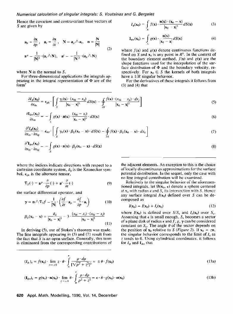
Hence the covariant and contravariant base vectors of S are given by Z&o) = J-f(x)

s

n(x) f (x0 - xl Ix0 - xl3 dS(x) (3)

8X aP=--,

aP a, = e

at ’ N=ap/\a,, n=N

IN

I+,(%) = J g(x) . fi dS(x) (4) S

(2)

ap = L.(ar//N), a’ = -L*(apAN) lNl2 INI

where N is the normal to S. For three-dimensional applications the integrals ap-

pearing in the integral representation of @ are of the form’

where f(x) and g(x) denote continuous functions defined on S and x0 is any point in R3. In the context of the boundary element method, f(x) and g(x) are the shape functions used for the interpolation of the surface distribution of Q and the boundary velocity, respectively. For x0 E S the kernels of both integrals have a l/R singular behavior.

For the derivatives of these integrals it follows from (3) and (4) that

a4dxo) - = %k ’ U Yjtx) ’ CXOk - xk)

ax0i s I% - xl3 dScx) _ $ f(X) * ~~~~x~~) . “1

as

a#m (x0) -= - axoi I g(x) . n(x). k: ‘$ * dS(x)

s

(5)

(6)

a%(~) dXoi * dXoj

= Eik/ ’ Y&d * ~&a - X) . dS(x) - 4 f(x) . p/jbo - x) * dXk

I (7)

J as

a%, (x0) = - axoi - axoj / g(x) . n(x) . P&O

s - x) . dS(x)

where the indices indicate directions with respect to a Cartesian coordinate system, 6, is the Kronecker sym- bol, Eijk is the alternate tensor,

V,(s) = ap.i(.) + al-$(*)

the surface differential operator, and

(10)

&(x0 - x) = & - 3. CxOi - xi) * (XOj - +jl

1x0 - XI5 (11)

In deriving (5), use of Stokes’s theorem was made. The line integrals appearing in (5) and (7) result from the fact that S is an open surface. Generally, this term is eliminated from the corresponding contributions of

(8)

the adjacent elements. An exception to this is the choice of locally discontinuous approximations for the surface potential distribution. In the sequel, only the case with no line integral contribution will be examined.

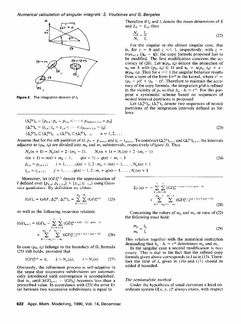
Relatively to the singular behavior of the aforementioned integrals, let %(x0, E) denote a sphere centered at x0 with radius E and S, its intersection with S. Hence any surface integral Z(xo) defined over S can be de- composed as

Z(x0) = Z(x0) + Z&o) (12)

where Z(xo) is defined over S/S, and I&,) over S,. Assuming that E is small enough, S, becomes a sector of a plane disk of radius E and f, g, y can be considered constant on S,. The angle 8 of the sector depends on the position of x0 relative to S (Figure 2). If x0 = zn, the singular behavior corresponds to the limit of I, as z tends to 0. Using cylindrical coordinates, it follows for Z+ and I,, that

(13b)

620 Appt. Math. Modelling, 1990, Vol. 14, December


Concerning the first derivatives of I+, and I,,, the term responsible for the singular behavior gives

I

(cos 13 - 1). lim (log 2~ - 1 - log 1~1) i= 1

]im [ ,xoi - “1 dS = z-*,1

-sin 8 * lim (loa2~ - 1 - log 1~1) i=2 (14)

i=3

Therefore they all exist only for interior to S points (6 = 259. For points along the boundary of S the derivatives with respect to xl- and x2-directions contain a logarithmic singularity. The corresponding singular terms are cancelled from the contributions of the adjacent elements provided that the flow boundary is smooth. For the second derivatives of I, and I,,, following a similar approach, a I/[z~ singularity appears even for interior points. Of course, the deformation field is never calculated for z, = 0. The only possible case that might present difficulties is that of a vortex particle approaching the solid boundary. In this case the singularity is cancelled by the cutoff function introduced to render the deformation field finite.’

In the sequel the two methods proposed are presented. For the self-adaptive method the integrals in expressions (3)-(8) are written with respect to cur- vilinear coordinates p and f. Owing to the fact that dS(x) = IN(p, t)l dp dt, the general form of all integrals is

(15)

The integration schemes

The self-adaptive fully numerical method

The self-adaptive fully numerical method proposed is a copy formula based on Gaussian quadrature rules. To construct copy formulas, at first a Gaussian quadrature rule is selected. For double integrals, if L, and L, are the number of integration points for the two integrations, the formula derived takes the form

1 1

where (ti, wf), i = l(l)L,and (nj, wj”), j = I(l)L, denote the abscissas and weight coefficients.

To define copy formulas, the integral

defined over 1R as in (1) is considered. Let %(Ln) denote a repartition of fl into rectangular subsets, that is,

g(n) = W, = M,P51 x [G, Gl, e = l(l)E} (18)

with 1R = U,LR, and Sz, fl a,, = 0 for every e # e’. The simplest choice possible is the one based on partitions of the integrations intervals. Let A? and A;Y denote two partitions defined by

A~={(P~:P~=P,<...<PN~+,=P~}

A;Y’={t,:t,=r,<...<r,,+,=tp} (19)

resulting in elements of the form fin(k,lJ = [pk, pk+ 1] x

It,, t,+ 11. Consequently, if a L&L, Gaussian quadrature rule

is applied for every a,, the following copy formula is derived:

Z(F; a) = GI(F; A?, A;“‘)

= ; $ /$’ 2 hj” 2 w’ 2 ~7 . Fk,(t;, ,-,j)

k-1 /=I i-l J=I

where

Fk,(& 7) = F(P’~‘(~) f(‘)(v)) 7

(20)

h’k’

hhk’=P,+, -Pk p’k’(t) = -!L. 5 + Pk + Pktl

2 2 ’ ‘EEL-1,11,

hj” t”‘(V) = - . 77 +

I/ + I/+ I 2 2 ’ TE[-l,ll, hj” = t,, , - t,

(21)

Since S is curved, in order to produce good ap- giving good approximations but also permitting a sys- proximations of the integrands it is advisable to select tematic construction of local refinements. As a result partitions that produce almost uniform integration grids. the computational effort required is kept to a minimum, This choice is computational simple to handle, not only since repetitions of a large part of calculations is avoided.

Appl. Math. Modelling, 1990, Vol. 14, December 621


Therefore if lP and 1, denote the mean dimensions of S and L, = L,, then

N 1 P=B N, 1,

(22)

For the singular or the almost singular case, that is, for z = 0 and z << 1, respectively, with z, = max,,s (Ix0 - xl), the copy formula proposed has to be modified. The first modification concerns the accuracy of (20). Let x(pO, to) denote the projection of x0 on S with (pa, ro) E R and x0 = x(po, to) + E . n(po, to). Thus for E << 1 the singular behavior results from a term of the form l/r” in the kernel, where r2 = (pa - p)2 + (to - t)2. Therefore to maintain the accuracy of the copy formula, the integration grid is refined

E in the vicinity of pa so that h, . h, = r”‘. For this pur-

Figure 2. The integration domain of 1, pose a systematic scheme based on sequences of nested interval partitions is proposed.

Let (AT),, (A?),, denote two sequences of nested partitions of the integration intervals defined as follows:

(A?), = {~/‘,n: pa = PI,~ < . . . <PAM,)+ i,n = pp>

W% = kn : t, = r~,n < . . . < Tut+ 1.n = t,d (23)

(A,““), c (A,““), + 1, CAY% c W’% + I, n= 1,2,...

Assume that for the nth partition of a, pa = puCn),,, and lo = rq(n),n. To construct (A,““),, 1 and (A;“‘),,. 1, the intervals adjacent to (pa, to) are divided into mP and m, subintervals, respectively (Figure 3). Thus

N,(n + 1) = N,(n) + 2. (m, - l), N,(n + 1) = N,(n) + 2. (m, - 1)

u(n+ l)=u(n)+m,- 1, q(n + 1) = q(n) + m, - 1 (24)

Pi,n = Pi,” + 17 i= 1 . . 9 u(n)- 1,2.m,+u(n)- l,...,N,,(n)+ 1

fj,n = fj.n + I ; j= 1,::. ,q(n)-1,2*m,+q(n)-l,..., N,(n)+1

Moreover, let (GZ), W) denote the approximation of Z defined over [P& pkt ,,,I x [TV,; h+ l,nl using Gaus- sian quadrature. By defimtion we obtain

(GZ), = GZ(F, A,N, A?),, = 2 2 (GZ)ik,” (25) k=I /=I

as well as the following recursion relation:

(GZ), + I = (GZ), _ $ $ (GZ)~k+U(“)-‘.l+q(“)~‘)

k=Ol=O

m,-I ml-1

+ c 2 (GZ)lfi++P(n+I),(+q(n+l)) (26)

k= -m,l= -m,

In case (pa, to) belongs to the boundary of fl, formula (25) still holds, provided that

(GZ)kks[’ = 0 7 k>N&), 1> Nth) (27)

Obviously, the refinement process is self-adaptive in the sense that successive subdivisions are automati- cally introduced until convergence is accomplished, that is, until ](GZ),+i - (GZ),] becomes less than a prescribed value. In accordance with (25) the error Er (n) between two successive subdivisions is equal to

Er(n) = _ 2 $ (GZ)~k+U(fl)-l.I+q(“)~I)

k=O/=O

ml,-I ml-1

+ x C (G#k;,u(n+ I).l+q(n+ 1))

k= -m,l= -WI, (28)

Concerning the values of m,, and m,, in view of (22) the following must hold:

!%=P 1 (29)

m, L

This relation together with the numerical restriction demanding that h, . h, = rm determines mP and m,.

In the singular case a second modification is necessary. This is due to the fact that the refined copy formula given above corresponds to Z as in (15). There- fore the limit of Z, given in (16) and (17) should be added if bounded.

The semianalytic method Under the hypothesis of small curvature a local co-

ordinate system O[x, y, z14 always exists, with respect

622 Appl. Math. Modelling, 1990, Vol. 14, December


a z

I ; I

s

b

Figure 4. Definition of z.

where

I -

s S

a 7

Figure 3. The integration grid for the fully numerical method. (a) Initial grid (NP = 3, Nr = 4); (b) refined grid (NP = Nt = 2, m p = m, = 2)

to which S is given by

z = 4k Y) = E * il& Y), (x7 Y) E so (30)

where E > 0 is a measure of the curvature of S and So is the projection of S on the plane z = 0. Thus for the normal to S it follows that

INI = 1 + O(E*) (31)

Moreover, if 5(x, y) is extended over R2, that is, 5(x, y) = 0 for (x, y) j-2 So, the coordinates of any point P can be expressed as (x0, y,, z. + l(xo, yo)) (Figure 4). Therefore the distance R from a point Q(.x, y, 5(x, y)) of S is expressed as

R* = (xo - 4’ + (YO - Y)* + (zo + LUG, Y))*

(32)

““s”;;c;tGf Y) = 5(x0, YO) - Ll’(x, ~1. = O(E), it follows from the Taylor expan-

sion of l/R that

zo.A5 *- R$ >

+ O(2) (33)

Ri; = (x0 - x)* + (y,, - y)’ + z; (34)

Next, the following approximations are introduced:

A[(x,y) = 2 cije(xo - x)‘.(yo - y)j i,j=O

fk Y) = 2 %l. (x0 - #o (Yo - Y)’ (35) k.l=O

&4x, Y) = i: bk, . (x0 - XJk. (yo - y)’ k./=O

For first-order accuracy it follows that the integrals Z+ and I+,, and their first and second derivatives are expressed as linear combinations of integrals of the form

B(kkm) = / (xo-x)k~(Yo-Y)'ds*dt

(36) &I

R,”

These expansions as well as the evaluation of B(k, I; m) are given in the Appendix.14 The integrals B(k, I; m) contain the two basic singularities (that is, the log and arctan singularity) explicitly. In the final expressions the singular terms appear exactly as in (16) and (17). Consequently, in the evaluation of the first and second derivatives of Z, and I+, for z. = 0 the singular terms must be substituted by their local limits.

In equations (35) the coefficients cij, &/, and bkl are of local character and depend on x0 and yo. This is the reason that the whole procedure must be repeated for every combination of surface element and evaluation point. Moreover, these coefficients depend on the no-



da1 values of the approximated function. To determine the coefftcients in (35), use is made of the fact that equations (35) are exact at the nodes is made. The nodal value of &x, y) and g(x, y) are given, whereas the nodal values of f(x, y) are the unknowns of the problem. Therefore the solution of two linear systems and one matrix inversion is needed. Following this procedure, the contributions of the interpolation coefficients cijr ukl, and bkl appearing in the final expressions are attributed to the nodal values of 5(x, y), f(x, y), and g(x, y), respectively.

Convergence and accuracy tests

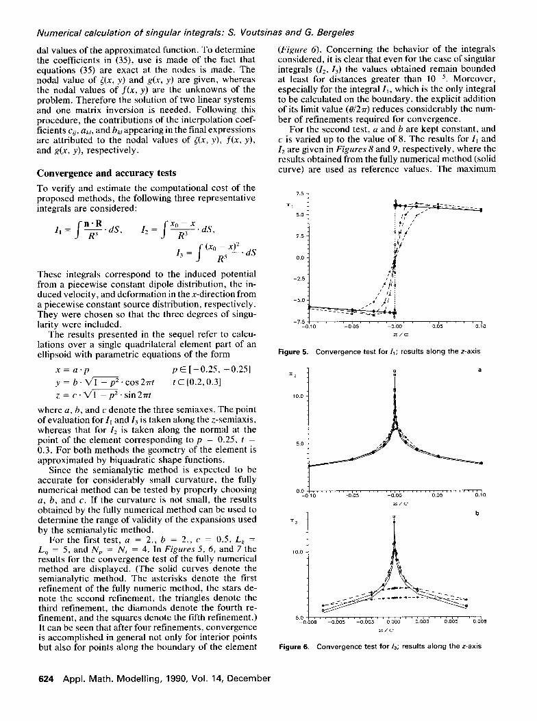
To verify and estimate the computational cost of the proposed methods, the following three representative integrals are considered:

I, = /

$dS, I* = /

7 .dS.

z 3

= (xo - x)2. dS

R5

These integrals correspond to the induced potential from a piecewise constant dipole distribution, the induced velocity, and deformation in the x-direction from a piecewise constant source distribution, respectively. They were chosen so that the three degrees of singularity were included.

The results presented in the sequel refer to calculations over a single quadrilateral element part of an ellipsoid with parametric equations of the form

x=a*p p E [ -0.25, +0.25]

y = b-m.cos2vt t E [0.2,0.31

2 = c. m. sin2*t

where a, 6, and c denote the three semiaxes. The point of evaluation for I, and Z3 is taken along the z-semiaxis, whereas that for Z2 is taken along the normal at the point of the element corresponding to p = 0.25, t = 0.3. For both methods the geometry of the element is approximated by biquadratic shape functions.

Since the semianalytic method is expected to be accurate for considerably small curvature, the fully numerical method can be tested by properly choosing a, b, and c. If the curvature is not small, the results obtained by the fully numerical method can be used to determine the range of validity of the expansions used by the semianalytic method.

For the first test, a = 2., b = 2., c = 0.5, L, = L, = 5, and NP = N, = 4. In Figures 5, 6, and 7 the results for the convergence test of the fully numerical method are displayed. (The solid curves denote the semianalytic method. The asterisks denote the first refinement of the fully numeric method, the stars denote the second refinement, the triangles denote the third retinement, the diamonds denote the fourth refinement, and the squares denote the fifth refinement.) It can be seen that after four refinements, convergence is accomplished in general not only for interior points but also for points along the boundary of the element

(Figure 6). Concerning the behavior of the integrals considered, it is clear that even for the case of singular integrals (I,, Z3) the values obtained remain bounded at least for distances greater than 10P5. Moreover, especially for the integral II, which is the only integral to be calculated on the boundary, the explicit addition of its limit value (0/2rr) reduces considerably the number of refinements required for convergence.

For the second test, a and b are kept constant, and c is varied up to the value of 8. The results for I, and Z2 are given in Figures 8 and 9, respectively, where the results obtained from the fully numerical method (solid curve) are used as reference values. The maximum

7.5 7

=1 - --“, /- -+- ---_-=--___

5.0 - /’

2.5 -

-7.5 I 1 I I I I I I I I I I I I I I 1 I -0.10 -0.05 -0.00 0.05 0.10

Z/C

Figure 5. Convergence test for I,; results along the z-axis

a

0.01.,.,.....,..,.,,,,,,.,,.,.,,,,,,,......, -0.10 -0.05 -0.00 0.05 0.10

Z/C

b

Figure 6. Convergence test for 13; results along the z-axis

624 Aool. Math. Modellina. 1990. Vol. 14. December rr

Figure 7. Convergence test for &; results along the normal to S at the corner point p = 0.25, t = 0.2

5.00 1

-I

\

3.00 , I I,, , I I,,,, ,r,, I ,,,, I ,,, I,, , 1 ,,,,I 0.0 1.0 2.0 3.0 4.0 5.0 6.0 7.0 6.0 9.0

c

Figure 8. Accuracy test for I,; results at the point p = t = 0, z/c = 10 -4 (the solid curve denotes the fully numerical method, the dashed curve denotes the semianalytic method)

error prescribed for convergence of the fully numerical method was set equal to 10p6. In both cases the distance of the point of evaluation from S is equal to 10 -‘. It is clear that as the curvature increases, the difference between the results obtained from the two methods increases as well. This means that when the semianalytic method is used, the surface grid must be con-

0.0 1.0 2.0 3.0 4.0 5.0 6.0 7.0 6.0

c

Figure 9. Accuracy test for 12; results at the corner point p = 0.25, r = 0.2, z/c = 10m4 (the solid curve denotes the fully numerical method, the dashed curve denotes the semianalytic method)


strutted so that the curvature of all elements is mod- erate.

Concerning the computational cost, the fully numerical method and the semianalytic method require approximately the same time only for points with distance from S d << 1. As the distance increases, the fully numerical method becomes faster. In Table 1 the required CPU time (in seconds) for the fully numerical method is given as a function of the number of refinements. As has already been noted for the semianalytic method, the whole procedure must be repeated for every pair (element and point of evaluation). Accord- ing to the analysis iven in Ref. 4 this is necessary for points with dl 3 A < 2.4, where A is the area of the element. For the results presented, A = 0.25. Therefore for all the control points surrounding the element the exact expressions of the semianalytic method should be used. In contrast, for the fully numerical method, time-consuming calculation is needed only for dlk’k < 0.05, as is clearly shown in Figures 5, 6, and 7. To reduce the CPU time required in the case of the semianalytic scheme, the method of multi- pole expansions given in Ref. 4 can be used.

Table 1. CPU time required for the fully numerical method (in seconds)

Number of refinements Semianalytic

Np x Nt 1st 2nd 3rd 4th 5th method

2. 2 0.5 2.5 5.0 8.0 13.0 8.0 4. 4 0.8 3.0 6.0 10.0 16.0 8.0 6, 6 1.7 4.0 7.0 12.0 17.5 8.0 8. 8 2.7 5.0 8.0 14.0 19.0 8.0



1.0 -

0.5 -

0.0 I I , I I I I, I I I I, I1 I I 0.00 0.50 1.00 1.50 2.00

x

Figure 10. Velocity distribution along the meridian in the xz- plane of an ellipsoid (a = 2., b = I., c = 0.5) for an x onset flow (the solid curve denotes the analytic solution, the squares denote the numerical results)

Concerning the memory needed, for the fully numerical method a working area of about 60K is necessary, whereas for the semianalytic method, 2K are sufficient. Compared to the total working area required (about 300K), even the 60K used by the fully numerical method represent a rather small part. For both methods the working area mentioned above is independent of the number of elements used.

Conclusions

From the preceding analysis it follows that the two methods proposed behave well and can produce equally accurate results. Of the two, the fully numerical method is faster and thus preferable. Details concerning the application of the fully numerical method to specific flow problems can be found in Ref. 15. Here, to get some idea of the efficiency of this scheme, in Figure 10 the numerical velocity distribution along the meridian of an ellipsoid is compared to the analytic one. The accuracy of the numerical solution obtained is high even for noncontrol points. The boundary element scheme used is a superparametric one, based on a 40 x 20 mesh for the geometry approximation and a 9 x 8 mesh for the approximation of the potential

surface distribution. In both approximations, biquadratic shape functions were chosen. The CPU time required for this application is 10 minutes on a XT/PC running at 8 MHz and supplied with a mathematical coprocessor.

References

4

5

6

7

8

9

10

11

12

13

14

15

Batchelor, G. K. An Introduction to Fluid Dynamics. Cam- bridge University Press, London, 1967, p. 84 Brebbia, C. A. and Walker, S. Boundary Element Techniques in Engineering. Newnes-Butterworths, London, 1980 Huberson, S. Calcul d’Ccoulements tridimensionnels instation- naires incompressibles par une mCthode particulaire. J. Mb- chanique ThPor. Appl. 1981, 3(l), 805-819 Hess, J. L. and Smith, A. M. 0. Calculation of non-lifting potential flow about arbitrary three-dimensional bodies. Rept. No. E.S. 40622, Douglas Aircraft Co.. 1962. D. 66 Webster, W. C. The filow about three-dimensidnal smooth bodies. J. Ship Res. 1975, 19(4), 206-218 Hoeijmakers, H. W. M. A panel method for determination of the aerodynamic characteristics of complex configurations in linearized subsonic or supersonic flow. N.L.R. Tech. Rept. 80124 U, 1980 Morino, L. and Kuo, C.-C. Subsonic potential aerodynamics for complex configurations: A general theory. AIAA J. 1974, 12(2), 191-197 Morino, L., Chen, L. T. and Suciu, E. 0. Steady and oscil- latory subsonic and supersonic aerodynamics around complex ConIigurations. AIAA J. 1975, 13, 368-374 Johnson, F. T., Tinoco, E. N., Lu, P. and Epton, M. A. Three- dimensional flow over wings with leading-edge vortex sepa- ration. AIAA J. 1980, 18, 367-380 Johnson, F. T. and Rubbert, P. E. Advanced panel-type influ- ence coefficient methods applied to subsonic flows. AIAA Pa- per 75-50, 1975 Mustoe, G. G. W. Advanced integration schemes over boundary elements and volume cells for two and three dimensional non-linear analysis. Developments in Boundary Element Method, Vol. 3, ed. P. K. Banerjee and S. Mukherjee. Elsevier, Am- sterdam, 1983, pp. 213-270 Pina, H. G. L., Fernandes, J. L. M. and Brebbia, C. A. Some numerical integration formulae over triangles and squares with l/R singularity. Appl. Math. Model&g 1981, 5, 209-211 Petit Bois, G. Tables of Indefinite Integrals. Dover, New York, 1961 Coulmy, G. Formulations des effets des singularit&. Rapport L.I.M.S.I., Orsay, France, 1985 Voutsinas, S. and Bergeles, G. Higher order superparametric boundary element methods for the numerical solution of three dimensional potential flows. Rept. 2189, NTUA, Laboratory of Aerodynamics, 1989

Appendix: The derivation of the semianalytic expansions

For first-order accuracy it follows from (30), (31), (33), and (36) that

N.R 1 R3=a zo + 2 c&o - x)‘(y, - y)j. l-;-:-Al

i.j=O

N -2

R - x)‘-‘(Yo - y)j-’

’ J -%I 1 -~.(Yo - Y)RO

_i.(xo - x)Ro _zo*(xo - X).(YO - Y)R; I

Using the above approximations and the fact that

j- (. . .) . dS = / (. . .) . INI . dp . dt = j- (. . .) * dp . dt S s SO


Numerical calculation of singular integrals: S. Voutsinas and G. Berg&s

after some manipulations it follows that

~0. B(k, 1; 3) + 2 cti. [( 1 - i - j) * B(k + i, 1 + j; 3) - 3 . $, . B(k + i, 1 + j; 5)]

v(&)x = i bk/ * f: Cij *

i.B(k + i,f +j;3) i.B(k + i - I,1 +j + 1;3)

k./=O i,j=O i.zo.B(k + i - 1,f +j;3) 1 v(&,,&, = i bk, . i co. [

j.B(k+i+ l,l+j- 1;3)-

j. B(k + i, f + j; 3) k.l=O i,j=O j.z,.B(k + i,f +j - 1;3)

v&m), = - i b/c, k./=O

’ [E!;:t;:s] + igo c[i [!:!I

&,Z, = 5 %q . p,q=o r

&; + 2 Ckj.s!$;g(k,I) k.l=O I

Z,x,I+n = - i b,, . Dnf; + i ck/. E@j’(k,f) P,Y’O k.l=O

U1 =(k-k.j+f.i).B(k+i- l,f+j;3)-3.k*zz.B(k+i- l,f+j;5) U,=(f-f*i+k*j).B(k+i,f+j- 1;3)-3.f.za*B(k+i,f+j- 1;.5) u, = 3 . zo . B(k + i, 1 + j; 5)

U,, = -3.zo.B(k + i + 1,1 +j;5)

U,, = -3.zo.B(k + i,f +j + 1;5)

U,,, = B(k + i,f +j;3) - 3.zi.B(k + i,l +j;5)

Of.7 = 61, .P’{-3zo[%, .B(p,q;5) + a,,. B(P - 13 4 + 1; 91 + SJ, . rap - 1,q; 3) - . . . - 3*zo*B(p - l,q;5)11+ &2*q*{-32o[~J,.B(P + I,q - 1;5) + . * . + a,, * Rp, 4; 91 + 6.n. Lap, 4 - 1; 3) - 3 . zo . lo, q - 1; 5)l) + *.. + h,.{~,,.[p.B(p - l,q;3) - 3.(P + 4).&p + l,q;5)1 + . . . + SJZ . [q. RP, q - 1; 3) - 3. (P + 4). WP, 4 + 1; 5)l + 36,, (P + q) ZOBCP, q; 5))

0 Dn”j = [I 0 . [S,, . B(p, q; 3)) - 3 * z@+J, B(p + & + S,, , q + & + S,,; 5)]

1

E~P(k,l)=3.[(pf-kq-p).B(k+p,f+q;5)+5.p.z~.B(k+p,l+q;7)]

E$‘;(k,f)=(pl-kq).[3*B(k+p- l,l+q+ 1;5)-B(k+p- l,l+q- 1;3)]- . . . -3.p.[B(k+p-l,l+q+l;5)-5.z;.B(k+p-l,f+q+1;7)]

Eyg(k, f) = 3 - z. * (pl - kq) . B(k + p - 1,1 + q; 5) - . . . - 3.p.zo.[3.B(k+p - 1,f + q;5) - 5.z;.B(k +p - 1,f + q;7)]

E:f(k,f)=(pf-kq).[3*B(k+p- l,f+q+ 1;5)-B(k+p- l,f+q- 1;3)]- . . . -3.q.[B(k+p+ l,l+q- 1;5)-5ez:,.B(k+p+ l,l+q- 1;7)]

E~~(k,f)=3.[(kq-pf-q).B(k+p,f+q;5)+5.q.z~.B(k+p,f+q;7)]

Appl. Math. Modeling, 1990, Vol. 14, December 627


E~g(k,f)=3.zo.(pl-kq).B(k+p,1+q-1;5)-

. . . -3.q.zo*[3*B(kt-p,I+q- 1;5)-5*z:,.B(k+p,l+q- 1;7)]

Ef;:(k,l)=3*z”.[p.B(k+p+ 1,I+q;5)-5.(p+q).B(k+p+ l,l+q;7)1

E~~(k,z)=3’Z~.[q~B(k+p,f+q+1;5)-5~(p+q).B(k+p,1+q+1;7)]

E;g(k,f)=3*(p+q)*[B(k+p,I+q;5)-5.z;*B(k+p,1+q+ 1;7)1

[En;j(k,1)], = k*[-&,*B(p + k - 1,q + 1;3) +

. . . + 3 . zF’~J~ . B(p + k - 1 + &r + S,, , q + 1 + & + S,,; 5)]

[Er@(k,1)], = I.[-&*B(p + k,q + I - 1;3) +

. . . + 3 . z~+J, + B(p + k + 6,! + S,, , q + 1 - 1 + & + aJz; 5)]

[E@(k, /)I_ = 15 . z@‘~JT+’ . B(p + k + &, + SJ,, q + 2 + &, + S,,; 7) - i . . . - 3. [6,J. zo . B(p + k, q + I; 5) +

. . . + Sf3 * zip . B(p + k + aJ,, q + 1 + S,,; 5) +

. . . + a,, . zp . RP + k + %I, q + 1 + 62; 5)l

In all the above expressions, indices I and J indicate coordinate directions of the O[x, y, z] system. The correspondence assumed is 1 + x, 2 * y, and 3 + z.

In relation to the calculation of B(k, I; m) it is easy to prove that they satisfy the following recursion relations:

(m - 2).E(k,l;m) = {

(k - 1). B(k - 2,l; m - 2) + Gx(k - 1,l; m - 2)

(I - l)*B(k,I - 2;m - 2) + Gy(k,f - 1;m - 2)

The terms Gx and Gy are line integrals defined over the boundary of SO, given by (Figure AI)

Y”+ I d,

Gx(k,f;m) = - c I (x0 - X”(Y))“. (Yo - Y)’

” Rb: .dy = - ~sin/3V*IF’,(k,I;m)ds

” V” 0 X”+, d,,

Gy(k, 1; m) = c I (x0 - XV. (Yo - Y”(X))’

.dx = Ccos&*~F,,(k.I:m)ds ” RI; ” xv 0

where E(. . .) denotes summation over the four sides of So,

X”(Y) = x, + (Y - Y”) . cot P”

Y Ax) = Y, + (x - x,) . tan Py

Figure Al. Notations for the calculation of Gx and Gy



Y

Figure A2. Notations for the calculation of B(0, 0; m)

denote the equations of the vth side, d, denotes its length, and

F,(k, 1; m) = ( - I)‘+‘. Cos” flu. sin/p,. (s - SO” - %“HS - SO” - av,) V(s - s,),)* + h&, + zp

The calculation of Gx and Gy is based on the following formulas:

d”

F,(k,l;m)ds= ii k . I ~(Y;,.~<,.cos~~,. 0 0

sin/p,.Ai:,t'~~i-j

0 i=Oj=O I

~~ = m

(s-Sov)p~ds=(_~)P+I. R,”

_ P-I . AP,,-_-$

m-2

x0 - X” Yo - YY ax” = ___ - SO”,

cos P” Lyy” = ___ - so,,

sin py R. = v(s - so)* + h;, + z:,

where (-) denotes the binomial coefficients. Therefore it follows that it suffices to calculate At and B(0, 0; m) for m = +l, k3, 25,. . . . The integrals A$ are given in Ref. 13, whereas the integrals B(0, 0; m) are calculated by introducing polar coordinates. I4 Thus in accordance with Figure A2 we get

B(0, 0; m) = I dq I (p’ + zg) -m’2 . p. dp ‘p +I

1 =-. “-q-j&)

( m-2 Zo"-* y 9"

vpv+*

I c?! = L . tan zo . (s - SO”) d”

Ro zo (s - so,)* + h& + z; s=o ‘pu

and cp as in Figure A2.


Numerical calculation of singular integrals appearing in three-dimensional potential flow problems

Documents

Transcript of Numerical calculation of singular integrals appearing in three-dimensional potential flow problems