Zeta integrals, Schwartz spaces and local functional equations

arX

iv:1

508.

0559

4v5

[m

ath.

RT

] 1

4 Ja

n 20

20

Zeta integrals, Schwartz spaces and local functional equations

Wen-Wei Li

http://arxiv.org/abs/1508.05594v5

Abstract

According to Sakellaridis, many zeta integrals in the theory of automorphic forms can be produced orexplained by appropriate choices of a Schwartz space of test functions on a spherical homogeneous space,which are in turn dictated by the geometry of affine spherical embeddings. We pursue this perspectiveby developing a local counterpart and try to explicate the functional equations. These constructions arealso related to the L2-spectral decomposition of spherical homogeneous spaces in view of the Gelfand–Kostyuchenko method. To justify this viewpoint, we prove the convergence of p-adic local zeta integralsunder certain premises, work out the case of prehomogeneous vector spaces and re-derive a large portionof Godement–Jacquet theory. Furthermore, we explain the doubling method and show that it fits intothe paradigm of L-monoids developed by L. Lafforgue, B. C. Ngô et al., by reviewing the constructionsof Braverman and Kazhdan (2002). In the global setting, we give certain speculations about global zetaintegrals, Poisson formulas and their relation to period integrals.

Contents

1 Introduction 3

1.1 Review of prior works . . . . . . . . . . . . . . . . . . . . . . . . . . . . . . . . . . . . . . 31.2 Our formalism . . . . . . . . . . . . . . . . . . . . . . . . . . . . . . . . . . . . . . . . . . 61.3 Positive results . . . . . . . . . . . . . . . . . . . . . . . . . . . . . . . . . . . . . . . . . . 111.4 Structure of this book . . . . . . . . . . . . . . . . . . . . . . . . . . . . . . . . . . . . . . 121.5 Conventions . . . . . . . . . . . . . . . . . . . . . . . . . . . . . . . . . . . . . . . . . . . . 13

2 Geometric background 16

2.1 Review of spherical varieties . . . . . . . . . . . . . . . . . . . . . . . . . . . . . . . . . . . 162.2 Boundary degenerations . . . . . . . . . . . . . . . . . . . . . . . . . . . . . . . . . . . . . 192.3 Cartan decomposition . . . . . . . . . . . . . . . . . . . . . . . . . . . . . . . . . . . . . . 212.4 Geometric data . . . . . . . . . . . . . . . . . . . . . . . . . . . . . . . . . . . . . . . . . . 23

3 Analytic background 26

3.1 Integration of densities . . . . . . . . . . . . . . . . . . . . . . . . . . . . . . . . . . . . . . 263.2 Direct integrals and L2-spectral decomposition . . . . . . . . . . . . . . . . . . . . . . . . 283.3 Gelfand–Kostyuchenko method . . . . . . . . . . . . . . . . . . . . . . . . . . . . . . . . . 293.4 Hypocontinuity and barreled spaces . . . . . . . . . . . . . . . . . . . . . . . . . . . . . . 31

4 Schwartz spaces and zeta integrals 33

4.1 Coefficients of smooth representations . . . . . . . . . . . . . . . . . . . . . . . . . . . . . 334.2 The group case . . . . . . . . . . . . . . . . . . . . . . . . . . . . . . . . . . . . . . . . . . 354.3 Auxiliary definitions . . . . . . . . . . . . . . . . . . . . . . . . . . . . . . . . . . . . . . . 364.4 Schwartz spaces: desiderata . . . . . . . . . . . . . . . . . . . . . . . . . . . . . . . . . . . 384.5 Model transitions: the local functional equation . . . . . . . . . . . . . . . . . . . . . . . . 414.6 Connection with L2 theory . . . . . . . . . . . . . . . . . . . . . . . . . . . . . . . . . . . 43

5 Convergence of some zeta integrals 47

5.1 Cellular decompositions . . . . . . . . . . . . . . . . . . . . . . . . . . . . . . . . . . . . . 475.2 Smooth asymptotics . . . . . . . . . . . . . . . . . . . . . . . . . . . . . . . . . . . . . . . 495.3 Proof of convergence . . . . . . . . . . . . . . . . . . . . . . . . . . . . . . . . . . . . . . . 52

6 Prehomogeneous vector spaces 54

6.1 Fourier transform of half-densities . . . . . . . . . . . . . . . . . . . . . . . . . . . . . . . 546.2 Review of prehomogeneous vector spaces . . . . . . . . . . . . . . . . . . . . . . . . . . . . 566.3 Local functional equation . . . . . . . . . . . . . . . . . . . . . . . . . . . . . . . . . . . . 596.4 Local Godement–Jacquet integrals . . . . . . . . . . . . . . . . . . . . . . . . . . . . . . . 61

7 The doubling method 66

7.1 Geometric set-up . . . . . . . . . . . . . . . . . . . . . . . . . . . . . . . . . . . . . . . . . 667.2 The symplectic case . . . . . . . . . . . . . . . . . . . . . . . . . . . . . . . . . . . . . . . 697.3 Doubling zeta integrals . . . . . . . . . . . . . . . . . . . . . . . . . . . . . . . . . . . . . . 737.4 Relation to reductive monoids . . . . . . . . . . . . . . . . . . . . . . . . . . . . . . . . . . 757.5 Remarks on the general case . . . . . . . . . . . . . . . . . . . . . . . . . . . . . . . . . . . 80

1

8 Speculation on the global integrals 82

8.1 Basic vectors . . . . . . . . . . . . . . . . . . . . . . . . . . . . . . . . . . . . . . . . . . . 828.2 Theta distributions . . . . . . . . . . . . . . . . . . . . . . . . . . . . . . . . . . . . . . . . 848.3 Relation to periods . . . . . . . . . . . . . . . . . . . . . . . . . . . . . . . . . . . . . . . . 868.4 Global functional equation and Poisson formula . . . . . . . . . . . . . . . . . . . . . . . . 90

Bibliography 94

Index 98

2

Chapter 1

Introduction

Zeta integrals are indispensable tools for studying automorphic representations and their L-functions.In broad terms, it involves integrating automorphic forms (global case) or “coefficients” of representa-tions (local case) against suitable test functions such as Eisenstein series or Schwartz–Bruhat functions;furthermore, these integrals are often required to have meromorphic continuation in some complex pa-rameter λ and satisfy certain symmetries, i.e. functional equations. These ingenious constructions areusually crafted on a case-by-case basis; systematic theories are rarely pursued with a notable exception[47], which treats only the global zeta integrals. The goal of this work is to explore some aspects of thisgeneral approach, with an emphasis on the local formalism.

1.1 Review of prior works

To motivate the present work, let us begin with an impressionist overview of several well-known zetaintegrals.

From Tate’s thesis to Godement–Jacquet theory

The most well-understood example is Tate’s thesis (1950). Consider a number field F and a Heckecharacter π : F×\A×

F → C×. Fix a Haar measure d×x on A×F and define

ZTate(λ, π, ξ) :=∫

A×F

π(x)|x|λξ(x) d×x =∏

v

ZTatev (λ, πv , ξv),

ZTatev (λ, πv , ξv) :=

∫

F×v

πv(xv)|xv |λvξv(xv) d×xv

where ξ =∏v ξv belongs to the Schwartz–Bruhat space S =

⊗′vSv of AF , and the local and global

measures are chosen in a compatible manner. The adélic integral and its local counterparts converge forRe(λ)≫ 0, and they admit meromorphic continuation to all λ ∈ C (rational in qλv for v ∤∞). When thetest functions ξ vary, the greatest common divisor of ZTate(λ, π, ·) (resp. ZTate

v (λ, πv , ·)), which exists insome sense, gives rise to the L-factor L(λ, π) (resp. L(λ, πv)). Computations at unramified places justifythat this is indeed the complete Hecke L-function for π. Moreover, the functional equation for L(λ, π)stems from those for ZTate and ZTate

v : let F = Fψ : S → S be the Fourier transform with respect to anadditive character ψ =

∏v ψv of F\AF , the local functional equation reads

ZTatev (1− λ, πv,Fv(ξv)) = γTate

v (λ, πv)ZTatev (λ, πv, ξv)

where πv := π−1v , i.e. the contragredient.

A. Weil [58] reinterpreted ZTatev (λ, π, ·) as a family of F×

v -equivariant tempered distributions on theaffine line Fv, baptized zeta distributions, and similarly for the adélic case. Specifically, ZTate

v (λ, π, ·)may be viewed as elements in HomF×

v(πv ⊗ | · |λ,S∨

v ), varying in a meromorphic family in λ. Thelocal functional equation can then be deduced from the uniqueness of such families, using the Fouriertransform. In a broad sense, the Gm-equivariant affine embedding Gm → Ga is the geometric backdropof Tate’s thesis. Convention: the groups always act on the right of the varieties.

3

Tate’s approach is successfully generalized to the standard L-functions of GL(n) by Godement andJacquet [21] for any n ≥ 1; they also considered the inner forms of GL(n). The affine embeddingGm → Ga is now replaced by GL(n) → Matn×n, which is GL(n) × GL(n)-equivariant under the rightaction x(g1, g2) = g−1

2 xg1. To simplify matters, let us consider only the local setting and drop the indexv. Denote now by S the Schwartz–Bruhat space of the affine n2-space Matn×n(F ), where F stands fora local field. Given an irreducible smooth representation π of GL(n, F ), the Godement–Jacquet zetaintegrals are

ZGJ(λ, v ⊗ v, ξ) :=∫

GL(n,F )

〈v, π(x)v〉| det x|λ− 12 +n

2 ξ(x) d×x,

v ⊗ v ∈ Vπ ⊗ Vπ, ξ ∈ S

(1.1.1)

where π still denotes the contragredient representation of π, the underlying vector spaces being denotedby Vπ, Vπ , etc. Note that we adopt the Casselman–Wallach representations, or SAF representations(abbreviation for smooth admissible Fréchet, see [5]) in the Archimedean case. The integral is convergentfor Re(λ)≫ 0, with meromorphic/rational continuation to all λ ∈ C. The shift in the exponent of | detx|ensures that taking greatest common divisor yields the standard L-factor L(λ, π) in the unramified case.Furthermore, we still have the local functional equation

ZGJv (1− λ, v ⊗ v,F(ξ)) = γGJ(λ, π)ZGJ(λ, v ⊗ v, ξ),

where F = Fψ : S ∼→ S is the Fourier transform. Note that Godement and Jacquet did not explicitly

use Weil’s idea of characterizing equivariant distributions in families.Let us take a closer look at the local integral (1.1.1) and its functional equation. The shift by − 1

2in the exponent of | detx| is harmless: if we shift the zeta integrals to λ 7→ ZGJ(λ + 1

2 , · · · ), the localfunctional equation will interchange λ with −λ and the greatest common divisor will point to L(1

2 +λ, π);the evaluation at λ = 0 then yields the central L-value, which is more natural. On the other hand, theshift by n

2 remains a mystery: the cancellation − 12 + 1

2 = 0 in the case n = 1 turns out to be just a happycoincidence.

What is the raison d’être of n/2 here? Later we shall see in the discussion on L2-theory that thisamateurish question does admit a sensible answer.

The doubling method

In [17, 39], Piatetski-Shapiro and Rallis proposed a generalization of Godement–Jacquet integrals forclassical groups, called the doubling method. For ease of notations, here we consider only the caseG = Sp(V ) over a local field F , where V is a symplectic F -vector space. Doubling means that we takeV := V ⊕ (−V ) where −V stands for the F -vector space V carrying the symplectic form −〈·|·〉V , sothat G×G embeds naturally into G := Sp(V ). The diagonal image of V is a Lagrangian subspace ofV , giving rise to a canonical Siegel parabolic P ⊂ G. It is shown in [17] that P ∩ (G×G) = diag(G)and G embeds equivariantly into P\G as the unique open G×G-orbit.

There is a natural isomorphism σ : Pab∼→ Gm. Given a continuous character χ : Pab(F )→ C×, one

can form the normalized parabolic induction IG

P (χ ⊗ |σ|λ) for λ ∈ C. The doubling zeta integral ofPiatetski-Shapiro and Rallis takes the form

Zλ(λ, s, v ⊗ v) =∫

G(F )

sλ(x)〈v, π(x)v〉dx, Re(λ)≫ 0

where π is an irreducible smooth representation of G(F ), v ⊗ v ∈ π ⊗ π and sλ is a good section inIG

P (χ⊗ |σ|λ) varying meromorphically in λ. In loc. cit., unramified computations show that these zetaintegrals point to L(1

2 +λ, χ× π). Furthermore, one still obtains a parametrized family of integrals thatadmits meromorphic/rational continuation and functional equations. These properties are deduced fromthe corresponding properties of suitably normalized intertwining operators for IG

P (χ⊗ |σ|λ).It is explained in [17] that the doubling method actually subsumes the Godement–Jacquet integral

as a special case. In comparison with the prior constructions, here the compactification G → P\G

replaces the affine embedding GL(n) → Matn×n, and the good sections sλ ∈ IG

P (χ ⊗ |σ|λ) replaceSchwartz–Bruhat functions. The occurrence of matrix coefficients in both cases can be explained by thepresence of the homogeneous G×G-space G; this will be made clear later on.

4

On the contrary, Braverman and Kazhdan [12] reinterpreted the doubling method à la Godement–Jacquet, namely by allowing χ to vary and by replacing the good sections sλ by functions from someSchwartz space S(XP ), where XP := Pder\G is a quasi-affine homogeneous G-space; elements fromS(XP ) may be viewed as universal good sections. The embedding in question becomes Pab ×G → XP

which is Pab ×G×G-equivariant. This turns out to be closely related to the theory of L-monoids to bediscussed below. See also [20].

Braverman–Kazhdan: L-monoids

In [11], Braverman and Kazhdan proposed a bold generalization of Godement–Jacquet theory that shouldyield more general L-functions. To simplify matters, we work with a local field F of characteristic zeroand a split connected reductive F -groupG; the L-factor in question is L(λ, π, ρ), where π is an irreduciblesmooth representation of G(F ) and ρ : G→ GL(N,C) is a homomorphism of C-groups. The basic ideais to generalize (GL(n) → Matn×n, det) into (G → Xρ, detρ), where• detρ : G→ Gm is a surjective homomorphism, dual to an inclusion C× → G, and we assume thatρ(z) = z · id for each z ∈ C×;• Xρ is a normal reductive algebraic monoid with unit group G, constructed in a canonical fashion

from ρ, so that G → Xρ is a G×G-equivariant open immersion;• furthermore, we assume that detρ extends to Xρ → Ga such that det−1

ρ (0) equals ∂Xρ := Xρ rG(set-theoretically at least).

Given these data, one forms the zeta integral∫G(F ) ξ(x)〈v, π(x)v〉| detρ(x)|λ dx as before, except that ξ

is now taken from a conjectural Schwartz space S attached to (G, ρ). Expectations include(i) C∞

c (G(F )) ⊂ S ⊂ C∞(G(F )) is G×G(F )-stable;(ii) these zeta integrals should converge for Re(λ)≫ 0 and admit meromorphic/rational continuations;(iii) in the unramified situation, there should be a distinguished element ξ ∈ S, called the basic function

for Xρ, whose zeta integral yields L(λ, π, ρ) (or with some shift in λ, cf. the previous discussions);(iv) upon fixing an additive character ψ, there should exist a Fourier transform Fρ : S → S, which

fits into the local functional equation as in the Godement–Jacquet case, and preserves the basicfunction.

By [11], prescribing Fρ is equivalent to prescribing the γ-factor γ(λ, π, ρ) that figures in the conjecturallocal functional equation. Furthermore, in the global setting one may form the adélic Schwartz space asa restricted ⊗-product S =

⊗′vSv using the basic functions, and one expects a “Poisson formula” for

Fρ, at least when ξv ∈ C∞c (G(Fv)) for some v.

The idea of embedding G into a reductive monoid to produce L-factors is then refined by L. Lafforgue[33] and B. C. Ngô [38], leading up to the concept of L-monoids. The precise definition of S is expectedto come from the geometry of Xρ. This is illustrated by the following idea of Ngô: in the unramifiedsetting, the values of the basic function ξ

v is expected to come from the traces of Frobenius of someversion of IC-complex on the formal arc space of Xρ, upon passing to the equal-characteristic setting.The main difficulty turns out to be the singularity of Xρ. We refer to [38, 9] for further discussions anddevelopments in this direction.

In [33], L. Lafforgue is able to define S using the Plancherel formula for G, whose elements are calledfunctions of L-type in [33, Définition II.15], and the Fourier transform Fρ also admits a natural definitionin spectral terms. The crucial premise here is to have the correct local factors L(λ, π, ρ), ε(λ, π, ρ) for πin the tempered dual of G(F ).

Integral representations and spherical varieties

The group G endowed with G ×G-action is just an instance of homogeneous spaces, called the “groupcase”. Many basic problems in harmonic analysis, such as the L2-spectral decomposition, can be for-mulated on homogeneous spaces, and a generally accepted class of spaces is the spherical homogeneousspaces. Indeed, this can be justified from considerations of finiteness of multiplicities [31] and the workof Sakellaridis–Venkatesh [48]. Assume G split. A G-variety X is called spherical if it is normal with anopen dense Borel orbit.

In [47], Sakellaridis proposed to understand many global zeta integrals in terms spherical homogeneousG-spaces X+ and their affine equivariant embeddings X+ → X . As in [11, 12], his construction relieson a conjectural Schwartz space S =

⊗′vSv, whose structure is supposed to be dictated by the geometry

5

of X . Specifically, the restricted ⊗-product is taken with respect to basic functions ξv ∈ Sv at each

unramified place v. Notice that these functions are rarely compactly supported and they should berelated to L-factors (cf. [45]). His construction subsumes many known global zeta integrals by using thesetting of “preflag bundles”.

As in the predecessors [10, 12], the Schwartz spaces and basic functions here are partly motivatedby the geometric Langlands program. For example, the basic functions in loc. cit. are closely related tothe IC-sheaves of Drinfeld’s compactification BunP of the moduli stack BunP over a smooth projectivecurve over some Fq, where P ⊂ G is a parabolic; it arises in the study of geometric Eisenstein series andprovides a global model of the singularities of local spaces in question.

Other integrals

There are other sorts of zeta integrals that emerged in the pre-Langlands era, many of them have directarithmetic significance. We take our lead from the local Igusa zeta integrals: let F be a local field ofcharacteristic zero, X be an affine space over F with a prescribed additive Haar measure on X(F ), andf ∈ F [X ]. Pursuing the ideas of Gelfand et al., Igusa considered

∫

X(F )

ξ(x)|f(x)|λ dx, ξ ∈ S(X(F ))

where S(X(F )) stands for the Schwartz–Bruhat space of X(F ), and the integral converges wheneverRe(λ) > 0. It turns out that this extends to a meromorphic/rational family in λ of tempered distributions,also known as complex powers of f as it interprets |f |λ as a tempered distribution for all λ away fromthe poles. An extensive survey can be found in [25].

To bring harmonic analysis into the picture, we switch to the case of a reductive prehomogeneousvector space (G, ρ,X), where G is a split connected reductive group, ρ : G → GL(X) is an algebraicrepresentation — thus G acts on the right of X — and we assume there exists an open G-orbit X+ in X .To simplify matters, let us suppose temporarily that ∂X := XrX+ is the zero locus of some irreduciblef ∈ F [X ], then such f is unique up to F× and defines a relative invariant, i.e. f(xg) = ω(g)f(x) foran eigencharacter ω ∈ X∗(G) := Hom(G,Gm). These prehomogeneous zeta integrals along with theirglobal avatars have been studied intensively by M. Sato, T. Shintani and their school; we refer to [49, 27]for detailed surveys.

In comparison with the local Godement–Jacquet integrals, corresponding to the case G := GL(n) ×GL(n), X := Matn×n and f := det, a natural generalization is to replace Igusa’s integrand |f |λξ byϕ(v)|f |λξ, where ϕ ∈ Nπ := HomG(F )(π,C∞(X+(F ))) and v ∈ π, where π is an irreducible smooth rep-resentation of G(F ); the function ϕ(v) is called a (generalized) coefficient of π in X+. In the Godement–Jacquet case we have dimNπ ≤ 1, with equality if and only if π ≃ σ ⊠ σ for some σ, in which caseNπ is generated by the matrix coefficient v ⊗ v 7→ 〈v, σ(·)v〉. This approach is pioneered by Bopp andRubenthaler [7] in a classical setting. The upshot here is to have a good understanding of the harmonicanalysis on X+(F ), including the asymptotics for the coefficients ϕ(v).

1.2 Our formalism

More general zeta integrals

Over a local field F of characteristic zero, we synthesize the previous constructions by considering• G: a split connected reductive F -group,• X+: an affine spherical homogeneous G-space, and• X+ → X : an equivariant open immersion into an affine spherical G-variety X .As in the prehomogeneous zeta integrals, we wish to be able to “twist” the functions on X+(F ) by

complex powers of some relative invariants. To this end we introduce Axiom 2.4.3. Roughly speaking,its content is:

(A) the G-eigenfunctions in F (X) = F (X+) span a lattice Λ, and the eigenfunctions in F [X ] generatea monoid ΛX in Λ, we require that ΛX,Q := Q≥0ΛX is a simplicial cone in ΛQ := QΛ;

(B) take minimal integral generators ω1, . . . , ωr of ΛX,Q with eigenfunctions (i.e. relative invariants)f1, . . . , fr (unique up to F×), we require that their zero loci cover ∂X .

6

We may define• the continuous character |ω|λ =

∏ri=1 |ωi|

λi of G(F ), and• the |ω|λ-eigenfunction |f |λ =

∏ri=1 |fi|

λi on X+(F )for λ =

∑ri=1 λiωi ∈ ΛC := ΛQ ⊗ C. We have r = 1 in most classical cases.

Let us turn to harmonic analysis. The guiding principle here is to set the L2-theory as our background.Specifically, we consider functions on X+(F ) with values in a G(F )-equivariant vector bundle E endowedwith a G(F )-equivariant, positive definite hermitian pairing

E ⊗ E → L

where L stands for the density bundle on X+(F ). Sections of L , called the “densities” on X+(F ), arefunctions that carry measures: their integrals are canonically defined provided that a Haar measure onF is chosen, say by fixing a non-trivial unitary character ψ of F . Densities can be expressed locally asφ|ω| where φ is a C∞-function and ω is an algebraic volume form. The typical choice of E is the bundle

of half-densities L12 , whose local sections take the form φ|ω|

12 . Indeed, we have L

12 = L

12 together

with an isomorphism L12 ⊗L

12

∼→ L , which we shall denote simply by multiplication. Note that L

and L12 are often equivariantly trivializable, but we shall refrain from doing so; the benefit will be seen

shortly.Define

C∞(X+) := C∞(X+(F ),E ) ≃ C∞(X+(F ),E ∨ ⊗L ),

C∞c (X+) := C∞

c (X+(F ),E ),

L2(X+) := L2(X+(F ),E ).

The formalism of densities implies that G(F ) acts canonically on all these spaces, and L2(X+) becomesa unitary representations of G(F ). Equipping C∞(X+) and C∞

c (X+) with natural topologies, theybecome smooth continuous G(F )-representations. All topological vector spaces in this work are locallyconvex by assumption.

Given an irreducible smooth representation π of G(F ), taken to be an SAF representation forArchimedean F , we define Nπ := HomG(F )(π,C∞(X+)) (the continuous Hom). To achieve this, πhas to be viewed as a continuous representation for all F . This is unavoidable in the Archimedean case,whereas in the non-Archimedean case it can be naturally done by introducing the notion of algebraictopological vector spaces (Definition 4.1.1).

At this stage, we incorporate the basic Axiom 4.1.9 that asserts

dimNπ < +∞ for all π,

which has been established in many cases. Note that the representations with nonzero Nπ are the basicobjects in the harmonic analysis over X+(F ). Write πλ := π ⊗ |ω|λ for λ ∈ ΛC. Upon fixing a choice off1, . . . , fr, elements of Nπ may be twisted by ΛC by

Nπ∼−→ Nπλ

ϕ 7−→ ϕλ := |f |λϕ.

The Schwartz space S is taken to be a subspace of C∞(X+(F ),E ) ∩ L2(X+) in which C∞c (X+)

embeds continuously; moreover S should be a smooth continuous G(F )-representation. The desired zetaintegrals take the form

Zλ,ϕ(v ⊗ ξ) =∫

X+(F )

ϕλ(v)ξ∈L

, v ∈ π, ξ ∈ S, ϕ ∈ Nπ,

which is required to converge for λ ∈ ΛC, Re(λ) ≫X

0, the latter notation meaning that λ =∑r

i=1 λiωi

with Re(λi)≫ 0 for all i. The analogy with the local zeta integrals reviewed before should be evident.The precise requirements on S and Zλ are collected in Axiom 4.4.1. Below is a digest.

• The topological vector space S is required to be separable, nuclear and barreled. We will see theuse of nuclearity when discussing the L2-theory; being barreled implies that S∨ is quasi-completewith respect to the topology of pointwise convergence, which is used to address continuity aftermeromorphic continuation.

7

• Set Sλ := |f |λS, endowed with the topology from S. We assume that when Re(λ) ≥X

0, we still

have the inclusion Sλ → L2(X+) that is continuous with dense image. Furthermore, the family ofembeddings αλ : S → L2(X+), given by αλ(ξ) = |f |λξ for Re(λ) ≥

X0, is required to be holomorphic

in a weak sense. Again, these properties are motivated by L2 considerations.

• In the Archimedean case, functions from S should have rapid decay on X(F ) upon twisting bysome |f |λ0 ; here the rapid decay is defined in L2 terms, and we defer the precise yet tentativedefinition to §4.3. In the non-Archimedean case, we assume that the closure of Supp(ξ) in X(F )is compact for each ξ ∈ S.

• The zeta integrals Zλ,ϕ above are assumed to be convergent and separately continuous for Re(λ)≫X

0, and admit meromorphic (rational for non-Archimedean F ) continuation to all λ ∈ ΛC.

An often overlooked point in the literature is that the meromorphically continued zeta integrals are stillseparately continuous off the poles, by a principle from Gelfand and Shilov [18, Chapter I, A.2.3] relyingon the quasi-completeness of S∨. Available tools from functional analysis [8, III] imply that the G(F )-invariant bilinear form Zϕ,λ : πλ ⊗ S → C is hypocontinuous off the poles, which essentially means thatit induces a continuous intertwining operator πλ → S∨, where S∨ carries the strong topology. Weil’svision of zeta distributions [58] is therefore revived.

Local functional equation

Let T denote the space of characters |ω|λ, λ ∈ ΛC. Define O to be the space of holomorphic (regularalgebraic when F is non-Archimedean) functions on T and put K := Frac(O). Let π be an irreduciblesmooth representation of G(F ). Granting Axiom 4.4.1, the zeta integrals induce a K-linear injection

Tπ : Nπ ⊗K → Lπ

where Lπ stands for the K-vector space of “reasonable” meromorphic families of invariant pairings πλ ⊗S → C parametrized by λ ∈ ΛC. Now consider two affine spherical embeddings X+

i → Xi under G,with lattices of eigencharacters Λi (i = 1, 2), each satisfying the aforementioned conditions with givenSchwartz spaces Si. The motto here is:

Intertwining operator F : S2 → S1 99K local functional equation.

In this work we call such an F a model transition, a term borrowed from Lapid and Mao [34]. Forsimplicity, let us assume Λ1 = Λ2 so that X+

1 , X+2 share the same objects O and K. Pulling back by

F gives rise to a natural isomorphism F∨ : L(1)π

∼→ L

(2)π for every π. Definition 4.5.2 says that the local

functional equation attached to π and F , if it exists, is the unique K-linear map γ(π) that renders thefollowing diagram commutative.

L(1)π L

(2)π

N(1)π ⊗K N

(2)π ⊗K

F∨

γ(π)

This formalism is compatible with the local functional equations in the cases of Godement–Jacquet,Braverman–Kazhdan, etc., where the spaces Nπ are at most one-dimensional and we retrieve the usual γ-factors. For prehomogeneous vector spaces, we recover the γ-matrices when π is the trivial representation;see for example [49].

The existence of γ(π) is by no means automatic. However, it can be partly motivated by the L2-theoryif we assume that F extends to an isometry L2(X+

2 ) ∼→ L2(X+

1 ); see below.

L2-theory

The decomposition of the unitaryG(F )-representation L2(X+) is a classical concern of harmonic analysis.The abstract Plancherel decomposition gives an isometry

L2(X+) ≃∫ ⊕

Πunit(G(F ))

Hτ dµ(τ) (1.2.1)

8

where Πunit(G(F )) stands for the unitary dual, Hτ is a τ -isotypic unitary representation on a separableHilbert space, and µ is the corresponding Plancherel measure on Πunit(G(F )). The abstract theory sayslittle beyond the existence and essential uniqueness of such a decomposition. The refinements hinge onusing finer spaces of test functions on X+(F ).

According to an idea of Gelfand and Kostyuchenko [19, Chapter I] (see also [36]), later rescued fromoblivion by Bernstein [6], the scenario here is to seek a separable topological vector space S with acontinuous embedding α : S → L2(X+) of dense image, such that there exists a family of intertwiningoperators ατ : S → Hτ such that α =

∫ ⊕ατ dµ(τ); in this case we say α is pointwise defined. As a

motivating example, recall the classical study of L2(R) under R-translations. For the unitary characterτ(x) = e2πiax of R, the required map ατ amounts to the usual Fourier transform evaluated at a, well-defined only for functions of rapid decay on R. This is the starting point of classical Fourier analysis.

Coming back to the homogeneous G-space X+ satisfying the previous axioms, the minimalist choiceof S is C∞

c (X+) or the Schwartz space à la Harish-Chandra C (X+) [6, 3.5 Definition]; the fact that α ispointwise defined is established in loc. cit. Loosely speaking, given (1.2.1), specifying S → L2(X+) to-gether with (ατ : S → Hτ )τ∈Πunit(G(F )) amounts to a refined Plancherel decomposition. Harish-Chandra’stheory is a highly successful instance for the group case, so are Sakellaridis–Venkatesh [48] for wavefrontspherical homogeneous spaces over non-Archimedean F and the works by van den Ban, Schlichtkrull,Delorme et al. for real symmetric spaces, just to mention a few.

Write Hτ = τ⊗Mτ whereMτ is equipped with the trivial G(F )-representation. Following [6], we willexplain in §3.3 that the dual Hilbert space M∨

τ injects into HomG(F )(S, τ), which is in turn embeddedinto HomG(F )(π,S∨) by taking adjoint, where π := τ∞ denotes the smooth part of the complex-conjugateτ . Furthermore, it is shown in [6] that

HomG(F )(C∞c (X+), τ) ≃ HomG(F )(π,C

∞(X+)) = Nπ.

Therefore the L2 theory is connected to the “smooth theory”, i.e. the study of Nπ, the coefficients, etc.Our proposal is to understand the Schwartz space S in zeta integrals from the same angle. The first

task is to show α : S → L2(X+) is pointwise defined. The Gelfand–Kostyuchenko method asserts thatit suffices to assume S nuclear. This result was stated in [19, Chapter I, 4] and [36, Chapter II, §1] inslightly different terms; we will give a quick proof in §3.3 based on [6]. The advantage of working withgeneral S is as follows.

1. Consider two homogeneous spaces X+1 , X+

2 together with an isomorphism F : L2(X+2 )

∼→ L2(X+

1 )of unitary G(F )-representations. One infers that the same Plancherel measure may be used for bothsides. On the other hand, the comparison of refined Plancherel decompositions depends cruciallyon the choice of test functions.

2. It is known that F disintegrates into isometries η(τ) :M(2)τ

∼→M

(1)τ between multiplicity spaces.

If F restricts to a continuous isomorphism S2∼→ S1 between given Schwartz spaces, then η(τ)∨

is restricted from F∗ : HomG(F )(S1, τ)∼→ HomG(F )(S2, τ). For studying η(τ) (thus F), the main

hurdle is to understand the spaces HomG(F )(Si, τ) ⊂ HomG(F )(π,S∨i ) together with the image of

M(i),∨τ therein.

3. The spaces N (1)π and N (2)

π are relatively easier to cope with, but F seldom preserves C∞c . Omitting

indices, the problem may thus be reformulated as follows: how to pass from Nπ to HomG(F )(π,S∨)

in a manner that respects the embeddings of M∨τ ? The situation is complicated by the non-

injectivity of S∨ → C∞c (X+)∨ ⊃ C∞(X+), since C∞

c (X+) is rarely dense in S.

4. Our tentative answer is to relate them via meromorphic continuation, more precisely, by zetaintegrals. We contend that the restriction of γ(π) : N

(1)π ⊗K → N

(2)π ⊗K to the images of M(i),∨

τ

can be evaluated at λ = 0, for µ-almost all τ , and it gives η(τ)∨.

The heuristics here is that upon twisting a coefficient ϕ(v) by |f |λ, where ϕ ∈ Nπ , v ∈ π andRe(λ)≫

X0, it will decrease rapidly towards ∂X , thus behaves like an element of S∨. We are still unable

to obtain complete results in this direction, but we can partially justify some special cases, including thenon-Archimedean Godement–Jacquet case, under

9

• a condition (4.6.7) of generic injectivity of the restriction map

HomG(F )(πλ,S∨)→ HomG(F )(πλ, C

∞c (X+)∨);

• a technical condition (4.6.6) which may be regarded as a parametrized Gelfand–Kostyuchenkomethod; unfortunately, the author is not yet able to establish this property.

Recall that in the case of L-monoids (Braverman–Kazhdan), Lafforgue’s work [33] turns the pictureover by taking the local factors and Harish-Chandra’s Plancherel formula as inputs, and produces theSchwartz functions and the Fourier transform in spectral terms. On the contrary, our approach startsfrom a function space S and outputs a refined spectral decomposition for L2. These two approachesshould be seen as complementary.

To conclude the discussion, let us revisit the local Godement–Jacquet integral (1.1.1). Fix an ad-ditively invariant volume form η 6= 0 on Matn×n so that |Ω| := | det |−n|η| gives a Haar measure onGL(n, F ). Let π be an irreducible smooth representation of GL(n, F ). According to the formalism abovewith E = L

12 , one should consider the integration of the following smooth sections of L

12 , multiplied

by | det |λ:• coefficients ϕ(v ⊗ v) = 〈v, π(·)v〉|Ω|

12 where v ⊗ v ∈ π ⊠ π, against

• a Schwartz–Bruhat half-density ξ = ξ0|η|12 on Matn×n(F ), where ξ0 is a Schwartz–Bruhat function

on Matn×n(F ). This is a reasonable candidate of L12 -valued Schwartz space on Matn×n(F ) since

the bundle L12 extends naturally to Matn×n(F ), and it is contained in L2(GL(n)) = L2(Matn×n).

When F is Archimedean, this coincides with the Schwartz space S(Matn×n(F ),L12 ) of [1, Defini-

tion 5.1.2].Since |η|

12 = | det |

n2 |Ω|

12 , the zeta integral Zλ,ϕ((v ⊗ v)⊗ ξ) equals

∫

GL(n,F )

〈v, π(·)v〉ξ0| det |λ+n2 |Ω| = ZGJ

(λ+

1

2, v ⊗ v, ξ

).

This explains the shift by n2 in (1.1.1). Another bonus is that the Schwartz–Bruhat half-densities behave

much better under Fourier transform, see §6.1.

On the global case

Our brief, speculative treatment of the global setting in §8 is largely based on [47, §3]; however, extra careis needed to deal with functions with values in a bundle. Let F be a number field and A := AF , considera split connected reductive F -group G and an affine spherical embedding X+ → X of G-varieties overF , satisfying Axiom 2.4.3 with everything defined over F . Furthermore, assume that the lattice Λ andthe monoid ΛX coincide with their local counterparts at each place v of F . Choose relative invariants fiover F with eigencharacters ωi as in the local case, so that |f |λ, |ω|λ make adélic sense.

Suppose that the Schwartz spaces Sv ⊂ L2(X+v ) are given at each place v, say with values in a

G(Fv)-equivariant vector bundle Ev. We need two ingredients.

1. The choice of basic vectors (Definition 8.1.1, called basic functions in [47]) ξv ∈ S

G(ov)v for almost

all v ∤∞, at which our data have good reduction. One can then define S :=⊗′

vSv and E :=⊗′

vEv

(a bundle over X+(A)) with respect to ξv . Let L denote the density bundle on the adélic space

X+(A), and similarly for L12 , we require that the local pairings patch into a well-defined E ⊗E →

L ; morally, this is a condition about the convergence of infinite products of local measures.

2. Suppose that a system of global “evaluation maps” (evγ : S → C)γ∈X+(F ) is given, subject tosuitable equivariance properties (Hypothesis 8.1.4). In §8.2 we will construct a canonical closedcentral subgroup a[X ] ⊂ G(F∞) acting trivially on X+(A). We require that

ϑ :=∑

γ∈X+(F )

evγ

defines aG(F )a[X ]-invariant continuous linear functional of S, which gives rise to aG(A)-equivariantmap ξ 7→ ϑξ ∈ C∞(XG,X) by Frobenius reciprocity; here XG,X := a[X ]G(F )\G(A).

10

Note that distributions akin to ϑ are ubiquitous in the theory of automorphic forms.Choose an invariant measure on XG,X and let π be a smooth cuspidal automorphic representation of

G(A) realized on XG,X . The global zeta integral takes the form

Zλ(φ ⊗ ξ) =

∫

XG,X

ϑξφλ, ξ ∈ S, φ ∈ π, λ ∈ ΛC,

where φλ := φ|ω|λ, supposed to converge for Re(λ) ≥Xλ(π) for some λ(π); furthermore, we suppose that

Zλ admits meromorphic continuation to all λ. This is the content of Axiom 8.2.3.We will discuss the global functional equation in §8.4, which takes the form Z

(1)λ (φ⊗F(ξ)) = Z

(2)λ (φ⊗

ξ). The conjectural Poisson formula will also be briefly mentioned, but we do not attempt to build ageneral theory of Poisson formulas.

As in the local situation, the prehomogeneous vector spaces furnish a useful testing ground for theglobal conjectures. Nonetheless, it has been observed in [47, p.656] that the resulting zeta integrals donot produce new L-functions.

1.3 Positive results

One may wonder if it is possible to prove anything under this generality. Below is a list of local evidenceobtained in this work. Let F be a local field of characteristic zero.

1. The minimal requirement: convergence of zeta integrals for Re(λ) ≫X

0. We prove this for F

non-Archimedean, X+ wavefront and E = L12 in Corollary 5.3.7. The natural idea is to use the

assumption that Supp(ξ) has compact closure in X(F ), the smooth asymptotics of the coefficients,which make use of a smooth complete toroidal compactification X+ → X , and the Cartan decom-position for spherical homogeneous spaces. One technical point is to make X+ → X compatiblewith the geometry of X , see §2.3. The wavefront assumption is imposed in order to use the smoothasymptotics [48, §5].

For partial results in the Archimedean case, we refer to [35].

2. The case where X is a F -regular prehomogeneous vector space. Indeed, this is the only case withcomplete definitions of Schwartz space, model transition and Poisson formulas. Another reasonis that the difficulty of choosing S often comes from the singularities of X , whereas non-singularaffine spherical G-varieties are fibered in prehomogeneous vector spaces — this fact is due to Luna,see [30, Theorem 2.1].

We will prove that (i) the spaces of Schwartz–Bruhat half-densities satisfy all the required prop-erties, except temporarily those concerning Archimedean zeta integrals (Theorem 6.2.7) — therationality is established by invoking Igusa’s theory; (ii) upon fixing an additive character ψ, theFourier transformF : S(X)

∼→ S(X) of Schwartz–Bruhat half-densities is well-defined: the resulting

theory is actually simpler than the classical one (Theorem 6.1.6); (iii) the local functional equationfor the Fourier transform holds under a geometric condition (Hypothesis 6.3.2), which includes thewell-known case of symmetric bilinear forms on an F -vector space, the Godement–Jacquet caseX = Matn×n and their dual. In fact, the hypothesis for X implies that Tπ : Nπ ⊗ K → Lπ is anisomorphism.

We will actually re-derive the local Godement–Jacquet theory in §6.4 as an application of thegeneral prehomogeneous theory, with improvements on continuity issues in the Archimedean case.The local functional equation so interpreted relates two different spherical GL(n)×GL(n)-varieties,namely the prehomogeneous vector space Matn×n and its dual, the latter being isomorphic toMatn×n with the flipped action x(g1, g2) = g−1

1 xg2. The result is a conceptually cleaner theory.

However, little is known beyond the Godement–Jacquet case, and we give no predictions on thegeneral structure of γ-factors (or γ-matrices) in the prehomogeneous case.

3. The doubling method of Piatetski-Shapiro and Rallis is considered in §7, following the reinterpre-tation by Braverman and Kazhdan [12] in terms of Schwartz spaces. Modulo certain conjectures or

11

working hypotheses inherent in loc. cit., we will set up a geometric framework and then reconciletheir theory with ours in Proposition 7.3.2.

To simplify matters and stay within the realm of split connected groups, we will mainly work withthe symplectic case, then sketch the general setting in §7.5; another reason is that the formalismof [12] coincides with that of [39, 17] only in the symplectic case.

We will also interpret the affine spherical embedding X+ → X in doubling method as a reductivemonoid. In Theorem 7.4.9, everything is shown to be compatible with the recipe in [33, 38] ofattaching L-monoids to irreducible representations of the Langlands dual group. Consequently, oneobtains a family of examples in Braverman–Kazhdan–Ngô program that goes beyond Godement–Jacquet, whereas the Schwartz space, Fourier transform and Poisson formula (in the global case)are still available to some extent.

As for the global case, let F be a number field.

1. We will show that in Theorem 8.3.6 that for λ in the range of convergence, we have

Zλ(φ⊗ ξ) =

∫

X+(A)

ξ|f |λP(φ)

where P is an intertwining operator π → C∞(X+(A),E ) made from period integrals over Hγ :=StabG(γ), for various γ ∈ X+(F ); see (8.3.5) for the precise recipe. In particular,

• the global twists by automorphic characters |ω|λ correspond to local twists by relative invari-ants |f |λ, and• Zλ factorizes into local zeta integrals provided that P factorizes into local coefficients ϕv ∈Nπv .

This partly justifies our local formalism.

2. To illustrate the use of Poisson formulas, we deduce the global Godement–Jacquet functionalequation in Example 8.4.3. The core arguments are the same as the classical ones.

Notice one obvious drawback of our current formalism: it excludes the theories involving unipotentintegration such as the Rankin–Selberg convolutions, automorphic descent, etc. To remedy this, one willneed an in-depth study of the Whittaker-type inductions [48, §2.6] as well as the unfolding procedure[48, §9.5] of Sakellaridis–Venkatesh. Another drawback is that we do not attempt to locate the poles ofzeta integrals or to make the γ-factors explicit.

Acknowledgements The author is grateful to Professors Bill Casselman, Wee Teck Gan, YiannisSakellaridis, Freydoon Shahidi, Binyong Sun and Satoshi Wakatsuki for encouragements and fruitfuldiscussions. His thanks also go to the anonymous referees for their helpful remarks.

1.4 Structure of this book

• In §2 we collect vocabularies of spherical embeddings, the Luna–Vust classification, the Cartandecomposition and boundary degenerations set up in [48], and then state the geometric Axiom2.4.3.• In §3 we define the integration of densities, the formalism of direct integrals and the Gelfand–

Kostyuchenko method concerning pointwise defined continuous maps S → L2(X+); we also includea brief review of hypocontinuous bilinear forms in order to fix notations.• In §4 we specify the bundles, sections and coefficients in question, and state the Axioms 4.1.9, 4.4.1

concerning Schwartz spaces and zeta integrals. We then move to model transitions, the notion oflocal functional equations and γ-factors. This chapter ends with a heuristic discussion relating theSchwartz spaces to L2-theory.• The convergence of local zeta integrals in the non-Archimedean case is partly addressed in §5.

We begin by setting up some results from convex geometry, then we review the theory of smoothasymptotics with values in L

12 , and establish the convergence for Re(λ)≫

X0.

12

• The example of prehomogeneous vector spaces is treated in §6. We rewrite the theory of Schwartz–Bruhat functions and their Fourier transform in terms of half-densities, following [48, §9.5] closely.After a rapid review of prehomogeneous vector spaces and their dual, we verify the relevant axioms,mainly in the non-Archimedean case, and prove the local functional equation under Hypothesis 6.3.2over non-Archimedean F . The local Godement–Jacquet theory is then realized as a special case.• In §7, we review the general theory in [12] on the Schwartz space and Fourier transforms for XP :=Pder\G, specialize it to the doubling method for classical groups and discuss the correspondingzeta integrals. We then realize the doubling method as a special case of our formalism, and relateit to L-monoids in the sense of Braverman–Kazhdan, Lafforgue and Ngô. Except in §7.5, we willfocus on the symplectic case of doubling.• The §8 is a sketch of the global case. Requirements on the basic vectors, ϑ-distributions and the

global integrals Zλ are set up, including the Axiom 8.2.3 on the convergence and meromorphy ofZλ. We relate Zλ to period integrals, and conclude by a discussion on global functional equationsand Poisson formulas, with an illustration in the global Godement–Jacquet case.

The necessary hypotheses and conjectures will be summarized in the beginning of each chapter. Belowis a dependency graph of the chapters.

1

2

3

4 5

6

7

8

1.5 Conventions

Convex geometry

Let V be a finite-dimensional affine space over R, i.e. a torsor under translations by a finite-dimensionalR-vector space. It makes sense to speak of affine closures, convexity, etc. in V . A polyhedron in V isdefined to be the intersection of finitely many half-spaces v : α(v) ≥ 0, where α : V → R is an affineform. Bounded polyhedra are called polytopes; equivalently, a polytope is the convex hull of finitelymany points in V . The relative interior of a polyhedron P will be denoted by rel. int(P ). Faces of P aredefined as subsets of the form H ∩P , where H is an affine hyperplane bounding P . The union of properfaces of P equals ∂P = P r rel. int(P ).

Suppose that a base point 0 ∈ V is chosen. A cone in V is defined as the intersection of finitelymany v : α(v) ≥ 0 where α are now taken to be linear forms. Equivalently, a cone takes the formC =

∑ki=1 R≥0vi for some generators v1, . . . , vk; in particular, C is polyhedral and finitely generated by

definition. There is a unique minimal system of generators for C up to dilation, namely take vi fromthe extremal rays (i.e. 1-dimensional faces) of C. A cone C is called strictly convex if C ∩ (−C) = 0,simplicial if C is generated by a set of linearly independent vectors. A fan in V is a collection of conesclosed under intersections and taking faces.

We will primarily work with rational polytopes, cones and fans. This means that the space V , thebase point, its affine or linear forms are all defined over Q. Faces of rational polytopes are still rational.

Fields

Given a field F , the symbol F will stand for some algebraic closure of F ; the Galois cohomology will bedenoted by H•(F, ·).

When F is a local field, the normalized absolute value will be denoted as | · | = | · |F ; when F = C weset |z| := zz so that Artin’s product formula for absolute values holds. For a global field F , we denote itsring of adèles as A = AF . When F is a global field or a non-Archimedean local field, its ring of integerswill be denoted by oF . Let v be a place of a global field F , i.e. an equivalence class of valuations of rank

13

1, then Fv denotes the completion of F at v. If v ∤ ∞ (i.e. non-Archimedean), we abbreviate oFv as ov,and mv ⊂ ov stands for the maximal ideal.

For a global field F we write | · | =∏v | · |v : AF → R≥0 to denote the adélic absolute value. The role

of | · | will be clear from the context.

Varieties

Let k be a field. Unless otherwise specified, the k-varieties are assumed to be separated, geometricallyintegral schemes of finite type over Spec(k). Recall that a k-variety X is called quasi-affine if it admits anopen immersion into an affine k-variety. Call X strongly quasi-affine if Γ(X,OX) is a finitely generated k-

algebra and X → Spec(Γ(X,OX)) is an open immersion. In the latter case, call Xaff

:= Spec(Γ(X,OX))the affine closure of X .

For general schemes over Spec(R) where R is a ring, we usually distinguish the scheme X itself andthe set X(R); the latter is endowed with a natural topology when R is a topological ring. If for everyx ∈ X the local ring OX,x is a normal domain, we say X is a normal scheme.

Groups

Let G be an affine algebraic k-group. Its identity connected component is denoted by G and its centerdenoted by ZG. The normalizer (resp. centralizer) subgroups in G are denoted as ZG(·) (resp. NG(·)).We adopt the standard notations Gm, Ga, GL, etc. for the well-known groups, with one slight abuse: Ga

usually comes with the monoid structure under multiplication aside from the additive one, and Ga ⊃ Gm.In a similar spirit, GL(n) embeds into the space of n× n-matrices denoted by Matn×n.

We write X∗(G) = Homk-grp(G,Gm), which is naturally a Z-module. When G is a torus we defineX∗(G) = Hom(Gm, G). For any commutative ringR we setX∗(G)R := X∗(G)⊗R, and same forX∗(G)R.Write G։ Gab := G/Gder for the abelianization. The unipotent radical of a parabolic subgroup P ⊂ Gis denoted by UP , and we denote opposite parabolic subgroups by P−. The Lie algebras are indicatedby gothic typeface.

G-varieties

Let G be an affine algebraic k-group. A G-variety is an irreducible k-variety X equipped with a rightaction X × G → X , written as (x, g) 7→ xg. Call X homogeneous if it consists of a single G-orbit.By choosing x0 ∈ X(k), a given G-space X is isomorphic to H\G (the geometric quotient) for H :=StabG(x0). The group AutG(X) of its G-automorphisms is isomorphic to H\NG(H), therefore forms analgebraic k-group; more precisely, we let a coset Ha in H\NG(H) act on the left of H\G by

Hg 7→ Hag.

Set Z(X) := AutG(X). We refer to [53, §1, Appendix D] or [50, II. §4] for quotients for G-varieties.

Vector spaces

The topological vector spaces considered in this work are all complex, Hausdorff and locally convex. Fora vector space E, we denote its dual space as E∨, and its exterior algebra as

∧E =

⊕k≥0

∧kE. When

E is a topological vector space, E∨ stands for the continuous dual of E, i.e. the space of continuouslinear functionals; depending on the context, it will be equipped with either the strong topology (i.e. ofbounded convergence) or the weak topology (i.e. of pointwise convergence), see [54, p.198]. The scalarproduct on a Hilbert space E will be denoted by (·|·) = (·|·)E . The complex conjugate of a C-vectorspace E will be denoted by E; in the case of Hilbert spaces, E is canonically isomorphic to E∨.

When E1, E2 are topological vector spaces, Hom(E1, E2) will mean the vector space of continuouslinear maps E1 → E2 unless otherwise specified. For nuclear spaces we will denote the completed tensorproduct as ⊗. The same notation also stands for the completed tensor product for Hilbert spaces [8, V,§3]. The meaning is always clear from the context.

14

Representations

Unless otherwise specified, all representations are realized on C-vector spaces and the group acts from theleft. The underlying vector space of a representation π will be systematically denoted as Vπ, sometimesidentified with π itself by abusing notation. A continuous representation of a locally compact separatedgroup Γ on a topological vector space V corresponds to a continuous linear action Γ × V → V . Theunitary representations are always realized as isometries on Hilbert spaces. The contragredient (in asuitable category) of a representation π is denoted by π.

When discussing representations of Lie groups, we will occasionally work in the category of Harish-Chandra modules or admissible (g,K)-modules; such modules are of finite length. The precise definitioncan be found in [5, §4].

The modular character δΓ : Γ → R×>0 is specified by dµ(gxg−1) = δΓ(g) dµ(x) where µ is any left

Haar measure on Γ.Given Γ-representations V1, V2, denote by HomΓ(V1, V2) the vector space of continuous Γ-invariant

linear maps V1 → V2. The tensor product of two representations π1, π2 (in suitable categories) of groupsG1, G2 is denoted by π1 ⊠ π2, which is a representation G1 ×G2.

LetH be a subgroup of an affine F -groupG over a local field, we denote by IndGH(·) the (unnormalized)induction functor of smooth representations from H(F ) to G(F ), which will be recalled in §4.1. If

P ⊂ G is a parabolic subgroup with Levi quotient M := P/UP , we denote by IGP (−) := IndGP

(−⊗ δ

12

P

)

the functor of normalized parabolic induction of smooth representations from M(F ) to G(F ), whereδP = δP (F ) factorizes through M(F ).

15

Chapter 2

Geometric background

2.1 Review of spherical varieties

The main purpose of this section is to fix notation. We refer to [28] for a detailed treatment.Let k be an algebraically closed field of characteristic zero. Fix a connected reductive k-group G, a

Borel subgroup B ⊂ G and denote by B ։ B/U =: A its Levi quotient.A G-variety X is spherical if X is normal and there exists an open dense B-orbit X in X , which is

unique. Hence there exists a unique open dense G-orbit X+ in X . By a spherical embedding we mean aG-equivariant open immersion X+ → X of k-varieties, where X+ is homogeneous and X is spherical. Aspherical embedding X+ → X is called simple if there exists a unique closed G-orbit in X ; it is calledaffine if X is affine.

The boundary ∂X is defined as X rX+, equipped with the reduced induced scheme structure.For spherical homogeneous spaces, quasi-affine implies strongly quasi-affine by [47, Proposition 2.2.3],

thus one can define the affine closure H\Gaff

for quasi-affine spherical homogeneous G-spaces H\G.Let P be a parabolic subgroup ofG, with unipotent radical UP and Levi quotient π : P ։ P/UP = M .

For any M -variety Y , its parabolic induction is defined to be the geometric quotient

X := YP×G =

Y ×G

(yp, g) ∼ (y, pg), p ∈ P, (2.1.1)

where Y is inflated into a P -variety via π; see [50, II. §4.8] for generalities on such contracted productswhich are often called homogeneous fiber bundles. The class containing (y, g) will be denoted by [y, g].The G-action on X is [y, g]g′ = [y, gg′].

• Mapping [y, g] to the coset Pg yields a G-equivariant fibration X ։ P\G, whose fiber over P · 1 isjust Y .

• If Y ≃ HM\M , then X is isomorphic to π−1(HM )\G.

• Conversely, if X ≃ H\G is a homogeneous G-variety with UP ⊂ H ⊂ P , then X is parabolically

induced from of Y := HM\M with HM := π(H) ⊂M . Indeed, [HMm, g] ∈ YP×G corresponds to

Hπ−1(m)g.

• X is spherical if and only if Y is spherical.

To a spherical G-variety X are attached the following birational invariants.

1. Write k(X)(B) for the group of B-eigenvectors in k(X)×, which are U -invariant by stipulation. Toeach f ∈ k(X)(B) is associated a unique eigencharacter λ ∈ X∗(B) = X∗(A). Let Λ(X) ⊂ X∗(A)be the subgroup formed by these eigencharacters. We deduce a short exact sequence

1→ k× → k(X)(B) → Λ(X)→ 0. (2.1.2)

2. Denote by A ։ AX the homomorphism of tori dual to Λ(X) → X∗(A). Set Q := X∗(AX) ⊗ Q.Every discrete valuation v of k(X) which is trivial on k× induces an element ρ(v) of Q.

16

3. Let V be the set of G-invariant discrete valuations of k(X) which are trivial on k×.

4. Let DB be the set of B-stable prime divisors in X+; thus the divisors in DB are supported inX+ r X . Since our varieties are normal, to each D ∈ DB we may define ρ(D) ∈ Q as thecorresponding normalized valuation of k(X). Hence a canonical map

ρ : DB −→ Q.

By [28, Corollary 1.8], the map v 7→ ρ(v) embeds V as a subset of Q. Moreover, [28, Corollary5.3] asserts that V is a cone in Q which contains the image of the anti-dominant Weyl chamber underX∗(A)⊗Q ։ Q. Call V ⊂ Q the valuation cone of X .

Definition 2.1.1. Call a spherical variety X wavefront if V equals the image of the anti-dominant Weylchamber in Q.

The notions above depend only on X+ and not its embedding in X .

Definition 2.1.2. Given the data above on X+, a strictly convex colored cone is a pair (C,F) where

• C ⊂ Q is a strictly convex cone, finitely generated over Q;

• F ⊂ DB and ρ(F) 6∋ 0;

• rel. int(C) ∩ V 6= ∅;

• C is generated by ρ(F) and finitely many elements from V .

Elements of the set F are called the colors.

Assume henceforth that the spherical embedding is simple with the closed G-orbit Y . We denote byD(X) the set of B-stable prime divisors D on X with D ⊃ Y . To each D ∈ D(X) we associate thenormalized valuation vD : k(X)→ Z, viewed as an element of Q. Set

VX := vD : D ∈ D(X) is G-stable ,

FX :=D ∈ D(X) : D ∩X+ ∈ DB

→ DB ,

CX := the convex cone in Q generated by VX ∪ ρ(FX).

The Luna–Vust classification of simple spherical embeddings can now be stated as follows.

Theorem 2.1.3 (Luna–Vust). Given a spherical homogeneous G-space X+, there is a bijection

simple spherical embeddings of X+

/ ≃

1:1←→ strictly convex colored cones

[X+ → X ] 7−→ (CX ,FX).

Furthermore,

• A valuation v : k(X) ։ Z ⊔ ∞ lies in VX if and only if Q≥0v is an extremal ray of CX notintersecting of ρ(FX);

• every affine spherical embedding X+ → X is simple;

• X is affine if and only if there exists χ ∈ Q∨ such that χ|V ≤ 0, χ|CX = 0 and χ|ρ(DBrFX) > 0;

• X+ is quasi-affine if and only if ρ(DB) does not contain 0 and generates a strictly convex cone.

Proof. See [28, §3 and Theorem 6.7]. The description of VX can be found in [28, Lemma 2.4].

A face of a colored cone (C,F) is a pair (C0,F0) where C0 is a face of C such that rel. int(C0)∩V 6= ∅,and F0 = F ∩ ρ−1(C0).

17

Proposition 2.1.4. Let (CX ,FX) be the colored cone attached to X+ → X. There is an order-reversingbijection

G-orbits ⊂ X1:1←→ faces of (CX ,FX)

such that a valuation v ∈ V ∩ C lies in rel. int(C0) of a face (C0,F0) if and only if the center of v existsin X and equals the orbit closure in X corresponding to (C0,F0).

Proof. See [28, Theorem 2.5 and Lemma 3.2]. Generalities on valuations can be found in [28, §1].

In particular, the center (see [53, Definition B.4]) of any nonzero v ∈ V∩C is a proper G-orbit closure,since C0 = 0 corresponds to the G-orbit X+. The morphisms between spherical embeddings also havea combinatorial description as follows.

Theorem 2.1.5 ([28, Theorem 4.1]). Let X+ → X and Y + → Y be spherical embeddings under G, anddenote their Luna–Vust data as QX+ , QY + etc. Let ϕ : X+ → Y + be a G-equivariant morphism, wehave

• ϕ induces ϕ∗ : ΛX+ → ΛY + , thus ϕ∗ : QX+ ։ QY + ;

• ϕ∗ maps VX+ onto VY + ;

• ϕ extends to a G-equivariant morphism X → Y if and only if ϕ∗(CX) ⊂ CY and ϕ∗(FXrFϕ) ⊂ FY .

Here Fϕ denotes the subset of D ∈ DBX+ that maps dominantly to Y +.

Example 2.1.6. Consider X+ = GL(n) under the G := GL(n)×GL(n)-action given by x(g, h) = g−1xh.Take B ⊂ G to be

B = lower triangular × upper triangular .

Then A։ AX+ may be identified with the quotient

Gnm ×Gnm −→ Gnm

(a, b) 7−→ a−1b.

Take the standard basis ǫ1, . . . ǫn ∈ X∗(AX+) and denote by ǫ∗1, . . . , ǫ

∗n the dual basis of Λ(X+). This is

a wavefront spherical variety, indeed we have V =⋂

1≤i<j≤nǫ∗i − ǫ

∗j ≤ 0 inside Q = Qǫ1 ⊕ · · · ⊕Qǫn.

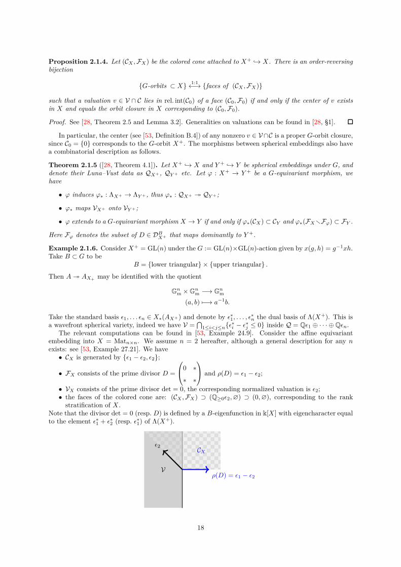
The relevant computations can be found in [53, Example 24.9]. Consider the affine equivariantembedding into X = Matn×n. We assume n = 2 hereafter, although a general description for any nexists: see [53, Example 27.21]. We have• CX is generated by ǫ1 − ǫ2, ǫ2;

• FX consists of the prime divisor D =

0 ∗

∗ ∗

and ρ(D) = ǫ1 − ǫ2;

• VX consists of the prime divisor det = 0, the corresponding normalized valuation is ǫ2;• the faces of the colored cone are: (CX ,FX) ⊃ (Q≥0ǫ2,∅) ⊃ (0,∅), corresponding to the rank

stratification of X .Note that the divisor det = 0 (resp. D) is defined by a B-eigenfunction in k[X ] with eigencharacter equalto the element ǫ∗

1 + ǫ∗2 (resp. ǫ∗

1) of Λ(X+).

Vρ(D) = ǫ1 − ǫ2

ǫ2CX

18

Non-simple spherical embeddings can be obtained by patching simple ones, which leads to a classifi-cation via strictly convex colored fans.

Definition 2.1.7. Given a spherical homogeneous G-space X+, a colored fan is a collection of coloredcones in Q that

(i) is stable under passing to faces (defined above), and(ii) the intersections with V of these cones form a fan inside V .

Call a colored fan strictly convex if all its cones are strictly convex.

The bijection of Proposition 2.1.4 and the description of morphisms in Theorem 2.1.5 generalize tothis context. Such generality will not be needed except for the case of toroidal embeddings, which is tobe discussed in the next section.

Attach a parabolic subgroup to X+ as follows. Take X+ = X to be spherical. Set P (X) :=g ∈ G : Xg = X

; clearly P (X) ⊃ B. We make the following choices:

• a Levi factor L(X) ⊂ P (X), say by choosing a base point x0 ∈ X together with a P (X)-eigenfunction f with zero locus X r X, as in [48, §2.1];

• a maximal torus A → B ∩ L(X).

Set H := StabG(x0) so that we deduce an isomorphism X+ ≃ H\G from the choice of x0. It is knownthat L(X) ∩H ⊃ L(X)der. Together with the choices above, by [48, §2.1] we have an identification ofF -tori

L(X)/L(X) ∩H = A/A ∩H∼→ AX ; (2.1.3)

in particular, we may identify AX as a closed subvariety of X via the orbit map AX ∋ a 7→ x0a.

2.2 Boundary degenerations

Assume char(k) = 0 and consider a spherical homogeneous G-space X .

Notation 2.2.1. A spherical embedding X → X is called toroidal if it is colorless, i.e. no divisor in DB

can contain a G-orbit in its closure inside X. As in [48], the term complete toroidal compactification willmean a toroidal embedding with X proper.

Luna–Vust theory specializes to give the natural bijection

X → X :

toroidal embeddings

1:1←→ strictly convex fans in V , (2.2.1)

X → X :

toroidal compactifications

1:1←→

subdivisons of V by

a strictly convex fan

. (2.2.2)

A strictly convex fan subdividing V means a strictly convex fan in Q whose union of cones equals V .

Smooth complete toroidal compactifications of X always exist [53, §29.2], but there is no canonicalchoice unless when V is strictly convex. Below is a summary of some notions introduced in [48, §2].

• There is a finite crystallographic reflection group WX , called the little Weyl group of X , such thatV is a fundamental domain for the WX -action on Q. There is a natural way to embed WX intothe Weyl group W associated to G and B.

• Let ∆X be the set of integral generators of the extremal rays of

α ∈ ΛQ : 〈α,V〉 ≤ 0 ;

its elements are called the (normalized, simple) spherical roots. Together with the WX -action onQ, they are known to form a based root system.

19

• Choose a smooth complete toroidal compactification X → X. By [48, 2.3.6], we have a notionof correspondence (non-bijective in general) between (i) G-orbits Z ⊂ X or their closures, and(ii) subsets Θ ⊂ ∆X . Specifically, to the complete toroidal compactification is associated a sub-division of V into a strictly convex fan by (2.2.1); each cone therein intersects X∗(AX) in a freemonoid. To each Z is attached a face FZ of that fan, by Proposition 2.1.4. We stipulate thatZ ↔ Θ if FZ is orthogonal to Θ, but not orthogonal to any subset Θ′ ) Θ of ∆X . For example,Θ = ∆X corresponds to Z = X .

For any orbit closure Z ↔ Θ, the normal cone NZX is known to be spherical. Denote by XΘ itsopen G-orbit: this homogeneous G-space is called the boundary degeneration of X attached to Θ.It is wavefront if X is.

• Note that one Θ may correspond to several Z. As indicated in [48, Proposition 2.5.3], the resultingboundary degenerations XΘ are all isomorphic; they are also independent of the choice of X .

• To each Θ is attached a face Θ⊥ ∩V of V , as well as the subtorus AΘ := AX,Θ ⊂ AX characterizedby X∗(AΘ) = Θ⊥ ∩X∗(AX). By [48, 2.4.6], there is a canonical identification

AΘ∼→ Z(XΘ) := AutG(XΘ)0.

• Furthermore, there is an embedding G∆XrΘm → AΘ, whose image in Z(XΘ) acts by dilating the

fibers of prZ : NZX → Z; the GIT quotient of XΘ by G∆XrΘm is isomorphic to Z via the projection

morphism prZ .

Remark 2.2.2. The basic tool for establishing these properties is the Local Structure Theorem due toBrion, Luna and Vust (see [48, Theorem 2.3.4]). Morally, its effect is to reduce things to the toric caseG = A. For a general toroidal embedding X → X in characteristic zero, it asserts that X is covered byG-translates of the P (X)-stable open subset

XB := X r⋃

D∈DB

D∼← Y

L(X)× P (X) ≃ Y × UP (X) (2.2.3)

where• D stands for the closure in X of the prime divisor D ⊂ X ,• Y is the closure of AX in XB which is an L(X)ab-variety, as a toric variety it corresponds to the

fan in V attached to X+ → X,

• YL(X)× P (X) is a contracted product (cf. (2.1.1)) and the morphisms are the obvious ones.

Furthermore, Y meets every G-orbit in X . Therefore X is smooth if and only if Y is. In view of(2.2.3) and Theorem 2.1.5, the existence of smooth complete toroidal compactifications for X is nowclear: simply take any complete toroidal embedding into X and desingularize X by subdividing thecorresponding fan in V .

Remark 2.2.3. The open B-orbits of X and XΘ can be identified as follows (see [48, 2.4.5]):

X ≃ XΘ as B-varieties. (2.2.4)

If we express X as AX+ × UP (X) using the Local Structure Theorem, then (2.2.4) is unique up to aB-isomorphism of the form (y, u) 7→ (y, y−1vyu), for some v ∈ UP (X) fixed by ker[L(X) ։ AX ].

The identification (2.2.4) of B-varieties pins down the isomorphism AΘ∼→ Z(XΘ) as follows: a ∈ AΘ

acts by x0b 7→ x0ab, where b ∈ B. This is well-defined by (2.1.3).

The reader may convince himself of all those claims about XΘ by checking the case of toric varieties.For example, the identification (2.2.4) should become evident in the toric setting.

Remark 2.2.4. Non-complete smooth toroidal embeddings have to be used in certain situations, andthe notion of boundary degenerations has to be modified accordingly. This is the case for “Whittakerinductions” dealt in [48, §2.6].

20

2.3 Cartan decomposition

Consider now a local field F of characteristic zero.Let G be a connected reductive F -group. We assume G split in order to apply the results of [48],

although some other cases will be discussed in Remark 2.3.4. As before, we fix a Borel subgroup B ⊂ Gwith A := B/U . Let X+ be a spherical homogeneous G-space defined over F , with the open B-orbit X .The first observation is the existence of F -rational points.

Proposition 2.3.1 (Cf. [46, Theorem 1.5.1] and its proof). Under the assumptions above, we haveX+(F ) 6= ∅. Here F can be any field of characteristic zero.

Henceforth we fix x0 ∈ X(F ) and some regular function on X+ with vanishing locus X+ r X. Thesechoices define P (X) and its Levi factor L(X). To apply the Luna–Vust classification (Theorem 2.1.3) wehave to work over an algebraic closure F . However, since Gal(F /F ) acts trivially on Q, the Luna–Vustdata not involving colors do not require the algebraic-closeness of F ; cf. the remarks in [47, §2.2].

For the next definition, recall that in §2.1 we have defined a quotient torus AX+ of A which may beregarded as a closed subvariety of X via AX+ ∋ a 7→ x0a; furthermore, X∗(AX+ ) = Λ(X+). All theseconstructions are defined over F .

Definition 2.3.2. Let H : AX+(F )→ Hom(Λ(X+),Q) = Q be the homomorphism characterized by

〈χ,H(a)〉 = − log |χ(a)|, χ ∈ Λ(X+), a ∈ AX(F ).

Here log = logq when F is non-Archimedean with residual field Fq. Note that H is trivial on the maximalcompact subgroup of AX+(F ), and its image equals X∗(AX+ ) when F is non-Archimedean. Define

AX+ (F )+ := H−1(V).

In the literature −H is often used. Our convention here agrees with that of [48, §1.7].

Theorem 2.3.3. The Cartan decomposition holds for X+(F ), namely there exists a compact subsetK ⊂ G(F ) such that

AX+(F )+K = X+(F ).

In the non-Archimedean case, it is customary to enlarge K so that K is compact open.

Alternatively, there exist x0, . . . , xk ∈ X(F ) such that⋃ki=0 xiA(F )+K = X+(F ), where A(F )+ is

the inverse image of AX+(F )+ in A(F ).

Proof. It is established under the following circumstances: (i) F is Archimedean and X+ is a symmetricspace [16, Theorem 4.1], in which case K can be taken to be a maximal compact subgroup in goodposition relative to A; (ii) the general Archimedean case for “real spherical spaces” is addressed in [29,Theorem 5.13], cf. the (2.8) of loc. cit.; (iii) F is non-Archimedean and X+ is any spherical homogeneousG-space [48, Lemma 5.3.1].

Remark 2.3.4. Recall that X+ is a symmetric space means that there exists an involution σ : G → G,with fixed subgroup Gσ, such that H = StabG(x0) satisfies (Gσ) ⊂ H ⊂ Gσ. Symmetric spaces arewavefront spherical varieties. Cartan decomposition holds for symmetric spaces over a local field F withchar(F ) 6= 2, and we do not need to assume G split in that case. See [3] for the non-Archimedean setting.

Let us turn to the notion of boundaries in the Cartan decomposition.

• Take a smooth complete toroidal compactification X+ → X as in §2.2, which is automaticallydefined over F . For any subset Θ ⊂ ∆X+ we define

AΘ(F )>0 := a ∈ AΘ(F ) : ∀α ∈ ∆X+ r Θ, 〈−α,H(a)〉 = log |α(a)| > 0

= H−1(rel. int(Θ⊥ ∩ V)

).

Then AΘ(F )>0 is precisely the subset of elements in AΘ(F ) that steer every x ∈ XΘ towards someZ ↔ Θ. In short, AΘ(F )>0 contracts the fibers of various NZ(X) → Z. Cf. [48, Lemma 2.4.9]and Remark 2.2.3. The avatars AΘ(F )≥0 are defined by using ≥ 0 or by omitting rel. int in theformulas above.

21

• A similar description exists for an affine spherical embedding X+ → X , cf. [47, p.624]. Here wehave to choose a proper birational G-equivariant morphism X → X , such that X+ → X is toroidal.This is addressed combinatorially by applying Theorem 2.1.5 with ϕ := id : X+ → X+: a canonicalchoice is to take X = Xcan to be the “decolorization” of X , by taking the cone CX := CX ∩ V andFX := ∅.

Given a face F of the colored cone (CX ,FX), the subgroup F ∩ X∗(AX+ ) defines a subtorusAF ⊂ AX+ . Set

AF(F )>0 := H−1(rel. int(F ∩ V)).

Translation by elements of AF (F )>0 steers elements in X to the G-orbit closure corresponding toF , cf. Proposition 2.1.4. Indeed, this can be seen on the level of X by Remark 2.2.2. Replacingrel. int(F ∩ V) by F ∩ V gives rise to AF (F )≥0

Again, the reader is invited to check these properties in the case G = A. The rigorous argument goes byreducing to the toric setting via Remark 2.2.2; in the case of X one has to pass to the toroidal embeddingX.

Next, we explain a way of choosing the spherical embeddings X ։ X ⊃ X+ andX+ → X compatibly.

• Choose a fan F subdividing V , such that there exists a subfan F′ that subdivides CX ∩ V . Upontaking refinements, we may assume that both F and F′ give rise to smooth toroidal embeddings ofX+.

• Let X+ → X and X+ → X be the toroidal embeddings determined by F and F′, respectively.Notice that X is not necessarily equal to the Xcan determined by CX := CX ∩ V ; nevertheless,Theorem 2.1.5 connects them by proper birational equivariant morphisms X → Xcan → X , whosecomposite we denote as p. On the other hand, Luna–Vust theory says that X embeds as a G-stableopen subvariety of X.

• All the morphisms above induce identity on X+. The situation is summarized as

X X

X+ X

p (2.3.1)

in which every → is an open immersion.

• As in Remark 2.2.2, define the open P (X)-subvariety XB := X r⋃D∈DB D, where D denotes the

closure of D in X ; here we are implicitly working over the algebraic closure F . Let Y stand for theclosure of AX+ in XB. Recall that it is a toric variety defined by the fan F in Q; thus Y is definedover F .

• Similarly, set XB := Xr⋃D∈DB D with D standing for the closure in X. We obtain a toric variety

Y in the same manner, whose fan is F′ ⊂ Q. There is a natural morphism Y → Y of toric varieties:they share the common open stratum AX+ . Thus it makes sense to write Y (oF ) → Y (oF ).

Proposition 2.3.5. For non-Archimedean F , the compact open subset K ⊂ G(F ) in the Cartan decom-position AX+(F )+K = X+(F ) can be taken such that

(Y (oF ) ∩ Y (F ))K = X(F )

Proof. We shall plug X+ → X into the elegant proof of [48, Lemma 5.3.1]; this is justified since X is awonderful compactification in the sense of [48, §2.3]. In that proof, a compact open subset K ⊂ G(F ) isconstructed such that

(Y (oF ) ∩ Z(F ))K = Z(F ), Z ⊂ X : G-orbit. (2.3.2)

The construction proceeds by induction: one starts with the closed G-orbits. Taking Z = X+ gives theCartan decomposition since Y (oF ) ∩X+ = Y (oF ) ∩AX+(F ) = H−1(V), as the fan F subdivides V .

22

Now we take the union over all G-orbits Z ⊂ X in (2.3.2). It implies that X(F ) equals

⋃

Z⊂X

(Y (oF ) ∩ Z(F ))K =

⋃

Z⊂X

Y (oF ) ∩ Z(F )

K

= (Y (oF ) ∩ X(F ))K.

We contend that Y = Y ∩ X. Indeed, X ⊂ X is open dense, so it is routine to verify (over the algebraicclosure) that (i) D ∩ X = D for each D ∈ DB, thus (ii) XB ∩ X = XB, (iii) therefore Y ∩ X = Y ∩ XB

is an irreducible closed subvariety of XB containing AX+ , from which Y = Y ∩ X.Conclusion: Y (oF ) ∩ X(F ) = Y (oF ) ∩ Y (F ), and our assertion follows immediately.

Corollary 2.3.6. With previous notations, X(F ) is a union of compact open subsets of the form CX =

CY ·K where CY ⊂ Y (F ) satisfies

CY ∩AX+(F ) =m⋃

i=0

H−1 (vi + CX ∩ V)

for some m and v0, . . . , vm ∈ V.

Proof. First, Y (F ) can be expressed a union of compact open subsets CY whose intersection with AX+(F )takes the form above, except that v0, . . . , vm are taken from Q. This is an immediate consequence of thetopology on Y (F ) and of the toric structure on Y ; cf. [2, §I.1] for the real case.

To finish the proof, it suffices to intersect the compact open subsets constructed above with Y (oF ).Since Y (oF ) ∩AX+(F ) = H−1(V), the effect is to limit v0, . . . , vm to V .

An easy yet useful observation that

CX ∩X+(F ) = (CY ∩AX+(F ))K =

m⋃

i=0

H−1 (vi + CX ∩ V)K

with the notation of the proof.

2.4 Geometric data

Let F be a local field of characteristic zero. Fix a split connected reductive F -group G. We may stilldefine the group of F -rational characters X∗(G) and X∗(G)Q := X∗(G)⊗Z Q, X∗(G)R := X∗(G)⊗Z R,etc. They coincide with those defined over F since Gab is split.

Let X+ → X be an affine spherical embedding. Define

F (X+)(G)λ :=

f ∈ F (X+) : ∀g ∈ G, f(•g) = λ(g)f(•)

, λ ∈ X∗(G),

Λ :=λ ∈ X∗(G) : F (X+)

(G)λ 6= (0)

(a subgroup of X∗(G)),

F (X+)(G) :=⋃

λ∈Λ

F (X+)(G)λ ,

r := rk(Λ).

Note that dimF F (X+)(G)λ = 1 for all λ ∈ Λ, and F (X+)

(G)0 = F (X+)G = F . For f ∈ F (X+)(G), f 6= 0,

the “eigencharacter” λ for which f ∈ F (X+)(G)λ is uniquely determined. These are birational invariants

and depend only on the homogeneous G-space X+.The affine embedding enters into the picture via the objects

F [X ](G)λ := F (X+)

(G)λ ∩ F [X ], λ ∈ Λ,

ΛX :=λ ∈ Λ : F [X ]

(G)λ 6= (0)

.

Lemma 2.4.1. The group Λ is generated by its submonoid ΛX.

23

Proof. Form the GIT quotient X Gder, which is an affine Gab-variety, and note that

X∗(G) = X∗(Gab),

F (X+)(G)λ = F (X)

(G)λ = F (X Gder)

(Gab)λ ,

F [X ](G)λ = F [X Gder]

(Gab)λ .

The required result now follows from [53, Lemma D.7] since Gab is an F -torus.

Set ΛQ := Λ⊗Q, ΛR := Λ⊗ R, etc. Therefore ΛX generates a cone ΛX,Q = Q>0ΛX inside ΛQ.

Definition 2.4.2. Call nonzero f ∈ F [X ] a relative invariant with eigencharacter λ ∈ ΛX if f ∈ F [X ](G)λ .

In this case we write f ↔ λ. The Weil divisor div(f) on X is then G-invariant.

Axiom 2.4.3. Hereafter, we shall assume that the affine spherical embedding X+ → X satisfies

(G1) ΛX,Q is a simplicial cone inside ΛQ; consequently, the minimal integral generators ω1, . . . , ωr ∈ ΛXof the extremal rays of ΛX,Q form a basis of ΛQ;

(G2) Choose relative invariants f1, . . . , fr ∈ F [X ] such that fi ↔ ωi (each is unique up to F×); assumethat

X rX+ =

r⋃

i=1

Supp(div(fi)).

In practice, the vanishing loci of fi are often irreducible or even geometrically irreducible.

The lattice Λ can be described in terms of the stabilizer of a chosen base point as follows.

Lemma 2.4.4 (Cf. [27, Proposition 2.11]). Fix x0 ∈ X+(F ) and let H := StabG(x0). Then Λ = ω ∈

X∗(G) = X∗(Gab) : ω|H = 1.

Proof. Suppose ω ∈ Λ and select a relative invariant f ↔ ω. Considerations of H ∋ h 7→ f(x0h) showthat ω|H = 1. Conversely, given ω ∈ X∗(G) such that ω|H = 1, we define a regular function f on H\Gby f(x0g) = ω(g). Since char(F ) = 0, we have H\G ∼

→ X+ via g 7→ x0g, therefore f affords the requiredrelative invariant.

Notation 2.4.5. Every λ ∈ ΛC can be written uniquely as λ =∑r

i=1 λiωi with λi ∈ C. We write

• Re(λ) ≥X

0 if Re(λi) ≥ 0 for all i;

• Re(λ)≫X

0 if Re(λi)≫ 0 for all i;

• |ω|λ :=∏ri=1 |ωi|

λi , an unramified character of G(F );

• |f |λ :=∏ri=1 |fi|

λi , a nowhere vanishing C∞ function on X+(F ).

Note that |f |λ depends on the choice of f1, . . . , fr, and |f |λ(•g) = |f |λ(•)|ω|λ(g) for every g ∈ G(F ).

To X+ → X is associated the colored cone (CX ,FX), CX ⊂ Q; one may pass to F if necessary.Every ω ∈ Λ ⊂ X∗(G) induces an element χω ∈ Λ(X+) ⊂ Q∨ by taking the class of f ↔ ω, sincef ∈ F (X+)(G) ⊂ F (X+)(B). This is compatible with the restriction map X∗(G)→ X∗(B).

The next result will be useful in §5.

Lemma 2.4.6. Assume CX 6= 0. For any ω ∈ ΛX we have χω|CX ≥ 0. Moreover,

ω 6= 0 =⇒ 〈χω , ρ〉 > 0, ∀ρ ∈ rel. int(CX),

ω ∈ rel. int(ΛX,Q) =⇒ 〈χω , ρ〉 > 0, ∀ρ ∈ CX ∩ V , ρ 6= 0.

24

Proof. Let f ↔ ω be a relative invariant. Since f ∈ F [X ], by definition we have 〈χω, ρ(D)〉 = vD(f) ≥ 0for any prime divisor D on X×F F , where vD stands for the normalized valuation attached to D. TakingD from FX ∪ VX yields the first assertion.

Assume r = rk(Λ) ≥ 1 in what follows. For the second assertion, notice that div(f) 6= 0 implies〈χω, w〉 = w(f) > 0 for some w ∈ VX . On the other hand, by the description of VX in Theorem 2.1.3,we may express ρ ∈ rel. int(CX) as

ρ =∑

v∈VX

avv +∑

D∈FX

aDρ(D), aD ≥ 0, av > 0.

Consequently we have ρ = ǫw + ρ′ with ǫ > 0 sufficiently small so that ρ′ ∈ CX . Now the positivity of〈χω, ρ〉 follows from the first part.

To prove the last assertion, write ω =∑r

i=1 λiωi with λi > 0 for all i. We may even assumeλi ∈ Z so that Supp(div(f)) = ∂X by Axiom 2.4.3. By Proposition 2.1.4, every nonzero ρ ∈ CX ∩ V(as a valuation) has center equal to some G-orbit closure Z ( X . This means that the valuation ringOρ := h ∈ F (X) : ρ(h) ≥ 0 dominates the local ring OX,Z of Z; as f lies in the maximal ideal mX,Z ,we see 〈χω , ρ〉 = ρ(f) > 0 as required.

The reader is invited to check this in the situation Example 2.1.6, in which case ΛX is generated byǫ∗

1 + ǫ∗2.

25

Chapter 3

Analytic background

3.1 Integration of densities

Let F be a local field of characteristic zero and G be an affine F -group. Consider a smooth G-variety Yover F , so that Y (F ) becomes an F -analytic manifold with right G(F )-action. The constructions belowcan be performed for a broader class of geometric objects, such as the semi-algebraic F -manifolds, butwe shall restrict to the smooth algebraic case.

Fix a Haar measure on F (eg. by fixing a nontrivial unitary additive character), which induces aHaar measure on Fn for every n. We begin by clarifying the meaning of integration over Y (F ), usingthe language of densities as illustrated in [4, p.29].

Definition 3.1.1. There is a canonical line bundle L over Y (F ), called the density bundle, with thefollowing structures.

• L is obtained from an R>0-torsor on Y (F ), therefore it makes sense to talk about its real orpositive sections.

• L is G(F )-equivariant, i.e. equipped with a morphism pr∗1L → a∗L where a (resp. pr1) is the

action (resp. projection) morphism Y (F )×G(F )→ Y (F ), subject to the usual constraints. Groupsact on the right of bundles, therefore act on the left of their spaces of sections.

• For any open set U ⊂ Y (F ), there is a canonical linear functional (the “integration”)∫

U

: Cc(U ,L ) −→ C

where Cc(U , ·) stands for the space of compactly-supported continuous sections, such that

– if a is a real (resp. positive) section, then∫

Ua is real (resp. positive when U 6= ∅);

–∫

Uga =

∫Uga for all g ∈ G(F );

–∫

U⊔U ′ a =∫

Ua|U +

∫U ′ a|U ′ .

The integration functional depends on the choice of a measure on F . Cf. the construction below.

In particular, one has the notion of integrable or L1 sections of L . The group G(F ) acts on the left ofthe L1-space.

The density bundle can be constructed concretely as follows.

1. Let G := Isom(OY ,∧max

ΩY/F ) be the Gm-torsor over Y corresponding to the line bundle∧max

ΩY/F .We pass to the F -analytic topos by using | · | : Gm(F ) = F× → R>0, therefore obtain an R>0-torsor|G| on Y (F ). The density bundle is simply

L := |G|R>0

× C.

26

2. Over a small open subset U ⊂ Y (F ), the sections of L can be written as η = ϕ|ω| where ϕ is a C∞

function on U , and ω is a nowhere vanishing section of∧max ΩY/F over some Zariski open subset

U with U(F ) ⊃ U . The choice of |ω| trivializes L |U , and our notation “explains” the transitionlaw

ϕ|ω| = ϕ∣∣∣ ωω′

∣∣∣ · |ω′|

where ω/ω′ ∈ Γ(U,O×Y ).

3. Locally around each point y ∈ Y (F ), there exists an F -analytic chart ≃ Fn. To define theintegration functional, it suffices to define

∫Uη for U open in Fn, by the usual procedure, cf. [57,

§2.2.1]. Express a section η of L as

η = ϕ| dx1 ∧ · · · ∧ dxn|

and set∫

Uη :=

∫Uϕdx1 · · · dxn with respect to the chosen measure on Fn. The formula of change

of variables asserts that∫

U is well-defined; furthermore, it also implies that∫

U is invariant underall automorphisms. There exists a G(F )-invariant Radon measure on Y (F ) if and only if L istrivial as an equivariant line bundle.

4. More generally, one can define the R>0-torsor |G|t using | · |t : F× → R>0, for every t ∈ R, therebyobtains the line bundle of t-densities L t on Y (F ). Observe that

• L 1 = L and L 0 is identified with the trivial line bundle C;• for any t, t′ ∈ R, there is a canonical isomorphism

Lt ⊗L

t′ ∼→ L

t+t′ (3.1.1)

satisfying the usual constraints.

The density bundles inherit their equivariant structures from that of ΩY/F .

5. Let us explicate the case of a homogeneous space Y = H\G. It suffices to describe L on eachG(F )-orbit in (H\G)(F ), say the one containing the coset x0 := H(F ) · 1. The fiber of

∧maxΩY/F

at x0 is

(

max∧g∨)⊗ (

max∧h∨)−1.

Thus H acts on that fiber via (det AdG∣∣H

)−1 det AdH : H → Gm. Upon taking | · | on F -points,one sees that L t

∣∣x0G(F )

corresponds to the induced representation

IndGH(δH · δ

−1G |H

)t, t ∈ R. (3.1.2)

We recover the familiar criterion of the existence of invariant Radon measures (t = 1) on homoge-neous spaces.

Consider a complex vector bundle E on Y (F ) (always assumed to be of finite rank) equipped with apositive definite hermitian pairing

E ⊗ E → L (3.1.3)

on the fibers. Define the separable Hilbert space L2(Y (F ),E ) as the completion of Cc(Y (F ),E ) withrespect to the scalar product

(ξ|ξ′) :=

∫

Y (F )

ξξ′

L -valued

.

When E isG(F )-equivariant and the pairing (3.1.3) is invariant,G(F ) acts on L2(Y (F ),E ) via isometries.

Remark 3.1.2. Vector bundles with a pairing (3.1.3) can be constructed as follows. Let E0 be an equiv-ariant hermitian vector bundle on Y (F ). Since L 1/2 ⊗L 1/2 ∼

→ L is defined over R, the vector bundle

E := E0 ⊗L1/2

is equivariant and equipped with a pairing as in (3.1.3). Hence we get a canonical unitary representationof G(F ) on L2(Y (F ),E ), in view of (3.1.1). They typical case is E0 = C, so that E = L 1/2.

Such an approach has already been adopted in [6, 3.7].

27

3.2 Direct integrals and L2-spectral decomposition

What follows is fairly standard: the details can be found in [15, II.1, II.2] or [55, Chapter 14], for example.Let Π be a topological space with a positive Borel measure µ. Consider a family (also known as a

“field”) of separable Hilbert spaces H : τ 7→ Hτ , where τ ∈ Π. Assume (Hτ )τ is measurable, which meansthat we are given C-vector space S of sections s : τ 7→ s(τ) ∈ Hτ , verifying

(i) for all s ∈ S, the function τ 7→ ‖s(τ)‖ is measurable on Π;(ii) if t is a section such that τ 7→ (t(τ)|s(τ)) is measurable for all s ∈ S, then t ∈ S;(iii) there exists a sequence s1, s2, . . . in S such that for every τ ∈ Π, the subset si(τ)i≥1 is dense in

Hτ ; call it a fundamental sequence.Sections belonging to S are called measurable. Consider two basic examples.• The constant family Hτ = H0 for some fixed H0: here S is taken to be the space of s such thatτ 7→ (s(τ)|v) is measurable for every v ∈ H.• Let (Hτ )τ and (H′

τ )τ ′ be measurable families. The family of completed tensor products (Hτ ⊗H′τ )τ

of Hilbert spaces is measurable by requiring that s⊗ s′ is measurable whenever s and s′ are.For every s ∈ S, put

‖s‖2 :=

∫

Π

‖s(τ)‖2 dµ(τ).

Elements s ∈ S with ‖s‖ < +∞ are called L2 sections; they form a C-vector space. Define

∫ ⊕

Π

Hτ dµ(τ) :=s ∈ S : L2-section

/s ∈ S : ‖s‖ = 0.

It turns out that∫ ⊕

ΠHτ dµ(τ) equipped with ‖ · ‖2 becomes a separable Hilbert space, called the direct

integral of the measurable family (Hτ )τ .Let H = (Hτ )τ , H′ = (H′

τ )τ be two measurable families of separable Hilbert spaces over (Π, µ).Consider a family F of continuous linear maps from H to H′, that is,

Fτ ∈ Hom(Hτ ,H′τ ), τ ∈ Π.

Call F measurable if it preserves measurable sections. If the operator norms τ 7→ ‖Fτ‖ form an L∞

function on Π, then we obtain a continuous linear map∫ ⊕

Π

Fτ dµ(τ) :

∫ ⊕

Π

Hτ dµ(τ)→

∫ ⊕

Π

H′τ dµ(τ)

of norm equal to the L∞-norm of τ 7→ ‖Fτ‖. Here comes more definitions.

• Operators of the form∫ ⊕

Π Fτ dµ(τ) above are called decomposable.

• There is a continuous injection from L∞(Π, µ) to the space of decomposable operators, namely bysending f to the measurable family Ff : τ 7→ f(τ) · id. Operators arising in this manner are calleddiagonalizable.

Let Γ be a separable locally compact group which is CCR (see [55, 14.6.9]). Denote by Πunit(Γ) theunitary dual of Γ equipped with the Fell topology. We pick a representative for each equivalence classof unitary representations in Πunit(Γ).

Theorem 3.2.1 (Abstract Plancherel decomposition). Let L be a unitary representation of Γ on sepa-rable Hilbert spaces. There exists an isomorphism of unitary representations of Γ

Φ : L∼→

∫ ⊕

Πunit(Γ)

τ⊗Mτ dµ(τ)

for some positive Borel measure µ on Πunit(Γ), called the Plancherel measure, and a measurable familyof separable Hilbert spaces τ 7→ Mτ , called the multiplicity spaces, on which G(F ) acts trivially.

The data µ, (Mτ )τ and Φ are unique in the following sense. If Φ′ : L∼→∫ ⊕

Πunit(Γ) τ⊗M′τ dµ′(τ) is

another decomposition, then:

28

• the measures µ, µ′ are equivalent: thus there exists a measurable a : Πunit(Γ)→ R>0 (the Radon–Nikodym derivative) such that dµ′ = a dµ;• there exists a measurable family of continuous linear maps H(τ) : τ⊗Mτ

∼→ τ⊗M′

τ such thata(τ)H(τ) is an isometry for µ-almost all τ , and

Φ′Φ−1 =

∫ ⊕

Πunit(Γ)

H(τ) dµ(τ).

Proof. For the existence of direct integral decompositions, see [55, 14.10.* and 14.13.8].As for the uniqueness, let F := Φ′Φ−1. In view of [15, II.6.3 Théorème 4], it suffices to show that F

induces an isomorphism of the C∗-algebras of diagonalizable operators. Denote by C∗(Γ) the C∗-algebraattached to Γ [55, p.274] and let A be its strong closure in End(L). By [55, p.330], the center Z(A) getsidentified with the algebra of diagonalizable operators under Φ. The same holds true under Φ′. Since Ftransports these structures, it preserves the algebras of diagonalizable operators.

Corollary 3.2.2 (Disintegration of intertwining operators). Let L, L′ be unitary representations of Γas before, and F : L

∼→ L′ is an isomorphism of unitary representations of Γ, then:

• There exist a Borel measure µ on Πunit(Γ), measurable families of multiplicity spaces Mτ , M′τ ,

together with isomorphisms

L∼→

∫ ⊕

τ⊗Mτ dµ(τ), L′ ∼→

∫ ⊕

τ⊗M′τ dµ(τ);

• Given the decompositions above, there exists a measurable family of isometries η(τ) : Mτ∼→M′

τ

such that F corresponds to∫ ⊕

(idτ ⊗ η(τ)) dµ(τ), provided that dimCMτ is finite for µ-almost allτ .

Proof. Apply the uniqueness part of Theorem 3.2.1, and note that H(τ) must be of the form idτ ⊗ η(τ)for some η(τ) whenever dimCMτ is finite.

We shall apply these results to a G(F )-equivariant vector bundle E on Y (F ) together with a pairing(3.1.3), thereby making L2(Y (F ),E ) into a unitary representation of G(F ), where F , Y , G are as in §3.1and G is reductive. In this case G(F ) is known to be CCR.

3.3 Gelfand–Kostyuchenko method

The main reference here is [6]. We consider

• a separable Hilbert space L which equals a direct integral∫ ⊕

Π Hτ dµ(τ) of Hilbert spaces;

• a separable topological vector space S, with continuous dual S∨ endowed with the strong topology.

Definition 3.3.1. A continuous linear map α : S → L is said to be pointwise defined if there exists afamily

ατ : S → Hτ , τ ∈ Π

such that for all ξ ∈ S, the section τ 7→ ατ (ξ) is measurable and represents α(ξ) ∈ L.

Evidently, one can neglect those ατ for τ in a set of µ-measure zero. We collect some more factsbelow, cf. [6, 1.3 Lemma].

1. Any two families (ατ )τ , (α′τ )τ coincide off a subset of µ-measure zero.

2. Let Γ be a locally compact separable group acting on S, Hτ (for each τ ∈ Π) and thus on L byisometries, such that α is Γ-equivariant, then one can choose ατ to be Γ-equivariant for all τ .

3. If α has dense image, then ατ has dense image in Hτ for µ-almost all τ ∈ Π.

4. Given continuous linear maps ϕ : S → S′ and α′ : S′ → L. If α′ is pointwise defined, then so isα := α′ϕ : S → L;

29

Denote by S† the conjugate of S∨. If α if injective of dense image, taking hermitian adjoint yields

S → L → S†.

This is naturally connected to the idea of rigged Hilbert spaces or Gelfand triples [19] when α is injective,pointwise defined and of dense image. In fact, let α†

τ : Hτ → S† be the hermitian adjoint of ατ for

µ-almost all τ . In [6, p.667 (**)] it is shown that

ξ =

∫

τ∈Π

α†τατ (ξ) dµ(τ), ξ ∈ S ⊂ S†. (3.3.1)

This may be viewed as an expansion for L into generalized eigenvectors, with the help of “test vectors”from S. These observations lead to the following description of the components Hτ in L, for µ-almostall µ.

Proposition 3.3.2. Suppose that α : S → L is pointwise defined of dense image. Denote by ‖ · ‖τ thecontinuous semi-norm ξ 7→ ‖ατ (ξ)‖Hτ on S. For µ-almost all τ , the map ατ induces an isomorphism

(the completion of S relative to ‖ · ‖τ )∼→ Hτ

between topological vector spaces.

Proposition 3.3.3. Suppose in addition that• we are given a locally compact separable group Γ, acting unitarily on L such that α : S → L is

Γ-equivariant;• the direct integral for L is the spectral decomposition in Theorem 3.2.1, i.e. Π = Πunit(Γ) andHτ = τ⊗Mτ .

For µ-almost all τ , there is a canonical inclusion of vector spaces

Hom(Mτ ,C) → a ∈ HomΓ(S, τ) : ∃C > 0, ‖a(·)‖ ≤ C‖ · ‖τ

where Hom(· · · ) and HomΓ(· · · ) stand for the continuous Hom-spaces. It is an isomorphism whendimCMτ is finite.

Proof. We may view Hom(Mτ ,C) as a subspace of HomΓ(τ⊗Mτ , τ), which is full when Mτ is finite-dimensional, by Schur’s Lemma. Now apply the previous result.

The following result asserts that α : S → L is pointwise defined when S is nuclear . It has been statedin [19, I.4, Theorem 5] and [36, Chapter II, §1] in a different flavor. For the theory of nuclear spaces, see[54, §50].

Theorem 3.3.4. Assume that S is nuclear. Then any continuous linear map α : S → L is pointwisedefined. In particular, any continuous linear map issuing from S is fine in the sense of [6, 1.4].

Proof. By the Gelfand–Kostyuchenko Theorem [6, 1.5, Theorem], Hilbert–Schmidt operators betweenseparable Hilbert spaces are pointwise defined. Therefore it suffices to factorize α into

Sα1−→ L1

α2−→ L

where L1 is a separable Hilbert space, α1 is continuous linear, and α2 is Hilbert–Schmidt.By [54, Theorem 50.1], α is a nuclear mapping: there exist• fi ∈ S∨: an equicontinuous family [54, Definition 14.3] of linear functionals, for i = 1, . . . (at most

countable),• ηi ∈ L with ‖ηi‖ ≤ 1 for i = 1, . . .,• (λ1, . . .): an ℓ1-sequence of complex numbers

(see also [54, Proposition 47.2] and its proof), such that for each ξ ∈ S

α(ξ) =∑

i≥1

λi〈fi, ξ〉ηi (convergent sum).

30

Set L1 to be the Hilbert space with an orthonormal basis (ηi)i, with the same indices i as before. Wemay also write λi = λiµi in such a manner that (λi)i, (µi)i are both ℓ2-sequences. We define first

α1 : S −→ L1

ξ 7−→∑

i≥1

λi〈fi, ξ〉ηi,

which is well-defined and continuous since (fi)i is equicontinuous, (ηi)i is orthonormal and (λi)i is ℓ2.Secondly, define

α2 : L1 −→ L

ηi 7→ µiηi, ∀i ≥ 1,

which is Hilbert–Schmidt by [6, 1.5 Lemma] since ‖ηi‖ ≤ 1 and (µi)i is ℓ2. Obviously α = α2α1.

Most spaces of test functions in harmonic analysis are nuclear spaces. See [54, §51] for a few examplesin the Archimedean case.

3.4 Hypocontinuity and barreled spaces

The following review is meant to fix notations. We follow the definition in [8, III, §5].LetX,Y, Z be topological vector spaces. A bilinear mapB : X×Y → Z is called separately continuous

if B(x, ·) : Y → Z and B(·, y) : X → Z are both continuous linear maps for all x, y; it is called jointlycontinuous if B itself is a continuous map.

Definition 3.4.1. Let S be a family of bounded sets of Y . A separately continuous bilinear mapB : X×Y → Z is called S-hypocontinuous if for every open neighborhoodW ⊂ Z of 0 and every V ∈ S,there exists an open neighborhood U ⊂ X of 0 such that

B(U × V) ⊂ W .

It is known [8, III, §5.3, Proposition 3] that the condition is equivalent to: B induces a continuouslinear map θ : X → HomS(Y, Z) characterized by θ(x)(y) = B(x, y), where HomS(Y, Z) is the spaceof continuous linear maps Y → Z with the locally convex topology given by uniform convergence oversubsets in S (cf. [54, §19, §32]); HomS(Y, Z) is Hausdorff when

⋃S is dense in Y .

The S-hypocontinuity interpolates between joint and separate continuity. When S equals the set ofall bounded subsets of Y , we say that B : X ×Y → Z is a hypocontinuous bilinear form. We will mainlybe interested in the case Z = C; in this case, a hypocontinuous X × Y → C gives rise to a continuouslinear map X → Y ∨ where Y ∨ = HomS(Y,C) is the strong dual of Y .

The notion of barreled topological vector spaces is standard; the precise definition may be found in[54, §33]. It suffices for us to collect some of their basic properties.

Proposition 3.4.2. The property of being barreled is preserved by arbitrary lim−→

. Furthermore

• Fréchet spaces are barreled, therefore LF-spaces are barreled as well;

• the dual of a barreled space is quasi-complete with respect to the topology of pointwise convergence.Here quasi-completeness means that every bounded and closed subset is complete.

Proof. The permanence under lim−→

can be found in [8, III, §4.1, Corollaire 3]. The case of Fréchet spacesis also discussed therein. The quasi-completeness of the dual is proved in [54, Corollary 2 to Theorem34.2].

Proposition 3.4.3 ([8, III, §5.3, Proposition 6]). Suppose that X is a barreled space, then every sepa-rately continuous bilinear map B : X × Y → Z is S-hypocontinuous, for every family S of bounded setsin Y .

We record a well-known condition for joint continuity.

31

Proposition 3.4.4 ([54, Corollary to Theorem 34.1]). Let B : X × Y → Z be a separately continuousbilinear map. If X is Fréchet and Y is metrizable, then B is jointly continuous.

The notion of barreled spaces are used in this work to study holomorphic families of linear functionals.Consider an open subset U ⊂ Cr, a locally convex topological vector space V , its continuous dual V ∨

and a map T : U → V ∨, written as λ 7→ Tλ. For the following application, we say T is holomorphicif λ 7→ Tλ(v) is holomorphic for all v ∈ V . This also implies that T : λ 7→ Tλ is continuous if V ∨ isendowed with the topology of pointwise convergence.

The following method of analytic continuation is due to Gelfand–Shilov [18, Chapter I, A.2.3], seealso [25, Proposition 5.2.1]. The following formulation is proved in [35, §8].

Theorem 3.4.5. Suppose the space V is barreled. Given a map

T : Cr −→ HomC(V,C)

λ 7−→ Tλ

where HomC stands for the algebraic Hom. Assume that

• for each v ∈ V , the function λ 7→ Tλ(v) is holomorphic on Cr;

• there exists an open subset U 6= ∅ of Cr such that T restricts to a holomorphic map U → V ∨.

Then T is actually a holomorphic map Cr → V ∨.

32

Chapter 4

Schwartz spaces and zeta integrals

Throughout this chapter, we fix• a local field F of characteristic zero,• a split connected reductive F -group G,• an affine spherical embedding X+ → X satisfying Axiom 2.4.3,• relative invariants fi ∈ F [X ] of eigencharacter ωi (Definition 2.4.2) for 1 ≤ i ≤ r := rk(Λ).The Hypothesis 4.6.4 will be made in the discussion of the L2-aspect, which serves to motivate the

overall framework.

4.1 Coefficients of smooth representations

The algebraic Hom between topological vector spaces will be denoted by Homalg when confusion mayarise.

Definition 4.1.1. We call a topological vector space V algebraic if it is a countable inductive limit offinite-dimensional vector spaces, each equipped with its usual topology.

Lemma 4.1.2. Let V,W be topological vector spaces. Suppose that V is algebraic, then Homalg(V,W ) =Hom(V,W ).

Proof. Write V = lim−→i

Vi where each Vi is finite-dimensional. Then we have

Homalg(V,W ) = lim←−i

Homalg(Vi,W ) = lim←−i

Hom(Vi,W ),

the last equality resulting from [54, Theorem 9.1]. The universal property of topological inductive limitsyields Hom(V,W ).

Lemma 4.1.3. Algebraic topological vector spaces are separable, nuclear, and barreled.

Proof. The required properties are preserved by countable lim−→

:• separable: clear,• nuclear: [54, (50.8)],• barreled: by Proposition 3.4.2.

Obviously, finite-dimensional vector spaces have these virtues.

We review the notion of smooth representations below. Let (π, Vπ) be a continuous representation ofG(F ). We define its smooth part (π∞, V ∞

π ) as follows.

• (For F Archimedean) Take V ∞π to be the subspace of smooth vectors, i.e. v ∈ V ∞

π if and only ifγv : g 7→ π(g)v is smooth; so the universal enveloping algebra of g acts on V ∞

π . Given a continuoussemi-norm p on Vπ, the corresponding k-th Sobolev semi-norm is given by

pk(v) =

∑

m1+···+mn≤k

p(π(Xm11 · · ·Xmn

n )v)2

12

33

where X1, . . . , Xn is a basis of g. We endow V ∞π with the locally convex topology induced by pk

for all p and all k ∈ Z≥1, as in [5, 2.4.3].

• (For F non-Archimedean) Take V ∞π =

⋃J⊂G(F ) V

Jπ where J ranges over the compact open sub-

groups. It is a smooth representation of G(F ) in the usual sense. For each J , the subspaceV Jπ inherits its topology from Vπ, therefore V ∞

π acquires the topology of lim−→

. Let us check that(π∞, V ∞

π ) is a continuous representation of G(F ). Recall that a local base at 0 ∈ V ∞π consists of

subsets of the form ∑

J∈J

im [UJ → V ∞π ]

where J is a finite set of subgroups J and UJ is a balanced convex neighborhood of 0 ∈ V Jπ , foreach J ∈ J . By taking J ′ so small that J ′ ⊂ J for all J ∈ J , we can assure

J ′ ×∑

J∈J

im [UJ → V ∞π ]→

∑

J∈J

im [UJ → V ∞π ]

under the action map, which implies continuity by linearity.

When π is admissible, the topology on each V Jπ (finite-dimensional) is unique, and V ∞π becomes

algebraic. There is no need to worry about topologies in such a setting.

Call π smooth if π = π∞. As observed above, this is compatible with the standard notion for non-Archimedean F .

Definition 4.1.4. In this work, by a nice representation of G(F ) we mean:

• (For F Archimedean) A smooth representation on a Fréchet space that is admissible of moderategrowth, also known as Casselman–Wallach representations or SAF representations in [5]; they arethe unique “SF-globalizations” of Harish-Chandra modules.

• (For F non-Archimedean) A representation (π, Vπ) of G(F ) which is smooth admissible of finitelength.

For example, let τ be an irreducible unitary representation of G(F ). It is well known that its smoothpart τ∞ is a nice representation.

Lemma 4.1.5. The underlying space Vπ of a nice representation π is separable, nuclear, and barreled.

Proof. In the Archimedean case, [5, Corollary 5.6] implies that Vπ is Fréchet as well as nuclear, whereasits separability is well-known (pass to Harish-Chandra modules). The non-Archimedean case followsfrom Lemma 4.1.3.

Next, consider the data

• an equivariant vector bundle E on X+(F ), equipped with a G(F )-invariant pairing E ⊗E → L asin (3.1.3);

• the following functions spaces on X+(F ) with values in vector bundles:

C∞(X+) := C∞(X+(F ),E ) ≃ C∞(X+(F ),E ∨ ⊗L ),

C∞c (X+) := C∞

c (X+(F ),E ),

L2(X+) := L2(X+(F ),E ),

where the isomorphism results from (3.1.3).

We topologize C∞c (X+) and C∞(X+) in the standard manner [6, 2.2], making them into continuous

representations of G(F ). Specifically,• Cc(X+) is realized as the lim

−→of CΩ(X+) := ξ ∈ Cc(X+) : Supp(ξ) ⊂ Ω, carrying the norms

supΩ ‖ · ‖, where Ω ⊂ X+(F ) ranges over the compact subsets 1;

1Here we take ‖ · ‖ to be any continuous family of norms on the fibers of E |Ω, the choice being immaterial because Ω is

compact.

34

• C(X+) carries the semi-norms supΩ ‖ · ‖ with the Ω above;Taking smooth parts yields the topological vector spaces C∞

c (X+) and C∞(X+). One can verify thatC∞c (X+) is actually algebraic when F is non-Archimedean.

Note that C∞c (X+) ⊂ L2(X+), and the integration of densities furnishes an invariant pairing

C∞(X+)⊗ C∞c (X+)→ C. The next result furnishes a bridge between L2 and smooth theories.

Theorem 4.1.6. Let τ be an irreducible unitary representation of G(F ) and put π := τ∞, where τstands for the contragredient of τ as a Hilbert representation. There is a C-linear isomorphism

HomG(F )(C∞c (X+), τ)

∼→ HomG(F )(π,C

∞(X+))

ϕ 7→ ϕ|τ∞ ,

where ϕ : τ → C∞c (X+)∨ is the adjoint of ϕ.

Proof. This is just a paraphrase of [6, Proposition 2.4], where E = C and the hermitian adjoint is used;the arguments in loc. cit. carry over verbatim.

Remark 4.1.7. If we consider the hermitian adjoint as in loc. cit., the result will be an anti-linearisomorphism onto HomG(F )(τ

∞, C∞(X+(F ),E )).

Notation 4.1.8. For an irreducible nice representation π of G(F ), we adopt the notation

Nπ := HomG(F )(π,C∞(X+)).

The representations with Nπ 6= 0 are the main objects in the study of distinguished representations .The elements ϕ(v) ∈ C∞(X+) for ϕ ∈ Nπ, v ∈ Vπ are often called the coefficients of π.

Axiom 4.1.9. For any irreducible nice representation π, the space Nπ is finite dimensional.

Remark 4.1.10. Under the Axiom 2.4.3, this condition is almost known to hold. Indeed, the Archimedeancase is covered by [31, Theorem A] since we may deal with the finitely many G(F )-orbits in X+(F )separately. As for the non-Archimedean case, there is no need to impose continuity and when X+ iswavefront and E is trivializable, the finiteness statement is just [48, Theorem 5.1.5]. That result can beextended to the case E = L

12 (cf. Remark 3.1.2), which will be covered by Theorem 5.2.5. The case of

“Whittaker induction” is also known: see Remark 2.2.4.

4.2 The group case

In this section, H stands for a connected reductive F -group and G := H ×H . The group case signifiesthe homogeneous G-variety X+ := H equipped with the action

x(g1, g2) = g−12 xg1, x ∈ X+, (g1, g2) ∈ G. (4.2.1)

Take x0 = 1 ∈ X+(F ), then its stabilizer equals the diagonal image diag(H) ⊂ G. When H is quasi-split,we will work with Borel subgroups of G of the form B−×B. It follows from Bruhat decomposition thatX+ is a spherical homogeneous G-space; in fact X+ is a symmetric space defined by the involution(g1, g2) 7→ (g2, g1), therefore X+ is wavefront. Our aim is to describe the “coefficients” of §4.1 in thissetting.

The G-action above is by no means the canonical one. We may flip the two components of G andobtain a new action

x(g1, g2) = g−11 xg2, x ∈ X+, (g1, g2) ∈ G. (4.2.2)

The actions (4.2.1) and (4.2.2) are intertwined by x 7→ x−1. We shall denote the case of (4.2.2) by X+

when confusion may arise.Hereafter, F is a local field and H is split with a chosen Borel subgroup B. Take the bundle E := L

12

of half-densities on X+(F ) and set C∞(X+) := C∞(X+,L12 ) as usual. As before, G(F ) acts in two

ways, thus we write C∞(X+), C∞(X+) to distinguish. Consider an irreducible nice representation Π ofG(F ) together with the continuous Hom-spaces

NΠ := HomG(F )(Π, C∞(X+)),

NΠ := HomG(F )(Π, C∞(X+)).

35

• The equivariant bundle L12 on X+(F ) can be trivialized by taking some Haar measure |Ω| on

H(F ) and form the invariant global section |Ω|12 of L

12 . The construction works for X+ as well.

• The space NΠ is nonzero if and only if Π ≃ π ⊠ π for some irreducible nice representation π ofH(F ). In this case, NΠ is in bijection with the space of Haar measures |Ω|, by taking matrixcoefficients

ϕ|Ω| : π ⊠ π −→ C∞(X+)

v ⊗ v 7−→ 〈v, π(·)v〉 · |Ω|12 .

Some words on the proof are in order. Upon trivializing L12 , the case of non-Archimedean F

is routine: everything is algebraic. As for the Archimedean case, a similar description of NΠ iswell-known in the algebraic setting of Harish-Chandra modules; one can pass to the setting of nicerepresentations by Frobenius reciprocity and the “group case” of automatic continuity [5, §11.2].The underlying space of π ⊠ π is actually the completed tensor product Vπ⊗Vπ of nuclear spaces.

• The same holds for NΠ except that NΠ is now spanned by

ϕ|Ω| : π ⊠ π −→ C∞(X+)

v ⊗ v 7−→ 〈π(v), v〉 · |Ω|12 .

• All in all, we deduce a canonical isomorphism of linesNΠ∼→ NΠ given by ϕ|Ω| 7→ ϕ|Ω|. Furthermore,

the following diagram of G(F )-representations commutes

C∞(X+) C∞(X+)

Π⊗NΠ Π⊗ NΠ

β 7→β∨

∼

β∨(x) := β(x−1).

Finally, we remark that when H is a torus, there is no need to distinguish left and right translations.Hence we may view X+ = H as a homogeneous H-space via H = H × 1 → G. For any continuouscharacter χ of H(F ) we have dimNχ = 1, with generator ϕ|Ω| : 1 7→ χ(·)|Ω|

12 ∈ C∞(X+). Furthermore,

X+ = H is still wavefront under this setting.

4.3 Auxiliary definitions

The following notions will enter into the Axiom 4.4.1. As they are more or less intuitive, we collect themhere to facilitate the reading.

We begin by clarifying the meaning of meromorphic or rational (in the non-Archimedean case) fam-ilies. Our formulation is based on Bernstein’s approach; for the general theory we recommend [42,VI.8].

Definition 4.3.1. Define T to be the complex manifold of unramified characters |ω|λ : λ ∈ ΛC. Noticethat T also parametrizes the functions |f |λ : λ ∈ ΛC on X+(F ). When F is non-Archimedean, Tis the complex algebraic torus corresponding to the group algebra of Hom(Λ,Z). Define O to be thealgebra of

• holomorphic functions on T for F Archimedean;

• regular algebraic functions on T , for F non-Archimedean.

In either case, the map “evaluation at g ∈ G(F )” furnishes a group homomorphism

|ω|univ : G(F )→ O×.

On the other hand, for every |ω|λ ∈ T , the homomorphism “evaluation at |ω|λ” is denoted by

evλ : O → C.

Finally, denote the fraction field of O by

K := Frac(O).

36

Suppose that (π, Vπ) is a nice representation of G(F ). Let G(F ) act on Vπ ⊗O by

π(g) : v ⊗ b 7→ π(g)v ⊗ |ω|univ(g)b,

which turns out to be O-linear, and whose reduction via evλ yields πλ = π ⊗ |ω|λ. Set Vπ := Vπ ⊗ Kwhich still carries a G(F )-action π. It captures the idea of the family of representations πλ parametrizedby T .

Definition 4.3.2. Suppose given a continuous representation of G(F ) on a space S. For every nonzerot ∈ O (the “denominator”), denote by L

π,t the K-vector space of K-linear maps B : π ⊗CS −→ K that

• B is G(F )-invariant: B(π(g)v, gξ) = B(v, ξ) for all g ∈ G(F );

• B ((Vπ ⊗ tO)⊗ S) ⊂ O.

Denote by Lπ,t ⊂ Lπ,t the subspace of B : π ⊗ S → K such that the “evaluation of tB”

v ⊗ ξ 7−→ evλ (B(v ⊗ t, ξ))

is a hypocontinuous bilinear form Vπ × S → C for every λ.Therefore, B ∈ Lπ,t induces a meromorphic family λ 7→ θλ of elements of HomG(F )(πλ,S

∨) (withstrong topology on S∨), characterized by

t(λ)θλ(v) : ξ 7→ evλ (B(v ⊗ t, ξ)) , (4.3.1)

where v ∈ Vπ, λ ∈ ΛC, ξ ∈ S. Meromorphy (say with denominator t) means that the function λ 7→t(λ)θλ(v) is holomorphic in λ for every v. Recall that the notion of holomorphy is defined prior toTheorem 3.4.5.

When t(λ) 6= 0, one can extend evλ to t−1O → C, therefore the reduction at λ of B can be definedas a G(F )-invariant bilinear form Bλ : πλ ⊗ S → C. Finally, we accommodate arbitrary denominatorsby setting

Lπ := lim

−→t

Lπ,t,

Lπ := lim−→t

Lπ,t

where the indices t ∈ O r 0 are directed by divisibility.

The passage from Lπ,t to Lπ,t is greatly facilitated by the following device.

Lemma 4.3.3. Suppose S is barreled. Let t ∈ O r 0, B ∈ Lπ,t. If the evaluations of tB (see above)

are separately continuous at every λ in some nonempty open subset U ⊂ ΛC, then B ∈ Lπ,t.

Proof. By Lemma 4.1.5 we know Vπ is barreled. By Proposition 3.4.3, it suffices to establish the separatecontinuity of the evaluations of tB at every λ. In what follows, we equip S∨ with the topology of pointwiseconvergence (i.e. weak topology).

Fix v ∈ Vπ, we obtain as in (4.3.1) a family in λ ∈ ΛC of linear functionals t(λ)θλ(v) : S → C. Theybelong to S∨ whenever λ ∈ U . The first task is to propagate this property to all λ.

Given ξ ∈ S, the function λ 7→ 〈t(λ)θλ(v), ξ〉 lies in O by the definition of Lπ,t, hence holomorphic

in λ ∈ ΛC. Since S is barreled, the required continuity of t(λ)θλ(v) follows from the method of analyticcontinuation in Theorem 3.4.5.

By the same reasoning, for every fixed ξ ∈ S the continuity in v ∈ Vπ for λ ∈ U propagates to thewhole ΛC, since Vπ is barreled. This completes our proof.

Hence the defining condition of Lπ,t is independent of the denominator t: for nonzero t′ ∈ O:

B ∈ Lπ,t ∩ Lπ,tt′ =⇒ B ∈ Lπ,t.

Indeed, it suffices to evaluate B over some nonempty open U outside the zero locus of tt′.As for the L2-part of our axioms, a (nonstandard) variant of the notion of holomorphy will be used.

37

Definition 4.3.4. Let W be a topological vector space and H be a separable Hilbert space. A family

of continuous linear maps βλ : W → H indexed by D :=

λ ∈ ΛC : Re(λ) ≥

X0

is called holomorphic if

it satisfies

∀ξ ∈ W, [λ 7→ βλ(ξ)] is continuous,

∀ξ ∈W, ∀b ∈ H, [λ 7→ (βλ(ξ)|b)H ] is holomorphic

where λ ∈ D (resp. the interior of D) in the first (resp. the second) condition.

To see how this leads to a stronger version of holomorphy, we refer to [44, Theorem 3.31].Assume F is Archimedean now; it is harmless to work with F = R. There exist natural structures

of Nash manifolds and Nash bundles on X+(F ) and L , respectively; for the latter construction, see [1,A.1.1]. We recommend [1, §1] for generalities on semi-algebraic geometry over R.

Definition 4.3.5. A smooth section Ξ of L is said to have rapid decay, if for any semi-algebraic functionp on the affine variety X(F ) we have

νp(Ξ) :=

∫

X+(F )

(1 + |p|2

)|Ξ| < +∞.

Note that the definition depends on X+ → X . The notion of rapid decay of L 1/2-valued sectionscan be defined similarly. The main differences from the definition of Schwartz functions in [1, Remark4.1.5] are that (i) we do not consider differential operators, and (ii) X is singular in general, thus X(F )is not a Nash manifold.

4.4 Schwartz spaces: desiderata

Fix a G(F )-stable subspace S of C∞(X+(F ),E ) (the “Schwartz space”) subject to the following condi-tions:

• S carries a topology so that S is a smooth continuous G(F )-representation.

• C∞c (X+) is continuously included in S.

• For every λ ∈ ΛC we setSλ := |f |λS

which still lies between C∞(X+(F ),E ) and C∞c (X+). We topologize Sλ by requiring that

mλ : S∼−→ Sλ, ξ 7→ |f |λξ

is a continuous isomorphism. Upon recalling how the topology of C∞c (X+) is defined, one sees that

the foregoing conditions for S still hold true for Sλ.

The geometry of X intervenes now. For every irreducible nice representation π, we put

πλ := π ⊗ |ω|λ, λ ∈ ΛC

realized on the same underlying vector space as π. Elements of Nπ can be twisted by relative invariantsof X : for every ϕ ∈ Nπ, define

ϕλ : πλ −→ C∞(X+)

v 7−→ |f |λϕ(v).

It is clearly equivariant, and we have ϕλ ∈ Nπλ — indeed, the continuity of ϕλ follows from the wayC∞(X+) is topologized. Furthermore, ϕλ+µ = (ϕλ)µ and ϕ0 = ϕ. Notice that ϕλ depends on the choiceof relative invariants, albeit in a mild manner.

Axiom 4.4.1. We assume the validity of Axiom 4.1.9.

38

• The functional-analytic axioms (mainly used in §4.6):

(F1) S is a separable nuclear space.

(F2) S is barreled.

(F3) We have Sλ ⊂ L2(X+) whenever Re(λ) ≥X

0. Denote the inclusion map S → L2(X+) by α,

so that Sλ → L2(X+) may be viewed as a family of inclusions

αλ : S → L2(X+)

ξ 7→ |f |λα(ξ).

We require that αλ is continuous whenever Re(λ) ≥X

0. Note that αλ is no longer equivariant:

the character |ω|λ intervenes. By Theorem 3.3.4 αλ is pointwise defined, and αλ has denseimage in L2(X+) since C∞

c (X+) does.

(F4) The family αλ : S → L2(X+) is holomorphic in the sense of Definition 4.3.4.

• The smooth axioms:

(S1) For Archimedean F , there exists λ0 ∈ ΛR such that |f |2λ‖ξ‖2 is of rapid decay (Definition4.3.5) for all ξ ∈ S when Re(λ) ≥

Xλ0. Furthermore, we require that the semi-norms ξ 7→

νp(|f |2λ‖ξ‖2

)in Definition 4.3.5 are continuous in ξ ∈ S, for all p.

(S2) For non-Archimedean F , the support of any ξ ∈ S has compact closure in X(F ).

(S3) Given an irreducible nice representation (π, Vπ) and ϕ ∈ Nπ, we assume that the G(F )-invariant bilinear form

Zλ = Zλ,ϕ : Vπ ⊗ S −→ C

v ⊗ ξ 7−→

∫

X+(F )

ϕλ(v)ξ(4.4.1)

is well-defined by a convergent integral whenever Re(λ)≫X

0, and is separately continuous.

(S4) Furthermore, Zλ admits a meromorphic (rational for non-Archimedean F ) continuation tothe whole T in the sense of Definition 4.3.2: there exists a homomorphism of K-vector spaces

Z = Zϕ : π ⊗CS −→ K

verifying:

(a) Z ∈ Lπ, hence Z ∈ Lπ by the previous condition together with Lemma 4.3.3;

(b) when Re(λ)≫X

0, the reduction of Z with respect to evλ is well-defined and coincides with

the previous integral pairing. Hence we shall unambiguously denote the meromorphic(rational for non-Archimedean F ) family deduced from Z as Zλ.

If we change the relative invariants fi to cifi with ci ∈ F×, and put

|c|λ :=

r∏

i=1

|ci|λi , λ =

r∑

i=1

λiωi ∈ ΛC,

then Zλ above will be replaced by |c|λZλ. The properties such as rationality, etc. remain unaffected.

Remark 4.4.2. The family Zλ may be called the zeta integrals. As explained in Definition 4.3.2, Zinduces a meromorphic family ϕλ ∈ HomG(F )(πλ,S

∨), and their restriction to C∞c (X+) coincides with

the original ϕλ : πλ → C∞(X+) ⊂ C∞c (X+)∨. Indeed, ϕλ|C∞

c (X+) = ϕλ for Re(λ) ≫X

0 by the

construction of zeta integrals, thus they coincide for all λ by meromorphy. Hereafter, we may safelywrite ϕλ in place of ϕλ. Call ϕλ the family of zeta distributions.

39

Remark 4.4.3. One might be tempted to regard S as a space determined by the spherical embeddingX+ → X . We are cautious about this point, since candidates of S may involve extra structures on Xsuch as affine bundles, etc.

Remark 4.4.4. Let us turn to the functional-analytic aspects. The barreledness assumption on S isusually easy: by Proposition 3.4.2, the Fréchet spaces, LF-spaces, and the algebraic spaces in Definition4.1.1 are included.

The separate continuity of the zeta integrals seems to be a minimal requirement. When F is non-Archimedean, the continuity in v ∈ Vπ is automatic by Lemma 4.1.2; if S is algebraic as well, then theseparate continuity holds. For Archimedean F , the continuity will require some real effort. Note thatone can actually deduce joint continuity under the assumptions of Proposition 3.4.4. Similar analyticsubtleties are encountered in the study of Archimedean Rankin–Selberg integrals, eg. [26].

Remark 4.4.5. Let us verify Axiom 4.4.1 for S := C∞c (X+), in which case S = Sλ. The required

properties of S have been verified in Remark 4.4.4. For every ϕ ∈ Nπ the zeta integral

v ⊗ ξ 7−→

∫

X+(F )

ϕ(v)|f |λξ

converges for all λ. To show that it is deduced from some Z, observe that in the non-Archimedean case,(i) the compactness of Supp(ξ) and (ii) that ϕλ(v), ξ and |f | are all stable under translation by someopen compact subgroup J ⊂ G(F ), implies that

∫X+(F ) ϕ(v)|f |λξ actually comes from an O-valued finite

sum via evλ. For the Archimedean case, it suffices to observe that∫X+(F ) ϕ(v)|f |λξ is holomorphic in λ

and bounded independently of Im(λ).

Returning to the general scenario, now we have the K-linear map

Tπ : Nπ ⊗CK −→ Lπ ,

ϕ⊗ a 7−→ aZϕ.(4.4.2)

Indeed, the denominator t can be chosen to work for all ϕ since dimCNπ <∞.

Lemma 4.4.6. The composite

Nπ ⊗KTπ−−→ Lπ →

meromorphic families ϕλ ∈ HomG(F )(πλ,S

∨)

is injective, thus Tπ is injective as well. The last inclusion is explained in Definition 4.3.2.

Proof. Upon clearing denominators, it suffices to show the injectivity on Nπ ⊗O which follows from thediscussions in Remark 4.4.2.

Lemma 4.4.7. Let λ ∈ ΛC. We have a commutative diagram

Lπ Lπλ

Nπ Nπλ

∼

Tπ

∼

Tπλ

in which the lower horizontal arrow is ϕ 7→ ϕλ = |f |λϕ, and the upper one is a transport by structure bytranslating the torus T by |ω|λ.

Proof. It suffices to check this in the convergence range of zeta integrals.

Thus far, the convergence for zeta integrals for Re(λ)≫X

0 is part of our assumptions. The following

observation will be helpful for establishing the convergence in some cases. See Corollary 5.3.7 for example.

Proposition 4.4.8. Let ϕ ∈ Nπ, v ∈ Vπ and ξ ∈ S. Given an open subset U ⊂ X(F ) such thatU ⊃ ∂X(F ), we write U ′ := X(F ) r U = X+(F ) r U . If

• ϕλ(v) is in L2(U) for Re(λ)≫X

0;

40

• when F is non-Archimedean, ξ|U ′ = 0;

• when F is Archimedean, ϕ(v) has at most polynomial growth over U ′, i.e. there exists a semi-algebraic function p on X(F ) such that (1 + |p|)−1ϕ(v) is in L2(U ′);

then the zeta integrals Zλ,ϕ(v ⊗ ξ) are convergent for Re(λ)≫X

0.

Proof. Decompose∫X+(F )

ϕλξ into∫

U+∫

U ′ . The first integral converges for Re(λ)≫X

0 by our assump-

tion, since S ⊂ L2(X+). The convergence for∫

U ′ follows immediately for non-Archimedean F .When F is Archimedean, we write the integral over U ′ as

∫

U ′

ϕ(v)

1 + |p|· (1 + |p|)|f |λξ.

To show the convergence, it suffices to notice that (1 + |p|)|f |λξ is L2 if Re(λ) ≥Xλ0, since |f |2λ‖ξ‖2 is of

rapid decay.

4.5 Model transitions: the local functional equation

To formulate the model transition, we fix G and consider two sets of data, for i = 1, 2:

X+i → Xi affine spherical embedding

f(i)j ↔ ω

(i)j , 1 ≤ j ≤ r(i) chosen relative invariants

ΛXi ⊂ Λi monoids/lattices generated by ω(i)j

Si ⊂ C∞(X+i (F ),Ei) Schwartz spaces

each satisfying the Axioms 2.4.3, 4.1.9 and 4.4.1. Assume moreover that

Λ2 ⊂ Λ1 (4.5.1)

Hence the objects in Definition 4.3.1 are related as

T2 → T1,

O1 ։ O2.

We do not presume any inclusion between the monoids ΛX2 and ΛX1 .

Definition 4.5.1. By a model transition between the data above, we mean a G(F )-equivariant isomor-phism of topological vector spaces

F : S2∼→ S1

that comes from the restriction of an isomorphism of unitary representations of G(F )

F : L2(X+2 )

∼→ L2(X+

1 ).

Again, the L2-aspect will only be used in §4.6.

Some extra efforts are needed to cope with the possibility that Λ1 6= Λ2. Define the multiplicativesubset

O1 := a ∈ O1 : a|T2 6= 0 ⊂ O1 r 0;

denote the corresponding localization of O1 by K1 ⊂ K1. The restriction homomorphism ResT1

T2: K1 →

K2 is well-defined.Let π be an irreducible nice representation of G(F ). Define the objects N (i)

π , L(i)π , etc. as in §4.4, for

i = 1, 2. We defineL(1),π = lim

−→t∈O

1

L(1)π,t.

41

Pulling back by F followed by ResT1

T2gives a K1-linear map

F∨ : L(1),π → L(2)

π .

The construction below requires a further condition of avoidance of singularities:

∀ϕ ∈ N (1)π , Z(1)

π,ϕ ∈ L(1),π . (4.5.2)

Definition 4.5.2. Let π be an irreducible nice representation π verifying (4.5.2). We say that the localfunctional equation holds for F at π, if there exists a K1-linear map

γ(π) : N (1)π ⊗

CK1 → N

(2)π ⊗

CK2

rendering the following diagram commutative

L(1),π L

(2)π

N(1)π ⊗K1 N

(2)π ⊗K2

F∨

γ(π)

(4.5.3)

in which case γ(π) is uniquely determined by applying Lemma 4.4.6 to X2.

We call γ(π) the γ-factor associated with the local functional equation.By K1-linearity, γ(π) is determined by its restriction N (1)

π = N(1)π ⊗ 1 → N

(2)π ⊗ K2, which may be

regarded as a meromorphic/rational family of C-linear maps from N (1)π to N (2)

π parametrized by T2. Itmakes sense to evaluate γ(π) at a point of T2 off the singular locus. For the point corresponding toλ ∈ Λ2,C, we denote the evaluation by

γ(π, λ) : N (1)π → N (2)

π . (4.5.4)

For λ ∈ Λ2,C, recall the isomorphism N (i)π

∼→ N

(i)πλ given by ϕ 7→ ϕλ = ϕ|f (i)|λ, i = 1, 2. The γ-factor

behaves well under this shift.

Lemma 4.5.3. Suppose that λ ∈ Λ2,C and (4.5.2) holds for π, then it also holds for πλ. Moreover, thefollowing diagram commutes:

N(1)πλ N

(2)πλ ⊗K2

N(1)π N

(2)π ⊗K2

γ(πλ)

γ(π)

≃ ≃

where the vertical arrows are given by ϕ 7→ ϕλ and the automorphism of K2 of “translation by |ω|λ” inT2 (see Lemma 4.4.7). In the language of (4.5.4), this amounts to

[γ(π, λ+ µ)(ϕ)]λ = γ(πλ, µ)(ϕλ), ϕ ∈ N (2)π , µ ∈ Λ2.

Proof. By Lemma 4.4.7, if ϕ ∈ N (1)π has image in L(1)

π,t with t ∈ O1, then ϕλ has image in L(1)π,t′ where

t′ is obtained from t via a translation by λ, thus still in O1 since λ ∈ ΛC,2. Furthermore, Lemma 4.4.7furnish the commutative diagrams

L(1),π L

(1),πλ

N(1)π N

(1)πλ

∼

∼

L(2)π L

(2)πλ

N(2)π N

(2)πλ

∼

∼

The upper rows of both diagrams are connected by a roof by applying F∨, which is obviously com-mutative. On the other hand, the left (resp. right) vertical arrows are connected by the commutativediagram (4.5.3) for π (resp. πλ). Assembling all these and bearing in mind that the vertical arrows areall injective, we obtain the required commutative diagram in the bottom.

42

The effect of changing relative invariants is easy to analyze.

Lemma 4.5.4. Suppose that f(i)j is changed to c

(i)j f

(i)j , for i = 1, 2 and 1 ≤ j ≤ r(i). Define

∣∣c(i)∣∣λ =

∏j

∣∣∣c(i)j

∣∣∣λj

if λ =∑

j λjω(i)j ∈ Λi,C. Then γ(π) will be replaced by

(mult. by |c(2)|•

) γ(π)

(mult. by |c(1)|•

).

Here |c(i)|• ∈ O×i stands for the function |ω|λ 7→ |c(i)|λ on Ti. In particular, the evaluation γ(π, 0) at

λ = 0 is independent of the choice of relative invariants whenever it is well-defined.

Remark 4.5.5. When Λ1 = Λ2, the superscripts will disappear and K1 = K2 =: K, so that γ(π) becomesa linear map between finite-dimensional K-vector spaces. Once bases are chosen, it may also be calledthe γ-matrix, or even a single meromorphic/rational function when both sides have dimension one.

Furthermore, the roles of X1, X2 are symmetric in this case, hence γ(π) is a K-isomorphism. It followsthat N (1)

π and N (2)π are isomorphic. Indeed, one can exploit leading terms of γ(π, λ) and γ(π, λ)−1 at

λ = 0.

4.6 Connection with L2 theory

Let X+ → X , S ⊂ L2(X+) be as in §4.4, together with all the axioms therein. Choose a Plancherelmeasure µ for the spectral decomposition of L2(X+).

Let τ ∈ Πunit(G(F )) be an irreducible unitary representation, realized on a Hilbert space. Its con-tragredient τ can be identified with its complex conjugate τ . Throughout this section, we adopt system-atically the convention

π := τ∞.

The L2-multiplicity space Mτ defined in Theorem 3.2.1 for µ-almost all τ is actually a Hilbert space.Put M∨

τ := Hom(Mτ ,C).

Proposition 4.6.1. For µ-almost all τ ∈ Πunit(G(F )), the space M∨τ is canonically a subspace of Nπ,

hence of finite dimension.

Proof. Apply Proposition 3.3.3 to τ and to the space C∞c (X+) of test functions. Theorem 4.1.6 asserts

thatHomG(F )(C

∞c (X+), τ) ≃ HomG(F )(π,C

∞(X+)) = Nπ

by adjunction. Finiteness results from Axiom 4.1.9.

Corollary 4.6.2. If dimNπ ≤ 1 for µ-almost all irreducible unitary representation τ of G(F ), thenMτ

is one-dimensional for µ-almost all τ ∈ Πunit(G(F )).

On the other hand, by Axiom 4.4.1 we may also plug S into Proposition 3.3.3. This yields

M∨τ → HomG(F )(S, τ) for µ-almost all τ . (4.6.1)

The continuous inclusion C∞c (X+) → S and Theorem 4.1.6 give the commutative diagram

HomG(F )(S, τ) Nπ

M∨τ

. (4.6.2)

Lemma 4.6.3. For any τ ∈ Πunit(G(F )), taking adjoint gives an injective map

HomG(F )(S, τ) → HomG(F )(π,S∨).

43

Proof. This map α 7→ α∨ is characterized by

〈α∨(v), ξ〉 = 〈v, α(ξ)〉τ⊗τ→C = (α(ξ)|v)τ

for all v in the underlying space of π = τ∞ = τ∞ and all ξ ∈ S. It remains to recall that τ∞ → τ iscontinuous of dense image.

The following hypothesis will be invoked in the comparison of Plancherel decompositions. Detaileddiscussions will be deferred to the end of this section.

Hypothesis 4.6.4. Assume that

• for µ-almost all τ , the zeta integrals Zλ,ϕ for ϕ ∈ M∨τ are holomorphic at λ = 0, where we regard

M∨τ as a subspace of Nπ ;

• for every ϕ ∈ M∨τ , the element of HomG(F )(π,S

∨) arising from Zλ=0,ϕ coincides with the imageof M∨

τ → HomG(F )(S, τ) → HomG(F )(π,S∨).

Henceforth, we work with two sets of data X+i → Xi, Si, etc. (i = 1, 2) as in §4.5, together with the

model transition F : S2∼→ S1 (recall Definition 4.5.1). On the L2-aspect, the existence of F has several

immediate consequences.

1. By the uniqueness part of Theorem 3.2.1, we may use the same Plancherel measure µ for decom-posing both L2(X+

1 ) and L2(X+2 ). In forming these spectral decompositions, we fix representatives

of elements in Πunit(G(F )) so that the multiplicity spacesM(1)τ ,M(2)

τ are also uniquely defined asfinite-dimensional Hilbert spaces, up to isometries.

2. Corollary 3.2.2 now gives a measurable family of isometries η(τ) : M(2)τ

∼→M

(1)τ for µ-almost all

τ , such that F disintegrates into the decomposable operator

∫ ⊕

Πunit(G(F ))

(id⊗ η(τ)) dµ(τ) :

∫ ⊕

Πunit(G(F ))

τ ⊗M(2)τ dµ(τ)

∼→

∫ ⊕

Πunit(G(F ))

τ ⊗M(1)τ dµ(τ).

3. Taking adjoint gives a measurable family η(τ)∨ :M(1),∨τ

∼→M

(2),∨τ . It consists of isometries if we

endow these spaces with their usual Hilbert structure. One can describe η(τ)∨ even more explicitly.In view of the canonical inclusions (4.6.1), (4.6.2), and the fact that

∫ ⊕(id ⊗ η(τ)) dµ(τ) comes

from a transport of structure by F : S2∼→ S1 which extends to L2(X+

2 )∼→ L2(X+

1 ), we arrive atthe commutative diagram

N(1)π N

(2)π

HomG(F )(S1, τ) HomG(F )(S2, τ)

M(1),∨τ M

(2),∨τ

F∗

∼

η(τ)∨

∼

(4.6.3)

for µ-almost all τ . Here F∗ stands for pull-back by F .

Denote by F∨∗ the push-forward via F∨ : S∨

1∼→ S∨

2 . The diagram

HomG(F )(S1, τ) HomG(F )(S2, τ)

HomG(F )(π,S∨1 ) HomG(F )(π,S

∨2 )

F∗

F∨∗

(4.6.4)

is easily seen to commute, the injectivity being assured by Lemma 4.6.3.

44

4. In view of (4.6.3) and (4.6.4), our goal may be rephrased as:

See the effect of F∨∗ inside N (i)

π using zeta integrals.

This is exactly the content of Hypothesis 4.6.4. Granting the local functional equation (Definition4.5.2), η(τ)∨ can be obtained by

• first restrict F∨∗ : HomG(F )(πλ,S

∨1 )→ HomG(F )(πλ,S

∨2 ) (for λ ∈ Λ2,C) to γ(π) : N

(1)π ⊗K1 →

N(2)π ⊗K2 using the injections of Lemma 4.4.6;

• secondly, restrict the domain of γ(π) toM(1),∨τ =M

(1),∨τ ⊗1, thereby obtaining a meromorphic

family in λ ∈ Λ2,C of linear maps M(1),∨τ → N

(2)π ;

• the Hypothesis 4.6.4 now implies that γ(π) restricted toM(1),∨τ and evaluated at λ = 0 gives

η(τ)∨.

5. Summing up, γ(π) disintegrates F : L2(X+2 )

∼→ L2(X+

1 ) under Hypothesis 4.6.4 and the localfunctional equation. Note that the evaluation at λ = 0 is independent of the choice of relativeinvariants, by Lemma 4.5.4.

Corollary 4.6.5. The model transition F is determined by its γ-factors.

Proof. Indeed, F is determined by the associated isometry L2(X+2 )

∼→ L2(X+

1 ).

Corollary 4.6.6. Under the conditions of Corollary 4.6.2, the γ-factors γ(π) satisfy |γ(π, 0)| = 1 forµ-almost all τ .

In the rest of this section, we shall give some heuristics in support of Hypothesis 4.6.4. Retain thenotations thereof, and recall that

Sλ := |f |λS → L2(X+), Re(λ) ≥X

0.

Alternatively, we may work with the family of non-equivariant embeddings αλ : S → L2(X+) given byαλ(ξ) = |f |λξ.

Since Sλ is still nuclear, the foregoing constructions carry over. Write τ−λ := τ ⊗ |ω|−λ for τ ∈Πunit(G(F )); this representation is still realized on a Hilbert space, albeit non-unitary in general. Thearguments below apply to µ-almost all τ as usual. It is routine to check the commutativity of the diagrambelow (except the dashed arrow):

M∨τ

HomG(F )(π, (Sλ)∨) HomG(F )(Sλ, τ) Nπ

HomG(F )(πλ,S∨) HomG(F )(S, τ−λ) Nπλ

≃ ≃≃

(4.6.5)

where the rightmost vertical arrow is ϕ 7→ ϕλ, and the other vertical arrows are the obvious ones. Thedashed arrow is given by zeta integrals whenever they are defined at λ.

In order to proceed, we impose two assumptions for µ-almost all τ .

• The family of mapsM∨τ → HomG(F )(S, τ−λ) can be re-encoded into elements βλ,τ ∈ HomG(F )(S, τ−λ⊗

Mτ ), as dimCMτ <∞. Note that τ−λ and τ share the same underlying Hilbert space, so it makessense to talk about holomorphy in the sense of Definition 4.3.4. We assume

The family M∨τ → HomG(F )(S, τ−λ) is holomorphic in λ when Re(λ) ≥

X0. (4.6.6)

Morally, this should be a consequence of the holomorphy of αλ : S → L2(X+) (or some strength-ening thereof); the author is unable to give a rigorous argument thus far.

45

• The restriction map is assumed to satisfy

HomG(F )(πλ,S∨) → HomG(F )(πλ, C

∞c (X+)∨)

when λ ∈ some open subset U 6= ∅, Re(λ)≫X

0.(4.6.7)

This is intuitively plausible, since highly “X-positive” twists tend to suppress contributions from∂X . We will establish (4.6.7) in the prehomogeneous, non-Archimedean case in Theorem 6.3.5under certain geometric assumptions.

In the diagram (4.6.5), composition ofM∨τ → Nπ with the zeta integral 99K furnishes a meromorphic

family θλ : M∨τ → HomG(F )(πλ,S

∨). We want to compare it with the holomorphic family θ′λ :M∨

τ →HomG(F )(πλ,S

∨) derived from M∨τ → HomG(F )(Sλ, τ), under the assumption (4.6.6).

Recall thatNπλ ⊂ HomG(F )(πλ, C∞c (X+)∨). By Remark 4.4.2, the image of θλ in HomG(F )(πλ, C

∞c (X+)∨)

equals ϕλ ∈ Nπλ when Re(λ) ≫X

0. An easy diagram-chasing shows that θ′λ also maps to ϕλ in

HomG(F )(πλ, C∞c (X+)∨). By assumption (4.6.7) we have θλ = θ′

λ for λ in some nonempty open subset.Hence θλ = θ′

λ for all Re(λ) ≥X

0 by meromorphy.

Consequently, Zλ,ϕ is well-defined for all ϕ ∈M∨τ whenever Re(λ) ≥

X0. Indeed, it coincides with the

map M∨τ → HomG(F )(Sλ, τ) that defines αλ pointwise. All in all:

Proposition 4.6.7. The Hypothesis 4.6.4 holds under the assumptions (4.6.6), (4.6.7).

46

Chapter 5

Convergence of some zeta integrals

We will need the Hypothesis 5.2.2 on the existence of eigenmeasures. This is always met in practice.

5.1 Cellular decompositions

In this section we consider

• a finite-dimensional vector space V ,

• an affine space A under V ,

• a strictly convex cone Fmax in V .

Furthermore, these objects are assumed to be rational, i.e. defined over Q, and the same assumptionpertains to all the constructions below.

By an embedded polytopal complex in A, we mean a compact subset of A obtained by gluing a finitefamily of polytopes in A intersecting in faces. In a similar vein, one may defined embedded polyhedralcomplexes as well. For a rigorous definition we refer to [14, Definition 1.39]. We will not distinguish theembedded complex and its support, until necessary.

We shall make use of the decomposition [14, Proposition 1.28]: let E be a polyhedron in A thatcontains no affine subspaces of A. There is then a decomposition into a Minkowski sum

E = B + F (5.1.1)

where

• F := rec(E) ⊂ V is the recession cone, i.e. the cone v ∈ V : E +R≥0v ⊂ E of “directions towardsinfinity”, and

• B is an embedded polytopal complex — there is actually a canonical choice, namely taking B tobe the bottom of E (i.e. the union its bounded faces).

Such decompositions behave well when polyhedra are glued: if E is a face of E ′, then F ⊂ F ′ and B ⊂ B′

by their definitions. Moreover, in any decomposition of the form (5.1.1) we have F = rec(E). Also noticethat rec(E) can be described from presentations of E :

E =⋂

α∈A

α ≥ 0 =⇒ rec(E) =⋂

α∈A

~α ≥ 0,

where A is a finite set of affine forms on A and ~α ∈ V ∨ stands for the vectorial part of α; see [14, 1.C].Let F be a face of Fmax and B ⊂ A be a polytope. Suppose that we are given a predicate “B beingF-deep”, subject to the conditions

(i) if B is F -deep and w ∈ F , then B + w is also F -deep;

(ii) for every B and F , there exists v ∈ F such that B + v is F -deep;

47

(iii) any B is 0-deep.

It follows that being F -deep can be viewed as a property of B+F , which turns out to be an embeddedpolyhedral complex in A: one reduces to the case where B is a polytope, and use the fact [14, Theorem1.30] that the Minkowski sum of polyhedra is still a polyhedron.

Proposition 5.1.1. Given a polyhedron Emax in A containing no affine subspaces, such that rec(Emax) =Fmax, there exists a family of embedded polytopal complexes BF ⊂ A indexed by certain faces F of Fmax,which verifies

• BF is F-deep for every F ,

• the following decomposition holds in A:

Emax =⋃

F

(BF + F) ;

• the subsets BF + F are embedded polyhedral complexes in A, and they intersect only in faces.

A typical situation is depicted below (cf. Example 2.1.6): here we take Emax = pt+ Fmax.

pt

Fmax

In this case, the polytopal complexes BF are the two segments , the dot and the V-shaped area

.

Proof. We shall begin with a decomposition

Emax = Bmax + Fmax

of type (5.1.1), and argue by induction on dimFmax.If Fmax = 0, then BFmax := Bmax works well. In dimension ≥ 1, take vmax ∈ rel. int(Fmax) such

that Bmax + vmax is Fmax-deep. There exists a decomposition

Emax r rel. int (Emax + vmax) =⋃

E:polyhedra

E

as an embedded polyhedral complex in A. Indeed, the presentations of polyhedra may be written as

Emax =⋂

α∈A

α ≥ 0,

rel. int (Emax + vmax) =⋂

α∈A

α > cα

for some finite set A of affine forms on A, where cα = ~α(vmax). Assume that the presentation above forEmax is irredundant. It is then routine to decompose the difference set into polyhedra E : in fact, theyare defined by affine forms with vectorial parts equal to ~α, for various α ∈ A.

The construction above also entails that for each E ,

• E contains no affine subspace of A;

• the recession cones F := rec(E) are faces of Fmax;

• furthermore, dimF < dimFmax.

48

The second assertion above follows from the description of recession cones via presentations. Let usjustify the last assertion. Assume on the contrary that F intersects rel. int(Fmax), then for every w ∈ E ,there exists v ∈ F which is so deep in F that

w − vmax + v ∈ rel. int (Emax) ,

equivalently,w + v ∈ E ∩ rel. int(Emax + vmax)

which leads to contradiction.All in all,

Emax =(⋃E)∪ (Emax + vmax)

Fmax-deep

.

This is a decomposition as an embedded polyhedral complex. Since F is a proper face of Fmax, byinduction hypothesis each E can be decomposed into the form

⋃F ′⊂F (BF ′ +F ′) where BF ′ is F ′-deep.

The proof can be completed by collecting terms according to F ′ and gluing.

We take this opportunity to record an obvious result here.

Proposition 5.1.2. Let P ⊂ Q be polyhedra in an affine space A. There exists a unique face F of Qsuch that rel. int(P ) ⊂ rel. int(F).

Proof. Establish the existence first. We may assume rel. int(P ) 6⊂ rel. int(Q). We contend that rel. int(P ) ⊂∂Q. Indeed, if their relative interiors intersect, then P and Q have the same affine closure in A. Sincethe relative interior equals the topological interior taken inside the affine closure, this would lead torel. int(P ) ⊂ rel. int(Q) which is contradictory. Thus we have

rel. int(P ) ⊂ ∂Q =⋃

H:hyperplanes

Q ∩H (finite union).

The affine closure of P can thus be covered by finitely many hyperplanes H ⊂ A, from which we seeP ⊂ Q ∩H for some H . One can now proceed by induction on dimA.

To show the uniqueness, suppose that F , F ′ both satisfy our requirement. Then rel. int(F) ∩rel. int(F ′) 6= ∅, hence F = F ′ since they are faces of Q.

5.2 Smooth asymptotics

Let F be a non-Archimedean local field of characteristic zero. Consider a spherical homogeneous G-spaceX+, with open B-orbit X, etc. Keep the notations from §2.

We begin by reviewing the exponential maps constructed in [48, §4.3]. Let

• X+ → X be a smooth complete toroidal compactification,

• Θ ⊂ ∆X+ corresponding to a G-orbit closure Z in X,

• J ⊂ G(F ) be an open compact subgroup.

In loc. cit., a canonical germ of F -analytic morphisms from some open neighborhood of Z(F )/J in(NZX)(F )/J to X(F )/J is constructed, which is denoted by expΘ,J . By a germ we mean an equivalenceclass of pairs (UZ , θ), where• UZ is an open neighborhood of Z(F )/J in (NZX)(F )/J ,• θ : UZ → X(F )/J is F -analytic,• (UZ , θ) ∼ (U ′

Z , θ′) if θ agrees with θ′ over UZ ∩ U ′

Z .The germ expΘ,J is eventually equivariant: here “equivariant” refers to the the Hecke algebra H(G(F ) J), and we say “eventually” because equalities are taken in the sense of germs. As usual, the constructionof representatives of expΘ,J boils down to the case of toric varieties via the Local Structure Theorem inRemark 2.2.2; in particular, expΘ,J is compatible with (2.2.4); cf. the proof of [48, Lemma 4.3.2].

In loc. cit. one prefers to work in XΘ instead of NZX , so that the open neighborhoods UZ arereplaced by open neighborhoods NΘ of the “Θ-infinity” ∞Θ inside XΘ(F )/J . Specifically, we define

49

∞Θ :=⋃Z↔Θ Z ⊂ X; a neighborhood of∞Θ signifies the intersection with X+(F ) of a neighborhood of

∞Θ(F ) in X(F ). This is justified as different Z yields isomorphic XΘ, and it is shown in [48, Proposition4.3.3] that expΘ,J is independent of the choice of X and Z. We shall make free use of this formalism.To work with arbitrarily small J , one may take lim←−J and obtains a distinguished projective system ofgerms denoted by expΘ.

The next step is to discuss the smooth asymptotics map of [48, §5]. We begin by studying the effectof expΘ on densities (Definition 3.1.1). Define the sheaves Ωmax

XΘ/F, Ωmax

X+/F of differential forms of topdegree relative to Spec(F ), in the usual manner.

Proposition 5.2.1. Let ω be a rational section of ΩmaxX+/F . There is a canonical way to associate a

rational section ω of ΩmaxXΘ/F

such that

• if ω is regular everywhere, then so is ω;

• if ω is a G-eigenform, then so is ω with the same eigencharacter;

• the recipe is compatible with (2.2.4), in particular ω 6= 0 =⇒ ω 6= 0;

• ω is an AΘ-eigenform for the action described in §2.2.

Proof. See [48, 4.2.2, 4.2.4]. The G-equivariance is clear from the construction via degeneration. Theexplicit form of AΘ-eigencharacter of ω can also be found there.

Hypothesis 5.2.2. As in [48], we assume henceforth that there exists ω 6= 0 such that |ω| is a G(F )-eigendensity (or eigenmeasure), and so is |ω| with the same eigencharacter. Cf. the discussions in [48,§4.1]. The requirement will always be met for the examples under consideration.

Theorem 5.2.3 ([48, Theorem 5.1.2]). Assume X+ is wavefront. There is a G(F )-equivariant linearmap

e∗Θ : C∞(X+(F ))→ C∞(XΘ(F ))

characterized as follows: for every compact open subgroup J ⊂ G(F ) and every representative of thegerm expΘ,J (denoted by the same symbol), there exists a small J-stable open neighborhood NΘ of ∞Θ

such that

e∗Θ(a)|NΘ

= (expΘ,J)∗(a)|NΘ, a ∈ C∞(X+(F ))J . (5.2.1)

where NΘ := exp−1Θ,J(NΘ) ⊂ XΘ(F ). In fact, it suffices to consider an open neighborhood NΘ of some

orbit closure Z ↔ Θ. Here C∞(· · · ) stands for the space of smooth functions.

This is expected to hold for non-wavefront X+. In practice, one also has to allow an equivariantvector bundle E . To simplify matters, we confine ourselves to the case of density bundles.

Proposition 5.2.4. Let s ∈ R. The map e∗Θ defined above and the operation ω 7→ ω combine into a

G(F )-equivariant morphism

e∗Θ : C∞(X+(F ),L s) −→ C∞(XΘ(F ),L s

Θ)

a|ω|s 7−→ e∗Θ(a)|ω|s

where L s (resp. L sΘ) stands for the bundle of s-densities on X+(F ) (resp. XΘ(F )), and ω stands for a

regular section of ΩmaxX+/F . Moreover, it is compatible with the multiplication of densities (3.1.1):

e∗Θ(a)e∗

Θ(a′) = e∗Θ(aa′)

where a ∈ C∞(X+(F ),L s), a′ ∈ C∞(X+(F ),L s′

), thus aa′ ∈ C∞(X+(F ),L s+s′

) for some s, s′ ∈ R.

Note that taking s = 0 reverts to the asymptotics for smooth functions.

50

Proof. We may define e∗Θ as a|ω|s 7→ e∗

Θ(a)|ω|s by fixing |ω|, Its compatibility with respect to (3.1.1) isthen reduced to the case s = s′ = 0, which is clear by the construction in [48, §5.2]. The equivariance isevident.

Now let ω1, ω2 be two nonzero sections giving rise to eigendensities. To show that they define thesame map e∗

Θ for densities, all boils down to the equality

e∗Θ

(∣∣∣∣ω1

ω2

∣∣∣∣s)

=

∣∣∣∣ω1

ω2

∣∣∣∣s

in C∞(XΘ(F )). This might be checked by inspecting the constructions of e∗Θ and ωi; here we adopt the

following indirect approach.Note that ω1/ω2 and ω1/ω2 are invertible regular functions on X+ and XΘ, respectively. Therefore

one can define the linear map

e∗Θ(a) :=

∣∣∣∣ω1

ω2

∣∣∣∣−s

e∗Θ

(a

∣∣∣∣ω1

ω2

∣∣∣∣s)

from C∞(X+(F )) to C∞(XΘ(F )). It suffices to show e∗Θ = e∗

Θ by putting a = 1, since e∗Θ(1) = 1 is

easily checked from construction. We invoke the characterization (5.2.1) for this purpose.First, e∗

Θ is G(F )-equivariant: suppose that |ωi| has G(F )-eigencharacter χi, then so does |ωi| (fori = 1, 2). Thus for any g ∈ G(F ) and a ∈ C∞(X+(F )),

e∗Θ(ga) =

∣∣∣∣ω1

ω2

∣∣∣∣−s

e∗Θ

(ga ·

∣∣∣∣ω1

ω2

∣∣∣∣s)

=χ1(g)s

χ2(g)s

∣∣∣∣gω1

gω2

∣∣∣∣−s

χ2(g)s

χ1(g)se∗

Θ

(ga ·

∣∣∣∣gω1

gω2

∣∣∣∣s)

=

∣∣∣∣gω1

gω2

∣∣∣∣−s

e∗Θ

(ga ·

∣∣∣∣gω1

gω2

∣∣∣∣s)

= e∗Θ(a).

Secondly, we verify (5.2.1) for e∗Θ. Let a ∈ C∞(X+(F ))J . To show the equality of smooth functions

e∗Θ(a)|NΘ

= (expΘ,J)∗(a)|NΘfor an open neighborhood NΘ of ∞Θ, we may restrict both sides to the

open dense subset NΘ ∩ XΘ(F ). Recall that under the identification (2.2.4), we may identify ωi and ωi(i = 1, 2), hence e∗

Θ(a)|NΘ= e∗

Θ(a)|NΘ= (expΘ,J)∗(a)|NΘ

as required.

Observe that C∞(X+(F ),L s) is naturally endowed with an AΘ(F )×G(F )-action (recall that AΘ ≃Z(XΘ)). An element of C∞(X+(F ),L s) is called AΘ(F )-finite if it is contained in a finite-dimensionalAΘ(F )-stable subspace.

Theorem 5.2.5. Let π be an irreducible nice representation of G(F ). The space HomG(F )(π,C∞(X+(F ),L s))

is finite-dimensional when X+ is wavefront.

Proof. Same as the proof of [48, Theorem 5.1.5]. There is no worry about continuity by Lemma 4.1.2.

Again, the result is expected to hold without wavefront assumption.

Theorem 5.2.6. Let π and X+ be as above. For every

ϕ ∈ HomG(F )(π,C∞(X+(F ),L s)),

its image is mapped to the space of AΘ(F )-finite elements in C∞(XΘ(F ),L s) under e∗Θ.

Consequently, ϕ(v) is a X rX-finite function, cf. the discussion preceding [48, Corollary 5.1.8].

Proof. Same as the proof of [48, Corollary 5.1.8]. More precisely, every v ∈ Vπ lies in V Jπ for someopen compact subgroup J , therefore ϕ(v) lies in the sum of finitely many copies of V Jπ mapped intoC∞(XΘ(F ),L s) by Theorem 5.2.5, which is finite-dimensional by admissibility. Since the AΘ(F )-translates of ϕ(v) belong to the same subspace, the finiteness follows.

51

5.3 Proof of convergence

Let F be a non-Archimedean local field of characteristic zero; denote by q the cardinality of its residuefield. We consider an affine spherical embedding X+ → X satisfying the Axiom 2.4.3. The main resultswill be stated with the wavefront assumption; see the remarks after Theorem 5.2.3.

In what follows, we adopt the formalism in §4.1 with E := L 1/2, the hermitian pairing E ⊗ E → L

being that induced from (3.1.1). In particular, C∞(X+) (resp. C∞(XΘ) for some Θ ⊂ ∆X+) now standsfor the space of L 1/2-valued smooth sections on X+(F ) (resp. L

1/2Θ -valued on XΘ(F )).

Recall that the image of H : AX+(F ) → Q is the lattice X∗(AX+ ) = Hom(ΛX+ ,Z). We choose auniformizer ∈ F and define the homomorphism

a : X∗(AX+ ) −→ AX+(F )

λ 7−→ λ().

The conventions in §2.3 imply that

H a = id,

AX+(F )+ = a(V ∩X∗(AX+))×AX+(oF ).

Notation 5.3.1. For any face F of CX ∩ V , write

F ≺ Θ

if V ∩Θ⊥ is the unique face of V whose relative interior contains rel. int(F); see Proposition 5.1.2.

Recall that we have chosen x0 ∈ X(F ). Choose a compact open subset K ⊂ G(F ) such that that theCartan decomposition holds: X+(F ) = AX+ (F )+K where AX+ ≃ x0A → X+. EnlargeK appropriatelyso that Proposition 2.3.5 holds.

Lemma 5.3.2. Let C be a compact subset of X(F ). There exist v0, . . . , vm ∈ V verifying

C ∩X+(F ) ⊂m⋃

i=0

H−1 (vi + (CX ∩ V))K.

Proof. Take the morphisms p : X → X andX+ → X as in (2.3.1). By Corollary 2.3.6 and the subsequentobservation, X(F ) may be covered by open subsets CX such thatCX∩X

+(F ) ⊂⋃mi=0 H−1 (vi + (CX ∩ V))K

for some m and v0, . . . , vm ∈ V .Since p is proper, p−1(C) is covered by finitely many open subsets CX described above. Therefore

C ∩X+(F ) = p−1(C) ∩X+(F ) is of the required form.

For the next results, we fix an open compact subgroup J ⊂ G(F ). For any Θ ⊂ ∆X+ , we let AΘ acton the left of XΘ.

Lemma 5.3.3. For every b ∈ XΘ(F ), there exists η ∈ C∞(AΘ(F )bJ) which is AΘ(F )×J-invariant andnon-vanishing.

Proof. Let S be the stabilizer of b under AΘ(F ) × J-action. It acts on the fiber of L1/2Θ by some

continuous character S → R×>0, and we have AΘ(F )bJ ≃ S\(AΘ(F ) × J). Thus it suffices to show S

is compact (cf. the criterion for the existence of invariant measures). Indeed, the projection of S toAΘ(F ) equals a ∈ AΘ(F ) : ab ∈ bJ; it must be bounded since J is compact and AΘ dilates the normalcone.

Note that such η is unique up to C×.

Definition 5.3.4. Given ξ ∈ SJ and a face F of CX ∩ V , an embedded polytopal complex B ⊂ Q iscalled F-deep, if F ≺ Θ and

• the germ expΘ,J of exponential maps has a representative whose image contains H−1(B + F)K,noting that the latter contains the Θ-infinity since F ≺ Θ;

52

• the property (5.2.1) characterizing e∗Θ holds for all NΘ ⊂H−1(B + F)K.

Lemma 5.3.5. The notion of F-deepness conforms to the requirements in §5.1. Consequently, Propo-sition 5.1.1 holds in this context.

Proof. Given B ⊂ Q, taking deep v0 ∈ rel. int(F) has the effect of moving H−1(B + v0 + F)K towards∞Θ — here K ⊂ G(F ) is harmless by compactness; see §2.3. The conditions become vacuous whenF = 0 ≺ Θ = ∆X+ .

Proposition 5.3.6. Assume X+ is wavefront. Let π be an irreducible nice representation of G(F ) andϕ ∈ Nπ = HomG(F )(π,C

∞(X+)). Let C+ := H−1(v0 + CX ∩ V)K, where v0 ∈ V. We have

ϕλ(v)|C+ ∈ L2(C+), v ∈ V Jπ

whenever Re(λ)≫X

0.

Proof. In view of Lemma 5.3.5, we can apply Proposition 5.1.1 with Fmax := CX ∩ V to decompose

v0 + CX ∩ V =⋃

F⊂CX∩Vface

(BF + F),

such that BF is F -deep for all faces F . Thus we are reduced to showing that ϕλ(v) is L2 over H−1(BF +F)K for all F . Suppose that F ≺ Θ, we may apply e∗

Θ (which is the same as exp∗Θ,J over H−1(BF +F)K)

to pass to the situation inside XΘ(F ). The integration over H−1(BF +F) now comes from the AΘ-actionon XΘ.

By Theorem 5.2.6, e∗Θ(ϕλ(v)) is AΘ(F )-finite. It suffices to show its square-integrability over open

subsets of the form AF (F )>0bJ . Observe that F ≺ Θ =⇒ AF ⊂ AΘ. Upon trivializing L1/2Θ over

AΘ(F )bJ by Lemma 5.3.3, the function a 7→ e∗Θ(ϕλ(v))(ab) on AΘ(F ) becomes a linear combination

of expressions χλ(a)Q(H(a)), where χλ is a continuous character of AΘ(F ) and Q : X∗(AΘ) → C is apolynomial function.

Since ϕλ(v) = |f |λϕ(v), we haveχλ = |ω|λχ0, λ ∈ ΛC.

It suffices to show the square-integrability of χλ(a)Q(H(a)) = |ω|λ(a)χ0(a)Q(H(a)) over AF (F )>0 forRe(λ) ≫

X0. Thanks to Lemma 2.4.6, we know that 〈λ, v〉 > 0 for every λ ∈ rel. int(ΛX,Q) and every

extremal ray Q≥0v of F , and the square-integrability follows.

Corollary 5.3.7. Assume X+ is wavefront. Given v ∈ Vπ and ξ ∈ S, the zeta integral Zλ,ϕ(v ⊗ ξ)converges whenever Re(λ)≫

X0

Proof. The Axiom 4.4.1 asserts that Supp(ξ) has compact closure in X(F ). It remains to apply Lemma5.3.2, Proposition 5.3.6 together with Proposition 4.4.8, by working with a small enough J .

53

Chapter 6

Prehomogeneous vector spaces

Unless otherwise specified, F will denote a local field of characteristic zero. We also fix a nontrivialcontinuous unitary character ψ : F → C× and use the self-dual Haar measure on F ; note that ψ−1 leadsto the same measure. The integration of densities on F -analytic manifolds is thus normalized.

The discussions in §6.3 on the non-Archimedean local functional equations will rely on the Hypothesis6.3.2.

6.1 Fourier transform of half-densities

The constructions below are largely extracted from [48, §9.5].Let V be a finite-dimensional F -vector space. We consider an affine space A under V . The group of

affine automorphisms Aut(A) sits in the short exact sequence

0→ V → Aut(A)→ GL(V )→ 1;

here V embeds as the normal subgroup of pure translations. It is always possible to choose a basepoint0 ∈ A to identify A with V , and this gives rise to a section GL(V )→ Aut(A). Nevertheless, in view offuture applications, we will stick to the affine set-up as far as possible.

Let L s denote the sheaf of s-densities on A, where s ∈ R. It is trivializable as a V -equivariant sheaf:choose a basis of e1, . . . , en of V and let x1, . . . , xn ∈ V ∨ be the dual linear functionals, the density| dx1 ∧ · · · ∧ dxn|s affords an everywhere nonvanishing, translation-invariant section for L s. We willmainly work with s = 1

2 .

Definition 6.1.1. Choose a basepoint 0 ∈ A and a basis of V as above. Define the space of Schwartz–Bruhat half-densities as

S(A) := SB(V ) · | dx1 ∧ · · · ∧ dxn|12

where SB(V ) is the space of usual Schwartz–Bruhat functions on V ≃ A; see [56, §11]. Equip S(A) withthe topology coming from SB(V ).

It is routine to show that the topology on S(A) is independent of the basepoint 0 and the basis.

Lemma 6.1.2. The topological vector space S(A) is a separable, nuclear and barreled. For F Archimedeanit is Fréchet. For F non-Archimedean it is algebraic in the sense of Definition 4.1.1. The group Aut(A)acts continuously on the left of S(A).

Proof. It suffices to establish these properties for SB(V ). In the Archimedean case, it is well-knownto be a separable Fréchet space, thus barreled; the nuclear property is proved in [54, p.530]. In thenon-Archimedean case, recall that SB(V ) is defined to be the topological vector space

lim−→

W⊃W ′

Maps(W/W ′,C)

where W,W ′ range over compact open additive subgroups of V , i.e. lattices — in fact, it suffices to take acountable family — and Maps(W/W ′,C) is finite-dimensional, thus endowed with the standard topology.Hence SB(V ) is algebraic, the required topological properties are then assured by Lemma 4.1.3. Theassertion concerning Aut(A)-action is evident.

54

Let L s denote the sheaf of s-densities on V ∨. We set out to define a canonical Ga-torsor R over V ∨,where V ∨ is now viewed as an F -variety by slightly abusing notation. At each λ ∈ V ∨, the fiber of R isthe contracted product

Rλ := AV×Ga,

i.e. its elements are equivalence classes [a, t] such that [a+ v, t] = [a, 〈λ, v〉+ t], where a ∈ A, v ∈ V andt ∈ Ga. One readily verifies that various Rλ glue into a Ga-torsor R over V ∨. Every choice of base point0 ∈ A yields a section (thus a trivialization) of R: simply take

λ 7−→ [0, 0] ∈ Rλ. (6.1.1)

Notation 6.1.3. Being canonical, the torsor R → V ∨ becomes equivariant under the action of Aut(A).Our convention is to let Aut(A) act on the right of V , V ∨ (see below) as well as on R. In terms ofequivalence classes, g ∈ Aut(A) acts on R as

Rλ −→ Rλg

[a, t] 7−→ [ag, t].

Note that 〈λg, v〉 = 〈λ, v~g−1〉 for all v ∈ V , i.e. the contragredient, and ~g ∈ GL(V ) stands for the vectorialpart of g. When g is a pure translation a 7→ a+ v, we have λg = λ, whereas

[a, t]g = [ag, t] = [a+ v, t] = [a, t+ 〈λ, v〉]

on the fiber above λ.

Using ψ : Ga(F ) = F → C×, we obtain the C×-torsor Rψ over V ∨ from R, now regarded in thecategory of F -analytic manifolds. Again, any choice of base point trivializes Rψ. Also, Rψ is equivariantunder Aut(A). If g is a pure translation a 7→ a+ v, then g dilates each fiber Rψ,λ by the factor ψ(〈λ, v〉).It is also clear from this description that• Rψ ⊗Rψ−1 is canonically trivialized, and• Rψ = Rψ−1 , thus Rψ carries a canonical hermitian pairing.The canonical pairing 〈·, ·〉 : V ⊗ V ∨ → F induces a pairing between

∧maxV and

∧maxV ∨, which

is still denoted by 〈·, ·〉. Also, the bi-character ψ(〈·, ·〉) allows us to talk about duality between Haarmeasures on V and V ∨.

Lemma 6.1.4. Let η ∈∧max V ∨ and η′ ∈

∧max V . Suppose that η, η′ 6= 0 so that they induce Haarmeasures on V and V ∨, respectively. Then the measures are dual with respect to ψ if and only if|〈η, η′〉| = 1.

Proof. It suffices to verify the case dimF V = 1. Then the assertion stems from the fact that our Haarmeasure on F is self-dual with respect to ψ.

In general, any given vector bundle E over V ∨ can be twisted by the C×-torsorRψ by forming E ⊗Rψ .We retain the bracket notation for denoting elements in the fibers of E ⊗Rψ , namely:

[a, s] = s⊗ [a, 1], a ∈ A, s ∈ Eλ (6.1.2)

[a+ v, s] = [a, ψ(〈λ, v〉)s] , v ∈ V. (6.1.3)

We also write [·, ·]λ in order to indicate the λ ∈ V ∨. If E is Aut(A)-equivariant as well, then the actionis [a, s]λg = [ag, sg]λg.

Now consider the sheaf Ls of s-densities over V ∨, for s ∈ R: it is also Aut(V ∨)-equivariant. Since Rψ

is trivializable, we may define the Schwartz–Bruhat space S(V ∨, Rψ) as a subspace of C∞(V ∨, L 1/2 ⊗Rψ), on which Aut(A) acts continuously on the left.

By the generalities from §3.1, one has the canonically defined unitary representations

L2(A,L 1/2), L2(V ∨, L 1/2 ⊗Rψ)

of Aut(A). They contain S(A) and S(V ∨, Rψ) as dense subspaces, respectively. Under this set-up, theelementary properties of Fourier transform can be summarized into a single statement as follows.

55

Theorem 6.1.5. There is a canonical Aut(A)-equivariant continuous isomorphism, called the Fouriertransform:

F : S(A)∼−→ S(V ∨, Rψ)

ξ 7−→

(λ 7→

∫

a∈A

[a, ξ(a)]λ

)

in the notation of (6.1.2); it extends to an Aut(A)-equivariant isometry

F : L2(A,L12 )

∼−→ L2(V ∨, L

12 ⊗Rψ).

Proof. Let us explain the integral over∫

A first. The integrand is an element in the fiber of Rψ ⊗L12 at

λ. To integrate it, we may multiply by some |η|1/2 with η ∈∧max

V ∨ nonzero, and divide it out afterintegration; such an operation is justified by the canonical pairing between

∧maxV and

∧maxV ∨.

In down-to-earth terms, one chooses a base point 0 ∈ A to identify V with A and trivialize Rψ. Thenotation (6.1.2) leads to

λ 7→

∫

v∈V

ξ(v)ψ (〈λ, v〉) . (6.1.4)

This is almost the familiar Fourier transform SB(V )∼→ SB(V ∨), except that we have to multiply some

|η|1/2 then divide it out, as has been performed previously. It follows that F is a continuous isomorphism.The fact that F is an L2-isometry is basically a consequence of Lemma 6.1.4.

In the same manner, the Aut(A)-equivariance can be deduced from the variance of usual Fouriertransform under translations and linear transforms. Alternatively, it also follows from the formulaλ 7→

∫a∈A

[a, ξ(a)]λ by formal manipulations.

Corollary 6.1.6. By choosing a base point 0 ∈ A so that A ≃ V , the Fourier transform becomes anGL(V )-equivariant continuous isomorphism

F : S(V )∼−→ S(V ∨)

defined by (6.1.4). It extends to an equivariant isometry L2(V,L12 )

∼→ L2(V ∨, L

12 ).

Proof. Only the equivariance requires explanation. The choice of 0 ∈ A embeds GL(V ) as a subgroupof Aut(A). It suffices to notice that the trivializing section (6.1.1) of R is GL(V )-stable.

A similar normalization of Fourier transforms has appeared in [7, §7.10] and [52]. For a versionfibered in families, see [48, 9.5.8].

6.2 Review of prehomogeneous vector spaces

The first part of this section is algebro-geometric: we only require F to be a field of characteristic zerowith algebraic closure F , and G can be any connected affine F -group.

Definition 6.2.1. A prehomogeneous vector space over F is a triplet (G, ρ,X) where• G is a connected affine algebraic F -group,• X is a finite-dimensional F -vector space on which GL(X) acts on the right,• ρ : G→ GL(X) is an algebraic representation, making V into a G-variety,

such that there exists an open dense G-orbit X+ in X . Equivalently, there exists x0 ∈ X(F ) such thatx0ρ(G) = V . We shall often abbreviate the triplet by X or by ρ.

We adopt the shorthand xg for xρ(g). The contragredient representation ρ : G → GL(X) furnishesthe dual triplet (G, ρ, X), but the latter is not prehomogeneous in general. The prehomogeneity of X willbe crucial in the study of local functional equations. For this purpose, we record the convenient notionof regularity to ensure the prehomogeneity of ρ. As a byproduct, the density bundles are trivializable inthe regular case.

56

Definition 6.2.2 (Cf. [27, Chapter 2] or [49, p.468]). A relative invariant over F for a prehomogeneousvector space (G, ρ,X) is an eigenvector f ∈ F (X)× for the left G-action, say with the eigencharacterω ∈ X∗(G). Call a relative invariant f non-degenerate if f−1 df : X 99K X is a birational equivalence.Prehomogeneous vector spaces admitting some non-degenerate relative invariant over F are called F -regular, or simply regular.

Note that the rational map f−1 df is always G-invariant, see [27, Proposition 2.13].

Remark 6.2.3. In this generality, by [49, §1.1] there are relative invariants f1, . . . , fr ∈ F [X ] such that• every relative invariant f has a unique factorization into c

∏ri=1 f

aii with ai ∈ Z and c ∈ F×;

• their characters ω1, . . . , ωr are linearly independent;• the zero loci of f1, . . . , fr are precisely the irreducible components of codimension one of ∂X =X rX+.

We may use the same indexing for fi and the codimension-one components of ∂X , so that each fi isunique up to F×. Call them the basic relative invariants. The eigencharacters of relative invariants forma subgroup X∗

ρ(G) ⊂ X∗(G).

Theorem 6.2.4. If (G, ρ,X) is regular, its dual (G, ρ, X) is prehomogeneous and regular as well. In thecase, (det ρ)2 is the eigencharacter of some relative invariant f of (G, ρ,X). Moreover, in this case

• X∗ρ(G) = X∗

ρ(G);

• f−1 df is a G-equivariant isomorphism X+ ∼→ X+;

• ∂X is a hypersurface if and only if ∂X is.

Proof. See [49, §1]; the case over F is discussed in detail in [27, Theorem 2.16 and Corollary 2.17].

Notation 6.2.5. We denote the Schwartz–Bruhat spaces of half-densities attached to X (resp. X) asS(X) (resp. S(X)) as in §6.1. The L2-spaces associated to half-densities are abbreviated as L2(X) (resp.L2(X)), so that the Fourier transform in Corollary 6.1.6 gives the commutative diagram:

L2(X) L2(X)

S(X) S(X)

F∼

∼

F

Some easy observations:• Since (det ρ)2 ∈ X∗

ρ(G), the G-equivariant sheaf of s-densities L s is trivializable for all s ∈ R.• L2(X+) = L2(X) (resp. L2(X+) = L2(X) if X is prehomogeneous) since the complement has lower

dimension.• The topological vector spaces displayed above are continuousG(F )-representations, and the Fourier

transform F is G(F )-equivariant.Hereafter, we revert to the usual convention that F is a local field of characteristic zero, and G is split

connected reductive. Consider a prehomogeneous vector space (G, ρ,X); assume that the open G-orbitX+ is an affine spherical homogeneous G-space. The first goal is to verify the geometric Axiom 2.4.3 forX+ → X .

Theorem 6.2.6. Under the conventions above, the Axiom 2.4.3 is satisfied.

Proof. The relative invariants for prehomogeneous vector spaces defined above is just a specialization forthe general theory in §2.4. The condition (G1) on ΛX,Q follows from Remark 6.2.3. Furthermore, sincethe zero loci of basic relative invariants cover the codimension-one components of ∂X , the condition(G2) is equivalent to that ∂X is a hypersurface. This is in turn equivalent to X+ being affine, by [27,Theorem 2.28].

When X+ is a symmetric space, the conditions above hold true; moreover, X+ is wavefront in thatcase.

Keeping the assumptions in Theorem 6.2.6, the notation in §2.4 applies to X+ → X . We defineaccordingly fi ↔ ωi, ΛX , Λ, etc. In this section we work with half-densities, i.e. the case E = L

12 .

57

Theorem 6.2.7. Let X+ → X be as above, and set S := S(X).

• When F is non-Archimedean and X+ is wavefront, the Axioms 4.1.9 and 4.4.1 are satisfied.

• When F is Archimedean, the requirements on S in Axiom 4.4.1 are satisfied. Those concerning thezeta integrals are temporarily unknown except when π is the trivial representation, or when X+ isan essentially symmetric G-space.

Here we say X+ is essentially symmetric if it admits a finite equivariant étale covering by a symmetricG-space.

Proof. The assertions on Axiom 4.1.9 follow directly from Remark 4.1.10. As to Axiom 4.4.1, thetopological properties of S are ensured by Lemma 6.1.2.

Obviously C∞c (X+) injects continuously into S. Let us show that

Re(λ) ≥X

0 =⇒[Sλ := |f |λS → L2(X+) continuously

].

Note that |f |λ extends to a continuous function on X(F ), thus bounded over compacta. The continuousinjection follows easily for non-Archimedean F . On the other hand, the Archimedean case follows fromthe rapid decay of Schwartz functions, say in the sense of Definition 4.3.5 since |f | is a semi-algebraicfunction over X(F ). Let αλ : S → L2(X+) be the continuous injection obtained by composition withmλ : S

∼→ Sλ. By similar arguments, it is routine to establish the holomorphy of αλ in the sense of

Definition 4.3.4.Now turn to the “smooth axioms” for non-Archimedean F . Suppose that the residual field of F is

Fq and X+ is wavefront.

• The support condition on ξ ∈ S is immediate from the definition of S.

• The convergence of Zλ : πλ ⊗ S → C for Re(λ)≫X

0 results from Corollary 5.3.7, and the separate

continuity is automatic by Remark 4.4.4.

• It remains to check the rational continuation of Zλ(v ⊗ ξ), where v ∈ Vπ and ξ ∈ S are fixed. Forthis purpose we extract the following fact from the proof of [48, Proposition 15.3.6] — see also [46,§4.5].

Let Y be a normal F -variety with a divisor D defined over F . Consider the data

– Ξ ∈ C∞c (Y (F )),

– θ: a D-finite function – the precise meaning is explained before [48, Corollary 5.1.8],– |f |λ =

∏ri=1 |fi|

λi such that each fi ∈ F (Y ) has polar divisor supported in D, and λi ∈ C,– Ω: a rational F -volume form on Y with polar divisor supported in D,– I(λ1, . . . , λr) :=

∫Y (F )

θΞ|f |λ|Ω|, viewed as an integral (if convergent) parametrized by points

of T := (C×)r via (λi)ri=1 7→ (qλi )ri=1.

Conclusion: if I(λ1, . . . , λr) converges for (λ1, . . . , λr) in some nonempty open subset, then itextends to a rational function over T . Such a continuation is clearly unique. As indicated in loc.cit., this follows essentially from Igusa’s theory on complex powers. Specifically, it may be viewedas a generalization of the proof of [25, Theorem 8.2.1].

Apply this to Y = X with D = X rX+, where p : X ։ X is a proper birational G-equivariantmorphism such that X is open in a smooth complete toroidal compactification X of X+; it isconstructed in §2.3, cf. (2.3.1). To ease notations, we assume L

12 trivialized in what follows. Take

Ξ = ξ p, θ = ϕλ(v) and |f |λ be the familiar complex power of relative invariants. Let us checkthe premises:

– Ξ ∈ C∞c (X(F )) since ξ ∈ C∞

c (X(F )) and p is proper,– the D-finiteness of θ follows from the (XrX+)-finiteness asserted in Theorem 5.2.6, by pulling

back via X → X (see the discussions preceding [48, Corollary 5.1.8]),– take Ω to be any nonzero rational G-eigenform on X of top degree.

Since the convergence of I(λ) = I(λ1, . . . , λr) for Re(λ) ≫X

0 is known, the rational continuation

follows.

58

Finally, when F is Archimedean and π is trivial, everything reduces to the classical setting studied byM. Sato, T. Shintani et al. See [49, §1.4]. Here v ranges over a 1-dimensional vector space, therefore canbe neglected; the continuity of Zλ in ξ is contained in loc. cit. For the Archimedean case with essentiallysymmetric X+, see [35].

6.3 Local functional equation

Assume F to be local non-Archimedean. In the first place, we consider a connected reductive F -groupG and a parabolic subgroup P , with Levi quotient P/UP ։M .

For every smooth representation π of G(F ), define the (unnormalized) Jacquet module πP as thevector space

Vπ/ ∑

u∈UP (F )

im(π(u) − id)

equipped with the natural, unnormalized M(F )-action. Observe that for every continuous characterχ : G(F )→ C×, we have the equality

(π ⊗ χ)P = πP ⊗ (χ|M(F ))

as smooth representations of M(F ): since χ(u) = 1 for any unipotent u ∈ G(F ), it factors througha continuous character χ|M(F ) : M(F ) → C, which can be viewed as a true restriction once a Levidecomposition of P is chosen.

Consider now a subgroup Λ ⊂ X∗(G), giving rise to a complex torus T of unramified characters ofG(F ). Suppose given a subgroup H ⊂ G such that UP ⊂ H ⊂ P . Denote HM := H/UP ⊂ M . Thediagram

G H HM

P M

mod UP

is commutative with a cartesian square. By the previous observation, a continuous character χ : G(F )→C× can thus be “restricted” to HM (F ) in either way, with the same result. We may further restrict χto the (ZM ∩HM )(F ); note that ZM ∩HM is a diagonalizable F -group.

Lemma 6.3.1. Let T be the complex torus of unramified characters associated to Λ as above. Let πbe a smooth representation of G(F ) of finite length and σ be a continuous character of H(F ). Supposethat for every χ ∈ T in general position, there exists a non-trivial intertwining operator of smoothG(F )-representations

π ⊗ χ → C∞(H(F )\G(F ), σ).

Then the restriction of T to (ZM ∩HM )(F ) is finite.

Proof. Denote the trivial representation by 1. For χ0 ∈ T in general position (i.e. in a Zariski-opensubset), the assumption gives

π ⊗ χ0 → C∞(H(F )\G(F ), σ) ≃ IndGH(σ)

= IndGP IndPH(σ) = IndGP IndMHM (σ);

we recall that Ind(· · · ) stands for the unnormalized smooth induction, and the representation IndMHM (1)is inflated to P (F ). By Frobenius reciprocity, this is equivalent to

πP ⊗ (χ0|M(F )) = (π ⊗ χ0)P6=0−−→ IndMHM (σ).

Consider the actions of (ZM ∩HM )(F ) on both sides in the displayed formula. On the right it actsby the character σ. On the left, πP ⊗ χ0|M(F ) has a finite Jordan–Hölder series by [42, VI.6.4] whosesubquotients admit central characters under (ZM ∩HM )(F ). These central characters form a set Ξ(χ0)containing σ. For χ in general position, Ξ(χχ0) = χ|ZM∩HM (F )Ξ(χ0), whereas Ξ(χχ0) ∩ Ξ(χ0) ∋ σ.Hence χ lies in the inverse image of finitely many points of Hom(ZM ∩HM (F ),C×), namely those ω/ω′

with ω, ω′ ∈ Ξ(χ0). This forces the restriction of T to (ZM ∩HM )(F ) to be finite.

59

Revert to the case that G is a split connected reductive F -group and X+ → X carries a prehomoge-neous structure (G, ρ,X). Assume that• the premises of Theorem 6.2.7 hold, so that the conventions in §2.4 are in force;• the prehomogeneous vector space (G, ρ,X) is regular so that the dual triplet (G, ρ, X) is also

prehomogeneous.Theorem 6.2.4 implies that the premises of Theorem 6.2.7 also hold for X. All in all, the Fouriertransform F : S(X)

∼→ S(X) is a model transition according to Definition 4.5.1. Here we take

X1 := X, X2 := X.

The notations C∞(X+), C∞c (X+), etc. have the same meaning as in §4.4. Also note the situation is

symmetric in X and X: both Λ1 and Λ2 are equal to Λ := X∗ρ(G). Thus we have the same complex

torus of unramified characters T1 = T = T2, attached to the same O, and the superscript in §4.5 canbe dropped.

Hypothesis 6.3.2. Suppose that for every y ∈ (∂X)(F ) with stabilizer H := StabG(y), there exists aparabolic subgroup P ⊂ G with Levi quotient M := P/UP , such that

• UP ⊂ H ⊂ P , so we can set HM := H/UP ;

• the restriction of T to (ZM ∩HM )(F ) contains a complex torus of positive dimension.

Remark 6.3.3. When the spherical homogeneous M -space HM\M is factorizable, i.e. hM = (hM ∩ zM )⊕(hM ∩mder) (cf. [48, 9.4.1]), the second condition above is equivalent to: the restriction of T to HM (F )contains a complex torus of positive dimension.

Example 6.3.4. Let X be the variety of symmetric bilinear forms on a finite-dimensional F -vectorspace V , whose elements may be identified with linear maps b : V → V ∨ such that the composite

V∼→ (V ∨)∨ b∨

−→ V ∨ equals b. Then G := GL(V ) operates transitively on the right of X with the denseopen orbit X+ consisting of non-degenerate forms, i.e. of invertible b. Therefore X+ is a symmetricG-space and ∂X is a prime divisor.

The dual X may be identified with the variety of symmetric bilinear forms on V ∨. Indeed, the non-degenerate pairing is (b, b) 7→ tr(bb : V → V ), and the G-action on X makes it invariant. In fact X isregular as a prehomogeneous vector space; the proof is the same as that of Proposition 6.4.2, so we omitit.

Let x ∈ X(F ) whose radical (that is, V ⊥ relative to x) we denote by Rx, and H := StabG(x). SetP := StabG(Rx). We have

UP ⊂ H ⊂ P,

M = GL(Rx)×GL(V/Rx),

HM = GL(Rx)×O(V/Rx, x) ⊂M.

Levi decompositions P = MUP arise from choices of an orthogonal decomposition V = V0 ⊕Rx relativeto x. The Hypothesis 6.3.2 for X and X is readily verified.

Theorem 6.3.5. Under the Hypothesis 6.3.2, the K-linear map Tπ : Nπ ⊗ K → Lπ defined in (4.4.2)for X+ → X is an isomorphism.

Moreover, (4.6.7) is satisfied in this case.

Proof. First of all, there is no worry about topologies since S(X), S(X) and the underlying spaces ofirreducible nice representations are all algebraic. It suffices to show the surjectivity of Tπ by Lemma4.4.6.

Let Z : π⊗S(X)→ K be a an element of Lπ,t where π is an irreducible nice representation of G(F ),and recall that t ∈ O r 0 is a denominator of the rational family Z. To show that Z comes fromNπ ⊗K, we may clear the denominator t and assume Z regular, i.e. Z ∈ Lπ,1.

When restricted to C∞c (X+), from Z we deduce a family ϕλ : πλ → C∞(X+) by Theorem 4.1.6,

where λ ∈ ΛC. Twisting back gives a rational family |f |−λϕλ : π → C∞(X+); it is actually regular overT as ϕλ is. As dimNπ <∞, it is actually an element of Nπ⊗O. Therefore, the machine of zeta integrals,

60

i.e. the map Tπ, applies to yield Z ′ ∈ Lπ,t′ for some t′ ∈ Or 0. By construction and Remark 4.4.2, Z ′

restricted to C∞c (X+) coincides with |f |λ|f |−λϕλ = ϕλ. Hence Z ′ − Z vanishes over π ⊗ C∞

c (X+). Wecontend that Z ′ = Z.

To show this, we may clear denominators by considering the regular family t′(Z ′ − Z) parametrizedby T . Denote by Tλ : πλ → S(X)∨ the family of tempered distributions on X associated to t′(Z ′ − Z).It boils down to showing Tλ = 0.

Our spaces C∞c (X+), S(X) are L

12 -valued, but it is easy to switch to the usual framework since L

12

is equivariantly trivializable, although this is not strictly necessary. The theory of tempered distributionsover non-Archimedean X(F ) implies that Tλ is represented by C∞-functions (valued in half-densities)over the G(F )-orbits of lower dimension, for every λ. Suppose on the contrary that Tλ 6= 0 and let

yG(F ) be a G(F )-orbit with maximal dimension such that Tλ contains an intertwining operator πλ6=0−−→

C∞(yG(F ),L12 |yG(F )). Here y ∈ X(F ) and we put H := StabG(y), everything varies algebraically over

T . Lemma 6.3.1 and Hypothesis 6.3.2 applied to this π, y, H and suitable σ lead to contradiction.The arguments in the previous paragraph actually establishes (4.6.7) under Hypothesis 6.3.2. This

completes the proof.

Theorem 6.3.6. Under the Hypothesis 6.3.2 for X, the local functional equation (Definition 4.5.2) holdsfor F : S(X)

∼→ S(X).

Proof. Recall that we put X1 = X, X2 = X . Fix π and form N (i)π and L(i)

π accordingly for i = 1, 2. Weclaim that every arrow in the diagram

L(1)π L

(2)π

N(1)π ⊗K N

(2)π ⊗K

F∨

is a K-isomorphism. Indeed, the case for F∨ stems from the facts that T1 = T = T2 and F is anisomorphism, whereas the vertical arrows can be dealt by Theorem 6.3.5. Hence it can be completedinto the commutative diagram (4.5.3) for some γ(π) : N

(1)π ⊗K → N

(2)π ⊗K, as required.

The Hypothesis 6.3.2 can be viewed as a variant of the condition [49, p.474 (A.2)] in the study ofprehomogeneous local zeta integrals, which corresponds to the case of trivial representation π = 1.

The local functional equation for prehomogeneous zeta integrals is established for Archimedean F :see [49, §1.4, Theorem R]. Again, the γ-matrix appears in this framework.

6.4 Local Godement–Jacquet integrals

In what follows, G := GL(n)×GL(n) operates on the right of X := Matn×n via

A(g1, g2) = g−12 Ag1, A ∈Matn×n, (g1, g2) ∈ G.

This gives rise to a representation ρ of G on the vector space X . It is prehomogeneous: the open orbit is

X+ := GL(n) = det 6= 0 ⊂ X

which falls under the group case of §4.2: indeed, the G-action on X+ coincides with (4.2.1).Up to a multiplicative constant, the relative invariants are generated by the determinant det ∈ F [X ].

The eigencharacter of det is(g1, g2) 7−→ det g−1

2 det g1,

whose restriction to ZG ≃ G2m is (z2, z2) 7→ (z−1

2 z1)n. It generates the group X∗ρ(G). These descriptions

work over any field F . Note that det plays two slightly different roles: (i) as an element of F [X ], and(ii) as a homomorphism GL(n)→ Gm.

By direct computation or Theorem 6.2.6, these data conform to Axiom 2.4.3, and we may identify Λwith Z, ΛX with Z≥0.

61

There is another equally reasonable G-action on X described as follows. As vector spaces, one canidentify X = Matn×n with its dual X by the perfect symmetric pairing

〈·, ·〉 : A⊗B 7−→ tr(AB).

Lemma 6.4.1. Under the identification above, the contragredient triplet (G, ρ, X) is simply the flippedG-action on X

A(g1, g2) = g−11 Ag2,

cf. the action (4.2.2).

Proof. For all A,B ∈Matn×n, we have

〈A,Bρ(g−11 , g−1

2 )〉 = 〈A, g2Bg−11 〉 = tr(Ag2Bg

−11 )

= tr(g−11 Ag2B) = 〈g−1

1 Ag2, B〉.

As 〈A,Bρ(g−11 , g−1

2 )〉 = 〈Aρ(g1, g2)〉, we deduce Aρ(g1, g2) = g−11 Ag2 for all (g1, g2) ∈ G.

This already implies the prehomogeneity of (G, ρ,X): indeed, X+ is identifiable with X+. We canactually say more.

Proposition 6.4.2. The prehomogeneous vector space (G, ρ,X) is regular.

Proof. Apply Cramer’s rule to show that the rational map

d(det)

det: X 99K X ≃ X

is actually A 7→ A−1, hence birational.

For (G, ρ,X), the basic relative invariant is always det ∈ F [X ], but its eigencharacter changes into

(g1, g2) 7−→ det g2 det g−11 ,

whose restriction to ZG = G2m is (z1, z2) 7→ (z2z

−11 )n. Despite the identifications X = X and X+ = X+,

we will distinguish their G-actions by writing X or ρ whenever necessary. Over a local field F , they havethe same Schwartz space S(X) = S(X) as defined in §6.1, but equipped with different G(F )-actionsconnected by flipping.

We proceed to describe the G-orbits in X . By linear algebra, they are parametrized by integers0 ≤ m ≤ n, with representatives

em :=

1m

0n−m

∈ X(F )

where 1m (resp. 0n−m) is the identity m×m-matrix (resp. zero (n−m)× (n−m)-matrix). Put

Pm :=

∗m×m

∗ ∗

, P−

m :=

∗ ∗

∗m×m

,

UPm×P−m

:= the unipotent radical of Pm × P−m ⊂ G,

Lm :=

1m

∗

⊂ GL(n).

Then the stabilizer of em is

StabG(em) =

a∗ ∗

,

a∗ ∗

: a ∈ GL(m)

= diag

GL(m)

1

· (Lm)2 · UPm×P−

m,

62

Denote by M the Levi quotient of Pm × P−m ⊂ G. Thus the orbit emG is parabolically induced from

some homogeneous M -space (recall (2.1.1)). Indeed, we have StabG(em) ⊂ Pm × P−m and

HM := StabG(em)/UPm×P−

m≃ diag(GL(m)) ·GL(n−m)2.

Writing M = (GL(m)×GL(n−m))2, the inducing M -variety is readily seen to be

GL(m)

GL(m)×GL(m)-variety

× ptGL(n−m)2-variety

where the first slot is operated upon as in (4.2.1).

Proposition 6.4.3. For 0 ≤ m < n, the restriction of (g1, g2) 7→ det g−12 det g1 to the torus ZM ∩HM

has infinite order. Consequently, the family | det g2|−s| det g1|s in s ∈ C restricts to a complex torus ofunramified characters on (ZM ∩HM )(F ) when F is local non-Archimedean.

The “restrictions” here are performed as in Lemma 6.3.1 for both the algebraic and unramifiedcharacters: the unipotent radicals always factor out.

Proof. We may embed HM in G in the standard manner. The restriction of det g−12 det g1 is trivial on

diag(GL(m)). It remains to observe that det g−12 det g1 on the center of GL(n−m)2 has infinite order.

Now comes the zeta integrals. Our reference for the Godement–Jacquet local zeta integrals will be[23].

Theorem 6.4.4. Let F be a local field of characteristic zero. The Axioms 2.4.3 and 4.4.1 are verifiedfor the regular prehomogeneous vector space (G, ρ,X) and its dual together with their spaces of Schwartz–Bruhat half-densities.

Proof. We have verified Axiom 2.4.3 in Theorem 6.2.6. By Theorem 6.2.7, the Axiom 4.4.1 is satisfiedin the non-Archimedean case, and it remains to check the properties of Archimedean zeta integrals. Itsuffices to consider the triple (G, ρ,X) with F = R. The required properties in this case are all establishedin [35]. Let us give some quick remarks and compare with the original results of Godement–Jacquet.

• The convergence of zeta integrals for Re(λ)≫ 0 has been established for the K ×K-finite vectorsof the form v⊗ v in π⊠ π, where K ⊂ GL(n, F ) is any maximal compact subgroup in good positionrelative to A — see [23, §15.9]. To deal with the general case and show continuity, one invokes theasymptotics of matrix coefficients obtained in [32, Theorem 5.8 or Corollary 5.9].

• Meromorphic continuation: Godement and Jacquet only considered a K × K-invariant subspaceS0 ⊂ S(X) spanned by “Gaussian × polynomials”; the precise definition depends on ψ as well andcan be found in [21, p.115]. This restriction on ξ has been removed in [35]. When restricted to theK × K-finite vectors in VΠ, the zeta integrals admit meromorphic continuation by [23, Theorem15.9.1] or [21, Theorem 8.7]; the latter reference allows general π and F = C. The point is toextend this to all vectors of VΠ and obtain meromorphy together with continuity. This has alsobeen achieved in [35]: the basic tool is the method of analytic continuation of Theorem 3.4.5.

• Finally, the G(F )-invariance follows from the case Re(λ)≫ 0 by meromorphy.

This completes our proof modulo [35].

Recall that the Fourier transform of Schwartz–Bruhat half-densities F : S(X)∼→ S(X) affords a

model transition.

Corollary 6.4.5. Let F be a local field of characteristic zero. The local functional equation holds forF : S(X)

∼→ S(X) and every irreducible nice representation Π of G(F ).

The proof is divided into two cases plus one necessary intermezzo.

Proof of Corollary 6.4.5: non-Archimedean case. By Proposition 6.4.3 we know Hypothesis 6.3.2 is sat-isfied for both X and X by symmetry. It remains to apply Theorem 6.3.6.

63

Remark 6.4.6. Let us reconcile Corollary 6.4.5 with the usual Godement–Jacquet local functional equa-tion treated in [22].

Let the representation Π = π ⊠ π be irreducible and nice. Choose η ∈∧max

X r 0, we obtain aHaar measure |Ω| := | det |−n|η| on GL(n, F ), hence an invariant global section |Ω|

12 of L

12 . For this

choice and §4.2 we obtain generators ϕ and ϕ of NΠ and NΠ, respectively. We may write

Z(λ, ξ, v ⊗ v) := Zλ,ϕ ((v ⊗ v)⊗ ξ)

Z(λ, ξ, v ⊗ v) := Zλ,ϕ ((v ⊗ v)⊗ ξ)

for v ⊗ v ∈ Vπ ⊗ Vπ, ξ ∈ S(X) = S(X) and λ ∈ ΛC = C. By the previous conventions, Πλ =π| det |λ ⊠ π| det |−λ, hence

ϕλ = | det |λϕ, ϕλ = | det |−λϕ.

This behavior is compatible with the fact that the basic relative invariants of X and X are opposite:ΛX = Z≥0 whereas ΛX = Z≤0, if we let 1 ∈ Z correspond to the eigencharacter det g−1

2 det g1.By the choice of η, every ξ ∈ S(X) may be expressed as

ξ = ξ0|η|12 = ξ0| det(·)|

n2 · |Ω|

12 , ξ0 ∈ SB(X).

Simply put, S(X) may be identified with | det |n2 SB(X) by choosing η; similarly, S(X) is identifiable

with the same function space, but the G(F )-action is flipped.To facilitate the transition to the Godement–Jacquet set-up, we shall assume that |η| gives the self-

dual Haar measure on X(F ) relative to ψ. Unwinding the constructions in Theorem 6.1.5 (or its proof),we get the commutative diagram of continuous linear maps:

ξ S(X) S(X)

ξ0 SB(X) SB(X)

F

≃ ≃

F0:=usual Fourier

(6.4.1)

Denote by ZGJ(· · · ) the usual Godement–Jacquet integrals as defined in [23, (15.4.3)]. Using |Ω| =| det |−n|η| to perform integration over X+(F ) = GL(n, F ), we see that

Z(λ, ξ, v ⊗ v) =

∫

X+(F )

| det |λ+ n2 〈v, π(·)v〉ξ0 |Ω|

= ZGJ

(λ+

1

2, ξ0, 〈v, π(·)v〉

), Re(λ)≫ 0,

Z(λ, ξ, v ⊗ v) =

∫

X+(F )

| det |−λ+ n2 〈π(·)v, v〉ξ0|Ω|

= ZGJ

(−λ+

1

2, ξ0, 〈π(·)v, v〉

), Re(λ)≪ 0.

By meromorphy, these relations between Z, Z and ZGJ extends to all λ.Recall that NΠ, NΠ have been identified with C. The final step is to reinterpret Definition 4.5.2. It

asserts the existence of a factor γ(π, λ), rational in qλ, such that

Z(λ,F(ξ), v ⊗ v) = γ(π, λ)Z(λ, ξ, v ⊗ v)

as a meromorphic function in λ ∈ C, for all v⊗ v and ξ ∈ S(X). Now we switch to ZGJ. Put µ := λ+ 12 ,

γGJ(µ, π) := γ(π, µ− 1

2

), β := 〈v, π(·)v〉 and β∨(x) = β(x−1). Diagram (6.4.1) reads as F(ξ)0 = F0(ξ0).

Therefore

ZGJ(1− µ,F0(ξ0), β∨) = γGJ(µ, π)ZGJ(µ, ξ0, β), ξ0 ∈ SB(X). (6.4.2)

This is exactly the Godement–Jacquet local functional equation stated in [23, Theorem 15.4.4 (3)]. TheArchimedean case admits a similar interpretation.

Remarkably, our formalism is free from mysterious shifts such as (n− 1)/2: it is just a shadow of thehalf-densities.

64

Proof of Corollary 6.4.5: Archimedean case. Thanks to the foregoing remark, we can exploit the Archimedeancase of (6.4.2) established by Godement–Jacquet as in [22, Theorem 15.9.1]. However, the original ar-guments by Godement and Jacquet include two premises:

• the zeta integrals apply only to K ×K-finite pure tensors in π ⊠ π;

• the Schwartz–Bruhat half-density ξ is taken from the subspace S0 in the proof of Theorem 6.4.4,which is known to be dense and preserved under Fourier transform.

These two premises are easily removed by the continuity of Zλ established in Theorem 6.4.4, uponclearing denominators.

65

Chapter 7

The doubling method

In order to reconcile our framework with that of Braverman–Kazhdan [12], two Conjectures 7.1.5 and7.3.4 will be postulated.

7.1 Geometric set-up

Consider a field F ; assume char(F ) = 0 unless otherwise specified. Let G be a connected reductiveF -group and consider a parabolic subgroup P ⊂ G with Levi quotient P/UP = M . To simplify matters,we assume that

M(F ) ։Mab(F ) (7.1.1)

Consider the homogeneous Mab ×G-space

XP := Pder\G

endowed with the action

(Pdery) · (m, g) = Pderm−1yg, (m, g) ∈Mab ×G

where m ∈ P is any lifting of m. From the Bruhat decomposition, one easily sees that XP is spherical.By considering the stabilizer of the coset Pder ·1 ∈ XP (F ), we may also realize XP as P\(Mab×G),

the embedding of P being determined by P → P/Pder∼→Mab (abelianization) and P → G (inclusion).

Since H1(F, Pder) → H1(F, P ) is injective by (7.1.1) whereas the injectivity of H1(F, P ) → H1(F,G)is well-known, we have

XP (F ) = (Pder\G)(F ) = Pder(F )\G(F ).

Proposition 7.1.1. Over the algebraic closure, the Luna–Vust datum for XP is described as follows:

• ΛXP = X∗(Mab), V = Q = X∗(Mab)Q;

• DB is in natural bijection with ∆P = ∆0 r ∆M0 where ∆0 (resp. ∆M

0 ) denotes the set of simplecoroots of G (resp. of M), with respect to compatibly chosen Borel subgroups;

• furthermore, XP is quasi-affine and XPaff

corresponds to the colored cone (C,F) with F = DB and

C generated by ρ(D) : D ∈ DB, i.e. by the images in X∗(Mab) of the coroots in ∆P .

Proof. The Mab ×G-space XP is horospherical, i.e. the stabilizer of any x0 ∈ XP contains a maximal

unipotent subgroup, hence V = Q by [28, Corollary 6.2]. The descriptions of ΛXP and colors followreadily from Bruhat decomposition. The description of (C,F) is an easy consequence of Theorem 2.1.3;see also [47, Remarks 4.3.3].

Now we move to the case of a local field F . By the description in §3.1 of L s, the line bundle onXP (F ) of s-densities, P (F ) acts on the fiber of L s at Pder · 1 via the character

t 7→ δP (t)s = |det(Ad(t)|uP )|s , t ∈ P (F ).

66

As usual, we use L12 -valued sections to define

L2(XP ), C∞c (XP ) := C∞

c (XP (F ),L12 ), C∞(XP ) := C∞(XP (F ),L

12 ).

Therefore (Mab×G)(F ) acts unitarily on L2(XP ). Note that in [12, 47] one adopts the usual L2-spacewith respect to a G(F )-invariant measure |Ξ|; it transforms under Mab(F ) as |mΞ| = δP (m)|Ξ| bythe formula above, thus the unitary Mab(F )-action on L2(XP , |Ξ|

12 ) is ξBK(y) 7→ ξBK(m−1y)δP (m)

12 .

Summing up, a function ξBK in the framework of [12, (1.1)] corresponds to a section ξ = ξBK|Ξ|12 . The

conclusions remain unchanged.

Remark 7.1.2. Let χ (resp. π) be a character of Mab(F ) (resp. representation of G(F )) that is smoothand continuous, and put Π := χ ⊠ π. Frobenius reciprocity for continuous representations (see forexample [6, §2.5]) implies

HomMab×G(F )(χ⊠ π,C∞(XP )) = HomP (F )(χ⊠ π, δ12

P ) = HomP (F )(π, χ⊗ δ12

P )

= HomG(F )(π, IG

P (χ)).

Here the Hom-spaces are continuous by default. Specializing to the case π nice and irreducible, thisyields a description for NΠ. Unsurprisingly, we see that XP captures the part of the spectrum of G(F )parabolically induced from various χ : M(F )→Mab(F )→ C×.

Now assume• F : non-Archimedean local field of characteristic zero,• ψ : F → C×: nontrivial unitary character,• G: split connected reductive group such that G

der is simply connected.We normalize the Haar measure on F by ψ. For any two parabolic subgroups P,Q ⊂ G shar-

ing a common Levi component M , Braverman and Kazhdan [12, Theorem 1.4] defined a normalizedintertwining operator of (Mab ×G)(F )-representations

FQ|P = FQ|P,ψ : L2(XP )→ L2(XQ)

satisfying(i) FQ|P is an isometry;(ii) FR|QFQ|P = FR|P for all P,Q,R sharing the same M ;(iii) FP |P = id, consequently FP |QFQ|P = id for all P,Q.

Let us review the construction in loc. cit. of FP |Q briefly: it is the composite of two operators asfollows.

1. The intertwining operator RQ,P : C∞c (XQ) → C∞(XP ) defined by the same formula as the stan-

dard intertwining operator JP |Q(·), essentially an integration over (UP ∩ UQ\UP )(F ) (see [12,(1.4)]). It is convergent since unipotent group acts with Zariski-closed orbits on any affine variety.Since we are working with half-densities, by pairing uP /uP ∩ uQ with uQ/uP ∩ uQ via Killing formone can verify that RQ,P is well-defined: it does not involve any choice of Haar measures, cf. theproof of Theorem 6.1.5.

2. Define an action φ 7→ η ∗ φ on the compactly supported functions or sections φ on XP (F ), whereη is a density-valued function on Mab(F ):

η ∗ φ : x 7→

∫

Mab

η(m)φ(x · m).

It is an authentic convolution if we let m ∈ Mab act on the left of XP via Pdery 7→ Pdermy. Thesecond operator is then given by left convolution with a suitable distribution ηQ,P,ψ on Mab(F ),but some regularization is needed: see [12, §2] for the precise meaning.

3. Finally, [12, Theorem 1.6] asserts that FP |Q(ξ) := ηQ,P,ψ ∗ RQ,P (ξ) is well-defined on a densesubspace C0

c (XQ) ⊂ C∞c (XQ) dense in L2(XQ), with image in C∞

c (XP ), and extends to an isometryL2(XQ)

∼→ L2(XP ).

67

The Schwartz space S(XP ) is defined as the smooth (Mab ×G)(F )-representation

S(XP ) :=∑

Q

FP |Q(C∞c (XQ)), (7.1.2)

the sum ranging over all Q with the same Levi component M . Therefore S(XP ) is a vector subspaceof L2(XP ) ∩ C∞(XP ); indeed, the smoothness follows from equivariance. In loc. cit. it is denoted asS(G,M) since the spaces S(XP ) for different P are canonically identified via the normalized intertwiningoperators; similarly, they write L2(XP ) as L2(G,M).

Lemma 7.1.3. For every ξ ∈ S(XP ), the closure of Supp(ξ) in XPaff

(F ) is compact.

Proof. In view of Corollary 2.3.6 and the description of Luna–Vust data for XPaff

in Proposition 7.1.1,this is equivalent to [12, Conjecture 5.6]. The general case is established in [20, Lemma 5.1]; cf.the discussion in the beginning of [20, §4].

Remark 7.1.4. Below is a summary of several facts from the constructions in [12] (see the Introduction,§1.5 and §§3–4 therein). Let χ be an irreducible nice representation of Mab(F ).

• Choose a Haar measure of Mab(F ) and form the (Mab ×G)(F )-equivariant map

χ⊠ C∞c (XP ) −→ C∞(XP )

1⊗ ξ 7−→

∫

Mab(F )

χ(m)(mξ)(·) dm

According to Remark 7.1.2 with π := C∞c (XP ), the recipe gives a G(F )-equivariant map (extrac-

tion of the χ-component) C∞c (XP )→ IG

P (χ), which is easily seen to be surjective.

• This operation extends to a rational family of (Mab × G)(F )-equivariant maps χ ⊠ S(XP ) →C∞(XP ), or equivalently the G(XP )-equivariant maps

S(XP ) −→ IG

P (χ).

when χ varies in a X∗(Mab)C-orbit. Rationality here is understood as in §4.3, by working with achosen X∗(Mab)C-orbit T of unramified characters.

• For every pair of parabolic subgroups P,Q ⊂ G sharing the same Levi M , there exists a rationalfamily of normalized intertwining operators RP |Q(χ) : IG

Q (χ) → IG

P (χ) with χ varying in T ,making the diagram

S(XQ) S(XP )

IG

Q (χ) IG

P (χ)

FP |Q

RP |Q(χ)

commutative for χ in general position. Thus RP |Q(χ) can be thought as the χ-component of FP |Q.More precisely, RP |Q(χ) equals the product of some rational function on T with the standard

intertwining operator JP |Q(χ) : IG

Q (χ)→ IG

P (χ), which is also rational.

The statements concerning ξ ∈ C∞c (XP ) are easy. Now consider the rational continuation to S(XP ).

We begin with the case ξ = FP |Q(ξQ) where ξQ ∈ C∞c (XQ). In the proof of [12, Proposition 4.2],

C0c (XQ) is defined as τP,Q ∗ C∞

c (XQ) where τP,Q belongs to Bernstein’s center of Mab. Moreover, it is

shown that RQ,P restricts to C0c (XQ) → C∞

c (XP ), and “covers” JP |Q(χ) : IG

Q (χ) → IG

P (χ) as in thediagram above.

On the other hand, there exists a rational function χ 7→ rP,Q,ψ(χ) such that convolution by ηQ,P,ψ on

C∞c (XP ) covers the map IG

P (χ)rP,Q,ψ(χ)·id−−−−−−−−→ IG

P (χ), for general χ; this follows by [12, 2.3]. Thus the

68

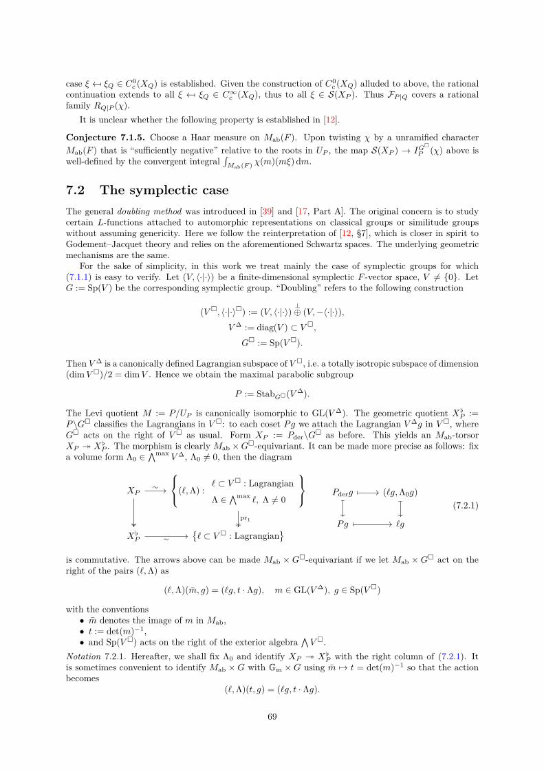
case ξ ←[ ξQ ∈ C0c (XQ) is established. Given the construction of C0

c (XQ) alluded to above, the rationalcontinuation extends to all ξ ←[ ξQ ∈ C∞

c (XQ), thus to all ξ ∈ S(XP ). Thus FP |Q covers a rationalfamily RQ|P (χ).

It is unclear whether the following property is established in [12].

Conjecture 7.1.5. Choose a Haar measure on Mab(F ). Upon twisting χ by a unramified characterMab(F ) that is “sufficiently negative” relative to the roots in UP , the map S(XP ) → IG

P (χ) above iswell-defined by the convergent integral

∫Mab(F ) χ(m)(mξ) dm.

7.2 The symplectic case

The general doubling method was introduced in [39] and [17, Part A]. The original concern is to studycertain L-functions attached to automorphic representations on classical groups or similitude groupswithout assuming genericity. Here we follow the reinterpretation of [12, §7], which is closer in spirit toGodement–Jacquet theory and relies on the aforementioned Schwartz spaces. The underlying geometricmechanisms are the same.

For the sake of simplicity, in this work we treat mainly the case of symplectic groups for which(7.1.1) is easy to verify. Let (V, 〈·|·〉) be a finite-dimensional symplectic F -vector space, V 6= 0. LetG := Sp(V ) be the corresponding symplectic group. “Doubling” refers to the following construction

(V , 〈·|·〉) := (V, 〈·|·〉)⊥⊕ (V,−〈·|·〉),

V ∆ := diag(V ) ⊂ V ,

G := Sp(V ).

Then V ∆ is a canonically defined Lagrangian subspace of V , i.e. a totally isotropic subspace of dimension(dim V )/2 = dim V . Hence we obtain the maximal parabolic subgroup

P := StabG(V ∆).

The Levi quotient M := P/UP is canonically isomorphic to GL(V ∆). The geometric quotient XP :=

P\G classifies the Lagrangians in V : to each coset Pg we attach the Lagrangian V ∆g in V , whereG acts on the right of V as usual. Form XP := Pder\G as before. This yields an Mab-torsorXP ։ X

P . The morphism is clearly Mab ×G-equivariant. It can be made more precise as follows: fix

a volume form Λ0 ∈∧max

V ∆, Λ0 6= 0, then the diagram

XP

(ℓ,Λ) :

ℓ ⊂ V : Lagrangian

Λ ∈∧max

ℓ, Λ 6= 0

XP

ℓ ⊂ V : Lagrangian

∼

pr1

∼

Pderg (ℓg,Λ0g)

Pg ℓg

(7.2.1)

is commutative. The arrows above can be made Mab × G-equivariant if we let Mab × G act on theright of the pairs (ℓ,Λ) as

(ℓ,Λ)(m, g) = (ℓg, t · Λg), m ∈ GL(V ∆), g ∈ Sp(V )

with the conventions• m denotes the image of m in Mab,• t := det(m)−1,• and Sp(V ) acts on the right of the exterior algebra

∧V .

Notation 7.2.1. Hereafter, we shall fix Λ0 and identify XP ։ XP with the right column of (7.2.1). It

is sometimes convenient to identify Mab ×G with Gm ×G using m 7→ t = det(m)−1 so that the actionbecomes

(ℓ,Λ)(t, g) = (ℓg, t · Λg).

69

On the other hand, G×G embeds naturally into G. Set V + := V ⊕ 0 and V − := 0 ⊕ V ; theyare Lagrangians of V .

Theorem 7.2.2 ([17, I. Lemma 2.1]). For every field extension E of F , the (G×G)(E)-orbits in XP (E),

or equivalently the (G×G)(E)-orbits of Lagrangians ℓ ⊂ V ⊗FE, are classified by the invariant

κ(ℓ) := κ±(ℓ) = dimE

(ℓ ∩ (V ± ⊗

FE)

).

In particular, there exists an Zariski-open dense orbit X+,; it is characterized as ℓ : κ(ℓ) = 0, andwe have κ(V ∆) = 0. Moreover, P ∩ (G ×G) = diag(G).

For any γ ∈ (X r X+,)(F ), there exists a proper parabolic subgroup R ⊂ G × G such that UR ⊂StabG×G(γ).

Implicit in the statements is the property that κ+(ℓ) = κ−(ℓ). Let G×G act on G as in (4.2.1). Thetheorem furnishes the G×G-equivariant embedding

G → XP

g 7−→ V ∆(g, 1) : Lagrangian ⊂ V .(7.2.2)

It is an open immersion onto the open G × G-orbit X+,. From the Mab-torsor structure, the inverseimage X+ ⊂ XP of X+, is readily seen to be an open dense Mab ×G×G-orbit in XP .

Lemma 7.2.3. Choose Λ0 ∈∧max

V ∆r0 in (7.2.1) as before. The composite below is an Mab×G×G-equivariant isomorphism (cf. (Notation 7.2.1))

Mab ×G Gm ×G X+

(m, g) (det(m)−1, g)

(t, g) (V ∆(g, 1), tΛ0(g, 1))

∼

that covers (7.2.2), the action on Mab ×G being (m, g)(a,g1,g2)7−→ (ma, g−1

2 gg1).

Proof. Let (ℓ,Λ) ∈ X+ with ℓ↔ g ∈ G under (7.2.2), the inverse morphism is given by sending (ℓ,Λ) to(Λ

Λ0g, g)

. The equivariance is routine to check.

For any m ≥ 0, let P∨(∧m

V ) denote the space classifying lines in∧m

V . The identification in(7.2.1) leads to the cartesian diagram

XP

∧dimVV r 0

XP P∨(

∧dimVV )

(7.2.3)

where the lower horizontal arrow is the Plücker embedding: namely a Lagrangian ℓ is mapped to theline

∧dimV ℓ in∧dimV V . All arrows are Mab × G-equivariant. As dim

∧dimV V ≥ 2, one infers

immediately that XP is quasi-affine: it is even possible to write down the defining equations ofX := XPaff

inside the affine space∧dimV

V . We obtain Mab ×G×G-equivariant embeddings

X+ open−−−→ XP

open−−−→ X := XP

aff closed−−−−→

dimV∧V .

Note that X = XP ⊔ ~0.

Lemma 7.2.4. The homogeneous Mab×G×G-space X+ is spherical and wavefront. Moreover, X+ → Xis an affine spherical embedding.

70

Proof. Combining Lemma 7.2.3 with the discussions in §4.2 gives the first part. For the second part, itis routine to see that X = XP

affis geometrically integral; the normality follows from that of XP .

Lemma 7.2.5. Under the affine embedding X+ → X above, the reduced closed subscheme ∂X := XrX+

is the zero locus of the relative invariant under Mab ×G×G

f+ :

dimV∧V −→

max∧V ≃ Ga

Λ 7−→ Λ ∧ v+

where v+ ∈∧max

V +, v+ 6= 0 under the Plücker embedding. Furthermore, the restriction of f+ toGm × G

∼→ X+ ⊂ X (using Lemma 7.2.3) is proportional to pr1 : Gm × G ։ Gm. Consequently its

eigencharacter is given by

ω1 : Mab ×G×G −→ Gm

(m, g1, g2) 7−→ t := (detm)−1.

The same conclusion holds if we use V −, v− and the corresponding regular function f−.

Proof. It suffices to deal with the case of V +. By Theorem 7.2.2, the open orbit X+ realized as theinverse image of X+, ⊂ X

P is characterized by ℓ ∩ V + 6= 0. This is equivalent to Λ ∧ v+ 6= 0 in∧maxV , where Λ ∈

∧dimVV lies over the image of ℓ under the Plücker embedding. It suffices to

show that f+ : Λ 7→ Λ∧v+ pulled back to Gm×G via Lemma 7.2.3 is proportional to pr1 : Gm×G→ Gm.Fix Λ0 ∈

∧maxV ∆ as in (7.2.1). For any (t, g) ∈ Gm ×G,

f+(Λ0(t, g)) = tΛ0(g, 1) ∧ v+ = t(Λ0 ∧ v

+(g−1, 1))

(g, 1)

= (det g−1)t(Λ0 ∧ v+)(g, 1)

= (det g−1) det(g, 1) · tΛ0 ∧ v+ = tΛ0 ∧ v

+

where we used the fact V + ⊂ V is stable under G× 1.

Lemma 7.2.6. The closed subscheme ∂X of X is geometrically integral.Moreover, the valuation v∂X : F (X)→ Z satisfies v∂X(f±) = 1 if it is normalized to have image Z.

Consequently, ∂X is defined by the ideal generated by f±.

Proof. According to Theorem 7.2.2, XP is stratified into G×G-orbits Ωd = ℓ : κ(ℓ) = d with

Ωa ⊂ Ωb ⇐⇒ a ≥ b.

The closure relation entails that there is at most one G×G-orbit of codimension one. By pulling back,the same property lifts to the Mab ×G ×G-orbits in XP , and then extends to X since X = XP ⊔ ~0by construction. In fact, our arguments below will give a recipe to steer an element of Ωa towards Ωa+1

by one-parameter subgroups, a = 0, 1, . . ..Being the zero locus of f±, by Krull’s theorem each irreducible component of ∂X has codimension

≤ 1. We infer that there exists a unique orbit O in X of codimension one, thus ∂X = O is irreduciblesince O is. As our arguments are based on Theorem 7.2.2 which works over any field extension of F , theirreducibility persists under field extensions. An immediate consequence is: any element of X lying overa Lagrangian ℓ ∈ X+, with κ(ℓ) = 1 (i.e. ℓ ∈ Ω1) belongs to O.

It remains to show v∂X(f+) = 1. We contend that for any x0 ∈ X+(F ), there exists a homomorphismof F -groups µ : Gm → G such that the morphism

c : Gm −→ X+

t 7−→ tx0(1, µ(t))

extends to c : Ga → X such that c(0) lies in the Mab ×G×G-orbit of codimension one. As (Mab ×G×G)(F ) operates transitively on X+(F ), we may assume that x0 is any element lying over V ∆ ∈ X+,(F ).

71

Decompose V into an orthogonal direct sum V0⊕V1 of symplectic vector spaces such that dimF V0 = 2.Choose a basis v, w of V0 verifying 〈v|v′〉 = 1, and any basis vi : 1 ≤ i ≤ dim V1 of V1. Set

b :=

dimV1∧

i=1

(vi, vi) ∈ im[max∧

V ∆1 →

dimV1∧V ]

multiplied in any order, with the convention b = 1 when V1 = 0. We may suppose that x0 =

(v, v) ∧ (w,w) ∧ b under the embedding X+ →∧dimV

V r 0 in (7.2.3). Take

µ(t) :=

v 7→ tv, w 7→ t−1w on V0

idV1 on V1.

In what follows, o(t) stands for any expression valued in∧V that involves only positive powers of t.

We compute

c(t) = t((v, tv) ∧ (w, t−1w) ∧ b

)

= t(((v, 0) + (0, tv)) ∧ ((w, 0) + (0, t−1w)) ∧ b

)

= t((

(v, 0) ∧ (w, 0) + t−1(v, 0) ∧ (0, w) + o(t) + (0, v) ∧ (0, w))∧ b)

= (v, 0) ∧ (0, w) ∧ b + o(t).

Hence c extends to Ga by mapping 0 to (v, 0) ∧ (0, w) ∧ b. Observe that (v, 0) ∧ (0, w) ∧ b lies over theimage of the Lagrangian ℓ = (Fv, 0)⊕ (0, Fw)⊕ V ∆

1 of V 0 ⊕ V

1 = V under (7.2.3). Since

κ(ℓ) = κV0 ((Fv, 0)⊕ (0, Fw)) + κV1 (V ∆1 ) = 1 + 0 = 1,

it must lie in the codimension-one stratum by the arguments above. This establishes our claim.Now we are in position to invoke the techniques of [53, §24.1]. Pick any x0 and construct c as above.

By (24.1) in loc. cit., for g ∈Mab ×G×G in general position we have

ordt=0( c∗(gf+)

∈F [Ga]≃F [t]

) = v∂X(f+) · i(c(0), ∂X · c;X)

where i(c(0), ∂X · c;X) is defined to be ordt=0(c∗(gh)) for any local parameter h of ∂X ; it makes sensefor generic g since the orbit closure containing c(0) equals ∂X .

Evaluate the left hand side first. Since f+ is a relative invariant, g can be neglected. As f+ haseigencharacter ω1, the regular function c∗(f+)(t) = f+(c(t)) is linear in t by construction of c. Soordt=0(c∗(gf+)) = 1, which implies that v∂X(f+) = i(c(0), ∂X · c;X) = 1. This completes the proof.

Theorem 7.2.7. The relative invariants of X are of the form c(f±)n with c ∈ F×, n ∈ Z, and themonoid ΛX is generated by ω1. Consequently, the geometric Axiom 2.4.3 is satisfied by the sphericalMab ×G×G-embedding X+ → X.

Proof. Observe that X∗(G) = 0. Apply Lemma 2.4.4 together with Lemma 7.2.3 to deduce that Λ isgenerated by ω1. By Lemma 7.2.5 we have ω1 ∈ ΛX ⊂ Λ since it is the eigencharacter of f±.

Since (f±)−1 has nontrivial polar divisor, namely ∂X , we see −ω1 /∈ ΛX . The only possibility isΛX = Z≥0 · ω1 and f± generates all relative invariants, as required.

Remark 7.2.8. The following observation will be useful in the global setting: for every γ ∈ ∂X(F ), thereexists a proper parabolic subgroup R ⊂Mab×G×G such that UR stabilizes γ. Indeed, by construction∂X maps onto ∂X = X r X,+. Suppose γ 6= ~0, otherwise our claim will be trivial. Theorem 7.2.2affords such a UR stabilizing the image γ ∈ ∂X(F ) of γ. To ascend to X , it suffices to observe thatthe fiber over γ is a Gm-torsor, on which the unipotent group UR can only act trivially. As in Theorem7.2.2, this property holds true over any field F of characteristic 6= 2.

As one of the referees pointed out, this property holds for wavefront spherical varieties except fororbits “along the center”: see [48, Lemma 2.7.1] for boundary degenerations, to which the general casecan be related via blowups. We refer to loc. cit. for details.

72

7.3 Doubling zeta integrals

Retain the notations in §7.2; in particular F is non-Archimedean, and Mab = GL(V ∆)/ SL(V ∆). SinceX+ ≃ Gm × G as Mab × G × G-varieties, the density bundles L s over X+ are equivariantly triv-ializable — this amounts to the existence of Haar measures on (Gm × G)(F ). Nevertheless, we re-tain the convention that C∞(X+), C∞

c (X+) and L2(X+) all consist of L12 -valued sections. Define

NΠ := HomMab×G×G(F )(Π, C∞(X+)).

Lemma 7.3.1. Consider an irreducible nice representation Π of (Mab×G×G)(F ). Then NΠ is nonzeroif and only if Π ≃ χ⊠ π⊠ π for some continuous character χ of GL(V ∆, F )/ SL(V ∆, F ) and irreduciblenice representation π of G(F ).

In this case, NΠ is canonically isomorphic to the one-dimensional space of invariant sections of L

over (Gm ×G)(F ): to any Haar measure |Ω| on (Gm ×G)(F ), we associate

ϕ : χ⊠ π ⊠ π −→ C∞(X+)

1⊗ v ⊗ v 7−→ (χ det) 〈v, π(·)v〉|Ω|12

where we identify X+, Gm ×G and Mab ×G by the recipe of Notation 7.2.1.

Proof. This is a special case of §4.2; the contragredient comes from the way Mab acts on XP .

By restriction to X+(F ), we view S := S(XP ) as a subspace of C∞(X+). In view of Theorem 7.2.7,hereafter we may take f+ to be the generator of ΛX and work in the formalism of §4.4. The datumv+ can even be chosen so that f+(t, g) = t if we identify Gm × G with X+. Also, we identify Λ withZ, ΛC with C in such a manner that Re(λ) ≥

X0 ⇐⇒ Re(λ) ≥ 0. The eigencharacter of |f+|λ under

Mab(F ) now becomes |ω1|λ : m 7→ | detm|−λ, where we denote by m ∈ P (F ) any inverse image of m. In

particular,ϕλ(1 ⊗ v ⊗ v) = (χ| · |−λ) det

on Mab

· 〈v, π(·)v〉

on G

|Ω|12 .

To discuss zeta integrals, fix• Π = χ⊠ π ⊠ π,• ϕ ∈ NΠ associated to a (Mab ×G×G)(F )-invariant density |Ω| as in Lemma 7.3.1.

For λ ∈ C, Re(λ)≫ 0, The zeta integral for ξ ∈ S and the vector 1⊗ v ⊗ v is

Zλ,ϕ ((1⊗ v ⊗ v)⊗ ξ) =

∫

X+

ξϕλ(1⊗ v ⊗ v)

=

∫g∈G(F )

m∈Mab(F )

ξ0

(δ

12

P · (χ| · |−λ) det

)(m)〈v, π(g)v〉|Ω|,

(7.3.1)

where ξ0 := ξδ− 1

2

P |Ω|− 1

2 : X+(F )→ C.

Apart from the δ12

P -shift, we claim that it equals the integral in [12, Theorem 7.5] in their “case 2”.The comparison goes as follows.

• As remarked in §7.1, in [12] one fixes a G(F )-invariant measure |Ξ| on XP (F ), the Mab(F )-action

on L2(XP (F )) is twisted by δ12

P . Their Schwartz function ξBK and our ξ ∈ S(XP ) are related viaξ = ξBK|Ξ|

12 .

• We have seen in §7.1 that |Ξ| has eigencharacter δP under Mab(F )-action. Hence |Ω| := δ−1P · |Ξ|

is a (Mab ×G×G)(F )-invariant density on X+(F ).

• Summing up, ξ0 = ξδ− 1

2

P |Ω|− 1

2 = ξ|Ξ|−12 = ξBK.

Proposition 7.3.2. The space S admits a natural structure of algebraic topological vector space. Itsatisfies Axiom 4.4.1.

73

Proof. For everyQ, the space C∞c (XQ) is algebraic with a continuous G(F )-action. Since S is expressed

as a finite lim−→

of those spaces in (7.1.2), S is algebraic as well. The required topological properties of Sfollows from Lemma 4.1.3, and it is a continuous G(F )-representation.

We also know that α : S → L2(XP ) = L2(X+). Since |f |λ is a continuous on X(F ) when Re(λ) ≥ 0,we also have Sλ ⊂ L2(X+). The continuity of αλ : S → L2(X+) is automatic by algebraicity. Theholomorphy of αλ over λ ∈ C : Re(λ) ≥ 0 boils down to that of

∫XP|f |λξb for given b ∈ L2(XP ) and

ξ ∈ S, which is in turn guaranteed by Lemma 7.1.3 and dominated convergence.It remains to verify the conditions concerning zeta integrals. Convergence for Re(λ) ≫ 0 is implied

by Corollary 5.3.7. Since Zλ equals the integral in [12, §7], the rationality, etc. of Zλ are recorded in loc.cit.; continuity does not matter since the topological vector spaces in view are all algebraic.

For discussions on the Archimedean case, see [12, §6.1]. One expects a suitable Fréchet space S =S(XP ) ⊂ L2(XP ). See also [20, §5.2].

Remark 7.3.3. In order to get the usual doubling zeta integral, one has to choose a Haar measure onMab(F ), assume Conjecture 7.1.5 and integrate ξϕλ(1 ⊗ v ⊗ v) along Mab(F )-orbits for Re(λ) ≫ 0.This procedure has been summarized in Remark 7.1.4. The conclusion is that it yields a section fλ ∈

IG

P (χ⊗ | det |λ), rational in qλ, and that (7.3.1) becomes∫

G

fλ(g, 1)〈v, π(g)v〉|Ω′′|

for some invariant density |Ω′′| on G(F ), where we used the natural inclusion G×G → G. This is theoriginal integral in [17, p. 3] except that our parabolic induction is normalized. The sections fλ(g, 1) soobtained are good sections in the sense of [40, p.110], which play a pivotal role in the doubling method.Consequently, one should view S as a space of universal good sections. See [51] for further details.

Now move to the functional equations. Two types of model transitions are involved.

1. Let Q be another parabolic subgroup of G sharing the same Levi component M as P . In fact,the only choice in our framework is the opposite parabolic Q = P−. The model transition is thenFQ|P : S(XP )

∼→ S(XQ).

2. Let w ∈ NG(M)(F )/M(F ) and wQ := wQw−1. We have the isomorphism

XwQ∼−→ XQ

(wQ)g′ 7−→ Qw−1g′, g′ ∈ G

between G-varieties over F . In contrast, acting by wmw−1 ∈Mab on XwQ corresponds to actingby m on XQ; this is remedied by twisting the Mab×G-structure on XwQ accordingly. Therefore,transport of structure gives rise to the model transition

Fw : L2(XQ)∼−→ L2(XwQ)

S(XQ)∼−→ S(XwQ).

Usually we assume wQ = P , and such a w exists in our setting. In this case, conjugation by winduces the involution t 7→ t−1 of Mab.

We have Λ1 = Z = Λ2 in the notation of §4.5. Thus F := FwFQ|P furnishes a model transition

S(XP )∼→ S(XP ) if we take Q = P− and wQ = P . More precisely, X1 = X = XP

aff= X2 and

S1 = S(XP ) = S2, but the objects with subscript 1 are endowed with the twisted Mab-action as above;F : S2

∼→ S1 is Mab ×G×G(F )-equivariant under the conventions above.

Conjecture 7.3.4. Set S := S(XP ). Let χ⊠ π⊠ π be an irreducible nice representation of (Mab×G×G)(F ). When we vary χ in a family χ⊗ | det |λ, λ ∈ C, the space

HomMab×G×G(F ) (χ⊠ π ⊠ π,S∨)

is at most one-dimensional for χ in general position.

74

Theorem 7.3.5. Under the assumptions of Proposition 7.3.2 and admit either• Conjecture 7.1.5, or• Conjecture 7.3.4,

then the local functional equation (Definition 4.5.2) holds for F .

Proof. Let Π := χ⊠π⊠ π be an irreducible nice representation of (Mab×G×G)(F ). The elements ϕ(2)

of N (2)Π have been described as in Lemma 7.3.1; as for X1 = X , there is a twist

ϕ(1) : 1⊗ v ⊗ v 7−→ χ(·)〈v, π(·)v〉|Ω|12

and ϕ(1)λ = | det |λϕ(1).

Assume Conjecture 7.1.5. In view of the twists and Remark 7.3.3, our assertion reduces to thedoubling functional equation [39, Theorem 2.1] provided that we can relate F = FwFQ|P to a rational

family of intertwining operator R(w, λ) : IG

P (χ ⊗ | det |λ) → IG

P (χ ⊗ | det |−λ) such that the followingdiagram commutes for general λ ∈ C:

S(XP ) S(XP )

IG

P (χ⊗ | det |λ) IG

P (χ⊗ | det |−λ)

F

R(w,χ⊗| det |λ)

Apart from an easy w-twist, this is contained in Remark 7.1.4.Under Conjecture 7.3.4, the arguments are completely the same as [39, Theorem 2.1].

Remark 7.3.6. Methodologically, the route via Conjecture 7.3.4 seems more natural. It also implies therationality of zeta integrals by Bernstein’s principle [17, Part B, §12], the isomorphism NΠ ⊗ K

∼→ LΠ,

as well as the condition (4.6.7); see the proof of Theorem 6.3.5.

7.4 Relation to reductive monoids

Most of the following basic results are extracted from [53, §27.1] and [43].

Definition 7.4.1. By an F -monoid Y , we mean a monoid-like object in the category of algebraic F -varieties, or equivalently a representable functor hY : Var

opF → Monoid. The subfunctor of invertible

elements is represented by an open subvariety G := G(Y ), which is actually an F -group called the unitgroup of Y . Call Y normal, affine, etc., if Y has those properties as a variety. An F -monoid Y with unitgroup G is naturally a G×G-variety under multiplication, cf. (4.2.1):

y(g1, g2) = g−12 yg1.

Fix the ground field F . Monoids with connected reductive unit groups are called reductive monoids.Suppose that Y is an affine, normal reductive monoid with unit group G. Then G → Y can be viewed asa spherical embedding under the G×G-action.. The abelianization of Y is defined as the GIT quotientab : Y → Y Gder ×Gder.

Following [38], we say that Y is flat if ab is a flat morphism with geometrically reduced fibers. Flatmonoids are systematically studied by Vinberg and Rittatore.

Example 7.4.2. The variety Matn×n is a normal affine monoid under matrix multiplication. Its unitgroup is GL(n). It is a flat monoid whose abelianization can be identified with det : Matn×n → Ga (eg.by Igusa’s criterion [50, II. §4.5]). This space has been considered in §6.4.

Theorem 7.4.3 (A. Rittatore). Let G be a split connected reductive F -group. The category of normalaffine reductive monoids with unit group G is equivalent to the category of affine spherical embeddings ofG.

75

More precisely, the monoid structure of a given spherical embedding Y of G is uniquely determined,since the multiplication must restrict to the group law over the open dense orbit G.

Consequently, such monoids are classified by Luna–Vust theory (Theorem 2.1.3) applied to the ho-mogeneous G×G-space G, at least over the algebraic closure. It turns out that their colored cones havefull colors, and each color is defined over F .

Corollary 7.4.4 (See [53, Theorem 27.12]). The normal affine reductive monoids Y are classified bycolored cones of the form (CY ,DB).

Now revert to the setting in §7.2. Recall that the affine variety X carries a right Mab-action com-muting with G. Identify Mab and Gm as in Notations 7.2.1, written as m↔ t. Then we can let Gm acton the left of X via tx = xm−1. Also recall that there is a distinguished point ~0 ∈ X(F ). This endowsX with a conical structure. For every x ∈ X(F ) we have

limt→0

tx = ~0 ∈ X(F ),

the limit being taken in the algebraic sense: the orbit map Gm → X extends to Ga → X , and ~0 ∈ X(F )is the image of 0 ∈ Ga. This implies that limt→0 f(tx) = f(~0) ∈ P1(F ), for every f ∈ F (X)× and x ∈ X .

Lemma 7.4.5. Suppose that f ∈ F (X)× satisfies f(tx) = tdf(x) under the Gm-action, for some d ∈ Z.If d = 0 then f is constant.

Proof. Assume d = 0. For any x ∈ X we have f(x) = limt→0 f(tx) = f(~0). Hence f is constant.

Also recall that the open orbit X+ ≃ Gm ×G is a Mab ×G ×G-variety. By recalling the definitionof the group actions together with the fact Mab ≃ Gm, this resembles the setting of monoids with unitgroup Mab×G. One exception: here the acting group is Mab×G×G instead of (Mab×G)2; as remarkedat the end of §4.2, this is actually irrelevant. One retrieves the required M2

ab-action by composing withM2

ab →Mab, (a, b) 7→ ab−1. We shall omit this formal step.

Proposition 7.4.6. The Mab×G×G-variety X admits a canonical structure of affine normal reductivemonoid with unit group Mab ×G. Furthermore, it is a flat monoid with singular locus equal to ~0.

Proof. Since X+ → X is an affine spherical embedding, it suffices to apply Theorem 7.4.3 to deduce themonoid structure. On the other hand, the relative invariant f+ defines a dominant morphism X → Ga,hence flat; we claim that f+ is the abelianization of X . Since f+ pulls back to pr1 : Gm×G→ Gm overGm ⊂ Ga, it is indeed the GIT quotient by G×G by Igusa’s criterion [50, II. §4.5].

The scheme-theoretic fibers of f+ over Gm are all isomorphic to G, whereas the fiber over 0 ∈ Ga isthe geometrically integral scheme ∂X by Lemma 7.2.6. Thus X is a flat monoid.

By (7.2.3), there are exactly two G-orbits in X = XPaff

, namely XP and 0, thus it suffices toshow X is singular. The singularity of X follows from [53, Theorem 27.25]. Alternatively, one may apply[43, Theorem 5.5] using the fact that the monoid X has a “zero element”, namely ~0.

Note that Lemma 7.2.6 is necessary for the proof.We are ready to describe the Luna–Vust datum for X . It is customary to work with a Borel subgroup

of Mab × G × G of the form Mab × B− × B; let A be the Levi quotient of B. Some generalities aboutthe homogeneous space X+ ≃ Gm ×G are needed; details can be found in [53, p.161].

• Observe thatΛX+ = X∗(Gm)⊕X∗((A×A)/diag(A)) = Z⊕X∗(A)

where the last equality comes from Z = X∗(Gm) ≃ X∗(Mab) and the second projection A ×A/diag(A)

∼→ A.

• The colors for X+ are exactly the products of Gm with the closures of the Bruhat cells B−wBin X+, where w represents the simple root reflections, indexed by either the simple coroots α ordually the fundamental weights . The color D corresponding to equals the zero loci of thefollowing matrix coefficient of the irreducible algebraic G-representation (ρ, Vρ) with highest weight

f : (t, g) 7→ 〈v−, vρ(g)〉, f ∈ F (X+),

76

where v (resp. v−) is a highest weight vector in in Vρ (resp. the lowest weight vector in V ∨ρ ). The

eigencharacter of f under Gm × B− × B equals (0, ) ∈ ΛX+ = Z ⊕X∗(A). All are F -rationalsince G is split.

• The valuation cone V ⊂ Q equals the anti-dominant Weyl chamber⋂

α

〈α, ·〉 ≤ 0, α ∈ X∗(A) ranges over the positive roots.

• Choose a symplectic basis e1, . . . , en, fn, . . . , f1 of the symplectic F -space V , i.e. 〈ei|ej〉 = 〈fi|fj〉 =0 and 〈ei|fj〉 = δi,j (Kronecker’s delta), so that G = Sp(V ) → GL(2n). We can take B to be theupper triangular subgroup intersected with G, thereby obtain the basis ǫ∗

1, . . . , ǫ∗n of X∗(A) given

by

ǫ∗i :

t1. . .

tn

t−1n

. . .

t−11

7→ ti, i = 1, . . . , n.

The dual basis of X∗(A) is denoted by ǫ1, . . . , ǫn. The fundamental weights are given by

i := ǫ∗1 + . . .+ ǫ∗

i , i = 1, . . . , n.

On the other hand, the simple roots are ǫ∗i − ǫ

∗i+1 with 1 ≤ i < n and 2ǫ∗

n, relative to the Borelsubgroup B chosen above.

• For i = 1, . . . , n, the normalized discrete valuation corresponding to Di is ρ(Di) ∈ Q. Since∂X = f+ = 0 does not contain any color, we have ρ(Di)(f

+) = 0 for all i. Also notice that f+

has eigencharacter (1, 0) ∈ Z ⊕X∗(A), hence (ρ(Di))ni=1 lie in 0 ⊕ X∗(A) and form the dual

basis of the fundamental weights, i.e. the simple coroots. Specifically, the simple coroot dual toi = ǫ∗

1 + · · ·+ ǫ∗i is

αi =

ǫi − ǫi+1, 1 ≤ i < n

ǫn, i = n.

Theorem 7.4.7. The colored cone associated to X+ → X is (C,DMab×B−×B) where C is the conegenerated by the colors

ρ(Di) = αi, i = 1, . . . , n,

together with(1,−ǫ1) ∈ ΛX+ ∩ V .

Proof. By Corollary 7.4.4, the colored cone (C,F) associated to X+ → X satisfies F = all colors, andwe have seen that the corresponding valuations are given by simple coroots.

Recall that ∂X is a prime divisor by Lemma 7.2.6. Write = i. The poles of the defining equationsf ∈ F (X) for the colors D ⊂ X+ can only lie in ∂X . The defining equation of the prime divisor D

in X is thus given by tdf, where d = −v∂X(f) (recall that X is normal and t ∈ F [X+] ⊂ F (X) is auniformizer for ∂X). We contend that d = 1 for every fundamental weight ; in particular tf ∈ F [X ].

Write Gm = SpecF [s, s−1]. By the proof of Lemma 7.2.6, for g ∈ Mab ×G × G in general positionwe have

v∂X(f) = ords=0 (f(c(s)g)) · i(c(0), ∂X · c;X)

= ords=0 (f(x0(1, µ(s))g)) · i(c(0), ∂X · c;X)

=1

,

77

where the base point x0 ∈ X+(F ), the morphism c : Gm → X+ and µ : Gm → G are defined in the citedproof, namely c(s) = sx0(1, µ(s)). Here we used the fact that f is invariant under Mab-action. For thesame reason, it suffices to take g = (1, g1, g2) with generic g1, g2 ∈ G.

By Lemma 7.2.3, we identify X+ with Gm × G so that x0 = (1, 1); the Gm × G × G-action is alsospecified there. Let ρ be the (right) G-representation of highest weight ; take vectors v and v− inρ and ρ, with weights and − respectively such that 〈v−, v〉 = 1. Then

f(g) = 〈v−, ρ(g)v〉 , g ∈ G.

Thus we have to calculate, for generic g1, g2 ∈ G:

ords=0

⟨ρ(g2)v−, ρ(µ(s)−1)ρ(g1)v

⟩.

Consider the standard representation of G on V =⊕n

i=1(Fek⊕Fe−k). Recall that 1 the fundamentalweights of G are k = ǫ∗

1 + · · ·+ ǫ∗k with k = 1, . . . , n; the corresponding highest weight representations

ρk are realized on

Ek := 〈ea1 ∧ · · · eal ∧ e−b1 ∧ · · · ∧ e−bm : 1 ≤ a1 < · · · < bm ≤ n, l+m = k〉

⊂ ∧kV, k = 1, . . . , n.

We then takevk = e1 ∧ · · · ∧ ek, v−k = e∗

1 ∧ · · · ∧ e∗k mod E⊥

k .

In the proof of Lemma 7.2.6 we took

µ(s) : e±i 7→

s±1e±i, i = 1,

e±i, i > 1.(1 ≤ i ≤ n)

Using this realization, it is clear that

δ(s, g1, g2) :=⟨ρk(g2)v−k , ρk(µ(s)−1)ρk(g1)vk

⟩∈ s−1F [s],

and ords=0 (δ(s, g1, g2)) for generic (g1, g2) equals actually

inf(g1,g2)∈G2

ords=0 (δ(s, g1, g2)) , which is ≥ −1.

If the right hand side is ≥ 0 then f ∈ F [X ] and is invariant under the Gm-dilation on X . This wouldimply the constancy of f by Lemma 7.4.5. This leads to a contradiction. Hence v∂X(f) = −1.

Since (t, g) 7→ t has eigencharacter (1, 0), we see D is defined by an eigenfunction of eigencharacter(1, ). If we express the normalized discrete valuation of the divisor ∂X as

v∂X =

(a0,

n∑

i=1

aiǫi

)∈ ΛX+ ∩ V ,

then:

(i) since f± has eigencharacter (1, 0, . . . , 0), we infer 1 = v∂X(f±) = a0 from Lemma 7.2.6;

(ii) since Di 6⊃ ∂X , we have 0 = v∂X(tfi) = a0 + a1 + · · ·+ ai, for i = 1, . . . , n.

This system of (n+ 1) equations is easily solved to yield v∂X = (1,−ǫ1).

Consider Langlands’ dual group (Mab ×G)∧ over C: it comes equipped with a dual Borel subgroupGm,C× B and a dual maximal torus Gm,C× A ⊂ Gm,C× B, together with identifications X∗(A) = X∗(A)

and X∗(A) = X∗(A), under which the based root datum of (G, B, A) is dual to that of G. In particular,the roots/coroots, fundamental weights/coweights get exchanged.

We have (Mab × G)∧ = Gm,C × G and G ≃ SO(2n+ 1,C). The standard representation std : G →GL(2n+ 1,C) is thus defined. Tensored with the identity representation of Gm,C on C, we get

id ⊠ std : (Mab ×G)∧ → GL(2n+ 1,C).

This algebraic representation is irreducible since std is; this standard fact will be reproved in whatfollows.

1See N. Bourbaki, Lie groups and Lie algebras, Chapters 7—9, pp.206–207.

78

Proposition 7.4.8. The representation id ⊠ std has B-lowest weight equal to (1,−ǫ1) ∈ Z ⊕X∗(A) =X∗(Gm,C × A), and B-highest weight equal to (1, ǫ1).

Proof. The standard representation of SO(2n+ 1,C) has weights

−ǫ1, . . . ,−ǫn, 0, ǫn, . . . , ǫ1

as elements of X∗(A) = X∗(A), which are strictly increasing in the order relative to B. Hence −ǫ1 is theunique B-lowest weight; in particular std is irreducible. The passage to id ⊠ std is straightforward.

We conclude this section by recalling the recipe of Braverman and Kazhdan [11] that connects re-ductive monoids to L-functions. Here the group under inspection is Mab ×G ≃ Gm ×G. The inclusionGm,C → (Gm × G) is clearly dual to pr1 : Gm × G → Gm. Let ρ := id ⊠ std be the irreduciblerepresentation of Gm,C × G; it restricts to z 7→ z · id on Gm,C.

Following [11, §5.5], one attaches an irreducible affine normal monoid Xρ to ρ with unit group Gm×G.L. Lafforgue explained their construction in [33, Définition V.9]. In our setting where ρ is irreducibleand (Gm×G)der = G is simply connected, this construction has been rephrased by B. C. Ngô in [38] and[9, §4] in terms of Vinberg’s theory, which is essentially the dual version of Luna–Vust classification inthe case of reductive monoids. In this situation Xρ will be a flat reductive monoid, called the L-monoidassociated to ρ.

Theorem 7.4.9. The reductive monoids Xρ and X are isomorphic.

Proof. We shall adopt Lafforgue’s description in [33]: the idea is to characterize the monoid in terms ofthe closure of a maximal torus with Weyl group action — see [43, Theorem 5.4]. Fix a maximal torusT ⊂ Gm × B of Gm ×G. The closure T in X is an affine normal toric variety under T , see [13, 6.2.14].Furthermore, [53, Proposition 27.18] implies that as a toric variety T is determined by the cone CT ⊂ Qgenerated by the Weyl translates of CX ∩V . Combine Theorem 7.4.7, Proposition 7.4.8 and the standardproperties of the weights of ρ, we see CT is the convex hull of the Weyl translates of the Gm,C× B-lowestweight (1,−ǫ1) ∈ Z⊕X∗(A) of ρ. This is exactly the characterization of Xρ in [33, Définition V.9].

As illustrated by [39, 17], the doubling zeta integrals or the integrals (7.3.1) point to the L-factor

L

(·+

1

2, χ× π

)= L

(·+

1

2, χ⊠ π, ρ

)

by taking the greatest common divisor for various ξ, where χ ⊠ π is an irreducible nice representationof Mab ×G(F ). The Braverman–Kazhdan program addresses the same issue by considering integrals ofthe same kind as (7.3.1), namely: matrix coefficients integrated against “Schwartz functions”. Morally,their approach is based on the following inputs

(i) a certain Schwartz space that should be intimately related to the flat monoid Xρ;

(ii) a Fourier transform that should give rise to local functional equations;

(iii) a Poisson summation formula in the global setting.

The standard case is Godement–Jacquet theory whose corresponding monoid is described as in Example7.4.2. The preceding results affirm that

• the geometry is correct: Xρ = X underlies both the L-monoid and the doubling constructions, andit conforms to our formalism in §2.4 and §4.4;

• the doubling integrals go beyond Godement–Jacquet — in particular, the space X is singular;

• we do have the Schwartz space and Fourier transform of at our disposal, and they also fit into ourgeneral setting §4.5 of model transition.

A weak version of the Poisson formula for doubling integrals will be discussed in §8.4. Although ourconstructions still hinge on several conjectures, there seem to be good signs for further works.

79

7.5 Remarks on the general case

The reason for limiting to the symplectic case is threefold: (1) it is simpler; (2) in that case the formalismsof [12] and [39, 17] coincide; (3) the doubling method for unitary or orthogonal groups will involve non-split or disconnected groups which deviates from our general framework, albeit harmlessly.

We sketch the general case of doubling following [39, 17]; see also [51]. Consider a field extensionE|F with [E : F ] ≤ 2. Fix ǫ ∈ ±1 and a finite-dimensional ǫ-Hermitian space (V, (·|·)) relative toE|F . Define G = G(V ) as the corresponding unitary group. Consider the ǫ-Hermitian space V :=

(V, (·|·))⊥⊕ (V,−(·|·)) and the unitary group G := G(V ). The diagonal V ∆ is still a maximal totally

isotropic subspace in V . Define the Siegel parabolic P := StabG(V ∆) of G, with Levi quotient M .Set XP := G/Pder and X

P := G/P .Note that M ≃ GLE(V ∆), Mab ≃ Gm,E so our assumption (7.1.1) is verified. When E = F and

ǫ = −1, we revert to the symplectic case. When E = F and ǫ = 1, the groupsG and G are disconnected.

• By defining the Lagrangians of V as maximal totally isotropic E-vector subspaces, the morphismXP ։ X

P admits a linear-algebraic description parallel to (7.2.1), and we still have the Plückerembeddings.

• Lemma 7.2.3 still holds: we obtain an Mab ×G×G-equivariant embedding Mab ×G → XP withopen image X+ ⊂ XP by choosing any nonzero Λ0 ∈

∧max V ∆. This embedding stems fromTheorem 7.2.2, which holds in the general setting by [17, I. Lemma 2.1].

Note that Mab ×G differs from the group H considered in [12, §7] except in the symplectic case.

• As in §7.2, we takeX := XPaff

= XP ⊔0, and deduce an Mab×G×G-equivariant open embeddingX+ → X . The boundary ∂X := X rX+ is again the zero locus of a relative invariant f+ as inLemma 7.2.5, with the same proof.

• Lemma 7.2.6 (hence Theorem 7.2.7) also holds in this setting. It is a statement about geometryand one should check it on the algebraic closure F . When [E : F ] = 2, as E⊗F F ≃ F ×F , we arereduced to the doubling method for general linear groups; the required geometric properties arefurnished in [17, I.4.2].

• Remark 7.2.8 also holds in the general setting, as proven in loc. cit.

• The zeta integrals are as in §7.3 except that GL(V ∆)det−−→ Gm becomes GLE(V ∆)

detE−−−→ Gm,E, and| · | becomes | · |E : E → R≥0. The result still takes the form (7.3.1), namely

Zλ,ϕ ((1⊗ v ⊗ v)⊗ ξ) =

∫

X+

ξϕλ(1⊗ v ⊗ v)

=

∫g∈G(F )

m∈Mab(F )

ξ0

(δ

12

P · (χ| · |−λE ) det

E

)(m)〈v, π(g)v〉|Ω|,

Re(λ)≫ 0,

with the same assumptions on |Ω|, 1⊗v⊗ v ∈ χ⊗π⊗ π, ξ ∈ S and ξ0 := ξδ− 1

2

P |Ω|− 1

2 : X+(F )→ C.

• The zeta integrals also have an interpretation as integration of matrix coefficients of G against thegood sections in doubling method. There are subtleties related to normalization of intertwiningoperators; we refer to [51] for details.

• As for the relation to reductive monoids, cf. §7.4, we assume E = F and G is split in order tocomply with [9]. Proposition 7.4.6 and its proof carry over, showing thatX+ → X is a flat reductivemonoid. When ǫ = +1, we choose a basis e1, . . . , en, fn, . . . , f1 for V such that (ei|fj) = δi,j and(ei|ej) = (fi|fj) = 0 for all 1 ≤ i, j ≤ j. It yields a basis ǫ1, . . . , ǫn for X∗(A). The Luna–Vustdatum (C,F) computed in this basis is still given by Theorem 7.4.7:

F = all colors, C is generated by the simple coroots and (1,−ǫ1).

80

This is to be compared with the irreducible representation ρ := id ⊠ std of Gm,C × G. Here thedual group G of the identity connected component of G equals SO(2n + 1,C) (resp. Sp(2n,C),SO(2n,C)) if G is symplectic (resp. odd orthogonal, even orthogonal) of rank n. The highest (resp.lowest) weight of ρ is still given by Proposition 7.4.8, namely (1, ǫ1) (resp. (1,−ǫ1)).

Now we can show that X coincides with the monoid Xρ in [33, Définition V.9] (or [9, 38]) as donein Theorem 7.4.9. The proof carries over verbatim.

81

Chapter 8

Speculation on the global integrals

The constructions of basic vectors (also known as “basic functions”) and ϑ-distributions stem from [47,§3], to which we refer for further examples. In what follows, fix• F : a number field with the ring of adèles A = AF and F∞ :=

∏v|∞ Fv;

• G: split connected reductive F -group with a chosen Borel subgroup B;• ψ : F\A→ C×: non-trivial unitary character, by which one normalizes the Haar measures on eachFv.

We will consider affine spherical embeddings X+ → X under G subject to the same geometric Axiom2.4.3, except that everything is now defined over the number field F . The objects Λ, ΛX , etc. are thusdefined. In particular, the chosen relative invariants (fi)

ri=1 and their eigencharacters (ωi)

ri=1 are defined

over F ; the character |ω|λ : G(A)→ C× is automorphic for all λ ∈ ΛC.Assume furthermore that the monoids ΛXv for each place v equals ΛX . Therefore f1, . . . , fr can be

used in the local settings. We will choose an arbitrary oF -model of G and of the G-equivariant embeddingX+ → X .

We will impose two Hypotheses 8.1.4, 8.2.2 later on.

8.1 Basic vectors

Let X+ → X be an affine spherical embedding under G-action.

• We have the G(A)-equivariant line bundle L of densities over the adélic space X+(A). It is not

defined as a restricted ⊗-product.

• Suppose that for each place v of F , we are given:

– a G(Fv)-equivariant vector bundle Ev over the Fv-analytic manifold X+(Fv);

– a non-degenerate equivariant Ev ⊗ Ev → Lv as in (3.1.3), where Lv stands for the densitybundle over X+(Fv);

– a smooth continuous representation Sv of G(Fv) satisfying Axiom 4.4.1 with respect to Ev.

Moreover, we adopt the convention L2(X+v ) := L2(X+(Fv),Ev), C∞

c (X+v ) := C∞

c (X+(Fv),Ev) as

in §4.1, so that Sv ⊂ L2(X+v ). The typical example is the bundle of half-densities: Ev = L

12v .

• Observe that for almost all places v ∤ ∞, the oF -model of the G-equivariant embedding X+ → Xand the relative invariants are unramified at v, this means:

– G is a smooth connected reductive group scheme over ov, hence G(ov) ⊂ G(Fv) is a hyper-special subgroup;

– X+ is smooth over ov;

– fi ∈ ov[X ] ∩ ov[X+]× for i = 1, . . . , r.

Definition 8.1.1. By a system of basic vectors, we mean a family of distinguished elements ξv ∈ Sv

chosen for almost all v ∤∞ at which our data are unramified, such that

82

(i) ξv is G(ov)-invariant,

(ii) Supp(ξv) ⊂ X(ov) ∩X+(Fv),

(iii) ξv is non-vanishing over X+(ov),

(iv) the global pairing E ⊗ E → L is well-defined (see below).

The adélic Schwartz space with respect to the system of basic vectors is

S :=⊗′

vSv = lim

−→S

⊗

v∈S

Sv

where S ranges over finite sets of places of F that contain v : v | ∞, and the transition map⊗

v∈S Sv →⊗v∈V Sv is given by multiplication by

∏v∈VrS ξ

v whenever V ⊃ S.

Given a system of basic vectors, define similarly the bundle E over X+(A) whose fiber at x = (xv)v ∈X+(A) equals

Ex :=⊗′

vEv,xv ,

the restricted product being taken with respect to the values of basic vectors ξv at xv. In a similar vein

one defines E x. A priori, the local pairings Ev ⊗ E v → Lv do not necessarily give rise to E ⊗ E → L ,due to the possible divergence of infinite products of local densities. Our last assertion ensures theconvergence.

Remark 8.1.2. The space S can be topologized in many ways. Here we adopt the inductive topology for⊗-products (see [24, pp.92-93]) on each

⊗v∈S Sv, and then pass to lim

−→S.

Remark 8.1.3. In view of the definition of S and the topology on X+(A), the condition (iv) for basicvectors is equivalent to that every ξ ∈ S is locally L2 over X+(A).

Hypothesis 8.1.4. We suppose that for every γ ∈ X+(F ), a linear surjection

evγ : Eγ ։ C

is given with the following properties.

(i) There exists an automorphic character χγ : Hγ(A) → C× where Hγ := StabG(γ), such thatevγ(· h) = χγ(h)evγ(·) for all h ∈ Hγ(A), and χγ = 1 on (Hγ ∩ ZG)(A).

(ii) For every g ∈ G(F ), the composite of evγg with g : Eγ∼→ Eγg equals evγ .

The maps evγ will be used to define ϑ-distributions in §8.2. Furthermore, we will often extend it tothe F -points of some subvariety larger than X+, see §8.4.

Example 8.1.5. Take Ev = L12v . Suppose that we are given a family of convergence factors

λv > 0 : v is a place of F

(terminology borrowed from [57, §2.3]), such that for every γ ∈ X+(F ) and every algebraic volume form

ω of X+ satisfying ω(γ) 6= 0, the infinite product∏v/∈S λvξ

v(γ)|ω(γ)|

− 12

v converges, where S is a largefinite set of places and γ ∈ X+(ov) for v /∈ S. Note that this condition is independent of the choice of ω.The conclusion is that one can define

evγ :⊗

v

tv 7−→∏

v

λv ·tv

|ω(γ)|12v

.

It varies under Hγ(A) according to an automorphic character χγ by the discussions preceding (3.1.2),and χγ is easily seen to be trivial on (Hγ ∩ ZG)(A). The second property relating evγ and evγg stemsfrom Artin’s product formula.

We refine Example 8.1.5 in two special cases below.

83

Example 8.1.6. Suppose thatX is a prehomogeneous vector space underG-action (see §6) and Ev = L12v

as above. We retain the assumptions in Theorem 6.2.6 so that X+ → X satisfies all our premises. Inthis case we take Sv = S(Xv) to be the space of Schwartz–Bruhat half-densities on X(Fv). Take anoF -structure of G and X : concretely, this means that we fix an oF -lattice L ⊂ X(F ) which is G(oF )-invariant. Choose an algebraic volume form ω on X that comes from

∧dimX L r 0. Then X and ωhave good reduction at almost all v ∤∞.

At those places v ∤∞, the basic vectors are taken to be

ξv = 1X(ov)λ

−1v |ω|

12v ,

where λv > 0 is taken such that ‖ξv‖L2 = 1; the square of λv is essentially the convergence factor in the

theory of Tamagawa measures.The global pairing L

12 ⊗L

12 → L is well-defined by the choice of λv and Remark 8.1.3.

We claim that S with the topology from Remark 8.1.2 is isomorphic to the usual space in [56, §11]of adélic Schwartz–Bruhat half-densities on X(A) if there is only one Archimedean place; otherwise wemust use

⊗v|∞Sv ⊗

⊗v∤∞ Sv instead. Notice that the inductive topology on

⊗v|∞ Sv coincides with

the projective topology since the Archimedean Schwartz spaces are nuclear Fréchet. The claim followsbecause for v ∤∞, the space Sv is a strict inductive limit of finite-dimensional spaces as in Lemma 6.1.2,and it remains to remark that inductive tensor product preserves such limits.

The definition of evγ is straightforward: indeed, the convergence factors λv have just been defined.It corresponds to the usual evaluation map of Schwartz–Bruhat half-densities at rational points.

Since X is non-singular, we see that evγ is defined for all γ ∈ X(F ) by exactly the same recipe ofExample 8.1.5.

Example 8.1.7. Consider the space XP in §7.1; it is a spherical homogeneous space under Mab ×G

with the notations thereof. The spaces Sv have been defined at non-Archimedean v: they take values in

the bundle Ev := L12v . The basic vectors are defined in [12, p.548] as functions, denoted by cP = cP,0

therein. To obtain a section of L12v , one has to choose a G(Fv)-invariant measure |Ξ|v on XP (Fv). By

[12, (5.4)] we have cP = |Ξ|12v on the G(oF )-orbit containing Pder · 1. We prefer not to pin down the

choice of |Ξ|v here: it is enough to satisfy (iv) of Definition 8.1.1.Granting the definition of Sv for v | ∞ (see [12, §6.1]), one can fix |Ξ|v at the remaining places v and

define S =⊗′

vSv, whose elements may be viewed as functions. Let γ ∈ XP (F ). In loc. cit. the map evγis simply the evaluation of functions in S at γ. In terms of our formalism in Example 8.1.5, it amounts

to taking λv = |ω(γ)|12v · |Ξ|

− 12

v .In the doubling method, eg. in §7.2, one usually works with a smaller group G such that G × G is

canonically embedded in G, and work with the spherical varietyX := XPaff

with openMab×G×G-orbitX+. The global formalism developed in this section applies to X+ → X instead of XP . Nonetheless, asin the previous case of prehomogeneous vector spaces, the maps evγ are actually defined on the largervariety XP .

8.2 Theta distributions

Retain the conventions on X+ → X , S, etc. from the previous section.

• Choose x0 ∈ X+(F ) (Proposition 2.3.1) and put Z[X ] := StabG(x0)∩ZG. This is a diagonalizable

F -group which is independent of the choice of x0. It is well-known that there is a closed subgroupa[X ] ⊂ Z[X ](F∞) isomorphic to RdimZ[X], such that Z[X ](A)/a[X ]Z[X ](F ) is compact; werecapitulate the construction as follows. The F -torus Z[X ] being split, it is isomorphic to C×QFfor a split Q-torus C. From C → ResF/Q(C ×Q F ), with ResF/Q standing for Weil restriction,we deduce C(R) → Z[X ](F∞) = ResF/Q(C ×Q F )(R). Now we can take a[X ] to be the identityconnected component of C(R) under the usual topology, viewed as a subgroup of Z[X ](F∞).

• The automorphic quotient in our context is

XG,X := a[X ]G(F )\G(A).

84

Hereafter, we fix a Haar measure on a[X ] and use the Tamagawa measure on G(A), so that XG,X isequipped with a Radon measure. The use of Tamagawa measure is immaterial for the constructionsto follow: one can actually use any invariant measure.

Denote by Acusp(G,X) the space of cuspidal smooth automorphic forms living on the space XG,X .More precisely, our conventions are:

– elements of Acusp(G,X) are not required to have unitary central character,– K-finiteness is not imposed on automorphic forms, and– the forms in Acusp(G,X) have rapid decay and uniform moderate growth by [37].

For φ ∈ Acusp(G,X) we put φλ := φ|ω|λ; it still lies in Acusp(G,X) by Lemma 2.4.4.

• The cuspidal automorphic representations in our context are continuous G(A)-subrepresentations πtogether with a given automorphic realization π → Acusp(G,X). The representation π decomposes

as π ≃⊗

v|∞πv ⊗⊗′

v∤∞πv with each πv being an irreducible nice representation of G(Fv). Inparticular, πv is an irreducible SAF representation when v|∞, and π is essentially unitary.

Definition 8.2.1. By a ϑ-distribution, we mean a G(F )a[X ]-invariant continuous linear functional

ϑ : S −→ C.

By Frobenius reciprocity for smooth continuous representations, this is equivalent to giving a G(A)-equivariant continuous linear map

ϑ : S −→ C∞(XG,X)

ξ 7−→ [ϑξ(g) := ϑ(gξ)] .

For a precise description of the topology on C∞(XG,X), see [6, p.677].

Henceforth, we shall assume Hypothesis 8.1.4 and consider the ϑ-distribution

ϑ(ξ) =∑

γ∈X+(F )

evγ(ξ), ξ ∈ S. (8.2.1)

Hypothesis 8.2.2. The linear functional ϑ in (8.2.1) is indeed a ϑ-distribution.

Granting its convergence, the required invariance of ϑ is automatic by the conditions in Hypothesis8.1.4.

Our aim is to integrate ϑξ ∈ C∞(XG,X), for a given ξ ∈ S, against suitable functions of over XG,X .For this purpose, it seems necessary to assume that ϑξ is of moderate growth, cf. [47, Proposition 3.1.3].We skip this intermediate step and formulate the following axiom.

Axiom 8.2.3 (Cf. [47, Conjecture 3.2.4]). Assume Hypothesis 8.2.2. For every cuspidal automorphicrepresentation π → Acusp(G,X), we assume that there exists λ(π) ∈ ΛR such that integral

Zλ(φ⊗ ξ) :=

∫

XG,X

ϑξφλ

is convergent (as a double integral∫XG,X

∑γ · · · ) for every ξ ∈ S, φ ∈ Vπ and Re(λ) ≥

Xλ(π), therefore

Zλ defines a G(A)-invariant bilinear form.Furthermore, we assume that Zλ admits a meromorphic continuation to all λ ∈ ΛC for any fixed φ

and ξ. Call Zλ the global zeta integral associated to ϑ.

Remark 8.2.4. The analogy with Axiom 4.4.1 is clear. However, here we make no assumption on con-tinuity. Let us indicate briefly what may be expected in general. Equip Vπ with the topology via itsautomorphic realization and suppose that the pairing Zλ : πλ ⊗ S → C is separately continuous forRe(λ) ≥

Xλ(π). If we topologize S as in Remark 8.1.2, the continuity in S can be checked on each Sv.

• The automorphic realization makes Vπ into a lim−→

of Fréchet spaces (say by varying the level), thusbarreled. It follows that Zλ is hypocontinuous for Re(λ) ≥

Xλ(π).

85

• If S is also barreled, then the hypocontinuity extends to all λ ∈ ΛC upon clearing denominatorsby the arguments of Lemma 4.3.3, i.e. by the Theorem 3.4.5 of Gelfand–Shilov. This will yield ameromorphic family in HomG(A)(πλ,S

∨) as in the local case.

It is unclear if one can deduce the barreledness of S from those of Sv.

Definition 8.2.5. We say that Zλ is factorizable if it is proportional to an Euler product

Z locλ,(ϕv)v

:=∏

v

(Zλ,ϕv : πv,λ ⊗ Sv → C)

for some family (ϕv ∈ Nπv )v, whenever Re(λ)≫X

0. Here Zλ,ϕv is the local zeta integral of Axiom 4.4.1.

If Zλ is a linear combination of such Euler products, we say Zλ is essentially factorizable.

As is well-known, factorizability holds true if the space HomG(Fv)(πv,λ ⊗ Sv,C) (say the algebraicHom) has dimension ≤ 1 for generic λ and every v. We prefer not to include this into the axiom.

8.3 Relation to periods

Keep the setting of §8.1 and §8.2. Specifically, we consider a paring Ev ⊗ E v → Lv at each place v ofF . In addition, a system of basic vectors ξ

v is chosen, which gives rise to S =⊗′

vSv and E =⊗′

vEv.Define

J + :=

(x, g) ∈ X+(A)× XG,X : xg−1 ∈ X+(F )

X+(F )× XG,X

(x, g) (xg−1, g).

∼

Therefore J+ is a disjoint union of XG,X , from which it acquires the natural topology and Radonmeasure.

Consider the pull-push diagram

J+

X+(A) XG,X

p1 p2 (8.3.1)

made from the projection maps. We have seen that p2 is surjective, whereas the image of p1 is a unionof G(A)-orbits. Also notice that p1, p2 are both equivariant if we let G(A) act on the right of J + by(x, g)g′ = (xg′, gg′).

Notation 8.3.1. For every x ∈ J + we set Hx := StabG(x), regarded as a scheme over A. Observe thatHx(A) ⊃ a[X ]. For γ ∈ X+(F ) we endow Hγ(A) with the right-invariant Tamagawa measure. Again,any coherent way of choosing Haar measures for various Hγ will do the job.

Lemma 8.3.2. Over J +, there is a canonical isomorphism τ = (τ(x,g))(x,g)∈J : p−11 E

∼→ p−1

2 C, whereC stands for the constant sheaf over XG,X . It satisfies

τ(xg′,gg′)(ξg′) = τ(x,g)(ξ) ∈ C, g′ ∈ G(A), ξ ∈ Ex,

τ(x,g)(ξh) = τ(x,gh−1)(ξ) = χγ(ghg−1)τ(x,g)(ξ), h ∈ Hx(A)

where χγ : Hγ(A)→ C× is the automorphic character postulated in Hypothesis 8.1.4 satisfying evγ(· t) =χγ(t)evγ(·).

Proof. Let (x, g) ∈ J +, γ := xg−1 ∈ X ′(F ). At the fiber over (x, g), use the G(A)-structure on E to set

τ(x,g) : p−11 (E )(x,g) = Eγg

g−1

−−→ Eγevγ−−→ C = p−1

2 (C)(x,g). (8.3.2)

It is routine to verify the required properties. In view of the topology on J +, the family (τ(x,g))(x,g)

glues into an isomorphism p−11 E ≃ p−1

2 C between bundles.

86

Given (x, g) ∈ J+, we will also need the adjoint map τ(x,g) : Lx∼→ E x. It is characterized by the

commutativity ofC⊗Lx

Ex ⊗Lx Lx

Ex ⊗ E x

naturalτ(x,g)⊗id

id⊗τ(x,g)

(8.3.3)

since both pairings towards Lx are non-degenerate. We still have τ(x,ghg−1) = χ(g−1hg)τ(x,g) as inLemma 8.3.2.

For any x ∈ X+(A), set

Yx := g ∈ XG,X : xg−1 ∈ X+(F ) = p2(p−11 (x)).

Lemma 8.3.3. The set Yx/Hx(A) is finite.

Proof. By mapping g ∈ Yx to γ := xg−1, the set Yx/Hx(A) is in bijection with the set of G(F )-orbitsin the (xG(A)) ∩X+(F ): taking quotient by a[X ] has no effect here. Suppose that Yx/Hx(A) 6= ∅ andchoose γ0 ∈ (xG(A)) ∩X+(F ).

Every γ ∈ (xG(A)) ∩ X+(F ) surely lies in the G(F )-orbit of γ0, and the obstacle for upgradingthis to G(F )-orbit is an element inv(γ0, γ) ∈ ker

(H1(F,Hx)→ H1(F,G)

). Furthermore, inv(γ0, γ)

has trivial image in H1(Fv, Hx) at every place v of F . We conclude by applying the finiteness ofker(H1(F,Hx)→

∏v H

1(Fv, Hx)): see [41, Theorem 6.15], noting that in loc. cit. an “algebraic group”

means a possibly disconnected linear F -group.

For γ ∈ X+(F ) and φ ∈ Acusp(G,X), the period integrals∫a[X]Hγ(F )\Hγ(A) φ are convergent: it suffices

to notice that φ is rapidly decreasing modulo center, Z[X ] = Hγ ∩ ZG and Z[X ](F )a[X ]\Z[X ](A) iscompact. Since one can view Hγ(A)\G(A) as an open subset of X+(A) containing γ via the action map,it makes sense to define

mesγ := (the quotient of right Tamagawa measures ) ∈ Lγ . (8.3.4)

This element can be transported: write mesγ g ∈ Lγg for g ∈ G(A). We obtain an automorphic characterδγ : Hγ(A)→ R×

>0 characterized bymesγ h = δγ(h) mesγ .

Definition 8.3.4. For every x ∈ p1(J +) we put

Px(φ) :=∑

g∈Yx/Hx(A)

γ:=xg−1

τ(x,g)

∫

a[X]Hγ(F )\Hγ (A)

(δγχ−1γ )(·)φ(· g) ·mesγ g

∈Lx

, (8.3.5)

which is E x-valued; the sum is finite by Lemma 8.3.3. Recall that χγ , τ(x,g) : Lx∼→ E x are defined

after Lemma 8.3.2; their variance properties entail that τ(x,g)(∫· · · ) mesγ g depends only on the coset

g ∈ Yx/Hx(A). Extension by zero defines Px for all x ∈ X+(A).

Proposition 8.3.5. For any cuspidal automorphic representation π → Acusp(G,X),

(i) the functionals Px give rise to a G(A)-equivariant linear map

P : π −→ C∞(X+(A)) := C∞(X+(A),E )

φ 7−→ [P(φ) : x 7→ Px(φ)];

(ii) for all λ ∈ ΛC and φ ∈ π, we have P(φλ) = |f |λP(φ).

87

Proof. Let x ∈ X+(A) and g′ ∈ G(A). From Yxg′ = Yx · g′ and Hxg′ = g′−1Hxg′, we deduce

Pxg′(φ) =∑

g′′∈Yxg′/Hxg′ (A)

γ:=xg′g′′−1

τ(xg′,g′′)

∫

a[X]Hγ(F )\Hγ (A)

(δγχ−1γ )(·)φ(· g′′) ·mesγ g

′′

∈Lxg′

,

=∑

g∈Yx/Hx(A)

γ=xg−1

τ(xg′,gg′)

∫

a[X]Hγ(F )\Hγ(A)

(δγχ−1γ )(·)φ(· gg′) ·mesγ gg

′

(setting g′′ = gg′)

=

∑

g∈Yx/Hx(A)

γ=xg−1

τ(x,g)

∫

a[X]Hγ(F )\Hγ (A)

(δγχ−1γ )(·)(g′φ)(· g) ·mesγ g

∈Lx

g

′

= Px(g′φ)g′ ∈ E xg′ .

We have exploited the equivariance τ(xg′,gg′)(ξg′) = τ(x,g)(ξ)g

′: it results from the corresponding propertyof τ in Lemma 8.3.2. This proves the first assertion.

To prove the second assertion, observe that replacing φ by φλ amounts to insert a factor |ω|λ(· g) inthe

∫a[X]Hγ(F )\Hγ (A) · · · in (8.3.5). Lemma 2.4.4 implies that |ω|λ(· g) = |ω|λ(g). It remains to notice

that when (x, g) ∈ J+, we have

|f(x)|λ = |f(γg)|λ = |f(γ)|λ|ω(g)|λ = |ω(g)|λ

by the product formula.

As a preparation for the next result, we inspect how the measure on J+ decomposes under thefibrations p1 and p2.

• The fibers of p2 : J + → XG,X are identifiable with the discrete space X+(F ), equipped with thecounting measure. Under this convention p2 preserves measures locally.

• The fiber of p1 : J → X ′(A) over x is

x ×⊔

γ∈X+(F )

g ∈ XG,X : γg = x.

Those γ with g ∈ G(A) : γg = x 6= ∅ is in natural bijection with Yx/Hx(A). For these γ, thetransporter g ∈ G(A) : γg = x is an (Hγ(A), Hx(A))-bitorsor under bilateral translation. Weshall equip g ∈ XG,X : γg = x with the Tamagawa measure of Hγ(F )\Hγ(A) divided by theHaar measure on a[X ] using the bitorsor structure.

Theorem 8.3.6. Let π → Acusp(G,X) be a cuspidal automorphic representation and φ ∈ π. The zetaintegral Zλ(φ⊗ ξ) in Axiom 8.2.3 satisfies

Zλ(φ ⊗ ξ) =

∫

XG,X∋g

∑

γ∈X+(F )

evγ(gξ)φλ(g) =

∫

X+(A)

ξP(φλ)

=

∫

X+(A)

ξ|f |λP(φ)

for λ ∈ ΛC in its range of convergence. The integrands in the last two expressions are viewed as sectionsof L via E ⊗ E → L .

Proof. The first equality follows from the definition of ϑ-distribution. For every (x, g) ∈ J+, Lemma

88

8.3.2 yields

Ex Exg−1=:γ C

p∗1(ξ)(x, g) = ξ(x) ξ(x)g−1 evγ(ξ(x)g−1)

(gξ)(γ) evγ(gξ).

g−1

τ(x,g)

evγ

The pull-push diagram (8.3.1) leads to

Zλ(φ⊗ ξ) =

∫

XG,X

p2!(p∗1ξ)φλ =

∫

J +

p∗1(ξ)p∗

2(φλ),

where

• p∗1(ξ) is a section of p−1

1 E over J+, which is also viewed as a section of C = p−12 C via τ ;

• p2! denotes the summation over γ = xg−1 of sections of p−12 C, along fibers of p2.

The next step is to push the integral down to X+(A) via p1, namely∫

X+(A)∋x

∫

p−11 (x)∋(x,g)

τ(x,g)(ξ)φλ(g).

According to the prior discussions, the properties in Lemma 8.3.2 together with (8.3.4), it transformsinto ∫

X+(A)∋x

∑

g∈Yx/Hx(A)

γ:=xg−1

τ(x,g)(ξ)

∫

a[X]Hγ(F )\Hγ(A)

(δγχ−1γ )(·)φλ(· g) ·mesγ g

∈Lx

.

Note that∫X+(A)

makes sense as the integrand is a section of L . We may use (8.3.3) to rewrite it as

∫

X+(A)∋x

∑

g∈Yx/Hx(A)

γ=xg−1

ξ(x) τ(x,g)

∫

a[X]Hγ(F )\Hγ (A)

(δγχ−1γ )(·)φλ(· g) ·mesγ g;

the integrand still takes value in L ← E ⊗ E . All in all, we have arrived at∫

X+(A)∋x

ξ(x)Px(φλ)

upon recalling (8.3.5), whence the second equality. The last equality results from Proposition 8.3.5(ii).

Corollary 8.3.7. If Zλ(φ⊗ ξ) is not identically zero for ξ ∈ S, φ ∈ π and Re(λ)≫X

0, then there exists

γ ∈ X+(F ) such that π is globally (Hγ , δ−1γ χγ)-distinguished.

Proposition 8.3.8. Suppose G = H × H where H is a split connected reductive F -group, X+ = H

under the action (4.2.1), and Ev = L12v at each place v. Let Π be a cuspidal automorphic representation

realized on XG,X. If Zλ(φ ⊗ ξ) is not identically zero for φ ∈ Π, then Π ≃ π ⊠ π for some cuspidalautomorphic representation of H(A). In this case,

Px(φ) = 〈xφ1, φ2〉Pet · |Ω|12 , φ = φ1 ⊗ φ2 ∈ Π

where |Ω| stands for some Haar measure on H(A), and 〈·, ·〉Pet is the Petersson pairing between π andπ. The global zeta integrals are factorizable in this case.

Proof. For every x ∈ X+(A) = H(A):• H ≃ Hx = (x−1hx, h) : h ∈ H ⊂ H ×H ;

89

• Z[X ] = diag(ZH), thus a[X ]Hx(F )\Hx(A) is just the usual automorphic quotient XHx associatedto Hx;• the set Yx/Hx(A) is a singleton with representative g = (x, 1) ∈ H ×H(A);• accordingly we may take γ = 1 in (8.3.5), so Hγ = diag(H); note that δγ = χγ = 1.

The first assertion follows immediately from Corollary 8.3.7. Assume hereafter Π = π ⊠ π. Recall thatwe have put a Haar measure on Hγ(A) = H(A), namely the Tamagawa measure. For φ = φ1 ⊗ φ2, theformula (8.3.5) reduces to

Px(φ) = τ(x,(x,1))

∫

XHγ≃XH∋h

φ1(hx)φ2(h) ·mes1(x, 1).

Note that the integral is just 〈xφ1, φ2〉Pet by the very definition of the Petersson pairing.It remains to clarify the term T (x) := τ(x,(x,1))(mes1(x, 1)) ∈ E x. The equivariance of τ implies

T (x) = T (1)x, hence T : x 7→ T (x) is a positive, right H(A)-invariant section of L12 . Therefore

T = |Ω|12 for some Haar measure |Ω| on H(A). We shall not attempt to evaluate |Ω|, as it depends on

our initial choice of measures on H(A) and a[X ].Finally, the factorizability of Zλ follows from the well-known factorizability of Petersson pairings;

more precisely, 〈·, ·〉Pet factors into integral pairings of local matrix coefficients.

8.4 Global functional equation and Poisson formula

In this section we work with two affine spherical embeddings X+i → Xi for i = 1, 2, both subject to the

previous conditions. Thus our data include the basic vectors ξ,(i)v for almost all v ∤ ∞ as well as the

ϑ-distributions ϑ(i) : Si → C. Axiom 8.2.3 will be imposed later on.In order to talk about model transition, hereafter we assume Λ2 ⊂ Λ1 as in the local setting.Assume that we are given a family of model transitions Fv : S2,v

∼→ S1,v at each place v, as in §4.5.

Moreover we assumeFv(ξ,(2)v

)= ξ,(1)

v for almost all v ∤∞.

Consequently, the adélic model transition

F :=⊗

v

Fv : S2∼→ S1

is well-defined as a continuous G(A)-equivariant linear map.

Definition 8.4.1. Given F =⊗

v Fv as above, assume the Axiom 8.2.3 so that Z(i)λ is defined for

i = 1, 2, we say that the global functional equation for zeta integrals holds for a cuspidal automorphicrepresentation π → Acusp(G,X2) ∩ Acusp(G,X2), if

Z(1)λ (φ ⊗F(ξ)) = Z

(2)λ (φ⊗ ξ), ξ ∈ S2, φ ∈ Vπ

where both sides are interpreted as meromorphic families in λ ∈ Λ2,C.Here is an implicit assumption that Λ2,C is not contained in the singular locus of λ 7→ Z

(1)λ (φ⊗F(ξ)).

The meromorphy and the global functional equation for Z(i)λ (i = 1, 2) are often established at once,

by invoking a Poisson formula relating ϑ(1) and ϑ(2). The upshot is to work with the new distribution

ϑ(i)(ξ) :=∑

γ∈X′i(F )

evγ(ξ), ξ ∈ Si

where X ′i is subvariety lying between Xi and X+

i , such that one still have the maps evγ for γ ∈ X ′i(F )

that satisfy the properties in Hypothesis 8.1.4, for i = 1, 2. Granting the convergence of ϑ(1), ϑ(2), thePoisson formula would take the form

ϑ(1)(F(ξ)) = ϑ(2)(ξ), ξ ∈ S2. (8.4.1)

To plug this into Zλ, it is often necessary to assume that the orbits in (X ′ rX)(F ) are all negligible.We say an element γ ∈ X(F ) is negligible if StabG(γ) ⊃ UP for some parabolic subgroup of P ( G; itseffect is that the integration of evγ(gξ) against a cusp form, whenever convergent, will be zero. Certainly,this assumptions excludes the case where G is a torus and X ′(F ) 6= X+(F ). Known instances include

90

• Wavefront spherical varieties with a structure of preflag bundle [47, §4.4].

• Spaces arising in the doubling method, cf. Remark 7.2.8.

• The Godement–Jacquet case with n > 1: X = Matn×n under G = GL(n)×GL(n)-action. This isseen in §6.4.

• The spaces of symmetric bilinear forms on an F -vector space of dimension > 1 (Example 6.3.4).

We refer to Remark 7.2.8 for further discussions on this property.We hesitate to formalize a general theory for deducing meromorphy and functional equation from

(8.4.1), which would require finer properties of the Schwartz spaces and the geometry of X1, X2. Instead,let us inspect the mechanism in concrete examples in which Si, F and ϑ(i) are already available.

In what follows, we fix a nontrivial unitary character ψ =∏v ψv : A/F → C× and normalize the

Haar measures on A and on each Fv accordingly. Such a ψ is unique up to dilation by F×. For almost allv ∤∞, we have ψv|oV = 1 but ψv|m−1

v6≡ 1; such an additive character is called unramified. The self-dual

Haar measure with respect to unramified ψv is characterized by mes(ov) = 1.

Example 8.4.2. In the prehomogeneous case (Example 8.1.6), we take ϑ to be the linear functional

ϑ = ϑX :=∑

γ∈X(F )

evγ : S(X)→ C.

Its convergence and continuity are well-known. Hereafter, we assume that X is F -regular so that thedual space X is prehomogeneous as well.

The local Fourier transforms Fv patch together to an adélic model transition F : S(X)∼→ S(X).

Indeed, the basic vectors ξv are preserved since ψv is unramified almost everywhere and Fv is an isometry,

so there is no worry about the convergence factors λv.The Poisson formula ϑX(Fξ) = ϑX(ξ) is almost classical: one can get rid of half-densities as in the

proof of Theorem 6.1.5.The meromorphy and global functional equation for ZXλ are currently unknown. However, if π is

allowed to be the trivial representation of G(A) (which is non-cuspidal), then this is known under mildconditions — see [27, Chapter 5] and the references therein.

Example 8.4.3. As illustrated in §6.4, Godement–Jacquet theory may be regarded as a special case ofprehomogeneous vector spaces. This is also true in the global setting. Specifically, consider X+ = GL(n),X = Matn×n with G = GL(n) × GL(n)-action as in (4.2.1), a cuspidal representation Π := π ⊠ π ofG(A) and φ = φ1 ⊗ φ2 ∈ Π. Identify ΛX with Z≥0 as in §6.4, and define GL(n,A)1 := g ∈ GL(n,A) :| det g| = 1 as usual.

The meromorphy, etc. for zeta integrals can also be posed for the dual prehomogeneous vector spaceX of X , and X will play a crucial role in the arguments below.

1. Let us address the convergence of Zλ(φ ⊗ ξ) first. The stabilizer of x0 := 1 ∈ X+(F ) is H =diag(GL(n)), so Z[X ] = diag(Gm) ⊂ G2

m = ZG. The construction in the beginning of §8.2 producesa subgroup a ⊂ Gm(F∞) = F×

∞, a ≃ R×>0, viewed also as a subgroup of Z[X ](F∞) ⊂ H(F∞). Hence

Zλ(φ⊗ ξ) =

∫

aG(F )\G(A)∋(g1,g2)

ϑξ(g1, g2)φ1(g1)φ2(g2)| det g−12 g1|

λ dg1 dg2.

The convergence for Re(λ) ≫ 0 follows because (i) ϑξ has moderate growth, (ii) φ1, φ2 are bothrapidly decreasing modulo center, (iii) Z[X ]\ZG acts on X by dilation: det(g−1

2 g1) → 0 impliesg−1

2 xg1 → 0 when (g1, g2) ∈ ZG.

2. As a special case of Proposition 8.3.8,

Zλ(φ⊗ ξ) =

∫

GL(n,A)∋x

| det x|λ〈xφ1, φ2〉Pet ξ(x)|Ω|12

∈Lx

in its range of convergence, where

91

• 〈·, ·〉Pet stands for the Petersson bilinear pairing φ1 ⊗ φ2 7→∫XGL(n)

φ1φ2, where the space

XGL(n) := R×>0 GL(n, F )\GL(n,A) is naturally isomorphic to GL(n, F )\GL(n,A)1 and carries

a chosen Haar measure;• |Ω| is some Haar measure on GL(n,A).

Up to a constant factor depending on measures, Zλ(φ⊗ξ) equals the adélic Godement–Jacquet inte-gralZGJ

(12 + λ, ξ0, β

)in [23, Definition 15.2.3], where β(x) := 〈xφ1, φ2〉Pet and ξ0 := ξ| det |−

n2 |Ω|−

12

are both C-valued smooth functions on X+(A). The precise recipe can be found in §6.4.

3. Now consider the meromorphy and global functional equation for Zλ. To simplify matters, weassume n > 1 . The arguments are the same as in [23, Theorem 15.2.4]; we translate them intoour formalism as follows. Firstly, make the standard identification

aG(F )\G(A) =(GL(n, F )\R×

>0 GL(n,A)1)×(GL(n, F )\GL(n,A)1

)

where R×>0 embeds into GL(n,A) via t 7→

(t

. . .t

). Denote by ωπ the central character of π, and

rewrite the defining integral for Zλ(φ⊗ ξ) as∫

t∈R×>0

tnλωπ(t)

∫g1∈GL(n,F )\ GL(n,A)1

g2∈GL(n,F )\ GL(n,A)1

ϑξ(tg1, g2)φ1(g1)φ2(g2) =

∫ 1

0

+

∫ ∞

1

· · · .

Here R×>0 carries the measure d×t = t−1 dt. Thanks to the rapid decay of φ1, φ2 on GL(n, F )\GL(n,A)1

and ξ on X(A), the integral∫∞

1is absolute convergent and defines an entire function in λ.

As for∫ 1

0, observe that when Re(λ) ≫ 0, we may replace ϑξ(tg1, g2) by ϑξ(tg1, g2) = ϑ((tg1, g2)ξ)

in the integrand, since the orbits in (X r X+)(F ) are negligible, and the∫ 1

0

∫(g1,g2)

∑γ∈X(F ) · · ·

is still convergent. Now the Poisson formula can be applied to ϑξ inside∫ 1

0 · · · , leading to theexpression ∫

t∈]0,1[

tnλωπ(t)

∫g1∈GL(n,F )\ GL(n,A)1

g2∈GL(n,F )\ GL(n,A)1

ϑF(ξ)(tg1, g2)φ1(g1)φ2(g2).

Notice that ϑF(ξ) is defined on the prehomogeneous vector space X dual to X ; thus the G-action

here is x(tg1, g2) = g−11 t−1xg2, cf. (4.2.2). Upon unwinding it into

∫ 1

0

∫(g1,g2)

∑γ∈X(F ) · · · , the

multiple integral is still convergent whenever Re(λ)≫ 0. Indeed, the terms associated with γ 6= 0have rapid decay as t → 0 since the action is flipped, whereas the term ev0(F(ξ)) associated toγ = 0 gives rise to a convergent integral since Re(λ)≫ 0.

By another argument involving negligible orbits, the θF(ξ) in the resulting integral∫ 1

0can be

replaced by θF(ξ), giving rise to an expression that converges and is actually holomorphic for all λ.

Evidently, the final expression Zλ =∫∞

1 +∫ 1

0 · · · is symmetric under exchanging X ↔ X , ξ ↔F(ξ), and everything lies in its own domain of holomorphy. Hence we have established the entirenessand the global functional equation for Zλ at once.

When n = 1, the boundary term γ = 0 is no longer negligible, and some fractions involving ev0(ξ),ev0(F(ξ)) will appear in the arguments above. This is certainly familiar from Tate’s thesis.

Example 8.4.4. In the case X = XP of Example 8.1.7, choose any other parabolic subgroup Q ⊂ G

sharing the same Levi component with P . Then we have the local model transition FQ|P,v : S(XP )v∼→

S(XQ)v. If the basic vectors cP,v, cQ,v (with the notations in [12]) are chosen to have the same L2-norm,then FQ|P,v(cP,v) = cQ,v by [12, p.548]. Thus FQ|P =

⊗v FQ|P,v : S(XP )

∼→ S(XQ) is well-defined.

Let ξ =⊗

v ξv ∈ S(XP ) such that there exists places w 6= w′ of F with ξw ∈ C∞c (XP,w) and

FQ|P,w′(ξw′) ∈ C∞c (XQ,w′). For such ξ, define

ϑ(ξ) :=∑

γ∈XP (F )

evγ(ξ).

The Poisson formula in this context is recorded in [12, Theorem 6.4] (see also the proof). For theconnections of Zλ to Eisenstein series, see [10, §7.22].

92

Wen-Wei LiAcademy of Mathematics and Systems ScienceChinese Academy of Sciences55, Zhongguancun donglu,100190 Beijing, People’s Republic of China.Current E-mail address: [email protected]

93

mailto:[email protected]

Bibliography

[1] A. Aizenbud and D. Gourevitch. Schwartz functions on Nash manifolds. Int. Math. Res. Not. IMRN,(5):Art. ID rnm 155, 37, 2008.

[2] A. Ash, D. Mumford, M. Rapoport, and Y.-S. Tai. Smooth compactifications of locally symmet-ric varieties. Cambridge Mathematical Library. Cambridge University Press, Cambridge, secondedition, 2010. With the collaboration of Peter Scholze.

[3] Y. Benoist and H. Oh. Polar decomposition for p-adic symmetric spaces. Int. Math. Res. Not.IMRN, (24):Art. ID rnm121, 20, 2007.

[4] N. Berline, E. Getzler, and M. Vergne. Heat kernels and Dirac operators. Grundlehren Text Editions.Springer-Verlag, Berlin, 2004. Corrected reprint of the 1992 original.

[5] J. Bernstein and B. Krötz. Smooth Fréchet globalizations of Harish-Chandra modules. Israel J.Math., 199(1):45–111, 2014.

[6] J. N. Bernstein. On the support of Plancherel measure. J. Geom. Phys., 5(4):663–710 (1989), 1988.

[7] N. Bopp and H. Rubenthaler. Local zeta functions attached to the minimal spherical series for aclass of symmetric spaces. Mem. Amer. Math. Soc., 174(821):viii+233, 2005.

[8] N. Bourbaki. Espaces vectoriels topologiques. Chapitres 1 à 5. Masson, Paris, new edition, 1981.Éléments de mathématique. [Elements of mathematics].

[9] A. Bouthier, B. C. Ngô, and Y. Sakellaridis. On the formal arc space of a reductive monoid. Amer.J. Math., 138(1):81–108, 2016.

[10] A. Braverman and D. Kazhdan. On the Schwartz space of the basic affine space. Selecta Math.(N.S.), 5(1):1–28, 1999.

[11] A. Braverman and D. Kazhdan. γ-functions of representations and lifting. Geom. Funct. Anal.,(Special Volume, Part I):237–278, 2000. With an appendix by V. Vologodsky, GAFA 2000 (TelAviv, 1999).

[12] A. Braverman and D. Kazhdan. Normalized intertwining operators and nilpotent elements in theLanglands dual group. Mosc. Math. J., 2(3):533–553, 2002. Dedicated to Yuri I. Manin on theoccasion of his 65th birthday.

[13] M. Brion and S. Kumar. Frobenius splitting methods in geometry and representation theory, volume231 of Progress in Mathematics. Birkhäuser Boston Inc., Boston MA, 2005.

[14] W. Bruns and J. Gubeladze. Polytopes, rings, and K-theory. Springer Monographs in Mathematics.Springer, Dordrecht, 2009.

[15] J. Dixmier. Les algèbres d’opérateurs dans l’espace hilbertien (algèbres de von Neumann). Les GrandsClassiques Gauthier-Villars. [Gauthier-Villars Great Classics]. Éditions Jacques Gabay, Paris, 1996.Reprint of the second (1969) edition.

[16] M. Flensted-Jensen. Spherical functions of a real semisimple Lie group. A method of reduction tothe complex case. J. Funct. Anal., 30(1):106–146, 1978.

94

[17] S. Gelbart, I. Piatetski-Shapiro, and S. Rallis. Explicit constructions of automorphic L-functions,volume 1254 of Lecture Notes in Mathematics. Springer-Verlag, Berlin, 1987.

[18] I. M. Gel′fand and G. E. Shilov. Generalized functions. Vol. 1. Academic Press [Harcourt BraceJovanovich, Publishers], New York-London, 1964 [1977]. Properties and operations, Translated fromthe Russian by Eugene Saletan.

[19] I. M. Gel′fand and N. Y. Vilenkin. Generalized functions. Vol. 4. Academic Press [Harcourt BraceJovanovich, Publishers], New York-London, 1964 [1977]. Applications of harmonic analysis, Trans-lated from the Russian by Amiel Feinstein.

[20] J. R. Getz and B. Liu. A refined poisson summation formula for certain braverman-kazhdan spaces.ArXiv e-prints, jul 2017.

[21] R. Godement and H. Jacquet. Zeta functions of simple algebras. Lecture Notes in Mathematics,Vol. 260. Springer-Verlag, Berlin-New York, 1972.

[22] D. Goldfeld and J. Hundley. Automorphic representations and L-functions for the general lineargroup. Volume I, volume 129 of Cambridge Studies in Advanced Mathematics. Cambridge UniversityPress, Cambridge, 2011. With exercises and a preface by Xander Faber.

[23] D. Goldfeld and J. Hundley. Automorphic representations and L-functions for the general lineargroup. Volume II, volume 130 of Cambridge Studies in Advanced Mathematics. Cambridge UniversityPress, Cambridge, 2011. With exercises and a preface by Xander Faber.

[24] A. Grothendieck. Résumé des résultats essentiels dans la théorie des produits tensoriels topologiqueset des espaces nucléaires. Ann. Inst. Fourier, 4:73–112, 1952.

[25] J.-i. Igusa. An introduction to the theory of local zeta functions, volume 14 of AMS/IP Studies inAdvanced Mathematics. American Mathematical Society, Providence, RI, 2000.

[26] H. Jacquet. Archimedean Rankin-Selberg integrals. In Automorphic forms and L-functions II. Localaspects, volume 489 of Contemp. Math., pages 57–172. Amer. Math. Soc., Providence, RI, 2009.

[27] T. Kimura. Introduction to prehomogeneous vector spaces, volume 215 of Translations of Mathe-matical Monographs. American Mathematical Society, Providence, RI, 2003. Translated from the1998 Japanese original by Makoto Nagura and Tsuyoshi Niitani and revised by the author.

[28] F. Knop. The Luna-Vust theory of spherical embeddings. In Proceedings of the Hyderabad Confer-ence on Algebraic Groups (Hyderabad, 1989), pages 225–249. Manoj Prakashan, Madras, 1991.

[29] F. Knop, B. Krötz, E. Sayag, and H. Schlichtkrull. Simple compactifications and polar decompositionof homogeneous real spherical spaces. Selecta Math. (N.S.), 21(3):1071–1097, 2015.

[30] F. Knop and B. Van Steirteghem. Classification of smooth affine spherical varieties. Transform.Groups, 11(3):495–516, 2006.

[31] T. Kobayashi and T. Oshima. Finite multiplicity theorems for induction and restriction. Adv. Math.,248:921–944, 2013.

[32] B. Krötz, E. Sayag, and H. Schlichtkrull. Decay of matrix coefficients on reductive homogeneousspaces of spherical type. Math. Z., 278(1-2):229–249, 2014.

[33] L. Lafforgue. Noyaux du transfert automorphe de Langlands et formules de Poisson non linéaires.Jpn. J. Math., 9(1):1–68, 2014.

[34] E. Lapid and Z. Mao. Model transition for representations of metaplectic type. Int. Math. Res.Not. IMRN, (19):9486–9568, 2015. With an appendix by Marko Tadić.

[35] W.-W. Li. Towards generalized prehomogeneous zeta integrals. In V. Heiermann and D. Prasad, ed-itors, Relative Aspects in Representation Theory, Langlands Functoriality and Automorphic Forms,number 2221 in Lecture Notes in Mathematics. Springer International Publishing. arXiv:1610.05973.

95

[36] K. Maurin. General eigenfunction expansions and unitary representations of topological groups.Monografie Matematyczne, Tom 48. PWN-Polish Scientific Publishers, Warsaw, 1968.

[37] S. D. Miller and W. Schmid. On the rapid decay of cuspidal automorphic forms. Adv. Math.,231(2):940–964, 2012.

[38] B. C. Ngô. On a certain sum of automorphic L-functions. In Automorphic forms and relatedgeometry: assessing the legacy of I. I. Piatetski-Shapiro, volume 614 of Contemp. Math., pages337–343. Amer. Math. Soc., Providence, RI, 2014.

[39] I. Piatetski-Shapiro and S. Rallis. ǫ factor of representations of classical groups. Proc. Nat. Acad.Sci. U.S.A., 83(13):4589–4593, 1986.

[40] I. Piatetski-Shapiro and S. Rallis. Rankin triple L functions. Compositio Math., 64(1):31–115, 1987.

[41] V. Platonov and A. Rapinchuk. Algebraic groups and number theory, volume 139 of Pure andApplied Mathematics. Academic Press, Inc., 1994. Translated from the 1991 Russian original byRachel Rowen.

[42] D. Renard. Représentations des groupes réductifs p-adiques, volume 17 of Cours Spécialisés [Spe-cialized Courses]. Société Mathématique de France, Paris, 2010.

[43] L. E. Renner. Linear algebraic monoids, volume 134 of Encyclopaedia of Mathematical Sciences.Springer-Verlag, Berlin, 2005. Invariant Theory and Algebraic Transformation Groups, V.

[44] W. Rudin. Functional analysis. International Series in Pure and Applied Mathematics. McGraw-Hill,Inc., New York, second edition, 1991.

[45] Y. Sakellaridis. Inverse satake transforms. In M. Werner, S. W. Shin, and N. Templier, edi-tors, Geometric Aspects of the Trace Formula, Simons Symposia. Springer International Publishing.arXiv:1410.2312.

[46] Y. Sakellaridis. On the unramified spectrum of spherical varieties over p-adic fields. Compos. Math.,144(4):978–1016, 2008.

[47] Y. Sakellaridis. Spherical varieties and integral representations of L-functions. Algebra NumberTheory, 6(4):611–667, 2012.

[48] Y. Sakellaridis and A. Venkatesh. Periods and harmonic analysis on spherical varieties. Astérisque,(396):viii+360, 2017.

[49] F. Sato. On functional equations of zeta distributions. In Automorphic forms and geometry ofarithmetic varieties, volume 15 of Adv. Stud. Pure Math., pages 465–508. Academic Press, Boston,MA, 1989.

[50] I. R. Shafarevich, editor. Algebraic geometry. IV, volume 55 of Encyclopaedia of MathematicalSciences. Springer-Verlag, Berlin, 1994. Linear algebraic groups. Invariant theory, A translation ofıt Algebraic geometry. 4 (Russian), Akad. Nauk SSSR Vsesoyuz. Inst. Nauchn. i Tekhn. Inform.,Moscow, 1989 [ MR1100483 (91k:14001)], Translation edited by A. N. Parshin and I. R. Shafarevich.

[51] F. Shahidi. On generalized fourier transforms for standard l-functions (with an appendix by wen-weili). ArXiv e-prints, oct 2017.

[52] E. M. Stein. Analysis in matrix spaces and some new representations of SL(N, C). Ann. of Math.(2), 86:461–490, 1967.

[53] D. A. Timashev. Homogeneous spaces and equivariant embeddings, volume 138 of Encyclopaedia ofMathematical Sciences. Springer, Heidelberg, 2011. Invariant Theory and Algebraic TransformationGroups, 8.

[54] F. Trèves. Topological vector spaces, distributions and kernels. Academic Press, New York, 1967.

96

[55] N. R. Wallach. Real reductive groups. II, volume 132 of Pure and Applied Mathematics. AcademicPress Inc., Boston, MA, 1992.

[56] A. Weil. Sur certains groupes d’opérateurs unitaires. Acta Math., 111:143–211, 1964.

[57] A. Weil. Adeles and algebraic groups, volume 23 of Progress in Mathematics. Birkhäuser Boston,Mass., 1982. With appendices by M. Demazure and Takashi Ono.

[58] A. Weil. Fonction zêta et distributions. In Séminaire Bourbaki, Vol. 9, pages Exp. No. 312, 523–531.Soc. Math. France, Paris, 1995.

97

Index

~0, 70

A

a[X ], 84AF , 22AF (F )>0, 22AΘ, 20AΘ(F )>0, 21AX , 16AX+(F )+, 21Acusp(G,X), 85affine closure, 14αλ, 39XG,X , 84AutG(X), 14

B

basic vector, 82boundary degeneration, 20

C

CX , 17Cartan decomposition, 21cellular decomposition, 48χγ , 83color, 17colored fan, 19complete toroidal compactification, 19cone

colored, 17simplicial, 13strictly convex, 13

D

DB, 17∆X , 19δγ , 87density, 26

half, 27direct integral, 28

E

E , 27e∗

Θ, 50evγ , 83expΘ, 49

F

FX , 17|f |λ, 24Fourier transform, 56FQ|P , 67f+, 71functional equation

global, 90local, 42

G

γ(π), 42γ(π, λ), 42G, 66, 69Godement–Jacquet integrals, 61

global, 91group case, 35

H

H, 21hypocontinuous, 31

I

Igusa’s theory, 58∞Θ, 49

K

K, 36

L

L(X), 19Λ, 23Λ(X), 16ΛX , 23L-monoid, 79Lπ,t, 37L s, 27

M

Mτ , 30mesγ , 87model transition, 41

global, 90monoid, 75

abelianization, 75flat, 75

98

N

Nπ, 35negligible orbit, 90

O

O, 36|ω|λ, 24

P

P (X), 19Px(φ), 87ϕλ, 38φλ, 85πλ, 38Plancherel measure, 28pointwise defined, 29Poisson formula, 90prehomogeneous vector space, 56, 91

regular, 57

Q

Q, 16quasi-affine, 14

R

rapid decay, 38recession cone, 47rec(E), 47relative invariant, 24, 57

basic, 57representation

Casselman–Wallach, 34coefficients of, 35cuspidal automorphic, 85distinguished, 35nice, 34SAF, 34smooth, 33

S

Sλ, 38S(XP ), 68Schwartz–Bruhat half-density, 54spherical embedding, 16

affine, 16simple, 16toroidal, 19

spherical variety, 16horospherical, 66wavefront, 17

T

T , 36ϑ-distribution, 85topological vector space

algebraic, 33barreled, 31

nuclear, 30quasi-complete, 31strong dual, 14

V

V , 17valuation cone, 17V , 69V , 69

X

XP , 66X∗ρ(G), 57

ξv , 82X+, 16X, 16

Z

Z(X), 14Z[X ], 84Zλ, 39, 85

99

Zeta integrals, Schwartz spaces and local functional equations

Documents

Transcript of Zeta integrals, Schwartz spaces and local functional equations