ON q-ANALOGUES OF MULTIPLE ZETA VALUES Johannes ...

Functiones et Approximatio53.1 (2015), 135–165doi: 10.7169/facm/2015.53.1.8

ON q-ANALOGUES OF MULTIPLE ZETA VALUES

Johannes Singer

Abstract: We study a q-analogue of multiple zeta values that was proposed by Zudilin and isclosely related to that of Schlesinger. We explore the double q-shuffle structure and provide anEuler decomposition formula. Furthermore we compare our results with the classical multiplezeta values and the q-models of Ohno-Okuda-Zudilin and Bradley.Keywords: multiple zeta values, q-analogues, double shuffle relation, Euler decomposition for-mula.

1. Introduction

The classical multiple zeta values (MZVs) are multidimensional generalizations ofthe Riemann zeta function which are defined for k1, . . . , kn ∈ N with k1 > 1 bythe iterated sums

ζ(k1, . . . , kn) :=∑

m1>···>mn>0

1

mk11 · · ·m

knn

. (1)

The first appearance could be traced back to Euler. For instance, he proved theidentity ζ(2, 1) = ζ(3). The systematic study of MZVs was initiated by Hoffman[10] and Zagier [18]. The Q-vector space spanned by

M := 〈ζ(k1, . . . , kn) : k1, . . . , kn ∈ N, k1 > 1, n ∈ N〉Q

is an algebra with two different products - the shuffle and the quasi shuffle product -that do not coincide. Therefore there are many Q-linear relations involving MZVs.We remember that the quasi shuffle product relies on the series representation (1)of MZVs. The shuffle product is induced from the integral representation of MZVs([18])

ζ(k1, . . . , kn) =

∫1>t1>···>tk>0

ω1(t1) · · ·ωk(tk),

2010 Mathematics Subject Classification: primary: 11M32

136 Johannes Singer

where k := k1 + · · · + kn and ωi(t) := dt/(1 − t) if i ∈ {k1, k1 + k2, . . . , k1 +· · ·+kn} and ωi(t) := dt/t otherwise. In [12] Ihara, Kaneko and Zagier introduceda regularization procedure for the double shuffle relation and there is the conjecturethat all Q-linear relations of MZVs can be obtained by this extended double shufflerelation.

In this paper we study a q-analog of MZVs (q-MZVs). Let 0 < q < 1 be a fixedreal number. For k := (k1, . . . , kn) ∈ Nn0 with k1 > 0 we consider the model

ζq[k] :=∑

m1>···>mn>0

qk1m1+···+knmn

[m1]k1q · · · [mn]knq, (2)

where [m]q := 1−qm1−q . Additionally, we regard the q-analog of multiple zeta star

values (q-MZSVs) given by

ζ?q [k] :=∑

m1>···>mn>0

qk1m1+···+knmn

[m1]k1q · · · [mn]knq. (3)

The iterated sums (2) and (3) converge for k1, . . . , kn ∈ N0 with k1 > 0 (see [19,Proposition 2.2]). If (k1, . . . , kn) ∈ Nn with k1 > 1, then the q-MZVs reduce tothe classical MZVs in the limit q ↑ 1. In [20] Zudilin proposed model (2) as anappropriate q-extension of MZVs. It essentially coincides with that of Schlesingerin [15]. For technical reasons we regard the extended model given by

ζq[k] := (1− q)−|k|ζq[k]. (4)

On the one hand, model (4) has a very natural quasi q-shuffle product whichcoincides with that of classical MZVs. On the other hand, there was no suitableq-shuffle product and hence a lack of Q-linear relations in the algebra

Mq := 〈ζq[k1, . . . , kn] : k1, . . . , kn ∈ N0, k1 > 0, n ∈ N〉Q.

In this paper we propose a q-shuffle product (Theorem 3.2) that is not compatiblewith the quasi q-shuffle product (Theorem 3.3). Therefore we can establish doubleq-shuffle relations for that model (Theorem 3.4). The key ingredient is a repre-sentation of (4) via an iteration of Rota-Baxter operators (Proposition 2.6). Thisprogress considerably relies on the techniques of [4, 3] where Castillo Medina,Ebrahimi-Fard and Manchon studied the model

zq[k] :=∑

m1>···>mn>0

qm1

(1− qm1)k1 · · · (1− qmn)kn(5)

for k := (k1, . . . , kn) ∈ Nn with k1 > 1 which was first proposed by Ohno, Okuda

On q-analogues of multiple zeta values 137

and Zudilin in [13]. Moreover the most studied q-analogue in literature is that ofBradley (see [2]) given by

ζB

q [k] :=∑

m1>···>mn>0

q(k1−1)m1+···+(kn−1)mn

(1− qm1)k1 · · · (1− qmn)kn(6)

for k := (k1, . . . , kn) ∈ Nn with k1 > 1.The Rota-Baxter operator characterization of model (4) allows us – as in [4] –

to find an Euler decomposition formula (Theorem 5.2) that relies on an identityof Rota-Baxter operators (Theorem A.2). Furthermore we generalise this identityto a specific class of two different Rota-Baxter operators (Theorem 5.5) whichallows us to present a completely combinatorial proof of Euler’s decompositionformula for model (6) (Corollary 5.6). In [1] Bradley has already proved thisformula. However he used a differential identity. By mathematical folklore it iswell known that Euler’s formula relies on the shuffle product. Therefore, in theq-case we can interpret the Rota-Baxter operator characterization as a substituteof the integral representation for classical MZVs. The q-shuffle product inducedby the iteration of Rota-Baxter operators for Bradley’s model is addressed in theforthcoming paper [16].

Finally, we show that period-1 sums of the models (2) and (3) completelyreduce to a polynomial equation in q-ZVs over Q (Corollary 6.3). For this reasonwe study polynomials that arise form the well known Spitzer identity for Rota-Baxter operators (Theorem 6.2). To translate this result in the q-MZ(S)Vs setting,we use the concept of free Rota-Baxter algebras. In order to apply this techniques,we employ a Rota-Baxter operator description of the models (2) and (3) that isdifferent from that regarded in Section 2 and is related to the quasi q-shuffleproduct.

The paper is organized as follows. In Section 2 we introduce the concept ofRota-Baxter algebras and review the construction of free Rota-Baxter algebrasand their connection to q-MZ(S)V. Furthermore we provide several examples ofRota-Baxter operators and present characterizations of the models given abovevia iterations of these operators. Section 3 is devoted to the algebraic theoryof Q-linear relations of model (4). We establish a double q-shuffle product on thealgebraMq. Furthermore we illuminate the differential algebra structure ofMq inSection 4. Euler’s decomposition formulas for the models (4) and (6) are providedin Section 5. In Section 6 we show that period-1 sums of q-MZ(S)V can be writtenas certain polynomials in q-ZV. In the Appendix A we just recall the main resultsof [5] used in our article because the paper has a problem in the correct display ofits results.

Notation. We write N := {1, 2, 3 . . . } for the positive integers andN0 := {0, 1, 2, . . . } for the additive monoid. The binomial coefficient is definedfor any k, n ∈ N0 with k 6 n by

(nk

):= n!

k!(n−k)! . Furthermore we declare thecommon convention

(nk

):= 0 if k > n. Further the multinomial coefficient is given

for k1, . . . , kn ∈ N0 and k := k1 + · · · + kn by(

kk1,...,kn

):= k!

k1!···kn! . For an index

138 Johannes Singer

k := (k1, . . . , kn) ∈ Nn0 we call n the depth of k and denote by |k| := k1 + · · ·+ knthe weight and by ht(k) := #{i ∈ {1, . . . , n} : ki > 0} the height of k. Thesymmetric group on m ∈ N symbols is denoted by Sm.

2. Rota-Baxter algebras and q-multiple zeta values

2.1. (Free) Rota-Baxter algebras and mixable shuffle

Let k be a ring, λ ∈ k and A a k-algebra. A Rota-Baxter operator of weight λ onA over k is a k-module endomorphism L of A such that

L(x)L(y) = L(xL(y)) + L(L(x)y) + λL(xy)

for any x, y ∈ A. A Rota-Baxter k-algebra of weight λ is a pair (A, L) with ak-algebra A and a Rota-Baxter operator L of weight λ on A over k. Let (L1,A1)and (L2,A2) be two Rota-Baxter k-algebras of weight λ. A homomorphism ofRota-Baxter k-algebras f : (L1,A1) → (L2,A2) is a homomorphism f : A1 → A2

of k-algebras satisfying f ◦ L1 = L2 ◦ f on A1.We review the construction of the free Rota-Baxter algebra of a given unitary

k-algebra A (for details see [8, 9]). Let n ∈ N0. Then we denote by A⊗n the n-foldtensor product of A in the category of k-modules with the convention A⊗0 = k.For n,m ∈ N we define the set of (n,m)-shuffles by

Sn,m = {σ ∈ Sn+m : σ−1(1) < · · · < σ−1(n), σ−1(n+ 1) < · · · < σ−1(m+ n)}.

Let σ ∈ Sn,m. A pair of indices (k, k + 1) with 1 6 k < m+ n is called admissiblefor σ if σ(k) 6 n < σ(k+ 1). The set of admissible indices for σ is denoted by Tσ.We denote by

Sn,m := {(σ, T ) : σ ∈ Sn,m, T ⊆ Tσ}

the set of mixable shuffles. Let x := x1⊗ · · · ⊗ xn ∈ A⊗n and y := y1⊗ · · · ⊗ ym ∈A⊗m for n,m ∈ N. We denote by x⊗ y = x1⊗· · ·⊗xn⊗ y1⊗· · ·⊗ ym ∈ A⊗(n+m)

and for σ ∈ Sn,mσ(x⊗ y) = zσ(1) ⊗ zσ(2) ⊗ · · · ⊗ zσ(n+m)

where

zk :=

{xk k ∈ {1, . . . , n};yk−n k ∈ {n+ 1, . . . ,m+ n}.

Let σ ∈ Sn,m. For T ⊆ Tσ we call

σ(x⊗ y;T ) := zσ(1)⊗ · · · ⊗zσ(n+m)

the mixable shuffle of x and y, where for each pair (k, k + 1), 1 6 k < n+m,

zσ(k)⊗zσ(k+1) :=

{zσ(k)zσ(k+1) (k, k + 1) ∈ T ;

zσ(k) ⊗ zσ(k+1) (k, k + 1) 6∈ T.


Example 2.1. Let σ1 :=

(1 2 31 2 3

), σ2 :=

(1 2 32 1 3

), x := x1 and y :=

y1 ⊗ y2. Then we have

σ1(x⊗ y; (1, 2)) = x1y1 ⊗ y2, σ2(x⊗ y; (2, 3)) = y1 ⊗ x1y2.

The binary operation �+ given by

x �+ y :=∑

(σ,T )∈Sn,m

λ|T |σ(x⊗ y;T ) ∈n+m⊕j=0

A⊗j

can be extended by k-linearity and additivity to the k-bilinear map

�+ : �+k (A)×�+

k (A)→ �+k (A),

in which

�+k (A) :=

⊕j∈N0

A⊗j .

This binary operation is called mixable shuffle product of weight λ.Now we construct the free Rota-Baxter algebra on a unitary k-algebra A. As

A-modules we have �k(A) := A ⊗ �+k (A) ∼=

⊕j∈NA⊗j . Then we define the

product � on �k(A) via

(x0 ⊗ x1 ⊗ · · · ⊗ xn) � (y0 ⊗ y1 ⊗ · · · ⊗ ym)

:= (x0y0)⊗ ((x1 ⊗ · · · ⊗ xn) �+ (y1 ⊗ · · · ⊗ ym)) ∈ A⊗(n+m+1).

Further we establish the k-linear endomorphism PA on �k(A) by

PA(x0 ⊗ x1 ⊗ · · · ⊗ xn) = 1A ⊗ x0 ⊗ x1 ⊗ · · · ⊗ xn

and extending by additivity. Further let jA : A → �k(A) be the canonical inclu-sion map.

Theorem 2.2. [8, Theorem 4.1] Let A be a unitary k-algebra. Then the k-module�k(A) with the multiplication � is a unitary commutative k-algebra. Furthermorethe pair (�k(A), PA) with jA : A → �k(A) is a free Rota-Baxter algebra on A ofweight λ, i. e. for any Rota-Baxter k-algebra (R, P ) of weight λ and any k-algebrahomomorphism ϕ : A → R there exists a unique Rota-Baxter k-algebra homomor-phism ϕ : (�k(A), PA)→ (R, P ) such that the following diagram commutes:

A �k(A)

R

//jA

��

ϕ

''

ϕ

140 Johannes Singer

Now we recall the concept of MZV algebras introduced in [6]. Let R bea k-algebra and P : R → R a partially defined map. If P satisfies the Rota-Baxteridentity we call it partially defined Rota-Baxter operator. For f := (f1, . . . , fn) ∈Rn we define the symbol Pf := P [f1[P [f2 . . . P [fn] . . . ]]]. Let A be a filtered subal-gebra of R. The corresponding ideals with respect to the filtration are denoted byAk, k > 0. Then A is called iteratively summable of level k if the formal symbolsPf are well-defined for all fi ∈ A (i > 1) with fn ∈ Ak. For this algebra we call

Ak :={P(f1,...,fn) : fi ∈ A, i = 1, . . . , n, fn ∈ Ak

}.

the MZV algebra of level k.Now let A be a filtered k-algebra. The MZV algebra of level k generated by A

in �k(A) is the subspace M(A)k of �k(A) generated by the pure tensors of theform 1 ⊗ a1 ⊗ · · · ⊗ an ∈ 1 ⊗ A⊗n with an ∈ Ak. We call M(A)k the universalMZV algebra of level k generated by A.

Theorem 2.3. [6, Theorem 3.3] Let R be a k-algebra with a partially defined Rota-Baxter operator P and let k ∈ N0. Let A be an iteratedly summable subalgebra ofR of level k. Then we have:

(i) The MZV algebra Ak is a subalgebra of R.(ii) The universal MZV algebra M(A)k is a subalgebra of �(A)k.(iii) There is an algebra surjection

Pk : M(A)k → Ak, 1⊗ f1 ⊗ · · · ⊗ fn 7→ P(f1,...,fn).

(iv) For an algebra homomorphism ν : A → k (evaluation) we obtain an algebrahomomorphism ν ◦Pk : M(A)k → k.

Therefore all algebraic relation among elements fi, i ∈ {1, . . . , n} in M(A)kfor a fixed k can be "transformed" into algebraic relations of the MZV algebra Akvia Pk or to k via ν ◦Pk (see [6, Corollary 3.4]). We use this result in Section 6.

2.2. Examples of Rota-Baxter algebras

Now we provide several well known examples of Rota-Baxter algebras which arerelated to MZVs and their q-analogues (see e. g. [4], [3] and for further exam-ples [7]).

Example 2.4. Let A1 be the R-algebra of continuous functions on R. Due to theintegration by parts formula the integration operator I : A1 → A1

I[f ](x) :=

∫ x

0

f(t)dt (x ∈ R)

is a Rota-Baxter operator of weight 0.


For a formal power series f ∈ Q[[t]] we define the q-dilation operator as

Eq[f ](t) := f(qt),

where 0 < q < 1. Let A := tQ[[t, q]] be the space of formal power series in the twovariables t and q without an term of degree zero in t. We can interpret A as theQ[[q]]-algebra tQ[[t]]. Then the Q[[q]]-linear map Pq : A → A is defined by

Pq[f ](t) :=∑n>0

Enq [f ](t). (7)

On the same algebra A we define the linear operator P q : A → A given by

P q[f ](t) :=∑n>0

Enq [f ](t). (8)

We have the following result:

Proposition 2.5. Let 0 < q < 1 and A the Q[[q]]-algebra tQ[[t]].

(i) The pair (A, Pq) is a Rota-Baxter Q[[q]]-algebra of weight 1, i. e.

Pq[f ]Pq[g] = Pq[Pq[f ]g] + Pq[fPq[g]] + Pq[fg]

for any f, g ∈ A.(ii) The pair (A, P q) is a Rota-Baxter Q[[q]]-algebra of weight −1, i. e.

P q[f ]P q[g] = P q[P q[f ]g] + P q[fP q[g]]− P q[fg]

for any f, g ∈ A.(iii) For the mixed product we have

Pq[f ]P q[g] = P q[Pq[f ]g] + Pq[fP q[g]]

for f, g ∈ A.

Proof. (i) and (ii) can be found in [4]. For (iii) we have

Pq[f ](t)P q[g](t) =∑n>0

f(qnt)∑m>0

g(qmt)

=∑

n>m>0

f(qnt)g(qmt) +∑

m>n>0

f(qnt)g(qmt)

=∑

n>0,m>0

f(qn+mt)g(qmt) +∑

m>0,n>0

f(qnt)g(qm+nt)

= P q[Pq[f ]g](t) + Pq[fP q[g]](t)

for any f, g ∈ A. �

142 Johannes Singer

2.3. Models arising from the iteration of Rota-Baxter operators

In this section we provide Rota-Baxter operator identities for the extended versionsof the models regarded in the introduction.

Proposition 2.6. Let 0 < q < 1 and n ∈ N. With the operators Pq and P qdefined in (7) and (8) and y(t) := t

1−t ∈ tQ[[t]] we have(i) for k := (k1, . . . , kn) ∈ Nn0 with k1 > 0

ζq[k] = P k1q [yP k2q [y · · ·P knq [y] · · · ]](1);

(ii) for k := (k1, . . . , kn) ∈ Nn with k1 > 1

zq[k] = Pk1q [yP

k2q [y · · ·P knq [y] · · · ]](q);

(iii) for k := (k1, . . . , kn) ∈ Nn with k1 > 1

ζB

q [k] = P k1−1q P q[yP

k2−1q P q[y · · ·P kn−1

q P q[y] · · · ]](1).

Remark 2.7. In [4, Eq. (20)] the authors provide a characterization of ζBq via theiteration of the Rota-Baxter operator Pq and a set of power series in Q[[t, q]] whosecardinality is equal to the length of k. Heuristically, they work with an algebrawhich is induced by infinitely many letters. In contrast to this our description inProposition 2.6 (iii) relies only on the two Rota-Baxter operators Pq and P q aswell as on y ∈ tQ[[t]]. Therefore the underlying algebra is induced by only threeletters. The reduction to three letters is in accordance with the double shufflerelation of Takeyama in [17].

Proof of Proposition 2.6. (ii) was proved in [3, Eq. (17)]. (i) follows by induc-tion on the height of k. Let k := (k1, . . . , kn) ∈ Nn0 with k1 > 0 and fixed n ∈ N.For ht(k) = 1 the index is of the form k = (k1, 0, . . . , 0) with k1 > 0. Then wehave

P k1q [yn](t) = P k1−1q

[∑m>0

(qmt

1− qmt

)n]= P k1−1

q

[∑m>0

n∏i=1

∑li>0

qmlitli

]

= P k1−1q

∑li>0

i=1,...,n

tl1+···+ln ql1+···+ln

1− ql1+···+ln

= P k1−1

q

[ ∑m1>···>mn>0

tm1qm1

1− qm1

]

=∑

m1>···>mn>0

tm1qk1m1

(1− qm1)k1

and evaluation at t = 1 shows that the base case is true. By the inductionhypothesis, (i) is true for ht(k) := s ∈ N. Then in the inductive step s→ s+ 1 we


assume that ht(k) = s+1 and therefore k = (k′,k′′) with k′ := (k′1, 0, . . . , 0) ∈ Na(1 6 a 6 n − 1) and k′′ := (k′′a+1, . . . , k

′′n) ∈ N(n−a) such that ht(k′) = 1 and

ht(k′′) = s. Then we obtain

P k1q [yP k2q [y · · ·P knq [y] · · · ]](t)

= Pk′1q

ya(t)∑

ma+1>···>mn>0

tma+1qk′′a+1ma+1+···+k′′nmn

(1− qma+1)k′′a+1 . . . (1− qmn)k

′′n

= P

k′1−1q

∑m>0

(qmt

1− qmt

)a ∑ma+1>···>mn>0

qmma+1tma+1

× qk′′a+1ma+1+···+k′′nmn

(1− qma+1)k′′a+1 . . . (1− qmn)k

′′n

]

= Pk′1−1q

∑li>0

i=1,...,a

∑ma+1>···>mn>0

tl1+···+la+ma+1ql1+···+la+ma+1

1− ql1+···+la+ma+1

× qk′′a+1ma+1+···+k′′nmn

(1− qma+1)k′′a+1 . . . (1− qmn)k

′′n

]

= Pk′1−1q

∑m1>···>ma>ma+1>···>mn>0

tm1qm1

1− qm1

qk′′a+1ma+1+···+k′′nmn

(1− qma+1)k′′a+1 . . . (1− qmn)k

′′n

=

∑m1>···>ma>ma+1>···>mn>0

tm1qk′1m1

(1− qm1)k′1

qk′′a+1ma+1+···+k′′nmn

(1− qma+1)k′′a+1 . . . (1− qmn)k

′′n

.

Now we evaluate at t = 1 and get the claim. (iii) follows by a similar inductionon the shifted height of k := (k1, . . . , kn) which is defined by ht(k) := #{i ∈{1, . . . , n} : ki > 1}. �

In [4, Corollary 5] it was shown that

ζB

q [k] = (−1)|k|zq−1 [k] +

n−1∑j=1

∑l2+···+ln=j

li∈{0,1},i=2,...,n

(−1)|k|−jzq−1 [k1, k2 − l2, . . . , kn − ln]

for k := (k1, . . . , kn) ∈ Nn with k1 > 1. In the next lemma we disclose theconnection between the models (4) and (5).

Lemma 2.8. Let n ∈ N. For k := (k1, . . . , kn) ∈ Nn0 with k1 > 0 we have

zq[k] =

k1∑r1=1

k2∑r2=0

· · ·kn∑rn=0

(k1 − 1

r1 − 1

) n∏j=2

(kjrj

)ζq[r1, . . . , rn].

144 Johannes Singer

Proof. The shift operator Sj : Mq →Mq is defined as

Sjζq[k1, . . . , kn] := ζq[k1, . . . , kn] + ζq[k1, . . . , kj−1, kj − 1, kj+1, . . . , kn]

for j ∈ {1, . . . , n}. Obviously, for s1, . . . , sn ∈ N0 with s1 6 k1 − 1 and sj 6 kj forj 6= 1 we have

Ss11 ◦ · · · ◦ Ssnn ζq[k1, . . . , kn] =

s1∑r1=0

· · ·sn∑rn=0

n∏j=1

(sjrj

)ζq[k1 − r1, . . . , kn − rn]

by the definition of the shift operator. On the other hand, we see that

Snζq[k1, · · · , kn]

= ζq[k1, . . . , kn] + ζq[k1, . . . , kn−1, kn − 1]

=∑

m1>···>mn>0

qk1m1+···+kn−1mn−1

(1− qm1)k1 . . . (1− qmn−1)kn−1

(qknmn

(1− qmn)kn+

q(kn−1)mn

(1− qmn)kn−1

)

=∑

m1>···>mn>0

qk1m1+···+kn−1mn−1+(kn−1)mn

(1− qm1)k1 . . . (1− qmn)kn.

Therefore we easily get by induction that

Ss11 ◦ · · · ◦ Ssnn ζq[k1, . . . , kn] =∑

m1>···>md>0

q(k1−s1)m1+···+(kn−sn)mn

(1− qm1)k1 . . . (1− qmn)kn

(cf. [19, proof of Proposition 2.5]). We choose s1 = k1 − 1 and sj = kj forj ∈ {2, . . . , n} to complete the proof. �

3. Algebraic theory of Q-linear relations

This section is devoted to the study of the Q-linear relations for the model ζq thatare induced by a double q-shuffle product.

3.1. q-shuffle

Let X := {y, p} be the set of letters and X∗ be the free monoid of X with respectto concatenation. The elements of X∗ are called words and the empty word in X∗is denoted by 1. The q-shuffle product � : X∗×X∗ → Q〈X〉 is defined iterativelyby

(i) 1� v = v� 1 = v for any v ∈ X∗;(ii) (yu)� v = u� (yv) = y(u� v) for any u, v ∈ X∗;(iii) (pu)� (pv) = p(u� (pv)) + p((pu)� v) + p(u� v) for any u, v ∈ X∗.

Now we can extent the q-shuffle product to Q〈X〉 by distributivity.

Lemma 3.1. The q-shuffle product � is commutative and associative.


Proof. We define the length l(u) of the word u ∈ X∗ as the number of lettersof u. Now let v, w ∈ X∗. We prove commutativity by induction on the lengthl(v) + l(w). The base case is obvious due to (i). By induction hypothesis we get:

Case 1: v or w begin with y. Without loss of generality let v = yv′ (v′ ∈ X∗)with l(v′) = l(v)− 1:

v� w = y(v′ � w) = y(w� v′) = w� v

Case 2: v and w begin with p. Therefore we have v = pv′ and w = pw′

(v′, w′ ∈ X∗) with l(v′) = l(v)− 1 and l(w′) = l(w)− 1 :

v� w = p(v′ � pw′) + p(pv′ � w′) + p(v′ � w′) = w� v

Now we prove associativity by induction on the length l(u)+l(v)+l(w) for u, v, w ∈X∗. The base case is clear. The induction hypothesis implies:

Case 1: u, v or w begin with y. Without loss of generality let u = yu′ (u′ ∈ X∗)with l(u′) = l(u)− 1:

(u� v)� w = (y(u′ � v)� w) = y((u′ � v)� w) = y(u′ � (v� w))

= u� (v� w)

Case 2: u, v and w begin with p. Therefore we have u = pu′, v = pv′ andw = pw′ (u′, v′, w′ ∈ X∗) with l(u′) = l(u)−1, l(v′) = l(v)−1 and l(w′) = l(w)−1:

(u� v)� w = (pu′ � pv′)� pw′ = p {(u′ � pv′)� pw′ + p(u′ � pv′)� w′

+(u′ � pv′)� w′ + (pu′ � v′)� pw′

+p(pu′ � v′)� w′ + (pu′ � v′)� w′

+(u′ � v′)� pw′ + p(u′ � v′)� w′

+(u′ � v′)� w′}= p {u′ � p(v′ � pw′) + pu′ � (v′ � pw′)

+u′ � (v′ � pw′) + u′ � p(pv′ � w′)

+pu′ � (pv′ � w′) + u′ � (pv′ � w′)

+u′ � p(v′ � w′) + pu′ � (v′ � w′)

+u′ � (v′ � w′)}= pu′ � (pv′ � pw′) = u� (v� w)

This completes the proof. �

The set Y := pX∗y consists of the words beginning with p and ending with y.This generates the subalgebra 〈Y 〉Q of Q〈X〉 given by

〈Y 〉Q = Q1 + pQ〈X〉y

Now we define the map ζ�

q : Y → R by

ζ�

q [pk1y · · · pkny] := ζq[k1, . . . , kn]

and extend it via ζ�

q [1] := 1 and Q-linearity to 〈Y 〉Q.

146 Johannes Singer

Now we have the following result:

Theorem 3.2. The map

ζ�

q : (〈Y 〉Q,�)→ (Q[[q]], ·)

is a homomorphism of commutative algebras. Especially we have

ζ�

q [u]ζ�

q [v] = ζ�

q [u� v]

for all u, v ∈ Y .

Proof. The associativity and commutativity of the shuffle product � is an imme-diate consequence of Lemma 3.1. Due to relation (iii) in the definition of � andthe Rota-Baxter identity for Pq, the map φq : 〈Y 〉Q → A given by

pk1ypk2y · · · pkny 7→ P k1q [yP k2q [y · · ·P knq [y] · · · ]]

is an algebra homomorphism. Since

ζ�

q [w] = φq(w)(t) |t=1

for any word w ∈ Y we obtain the claimed formula. �

3.2. Quasi q-shuffle

Let U := {ui : i ∈ N0} and U∗ the free monoid of U with respect to concatena-tion. The empty word is denoted by 1. Now we define the quasi q-shuffle productt : U∗ × U∗ → Q〈U〉, that coincides with the classical quasi shuffle product, re-cursively

(i) us t 1 = 1 t us = us for all s ∈ N0;(ii) (usv) t (utw) = us(v t (utw)) + ut((usv) tw) + us+t(v tw) for all s, t ∈ N0

and v, w ∈ U∗.

Now we extend t to Q〈U〉 by distributivity. Further we define the set of convergentwords by

V := {uk1 · · ·ukn ∈ U∗ : (k1, . . . , kn) ∈ Nn0 , n ∈ N, k1 > 0}

and denote 〈V 〉Q as the subalgebra of Q〈U〉 that is generated by V .The map ζ

tq : V → R is given by

ζtq [uk1 · · ·ukn ] := ζq[k1, . . . , kn]

for words in V and is extended to 〈V 〉Q by ζtq [1] := 1 and Q-linearity.


Theorem 3.3. The map

ζtq : (〈V 〉Q,t)→ (Q[[q]], ·)

is a homomorphism of commutative algebras. Especially we have

ζtq [u]ζ

tq [v] = ζ

tq [u t v]

for all u, v ∈ V .

Proof. From [11, Theorem 2.1] we know that t is commutative and associative.The second claim is an obvious consequence of the multiplication of two series ofMZVs. One should keep in mind that we just have to substitute the terms qm/[m]qto obtain the classical MZVs. �

3.3. Double q-shuffle relation

Using Theorem 3.2 and 3.3 we can produce Q-linear relations between the ζq. Wedefine the map Φ: Y → V via

pk1y · · · pkny 7→ uk1 · · ·ukn

and extend it to the Q-vector spaces that are spanned by Y and V . Obviously,the extended map Φ: 〈Y 〉Q

∼−→ 〈V 〉Q is a Q-vector space isomorphism.

Theorem 3.4. For u, v ∈ Y we have

ζtq [Φ(u) t Φ(v)− Φ(u� v)] = 0.

Proof. For w := pk1y · · · pkny ∈ Y with (k1, . . . , kn) ∈ Nn0 , k1 > 0, we have

ζ�

q [w] = ζq[k1, . . . , kn] = ζtq [Φ(w)].

Therefore Theorem 3.2 and 3.3 imply

ζtq [Φ(u) t Φ(v)] = ζ

tq [Φ(u)]ζ

tq [Φ(v)] = ζ

�

q [u]ζ�

q [v]

= ζ�

q [u� v] = ζtq [Φ(u� v)]

for u, v ∈ Y . �

3.4. q-regularization and classical case

The q-MZVs allow us to deduce identities for classical MZVs. The parameter qacts as an intrinsic regulator. Therefore we need no additional regularization inthe sense of Ihara, Kaneko and Zagier. The most prominent relation which isnot covered by classical unregulated double shuffle relation is Euler’s identity forMZVs given by ζ(2, 1) = ζ(3). For py, p2y ∈ Y we calculate

Φ(py) t Φ(p2y) = u1u2 + u2u1 + u3

148 Johannes Singer

and

Φ(py� p2y) = u1u2 + 2u2u1 + u2u0 + u21.

Therefore we get

ζq[3] = ζq[2, 1] + ζq[2, 0] + ζq[1, 1]. (9)

Multiplying (9) with (1− q)3 results in

ζq[3] = ζq[2, 1] + (1− q) (ζq[2, 0] + ζq[1, 1]) .

Since limq↑1(1− q) (ζq[2, 0] + ζq[1, 1]) = 0 we get Euler’s identity in the limit q ↑ 1.For p2y ∈ Y we calculate

Φ(p2y) t Φ(p2y) = 2u2u2 + u4

and

Φ(p2y� p2y) = 2u2u2 + 4u3u1 + 2u3u0 + 4u2u1 + u2u0.

Therefore we get

ζq[4] = 4ζq[3, 1] + 2ζq[3, 0] + 4ζq[2, 1] + ζq[2, 0].

Again, we get the classical identity ζ(4) = 4ζ(3, 1) in the limit q ↑ 1.For py ∈ Y we calculate

Φ(py) t Φ(py) = 2u1u1 + u2

and

Φ(py� py) = 2u1u1 + u1u0.

Therefore we get

ζq[2] = ζq[1, 0]. (10)

and in the limit case we obtain

limq↑1

(1− q)ζq[1, 0] =π2

6.

4. Differential algebra structure

We introduce the derivation operator δ : Q[[q]] → Q[[q]] given by δ := q ddq . Themain result of this section is


Theorem 4.1. The algebra Mq of q-MZVs is a differential algebra with respectto δ. Especially we have

δζq[k1, . . . , kn]

=

n∑r=1

kr

{(n− r + 1)

(ζq[k1, . . . , kn] + ζq[k1, . . . , kr + 1, . . . , kn]

)+

n∑s=r

(ζq[k1, . . . , ks, 0, ks+1, . . . , kn] + ζq[k1, . . . , kr + 1, . . . , ks, 0, ks+1, . . . , kn]

)}for (k1, . . . , kn) ∈ N0 with k1 > 0.

Proof. It suffices to prove the formula. We get

δζq[k1, . . . , kn] =∑

m1>···>mn>0

(k1m1 + · · ·+ knmn)qk1m1+···+knmn

(1− qm1)k1 · · · (1− qmn)kn

+∑

m1>···>mn>0

n∑r=1

krmrqk1m1+···+(kr+1)mr+···+knmn

(1− qm1)k1 · · · (1− qmr )kr+1 · · · (1− qmn)kn

=

n∑r=1

kr∑

m1>···>mn>0

mrqk1m1+···+knmn

(1− qm1)k1 · · · (1− qmn)kn

+

n∑r=1

kr∑

m1>···>mn>0

mrqk1m1+···+(kr+1)mr+···+knmn

(1− qm1)k1 · · · (1− qmr )kr+1 · · · (1− qmn)kn.

Now we use

mr = (n− r + 1) + (mr −mr+1 − 1)

+ (mr+1 −mr+2 − 1) + · · ·+ (mn−1 −mn − 1) + (mn − 1).

By summation along the anti-diagonal we get∑m1>···>mn>0

(ms −ms+1 − 1)qk1m1+···+knmn

(1− qm1)k1 . . . (1− qmn)kn= ζq[k1, . . . , ks, 0, ks+1, . . . , kn].

Therefore

δζq[k1, . . . , kn]

=

n∑r=1

kr

{(n− r + 1)ζq[k1, . . . , kn] +

n∑s=r

ζq[k1, . . . , ks, 0, ks+1, . . . , kn]

}

+

n∑r=1

kr

{(n− r + 1)ζq[k1, . . . , kr + 1, . . . , kn]

+

n∑s=r

ζq[k1, . . . , kr + 1, . . . ks, 0, ks+1, . . . , kn]

},

which yields the claim. �

150 Johannes Singer

5. Euler’s decomposition formula

In the framework of classical MZVs, Euler proved the following decompositionformula

ζ(a)ζ(b) =

a−1∑l=0

(b+ l − 1

b− 1

)ζ(b+ l, a− l) +

b−1∑l=0

(a+ l − 1

a− 1

)ζ(a+ l, b− l) (11)

for a, b > 2. This result can be deduced from [5, Theorem 1] (see Theorem A.1)using the Rota-Baxter operator I.

For model (4), using the shuffle product induced by the operator Pq, we getTheorem 5.2. The result relies on the same identity in Rota-Baxter algebras asin [4]. The second part of this section is devoted to Bradley’s model. We useProposition 2.6 (iii) to present a purely combinatorial proof of Euler’s decomposi-tion formula (Corollary 5.6) relying on a Rota-Baxter operator identity (Theorem5.5). Note that the proof of Euler’s decomposition formula in [2] relies on a dif-ferential identity. Zhao also provided a rather complicated formula in [19] using aq-analogue of Jackson’s integral formula. In [17] Takeyama proposed an extensionof the algebra

MBq :=

⟨ζB

q [k] : k ∈ Nn, k1 > 1, n ∈ N⟩Q

and proved that there is a double shuffle product. Takeyama’s extension alsocontains the terms ϕq[k] (k ∈ N). The iteration of Rota-Baxter operators P andP as described in Proposition 2.6 can also be used to establish a double shuffleproduct. This will be discussed in [16].

5.1. Euler’s decomposition formula for Zudilin’s model

We start with the following result:

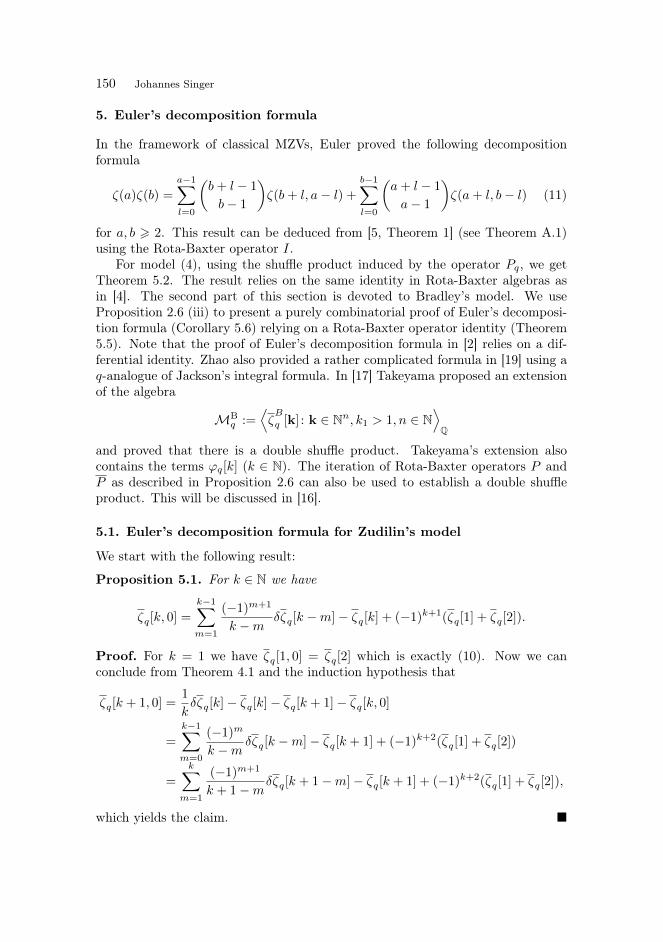
Proposition 5.1. For k ∈ N we have

ζq[k, 0] =

k−1∑m=1

(−1)m+1

k −mδζq[k −m]− ζq[k] + (−1)k+1(ζq[1] + ζq[2]).

Proof. For k = 1 we have ζq[1, 0] = ζq[2] which is exactly (10). Now we canconclude from Theorem 4.1 and the induction hypothesis that

ζq[k + 1, 0] =1

kδζq[k]− ζq[k]− ζq[k + 1]− ζq[k, 0]

=

k−1∑m=0

(−1)m

k −mδζq[k −m]− ζq[k + 1] + (−1)k+2(ζq[1] + ζq[2])

=

k∑m=1

(−1)m+1

k + 1−mδζq[k + 1−m]− ζq[k + 1] + (−1)k+2(ζq[1] + ζq[2]),

which yields the claim. �


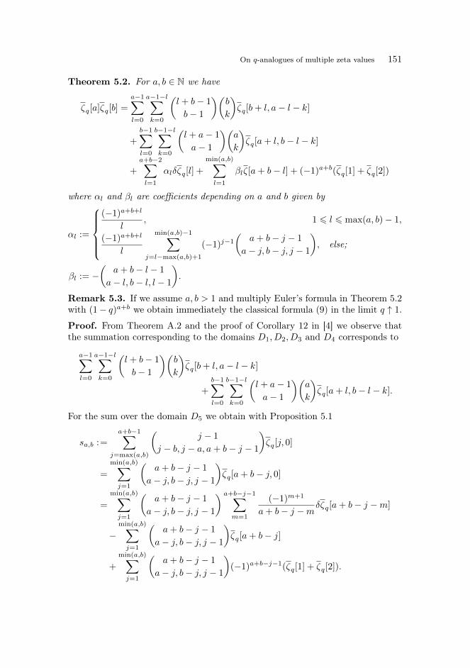
Theorem 5.2. For a, b ∈ N we have

ζq[a]ζq[b] =

a−1∑l=0

a−1−l∑k=0

(l + b− 1

b− 1

)(b

k

)ζq[b+ l, a− l − k]

+

b−1∑l=0

b−1−l∑k=0

(l + a− 1

a− 1

)(a

k

)ζq[a+ l, b− l − k]

+

a+b−2∑l=1

αlδζq[l] +

min(a,b)∑l=1

βlζ[a+ b− l] + (−1)a+b(ζq[1] + ζq[2])

where αl and βl are coefficients depending on a and b given by

αl :=

(−1)a+b+l

l, 1 6 l 6 max(a, b)− 1,

(−1)a+b+l

l

min(a,b)−1∑j=l−max(a,b)+1

(−1)j−1

(a+ b− j − 1

a− j, b− j, j − 1

), else;

βl := −(

a+ b− l − 1

a− l, b− l, l − 1

).

Remark 5.3. If we assume a, b > 1 and multiply Euler’s formula in Theorem 5.2with (1− q)a+b we obtain immediately the classical formula (9) in the limit q ↑ 1.

Proof. From Theorem A.2 and the proof of Corollary 12 in [4] we observe thatthe summation corresponding to the domains D1, D2, D3 and D4 corresponds to

a−1∑l=0

a−1−l∑k=0

(l + b− 1

b− 1

)(b

k

)ζq[b+ l, a− l − k]

+

b−1∑l=0

b−1−l∑k=0

(l + a− 1

a− 1

)(a

k

)ζq[a+ l, b− l − k].

For the sum over the domain D5 we obtain with Proposition 5.1

sa,b :=

a+b−1∑j=max(a,b)

(j − 1

j − b, j − a, a+ b− j − 1

)ζq[j, 0]

=

min(a,b)∑j=1

(a+ b− j − 1

a− j, b− j, j − 1

)ζq[a+ b− j, 0]

=

min(a,b)∑j=1

(a+ b− j − 1

a− j, b− j, j − 1

) a+b−j−1∑m=1

(−1)m+1

a+ b− j −mδζq[a+ b− j −m]

−min(a,b)∑j=1

(a+ b− j − 1

a− j, b− j, j − 1

)ζq[a+ b− j]

+

min(a,b)∑j=1

(a+ b− j − 1

a− j, b− j, j − 1

)(−1)a+b−j−1(ζq[1] + ζq[2]).

152 Johannes Singer

In order to simplify the terms we use the following combinatorial result:

Lemma 5.4. For a, b ∈ N we have

min(a,b)∑j=1

(−1)j+1

(a+ b− j − 1

a− j, b− j, j − 1

)= 1.

Proof. Without loss of generality we assume a 6 b ∈ N. We prove the claim byinduction on a. The base case is true because(

b− 1

0, b− 1, 0

)= 1

for all b > 1. In the inductive step let a + 1 6 b. Then obviously a 6 b and weobtain with the induction hypothesis

a+1∑j=1

(−1)j+1

(a+ b− j

a− j + 1, b− j, j − 1

)

= (−1)a(

b− 1

0, b− a− 1, a

)+

a∑j=1

(−1)j+1 a+ b− ja− j + 1

(a+ b− j − 1

a− j, b− j, j − 1

)

= 1 + (−1)a(

b− 1

0, b− a− 1, a

)+ (b− 1)

a∑j=1

(−1)j+1

(a+ b− j − 1

a− j + 1, b− j, j − 1

)

= 1 + (b− 1)

a+1∑j=1

(−1)j+1

(a+ b− j − 1

a− j + 1, b− j, j − 1

)= 1.

The last equality is true, since we have

a+1∑j=1

(−1)j+1

(a+ b− j − 1

a− j + 1, b− j, j − 1

)=

a∑j=0

(−1)a−j

j + b− 1

(j + b− 1

j, b− a+ j − 1, a− j

)= 0

due to [4, Lemma 11]. This completes the proof. �


Therefore we have

sa,b =

min(a,b)∑j=1

(a+ b− j − 1

a− j, b− j, j − 1

)(−1)a+b−j

a+b−j−1∑m=1

(−1)m+1

mδζq[m]

−min(a,b)∑j=1

(a+ b− j − 1

a− j, b− j, j − 1

)ζq[a+ b− j] + (−1)a+b(ζq[1] + ζq[2])

= (−1)a+b

max(a,b)−1∑m=1

(−1)m

mδζq[m]

+

min(a,b)∑j=1

(a+ b− j − 1

a− j, b− j, j − 1

) a+b−j−1∑m=max(a,b)

(−1)a+b−j−1+m

mδζq[m]

+

min(a,b)∑j=1

βjζq[a+ b− j] + (−1)a+b(ζq[1] + ζq[2])

= (−1)a+b

max(a,b)−1∑m=1

(−1)m

mδζq[m]

+

a+b−2∑m=max(a,b)

(−1)m

mδζq[m]

min(a,b)−1∑j=m−max(a,b)+1

(−1)a+b−j−1

(a+ b− j − 1

a− j, b− j, j − 1

)

+

a−1∑j=0

βjζq[j + b] + (−1)a+b(ζq[1] + ζq[2])

=

a+b−2∑k=1

αkδζq[k] +

min(a,b)−1∑j=1

βjζq[a+ b− j] + (−1)a+b(ζq[1] + ζq[2])

finishing the proof of Theorem 5.2. �

5.2. Euler’s decomposition formula for Bradley’s model

Let (P,A) and (Q,A) be two Rota-Baxter k-algebras of weight α respectively β.We call them compatible, if they satisfy the relations

P [f ]Q[g] = P [fQ[g]] +Q[P [f ]g] (12)

and

Q[f ]P [g] = Q[fP [g]] + P [Q[f ]g] (13)

for any f, g ∈ A. One should note that this is fulfilled by P and P as shownin Proposition 2.5. Now we are interested in the operator T (a1, a2; b1, b2; c1, c2) :A×A → A which is defined as

T (a1, a2; b1, b2; c1, c2) = P c1Qc2 [P a1 [Qa2 [·]] · P b1 [Qb2 [·]]]

154 Johannes Singer

for a1, a2, b1, b2, c1, c2 ∈ N0. We have the following result:

Theorem 5.5. Let (P,A) and (Q,A) be two compatible Rota-Baxter k-algebrasof weight α respectively β. For a, b ∈ N we have

T (a− 1, 1; b− 1, 1; 0, 0)

=

a−1∑s=0

a−1−s∑t=0

αt(s+ b− 1

b− 1

)(b− 1

t

)T (a− s− t− 1, 1; 0, 0; b+ s− 1, 1)

+

b−1∑s=0

b−1−s∑t=0

αt(s+ a− 1

a− 1

)(a− 1

t

)T (0, 0; b− s− t− 1, 1; a+ s− 1, 1)

+ β

min(a,b)∑s=1

αs−1

(a+ b− s− 1

a− s, b− s, s− 1

)T (0, 0; 0, 0; a+ b− s− 1, 1).

In order to prove the theorem we use the graphical notation of [5]. A producton A is represented by

the Rota-Baxter operator P by

and the Rota-Baxter operator Q by

We have four calculation rules:(A) The Rota-Baxter identity of P is decoded by

=

type P1

+

type P2

+ α

type P3

(B) The Rota-Baxter identity of Q is decoded by

=

type Q1

+

type Q2

+ β

type Q3


(C) Due to equation (12) the mixed application of the operators P and Q is givenby

=

type M1

+

type M2

(D) Due to equation (13) the mixed application of the operators Q and P is givenby

=

type M3

+

type M4

Proof of Theorem 5.5. Let a, b ∈ N. We regard the operator T (a − 1, 1; b −1, 1; 0, 0) which corresponds to the tree

a-1 b-1

From the iterated applications of the Rota-Baxter identities of P and Q and theinterplay of P and Q we conclude that the tree can be written as a k[α, β]-linearcombination of trees exhibiting the following three canonical forms

i

j

i

j j

with i, j ∈ N0 depending on a and b.We begin by counting the occurrence of the canonical form related to

T (i, 1; 0, 0; j, 1) (for i, j ∈ N0 depending on a, b) which is represented by the fol-lowing tree:

i

j

There are j + 1 applications of our calculation rules (A)-(D). The last applicationis either of type M1 if i > 0 or of type Q1 if i = 0. Therefore we have j applicationsof our calculation rules (A)-(D) to transform the tree T (a− 1, 1; b− 1, 1; 0, 0) to

i

j

156 Johannes Singer

In order to attain this form we have to move b − 1 dots from the right leg tothe neck. Furthermore we can annihilate dots but we can not create new ones.Therefore b−1 6 j 6 a+b−2. For i we have the obvious restriction 0 6 i 6 a−1.Additionally, we have to ensure i+j 6 a+b−2. Hence i 6 min(a−1, a+b−j−2) =a + b − j − 2 since j > b − 1. On the other hand the number of annihilated dotsis bounded from above by min(a, b)− 1. Hence i+ j > max(a, b)− 1 and finally

i > max(0,max(a, b)− 1− j) = max(0, a− j − 1)

due to j > b− 1. Now the j moves of dots rely on k1 moves of type P2 or M2, k2

moves of type P1 or M3 and k3 moves of type P3. Note that there is no intrinsicpermutation of P2 and M2 in k1 because k1 counts the number of dots moved fromthe left leg to the neck. The choice of type P2 or M2 is then determined by thefact of having a dot or a stroke on the right leg. The same argument holds for k2.All in all we get the following system of equations

k1 + k2 + k3 = j, k1 + k3 = a− 1− i, k2 + k3 = b− 1.

Then we obtain

k1 = j − b+ 1, k2 = i+ j − a+ 1, k3 = a+ b− i− j − 2.

Hence the term T (i, 1; 0, 0; j, 1) arises(j

k1, k2, k3

)=

(j

j − b+ 1, i+ j − a+ 1, a+ b− i− j − 2

)times in the the expansion of T (a − 1, 1; b − 1, 1; 0, 0). The power of the weightfactor α of our canonical form is determined by k3. All in all the number ofappearances of the canonical form in the expansion of the original operator T isgiven by

a+b−2∑j=b−1

a+b−j−2∑i=max(0,a−j−1)

αa+b−i−j−2

×(

j

j − b+ 1, i+ j − a+ 1, a+ b− i− j − 2

)T (i, 1; 0, 0; j, 1)

=

a−1∑j=0

min(b−1,a−j−1)∑i=0

αi(

j + b− 1

j, b− i− 1, i

)T (a− i− j − 1, 1; 0, 0; b+ j − 1, 1)

=

a−1∑j=0

a−j−1∑i=0

αi(j + b− 1

b− 1

)(b− 1

i

)T (a− i− j − 1, 1; 0, 0; b+ j − 1, 1).

In the second case we count the trees corresponding to T (0, 0; i, 1; j, 1). Thisis completely analogous to the first case.


In the last case we count the trees reducing to T (0, 0; 0, 0; j, 1). The graphicalrepresentation is given by

j

There are j + 1 moves obeying the calculation rules (A)-(D). The last move mustbe of type Q3 and gives rise to the weight factor β. Therefore we have to apply jmoves of dots to the tree

j

With a similar argumentation as in the first case we deduce max(a, b) − 1 6 j 6a + b − 2. The j moves of dots rely on k1 moves of type P2 or M2, k2 moves oftype P1 or M3 and k3 moves of type P3. We get the following system of equations

k1 + k2 + k3 = j, k1 + k3 = a− 1, k2 + k3 = b− 1.

Therefore we get

k1 = j − b+ 1, k2 = j − a+ 1, k3 = a+ b− j − 2

and the term T (0, 0; 0, 0; j, 1) arises(j

j − b+ 1, j − a+ 1, a+ b− j − 2

)times in the the expansion of T (a− 1, 1; b− 1, 1; 0, 0). This leads to

β

a+b−2∑j=max(a,b)−1

αa+b−j−2

(j

j − b+ 1, j − a+ 1, a+ b− j − 2

)T (0, 0; 0, 0; j, 1)

= β

min(a,b)∑j=1

αj−1

(a+ b− j − 1

a− j, b− j, j − 1

)T (0, 0; 0, 0; a+ b− j − 1, 1).

This concludes the proof. �

158 Johannes Singer

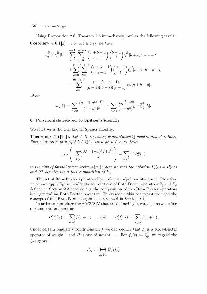
Using Proposition 2.6, Theorem 5.5 immediately implies the following result:

Corollary 5.6 ([1]). For a, b ∈ N>2 we have

ζB

q [a]ζB

q [b] =

a−1∑s=0

a−1−s∑t=0

(s+ b− 1

b− 1

)(b− 1

t

)ζB

q [b+ s, a− s− t]

+

b−1∑s=0

b−1−s∑t=0

(s+ a− 1

a− 1

)(a− 1

t

)ζB

q [a+ s, b− s− t]

−min(a,b)∑s=1

(a+ b− s− 1)!

(a− s)!(b− s)!(s− 1)!ϕq[a+ b− s],

where

ϕq[k] :=∑n>0

(n− 1)q(k−1)n

(1− qn)k=∑n>0

nq(k−1)n

(1− qn)k− ζBq [k].

6. Polynomials related to Spitzer’s identity

We start with the well known Spitzer-Identity.

Theorem 6.1 ([14]). Let A be a unitary commutative Q-algebra and P a Rota-Baxter operator of weight λ ∈ Q×. Then for a ∈ A we have

exp

−∑k>1

λk−1(−x)kP (ak)

k

=∑n>0

xnPna (1)

in the ring of formal power series A[[x]] where we used the notation Pc(a) = P (ac)and Pna denotes the n-fold composition of Pa.

The set of Rota-Baxter operators has no known algebraic structure. Thereforewe cannot apply Spitzer’s identity to iterations of Rota-Baxter operators Pq and P qdefined in Section 2.2 because e. g. the composition of two Rota-Baxter operatorsis in general no Rota-Baxter operator. To overcome this constraint we need theconcept of free Rota-Baxter algebras as reviewed in Section 2.1.

In order to reproduce the q-MZ(S)V that are defined by iterated sums we definethe summation operators

P [f ](x) :=∑n>0

f(x+ n) and P [f ](x) :=∑n>0

f(x+ n).

Under certain regularity conditions on f we can deduce that P is a Rota-Baxteroperator of weight 1 and P is one of weight −1. For fk(t) := qkt

[t]kqwe regard the

Q-algebra

Aq :=⊕k∈N0

Qfk(t)


with a filtration given by Aq,m =⊕

k>mQfk(t). For f := (f1, . . . , fn) ∈ Anqwe define the symbol Pf := P [f1[P [f2 . . . P [fn] . . . ]]]. Since Aq is an iterativelysummable subalgebra of level 1 of the algebra of continuous function Cq(]0,∞[)on ]0,∞[ in the parameter q, the MZV algebra is given by

Aq,1 :={P(f1,...,fn) : fi ∈ Aq, i = 1, . . . , n, fn ∈ Aq,1

}.

The MZV algebra Aq,1 is the algebra of q-MZVs if we employ the evaluation ho-momorphism f 7→ f(0). The algebra of q-MZSVs is obtained by replacing P by Pin Aq,1 and employing the evaluation f 7→ f(1).

Theorem 6.2. Let s ∈ N and A be a unitary commutative Q-algebra and Pa Rota-Baxter operator of weight λ ∈ Q×. Then there is a unique sequence(Q

(λ)n )n∈N of polynomials with Q

(λ)n ∈ Q[X1, . . . , Xn] and deg(Q

(λ)n ) = n such

that

Pnas(1) = Q(λ)n

(P (as), P (a2s), . . . , P (asn)

)(14)

for a ∈ A satisfying

(i) Q(λ)0 = 1 and ∇nQ(λ)

n =

n∑k=1

(−λ)k−1

kQ

(λ)n−k~ek,

(ii) Q(λ)n ({0}n) = 0

for all n ∈ N in which ∇n :=∑nk=1 ∂Xk~ek where ~ek is the k-th canonical unit

vector and {k}n denotes the n-tuple (k, . . . , k).

Corollary 6.3. For k, n ∈ N we have

ζq[{k}n] = Q(1)n (ζq[k], ζq[2k], . . . , ζq[nk])

and

ζ?q [{k}n] = Q(−1)n (ζ?q [k], ζ?q [2k], . . . , ζ?q [nk]),

where (Q(1)n )n∈N and (Q

(−1)n )n∈N are the unique sequences of polynomials in The-

orem 6.2.

Proof. For the filtered algebra Aq we regard the corresponding free Rota-Baxteralgebra (�Q(Aq), PAq ) of weight 1 respectively −1 and we can apply Theorem6.2. For a := fk(t) = qkt

[t]kq∈ Aq, equation (14) is an algebraic relation in M(Aq)k.

Using the evaluation ν : f 7→ f(0) respectively ν : f 7→ f(1), the relation reducesvia ν ◦Pk to the claim in which Pk(1⊗f1⊗f2⊗· · ·⊗fn) := P(f1,...,fn) respectivelyPk(1⊗ f1 ⊗ f2 ⊗ · · · ⊗ fn) := P (f1,...,fn). �

Example 6.4.

(a) For a Rota-Baxter operator of weight 1 we get the polynomials listed in Table 1.

160 Johannes Singer

(b) The first three nontrivial identities for q-MZVs are

ζq[s, s] =1

2ζq[s]

2 − 1

2ζq[2s],

ζq[s, s, s] =1

6ζq[s]

3 − 1

2ζq[s]ζq[2s] +

1

3ζq[3s],

ζq[s, s, s, s] =1

24ζq[s]

4 − 1

4ζq[s]

2ζq[2s] +1

3ζq[s]ζq[3s] +

1

8ζq[2s]

2 − 1

4ζq[4s].

and for q-MZSV are

ζ?q [s, s] =1

2ζ?q [s]2 +

1

2ζ?q [2s],

ζ?q [s, s, s] =1

6ζ?q [s]3 +

1

2ζ?q [s]ζ?q [2s] +

1

3ζ?q [3s],

ζ?q [s, s, s, s] =1

24ζ?q [s]4 +

1

4ζ?q [s]2ζ?q [2s] +

1

3ζ?q [s]ζ?q [3s] +

1

8ζ?q [2s]2 +

1

4ζ?q [4s].

n p(n) Q(1)n

0 0 1

1 1 X1

2 2 12X

21 − 1

2X2

3 3 16X

31 − 1

2X1X2 + 13X3

4 5 124X

41 − 1

4X21X2 + 1

3X1X3 + 18X

22 − 1

4X4

5 7 1120X

51 − 1

12X31X2 + 1

6X21X3 + 1

8X1X22 − 1

4X1X4 − 16X2X3 + 1

5X5

6 11 1720X

61 − 1

48X41X2 + 1

18X31X3 + 1

16X21X

22 + 1

8X21X4 − 1

6X1X2X3 − 148X

32

+ 15X1X5 + 1

8X2X4 + 118X

23 − 1

6X6

Table 1. List of the polynomials Q(1)n for a Rota-Baxter operator of weight 1 for n =

1, . . . , 6, where p(n) denotes the number of integer partitions of n.

Proposition 6.5. Let s, n ∈ N. Then we have

Pnas(1) = (−λ)nn∑r=1

(−λ)−r

r!

∑n1+···+nr=nn1,...,nr>1

r∏i=1

P (asni)

ni.

Proof. Let s ∈ N. Now we consider

fs(z) :=∑k>1

(−λ)k−1zskP (ask)

k.


From the Taylor expansion of the exponential function we can deduce

∂sn

∂zsnexp(fs(z)) =

∑r>0

1

r!

∂sn

∂zsnfs(z)

r

=∑r>0

1

r!

∑n1+···+nr=sn

(sn

n1, . . . , nr

) r∏i=1

∂ni

∂znifs(z).

In the last step we used the generalized Leibniz rule. Now

∂l

∂zlfs(z)

∣∣∣∣z=0

=

{0 if l 6≡ 0 mod s or l = 0,(−λ)l/s−1l!

l/s P (al) if l ≡ 0 mod s and l 6= 0,

implies

∂sn

∂zsnexp(fs(z))

∣∣∣∣z=0

=∑r>0

1

r!

∑n1+···+nr=nn1,...,nr>1

(sn

sn1, . . . , snr

) r∏i=1

(−λ)ni−1(sni)!

niP (asni)

and therefore we get

1

(sn)!

∂sn

∂zsnexp(fs(z))

∣∣∣∣z=0

= (−λ)nn∑r=1

(−λ)−r

r!

∑n1+···+nr=nn1,...,nr>1

r∏i=1

P (asni)

ni.

Theorem 6.1 with a substituted by as implies the claim. �

Proof of Theorem 6.2. Let n, r > 1. We introduce the following notation. Letn1 + · · · + nr = n be an integer partition of n with length r and suppose thatn1 > . . . > nr > 1. Therefore we have 1 6 r 6 n. Then we define

am := #{i ∈ {1, . . . , r} : ni = m}

for 1 6 m 6 n. Let j ∈ {1, . . . .n} and aj 6= 0. Then we can ensure thatan−j+1 = · · · = an = 0. Furthermore we denote by n1 + · · · + nr = n − j theinteger partition of n− j with length r arising from our old partition by deletingexactly one summand j. Now we have 0 6 r 6 n− j. We can conclude using thedefinition

am := #{i ∈ {1, . . . , r} : ni = m}

that ai = ai for i 6= j and aj = aj − 1. If we substitute P (asni) by the variable

162 Johannes Singer

Xni for i ∈ {1, . . . , r} we get

Q(λ)n (X1, . . . , Xn) = (−λ)n

n∑r=1

(−λ)−r

r!

∑n1+···+nr=nn1,...,nr>1

r∏i=1

Xni

ni

= (−λ)nn∑r=1

(−λ)−r∑

n1+···+nr=nn1>···>nr>1, aj=0

1

a1! · · · an!

n∏i=1

Xaii

iai

+ (1− δn(j))(−λ)nn∑r=1

(−λ)−r∑

n1+···+nr=nn1>···>nr>1, aj 6=0

1

a1! · · · an!

n∏i=1

Xaii

iai

+(−λ)n−1

nXnδn(j),

where δn(j) denotes Kronecker’s delta. Now we determine ∂XjQ(λ)n (X1, . . . , Xn).

The first term in the last equation vanishes since it does not depend on Xj . Nowwe get

∂XjQ(λ)n (X1, . . . , Xn)

= (1− δn(j))(−λ)nn∑r=1

(−λ)−r∑

n1+···+nr=nn1>···>nr>1, aj 6=0

1

a1! · · · (aj − 1)! · · · an!

Xaj−1j

jaj

n∏i=1i 6=j

Xaii

iai

+(−λ)n−1

nδn(j)

= (1− δn(j))(−λ)j−1

j(−λ)n−j

n−j∑r=1

(−λ)−r∑

n1+···+nr=n−jn1>···>nr>1

1

a1! · · · aj ! · · · an−j !

n−j∏i=1

X aii

iai

+(−λ)n−1

nδn(j)

=(−λ)j−1

jQ

(λ)n−j(X1, . . . , Xn−j).

Therefore condition (i) is verified. (ii) is an immediate consequence of Proposi-tion 6.5. Uniqueness can be shown by induction on n using condition (i). �

Acknowledgement. I am very grateful to Andreas Knauf (Erlangen) who pro-posed me to work on the subject of MZV and for his comments on this work.Further I am much obliged to Kurusch Ebrahimi-Fard (Madrid) and DominiqueManchon (Clermont-Ferrand) who explained me their papers [4, 3] and for discus-sion and comments on this article. Finally I thank Henrik Bachmann (Hamburg)for implementing and sharing his Pari GP code for the q-analogues studied in thispaper.


Note added in proof. The author was informed that J. Zhao published a preprint(arXiv:1412.8044) in December 2014 that includes parts of the results provided inthis work.

Appendix A. Comments on [5]

In this appendix we just recall the main results of [5]. It has already been men-tioned by Castillo Medina, Ebrahimi-Fard and Manchon in [4] that there are someproblems with the display of the results concerning Theorem 3. However it is pos-sible to correct the calculations in the proof. Let (A, P ) be a Rota-Baxter algebraof weight λ. Then for a, b, c ∈ N0 the operator T (a, b, c) : A×A → A is given by

T (a, b, c) := P c[P a[·] · P b[·]].

Then we have the following results:

Theorem A.1 ([5]). Let a, b > 1 and c > 0 be integers. The following identityholds in any Rota-Baxter algebra of weight 0:

T (a, b, c) =

b−1∑i=0

(a+ i− 1

a− 1

)T (0, b− i, a+ c+ i)

+

a−1∑i=0

(b+ i− 1

b− 1

)T (a− i, 0, b+ c+ i)

Theorem A.2 ([5],[4]). Let a, b > 1 and c > 0 be integers. The following identityholds in any Rota-Baxter algebra of weight λ:

T (a, b, c) =∑

(i,j)∈D1

λa+b−i−j(

j − 1

i+ j − b− 1, j − a, a+ b− i− j

)T (0, i, c+ j)

+∑

(i,j)∈D2

λa+b−i−j(

j − 1

i+ j − b, j − a, a+ b− i− j − 1

)T (0, i, c+ j)

+∑

(i,j)∈D3

λa+b−i−j(

j − 1

j − b, i+ j − a− 1, a+ b− i− j

)T (i, 0, c+ j)

+∑

(i,j)∈D4

λa+b−i−j(

j − 1

j − b, i+ j − a, a+ b− i− j − 1

)T (i, 0, c+ j)

+∑j∈D5

λa+b−j(

j − 1

j − b, j − a, a+ b− j − 1

)T (0, 0, c+ j),

164 Johannes Singer

where

D1 :={

(i, j) ∈ N2 : 1 6 i 6 b, a 6 j, b− i+ 1 6 j, j 6 a+ b− i},

D2 :={

(i, j) ∈ N2 : 1 6 i 6 b− 1, a 6 j, b− i 6 j, j 6 a+ b− i− 1},

D3 :={

(i, j) ∈ N2 : 1 6 i 6 a, a− i+ 1 6 j, b 6 j, j 6 a+ b− i},

D4 :={

(i, j) ∈ N2 : 1 6 i 6 a− 1, a− i 6 j, b 6 j, j 6 a+ b− i− 1},

D5 := {j ∈ N : a 6 j, b 6 j, j 6 a+ b− 1} .

References

[1] D. Bradley, A q-analog of Euler’s decomposition formula for the double zetafunction, Int. J. Math. Math. Sci. 21 (2005), 3453–3458.

[2] D. Bradley, Multiple q-zeta values, J. Algebra (2005), 752–798.[3] J. Castillo Medina, K. Ebrahimi-Fard, D. Manchon, Unfolding the double

shuffle structure of q-multiple zeta values, Bull. Aust. Math. Soc. 91(3) (2015),368–388.

[4] J. Castillo Medina, K. Ebrahimi-Fard, D. Manchon, On Euler’s decompositionformula for qMZVs, Ramanujan J. 37(2) (2015), 365–389.

[5] R. Diaz, M. Paez, An Identity in Rota-Baxter Algebras, Sem. Lothar. Combin.57(B57b) (2007).

[6] K. Ebrahimi-Fard, L. Guo, Multiple zeta values and Rota–Baxter algebras,Integers 8(2) (2006).

[7] L. Guo, An Introduction to Rota-Baxter Algebra, volume IV of Surveys ofModern Mathematics.

[8] L. Guo, W. Keigher, Baxter algebras and shuffle products, Adv. Math (2000),117–149.

[9] L. Guo, W. Keigher, On free Baxter algebras: completions and the internalconstruction, Adv. Math. (2000), 101–127.

[10] M. Hoffman, Multiple harmonic series, Pacific Journal of Mathematics 152(2)(1992), 275–290.

[11] M. Hoffman, Quasi-shuffle products, J. Algebraic Combin. 11(1) (2000), 49–68.

[12] K. Ihara, M. Kaneko, D. Zagier, Derivation and double shuffle relations formultiple zeta values, Compos. Math. 142 (2006).

[13] Y. Ohno, J. Okuda, W. Zudilin, Cyclic q-MZSV sum, J. Number Theory132(1) (2012), 144–155.

[14] G.-C. Rota, D. Smith, Fluctuation theory and Baxter algebras, InstitutoNazionale di Alta Matematica IX (1972), 179–201.

[15] K.-G. Schlesinger, Some remarks on q-deformed multiple polylogarithms,arXiv:math/0111022, 2001.

[16] J. Singer, On Bradley’s q-MZVs and a Generalized Euler Decomposition For-mula, submitted,

[17] Y. Takeyama, The Algebra of a q-Analogue of Multiple Harmonic Series,SIGMA 9.


[18] D. Zagier, Values of zeta functions and their applications, in First EuropeanCongress of Mathematics, volume 120, 497–512. Birkhäuser-Verlag, Basel,1994.

[19] J. Zhao, Multiple q-zeta functions and multiple q-polylogarithms, RamanujanJ. 14(2) (2007), 189–221.

[20] W. Zudilin, Algebraic relations for multiple zeta values, Uspekhi Mat. Nauk58, 2003.

Address: Johannes Singer: Department Mathematik, Friedrich-Alexander-Universität Erlangen-Nürnberg, Cauerstraße 11, 91058 Erlangen, Germany.

E-mail: [email protected]: 3 October 2014; revised: 27 January 2015

ON q-ANALOGUES OF MULTIPLE ZETA VALUES Johannes ...

Documents

Transcript of ON q-ANALOGUES OF MULTIPLE ZETA VALUES Johannes ...