Applied Mathematics and Computation 256 (2015) 754–768

Contents lists available at ScienceDirect

Applied Mathematics and Computation

journal homepage: www.elsevier .com/ locate /amc

Blow-up collocation solutions of nonlinear homogeneousVolterra integral equations

http://dx.doi.org/10.1016/j.amc.2015.01.0570096-3003/� 2015 Elsevier Inc. All rights reserved.

⇑ Corresponding author.E-mail addresses: rbenitez@unex.es (R. Benítez), vbolos@uv.es (V.J. Bolós).

1 Work supported by project MTM2008-05460.

R. Benítez a,⇑,1, V.J. Bolós b,1

a Dpto. Matemáticas, Centro Universitario de Plasencia, Universidad de Extremadura, Avda. Virgen del Puerto 2, 10600 Plasencia, Spainb Dpto. Matemáticas para la Economía y la Empresa, Facultad de Economía, Universidad de Valencia, Avda. Tarongers s/n, 46022 Valencia, Spain

a r t i c l e i n f o a b s t r a c t

Keywords:Nonlinear integral equationsBlow-up phenomenaCollocation methodsNontrivial solutions

In this paper, collocation methods are used for detecting blow-up solutions of nonlinearhomogeneous Volterra–Hammerstein integral equations. To do this, we introduce theconcept of ‘‘blow-up collocation solution’’ and analyze numerically some blow-up timeestimates using collocation methods in particular examples where previous results aboutexistence and uniqueness can be applied. Finally, we discuss the relationships betweennecessary conditions for blow-up of collocation solutions and exact solutions.

� 2015 Elsevier Inc. All rights reserved.

1. Introduction

Some engineering and industrial problems are described by explosive phenomena which are modeled by nonlinear inte-gral equations whose solutions exhibit blow-up at finite time (see [1,2] and references therein). Many authors have studiednecessary and sufficient conditions for the existence of such a blow-up time. Particularly, in [3–9], equation

y tð Þ ¼Z t

0K t; sð ÞG y sð Þð Þds; t 2 I :¼ 0; t

� �; ð1Þ

was considered. In these works, conditions for the existence of a finite blow-up time, as well as upper and lower estimates ofit, were given, although they were not very accurate in some cases.

A way for improving these estimations is to study numerical approximations of the solution; in this aspect, collocationmethods have proven to be a very suitable technique for approximating nonlinear integral equations, because of its stabilityand accuracy (see [10]). Hence, the aim of this paper is to test the usefulness of collocation methods for detecting blow-upsolutions of the nonlinear homogeneous Volterra–Hammerstein integral equation (HVHIE) given by Eq. (1).

Very recently, Yang and Brunner [11] analyzed the blow-up behavior of collocation solutions for a similar Hammerstein–Volterra integral equation with a convolution kernel

yðtÞ ¼ /ðtÞ þZ t

0Kðt � sÞGðs; yðsÞÞds; t 2 I: ð2Þ

Eq. (1) should not be regarded as a particular case of (2) (for a convolution kernel), because in [11] a positive non-homogeneity / and a Lipschitz-continuous nonlinearity G were considered. Indeed, under the hypotheses on the kerneland the nonlinearity considered in [11], it is well-known that Eq. (1) has only the trivial solution (y � 0) and moreover, under

R. Benítez, V.J. Bolós / Applied Mathematics and Computation 256 (2015) 754–768 755

the conditions we shall state in Section 3, the collocation equations given in [11] lead to the trivial sequence (yn ¼ 0 for alln 2 N). Thus, Eq. (1) considered here is beyond the scope of the standard techniques, which usually impose conditions thatguarantee the uniqueness of the solutions.

An approach for solving this problem, which we shall follow in this paper, is writing Eq. (1) as an implicitly linear homo-geneous Volterra integral equation (HVIE), i.e. setting z ¼ G � y and plugging it into the nonlinear integral Eq. (1) to obtain

2 In [misunddecreas

zðtÞ ¼ G Vzð Þ tð Þð Þ ¼ GZ t

0K t; sð ÞzðsÞds

� �; t 2 I; ð3Þ

being V the linear Volterra operator. There is a one-to-one correspondence between solutions of (1) and (3) (see [10,12]), inparticular, if z is a solution of (3), then y :¼ Vz is a solution of (1).

This paper is structured as follows: in Section 2 we introduce briefly the basic definitions and state the notation. Next, wedevote Section 3 to generalize the results about existence and uniqueness of nontrivial collocation solutions obtained in [13]in order to apply the results to blow-up problems. In Section 4, we introduce the concept of ‘‘blow-up collocation solution’’and analyze numerically some blow-up time estimates using collocation methods in particular examples where the previousresults about existence and uniqueness can be applied. Finally, in Section 5, we discuss the relationships between necessaryconditions for blow-up of collocation solutions and exact solutions.

2. Collocation problems for implicitly linear HVIEs

Following the notation of [10], a collocation problem for Eq. (3) in I ¼ ½0; T� is given by a meshIh :¼ tn : 0 ¼ t0 < t1 < � � � < tN ¼ Tf g and a set of m collocation parameters 0 6 c1 < � � � < cm 6 1. We denotehn :¼ tnþ1 � tn; n ¼ 0; . . . ;N � 1, and the quantity h :¼max hn : n ¼ 0; . . . N � 1f g is the diameter2 of Ih. Moreover, the colloca-tion points are given by tn;i :¼ tn þ cihn; i ¼ 1; . . . ;m, and the set of collocation points is denoted by Xh (see [10,15]). A collocationsolution zh is then given by the collocation equation.

zh tð Þ ¼ GZ t

0K t; sð Þzh sð Þds

� �; t 2 Xh;

where zh is in the space of piecewise polynomials of degree less than m.From now on, a ‘‘collocation problem’’ or a ‘‘collocation solution’’ will be always referred to the implicitly linear HVIE (3).

So, if we want to obtain an estimation of a solution of the nonlinear HVHIE (1), then we have to consider yh :¼ Vzh.At the beginning of Section 4, we define the concepts of ‘‘blow-up collocation problems’’ and ‘‘blow-up collocation solu-

tions’’. To do this, we extend the definition of ‘‘collocation solution’’ to meshes Ih with infinite points. Taking this intoaccount, it is noteworthy that if zh is a blow-up collocation solution, then yh also blows up at the same blow-up time.

As it is stated in [10], a collocation solution zh is completely determined by the coefficients Zn;i :¼ zh tn;i� �

, forn ¼ 0; . . . ;N � 1 and i ¼ 1; . . . ;m, since zh tn þ vhnð Þ ¼

Pmj¼1Lj vð ÞZn;j for all v 2 0;1� �, where L1 vð Þ :¼ 1, Lj vð Þ :¼

Qmk – j

v�ckcj�ck

, for

j ¼ 2; . . . ;m, are the Lagrange fundamental polynomials with respect to the collocation parameters. The values of Zn;i aregiven by the system

Zn;i ¼ G Fn tn;i� �

þ hn

Xm

j¼1

Bn i; jð ÞZn;j

!; ð4Þ

where

Bn i; jð Þ :¼Z ci

0K tn;i; tn þ shn� �

Lj sð Þds;

and

Fn tð Þ :¼Z tn

0K t; sð Þzh sð Þds: ð5Þ

The term Fn tn;i� �

is called the lag term.

3. Existence and uniqueness of nontrivial collocation solutions

In [13], we used collocation methods for approximating the nontrivial solutions of (1). In particular, we studied the col-location solutions of the implicitly linear HVIE (3) under the assumption of some general conditions. Specifically, it wasrequired that the kernel K was a locally bounded function; nevertheless, non locally bounded kernels, e.g. weakly singularkernels, appear in many cases of blow-up solutions (see [7,14]) and so, in the present work, we shall first replace this

10,13], the diameter h is also called stepsize. Here, in order to emphasize the variability of the stepsizes, we shall not follow this notation for preventingerstandings. Moreover, in the algorithms presented in Section 4.1, the initial stepsize h0 is set equal to h, but in successive iterations the stepsizes maye.

756 R. Benítez, V.J. Bolós / Applied Mathematics and Computation 256 (2015) 754–768

condition with another not excluding this kind of kernels. Hence, the general conditions that we are going to impose (even ifthey are not explicitly mentioned) are:

� Over K. The kernel K : R2 ! 0;þ1½ ½ has its support in t; sð Þ 2 R2 : 0 6 s 6 t� �

.

For every t > 0, the map s # K t; sð Þ is locally integrable, and KðtÞ :¼R t

0 K t; sð Þds is a strictly increasing function. Moreover,

limt!aþR t

a K t; sð Þds ¼ 0 for all a P 0.3 Note that for convolution kernels (i.e. Kðt; sÞ ¼ kðt � sÞ) this last condition is alwaysheld, because k is locally integrable and then

limt!aþ

Z t

akðt � sÞds ¼ lim

t!aþ

Z t�a

0kðsÞds ¼ lim

t!0þ

Z t

0kðsÞds ¼ 0:

� Over G. The nonlinearity G : 0;þ1½ ½ ! 0;þ1½ ½ is a continuous, strictly increasing function, and Gð0Þ ¼ 0.

Note that, since G is injective, the solution y of Eq. (1) is also given by y ¼ G�1 � z, where z is a solution of (3). Also, sinceGð0Þ ¼ 0, the zero function is always a solution of both Eqs. (1) and (3), called trivial solution. Moreover, for convolution ker-nels, given a solution zðtÞ of (3), any horizontal translation of z, zcðtÞ defined by

3 Thi

zcðtÞ ¼0; if t < c;zðt � cÞ if t P c;

is also a solution of (3) (see [17,16,13]). Motivated by this fact we give the next definitions, that are also valid for noncon-volution kernels:

Definition 3.1. We say that a property P holds near zero if there exists � > 0 such that P holds on 0; d� ½ for all 0 < d < �. Onthe other hand, we say that P holds away from zero if there exists s > 0 such that P holds on t; þ1� ½ for all t > s.

The concept ‘‘away from zero’’ was originally defined in a more restrictive way in [13]; nevertheless both definitions areappropriate for our purposes.

Definition 3.2. We say that a solution of (3) is nontrivial if it is not identically zero near zero. Moreover, given a collocationproblem, we say that a collocation solution is nontrivial if it is not identically zero in t0; t1� �.

Given a kernel K, a nonlinearity G and some collocation parameters c1; . . . ; cmf g, in [13] there were defined three kinds ofexistence of nontrivial collocation solutions (of the corresponding collocation problem) in an interval I ¼ 0; T½ � using a meshIh: existence near zero, existence for fine meshes, and unconditional existence. For these two last kinds of existence, it is ensuredthe existence of nontrivial collocation solutions in any interval, and hence, there is no blow-up. On the other hand, existencenear zero is equivalent to the existence of a nontrivial collocation solution with adaptive stepsize, as it is defined in [11]. In thiscase, collocation solutions can always be extended a little more, but it is not ensured the existence of nontrivial collocationsolutions for arbitrary large T and, thus, it can blow up in finite time. For the sake of clarity and readability, let us recall thedefinition of existence near zero given in [13]:

Definition 3.3. We say that there is existence near zero if there exists H0 > 0 such that if 0 < h0 6 H0 then there are nontrivialcollocation solutions in 0; t1½ �; moreover, there exists Hn > 0 such that if 0 < hn 6 Hn then there are nontrivial collocationsolutions in 0; tnþ1½ � (for n ¼ 1; . . . ;N � 1 and given h0; . . . ;hn�1 > 0 such that there are nontrivial collocation solutions in0; tn½ �). Note that, in general, Hn depends on h0; . . . ;hn�1.

As in [13], we shall restrict our analysis to two particular cases of collocation problems, namely:

� Case 1: m ¼ 1 with c1 > 0.� Case 2: m ¼ 2 with c1 ¼ 0.

In these cases, system (4) is reduced to a single nonlinear equation, whose solution is given by the fixed points ofG aþ byð Þ for some a; b. Determining conditions for the existence of collocation solutions in the general case is a problemof an overwhelming difficulty. In fact, in [13] examples of equations for which, in cases 1 and 2, there existed nontrivial col-location solutions, yet in some other cases, for the same equation, there were no nontrivial collocation solutions, were given.

The proofs of the results obtained in [13] rely on the locally boundedness of the kernel K. Therefore, we will revise suchproofs, imposing the new general conditions given at the beginning of this section, and avoiding other hypotheses that turnout to be unnecessary. For example, we extend these results to decreasing convolution kernels, among others.

From the previous work [13], we quote a lemma on nonlinearities G satisfying the general conditions:

s last condition is new with respect to those given in [13], and replaces the locally boundedness condition.

R. Benítez, V.J. Bolós / Applied Mathematics and Computation 256 (2015) 754–768 757

Lemma 3.1. The following statements are equivalent to the statement that G yð Þy is unbounded (in 0; þ1� ½):

(i) There exists b0 > 0 such that G byð Þ has nonzero fixed points for all 0 < b 6 b0.(ii) Given A P 0, there exists bA > 0 such that G aþ byð Þ has nonzero fixed points for all 0 6 a 6 A and for all 0 < b 6 bA.

3.1. Case 1: m ¼ 1 with c1 > 0

First, we shall consider m ¼ 1 with c1 > 0. Eq. (4) are then reduced to

Zn;1 ¼ G Fn tn;1ð Þ þ hnBnZn;1ð Þ; n ¼ 0; . . . ;N � 1; ð6Þ

where

Bn :¼ Bn 1;1ð Þ ¼Z c1

0K tn;1; tn þ shnð Þds; ð7Þ

and the lag terms Fn tn;1ð Þ are given by (5) with i ¼ 1. Note that Bn > 0 because the integrand in (7) is strictly positive almosteverywhere in 0; c1� ½.

Remark 3.1. In [13], it is ensured that limhn!0þhnBn ¼ 0 taking into account (7) and the old general conditions imposed overK. Thus, we must ensure that the limit also vanishes considering the new general conditions. In fact, with a change of variable,we can express (7) as

Bn ¼1hn

Z tn;1

tn

K tn;1; sð Þds: ð8Þ

Hence, by (8) and the new condition, we have

limhn!0þ

hnBn ¼ limt!tþn

Z t

tn

K t; sð Þds ¼ 0;

since tn;1 ¼ tn þ c1hn.Now, we are in position to give a characterization of the existence near zero of nontrivial collocation solutions:

Proposition 3.1. There is existence near zero if and only if G yð Þy is unbounded.

Proof. (() Let us prove that if G yð Þy is unbounded, then there is existence near zero. So, we are going to prove by induction

over n that there exist Hn > 0, for n ¼ 0; . . . ;N � 1, such that if 0 < hn 6 Hn then there exist solutions of the system (6) withZn;1 > 0:

� For n ¼ 0, taking into account Remark 3.1 and Lemma 3.1(i), we choose a small enough H0 > 0 such that 0 < h0B0 6 b0 forall 0 < h0 6 H0. So, since the lag term is 0, we can apply Lemma 3.1(i) to Eq. (6), concluding that there exist strictly posi-tive solutions for Z0;1.� Let us suppose that, choosing one of those Z0;1 and given n > 0, there exist H1; . . . ;Hn�1 > 0 such that if 0 < hi 6 Hi with

i ¼ 1; . . . ;n� 1, then there exist coefficients Z1;1; . . . ; Zn�1;1 fulfilling Eq. (6). Note that these coefficients are strictly posi-tive, and hence, it is guaranteed that the corresponding collocation solution zh is (strictly) positive in 0; tn� �.� Finally, we are going to prove that there exists Hn > 0 such that if 0 < hn 6 Hn then there exists Zn;1 > 0 fulfilling Eq. (6)

with the previous coefficients Z0;1; . . . Zn�1;1:Let us define

A :¼max Fn tn þ c1�ð Þ : 0 6 � 6 1f g:

Note that A exists because s # K t; sð Þ is locally integrable for all t > 0, and zh is bounded in 0; tn½ �; hence, Fn, given by (5), isbounded in tn; tn þ c1½ �. Moreover, A P 0 because K and zh are positive functions.So, applying Lemma 3.1(ii), there exists bA > 0 such that G aþ byð Þ has positive fixed points for all 0 6 a 6 A and for all0 < b 6 bA. On one hand, taking into account Remark 3.1, we choose a small enough 0 < Hn 6 1 such that0 < hnBn 6 bA for all 0 < hn 6 Hn; on the other hand, choosing one of those hn, we have 0 6 Fn tn;1ð Þ 6 A. Hence, we obtainthe existence of Zn;1 as the strictly positive fixed point of G Fn tn;1ð Þ þ hnBnyð Þ.

()) For proving the other condition, we use Lemma 3.1(i), taking into account Remark 3.1. h

A similar result was proved in [13] with the additional hypothesis ‘‘K t; sð Þ 6 K t0; sð Þ for all 0 6 s 6 t < t0’’ (or ‘‘k is increas-ing’’ for the particular case of convolution kernels Kðt; sÞ ¼ kðt � sÞ). We have shown that this hypothesis is not needed andthe difference between the proofs is the choice of A.

758 R. Benítez, V.J. Bolós / Applied Mathematics and Computation 256 (2015) 754–768

Taking into account Remark 3.1, we can adapt the results given in [13] about sufficient conditions on existence for finemeshes and unconditional existence to our new general conditions. This will help us to identify collocation problems withoutblow-up (see Proposition 3.2 below).

In the following results recall the Definition 3.1 of the concepts ‘‘near zero’’ and ‘‘away from zero’’.

Proposition 3.2. Let GðyÞy be unbounded near zero.

� If K is a convolution kernel and GðyÞy is bounded away from zero, then there is existence for fine meshes.

� If yGðyÞ is unbounded away from zero, then there is unconditional existence.

If, in addition, GðyÞy is a strictly decreasing function, then there is at most one nontrivial collocation solution.

The proof is analogous to the one given in [13]. Note that the property ‘‘ yGðyÞ is unbounded away from zero’’ appears there

as ‘‘there exists a sequence ynf gþ1n¼1 of positive real numbers and divergent to þ1 such that limn!þ1

G ynð Þyn¼ 0’’, but both are

equivalent.

3.2. Case 2: m ¼ 2 with c1 ¼ 0

Considering m ¼ 2 with c1 ¼ 0, we have to solve the following equations:

Zn;1 ¼ G Fn tn;1ð Þð Þ; ð9ÞZn;2 ¼ G Fn tn;2ð Þ þ hnBn 2;1ð ÞZn;1 þ hnBn 2;2ð ÞZn;2ð Þ; ð10Þ

for n ¼ 0; . . . ;N � 1, where

Bn 2; jð Þ ¼Z c2

0K tn;2; tn þ shnð ÞLj sð Þds; j ¼ 1; 2; ð11Þ

and Fn tn;i� �

, for i ¼ 1; 2, are given by (5). Note that Bn 2; jð Þ > 0 for j ¼ 1; 2, because the integrand in (11) is strictly positivealmost everywhere in 0; c2� ½.

Remark 3.2. As in the first case, we have to ensure that limhn!0þhnBn 2; jð Þ ¼ 0 for j ¼ 1; 2, taking into account the newgeneral conditions (see Remark 3.1). Actually, since 0 < Lj sð Þ < 1 for s 2 0; c2� ½, we have

0 6 hnBn 2; jð Þ 6 hn

Z c2

0K tn;2; tn þ shnð Þds ¼

Z tn;2

tn

K tn;2; sð Þds: ð12Þ

Hence, by (12) and the general conditions, the following inequalities are fulfilled:

0 6 limhn!0þ

hnBn 2; jð Þ 6 limt!tþn

Z t

tn

K t; sð Þds ¼ 0:

Analogously to the previous case, we present a characterization of the existence near zero of nontrivial collocationsolutions:

Proposition 3.3. Let the map t # K t; sð Þ be continuous in s; �� ½ for some � > 0 and for all 0 6 s < � (this hypothesis can be

removed if c2 ¼ 1). Then there is existence near zero if and only if G yð Þy is unbounded.

Proof. (() Let us prove that if G yð Þy is unbounded, then there is existence near zero. So, we are going to prove by induction

over n that there exist Hn > 0, for n ¼ 0; . . . ;N � 1, such that if 0 < hn 6 Hn then there exist solutions of the system (10) withZn;2 > 0:

� For n ¼ 0, taking into account Remark 3.2 and Lemma 3.1(i), we choose a small enough H0 > 0 such that0 < h0B0 2;2ð Þ 6 b0 for all 0 < h0 6 H0. So, since the lag terms are 0 and Z0;1 ¼ G 0ð Þ ¼ 0, we can apply Lemma 3.1(i) toEq. (10), concluding that there exist strictly positive solutions for Z0;2.� Let us suppose that, choosing one of those Z0;2 and given n > 0, there exist constants H1; . . . ;Hn�1 > 0 such that if

0 < hi 6 Hi, for i ¼ 1; . . . ;n� 1, then there exist coefficients Z1;2; . . . ; Zn�1;2 fulfilling Eq. (10). Moreover, let us suppose thatzh is positive in 0; tn½ �, i.e. these coefficients satisfy Zl;2 P 1� c2ð ÞZl;1 P 0 for l ¼ 1; . . . ;n� 1, where Zl;1 is given by (9).� Finally, we are going to prove that there exists Hn > 0 such that if 0 < hn 6 Hn then there exists Zn;2 > 0 fulfilling Eq. (10)

with the previous coefficients, and zh is positive in 0; tnþ1½ �, i.e. Zn;2 P 1� c2ð ÞZn;1 P 0:Let us define

R. Benítez, V.J. Bolós / Applied Mathematics and Computation 256 (2015) 754–768 759

A :¼max Fn tn þ c2�ð Þ þ �G Fn tn þ c1�ð Þð ÞZ c2

0K tn;2; tn þ shnð ÞL1 sð Þds : 0 6 � 6 1

: ð13Þ

Note that A exists and A P 0 because s # K t; sð Þ is locally integrable for all t > 0; zh is bounded and positive in 0; tn½ �, thenonlinearity G is bounded and positive, and the polynomial L1 is bounded and positive in 0; c2½ �.So, applying Lemma 3.1(ii), there exists bA > 0 such that G aþ byð Þ has positive fixed points for all 0 6 a 6 A and for all0 < b 6 bA. On one hand, taking into account Remark 3.2, we choose a small enough 0 < Hn 6 1 such that0 < hnBnð2;2Þ 6 bA for all 0 < hn 6 Hn; on the other hand, taking into account (5), the lag terms Fn tn;i

� �are positive for

i ¼ 1; 2, because K and zh are positive. Therefore, by (9), Zn;1 ¼ G Fn tn;1ð Þð Þ is positive, because G is positive. Moreover,hnBn 2;1ð Þ is positive. So,

0 6 Fn tn;2ð Þ þ hnBn 2;1ð ÞZn;1 6 A:

Hence, we obtain the existence of Zn;2 as the strictly positive fixed point of the function G aþ byð Þ wherea :¼ Fn tn;2ð Þ þ hnBn 2;1ð ÞZn;1 and b :¼ hnBnð2;2Þ.Concluding, we have to check that Zn;2 P 1� c2ð ÞZn;1. On one hand,

Zn;2 ¼ G Fn tn;2ð Þ þ hn

X2

j¼1

Bn 2; jð ÞZn;j

!P G Fn tn;2ð Þð Þ;

because Bn 2; jð ÞZn;j P 0 for j ¼ 1; 2. On the other hand, since t # K t; sð Þ is continuous in s; �� ½ for some � > 0 and for all0 6 s < �, we can suppose that the stepsize is small enough for tn;1 < �, and then FnðtÞ is continuous in tn;1. Hence, sinceG is continuous, G FnðtÞð Þ is also continuous in tn;1, i.e. limhn!0þG Fn tn;2ð Þð Þ ¼ G Fn tn;1ð Þð Þ. Therefore, choosing a small enoughhn, we have

G Fn tn;2ð Þð ÞP 1� c2ð ÞG Fn tn;1ð Þð Þ ¼ 1� c2ð ÞZn;1:

()) For proving the other condition, we use Lemma 3.1(i), taking into account Remark 3.2. h

It is noteworthy that a similar result was proved in [13], but the hypothesis on the kernel was ‘‘K t; sð Þ 6 K t0; sð Þ for all0 6 s 6 t < t0’’, and so, unlike Proposition 3.3, it could not be applied to decreasing convolution kernels (for example). Again,the main difference between both proofs lies in the choice of A.

Note that for convolution kernels Kðt; sÞ ¼ kðt � sÞ, the hypothesis on K is equivalent to say that k is continuous near zero,which is a fairly weak hypothesis. On the other hand, for general kernels, this hypothesis is only needed to ensure thatt # K t; sð Þ is continuous in tn;1. Therefore, if it is not continuous, it is important to choose hi such that the mappingt # K t; sð Þ is continuous at the collocation points ti;1, i ¼ 0; . . . N � 1. More specifically, the hypothesis on K is only neededto check that Zn;2 P 1� c2ð ÞZn;1, and hence, to ensure that zh is positive in 0; tn½ �. Nevertheless, this hypothesis is not neededto verify that Z0;2 > Z0;1 ¼ 0, and so, it is always ensured the existence of Z1;2 (and obviously Z1;1), even if the hypothesis doesnot hold. Hence, if we use another method to check that Z1;2 P 1� c2ð ÞZ1;1 (e.g., numerically), then it is ensured the existenceof Z2;2. Repeating this reasoning we can guarantee the existence of Zn;2, removing the hypothesis on K. Thus, we can state aresult analogous to Proposition 3.3 without hypothesis on the kernel:

Proposition 3.4. G yð Þy is unbounded if and only if there exists H0 > 0 such that there are nontrivial collocation solutions in 0; t1½ � for

0 < h0 6 H0. In this case, there always exists H1 > 0 such that there are nontrivial collocation solutions in 0; t2½ � for 0 < h1 6 H1.

Moreover, if G yð Þy is unbounded and there is a positive nontrivial collocation solution in 0; tn½ �, then there exists Hn > 0 such that

there are nontrivial collocation solutions in 0; tnþ1½ � for 0 < hn 6 Hn.

Considering Remark 3.2 and taking the coefficient A given in (13), we can adapt some results of [13] about sufficient con-ditions on existence for fine meshes and unconditional existence to our new general conditions. These results are useful foridentifying collocation problems without blow-up.

Proposition 3.5. Let GðyÞy be unbounded near zero, and let the map t # K t; sð Þ be continuous in s; �� ½ for some � > 0 and for all

0 6 s < � (this hypothesis can be removed if c2 ¼ 1).

� If K is a convolution kernel and GðyÞy is bounded away from zero, then there is existence for fine meshes.

� If yGðyÞ is unbounded away from zero, then there is unconditional existence.

If, in addition, GðyÞy is a strictly decreasing function, then there is at most one nontrivial collocation solution.

Moreover, as in Proposition 3.4, we can state a result about unconditional existence without hypothesis on the kernel:

Proposition 3.6. Let G yð Þy be unbounded near zero. If y

GðyÞ is unbounded away from zero and there is a positive nontrivial collocation

solution in 0; tn½ �, then there is a nontrivial collocation solution in 0; tnþ1½ � for any hn > 0.

If, in addition, G yð Þy is a strictly decreasing function, then there is at most one nontrivial collocation solution.

760 R. Benítez, V.J. Bolós / Applied Mathematics and Computation 256 (2015) 754–768

3.3. Nondivergent existence and uniqueness

Our interest is the study of existence of nontrivial collocation solutions using meshes Ih with arbitrary small h > 0. So, weare not interested in collocation problems whose collocation solutions ‘‘escape’’ to þ1when a certain hn ! 0þ, since this is adivergence symptom. Following this criterion, we define the concept of ‘‘nondivergent existence’’:

Let 0 ¼ t0 < � � � < tn be a mesh such that there exist nontrivial collocation solutions, and let Shn be the index set of thenontrivial collocation solutions of the corresponding collocation problem with mesh t0 < � � � < tn < tn þ hn. Given s 2 Shn ,we denote by Zs;n;i the coefficients of the corresponding nontrivial collocation solution satisfying Eqs. (4). Then, we say thatthere is nondivergent existence in tþn if

infs2Shn

maxi¼1;...;m

Zs;n;i� �

;

exists for small enough hn > 0 and it does not diverge to þ1 when hn ! 0þ. Given a mesh Ih ¼ 0 ¼ t0 < � � � < tNf g such thatthere exist nontrivial collocation solutions, we say that there is nondivergent existence if there is nondivergent existence in tþnfor n ¼ 0; . . . ;N. See [13] for a more detailed analysis, where we also define the concept of nondivergent uniqueness.

In [13] it is proved the next result:

Proposition 3.7. In cases 1 and 2 with existence of nontrivial collocation solutions, there is nondivergent existence if and only ifG yð Þ

y is unbounded near zero. Moreover, if, in addition, G is ‘‘well-behaved’’, in the sense stated below, then there is nondivergent

uniqueness.

We say that G is ‘‘well-behaved’’ if G aþyð Þy is strictly decreasing near zero for all a > 0. Note that this condition is very weak

(see [13]).So, taking into account Propositions 3.1, 3.3 and 3.7, the main result of this paper is:

Theorem 3.1. (Hypothesis only for case 2 with c2 – 1: the map t # K t; sð Þ is continuous in s; �� ½ for some � > 0 and for all

0 6 s < �.) There is nondivergent existence near zero if and only if G yð Þy is unbounded near zero. Moreover, if in addition, G is ‘‘well-

behaved’’ then, there is nondivergent uniqueness near zero.In the same way, we can combine Propositions 3.4 and 3.7 obtaining a result about nondivergent existence and unique-

ness without hypothesis on the kernel, and, as Theorem 3.1, it can be useful to study numerically problems with decreasingconvolution kernels in case 2 with c2 – 1.

We can also combine Propositions 3.2, 3.5 and 3.6 with Proposition 3.7, obtaining results about nondivergent existenceand uniqueness (for fine meshes and unconditional) that are useful for identifying collocation problems without blow-up.Some of these results can be reformulated as necessary conditions for the existence of blow-up (see Section 5).

4. Blow-up collocation solutions

In this section we will extend the concept of collocation problem and collocation solution in order to consider the case of‘‘blow-up collocation solutions’’.

Definition 4.1. We say that a collocation problem is a blow-up collocation problem (or has a blow-up) if the followingconditions are held:

1. There exists T > 0 such that there is no collocation solution in I ¼ 0; T½ � for any mesh Ih.2. Given M > 0 there exists 0 < s < T , and a collocation solution zh defined on 0; s½ � such that jzhðtÞj > M for some t 2 ½0; s�.

We can not speak about ‘‘blow-up collocation solutions’’ in the classic sense, since ‘‘collocation solutions’’ are defined incompact intervals and obviously they are bounded; so, we have to extend first the concept of ‘‘collocation solution’’ to half-open intervals I ¼ 0; T½ ½ before we are in position to define the notion of ‘‘blow-up collocation solution’’.

Definition 4.2. Let I :¼ ½0; T½ and Ih be an infinite mesh given by a strictly increasing sequence tnf gþ1n¼0 with t0 ¼ 0 andconvergent to T.

� A collocation solution on I using the mesh Ih is a function defined on I such that it is a collocation solution (in the classicsense) for any finite submesh tnf gN

n¼0 with N 2 N.� A collocation solution on I is a blow-up collocation solution (or has a blow-up) with blow-up time T if it is unbounded.

Remark 4.1. In [11] it is defined the concept of collocation solution with adaptive stepsize that uses an infinite mesh Ih. It isstated that this kind of collocation solutions blows up in finite time if

R. Benítez, V.J. Bolós / Applied Mathematics and Computation 256 (2015) 754–768 761

TbðIhÞ :¼ limn!1

tn ¼ limn!1

Xn

i¼0

hi <1;

without imposing any condition about unboundedness on the collocation solution. In this case, TbðIhÞ is called the numericalblow-up time. According to this definition, we could remove the second point in Definition 4.1. However, this definition ofnumerical blow-up time in [11] is made in the framework of a Lipschitz nonlinearity G in the non-homogeneous case, andit is proved (in case 1) that the corresponding collocation solution is effectively unbounded if we choose a given adaptivestepsize that depends on the Lipschitz constant of G. Nevertheless, we can not use this framework in our case (homogeneouscase), because supposing a Lipschitz-continuous nonlinearity G would imply that the unique solution of (1) or (3) is the triv-ial one. On the other hand, if we consider a non-Lipschitz nonlinearity, then we can not assure that the collocation solution isunbounded since the adaptive stepsize given in [11] becomes zero in the homogeneous case. Therefore, in Definition 4.1 it isnecessary the condition about unboundedness, and in Definition 4.2 we impose explicitly that the collocation solution has tobe unbounded.

Given a collocation problem with nondivergent uniqueness near zero, a necessary condition for the nondivergent collo-cation solution to blow-up is that there is neither existence for fine meshes nor unconditional existence. So, for example,given a convolution kernel Kðt; sÞ ¼ kðt � sÞ, in cases 1 and 2 we must require that G yð Þ

y is unbounded away from zero (more-

over, in case 2 with c2 – 1, we must demand that there exists � > 0 such that k is continuous in 0; �� ½).For instance, in [5] it is studied Eq. (1) with convolution kernel kðt � sÞ ¼ ðt � sÞb; b P 0, and nonlinearity

GðyÞ ¼ ta; 0 < a < 1, concluding that the nontrivial (exact) solution does not have blow-up. If we consider a collocation prob-lem with the above kernel and nonlinearity in cases 1 and 2, then we can ensure unconditional nondivergent uniqueness (byPropositions 3.2, 3.5 and 3.7); thus, we can also conclude that the nondivergent collocation solution has no blow-up. Actually,we reach the same conclusion considering any kernel satisfying the general conditions (in case 1 and case 2 with c2 ¼ 1) andsuch that t # K t; sð Þ is continuous in s; �� ½ for some � > 0 and for all 0 6 s < � (in case 2 with c2 – 1). In Section 5 we discuss inmore detail the relationships between necessary conditions for blow-up of collocation solutions and exact solutions.

4.1. Numerical algorithms

Given a blow-up collocation problem with nondivergent uniqueness near zero (always in cases 1 and 2), we are going todescribe a general algorithm to compute the nontrivial collocation solution and estimate the blow-up time. Given stepsizesh0; . . . ;hn, the collocation solution at tnþ1 is obtained from the attracting fixed point of a certain function y # Gðaþ byÞ, givenby Eq. (6) in case 1, or (10) in case 2. Therefore, the key point in the algorithm is to decide whether there is a fixed point ornot and, if so, estimate it.

In order to check that there is no fixed point, the most straightforward technique consists on iterating the function and, ifa certain bound (which may depend on the fixed points found in the previous steps) is overcomed, then it is assumed thatthere is no fixed point.

So, if for a certain n there is no fixed point, then a smaller hn should be taken (e.g. hn=2 is used in the examples below), andthis procedure is repeated with the new a and b corresponding to this new value of hn. If hn becomes smaller than a giventolerance (e.g. 10�12 in our examples), the algorithm stops and tn ¼ h0 þ � � � þ hn�1 is the estimation of the blow-up time.

Finally, we need to determine whether the obtained collocation solution is unbounded or not, but it is not strictly possiblesince we have computed the collocation solution only for a finite mesh. Therefore, we will check if the collocation solutionovercomes a previously fixed threshold bound M > 0.

To sum up, the algorithm consists mainly on:

1. Set n ¼ 0 and an initial stepsize h0ð¼ hÞ.2. Check if there is a fixed point in (6) (case 1) or (10) (case 2), taking into account Section 2.3. If there is fixed point, then compute it, set n ¼ nþ 1, hn ¼ hn�1, and repeat 2.4. If there is not fixed point, then repeat 2 with a smaller stepsize hn. If hn becomes smaller than a given tolerance, the algo-

rithm ends and the blow-up time estimation is given by tn ¼ h0 þ � � � þ hn�1.

Note that the initial stepsize h0 is also denoted by h because it coincides with the diameter of the mesh.

4.2. Examples

We will consider the following examples:

1. K t; sð Þ ¼ 1 and G yð Þ ¼ffiffiffiyp

if y 2 0;1½ �y2 if y 2 1; þ1� ½

,

2. K t; sð Þ ¼ 1 and G yð Þ ¼ffiffiffiyp

if y 2 0;1½ �ey�1 if y 2 1; þ1� ½

,

3. K t; sð Þ ¼ kðt � sÞ ¼ t � s and G yð Þ of Example 1.

762 R. Benítez, V.J. Bolós / Applied Mathematics and Computation 256 (2015) 754–768

4. K t; sð Þ ¼ kðt � sÞ ¼ 1ffiffiffiffiffiffiffiffiffiffip t�sð Þp and G yð Þ of Example 1.

In Example 1, the fixed points of Gðaþ byÞ can be found analytically:

� If 0 6 a < 1 and 1� a < b 6 14a, then the fixed point is 1�2ab�

ffiffiffiffiffiffiffiffiffiffi1�4abp

2b2 .

� If 0 6 a < 1 and b 6 1� a, then the fixed point is 12 bþ

ffiffiffiffiffiffiffiffiffiffiffiffiffiffiffiffiffib2 þ 4a

q� �.

� If a P 1 and b 6 14a, then the fixed point is 1�2ab�

ffiffiffiffiffiffiffiffiffiffi1�4abp

2b2 .

If b > 14a then there is no solution for the corresponding hn. Hence a smaller hn is taken as described in the general case.

However, both the computational cost and accuracy of the general and specific algorithms are similar.In the first two examples, the blow-up time of the corresponding (exact) solution is t ¼ 3, while in the other two the

blow-up time is unknown. In [7] it was studied a family of equations to which Example 4 belongs.In all examples, both K and G fulfill the general conditions and the hypotheses of Theorem 3.1, and thus it is ensured the

nondivergent existence and uniqueness near zero. Note that since the kernel in Example 4 is decreasing and unbounded nearzero this case is out of the scope of the study of [13].

On the other hand, in all examples, GðyÞy is unbounded away from zero and y

GðyÞ is bounded away from zero, and hence there

can exist a blow-up (see Propositions 3.2 and 3.5).We have found the numerical nondivergent collocation solutions for a given diameter h (it is in fact the initial stepsize h0),

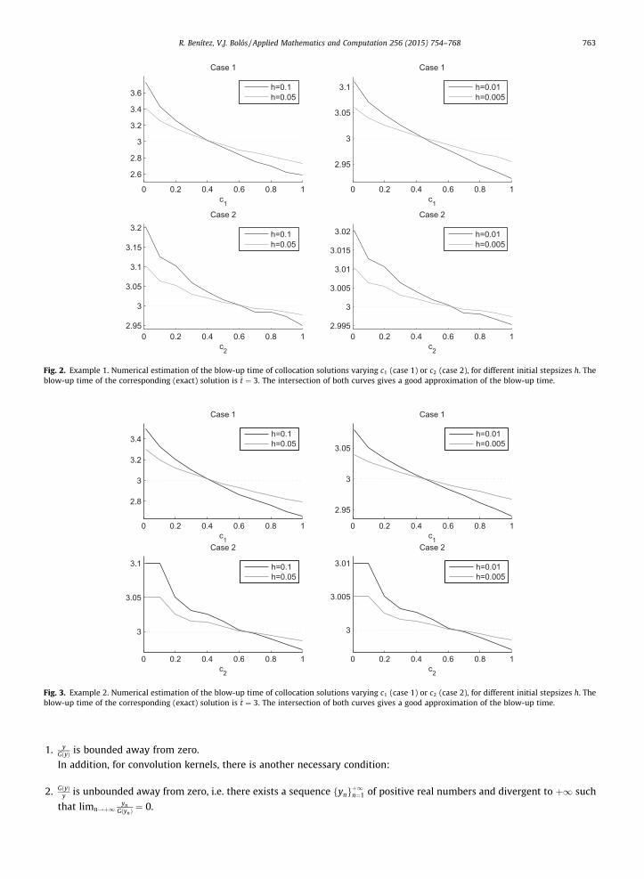
using the algorithms described in Section 4.1 (the specific for the Example 1 and the general for the rest). In Figs. 2–5 theestimations of the blow-up time of the collocation solutions for a given initial stepsize h are depicted, varying c1 in case1 or c2 in case 2. Note that the different graphs for different h intersect each other in a fairly good approximation of theblow-up time, as it is shown in Tables 1, 2, 4 and 5. Moreover, we can use a more general technique consisting on extrap-olating the minimum ðm1;m2Þ and maximum ðM1;M2Þ times of two results with different initial stepsizes h01; h02 respec-tively, with h01 > h02 (see Fig. 1); in this way the blow-up time estimation is given by

Fig. 1.with h0

t � M1 �ðM1 �M2ÞðM1 �m1ÞðM1 �M2Þ þ ðm2 �m1Þ

: ð14Þ

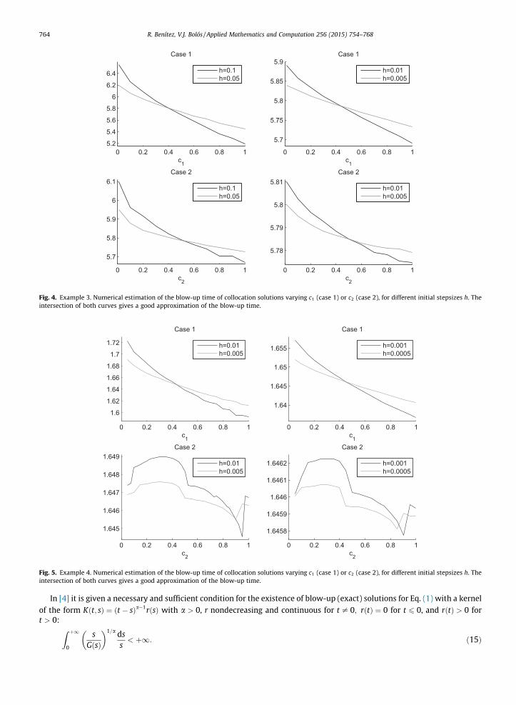
In Examples 3 and 4 we do not know the exact value of the blow-up time. However, in order to make a study of the rel-ative error analogous to the previous examples, we have taken as blow-up time for Example 3 the approximation forh ¼ 0:001 in case 2 with c2 ¼ 0:5: t ¼ 5:78482; in Example 4 the blow-up time value has been taken as the approximationfor h ¼ 0:0001 in case 2 with c2 ¼ 2=3 (Radau I collocation points): t ¼ 1:645842. Results are shown in Tables 7, 8, 10 and 11.

The relative error of varying c1 (case 1) or c2 (case 2) is the ‘‘relative vertical size’’ of the graph, and it decreases at thesame rate as h. On the other hand, the relative error of the intersection decreases faster, in some cases at the same rate

as h2.Moreover, in case 1, the best approximations are obtained with c1 � 0:5, and in case 2 with c2 � 2=3 (approximately

Radau I) for Examples 1, 2 and 4 (see Tables 3, 6 and 12), while for Example 3 the best approximations are obtained withc2 � 0:5; however, in Table 9 are also shown the approximations and their corresponding errors for the Radau I collocationpoints. On the other hand, the intersections technique offers better results, but at a greater computational cost.

5. Discussion and comments

The main necessary conditions for a collocation problem to have a blow-up are obtained from Propositions 3.2 (case 1)and 3.5 (case 2), and are mostly related to the nonlinearity, since the assumption on the kernel ‘‘the map t # K t; sð Þ is con-tinuous in s; �� ½ for some � > 0 and for all 0 6 s < �’’ is only required in case 2 with c2 – 1 and it is a very weak hypothesis.Hence, assuming that the kernel satisfies this hypothesis, the main necessary condition for the existence of a blow-up is:

Extrapolation technique given by (14). M1; M2 and m1; m2 are the maximum and minimum times respectively, using initial stepsizes h01 and h02,1 > h02.

0 0.2 0.4 0.6 0.8 1

2.6

2.8

3

3.2

3.4

3.6

c1

Case 1

0 0.2 0.4 0.6 0.8 1

2.95

3

3.05

3.1

c1

Case 1

0 0.2 0.4 0.6 0.8 12.95

3

3.05

3.1

3.15

3.2

c2

Case 2

0 0.2 0.4 0.6 0.8 12.995

3

3.005

3.01

3.015

3.02

c2

Case 2

h=0.1h=0.05

h=0.01h=0.005

h=0.1h=0.05

h=0.01h=0.005

Fig. 2. Example 1. Numerical estimation of the blow-up time of collocation solutions varying c1 (case 1) or c2 (case 2), for different initial stepsizes h. Theblow-up time of the corresponding (exact) solution is t ¼ 3. The intersection of both curves gives a good approximation of the blow-up time.

0 0.2 0.4 0.6 0.8 1

2.8

3

3.2

3.4

c1

Case 1

0 0.2 0.4 0.6 0.8 1

2.95

3

3.05

c1

Case 1

0 0.2 0.4 0.6 0.8 1

3

3.05

3.1

c2

Case 2

0 0.2 0.4 0.6 0.8 1

3

3.005

3.01

c2

Case 2

h=0.01h=0.005

h=0.1h=0.05

h=0.01h=0.005

h=0.1h=0.05

Fig. 3. Example 2. Numerical estimation of the blow-up time of collocation solutions varying c1 (case 1) or c2 (case 2), for different initial stepsizes h. Theblow-up time of the corresponding (exact) solution is t ¼ 3. The intersection of both curves gives a good approximation of the blow-up time.

R. Benítez, V.J. Bolós / Applied Mathematics and Computation 256 (2015) 754–768 763

1. yGðyÞ is bounded away from zero.

In addition, for convolution kernels, there is another necessary condition:

2. GðyÞy is unbounded away from zero, i.e. there exists a sequence ynf g

þ1n¼1 of positive real numbers and divergent to þ1 such

that limn!þ1yn

G ynð Þ¼ 0.

0 0.2 0.4 0.6 0.8 1

5.7

5.75

5.8

5.85

5.9

c1

Case 1

0 0.2 0.4 0.6 0.8 1

5.7

5.8

5.9

6

6.1

c2

Case 2

0 0.2 0.4 0.6 0.8 1

5.78

5.79

5.8

5.81

c2

Case 2

0 0.2 0.4 0.6 0.8 15.2

5.4

5.6

5.8

6

6.2

6.4

c1

Case 1

h=0.1h=0.05

h=0.1h=0.05

h=0.01h=0.005

h=0.01h=0.005

Fig. 4. Example 3. Numerical estimation of the blow-up time of collocation solutions varying c1 (case 1) or c2 (case 2), for different initial stepsizes h. Theintersection of both curves gives a good approximation of the blow-up time.

0 0.2 0.4 0.6 0.8 1

1.64

1.645

1.65

1.655

c1

Case 1

0 0.2 0.4 0.6 0.8 1

1.645

1.646

1.647

1.648

1.649

c2

Case 2

0 0.2 0.4 0.6 0.8 1

1.6458

1.6459

1.646

1.6461

1.6462

c2

Case 2

0 0.2 0.4 0.6 0.8 1

1.6

1.62

1.64

1.66

1.68

1.7

1.72

c1

Case 1

h=0.01h=0.005

h=0.001h=0.0005

h=0.01h=0.005

h=0.001h=0.0005

Fig. 5. Example 4. Numerical estimation of the blow-up time of collocation solutions varying c1 (case 1) or c2 (case 2), for different initial stepsizes h. Theintersection of both curves gives a good approximation of the blow-up time.

764 R. Benítez, V.J. Bolós / Applied Mathematics and Computation 256 (2015) 754–768

In [4] it is given a necessary and sufficient condition for the existence of blow-up (exact) solutions for Eq. (1) with a kernel

of the form Kðt; sÞ ¼ ðt � sÞa�1rðsÞ with a > 0, r nondecreasing and continuous for t – 0; rðtÞ ¼ 0 for t 6 0, and rðtÞ > 0 fort > 0:

Z þ1

0

sGðsÞ

� �1=a dss< þ1: ð15Þ

Table 1Example 1. Numerical data of Fig. 2 (case 1: m ¼ 1; c1 > 0).

Case 1 Varying c1 Extrapolation Intersection

h min. t max. t Rel. error t Rel. error t Rel. error

0.1 2:60 (c1 ¼ 1) 3:66 (c1 ¼ 0:01) 4 � 10�1 3.033 1:1 � 10�2 3:03 (c1 ¼ 0:39) 10�2

0.05 2:78 (c1 ¼ 1) 3:40 (c1 ¼ 0:01) 2 � 10�1

0.01 2:92 (c1 ¼ 1) 3:11 (c1 ¼ 0:01) 6 � 10�2 3.0044 1:5 � 10�3 3:002 (c1 ¼ 0:44) 7 � 10�4

0.005 2:96 (c1 ¼ 1) 3:06 (c1 ¼ 0:01) 3 � 10�2

Table 2Example 1. Numerical data of Fig. 2 (case 2: m ¼ 2; c1 ¼ 0).

Case 2 Varying c2 Extrapolation Intersection

h min. t max. t Rel. error t Rel. error t Rel. error

0:1 2:95 (c2 ¼ 1) 3:20 (c2 ¼ 0:01) 8 � 10�2 3.008 2:6 � 10�3 3:0003 (c2 ¼ 0:618) 10�4

0:05 2:98 (c2 ¼ 1) 3:10 (c2 ¼ 0:01) 4 � 10�2

0:01 2:995 (c2 ¼ 1) 3:020 (c2 ¼ 0:01) 8 � 10�3 3.0008 2:6 � 10�4 3:000003 (c2 ¼ 0:623) 10�6

0:005 2:998 (c2 ¼ 1) 3:010 (c2 ¼ 0:01) 4 � 10�3

Table 3Example 1. Numerical estimations and relative errors of the blow-up time of collocation solutions in case 1 with c1 ¼ 0:5, and case 2 with Radau I collocationpoints, c1 ¼ 0; c2 ¼ 2=3, for different initial stepsizes h.

h Case 1 – c1 ¼ 0:5 Case 2 – Radau I

Blow-up Rel. error Blow-up Rel. error

0:1 2:933883 2:2 � 10�2 2:995253 1:6 � 10�3

0:05 2:965002 1:2 � 10�2 2:997602 8 � 10�4

0:01 2:992885 2:4q � 10�3 2:999519 1:6 � 10�4

0:005 2:996434 1:2 � 10�3 2:999759 8 � 10�5

Table 4Example 2. Numerical data of Fig. 3 (case 1: m ¼ 1; c1 > 0).

Case 1 Varying c1 Extrapolation Intersection

h min. t max. t Rel. error t Rel. error t Rel. error

0:1 2:68 (c1 ¼ 1) 3:50 (c1 ¼ 0:01) 3 � 10�1 3:018 6 � 10�3 3:015 (c1 ¼ 0:399) 5 � 10�3

0:05 2:82 (c1 ¼ 1) 3:30 (c1 ¼ 0:01) 1:5 � 10�1

0:01 2:94 (c1 ¼ 1) 3:08 (c1 ¼ 0:01) 4:6 � 10�2 3:01 3:3 � 10�3 3:0008 (c1 ¼ 0:444) 2:6 � 10�4

0:005 2:98 (c1 ¼ 1) 3:04 (c1 ¼ 0:01) 2:3 � 10�2

Table 5Example 2. Numerical data of Fig. 3 (case 2: m ¼ 2; c1 ¼ 0).

Case 2 Varying c2 Extrapolation Intersection

h min. t max. t Rel. error t Rel. error t Rel. error

0:1 2:97 (c2 ¼ 1) 3:10 (c2 ¼ 0:01) 4:3 � 10�2 3:007 2:4 � 10�3 3:00012 (c2 ¼ 0:6466) 4 � 10�5

0:05 2:99 (c2 ¼ 1) 3:05 (c2 ¼ 0:01) 2 � 10�2

0:01 2:997 (c2 ¼ 1) 3:010 (c2 ¼ 0:01) 4:3 � 10�3 3:000003 10�6 3:000011 (c2 ¼ 0:65114) 3:6 � 10�6

0:005 2:9985 (c2 ¼ 1) 3:005 (c2 ¼ 0:01) 2:15 � 10�3

R. Benítez, V.J. Bolós / Applied Mathematics and Computation 256 (2015) 754–768 765

This also holds for convolution kernels of Abel type Kðt; sÞ ¼ ðt � sÞa�1 with a > 0, generalizing some results given in [3]. Nextwe will show that necessary conditions 1 and 2 above mentioned are also necessary conditions for the integral given in (15)to be convergent, and thus for the existence of a blow-up (exact) solution.

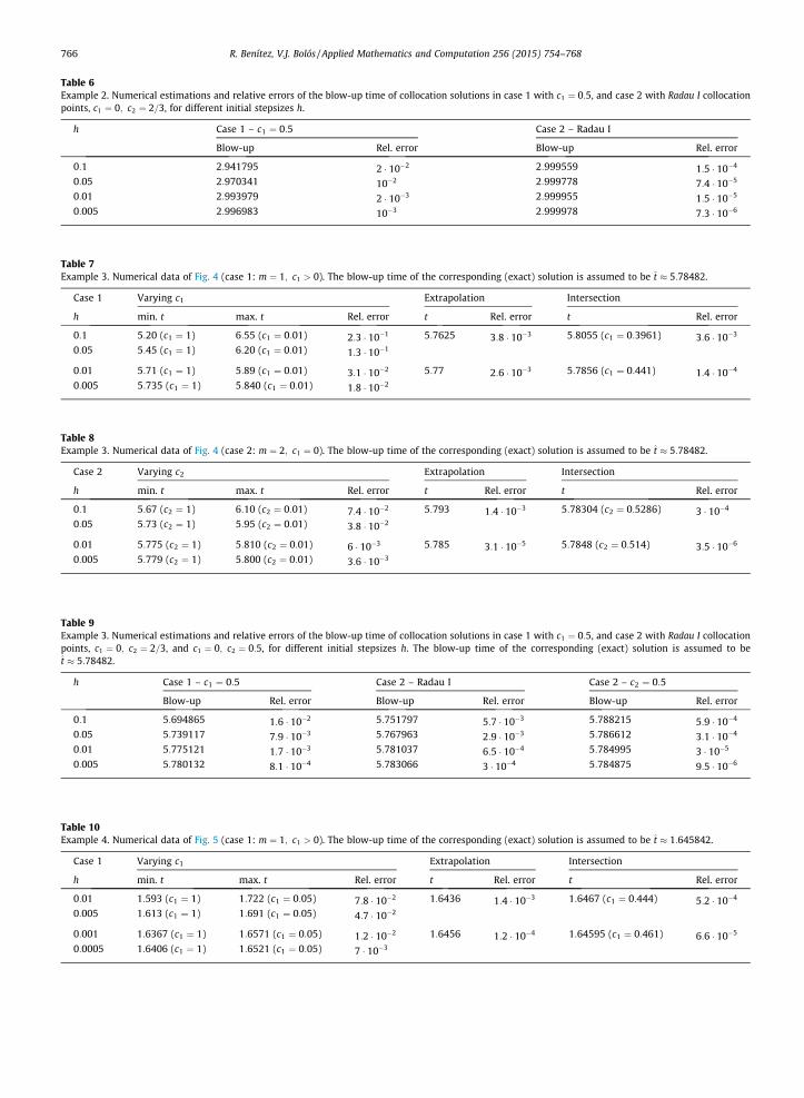
Table 6Example 2. Numerical estimations and relative errors of the blow-up time of collocation solutions in case 1 with c1 ¼ 0:5, and case 2 with Radau I collocationpoints, c1 ¼ 0; c2 ¼ 2=3, for different initial stepsizes h.

h Case 1 – c1 ¼ 0:5 Case 2 – Radau I

Blow-up Rel. error Blow-up Rel. error

0:1 2:941795 2 � 10�2 2:999559 1:5 � 10�4

0:05 2:970341 10�2 2:999778 7:4 � 10�5

0:01 2:993979 2 � 10�3 2:999955 1:5 � 10�5

0:005 2:996983 10�3 2:999978 7:3 � 10�6

Table 7Example 3. Numerical data of Fig. 4 (case 1: m ¼ 1; c1 > 0). The blow-up time of the corresponding (exact) solution is assumed to be t � 5:78482.

Case 1 Varying c1 Extrapolation Intersection

h min. t max. t Rel. error t Rel. error t Rel. error

0:1 5:20 (c1 ¼ 1) 6:55 (c1 ¼ 0:01) 2:3 � 10�1 5:7625 3:8 � 10�3 5:8055 (c1 ¼ 0:3961) 3:6 � 10�3

0:05 5:45 (c1 ¼ 1) 6:20 (c1 ¼ 0:01) 1:3 � 10�1

0:01 5:71 (c1 ¼ 1) 5:89 (c1 ¼ 0:01) 3:1 � 10�2 5:77 2:6 � 10�3 5:7856 (c1 ¼ 0:441) 1:4 � 10�4

0:005 5:735 (c1 ¼ 1) 5:840 (c1 ¼ 0:01) 1:8 � 10�2

Table 8Example 3. Numerical data of Fig. 4 (case 2: m ¼ 2; c1 ¼ 0). The blow-up time of the corresponding (exact) solution is assumed to be t � 5:78482.

Case 2 Varying c2 Extrapolation Intersection

h min. t max. t Rel. error t Rel. error t Rel. error

0:1 5:67 (c2 ¼ 1) 6:10 (c2 ¼ 0:01) 7:4 � 10�2 5:793 1:4 � 10�3 5:78304 (c2 ¼ 0:5286) 3 � 10�4

0:05 5:73 (c2 ¼ 1) 5:95 (c2 ¼ 0:01) 3:8 � 10�2

0:01 5:775 (c2 ¼ 1) 5:810 (c2 ¼ 0:01) 6 � 10�3 5:785 3:1 � 10�5 5:7848 (c2 ¼ 0:514) 3:5 � 10�6

0:005 5:779 (c2 ¼ 1) 5:800 (c2 ¼ 0:01) 3:6 � 10�3

Table 9Example 3. Numerical estimations and relative errors of the blow-up time of collocation solutions in case 1 with c1 ¼ 0:5, and case 2 with Radau I collocationpoints, c1 ¼ 0; c2 ¼ 2=3, and c1 ¼ 0; c2 ¼ 0:5, for different initial stepsizes h. The blow-up time of the corresponding (exact) solution is assumed to bet � 5:78482.

h Case 1 – c1 ¼ 0:5 Case 2 – Radau I Case 2 – c2 ¼ 0:5

Blow-up Rel. error Blow-up Rel. error Blow-up Rel. error

0:1 5:694865 1:6 � 10�2 5:751797 5:7 � 10�3 5:788215 5:9 � 10�4

0:05 5:739117 7:9 � 10�3 5:767963 2:9 � 10�3 5:786612 3:1 � 10�4

0:01 5:775121 1:7 � 10�3 5:781037 6:5 � 10�4 5:784995 3 � 10�5

0:005 5:780132 8:1 � 10�4 5:783066 3 � 10�4 5:784875 9:5 � 10�6

Table 10Example 4. Numerical data of Fig. 5 (case 1: m ¼ 1; c1 > 0). The blow-up time of the corresponding (exact) solution is assumed to be t � 1:645842.

Case 1 Varying c1 Extrapolation Intersection

h min. t max. t Rel. error t Rel. error t Rel. error

0:01 1:593 (c1 ¼ 1) 1:722 (c1 ¼ 0:05) 7:8 � 10�2 1:6436 1:4 � 10�3 1:6467 (c1 ¼ 0:444) 5:2 � 10�4

0:005 1:613 (c1 ¼ 1) 1:691 (c1 ¼ 0:05) 4:7 � 10�2

0:001 1:6367 (c1 ¼ 1) 1:6571 (c1 ¼ 0:05) 1:2 � 10�2 1:6456 1:2 � 10�4 1:64595 (c1 ¼ 0:461) 6:6 � 10�5

0:0005 1:6406 (c1 ¼ 1) 1:6521 (c1 ¼ 0:05) 7 � 10�3

766 R. Benítez, V.J. Bolós / Applied Mathematics and Computation 256 (2015) 754–768

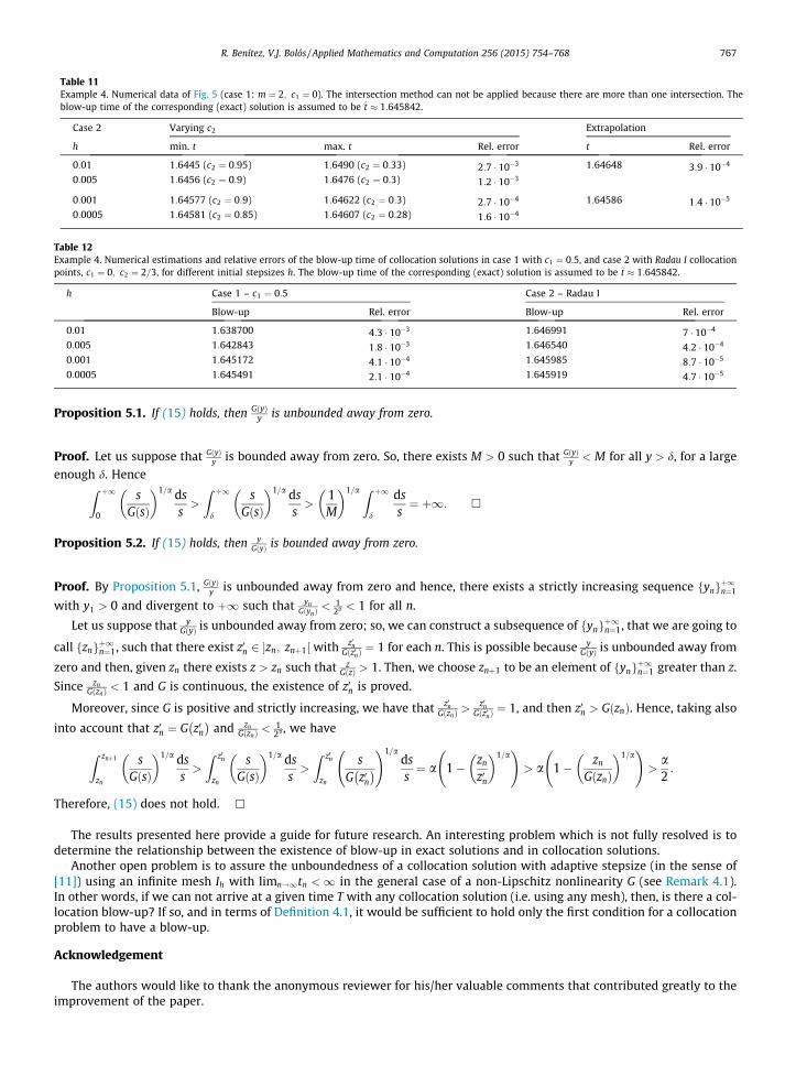
Table 11Example 4. Numerical data of Fig. 5 (case 1: m ¼ 2; c1 ¼ 0). The intersection method can not be applied because there are more than one intersection. Theblow-up time of the corresponding (exact) solution is assumed to be t � 1:645842.

Case 2 Varying c2 Extrapolation

h min. t max. t Rel. error t Rel. error

0:01 1:6445 (c2 ¼ 0:95) 1:6490 (c2 ¼ 0:33) 2:7 � 10�3 1:64648 3:9 � 10�4

0:005 1:6456 (c2 ¼ 0:9) 1:6476 (c2 ¼ 0:3) 1:2 � 10�3

0:001 1:64577 (c2 ¼ 0:9) 1:64622 (c2 ¼ 0:3) 2:7 � 10�4 1:64586 1:4 � 10�5

0:0005 1:64581 (c2 ¼ 0:85) 1:64607 (c2 ¼ 0:28) 1:6 � 10�4

Table 12Example 4. Numerical estimations and relative errors of the blow-up time of collocation solutions in case 1 with c1 ¼ 0:5, and case 2 with Radau I collocationpoints, c1 ¼ 0; c2 ¼ 2=3, for different initial stepsizes h. The blow-up time of the corresponding (exact) solution is assumed to be t � 1:645842.

h Case 1 – c1 ¼ 0:5 Case 2 – Radau I

Blow-up Rel. error Blow-up Rel. error

0:01 1:638700 4:3 � 10�3 1:646991 7 � 10�4

0:005 1:642843 1:8 � 10�3 1:646540 4:2 � 10�4

0:001 1:645172 4:1 � 10�4 1:645985 8:7 � 10�5

0:0005 1:645491 2:1 � 10�4 1:645919 4:7 � 10�5

R. Benítez, V.J. Bolós / Applied Mathematics and Computation 256 (2015) 754–768 767

Proposition 5.1. If (15) holds, then GðyÞy is unbounded away from zero.

Proof. Let us suppose that GðyÞy is bounded away from zero. So, there exists M > 0 such that GðyÞ

y < M for all y > d, for a large

enough d. Hence

Z þ1

0

sGðsÞ

� �1=a dss>

Z þ1

d

sGðsÞ

� �1=a dss>

1M

� �1=a Z þ1

d

dss¼ þ1: �

Proposition 5.2. If (15) holds, then yGðyÞ is bounded away from zero.

Proof. By Proposition 5.1, GðyÞy is unbounded away from zero and hence, there exists a strictly increasing sequence ynf g

þ1n¼1

with y1 > 0 and divergent to þ1 such that ynG ynð Þ

< 12a < 1 for all n.

Let us suppose that yGðyÞ is unbounded away from zero; so, we can construct a subsequence of ynf g

þ1n¼1, that we are going to

call znf gþ1n¼1, such that there exist z0n 2 zn; znþ1� ½ with z0nG z0nð Þ¼ 1 for each n. This is possible because y

GðyÞ is unbounded away from

zero and then, given zn there exists z > zn such that zGðzÞ > 1. Then, we choose znþ1 to be an element of ynf g

þ1n¼1 greater than z.

Since znG znð Þ < 1 and G is continuous, the existence of z0n is proved.

Moreover, since G is positive and strictly increasing, we have that z0nG znð Þ >

z0nG z0nð Þ¼ 1, and then z0n > G znð Þ. Hence, taking also

into account that z0n ¼ G z0n� �

and znG znð Þ <

12a, we have

Z znþ1

zn

sGðsÞ

� �1=a dss>

Z z0n

zn

sGðsÞ

� �1=a dss>

Z z0n

zn

sG z0n� �

!1=adss¼ a 1� zn

z0n

� �1=a !

> a 1� zn

G znð Þ

� �1=a !

>a2:

Therefore, (15) does not hold. h

The results presented here provide a guide for future research. An interesting problem which is not fully resolved is todetermine the relationship between the existence of blow-up in exact solutions and in collocation solutions.

Another open problem is to assure the unboundedness of a collocation solution with adaptive stepsize (in the sense of[11]) using an infinite mesh Ih with limn!1tn <1 in the general case of a non-Lipschitz nonlinearity G (see Remark 4.1).In other words, if we can not arrive at a given time T with any collocation solution (i.e. using any mesh), then, is there a col-location blow-up? If so, and in terms of Definition 4.1, it would be sufficient to hold only the first condition for a collocationproblem to have a blow-up.

Acknowledgement

The authors would like to thank the anonymous reviewer for his/her valuable comments that contributed greatly to theimprovement of the paper.

768 R. Benítez, V.J. Bolós / Applied Mathematics and Computation 256 (2015) 754–768

Appendix A. Supplementary data

Supplementary data associated with this article can be found, in the online version, at http://dx.doi.org/10.1016/j.amc.2015.01.057.

References

[1] C.M. Kirk, Numerical and asymptotic analysis of a localized heat source undergoing periodic motion, Nonlinear Anal. 71 (2009) e2168–e2172.[2] F. Calabrò, G. Capobianco, Blowing up behavior for a class of nonlinear VIEs connected with parabolic PDEs, J. Comput. Appl. Math. 228 (2009) 580–588.[3] W. Mydlarczyk, A condition for finite blow-up time for a Volterra integral equation, J. Math. Anal. Appl. 181 (1994) 248–253.[4] W. Mydlarczyk, The blow-up solutions of integral equations, Colloq. Math. 79 (1999) 147–156.[5] T. Małolepszy, W. Okrasinski, Conditions for blow-up of solutions of some nonlinear Volterra integral equations, J. Comput. Appl. Math. 205 (2007)

744–750.[6] T. Małolepszy, W. Okrasinski, Blow-up conditions for nonlinear Volterra integral equations with power nonlinearity, Appl. Math. Letters. 21 (2008)

307–312.[7] T. Małolepszy, W. Okrasinski, Blow-up time for solutions for some nonlinear Volterra integral equations, J. Math. Anal. Appl. 366 (2010) 372–384.[8] H. Brunner, Z.W. Yang, Blow-up behavior of Hammerstein-type Volterra integral equations, J. Integral Equations Appl. 24 (4) (2012) 487–512.[9] T. Małolepszy, Nonlinear Volterra integral equations and the Schröder functional equation, Nonlinear Anal. T.M.A. 74 (2011) 424–432.

[10] H. Brunner, Collocation Methods for Volterra Integral and Related Functional Differential Equations, Cambridge University Press, Cambridge, 2004.[11] Z.W. Yang, H. Brunner, Blow-up behavior of collocation solutions to Hammerstein-type Volterra integral equations, SIAM J. Numer. Anal. 51 (2013)

2260–2282.[12] M.A. Krasnosel’skii, P.P. Zabreiko, Geometric Methods of Nonlinear Analysis, Springer Verlag, New York, 1984.[13] R. Benítez, V.J. Bolós, Existence and uniqueness of nontrivial collocation solutions of implicitly linear homogeneous Volterra integral equations, J.

Comput. Appl. Math. 235 (2011) 3661–3672.[14] T. Małolepszy, Blow-up solutions in one-dimensional diffusion models, Nonlinear Anal. T.M.A. 95 (2014) 632–638.[15] H. Brunner, Implicitly linear collocation methods for nonlinear Volterra integral equations, Appl. Numer. Math. 9 (1992) 235–247.[16] M.R. Arias, R. Benítez, Aspects of the behaviour of solutions of nonlinear Abel equations, Nonlinear Anal. T.M.A. 54 (2003) 1241–1249.[17] M.R. Arias, R. Benítez, A note of the uniqueness and the attractive behaviour of solutions for nonlinear Volterra equations, J. Integral Equations Appl. 13

(4) (2001) 305–310.