Modeling Of Species Interaction in a Habitat Using Lotka- Volterra Type Systems

IOSR Journal of Mathematics (IOSR-JM)

e-ISSN: 2278-5728, p-ISSN: 2319-765X. Volume 10, Issue 4 Ver. IV (Jul-Aug. 2014), PP 45-54 www.iosrjournals.org

www.iosrjournals.org 45 | Page

Modeling Of Species Interaction in a Habitat Using Lotka-

Volterra Type Systems

Nweze N. O.1, Offiong N. M.

1*, Adehi M. U.

1, Chaku S. E.

1, Abdullahi S.

A.1, Muhammad N. Mahammmad

2

1,2Department of Mathematical Sciences, Nasarawa State University, Keffi, Nasarawa, Nigeria.

Correspondence: [email protected]

[email protected]

Abstract: Mathematical models have been useful in the area of modeling of real life situations; its application

can be found in virtually all spheres of scientific researches. As such, we adopt its use in the field of ecology

where preys have to compete with other prey for survival. In this paper, we considered Lotka-Volterra type

systems, consisting of two first order differential equations which were used to model the population size of

prey–predator interaction. We also proposed a system of first order differential equations to model the

population sizes of a prey and two predators. Under these conditions one of the predators dies out while the

remaining predator and prey approach periodic behavior as time increases. Also we model the population size

of two preys and one predator where there may be interaction between the preys. Under these conditions we

found that one of the preys died out while the remaining preys and predators approached periodic behavior as

time increased. For critical cases, each positive solution of the system was seen to be periodic in nature.

Various examples and results were presented and further study was proposed.

Keywords: Mathematical Models, Lotka-Volterra, differential equation, habitat, predator, prey.

I. Introduction Ecologists strive to understand how interspecies interaction contributes to distribution and abundance

of particular species. Decades of modeling, observation studies and experimental approaches have led ecologists

to conclude that species sharing the same habitat often play important but highly diverse roles in affecting each

other according to Chesson [1]. Keddy [2], mentioned that interactions among species were viewed as a simple

mutually negative interaction either directly through interferences or indirectly through exploitation of shared

resources. Understanding such mutually negative interactions among competing species remains a cornerstone

of community ecology. Keddy showed apparent competition occurs when two or more prey species share a common predator, and predator’s numbers are limited by prey availability. By presenting itself as an additional

food resource, the second prey species allows the abundance of the predator to increase and, as a result reduces

the density of the target species. If more than one prey species is present, and both utilities those enemy-free

resources, the species can limit each other’s numbers.

An apparent mutualism between prey species that share a common predator can arise if predator

populations are limited by factors other than prey availability, Abrams [3]. In this case, the presence of a prey

species satisfies the predator, thus allowing a relief of predator pressure on the target species; that is, the species

indirectly benefits the target species. Co-operation or symbiosis infection occurs when two species help each

other in some ways. Week-strong interaction occurs when one species is simply better suited to survive than

other. Competition between species may be indirect, in which the competitors use a resource but do not confront

each other over it, in direct competition, the two species may fight over a resource. Sometimes competition may be mediated by a third organism, such as predator or parasite. The Difference in size between a predator and its

prey has an effect on the development of specialized structures of the predator for subduing the prey. For the

most part, predator feed in species smaller than themselves; consider herbivorous to be predators of plants, just

as carnivores are predators of animals.

II. Literature Survey The Lotka-Volterra predator-prey and competition model was initially proposed by Alfred .J. Lotka in

the theory autocatalytic chemical reaction in 1910. This was effectively the logistic equation, Berryman (1992),

which was originally derived by Pierre Francis Verhulst. The Lotka-Volterra model and Holling’s extension have been used to model the moose and wolf population Jost[4].

Given two species of animals, interdependence might arise because one species (the prey) serves as

food source for the other species (the predator). Models of this type are thus called predator prey models. Let P

mailto:[email protected]

Modeling Of Species Interaction in a Habitat Using Lotka-Volterra Type Systems


denote the size of the prey population and Q donate the size of the predator population. The growth rate of prey

populations is determined by the equation:

QQ

P

dt

dP

1 ……………………….…….. (1)

where α, β and Q are parameters, Barntt [5]. In the absence of predators (when Q=0) the growth of the prey

population thus follows the logistic model where Q is called carrying capacity of the environment. The growth

rate of the predator is determined by the equation.

PQdt

dQ . ….………………………. .. (2)

where γ, δ are parameters. In the absence of prey (when P = 0) the predator population would shrink at rate γ.

However, the predator growth rate rises as the prey population becomes larger. The two equations (1) and (2)

can be described as:

PhQK

P

dt

dP

1 . …………….………….. (3)

QhPdt

dQ .…………………….………….. (4)

where h is the period of the interaction, this version of the predator prey model provides a useful starting point,

provides the needed basic insight that more predators are bad for prey, while more prey are good for predators.

In the Lotka-Volterra model, the prey population faces a capacity constraint giving by parameter K, if there is no

capacity constraint so that k is infinite the two equation system is giving below. In the development of this model, a number of assumption, were made by Lotka-Volterra. These include:

If there are no predators, the prey population will grow at the rate proportional to the population of the

prey species.

If there are no prey, the species decline at the rate proportional to the population if the predator.

The presence of both predators and prey is beneficial to growth of predators’ species and is harmful to

growth of prey species. More especially the predator species increases and the prey species decreases at rate

proportional to the product of the two populations.

During the process, the environment does not change in favor of one species and the genetic adaptation

is sufficiently slow. As differential equations are used, the solution is deterministic and continues. This in turn,

implies that the generations of both the predators and prey are continually over lapping Cook [6]. This

assumption gives the system of non-linear first order ordinary differential equations.

Qpdt

dp . . . . . . . . . . . . . . . . . . . . . . (5)

pQdt

dQ . . . . . . . . . . . . . . . . . . . . . . (6)

Where:

P = prey population

Q = predator population

α = the growth rate of prey

γ = death rate of predator δ = growth rate of predator

Equation (5) can be express as:

Qpdt

dp …………………………………….. (7)

This means the change in prey’s numbers is given by its own growth minus the rate at which it is

preyed upon. Equation (6) can also be express as:

PQQdt

dQ ………………………………….. (8)

The equation expresses the change in the predator population as the death rate of predator plus growth rate of the predator.

The above equations (7) and (8) can be solved numerically and the orbits can be defined as follows:



QP

PQ

dP

dQ

PQP

PQQ

dP

dQ

dP

dQ=

PQ

QP

…………………………………… (9)

Equation (9) is a separable first order differential equation and may be written as:

dt

dP

P

P

dt

dQ

Q

Q..

dt

dPP

Pdt

dQ

Q

….………………….. (10)

Integrating equation (10) yields

CPInPQInQ ….…………………….. (11)

From equation (11), we have that

PQ CPQ

CQP

PQFQP

, β, ϒ, δ > 0

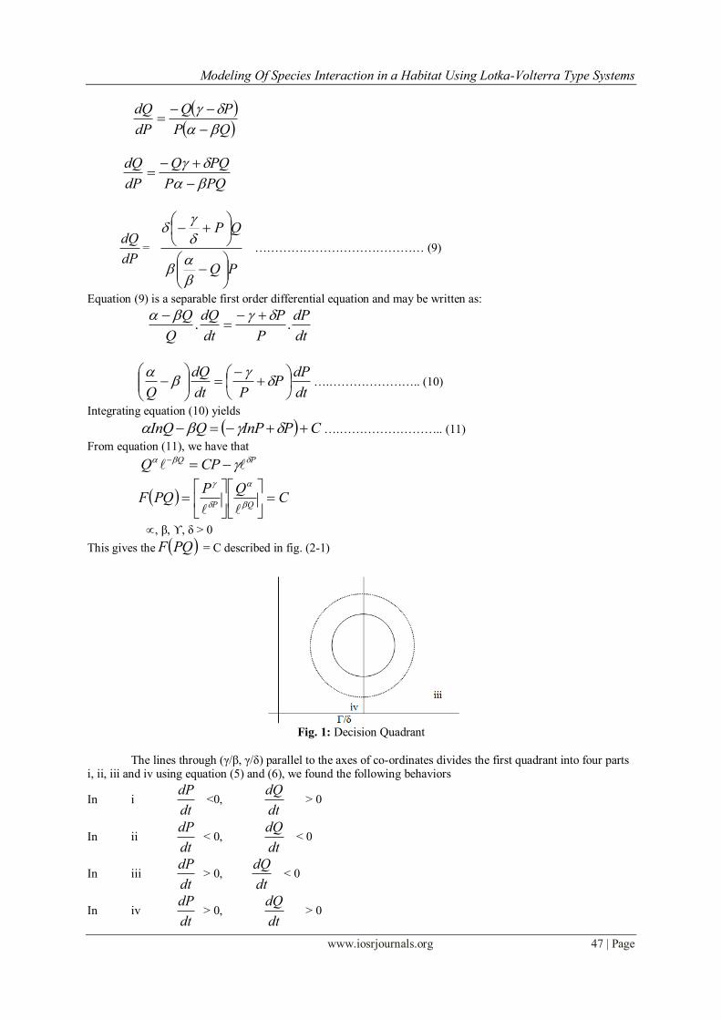
This gives the PQF = C described in fig. (2-1)

Fig. 1: Decision Quadrant

The lines through (γ/β, γ/δ) parallel to the axes of co-ordinates divides the first quadrant into four parts i, ii, iii and iv using equation (5) and (6), we found the following behaviors

In i dt

dP <0,

dt

dQ > 0

In ii dt

dP < 0,

dt

dQ < 0

In iii dt

dP > 0,

dt

dQ < 0

In iv dt

dP > 0,

dt

dQ > 0



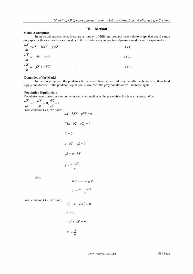
III. Method Model Assumption:

In an actual environment, there are a number of different predator-prey relationships that could single

prey species this scenario is examined, and the predator-prey interaction dynamics model can be expressed as;

dt

dX= gXZbXYaX

. . . . . . . . . . . . . . . (3.1)

cXYdYdt

dY . . . . . . . . . . (3.2)

eXZfZdt

dZ . . . . . . . . . . . (3.3)

Dynamics of the Model

In the model system, the predators thrive when there is plentiful prey but ultimately, outstrip their food

supply and decline. If the predator population is low, then the prey population will increase again.

Population Equilibrium

Population equilibrium occurs in the model when neither of the population levels is changing. When

.0,0,0 dt

dZ

dt

dY

dt

dX

From equation (3.1) we have:

g

bYaZ

bYagZ

gZbYa

X

gZbYaX

gXZbXYaX

0

0

0

0

Also

b

gZaY

gZabY

From equation (3.2) we have,

c

dX

cXd

Y

cXdY

0

0

0



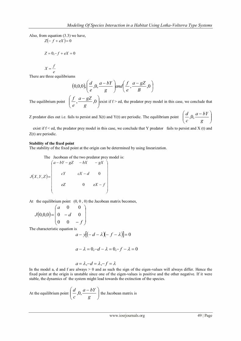
Also, from equation (3.3) we have,

e

fX

eXfZ

eXfZ

0,0

0

There are three equilibriums

0,,,0,,0,0,0

B

gZa

e

fand

g

bYa

e

d

The equilibrium point

0,,

g

gZa

e

fexist if f > ed, the predator prey model in this case, we conclude that

Z predator dies out i.e. fails to persist and X(t) and Y(t) are periodic. The equilibrium point

g

bYa

c

d,0,

exist if f < ed, the predator prey model in this case, we conclude that Y predator fails to persist and X (t) and

Z(t) are periodic.

Stability of the fixed point

The stability of the fixed point at the origin can be determined by using linearization.

The Jacobean of the two predator prey model is:

feXeZ

dcXcY

gXbXgZbYa

ZYXJ

0

0,,

At the equilibrium point (0, 0 , 0) the Jacobean matrix becomes,

f

d

a

J

00

00

00

0,0,0

The characteristic equation is

fda

fda

fdya

,,

0,0,0

0

In the model a, d and f are always > 0 and as such the sign of the eigen-values will always differ. Hence the

fixed point at the origin is unstable since one of the eigen-values is positive and the other negative. If it were

stable, the dynamics of the system might lead towards the extinction of the species.

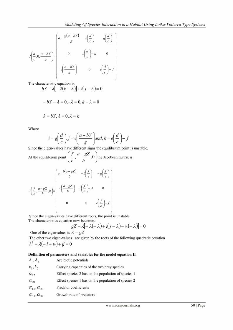
At the equilibrium point

g

bYa

c

d,0, the Jacobean matrix is



The characteristic equation is:

0 jikbY

kbY

kbY

,0,

0,0,0

Where

fc

dekand

g

bYaej

c

dgi

,,

Since the eigen-values have different signs the equilibrium point is unstable.

At the equilibrium point

0,,

b

gZa

e

fthe Jacobean matrix is:

fe

fe

de

fc

b

gZac

e

fg

e

fb

b

gZaba

b

gZa

e

fJ

00

00,,

Since the eigen-values have different roots, the point is unstable.

The characteristics equation now becomes:

0 wjigZ

One of the eigenvalues is gZ

The other two eigen-values are given by the roots of the following quadratic equation

02 ijwi

Definition of parameters and variables for the model equation II

21, Are biotic potentials

21,kk Carrying capacities of the two prey species

12 Effect species 2 has on the population of species 1

21

Effect species 1 has on the population of species 2

2313, Predator coefficients

3231, Growth rate of predators

fc

de

g

bYae

dc

dc

c

dg

c

db

g

bYaga

g

bYa

c

dJ

0

00,0,



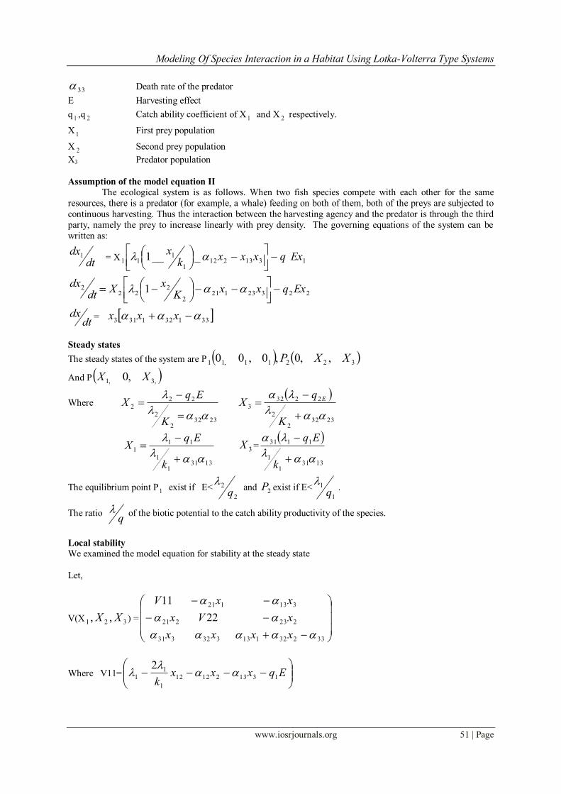
33 Death rate of the predator

E Harvesting effect

q 1 ,q 2 Catch ability coefficient of X 1 and X 2 respectively.

X 1 First prey population

X 2 Second prey population

X3 Predator population

Assumption of the model equation II

The ecological system is as follows. When two fish species compete with each other for the same

resources, there is a predator (for example, a whale) feeding on both of them, both of the preys are subjected to

continuous harvesting. Thus the interaction between the harvesting agency and the predator is through the third

party, namely the prey to increase linearly with prey density. The governing equations of the system can be

written as:

dtdx1 = X 1313212

1

111 ___1 Exqxxx

kx

223231212

222

2 1 ExqxxK

xX

dtdx

dtdx = 331321313 xxx

Steady states

The steady states of the system are P 32211,11 ,,0,0,00 XXP

And P ,3,1 ,0 XX

Where

23322

2

22

2

K

EqX

23322

2

2232

3

K

qX E

13311

1

11

1

k

EqX 3X =

13311

1

1131

k

Eq

The equilibrium point P1 exist if E<2

2

q

and 2P exist if E<1

1

q

.

The ratio q

of the biotic potential to the catch ability productivity of the species.

Local stability

We examined the model equation for stability at the steady state

Let,

V(X 321 ,, XX ) =

33232113332331

223221

313121

22

11

xxxx

xVx

xxV

Where V11=

Eqxxx

k131321212

1

1

1

2



V22=

Eqxxx

k2323212

2

2

2

2

At the steady (0, 0, 0), we have,

V (0, 0, 0) =

000

00

00

22

11

Eq

Eq

The eigen-values of this matrix are 0, EqEq 2211 ,

V

3332331

2232

22221

2313121

32

00

,,0

xxx

xk

Xx

Eqxx

XX

The characteristic equation is:

032322332

2

2

32

2

22

13132121

xxxx

kxx

kEqxx

One of the eigenvalues of the matrix V (0, 32 , XX ) is

Eqxx 13132121 .

The other two eigenvalues are given by the roots of the following quadratic equation

0323223

2

2

32

222

xxk

xk

x

. . . . . . . . . . . . (3.4)

In equation (3.4) the roots =-

32

22 xk

x and product of the roots = 323223

2

2 xxk

Therefore the roots are real and negative or complex conjugates having negative real parts.

Hence it is unstable.

3332331

23231212

113121111

31 00),0,(

xxx

Eqxx

xxkx

XXv

One of the eigen-values of the matrix is

Eqxx 23231212

The other two eigen-values are given by the roots of the quadratic equation

02113312

22

1

112

xxk

xk

x

. . . . . . . . . . . . . . (3.5)

In equation (3.5) the sum of the roots =

21

11 xk

x and product of the roots =

2113312

2 xxk

Therefore the roots are real and negative. Thus the equilibrium point (X 31 ,0, X ) is not stable.

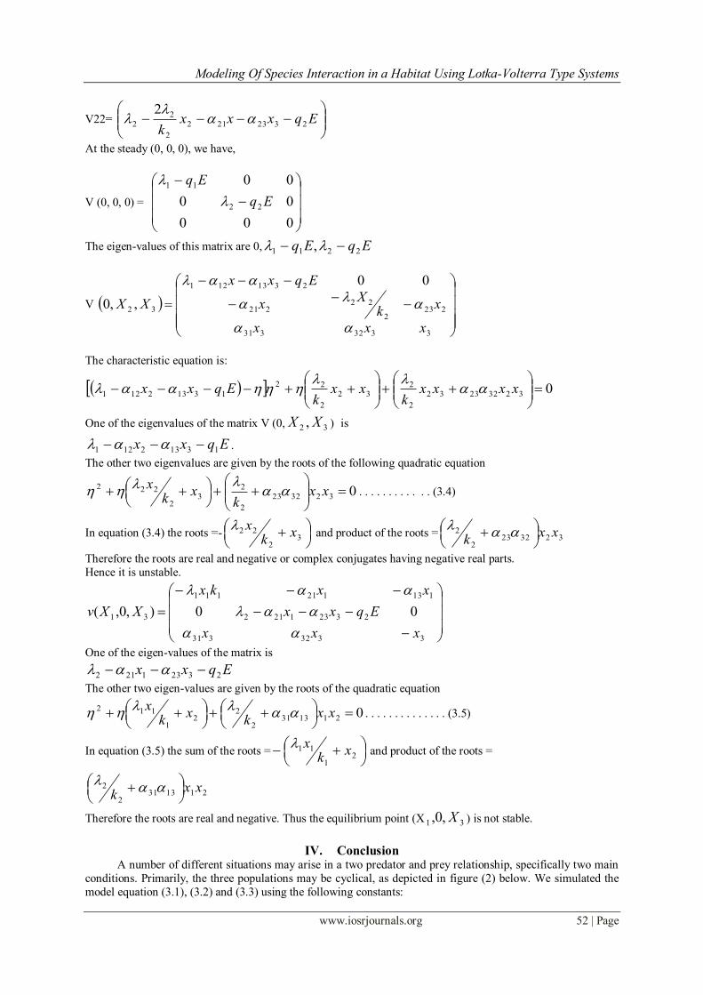
IV. Conclusion A number of different situations may arise in a two predator and prey relationship, specifically two main

conditions. Primarily, the three populations may be cyclical, as depicted in figure (2) below. We simulated the

model equation (3.1), (3.2) and (3.3) using the following constants:



a=2, b=2, c=2, d=1, e=1, f= 21 g=1

X (prey population) is red, Y (first predator population) is blue, Z (second predator population) is green.

Fig. 2: Predator Population Chart

Secondly, since both predators derive their sole nourishment from the same prey species, the most

efficient predator will eventually dominate the relationship and grow at a vast rate, whereas, the other predator

will dwindle in number. The efficient predator and prey relationship shows a continuously cyclical pattern as

shown in fig 4.2 below. The graph clearly illustrates in that in each cycle the prey population is reduced to

extremely low number, but yet recovers while the predator population remain sizeable at the lowest prey

density.

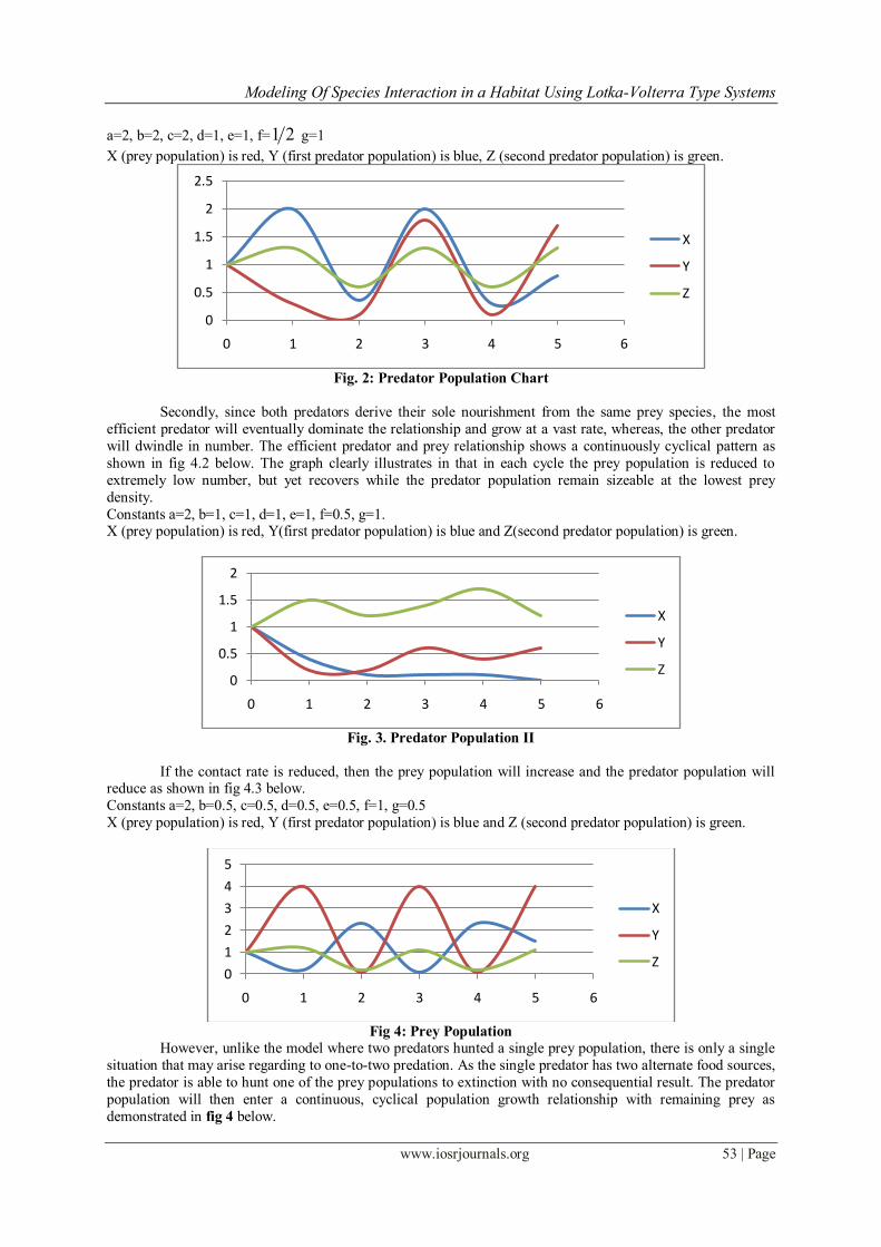
Constants a=2, b=1, c=1, d=1, e=1, f=0.5, g=1. X (prey population) is red, Y(first predator population) is blue and Z(second predator population) is green.

Fig. 3. Predator Population II

If the contact rate is reduced, then the prey population will increase and the predator population will reduce as shown in fig 4.3 below.

Constants a=2, b=0.5, c=0.5, d=0.5, e=0.5, f=1, g=0.5

X (prey population) is red, Y (first predator population) is blue and Z (second predator population) is green.

Fig 4: Prey Population

However, unlike the model where two predators hunted a single prey population, there is only a single

situation that may arise regarding to one-to-two predation. As the single predator has two alternate food sources,

the predator is able to hunt one of the prey populations to extinction with no consequential result. The predator

population will then enter a continuous, cyclical population growth relationship with remaining prey as

demonstrated in fig 4 below.

0

0.5

1

1.5

2

2.5

0 1 2 3 4 5 6

X

Y

Z

0

0.5

1

1.5

2

0 1 2 3 4 5 6

X

Y

Z

0

1

2

3

4

5

0 1 2 3 4 5 6

X

Y

Z



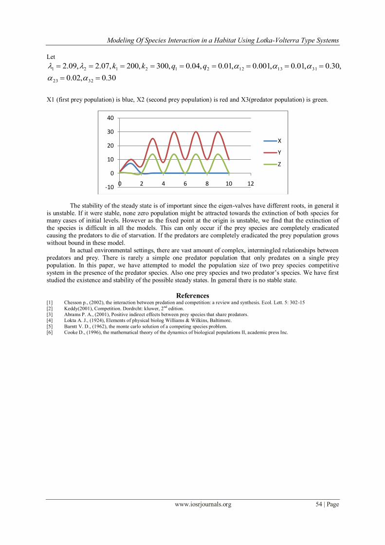
Let

30.0,02.0

,30.0,01.0,001.0,01.0,04.0,300,200,07.2,09.2

3223

311312212121

qqkk

X1 (first prey population) is blue, X2 (second prey population) is red and X3(predator population) is green.

The stability of the steady state is of important since the eigen-valves have different roots, in general it

is unstable. If it were stable, none zero population might be attracted towards the extinction of both species for many cases of initial levels. However as the fixed point at the origin is unstable, we find that the extinction of

the species is difficult in all the models. This can only occur if the prey species are completely eradicated

causing the predators to die of starvation. If the predators are completely eradicated the prey population grows

without bound in these model.

In actual environmental settings, there are vast amount of complex, intermingled relationships between

predators and prey. There is rarely a simple one predator population that only predates on a single prey

population. In this paper, we have attempted to model the population size of two prey species competitive

system in the presence of the predator species. Also one prey species and two predator’s species. We have first

studied the existence and stability of the possible steady states. In general there is no stable state.

References [1] Chesson p., (2002), the interaction between predation and competition: a review and synthesis. Ecol. Lett. 5: 302-15

[2] Keddy(2001), Competition. Dordrcht: kluwer, 2nd

edition.

[3] Abrams P. A., (2001), Positive indirect effects between prey species that share predators.

[4] Lokta A. J., (1924), Elements of physical biolog Williams & Wilkins, Baltimore.

[5] Barntt V. D., (1962), the monte carlo solution of a competing species problem.

[6] Cooke D., (1996), the mathematical theory of the dynamics of biological populations II, academic press Inc.

-10

0

10

20

30

40

0 2 4 6 8 10 12

X

Y

Z

Modeling Of Species Interaction in a Habitat Using Lotka- Volterra Type Systems

Documents

Transcript of Modeling Of Species Interaction in a Habitat Using Lotka- Volterra Type Systems