International Journal of Automation and Computing 6(4), November 2009, 420-430

DOI: 10.1007/s11633-009-0420-0

Crosscumulants Based Approaches for the Structure

Identification of Volterra Models

Houda Mathlouthi1,∗ Kamel Abederrahim1 Faouzi Msahli2 Gerard Favier3

1National School of Engineers of Gabes, Route de Medenine 6029 Gabes, Tunisia2National School of Engineers of Monastir, Avenue Ibn Jazzar 5019, Monastir, Tunisia

3I3S Laboratory, UNSA/CNRS, 2000 Route des Lucioles, Batiment Algorithmes, Euclide, Sophia-Antipolis, Biot, France

Abstract: In this paper, we address the problem of structure identification of Volterra models. It consists in estimating the modelorder and the memory length of each kernel. Two methods based on input-output crosscumulants are developed. The first one uses zeromean independent and identically distributed Gaussian input, and the second one concerns a symmetric input sequence. Simulationsare performed on six models having different orders and kernel memory lengths to demonstrate the advantages of the proposed methods.

Keywords: Structure identification, Volterra model, crosscumulants, Gaussian input, symmetric input.

1 Introduction

Nonlinear systems have received great attention in re-cent years since a broad class of physical systems exhibitsa nonlinear behaviour. Several approaches have been pro-posed in the literature for nonlinear representation, analy-sis, modeling, identification, and control[1−3]. This paperaddresses the problem of Volterra system structure identi-fication based on higher–order statistics (HOS). The trun-cated Volterra model has been the most popular since it canrepresent any nonlinear system time invariant with fadingmemory[1, 2, 4−7]. Moreover, the parameters of this modelare linearly related to the output, which allows the exten-sion of some results of linear systems to nonlinear ones.For these reasons, the truncated Volterra model has foundapplications in many fields such as signal processing andcontrol. On the other hand, HOS are very useful in deal-ing with non-Gaussian and/or nonminimum phase linearsystems, as well as non-linear systems.

For the identification of truncated Volterra model, twomain problems must be considered: one is the identifica-tion of the model kernels and the other is the identificationof the model structure defined by the model order and thekernel memory lengths. Several methods have been pro-posed in the literature for the identification of the kernelsof Volterra models. They can be classified in two classes:nonparametric and parametric. The nonparametric iden-tification methods consist in developing closed form solu-tions that are based on the input–output statistical infor-mation (cumulants and polyspectra). This approach is in-teresting from a theoretical point of view because it showsthe possibility of estimating the kernels of Volterra modelfrom input-output statistical information. However, theyare not recommended in practical applications because theyneed a large number of parameters to be identified. Para-metric identification approaches use adaptive least squaresalgorithms to estimate the unknown model kernels. Thisapproach presents the advantage of requiring only a finite

Manuscript received September 1, 2008; revised March 4, 2009*Corresponding author.E-mail address: mathlouthi houda@yahoo.fr

number of parameters to be identified. For the sake of sim-plicity, these methods assume that the model order and thememory length of each kernel are a priori known or theyare chosen arbitrarily[8−14]. However, successful identifica-tion of Volterra parameters depends on the correct modelorder and the memory length of each kernel. This is one ofthe most difficult problems that represent an area of re-search where few efforts have been devoted in the past.A method to identify only the memories of second-orderVolterra model is proposed in [15]. This order selection isbased on three different hypothesis testing of the randomvariable array mean.

In this paper, we are concerned only with identificationof the order and the kernel memory lengths of a truncateddiscrete Volterra model when the input is a zero mean, inde-pendent and identically distributed (i.i.d.) sequence. Twotypes of input sequence are considered, which are Gaus-sian and symmetric input sequences. In fact, we proposea method for each type of input sequence that exploits theinput statistics characteristics. The first one concerns theGaussian i.i.d input. The general form of this method isdeveloped for the second and third order Volterra modelsto find the memory of each kernel. The second method isdeveloped for symmetric input sequence for the same ob-jective of estimation (quadratic and cubic kernel memoryestimation).

This paper is organized as follows. Section 2 presentsthe model and its assumptions. Section 3 proposes two newmethods. Results of simulations are presented in Section 4.

2 Problem formulation

In the following section, we address the problem of esti-mating the order and the kernel memory lengths of a dis-crete, causal stationary Volterra system described by

x (n) =

r∑

i=1

Ki∑

k1=0

· · ·Ki∑

ki=0

hi (k1, · · · , ki)u (n − k1) · · ·

u (n − ki) (1)

H. Mathlouthi et al. / Crosscumulants Based Approaches for the Structure Identification of Volterra Models 421

where {u (n)} is the input sequence, r is the Volterra modelorder, hi (·) is the i-th kernels of the Volterra system hav-ing memory Ki, and {x (n)} is the nonobservable outputsequence.

Relation (1) can be rewritten as follows:

x (n) =r∑

i=1

yi (n) (2)

where

y1 (n) =K1∑

k1=0

h1 (k1)u (n − k1)

y2 (n) =K2∑

k1=0

K2∑k2=0

h2 (k1, k2) u (n − k1)u (n − k2)

· · ·yr (n) =

Kr∑k1=0

· · ·Kr∑

kr=0

hr (k1, · · · , kr) u (n − k1) · · ·u (n − kr).

The observed output process {y (n)} is given by

y (n) = x (n) + v (n) (3)

where {v (n)} is the noise sequence.The following conditions are assumed to be verified:Assumption 1. The input sequence {u (n)} is a zero

mean, i.i.d, Gaussian or symmetric two-level sequence andstationary process.

Assumption 2. The additive noise {v (n)} is an i.i.d.Gaussian process, independent of the input sequence andwith unknown variance.

Assumption 3. The Volterra kernels hi (τ1, τ2, · · · , τi)are absolutely summable sequences satisfying the causal-ity condition. Moreover, the kernels hi (τ1, τ2, · · · , τi)for i � 2, are symmetric, that is, hi (τ1, τ2, · · · , τi) =hi (π (τ1, τ2, · · · , τi)) where π (·) is a permutation function.

3 The proposed structure identificationmethods

We propose two methods for the structure identificationof Volterra models. They consist in estimating the order ofVolterra models that will be used to determine the kernelmemory lengths. These methods are based on the cross-cumulants and the statistics proprieties of the input se-quence using the vanished statistical input-output informa-tion. The first one is used when the system is excited by aGaussian input. However, the second one is applied whenthe input is a symmetric sequence.

3.1 Structure identification of Volterramodels excited by a Gaussian se-quence

3.1.1 Principle

The principle of the proposed methods can be summa-rized by the following two steps:

Step 1. Identification of the Volterra model order. Theestimation of the order of Volterra model is based on thecrosscumulant (Cum) between one copy of the output se-quence and i copies of the input which is defined by

cy(1)u(i) (τ1, · · · , τi) =Cum[y (k) , u (k + τ1) , · · · ,

u (k + τi)]. (4)

If the input is Gaussian, it is easy to show the followingrelation:

{cy(1)u(i) (τ1, · · · , τi) �= 0, if i � r

cy(1)u(i) (τ1, · · · , τi) = 0, otherwise.

In fact, the order of the Volterra model can be identifiedusing the following algorithm:

j = 1;repeat

j = j + 1;s = cy(1)u(j) (τ1, · · · , τj)

until s = 0;

r = j − 1;

Step 2. Identification of the kernel memory lengths. Re-lationship (4) can be expressed as follows (see Appendix A):

cy(1)u(i) (τ1, · · · , τi) = fi (hi (· · · )) + fi+2 (hi+2 (· · · )) + · · ·(5)

In fact, we must follow this procedure in order to determinethe memory length of each kernel:

Step 2.1. Identification of the memory Kr of the r-thkernel using cy(1)u(r) (−τ1, · · · ,−τr) which verifies

cy(1)u(r) (−τ1, · · · ,−τr) = 0

for all (τ1, · · · , τr) /∈ {0, · · · , Kr} .

Step 2.2. Identification of the memory Kr−1 of the(r − 1)-th kernel using cy(1)u(r−1) (−τ1, · · · ,−τr−1) whichis defined by

cy(1)u(r−1) (−τ1, · · · ,−τr−1) = 0

for all (τ1, · · · , τr−1) /∈ {0, · · · , Kr−1} .

Step 2.3. The estimation of Ki for i < r−1 requires thedetermination of cy(1)u(i) (τ1, · · · , τi) −∑t=i+2 ft (ht (· · · ))and find the memory which verifies

cy(1)u(i) (τ1, · · · , τi) −∑

t=i+2

ft (ht (· · · )) = 0

for all (τ1, · · · , τi) /∈ {0, · · · , Ki} .

The use of the proposed method can be shown in thecases of the second and third order Volterra models.

Case 1. Second-order Volterra modelIf we take r = 2 in (1), we get the relation of the second-

order Volterra model:

y (n) =K1∑

k1=0

h1 (k1)u (n − k1)+

K2∑k1=0

K2∑k2=0

h2 (k1, k2) u (n − k1)u (n − k2) + v (n) =

y1 (n) + y2 (n) + v (n) .

(6)The second and third order crosscumulants, with only

one copy of output sequence y, are defined by

cy(1)u(1) (−τ1) = γ2u

K1∑k1=0

h1 (k1) δ (−τ1 + k1) =

γ2uh1 (τ1)

(7)

422 International Journal of Automation and Computing 6(4), November 2009

cy(1)u(2) (−τ1,−τ2) = 2γ22uh2 (τ1, τ2) . (8)

The complete structure identification procedure of thesecond-order Volterra model is outlined below:

Step 1. Check over cy(1)u(t) (−τ1, · · · ,−τt) = 0 for t > r.Step 2. Estimate cy(1)u(2) (−τ1,−τ2).Step 3. Determine the smallest integer l which verifies

{cy(1)u(2) (−τ1,−τ2) �= 0, if 0 � τ1, τ2 � l

cy(1)u(2) (−τ1,−τ2) = 0, if max (τ1, τ2) > l.

Thus, K2 = l.Step 4. Estimate cy(1)u(1) (−τ1).Step 5. Determine the smallest integer k which verifies

{cy(1)u(1) (−τ1) �= 0 if 0 � τ1 � k

cy(1)u(1) (−τ1) = 0 if τ1 > k.

Thus, K1 = k.Case 2. Third-order Volterra model. The third-order

Volterra model is defined from (1) by setting r = 3:

y (n) =K1∑

k1=0

h1 (k1) u (n − k1)+

K2∑k1=0

K2∑k2=0

h2 (k1, k2) u (n − k1) u (n − k2)+

K3∑k1=0

K3∑k2=0

K3∑k3=0

(h3 (k1, k2, k3) u (n − k1)·u (n − k2)u (n − k3)) + v (n) =

y1 (n) + y2 (n) + y3 (n) + v (n) .

(9)

If the Volterra order model is equal to three, the statis-tic information necessary for estimating the kernel memorylengths is cy(1)u(t) ( · , · · · , · ) for t � 3. The crosscumu-lants cy(1)u(t) ( · , · · · , · ) for t > r are used to verify theorder of the model. In this case, this statistic informationwill be null.

The second, the third, and the fourth order crosscumu-lants are given by

cy(1)u(1) (−τ1) = γ2uh1 (τ1) + 3γ22u

K3∑

k=0

h3 (k, k, τ1) (10)

cy(1)u(2) (−τ1,−τ2) = 2γ22uh2 (τ1, τ2) (11)

cy(1)u(3) (−τ1,−τ2,−τ3) = 6γ32uh3 (τ1, τ2, τ3) . (12)

The complete structure identification of the third-orderVolterra model can be summarized as follows:

Step 1. Check over cy(1)u(t) (−τ1, · · · ,−τt) = 0 for t > 3.Step 2. Estimate cy(1)u(3) (−τ1,−τ2,−τ3).Step 3. Determine the smallest integer l verifies

{cy(1)u(3) (−τ1,−τ2,−τ3) �= 0, if 0 � τ1, τ2, τ3 � l

cy(1)u(3) (−τ1,−τ2,−τ3) = 0, if max (τ1, τ2, τ3) > l.

Thus, K3 = l.Step 4. Estimate cy(1)u(2) (−τ1,−τ2).Step 5. Determine the smallest integer k which verifies

{cy(1)u(2) (−τ1,−τ2) �= 0, if 0 � τ1, τ2 � k

cy(1)u(2) (−τ1,−τ2) = 0, if max (τ1, τ2) > k.

Thus, K2 = k.Step 6. Estimate cy(1)u(1) (−τ1).Step 7. For this step we must use the fourth-

order crosscumulant to find the function f3 (h3) =[∑K3k3=0 cy(1)u(3) (−k3,−k3,−τ1)

]/2. In fact we will find

the smallest integer s which verifies{

cy(1)u(1) (−τ1) − f3 (h3) = 0, if τ1 > s

cy(1)u(1) (−τ1) − f3 (h3) �= 0, if τ1 � s.

Thus, K1 = s.3.1.2 Reformulation of the proposed method

This method gives correct results when crosscumulantsare known. However, in practice, the crosscumulants areestimated from the data. Consequently, the exact cross-cumulants are unknown and cannot be estimated correctly.Therefore, if additional samples of crosscumulants are used,then better results can be expected. In fact, we will pro-pose another formulation of this method which uses morecrosscumulants. This formulation is based on the followingcrosscumulants matrixes:

M (j) =

⎡

⎢⎢⎢⎢⎢⎣

m(j)0,0 m

(j)0,1 · · · m

(j)0τ2 max

m(j)1,0 m

(j)11

......

. . .

m(j)τ1max0 · · · m

(j)τ1maxτ2max

⎤

⎥⎥⎥⎥⎥⎦

where

m(j)τ1τ2 = cy(1)u(j)

⎛

⎜⎝0, · · · , 0︸ ︷︷ ︸j−2

,−τ1,−τ2

⎞

⎟⎠

N (j) =

⎡

⎢⎢⎢⎢⎢⎣

n(j)0,0 n

(j)0,1 · · · n

(j)0τ2 max

n(j)1,0 n

(j)1,1

......

. . .

n(j)τ1 max0 · · · n

(j)τ1 maxτ2 max

⎤

⎥⎥⎥⎥⎥⎦

where

n(j)τ1τ2 =

⎧⎪⎪⎪⎪⎪⎪⎪⎨

⎪⎪⎪⎪⎪⎪⎪⎩

cy(1)u(j)

⎛

⎜⎝0, · · · , 0︸ ︷︷ ︸j−2

,−τ1,−τ2

⎞

⎟⎠ , if j = r − 1 or r

cy(1)u(j) (0, · · · , 0,−τ1,−τ2)−tmax∑t=1

fj+2t (hj+2t (·)), otherwise

r − 2 < j + 2tmax � r.

Using the matrixes M (j) and N (j), the proposed methodcan be reformulated as follows:

Step 1. Identification of order Volterra model

j = 1; Repeatj = j + 1;Constructing M (j)

Until M (j) is a zero matrix;

r = j − 1;

H. Mathlouthi et al. / Crosscumulants Based Approaches for the Structure Identification of Volterra Models 423

Remark 1. The crosscumulants of M (j) can be esti-mated from output-input data. In fact, it is impossible toobtain a zero matrix. To overcome this problem, the fol-lowing test variable can be computed:

ηM(j) =

√√√√τ1max+1∑

i

(σ(M(j)) (i)

)2

where σ(M(j)) regroups singular values of the matrix M.

If we have a zero matrix, the associate test variable ηM(j)

is equal to zero[16]. In practice, ηM(j) must be < ε.Step 2. Identification of kernel memory lengths. We use

the following test variable, in the same way, for the secondstep:

λN(j) (k) =k∑

l=1

(Nl)2

where Nl =√∑τ1max+1

t=1 (N (t, l))2 if N is a matrix.

The normalized λN(j) is given by

λN(j) (k) =λN(j) (k)

max (λN(j) ).

To estimate the kernel memory, we must use N (j) tocompute the λN(j) (·) using the following algorithm:

For j = r : 1Constructing N (j)

For i = 0 : τ2 max

Compute λN(j) (i);

EndNormalized λ

N(j) (·)k = 0;Repeat

k = k + 1;Until λ

N(j) (k) = 1Kj = k − 1

End

Case 1. Second-order Volterra modelThe expanded form of the proposed algorithm for the

second-order Volterra model is given by the following steps:Step 1. Check over ηM(j) = 0 for j > 2.Step 2. N (2) =

[cy(1)u(2) (−τ1,−τ2)

](τ1,τ2)

.

Step 3. Determine the smallest integer l such thatλN(2) (l) = 1, so K2 = l − 1.

Step 4. Estimate N (1) =[cy(1)u(1) (−τ1)

](τ1)

and deter-

mine the smallest integer k which verifies λN(1) (k) = 1, soK1 = k − 1.

Case 2. Third-order Volterra modelThe expanded form of the proposed algorithm for the

third-order Volterra model is given by the following steps:Step 1. Check over ηM(j) = 0 for j > 3Step 2. Estimate N (3) =

[cy(1)u(3) (0,−τ1,−τ2)

](τ1,τ2)

.

Step 3. Determine the smallest integer l which verifiesλN(3) (l) = 1, so K3 = l − 1.

Step 4. Estimate N (2) =[cy(1)u(2) (0,−τ1)

](τ1)

.

Step 5. Determine the smallest integer k which verifiesλN(2) (k) = 1, so K2 = k − 1.

Step 6. Estimate N (1) =[cy(1)u(1) (−τ1)

−(∑K3

i=0 cy(1)u(3) (−i,−i,−τ1))/2]τ1=0,1,2,··· and deter-

mine the smallest integer t for which λN(1) (t) attains theunity, so K1 = t − 1.

3.2 Structure identification of Volterramodels excited by a symmetric se-quence

The Gaussian signal is very popular, from a theoreticalpoint of view, for non-linear system identification becausemost identification methods of Volterra models impose thatthe excitation signal be Gaussian. However, this signal isnot recommended by the experts in practical situations be-cause it causes the wear of the actuators. Moreover, itrequires a very high number of measurements. In fact, wepropose another approach assuming that the input is a sym-metric sequence and the order of the Volterra model is lessthan four. This order is very sufficient because the numberof parameters of this model increases exponentially whenthe order increases.

The input sequence {u (n)} has the following character-istics:

u = 0, γ2u = 1, γ4u = −2,

γ6u = 16, γ(2n+1)u = 0.

To estimate the order and the memory length of each kernel,three steps, based on the matrixes Md, M (1), M (2), andM (3) will be applied:

Step 1. To estimate the order of Volterra model, we con-struct the following diagonal matrix:

Md =

⎡

⎢⎣cy(1)u(1) (0) − γ2u 0 0

0 cy(1)u(3) (0, 0, 0) − γ4u

0 0 cy(1)u(5) (0, · · · , 0) − γ6u

⎤

⎥⎦ .

If ηMd is zero, then the order of the model is equal to 2, goto step 2; else it is a third order Volterra model, and go toStep 3.

Remark 2. We suppose that h1 (0) = 1.Step 2. Estimate the i-th kernel memory length Ki in

the case of second-order Volterra model.Step 2.1. Determine the smallest integer l which verifies

λM(1) (l) = 1, so K1 = l − 1.Step 2.2. Determine the smallest integer k for which

λM(2) (k) to attain the unity, so K2 = k − 1.Step 3. Estimate the i-th kernel memory length Ki in

the case of third-order Volterra model.Step 3.1. Determine the smallest integer k which verifies

λM(1) (k) = 1, so max (K1, K3) = k − 1.Step 3.2. Determine the smallest integer s for which the

test variable λM(3) (s) of the matrix M (3) attains the unity;if s−1 � max (K1, K3), K3 = max (K1, K2) and we supposethat K1 = K3; else K3 = s− 1 and K1 = max (K1, K3).

Step 3.3. Determine the smallest integer l which verifiesλM(2) (l) = 1, so that K2 = l − 1.

3.3 Case of Volterra model with complexkernels

The proposed approaches can be extended to identify thestructure of Volterra models having complex kernels. Inthis case, we must use the norm of the complex values.Consequently, the extension can be summarized as follows:

424 International Journal of Automation and Computing 6(4), November 2009

Case 1. Gaussian input1) Step 1 in Section 3.1.2 consists in identifying the

model order using the test variable ηM(j) which is definedas (model with complex kernels)

ηM(j) =

√∑

i

∥∥∥σ(M(j)) (i)∥∥∥

2

.

2) Step 2 in Section 3.1.2 allows identifying the memorykernel lengths. It uses the normalized variable:

λN(j) (k) =k∑

l=1

(Nl)2

where Nl =√∑

t ‖N (t, l)‖2.

The normalized λN(j) is given by

λN(j) (k) =λN(j) (k)

max (λN(j) ).

Case 2. Symmetric inputStep 1 in Section 3.2 is based on the use of the following

diagonal matrix Mdc:

Mdc =

⎡

⎢⎣sign (γ2u)

∥∥cy(1)u(1) (0)∥∥ − γ2u 0 0

0 sign (γ4u)∥∥cy(1)u(3) (0, 0, 0)

∥∥ − γ4u 0

0 0 sign (γ6u)∥∥cy(1)u(5) (0, · · · , 0)

∥∥− γ6u

⎤

⎥⎦ .

If ηMdc is zero, then the model order is equal to 2, go toStep 2 in Section 3.2; else it is a third-order Volterra model,and go to Step 3 in Section 3.2;

Remark 3. We suppose that ‖h1 (0)‖ = 1.

3.4 Properties of the proposed methods

The proposed methods have several interesting charac-teristics, which can be summarized as follows:

1) The Volterra model to be identified can have differentkernel memory lengths.

2) The Volterra model can have complex kernels.3) The methods are based on the two main popular input

sequences that are used in most parametric identificationmethods.

4) The finite impulse response (FIR) linear system is aspecial case of Volterra model and consequently the pro-posed methods can be applied to identify the structure ofthese systems.

4 Simulation results

The objective of the simulations is to illustrate the per-formance of the proposed methods.

The simulations are performed under the following con-ditions:

1) The input signal u(n) is a zero mean, Gaussian orsymmetric sequence, i.i.d. sequence.

2) The additive colored noise v(n) is simulated as theoutput of MA(p) model derived by a Gaussian sequencew(n).

3) The signal-to-noise ratio (SNR) is defined as

SNR = 10 log10

{E[x2 (n)

]

E [v2 (n)]

}(dB).

4) The parameters were obtained from 500 Monte Carloruns, where N data are used to estimate the crosscumu-lants.

Six simulation examples, presented in Table 1, are se-lected from [1, 6]. According to this table, we can deducethe orders and the kernel memory lengths for each model(see Table 2).

We can remark that the considered models have differentmemory lengths. Moreover, models 5 and 6 have complexkernels.

4.1 Method 1: System excited by Gaus-sian input

We consider the two versions of this method: initial andreformulated one.

4.1.1 Initial version of method 1

This method requires the estimation of the crosscumu-lants from input-output data. Consequently, we must deter-mine the number of data ensuring crosscumulant estimateswith lower standard deviation. For this reason, we havesimulated models 1 and 3 for different numbers of data.

The obtained results are presented in Tables 3 and 4which show that this method needs a large number of mea-sures (N > 2000) in order to obtain crosscumulant esti-mates with lower standard deviation. Therefore, we usethe crosscumulants estimates with N = 5000 to identifythe structures of models 1 and 3:

Model 1.Step 1. Identification of the Volterra model order.The cy(1)u(3) (0, 0,−i) estimates are nearly zeros. Con-

sequently, we can deduce that it is a second-order Volterramodel.

Step 2. Identification of the kernel memory lengths.1) For all i > 3, the estimates of cy(1)u(2) (0,−i) are

nearly zeros, which implies that Kmodel12 = 3.

2) For all i > 2, the estimates of cy(1)u(1) (−i) are nearlyzeros, which implies that Kmodel1

1 = 2.Model 3.Step 1. Identification of the Volterra model order.

The fifth-order crosscumulants are close to zeros andcy(1)u(3) (0, 0,−i) are not all nulls. Therefore, the order ofmodel 3 is equal to three.

Step 2. Identification of the kernel memory lengths.1) For all i > 2, the estimates of cy(1)u(3) (0, 0,−i) are

almost null. Therefore, K3 is equal to 2.2) The kernel memory length Kmodel3

2 = 2 and Kmodel31 =

3 since cy(1)u(2) (0,−i) = 0 if i > 2 and cy(1)u(1) (−i) −[∑K3k=0 cy(1)u(3) (−k,−k,−i)

]/2 = 0 if i > 3.

This approach is interesting from a theoretical point ofview since it shows the possibility to identify the structure ofVolterra model using few samples of crosscumulants. How-ever, it requires a large amount of data in order to obtainacceptable results. Moreover, it needs to select a thresholdsince it is impossible to have zero values of crosscumulantestimates from input-output data.4.1.2 Reformulation of method 1

In the same way, we determine the number of data ensur-ing good estimation. In fact, we have simulated models 1and 3 for different numbers of data. Fig. 1 illustrates theestimation of the test variable ηM(j) . It is easy to remark

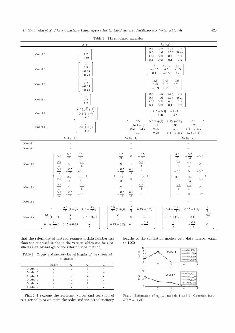
H. Mathlouthi et al. / Crosscumulants Based Approaches for the Structure Identification of Volterra Models 425

Table 1 The simulated examples

h1 (:) h2 (:, :)

Model 1

⎡

⎢⎣1

1.2

0.32

⎤

⎥⎦

⎡

⎢⎢⎢⎣

0.5 0.5 0.25 0.1

0.5 0.6 0.35 0.25

0.25 0.35 0.4 0.1

0.1 0.25 0.1 0.2

⎤

⎥⎥⎥⎦

Model 2

⎡

⎢⎢⎢⎣

1

0.5

−0.66

−0.78

⎤

⎥⎥⎥⎦

⎡

⎢⎣0 −0.15 0.1

−0.15 0.5 −0.5

0.1 −0.5 0.4

⎤

⎥⎦

Model 3

⎡

⎢⎢⎢⎣

1

0.5

−0.66

−0.78

⎤

⎥⎥⎥⎦

⎡

⎢⎣0.5 0.43 −0.9

0.43 0.12 0.7

−0.9 0.7 0.1

⎤

⎥⎦

Model 4

⎡

⎢⎣1

0.5

1.2

⎤

⎥⎦

⎡

⎢⎢⎢⎣

0.5 0.5 0.25 0.1

0.5 0.6 0.35 0.25

0.25 0.35 0.4 0.1

0.1 0.25 0.1 0.2

⎤

⎥⎥⎥⎦

Model 5

⎡

⎢⎢⎣

0.5(√

3 + j)

0.5 (1 + j)

−0.6

⎤

⎥⎥⎦

[0.5 + 0.2j −1.43

−1.43 −0.5

]

Model 6

⎡

⎢⎣j

0.5 (1 + j)

−0.6

⎤

⎥⎦

⎡

⎢⎢⎢⎣

0.5 0.5 (1 + j) 0.25 + 0.2j 0.1

0.5 (1 + j) 0.6 0.35 0.25

0.25 + 0.2j 0.35 0.4 0.1 + 0.15j

0.1 0.25 0.1 + 0.15j 0.2 (1 + j)

⎤

⎥⎥⎥⎦

h3 (:, :, 0) h3 (:, :, 1) h3 (:, :, 2)

Model 1 – – –

Model 2 – – –

Model 3

⎡

⎢⎢⎢⎢⎢⎢⎢⎢⎣

0.50.2

3

0.1

3

0.2

30 − 0.5

6

0.1

3−0.5

6−0.1

⎤

⎥⎥⎥⎥⎥⎥⎥⎥⎦

⎡

⎢⎢⎢⎢⎢⎢⎢⎢⎣

0.2

30 − 0.5

6

0 10.4

3

− 0.5

6

0.4

30

⎤

⎥⎥⎥⎥⎥⎥⎥⎥⎦

⎡

⎢⎢⎢⎢⎢⎢⎢⎢⎣

0.1

3− 0.5

6−0.1

− 0.5

6

0.4

30

−0.1 0 −0.7

⎤

⎥⎥⎥⎥⎥⎥⎥⎥⎦

Model 4

⎡

⎢⎢⎢⎢⎢⎢⎢⎢⎣

0.50.2

3

0.1

3

0.2

30 − 0.5

6

0.1

3−0.5

6−0.1

⎤

⎥⎥⎥⎥⎥⎥⎥⎥⎦

⎡

⎢⎢⎢⎢⎢⎢⎢⎢⎣

0.2

30 − 0.5

6

0 10.4

3

− 0.5

6

0.4

30

⎤

⎥⎥⎥⎥⎥⎥⎥⎥⎦

⎡

⎢⎢⎢⎢⎢⎢⎢⎢⎣

0.1

3− 0.5

6−0.1

− 0.5

6

0.4

30

−0.1 0 −0.7

⎤

⎥⎥⎥⎥⎥⎥⎥⎥⎦

Model 5 – – –

Model 6

⎡

⎢⎢⎢⎢⎢⎢⎢⎢⎣

00.8

3(1 + j) 0.4 +

1.4

3j

0.8

3(1 + j)

2

30.15 + 0.2j

0.4 +1.4

3j 0.15 + 0.2j

1

3

⎤

⎥⎥⎥⎥⎥⎥⎥⎥⎦

⎡

⎢⎢⎢⎢⎢⎢⎢⎢⎣

0.8

3(1 + j)

2

30.15 + 0.2j

2

30 0.4

0.15 + 0.2j 0.4 −0.8

3

⎤

⎥⎥⎥⎥⎥⎥⎥⎥⎦

⎡

⎢⎢⎢⎢⎢⎢⎢⎢⎣

0.4 +1.4

3j 0.15 + 0.2j

1

3

0.15 + 0.2j 0.4 − 0.8

3

1

3− 0.8

30

⎤

⎥⎥⎥⎥⎥⎥⎥⎥⎦

that the reformulated method requires a data number lessthan the one used in the initial version which can be clas-sified as an advantage of the reformulated method.

Table 2 Orders and memory kernel lengths of the simulated

examples

Order K1 K2 K3

Model 1 2 2 3 –

Model 2 2 3 2 –

Model 3 3 3 2 2

Model 4 3 2 3 2

Model 5 2 2 1 –

Model 6 3 2 3 2

Figs. 2–4 regroup the necessary values and variation oftest variables to estimate the order and the kernel memory

lengths of the simulation models with data number equalto 1000.

Fig. 1 Estimation of ηM(j) , models 1 and 3, Gaussian input,

SNR = 10 dB

426 International Journal of Automation and Computing 6(4), November 2009

Table 3 Estimation of crosscumulants, model 1, SNR = 10 dB

N = 1000 N = 2000 N = 5000

Cross-cumulants iMean

Standard

deviationMean

Standard

deviationMean

Standard

deviation

0 −0.0213 0.4207 −0.0126 0.3082 −0.0126 0.1967

1 −0.0249 0.2667 −0.0083 0.1985 −0.0117 0.1306

2 0.0061 0.2395 −0.0024 0.1679 −0.0027 0.1054cy(1)u(3) (0, 0,−i)

3 0.0195 0.2163 0.0101 0.1551 −0.0006 0.0995

4 −0.0137 0.1894 −0.0041 0.1434 −0.0044 0.0949

5 0.0066 0.1851 0.0003 0.1430 0.0017 0.0921

0 0.98780.98780.9878 0.19320.19320.1932 1.00191.00191.0019 0.13830.13830.1383 0.99890.99890.9989 0.08990.08990.0899

1 0.98150.98150.9815 0.17590.17590.1759 0.99300.99300.9930 0.12610.12610.1261 0.99720.99720.9972 0.07720.07720.0772

2 0.50220.50220.5022 0.14480.14480.1448 0.50180.50180.5018 0.10090.10090.1009 0.50310.50310.5031 0.06460.06460.0646cy(1)u(2) (0, −i)

3 0.19750.19750.1975 0.11950.11950.1195 0.19880.19880.1988 0.08430.08430.0843 0.20180.20180.2018 0.05400.05400.0540

4 −0.0111 0.1062 −0.0021 0.0761 −0.0007 0.0492

5 −0.0010 0.1075 −0.0001 0.0756 0.0020 0.0507

0 0.99680.99680.9968 0.09080.09080.0908 1.00071.00071.0007 0.06840.06840.0684 1.00081.00081.0008 0.04260.04260.0426

1 1.18881.18881.1888 0.10850.10850.1085 1.19681.19681.1968 0.08540.08540.0854 1.19831.19831.1983 0.05260.05260.0526

2 0.31940.31940.3194 0.09450.09450.0945 0.32030.32030.3203 0.06840.06840.0684 0.32030.32030.3203 0.04260.04260.0426cy(1)u(1) (−i)

3 0.0027 0.0826 0.0005 0.0590 0.0012 0.0375

4 −0.0030 0.0798 −0.0016 0.0569 −0.0001 0.0360

5 −0.0028 0.0793 −0.0006 0.0573 0.0023 0.0366

Table 4 Estimation of crosscumulants, model 3, SNR = 10 dB

N = 1000 N = 2000 N = 5000

Cross-cumulants iMean

Standard

deviationMean

Standard

deviationMean

Standard

deviation

0 −0.1783 3.7103 −0.1280 2.8709 −0.0369 1.7863

1 −0.1208 1.7640 −0.0567 1.3300 −0.0788 0.8347

2 0.0045 1.4755 −0.0459 1.0807 −0.0365 0.6609cy(1)u(4) (0, 0, 0,−i)

3 0.0245 1.4830 0.0443 1.0621 −0.0163 0.6471

4 −0.0058 1.3105 −0.0280 0.9623 −0.0131 0.6339

5 −0.0192 1.3238 0.0096 1.0884 −0.0027 0.5931

0 2.89952.89952.8995 1.33741.33741.3374 3.03163.03163.0316 0.94720.94720.9472 3.01033.01033.0103 0.59040.59040.5904

1 0.34200.34200.3420 0.75630.75630.7563 0.38240.38240.3824 0.58850.58850.5885 0.39080.39080.3908 0.36530.36530.3653

2 0.14240.14240.1424 0.65100.65100.6510 0.16390.16390.1639 0.45210.45210.4521 0.18500.18500.1850 0.30870.30870.3087cy(1)u(3) (0, 0,−i)

3 0.0215 0.5806 0.0041 0.4244 −0.0047 0.2705

4 0.0026 0.5655 0.0015 0.3975 0.0063 0.2646

5 0.0036 0.5617 0.0033 0.4327 −0.0053 0.2620

0 0.98030.98030.9803 0.54490.54490.5449 1.01741.01741.0174 0.39790.39790.3979 0.99640.99640.9964 0.26400.26400.2640

1 0.79100.79100.7910 0.40640.40640.4064 0.81650.81650.8165 0.29400.29400.2940 0.83610.83610.8361 0.18970.18970.1897

2 −1.7726−1.7726−1.7726 0.38340.38340.3834 −1.7946−1.7946−1.7946 0.27660.27660.2766 −1.8050−1.8050−1.8050 0.17170.17170.1717cy(1)u(2) (0,−i)

3 0.0011 0.2932 0.0037 0.2107 0.0019 0.1276

4 −0.0267 0.2792 −0.0067 0.1917 −0.0019 0.1249

5 0.0016 0.2893 0.0054 0.2144 0.0075 0.1313

0 1.03171.03171.0317 0.80790.80790.8079 0.98560.98560.9856 0.56310.56310.5631 0.99920.99920.9992 0.33260.33260.3326

1 0.53300.53300.5330 1.19801.19801.1980 0.47740.47740.4774 0.83200.83200.8320 0.50940.50940.5094 0.51860.51860.5186cy(1)u(1) (−i)−

2 −0.5988−0.5988−0.5988 0.87020.87020.8702 −0.6155−0.6155−0.6155 0.62990.62990.6299 −0.6426−0.6426−0.6426 0.37220.37220.37221

2

−K3∑

k=0

cy(1)u(3) (k, k, −i) 3 −0.7733−0.7733−0.7733 0.55680.55680.5568 −0.7695−0.7695−0.7695 0.39180.39180.3918 −0.7741−0.7741−0.7741 0.23450.23450.2345

4 −0.0342 0.5299 −0.0076 0.3604 −0.0002 0.2596

5 −0.0128 0.5036 −0.0051 0.3826 0.0094 0.2523

H. Mathlouthi et al. / Crosscumulants Based Approaches for the Structure Identification of Volterra Models 427

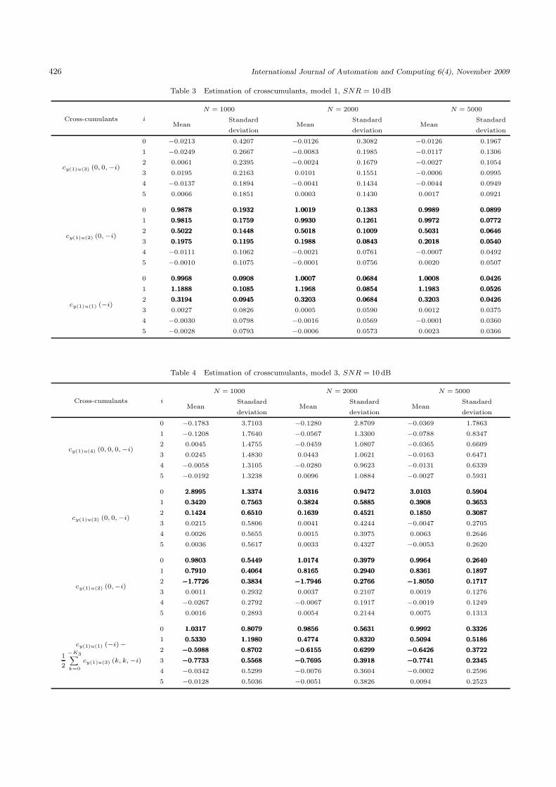
Fig. 2 Estimation of ηM(j) , models 1–4, Gaussian input,

SNR = 10dB, N = 1000

Fig. 3 Estimation of λN(j) (·), models 1 and 2, Gaussian input,

SNR = 10dB, N = 1000

Fig. 4 Estimation of λN(j) (·), models 3 and 4, Gaussian input,

SNR = 10dB, N = 1000

Step 1. Identification of model order.From Fig. 2, we notice that, for all j > 2 the test variable

ηM(j) is null for models 1 and 2, so we can deduce that

the two first models are second order Volterra models. Formodel 3 and model 4, we observe that ηM(j) value attainzero for j = 4, which confirm that they are the third-orderVolterra models.

Step 2. Identification of kernel memory lengths.Based on estimated values of cy(1)u(2) (−i,−j) and

cy(1)u(1) (−i) we determine the test variable λN(j) (·) forj = 1 and j = 2 (see Fig. 3) which is used to identify thekernel memories (K1 and K2) of models 1 and 2:

Kmodel11 = 2, Kmodel1

2 = 3,

Kmodel21 = 3, Kmodel2

2 = 2.

For the third-order Volterra model, λN(3) (·) and λN(2) (·)will be used to estimate K3 and K2. Using the second andthe fourth statistic information presented in N (1), we candetermine kernel memory length K1.

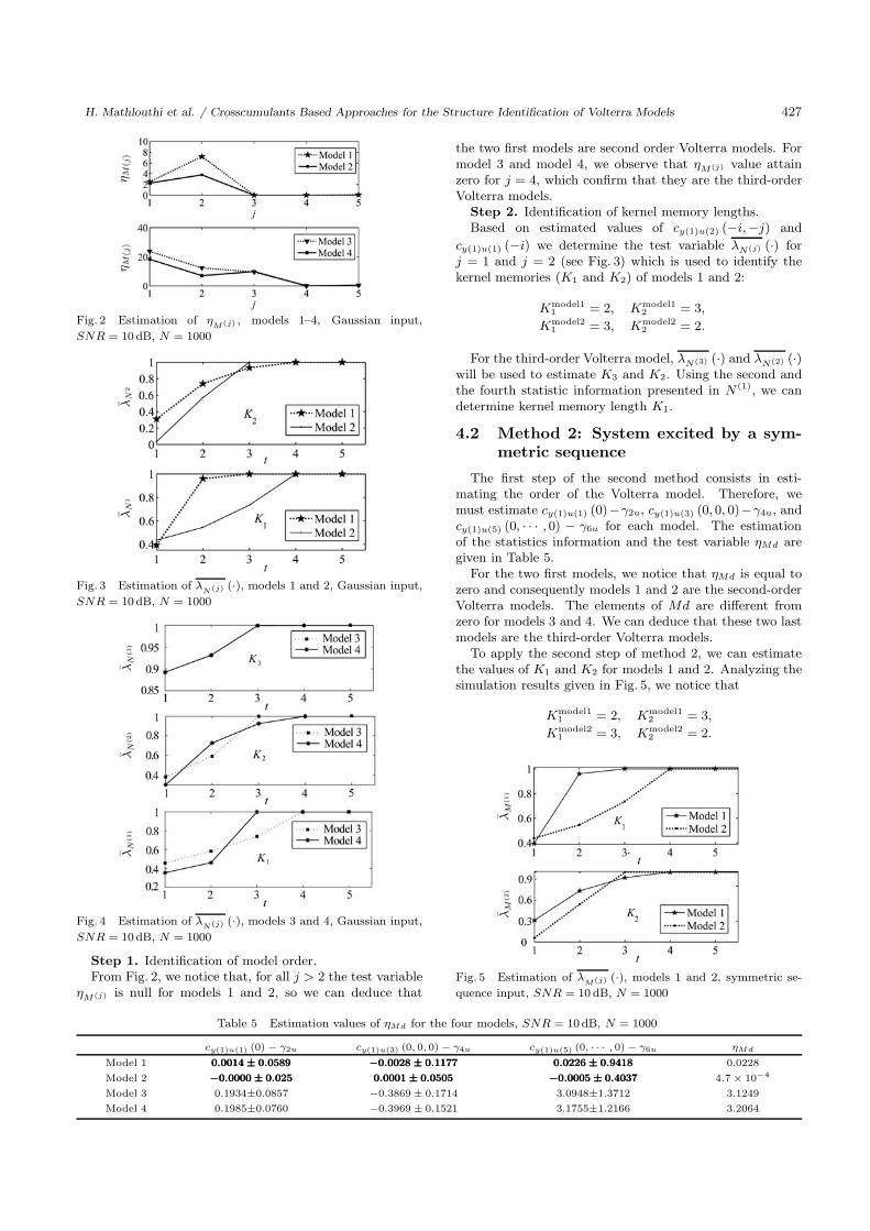
4.2 Method 2: System excited by a sym-metric sequence

The first step of the second method consists in esti-mating the order of the Volterra model. Therefore, wemust estimate cy(1)u(1) (0)−γ2u, cy(1)u(3) (0, 0, 0)−γ4u, andcy(1)u(5) (0, · · · , 0) − γ6u for each model. The estimationof the statistics information and the test variable ηMd aregiven in Table 5.

For the two first models, we notice that ηMd is equal tozero and consequently models 1 and 2 are the second-orderVolterra models. The elements of Md are different fromzero for models 3 and 4. We can deduce that these two lastmodels are the third-order Volterra models.

To apply the second step of method 2, we can estimatethe values of K1 and K2 for models 1 and 2. Analyzing thesimulation results given in Fig. 5, we notice that

Kmodel11 = 2, Kmodel1

2 = 3,

Kmodel21 = 3, Kmodel2

2 = 2.

Fig. 5 Estimation of λM(j) (·), models 1 and 2, symmetric se-

quence input, SNR = 10 dB, N = 1000

Table 5 Estimation values of ηMd for the four models, SNR = 10dB, N = 1000

cy(1)u(1) (0) − γ2u cy(1)u(3) (0, 0, 0) − γ4u cy(1)u(5) (0, · · · , 0) − γ6u ηMd

Model 1 0.0014 ± 0.05890.0014 ± 0.05890.0014 ± 0.0589 −0.0028 ± 0.1177−0.0028 ± 0.1177−0.0028 ± 0.1177 0.0226 ± 0.94180.0226 ± 0.94180.0226 ± 0.9418 0.0228

Model 2 −0.0000 ± 0.025−0.0000 ± 0.025−0.0000 ± 0.025 0.0001 ± 0.05050.0001 ± 0.05050.0001 ± 0.0505 −0.0005 ± 0.4037−0.0005 ± 0.4037−0.0005 ± 0.4037 4.7 × 10−4

Model 3 0.1934±0.0857 −0.3869 ± 0.1714 3.0948±1.3712 3.1249

Model 4 0.1985±0.0760 −0.3969 ± 0.1521 3.1755±1.2166 3.2064

428 International Journal of Automation and Computing 6(4), November 2009

Step 3 of the method 2 is concerned with the third-order Volterra models: it is the case of models 3 and4. Using λM(1) (·) and λM(2) (·), we can estimate K2 andK = max(K1, K3):

Kmodel32 = 2, Kmodel3= 3,

Kmodel42 = 3, Kmodel4= 2.

In this case we must estimate M (3) (see Fig. 6):1) For model 3, λM(3) (k) attains the unity for k =

3 < Kmodel3 + 1 which implies that Kmodel31 = 3 and

Kmodel33 = 2.2) For model 4, λM(3) (k) attains the unity for k = 3 =

Kmodel4 + 1 which implies that Kmodel43 = 2 if we suppose

that Kmodel41 = 2.

Fig. 6 Estimation of λM(j) (·) models 3 and 4, symmetric se-

quence input, SNR = 10dB, N = 1000

4.3 Complex kernels

This paragraph presents simulations of models 5 and 6which are characterized by complex kernels. The obtainedresults are presented in Figs. 7 and 8 and Table 6 which il-lustrate the performance of the proposed approach even inthe case of complex kernels.

Fig. 7 Estimation of λM(j) (·), model 5, symmetric sequence in-

put, SNR = 10dB, N = 1000

Fig. 8 Estimation of λM(j) (·), model 6, symmetric sequence in-

put, SNR = 10 dB, N = 1000

Table 6 Estimation of ηMd, models 5 and 6, SNR = 10 dB,

N = 1000

Model 5 Model 6

sign(γ2u)∥∥cy(1)u(1) (0)

∥∥ − γ2u −0.0011 2.1589

sign(γ4u)∥∥cy(1)u(3) (0, 0, 0)

∥∥ − γ4u −0.0021 4.3178

sign(γ6u)∥∥cy(1)u(5) (0, · · · , 0)

∥∥ − γ6u −0.0169 34.5422

ηMdc 0.01710.01710.0171 34.877934.877934.8779

5 Conclusions

In this paper, we have addressed the problem of struc-ture identification of Volterra models. In fact, we have pro-posed two methods which consist in estimating the orderof Volterra models that will be used to identify the lengthof each kernel memory. The first method can be appliedwhen the excitation is a Gaussian sequence. However, thesecond one assumes that the input is a symmetric two-levelsequence. These sequences are very popular in parametricidentification of Volterra methods. Moreover, we have de-veloped a reformulation of these methods which consist ofusing more crosscumulants in order to improve the perfor-mance. On the other hand, the proposed methods can beused to identify Volterra model structures having differentkernel memories. In addition, they can be used to iden-tify Volterra models having complex kernels. Finally, ourmethods can be applied to identify the structure of FIR lin-ear systems. Numerical simulation results were presentedto demonstrate the performance of the proposed methods.In the next work, we will propose the extension of the ap-proach to other sequences such as phase amplitude modu-lation with 8 levels (PAM8), quadrature phase shift keying(QPSK), asymmetric phase shift keying (APSK), etc.

Appendix A.

Basic relationships with Gaussian input.

H. Mathlouthi et al. / Crosscumulants Based Approaches for the Structure Identification of Volterra Models 429

For the r-th order Volterra model,

cy(1)u(m) (τ1, · · · , τm) =Cum[y (k) , u (k + τ1) , · · · ,

u (k + τm)]

cy(1)u(m) (τ1, · · · , τm) =

imax∑

i=0

cym+2i(1)u(m) (τ1, · · · , τm) =

fm (hm (· · · )) + fm+2 (hm+2 (· · · )) + · · ·

where r − 1 � imax � r, and

cym(1)u(m) (τ1, · · · , τm) = fm (hm (· · · )) =

m!γm2u

n∑i1=0

· · ·n∑

im=0

hm (i1, · · · , im) δ (i1 + τ1) · · ·δ (im + τm)

cym+2(1)u(m) (τ1, · · · , τm) = fm+2 (hm+2 (· · · )) =

(m+2)!

2γm+12u

n∑

i1=0

· · ·n∑

im+2=0

hm+2 (i1, · · · , im+2) δ (i1+τ1)

· · · δ (im + τm) δ (im+1 − im+2) .

Appendix B.

Definition and characteristics of HOS.Let V = (v1, v2, · · · , vk)T be a complex vector and

X= (x1,x2, · · · , xk)T a random vector with E |xj |k <

∞, j = 1, · · · , k. The p-th order cumulant of these randomvariables is defined as a coefficient of v1, v2, · · · , vk in theTaylor series expansion of the cumulant generating functionΨX (V ) = ln

(E{exp(jV TX

)}). The p-th order cumulant

sequence of a stationary random signal {x (k)} is writtenas[17−20]:

cx(p) (τ1, τ2, · · · , τp−1) = Cum [x (n) , x (n + τ1), · · ·x (n + τp−1)] .

The crosscumulants are defined in a similar way:

cx1(1)x2(1)···xp(1) (τ1, τ2, · · · , τp−1) =

Cum [x1 (n) , x2 (n + τ1) , · · · , xp (n + τp−1)] .

The properties of cumulants may be summarized as follows:

1) Cum [β1x1, β2x2, · · · , βkxk] =(∏k

i=1 βi

)Cum[x1, x2,

· · · , xk] where {βi}i=1,2,··· ,k are constants.2) Cumulants are symmetric functions in their argu-

ments:

Cum [x1, x2, · · · , xk] = Cum [xi1 , xi2 , · · · , xik ]

where (i1, i2, · · · , ik) are obtained from a permutation of(1, 2, · · ·, k).

3) The cumulants are additives in their arguments:

Cum [y + z, x1, x2, · · · , xk] = Cum [y, x1, x2, · · · , xk] +

Cum [z, x1, x2, · · · , xk]

where y and z are two random variables.

4) If the random variables {xi}i=1,2,··· ,k can be di-vided into two or more groups which are statistically in-dependent, their k-th-order cumulant is identical to zero:Cum [x1, x2, · · · , xk] = 0.

Gaussian sequence. If the random variable {u (k)} isa Gaussian sequence, we have[17,21]

Momu(m) (τ1, τ 2, · · · , τm−1) =⎧⎨

⎩

∑∏Momu(2) (τi − τj) , if m is an odd integer

0, otherwise

where Momu(m) represent the m-th order moment of{u (k)}. Therefore, the cumulants expressions, when{u (k)} is also a stationary i.i.d. sequence, are given by

cu(m) (τ1, τ 2, · · · , τm−1) ={

cu(2) (τ1) = γ2u, if m = 2 and τ1 = 0

0, otherwise.

Symmetric sequence. If the random variable {u (k)}is a symmetric sequence, we have[2, 14]

cu(m) (τ1, τ 2, · · · , τm−1) ={

γmu, if m = kp and all τi = 0

0, otherwise.

For a symmetric two-level sequence input (p = 2), we have

γ2u = Momu(2) (0) = 1

γ4u = Momu(4) (0, 0, 0) − 3Momu(2) (0) = −2

γ6u = Momu(6) (0, 0, 0, 0, 0) − 15Momu(4) (0, 0, 0)

Momu(2) (0) + 30(Momu(2) (0)

)3= 16.

References

[1] V. J. Mathews, G. L. Sicuranza. Polynomial Signal Process-ing, Wiley InterScience, 2000.

[2] T. Ogunfunmi. Adaptive Nonlinear System Identification:The Volterra and Wiener Model Approaches, Springer,2007.

[3] O. M. Mohamed Vall, R. M′hiri. An Approach to Polyno-mial NARX/NARMAX Systems Identification in a Closed-loop with Variable Structure Control. International Journalof Automation and Computing, vol. 5, no. 3, pp. 313–318,2005.

[4] S. A. Billings. Identification of Nonlinear Systems – A Sur-vey. IEE Proceedings Part D: Control Theory and Applica-tions, vol. 127, no. 6, pp. 272–285, 1980.

[5] O. Nelles. Nonlinear System Identification, Springer, BerlinHeidelberg, Germany, 2001.

[6] M. Schetzen. The Volterra and Wiener Theories of Nonlin-ear Systems, John Wiley and Sons Inc., New York, USA,1980.

[7] Y. Li, H. Kashiwagi. High-order Volterra Model PredictiveControl and Its Application to a Nonlinear PolymerisationProcess. International Journal of Automation and Comput-ing, vol. 2, no. 2, pp. 208–214, 2005.

[8] P. Koukoulas, N. Kalouptsidis. Nonlinear System Identifi-cation Using Gaussian Inputs. IEEE Transactions on SignalProcessing, vol. 43, no. 8, pp. 1831–1841, 1995.

[9] P. Koukoulas, N. Kalouptsidis. Third order Volterra SystemIdentification. In Proceedings of IEEE International Con-ference on Acoustics, Speech, and Signal Processing, IEEEComputer Society, vol. 3, pp. 2405–2408, 1997.

430 International Journal of Automation and Computing 6(4), November 2009

[10] P. Koukoulas, N. Kalouptsidis. Second-order Volterra Sys-tem Identification. IEEE Transactions on Signal Processing,vol. 48, no. 12, pp. 3574–3577, 2000.

[11] P. Koukoulas, N. Kalouptsidis. Blind Identification of Sec-ond Order Hammerstein Series. Signal Processing, vol. 83,no. 1, pp. 213–234, 2003.

[12] N. Kalouptsidis, P. Koukoulas. Blind Identification ofVolterra – Hammerstein Systems. IEEE Transactions onSignal Processing, vol. 53, no. 8, pp. 2777–2787, 2005.

[13] P. Koukoulas, V. Tsoulkas, N. Kalouptsidis. A CumulantBased Algorithm for the Identification of Input–outputQuadratic Systems. Automatica, vol. 38, no. 3, pp. 391–407, 2002.

[14] E. J. Powers, C. P. Ritz, C. K. An, S. B. Kim, R. W. Miksad,S. W. Nam. Applications of Digital Polyspectral Analysisto Nonlinear Systems Modelling and Nonlinear Wave Phe-nomena. In Proceedings of Workshop on Higher-order Spec-tral Analysis, IEEE Press, Vail, Colorado, USA, pp. 73–77,1989.

[15] J. M. Le Caillec, R. Garello. Time Series Nonlinearity Mod-elling: A Giannakis Formula Type Approach. Signal Pro-cessing, vol. 83, no. 8, pp. 1759–1788, 2003.

[16] G. H. Golub, C. F. Van Loan. Matrix Computations, TheJohns Hopkins University Press, USA, 1996.

[17] C. L. Nikias, A. P. Petropulu. Higher-order Spectra Anal-ysis: A Nonlinear Signal Processing Framework, Prentice-Hall, Englewood Cliffs, New Jersey, USA, 1993.

[18] J. L. Lacoume, P. O. Amblard, P. Comon. Statistiquesd′ordre suprieur pour le traitement du signal, Masson,Paris, France, 1997. (in French)

[19] J. M. Mendel. Tutorial on Higher Order Statistics (Spectra)in Signal Processing and System Theory: Theorical Resultsand Some Applications. Proceedings of the IEEE, vol. 79,no. 3, pp. 278–305, 1991.

[20] C. L. Nikias, J. M. Mendel. Signal Processing with Higher-order Spectra. IEEE Signal Processing Magazine, vol. 10,no. 3, pp. 10–37, 1993.

[21] G. Favier, Estimation parametrique de modeles entresortie.In Signaux aleatoires: modelisation, estimation, detection,Traite IC2, chapitre 7, M. Gugliemi (ed.), Lavoisier, HermesScience Publications, Paris, France, 2004. (in French)

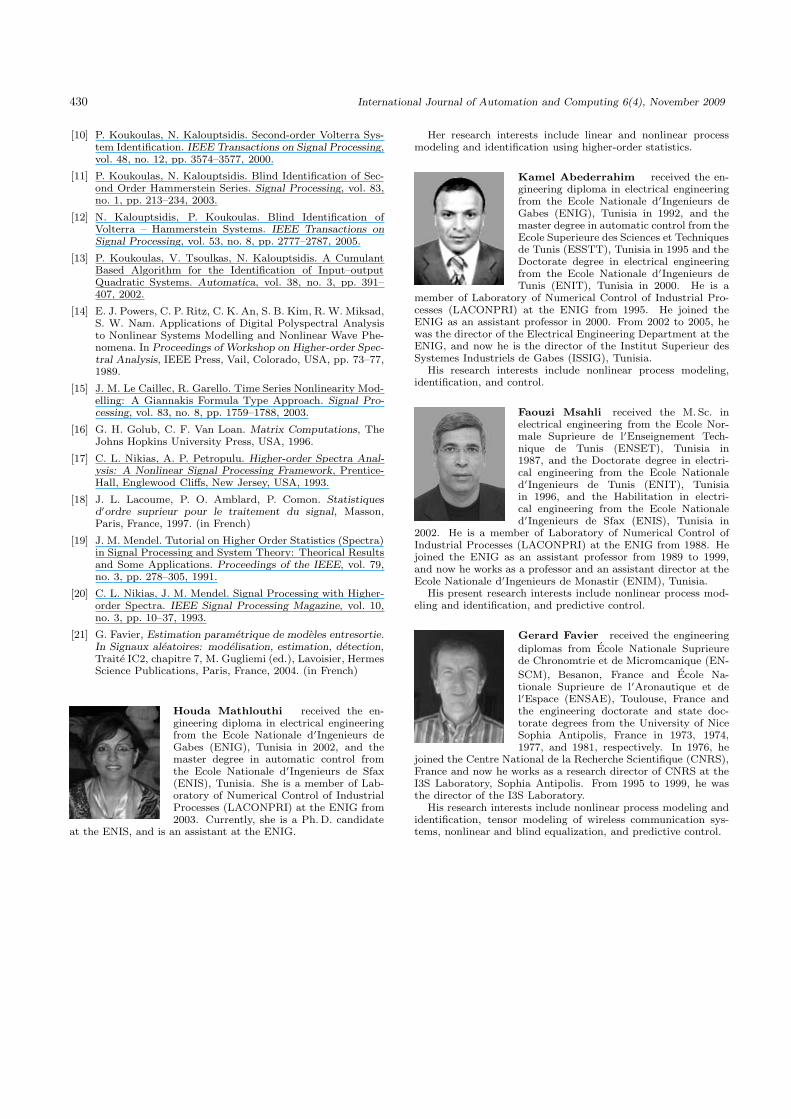
Houda Mathlouthi received the en-gineering diploma in electrical engineeringfrom the Ecole Nationale d′Ingenieurs deGabes (ENIG), Tunisia in 2002, and themaster degree in automatic control fromthe Ecole Nationale d′Ingenieurs de Sfax(ENIS), Tunisia. She is a member of Lab-oratory of Numerical Control of IndustrialProcesses (LACONPRI) at the ENIG from2003. Currently, she is a Ph. D. candidate

at the ENIS, and is an assistant at the ENIG.

Her research interests include linear and nonlinear processmodeling and identification using higher-order statistics.

Kamel Abederrahim received the en-gineering diploma in electrical engineeringfrom the Ecole Nationale d′Ingenieurs deGabes (ENIG), Tunisia in 1992, and themaster degree in automatic control from theEcole Superieure des Sciences et Techniquesde Tunis (ESSTT), Tunisia in 1995 and theDoctorate degree in electrical engineeringfrom the Ecole Nationale d′Ingenieurs deTunis (ENIT), Tunisia in 2000. He is a

member of Laboratory of Numerical Control of Industrial Pro-cesses (LACONPRI) at the ENIG from 1995. He joined theENIG as an assistant professor in 2000. From 2002 to 2005, hewas the director of the Electrical Engineering Department at theENIG, and now he is the director of the Institut Superieur desSystemes Industriels de Gabes (ISSIG), Tunisia.

His research interests include nonlinear process modeling,identification, and control.

Faouzi Msahli received the M. Sc. inelectrical engineering from the Ecole Nor-male Suprieure de l′Enseignement Tech-nique de Tunis (ENSET), Tunisia in1987, and the Doctorate degree in electri-cal engineering from the Ecole Nationaled′Ingenieurs de Tunis (ENIT), Tunisiain 1996, and the Habilitation in electri-cal engineering from the Ecole Nationaled′Ingenieurs de Sfax (ENIS), Tunisia in

2002. He is a member of Laboratory of Numerical Control ofIndustrial Processes (LACONPRI) at the ENIG from 1988. Hejoined the ENIG as an assistant professor from 1989 to 1999,and now he works as a professor and an assistant director at theEcole Nationale d′Ingenieurs de Monastir (ENIM), Tunisia.

His present research interests include nonlinear process mod-eling and identification, and predictive control.

Gerard Favier received the engineering

diplomas from Ecole Nationale Suprieurede Chronomtrie et de Micromcanique (EN-

SCM), Besanon, France and Ecole Na-tionale Suprieure de l′Aronautique et del′Espace (ENSAE), Toulouse, France andthe engineering doctorate and state doc-torate degrees from the University of NiceSophia Antipolis, France in 1973, 1974,1977, and 1981, respectively. In 1976, he

joined the Centre National de la Recherche Scientifique (CNRS),France and now he works as a research director of CNRS at theI3S Laboratory, Sophia Antipolis. From 1995 to 1999, he wasthe director of the I3S Laboratory.

His research interests include nonlinear process modeling andidentification, tensor modeling of wireless communication sys-tems, nonlinear and blind equalization, and predictive control.