World Trotting Conference symposium opens in PEI - Harness ...
Upload
khangminh22Category
view
5download
0
HAL Id: hal-02408192https://hal.archives-ouvertes.fr/hal-02408192
Submitted on 7 Jan 2021
HAL is a multi-disciplinary open accessarchive for the deposit and dissemination of sci-entific research documents, whether they are pub-lished or not. The documents may come fromteaching and research institutions in France orabroad, or from public or private research centers.
L’archive ouverte pluridisciplinaire HAL, estdestinée au dépôt et à la diffusion de documentsscientifiques de niveau recherche, publiés ou non,émanant des établissements d’enseignement et derecherche français ou étrangers, des laboratoirespublics ou privés.
The fixed point property and a technique to harnessdouble fixed point combinators
Giulio Manzonetto, Andrew Polonsky, Alexis Saurin, Jakob Grue Simonsen
To cite this version:Giulio Manzonetto, Andrew Polonsky, Alexis Saurin, Jakob Grue Simonsen. The fixed point propertyand a technique to harness double fixed point combinators. Journal of Logic and Computation, OxfordUniversity Press (OUP), 2019, 29 (5), pp.831-880. �10.1093/logcom/exz013�. �hal-02408192�

The fixed point property and a technique toharness double fixed point combinators
GIULIO MANZONETTO, Université Paris 13, Laboratoire d’Informatique deParis-Nord, CNRS UMR 7030, France.
ANDREW POLONSKY, Department of Computer Science, Appalachian StateUniversity Boone, NC 28608, USA.
ALEXIS SAURIN, Université de Paris, IRIF, CNRS, F-75013 Paris, France.
JAKOB GRUE SIMONSEN, Department of Computer Science, University ofCopenhagen (DIKU), Universitetsparken 1, 2100 Copenhagen Ø, Denmark.
AbstractThe λ-calculus enjoys the property that each λ-term has at least one fixed point, which is due to the existence of a fixed pointcombinator. It is unknown whether it enjoys the ‘fixed point property’ stating that each λ-term has either one or infinitelymany pairwise distinct fixed points. We show that the fixed point property holds when considering possibly open fixed points.The problem of counting fixed points in the closed setting remains open, but we provide sufficient conditions for a λ-term tohave either one or infinitely many fixed points. In the main result of this paper we prove that in every sensible λ-theory thereexists a λ-term that violates the fixed point property.
We then study the open problem concerning the existence of a double fixed point combinator and propose a proof techniquethat could lead towards a negative solution. We consider interpretations of the λY-calculus into the λ-calculus together withtwo reduction extension properties, whose validity would entail the non-existence of any double fixed point combinators.We conjecture that both properties hold when typed λY-terms are interpreted by arbitrary fixed point combinators. We provereduction extension property I for a large class of fixed point combinators.
Finally, we prove that the λY-theory generated by the equation characterizing double fixed point combinators is aconservative extension of the λ-calculus.
1 Introduction
A fundamental result in the λ-calculus is the fixed point theorem [2, Thm. 2.1.5] stating that every λ-term M has at least one fixed point, i.e. a λ-term X satisfying MX =β X . The λ-calculus also enjoysthe range property [2, Thm. 20.2.5] stating that the range of every combinator (closed λ-term) Mis either a singleton, when M represents a constant function, or infinite, in the sense that it containsdenumerably many pairwise β-distinct λ-terms. It is therefore natural to wonder whether a similarproperty, which we call here ‘the fixed point property’, is enjoyed by the set of fixed points of anarbitrary closed λ-term:
Does every combinator have either one or infinitely many (closed) fixed points?
The above question appears as Problem 25 in the Typed Lambda Calculi and Applications (TLCA)list of open problems [16] and was first raised by Intrigila and Biasone in [17]; the first part of thepresent paper reports progress on this question. We first prove that if one considers open λ-terms,
Vol. 29, No. 5, © The Author(s) 2019. Published by Oxford University Press. All rights reserved. For permissions, pleasee-mail: [email protected].
Advance Access Publication on 10 July 2019 doi:10.1093/logcom/exz013
Dow
nloaded from https://academ
ic.oup.com/logcom
/article/29/5/831/5528041 by UN
IVERSITE D
E PARIS (U
DP) user on 07 January 2021

832 The fixed point property and a technique to harness double fixed point combinators
then the question has a positive answer (Theorem 4.6). This result is not particularly difficult toachieve, but we believe it is interesting since it motivates the restriction to combinators and closedfixed points. For the more difficult question of closed fixed points, in [17] the authors prove thatthe fixed point property is satisfied by all combinators having a fixed point that is β-normalizable.We present several results in the same spirit. For example, we prove that the set of fixed points ofa closed zero1 λ-term is always infinite (Proposition 5.4) and that if a combinator has a fixed pointthat is a recurrent2 zero λ-term then it has either one or infinitely many fixed points (Theorem 5.7).
The problem of determining whether the fixed point property or the range property holds radicallychanges when considering as equality between λ-terms an arbitrary λ-theory T , i.e. an arbitrarycontext-closed extension of β-convertibility. Indeed, a set containing infinitely many β-distinctλ-terms might become finite modulo T . For instance, it is well known that the range property isvalid in every recursively enumerable λ-theory [2, Thm. 20.2.5] and in every λ-theory equating allλ-terms having the same Böhm tree (BT) [2, Thm. 20.2.6], while Polonsky recently proved that itfails in the λ-theory H generated by equating all unsolvables [26]. This last result led Intrigila andStatman to conjecture in [18] that in the λ-theory H ‘a very complicated example could exist with,say, exactly two fixed points’. In Corollary 6.3 we show that a λ-term satisfying such a propertyexists in every sensible λ-theory T (in particular, in H), thus proving their conjecture. Starting fromthis example, we are able to construct for every natural number k > 0 a λ-term having exactly kpairwise T -distinct fixed points (Proposition 6.6). In [18], the authors also managed to construct inan ingenious, but complex way, a λ-theory satisfying the range property but not satisfying the fixedpoint property. An easy consequence of our result (Corollary 6.5) is that the same holds for the muchmore natural λ-theory B generated by equating all λ-terms having the same BT, as it is obviouslysensible and satisfies the range property by [2, Thm. 20.2.6].
The fixed point theorem of λ-calculus is a consequence of the existence of fixed point combinatorsthat are λ-terms Y satisfying YX =β X (YX ) for all λ-terms X . Clearly, every fixed point combinatorY satisfies the equation δY =β Y where δ is the λ-term SI =β λyx.x(yx). Moreover, Böhm noticedthat if Y is a fixed point combinator then Yδ is also. This consideration led Statman to raise in[29] the question of whether there exists a double fixed point combinator, namely a fixed pointcombinator Y satisfying Yδ =β Y . Intuitively, the application of δ has the effect of ‘slowing down’the head reduction of Y and this should entail that Yδ and Y cannot have a common reduct. For thisreason Statman conjectured that double fixed point combinators do not exist. A proof of Statman’sconjecture has been suggested by Intrigila in [15]. However, in 2011, Endrullis [8] has discovered agap in a crucial case of the argument. The problem is therefore considered open.
The second part of the paper is devoted to presenting a proof technique that we believe willbe useful in settling Statman’s conjecture. The main technical tool that we use is the λY-calculus[1, Section 6.1], a classic extension of the λ-calculus with a unary constant Y behaving as a fixedpoint combinator. We first show that the λY-calculus can be soundly interpreted in the λ-calculus,by replacing a fixed point operator for each occurrence of Y in a λY-term M . We then define twoproperties of such an interpretation map, which we call ‘reduction extension properties’, and weanalyse under what circumstances they actually hold. On the one hand, we are able to prove thatproperty I holds for a large class of reducing fixed point combinators (Corollary 7.31), includingall putative double fixed point combinators. On the other hand, it is not difficult to check thatproperty II fails in the untyped setting because the interpretation map is not injective. We conjecture
1Intuitively, zero λ-terms are λ-terms that cannot be converted to an abstraction. We refer to Section 5.2 for a morethorough discussion about this terminology.
2A λ-term M is recurrent if, for all λ-terms N , M �β N entails N �β M (this notion is due to M. Venturini-Zilli).
Dow
nloaded from https://academ
ic.oup.com/logcom
/article/29/5/831/5528041 by UN
IVERSITE D
E PARIS (U
DP) user on 07 January 2021
The fixed point property and a technique to harness double fixed point combinators 833
however that a generalized version of both properties (Definition 7.27) holds for all fixed pointcombinators in the simply typed setting, and we show that this would entail the non-existence ofdouble fixed point combinators (as discussed at the end of Section 7).
Finally, we analyse the question of whether the λY-theory δ∗ generated by the equation Yx = Yδx(the equation characterizing double fixed point combinators) is a conservative extension of theλ-calculus. Indeed, as discussed in Section 8, a negative answer would entail the non-existence ofdouble fixed point combinators. Unfortunately, it turns out that the answer is positive, as shown inTheorem 8.9.
2 Preliminaries
In this preliminary section we introduce some notions and notations that are used in the rest of thearticle.
2.1 Lambda calculus
For the λ-calculus we mainly use the notations of Barendregt’s first book [2].Let us fix an infinite set Var of variables. The set Λ of λ-terms is generated by
Λ : M , N := x | λx.M | MN (for x ∈ Var).
As usual we assume that application associates to the left and has a higher precedence thanλ-abstraction. For instance, we write λxyz.xyz for λx.(λy.(λz.((xy)z))).
NOTATION 2.1We write MnN for M(· · · (MN) · · · ) and NM∼n for (· · · (NM) · · · )M (n times). In particular, forn = 0, we have M0N = N = NM∼0.
The set FV(M) of free variables of M and α-conversion are defined as in [2, Section 2.1]. We saythat a λ-term M is closed whenever FV(M) = Ø and we denote by Λo the set of all closed λ-terms.The set of positions, denoted pos(M), in a λ-term M is the subset of {0, 1}∗ defined inductively bypos(x) = {ε}, pos(λx.M) = {ε} ∪ 0 · pos(M) and pos(MN) = {ε} ∪ 0 · pos(M) ∪ 1 · pos(N). If M isa λ-term and p is a position in M , the subterm of M at p is defined in the obvious way.
CONVENTION
Hereafter, we consider λ-terms up to α-conversion and we adopt Barendregt’s variable convention[2, Conv. 2.1.13].
By historical tradition, any binary relation on Λ is called a notion of reduction on Λ. We say that anotion of reduction r ⊆ Λ × Λ is compatible (or contextual) whenever it is compatible with respectto the operations of application and lambda abstraction. A reduction relation on Λ is any compatiblenotion of reduction.
The main compatible relation of the λ-calculus is the β-relation →β , which is the compatibleclosure of the following notion of reduction:
(λx.M)N → M[N/x], (β)
where M[N/x] denotes the λ-term obtained by simultaneously substituting all free occurrencesof x in M for N , subject to the usual proviso of avoiding capture of free variables in N . The
Dow
nloaded from https://academ
ic.oup.com/logcom
/article/29/5/831/5528041 by UN
IVERSITE D
E PARIS (U
DP) user on 07 January 2021

834 The fixed point property and a technique to harness double fixed point combinators
η-relation →η is the compatible closure of
λx.Mx → M (for x /∈ FV(M)). (η)
Concerning specific combinators we fix the following notations:
I = λx.x, K = λxy.x, F = λxy.y, B = λfgx.f (g(x)), S = λxyz.xz(yz),Δ = λx.xx, Ω = ΔΔ, Δ3 = λx.xxx, Ω3 = Δ3Δ3, δ = λyx.x(yx),
where I is the identity, K and S are the combinators of combinatory logic, F is the second projection,B the functional composition, Ω the paradigmatic looping λ-term and Ω3 the ‘garbage’ producinglooping λ-term. It is easy to check that δ is the β-normal form of SI. We denote the n-th Churchnumeral by cn [2, Def. 6.4.4]. The symbol = denotes definitional equality (possibly moduloα-conversion).
The pairing is encoded in the λ-calculus as follows (for x /∈ FV(MN)):
[M , N] = λx.xMN , with projections π1 = λx.xK and π2 = λx.xF.
For instance, π1[M1, M2] →β [M1, M2]K →β KM1M2 →β (λy.M1)M2 →β M1.
2.2 Rewriting
Given a reduction relation →r, we denote its transitive and ref lexive closure by �r and its transitive,symmetric and ref lexive closure by =r. The relation �r is called multistep r-reduction, while =r iscalled r-conversion. We write r← (resp. r�) for the relational inverse of →r (resp. �r) and ↔r forthe symmetric closure of →r, i.e. →r ∪ r←. Given two reduction relations →r and →r′ , we write→rr′ for the relation →r ∪ →r′ . Similarly, we denote by =rr′ the least contextual relation including=r ∪ =r′ .
DEFINITION 2.2We recall the following standard auxiliary definitions.
• Given a notion of reduction →, a redex is any term R such that R → P for some term P. Forany term M , a redex in M is a pair (C[], R) where C[] is a one-hole context such that M = C[R]and R is a redex.
• Given a reduction relation →r and two terms M and N such that M �r N , we call any witnessM = M0 →r M1 →r · · · →r Mn = N of M �r N a reduction sequence from M to N .Par abus de langage, we shall occasionally refer to M �r N as a reduction sequence withoutspecifying the witness.
• Given a term M and a reduction relation →r, the reduction graph of M , denoted Gr(M) is thedirected graph whose nodes are all terms N such that M �r N and there is an edge from nodeP to node Q if P →r Q.
• A finite or infinite sequence
M = M0 →r M1 →r M2 →r · · ·
is called cofinal in Gr(M) if, for every node P of Gr(M), there is a directed path in Gr(M) fromP to some Mi.
Dow
nloaded from https://academ
ic.oup.com/logcom
/article/29/5/831/5528041 by UN
IVERSITE D
E PARIS (U
DP) user on 07 January 2021

The fixed point property and a technique to harness double fixed point combinators 835
• As usual, for a step M →β N , the residual relation maps every set F of β-redexes in M to a setof β-redexes in N , the set of residuals of F across the step;3 the relation extends transitively toreduction sequences M �β N in the obvious way.
• A development of a set of redexes F in M is a reduction sequence M →β M1 →β M2 →β · · ·such that every step in the sequence is the contraction of a residual of a redex in F .
• A development of a set of redexes F in a term M is complete if it is finite and its final termhas an empty set of residuals of F across the sequence. By standard results, all maximaldevelopments of F are complete, hence finite, and all complete developments of F end inthe same term. Furthermore, if F and G are sets of redexes in a term M , the set of residuals ofG is the same across any complete development of F , and is denoted G/F .
• A reduction sequence M = M0 →β M1 →β M2 →β · · · is standard if, for all i, j with j < i,the redex contracted in the step Mi →β Mi+1 is not a residual across Mj →β · · · →β Mi of anyredex to the left (in Mj) of the redex contracted in Mj →β Mj+1 (i.e. intuitively in a standardreduction, leftmost-outermost redexes are contracted first).
• Permutation equivalence is the smallest equivalence relation ≡ on reduction sequencessuch that
1. ρ; σ ; τ ≡ ρ; σ ′; τ whenever σ ≡ σ ′ and2. if F and G are sets of redexes of the same term, then σ ≡ τ whenever σ is obtained by
first performing a complete development of F followed by a complete development ofG/F , and τ is obtained by first performing a complete development of G followed by acomplete development of F/G.
• A redex with history is a pair (M �β N , R) consisting of a reduction sequence M �β N and aredex R in N . A redex with history (M �β P, S) is a copy of a redex with history (M �β N , R)
if there is a reduction sequence N �β P such that (i) M �β N �β P is permutation equivalentto M �β P, and (ii) S is a residual of R across N �β P. The symmetric and transitive closureof the copy relation is called the family relation on redexes with history and is obviously anequivalence relation. If two redexes with history are elements of the same equivalence class inthe family relation they are said, par abus de langage, to belong to the same family relation.
REMARK 2.3It is easy to check that M =r N if and only if there exists a sequence M = M0 ↔r M1 ↔r · · · ↔rMk = N of length k � 0.
2.3 Solvability
Lambda terms are classified as solvable or unsolvable, depending on their capability of interactionwith the environment.
DEFINITION 2.4A closed λ-term M is solvable if there are P1, . . . , Pk ∈ Λ such that MP1 · · · Pk =β I. An openλ-term M is solvable if its closure λx1 . . . xn.M is.
We say that a λ-term M is in head normal form (hnf ) if it has the shape λx1 . . . xn.xiM1 · · · Mkwhere n, k � 0 and either 1 � i � n or xi occurs freely. We say that M has an hnf whenever
3We omit the details, see [2, Ch. 11.2].
Dow
nloaded from https://academ
ic.oup.com/logcom
/article/29/5/831/5528041 by UN
IVERSITE D
E PARIS (U
DP) user on 07 January 2021

836 The fixed point property and a technique to harness double fixed point combinators
M �β N for some N in hnf. It is well known that if a λ-term has an hnf, then such an hnf can beobtained by repeatedly reducing its head redex λx1 . . . xn.(λx.M)NM1 · · · Mk . Solvability has beencharacterized in terms of head normalization by Wadsworth.
THEOREM 2.5 (Wadsworth [31]).A λ-term M is solvable if and only if it has a hnf.
Every closed λ-term M can be turned into an unsolvable one by applying enough Ω’s. In otherwords, for k large enough, MΩ∼k is unsolvable [2, Lemma 17.4.4]. The following lemma will beuseful in Section 6 and is a revisitation of such a result.
LEMMA 2.6Let M ∈ Λ and y ∈ Var. If MyΩ∼n is solvable for all n ∈ N, then M =β λx0 . . . xk .x′M1 · · · Mm forsome k, m � 0 and x′ ∈ FV(M) ∪ {x0}.PROOF. For n = 0 we have that My is solvable, which entails that M has an hnf λx0 . . . xk .x′M1 · · · Mm.Toward contradiction, suppose x′ = xj, with 0 < j � k. Then for the appropriate M ′
1, . . . , M ′m ∈ Λ
we have MyΩ∼k =β ΩM ′1 · · · M ′
m, which is unsolvable. This contradicts the hypothesisfor n = k. �
2.4 Lambda theories
The equational theories of the untyped λ-calculus are called λ-theories and become the main objectof study when considering the equivalence between λ-terms more important than the process ofcomputation.
More precisely, we will be considering congruences, which are compatible binary equivalencerelations on Λ.
DEFINITION 2.7A λ-theory T is any congruence on Λ containing the β-conversion.
As a matter of notation, we write T � M = N or just M =T N for (M , N) ∈ T . Let T be aλ-theory and M be a λ-term, we write ΛT for the set Λ modulo T and [M]T for the T -equivalenceclass of M . Similarly, we set Λo
T = {[M]T | M ∈ Λo}. Given a subset X ⊆ ΛT , we write M ∈T Xwhenever [M]T ∈ X .
The set of all λ-theories, ordered by set-theoretical inclusion, constitutes a complete lattice λT ofcardinality 2ℵ0 . As shown by Salibra and his coauthors in their works [22, 23, 27], λT has a veryrich mathematical structure. The lattice λT has a bottom element λβ that equates only β-convertibleλ-terms, and a top element ∇ that equates all λ-terms.
DEFINITION 2.8A λ-theory T is
• consistent if T �= ∇,• inconsistent if it is not consistent,• sensible if it equates all unsolvable terms,• extensional whenever, for all λ-terms M , N and any variable x /∈ FV(MN), Mx =T Nx implies
M =T N .
CONVENTION
We will only consider consistent λ-theories and omit the assumption.
Dow
nloaded from https://academ
ic.oup.com/logcom
/article/29/5/831/5528041 by UN
IVERSITE D
E PARIS (U
DP) user on 07 January 2021

The fixed point property and a technique to harness double fixed point combinators 837
By [2, Thm. 2.1.29], T is extensional exactly when it contains the η-conversion.We denote by λβη the smallest extensional λ-theory and by H the smallest sensible λ-theory. We
denote by B the λ-theory equating two λ-terms if and only if they have the same BT [2, Def. 10.1.4].It is well known that H also admits a unique maximal extension, which is denoted by H∗ [31]. Asshown in [2, Thm. 17.4.16], the strict inclusions H � B � H∗ hold.
The λ-theories H, B and H∗ have been extensively studied in the literature. In particular, Hylandproved in [14] that two λ-terms M and N are equal in H∗ exactly when their BTs are equal up to‘possibly infinite’ η-expansions (see also [2, Thm. 16.2.7]). As an easy consequence, we get thefollowing remark that will be used in Section 6.
REMARK 2.9Let T be a sensible λ-theory. For all M , N ∈ Λ, if T � M = N then one of the following conditionsholds:
(i) M =T N =T Ω ,(ii) There are k, m � 0 such that
M =βη λx1 . . . xk .yM1 · · · Mm and N =βη λx1 . . . xk .yN1 · · · Nm,
where T � Mi = Ni for all 1 � i � m.
By condition (ii), if M =T λx1 . . . xk1 .yM1 · · · Mm1 and N =T λx1 . . . xk2 .yN1 · · · Nm2 then m1−k1 =m2 − k2. Intuitively, this means that the number of λ-abstractions and applications can be matchedby performing some η-expansions.
3 Fixed points and fixed point combinators
In λ-calculus a fixed point of a λ-term F is an X ∈ Λ satisfying FX =β X . The fixed point theoremstates that all λ-terms have a fixed point [2, Thm. 2.1.5], a result that follows from the existence offixed point combinators.
THEOREM 3.1For every λ-term M , there exists X such that MX =β X . Actually, there exists a closed λ-term Ysuch that for any λ-term M , M(YM) =β YM .
In this section we start by defining fixed points relative to some λ-theory T , and then providesome notions of fixed point combinators and examples.
DEFINITION 3.2Let T be a λ-theory.
(1) Given two λ-terms M , N , we say that N is a fixed point of M in T whenever MN =T N .(2) For M ∈ Λ, we let FixT (M) = {[N]T | N ∈ Λ, MN =T N} be the set of all (T -classes of)
fixed points of M in T .(3) Similarly, for M ∈ Λo, we let Fixo
T (M) = FixT (M) ∩ ΛoT be the set of (T -classes of) all
closed fixed points of M in T .
When T = λβ we simply say that N is a fixed point of M and write Fix(M) and Fixo(M) for theset of its open and closed fixed points, respectively.
Dow
nloaded from https://academ
ic.oup.com/logcom
/article/29/5/831/5528041 by UN
IVERSITE D
E PARIS (U
DP) user on 07 January 2021

838 The fixed point property and a technique to harness double fixed point combinators
REMARK 3.3Given a λ-theory T and λ-terms M , N , if N ∈T FixT (M) then for all λ-theories T ′ ⊇ T wehave N ∈T ′ FixT ′(M). In particular, if N is a fixed point of M we have N ∈T FixT (M) for allλ-theories T .
EXAMPLE 3.4
(i) Since IM =β M for all M ∈ Λ, we have that every λ-term is a fixed point of the identity I.Therefore, Fix(I) = Λλβ and Fixo(I) = Λo
λβ .(ii) Since FM =β I for all M ∈ Λ, we have that only λ-terms β-convertible with I are fixed
points of F and therefore that both Fix(F) and Fixo(F) are singletons.
3.1 Fixed point combinators
As shown in the fixed point theorem, every λ-term has at least one fixed point, since fixed pointscan be constructed through fixed point combinators.
DEFINITION 3.5
(i) A λ-term Y is a fixed point combinator (or fpc) if Yx =β x(Yx) for every x /∈ FV(Y );(ii) An fpc Y is reducing if Yx �β x(Yx) for every x /∈ FV(Y );
(iii) An fpc Y is terminal if it is reducing and there is a reduction ρ : Yx �β x(Yx) with theproperty that the sequence of terms in the infinite reduction
is cofinal in the reduction graph Gβ(Yx).
Note that, following a well-established tradition [9, 10], we do not require that fpc’s are actualcombinators in the sense of being closed λ-terms. From the existence of closed fpc’s Y it followshowever that YM ∈λβ Fix(M); therefore, FixT (M) �= Ø (resp. Fixo
T (M) �= Ø) for all (closed)λ-terms M .
DEFINITION 3.6Let T ∈ λT and M ∈ Λ. A fixed point N ∈T FixT (M) is called canonical if N =T YM for somefpc Y .
We now provide some examples of open and closed fpc’s, reducing and non-reducing fpc’s andterminal and non-terminal fpc’s.
EXAMPLE 3.7
• Curry’s fixed point combinator Y = λf .Δf Δf where Δf = λx.f (xx), which is closed and notreducing.
• Geuvers and Verkoelen’s fixed point combinator λf .(Δ(λxy.f (yxy))Δ) defined in [12] is alsoclosed and not reducing.
• Turing’s fixed point combinator Θ = WW where W = λwx.x(wwx), which is closed andreducing.
• Turing’s fpc can be parametrized by setting ΘM = VVM for M ∈ Λ and V = λvpx.x(vvpx).Indeed ΘM x = VVMx �β x(VVMx) = x(ΘM x), so ΘM is a reducing fpc for all M ∈ Λ.Notice that for any variable z, Θz is open and terminal, while ΘΩ3 is closed and not terminal.
Dow
nloaded from https://academ
ic.oup.com/logcom
/article/29/5/831/5528041 by UN
IVERSITE D
E PARIS (U
DP) user on 07 January 2021
The fixed point property and a technique to harness double fixed point combinators 839
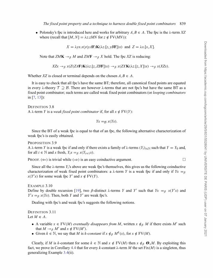
• Polonsky’s fpc is introduced here and works for arbitrary A, B ∈ Λ. The fpc is the λ-term XZwhere (recall that [M , N] = λz.zMN for z /∈ FV(MN)):
X = λyx.x(y(yAF)K(λz.[z, yBF])x) and Z = λx.[x, X ].
Note that ZMK �β M and ZMF �β X hold. The fpc XZ is reducing:
XZx �β x(Z(ZAF)K(λz.[z, ZBF])x) �β x(ZX K(λz.[z, X ])x) �β x(XZx).
Whether XZ is closed or terminal depends on the chosen A, B ∈ Λ.
It is easy to check that all fpc’s have the same BT; therefore, all canonical fixed points are equatedin every λ-theory T ⊇ B. There are however λ-terms that are not fpc’s but have the same BT as afixed point combinator; such terms are called weak fixed point combinators (or looping combinatorsin [7, 13]):
DEFINITION 3.8A λ-term Y is a weak fixed point combinator if, for all x /∈ FV(Y ):
Yx =B x(Yx).
Since the BT of a weak fpc is equal to that of an fpc, the following alternative characterization ofweak fpc’s is easily obtained.
PROPOSITION 3.9A λ-term Y is a weak fpc if and only if there exists a family of λ-terms (Yi)i∈N such that Y = Y0 and,for all i ∈ N and x fresh, Yix =β x(Yi+1x).
PROOF. (⇐) is trivial while (⇒) is an easy coinductive argument. �Since all the λ-terms Yi’s above are weak fpc’s themselves, this gives us the following coinductive
characterization of weak fixed point combinators: a λ-term Y is a weak fpc if and only if Yx =β
x(Y ′x) for some weak fpc Y ′ and x /∈ FV(Y ).
EXAMPLE 3.10Define by double recursion [19], two β-distinct λ-terms Y and Y ′ such that Yx =β x(Y ′x) andY ′x =β x(Yx). Then, both Y and Y ′ are weak fpc’s.
Dealing with fpc’s and weak fpc’s suggests the following notions.
DEFINITION 3.11Let M ∈ Λ.
• A variable x ∈ FV(M) eventually disappears from M , written x /∈β M if there exists M ′ suchthat M �β M ′ and x /∈ FV(M ′).
• Given k ∈ N, we say that M is k-constant if x /∈β Mk(x), for x /∈ FV(M).
Clearly, if M is k-constant for some k ∈ N and x /∈ FV(M) then x /∈β ΘxM . By exploiting thisfact, we prove in Corollary 4.4 that for every k-constant λ-term M the set Fix(M) is a singleton, thusgeneralizing Example 3.4(ii).
Dow
nloaded from https://academ
ic.oup.com/logcom
/article/29/5/831/5528041 by UN
IVERSITE D
E PARIS (U
DP) user on 07 January 2021
840 The fixed point property and a technique to harness double fixed point combinators
3.2 Derived fixed point combinators
An interesting line of research [19], consists in defining new fixed point combinators starting fromexisting ones. Notice, for instance, that Δδ = λw.δ(ww) =β W where δ = λyx.x(yx); therefore,Yδ =β (λx.δ(xx))(λx.δ(xx)) =β Θ . In other words, Turing’s fixed point combinator can be obtainedfrom Curry’s one by applying δ.
The following properties concerning the interaction between fpc’s and δ have been pointed out byBöhm (see [2, Lemma 6.5.3]).
LEMMA 3.12Let Y ∈ Λ.
(i) Y is an fpc if and only if δY =β Y ,(ii) if Y is a (reducing) fpc then also Yδ is.
Statman raised in [29] the following natural question and conjectured that it has a negative answer.(This question will be discussed more thoroughly in Section 7.)
PROBLEM 1Is there a double fpc, which is an fpc Y satisfying Y =β Yδ?
This problem is interesting because Lemma 3.12 tells us that starting from an fpc Y ; it is alwayspossible to define infinitely many fpc’s (Yn)n∈N by setting
Y0 = Y , Yn+1 = Ynδ.
The difficult part is to prove that all the fpc’s so obtained are β-distinct, a result that would clearlyfollow from Statman’s conjecture. In the following case we know the answer, but the general case isan open question.
EXAMPLE 3.13The Scott sequence (Yn)n∈N is generated by taking as Y0 Curry’s fpc Y. As mentioned earlier, Turing’sfpc Θ occurs as Y1 in such a sequence. As shown by Klop in [19, Thm. 2.1] with an ad hoc argument,the Scott sequence contains no repetitions (i.e. Yi =β Yj if and only if i = j).
Other fpc’s can be found starting from existing ones by mechanical search.
EXAMPLE 3.14Let Y ∈ Λ be an fpc. Klop’s Bible4 fixed point combinator is given bry = λe.BYBeL, where B isthe composition, and works for arbitrary L ∈ Λ. Notice that L remains in passive position during thereduction:
3.3 The fixed point property
We have seen in Example 3.4 that, on the one hand, there are λ-terms having infinitely many fixedpoints, like the identity I. On the other hand, there are λ-terms M possessing only one fixed point,namely those having a constant output like the second projection F. Indeed, whenever there is an
4The name of such a combinator comes from the Dutch translation of ‘bible’, namely bijbel.
Dow
nloaded from https://academ
ic.oup.com/logcom
/article/29/5/831/5528041 by UN
IVERSITE D
E PARIS (U
DP) user on 07 January 2021

The fixed point property and a technique to harness double fixed point combinators 841
M ′ such that MN =β M ′ for all N , we have that Fix(M) is a singleton. Therefore, it makes senseto wonder how many fixed points a λ-term M possesses, as Intrigila and Biasone did (in the closedcase) [17].
The following terminology is inspired by the range property of λ-calculus [2, Thm. 17.1.16].
DEFINITION 3.15Let T be a λ-theory.
• A closed λ-term M has the fixed point property (fpp) in T whenever FixoT (M) is either a
singleton or infinite.• A λ-term M has the open fixed point property in T if FixT (M) is either a singleton or infinite.• The λ-theory T satisfies the fixed point property (resp. open fpp) if every closed λ-term
(resp. possibly open λ-term) has the same property in T .
As usual, when T is omitted, we assume that we are considering T = λβ. In this terminology, theProblem 25 of the TLCA list can be rephrased as follows.
PROBLEM 2 ([16]).Does λβ satisfy the fixed point property?
Some modest advances on this problem are presented in Section 5, while in the next section wegive a positive answer to the analogue question concerning the open fixed point property. However,we will be also interested in the following generalization of Problem 2 to arbitrary λ-theories.
PROBLEM 3What are the λ-theories satisfying the fixed point property?
In Section 6 we will show that no sensible λ-theory T satisfies the fixed point property(Theorem 6.4).
4 Canonical open fixed points are not normal
In this section we show that λβ satisfies the open fixed point property. More precisely, we show thatevery λ-term exhibiting a non-constant behaviour has infinitely many canonical fixed points. Sucha result is not particularly difficult to prove and motivates the choice made by Intrigila and Biasoneof raising the question for closed fixed points only. (cf. [18], where such a property is proved for aλ-calculus having infinitely many constants.)
The proof relies on the following property of Turing’s parametrized fpc, which will haveinteresting consequences for closed fixed points as well (e.g. Proposition 5.4).
LEMMA 4.1For all M , N ∈ Λ, we have ΘM =β ΘN if and only if M =β N .
PROOF. (⇒) First, notice that the head reduction of Θzx is given by
Θzx = VVzx →β (λzx.x(VVzx))zx →β (λx.x(VVzx))x →β x(VVzx). (3)
Suppose now that ΘM =β ΘN holds, then there are two standard reductions ρ, σ from ΘM x andΘN x toward a common reduct X , namely
ΘM x = VVMxρ�β X
σ
β� VVNx = ΘN x.
Dow
nloaded from https://academ
ic.oup.com/logcom
/article/29/5/831/5528041 by UN
IVERSITE D
E PARIS (U
DP) user on 07 January 2021

842 The fixed point property and a technique to harness double fixed point combinators
Each of these reductions must again factor through an initial segment of (3) and there are twosubcases. If this segment is empty, then ρ and σ are actually internal reductions. By inspection,the only subterms of ΘM x, ΘN x that may have redexes are M and N , respectively. Thus, ρ and σ
yield a confluence between M and N , so we are done.Otherwise, ρ and σ factor through a segment of (3) of the same length (in order to result in the
same shape of the final λ-term). In this case, the internal reductions which follow the segment areagain a confluence between ΘM x and ΘN x, allowing us to conclude by induction hypothesis.
(⇐) Trivial. �LEMMA 4.2Let M ∈ Λ and z /∈ FV(M). If z /∈β ΘzM then Fix(M) is a singleton.
PROOF. Let σ : ΘzM �β X be a standard reduction, with z /∈ FV(X ).We consider the projection of σ across the canonical reduction sequence
ΘzM �β M(ΘzM) �β M(M(Θz)) �β · · ·�β Mk(ΘzM) = Mk(VVzM) �β · · ·
Notice that the redex VV occurring inside each term in the sequence above is created during thecontraction of this redex in the previous term.
In particular, for any given k, we know that such a redex could not have been contracted by anyreduction starting with ΘzM and shorter than k steps.
We now complete the projection diagram with k = |σ |, the length of σ :
As just observed, the underlined redex cannot stand in the family relation to any redex contracted inσ (since it requires |σ | redex contractions to be created).
Therefore, this redex remains untouched by the reduction ρ. As a result, the reduction ρ :M |σ |(VVzM) �β Z lifts as (ρ0; · · · ; ρ )[VVz/v], where
ρ0 : M |σ |(vM) �βZ0[vM , . . . , vM], ρi : M �β Mi (1 � i � )
Z =Z0[VVzM1, . . . , VVzM ].
But since z is not a free variable of X , it cannot occur in Z either. That is, we must have = 0, andtherefore the reduction ρ0 is of the form:
ρ0 : M |σ |(vM) �β Z0, forv /∈ FV(Z0).
Putting it all together, we find
ΘzM �β Mk(vM)[VVz/v] �β Z0[VVz/v] = Z0.
Now we are done, since for X =β MX and k = |σ |, we have
X =β Mk(X ) = Mk(vM)[KX/v] =β Z0[KX/v] = Z0,
whence all fixed points of M are β-convertible with Z0. �
Dow
nloaded from https://academ
ic.oup.com/logcom
/article/29/5/831/5528041 by UN
IVERSITE D
E PARIS (U
DP) user on 07 January 2021
The fixed point property and a technique to harness double fixed point combinators 843
PROPOSITION 4.3Let M ∈ Λ and let y, z /∈ FV(M) be distinct variables. If ΘyM =β ΘzM then the set Fix(M) is asingleton.
PROOF. Since ΘyM =β ΘzM they have a common reduct X , i.e. ΘyM �β X β� ΘzM . Clearlyneither y nor z can occur in X , so we conclude by Lemma 4.2. �
Since x /∈β Mk(x) entails z /∈β ΘzM , which in turn implies ΘyM =β ΘzM , we obtain thefollowing property of k-constant λ-terms.
COROLLARY 4.4Let k ∈ N. For every k-constant λ-term M the set Fix(M) is a singleton.
THEOREM 4.5For every λ-term M , either M is k-constant for some k ∈ N, or it has infinitely many, pairwisedistinct, canonical fixed points.
PROOF. If M is k-constant, then Fix(M) is a singleton by Corollary 4.4. Otherwise, given a freshvariable x, every M ′ satisfying ΘxM �β M ′ contains a free occurrence of x. This entails thatΘyM �=β ΘzM for all distinct y, z that do not occur in M . Therefore, {ΘzM | z ∈ Var − FV(M)} ⊆Fix(M) and this set is infinite. �
We obtain the following result concerning the open fpp for λβ.
THEOREM 4.6The λ-theory λβ satisfies the open fixed point property.
5 Some results concerning sets of fixed points in λβ
5.1 First observations
In this section we work in λβ.
EXAMPLE 5.1The following examples are meant to illustrate the basic behaviour of the sets Fix(M) and Fixo(M).
(1) Define, for any n � 1, Appn = λfx1 . . . xn.f x1 · · · xn. Let 0n ⊆ Λ be the set of λ-terms Msuch that M =β λy1 . . . yn.N for some λ-term N .(Notice that 0n+1 ⊆ 0n for each n; the elements of 0n − 0n+1 are sometimes called terms oforder n.)If M ∈ 0n, then M=βλy1 . . . yn.N for some N , and hence
Appn M=βλx1 . . . xn.M x1 · · · xn
=βλx1 . . . xn.N[x1/y1, . . . , xn/yn]=αλy1 . . . yn.N = M ,
whence M ∈λβ Fix(Appn).Conversely, if M /∈ 0n, then Appn M �β λx1 . . . xn.Mx1 · · · xn ∈ 0n, and thus M /∈λβ
Fix(Appn). Hence, Fix(Appn) = {[M]β | M ∈ 0n}.(2) For all λ-terms F we prove that Fix(F) �= {[Ω]β , [K]β} �= Fixo(F).
Assume, by contradiction, that F satisfies Fix(F) = {[Ω]β , [K]β}. Observe that [Ω]β = {M |M �β Ω}, whence F Ω=βΩ if and only if F Ω �β Ω . Split on cases according to the
Dow
nloaded from https://academ
ic.oup.com/logcom
/article/29/5/831/5528041 by UN
IVERSITE D
E PARIS (U
DP) user on 07 January 2021

844 The fixed point property and a technique to harness double fixed point combinators
solvability of F.
• If F is unsolvable then F �β λx.Ω , but then F K=βΩ �=β K, a contradiction.• If F is solvable, then F �β λx1 . . . xn.xiN1 · · · Nk for some n, i, k � 0. As
(λx1 . . . xn.xiN1 · · · Nk)Ω �β Ω , we must have i, n = 1 and k = 0. Hence, F=βIand thus Fix(F) = Λλβ , a contradiction.
(3) Let x /∈ FV(M) and F = λx.M (note that if M is closed, then so is F). Then if N=βM we haveF N=βM=βN , hence N ∈λβ Fix(F); and if N �=β M , then F N = (λx.M)N →β M[N/x] =M �=β N , whence N /∈λβ Fix(F). Thus, for every M ∈ Λ, there exists a λ-term F such thatFix(F) = {[M]β}. If M ∈ Λo, we may choose F ∈ Λo.
(4) Define 〈·〉 by 〈T〉 = λz.zT , where z /∈ FV(T). Set F = λx.x〈x〉, X = 〈I〉 and Z = λxy.x〈y〉.Then, we have
FX =β X 〈X 〉 =β 〈I〉〈〈I〉〉 =β 〈〈I〉〉I =β I〈I〉 =β 〈I〉 = X
FZ =β Z〈Z〉 =β λy.〈Z〉〈y〉 =β λy.〈y〉Z =β λy.Zy =β Z
yet at the same time
X (KI)K = 〈I〉(KI)K =β (KI)IK =β IK =β K
Z(KI)K =β KI〈K〉 =β I.
The last two equations show that X �=β Z. Hence, there is a closed λ-term F with Fixλβ(F) �=Λβ (since FΩ �=β Ω) such that there are at least two elements in Fixo
λβ(F) having distinctnormal forms.
The first result of the section is that unless Fix(F) and Fixo(F) are singletons, they cannot solelyconsist of equivalence classes of λ-terms in normal forms.
PROPOSITION 5.2Let F be a closed λ-term. If Fix(F) contains at least two elements, then at least one element does nothave a normal form.
PROOF. By the fixed point theorem, F has at least one fixed point of the form YF for some fpc Y .We shall prove that if YF has a normal form, then F has at most one fixed point; the desideratumfollows immediately from this.
Any λ-term having a normal form is an isolated point in the tree topology on Λ [2, Lem. 14.3.23];hence, YF is isolated.
By the continuity theorem [2, Thm. 14.3.22], the map X �→ XF is continuous, whence there isa neighbourhood of Y in the tree topology that is mapped to the singleton YF. As the BT of Y isλf .f (f (f (· · · ))) and the tree topology has as basic opens all (extensions of) finite approximants ofBTs (see, e.g. [2, Cor. 10.2.7]), there exists a k > 0 such that (λf .f k(Ω)) is mapped to YF. Hence,(λf .f k(Ω))F = YF and (λf .f k(Ω))F is a normalizing term.
By the genericity lemma [2, Prop. 14.3.24], there is a fresh variable z such that Fk(Ω) =(λf .f k(Ω))F = Fk(z). As z is fresh, for any term M , we have Fk(M) = (λf .f k(Ω))F, and thusFk(M) = YF.
If M is a fixed point of F, then M =β FM , and thus M =β Fk(M) = YF, concluding theproof. �
The results in the rest of this section concern terms that have no weak hnf, namely terms that donot reduce to an abstraction regardless of which substitution is applied to them.
Dow
nloaded from https://academ
ic.oup.com/logcom
/article/29/5/831/5528041 by UN
IVERSITE D
E PARIS (U
DP) user on 07 January 2021
The fixed point property and a technique to harness double fixed point combinators 845
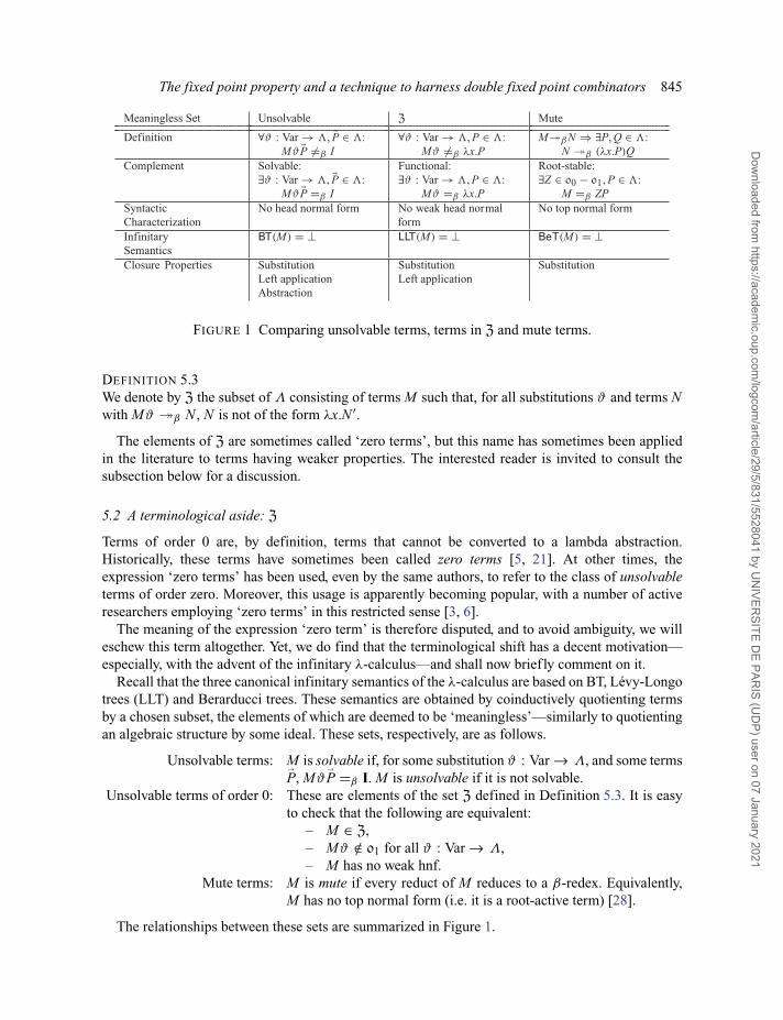
FIGURE 1 Comparing unsolvable terms, terms in Z and mute terms.
DEFINITION 5.3We denote by Z the subset of Λ consisting of terms M such that, for all substitutions ϑ and terms Nwith Mϑ �β N , N is not of the form λx.N ′.
The elements of Z are sometimes called ‘zero terms’, but this name has sometimes been appliedin the literature to terms having weaker properties. The interested reader is invited to consult thesubsection below for a discussion.
5.2 A terminological aside: Z
Terms of order 0 are, by definition, terms that cannot be converted to a lambda abstraction.Historically, these terms have sometimes been called zero terms [5, 21]. At other times, theexpression ‘zero terms’ has been used, even by the same authors, to refer to the class of unsolvableterms of order zero. Moreover, this usage is apparently becoming popular, with a number of activeresearchers employing ‘zero terms’ in this restricted sense [3, 6].
The meaning of the expression ‘zero term’ is therefore disputed, and to avoid ambiguity, we willeschew this term altogether. Yet, we do find that the terminological shift has a decent motivation—especially, with the advent of the infinitary λ-calculus—and shall now brief ly comment on it.
Recall that the three canonical infinitary semantics of the λ-calculus are based on BT, Lévy-Longotrees (LLT) and Berarducci trees. These semantics are obtained by coinductively quotienting termsby a chosen subset, the elements of which are deemed to be ‘meaningless’—similarly to quotientingan algebraic structure by some ideal. These sets, respectively, are as follows.
Unsolvable terms: M is solvable if, for some substitution ϑ : Var → Λ, and some terms�P, Mϑ �P =β I. M is unsolvable if it is not solvable.
Unsolvable terms of order 0: These are elements of the set Z defined in Definition 5.3. It is easyto check that the following are equivalent:
– M ∈ Z,– Mϑ /∈ 01 for all ϑ : Var → Λ,– M has no weak hnf.
Mute terms: M is mute if every reduct of M reduces to a β-redex. Equivalently,M has no top normal form (i.e. it is a root-active term) [28].
The relationships between these sets are summarized in Figure 1.
Dow
nloaded from https://academ
ic.oup.com/logcom
/article/29/5/831/5528041 by UN
IVERSITE D
E PARIS (U
DP) user on 07 January 2021

846 The fixed point property and a technique to harness double fixed point combinators
Intuitively, one thinks of elements of Z as terms that are not convertible to a lambda abstraction(i.e. terms of order 0), which would make the terminology ‘zero terms’ appropriate. The subtlety isthat terms of order 0 are not closed under substitution. Indeed, a more robust notion is obtained bydefining zero terms to be terms that are hereditarily of order 0 (in the sense that all their instancesare such). In such an interpretation, zero terms will be precisely the elements of Z.
5.3 Fixed points of elements of Z
We first prove the proposition below.
PROPOSITION 5.4If F belongs to Z, then Fix(F) is infinite. Moreover, if F is closed then Fixo(F) is infinite as well.
PROOF. Let, for n � 0, Xn = YnF, where Yn = Θcn are pairwise β-distinct fpc’s by Lemma 4.1.Observe that {[Xn]β | n ∈ N} ⊆ Fix(F). Moreover, when F is closed, then so is YnF and hence [Xn]βis an element of Fixo(F). The remainder of the proof is devoted to showing the claim below, fromwhich the main result immediately follows.
CLAIM 1 For m �= n, Xn �=β Xm.�
SUBPROOF. The proof uses Claim 2, proved below.Suppose that Xn =β Xm. By the Church–Rosser theorem, there is a λ-term X such that Xn �β
X β� Xm, and by Claim 2 we obtain
YnF �β F0(F1(· · · ZFk)) = X = F′0(F
′1(· · · Z′F′
k′)) β� YmF.
We posit that k = k′. For contradiction and without loss of generality, assume that k < k′. Thenwe have
Z = F′k , Fk = F′
k+1(· · · Z′F′k′),
which contradicts that F =β F′k belongs to Z, while Yn =β Z is an fpc.
Hence, k = k′, but then X has at depth k + 1 the subterm Z = Z′, which is a β-reduct of both Ynand Ym. This is impossible by Lemma 4.1, unless n = m. �
CLAIM 2For any n � 0 and any λ-term X such that YnF �β X , there is a k � 0 and there are λ-terms F0, F1, . . . , Fk , Z with F �β F0, F �β F1, . . . , F �β Fk and Yn �β Z such thatX = F0(F1(· · · ZFk)) (intuitively, k is the number of ‘unfoldings’ of the fpc Yn applied to F).
SUBPROOF. Since Yn is a reducing fpc, we may consider the infinite reduction sequence
YnF �β F(YnF) �β F(F(YnF)) �β · · ·Notice that in any reduction sequence starting from YnF there can only be one reduction stepcontracting a redex that occurs at the root. Indeed, since we are considering Yn = Θcn = VVcna redex is created at the root only if it is of shape (λx.xΘx
cn)F0 with Θcn x �β Θx
cnand F �β F0.
Its contractum will therefore have shape F0ΘF0cn and none of its descendants will have a redex at the
root since F ∈ Z entails that F0 never reduces to an abstraction. Similarly, in any reduction sequenceof this kind there is at most one reduction step contracting a redex occurring at a position of depth k
Dow
nloaded from https://academ
ic.oup.com/logcom
/article/29/5/831/5528041 by UN
IVERSITE D
E PARIS (U
DP) user on 07 January 2021

The fixed point property and a technique to harness double fixed point combinators 847
in the right spine of the syntax tree; this deeper redex can be created only once all redexes at previouspositions in the spine have been contracted (those reduction steps correspond to steps in the fixedpoint combinator unfolding).
Assume wlog that the reduction sequence YnF �β X contracts k � 0 redexes in the rightspineof the syntax tree of Yn. Consider the projection of YnF �β X across YnF �β F(F(· · · F(YnF)))
(k + 1 F’s) and write the projection diagram as
By the above arguments, the reduction X �β H consist solely of steps inside descendants of Fand Yn; whence, X = F0(F1(· · · ZFk)) for λ-terms Z, F0, . . . , Fk with Yn �β Z, F �β F0, F �β
F1, . . . , F �β Fk , as desired. �The result now follows, as {[Xn]β | n ∈ N} is infinite by Claim 1.
5.4 Recurrent elements of Z as fixed points
Recall that a λ-term M is recurrent if, for all λ-terms N , M �β N implies N �β M . For example, Ωand ΘI are recurrent elements of Z, λy.y(ΘI) is recurrent, but does not belong to Z, and Ω3 = Δ3Δ3is an element of Z, but is not recurrent.
We proceed to prove a general result that recurrent terms belonging to Z can only be fixed pointsof a combinator if all λ-terms are fixed points of that combinator, unless the combinator is constant.We first prove Lemma 5.6 below; the general result is Theorem 5.7.
The proofs of both lemma and theorem make use of a result colloquially called ‘Barendregt’sLemma’; we use it in the following form due to van Daalen (see, e.g. [11] for a comprehensivetreatment).
LEMMA 5.5 (Barendregt’s lemma).Let M[L/x] �β N . Then there exist a k-hole context C[x1, . . . , xk] (with k � 0), λ-termsxP1
1 · · · P1m1
, . . . , xPk1 · · · Pk
mkwith x /∈ FV(C[]) and Q1, . . . , Qk such that
(i): M �β C[xP11 · · · P1
m1, . . . , xPk
1 · · · Pkmk
].(ii): (xPi
1 · · · Pimi
)[L/x] �β Qi.(iii): N = C[Q1, . . . , Qk].
LEMMA 5.6If R = C[Q] is a recurrent term belonging5 to Z, and R �β Q, then either C[z] �β R or C[z] �β z(for z /∈ FV(C[])).
5In fact, it is easy to see that this lemma holds for all recurrent R, not just members of Z. This is because any recurrentterm can be presented as R = N[R1, . . . , Rk ], where N[x1, . . . , xk ] is a normal context (no redexes), and Ri are root recurrent(recurrent and reducing to a redex). (This normal form for recurrent terms is obtained by induction on the term structureof R.)
If we now have R = C[Q] �β C[R], with R = N[R1, . . . , Rk ] and N normal, then C[R] = N[R′1, . . . , R′
k ] and so
C[N[�R]] = N[�R′]. This can only happen if C[x] = x, C[x] = N[�R′], or N[�R] = Ri for some i—in which case Ri = R �β
C[Ri] and our lemma applies. Since we will not need this level of generality, we do not pursue this observation further.
Dow
nloaded from https://academ
ic.oup.com/logcom
/article/29/5/831/5528041 by UN
IVERSITE D
E PARIS (U
DP) user on 07 January 2021
848 The fixed point property and a technique to harness double fixed point combinators
PROOF. Let z /∈ FV(C[]) and assume, for purposes of contradiction, that neither C[z] �β R, norC[z] �β z. Assume now C[z] �β N . If z /∈ FV(N), we have that R = C[Q] �β N[Q/z] = N , andby recurrence of R, that N �β R and hence C[z] �β R, contradicting the assumptions. Hence, wemust have z ∈ FV(N) and, since N is an arbitrary reduct of C[z] and we have assumed that C[z] doesnot β-reduce to z, every reduct of C[z] must contain z as a free variable strictly below the root.
As R is recurrent and R �β Q, we have Q �β R. Thus, we have the reduction sequence
R = C[Q] �β C[R] = C[C[Q]] �β C[C[R]] �β C[C[C[R]]] �β · · ·Hence, for all n � 1 we have R �β Cn[R], and thus by recurrence of R that Cn[R] �β R. Observethat for every n � 1, the λ-term Cn[R] is an element of Z as it is a reduct of R.
CLAIM 3 Let n � 0 and assume Cn[R] �β W . Then the length of the longest position in W is atleast n.
�SUBPROOF. Proceed by induction:
• n = 0: Trivial.• n � 1: By Barendregt’s lemma, we have that C[Cn−1[R]] �β W implies the existence of a
k-hole context D[x1, . . . , xk] (with k � 0) together with λ-terms zP11 · · · P1
m1, . . . , zPk
1 · · · Pkmk
and Q1, . . . , Qk such that z does not occur free in D[] and the following hold:
(1) C[z] �β D[zP11 · · · P1
m1, . . . , zPk
1 · · · Pkmk
],(2) (zPi
1 · · · Pimi
)[Cn−1[R]/z] �β Qi for all 1 � i � k, and(3) W = D[Q1, . . . , Qk].
As Cn−1[R] is an element of Z, hence cannot reduce to an abstraction, there is a k-hole contextD′[x1, . . . , xk] such that we may write (i), (ii) and (iii) above as (i) C[z] �β D′[z, . . . , z],(ii) Cn−1[R] �β Qi for all 1 � i � k and (iii) W = D′[Q1, . . . , Qk]. Note that by theprevious observations, D′[z, . . . , z] cannot have a variable at the root as otherwise C[z] �β z,a contradiction. Moreover, we cannot have k = 0 because, as shown earlier, every reduct ofC[z] must contain z as a free variable and z does not occur in D′[]. Hence, the length of thelongest position in D′[Q1, . . . , Qk] is at least one more than the length of the longest positionin any of the Qi’s.But as Cn−1[R] �β Qi for all 1 � i � k, the induction hypothesis furnishes that the longestposition in any Qi is at least n − 1; hence, the length of the longest position in W is atleast n. �
Let d � 1 be an integer strictly greater than the length of the longest position in R. By Claim 3above, Cd[R] �β R implies that the length of the longest position in R is at least d, a contradiction.Hence, the original assumption leads to contradiction, and we must thus have either C[z] �β R, orC[z] �β z, as desired.
THEOREM 5.7Let F be any λ-term. If there is a recurrent R ∈ Z such that R ∈λβ Fix(F), then the following hold:
(1) For a fresh variable z, either Fz �β R or Fz �β z.(2) Either F =β KR or F =β I.
Dow
nloaded from https://academ
ic.oup.com/logcom
/article/29/5/831/5528041 by UN
IVERSITE D
E PARIS (U
DP) user on 07 January 2021
The fixed point property and a technique to harness double fixed point combinators 849
(3) In any λ-theory T , either FixT (F) = {[R]T } or FixT (F) = ΛT . Thus, if F ∈ Λo theneither Fixo
T (F) = {[R]T } or FixoT (F) = Λo
T .
PROOF. First, we observe that (1) implies both (2) and (3).
(2): If Fz �β R for a fresh z, then z must be erased in the reduction sequence, whichhas therefore length at least 1. By the standardization theorem [2, 11.4.7], Fz �h(λz.C[z])z →β C[z] �β R; hence, F �h (λz.C[z]) �β (λz.R) =β KR.If Fz �β z, then F must β-reduce to an abstraction whence the reduction sequence isnon-empty. By the standardization theorem, Fz �h (λz.C[z])z →β C[z] �β z; hence,F �h (λz.C[z]) �β (λz.z) and F =β I.
(3): Immediate by (2).
The remainder of the proof is devoted to proving (1). By the above observations, this suffices toprove the theorem.
Suppose FR =β R for R a recurrent term in Z. By the Church–Rosser theorem, there is a λ-termN such that FR �β N β� R. By recurrence of R, we obtain N �β R and consequently FR �β R.Let x /∈ FV(F) and set M = Fx. By Barendregt’s lemma there is a context C[x1, . . . , xk] withx /∈ FV(C[]), λ-terms P1
1, . . . , P1m1
, . . ., Pk1, . . . , Pk
mkand Q1, . . . , Qk such that
(i) M �β C[xP11 · · · P1
m1, . . . , xPk
1 · · · Pkmk
],(ii) (xPi
1 · · · Pimi
)[R/x] �β Qi for all 1 � i � k,(iii) R = C[Q1, . . . , Qk].
Since R ∈ Z, point (ii) yields that
(xPi1 · · · Pi
mi)[R/x] = R(Pi
1[R/x]) · · · (Pimi
[R/x])
�β Qi = RiSi1 · · · Si
mi,
where R �β Ri and Pij[R/x] �β Si
j .For all i with 1 � i � k, consider the one-hole context
Ci[z] = C[Q1, . . . , Qi−1, z�Si, Qi+1, . . . , Qk].
Point (iii) yields that R = Ci[Ri] for each i, so we may apply Lemma 5.6 to conclude that eitherCi[z] �β z or Ci[z] �β R, for each i.
If, for some i, Ci[z] indeed reduces to z, then we conclude the proof by the following sequence ofinferences:
1. The vector �Si must be empty, so that mi = 0;2. By the genericity lemma [2, Prop. 14.3.24], C[Q1, . . . , Qi−1, z, Qi+1, . . . , Qk] = Ci[z] �β z
implies that C[x1, . . . , xk] �β xi, since Qj = Rj�Sj are unsolvable, and z is normal;3. Hence, Fx �β C[x�P1, . . . , x�Pk] �β x.
Suppose, on the other hand, that for each i, there is a reduction ρi : Ci[z] �β R. We then concludeby the following sequence of inferences.
(1) For each i, we have the reduction ρ∗i = ρi[Ri/z] : R = Ci[Ri] �β R, which erases the
displayed occurrence of Ri along the way.(2) By the Church–Rosser theorem, these can be joined together to yield
Dow
nloaded from https://academ
ic.oup.com/logcom
/article/29/5/831/5528041 by UN
IVERSITE D
E PARIS (U
DP) user on 07 January 2021

850 The fixed point property and a technique to harness double fixed point combinators
where all the alternative paths from C[Q1, . . . , Qk] to Z are equivalent; hence, no subtermof Z descends from Qi (which gets erased by ρ∗
i ).(3) The equivalent composite reductions above therefore lift to a reduction C[x1, . . . , xk] �β Z.(4) By recurrence, also Z �β R.(5) By point (i), we get Fx �β C[x1 �P1, . . . , xk �Pk] �β Z �β R, as desired.
This completes the proof of (i), and of the theorem. �The assumptions that the λ-term R is recurrent and belongs to Z cannot be omitted, as seen in the
next example.
EXAMPLE 5.8Consider the following examples.
1. Let F = λxy.y(xI). Then, Fix(F) = {[λy.yM]β | M ∈ Λ, y /∈ FV(M)} and Fixo(F) ={[λy.yM]β | M ∈ Λo}. Clearly, both Fix(F) and Fixo(F) are infinite and have empty intersec-tion with Z. Furthermore, both Fix(F) and Fixo(F) contain infinitely many distinct elements[Q]β where Q is a closed recurrent term, namely all λ-terms Q of the form Q = λy.yR whereR is a closed recurrent term.
2. Thus, F is a closed λ-term with infinitely many non-β-convertible closed recurrent terms asfixed points, showing that the assumption of R ∈ Z in Theorem 5.7 cannot be omitted.
3. Define J = λwxy.x(wwxy) and note that JJiz �β i(JJiz). Set F = JJI and, for each n � 0,consider Yn = Θcn .
4. Then, as Yn is an fpc, we get {[YnF]β | n ∈ N} ⊆ Fix(F). Furthermore, by Lemma 4.1 andthe construction of F it is easy to see that for m �= n we have YmF �=β YnF, whence Fixo(F)
is infinite. Furthermore, note that YnF �β F(YnF) �β I(F(YnF)) and that F(YnF) does notreduce to YnF whence none of the YnF is recurrent. It is straightforward to check that for anyn � 0, we have YnF ∈ Z.
5. Hence, F is a closed λ-term with infinitely many non-β-convertible elements of Z as fixedpoints, showing that the assumption of R being recurrent in Theorem 5.7 cannot be omitted.
As an application of the previous theorem, recall the notion of Plotkin terms from [25]; these areλ-terms P such that, for fresh x, every reduct of Px contains x, and yet PX =β PI for every closedX ∈ Λo.
The standard construction of such terms (see [2, Def. 17.3.26]) yields a zero term Z =β PI, whichmoreover satisfies PZ =β Z (since Z ∈ Λo). If Z was recurrent, then Theorem 5.7 would apply,implying that P is either identity or constant on all (open) terms. Since P is neither, it follows that Zis not recurrent.6
6One might suspect that this non-recurrence is due to Plotkin terms being universal generators, but this is not so; the termWWc0, with Wwn = K(wwc0)[En, ww(S+n)] is a universal generator, and it is recurrent.
Dow
nloaded from https://academ
ic.oup.com/logcom
/article/29/5/831/5528041 by UN
IVERSITE D
E PARIS (U
DP) user on 07 January 2021
The fixed point property and a technique to harness double fixed point combinators 851
6 The Fixed Point Property Fails in All Sensible Theories
In this section we prove that no sensible λ-theory T can satisfy the fixed point property. Moreprecisely, we are going to show that the λ-term defined as
Ξ = λxy.x(x(Ky))Ω
only has two possible fixed points modulo T . Interestingly, Ξ is also a counterexample to the openfixed point property. This shows that, in contrast to the theory λβ, neither fixed point properties holdin, say, H,B or H∗.
LEMMA 6.1Ω ∈H FixH(Ξ); hence, Ω ∈T FixT (Ξ) for every sensible λ-theory T .
PROOF. We have ΞΩ =H λy.Ω(Ω(Ky))Ω =H Ω . �We now show that the only solvable fixed point of Ξ in every sensible λ-theory T is the identity.
PROPOSITION 6.2Let M ∈ Λ and T be a sensible λ-theory. If M ∈T FixT (Ξ) then M �=T Ω entails M =T I.
PROOF. All the equalities in this proof are intended to take place in the λ-theory T .Let M �= Ω be a fixed point of Ξ in T . Since M is solvable, it has a hnf:
M = λx0 . . . xk .x′M1 · · · Mm. (4)
CLAIM 4The head variable x′ of the hnf of M must be x0.
SUBPROOF. From M = ΞM it follows, for fresh variables y and z, that
My = ΞMy = M(M(Ky))Ω = (MzΩ)[M(Ky)/z]. (5)
Now, let (yi)i∈N be fresh variables and denote by σi the substitution [M(Kyi)/yi+1]. By iteratingequation (5) we get
My0 = (My1Ω)σ0 = (My2Ω∼2)σ1σ0 = · · · = (MynΩ
∼n)σn−1 · · · σ0. (6)
In particular, taking n = k, we get
My0 = (MykΩ∼k)−→σ k = x′M1 · · · Mm[yk/x0][ �Ω/�x]−→σ k
= (Myk+1Ω∼k+1)−→σ k+1 = x′M1 · · · Mm[yk+1/x0][ �Ω/�x]−→σ k+1Ω ,
whence x′ cannot be a free variable, for no consistent theory can satisfy x′ �P = x′ �Q with unequalnumber of P’s and Q’s.
Since M is solvable, so is My0, and, by (6), so are MynΩ∼n, for all n ∈ N.
By Lemma 2.6, we get x′ = x0. �We now need to prove that also the indices k, m must be equal to 0.
CLAIM 5If k = 0 then also m = 0.
Dow
nloaded from https://academ
ic.oup.com/logcom
/article/29/5/831/5528041 by UN
IVERSITE D
E PARIS (U
DP) user on 07 January 2021
852 The fixed point property and a technique to harness double fixed point combinators
SUBPROOF. Assume, by contradiction, that k = 0 while m > 0. On the one hand, we have M =λx0.x0M1 · · · Mm. On the other hand, we have
ΞM = λy.M(M(Ky))Ω= λy.M(KyM ′
1 · · · M ′m)Ω for M ′
i = Mi[Ky/x0]= λy.KyM ′
1 · · · M ′mM ′′
1 · · · M ′′mΩ for M ′′
i = Mi[KyM ′1 · · · M ′
m/x0]= λy.yM ′
2 · · · M ′mM ′′
1 · · · M ′′mΩ as we assumed m > 0.
Since M = ΞM we must have m = 2m, which is impossible for m > 0. �
CLAIM 6If k = m then k = 0.
SUBPROOF. By induction on k ∈ N, we show that M = λx0 . . . xk .x0M1 · · · Mk implies M = I.
k = 0 : Trivial, since M has already the required form.k > 0 : In the induction case, we have the following chain of equalities:
M = ΞM as M ∈T FixT (Ξ)
= λy.M(M(Ky))Ω by def. of Ξ
= λy.M(λx1 . . . xk .KyM ′1 · · · M ′
k)Ω for M ′i = Mi[Ky/x0]
=β λy.M(λx1 . . . xk .yM ′2 · · · M ′
k)Ω since k > 0= λy.(λw0 . . . wk .w0N1 · · · Nk)(λx1 . . . xk .yM ′
2 · · · M ′k)Ω by α-renaming M
=β λyw2 . . . wk .((λx1 . . . xk .yM ′2 · · · M ′
k)N′1 · · · N ′
k)[Ω/w1]forN ′
j = Nj[λx1 . . . xk .yM ′2 · · · M ′
k/w0]=β λyw2 . . . wk .yM ′′
2 · · · M ′′k ,
where M ′′i = M ′
i [N′1/x1] · · · [N ′
k/xk][Ω/w1]= λz0 . . . zk−1.z0P1 · · · Pk−1 by α-renaming= I by ind. hyp.
Since M = λx0.x0, we conclude that k = 0. �Assume now k > 0 and k �= m towards a contradiction. Easy calculations give
MyΩ = λx2 . . . xk .y(M1[y/x0][Ω/x1]) · · · (Mm[y/x0][Ω/x1]).
As a matter of notation we set V = λy.MyΩ , and to simplify the reasoning on the indices we performsome α-renaming, namely we let
V = λyz1 . . . zk−1.yV1 · · · Vm,
where Vi = Mi[y/x0][Ω/x1][z1/x2] · · · [zk−1/xk] for 1 � i � m. We first prove the following claims.
CLAIM 7For all n ∈ N, we have My = V n(M(Kny)).
SUBPROOF. We proceed by induction on n.
• Case n = 0. Trivial since My = M(K0y) = V 0(M(K0y)).
Dow
nloaded from https://academ
ic.oup.com/logcom
/article/29/5/831/5528041 by UN
IVERSITE D
E PARIS (U
DP) user on 07 January 2021
The fixed point property and a technique to harness double fixed point combinators 853
• Case n + 1. We have
My = ΞMy as M ∈T FixT (Ξ)
= M(M(Ky))Ω by def. of Ξ
= V(M(Ky)) by def. of V= V(V n(M(Kn(Ky)))) by induction hypothesis= V n+1(M(Kn+1y))
�In the proofs below we use the following basic properties of K (for a fresh x):
(K1) for all i, j � 0 we have λw1 . . . wi.Kjx =β Ki+jx,(K2) if i > j then (Kix)P1 · · · Pj =β Ki−jx for arbitrary P1, . . . , Pj ∈ Λ,(K3) if i � j then (Kix)P1 · · · Pj =β xPi+1 · · · Pj for arbitrary P1, . . . , Pj ∈ Λ.
CLAIM 8For all n � m, we have My = V(V n(Kn+1−m+ky)).
SUBPROOF. We establish the following chain of equalities:
My = V n+1(M(Kn+1y)) by Claim 7= V n+1(λx1 . . . xk .(Kn+1y)M ′
1 · · · M ′m) by (4) with x′ = x0
where M ′i = Mi[Kn+1y/x0] for1 � i � m
=β V n+1(λx1 . . . xk .Kn+1−my) by (K2), since n + 1 > m=β V n+1(Kn+1−m+ky) by(K1).
�We split into subcases, depending on whether m is greater than k.
CLAIM 9When k > m we have for all n ∈ N (and for appropriate Xi ∈ Λ):
(i) V n(Vy) = λx1 . . . xk−1+(k−1−m)n.yX1 · · · Xm,(ii) if n � m then My = K(2+n)(k−m)y.
SUBPROOF. (i) We proceed by induction on n.
• If n = 0 then the case follows by definition of V .• If n > 0 then we have
V n(Vy) = V(V n−1(Vy)) by def.= V(λx1 . . . xk−1+(k−1−m)(n−1).yX1 · · · Xm) by ind. hyp.
=β λz1 . . . zk−1.(λx1 . . . xk−1+(k−1−m)(n−1).y �X )V ′1 · · · V ′
m,where V ′
i = Vi[λx1 . . . xk−1+(k−1−m)(n−1).y �X/y] for 1 � i � m=β λz1 . . . zk−1xm+1 . . . xk−1+(k−1−m)(n−1).yX ′
1 · · · X ′m as k > m,
where X ′i = Xi[V ′
1/x1] · · · [V ′m/xm]
So the number of abstractions is k − 1 + k − 1 + (k − 1 − m)(n − 1) − m = k − 1 + (k − 1 − m)n.(ii) For n � m we have the following:
My = V n(V(Kn+1−m+ky)) by Claim 8= λx1 . . . xk−1+(k−1−m)n.(Kn+1−m+ky)X1 · · · Xm by (i)
=β λx1 . . . xk−1+(k−1−m)n.K(n+1−m+k)−my by (K2) as n � m, k > m=β Kk−1+(k−1−m)n+(n+1−m+k)−my by (K1).
So, the number of K’s is k −1+ (k −1−m)n+ (n+1−m+k)−m = (k −1−m)n+n+2k −2m =(k − 1 − m + 1)n + 2(k − m) = (k − m)(n + 2). �
Dow
nloaded from https://academ
ic.oup.com/logcom
/article/29/5/831/5528041 by UN
IVERSITE D
E PARIS (U
DP) user on 07 January 2021

854 The fixed point property and a technique to harness double fixed point combinators
In Claim 9(ii) we have shown that, for all n large enough, My has a hnf with (k−m)(n+2) externalλ-abstractions and 0 applications. By Remark 2.9, we have (k − m)(n + 2) = k − m for all suchn, which is only possible if this quantity is independent from n. As we are supposing k > m this isimpossible.
CLAIM 10When 0 < k < m we have for all n ∈ N (and for appropriate Xi ∈ Λ):
(i) V n(Vy) = λx1 . . . xk−1.yX1 · · · Xm+(m−k+1)n,(ii) if n � m then My = λx1 . . . xk−1.yX1 · · · X(m−k)n+2m−k−1.
SUBPROOF. (i) We proceed by induction on n.
• If n = 0 then the case follows by definition of V .• If n > 0 then we have
V n(Vy) = V(V n−1(Vy)) by def.= V(λx1 . . . xk−1.yX1 · · · Xm+(m−k+1)(n−1)) by ind. hyp.
=β λ�z.(λx1 . . . xk−1.yX1 · · · Xm+(m−k+1)(n−1))V1 · · · Vm=β λz1 . . . zk−1.yX ′
1 · · · X ′m+(m−k+1)(n−1)Vk · · · Vm as k < m,
where X ′i = Xi[V1/x1] · · · [Vk−1/xk−1] for 1 � i � m.
So the number of applications is m + (m − k + 1)(n − 1) + m − k + 1 = m + (m − k + 1)n.(ii) For n � m we have the following:
My = V n(V(Kn+1−m+ky)) by Claim 8= λx1 . . . xk−1.(Kn+1−m+ky)X1 · · · Xm+(m−k+1)n by (i)
=β λx1 . . . xk−1.yX(n+1−m+k)+1 · · · Xm+(m−k+1)n,
where the last equality follows by (K3) since k < m � n so that m+(m−k +1)n−(n+1−m+k) =(m − k + 1)n + m − n − 1 + m − k = (m − k + 1 − 1)n + 2m − k − 1 = (m − k)n + 2m − k − 1 > 0.In particular, the number of applications is what is claimed. �
By Claim 10(ii), for all n large enough, My has a hnf with (m − k)n + 2m − k − 1 applications andk − 1 external abstractions, so the difference is (m − k)n + 2m − 2k. By Remark 2.9, we must have(m − k)n + 2m − 2k = m − k for all such n, which is only possible if this quantity is independentfrom n. As we are supposing k < m this is impossible.
As we ruled out all other possibilities, we conclude k = m = 0 and M = I.As a consequence of Lemma 6.1 and Proposition 6.2 we obtain the following.
COROLLARY 6.3For every sensible λ-theory T , Fixo
T (Ξ) = FixT (Ξ) = {[Ω]T , [I]T } is of cardinality 2.
We are now able to present the main result of the paper.
THEOREM 6.4No sensible λ-theory T satisfies the fixed point property.
This gives a partial answer to Problem 3 and has the following corollary.
COROLLARY 6.5The λ-theory B satisfies the range property, but not the fixed point property.
Dow
nloaded from https://academ
ic.oup.com/logcom
/article/29/5/831/5528041 by UN
IVERSITE D
E PARIS (U
DP) user on 07 January 2021
The fixed point property and a technique to harness double fixed point combinators 855
We conclude this section with one more observation.
PROPOSITION 6.6Let T be a sensible λ-theory. For all k > 0, there exists Mk ∈ Λo such that FixT (Mk) = Fixo
T (Mk)
has cardinality k.
PROOF. We define inductively the following sequence of terms:
F1 = F = λxy.y, F2 = Ξ , Fn+1 = λx.[Ξ(π1x), π1xFn(π2x)]forn � 2
and proceed by induction on k.The case k = 1 is trivial since FixT (F) = Fixo
T (F) = {[I]T }.The case k = 2 follows by Proposition 6.2.Assume k > 2. Suppose that X ∈ FixT (Fk), which means that X =T FkX . Then X must be such
that X =T [X1, X2], where
X1 =T ΞX1 X2 =T X1Fk−1X2.
Since X1 =T ΞX1, Proposition 6.2 entails that either X1 =T Ω or X1 =T I. In the former casewe must have also X2 =T Ω . In the latter, the fact that X1 =T I entails that X2 =T Fk−1X2. Byinduction hypothesis, there are exactly k − 1 solutions to this equation (modulo T ). It is easy tocheck that each of these solutions indeed furnishes a fixed point of Fk . Therefore, the set
FixT (Fk) = {[[Ω , Ω]]T } ∪ {[[I, X ]]T | X ∈T FixT (Fk−1)}consists of closed terms and, by Remark 2.9, has cardinality k. �
7 The Double Fixed Points Problem
In this section we focus on Problem 1, originally stated by Statman [29] and attacked by Intrigila [15],namely the question of whether double fixed point combinators exist. Intrigila’s proposal is centredon the remark that, in the BT model, both Y and Yδ are indeed equated and thus that somehow fixedpoint unrollings had to be tamed with. While Intrigila defined a notion of weight to perform thistask, we approach the question differently by factoring the behaviour of the fixed point combinatoritself through a notion of interpretation of the λY-calculus in the λ-calculus and the identificationof structural properties of this interpretation from which the non-existence of double fixed pointcombinators would follow.
7.1 Background on the λY-calculus
The λY-calculus is an extension of the untyped λ-calculus with a unary term constructor Yrepresenting a fixed point combinator. Formally, the set ΛY of λY-terms is generated by the followinggrammar:
ΛY : M , N ::= x | MN | λx.M | YM .
In order to endow the Y construct with the behaviour of a fixed point combinator, we consider anadditional reduction →Y, which is the contextual closure of the rule:
YM → M(YM). Y
The λY-calculus thus becomes a higher-order rewriting system with reduction →βY generated bythe rules (β) and (Y). Most of the notions introduced in Section 2 for the λ-calculus are inherited by
Dow
nloaded from https://academ
ic.oup.com/logcom
/article/29/5/831/5528041 by UN
IVERSITE D
E PARIS (U
DP) user on 07 January 2021

856 The fixed point property and a technique to harness double fixed point combinators
the λY-calculus in the obvious way. In particular, a λY-theory is a congruence on ΛY containing theβY-conversion.
Several standard references provide background on the λY-calculus [1, 24, 30]. The usualrewriting theoretic properties of the λ-calculus carry over to the λY-extension with virtually thesame proofs. We still review these arguments as later on we will employ some refinements of them,but we refer to Appendix A for the most technical proofs.
THEOREM 7.1The reduction →βY is confluent.
PROOF. The λY-calculus possesses two rewriting rules. By inspection, it is evident that the system isorthogonal—there is no possible overlap between redex patterns of the two rules. We conclude since,by [4, Thm. 11.6.19], every orthogonal higher-order term rewriting system is confluent. �
As a consequence, two βY-convertible λY-terms M and N have a common reduct.
COROLLARY 7.2Let M , N ∈ ΛY. If M =βY N , then there exists Z ∈ ΛY such that M �βY Z βY� N .
In fact, the system λY is a conservative extension of the λ-calculus.
COROLLARY 7.3λY is conservative over λ.
PROOF. Let M , N ∈ Λ such that M =βY N . By Corollary 7.2, there is a λY-term Z such thatM �βY Z βY� N . Since neither M nor N contain the symbol Y, and this symbol cannot be created byβ-reduction, there is no point during these reductions where such a symbol can appear. Consequently,there is no point during these reductions where the Y-rule can be applied. We conclude that thesereductions in λY are actually reductions in λ, hence M =β N holds. �
7.1.1 Standardization and parallel reduction We now present some reduction relations that arewell known in the setting of the λ-calculus, and are here extended to the λY-calculus.
DEFINITION 7.4
(1) The weak head reduction is defined by the following two rules (for k � 0):
(λx.M)N0 · · · Nk →w M[N0/x]N1 · · · Nk
YN0 · · · Nk →w N0(YN0)N1 · · · Nk
(2) The standard reduction is obtained from the weak head reduction by setting:
Dow
nloaded from https://academ
ic.oup.com/logcom
/article/29/5/831/5528041 by UN
IVERSITE D
E PARIS (U
DP) user on 07 January 2021

The fixed point property and a technique to harness double fixed point combinators 857
(3) The parallel reduction is the least congruence closed under simultaneous development:
We refer to the appendix for the basic results on these notions of reduction, including thestandardization theorem. The proofs in the next two sections will only use the following facts aboutparallel reduction—whose proofs may be found there as well. Note that the transitive closure ofparallel reduction is equal to �βY.
PROPOSITION 7.5For M , N ∈ ΛY, we have that M ⇒ M ′ and M ′ �Y N entail M ⇒ N . In particular, M �Y Nimplies M ⇒ N .
PROPOSITION 7.6For M , N ∈ ΛY, we have that M ⇒ M ′ and N ⇒ N ′ entail M[N/x] ⇒ M ′[N ′/x].
7.1.2 The simply typed case We now consider the version of λY endowed with simple types overone ground type o. The typing restriction will prove to have several important advantages.
DEFINITION 7.7The typed λY-calculus, λY→, is an extension of the simply typed λ-calculus obtained by adding anew unary term constructor YA, for each type A:
A, B ∈ T ::= o | A → B
M , N ∈ Λ→Y ::= x | MN | λx:A.M | YAM .
The typing rule for the new term constructor is the following:
The reduction rule is as in the untyped case:
YAM → M(YAM). Y
PROPOSITION 7.8λY→ satisfies the subject reduction property.
PROOF. Routine. �
7.2 Interpretation of the constructor Y by fixed point combinators
7.2.1 Interpretation by fixed point combinators We have seen that in a λY-term M the constantY represents a generic fixed point combinator. Therefore, it is possible to retrieve a regular λ-termby substituting some fpc Y for every occurrence of Y in M . The λ-term M ′ so defined is called the‘interpretation of M in Λ’—and it depends on Y . In the next definition we are more liberal andconsider also the case where Y is substituted by a weak fixed point combinator.
Dow
nloaded from https://academ
ic.oup.com/logcom
/article/29/5/831/5528041 by UN
IVERSITE D
E PARIS (U
DP) user on 07 January 2021
858 The fixed point property and a technique to harness double fixed point combinators
DEFINITION 7.9Given a weak fpc Y ∈ Λ, we define the interpretation of a λY-term in Λ with respect to Y as themap [[·]]Y : ΛY → Λ given by
[[x]]Y = x
[[MN]]Y = [[M]]Y [[N]]Y
[[λx.M]]Y = λx.[[M]]Y
[[YM]]Y = Y [[M]]Y .
Such an interpretation is clearly compositional and enjoys several interesting properties.
LEMMA 7.10 (Substitution lemma for λY).Let M , N ∈ ΛY and let Y ∈ Λ be a weak fpc. Then, for all x /∈ FV(Y ), we have
[[M[N/x]]]Y = [[M]]Y [[[N]]Y /x].
PROOF. Straightforward by compositionality of the interpretation map [[·]]Y . �In general a weak fpc Y can be such that Yx �β x(Y ′x) for Y �=β Y ′, and in this case the
interpretation is unsound; we have Yx →Y x(Yx) but [[Yx]]Y �=β [[x(Yx)]]Y . However, when Y is anactual fpc the resulting interpretation is sound.
PROPOSITION 7.11 (Soundness).Let Y ∈ Λ be an fpc. For all M , N ∈ ΛY, if M =βY N then [[M]]Y =β [[N]]Y .
PROOF. First, notice that by Lemma 7.10, if M =β M ′, then we have [[M]]Y =β [[M ′]]Y . Notice alsothat, if M =Y M ′, then we have [[M]]Y =β [[M ′]]Y because Y is an fpc. The result then easily followsby induction on the number of alternations between =β and =Y in a proof that M =βY N . �
REMARK 7.12The converse to the above proposition fails for two reasons. One of these is rather trivial, the othermuch deeper.
• The first problem has to do with the fact that the interpretation function [[·]]Y is not injectiveeven with respect to α-conversion. For example, fix any untyped fpc Y , and considerM = λx.[Yx,Yx] and N = λx.[Yx, Yx]. Trivially [[M]]Y = [[N]]Y , but M �=βY N by a Church–Rosser argument.
• The exotic reason is related to the Plotkin terms already discussed on Page 55; there exist(unsolvable) λ-terms P ∈ Λo with the property that PX =β PI for all X ∈ Λo, and yetPx �β P′ implies that x ∈ FV(P′).
For the counterexample now take M=PI and N=P(λz.Yz). Just as x can never be erasedfrom Px by any β-reduction, also Y can never be erased from P(λz.Yz) by any βY-reduction.Yet, for a closed fpc Y , [[λz.Yz]]Y becomes a closed λ-term, and so [[N]]Y =β PI =β [[M]]Y .
7.2.2 Interpretation of Y by fpc’s in the typed case We now prove that both of the pathologiesdescribed in Remark 7.12 disappear when considering the simply typed λY-calculus. We start byshowing that the interpretation becomes injective.
Dow
nloaded from https://academ
ic.oup.com/logcom
/article/29/5/831/5528041 by UN
IVERSITE D
E PARIS (U
DP) user on 07 January 2021
The fixed point property and a technique to harness double fixed point combinators 859
DEFINITION 7.13For a given fpc Y , the interpretation of λY→ in Λ is defined as in the untyped case, namely forgettingthe types.
PROPOSITION 7.14Let Y be an fpc. Then the map
[[·]]Y : Λ→Y → Λ
is injective—with respect to syntactic equality.
PROOF. The structure of [[M]]Y is completely determined by M ; the only two clauses in the definitionof [[·]]Y , which result in the same term constructor, are those for the application and for Y.
[[M1M2]]Y = [[M1]]Y [[M2]]Y
[[YN]]Y = Y [[N]]Y
Suppose there are M1, M2, N ∈ Λ→Y such that
[[M1]]Y [[M2]]Y = Y [[N]]Y
Then we must have [[M1]]Y = Y . We claim that this is impossible. First of all, note that Y itself is nota λY→-term, so M1 �= Y. Now, if Y occurs in M1 then Y occurs as a strict subterm of [[M1]]Y = Y .This is impossible for finite terms.
Otherwise Y does not occur in M1, [[M1]]Y = M1 and M1 is a Y-free simply typed term, thusnormalizing, which Y is not. �PROPOSITION 7.15Let M , N ∈ Λ→
Y . Suppose that, for every fpc Y , [[M]]Y =β [[N]]Y . Then M =βY N .
PROOF. We consider the interpretation of Y by Turing’s fpc Θ and to lighten the notation we simplywrite [[·]] for [[·]]Θ . We first show that for any one-step reduct [[M]] →β Z′ there exists a λY→-termZ such that
M =βY Z, [[Z]] = Z′.
To see this, write [[M]] = C[R], where R is the contracted redex. Notice that R cannot be a propersubterm of Θ , which has only one redex, occurring at the root:
Θ = WW, W = λwx.x(wwx).
Case 1: If R is indeed the λ-term Θ = WW, then it must descend from an occurrence of Y; in thiscase we have
[[M]] = C[Θ] = C′[Θ[[N]]], C[x] = C′[x[[N]]]
M = C0[YN], [[C0[X ]]] = C′[[[X ]]]
[[M]] →β Z′ = C′[(λx.x(WWx))[[N]]].
Dow
nloaded from https://academ
ic.oup.com/logcom
/article/29/5/831/5528041 by UN
IVERSITE D
E PARIS (U
DP) user on 07 January 2021
860 The fixed point property and a technique to harness double fixed point combinators
But now we have
M = C0[YN] →Y C0[N(YN)] β←C0[(λx.x(Yx))N] = Z
[[Z]] = [[C0[(λx.x(Yx))N]]]
= C′[[[(λx.x(WWx))N]]]
= C′[(λx.x(WWx))[[N]]] = Z′,
where we find M =βY Z and [[Z]] = Z′.Case 2: If R does not come from Y, then the only possibility left is that it is the image of a redex,
which already appears in M :
[[C0[X ]]] = C[[[X ]]], [[(λx.P)Q]] = R
M = C0[(λx.P)Q] →β C0[P[Q/x]] = Z
[[M]] = [[C0[(λx.P)Q]]] = C[R] →β Z′ = C[[[P]][[[Q]]/x]]
[[Z]] = [[C0[P[Q/x]]]] = C[[[P[Q/x]]]].
By Lemma 7.10, we have [[P]][[[Q]]/x] = [[P[Q/x]]]; hence, Z′ = [[Z]] and M →β Z.
The result then follows by induction, applying Proposition 7.14. �
7.3 The reduction extension properties
We now present structural properties of the interpretation map [[−]]Y that we call ‘reductionextension properties’. To present them in diagrammatic form, we first need to introduce somenotations.
NOTATION 7.16Let M , N ∈ �Y, and let Y be a weak fpc. We write
[[M]]Y[[·]]Y� [[N]]Y
whenever M �βY N .
DEFINITION 7.17A weak fpc Y satisfies the reduction extension properties if the following properties hold for allM ∈ ΛY. (Note that M ′, N ∈ ΛY while P ∈ Λ.)
where solid arrows denote the assumption reductions and dotted arrows denote the entailed ones.In words, property I states that for all M ∈ ΛY, P ∈ Λ, [[M]]Y �β P entails that there exists anN ∈ ΛY such that M �βY N and P �β [[N]]Y . Similarly, property II states that for all M , M ′ ∈ ΛY,[[M]]Y �β [[M ′]]Y entails that there exists an N ∈ ΛY such that M �βY N βY� M ′.
Those properties are interesting because of the following observation.
Dow
nloaded from https://academ
ic.oup.com/logcom
/article/29/5/831/5528041 by UN
IVERSITE D
E PARIS (U
DP) user on 07 January 2021
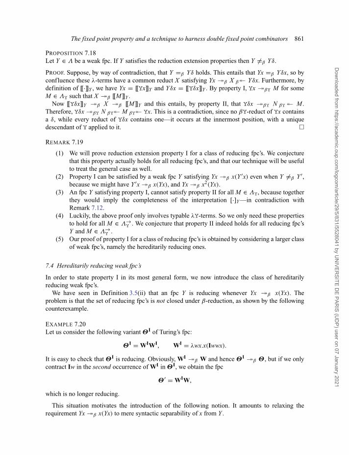
The fixed point property and a technique to harness double fixed point combinators 861
PROPOSITION 7.18Let Y ∈ Λ be a weak fpc. If Y satisfies the reduction extension properties then Y �=β Yδ.
PROOF. Suppose, by way of contradiction, that Y =β Yδ holds. This entails that Yx =β Yδx, so byconfluence these λ-terms have a common reduct X satisfying Yx �β X β� Yδx. Furthermore, bydefinition of [[·]]Y , we have Yx = [[Yx]]Y and Yδx = [[Yδx]]Y . By property I, Yx �βY M for someM ∈ ΛY such that X �β [[M]]Y .
Now [[Yδx]]Y �β X �β [[M]]Y and this entails, by property II, that Yδx �βY N βY � M .Therefore, Yδx �βY N βY� M βY� Yx. This is a contradiction, since no βY-reduct of Yx containsa δ, while every reduct of Yδx contains one—it occurs at the innermost position, with a uniquedescendant of Y applied to it. �
REMARK 7.19
(1) We will prove reduction extension property I for a class of reducing fpc’s. We conjecturethat this property actually holds for all reducing fpc’s, and that our technique will be usefulto treat the general case as well.
(2) Property I can be satisfied by a weak fpc Y satisfying Yx �β x(Y ′x) even when Y �=β Y ′,because we might have Y ′x �β x(Yx), and Yx �β x2(Yx).
(3) An fpc Y satisfying property I, cannot satisfy property II for all M ∈ ΛY, because togetherthey would imply the completeness of the interpretation [·]Y —in contradiction withRemark 7.12.
(4) Luckily, the above proof only involves typable λY-terms. So we only need these propertiesto hold for all M ∈ Λ→
Y . We conjecture that property II indeed holds for all reducing fpc’sY and M ∈ Λ→
Y .(5) Our proof of property I for a class of reducing fpc’s is obtained by considering a larger class
of weak fpc’s, namely the hereditarily reducing ones.
7.4 Hereditarily reducing weak fpc’s
In order to state property I in its most general form, we now introduce the class of hereditarilyreducing weak fpc’s.
We have seen in Definition 3.5(ii) that an fpc Y is reducing whenever Yx �β x(Yx). Theproblem is that the set of reducing fpc’s is not closed under β-reduction, as shown by the followingcounterexample.
EXAMPLE 7.20Let us consider the following variant ΘI of Turing’s fpc:
ΘI = WIWI, WI = λwx.x(Iwwx).
It is easy to check that ΘI is reducing. Obviously, WI �β W and hence ΘI �β Θ , but if we onlycontract Iw in the second occurrence of WI in ΘI, we obtain the fpc
Θ ′ = WIW,
which is no longer reducing.
This situation motivates the introduction of the following notion. It amounts to relaxing therequirement Yx �β x(Yx) to mere syntactic separability of x from Y .
Dow
nloaded from https://academ
ic.oup.com/logcom
/article/29/5/831/5528041 by UN
IVERSITE D
E PARIS (U
DP) user on 07 January 2021
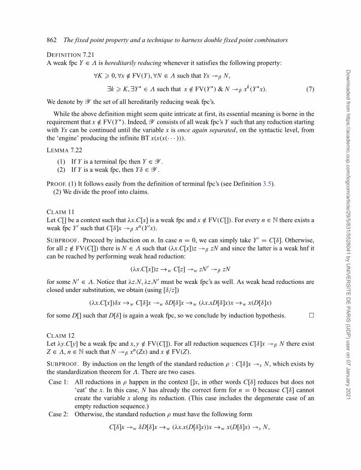
862 The fixed point property and a technique to harness double fixed point combinators
DEFINITION 7.21A weak fpc Y ∈ Λ is hereditarily reducing whenever it satisfies the following property:
∀K � 0, ∀x /∈ FV(Y ), ∀N ∈ Λ such that Yx �β N ,
∃k � K, ∃Y∗ ∈ Λ such that x /∈ FV(Y∗) & N �β xk(Y∗x). (7)
We denote by Y the set of all hereditarily reducing weak fpc’s.
While the above definition might seem quite intricate at first, its essential meaning is borne in therequirement that x /∈ FV(Y∗). Indeed, Y consists of all weak fpc’s Y such that any reduction startingwith Yx can be continued until the variable x is once again separated, on the syntactic level, fromthe ‘engine’ producing the infinite BT x(x(x(· · · ))).LEMMA 7.22
(1) If Y is a terminal fpc then Y ∈ Y .(2) If Y is a weak fpc, then Yδ ∈ Y .
PROOF. (1) It follows easily from the definition of terminal fpc’s (see Definition 3.5).(2) We divide the proof into claims.
CLAIM 11Let C[] be a context such that λx.C[x] is a weak fpc and x /∈ FV(C[]). For every n ∈ N there exists aweak fpc Y ′ such that C[δ]x �β xn(Y ′x).
SUBPROOF. Proceed by induction on n. In case n = 0, we can simply take Y ′ = C[δ]. Otherwise,for all z /∈ FV(C[]) there is N ∈ Λ such that (λx.C[x])z �β zN and since the latter is a weak hnf itcan be reached by performing weak head reduction:
(λx.C[x])z →w C[z] �w zN ′ �β zN
for some N ′ ∈ Λ. Notice that λz.N , λz.N ′ must be weak fpc’s as well. As weak head reductions areclosed under substitution, we obtain (using [δ/z])
(λx.C[x])δx →w C[δ]x �w δD[δ]x →w (λx.xD[δ]x)x →w x(D[δ]x)
for some D[] such that D[δ] is again a weak fpc, so we conclude by induction hypothesis. �
CLAIM 12Let λy.C[y] be a weak fpc and x, y /∈ FV(C[]). For all reduction sequences C[δ]x �β N there existZ ∈ Λ, n ∈ N such that N �β xn(Zx) and x /∈ FV(Z).
SUBPROOF. By induction on the length of the standard reduction ρ : C[δ]x �s N , which exists bythe standardization theorem for Λ. There are two cases.
Case 1: All reductions in ρ happen in the context []x, in other words C[δ] reduces but does not‘eat’ the x. In this case, N has already the correct form for n = 0 because C[δ] cannotcreate the variable x along its reduction. (This case includes the degenerate case of anempty reduction sequence.)
Case 2: Otherwise, the standard reduction ρ must have the following form
C[δ]x �w δD[δ]x →w (λx.x(D[δ]x))x →w x(D[δ]x) �s N ,
Dow
nloaded from https://academ
ic.oup.com/logcom
/article/29/5/831/5528041 by UN
IVERSITE D
E PARIS (U
DP) user on 07 January 2021
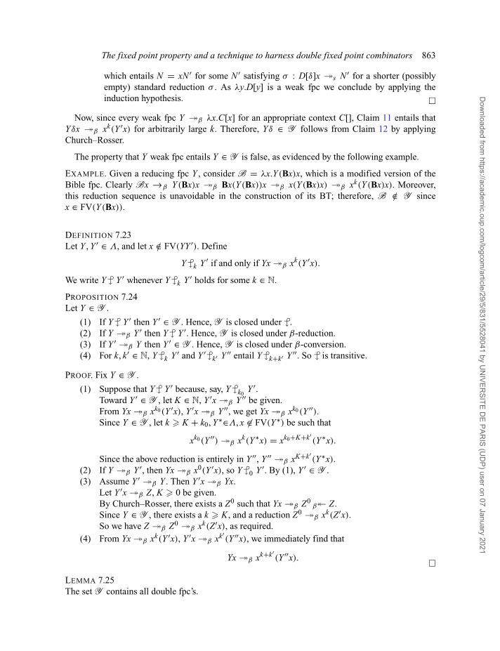
The fixed point property and a technique to harness double fixed point combinators 863
which entails N = xN ′ for some N ′ satisfying σ : D[δ]x �s N ′ for a shorter (possiblyempty) standard reduction σ . As λy.D[y] is a weak fpc we conclude by applying theinduction hypothesis. �
Now, since every weak fpc Y �β λx.C[x] for an appropriate context C[], Claim 11 entails thatYδx �β xk(Y ′x) for arbitrarily large k. Therefore, Yδ ∈ Y follows from Claim 12 by applyingChurch–Rosser.
The property that Y weak fpc entails Y ∈ Y is false, as evidenced by the following example.
EXAMPLE. Given a reducing fpc Y , consider B = λx.Y (Bx)x, which is a modified version of theBible fpc. Clearly Bx →β Y (Bx)x �β Bx(Y (Bx))x �β x(Y (Bx)x) �β xk(Y (Bx)x). Moreover,this reduction sequence is unavoidable in the construction of its BT; therefore, B /∈ Y sincex ∈ FV(Y (Bx)).
DEFINITION 7.23Let Y , Y ′ ∈ Λ, and let x /∈ FV(YY ′). Define
Y
�
k Y ′ if and only if Yx �β xk(Y ′x).
We write Y
�
Y ′ whenever Y
�
k Y ′ holds for some k ∈ N.
PROPOSITION 7.24Let Y ∈ Y .
(1) If Y
�
Y ′ then Y ′ ∈ Y . Hence, Y is closed under
�
.(2) If Y �β Y ′ then Y
�Y ′. Hence, Y is closed under β-reduction.
(3) If Y ′ �β Y then Y ′ ∈ Y . Hence, Y is closed under β-conversion.(4) For k, k′ ∈ N, Y
�
k Y ′ and Y ′ �
k′ Y ′′ entail Y
�
k+k′ Y ′′. So
�
is transitive.
PROOF. Fix Y ∈ Y .
(1) Suppose that Y
�
Y ′ because, say, Y
�
k0Y ′.
Toward Y ′ ∈ Y , let K ∈ N, Y ′x �β Y ′′ be given.From Yx �β xk0(Y ′x), Y ′x �β Y ′′, we get Yx �β xk0(Y ′′).Since Y ∈ Y , let k � K + k0, Y∗∈Λ, x �∈ FV(Y∗) be such that
xk0(Y ′′) �β xk(Y∗x) = xk0+K+k′(Y∗x).
Since the above reduction is entirely in Y ′′, Y ′′ �β xK+k′(Y∗x).
(2) If Y �β Y ′, then Yx �β x0(Y ′x), so Y
�
0 Y ′. By (1), Y ′ ∈ Y .(3) Assume Y ′ �β Y . Then Y ′x �β Yx.
Let Y ′x �β Z, K � 0 be given.By Church–Rosser, there exists a Z0 such that Yx �β Z0
β� Z.Since Y ∈ Y , there exists a k � K, and a reduction Z0 �β xk(Z′x).So we have Z �β Z0 �β xk(Z′x), as required.
(4) From Yx �β xk(Y ′x), Y ′x �β xk′(Y ′′x), we immediately find that
Yx �β xk+k′(Y ′′x). �
LEMMA 7.25The set Y contains all double fpc’s.
Dow
nloaded from https://academ
ic.oup.com/logcom
/article/29/5/831/5528041 by UN
IVERSITE D
E PARIS (U
DP) user on 07 January 2021

864 The fixed point property and a technique to harness double fixed point combinators
PROOF. If Y is a double fpc, then Y =β Yδ. By Lemma 7.22(2), Yδ ∈ Y . By Proposition 7.24(3) Yis closed under =β , so we get Y ∈ Y . �
7.5 Non-uniform reduction extension properties
To allow for the fact that weak fpc’s may change at various stages on the BT, the statements of thereduction extension properties need to be refined accordingly.
NOTATION 7.26Let �r be a notion of reduction for λY, and let Y , Y ′ be weak fpc’s. We write
[[M]]Y[[·]]−→−→r [[N]]Y ′ if and only if M �r N and Y
�
Y ′.
As special cases, we consider
• [[M]]Y[[·]]−→−→ [[N]]Y ′ if M �βY N and Y
�Y ′.
• [[M]]Y[[·]]�⇒�⇒ [[N]]Y ′ if M ⇒ N and Y
�Y ′.
DEFINITION 7.27 (Non-uniform reduction extension properties).A weak fpc Y ∈ Λ satisfies the non-uniform reduction extension properties if the following hold.
We now show that non-uniform property I holds for all hereditarily reducing weak fpc’s. Fromnow on, and until the end of the section, we consider fixed Y ∈ Y and M ∈ ΛY.
LEMMA 7.28If Y
�
Y ′ holds then there exists N ∈ ΛY such that M �Y N and [[M]]Y �β [[N]]Y ′ .
PROOF. We proceed by structural induction on M .
M = x: In this case we just take N = x.M = λx.M0: By definition, we have [[M]]Y = λx.[[M0]]Y . By induction hypothesis, there exists
N0 ∈ �Y such that M0 �Y N0 and [[M0]]Y �β [[N0]]Y ′ hold. As a consequence,λx.M0 �Y λx.N0. Moreover, [[M]]Y = λx.[[M0]]Y �β λx.[[N0]]Y ′ = [[λx.N0]]Y ′ .
M = M1M2: By definition, we have [[M]]Y = [[M1]]Y [[M2]]Y . By induction hypothesis, thereexist N1, N2 ∈ �Y such that Mi �Y Ni and [[Mi]]Y �β [[Ni]]Y ′ for i ∈ {1, 2}.As a consequence, M1M2 �Y N1N2. Moreover, [[M]]Y = [[M1]]Y [[M2]]Y �β
[[N1]]Y ′[[N2]]Y ′ = [[N1N2]]Y ′ .M = YM3: By definition, we have [[M]]Y = [[YM3]]Y = Y [[M3]]Y . By induction hypothesis,
there exists N3 ∈ �Y such that M3 �Y N3 and [[M3]]Y �β [[N3]]Y ′ . Since Y
�
Y ′holds, there exists k ∈ N such that Yx �β xk(Y ′x). Setting N = Nk
3 (YN3), we
Dow
nloaded from https://academ
ic.oup.com/logcom
/article/29/5/831/5528041 by UN
IVERSITE D
E PARIS (U
DP) user on 07 January 2021
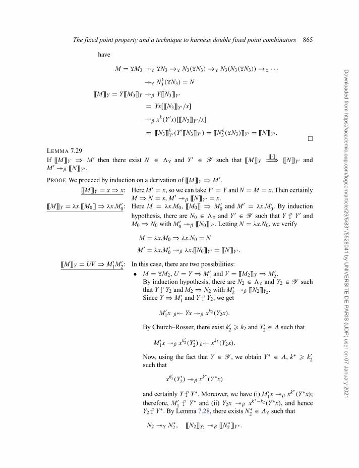
The fixed point property and a technique to harness double fixed point combinators 865
have
M = YM3 �Y YN3 →Y N3(YN3) →Y N3(N3(YN3)) →Y · · ·�Y Nk
3 (YN3) = N
[[M]]Y = Y [[M3]]Y �β Y [[N3]]Y ′
= Yx[[[N3]]Y ′/x]
�β xk(Y ′x)[[[N3]]Y ′/x]
= [[N3]]kY ′(Y ′[[N3]]Y ′) = [[Nk
3 (YN3)]]Y ′ = [[N]]Y ′ .�
LEMMA 7.29If [[M]]Y ⇒ M ′ then there exist N ∈ �Y and Y ′ ∈ Y such that [[M]]Y
[[·]]�⇒�⇒ [[N]]Y ′ andM ′ �β [[N]]Y ′ .
PROOF. We proceed by induction on a derivation of [[M]]Y ⇒ M ′.[[M]]Y = x ⇒ x: Here M ′ = x, so we can take Y ′ = Y and N = M = x. Then certainly
M ⇒ N = x, M ′ �β [[N]]Y ′ = x.[[M]]Y = λx.[[M0]] ⇒ λx.M ′
0: Here M = λx.M0, [[M0]] ⇒ M ′0 and M ′ = λx.M ′
0. By induction
hypothesis, there are N0 ∈ �Y and Y ′ ∈ Y such that Y
�
Y ′ andM0 ⇒ N0 with M ′
0 �β [[N0]]Y ′ . Letting N = λx.N0, we verify
M = λx.M0 ⇒ λx.N0 = N
M ′ = λx.M ′0 �β λx.[[N0]]Y ′ = [[N]]Y ′ .
[[M]]Y = UV ⇒ M ′1M ′
2: In this case, there are two possibilities:
• M = YM2, U = Y ⇒ M ′1 and V = [[M2]]Y ⇒ M ′
2.By induction hypothesis, there are N2 ∈ �Y and Y2 ∈ Y suchthat Y
�
Y2 and M2 ⇒ N2 with M ′2 �β [[N2]]Y2 .
Since Y ⇒ M ′1 and Y
�
Y2, we get
M ′1x β� Yx �β xk2(Y2x).
By Church–Rosser, there exist k′2 � k2 and Y ′
2 ∈ Λ such that
M ′1x �β xk′
2(Y ′2) β� xk2(Y2x).
Now, using the fact that Y ∈ Y , we obtain Y∗ ∈ Λ, k∗ � k′2
such that
xk′2(Y ′
2) �β xk∗(Y∗x)
and certainly Y
�
Y∗. Moreover, we have (i) M ′1x �β xk∗
(Y∗x);therefore, M ′
1
�
Y∗ and (ii) Y2x �β xk∗−k2(Y∗x), and henceY2
�
Y∗. By Lemma 7.28, there exists N∗2 ∈ ΛY such that
N2 �Y N∗2 , [[N2]]Y2 �β [[N∗
2 ]]Y∗ .
Dow
nloaded from https://academ
ic.oup.com/logcom
/article/29/5/831/5528041 by UN
IVERSITE D
E PARIS (U
DP) user on 07 January 2021
866 The fixed point property and a technique to harness double fixed point combinators
Now M ⇒ YN2 �Y YN∗2 , and so M ⇒ YN∗
2 . More-over, M ′ = M ′
1M ′2 �β M ′
1[[N2]]Y2 �β M ′1[[N∗
2 ]]Y∗ �β
[[N∗2 ]]k∗
Y∗(Y∗[[N∗2 ]]Y∗) = [[N∗
2k∗
(YN∗2 )]]Y∗ .
• M = M1M2, U = [[M1]]Y ⇒ M ′1, V = [[M2]]Y ⇒ M ′
2 andM ′ = M ′
1M ′2. By induction hypothesis, for i ∈ {1, 2}, there are
Ni ∈ �Y and Yi ∈ Y such that Y
�
Yi and Mi ⇒ Ni withM ′
i �β [[Ni]]Yi .From the first of these conditions Y
�Y1, Y
�
Y2, we get
xk1(Y1x) β� Yx �β xk2(Y2x)
By Church–Rosser, there exist k12 � max{k1, k2} and Y12 ∈ Λ
such that
xk1(Y1x) �β xk12(Y12) β� xk2(Y2x).
Now, using the fact that Y ∈ Y , we obtain Y∗ ∈ Λ, k∗ � k12such that
xk12(Y12) �β xk∗(Y∗x)
and certainly Y
�
Y∗. Moreover, for i ∈ {1, 2}, we have Yix �β
xk∗−ki(Y∗x) and therefore Yi
�
Y∗. By Lemma 7.28, there existN∗
1 , N∗2 ∈ ΛY such that
Ni �Y N∗i , [[Ni]]Yi �β [[N∗
i ]]Y∗ . (i ∈ {1, 2})Now M = M1M2 ⇒ N1N2 �Y N∗
1 N∗2 , and so M ⇒
N∗1 N∗
2 . Moreover, M ′ = M ′1M ′
2 �β [[N1]]Y1 [[N2]]Y2 �β
[[N∗1 ]]Y∗[[N∗
2 ]]Y∗ = [[N∗1 N∗
2 ]]Y∗ .
[[M]]Y = (λx.M0)M1 ⇒ M ′0[M ′
1/x], Mi ⇒ M ′i : In this case, there are two possibilities:
• M = (λx.P0)P1 and Mi = [[Pi]]Y .By induction hypothesis, we find Y0, Y1 with Y
�
Yi, k0, k1 � 0, andQ0, Q1 such that for each i ∈ {0, 1} the following holds
Yx �β xki(Yix),
Pi ⇒ Qi,
M ′i �β [[Qi]]Yi .
As in the previous case, we first obtain Y∗ with Y0, Y1
�
Y∗ such that
xk0(Y0x) �β xk∗(Y∗x) β� xk1(Y1x).
Next, for each i ∈ {0, 1}, we apply Lemma 7.28 on Yi
�
Y∗ and Qi inorder to obtain Q′
0, Q′1 satisfying
Qi �Y Q′i,
[[Qi]]Yi �β [[Q′i]]Y∗ .
Dow
nloaded from https://academ
ic.oup.com/logcom
/article/29/5/831/5528041 by UN
IVERSITE D
E PARIS (U
DP) user on 07 January 2021
The fixed point property and a technique to harness double fixed point combinators 867
From Pi ⇒ Qi �Y Q′i, we obtain Pi ⇒ Q′
i, and so
M = (λx.P0)P1 ⇒ Q′0[Q′
1/x].
Moreover, from M ′i �β [Qi]Yi �β [Q′
i]Y∗ , we have M ′i �β [Q′
i]Y∗and therefore
M ′ = M ′0[M ′
1/x] �β [[Q′0]]Y∗[[[Q′
1]]Y∗/x] = [[Q′0[Q′
1/x]]]Y∗ ,
where the last equality is by the substitution lemma.• M = YP, λx.M0 = Y and M1 = [[P]]Y . Then Mi ⇒ M ′
i gives
Yx = (λx.M0)x →β M0 �β M ′0
[[P]]Y ⇒ M ′1.
By induction hypothesis, we find Y
�
Y ′, P ⇒ Q with M ′1 �β [[Q]]Y ′ .
Since Y
�
Y ′, there exists k0 ∈ N such that Yx �β xk0(Y ′x). Noticethat we also have Yx �β M ′
0. Now let these reductions be joined
xk0(Y ′x) �β Z β� M ′0.
Using that Y ∈ Y , let k � k0, Y∗ ∈ Λ be such that Z �β xk(Y∗x).Then we obtain
xk0(Y ′x) �β xk(Y∗x) β� M ′0.
In particular Y ′ � Y∗, and by the previous lemma, there is R ∈ �Y
such that
Q �Y R, [[Q]]Y ′ �β [[R]]Y∗ .
As P ⇒ Q we get, setting N = Rk(YR), that
YP ⇒ YQ �Y YR →Y R(YR) →Y · · · →Y Rk(YR)
and so M ⇒ N . At the same time, from M ′0 �β xk(Y∗x), M ′
1 �β
[[Q]]Y ′ �β [[R]]Y∗ we find
M ′0[M ′
1/x] �β xk(Y∗x)[[[R]]Y∗/x]
= [[R]]kY∗(Y∗[[R]]Y∗)
= [[Rk(YR)]]Y∗
and hence M ′ �β [[N]]Y∗ . Indeed, we also have Y
�
Y ′ � Y∗ fromwhich we conclude by transitivity. �
We are now ready to prove that non-uniform reduction extension property I holds for all Y ∈ Y .
THEOREM 7.30Let Y ∈ Y . For all M ∈ ΛY, M ′ ∈ Λ:
[[M]]Y �β M ′ ⇒ ∃(N , Y ′) : [[M]]Y[[·]]−→−→ [[N]]Y ′ , M ′ �β [[N]]Y ′ .
PROOF. By induction on the length of the reduction sequence [[M]]Y �β M ′.
Dow
nloaded from https://academ
ic.oup.com/logcom
/article/29/5/831/5528041 by UN
IVERSITE D
E PARIS (U
DP) user on 07 January 2021
868 The fixed point property and a technique to harness double fixed point combinators
[[M]]Y = M ′: Take N = M , Y ′ = Y .[[M]]Y �β M0 →β M ′: By induction hypothesis, there are N0 ∈ ΛY, Y
�
Y0 and reductions
ρ : M �βY N0
σ : M0 �β [[N0]]Y0 .
Projecting the redex R contracted in M0R→β M ′ over σ induces a parallel
reduction
R\σ : [[N0]]Y0 ⇒ M1
and the finite reduction σ\R : M ′ �β M1.[[M]]Y �β M0 →β M ′: By Lemma 7.29, we can find N1 ∈ ΛY, Y0
�
Y1 and reductions
ρ1 : N0 ⇒ N1
σ1 : M1 �β [[N1]]Y1 .
Now ρ ; ρ1 : M �βY N0 ⇒ N1 clearly yields a reduction
M �βY N1
and σ\R ; σ1 : M ′ �β M1 �β [[N1]]Y1 yields
M ′ �β [[N1]]Y1 .
Furthermore, Y
�
Y0
�
Y1, from which we conclude since
�
is transitive.�In the particular case of terminal (reducing) fpc’s, the theorem above entails that also the reduction
extension property I from Definition 7.17 holds.
COROLLARY 7.31Every terminal fpc Y satisfies the reduction extension property I.
PROOF. If Y is terminal, then Y ∈ Y can be witnessed with Y ′ = Y for any reduction starting fromYx. (That is, the fpc never changes.) In particular, the previous theorem is valid with Y ′ = Y .
That is, [[M]]Y �β M ′ implies [[M]]Y[[·]]Y−−−−� [[N]]Y β� M ′. �
We end this section by presenting two conjectures; the first implies that non-uniform extensionproperty I holds for all reducing fpc’s (by Theorem 7.30), while the second entails the non-existenceof double fixed point combinators in the simply typed setting.
CONJECTURE 1If Y is a reducing fpc then Y ∈ Y .
CONJECTURE 2In the simply typed setting, every fpc Y ∈ Y satisfies non-uniform reduction extension property IIfor all M ∈ Λ→
Y .
Indeed, from Lemma 7.25 and Theorem 7.30 we get that every double fpc would satisfy non-uniform reduction property I. If Conjecture 2 holds, then Y moreover satisfies non-uniform reductionproperty II. Now, the same argument as in Proposition 7.18 applies; the interpretation of Λ→
Y ref lectsconversion, leading to the impossible λY-equality Yx = Yδx.
Dow
nloaded from https://academ
ic.oup.com/logcom
/article/29/5/831/5528041 by UN
IVERSITE D
E PARIS (U
DP) user on 07 January 2021
The fixed point property and a technique to harness double fixed point combinators 869
8 Conservativity of Double Fixed Point Operators
We analyse another possible proof technique, suggested by Klop, for proving the non-existence ofdouble fixed point combinators. Consider the following λY-theory.
DEFINITION 8.1Let δ∗ be the λY-theory generated by the axiom Yx = Yδx.
In [20], Klop raised the question of whether the λY-theory δ∗ generated by the equationcharacterizing double fixed point combinators is a conservative extension of the λ-calculus. Themotivation for this question is that, if this theory was found not to be conservative over Λ, thiswould immediately yield a proof of Statman’s conjecture. Indeed, assuming that some fixed pointcombinator Y satisfies the equation Y =β Yδ, any equation between pure λ-terms that is provablewith the axiom Yx = Yδx could be derived in the pure λ-calculus using Y , showing that δ∗ isconservative over Λ.
The rest of the section is devoted to proving that Klop’s question has a positive answer. This resultshows that, unfortunately, this strategy cannot be used to settle Statman’s conjecture.
8.1 The υ-reduction
To characterize equality in δ∗ using standard rewriting techniques, we introduce a new notion ofreduction:
YδM → YM . υ
LEMMA 8.2For all M , N ∈ ΛY, δ∗ � M = N if and only if M =βYυ N .
PROOF. (⇒) By definition, =βYυ is a contextual equivalence and therefore a λY-theory. A simpleinspection of the υ-rule shows that =βYυ validates every axiom of the theory δ∗. We conclude sinceδ∗ is the least λY-theory validating these axioms.
(⇐) This implication follows by an easy induction on the length of the conversion sequenceM = M1 ↔βYυ · · · ↔βYυ Mk = N . �
The conservativity of δ∗ will follow from the confluence property enjoyed by βYυ-reduction.Note that this system is not (weakly) orthogonal, due to the overlap between λY- and υ-redexes.It is not terminating either; thus, Newman’s lemma does not apply. Therefore, we need to proveconfluence directly. As a first step, we show that υ-reduction enjoys the strong diamond property.
PROPOSITION 8.3Let M , N , P ∈ ΛY. If N υ←M →υ P, then there exists Q ∈ ΛY such that N →υ Q υ←P.
PROOF. Assume that Nυ←M →υ P by contracting the redexes L and R, respectively. If the tworedexes are disjoint, then we easily close the diagram
NR/L−→υ Q
L/Rυ←− P.
Otherwise, one redex is contained in the other one, say, R occurs within L. Since L is an υ-redexit must have the shape YδN ′, so the occurrence of R must be contained in N ′, witnessed by N ′→υP′.That is, for some λY-context C[], we must have
N = C[YN ′] Lυ← C[YδN ′] = M
R→υ C[YδP′] = P.
Dow
nloaded from https://academ
ic.oup.com/logcom
/article/29/5/831/5528041 by UN
IVERSITE D
E PARIS (U
DP) user on 07 January 2021
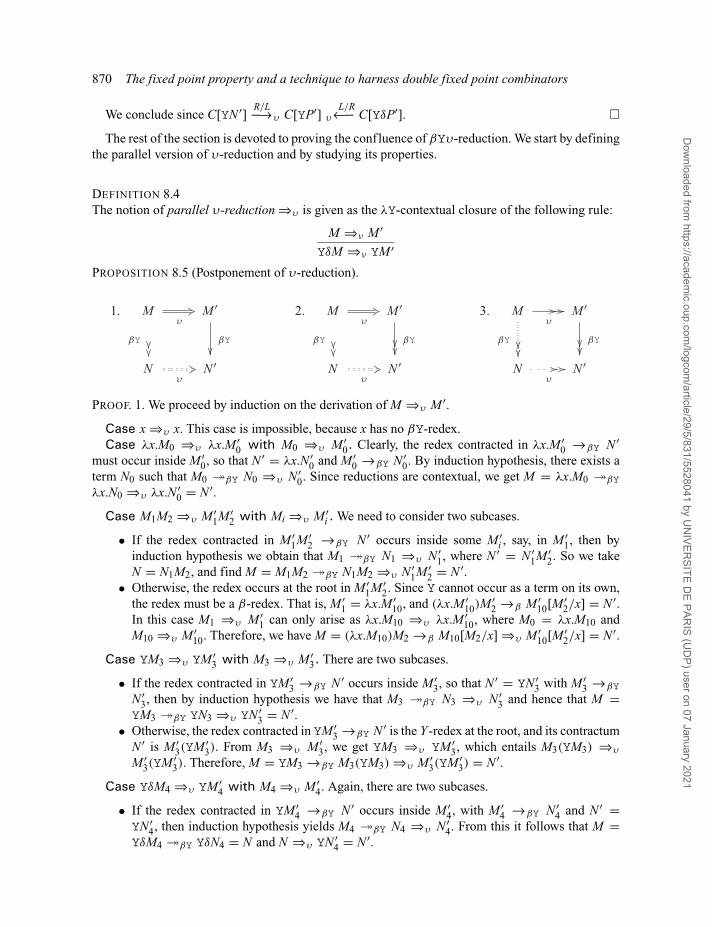
870 The fixed point property and a technique to harness double fixed point combinators
We conclude since C[YN ′] R/L−→υ C[YP′] L/Rυ←− C[YδP′]. �
The rest of the section is devoted to proving the confluence of βYυ-reduction. We start by definingthe parallel version of υ-reduction and by studying its properties.
DEFINITION 8.4The notion of parallel υ-reduction ⇒υ is given as the λY-contextual closure of the following rule:
M ⇒ν M ′
YδM ⇒ν YM ′
PROPOSITION 8.5 (Postponement of υ-reduction).
PROOF. 1. We proceed by induction on the derivation of M ⇒υ M ′.
Case x ⇒υ x. This case is impossible, because x has no βY-redex.Case λx.M0 ⇒υ λx.M ′
0 with M0 ⇒υ M ′0. Clearly, the redex contracted in λx.M ′
0 →βY N ′must occur inside M ′
0, so that N ′ = λx.N ′0 and M ′
0 →βY N ′0. By induction hypothesis, there exists a
term N0 such that M0 �βY N0 ⇒υ N ′0. Since reductions are contextual, we get M = λx.M0 �βY
λx.N0 ⇒υ λx.N ′0 = N ′.
Case M1M2 ⇒υ M ′1M ′
2 with Mi ⇒υ M ′i . We need to consider two subcases.
• If the redex contracted in M ′1M ′
2 →βY N ′ occurs inside some M ′i , say, in M ′
1, then byinduction hypothesis we obtain that M1 �βY N1 ⇒υ N ′
1, where N ′ = N ′1M ′
2. So we takeN = N1M2, and find M = M1M2 �βY N1M2 ⇒υ N ′
1M ′2 = N ′.
• Otherwise, the redex occurs at the root in M ′1M ′
2. Since Y cannot occur as a term on its own,the redex must be a β-redex. That is, M ′
1 = λx.M ′10, and (λx.M ′
10)M′2 →β M ′
10[M ′2/x] = N ′.
In this case M1 ⇒υ M ′1 can only arise as λx.M10 ⇒υ λx.M ′
10, where M0 = λx.M10 andM10 ⇒υ M ′
10. Therefore, we have M = (λx.M10)M2 →β M10[M2/x] ⇒υ M ′10[M ′
2/x] = N ′.
Case YM3 ⇒υ YM ′3 with M3 ⇒υ M ′
3. There are two subcases.
• If the redex contracted in YM ′3 →βY N ′ occurs inside M ′
3, so that N ′ = YN ′3 with M ′
3 →βY
N ′3, then by induction hypothesis we have that M3 �βY N3 ⇒υ N ′
3 and hence that M =YM3 �βY YN3 ⇒υ YN ′
3 = N ′.• Otherwise, the redex contracted in YM ′
3 →βY N ′ is the Y -redex at the root, and its contractumN ′ is M ′
3(YM ′3). From M3 ⇒υ M ′
3, we get YM3 ⇒υ YM ′3, which entails M3(YM3) ⇒υ
M ′3(YM ′
3). Therefore, M = YM3 →βY M3(YM3) ⇒υ M ′3(YM ′
3) = N ′.
Case YδM4 ⇒υ YM ′4 with M4 ⇒υ M ′
4. Again, there are two subcases.
• If the redex contracted in YM ′4 →βY N ′ occurs inside M ′
4, with M ′4 →βY N ′
4 and N ′ =YN ′
4, then induction hypothesis yields M4 �βY N4 ⇒υ N ′4. From this it follows that M =
YδM4 �βY YδN4 = N and N ⇒υ YN ′4 = N ′.
Dow
nloaded from https://academ
ic.oup.com/logcom
/article/29/5/831/5528041 by UN
IVERSITE D
E PARIS (U
DP) user on 07 January 2021
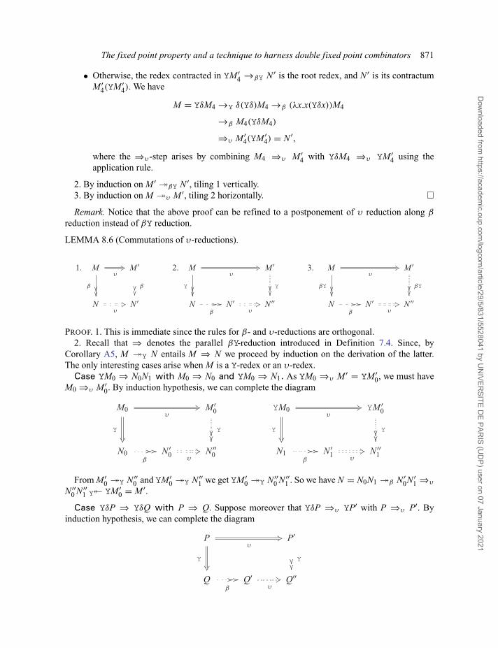
The fixed point property and a technique to harness double fixed point combinators 871
• Otherwise, the redex contracted in YM ′4 →βY N ′ is the root redex, and N ′ is its contractum
M ′4(YM ′
4). We have
M = YδM4 →Y δ(Yδ)M4 →β (λx.x(Yδx))M4
→β M4(YδM4)
⇒υ M ′4(YM ′
4) = N ′,
where the ⇒υ -step arises by combining M4 ⇒υ M ′4 with YδM4 ⇒υ YM ′
4 using theapplication rule.
2. By induction on M ′ �βY N ′, tiling 1 vertically.3. By induction on M �υ M ′, tiling 2 horizontally. �Remark. Notice that the above proof can be refined to a postponement of υ reduction along β
reduction instead of βY reduction.
LEMMA 8.6 (Commutations of υ-reductions).
PROOF. 1. This is immediate since the rules for β- and υ-reductions are orthogonal.2. Recall that ⇒ denotes the parallel βY-reduction introduced in Definition 7.4. Since, by
Corollary A5, M �Y N entails M ⇒ N we proceed by induction on the derivation of the latter.The only interesting cases arise when M is a Y-redex or an υ-redex.
Case YM0 ⇒ N0N1 with M0 ⇒ N0 and YM0 ⇒ N1. As YM0 ⇒υ M ′ = YM ′0, we must have
M0 ⇒υ M ′0. By induction hypothesis, we can complete the diagram
From M ′0 �Y N ′′
0 and YM ′0 �Y N ′′
1 we get YM ′0 �Y N ′′
0 N ′′1 . So we have N = N0N1 �β N ′
0N ′1 ⇒υ
N ′′0 N ′′
1 Y� YM ′0 = M ′.
Case YδP ⇒ YδQ with P ⇒ Q. Suppose moreover that YδP ⇒υ YP′ with P ⇒υ P′. Byinduction hypothesis, we can complete the diagram
Dow
nloaded from https://academ
ic.oup.com/logcom
/article/29/5/831/5528041 by UN
IVERSITE D
E PARIS (U
DP) user on 07 January 2021

872 The fixed point property and a technique to harness double fixed point combinators
Thus, we have N = YδQ �β YδQ′ ⇒υ YQ′′Y� YP′ = M ′.
Case YδP ⇒ N1N2Q with δ ⇒ N1,Yδ ⇒ N2 and P ⇒ Q. We also suppose that YδP ⇒υ YP′with P ⇒υ P′. The fact that δ is a normal form entails N1 = δ, so we obtain YδP ⇒ δN2Q. Sincethe only Y-reducts of Yδ are λY-terms of the form δk(Yδ) for some k we must have N2 = δk(Yδ). Wealso have the β-reduction:
N = N1N2Q = δ(δk(Yδ))Q →2β Q(δk(Yδ)Q)
= Q(δ(δk−1(Yδ))Q) →2β Q(Q(δk−1(Yδ)Q))
→2(k−1)β Qk+1(YδQ).
By induction hypothesis, we have Q �β R ⇒υ S Y� P′. Therefore,
Notice that Rk+1(YδR) ⇒υ Sk+1(YS) is obtained by putting together the reduction R ⇒υ S atk + 2 disjoint positions, while using a single υ-reduction step to remove the δ occurring at depthk + 1. The Y-reduction YP′ �Y Sk+1(YS) is obtained as
YP′ →Y P′(YP′) �Y S(YP′) → S(P′(YP′)) �Y S(S(YP′)) �Y · · ·�Y Sk+1(YP′) �Y Sk+1(YS).
3. We proceed by induction on the length n of the reduction M �βY N .
Case n = 0. In this case M = N and there is nothing to prove.Case n > 0. The reduction M �βY N factors as M �βY N0 →βY N . By applying the induction
hypothesis to M �βY N0 of length n − 1, we have
There are two subcases.
• If N0 →βY N contracts a β-redex, then we conclude by
where the square on the left exists by confluence of β, and the one on the right by part 1.
Dow
nloaded from https://academ
ic.oup.com/logcom
/article/29/5/831/5528041 by UN
IVERSITE D
E PARIS (U
DP) user on 07 January 2021
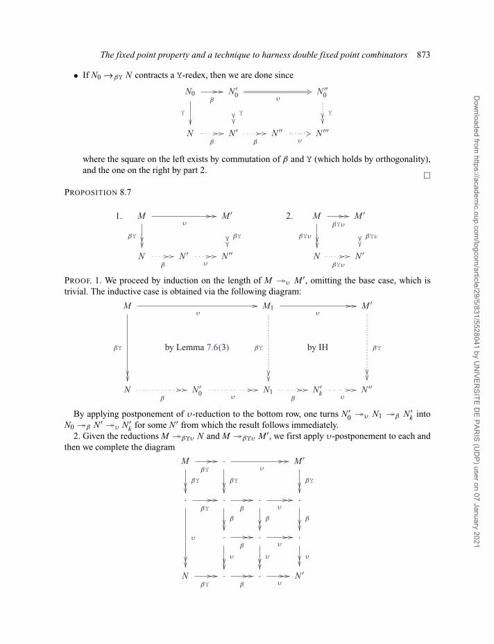
The fixed point property and a technique to harness double fixed point combinators 873
• If N0 →βY N contracts a Y-redex, then we are done since
where the square on the left exists by commutation of β and Y (which holds by orthogonality),and the one on the right by part 2. �
PROPOSITION 8.7
PROOF. 1. We proceed by induction on the length of M �υ M ′, omitting the base case, which istrivial. The inductive case is obtained via the following diagram:
By applying postponement of υ-reduction to the bottom row, one turns N ′0 �υ N1 �β N ′
k intoN0 �β N ′ �υ N ′
k for some N ′ from which the result follows immediately.2. Given the reductions M �βYυ N and M �βYυ M ′, we first apply υ-postponement to each and
then we complete the diagram
Dow
nloaded from https://academ
ic.oup.com/logcom
/article/29/5/831/5528041 by UN
IVERSITE D
E PARIS (U
DP) user on 07 January 2021

874 The fixed point property and a technique to harness double fixed point combinators
The squares that appear along the main diagonal are obtained by confluence of βY-, β- and υ-reductions, individually. The rectangles covering the bottom-left and top-right corners are given bypart 1. The remaining squares follow by commutation of υ- and β-reductions (Lemma 8.6(1)). �
By the well-known Theorem 3.1.12 in [2], we obtain the following corollary.
COROLLARY 8.8Let M , N ∈ ΛY. If M =βYυ N then there exists a λY-term Z such that M �βYυ Z βYυ� N .
THEOREM 8.9The λY-theory δ∗ is a conservative extension of λ-calculus.
PROOF. Let M , N ∈ Λ and suppose that δ∗ � M = N . By Lemma 8.2 we have M =βYυ N and, byCorollary 8.8, there exists a λY-term Z such that
M �βYυ Z βYυ� N .
Since none of the reduction rules are able to create a new occurrence of the symbol Y, there is nopoint in these reductions where Y - or υ-redexes can appear. Thus, the reductions above are actuallyβ-reductions, so we conclude that M =β N . �
9 Conclusions
We have investigated two questions concerning (sets of) fixed points of terms in λ-calculus, theveracity of the fixed point property, and the existence of a double fixed point combinator. We haveprovided partial answers to both questions, and established several promising new techniques fortackling full solutions.
One novel aspect of the present work is to consider the questions in different λ-theories. Forexample, we have devised an example showing that the fixed point property patently fails in anysensible lambda theory, thus proving a conjecture of Intrigila and Statman.
Apart from the major problem of settling the status of the two main questions in the most fine-grained λ-theory—i.e. the ‘usual’ theory whose equivalence classes consist of terms that are β-equivalent—several lesser open problems remain; e.g. providing a characterization of the fixedpoint property in semi-sensible theories, and investigating the usefulness of the novel technique forrefuting the existence of double fixed points combinators in the setting of (simple) types. We urgethe reader to peruse the conjectures and suggestions that occur throughout the paper, both explicitlyand in the running text.
A Technical Appendix
A.1 Standardization
The standard reduction can be thought of as a ‘canonical serialization’ of the usual multistepreduction. This idea is made precise by the standardization theorem, which we now prove.
LEMMA A1 (Substitution lemma).For M , M ′, N , N ′ ∈ ΛY, we have
(i) N �s N ′ implies M[N/x] �s M[N ′/x],(ii) M →w M ′ and N �s N ′ imply M[N/x] �s M ′[N ′/x],
(iii) M �s M ′ and N �s N ′ imply M[N/x] �s M ′[N ′/x].
Dow
nloaded from https://academ
ic.oup.com/logcom
/article/29/5/831/5528041 by UN
IVERSITE D
E PARIS (U
DP) user on 07 January 2021

The fixed point property and a technique to harness double fixed point combinators 875
PROOF OF LEMMA A.1
(i) By the fact that �s is a congruence.(ii) First notice that M[N/x] →w M ′[N/x]. This can be seen by considering the possible shape of
M →w M ′, where
((λy.M0)N0 · · · Nk)[N/x] = (λy.M0[N/x])N0[N/x] · · · Nk[N/x]
→w M0[N/x][N0[N/x]/y]N1[N/x] · · · Nk[N/x]
= M0[N0/y][N/x]N1[N/x] · · · Nk[N/x]
= (M0[N0/y]N1 · · · Nk)[N/x]
(YN0 · · · Nk)[N/x] = YN0[N/x] · · · Nk[N/x]
→w N0[N/x](YN0[N/x])N1[N/x] · · · Nk[N/x]
= (N0(YN0)N1 · · · Nk)[N/x].
Next, we have M ′[N/x] �s M ′[N ′/x] by point (i).(ii) Thus, M[N/x] →w M ′[N/x] �s M ′[N ′/x].(ii) By the redex rule for �s, we have (ii).
(iii) By induction on M �s M ′, using (ii) in case of the redex rule. �LEMMA A2For M , N ∈ ΛY, we have that M �s λx.N entails M �w λx.M ′ and M ′ �s N for some M ′ ∈ ΛY.
PROOF OF LEMMA A2. We proceed by induction on the derivation of M �s λx.N . Since M reducesto an abstraction, there are only two possibilities:
• M �s λx.N because M = λx.M ′ and M ′ �s N . This case is trivial as M �w λx.M ′ followsfrom the ref lexivity of �w.
• M �s λx.N because M →w M1 and M1 �s λx.N . By induction hypothesis, there existsM ′ ∈ ΛY such that M1 �w λx.M ′ with M ′ �s N . Since →w ⊆ �w and �w is transitive, weconclude M �w λx.M ′. �
THEOREM A3 (Standardization).For all M , N , N ′ ∈ ΛY, we have
(i) M �s N →βY N ′ implies M �s N ′,(ii) M �s N �βY N ′ implies M �s N ′,
(iii) M �βY N implies M �s N .
PROOF OF THEOREM A3. (i) By induction on the derivation of M �s N .
M →w M ′ �s N→βY N ′: By induction hypothesis, we have M ′ �s N ′. Now M →w M ′ �sN ′, whence M �s N ′.
M = x �s x= N : This case is inconsistent with N →βY N ′.M = λx.M0 �s λx.M ′
0= N : Since N = λx.M ′0 is not a redex, the redex contracted in N →βY N ′
must occur below, in M ′0. So M ′
0 →βY M ′′0 and N ′ = λx.M ′′
0 .By induction hypothesis, M0 �s M ′′
0 , whence M = λx.M0 �sλx.M ′′
0 = N ′.M = M1M2, Mi �s M ′
i : We distinguish two subcases.
Dow
nloaded from https://academ
ic.oup.com/logcom
/article/29/5/831/5528041 by UN
IVERSITE D
E PARIS (U
DP) user on 07 January 2021
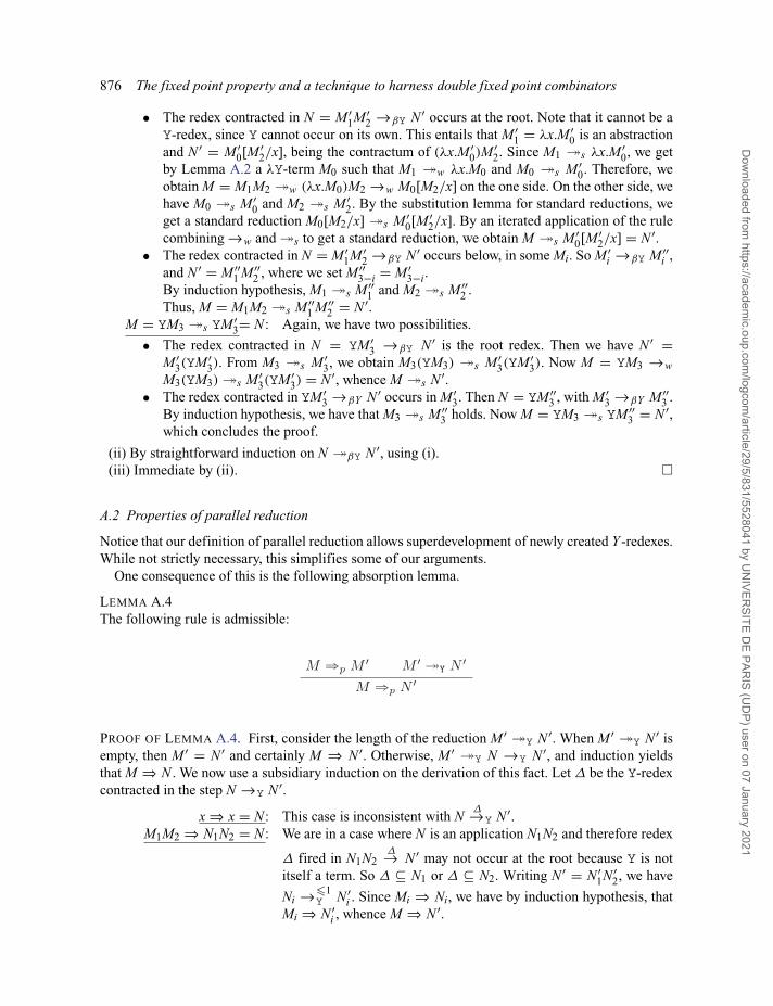
876 The fixed point property and a technique to harness double fixed point combinators
• The redex contracted in N = M ′1M ′
2 →βY N ′ occurs at the root. Note that it cannot be aY-redex, since Y cannot occur on its own. This entails that M ′
1 = λx.M ′0 is an abstraction
and N ′ = M ′0[M ′
2/x], being the contractum of (λx.M ′0)M
′2. Since M1 �s λx.M ′
0, we getby Lemma A.2 a λY-term M0 such that M1 �w λx.M0 and M0 �s M ′
0. Therefore, weobtain M = M1M2 �w (λx.M0)M2 →w M0[M2/x] on the one side. On the other side, wehave M0 �s M ′
0 and M2 �s M ′2. By the substitution lemma for standard reductions, we
get a standard reduction M0[M2/x] �s M ′0[M ′
2/x]. By an iterated application of the rulecombining →w and �s to get a standard reduction, we obtain M �s M ′
0[M ′2/x] = N ′.
• The redex contracted in N = M ′1M ′
2 →βY N ′ occurs below, in some Mi. So M ′i →βY M ′′
i ,and N ′ = M ′′
1 M ′′2 , where we set M ′′
3−i = M ′3−i.
By induction hypothesis, M1 �s M ′′1 and M2 �s M ′′
2 .Thus, M = M1M2 �s M ′′
1 M ′′2 = N ′.
M = YM3 �s YM ′3= N : Again, we have two possibilities.
• The redex contracted in N = YM ′3 →βY N ′ is the root redex. Then we have N ′ =
M ′3(YM ′
3). From M3 �s M ′3, we obtain M3(YM3) �s M ′
3(YM ′3). Now M = YM3 →w
M3(YM3) �s M ′3(YM ′
3) = N ′, whence M �s N ′.• The redex contracted in YM ′
3 →βY N ′ occurs in M ′3. Then N = YM ′′
3 , with M ′3 →βY M ′′
3 .By induction hypothesis, we have that M3 �s M ′′
3 holds. Now M = YM3 �s YM ′′3 = N ′,
which concludes the proof.
(ii) By straightforward induction on N �βY N ′, using (i).(iii) Immediate by (ii). �
A.2 Properties of parallel reduction
Notice that our definition of parallel reduction allows superdevelopment of newly created Y -redexes.While not strictly necessary, this simplifies some of our arguments.
One consequence of this is the following absorption lemma.
LEMMA A.4The following rule is admissible:
PROOF OF LEMMA A.4. First, consider the length of the reduction M ′ �Y N ′. When M ′ �Y N ′ isempty, then M ′ = N ′ and certainly M ⇒ N ′. Otherwise, M ′ �Y N →Y N ′, and induction yieldsthat M ⇒ N . We now use a subsidiary induction on the derivation of this fact. Let Δ be the Y-redexcontracted in the step N →Y N ′.
x ⇒ x = N : This case is inconsistent with NΔ→Y N ′.
M1M2 ⇒ N1N2 = N : We are in a case where N is an application N1N2 and therefore redex
Δ fired in N1N2Δ→ N ′ may not occur at the root because Y is not
itself a term. So Δ ⊆ N1 or Δ ⊆ N2. Writing N ′ = N ′1N ′
2, we have
Ni →�1Y N ′
i . Since Mi ⇒ Ni, we have by induction hypothesis, thatMi ⇒ N ′
i , whence M ⇒ N ′.
Dow
nloaded from https://academ
ic.oup.com/logcom
/article/29/5/831/5528041 by UN
IVERSITE D
E PARIS (U
DP) user on 07 January 2021

The fixed point property and a technique to harness double fixed point combinators 877
λx.M0 ⇒ λx.N0 = N : Clearly, Δ ⊆ N0, so that N0 →Y P and N ′ = λx.P. By induction,M0 ⇒ N0 →Y P yields M0 ⇒ P, and hence
M = λx.M0 ⇒ λx.P = N ′.
(λx.P)Q ⇒ P′[Q′/x] = N : with P ⇒ P′ and Q ⇒ Q′. Since Y cannot occur as a term on its own,a Y-redex cannot be created by a substitution instance P′[Q′/x]. SoΔ is inside either P′ or Q′. That is, either N ′ = P′′[Q′/x], where
P′ Δ→Y P′′, or N ′ = P′[Q′′/x], where Q′ Δ→Y Q′′. In either case, wecan use induction hypothesis to get P ⇒ P′′, respectively Q ⇒ Q′′,and therefore M ⇒ N ′.
YP ⇒ YP′ = N : with P ⇒ P′. We split into two subcases.
• If Δ ⊆ P′, so that YP′ Δ→Y YQ = N ′, then P ⇒ P′ →Y Q yields by inductionP ⇒ Q. Then M = YP ⇒ YQ = N ′.
• If Δ is the root redex YP′, then N ′ = P′(YP′), and we need only apply the Y-redexrule:
YP ⇒ P′Q: with M = YP and N = P′Q Δ→Y N ′. That is, the last derivation steplooks as follows:
Since P′ cannot be Y itself, Δ must be in either P′ or in Q. In theformer case, we apply induction to P ⇒ P′ →Y P∗ without changingthe second hypothesis, so the conclusion of the rule becomes YP ⇒P∗Q. In the latter case, we apply induction to YP ⇒ Q →Y Q∗without changing the first hypothesis, so the conclusion becomesYP ⇒ P′Q∗, as desired. �
Therefore, a Y-reduction sequence of arbitrary length can be turned into a single step of parallelreduction.
COROLLARY A.5For all M , N ∈ ΛY, M �Y N entails M ⇒ N .
Parallel reduction also satisfies the usual substitution property.
LEMMA A.6 (Substitution lemma for ⇒).For M , M ′, N , N ′ ∈ ΛY, we have
(i) N ⇒ N ′ implies M[N/x] ⇒ M[N ′/x],(ii) M ⇒ M ′ and N ⇒ N ′ imply M[N/x] ⇒ M ′[N ′/x].
PROOF OF LEMMA A.6.
(i) By the fact that ⇒ is a congruence.
Dow
nloaded from https://academ
ic.oup.com/logcom
/article/29/5/831/5528041 by UN
IVERSITE D
E PARIS (U
DP) user on 07 January 2021
878 The fixed point property and a technique to harness double fixed point combinators
(ii) By induction on M ⇒ M ′. The only interesting case is the redex rule
M = (λy.P)Q P ⇒ P′
M ′ = P′[Q′/y] Q ⇒ Q′.
In this case
M[N/x] = (λy.P[N/x])Q[N/x] (A.1)
M ′[N ′/x] = P′[Q′/y][N ′/x] = P′[N ′/x][Q′[N ′/x]/y]. (A.2)
Note that the side condition y /∈ FV(N ′) needed for the application of the substitutionlemma in (A.2) is inherited under N ⇒ N ′ from the rules for capture-avoiding substitutionin (A.1), where y is chosen implicitly to be such that y /∈ FV(N). By induction hypothesis,we have
P[N/x] ⇒ P′[N ′/x]
Q[N/x] ⇒ Q′[N ′/x].
By applying the redex rule for ⇒, we get
M[N/x] = (λy.P[N/x])Q[N/x] ⇒ P′[N ′/x][Q′[N ′/x]/y] = M ′[N ′/x]. �
Acknowledgements
We are grateful to the anonymous reviewers whose suggestions helped improve and clarify thismanuscript substantially.
References
[1] R. M. Amadio and P.-L. Curien. Domains and Lambda-Calculi. Cambridge University Press,New York, NY, USA, 1998.
[2] H. P. Barendregt. The Lambda Calculus, Its Syntax and Semantics, 2nd edn. Vol. 103 of Studiesin Logic and the Foundations of Mathematics. North-Holland, 1984.
[3] I. Bethke. et al. Lambda Calculus, pp. 548–587. Vol. 55 of Cambridge Tracts in TheoreticalComputer Science, 2003.
[4] M. Bezem, J. W. Klop and R. de Vrijer. Term Rewriting Systems—TeReSe. Vol. 55 ofCambridge Tracts in Theoretical Computer Science. Cambridge University Press, 2003.
[5] A. Bucciarelli, A. Carraro, G. Favro and A. Salibra. Graph easy sets of mute lambda terms.Theoretical Computer Science, 629, 51–63, 2016.
[6] A. Carraro and A. Salibra. Ordered models of the lambda calculus. Logical Methods inComputer Science, 9, 2013.
[7] T. Coquand and H. Herbelin. A-translation and looping combinators in pure type systems.Journal of Functional Programming, 4, 77–88, 1994.
[8] J. Endrullis.. Private communication, 2011.[9] J. Endrullis, D. Hendriks and J. W. Klop. Modular construction of fixed point combinators and
clocked Böhm trees. In Proceedings of the 25th Annual IEEE Symposium on Logic in ComputerScience, LICS 2010, pp. 111–119. IEEE Computer Society, 2010.
Dow
nloaded from https://academ
ic.oup.com/logcom
/article/29/5/831/5528041 by UN
IVERSITE D
E PARIS (U
DP) user on 07 January 2021

The fixed point property and a technique to harness double fixed point combinators 879
[10] J. Endrullis, D. Hendriks, J. W. Klop and A. Polonsky. Discriminating lambda-terms usingclocked Böhm trees. Logical Methods in Computer Science, 10, 2014.
[11] J. Endrullis and R. C. de Vrijer. Reduction under substitution. In Rewriting Techniques andApplications, 19th International Conference, RTA 2008, Hagenberg, Austria, July 15–17, 2008,Proceedings, A. Voronkov ed., pp. 425–440. Vol. 5117 of Lecture Notes in Computer Science.Springer, 2008.
[12] H. Geuvers and J. Verkoelen. On fixed point and looping combinators in type theory, 2009.http://www.cs.ru.nl/herman/PUBS/TLCApaper.pdf.
[13] H. Geuvers and B. Werner. On the Church–Rosser property for expressive type systems and itsconsequences for their metatheoretic study. In Proceedings Ninth Annual IEEE Symposium onLogic in Computer Science, pp. 320–329. IEEE Computer Society, 1994.
[14] J. M. E. Hyland. A syntactic characterization of the equality in some models for the lambdacalculus. Journal London Mathematical Society (2), 12, 361–370, 1975/76.
[15] B. Intrigila. Non-existent Statman’s double fixedpoint combinator does not exist, indeed.Information and Computation, 137, 35–40, 1997.
[16] B. Intrigila. TLCA list, Problem #25: how many fixed points can a combinator have? 2000.http://tlca.di.unito.it/opltlca/. (First raised in [17].)
[17] B. Intrigila and E. Biasone. On the number of fixed points of a combinator in lambda calculus.Mathematical Structures in Computer Science, 10, 595–615, 2000.
[18] B. Intrigila and R. Statman. Lambda theories allowing terms with a finite number of fixedpoints. Mathematical Structures in Computer Science, 1–23, 2015.
[19] J. W. Klop. New fixed point combinators from old. In Reflections on Type Theory,lambda-Calculus, and the Mind, pp. 197–210. Radboud University, 2007. (Essays dedicated to HenkBarendregt on the Occasion of his 60th Birthday.)
[20] J. W. Klop. Personal communication, 2014.[21] A. Kurz, D. Petrisan, P. Severi and F. de Vries. Nominal coalgebraic data types with applications
to lambda calculus. Logical Methods in Computer Science, 9, 2013.[22] S. Lusin and A. Salibra. The lattice of lambda theories. Journal of Logic and Computation, 14,
373–394, 2004.[23] G. Manzonetto and A. Salibra. From λ-calculus to universal algebra and back. In Mathematical
Foundations of Computer Science 2008: 33rd International Symposium, MFCS 2008, Torun,Poland, August 25–29, 2008, Proceedings, E. Ochmanski and J. Tyszkiewicz, eds, pp. 479–490.Vol. 5162 of Lecture Notes in Computer Science. Springer, 2008.
[24] L. Ong. Correspondence between operational and denotational semantics. In Handbook ofLogic in Computer Science, S. Abramsky, D. Gabbay, and T. S. E. Maibaum, eds, vol. 4,pp. 269–365. Oxford University Press, 1995.
[25] G. D. Plotkin. The lambda-calculus is ω-incomplete. Journal of Symbolic Logic, 39, 313–317,1974.
[26] A. Polonsky. The range property fails for H. Journal of Symbolic Logic, 77, 1195–1210, 2012.[27] A. Salibra.. Nonmodularity results for lambda calculus. Fundamenta Informaticae, 45,
379–392, 2001.[28] P. Severi and F. de Vries. Order structures on Böhm-like models. In Computer Science Logic:
19th International Workshop, CSL 2005, C. L. Ong ed., pp. 103–118. Vol. 3634 of LectureNotes in Computer Science. Springer, 2005.
[29] R. Statman. Some examples of non-existent combinators. Theoretical Computer Science, 121,441–448, 1993.
Dow
nloaded from https://academ
ic.oup.com/logcom
/article/29/5/831/5528041 by UN
IVERSITE D
E PARIS (U
DP) user on 07 January 2021
880 The fixed point property and a technique to harness double fixed point combinators
[30] R. Statman. On the lambdaY calculus. Annals of Pure and Applied Logic, 130, 325–337,2004.
[31] C. Wadsworth. The relation between computational and denotational properties for Scott’sD∞-models of the lambda-calculus. SIAM Journal of Computing, 5, 488–521, 1976.
Received 00 Month 20xx
Dow
nloaded from https://academ
ic.oup.com/logcom
/article/29/5/831/5528041 by UN
IVERSITE D
E PARIS (U
DP) user on 07 January 2021
Copyright © 2022 FDOKUMEN