Equivariant GW Theory of Stacky Curves
52
This is a repository copy of Equivariant GW Theory of Stacky Curves. White Rose Research Online URL for this paper: http://eprints.whiterose.ac.uk/98527/ Version: Accepted Version Article: Johnson, P. orcid.org/0000-0002-6472-3000 (2014) Equivariant GW Theory of Stacky Curves. Communications in Mathematical Physics, 327 (2). pp. 333-386. ISSN 0010-3616 https://doi.org/10.1007/s00220-014-2021-1 [email protected] https://eprints.whiterose.ac.uk/ Reuse Unless indicated otherwise, fulltext items are protected by copyright with all rights reserved. The copyright exception in section 29 of the Copyright, Designs and Patents Act 1988 allows the making of a single copy solely for the purpose of non-commercial research or private study within the limits of fair dealing. The publisher or other rights-holder may allow further reproduction and re-use of this version - refer to the White Rose Research Online record for this item. Where records identify the publisher as the copyright holder, users can verify any specific terms of use on the publisher’s website. Takedown If you consider content in White Rose Research Online to be in breach of UK law, please notify us by emailing [email protected] including the URL of the record and the reason for the withdrawal request.
-
Upload
khangminh22 -
Category
Documents
-
view
4 -
download
0
Transcript of Equivariant GW Theory of Stacky Curves

This is a repository copy of Equivariant GW Theory of Stacky Curves.
White Rose Research Online URL for this paper:http://eprints.whiterose.ac.uk/98527/
Version: Accepted Version
Article:
Johnson, P. orcid.org/0000-0002-6472-3000 (2014) Equivariant GW Theory of Stacky Curves. Communications in Mathematical Physics, 327 (2). pp. 333-386. ISSN 0010-3616
https://doi.org/10.1007/s00220-014-2021-1
[email protected]://eprints.whiterose.ac.uk/
Reuse
Unless indicated otherwise, fulltext items are protected by copyright with all rights reserved. The copyright exception in section 29 of the Copyright, Designs and Patents Act 1988 allows the making of a single copy solely for the purpose of non-commercial research or private study within the limits of fair dealing. The publisher or other rights-holder may allow further reproduction and re-use of this version - refer to the White Rose Research Online record for this item. Where records identify the publisher as the copyright holder, users can verify any specific terms of use on the publisher’s website.
Takedown
If you consider content in White Rose Research Online to be in breach of UK law, please notify us by emailing [email protected] including the URL of the record and the reason for the withdrawal request.

EQUIVARIANT GW THEORY OF STACKY CURVES
PAUL JOHNSON
Abstract. We extend Okounkov and Pandharipande’s work on the equivari-ant Gromov-Witten theory of P1 to a class of stacky curves X . Our main
result uses virtual localization and the orbifold ELSV formula to express thetau function τX as a vacuum expectation on a Fock space.
As corollaries, we prove the Decomposition Conjecture for these X , andprove that τX satisfies a version of the 2-Toda hierarchy. Coupled with de-generation techniques, the result should lead to treatment of general orbifoldcurves.
Contents
1. Introduction 21.1. Basic setup 21.2. Main Results 51.3. Overview of the paper 61.4. Related work and future directions 81.5. Acknowledgements 82. Basics on orbifolds and gerbes 82.1. Root construction 82.2. Cocycle description of isotropy groups 92.3. Two lemmas about maps to X 113. Localization 133.1. Generating Functions 133.2. Fixed point loci 143.3. The virtual normal bundle 183.4. Normalization exact sequence 193.5. Global localization contributions 224. Orbifold ELSV formula and Fock spaces 234.1. Wreath Hurwitz Numbers 234.2. Orbifold ELSV formula 254.3. Infinite Wedge 264.4. Wreath Product Fock spaces 285. Interpolating orbifold ELSV 315.1. Statement of the Theorem 315.2. Step 1: agreement with orbifold ELSV 335.3. Step 2: convergence and rationality 356. The main theorem and applications 396.1. Proof of the main theorem 396.2. Decomposition 446.3. Equivariant string and divisor equations 456.4. 2-Toda: Explicit form of the lowest equation 47
1

2 PAUL JOHNSON
6.5. 2-Toda: The full hierarchy 48References 50
1. Introduction
In their trilogy [OP06b] [OP06a] [OP06c], Okounkov and Pandharipande com-pletely determine the Gromov-Witten theory of curves. This paper is the beginningof a program to extend their results to stacky curves. More specifically, this paperis the stacky analog of the logical starting place of their program, [OP06a], whichstudies the equivariant Gromov-Witten theory of P1.
The main result of [OP06a] is an explicit formula for the C∗-equivariant Gromov-Witten theory of P1 as a vacuum expectation on the infinite wedge. In addition tobeing an important tool for the rest of the trilogy, this description quickly impliesthat the equivariant Gromow-Witten theory of P1 satisfies a form of the 2-Todahierarchy. In rough outline, the strategy of [OP06a] is to first use virtual localizationand the ELSV formula to reduce everything to the combinatorics of the symmetricgroup. The resulting combinatorics are then handled using the infinite wedge, whichalso makes contact with integrable hierarchies.
We follow the structure and proofs of [OP06a] rather closely. Our main resultis an explicit formula for the C∗-equivariant Gromov-Witten theory of stacky toricP1 in terms of vacuum expectations on a certain Fock space. This is the naturalanalog of the main result [OP06a], and the proof follows the same method. Thefirst step of the proof is essentially the same: the orbifold structure must be takeninto account in the localization calculation, and in place of the ELSV formula thereis the orbifold ELSV formula of [JPT11], but the general form is the same.
In the second step there is a larger novelty: for ineffective orbifolds, the infinitewedge is not a large enough Fock space. On an ineffective orbifold, also known asa gerbe, the generic point has a nontrivial stabilizer group K. In this case, insteadof the symmetric group, the orbifold ELSV formula uses the wreath product Kn
of Sn with Kn. To handle these combinatorics, we use a larger Fock space ZK ,which has been studied in a context convenient for us by Wang and collaborators[FW01, QW07]. The Fock space ZK plays the same role for the wreath product Kn
as the infinite wedge plays for the symmetric group, and indeed ZK can be viewedas a tensor product of |K| copies of the infinite wedge. Utilizing this decompositionof ZK as a tensor product, we can use the same proofs as [OP06a].
As a result of our formula, we again get a connection to the 2-Toda hierarchy.Furthermore, in the ineffective case we obtain a proof of the decomposition conjec-ture of [HHP+07], which in our case expresses the τ function for ineffective orbifoldsas a product of related τ functions for effective orbifolds after an appropriate changeof variables.
In the rest of the introduction we introduce the notation needed (Section 1.1) tostate our results more carefully (Section 1.2), then give an overview of the structureof the paper (Section 1.3) and a brief discussion of related work and future directions(Section 1.4).
1.1. Basic setup.

EQUIVARIANT GW THEORY OF STACKY CURVES 3
1.1.1. Targets. The effective orbifolds we consider are are denoted Cr,s. The coarsemoduli space of Cr,s is P1; however Cr,s has orbifold structure Zr at 0 and Zs atinfinity.
Our general target X is a toric stack that is a gerbe over Cr,s. In the onedimensional case, being toric is equivalent to X having all abelian isotropy groups.Denote the generic isotropy group by K, so that X is a K-gerbe over Cr,s withtrivial band.
Denote the isotropy groups of X over 0 and ∞ as R and S, respectively. Theyare extensions of Zr and Zs by K, and so have canonical surjections to the corre-sponding cyclic groups. More explicit discussions of gerbes, the space X and thegroups R and S are found in Section 2.
1.1.2. Equivariant Chen-Ruan cohomology. In orbifold Gromov-Witten theory, thestate space is Chen-Ruan Cohomology. As a vector space, the Chen-Ruan coho-mology H∗
CR,C∗(X ) is the cohomology of the inertia stack IX , which we think of
as the space of constant loops S1 → X . However, this is only as vector spaces – ingeneral there is a grading shift and a different cup-product. For an introduction toorbifolds and Chen-Ruan cohomology, see [ALR07].
As we are doing C∗-equivariant Gromov-Witten theory, we need to consider theC∗-equivariant Chen-Ruan cohomology. Thus, our cohomology rings are modulesover H∗
CR(pt) = C[t]. Let F be the fixed point set of the C∗ action on IX . ThenAtiyah-Bott localization [AB84] implies that if we invert t, we have H∗
CR(X ) ∼=H∗
CR(F ) as C[t, t−1] modules. Throughout the rest of this paper we tacitly invertt and use this isomorphism.
Note that F consists of the constant loops that map to 0 or ∞, and so consistsof |R|+ |S| isolated points, naturally labeled by elements of R and S. Use 0ρ and∞σ to denote the corresponding basis of H∗
CR(X ) as a C[t, t−1] module.The elements 0ρ have degree zero in H∗(IX ), but due to degree shifting have
potentially nonzero degree ι(ρ) in H∗CR(X ). Identifying the elements of Zr with the
rational numbers k/r, 0 ≤ k < 1, we have ι(ρ) = φ(ρ), where φ is the natural mapφ : R→ Zr.
We use r and s to denote tuples of elements of R and S, respectively. The numberof elements in a tuple, i.e. its length, is denoted ℓ(r), while the elements themselvesare ri, 1 ≤ i ≤ ℓ(r). Finally, use
ι(r) =
ℓ(r)∑
i=1
ι(ri).
1.1.3. Moduli spaces. Our main focus of study are the two moduli spacesMg,r,s(X , d)
and Mg,r(BR), which we now describe.In orbifold Gromov-Witten theory, the marked points get orbifold structure and
are forced to map to certain twisted sectors. This gives additional discrete invariantsfor the moduli space of maps to the target space. Consider the moduli spaceM = Mg,r,s(X , d) of stable degree d maps from genus g nodal orbifold curves Σto X . The curve Σ has ℓ(r) + ℓ(s) marked points, where the ith marked point ispulling back the cohomology class 0ri
(or ∞si).
This space is generally singular, but it carries a virtual fundamental class of theexpected dimension
dimC[Mg,r,s(X , d)]vir = 2g − 2 + d(1/r + 1/s) + ℓ(r) + ℓ(s)− ι(r)− ι(s).

4 PAUL JOHNSON
The C∗ action on X induces a C∗ action on M, and the virtual fundamental classbecomes an equivariant class, so that we can pull back and integrate equivariantChen-Ruan cohomology classes from X . Applying virtual localization to M, thefixed point loci are products of simpler moduli spaces Mg,n(BR) and Mg,m(BS).
A point in Mg,n(BR) is given by a orbifold curve Σ together with a non-orbifold
R-cover Σ. The monodromy at each marked point corresponds to a conjugacy classin R, and we use Mg,r to denote the subset of Mg,n(BR) having monodromy riaround the ith marked point point.
A superscript bullet indicates disconnected source curves. For example, M•g,r
denotes the same moduli space as above, but with Σ and Σ allowed to be dis-connected. The genus of a disconnected curve is defined by noting that the eulercharacteristic χ(Σ) = 2 − 2g for connected curves and is additive under disjointunion, and so we can use χ(Σ) = 2−2g to define the genus for disconnected curves.
1.1.4. The τ function. Over each of the moduli spaces we consider certain integralspackaged into generating functions – we describe this now.
The evaluation maps evi : Mg,r,s(X , d) → IX allow us to pull back Chen-Ruancohomology classes.
In addition to pulled back classes, we also consider ψ classes, given by ψi =c1(Li), where the fiber of Li over a curve Σ is the cotangent bundle at the ithmarked point: Li = T ∗
piΣ.
Define⟨
ℓ(r)∏
i=1
τai(0ri
)
ℓ(s)∏
j=1
τbj (∞sj)
⟩X
g,d
=
∫
[Mg,r,s(X ,d)]vir
ℓ(r)∏
i=1
ψaii ev∗i (0ri
)
ℓ(s)∏
j=1
ψbjj ev∗j (∞sj
).
The τ function is a generating function for all disconnected invariants of X . It isa formal series in q and u, encoding the degree and the genus, respectively, as wellas two infinite sets of variables x = xi(ρ)|0 ≤ i ∈ Z, ρ ∈ R and x∗ = x∗j (σ)|0 ≤j ∈ Z, σ ∈ S, encoding the integrated classes.
The τ function is defined as:
τX (x, x∗, u) =∑
g∈Z
∑
d≥0
u2g−2qd
⟨exp
∑
i,ρ
xi(ρ)τi(0ρ) +∑
j,σ
x∗j (σ)τj(∞σ)
⟩•
g,d
where in the sums i, j run from 0 to ∞, and ρ and σ run over R and S, respectively.
1.1.5. The Hurwitz-Hodge function. In calculating τX through virtual localization,we are lead to consider certain Hurwitz-Hodge integrals over Mg,r(BR) that we nowdescribe.
The Hodge bundle E overMg,r(BR) has fiberH0(Σ, ωΣ), where ω is the dualizing
sheaf, which is the canonical sheaf if Σ is smooth. The R action on Σ induces an Raction on E, and so E splits into subbundles EV , where EV is the part of E wherewhere R acts by a given irreducible representation V of R.
In the orbifold case, the orbifold structure at the marked point has an effect onthis Chern class. If the ith marked point has a Zri isotropy group, define ψi = riψi.The ψ classes ignore the effect of the orbifold structure.
The Hurwitz-Hodge classes are the Chern classes of the bundles EV , namelyλVi = ci(EV ). Integrals of λ
Vi and ψ classes are called Hurwitz-Hodge integrals.
EQUIVARIANT GW THEORY OF STACKY CURVES 5
The representation of R of interest is T0X , which write as T for brevity. Packagethe Hurwitz-Hodge integrals that are linear in the λTi into the following Hurwitz-Hodge generating function, which appears in the localization calculation:
H•r(z1, . . . , zn, u) =
∑
g∈Z
u2g−2
∫
M•g,r(BR)
n∏
i=1
zi
1− ziψi
m∑
i=0
(−r)iλTi .
Here, the bullet in M•means not only that we are allowing disconnected curves,
but are actually allowing unstable curves. In the unstable case, there is an ad-hocdefinition of the resulting integrals that is compatible with both localization andthe orbifold ELSV formula. This convention allows for a uniform treatment oflocalization.
1.1.6. Fock space formalism. Our two theorems are expressions for the two gener-ating functions τX and H•
rin terms of operators acting on a certain vector space
ZK called a Fock space. We give now just enough information about this Fockspace to state our results – for more details, see Sections 4.3 and 4.4.
The Fock space ZK occurs in the study of the representation theory of wreathproducts: ZK is a graded vector space (the degree of an element is called itsenergy), and its nth graded piece has a natural basis indexed by the irreduciblerepresentations of Sn ⋊Kn, the wreath product of Sn with K. From this, we seeZK has an inner product (·, ·), and a preferred vector of energy zero, denoted v∅and called the vacuum vector.
The Fock space ZK is a representation of many important algebras. This is mosteasily seen by noting that another way of looking at ZK is as a tensor product
of n copies of the infinite wedge∧∞
2 V . Since the infinite wedge is a projectiverepresentation of gl∞, ZK has |K| copies of gl∞ acting on it. If M is an operatorin their product, we write 〈M〉 = (v∅,Mv∅), called the vacuum expectation of M .
1.2. Main Results.
1.2.1. Operator Expression for the Hurwitz-Hodge function. Our first theorem is anexpression for the Hurwitz-Hodge generating function as a vacuum expectation onZK .
Theorem A.
H•r
(zr,
u
r1/2
)= (u|K|)−ℓ(r)
⟨ℓ(r)∏
i=1
Ari(zi, u)
⟩.
The operators Ari(zi, u) are defined in Equation (37) – they are complicated butexplicit operators on the Fock space ZK .
The proof is presented in Section 5. The geometric content of the theorem iscontained in the orbifold ELSV formula of [JPT11], and in some sense this theoremcan be understood as an interpolation of this formula. In particular, the proof doesnot depend on the localization calculation of Section 3.
1.2.2. Operator Expression. Our main result is an expression for τX as a vacuumexpectation on ZK .
Theorem B.
τX (x, x∗, u) =
⟨e∑
xi(r)Ar[i]eαr(0)u|R| qHe
α−s(0)
u|S| e∑
x∗j (s)A
∗s[j]
⟩.

6 PAUL JOHNSON
Here the α are the bosonic operators acting on the Fock space, H is a twistedversion of the energy operator (the twisting reflects the gerbe structure of X ), andthe operators A are closely related to the operator A from our first theorem.
The proof of the main theorem is essentially combining the localization calcu-lation of Section 3 with Theorem A. The main theorem is proved in the first partof Section 6. The remainder of this section explores several corollaries of the maintheorem. We highlight two of these now.
1.2.3. Decomposition Conjecture. The first application of our main theorem, carriedout in Section 6.2, is to verify the Decomposition Conjecture of [HHP+07] for ourX . For more on the decomposition conjecture, see [TT].
Given any G-gerbe X over an effective orbifold B, the Decomposition Conjecturedescribes how to construct a disconnected and effective cover Y of B and a flat gerbec on Y. It then asserts that conformal field theories on X are equivalent to thoseon Y twisted by c. This has several mathematical implications, in particular thatthe Gromov-Witten theory of X is equivalent to the Gromov-Witten theory of Ytwisted by c.
In our case (and whenever X has trivial band) the space Y is |K| copies of Cr,s,indexed by representations γ of K. Furthermore, in our case the only effect of thetwisting is a rescaling of variables. Thus informally we have:
Corollary C: Decomposition. After an appropriate change of variables, we have:
τX =∏
γ∈K∗
τCγr,s.
The proof follows from our operator expression for τX , essentially since ZK is atensor product copies of |K| copies of the infinite wedge.
1.2.4. The 2-Toda Hierarchy. The main corollary of our main theorem, derived inSection 6.5, is that our τ functions satisfy integrable hierarchies.
Corollary D: Integrability. The tau function τCr,sis a τ function for the 2Toda
hierarchy.
Using a different approach [MT11], Milanov and Tseng have already obtainedthis result. Note that the exact integrable hierarchy that τ satisfies is some reduc-tion of the 2-Toda hierarchy, as is already the case with non-orbifold P1. However,the relationship between this reduction and the expression in the infinite wedge isnot yet clear.
In the noneffective case, since τX a product of the τCγr,s, we see that τX satisfies
|K| commuting copies of the 2-Toda hierarchy. The Fock space ZK was used in asimilar way in [QW07], and this result and the decomposition conjecture were partof our motivation for bringing ZK into the picture.
1.3. Overview of the paper. In this section, we give a quick overview of thebody of the paper, section by section.
Section 2: Basics on orbifolds and gerbes. This section collects results on toricorbifold curves X . All of our gerbes can be constructed as root stacks, which wereview in Section 2.1. In Section 2.2 we use the root stack construction to giveexplicit cocycle descriptions of the isotropy groups R and S.

EQUIVARIANT GW THEORY OF STACKY CURVES 7
In Section 2.3 we prove two lemmas describing how the orbifold and gerbe struc-tures of X interact with the orbifold structure of source curves Σ mapping intoX . Lemma 1 describes the effective isotropy, while Lemma 2 addresses the gerbyisotropy. While the behavior of the effective isotropy is locally determined and wellknown, the gerby isotropy is a global phenomenon. For gerbes over P1 this globalbehavior was used in [CC09] to study Hurwitz-Hodge integrals. It is slightly morecomplicated, and we believe new, to describe what happens for gerbes over Cr,s.
Section 3: Localization. In Section 3 we carry out the virtual localization calcula-tion that determines τX from H•
r.
The results of [GP99] say that Atiyah-Bott localization holds for virtual funda-mental classes. Thus, to perform our equivariant integrals over Mg,r,s(X , β), it isenough to determine the fixed point locus F and its virtual normal bundle insideM.
In general, this calculation is standard, and essentially we use the same tech-niques as [GP99] and [OP06a]. However, localization in the context of orbifoldsand gerbes is less standard, and so we provide a thorough description of the calcu-lation.
Section 4: Orbifold ELSV formula and Fock spaces. Section 4 introduces the re-maining tools in the proof: the orbifold ELSV formula and the Fock space ZK .
The orbifold ELSV formula expresses H•rin terms of Hurwitz numbers, which
count covers of P1 having specified ramification. Considering the monodromy of thecover reduces Hurwitz theory to group theory. The resulting group theory questionhas a convenient expression in terms of representation theory, as was known alreadyto Frobenius.
In the effective case, the pertinent groups are the symmetric groups, and the per-tinent Hurwitz numbers count covers that have profile µ over 0, profile (r, r, . . . , r, r)over ∞, and simple ramification over the appropriate number of other points. Inthe noneffective case, the symmetric group is replaced by the wreath product.
The representation theory needed to calculate Hurwitz numbers is conveniently
encoded in the Fock spaces. In Section 4.3 we introduce the infinite wedge∧∞
2 Vand the operators on it, and explain how to express Hurwitz numbers as a vacuumexpectation. Section 4.4 then extends this to wreath Hurwitz numbers and ZK .
Section 5: Interpolating orbifold ELSV. Section 5 is devoted to proving our Theo-rem A, which can be understood as follows.
The orbifold ELSV formula is only valid when the zi are integers satisfyingcertain congruence relations, essentially because the Hurwitz numbers make senseonly in this situation. However, for our application we require a formula valid forany zi.
It is clear from the definition that the coefficients of u in H•r(z, u) are rational
functions of z, andhence are determined by the infinite set of values provided bythe orbifold ELSV formula. The expression for Hurwitz numbers in terms of Fockspace, after some manipulation, allows for an interpolation to non-integer values.Theorem A says that this interpolation agrees with H•
r(z, u).
The proof has two steps. First, we show that when zi are integers of the rightform, the complicated A operators simplify to the operators appearing in the de-scription of Hurwitz numbers. We then show that their vacuum expectation is,after a combinatorial factor, rational.

8 PAUL JOHNSON
The proof of the second step follows from a technical commutator calculationinvolving hypergeometric functions. We have not included this proof: it is lengthy,but once the correct definition of the A operators is found there is no substantivedifference from the proof in [OP06a] for the non-orbifold setting. The completeproof may be found in Chapter VII of the author’s thesis [Joh].
Section 6: The main theorem and applications. The main theorem is proved insection 6.1. The hard work has already been done; all that remains to do is to wiretogether Theorem A and the localization calculation. The remainder of Section 6derives several consequences of Theorem B.
First, we prove the decomposition conjecture in Section 6.2. With the decom-position conjecture in hand, we can work with the effective case for the rest of thepaper.
Before proving the full force of Corollary D, we derive a few smaller corollariesby hand, proving the equivariant divisor and string equations in Section 6.3, andderiving the lowest equation of the 2-Toda hierarchy by hand in Section 6.4.
The proof of Corollary D is contained in Section 6.5. The proof consists inshowing that the A operators can be conjugated to the standard bosonic operatorsαk. This conjugation gives a change of variables between the Gromov-Witten timesand the 2-Toda times. The proof for the change of variables is rather technical anddepends again on some hypergeometric function calculations. Again, we omit thisas they are nearly identical to those found in [OP06a] and send the reader wantingfull details to [Joh].
1.4. Related work and future directions. Gromov-Witten theory of orbifoldcurves has been studied before, largely from the angle of integrable systems andin particular Frobenius manifolds. Milanov and Tseng have studied Cr,s in boththe equivariant [MT11] and nonequivariant [MT08] settings, in particular provingCorollary D. Rossi has approached them from the point of view of Symplectic FieldTheory [Ros10] – see also [Ros08] for an approach to the Gromov-Witten theory ofsmooth curves from this perspective.
One benefit to our approach is that it handles the ineffective case. A longer termbenefit is that our approach, coupled with degeneration techniques, should lead to afurther extension of Okounkov and Pandharipande’s program, yielding connectionsto Hurwitz theory, modular forms in case the target has Euler characteristic zero,and the Virasoro constraints. The symplectic field theory technique is quite similarto degeneration, and can obtain some of these results; it would be interesting tocarefully compare the two approaches.
1.5. Acknowledgements. This paper is an adaptation of my thesis, [Joh], andwould not have been possible without the guidance and encouragement of my advi-sor, Yongbin Ruan. I also greatly benefitted from conversations about the relatedwork [JPT11] with my coauthors Rahul Pandharipande and Hsian-Hua Tseng. Theauthor was supported in part by NSF grants DMS-0602191 and DMS-0902754.
2. Basics on orbifolds and gerbes
2.1. Root construction. In this section we collect some facts on the root con-struction, which produces Zn-gerbes from line bundles. It is a result of [FMN] thatall toric stacks can be constructed by root constructions. For curves this resultfollows from the Meyer-Vietoris theorem.
EQUIVARIANT GW THEORY OF STACKY CURVES 9
We briefly recall three points of view on the root construction in terms of ge-ometry, cohomology, and category theory. We also recall how iterating the rootconstruction can produces general abelian groups K.
2.1.1. Geometry. Geometrically, the construction of a Zn gerbe on Cr,s from a linebundle L is easily described. The total space of the line bundle has a natural C∗
action, which is just the usual C∗ action on each fiber. Removing the zero sectionof the total space of L gives the associated C∗ bundle for L.
Taking the quotient by the natural C∗ action gives Cr,s back. If instead we takethe quotient by C∗ acting by the nth power of the standard action, then the genericpoint has a Zn stabilizer. The result is thus a Zn gerbe over Cr,s, which we denote
by C(L,n)r,s .
2.1.2. Cohomology. For an abelian group K, banded K-gerbes on X are classifiedby H2(X,K). In case K = Zn, we have the short exact sequence
0 → Z·n→ Z → Zn → 0.
Part of the corresponding long exact sequence in cohomology is:
(1) H2(Cr,s,Z)·n→ H2(Cr,s,Z)
g→ H2(Cr,s,Zn) → H3(Cr,s,Z).
Since H2(Cr,s,Z) classifies topological line bundles over Cr,s and H2(Cr,s,Zn) clas-sifies Zn gerbes with trivial band, the map g gives a way to construct a bandedZn gerbe out of a line bundle. This is the cohomological description of the rootconstruction.
It is easily seen using Meyer-Vietoris that H3(Cr,s,Z) = 0, and so every bandedZn gerbe can be constructed this way.
2.1.3. Universal property. The most powerful view of the root construction, andthe one that explains its name, is the categorical viewpoint. Namely, we constructYL,n by giving L an nth root.
Let f : YL,n → Y be the forgetful map. Then, YL,n “comes with” a line bundleM and an isomorphism ϕ : Mn → f∗L, and this line bundle M is the only thingthat distinguishes YL,n from Y.
We understand YL,n if we understand all maps to it. Define a map to YL,n tobe a map to Y, together with a line bundle that’s an nth root of the pullback ofL. More precisely, a map g : Z → YL,n consists of a triple (h,N, ϕ), with h a mapfrom Z to Y, N a line bundle on Z, and ϕ an isomorphism from Nn to h∗(L).
2.1.4. Iteration. For K a more complicated abelian group, K-gerbes are easily con-structed using a fibered product of the root construction.
Explicitly, with K = ⊕mj=1Znj
, let L1, . . . , Lm be line bundles on Cr,s. Then forma K-gerbe by taking the fibered product of the root constructions for each of theseline bundles. We denote this by:
C(Lj ,nj)r,s = C(L1,n1)
r,s ×Cr,s· · · ×Cr,s
C(Lm,nm)r,s .
2.2. Cocycle description of isotropy groups. We now use the categorical view-point of the root construction to give explicit cocycle descriptions of the isotropy
groups R and S of X = C(Lj ,nj)r,s over 0 and ∞. We do this by constructing faithful
representations of R and S.
10 PAUL JOHNSON
2.2.1. A faithful representation. We now construct a faithful representation V ofR. The argument is easily adapted to give a faithful representation of S.
First, note that Lj is a representation of Zr. Let the action of 1r ∈ Zr on Lj by
e2πikj/r.Let Mj be the njth root of Lj . Then Mj |0 is a one dimensional representation
of R.Another one dimensional representation of R is T0X . We now show that
V =m⊕
j=1
Mj |0 ⊕ T0X
is a faithful representation of R, which identifies R as a subgroup of (S1)m+1.To do this, note that although we do not yet know R, we know a generating set
for R: a generating set for K together with any element that maps to 1r ∈ Zr.From the fiber product construction, it is clear that each Znj
acts trivially onMk for k 6= j, but nontrivially on Mj . In particular, R has an element gj that
generates Znj, acts on Mj by multiplication by e2πi/nj , and acts trivially on Mk
for k 6= j.Now, consider T0X . It is clear that K acts trivially on T0X , but any element
mapping to 1 ∈ Zr acts as e2πi/r. Hence, we see V is in fact faithful.Identifying S1 with R/Zm the element gj , 1 ≤ j ≤ m becomes (0, . . . , 0, 1
nj, 0, . . . , 0).
2.2.2. The cocycle description. To construct a cocycle description of R, we need tochoose a lifting of 1r ∈ Zr to R. The representation V gives us one way of makingthis choice.
Since Mj is an njth root of Lj , we see that any preimage of 1r in R must act by
an njth root of e2πikj/r. Now gj acts on Mj by e2πi/nj and is in K. Adding some
gj if necessary, we can choose a preimage of g0 of 1r that acts on Mj by e2πikj/(rnj)
for all j.In the identification of R as a subgroup of (S1)m+1, this amounts to taking
g0 = (kj
njr, . . . , km
nmr ,1r ). Thus, writing down the multiplication in terms of the
gi, 0 ≤ i ≤ m then gives us a K 2-cocycle β on Zr that describes R as a possiblynontrivial extension of Zr by K:
(2) β(a, b) =
( k1
n1, . . . , km
nm) a+ b ≥ 1
0 a+ b < 1.
The data of β is contained in the element ( k1
n1, . . . , km
nm) ∈ K. We denote this
element by k0 for R, and the similar element of K describing the group S we denoteby k∞. As the arguments for R and S are often analogous, we sometimes just givethe argument for R and drop the subscript and write k. When we wish to use thecocycle description of elements of R, we write them as ri = (ai, ki) ∈ Zr×βK = R.
2.2.3. Inverses. We now describe inverses in the cocycle description. Some care isrequired, since typically −ri 6= (−ai,−ki). Introduce
δr(x) =
0 x 6= 0 mod r1 x = 0 mod r
and
δ∨r (x) =
1 x 6= 0 mod r0 x = 0 mod r
EQUIVARIANT GW THEORY OF STACKY CURVES 11
so thatδr(x) + δ∨r (x) = 1.
Then it follows that
(3) − (a, k) = (−a,−k − δ∨r (a)k).
2.3. Two lemmas about maps to X . In this section we prove two lemmas thattogether give us a complete understanding about how the orbifold structure ofX affects maps from curves into X . Due to localization, we only need to considerorbifold maps that give the map z 7→ zd from P1 → P1 on the underlying topologicalspaces. The results of this section describe the behavior of the orbifold structure ofsuch maps. Again, due to localization, the source curve has orbifold structure onlyover 0 and ∞.
2.3.1. The effective case. The behavior of the effective orbifold structure is com-pletely determined locally by the degree of the map.
Lemma 1. Let Zr and Zn act on C as their standard embeddings in C∗, and letf : C/Zr → C/Zn be a representable map of orbifolds which on coarse modulispaces gives the map z 7→ zd. Then r = n/ gcd(d, n) and the standard generator ofZr maps to d ∈ Zn.
Proof. The map f : C/Zr → C/Zn must lift to an equivariant map g from C → C
which covers f :
Cg
−−−−→ C
zr
y zn
y
C/Zrf
−−−−→ C/Zn
Since f is of the form z 7→ zd, then we must have g(z) = za, and commutativitygives an = rd. Then there is some k with a = kd/ gcd(d, n) and r = kn/ gcd(d, n).We need to show that k = 1.
Suppose the generator 1 ∈ Zr maps to l ∈ Zn, then since g is equivariant, wehave
e2πia/rza = g(e2πi/rz) = e2πil/rg(z) = e2πil/rza
Since f is representable, the map on isotropy groups must be injective, and sowe must have that e2πia/r has order r, that is, a and r are relatively prime - whichforces k = 1.
Finally, we see that the generator of Zr maps to a/r = d/n ∈ Zd.
2.3.2. The gerby case. In contrast to the effective part, the image of a degree d mapin the ineffective part of the isotropy is completely unconstrained locally. Instead,there is a global monodromy constraint.
We only need to consider maps from P1 with two orbifold points, mapping tozero and infinity. The key point is that if the degree of the map and the orbifoldbehavior of one of the points is fixed, the orbifold behavior at the other markedpoint uniquely determined by the gerbe structure. We prove this first in the caseof the Zn gerbe coming from a line bundle L; the general case then follows fromthe fibered product construction.
The proof uses the categorical properties of the nth root construction and theexistence and basic properties of the orbifold Chern-Weil class cw1(L) ∈ H2(Y,Q)of an orbifold line bundle L on Y, (see, for instance, [CR04]).
12 PAUL JOHNSON
Lemma 2. Suppose that C is an orbifold that is topologically a P1 with orbifold
structure only over 0 and ∞, X = C(L,n)r,s , and f : C → X is a representable, C∗
fixed map of degree d. Suppose further that 1r ∈ Zr acts on L0 by a/r and that1s ∈ Zs acts on L∞ by b/s. From this, we have cw1(L) = ℓ + a/r + b/s for someℓ ∈ Z.
Then if the generator of the isotropy group of 0 in C maps to (d, u) ∈ R, and thegenerator of the isotropy over ∞ maps to (d, v) ∈ S, we have that
dℓ+
⌊d
r
⌋a+
⌊d
s
⌋b = u+ v mod n.
Note that since u and v are in Zn, Lemma 2 determines one from the other.
Proof. By Lemma 1, the image of the isotropy group in the effective parts of theisotropy groups are indeed as given, and so we must show that the ineffective partsof the isotropy satisfy the above relation.
By construction, on X the line bundle L has an nth root M . We have
(4) cw1(f∗(M)) =
d
ncw1(L) =
dℓ
n+d
r
a
n+d
s
b
n.
On the other hand, we know that the fractional part of cw1(f∗(M)) is determined
by the behavior of the isotropy groups onM , which are known: 1 ∈ Zn acts as 1/n,and 1/r ∈ Zr, 1/s ∈ Zs act by a/(nr), b/(ns), respectively.
Thus, the generator of the isotropy group at 0 on C acts on f∗(M) by⟨dr
⟩an + u
n ,
while the generator of the isotropy group at ∞ acts on f∗(M) by⟨ds
⟩bn + v
n .Subtracting these contributions from the total Chern-Weil class of f∗(M) in (4),
we see that the contribution from 0 can be viewed as
d
r
a
n−
⟨d
r
⟩a
n−u
n=
⌊d
r
⌋a
n−u
n
and a similar equation holds for the contribution from zero. Thus we see that
dℓ
n+a
n
⌊d
r
⌋+b
n
⌊d
s
⌋−u
n−v
n
must be an integer, which is the desired result.
For the fibered product case, with X a K gerbe over Cr,s, u and v are elementsof K. The result of our lemma is an equation that holds in each Zni , with a, b, ℓreplaced by ai, bi, ℓi. The ai and bi package together to k0 and k∞, respectively,and we package the ℓi as L, so that we have:
(5) u+ v = dL+
⌊d
r
⌋k0 +
⌊d
s
⌋k∞
as an equation in K.Note that this monodromy condition seemingly depends upon which line bun-
dles Li we pick to construct X , and not just the gerbe X itself. This is becausedifferent line bundles produce different cocycles for the group extensions R and S.The change in Equation 5 produced by choosing a different line bundle is exactlycountered by the different cocycle description of R.

EQUIVARIANT GW THEORY OF STACKY CURVES 13
3. Localization
3.1. Generating Functions.
3.1.1. Hurwitz-Hodge generating function. Localization expresses the Gromov-Witteninvariants of X in terms of Hurwitz-Hodge integrals. These integrals are encodedin the generating function
H0,g,r (z1, . . . , zn) =
∫
Mg,r(BR)
ℓ(r)∏
i=1
zi
1− ziψi
∞∑
i=0
(−r)iλT0i .
Similarly, H∞,g,s encodes the Hodge integrals that occur at ∞. The superscript
denotes the connected theory; a superscript • means we allow disconnected curves.If neither a nor • superscript is present, the generating function is assumed to beconnected. We frequently omit the 0 or ∞ subscript if it is unimportant.
3.1.2. Unstable Contributions. In the cases where Mg,r(BR) is unstable, we set thevalue of H
g by hand. We give the unstable definitions for H0,g ; those for H∞,
g areobtained by replacing |R| by |S|.
First, if∑n
i=1 ri 6= 0 ∈ R, the monodromy condition is not met, and we setH
g,r = 0. The remaining contributions are:
(6) H00,id(z) =
1
|R|z, H0
0,(r1,−r1)(z1, z2) =
z1z2|R|(z1 + z2)
.
These definitions are ad-hoc, but they satisfy two consistency checks: they agreewith the localization procedure and the orbifold ELSV formula.
Note that in the stable cases Hg,r is a polynomial, while in the unstable cases
it is only a rational function. This fact allows us to remove the unwanted unstablecases later.
3.1.3. All genus generating functions. Assemble the Hg into an all genus generatingfunction, with the variable u indexing the genus:
Hr(z1, . . . , zn, u) =
∑
g≥0
u2g−2Hg,r(z1, . . . , zn).
In the disconnected all genus generating function we must allow negative genus:
H•r(zr, u) =
∑
g∈Z
u2g−2H•g,r(zr).
Although the sum is over arbitrary negative powers of u, for any fixed numberof marked points there are only finitely many negative powers of u: only genus0 connected curves contribute negative powers of u it must be genus 0, and thecontribution of genus 0 curves vanish unless there are marked points.
Because of the unstable contributions, H•r(zr) is a rational function, with simple
poles occurring at zi = 0 for those i with ri = 0 and at zi + zj = 0 when ri = −rj .
14 PAUL JOHNSON
3.1.4. n-point functions. We denote by Gg,d,r,s(zr, ws) the ℓ(r)+ℓ(s)-point function
of genus g, degree d equivariant Gromow-Witten invariants of X :
Gg,d,r,s(zr, ws) =
∫
[Mg,r+s(X ,d)]virC∗
ℓ(r)∏
i=1
ziev∗i (0ri)
1− ziψi
ℓ(s)∏
j=1
wjev∗j (∞sj )
1− wjψj
.
When d = 0 and the moduli space is unstable, we make the following conventions,which are compatible with the localization procedure and the unstable contributionsdefined earlier. All unstable 0-point functions are set to 0:
G0,0() = G
1,0() = 0.
Any unstable 1 or 2 point functions that is empty by monodromy considerationsare set to zero, i.e. if
∑ri or
∑sj are nonzero. The remaining 1 and 2-point
functions are defined as follows:
G0,0(z1) =
1
|R|z1, G
0,0(w1) =1
|S|w1(7)
G0,0,r1,−r1(z1, z2) =
tz1z2|R|(z1 + z2)
, G0,0,s1,−s1(w1, w2) =
tw1w2
|S|(w1 + w2)
G0,0,0,0(z1, w1) = 0.
Define Gd,r,s(zr, ws, u) to take into account all genus invariants:
Gd,r,s(zr, ws, u) =
∑
g≥0
u2g−2Gg,d,r,s(zr, ws).
Similarly, we denote the disconnected functions by G•d,r,s(zr, ws, u).
G•d,r,s(zr, ws, u) =
∑
P∈Partd(r,s)
1
Aut(P )
ℓ(P )∏
i=1
Gdi(zPi
, wP ′i, u).
Here an element P ∈ Partd(r, s) is a set of triples (di, Pi , P′i ) such that the di form
a partition of d, where some parts could be 0, and the Pi , P′i form partitions of r, s,
respectively, where some parts are allowed to be empty. Since the unstable zeropoint, zero degree functions are defined to vanish only a finite number of partitionshave nonzero contribution to any given term.
3.2. Fixed point loci. In this section we describe the fixed point loci of the C∗
action on Mg,r,s(X , d). For connected curves, the fixed point loci are denote MΓ,where Γ ranges over certain labeled graphs. Summing over connected graphs of agiven type is complicated. It is easier to work with disconnected curves, which givea sum over K-labeled partitions.
3.2.1. Localization graphs. We now describe how graphs correspond to fixed pointloci. Our notation for graphs is as follows. The sets of edges e and vertices v of Γare denoted E(Γ) and V (Γ), respectively. An incident edge-vertex pair is called aflag of Γ, and is denoted F , with F (Γ) being the set of all flags.
Consider a stable map f : C → X fixed under the induced C∗ action onMg,r,s(X , d). Any marked point, node, or contracted component must map toa fixed point of X , namely 0 or ∞. Furthermore, any ramification points of anoncontracted component must lie over 0 or ∞ as well. Thus, any noncontractedcomponent can be ramified over at most two points, and so, on the level of coarsecurves the only possible noncontracted component allowed is the standard degree
EQUIVARIANT GW THEORY OF STACKY CURVES 15
d map P1 → P1, z 7→ zd, which we call edge maps. The edges of a graph Γ are inbijection with the noncontracted components.
If we have two contracted components connected directly by a node, we maysmooth that node and remain a fixed map. We call a maximal set of contractedcomponents connected by nodes a vertex map. We always act as though there isa contracted component at either end of every edge graph – if there is not, weconventionally “destabilize” our curve and add an unstable component contractedto that component. Destabilization is discussed in the next subsection, 3.2.2
In contrast to nodes between contracted components, a node between an edgeand a vertex map cannot be smoothed without leaving the fixed point locus. Sucha node corresponds to an incident edge-vertex pair, and hence of a flag F of Γ.
3.2.2. Destabilization. As a first example of destabilization, consider the case wheretwo edge maps joining directly in a node, with no contracted component betweenthem. In this situation, destabilization means we act as though there were anunstable, contracted genus 0 curve two marked points in between the two edgemaps. We then use our established conventions (6) for Hodge integrals over unstablecurves in the localization procedure.
The advantage of the destabilization procedure is that it allows for uniformtreatment of the localization process, rather than needing to deal with all thesubcases. Of course, it is necessary to check that this convention is consistent withthe localization procedure; this is easily done, or see Section 3.6 of [Joh].
An example illustrating essentially all the possibilities of destabilization is agenus 0 degree 3 stable map with one marked point to C2,3, consisting of two P1
components, one mapping with degree 2 to the target, joined by a node mappingto ∞ to the other component, which has degree 1. For this to happen, we seethat our two components must be joined with a node with Z3 isotropy, and thepoint mapping to 0 with degree 1 must have Z2 isotropy – this is the one markedpoint. The destabilization consists of a chain of 5 P1 components, joined withnodes. The first and last components are contracted to 0, and the middle compo-nent is contracted to ∞. Thus, we consider the fixed point set of this graph to beM0,2(BZ2, 1/2, 1/2)×M0,1(BZ2, 0)×M0,2(BZ3, 1/3, 2/3). We evaluate tautolog-ical classes on these unstable moduli spaces using Equation 6.
3.2.3. Graph labelings. Each edge e ∈ E(Γ) carries a labeling of the degree d(e) ∈Z≥1 of the map from P1 → P1 that the edge represents. By Lemma 1, the degreealso determines the behavior of the effective orbifold structure at each flag, and sofor Cr,s, this is the only labeling needed.
However, in the ineffective case, further labeling is necessary to determine howthe edge interacts with the gerbe structure. By Lemma 2, to do so it is enough tospecify a single element k(e) ∈ K. Define k(e) so that
(8)
(d(e),−k(e) +
⌊d(e)
s
⌋k∞
)∈ S
is the monodromy on the edge side of the node over ∞.Given an edge e we use ρ(e) and σ(e) to denote the orbifold structure on the
vertex sides of the nodes over both 0 and ∞. We now present formulas for ρ(e) andσ(e) in terms of k(e).

16 PAUL JOHNSON
By the balancing condition, σ(e) is the inverse of the monodromy on the edgeside of the node over ∞, which is given by Equation (8). Recalling Equation (3)
−(a, k) = (−a,−k − δ∨r (a))
and using
(9)⌊ar
⌋+
⌊−a
r
⌋= −δ∨r (a),
it follows that
(10) σ(e) =
(−d(e), k(e) +
⌊−d(e)
s
⌋k∞
).
The factor of⌊±d(e)
s
⌋k∞ appears awkward, but it is a convenient, symmetric way to
account for Equation (3) for −(a, k). Additionally, this choice of k(e) is convenientlater in our operator description of Gromov-Witten theory.
To determine ρ(e), we use Lemma 2. In particular, for a degree d map with
monodromy (d(e),−k(e) +⌊d(e)s k∞
⌋) on the edge side at infinity, the monodromy
on the edge side at 0 must be (d(e), k(e) +⌊d(e)r
⌋k0 + d(e)L) from 5.
Since ρ(e) is the monodromy on the vertex side over 0, using the balancingcondition and arithmetic as in our deduction of Equation (10) gives
(11) ρ(e) =
(−d(e),−k(e)− d(e)L+
⌊−d(e)
r
⌋k0
).
If F is a flag on e, we write ρ(F ) or σ(F ) to denote ρ(e) or σ(e).
3.2.4. Vertex Labelings. Each vertex v ∈ V (Γ) carries the labeling of which fixedpoint it mapped to - we write v0 or v∞ when we want to indicate that a vertex ismapped to zero or infinity. The genus of the contracted curve is denoted g(v).
In addition to these labelings, each vertex needs labelings for the marked pointsand the nodes connected to it.
The marked points contained on a contracted curve mapping to zero are a subsetof the set r of all marked points mapping to zero. We denote this subset by r(v0),or, for a vertex mapping to ∞, by s(v∞).
The nodes on a vertex curve are in bijection with the edges e incident to thevertex v. We write e(v) for the number of edges incident to v. Choosing a labelingfor them as e1, . . . , ee(v), we use di to denote the degree of ei.
For each edge e incident to a vertex v, the vertex curve has a marked point thatis half of the corresponding node. The orbifold structure of this marked point isdetermined by the labelings of the edge e as discussed above. We write ρ(v0) orσ(v∞) to denote the tuples ρ(ei) or σ(ei), where i ranges over all adjacent edges.
3.2.5. Topology of connected fixed point sets. To determine the topology of the thefixed point locus MΓ, we note that the only deformations allowed while stayingwithin the fixed point locus are deforming the vertex curves. Thus, each vertex vcontributes a moduli space of stable maps to R or S, which we denote Mv. Thediscussion of vertex labelings makes clear that
Mv0= Mg(v0),r(v0)+ρ(v0)(BR)
and similarly for a vertex over infinity.

EQUIVARIANT GW THEORY OF STACKY CURVES 17
Thus, the fixed point locus corresponding to a labeled graph Γ is the product ofthese moduli spaces over all vertices:
MΓ =∏
v∈V (γ)
Mv.
However, there are extra automorphism factors coming from global symmetry ofthe graph and from the orbifold structure, which we now describe.
3.2.6. Automorphisms and gluing factors. To write MΓ as a product of Mv0, we
assumed that all vertices were distinguishable. However, this need not be the case.Let Aut(Γ) denote the of automorphisms of Γ that preserve all labelings of Γ. ThenAut(Γ) acts naturally on the product of Mv, and the moduli space is really thequotient.
Furthermore, each edge curve contributes some automorphisms. To begin with,we have the usual automorphism group Zd of a degree d map obtained by rotatingby dth roots of unity. Additionally, in the presence of a gerbe, each edge has anadditional |K| worth of automorphisms, see, e.g., [CC09].
Finally, there are subtle automorphism type factors coming from gluing nodestogether. As presented in [AGV08], maps from a nodal curve C with componentsC1 and C2 glue along the rigidified inertia stack
hom(C,X ) = hom(C1,X )∐I(X ) hom(C2,X ).
and not over the usual inertia stack I.Recall that point (x, g) of the inertia stack has isotropy group G(x,g) isomorphic
to C(g), the centralizer of g in Gx. In the rigidified inertia stack, these isotropygroups are replaced by C(g)/〈g〉. In our case, this is the group R/〈ρ(e)〉.
The result of these gluing factors is that for each flag F over 0, the fundamentalclass of the actual fixed point set differs from that of the product of the Mv by afactor of |R|/|ρ(F )|, and similarly for flags over ∞.
A lower level, geometric explanation of this factor is as follows. Consider thenode corresponding to a flag F over 0. Let C1 and C2 be the two component
curves meeting at the node, and let Ci be orbifold charts of Ci in neighborhoods
of the orbifold node in question. Then the fibers of C1, C2 over the node are eachisomorphic as R-sets to R/ρ(e). Gluing the map into a map of nodal curves isequivalent to giving a R-equivariant isomorphism of these two fibers, and there areclearly |R|/|ρ(e)| distinct such isomorphisms.
Taking all of these factors into account, on the level of virtual fundamentalclasses, we have:
(12)[MΓ
]=
1
Aut(Γ)
∏
e∈E(Γ)
1
|K|d(e)
|R|
|ρ(e)|
|S|
|σ(e)|
∏
v∈v(Γ)
[Mv
].
3.2.7. Disconnected Curves. Some additional notation is needed for disconnectedcurves.
For any map, the set of d(e) and k(e) together form a K-weighted partition ofd, which wedenote µ = (µi, ki). We write ρ(µ) and σ(µ) to denote the set of allρ(ei) and σ(ei), and ρ(µi) to denote ρ(ei). We write g0 and g∞ for the genus of the(disconnected) curves over 0 and ∞.

18 PAUL JOHNSON
3.3. The virtual normal bundle. We now determine the virtual normal bundleof each MΓ.
3.3.1. Virtual normal Bundle. Assume for now that the moduli space M is smooth.Consider a point f ∈ MΓ ⊂ M in some fixed point locus MΓ. Then we have thesplitting
TfM = TfMΓ ⊕NfMΓ
of the tangent bundle of M into the tangent bundle of MΓ and the normal bundleof MΓ. This splitting is determined by the C∗ action on TfM: TfMΓ is the 0-
eigenspaces of the action, and the nonzero, or moving, eigenspaces make up NfMγ .
Though M in general is not smooth, the same arguments hold if we work withthe virtual tangent bundle.
Intuitively, the virtual tangent bundle should be the linear space of deformationsof the map, minus the linear space of obstructions of the map. In addition, wesubtract off first order automorphisms of the map/curve (which may also havefirst order obstructions we need to add back). In this rough view, sections off∗(TX ) correspond to ways of deforming f , and its first cohomology is first orderobstructions. Similarly, sections of TC correspond to first order automorphisms,and its cohomology to obstructions of these.
The precise version of this argument (see [GP99]) gives the exact sequence:
0 →H0(C, TC) → H0(C, f∗(TX )) → T 1 →
→H1(C, TC) → H1(C, f∗(TX )) → T 2 → 0,
where T 1 − T 2 is the virtual tangent bundle to M in K-theory.Using superscript m to denote the moving part, we find that the reciprocal of
the Euler class of the normal bundle:
(13)1
e(N)=e(H0(C, TC)m)
e(H1(C, TC)m)
e(H1(C, f∗(TX ))m)
e(H0(C, f∗(TX ))m)
We now compute each of the four equivariant Euler classes appearing in Equa-tion (13). The terms corresponding to TC are computed directly in the next twosections, 3.3.2 and 3.3.3, while the terms containg f∗TX are computed using thenormalization long exact sequence in Section 3.4.
In the next two sections, we determine only the contributions of vertices over 0.The contributions coming of vertices over ∞ have the same form with t replacedby −t, r by s, and R by S.
3.3.2. H0(C, TC): Automorphisms. The term H0(C, TC) parameterizes infinitesi-mal automorphisms of the source curve. Conventionally, all vertex components arestable, and hence have no infinitesimal automorphisms.
Each edge curve is topologically P1, and by our destabilization convention, eachedge curve has a node over 0 and ∞ that must be fixed by the automorphisms, andso we see that each H0(Ce, TCe) is one dimensional. It is spanned by any sections of TCe vanishing at both 0 and ∞, and hence s vanishes simply at each of 0 and∞.
We calculate the C∗ action on this section s using Chern-Weil theory. Choosinga connection ∇ on TP1, locally the derivative ∇s is a section of TCe ⊗ T ∗Ce.Furthermore, since s vanishes simply, ∇s does not at 0. Hence we may identifyH0(Ce, TCe) with TCe⊗T
∗Ce. Since the C∗ actions on TP1 and T ∗P1 have opposite

EQUIVARIANT GW THEORY OF STACKY CURVES 19
weights and group actions, T0Ce⊗T∗0Ce has a weight 0 C∗ action and contributes to
the tangent bundle rather than the normal bundle. Hence, e(H0(Ce, TCe)m) = 1.
Note that in fact H0(C, TC) can contain directions with nontrivial weights: forinstance, in an edge curve e without nodes or marked points over 0, sections s donot have to vanish at 0, and so there are more automorphisms in these cases. Thecontributions from these extra automorphisms are contained in the unstable termsof our Hurwtiz-Hodge generating function H(z).
3.3.3. H1(C, TC): Node smoothings. The term H1(C, TC) parameterizes infinites-imal smoothings of the nodes in the source curve. By our graph conventions thereis a node for every flag, and these are the only nodes that contribute to the normalbundle. The node n between Ce and Cv contributes TnCe ⊗ TnCv. Note that evenif we have a twisted node, this space has trivial group action, since all nodes arebalanced.
As TnCv is on the contracted component, it has trivial C∗ action. Hence theEuler class of this bundle is the negative of the ψ class on Mv:
e(TnCe) = −ψ = −1
|ρ(e)|ψ.
On the other hand, TnCe is topologically trivial on MΓ, but has nontrivial C∗
action.Since T0X has C∗ weight 1, and the map has degree d and is equivariant, we
see that C∗ acts on TnCe with weight 1/d. In addition, the Euler class receives afactor of 1/|ρ(e)| from the orbifold structure, and so the euler class of TnCe on MΓ
is 1/(d|ρ(e)|).Thus a node n attached to an edge of degree d, with isotropy mapping to ρ(e)
at 0 contributes to e(H1(Ce, TCe)) by:
t
|ρ(e)|d−
1
|ρ(e)|ψ =
t
|ρ(e)|d(1− dψ/t).
Putting together the contributions of all node smoothing terms at a given vertexv0, we see the contribution to 1
e(NΓ)is:
(14) t−e(v)
e(v0)∏
i=1
(|ρ(ei)|
di
1− diψi/t
).
3.4. Normalization exact sequence. We calculateH0(C, f∗(TX )) andH1(C, f∗(TX ))together by using the normalization long exact sequence.
We have the short exact sequence
0 → OC →⊕
e∈E(Γ)
OCe
⊕
v∈V(Γ)
OCv →⊕
F∈F(Γ)
OF → 0
Tensoring the above sequence by ξ = f∗(TX ) and taking cohomology gives
0 → H0(C, ξ) →⊕
e∈E(Γ)
H0(Ce, ξ)⊕
v∈V(Γ)
H0(Cv, ξ) →⊕
F∈F(Γ)
H0(Cf , ξ) →
→ H1(C, ξ) →⊕
e∈E(Γ)
H1(Ce, ξ)⊕
v∈V(Γ)
H1(Cv, ξ) →⊕
F∈F(Γ)
H1(Cf , ξ) → 0.
We now exam the terms of this sequence in detail.

20 PAUL JOHNSON
3.4.1. Flags. As the CF are not curves but nodes, they are zero dimensional andso H1(CF , ξ) = 0.
To calculate H0(CF , ξ), first note that it is zero unless the action of the isotropygroup of the node on ξ0 is trivial. The R representation ξ0 is the pullback of thestandard representation of Zr, and so we see that ξ0 is the trivial representation ofR if and only if the image of ρ(F ) in Zr is zero. But the image of ρ(F ) in Zr isd(F ) mod r.
Finally, as a C∗ representation, H0(CF , ξ) is the equivalent to T0X , and so itsEuler class is t/r.
Thus, the flag contribution from each vertex v0 is
(15)
(t
r
)(#di=0 mod r)
.
3.4.2. Edges. We compute the contribution of Hi(Ce, ξ) by using the isomorphismwith the cohomology of the desingularizationHi(|Ce|, |ξ|). If Ce is an edge of degreed, then ξ = f∗TX has degree cw1(ξ) = d · cw1(X ) = d(1/r + 1/s).
The curve Ce has isotropy Z|ρ(e)| at 0, and the generator acts on f∗(T0X ) byits image in Zr, which is d mod r. The generator acts by 1/|ρ(e)| on the tangentbundle and
⟨dr
⟩on f∗TX . Recalling the discussion of the desingularization, we see
that the C∗ weight of |f∗TX| is that of f∗TX ⊗ (T ∗Ce)a, where a = |ρ(e)|
⟨dr
⟩.
Thus, the C∗ weight of |f∗TX| at 0 is:
1
r− |ρ(e)|
⟨d
r
⟩1
|ρ(e)|d=
d
dr−d mod r
dr=
1
d
⌊d
r
⌋.
Similarly, we see that the degree of |f∗TX| is
d
r+d
s−d mod r
r−d mod s
s=
⌊d
r
⌋+
⌊d
s
⌋.
As the degree is nonnegative, H1(Ce, f∗TX ) = 0, while H0(Ce, f
∗TX ) has di-mension
⌊dr
⌋+⌊ds
⌋+ 1. Any eigensection of the desingularization |f∗TX| vanishes
only at 0 and ∞, and so the eigensections are given by sections that vanish to orderk at 0 and order
⌊dr
⌋+⌊ds
⌋− k at ∞, for 0 ≤ k ≤
⌊dr
⌋+
⌊ds
⌋.
To determine the weight of a section vanishing k times at 0, note that the kthderivative is locally a section of |f∗TX|⊗ωk
|Ce|, and that this section is nonzero at 0.
Now, the weight of ω|Ce| at 0 is −1/d, and so we see that the eigensection vanishing
to order k at 0 has C∗ weight⟨dr
⟩1d − k
d . Hence, as k varies there are sections of
every weight that’s a multiple of 1/d from −⌊ds
⌋/d to
⌊dr
⌋/d. One section has zero
weight, and so contributes to the virtual tangent bundle rather than the virtualnormal bundle.
We split this edge contribution between the zero and infinity by associating thepositive weighted sections with 0 and the negatively weighted sections with ∞.With this convention, as well as the convention that contributions over ∞ have treplaced by −t, we see that the contribution coming from a degree d edge attachedto 0 is:
(16)d⌊
dr ⌋t−⌊
dr ⌋
⌊dr
⌋!
.
EQUIVARIANT GW THEORY OF STACKY CURVES 21
3.4.3. Vertices. We now consider the terms Hi(Cv, f∗T0X ). For a vertex over 0, we
have f : Cv → BR, and so f is equivalent to a principal R bundle Cv over Cv. The
bundle f∗T0X on Cv corresponds to a topological trivial bundle on Cv, but with apotentially nontrivial lift of the R action. The group Hi(Cv, f
∗T0X ) is isomorphic
to the R invariant part of Hi(Cv,O)⊗ T0X .
The dimension of H0(Cv,O) is the number of components of the R-cover C.
Letting H ⊂ R be the monodromy group of the cover, C has |R|/|H| components,
and as an R representation H0(Cv,O) is the regular representation of R/H.Thus, H0(Cv, f
∗T0X ) is one dimensional if the R action on T0X factors throughR/H, and zero otherwise. Equivalently, it is one dimensional if H ⊂ K, and zerootherwise.
Define δK to be 1 if H ⊂ K, and 0 otherwise. Then, since T0X has C∗ weight1/r, we have:
(17) e(H0(Cv, f∗T0X )) =
(t
r
)δK
.
To calculate H1(Cv, f∗T0X ), we apply Serre duality to see that:
(H1(Cv,O)⊗ T0X )R = (H0(Cv, ω)∨ ⊗ T0)
R
= (E∨)T∗0
= E∨T0.
In addition to the topological structure of the bundle, T0X has a C∗ action withweight 1/r.
Altogether, the equivariant Euler class of H1(Cv, f∗T0X ) is
(18)
(t
r
)m
−
(t
r
)m−1
λT01 + · · · ± λT0
m =
(t
r
)m m∑
i=0
(−r
t
)i
λT0i .
Here we are using m = dim(ET0) = g − 1 + ι(r(v) + ρ(v)) + δK .
The δK term here exactly cancels the contribution of H0(Cv, ξ), and we cancelthem here and in future occurences.
3.4.4. Total Contribution. We now combine contributions from Equations (12),(14),(15),(16) and (18) to find the total contribution of a vertex lying over 0 to
1e(NΓ)
.
First, note the 1/|ρ(e)| and 1/|σ(e)| factors appearing in (12) cancel the similarterms appearing in (14). Combining those terms and simplifying using
ρ(v) + #di = 0 mod r = e(v)−
e(v)∑
i=1
⟨dir
⟩
and ⟨dir
⟩+
⌊dir
⌋=dir
we obtain
(19)tg−1+ι(r(v))−
∑di/r
rg−1+ι(r(v))−
∑⟨dir
⟩+e(v)
e(v)∏
i=1
d
⌊dir
⌋
i⌊di
r
⌋!
di
1− diψi/t
∑(−r/t)iλT0
i

22 PAUL JOHNSON
as the total contribution of a vertex v0.As always, the contribution from a vertex v∞ is completely analogous,with t
replaced by −t, and r and R replaced by s and S.
3.5. Global localization contributions. We now apply the localization calcula-tions to express the Gromov-Witten generating functionG• in terms of the Hurwitz-Hodge generating functions H•. We’ve established the contribution to the virtualnormal bundle from each vertex appearing in a localization graph. We now inves-tigate the effect of localization on the integrands appearing in G•
r,s.
3.5.1. Integrands. The integrand over the point 0 is exactly
ℓ(r)∏
i=1
ziev∗i (0ri)
1− ziψi
.
Let ϕ : MΓ → Mg,r,s(X , d) be the inclusion. We have ϕ∗(ψ) = ψ; considerϕ∗(0ri). For ri not belonging to K, the corresponding component of the IX is zerodimensional, and we have ϕ∗(ri) = ri. However, for ri ∈ K, the component of thetwisted sector is one dimensional, and we have ϕ∗(ri) = tri. Thus, localizing givesus a factor of
t#(ri∈K),
and otherwise, considering both the integrand and the virtual normal bundle, theintegral appearing is
∫
M•g0,r+ρ(µ)(BR)
ℓ(r)∏
i=1
zi
1− ziψi
ℓ(µ)∏
j=1
µi
1− µiψ/t
∞∑
ℓ=0
(−r/t)ℓλT0
ℓ .
3.5.2. Rescaling. After some rescalings, we can express this in terms ofH0,•g,0 . Namely,
replacing ψ with tψ and λi with tiλi multiplies the integral by t to the dimension
of Mg0,r+ρ(µ)(BR), which is 3g0− 3+ ℓ(r)+ ℓ(µ). After this, the z terms appear as
zi
1− tziψi
,
and so we must multiply the integrand by tℓ(r). Canceling part of this term withthe factor of t#(ri∈K) appearing from localization, we see that the contribution canbe written as
t−(3g0−3+ℓ(r)+ℓ(µ)+#(ri /∈K))H0,•g0,r+ρ(µ)(tzr, µ),
with the analogous statement for the integrals appearing over ∞.Combining this with the other factors appearing in (19), as well as the factors
of |R| and |S| appearing from the node gluing and automorphism in equation (12),we can write the total vertex contribution over 0 as
(20) |K|ℓ(µ)t2−2g0+ι(r(v))−|µ|/r−#(ri /∈K)−ℓ(µ)−ℓ(r)
rg−1+ι(r(v))−∑〈µi
r 〉
ℓ(µ)∏
i=1
µ⌊µi
r ⌋i⌊µi
r
⌋!
H0,•
g0,r+ρ(µ)(tzr, µ)
with similar contribution over ∞. To obtain the global contribution, we mustcombine these with the remaining global gluing and automorphism factor of
1
Aut(Γ)
∏
e∈E(Γ)
1
|K|d(e).

EQUIVARIANT GW THEORY OF STACKY CURVES 23
This differs from equation (12) because we have canceled the factor of |σ(e)||ρ(e)|in the previous section, as well as the contributions of |R| and |S| appearing justpreviously. Additionally, working with automorphisms of the weighted partition µcorrectly accounts for the weight shift:
1
z(µ),
where
z(µ) = Aut(µ)
ℓ(µ)∏
i=1
|K|µi.
For each component of a graph, the corresponding genus is the sum of the generaof all the vertices, plus the number of loops in the graph, which can be calculatedby e− v + 1. Thus the total genus of a connected graph is:
g(Γ) = |E(Γ)| − |V (Γ)|+ 1 +∑
v∈V (Γ)
g(v) = |E(Γ)|+ 1 +∑
v∈V (Γ)
(g(v)− 1).
Working with our disconnected curves and partitions, it is more convenient to usethe euler characteristic, which is additive under disjoin union:
2g(Γ)− 2 = (2g0 − 2) + (2g∞ − 2) + 2ℓ(µ).
We can now express the disconnected n+m point function G•d,r,s in terms of the
functions HDefine
(21)
Jr(zr, µ, u, t) =r∑〈µi
r 〉−ι(r)(|K|u/t)ℓ(µ)
t|µ|/r+#(ri /∈K)+ℓ(r)−ι(r)
ℓ(µ)∏
i=1
µ⌊µi
r ⌋i⌊µi
r
⌋!
H0,•
r+ρ(µ)
(µ, tzr,
u
tr1/2
)
And for Js we replace r with s and ρ with σ, but otherwise keep things the same.Then we have:
(22) G•d,r,s(zr, ws, u) =
∑
|µ|=d
1
z(µ)Jr(zr, µ, u, t)Js(zs, µ, u,−t).
4. Orbifold ELSV formula and Fock spaces
The previous sections have reduced the study of the Gromov-Witten invariantsof X to studying Hurwitz-Hodge intergrals. That is the geometric portion of thispaper; we now turn to algebra.
The transition from geometry to algebra is made by using the orbifold ELSVformula of [JPT11], which expresses Hurwitz-Hodge integrals in terms of certainwreath Hurwitz numbers.
We first recall the definition of the wreath Hurwitz numbers and the statementof the orbifold ELSV formula, and recast this formula in a form more convenientto us.
Wreath Hurwitz numbers can be calculated in terms of representation theory. Inthe second part of this section we explain how this representation theory is encoded
in the Fock space ZK , though first we warm up with the infinite wedge∧∞
2 V .
4.1. Wreath Hurwitz Numbers. To state the orbifold ELSV formula, we firstintroduce the notion of wreath Hurwitz numbers.

24 PAUL JOHNSON
4.1.1. Hurwitz Numbers and Representation Theory. Hurwitz numbers count thenumber of maps between curves with prescribed monodromy in a given groupG. That is, we pick a curve C, distinct points p1, . . . , pn ∈ C, and conjugacyclasses (g1), . . . , (gn) of G. The Hurwitz number then counts the G-covers ofC \ p1, . . . , pn with monodromy (gi) around pi.
For C a genus g curve, we denote this number Covg((g1), . . . , (gn)). We weighteach cover by the inverse of the size of its automorphism group, and do not requirethat the cover be connected.
The number Covg((g1), . . . , (gn)) has the following expression as a sum overirreducible representations, which Okounkov traces back at least as far as Burnside[Oko00]:
(23) Cov((g1), . . . , (gn)) =∑
R
(dimR
|G|
)2−2g n∏
i=1
|(gi)|χR(gi)
dimR.
Detailed expositions of Equation (23) can be found in many places, for instance[LZ04] and [Rot].
4.1.2. Wreath Products. Use Gd to denote the wreath product of Gd with Sd:
Gd = Gd ≀ Sd = (k, σ)|k = (k1, . . . , kd) ∈ Gd, σ ∈ Sd,
(g, σ)(g′, σ′) = (gσ(g′), σσ′).
4.1.3. Labeled Partitions. The conjugacy classes and representations of Gd are eachindexed by labeled partitions. We set our notation for these now.
An over line distinguishes labeled partitions (µ) from unlabeled partitions (µ).A labeled partition µ of d consists of an unordered multi-set of pairs (µi, s),
where each s is an element of some labeling set S, and the µi form a usual partitionµ of d, called the underlying partition. The notation |µ| and ℓ(µ) refers to the sizeand length of the underlying partition µ.
For us, the labeling set is always one of two sets of cardinality equal to theclass number of G – this is the number of conjugacy classes of G, or equivalentlythe number of irreducible representations of G. We use G∗ to denote the set ofirreducible representations of G and G∗ to denote the set of conjugacy classes of G.
Partitions labeled with conjugacy classes of G index the conjugacy classes of Gd
via a generalization of the usual cycle type for the symmetric group. We call suchlabeled partitions a cycle type. We use the symbol µ or ν to denote partitionslabeled by conjugacy classes of G.
Partitions labeled with irreducible representations of G index the representationsof Gd. We use λ to denote a partition labeled by representations of G.
Given an S-labeled partition µ, we can form S separate partitions µs, for s ∈ S,by taking only those parts of µ labeled by s.
4.1.4. Notation. We use z(µ) to denote the size of the centralizer of an element ofcycle type µ. We use ζc to denote the size of the centralizer of an element in theconjugacy class c of G. When G is abelian, we have
z(µ) = |G|ℓ(µ)|Aut(µ)|,
where an automorphism of a labeled partition must preserve the labels.For a cycle type µ we denote the corresponding element in ZGd, the center of
the group algebra of Gd, as Cµ. For c ∈ G∗, we denote by Tc ∈ ZGd the element

EQUIVARIANT GW THEORY OF STACKY CURVES 25
corresponding to the cycle type (2c) = (2, c), (1, Id), . . . (1, Id). Of particularinterest is the class T0, corresponding to the case where c = Id.
4.1.5. Wreath Hurwitz numbers. The disconnected double wreath Hurwitz number,Hur•g,G(µ, ν), is the count of covers of P1, with arbitrary prescribed monodromiesµ and ν over 0 and ∞, and monodromy T0 around b = 2g − 2 + ℓ(µ) + ℓ(ν) otherdistinct points.
The connected version of wreath Hurwitz numbers does not require that theentire cover is connected, but only that a quotient of the cover is connected, see[JPT11]. Since we work primarily with the disconnected Hurwitz numbers, we willnot touch further on this point.
Equation (23) simplifies in the case of double wreath Hurwitz numbers.Define the central character fµ(λ) by
fµ(λ) =|Cµ|χ
λ(µ)
dimλ.
We use fµ(λ) to denote the complex conjugate of fµ(λ).Since
dimλ
|Gd|fµ(λ) =
|Cµ|
|Gd|χλ(µ) =
1
z(µ)χλ(µ),
in the case of double Wreath Hurwitz numbers Equation 23 becomes
(24) Hur•g,G(µ, ν) =1
z(µ)
1
z(ν)
∑
λ⊢d
χλ(µ)χλ(ν)fT (λ)b.
4.2. Orbifold ELSV formula. We now review the orbifold ELSV formula of[JPT11].
4.2.1. Recall that any irreducible representation φ of a finite abelian group R ispulled back from the standard representation U of Zr as the group of units:
0 → K → Rφ→ Zr → 0.
Choose a preimage x ∈ R of 1 ∈ Zr, and define k = rx ∈ K, and define rk to bethe weighted partition
rk = (r,−k), . . . (r,−k)︸ ︷︷ ︸d/r times
.
Since K is abelian a K∗-weighted partition is really just a K weighted partition.For µ = (µi, k
µi ) , define an ℓ-tuple of elements of R by
−µ = kµ1 − µ1x, . . . , kµℓ − µℓx.
Note that while the parts of µ are unordered, an ordering is chosen for −µ.
26 PAUL JOHNSON
4.2.2. The Formula. With the notation established, Theorem 3 in [JPT11] givesthe following formula for certain Kd Hurwitz numbers in terms of Hurwitz-Hodgeintegrals:
Hurg,K(rk, µ) =b!
Aut(µ)r1−g+
∑〈µi
r 〉
ℓ(µ)∏
i=1
µ⌊µi
r ⌋i⌊µi
r
⌋!
∫
Mg,−µ(BR)
∑∞i=0(−r)
iλφi∏ℓ(µ)j=1(1− µjψj)
=|K|ℓ(µ)b!
z(µ)r1−g+
∑〈µi
r 〉
ℓ(µ)∏
i=1
µ⌊µi
r ⌋i⌊µi
r
⌋!
H0,
g,−µ(µ).(25)
4.2.3. Disconnected and Unstable. For the representation theoretic calculation ofthe wreath Hurwitz numbers, it is more convenient to use disconnected invariants.
While the Hurwitz number side makes sense for all values of ℓ(µ) and g, theHurwitz-Hodge integral side is unstable when g = 0 and ℓ(µ) is one or two. However,in these cases it is easily checked by hand that our definition of the unstable terms,and Equation (6), agrees with resulting Hurwitz numbers.
4.2.4. Orbifold ELSV restated. We now restate the orbifold ELSV formula in a waymore convenient for our purposes.
Suppose that⟨−µi
r
⟩= ai
r , 0 ≤ ai < r. Then we have that
−µi = kµi − µix
= kµi +
(⌊−µi
r
⌋r + ai
)x
= kµi +
⌊−µi
r
⌋k+ aix,
giving the monodromy conditions −µ in terms of the cocycle description of R =Zr ×β K.
Forr = (r1, . . . , rℓ(r)); ri = (ai, ki) ∈ Zr ×β K = R
we introduce the K-weighted partition
µr
i =
(µi, ki −
⌊−µi
r
⌋k
).
Shifting the monodromy conditions of both sides of Equation (25) by⌊−µi
r
⌋, sum-
ming over genus, and passing to disconnected invariants, we see that for µ a partitionwith −µi mod r = ai, we have:
(26) H0,•r
(µ, u) =∑
g
(ur1/2
)2g−2 r−∑〈µi
r 〉
|K|ℓ(µ)z(µr)
b!
ℓ(µ)∏
i=1
⌊µi
r
⌋!
µ⌊µi
r ⌋i
Hur•g,K(rk, µ
r).
4.3. Infinite Wedge. The character theory used to compute Hurwitz numbers isconveniently encoded as vacuum expectations on certain Fock spaces. In the caseof an effective orbifold, the pertinent groups are the symmetric group, and the Fockspace is the infinite wedge. For ineffective orbifolds, a larger Fock space is requiredthat we introduce in the next section. This larger Fock space is a tensor productof copies of the infinite wedge.
This section gives a brief introduction to the infinite wedge. We do not giveproofs, or even full definitions, but just set notation and collect needed facts. We

EQUIVARIANT GW THEORY OF STACKY CURVES 27
follow the notation of Okounkov and Pandharipande. There are many introductionsto the infinite wedge – we recommend [KR87] and [MJD00].
4.3.1. Let V be the vector space with basis labeled by the half-integers. Weunderline the label to denote the corresponding basis vector:
V =⊕
i∈Z
i+1
2.
The infinite wedge∧∞
2 V is the span of vectors of the form i1 ∧ i2 ∧ . . . with
ik ∈ Z + 12 a decreasing series of half integers so that ik + k + 1/2 is constant for
k >> 0.
4.3.2. The projective gl∞ action. We use gl∞ to denote the lie algebra of operatorswith finitely many nonzero diagonals; that is, operators of the form
∑
i,j
ai,jEi,j
∣∣∣∣∣ai,j = 0|i− j| >> 0
.
If one attempts to have gl∞ act on the infinite wedge following the Leibniz rule,infinite sums occur. We can fix this by changing the action of the diagonal elementsof the infinite wedge, but at the cost of having the infinite wedge be only a projectiverepresentation of gl∞.
The new action of the diagonal elements can be summarized as
Ekk · i1 ∧ i2 ∧ · · · =
i1 ∧ i2 ∧ . . . k > 0, k ∈ in−i1 ∧ i2 ∧ . . . k < 0, k /∈ in0 otherwise
.
4.3.3. Operators on the infinite wedge. The charge operator C is the operator
C =∑
k∈Z+1/2
Ek,k.
Vectors of∧∞
2 V that are eigenvectors of C with eigenvalue x are said to have
charge x. Similarly, if L is an operator on∧∞
2 V with [C,L] = x then L is said tohave charge x.
The kernel of C consists of those vectors of∧∞
2 V with charge 0, and is denoted∧∞20 V . Note that charge 0 operators preserve
∧∞20 V , and since the operators in
gl∞ have charge 0,∧∞
20 V is a representation of gl∞.
The energy operator H is defined by
H =∑
k∈Z+ 12
kEk,k.
Vectors of∧∞
2 V that are eigenvectors of H with eigenvalue h are said to haveenergy h, and operators with [H,L] = h are also said to have energy h.
For 0 6= k ∈ Z, define the operator
αk =∑
i∈Z+ 12
Ei−k,i.
28 PAUL JOHNSON
The operators αk form a Bosonic Heisenberg algebra – that is, they satisfy thefollowing commutation relation:
[αn, αm] = nδn,−m.
4.3.4. The subspace∧∞
20 V has a natural basis vλ labeled by partitions λ:
vλ = λ1 −1
2∧ λ2 −
3
2∧ λ3 −
5
2∧ . . . .
We give∧∞
20 V an inner product by making the basis vλ orthonormal.
It is easily seen that the vλ form an eigenbasis of∧
0 V for H, with Hvλ = |λ|vλ.The vacuum vector |0〉 corresponds to the zero partition. The vacuum expecta-
tion 〈A〉 of an operator A on∧∞
2 V is defined by the inner product
〈A〉 = (A |0〉 , |0〉).
4.3.5. Character Theory. The infinite wedge is useful for encoding the charactertheory of the symmetric group.
Another basis of∧∞
20 V indexed by partitions µ is
α−µ |0〉 =
ℓ(µ)∏
i=1
α−µi |0〉 .
From the Murnaghan-Nakayama rule, it follows that the change of basis matrixbetween the vλ and α−µ bases is the character table of the symmetric group:
(27) α−µ |0〉 =∑
|λ|=|µ|
χλ(µ)vλ.
Furthermore, let T be the conjugacy class of a transposition, and define
F2 =∑
k∈Z+ 12
k2
2Ek,k.
Then it follows from a formula of Frobenius that
(28) F2vλ = fT (λ)vλ.
4.4. Wreath Product Fock spaces. We now introduce a larger Fock space ZG
that is useful in computing the representation theory of Gd. Our knowledge ofZG comes from the work of Weiqiang Wang and collaborators; in particular, wemake use of a formula from [FW01] and our intial motivation for applying ZG toGromov-Witten theory came from [QW07].
4.4.1. Definition. There are more subtle aspects to ZG, but for our applications it
is enough to understand ZG as the tensor product of |G∗| copies of∧∞
2 V , indexed
by the representations of G. We denote vectors in the copy of∧∞
2 V labeled by γby using a superscript γ.
We mostly work in the subspace of ZG given by the tensor product of |K∗| copes
of∧∞
20 V – that is, the subspace where each component has charge zero. Denote
this subspace RG, as there is a natural identification
RG =⊕
d
R(Gd)
of RG with the direct sum of the representation rings of the wreath products Gd.

EQUIVARIANT GW THEORY OF STACKY CURVES 29
Give RG an inner product in the following way: for a G∗ labeled partition λ weintroduce the vector
vλ =⊗
γ∈G∗
vλγ .
The vλ form a basis, and we declare it to be orthonormal.The vacuum vector |0〉 ∈ RG is the tensor product of the vacuum vector living
in each copy of∧∞
2 V .
4.4.2. Operators on ZG. For M an operator on∧∞
2 V , and γ ∈ G∗, define anoperator Mγ on ZG by
Mγ = Id⊗ · · · Id⊗M ⊗ Id · · · Id
where the M occurs on the component labeled γ.This notation allows us to transfer the operators C,H and α to operators Cγ , Hγ
and αγn on ZG.
The operators αγn satisfy the commutation relations
[αγn, α
γ′
m] = nδγ,γ′δn,−m.
There are also α operators indexed by conjugacy classes in G. For c ∈ G∗, define
(29) αcn = αn(c) =
∑
γ∈G∗
γ(c−1)αγn.
The operators αcn and αγ
n span the same space of operators, and so Equation(29) can be inverted using character theory:
(30) αγn =
∑
c∈G∗
1
ζcγ(c)αc
n.
This observation and character theory tell us that
[αcn, α
c′
m] = nζcδc,c′δn,−m.
4.4.3. Bases. In this section we describe three distinguished bases of RG and theirrelationship, following Remark 3.1 of [QW07].
Define the vector α−µ |0〉 by
α−µ |0〉 =
ℓ(µ)∏
i=1
αci−µi
|0〉 .
The α−µ |0〉 form a basis of RG, and as an extension of Equation (27) expressingthe change of basis between α−µ |0〉 and vλ, we have
(31) α−µ |0〉 =∑
|λ|=|µ|
χλ(µ)vλ.
Thus, the two bases vλ and α−µ |0〉 encoded the representation theory of Gd.
The operators αγ−n give rise to a third basis for RG. For ξ a G
∗ labeled partition,define
α−ξ |0〉 =
ℓ(ξ)∏
i=1
αγi
−ξi|0〉 .
The basis α−ξ |0〉 factors the representation theory of Gd into the representationtheory of Sd and the representation theory of G: changing from the α−µ basis to

30 PAUL JOHNSON
the α−ξ basis uses the representation theory of G, while the changing from the α−ξ
basis to the vλ basis uses the representation theory of Sd.In more detail: to change basis between α−ξ |0〉 and α−µ |0〉, one repeatedly
applies either Equation (29) or (30); these Equations are just the character tableof G, and the repetition gives some combinatorial complication.
The change of basis between α−ξ |0〉 and vλ is the tensor product of |G∗| copiesof the character table of Sd.
The third basis of RG is essential to our proof of the decomposition conjecture.It was utilized in a very similar manner in [QW07].
4.4.4. Multiplication by generalized transpositions. Equation (28), which says thatthe operator F2 encodes multiplication by a transposition, is extended by Frenkeland Wang in [FW01] to wreath products. We recall their formula now.
For c ∈ G∗, define
Fc2 =
∑
γ∈G∗
|G|2
(dim γ)2γ(c)
ζcFγ
2 .
Theorem (3) of [FW01] states that:
(32) Fc2vλ = χλ(Tc)vλ.
4.4.5. Hurwitz Numbers on Fock Space. The connection between RG and repre-sentation theory of Gd together with Equation (24) for wreath Hurwitz numbersin terms of representation theory leads to the following formula for wreath doubleHurwitz numbers:
Lemma 3.
Hur•g,G(µ, ν) =1
z(µ)
1
z(ν)
⟨ℓ(µ)∏
i=1
αµi(cµi )
(F0
2
)b ℓ(ν)∏
j=1
α−νj(cνj )
⟩.
Lemma (3) is the wreath Hurwitz number analog of Okounkov’s expression[Oko00] for double Hurwitz numbers in terms of the infinite wedge.
In [Oko00], Okounkov uses this expression to prove that double Hurwitz numberssatisfy the 2-Toda hierarchy. The decomposition conjecture leads us to expectthatwreath double Hurwitz numbers should satisfy commuting copies of the 2-Todahierarchy. This follows from Lemma 3 in an argument parallel to that of [Oko00].The result is straightforward and we do not present the details here, but it may befound for the abelian case in [Joh], and the general case in [ZZ12].
4.4.6. Orbifold ELSV in terms of infinite wedge. We end this section by combiningthe orbifold ELSV formula with our expression for wreath Hurwitz numbers on aFock space.
Thus, we are specializing to G = K is abelian. In this case some formulassimplify. In particular, the definition of Fc
2 in Equation 32 for c = 0 is the identitybecomes
(33) F02 = |K|
∑
γ
Fγ2 .
To keep our formulas compact, for m ∈ Z and k ∈ K we introduce the operatorαkm defined by:
(34) αkm = αm(k −
⌊mr
⌋k).
EQUIVARIANT GW THEORY OF STACKY CURVES 31
Then by Equation (3) we have:
Hur•g,K(rk, µr) =
1
|K|d/rrd/r(d/r)!
1
z(µr)
⟨αr(−k)d/r
(F0
2
)b ℓ(µ)∏
i=1
αki−µi
⟩
=1
z(µr)
⟨e
αr(−k)|R|
(F0
2
)b ℓ(µ)∏
i=1
αki−µi
⟩.
Though replacing a single power with an exponential seems to add other terms tothe sum, these terms vanish as the vacuum expectation of an operator with nonzeroenergy is zero.
Substituting this into Equation (26) with u replaced with u/r1/2, we obtain, fora partition µ with −µi mod r = ai:(35)
H0,•r
(µ,
u
r1/2
)= u−|µ|/r−ℓ(µ) r
−∑〈µi
r 〉
|K|ℓ(µ)
ℓ(µ)∏
i=1
⌊µi
r
⌋!
µ⌊µi
r ⌋i
⟨e
αr(−k)|R| euF
02
ℓ(µ)∏
i=1
αki−µi
⟩.
5. Interpolating orbifold ELSV
In this section we prove Theorem A, which interpolates the orbifold ELSV for-mula to obtain an expression for the Hurwitz-Hodge function H•
ras a vacuum
operator expression.Section 5.1 introduces the main operators E and A and states Theorem B. The
remaining two sections carry out the proof. Section 5.2 carries out Step 1, which isto show that for z satisfying the congruence conditions of the previous section, theA operators simplify drastically. In this case, Theorem A reduces to the orbifoldELSV formula.
Step 2, covered in Section 5.3, shows that the operator expression converges forall values of z in a certain region, and is actually the expansion of a rational functionthere. Theorem A then follows, as both sides are rational functions, and by Step 1they agree on a Zariski dense set, and therefore must be equal.
5.1. Statement of the Theorem.
5.1.1. Basic Notation. Before we introduce the key operators, we recall some pre-liminary notation. Recall the Pochhammer symbol:
(x+ 1)n =(x+ n)!
x!=
(x+ 1)(x+ 2) · · · (x+ n) n ≥ 0(x(x− 1) · · · (x+ n+ 1))−1 n ≤ 0
.
From the definition, (x+1)n vanishes for −n ≤ x ≤ −1 an integer, and 1/(x+1)nvanishes for 0 ≤ x ≤ −(n+ 1) an integer.
We also use the notation
ς(z) = ez2 − e
−z2 ,
and
S(z) =ς(z)
z=
sinh(z/2)
z/2.

32 PAUL JOHNSON
5.1.2. The E operators. In their work on the Gromov-Witten theory of curves, Ok-ounkov and Pandharipande make extensive use of operators Er for r ∈ Z. Similarly,define:
Eγr (z) =
∑
k∈Z+ 12
ez(k−r2 )Eγ
k−r,k +δr,0ς(z)
.
Note that while the definition of E(i)(z) given in Section 4.2 of [QW07] is quitesimilar to our Eγ
0 (z), they are not quite the same.The operator Eγ
r (z) has energy −r, and specializes to the standard bosonic op-erator αγ
r on ZG:
Eγr (0) =
∑
k∈Z+ 12
Eγk−r,k = αγ
r , r 6= 0.
Additionally, we have Eγr (z)
∗ = Eγ−r(z), and
(36) [Eγr (z), E
γs (w)] = ς
(det
[r zs w
])Eγr+s(z + w).
For γ 6= γ′, we of course have
[Eγr (z), E
γ′
s (w)] = 0.
5.1.3. The A operators. The A operators have a complicated definition; the mo-tivation is that this makes Theorem A hold. The reader desperate for motivationbeforehand is invited to peek at the statement of Lemma 5.
For 0 ≤ a ≤ r − 1 and γ ∈ K∗, define
(37) Aγa/r(z, u) =
z(γ(−k)r)a/r
z + aS(|R|uz)
z+ar
∞∑
i=−∞
ziS(|R|uz)i
(1 + z+ar )i
Eγir+a
(|K|uz
).
The operators Aγa,r(z, u) play the role of the operators A(x, y) in [OP06a], al-
though we have made a few minor changes. First, we use z, u as the two variables,where [OP06a] has z, zu. Additionally, we have conjugated their operators, as wenow discuss.
In case R is the trivial group, there is only one such operator, A00/1, which
simplifies to
A00/1(z, u) = S(uz)z
∞∑
i=−∞
u−iς(uz)i
(1 + z)iE0i (uz).
This is the same as the operator A(z, uz) from [OP06a] except for the factor of u−i.As Ei has energy i, this change amounts to conjugating by the operator uH – thatis,
A00/1 = uHA(z, uz)u−H .
Since H and its adjoint fix the vacuum, this does not affect operator expectationsof products of the A. This modification is rather natural – it appeared already in[OP06a] in the proof of Proposition 9.
From our perspective, the advantage of this modification is that it is naturalfrom the point of view of the decomposition conjecture. The relevant propertiesare visible now: the only dependence of A on the choice of K and R appear in aglobal factor of γ(k) and in the factors of |K|. Due to our modification, this seconddependence can be absorbed by rescaling u (recall that |R| = r|K|).

EQUIVARIANT GW THEORY OF STACKY CURVES 33
The operators that appear in the ELSV formula are linear combinations of theAγ operators. For r = (a, k) ∈ Zr ×β K = R, define:
(38) Ar =∑
γ∈K∗
γ(−k)Aγa/r.
5.1.4. The Theorem. Our main theorem is that the Hurwitz-Hodge generating func-tion is a vacuum expectation of a product of the operators Ar:
Theorem A.
(39) H•r(zr,
u
r1/2) = (u|K|)−ℓ(r)
⟨ℓ(r)∏
i=1
Ari(zi, u)
⟩.
The remainder of this section is devoted to the proof of Theorem A.
5.2. Step 1: agreement with orbifold ELSV. In this section we prove thefollowing statement:
Lemma 4. Let ri = (ai, ki) ∈ Zr ×β K = Rn and let zi be positive integers withzi ≡ −ai mod r. Then Theorem A (Equation 5.3.1) holds.
The proof is straightforward. We unravel the definition of theA operators until itis plain that, given our restrictions on z and r, the operator expression in Equation5.3.1 reduces to Equation 35.
5.2.1. We begin by recalling Equation (35):
H0,•r
(µ,
u
r1/2
)= u−|µ|/r−ℓ(µ) r
−∑〈µi
r 〉
|K|ℓ(µ)
ℓ(µ)∏
i=1
⌊µi
r
⌋!
µ⌊µi
r ⌋i
⟨e
αr(−k)|R| euF
02
ℓ(µ)∏
i=1
αki−µi
⟩
for µi = −ai mod r.Since αr(−k) and F0
2 both annihilate the vacuum, the vacuum expectation above(ignoring the prefactors) is equivalent to
⟨ℓ(µ)∏
i=1
eαr(−k)
|R| euF02 αki
−µie−uF0
2 e−αr(−k)
|R|
⟩.
5.2.2. It is useful to change our point of view so that the identification of RK with⊗∧∞20 V γ is more visible. By Equation (29) we have
αr(−k) =∑
γ∈K∗
γ(k)αγr .
Similarly, expanding αki−µi
by its definition (34) we find that
αki−µi
=∑
γ∈K∗
γ(−ki)γ(k)⌊−µi
r ⌋αγ−µi
.
Using Equation (33) to expand F02 , this gives
eαr(−k)
|R| euF02 αki
−µie−uF0
2 e−αr(−k)
|R|
=∑
γ∈K∗
γ(−ki)γ(k)⌊−µi
r ⌋(e
αγr
|R| eu|K|Fγ2 αγ
−µie−u|K|Fγ
2 e−γ(k)α
γr
|R|
).

34 PAUL JOHNSON
5.2.3. Since both Hγ and Hγ∗ annihilate the vacuum, we can further conjugateeach operator by cH
γ
γ , for any constants cγ , and not change the vacuum expectation.
This conjugation multiplies operators of energy E by cEγ .Conjugate each operator by
∏
γ∈K∗
(uγ(k))Hγ
r .
This leaves Fγ2 fixed, rescales αγ
r by (uγ(k))−1, and rescales αγ−µi
by (uγ(k))µi/r.Thus, we see that it changes
eγ(k)αγr
|R| eu|K|Fγ2 αγ
−µie−u|K|Fγ
2 e−γ(k)α
γr
|R|
to
(uγ(k))µi/reαγr
u|R| eu|K|Fγ2 αγ
−µie−u|K|Fγ
2 e−αγr
u|R| .
Applying this conjugation to Equation (35), we can combine and simplify powersof u and γ(k) using
m
r+
⌊−m
r
⌋=
⟨mr
⟩− δ∨r (m) = −
⟨−m
r
⟩,
and see that the proof of Lemma 4 reduces to the following lemma.
Lemma 5. For z = −a mod r, we have
Aγa/r(z, u) = r−〈
zr 〉γ(−k)a/r
⌊zr
⌋!
z⌊zr ⌋
(e
αγr
u|R| eu|K|Fγ2 αγ
−ze−u|K|Fγ
2 e−αγr
u|R|
).
5.2.4. Proof of Lemma 5. We begin by investigating the term in parentheses.Equation (2.14) of [OP06a] states that
euF2α−me−uF2 = E−m(um),
and so
eu|K|Fγ2 αγ
−ze−u|K|Fγ
2 = Eγ−z(u|K|z).
Now we consider the effect of the eαγr/(u|R|) terms. Since
[αr, E−m(w)] = ς(rw)E−m+r(w),
we see that
eαγr
u|R| Eγ−m(w)e
−αγr
u|R| =∞∑
i=0
1
i!
[(αγr
u|R|
)i
, Eγ−m(w)
]e
−αγr
u|R| + Eγ−m(w)
=∑
0≤j≤i
(1
u|R|
)j1
i!
(i
j
)[αγ
r , [. . . , [αγr︸ ︷︷ ︸
j times
, Eγ−m(w)]] . . . ]
(αγr
u|R|
)i−j
e−α
γr
u|R|
=
∞∑
j=0
1
j!
(ς(rw)
u|R|
)j
Eγ−m+jr(w).
EQUIVARIANT GW THEORY OF STACKY CURVES 35
When m = z and w = u|K|z, we see that ς(rw)u|R| = zS(u|R|z). Writing −z =
a− ( z+ar )r, we set b = z+a
r , and h = j − b, so that the sum becomes:
(40)
∞∑
h=−b
1
(h+ b)!(zS(u|R|z))
h+bEγa−br+jr(u|K|z)
=1
b!(zS(u|R|z))
b∞∑
h=−b
(zS(u|R|z))h b!
(h+ b)!Eγa+hr(u|K|z).
Sinceb!
(h+ b)!=
1
(1 + b)h=
1
(1 + z+ar )h
vanishes if b ∈ Z, b ≤ −(h+1), extending the sum to all h ∈ Z does not change thevalue when z = −a mod r. Using b = (z+ a)/r =
⌊zr
⌋+ δ∨r (a), we can rewrite the
prefactor in Equation (40) as(
rz
z + a
)δ∨r (a)z⌊
zr ⌋
⌊zr
⌋!S(u|R|z)
z+ar .
Substituting this in and simplifying proves Lemma 5, and hence Lemma 4 as well.
5.3. Step 2: convergence and rationality. We now complete Step 2 of theproof, by showing the vacuum expectation of the A operators in Theorem A con-verge, and that each coefficient of a given power of u converges to a rational function.
The proof depends on several technical results that are the analogs of the ap-pendices of [OP06a]. The proofs given in [OP06a] carry over to our situation withalmost no change, and so omit them, though the interested reader may find themwritten out in full in [Joh].
5.3.1. Convergence. The first step is see for what values of zr the left hand side iswell defined. When zi 6= −ai mod r, the sum in the definition of Aγ
ai/ris infinite
in both dimensions, and so the energy of the operators Ari(z, u) is not bounded oneither side, and so there is no immediate reason to suppose that Equation makessense except as a formal power series.
In fact, the right hand side of Equation has nice convergence properties. Inparticular, define Ω ⊂ Cn by
Ω =
(z1, . . . , zn) ∈ Cn
∣∣∣∣∀k, |zk| >k−1∑
i=1
|zi|
.
The operators Aγa/r have poles at negative integers, but away from these, we have
Lemma 6. Let K be a compact set,
K ⊂ Ω ∩ zi 6= −1,−2, . . . , i = 1, . . . , n.
Then for all γ ∈ K∗, 0 ≤ ai < r, and µ, λ partitions, the series⟨Aγ
a1/r(z1, u) · · · A
γan/r
(zn, u)vµ, vλ
⟩
converges uniformly and absolutely for all sufficiently small u 6= 0.
This is the analog of Proposition 3 in Section 2.3 of [OP06a], and we omit theproof.
36 PAUL JOHNSON
5.3.2. Laurent Series. As a consequence of Proposition 6, we see that the vacuumexpectation ⟨
Aγa1/r
(z1, u) · · · Aγan/r
(zn, u)⟩
is an analytic function of (z1, . . . , zn, u) in a neighborhood of the origin intersectΩ× C∗. Hence, we may expand it as a convergent Laurent series.
It is important for us to understand the terms appearing with negative exponents.To that end, for any ring U , we denote by U((z)) the ring of formal Laurent serieswith coefficients in U and degree bounded below:
U((z)) =∑
i∈Z
uizi∣∣∣ui ∈ U, ui = 0∀i << 0
.
Then we have
Lemma 7.⟨Aγ
a1/r(z1, u) · · · A
γan/r
(zn, u)⟩∈ C[u±1]((zn))((zn−1)) · · · ((z1)).
Note that this does not say that power of zn appearing in the right hand sideis bounded below. Rather, if we fix arbitrary p1, . . . , pn−1, then the powers of znappearing as the coefficient of zp1
1 · · · zpn−1
n−1 are bounded below. However, as the pigo to infinity, the powers of zn can go to negative infinity.
Proof. The key point is that the power of z appearing in the energy m part of Aγa/r
is bounded below by some function f(m) that satisfies:
limm→∞
f(m) = ∞.
Being bounded below by f(m) implies that the vacuum expectation of Aγa/r applied
to any vector in the infinite wedge has exponent of z bounded below. Knowing thatf(m) goes to infinity implies that for any fixed k, the coefficient of zk in Aγ
a/r can
only raise the energy a bounded amount. To see this, observe that the energy mpart has coefficients in zf(m)C[z], and for m sufficiently high this does not containzk.
So it is enough to establish the key point. First note that the energy m part ofAγ
a/r is the term of Definition (37) containing Eγm.
Next, note the expansion of Eγm contains only positive powers of z, except for
the z−1 term appearing in E0.Finally, the powers of z appearing in the coefficient of Eγ
m is bounded below by⌊mr
⌋. Indeed, the prefactors of z/(z + a) and S appearing in the Definition (37)
contribute only positive powers of z, the ςi factor of the coefficient of Eir+a hasleading term zi, and the factor 1
(1+(z+a)/r)ialso contributes only positive terms.
5.3.3. Commutators of the A. The rationality result follows from a commutatorformula for the A operators, which we now motivate and state.
Let us first consider the function H•r(zr, u), and its coefficients of u, the rational
functions H•g,r. On the domain Ω, we can expand the function H•
g,r as a Laurentseries. Note that permuting the zi changes the definition of the domain Ω, andhence the Laurent expansion.
EQUIVARIANT GW THEORY OF STACKY CURVES 37
In particular, the function 1z+w , which appears in H•
g,r as part of the unstable
contributions (Equation (6)), can be expanded as a geometric series in two differentways, depending on which of |z| and |w| is bigger:
1
z + w=
1
w−
z
w2+z2
w3− . . . , |z| < |w|
1
z + w=
1
z−w
z2+w2
z3− . . . , |z| > |w|.
Taking the difference of these expansions gives the formal series
δ(z,−w) =1
w
∑
n∈Z
(−z
w
)n
,
which converges nowhere. However, this series acts as a formal delta function atz = −w because it satisfies
(41) (z + w)δ(z,−w) = 0.
Let us investigate what changing this choice of Laurent expansion does to H•r.
To that end, let us always expand the variables out in the order they appear, andlet r and r be obtained from r by adding some s and t, in the opposite orders:
r = r1, . . . , rn, s, t r = r1, . . . , rn, t, s.
Since the two point unstable contributionzizj
|R|(zi+zj)occurs in genus 0 and only
when ri = r−1i+1, we see that switching the order of (x, s) and (y, t) only matters
when t = −s, when we have
H•r(zr, x, y,
u
r1/2)−H•
r(zr, y, x,
u
r1/2) =
( u
r1/2
)−2
δs,−txy
|R|δ(x,−y)H•
r(zr,
u
r1/2)
= δs,−txy
u2|K|δ(x,−y)H•
r(zr,
u
r1/2).
Comparing this with Lemma 4 and taking note of the prefactor of (u|K|)−ℓ(r)
suggests the following formula for the commutators of the Ari(z, u):
[Ar1(z, u),Ar2(w, u)] = δr1,−r2 |K|zwδ(z,−w).
This formula is a corollary of the following commutator formula for theAγa/r(z, u),
which we make further use of later:
Lemma 8.
[Aγa/r(z, u),A
γ′
b/r(w, u)] = δγ,γ′δr(a+ b)γ(k)−(a+b)/rzwδ(z,−w).
The proof of Lemma 8 is only a minor modification of Theorem 1 from [OP06a](proven in Section 5 of that paper). We omit it, but note again that the proof iswritten in full detail in [Joh].
We now show that the predicted formula for the commutators of Ar follows fromLemma 8.
Corollary 9.
[Ar1(z, u),Ar2(w, u)] = δr1,−r2 |K|zwδ(z,−w).

38 PAUL JOHNSON
Proof. Let r1 = (a, k1) and r2 = (b, k2) be elements of R, where we have writtenour elements using our description of R = Zr ×β K. Then, expanding Ar1 ,Ar2 byDefinition (38) and using Lemma 8, we have:
[Ar1(z, u),Ar2(w, u)] =∑
γ,γ′∈K∗
γ(−k1)γ′(−k2)[A
γa/r(z, u),A
γ′
b/r(w, u)]
= δa,b∨zwδ(z,−w)∑
γ∈K∗
γ(−k1 − k2 − δ∨r (a)k)
By character orthogonality, the sum is zero if k1 + k2 6= −δ∨r (a)k, and |K|otherwise. From the definition of R = Zr ×β K, this combines with δa,b∨ to give|K|δr1,−r2 .
5.3.4. Rationality. We now show that the the vacuum expectation of our productsof A are rational. The point is that if Theorem A is true, we explicitly understandthe denominators that occur: they are the factors of 1/zi and 1/(zi + zj) comingfrom the unstable contributions. Once these contributions are taken into account,the remaining terms are actually polynomial.
Lemma 10. The series:
∏
i<jri=−rj
(zi + zj)
〈Ar1(z1, u) · · · Arn(zn, u)〉
is independent of the ordering of the (zi, ri), and is an element of∏
i|ρi=0
z−1i C[u±1][[z1, . . . , zn]].
Proof. That the series is independent of the ordering follows from Corollary 9 andEquation (41). Because the series is independent of ordering, to show that it is apower series except for a factor of z−1
i for i with ri = 0, it is enough to do so forz1. However, this follows from the proof of Lemma 7 and Equation (38) expandingAri
in terms of Aγa/r.
Lemma 11. The coefficients of powers of u in the right hand side of Lemma 4,
[um] 〈Ar1(z1, u) · · · Arn
(zn, u)〉 ,m ∈ Z
are rational functions in the zi, with at most simple poles along the divisors zi+zj =0 for i, j with ri + rj = 0, and divisors zi = 0 with ri = 0.
Proof. From Lemma 10 and the fact that expanding 1/(zi+zj) on Ω only introducesnegative powers of zn, we see that it is enough to show that the coefficient of zn isbounded from above.
We accomplish this by closely considering the powers of u. First, we pair anyoccurrence of zℓn for ℓ positive with a factor of uℓ/2. Then we show that theremaining powers of u appearing have degree bounded below.
We consider the expansion of the A in terms of the E , and hence terms of theform
〈Ek1(u|K|z1) · · · Ekn(u|K|zn)〉 .
These terms vanish unless∑ki = 0 and kn ≤ 0.
EQUIVARIANT GW THEORY OF STACKY CURVES 39
In what follows, we work closely with Equation 37, the definition of Aγ1/r. Note
first that Ek appears only if k = a+ ri. Thus, we see that if an = 0, we have i ≤ 0,while if an 6= 0 we have i ≤ −1. In either case, the pole at z = −a occurring in theprefactor of A is canceled, and the vacuum expectation depends on zn only throughterms of the form
(42) (ur)a/rS(|R|uz)z+ar
from the prefactor,
(43) exu|K|zn
from the definition of E , and
(44)znr
(zn + an
r− 1
)· · ·
(zn + an
r+ i+ 1
)× (znS(|R|uzn))
i
from the coefficient of Ean+ir, where the first term in the product is zn/r insteadof (zn + an)/r because we have multiplied it by the prefactor zn/(zn + an).
Now, it is clear that in term (43), zmn occurs with coefficient um. There is a lessobvious grouping for the terms of the form (42) - rewriting S as elnS , and usingthe Taylor expansion for ln(1+x), we see that the term zℓn occurs with a coefficientof up, with p ≥ ℓ/2. Finally, to handle the zn appearing in (44), observe that thefirst product is a polynomial in zn of degree −i, and so we can pair it with thezin appearing, to get all negative powers of zn, except for those paired with u. Wehave thus shown that all positive appearances of zn occur with a positive power ofu as well. Furthermore, the only u appearing as a negative power are those comingfrom the constant term of E0, and so we are done.
6. The main theorem and applications
We now prove Theorem B and derive several corollaries.
6.1. Proof of the main theorem. The proof of Theorem B consists of pluggingthe interpolated orbifold ELSV formula (Theorem A) into the localization calcu-lation of Section 3 and simplifying. We work mostly with the n-point functionsG•
d,r,s(zr, ws, u), and turn to τX only at the end.
6.1.1. Plugging in. Recall that the culmination of our localization calculation wasEquation (22):
G•d,r,s(zr, ws, u) =
∑
|µ|=d
1
z(µ)Jr(zr, µ, u, t)Js(zs, µ, u,−t).
Combining the definition of J, Equation (21), with Theorem A for H gives:
Jr(zr, µ, u, t) =r∑〈µi
r 〉−ι(r)(|K|u/t)ℓ(µ)
t|µ|/r+#(ri /∈K)+ℓ(r)−ι(r)
ℓ(µ)∏
i=1
µ⌊µi
r ⌋i⌊µi
r
⌋!
H0,•
r+ρ(µ)
(µ, tzr,
u
tr1/2
)
=r∑〈µi
r 〉−ι(r)(|K|u/t)−ℓ(r)
t|µ|/r+#(ri /∈K)+ℓ(r)−ι(r)
ℓ(µ)∏
i=1
µ⌊µi
r ⌋i⌊µi
r
⌋!
⟨ℓ(r)∏
i=1
Ari
(tzi,
u
t
) ℓ(µ)∏
j=1
Aρ(µj)
(µj ,
u
t
)⟩.

40 PAUL JOHNSON
6.1.2. From two vacuum expectations to one. The overall localization calculationis quadratic in the J function, but we would like to express the GW invariants asa single vacuum expectation. To that end, define the operator P∅ to be projectiononto the vacuum vector. Then, taking the adjoint of the operator definition ofJs(zs, µ, u,−t), we can write G• as a single vacuum expectation as follows:
(45) G•d,r,s(zr, ws, u) =
∑
|µ|=d
1
z(µ)×
r∑〈µi
r 〉−ι(r)(
|K|ut
)−ℓ(r)
t|µ|/r+#(ri /∈K)+ℓ(r)−ι(r)
ℓ(µ)∏
i=1
µ⌊µi
r ⌋i⌊µi
r
⌋!
s∑〈µi
s 〉−ι(s)(
|K|u−t
)−ℓ(s)
(−t)|µ|/s+#(si /∈K)+ℓ(s)−ι(s)
ℓ(µ)∏
i=1
µ⌊µi
s ⌋i⌊µi
s
⌋!
⟨∏Ari
(tzi,
u
t
) ℓ(µ)∏
j=1
Aρ(µj)
(µj ,
u
t
)P∅
ℓ(µ)∏
j=1
A∗σ(µj)
(µj ,
u
−t
)∏A∗
si
(−twi,−
u
t
)⟩.
6.1.3. Definitions. We introduce some definitions to simplify Equation (45). Wemodify the Ar operators by including any of the prefactors pertaining to r or s,and we gather the remaining Aµ operators and all prefactors containing to µ intoan operator we call Qd.
Collecting every factor relating to ri together, we have:
1
t
(t
r
)a/rtδr(a)
|K|uAγ
a/r(tz, u/t)
=(tγ(−k))
a/r
|K|u
tδr(a)z
(tz + a)S(|R|uz)
tz+ar
∞∑
i=−∞
(tzS(|R|uz))i
(1 + tz+ar )i
Eγir+a(|K|uz).
A similar statement is true when working with s, after replacing r and its variantswith s and replacing t with −t.
Conjugating the To simplify, we conjugate Ar and As by tH/r and (−t)H/S ,respectively. As before, since En(z) has energy −n, this has the effect of rescalingEn(z) by (±t)−n/r. We denote the resulting rescaled operator by A:
(46) Aγa/r =
(γ(−k))a/r
|K|u
tδr(a)z
(tz + a)S(|R|uz)
tz+ar
∞∑
i=−∞
(zS(|R|uz))i
(1 + tz+ar )i
Eγir+a(|K|uz).
Furthermore, following Definition (38), define
Ari(z) =∑
γ∈K∗
γ(−ki)Aγa/r(z).
Having dealt with the terms dealing with r, we now examine those dealing withµ. Collect all terms dealing with µ into the operator Qd. That is, define:
(47) Qd =∑
|µ|=d
1
z(µ)r∑〈µi
r 〉t−|µ|/rs∑〈µi
s 〉(−t)−|µ|/s
ℓ(µ)∏
i=1
µ⌊µi
r ⌋i⌊µi
r
⌋!
ℓ(µ)∏
i=1
µ⌊µi
s ⌋i⌊µi
s
⌋!
ℓ(µ)∏
j=1
Aρ(µj)
(µj ,
u
t
)P∅
ℓ(µ)∏
j=1
A∗σ(µj)
(µj ,
u
−t
).

EQUIVARIANT GW THEORY OF STACKY CURVES 41
With these definitions, and remembering the additional conjugations we havemade, we see that Equation (45) can be compactly written as:
(48) G•d,r,s(zr, ws, u) =
⟨∏Ari
(zi)tH/rQd(−t)
H/s∏
A∗si(wi)
⟩.
6.1.4. Simplifying Qd. We continue now by simplifying the form of the operatorQd. The simplification has two steps. First, the operators A appearing in Qd areall evaluated at integers µi, where they have a particularly simple form. Second,currently we have Qd written in terms of a projection onto the vacuum, but it isbetter written in terms of projection onto the energy d subspace of the Fock space.
We work now with the operators appearing before the P∅, and then explain whatdiffers when dealing with terms after the P∅.
By Lemma 5, we have
Aρ(µj)
(µj ,
u
t
)= r−〈
µjr 〉
⌊µj
r
⌋!
µ⌊
µjr ⌋
j
×
∑
γ∈K∗
γ(−k0)
⟨−µjr
⟩
γ(−ρ(µj))etα
γr
u|R| eu|K|
t Fγ2 αγ
−µje−
u|K|t Fγ
2 e−tα
γr
u|R| .
The prefactors on the first line here cancel with those in Equation (47), leavingonly the power of t from (47). Furthermore, recalling Equation (11),
ρ(µj) =
(−d(µj),−kj − µjL+
⌊−µj
r
⌋k0
),
we see that the γ terms in appearing in Aρ(µj)
(µj ,
ut
)is
γ(−k0)
⟨−µjr
⟩
γ(−ρ(µj)) = γ(kj)γ(L)µjγ(−k0)
−µj/r.
Recall further that all the exponentials were introduced by conjugating each αoperator by them, and we can undo this conjugation now. First, since Fη
2 and αηk
commute with αγn for γ 6= η, we can replace the Fγ
2 and αγr by the corresponding
sums over all representations γ, and further simplify using∑
γ
αγr = αr(0), |K|
∑
γ
Fγ2 = F0
2 .
Then, the exponentials at the end of one A are exactly inverse to those at thebeginning of the next A, and so all the intermediate exponentials cancel, leavingjust those at the beginning and end.
Finally, the last two exponentials fix the vacuum vector, and so they can beforgotten, leaving just the initial exponential terms
etαr(0)u|R| e
ut F
02 .
Together, we see that for a given µ, the product of the A terms appearing beforethe P∅ along with the appropriate prefactors together give:
etαr(0)u|R| e
ut F
02
ℓ(µ)∏
j=1
∑
γ∈K∗
γ(kj)γ(L)µjγ(k0)
µjr αγ
−µj
.

42 PAUL JOHNSON
Working with the operators after the P∅ is nearly identical. Since the innerproduce is Hermitian, and (αγ
n)∗ = αγ
−n, effectively we replace all γ(k) terms byγ(−k). The terms α0
n and F02 contain only γ(0) terms, and so remain unchanged.
Recalling Equation 10, we see:
σ(µj) =
(−d(µj), kj +
⌊−µj
s
⌋k∞
),
and so the γ factor appearing in A∗ρ(µj)
(µj ,
ut
)is
γ(−k∞)
⟨−µj
s
⟩
γ(σ(µj)) = γ(kj)γ(k∞)−µj/s.
Putting together these arguments, define:
Pd =∑
|µ|=d
1
z(µ)
ℓ(µ)∏
j=1
∑
γ∈K∗
γ(kj)γ(L)µjγ(k0)
µjr αγ
−µj
P∅
ℓ(µ)∏
j=1
∑
γ∈K∗
γ(kj)γ(k∞)µjs αγ
−µj
∗
,
so that, simplifying using |µ| = d, we have:
Qd = t−d/r(−t)−d/s exp
(tαr(0)
u|R|
)exp
(utF0
2
)Pd exp
(u
−tF0
2
)exp
(−tα−s(0)
u|S|
).
6.1.5. Gerbes and Pd. We now examine the operator Pd, explaining how it is atwisted version of the operator Pd that projects on to the energy d eigenspace ofZK , and furthermore that this twisting is related to the twisting of the gerbe.
Observe that we can write the projection operator Pd as
Pd =∑
|µ|=d
1
z(µ)
ℓ(µ)∏
j=1
α−µj(−ki)P∅
ℓ(µ)∏
j=1
αµj(ki)
=∑
|µ|=d
1
z(µ)
ℓ(µ)∏
j=1
∑
γ∈K∗
γ(kj)αγ−µj
P∅
ℓ(µ)∏
j=1
∑
γ∈K∗
γ(−kj)αγµj
.
Apart from the factors of γ(L), γ(k0) and γ(k∞) appearing in Pd, the two operators
are the same: if L = k0 = k∞=0, then Pd = Pd. The situation where these arezero corresponds to when X is the trivial K gerbe, with trivial cocycle description.
The twisting of Pd reflects the twisting of the gerbe.
To understand the relationship between Pd and Pd better, it is convenient to
think in terms of the decomposition of ZK =⊗∧∞
2 V γ . For the projection oper-ator Pd, we have:
Pd =∑
∑dγ=d
⊗
γ∈K∗
Pγdγ
=∑
∑dγ=d
⊗
γ∈K∗
∑
|µγ |=dγ
∏αγ−µγ
jP
γ∅
∏αγµγj
.
Since the twisted projection operator Pd differs from Pd by multiplying αγ−µj
by(γ(L)(γ(k0)/t)
1/r)µj
, and similarly with the operators over infinity, we have:
Pd =∑
∑dγ=d
⊗
γ∈K∗
γ(k0)dγ/rγ(L)dγγ(k∞)dγ/sP
γdγ.

EQUIVARIANT GW THEORY OF STACKY CURVES 43
Since Pd acts diagonally in the vλ basis, and the operator F02 does as well, they
commute. This allows us to simplify
Qd = t−d/r(−t)−d/s exp
(tαr(0)
u|R|
)Pd exp
(−tα−s(0)
u|S|
).
Finally, recall that Qd appeared as Ht/rQdH−t/s. Moving the H operator past
an αr(0) rescales it by 1/t, and HPd = dPd = PdH, we see that Equation (48)simplifies to:
G•d,r,s(zr, ws, u) =
⟨∏Ari
(zi)eαr(0)u|R| Pde
α−s(0)
u|S|
∏A∗
si(wi)
⟩.
6.1.6. Generating Functions. Our operator formula so far has been specifically fordegree d Gromov-Witten invariants; we now extend this to the τ function, provingTheorem B.
Define
H =∑
d
dPd
and defining
G•r,s(zr, ws, u, q) =
∑
d
G•d,r,s(zr, ws, u)q
d,
we have that
(49) G•r,s(zr, ws, u, q) =
⟨∏Ari
(zi)eαr(0)u|R| qHe
α−s(0)
u|S|
∏A∗
si(wi)
⟩.
Recall that the definition of G•r,s includes unstable contributions, and hence is
not the true Gromov-Witten potential. We now remedy this, and express the τfunction as a vacuum expectation.
The unstable contributions in the definition of G•r,s, as defined in Equation (7),
result from the degree 0, genus 0, one and two point functions, and so all unsta-ble contributions contain a zi or wi with a non-positive exponent. Thus, if werestrict our attention to only positive powers of the variables there are no unstablecontributions and we recover the usual Gromow-Witten potential.
Define Ar[i] = [zi+1]Ar(z), i.e., the coefficient of zi+1 in Ar(z). Then, we have
∑
g∈Z
∑
d≥0
u2g−2qd⟨∏
τki(0ri
)∏
τℓj (∞sj)⟩•
g,d
=
⟨∏Ari
[ki]eαr(0)u|R| qHe
α−s(0)
u|S|
∏A∗
sj[ℓj ]
⟩.
Additionally, define
τ(x, x∗, u) =∑
g∈Z
∑
d≥0
u2g−2qd⟨exp
(∑xi(r)τi(0r) +
∑x∗j (s)τj(∞s)
)⟩•
g,d
Letting
ΦR(x) = exp
∑
i≥0
∑
ρ∈R
xi(ρ)Aρ[i]
44 PAUL JOHNSON
and
ΦS(x∗) = exp
∑
i≥0
∑
σ∈S
x∗i (σ)A∗σ[i]
,
we have:
Theorem B.
τ(x, x∗, u) =
⟨ΦR(x)e
αr(0)u|R| qHe
α−s(0)
u|S| ΦS(x∗)
⟩.
6.2. Decomposition. We now show how the decomposition conjecture followsfrom the main theorem.
The decomposition conjecture is stated in terms of twisted Gromov-Witten the-ory. In our case, this twisting winds up just being a rescaling of certain variablesin the τ function, which we now summarize
(50)
Meaning Variable Scaling factor
0a/rψi insertion xi(a/r) γ(k0)
−a/r
∞b/sψj insertion x∗j (b/s) γ(k∞)−b/s
Degree variable q γ(k0)1/rγ(k∞)1/sγ(L)
Genus variable u 1/|K|
First, we have to define the change of variables. Recalling that
A(a/r,k)(z) =∑
γ∈K∗
γ(−k)Aγa/r(z),
defineyi(a/r, γ) =
∑
k∈K
γ(−k)xi(a/r, k),
so that ∑
k∈K
xi(a/r, k)A(a/r,k)[i] =∑
γ∈K∗
yi(a/r, γ)Aγa/r(z)[i].
Further, for a representation γ of K, define
ΦγR(y) = exp
∑
i≥0
∑
a/rinZr
yi(a/r, γ)Aγa/r[i]
and
ΦγS(y
∗) exp
∑
i≥0
∑
b/sinZs
yi(b/s, γ)Aγb/s[i]
Then the above gives
ΦR(x) =∏
γ∈K∗
ΦγR(yγ)
and similarly for S, where yγ consists of the set of variables yi(a/r, γ).Then, expressed in the y variables, we have that
Corollary C: Decomposition.
τ(y, y∗, u) =
⟨∏
γ∈K∗
ΦγR(yγ)
∑
γ∈K∗
eαγr
u|R|
qH
∑
γ∈K∗
eαγ−s
u|S|
∏
γ∈K∗
ΦγS(y
∗γ)
⟩
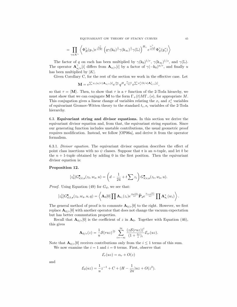
EQUIVARIANT GW THEORY OF STACKY CURVES 45
=∏
γ∈K∗
⟨Φγ
R(yγ)eαγr
u|R|
(qγ(k0)
1r γ(k∞)
1s γ(L)
)Hγ
eαγ−s
u|S| ΦγS(y
∗γ)
⟩
The factor of q on each has been multiplied by γ(k0)1/r, γ(k∞)1/s, and γ(L).
The operator Aγa/r[i] differs from Aa/r[i] by a factor of γ(−k0)
a/r, and finally u
has been multiplied by |K|.Given Corollary C, for the rest of the section we work in the effective case. Let
M = e∑
xi(a/r)Aa/r[i]eαrur qHe
α−sus e
∑x∗j (b/s)A
∗b/s[j],
so that τ = 〈M〉. Then, to show that τ is a τ function of the 2-Toda hiearchy, wemust show that we can conjugate M to the form Γ+(t)MΓ−(s), for appropriateM .This conjugation gives a linear change of variables relating the xi and x
∗i variables
of equivariant Gromov-Witten theory to the standard ti, si variables of the 2-Todahierarchy.
6.3. Equivariant string and divisor equations. In this section we derive theequivariant divisor equation and, from that, the equivariant string equation. Sinceour generating function includes unstable contributions, the usual geometric proofrequires modification. Instead, we follow [OP06a], and derive it from the operatorformalism.
6.3.1. Divisor equation. The equivariant divisor equation describes the effect ofpoint class insertions with no ψ classes. Suppose that r is an n-tuple, and let r bethe n + 1-tuple obtained by adding 0 in the first position. Then the equivariantdivisor equation is:
Proposition 12.
[z10 ]G•d,r,s(zr, ws, u) =
(d−
1
24+ t
∑zi
)G•
d,r,s(zr, ws, u).
Proof. Using Equation (49) for Gd, we see that:
[z10 ]G•d,r,s(zr, ws, u, q) =
⟨A0[0]
∏Ari
(zi)eαr(0)ur Pde
α−s(0)
us
∏A∗
si(wi)
⟩.
The general method of proof is to commute A0/r[0] to the right. However, we firstreplace A0/r[0] with another operator that does not change the vacuum expectationbut has better commutation properties.
Recall that A0/r[0] is the coefficient of z in A0. Together with Equation (46),this gives
A0/r(z) =1
uS(ruz)
tzr
∞∑
i=−∞
(zS(ruz))i
(1 + tzr )i
Eir(uz).
Note that A0/r[0] receives contributions only from the i ≤ 1 terms of this sum.We now examine the i = 1 and i = 0 terms. First, observe that
Er(uz) = αr +O(z)
and
E0(uz) =1
uz−1 + C + (H −
1
24)uz +O(z2).

46 PAUL JOHNSON
As the adjoints of both C and H annihilate the vacuum, as does any operator withpositive energy, we see that
A0/r[0] =1
uαr −
1
24+ . . . ,
where the dots are terms whose adjoint annihilates the vacuum. In fact, we findit convenient to include H in our operator, which does not change the vacuumexpectation, and so we have:
[z10 ]G•d,r,s(zr, ws, u, q) =
⟨(1
uαr +H −
1
24
)∏Ari
(zi)eαr(0)ur Pde
α−s(0)
us
∏A∗
si(wi)
⟩.
We now investigate the commutator of 1uαr +H − 1
24 with Aa/r(z).First, since
[αr, Ea+ir(uz)] = ς(urz)Ea+(i+1)r(uz),
we have[1
uαr,
∞∑
i=−∞
(zS(ruz))i
(1 + tz+ar )i
Eγir+a(uz)
]=
∞∑
i=−∞
(a+ ri+ tz)(zS(ruz))
i
(1 + tz+ar )i
Eγir+a(uz).
The sum here is the one that appears in the definition of Aa/r(z). The equalityfollows from the identity (1 + x+ y)(1 + x)y = (1 + x)1+y and a reindexing of thesum.
Observe that we also have
[H, Ea+ir(uz)] = −(a+ ir)Ea+ir(uz).
Canceling this from part of the previous commutator calculation gives[1
uαr +H,Aa/r(z)
]= tzAa/r(z),
and so commuting 1uαr + H − 1
24 past the Aa/r(z) produces the t∑zi factor
appearing in Proposition 12.Since [H,αr] = −rαr, we have
[1
uαr +H −
1
24, e
αrur
]= −
1
ue
αrur αr,
and so (1
uαr +H −
1
24
)e
αrur = e
αrur
(H −
1
24
),
and together with HPd = dPd, this finishes the proof of Proposition 12.
6.3.2. String equation. The equivariant string equation describes insertions of theidentity class in equivariant cohomology with no ψ classes. However, due to local-ization, we can express this in terms of insertions of 0(0, 0) and ∞(0, 0), as
1 =0(0)−∞(0)
t.
The following differential operator, then, inserts τ0(1):
(51) ∂ =1
t
(∂
∂y0(0)−
∂
∂y∗0(0)
).
To obtain an explicit form for the lowest equation of the hierarchy, we use thestring equation in the following form

EQUIVARIANT GW THEORY OF STACKY CURVES 47
Proposition 13.
⟨eτ0(1)
∏τki(0(ai/r))
∏τℓj (∞(bj/s))
⟩•
g,d
=[∏
zi(ai/r)ki+1
∏wj(bj/s)
ℓj+1]e∑
zi(ai/r)+∑
wj(bj/s)G•g,d(z, w, u).
6.4. 2-Toda: Explicit form of the lowest equation. Further following [OP06a],we now derive an explicit form of the lowest equation of the 2-Toda hierarchy inthe effective case.
6.4.1. The lowest equation of the 2-Toda hierarchy. As explained in [OP06a], oneway of writing the lowest form of the 2-Toda hierarcy is
(52)⟨T−1MT
⟩ ⟨TMT−1
⟩= 〈M〉 〈α1Mα−1〉 − 〈α1M〉 〈Mα−1〉 .
Here, T is the translation operator on∧∞
2 V :
T · i1 ∧ i2 ∧ · · · = i1 + 1 ∧ i2 + 1 ∧ · · · .
To derive the lowest equation of the hierarchy, we determine the effect of the inser-tions of the T and α operators on the τ function.
6.4.2. The α1 operator in terms of GW theory. We begin with the α1 operator. Thekey observation is that A1/r[1] is closely realated to the operator α1. Indeed, usingthe same reasoning as in the proof of the equivariant divisor equation (Proposition12), we see that
[z]A1/r(z) =1
uα1 + . . . ,
where the . . . are terms whose adjoint annihilates the vacuum, or possibly constantterms in case r = 1. We disregard the possibility of constant terms, as it is clearthat adding or removing a constant from either α1 or α−1 does not change thevalidity of Equation (52).
With this assumption, we have that
∂
∂x0(1/r)τ(x, x∗, u) = 〈(
1
uα1)M〉
and∂
∂x∗0(1/s)τ(x, x∗, u) = 〈M(
1
uα−1)〉.
Clearly this works for taking both derivatives as well, and so substituting intoEquation (52) gives
(53) τ∂2
∂x0(1/r)∂x∗0(1/s)τ −
∂
∂x∗0(1/s)τ
∂
∂x0(1/r)τ =
1
u2〈T−1MT 〉〈TMT−1〉.
6.4.3. Conjugation by T in terms of GW theory. We describe how conjugating M
by powers of T affects the τ function.We first describe how conjugating by T affects theA operators. The key equation
here is
T−1Er(z)T = ezEr(z),
which follows from the definition, with some care needed for E0. From this, itfollows that
T−1Aa/r(z)T = euzAa/r(z),

48 PAUL JOHNSON
and so conjugating by T multiplies each Ari(zi) by exp(ziu). By our form of
the equivariant string equation, Proposition 13, this is equivalent to applying theoperator eu∂ .
We now investigate how conjugating by T effects the remaining terms. Since αk
and T commute, the exponential terms remain unchanged, and we only need todetermine the effect on H:
T−nHTn = H + nC +n2
2.
Since C commutes with the A and the αk and annihilates the vacuum, its appear-
ance has no effect, and we may replace T−nqHTn with qn2/2qH . This gives
(54)⟨T−nMTn
⟩= qn
2/2enu∂τ
and so
(55)⟨T−1MT
⟩ ⟨TMT−1
⟩= qeu∂τe−u∂τ.
Equations (53) and (55) and a calculation give us the following form for thelowest equation of the 2-Toda hierachy.
Proposition 14. Suppose, r, s > 1. Then the τ function satisfies the following2-Toda equation:
∂2
∂x0(1/r)∂x∗0(1/s)log τ =
q
u2eu∂τe−u∂τ
τ2.
6.5. 2-Toda: The full hierarchy. We end by discussing that M can be conju-gated to the required form, and show the resulting linear change of variables fromthe Gromov-Witten times to the standard 2-Toda times. We treat all our matricesas operators acting on V , not on
∧∞2 V .
More particular, we want to show that there exists an upper triangular matrixWr, called the dressing matrix, so that
W−1r exp
(∑xi(a/r)Aa/r[i]
)Wr = Γ+(t).
This gives a linear change of variables between the 2-Toda time variables t and theGromov-Witten variables xi(a/r). Taking the adjoint and replacing t with −t, weset
W †s =W ∗
s |t 7→−t ,
so that
W †s exp
(∑x∗i (a/r)A
∗a/r[i]
) (W †
s
)−1= Γ−(v).
Then we have that
〈M〉 =⟨WrΓ+(t)MΓ−(v)W
†s
⟩,
with
M =W−1r e
αrur qHe
α−sus
(W †
s
)−1.
When Wr and W †s are upper triangular, we have
W ∗r v∅ =W †
s v∅ = v∅.
When Wr and W †s are unitriangular, we have in addition
(56) W ∗r T
nv∅ =W †s T
nv∅ = Tnv∅,

EQUIVARIANT GW THEORY OF STACKY CURVES 49
which implies
τn =⟨T−nMTn
⟩=
⟨T−nWrΓ+(t)MΓ−(v)W
†s T
n⟩=
⟨T−nΓ+(t)MΓ−(v)T
n⟩,
and hence that the τn were τ functions of the 2-Toda hierarchy.OurWr are upper triangular but not unitriangular. In this case τ0 is unchanged,
but the τn are multiplied by functions of q, u and t. This is not a problem, as the τnfor n 6= 0 are not a-priori related Gromov-Witten theory. Rather, τ0 is the originalGromov-Witten potential, and the τn are related to Gromov-Witten theory via
(54): τn = qn2/2enu∂τ0.
For k ≥ 0, the operators Aa/r[k] have the form
Aa/r[k] =
1auαa+kr + . . . a 6= 01uα(k+1)r + . . . a = 0
where the dots stand for terms of larger energy. Hence, there exists an uppertriangular matrix Wr so that
W−1r A1/r[0]Wr = α1.
Note that W is not unique - we can multiply Wr by an element that commuteswith α1.
Since the Aa/r[k] commute by Theorem 8, and have the form above, if we define
Aa/r[k] =WAa/r[k]W−1
then we have
(57) Aa/r[k] =∑
ℓ≤k+1
ca,k,ℓ(u, t)αa+ℓr,
since the Aa/r[k] commute with A1/r[0] = α1.
Corollary D: Integrability. After the change of variables, τCr,sis the tau function
for the 2-Toda hierarchy.
In fact, we have the following fact
Lemma 15. The coefficients ca,k,ℓ(u, t) are monomials in u, t.
The proof of Lemma 15 is somewhat involved, and again requires some hyper-geometric function identities. Since the proof is a straightforward adaptation ofSection 4.4.5 of [OP06a] (the Lemma itself being an analog of Propositions 14 and15 from [OP06a]), and the full proof is written out in [Joh], we do not give it here.
However, once this lemma is in hand, the change of variables follows easily. Ifthe ca,k,ℓ(u, t) are monomials, they are identical to their asymptotics as u→ 0, andso the full change of variables is equivalent to the change of variables in the u→ 0limit. But by Equation (46), in the u→ 0 limit, we have:
Aa/r(z) ∼1
u
tδr(0)z
(tz + a)
∞∑
i=−∞
zi
(1 + tz+ar )i
αir+a
and in the u→ 0 limit the operator Wr is diagonal, and we have, for a 6= 0:
∑
k≥0
zk+1Aa/r[k] =1
u
∑
n≥0
zn+1
∏ni=0(i+
tz+ar )
αa+nr

50 PAUL JOHNSON
and for a = 0: ∑
k≥0
zk+1A0/r[k] =1
u
∑
n≥1
zn∏ni=1(i+
tzr )αnr.
References
[AB84] M.F. Atiyah and R. Bott. The moment map and equivariant cohomology. Topology,23(1):1–28, 1984.
[AGV08] Dan Abramovich, Tom Graber, and Angelo Vistoli. Gromov-Witten theory of Deligne-Mumford stacks. Amer. J. Math., 130(5):1337–1398, 2008.
[ALR07] Alejandro Adem, Johann Leida, and Yongbin Ruan. Orbifolds and stringy topology.
Cambridge University Press, 2007.[CC09] Charles Cadman and Renzo Cavalieri. Gerby localization, Z3 Hodge integrals and the
GW theory of [C3/Z3]. Amer. J. Math., 131(4):1009–1046, 2009.[CR04] Weimin Chen and Yongbin Ruan. A new cohomology theory of orbifold. Comm. Math.
Phys., 248(1):1–31, 2004.[FMN] Barbara Fantechi, Etienne Mann, and Fabio Nironi. Smooth toric DM stacks. Preprint,
arXiv:0708.1254.[FW01] Igor Frenkel and Weiqiang Wang. Virasoro algebra and wreath product convolution.
J. Alg., 242:656–671, 2001.[GP99] Tom Graber and Rahul Pandharipande. Localization of virtual classes. Invent. Math.,
135(2):487–518, 1999.
[HHP+07] Simeon Hellerman, Andre Henriques, Tony Pantev, Eric Sharpe, and Matt Ando. Clus-ter decomposition, T-duality, and gerby CFTs. Adv. Theor. Math. Phys., 11(5):751–
818, 2007.[Joh] Paul Johnson. Equivariant Gromov-Witten theory of one dimensional stacks.
arXiv:0903.1068.[JPT11] Paul Johnson, Rahul Pandharipande, and Hsian-Hua Tseng. Abelian Hurwitz-Hodge
integrals. Michigan Mathematical Journal, 60(1), 2011.[KR87] V. G. Kac and A. K. Raina. Bombay lectures on highest weight representations of
infinite-dimensional Lie algebras. World Scientific Publishing Co., Inc., 1987.[LZ04] Sergei K. Lando and Alexander K. Zvonkin. Graphs on surfaces and their applications.
Encyclopaedia of Mathematical Sciences. Spring-Verlag, Berlin, 2004.
[MJD00] T. Miwa, M. Jimbo, and E. Date. Solitons: Differential Equations, Symmetries andInfinite Dimensional Algebras. Cambirdge University Press, 2000.
[MT08] Todor Milanov and Hsian-Hua Tseng. The spaces of Laurent polynomials, p1-orbifolds, and integrable hierarchies. Journal fur die Reine und Angewandte Math-ematik (Crelle’s Journal), 622:189–235, 2008.
[MT11] Todor Milanov and Hsian-Hua Tseng. Equivariant orbifold structures on the projectiveline and integrable hierarchies. Advances in Mathematics, 226(1):641–672, 2011.
[Oko00] Andrei Okounkov. Toda equations for Hurwitz numbers. Math. Res. Lett., 7(4):447–453, 2000.
[OP06a] Andrei Okounkov and Rahul Pandharipande. The equivariant Gromow-Witten theoryof P1. Ann. of Math. (2), 163(2):561–605, 2006.
[OP06b] Andrei Okounkov and Rahul Pandharipande. Gromov-Witten theory, Hurwitz theory,and completed cycles. Ann. of Math. (2), 163(2):517–560, 2006.
[OP06c] Andrei Okounkov and Rahul Pandharipande. Virasoro constraints for target curves.Invent. Math., 163(1):47–108, 2006.
[QW07] Zhenbo Qin and Weiqiang Wang. Hilbert schemes of points on the minimal resolutionand soliton equations. In Y.-Z. Huang and K. Misra, editors, Lie algebras, vertexoperator algebras and their applications, volume 442 of Contemp. Math., pages 435–462, (2007).
[Ros08] Paolo Rossi. Gromov-Witten invariants of target curves via symplectic field theory.
Journal of Geometry and Physics, 58(8):931–941, 2008.[Ros10] Paolo Rossi. Gromov-Witten theory of orbicurves, the space of tri-polynomials and
symplectic field theory of Seifert fibrations. Math. Ann., 348(2):265–287, 2010.[Rot] Mike Roth. Counting covers of an elliptic curve.
www.mast.queens.ca/ mikeroth/notes/covers.pdf.

EQUIVARIANT GW THEORY OF STACKY CURVES 51
[TT] Hsian-Hua Tseng and Xiang Tang. Duality theorems of etale gerbes on orbifolds.arXiv:1004.1376.
[ZZ12] HanXiong Zhang and Jian Zhou. Wreath Hurwitz numbers, colored cut-and-join equa-tions, and 2-Toda hierarchy. Sci. China Math., 55(8):1627–1646, 2012.