Research article

Plant species accumulation curves are determined by evenness and spatial aggregation in

drylands worldwide

Niv DeMalach1* (nivdemalach@gmail.com)

Hugo Saiz2

Eli Zaady3

Fernando T. Maestre2

1 Department of Ecology, Evolution and Behavior, The Hebrew University of Jerusalem, Givat

Ram, Jerusalem, 91904, Israel

2Departamento de Biología y Geología, Física y Química Inorgánica, Universidad Rey Juan

Carlos, c/ Tulipán s/n, 28933 Móstoles, Spain

3Department of Natural Resources, Institute of Plant Sciences, Agriculture Research

Organization, Ministry of Agriculture, Gilat Research Center, Gilat 85280, Israel

* Corresponding author: Tel. 972-2-6584659, Fax: 972-2-6858711

Key words: species area relationship, species richness, aridity, scale-dependence, pH,

biodiversity,

ABSTRACT

Species accumulation curves (SAC), i.e. the relationship between species richness and the

number of sampling units in a given community, can be used to describe diversity patterns while

accounting for the well-known scale-dependence of species richness. Despite their value, the

functional form and the parameters of SAC, as well as their determinants, have barely been

investigated in plant communities, particularly in drylands. We characterized the SAC of

perennial plant communities from 233 dryland ecosystems from six continents by comparing the

fit of major functions (power-law, logarithmic and Michaelis-Menten). We tested the theoretical

prediction that the effects of aridity and soil pH on SAC are mediated by vegetation attributes

such as evenness, cover, and spatial aggregation. We found that the logarithmic relationship was

the most common functional form, followed by Michaelis-Menten and power-law. Functional

form was mainly determined by evenness while the SAC parameters (intercept and slope) were

largely determined by spatial aggregation. In addition, aridity decreased small scale richness

(intercept of SAC) but did not affect accumulation rate (slope of the SAC). Our results highlight

the role that attributes such as spatial aggregation and evenness play as main mediators of the

SAC of vegetation in drylands, the Earth´s largest biome.

1. INTRODUCTION

Understanding how biodiversity varies in space and time is one of the main scientific challenges

of this century [1, 2]. Species richness, the number of species in a given area, is the simplest and

most used biodiversity index [e.g. 3, 4, 5]. However, species richness is extremely sensitive to

the spatial scale considered [6, 7], and this scale-dependence is a major source of divergence

among studies [8-10]. The main solution for this scale-dependence is the use of “Species-Area

Relationships” (hereafter SAR) when characterizing communities, which describe how the total

number of species varies as the sampled area increases [11, 12]. Here we focused on a common

SAR type known as ‘Species Accumulation Curve’ (hereafter SAC), which describes the

expected (mean) number of species as a function of the number of sampling units [13-15]. The

expected richness is computed based on all possible combination of sampling units (disregarding

their spatial location within a site). A main advantage of this computation approach is its ability

to produce a smooth curve (rather than a step function). This curve could be described by simple

mathematical functions [16]. Importantly, SAC is a specific type of SAR, since the size of the

area sampled is a linear function of the number of sampling units [‘SAR type III’, 17].

Ecological communities could vary both in the type of function that best characterizes their SAC

(hereafter ‘Functional form’) and in the parameter values of that function (hereafter ‘SAC

parameters’). The functional form of the SAC could be described by various functions [12] but

the simplest ones are power law (‘Arrhenius’), logarithmic (‘Gleason’) and Michaelis-Menten.

These functions differ in their degree of ‘saturation’ (i.e. the speed at which the slope of the

accumulation curve decreases), with Michaelis-Menten being the most ‘saturated’ function,

Logarithmic function being intermediate and Power-law being the least ‘saturated’ (Fig. 1).

Ecological models propose that both functional form and SAC parameters are determined by the

following proximate factors (hereafter mediators): density, evenness, spatial aggregation and

species pool [13, 18, 19]. Both density (number of individuals per area) and evenness (similarly

in relative abundance among species) increase richness at small spatial scales by increasing the

probability of species detection [18, 19]. Nonetheless, their effect on richness declines with

increasing the number of sampling units [13]. Spatial aggregation (intraspecific clustering in

spatial distribution) decreases richness at small scales since aggregated species are less likely to

be sampled, but this effect decreases as more sampling units are incorporated [13, 18, 19].

Species pool size (the number of species that could colonize a site as determined by evolutionary

and historical processes) has a positive effect on richness at all scales although its relative

importance should increase with increasing the number of sampling units[13].

A full understanding of SAC drivers includes a ‘causal cascade’ where abiotic factors affect the

mediators (e.g. pH affects evenness), thereby affecting SAC functional form and parameters[13].

Recently, the effect of the different mediators on scale-dependent richness response to gradients

was tested in animal communities [20]. In contrast, the effects of such mediators on plant SAC

was almost never studied despite the evidences that plant SACs (and other SAR types) are

affected by environmental gradients [9, 14, 21]. Here, we aimed to do so by using data gathered

from 233 dryland sites from six continents [22, 23]. Drylands cover 41% of Earth’s land surface

and support over 38% of the human population [22]. These drylands are threatened by global

land-use and climate changes that may further decrease water availability [24]. Previous studies

with this database have revealed that abiotic factors such as aridity and pH are main determinants

of diversity patterns at the site scale (30x30 M2)[25, 26] . However, their effect on SAC has

never been investigated. Hence, in this contribution we studied SAC patterns focusing on the

following questions:

(1) What is the relative role of different mediators (evenness, density, spatial aggregation and

species pool) in determining SAC patterns?

(2) How aridity and pH affect the SAC mediators? How these effects are translated into SAC

patterns?

2. METHODS

(a) Study area and fitting species accumulation curves

The study includes 233 sites representative of the major types of dryland vegetation from all

continents except Antarctica, which cover a wide range of plant species richness (from 2 to 49)

and environmental conditions (mean annual temperature and precipitation ranged from -1.8 to

28.2 ºC, and from 66 to 1219 mm, respectively). In all sites, vascular perennial vegetation was

sampled using a standardized protocol [22]. Each site included 80 sampling units (1.5x1.5m)

located along four 30-m length parallel transects (20 sampling units per transect, eight meters

distance between transects) where the presence and cover of each perennial species was

estimated. For each site, a species accumulation curve (SAC) was built using the ‘Vegan’ R

package [27]. Then, each SAC was fitted to the following functions:

(1) Power-law function: S = b0 ∙ Ab1

(2) Logarithmic function: S = b0 + b1 ∙ log (A)

(3) Michaelis-Menten function: S = b0 ∙A

b1 + A

In all functions, S is the number of species (the dependent variable), A is the number of sampling

units (the independent variable) and b0 and b1 are the two (estimated) parameters. The best

function for each site was chosen based on the lowest corrected Akaike Information Criterion

(AICc) of the fitted model [28].

(b) Mediators of species accumulation curve

We estimated potential mediators of SAC (spatial aggregation, evenness, density) using several

indices. As an index for spatial aggregation, we calculated the slope of the relationship between

the incidence (proportion of the sampling units where the species was found) and the log

abundance of each species. The steeper the slope, the more aggregated the plant community [see

29, 30 for details]. For evenness we used Pielou’s classical index [31]: 𝐻

𝐻max, where H is Shannon

entropy index and 𝐻max is the Shannon value obtained for the most even community with the

same number of species (i.e. a theoretical ‘ideal community’ where all species have equal

abundance). Cover (sum of the relative cover of different species) was used as a proxy for

density because we did not directly measured the number of individuals per area. Still, we

separated between the total cover of woody species (‘woody cover’) and total cover of perennial

herbs (‘herbaceous cover’) assuming the latter group may include more individuals for a given

cover (more herbs than shrubs could grow in a given level of cover due to their typically smaller

size).

The last mediator, species pool (the number of species that could colonize a site as determined

by evolutionary and historical processes) could not be estimated in our observational dataset.

Importantly, the common proxy for species pool, site richness (number of species found in a

given site when all sampling units are combined) is inevitably determined by SAC, which may

lead to a circular reasoning [32, 33]. Hence, we assessed the role of species pool only indirectly

as the sum of all the effects of aridity and pH which are not mediated by the other mediators (see

next sections for details).

(c) Classification of the functional forms

A classification tree was used for testing whether the potential mediators (spatial aggregation,

evenness, herbaceous cover and woody cover) were able to predict SAC functional form. The

analysis was conducted using the R package ‘party’, which allow unbiased recursive partitioning

based on conditional inference, thereby reducing the risk of overfitting [34]. Importantly,

although in most sites the differences (∆AICc) between the best model and the second best

model were high (median ∆AICc =107), nine sites where the AICc differences were lower than

seven (i.e. sites with high uncertainty regarding the best model) were excluded from this

classification analysis [35].

(d) Estimating the drivers of SAC parameters

We built a structural equation model (SEM) using the R package ‘piecewiseSEM’ that allows a

flexible analysis based on the local estimation method [36]. The SEM estimated the causal

effects of the potential mediators (spatial aggregation, evenness, herbaceous cover and woody

cover) as well as the abiotic factors, aridity (1-evaporation/precipitation) and soil pH [37]. The

model also included a ‘direct’ effect of aridity and pH on SAC parameters, which represent

effects that are independent of the mediators. Since theory suggests that species pool is the only

proximate factor (mediator) that can affect SAC besides spatial aggregation, evenness and

density [13], any ‘direct’ effect of aridity and pH could be interpreted as a species pool mediated

effect of these environmental factors.

Obviously, parameters of different SAC functional forms cannot be compared. Hence, we

applied the logarithmic functional form for all sites since this function had the highest

explanatory power across sites (the median R2 for all sites was 0.99), meaning that even in cases

where the model was not the ‘best’ in terms of AICc, it could still be used as an approximation.

Nonetheless, 14 sites where the R2

of logarithmic function was less than 0.90 were excluded

from the analysis to avoid large biases. The logarithmic function includes two coefficients, an

intercept (hereafter ‘small-scale richness’, b0) and a slope (hereafter ‘accumulation rate’, b1).

We transformed several variables to meet the assumptions of SEM: accumulation rate and

aggregation were log transformed while all the bounded indices (evenness, aridity, herbaceous

and woody cover) were logit transformed. In addition, and to avoid problems of spatial

autocorrelation (independence among nearby sites) we used Moran Eigenvectors Maps that were

built with the R package ‘adespatial’ [see 38]. The inclusion of these eigenvectors enables the

reduction of potential bias in parameter estimation caused by unmeasured factors related to

spatial autocorrelation such as disturbances, historical land-use or soil characteristics. For

reducing these confounding effects as much as possible (i.e. applying the most conservative

approach), we included all the 38 positive eigenvectors in all the relationships in the SEM. More

details on the model formulation are found in the electronic supplementary material.

3. RESULTS

All the three functional forms were found in the drylands studied (Fig. 2). The logarithmic

function was the most common (112 sites [48%]) followed by Michaelis-Menten (79 sites

[34%]) and power-law (42 sites [18%]) functions. Evenness was the only variable that predicted

SAC functional form in the classification tree, although its predictive power was relatively

modest (Fig. 3). Power-law and logarithmic relationships were (similarly) common under low

evenness levels. The logarithmic relationship was the most common form under intermediate

levels of evenness, while Michalis-Menten was the most common form under high levels of

evenness.

The results of the structural equation model (Fig 4) show the main determinants on SAC

intercept (b0, ‘small scale richness’) and slope (b1, ‘accumulation rate’). There was has a positive

effect of aridity on woody cover and evenness, and a negative effect on herbaceous cover. Still,

evenness had only a modest positive effect on small scale richness, and did not affect

accumulation rate. Furthermore, there was no effect of cover on any of the SAC parameters.

Aridity had no significant effects on spatial aggregation. In addition, there were negative effects

of pH on evenness and on small-scale richness. Interestingly, spatial aggregation was found to be

a main determinant of SAC parameters. Increasing aggregation reduced small-scale richness and

increased accumulation rate. Importantly, the strongest effects of aridity and pH on SAC were

‘direct’ effects on small scale richness (i.e. an effect that was not mediated by cover, aggregation

and evenness).

4. DISCUSSION

In this study we used, for the first time, species accumulation curves (SAC) for characterizing

the richness of perennial plants in drylands worldwide. We found that SAC functional form is

mainly determined by evenness and that SAC parameters are mainly determined by aggregation.

In addition, we found that aridity decreases small scale richness (b0, the intercept of the SAC) but

does not affect accumulation rate (b1, the slope of the SAC).

Debates regarding SAR functional forms date back to the beginning of the 20th

century [12]. So

far, the most common approach for describing SAR is based on the power-law function [12, 39].

While theoretical models suggest that SAR should become more ‘saturated’ (lower second

derivative) as evenness increases [13, 19], a recent review of SAR functions found these

suggestions unsupported by empirical data [12]. Our findings are fully consisted with theoretical

models [13, 19]. The most even communities were characterized mostly the asymptotic

Michaelis-Menten SAC. Communities with intermediate levels of evenness were mostly

characterized by the logarithmic function that tends to ‘saturate’ faster than power law.

Communities with high evenness were characterized by power law or logarithmic functions in

similar proportion. Still, we found that evenness cannot fully predict the SAC functional form

suggesting that there are possible important unmeasured factors (e.g. species pool). Small

species pool of drylands (which could be lead to asymptotic relationship) may explain the low

proportion of power-law SAC found in our study (18%). Many previous vegetation SAR were

documented in tropical forests with larger species pool [39] which could increase the proportion

of the power law functional form. In addition, most previous studies investigated other type of

SAR rather than SAC [39]. Hence, it remained to be tested whether the differences between our

results and previous studies reflect differences between drylands vegetation and other systems or

differences between SAC and other SAR types.

Interestingly, in most communities (c. 96%) the different functional forms were very

distinguishable (AICc > 7). In contrast with other SAR types (where different functions are not

always distinguishable [12, 39]), SACs are smooth functions with large ‘sample size’ (sample

size equals the amount of sampling unit) allowing high statistical power. However, despite the

detectable differences between functional forms we found that the logarithmic function could be

used as approximation for all SAC since its bias is relativity small as indicated by the high

explanatory power (R2

> 0.90 for 94% of the sites).

The structural equation model did not support our expectation that the effects of aridity and pH

on SAC parameters should be mediated by aggregation, cover and evenness. Although aridity

decreased herbaceous cover, there were no effects of cover on SAC parameters. A possible

explanation for this finding is that woody and herbaceous covers are not good indicators of

density in this dataset. In addition, evenness increased with aridity and decreased with increasing

soil pH but the positive effect of evenness on small scale richness was modest. We found that

SAC parameters were mostly affected by our spatial aggregation index [29]. Aggregation

decreased small scale richness but increased accumulation rate. Again, this finding is in

accordance with theory but has rarely been supported by empirical data [19]. Furthermore, our

approach underestimates the role of aggregation since our index quantifies only aggregation at

the sampling unit level. Nevertheless, it is possible that aggregation occurring across other scales

could also affect SAC parameters. Surprisingly, while aggregation is an important mediator of

SAC parameters, it was not affected by aridity or pH. Hence, the drivers of aggregations remain

to be tested in future studies.

We found a ‘direct’ negative effect of aridity on small scale richness and a modest positive effect

of pH on small scale richness. These effects may represent unmeasured factors such as historical

and evolutionary processes leading to small species pool in more arid and more acidic sites.

Unfortunately, this interpretation could not be rigorously tested using our dataset due to the

difficulty in defining the species pool [32, 33]. Additionally, underestimation of the roles

aggregation and density (see above) may also lead to overestimation of a ‘direct’ effect of aridity

and pH [40].

CONCLUSIONS

Our findings support untested theoretical predictions [13, 18, 19] and question the automatic use

of power law functions to describe SARs. The findings that evenness and spatial aggregation are

main mediators of SAC highlight the role of understanding their main drivers (e.g. competition,

heterogeneity, dispersal). Hence, we suggest that future theoretical and empirical studies will

focus on the mechanism of spatial aggregation and evenness that determine diversity in several

scales instead of focusing on species number in a given (arbitrary) scale.

The link between functional form and evenness has important implications for conservation as

well as for any efforts to characterize the number of species in a given area. While it is

reasonable to expect an asymptote (when enough sampling units are sampled) in even

communities that tend to ‘saturate’, uneven communities are unlikely to reach an asymptote.

Thus, uneven communities inevitably require extrapolation methods for estimating the total

number of species [41]. In addition, the important role of aggregation in determining SAC slope

highlights the bias obtained from simple extrapolation from small scales (often used for

experiments) to large scales (the target of conservation efforts). Such extrapolation will

underestimate the number of species in large areas where species show high aggregated spatial

dispersion while overestimating species number in communities with low spatial aggregation.

DATA ACCESSIBILITY

Data is available on figshare: https://figshare.com/s/b4010a4331d73d99239f

AUTHORS' CONTRIBUTIONS

F.T.M. designed the field surveys and N.D. designed the data analysis. N.D. and H.S. analyzed

the data. The first draft was written by N.D and all authors contributed substantially to revisions.

COMPETING INTERESTS

We declare we have no competing interests.

FUNDING

This work was funded by the European Research Council under the European Community’s

Seventh Framework Program (FP7/2007-2013)/ERC Grant agreement 242658 (BIOCOM). FTM

and HS are supported by the European Research Council (ERC Grant agreement 647038

[BIODESERT]). HS is supported by a Juan de la Cierva-Formación grant from MINECO.

ACKNOWLEDGMENT

We thank all the members of the EPES-BIOCOM network for the collection of field data, all the

members of the Maestre lab for their help with data organization and management and Ron Milo

for comments on previous versions of this manuscript.

REFERENCES

[1] Pennisi, E. 2005 What Determines Species Diversity? Science 309, 90. [2] Sala, O. E., Chapin, F. S., III, Armesto, J. J., Berlow, E., Bloomfield, J., Dirzo, R., Huber-Sanwald, E., Huenneke, L. F., Jackson, R. B., Kinzig, A., et al. 2000 Biodiversity - Global biodiversity scenarios for the year 2100. Science 287, 1170-1174. [3] Soons, M. B., Hefting, M. M., Dorland, E., Lamers, L. P. M., Versteeg, C. & Bobbink, R. 2017 Nitrogen effects on plant species richness in herbaceous communities are more widespread and stronger than those of phosphorus. Biological Conservation. (DOI:http://dx.doi.org/10.1016/j.biocon.2016.12.006). [4] DeMalach, N., Zaady, E. & Kadmon, R. 2017 Contrasting effects of water and nutrient additions on grassland communities: A global meta-analysis. Global Ecology and Biogeography 26, 983-992. (DOI:10.1111/geb.12603). [5] Vellend, M., Dornelas, M., Baeten, L., Beausejour, R., Brown, C. D., De Frenne, P., Elmendorf, S. C., Gotelli, N. J., Moyes, F., Myers-Smith, I. H., et al. 2017 Estimates of local biodiversity change over time stand up to scrutiny. Ecology 98, 583-590. (DOI:10.1002/ecy.1660). [6] Whittaker, R. J., Willis, K. J. & Field, R. 2001 Scale and species richness: towards a general, hierarchical theory of species diversity. Journal of Biogeography 28, 453-470. (DOI:10.1046/j.1365-2699.2001.00563.x). [7] Rahbek, C. 2005 The role of spatial scale and the perception of large-scale species-richness patterns. Ecology Letters 8, 224-239. (DOI:10.1111/j.1461-0248.2004.00701.x). [8] Mittelbach, G. G., Steiner, C. F., Scheiner, S. M., Gross, K. L., Reynolds, H. L., Waide, R. B., Willig, M. R., Dodson, S. I. & Gough, L. 2001 What is the observed relationship between species richness and productivity? Ecology 82, 2381-2396. (DOI:10.1890/0012-9658(2001)082[2381:witorb]2.0.co;2). [9] Chiarucci, A., Viciani, D., Winter, C. & Diekmann, M. 2006 Effects of productivity on species-area curves in herbaceous vegetation: evidence from experimental and observational data. Oikos 115, 475-483. (DOI:10.1111/j.2006.0030-1299.15116.x). [10] Weiher, E. 1999 The combined effects of scale and productivity on species richness. Journal of Ecology 87, 1005-1011. (DOI:10.1046/j.1365-2745.1999.00412.x). [11] Scheiner, S. M. 2003 Six types of species-area curves. Global Ecology and Biogeography 12, 441-447. (DOI:10.1046/j.1466-822X.2003.00061.x). [12] Dengler, J. 2009 Which function describes the species-area relationship best? A review and empirical evaluation. Journal of Biogeography 36, 728-744. (DOI:10.1111/j.1365-2699.2008.02038.x). [13] Chase, J. M. & Knight, T. M. 2013 Scale-dependent effect sizes of ecological drivers on biodiversity: why standardised sampling is not enough. Ecology Letters 16, 17-26. (DOI:10.1111/ele.12112). [14] Harvey, E. & MacDougall, A. S. 2018 Non-interacting impacts of fertilization and habitat area on plant diversity via contrasting assembly mechanisms. Diversity and Distributions, in press. (DOI:10.1111/ddi.12697). [15] Ugland, K. I., Gray, J. S. & Ellingsen, K. E. 2003 The species-accumulation curve and estimation of species richness. Journal of Animal Ecology 72, 888-897. (DOI:10.1046/j.1365-2656.2003.00748.x). [16] Gray, J. S., Ugland, K. I. & Lambshead, J. 2004 Species accumulation and species area curves - a comment on Scheiner (2003). Global Ecology and Biogeography 13, 473-476. (DOI:10.1111/j.1466-822X.2004.00114.x). [17] Scheiner, S. M., Chiarucci, A., Fox, G. A., Helmus, M. R., McGlinn, D. J. & Willig, M. R. 2011 The underpinnings of the relationship of species richness with space and time. Ecological Monographs 81, 195-213. (DOI:10.1890/10-1426.1). [18] He, F. L. & Legendre, P. 2002 Species diversity patterns derived from species-area models. Ecology 83, 1185-1198. (DOI:10.2307/3071933).

[19] Tjorve, E., Kunin, W. E., Polce, C. & Tjorve, K. M. C. 2008 Species-area relationship: separating the effects of species abundance and spatial distribution. Journal of Ecology 96, 1141-1151. (DOI:10.1111/j.1365-2745.2008.01433.x). [20] Blowes, S. A., Belmaker, J. & Chase, J. M. 2017 Global reef fish richness gradients emerge from divergent and scale-dependent component changes. Proceedings of the Royal Society B: Biological Sciences 284. [21] Shmida, A. & Wilson, M. V. 1985 Biological Determinants of Species Diversity. Journal of Biogeography 12, 1-20. (DOI:10.2307/2845026). [22] Maestre, F. T., Quero, J. L., Gotelli, N. J., Escudero, A., Ochoa, V., Delgado-Baquerizo, M., Garcia-Gomez, M., Bowker, M. A., Soliveres, S., Escolar, C., et al. 2012 Plant Species Richness and Ecosystem Multifunctionality in Global Drylands. Science 335, 214-218. (DOI:10.1126/science.1215442). [23] Ochoa-Hueso, R., Eldridge, D. J., Delgado-Baquerizo, M., Soliveres, S., Bowker, M. A., Gross, N., Le Bagousse-Pinguet, Y., Quero, J. L., Garcia-Gomez, M., Valencia, E., et al. 2018 Soil fungal abundance and plant functional traits drive fertile island formation in global drylands. Journal of Ecology 106, 242-253. (DOI:10.1111/1365-2745.12871). [24] Reynolds, J. F., Stafford Smith, D. M., Lambin, E. F., Turner, B. L., Mortimore, M., Batterbury, S. P. J., Downing, T. E., Dowlatabadi, H., Fernandez, R. J., Herrick, J. E., et al. 2007 Global desertification: Building a science for dryland development. Science 316, 847-851. (DOI:10.1126/science.1131634). [25] Soliveres, S., Maestre, F. T., Eldridge, D. J., Delgado-Baquerizo, M., Quero, J. L., Bowker, M. A. & Gallardo, A. 2014 Plant diversity and ecosystem multifunctionality peak at intermediate levels of woody cover in global drylands. Global Ecology and Biogeography 23, 1408-1416. (DOI:10.1111/geb.12215). [26] Ulrich, W., Soliveres, S., Maestre, F. T., Gotelli, N. J., Quero, J. L., Delgado-Baquerizo, M., Bowker, M. A., Eldridge, D. J., Ochoa, V., Gozalo, B., et al. 2014 Climate and soil attributes determine plant species turnover in global drylands. Journal of Biogeography 41, 2307-2319. (DOI:10.1111/jbi.12377). [27] Oksanen, J., Blanchet, F. G., Kindt, R., Legendre, P., Minchin, P. R., O’hara, R. B., Simpson, G. L., Solymos, P., Stevens, M. H. H. & Wagner, H. 2013 Package ‘vegan’. Community ecology package, version 2. [28] Grueber, C. E., Nakagawa, S., Laws, R. J. & Jamieson, I. G. 2011 Multimodel inference in ecology and evolution: challenges and solutions. Journal of Evolutionary Biology 24, 699-711. (DOI:10.1111/j.1420-9101.2010.02210.x). [29] Wright, D. H. 1991 Correlations between incidence and abundance are expected by chance. Journal of Biogeography 18, 463-466. (DOI:10.2307/2845487). [30] Hartley, S. 1998 A positive relationship between local abundance and regional occupancy is almost inevitable (but not all positive relationships are the same). Journal of Animal Ecology 67, 992-994. (DOI:10.1046/j.1365-2656.1998.6760992.x). [31] Smith, B. & Wilson, J. B. 1996 A consumer's guide to evenness indices. Oikos, 70-82. [32] Herben, T. 2000 Correlation between richness per unit area and the species pool cannot be used to demonstrate the species pool effect. Journal of Vegetation Science 11, 123-126. (DOI:10.2307/3236783). [33] Švamberková, E., Vítová, A. & Lepš, J. 2017 The role of biotic interactions in plant community assembly: What is the community species pool? Acta Oecologica 85, 150-156. [34] Hothorn, T., Hornik, K. & Zeileis, A. 2006 Unbiased recursive partitioning: A conditional inference framework. Journal of Computational and Graphical Statistics 15, 651-674. (DOI:10.1198/106186006x133933). [35] Ulrich, W., Soliveres, S., Thomas, A. D., Dougill, A. J. & Maestre, F. T. 2016 Environmental correlates of species rank abundance distributions in global drylands. Perspectives in Plant Ecology Evolution and Systematics 20, 56-64. (DOI:10.1016/j.ppees.2016.04.004).

[36] Lefcheck, J. S. 2016 PIECEWISESEM: Piecewise structural equation modelling in R for ecology, evolution, and systematics. Methods in Ecology and Evolution 7, 573-579. (DOI:10.1111/2041-210x.12512). [37] Delgado-Baquerizo, M., Maestre, F. T., Reich, P. B., Jeffries, T. C., Gaitan, J. J., Encinar, D., Berdugo, M., Campbell, C. D. & Singh, B. K. 2016 Microbial diversity drives multifunctionality in terrestrial ecosystems. Nature Communications 7. (DOI:10.1038/ncomms10541). [38] Dray, S., Pelissier, R., Couteron, P., Fortin, M. J., Legendre, P., Peres-Neto, P. R., Bellier, E., Bivand, R., Blanchet, F. G., De Caceres, M., et al. 2012 Community ecology in the age of multivariate multiscale spatial analysis. Ecological Monographs 82, 257-275. (DOI:10.1890/11-1183.1). [39] Drakare, S., Lennon, J. J. & Hillebrand, H. 2006 The imprint of the geographical, evolutionary and ecological context on species-area relationships. Ecology Letters 9, 215-227. (DOI:10.1111/j.1461-0248.2005.00848.x). [40] Freckleton, R. P. 2011 Dealing with collinearity in behavioural and ecological data: model averaging and the problems of measurement error. Behavioral Ecology and Sociobiology 65, 91-101. (DOI:10.1007/s00265-010-1045-6). [41] Walther, B. A. & Moore, J. L. 2005 The concepts of bias, precision and accuracy, and their use in testing the performance of species richness estimators, with a literature review of estimator performance. Ecography 28, 815-829. (DOI:10.1111/j.2005.0906-7590.04112.x).

FIGURE CAPTIONS

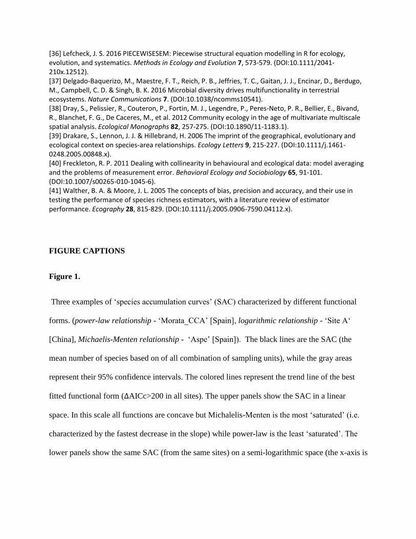
Figure 1.

Three examples of ‘species accumulation curves’ (SAC) characterized by different functional

forms. (power-law relationship - ‘Morata_CCA’ [Spain], logarithmic relationship - ‘Site A‘

[China], Michaelis-Menten relationship - ‘Aspe’ [Spain]). The black lines are the SAC (the

mean number of species based on of all combination of sampling units), while the gray areas

represent their 95% confidence intervals. The colored lines represent the trend line of the best

fitted functional form (∆AICc>200 in all sites). The upper panels show the SAC in a linear

space. In this scale all functions are concave but Michalelis-Menten is the most ‘saturated’ (i.e.

characterized by the fastest decrease in the slope) while power-law is the least ‘saturated’. The

lower panels show the same SAC (from the same sites) on a semi-logarithmic space (the x-axis is

logarithmic). In this scale power-law function is convex, logarithmic function is linear and

Michaelis-Menten function is concave.

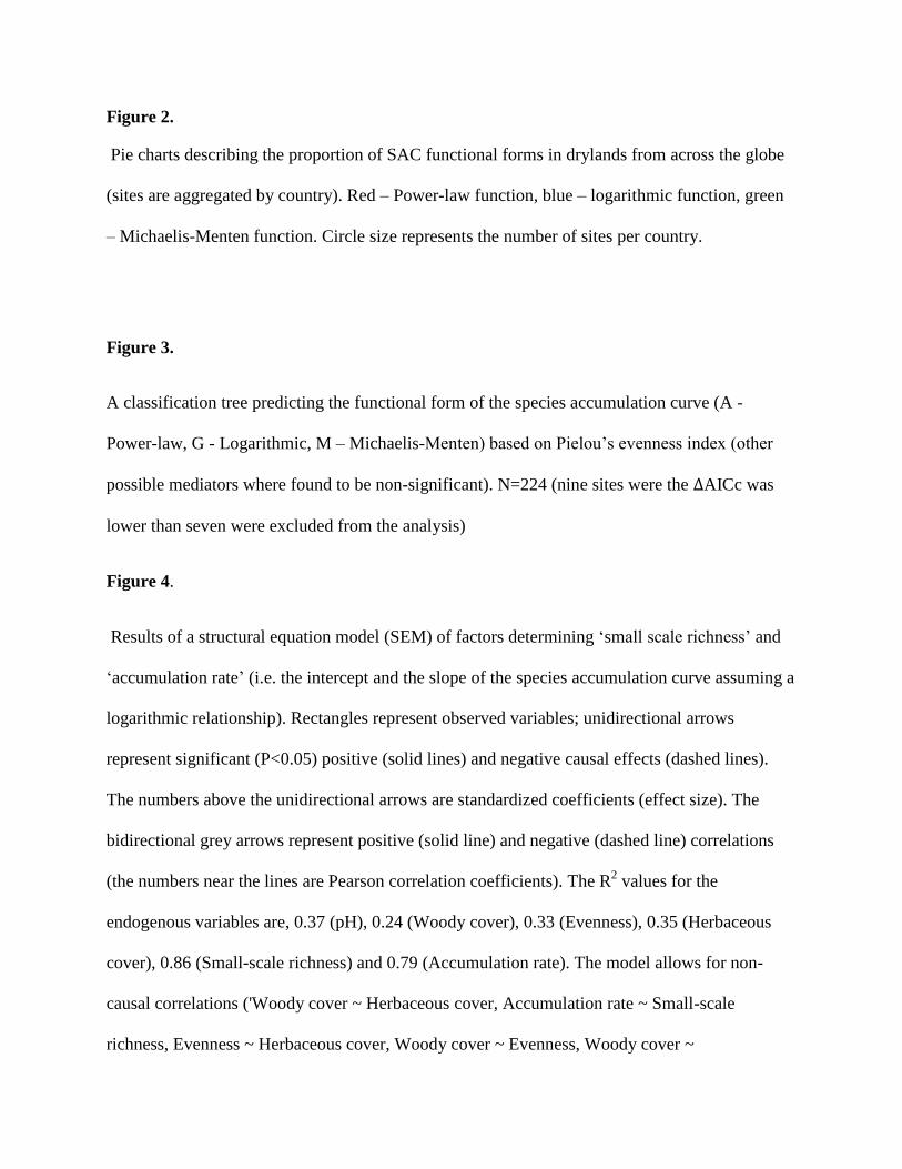
Figure 2.

Pie charts describing the proportion of SAC functional forms in drylands from across the globe

(sites are aggregated by country). Red – Power-law function, blue – logarithmic function, green

– Michaelis-Menten function. Circle size represents the number of sites per country.

Figure 3.

A classification tree predicting the functional form of the species accumulation curve (A -

Power-law, G - Logarithmic, M – Michaelis-Menten) based on Pielou’s evenness index (other

possible mediators where found to be non-significant). N=224 (nine sites were the ∆AICc was

lower than seven were excluded from the analysis)

Figure 4.

Results of a structural equation model (SEM) of factors determining ‘small scale richness’ and

‘accumulation rate’ (i.e. the intercept and the slope of the species accumulation curve assuming a

logarithmic relationship). Rectangles represent observed variables; unidirectional arrows

represent significant (P<0.05) positive (solid lines) and negative causal effects (dashed lines).

The numbers above the unidirectional arrows are standardized coefficients (effect size). The

bidirectional grey arrows represent positive (solid line) and negative (dashed line) correlations

(the numbers near the lines are Pearson correlation coefficients). The R2 values for the

endogenous variables are, 0.37 (pH), 0.24 (Woody cover), 0.33 (Evenness), 0.35 (Herbaceous

cover), 0.86 (Small-scale richness) and 0.79 (Accumulation rate). The model allows for non-

causal correlations ('Woody cover ~ Herbaceous cover, Accumulation rate ~ Small-scale

richness, Evenness ~ Herbaceous cover, Woody cover ~ Evenness, Woody cover ~

Aggregation). The model is in agreement with the data (local estimation, AICc =-1581,

Fisher.C=6.99, p-value=0.14). All the parameters of the model are summarized in table S1.

N=219

FIGURES

Figure 1.

Figure 2.

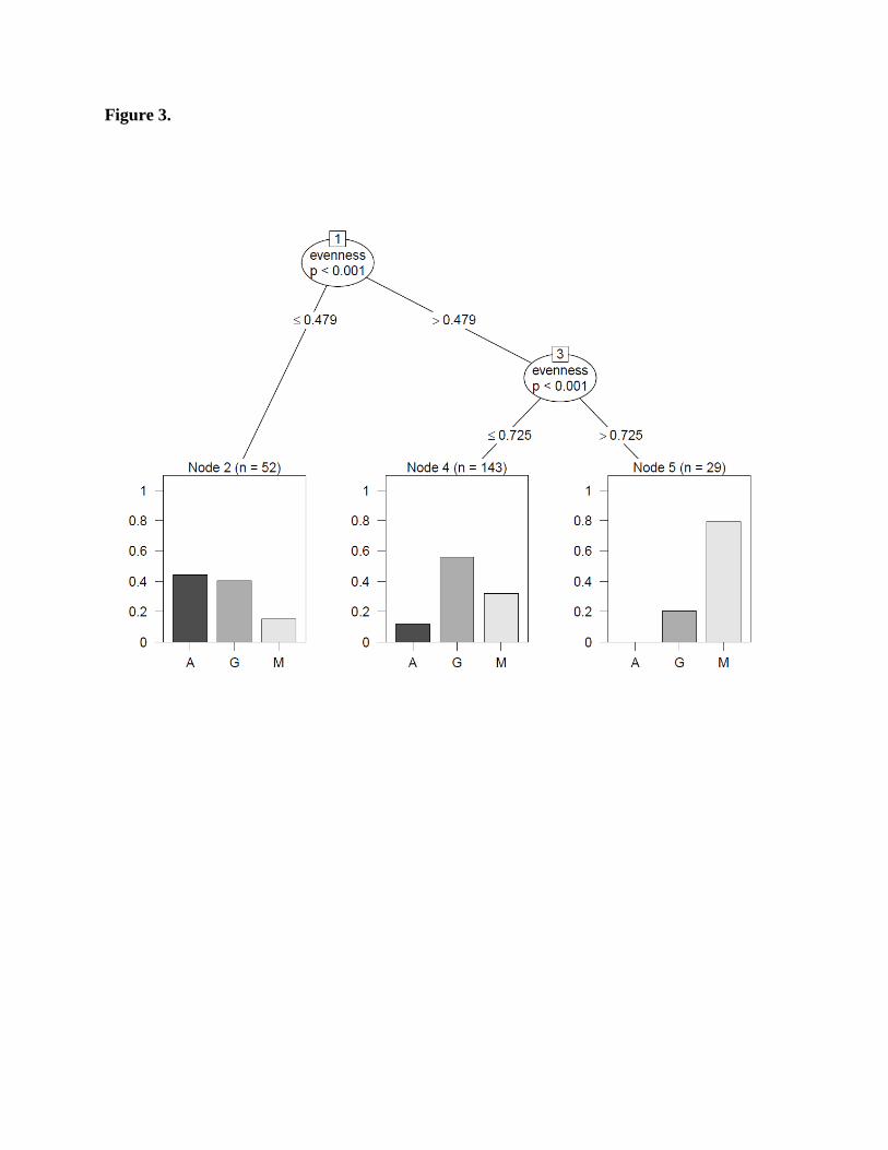
Figure 3.

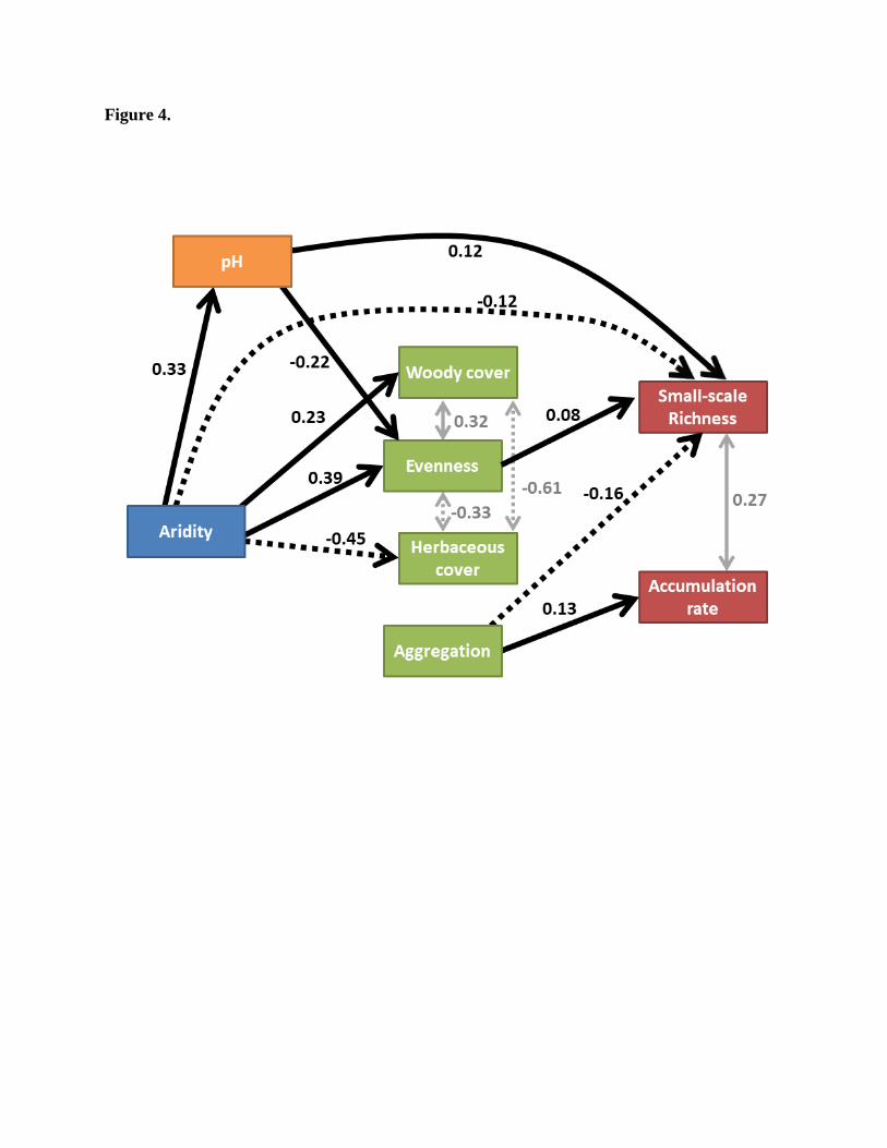
Figure 4.

SUPPLEMENTARY MATERIAL

The structural equation model

The model includes the seven following equations:

(1) pH= α11 + α12 Aridity + α13Spatial eigenvectors+ e1

(2) Woody_Cover = α21 + α22 Aridity + α23 pH + spatial eigenvectors + e2

(3) Evenness = α31 + α32 Aridity + α33 pH + α34Spatial eigenvectors + e3

(4) Herbaceous_Cover = α41 + α42 Aridity + α43 pH + α44Spatial eigenvectors + e4

(5) Aggregation = α51 + α52 Aridity + α53 pH + α55Spatial eigenvectors + e5

(6) Small_Scale_Richness = α61 + α62 Woody_Cover + α63 Evenness +

α64 Herbaceous_Cover + α65 Aggregation +α66Aridity + α67 pH + α68Spatial

eigenvectors + e6

(7) Accumulation_Rate = α71 + α72 Woody_Cover + α73 Evenness + α74Herbaceous_Cover +

α75Aggregation+ α76 Aridity + α77 pH + α78Spatial eigenvectors + e7

Equation 1 describes the effect of Aridity on pH. Equations 2-5 describe the effects of Aridity

and pH on the following variables: Woody_cover, Evenness, Herbaceous_Cover and

Aggregation (hereafter ‘mediators’). Equations 6-7 describe the effects Aridity and pH and the

mediators on Local_Scale_Richness and Accumulation_Rate (the intercept and the slope of the

species accumulation curve assuming logarithmic relationship). The notions e1-e7 represent the

error terms.

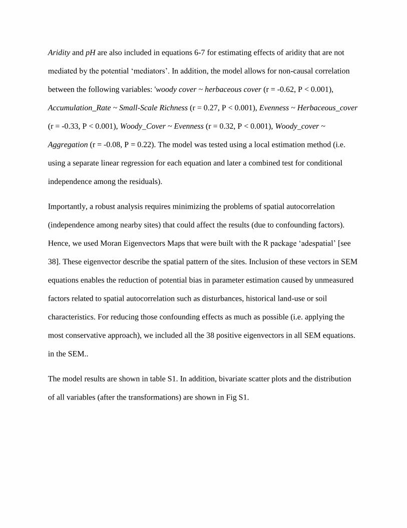
Aridity and pH are also included in equations 6-7 for estimating effects of aridity that are not

mediated by the potential ‘mediators’. In addition, the model allows for non-causal correlation

between the following variables: 'woody cover ~ herbaceous cover (r = -0.62, P < 0.001),

Accumulation_Rate ~ Small-Scale Richness (r = 0.27, P < 0.001), Evenness ~ Herbaceous_cover

(r = -0.33, P < 0.001), Woody_Cover ~ Evenness (r = 0.32, P < 0.001), Woody_cover ~

Aggregation (r = -0.08, P = 0.22). The model was tested using a local estimation method (i.e.

using a separate linear regression for each equation and later a combined test for conditional

independence among the residuals).

Importantly, a robust analysis requires minimizing the problems of spatial autocorrelation

(independence among nearby sites) that could affect the results (due to confounding factors).

Hence, we used Moran Eigenvectors Maps that were built with the R package ‘adespatial’ [see

38]. These eigenvector describe the spatial pattern of the sites. Inclusion of these vectors in SEM

equations enables the reduction of potential bias in parameter estimation caused by unmeasured

factors related to spatial autocorrelation such as disturbances, historical land-use or soil

characteristics. For reducing those confounding effects as much as possible (i.e. applying the

most conservative approach), we included all the 38 positive eigenvectors in all SEM equations.

in the SEM..

The model results are shown in table S1. In addition, bivariate scatter plots and the distribution

of all variables (after the transformations) are shown in Fig S1.

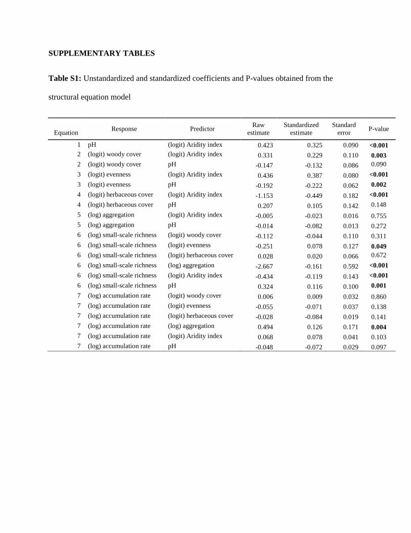
SUPPLEMENTARY TABLES

Table S1: Unstandardized and standardized coefficients and P-values obtained from the

structural equation model

Equation Response Predictor

Raw

estimate

Standardized

estimate

Standard

error P-value

1 pH (logit) Aridity index 0.423 0.325 0.090 <0.001

2 (logit) woody cover (logit) Aridity index 0.331 0.229 0.110 0.003

2 (logit) woody cover pH -0.147 -0.132 0.086 0.090

3 (logit) evenness (logit) Aridity index 0.436 0.387 0.080 <0.001

3 (logit) evenness pH -0.192 -0.222 0.062 0.002

4 (logit) herbaceous cover (logit) Aridity index -1.153 -0.449 0.182 <0.001

4 (logit) herbaceous cover pH 0.207 0.105 0.142 0.148

5 (log) aggregation (logit) Aridity index -0.005 -0.023 0.016 0.755

5 (log) aggregation pH -0.014 -0.082 0.013 0.272

6 (log) small-scale richness (logit) woody cover -0.112 -0.044 0.110 0.311

6 (log) small-scale richness (logit) evenness -0.251 0.078 0.127 0.049

6 (log) small-scale richness (logit) herbaceous cover 0.028 0.020 0.066 0.672

6 (log) small-scale richness (log) aggregation -2.667 -0.161 0.592 <0.001

6 (log) small-scale richness (logit) Aridity index -0.434 -0.119 0.143 <0.001

6 (log) small-scale richness pH 0.324 0.116 0.100 0.001

7 (log) accumulation rate (logit) woody cover 0.006 0.009 0.032 0.860

7 (log) accumulation rate (logit) evenness -0.055 -0.071 0.037 0.138

7 (log) accumulation rate (logit) herbaceous cover -0.028 -0.084 0.019 0.141

7 (log) accumulation rate (log) aggregation 0.494 0.126 0.171 0.004

7 (log) accumulation rate (logit) Aridity index 0.068 0.078 0.041 0.103

7 (log) accumulation rate pH -0.048 -0.072 0.029 0.097

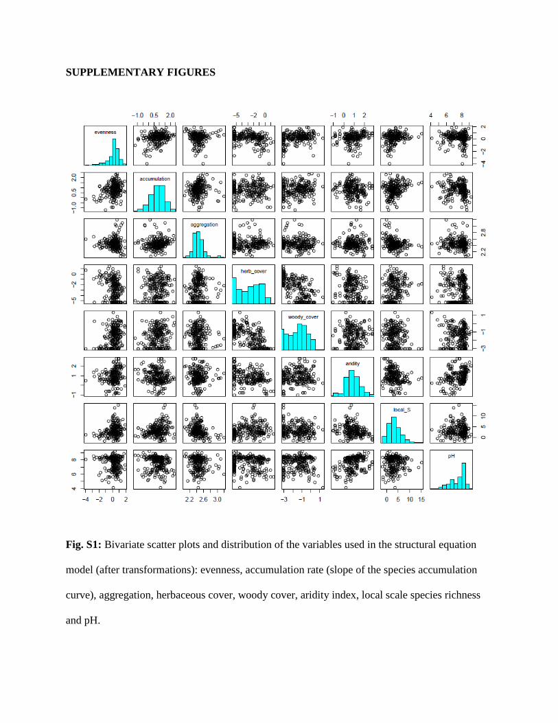
SUPPLEMENTARY FIGURES

Fig. S1: Bivariate scatter plots and distribution of the variables used in the structural equation

model (after transformations): evenness, accumulation rate (slope of the species accumulation

curve), aggregation, herbaceous cover, woody cover, aridity index, local scale species richness

and pH.