Holographic Axion Model:A simple gravitational tool for quantum matter

Matteo Baggioli,1, 2, 3, ∗ Keun-Young Kim,4, † Li Li,5, 6, 7, ‡ and Wei-Jia Li8, §1Wilczek Quantum Center, School of Physics and Astronomy,

Shanghai Jiao Tong University, Shanghai 200240, China2Shanghai Research Center for Quantum Sciences, Shanghai 201315, China.

3Instituto de Fisica Teorica UAM/CSIC, Universidad Autonoma de Madrid, Madrid 28049, Spain.4School of Physics and Chemistry, Gwangju Institute of Science and Technology,

Gwangju 61005, Korea.5CAS Key Laboratory of Theoretical Physics, Institute of Theoretical Physics,

Chinese Academy of Sciences, Beijing 100190, China6School of Physical Sciences, University of Chinese Academy of Sciences,

Beijing 100049, China7School of Fundamental Physics and Mathematical Sciences, Hangzhou Institute for Advanced Study,

University of Chinese Academy of Sciences, Hangzhou 310024, China8Institute of Theoretical Physics, School of Physics,

Dalian University of Technology, Dalian 116024, China.

This is a complete and exhaustive review on the so-called holographic axion model – a bottom-upholographic system characterized by the presence of a set of shift symmetric scalar bulk fields whoseprofiles are taken to be linear in the spatial coordinates. This simple model implements the breakingof translational invariance of the dual field theory by retaining the homogeneity of the backgroundgeometry and therefore allowing for controllable and fast computations. The usages of this modelare very vast and they are a proof of the spectacular versatility of the framework. In this review, wetouch upon all the up-to-date aspects of this model from its connection with massive gravity andeffective field theories, to its role in modeling momentum dissipation and elastic properties endingwith all the phenomenological features and its hydrodynamic description. In summary, this is acomplete guide to one of the most used models in Applied Holography and a must-read for anyresearcher entering this field.

Keywords: gauge/gravity duality, holographic axion, translational symmetry breaking, effectivefield theoryPACS numbers: 11.25.Tq, 04.70.Bw, 52.25.Fi, 73.22.Gk

CONTENTS

I. Introduction 2A. Scope of this review 3B. The Drude model 3C. Effective field theories for solids and fluids 5D. Gauge-Gravity duality briefing 8E. Holographic axion model 10F. From inhomogeneous lattices to massive

gravity and homogeneous models 10G. Other holographic homogeneous models 11

II. A simple model for momentum relaxation 12A. The origins 12B. A holographic Drude model 12C. Coherent-incoherent transition 14D. DC conductivities from horizon data 16

∗ b.matteo@sjtu.edu.cn† fortoe@gist.ac.kr‡ liliphy@itp.ac.cn§ weijiali@dlut.edu.cn

E. Thermoelectric transport 17

III. Breaking translations spontaneously 17A. Axion model 2.0 17B. From explicit breaking to spontaneous

breaking 18C. Elastic black holes 18D. Holographic phonons 19E. Zoology of solids and fluids 21F. The dual view 21

IV. On the hydrodynamic description 22A. A puzzle 22B. Strain pressure and its resolution 23C. The hydrodynamics of phonons 24D. Zero strain pressure and stability 25E. Phasons dynamics 25F. The dynamics of shear waves with

momentum dissipation 26

V. Bounds from hydrodynamics and holography 27A. The violation of the KSS bound 27B. From viscosity to diffusion 29C. Butterfly velocity and chaos 30

arX

iv:2

101.

0189

2v2

[he

p-th

] 2

2 Fe

b 20

21

2

D. Pole-skipping and the complex plane 30E. Bounds on thermal and crystal diffusion 33F. Diffusion bound from causality 34G. A bound on stiffness 36

VI. Holographic pinned structures 38A. Pseudo-Goldstone modes 38B. Phase relaxation and universality 40C. Optical conductivity and pinning 41

VII. Phenomenology 42A. Metal-Insulator transitions 42B. The scalings of strange metals 44C. Superconductivity 45D. Conductivities at finite magnetic field 46E. Magnetophonons 47F. Non-linear elasticity and rheology 48G. Plasmons 50

VIII. Additional topics 52A. SYKology 52B. Quantum information 52C. Fermionic response 52D. Modeling graphene 53E. Topological effects 54F. Non-equilibrium physics and thermalization 55

IX. Outlook 56A. Open questions 56B. Conclusions 57

Acknowledgments 57

A. Notations and conventions 57

References 57

I. INTRODUCTION

The Holographic Correspondence (or equivalentlyHolography, AdS-CFT or Gauge-Gravity duality) isnowadays a respected and widely used tool for appli-cations, ranging from QCD and condensed matter tohydrodynamics and quantum information [1–8]. For thisscope, it is often used in its bottom-up version, indeedagnostic of its historical stringy origins [9] and detachedfrom any issues related with quantum gravity [10]. Onthe contrary, it is treated as an efficient and powerfulplayground to learn about physical situations in whichother more Kosher methods are of no help. In particu-lar, it appears to be extremely advantageous (if not eventhe only available tool) for systems at strong coupling(where perturbative methods fail), situations dominatedby a many-body collective dynamics and no well-definedelementary excitations (where the single-particle approx-imation fails) and dissipative systems (where a suitablefinite temperature field-theory formulation is far fromobvious).

With this applied (and if one wants less fundamental)task in mind, it is clear that the most important chal-lenge is to make this playground as close as possible tothe reality, or in other words to the realistic physicalsituation to which we want to apply it. A representativeepitomic case is the comparison between QCD, a SU(3)non-abelian gauge theory, and N = 4 supersymmetricYang-Mills theory in the large N limit. The scope is tomove as close as possible to reality without losing thesolvability and the analytic control on the (possibly toy)model.In condensed matter, the reality is obviously not

Poincaré invariant. Inevitably, both translations androtations are broken (at least spontaneously, SSB).This is the key behind the “rigidity” of matter, the theoryof elasticity, the propagation of sound in materials andthe thermodynamics of solids. Not only that, but in mostof the situations, such as electronic transport, translationsare broken explicitly (EXB), giving rise to the finite con-ductivity measured in all common metals. Finally, thereare also several situations in which translations are brokenboth explicitly and spontaneously, in what is called the“pseudo-spontaneous” limit. This is indeed the case forpinned charge density waves [11], where impurities pinthe phason Goldstone mode producing a peculiar finitefrequency peak in the optical conductivity.As a consequence, in order to have a realistic descrip-

tion, it is imperative to introduce and understand indetail the breaking of spatial translations in the dualboundary theory. The early days of Applied Hologra-phy focused in particular on the questions around QuarkGluon Plasma (QGP) and its strongly coupled hydrody-namic description [12]. An exemplary result is the famousKovtun-Son-Starinets (KSS) bound on the viscosityto entropy ratio [13]. In that context, the role of transla-tions is minimal, if not even negligible. Nevertheless, in thelast decade, due to the increasing interest around stronglycoupled phases of matter with no quasiparticles and nostandard solid state theory description (e.g. Non-Fermiliquids, strange metals, High-Tc superconductors), theneed for holographic setups with no translationalinvariance has become unavoidable [2].Historically, this program has started with the “brute

force” attempt of embedding into the standard holo-graphic models bulk fields with spatially dependent bound-ary conditions, mimicking an explicit lattice source. Afterintroducing a gravitational background lattice by addinga periodic source for a neutral scalar, the model of [14] wasable to dissipate the momentum of the dual field theory.At the same time, concomitant works [15, 16] describinga possible mechanism for the spontaneous breaking oftranslations in presence of finite charge density have ap-peared. Despite the validity and novelty of those works, nomuch progress has been done using those models until therecent days, mainly because of the technical difficultiesassociated with them.

On the contrary, a totally new fresh wave on the topichas been initiated by the so-called homogeneous mod-

3

els, holographic setups in which translations are brokenbut the background geometry remains homogeneous [17–20]. Among them, a particular subset emerges, becauseof the possibility of having a closed-form analytical back-ground. This subset is represented by the holographicaxion model [18, 21], which is equivalent to (or betterwhich incorporates) the original massive gravity propos-als [22].

This model has dominated the scene of Applied Holog-raphy without translational invariance and it is the topicof this review. It is nowadays a well-known and widelyused model which represents mandatory knowledge forany researchers in the field. Because of this reason, andthe immense progress made in the last decade around thismodel, we have found it timely to collect all this materialin a single and self-contained review where all the funda-mental points will be described. This review attempts tobe as exhaustive as possible, covering all the directionsin which this model has been utilised and all the mainfeatures to understand it in plain. It is intended both forearly researchers starting to work with the model, butalso for more advanced “holographers” who will findthrough the text several open questions and unfinishedtasks to think over.

A. Scope of this review

This review was born as a collective effort to organizeand collect in a single self-consistent manuscript all theinformation about the holographic axion model, fromits origins to the most recent developments. This work isintended for a very diverse audience, ranging from youngstudents up to the most experienced researchers in thefield.

There is certainly a gap between a series of cutting-edgeresearch papers (in this case started around 2012) and thefull understanding of the questions behind them, whichonly time can close. This review, in a sense, wants to closesuch a gap (after approximately 10 years of studies). Wewould like also to take advantage of this opportunity toclarify some points which are very often confused in theliterature and taught in the wrong way to early researchers.In particular, we want to emphasize that:

• The holographic axion model is not just an ad-hoctool to break translations, but its structure canbe consistently mapped to and derived from thestandard effective field theory formulations;

• Holographic massive gravity (intended as the orig-inal dRGT construction [17]) and the holographicaxion model are not different beasts, as often con-veyed in the literature, but they are exactly thesame theory written in a different gauge 1;

1 To be more precise, dRGT is just a particular choice of thepotential in the holographic axion model [23].

• The presence of bulk axion fields with profile φI =xI does not necessarily imply the breaking of mo-mentum conservation but it can lead to a muchricher structure of theories.

Finally, we have devoted a final part of the review tostimulate the more experienced researchers in the fieldwith some open questions which, to the best of ourknowledge, are yet not resolved.

The organization of this review is as follows. In Sec-tion I, we introduce the topics of this review and weprovide the motivations behind it. We describe the sim-plest holographic axion model which captures the keyfeatures of the explicit breaking of translations and itsphysical consequences in Section II. Section III generalizesthe original model to the case that breaks translationsspontaneously and discusses the associated physics. Wecompare the holographic results to the hydrodynamic de-scription in Section IV. Some universal bounds extractedfrom holographic axion models are discussed in Section V.Section VI makes a step forward and combines the ex-plicit and spontaneous breaking of translations in thepseudo-spontaneous regime. We proceed to give a list ofphenomena and topics for which the holographic axionmodels have been applied in Sections VII and VIII. Weconclude this review with a number of open questionsrelated to the holographic axion models and a short con-clusion in Section IX. The symbols and notations used inthis review are summarized in appendix.

B. The Drude model

A first important scenario where the role of transla-tions appears fundamental is in the determination of thetransport properties of metals, e.g. the electric conductiv-ity. Let us imagine a simple model for electric conductionand represent our conducting electrons as simple sphericalballs non-interacting within each-other and following aclassical Newtonian dynamics. Whenever an external andfrequency independent (DC) electric field ~E is switchedon, the electrons will be accelerated by a force ~F = q ~E,with q being the electron charge. Assuming the momen-tum of the electrons being conserved, the electrons willflow unaffected forever and the corresponding electric con-ductivity σ = J/E will result to be infinite. We wouldbe able to have a finite electric current at late time evenwhen the electric field is removed ( exactly like in a super-conductor, but for a different reason). This is the samesituation that we would encounter if we kick a marble ona table and we would neglect any friction effect betweenthe two; the marble will simply roll forever.This is obviously not a truthful representation of the

reality since all metals have a finite DC conductivity – i.e.a finite conductivity at zero frequency ω = 0, in responseto a static electric field. In order to recover this well-knownexperimental fact, the non-conservation or dissipation of

4

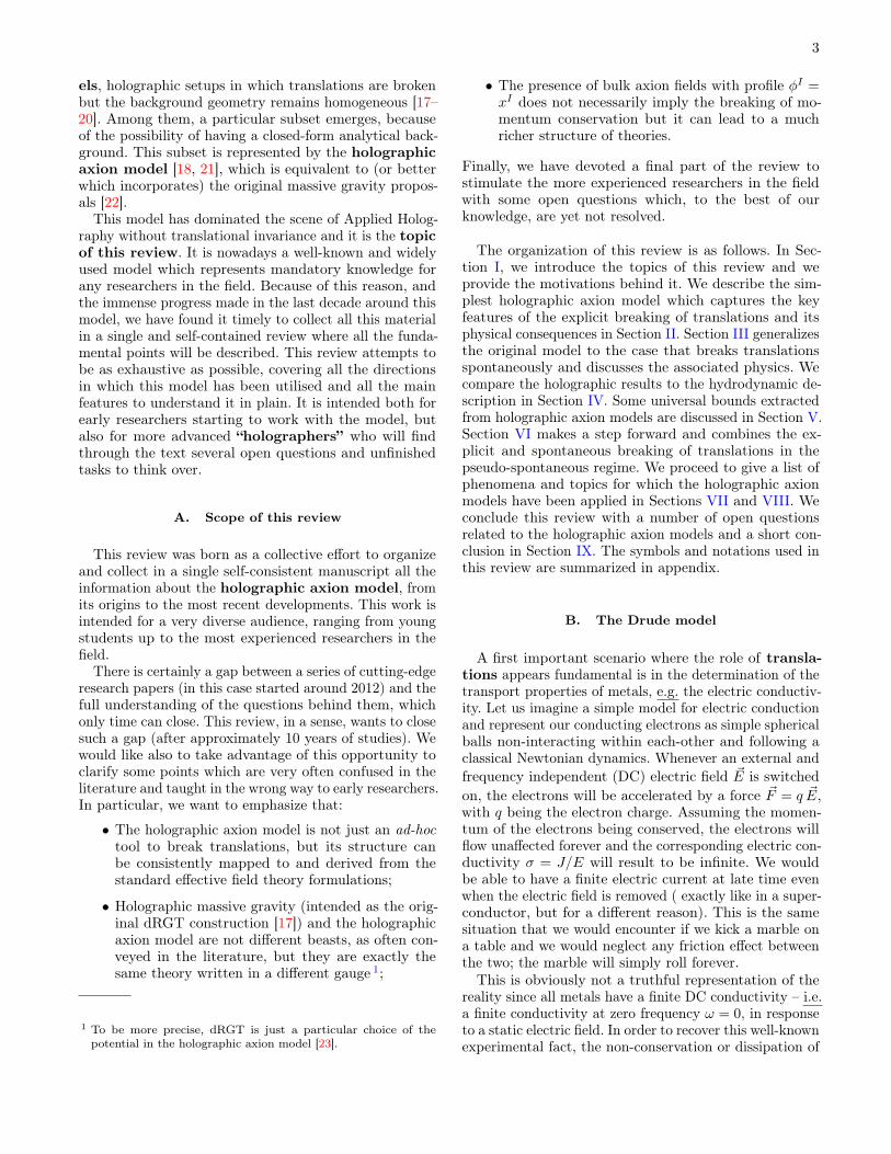
the electron momentum has to be considered. This can bedone by following the simpleDrude model introduced in1900 (only three years after the discovery of the electronby the British physicist J. J. Thomson) by Paul Drude [24–26]. Drude borrowed the basic elements of his theory fromthe kinetic theory of gases and he simply imagined ametal as a dilute gas of free electrons. Nevertheless, hemade a step forward and considered the presence in ametal of also heavy and immobile ions around which theelectrons are moving driven by the external electric field(see Fig. 1).

Figure 1. A schematic illustration for the Drude model. Inorange the electrons, while in green the immobile ions. Thered arrows identify the direction of a constant applied electricfield. The average time between collisions is given by τ .

The electrons, during their motion, collide against theheavier ions losing their momenta and deflecting theirtrajectories. From an effective field theory (EFT) pointof view, the dynamics of the electrons, or more specificallyof their average momentum, is determined by the simpleequation:

d

dt〈px(t)〉 = q Ex −

1

τ〈px(t)〉 , (1)

where for simplicity we have considered an isotropic sys-tem and aligned the external electric field along the spatialx direction. The first term in the r.h.s. is the standarddriving force induced by the external electric field. Thesecond, and more important, is an effective term which in-duces a relaxation of the average momentum at a constantrate Γ ≡ 1/τ . The timescale τ is an effective parameterwhich corresponds to the average time between consec-utive collisions and it determines “how fast” momentumgets lost. From a more theoretical perspective, this secondterm encodes the effects due to the explicit breaking oftranslations.Using classical identities, we can write down the aver-

age momentum of the electrons and the relative electriccurrent generated in terms of their average velocity:

〈px(t)〉 = m 〈vx(t)〉 , 〈Jx(t)〉 = n q 〈vx(t)〉 , (2)

where m and n are respectively the electron mass andnumber density. Using these relations in the dynamicalequation (1), and a standard Fourier decomposition, weimmediately get

− i ω 〈vx〉 =q

mEx −

1

τ〈vx〉 . (3)

Finally, utilizing the definition for the electric conduc-tivity, we obtain the expression for the low-frequencyconductivity in the Drude model, which reads

σxx =JxEx

=σDC

1 − i ω τ, σDC =

n q2 τ

m. (4)

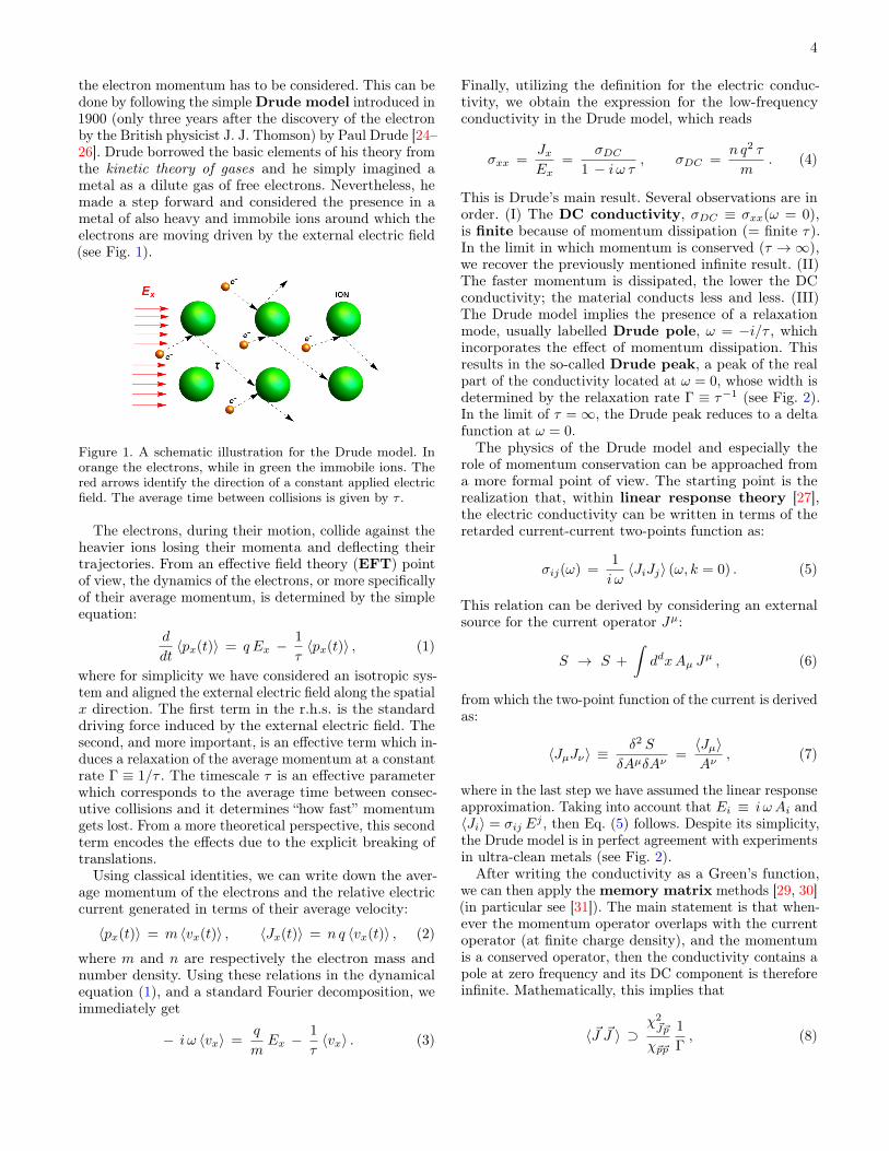
This is Drude’s main result. Several observations are inorder. (I) The DC conductivity, σDC ≡ σxx(ω = 0),is finite because of momentum dissipation (= finite τ).In the limit in which momentum is conserved (τ →∞),we recover the previously mentioned infinite result. (II)The faster momentum is dissipated, the lower the DCconductivity; the material conducts less and less. (III)The Drude model implies the presence of a relaxationmode, usually labelled Drude pole, ω = −i/τ , whichincorporates the effect of momentum dissipation. Thisresults in the so-called Drude peak, a peak of the realpart of the conductivity located at ω = 0, whose width isdetermined by the relaxation rate Γ ≡ τ−1 (see Fig. 2).In the limit of τ =∞, the Drude peak reduces to a deltafunction at ω = 0.The physics of the Drude model and especially the

role of momentum conservation can be approached froma more formal point of view. The starting point is therealization that, within linear response theory [27],the electric conductivity can be written in terms of theretarded current-current two-points function as:

σij(ω) =1

i ω〈JiJj〉 (ω, k = 0) . (5)

This relation can be derived by considering an externalsource for the current operator Jµ:

S → S +

∫ddxAµ J

µ , (6)

from which the two-point function of the current is derivedas:

〈JµJν〉 ≡δ2 S

δAµδAν=〈Jµ〉Aν

, (7)

where in the last step we have assumed the linear responseapproximation. Taking into account that Ei ≡ i ω Ai and〈Ji〉 = σij E

j , then Eq. (5) follows. Despite its simplicity,the Drude model is in perfect agreement with experimentsin ultra-clean metals (see Fig. 2).After writing the conductivity as a Green’s function,

we can then apply the memory matrix methods [29, 30](in particular see [31]). The main statement is that when-ever the momentum operator overlaps with the currentoperator (at finite charge density), and the momentumis a conserved operator, then the conductivity contains apole at zero frequency and its DC component is thereforeinfinite. Mathematically, this implies that

〈 ~J ~J 〉 ⊃χ2~J~p

χ~p~p

1

Γ, (8)

5

Re[σ]

Im[σ]

σDC

0.0 0.5 1.0 1.5 2.0 2.5 3.0ωτ0.0

0.2

0.4

0.6

0.8

1.0

Figure 2. Top: The optical conductivity in the Drude model.For simplicity we have fixed σDC = 1. Bottom: The excellentagreement between the Drude model and the experimentaldata in UPD2Al3 at T = 2.75 K taken from [28]. Here σ1 =Re [σ] and σ2 = Im [σ].

where χ ~J~p is the off-diagonal susceptibility establishingthe mixing between the two operators (and in this casesimply coinciding with the charge density). Moreover, χ~p~pis the momentum susceptibility determining the relationbetween momentum ~p and velocity ~v. The latter coincideswith E + p (energy + pressure) in relativistic systems [32]and it is simply the mass density % in non-relativisticones [33]. Finally, Γ is the momentum relaxation rate,defined as

Γ = limω→0

M~p~p

χ~p~p, (9)

with MAB being the memory matrix (see [31] for moredetails). This rate being non-zero stems directly from thefact that

[H, ~p ] 6= 0 , (10)

namely there is an operator in the theory which explicitlybreaks translational invariance. Notice that the r.h.s. of(8) reproduces exactly what is known as Drude Weightwhich is highly discussed in the context of many-bodyphysics (see, for example, the Mazur-Susuki bound [34]and its holographic counterpart [35]).

C. Effective field theories for solids and fluids

Another situation in which translational invarianceplays a fundamental role is in the definition of solidsand in the study of elasticity [33, 36, 37]. A solid is asystem with long-range order. From a more fundamentalperspective, it is a configuration in which spatial trans-lations are spontaneously broken (SSB). This is tanta-mount to say that a solid selects a preferred length-scale.The corresponding Goldstone bosons are the (acoustic)phonons [38]. Despite the standard condensed matterdescription of solids is not introduced with this language,but rather via more phenomenological models of springsand atoms, an effective field theory description of solidsand elasticity is definitely helpful and welcome [39].The standard formulation of spontaneous symmetry

breaking (think, for example, about superconductivity) isdone in terms of Ginzburg-Landau theory and the well-known double-well potential [40]. Despite attempts ofthis kind have been pursued for spacetime symmetriesand phonons [41–44], the most successful framework inthis case [45] appears slightly different. The main ideais rather simple. Despite Lorentz invariance and the as-sociated Poincaré group are fundamental pillars for thedescription of our world at high energy (e.g. special rela-tivity), all phases of matter at low energy are obviouslynot respecting these rules. Matter always selects a pre-ferred reference frame, being the velocity of a fluid orthe lattice structure of a crystal, and it therefore breaksspontaneously part of the Poincaré group. Classifyingthe possible symmetry breaking patterns of the Poincarégroup is therefore equivalent to classify the possible differ-ent phases of matter at low energy. Once this principle isaccepted, all the methods relative to SSB (e.g. the Cosetconstruction [46]) are applicable and useful to perform afull “zoology” of matter. Because of spacetime limitations,we will describe in detail only the EFT formulation ofsolids and fluids, putting aside superfluids, supersolids,framids, etc.

Figure 3. A pure shear deformation and its effects on a square2D lattice.

Before moving to the modern EFT framework, letus briefly review the basics of the theory of elastic-ity [33, 36, 37]. The theory of elasticity describes thedynamics of objects under mechanical deformations andit is based on the so-called (infinitesimal) displacements,

6

the geometrical deviations from equilibrium (see Fig. 3):

~u ≡ ~x − ~xeq . (11)

The fundamental object describing mechanical deforma-tions is the strain tensor, which is defined as the sym-metrized derivative of the displacement:

εij = ∂i uj + ∂j ui , (12)

from which the final position xi can be written as xi =xieq + εij dx

j 2. Once the strain tensor is defined, oneneeds to use the constitutive relation which at linearlevel relates the strain tensor to the stress tensor σij :

σij = Cijkl εkl + . . . , (13)

with Cijkl being the elastic tensor. For an isotropicsystem in d-spatial dimensions, we have

σij = K δij εkk + 2G

(εij −

1

dδij εkk

), (14)

where K,G are respectively the bulk and shear elasticmoduli and εkk the bulk strain, defined as the trace of thestrain tensor. Finally, we can write down the equation ofelasto-dynamics (which is simply the Newton’s equation~F = m~a):

% ui = fi = ∇j σij , (15)

which constitutes the missing piece to find the full dy-namics of the system. Here % stands for the mass densityand fi for the force density. By plugging Eq. (14) intoEq. (15), and after decomposing the modes into transverseand longitudinal with respect to the momentum ~k, oneobtains two sets of propagating sound modes:

ω = ± vT,L k , (16)

which are indeed our transverse (or shear) and longitu-dinal phonons. One can also derive that the phononspropagation speeds are directly related to the elastic mod-uli. In particular, in two spatial dimension, one finds

v2T =

G

%, v2

L =G + K

%. (17)

This is a beautiful result which is obtained only by usingsymmetries. Nevertheless, to make the role of symmetries,and in particular translations, more evident we need topass to a more field theory inspired formalism.The main idea consists in introducing a set of real

scalar fields

ΦI , I = 1 , . . . , dspatial , (18)

2 In this review, we will not consider the possibility of having non-affine displacements and incompatible deformations. See [47] formore details.

one for each of the spatial directions. These scalar fieldsact as a set of co-moving coordinates and they selecta preferred reference frame

〈ΦI〉 ≡ ΦIeq = xI , (19)

so that, at equilibrium, they are identified with the spa-tial coordinates themselves (see Fig. 4). The mechanicaldeformations are then associated to the fluctuations ofthese scalar fields around equilibrium:

ΦI = ΦIeq + πI , (20)

where, as we will see, the fluctuations πI are exactly theGoldstone modes associated with translational invariance– the phonons.

Figure 4. The EFT parametrization in terms of a set of scalarfields ΦI . The equilibrium configuration is clearly ΦIeq = xI .

In order to build an effective field theory for the scalarsΦI , we need to establish which are the fundamental sym-metries of our system. For simplicity, we will consideronly isotropic solids, imposing therefore invariance under

R : ΦI → RIJ ΦJ . (21)

and assuming the equilibrium configuration to be ΦI =δIj x

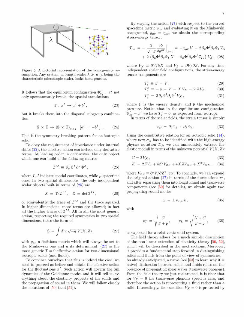
j . More importantly, we will assume that at largescales, scales λ much larger than the microscopic charac-teristic distance a, the physics is homogeneous (see [48]).This assumption appears to be very natural and it isrelated to the fact that every solid (imagine, for example,the table you are sit at) looks like homogeneous as far asyou do not probe it at distances comparable to its crystalstructure (see Fig. 5).This is obviously connected to the continuous descrip-

tion and to the fact that our EFT breaks down whenwe reach the microscopic scale a (at which, for example,phonons are not well defined anymore). The microscopicscale a, in this case the lattice spacing, represents the UVcutoff of our effective theory. In fluids, the microscopicscale is given in terms of the inter-molecular distancewhich plays exactly the same cutoff role (see, e.g. [49]).

In order to retain homogeneity at large scales, we needto also impose invariance under the internal global shifts

S : ΦI → ΦI + aI . (22)

7

Figure 5. A pictorial representation of the homogeneity as-sumption. Any system, at length-scales λ a (a being thecharacteristic microscopic scale), looks homogeneous.

It follows that the equilibrium configuration ΦIeq = xI notonly spontaneously breaks the spatial translations

T : xI → xI + bI , (23)

but it breaks them into the diagonal subgroup combina-tion

S × T → (S × T)diag[aI = −bI

]. (24)

This is the symmetry breaking pattern for an isotropicsolid.To obey the requirement of invariance under internal

shifts (22), the effective action can include only derivativeterms. At leading order in derivatives, the only objectwhich one can build is the following matrix

IIJ ≡ ∂µ ΦI ∂µ ΦJ , (25)

where I, J indicate spatial coordinates, while µ spacetimeones. In two spatial dimensions, the only independentscalar objects built in terms of (25) are

X = Tr IIJ , Z = det IIJ , (26)

or equivalently the trace of IIJ and the trace squared.In higher dimensions, more terms are allowed; in factall the higher traces of IIJ . All in all, the most genericaction, respecting the required symmetries in two spatialdimensions, takes the form of

S =

∫d3x√−g V (X,Z) , (27)

with gµν a fictitious metric which will always be set tothe Minkowski one and g its determinant. (27) is themost generic T = 0 effective action for two-dimensionalisotropic solids (and fluids).To convince ourselves that this is indeed the case, we

need to proceed as before and obtain the effective actionfor the fluctuations πI . Such action will govern the fulldynamics of the Goldstone modes and it will tell us ev-erything about the elasticity property of the solids andthe propagation of sound in them. We will follow closelythe notations of [50] (and [51]).

By varying the action (27) with respect to the curvedspacetime metric gµν and evaluating it on the Minkowskibackground, gµν = ηµν , we obtain the correspondingstress-energy tensor:

Tµν = − 2√−g

δS

δgµν

∣∣∣g=η

= − ηµν V + 2 ∂µΦI∂νΦI VX

+ 2(∂µΦI∂νΦI X − ∂µΦI∂νΦJ IIJ

)VZ . (28)

where VX ≡ ∂V/∂X and VZ ≡ ∂V/∂Z. For any timeindependent scalar field configurations, the stress-energytensor components are

T tt ≡ E = V , (29)T xx ≡ − p = V − X VX − 2Z VZ , (30)

T xy = 2 ∂xΦI∂yΦI VX , (31)

where E is the energy density and p the mechanicalpressure. Notice that in the equilibrium configurationΦIeq = xI we have T xy = 0, as expected from isotropy.

In terms of the scalar fields, the strain tensor is simply:

εij = ∂i Φj + ∂j Φi . (32)

Using the constitutive relation for an isotropic solid (14),where now σij has to be identified with the high-energyphysics notation Tij , we can immediately extract theelastic moduli in terms of the unknown potential V (X,Z):

G = 2VX , (33)

K = 2ZVZ + 4Z2VZZ + 4XZVXZ +X2VXX . (34)

where VZZ ≡ ∂2V/∂Z2, etc. To conclude, we can expandthe original action (27) in terms of the fluctuations πI ,and after separating them into longitudinal and transversecomponents (see [50] for details), we obtain again twopropagating sound modes

ω = ± vT,L k , (35)

with

vT =

√G

E + p, vL =

√K +G

E + p, (36)

as expected for a relativistic solid system.The field theory allows for a much simpler description

of the non-linear extension of elasticity theory [50, 52],which will be described in the next sections. Moreover,it provides a fundamental step forward in distinguishingsolids and fluids from the point of view of symmetries.As already anticipated, a naive (see [53] to learn why it isnaive) distinction between solids and fluids relies on thepresence of propagating shear waves (transverse phonons).From the field theory we just constructed, it is clear thatfor VX = 0 the transverse phonons speed is zero, andtherefore the action is representing a fluid rather than asolid. Interestingly, the condition VX = 0 is protected by

8

Figure 6. The action of a volume preserving diffeomorphism(37). The total volume remains unchanged.

a specific symmetry which is known as volume-preservingdiffeomorphisms(VPD):

Φa → ξb(Φ) , det∂ξb

∂Φa= 1 . (37)

The action of such a symmetry is a coordinates trans-formation for the mapping ΦI which does not changethe volume of the system. In other words, invariance un-der (37) is the mathematical formulation of the fact thatfluids do take the shape of the container while solids donot.

In conclusion, the effective action

S =

∫d3xV (Z) , (38)

is the correct description for fluids. Not surprisingly,it bears important relationships with the holographicdescription of fluids [54].

The story becomes highly more complicated when thetheory is promoted to the full non-linear dynamics andfluctuations are taken into account [55].

D. Gauge-Gravity duality briefing

The AdS-CFT correspondence, known also asHolography or Gauge-Gravity duality, was originally dis-covered in 1998 by J.Maldacena [9] (see also [56]) andit stands by now as one of the most powerful tools intheoretical physics, providing a deep and fundamentalconnection between quantum field theory (QFT) and grav-ity. We refer to the literature [2–5, 10, 57–64] for a moredetailed introduction of the correspondence.

In one sentence, the slogan of the Gauge-Gravity dualitycould be phrased as:

quantum field theory (d-dim) = gravity (d+ 1-dim) ,(39)

where the = sign has to be translated as “dual to”. In par-ticular, the abstract relation (39) indicates the existenceof a duality between a gravitational description in d+ 1dimensions and a QFT one in d dimensions. This idea isartistically represented in Fig. 7 and it can be formally

Figure 7. An artistic representation of the Gauge-gravity du-ality. The bulk contains a black hole object dual to a finitetemperature thermal state. The bulk spacetime terminates atthe so-called boundary where the dual field theory “lives”. Thebulk description contains an extra-dimension, usually denotedas radial coordinate, which describes the energy scale of thedual field theory. The dynamics of the bulk fields, including themetric gµν happens in a (d+ 1)-dimensional curved spacetimewhich is asymptotically AdS. In this picture, the boundaryfield theory lives on the surface of the colored sphere and thebulk region is represented by the 3D region enclosed by sucha surface.

interpreted as:⟨e∫φ0(x,t)O

⟩QFT

= Zgravity [φ0(x, t) ≡ φ(x, t, u)∂Σ] ,

(40)

which is known as the GPKW (Gubser, Polyakov, Kle-banov, Witten) master rule [65, 66] and its the pillarof the “dictionary” defining the = sign in Eq. (39). Here∂Σ indicates the boundary of the gravitational spacetimeΣ at which the QFT source φ0 is identified using theholographic dictionary.The core of framework is a (d + 1) dimensional bulk

where all the bulk fields, including the metric gµν , liveand fluctuate. Their dynamics is controlled by a bulkaction Sbulk[φ(x, u), gµν(x, u) . . . ] defined on a specificbulk geometry. In the limit of largeN and infinite couplingfor the dual field theory, the gravitational dynamics canbe assumed to be classical and stringy corrections canbe consistently neglected. This is the limit in which thesize of the spacetime geometry l is much larger than thePlanck scale lp and than the string length ls. For all ourpurposes, we will not deviate from such regime. In our

9

examples, the structure of the background geometry canbe written as follows:

ds2bulk(d+1)

=L2

u2

du2

g(u)+ −f(u) dt2 + gij dx

idxj︸ ︷︷ ︸d-dimensional

,

(41)where L denotes the AdS radius3, u takes the name ofradial-coordinate or holographic coordinate and it plays avery fundamental role in the holographic construction. Inparticular, this extra-dimension describes the energy scaleof the dual system, providing a nice geometric realizationof the renormalization flow (RG) of the dual field theory(see Fig. 8).4

The radial coordinate of (41) spans from [0, uh] where

u = 0 : conformal boundary , (42)

and

g(uh) = f(uh) = 0 , uh : black hole horizon . (43)

More precisely, u = 0 is the (conformal) boundary of theasymptotically Anti-de-Sitter (AdS) bulk geometry (41)which is equipped with (a normally flat) metric (−1, gij).The other extreme, u = uh, is the location of the blackhole horizon which provides the temperature for the dualfield theory, technically given by the surface gravity at itshorizon. Another very popular convention in the literatureis to use r ≡ L2/u in which the horizon is set at r = rhand the conformal boundary at r =∞. The two choicesare related by a simple coordinates transformation.The gravitational bulk action appearing in (40) is

uniquely defined by choosing boundary conditions (b.c.s)for the various bulk fields. At the horizon u = uh, theappropriate b.c.s. are simply given by the regularity ofthe solution. At the boundary u = 0 the b.c.s. uniquelydetermine the dual field theory and, in particular, thesources with which we deform it. In particular, given aconcrete bulk field φ(t, x, u), its asymptotic expansion inthe standard quantization scheme is generally given by

φ(t, x, u) = φ0 u∆L(1 + . . . ) + 〈O〉u∆S (1 + . . . ) , (44)

where by definition ∆L < ∆S such that the first term isthe “leading term” (the one falling-off more slowly towardsthe boundary) and the second the subleading one. Thecoefficient of the leading term determines the source φ0

for the dual operator O living in the dual field theory. Thesubleading term determines its vacuum expectation value(vev) 〈O〉. The powers ∆L,S are uniquely determined interms of the spacetime dimension d and the conformaldimension ∆ of the field theory operator O. Once the

3 In most case, we set L ≡ 1 for simplicity.4 To be precise, the u coordinate appearing in (41) coincides withthe inverse of the energy scale of the dual field theory.

IR UVu

d−1,1

u

RAdSd+1

minkowski

UVIR

Figure 8. Holography provides a geometric representation ofRG flow. Top: A series of block spin transformations (coarse-graining process) labeled by the length scale u. Bottom: acartoon of AdS space, where the radial coordinate u playsthe role of energy scale of the dual system. Excitations withdifferent energy scale get put in different place in the bulk.Figures updated from [58].

sources and the vevs are identified, the gravitational pic-ture can be mapped into a dual field theory:

S = SCFT +∑i

∫ddxφi0 〈Oi〉 , (45)

and the correlation functions for the various operators canbe obtained using the standard variational prescription.

This is a very brief explanation of how the dualityworks. For space limitations, we have skipped several im-portant features which the interested Reader can findin the literature mentioned above. Since the field of ap-plied holography is a vast subject spanning decades ofresearch, we limit this review to recent developments andunderstandings on strongly coupled quantum matter usingholographic axion models. Other active areas of appliedholography include condensed matter [2, 3, 67–69], nuclearphysics [70], quantum information [71], non-equilibriumphysics [72, 73] and so on. It is likely to have even widerapplicability in the future.

10

E. Holographic axion model

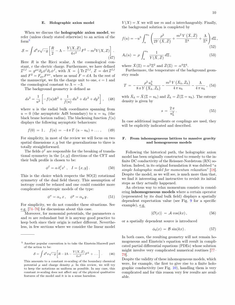
When we discuss the holographic axion model, werefer (unless clearly stated otherwise) to an action of theform5

S =

∫d4x√−g[R

2− Λ− Y (X,Z)

4 e2F 2 −m2V (X,Z)

].

(47)Here R is the Ricci scalar, Λ the cosmological con-stant, e the electric charge. Furthermore, we have definedIIJ = gµν∂µφ

I∂νφJ , with X = 1

2 Tr IIJ , Z = det IIJand F 2 = FµνF

µν , where as usual F = dA. In the rest ofthe manuscript, we fix the charge unit to one, e = 1 andthe cosmological constant to Λ = −3.

The background geometry is defined as

ds2 =1

u2

[−f(u)dt2 +

1

f(u)du2 + dx2 + dy2

], (48)

where u is the radial bulk coordinates spanning fromu = 0 (the asymptotic AdS boundary) to u = uh (theblack brane horizon radius). The blackening function f(u)displays the following asymptotic behaviours:

f(0) = 1 , f(u) = −4π T (u− uh) + . . . , (49)

For simplicity, in most of the review we will focus on twospatial dimensions x, y but the generalizations to three istotally straightforward.

The fields φI are responsible for the breaking of transla-tional symmetry in the x, y directions of the CFT andtheir bulk profile is chosen to be:

φI = α δIi xi , I = x, y . (50)

This is the choice which respects the SO(2) rotationalsymmetry of the dual field theory. This assumption ofisotropy could be relaxed and one could consider morecomplicated anisotropic models of the type:

φx = αx x , φy = αy y . (51)

For simplicity, we do not consider these situations. Seee.g. [74–76] for discussions about this case.Moreover, for monomial potentials, the parameters α

and m are redundant but it is anyway good practice tokeep both since their origin is rather different. Neverthe-less, in few sections where we consider the linear model

5 Another popular convention is to take the Einstein-Maxwell partof the action to be:

S =

∫d4x√−g[R− 2Λ−

Y (X,Z)

4 e2F 2 + . . .

]. (46)

This amounts to a constant re-scaling of the boundary chemicalpotential µ and charge density ρ. In this review, we will tryto keep the notations as uniform as possible. In any case, thisconstant re-scaling does not affect any of the physical qualitativefeatures of the model and it is in a sense harmless.

V (X) = X we will use m and α interchangeably. Finally,the background solution is completed by

f(u) = −u3

∫ uh

u

(ρ2

2Y(X, Z

) +m2 V

(X, Z

)Ξ4

+Λ

Ξ4

)dΞ ,

(52)

At(u) = ρ

∫ uh

u

1

Y (X, Z)dΞ , (53)

where X(Ξ) = α2Ξ2 and Z(Ξ) = α4Ξ4.Furthermore, the temperature of the background geom-

etry reads

T = − ρ2 u3h

8π Y(Xh, Zh

) − m2 V(Xh, Zh

)4π uh

− Λ

4π uh, (54)

with Xh = X(Ξ = uh) and Zh = Z(Ξ = uh). The entropydensity is given by

s =2π

u2h

. (55)

In case additional ingredients or couplings are used, theywill be explicitly indicated and described.

F. From inhomogeneous lattices to massive gravityand homogeneous models

Following the historical path, the holographic axionmodel has been originally constructed to remedy to the in-finite DC conductivity of the Reissner-Nordstrom (RN) so-lution. Indeed, in its original formulation it was dubbed “asimple holographic model for momentum relaxation” [18].Despite the model, as we will see, is much more than that,we find it interesting and instructive to revisit its initialsteps as they actually happened.

An obvious way to relax momentum consists in consid-ering inhomogeneous models where a certain operator(represented by its dual bulk field) displays a spatiallydependent expectation value (see Fig. 9 for a specificexample), e.g.

〈O(x)〉 = A cos(kx) , (56)

or a spatially dependent source is introduced

φ0(x) = B sin(kx) . (57)

In both cases, the resulting geometry will not remain ho-mogeneous and Einstein’s equation will result in compli-cated partial differential equations (PDEs) whose solutionmight involve very complicated numerical routines [77–79].Despite the validity of these inhomogeneous models, whichwere, for example, the first to give rise to a finite holo-graphic conductivity (see Fig. 10), handling them is verycomplicated and for this reason very few results are avail-able.

11

Figure 9. A holographic example of highly inhomogeneous 2Dsolutions. Figure taken from [80].

Figure 10. The first holographic computation showing a finiteDC electric conductivity in a inhomogeneous periodic lattice.Figure taken from [14].

A possible way to overcome the difficulties of the inho-mogeneous models is to consider simpler models whichretain some of their major features (such as the symmetrybreaking patterns) but allow for much more reliable andfast computations (which sometimes are even analytical).This is exactly the way the homogeneous models withbroken translations became famous and spread aroundthe holographic community. As we will investigate in de-tail, these models, despite their simplicity, will recovermost of the features of the more complicated counterpartsand they will reveal extremely useful and rich phenomena.There is more than that! The homogeneous models,

and in particular massive gravity in its general formu-lation, emerge as the universal low-energy descriptionfor any holographic models with broken translations. Allholographic models with broken translations provide ina way or in another a mass to the graviton (or at leastsome of its components) and this is nothing else that auniversal statement regarding the Ward-identity for trans-lations. By identifying the translations at the boundarywith the diffeomorphisms in the bulk, it appears obviousthat any model with broken translations must involve agravitational picture where diffeomorphisms are brokenand therefore the graviton being massive.

This statement has been shown explicitly for a concretelattice construction in [81] making a beautiful connectionbetween the more realistic lattice models and the more

useful homogeneous relatives. Let us briefly revisit thefundamental steps. Let us take a simple gravitational bulkaction in four dimensions:

S =

∫d4x√−g

[R +

6

L2− 1

4F 2 − 1

2∂µφ∂

µφ − m2

2φ2

],

(58)where the mass of the scalar is chosen m2 < 0 in order tohave the dual operator O marginally relevant.6 In general,the associated holographic conductivity would be infinitebecause of translational invariance. Nevertheless, whenspatially dependent boundary conditions are introduced,this is not anymore the case. The authors of [81] didthat perturbatively by introducing a source for the scalaroperator:

φ0(x) = ε cos(kL x) , (59)

where ε 1 is taken to be infinitesimal. This source mim-ics the effect of a periodic lattice with wave-vector kL.The boundary source (59) corresponds to a bulk profileof the type φ(u, x) = φu(u)φ0(x) with u the holographicradial coordinate. The main idea is then to solve pertur-batively the bulk equations of motion up to order O(ε2)by using an appropriate expansion for the various bulkfields gµν , Aµ.The most important result is that the effective action

at order O(ε2) contains a term

S(ε2)eff =

1

2

∫d4x√gM2(u) gxx , (60)

where

M2(u) =1

2ε2 k2

L φ2u(u) . (61)

By performing standard perturbation techniques, this neweffective term gives a mass to the graviton componentsδgtx, δgrx, as already anticipated. The fact that the vec-tor components of the graviton become massive leads tothe expected finite DC conductivity. Most importantly,this simple computation shows directly the universal ap-pearance of an effective graviton mass as a result of ainhomogeneous holographic lattice. In other words, itconstitutes strong evidence that massive gravity is theuniversal low energy effective holographic description forsystems with broken translations.

G. Other holographic homogeneous models

In a broad sense, we define a holographic model “homo-geneous” if the background geometry does not depend onthe boundary spacetime coordinates (t, xi). In the context

6 Notice this is not a problem in curved spacetime as far as theBreitenlohner-Freedman (BF) bound [82] is respected.

12

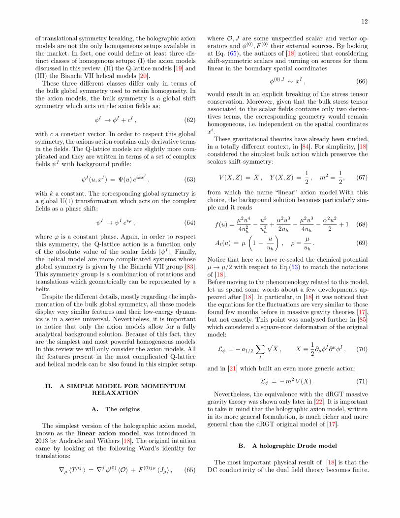
of translational symmetry breaking, the holographic axionmodels are not the only homogeneous setups available inthe market. In fact, one could define at least three dis-tinct classes of homogenous setups: (I) the axion modelsdiscussed in this review, (II) the Q-lattice models [19] and(III) the Bianchi VII helical models [20].

These three different classes differ only in terms ofthe bulk global symmetry used to retain homogeneity. Inthe axion models, the bulk symmetry is a global shiftsymmetry which acts on the axion fields as:

φI → φI + cI , (62)

with c a constant vector. In order to respect this globalsymmetry, the axions action contains only derivative termsin the fields. The Q-lattice models are slightly more com-plicated and they are written in terms of a set of complexfields ψI with background profile:

ψI(u, xI) = Ψ(u) eikxI

. (63)

with k a constant. The corresponding global symmetry isa global U(1) transformation which acts on the complexfields as a phase shift:

ψI → ψI eiϕ , (64)

where ϕ is a constant phase. Again, in order to respectthis symmetry, the Q-lattice action is a function onlyof the absolute value of the scalar fields |ψI |. Finally,the helical model are more complicated systems whoseglobal symmetry is given by the Bianchi VII group [83].This symmetry group is a combination of rotations andtranslations which geometrically can be represented by ahelix.

Despite the different details, mostly regarding the imple-mentation of the bulk global symmetry, all these modelsdisplay very similar features and their low-energy dynam-ics is in a sense universal. Nevertheless, it is importantto notice that only the axion models allow for a fullyanalytical background solution. Because of this fact, theyare the simplest and most powerful homogeneous models.In this review we will only consider the axion models. Allthe features present in the most complicated Q-latticeand helical models can be also found in this simpler setup.

II. A SIMPLE MODEL FOR MOMENTUMRELAXATION

A. The origins

The simplest version of the holographic axion model,known as the linear axion model, was introduced in2013 by Andrade and Withers [18]. The original intuitioncame by looking at the following Ward’s identity fortranslations:

∇µ 〈Tµj 〉 = ∇j φ(0) 〈O〉 + F (0)jµ 〈Jµ〉 , (65)

where O, J are some unspecified scalar and vector op-erators and φ(0), F (0) their external sources. By lookingat Eq. (65), the authors of [18] noticed that consideringshift-symmetric scalars and turning on sources for themlinear in the boundary spatial coordinates

φ(0),I ∼ xI , (66)

would result in an explicit breaking of the stress tensorconservation. Moreover, given that the bulk stress tensorassociated to the scalar fields contains only two deriva-tives terms, the corresponding geometry would remainhomogeneous, i.e. independent on the spatial coordinatesxi.

These gravitational theories have already been studied,in a totally different context, in [84]. For simplicity, [18]considered the simplest bulk action which preserves thescalars shift-symmetry:

V (X,Z) = X , Y (X,Z) =1

2, m2 =

1

2, (67)

from which the name “linear” axion model.With thischoice, the background solution becomes particularly sim-ple and it reads

f(u) =µ2u4

4u2h

− u3

u3h

+α2u3

2uh− µ2u3

4uh− α2u2

2+ 1 (68)

At(u) = µ

(1 − u

uh

), ρ =

µ

uh. (69)

Notice that here we have re-scaled the chemical potentialµ→ µ/2 with respect to Eq.(53) to match the notationsof [18].Before moving to the phenomenology related to this model,let us spend some words about a few developments ap-peared after [18]. In particular, in [18] it was noticed thatthe equations for the fluctuations are very similar to thosefound few months before in massive gravity theories [17],but not exactly. This point was analyzed further in [85]which considered a square-root deformation of the originalmodel:

Lφ = − a1/2

∑I

√X , X ≡ 1

2∂µφ

I∂µφI , (70)

and in [21] which built an even more generic action:

Lφ = −m2 V (X) . (71)

Nevertheless, the equivalence with the dRGT massivegravity theory was shown only later in [22]. It is importantto take in mind that the holographic axion model, writtenin its more general formulation, is much richer and moregeneral than the dRGT original model of [17].

B. A holographic Drude model

The most important physical result of [18] is that theDC conductivity of the dual field theory becomes finite.

13

Figure 11. The incoherent and coherent contributions to theelectric current. The incoherent processes transport charge butthey do not transport momentum (e.g. particle-antiparticlepair).

In particular, it takes the simple form:

σDC ≡ σ(ω = 0) = u3−dh

(1 + (d− 2)2 µ

2

α2

), (72)

where µ is the chemical potential of the dual field theory.We will describe in detail how to obtain this result (atleast for d = 3) in Section IID. Expression (72) displaysa very specific structure which is in common of all theholographic models. In particular, the full DC conductivitycan be split into two contributions:

σDC = σ(0)DC + σDrude

DC . (73)

The first contribution, which in this simple case is justσ

(0)DC = u3−d

h , coincides in the limit of strong momentumrelaxation with the incoherent conductivity [86]:

σincoherentDC =

(s T

s T + µρ

)2 ( s

4π

) d−2d

(74)

which can be derived by considering the incoherent current

J incoherent = J − χPJχPP

P (75)

where, here, both the momentum P and the currents Jare intended as operators7.The incoherent conductivity relates to the part of theelectric current J which does not overlap with the mo-mentum operator and it is therefore insensitive to anymomentum relaxing mechanism (in this case independentof α). This contribution is finite even in absence of mo-mentum dissipation and it corresponds to the probe limit

7 We thank Blaise Gouteraux for clarifying this point to us.

α/T = 7

α/T = 5

α/T = 3

α = 0

2 4 6 8 10ΩT

1

2

3

4

5

Re@ΣD

α = 0

α/T = 3

α/T = 5α/T = 7

2 4 6 8 10ΩT

1

2

3

4Im@ΣD

Figure 12. The optical conductivity of the linear axion modelfor various values of the momentum dissipation rate α/µ.Figure taken from [88].

result (with no backreaction of the bulk fields on thebackground metric) in the limits of strong momentumdissipation or zero charge density.

The second contribution corresponds to the part of theelectric current which transports also momentum (seeFig. 11) and it is infinite in the absence of momentumdissipation α → 0). It is the equivalent of the Druderesult (4) and it vanishes in the limit µ = 0, at whichelectric current and momentum decouple.

One can do more and compute also the AC – frequencydependent – electric conductivity. In order to do that,one has to switch on fluctuations for the gauge field, themetric and the scalar fields. A consistent truncation atzero momentum (k = 0) is given by

δAx = e−iωt ax(u) , δgtx = e−iωt htx(u) ,

δφ = e−iωt ϕ(u) , (76)

and the corresponding equations of motion can be foundin the original work [18]. Following the standard proce-dure to compute the holographic conductivity (see [6]and [87]), one can finally obtain numerically σ(ω). TheAC conductivity was originally presented in [88] and it ishere reproduced in Fig. 12.

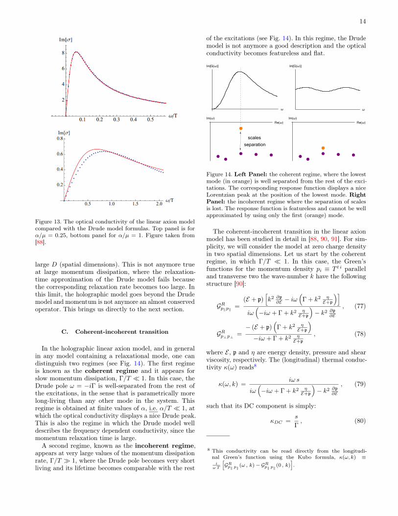
The first important result is that the DC conductivity isfinite and it appears in perfect agreement with the analyticformula (72). Moreover, at slow momentum relaxation,α/T 1, the conductivity shows a nice Drude peak.Indeed, one can fits the numerical data with the Drudeformula very well (see Fig. 13). See [89] for a study in

14

Figure 13. The optical conductivity of the linear axion modelcompared with the Drude model formulas. Top panel is forα/µ = 0.25, bottom panel for α/µ = 1. Figure taken from[88].

large D (spatial dimensions). This is not anymore trueat large momentum dissipation, where the relaxation-time approximation of the Drude model fails becausethe corresponding relaxation rate becomes too large. Inthis limit, the holographic model goes beyond the Drudemodel and momentum is not anymore an almost conservedoperator. This brings us directly to the next section.

C. Coherent-incoherent transition

In the holographic linear axion model, and in generalin any model containing a relaxational mode, one candistinguish two regimes (see Fig. 14). The first regimeis known as the coherent regime and it appears forslow momentum dissipation, Γ/T 1. In this case, theDrude pole ω = −iΓ is well-separated from the rest ofthe excitations, in the sense that is parametrically morelong-living than any other mode in the system. Thisregime is obtained at finite values of α, i.e. α/T 1, atwhich the optical conductivity displays a nice Drude peak.This is also the regime in which the Drude model welldescribes the frequency dependent conductivity, since themomentum relaxation time is large.A second regime, known as the incoherent regime,

appears at very large values of the momentum dissipationrate, Γ/T 1, where the Drude pole becomes very shortliving and its lifetime becomes comparable with the rest

of the excitations (see Fig. 14). In this regime, the Drudemodel is not anymore a good description and the opticalconductivity becomes featureless and flat.

ω

Im[G(ω)]

ω

Im[G(ω)]

Re(ω)

Im(ω)

Re(ω)

Im(ω)

scales

separation

Figure 14. Left Panel: the coherent regime, where the lowestmode (in orange) is well separated from the rest of the exci-tations. The corresponding response function displays a niceLorentzian peak at the position of the lowest mode. RightPanel: the incoherent regime where the separation of scalesis lost. The response function is featureless and cannot be wellapproximated by using only the first (orange) mode.

The coherent-incoherent transition in the linear axionmodel has been studied in detail in [88, 90, 91]. For sim-plicity, we will consider the model at zero charge densityin two spatial dimensions. Let us start by the coherentregime, in which Γ/T 1. In this case, the Green’sfunctions for the momentum density pi ≡ T t i paralleland transverse two the wave-number k have the followingstructure [90]:

GRp‖p‖ =(E + p)

[k2 ∂p

∂E − iω(

Γ + k2 ηE+p

)]iω(−iω + Γ + k2 η

E+p

)− k2 ∂p

∂E

, (77)

GRp⊥p⊥ =− (E + p)

(Γ + k2 η

E+p

)−iω + Γ + k2 η

E+p

, (78)

where E , p and η are energy density, pressure and shearviscosity, respectively. The (longitudinal) thermal conduc-tivity κ(ω) reads8

κ(ω, k) =iω s

iω(−iω + Γ + k2 η

E+p

)− k2 ∂p

∂E

, (79)

such that its DC component is simply:

κDC =s

Γ, (80)

8 This conductivity can be read directly from the longitudi-nal Green’s function using the Kubo formula, κ(ω, k) ≡iω T

[GRp‖ p‖ (ω , k)− GRp‖ p‖ (0 , k)

].

15

and it is controlled by the momentum relaxation rate Γ,as expected.Now, by looking at the poles of the parallel Green

function, we can find the dispersion relation of the lowestmodes in the longitudinal spectrum:

ω = ± k

öp

∂E− 1

4

(Γk−1 +

η

E + pk

)2

− i

2

(Γ +

η

E + pk2

), (81)

which already indicates that the original longitudinalsound mode is destroyed by the presence of momentumdissipation. Moreover, there is an interesting crossoverbetween diffusive-like behaviour at small momentum andpropagating like at high one. More precisely, for k/Γ 1,Eq. (81) gives two propagating sound modes:

ω = ± k√∂p

∂E− i

2

(Γ +

η

E + pk2

), (82)

while at large distances, k/Γ 1, there are two separatedmodes, one diffusive and one damped Drude-like:

ω = − i ∂p∂E

Γ−1 k2 + . . . , (83)

ω = − iΓ + i k2

(∂p

∂EΓ−1 − η

E + p

)+ . . . , (84)

This means that heat is transported ballistically at shortdistances but diffusively at long ones. The crossover hap-pens exactly at

Γ k−1 +η

E + pk = 2

öp

∂E, (85)

and it is shown in Fig. 15.

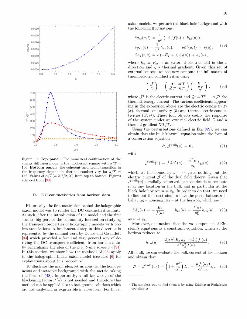
Figure 15. The imaginary part of the lowest mode in thelongitudinal sector of the linear axion model with α/T = 1/2in the coherent regime showing the diffusive-to-propagatingcrossover. Figure adapted from [90].

From the coherent regime where Γ/T 1 with

Γ =α2

4π T, (86)

we can increase further the axions strength α. At a cer-tain point, Γ/T ∼ O(1), the Drude pole collides on theimaginary axes with a secondary pole coming up andit produces to off-axes poles with finite real part whichat this point are not anymore well detached from therest of the excitations. This collision is shown explicitlyin Fig. 16. Once the incoherent regime is reached, the

Figure 16. The modes collision associated to the coherent-incoherent transition in the linear axion model. Here thewave-number k is taken to be zero and the parameter α/T isincreased from 0 to 12 in the direction of the arrows. There is aDrude-like pole near the origin at weak momentum dissipationrate. As α increases, it moves down the imaginary axis andcollides with another purely imaginary pole at α/T ≈ 9.5,producing two off-axis poles. Figure adapted from [90].

only conserved, and therefore long-living, quantity is theenergy density E . Its Green’s function takes the form [90]:

GREE = T 2 ∂s

∂T

DE k2

iω −DEk2, (87)

where DE is the energy diffusion constant. Finally, theDC thermal conductivity is

κDC = T∂s

∂TDE = cvDE , (88)

and it obeys the well-known Einstein’s relation. As al-ready mentioned before, the frequency dependent thermalconductivity passes from displaying a well-defined coher-ent peak to a flat incoherent response. These features areshown in Fig. 17.

The same phenomenology has been later found also inholographic axion model with fluid symmetry [92] con-firming its universal character.

16

Figure 17. Top panel: The numerical confirmation of theenergy diffusion mode in the incoherent regime with α/T =100. Bottom panel: the coherent-incoherent transition inthe frequency dependent thermal conductivity for k/T =1/2. Values of α/T (= 2, 7/2, 20) from top to bottom. Figuresadapted from [90].

D. DC conductivities from horizon data

Historically, the first motivation behind the holographicaxion model was to render the DC conductivities finite.As such, after the introduction of the model and the firststudies big part of the community focused on studyingthe transport properties of holographic models with bro-ken translations. A fundamental step in this direction isrepresented by the seminal work by Donos and Gauntlett[93] which provided a fast and very general way of de-riving the DC transport coefficients from horizon data,by generalizing the idea of the membrane paradigm [94].In this section, we show how the methods of [93] applyto the holographic linear axion model (see also [6] forexplanations about this procedure).

To illustrate the main idea, let us consider the homoge-neous and isotropic background with the metric takingthe form of (48). Importantly, a full knowledge of theblackening factor f(u) is not needed and therefore thismethod can be applied also to background solutions whichare not analytical or expressible in close form. For linear

axion models, we perturb the black hole background withthe following fluctuations:

δgtx(u, t) =1

u2(−t ζ f(u) + htx(u) ) ,

δgxu(u) =1

u2hxu(u), δφ1(u, t) = χ(u) ,

δAx(t, u) = t (−Ex + ζ At(u)) + ax(u) ,

(89)

where Ex ≡ Fxt is an external electric field in the xdirection and ζ a thermal gradient. Given this set ofexternal sources, we can now compute the full matrix ofthermoelectric conductivities using(

JQ

)=

(σ A T

A T κ T

)(E−∇TT

), (90)

where J I is the electric current and Qi = T ti − µJ i thethermal/energy current. The various coefficients appear-ing in the expression above are the electric conductivity(σ), thermal conductivity (κ) and thermoelectric conduc-tivities (A, A). These four objects codify the responseof the system under an external electric field E and athermal gradient ∇T/T .Using the perturbations defined in Eq. (89), we can

obtain that the bulk Maxwell equation takes the form ofa conservation equation

∂u J bulk(u) = 0 , (91)

with

J bulk(u) = f δA′x(u) − u2 µ

uhhtx(u) , (92)

which, at the boundary u = 0, gives nothing but theelectric current J of the dual field theory. Given thatJ bulk(u) is radially conserved, one can decide to computeit at any location in the bulk and in particular at theblack hole horizon u = uh. In order to do that, we needto find out the constraints to have the perturbations well-behaving – non-singular – at the horizon, which are 9:

δA′x(u) = − Exf(u)

, htx(u) =f(u)

u2h

hxu(u) , (93)

as u→ uh.Moreover, one notices that the uu-component of Ein-

stein’s equations is a constraint equation, which at thehorizon reduces to

hxu(u) =2µu2Ex uh − u2

h ζ f′(u)

α2 u2h f(u)

. (94)

All in all, we can evaluate the bulk current at the horizonand obtain that

J = J bulk(uh) =

(1 +

µ2

α2

)Ex −

µ f ′(uh)

α2 uhζ . (95)

9 The simplest way to find them is by using Eddington-Finkelsteincoordinates.

17

From above equation, we can obtain

σ ≡ ∂J∂Ex

= 1 +µ2

α2, (96)

A = A =1

T

∂J∂ζ

=4π µ

α2 uh, (97)

where the two off-diagonal terms are equivalent because ofthe Onsager’s relation. It is interesting to notice that thetransport coefficients above obey the Kelvin’s formula:

A

σ

∣∣∣T=0

= limT→0

∂s

∂ρ

∣∣∣T

(98)

with ρ the charge density, as observed in [95].In order to compute thermal transport, we have to

work a bit harder. The key observation is that the bulkequations of motion hiddenly imply the conservation ofanother combination of bulk fields:

Q(u) = f2(u)

(δgtx(u)

f(u)

)′− At(u)J (u) (99)

which reduces at the boundary u = 0 to the thermal/en-ergy current of the dual field theory. This fact can bederived “brute-force” or in a more elegant way using theproperties of the solution as done in [93]. By followingthe same procedure, one finally obtain

κ =(4π)2 T

α2 u2h

. (100)

After this initial finding, the thermoelectric transport hasbeen computed in many holographic models with andwithout an external magnetic field. See [75, 96–110] for asubset of the related developments.

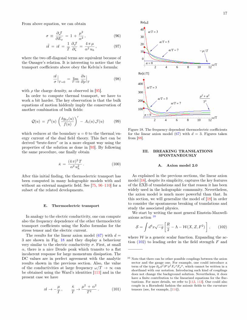
E. Thermoelectric transport

In analogy to the electric conductivity, one can computealso the frequency dependence of the other thermoelectrictransport coefficients using the Kubo formulas for thestress tensor and the electric current.The results for the linear axion model (67) with d =

3 are shown in Fig. 18 and they display a behaviourvery similar to the electric conductivity σ. First, at smallα, there is a nice Drude peak which transits to a flatincoherent response for large momentum dissipation. TheDC values are in perfect agreement with the analyticresults shown in the previous section. Also, the valueof the conductivities at large frequency ω/T → ∞ canbe obtained using the Ward’s identities [111] and in thepresent case we have

A → −µT,

κ

T→ µ2 + α2

T 2. (101)

α/T = 3

α/T = 5

α/T = 7

α = 0

- Μ T

2 4 6 8 10 12ΩT

0

10

20

30

40

Re@ΑD

α/T = 3

α/T = 5α/T = 7

α = 0

Μ2 + α2

T2

2 4 6 8 10 12ΩT

100

200

300

400

Re@Κ TD

Figure 18. The frequency dependent thermoelectric coefficientsfor the linear axion model (67) with d = 3. Figures takenfrom [88].

III. BREAKING TRANSLATIONSSPONTANEOUSLY

A. Axion model 2.0

As explained in the previous sections, the linear axionmodel [18], despite its simplicity, captures the key featuresof the EXB of translations and for that reason it has beenwidely used in the holographic community. Nevertheless,the axion model is much more powerful than that. Inthis section, we will generalize the model of [18] in orderto consider the spontaneous breaking of translations andstudy the associated physics.

We start by writing the most general Einstein-Maxwell-axions action 10

S =

∫d4x√−g[R

2− Λ−W(X,Z, F 2)

], (102)

where W is a generic scalar function. Expanding the ac-tion (102) to leading order in the field strength F and

10 Note that there can be other possible couplings between the axionsector and the gauge one. For example, one could introduce aterm of the type ∂µφI∂νφIFνρFρµ, which cannot be written in ashorthand with our notation. Introducing such kind of couplingsdoes not change the background solution. Nevertheless, it doeshave a finite contribution to the linearized equations for the fluc-tuations. For more details, we refer to [112, 113]. One could alsocouple in a Horndeski fashion the axionic fields to the curvaturetensors (see, for example, [114]).

18

ignoring non-scalar couplings between the various sec-tors, the generic expression (102) reduces to (47) whichis general enough to discuss all the important physicalfeature of the holographic axion model. Self-consistencyof action (47) imposes precise constraints on the scalarfunctions Y (X,Z) and V (X,Z). An analysis of the trans-verse fluctuations showed that we should require thatV ′(X, Z) > 0, Y (X, Z) > 0 and Y ′(X, Z) < 0 to avoidghosty instability [115]. Note that in more complicatedbackgrounds, for instance, turning on an external mag-netic field, the constraints on V and Y will become tighterbut still equivalent to impose the positivity of the electricconductivity [116].Now, let us explain the physical interpretation of the

V -term and Y F 2-term in (47) from the point of view ofthe dual field theory side, respectively.

• Setting Y (X,Z) = 0, the system is neutral. Theaxions configuration (51) breaks the spatial trans-lations explicitly (as the simple axion model) orspontaneously (which is the focus of this section). Inanalogy to the EFT description (27), V (X) providesan effective description for solids holographically,while V (Z) is related to fluids and we will come tothis later.

• The coupling Y F 2 can be viewed as the holographicdual of some charged disorders or charge lattices,depending on the form of Y (X,Z). In the SSB pat-tern, it might be viewed as an analogy to chargedensity waves (CDWs). The simple linear axionmodel behaves like a metal. But the presence ofsuch a coupling can significantly change the chargetransport of the system and finally a metal-insulatortransition (MIT) may come as the result.

We shall compare the differences of the low energyspectrum in solids and fluids in subsection III E, and wewill systematically investigate the charge transport andMIT in section VIIA.

B. From explicit breaking to spontaneous breaking

We continue by considering a simpler solid action ofthe type:

S =

∫d4x√−g[R

2− Λ−m2 V (X)

], (103)

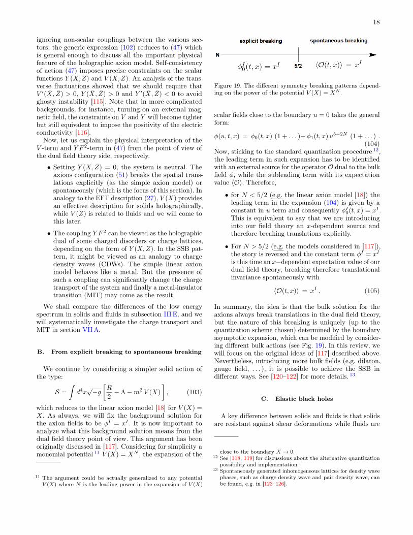
which reduces to the linear axion model [18] for V (X) =X. As always, we will fix the background solution forthe axion fields to be φI = xI . It is now important toanalyze what this background solution means from thedual field theory point of view. This argument has beenoriginally discussed in [117]. Considering for simplicity amonomial potential 11 V (X) = XN , the expansion of the

11 The argument could be actually generalized to any potentialV (X) where N is the leading power in the expansion of V (X)

Figure 19. The different symmetry breaking patterns depend-ing on the power of the potential V (X) = XN .

scalar fields close to the boundary u = 0 takes the generalform:

φ(u, t, x) = φ0(t, x) (1 + . . . )+φ1(t, x)u5−2N (1 + . . . ) .(104)

Now, sticking to the standard quantization procedure 12,the leading term in such expansion has to be identifiedwith an external source for the operator O dual to the bulkfield φ, while the subleading term with its expectationvalue 〈O〉. Therefore,

• for N < 5/2 (e.g. the linear axion model [18]) theleading term in the expansion (104) is given by aconstant in u term and consequently φI0(t, x) = xI .This is equivalent to say that we are introducinginto our field theory an x-dependent source andtherefore breaking translations explicitly.

• For N > 5/2 (e.g. the models considered in [117]),the story is reversed and the constant term φI = xI

is this time an x−dependent expectation value of ourdual field theory, breaking therefore translationalinvariance spontaneously with

〈O(t, x)〉 = xI . (105)

In summary, the idea is that the bulk solution for theaxions always break translations in the dual field theory,but the nature of this breaking is uniquely (up to thequantization scheme chosen) determined by the boundaryasymptotic expansion, which can be modified by consider-ing different bulk actions (see Fig. 19). In this review, wewill focus on the original ideas of [117] described above.Nevertheless, introducing more bulk fields (e.g. dilaton,gauge field, . . . ), it is possible to achieve the SSB indifferent ways. See [120–122] for more details. 13

C. Elastic black holes

A key difference between solids and fluids is that solidsare resistant against shear deformations while fluids are

close to the boundary X → 0.12 See [118, 119] for discussions about the alternative quantization

possibility and implementation.13 Spontaneously generated inhomogeneous lattices for density wave

phases, such as charge density wave and pair density wave, canbe found, e.g. in [123–126].

19

not. Then, the excitations moving inside a solid are wavespropagating in an elastic medium.

To see why the background solution given by the model(103) is dual to some elastic medium, we look at thespin-2 perturbations hxy which encodes the informationabout the Green’s function of the stress tensor Txy on theboundary. Interestingly, the shear equation is massive:

hxy = M2(u)hxy , (106)

where the effective mass of graviton becomes

u2M2(u) = m2 VX(X) , (107)

and VX ≡ dV/dX. Near the AdS boundary, we have thefollowing expansion,

hxy = h(0)(1 + . . . ) + h(3)u3(1 + . . . ) , (108)

where h(0) and h(3) are u-independent coefficients. Im-posing the infalling condition at the horizon and fixingthe leading coefficient h(0), this differential equation canbe solved numerically, or even analytically for small ωand m2 in Fourier space by using the perturbative meth-ods [6, 127]. According to the holographic dictionary, theGreen’s function of the stress tensor reads

G(R)TxyTxy

=3

2

h(3)

h(0), (109)

up to a contact term. In the low frequency expansion, weobtain that

G(R)TxyTxy

(ω)∣∣∣k=0

= G− i ω η +O(ω2) , (110)

where G is the shear modulus and η the shear viscosity.In the massive gravity case, the non-zero effective massbrings a non-trivial contribution to the real part of theGreen’s function. As a result, for small m, this gives

G = m2

∫ uh

0

VX(u2)

u2du+O(m4) . (111)

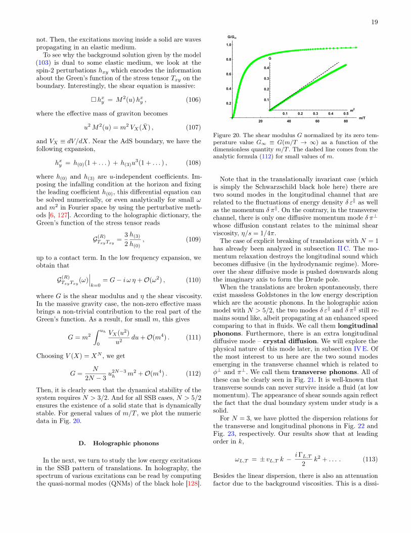
Choosing V (X) = XN , we get

G =N

2N − 3u2N−3h m2 +O(m4) . (112)

Then, it is clearly seen that the dynamical stability of thesystem requires N > 3/2. And for all SSB cases, N > 5/2ensures the existence of a solid state that is dynamicallystable. For general values of m/T , we plot the numericdata in Fig. 20.

D. Holographic phonons

In the next, we turn to study the low energy excitationsin the SSB pattern of translations. In holography, thespectrum of various excitations can be read by computingthe quasi-normal modes (QNMs) of the black hole [128].

0.1 0.2 0.3 0.4 0.5m2

0.1

0.2

0.3

0.4

G

20 40 60 80m/T

0.2

0.4

0.6

0.8

1.0

G/G∞

Figure 20. The shear modulus G normalized by its zero tem-perature value G∞ ≡ G(m/T → ∞) as a function of thedimensionless quantity m/T . The dashed line comes from theanalytic formula (112) for small values of m.

Note that in the translationally invariant case (whichis simply the Schwarzschild black hole here) there aretwo sound modes in the longitudinal channel that arerelated to the fluctuations of energy density δ ε‖ as wellas the momentum δ π‖. On the contrary, in the transversechannel, there is only one diffusive momentum mode δ π⊥whose diffusion constant relates to the minimal shearviscosity, η/s = 1/4π.

The case of explicit breaking of translations with N = 1has already been analyzed in subsection IIC. The mo-mentum relaxation destroys the longitudinal sound whichbecomes diffusive (in the hydrodynamic regime). More-over the shear diffusive mode is pushed downwards alongthe imaginary axis to form the Drude pole.

When the translations are broken spontaneously, thereexist massless Goldstones in the low energy descriptionwhich are the acoustic phonons. In the holographic axionmodel with N > 5/2, the two modes δ ε‖ and δ π‖ still re-mains sound like, albeit propagating at an enhanced speedcomparing to that in fluids. We call them longitudinalphonons. Furthermore, there is an extra longitudinaldiffusive mode – crystal diffusion. We will explore thephysical nature of this mode later, in subsection IVE. Ofthe most interest to us here are the two sound modesemerging in the transverse channel which is related toφ⊥ and π⊥. We call them transverse phonons. All ofthese can be clearly seen in Fig. 21. It is well-known thattransverse sounds can never survive inside a fluid (at lowmomentum). The appearance of shear sounds again reflectthe fact that the dual boundary system under study is asolid.

For N = 3, we have plotted the dispersion relations forthe transverse and longitudinal phonons in Fig. 22 andFig. 23, respectively. Our results show that at leadingorder in k,

ωL,T = ± vL,T k −iΓL,T

2k2 + . . . . (113)

Besides the linear dispersion, there is also an attenuationfactor due to the background viscosities. This is a dissi-

20

Figure 21. The spectrum of hydrodynamic modes can be readfrom the QNMs of the black hole. Top: Gapless modes propa-gating at the sound speed vT in the transverse channel, whichare related to the transverse phonons and transverse momen-tum in the dual field theory. Bottom: Gapless sound modespropagating at the speed vL in the longitudinal channel, re-lated to the longitudinal phonons and longitudinal momentum.In addition, there is an unexpected diffusive mode(orangedots), which we will call it crystal diffusion mode hereafter.

pative term due to finite temperature effects and can beformulated in the standard hydrodynamic approach, butdealing with it in the framework of EFT is challenging.The exact forms of ΓT,L will be discussed in section IV.

One can further check that the numerical data fromthe holographic model are in perfect agreement with theprediction of the elasticity theory, i.e.

vT =

√G

χππ, vL =

√K +G

χππ. (114)

Here, the momentum susceptibility χππ ≡ δTtiδvi = E + p.

One can see a comparison of vT extracted from the QNMsand the prediction of the elasticity theory in Fig. 24.

Finally, in a conformal solid, vL and vT are not indepen-dent of each other. One can verify this by explicitly com-puting the bulk modulus which is given by K = 3

4E [129]or using the EFT method of conformal solids [130]. As aresult, we have that

v2L =

1

2+ v2

T , (115)

which represents a further validity check for the holo-graphic model.

0.0 0.5 1.0 1.5k/T0.00

0.05

0.10

0.15

0.20

0.25

0.30

0.35

Re[ω]/T

0.5 1.0 1.5k/T

-0.14

-0.12

-0.10

-0.08

-0.06

-0.04

-0.02

0.00

Im[ω]/T

Figure 22. The dispersion relation of the transverse phonons inthe holographic axion model with V (X) = X5. m/T increasesfrom the red line to the blue one. Figure taken from [117].

m/T = 0

m/T = 3.5

m/T = 12.6

0.5 1.0 1.5 2.0 2.5 3.0k/T

0.5

1.0

1.5

2.0

2.5

3.0Re[ω/T]

Figure 23. The real part of the dispersion relation of thelongitudinal phonons in the holographic axion model. Figuretaken from [129].

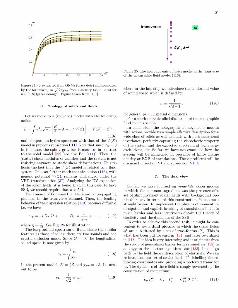
21

Figure 24. vT extracted from QNMs (black dots) and computedby the formula vT =

√G/χππ from elasticity (solid lines) for

n ∈ [3, 8] (green-orange). Figure taken from [117].

E. Zoology of solids and fluids

Let us move to a (reduced) model with the followingaction

S =

∫d4x√−g[R

2− Λ−m2 V (Z)

], V (Z) = Zn ,

(116)and compare its hydro-spectrum with that of the V (X)model in previous subsection IIID. Note that since VX = 0in this case, the spin-2 graviton is massless in contrastto the solid model [22] (see also Eq. (111)). Then, the(static) shear modulus G vanishes and the system is notresisting anymore to static shear deformations. This re-flects the fact that the V (Z) model is related to a fluidsystem. One can further check that the action (116), withgeneric potential V (Z), remains unchanged under theVPD transformation (37). Analyzing the UV expansionof the axion fields, it is found that, in this case, to haveSSB, we should require that n > 5/4.

The absence of G means that there are no propagatingphonons in the transverse channel. Then, the leadingbehavior of the dispersion relation (113) becomes diffusive,i.e, we have

ωT = −iDT k2 + . . . , DT =

η

χππ+ . . . , (117)

where η = s4π . See Fig. 25 for illustration.

The longitudinal spectrum of fluids share the similarfeatures as those of solids: there are two sounds and onecrystal diffusion mode. Since G = 0, the longitudinalsound speed is now given by

vL =

√K

χππ. (118)

In the present model, K = 34E and χππ = 3

2E . It turnsout to be

vL =1√2≡ vc , (119)

transverse ω

δϕ⊥ , δπ⊥

Figure 25. The hydrodynamic diffusive modes in the transverseof the holographic fluid model (116).

where in the last step we introduce the conformal valueof sound speed which is defined by

vc ≡1√d− 1

, (120)

for general (d− 1) spatial dimensions.For a much more detailed discussion of the holographic

fluid models see [92].In conclusion, the holographic homogeneous models

with axions provide us a simple effective description for awide class of solids as well as fluids with no translationalinvariance, perfectly capturing the viscoelastic propertyof the system and the expected spectrum of low energyexcitations, etc. So far, we have not examined how thesystem will be influenced in presence of finite chargedensity or EXB of translations. These problems will bediscussed in section VI and subsection VIIA.

F. The dual view

So far, we have focused on bona-fide axion modelsin which the common ingredient was the presence of aset of shift invariant scalar fields with background pro-file φI ∼ xI . In terms of this construction, it is almoststraightforward to implement the physics of momentumdissipation and explicit breaking of translations but it ismuch harder and less intuitive to obtain the theory ofelasticity and the dynamics of the SSB.In order to achieve this second task, it might be con-

venient to use a dual picture in which the scalar fieldsφI are substituted by a set of two-forms JIµν . This iswhat has been put forward in [131] and later re-utilizedin [118]. The idea is very interesting and it originates fromthe study of generalized higher form symmetries [132] inanalogy to the electromagnetism case [133]. Let us goback to the field theory description of elasticity. We canre-introduce our set of scalar fields ΦI , labelling the co-moving coordinates and providing a preferred frame forus. The dynamics of these field is simply governed by theconservation of momentum:

∂µ PµI = 0 , PµI = CµνIJ ∂νΦJ , (121)

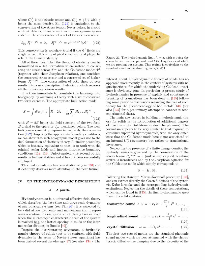
22

where CijIJ is the elastic tensor and CttIJ = % δIJ with %being the mass density. Eq. (121) is equivalent to theconservation of the stress tensor. Nevertheless, in a solidwithout defects, there is another hidden symmetry en-coded in the conservation of a set of two-form currents:

∂µ1 Jµ1 ... µdI = 0 , Jµ1 ... µd

I = εµ1...µd ν ∂νΦI . (122)

This conservation is somehow trivial if the ΦI fields aresingle valued. It is a topological constraint and plays therole of the Bianchi identity.All of these mean that the theory of elasticity can be

formulated in a dual formalism where instead of consid-ering the stress tensor Tµν and the Goldstone modes ΦI

(together with their Josephson relation), one considersthe conserved stress tensor and a conserved set of higher-forms Jµ1...µd

I . The conservation of both these objectsresults into a new description of elasticity which recoversall the previously known results.It is then immediate to translate this language into

holography, by assuming a theory with a set of conservedtwo-form currents. The appropriate bulk action reads

S =

∫d4x√−g

[R− 2Λ− 1

12

∑I

HI,abcHabcI

],

(123)with H = dB being the field strength of the two-formBµν dual to the operator Jµν mentioned before. The localbulk gauge symmetry imposes immediately the conserva-tion (122). Imposing the appropriate boundary conditions,we can show that such holographic model gives rise to thedual formulation of elasticity theory. A similar possibility,which is basically equivalent to that, is to work with theoriginal scalar fields and impose alternative boundaryconditions [118, 119]. Unfortunately, this second optionresults in bad instabilities and it has not been successfullyemployed.

This dual formulation has been studied only in [131] andit definitely deserves more attention in the near future.

IV. ON THE HYDRODYNAMIC DESCRIPTION

A. A puzzle

Hydrodynamics is a universal effective field theorywhich describes the late-time and large-scale dynamicsof any physical systems (see Fig. 26). It is expected tobe valid at low frequency and momentum and it repre-sents a continuum description which clearly breaks downwhen the microscopic characteristic scale of the systemis reached (e.g. the lattice spacing in solids or the inter-molecular distance in liquids [49]).Despite the disorientating oxymoron, a hydrody-

namic theory of solids (not to be confused with fluid-dynamics in the sense of Navier-Stokes equations) hasbeen derived several decades ago [37] (see also [134]). The

Figure 26. The hydrodynamic limit λ a, with a being thecharacteristic microscopic scale and λ the length-scale at whichwe are probing out system. This regime is equivalent to thestandard small momentum regime k/T 1.

interest about a hydrodynamic theory of solids has re-appeared more recently in the context of systems with noquasiparticles, for which the underlying Galilean invari-ance is obviously gone. In particular, a precise study ofhydrodynamics in presence of explicit and spontaneousbreaking of translations has been done in [135] follow-ing some previous discussions regarding the role of suchtheory for the phenomenology of bad metals [136] (seealso [137] for a preliminary attempt to connect it withexperimental data).

The main new aspect in building a hydrodynamic the-ory for solids is the introduction of additional degreesof freedom – the Goldstone modes (the phonons). Theformalism appears to be very similar to that required toconstruct superfluid hydrodynamics, with the only differ-ence that the Goldstone mode here is not associated toan internal U(1) symmetry but rather to translationalinvariance.Neglecting the presence of a finite charge density, the

hydrodynamics is governed by the conservation of thestress tensor ∂µTµν = 0 (unless any explicit breakingsource is introduced) and by the Josephson equation forthe Goldstone mode which simply corresponds to

Φ = [H ,Φ] . (124)

Following the standard Martin-Kadanoff procedure [138],one can extract directly the Green functions of the systemvia Kubo formulas and the corresponding hydrodynamicexcitations. Neglecting the details of these computations,which can be found in [135], the final hydrodynamic spec-trum of a solid contains:

transverse sound : ω = ± vT k −iΓT

2k2 + . . . ,

(125)

longitudinal sound : ω = ± vL k −iΓL

2k2 + . . . ,

(126)

crystal diffusion : ω = − iDφ k2 + . . . . (127)

The first two sets of modes are the standard phononicsound modes which are now attenuated with the charac-teristic diffusive-like damping due to the viscosity of the

23

system. The third mode is more interesting and maybeunusual. We will discuss in much more detail the physicalnature of this mode in Section IVE.

holographic model

hydrodynamics

0.5 1.0 1.5 2.0 2.5 3.0m/T0.00

0.05

0.10

0.15

0.20

0.25DϕT

Figure 27. The discrepancy between the hydrodynamic theoryof [135] and the holographic model of [117] reported in [129].The diffusion constant of the longitudinal crystal diffusionmode is denoted as Dφ.

The hydrodynamic theory indicates a concrete expres-sion for the diffusion constant Dφ which at leading orderreads

Dφ = (G+ K) ξ + . . . , (128)

where G,K are respectively the shear and bulk elasticmoduli. The new transport coefficient ξ is a dissipativeterm which controls the Goldstone diffusion and whichappears in the Goldstone’s two-points function:

GΦIΦJ =

(− 1

ω2 χππ+ ξ

i

ω

)δIJ + . . . . (129)

All the transport coefficients (G,K, ξ) can be computedindependently using the corresponding Kubo formulasat strictly zero momentum k = 0. On the contrary, thedispersion relation of the hydrodynamics modes can beobtained via a more complicated numerical computationof the QNMs of the system at finite momentum (see [139]for details).

The comparison between the two results was performedfor a large class of holographic axion models in [129] andpresented a surprising outcome. The numerical data, ex-tracted from the dispersion relation of the crystal diffusionmode, were not well described by the hydrodynamics for-mula (128). As evident from Fig. 27, the hydrodynamicsprediction is completely off with respect to the numericalholographic data. To be more concrete, the hydrodynamicframework of [135] does not correctly describe the low-energy physics of the holographic axion models [117].What is happening and what causes this discrepancy?

B. Strain pressure and its resolution

In order to understand the discrepancy discussed inthe previous subsection, we have to re-consider the hy-drodynamic description of [135] in more detail. This was

done in [118] (and later [140] for the charged case) usinga slightly different formalism which we will follow in thissection.

The fundamental ingredients of the hydrodynamic the-ory are the fluid velocity uµ, temperature T , and transla-tion Goldstone bosons ΦI . To proceed, we define the one-form eIµ = ∂µΦI , the crystal metric tensor hIJ = eIµe

Jµ,eIµ = h−1

IJ eJµ, hµν = h−1

IJ eIµeJν , and the strain tensor

uµν = 12 (h−1

IJ − δIJ/α2)eIµeJν , where α is simply a con-

stant. The constitutive relations for an isotropic viscoelas-tic medium are

Tµν =(E + p + TP ′uλλ

)uµuν +

(p + Puλλ

)ηµν + Phµν

−η σµν − ζ Pµν∂ρuρ − 2Guµν − (K−G)uλλhµν ,

(130)

together with the thermodynamic identities dp = sdT ,E = Ts− p and Pµν = ηµν + uµuν . Here, K is the part ofthe total bulk modulus depending on the SSB strength– its “solid” contribution – not to be confused with thetotal bulk modulus K = −V d〈T xx〉/dV . Additionally,σµν = 2P ρ(µP ν)σ∂ρuσ − Pµν∂ρuρ is the standard fluidshear tensor encoding the dissipative/viscous part of theresponse, while η and ζ are shear and bulk viscosities.The most important and new parameter entering here isthe strain pressure P with P ′ = ∂TP.The dynamics of the system is governed by the stress-

energy tensor conservation:

∂µTµν = 0 , (131)

and by the Josephson’s relation:

uµeIµ =hIJ

Σ∂µ(PeµJ − (K −G)uλλe

µJ − 2GuµνeJν

),

(132)where Σ is a dissipative coefficient characteristic of spon-taneously broken translations.

0.5 1.0 1.5 2.0 2.5 3.0m/T

0.14

0.16

0.18

0.20

0.22

0.24

D||T

Figure 28. The comparison of the crystal diffusion constantpredicted by hydrodynamics (134) with the holographic results.The previous discrepancy is now successfully resolved. Figuretaken from [119].

We expand the equations above around an equilibriumstate with uµ = δµt , T = T0, and ΦI = αxI , and we

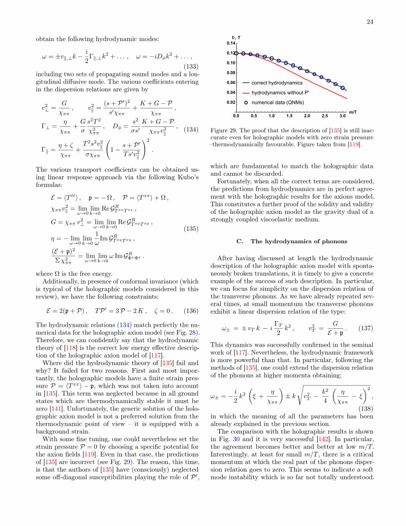
24

obtain the following hydrodynamic modes:

ω = ±v‖,⊥k −i

2Γ‖,⊥k

2 + . . . , ω = −iDφk2 + . . . ,

(133)including two sets of propagating sound modes and a lon-gitudinal diffusive mode. The various coefficients enteringin the dispersion relations are given by

v2⊥ =

G

χππ, v2

‖ =(s+ P ′)2

s′χππ+K +G− P

χππ,

Γ⊥ =η

χππ+G

σ

s2T 2

χ2ππ

, Dφ =s2

σs′K +G− Pχππv2

‖,

Γ‖ =η + ζ

χππ+T 2s2v2

‖

σχππ

(1− s+ P ′

Ts′v2‖

)2

.

(134)

The various transport coefficients can be obtained us-ing linear response approach via the following Kubo’sformulas:

E = 〈T tt〉 , p = −Ω , P = 〈T xx〉+ Ω ,

χππv2‖ = lim

ω→0limk→0

ReGRTxxTxx ,

G = χππ v2⊥ = lim

ω→0limk→0

ReGRTxyTxy ,

η = − limω→0

limk→0

1

ωImGRTxyTxy ,

(E + p)2

Σχ2ππ

= limω→0

limk→0

ω ImGRΦxΦx .

(135)

where Ω is the free energy.Additionally, in presence of conformal invariance (which

is typical of the holographic models considered in thisreview), we have the following constraints:

E = 2(p + P) , TP ′ = 3P − 2K , ζ = 0 . (136)

The hydrodynamic relations (134) match perfectly the nu-merical data for the holographic axion model (see Fig. 28).Therefore, we can confidently say that the hydrodynamictheory of [118] is the correct low energy effective descrip-tion of the holographic axion model of [117].Where did the hydrodynamic theory of [135] fail and

why? It failed for two reasons. First and most impor-tantly, the holographic models have a finite strain pres-sure P = 〈T xx〉 − p, which was not taken into accountin [135]. This term was neglected because in all groundstates which are thermodynamically stable it must bezero [141]. Unfortunately, the generic solution of the holo-graphic axion model is not a preferred solution from thethermodynamic point of view – it is equipped with abackground strain.With some fine tuning, one could nevertheless set the

strain pressure P = 0 by choosing a specific potential forthe axion fields [119]. Even in that case, the predictionsof [135] are incorrect (see Fig. 29). The reason, this time,is that the authors of [135] have (consciously) neglectedsome off-diagonal susceptibilities playing the role of P ′,

correct hydrodynamics

hydrodynamics without P'

numerical data (QNMs)

0.0 0.5 1.0 1.5 2.0 2.5 3.0m/T

0.02

0.04

0.06

0.08

0.10

0.12

0.14D||T

Figure 29. The proof that the description of [135] is still inac-curate even for holographic models with zero strain pressure–thermodynamically favourable. Figure taken from [119].

which are fundamental to match the holographic dataand cannot be discarded.

Fortunately, when all the correct terms are considered,the predictions from hydrodynamics are in perfect agree-ment with the holographic results for the axions model.This constitutes a further proof of the solidity and validityof the holographic axion model as the gravity dual of astrongly coupled viscoelastic medium.

C. The hydrodynamics of phonons

After having discussed at length the hydrodynamicdescription of the holographic axion model with sponta-neously broken translations, it is timely to give a concreteexample of the success of such description. In particular,we can focus for simplicity on the dispersion relation ofthe transverse phonons. As we have already repeated sev-eral times, at small momentum the transverse phononsexhibit a linear dispersion relation of the type:

ω± = ± vT k − iΓT2k2 , v2

T =G

E + p. (137)

This dynamics was successfully confirmed in the seminalwork of [117]. Nevertheless, the hydrodynamic frameworkis more powerful than that. In particular, following themethods of [135], one could extend the dispersion relationof the phonons at higher momenta obtaining:

ω± = − i2k2

(ξ +

η

χππ

)± k

√v2T −

k2

4

(η

χππ− ξ

)2

,

(138)in which the meaning of all the parameters has beenalready explained in the previous section.

The comparison with the holographic results is shownin Fig. 30 and it is very successful [142]. In particular,the agreement becomes better and better at low m/T .Interestingly, at least for small m/T , there is a criticalmomentum at which the real part of the phonons disper-sion relation goes to zero. This seems to indicate a softmode instability which is so far not totally understood.

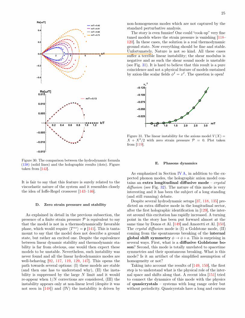
25

m/T = 0.42

m/T = 0.51

m/T = 0.60

m/T = 0.73

2 4 6 8k/T

-0.4

-0.2

0.0

0.2

0.4

Re[ω/T]

m/T = 0.13

0.2 0.4 0.6 0.8 1.0 1.2k/T

-0.015

-0.010

-0.005

0.005

0.010

0.015Re[ω/T]

Figure 30. The comparison between the hydrodynamic formula(138) (solid lines) and the holographic results (dots). Figuretaken from [142].

It is fair to say that this feature is surely related to theviscoelastic nature of the system and it resembles closelythe idea of Ioffe-Regel crossover [143–146].

D. Zero strain pressure and stability

As explained in detail in the previous subsection, thepresence of a finite strain pressure P is equivalent to saythat the model is not in a thermodynamically favorablephase, which would require 〈T xx〉 = p [141]. This is tanta-mount to say that the model does not describe a groundstate, but rather an excited one. Despite the equivalencebetween linear dynamic stability and thermodynamic sta-bility is far from obvious, one would then expect thesemodels to be unstable. Nevertheless, such instability wasnever found and all the linear hydrodynamics modes arewell-behaving [92, 117, 119, 129, 147]. This opens thepath towards several options: (I) these models are stable(and then one has to understand why), (II) the insta-bility is suppressed by the large N limit and it wouldre-appear when 1/N corrections are considered, (III) theinstability appears only at non-linear level (despite it wasnot seen in [148]) and (IV) the instability is driven by

non-homogeneous modes which are not captured by thestandard perturbative analysis.

The story is even funnier! One could “cook-up” very finetuned models where the strain pressure is vanishing [118–120]. In these cases, the solution is a real thermodynamicground state. Now everything should be fine and stable.Unfortunately, Nature is not so kind. All these casessuffer a terrible linear instability; the shear modulus isnegative and as such the shear sound mode is unstable(see Fig. 31). It is hard to believe that this result is a purecoincidence and not a physical feature of models sustainedby axion-like scalar fields φI = xI . The question is open!

Figure 31. The linear instability for the axions model V (X) =X + X2/2 with zero strain pressure P = 0. Plot takenfrom [119].

E. Phasons dynamics

As emphasized in Section IVA, in addition to the ex-pected phonon modes, the holographic axion model con-tains an extra longitudinal diffusive mode – crystaldiffusion (see Fig. 32). The nature of this mode is veryinteresting and it has been the subject of a long standing(and still running) debate.

Despite several hydrodynamic setups [37, 118, 135] pre-dicted an extra diffusive mode in the longitudinal sector,after the first holographic identification in [129], the inter-est around this excitation has rapidly increased. A turningpoint in the story has been put forward almost at thesame time by Donos et Al. [149] and Amoretti et Al. [150].The crystal diffusion mode is (I) a Goldstone mode, (II)coming from the spontaneous breaking of the internalglobal shift symmetry φ→ φ+a. This is surprising inseveral ways. First, what is a diffusive Goldstone bo-son? Second, this mode is totally unrelated to spacetimesymmetries and their spontaneous breaking. What is thismode? Is it an artifact of the simplified assumption ofhomogeneity or not?Taking into account the results of [149, 150], the first

step is to understand what is the physical role of the inter-nal space and shifts along that. A recent idea [151] triedto connect the dynamics of this mode with the physicsof quasicrystals – systems with long range order butwithout periodicity. Quasicyrstals have a long and curious

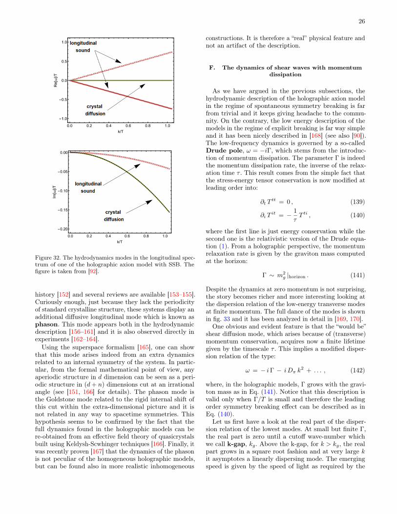
26

Figure 32. The hydrodynamics modes in the longitudinal spec-trum of one of the holographic axion model with SSB. Thefigure is taken from [92].

history [152] and several reviews are available [153–155].Curiously enough, just because they lack the periodicityof standard crystalline structure, these systems display anadditional diffusive longitudinal mode which is known asphason. This mode appears both in the hydrodynamicdescription [156–161] and it is also observed directly inexperiments [162–164].Using the superspace formalism [165], one can show

that this mode arises indeed from an extra dynamicsrelated to an internal symmetry of the system. In partic-ular, from the formal mathematical point of view, anyaperiodic structure in d dimension can be seen as a peri-odic structure in (d+ n) dimensions cut at an irrationalangle (see [151, 166] for details). The phason mode isthe Goldstone mode related to the rigid internal shift ofthis cut within the extra-dimensional picture and it isnot related in any way to spacetime symmetries. Thishypothesis seems to be confirmed by the fact that thefull dynamics found in the holographic models can bere-obtained from an effective field theory of quasicrystalsbuilt using Keldysh-Scwhinger techniques [166]. Finally, itwas recently proven [167] that the dynamics of the phasonis not peculiar of the homogeneous holographic models,but can be found also in more realistic inhomogeneous

constructions. It is therefore a “real” physical feature andnot an artifact of the description.

F. The dynamics of shear waves with momentumdissipation

As we have argued in the previous subsections, thehydrodynamic description of the holographic axion modelin the regime of spontaneous symmetry breaking is farfrom trivial and it keeps giving headache to the commu-nity. On the contrary, the low energy description of themodels in the regime of explicit breaking is far way simpleand it has been nicely described in [168] (see also [90]).The low-frequency dynamics is governed by a so-calledDrude pole, ω = −iΓ, which stems from the introduc-tion of momentum dissipation. The parameter Γ is indeedthe momentum dissipation rate, the inverse of the relax-ation time τ . This result comes from the simple fact thatthe stress-energy tensor conservation is now modified atleading order into:

∂t Ttt = 0 , (139)

∂i Tit = − 1

τT ti , (140)

where the first line is just energy conservation while thesecond one is the relativistic version of the Drude equa-tion (1). From a holographic perspective, the momentumrelaxation rate is given by the graviton mass computedat the horizon:

Γ ∼ m2g |horizon . (141)

Despite the dynamics at zero momentum is not surprising,the story becomes richer and more interesting looking atthe dispersion relation of the low-energy transverse modesat finite momentum. The full dance of the modes is shownin fig. 33 and it has been analyzed in detail in [169, 170].

One obvious and evident feature is that the “would be”shear diffusion mode, which arises because of (transverse)momentum conservation, acquires now a finite lifetimegiven by the timescale τ . This implies a modified disper-sion relation of the type:

ω = − iΓ − iDπ k2 + . . . , (142)

where, in the holographic models, Γ grows with the gravi-ton mass as in Eq. (141). Notice that this description isvalid only when Γ/T is small and therefore the leadingorder symmetry breaking effect can be described as inEq. (140).Let us first have a look at the real part of the disper-

sion relation of the lowest modes. At small but finite Γ,the real part is zero until a cutoff wave-number whichwe call k-gap, kg. Above the k-gap, for k > kg, the realpart grows in a square root fashion and at very large kit asymptotes a linearly dispersing mode. The emergingspeed is given by the speed of light as required by the

27

massive particle

k-gap

2 4 6 8 10 12k/T

-10

-5

0

5

10

Re[ω]/T

2 4 6 8 10 12k/T

-15

-10

-5

0

Im[ω]/T

Figure 33. The transverse spectrum of excitations for the linearmodel V (X) = X. m/T increases from the blue line to thered one. Figures taken from [169].

UV relativistic fixed point of the theory. Importantly, thisfeature arises because of the collision of the Drude pole(142) with a second non-hydrodynamic mode. This colli-sion is actually a manifestation of the coherent-incoherenttransition described in [88, 90].

When momentum dissipation becomes very strong, thek−gap approaches the origin and the dispersion relationbecomes of the massive particle type, Re[ω]2 = k2 +M2,with an approximately constant lifetime given by Γ−1.This feature, of having an emerging transverse shear wavesat low frequency is very interesting since it resembleswhat is happening in realistic liquids. The presence ofthese emerging propagating phonons is tested indirectlyin recent experiments [171–173] (see also [174]) and itcan be explained by the so-called k-gap or telegraphequation [175, 176]. In a specific limit of the linear axionstheory the corresponding dispersion relation can be foundanalytically [90]. Interestingly, this k-gap dynamics isshared by several holographic models [177–182] and it canbe explained by using the quasi-hydrodynamic theoryof [183]. Finally, we can verify that the critical momentumkg is as expected inversely proportional to the relaxationtime τ (top panel of Fig. 34) and compare the latter withthe famous Arrhenius law for fluids [184] (bottom panelof Fig. 34).

0.6 0.7 0.8 0.9 1.0

1

τ

0.6

0.7

0.8

0.9

1.0

kgap

5.0 5.5 6.0 6.5m/T

-2.5

-2.0

-1.5

-1.0

Log[τT]

Figure 34. Top: The numerical confirmation that kg ∼ 1/τ .Bottom: The behaviour of the relaxation time in function ofthe inverse of the temperature which is in qualitative agreementwith the Arrhenius law [184] . Figures taken from [169].

V. BOUNDS FROM HYDRODYNAMICS ANDHOLOGRAPHY

A. The violation of the KSS bound

Continuing with the hydrodynamic description of theaxion model, we cannot avoid mentioning one of themost surprising, and perhaps less understood outcome.The main character of this story is the shear viscosity,defined via the Kubo formula:

η ≡ − limω→0

1

ωIm〈TxyTxy〉 . (143)

One of the most remarkable achievements of the holo-graphic duality is the discovery of the so-called Kovtun-Son-Starintes(KSS) bound [13]. The statement of thebound is that the ratio of shear viscosity and entropydensity should be bounded below by a universal constant,

η

s≥ 1

4π

(~kB

), (144)

where the Planck constant ~ and the Boltzmann constantkB will be set to unit hereinafter. In the strong couplinglimit (which is usually assumed in the holographic compu-tations), the equality holds and the inequality is saturated.

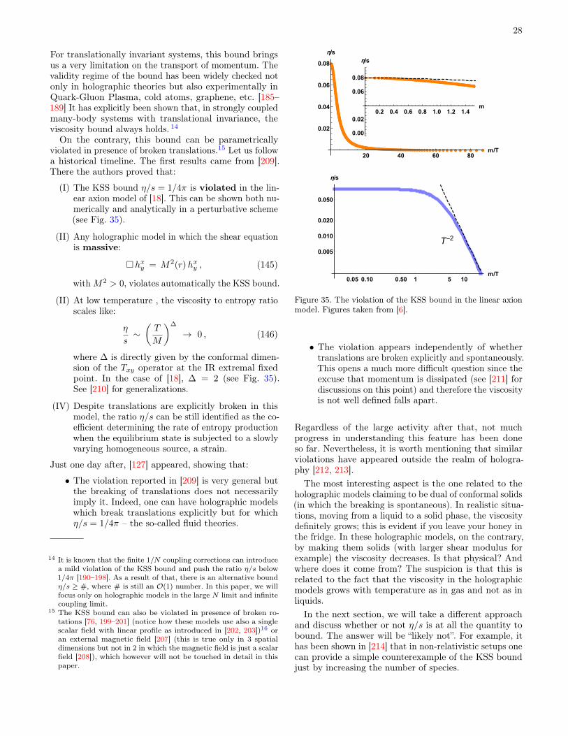
28

For translationally invariant systems, this bound bringsus a very limitation on the transport of momentum. Thevalidity regime of the bound has been widely checked notonly in holographic theories but also experimentally inQuark-Gluon Plasma, cold atoms, graphene, etc. [185–189] It has explicitly been shown that, in strongly coupledmany-body systems with translational invariance, theviscosity bound always holds. 14

On the contrary, this bound can be parametricallyviolated in presence of broken translations.15 Let us followa historical timeline. The first results came from [209].There the authors proved that:

(I) The KSS bound η/s = 1/4π is violated in the lin-ear axion model of [18]. This can be shown both nu-merically and analytically in a perturbative scheme(see Fig. 35).

(II) Any holographic model in which the shear equationis massive:

hxy = M2(r)hxy , (145)

withM2 > 0, violates automatically the KSS bound.

(II) At low temperature , the viscosity to entropy ratioscales like:

η

s∼(T

M

)∆

→ 0 , (146)

where ∆ is directly given by the conformal dimen-sion of the Txy operator at the IR extremal fixedpoint. In the case of [18], ∆ = 2 (see Fig. 35).See [210] for generalizations.

(IV) Despite translations are explicitly broken in thismodel, the ratio η/s can be still identified as the co-efficient determining the rate of entropy productionwhen the equilibrium state is subjected to a slowlyvarying homogeneous source, a strain.

Just one day after, [127] appeared, showing that:

• The violation reported in [209] is very general butthe breaking of translations does not necessarilyimply it. Indeed, one can have holographic modelswhich break translations explicitly but for whichη/s = 1/4π – the so-called fluid theories.

14 It is known that the finite 1/N coupling corrections can introducea mild violation of the KSS bound and push the ratio η/s below1/4π [190–198]. As a result of that, there is an alternative boundη/s ≥ #, where # is still an O(1) number. In this paper, we willfocus only on holographic models in the large N limit and infinitecoupling limit.

15 The KSS bound can also be violated in presence of broken ro-tations [76, 199–201] (notice how these models use also a singlescalar field with linear profile as introduced in [202, 203])16 oran external magnetic field [207] (this is true only in 3 spatialdimensions but not in 2 in which the magnetic field is just a scalarfield [208]), which however will not be touched in detail in thispaper.

0.2 0.4 0.6 0.8 1.0 1.2 1.4m

0.00

0.02

0.06

0.08

η/s

20 40 60 80m/T

0.02

0.04

0.06

0.08

η/s

T-2

0.05 0.10 0.50 1 5 10m/T

0.005

0.010

0.020

0.050

η/s

Figure 35. The violation of the KSS bound in the linear axionmodel. Figures taken from [6].

• The violation appears independently of whethertranslations are broken explicitly and spontaneously.This opens a much more difficult question since theexcuse that momentum is dissipated (see [211] fordiscussions on this point) and therefore the viscosityis not well defined falls apart.

Regardless of the large activity after that, not muchprogress in understanding this feature has been doneso far. Nevertheless, it is worth mentioning that similarviolations have appeared outside the realm of hologra-phy [212, 213].The most interesting aspect is the one related to the

holographic models claiming to be dual of conformal solids(in which the breaking is spontaneous). In realistic situa-tions, moving from a liquid to a solid phase, the viscositydefinitely grows; this is evident if you leave your honey inthe fridge. In these holographic models, on the contrary,by making them solids (with larger shear modulus forexample) the viscosity decreases. Is that physical? Andwhere does it come from? The suspicion is that this isrelated to the fact that the viscosity in the holographicmodels grows with temperature as in gas and not as inliquids.In the next section, we will take a different approach

and discuss whether or not η/s is at all the quantity tobound. The answer will be “likely not”. For example, ithas been shown in [214] that in non-relativistic setups onecan provide a simple counterexample of the KSS boundjust by increasing the number of species.

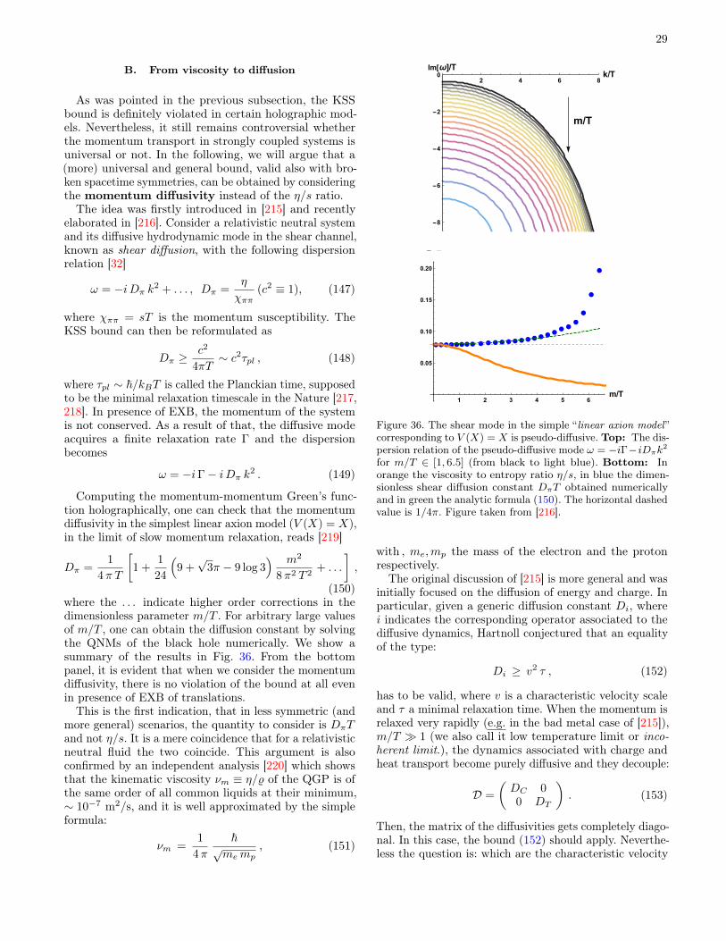
29

B. From viscosity to diffusion

As was pointed in the previous subsection, the KSSbound is definitely violated in certain holographic mod-els. Nevertheless, it still remains controversial whetherthe momentum transport in strongly coupled systems isuniversal or not. In the following, we will argue that a(more) universal and general bound, valid also with bro-ken spacetime symmetries, can be obtained by consideringthe momentum diffusivity instead of the η/s ratio.The idea was firstly introduced in [215] and recently

elaborated in [216]. Consider a relativistic neutral systemand its diffusive hydrodynamic mode in the shear channel,known as shear diffusion, with the following dispersionrelation [32]

ω = −iDπ k2 + . . . , Dπ =

η

χππ(c2 ≡ 1), (147)

where χππ = sT is the momentum susceptibility. TheKSS bound can then be reformulated as

Dπ ≥c2

4πT∼ c2τpl , (148)

where τpl ∼ ~/kBT is called the Planckian time, supposedto be the minimal relaxation timescale in the Nature [217,218]. In presence of EXB, the momentum of the systemis not conserved. As a result of that, the diffusive modeacquires a finite relaxation rate Γ and the dispersionbecomes

ω = −iΓ− iDπ k2 . (149)

Computing the momentum-momentum Green’s func-tion holographically, one can check that the momentumdiffusivity in the simplest linear axion model (V (X) = X),in the limit of slow momentum relaxation, reads [219]

Dπ =1

4π T

[1 +

1

24

(9 +√

3π − 9 log 3) m2

8π2 T 2+ . . .

],

(150)where the . . . indicate higher order corrections in thedimensionless parameter m/T . For arbitrary large valuesof m/T , one can obtain the diffusion constant by solvingthe QNMs of the black hole numerically. We show asummary of the results in Fig. 36. From the bottompanel, it is evident that when we consider the momentumdiffusivity, there is no violation of the bound at all evenin presence of EXB of translations.

This is the first indication, that in less symmetric (andmore general) scenarios, the quantity to consider is DπTand not η/s. It is a mere coincidence that for a relativisticneutral fluid the two coincide. This argument is alsoconfirmed by an independent analysis [220] which showsthat the kinematic viscosity νm ≡ η/% of the QGP is ofthe same order of all common liquids at their minimum,∼ 10−7 m2/s, and it is well approximated by the simpleformula:

νm =1

4π

~√memp

, (151)

m/T

2 4 6 8k/T

-8

-6

-4

-2

0Im[ω]/T

1 2 3 4 5 6m/T

0.05

0.10

0.15

0.20

DTT

Figure 36. The shear mode in the simple “ linear axion model ”corresponding to V (X) = X is pseudo-diffusive. Top: The dis-persion relation of the pseudo-diffusive mode ω = −iΓ−iDπk2for m/T ∈ [1, 6.5] (from black to light blue). Bottom: Inorange the viscosity to entropy ratio η/s, in blue the dimen-sionless shear diffusion constant DπT obtained numericallyand in green the analytic formula (150). The horizontal dashedvalue is 1/4π. Figure taken from [216].

with , me,mp the mass of the electron and the protonrespectively.

The original discussion of [215] is more general and wasinitially focused on the diffusion of energy and charge. Inparticular, given a generic diffusion constant Di, wherei indicates the corresponding operator associated to thediffusive dynamics, Hartnoll conjectured that an equalityof the type:

Di ≥ v2 τ , (152)

has to be valid, where v is a characteristic velocity scaleand τ a minimal relaxation time. When the momentum isrelaxed very rapidly (e.g. in the bad metal case of [215]),m/T 1 (we also call it low temperature limit or inco-herent limit.), the dynamics associated with charge andheat transport become purely diffusive and they decouple:

D =

(DC 00 DT

). (153)

Then, the matrix of the diffusivities gets completely diago-nal. In this case, the bound (152) should apply. Neverthe-less the question is: which are the characteristic velocity

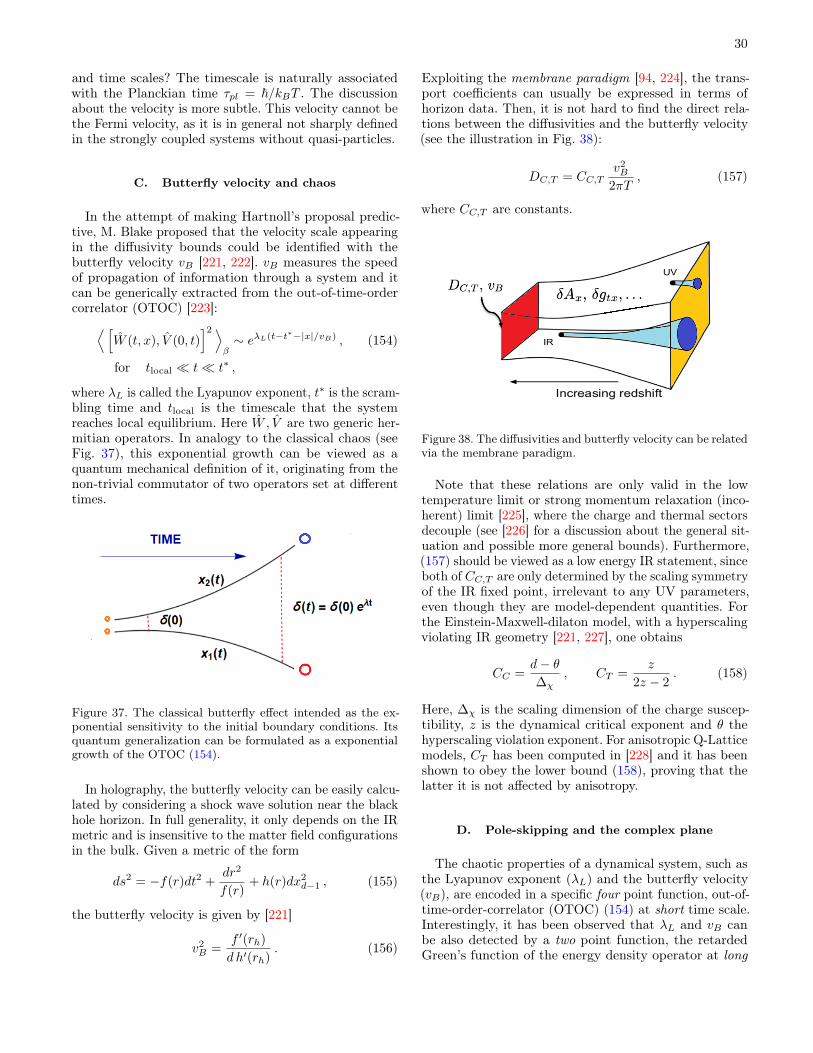
30

and time scales? The timescale is naturally associatedwith the Planckian time τpl = ~/kBT . The discussionabout the velocity is more subtle. This velocity cannot bethe Fermi velocity, as it is in general not sharply definedin the strongly coupled systems without quasi-particles.

C. Butterfly velocity and chaos

In the attempt of making Hartnoll’s proposal predic-tive, M. Blake proposed that the velocity scale appearingin the diffusivity bounds could be identified with thebutterfly velocity vB [221, 222]. vB measures the speedof propagation of information through a system and itcan be generically extracted from the out-of-time-ordercorrelator (OTOC) [223]:⟨ [

W (t, x), V (0, t)]2 ⟩

β∼ eλL(t−t∗−|x|/vB) , (154)

for tlocal t t∗ ,

where λL is called the Lyapunov exponent, t∗ is the scram-bling time and tlocal is the timescale that the systemreaches local equilibrium. Here W , V are two generic her-mitian operators. In analogy to the classical chaos (seeFig. 37), this exponential growth can be viewed as aquantum mechanical definition of it, originating from thenon-trivial commutator of two operators set at differenttimes.

Figure 37. The classical butterfly effect intended as the ex-ponential sensitivity to the initial boundary conditions. Itsquantum generalization can be formulated as a exponentialgrowth of the OTOC (154).

In holography, the butterfly velocity can be easily calcu-lated by considering a shock wave solution near the blackhole horizon. In full generality, it only depends on the IRmetric and is insensitive to the matter field configurationsin the bulk. Given a metric of the form

ds2 = −f(r)dt2 +dr2

f(r)+ h(r)dx2

d−1 , (155)

the butterfly velocity is given by [221]

v2B =

f ′(rh)

d h′(rh). (156)

Exploiting the membrane paradigm [94, 224], the trans-port coefficients can usually be expressed in terms ofhorizon data. Then, it is not hard to find the direct rela-tions between the diffusivities and the butterfly velocity(see the illustration in Fig. 38):

DC,T = CC,Tv2B

2πT, (157)

where CC,T are constants.

Figure 38. The diffusivities and butterfly velocity can be relatedvia the membrane paradigm.

Note that these relations are only valid in the lowtemperature limit or strong momentum relaxation (inco-herent) limit [225], where the charge and thermal sectorsdecouple (see [226] for a discussion about the general sit-uation and possible more general bounds). Furthermore,(157) should be viewed as a low energy IR statement, sinceboth of CC,T are only determined by the scaling symmetryof the IR fixed point, irrelevant to any UV parameters,even though they are model-dependent quantities. Forthe Einstein-Maxwell-dilaton model, with a hyperscalingviolating IR geometry [221, 227], one obtains

CC =d− θ∆χ

, CT =z

2z − 2. (158)

Here, ∆χ is the scaling dimension of the charge suscep-tibility, z is the dynamical critical exponent and θ thehyperscaling violation exponent. For anisotropic Q-Latticemodels, CT has been computed in [228] and it has beenshown to obey the lower bound (158), proving that thelatter it is not affected by anisotropy.

D. Pole-skipping and the complex plane

The chaotic properties of a dynamical system, such asthe Lyapunov exponent (λL) and the butterfly velocity(vB), are encoded in a specific four point function, out-of-time-order-correlator (OTOC) (154) at short time scale.Interestingly, it has been observed that λL and vB canbe also detected by a two point function, the retardedGreen’s function of the energy density operator at long

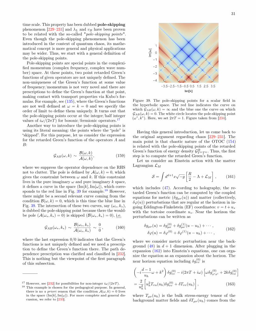
31

time scale. This property has been dubbed pole-skippingphenomenon [229–231] and λL and vB have been provento be related with the so-called "pole-skipping points".Even though the pole-skipping phenomenon has beenintroduced in the context of quantum chaos, its mathe-matical concept is more general and physical applicationsmay be wider. Thus, we start with a general definition ofthe pole-skipping points.

Pole-skipping points are special points in the complexi-fied momentum (complex frequency, complex wave num-ber) space. At these points, two point retarded Green’sfunctions of given operators are not uniquely defined. Thenon-uniqueness of the Green’s function at some valueof frequency/momentum is not very novel and there areprescriptions to define the Green’s function at that point,making contact with transport properties via Kubo’s for-mulas. For example, see (135), where the Green’s functionsare not well defined at ω = k = 0 and we specify theorder of limit to define them uniquely. It turns out thatthe pole-skipping points occur at the integer/half integervalues of iω/(2πT ) for bosonic/fermionic operators.17

Another way to introduce the pole-skipping points isusing its literal meaning: the points where the “pole” is“skipped”. For this purpose, let us consider the expressionfor the retarded Green’s function of the operators A andB:

GAB(ω, k) ∼ B(ω, k)

A(ω, k), (159)

where we suppress the operator dependence on the RHSnot to clutter. The pole is defined by A(ω, k) = 0, whichgives the constraint between ω and k. If this constraintlives in the pure imaginary ω and pure imaginary k space,it defines a curve in the space (Im[k], Im[ω]), which corre-sponds to the red line in Fig. 39 for example.18 However,there might be a second relevant curve coming from thecondition B(ω, k) = 0, which is this time the blue line inFig. 39. The intersection of these two curves, say (ω∗, k∗),is dubbed the pole-skipping point because there the would-be pole (A(ω∗, k∗) = 0) is skipped (B(ω∗, k∗) = 0), i.e.

GAB(ω∗, k∗) ∼B(ω∗, k∗)

A(ω∗, k∗)∼ 0

0, (160)

where the last expression 0/0 indicates that the Green’sfunctions is not uniquely defined and we need a prescrip-tion to define the Green’s function there. The path de-pendence prescription was clarified and classified in [232].This is nothing but the viewpoint of the first paragraphof this subsection.

17 However, see [232] for possibilities for non-integer iω/(2πT ).18 This example is chosen for the pedagogical purpose. In general,

there is no a priori reason that the condition A(ω, k) = 0 livesin the space (Im[k], Im[ω]). For more complete and general dis-cussion, we refer to [233].

Figure 39. The pole-skipping points for a scalar field inthe hyperbolic space. The red line indicates the curve onwhich GAB(ω, k) = ∞ and the blue one the curve on whichGAB(ω, k) = 0. The white circle locates the pole-skipping point(ω∗, k∗). Here, we set 2πT = 1. Figure taken from [234].

Having this general introduction, let us come back tothe original argument regarding chaos [229–231]. Themain point is that chaotic nature of the OTOC (154)is related with the pole-skipping points of the retardedGreen’s function of energy density GRT ttT tt . Thus, the firststep is to compute the retarded Green’s function.Let us consider an Einstein action with the matter

Lagrangian LM

S =

∫dd+1x

√−g[R

2− Λ + LM

], (161)

which includes (47). According to holography, the re-tarded Green’s function can be computed by the coupledequations for metric (δgµν(u)) and matter (collectively,δϕ(u)) perturbations that are regular at the horizon in in-going Eddington-Finkelstein (EF) coordinates: v = t+ u∗with the tortoise coordinate u∗. Near the horizon theperturbations can be written as

δgµν(u) = δg(0)µν + δg(1)

µν (u− uh) + · · · ,

δϕ(u) = δϕ(0) + δϕ(1)(u− uh) + · · · ,(162)

where we consider metric perturbation near the back-ground (48) in d + 1 dimension. After plugging in theexpansion (162) into Einstein’s equations, one can orga-nize the equation as an expansion about the horizon. Thenear horizon equation including δg(0)

vv is(−id− 1

uhω + k2

)δg(0)vv − i(2πT + iω)

[ωδg

(0)xixi + 2kδg(0)

vx

]=

2

u2h

[u2hTvu(uh)δg(0)

vv + δTvv(uh)

], (163)

where Tµν(uh) is the bulk stress-energy tensor of thebackground matter fields and δTµν(uh) comes from the

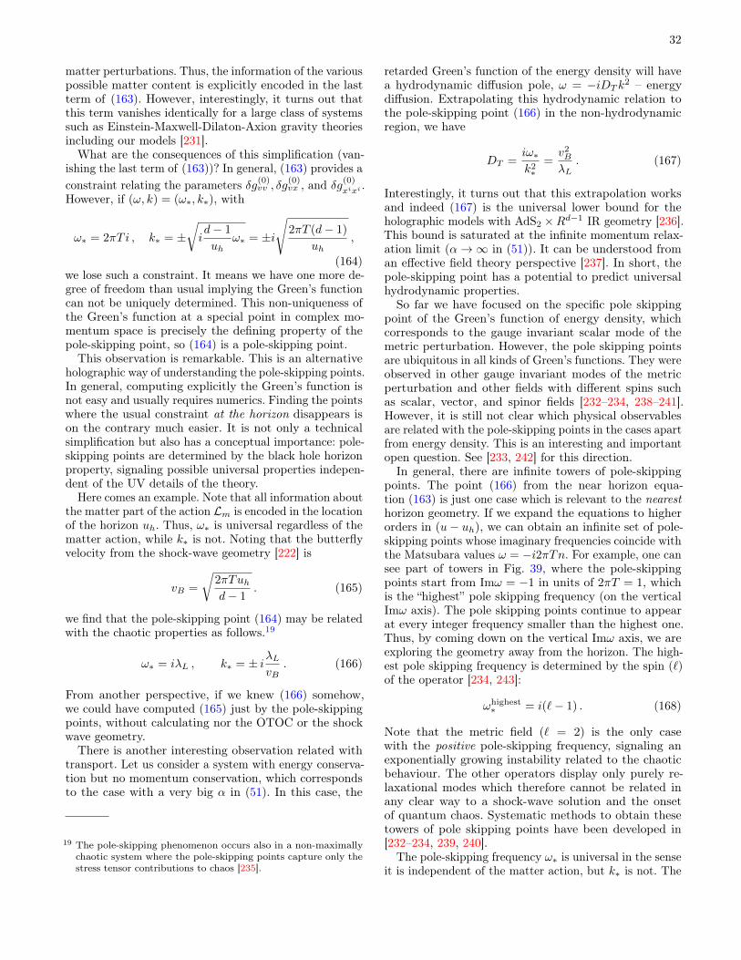
32

matter perturbations. Thus, the information of the variouspossible matter content is explicitly encoded in the lastterm of (163). However, interestingly, it turns out thatthis term vanishes identically for a large class of systemssuch as Einstein-Maxwell-Dilaton-Axion gravity theoriesincluding our models [231].What are the consequences of this simplification (van-

ishing the last term of (163))? In general, (163) provides aconstraint relating the parameters δg(0)

vv , δg(0)vx , and δg

(0)xixi .

However, if (ω, k) = (ω∗, k∗), with

ω∗ = 2πT i , k∗ = ±√id− 1

uhω∗ = ±i

√2πT (d− 1)

uh,

(164)we lose such a constraint. It means we have one more de-gree of freedom than usual implying the Green’s functioncan not be uniquely determined. This non-uniqueness ofthe Green’s function at a special point in complex mo-mentum space is precisely the defining property of thepole-skipping point, so (164) is a pole-skipping point.This observation is remarkable. This is an alternative

holographic way of understanding the pole-skipping points.In general, computing explicitly the Green’s function isnot easy and usually requires numerics. Finding the pointswhere the usual constraint at the horizon disappears ison the contrary much easier. It is not only a technicalsimplification but also has a conceptual importance: pole-skipping points are determined by the black hole horizonproperty, signaling possible universal properties indepen-dent of the UV details of the theory.

Here comes an example. Note that all information aboutthe matter part of the action Lm is encoded in the locationof the horizon uh. Thus, ω∗ is universal regardless of thematter action, while k∗ is not. Noting that the butterflyvelocity from the shock-wave geometry [222] is

vB =

√2πTuhd− 1

. (165)

we find that the pole-skipping point (164) may be relatedwith the chaotic properties as follows.19

ω∗ = iλL , k∗ = ± iλLvB

. (166)

From another perspective, if we knew (166) somehow,we could have computed (165) just by the pole-skippingpoints, without calculating nor the OTOC or the shockwave geometry.

There is another interesting observation related withtransport. Let us consider a system with energy conserva-tion but no momentum conservation, which correspondsto the case with a very big α in (51). In this case, the

19 The pole-skipping phenomenon occurs also in a non-maximallychaotic system where the pole-skipping points capture only thestress tensor contributions to chaos [235].

retarded Green’s function of the energy density will havea hydrodynamic diffusion pole, ω = −iDT k

2 – energydiffusion. Extrapolating this hydrodynamic relation tothe pole-skipping point (166) in the non-hydrodynamicregion, we have

DT =iω∗k2∗

=v2B

λL. (167)

Interestingly, it turns out that this extrapolation worksand indeed (167) is the universal lower bound for theholographic models with AdS2 ×Rd−1 IR geometry [236].This bound is saturated at the infinite momentum relax-ation limit (α→∞ in (51)). It can be understood froman effective field theory perspective [237]. In short, thepole-skipping point has a potential to predict universalhydrodynamic properties.So far we have focused on the specific pole skipping

point of the Green’s function of energy density, whichcorresponds to the gauge invariant scalar mode of themetric perturbation. However, the pole skipping pointsare ubiquitous in all kinds of Green’s functions. They wereobserved in other gauge invariant modes of the metricperturbation and other fields with different spins suchas scalar, vector, and spinor fields [232–234, 238–241].However, it is still not clear which physical observablesare related with the pole-skipping points in the cases apartfrom energy density. This is an interesting and importantopen question. See [233, 242] for this direction.In general, there are infinite towers of pole-skipping

points. The point (166) from the near horizon equa-tion (163) is just one case which is relevant to the nearesthorizon geometry. If we expand the equations to higherorders in (u− uh), we can obtain an infinite set of pole-skipping points whose imaginary frequencies coincide withthe Matsubara values ω = −i2πTn. For example, one cansee part of towers in Fig. 39, where the pole-skippingpoints start from Imω = −1 in units of 2πT = 1, whichis the “highest” pole skipping frequency (on the verticalImω axis). The pole skipping points continue to appearat every integer frequency smaller than the highest one.Thus, by coming down on the vertical Imω axis, we areexploring the geometry away from the horizon. The high-est pole skipping frequency is determined by the spin (`)of the operator [234, 243]:

ωhighest∗ = i(`− 1) . (168)

Note that the metric field (` = 2) is the only casewith the positive pole-skipping frequency, signaling anexponentially growing instability related to the chaoticbehaviour. The other operators display only purely re-laxational modes which therefore cannot be related inany clear way to a shock-wave solution and the onsetof quantum chaos. Systematic methods to obtain thesetowers of pole skipping points have been developed in[232–234, 239, 240].

The pole-skipping frequency ω∗ is universal in the senseit is independent of the matter action, but k∗ is not. The

33

pole skipping wave number k∗ depends on the momentumrelaxation parameter α in (51), chemical potential µ, andother parameters in the matter action. In particular, k∗can be real number or complex number (see Fig. 40).

Figure 40. Pole-skipping wave number (k∗) can be real(red),complex(blue), and pure imaginary(green) for scalar fieldperturbation in AdS4. The momentum relaxation parame-ter α = 2, 2, 1 for Im[ω] = −1,−2,−3 (from top to bottom)respectively. Here, the “bar” variables denote the quantitiesscaled by 2πT . Figure taken from [233].

The pole skipping phenomena have been studied in theSYK models and the conformal field theory [243–245].The relations between OTOC and pole skipping points (aswell as the comparison between field theory and gravityanalysis) have been investigated in [232, 234, 243, 246]where the hyperbolic space was considered to have ananalytic control. However, the final qualitative resultsare believed to hold in flat space too. The pole skippingpoints were studied also for rotating black holes andtopologically massive gravity [247, 248]. For more generaland detailed pole skipping analysis for our axion model,we refer to [233, 238].

Let us conclude with a recent development. The ideaof determining a property coming from a 4-points func-tion using only a 2-points one it is suspicious and it canhardly be generic. Indeed, the relation discussed in thissection is valid only for maximally chaotic systems (sat-urating the chaos-bound λL ≤ 2πT [249]), but it fails ingeneral as recently shown in [235]. In general, the poleskipping phenomenon determines only the stress tensorcontribution to many-body chaos which encodes the fullchaotic dynamics at maximal chaos but can be decreasedin non-maximally chaotic theories or completely cancelledin integrable systems [250].

E. Bounds on thermal and crystal diffusion

Violations of the bound (152) are reported in the case ofthe charge diffusivityDC .More precisely, CC can be madearbitrarily small when certain gauge-axion couplings areconsidered [113]. This is because the charge transport iscontrolled by the Maxwell equation while chaos, and moreprecisely the butterfly velocity, is controlled by the Ein-stein equations. A priori, it is therefore hard to envisagea universal connection between the two quantities. Thecase of the energy diffusivity is much stronger. Indeed,one can verify that

DT =f ′hd/2−1

(f ′hd/2−1)′h′

h

∣∣∣rh

v2B

2πT, (169)

with all quantities evaluated at the black hole horizonr = rh. Since CT can always be resolved in terms ofthe horizon metric, there is no strong evidence so far tosuggest that CT ∼ O(1) can be violated. We then takethe position that there exists a universal lower bound forthermal diffusion:

DT ≥ CTv2B

2πT. (170)

It is worth noting that this bound was checked recentlyin experiments 20 [252–256] and confirmed by severalholographic and field theory computations. Only onesubtle violation has been identified in a class of SYKchains [257], and its meaning is still under debate.Finally, it is interesting to notice that this bound canbe formally derived using a mathematical propertyof the hydrodynamic expansion known as univalence [242].

All the diffusion bounds discussed in the previous sec-tion attain to the explicit breaking case. Now, let us moveto the SSB case. For simplicity, we will only focus onthe 4-dimensional axions model with V (X) = XN in therest of this subsection. All the results can be directlygeneralized to the hyperscaling violating case by simplyadding a dilaton scalar. As was pointed in the previoussubsection IVA, in presence of SSBm the diffusive shearmode become sound-like (propagating) and an additionalcrystal diffusion mode, associated with the axions fluctua-tions in the longitudinal channel, appears. In this scenario,the only diffusive mode to which the Hartnoll bound (152)could apply is the latter.Let us start with the zero charge density case. The

crystal diffusive mode is decoupled from the charge sector.Its diffusion constant is given by [118, 119]:

Dφ = ξ(K +G− P) χππ

s′ T 2 v2L

. (171)

20 It is worth pointing out that the observation of a Planckiantimescale in these experiments can be just the effect of electrons-phonons interactions as in any common metal [251].

34

longitudinal

transverse

butterfly

5 10 15 20m/T

0.5

1.0

1.5

2.0

(v/vc)2

Figure 41. Top: Various velocities in the holographic systemswith SSB of translations. We consider V (X) = XN by fixingN = 3. In orange the speed of longitudinal sound; in cyan thespeed of transverse sound and in green the butterfly velocity.All the velocities are normalized by the conformal value v2c =1/2. Bottom: The dimensionless ratio DφT/v2B in function ofm/T for various N ∈ [3, 9] (from black to blue). The dashedline is the AdS2 value 1/2π. Figure taken from [216].

Note that this result perfectly matches the numeric datafrom the QNMs [119]. Using this expression, one can eas-ily check that the dimensionless quantity DφT decreasesmonotonously upon increasing m/T . On the other hand,there are three distinct velocities in the system, vL, vT andvB . The sound’s ones both grow monotonically with m/Tapproaching constant values at m/T → ∞; on the con-trary, the butterfly velocity decreases with m/T , exactlyas the diffusion constant Dφ. Using all this information,we can check that the dimensionless ratio DφT/v

2B obeys

a universal bound which is approached at infinite m/T ,independently of the value of N (see Fig. 41):

Dφ T ≥1

2πv2B . (172)

Furthermore, we find that, at least for N = 3, thelinearized field equations become simple enough to be

Coefficient Valueξ (3−m2)2/324K 9/2G 3/2P 3χππ 3T (3−m2)/4πs′ 8π2/9vL 1

Table I. Various coefficients in the low temperature limit,m/T →∞, for V (X) = X3 where the spatial translations arebroken spontaneously. To achieve the data, we have assumeduh = 1.

solved analytically. In the low temperature limit, thenear horizon geometry is AdS2 ×R2. The butterfly veloc-ity reads v2

B = πT/uh, going smoothly to be vanishingas m/T → ∞. All the other coefficients appearing inEq. (171) can be obtained analytically and they are sum-marized in Table VE. For more details about the deriva-tion, one refers to [216]. Through a highly non-trivialcooperation of these coefficients, we finally achieve that

DφT

v2B

→ 1

2π≡ AdS2 bound (173)

as m/T → ∞, which is the same value as the thermaldiffusion in the EXB case. It would be interesting tounderstand if this is just a coincidence or there is somedeeper physics behind.

At finite charge density, the crystal diffusion mode cou-ples to the charge diffusion mode [140] and the modelexhibits two diffusive modes in the longitudinal chan-nel [147]:

ω1,2 = −iD1,2 k2 + . . . , (174)

where we denote with subscript “1” the mode related tocrystal diffusion and with subscript “2” the one related tocharge diffusion at zero density. Repeating the numericcalculations, one can check that D1 is bounded belowagain butD2 is not, a property reminiscent of the situationin presence of gauge-axion couplings or inhomogeneities.Here, we find a novel approach to violate the proposedbound on charge diffusion, i.e. by introducing the phononicdynamics via the SSB of translational symmetry.

To derive the lower bound above, it was assumed thatthe IR geometry has an AdS2 sector. However, the conclu-sions should also be valid for the Lifshitz or hyperscalingviolating case by using the IR scaling argument. Finally,we conclude that the crystal diffusion is similarly boundedbelow as the thermal one.

F. Diffusion bound from causality

Now let us turn to investigate how another fundamentalprinciple – causality – tha tmay limit diffusive processes

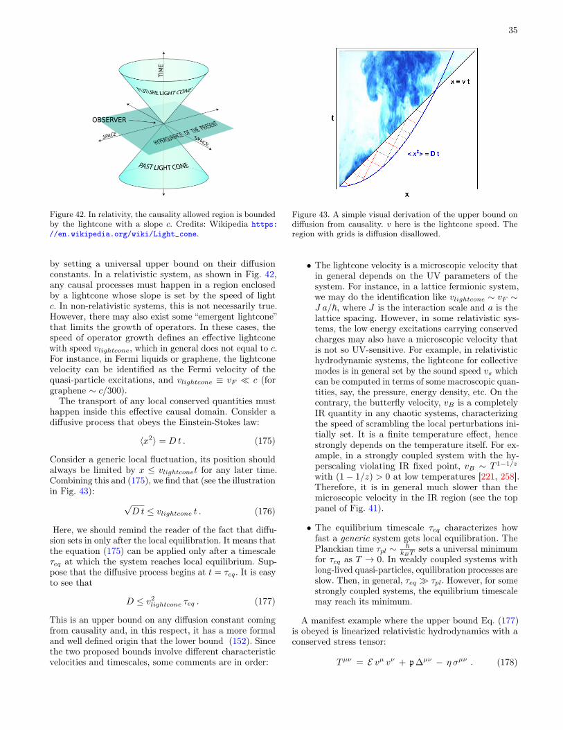
35

Figure 42. In relativity, the causality allowed region is boundedby the lightcone with a slope c. Credits: Wikipedia https://en.wikipedia.org/wiki/Light_cone.

by setting a universal upper bound on their diffusionconstants. In a relativistic system, as shown in Fig. 42,any causal processes must happen in a region enclosedby a lightcone whose slope is set by the speed of lightc. In non-relativistic systems, this is not necessarily true.However, there may also exist some “emergent lightcone”that limits the growth of operators. In these cases, thespeed of operator growth defines an effective lightconewith speed vlightcone, which in general does not equal to c.For instance, in Fermi liquids or graphene, the lightconevelocity can be identified as the Fermi velocity of thequasi-particle excitations, and vlightcone ≡ vF c (forgraphene ∼ c/300).The transport of any local conserved quantities must

happen inside this effective causal domain. Consider adiffusive process that obeys the Einstein-Stokes law:

〈x2〉 = D t . (175)

Consider a generic local fluctuation, its position shouldalways be limited by x ≤ vlightconet for any later time.Combining this and (175), we find that (see the illustrationin Fig. 43):

√D t ≤ vlightcone t . (176)

Here, we should remind the reader of the fact that diffu-sion sets in only after the local equilibration. It means thatthe equation (175) can be applied only after a timescaleτeq at which the system reaches local equilibrium. Sup-pose that the diffusive process begins at t = τeq. It is easyto see that

D ≤ v2lightcone τeq . (177)

This is an upper bound on any diffusion constant comingfrom causality and, in this respect, it has a more formaland well defined origin that the lower bound (152). Sincethe two proposed bounds involve different characteristicvelocities and timescales, some comments are in order:

Figure 43. A simple visual derivation of the upper bound ondiffusion from causality. v here is the lightcone speed. Theregion with grids is diffusion disallowed.

• The lightcone velocity is a microscopic velocity thatin general depends on the UV parameters of thesystem. For instance, in a lattice fermionic system,we may do the identification like vlightcone ∼ vF ∼J a/~, where J is the interaction scale and a is thelattice spacing. However, in some relativistic sys-tems, the low energy excitations carrying conservedcharges may also have a microscopic velocity thatis not so UV-sensitive. For example, in relativistichydrodynamic systems, the lightcone for collectivemodes is in general set by the sound speed vs whichcan be computed in terms of some macroscopic quan-tities, say, the pressure, energy density, etc. On thecontrary, the butterfly velocity, vB is a completelyIR quantity in any chaotic systems, characterizingthe speed of scrambling the local perturbations ini-tially set. It is a finite temperature effect, hencestrongly depends on the temperature itself. For ex-ample, in a strongly coupled system with the hy-perscaling violating IR fixed point, vB ∼ T 1−1/z

with (1− 1/z) > 0 at low temperatures [221, 258].Therefore, it is in general much slower than themicroscopic velocity in the IR region (see the toppanel of Fig. 41).

• The equilibrium timescale τeq characterizes howfast a generic system gets local equilibration. ThePlanckian time τpl ∼ ~

kBTsets a universal minimum

for τeq as T → 0. In weakly coupled systems withlong-lived quasi-particles, equilibration processes areslow. Then, in general, τeq τpl. However, for somestrongly coupled systems, the equilibrium timescalemay reach its minimum.

A manifest example where the upper bound Eq. (177)is obeyed is linearized relativistic hydrodynamics with aconserved stress tensor:

Tµν = E vµ vν + p∆µν − η σµν . (178)

36

Using the hydrodynamics method, one can show thatin the transverse channel there is a diffusive momentummode with the dispersion relation:

ω = −i η

E + pk2 + . . . , (179)

which is the result of the momentum conservation. This,however, suffers the problem of superluminality, becauseits group velocity

vg ≡∣∣∣dωdk

∣∣∣ ∼ k , (180)

can be arbitrarily large if there is no cut-off on the mo-mentum k. One well-known solution to this problem 21 isto introduce a fictitious relaxation time τπ which arisesfrom the constitutive relation of the stress tensor to higherorder. As a result, the diffusive equation gets modified as

ω2 + i ω τ−1π = v2

T k2 , v2

T =η

(E + p) τπ, (181)

which is known as the Israel-Stewart formalism [260].Solving this simple equation, we get

ω =1

2τπ

(−i±

√4v2T k

2 τ2π − 1

). (182)

This time, the diffusive dynamics sets only when k <kg ≡ 1/(2vT τπ). Here, kg is just the k-gap mentionedpreviously. Above the kg momentum, momentum propa-gates ballistically at the sound speed vT ≤ c. IdentifyingvT ∼ vlightcone and τπ ∼ τeq and expanding (182), one canobserve that Dπ = v2

T τπ ∼ v2lightcone τeq. Consequently,

the causality requirement

v2T ≤ c2 , (183)

is equivalent to an upper bound on the diffusion constant

Dπ ≤ c2τπ , (184)

which takes exactly the form of Eq. (177), with c beingthe relativistic lightcone velocity and τπ the equilibrationtime.In holographic systems, the equilibration process is

dominated by the first non-hydrodynamic modes. 22 Then,we may identify

τeq ∼1

Im [ωQNM], (185)

21 It is actually well-known that a superluminal group velocity doesnot imply any violation of causality [259]. This is a “problem” onlyfor numerical simulation using linearized relativistic hydrodynam-ics as initial conditions. There is absolutely no fundamental norphysical problem here.

22 The hydrodynamic modes are gapless, hence do not set any finitetimescale for relaxations. Then, we should look at the gappedmodes. Here, the lowest lying gapped QNM is what we term thefirst non-hydrodynamic mode.

first non-hydrodynamic

mode

τeq-1

0.005 0.010 0.015 0.020k

-2.0

-1.5

-1.0

-0.5

0.0Im(ω)

Figure 44. The local equilibrium timescale is extracted fromthe imaginary part of the first non-hydrodynamic mode as inEq. (185). The arrow indicates its motion as the increase ofm/T .

where ωQNM is the complex frequency of the first non-hydrodynamic QNM. Back to the holographic axionmodel, the longitudinal sound speed plays the role ofthe lightcone velocity, i.e. vL ∼ vlightcone. Then, one candirectly check the upper bound by computing the blackhole QNMs (see how to extract the local equilibriumtimescale τeq in Fig. 44). The results for zero density andcharged case have been shown in Fig. 45, respectively.It is obvious that the upper bound on diffusion fromcausality (177) is respected for all the cases.Then, above analysis suggests that the diffusion con-

stants may always be constrained in an intermediaterange:

v2B τpl ≤ D ≤ v2

ligthcone τeq . (186)

In Fig. 46 we show a "sandwich-like" illustration for thisfeature. Note that for many cases of holographic systemsor quantum critical systems, the equilibrium time reachesthe minimum, τeq ∼ τpl and the butterfly velocity de-termines the lightcone speed (assuming that there is noquasiparticle or well-defined microscopic velocity), forwhich we may have that D ∼ v2

Bτpl, i.e. the diffusionallowed region shrinks to a single point. Recently, [261]proposed to define the velocity scales in the diffusivebound as the ratio between the frequency and the mo-mentum setting the radius of convergence of the linearhydrodynamic theory.

G. A bound on stiffness

Now, let us move to check if there is also some constrainton the propagating speed of the longitudinal sound modes.In some previous studies [262, 263], it has been proposedfrom the holographic duality that there exists an upper

37

D1 /c2τeq

D2 /c2τeq

D1 /vL2τeq

D2 /vL2τeq

0 1 2 3 4 5m/T0.0

0.2

0.4

0.6

0.8

0 1 2 3 4m/T0.1

0.2

0.3

0.4

0.5

0.6

0.7

D1 /c2τeq

D2 /c2τeq

D1 /vL2τeq

D2 /vL2τeq

D1 /c2τeq

D2 /c2τeq

D1 /vL2τeq

D2 /vL2τeq

Figure 45. The upper bound on diffusion.c is the speed of lightand vL is the speed of longitudinal sound. Top: The dimen-sionless ratio at zero density, where D1 is the crystal diffusionand D2 the charge diffusion. Bottom: The dimensionless ratioat finite density, where the blue points are for µ/T = 3 andthe red for µ/T = 5.

Figure 46. The diffusion allowed region is bounded by quantummechanics and causality.

bound on speed of sound modes, which is set by its confor-mal value, vc ≡ 1/(d− 1) for d dimensional system. Thisproposal has been later related to the physics of neutronstars, very compact objects which display an extremelystiff equation of state [264]. This bound however has beenlater checked in various holographic models and its viola-

N

5 10 15m/T

0.2

0.4

0.6

0.8

1.0

κ/κc

Figure 47. The stiffness κ for N ∈ [3, 9] (from black to yellow)in function of m/T . Figure taken from [216].

tion has been observed both at finite charge density caseor in presence of multi-trace deformations [265, 266].Note that all these previous discussions were confined

to fluid systems with no long-range order, where thelongitudinal sounds are simply pressure waves, i.e.

v2L =

∂p

∂E. (187)

Note that the r.h.s. of Eq. (187) also defines the stiffnessof the system

κ ≡ ∂p

∂E. (188)

This then means that the bound on the sounds is simul-taneously a bound on the stiffness:

κ ≤ κc, κc ≡1

d− 1. (189)

In the holographic axion model, the SSB of translationsresults in a non-zero shear elasticity G and the dualsystems on boundary is a solid (see also Eq. (111)). Thepresence of a finite G speeds up the longitudinal sounds,which becomes [130]:

v2L = v2

c + v2T ≥ v2

c . (190)

The first equivalence is a direct consequence of conformalinvariance, i.e. 〈Tµµ 〉 = 0. Again, this is a new way to breakthe proposed bound on the sound speed. Nevertheless,we will verify that the result above does not imply aviolation of the stiffness bound. That is to say the boundsconjectured in [262, 263] has to be viewed as a limit tothe stiffness instead of a bound on the speed of sound.

As was revealed earlier, in presence of the finite strainpressure P , the total pressure 〈T xx〉 is no longer equal tothe thermodynamic pressure p. For the conformal solid,the traceless stress tensor implies that

〈T xx〉 = p + P =1

d− 1E , P > 0 . (191)

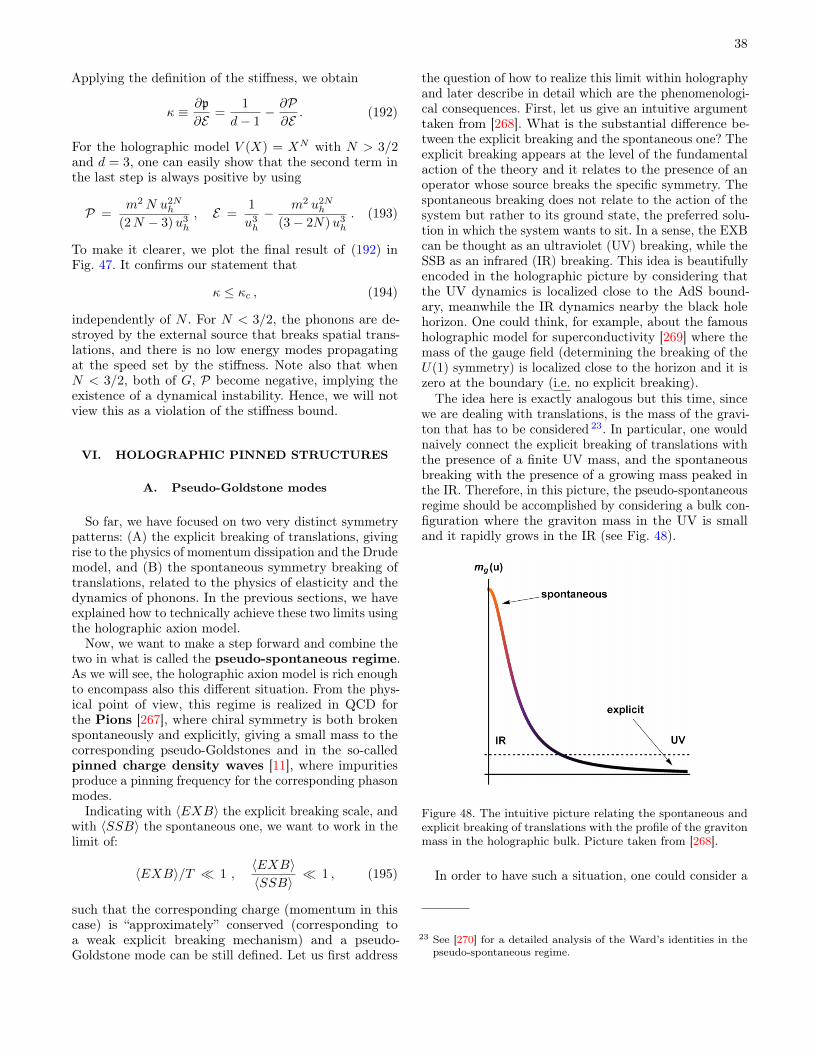
38

Applying the definition of the stiffness, we obtain

κ ≡ ∂p

∂E=

1

d− 1− ∂P∂E

. (192)

For the holographic model V (X) = XN with N > 3/2and d = 3, one can easily show that the second term inthe last step is always positive by using

P =m2N u2N

h

(2N − 3)u3h

, E =1

u3h

− m2 u2Nh

(3− 2N)u3h

. (193)

To make it clearer, we plot the final result of (192) inFig. 47. It confirms our statement that

κ ≤ κc , (194)

independently of N . For N < 3/2, the phonons are de-stroyed by the external source that breaks spatial trans-lations, and there is no low energy modes propagatingat the speed set by the stiffness. Note also that whenN < 3/2, both of G, P become negative, implying theexistence of a dynamical instability. Hence, we will notview this as a violation of the stiffness bound.

VI. HOLOGRAPHIC PINNED STRUCTURES

A. Pseudo-Goldstone modes

So far, we have focused on two very distinct symmetrypatterns: (A) the explicit breaking of translations, givingrise to the physics of momentum dissipation and the Drudemodel, and (B) the spontaneous symmetry breaking oftranslations, related to the physics of elasticity and thedynamics of phonons. In the previous sections, we haveexplained how to technically achieve these two limits usingthe holographic axion model.

Now, we want to make a step forward and combine thetwo in what is called the pseudo-spontaneous regime.As we will see, the holographic axion model is rich enoughto encompass also this different situation. From the phys-ical point of view, this regime is realized in QCD forthe Pions [267], where chiral symmetry is both brokenspontaneously and explicitly, giving a small mass to thecorresponding pseudo-Goldstones and in the so-calledpinned charge density waves [11], where impuritiesproduce a pinning frequency for the corresponding phasonmodes.

Indicating with 〈EXB〉 the explicit breaking scale, andwith 〈SSB〉 the spontaneous one, we want to work in thelimit of:

〈EXB〉/T 1 ,〈EXB〉〈SSB〉

1 , (195)

such that the corresponding charge (momentum in thiscase) is “approximately” conserved (corresponding toa weak explicit breaking mechanism) and a pseudo-Goldstone mode can be still defined. Let us first address

the question of how to realize this limit within holographyand later describe in detail which are the phenomenologi-cal consequences. First, let us give an intuitive argumenttaken from [268]. What is the substantial difference be-tween the explicit breaking and the spontaneous one? Theexplicit breaking appears at the level of the fundamentalaction of the theory and it relates to the presence of anoperator whose source breaks the specific symmetry. Thespontaneous breaking does not relate to the action of thesystem but rather to its ground state, the preferred solu-tion in which the system wants to sit. In a sense, the EXBcan be thought as an ultraviolet (UV) breaking, while theSSB as an infrared (IR) breaking. This idea is beautifullyencoded in the holographic picture by considering thatthe UV dynamics is localized close to the AdS bound-ary, meanwhile the IR dynamics nearby the black holehorizon. One could think, for example, about the famousholographic model for superconductivity [269] where themass of the gauge field (determining the breaking of theU(1) symmetry) is localized close to the horizon and it iszero at the boundary (i.e. no explicit breaking).

The idea here is exactly analogous but this time, sincewe are dealing with translations, is the mass of the gravi-ton that has to be considered 23. In particular, one wouldnaively connect the explicit breaking of translations withthe presence of a finite UV mass, and the spontaneousbreaking with the presence of a growing mass peaked inthe IR. Therefore, in this picture, the pseudo-spontaneousregime should be accomplished by considering a bulk con-figuration where the graviton mass in the UV is smalland it rapidly grows in the IR (see Fig. 48).

Figure 48. The intuitive picture relating the spontaneous andexplicit breaking of translations with the profile of the gravitonmass in the holographic bulk. Picture taken from [268].

In order to have such a situation, one could consider a

23 See [270] for a detailed analysis of the Ward’s identities in thepseudo-spontaneous regime.

39

potential of the form:

V (X) = X + β XN , β 1 , (196)

since the graviton mass is proportional to m2g(u) ∼

VX(X) and the argument X ∼ u2 vanishes at the bound-ary and grows towards the black hole horizon.This intuition turns out to be correct and it can be

formalized better using the language of the previous sec-tions. Given a potential V (X) = XN , we know now thatthe breaking of translations is explicit if N < 5/2 andspontaneous if N > 5/2. Therefore, to reach the pseudo-spontaneous regime, we need to utilize a potential of thetype:

V (X) = XN + β XM , N < 5/2, M > 5/2 . (197)

This is exactly what has been done in [268] which first 24studied the dynamics of pinning phonons in holography.Curiously 25, this model was considered long time before,in [21], but the connection with the pseudo-spontaneousbreaking of translations has not been given therein. A fullunderstanding of this regime has appeared later in [142].A slightly different way to realize this regime can also befound in [121].

Let us analyze in detail what one would expect in thisregime. Following the hydrodynamic description of [135],in presence of both explicit and spontaneous breakingof translations, the low-energy hydrodynamic spectrumat zero momentum is described by the solutions of theequation:

(Ω − i ω) (Γ − i ω) + ω20 = 0 , (198)

where Γ is the momentum relaxation rate (how fastmomentum is dissipated), Ω the phase relaxation rate(measuring the lifetime of the Goldstones) and ω0 theso-called pinning frequency – the mass of the (not any-more) Goldstone modes. The two modes involved in thequadratic equation (198) are the transverse momentumπ⊥ and the transverse component of the Goldstone field.Solving Eq. (198) we obtain a pair of excitations whosefrequencies are given by

ω± = − i

2(Γ + ω) ± 1

2

√4ω2

0 − (Γ− Ω)2. (199)

For 4ω20 − (Γ − Ω)2 < 0, the two modes lie along the

imaginary axes; they are purely decaying modes. Exactlyat 4ω2

0 − (Γ − Ω)2 = 0, the two modes collide on theimaginary axes and for 4ω2

0 − (Γ − Ω)2 > 0 they moveonto the complex plane acquiring a finite and growing real

24 The same day, a work [271] studying this regime in the contextof holographic helical lattices was posted in arXiv.

25 It is also funny to notice that historically this regime was achievedbefore the fully spontaneous one [117], which for technical reasonshas been the most difficult to construct.

Figure 49. The dynamics of the low-energy hydrodynamicmodes in the pseudo-spontaneous regime. The dance of themodes is perfectly described by Eq. (198). Figure adaptedfrom [142].

part. This dynamics is perfectly obeyed by the holographicmodels, see, for example, Fig. 49.

Interestingly, this collision is not an exclusive feature ofthe pseudo-spontaneous regime. Indeed, this collision isthe same giving rise to the incoherent-coherent transitionin the models with pure explicit breaking [90]. Rather, apeculiar characteristic of the pseudo-spontaneous regimeis the fact that such collision happens at low frequency,within the so-called hydrodynamic regime. Increasing theamount of spontaneous breaking, both Γ and Ω becomesmaller and the collision happens close to the origin ω = 0.This tendency is shown explicitly in Fig. 50. Notice thatin the purely spontaneous regime, both modes wouldcollapse at the origin and form the propagating shearsound.

Figure 50. The collision between the two modes by mov-ing towards the pseudo-spontaneous regime. Figure adaptedfrom [142]. Notice how this dynamics was already presentin [21].

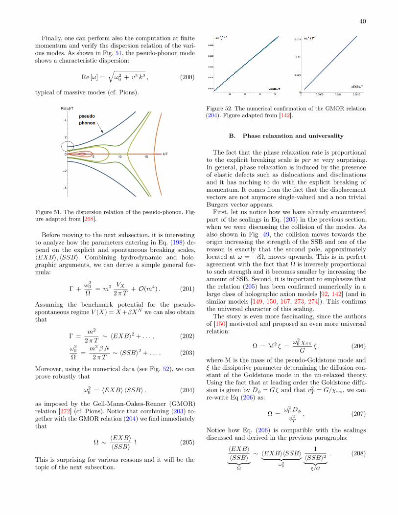
40

Finally, one can perform also the computation at finitemomentum and verify the dispersion relation of the vari-ous modes. As shown in Fig. 51, the pseudo-phonon modeshows a characteristic dispersion:

Re [ω] =√ω2

0 + v2 k2 , (200)

typical of massive modes (cf. Pions).

Figure 51. The dispersion relation of the pseudo-phonon. Fig-ure adapted from [268].

Before moving to the next subsection, it is interestingto analyze how the parameters entering in Eq. (198) de-pend on the explicit and spontaneous breaking scales,〈EXB〉, 〈SSB〉. Combining hydrodynamic and holo-graphic arguments, we can derive a simple general for-mula:

Γ +ω2

0

Ω= m2 VX

2π T+ O(m4) . (201)

Assuming the benchmark potential for the pseudo-spontaneous regime V (X) = X+βXN we can also obtainthat

Γ =m2

2π T∼ 〈EXB〉2 + . . . , (202)

ω20

Ω=

m2 β N

2π T∼ 〈SSB〉2 + . . . . (203)

Moreover, using the numerical data (see Fig. 52), we canprove robustly that

ω20 = 〈EXB〉 〈SSB〉 , (204)

as imposed by the Gell-Mann-Oakes-Renner (GMOR)relation [272] (cf. Pions). Notice that combining (203) to-gether with the GMOR relation (204) we find immediatelythat

Ω ∼ 〈EXB〉〈SSB〉

! (205)

This is surprising for various reasons and it will be thetopic of the next subsection.

Figure 52. The numerical confirmation of the GMOR relation(204). Figure adapted from [142].

B. Phase relaxation and universality

The fact that the phase relaxation rate is proportionalto the explicit breaking scale is per se very surprising.In general, phase relaxation is induced by the presenceof elastic defects such as dislocations and disclinationsand it has nothing to do with the explicit breaking ofmomentum. It comes from the fact that the displacementvectors are not anymore single-valued and a non trivialBurgers vector appears.First, let us notice how we have already encountered

part of the scalings in Eq. (205) in the previous section,when we were discussing the collision of the modes. Asalso shown in Fig. 49, the collision moves towards theorigin increasing the strength of the SSB and one of thereason is exactly that the second pole, approximatelylocated at ω = −iΩ, moves upwards. This is in perfectagreement with the fact that Ω is inversely proportionalto such strength and it becomes smaller by increasing theamount of SSB. Second, it is important to emphasize thatthe relation (205) has been confirmed numerically in alarge class of holographic axion models [92, 142] (and insimilar models [149, 150, 167, 273, 274]). This confirmsthe universal character of this scaling.The story is even more fascinating, since the authors

of [150] motivated and proposed an even more universalrelation:

Ω = M2 ξ =ω2

0 χππG

ξ , (206)

where M is the mass of the pseudo-Goldstone mode andξ the dissipative parameter determining the diffusion con-stant of the Goldstone mode in the un-relaxed theory.Using the fact that at leading order the Goldstone diffu-sion is given by Dφ = Gξ and that v2

T = G/χππ, we canre-write Eq (206) as:

Ω =ω2

0 Dφ

v2T

. (207)

Notice how Eq. (206) is compatible with the scalingsdiscussed and derived in the previous paragraphs:

〈EXB〉〈SSB〉︸ ︷︷ ︸

Ω

∼ 〈EXB〉〈SSB〉︸ ︷︷ ︸ω2

0

1

〈SSB〉2︸ ︷︷ ︸ξ/G

. (208)

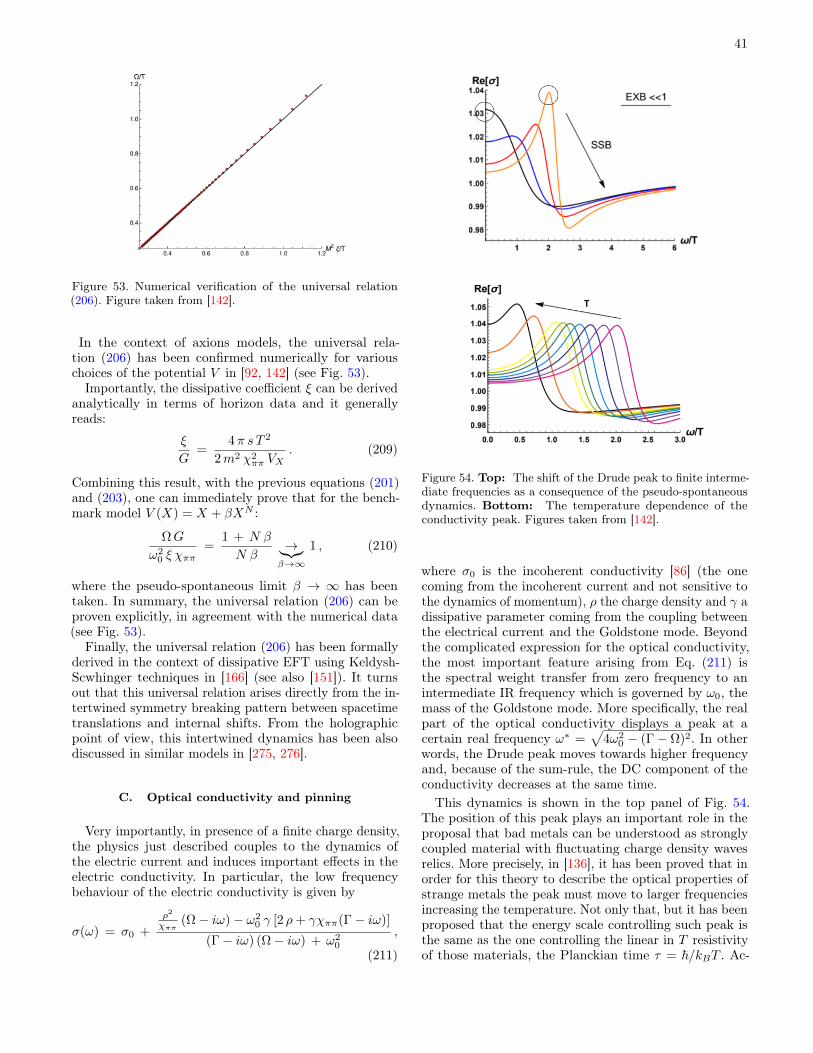
41

Figure 53. Numerical verification of the universal relation(206). Figure taken from [142].

In the context of axions models, the universal rela-tion (206) has been confirmed numerically for variouschoices of the potential V in [92, 142] (see Fig. 53).

Importantly, the dissipative coefficient ξ can be derivedanalytically in terms of horizon data and it generallyreads:

ξ

G=

4π s T 2

2m2 χ2ππ VX

. (209)

Combining this result, with the previous equations (201)and (203), one can immediately prove that for the bench-mark model V (X) = X + βXN :

ΩG

ω20 ξ χππ

=1 + N β

N β→︸︷︷︸

β→∞

1 , (210)

where the pseudo-spontaneous limit β → ∞ has beentaken. In summary, the universal relation (206) can beproven explicitly, in agreement with the numerical data(see Fig. 53).

Finally, the universal relation (206) has been formallyderived in the context of dissipative EFT using Keldysh-Scwhinger techniques in [166] (see also [151]). It turnsout that this universal relation arises directly from the in-tertwined symmetry breaking pattern between spacetimetranslations and internal shifts. From the holographicpoint of view, this intertwined dynamics has been alsodiscussed in similar models in [275, 276].

C. Optical conductivity and pinning

Very importantly, in presence of a finite charge density,the physics just described couples to the dynamics ofthe electric current and induces important effects in theelectric conductivity. In particular, the low frequencybehaviour of the electric conductivity is given by

σ(ω) = σ0 +

ρ2

χππ(Ω− iω)− ω2

0 γ [2 ρ+ γχππ(Γ− iω)]

(Γ− iω) (Ω− iω) + ω20

,

(211)

Figure 54. Top: The shift of the Drude peak to finite interme-diate frequencies as a consequence of the pseudo-spontaneousdynamics. Bottom: The temperature dependence of theconductivity peak. Figures taken from [142].

where σ0 is the incoherent conductivity [86] (the onecoming from the incoherent current and not sensitive tothe dynamics of momentum), ρ the charge density and γ adissipative parameter coming from the coupling betweenthe electrical current and the Goldstone mode. Beyondthe complicated expression for the optical conductivity,the most important feature arising from Eq. (211) isthe spectral weight transfer from zero frequency to anintermediate IR frequency which is governed by ω0, themass of the Goldstone mode. More specifically, the realpart of the optical conductivity displays a peak at acertain real frequency ω∗ =

√4ω2

0 − (Γ− Ω)2. In otherwords, the Drude peak moves towards higher frequencyand, because of the sum-rule, the DC component of theconductivity decreases at the same time.This dynamics is shown in the top panel of Fig. 54.

The position of this peak plays an important role in theproposal that bad metals can be understood as stronglycoupled material with fluctuating charge density wavesrelics. More precisely, in [136], it has been proved that inorder for this theory to describe the optical properties ofstrange metals the peak must move to larger frequenciesincreasing the temperature. Not only that, but it has beenproposed that the energy scale controlling such peak isthe same as the one controlling the linear in T resistivityof those materials, the Planckian time τ = ~/kBT . Ac-

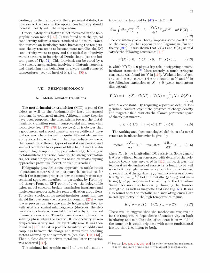
42

cordingly to their analysis of the experimental data, theposition of the peak in the optical conductivity shouldincrease linearly with the temperature.

Unfortunately, this feature is not recovered in the holo-graphic axion model [142]. It was found that the opticalconductivity follows a more standard and natural transi-tion towards an insulating state. Increasing the tempera-ture, the system tends to become more metallic, the DCconductivity wants to grow and the optical conductivitywants to return to its original Drude shape (see the bot-tom panel of Fig. 54). This drawback can be cured by afine-tuned generalization, involving a dilatonic coupling,and displaying this behaviour in a very small range oftemperatures (see the inset of Fig. 3 in [150]).

VII. PHENOMENOLOGY

A. Metal-Insulator transitions

The metal-insulator transition (MIT) is one of theoldest as well as the fundamentally least understoodproblems in condensed matter. Although many theorieshave been proposed, the mechanisms toward the metal-insulator transition remain controversial and somewhatincomplete (see [277, 278] for reviews). It is obvious thata good metal and a good insulator are very different phys-ical systems, characterized by quite different elementaryexcitations. In particular, in the intermediate regime ofthe transition, different types of excitations coexist andsimple theoretical tools prove of little help. Since the dis-covery of high temperature superconductivity, the study ofmetal-insulator transition came to the strong correlationera, for which physical pictures based on weak-couplingapproaches prove insufficient or even misleading.Holography provides a new approach to tackle states

of quantum matter without quasiparticle excitations, forwhich the transport properties deviate strongly from con-ventional approach described, in particular, by Fermi liq-uid theory. From an EFT point of view, the holographicaxion model concerns broken translation invariance andimplements non-perturbative renormalization group flows.To realise a holographic metal-insulator transition, oneshould first overcome the obstruction found in [279] whereit was proven that in some simple holographic theorieswith arbitrary spatial inhomogeneity (disorder) the elec-trical conductivity is bounded from below by a universalminimal conductance. Therefore, one can not obtain an in-sulating phase where the electric DC conductivity at zerotemperature is very small or eventually zero. It was thenfound in [115] that it is possible to introduce additionalcouplings between the charge and translation breakingsectors allowed by the symmetries (see also [112, 113] ).Then a clear disorder-driven metal-insulator transitionwas observed [115].

The minimal holographic model of a metal-insulator

transition is described by (47) with Z = 0

S =

∫d4x√−g[R

2− Λ− Y (X)

4e2FµνF

µν −m2V (X)

].

(212)The consistency of a theory imposes some constraintson the couplings that appear in the Lagrangian. For thetheory (212), it was shown that V (X) and Y (X) shouldsatisfy the following constraints [115]:

V ′(X) > 0, Y (X) > 0, Y ′(X) < 0 , (213)

in which Y ′(X) < 0 plays a key role in triggering a metal-insulator transition.26 More recently, a much stringentconstraint was found for Y in [116]. Without loss of gen-erality, one can parametrize the couplings Y and V inthe following expansion as X → 0 (weak momentumdissipation):

Y (X) = 1− γ X +O(X2), V (X) =1

2m2X +O(X2) ,

(214)with γ a constant. By requiring a positive definite lon-gitudinal conductivity in the presence of charge densityand magnetic field restricts the allowed parameter spaceof theory parameters.

0 6 γ 6 1/6 ⇒ −1/6 6 Y ′(0) 6 0 . (215)

The working and phenomenological definition of a metalversus an insulator behavior is given by

metal:dRxxd T

> 0, insulator:dRxxd T

< 0 , (216)

where Rxx is the longitudinal DC resistivity. Some genericfeatures without being concerned with details of the holo-graphic theory was uncovered in [116]. In particular, thetemperature dependence of resistivity is found to be wellscaled with a single parameter T0, which approaches zeroat some critical charge density ρc, and increases as a powerlaw T0 ∼ |ρ − ρc|1/2 both in metallic (ρ > ρc) and insu-lating (ρ < ρc) regions in the vicinity of the transition.Similar features also happen by changing the disorderstrength α as well as magnetic field (see Fig. 55). It wasalso found that the metallic and insulating curves aremirror symmetry in the high temperature regime:

Rxx(ρ− ρc, T ) = 1/Rxx(ρc − ρ, T ) . (217)

These results suggest that the mechanism responsiblefor the temperature dependence of conductivity on bothinsulating and metallic sides of the transition would bethe same, or it would originate with some fundamentalfeature that is common to both.

26 See e.g. [20, 123, 271, 280–283] for other holographic realizationsof metal-insulator transitions driven via other mechanisms.

43

0.1 0.5 1 5 10 50 100

0.01

0.10

1

10

100

0.1 1 10 100 1000

0.010

0.050

0.100

0.500

1

5

Figure 55. Temperature dependence of the resistivity versusdisorder strength at zero magnetic field for the model withY = 1 − X

6, V = X

2m2 . Top: The metal-insulator transitiondriven by the disorder strength α. Bottom: Scaling of resistivitywith scaled temperature T/T0. The collapse of data into twoseparated curves both in the metallic and insulating sides ismanifest. Other parameters are chosen by e = ρ = 1. Figuretaken from [116].

The holographic results are reminiscent of the scalingbehaviors for resistivity near the transition point reportedin some two dimensional samples and materials, whichshows the collapse of data into two separated curvesand displays remarkable mirror symmetry over a broadinterval of temperatures [284–287]. This observation hasbeen interpreted as evidence that the transition region isdominated by strong coupling effects characterizing theinsulating phase [288]. Nevertheless, the dependence ofT0 near ρc is a power law with the power that is differentfrom holographic result 1/2, suggesting that holographictheory (212) falls into a different universality class fromthose materials. A natural extension is to consider aholographic setup that is asymptotically Lifshitz with adynamical exponent z which parametrizes the relativescaling of space and time, making the model compatiblewith experimental data.

The phase diagram gets richer and incorporates severalphases of matter depending on the parameters. As shownin Fig. 56, there are as many as four different phases inthe temperature-disorder phase diagram: good metal (a),bad or incoherent metal (b), bad insulator (c) and goodinsulator (d). Some representative examples of the ACelectric conductivity for each phase are shown in Fig. 57.A coherent metallic phase with a sharp Drude peak is

Figure 56. Phases diagram for the model with Y = 1− X6, V =

X2m2 in the absence of magnetic field. Four regions are denotedby (a) good metal, (b) incoherent metal, (c) bad insulator and(d) good insulator, respectively. Other parameters are chosenby e = ρ = 1. The figure is updated from [116].

obtained for small α. As α increases, the Drude peakis suppressed and one arrives at an incoherent metallicphase where there is no clear and dominant localized longlived excitation, see green curves of Fig. 57. When thedisorder is strong enough, the spectral weight transfersto the mid-infrared, resulting in an insulating behavior.As a consequence, the DC conductivity keeps decreasing,and then triggers the transition from bad insulator togood insulator. Therefore, there is a clear disorder-driventransition from a coherent metal with a sharp Drudepeak to a good insulator with a tiny or vanishing DCconductivity at zero temperature.The investigation of transport in this minimal holo-

graphic setup of a metal-insulator transition uncoveredsome interesting features, shedding light on this interest-ing transition and the physical mechanism that drives it.There are still many interesting questions. There are asmany as four different phases in the temperature-disorderphase diagram of Fig. 56, but all phases share the samesymmetries of the underlying theory, and thus beyond asimple Ginzburg-Landau description. Some observableswere examined in order to characterise different phases,but failed [116]. It is still an open question to find a goodprobe to the metal-insulator transitions. The scaling ex-ponent of T0 from the holographic setup is different fromthe experiments which yielded scaling exponents between1.25 and 1.6 [284–287]. It is interesting to generalise themodel to obtain an exponent that is compatible withexperimental observation. It is also worth studying thethermal response and the mechanical response.

44

0.1 0.2 0.3 0.4 0.5 0.6ω

0.5

1.0

1.5

2.0

Re[σxx]

2 4 6 8 10 12ω

0.2

0.4

0.6

0.8

1.0

Re[σxx]

Figure 57. Representative examples of the AC electric con-ductivity σxx with unitary charge density ρ = 1. There arefour phases: (a) good metal (red) with (α = 0.6, T = 0.5),(b) incoherent metal (green) with (α = 1.5, T = 0.5), (c) badinsulator (blue) with (α = 4.5, T = 0.3) and (d) good insulator(purple) with (α = 7.8, T = 0.05). Figures taken from [116].

B. The scalings of strange metals

The anomalous metallic transport in the high-temperature superconducting cuprates is one of the mostremarkable puzzles in condensed matter physics. Theso-called strange metal phase is characterized by uni-versal temperature scalings which are robust across widelydifferent systems, and are believed to be controlled byan underlying strongly interacting quantum critical sec-tor. Its anomalous features include a linear temperaturedependence for the resistivity Rxx ∼ T and the scalingof the Hall angle cot(ΘH) ∼ T 2 (see Fig. 58). Realizingthe anomalous temperature dependence of both Rxx andcot(ΘH) at once within a holographic model has provento be a challenge. Although many efforts were made, stan-dard Einstein-Maxwell-dilaton (EMD) theories have thusfar been unable to give the expected anomalous scalingsof the strange metal (see e.g. [102, 106, 289]). As we aredealing with strongly correlated electron matter, it maybe crucial to take into account the nontrivial dynamicsbetween the charge degrees of freedom to reliably capturetransport in these phases [290–292].The first consistent holographic realization of the

strange metal scalings of the resistivity and Hall angle wasgiven in [294] by working with a string-theory-motivatedgravitational model encoded by the Dirac-Born-Infeld

Figure 58. Experimental observation of the cuprates scalingsfor the in-plane resistivity Rxx ∼ T and inverse Hall anglecot(ΘH) ∼ T 2. Figures taken from [293].

(DBI) action.27 The motivation is to describe a stronglycoupled quantum theory containing a sector of dilutecharge carriers that interact amongst themselves as wellas with a quantum critical bath. The charge degrees offreedom is treated as a probe when compared to the largerset of neutral quantum critical degrees of freedom. Thegravitational theory takes the generic form

S =

∫d4x√−g[Lbath + Lcharge] . (218)

The bath sector Lbath is supported, for example, by a neu-tral scalar and axionic scalars. The charge sector Lchargedescribes the dynamics of a U(1) gauge field, taking intoaccount non-linear interactions between the charged de-grees of freedom. In [294] the bath geometry is nonrela-tivistic and hyperscaling-violating supported by a neutralscalar field and two axions φI . In the so-called probe limitfor which the backreaction of the DBI interactions on thegeometry can be safely neglected, the nonlinear dynamicsof the gauge field sector allows a clean scaling regime forthe cuprate strange metals:

Rxx ∼ T, cot(ΘH) =RxxRyx

∼ T 2 , (219)

27 Note that the strangle metal scalings have also been realized inthe Einstein-Maxwell-dilaton-axion model with a hyperscaling IRgeometry only for a special value of B [97].

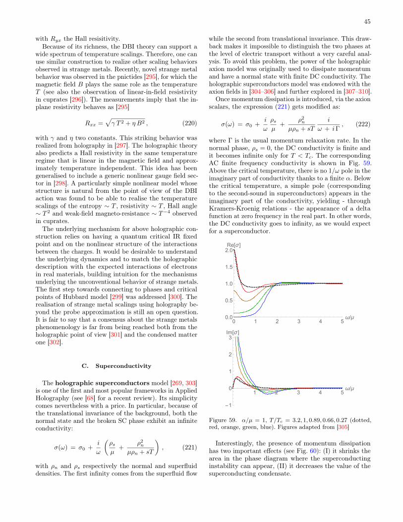
45

with Ryx the Hall resisitivity.Because of its richness, the DBI theory can support a

wide spectrum of temperature scalings. Therefore, one canuse similar construction to realize other scaling behaviorsobserved in strange metals. Recently, novel strange metalbehavior was observed in the pnictides [295], for which themagnetic field B plays the same role as the temperatureT (see also the observation of linear-in-field resistivityin cuprates [296]). The measurements imply that the in-plane resistivity behaves as [295]

Rxx =√γ T 2 + η B2 , (220)

with γ and η two constants. This striking behavior wasrealized from holography in [297]. The holographic theoryalso predicts a Hall resistivity in the same temperatureregime that is linear in the magnetic field and approx-imately temperature independent. This idea has beengeneralised to include a generic nonlinear gauge field sec-tor in [298]. A particularly simple nonlinear model whosestructure is natural from the point of view of the DBIaction was found to be able to realise the temperaturescalings of the entropy ∼ T , resistivity ∼ T , Hall angle∼ T 2 and weak-field magneto-resistance ∼ T−4 observedin cuprates.

The underlying mechanism for above holographic con-struction relies on having a quantum critical IR fixedpoint and on the nonlinear structure of the interactionsbetween the charges. It would be desirable to understandthe underlying dynamics and to match the holographicdescription with the expected interactions of electronsin real materials, building intuition for the mechanismsunderlying the unconventional behavior of strange metals.The first step towards connecting to phases and criticalpoints of Hubbard model [299] was addressed [300]. Therealisation of strange metal scalings using holography be-yond the probe approximation is still an open question.It is fair to say that a consensus about the strange metalsphenomenology is far from being reached both from theholographic point of view [301] and the condensed matterone [302].

C. Superconductivity

The holographic superconductors model [269, 303]is one of the first and most popular frameworks in AppliedHolography (see [68] for a recent review). Its simplicitycomes nevertheless with a price. In particular, because ofthe translational invariance of the background, both thenormal state and the broken SC phase exhibit an infiniteconductivity:

σ(ω) = σ0 +i

ω

(ρsµ

+ρ2n

µρn + sT

), (221)

with ρn and ρs respectively the normal and superfluiddensities. The first infinity comes from the superfluid flow

while the second from translational invariance. This draw-back makes it impossible to distinguish the two phases atthe level of electric transport without a very careful anal-ysis. To avoid this problem, the power of the holographicaxion model was originally used to dissipate momentumand have a normal state with finite DC conductivity. Theholographic superconductors model was endowed with theaxion fields in [304–306] and further explored in [307–310].

Once momentum dissipation is introduced, via the axionscalars, the expression (221) gets modified as:

σ(ω) = σ0 +i

ω

ρsµ

+ρ2n

µρn + sT

i

ω + iΓ, (222)

where Γ is the usual momentum relaxation rate. In thenormal phase, ρs = 0, the DC conductivity is finite andit becomes infinite only for T < Tc. The correspondingAC finite frequency conductivity is shown in Fig. 59.Above the critical temperature, there is no 1/ω pole in theimaginary part of conductivity thanks to a finite α. Belowthe critical temperature, a simple pole (correspondingto the second-sound in superconductors) appears in theimaginary part of the conductivity, yielding - throughKramers-Kroenig relations - the appearance of a deltafunction at zero frequency in the real part. In other words,the DC conductivity goes to infinity, as we would expectfor a superconductor.

0 1 2 3 4 5ω/μ0.0

0.5

1.0

1.5

2.0Re[σ ]

1 2 3 4 5ω/μ

-1

0

1

2

3Im[σ ]

Figure 59. α/µ = 1, T/Tc = 3.2, 1, 0.89, 0.66, 0.27 (dotted,red, orange, green, blue). Figures adapted from [305]

Interestingly, the presence of momentum dissipationhas two important effects (see Fig. 60): (I) it shrinks thearea in the phase diagram where the superconductinginstability can appear, (II) it decreases the value of thesuperconducting condensate.

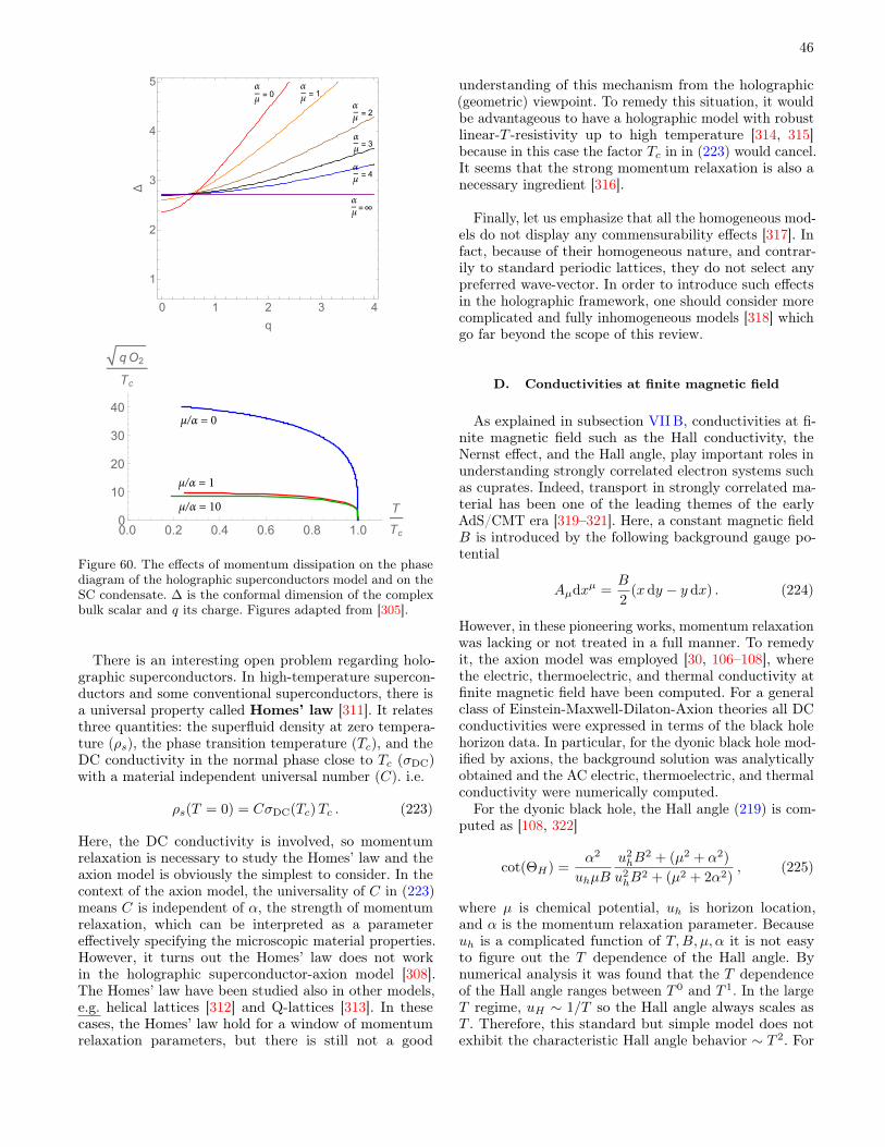
46

αμ = 0 = 1

= 2

= 3

=∞

= 4

0 1 2 3 4

1

2

3

4

5

q

Δ

αμ

αμ

αμ

αμ

αμ

μ/α = 0

μ/α = 1

μ/α = 10

0.0 0.2 0.4 0.6 0.8 1.0

T

Tc0

10

20

30

40

qO2

Tc

Figure 60. The effects of momentum dissipation on the phasediagram of the holographic superconductors model and on theSC condensate. ∆ is the conformal dimension of the complexbulk scalar and q its charge. Figures adapted from [305].

There is an interesting open problem regarding holo-graphic superconductors. In high-temperature supercon-ductors and some conventional superconductors, there isa universal property called Homes’ law [311]. It relatesthree quantities: the superfluid density at zero tempera-ture (ρs), the phase transition temperature (Tc), and theDC conductivity in the normal phase close to Tc (σDC)with a material independent universal number (C). i.e.

ρs(T = 0) = CσDC(Tc)Tc . (223)

Here, the DC conductivity is involved, so momentumrelaxation is necessary to study the Homes’ law and theaxion model is obviously the simplest to consider. In thecontext of the axion model, the universality of C in (223)means C is independent of α, the strength of momentumrelaxation, which can be interpreted as a parametereffectively specifying the microscopic material properties.However, it turns out the Homes’ law does not workin the holographic superconductor-axion model [308].The Homes’ law have been studied also in other models,e.g. helical lattices [312] and Q-lattices [313]. In thesecases, the Homes’ law hold for a window of momentumrelaxation parameters, but there is still not a good

understanding of this mechanism from the holographic(geometric) viewpoint. To remedy this situation, it wouldbe advantageous to have a holographic model with robustlinear-T -resistivity up to high temperature [314, 315]because in this case the factor Tc in in (223) would cancel.It seems that the strong momentum relaxation is also anecessary ingredient [316].

Finally, let us emphasize that all the homogeneous mod-els do not display any commensurability effects [317]. Infact, because of their homogeneous nature, and contrar-ily to standard periodic lattices, they do not select anypreferred wave-vector. In order to introduce such effectsin the holographic framework, one should consider morecomplicated and fully inhomogeneous models [318] whichgo far beyond the scope of this review.

D. Conductivities at finite magnetic field

As explained in subsection VIIB, conductivities at fi-nite magnetic field such as the Hall conductivity, theNernst effect, and the Hall angle, play important roles inunderstanding strongly correlated electron systems suchas cuprates. Indeed, transport in strongly correlated ma-terial has been one of the leading themes of the earlyAdS/CMT era [319–321]. Here, a constant magnetic fieldB is introduced by the following background gauge po-tential

Aµdxµ =B

2(xdy − y dx) . (224)

However, in these pioneering works, momentum relaxationwas lacking or not treated in a full manner. To remedyit, the axion model was employed [30, 106–108], wherethe electric, thermoelectric, and thermal conductivity atfinite magnetic field have been computed. For a generalclass of Einstein-Maxwell-Dilaton-Axion theories all DCconductivities were expressed in terms of the black holehorizon data. In particular, for the dyonic black hole mod-ified by axions, the background solution was analyticallyobtained and the AC electric, thermoelectric, and thermalconductivity were numerically computed.

For the dyonic black hole, the Hall angle (219) is com-puted as [108, 322]

cot(ΘH) =α2

uhµB

u2hB

2 + (µ2 + α2)

u2hB

2 + (µ2 + 2α2), (225)

where µ is chemical potential, uh is horizon location,and α is the momentum relaxation parameter. Becauseuh is a complicated function of T,B, µ, α it is not easyto figure out the T dependence of the Hall angle. Bynumerical analysis it was found that the T dependenceof the Hall angle ranges between T 0 and T 1. In the largeT regime, uH ∼ 1/T so the Hall angle always scales asT . Therefore, this standard but simple model does notexhibit the characteristic Hall angle behavior ∼ T 2. For

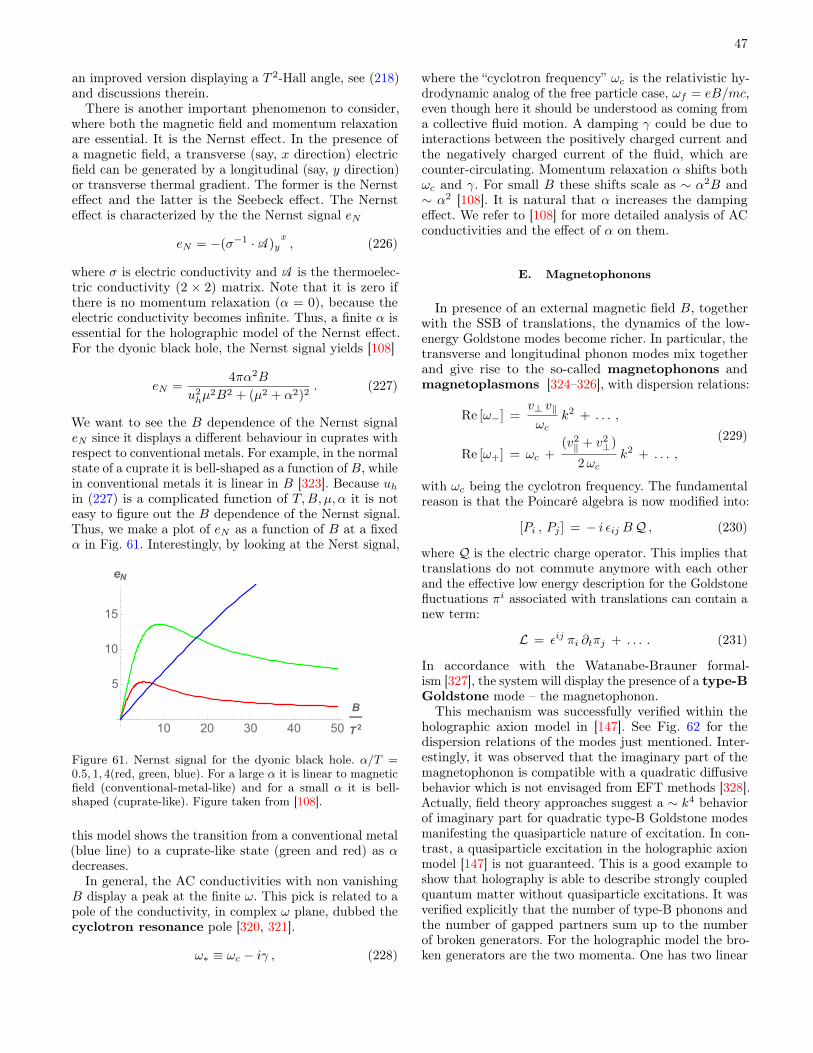
47

an improved version displaying a T 2-Hall angle, see (218)and discussions therein.There is another important phenomenon to consider,

where both the magnetic field and momentum relaxationare essential. It is the Nernst effect. In the presence ofa magnetic field, a transverse (say, x direction) electricfield can be generated by a longitudinal (say, y direction)or transverse thermal gradient. The former is the Nernsteffect and the latter is the Seebeck effect. The Nernsteffect is characterized by the the Nernst signal eN

eN = −(σ−1 · A)yx, (226)

where σ is electric conductivity and A is the thermoelec-tric conductivity (2 × 2) matrix. Note that it is zero ifthere is no momentum relaxation (α = 0), because theelectric conductivity becomes infinite. Thus, a finite α isessential for the holographic model of the Nernst effect.For the dyonic black hole, the Nernst signal yields [108]

eN =4πα2B

u2hµ

2B2 + (µ2 + α2)2. (227)

We want to see the B dependence of the Nernst signaleN since it displays a different behaviour in cuprates withrespect to conventional metals. For example, in the normalstate of a cuprate it is bell-shaped as a function of B, whilein conventional metals it is linear in B [323]. Because uhin (227) is a complicated function of T,B, µ, α it is noteasy to figure out the B dependence of the Nernst signal.Thus, we make a plot of eN as a function of B at a fixedα in Fig. 61. Interestingly, by looking at the Nerst signal,

10 20 30 40 50

B

T 2

5

10

15

eN

Figure 61. Nernst signal for the dyonic black hole. α/T =0.5, 1, 4(red, green, blue). For a large α it is linear to magneticfield (conventional-metal-like) and for a small α it is bell-shaped (cuprate-like). Figure taken from [108].

this model shows the transition from a conventional metal(blue line) to a cuprate-like state (green and red) as αdecreases.In general, the AC conductivities with non vanishing

B display a peak at the finite ω. This pick is related to apole of the conductivity, in complex ω plane, dubbed thecyclotron resonance pole [320, 321].

ω∗ ≡ ωc − iγ , (228)

where the “cyclotron frequency” ωc is the relativistic hy-drodynamic analog of the free particle case, ωf = eB/mc,even though here it should be understood as coming froma collective fluid motion. A damping γ could be due tointeractions between the positively charged current andthe negatively charged current of the fluid, which arecounter-circulating. Momentum relaxation α shifts bothωc and γ. For small B these shifts scale as ∼ α2B and∼ α2 [108]. It is natural that α increases the dampingeffect. We refer to [108] for more detailed analysis of ACconductivities and the effect of α on them.

E. Magnetophonons

In presence of an external magnetic field B, togetherwith the SSB of translations, the dynamics of the low-energy Goldstone modes become richer. In particular, thetransverse and longitudinal phonon modes mix togetherand give rise to the so-called magnetophonons andmagnetoplasmons [324–326], with dispersion relations:

Re [ω−] =v⊥ v‖

ωck2 + . . . ,

Re [ω+] = ωc +(v2‖ + v2

⊥)

2ωck2 + . . . ,

(229)

with ωc being the cyclotron frequency. The fundamentalreason is that the Poincaré algebra is now modified into:

[Pi , Pj ] = − i εij BQ , (230)

where Q is the electric charge operator. This implies thattranslations do not commute anymore with each otherand the effective low energy description for the Goldstonefluctuations πi associated with translations can contain anew term:

L = εij πi ∂tπj + . . . . (231)

In accordance with the Watanabe-Brauner formal-ism [327], the system will display the presence of a type-BGoldstone mode – the magnetophonon.This mechanism was successfully verified within the

holographic axion model in [147]. See Fig. 62 for thedispersion relations of the modes just mentioned. Inter-estingly, it was observed that the imaginary part of themagnetophonon is compatible with a quadratic diffusivebehavior which is not envisaged from EFT methods [328].Actually, field theory approaches suggest a ∼ k4 behaviorof imaginary part for quadratic type-B Goldstone modesmanifesting the quasiparticle nature of excitation. In con-trast, a quasiparticle excitation in the holographic axionmodel [147] is not guaranteed. This is a good example toshow that holography is able to describe strongly coupledquantum matter without quasiparticle excitations. It wasverified explicitly that the number of type-B phonons andthe number of gapped partners sum up to the numberof broken generators. For the holographic model the bro-ken generators are the two momenta. One has two linear

48

phonon modes at zero magnetic field. At finite magneticfield, there are one massless type-B magnetophonon andits gapped partner – the magnetoplasmon.

BT2

0.01 0.02 0.03 0.04k/T

0.002

0.004

0.006

0.008

Re[ω/T]

BT2

0.00 0.01 0.02 0.03 0.04 0.05k/T0.00

0.02

0.04

0.06

0.08

Re[ω/T]

Figure 62. The dispersion relations of the magnetophononand magnetoplasmon in the holographic axion model with anexternal magnetic field. The arrow indicates the direction ofgrowth of B. Figures adapted from [147].

The situation becomes even more interesting when asmall amount of disorder – EXB of translations – is in-troduced in the system. In this case, the magnetophonongets pinned producing a characteristic peak feature inthe optical transport. Despite several theoretical frame-works [329–332], a concrete understanding of this phe-nomenon and in particular of the B dependence of thepinning frequency is still lacking. The dependence of themagnetophonon peak ωpk as a function of magnetic fieldis easy to measure accurately and can give useful informa-tion on the feature of disorder in the material. In moredetail, the dependence is sensitive to whether the materialis in a classical or quantum regime. In the classical regimethe classical treatment of the pinning mechanism predictsωpk ∼ 1/B, while in the quantum regime, the results canbe quite different and the peak can increase with themagnetic field.

In the holographic axion model, it was found [147] thatthe pinning frequency increases with the magnetic fieldB (in contrast to what discussed in [332]) and at large

magnetic field it scales like ∼ B1/2 (see Fig. 63). Inter-estingly, this scaling is consistent with the experimentalmeasurement in certain two-dimensional materials [324].This does not imply that the holographic model describesany specific material, but rather that the scaling foundfrom holography is consistent with realistic observation,while at odds with the discussion in [332]. It would beinteresting to understand what these results tell us aboutthe nature of the “disorder” implemented by the holo-graphic axion model.

0 20 40 60 80 100 120ω/T0

1

2

3

4

Re[σxx ]

BT21/2

100 500 1000 5000 1 ×104 5 ×104B/T2

20

50

100

200

ωpk/T

Figure 63. The optical conductivity moving the magnetic fieldB and the scaling of the peak. The position of the peak in-creases monotonically with the magnetic field. Figures adaptedfrom [147].

F. Non-linear elasticity and rheology

A basic aspect of matter is to understand and charac-terize the response of materials under mechanical defor-mations. So far, we have considered the elastic propertiesof the holographic axion model only in the linear regime,where the external strain is small, and the stress-strainrelation can be linearized as:

σij = Cijkl εkl . (232)

More in general, one could consider an arbitrarily large ex-ternal strain, such that the stress-strain relation becomes

49

highly non-linear28:

σ(ε) . (233)

This scenario indicates the onset of non-linear elastic-ity, in which the higher order corrections:

σ ∼ ε + ε2 + ε3 + ε4 + . . .︸ ︷︷ ︸higher-order

, (234)

cannot be neglected anymore.The non-linear elastic features of the various solids can

vary a lot and they can be very useful to characterize them.For example, metals and rubbers are very different in thisrespect (see Fig. 64). In particular, in one case (the metal)

Figure 64. The different nonlinear elastic behaviour betweenmetals and rubbers.

the stress-strain curve exponent becomes sub-linear atlarge strain. This phenomenon is called strain-softeningand it indicates that the material becomes softer by in-creasing the deformation strain. In the second case (therubber), the non-linear behaviour is faster than linear;the material becomes more rigid at finite deformations –strain hardening.From the field theory point of view, the non-linear

elasticity theory has been recently implemented in [333].In order to follow the same logic from the holographicperspective, a few ingredients must be changed. Sincethe deformation strain is now an O(1) external field, itmust be endowed in the background configuration and,in particular, the scalars profile must be modified into:

φI = OIj xj , (235)

with

OIj = α

(√1 + ε2/4 ε/2

ε/2√

1 + ε2/4

). (236)

For α = 1, we have DetOIj = 1, which means the defor-mation does not change the volume of the system, it is

28 Here, σ has not to be confused with the electric conductivity.

a pure-shear deformation, parametrized by the param-eter ε. On the contrary, the α parameter accounts forthe changes of volume: it is a bulk-strain deformation.Notice that the background configuration (236) breaksexplicitly the isotropy of the system.

1 100 104 106ε

10-4

0.1

100

105

108

σ

εν1S

εν2S

0.1 1 10 100 ε

0.01

1

100

104

σ

Figure 65. Top panel: Shear stress strain curve for variouspotentials and relative (dashed) large strain scaling. Bottompanel: Shear stress strain curves for different temperaturesand comparison with the analytic formula (238) (dashed lines).As expected for T/m 1 the formula gives a very goodapproximation. Figures taken from [52].

In order to find a background solution with the scalarconfiguration of Eq. (236), the metric ansatz must bemodified into:

ds2 =1

u2

(−f(u) e−χ(u) dt2 +

du2

f(u)+ γij(u) dxidxj

),

(237)where γij is a two dimensional spatial metric with unitarydeterminant. This time, the background has to be foundnumerically by solving a simple set of ordinary differentialequations in the radial coordinate u. The stress-tensorT ij can be then obtained using standard methods [334]and it is a non-linear function of the background strainsα and ε. In particular, for a generic potential V = (X,Z),an analytic formula can be derived:

σ(ε) =1

2m2α2ε

√4 + ε2

∫ uh

0

VX(X, Z

)ζ2

dζ , (238)

50

which is valid at small graviton mass, m/T 1. Here, wehave defined (X, Z) = (α2 1

2 (2 + ε2)ζ2, ζ4α4) and σ ≡ T xy .The convergence of the integral in (238) is equivalent tothe positivity of the linear bulk modulus. In order to makesome more quantitative predictions, we will consider thebenchmark potential:

V (X,Z) = Xa Zb−a

2 , (239)

The non-linear stress-strain curves for different powersare shown in Fig. 65 together with the comparison withthe perturbative expression Eq. (238). At intermediatestrain, a power law scaling σ ∼ ενS1 appears, with

νS1 = 2a . (240)

Additionally, at much larger values of the strain, a sec-ondary scaling appears σ ∼ ενS2 with a different exponent

νS2 = 3a

b. (241)

The presence of two scaling regimes happens only at highenough temperature. At low temperature, the stress-straincurve directly interpolates from the linear regime to theνS2 scaling. A similar power law behaviour appears in thebulk stress-strain curve [52], where there is a universalscaling

σL ∝ κ3 , (242)

with κ ≡ ∂ · φ and σL = Txx(κ)− T eqxx.Until now, we have discussed the realm of non-linear

elasticity only in the context of static deformations. Never-theless, the biggest interest in the field of rheology dealswith time dependent deformations and the correspondingreaction of the system. In particular, a typical experiment– oscillatory shear test – consists in an external shear straintaking a simple sinusoidal form

γ(t) = γ0 sin(2πωt) , (243)

where γ0 is the strain amplitude and ω the characteristicfrequency.Particularly challenging is the regime where the am-

plitude of the external strain is large, γ0 = O(1), whichtakes the name of large amplitude oscillatory shear regime(LAOS). In the LAOS regime, linear viscoelasticity is notapplicable anymore and the response is fully nonlinear andvery little is known [335–337]. The LAOS regime has beenrecently studied in the holographic axion model in [148]and the non-linear regime has been directly observed withseveral methods (see Fig. 66).

Moreover, it has been found that at least for the poten-tials considered, the holographic model displays a well-defined strain-hardening mechanism. More generally, de-pending on the potential chosen in Eq. (239) the holo-graphic axion model can exhibit either strain-softeningor strain hardening. See Fig. 67 for a map of the twosituations depending on the powers in Eq. (239).

γ0=0.1

t

σ/m

γ

σ/m

γ0=0.5

γ0=0.7

0.2 0.4 0.6 0.8γ0

2

4

6

8

G''(γ0)/G''(0)

0.2 0.4 0.6 0.8γ0

5

10

15

20

25

30

G'(γ0)/G'(0)

Figure 66. The onset of nonlinear elasticity by increasing thestrain amplitude. Top panel: the real time dynamics and theLissajiou’s figures. Bottom panel: the non-linear complexmodulus. Figures updated from [148].

G. Plasmons

An interesting phenomenological direction which hasbeen recently investigated is the dynamics of plasmonmodes in strongly coupled materials and therefore holo-graphic models. The seminal work can be found in [338]and it was motivated by the recent surprising experimen-tal results of [339, 340] (see also [341, 342] for discussionsaround this point). The main idea is to modify the bound-ary conditions of the gauge fields fluctuation to imposethe Maxwell equations in the boundary dual field theory.This can be achieved by fixing:

ω2 δAx + λ δA′x = 0 , (244)

which is a mixed boundary condition and makes thegauge field dynamical at the boundary. The parame-ter λ measures the strength of the emergent Coulombforce in the boundary theory. Doing so, a nice plasmonmode Re [ω] =

√ω2p + k2 is obtained at finite charge (see

Fig. 68).The effects of the explicit and spontaneous breaking

of translations, using the holographic axion model, havebeen studied in a series of follow-up works [180, 182]. Thefirst observation is that the lifetime of the plasmon modeobeys a inverse Matthiessen’ rule (see Fig. 69):

τ−1 = τ−1EM + τ−1

M , (245)

51

strain

softening

strain

hardening

0.0 0.5 1.0 1.5 2.0

2.5

2.6

2.7

2.8

2.9

3.0

a

b

Figure 67. The phase diagram of the holographic axion modelwith benchmark potential (239) according to the non-linearelastic properties.

Figure 68. The appearance of plasmons in the Reissner-Nordstrom background as a consequence of imposing the mixedboundary conditions (244). Figure from [338].

where τEM is the contribution for the Coulomb interac-tions and τM is the contribution coming from momentumdissipation and equal to the inverse of the momentumrelaxation rate Γ. Additionally, in the transverse spec-trum, momentum dissipation induces a peculiar modesrepulsion dynamics which was discussed in [180].

Finally, [182] analyzed also the plasmons dynamics inpresence of elasticity – SSB of translations. An interestingtransition appears at the point in which the shear viscositybecomes comparable with the shear modulus (see Fig. 70).At that value, the fluid becomes to behave more like asolid and the plasma frequency – the mass of the plasmon– starts to rapidly decay as shown in Fig. 70.

The physics of holographic plasmons is still highly un-explored and more work, specially in connection with apossible hydrodynamic description, is needed.

Figure 69. The numerical confirmation of the inverseMatthiessen’ rule for the plasmon lifetime. The dashed lines areEq.(245) and the colored dots the numerical data for variousλ. Figure taken from [182].

Figure 70. The fluid to solid crossover and the depletion ofthe plasma frequency ωp. Figure taken from [182].

52

VIII. ADDITIONAL TOPICS

A. SYKology

The Sachdev-Ye-Kitaev (SYK) model is a many bodyquantum system which has become very popular in thephysics community because it is strongly coupled, exactlysolvable, chaotic and nearly conformal invariant [343].Moreover, it bears several interesting relations with AdS2

gravity, black holes physics and strange metals [344].The relation between the SYK model and axions-like

holographic model was put forward in [95] with specialemphasis on the thermodynamic, transport and quantumchaos properties. More specifically several connectionsbetween the two frameworks were successfully establishedand analyzed later in [345].Recently, several works [235, 261] computed exactly

the energy-energy correlator in the SYK model and theycompared it with that extracted from the linear axionmodel of [18]. Again, in the strong coupling limit, theresults obtained from the two frameworks were found tobe very similar. These findings contribute to the questionabout which is the gravity dual of the disordered SYKmodel and if that has to do with our holographic axionmodel with momentum dissipation.

B. Quantum information

There are increasing evidences for the existence of adeep connection between quantum information in theboundary field theory and the spacetime geometry inbulk. This link was initially triggered by the definitionof entanglement entropy and its holographic dual – theRyu-Takayanagi formula [346, 347]. See [348] for a re-view. However, there are many other quantum informa-tional quantities, which capture several aspects of quan-tum information different from the entanglement entropy.According to holography, these informational concepts"must" have their own dual geometric objects. For exam-ple, quantum information probes for mixed states havebeen proposed: the entanglement of purification, the loga-rithmic negativity, the odd entanglement entropy and thereflected entropy. Their holographic dual is related to theso-called entanglement wedge cross section.29 Quantumcomplexity is another important concept, because it isconjectured to explore the inside of the black hole horizon,while entanglement entropy can not [350]. This line ofresearch played a key role to achieve a possible resolutionof the black hole information paradox [351].

It is natural to consider the axion model to study var-ious quantum informational quantity, because momen-tum relaxation is ubiquitous and plays an important role

29 For more description of the concepts we refer to [349] and refer-ences therein.

in real quantum systems. The momentum relaxation ef-fect on the holographic entanglement entropy [352] andthe complexity in the complexity-action conjecture [353]have already been studied. Under thermal quench, holo-graphic entanglement entropy [354], subregion complexityin the complexity-volume conjecture [355] have been in-vestigated. Towards the entanglement measure for mixedstates, holographic entanglement entropy, mutual infor-mation, and entanglement of purification have been con-sidered in [356].

C. Fermionic response

The fermionic spectral function is a very important ob-servable, specially in strongly correlated materials, whichcan be directly probed experimentally with Angle Re-solved Photoemission Spectroscopy (ARPES) or ScanningTunneling Microscopy (STM). The fermionic spectral func-tion has been considered in the realm of Holography inseveral pioneering works [357–360] in relation to possiblenon-Fermi liquids signatures.

The holographic spectral function can be computed bysolving the bulk Dirac equation. A class of fermion bulkaction with the mass and the dipole coupling is given by

Sspinor = i

∫d4x√−gψ

(ΓMDM −m−

ip

2ΓMNFMN

)ψ ,

ΓMN =1

2[ΓM ,ΓN ] , (246)

with ΓM and DM the Gamma matrices and the covariantderivative in a curved spacetime, respectively. The dipoleinteraction drives the dynamical formation of a Mott-likegap in the absence of continuous symmetry breaking [361].The study of holographic fermions in terms of fermionmass (m), dipole coupling (p) and the strength of momen-tum relaxation (α) has been conducted in [362].

The holographic spectral function with momentum re-laxation in two linear axion models was systematicallyinvestigated in [362], where the momentum relaxationstrength α is introduced via the bulk profile φI = αδIi x

i.By classifying the shape of spectral functions, the com-plete phase diagrams in (m, p, α) space were constructed(see Fig. 71). Although the DC electric transport of twomodels are very different, the effects of momentum re-laxation on the spectral function are similar. This maybe due to the fact that holographic fermion does notback-react to geometry.

Some common features were highlighted as follows [362].First, it was found that for a given dipole coupling andmomentum relaxation, the spectral functions tend to be-come sharper by increasing the mass of the bulk fermion.Second, a new peak at finite frequency can be generatedas the dipole coupling increases. Third, in general thespectral function becomes more suppressed and broaderas the strength of momentum relaxation is increased. In-terestingly, the suppression of spectral weight and the

53

α _

Figure 71. Phase diagram in (m, p, α) space for the Einstein-Maxwell-linear axion model of [362]. Depending on the shapeof spectral functions, one can classify different phases, suchas fermi liquid like (FL), bad metal prime (BM’), bad metal(BM), pseudogap (PG), gapped (G) and so on. See [362] formore details. Figure taken from [362].

gradual disappearance of Fermi surface along the sym-metry breaking direction were also observed in the inho-mogeneous holographic models by increasing the latticestrength [363–367]. The homogeneous holographic latticescan simulate the effects of translational symmetry break-ing while retaining the homogeneity of the spacetimegeometry. However, homogeneous lattices are unable tocapture the physics of Umklapp, motivating the need towork with periodic lattices [368].

D. Modeling graphene

Experimental measurements have uncovered evidenceof the strongly coupled nature of the graphene. As amatter of fact, the Wiedemann-Franz law (the ratio ofheat and electric conductivities, L = κ/Tσ) is violatedby up to a factor of 20 near the charge neutral point inextremely clean graphene [369]. It has been argued thatgraphene near charge neutrality forms a strongly coupledDirac fluid without well-defined quasiparticle excitations.A fundamental reason for the appearance of the stronginteraction in graphene is due to the smallness of theFermi sea: electron-hole pair creation near the Dirac coneis insufficient to screen the Coulomb interaction, thusthere should be a regime where electrons are strongly cor-related. A hydrodynamics description with disorder anda single conserved U(1) current was adopted to explainexperimental observations [320, 370], but still left roomfor improvement.

In contrast to the one current model, there are a few mo-tivations including an extra current in the graphene [371].The first one is from the effect of imbalance between theelectrons and holes due to the kinematic constraints of theDirac cone, which also suggests the two conserved chargescan be proportional. Other candidates include spin chargeseparation, valley currents, phonons and so on. The linear

Figure 72. Comparison with experimental data. Density plotof electric conductivity σ and of thermal conductivity κ. Redcircles are for data used in [369] and black curves are forthe holographic model with two currents. The regime markedin blue is for the Fermi Liquid (FL) that is far from theholographic theory. Figure taken from [371].

axion model with two distinct conserved U(1) currentswas proposed in [371] to describe the experimental data.The electric, thermo-electric and thermal conductivitiescan be computed analytically. Then, under the assump-tion that the two conserved charges are proportional toeach other, the holographic results for the density de-pendence of the electric and heat conductivities have asignificantly improved match to the experimental datathan the models with only one current (see Fig. 72). Theholographic model also suggested an additive structurein the transport coefficients: the additivity of dissipativepart of the inverse heat conductivity.

D[1/κ] =∑i

D[1/κi], D[1/σ] =∑i

D[1/σi] , (247)

where κi and σi are the heat conductivity and electric con-ductivity for the i-th current. D[f ] denotes the dissipativepart of f and D[f ] = f −D[f ].Quantum criticality has been argued to be crucial for

interpreting a wide variety of experiments. A large classof quantum critical points can be characterized by twoscaling exponents, known as the dynamical critical expo-nent z and the hyperscaling violation exponent θ. Thecase for the holographic model of [371] corresponds to(z = 1, θ = 0). A different set of dynamical exponentswas considered in [372] where it was found that thegraphene data can be fit much more naturally by consider-ing (z = 3/2, θ = 1). Furthermore, the Seebeck coefficient

54

T=130 K

T=200 K

T=270 K

-200 -100 0 100 200-1.0

-0.5

0.0

0.5

1.0

Q(1010cm-2)

S/T(μV/K

2)

z=1, θ=0

T=130 K

T=200 K

T=270 K

-200 -100 0 100 200-1.0

-0.5

0.0

0.5

1.0

Q(1010cm-2)

S/T(μV/K

2)

z=3/2, θ=1

Figure 73. Seebeck coefficient as a function of charge density Q.Circles are for experimental data used in [373] and dashed linefor hydrodynamics result. Seebeck coefficient at low tempera-ture fits well with experiment for the holographic two currentsmodel with (z = 3/2, θ = 1). Figure updated from [372].

can also be fit using (z = 3/2, θ = 1) (see Fig. 73). Incontrast, the previous model with (z = 1, θ = 0) failsto describe features of the experimental data at largedensity. The fact that this model does not fit with theexperimental data for large temperature was argued tobe due to the absence of phonon effect that is importantfor large temperature [372].

E. Topological effects

The bulk Chern-Simons terms play an important role inholography since it contributes to various new effects andnew physics. For example, the Chern-Simons term A ∧F ∧F can yield a charge density wave instability [15, 374],a metal-insulator transition [20], and the presence of anon-trivial chiral magnetic conductivity [375, 376].

On the contrary, what if we want to study the boundaryChern-Simons term, A∧ F ? The boundary A∧ F term isimportant because it may be interpreted as the spin-orbit

coupling. The spin-orbit coupling in 2 + 1 dimension isrelevant to interesting phenomena in topological insulatorsand Weyl semi-metals [377].30 The boundary A ∧ F termcan be holographically lifted to F ∧ F in bulk [380]. Tohave a non-trivial dynamical effect we may couple F ∧ Fwith some scalar operators.

Related with the axion model, one possible coupling is

qχXF ∧ F , (248)

where X is the kinetic term of the axion fields and qχ isintroduced to quantify the strength of this interaction.For the model (46) with Y = 1, V = X together withthe interaction (248), thermodynamic properties of thesystem and electric and thermal conductivities have beencomputed [380–382].From the structure of (248), which is schematically∼ qχα

2ρB, we see that there can be a magnetization(∼ qχα

2ρ) even without explicit magnetic field. In thissense, the axion charge αmay be interpreted as a magneticimpurity. This magnetic impurity induces a Hall currentwithout an external magnetic field, so it may explain thepresence of an anomalous Hall effect, which is ten timeslarger than the one observed in non-magnetic materials.Regarding the AC electric conductivity, the interac-

tion (248) induces a new quasi-particle pole [382]. Thisexcitation is attributed to a new coupling between twogauge field fluctuations ax and ay by (248): qχα2∂uay∂tax.This quasi-particle pole may be considered as a kind ofcyclotron pole (228) induced this time by a magnetic im-purity, not by an external magnetic field. Note that, for acyclotron pole, ax and ay are connected indirectly by ametric fluctuation.

As another interaction, we may consider [383, 384]

ϕF ∧ F , (249)

where ϕ is a real scalar in the holographic superconduc-tor model [303] with axion [308]. The basic idea is touse spontaneous Z2 symmetry breaking to induce spon-taneous magnetization. Because ϕ is a real scalar (thesymmetry is not U(1) but Z2) the system is not super-conducting and the conductivity is finite below the sym-metry breaking transition [303]. The essential structureof (249) is ∼ 〈O〉ρB, where 〈O〉 is the (spontaneous) con-densate of the operator dual to ϕ. Thus, even withoutB the magnetization can be finite due to spontaneousZ2 symmetry breaking [383]. If α increases, the magne-tization increases so α can be interpreted as magneticimpurity. This model exhibits magnetic hysteresis as well.Interestingly this model finds its applications in topolog-ical insulators, [385, 386], where it is observed that themagnetoconductance starts showing hysteresis behavior

30 The spin-orbit interaction involves fermions but after integratingout fermions we may effectively deal with the Chern-Simons termA ∧ F [378, 379].

55

similar to magnetization as magnetic doping increases.This is called hysteric magnetoconductance phase. Theholographic model with the new coupling (249) qualita-tively reproduces this phase as α, which is identified withmagnetic impurity strength, increases.

F. Non-equilibrium physics and thermalization

This review so far has mainly focused on the nature ofholographic quantum matter at equilibrium and on theconsequence of perturbing states very near equilibrium,for which the linear response theory applies. The non-equilibrium physics of strongly coupled quantum matteris an important but largely unexplored frontier. Non-equilibrium phenomena are general problems in ultra-relativistic heavy-ion collisions, cold atom systems, con-densed matter physics and so on, for which there arealmost no techniques from standard field theory to apply.By mapping the physics of quantum matter into a dualgravitational theory, one is able to study difficult non-equilibrium process by solving tractable non-stationarygeneral relativity problems [387].A simple way to drive a system far from equilibrium

is through a quantum quench by turning on a time de-pendent source s(t). Two typical examples are as follows.Typically, s(t) can either interpolate between an initialand a final state s(−∞) = 0 and s(∞) = 1 or alterna-tively oscillate between them. The far from equilibriumdynamics will tend to drive quantum matter to a finitetemperature states. This thermal effect is natural frombulk perspective as the energy will be absorbed by theblack hole.

Transport properties of strongly coupled systems fromholographic duality have been the subject of much re-cent interest. The nonlinear response of a finite chargedensity system resulting from an electric field quench ina simple Einstein-Maxwell-axion model was investigatedin [388, 389]. For the finite-time pulsed quench, the elec-tric field is smoothly turned on, held for some time andthen turned off again, see the red dashed curve in toppanel of Fig. 74. As can be seen from Fig. 74, the systemreturns to equilibrium after turning the electric field off. Itwas found in [388] that the system returns to equilibriumwith the approach governed by the longest lived QNMsof the final black brane whose spectrum depends on thestrength of momentum relaxation k via φI = αδIi x

i. By di-aling α, one can see a qualitative change in the relaxationof currents, due to the pole collision and the presence ofoff-axis mode. In the small α coherent regime, the relevantQNMs are purely decaying, while in a large α incoherentregime, the heat current acquires enhanced contributionsfrom a branch of QNMs that oscillate and decay.

The nonlinear thermoelectric response induced by hold-ing the electric field constant was also discussed in [388].For small electric field, there is a steady state describedby DC linear response, due to a balance between thedriving electric field and the momentum sink. When the

Figure 74. Evolution for the case with top hat electric field.Top panel: The solid curve denotes the electric field J . Thered dashed curve shows the quenched electric field E(t) andthe blue dashed curve gives the approximation to the electricconductivity. Middle panel: The energy current. Bottom panel:The evolution of event horizon and apparent horizon. The bulkdistribution of the axion field with the linear x-dependencesubtracted is illustrated in color. The charge density has beenset to one. Figure updated from [388].

electric field is large, Joule heating will introduce signifi-cant time dependence on the bulk geometry. Nevertheless,in a regime where the rate of temperature increase issmall, the nonlinear electric conductivity can be well ap-proximated by a DC linear response calculation, oncean appropriate effective temperature TE is taken into ac-count (see Fig. 75). In contrast, the linear response resultfor the thermoelectric DC conductivity α does not givegood agreement over the same timescales, which means αshould have an explicit dependence on the electric field.

Another interesting case is driving a system with a veryshort and intense coherent electromagnetic pulse, afterwhich the time evolution of the system is monitored bya linear response probe. The study of this pump-probeexperiment from holography was presented in [389]. Aholographic state at finite density with mildly brokentranslation invariance through linear axions was excitedby oscillating electric field pulse. The thermalization pro-cess was numerically investigated by varying the pulsefrequency ωP . It was found that in all circumstances thethermalization continues to be instantaneous for pumppulses devoid of a zero frequency component. For pumpelectric field with a significant DC component, the fulltime evolution is governed by a single thermalizationtime which is precisely half of the equilibrium momentumrelaxation time at the final temperature. This featurecan be understood from the fact that the metric compo-nent corresponding to momentum appears squared in thecomputation of the time-dependent conductivity. It wasconjectured in [389] that large class of systems with a

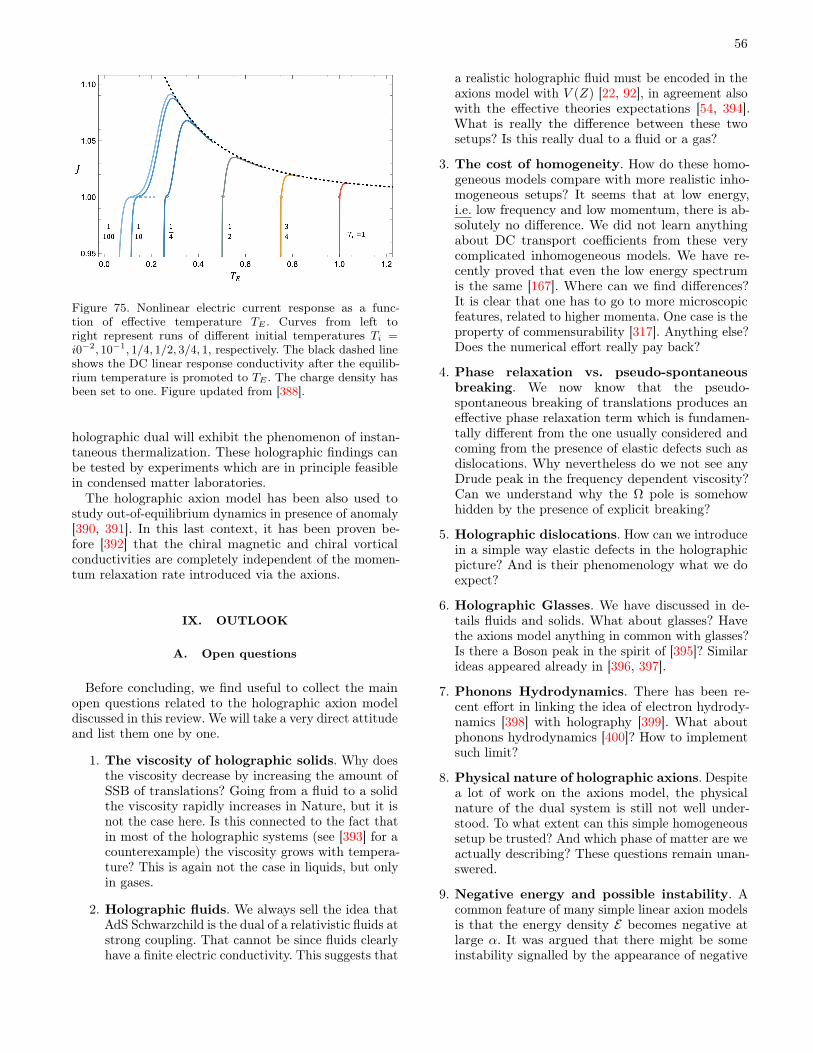
56

Figure 75. Nonlinear electric current response as a func-tion of effective temperature TE . Curves from left toright represent runs of different initial temperatures Ti =i0−2, 10−1, 1/4, 1/2, 3/4, 1, respectively. The black dashed lineshows the DC linear response conductivity after the equilib-rium temperature is promoted to TE . The charge density hasbeen set to one. Figure updated from [388].

holographic dual will exhibit the phenomenon of instan-taneous thermalization. These holographic findings canbe tested by experiments which are in principle feasiblein condensed matter laboratories.The holographic axion model has been also used to

study out-of-equilibrium dynamics in presence of anomaly[390, 391]. In this last context, it has been proven be-fore [392] that the chiral magnetic and chiral vorticalconductivities are completely independent of the momen-tum relaxation rate introduced via the axions.

IX. OUTLOOK

A. Open questions

Before concluding, we find useful to collect the mainopen questions related to the holographic axion modeldiscussed in this review. We will take a very direct attitudeand list them one by one.

1. The viscosity of holographic solids. Why doesthe viscosity decrease by increasing the amount ofSSB of translations? Going from a fluid to a solidthe viscosity rapidly increases in Nature, but it isnot the case here. Is this connected to the fact thatin most of the holographic systems (see [393] for acounterexample) the viscosity grows with tempera-ture? This is again not the case in liquids, but onlyin gases.

2. Holographic fluids. We always sell the idea thatAdS Schwarzchild is the dual of a relativistic fluids atstrong coupling. That cannot be since fluids clearlyhave a finite electric conductivity. This suggests that

a realistic holographic fluid must be encoded in theaxions model with V (Z) [22, 92], in agreement alsowith the effective theories expectations [54, 394].What is really the difference between these twosetups? Is this really dual to a fluid or a gas?

3. The cost of homogeneity. How do these homo-geneous models compare with more realistic inho-mogeneous setups? It seems that at low energy,i.e. low frequency and low momentum, there is ab-solutely no difference. We did not learn anythingabout DC transport coefficients from these verycomplicated inhomogeneous models. We have re-cently proved that even the low energy spectrumis the same [167]. Where can we find differences?It is clear that one has to go to more microscopicfeatures, related to higher momenta. One case is theproperty of commensurability [317]. Anything else?Does the numerical effort really pay back?

4. Phase relaxation vs. pseudo-spontaneousbreaking. We now know that the pseudo-spontaneous breaking of translations produces aneffective phase relaxation term which is fundamen-tally different from the one usually considered andcoming from the presence of elastic defects such asdislocations. Why nevertheless do we not see anyDrude peak in the frequency dependent viscosity?Can we understand why the Ω pole is somehowhidden by the presence of explicit breaking?

5. Holographic dislocations. How can we introducein a simple way elastic defects in the holographicpicture? And is their phenomenology what we doexpect?

6. Holographic Glasses. We have discussed in de-tails fluids and solids. What about glasses? Havethe axions model anything in common with glasses?Is there a Boson peak in the spirit of [395]? Similarideas appeared already in [396, 397].

7. Phonons Hydrodynamics. There has been re-cent effort in linking the idea of electron hydrody-namics [398] with holography [399]. What aboutphonons hydrodynamics [400]? How to implementsuch limit?

8. Physical nature of holographic axions. Despitea lot of work on the axions model, the physicalnature of the dual system is still not well under-stood. To what extent can this simple homogeneoussetup be trusted? And which phase of matter are weactually describing? These questions remain unan-swered.

9. Negative energy and possible instability. Acommon feature of many simple linear axion modelsis that the energy density E becomes negative atlarge α. It was argued that there might be someinstability signalled by the appearance of negative

57

energy density, but such instability was never foundand all the linearized excitations are well behaved.How to understand this negative energy issue? Doesit have any important consequence or limitation forsome of the simplest holographic quantum matters?

10. The residual entropy density. Another commonfeature of linear axion models is the residual entropydensity at zero temperature, corresponding to theAdS2 IR extreme geometry. What’s the nature ofthis residual entropy? Is there any possible relationto localization or glasses? Recent developments inthe SYK model taught us that such feature doesnot come from a degeneracy of the ground statebut from the piling up of a very close excited states[345]. Can we understand it from the gravitationalpicture? Is it again related to the highly unstablecharacter of the AdS2 geometry?

11. Make it useful. It is a truth acknowledged byseveral researchers in (and specially outside) thecommunity, that AdS-CMT has not produced yeta strong smoking-gun result able to justify its use-fulness for realistic condensed matter systems. Canwe push the framework further, connect it to exper-iments, predict new phenomena and explain unre-solved ones? This seems the only way for the toolto survive without becoming a niche product for asmall group of enthusiasts.

B. Conclusions

In conclusion, we hope to have convinced the Readerthat, despite the apparent simplicity, the holographicaxion model displays an incredibly rich set of features andapplications which go far beyond the idea of dissipatingmomentum and make the DC electric conductivity finite.

In any case, whether you want to use them just to avoidannoying infinities or if you want to dig deeper in thephysics of solids and fluids at strong coupling, this reviewis made for you. At the cost of resulting rather lengthy,we have made the effort of being as comprehensive aspossible and discuss all the different faces of the model.We hope that any of you, in one way or another, willbenefit from this read and will learn something new you

were not aware of before. We also wish to have inspirednew thoughts on the topic and the incentive for futuredevelopments in the field.

ACKNOWLEDGMENTS

We are grateful to the uncountable number of colleagueswhich participated with us in the process of understandingall the secrets of the holographic axion model. We thankTeng Ji, Giorgio Frangi, Hyun-Sik Jeong, Xi-Jing Wangand Yongjun Ahn for useful comments and helping proof-reading an early version of this manuscript.M.B. acknowledges the support of the Shanghai

Municipal Science and Technology Major Project (GrantNo.2019SHZDZX01) and of the Spanish MINECO“Centro de Excelencia Severo Ochoa” Programme undergrant SEV-2012-0249. K.K. was supported by BasicScience Research Program through the National ResearchFoundation of Korea (NRF) funded by the Ministry of Sci-ence, ICT & Future Planning (NRF-2017R1A2B4004810)and the GIST Research Institute(GRI) grant fundedby the GIST in 2020. L.L. is supported in part by theNational Natural Science Foundation of China (NSFC)Grants No.12075298, No.11991052 and No.12047503.W.J.L. is supported in part by the NSFC under grantNo.11905024 and DUT under grant No.DUT19LK20.

Appendix A: Notations and conventions

In order to avoid confusion, in this appendix we describein detail all the symbols and notations used in this review.Greek letters µ, ν, ... run over spacetime indices, while

Latin letters i, j, ... denote spatial ones. The axion flavorindices I, J, ... run over the number of broken translations.In this review, we also omit the summation symbol overthe axion flavor indices, and use the Einstein conventionfor them too.

We always utilize a mostly plus metric (−1, 1, 1, 1) andwe define the Fourier transform of a field Ψ using theplain-wave e−iωt+ikx. Finally, we indicate in Table I allthe symbols used.

[1] M. Ammon and J. Erdmenger. Gauge/Gravity Duality.Cambridge University Press, 2015.

[2] Sean A. Hartnoll, Andrew Lucas, and Subir Sachdev.Holographic quantum matter. 2016.

[3] Sean A. Hartnoll. Lectures on holographic methodsfor condensed matter physics. Class. Quant. Grav.,26:224002, 2009.

[4] J. Zaanen, Y. Liu, Y.W. Sun, and K. Schalm.Holographic Duality in Condensed Matter Physics.Cambridge University Press, 2015.

[5] Jorge Casalderrey-Solana, Hong Liu, David Ma-teos, Krishna Rajagopal, and Urs Achim Wiedemann.Gauge/String Duality, Hot QCD and Heavy Ion Collisions.Cambridge University Press, 2014.

[6] Matteo Baggioli. Applied Holography:A Practical Mini-Course. SpringerBriefs in Physics.Springer, 2019.

[7] Michal P. Heller. Holography, Hydrodynamization andHeavy-Ion Collisions. Acta Phys. Polon. B, 47:2581,2016.

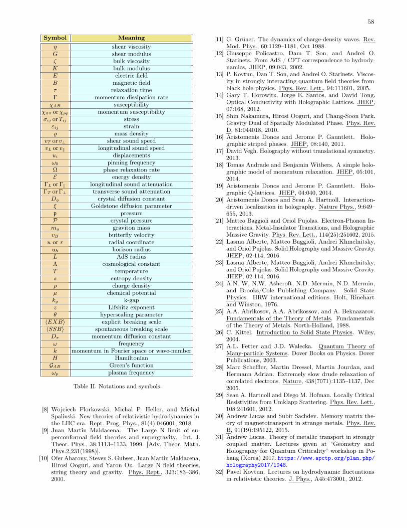
58

Symbol Meaningη shear viscosityG shear modulusζ bulk viscosityK bulk modulusE electric fieldB magnetic fieldτ relaxation timeΓ momentum dissipation rateχAB susceptibility

χππ orχpp momentum susceptibilityσij orTij stress

εij strain% mass density

vT or v⊥ shear sound speedvL or v‖ longitudinal sound speedui displacementsω0 pinning frequencyΩ phase relaxation rateE energy density

ΓL orΓ‖ longitudinal sound attenuationΓT orΓ⊥ transverse sound attenuationDφ crystal diffusion constantξ Goldstone diffusion parameterp pressureP crystal pressuremg graviton massvB butterfly velocity

u or r radial coordinateuh horizon radiusL AdS radiusΛ cosmological constantT temperatures entropy densityρ charge densityµ chemical potentialkg k-gapz Lifshitz exponentθ hyperscaling parameter

〈EXB〉 explicit breaking scale〈SSB〉 spontaneous breaking scaleDπ momentum diffusion constantω frequencyk momentum in Fourier space or wave-numberH HamiltonianGAB Green’s functionωp plasma frequency

Table II. Notations and symbols.

[8] Wojciech Florkowski, Michal P. Heller, and MichalSpalinski. New theories of relativistic hydrodynamics inthe LHC era. Rept. Prog. Phys., 81(4):046001, 2018.

[9] Juan Martin Maldacena. The Large N limit of su-perconformal field theories and supergravity. Int. J.Theor. Phys., 38:1113–1133, 1999. [Adv. Theor. Math.Phys.2,231(1998)].

[10] Ofer Aharony, Steven S. Gubser, Juan Martin Maldacena,Hirosi Ooguri, and Yaron Oz. Large N field theories,string theory and gravity. Phys. Rept., 323:183–386,2000.

[11] G. Grüner. The dynamics of charge-density waves. Rev.Mod. Phys., 60:1129–1181, Oct 1988.

[12] Giuseppe Policastro, Dam T. Son, and Andrei O.Starinets. From AdS / CFT correspondence to hydrody-namics. JHEP, 09:043, 2002.

[13] P. Kovtun, Dan T. Son, and Andrei O. Starinets. Viscos-ity in strongly interacting quantum field theories fromblack hole physics. Phys. Rev. Lett., 94:111601, 2005.

[14] Gary T. Horowitz, Jorge E. Santos, and David Tong.Optical Conductivity with Holographic Lattices. JHEP,07:168, 2012.

[15] Shin Nakamura, Hirosi Ooguri, and Chang-Soon Park.Gravity Dual of Spatially Modulated Phase. Phys. Rev.D, 81:044018, 2010.

[16] Aristomenis Donos and Jerome P. Gauntlett. Holo-graphic striped phases. JHEP, 08:140, 2011.

[17] David Vegh. Holography without translational symmetry.2013.

[18] Tomas Andrade and Benjamin Withers. A simple holo-graphic model of momentum relaxation. JHEP, 05:101,2014.

[19] Aristomenis Donos and Jerome P. Gauntlett. Holo-graphic Q-lattices. JHEP, 04:040, 2014.

[20] Aristomenis Donos and Sean A. Hartnoll. Interaction-driven localization in holography. Nature Phys., 9:649–655, 2013.

[21] Matteo Baggioli and Oriol Pujolas. Electron-Phonon In-teractions, Metal-Insulator Transitions, and HolographicMassive Gravity. Phys. Rev. Lett., 114(25):251602, 2015.

[22] Lasma Alberte, Matteo Baggioli, Andrei Khmelnitsky,and Oriol Pujolas. Solid Holography and Massive Gravity.JHEP, 02:114, 2016.

[23] Lasma Alberte, Matteo Baggioli, Andrei Khmelnitsky,and Oriol Pujolas. Solid Holography and Massive Gravity.JHEP, 02:114, 2016.

[24] A.N. W, N.W. Ashcroft, N.D. Mermin, N.D. Mermin,and Brooks/Cole Publishing Company. Solid StatePhysics. HRW international editions. Holt, Rinehartand Winston, 1976.

[25] A.A. Abrikosov, A.A. Abrikossov, and A. Beknazarov.Fundamentals of the Theory of Metals. Fundamentalsof the Theory of Metals. North-Holland, 1988.

[26] C. Kittel. Introduction to Solid State Physics. Wiley,2004.

[27] A.L. Fetter and J.D. Walecka. Quantum Theory ofMany-particle Systems. Dover Books on Physics. DoverPublications, 2003.

[28] Marc Scheffler, Martin Dressel, Martin Jourdan, andHermann Adrian. Extremely slow drude relaxation ofcorrelated electrons. Nature, 438(7071):1135–1137, Dec2005.

[29] Sean A. Hartnoll and Diego M. Hofman. Locally CriticalResistivities from Umklapp Scattering. Phys. Rev. Lett.,108:241601, 2012.

[30] Andrew Lucas and Subir Sachdev. Memory matrix the-ory of magnetotransport in strange metals. Phys. Rev.B, 91(19):195122, 2015.

[31] Andrew Lucas. Theory of metallic transport in stronglycoupled matter. Lectures given at ”Geometry andHolography for Quantum Criticality” workshop in Po-hang (Korea) 2017. https://www.apctp.org/plan.php/holography2017/1948.

[32] Pavel Kovtun. Lectures on hydrodynamic fluctuationsin relativistic theories. J. Phys., A45:473001, 2012.

59

[33] L.L. D and L.E. M. Theory of Elasticity. Course oftheoretical physics. Pergamon Press, 1989.

[34] X. Zotos, F. Naef, and P. Prelovsek. Transport andconservation laws. Phys. Rev. B, 55:11029–11032, May1997.

[35] Antonio M. García-García and Aurelio Romero-Bermúdez. Drude weight and Mazur-Suzuki boundsin holography. Phys. Rev. D, 93(6):066015, 2016.

[36] P.M. Chaikin and T.C. Lubensky. Principles ofCondensed Matter Physics. Cambridge University Press,2000.

[37] P. C. Martin, O. Parodi, and P. S. Pershan. Unifiedhydrodynamic theory for crystals, liquid crystals, andnormal fluids. Phys. Rev. A, 6:2401–2420, Dec 1972.

[38] H. Leutwyler. Phonons as goldstone bosons. Helv. Phys.Acta, 70:275–286, 1997.

[39] Matteo Baggioli. Phases of Matter & Collective Excita-tions in the eyes of a high energy theorist. Lectures givenat ”Quantum Matter and Quantum Information withHolography” workshop in Pohang (Korea) 2020. https://www.apctp.org/plan.php/holography2020/3039.

[40] Aron J. Beekman, Louk Rademaker, and Jasper vanWezel. An Introduction to Spontaneous Symmetry Break-ing. 9 2019.

[41] Muneto Nitta, Shin Sasaki, and Ryo Yokokura. SpatiallyModulated Vacua in a Lorentz-invariant Scalar FieldTheory. Eur. Phys. J. C, 78(9):754, 2018.

[42] Sven Bjarke Gudnason, Muneto Nitta, Shin Sasaki, andRyo Yokokura. Temporally, spatially, or lightlike modu-lated vacua in Lorentz invariant theories. Phys. Rev. D,99(4):045011, 2019.

[43] Daniele Musso. Simplest phonons and pseudo-phononsin field theory. Eur. Phys. J. C, 79(12):986, 2019.

[44] Daniele Musso and Daniel Naegels. Independent Gold-stone modes for translations and shift symmetry froma real modulated scalar. Phys. Rev. D, 101(4):045016,2020.

[45] Alberto Nicolis, Riccardo Penco, Federico Piazza, andRiccardo Rattazzi. Zoology of condensed matter:Framids, ordinary stuff, extra-ordinary stuff. JHEP,06:155, 2015.

[46] Alberto Nicolis, Riccardo Penco, and Rachel A. Rosen.Relativistic Fluids, Superfluids, Solids and Supersolidsfrom a Coset Construction. Phys. Rev., D89(4):045002,2014.

[47] H. Kleinert. Gauge Fields in Condensed Matter. Num-ber v. 2 in Gauge Fields in Condensed Matter. WorldScientific, 1989.

[48] V. L. Gurevich and A. Thellung. Quasimomentum inthe theory of elasticity and its conservation. Phys. Rev.B, 42:7345–7349, Oct 1990.

[49] Matteo Baggioli. How small hydrodynamics can go. 102020.

[50] Lasma Alberte, Matteo Baggioli, Victor Cancer Castillo,and Oriol Pujolas. Elasticity bounds from Effective FieldTheory. Phys. Rev. D, 100(6):065015, 2019. [Erratum:Phys.Rev.D 102, 069901 (2020)].

[51] Matteo Baggioli, Victor Cancer Castillo, and Oriol Pujo-las. Scale invariant solids. Phys. Rev. D, 101(8):086005,2020.

[52] Matteo Baggioli, Victor Cancer Castillo, and Oriol Pujo-las. Black Rubber and the Non-linear Elastic Responseof Scale Invariant Solids. JHEP, 20:013, 2020.

[53] Matteo Baggioli, Mikhail Vasin, Vadim V. Brazhkin, and

Kostya Trachenko. Gapped momentum states. Phys.Rept., 865:1–44, 2020.

[54] Jan de Boer, Michal P. Heller, and Natalia Pinzani-Fokeeva. Effective actions for relativistic fluids fromholography. JHEP, 08:086, 2015.

[55] Hong Liu and Paolo Glorioso. Lectures on non-equilibrium effective field theories and fluctuating hydro-dynamics. PoS, TASI2017:008, 2018.

[56] Edward Witten. Anti-de Sitter space and holography.Adv. Theor. Math. Phys., 2:253–291, 1998.

[57] John McGreevy. TASI 2015 Lectures on Quantum Mat-ter (with a View Toward Holographic Duality). pages215–296, 2017.

[58] John McGreevy. Holographic duality with a view to-ward many-body physics. Adv. High Energy Phys.,2010:723105, 2010.

[59] Horatiu Nastase. Introduction to AdS-CFT. 2007.[60] Alfonso V. Ramallo. Introduction to the AdS/CFT cor-

respondence. Springer Proc. Phys., 161:411–474, 2015.[61] Martin Ammon and Johanna Erdmenger.

Gauge/Gravity Duality: Foundations and Applications.Cambridge University Press, New York, NY, USA, 1stedition, 2015.

[62] A Zaffaroni. Introduction to the AdS-CFT correspon-dence. Classical and Quantum Gravity, 17(17):3571–3597, aug 2000.

[63] Joseph Polchinski. Introduction to Gauge/Gravity Du-ality. pages 3–46, 2010.

[64] Makoto Natsuume. AdS/CFT Duality User Guide. Lect.Notes Phys., 903:pp.1–294, 2015.

[65] Edward Witten. Anti-de Sitter space and holography.Adv. Theor. Math. Phys., 2:253–291, 1998.

[66] S. S. Gubser, Igor R. Klebanov, and Alexander M.Polyakov. Gauge theory correlators from noncriticalstring theory. Phys. Lett., B428:105–114, 1998.

[67] Y. Liu J. Zaanen, Y.W. Sun and K. Schalm. The ads/cmtmanual for plumbers and electricians. 2012.

[68] Rong-Gen Cai, Li Li, Li-Fang Li, and Run-Qiu Yang.Introduction to Holographic Superconductor Models. Sci.China Phys. Mech. Astron., 58(6):060401, 2015.

[69] Karl Landsteiner, Yan Liu, and Ya-Wen Sun. Holo-graphic topological semimetals. Sci. China Phys. Mech.Astron., 63(5):250001, 2020.

[70] Jorge Casalderrey-Solana, Hong Liu, David Mateos,Krishna Rajagopal, and Urs Achim Wiedemann.Gauge/String Duality, Hot QCD and Heavy Ion Col-lisions. 2011.

[71] Mukund Rangamani and Tadashi Takayanagi.Holographic Entanglement Entropy, volume 931.Springer, 2017.

[72] Veronika E. Hubeny and Mukund Rangamani. A Holo-graphic view on physics out of equilibrium. Adv. HighEnergy Phys., 2010:297916, 2010.

[73] Hong Liu and Julian Sonner. Holographic systems farfrom equilibrium: a review. 10 2018.

[74] Sachin Jain, Nilay Kundu, Kallol Sen, Aninda Sinha,and Sandip P. Trivedi. A Strongly Coupled AnisotropicFluid From Dilaton Driven Holography. JHEP, 01:005,2015.

[75] Xian-Hui Ge, Yi Ling, Chao Niu, and Sang-Jin Sin. Ther-moelectric conductivities, shear viscosity, and stabilityin an anisotropic linear axion model. Phys. Rev. D,92(10):106005, 2015.

[76] Sachin Jain, Rickmoy Samanta, and Sandip P. Trivedi.

60

The Shear Viscosity in Anisotropic Phases. JHEP,10:028, 2015.

[77] Óscar J.C. Dias, Jorge E. Santos, and Benson Way. Nu-merical Methods for Finding Stationary GravitationalSolutions. Class. Quant. Grav., 33(13):133001, 2016.

[78] Alexander Krikun. Numerical Solution of the BoundaryValue Problems for Partial Differential Equations. Crashcourse for holographer. 1 2018.

[79] Tomas Andrade. Holographic Lattices and NumericalTechniques. 12 2017.

[80] Aristomenis Donos and Jerome P. Gauntlett. Minimallypacked phases in holography. JHEP, 03:148, 2016.

[81] Mike Blake, David Tong, and David Vegh. HolographicLattices Give the Graviton an Effective Mass. Phys. Rev.Lett., 112(7):071602, 2014.

[82] Peter Breitenlohner and Daniel Z. Freedman. PositiveEnergy in anti-De Sitter Backgrounds and Gauged Ex-tended Supergravity. Phys. Lett. B, 115:197–201, 1982.

[83] Norihiro Iizuka, Shamit Kachru, Nilay Kundu, PrithviNarayan, Nilanjan Sircar, and Sandip P. Trivedi. BianchiAttractors: A Classification of Extremal Black BraneGeometries. JHEP, 07:193, 2012.

[84] Yannis Bardoux, Marco M. Caldarelli, and Christos Char-mousis. Shaping black holes with free fields. JHEP,05:054, 2012.

[85] Marika Taylor and William Woodhead. Inhomogeneitysimplified. Eur. Phys. J. C, 74(12):3176, 2014.

[86] Richard A. Davison, Blaise Goutéraux, and Sean A.Hartnoll. Incoherent transport in clean quantum criticalmetals. JHEP, 10:112, 2015.

[87] David Tong. Lectures on Holographic Conductiv-ity, http://www.damtp.cam.ac.uk/user/tong/talks/zakopane.pdf.

[88] Keun-Young Kim, Kyung Kiu Kim, Yunseok Seo, andSang-Jin Sin. Coherent/incoherent metal transition in aholographic model. JHEP, 12:170, 2014.

[89] Tomas Andrade, Simon A. Gentle, and Benjamin With-ers. Drude in D major. JHEP, 06:134, 2016.

[90] Richard A. Davison and Blaise Goutéraux. Momen-tum dissipation and effective theories of coherent andincoherent transport. JHEP, 01:039, 2015.

[91] Richard A. Davison and Blaise Goutéraux. Dissectingholographic conductivities. JHEP, 09:090, 2015.

[92] Matteo Baggioli and Sebastian Grieninger. Zoology ofsolid \& fluid holography — Goldstone modes and phaserelaxation. JHEP, 10:235, 2019.

[93] Aristomenis Donos and Jerome P. Gauntlett. Ther-moelectric DC conductivities from black hole horizons.JHEP, 11:081, 2014.

[94] Nabil Iqbal and Hong Liu. Universality of the hydrody-namic limit in AdS/CFT and the membrane paradigm.Phys. Rev., D79:025023, 2009.

[95] Richard A. Davison, Wenbo Fu, Antoine Georges, YingfeiGu, Kristan Jensen, and Subir Sachdev. Thermoelectrictransport in disordered metals without quasiparticles:The Sachdev-Ye-Kitaev models and holography. Phys.Rev. B, 95(15):155131, 2017.

[96] Andrea Amoretti, Alessandro Braggio, Nicola Maggiore,Nicodemo Magnoli, and Daniele Musso. Analytic dcthermoelectric conductivities in holography with massivegravitons. Phys. Rev. D, 91(2):025002, 2015.

[97] Zhenhua Zhou, Jian-Pin Wu, and Yi Ling. DC and Hallconductivity in holographic massive Einstein-Maxwell-Dilaton gravity. JHEP, 08:067, 2015.

[98] Andrew Lucas. Hydrodynamic transport in stronglycoupled disordered quantum field theories. New J. Phys.,17(11):113007, 2015.

[99] Elliot Banks, Aristomenis Donos, and Jerome P.Gauntlett. Thermoelectric DC conductivities and Stokesflows on black hole horizons. JHEP, 10:103, 2015.

[100] Xian-Hui Ge, Yu Tian, Shang-YuWu, and Shao-FengWu.Hyperscaling violating black hole solutions and Magneto-thermoelectric DC conductivities in holography. Phys.Rev. D, 96(4):046015, 2017. [Erratum: Phys.Rev.D 97,089901 (2018)].

[101] Jian-Pin Wu, Xiao-Mei Kuang, and Guoyang Fu. Mo-mentum dissipation and holographic transport withoutself-duality. Eur. Phys. J. C, 78(8):616, 2018.

[102] Mike Blake and Aristomenis Donos. Quantum Criti-cal Transport and the Hall Angle. Phys. Rev. Lett.,114(2):021601, 2015.

[103] Aristomenis Donos and Jerome P. Gauntlett. The ther-moelectric properties of inhomogeneous holographic lat-tices. JHEP, 01:035, 2015.

[104] Long Cheng, Xian-Hui Ge, and Zu-Yao Sun. Thermo-electric DC conductivities with momentum dissipationfrom higher derivative gravity. JHEP, 04:135, 2015.

[105] Andrew Lucas. Conductivity of a strange metal: fromholography to memory functions. JHEP, 03:071, 2015.

[106] Andrea Amoretti and Daniele Musso. Magneto-transportfrom momentum dissipating holography. JHEP, 09:094,2015.

[107] Mike Blake, Aristomenis Donos, and Nakarin Lohit-siri. Magnetothermoelectric Response from Holography.JHEP, 08:124, 2015.

[108] Keun-Young Kim, Kyung Kiu Kim, Yunseok Seo, andSang-Jin Sin. Thermoelectric Conductivities at FiniteMagnetic Field and the Nernst Effect. JHEP, 07:027,2015.

[109] Aristomenis Donos, Jerome P. Gauntlett, Tom Griffin,and Luis Melgar. DC Conductivity of Magnetised Holo-graphic Matter. JHEP, 01:113, 2016.

[110] Sera Cremonini, Hai-Shan Liu, Hong Lu, and C.N. Pope.DC Conductivities from Non-Relativistic Scaling Ge-ometries with Momentum Dissipation. JHEP, 04:009,2017.

[111] Keun-Young Kim, Kyung Kiu Kim, Yunseok Seo, andSang-Jin Sin. Gauge Invariance and Holographic Renor-malization. Phys. Lett. B, 749:108–114, 2015.

[112] Blaise Gouteraux, Elias Kiritsis, and Wei-Jia Li. Effec-tive holographic theories of momentum relaxation andviolation of conductivity bound. JHEP, 04:122, 2016.

[113] Matteo Baggioli, Blaise Goutéraux, Elias Kiritsis, andWei-Jia Li. Higher derivative corrections to incoherentmetallic transport in holography. JHEP, 03:170, 2017.

[114] Matteo Baggioli and Wei-Jia Li. Diffusivities bounds andchaos in holographic Horndeski theories. JHEP, 07:055,2017.

[115] Matteo Baggioli and Oriol Pujolas. On holographicdisorder-driven metal-insulator transitions. JHEP,01:040, 2017.

[116] Yu-Sen An, Teng Ji, and Li Li. Magnetotransport andComplexity of Holographic Metal-Insulator Transitions.JHEP, 10:023, 2020.

[117] Lasma Alberte, Martin Ammon, Matteo Baggioli,Amadeo Jiménez-Alba, and Oriol Pujolàs. HolographicPhonons. 2017.

[118] Jay Armas and Akash Jain. Viscoelastic hydrodynamics

61

and holography. 2019.[119] Martin Ammon, Matteo Baggioli, Seán Gray, Sebastian

Grieninger, and Akash Jain. On the HydrodynamicDescription of Holographic Viscoelastic Models. Phys.Lett. B, 808:135691, 2020.

[120] Andrea Amoretti, Daniel Areán, Blaise Goutéraux, andDaniele Musso. Effective holographic theory of chargedensity waves. Phys. Rev., D97(8):086017, 2018.

[121] Wei-Jia Li and Jian-Pin Wu. A simple holographic modelfor spontaneous breaking of translational symmetry. Eur.Phys. J. C, 79(3):243, 2019.

[122] Xi-Jing Wang and Wei-Jia Li. Work in progress.[123] Yi Ling, Chao Niu, Jianpin Wu, Zhuoyu Xian, and Hong-

bao Zhang. Metal-insulator Transition by HolographicCharge Density Waves. Phys. Rev. Lett., 113:091602,2014.

[124] Sera Cremonini, Li Li, and Jie Ren. Holographic Pairand Charge Density Waves. Phys. Rev., D95(4):041901,2017.

[125] Sera Cremonini, Li Li, and Jie Ren. Intertwined Ordersin Holography: Pair and Charge Density Waves. JHEP,08:081, 2017.

[126] Rong-Gen Cai, Li Li, Yong-Qiang Wang, and Jan Zaa-nen. Intertwined Order and Holography: The Case ofParity Breaking Pair Density Waves. Phys. Rev. Lett.,119(18):181601, 2017.

[127] Lasma Alberte, Matteo Baggioli, and Oriol Pujolas. Vis-cosity bound violation in holographic solids and theviscoelastic response. JHEP, 07:074, 2016.

[128] Emanuele Berti, Vitor Cardoso, and Andrei O. Starinets.Quasinormal modes of black holes and black branes.Class. Quant. Grav., 26:163001, 2009.

[129] Martin Ammon, Matteo Baggioli, Seán Gray, and Sebas-tian Grieninger. Longitudinal Sound and Diffusion inHolographic Massive Gravity. JHEP, 10:064, 2019.

[130] A. Esposito, S. Garcia-Saenz, A. Nicolis, and R. Penco.Conformal solids and holography. JHEP, 12:113, 2017.

[131] Sa šo Grozdanov and Napat Poovuttikul. Generalizedglobal symmetries in states with dynamical defects: Thecase of the transverse sound in field theory and hologra-phy. Phys. Rev. D, 97:106005, May 2018.

[132] Davide Gaiotto, Anton Kapustin, Nathan Seiberg, andBrian Willett. Generalized Global Symmetries. JHEP,02:172, 2015.

[133] Sašo Grozdanov, Diego M. Hofman, and Nabil Iqbal.Generalized global symmetries and dissipative magneto-hydrodynamics. Phys. Rev. D, 95(9):096003, 2017.

[134] B. I. Halperin and David R. Nelson. Theory of two-dimensional melting. Phys. Rev. Lett., 41:121–124, Jul1978.

[135] Luca V. Delacrétaz, Blaise Goutéraux, Sean A. Hartnoll,and Anna Karlsson. Theory of hydrodynamic transportin fluctuating electronic charge density wave states. Phys.Rev. B, 96(19):195128, 2017.

[136] Luca V. Delacrétaz, Blaise Goutéraux, Sean A. Hart-noll, and Anna Karlsson. Bad Metals from FluctuatingDensity Waves. SciPost Phys., 3(3):025, 2017.

[137] Andrea Amoretti, Martina Meinero, Daniel K. Brat-tan, Federico Caglieris, Enrico Giannini, Marco Affronte,Christian Hess, Bernd Buechner, Nicodemo Magnoli, andMarina Putti. Hydrodynamical description for magneto-transport in the strange metal phase of Bi-2201. Phys.Rev. Res., 2(2):023387, 2020.

[138] Leo P Kadanoff and Paul C Martin. Hydrodynamic

equations and correlation functions. Annals of Physics,24:419 – 469, 1963.

[139] Sebastian Leonard Grieninger.Non-equilibrium dynamics in Holography. PhDthesis, Jena U., 2020.

[140] Jay Armas and Akash Jain. Hydrodynamics for chargedensity waves and their holographic duals. 1 2020.

[141] Aristomenis Donos and Jerome P. Gauntlett. On thethermodynamics of periodic AdS black branes. JHEP,10:038, 2013.

[142] Martin Ammon, Matteo Baggioli, and Amadeo Jiménez-Alba. A Unified Description of Translational SymmetryBreaking in Holography. 2019.

[143] S. N. Taraskin and S. R. Elliott. Ioffe-regel crossoverfor plane-wave vibrational excitations in vitreous silica.Phys. Rev. B, 61:12031–12037, May 2000.

[144] SN Taraskin and SR Elliott. Vector vibrations and theioffe-regel crossover in disordered lattices. Journal ofPhysics: Condensed Matter, 14(12):3143, 2002.

[145] YM Beltukov, VI Kozub, and DA Parshin. Ioffe-regelcriterion and diffusion of vibrations in random lattices.Physical Review B, 87(13):134203, 2013.

[146] Hiroshi Shintani and Hajime Tanaka. Universal linkbetween the boson peak and transverse phonons in glass.Nature Materials, 7:870 EP –, Oct 2008. Article.

[147] Matteo Baggioli, Sebastian Grieninger, and Li Li. Magne-tophonons \& type-B Goldstones from Hydrodynamicsto Holography. JHEP, 09:037, 2020.

[148] Matteo Baggioli, Sebastian Grieninger, and HesamSoltanpanahi. Nonlinear Oscillatory Shear Tests in Vis-coelastic Holography. Phys. Rev. Lett., 124(8):081601,2020.

[149] Aristomenis Donos, Daniel Martin, Christiana Pan-telidou, and Vaios Ziogas. Hydrodynamics of brokenglobal symmetries in the bulk. JHEP, 10:218, 2019.

[150] Andrea Amoretti, Daniel Areán, Blaise Goutéraux,and Daniele Musso. Universal relaxation in a holo-graphic metallic density wave phase. Phys. Rev. Lett.,123(21):211602, 2019.

[151] Matteo Baggioli. Homogeneous holographic viscoelasticmodels and quasicrystals. Phys. Rev. Res., 2(2):022022,2020.

[152] P. Steinhardt. The Second Kind of Impossible: TheExtraordinary Quest for a New Form of Matter. Simon& Schuster, 2019.

[153] Ted Janssen. Aperiodic crystals: A contradictio in ter-minis? Physics Reports, 168(2):55–113, 1988.

[154] D.P. DiVincenzo and P.J. Steinhardt. Quasicrystals:The State of the Art. Series on directions in condensedmatter physics. World Scientific, 1999.

[155] C. Janot. Quasicrystals: A Primer. Monographs on thephysics and chemistry of materials. Clarendon Press,1997.

[156] T. C. Lubensky, Sriram Ramaswamy, and John Toner.Hydrodynamics of icosahedral quasicrystals. Phys. Rev.B, 32:7444–7452, Dec 1985.

[157] W. Finger and T. M. Rice. Theory of the crossover in thelow-frequency dynamics of an incommensurate system,hg3−δAsf6. Phys. Rev. Lett., 49:468–470, Aug 1982.

[158] M. B. Walker and R. J. Gooding. Theory of coupledphason and sound-wave normal modes in the incommen-surate phase of quartz. Phys. Rev. B, 32:7412–7416, Dec1985.

[159] R. Currat, E. Kats, and I. Luk’yanchuk. Sound modes

62

in composite incommensurate crystals. The EuropeanPhysical Journal B - Condensed Matter and ComplexSystems, 26(3):339–347, Apr 2002.

[160] R. Zeyher and W. Finger. Phason dynamics of incom-mensurate crystals. Phys. Rev. Lett., 49:1833–1837, Dec1982.

[161] Eleni Agiasofitou and Markus Lazar. The elastody-namic model of wave-telegraph type for quasicrystals.International Journal of Solids and Structures, 51(5):923– 929, 2014.

[162] S. Francoual, F. Livet, M. de Boissieu, F. Yakhou, F. Bley,A. Létoublon, R. Caudron, and J. Gastaldi. Dynamicsof phason fluctuations in the i−AlPdMn quasicrystal.Phys. Rev. Lett., 91:225501, Nov 2003.

[163] D Durand, R Papoular, R Currat, M Lambert,JF Legrand, and F Mezei. Investigation of the incom-mensurate transition of sodium nitrite by the neutronspin-echo technique. Physical Review B, 43(13):10690,1991.

[164] M. Quilichini and R. Currat. Neutron evidence for anoverdamped phason branch in incommensurate k2seo4.Solid State Communications, 48(12):1011 – 1015, 1983.

[165] T Janssen and A Janner. Aperiodic crystals and su-perspace concepts. Acta Crystallographica Section B:Structural Science, Crystal Engineering and Materials,70(4):617–651, 2014.

[166] Matteo Baggioli and Michael Landry. Effective FieldTheory for Quasicrystals and Phasons Dynamics. 8 2020.

[167] Tomas Andrade, Matteo Baggioli, and Alexander Krikun.Phase relaxation and pattern formation in holographicgapless charge density waves. 9 2020.

[168] Richard A. Davison. Momentum relaxation in holo-graphic massive gravity. Phys. Rev. D, 88:086003, 2013.

[169] Matteo Baggioli and Kostya Trachenko. Low frequencypropagating shear waves in holographic liquids. JHEP,03:093, 2019.

[170] M. Baggioli and K. Trachenko. Maxwell interpolationand close similarities between liquids and holographicmodels. Phys. Rev., D99(10):106002, 2019.

[171] Laurence Noirez and Patrick Baroni. Identification of alow-frequency elastic behaviour in liquid water. Journalof Physics: Condensed Matter, 24(37):372101, aug 2012.

[172] Eni Kume, Patrick Baroni, and Laurence Noirez. Strain-induced violation of temperature uniformity in mesoscaleliquids. Scientific Reports, 10(1):13340, Aug 2020.

[173] Eni Kume, Alessio Zaccone, and Laurence Noirez. Un-expected thermo-elastic effects in liquid glycerol by me-chanical deformation. arXiv preprint arXiv:2009.09788,2020.

[174] M. Grimsditch, R. Bhadra, and L. M. Torell. Shearwaves through the glass-liquid transformation. Phys.Rev. Lett., 62:2616–2619, May 1989.

[175] Matteo Baggioli, Mikhail Vasin, Vadim Brazhkin, andKostya Trachenko. Gapped momentum states. PhysicsReports, 865:1 – 44, 2020. Gapped momentum states.

[176] M. Baggioli, M. Vasin, V.V. Brazhkin, and K. Trachenko.Field Theory of Dissipative Systems with Gapped Mo-mentum States. Phys. Rev. D, 102(2):025012, 2020.

[177] Sašo Grozdanov and Napat Poovuttikul. Generalizedglobal symmetries in states with dynamical defects: Thecase of the transverse sound in field theory and hologra-phy. Phys. Rev., D97(10):106005, 2018.

[178] Diego M. Hofman and Nabil Iqbal. Generalized globalsymmetries and holography. SciPost Phys., 4(1):005,

2018.[179] Raul E. Arias and Ignacio Salazar Landea. Hydrody-

namic Modes of a holographic p− wave superfluid. JHEP,11:047, 2014.

[180] Matteo Baggioli, Ulf Gran, and Marcus Tornsö. Trans-verse Collective Modes in Interacting Holographic Plas-mas. JHEP, 04:106, 2020.

[181] Ulf Gran, Marcus Tornsö, and Tobias Zingg. ExoticHolographic Dispersion. JHEP, 02:032, 2019.

[182] Matteo Baggioli, Ulf Gran, Amadeo Jimenez Alba, Mar-cus Tornsö, and Tobias Zingg. Holographic Plasmon Re-laxation with and without Broken Translations. JHEP,09:013, 2019.

[183] Sašo Grozdanov, Andrew Lucas, and Napat Poovuttikul.Holography and hydrodynamics with weakly broken sym-metries. Phys. Rev. D, 99(8):086012, 2019.

[184] Svante Arrhenius. Über die dissociationswärme undden einfluss der temperatur auf den dissociationsgradder elektrolyte. Zeitschrift für Physikalische Chemie,4U(1):96 – 116, 01 Jul. 1889.

[185] Thomas Schafer and Derek Teaney. Nearly Perfect Flu-idity: From Cold Atomic Gases to Hot Quark GluonPlasmas. Rept. Prog. Phys., 72:126001, 2009.

[186] Sera Cremonini. The Shear Viscosity to Entropy Ratio: AStatus Report. Mod. Phys. Lett., B25:1867–1888, 2011.

[187] Matthew Luzum and Paul Romatschke. ConformalRelativistic Viscous Hydrodynamics: Applications toRHIC results at s(NN)**(1/2) = 200-GeV. Phys. Rev.C, 78:034915, 2008. [Erratum: Phys.Rev.C 79, 039903(2009)].

[188] James L. Nagle, Ian G. Bearden, and William A. Zajc.Quark-Gluon Plasma at RHIC and the LHC: PerfectFluid too Perfect? New J. Phys., 13:075004, 2011.

[189] Chun Shen, Ulrich Heinz, Pasi Huovinen, and HuichaoSong. Radial and elliptic flow in Pb+Pb collisions atthe Large Hadron Collider from viscous hydrodynamic.Phys. Rev. C, 84:044903, 2011.

[190] Alex Buchel, James T. Liu, and Andrei O. Starinets.Coupling constant dependence of the shear viscosity inN=4 supersymmetric Yang-Mills theory. Nucl. Phys. B,707:56–68, 2005.

[191] Alex Buchel. Shear viscosity of CFT plasma at finitecoupling. Phys. Lett. B, 665:298–304, 2008.

[192] Robert C. Myers, Miguel F. Paulos, and Aninda Sinha.Quantum corrections to eta/s. Phys. Rev. D, 79:041901,2009.

[193] Alex Buchel, Robert C. Myers, Miguel F. Paulos, andAninda Sinha. Universal holographic hydrodynamics atfinite coupling. Phys. Lett. B, 669:364–370, 2008.

[194] Ahmad Ghodsi and Mohsen Alishahiha. Non-relativisticD3-brane in the presence of higher derivative corrections.Phys. Rev. D, 80:026004, 2009.

[195] Alex Buchel. Resolving disagreement for eta/s in a CFTplasma at finite coupling. Nucl. Phys. B, 803:166–170,2008.

[196] Mauro Brigante, Hong Liu, Robert C. Myers, StephenShenker, and Sho Yaida. Viscosity Bound Violation inHigher Derivative Gravity. Phys. Rev. D, 77:126006,2008.

[197] Mauro Brigante, Hong Liu, Robert C. Myers, StephenShenker, and Sho Yaida. The Viscosity Bound andCausality Violation. Phys. Rev. Lett., 100:191601, 2008.

[198] Yevgeny Kats and Pavel Petrov. Effect of curvature

63

squared corrections in AdS on the viscosity of the dualgauge theory. JHEP, 01:044, 2009.

[199] Anton Rebhan and Dominik Steineder. Violation ofthe Holographic Viscosity Bound in a Strongly CoupledAnisotropic Plasma. Phys. Rev. Lett., 108:021601, 2012.

[200] Dimitrios Giataganas. Observables in Strongly CoupledAnisotropic Theories. PoS, Corfu2012:122, 2013.

[201] Viktor Jahnke, Anderson Seigo Misobuchi, and DiegoTrancanelli. Holographic renormalization and anisotropicblack branes in higher curvature gravity. JHEP, 01:122,2015.

[202] David Mateos and Diego Trancanelli. The anisotropicN=4 super Yang-Mills plasma and its instabilities. Phys.Rev. Lett., 107:101601, 2011.

[203] David Mateos and Diego Trancanelli. Thermodynam-ics and Instabilities of a Strongly Coupled AnisotropicPlasma. JHEP, 07:054, 2011.

[204] Dimitrios Giataganas. Probing strongly coupledanisotropic plasma. JHEP, 07:031, 2012.

[205] Dimitrios Giataganas and Hesam Soltanpanahi. Uni-versal Properties of the Langevin Diffusion Coefficients.Phys. Rev. D, 89(2):026011, 2014.

[206] Dimitrios Giataganas, Umut Gursoy, and Juan F. Pe-draza. Strongly-coupled anisotropic gauge theories andholography. Phys. Rev. Lett., 121(12):121601, 2018.

[207] Stefano Ivo Finazzo, Renato Critelli, Romulo Rouge-mont, and Jorge Noronha. Momentum transport instrongly coupled anisotropic plasmas in the presence ofstrong magnetic fields. Phys. Rev. D, 94(5):054020, 2016.[Erratum: Phys.Rev.D 96, 019903 (2017)].

[208] Evgeny I. Buchbinder and Alex Buchel. The Fate ofthe Sound and Diffusion in Holographic Magnetic Field.Phys. Rev. D, 79:046006, 2009.

[209] Sean A. Hartnoll, David M. Ramirez, and Jorge E. San-tos. Entropy production, viscosity bounds and bumpyblack holes. JHEP, 03:170, 2016.

[210] Yi Ling, Zhuo-Yu Xian, and Zhenhua Zhou. HolographicShear Viscosity in Hyperscaling Violating Theories with-out Translational Invariance. JHEP, 11:007, 2016.

[211] Piyabut Burikham and Napat Poovuttikul. Shear viscos-ity in holography and effective theory of transport with-out translational symmetry. Phys. Rev., D94(10):106001,2016.

[212] Xian-Hui Ge, Shao-Kai Jian, Yi-Li Wang, Zhuo-Yu Xian,and Hong Yao. Violation of the viscosity/entropy boundin translationally invariant non-Fermi liquids. Phys. Rev.Res., 2(2):023366, 2020.

[213] Matthew P. Gochan, Hua Li, and Kevin S. Bedell. Vis-cosity Bound Violation in Viscoelastic Fermi Liquids. 12018.

[214] Thomas D. Cohen. Is there a “most perfect fluid” con-sistent with quantum field theory? Phys. Rev. Lett.,99:021602, Jul 2007.

[215] Sean A. Hartnoll. Theory of universal incoherent metallictransport. Nature Phys., 11:54, 2015.

[216] Matteo Baggioli and Wei-Jia Li. Universal bounds ontransport in holographic systems with broken transla-tions. SciPostPhys, 9(1):007, 2020.

[217] Jan Zaanen. Why the temperature is high. Nature,430(6999):512–513, Jul 2004.

[218] Jan Zaanen. Planckian dissipation, minimal viscosityand the transport in cuprate strange metals. SciPostPhys., 6:61, 2019.

[219] Tudor Ciobanu and David M. Ramirez. Shear hydrody-

namics, momentum relaxation, and the KSS bound. 82017.

[220] Kostya Trachenko, Vadim Brazhkin, and Matteo Baggioli.Similarity between the kinematic viscosity of quark-gluonplasma and liquids at the viscosity minimum. 3 2020.

[221] Mike Blake. Universal Charge Diffusion and the But-terfly Effect in Holographic Theories. Phys. Rev. Lett.,117(9):091601, 2016.

[222] Mike Blake. Universal Diffusion in Incoherent BlackHoles. Phys. Rev., D94(8):086014, 2016.

[223] A. I. Larkin and Yu. N. Ovchinnikov. Quasiclas-sical Method in the Theory of Superconductivity.Soviet Journal of Experimental and Theoretical Physics,28:1200, June 1969.

[224] Thibault Damour and Marc Lilley. String theory, gravityand experiment. Les Houches, 87:371–448, 2008.

[225] Keun-Young Kim and Chao Niu. Diffusion and ButterflyVelocity at Finite Density. JHEP, 06:030, 2017.

[226] Pavel Kovtun. Fluctuation bounds on charge and heatdiffusion. J. Phys. A, 48(26):265002, 2015.

[227] Mike Blake, Richard A. Davison, and Subir Sachdev.Thermal diffusivity and chaos in metals without quasi-particles. Phys. Rev., D96(10):106008, 2017.

[228] Hyun-Sik Jeong, Yongjun Ahn, Dujin Ahn, Chao Niu,Wei-Jia Li, and Keun-Young Kim. Thermal diffusivityand butterfly velocity in anisotropic Q-Lattice models.JHEP, 01:140, 2018.

[229] Sašo Grozdanov, Koenraad Schalm, and Vincenzo Scopel-liti. Black hole scrambling from hydrodynamics. Phys.Rev. Lett., 120(23):231601, 2018.

[230] Mike Blake, Hyunseok Lee, and Hong Liu. A quantumhydrodynamical description for scrambling and many-body chaos. JHEP, 10:127, 2018.

[231] Mike Blake, Richard A. Davison, Sašo Grozdanov, andHong Liu. Many-body chaos and energy dynamics inholography. JHEP, 10:035, 2018.

[232] Yongjun Ahn, Viktor Jahnke, Hyun-Sik Jeong, Keun-Young Kim, Kyung-Sun Lee, and Mitsuhiro Nishida.Classifying pole-skipping points. arXiv preprintarXiv:2010.16166, 10 2020.

[233] Yongjun Ahn, Viktor Jahnke, Hyun-Sik Jeong, Chang-Woo Ji, Keun-Young Kim, and Mitsuhiro Nishida. workin progress.

[234] Yongjun Ahn, Viktor Jahnke, Hyun-Sik Jeong, Keun-Young Kim, Kyung-Sun Lee, and Mitsuhiro Nishida.Pole-skipping of scalar and vector fields in hyperbolicspace: conformal blocks and holography. JHEP, 09:111,2020.

[235] Changha Choi, Márk Mezei, and Gábor Sárosi. Poleskipping away from maximal chaos. 10 2020.

[236] Mike Blake and Aristomenis Donos. Diffusion and Chaosfrom near AdS2 horizons. JHEP, 02:013, 2017.

[237] Michael Crossley, Paolo Glorioso, and Hong Liu. Ef-fective field theory of dissipative fluids. JHEP, 09:095,2017.

[238] Sašo Grozdanov, Pavel K. Kovtun, Andrei O. Starinets,and Petar Tadić. The complex life of hydrodynamicmodes. 2019.

[239] Mike Blake, Richard A. Davison, and David Vegh. Hori-zon constraints on holographic Green’s functions. JHEP,01:077, 2020.

[240] Makoto Natsuume and Takashi Okamura. Nonunique-ness of Green’s functions at special points. JHEP, 12:139,2019.

64

[241] Nejc Ceplak, Kushala Ramdial, and David Vegh.Fermionic pole-skipping in holography. JHEP, 07:203,2020.

[242] Sašo Grozdanov. Bounds on transport from univalenceand pole-skipping. 8 2020.

[243] Felix M. Haehl, Wyatt Reeves, and Moshe Rozali.Reparametrization modes, shadow operators, and quan-tum chaos in higher-dimensional CFTs. JHEP, 11:102,2019.

[244] Yingfei Gu, Xiao-Liang Qi, and Douglas Stanford. Localcriticality, diffusion and chaos in generalized Sachdev-Ye-Kitaev models. 2016.

[245] Felix M. Haehl and Moshe Rozali. Effective Field Theoryfor Chaotic CFTs. JHEP, 10:118, 2018.

[246] Yongjun Ahn, Viktor Jahnke, Hyun-Sik Jeong, and Keun-Young Kim. Scrambling in Hyperbolic Black Holes: shockwaves and pole-skipping. JHEP, 10:257, 2019.

[247] Viktor Jahnke, Keun-Young Kim, and Junggi Yoon. Onthe Chaos Bound in Rotating Black Holes. JHEP, 05:037,2019.

[248] Yan Liu and Avinash Raju. Quantum Chaos in Topo-logically Massive Gravity. JHEP, 12:027, 2020.

[249] Juan Maldacena, Stephen H. Shenker, and Douglas Stan-ford. A bound on chaos. JHEP, 08:106, 2016.

[250] Eric Perlmutter. Bounding the Space of HolographicCFTs with Chaos. JHEP, 10:069, 2016.

[251] Connie H. Mousatov and Sean A. Hartnoll. Phonons,electrons and thermal transport in planckian high tcmaterials, 2020.

[252] Connie H Mousatov and Sean A Hartnoll. On theplanckian bound for heat diffusion in insulators. NaturePhysics, 16(5):579–584, 2020.

[253] Jiecheng Zhang, Eli M Levenson-Falk, BJ Ramshaw,DA Bonn, Ruixing Liang, WN Hardy, Sean A Hartnoll,and Aharon Kapitulnik. Anomalous thermal diffusiv-ity in underdoped yba2cu3o6+ x. Proceedings of theNational Academy of Sciences, 114(21):5378–5383, 2017.

[254] Liangcai Xu, Benoit Fauqué, Zengwei Zhu, ZbigniewGalazka, Klaus Irmscher, and Kamran Behnia. Thermalconductivity of bulk in _2 o _3 single crystals.arXiv preprint arXiv:2008.13519, 2020.

[255] Jiecheng Zhang, Erik D Kountz, Kamran Behnia, andAharon Kapitulnik. Thermalization and possible signa-tures of quantum chaos in complex crystalline materi-als. Proceedings of the National Academy of Sciences,116(40):19869–19874, 2019.

[256] Kamran Behnia and Aharon Kapitulnik. A lower boundto the thermal diffusivity of insulators. Journal ofPhysics: Condensed Matter, 31(40):405702, 2019.

[257] Andrew. Lucas and Julia. Steinberg. Charge diffusionand the butterfly effect in striped holographic matter.JHEP, 10:143, 2016.

[258] Daniel A. Roberts and Brian Swingle. Lieb-RobinsonBound and the Butterfly Effect in Quantum Field Theo-ries. Phys. Rev. Lett., 117(9):091602, 2016.

[259] P. C. Peters. Does a group velocity larger than c violaterelativity? American Journal of Physics, 56(2):129–131,1988.

[260] W. Israel and J.M. Stewart. Transient relativistic ther-modynamics and kinetic theory. Annals of Physics,118(2):341 – 372, 1979.

[261] Daniel Arean, Richard A. Davison, Blaise Goutéraux,and Kenta Suzuki. Hydrodynamic diffusion and itsbreakdown near AdS2 fixed points. 11 2020.

[262] Paul M. Hohler and Mikhail A. Stephanov. Holographyand the speed of sound at high temperatures. Phys. Rev.D, 80:066002, 2009.

[263] Aleksey Cherman, Thomas D. Cohen, and Abhinav Nel-lore. A Bound on the speed of sound from holography.Phys. Rev. D, 80:066003, 2009.

[264] Paulo Bedaque and Andrew W. Steiner. Sound ve-locity bound and neutron stars. Phys. Rev. Lett.,114(3):031103, 2015.

[265] Carlos Hoyos, Niko Jokela, David Rodriguez Fernandez,and Aleksi Vuorinen. Breaking the sound barrier inAdS/CFT. Phys. Rev. D, 94(10):106008, 2016.

[266] Andres Anabalon, Tomas Andrade, Dumitru Astefane-sei, and Robert Mann. Universal Formula for the Holo-graphic Speed of Sound. Phys. Lett. B, 781:547–552,2018.

[267] C.P. Burgess. Goldstone and pseudoGoldstone bosonsin nuclear, particle and condensed matter physics. Phys.Rept., 330:193–261, 2000.

[268] Lasma Alberte, Martin Ammon, Matteo Baggioli,Amadeo Jiménez, and Oriol Pujolàs. Black hole elasticityand gapped transverse phonons in holography. JHEP,01:129, 2018.

[269] Sean A. Hartnoll, Christopher P. Herzog, and Gary T.Horowitz. Building a Holographic Superconductor. Phys.Rev. Lett., 101:031601, 2008.

[270] Andrea Amoretti, Daniel Areán, Riccardo Argurio,Daniele Musso, and Leopoldo A. Pando Zayas. A holo-graphic perspective on phonons and pseudo-phonons.JHEP, 05:051, 2017.

[271] Tomas Andrade, Matteo Baggioli, Alexander Krikun,and Napat Poovuttikul. Pinning of longitudinal phononsin holographic spontaneous helices. JHEP, 02:085, 2018.

[272] Murray Gell-Mann, R. J. Oakes, and B. Renner. Behaviorof current divergences under su3 × su3. Phys. Rev.,175:2195–2199, Nov 1968.

[273] Andrea Amoretti, Daniel Areán, Blaise Goutéraux, andDaniele Musso. Diffusion and universal relaxation ofholographic phonons. 2019.

[274] Tomas Andrade and Alexander Krikun. Coherent trans-port in holographic strange insulators. 2018.

[275] Andrea Amoretti, Daniel Areán, Blaise Goutéraux, andDaniele Musso. Gapless and gapped holographic phonons.JHEP, 01:058, 2020.

[276] Aristomenis Donos, Daniel Martin, Christiana Pan-telidou, and Vaios Ziogas. Incoherent hydrodynamicsand density waves. Class. Quant. Grav., 37(4):045005,2020.

[277] Masatoshi Imada, Atsushi Fujimori, and YoshinoriTokura. Metal-insulator transitions. Rev. Mod. Phys.,70:1039–1263, 1998.

[278] V. Dobrosavljevic. Introduction to Metal-Insulator Tran-sitions. arXiv e-prints, page arXiv:1112.6166, December2011.

[279] Saso Grozdanov, Andrew Lucas, Subir Sachdev, andKoenraad Schalm. Absence of disorder-driven metal-insulator transitions in simple holographic models. Phys.Rev. Lett., 115(22):221601, 2015.

[280] Eric Mefford and Gary T. Horowitz. Simple holographicinsulator. Phys. Rev. D, 90(8):084042, 2014.

[281] Mukund Rangamani, Moshe Rozali, and Darren Smyth.Spatial Modulation and Conductivities in Effective Holo-graphic Theories. JHEP, 07:024, 2015.

[282] Matteo Baggioli and Oriol Pujolas. On Effective Holo-

65

graphic Mott Insulators. JHEP, 12:107, 2016.[283] Sera Cremonini, Anthony Hoover, and Li Li. Backre-

acted DBI Magnetotransport with Momentum Dissipa-tion. JHEP, 10:133, 2017.

[284] S. V. Kravchenko, Whitney E. Mason, G. E. Bowker,J. E. Furneaux, V. M. Pudalov, and M. D’iorio. Scalingof an anomalous metal-insulator transition in a two-dimensional system in silicon at B=0. Phys. Rev. B,51(11):7038–7045, March 1995.

[285] S. V. Kravchenko, D. Simonian, M. P. Sarachik, WhitneyMason, and J. E. Furneaux. Electric Field Scaling at aB = 0 Metal-Insulator Transition in Two Dimensions.Phys. Rev. Lett. , 77(24):4938–4941, December 1996.

[286] P. T. Coleridge, R. L. Williams, Y. Feng, and P. Za-wadzki. Metal-insulator transition at B=0 in p-typeSiGe. Phys. Rev. B, 56(20):R12764–R12767, November1997.

[287] M. Y. Simmons, A. R. Hamilton, M. Pepper, E. H. Lin-field, P. D. Rose, D. A. Ritchie, A. K. Savchenko, andT. G. Griffiths. Metal-Insulator Transition at B = 0in a Dilute Two Dimensional GaAs-AlGaAs Hole Gas.Phys. Rev. Lett. , 80(6):1292–1295, February 1998.

[288] V. Dobrosavljević, Elihu Abrahams, E. Miranda, andSudip Chakravarty. Scaling Theory of Two-DimensionalMetal-Insulator Transitions. Phys. Rev. Lett. ,79(3):455–458, July 1997.

[289] Andrea Amoretti, Matteo Baggioli, Nicodemo Magnoli,and Daniele Musso. Chasing the cuprates with dilatonicdyons. JHEP, 06:113, 2016.

[290] Sean A. Hartnoll, Joseph Polchinski, Eva Silverstein,and David Tong. Towards strange metallic holography.JHEP, 04:120, 2010.

[291] Bom Soo Kim, Elias Kiritsis, and Christos Panagopou-los. Holographic quantum criticality and strange metaltransport. New J. Phys., 14:043045, 2012.

[292] Andreas Karch. Conductivities for Hyperscaling Violat-ing Geometries. JHEP, 06:140, 2014.

[293] A. W. Tyler and A. P. Mackenzie. Hall effect of singlelayer, tetragonal Tl 2Ba 2CuO 6+δ near optimal doping.Physica C Superconductivity, 282:1185–1186, August1997.

[294] Erin Blauvelt, Sera Cremonini, Anthony Hoover, Li Li,and StevenWaskie. Holographic model for the anomalousscalings of the cuprates. Phys. Rev. D, 97(6):061901,2018.

[295] Ian M. Hayes, Ross D. McDonald, Nicholas P. Brez-nay, Toni Helm, Philip J. W. Moll, Mark Wartenbe,Arkady Shekhter, and James G. Analytis. Scalingbetween magnetic field and temperature in the high-temperature superconductor BaFe2(As1−xPx)2. NaturePhysics, 12(10):916–919, October 2016.

[296] P. Giraldo-Gallo, J. A. Galvis, Z. Stegen, K. A. Modic,F. F. Balakirev, J. B. Betts, X. Lian, C. Moir, S. C. Riggs,J. Wu, A. T. Bollinger, X. He, I. Božović, B. J. Ramshaw,R. D. McDonald, G. S. Boebinger, and A. Shekhter.Scale-invariant magnetoresistance in a cuprate supercon-ductor. Science, 361(6401):479–481, August 2018.

[297] Elias Kiritsis and Li Li. Quantum Criticality and DBIMagneto-resistance. J. Phys. A, 50(11):115402, 2017.

[298] Sera Cremonini, Anthony Hoover, Li Li, and StevenWaskie. Anomalous scalings of cuprate strange met-als from nonlinear electrodynamics. Phys. Rev. D,99(6):061901, 2019.

[299] Subir Sachdev. The landscape of the Hubbard model.

Theoretical Advanced Study Institute in Elementary Par-ticle Physics: String theory and its Applications: FrommeV to the Planck Scale. pages 559–620, 12 2010.

[300] Subir Sachdev. Holographic metals and the fractionalizedFermi liquid. Phys. Rev. Lett., 105:151602, 2010.

[301] D. V. Khveshchenko. Die hard holographic phenomenol-ogy of cuprates, 2020.

[302] Navinder Singh. Leading theories of the cuprate super-conductivity: a critique, 2020.

[303] Sean A. Hartnoll, Christopher P. Herzog, and Gary T.Horowitz. Holographic Superconductors. JHEP, 12:015,2008.

[304] Tomas Andrade and Simon A. Gentle. Relaxed super-conductors. JHEP, 06:140, 2015.

[305] Keun-Young Kim, Kyung Kiu Kim, and Miok Park. ASimple Holographic Superconductor with MomentumRelaxation. JHEP, 04:152, 2015.

[306] Matteo Baggioli and Mikhail Goykhman. Phases ofholographic superconductors with broken translationalsymmetry. JHEP, 07:035, 2015.

[307] Matteo Baggioli and Mikhail Goykhman. Under TheDome: Doped holographic superconductors with brokentranslational symmetry. JHEP, 01:011, 2016.

[308] Kyung Kiu Kim, Miok Park, and Keun-Young Kim.Ward identity and Homes’ law in a holographic super-conductor with momentum relaxation. JHEP, 10:041,2016.

[309] Yi Ling and Xiangrong Zheng. Holographic supercon-ductor with momentum relaxation and Weyl correction.Nucl. Phys. B, 917:1–18, 2017.

[310] Blaise Goutéraux and Eric Mefford. Normal chargedensities in quantum critical superfluids. Phys. Rev.Lett., 124(16):161604, 2020.

[311] C. C. Homes, S. V. Dordevic, M. Strongin, D. A. Bonn,Ruixing Liang, W. N. Hardy, Seiki Komiya, Yoichi Ando,G. Yu, N. Kaneko, and et al. A universal scaling re-lation in high-temperature superconductors. Nature,430(6999):539–541, Jul 2004.

[312] Johanna Erdmenger, Benedikt Herwerth, Steffen Klug,Rene Meyer, and Koenraad Schalm. S-Wave Supercon-ductivity in Anisotropic Holographic Insulators. JHEP,05:094, 2015.

[313] Keun-Young Kim and Chao Niu. Homes’ law in Holo-graphic Superconductor with Q-lattices. JHEP, 10:144,2016.

[314] Hyun-Sik Jeong, Keun-Young Kim, and Chao Niu.Linear-T resistivity at high temperature. JHEP, 10:191,2018.

[315] Yongjun Ahn, Hyun-Sik Jeong, Dujin Ahn, and Keun-Young Kim. Linear-T resistivity from low to high tem-perature: axion-dilaton theories. JHEP, 04:153, 2020.

[316] Hyun-Sik Jeong and Keun-Young Kim. Work in progress.[317] Tomas Andrade and Alexander Krikun. Commensurabil-

ity effects in holographic homogeneous lattices. JHEP,05:039, 2016.

[318] Tomas Andrade and Alexander Krikun. Commensuratelock-in in holographic non-homogeneous lattices. JHEP,03:168, 2017.

[319] Sean A. Hartnoll and Pavel Kovtun. Hall conductivityfrom dyonic black holes. Phys. Rev. D, 76:066001, 2007.

[320] Sean A. Hartnoll, Pavel K. Kovtun, Markus Muller, andSubir Sachdev. Theory of the Nernst effect near quantumphase transitions in condensed matter, and in dyonicblack holes. Phys. Rev., B76:144502, 2007.

66

[321] Sean A. Hartnoll and Christopher P. Herzog. Ohm’s Lawat strong coupling: S duality and the cyclotron resonance.Phys. Rev., D76:106012, 2007.

[322] Mike Blake and Aristomenis Donos. Quantum Criti-cal Transport and the Hall Angle. Phys. Rev. Lett.,114(2):021601, 2015.

[323] Yayu Wang, Lu Li, and N. P. Ong. Nernst effect inhigh-tcsuperconductors. Physical Review B, 73(2), Jan2006.

[324] Yong P Chen. Quantum Solids of Two DimensionalElectrons in Magnetic Fields. PhD thesis,Princeton U, Dept. of Electrical Engineering,https://search.proquest.com/docview/305420029,2005.

[325] Hidetoshi Fukuyama and Patrick A. Lee. Pinning andconductivity of two-dimensional charge-density waves inmagnetic fields. Phys. Rev. B, 18:6245–6252, Dec 1978.

[326] B. G. A. Normand, P. B. Littlewood, and A. J. Millis.Pinning and conductivity of a two-dimensional charge-density wave in a strong magnetic field. Phys. Rev. B,46:3920–3934, Aug 1992.

[327] Haruki Watanabe and Hitoshi Murayama. EffectiveLagrangian for Nonrelativistic Systems. Phys. Rev. X,4(3):031057, 2014.

[328] Tomoya Hayata and Yoshimasa Hidaka. Dispersion rela-tions of Nambu-Goldstone modes at finite temperatureand density. Phys. Rev., D91:056006, 2015.

[329] H. A. Fertig. Electromagnetic response of a pinnedwigner crystal. Phys. Rev. B, 59:2120–2141, Jan 1999.

[330] Michael M. Fogler and David A. Huse. Dynamical re-sponse of a pinned two-dimensional wigner crystal. Phys.Rev. B, 62:7553–7570, Sep 2000.

[331] R. Chitra, T. Giamarchi, and P. Le Doussal. Pinnedwigner crystals. Phys. Rev. B, 65:035312, Dec 2001.

[332] Luca V. Delacrétaz, Blaise Goutéraux, Sean A. Hartnoll,and Anna Karlsson. Theory of collective magnetophononresonance and melting of a field-induced Wigner solid.Phys. Rev., B100(8):085140, 2019.

[333] Lasma Alberte, Matteo Baggioli, Víctor Cáncer Castillo,and Oriol Pujolàs. Elasticity bounds from effective fieldtheory. Phys. Rev. D, 100:065015, Sep 2019.

[334] Vijay Balasubramanian and Per Kraus. A Stress ten-sor for Anti-de Sitter gravity. Commun. Math. Phys.,208:413–428, 1999.

[335] A.C. Pipkin. Lectures on viscoelasticity theory. Numberv. 7, pt. 1 in Applied mathematical sciences. Springer-Verlag, 1986.

[336] Kyu Hyun, Manfred Wilhelm, Christopher O. Klein,Kwang Soo Cho, Jung Gun Nam, Kyung Hyun Ahn, Se-ung Jong Lee, Randy H. Ewoldt, and Gareth H. McKin-ley. A review of nonlinear oscillatory shear tests: Analy-sis and application of large amplitude oscillatory shear(laos). Progress in Polymer Science, 36(12):1697 – 1753,2011.

[337] Simon Rogers. Large amplitude oscillatory shear: Simpleto describe, hard to interpret, 7 2018.

[338] Ulf Gran, Marcus Tornsö, and Tobias Zingg. HolographicPlasmons. JHEP, 11:176, 2018.

[339] M Mitrano, AA Husain, S Vig, A Kogar, MS Rak,SI Rubeck, J Schmalian, B Uchoa, J Schneeloch,R Zhong, et al. Anomalous density fluctuations in astrange metal. Proceedings of the National Academy ofSciences, 115(21):5392–5396, 2018.

[340] Ali A Husain, Matteo Mitrano, Melinda S Rak, Saman-

tha Rubeck, Bruno Uchoa, Katia March, ChristianDwyer, John Schneeloch, Ruidan Zhong, Genda D Gu,et al. Crossover of charge fluctuations across the strangemetal phase diagram. Physical Review X, 9(4):041062,2019.

[341] Aurelio Romero-Bermúdez, Alexander Krikun, KoenraadSchalm, and Jan Zaanen. Anomalous attenuation ofplasmons in strange metals and holography. Phys. Rev.B, 99(23):235149, 2019.

[342] Tomas Andrade, Alexander Krikun, and Aurelio Romero-Bermúdez. Charge density response and fake plasmonsin holographic models with strong translation symmetrybreaking. JHEP, 12:159, 2019.

[343] Vladimir Rosenhaus. An introduction to the SYK model.J. Phys. A, 52:323001, 2019.

[344] Dmitrii A. Trunin. Pedagogical introduction to SYKmodel and 2D Dilaton Gravity. 2 2020.

[345] Subir Sachdev. Bekenstein-hawking entropy and strangemetals. Phys. Rev. X, 5:041025, Nov 2015.

[346] Shinsei Ryu and Tadashi Takayanagi. Holographic deriva-tion of entanglement entropy from the anti–de sitterspace/conformal field theory correspondence. PhysicalReview Letters, 96(18), May 2006.

[347] Shinsei Ryu and Tadashi Takayanagi. Aspects of holo-graphic entanglement entropy. Journal of High EnergyPhysics, 2006(08):045–045, Aug 2006.

[348] Mukund Rangamani and Tadashi Takayanagi. Holo-graphic entanglement entropy. Lecture Notes in Physics,2017.

[349] Hyun-Sik Jeong, Keun-Young Kim, and MitsuhiroNishida. Reflected Entropy and Entanglement WedgeCross Section with the First Order Correction. JHEP,12:170, 2019.

[350] Leonard Susskind. Three Lectures on Complexity andBlack Holes. 10 2018.

[351] Ahmed Almheiri, Thomas Hartman, Juan Maldacena,Edgar Shaghoulian, and Amirhossein Tajdini. The en-tropy of Hawking radiation. 6 2020.

[352] M. Reza Mohammadi Mozaffar, Ali Mollabashi, andFarzad Omidi. Non-local Probes in Holographic Theorieswith Momentum Relaxation. JHEP, 10:135, 2016.

[353] H. Babaei-Aghbolagh, Komeil Babaei Velni,Davood Mahdavian Yekta, and H. Mohammadzadeh.Holographic complexity for black branes with momentumrelaxation. 9 2020.

[354] Yong-Zhuang Li and Xiao-Mei Kuang. Probes of holo-graphic thermalization in a simple model with momen-tum relaxation. Nuclear Physics B, 956:115043, Jul 2020.

[355] Yu-Ting Zhou, Xiao-Mei Kuang, Yong-Zhuang Li, andJian-Pin Wu. Holographic subregion complexity un-der a thermal quench in an Einstein-Maxwell-axiontheory with momentum relaxation. Phys. Rev. D,101(10):106024, 2020.

[356] Yi-fei Huang, Zi-jian Shi, Chao Niu, Cheng-yong Zhang,and Peng Liu. Mixed State Entanglement for Holo-graphic Axion Model. Eur. Phys. J. C, 80(5):426, 2020.

[357] Sung-Sik Lee. A Non-Fermi Liquid from a Charged BlackHole: A Critical Fermi Ball. Phys. Rev. D, 79:086006,2009.

[358] Hong Liu, John McGreevy, and David Vegh. Non-Fermiliquids from holography. Phys. Rev. D, 83:065029, 2011.

[359] Mihailo Cubrovic, Jan Zaanen, and Koenraad Schalm.String Theory, Quantum Phase Transitions and theEmergent Fermi-Liquid. Science, 325:439–444, 2009.

67

[360] Thomas Faulkner, Hong Liu, John McGreevy, and DavidVegh. Emergent quantum criticality, Fermi surfaces, andAdS(2). Phys. Rev., D83:125002, 2011.

[361] Mohammad Edalati, Robert G. Leigh, and Philip W.Phillips. Dynamically Generated Mott Gap from Holog-raphy. Phys. Rev. Lett., 106:091602, 2011.

[362] Hyun-Sik Jeong, Keun-Young Kim, Yunseok Seo, Sang-Jin Sin, and Shang-Yu Wu. Holographic SpectralFunctions with Momentum Relaxation. Phys. Rev. D,102(2):026017, 2020.

[363] Sera Cremonini, Li Li, and Jie Ren. HolographicFermions in Striped Phases. JHEP, 12:080, 2018.

[364] Sera Cremonini, Li Li, and Jie Ren. Spectral WeightSuppression and Fermi Arc-like Features with StrongHolographic Lattices. JHEP, 09:014, 2019.

[365] Floris Balm, Alexander Krikun, Aurelio Romero-Bermúdez, Koenraad Schalm, and Jan Zaanen. Isolatedzeros destroy Fermi surface in holographic models witha lattice. JHEP, 01:151, 2020.

[366] Askar Iliasov, Andrey A. Bagrov, Mikhail I. Katsnelson,and Alexander Krikun. Anisotropic destruction of theFermi surface in inhomogeneous holographic lattices.JHEP, 01:065, 2020.

[367] Subir Mukhopadhyay and Nishal Rai. Holographic Fermisurfaces in charge density wave from D2-D8. 8 2020.

[368] A. Bagrov, N. Kaplis, A. Krikun, K. Schalm, and J. Za-anen. Holographic fermions at strong translational sym-metry breaking: a Bianchi-VII case study. JHEP, 11:057,2016.

[369] Jesse Crossno, Jing K. Shi, Ke Wang, Xiaomeng Liu,Achim Harzheim, Andrew Lucas, Subir Sachdev, PhilipKim, Takashi Taniguchi, Kenji Watanabe, Thomas A.Ohki, and Kin Chung Fong. Observation of the Diracfluid and the breakdown of the Wiedemann-Franz lawin graphene. Science, 351(6277):1058–1061, March 2016.

[370] Andrew Lucas, Jesse Crossno, Kin Chung Fong, PhilipKim, and Subir Sachdev. Transport in inhomogeneousquantum critical fluids and in the Dirac fluid in graphene.Phys. Rev. B, 93(7):075426, 2016.

[371] Yunseok Seo, Geunho Song, Philip Kim, Subir Sachdev,and Sang-Jin Sin. Holography of the Dirac Fluidin Graphene with two currents. Phys. Rev. Lett.,118(3):036601, 2017.

[372] Geunho Song, Yunseok Seo, and Sang-Jin Sin. Determi-nation of Dynamical exponents of Graphene at quantumcritical point by holography. 7 2020.

[373] Fereshte Ghahari, Hong-Yi Xie, Takashi Taniguchi,Kenji Watanabe, Matthew S. Foster, and Philip Kim.Enhanced Thermoelectric Power in Graphene: Vio-lation of the Mott Relation by Inelastic Scattering.Phys. Rev. Lett. , 116(13):136802, April 2016.

[374] Aristomenis Donos and Jerome P. Gauntlett. Holo-graphic charge density waves. Phys. Rev. D,87(12):126008, 2013.

[375] Ho-Ung Yee. Holographic Chiral Magnetic Conductivity.JHEP, 11:085, 2009.

[376] Keun-Young Kim, Bindusar Sahoo, and Ho-Ung Yee.Holographic chiral magnetic spiral. JHEP, 10:005, 2010.

[377] Xiao-Liang Qi and Shou-Cheng Zhang. Topologicalinsulators and superconductors. Reviews of ModernPhysics, 83(4):1057–1110, Oct 2011.

[378] Yeong-Chuan Kao and Mahiko Suzuki. Radiatively in-duced topological mass terms in (2 + 1)-dimensionalgauge theories. Phys. Rev. D, 31:2137–2138, Apr 1985.

[379] Marc D. Bernstein and Taejin Lee. Radiative correctionsto the topological mass in (2+1)-dimensional electrody-namics. Phys. Rev. D, 32:1020–1020, Aug 1985.

[380] Yunseok Seo, Keun-Young Kim, Kyung Kiu Kim, andSang-Jin Sin. Character of matter in holography:Spin–orbit interaction. Phys. Lett. B, 759:104–109, 2016.

[381] Yunseok Seo, Geunho Song, and Sang-Jin Sin. StrongCorrelation Effects on Surfaces of Topological Insulatorsvia Holography. Phys. Rev. B, 96(4):041104, 2017.

[382] Geunho Song, Yunseok Seo, Keun-Young Kim, and Sang-Jin Sin. Interaction induced quasi-particle spectrum inholography. JHEP, 11:103, 2019.

[383] Kyung Kiu Kim, Keun-Young Kim, Yunseok Seo, andSang-Jin Sin. Building Magnetic Hysteresis in Hologra-phy. JHEP, 07:158, 2019.

[384] Kyung Kiu Kim, Keun-Young Kim, Sang-Jin Sin, andYunseok Seo. Hysteric Magnetoconductance. arXivpreprint arXiv:2008.13147, 8 2020.

[385] Lihong Bao, Weiyi Wang, Nicholas Meyer, Yanwen Liu,Cheng Zhang, Kai Wang, Ping Ai, and Faxian Xiu. Quan-tum corrections crossover and ferromagnetism in mag-netic topological insulators. Scientific Reports, 3(1):2391,2013.

[386] Y. Ni, Z. Zhang, I. C. Nlebedim, R. L. Hadimani, G. Tut-tle, and D. C. Jiles. Ferromagnetism of magneticallydoped topological insulators in crxbi2xte3 thin films.Journal of Applied Physics, 117(17):17C748, 2015.

[387] Paul M. Chesler and Laurence G. Yaffe. Numericalsolution of gravitational dynamics in asymptotically anti-de Sitter spacetimes. JHEP, 07:086, 2014.

[388] Benjamin Withers. Nonlinear conductivity and the ring-down of currents in metallic holography. JHEP, 10:008,2016.

[389] A. Bagrov, B. Craps, F. Galli, V. Keränen, E. Keski-Vakkuri, and J. Zaanen. Holography and thermaliza-tion in optical pump-probe spectroscopy. Phys. Rev. D,97(8):086005, 2018.

[390] Jorge Fernández-Pendás and Karl Landsteiner. Outof equilibrium chiral magnetic effect and momentumrelaxation in holography. Phys. Rev. D, 100(12):126024,2019.

[391] Sergio Morales-Tejera and Karl Landsteiner. Out ofequilibrium Chiral Vortical Effect in Holography. Phys.Rev. D, 102(10):106020, 2020.

[392] Christian Copetti, Jorge Fernández-Pendás, Karl Land-steiner, and Eugenio Megías. Anomalous transport andholographic momentum relaxation. JHEP, 09:004, 2017.

[393] Sera Cremonini, Umut Gursoy, and Phillip Szepietowski.On the Temperature Dependence of the Shear Viscosityand Holography. JHEP, 08:167, 2012.

[394] Sergei Dubovsky, Lam Hui, Alberto Nicolis, andDam Thanh Son. Effective field theory for hydrody-namics: thermodynamics, and the derivative expansion.Phys. Rev. D, 85:085029, 2012.

[395] Matteo Baggioli and Alessio Zaccone. Universal originof boson peak vibrational anomalies in ordered crys-tals and in amorphous materials. Phys. Rev. Lett.,122(14):145501, 2019.

[396] Dionysios Anninos, Tarek Anous, Frederik Denef, andLucas Peeters. Holographic Vitrification. JHEP, 04:027,2015.

[397] Davide Facoetti, Giulio Biroli, Jorge Kurchan, andDavid R. Reichman. Classical Glasses, Black Holes,and Strange Quantum Liquids. 2019.

68

[398] Andrew Lucas and Kin Chung Fong. Hydrodynamicsof electrons in graphene. J. Phys. Condens. Matter,30(5):053001, 2018.

[399] Johanna Erdmenger, Ioannis Matthaiakakis, René Meyer,and David Rodríguez Fernández. Strongly coupled elec-

tron fluids in the Poiseuille regime. Phys. Rev. B,98(19):195143, 2018.

[400] Andrea Cepellotti, Giorgia Fugallo, Lorenzo Paulatto,Michele Lazzeri, Francesco Mauri, and Nicola Marzari.Phonon hydrodynamics in two-dimensional materials.Nature Communications, 6(1):6400, Mar 2015.