Time dependence of holographic complexity in Gauss-Bonnet gravity

Yu-Sen An,1,2,* Rong-Gen Cai,1,2,† and Yuxuan Peng1,‡1CAS Key Laboratory of Theoretical Physics, Institute of Theoretical Physics,

Chinese Academy of Sciences, Beijing 100190, China2School of Physical Sciences, University of Chinese Academy of Sciences, Beijing 100049, China

(Received 24 June 2018; published 12 November 2018)

We study the effect of the Gauss-Bonnet term on the complexity growth rate of dual field theory usingthe “complexity-volume” (CV) and CV2.0 conjectures. We investigate the late time value and full timeevolution of the complexity growth rate of the Gauss-Bonnet black holes with horizons with zero curvature(k ¼ 0), positive curvature (k ¼ 1) and negative curvature (k ¼ −1), respectively. For the k ¼ 0 and k ¼ 1

cases, we find that the Gauss-Bonnet term suppresses the growth rate as expected, while in the k ¼ −1 casethe effect of the Gauss-Bonnet term may be opposite to what is expected. The reason for it is brieflydiscussed, and the comparison of our results to the result obtained by using the “complexity-action” (CA)conjecture is also presented. We also briefly investigate two proposals applying some generalized volumefunctionals dual to the complexity in higher curvature gravity theories, and find their behaviors are differentfor k ¼ 0 at late times.

DOI: 10.1103/PhysRevD.98.106013

I. INTRODUCTION

The Anti-de Sitter/Conformal Field Theory (AdS/CFT)correspondence relates a gravity theory in an asymptoti-cally AdS spacetime, often referred to the bulk, to aconformal field theory without gravity living on theboundary of this spacetime [1–4]. This correspondenceis the most important realization of the holographicprinciple [5,6]. Studies on the relation between gravityand quantum information in the context of AdS/CFTcorrespondence has been an important topic in recentyears, and one famous subject in this direction is theholographic entanglement entropy proposed by Ryu andTakayanagi [7]. The Ryu-Takayanagi formula allows oneto express the entanglement entropy of a conformal fieldtheory in some subregion of the boundary by the minimalarea of a bulk codimension two surface anchored at theboundaries of the subregion. Interestingly, the holo-graphic duality also suggests that the dynamics of thebulk spacetime emerges from quantum entanglement onthe boundary [8–10].More recently the quantum complexity, another quantity

in quantum information theory, attracted a lot of attention.

The quantum complexity of a certain state describes howmany simple operations (quantum gates) at least are neededto obtain this state from some chosen reference state. For adiscrete system composed of a number of quantum bits, thecomplexity measures its ability of computation. The con-cept of quantum complexity in quantum field theory is stillunclear. However, there are two potential holographicdescriptions for it in the bulk spacetime. The first one isthat the volume of the Einstein-Rosen bridge of an eternalAdS black hole with two asymptotic boundaries is propor-tional to the quantum complexity of the dual field theory.This conjecture is often called the “complexity-volume”(CV) conjecture, originally proposed by Susskind in [11] inthe purpose of finding the boundary dual of the size of theEinstein-Rosen bridge which increases for an exponentiallylong time. The mathematical relation is

CV ¼ max½V�Gl

: ð1:1Þ

Strictly speaking, CV denotes the complexity of a specificstate of a system composed of two identical copies ofconformal field theories (CFTs). The two identical copiesare denoted by the “left” part CFTL and the “right” partCFTR, respectively, and the specific state jΨi is the thermo-field double (TFD) state,

jTFDi≡ 1ffiffiffiffiffiffiffiffiffiffiZðβÞp X

n

e−βEn2 jniLjniR; ð1:2Þ

evolved to some certain time denoted by τL and τR, the timecoordinates of the two copies:

*anyusen@itp.ac.cn†cairg@itp.ac.cn‡yxpeng@itp.ac.cn

Published by the American Physical Society under the terms ofthe Creative Commons Attribution 4.0 International license.Further distribution of this work must maintain attribution tothe author(s) and the published article’s title, journal citation,and DOI. Funded by SCOAP3.

PHYSICAL REVIEW D 98, 106013 (2018)

2470-0010=2018=98(10)=106013(18) 106013-1 Published by the American Physical Society

jΨi ¼ e−iðHLτLþHRτRÞjTFDi; ð1:3Þ

where HL and HR are the Hamiltonian operators of the twosubsystems. The symmetry of this state allows us to chooseτL ¼ τR. The states jniL and jniR are the energy eigenstatesof energy En of the two copies and the sum is over all theenergy eigenstates.When the degrees of freedomof one copyis traced out, the reduced density matrix of the other copy isjust that of a thermal state with temperature 1=β, and ZðβÞ isthe correspondingpartition function.The holographic dual ofthe state jΨi is an eternal AdS black hole [12] whose Penrosediagram is shown in Fig. 1. The V in the right-hand side ofEq. (1.1) is the volume of a certain codimension one surfaceconnecting the constant time slices τ ¼ τL and τ ¼ τR onboth boundaries, and the symbol “max” means that wechoose the surface such that the volume is maximal.1 Theconstant G is the Newton constant, and l is some lengthscale, usually chosen to be the curvature radius of the AdSspacetime.The other conjecture of holographic complexity is the so-

called “complexity-action” (CA) conjecture proposed in[14,15]. It relates the complexity of the boundary CFT stateto the gravitational action in the so-called Wheeler-DeWitt(henceforth WdW) patch in the bulk, and successfullyavoids the unclear dimensionful parameter l appearing inthe CV conjecture. As is shown in Fig. 2, the WdW patch isthe domain of dependence of any spacelike hypersurfaceconnecting the two time slices on τL and τR on the

boundaries. The precise relation between the complexityCA and the action I is

CA ¼ Iπℏ

; ð1:4Þ

where ℏ is just the reduced Planck constant. Thesestudies motivated a lot of discussions on holographiccomplexity [16–21].There has also been an upsurge in the study of complex-

ity on the field theory side recently [22–29], just after theholographic conjecture was proposed.One important property of the complexity of a quantum

system is the bound on its growth rate proposed in [15]

dCdτ

≤2Eπℏ

; ð1:5Þ

which is often referred to as the “Lloyd bound” since it wasinspired by the bound conjectured by Lloyd [30]. Here E isthe total energy of the system. Verification of this bound onthe gravity side using the CA conjecture was first done in[14,15]. The results therein showed that at late times thecomplexity growth rate approaches a certain limit, and forthe neutral AdS black holes in Einstein gravity theory thelate time limit is just the right-hand side of Eq. (1.5). Thebound for rotating and charged black holes is tighter thanEq. (1.5). Afterwards, Cai et al. [31] presented a universalformula for the action growth expressed in terms ofsome thermodynamical quantities associated with the outerand inner horizons of the AdS black holes. For relateddiscussions, see also the papers [32–35] and references

FIG. 1. The Penrose diagram of an eternal neutral AdS blackhole. The codimension one spacelike surface with maximalvolume connecting two boundary time slices at time τL and τRis shown in the diagram by green color. The two time slices onboth boundaries are chosen so that the maximal surface issymmetric and τL ¼ τR without losing generality. The maximalsurface can be divided into two equivalent parts at the minimalradius rmin.

FIG. 2. The Wheeler-DeWitt patch of the AdS black hole isshown in this figure. Each of the time slices at τL and τR acts as anendpoint of two null-sheets pointing into the bulk. The two lowersheets intersect at the point with radial coordinate rm and the twoupper ones end at the singularity. The region enclosed by the nullsheets together with the boundaries and joint points is called theWheeler-DeWitt patch.

1Another interpretation of the volume other than the complex-ity was proposed by Ref. [13].

YU-SEN AN, RONG-GEN CAI, and YUXUAN PENG PHYS. REV. D 98, 106013 (2018)

106013-2

therein. There have also been a lot of discussions on thecomplexity growth rate in different spacetime settings anddifferent gravity theories other thanEinstein gravity [36–50].While the CA conjecture passed several nontrivial tests,

there are also some problems suggesting the correction ofthis conjecture, such as the violation of the Lloyd bound infull time evolution of the action found in the paper [51].The results therein show that the growth rate in the CVconjecture grows monotonically with time, and itapproaches a certain bound from below,2 while in theCA conjecture the complexity growth rate grows with timeand exceeds the Lloyd bound, and then approaches thebound from above at late times. Recently several studiesalso found some violation of this bound in the late timelimit in the CA conjecture, such as [53–55].Besides the usual CV and CA duality, there are also

various interesting modified holographic proposals dis-cussed in the papers [38,56–59]. In Ref. [56], based on theblack hole chemistry, the authors proposed that the com-plexity should be dual to the spacetime volume of theWdWpatch

CV ¼ 1

ℏP × VWdW; ð1:6Þ

which is called the “CV2.0” conjecture. In Ref. [38,57], theauthors proposed that the volume should be modified inthe presence of the higher curvature terms. In Ref. [38],the authors discussed two possible forms of the modifiedvolume in critical gravity. It should be noted that theseproposals need to be investigated in other higher curvaturegravity theories to test whether they are true.Gauss-Bonnet gravity is an important generalization of

Einstein gravity when we go to higher curvature case. It is aspecial case of the Lovelock gravity theory [60], the generalsecond-order covariant gravity theory in dimensions higherthan four. Moreover, the Gauss-Bonnet term can be regardedas corrections from the heterotic string theory [61,62].It is an important task to test the various holographic

complexity conjectures beyond Einstein gravity, and theEinstein-Gauss-Bonnet black hole is a natural testingground. A straightforward way of doing this is to generalizethe work [51] to Einsein-Gauss-Bonnet gravity. In work[51] the full time dependence of holographic complexitygrowth rate for Einstein gravity is calculated for both CAand CV conjectures. However, when generalizing to thehigher curvature case one will need the proper boundaryand joint terms of the gravitational action. For the Einsteingravity these terms were first introduced in the paper [63].Ref. [64] studied action terms at joints between certainboundary segments of a WdW patch in Lovelock gravity,and by using the results therein the late time complexitygrowth rate of the black holes in Lovelock gravity was

obtained in [65]. Ref. [66] gave the action terms on the nullboundaries for Lovelock gravity, and these terms may beused to derive the full-time behavior of the complexity inLovelock gravity.Despite several works concerning the growth rate of

complexity in Gauss-Bonnet case using the CA proposal,the analysis using various volume proposals for complexityis still lacked. Moreover, as argued in [15], since suchcorrections weaken the interaction of the boundary fieldtheory, the complexity growth rate will be reduced. Thispaper will examine the growth rate of holographic com-plexity of the AdS black holes in the Einstein-Gauss-Bonnet (henceforth EGB) gravity theory using variousvolume proposals. By comparing various volume proposalsto the action proposal, we try to judge which proposal isbetter according to their growth behavior and the picturegiven in [15].This paper is organized as follows. In Sec. II, we give a

brief introduction of the Einstein-Gauss-Bonnet black hole,which is the spacetime where our computation is carried. InSec. III, we investigate the complexity growth rate using theCV proposal. We plot the late time and full time depend-ence of the complexity growth rate for black holes withdifferent horizon curvatures. The charged case is alsodiscussed. In Sec. IV, we briefly investigate the complexitygrowth using the “CV2.0 conjecture” first proposed in [56].In Sec. V, we investigate two proposals of generalizedvolumes dual to the complexity [38,57] in the presence ofhigher curvature corrections, and plot the late time com-plexity growth rate in k ¼ 0 for different coupling αs,and the two proposals shows very different properties. InSec. VI, we summarize our results and give some con-clusions and discussions.

II. ADS BLACK HOLE SOLUTIONS INEINSTEIN-GAUSS-BONNET GRAVITY THEORY

The action of EGB gravity theory with a negativecosmological constant and a Maxwell field is

S ¼ 1

16πG

Zddþ1x

ffiffiffiffiffiffi−g

p �Rþ dðd − 1Þ

L2

þαðR2 − 4RabRab þ RabcdRabcdÞ�

−1

4π

Zddþ1x

ffiffiffiffiffiffi−g

pFabFab: ð2:1Þ

The spacetime dimension D ¼ dþ 1 ≥ 5 since in fourdimensions the Gauss-Bonnet term is just a topologicalterm. G is the Newton constant and the relation betweenthe cosmological constant Λ and the curvature length scaleL is Λ ¼ −dðd − 1Þ=ð2L2Þ. The Gauss-Bonnet coupling isdenoted by α and to avoid verboseness we use the symbolα≡ αðd − 2Þðd − 3Þ. In the heterotic string theory α ispositive [67], while for d ¼ 4 the causality of the boundaryCFT gives the constraint −7=36 ≤ α=L2 ≤ 9=100 [68–71].

2If we appropriately choose the constant l, then this bound isthe Lloyd bound [52], as will also be mentioned in this paper.

TIME DEPENDENCE OF HOLOGRAPHIC COMPLEXITY IN … PHYS. REV. D 98, 106013 (2018)

106013-3

Considering these facts, we will restrict ourselves to theparameter range3 0 ≤ α=L2 ≤ 9=100 when d ¼ 4. Theelectromagnetic field strength appears as the tensor Fabas usual, while in most part of this paper we only study thecase of neutral black holes without electromagnetic fields.The (dþ 1)-dimensional static black hole solutions of theabove action are described by the line element

ds2 ¼ −fðrÞdτ2 þ 1

fðrÞ dr2 þ r2hijdxidxj ð2:2Þ

where4

fðrÞ ¼ kþ r2

2α

1 ∓

ffiffiffiffiffiffiffiffiffiffiffiffiffiffiffiffiffiffiffiffiffiffiffiffiffiffiffiffiffiffiffiffiffiffiffiffiffiffiffiffiffiffiffiffiffiffiffiffiffiffiffi1þ 4α

�Mrd

−1

L2−

Q2

r2d−2

�s !;

ð2:3Þand

M ≡ 16πGMðd − 1ÞΩk;d−1

; Q2 ≡ 2ðd − 2ÞGQ2

ðd − 1Þ : ð2:4Þ

In the expressions above the black hole mass and chargeare M and Q, respectively, and Ωk;d−1 is the volume of themaximally symmetric (d − 1)-dimensional submanifoldwith the metric hij, and this submanifold can have zero,positive or negative curvature, corresponding to the param-eter k equal to 1, 0 or −1, respectively. The solution withk ¼ 1 was found in the paper [67], and the solutions withk ¼ 0, −1 were first given in the paper [73] and the chargedsolutions were found in [74]. For these three cases thehorizons can have spherical, planar and hyperbolic topology,respectively. There are two branches of solutions due to thechoice of the sign in front of the square root in the expression(2.3), and throughout this paper we study the branch with aminus sign “−” which approaches the asymptotically AdSblack hole solution in Einstein gravity theory in the limitα → 0. The mass parameter can be expressed in terms of thehorizon radius rh and the other parameters as

M ¼ ðd − 1ÞΩk;d−1rd−2h

16πG

�kþ αk2

r2hþ r2hL2

þ 2ðd − 2ÞGQ2

ðd − 1Þr2d−4h

�:

The temperatureT and the entropyS of the black hole are [75]

T ¼ dr4h þ ðd − 2ÞkL2r2h þ αðd − 4Þk2L2

4πL2rhð2αkþ r2hÞ

−ðd − 2Þ2GQ2r5−2dh

2πðd − 1Þð2αkþ r2hÞ;

S ¼ Ωk;d−1rd−1h

4G

�1þ d − 1

d − 3

2αkr2h

�: ð2:5Þ

III. THE GROWTH RATE OF COMPLEXITYIN THE CV CONJECTURE

A. The method

Let us first review the method of calculating the com-plexity growth rate for an eternal AdS black hole, following[11,51]. The Penrose diagram of such a spacetime is shownin Fig. 1. There are two timelike boundaries on the leftand right separated by the black hole horizons, and the twocopies of CFT are denoted by CFTL and CFTR, respec-tively. The maximal codimension one surface indicatedby green color connects the two spacelike slices at theboundary time τL on the left side and τR on the right side.The minimal value of the radial coordinate of the surface isdenoted by rmin. The boundary time coordinates are chosento satisfy the relation τR ¼ t and τL ¼ −t with t in (2.2).Both τL and τR increase in the future direction, and one canalways impose a translation along t to have τL ¼ τR and themaximal surface symmetric with respect to the dashedcentral line (t ¼ 0). So we only need to care about the timeevolution with respect to the total time τ ¼ τL þ τR, and werestrict ourselves to the range τ ≥ 0, i.e., we only considerthe evolution in the upper half of the diagram. To find thesurface with maximal volume, the first step is to write theline element (2.2) in the Eddington-Finkelstein coordinates

ds2 ¼ −fðrÞdv2 þ 2dvdrþ r2hijdxidxj; ð3:1Þwhere

v ¼ tþ r�ðrÞ; dr� ¼ drfðrÞ : ð3:2Þ

Suppose the surface possesses the same maximal symmetryas the horizon does, i.e., its embedding does not depend onthe coordinates xi. Therefore, the surface can be describedby the parametric equations v ¼ vðλÞ and r ¼ rðλÞ withsome parameter λ, then its volume is an integral in thefollowing form,

V ¼ 2Ωk;d−1

Z∞

rmin

dλrd−1ffiffiffiffiffiffiffiffiffiffiffiffiffiffiffiffiffiffiffiffiffiffiffiffiffiffiffiffiffiffi−fðrÞ_v2 þ 2_v _r

q; ð3:3Þ

where the dots indicate derivative with respect to λ. Wehave used the fact that the surface is composed of twoequivalent parts and there appears the overall factor 2. Theintegration is evaluated over the right part of the surface.We can define the function L≡ rd−1

ffiffiffiffiffiffiffiffiffiffiffiffiffiffiffiffiffiffiffiffiffiffiffiffiffiffiffiffiffiffi−fðrÞ_v2 þ 2_v _r

p,

and this function should satisfy a set of Euler-Lagrange(henceforth E-L) equations. Since L does not dependexplicitly on v, one of the E-L equations gives that

E ¼ −∂L∂ _v ¼ rd−1ðf _v − _rÞffiffiffiffiffiffiffiffiffiffiffiffiffiffiffiffiffiffiffiffiffiffiffiffi

−f _v2 þ 2_v _rp ð3:4Þ

where E is a constant on the whole surface (but a functionof the boundary time τ). We are not using the other E-L

3Though the causality constraint is obtained only for the k ¼ 0black branes, we also consider this constraint for k ¼ �1 cases.

4Here we largely follow the notations in Ref. [72].

YU-SEN AN, RONG-GEN CAI, and YUXUAN PENG PHYS. REV. D 98, 106013 (2018)

106013-4

equation, but we consider the fact that the expression inEq. (3.3) is reparametrization invariant. Thus we are free tochoose λ to keep the radial volume element fixed as follows

rd−1ffiffiffiffiffiffiffiffiffiffiffiffiffiffiffiffiffiffiffiffiffiffiffiffi−f _v2 þ 2_v _r

q¼ 1: ð3:5Þ

The two equations above simplify to

E ¼ r2ðd−1ÞðfðrÞ _v − _rÞ; ð3:6Þ

r2ðd−1Þ _r2 ¼ fðrÞ þ r−2ðd−1ÞE2; ð3:7Þ

and further, the maximal volume can be written as

V ¼ 2Ωk;d−1

Z∞

rmin

dr_r

¼ 2Ωk;d−1

Z∞

rmin

drr2ðd−1Þffiffiffiffiffiffiffiffiffiffiffiffiffiffiffiffiffiffiffiffiffiffiffiffiffiffiffiffiffiffiffiffi

fðrÞr2ðd−1Þ þ E2

q : ð3:8Þ

Due to the symmetry of our setting, the point at rmin shouldbe a turning point of the surface, and the derivative _r thereshould be 0. Therefore, according to Eq. (3.7), we have

fðrminÞr2ðd−1Þmin þ E2 ¼ 0: ð3:9Þ

Let us consider the value of the coordinate v at theboundary and the turning point, denoted by v∞ and vmin,respectively. They satisfy the following relation,

v∞ − vmin ¼ τR þ r�ð∞Þ − r�ðrminÞ; ð3:10Þ

since, at the innermost point, t ¼ 0 due to the symmetry.Meanwhile,

v∞ − vmin ¼Z

v∞

vmin

dv

¼Z

∞

rmin

dr

"E

fðrÞffiffiffiffiffiffiffiffiffiffiffiffiffiffiffiffiffiffiffiffiffiffiffiffiffiffiffiffiffiffiffiffifðrÞr2ðd−1Þ þ E2

q þ 1

fðrÞ

#:

ð3:11Þ

From Eqs. (3.10) and (3.11), one can derive the timeevolution of dCV=dτ. Firstly, the time τ as a function of rmincan be written down directly from these two equations andEq. (3.9):

τ¼ 2

Z∞

rmin

drE

fðrÞffiffiffiffiffiffiffiffiffiffiffiffiffiffiffiffiffiffiffiffiffiffiffiffiffiffiffiffiffiffiffifðrÞr2ðd−1Þ þE2

q

¼−2Z

∞

rmin

dr

ffiffiffiffiffiffiffiffiffiffiffiffiffiffiffiffiffiffi−fðrminÞ

prd−1min

fðrÞffiffiffiffiffiffiffiffiffiffiffiffiffiffiffiffiffiffiffiffiffiffiffiffiffiffiffiffiffiffiffiffiffiffiffiffiffiffiffiffiffiffiffiffiffiffiffiffiffiffiffiffifðrÞr2ðd−1Þ−fðrminÞr2ðd−1Þmin

q : ð3:12Þ

The negative sign in the last line is due to the fact that E isnegative, which can be see from evaluating Eq. (3.6) at rmin.Secondly, one can prove that the following equation holds:

V2Ωk;d−1

¼Z

∞

rmin

dr

264

ffiffiffiffiffiffiffiffiffiffiffiffiffiffiffiffiffiffiffiffiffiffiffiffiffiffiffiffiffiffiffiffifðrÞr2ðd−1Þ þ E2

qfðrÞ þ E

fðrÞ

375

− EðτR þ r�ð∞Þ − r�ðrminÞÞ: ð3:13Þ

Taking the derivative of the above equation with respect toτ ¼ τL þ τR ¼ 2τR, one finally arrives at

dVdτ

¼ 1

2

dVdτR

¼ −Ωk;d−1E; ð3:14Þ

and the growth rate of complexity is

dCVdτ

¼ 1

GLdVdτ

¼ Ωk;d−1

GL

ffiffiffiffiffiffiffiffiffiffiffiffiffiffiffiffiffiffi−fðrminÞ

prd−1min : ð3:15Þ

With Eqs. (3.12) and (3.15) at hand, for any viable valueof rmin one can find out the boundary time τ by integration,and get the corresponding value of dCV=dτ by algebraiccalculation. There is one more point. To find out the latetime limit of dCV=dτ, note that as the total boundary time τincreases, the maximal surface moves in the future direc-tion, and the turning radius rmin decreases. According toEqs. (3.7) and (3.9), the minimal possible value of rminshould be the extreme value point, denoted by rmin, of thefunction

ffiffiffiffiffiffiffiffiffiffiffiffiffiffiffiffiffiffi−fðrminÞ

prd−1min . So the late time growth rate is just

limτ→∞

dCV

dτ¼ Ωk;d−1

GL

ffiffiffiffiffiffiffiffiffiffiffiffiffiffiffiffiffiffi−fðrminÞ

prd−1min : ð3:16Þ

Actually the method reviewed here applies to any blackhole solution with the form (2.2), in spite of the gravitytheory. In the following subsections, we first show theresults obtained by applying this method for the neutralstatic AdS black holes with k ¼ 0, 1 and −1 in EGBgravity, and then we briefly discuss the case of chargedblack holes with k ¼ 0.

B. The Neutral Black Hole with k = 0

In the neutral k ¼ 0 case, the analytic expression for thelate time limit (τ → ∞) of dCV=dτ is

limτ→∞

dCV

dτ¼ 2

ffiffiffi2

pπLMð−12αþL

ffiffiffiffiffiffiffiffiffiffiffiffiffiffiffiffiffiffi12αþL2

pþL2Þ

ðd− 1ÞðL2 − 4αÞ ffiffiffiα

p

×

ffiffiffiffiffiffiffiffiffiffiffiffiffiffiffiffiffiffiffiffiffiffiffiffiffiffiffiffiffiffiffiffiffiffiffiffiffiffiffiffiffiffiffiffiffiffiffiffiffiffiffiffiffiffiffiffiffiffiffiffiffiffiffiffiffiffiffiffiffiffiffiffiffiffiffiffiffiffiffiffiffiffiffiffiffiffiffiffiffiffiffiffiffiffiffiffiffiffiffiffiffiffiffiffiffiffiffiffiffiffiffiffiffiffiffiffiffiffiffiffiffiffiffiffiffiffiffiffiffiffiffiffiffiffiffiffiffiffiffiffiffiffiffiffiffiffiffiffiffiffiðL2 − 4αÞð4αþL

ffiffiffiffiffiffiffiffiffiffiffiffiffiffiffiffiffiffi12αþL2

pþL2Þ

L2ð−12αþLffiffiffiffiffiffiffiffiffiffiffiffiffiffiffiffiffiffi12αþL2

pþL2Þ

s− 1

vuut ;

ð3:17Þ

TIME DEPENDENCE OF HOLOGRAPHIC COMPLEXITY IN … PHYS. REV. D 98, 106013 (2018)

106013-5

and if α ¼ 0 then we recover the result in Einsteingravity [11,51]

limτ→∞

dCV

dτ¼ 8πM

d − 1: ð3:18Þ

The corrections due to the Gauss-Bonnet term are negative,thus suppressing the complexification rate of the blackhole. This can be partly seen by looking at the expansionaround α ¼ 0

limτ→∞

dCV

dτ¼ 8πM

d − 1

�1 −

α

2L2þ 11α2

8L4þOððα=L2Þ3Þ

�:

ð3:19Þ

For general values of αwe find that the late time complexitygrowth rate is always lower than that in Einstein gravity anddecreases as α increases. Interestingly, it is always propor-tional to the black hole mass M as in the case of Einsteingravity. Since in the case k ¼ 0 we have the relationM ∝ ST, the late time complexity growth rate satisfies therelation

limτ→∞

dCV

dτ∝ ST: ð3:20Þ

As pointed out in [11], this result is expected based on aquantum circuit model of complexity [76,77]: the entropyrepresents the width of the circuit and the temperature is anobvious choice for the local rate at which a particular qubitinteracts.The full time dependence of the complexity growth rate

in the case d ¼ 4 is shown in Fig. 3. The growth rate isshown in the dimensionless form 8πðd − 1ÞdCV=ðMdτÞ,proportional to the growth rate per unit energy. In thefollowing while talking about “complexity growth rate” wealways refer to this dimensionless quantity. This dimen-sionless growth rate in EGB gravity increases monotoni-cally as time goes on, similar to the case of Einstein gravity[51], while always less than the value in Einstein gravity.At τ=β ¼ 0 the growth rate is 0, since rmin ¼ rh and thesurface does not probe the structure inside the black holeat this time. As τ=β → ∞ the growth rate approaches aconstant which is just the late time value given inEq. (3.17). Moreover, the larger the Gauss-Bonnet couplingα, the less the growth rate. In fact, if we choose the lengthscale l as

l ¼ 4π2ℏLd − 1

ð3:21Þ

as in the paper [52], the growth rate obeys the Lloyd’sbound (1.5), and saturates it only when the Gauss-Bonnetcoupling α vanishes.

C. The neutral black hole with k= 1

For the neutral case with k ¼ 1, in additional to theGauss-Bonnet coupling α there is one more parameterdescribing the black hole—the radius rh of the horizon. Theanalytic expression of the late time complexity growth ratewas not found. As an alternative way of presenting theresults, its numerical value as a function of the ratio rh=Lfor d ¼ 4 and for different GB couplings are shown inFig. 4. The behavior of the function is similar to that inEinstein gravity. The late time limit of the growth ratevanishes when rh=L ¼ 0 (in the absence of black holehorizon), increases as rh=L increases, and approaches itscounterpart in the k ¼ 0 case in the limit rh=L ≫ 1, whichcan be considered as the high-temperature limit TL ≫ 1. Inthis limit, the characteristic thermal wavelength is muchshorter than the curvature scale L and the effect of anonzero k can be ignored. This is also true for the k ¼ −1case in the following subsection. Therefore, in the high-temperature limit for k ¼ �1 black holes, the relation(3.20) is also satisfied. We also find that the larger GBcoupling, the smaller late time growth rate, no matter howlarge rh=L is. As in the k ¼ 0 case, the largest late timegrowth rate is obtained in Einstein gravity.The full time evolution of the growth rate is similar to

that in the planar case. It increases monotonically as timegoes by and approaches to the bound from below at latetimes. Larger Gauss-Bonnet couplings correspond to lowergrowth rates all the time, as in Einstein gravity. This isshown in Fig. 5.

0.0 0.1 0.2 0.3 0.4 0.5

0.0

0.2

0.4

0.6

0.8

1.0

FIG. 3. The full time dependence of the complexity growth rateof five-dimensional k ¼ 0 static AdS black holes. The growth rateis converted to a dimensionless quantity by dividing it by8πM=ðd − 1Þ, the late time growth rate in Einstein gravity.The horizontal axis is τ=β with β ¼ 1=T, the inverse of theblack hole temperature. The red curve corresponds to the case inEinstein gravity i.e., α ¼ 0, and it approaches to 1 (the dashedline) from below at late times. The blue and the green curvescorrespond to α=L2 ¼ 0.04 and α=L2 ¼ 0.08 in EGB gravity,respectively, approaching constant values less than 1 [corre-sponding to Eq. (3.17)] from below at late times. In fact thegrowth rate appears to decrease as the parameter α=L2 increases,at any nonzero time.

YU-SEN AN, RONG-GEN CAI, and YUXUAN PENG PHYS. REV. D 98, 106013 (2018)

106013-6

D. The neutral black hole with k= − 1For the case of a neutral hyperbolic black hole (k ¼ −1),

the mass parameterM can take negative values. In a certainregion of the parameter space of M, the black holepossesses two horizons, and when the mass takes theminimal allowed value (shown below) which we call Mext,the black hole becomes extremal. If M is below this valuethere is no black hole horizon. The minimal M is

Mext ¼ −ðd − 1Þðd − 2ÞΩk;d−1L2rd−4ext

16πGd2

×

�1 −

dd − 2

4α

L2þ

ffiffiffiffiffiffiffiffiffiffiffiffiffiffiffiffiffiffiffiffiffiffiffiffiffiffiffiffiffiffiffi1 −

dðd − 4Þðd − 2Þ2

4α

L2

s �; ð3:22Þ

where the minimal value rext for the parameter rh satisfiesthe relation [73]

r2ext ¼ðd − 2ÞL2

2d

1þ

ffiffiffiffiffiffiffiffiffiffiffiffiffiffiffiffiffiffiffiffiffiffiffiffiffiffiffiffiffiffiffi1 −

dðd − 4Þðd − 2Þ2

4α

L2

s !: ð3:23Þ

In the case d ¼ 4, we have

rext ¼Lffiffiffi2

p ; Mext ¼Ω−1;3

64πGð12α − 3L2Þ: ð3:24Þ

As has been done in [51], to avoid negative energy, inthe k ¼ −1 case we calculate the following quantity as thedimensionless version of the complexity growth rate:

d − 1

8πðM −MextÞdCV

dτ: ð3:25Þ

For different values of M, there can be an inner horizon aswell as a singularity between the outer horizon r ¼ rh andr ¼ 0. However, the maximal surface never reaches theinner horizon or the singularity.5

The late time limit of ðd − 1Þ=ð8πðM −MextÞÞdCV=dτas a function of the ratio rh=L is plotted in Figs. 6 and 7.The function goes to infinity as rh=L approaches rext=L,and decreases as rh=L increases. Similar to the k ¼ 1 case,it also approaches the late time growth rate in the k ¼ 0case, but from above. So, in this case, the Lloyd’s bound isnot obeyed. However, for certain values of α=L2 and rh=Lthere is always an upper bound in the time evolution, as willbe shown later. If rh=L is not too small, a larger Gauss-Bonnet coupling corresponds to a smaller late time com-plexity growth rate. This fact is shown in Fig. 6. However,for very small values of rh=L, a larger Gauss-Bonnetcoupling corresponds to a larger late time growth rate,as shown in Fig. 7. In this case the complexity growth ratein Einstein gravity is the smallest. This fact is in contrast tothe flat and spherical cases, where the growth rate inEinstein gravity is always the largest.Figure 8 shows the full time dependence of the com-

plexity growth rate of larger black holes (rh=L ¼ 5), whileFig. 9 shows the results of relatively small black holes(rh=L ¼ 0.8). In the former case, a larger Gauss-Bonnetcoupling corresponds to a smaller complexity growth rate

0 2 4 6 8 100.0

0.2

0.4

0.6

0.8

1.0

FIG. 4. The late time complexity growth rate as a function ofthe ratio rh=L of five-dimensional k ¼ 1 AdS black holes. Thered, blue and green curves correspond to the case in Einsteingravity, the cases of α=L2 ¼ 0.04 and α=L2 ¼ 0.08 in EGBgravity, respectively. As the size rh=L of the black hole grows thelate time complexity growth rate increases, while approachingto the constant value of the k ¼ 0 case from below whenrh=L → ∞. Larger GB couplings correspond to smaller latetime growth rates for any nonzero values of rh=L.

0.0 0.1 0.2 0.3 0.4 0.5

0.0

0.1

0.2

0.3

0.4

0.5

0.6

FIG. 5. The full time dependence of the complexity growth rateof five-dimensional k ¼ 1 static AdS black holes. The red, blueand green curve correspond to the Einstein gravity case, the casesof α=L2 ¼ 0.04 and α=L2 ¼ 0.08 in EGB gravity, respectively.The parameter rh=L is set to 1. As in the k ¼ 0 case, each growthrate grows in time and approaches to a constant value from belowat late times, while the Gauss-Bonnet coupling suppresses thecomplexity growth rate.

5This is because once the turning point rmin exists, it isdefinitely outside any singularity, and it should also be in theregion where fðrÞ < 0 (outside the inner horizon) due to theembedding equations describing the maximal surface.

TIME DEPENDENCE OF HOLOGRAPHIC COMPLEXITY IN … PHYS. REV. D 98, 106013 (2018)

106013-7

in full time. The latter case is the opposite—a larger Gauss-Bonnet coupling corresponds to a larger growth rate in fulltime. In both cases the growth rate increases monotonicallyin time and approaches the late time limit from below.

E. The charged black hole with k= 0

This subsection will briefly discuss the effect of electriccharge of the black hole to the complexity growth rate.For simplicity we consider the k ¼ 0 case. Unlike in the CAconjecture [15,31], where the analytic expression is present,we only obtained the numerical value of the growth rate as afunction of the charge or time. Figure 10 shows the late time

complexity growth rate as a function of the charge of theblack hole. Thegrowth rate decreases as the charge increases,reaching zero for the extremal black hole, while the limit ofzero charge reproduces the result in the neutral case. This issimilar to the results in Einstein gravity found in [51].Moreover, we find that as in the neutral case, the largerthe Gauss-Bonnet parameter, the lower the growth rate. In aword, both the conserved charge and the Gauss-Bonnetcoupling suppress the rate of complexification.According to the numerical results for d ¼ 4 shown in

Fig. 11, the full time dependence of the complexity growthrate behaves in a similar way as the neutral black hole. Theupper bound is just the late time value of the monotonicallyincreasing growth rate. In a word, the effect of the Gauss-Bonnet coupling is not very much different from that of theneutral case.

4 6 8 10 12 14

0.98

1.00

1.02

1.04

1.06

1.08

FIG. 6. The late time complexity growth rate as a function ofthe ratio rh=L (rh=L ≥ 3) of five-dimensional k ¼ −1 AdS blackholes. The red, blue and green curves correspond to the case inEinstein gravity, the cases of α=L2 ¼ 0.04 and α=L2 ¼ 0.08 inEGB gravity, respectively. As the size rh=L of the black holegrows the late time complexity growth rate decreases, whileapproaching to the constant value of the k ¼ 0 case from abovewhen rh=L → ∞. In the range in this figure larger GB couplingscorrespond to smaller late time growth rates.

0.75 0.80 0.85 0.90 0.95 1.000

5

10

15

20

25

30

FIG. 7. The late time complexity growth rate as a function ofthe ratio rh=L (rext ≤ rh ≤ L) of five-dimensional k ¼ −1 AdSblack holes. The red, blue and green curves correspond to the casein Einstein gravity, the cases of α=L2 ¼ 0.04 and α=L2 ¼ 0.08 inEGB gravity, respectively. In the parameter range in this figurelarger GB couplings correspond to larger late time growth rates.

0.0 0.1 0.2 0.3 0.4 0.50.0

0.2

0.4

0.6

0.8

1.0

FIG. 8. The full time dependence of the complexity growth rateof five-dimensional k ¼ −1 static AdS black holes. The red, blueand green curves correspond to the case in Einstein gravity, thecases of α=L2 ¼ 0.04 and α=L2 ¼ 0.08 in EGB gravity, respec-tively. The parameter rh=L is set to 5, and the Gauss-Bonnetcoupling suppresses the complexity growth rate.

0.0 0.2 0.4 0.6 0.8

0

2

4

6

8

FIG. 9. The full time dependence of the complexity growth rateof five-dimensional k ¼ −1 static AdS black holes. The red, blueand green curves correspond to the case in Einstein gravity, thecases of α=L2 ¼ 0.04 and α=L2 ¼ 0.08 in EGB gravity, respec-tively. The parameter rh=L is set to 0.8, and the Gauss-Bonnetcoupling enhances the complexity growth rate.

YU-SEN AN, RONG-GEN CAI, and YUXUAN PENG PHYS. REV. D 98, 106013 (2018)

106013-8

IV. THE GROWTH RATE OF COMPLEXITYIN THE CV2.0 CONJECTURE

A. Late time results

The CV2.0 conjecture was first proposed in [56] byanalyzing the relation between complexity and black holechemistry, and it says that the holographic complexity isproportional to the spacetime volume of the WdW patch.The conjecture is formulated as below

CV ¼ 1

ℏP × VWdW; ð4:1Þ

where P is the pressure, and VWdW is the spacetime volumeof the WdW patch. It is interesting to see if we can obtainsimilar results as in the previous section in this conjecture.In this section, we only study the neutral black holes. Invarious examples of [56], it was shown that the late timecomplexity growth rate is expressed as

limτ→∞

dCV

dτ¼ PV th

ℏ; ð4:2Þ

where V th is the so-called thermodynamic volume. For theSchwarzschild-AdS black hole in Einstein gravity, theresult is

limτ→∞

dCV

dτ¼ M

ℏ: ð4:3Þ

As discussed in Ref. [51], the complexity does notincrease until the critical time, where the critical time isdenoted by

τc ¼ 2ðr�ð∞Þ − r�ðrsÞÞ: ð4:4ÞWe denote rs the position of singularity, and in the k ¼ 0and k ¼ 1 cases, the singularity is located at r ¼ 0, whilefor k ¼ −1 there is an additional singularity at rs > 0apart from r ¼ 0 when Mext < M < 0. The location ofsingularity is [73]

rds ¼4αrd−2h

1 − 4α=L2

�1 −

α

r2h−r2hL2

�: ð4:5Þ

When the time is above the critical time, to concretelycalculate the spacetime volume growth of the Gauss-Bonnet black hole, we partition the WdW patch intoseveral parts. We just need to calculate the volumes ofregions 1,2 and 3 (V1, V2 and V3) in Fig. 2, and multiplythe sum of these volumes by 2. The integration formula ofthe volume is

VWdW ¼ZWdW

ddþ1xffiffiffiffiffiffi−g

p ¼ Ωk;d−1

Zdtdrrd−1: ð4:6Þ

Consider the case in which r ¼ rs is the singularity, and

V1 ¼ Ωk;d−1

Zrh

rs

drrd−1ðτR þ r�ð∞Þ − r�ðrÞÞ ð4:7Þ

V2 ¼ 2Ωk;d−1

Z∞

rh

drrd−1ðr�ð∞Þ − r�ðrÞÞ ð4:8Þ

V3 ¼ Ωk;d−1

Zrh

rm

drrd−1ð−τR þ r�ð∞Þ − r�ðrÞÞ ð4:9Þ

0.00 0.05 0.10 0.15 0.20

0.70

0.75

0.80

0.85

0.90

0.95

1.00

FIG. 10. The late time complexity growth rate as a function ofthe ratio GQ2L2=r6h, representing the magnitude of the electriccharge, of five-dimensional charged planar AdS black holes. Thered, blue and green curves correspond to the case in Einsteingravity, the cases of α=L2 ¼ 0.04 and α=L2 ¼ 0.08 in EGBgravity, respectively. As the charge of the black hole grows, thelate time complexity growth rate decreases. The growth ratecontinuously approaches the value of the neutral black hole whenthe charge goes to zero. Though not shown in this figure, itreaches zero when the charge reaches the maximum valuecorresponding to the extremal black hole. The Gauss-Bonnetparameter suppresses the complexity growth rate.

0.0 0.1 0.2 0.3 0.4 0.5

0.0

0.1

0.2

0.3

0.4

0.5

0.6

FIG. 11. The full time dependence of the complexity growthrate of five-dimensional charged planar AdS black holes. The red,blue and green curves correspond to the case in Einstein gravity,the cases of α=L2 ¼ 0.04 and α=L2 ¼ 0.08 in EGB gravity,respectively. The parameter Q is set to satisfy GQ2L2=r6h ¼ 0.25.As in the neutral case, each growth rate grows monotonically intime and approaches to a constant value from below at late times.

TIME DEPENDENCE OF HOLOGRAPHIC COMPLEXITY IN … PHYS. REV. D 98, 106013 (2018)

106013-9

So

dVWdW

dτ¼ Ωk;d−1

dðrdm − rds Þ; ð4:10Þ

where rm is calculated by the equation

τ − τc2

¼ r�ðrsÞ − r�ðrmÞ: ð4:11Þ

Except for case k ¼ −1 and Mext < M < 0, there is onlyone spacetime singularity at r ¼ 0. We consider the casers ¼ 0 in the following and will discuss the case rs ≠ 0separately. In the late time limit rm → rh, recall that inextended phase space pressure is identified as the cosmo-logical constant P ¼ −Λ=8π, we find that the complexitygrowth rate is

dCV

dτ¼ ðd − 1ÞΩk;d−1rdh

16πL2: ð4:12Þ

As is calculated in Ref. [75], what appears on the right-hand side is precisely the thermodynamic volume

V th ¼�∂H∂P�

S¼ Ωk;d−1rdh

d: ð4:13Þ

As to the effect of the higher curvature terms on theholographic complexity growth, invoking the mass expres-sion of the Gauss-Bonnet black hole is a direct way to findit out. For k ¼ 0 case, we find that the complexity growthrate is independent of higher curvature corrections, which isdifferent from the CV conjecture. It follows from that thethermodynamic relations of k ¼ 0 GB black hole are thesame as those of the Einstein black hole despite verydifferent geometries.For k ≠ 0 cases, the result is

dCV

dτ¼ M −

ðd − 1ÞΩk;d−1rd−2h

16πG

�kþ k2α

r2h

�: ð4:14Þ

The late time results of the complexity growth rate asfunctions of the black hole size rh=L are shown in Fig. 12for k ¼ 1 and Fig. 13 for k ¼ −1.

B. Full time behavior

The full time evolution of complexity is easily performedby first solving the Eq. (4.11) to get rm, and then plugging itin the full time result of the complexity growth rate

dCV

dτ¼ ðd − 1ÞΩd−1rdm

16πL2: ð4:15Þ

Using the expression ofM (2.5), for the simplest case k ¼ 0we get the full time dependence of complexity growth ratein Fig. 14. We see that while the Gauss-Bonnet coupling

does not change the late time result, it reduces the full timevalue of the complexity growth rate. We also find thatthe results in the CV2.0 conjecture is similar to the CVconjecture, where they both grow monotonically.For the k ¼ 1 case, the expression of the complexity

growth rate at a general time is as follows,

dCV

dτ¼ M

�rmrh

�d b2

1þ ab2 þ b2

; ð4:16Þ

where b≡ rh=L and a≡ α=L2. We plot the full timeevolution of complexity for fixed b in Fig. 15 and find thatit behaves qualitatively the same as the k ¼ 0 case, exceptthat the late time limit depends on the value of α. In thiscase, the presence of the nonzero α always decreases thecomplexity growth rate.

0.0 0.5 1.0 1.5 2.0 2.50.0

0.2

0.4

0.6

0.8

FIG. 12. Relation between the horizon radius and complexitygrowth rate in late time limit for the k ¼ 1, d ¼ 4 case. The redcurve is the Einstein gravity, the blue curve is α ¼ 0.04L2, andthe green curve is α ¼ 0.08L2. The Gauss-Bonnet couplingsuppresses the complexity growth.

1.0 1.2 1.4 1.6 1.8 2.00

1

2

3

4

5

FIG. 13. Relation between the horizon radius and complexitygrowth rate in late time limit for the k ¼ −1, d ¼ 4 case. Weconsider the region of the radius corresponding to M > 0, andnote that we find exact cancellation of the effects of α, so theGauss-Bonnet coupling does not affect the late time results.

YU-SEN AN, RONG-GEN CAI, and YUXUAN PENG PHYS. REV. D 98, 106013 (2018)

106013-10

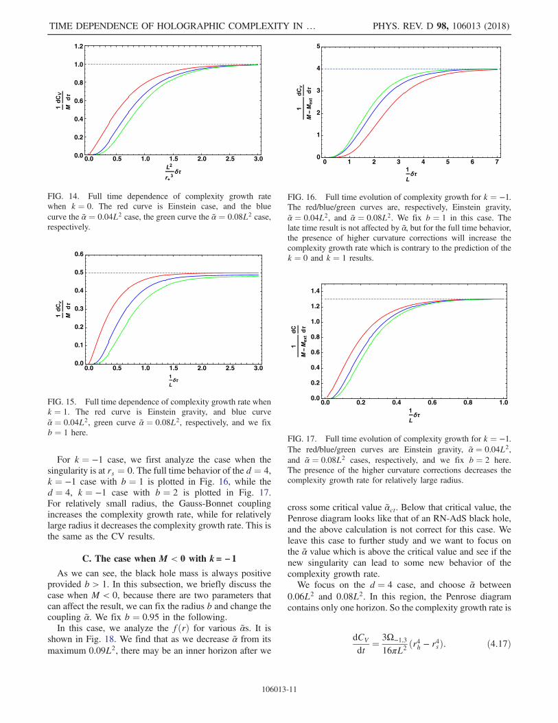
For k ¼ −1 case, we first analyze the case when thesingularity is at rs ¼ 0. The full time behavior of the d ¼ 4,k ¼ −1 case with b ¼ 1 is plotted in Fig. 16, while thed ¼ 4, k ¼ −1 case with b ¼ 2 is plotted in Fig. 17.For relatively small radius, the Gauss-Bonnet couplingincreases the complexity growth rate, while for relativelylarge radius it decreases the complexity growth rate. This isthe same as the CV results.

C. The case when M < 0 with k= − 1As we can see, the black hole mass is always positive

provided b > 1. In this subsection, we briefly discuss thecase when M < 0, because there are two parameters thatcan affect the result, we can fix the radius b and change thecoupling α. We fix b ¼ 0.95 in the following.In this case, we analyze the fðrÞ for various αs. It is

shown in Fig. 18. We find that as we decrease α from itsmaximum 0.09L2, there may be an inner horizon after we

cross some critical value αct. Below that critical value, thePenrose diagram looks like that of an RN-AdS black hole,and the above calculation is not correct for this case. Weleave this case to further study and we want to focus onthe α value which is above the critical value and see if thenew singularity can lead to some new behavior of thecomplexity growth rate.We focus on the d ¼ 4 case, and choose α between

0.06L2 and 0.08L2. In this region, the Penrose diagramcontains only one horizon. So the complexity growth rate is

dCV

dt¼ 3Ω−1;3

16πL2ðr4h − r4sÞ: ð4:17Þ

0.0 0.5 1.0 1.5 2.0 2.5 3.00.0

0.2

0.4

0.6

0.8

1.0

1.2

FIG. 14. Full time dependence of complexity growth ratewhen k ¼ 0. The red curve is Einstein case, and the bluecurve the α ¼ 0.04L2 case, the green curve the α ¼ 0.08L2 case,respectively.

0.0 0.5 1.0 1.5 2.0 2.5 3.00.0

0.1

0.2

0.3

0.4

0.5

0.6

FIG. 15. Full time dependence of complexity growth rate whenk ¼ 1. The red curve is Einstein gravity, and blue curveα ¼ 0.04L2, green curve α ¼ 0.08L2, respectively, and we fixb ¼ 1 here.

0 1 2 3 4 5 6 70

1

2

3

4

5

FIG. 16. Full time evolution of complexity growth for k ¼ −1.The red/blue/green curves are, respectively, Einstein gravity,α ¼ 0.04L2, and α ¼ 0.08L2. We fix b ¼ 1 in this case. Thelate time result is not affected by α, but for the full time behavior,the presence of higher curvature corrections will increase thecomplexity growth rate which is contrary to the prediction of thek ¼ 0 and k ¼ 1 results.

0.0 0.2 0.4 0.6 0.8 1.00.0

0.2

0.4

0.6

0.8

1.0

1.2

1.4

FIG. 17. Full time evolution of complexity growth for k ¼ −1.The red/blue/green curves are Einstein gravity, α ¼ 0.04L2,and α ¼ 0.08L2 cases, respectively, and we fix b ¼ 2 here.The presence of the higher curvature corrections decreases thecomplexity growth rate for relatively large radius.

TIME DEPENDENCE OF HOLOGRAPHIC COMPLEXITY IN … PHYS. REV. D 98, 106013 (2018)

106013-11

Using the mass expression in this case

M ¼ 3Ω−1;3r2h16π

�−1þ r2h

L2þ α

r2h

�ð4:18Þ

we get the analytic expression for the late time growth rate

1

M−Mext

dCV

dτ¼ 1

14þb4−b2

�b4 −

4ab2

1− 4a

�1−

ab2

−b2��

;

ð4:19Þ

and it is plotted in Fig. 19. We find that the late time result isdependent on the Gauss-Bonnet coupling α and moreoverthe late time result increases as the coupling increases,which is similar to the CV case.

V. THE GROWTH RATE OF COMPLEXITY INTHE GENERALIZED CV CONJECTURES

The calculations in this paper were done with theassumptions that the usual complexity-volume dualityholds in the Gauss-Bonnet case as in the Einstein case.But at this time, because of the lack of the concretederivation of the CV duality from field theory side, thisassumption may not be true and the volume may becorrected in the presence of higher curvature corrections.In Ref. [38], the authors propose two possible generaliza-tions of the volume in CV conjecture. The first is motivatedby the subregion complexity first proposed in Ref. [16].Because the complexity is defined to be the volumebetween the RT surface and the boundary, as the entangle-ment entropy is modified in the presence of the highercurvature corrections to match the Wald entropy [78,79],the author expected that the complexity should also bemodified accordingly as follows

CV1 ¼ −1

l

ZΣηEabcdϵabϵcd; ð5:1Þ

where Σ denotes the surface, η is its element volume, andEabcd is defined as

Eabcd ¼ ∂L∂Rabcd

−∇a1

∂L∂∇a1Rabcd

þ…

þ ð−1Þm∇ða1 � � �∇amÞ∂L

∂∇ða1 � � �∇amÞRabcd: ð5:2Þ

For a codimension one hypersurface, its normal vector uaand the vector normal to the constant radial coordinatesurface na form the bi-normal ϵab in the above expression.The other modification appears in Ref. [57] when they

investigated the “entanglement equilibrium” in the contextof higher order gravity theories, and some generalized formof volume is kept fixed when the entanglement entropy isvaried. For a codimension one maximal time slice, thecomplexity is dual to the following functionally,

CV2 ¼1

l

ZΣ½Eabcdðauaubhcd þ bhabhcdÞ þ c�η; ð5:3Þ

where the coefficients a, b and c are constants.In order to know whether these volume proposals are

suitable for describing complexity in Gauss-Bonnet gravity,we can calculate the complexity growth rate explicitly andtry to find whether it shows the expected physical proper-ties of complexity.For the Gauss-Bonnet gravity, the Lagrangian reads

L ¼ 1

16πGðR − 2Λþ αðR2 − 4RabRab þ RabcdRabcdÞÞ:

ð5:4Þ

0.060 0.065 0.070 0.075 0.080

4.975

4.980

4.985

4.990

4.995

5.000

5.005

FIG. 19. The late time complexity growth rate for k ¼ −1 andM < 0. In this case we fix b ¼ 0.95 and d ¼ 4, and we find thatin this case the Gauss-Bonnet coupling indeed increases thegrowth rate in this range of α.

0.0 0.2 0.4 0.6 0.8 1.0–1.0

–0.5

0.0

0.5

1.0

FIG. 18. The behavior of fðrÞ for various αs, where α is,respectively, 0.04L2, 0.05L2, 0.06L2, 0.07L2, 0.08L2 from up todown.

YU-SEN AN, RONG-GEN CAI, and YUXUAN PENG PHYS. REV. D 98, 106013 (2018)

106013-12

From this we have

16πGEabcd ¼�1

2þ αR

�2ga½cgd�b

− 4αðRa½cgd�b þ Rb½dgc�aÞ þ 2αRabcd: ð5:5Þ

To calculate the generalized volumes, we need the expres-sions of ua, na and the Riemann curvature. For the staticblack hole solution (2.2) in the Eddington coordinates,we assume that the unit normal ua has only two nonzerocomponents

ua ¼ ðuv; ur; 0;…; 0Þ ð5:6Þ

and so does na. These two vectors satisfy

−uaua ¼ nana ¼ 1; uana ¼ 0: ð5:7Þ

According to the metric (3.1), the vv; vr and rr compo-nents of the Ricci tensor are

Rvv ¼1

2ff00 þ ðd − 1Þ

2rff0Rrr ¼ 0; ð5:8Þ

Rvr ¼ −1

2f00 −

ðd − 1Þ2r

f0; ð5:9Þ

Rrr ¼ 0; ð5:10Þ

where “0 ” denotes the derivative with respect to r, and wecan see that for α; β ¼ v, r, we have the simple relation

Rαβ ¼ −1

2

�f00 þ ðd − 1Þ

rf0�gαβ: ð5:11Þ

Therefore, due to the normalization gabuaub ¼ −1, wehave

2Rabuaub ¼ f00 þ ðd − 1Þr

f0: ð5:12Þ

Applying the formulae in Ref. [80] the Ricci scalar is

R ¼ −f00 −2ðd − 1Þ

rf0 þ ðd − 1Þðd − 2Þ k − f

r2; ð5:13Þ

and meanwhile the v, r components of the Riemann tensorof the spacetime are just the same as those of the Riemanntensor of the v, r submanifold. Since this submanifold istwo-dimensional, there is only one nontrivial v, r compo-nent of the Riemann tensor. Therefore, for α, β, γ, δ ¼ v, r,

Rαβγδ ¼ −f00

2ðgαγgβδ − gαδgβγÞ: ð5:14Þ

Now we have all the materials to calculate the generalizedvolumes. In order for that when α ¼ 0 it reduces to theusual CV proposal, the generalized formula (5.1) turns outto be

CV1 ¼1

Gl

ZΣW1ðrÞη; ð5:15Þ

where

W1ðrÞ ¼ 1þ 2αRþ 4αRabðuaub − nanbÞ− 4αRabcduanbucnd

¼ 1þ 2αðd − 1Þðd − 2Þ k − fr2

; ð5:16Þ

for the specific static black hole. The second formula (5.3)gives

CV2 ¼1

Gl

ZΣW2ðrÞη; ð5:17Þ

where

W2ðrÞ ¼ a

�d2þ ðd − 2ÞαðRþ 2RabuaubÞ

�þ b

�dð1 − dÞ

2þ ðd − 2Þαðð3 − dÞRþ 4RabuaubÞ

�

¼ a

�d2þ αðd − 1Þðd − 2Þ

�−f0

rþ ðd − 2Þ k − f

r2

��

þ b

�dð1 − dÞ

2þ αðd − 2Þ

�ðd − 1Þf00 þ 2ðd − 1Þðd − 2Þf0

r− ðd − 1Þðd − 2Þðd − 3Þ k − f

r2

��

¼ 1þ αðd − 2Þ2d

�2ðd − 6Þðd − 2Þ k − fðrÞ

r2− ðdðdþ 5Þ − 16Þ f

0

r− ðdþ 4Þf00

�; ð5:18Þ

TIME DEPENDENCE OF HOLOGRAPHIC COMPLEXITY IN … PHYS. REV. D 98, 106013 (2018)

106013-13

where we set c ¼ 0 and normalized a and b according tothe analysis in [38]. The overall factor is fixed such that theexpression goes back to unity when α ¼ 0.For the static black hole the two generalized proposals

can be written in a unified form

CV ¼ Ωk;d−1

Gl

Zdλrd−1

ffiffiffiffiffiffiffiffiffiffiffiffiffiffiffiffiffiffiffiffiffiffiffiffiffiffiffiffiffiffi−fðrÞ_v2 þ 2_v _r

qWðrÞ: ð5:19Þ

By repeating a similar procedure as in Sec. III A, we findthe growth rate of the generalized holographic complexityto be

dCV

dτ¼ Ωk;d−1

GL

ffiffiffiffiffiffiffiffiffiffiffiffiffiffiffiffiffiffi−fðrminÞ

prd−1min jWðrminÞj: ð5:20Þ

Calculations for a five-dimensional static black hole withk ¼ 0 are performed for physically allowed α range, andthe results show that for the first proposal (5.1), the late-time complexity growth rate exceeds that of the Einsteingravity for a positive Gauss-Bonnet parameter. So thisproposal is not favorable, since one should see a decrease inthe complexity growth rate compared to Einstein gravity.The late-time complexity growth rate for the second proposal(5.3) for small Gauss-Bonnet parameters decreases drasti-cally as the Gauss-Bonnet parameter increases. It seems thatthis proposal is better than the first one (5.1) in this respect.It may be interesting to investigate other aspects of thisproposal to see whether it is an appropriate generalization,and we leave it to the future work. These results for bothproposals are shown in Fig. 20.We should note that the generalized volumes are just

conjectures without derivation and very strong implica-tions, unlike the case of holographic entanglemententropy. It is also interesting to find other forms ofgeneralized volumes from other physical directions. Itis also possible that we should stick to the volume of theextremal surface, since as far as the complexity growth

behavior is concerned, the “complexity-volume” conjec-ture shows rather good behavior.

VI. CONCLUSION AND DISCUSSION

A. Summary of our results

In this work we studied the holographic complexity ofAdS black holes in Einstein-Gauss-Bonnet gravity theoryin the context of the “complexity-volume” (CV) and theCV2.0 conjectures. Our results include the time depend-ence of the complexity growth rate dCV=dτ of neutral blackholes with different Gauss-Bonnet couplings and differenthorizon curvatures (k ¼ 0, 1 and k ¼ −1), and of chargedplanar black holes with different charge values. Our resultsare shown in five dimensions by numerical graphs exceptthat for the planar horizon case we obtained an analyticexpression for the late time complexity growth rate ingeneral dimensions. We also investigated two proposals ofgeneralized volumes dual to the complexity [38,57] in thepresence of higher curvature corrections. We find thatcomplexity growth rate for these two proposals behavesrather different and we find the proposal in [57] is better.However, we should note that we need further evidence forus to trust the proposal in Ref. [57].For all the cases we investigated, dCV=dτ increases

monotonically as time goes on, and approaches a certainconstant from below at late times. This is also the case inEinstein gravity [51]. The monotonic growth of dCV=dτin both gravity theories implies that the “complexityequals volume” conjecture is more favorable than the“complexity–action” (CA) conjecture in the sense of theLloyd’s bound.Our results found by using the CV conjecture also

indicate that except for small Gauss-Bonnet AdS blackholes with hyperbolic horizons, the growth rate can belarger than that in Einstein gravity. To be more specific, wefind that when k ¼ −1 and rh=L is large, or when k ¼ 0, 1we always have that

d − 1

8πðM −MextÞdCV

dτ

����EGB

<d − 1

8πðM −MextÞdCV

dτ

����Einstein

;

ð6:1Þ

which is expected. However, when k ¼ −1 and rh=L issmall, one may have

d − 1

8πðM −MextÞdCV

dτ

����EGB

>d − 1

8πðM −MextÞdCV

dτ

����Einstein

:

ð6:2Þ

As for the CV2.0 proposal, for the k ¼ 0 case, while thelate time result is the same as in the Einstein gravity, thehigher curvature corrections decrease the growth rate whenthe time is not too late. For the k ¼ 1 case, the higher order

0.00 0.02 0.04 0.06 0.080.0

0.5

1.0

1.5

2.0

FIG. 20. The late-time growth rate of the two generalizedvolume proposals for a five-dimensional static black hole withk ¼ 0. The blue curve corresponds to the first one (5.1) and theorange curve shows the second one (5.3).

YU-SEN AN, RONG-GEN CAI, and YUXUAN PENG PHYS. REV. D 98, 106013 (2018)

106013-14

corrections decrease the growth rate both at late times andin full time. In the k ¼ −1 case, we should distinguish thecase between theM > 0 case andM < 0 case. For theM > 0case, we find that the higher curvature corrections decreasethe complexity growth rate for relatively large black holes,while increase the growth rate for relatively small blackholes. And the late time limit is independent of α. However,in the M < 0 case, the complexity growth rate is enhancedeven in the late time limit.According to the AdS/CFT correspondence, higher cur-

vature terms in the bulk correspond to the large N or largecoupling constant corrections in the dual boundary fieldtheory. For example, in the AdS5=CFT4 case of the type IIBstring theory, the terms with R4 order in the bulk give thecorrection with the ’t Hooft coupling λ−3=2 in the boundaryfield theory [81]. It is expected that with those corrections inthe bulk and boundary, one is able to make a comparison ofcalculations from the bulk and the boundary. In this work wehave considered the effect of the Gauss-Bonnet term in thebulk. On one hand, the Gauss-Bonnet gravity is a naturalextension of Einstein gravity in high-dimensional spacetime,one can have an analytical black hole solution in the Gauss-Bonnet gravity and the vacuum of the theory is stable and thetheory has no ghost [67,73]. On the other hand, the Gauss-Bonnet term is a low energy correction term in the heteroticstring theory. Therefore, considering the effect of the Gauss-Bonnet term is of some interest not only in its own right inthe sense of gravity theory itself, but also in checking theAdS/CFT correspondence and/or in understanding the prop-erties of strong coupling field theory with the AdS/CFTcorrespondence. Our study in this paper shows that for thecases with k ¼ 0 and k ¼ 1, the Gauss-Bonnet term alwayssuppresses the complexity growth rate for both the late timelimit and the full time evolution cases. This conclusionagrees with the one from the CA conjecture [31], and it isalso expected from the field theory side considering theGauss-Bonnet term as some correction of large N expansion[81]. In particular, it is speculated that stringy correctionsshould reduce the complexity growth rate of the AdS blackhole solutions [15].

On the other hand, the enhancement we find in the k ¼ −1case is opposite to what is expected. This unexpectedbehavior makes us recall the fact that the boundary fieldtheory in a hyperbolic space is not well-behaved, as arguedin [82]. Therefore, this unexpected behavior might not betrustworthy.We note that it is still necessary to investigate the

complexity growth rate in the very weak coupling casefrom field theory side to complete the whole analysis.

B. Comparison to the CA result

It would be helpful to compare our results with thoseobtained by using the CA conjecture. The growth rate in thecontext of CA conjecture for a spherical black hole in EGBgravity with d ¼ 4 is [31]

limτ→∞

π

2MdCA

dτ¼�1 −

3αΩ1;4

16πGM

�: ð6:3Þ

As our results, this growth rate also contains a suppressioncompared to that in Einstein gravity. Recent studies on thenull boundary action term in Lovelock gravity [64,65]give a more general result. Nevertheless, the suppressionappearing in this expression is different from our result.This suppression only appears when d is even and k ≠ 0[65]. In our CV results, the suppression appears for all threevalues of k, and it appears for any d. Besides, we do nothave such an analytic expression as (6.3) for k ¼ 1 case inthe CV conjecture. Moreover, under the large black holelimit, the correction term −3αΩ1;4=ð16πGMÞ vanishes,which means that the effect of the corrections will dis-appear for large black holes. In our late time results in theCV conjecture, however, the effect of α becomes the sameas in the case of k ¼ 0 under the limit rh=L → ∞ and thiseffect is always finite. The suppression from the Gauss-Bonnet coupling appears in both cases while there arecurious differences between these cases—the suppressionseems to be more universal in the CV conjecture. Suchinvestigation may help judge which holographic proposalcaptures the essential features of complexity. We can give asummary of the result in Table I.

TABLE I. Effect of higher curvature corrections in various proposals.

CV CV2.0 CA

Late time k ¼ 0 Decrease Unchanged Unchangedk ¼ 1 Decrease Decrease Decrease for even d,

unchanged for odd dk ¼ −1 Decrease for large radius,

increase for small radiusUnchanged for M > 0 (d ¼ 4) Decrease for even d,

unchanged for odd d

Full time k ¼ 0 Decrease Decrease Unknownk ¼ 1 Decrease Decreasek ¼ −1 Decrease for large radius,

increase for small radiusDecrease for large radius,increase for small radius (M > 0)

TIME DEPENDENCE OF HOLOGRAPHIC COMPLEXITY IN … PHYS. REV. D 98, 106013 (2018)

106013-15

C. Choice of boundary time coordinateand future directions

In the above discussion, we have not considered what theboundary time should be in the presence of the Gauss-Bonnet coupling. Take the black brane as an example. Wenote that under the limit r → ∞, in order to set the speedof light on the boundary equal to 1 [68,83], we should shiftthe time coordinate t → t0 according to t ¼ Nt0, where

N ¼ffiffiffiffiffiffiffiffiffiffiffiffiffiffiffiffiffiffiffiffiffiffiffiffiffiffiffiffiffiffiffiffiffiffiffiffiffiffiffiffiffiffiffi1

2

�1þ

ffiffiffiffiffiffiffiffiffiffiffiffiffiffiffiffiffiffiffiffiffi1 − 4α=L2

q r: ð6:4Þ

Physically, we should use t0 to be the boundary time andcompute the boundary complexity growth rate

dCdt0

¼ NdCdt

: ð6:5Þ

Since N < 1 so the complexity growth rate should decreasemore. This decrease is naturally expected because of thefollowing reason.In Ref. [83], the authors investigated the localized shocks

and the Gauss-Bonnet coupling’s effect on the butterflyvelocity. In fact, that paper showed that for two spaceseparated perturbations VxðtÞ and Wyð0Þ, the commutatorbetween them takes the form

−h½VxðtÞ;Wyð0Þ�2i ¼1

N2e2πβ ðt−jx−yj=vBÞ ð6:6Þ

which gives a natural light cone of scrambling in terms ofthe butterfly velocity vB satisfying

vB ¼ 2π

βμ; μ ¼

ffiffiffiffiffiffiffiffiffiffiffiffiffiffiffiffiffiffiffiffiffiffidðd − 1Þ=2

p: ð6:7Þ

Although the scrambling time and butterfly velocity takethe same form in the Gauss-Bonnet case as in Einsteingravity, a constant scaling of the time coordinates which setthe speed of light on the boundary changes the value of β.So the butterfly velocity is decreased in the presence of theGauss-Bonnet coupling to the value

vB ¼ 1

2

ffiffiffiffiffiffiffiffiffiffiffiffiffiffiffiffiffiffiffiffiffiffiffiffiffiffiffiffiffiffiffiffiffiffi1þ

ffiffiffiffiffiffiffiffiffiffiffiffiffiffiffiffiffiffiffiffiffi1 − 4α=L2

qr ffiffiffiffiffiffiffiffiffiffiffid

d − 1

rð6:8Þ

while the result in Einstein gravity is vB ¼ ffiffiffiffiffiffiffiffiffiffiffiffiffiffiffiffiffiffiffiffiffiffiffiffiffiffid=ð2ðd − 1ÞÞp

.This is the same behavior as we found for the complexitygrowth, and is natural because complexity growth and

chaos are closely related. More concretely, using the tensornetwork picture in [15], smaller vB means smaller rate ofgrowth of complexity of the precursor operator.Finally let us talk about future directions. Firstly, we

have only studied the effect of the Gauss-Bonnet term to thecomplexity growth rate, since the single parameter makesthe problem clear and simple. It might be straightforward todo the same calculations in more general higher curvatureor higher derivative gravity theories, e.g., the Lovelockgravity theory.Secondly, it is tempting to compare the time dependence

of the complexity in both the CV and CA methods, as thepapers [51,52] did, in the presence of higher curvature orhigher derivative terms. However, we are still not able toanswer what the full time behavior of the complexity willbe for the higher curvature gravity theories in the context ofthe CA conjecture, since the contribution of the action onthe null boundaries of the Wheeler-DeWitt patch is yetunknown, although some progress has been made toidentify the contribution of the joints connecting twoboundary sections of the Wheeler-DeWitt patch in thepaper [64] for Lovelock gravity. The first step is to obtainproper boundary action for these theories, which is animportant and challenging work.Moreover, how to interpret the effect of higher curvature

corrections on the complexity growth is still interesting.An initial attempt of understanding the relation betweenthe butterfly velocity and complexity had been made inRef. [84]. But as we showed in the main body of this paper,even we do not take into account the effect of the slowingdown of scrambling in the black brane case (the effect ofrescaling the boundary time), the complexity growth rate isstill decreased. So the complexity growth and scramblingmay not slow down due to the same reason.

ACKNOWLEDGMENTS

We thank Li-Ming Cao and Run-Qiu Yang for valuablesuggestions and discussions. This work is supported in partby the National Natural Science Foundation of ChinaGrants No. 11690022, No. 11435006, No. 11447601,and No. 11647601, the Strategic Priority ResearchProgram of Chinese Academy of Science (CAS) GrantNo. XDB23030100, the Peng Huanwu InnovationResearch Center for Theoretical Physics GrantNo. 11747601, and the Key Research Program ofFrontier Sciences of Chinese Academy of Science. Y. P.is supported in part by the National Postdoctoral Programfor Innovative Talents Grant No. Y7Y2351B11.

YU-SEN AN, RONG-GEN CAI, and YUXUAN PENG PHYS. REV. D 98, 106013 (2018)

106013-16

[1] J. M. Maldacena, Adv. Theor. Math. Phys. 2, 231 (1998).[2] S. S. Gubser, I. R. Klebanov, and A. M. Polyakov, Phys.

Lett. B 428, 105 (1998).[3] E. Witten, Adv. Theor. Math. Phys. 2, 253 (1998).[4] O. Aharony, S. S. Gubser, J. M. Maldacena, H. Ooguri, and

Y. Oz, Phys. Rep. 323, 183 (2000).[5] G. ’t Hooft, Conf. Proc. C 930308, 284 (1993).[6] L. Susskind, J. Math. Phys. (N.Y.) 36, 6377 (1995).[7] S. Ryu and T. Takayanagi, Phys. Rev. Lett. 96, 181602

(2006).[8] N. Lashkari, M. B. McDermott, and M. Van Raamsdonk,

J. High Energy Phys. 04 (2014) 195.[9] T. Faulkner, M. Guica, T. Hartman, R. C. Myers, and M.

Van Raamsdonk, J. High Energy Phys. 03 (2014) 051.[10] B. Swingle and M. Van Raamsdonk, arXiv:1405.2933.[11] D. Stanford and L. Susskind, Phys. Rev. D 90, 126007

(2014).[12] J. M. Maldacena, J. High Energy Phys. 04 (2003) 021.[13] M. Miyaji, T. Numasawa, N. Shiba, T. Takayanagi, and K.

Watanabe, Phys. Rev. Lett. 115, 261602 (2015).[14] A. R. Brown, D. A. Roberts, L. Susskind, B. Swingle, and Y.

Zhao, Phys. Rev. Lett. 116, 191301 (2016).[15] A. R. Brown, D. A. Roberts, L. Susskind, B. Swingle, and Y.

Zhao, Phys. Rev. D 93, 086006 (2016).[16] M. Alishahiha, Phys. Rev. D 92, 126009 (2015).[17] O. Ben-Ami and D. Carmi, J. High Energy Phys. 11 (2016)

129.[18] S. Chapman, H. Marrochio, and R. C. Myers, J. High

Energy Phys. 01 (2017) 062.[19] D. Carmi, R. C. Myers, and P. Rath, J. High Energy Phys. 03

(2017) 118.[20] R. Q. Yang, C. Niu, and K. Y. Kim, J. High Energy Phys. 09

(2017) 042.[21] W. C. Gan and F.W. Shu, Phys. Rev. D 96, 026008 (2017).[22] R. Jefferson and R. C. Myers, J. High Energy Phys. 10

(2017) 107.[23] S. Chapman, M. P. Heller, H. Marrochio, and F. Pastawski,

Phys. Rev. Lett. 120, 121602 (2018).[24] R. Q. Yang, Phys. Rev. D 97, 066004 (2018).[25] R. Khan, C. Krishnan, and S. Sharma, arXiv:1801.07620.[26] R. Q. Yang, Y. S. An, C. Niu, C. Y. Zhang, and K. Y. Kim,

arXiv:1803.01797.[27] L. Hackl and R. C. Myers, arXiv:1803.10638.[28] J. Jiang, J. Shan, and J. Yang, arXiv:1810.00537.[29] M. Sinamuli and R. B. Mann, Phys. Rev. D 98, 026005

(2018).[30] S. Lloyd, Nature (London) 406, 1047 (2000).[31] R. G. Cai, S. M. Ruan, S. J. Wang, R. Q. Yang, and R. H.

Peng, J. High Energy Phys. 09 (2016) 161.[32] R. Q. Yang, Phys. Rev. D 95, 086017 (2017).[33] H. Huang, X. H. Feng, and H. Lu, Phys. Lett. B 769, 357

(2017).[34] R. G. Cai, M. Sasaki, and S. J. Wang, Phys. Rev. D 95,

124002 (2017).[35] X. H. Ge and B. Wang, J. Cosmol. Astropart. Phys. 02

(2018) 047.[36] D. Momeni, M. Faizal, S. Bahamonde, and R. Myrzakulov,

Phys. Lett. B 762, 276 (2016).[37] W. J. Pan and Y. C. Huang, Phys. Rev. D 95, 126013 (2017).

[38] M. Alishahiha, A. Faraji Astaneh, A. Naseh, and M. H.Vahidinia, J. High Energy Phys. 05 (2017) 009.

[39] P. Wang, H. Yang, and S. Ying, Phys. Rev. D 96, 046007(2017).

[40] W. D. Guo, S. W. Wei, Y. Y. Li, and Y. X. Liu, Eur. Phys. J.C 77, 904 (2017).

[41] Y. G. Miao and L. Zhao, Phys. Rev. D 97, 024035 (2018).[42] M. Ghodrati, Phys. Rev. D 96, 106020 (2017).[43] M.M. Qaemmaqami, Phys. Rev. D 97, 026006 (2018).[44] L. Sebastiani, L. Vanzo, and S. Zerbini, Phys. Rev. D 97,

044009 (2018).[45] M. Moosa, J. High Energy Phys. 03 (2018) 031.[46] M. Moosa, Phys. Rev. D 97, 106016 (2018).[47] L. P. Du, S. F. Wu, and H. B. Zeng, Phys. Rev. D 98, 066005

(2018).[48] S. Chapman, H. Marrochio, and R. C. Myers, J. High

Energy Phys. 06 (2018) 046.[49] R. Auzzi, S. Baiguera, and G. Nardelli, J. High Energy

Phys. 06 (2018) 063.[50] J. Jiang, arXiv:1810.00758.[51] D. Carmi, S. Chapman, H. Marrochio, R. C. Myers, and S.

Sugishita, J. High Energy Phys. 11 (2017) 188.[52] R. Q. Yang, C. Niu, C. Y. Zhang, and K. Y. Kim, J. High

Energy Phys. 02 (2018) 082.[53] Y. S. An and R. H. Peng, Phys. Rev. D 97, 066022 (2018).[54] B. Swingle and Y. Wang, J. High Energy Phys. 09 (2018)

106.[55] M. Alishahiha, A. Faraji Astaneh, M. R. Mohammadi

Mozaffar, and A. Mollabashi, J. High Energy Phys. 07(2018) 042.

[56] J. Couch, W. Fischler, and P. H. Nguyen, J. High EnergyPhys. 03 (2017) 119.

[57] P. Bueno, V. S. Min, A. J. Speranza, and M. R. Visser, Phys.Rev. D 95, 046003 (2017).

[58] R. Abt, J. Erdmenger, H. Hinrichsen, C. M. Melby-Thompson, R. Meyer, C. Northe, and I. A. Reyes, Fortschr.Phys. 66, 1800034 (2018).

[59] Z. Y. Fan and M. Guo, J. High Energy Phys. 08 (2018) 031.[60] D. Lovelock, J. Math. Phys. (N.Y.) 12, 498 (1971).[61] D. J. Gross and E. Witten, Nucl. Phys. B277, 1 (1986).[62] B. Zumino, Phys. Rep. 137, 109 (1986).[63] L. Lehner, R. C. Myers, E. Poisson, and R. D. Sorkin, Phys.

Rev. D 94, 084046 (2016).[64] P. A. Cano, Phys. Rev. D 97, 104048 (2018).[65] P. A. Cano, R. A. Hennigar, and H. Marrochio, Phys. Rev.

Lett. 121, 121602 (2018).[66] S. Chakraborty and K. Parattu, arXiv:1806.08823.[67] D. G. Boulware and S. Deser, Phys. Rev. Lett. 55, 2656

(1985).[68] M. Brigante, H. Liu, R. C. Myers, S. Shenker, and S. Yaida,

Phys. Rev. D 77, 126006 (2008).[69] M. Brigante, H. Liu, R. C. Myers, S. Shenker, and S. Yaida,

Phys. Rev. Lett. 100, 191601 (2008).[70] A. Buchel and R. C. Myers, J. High Energy Phys. 08 (2009)

016.[71] D. M. Hofman, Nucl. Phys. B823, 174 (2009).[72] T. Torii and H. Maeda, Phys. Rev. D 72, 064007 (2005).[73] R. G. Cai, Phys. Rev. D 65, 084014 (2002).[74] D. L. Wiltshire, Phys. Lett. B 169B, 36 (1986).

TIME DEPENDENCE OF HOLOGRAPHIC COMPLEXITY IN … PHYS. REV. D 98, 106013 (2018)

106013-17

[75] R. G. Cai, L. M. Cao, L. Li, and R. Q. Yang, J. High EnergyPhys. 09 (2013) 005.

[76] P.Hayden and J. Preskill, J. HighEnergyPhys. 09 (2007) 120.[77] L. Susskind, Fortschr. Phys. 64, 24 (2016); Addendum 64,

44 (2016).[78] R. M. Wald, Phys. Rev. D 48, R3427 (1993).[79] V. Iyer and R. M. Wald, Phys. Rev. D 50, 846 (1994).[80] R. G. Cai and L. M. Cao, Phys. Rev. D 88, 084047 (2013).

[81] S. S. Gubser, I. R. Klebanov, and A. A. Tseytlin, Nucl. Phys.B534, 202 (1998).

[82] E. Witten and S. T. Yau, Adv. Theor. Math. Phys. 3, 1635(1999).

[83] D. A. Roberts, D. Stanford, and L. Susskind, J. High EnergyPhys. 03 (2015) 051.

[84] S. A. Hosseini Mansoori and M.M. Qaemmaqami, arXiv:1711.09749.

YU-SEN AN, RONG-GEN CAI, and YUXUAN PENG PHYS. REV. D 98, 106013 (2018)

106013-18