A Short Introduction to GAUSS for Windows - CiteSeerX

A Short Introduction to GAUSS for WindowsRuud H. Koning

A Short Introduction to GAUSS for Windows

Ruud H. Koning

Second, corrected printing November 1999c© 1999, Ruud H. Koning.All rights reserved. No part of this publication may be reproduced, storedin a retrieval system, or transmitted, in any form or by any means,electronic, mechanical, photocopying, recording, or otherwise, without theprior written permission of the author.ISBN 90-804955-1-4

Contents

1 Introduction 1

2 Installing and Configuring GAUSS 3

3 Data Types and Operators 13

4 GAUSS Programs and Procedures 214.1 Gauss Programs 214.2 GAUSS Procedures 24

5 Libraries 33

6 File Input/Output 37

7 Maximum Likelihood Estimation 43

8 Graphics 538.1 Creating Graphics in GAUSS 538.2 Incorporating GAUSS Graphics in Text Documents 58

8.2.1 GAUSS Graphics in Microsoft Word Documents 588.2.2 GAUSS Graphics in LATEX2e Documents 60

9 Two Examples 639.1 A Kernel Estimation Library 639.2 Finite Sample Properties of the ML-estimator in Tobit Model 71

10 Exercises 75

A Converting ASCII to GAUSS datasets 81

B GAUSS Libraries 85

C Program Code 87

Index 88

Chapter 1

Introduction

During the last decade, powerful desktop computers have become avail-able to most researchers. Mainframe computers have been replaced bypersonal computers and user friendly numerical programs have replacedold FORTRAN compilers and punch cards. As far as applications are con-cerned, there is a trend from writing a program for each problem to theuse of professional software like statistical programs (SPSS, SAS), spread-sheet programs (Excel, Quattro), and matrix programming languages (Mat-Lab, GAUSS). Using a matrix programming language is attractive comparedto programming in a language like C++ or Pascal because the user doesnot have to implement the datatype ‘matrix of numbers’. Moreover, manyconvenient functions are available and this makes writing programs easier.In this booklet we focus on one particular matrix programming language:GAUSS. The GAUSS-programming environment does not create stand-aloneexecutables. Instead, a GAUSS program is compiled to pseudo-code and thispseudo-code is interpreted by the GAUSS interpreter.

GAUSS is available for different platforms. It was developed originallyfor MSDOS-based computers, and it has been ported to UNIX during thelast few years. In this book we discuss the Windows-version of GAUSS1.This version is a 32-bits program that runs under Windows95, Windows98,and Windows NT. The development of this program is still ongoing, but theWindows version (3.35) that is available at the time of writing of this bookis sufficiently developed. Most commands and examples will also run onthe other platforms.

GAUSS is a convenient matrix programming language for doing econo-metric research. It is somewhat less suitable as a data management pro-gram, statistical programs such as SPSS or SAS are more suited to that task.A major advantage of GAUSS to programming languages is the availability

1All examples and graphs in this book were made using version 3.2.35.

1

of libraries for specific tasks and the availability of many built-in functionsuseful to econometricians. One library especially useful to econometriciansis the maximum likelihood library that can be used for optimization of log-likelihood functions. A complete list of all libraries is given in Appendix B.Apart from the commercial libraries, one can also find program code andcomplete libraries on the internet. Moreover, most authors of scientific pa-pers are willing to share their code.

There is some GAUSS support on the internet. First of all, there is theGAUSS mailing list (subscribe by sending an email2 with contents sub-scribe gaussians to [email protected]) which is archived insearchable html-format at www.rhkoning.com/gauss and at gopher://eco.utexas.edu/11/mailing. GAUSS source code may be found at theGAUSS software archive at the American University http://gurukul.ucc.american.edu/econ/gaussres/GAUSSIDX.HTM. This page provides manylinks to other internet pages where code can be found. The developers ofGAUSS (Aptech Systems Inc.) provide some support by mail, they can bereached at [email protected]. Information on libraries and new productscan be obtained from their WWW-site at www.aptech.com.

In this booklet we give a short introduction to GAUSS. Two things shouldbe kept in mind. First of all, this booklet is no substitute for the completeGAUSS manual but we hope that the reader is able to use the latter moreefficiently after reading this one. Many more commands and proceduresthan the ones discussed in these notes are available. Second, the only wayto become proficient in a computer language is by making lots of errors.We recommend doing the exercises and following the examples through-out this book. The setup of this introduction is as follows. In chapter 2we discuss configuring GAUSS. Data types and operators are discussed inchapter 3 and how to write programs and procedures in chapter 4. We dealbriefly with writing GAUSS libraries in chapter 5. File handling is treatedin chapter 6. The optional GAUSS module maxlik is treated in chapter 7.It is possible to make publication quality graphics in GAUSS, this topic isdealt with in chapter 8. Two more elaborate examples of GAUSS-code canbe found in chapter 9. Exercises are given in chapter 10.

Stefan Steinhaus provided useful comments on the first printing. Read-ers of this introduction are kindly asked to report errors, omissions, andother comments to the author who can be reached by email at [email protected]. Sample code can be obtained from the web pagewww.rhkoning.com/gauss.

2Note that the email-software that registers subscriptions and cancellations does not ac-cept emails in HTML-format. Hence any such option in the email program of the user tryingto subscribe should be disabled when sending mail to the majordomo-software.

2

www.rhkoning.com/gauss

gurukul.ucc.american.edu/econ/gaussres/GAUSSIDX.HTM

gurukul.ucc.american.edu/econ/gaussres/GAUSSIDX.HTM

www.aptech.com

www.rhkoning.com/gauss

Chapter 2

Installing and Configuring GAUSS

In this chapter we discuss installing and configuring GAUSS for Windows.GAUSS runs on 386 (or better) computers with a mathematical coproces-sor, using Windows95, Windows98, or Windows NT as operating system.GAUSS requires approximately 7Mb of harddisk space and it will run com-fortably on a Pentium computer with at least 32Mb of RAM. Memory man-agement is taken care of by the operating system, but of course, GAUSS willbe faster if programs can be executed in RAM memory and disk swappingis avoided. The harddisk requirements increase if the user writes programsand libraries himself, or if one processes large data sets with GAUSS.

GAUSS is shipped on four 3.5” diskettes, each containing one file. Thefiles are called setup.exe, disk1.bnd, disk2.bnd, and disk3.bnd. Theprogram is best installed by copying these files into a temporary directoryon the harddisk and then by starting the program setup.exe. During theinstallation process the user has to enter the name name of the user andthe organization, and the folder where GAUSS is to be installed. The instal-lation program suggests installation in c:\gauss. From now on we assumethat GAUSS has been installed in that directory. Note that GAUSS does notaccept long filenames, so the installation folder should have a directoryname of 8 characters at the most. Then one can select a windows group forthe GAUSS icons and finally the program is installed. During the installationprocess a shortcut to the main program is put on the windows desktop.

A second program that needs to be installed is PlayW. This programis needed for conversion of graphs and can be downloaded free of chargefrom www.aptech.com. Again the user has to enter name and organization,and the installation program suggests to install PlayW in c:\gauss. Theicons will be placed in the same group as the GAUSS icons. After installationthe user needs to log off and to log on again so that the conversion programworks.

3

Finally some optional libraries may be installed. These libraries can bebought as add-ons to GAUSS, usually they are not shipped with the mainGAUSS program. Usually the diskettes with the library have three directo-ries: \src, \lib, and \examples. The library is installed by copying thefiles of these directories to the corresponding subdirectories of c:\gauss.

The windows helpfile of the main GAUSS program is by default storedin c:\windows\system32. This may cause difficulties in accessing the helpfile from within the GAUSS program. Often, these problems can be solvedby moving the helpfile to the directory where GAUSS is installed.

GAUSS itself is started by clicking on the GAUSS-icon that is put on thedesktop during the installation. Of course, the program can be started aswell by clicking on the file gauss.exe in the explorer, or by accessing itfrom the windows Start/Programs/Gauss menu. During startup, the pro-gram configures itself according to settings in the file gauss.cfg that canbe found in the directory where the program is installed. This configurationfile can be edited by the user. In this configuration file some variables areset that determine the behaviour of GAUSS. There is no graphical interfaceto this configuration file. The most important variables that need be setare the path where GAUSS looks for procedures (src_path), a variable thatdetermines the smoothness of screen output (fastio), and a variable thatdetermines the maximum width of matrices that are printe in the main win-dow (matwidth). Another important variable is max_workspace. This vari-able gives the amount of workspace of a GAUSS session in Mb. The value ofthis variable should be increased if the user encounters ‘out of workspace’error messages. Other switches and variables determine paths where dataare stored and read and the behaviour of the compilation process. For anew GAUSS user the default values can be retained, except perhaps thefour variables mentioned. During startup, GAUSS looks for a program filestartup (no extension) in the main GAUSS directory. This program file maycontain any valid GAUSS commands and these commands are executed dur-ing startup. An example of a startup file is

/* GAUSS startup file */chdir c:\gauss\prog;library dutil, maxlik;

After executing the startup file, the command window opens and the pro-gram gives a command prompt (gauss). The program is now ready to exe-cute commands enetered by the user. The screen immediately after startupis shown in figure 2.1.

GAUSS can be run in command mode or in edit mode. A GAUSS-sessionis automatically started in command mode, with the command prompt

4

Figure 2.1: GAUSS screen after starting up

(gauss). In command mode, commands are executed immediately afterthe <Enter> key is hit. An example of a simple statement in commandmode is

>>x=rndn(20,2);y=vcx(x);print y;

which is executed by pressing <Enter> after the last semicolon. This lineconsists of three GAUSS commands, separated by semicolons. All GAUSSstatements (both in command mode and edit mode) are separated by semi-colons. After pressing <Enter> the commands are compiled and executed.An example of statements entered in command mode and their output isgiven in figure 2.2. Even though GAUSS is a windows program, it sometimesbehaves differently frommost windows programs. There is no functionalityattached to the right mouse button. Moreover, it is not possible to put thecursor at a GAUSS statement somewhere in the command window and haveit executed by hitting <Enter>. It is possible though copy previous GAUSSstatements by selecting them using the left mouse button, and copyingthem to the windows clipboard using <ctrl><c>. The statements copied inthe clipboard can be pasted at the last command prompt with <ctrl><v>.

5

Figure 2.2: GAUSS command window

Only commands at the last GAUSS prompt will be executed if the user hitsthe <Enter> key.

In edit mode, GAUSS commands are typed in a file and they can bestored for later use. The edit mode is started either by entering the com-mand edit program1.prg at the GAUSS command prompt in commandmode, or by opening the file from the file menu (file/edit). The file is createdif it does not exist in the current working directory if one uses the secondmethod. It is not possible to create a file by entering edit program1.prgat the command prompt. The current working directory can be changed bythe command chdir c:\gauss\prog\book in command mode, or by thefunction changedir(s) (with s a string with the new directory) in a pro-gram. The current working directory is shown by the command cdir(0).The edit window is shown in the top half of figure 2.3.

The edit window has four buttons and two lines on top. The file name(with the complete path) of the file that is being edited is shown in thesecond line. The first line shows the name of the file that will be run if the

6

<ctrl><left> left one word <ctrl><right> right one word<ctrl><home> begin of text buffer <ctrl><right> end of text buffer<home><home> beginning of line <end><end> end of screen<F5> find text <shift><F5> find again<F6> replace text <shift><F6> replace again<ctrl><g> goto line <F1> on-line help<F2> save file <F3> run file<shift><F3> run current edited file <F4> edit file in edit-line<ctrl><F4> edit output file

Table 2.1: Command and edit mode keys

button Run is clicked. The file that is edited is copied to the run-list by click-ing the arrow on the left-side of the run-list. The filename that is displayedin the first line is copied to the second line by clicking the arrow on theleft-side of the edit-list. All files in the run-list and edit-list are displayed byclicking the arrow-down on the right side of these lines. The file in the editwindow is saved by clicking the Save button.

After entering the GAUSS commands as in the top half of figure 2.3, theprogram can be run. The file name is copied to the run list by clicking thearrow to the left of the run list. The program is run by clicking the Runbutton, and the output is displayed in the GAUSS command window as inthe lower half of figure 2.3. After running this program, the user can eithercontinue by giving interactive GAUSS commands in the command window,or he the user can change the program in the edit window. If one wants toedit the program, the Edit button in the command window can be clicked.This gives focus to the edit window. Of course, the program can be runagain by clicking the Run button in either the command window or the editwindow.

Some important keystrokes in command- and edit-mode are given intable 2.1. Some of these keystrokes are not applicable when in commandmode. When the user hits a key in command mode while running a pro-gram, the key that is pressed is handled as interactive input to the program.Online help is available in two different ways. Help can be obtained usingthe GAUSS help file, but also using the browser. The latter is convenient forsearching help on commands that are not standard GAUSS commands, butcommands provided by libraries or user defined procedures. The GAUSShelp file is opened by Help/Contents or by <F1> in either command oredit mode. The help index is displayed in figure 2.4.

Alternatively, help can be obtained using the browser. Since the user orthird parties can add functionality to GAUSS, it is important that the helpsystem can be extended as well. Help on added functionality can be ob-

7

Figure 2.3: GAUSS edit window (top) and command window (bottom)

8

Figure 2.4: GAUSS help file

9

Figure 2.5: GAUSS help browser

tained using the browser. The browser is started by File/Browse. A searchtopic can be filled in next to Topic:, and the browser looks for more in-formation after clicking Lookup. Whenever the information on a particularprocedure or command is found, the file defining that procedure is openedin the lower panel of the browser window, see figure 2.5. In case the in-formation on the topic is located in the GAUSS help file, the appropriatepage is opened. A more detailed decription on the browser can be found inthe browser helpfile that is distributed with GAUSS. The file is called brow-shlp.txt and is located in c:\gauss. By default the browser will load thisfile when it is started. This can be disabled by unchecking the option LoadBrowser Help on Startup. This option and some others can be set underOptions/View in the browser window.

Commands entered during an interactive GAUSS session are stored inthe file command.log and errors are stored in gauss.err. A GAUSS session

10

is ended by File/Exit GAUSS. All temporary files are deleted and the runand edit lists are cleared.

11

Chapter 3

Data Types and Operators

GAUSS knows only two data types and it is not possible to have new datatypes defined by the user. The two data types are matrices and strings.Matrices are two-dimensional arrays. The most simple matrix is a scalarwhich is a 1 × 1 matrix. In general, a matrix has n rows and m columnsand is referred to as an n×m matrix. The elements of a matrix are eithernumbers (numbers are stored in double precision, so that the number ofsignificant digits is 15 or 16, numbers must be in the range 4.19E − 307 <|x |< 1.67E308) or characters. In the latter case the elements may consistof up to eight characters so that the amount of memory required for eachelement does not exceed 8 bytes. GAUSS does not have the special datatype integer. A matrix may consist of elements of both types, for examplea data matrix may have characters with variable names in the first row andthe remaining rows can contain the data. In the virtual memory version ofGAUSS there is no limit on the size of the matrix apart from the amountof workspace available. The other data type is the string data type. Again,there is no limit to the length of the string, apart from the workspace avail-able.

In a GAUSS program or in a GAUSS-session there is no need to declarevariables before they are used1. On the other hand, local variables in a pro-cedure must be declared before they are used using the local statement,see section 4.2.

A matrix can be initialized in five ways. First, it can be initialized usingthe let-statement as in let x=f 1 2 3, 4 5 6g or in let x[2,3]= 1 23 4 5 6 where the matrices are filled row-wise. Second, a matrix can beinitialized by concatenation of existing matrices, for example2

1This is no longer the case if the autoloader and autodelete state are set to values differentfrom their default values. See the manual for details.

2Each of these commands can be entered consecutively in the GAUSS command window.

13

string1="this is a string";string2="and this a second string";string3=string1$+string2;

Analogously to keyboard initialization one can initialize a string with key-board using the command string=cons. Note that it is not necessary tospecify the (single) dimension of the string. The appropriate amount ofmemory to store the string will be allocated during the input from the key-board. Strings saved to disk in a previous GAUSS session are retrieved byloads s=string. The contents of the file string.fst are read into s. Astring can be printed by typing its name (without a $-sign preceding it):string3 followed by <enter> will print this is a string and this isa second string.

Certain character combinations are not allowed in strings. In general,the backslash \ indicates an escape character. Sometimes a backslash isneeded in a string (for example to indicate a path). In that case, one shoulduse a double backslash as for example in path="c:\\gauss". Some otherspecial characters are \b (backspace), \e (escape), \f (formfeed), \g (beep)and \t (tab). \123 generates a character whose ASCII-value is ‘123’.

Sometimes one wants to use the value of a string in an expression wherea literal is expected. For example, if GAUSS encounters a command to opena file, GAUSS must be able to make a distinction whether the string passedis the actual filename (a literal) or a variable that contains the filename.Functions associated with file input/output interpret strings usually as lit-erals. One must use the caret (ˆ, also known as the substitution operator)in order to get a filename from a string variable. Consider the followingexample:

data="dataset";load x1=data;load x2=ˆdata;

The matrix x1 will contain the data stored in a file with the name data andthe matrix x2 will contain the data stored in the file dataset. In the firstcase, data is interpreted as a literal and in the second case it is substitutedby the contents of the string.

Strings, character matrices and numbers can be converted into eachother. An example may be useful. Let c be a vector with character elements.An element of c can be transformed into a string by concatenating it with"". Similarly, a string can be transformed into a character element by pre-ceding it with 0. See the following examples:

c="x1"|"x2"; /* character vector */

15

s=""$+c[1]; /* string */z="string"; /* string */b=0$+z; /* character vector with one

element */

It is mandatory that "" and 0 come first in the concatenation. "" denotes anempty string and 0 denotes an empty character vector. A numerical valuecan be transformed in a character value using the function ftocv and into astring using ftos. Conversely, a string can be transformed into a numericalvariable by the function stof. The following lines create a character vectorwith character elements "var1" to "var10":

n=seqa(1,1,10); /* n is a 10-vector with 1,2,...,10 */var_n=0$+"var"$+ftocv(n,1,0);

The second argument of the function ftocv is the minimum field width (1in this case, as the shortest number is represented by 1 character) and thelast element indicates the number of decimal places.

GAUSS does not perform any type checking on the variables, so it ispossible to run the following program without encountering any errors:

s="this is a string";s=s+5;

GAUSS distinguishes between ‘regular’ and element-by-element opera-tors that are defined on both datatypes. Later, it will be shown that thelatter operations can be very convenient. The more important regular op-erators defined on matrices are + (addition), - (subtraction), * (matrix mul-tiplication), / (division, x=b/A is the solution to Ax=b), % (modulo division)and ! (factorial). All these operators are defined on matrices of appropri-ate dimensions only. Element-by-element operators are performed element-wise. Examples are .* (element-by-element multiplication), ./ (element-by-element division), .ˆ (element-by-element exponentiation, the same as ˆ)and .*. (Kronecker product). Element-by-element operators are obtainedby preceding the regular operator with a dot .. Other important matrixoperators are ’ (transpose), ˜ (horizontal concatenation) and | (verticalconcatenation). Two important operators defined on strings and charactermatrices are $+ (string concatenation) and ˆ (string variable substitution).

To illustrate the difference between ‘usual’ matrix multiplication andelementwise multiplication consider this example:

x=1˜2;y=3|4;

16

x1.0000000 2.0000000

y3.00000004.0000000

x*y11.000000

x.*y3.0000000 6.00000004.0000000 8.0000000

Of course, matrices need to be conformable when elementwise operatorsare used. Two matrices x and y are elementwise conformable if:

• they are of the same size, the operations are carried out on corre-sponding elements;

• x is a scalar and y is a matrix, the scalar is operated with every ele-ment in the matrix;

• x is a column vector of length n and y is an n×m matrix, the vectoris swept accross the matrix;

• x is a row vector of lengthm and y is an n×m matrix, the vector isswept down the matrix;

• x is a row vector and y is a column vector, the result will be theoutproduct of both vectors.

Various relational operators are defined in GAUSS. Most operators canappear in two forms other than their ‘regular’ form: the element-by-elementform and the $ form for comparisons between character data and betweenstrings. The element-by-element form is obtained from the regular form bypreceding that form with a dot .. The relational operators available are ==(is equal to), < (is less than), <= (is less than or equal to), > (is greater than),>= (is greater than or equal to) and /= (is unequal to). These expressionswill evaluate to 1 (true) or 0 (false) if they are used in their regular forms. Ifthe relational operator is used in its element-by-element form it evaluatesto a matrix of 0’s and 1’s, depending on whether the condition holds forthat pair of elements. If x and y are matrices of the same dimensions withfloating point numbers, x==y will evaluate to 1 or 0 (depending on whetherall elements of x and y are equal or not) while x.==y will evaluate to amatrix (of the same dimensions as x and y) with 1’s and 0’s, depending onwhich elements are equal or not. Consider for example

17

x=1˜2;y=1˜3;x==y

0.0000000x.==y

1.0000000 0.0000000

Finally, the following logical operators are implemented: AND, OR, NOT,XOR (exclusive OR) and EQV. Again, these operators can be used element-by-element by preceding them with a dot ..

Another example may illustrate the use of an elementwise operator. Thefollowing program simulates data for a probit model:

nobs=100; /* number of observations */true_beta=0|1|-1; /* vector with parameters */x=ones(nobs,1)˜2*rndn(nobs,2); /* x matrix with

intercept and regressors */y=(x*true_beta+rndn(nobs,1)).>0; /* vector with 0’s

and 1’s */

In the last line, every element of y is set to 0 or 1 depending on whetherthe corresponding element of the vector x*true beta + rndn(nobs,1) issmaller than 0 or not. This code is much faster and certainly more trans-parent than ‘usual’ code with some kind of loop. Elementwise operatorsshould be used as much as possible since this kind of code is executedmuch faster than similar code that performs the same task for each el-ement individually. This is illustrated by the program on page 22 whereelementwise operators and a loop are compared.

Sometimes one needs a submatrix of a given matrix. The desired rowsand columns can be selected by indicating them between square brackets:x[.,1] selects the first column of a matrix x, x[1:4,.] selects the firstfour rows of x. The upper left 4 × 4 block of x is selected by x[1:4,1:4].It is also possible to extract a submatrix using a vector with indices as in

c=1|4|6;a=x[c,.];

which selects rows 1, 4, and 6 into a new matrix a. Of course, the maximalelement of c should not exceed the number of rows of x and all elementsof c should be positive integer numbers.

A matrix may consist of both character and numerical data, as in theexample

x=30|40;

18

y="Pete"|"Joe";z=y˜x;

If one prints the matrix z using print z the first column will display verysmall numbers, not the character contents of y. As discussed earlier, char-acter data are printed correctly if the matrix is preceded by a $, so $z[.,1](the first column of the matrix z in the example above) will give sensibleresults. Both the character and numerical content of z are printed correctlyusing the GAUSS function printfmt, as in printfmt(z,0˜1). The first ar-gument of printfmt is the matrix to be printed. The second argument is arow vector with entries 0 and 1, depending on whether the correspondingcolumn of z contains character data (0) or numerical data (1).

Figure 3.1: A matrix with both numerical and character elements

19

Chapter 4

GAUSS Programs and Procedures

4.1 Gauss Programs

GAUSS programs can loosely be defined as files with valid GAUSS com-mands. A program file may consist of both the actual code of the programand additional procedures specific to that program. Comments in a GAUSSprogram or procedure are opened by /* or @ and closed by */ or @ respec-tively. Variable and procedure names in GAUSS are not case sensitive.

As a first command of a GAUSS program, the user can start with new;which clears the workspace. All matrices and procedures from previousprograms are deleted from memory. A program can be ended with theend; statement which closes all open files and terminates the program.The pause(10); statement halts execution of the program for 10 secondsand the system; statement exits GAUSS.

An important element in any program is the flow control. Various key-words are available in GAUSS to determine whether a piece of code shouldbe repeated some times or whether it should be executed at all. A GAUSS-loop is started using the do-while statement and ended by the endo state-ment. Within the loop, it is possible to jump to the top of the loop withthe continue-statement and to break out of the loop with the break-statement. In that case the program proceeds with the first command fol-lowing endo. Consider the following example:

i=1;do while (i<=100);i=i+1;print "i=" i;endo;

Note that a Boolean expression i<=100 determines whether the code withinthe loop should be executed again or not. Alternatively, the loop can be

21

controlled using the do-until-statement as in

i=1;do until (i>100);i=i+1;print "i=" i;endo;

It is not advisable to perform matrix operations using a do-while loopif they can be performed using elementwise operators instead. The fol-lowing program generates 100000 random numbers uniformly distributedbetween 0 and 10 and classifies them into the intervals [0,3), [3,7), and[7,10]. (hsec is a standard GAUSS function that returns time elapsed sincemidnight in hundredths of a second.)

r=100000;v=10*rndu(r,1);

et1=hsec;v1=zeros(r,1);i=1;do while (i<=r);if (v[i]<3);v1[i]=1;

elseif (v[i]>7);v1[i]=3;

else;v1[i]=2;

endif;i=i+1;endo;et1=(hsec-et1)/100;

et2=hsec;v2=(v.<3) + 2*(v.>=3).*(v.<=7) + 3*(v.>7);et2=(hsec-et2)/100;

et3=hsec;v3=dummy(v,3|7);v4=v3[.,1] + 2*v3[.,2] + 3*v3[.,3];et3=(hsec-et3)/100;

print "loop " et1;print "vectorized " et2;print "dummy " et3;

22

print "ratio loop/vectorized " (et1/et2);end;

Classification is much faster if done using the elementwise operators, inthis particular example the ‘vectorized’-code is almost three times as fast.In fact, even faster code is

v2=1+(v.>=3)+(v.>=7);

Code is executed conditionally using the if-endif-statements. Withinan if-endif-branch one can use elseif and else-statements for furtherconditioning. Both the if and elseif-statements must be followed by ascalar expression which determines whether the code should be executedor not. Each if-statement must be ended with an endif-statement. Con-sider the following example (% is the modulo division-operator):

i=1;do while (i<=20);if (i%2==0);print "i is even " i;elseif (i%3==0);print "i is odd and divisible by 3" i;else;print "i is odd and not divisible by 3" i;endif;i=i+1;endo;

After writing a program in the GAUSS-editor, the program is run byclicking on the arrow left of the run-list and clicking the Run button. If theprogram is already on top of the run-list clicking the Run button sufficesand the program is saved automatically before compilation and execution.In the DOS-version of GAUSS the user could use the debugger to debug aprogram. The debugger is not yet implemented in the Windows version, de-spite the presence of a button Debug. If the program has syntactical errors,GAUSS will issue error warnings during the compilation. Suppose for ex-ample that the period after i=i+1 is omitted, then compiling the programresults in

(gauss) run c:\gauss\prog\book\if-exam.prgI=I+1 ENDO

ˆC:\GAUSS\PROG\BOOK\IF-EXAM.PRG(10) : error G0008 : ’ENDO’ :Syntax error2 error(s)

23

A GAUSS program need not be run by clicking the Run button. Alter-natively it can be run from the GAUSS-command prompt using the com-mand run, so for instance the command run c:\gauss\prog\book\if-exam.prg compiles and executes the program if-exam.prg stored in thesubdirectory c:\gauss\prog\book. If no explicit path is given, GAUSS triesto find the program file in the current directory first, and then searchesalong the path in the environment variable src_path set in the configura-tion file gauss.cfg. During execution a program can be stopped by clickingthe Stop button in the command window.

4.2 GAUSS Procedures

Procedures are the building blocks of GAUSS. Many useful procedures areprovided with the installation and other handy procedures are shipped withthe GAUSS modules or with commercial extensions to GAUSS. GAUSS de-rives its flexibility from the possibilities for users to write their own pro-cedures. These procedures can be very simple or complex, even though itis recommended that complex procedures be broken into in a few simplerones. In this section we will discuss writing a procedure and some impor-tant standard procedures that belong to the standard installation of GAUSS.Many procedures of interest to econometricians can be found in the GAUSSsoftware archive, see page 2.

A procedure is created along the following steps. First, the source codemust be written in a file1. That file must have the same name as the pro-cedure2, and have extension .g. For example, the code of the procedureboxcox must be in the source file boxcox.g. This requirement implies thata procedure name can have up to eight characters. The file with the sourcecode must be placed in a subdirectory that is listed in the path for programfiles (the variable src_path in gauss.cfg, see chapter 2).

The actual code for the procedure consists of the following five parts:

1. procedure declaration,

2. declaration of the local variables,

3. actual code of the procedure,

1If the procedure is specific to one program (for example, a procedure that calculates aspecific likelihood function to be optimized) the code of the procedure may also be placedin the file that contains the code of the GAUSS program. In this case, that procedure can notbe called from other programs.

2If the procedure is part of a library, this is not necessary. Creation of libraries is dis-cussed in chapter 5.

24

4. returning values,

5. end of the procedure.

It is good practice to document the most important features of the proce-dure in the first couple of lines, between the comment terminators /* and*/. If the user needs help on the procedure he can use the help browser toobtain help. The help browser puts the source code of the procedure in thebrowser window, hence it is convenient if documentation is in the top ofthe source file.

Every procedure starts with a declaration, as for example proc (1) =boxcox(x,l);. The number of returns is put between parentheses, if onlyone object is returned this can be left out as in proc boxcox(x,l);. Theparameters of the procedure are passed after the procedure name. In thiscase, there are two parameters: x and l.

The second element of the procedure is the declaration of the local vari-ables. All variables in GAUSS are global ones, unless they are preceded bythe keyword local when they are declared. All global variables are accessi-ble from within the procedure and are not declared in one way or another.Local variables are declared as in local z;. After this command, z can beinitialized, it is not initialized by its declaration. A local variable may havethe same name as a global variable, within the procedure where it has beendeclared as the local variable temporarily ‘overrides’ the global variable ofthe same name. All parameters are passed by reference, that is, no copy toa new local variable is made. Hence, global variables can be changed fromwithin procedures.

Part 3 of any procedure is generally the most interesting part. In thispart the actual calculations are performed. In this section, other proceduresmay be called.

The fourth element of the procedure is returning the result of the cal-culations. The number of elements returned must coincide with the num-ber of returns given in the declaration. An example of the return state-ment is retp( z );. If the procedure has no returns, this statement can beskipped, if more than one element is returned, the elements are separatedby comma’s as in retp( z, x );. Finally, every procedure is terminatedwith the endp; command.

An example of a procedure that calculates the Box-Cox transform (theBox-Cox transform is a transformation in statistics that transforms a vari-able according to x(λ) = xλ−1

λ if λ ≠ 0 and x(λ) = lnx if λ = 0) is

proc (1)=boxcox1(x,l);local z;

25

if (l==0);z=ln(x);

else;z=(x.ˆl-1)/l;

endif;retp(z);endp;

An improved version of this procedure is listed below. In that procedure,first it is checked whether the second argument (l) is a scalar. If this is notthe case, an error message is printed using the errorlog-command and theprocedure returns value -1. After this check the actual calculations are per-formed, depending on the value of the second parameter. This procedurecould be extended with some help comments on top.

/* boxcox2, procedure to calculate the Box Cox transforminput: x: n x k matrix with positive elements

l: scalar, parameter of Box Cox transformoutput: y: n x k matrix with Box Cox transformations of

each element of x;*/proc boxcox2(x,l);if (rows(l)/=1 or cols(l)/=1);errorlog "boxcox2.g: l must be a scalar";retp(-1);

endif;if (x>0);if (l==0);retp( ln(x) );else;retp( (x.ˆl-1)/l );endif;

else;errorlog "boxcox2.g: x must be positive";retp(-1);

endif;endp;

This version uses less workspace because no local variables are declared.Moreover, note that it is possible to exit from the procedure with a retp-statement from anywhere within the procedure. The procedures checkswhether the parameters are admissable: the first parameter should be amatrix with positive numbers and the second parameter should be a scalar.If the second parameter is not a scalar, the procedure prints an error (bothto the screen of the command window and to the error log file gauss.err)

26

and returns -1. If the second parameter is a scalar, the procedure checkswhether the first parameter is a matrix with positive numbers. If this is thecase, the actual calculations are performed, otherwise another error mes-sage is printed.

Procedures can be called in different ways (eigrs2 is a procedure thatcalculates the eigenvalues and eigenvectors of a real, symmetric matrix):

x=boxcox(y,0.5);boxcox(y,0.5);{va,ve}=eigrs2(h);call eigrs2(h);

In the first case, the result of the procedure is stored in the matrix x. Thismatrix x is created and initialized automatically, if necessary. In the secondcase, the output of the procedure boxcox is copied to screen. The outputof the procedure eigrs2 consists of two elements. The first matrix in theretp-statement of eigrs2 is stored in va and the second matrix in thatstatement in ve. In the fourth case, the procedure is executed and all outputis discarded. This way of calling a procedure may be useful if the returnindicates successful completion of the procedure only (as is usually thecase with, for example, the procedure xy) and one is not interested in theresult.

One should note that GAUSS is not a very ‘safe’ language in the sensethat it hardly performs any type checking at either compilation or runtime. Hence, the user should do this when the procedure is written. Some-times a procedure uses global variables (for example the ols- and dstat-procedures to be discussed below). In general, it is better to pass globalvariables as parameters to the procedure. Global variables are variablesthat exists throughout a GAUSS program, whereas local variables are cre-ated when the procedure that defines them is called. Passing global vari-ables as parameters makes the procedure better usable in another context:global variables tend to be there when you need them, but also when youdon’t expect them. The following program is valid GAUSS code; it showsthe dangers of accessing global variables from within a procedure.

new;a=3;call change_a();print a;

proc (0)=change_a();a=5;endp;

27

The printed result is 5 even though most users would expect the result 3from the print a-statement.

A special kind of argument of a procedure is a pointer to another proce-dure. This is useful when writing some general purpose routines that takea procedure as their argument. For instance, the derivative of a procedurecan be approximated by

f ′(x) ≈ f (x + h)− f (x − h)2h

with h a small number. This general purpose procedure to approximatea derivative can be programmed taking a pointer to the function f as itsargument. See the example below:

new;x=1|2|3;numerical_derivative(&x2,x,1e-8);end;

proc numerical_derivative(&f,x,h);local f: proc;retp( (f(x+h)-f(x-h))/(2*h) );endp;

proc x2(x);retp( xˆ2 );endp;

Pointers to these procedures are obtained by preceding the name of theprocedure with an ampersand (&), a convention well-known to C- and C++-programmers. Note that the symbol for the procedure to be passed in theargument list of the procedure numerical_derivative (f in this case)must be declared as a local procedure in the local declaration list (localf:proc). It is the responsibility of the user that f is called correctly withinnumerical_derivative. For instance, if the procedure x2 were redefinedas

proc x2(x,k);retp( xˆk );endp;

GAUSS would give an error message because the call f(x+h) in the proce-dure numerical_derivative would be invalid, as this procedure has oneparameter only.

GAUSS is shipped with many standard procedures. A complete list canbe obtained from the help file. A list with procedures to generate random

28

rndbeta B(a, b) random variatesrndgam Γ (α,1) random variatesrndn N(0,1) random variatesrndnb NegBin(p,k) random variatesrndp P(λ) random variatesrndu U(0,1) random variates

Table 4.1: Random numbers

cdfbeta Beta distribution functioncdfbvn (*) bivariate normal distribution functioncdfbvn2 (*) bivariate normal distribution functioncdfbvn2e bivariate normal distribution functioncdfchic complement χ2 distribution functioncdfchii inverse χ2 distribution functioncdfchinc non-central χ2 distribution functioncdffc complement F distribution functioncdffnc non-central F distribution functioncdfgam incomplete Γ functioncdfmvn (*) multivariate normal distribution functioncdfn (*) standard normal distribution functioncdfnc(*) complement standard normal distribution functioncdfni inverse standard normal distribution functioncdftc complement Student’s t-distributioncdftci inverse complement Student’s t-distributioncdftnc non-central Student’s t-distributioncdftvn trivariate normal distribution functionpdfn standard normal density function

Table 4.2: Distribution functions (those functions marked with a * are alsoavailable in logarithmic form)

numbers is given in table 4.1 and a list with procedures to calculate statisti-cal distribution functions is given in table 4.2. The arguments to call theseprocedures vary, so they are omitted in these tables.

Two important GAUSS procedures are the procedure to perform linearregression and the procedure to calculate descriptive statistics. Both pro-cedures use both local and global variables. First we discuss the regressionprocedure. The procedure estimates parameters in the linear model

yi = β′xi + εi, i = 1, . . . , N. (4.1)

In equation (4.1), the k-vector xi is the vector with regressors that may ormay not include a constant term. The disturbances εi are assumed to beindependently distributed with zero mean and (constant) variance σ 2. Theparameters of the model (β and σ 2) can be estimated by

{vnam,m,b,stb,vc,stderr,sigma,cx,rsq,resid,dwstat}

29

=ols(dataset,depvar,indvar);

The parameters of this procedure are dataset (a string variable containingthe name of the dataset), depvar (a character vector with one element or ascalar pointing to the row in the dataset with the dependent variable) andindvar (a character vector with the names of the independent variables ora vector with the row indices of the independent variables). If dataset isa null string, the actual vector of the dependent variable and the matrixwith independent variables are assumed to be passed to the procedure asdepvar and indvar. The following two calls yield the same results:

call ols("testols,"Y1","X1"|"X2);call ols(0,y,x1˜x2);

assuming that the dataset testols contains the same values for the vari-ables as the vectors y, x1, and x2. The way OLS estimates are calculatedis partly determined by global variables. These global variables are alsoknown as ‘flags’. The first is __con (con is preceded by two underscores)if this variable is set to 0 the regression is estimated without an intercept.The default value is 1 so that an intercept is included. A second global vari-able is __miss, this one determines how missing values are treated. Thedefault value is 0 so that the procedure assumes all observations are valid.A third important global variable is _olsres (olsres is preceded by oneunderscore). If this variable is set to 1, the Durbin-Watson test statistic forautocorrelation is calculated and the OLS-residuals are determined. The de-fault value is 0. Finally, the variable __altnam may be set to a charactervector with the names of the variables, with the name of the dependentvariable as the last element. Detailed information on this procedure can beobtained from the online help by <alt>-h followed by h and ols.

Another useful standard procedure is dstat. This procedure calculatesthe mean, standard deviation, minimum, maximum and number of validcases of a dataset or a datamatrix. Its syntax is

{vnam,mean,var,std,min,max,valid,missing}=dstat(dataset,vars);

Again, dataset is a string variable with the name of the dataset to be an-alyzed and vars may be either a character vector or an index vector. Ifvars is 0, descriptive statistics of all variables in the dataset are listed. Ifdataset is 0, vars is assumed to be a datamatrix that is analyzed. Treat-ment of missing values is determined by the global variable __miss. Thisvariable has default value 0 so no checking for missing values is performed.

An example where both the ols- and dstat-procedure are used is

30

new;nobs=100;x=ones(nobs,1)˜3*rndn(nobs,3);beta=0|1|-1|0.5;sigma=1.5;y=x*beta+sigma*rndn(nobs,1);

_olsres=1;__altnam="CONSTANR"|"X1"|"X2"|"X3"|"DEPVAR";call dstat(0,x˜y);print;print; /* two empty lines */call ols(0,y,x);end;

The output of this program is shown in figure 4.1.

Figure 4.1: dstat and ols output

31

Chapter 5

Libraries

GAUSS is a modular language. It can be extended by libraries that add newprocedures to the language. These libraries are distributed both as com-mercial add-ons to GAUSS as well as free software. In this section, we willdescribe how add-on libraries can be used as well as how one can write alibrary.

Before we discuss writing libraries, we need to discuss the way GAUSSsearches for unknown references (like a matrix or a procedure). SupposeGAUSS is in the process of compiling a program and in encounters a ref-erence to a procedure that has not yet been compiled. The way GAUSSsearches for the unknown object using the autoloader the autoloader. First,the autoloader searches in the current directory (the current directory canbe retrieved in command mode by the command cdir(0)) and then alongthe searchpath given by src_path in the file gaussi.cfg (see also sec-tion 2). The exact way how is searched for unknown references is deter-mined by the state of the autoloader and the autodelete state. SupposeGAUSS encounters this line of code:

{b,s2}=ols_estimate(y,x);

Since ols_estimate is not an intrinsic GAUSS function, code for this func-tion needs to be located and compiled. If the autoloader is turned off, thenthe procedure must have been declared before with the command

external proc ols_estimate;

otherwise and ‘undefined symbol’ error is given. If the autoloader is turnedoff forward references (ie, references to objects not already defined) are notallowed. If both the autoloader is on and the autodelete-state is on GAUSSsearches for the unknown object along the following paths. First, GAUSStries to find it in the user library, then in user-specified libraries, then in the

33

GAUSS library and finally it searches for files with a .g extension in the cur-rent directory and along the path listed in src_path. In case the autoloaderis on but the autodelete-state is off, GAUSS does not search for files with a.g extension. Moreover, forward references to objects not listed in the li-braries are not allowed in that case. Compilation time is longest when boththe autoloader and the autodelete-state are on, but that situation is mostconvenient to the user. In the remainder of this section we assume that boththe autoloader and the autodelete-state are on. Under Options/Programone finds a menu with checkboxes. By checking or unchecking these boxesthe user can change the state of the autoloader and the autodelete state.Moreover, by unchecking the GAUSS or user library one can prevent thatthese libraries are searched when the autoloader looks for an unknown ob-ject. Considering the current speed of computers, it is recommended toleave all checkboxes checked.

A GAUSS library is best thought of as an index file where the pro-gram can find the exact location of references. Libraries are activated bya command like library maxlik, bstat;. After activation, proceduresand matrices defined in these libraries become available in a program. Twolibraries are activated by default when GAUSS is started: the gauss- anduser-libraries (unless this feature is turned off under Options/Program).The GAUSS-library is a library with native GAUSS procedures like dstat,bstat and many others. The user-library is empty at the moment GAUSSis installed on ones system, but the user can add own procedures to thislibrary (see below).

GAUSS libraries are stored as ASCII-files with extension .lcg in the di-rectory specified by the variable lib_path in gaussi.cfg. An example ofsuch a library file is course.lcg:

c:\gauss\prog\book\testlib3.srcml_estimation : procols_estimation : proc

This library consists of two objects: two procedures (ml_estimation andols_estimation). If the course1-library has been activated by the com-mand library course1 and the compiler encounters a reference to an ob-ject in this library, GAUSS ‘knows’ where to find the code for that particularobject and the file containing that object (in this example testlib1.src)will be compiled. In fact, all code in testlib1.src will be compiled so it issensible not to create too large library source code files. It is not necessaryto have all the code for one particular library in one file, as the followingexample shows:

/*** tscs.lcg - Time Series/Cross Sectional Analysis Library

34

** (C) Copyright 1988-1996 by Aptech Systems, Inc.** All Rights Reserved.*/

tscs.dec_ts_ver : matrix_tsmodel : matrix_tsstnd : matrix_tsmeth : matrix_tsise : matrix_tsmnsfn : string_ts_mn : string

tscs.srctscs : proc_tsgrpmeans : proc_tsprtp : proctscsset : proc_tsfile : proc

This library is the library file of the time-series/cross-section library, one ofthe libraries commercially available. A list with all commercially available li-braries can be found in Appendix B. All code for this library is found in twofiles: tscs.dec (a file with declarations of global variables, see below) andtscs.src (a file with the actual procedures that make up the library). Usu-ally library files with source code have extension .src or .arc. A secondfile with source code (say, testlib2.src) is added to our course1-libraryby

lib course1 testlib2.src

at the GAUSS-command prompt.The list of active libraries and the directory where these library files are

stored can be found by giving the command library without any librarynames in the command window. Most libraries use global variables to allowthe user to determine how calculations are made. These global variables canbe declared and initialized at compile time using the declare-statement.In the following source code file, the OLS-estimator is calculated, and anestimate for the variance of the error term in the linear regression model.

#include testlib3.dec

proc (0)=testlibset;_df_correction=1;

35

endp;

proc (2)=ols_estimation(y,x);local n,k,sxx,sxy,b,e,s2;n=rows(x);k=cols(x);sxx=x’x/n;sxy=x’y/n;b=inv(sxx)*sxy;e=y-x*b;if (_df_correction==1);s2=e’e/(n-k);

else;s2=e’e/n;

endif;retp( b, s2 );endp;

When this file is compiled, the include-statement ‘inserts’ the contentsof the file testlib3. dec into testlib3.src and the resulting code iscompiled. The file testlib3.dec contains the line

declare _df_correction?=0;

Here, the global variable _df_correction is declared and initialized. Whenthe code of the procedure ols_estimation is compiled, GAUSS ‘knows’that _df_correction is a global variable with value 0, unless the userhas initialized this variable earlier. In that case, _df_correction is notreinitialized, because it is declared using ?=. If the usual = were used,_df_correction would be reinitialized, even if it were initialized before.For details of initializing variables we refer to the manual.

When a library is activated, help on its procedures can be obtained in thebrowser window. Open the browser window by File/Browser and type thename of the procedure in the lookup window. Clicking the Lookup buttonputs the file with the source code of that procedure in the browser window.Note that the top of the file is displayed in the window, hence it is goodpractice to put comments in the top of the file.

36

Chapter 6

File Input/Output

GAUSS stores data in two different (binary) formats. It saves data as a ma-trix or as a string (the files have extension .fmt and .fst respectively), oras a GAUSS data set. In the the case that it is stored as a GAUSS data set , thedata are saved in two files, one file contains the actual data and the otherfile contains header information (like the names of the variables stored inthe data set). These files have extensions .dat and .dht. The advantageof storing data in a GAUSS data set is that some procedures in GAUSS canaccess that data set directly. If all the variables are not needed in the anal-ysis, it may be easier to not read all data into memory but to only read thevariables that are needed.

Exchanging data with other programs used to be a bit difficult in GAUSS.The DOS-version of GAUSS supported only import of files that were in somesort of ASCII-format. Data were converted from this format to GAUSS us-ing a utility program that is shipped with GAUSS. This program and thedata conversion are discussed in Appendix A. The Windows version, on theother hand, support import from and export to a variety of binary formatsof other programs. Data stored in these formats can be read into memoryusing import and they can be converted to a GAUSS-data set using im-portf. We discuss reading data into matrices first, and then we discussthese two procedures.

An ASCII-file with numeric data is read into a vector x with the load-command: load x[]=file.asc. The data are read row by row from the filefile.asc and must be separated by a white space (ie, a space, tab or re-turn). The data in file.asc must be data suitable for storage in the GAUSSdata type matrix: they must be numerical or a sequence of characters start-ing with the character ‘a’...‘z’ or their uppercase equivalents. WhenGAUSS encounters an invalid first character (for instance &), it reads thatand consecutive characters incorrectly. Suppose for instance that file.asccontains the following data:

37

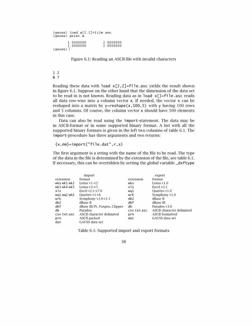
Figure 6.1: Reading an ASCII-file with invalid characters

1 2& 7

Reading these data with load x[2,2]=file.asc yields the result shownin figure 6.1. Suppose on the other hand that the dimension of the data setto be read in is not known. Reading data as in load x[]=file.asc readsall data row-wise into a column vector x. If needed, the vector x can bereshaped into a matrix by y=reshape(x,100,5) with y having 100 rowsand 5 columns. Of course, the column vector x should have 500 elementsin this case.

Data can also be read using the import-statement. The data may bein ASCII-format or in some supported binary format. A list with all thesupported binary formats is given in the left two columns of table 6.1. Theimport-procedure has three arguments and two returns:

{x,nm}=import("file.dat",r,s)

The first argument is a string with the name of the file to be read. The typeof the data in the file is determined by the extension of the file, see table 6.1.If necessary, this can be overridden by setting the global variable _dxftype

import exportextension format extension formatwks wk1 wk2 Lotus v1–v2 wks Lotus v1.0wk3 wk4 wk5 Lotus v3–v5 xls Excel v2.1xls Excel v2.1-v7.0 wq1 Quattro v1.0wq1 wq2 wb1 Quattro v1-v6 wrk Symphony v1.0wrk Symphony v1.0-v1.1 db2 dBase IIdb2 dBase II dbf dBase IIIdbf dBase III/IV, Foxpro, Clipper db Paradox v3.0db Paradox csv txt asc ASCII character delimitedcsv txt asc ASCII character delimited prn ASCII formattedprn ASCII packed dat GAUSS data setdat GAUSS data set

Table 6.1: Supported import and export formats

38

to an appropriate value (for instance, _dxftype="xls"). The second argu-ment is a string, giving either the range of the spreadsheet to be read (as inr=A1..G3"), or as a format descriptor for a packed ASCII-file (see the onlinehelp for more information on this descriptor). If this argument is set to 0,all data are read in. The third argument is the sheet number of the page tobe read in. Usually this is 1. When import reads spreadsheets it assumesthat the first row has the names of the variables. If this is not the case, theglobal variable _dxwkshdr should be reset to 0. The output x contains theactual data and the vector nm has the names of the variables. In order toread the data, GAUSS writes them to a buffer first. The size of this buffer is1 Mb, if the data set is bigger than that the global variable _dxbuffer (thesize of the buffer in Mb’s) can be increased.

The import statement reads both numerical and character variables. Ifwe read the data set file.asc with the & in the second line, the first columnis interpreted as a column with character values and the second column is anumerical column, as can be seen in figure 6.2 Instead of reading a data set

Figure 6.2: Reading an ASCII-file with invalid characters

into GAUSS memory, it is also possible to convert an existing data set intoa GAUSS data set. Instead of the import-command the importf-commandis used. An example is

y=importf("test.xls","test",0,1)

where the Excel-spreadsheet test.xls is converted to a GAUSS data setwith the same name. The procedure returns either 1 (successful conversion)or 0 (unsuccessful conversion).

Compiled procedures, strings, and matrices can be saved in a binaryformat. The advantage of saving a procedure in binary format is that it doesnot have to be recompiled again. Usually though, one wants to save a matrixor a string (array) so that these can be used later for further analysis. The

39

general format of the save-command is save name=symbol where name isa literal or a referenced string and symbol is a symbol (a matrix or a string,for example). Examples are (x is a matrix and s is a string):

save x;save names=s;save c:\tmp\xx=x;save path=c:\tmp x;

In the first case, x is saved into the binary file x.fmt in the current di-rectory, in the second case, s is saved into the binary file names.fst inthe current directory, in the third case, x is saved into the file xx.fmt inthe directory c:\tmp and in the final case x is saved into the file x.fmt inthe directory c:\tmp and all further objects saved with the save-commandwill be placed in this directory, unless an explicit filename is given as in thethird example. The extension .fmt indicates a matrix written to disk andthe extension .fst indicates a string written to disk.

A matrix file created using the save-command can be loaded into theworkspace using the load-command, for example by load x (x.fmt isloaded from the current directory into x) or load x=c:\tmp\xx (in thiscase c:\tmp\xx.fmt is loaded into x). A binary file containing a string canbe loaded with the loads-command, which works analogously to the load-command. Note that the load-command is used both to read ASCII-datainto a GAUSS matrix and to read matrix files saved earlier in a GAUSS-session. It is not possible to read ASCII-data using the loads-statement.

It is not always practical to store data in a matrix, sometimes it is moreconvenient to store them in a data set on disk, especially if the data set islarge. A data set can be created in two different ways: from within GAUSSor by using the exportf-command. First, one can use the saved-commandas in saved(x,data set,vnames) where x is the matrix to be saved inthe datafile, data set is a string variable containing the name of the dataset and vnames is a vector with the names of the columns of x. Upon suc-cessful completion, saved returns the value 1. It is customary to assignvariable names in capitals for numerical variables and in lowercase forcharacter variables. This convention determines whether GAUSS handlescharacter data and numerical data correctly by default. If no vector withvariable names is passed (i.e., vnames is set to 0), GAUSS creates a vectorwith variable names automatically, with names X1, X2, etc.

/* reading and writing datasets */

x=3*rndn(1000,3);y=rndn(1000,1);c=(y.<0).*"ltzero" + (y.>=0).*"gtzero";

40

data=x˜c;

/* uppercase-> numerical variableslowercase-> character variable

*/vnames="X1"|"X2"|"X3"|"sign";file_name="testdata";saved(data,file_name,vnames);

z=loadd(file_name);

Data can be read into memory using the loadd-command as in the exampleabove. This, however, is possible for small data sets only. If the data setis large data can be read by reading successive chunks from the datafile.Alternatively, data can be read row-wise from a data set, as in the examplebelow.

/* reading data row-wise */

file_name="testdata";vnames=getname(file_name);i=1;let data={};open fh=ˆfile_name;number_rows=rowsf(fh);do while not(eof(fh));data_row=readr(fh,1);data=data|data_row;endo;close(fh);

First, one assigns a file handle to the file that is going to be read. Then thedata set is accessed using the readr(fh,1)-command. The first argumentis the file handle, the second argument is the number of rows that is goingto be read. Finally, the data set is closed. All open files in a GAUSS sessionmay be closed with closeall. The variable names of the columns in thedata set can be retrieved by the command vnames=getnames(data set)where data set is a string variable with the name of the data set. A similarapproach can be used to write rows to a file using a writer-command.

Alternatively, a data set is created by the export- or exportf-command.In the first case a matrix x and a vector with variable names nm are writtento a file as in y = export(x,"data.dat",nm). The extension of the file-name determines again the format of the data to be saved, see table 6.1.Moreover, a GAUSS data set can be exported in the same way using theexportf-command as in y = exportf("data.dat", "data.xls", nm).

41

Note the extension of the first argument. It is mandatory even though onlyGAUSS data sets are converted this way.

Output of programs that is shown in the command window can be savedin a file as well. All output printed in the command window is copied toa file by the following command: output file=program.out reset. Thefile program.out is created in the current directory. GAUSS stops copyingoutput to this file after either the command output off or an end state-ment in a program. Note the qualifies reset. This qualifier ensures thatthe file program.out is created if necessary. Should a file with that namealready exist, it is overwritten. The command output file=program.outon appends output to the file program.out if it exists and it creates the fileif it does not exist.

42

Chapter 7

Maximum Likelihood Estimation

A very convenient GAUSS library is the maximum likelihood library1. This li-brary contains procedures to maximize a loglikelihood function, to performbootstrap analysis of nonlinear models, and to perform profile likelihoodanalysis. Note that this library is not distributed with the GAUSS-programitself: it must be bought separately2.

Computer language code for global optimization of functions is widelyavailable nowadays (see for instance Press, Teukolsky, Vetterling, and Flan-nery (1992)), but most of this code works well only with very well behavedfunctions. The optimization routines in the maxlik-library are based onDennis and Schnabel (1983) and they are designed to deal with likelihoodfunctions that are not globally concave. The maxlik-library has many flagsthat can be set by the user, here we will only deal with the most impor-tant ones. The reader is advised to read the Maximum Likelihood Manualfor more information. Of course, on-line help is available as soon as themaxlik-library has been activated.

We will discuss the use of the maxlik-library by means of a simple exam-ple. Consider the normal linear regression model with the data generatedaccording to

yi = β′xi + εi, εi ∼N (0, σ 2). (7.1)

The loglikelihood function of this model (apart from a constant) is given by

�(β,σ) = −N2ln2π − N

2lnσ 2 − 1

2σ 2

∑i(yi − β′xi)2 (7.2)

1In this manual we deal with version 4.0.20 of the maxlik-library. Previous version of thislibrary have a similar structure and the main procedures are used similarly.

2A related third-party library is the cml-library to do constrained maximum likelihoodestimation.

43

The maximum likelihood estimates of β and σ are the values β and σ thatmaximize function (7.2). In the following example we activate the maxlik-library, generate data according to model (7.1) and the maximum likelihoodestimates of the vector β and the scalar σ are determined using the maxlik-procedure:

library maxlik;maxset;

output file=maxlik1.out reset;nobs=5000;beta=1|-1|0.5|-0.25;s=2;x=ones(nobs,1)˜3*rndn(nobs,3);y=x*beta+s*rndn(nobs,1);theta0=ones(5,1);

/* set global variables */_max_ParNames="BETA1"|"BETA2"|"BETA3"|"BETA4"|"S";_max_Algorithm=2;_max_LineSearch=1;_max_CovPar=3;

{x,f,g,cov,retcode}=maxlik(x˜y,0,&loglik,theta0);call maxprt(x,f,g,cov,retcode);

end;

proc loglik(theta,z);local y,x,b,s;x=z[.,1:cols(z)-1];y=z[.,cols(z)];b=theta[1:cols(x)];s=theta[cols(x)+1];retp( -0.5*ln(sˆ2)-0.5*(y-x*b)ˆ2/sˆ2 );endp;

Apart from a call to the maxlik-procedure, the user only has to program afunction that has a column vector with contributions to the loglikelihoodas output. The maxlik-procedure takes a pointer to this likelihood functionas one of its arguments and the function is maximized (in fact, the negativeof the loglikelihood is minimized) using numerical derivatives and defaultoptimization algorithms.

The central procedure in the maxlik-library is the maxlik-procedure.This procedure has four arguments and its output consists of 5 elements:

44

{x,f,g,cov,retcode}=maxlik(dataset,vars,&loglik,theta0);{x,f,g,cov,retcode}=maxlik(data,0,&loglik,theta0);

In the first line, the data are read from the file dataset and the vector varsis a character vector with the names of the variables used in the analysis ora numerical vector with the indices of the selected variables. In the secondcase, the data are passed as a matrix data (see also the example above).The third argument is a pointer to a procedure that returns a vector withcontributions to the loglikelihood function. This procedure has two argu-ments: the first is the parameter vector and the second is the data matrix.If the data are read from file, the order of the columns in the data matrixis specified in the vector vars. The final argument of maxlik-procedure istheta0, a vector with starting values for the optimization.

In the example above the parameter vector of the loglik-proceduretheta equals β and σ stacked on top of each other. Each row of the datamatrix z consists of an observation ( x′i yi ) and correspondingly, each el-ement of the output vector with contributions to the loglikelihood is equalto

−12lnσ 2 − 1

2σ 2(yi − β′xi)2.

The first output vector, x, is the vector with estimated parameters. Thescalar f is the value of the function at the minimum (minus the mean log-likelihood), the vector g is the value of the gradient evaluated at x, thematrix cov is the covariance matrix of the parameters and the scalar ret-code indicates whether the optimization has terminated normally (in whichcase retcode = 0) or not. These results can be printed using the maxprt-procedure:

call maxprt(x,f,g,cov,retcode);

Optimization of the loglikelihood function proceeds in two steps. Ateach iteration a direction d is determined along which line a ‘better’ valuefor θ is searched, and a step length λ is calculated which improves thevalue of the likelihood function. The new value of θ is then determined asθi+1 = θi + λidi.

The direction is commonly computed as (omitting the subscript i index-ing the iteration) d = Ag, with A some square matrix and g the gradientof the loglikelihood function. Different choices of A are available, they cor-respond to different optimization algorithms. The optimization algorithmis set by the global variable _max_Algorithm. A first choice of A is to setA = I, with I the identity matrix. This method is the steepest descent algo-rithm (_max_Algorithm=1). Another choice is to set A equal to the inverse

45

of the Hessian of the loglikelihood function, which is known as the Newton-Raphson algorithm (_max_Algorithm=4). This is method is rather com-puter intensive (at every iteration the matrix of second derivatives must becalculated and inverted) and works only well if the loglikelihood function iswell-behaved. So-called secant methods approximate the Hessian of the log-likelihood function by adding updates to an Cholesky decomposition of theHessian. This Cholesky decomposition is then used to determine a directiond. The approximation of the Hessian improves with the number of itera-tions. Two such secant methods are implemented: the Broyden, Fletcher,Goldfarb, and Shanno algorithm (_max_Algorithm=2) and the Davidson,Fletcher and Powell algorithm (_max_Algorithm=3). Another well-knownoptimization algorithm in econometrics is implemented: the Berndt, Hall,Hall and Hausman method (_max_Algorithm=5). This method estimatesthe Hessian by the average of the outer products of the gradients of eachcontribution to the loglikelihood function. The default optimization algo-rithm as set in maxset is the BFGS-algorithm (_max_Algorithm=2) and formost problems there is no need to use another optimization algorithm asit is reasonably robust against scaling and conditioning of the model. Ofcourse, this default (as any other default) can be changed by editing the filemaxlik.dec where these flags are initialized.

Given the direction d, one has to determine the step length. The functionto be minimized by λ is �(θ+λd). The way λ is calculated is determined bythe global variable _max_LineSearch. The simplest method is to set λ =1 (_max_LineSearch=1). A better procedure is to fit a quadratic or cubicfunction (in λ) to �(·) and then to choose λ such that this approximatingfunction is maximized (_max_LineSearch=2). Other methods of obtaininga step length are based on a sequence of values of λ (_max_LineSearch=3,4, 5). The default choice is _max_LineSearch=2.

Optimization of the loglikelihood function stops if the algorithm hasconverged, or if the maximum number of iterations is reached. The latteris set by _max_MaxIters and the default maximum number of iterations is10000. Convergence is reached when the tolerance of the gradient (whichis defined as a constant times the largest element of the gradient vector)is below is below 1e − 4. The tolerance level can be set with the global_max_GradTol.

During the optimization process, intermediate results are printed at thescreen. This can be surpressed by setting the global variable __output to0. Resetting it to 1 prints output to the screen. Sometimes one wants toinspect the values of the coefficients, gradient, of Hessian during the opti-mization, especially if convergence problems are encountered. If the globalvariable _max_Diagnostic is set to 2 or 3 intermediate results are stored.

46

Suppose the optimization is halted because of an error (or by <c>). Currentvalues of the parameters, function, gradient, Hessian, and steplength areall stored in a data buffer _max_Diagnostic. Because this buffer is a hy-brid vector with both character elements and numerical elements, data canonly be retrieved using vread. A list of names of the information stored in_max_Diagnostic is obtained by vlist(_max_Diagnostic). The value of,say, the parameters is now retrieved as in

x=vread(_max_Diagnostic,"params")

The covariance matrix of the parameters can be estimated in three dif-ferent ways. The first estimate is the inverse of the Hessian (_max_CovPar=1), the second estimate is the inverse of the matrix of cross-products offirst derivatives (_max_CovPar=2) and the third estimate is an estimate ofthe covariance matrix that is consistent even if the data are heteroscedastic(see White (1982), _max_CovPar =3). The latter estimate can also be usedfor testing the specification of the model.

By default, the maxlik-procedure uses numerical derivatives during theoptimization. Of course, this may result in many evaluations of the loglike-lihood function at each iteration. It is possible to supply a procedure thatcalculates the derivative of the loglikelihood function analytically. That pro-cedure must have two arguments: a vector with parameters and a matrixwith the data. The output of this analytical gradient procedure is a matrixwith as many rows as the data matrix and the columns contain the deriva-tives with respect to the parameters. An analytical gradient is used by themaxlik-procedure if the global variable _max_GradProc is set to a pointerto that gradient procedure.

The derivatives of the loglikelihood function in the normal linear modelare given by

∂�i∂β

= 1σ 2(yi − β′xi)xi

∂�i∂σ

= − 1σ+ 1σ 3(yi − β′xi)2

where �i denotes the contributions of the ith observation to the loglikeli-hood. This analytical derivative is programmed as the procedure loglikgdbelow. Each row of the matrix returned from this procedure contains thederivatives given in the two equations above.


47

output file=maxlik2.out reset;

nobs=5000;beta=1|-1|0.5|-0.25;s=2;x=ones(nobs,1)˜3*rndn(nobs,3);y=x*beta+s*rndn(nobs,1);theta0=ones(5,1);

_max_GradProc=&loglikgd;_max_GradCheckTol=1e-3;_max_Diagnostic=2;/* now optimization using analytical gradient */{x0,f,g,cov,retcode}=maxlik(x˜y,0,&loglik,theta0);call maxprt(x0,f,g,cov,retcode);

end;

proc loglik(theta,z);local y,x,b,s;x=z[.,1:cols(z)-1];y=z[.,cols(z)];b=theta[1:cols(x)];s=theta[cols(x)+1];retp( -0.5*ln(sˆ2)-0.5*(y-x*b)ˆ2/sˆ2 );endp;

proc loglikgd(theta,z);local y,x,b,s,e,gb,gs;x=z[.,1:cols(z)-1];y=z[.,cols(z)];b=theta[1:cols(x)];s=theta[cols(x)+1];e=y-x*b;gb=e.*x/sˆ2;gs=-1/s+eˆ2/sˆ3;retp( gb˜gs );endp;

The global variable _max_GradTolCheck is the maximal difference that isallowed between the numerical gradient and the analytical gradient. If theanalytical gradient differs by too much from the numerical gradient, max-lik terminates with an error and prints both gradients. This can be used todebug the computer code of the analytical gradient. For example, consider

48

the Tobit model. In this model, data are generated according to:

y∗i = β′xi + εi, εi ∼N (0, σ 2)yi =max(0, yi).

Only yi and xi are observed so that the loglikelihood function up to aconstant), is

�(β,σ) =∑yi=0

lnΦ(−β′xi/σ)+ ∑yi>0

[−12lnσ 2 − 1

2σ 2

(yi − β′xi

)2] .and the gradient is

∂�∂β

= −∑yi=0

φ(−β′xi/σ)σΦ(−β′xi/σ)xi +

∑yi>0

12σ 2

(yi − β′xi

)xi

∂�∂σ

=∑yi=0

φ(−β′xi/σ)σ 2Φ(−β′xi/σ)xi +

∑yi>0

[− 1σ+ 1σ 3

(yi − β′xi

)2]

For example, in the code below data are generated according to the Tobitmodel, and the model is then estimated.

/* tobit model with error in gradient */


output file=maxlik3.out reset;

nobs=500;beta=1|-1|0.5|-0.25;x=ones(nobs,1)˜3*rndn(nobs,3);y=x*beta+2*rndn(nobs,1);y=(y.>0).*y;

_max_GradProc=&loglikgd;_max_GradCheckTol=1e-3;

{x0,f,g,cov,retcode}=maxlik(x˜y,0,&loglik,ones(5,1));call maxprt(x0,f,g,cov,retcode);

end;

proc loglik(theta,z);

49

local y,x,b,s;x=z[.,1:cols(z)-1];y=z[.,cols(z)];b=theta[1:cols(x)];s=theta[cols(x)+1];retp( (y.==0).*ln(cdfn(-x*b/s)) +(y./=0).*(-0.5*ln(sˆ2)-0.5*(y-x*b)ˆ2/sˆ2) );

endp;

proc loglikgd(theta,z);local y,x,b,s,e,gb1,gs1,gb0,gs0,a;x=z[.,1:cols(z)-1];y=z[.,cols(z)];b=theta[1:cols(x)];s=theta[cols(x)+1];e=y-x*b;a=-x*b/s;gb0=-(pdfn(a)./cdfn(a)).*x/s;gs0=(pdfn(a)./cdfn(a)).*a/s;gb1=e.*x/sˆ2;gs1=-1/s+eˆ2/sˆ3;retp( ((y.==0).*gb0+(y./=0).*gb1)˜((y.==0).*gs0+(y./=0).*gs1) );endp;

However, there is an error in the gradient: the 10th line of the gradientshould read

gs0=-(pdfn(a)./cdfn(a)).*a/s;

GAUSS checks whether the numerical gradient and the analytical gradientgive the same results. In this case they differ, and an error message isprinted, see figure 7.1. From the printed output it is clear that the erroris in the gradient for σ only, because the other elements of the gradientvector coincide. The error is solved by adding a minus sign in front of theexpression for gs0.

As a final check of the computer code, it is strongly recommended thatthe likelihood function and/or the gradient are tested using simulated data.This need not be time consuming and can prevent problems later on.

During the optimization process, it is possible to change the global vari-ables that determine the way the optimization routine looks for ‘better’parameter values, and to change the current point where the loglikelihoodis evaluated. By pressing <h> during the optimization process, a screen ap-pears where the user can select what global variables need to be changed.

50

Figure 7.1: Error in gradient

Note that it is suggested to press <alt><e> to edit the parameter vector.This keystroke is not applicable in the windows version of GAUSS, oneshould press <e> instead.

In this chapter we have discussed only a few procedures of the max-imum likelihood library. The library has more procedures than the onesdiscussed here. It has a procedure maxdensity to calculate kernel densityestimates, a procedure maxprofile to calculate profile likelihood traces, aprocedure maxboot to perform bootstrap simulation of parameters, and afew others. The user is referred to the manual or the online help for moreinformation.

51

Chapter 8

Graphics

GAUSS is equipped with graphics capabilities. With a few commands one isable to plot two- and three dimensional data and the graphs can be savedfor incorporation in a text document. First we discuss some elements of thegraphics library in GAUSS. Then we discuss how graphs can be included inwordprocessors such as Microsoft Word and LATEX.

8.1 Creating Graphics in GAUSS

In this section, we discuss configuration of the graphics library and themost important commands. The graphics library of GAUSS is configuredanalogously to the way GAUSS is configured by editing the file gauss.cfg,but not all settings in this file are relevant to the Windows version of GAUSS.For instance, the printer and the print layout can be set from the menubarof the command window, following File/Printer or File/Print Lay-out.... It is important that the directory that contains the file gauss.exeis listed in the DOS search path. It will not be possible to run the graphicsprogram if that is not the case. It is possible to create multiple windowswith each window containing a graph. This feature will not be discussedhere. General help on the graphics library is obtained by asking help @pqgin the online help program.

The graphics library is activated by library pgraph and global vari-ables are set to their default values by calling the procedure graphset (aprocedure without parameters). GAUSS graphics are created in four steps:

1. Activation of the graphics library.

2. Reading and formatting of the data.

3. Setting global variables to special values.

4. Calling the actual graphics procedure needed.

53

xy(x,y) logx(x,y) logy(x,y) loglog(x,y)bar(v,h) hist(x,v) histf(x,f) histp(x,p)box(g,h) xyz(x,y,z) surface(x,y,z) contour(x,y,z)

Table 8.1: Graph types

In this chapter we focus on the third and fourth step. After a graph is dis-played on screen the user has two options. Pressing <ESC> lets the programcontinue and pressing <enter> yields a menu with some saving and print-ing options.

In table 8.1 we give the commands that generate graphics. The namesof the procedures indicate the type of graph it creates. The most importantgraphs that can be generated are two- and three-dimensional plots (xy andxyz), contour and surface plots of three-dimensional data (contour andsurface), and histograms (hist, histf, and histp).

To illustrate the use of the graphics library, we give a simple examplefirst. A graph of the standard normal density function is generated in thefollowing program:

/* density function of standard normal */

library pgraph;graphset;

grid_size=0.02;x=seqa(-3,grid_size,6/grid_size);y=pdfn(x);

xy(x,y);

The standard normal density function is evaluated on a grid of the hori-zontal axis; the distance between successive points is 0.05. If the distancewould be too large, say 1.0, the graph would be too jagged. After runningthis program a new window appears with the output of the program. Thewindow is shown in figure 8.1.

Output is partly determined by global variables of the graphics library.Of course, these values must be set before the graph is drawn using oneof the commands in table 8.1. Global variables are set by calling a proce-dure (for example, title("example plot")) or by explicit assignment (forexample, _pdate=0). Not all global variables are applicable to each graphtype. Global variables are reset to their default values by calling the pro-cedure graphset. Axis can be named with xlabel("text on x-axis"),

54

Figure 8.1: Output of density.prg

ylabel("text on y-axis"), and zlabel("text on z-axis") and a ti-tle is given with title("title of the plot"). The date and time of cre-ation of the graph is printed in the upper left corner. This feature can beturned off by setting the global variable _pdate=0;. If _pdate is set to astring, then this string will be printed in the upper left corner and the datewill be appended.

The commands hist(x,v), histf(f,c) and histp(x,v) all producehistograms. They differ only in type of information displayed on the verti-cal axis (absolute numbers, frequencies or percentages) and input require-ments (raw data and a vector of breakpoints (hist and histp) or frequen-cies and a vector with category labels (histf). In the file below, we generatea vector with normal distributed numbers and a histogram is generated us-ing −1.5,−1,0,1 and 1.5 as breakpoints so that the first bar correspondsto observations x ≤ −1.5, the second category to −1.5 < x ≤ 1, etc.


55

x=rndn(100,1);b=-1.5|-1|0|1|1.5;title("histogram of normal distribution");ylabel("frequency");xlabel("x value");_pdate=0;call hist(x,b);

Two dimensional graphs can be plotted using the xy(x,y)xy command.Of course, the arguments x and ymust be of equal length unless one wantsto index the observations. The command xy(1,y) plots the curve (1, y1),(2, y2), etc. The second argument need not be a vector: if a matrix (with thesame number of rows as x) is passed as an argument, each column will begraphed. Consider for example the following program


ngrid=100;x=seqa(-3,6/ngrid,ngrid);y1=pdfn(x);y2=1./(pi*(1+xˆ2));

_plegctl=1˜4˜1˜0.32;_plegstr="Gaussian density\000Cauchy density";xlabel("ordinate");ylabel("density function");

xy(x,y1˜y2);

In this example, two density functions are graphed, viz. the density ofthe normal distribution and the density function of the Cauchy distribu-tion. The second argument passed to the xy-procedure is a 100 × 2-matrixand each column is graphed as a separate line. The legend in the graph isset by two variables. The 4-row vector _plegctl determines where the leg-end is placed. The first element determines whether the coordinates are setin plot coordinates (1), inches (2), or pixels (3), the second element gives thefont size of the legend (between 1 and 9) and the final two elements givethe horizontal and vertical coordinate of the lower left corner of the legend(in units specified by the first argument). In our example, coordinates aregiven in plot coordinates, font size is 4 and the coordinate of the lowerleft corner is (1,0.32). The text of the legend is specified in _plegstr. Dif-ferent curve labels are separated by the ASCII-0 character \000. The label

56

of the first curve is ‘Gaussian density’ and the label of the second curve is‘Cauchy density’. If the number of labels given in _plegstr is less than thenumber of columns in y empty labels will be printed in the legend other-wise the order of the curves in the legend correspond to the order of thecolumns in y. Additional text messages can be plot in the graph using theglobal variables _pmsgctl and _pmsgstr. By its default settings set usingthe graphset procedure, a line is drawn through the points plotted. Thetype of line plotted is controlled by the global variable _plctrl. If thisvariable is set to -1, only individual points are plotted and these points arenot joined by a line. The symbol at each point is controlled using _pstype.

It is also possible to draw three dimensional curves and contour linesare graphed using the surface and contour procedures. Both procedureshave three arguments: a row-vector x of length k, a vector y of length pand a p × k matrix z. The rows of z correspond to the elements of y andthe columns of z correspond to the elements of z. A graph of the surfaceabove the (x,y) plane is drawn by surface(x,y,z) and a two dimensionalgraph with isocontour curves is drawn by the command contour(x,y,z).A three dimensional graph of a function is obtained with the xyz(x,y,z)procedure. This procedure yields 3D results analogous to the xy procedurediscussed above. As an example, we give the following program that gener-ates three 3D plots based on a bivariate normal density function:


ngrid=51;x=seqa(-3,6/ngrid,ngrid);y=x;x1=pdfn(x);y1=pdfn(y);z=x1.*y1’;

xyz(x,y,z);surface(x’,y,z);contour(x’,y,z);

Graphical images can be printed from within a program or saved todisk in one of the file formats supported using the graphtprt procedure.First, consider printing a GAUSS graph. Suppose the graph has already beendrawn using one of the graphic procedures, for example xy. Then the graphis printed to a printer with the settings specified in pqgrun.cfg by the twocommands

57

graphprt("-p");rerun;

The rerun-command redraws the picture. The procedure graphprt has astring as its argument and certain flags are set in that string. These flags ap-ply to the first graph drawn after the call to graphprt. The most importantflags are -p (print the graph using the settings in pqgrun.cfg), -c=k (con-vert file format to (k=1) Encapsulated Postscript, (k=2) Lotus PIC-format,(k=3) Hewlett Packard Graphics Language HPGL format, or (k=4) colouredPCX bitmap), and -cf=test.ext (save the graphic file as test.ext). Thefollowing two commands would save the graphic last shown as Encapsu-lated Postscript file with name figure.eps in the subdirectory c:\tex\docs\graph:

graphprt("-c=1 -cf=c:\\tex\\docs\\graph\\figure.eps");rerun;

Note the double backslashes in the filename. Files can also be convertedfrom the window that shows the graphic. Using File/Convert/ from themenu bar one is presented a list with formats that the file can be convertedto, see figure 8.2. The name of the file depends on the setting of the variablecvt_filename in the file pqgrun.cfg. If this variable is commented out (byputting a # in front of it), the name will be cvt_<nnn>.<ext>, where <ext>indicates the type of conversion (eps for Encapsulated Postscript, pic forLotus .pic, hpg for HPGL, and pcx for PCX). Files are numbered sequentially,so the first converted file would be named as cvt_000.eps, the secondwould be cvt_001.eps, etc.

8.2 Incorporating GAUSS Graphics in Text Documents

8.2.1 GAUSS Graphics in Microsoft Word Documents

A utility PlayW to change graphic formats can be downloaded from theAptech website. At the time of writing, though, this utility is not completelyfunctional. Hence, it is not yet possible to cut-and-paste GAUSS graphicsfrom a graphics window into a Windows wordprocessor. It is easily possi-ble though to include GAUSS graphics in a Microsoft Word document. First,the graphic has to be saved in HPGL-format, either using the graphprt-command or from the File/Convert-menu. An HPGL-file can be read intoWord if the appropriate filter has been installed. That filter (with installa-tion instructions) can be downloaded free of charge, either from the Mi-

58

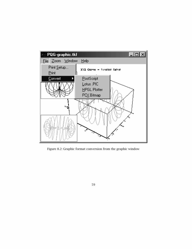
Figure 8.2: Graphic format conversion from the graphic window

59

crosoft website1 or from the website of the author2. An HPGL-file can nowbe inserted using ’Insert/Picture/From file’. Note that the filter assumes ex-tension hgl for HPGL-files, so it will not list files saved with extension hpgas GAUSS does by default. Hence, to choose an HPGL-file to be read in oneshould look for ‘all files’ and pick the appropriate HPGL-file. Since Worddoes not know which filter to use for files with extension hpg, the user isprompted for the format of the file. After choosing ‘HP Graphics Language’the file is read into the Word document.

8.2.2 GAUSS Graphics in LATEX2e Documents

It is not possible to cut-and-paste GAUSS graphics into LATEX2e-documents.However, it is simple to include GAUSS graphics in a LATEX2e-document. Theeasiest way to incorporate GAUSS graphics in LATEX2e documents is to savethe graph in Encapsulated Postscript format (.eps) and to read it in theLATEX document with the graphicx-package3. A Postscript file can be readinto a LATEX2e-document as in

\includegraphics[width=\textwidth]{c:/tex/docs/graph/figure.eps}

The optional parameter width is used to set the width of the picture asit appears in the document. Another useful parameter is angle which isused to rotate the picture. An example of a graphics file read into a LATEX2e-document is given in given in figure 8.3. Note that the background of thepicture, which is black when the picture is shown on screen, has beenchanged to a white background.

1http://support.microsoft.com/support/kb/articles/Q196/5/06.asp2www.rhkoning.com/gauss3This booklet was typeset using MiKTEX, that is available free of charge at ftp.dante.de

in the subdirectory win32/miktex. All graphics in this book were included as described inthis section.

60

Figure 8.3: Graph from examples/pxy.e

61

Chapter 9

Two Examples

In this chapter we give two examples of programs written in GAUSS. In thefirst example a library that calculates kernel estimates is discussed. In thesecond example the finite sample properties of the ML-estimator in a probitmodel are derived by means of a simulation study1.

9.1 A Kernel Estimation Library

Kernel estimation is a technique to estimate the density function of a ran-dom variable. Suppose we have n independently identically distributed ob-servations x1, . . . , xn from an (unknown) density function f (x). The den-sity function may be estimated parametrically by assuming some functionalform that depends on a few parameters which are estimated. Alternatively,it may be estimated non-parametrically, for instance by constructing a fre-quency distribution or a kernel estimate, which is basically a smoothedversion of a frequency distribution. A standard reference on density esti-mation is Silverman (1986). We follow his notation in this chapter. The ker-nel library implements five procedures for kernel estimation of unknowndensities. The first procedure (ukernel) estimates a univariate kernel ac-cording to

f (x) = 1nh

∑iK(x − zih

)(9.1)

In this equation, x is the point where the kernel is to be evaluated, zi (i =1, . . . , n) are the observations, h is the bandwidth, and K(·) is the kernelfunction. The second procedure estimates a multivariate kernel:

f (x) = 1nhd

∑iK(1h(x − zi)

)(9.2)

1All GAUSS code of these examples can be downloaded from www.rhkoning.com/gauss.

63

k_epan Epanechnikov kernel 1516(1− x2)2I[−1,1](| x |)

k_gauss Gaussian kernel 1√2π exp(−x2

2 )k_triang triangular kernel (1− | x |)I[0,1](| x |)k_rect rectangular kernel 1

2 I[−1,1](| x |)

Table 9.1: Kernel functions in kernel

Here, z and x are vectors and d is the dimenstion of the density to beestimated. The third procedure computes the Nadharaya-Watson kernel re-gression estimator:

m(x) =∑i K(1h(x − zi)

)yi∑

i K(1h(x − zi)

) (9.3)

Finally, two auxiliary procedures are implemented, one is used to calculatethe bandwidth (bandw1, h = 0.9n−1/5 min(σ , IQR/1.34) with IQR the in-terquartile range of the data and σ the standard deviation of the data, seeSilverman (1986), p. 47) and one procedure (view_ukernel) to display theresults of the univariate kernel estimation procedure. Besides these mainprocedures, four different kernel functions are implemented, see table 9.1.

/* kernel.src version 1.0Source file with functions of the kernel library:

ukernel procedure for univariate kernel estimationmkernel procedure for multivariate kernel estimationbandw1 procedure for automatic bandwidth selectionnw procedure for nonparametric regressionviewuknl procedere for plotting the estimated density

*/

/* comment the following line out if you don’t have the pgraphlibrary installed. You will not be able to use the procedureview_ukernel */

#include pgraph.ext

/* procedure to calculate a univariate kernel density estimateand itsderivativeusage: {f, d, h} = ukernel(x, z, h, w, &kf);input: x: T vector where density is to be estimated

64

z: n vector with observed data pointsh: scalar bandwidth, if h<=0 bandwidth is

determined by procedure bandw1(z)w: n vector with weights&kf: pointer to weighting function

output: f: T vector with estimated densityd: T vector with estimated derivativeh: scaler bandwidth

*/

proc (3)=ukernel(x, z,h,w, &kf);local arg, i, n, f, d, k, kff, kfd, pkff,argl,argh,kffl,kffh,fl,fh,hl,hh;local kf:proc;

/* error checking here */if (cols(x)>1);errorlog "ukernel.g: x has too many columns";retp(-1,-1,-1 );endif;if (cols(z)>1);errorlog "ukernel.g: z has too many columns";retp( -1,-1,-1 );endif;

/* initialization */i = 1;n = rows(x);k = cols(x);

/* determine bandwidth */if (h<=0);h=bandw1(z);endif;

f=zeros(n,1);d=zeros(n,1);do while (i<=n);arg = (x[i]-z)/h;{kff, kfd} = kf(arg);f[i] = meanc(kff.*w)/h;d[i] = meanc(kfd.*w)/(hˆ2);i=i+1;endo;

65

retp( f,d,h );endp;

/* procedure to calculate a multivariate kernel density estimateand its derivativeusage: {f, d, h} = mkernel(x, z, h, w, &kf);input: x: T x k matrix where density is to be estimated

z: n x k matrix with observed data pointsh: scalar, bandwidth parameter (same bandwidth

for all components), if h<=0 it is determinedby eq 4.14 of Silverman

w: n vector with weights&kf: pointer to weighting function

output: f: T vector with estimated densityd: T x k matrix with estimated derivativesh: scalar, bandwidth used

*/

proc (3)=mkernel(x, z, h, w, &kf);local arg,i,n,f,d,k,kff,kfd,pkff,p,deneq0;local kf:proc;

i = 1;n = rows(x);k = cols(x);if (h<=0);

p=1/(k+4);h=(4/(k+2))ˆp*nˆ(-p);

endif;f = zeros(n,1);d = zeros(n,k);do while (i<=n);arg = (x[i,.]-z)/h;{kff, kfd} = kf(arg);pkff = prodc(kff’);f[i] = meanc(pkff.*w)/(hˆk);deneq0=kff .==0;kff=kff+deneq0;d[i,.] = meanc((kfd.*pkff.*w)./kff)’/(hˆ(k+1));i = i+1;

endo;retp( f,d,h );endp;

66

/* computes Nadaraya-Watson kernel regression estimator

usage: {g,d,h} = nw(x,z,y,h,&kf);input: x: T-vector where regression function is

evaluatedz: n-vector with data on independent variabley: n-vector with data on dependent variableh: scalar, bandwidth, if h<=0 the bandwidth is

determined automatically using procedurebandw1

&kf: pointer to univariate kernel density estimatoroutput: g: T-vector with values of regression evaluated

in xd: T-vector with estimated derivative in xh: scalar bandwidth used

*/

proc (3)=nw(x, z, y,h,&kf);local num, numder, denom, denomder, g, s, n, k, d,v;local kf: proc;

n = rows(x);k = cols(x);g = zeros(n,1);d = zeros(n,1);

if (k ne 1);print "error in nw.g: too many columns in x";retp( g, d );endif;if (cols(z) ne 1);print "error in nw.g: too many columns in z";retp( g, d );endif;

{num,numder,h} = ukernel(x,z,h,y,&kf);{denom,denomder,h} = ukernel(x,z,h,1,&kf);s = (denom.==0);g = num./(denom+s);d = numder./(denom+s) - num.*denomder./(denomˆ2+s);retp( (1-s).*g, (1-s).*d,h );endp;

67

/* bandw1procedure to calculate the optimal bandwidth in kernel estimationof a density. The optimal bandwidth is calculated according toeq. 3.31 of Silverman (1986)

usage: h=bandw1(y);input: y: n-vector whose density will be estimated;output: h: scalar, optimal bandwidth choice;

*/

proc bandw1(y);local s, ys,n, a, iqr, qi1, qi3;

if (cols(y)>1);errorlog "input error in bandw1.g: too many columns";retp( -1 );

endif;s=sqrt(vcx(y));n=rows(y);ys=sortc(y,1);qi1=round(0.25*n);qi3=round(0.75*n);iqr=ys[qi3]-ys[qi1];retp( 0.9*minc(s|(iqr/1.34))/nˆ0.2 );endp;

/* view_ukernelprocedure to plot kernel density estimate. Library pgraph mustbe activated.

usage: call view_ukernel(x,f,h);input: x: n-vector with data points

f: n x k matrix (k=1 or k=3) with estimated densitiesfor different bandwidths

h: k-vector (k=1 or k=3) with bandwidthsoutput: noneglobals: all globals of the pgraph library

*/

proc (0)=view_ukernel(x,f,h);local data,k,xlow,xhigh,flow,fhigh,xlegend,ylegend;

68

/* error checking */if (cols(f) ne rows(h));errorlog "error in viewkrnl.g: rows(f) unequal to cols(h)";retp();endif;/* set global variables pgraph */_pdate=0;

k=cols(f);xlow=minc(x);xhigh=maxc(x);flow=minc(minc(f));fhigh=maxc(maxc(f));xlegend=xlow;ylegend=flow+0.8*(fhigh-flow);_plegctl=1|4|xlegend|ylegend;if (k==1);_plegstr="h=" $+ ftos(h,"%*.*lf",5,3);else;_plegstr="h=" $+ ftos(h[1],"%*.*lf",5,3) $+ "\0h="$+ftos(h[2],"%*.*lf",5,3)$+"\0h="$+ ftos(h[3],"%*.*lf",5,3);

endif;data=sortc(x˜f,1);xy(data[.,1],data[.,2:cols(data)]);endp;

/*This file contains some kernel functions. All functions take ann x k matrix u as their argument and return an n x k matrix withthe function evaluated in each point of x and an n x k matrix dwith the derivative of the function in each point of x.

k_bw: biweight kernel functionk_epan: Epanechnikov kernelk_gauss: Gaussian kernelk_triang: triangular kernelk_rect: rectangular kernel

usage:{f,d}=k_bw(u);

*/

69

proc (2)=k_bw(u);local select;select = abs(u).<=1;retp( 15/16*((1-u.ˆ2).ˆ2).*select, -15/4*u.*(1-u.ˆ2).*select);endp;

proc (2)=k_gauss(u);retp( pdfn(u), -u.*pdfn(u) );

endp;

proc (2)=k_epan(u);local c, s;s = abs(u).<sqrt(5);c = 0.75/sqrt(5);retp( c*(1-0.2*u.ˆ2).*s, -0.4*c*u.*s );

endp;

proc (2)=k_rect(u);retp( 0.5*(abs(u).<1), 0*u );

endp;

proc (2)=k_trian(u);local s, a;a = abs(u);s = a.<1;retp( (1-a).*s, (-(u.>=0) + (u.<=0)).*s );

endp;

The following example is a program that illustrates some of the proceduresof the library,. In this example, a standard normal density is estimated us-ing different kernel functions.

/* in this example we draw 1000 random numbers from a normaldistribution and we estimate the density using the kernellibrary. Three different graphs will be created using differentkernel funtions. Note that the pgraph library must be activatedin order to use view_ukernel.*/new;library kernel,pgraph;

70

nobs=1000;

r=rndn(nobs,1);

x_axis=seqa(-3,6/1000,1000);{f1,d1,h1}=ukernel(x_axis,r,0,1,&k_gauss);call view_ukernel(x_axis,f1,h1);{f2,d2,h2}=ukernel(x_axis,r,0,1,&k_epan);call view_ukernel(x_axis,f2,h2);{f3,d3,h3}=ukernel(x_axis,r,0,1,&k_rect);call view_ukernel(x_axis,f3,h3);end;

9.2 Finite Sample Properties of the ML-estimator in Tobit

Model

In the Tobit-model, data are generated according to

y∗i = β′xi + εi, εi ∼N (0, σ 2)yi =max(0, yi).

Only yi and xi are observed. If the fraction of observations with yi = 0is very small, the model resembles the standard linear model with normaldisturbances. However, if the fraction of zeros is non-negligible, the modelcannot be estimated using ordinary least squares. Consistent estimates ofthe parameters can be obtained using maximum likelihood. The finite sam-ple properties of this estimator is unknown in this model, asymptoticallythe estimator has a normal distribution. In order to assess whether theasymptotic distribution provides a reasonable approximation to the finitesample distribution, one can perform a small simulation study. In this ex-ample, 100 samples of 50 observations are drawn, and for each sample theparameters of the model are estimated. Two sets of endogenous variablesare generated, in model 1 approximately 16% of all observations on theendogenous variable are 0, in model 2 this percentage is 2.2%. We wouldexpect the estimates of model 2 to conform more closely to the standardnormal distribution than those of model 1.

library maxlik,kernel,pgraph;maxset;

output file=tobitsim.out reset;

nobs=50;nrep=100;

71

beta1=1|-1|0.5|-0.25;beta2=3|-1|0.5|-0.25;x=ones(nobs,1)˜3*rndn(nobs,3);

_max_GradProc=&loglikgd;_max_GradCheckTol=1e-3;

let b1={};let b2={};i=1;do while (i<=nrep);y1=x*beta1+2*rndn(nobs,1);y2=y1+2; /* same disturbances as in y1 */y1=(y1.>0).*y1;y2=(y2.>0).*y2;{x0,f,g,cov,retcode}=maxlik(x˜y1,0,&loglik,beta1|2);if (retcode==0);b1=b1|x0[1:4]’;

endif;{x0,f,g,cov,retcode}=maxlik(x˜y2,0,&loglik,beta2|2);if (retcode==0);b2=b2|x0[1:4]’;

endif;i=i+1;endo;

print "fraction succesful convergences model 1";rows(b1)/nrep;print "mean b1/max b1/min b1/var b1/beta1";meanc(b1)˜maxc(b1)˜minc(b1)˜diag(vcx(b1))˜beta1;print "fraction succesfull convergences model 2";rows(b2)/nrep;print "mean b2/max b2/min b2/var b2/beta2";meanc(b2)˜maxc(b2)˜minc(b2)˜diag(vcx(b2))˜beta2;

grid=seqa(-3,6/200,200);sb12=sqrt(vcx(b1[.,2]));sb22=sqrt(vcx(b2[.,2]));{f1,d1,h1}=ukernel(grid,(b1[.,2]-beta1[2])/sb12,0,1,&k_epan);{f2,d2,h2}=ukernel(grid,(b2[.,2]-beta2[2])/sb22,0,1,&k_epan);_plegctl={ 2 4 1 5 };

72

_plegstr="model 1\000model 2\000standard normal";call xy(grid,f1˜f2˜pdfn(grid));graphprt("-c=1 -cf=e:\\intro99\\pictures\\tobitsim.eps");rerun;

end;

proc loglik(theta,z);local y,x,b,s;x=z[.,1:cols(z)-1];y=z[.,cols(z)];b=theta[1:cols(x)];s=theta[cols(x)+1];retp( (y.==0).*ln(cdfn(-x*b/s)) +(y./=0).*(-0.5*ln(sˆ2)-0.5*(y-x*b)ˆ2/sˆ2) );

endp;

proc loglikgd(theta,z);local y,x,b,s,e,gb1,gs1,gb0,gs0,a;x=z[.,1:cols(z)-1];y=z[.,cols(z)];b=theta[1:cols(x)];s=theta[cols(x)+1];e=y-x*b;a=-x*b/s;gb0=-(pdfn(a)./cdfn(a)).*x/s;gs0=-(pdfn(a)./cdfn(a)).*a/s;gb1=e.*x/sˆ2;gs1=-1/s+eˆ2/sˆ3;retp( ((y.==0).*gb0+(y./=0).*gb1)˜((y.==0).*gs0+(y./=0).*gs1) );endp;

The result of this simulation is shown in figure 9.1. We do not wish todiscuss Monte Carlo simulation in detail, but to demonstrate that it can bestraightforward to perform a small simulation study in GAUSS.

73

Figure 9.1: Distribution of ML-estimator

74

Chapter 10

Exercises

1. Check your setup of GAUSS by running some of the example files inthe gauss\examples directory. Have problems fixed by your systemadministrator.

2. Make a subdirectory for the programs and procedures you’ll writeduring this course. Ensure that it is in the search path of GAUSS. Mod-ify the file startup such that the working directory is set to this di-rectory as soon as GAUSS is started.

3. Write a program that initializes a matrix with ones, a matrix U withuniform random numbers and one matrix with keyboard input. Countand print the number of elements of U that are smaller than 0.5.

4. Write a program that converts your day of birth (a string variable likebirth = "July-04-1956"; to a numerical vector with 3 elements,the first element representing the month, the second representing theday and the third representing the year.

5. Create a 1000-vector with N (1,4)-distributed random variables andcalculate the fraction of numbers smaller than 0, between 0 and 2, andexceeding 2. Use GAUSS to calculate the probabilities of these eventsand compare them with the fractions found.

6. Write a procedure that determines the Euclidean length of a vector x.

7. Write a procedure that calculates the OLS estimator in the linear re-gression model, its covariance matrix, and an estimate for the residualvariance.

8. Write a procedure that has two arguments (a matrix and a string witha file name) and that save the matrix to an ASCII file with the specifiedfile name.

75

9. In panel data econometrics one usually stacks the observations suchthat the individual index runs slow and the time index runs fast:

y =

y1

y2...yT

.

Here, y1 is an N-vector with the observations for all individuals inperiod 1, y2 is an N-vector with all observations in the second period,etc. Write a GAUSS program that re-orders the vector y such that thetime index runs fast and the individual index runs slow, i.e.

y =

y1

y2...yN

.

Here, y1 is a T -vector with all observations for individual 1, etc.

10. Write a procedure that calculates an N-vector with contributions tothe loglikelihood in a Tobit model with N observations. Minimize theamount of computations required.

11. Write a program that generates data according to the probit model:

y∗i = β′xi + εi εi ∼N (0,1)

yi ={0 y∗i ≤ 01 y∗i > 0 (10.1)

Only the xi’s and yi are observed. Save the observations in a dataset.

12. Using this dataset, calculate descriptive statistics and estimate β us-ing OLS.

13. Create a graph of the standard normal, t- and Cauchy-density func-tions. Save your graph and generate a print.

14. Write a procedure that calculates the contributions to the loglikeli-hood of a probit model. The first parameter of the procedure is theparameter β and the second part is a datamatrix Z.

76

15. Examine by means of a simple simulation study whether Glesjer’s testfor the presence of heteroscedasticity in a linear regression model ismore powerful than an omnibus test like the Breusch-Pagan test (seeGreene (1993), p. 394–396).

77

Bibliography

Dennis, J.E. and R.B. Schnabel (1983). Numerical Methods for Uncon-strained Optimization and Nonlinear Equations. Englewood Cliffs:Prentice Hall.

Greene, W.H. (1993). Econometric Analysis (third ed.). New York: MacMil-lan.

Press, W.H., S.A. Teukolsky, W.T. Vetterling, and B.P. Flannery (1992). Nu-merical Recipes in C (Second ed.). Cambridge: Cambridge UniversityPress.

Silverman, B.W. (1986). Density Estimation. London: Chapman & Hall.

White, H. (1982). Maximum likelihood estimation of misspecified models.Econometrica 50, 1–25.

79

Appendix A

Converting ASCII to GAUSS datasets

An ASCII dataset has to be converted to a GAUSS dataset before it can beused. To facilitate this conversion, the utility atog.exe has been provided.This utility can be operated both interactively and in batch mode. In caseone uses the utility interactively, it is started by atog at the DOS-commandprompt. The utility returns with a prompt \ after which a limited number ofcommands can be entered (see below). All commands are terminated witha semicolon (;). An interactive session is ended by the command quit.

In batch mode, the conversion to a GAUSS dataset is performed by atogconvert.cmd. The file convert.cmd contains the commands that performthe conversion. The most useful commands1 are

append append ASCII dataset to an existing GAUSS dataset,

help display help (interactive mode only),

input parameters name of the ASCII dataset,

output parameters name of the GAUSS dataset,

msym parameter missing value character (default dot ‘.’),

invar parameters specification of data in ASCII dataset,

outvar parameters list of names of variable to be saved in GAUSS dataset,

run execute commands entered (interactive mode only).

The most crucial command is the invar-command. This commands tellsatog how the data are organized in the ASCII dataset. ASCII datasets mayeither be softly delimited (elements are separated from each other by tabs,

1For a detailed description we refer to the GAUSS manual.

81

spaces, or carriage/returns-line feeds), hard delimited (elements are delim-ited by a printable character) or not be delimited at all (packed ASCII). Inthe first case, the command reads

invar $name #age weight $char[1:10] #numvar[03];

The first variable is a character variable (indicated by the $-sign), the sec-ond and third variable are numerical variables (indicated by the #-sign), thenext ten variables are labeled char1 to char10, and finally, the last threevariables are numerical again and labeled as numvar01, numvar02 and num-var03.

If the ASCII dataset is hard delimited, the format changes to somethinglike

input data.csv;output datacsv;invar delimit(,,N) #var1,var2,var3,var4,var5;outvar var1,var2,var3,var4,var5;

This command file converts the dataset

1,2,3,4,5,6,7,8,9,10,

The keyword delimit has two optional parameters: the first is the delim-iter (, in this example. One uses \r if each line contains one record and thevariables are separated by commas) and the second one indicates whetherthe last element of an observation is followed by a delimiter (in which caseit takes the value N). atog386 assumes that the last variable is not followedby a delimiter if no second argument is specified.

Note that the values taken character variables may not include spaces.atog386 reports an error if it encounters an input line like

34,s korea,belgium,0,0,32

because of the space in the second field. If the data are organized as packeddata with fixed records length there are no problems if a character variabletakes a value with a space in it.

A packed ASCII file must have records with fixed lengths. The keywordrecord is used to indicate the length of the record (including the finalCR/LF, which takes two positions). Furthermore, the format of the variablesmust be specified:

invar record=47 $(1,4)name #(5,2)age (7,4.2)weight$(*,1)char[1:10] #(*,8.2)numvar[03];

82

The first variable (name, a character variable) starts at position 1 and haslength 4. The age variable (numerical) starts at position 5 and has length2. The starting position of the weight variable is 7, it occupies 4 bytes, ofwhich the last two are decimals. A decimal point is inserted between thesecond and third element. The next ten variables are all character variablesof length 1. The asterisk in the format field indicates that the first fieldof that variable is the one immediately after the last field of the previousvariable, so that no position in the data file are skipped. The last three vari-ables are numerical, have length 8 and the last two numbers are convertedto decimals. A record has 45 fields and is terminated by a <CR><LF>, so thetotal length is 47 bytes.

An example of a complete command file for atog386 is

input c:\gauss\data\wbo.asc;output c:\gauss\data\wbo;invar huur inkomen ihs respnr;outvar huur inkomen ihs respnr;msym &; @ missing symbol@

Note that no double backslashes are used in naming both the input and theoutput file, the variables invar and outvar are literals. Comments are en-closed in @-signs. The command atog386 convert.cmd converts the ASCIIfile wbo.asc to the GAUSS dataset wbo.dat and accompanying header filewbo.dht.

83

Appendix B

GAUSS Libraries

GAUSS is available on the following platforms: MSDOS, Windows95/98/NT,DEC UNIX, HP-UX, IBM RISC, Linux, OS/2, SGI IRIX and Solaris. The graphicaluser interface differs between these implementations, the language itselfdoes not differ (except for the graphics commands).

The following GAUSS-libraries are distributed by Aptech Systems:

• Constrained Maximum Likelihood

• Constrained Optimization

• Curvefit

• Descriptive Statistics

• FANPAC

• Linear Programming

• Linear Regression

• Loglinear Analysis

• Maximum Likelihood

• Nonlinear Equations

• Optimization

• Quantal Response

• Time Series

85

Except for FANPAC, which runs under UNIX and Windows operating sys-tems only, all these libraries are supported on all platforms.

Apart from these modules some third-party modules are available aswell:

• CellVision (DOS)

• COINT (DOS, OS/2, UNIX, Windows)

• CTRLGAUSS (DOS, Windows)

• DATAWIZ (DOS, OS/2, Windows)

• FAIR-TAYLOR (DOS)

• Fastsort (DOS, UNIX)

• GAUSSX (DOS, UNIX, Windows)

• LALIB-386 (DOSm Windows)

• LINCS (DOS, OS/2, UNIX, Windows)

• MARKOV (DOS, Windows)

• Mercury (Windows)

• Mercury GE (Windows)

• MISS (DOS, OS/2, UNIX, Windows)

• Quadratic Programming (DOS, UNIX, Windows)

• QUEGAUSS (DOS, Windows)

• SimGAUSS (DOS, Windows)

• SNAP (DOS)

• SSATS (DOS, OS/2, UNIX, Windows)

• Stat/Transfer UNIX, Windows)

• TSAGL (DOS)

• TSM (DOS, OS/2, Windows)

More information on these modules can be found at the WWW-sites ofAptech Systems (www.aptech.com) and on those of other GAUSS distrib-utors.

86

Appendix C

Program Code

Computer code for the programs in this book can be downloaded fromwww.rhkoning.com/gauss. The archive file that contains the code is calledbookcode.zip. The files in that archive correspond to the programs in thebook according to the table below.

page 18 chap3\probit1.prgpage 22 chap4\vectoriz.prgpage 23 chap4\if-exam.prgpage 25 chap4\boxcox1.gpage 26 chap4\boxcox2.gpage 27 chap4\danger.prgpage 28 chap4\numder.prgpage 30 chap4\ols.prgpage 34 chap5\course1.lcgpage 35 chap5\testlib3.srcpage 36 chap5\testlib3.decpage 37 chap6\file.ascpage 40 chap6\datasets.prgpage 41 chap6\readdata.prgpage 44 chap7\maxlik1.prgpage 48 chap7\maxlik2.prgpage 50 chap7\maxlik3.prgpage 54 chap8\density.prgpage 56 chap8\hist.prgpage 57 chap8\3d.prgpage 64 chap9\kernel.srcgpage 69 chap9\kfunctio.srcgpage 70 chap9\kernel1.epage 71 chap9\tobitsim.prg

Table C.1: Files in the code archive

87

Index

LATEX2e, 60.eps, 60atog386, 82atog, 81break, 21cdfbeta, 29cdfbvn2e, 29cdfbvn2, 29cdfbvn, 29cdfchic, 29cdfchii, 29cdfchinc, 29cdffc, 29cdffnc, 29cdfgam, 29cdfmvn, 29cdfnc, 29cdfni, 29cdfn, 29cdftci, 29cdftc, 29cdftnc, 29cdftvn, 29cdir(0), 6, 33changedir(s), 6closeall, 41cons, 15continue, 21contour, 54, 57con, 14declare, 35do-until, 22do-while, 21, 22

dstat, 27, 30eigrs2, 27elseif, 23else, 23endif, 23endo, 21endp, 25end, 21errorlog, 26exportf, 40, 41export, 41external, 33ftocv, 16ftos, 16gauss.cfg, 24, 53gaussi.cfg, 33, 34getnames, 41graphicx, 60graphprt, 58graphset, 53, 55, 57graphtprt, 57histf, 54, 55histp, 54, 55hist, 54, 55hsec, 22if-endif, 23if, 23importf, 37, 39import, 37–39include, 36invar, 83let, 13library, 34, 35

88

lib, 35loadd, 41loads, 15, 40load, 37, 40local, 13, 25, 28maxboot, 51maxdensity, 51maxlik, 44, 45, 47, 48maxprofile, 51maxprt, 45new, 21ols, 27, 29, 30ones, 14output, 42outvar, 83pause, 21pdfn, 29pgraph, 53pqgrun.cfg, 53printfmt, 19proc, 25readr, 41record, 82rerun, 58reshape, 38retp, 25, 26rndbeta, 29rndgam, 29rndnb, 29rndn, 29rndp, 29rndu, 29run, 24saved, 40save, 40stof, 16surface, 54, 57system, 21title, 54vlist, 47vread, 47

writer, 41xlabel, 55xyz, 54, 57xy, 27, 54, 56ylabel, 55zeros, 14zlabel, 55

command mode, 4

edit mode, 4element-by-element operators, 16

flow control, 21

pointer, 28

substitution operator, 15

xy, 56

89

A Short Introduction to GAUSS for Windows - CiteSeerX

Documents

Transcript of A Short Introduction to GAUSS for Windows - CiteSeerX