Accelerating Gauss-Newton Filters on FPGAs - Radar Masters

The copyright of this thesis vests in the author. No quotation from it or information derived from it is to be published without full acknowledgement of the source. The thesis is to be used for private study or non-commercial research purposes only.

Published by the University of Cape Town (UCT) in terms of the non-exclusive license granted to UCT by the author.

Univers

ity of

Cap

e Tow

n

Univers

ity of

Cap

e Tow

n

Accelerating Gauss-Newton Filters onFPGAs

Jean-Paul Costa da Conceicao

A dissertation submitted to the Department of Electrical Engineering,

University of Cape Town, in fulfilment of the requirements

for the degree of Master of Science in Engineering.

Cape Town, December 2010

Univers

ity of

Cap

e Tow

n

Declaration

I declare that this dissertation is my own, unaided work. It is being submitted for the degree ofMaster of Science in Engineering in the University of Cape Town. It has not been submitted beforefor any degree or examination in any other university.

. . . . . . . . . . . . . . . . . . . . . . . . . . . . . . . . . . . . . . . . . . . . . . . . . . . . . . . . . . . . . . . . . . . . . . . . . . . . . . . . . . . . . . . . . .

Jean-Paul da Conceicao

Cape Town

17th December 2010

i

Univers

ity of

Cap

e Tow

n

Abstract

Radar tracking filters are generally computationally expensive, involving the manipulation of largematrices and deeply nested loops. In addition, they must generally work in real-time to be of anyuse. The now-common Kalman Filter was developed in the 1960’s specifically for the purposes oflowering its computational burden, so that it could be implemented using the limited computationalresources of the time. However, with the exponential increases in computing power since then,it is now possible to reconsider more heavy-weight, robust algorithms such as the original non-recursive Gauss-Newton filter on which the Kalman filter is based[54]. This dissertation investigatesthe acceleration of such a filter using FPGA technology, making use of custom, reduced-precisionnumber formats.

ii

Univers

ity of

Cap

e Tow

n

Acknowledgements

There are a number of people and organisations I would like to thank, and without whom this dis-sertation would not be possible:

Firstly I would like to thank Professor Michael Inggs for his supervision, and for arranging thefunding for my postgraduate studies. Thanks also to the SANDF for providing the funding for mysecond year of study.

The Centre for High Performance Computing (CHPC) in Rosebank, for the use of their facilities,friendly staff, and for the numerous courses and conferences I was able to attend and benefit fromwhile working there. I would especially like to thank Dr Jeff Chen and Dr Happy Sithole for wel-coming me and treating me as part of the organisation from day one, even though I was not on aCSIR studentship.

Everyone at the Advanced Computer Engineering (ACE) lab at the CHPC, who I had the pleasureof working with: Nick Thorne, Jane Hewitson, Dave MacLeod, Andrew Woods, Jason Salkinder,Andrew van der Byl, and Ray Hsieh. For all the help and support over the past two years, and for theafter-hours beers, hikes and braais we enjoyed together. I have learnt a lot from them all, and thisdissertation really would not have been possible without them.

Dr Norman Morrison of UCT, for the many hours spent teaching me the basics of filter theory, andfor making the latest drafts of his soon-to-be published textbook on the subject available to me. Iappreciate his time and effort, and his personal tuition really helped me to grasp the concepts a lotquicker than I would otherwise have been able to. I would also like to thank Dr Richard Lord for hishelpful email correspondence.

Joe Milburn, for always being happy to help me understand and build on his work, from the smallesttechnical difficulties to providing insight and opinions on the various problems I had. His input wasa great help to me.

Finally I would like to thank my family for all their help and support during my studies.

iii

Univers

ity of

Cap

e Tow

n

Contents

Declaration i

Abstract ii

Acknowledgements iii

List of Symbols xi

Nomenclature xii

1 Introduction 1

1.1 Problem Statement . . . . . . . . . . . . . . . . . . . . . . . . . . . . . . . . . . . 1

1.1.1 The Computing Brick Wall . . . . . . . . . . . . . . . . . . . . . . . . . . . 2

1.1.2 Reconfigurable Computing . . . . . . . . . . . . . . . . . . . . . . . . . . . 4

1.2 Algorithm of Study . . . . . . . . . . . . . . . . . . . . . . . . . . . . . . . . . . . 5

1.3 Objectives . . . . . . . . . . . . . . . . . . . . . . . . . . . . . . . . . . . . . . . . 6

1.4 Scope . . . . . . . . . . . . . . . . . . . . . . . . . . . . . . . . . . . . . . . . . . 7

1.5 Related Work . . . . . . . . . . . . . . . . . . . . . . . . . . . . . . . . . . . . . . 7

1.5.1 Previous study . . . . . . . . . . . . . . . . . . . . . . . . . . . . . . . . . 7

1.5.2 Accelerating Radar Algorithms . . . . . . . . . . . . . . . . . . . . . . . . 8

1.5.3 HPC with FPGAs . . . . . . . . . . . . . . . . . . . . . . . . . . . . . . . . 8

1.5.4 Floating-Point on FPGAs . . . . . . . . . . . . . . . . . . . . . . . . . . . . 9

1.6 Plan of Development . . . . . . . . . . . . . . . . . . . . . . . . . . . . . . . . . . 10

2 Background 11

2.1 Data Smoothing . . . . . . . . . . . . . . . . . . . . . . . . . . . . . . . . . . . . . 11

2.2 The Gauss-Newton Tracking Algorithm . . . . . . . . . . . . . . . . . . . . . . . . 11

2.2.1 Simple Example . . . . . . . . . . . . . . . . . . . . . . . . . . . . . . . . 12

iv

Univers

ity of

Cap

e Tow

n

CONTENTS CONTENTS

2.2.2 Our Case . . . . . . . . . . . . . . . . . . . . . . . . . . . . . . . . . . . . 14

2.3 Hardware Platform of Study . . . . . . . . . . . . . . . . . . . . . . . . . . . . . . 17

2.3.1 Xilinx Virtex Family . . . . . . . . . . . . . . . . . . . . . . . . . . . . . . 17

2.4 Number systems . . . . . . . . . . . . . . . . . . . . . . . . . . . . . . . . . . . . . 18

2.4.1 Fixed-Point Numbers . . . . . . . . . . . . . . . . . . . . . . . . . . . . . . 18

2.4.2 Floating-Point Numbers . . . . . . . . . . . . . . . . . . . . . . . . . . . . 18

2.4.3 Computing Just Right . . . . . . . . . . . . . . . . . . . . . . . . . . . . . 20

2.5 Experimental Setup . . . . . . . . . . . . . . . . . . . . . . . . . . . . . . . . . . . 20

2.5.1 Dataset . . . . . . . . . . . . . . . . . . . . . . . . . . . . . . . . . . . . . 21

3 Algorithm analysis 24

3.1 Code Profiling . . . . . . . . . . . . . . . . . . . . . . . . . . . . . . . . . . . . . . 24

3.1.1 Finding The Bottleneck . . . . . . . . . . . . . . . . . . . . . . . . . . . . 24

3.1.2 Initial Bottleneck Analysis . . . . . . . . . . . . . . . . . . . . . . . . . . . 28

3.2 Arithmetic Arrangement and IPL . . . . . . . . . . . . . . . . . . . . . . . . . . . . 32

3.3 Number Precision Investigation . . . . . . . . . . . . . . . . . . . . . . . . . . . . . 34

3.3.1 Floating-Point . . . . . . . . . . . . . . . . . . . . . . . . . . . . . . . . . 35

3.3.2 Fixed-Point . . . . . . . . . . . . . . . . . . . . . . . . . . . . . . . . . . . 37

3.4 Conclusions . . . . . . . . . . . . . . . . . . . . . . . . . . . . . . . . . . . . . . . 43

4 System Design 45

4.1 Introduction . . . . . . . . . . . . . . . . . . . . . . . . . . . . . . . . . . . . . . . 45

4.1.1 Parallelism . . . . . . . . . . . . . . . . . . . . . . . . . . . . . . . . . . . 46

4.1.2 Pipelining . . . . . . . . . . . . . . . . . . . . . . . . . . . . . . . . . . . . 47

4.1.3 Shifting . . . . . . . . . . . . . . . . . . . . . . . . . . . . . . . . . . . . . 48

4.1.4 Number Format Conversion . . . . . . . . . . . . . . . . . . . . . . . . . . 50

4.1.5 Use of DSP Blocks . . . . . . . . . . . . . . . . . . . . . . . . . . . . . . . 50

4.2 Floating-Point design . . . . . . . . . . . . . . . . . . . . . . . . . . . . . . . . . . 51

4.2.1 Xilinx Floating-Point Cores . . . . . . . . . . . . . . . . . . . . . . . . . . 51

4.3 Fixed-Point Design . . . . . . . . . . . . . . . . . . . . . . . . . . . . . . . . . . . 52

4.4 Investigation Using Bishop Libraries . . . . . . . . . . . . . . . . . . . . . . . . . . 56

4.5 Conclusions . . . . . . . . . . . . . . . . . . . . . . . . . . . . . . . . . . . . . . . 58

v

Univers

ity of

Cap

e Tow

n

CONTENTS CONTENTS

5 Implementation 59

5.1 Implementation . . . . . . . . . . . . . . . . . . . . . . . . . . . . . . . . . . . . . 59

5.1.1 Coding . . . . . . . . . . . . . . . . . . . . . . . . . . . . . . . . . . . . . 59

5.1.2 Simulation . . . . . . . . . . . . . . . . . . . . . . . . . . . . . . . . . . . 60

5.1.3 Synthesis . . . . . . . . . . . . . . . . . . . . . . . . . . . . . . . . . . . . 60

5.2 Verification . . . . . . . . . . . . . . . . . . . . . . . . . . . . . . . . . . . . . . . 61

5.2.1 Implementation Experiment on Coprocessor Card . . . . . . . . . . . . . . . 61

5.3 Testing . . . . . . . . . . . . . . . . . . . . . . . . . . . . . . . . . . . . . . . . . . 64

5.4 Conclusions . . . . . . . . . . . . . . . . . . . . . . . . . . . . . . . . . . . . . . . 66

6 Results 67

6.1 Accuracy Results . . . . . . . . . . . . . . . . . . . . . . . . . . . . . . . . . . . . 67

6.2 FPGA Hardware . . . . . . . . . . . . . . . . . . . . . . . . . . . . . . . . . . . . 67

6.2.1 Resource Usage . . . . . . . . . . . . . . . . . . . . . . . . . . . . . . . . . 67

6.2.2 Achievable Clock Speed . . . . . . . . . . . . . . . . . . . . . . . . . . . . 72

6.2.3 Latency . . . . . . . . . . . . . . . . . . . . . . . . . . . . . . . . . . . . . 74

6.2.4 Power . . . . . . . . . . . . . . . . . . . . . . . . . . . . . . . . . . . . . . 74

6.3 Projected Speedup . . . . . . . . . . . . . . . . . . . . . . . . . . . . . . . . . . . 74

6.3.1 Scaling . . . . . . . . . . . . . . . . . . . . . . . . . . . . . . . . . . . . . 75

7 Conclusions 77

7.1 Comments on FPGA Development . . . . . . . . . . . . . . . . . . . . . . . . . . . 78

7.2 Future Work . . . . . . . . . . . . . . . . . . . . . . . . . . . . . . . . . . . . . . . 78

A Precision Profiling Functions 80

A.1 Floating Point . . . . . . . . . . . . . . . . . . . . . . . . . . . . . . . . . . . . . . 80

A.2 Fixed Point . . . . . . . . . . . . . . . . . . . . . . . . . . . . . . . . . . . . . . . 82

B Detailed Fixed-Point Precision Profiling Results 85

C Python Scripts 96

C.1 Reduced-Precision Simulation . . . . . . . . . . . . . . . . . . . . . . . . . . . . . 96

C.2 FPGA Resource Usage Trials . . . . . . . . . . . . . . . . . . . . . . . . . . . . . . 101

C.3 Verification Scripts . . . . . . . . . . . . . . . . . . . . . . . . . . . . . . . . . . . 111

D Square-Root Shifting 115

vi

Univers

ity of

Cap

e Tow

n

CONTENTS CONTENTS

E Detailed Error Comparisons 117

Bibliography 123

vii

Univers

ity of

Cap

e Tow

n

List of Figures

1.1 Trends in the computing industry . . . . . . . . . . . . . . . . . . . . . . . . . . . . 3

1.2 FPGA vs Processor efficiency . . . . . . . . . . . . . . . . . . . . . . . . . . . . . 5

2.1 Gauss-Newton Algorithm . . . . . . . . . . . . . . . . . . . . . . . . . . . . . . . . 16

2.2 Floating-Point Number Format . . . . . . . . . . . . . . . . . . . . . . . . . . . . . 19

2.3 Block diagrams showing the workings of the existing code. . . . . . . . . . . . . . . 22

2.4 Examples of Radar Target Tracks . . . . . . . . . . . . . . . . . . . . . . . . . . . . 23

3.1 Performance Profile of the Algorithm . . . . . . . . . . . . . . . . . . . . . . . . . 26

3.2 Pseudocode and visualisation of the performance bottleneck . . . . . . . . . . . . . 27

3.3 Accuracy vs Precision for Reduced Precision Floating-Point . . . . . . . . . . . . . 36

3.4 Average Iterations to Convergence for Reduced Precision Floating-Point . . . . . . . 37

3.5 AccelChip Survey Results . . . . . . . . . . . . . . . . . . . . . . . . . . . . . . . 38

3.6 Accuracy vs Precision and Dynamic Range for Fixed-Point . . . . . . . . . . . . . . 40

3.7 Fixed-Point Data Flow Model . . . . . . . . . . . . . . . . . . . . . . . . . . . . . 42

3.8 Resource Requirements of Flexible vs Fixed Word Widths for Fixed-Point . . . . . . 44

4.1 Block Diagram of Hardware Design . . . . . . . . . . . . . . . . . . . . . . . . . . 46

4.2 Visualisation of Exploited Parallelism . . . . . . . . . . . . . . . . . . . . . . . . . 47

4.3 Gantt Chart Showing Critical Path of Design . . . . . . . . . . . . . . . . . . . . . . 48

5.1 Hardware Verification Process . . . . . . . . . . . . . . . . . . . . . . . . . . . . . 62

5.2 DIMETalk Network Used with Nallatech Coprocessor Card . . . . . . . . . . . . . . 64

5.3 Hardware Testing Process . . . . . . . . . . . . . . . . . . . . . . . . . . . . . . . . 65

6.1 Accuracy Results . . . . . . . . . . . . . . . . . . . . . . . . . . . . . . . . . . . . 68

6.2 Distribution of FPGA Resources in Designs . . . . . . . . . . . . . . . . . . . . . . 70

6.3 Scaling of Resource Requirements with Processing Elements . . . . . . . . . . . . . 73

viii

Univers

ity of

Cap

e Tow

n

LIST OF FIGURES LIST OF FIGURES

6.4 Projected Speedup . . . . . . . . . . . . . . . . . . . . . . . . . . . . . . . . . . . 76

B.1 X/Y Coordinate Accuracy for Varying Integer Lengths . . . . . . . . . . . . . . . . 86

B.2 Z Coordinate Accuracy for Varying Integer Lengths . . . . . . . . . . . . . . . . . . 87

B.3 Velocity X/Y Coordinate Accuracy for Varying Integer Lengths . . . . . . . . . . . . 88

B.4 Velocity Z Coordinate Accuracy for Varying Integer Lengths . . . . . . . . . . . . . 89

B.5 Average Iterations to Convergence for Increasing Integer Width . . . . . . . . . . . . 90

B.6 X/Y Coordinate Accuracy for Varying Fraction Lengths . . . . . . . . . . . . . . . . 91

B.7 Z Coordinate Accuracy for Varying Fraction Lengths . . . . . . . . . . . . . . . . . 92

B.8 Velocity X/Y Coordinate Accuracy for Varying Fraction Lengths . . . . . . . . . . . 93

B.9 Velocity Z Coordinate Accuracy for Varying Fraction Lengths . . . . . . . . . . . . 94

B.10 Average Iterations to Convergence vs Fraction Length . . . . . . . . . . . . . . . . . 95

E.1 Detailed X/Y Position Accuracies . . . . . . . . . . . . . . . . . . . . . . . . . . . 118

E.2 Detailed Z Position Accuracies . . . . . . . . . . . . . . . . . . . . . . . . . . . . . 119

E.3 Detailed X/Y Velocity Accuracies . . . . . . . . . . . . . . . . . . . . . . . . . . . 120

E.4 Detailed Z Velocity Accuracies . . . . . . . . . . . . . . . . . . . . . . . . . . . . . 121

E.5 Detailed Average Iterations to Convergence Results . . . . . . . . . . . . . . . . . . 122

ix

Univers

ity of

Cap

e Tow

n

List of Tables

2.1 FPGA Price Comparison . . . . . . . . . . . . . . . . . . . . . . . . . . . . . . . . 18

3.1 Input Variable Ranges . . . . . . . . . . . . . . . . . . . . . . . . . . . . . . . . . . 41

3.2 Fixed-Point Sizing Rules . . . . . . . . . . . . . . . . . . . . . . . . . . . . . . . . 42

4.1 FIFO/RAM Shifter Comparison . . . . . . . . . . . . . . . . . . . . . . . . . . . . 49

4.2 Divider Core Comparison . . . . . . . . . . . . . . . . . . . . . . . . . . . . . . . . 56

4.3 VHDL Library Design Summary . . . . . . . . . . . . . . . . . . . . . . . . . . . . 57

5.1 Nallatech Coprocessor Card Specifications . . . . . . . . . . . . . . . . . . . . . . . 63

6.1 Resource Usage Results: Synthesis . . . . . . . . . . . . . . . . . . . . . . . . . . . 69

6.2 Resource Usage Results: Post Place-And-Route . . . . . . . . . . . . . . . . . . . . 71

x

Univers

ity of

Cap

e Tow

n

List of Symbols

M — Sensitivity matrixT — Total Observation MatrixX — State VectorY — Observation VectorΦ — Transition Matrixf — Dopplerψ — Azimuth

xi

Univers

ity of

Cap

e Tow

n

Nomenclature

ADC : Analogue-to-Digital ConverterASIC : Application Specific Integrated CircuitAzimuth : Angle in a horizontal plane, relative to a fixed reference, usually

north or the longitudinal reference axis of the aircraft or satellite.BRAM : Block-RAMCORDIC : COordinate Rotational DIgital Computer, an algorithm for efficient

hardware implementation of trigonometry.Device : Peripheral controlled by the Host in a heterogeneous computing

system.Dopplerfrequency

: A shift in the radio frequency of the return from a target or otherobject as a result of the object’s radial motion relative to the radar.

DP : Double Precision. 64-bit floating point number format with a sign bit,11 exponent bits, and 52 mantissa bits.

DMA : Direct Memory AccessDSP : Digital Signal Processing/ProcessorFIFO : First-In, First-Out. A method of organising data in memory.FPGA : Field-Programmable Gate ArrayFPU : Floating-Point UnitGNA : Gauss-Newton AlgorithmGPU : Graphics Processing UnitGUI : Graphical User InterfaceHost : Computer which controls and interfaces with the Device in a

heterogeneous computing system.HPC : High Performance ComputingILP : Instruction Level ParallelismLUT : LookUp Table. Memory structure which is the fundamental building

block of FPGA fabric.MCA : Master Control AlgorithmNaN : Not a Number

xii

Univers

ity of

Cap

e Tow

n

LIST OF TABLES LIST OF TABLES

PCL : Passive Coherent LocationPE : Processing ElementRange : The radial distance from a radar to a target.RCS : Radar Cross Section. A measure of the reflectivity of a radar target.SAR : Synthetic Aperture Array, a technique for achieving increased

resolution for radar systems.SIMD : Single Instruction, Multiple DataSOC : System On ChipSP : Single Precision. 32-bit floating point number format with a sign bit,

8 exponent bits, and 23 mantissa bits.

xiii

Univers

ity of

Cap

e Tow

n

Chapter 1

Introduction

1.1 Problem Statement

Most remote-sensing applications which observe and track a moving target require some form ofdata smoothing, to reduce the effect of measurement noise and to clarify the result. Modern radardata-smoothing algorithms (otherwise known as “state estimators” or simply “filters”) are based onvarious forms of the minimum variance algorithm developed in the mid-1930’s. This algorithm inits original form is computationally expensive, involving the multiplication of large matrices, largematrix inversions, and nested loops. An additional obstacle to its practical application is that it isgenerally needed to process data in real-time to be of any use, for obvious reasons in applicationssuch as defence and air-traffic control, and also because the storage space requirements for raw datacan quickly become impractically large.

It was because of these difficulties that the now-common Kalman Filter was developed in the 1960’s -only a more computationally light-weight solution could be implemented using the limited resourcesof the time. The Kalman filter uses a recursive form of the minimum-variance algorithm, and wasoriginally developed specifically for the purpose of satellite-tracking. It has since become the stan-dard data smoothing algorithm used in industry, and consideration of the original non-recursive formof the minimum variance algorithm for radar engineering applications is now rare. However, withthe exponential increases in computing power over the last few decades, and the additional perfor-mance boosts to be gained from High-Performance-Computing (HPC) methods, it is now possibleto reconsider more heavy-weight, robust algorithms, which can offer significant advantages over theKalman Filter when properly used[54].

This dissertation investigates the acceleration of such a filter using reconfigurable computing tech-nology. The algorithm is a Gauss-Newton Polynomial Filter developed by Dr Norman Morrison, DrRichard Lord and Professor Michael Inggs of the Radar Remote Sensing Group at the University ofCape Town. It is designed for a Passive Coherent Location (PCL) radar system, and takes as inputDoppler and bearing readings from multiple receivers. The targeted hardware platforms for the de-

1

Univers

ity of

Cap

e Tow

n

1.1. PROBLEM STATEMENT CHAPTER 1. INTRODUCTION

sign are Xilinx Virtex-4 and Virtex-5 series FPGAs, working in tandem with an Intel Xeon 4-coreprocessor.

1.1.1 The Computing Brick Wall

There is another reason, besides the needs of filter algorithms, for investigating alternative processingmethods: they are fast becoming necessary for computing in general.

Figure 1.1a shows a graph of the increases in computational power over time between 1978 and2006. From the graph we observe that although microprocessors have improved at a steady rate ofabout 52% per year since 1986, the rate has dropped since 2002. Moore’s Law has however remainedtrue (see figure 1.1b), and the drop in performance is not due to decreasing transistor density, butinstead three ’walls’ which have been encountered in the industry[44]:

• Power Wall: the linear relationship between clock frequency and power consumption in pro-cessors has meant that power supply is becoming a major limiting factor of processor designs:if trends continue, server farms will become prohibitively power-hungry and expensive, mo-bile devices will have unacceptably short battery-lives, and keeping CPUs sufficiently coolwill become impractical or impossible. We thus cannot expect the same rate of improvementby simply increasing processor clock speeds.

• Memory Wall: memory technologies have always advanced at a much slower rate than pro-cessing technologies; though they have also improved exponentially, their exponent is muchsmaller than that of processors, and the difference between exponents thus grows exponentiallyitself[50, 49]. As a result we are in a situation where memory loads and stores are orders ofmagnitude slower than calculations, and most of the area on a microprocessor’s silicon die hasto be set aside for cache systems which are steadily growing larger and more complex. Thisproblem will only continue to worsen unless novel computing architectures are considered.

• ILP Wall: instruction-level-parallelism is exploited when compilers and processors identifyoperations which can be performed independently, and then perform these independent op-erations simultaneously. Techniques such as pipelining, out-of-order execution, and branchprediction are all methods used to achieve this in modern processors. Unfortunately, thereare diminishing returns in implementing more and more ILP [41], mainly because it resultsin hardware which is more suited to a specific problem and is less useful for general-purposecomputing.

According to [44] and many other researchers, “Power Wall + Memory Wall + ILP Wall = Brick

Wall” and the only way forward, if we are to maintain the exponential growth rate we have enjoyedsince the birth of computers, is to consider novel architectures that make use of some form of paral-lelism, such as multi-core processors or heterogeneous computing systems. To quote [66], “the free

2

Univers

ity of

Cap

e Tow

n


(a) A graph of processor performance from 1978 to 2006 using integer benchmarks[41].

(b) Graph contrasting the recent trends of transistor count with those of clock speed, powerand ILP in Intel processors[66]. Although clock speed and power hit a wall between 2000and 2005, Moore’s law has continued as expected.

Figure 1.1:

3

Univers

ity of

Cap

e Tow

n


lunch is over”, and programmers can no longer have their code accelerated by simply running it onthe next generation of processors with faster clock speeds.

1.1.2 Reconfigurable Computing

One option for an HPC platform is reconfigurable computing - the most successful example of whichis the Field Programmable Gate Array (FPGA). FPGAs were originally designed for the relativelysimple task of implementing glue-logic between other components, or fast hardware prototyping.A rapid increase in reconfigurable logic densities, on-board RAM sizes, and dedicated hardwarecomponents has meant that these devices are now useful for more demanding tasks, such as DigitalSignal Processing (DSP), and HPC in general. Reconfigurable computing technology has been usedsuccessfully for accelerated computing for over a decade[25, 45], and though at first they wereconfined to a relatively limited subset of computing tasks, recently they have been shown to be wellsuited to a range of problems, including those based on floating-point operations[67, 35].

Trends since 1997 have shown that FPGA computational densities are increasing faster than con-ventional microprocessors, as illustrated in figure 1.2 below. To quote[23]: “It clearly shows theinability of microprocessors to efficiently turn increasing die area and speed into useful computa-tion.” The reason for these order-of-magnitude differences is the simple structure of FPGAs, whichscales better than processor architectures. It must be noted however that with this simple hardwarestructure comes the penalty of increased development effort when using FPGAs.

FPGA architectures are also well suited to use in a radar applications; they are very power-efficientthanks to their low clock speeds (making them orders of magnitude less power hungry than conven-tional microprocessors and GPUs), are easy to upgrade remotely, with no need for physical hardwarechanges (which is currently a major cost in fields such as radio astronomy, where receiver installa-tions have relatively limited lifetimes), and they are already well-known in the field as DSPs. Acomplete system-on-chip (SOC) for a radar receiver, though infeasible at present, would be a veryattractive option for designers in future. Such a system could perform the various tasks of DSP, datasmoothing, and possible multi-track management in a highly parallel and pipelined manner, with nocommunication to external devices necessary.

Using FPGAs for HPC usually involves taking advantage of massive parallelism and fixed-pointnumber formats. Although clock speeds are an order of magnitude slower than that of ASICs andconventional microprocessors, the parallelism exploited usually results in a performance gain. Thetrue beauty of FPGAs, however, besides their potential for parallelism (where other architecturessuch as GPUs can outperform them) is their flexibility and high internal memory bandwidth[31].To make the most out of this hardware, designers should move away from the idea that all calcu-lations need to be done in standard single or double-precision floating-point format, and consider“computing-just-right”. Custom precision floating-point and fixed-point formats on FPGAs canmake designs more efficient and accurate than existing ones, and the topic is currently enjoying

4

Univers

ity of

Cap

e Tow

n

1.2. ALGORITHM OF STUDY CHAPTER 1. INTRODUCTION

Figure 1.2: Graph comparing the performance of FPGAs and processors between 1995 and2004[23]. While FPGA performance has been increasing, conventional processors show decreas-ing performance per unit area.

significant attention from researchers [31, 29, 32, 43].

Coprocessor cards and in-socket accelerators featuring the devices are commercially available (fromcompanies such Nallatechnal [14], DRCdrc [11], and Xtremedata[8], to name a few) and facili-tate the programming of the FPGA and communications between it and the conventional desktopcomputer.

1.2 Algorithm of Study

The algorithm investigated is computationally demanding for a number of reasons. Firstly, it is non-

recursive, and makes use of a significant amount of data gathered over the track’s history in orderto produce its output. Recursive filters such as the Kalman use only the most recent measurements.Secondly, it requires very high precision computation, and usually makes use of floating-point num-bers. Lastly (and perhaps most importantly) it is iterative in nature, and must cycle through the dataa number of times before producing its result. This makes accelerating it by taking advantage ofparallelism more difficult, and at first glance it does not appear to be ideally suited to acceleration on

5

Univers

ity of

Cap

e Tow

n

1.3. OBJECTIVES CHAPTER 1. INTRODUCTION

FPGA architectures. However, instead of relying only on massive data- or task-based parallelism,1

this study considers custom pipelines and reduced-precision number formats for acceleration on thehardware.

Although the original algorithm design is very general, this study focuses on a specific implementa-tion of it: a tenth degree Doppler-bearing filter, for use in applications resembling air-traffic control.The specific implementation we investigate is made even more weighty by the fact that it takes de-tections from an array of eight PCL radar receivers as input, further increasing the data that must beprocessed. Some aspects of its design are also nonlinear, which increases its complexity.

The algorithm is discussed in more mathematical detail in section 2.2, and analysed in terms of itscomputational load in chapter 3.

1.3 Objectives

The main objective of this dissertation is to investigate the acceleration of a Gauss-Newton radartracking algorithm using FPGA technology. This is divided into the following sub-goals:

• Carefully analyse the computational requirements of the algorithm, investigating the possibleparallelism/efficient pipelining that can be taken advantage of for acceleration.

• Investigate the FPGA resource requirements of the various filter components, with a view tominimising this so that maximum parallelism can be exploited.

• Investigate the effect of varying the bit-accuracy used in the algorithms. What reduction fromdouble precision can the filters tolerate, if any? Is there a bit-accuracy sweet spot, trading offaccuracy and FPGA area optimally? What exactly is the nature of the precision/performancetradeoff?

• Port sections of the algorithm to a reconfigurable computing platform, with a view to acceler-ating it.

• Compare accelerated versions of the algorithm with a conventional one, to determine if signif-icant speedups can be achieved and if acceptable accuracy has been maintained. Using theseresults, consider if any extra design effort, implementation complexity and cost is justified.

1Data-parallelism is made use of when a problem requires the same operation to be done to large amounts of data,task-parallelism involves performing many different, independent tasks simultaneously, usually on smaller amounts ofdata. An example of the former is a large matrix-multiply, and an operating system would be an example of the latter.

6

Univers

ity of

Cap

e Tow

n

1.4. SCOPE CHAPTER 1. INTRODUCTION

1.4 Scope

In this study we investigate the acceleration of an existing implementation of the Gauss-Newtontracking algorithm - making any significant changes to the underlying implementation of the theoryis not considered. It may be possible to tweak the algorithm to better suit reconfigurable hardware,but this is left for future work. Similarly, the existing software implementation which was used as aspeed and precision benchmark for the system was not improved upon. It is single threaded, but wascompiled with a high level of optimisation and makes use of ATLAS BLAS libraries for efficientlinear algebra.

All the radar data used in this project is synthetic and arguably simplistic, and is obtained from asimulator written in the IDL programming language. Testing with real-world data is left to futurework.

Only a portion of the algorithm is ported to hardware. Sections are examined in a piecewise mannerfor a hypothetical design which will fit on to either current hardware or an FPGA of the near future.We target Xilinx Virtex-4 and Virtex-5 FPGAs with low speed grades, and although both are stillwidely used they are not state of the art.

An active field of study is that of custom operators for FPGAs, including coarser-grained operatorsthan the standard arithmetic. For example. the FloPoCo project is looking at operators such as√

x2 + y2 + z2 and x√x2+y2+z2

[30]. Using such custom operators, or improving on existing operators

for FPGAs was not considered in this study, and we restrict ourselves to the use of standard operatorsand libraries which are commercially available and already widely used.

Finally, a major portion of any co-processor design is the consideration of communications betweenhost and device. In this dissertation we focus on the device-side design, that is, the section of workhandled by the FPGA. Communications and the physical implementation of the complete design arenot considered in detail, and the final speedup calculation is an estimate based on simulation resultsand existing communication options.

1.5 Related Work

1.5.1 Previous study

This study follows the work of Joseph Milburn of the University of Cape Town[52]. In his mastersdissertation, the same algorithm was ported from an IDL implementation to C, profiled to determinewhat the most computationally intensive sections were, and then accelerated by offloading thesesections from the conventional CPU to a ClearSpeed Advance X620 co-processor card. A speedup of2.22 was achieved, although there was an order of magnitude decrease in accuracy in the acceleratedimplementation. The CPU implementation written in C was used as a starting point for this study,

7

Univers

ity of

Cap

e Tow

n

1.5. RELATED WORK CHAPTER 1. INTRODUCTION

together with the original IDL simulation on which it was based.

1.5.2 Accelerating Radar Algorithms

There has been increasing interest in applying parallel processing techniques to surveillance appli-cations for over a decade, and much research has gone into accelerating radar algorithms. The term“radar algorithm” is a broad one, however, and can include such wide ranging examples as Synthetic-Aperture-Array (SAR) imaging (a task well suited to GPUs [33, 48]) and environment simulation[20]. The parallel tracking of multiple targets is a radar application that has attracted much attention[72, 26]. Although this intuitively seems a trivial task to parallelise, the assigning of detections totracks proves to be quite a challenging problem.

Interactive-Multiple-Model (IMM) radar tracking algorithms are another application which lendthemselves well to pluralisation. These algorithms track targets with more than one filter modelsimultaneously, and use a weighted sum of the different filter results as the final output. Exam-ples of work in this area include a study making use of transputers[27], and a hardware design forimplementation on an ASIC or FPGA[56].

Most research to date regarding radar tracking algorithms has considered various forms of theKalman filer. Parallel versions of the algorithm have been shown to perform well both on FPGAs[24]and various other parallel architectures[69, 21].

Although not identical to the algorithm investigated in this study, and not applied to a radar prob-lem, an FPGA implementation of a Gauss-Newton algorithm has been investigated by [19]. Theimplementation achieved significant speedup not only compared to a conventional CPU, but over aDSP as well. The hardware design was also contrasted with a Microblaze soft-core processor on thesame FPGA, showing a speedup of more than 100 compared to it. This highlights the importance ofmaking use of the flexibility of FPGAs as opposed to imitating the behaviour of processors.

Another filter known as the Gauss-Seidel Fast Affine Projection (GSFAP) algorithm has also beenshown to port well to FPGA hardware[51]. Although also not radar-related, it is similar to ouralgorithm in that it is iterative, non-recursive, and generally requires floating-point arithmetic.

1.5.3 HPC with FPGAs

In addition to the acceleration of specific computing problems, facilitating the use of FPGAs forgeneral HPC applications is also an active field of study. Examples of proposed FPGA-based ac-celeration platforms include the Nallatech in-socket FPGA front-side-bus accelerator [25], in whichFPGAs are housed in processor sockets like conventional CPUs, as opposed to accelerator cards thatattach to an expansion bus. This means that the devices have the same access to system memory asa CPU.

8

Univers

ity of

Cap

e Tow

n

1.5. RELATED WORK CHAPTER 1. INTRODUCTION

Other platforms such as the Berkeley Emulation Engine 2 (BEE2)[23], the Interconnect Break-Out Board (IBOB)[4] and the Reconfigurable Open Architecture Computing Hardware (ROACH)board[7], all developed by the Centre for Astronomy, Signal Processing and Electronics Research(CASPER)[2], are designed specifically with DSP applications in mind (in this case, radio astron-omy). Although they have been used successfully in many such applications (the BEE2 being usedby NASA’s Deep Space Network group [3]), because their processing power is based on reconfig-urable hardware they can also be used for general HPC; The BEE2 is used by Starbridge Systems[17]to accelerate Spice simulations, and fellow students at UCT are using the ROACH board to acceleratebioinformatics algorithms.

Much of the research into using FPGAs as computing platforms involves investigating means ofshortening development time and abstracting away low-level hardware design details, with an aimtowards eventually making them as easy to program as conventional CPUs. An Example of suchwork is the Berkeley Operating system for ReProgrammable Hardware (BORPH)[38], which han-dles hardware resources as if they were software processes on a CPU. Tools such as Nallatech’sDIME-C[34], and the MyHDL project[5] allow designers to avoid explicit hardware design by con-verting software source code to HDL, and GUI-based design tools such as Simulink have long beenused to shorten hardware development time.

For both of these reasons (the proven performance boosts, and the ever increasing ease of use), wecan expect FPGAs to see more and more use as a computing platform in future.

1.5.4 Floating-Point on FPGAs

The implementation of floating-point numbers on FPGAs had been investigated even before existinghardware made it possible, and once technology caught up a host of floating-point libraries andcores quickly appeared[31]. Whereas in the past floating-point applications were avoided because oflimited logic resources, many floating-point problems can now successfully be ported to FPGAs[35,67, 46]. As floating-point numbers are so useful and ubiquitous in computing, this interest shouldnot be surprising.

A number of options exist for designers wishing to perform floating-point arithmetic on an FPGA,for example:

• FloPoCo [29] is a floating-point core generator written in C++. The purpose of the FloPoCoproject is to explore the many ways in which the flexibility of FPGAs can be exploited forarithmetic, instead of relying on operators that mimick those available in processors. Examplesof custom operators available with FloPoCo are the large-accumulator for sums of products[32] and multiplication by a constant[58]. See [31] for more on the concept and philosophybehind FloPoCo.

9

Univers

ity of

Cap

e Tow

n

1.6. PLAN OF DEVELOPMENT CHAPTER 1. INTRODUCTION

• A set of fixed- and floating-point packages for VHDL[22] which has been in development fora number of years is now an official support library for VHDL-2008, the latest version of thelanguage. Unfortunately, not all FPGA development environments support VHDL-2008 yet,but older versions of the packages can be used and are available from the project website[9].The libraries aim to provide a higher level of abstraction to facilitate the use of fixed- andfloating-point arithmetic, so that hardware designers will eventually be able to use floating-point numbers just as easily as they now use integers[22].

• VFloat[71] is another variable precision floating-point library for FPGAs. A notable featureof this library is that it separates the normalisation and arithmetic components of the floating-point operators, allowing for greater control during design.

• Like most FPGA manufacturers, Xilinx now includes floating-point IP cores for basic arith-metic in its COREGen IP catalogue[59].

1.6 Plan of Development

The rest of the dissertation is laid out as follows:

Chapter 2 provides background information, providing more detail on the algorithm to be acceler-ated, the strengths and weaknesses of FPGAs and with regards to HPC, and fixed- and floating-pointnumber systems. We also make some comments on the concept of “computing-just-right”, and de-scribe the synthetic dataset used to characterise and test the design.

Chapter 3 discusses algorithm analysis, in which we present the results of profiling the softwareimplementation of the algorithm, which show where the performance bottleneck is located. In thischapter we also discuss the number precision investigation that was performed, and show the reduc-tion in precision and dynamic range that can be tolerated by the algorithm.

Chapter 4 discusses the FPGA hardware design, describing its structure and the reasons for thevarious design decisions made.

Chapter 5 discusses the implementation, verification, and testing of the design.

Chapter 6 presents the results of the design both in terms of its accuracy compared to the softwareimplementation, and its FPGA resource usage efficiency. A theoretical speedup is presented basedon synthesis results and current options for device-host communications.

Finally, in Chapter 7, conclusions are drawn from the results, and recommendations for future workare made.

10

Univers

ity of

Cap

e Tow

n

Chapter 2

Background

This chapter provides necessary background for the various aspects of the study. It begins withinformation on the algorithm to be accelerated: data smoothing methods in general, and then moredetail on the Gauss-Newton Polynomial Filter as used in the study. The specific hardware used,namely the Xilinx Virtex family of FPGAs, is then described. Background is provided on floating-and fixed-point number systems, and the concept of computing-just-right is discussed. Finally, theexperimental set up of the study is described, including information on the synthetic data set used toprofile and test the design.

2.1 Data Smoothing

Data smoothing is also known as “state estimation” or simply “filtering” when used in the propercontext. The process of data smoothing is useful not only for remote sensing applications like radar,but in any situation where we wish to capture general trends or important patterns in data and filterout noise. Data smoothing is used in control theory, computer vision, economics, and statisticalsurveys, for example. It should thus be noted that accelerated smoothing algorithms would be usefulfor a variety of applications besides the one suggested in this study.

As the focus of this dissertation is the technical aspect of porting certain sections of the algorithmonto FPGA hardware, the mathematical principles behind all of the Gauss-Newton filter’s innerworkings will not be discussed in great detail. For a more in depth discussion of the theory, see[55, 54].

2.2 The Gauss-Newton Tracking Algorithm

We now describe the Gauss-Newton Polynomial Filter investigated in the study. We begin with asimple example to explain the basic underlying concepts, then contrast it with our more realistic

11

Univers

ity of

Cap

e Tow

n

2.2. THE GAUSS-NEWTON TRACKING ALGORITHM CHAPTER 2. BACKGROUND

version in order to discuss the more complicated aspects.

2.2.1 Simple Example

The Observation Equation

We consider the problem of estimating the true state of a system based on noisy observations of itat discrete time instances. Let Xn be a vector of the states we wish to track. Let Y n be a vectorof observations made with the measuring instruments. Y n is then related to Xn by the observation

equation

Yn = MXn +Nn (2.1)

where Nn represents additive noise. We include the subscript n to indicate that we are dealing withthe most recent states and observations, which are part of a series in time.

As a simple example, let us define Xn to be the position and velocity of a radar target in x, y and zcoordinates:

Xn =

x

x

y

y

z

z

(2.2)

In the simplest case, we can directly observe some of the the states we wish to track, and M (whichwe term the sensitivity matrix) is then simply a matrix of the constants 1 and 0. For example, ifwe wish to track our states based on observations of the target’s position along x, y and z axes, theobservation equation is:

Yn =

y1

y2

y3

=

1 0 0 0 0 00 0 1 0 0 00 0 0 0 1 0

x

x

y

y

z

z

+

n1

n2

n3

(2.3)

12

Univers

ity of

Cap

e Tow

n


The Minimum Variance Algorithm and Transition Matrix

By use of the Minimum Variance Algorithm (which we will not prove here, see [54, 55] for proofs),it is possible to obtain the statistically best possible estimate of Xn by linear transformations of Yn

based on:

• equation 2.3

• the known variances of the observations (based mainly on the specifications of the measuringinstruments)

• State vectors vectors from previous timestamps in the batch (or leg) of data, since we wish toimplement the original, non-recursive form of the algorithm.

Because of this last requirement, and because filters are also required to make predictions aboutfuture observations, we require a method by which we can project the states backward or forward intime according to some model of the target behaviour.

This is done by means of what is known as the transition matrix, which is based on the filter model

(or internal model) of the system. The filter model is always a set of Differential Equations (DEs)which describe the change of states over time. For our simple example, the filter model might be:

D

x

x

y

y

z

z

=

0 1 0 0 0 0a b 0 0 0 00 0 0 1 0 00 0 c d 0 00 0 0 0 0 10 0 0 0 e f

x

x

y

y

z

z

(2.4)

If acceleration depended on position and velocity for our system. (Note that D indicates the deriva-tive operator).

Filter models can be either linear or nonlinear, and the complexity of the filter model determinesthe difficulty involved in constructing the transition matrix. For the simplest case of a linear (orpolynomial) filter model as in equation 2.4, it turns out that the transition matrix consists of thecoefficients of the Taylor Series expansion of the DEs, which are functions of the time interval wewish to project the state vector over.

The elements of the transition matrix are thus functions of the time interval between the state vector’scurrent time-stamp, tn, and the time we wish to project it to, tn-k. We therefore denote the transitionmatrix by Φ(tn−k− tn).

By multiplying the state vector by this matrix we can obtain the polynomial model’s prediction of thestates at any time before or after the current time instance. Part of the Minimum Variance Algorithm

13

Univers

ity of

Cap

e Tow

n


involves using it to obtain previous state estimates, and assembling these together with transitionmatrices and M matrices into a what is termed the Total Observation Matrix, denoted by T .

2.2.2 Our Case

The problem we investigate in this study is more complex than the preceding example in three ways:

1. the states of interest are the 0th to 10th derivatives of the radar target position in three dimen-sions

2. the observations are not a subset of the states themselves - they are instead Doppler and bearingobservations from 8 PCL receivers

3. instead of a matrix M, we have a set of equations relating these states to the observations weobtain from radar receivers, which we denote by G(Xn).

Our state vector and observation equation are thus:

Xn = (x, x, x, . . . D10x, y, y, y, . . . D10y, z, z, z, . . . D10z)T (2.5)

Yn =

y1...

y8

=

g1(x...D10x,y...D10y,z...D10z)

...g8(x...D10x,y...D10y,z...D10z)

+

v1...

v8

(2.6)

Where the Dn operator indicates the nth derivative.

These equations in G describe the relationship between the observations and the states. This rela-tionship is known as the filter’s observation scheme, and the complexity of tracking filters dependsin large part on whether it is linear or nonlinear. In our case the equations involve square roots andtrigonometry, as we are converting from Doppler and bearing readings to Cartesian coordinates; wehave a nonlinear observation scheme.

Use of the Minimum Variance Algorithm depends on linear algebra, and we cannot use it withonly this nonlinear observation scheme. We thus proceed by making use of a method of local

linearisation.

We linearise the equations in G by effectively replacing them with their first order Taylor series ex-pansion. We calculate the partial derivative of each equation with respect to each state, and assemblethese into a new M matrix. Using this M matrix in our observation equation, and performing theMinimum Variance Algorithm as we would for a linear observation scheme, results in us making thebest possible guess not of the actual state values, but of nominal states, which we know are close toour actual states. We denote the nominal state vector by X .

14

Univers

ity of

Cap

e Tow

n


We can also obtain nominal or “synthetic” observations Y by using the nominal state vector insteadof the actual state vector in equation 2.6.

If we could obtain some idea of how close this nominal state vector was to our true state vector, wecould add the difference to obtain an estimate of the true states. To this end, we define the residualsto be the difference between the nominal state vector and the actual state vector, and denote them byδX :

δX = Xn− Xn (2.7)

We similarly define δY as the difference between the actual and synthetic observations.

We now make a claim, the proof of which will not be dealt with here (for the proof, again see[54, 55]): The Minimum Variance Algorithm works to relate the residuals δX and δY just as it doesfor Xn and Yn.

The algorithm

Based on the equations and concepts discussed thus far, we can describe the Gauss-Newton algo-rithm as a series of simplified steps.

1. Begin with an estimate of the nominal state vector X , and use it to obtain Y by equation 2.6

2. Obtain the observation residual δY by the fact that δY = Yn− Y . (Yn is given; it is the actualobservations we receive from the instruments)

3. Using the Minimum Variance Algorithm, obtain an estimate of δX from the information inδY , the M matrices created from G by local linearisation, and the known variances of theobservation instruments.

4. Obtain X by X = δX + X

Because of the local linearisation used in our application of the Minimum Variance Algorithm, thefinal stage does not bring the nominal state to the true state, it only moves it in the direction of thetrue state. We can repeat the process, however, by treating X as a new X and starting again from step1. By iterating the algorithm we approach the true minimum variance estimate.

Most of figure 2.1 below, a flow chart showing the complete algorithm under investigation for thisstudy, should now be understandable. The highlighted blocks are the sections that make up theGauss-Newton algorithm itself, preceded by the initialisation stage, and controlled by what is knownas the Master Control Algorithm (MCA). The matrix R contains the known variances of the errorsin the observation vector. The matrix S is known as the covariance matrix, and represents (in looseterms) our confidence in the final estimation.

15

Univers

ity of

Cap

e Tow

n


Figure 2.1: High-level view of the complete algorithm including initialisation, the Gauss-Newtonalgorithm, and the MCA. The construction of the T matrix is necessary for the Minimum VarianceAlgorithm, which is applied to obtain δX in the second last stage before the stopping rule test.

16

.. ~L Inifiuliu X"

+ I '\ n_t - lfJ(tn_k - t")X,, (1;-0 .•• '-1

,\I m"Iri.~ Builll T

}',,-~ G{.¥'n_d I' n ... L)

I Coucatelwle Y,,_k ---+ 'Y'

y . "y

I Y. 9

R. d\" (TTR n 01 7) -1 TTRn -loY

I X' =x -\-t5X'"

N x' ...... x I-Slop ?

x*,v. x' x*lln

I (TTR" -1 1)01

S *lln s* .. ,n

Univers

ity of

Cap

e Tow

n

2.3. HARDWARE PLATFORM OF STUDY CHAPTER 2. BACKGROUND

Initialisation and the stopping rule

Two details remain to be discussed: the method by which the initial nominal state vector is obtained,and the stopping rule that determines when to stop iterating the algorithm.

Initialisation consists of passing the leg’s data through a much simpler prefilter. It fits a straight lineto the batch of observations, and passes the starting point of this line as the initial estimate for X .

The stopping condition consists of three tests applied after each iteration. If any of them pass, thestate vector estimate is stored and we proceed to the next leg of data.

• Residual limit: the residual vector, δX , represents the difference between the nominal state

vector and the actual state vector. The goal of the algorithm is to drive this as close to zeroas possible so that the state vector is a good estimation of the actual state of the target. Thisdifference is checked against a threshold value, and if it is less than the threshold this testreturns true.

• Successive estimation difference limit: if successive estimations are very close together, itis taken as a sign that the algorithm has converged. This test returns true if the differencebetween two successive state vector estimations is below a constant threshold.

• Maximum iterations limit: If neither of the two preceding conditions are met after the algo-rithm has repeated a maximum number of times this, test returns true and the MCA proceedsas if it had converged. In our application this was set to 50 iterations.

The stopping rule thresholds were kept the same as the original IDL implementation. It is possiblethat by tweaking them (and possibly other aspects of the algorithm) better results could be obtainedby the accelerated design, but investigations of this kind are left to future work.

2.3 Hardware Platform of Study

2.3.1 Xilinx Virtex Family

In this study we target FPGAs in the Xilinx Virtex-4 and Virtex-5 families. The Virtex-4 series wasintroduced 2004, and the Virtex-5 in 2006. The Virtex-6 range is also currently available, with the 7series lined up for the near future.

The Virtex range is separated into 3 sub-families: the “LX” range FPGAs are designed for logic-intensive applications, the “SX” range is DSP oriented with more dedicated DSP resources, and the“FX” range includes PowerPC processor blocks for embedded processing. The “T” suffix to the

17

Univers

ity of

Cap

e Tow

n

2.4. NUMBER SYSTEMS CHAPTER 2. BACKGROUND

part number indicates that the FPGA includes PCI express endpoints and RocketIO transceivers forhigh speed serial connectivity. The Virtex-5 series also introduced the “TX” sub-family, which isoptimised for very high bandwidth with more PCI and RocketIO transceivers.

Prices vary widely with volume and location, but as a general indication of relative cost table 2.1presents some suggested prices taken from the Xilinx online store. Prices are generally much higherthan that of alternative hardware: an Intel Xeon processor costs in the range of $224, and an NvidiaGeForce GTX280 about $420.

Sub-Family LX Range LXT Range SX RangePart LX30 LX330 LX30T LX330T SX35T SX95T

Price (USD) 266.60 9313.00 356.00 14057.00 489.00 2917.00

Table 2.1: Cost estimates for Virtex-5 FPGAs, showing an entry-level and top-of-the-range examplefrom each sub-family.

2.4 Number systems

We now provide information on number-systems used in modern processors.

2.4.1 Fixed-Point Numbers

The fixed-point number system represents real numbers in a simple, intuitive way. It consists of aseries of bits representing the integer part of the number, followed by a series of bits representingthe fractional part. The numbers can be signed or unsigned, with the two’s-compliment systemextending to include the fractional part of the number as expected.

Fixed-Point operations are similar to integer operations in hardware; the number is simply treatedas an integer, and for some operations such as multiply and divide an extra shifting step rescales theoutput so that the radix point remains fixed.

We will use the notation a : b to describe a fixed-point number format with a integer bits and b

fraction bits in this study.

2.4.2 Floating-Point Numbers

floating-point numbers offer a dynamic range far wider than what is possible with fixed-point num-bers of similar word lengths. Although they do this at the cost of precision1, and make mathematical

1Of course, the resolution of floating-point numbers is also not uniform: when dealing with very large numbers therepresentable values are very far apart, and when dealing with smaller numbers the precision is unnecessarily fine. This

18

Univers

ity of

Cap

e Tow

n

2.4. NUMBER SYSTEMS CHAPTER 2. BACKGROUND

operations more complicated in terms of hardware, the dynamic range is necessary for general-purpose computations and a floating-point unit (FPU) has become a standard feature of modernprocessors. Very few programming languages lack a floating-point datatype.

Although floating-point numbers are ubiquitous in computer systems, they are poorly understood bymost programmers and are mostly treated as a “black box”. We now provide a basic background onthe IEEE standard floating-point number format.

Figure 2.2 below shows the format of a typical floating-point number. It generally consists of:

• a bit indicating the sign

• ne bits representing the exponent, which determines the range of the number. In the IEEEstandard this is implicitly biased so that it represents an integer between 2ne and -(2ne- 1).

• nm bits that make up the significant figures of the number. This part is referred to as thesignificand or mantissa2. In the IEEE standard, an implicit 1 is placed before a radix point atthe start of the mantissa, so that it represents a fixed-point number m greater than or equal to 1and less than 2.

Figure 2.2: Format of a typical floating-point number system with a sign bit, exponent and mantissa.

The real number r represented by the binary word is then given by

r = s(m×2e) (2.8)

Where s is the sign, m is the mantissa value (with the implicit 1) and e is the exponent value (withthe implicit bias).

The IEEE 745 Standard for floating-point Arithmetic[40] is adhered to in almost all modern proces-sors, and specifies a bit layout as described above, and a range of mantissa/exponent length combi-nations of which two have become most popular: Single Precision (SP), with an 8-bit exponent anda 23-bit mantissa, and Double Precision (DP), with an 11-bit exponent and a 52-bit mantissa.

For more information on number systems used in computing, see [36], a comprehensive tutorial onthe subject.

can present problems in certain cases. For example, when accumulating many very small numbers, the running total canbecome so large that subsequent additions are completely ignored, as they are smaller than the precision of the total.

2We keep to the terms ’exponent’ and ’mantissa’ from this point forward.

19

Univers

ity of

Cap

e Tow

n

2.5. EXPERIMENTAL SETUP CHAPTER 2. BACKGROUND

2.4.3 Computing Just Right

Floating-point numbers offer a dynamic range far beyond what is possible with fixed-point numbers,but have three major drawbacks:

1. they come with a significant hardware cost

2. operations are much slower than integer fixed-point calculations

3. the inner workings of an FPU are complex and not entirely understood by most computerprogrammers

None of these are a major problem when writing software for mature, highly optimised machineswith decades of development behind their FPUs - but when using FPGAs all three present a consid-erable hurdle to designers.

As mentioned by [31], although a specific application seldom needs the full range and precision ofSP or DP floating-point numbers, with a conventional microprocessor it is easiest to simply convertall variables to a floating-point type, work with them using the highly optimised FPU (which is thereanyway), and then only output the significant digits of interest3. When designing hardware, however,it is wasteful to use the standard floating-point formats for every operation. Custom precisionsand computing-just-right can result in faster, more efficient designs with even more precision thanthe standard SP and DP floating-point formats. The practise of sticking to standard floating-pointremains widespread however, as the alternative makes development much more complicated (eveninfeasible for big designs) and the skills and design effort needed are much higher.

Designs using custom exponent and mantissa widths, using the minimum number of bits for therequired range and resolution but still using the tried and tested floating-point format, is a good starttowards making use of the strengths of FPGA technology. It is relatively easy to implement andmost existing cores and libraries are parametrisable in this way[29, 59]. Few designs make use ofthis, however, opting instead for the standard IEEE 745 SP or DP formats.

2.5 Experimental Setup

Dr Richard Lord of UCT has implemented both the Gauss-Newton algorithm and a simulator fordata generation in the IDL programming language. This implementation was the starting point ofthe work by Joe Milburn[52], which in turn formed the starting point of this study.

The simulator generates synthetic raw radar observation data, based on a chosen PCL receiver config-uration, target type, and flightpath (which together make up what is known as the “external model”).

3Scientific and engineering projects are very seldom interested in more than 5 significant digits - single precisionfloating-point stores 23.

20

Univers

ity of

Cap

e Tow

n


The data is stored in a text file, together with the true states of the target which make up the actualflightpath.

The tracking algorithm itself is very general and can be parametrised in a number of ways, includingthe order of the polynomial model and other details about the filter which determine the “internalmodel”, or the behaviour of the target as estimated by the filter. The data created by the simulator isthen read by this program and an estimation of the target track is generated.

A third IDL program tests the performance of the filter by comparing the true target track with theestimations created by the filter. Figure 2.3a shows a block diagram of the system.

The more specific filter implementation was ported to C by Joe Milburn to create a faster, moreefficient benchmark against which his accelerated version could be tested. It makes use of the AT-LAS BLAS libraries[1] for efficient linear algebra, and represents the conventional way in whichone would implement the filter on a standard CPU. It is single threaded and makes use of only oneprocessing core - multithreading was not investigated in the study, and is not explored in this oneeither.

The radar data generated by the IDL code was then read by the C filter, and the results were writtenback to text files which were brought back to the IDL project which compares the results with thetrue state of the target. Figure 2.3b below shows a flow chart of the process.

It must be noted that the simulated data is generated in a fairly simplistic way, and that the systemhas yet to be tested on real-world or more realistic radar data.

2.5.1 Dataset

A total of twenty-five synthetic data sets were created using the IDL simulator, to test the per-formance of the filter, and for profiling the range and precision requirements of variables. Theyrepresent Doppler and range measurements from 5 different target aircraft types each following 5different flight paths. The aircraft differ in terms of speed, manoeuvrability, and Radar Cross Sec-tion (RCS). Plots of some of the flight paths are shown below in figure 2.4, to provide an idea of thedistances and manoeuvres involved.

For all of the data used the receivers were configured in a circle with a radius of 40km as shown inthe figure.

21

Univers

ity of

Cap

e Tow

n


(a) Block diagram of the original IDL system[52]

(b) Block diagram of the testing arrangement used in the previous study[52]

Figure 2.3: Block diagrams showing the workings of the existing code.

22

Univers

ity of

Cap

e Tow

n


Figure 2.4: Plots of the target tracks in the X-Y plane for three simulations in the dataset. The goldcircles represent the receivers.

23

Univers

ity of

Cap

e Tow

n

Chapter 3

Algorithm analysis

This chapter describes the process of analysing the algorithm, which was performed in order todetermine how best to attempt to accelerate it. We begin by discussing the results of profiling the Ccode with the Intel Vtune performance analyser tool. From these results we show the computationbottleneck to be a series of equations which calculate the partial derivatives of the radar observationswith respect to the state vector. We then investigate the suitability of FPGA technology to this sectionof work, and proceed with the very first stage of acceleration, rearranging the equations so that theyare most efficient for computation in hardware. We then discuss the results of number precisioninvestigations, and show that the code hotspot requires significantly less range and precision thanDP floating-point.

3.1 Code Profiling

3.1.1 Finding The Bottleneck

In the work of Joe Milburn, both the IDL and the C implementations of the algorithm were profiled todetermine exactly where the ’hot spot’ or performance bottleneck was. Our own tests on the C codehave confirmed the results obtained there. In our own tests, the code was profiled on a server witha 3GHz four core Intel Xeon processor with eight GB of RAM. The profiling tool used was Intel’sVtune Performance Analyser[57]. No changes to the source code were necessary, but the code had tobe recompiled with appropriate flags linking the tool to it. The Vtune Performance Analyser offersa powerful array of features such as multiple thread profiling and the ability to create statistical callgraphs, and can profile on a time-based or event-based basis. For our purposes a simple time-basedprofile of the program’s single thread was sufficient. Another feature of the tool is the ability tocombine the data from multiple runs of the program, and this was made use of to obtain the resultsshown. All the data sets described in section 2.5.1 were processed separately, and their profile datawas then combined. In this manner a call-graph was obtained which lists the various functions of

24

Univers

ity of

Cap

e Tow

n

3.1. CODE PROFILING CHAPTER 3. ALGORITHM ANALYSIS

the program, their callers and callees, and a count of the number of clock cycles each function tookto complete on average. The results are visualised in figure 3.1.1 below.

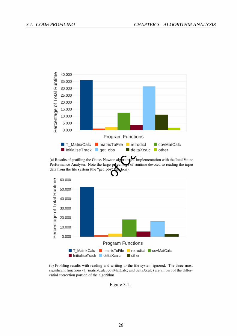
It was discovered that communication accounted for just over 30% with the Get_obs function takingup a significant part of the total running time. This function reads the simulated observation data forthe eight radar receivers from a text file and stores it in memory. As the focus of the project wasto investigate accelerating the Gauss-Newton algorithm itself, and the task of getting the data intomemory would most likely be handled differently in practise (for example, DMA from an ADC),this part of the program was ignored in the profile.

Of the remaining execution time, it was not surprising to find that the Gauss-Newton differentialcorrection (consisting of T matrix calculation, covariance matrix calculation, and the calculation ofδx) accounts for approximately 90%, making track initialisation and the MCA logic negligible incomparison. Within the differential correction section, the formation of the observation matrix ’T’is most significant. This is also to be expected; it exists within two nested loops, and must be donerepeatedly until the algorithm converges or the maximum limit of 50 iterations is reached, and thisfor each leg of the simulation. The T matrix calculation function was examined in more detail in thecall graph, and it was determined that of its child functions the calculation of the M matrix was mostsignificant within it. This function is called once for every observation within a leg (in our case,there are 80). The calculations of the partial derivatives in this function have to be done for eachreceiver, and account for the highest percentage of run-time within this function. Figure 3.2 presentspseudocode and a graphical display of the code sections of interest to illustrate this.

25

Univers

ity of

Cap

e Tow

n


(a) Results of profiling the Gauss-Newton algorithm C implementation with the Intel VtunePerformance Analyser. Note the large percentage of runtime devoted to reading the inputdata from the file system (the “get_obs” function).

(b) Profiling results with reading and writing to the file system ignored. The three mostsignificant functions (T_matrixCalc, covMatCalc, and deltaXcalc) are all part of the differ-ential correction portion of the algorithm.

Figure 3.1:

26

Univers

ity of

Cap

e Tow

n


(a) Pseudo code with the computational bottleneck highlighted in red. The Gauss-Newtonfilter’s computational intensity is made apparent by the multi-layered nested loops sur-rounding a significant chunk of arithmetic operations. The values in brackets in the right-hand margin represent the number of iterations for each loop.

(b) Visualisation of the percentage of total time spent in the functions of interest. The section ofcode to be implemented in reconfigurable hardware is highlighted in red. It represents 61% of the Tcalculation function, which accounts for approximately half of the total running time. The sectionto be offloaded to the FPGA is thus 32% of the complete tracking problem.

Figure 3.2:

It was thus determined that the place to start in accelerating the algorithm was the calculation of the

27

Univers

ity of

Cap

e Tow

n


partial derivatives which make up the M matrix.

3.1.2 Initial Bottleneck Analysis

The hotspot consists of a series of equations with no branching or control logic. The equations to beaccelerated are:

• Temporary variables:

A = (xx)+(yy)+(zz) (3.1)

B =√

x2 + y2 + z2 (3.2)

C = ((x− xk) x)+((y− yk) y)+((z− zk) z) (3.3)

D =√

(x− xk)2 +(y− yk)

2 +(z− zk)2 (3.4)

E =((x− xk)

2 +(y− yk)2)3/2

(3.5)

• Calculation and accumulation of residuals:

δY =

f − −2π

λ(A

B + CD)

cos(ψ)− (x−xk)D

sin(ψ)− (y−yk)D

(3.6)

δYAcc = δYAcc +δY (3.7)

• The partial derivatives of Doppler with respect to the x, y, and z coordinates:

δ fδx

=−2π

λ

[(xB

)−(

AxB3

)+(

xD

)−(

C (x− xk)D3

)](3.8)

δ fδy

=−2π

λ

[(yB

)−(

AyB3

)+(

yD

)−(

C (y− yk)D3

)](3.9)

δ fδ z

=−2π

λ

[(zB

)−(

AzB3

)+(

zD

)−(

C (z− zk)D3

)](3.10)

• Partial derivatives of Doppler with respect to the first derivatives of the states:

28

Univers

ity of

Cap

e Tow

n


δ fδ x

=−2π

λ

[( xB

)+(

(x− xk)D

)](3.11)

δ fδ y

=−2π

λ

[( yB

)+(

(y− yk)D

)](3.12)

δ fδ z

=−2π

λ

[( zB

)+(

(z− zk)D

)](3.13)

• Partial derivatives of the bearing angle observations (in the form of their sine and cosine) withrespect to x and y position:

δ sin(ψ)δy

=(x− xk)

2

E(3.14)

δ sin(ψ)δx

=−(x− xk)(y− yk)

E(3.15)

δ cos(ψ)δx

=(y− yk)

2

E(3.16)

δ cos(ψ)δy

=−(x− xk)(y− yk)

E(3.17)

where x, y, z are the target position coordinates and the subscript k is given to the positions of specificreceivers. The constant λ is the transmission wavelength of the system. The partial derivatives of thebearing observations with respect to velocity, as well as the partials involving any of the higher-orderderivatives, equate to zero and need not be calculated.

The required operators are thus standard arithmetic (add, subtract, multiply, divide), square root, andsine/cosine.

Initially we look for dependencies and duplication in the equations. First we note that temporaryvariables A and B do not depend on the target position relative to the individual receivers, and arethus common to the calculations for each receiver. We separate them from the rest of the calculations,and note that the rest (all the calculations that are receiver-specific) could be done in parallel for eachreceiver, and could be extended to include as many receivers as we wish.

We note that once the temporary variables have been calculated, the residual and partial equationsfor each receiver are also all independent, and can be performed simultaneously.

We also note that the Doppler partials (equations 3.8 to 3.13) consist of sets of identical operationsperformed on the three coordinates, which will simplify their implementation in hardware.

Finally we make the obvious observation that equations 3.15 and 3.17 are identical and need only becalculated once.

29

Univers

ity of

Cap

e Tow

n


Note the inclusion of the residuals calculation in this function. Although these have nothing to dowith the formation of the M matrix, it made sense to include them in this part of the code as theydepend on the same temporary variables A to D, as well as the relative positions of each receiver,which would otherwise have to be recalculated.

We then note that it is inefficient to offload everything in the hotspot to the coprocessor - to doso means that the host lies completely idle while waiting for its results. For maximum efficiencythe computational load should be as balanced as possible between host and device at all times.Unfortunately there is nothing outside of the ’getM’ function that can be done in parallel on the hostside, so we must choose something from within it. A detailed load balancing investigation was notcarried out, but it was decided to exclude the residuals calculations from the hardware design, andtreat them as part of the computation that would be handled by the host, for the following reasons:

• The residual calculations are a small percentage of the total work.1 It was decided that exclud-ing too little from the investigation would be safer than excluding too much, as it would beeasier to give the host more work in the event of an imbalance than to design more hardwarefor the device. We must also consider the fact that the offloaded section will be accelerated,so offloading only 50% of the work will result in an inefficient final design.

• As mentioned, the residual calculations are independent from the partials in that they do nothelp to form the M matrix, and so it makes sense to exclude them rather than some of thepartials, and avoid possible complications in synchronising the host and device work.

• Excluding the residuals means that we do not need to implement trigonometry on the FPGA.

Performing the residuals in parallel on the host side does however mean that there is some repetitionof work - namely the calculation of the temporary variables A to D.

Once the section of code to be ported to hardware was decided upon, it had to be considered in termsof its suitability for acceleration on the chosen hardware. The following aspects were considered,each examining whether either a specific strength of FPGAs could be exploited, or a weaknessavoided.

• Can parallelism be taken advantage of? The calculations have to be done for all observa-tions in a leg, a number of times until the algorithm converges, for each leg. Each iteration ofthe algorithm depends on the results of the previous iteration, so this is unfortunately inher-ently sequential and cannot be done in parallel. The legs are also inherently sequential; theyrepresent batches of data operated on in turn as they arrive from the radar system. Within eachleg are eighty observations for which the calculations are independent. However, perform-ing all the calculations in equations (3.1) to (3.17) eighty times, in floating-point, entirely in

1By doing a count of operators and making a rough adjustment for relative operator cost (weighting square root anddivision by a factor of three), the residuals account for 16% of the function.

30

Univers

ity of

Cap

e Tow

n


parallel is a lot to ask of even the largest current FPGAs, so we must look for more course-grained parallelism. From equation (3.3) onwards, all of the calculations must be done for eachreceiver, and most of them for multiple coordinates of the Cartesian system. These are all in-dependent tasks. Together with IPL, there is therefore much parallelism to be taken advantageof, even though the problem cannot be considered embarrassingly parallel.

• Can it be pipelined? This section of code can be considered a streaming or SIMD application- the exact same operations must be performed on a stream of data. There are there no branchesor loops within this section of code2, so it is ideal for pipelining. The eighty observations foreach leg which we cannot parallelise will instead make up the stream that flows through thepipeline3.

• Is there a high computation-to-communication ratio? The major bottleneck for most FPGAapplications is external communication, and ours is no exception. Unfortunately, for our cho-sen section of code we observe that that both input and output bandwidth requirements scalelinearly with the number of processing elements (PEs). One of the variables required for thecalculations is the position of the receiver, and this will be unique for every PE. The out-puts are also unique for each receiver and are not combined until much later in the algorithm.However, in this study we focus on the device-side design, and note that host-device com-munications as well as memory access speeds for FPGAs are an active field of research. Inaddition, with increasing fabric sizes we can soon expect to be able to port more work ontothe device, hopefully improving the ratio of work to communication.

• Is the problem data-intensive? One way to answer this question is to ask: Does the problemfit in the cache of a conventional microprocessor[35]? FPGAs have a much greater internalmemory bandwidth than CPUs, so to harness this strength, the problem should be too large tofit in the cache of a CPU. As a rough back-of-the-envelope calculation regarding this, we canconsider that the inputs to our code section are eighty of the the zeroth and first derivatives ofthe three position coordinates, as well as the constant positions of each of the eight receivers.If we transfer data in SP which is four bytes wide, the inputs alone require (80*6 + 8*3) * 4bytes for a total of 2kB. For the results of equations 3.1 to 3.17 one would need an additional14 registers for each of the 80 inputs, resulting in an additional 4,48kB and a total of 6.48kB.The L1 cache of the processor used for benchmarking our design was 32kB, and even thoughwe can expect many more registers to be necessary for the variables between input and output,the total will probably not exceed this. A more data-intensive problem would be better suitedto FPGA acceleration.

2This section of code itself does exist within a set of nested loops, which is not ideal. However, now that we havechosen the section to be accelerated, we consider it in isolation from the rest of the system.

3In addition, as is made evident in later sections, the latency of the pipeline will also be large in proportion to thelength of the data stream, so the benefits of parallelising all eighty observations are further diminished.

31

Univers

ity of

Cap

e Tow

n

3.2. ARITHMETIC ARRANGEMENT AND IPL CHAPTER 3. ALGORITHM ANALYSIS

• How does the data need to be represented? Because of their flexibility FPGAs are notrestricted to predefined data types and word lengths. For this reason they have been usedsuccessfully in applications where the data can be represented more efficiently than the datatypes of other systems allow. For example, in the bioinformatics problem of DNA similaritysearching, the four different nucleotides can be represented by 2 bits, whereas on a moreconventional processor the smallest data type is commonly 8 bits. In our application, wheredouble-precision floating-point would normally be used, we investigate the use of reducedprecision number formats for a more efficient design.

It should also be mentioned that although FPGAs have shown promising performance in linear-algebra applications [42, 47], conventional processors are already somewhat optimised for this bymaking use of vectorisation4, and GPUs are specifically designed with linear-algebra type prob-lems in mind. Our code hotspot is thus slightly more suited to FPGA acceleration as it is not anembarrassingly parallel linear-algebra problem.

3.2 Arithmetic Arrangement and IPL

The first step in accelerating the equations is to rearrange them so that they are calculated as effi-ciently as possible in hardware. This step should also be performed in software designs as significantperformance improvements can be made in this way quickly and easily.

Equations 3.1 to 3.17 were rearranged so as to minimise the number of operators required, and tominimise the use of more expensive operators such as divide and square root. For single precisionfloating-point, divide and square root operators can take up two to ten times as much resources asmultiplies[62], depending on DSP usage and latencies. As an example to demonstrate the savingsachieved, equation 3.11 as initially presented to the designer is reproduced here in a simplified form:

a = c[( p

B

)+( prel

D

)](3.18)

Where c is the Doppler constant, p is the target position presented as an input to the component,and prel is the position relative to the receiver calculated by an earlier stage. It was rearranged andimplemented in hardware as follows:

a =pD+Bprel

(1/c)BD(3.19)

Where 1/c is simply another constant precalculated and hard-coded into the design 5. This rearrange-ment replaces one division operator with three multiplies, at the cost of 16% longer latency in our

4In fact, recent studies[70] show that many quoted speedup values are exaggerated, as few researchers compare theirresults with code which is fully optimised on the conventional CPU.

5As an added bonus it so happens that 1/c is less than one, and thus needs no bits to represent its integer part.

32

Univers

ity of

Cap

e Tow

n

3.2. ARITHMETIC ARRANGEMENT AND IPL CHAPTER 3. ALGORITHM ANALYSIS

final design. A similar strategy was followed throughout the design, resulting in reduced logic re-source requirements and maximum potential use of dedicated DSP hardware on the FPGA (dividersgenerally cannot make use of DSP blocks, but multipliers can). As much ILP as possible was alsotaken advantage of for each component. For example, in this case the numerator and denominatorare calculated simultaneously.

After making the changes we are left with the final list of operations that make up our PE and are tobe implemented in hardware:

• Receive inputs:

– Target position: x, y, z

– Target velocity: x, y, z

– Position of each receiver: xk, yk, zk

– Temporary variables A and B, which are common to all PEs and will be calculated be-forehand.

• Calculate temporary variables:

prel = p− pk p ∈ {x,y,z} (3.20)

C = xxrel + yyrel + zzrel (3.21)

F = (xrel)2 +(yrel)2 (3.22)

D =√

F +(zrel)2 (3.23)

E =√

F×F (3.24)

• Calculate partial derivatives of Doppler with respect to position:

α =D3(B2 p−A2 p)+B3(D2 p−Cprel)

D3B3 p ∈ {x,y,z} (3.25)

• Calculate partial derivatives of Doppler observations with respect to velocity:

β =pD+Bprel

(1/c)BDp ∈ {x,y,z} (3.26)

In its original form 4 integer bits would be needed. A possible avenue for further investigation is the efficiency ofrepresentations throughout the algorithm in terms of bit width.

33

Univers

ity of

Cap

e Tow

n

3.3. NUMBER PRECISION INVESTIGATION CHAPTER 3. ALGORITHM ANALYSIS

• Calculate partial derivatives of bearing angle observations with respect to x and y position:

γ =(prel)

2

Ep ∈ {x,y} (3.27)

κ =−(xrel)(yrel)

E(3.28)

• For each receiver, return outputs:

– Doppler-Position partials: α = δ fδx , δ f

δy , δ fδ z

– Doppler-Velocity partials: β = δ fδ x , δ f

δ y , δ fδ z

– Bearing-Position partials6: γ = δ sin(ψ)δx , δ cos(ψ)

δy , δ sin(ψ)δy , δ cos(ψ)

δx

All changes that were made to the arrangement of equations were repeated in the software versionof the algorithm, so that comparisons and speedup calculations would be fair.

3.3 Number Precision Investigation

One of the major reasons for the computational burden that radar tracking filters present is that theygenerally require very high precision. Common practise (as with most scientific and engineeringsoftware) is to simply implement all operations in DP floating-point format for safety. This virtuallyeliminates the possibility of over- or underflow, and the precision of this number system is so fineover most of its range that it is not even considered an issue by designers. The designer treats thevariables as if they were real, with infinite precision, and has one less thing to concern himself with.

This makes sense in a microprocessor, with a dedicated FPU that is highly optimised. In an FPGA,however, it would be a great waste of resources, and would leave the main strength of the platform(its flexibility) under utilised. In fact, implementing the design proposed in this thesis in full 64-bitfloating-point would be impossible on even the most cutting-edge FPGA7.

The section of code to be ported to the FPGA was thus analysed in detail to determine the minimumnumerical precision required. Previous work by Joe Milburn [52] found that running the entirealgorithm in SP was not possible. Double precision accuracy was required to ensure that the iterativecorrection did not diverge. However, the possibility of running only certain sections of the code atreduced precision was not investigated.

6recall that δ sin(ψ)δx = δ cos(ψ)

δy , so there will be only three outputs representing the bearing partials.7It should also be noted that the inputs to a real system would ultimately come from an ADC - and precisions of more

than 16 bits for ADC outputs are rare. The entire system would thus be limited to the precision of its inputs, which woulddefinitely be less than single precision. Even in our original IDL simulation, the data comes from text files containingnumbers restricted 16 decimal digits in width.

34

Univers

ity of

Cap

e Tow

n


As a start, then, all variables in the code hotspot were changed from type double (DP) to type float(SP) in the C implementation. It was found that the algorithm still converged and worked properly,with final accuracies similar to those of the all-double version.

Investigation then continued, to determine if a further reduction in accuracy was possible. Two av-enues of investigation were followed: using a custom floating-point system with a reduced mantissalength, and a fixed-point number representation. Both methods were initially investigated in softwaresimulation, and are described below respectively.

3.3.1 Floating-Point

Reduced-precision floating-point operations were simulated by making use of a simple C function,included in appendix A. It works by simply setting the last few bits of its input variable to zero,effectively “blunting” the number to a lower precision. This operation was applied to the resultsof all operations in the partials calculation hotspot. All tests used the standard 8-bit exponent, andreduced exponent widths were not investigated as they do not save much in terms of hardware orcomputation time[31].8. Precision and range requirements could be further examined by taking eachequation or even each operator of the function in turn (using more than one word length in thedesign), but this was not investigated. With the help of a python script (included in appendix C), thealgorithm was then run for a range of simulated mantissa lengths and the results were compared tothe true state of the target to judge its performance relative to the standard single-precision version.The results are shown in figure 3.3a and 3.3b below. The poor estimation of the target altitude, z,is because of the small number of receivers in the simulation and their relatively uniform heights.The z estimations were similarly poor in the full-precision version of the algorithm. Increasing thenumber of receivers or arranging them with a range of different heights would have resulted in amore accurate estimation of z. Recall that a mantissa width of 23 is equivalent to SP floating-point -the rightmost result of each graph thus represents the performance of the original C code.

It can be seen that a clear knee exists in the graphs at a mantissa length in the region of 7 or 8 bits. Ofcourse, when using a finite dataset to characterise the behaviour of the algorithm, there is the dangerof over-fitting the design to the dataset, and for this reason all precision and range estimates hadorder-of-magnitude buffers added for safety (as seems to be common practise[31]). This requires 4more bits, so for a conservative design a mantissa length of 12 bits was chosen. According to thesesimulation results then, 8 exponent bits and 12 mantissa bits should be sufficient for the algorithmto work exactly as it does for full single-precision all the way through9.

8Later bit-true simulations of the design showed that the full 8-bit exponent was in fact necessary. Testing with a7-bit exponent resulted in overflows, and ultimately the algorithm diverging in most cases.

9We can also deduce from these results that number precision was not a contributing factor towards inaccuracy in theoriginal software implementation of the algorithm - a fact that was previously not known for certain.

35

Univers

ity of

Cap

e Tow

n


(a) Average errors in position versus mantissa width. Note the knee at a mantissa length ofapproximately 7 bits. The estimates for z are always much worse than for x and y; this isbecause of the number of receivers used and the fact that they lie on the same plane on the zaxis.

(b) Errors in the estimates of the first derivative. Note the similar knee at 7 bits for both x-yposition and altitude.

Figure 3.3:36

Univers

ity of

Cap

e Tow

n


The number of iterations before convergence for each leg was also examined, as it was suspectedthat lower precision would require more iterations to arrive at the answer, potentially nullifying thefinal speedup of the algorithm. It can be seen from figure 3.4 that although very low precisions doindeed result in longer times to convergence, there is again a knee at a bit width of approximately 7bits.

Figure 3.4: Plot of iterations to convergence for different mantissa widths. Values for less than 5 bitsquickly reached 50 (the imposed maximum) and are not shown.

3.3.2 Fixed-Point

The investigations for the fixed-point word lengths required were slightly more complicated thanthose for floating-point. The task is not trivial; in a recent survey conducted by AccelChip, Inc. (re-cently acquired by Xilinx), 53% of the respondents considered converting floating-point algorithmsto fixed-point to be the most challenging aspect of implementing them on an FPGA[39] (see figure3.5).

37

Univers

ity of

Cap

e Tow

n


Figure 3.5: Results of a survey conducted by AccelChip, Inc. Respondents were asked to indicatewhich part of implementing a floating-point algorithm on an FPGA they found most challenging[39].

Proprietary tools exist for fixed-point algorithm modelling: Matlab has a fixed-point toolbox[12] anda simulink toolbox [13] which provides bit-true simulations of fixed-point arithmetic designs usingwords up to 128 bits wide. It also provides useful tools such as automatic overflow and saturationdetection, customisable operators, and automated advisors for the conversion process.

Unfortunately these tools were not available, so alternatives were investigated. Many libraries andother resources exist for simulating fixed-point numbers of set widths[65, 68] (most are gearedtowards DSP programming, with 8- or 16-bit data types), but few support completely arbitrary wordwidths over the range that had to be explored. A library exists for python[16], and GNU Octaveoffers a fixed-point library[15], but this appears to be restricted to numbers 32 bits wide. Anotheroption for modeling fixed-point designs is SystemC language[18]. In the end an ’in house’ solutionwas developed, again using simple C functions, for ease of integration with the existing softwarewritten in C. It is included together with the functions for floating-point in appendix A. As thedataset used to characterise the data flow was quite large, C was also perhaps better suited to the taskas it is in general much faster than Matlab or python code.

In addition to this, it was possible to characterise the dataflow through the pipeline analytically usinginteger arithmetic and measurements of the input ranges. The two methods and how they were usedtogether are described below.

Software Simulation

The simulation functions convert a floating-point number to a floating-point representation of theclosest fixed-point value at a given range and precision. It was assumed that any fixed-point operatorimplemented in hardware would similarly provide the closest possible result to the true answer. Inthe case of an overflow or underflow, the largest representable positive or negative value is returned

38

Univers

ity of

Cap

e Tow

n


respectively.

This conversion was applied to the result of every arithmetic operation in the code hotspot, thus sim-ulating a fixed-point system using a single word length throughout the design. One notable short-coming of the simulation stage of the design was that only one form of rounding was investigated:round-to-zero.

A series of simulations were then run for a range of integer and fraction lengths. An exhaustivesearch of all integer-fraction combinations over the initial boundary estimates (0 to 40 for fractionlengths, 0 to 150 for integer lengths), would be impractical, and as it was assumed that there wouldbe no local minima of errors, the knee of the error-precision graph was located by successivelyfiner-grained searches.

The results showed a surprising spike just before the errors stabilise for increasing integer lengths(figure 3.3.2). After much investigation the exact reason for this remains unclear; the most likelyreason is that this is a region in which only certain variables in key equations overflow, which couldpotentially give far worse results than if more did. For example, if just the numerator or denomi-nator in a division overflowed, the answer could be very different from the ’1’ which would resultif both did. This is would explain why no such spike was found in the fraction length tests, or inthe floating-point investigations (overflow was not a problem with floating-point), but it is not con-firmed. Discovering the reason for the spike is complicated by the fact that the final errors are theresult of numerous iterations, and that for each iteration data flows not only through the reduced-precision hotspot, but through a considerable amount of conventional floating-point processing onthe proposed host side as well.

Regardless of the exact reason for the spike, it is clear that a 100 bit integer is enough for thealgorithm to function properly, and that the knee of the graph sits somewhere between 90 and 100.This means that throughout our design no variable ever leaves the range [(2100-1) : (-2100)].

For the fractional part, the results showed that for lengths shorter than approximately 13 bits thealgorithm could fail to converge, and the errors would sometimes diverge to infinity (or more specif-ically, NaNs). For lengths slightly longer than this the errors were very large (the worst of which isnot shown in the graphs), but a knee was found at a length of approximately 17 bits. In cases where afew of the simulations performed worse after the knee, we considered them to be outliers and choseaccording to the results of the majority for the best statistical performance.

A fixed-point number system with 100 integer bits and 17 fraction bits would therefore theoreticallybe enough for the algorithm to perform satisfactorily.

Because these simulations used only a single number format throughout the code hotspot, we havethus far discovered only the worst case requirements of the pipeline in terms of range and precision.In other words, we have determined the range required by the largest variable in the equations (100bits), and the precision required by the most sensitive (17 bits)10. In a fixed-hardware system where

10Note that the largest variable is not necessarily also the most sensitive

39

Univers

ity of

Cap

e Tow

n


(a)

(b)

Figure 3.6: Accuracies of X/Y position with varying word lengths, showing the unexpected spike inthe integer results for some of the simulations. At very short fraction lengths the algorithm failedto converge, and produced NaNs (not shown on graph). A subset of the results from measurementswith the entire dataset is shown; for the complete results, see appendix B.

40

100

100

30 20

50 70 90 110 130 150 40 60 80 100 120 140

Integer Length (bits)

"'Cessnax "'Cessnay ~ Helicopter x ... Helicopter y .. Performance Jet x 00(1. Performance Jet y .... Jet landing x '''' Jet landing y "'Jet straight x "'Jet straight y

+ Cessna_x ... cessnaJ ·9· helicopter_x ... helicopterJ ..... jet_x ... · jetJ .... jeUandinlLx .,.. jeUandinu ... jet_straight_x ... jecstraightJ

13 15 17 19 21 23 25 27 29 31 33 35 37 39

Fraction Length

Univers

ity of

Cap

e Tow

n


a few arithmetic units would be used and reused for all the calculations, they would have to be atleast of this size, but with an FPGA implementation it is wasteful and unnecessary to use a uniformnumber format over an entire fixed-point design (see figure 3.8), with the only saving being develop-ment time and effort. We thus investigate further to develop a custom datapath with different wordwidths for the various stages in the pipeline.

Dataflow Modelling

In addition to simulation and ’blindly’ profiling using the dataset, it is possible to analytically char-acterise the equations in terms of their range and precision requirements using integer arithmetic.

To this end, a measurement of the ranges of the inputs to the code hotspot was taken, saving theirmaximum and minimum values over the entire dataset to a file. The results are shown in table 3.1below. A rough initial approximation of the required resolution was also obtained by storing thesmallest value greater than zero.

x y z x y zMinimum -2.28e4 -2.35e4 -1.43e4 -97 -93.6 3.31e3Maximum 1.92e4 1.89e4 2.56e4 95.9 104 2.56e3

Smallest Positive 0.131 1.79e-3 3.29e-3 2.69e-4 7.01e-4 3.81e-4

Table 3.1: Maximum and minimum values of input variables to the code hotspot using the profilingdataset, along with the smallest positive value as a rough estimation of required precision.

From these results we can determine that we will need at least a format of 16:10 for the positioninputs11, and 13:13 for the derivative inputs. These values were verified by applying the conversionfunctions used in the earlier simulations to only the inputs, and testing the code on the dataset onceagain. Knowing the required input word sizes then served as a starting point for modelling the restof the pipeline.

It is a well known fact that to prevent overflow and retain precision with integer or fixed-pointnumbers, the result of a hardware multiply is twice as wide as its inputs. This rule of thumb isa subset of a more general sizing rule for fixed-point multiplication, and similar rules exist for alloperators. They are listed in table 3.2 below. By following these sizing rules throughout the design,one can be confident that overflows or underflows will never occur, and that the input precision willbe maintained.

These rules were programmed into a spreadsheet to model the dataflow. In this way various inputword lengths could easily be experimented with and their effect on later stages could be examinedconveniently.

Once the datapath was characterised in this way, the input widths obtained from table 3.1 wereentered, and the spreadsheet provided the necessary word widths for every variable in the pipeline.

11In twos compliment, 16 integer bits cover the range [-32768,32768], and 10 fraction bits have a resolution of 9.77e-4

41

Univers

ity of

Cap

e Tow

n


Operation Output Integer Width Output Fraction WidthAdd/Subtract max(Aint, Bint) + 1 max(Afrac, Bfrac)

Multiply Aint + Bint Afrac + BfracDivide Aint+Bfrac+1 Afrac+Bint

Square Root Aint/2 Afrac

Table 3.2: Table of number sizing rules, showing the output fraction and integer widths of operatorsA and B with integer lengths Aint, Bint and fraction lengths Afrac, Bfrac. [9]

All operators besides square root have results wider than either of their inputs, resulting in rapid bit-growth along the pipeline and the largest words right at the end of the equations. These unfortunatelyare the inputs to either division or square root cores, the most resource hungry elements of thedesign12. Figure 3.7 demonstrates this by showing the word sizes at each stage in one component inthe design.

Figure 3.7: Bit growth in the calculation of the Doppler-position partials. The inputs to the compo-nent are highlighted in yellow on the left, and their respective sizes are based on preceding stagesin the design. Note the unfortunate result that the most expensive operator (divide, on the extremeright) deals with the largest word sizes in the component.

As an additional test of the model, it was determined from the spreadsheet that one of the largestvariables in the pipeline is the B3D3 term marked in figure 3.7, with an integer length of 108 bits.This value makes sense if we recall the result for maximum range obtained by software simulation,and compare it with a likely value for B3D3: if our position inputs can be of the order of 3e4 metres,both B and D will be of order 5e4, and B3D3 will be of order 1.5e28 (See equations 3.2 and 3.4). thisrequires 94 bits to represent, which sits in the knee of the graph in figure 3.6a.

12See section 4.3 for more on this.

42

Univers

ity of

Cap

e Tow

n

3.4. CONCLUSIONS CHAPTER 3. ALGORITHM ANALYSIS

Note that strictly following sizing rules is a safe, worst-case design. There may be correlationsbetween variables which mean that certain ranges are in fact never reached, and these correlationsare only apparent when considering the equations as a whole. We also know from the simulationresults that our maximum integer and fraction lengths are smaller than the maximums reached in thedataflow model, so when the word widths reach this length we can safely shorten them to the lengthsdetermined by software profiling.

To show the savings made by using multiple word lengths in the design, Figure 3.8 contrasts theresource requirements of a flexible number format system with that of a design using the maximumword size throughout. The total number of register bits required to store all the variables at eachpipeline stage are shown. The resource usage of the hardware implementing the operations them-selves will also rise with rising input word size, making a flexible word size even more beneficial.

3.4 Conclusions

The code profiling confirms the conclusions of previous work, namely that the performance bottle-neck of the algorithm is the calculation of the partial derivatives that make up the sensitivity matrixM. Although this bottleneck section of code is perhaps not perfectly ideal for acceleration using re-configurable hardware because of its low communication to data ratio and the fact that it sits withinan unrollable loop, there is significant parallelism that can be taken advantage of, and by consideringit a streaming application we can create a deep custom pipeline for high throughput. In addition, soft-ware simulation revealed that the algorithm can tolerate a surprising reduction in dynamic range andprecision over this bottleneck portion of the code. In simulation at least, a floating-point number sys-tem with an 8-bit exponent and a 12-bit mantissa is sufficient. For fixed-point numbers, simulationshowed that a uniform number system with 100 integer and 20 fraction bits performed satisfactorily,and by making use of interval arithmetic a pipeline with multiple word sizes is proposed in order tofurther reduce hardware requirements.

43

Univers

ity of

Cap

e Tow

n

3.4. CONCLUSIONS CHAPTER 3. ALGORITHM ANALYSIS

(a)

(b)

Figure 3.8: Comparison of the total register bits needed to store the variables at each stage of thepipeline. Figure A shows the final design with flexible word widths, peaking at under 1500 bits,figure B shows a design using the maximum width throughout, peaking at over 6000.

44

.... . ~ Cl OJ c:: .l!l o I-

.~ III .... OJ .... . !!l Cl OJ c:: CIS .... 0 I-

1400

2 3 4 5 6 7 8 9 10 11

Operator Stage in Pipeline .x . xmin D Doplper Panial dot X . y . ymin D Doplper Partial dot Y • z D zmin • Doplper Partial dot Z . xdot .A • Doppler Partial X . C . ydot D squareds • Doppler Partial Y .D D B • zdot D Doppler Partial Z • dcos/dy and dsin/dx • dsin/dy • dcos/dx • Other

6000~-

5000

4000

3000

2000

1000

0 1 2 3 456 7 8 9

Operator Stage in Pipeline

10 11

• x • xmin D Doplper Partial dot X • ymin D Doplper Partial dot Y • z • Doplper Partial dot Z • xdot • A • C • ydot D squareds _D D B . zdot

• dcos/dy and dsin/dx • dsin/dy • dcos/dx

. y D zmin

• Doppler Partial X • Doppler Partial Y D Doppler Partial Z

• Other

12

12

Univers

ity of

Cap

e Tow

n

Chapter 4

System Design

This chapter describes the proposed hardware designs, and the process by which they were created.It details the various design choices made and the methods used to assist in making them. It beginsby discussing of the underlying concepts common to both designs, such as parallelism, pipelining,and efficient use of the dedicated FPGA hardware resources. It then proceeds to discuss the aspectsunique to each design, dealing with the floating-point and fixed-point designs in turn. Finally, itpresents the results of investigations into an alternative method of implementing the design using aVHDL fixed-point library.

4.1 Introduction

The equations were ported to hardware using arithmetic operator cores created with Xilinx COREGenerator[59], which is part of the ISE software toolkit used for programming Xilinx FPGAs. Thecores are all fully pipelined, with parameterisable latency. The designs are both pure hardwarearchitectures without the support of softcore microprocessors, and only a single clock domain wasnecessary.

Although the number precisions determining word lengths were decided upon early in the designprocess, both the fixed-point and the floating-point designs were implemented with parameterisableword lengths, both for safety in the event that the precision simulations proved inaccurate, and forease of later investigation into the effect of word length on the final design size. This parametrisationwas achieved for floating-point by simply storing the exponent and mantissa sizes in a VHDL pack-age included in all the source files, and defining all relevant signal and port widths in terms of these.For the fixed-point design, the signals and port widths for every stage are calculated in terms of thewidths of the preceding stage, according to the sizing rules given in table 3.2. Functions implement-ing the sizing rules were placed in a VHDL package, and the signal definitions which made use ofthem were also grouped together in this same package, in order to isolate the task of conforming tothe sizing rules as much as possible from the structural definition of the hardware. Constants such as

45

Univers

ity of

Cap

e Tow

n

4.1. INTRODUCTION CHAPTER 4. SYSTEM DESIGN

the Doppler constant used in calculating the Doppler partials, and the smallest representable value ofthe number system (to be used as a substitute for zero in division denominators) are also dependenton the word lengths and are calculated and stored in this package.

Although this successfully parametrised the HDL source code, for every change in word size theIP cores had to be regenerated using the Xilinx COREGen software. This would be a tedious andtime consuming process if done manually (especially for the fixed-point design, where most of theoperators required a unique core definition due to the changing word widths), but it was easy toautomate the task using python scripts (see appendix C), as the core parameters are stored in textfiles.

Figure 4.1 below displays a top-level view of both designs. Inputs are received in SP floating-pointfrom the host, converted to either reduced-precision floating-point or the initial fixed-point formats,passed through the pipeline, and finally the outputs are converted back to SP and passed to the host.

Figure 4.1: Diagram of the components making up the hardware design, showing their positions inthe pipeline and their relative size based on number of operators.

4.1.1 Parallelism

The design makes use of task-based parallelism which can be visualised in terms of three levels;first, the state vector must be processed independently for each receiver, and this represents our basicPE which can be duplicated for each receiver in a given PCL system. For each receiver the sameoperations must be performed, the only difference being the constant values for the specific receiver’s

46

Univers

ity of

Cap

e Tow

n


position in x, y, and z coordinates for the calculations1. The second level of parallelism exists withineach receiver’s hardware, where much of the work to be done consists of almost identical calculationsto be carried out for each of the x, y, and z components of the target’s position. Below this, as muchILP as possible is implemented for the operators in each of the equations. A simplified view ofthe component hierarchy is shown in figure 4.2, below to illustrate this. In addition note that thehardware making up the arithmetic cores themselves is as parallel as possible, although this is thecase with conventional hardware such as CPUs as well. In cases where this parallelism could becontrolled in our design (see section 4.2.1 below), it was always set to its maximum.

Figure 4.2: Three levels of task-based parallelism in the design: each instruction, within each posi-tion coordinate, within each receiver is parallelised.

4.1.2 Pipelining

All of the arithmetic cores used in the designs are fully pipelined. As the critical path of the designconsists of these arithmetic cores strung together in series, the entire design can be considered onelong pipelined from start to finish - a very deep pipeline with over 100 stages. Conventional CPUswould become very inefficient with pipelines this long, as control logic decisions such as branching

1For ease of testing and demonstration, these receiver position values are taken in together with the other inputs foreach sample in our design. In a practical system they could be hard-coded as they would remain constant, or be taken inthrough the input ports at start-up and saved at the cost of eight word-sized registers and a few extra clock cycles beforethe algorithm commenced.

47

Univers

ity of

Cap

e Tow

n


disrupt them and require the whole pipeline to be flushed before the program can continue2. How-ever, in our case we are free to make the pipeline as deep as we wish (within reason); we know thepipeline in our design will never be stalled in this way, and it was found that the pipeline depth hasnegligible affect on achieveable clock speed.

Since our design is to be fully pipelined it is important to determine the critical path of the workto be done, so that this can be optimised for minimum overall latency, and so that areas not on thecritical path can possibly be optimised in other ways such as hardware resource usage, at the ’free’expense of latency. The Gantt chart in figure 4.3 below shows the critical path of the design. It isbased on latencies for SP floating-point cores, and it was assumed that the latency ratios betweencores at lower precision and between fixed-point cores would be similar.

Figure 4.3: Gantt chart of the various components of the design. The critical path is in red, and thegiven values are latencies when implemented using Xilinx floating-point cores at SP. The calculationof A and B is not shown, as these are common to all receivers and will be calculated outside of theparallel PEs.

4.1.3 Shifting

A fully pipelined design means that a significant proportion of the hardware will have to be dedicatedto shifters, so that the various parallel branches of the data stream are kept synchronised. Twooptions were investigated for this purpose: a FIFO generator core, and a RAM based shift register,both available in the Xilinx ISE IP core catalogue.

To compare the two, the two floating-point designs were implemented and their synthesis resultscompared. One design used only the FIFO core, and one only RAM shifters. The results are shownin table 4.1 below, showing that the FIFO design was more efficient. It was thus the core used.

Another advantage of the FIFO core is that it allows for simpler implementation of a parameterisabledesign. As the latencies of the arithmetic cores depend on their input widths, experimenting with

2In [37], a detailed variable depth pipeline simulation tested 35 different workloads to find their optimum pipelinedepth. Most had a result between 21 and 24 stages. The results also indicated that the more modern workloads haddeeper optimum pipelines.

48

Univers

ity of

Cap

e Tow

n


RAM shifters FIFO shifters TotalUsed Utilisation Used Utilisation Available

Slice Registers 20635 29% 17797 25% 69120Slice LUTs 14589 21% 13107 18% 69120

Fully used LUT-FF pairs 12039 51% 10292 49% 23185

Table 4.1: Synthesis results comparing designs using FIFO and RAM-based shifter cores. The targetdevice was a Xilinx Virtex-5 XC5VLX110T and all synthesis options were set to default. Note theseresults are only for a single processing core, of which there would be one for each receiver.

different sized words at various points in the dataflow can become tedious if RAM shifters are used,as the latency of the core is fixed and has to be changed manually for each design. With the FIFO,read and write ports are simply connected to the control signals of preceding and following stages,and the design works for any combination of latencies in the arithmetic cores. The minimum sizeof a FIFO in depth is 512 bits, and any stage of the pipeline will have a latency well below this (infact, the maximum latency of the entire design is less than 512 clock cycles) so there is no danger oflosing synchronisation due to FIFO latency limits. There are however points in the pipeline where itwas necessary to specify shift latencies explicitly, as arithmetic control signals did not exist on bothsides of the shift. For this purpose the RAM shifter was used to shift a single control bit, and thiswas then used to control FIFO shifters.

Registers to be shifted were grouped together as much as possible to facilitate sharing of the FIFOprimitives. For example, in the top level view of the design (figure 4.1), the FIFO blocks shownrepresent the shifting of not one variable, but groups of as much as 11. Instead of instantiating aFIFO core for each variable, signals were concatenated and passed to one wide FIFO. A comparisonof floating-point designs combining signals in this way with ones instantiating separate FIFOs foreach variable showed that FIFO usage decreased from 71 to only 9 being used (an 87% saving), withan additional small saving in logic.

The FIFO core offers a feature known as first-word-fall-through. With this enabled, there is nolatency in a read operation and the control of the pipeline is simplified. First-word-fall-through wasenabled for all FIFO shifters in order to reduce latency and simplify control logic.

For the fixed-point design, the arithmetic cores could be set to have their latencies longer than theoptimal recommended latency. it was assumed that this simply added registers to the output ofthe optimal design, and so all fixed-point cores on the same stage of the pipeline simply had theirlatencies set equal to the core with the longest optimum latency. In this way the design was simplifiedand shifting resources were saved.

49

Univers

ity of

Cap

e Tow

n


4.1.4 Number Format Conversion

The Xilinx Floating-Point Operator v5.0 core[62] features an operator for conversion to and fromvarious floating- and fixed-point number formats. This core was used in both the floating-point andfixed-point designs. Alternatively, the conversion could be done in software on the host side, butas the conversion cores are relatively small and have short latencies it was decided that it could beimplemented in hardware to further reduce work on the processor side. Once the custom data pathdesign was completed, a wrapper component with converters for all the inputs and outputs of thesystem was simply added and made the new top level component of the design.

4.1.5 Use of DSP Blocks

For an efficient FPGA design it is important that as much of the dedicated hardware resources onthe device as possible are used. The major dedicated resources available on the Virtex FPGAs usedin this study are the FIFOs and the DSP multiply/accumulate blocks.

As the available logic and DSP resources can vary widely between FPGAs (even those of the samefamily), the design was made as parameterisable in its logic/DSP ratio as possible, opting for IPcores which allowed for control of their DSP usage.

In general implementations of the proposed designs there will be more operators than available DSPblocks, and most of the arithmetic will have to be performed using the reconfigurable logic of theFPGA. A decision then has to be made as to how the available DSP blocks are to be distributed. Indistributing DSP blocks, they should be placed on the critical path, so that the latency reductionsbenefit the design as a whole. Assigning them to operators with wider operands can also improvethe achievable clock speed.

The main benefit of making use of the DSP blocks in our designs is that they free up logic whichwould otherwise have to implement the operations. Their other benefits, such as latency reductionand faster clock speeds, are made less significant when the majority of the operations are imple-mented with FPGA fabric.

In Virtex 5 devices the dedicated DSP resources have a fairly course granularity: they are 25x18-bitmultiply-accumulates. Although many multipliers are easily cascaded to form bigger ones, one mul-tiplier cannot perform two different multiplies at once, and thus any multiplication where the inputsare not multiples of 25 or 18 bits wide results in inefficiency. It is noted in[31] that even a Pentiumprocessor has finer multiplication granularity than this, and since the main strength of reconfigurablehardware is supposed to be flexibility, finer-grained DSP hardware should be investigated for futureFPGAs.

50

Univers

ity of

Cap

e Tow

n

4.2. FLOATING-POINT DESIGN CHAPTER 4. SYSTEM DESIGN

4.2 Floating-Point design

4.2.1 Xilinx Floating-Point Cores

The Xilinx Floating-Point Operator Core v5.0[62] was used to implement the arithmetic for thefloating-point design.

Another option considered was the floating-point VHDL library by David Bishop[9], but it wasfound that while using VHDL packages which allow use of ’float’ type variables greatly simplifieddesign, the resource usage was too high - orders of magnitude more than when using cores. Thedesigner also has less control over aspects such as pipelining and DSP usage.

The floating-point core supports the following operators:

• standard arithmetic (multiply, divide, add/subtract)

• square root

• comparison

• conversion to and from fixed-point

• conversion between floating-point types

Which encompasses everything needed to perform the partial derivative calculations in section 3.1.All the operators are fully synchronous with only one clock, and fully pipelined. They can becustomised in terms of word length, latency, and interface. The multiply and add/subtract operatorscan also be customised for usage of the FPGA’s dedicated DSP hardware, though only if standardSP or DP is used for the case of add/subtract.

The core is compliant with the IEEE-745 floating-point standard, with only a few minor deviations3:

• Non-Standard Word lengths: The core supports number formats with exponent and mantissasizes outside of those specified in the standard.

• Denormalized Numbers: The IEEE standard extends the range of small numbers that can berepresented by allowing for denormalized numbers. When the exponent is zero, the implicit 1before the mantissa becomes zero, and the mantissa can represent numbers smaller than one.Such numbers are extremely small (in SP they are less than 2-126) and very rarely needed. Thecore treats numbers that would normally be denormalized as zero, and the datasheet mentionsthat an increase in dynamic range can be achieved on an FPGA using fewer resources bysimply increasing the width of the exponent[62].

3Note that similar simplifications are made in GPUs [10].

51

Univers

ity of

Cap

e Tow

n

4.3. FIXED-POINT DESIGN CHAPTER 4. SYSTEM DESIGN

• Rounding Modes: Only the default rounding mode (’Round to Nearest’) specified in thestandard is supported. Four additional modes are included in the standard. Although it is themost accurate, this rounding mode needs an extra adder in the critical path.

• Quiet NaNs: If a NaN (Not a Number) is given as one of the inputs to the core, the outputwill be a NaN, and no exception will be raised. The standard requires both ’Signaling NaNs’(where invalid operation exceptions are raised) and quiet NaNs. There are a total of five differ-ent exception types in the standard: invalid operation, division by zero, overflow, underflow,and inexact. The cores do not handle these differently, and simply produce NaNs at theiroutput for any exception case.

All cores can be parametrised in terms of latency, allowing designers to explore a tradeoff betweenresource usage, clock speed, and latency. For our designs, all were set to maximum latency in orderto maximise the potential clock speed and to reduce the hardware resources needed, as the abilityto fit more operators on the FPGA was considered worth the cost of extra latency cycles in a fullypipelined design. The deep pipeline also makes performance very sensitive to clock speed.

While most of the operators are able to produce an output at every clock cycle, the divides and squareroots have a “cycles per operation” parameter that can be set in order to reuse hardware and saveresources. In all instances, both were set to produce an output at each cycle - this resulted in a fullyparallel component that consequently required more resources, but as one of the goals of the designwas to exploit as much parallelism as possible this was seen as an acceptable tradeoff. Accordingto the core datasheet, increasing this to two operations per cycle would reduce the resource usage ofthe cores by approximately half[62], but in our design would shave less than an estimated 5% offof the total resource usage, and because the pipeline needs to remain synchronised this would alsoslow down the entire design by a factor of two. An experimental design with two clock domainswas investigated, where the divide and square root components were clocked at twice the frequencyof the rest of the design. As expected, this simply halved the speed at which the design could beclocked.

4.3 Fixed-Point Design

Although not part of a combined package as the floating-point cores are, Xilinx offers an array ofcores useful for fixed-point design including:

• add/subtract

• multiply

• multiply-accumulate

52

Univers

ity of

Cap

e Tow

n


• multiply-add

• divide

All the fixed-point cores used in the design actually perform integer operations, and the hardwaredoes not explicitly keep track of any radix point. The only points at which the radix point position isrequired explicitly are in the conversions to and from floating-point, and these were obtained fromthe spreadsheet modelling the dataflow mentioned in section 3.3.2. The spreadsheet was also usefulas a debug tool to determine the position of the radix point at different points in the pipeline duringdevelopment.

As Xilinx do not offer a fixed-point package in a single IP core, solutions had to be found for eachof the operations separately. They are discussed in turn below.

Multiply-Accumulate and Multiply-Add

In addition to standard arithmetic Xilinx offers Multiply-Accumulate and Multiply-Add cores forinteger/fixed-point numbers in its IP catalogue. These cores are useful as the operations are commonin DSP applications, and the DSP blocks are in fact multiply-adders so these cores enable moreefficient usage of the hardware.

By inspecting the dataflow of our design and doing a count of the operations, we calculate that ifthe multiply-accumulate core is made use of wherever possible, we can make significant resourcesavings: it would result in replacing 13 adds and 24 multiplies with 12 multiply-accumulate cores.For multiply-add, we can replace 13 adders 13 multipliers with 13 multiply-adders and some extrashifting overhead.

Although these savings could be made, it was decided to stay with separate add and multiply coresas with the floating-point design. Use of the multiply-accumulate core would disrupt the deep,synchronous pipeline. Furthermore, the core amounts to hardware-reuse, which goes against thegoal of maximum parallelism. For multiply-add, the reason was also twofold; firstly, the savings arenot as significant as one would expect; 7 DSP blocks, roughly 1344 LUTs and 2352 flip-flops wouldbe saved4, if we ignore the additional shifting overhead. Secondly, the multiply-add core cannotbe parametrised in terms of its DSP usage, possibly limiting the range of FPGAs that the designcould be implemented on. Being able to control the fabric/DSP usage ratio of the design as much aspossible makes the design more portable.

4Between 6 and 12% of the final design, see section 6.2.1.

53

Univers

ity of

Cap

e Tow

n


Square root

For the task of square root the COordinate Rotational DIgital Computer (CORDIC) algorithm wasused5. Xilinx offer a CORDIC core[60] which can be used for a number of operations, including:

• vector rotations

• vector translation between polar and rectangular coordinates

• basic trigonometry

By virtue of the fact that vector translation involves an implicit square root (the magnitude of a polarvector is equal to the square root of the sum of its rectangular coordinates), the core also offers alightweight square root operation.

The core can perform either an integer or a fractional square root. For the fractional case, the inputmust be expressed as an unsigned fixed-point number with an integer width of 1 bit[60]. For ourpurposes, therefore, some scaling and re-interpretation of the data was required. The core datasheetprovides information on how to do this, and it is discussed in appendix D. For our design the hard-ware requirements of this scaling amounted to two right-shifts, implemented combinatorially on theinput and output of the CORDIC core at negligible cost.

As the input is an unsigned number the core does not handle the exception case of a negative input.In our design, we observe that all the inputs to square root operations are the sums of squares (seeequations 3.1 to 3.5) and can never be negative. We therefore need not concern ourselves with thisexception case.

Another thing to note from equations 3.1 to 3.5 is that the only need for the square root operation inour design is for the calculation of the Euclidean Norm, or the magnitude of a vector in 2D and 3Dspace. Although the CORDIC operator does this directly when converting from rectangular to polarcoordinates, the Xilinx core works only in two dimensions. Extending the CORDIC algorithm to 3dimensions is not straightforward, mainly due to lack of analytical expressions for the convergenceof the algorithm[28], which would be necessary in order to build a core which does not disrupt thepipeline. For this reason it was decided to use the CORDIC core as a square root operator for the 3Dcases. In the 2D case (equation 3.5), the calculation of the sum of squares has to be done anyway6,so there would be no hardware saving in using CORDIC to do a vector translation instead of a squareroot. By performing the vector translation we can reduce the latency in performing the calculation,but recalling that this equation does not form part of the critical path (see figure 4.3), we stay with asquare root to simplify the design.

5This algorithm was widely used in early pocket calculators, another application where the minimisation of hardwareresource usage was a key goal.

6Recall that to calculate x3/2we multiply x by x1/2 (equation 3.24).

54

Univers

ity of

Cap

e Tow

n


Division

Xilinx offer an integer divider core in their IP catalogue[63] which implements hardware basedon a choice of two different division algorithms: Radix-2 Non-Restoring, and High-Radix division.Radix-2 is more efficient for shorter word sizes, while the High-Radix option is more suited to longerwords.

After investigations making use of this core it was decided that the division be done in floating-point.The design is thus a hybrid and not purely fixed-point, initially converting its inputs to fixed-point,then to a custom floating-point format as used in the floating-point design, and finally to single-precision in order to pass the results back to the host machine. There were three major reasons forthis decision, and they are discussed in turn below.

1. The divider core has a maximum input word length of 54 bits. Unfortunately, as observed infigure 3.7 our design results in dataflows which have the largest word sizes before and after thefinal divide operations, and in all instances (except the Doppler-velocity partial component)this is larger than the core can accept.

2. We recall that the outputs of the system have to be converted back to floating-point anyway atsome stage, in order for them to be used by the host machine. The divide is the final operationin the equations, and so is the only one that is affected by a conversion to floating-point beforeit. We therefore would not save on any conversion hardware by postponing the conversionuntil after the divide, besides the final float-float conversion converting the reduced precisionformat to SP. As we show in section 6.2.1, the logic footprint of this conversion is relativelysmall.

3. At these word sizes, the floating-point divider is in fact less resource hungry than the fixed-point version. Table 4.2 compares the floating and fixed-point division cores investigated.From it we can observe that at its maximum word size, the fixed-point core is worse than thefloating-point option in almost every respect. The two fixed-point cases shown differ onlyin their latency parameters, which in turn affects resource usage and achievable clock speed.Case 1 achieves a high clock speed at the expense of resources and latency, while case 2 lowerslatency and resource requirements but results in an acceptably low clock speed. Note also thehigh DSP requirements of the fixed-point cores compared to the floating-point core whichuses none. The savings achieved by using the intermediate reduced-precision format can beseen to be considerable. If the floating-point cores were able to produce outputs with differentprecisions to their inputs, the additional float-float conversion cores could have been avoided,but even with the cost of the extra converter the reduced-precision option was more efficientthan SP.

Note that at lower word sizes, requirements for the fixed-point core drop off sharply: for inputs 36bits wide less than half the resources are used[63]. This may mean that there are potentially more

55

Univers

ity of

Cap

e Tow

n

4.4. INVESTIGATION USING BISHOP LIBRARIES CHAPTER 4. SYSTEM DESIGN

Single Precision Reduced Precision fixed-point fixed-pointfloating-point floating-point Case 1 Case 2

Input Bit Widths 32 21 54 54Output Bit Widths 32 21 54 + 28 54 + 28

LUT-Flip Flop pairs 1407 547 1693 1091LUTs 780 303 1398 1009

Flip Flops 1367 492 1649 266Clock Speed (MHz) 381 426 337 47

Latency 26 16 43 8Block RAMs 0 0 1 1

DSP48s 0 0 17 17

Table 4.2: Comparison of the Xilinx floating-point and fixed-point dividers in terms of per-formance and resource requirements based on device data sheets[62, 63] and experimentalsynthesis. Quoted results are from builds on a Virtex 5 XC5VLX30-1 and XC5VSX35T-1for floating- and fixed-point respectively. Both fixed-point cases implement the High-Radixalgorithm, which is recommended for word sizes larger than 16. All cores are fully pipelinedand produce an output at every clock cycle.

efficient designs which use more dividers, but smaller, fixed-point ones placed earlier in the pipeline,before bit growth has progressed to its maximum. Our focus in this study was simply to minimisethe total dividers, and investigating this additional dimension in the solution space is left to futurework.

The point at which floating-point operations become more efficient than fixed-point was found to beeven earlier than division for one component in the design. In the Doppler-position partials, the wordwidths become too wide for the fixed-point cores two stages before the final division. Investigationshowed that, as for division, at these widths the floating-point cores were also less resource hungry.In this component we thus used not only floating-point dividers, but a total of four multipliers andone adder as well.

4.4 Investigation Using Bishop Libraries

An implementation of the algorithm making use of the floating- and fixed-point VHDL library byDavid Bishop[22] was also investigated. The library offers all the standard arithmetic operations,and conversion and resizing functions. It also offers a choice of rounding modes and can createboth signed and unsigned fixed-point hardware. The library is now part of the standard VHDL-2008support package, but as the ISE development environment still uses VHDL-93, older versions of thelibrary were downloaded from the project website[9] and used.

It was found that the libraries are not well suited to the XST synthesis software used, and the librarywebsite confirms this and recommends using alternative synthesis tools[9]. As a square root operator

56

Univers

ity of

Cap

e Tow

n

4.4. INVESTIGATION USING BISHOP LIBRARIES CHAPTER 4. SYSTEM DESIGN

is not provided, and XST cannot synthesis the hardware for the division operator in this library, theXilinx cores had to be used for this as in the other fixed-point design.

A major problem with the libraries is the fact that all of the operators are combinatorial. As a result,when medium to large word sizes are used the achievable clock speed is very low when comparedto implementations making use of fully pipelined cores.

It is also much more difficult to control the distribution of dedicated hardware resources such as DSPblocks, and synthesis settings had to be carefully tweaked such that the design did not require moreDSP blocks than what would be feasible on hardware.

Development time using the library was much shorter than manually connecting a series of IP cores,and an implementation using the libraries with more suitable synthesis tools is recommended forfuture work. Having the package included in future hardware development environments would alsohelp.

Slice Registers 20049LUTs 70710

Block RAM / FIFOs 3DSP blocks 120

Clock Frequency (MHz) 56.5Latency 72

Table 4.3: Summary of the fixed-point design making use of the Bishop libraries, based on synthesistargeting a Virtex-5 xc5vlx330t FPGA. When compared with the final results of the designs usingIP cores (see results section) the design was found to be inferior.

The design was a simplified version of the one using the Xilinx cores, and used a fixed word sizethroughout which was set to the average width of the multi-width design: an integer length of 30and a fraction length of 5. It would thus not work in practise and served only as a brief investigationinto the possibility of making use of the library. Note the amount of DSPs used - this is significantlyhigher than what was used by the final designs using the cores despite comparable fabric use. Theclock frequency is also very low compared to the final designs. The latency is almost doubledbecause of the necessary use of IP cores for division and square root. Were it not for this thethroughput might have been comparable to the IP cores design, even with the low clock speed, butas it stands the bishop library design is clearly inferior, at least on Xilinx hardware, and so was notinvestigated further. It does however exhibit a number of advantages such as quicker developmenttime and portability across different FPGA hardware, and a closer look at a design using theselibraries is suggested for future work.

57

Univers

ity of

Cap

e Tow

n

4.5. CONCLUSIONS CHAPTER 4. SYSTEM DESIGN

4.5 Conclusions

Two hardware designs making use of Xilinx IP cores are proposed: one using reduced precisionfloating-point, and one being a hybrid fixed/floating-point design with multiple fixed-point formatsand in which the last few operations of the pipeline are performed in reduced precision floating-point. The designs are both fully pipelined and present output at every clock cycle once the pipelineis full. Both designs are as parallel as possible, with no hardware reuse along the pipeline, and nosupport from a softcore processor.

58

Univers

ity of

Cap

e Tow

n

Chapter 5

Implementation

We now discuss the implementation, verification and testing of the design. First, we describe thetools and methods used in implementing the design, and then discuss how it was verified by compar-ing its outputs to those obtained by a DP floating-point software implementation of the calculations.We then discuss the testing phase, in which a simulated system was created by interfacing C codewith hardware simulations, and a portion of the design was implemented on a Virtex-4 FPGA housedon a Nallatech PCI-X coprocessor card.

5.1 Implementation

The design was iteratively coded, simulated, synthesised, and verified using ISE 12.1. The ISE de-velopment environment integrates the various tools necessary for FPGA development such as sourcecode syntax checking, synthesis, and place-and-route to create the final bitstream to be implementedon the device. It also provides a host of analysis tools for timing, power, and resource usage analysis.

5.1.1 Coding

The design was implemented in VHDL as opposed to Verilog due to familiarity with the language.Besides the case of the investigation using the Bishop fixed-point libraries, the same designs couldjust as easily have been implemented in Verilog, and ISE in fact allows for designers to mix the two.Coding was mostly a relatively simple matter of instantiating cores generated with the COREGensoftware and wiring their data and control ports. Python scripts were made use of to automate someof the more repetitive parts of the coding process, but more high-level methods such as making useof the schematic editor feature of ISE or languages such as MyHDL could perhaps have sped updevelopment.

59

Univers

ity of

Cap

e Tow

n

5.1. IMPLEMENTATION CHAPTER 5. IMPLEMENTATION

5.1.2 Simulation

The Isim simulation software package, which is provided as part of the ISE development environ-ment, was used for all hardware simulations. Isim provides the designer with a helpful GUI interfaceto display signal waveforms, and by visual inspection of control signals the proper functioning of thepipeline could be verified. ISE also allows the designer to view a post-synthesis Register TransferLevel (RTL) schematic of the design, in order to visually confirm that the synthesis process has gen-erated hardware as intended at this level of abstraction. Black-box testing was performed for eachcomponent of the design; component outputs were converted from binary to floating-point decimalwith the help of python scripts, and compared to expected results from the software version of thealgorithm.

5.1.3 Synthesis

Xilinx Synthesis Technology (XST) software was used for hardware synthesis. Synthesis can beconsidered the hardware equivalent of compilation, and converts source code into a netlist which isused by the place-and-route process to map the design to the FPGA fabric.

The Xilinx IP cores which make up the design are generated as “black box” components, whichare pre-synthesised. When the HDL compiler comes across a component declaration with a ’blackbox’ attribute, it looks for the pre-generated netlist file instead of VHDL source code, and uses thenetlist directly for synthesis without having to compile the source first. A warning is displayed,but otherwise the compiler proceeds on the assumption that the component is error-free when acomponent is synthesised in this way. This results in greatly reduced synthesis times for the designand accelerated development.

There is one major downside to making use of pre-synthesised black box components, however: itmeans that possible trims and hardware savings unique to our design are not taken advantage of inthe place-and-route process. For example, in their investigation of a custom euclidean norm operatorfor FPGAs, [31] reported that significant resource savings were achieved simply by resynthesisingthe arrangement of floating-point adders, multipliers, and square root hardware from the source codeinstead of implementing black boxes. The synthesis software was able to automatically eliminateunnecessary hardware such as that required for negative results from squarers. As the proprietary IPprovided by Xilinx is exclusively black-box, our design unfortunately misses out on these potentialbenefits. With access to the source code the entire design could be more efficient in terms of resourceusage.

Synthesis/toolflow options

An FPGA design does not end with HDL description; synthesis, mapping, and place-and-routeare complex processes which should be considered closely for an efficient design. Once the design

60

Univers

ity of

Cap

e Tow

n

5.2. VERIFICATION CHAPTER 5. IMPLEMENTATION

was completed, synthesis and mapping options were experimented with, setting them to optimise forarea or speed, and noting the effect of enabling options such as register duplication (which replicatesregisters to help reduce fanout) and retiming (which rearranges registers to improve timing results).Experimenting with these parameters is something of a trial-and-error exercise, as the results are notalways as expected. For example, builds set to optimise for speed resulted in even lower clock ratesfor our design. Although an extensive search of build-strategies was not carried out, it was foundfrom the tests performed that the default settings produced satisfactory results, with a good balancebetween resource requirements and timing performance.

5.2 Verification

Hardware verification was performed using hand written VHDL test benches and Isim. A few outputvalues were verified manually, and python scripting was then used to perform a more realistic testusing data obtained from runs of the C implementation of the algorithm.

Using the software version of the algorithm, input and output values of the code hotspot were savedto text files to an accuracy of 50 significant digits for every simulation in the dataset. In order toreduce this data to a practical size, only every tenth input-output pair was used for verification, asneighbouring pairs tended to be very similar. These were converted to text versions of their binaryrepresentation in python (script included in appendix C), and this was then passed to Isim to be usedas inputs to the test bench. The Isim behavioural simulation produced another text file containingbinary representations of the hardware outputs, and these were read by the python script, converted tofloating-point numbers, and compared with the results of performing the calculations in DP floating-point in python. The process is shown in figure 5.1.

It was not determined exactly how close to the software results the hardware would have to be atthis point in the code for proper functioning of the complete algorithm, and the comparisons wereonly done on an iteration-by-iteration basis i.e., each iteration was verified in isolation, withouttaking into account the fact that in practise the iteration inputs depend on their own previous outputs.Nevertheless, errors of less than 1% for all outputs was achieved on average, and this was assumedto be sufficient to proceed.

5.2.1 Implementation Experiment on Coprocessor Card

The concept of accelerating computation with FPGA based coprocessors is not a novel one, anda variety of coprocessor platforms have been commercially available for years. One such productis the H101-PCIXM Accelerator card from Nallatech[14]. It is a PCI-X expansion card housing aXilinx Virtex-4 FPGA as well as external memory and off-card serial I/O. The specifications of thecard and the FPGA it houses are given in table 5.1b and 5.1a respectively.

61

Univers

ity of

Cap

e Tow

n


Figure 5.1: Block diagram of the verification process.

62

Python 5.68 ... ~ ~ 1011 ... Ilccmvert doubles 7.32 ... ~ ~ 1110... binary strings)

nIlJ ....

Python 1010 ... ~ ~ 7.69... (convert binary 1011... ~ ~ 12.6... strings to

doubles)

Data Set (Inputs)

Compare Outputs

Errors

x = (a+b)/c y=x+12

Univers

ity of

Cap

e Tow

n


A section of the floating-point design was tested by running it on the card. Although a completesystem with communication between the C implementation of the algorithm and the card was notimplemented , implementing it on physical hardware served as a final verification of the design. TheVirtex-4 series of FPGAs was introduced in 2004, and is thus starting to show its age when comparedto the more recent Virtex-5 and Virtex-6 series. As it was not big enough for 8 instances of the entireprocessing core, a subset of it was implemented, namely the Doppler-velocity partials calculations.For this subsection 8 instances could be implemented in parallel for a slightly more realistic proofof concept.

Virtex-4 LX100Slices 49152

Max. Distributed RAM bits 786432Total Block RAM (kbits) 4320

Max Select I/O 960DSP blocks 96

(a)

Nallatech H101Form Factor 64-bit/133MHz PCI-X

Host Bandwidth Up to 400MB/sFPGA Xilinx Virtex-4 LX100-10

SDRAM Memory 0.5GB DDR2 SDRAMSRAM Memory 16MB DDR-II SRAM

Serial I/O 4x 2.5Gbps via PCI backplate(b)

Table 5.1: specifications for the Nallatech H101 Accelerator card and the Xilinx Virtex-4 LX100FPGA it houses.

Nallatech also offer an FPGA development environment known as the DIME toolchain. This con-sists primarily of DIME-C, a C-to-VHDL compiler, and DIMEtalk, GUI-based a design tool whichabstracts away much of the hardware design details. DIMEtalk was made use of for programmingthe FPGA. A project was created in DIMETalk with nodes for a clock controller, PCI interface core,and FIFOs for each input and output stream. The ISE project was then imported and connectedas a ’user VHDL component’. In order to do this the project was first synthesised as a black box,and this was then imported to the DIMETalk framework, treating the design as a single core. FIFOprimitives were instantiated in DIMETalk as opposed to the other I/O options (BRAMs or the on-board SDRAM) as this improved latency and simplified control logic. Although the GUI interfacedoes simplify development, ports still have to be connected manually and this can involve tedious,repetitive work. The DIMETalk network is shown in figure 5.2 below.

It was found that the major limitation of the Virtex-4 FPGA for our design was the number of DSPblocks. For our design the number of multipliers exceeded the number of DSP blocks and they hadto be used sparingly, with only 12 DSPs available per PE. The operators to be allocated a DSP blockwere chosen such that the savings in latency would shorten the critical path and thus benefit thedesign as a whole. All 96 of the DSP blocks were used by multipliers.

After a comparison with results from performing the calculations in DP floating-point in software,The design was found to perform as expected in terms of accuracy, with all outputs within 1% oftheir software equivalents.

63

Univers

ity of

Cap

e Tow

n

5.3. TESTING CHAPTER 5. IMPLEMENTATION

Figure 5.2: DIMETalk network created to facilitate programming the Nallatech coprocessor card.For simplicity much of the wiring has been removed - in the actual design every port of the GNdesign (the pink component at left) had to be manually connected to a FIFO block.

5.3 Testing

Testing is distinct from verification in that where verification checks whether what has been built iswhat was originally intended, testing checks whether what has been built performs properly. Ourverification steps confirmed that the equations were being performed correctly in isolation, and ourtesting stage checks if the integrated system works correctly, with data communicated between thehost and device.

A simulated system was tested by making calls to the same Isim simulation described in section 5.2from within the C code for every iteration of the algorithm, with data communicated via text files asin the verification stage. Figure 5.3 displays the system.

This provided a realistic simulation with a bit-true representation of the custom number system,although of course no information about potential speedup was acquired in this way as the Isimsimulations are much slower than the actual device would be. The system was tested using all thedata from the dataset, and in all cases was found to perform just as well as the original softwareversion in terms of precision. The results are presented in chapter 6.

64

Univers

ity of

Cap

e Tow

n

5.3. TESTING CHAPTER 5. IMPLEMENTATION

Figure 5.3: Block diagram of the testing process. The original software version of the algorithm wasedited such that the calculations were performed by an Isim simulation for every iteration.

65

Start

Initialization -........... ~ ........

1 Inputs

/ " GN algorithm

V Conversion

Float ~ ~ Text

"/ ~ Isim File

::~ Simulation System

~ ::: /~ "- Conversion

Text ~ ~ Float

No Outputs

Stop? ./ V~

Yes .-/ Save Output -

For one leg

For all legs

End

Univers

ity of

Cap

e Tow

n

5.4. CONCLUSIONS CHAPTER 5. IMPLEMENTATION

5.4 Conclusions

Both designs were successfully implemented in HDL targeting FPGAs, with verification showingthat they perform almost identically to the software version in terms of accuracy. This verifiesthe algorithm profiling described in section 3.3. The simulated system used for testing has beendescribed, and a section of the design was also programmed on to a Virtex-4 FPGA on a Nallatechcoprocessor card, and its functionality was verified.

66

Univers

ity of

Cap

e Tow

n

Chapter 6

Results

We now present the results of implementing the design. First we discuss the results in terms of thefilter accuracy, and show that both the reduced-precision floating-point and the fixed-point designperform just as well as the original software version. We then discuss the final hardware designs interms of four metrics: resource usage, achievable clock speed, pipeline latency, and power consump-tion. Finally we present a theoretical speedup, based on the latencies and achievable clock speeds ofthe designs and on the latencies of available host-device communication options.

6.1 Accuracy Results

It was found that the performance in terms of accuracy of the reduced precision implementationwas very close to that of the original double-precision code. Figure 6.1 compares the accuraciesof the final filter outputs for the fixed-point, floating-point, and original software implementations,as well as the average number of iterations to convergence. A closer look at the data is includedin appendix E. It can be seen that the accuracies are on average very similar for all outputs and allimplementations. There is however a slight increase in the average iterations till convergence in thefixed-point implementation.

6.2 FPGA Hardware

We discuss the results of implementing the hardware designs in terms of four metrics: resourceusage, achievable clock speed, pipeline latency, and power consumption.

6.2.1 Resource Usage

A comparison of resource requirements for the two designs is surprising in that the fixed-pointversion requires more resources than the floating-point version. It was found that the major reason

67

Univers

ity of

Cap

e Tow

n

6.2. FPGA HARDWARE CHAPTER 6. RESULTS

Figure 6.1: Average error comparison for output variables, and a comparison of the average iterationsto convergence over the entire data set.

for this is that the conversion from floating-point to fixed-point requires much more hardware thanconversion from one floating-point format to another. This makes sense intuitively - in our floating-point design, because the exponent width remains 8 bits, the conversion to our floating-point formatsimply involves discarding a few of the least significant mantissa bits, and using the conversion coresat all was perhaps unnecessary.

In addition to this, on the fixed-point side there is the fact that more than one fixed-floating conver-sion is performed for every output. Recall from section 4.3 that the final operations of the design aredone in floating-point, and thus both inputs to the cores have to be converted. There is also the finaladditional conversion back to single precision from the custom format. For the fixed-point design thecost of conversion hardware amounted to 7920 slice registers and 5978 LUTs, whereas the floating-point design used only 1240 slice registers and 1003 LUTs (the conversion cores do not make useof any dedicated hardware such as DSP blocks). Results from synthesis showing the difference inconversion resources is given in table 6.1

The number of FIFO primitives used on the FPGA is much lower than the number of instantiatedcores (of which there are more than 20). It was initially assumed that this meant not all instantiatedcores were making use of the FIFO hardware, but further investigation revealed that the amount oflogic (in addition to the FIFO hardware) used for shifting is much less than what one would expectif shifters were being implemented in logic. This suggests that the synthesiser is able to share FIFOhardware between multiple FIFO cores. The FIFO primitives are 1024 bits wide and 512 bits deep -none of the instantiated cores ever have to use even half of this.

When synthesising only the hardware for the arithmetic cores themselves, the fixed-point design was

68

1000~

"'"' 100 ~ E E 10 '-" .... e 1 .... .... w

0.1 X and Y Z Xdot and Ydot Zdot Iterations

Output Variable

• Fixed-Point • Floating-Point D Software

Univers

ity of

Cap

e Tow

n


Synthesis Floating-Point Floating-Point Total AvailableMinimum DSP Maximum DSP LX330T LX110T SX95T

Slice Registers 23856 16576 207360 69120 58880LUTs 19576 11736 207369 69120 58880

Slice Registers (conversion) 1240 1240 - - -LUTs (conversion) 1003 1003 - - -

BRAM / FIFOs 9 9 324 148 244DSP blocks 0 80 192 64 640

Clock (MHz) 262.8 262.5 - - -Latency 115 118 - - -

(a)

Synthesis Fixed-Point Fixed-Point Total AvailableMinimum DSP Maximum DSP LX330T LX110T SX95T

Slice Registers 37470 20329 207360 69120 58880LUTs 31774 14836 207369 69120 58880

Slice Registers (conversion) 7920 7920 - - -LUTs (conversion) 5978 5978 - - -

BRAM / FIFOs 6 4 324 148 244DSP blocks 2 83 192 64 640

Clock (MHz) 255.6 272.778 - - -Latency 118 119 - - -

(b)

Table 6.1: Comparison of resource usage for one PE. Results are from synthesis estimations usingdefault synthesis settings, targeting a Virtex-5 xc5vlx330t FPGA. The fixed-point design requires atleast two DSP blocks because some of its multipliers are set to “multiply by constant” mode, whichcannot be set to use only logic.

69

Univers

ity of

Cap

e Tow

n


approximately 20% smaller than floating-point with full DSP usage. When no DSPs were used, thedesign was found to be 96% bigger. This is because the resource requirements of the fixed-pointcores rises steeply with input size when they are not allowed to make use of embedded multipliers,and the variables in our data path are almost all wider than 12 bits, which is the largest input sizequoted in the “Resource Utilisation” section of the fixed-point multiplier core datasheet when noDSP blocks are used[64]. Perhaps this implies that for inputs wider than 12 bits, DSP usage isrecommended.

Figure 6.2: Distribution of resources in the fixed-point and floating-point designs with maximumDSP usage. Although the fixed-point design is slightly smaller in terms of pure arithmetic usage, theamount of resources needed for conversion make it a larger design in total. The values for shiftingshow only the logic used and do not reflect the amount of dedicated FIFO hardware that was alsomade use of by each design. The higher resource requirement for shifting in the fixed-point designcan be attributed to the fact that the word sizes were larger than the floating-point ones for most ofthe pipeline.

As synthesis results are only estimates, for actual results a full place-and-route should be performed.The actual resource usage and timing results are shown below in table 6.2. They show similarresource usage values, but a significant drop in achievable clock speed for all designs.

We note some difficulties in the results: with full DSP usage, only two PEs would fit on the LX330T,and because of the low slice count on the SX95T not more than two would be possible on this

70

Univers

ity of

Cap

e Tow

n


Post Floating-Point Floating-Point Total AvailablePlace-and-Route Minimum DSP Maximum DSP LX330T LX110T SX95T

Slices 8972 6597 51840 17280 14720Slice LUTs 19425 11763 207360 69120 58880

Slice Flip Flops/Registers 23466 16403 207369 69120 58880Slice LUT-Flip Flop pairs 25415 18122 207369 69120 58880

FIFOs 23 23 324 148 244Block RAM / FIFOs 9 9 324 148 244

DSP blocks 0 80 192 64 640Clock Frequency (MHz) 177.399 162.999 - - -

Latency 115 118 - - -(a)

Post Fixed-Point Fixed-Point Total AvailablePlace-and-Route Minimum DSP Maximum DSP LX330T LX110T SX95T

Slices 12760 7972 51840 17280 14720Slice LUTs 32258 15365 207360 69120 58880

Slice Flip Flops/Registers 37269 20025 207369 69120 58880Slice LUT-Flip Flop pairs 41732 23594 207369 69120 58880

FIFOs 24 24 324 148 244Block RAM / FIFOs 6 4 324 148 244

DSP blocks 2 83 192 64 640Clock Frequency (MHz) 168.719 175.778 - - -

Latency 118 119 - - -(b)

Table 6.2: Comparison of resource usage for one PE. Results are from post place-and-route, usingdefault synthesis settings, targeting a Virtex 5 xc5vlx330t FPGA. The only constraints set were thosefor timing, aiming for a clock speed of 200MHz, which was never achieved.

71

Univers

ity of

Cap

e Tow

n


device either. For a practical implementation, either an FPGA higher up in the SX range shouldbe used, or some of the cores would have to be implemented purely with logic, with usage resultssomewhere between the given values for maximum and minimum DSP use. In this case, the availableDSPs should be placed on the critical path of the pipeline, so that their reduced latency benefits thedesign as a whole, as in the Nallatech coprocessor card investigation of section 5.2.1. Note also thatproblems to do with available real estate on the FPGA will quickly become less significant as newgenerations of the devices are developed.

Resource/precision tradeoff

In order to investigate the relationship between precision and FPGA resource requirements, a portionof the design was configured and synthesised at various exponent and mantissa widths, with the helpof python scripting (see appendix C). Although the floating-point core datasheet does indicate arelatively linear increase in resource usage with increased precision, this does not necessarily implythat the design as a whole will behave this way as there are other factors such as FIFO shifter widthsand latency changes. The hardware used in these measurements was a subset of the complete design,consisting of 8 parallel instances of the Doppler-velocity partials component, but this component canbe considered representative of the entire design. The results are shown in figure 6.3.

Scaling

The scaling of resource requirements with the addition of receiver processing units was investigated.The resource usage will not necessarily increase linearly, as subtleties such as the course grainednature of DSP blocks and the sharing of FIFOs may come into play. In our design, however, it wasfound that there is a linear increase in requirements with number of processing units. Unfortunately,this also includes IO pin requirements; output bandwidth scales linearly with the number of proces-sors in our design, and the output would probably have to be serialised somehow in order to reducethe number of IO pins used for a practical design. Although the logic resources of a large Virtex-5could fit about ten PEs, there will only be enough I/O pins for one or two.

6.2.2 Achievable Clock Speed

With respect to clock speed the designs fare equally well, each estimating an achievable clock speedspeed of more than 150MHz. The slowest asynchronous signal in the design (which determines theachievable clock speed) was always found to reside within one of the arithmetic cores, indicatingthat more efficient control logic or placement of the cores would not speed up the clock.

72

Univers

ity of

Cap

e Tow

n


(a) Resource usage versus mantissa length. The usage rises fairly linearly with word size. Note the slice usage stoppingat its maximum for as long as possible - this is due to the place and route process working harder to fit the design.

(b) Comparison of exponent widths, with the y-axisrange set to that of figure A in order to show the rel-atively negligible effect of exponent size on hardwareresources.

(c) Achievable clock speed versus mantissa length.The clock speed drops fairly linearly with word size.

Figure 6.3: Synthesis results of a subset of the design, with 8 parallel instances of the componentwhich calculates Doppler partials with respect to velocity. Resource usage increases linearly withincreasing mantissa length, and clock speed decreases linearly as precision increases.

73

120000~

100000 -------------

Ql ~ 80000 en => Ql ~ :::::J o en Ql c:::

60000

20000 6'7"

.. Total Flip Flops I LUTs "'Total Slices ... Slice Flip Flops <6' Slices +- LUTs

o~~~~~~~~~~~~~-4567891011U~M~16u~~m21n

Mantissa length (bits)

120000 · --

~ 100000 -

gj 80000

~ 60000 . 5 40000~f=;===========;=====~~T en 20000 _0_ - _jO & o

5 6 7

Exponent length (bits) + Slice Flip -0- Slices ... LUTs

Flops

400 · -

~300L--""-~'-~~~~~~~.~.JJ ~ . ~

>. 200 u <: ~ 100 C"

~ o~~~~---~--~--579111315U1921

46810121416182022

Mantissa Length (bits)

+ clkfreq

Univers

ity of

Cap

e Tow

n

6.3. PROJECTED SPEEDUP CHAPTER 6. RESULTS

6.2.3 Latency

The reason for the long latency in the fixed-point design is the CORDIC square root core. At thenecessary word widths at this point in the data path, the core has a very long latency of 41 cycles.This core forms part of the critical path of the design and thus directly affects the latency of thedesign as a whole. Although requiring more hardware resources, the floating-point square root corehas a latency of only 17 cycles. Were it not for the very long latency of the square root operation, thefixed-point design would have a latency much shorter than that of the floating-point, as for all othercores used the latency is significantly less in the fixed-point case.

6.2.4 Power

According to the Xilinx XPower analyser, a tool included as part of the ISE design suite for analysingthe power consumption of FPGA designs, the floating-point design making full use of DSP hardwarewill consume approximately 3.295W. As the power consumption depends mostly on clock speed (afact which was also confirmed with the tool), and all the designs have similar clock speed they allconsume roughly the same amount of power. This is much less than the power dissipated by a highperformance CPU or GPU, so in this respect our design does well in taking advantage of a strengthof FPGAs.

6.3 Projected Speedup

As a fully integrated system was not developed, we can only provide theoretical speedup results.

Our first task is to measure the time taken for the code hotspot in the unaccelerated code. Accordingto timing results of the software implementation running on an Intel Xeon 3GHz processor, thefunction containing the arithmetic ported to hardware takes 0.62µs on average for each time it iscalled. For a single iteration of the algorithm, this function is called for every receiver and everysample in a leg. The total time taken for one iteration (which represents the amount of work done bythe hardware core) thus amounts to 399.57µs for a single-threaded design1.

From the post place-and-route results of the best design (floating-point with maximum DSP us-age), to be safe let us assume that our implemented FPGA hardware will have a clock frequencyof 150MHz, and have a latency (excluding any of-chip communications) of 118 clock cycles. Toprocess 80 inputs for one iteration of the algorithm would then take 198 clock cycles for the fullypipelined design. Thus if the calculations for each receiver are performed in parallel, the total pro-cessing time for one iteration is 1.32µs. The theoretical speedup purely for computation is thus399.57/1.32 = 302.7.

1These timing results were obtained by making calls to the system clock using functions from the C Standard Libraryand averaging over multiple runs of the code.

74

Univers

ity of

Cap

e Tow

n


Of course, communication to and from the FPGA should be an important consideration of the finaldesign, and any speedup calculations must take this into account. Although no physical system wasbuilt, we present some theoretical projections based on quoted communication speeds.

The Nalletech cards used in section 5.2.1 quote a maximum host bandwidth of 400MB/s. For everyiteration of the algorithm, we need to transport 80 samples for each of 11 inputs, in single-precisionfloating-point which is 4 bytes wide. This gives us a total of 3520 bytes on to the FPGA. The resultsto be passed back to the host consist of 80 samples for each of 9 outputs, but for each receiver(let us assume 8), also in single-precision. This amounts to 23040 bytes off of the FPGA, and atotal communication load of 26560 bytes per iteration. If we communicate at max bandwidth thismeans communication will take 66.4µs for each iteration. Taking this into account then, we obtain amore realistic speedup value of 399.57/65.72 = 6.08. Interestingly, the actual computation time hasbecome a negligible factor in the speedup and it depends almost wholly on communication speed.

The cards communicate via a PCI-X bus, which is far from the fastest communication protocolavailable today. If we consider PCI express, we could potentially have the FPGA communicatingover 16 lanes at 500MB/s per lane2, resulting in a theoretical maximum bandwidth of 8GB/s. At thisspeed we would achieve a speedup of 86.12. Of course this bandwidth would probably not quite beachievable in practise, but achieving even half of it would result in a significant speedup.

These results are still simplistic in that they assume that the FPGA can take in all the inputs for eachsample in one clock cycle, and similarly present all outputs for a sample at once. As the latencyof the pipeline is longer than 80 cycles it will never have to do input and output at the same time,but even so there are not enough IO pins for more than one or two PEs on even the largest Virtex-5FPGAs if communication is to be fully parallel. There will thus have to be some sharing of pinsresulting in increased latency on the FPGA, but as we have seen, latency on the device-side is anegligible issue for our design.

6.3.1 Scaling

Speedup

As including more processing cores on the FPGA will not affect the processing latency, and shouldnot affect achievable clock speed significantly, the only obstacle preventing superlinear speedup(in theory) is increased bandwidth. Based on the assumptions made in the previous section, figure6.4 shows how the expected speedup for various communication bandwidths scales with increasedparallelism.

2For PCI-e v2.x. The final specifications for v3.0 are delayed until 2011, but is it expected to be capable of up to1GB/s per lane[6].

75

Univers

ity of

Cap

e Tow

n


Figure 6.4: theoretical scaling of speedup with number of parallel PEs. Due to the linear increase inbandwidth requirements with increasing PEs, speedup reaches an asymptotic limit, as communica-tion time dominates the total latency.

76

Univers

ity of

Cap

e Tow

n

Chapter 7

Conclusions

Two hardware designs for implementation of the Gauss-Newton algorithm on an FPGA coprocessorsystem have been developed, verified and tested. Simulation results show that the system is just asaccurate as a software implementation, and the projected speedup results look very promising.

Results of profiling the software version of the algorithm confirm the conclusions of previous work,namely that the performance bottleneck of the algorithm is the calculation of the partial derivativesthat make up the sensitivity matrix. Although this section of code sits within an unrollable loop,there is significant parallelism that can be taken advantage of, and by considering it a streamingapplication we were able to create a deep custom pipeline for high throughput.

In addition, software simulation revealed the algorithm does not need to use full double-precisionfloating-point numbers in this bottleneck portion of the code, and can tolerate a surprising reductionin dynamic range and precision. Bit-true simulations confirmed that a floating-point number systemwith an 8-bit exponent and a 12-bit mantissa is sufficient. Using fixed-point numbers, a customdatapath with multiple word sizes which stay less than 128 bits wide would work, though it wasfound that a hybrid system which switched to floating-point towards the end of the pipeline wasmore efficient. Neither of these reduced-precision formats affected the final accuracy of the algo-rithm adversely, and the only noticeable difference was a slight increase in the average iterations toconvergence with the fixed-point design. This should not affect the final speedup greatly, and addinga few extra bits of precision would likely eliminate this small discrepancy.

Surprisingly, the reduced precision floating-point design required less FPGA resources than thefixed-point design. This was because the conversion from single precision to fixed-point used muchmore logic than the conversion between floating-point formats. The most expensive operators (thedividers) were also implemented in floating-point in this design, further reducing the potential sav-ings of the fixed-point design.

According to theoretical projections, the performance bottleneck has been accelerated to such anextent that its processing time is negligible when compared to host-device communication time. Un-fortunately, the bottleneck has a low communication to data ratio, which also scales linearly with the

77

Univers

ity of

Cap

e Tow

n

7.1. COMMENTS ON FPGA DEVELOPMENT CHAPTER 7. CONCLUSIONS

number of parallel PEs. Even so, we predict that in an eight-receiver system with a communicationspeed of 400MB/s between host machine and device, a speedup of 6.08 can be achieved on the codehotspot. With a bandwidth of 8GB/s (the theoretical maximum of PCI-e v3.0), we could expect avery impressive speedup of 86.12.

These speedups are however only relative to the code hotspot, and when considering at the entirealgorithm, Amdahl’s law comes into effect and we are left with a much more modest speedup result.This work has however shown that FPGAs can be successfully used to speed up even floating-pointbased problems which are not embarrassingly parallel. With rapidly increasing logic densities anddedicated hardware resources on these devices, a more significant speedup will soon be easy toachieve on the algorithm as a whole.

7.1 Comments on FPGA Development

In terms of development time, virtually any other hardware platform would be much faster to developwith. Joe Milburn estimated a learning curve of approximately 3 weeks for the ClearSpeed[52], andusing GPUs would also be much faster as they make use of a subset of the well known C language.Although tools such as ISE are a great help, they are not as mature as their equivalents for softwaredevelopment. Designers applying FPGAs to HPC will also most likely come from a software devel-opment background, and may find hardware design surprisingly different and challenging comparedwith what they are used to.

7.2 Future Work

The main recommendation for future work is that the study presented in this dissertation be extendedby porting more of the algorithm to hardware, possibly targeting a bigger FPGA. Performing more ofthe work in hardware will result in the impressive speedups on those sections being more significantto the algorithm as a whole, and would hopefully improve the communication to computation ratio,which we have seen is very important in this application. With more computation offloaded, the ratioof hardware used for number conversion to that used for actual computation should also improve,making the system more efficient and possibly making fixed-point the better option.

Future work should preferably make use of abstraction-layer tools such as MATLAB Simulink. TheVHDL coding for this study was time consuming and repetitive, and abstraction tools would saveon both development time and time taken familiarising oneself with the development environment.Development time for the investigations using the VHDL library was much shorter than manuallyconnecting the IP cores, and an investigation using these libraries with more suitable synthesis toolsis also recommended. Having the package included natively in future hardware development envi-ronments would also help.

78

Univers

ity of

Cap

e Tow

n

7.2. FUTURE WORK CHAPTER 7. CONCLUSIONS

The work presented here could also be improved upon in a number of other ways:

• The effects of different rounding modes for the custom number formats on resource usage andfinal accuracy have not been investigated.

• Not making use of multiply-adders and multiply-accumulators in favour of a more parametris-able fixed-point design was perhaps a mistake, as they ability to create highly specialiseddesigns is the main strength of reconfigurable computing. These operators would probablyhave saved substantial logic resources, and should at least be considered for future designs.

• Although minimising the use of more expensive operators such as square root and division atall costs seems a good idea intuitively, there could perhaps be more efficient designs whichuse more of these operators, as resource requirements are not only dependent on the operatortype but also on input word widths and DSP usage.

An interesting avenue of investigation could perhaps be the application of genetic algorithms or sim-ilar solution-space searching optimisation tools for fixed-point FPGA designs. The solution spacehas many dimensions: The arrangement of equations, which determines how many operators of eachkind are used, and where they sit in the pipeline. Position in the pipeline then determines the widthsof input variables, which in turn affects latency and resource usage for each core. There is then theproblem of how limited DSP blocks should be allocated. In this study they were placed purely toreduce latency, but perhaps there exist other solutions that take into account other factors such asresource savings and achievable clock speed. Another dimension is the effect of the design on thealgorithm’s average iterations to convergence - there may be solutions where this is much higherthan the pure-software average, but other advantages outweigh this cost.

Finally, we recommend that future work also looks at improving the C code and making use ofmultiple threads, so that speedup comparisons are more fair.

79

Univers

ity of

Cap

e Tow

n

Appendix A

Precision Profiling Functions

Simple functions were created in C to simulate running portions of the code at reduced precision.They are presented below.

A.1 Floating Point

For the floating point simulations, the last few bits of the single-precision floating point numberare set to zero and this rounded result is returned. The operation was applied to the result of everyarithmetic operation in the section of code to be offloaded to hardware.

1 f l o a t round_of f ( f l o a t input , i n t x )

2 {

3 s h o r t bits_to_chop = 23 − x ;

4 i f ( b its_to_chop < 1)

5 {

6 r e t u r n i n pu t ;

7 }

89 un ion f l i n t

10 {

11 f l o a t f l o a ;

12 i n t i n t e ;

13 } b i t s ;

14 b i t s . f l o a = i npu t ;

1516 i n t mask = 0 x f f f f f f f f << bits_to_chop ;

17 // p r i n t f ("mask a f t e r i n v e r t : %d\n" , mask ) ;

80

Univers

ity of

Cap

e Tow

n

A.1. FLOATING POINT APPENDIX A. PRECISION PROFILING FUNCTIONS

1819 b i t s . i n t e = b i t s . i n t e & mask ;

2021 r e t u r n b i t s . f l o a ;

22 }

81

Univers

ity of

Cap

e Tow

n

A.2. FIXED POINT APPENDIX A. PRECISION PROFILING FUNCTIONS

A.2 Fixed Point

The functions used for the fixed-point simulations were included as a header file. They consist of:

• A function which initialises global variables, to be called at the start of the algorithm

• The “conversion” function, which returns the closest number to its input that could be repre-sented by a fixed-point number of dimensions set by the global variables. If the input is toogreat (an overflow), it returns the largest number that can be represented, and similarly returnsthe most negative number in the case of underflow. This operation was applied to the outputsof every arithmetic operation in the section of code to be offloaded to hardware.

• “fixed square-root” and “fixed pow” functions which simply apply the conversion function tothe result of a sqrt or pow operation

• A function representing the zero-checking that was applied in hardware to the denominatorsof divisions. It replaces input too small to be represented by the chosen fixed-point formatwith the smallest representable number, instead of zero which would otherwise be the case.

1 #i f n d e f FIXED_H

2 #de f i n e FIXED_H

34 #i n c l u d e <math . h>

567 i n t INTBITS ;

8 i n t FRACBITS ;

9 i n t TOTALLENGTH;

10 // con s t i n t t o t a l L e n g t h = 20 ;

1112 i n t oF l oF l ag ;

1314 i n t f i x e d P o i n t I t e r a t o r ;

1516 doub l e f i x e dPo i n tVa l u e ;

17 doub l e f i x e dPo i n tVa l u eF r a c ;

18 doub l e max_poss ib le ;

19 doub l e m in_pos s ib l e ;

20 doub l e min_pos_poss ib le ;

2122 // p r i n t f ("max number = %f \n" , max_poss ib le ) ;

2324 // p r i n t f ("min number = %f \n" , m in_pos s i b l e ) ;

25

82

Univers

ity of

Cap

e Tow

n


26 vo i d f i x e d I n i t ( i n t INT , i n t FRAC)

27 {

28 INTBITS = ( INT ) ;

29 FRACBITS = (FRAC ) ;

30 TOTALLENGTH = INTBITS + FRACBITS ;

31 max_poss ib le = (pow (2 ,TOTALLENGTH − 1) − 1)/pow (2 ,FRACBITS ) ;

32 min_pos s ib l e = −1∗(pow (2 ,TOTALLENGTH − 1)/pow (2 ,FRACBITS ) ) ;

33 min_pos_poss ib le = 1/pow (2 ,FRACBITS ) ;

34 p r i n t f ("\ n i n t : %d f r a c : %d l e n g t h : %d\n" ,\

35 INTBITS , FRACBITS , TOTALLENGTH) ;

36 p r i n t f ("max : %e min : %e min_pos : %e\n" ,\

37 max_poss ib le , min_poss ib l e , min_pos_poss ib le ) ;

38 }

3940 doub l e convToFixed ( doub l e v a l )

41 {

4243 // check l i m i t s

44 i f ( v a l > max_poss ib le )

45 {

46 // p r i n t f ("OVERFLOW! %f > %f !\ n" , va l , max_poss ib le ) ;

47 oF l oF l ag += 1 ;

48 // e x i t ( 1 ) ;

49 r e t u r n max_poss ib le ;

50 }

51 e l s e i f ( v a l < min_pos s ib l e )

52 {

53 // p r i n t f ("UNDERFLOW! %f < %f !\ n" , va l , m in_pos s ib l e ) ;

54 oF l oF l ag += 1 ;

55 // e x i t ( 1 ) ;

56 r e t u r n min_pos s ib l e ;

57 }

58 e l s e

59 {

60 // save f r a c b i t and at the same t ime

61 // a s s i g n i n t pa r t to f i x e dPo i n tVa l u e

62 f i x e dPo i n tVa l u eF r a c = modf ( va l , &f i x e dPo i n tVa l u e ) ;

63 // i n t pa r t i s now s t o r e d i n f i x e dPo i n tVa l u e

64 // rac pa r t i s now s t o r e d i n f i x e dPo i n tVa l u eF r a c

6566 f i x e dPo i n tVa l u eF r a c −= fmod ( f i x e dPo i n tVa l u eF r a c , pow (2 , −1∗FRACBITS ) ) ;67 // b l un t ed f r a c t i o n pa r t i s now s t o r e d i n f i x e dPo i n tVa l u eF r a c

6869 f i x e dPo i n tVa l u e += f i x e dPo i n tVa l u eF r a c ;

7071 // check f o r e r r o r s − number can ' t be too p r e c i s e ,

83

Univers

ity of

Cap

e Tow

n


72 // too big , o r too sma l l

73 i f ( f a b s ( v a l − f i x e dPo i n tVa l u e )>min_pos_poss ib le \

74 | | f i x e dPo i n tVa l u e > max_poss ib le \

75 | | f i x e dPo i n tVa l u e < min_pos s ib l e )

76 {

77 p r i n t f (" changed %f to %f \n" , va l , f i x e dPo i n tVa l u e ) ;

78 p r i n t f (" someth ing went wrong . . . \ n " ) ;

79 e x i t ( 1 ) ;

80 }

8182 r e t u r n f i x e dPo i n tVa l u e ;

83 }

84 }

8586 doub l e f i x e d_sq r t ( doub l e v a l )

87 {

88 i f ( convToFixed ( s q r t ( v a l ) ) != convToFixed ( s q r t ( v a l ) ) )

89 {

90 p r i n t f (" s q r t made a NaN ( i npu t was %f )\n" , v a l ) ;

91 e x i t ( 1 ) ;

92 }

93 r e t u r n convToFixed ( s q r t ( v a l ) ) ;

94 }

9596 doub l e f ixed_pow ( doub l e arg1 , doub l e arg2 )

97 {

98 i f ( convToFixed (pow( arg1 , arg2 ) ) != convToFixed (pow( arg1 , a rg2 ) ) )

99 {

100 p r i n t f ("pow made a NaN ( i npu t was %f ^ %f )\n" , arg1 , a rg2 ) ;

101 e x i t ( 1 ) ;

102 }

103 r e t u r n convToFixed (pow( arg1 , a rg2 ) ) ;

104 }

105106 vo i d CantBeZero ( doub l e ∗ v a l )107 {

108 i f ( f a b s (∗ v a l ) < min_pos_poss ib le )

109 {

110 i f (∗ v a l >= 0)

111 ∗ v a l = min_pos_poss ib le ;

112 e l s e

113 ∗ v a l = −1∗min_pos_poss ib le ;

114 }

115 }

116117 #end i f

84

Univers

ity of

Cap

e Tow

n

Appendix B

Detailed Fixed-Point Precision ProfilingResults

This section presents fixed-point precision profiling results over the entire dataset.

85

Univers

ity of

Cap

e Tow

n

APPENDIX B. DETAILED FIXED-POINT PRECISION PROFILING RESULTS

Figure B.1: Accuracy of position estimates: X and Y coordinates versus integer bit width.

86

Univers

ity of

Cap

e Tow

n


Figure B.2: Accuracy of position estimates: Z coordinate versus integer bit width. Note that someof the simulations (“helicopter_1” and “Cessna_1”) performed worse after the ’knee’ of the graph.As all the other simulations perform better, we went with the majority for the best statistical perfor-mance.

87

Univers

ity of

Cap

e Tow

n


Figure B.3: Accuracy of velocity estimates: X and Y coordinates versus integer bit width.

88

Univers

ity of

Cap

e Tow

n


Figure B.4: Accuracy of velocity estimates: Z coordinate versus integer bit width.

89

Univers

ity of

Cap

e Tow

n


Figure B.5: Average iterations to convergence versus integer width. The imposed maximum was 50,and the software average was 4.5.

90

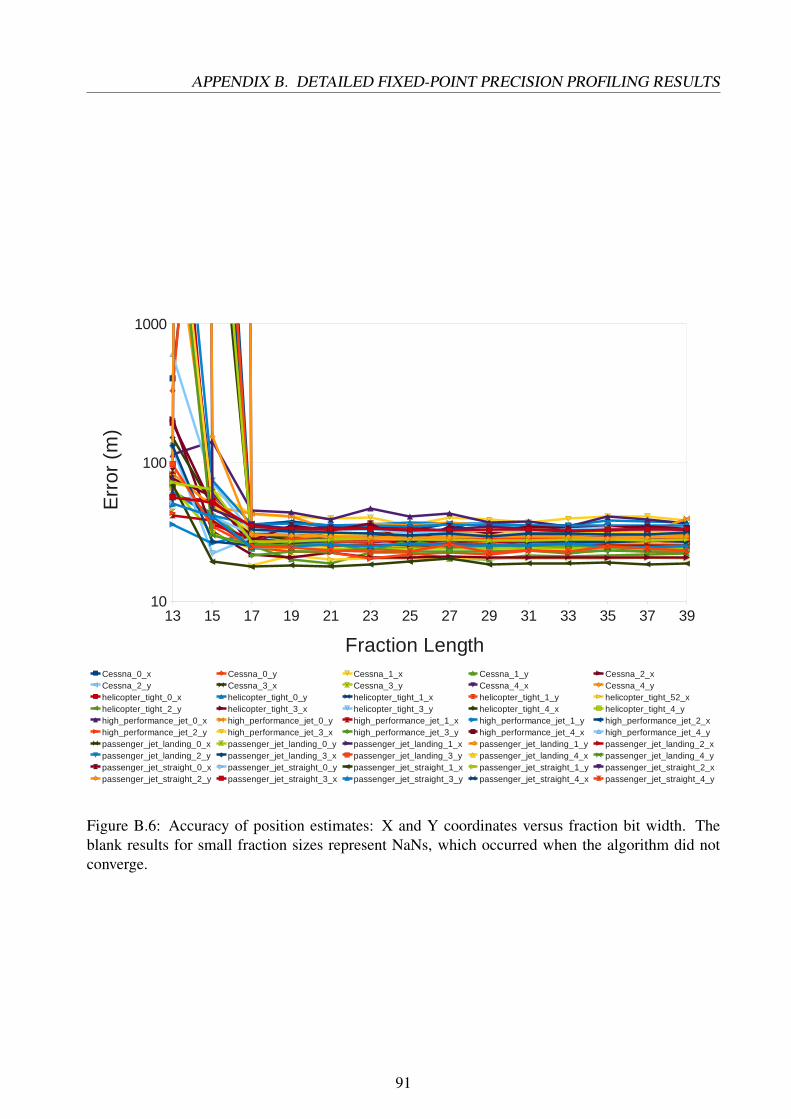
Univers

ity of

Cap

e Tow

n


Figure B.6: Accuracy of position estimates: X and Y coordinates versus fraction bit width. Theblank results for small fraction sizes represent NaNs, which occurred when the algorithm did notconverge.

91

Univers

ity of

Cap

e Tow

n


Figure B.7: Accuracy of position estimates: Z coordinate versus fraction bit width.

92

Univers

ity of

Cap

e Tow

n


Figure B.8: Accuracy of velocity estimates: X and Y coordinates versus fraction bit width.

93

Univers

ity of

Cap

e Tow

n


Figure B.9: Accuracy of velocity estimates: Z coordinate versus fraction bit width.

94

Univers

ity of

Cap

e Tow

n


Figure B.10: Average iterations to convergence versus fraction length.

95

Univers

ity of

Cap

e Tow

n

Appendix C

Python Scripts

This appendix provides listings of the various python scripts used to aid in profiling the algorithmand obtaining data from the software and hardware implementations of it.

C.1 Reduced-Precision Simulation

This script calls the C code simulation for a range of precisions and stores the accuracy results ina spreadsheet. Results are a comparison of the outputs of the simulation with the true states of thetarget, which are stored along with the synthetic radar data by the IDL data generator.

1 #!/ u s r / b i n / env python

23 impor t s y s

4 impor t os

5 impor t r e

6 from t ime impor t gmtime , s t r f t i m e

7 from x lwt impor t ∗89 #exp = sy s . a rgv [ 1 ]

10 #mant = sy s . a rgv [ 2 ]

1112 #TWEAKABLES

13 trueCompare = 0 # s e t t h i s to 0 to compare wi th joe ' s code r e s u l t s ,

14 #se t to 1 to compare wi th TRUEstate r e s u l t s .

15 #/TWEAKABLES

16 i f t rueCompare :

17 p r i n t "Comparing wi th the t r u e s t a t e s . \ n"

18 e l s e :

19 p r i n t "Comparing wi th joe ' s code . \ n"

2021 #se t up d i r e c t o r i e s and f i l e s :

96

Univers

ity of

Cap

e Tow

n

C.1. REDUCED-PRECISION SIMULATION APPENDIX C. PYTHON SCRIPTS

22 o u t p u t f i l e = open ( " . / d i f f e r e n c e s . t x t " , "w")

23 the t ime = s t r f t i m e ("%a , %d %b %Y %H:%M:%S +0000" , gmtime ( ) )

24 o u t p u t f i l e . w r i t e (" output f o r s c r i p t ran on " + the t ime + "\n\n")

25 o u t p u t f i l e . w r i t e("−−−−−−−−−−−−−−−−−−−−−−−−−−−−−−−−−−−−−−−−−−−−−−−−\n")26 o u t p u t f i l e . c l o s e ( )

2728 wb = Workbook ( )

29 ws = wb . add_sheet (" check i ng out c code ")

30 ws . w r i t e (0 ,0 ," mant i s s a l e n g t h ")

31 ws . w r i t e (0 ,1 ," x e r r o r ")

32 ws . w r i t e (0 ,2 ," y e r r o r ")

33 ws . w r i t e (0 ,3 ," z e r r o r ")

34 ws . w r i t e (0 ,4 ," x_dot e r r o r ")

35 ws . w r i t e (0 ,5 ," y_dot e r r o r ")

36 ws . w r i t e (0 ,6 ," z_dot e r r o r ")

37 ws . w r i t e (0 ,7 ," i t e r a t i o n s ")

38 ws . w r i t e (2 ,10 ," a l l a v e r ag e s ")

39 ws . w r i t e (32 ,10 ," a l l maxes ")

40 ws . w r i t e (62 ,10 ," a l l mins ")

41 wb . save (" c code e r r o r s . x l s ")

4243 os . system (" . / d i f f c o r r 1 23")

44 i f ( os . path . i s d i r ( " . / no rma l_r e su l t s " ) ) :

45 os . system ("rm −r no rma l_r e su l t s ")

46 os . system (" mkdir no rma l_ r e su l t s ")

47 os . system (" cp −r . / s t a t e v e c t o r . / no rma l_r e su l t s /")

48 os . system (" cp i t e r a t i o n s . t x t . / no rma l_r e su l t s /")

4950 #run prog f o r a l l d i f f e r e n t b i t w i d t h s

51 o u t p u t f i l e = open ( " . / d i f f e r e n c e s . t x t " , "a ")

5253 s i d e c o u n t e r = 3

54 row = 1

55 f o r i i n range (0 , 2 4 ) : # ove r a l l mant i s s a l e n g t h s

5657 o u t p u t f i l e . w r i t e ("\ n f o r a mant i s s a width o f " + s t r ( i ) + "\n")

58 o u t p u t f i l e . w r i t e("−−−−−−−−−−−−−−−−−−−−−−−−−−−−−−−−−−−−−−−−−−−\n\n")59 ws . w r i t e ( row , 0 , s t r ( i ) )

6061 os . system (" . / d i f f c o r r 1 " + s t r ( i ) )

62 # pas t e the i t e r a t i o n s t u f f i n

63 i t e r a t i o n s F i l e = open ( " . / i t e r a t i o n s . t x t " , " r ")

64 i t e r a t i o n s L i n e s = i t e r a t i o n s F i l e . r e a d l i n e s ( ) ;

65 i t e r a t i o n s F i l e . c l o s e ( ) ;

66 i t r ow = 0 ;

67 i t r owav e = 0 ;

97

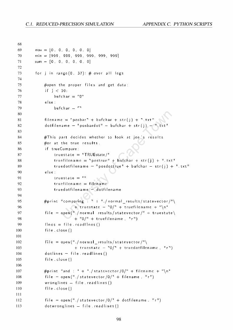
Univers

ity of

Cap

e Tow

n


6869 max = [0 , 0 , 0 , 0 , 0 , 0 ]

70 min = [999 , 999 , 999 , 999 , 999 , 999 ]

71 sum = [0 , 0 , 0 , 0 , 0 , 0 ]

7273 f o r j i n range (0 , 3 7 ) : # ove r a l l l e g s

7475 #open the p rope r f i l e s and get data :

76 i f j < 10 :

77 bu f cha r = "0"

78 e l s e :

79 bu f cha r = ""

8081 f i l e n ame = " posbar " + bu f cha r + s t r ( j ) + " . t x t "

82 do t f i l e n ame = " posba rdo t " + bu f cha r + s t r ( j ) + " . t x t "

8384 #This pa r t d e c i d e s whether to l ook at joe ' s r e s u l t s

85 #or at the t r u e r e s u l t s .

86 i f t rueCompare :

87 t r u e s t a t e = "TRUEstate /"

88 t r u e f i l e n ame = " po s t r u e " + bu f cha r + s t r ( j ) + " . t x t "

89 t r u e d o t f i l e n ame = " po sdo t t r u e " + bu f cha r + s t r ( j ) + " . t x t "

90 e l s e :

91 t r u e s t a t e = ""

92 t r u e f i l e n ame = f i l e n ame

93 t r u e d o t f i l e n ame = do t f i l e n ame

9495 #p r i n t " compar ing : " + " ./ no rma l_ r e su l t s / s t a t e v e c t o r /"\

96 + t r u e s t a t e + "0/" + t r u e f i l e n ame + "\n"

97 f i l e = open ( " . / no rma l_ r e su l t s / s t a t e v e c t o r /" + t r u e s t a t e \

98 + "0/" + t r u e f i l e n ame , " r ")

99 l i n e s = f i l e . r e a d l i n e s ( )

100 f i l e . c l o s e ( )

101102 f i l e = open ( " . / no rma l_ r e su l t s / s t a t e v e c t o r /"\

103 + t r u e s t a t e + "0/" + t r u e do t f i l e n ame , " r ")

104 d o t l i n e s = f i l e . r e a d l i n e s ( )

105 f i l e . c l o s e ( )

106107 #p r i n t "and : " + " ./ s t a t e v e c t o r /0/" + f i l e n ame + "\n"

108 f i l e = open ( " . / s t a t e v e c t o r /0/" + f i l ename , " r ")

109 wrong l i n e s = f i l e . r e a d l i n e s ( )

110 f i l e . c l o s e ( )

111112 f i l e = open ( " . / s t a t e v e c t o r /0/" + do t f i l e name , " r ")

113 do tw r ong l i n e s = f i l e . r e a d l i n e s ( )

98

Univers

ity of

Cap

e Tow

n


114 f i l e . c l o s e ( )

115116 #get data u s i n g REGULAR EXPRESSIONS . . .

117 s e a r c h e r = r e . comp i l e ( r '^\ s +(.?\d+.\d+)\ s +(.?\d+.\d+)\ s +(.?\d+.\d+) ')

118 #s t a r t , then one cha r a c t e r ,

119 #then o p t i o n a l c h a r a c t e r ( minus s i g n ) ,

120 #then s t r i n g o f numbers ,

121 #then any th i ng ( dec ima l p o i n t ) then a s t r i n g o f numbers .

122 #th r e e groups o f t h e s e .

123124 o l d r e s u l t = s e a r c h e r . s e a r c h ( l i n e s [ 7 9 ] )

125 d o t o l d r e s u l t = s e a r c h e r . s e a r c h ( d o t l i n e s [ 7 9 ] )

126127 r e s u l t = s e a r c h e r . s e a r c h ( w r o ng l i n e s [ 7 9 ] )

128 d o t r e s u l t = s e a r c h e r . s e a r c h ( d o tw r ong l i n e s [ 7 9 ] )

129130 #do the s u b t r a c t i o n and s t o r e r e s u l t s

131 f i r s t n um = s t r ( abs ( f l o a t ( o l d r e s u l t . group ( 1 ) )

132 − f l o a t ( r e s u l t . group ( 1 ) ) ) )

133 secondnum = s t r ( abs ( f l o a t ( o l d r e s u l t . group ( 2 ) )


135 th i rdnum = s t r ( abs ( f l o a t ( o l d r e s u l t . group ( 3 ) )


137138 fourthnum = s t r ( abs ( f l o a t ( d o t o l d r e s u l t . group ( 1 ) )

139 − f l o a t ( d o t r e s u l t . group ( 1 ) ) ) )

140 f i f t hnum = s t r ( abs ( f l o a t ( d o t o l d r e s u l t . group ( 2 ) )


142 s ixthnum = s t r ( abs ( f l o a t ( d o t o l d r e s u l t . group ( 3 ) )


144145 answer s = [ f i r s t num , secondnum , thirdnum ,

146 fourthnum , f i f thnum , s ixthnum ]

147148 o u t p u t f i l e . w r i t e ( f i r s t n um + "\ t \ t " + secondnum + "\ t \ t " + thi rdnum\

149 + "\ t \ t " + fourthnum + "\ t \ t " + f i f t hnum \

150 + "\ t \ t " + s ixthnum + "\n")

151152 f o r k i n range ( 0 , 6 ) :

153 v a l u e = f l o a t ( answers [ k ] )

154 ws . w r i t e ( row , k+1, v a l u e )

155 i f ( v a l u e > max [ k ] ) :

156 max [ k ] = va l u e

157 i f ( v a l u e < min [ k ] ) :

158 min [ k ] = va l u e

159 sum [ k ] = sum [ k ] + va l u e

99

Univers

ity of

Cap

e Tow

n


160161 ws . w r i t e ( row , 7 , i t e r a t i o n s L i n e s [ i t r ow ] [ : − 1 ] )

162 i t r owav e = i t r owav e + i n t ( i t e r a t i o n s L i n e s [ i t r ow ] [ : − 1 ] )

163 i t r ow = i t r ow + 1

164 row = row + 1

165166 ws . w r i t e ( row , 0 , "Max")

167 f o r k i n range ( 1 , 7 ) :

168 ws . w r i t e ( row , k , max [ k−1])169 ws . w r i t e ( s i d e c o u n t e r + 31 , k+8, max [ k−1])170 ws . w r i t e ( row+1, 0 , "Min")

171 f o r k i n range ( 1 , 7 ) :

172 ws . w r i t e ( row+1, k , min [ k−1])173 ws . w r i t e ( s i d e c o u n t e r + 61 , k+8, min [ k−1])174 ws . w r i t e ( row+2, 0 , "Ave ") 165 f o r k i n range ( 1 , 7 ) :

175 ws . w r i t e ( row+2, k , sum [ k−1]/36)176 ws . w r i t e ( s i d e c oun t e r , k+8, sum [ k−1]/36)177 ws . w r i t e ( row+2, 7 , i t r owav e /36)

178179 s i d e c o u n t e r = s i d e c o u n t e r + 1

180 row = row + 4



184 o u t p u t f i l e . c l o s e ( )

185186 p r i n t "Done . \ n"

100

Univers

ity of

Cap

e Tow

n

C.2. FPGA RESOURCE USAGE TRIALS APPENDIX C. PYTHON SCRIPTS

C.2 FPGA Resource Usage Trials

To investigate the scaling of resource requirements with word sizes, a script was written to parametriseand build the design for a range of word widths. It did this by editing the text files which store theIP core parameter values, resynthesising them in turn, and then rebuilding the design as a whole.


23 #bu i l d s my ISE p r o j e c t f o r the g i v en exponent and mant i s s a w id th s .

45 impor t s y s

6 impor t os

7 from t ime impor t t ime

89 s t a r t = t ime ( )

1011 exp = sy s . a rgv [ 1 ]

12 mant = sy s . a rgv [ 2 ]

1314 #f o r normal p a r t i a l s

15 ar i thComps = [ ' f loat_mul t ' , ' f l oa t_sub ' , ' f loat_add ' , ' f l o a t_d i v ' ,

16 ' f loat_mult_dsp ' , ' f l o a t_sq r t ' ]

17 #' s h i f t ' l e n g t h based on f i r s t l a t e n c y ,

18 #' sh i f t_ l ong ' l e n g t h based on second . s q r t l a t e n c y based on l a s t .

19 sh i f tComps = [ ' s h i f t ' , ' s h i f t_ l ong ' , ' s h i f t_dc a l c ' ,

20 ' B sh i f t ' , ' sh i f t_addminusmul t ' ]

2122 co regen = '/ opt / X i l i n x /11 .1/ ISE/ b in / l i n / co regen '

23 path_to_pro ject = '/home/ j p / ISE_pro j e c t s / f i l t e r s / Genera l_FP_dopp le r_par t i a l s / '

24 i p c o r eD i r = path_to_pro ject + ' i p c o r e_d i r / '

25 GNConsts = path_to_pro ject + ' GNConstants . vhd '

2627 de f ge tLa t ency ( x c o F i l e ) :

28 t r y :

29 f i l e = open ( x c oF i l e , " r ")


31 f i l e . c l o s e ( )

32 excep t IOEr ro r :

33 p r i n t " IOEr ro r on f i l e " + x c o F i l e + " . ( s c r a p e l a t e n c i e s s e c t i o n )\n"

34 s y s . e x i t ( )

3536 f o r l i n e i n l i n e s :

37 i f ( l i n e [ 0 : 1 4 ] == 'CSET c_latency ' ) :

38 Lat = l i n e [15 : −1]39 r e t u r n Lat

40

101

Univers

ity of

Cap

e Tow

n


414243 #gene r a t e a r i t hm e t i c co r e s−−−−−−−−−−−−−−−−−−−−−−−−−−−−−−−−−44 f o r comp i n ar i thComps :

45 x c o F i l e = '/home/ j p / ISE_pro j e c t s / f i l t e r s \

46 /Genera l_FP_dopp le r_par t i a l s / i p c o r e_d i r / ' + comp + ' . xco '

47 #ed i t i t s . xco f i l e

48 t r y :



51 f i l e . c l o s e ( )


53 p r i n t "∗∗∗∗∗∗∗∗∗∗∗∗∗∗∗∗∗∗∗∗∗∗∗∗∗∗∗∗∗∗∗∗ IOEr ro r on f i l e " + x c o F i l e \

54 + " . ( g en e r a t e a r i t h c o r e s s e c t i o n )\n"

55 s y s . e x i t ( )

5657 j = 0

58 t h e p l a c e s = [999 ,999 , 999 , 999 ]


60 i f ( l i n e [ 0 : 2 3 ] == 'CSET c_a_exponent_width ' ) :

61 t h e p l a c e s [ 0 ] = j

62 i f ( l i n e [ 0 : 2 3 ] == 'CSET c_a_fract ion_width ' ) :

63 t h e p l a c e s [ 1 ] = j

64 i f ( l i n e [ 0 : 2 8 ] == 'CSET c_result_exponent_width ' ) :

65 t h e p l a c e s [ 2 ] = j

66 i f ( l i n e [ 0 : 2 8 ] == 'CSET c_re su l t_f rac t i on_wid th ' ) :

67 t h e p l a c e s [ 3 ] = j

68 j = j + 1

6970 i f ( t h e p l a c e s [ 0 ] > 900 or t h e p l a c e s [ 1 ] > 900

71 or t h e p l a c e s [ 2 ] > 900 or t h e p l a c e s [ 3 ] > 900 ) :

72 p r i n t '∗∗∗∗∗PARSE ERROR ON ARITHMETIC XCO FILE ' + comp

7374 l i n e s [ t h e p l a c e s [ 0 ] ] = 'CSET c_a_exponent_width='\

75 + exp + '\n '

76 l i n e s [ t h e p l a c e s [ 1 ] ] = 'CSET c_a_fract ion_width='\

77 + s t r ( i n t (mant ) + 1) + '\n '

78 l i n e s [ t h e p l a c e s [ 2 ] ] = 'CSET c_resu l t_exponent_width='\

79 + exp + '\n '

80 l i n e s [ t h e p l a c e s [ 3 ] ] = 'CSET c_re su l t_ f r a c t i on_w id th='\

81 + s t r ( i n t (mant ) + 1) + '\n '

8283 t r y :

84 f i l e = open ( x c oF i l e , "w")

85 f i l e . w r i t e l i n e s ( l i n e s )

86 f i l e . c l o s e ( )

102

Univers

ity of

Cap

e Tow

n



88 p r i n t "∗∗∗∗∗∗∗∗∗∗∗∗∗∗ IOEr ro r on f i l e " + x c o F i l e +

89 " . ( g en e r a t e a r i t h c o r e s s e c t i o n )\n"

90 s y s . e x i t ( )

9192 #gene r a t e the co r e

93 command = coregen + '−b ' + ' ' + x c o F i l e + ' −p ' + i p c o r eD i r +' −r '94 p r i n t command

95 os . system (command)

9697 #get the l a t e n c y o f the mult and sub components ,

98 #s h i f t e r s must s h i f t t h i s depth .

99 s h o r t L a t = ' '

100 l ongLa t = ' '

101 DLat = ' '

102 BLat = ' '

103 minusLat = ' '

104 DefValue = ' ' #s h i f t e r needs d e f a u l t data to be same l e n g t h as word width

105106 #sc r ap e v a l u e s

107 x c o F i l e = i p c o r eD i r + ar i thComps [ 0 ] + ' . xco '

108 s h o r t L a t = ge tLa t ency ( x c o F i l e )

109110 x c o F i l e = i p c o r eD i r + ar i thComps [ 1 ] + ' . xco '

111 l ongLa t = ge tLa t ency ( x c o F i l e )

112113 minusLat = s t r ( i n t ( l ongLa t ) − i n t ( s h o r t L a t ) )

114 #DLat =

115116 #c r e a t e s t r i n g s f o r d e f a u l t data

117 p r i n t i n t ( exp ) + i n t (mant ) + 1

118 f o r i t i n range ( 0 , ( i n t ( exp ) + i n t (mant ) + 1 ) ) :

119 DefValue = DefValue + '0 '

120 #gene r a t e s h i f t e r c o r e s###################################

121 l a t e n c i e s = [ sho r tLa t , l ongLa t ]

122 i = 0

123 f o r comp i n sh i f tComps :

124 x c o F i l e = i p c o r eD i r + comp + ' . xco '

125 #ed i t i t s . xco f i l e

126 t r y :



129 f i l e . c l o s e ( )


131 p r i n t " IOEr ro r on f i l e " + x c o F i l e \

132 + " . ( g en e r a t e s h i f t e r c o r e s s e c t i o n )\n"

103

Univers

ity of

Cap

e Tow

n


133 s y s . e x i t ( )

134135 j = 0

136 t h e p l a c e s = [999 ,999 ,999 ,999 ,999 ]


138 i f ( l i n e [ 0 : 1 7 ] == 'CSET a s y n c i n i t v a l ' ) :

139 t h e p l a c e s [ 0 ] = j

140 i f ( l i n e [ 0 : 1 6 ] == 'CSET de f a u l t d a t a ' ) :

141 t h e p l a c e s [ 1 ] = j

142 i f ( l i n e [ 0 : 1 0 ] == 'CSET depth ' ) :

143 t h e p l a c e s [ 2 ] = j

144 i f ( l i n e [ 0 : 1 6 ] == 'CSET s y n c i n i t v a l ' ) :

145 t h e p l a c e s [ 3 ] = j

146 i f ( l i n e [ 0 : 1 0 ] == 'CSET width ' ) :

147 t h e p l a c e s [ 4 ] = j

148 j = j + 1

149150 i f ( t h e p l a c e s [ 0 ] > 900 or t h e p l a c e s [ 1 ] > 900 or

151 t h e p l a c e s [ 2 ] > 900 or t h e p l a c e s [ 3 ] > 900 or t h e p l a c e s [ 4 ] > 900 ) :

152 p r i n t '∗∗∗∗∗∗∗∗∗PARSE ERROR ON SHIFTER XCO FILE ' + comp

153154 l i n e s [ t h e p l a c e s [ 2 ] ] = 'CSET depth=' + l a t e n c i e s [ i ] + '\n '

155 l i n e s [ t h e p l a c e s [ 4 ] ] = 'CSET width=' + s t r ( i n t (mant ) + i n t ( exp ) + 1) + '\n '

156 l i n e s [ t h e p l a c e s [ 0 ] ] = 'CSET a s y n c i n i t v a l =' + DefValue + '\n '

157 l i n e s [ t h e p l a c e s [ 1 ] ] = 'CSET d e f a u l t d a t a =' + DefValue + '\n '

158 l i n e s [ t h e p l a c e s [ 3 ] ] = 'CSET s y n c i n i t v a l =' + DefValue + '\n '

159160 t r y :

161 f i l e = open ( x c oF i l e , "w")


163 f i l e . c l o s e ( )


165 p r i n t " IOEr ro r on f i l e " + x c o F i l e \

166 + " . ( g en e r a t e s h i f t e r c o r e s s e c t i o n )\n"

167 s y s . e x i t ( )

168169 #gene r a t e the co r e

170 command = coregen + '−b ' + ' ' + x c o F i l e + ' −p ' + i p c o r eD i r +' −r '171 p r i n t command


173 i = i+1

174175 #ed i t the p r o j e c t vhd l to ag r e e w i th t h e s e s i z e s :−−−−−−−−−−−−−−−−−−−176 t r y :

177 f i l e = open ( GNConsts , " r ")


104

Univers

ity of

Cap

e Tow

n



180 p r i n t " IOEr ro r on f i l e " + GNConsts + " .\ n"

181 s y s . e x i t ( )

182183 j = 0

184 t h e p l a c e s = [999 , 999 ]


186 i f ( l i n e [ 0 : 1 5 ] == ' con s t an t EXP ' ) :

187 t h e p l a c e s [ 0 ] = j

188 i f ( l i n e [ 0 : 1 6 ] == ' con s t an t MANT' ) :

189 t h e p l a c e s [ 1 ] = j

190 j = j+1

191192 i f ( t h e p l a c e s [ 0 ] > 900 or t h e p l a c e s [ 1 ] > 900 ) :

193 p r i n t '∗∗∗∗∗∗∗∗∗PYTHON SCRIPT ERROR − PARSE ERROR ON GNCONSTANTS FILE '

194195 l i n e s [ t h e p l a c e s [ 0 ] ] =\

196 ' c on s t an t EXP : i n t e g e r := ' + exp + ' ; −−exponent width \n '

197 l i n e s [ t h e p l a c e s [ 1 ] ] =\

198 ' c on s t an t MANT : i n t e g e r := ' + mant + ' ; −−mant i s s a width \n '

199200 f i l e . c l o s e ( )

201 t r y :

202 f i l e = open ( GNConsts , "w")


204 f i l e . c l o s e ( )


206 p r i n t " IOEr ro r on f i l e " + GNConsts + " .\ n"

207 s y s . e x i t ( )

208209 #run i s e −s y n t h e s i s210 os . c h d i r ( path_to_pro ject )

211 pa th_to_dot i s e_f i l e = '" ' + path_to_pro ject \

212 + ' Genera l_FP_dopp le r_par t i a l s . i s e " '

213 path_to_dotx s t_f i l e = '" ' + path_to_pro ject \

214 + ' Get_Dopp le r_par t i a l . x s t " '

215 path_to_dot sy r_f i l e = '" ' + path_to_pro ject \

216 + ' Get_Dopp le r_par t i a l . s y r " '

217 command = ' x s t − i s e ' + pa th_to_dot i s e_f i l e + ' − i n t s t y l e i s e − i f n '\

218 + path_to_dotx s t_f i l e \

219 + ' −ofn ' + path_to_dot sy r_f i l e


221222 #run i s e −t r a n s l a t e , map , p l a c e & rou t e ( implement d e s i g n

223 os . c h d i r ( path_to_pro ject )

224

105

Univers

ity of

Cap

e Tow

n


225 os . system (" ngdbu i l d − i s e " + path_to_dot i s e_f i l e

226 + " − i n t s t y l e i s e −dd _ngo −sd i p c o r e_d i r −nt t imestamp\

227 − i −p xc4v lx100−f f 1148 −12 Get_Dopp le r_par t i a l . ngc Get_Dopp le r_par t i a l . ngd ")

228229 os . system ("map − i s e " + pa th_to_dot i s e_f i l e

230 + " − i n t s t y l e i s e −p xc4v lx100−f f 1148 −12 −g loba l_opt o f f \

231 −cm area − i r o f f −pr o f f −c 100 −o Get_Doppler_part i \

232 al_map . ncd Get_Dopp le r_par t i a l . ngd Get_Dopp le r_par t i a l . p c f ")

233234 os . system (" par − i s e " + path_to_dot i s e_f i l e

235 + " −w − i n t s t y l e i s e −o l s t d −t 1 Get_Doppler_partial_map . ncd \

236 Get_Dopp le r_par t i a l . ncd Get_Dopp le r_par t i a l . p c f ")

237238 os . system (" t r c e − i s e " + pa th_to_dot i s e_f i l e

239 + " − i n t s t y l e i s e −v 3 −s 12 − f a s t p a t h s −xml \

240 Get_Dopp le r_par t i a l . twx \

241 Get_Dopp le r_par t i a l . ncd −o Get_Doppler_ p a r t i a l . twr Get_Dopp le r_par t i a l . p c f ")

242243 # sc r ap e l o g s and append to summary

244 os . c h d i r ( path_to_pro ject )

245 end = t ime ( )

246 du r a t i o n = s t r ( end − s t a r t )

247 t r y :

248 f i l e = open (" summary . l o g " , "a ")

249 f i l e . w r i t e("−−−−−−−−−−−−−−−−−−−−−−−−−−−−−−−−−\n\n")250 f i l e . w r i t e (" Running f o r exponent : " + exp + " and mant i s s a : " +

251 mant + " . P roce s s took "+ du r a t i o n +" seconds . \n\n")

252 f i l e . c l o s e ( )


255 p r i n t "∗∗∗∗∗∗∗∗∗∗∗∗∗∗∗ problem open ing summary f i l e . "

256 s y s . e x i t ( )

257258 os . system (" . / ScrapeLogs . py ")

106

Univers

ity of

Cap

e Tow

n


Another script was then called which scraped the log files for the information of interest.


2 impor t os

3 impor t g l ob

4 from x lwt impor t ∗56 #######################################################

7 # de f i n e the deed . . .

8 de f s c r a p e F i l e s ( l o c a t i o n ) :

910 checke r = 0

11 c l kF r e q = ' '

1213 # Open the syn th f i l e f o r read−on l y14 s y n t h F i l e = g lob . g l ob ( l o c a t i o n + '/∗ . s y r ' )15 i f s y n t h F i l e :

16 s y n t h F i l e = s y n t h F i l e [ 0 ]

17 p r i n t " found f i l e " + s y n t h F i l e

18 f i l e = open ( s y n t hF i l e , " r ")


20 # Loop through the l i n e s to f i n d the r i g h t l i n e

21 i = −122 f o r l i n e i n l i n e s :

23 i = i + 1

24 i f ( l i n e [ 0 : 1 9 ] == ' Clock S i g n a l ' ) :

25 checke r = checke r + 1

26 p r i n t " got c l o c k l oad . . . "

27 c lkLoad = l i n e s [ i + 2 ] [ 62 : −2 ]28 i f ( l i n e [ 0 : 1 9 ] == ' Minimum pe r i o d : ' ) :


30 p r i n t " got c l o c k f r e qu enc y . . . "

31 c l kF r e q = l i n e [28 : −2 ]32 # Clo se the f i l e

33 f i l e . c l o s e ( )

34 e l s e :

35 p r i n t " no s y n t h e s i s f i l e i n t h i s d i r e c t o r y . "

3637 # Open the imp l ementa t i on f i l e f o r read−on l y38 i m p l e F i l e = g lob . g l ob ( l o c a t i o n + '/∗ . mrp ' )

39 i f i m p l e F i l e :

40 i m p l e F i l e = imp l e F i l e [ 0 ]

41 p r i n t " found f i l e " + imp l e F i l e

4243 f i l e = open ( imp l e F i l e , " r ")


107

Univers

ity of

Cap

e Tow

n




4849 i = i + 1

50 i f ( l i n e [ 0 : 2 9 ] == ' Number o f S l i c e F l i p F l op s : ' ) :


52 s l c F l p F l p s = l i n e

53 p r i n t " got s l i c e F l i p F l op s . . . "

54 LUTs = l i n e s [ i +1]

55 p r i n t " got 4− i n pu t LUTS . . . "

56 o c c S l i c e = l i n e s [ i + 3 ]

57 p r i n t " got occup i ed s l i c e s . . . "

58 l o g S l i c e = l i n e s [ i + 4 ]

59 p r i n t " got l o g i c s l i c e s . . . "

60 u n r S l i c e = l i n e s [ i + 5 ]

61 p r i n t " got u n r e l a t e d s l i c e s . . . "

62 totLUT = l i n e s [ i + 7 ]

63 p r i n t " got t o t a l LUTs . . . "

64 logLUT = l i n e s [ i + 8 ]

65 p r i n t " got l o g i c LUTs . . . "

66 rtLUT = l i n e s [ i + 9 ]

67 p r i n t " got r ou t e LUTs . . . "

68 sh i f tLUT = l i n e s [ i + 10 ]

69 p r i n t " got s h i f t r e g i s t e r LUTS . . . "

70 i f ( l i n e [ 0 : 3 3 ] == ' Average Fanout o f Non−Clock Nets : ' ) :


72 aveNet = l i n e

7374 # Clo se the f i l e

75 f i l e . c l o s e ( )

76 e l s e :

77 p r i n t " no imp l ementa t i on f i l e i n t h i s d i r e c t o r y . "

7879 # Open the second imp l ementa t i on f i l e f o r read−on l y80 i m p l e F i l e 2 = g lob . g l ob ( l o c a t i o n + '/∗ . par ' )81 i f i m p l e F i l e 2 :

82 i m p l e F i l e 2 = imp l e F i l e 2 [ 0 ]

83 p r i n t " found f i l e " + imp l e F i l e 2

8485 f i l e = open ( imp l eF i l e 2 , " r ")




90

108

Univers

ity of

Cap

e Tow

n


91 i = i + 1

92 i f ( l i n e [ 0 : 2 7 ] == ' Dev ice U t i l i z a t i o n Summary : ' ) :


94 BUFGs = l i n e s [ i + 2 ]

95 p r i n t " got BUFGs . . . . "

96 DSP48 = l i n e s [ i + 3 ]

97 p r i n t " got DSPs . . . "

98 EIOBs = l i n e s [ i + 4 ]

99 p r i n t " got e x t e r n a l IOBs . . . "

100 LIOBs = l i n e s [ i + 5 ]

101 p r i n t " got LOCed IOBs . . . "

102 RAM16 = l i n e s [ i + 7 ]

103 p r i n t " got b l o ck RAMs . . . "

104 s l i c s = l i n e s [ i + 8 ]

105 p r i n t " got s l i c e s . . . "

106 SLICM = l i n e s [ i + 9 ]

107 p r i n t " got SLICEMs . . . "

108 i f ( l i n e [ 0 : 3 0 ] == ' | C lock Net | Reso ' ) :


110 f anou t = l i n e s [ i + 2 ] [ 4 6 : 5 1 ]

111 p r i n t " got f anou t . "

112 e l s e :

113 f anou t = "XXX"

114 # Clo se the f i l e

115 f i l e . c l o s e ( )

116 e l s e :

117 p r i n t " no second imp l ementa t i on f i l e i n t h i s d i r e c t o r y . "

118119120 # wr i t e data to f i l e

121 f i l e = open (" summary . l o g " , "a ")

122 f i l e . w r i t e("−−−−−−−−−−−−−−−−−−−−−−−−−−−−−−−−−−−−−−−−−−−\n")123 i f s y n t h F i l e :

124125 f i l e . w r i t e (" i n f i l e " + s y n t h F i l e + " :\ n\n")

126 f i l e . w r i t e (" c l o c k l oad : \ t \ t " + c lkLoad + "\n")

127 f i l e . w r i t e ( c l kF r e q + "\n\n")

128129 i f i m p l e F i l e :

130 f i l e . w r i t e (" i n f i l e " + imp l e F i l e + " :\ n\n")

131 # Save n i c e ones to l i s t

132 d a t a L i s t = [ s l c F l p F l p s , LUTs , o c cS l i c e ,

133 totLUT , logLUT , rtLUT , sh i f tLUT , aveNet ]

134135 f o r datum i n d a t a L i s t :

136 f i l e . w r i t e ( datum [ 0 : 3 5 ] + "\ t \ t \ t \ t \ t " + datum [36 : −1 ] + "\n")

109

Univers

ity of

Cap

e Tow

n


137 i f ( datum == o c c S l i c e ) :

138 f i l e . w r i t e ( l o g S l i c e )

139 f i l e . w r i t e ( u n r S l i c e )

140 i f i m p l e F i l e 2 :

141 f i l e . w r i t e (" i n f i l e " + imp l e F i l e 2 + " :\ n\n")

142 # Save n i c e ones to l i s t

143 d a t a L i s t = [BUFGs , DSP48 , EIOBs , LIOBs ,RAM16, s l i c s , SLICM ]

144145 f o r datum i n d a t a L i s t :

146 f i l e . w r i t e ( datum [ 0 : 3 5 ] + "\ t \ t \ t \ t \ t " + datum [36 : −1 ] + "\n")

147 i f ( datum == o c c S l i c e ) :

148 f i l e . w r i t e ( l o g S l i c e )

149 f i l e . w r i t e ( u n r S l i c e )

150151 f i l e . w r i t e (" c l o c k f anou t : \ t \ t \ t \ t \ t \ t \ t \ t \ t \ t \ t " + fanou t )

152 f i l e . w r i t e ("\n\n")

153 f i l e . c l o s e ( )

154155 #check i f i t t h e r e were no obv i ou s e r r o r s

156 i f s y n t h F i l e and im p l e F i l e :

157 i f ( ch e cke r == 6 ) :

158 p r i n t "The s c r i p t seems to have worked p r o p e r l y . \ n"

159 r e t u r n 0

160 e l s e :

161 p r i n t " someth ing went wrong . Make su r e e v e r y t h i n g i s t h e r e . \ n"

162 r e t u r n 1

163 e l s e :

164 r e t u r n 0

165166 ################################################################

167168 numErrors = 0

169170 i f ( l e n ( s y s . a rgv ) < 2 ) :

171 l o c a t i o n = os . getcwd ( )

172 e l s e :

173 l o c a t i o n = sy s . a rgv [ 1 ]

174175 p r i n t "\ nP ro c e s s i n g " , l o c a t i o n , " . . . "

176 numErrors = numErrors + s c r a p e F i l e s ( l o c a t i o n )

177178 i f ( numErrors == 0 ) :

179 p r i n t " the E n t i r e s c r i p t ran wi th no e r r o r s . \ n"

180 e l s e :

181 p r i n t " t h e r e were e r r o r s − check out the r e s u l t s . \ n"

110

Univers

ity of

Cap

e Tow

n

C.3. VERIFICATION SCRIPTS APPENDIX C. PYTHON SCRIPTS

C.3 Verification Scripts

For verification purposes, a script was created to compare simulation results with the results ofperforming the calculations in software. Inputs and outputs of the hardware simulation were textfiles containing binary representations of the data, and these had to be converted to decimal numbersfor the comparison. Note that the function definitions used in this script are not included in thislisting. For the full script, see the included DVD.


2 #t h i s i s automated t e s t i n g u s i n g an ISE t e s t b en ch wi th f i l e

3 #I /O f o r f l o a t i n g_po i n t p r o j e c t .

4 #you run the t e s t b en ch i n ISE then pas s the i n pu t and output

5 #to t h i s to check i t s a ccu racy .

6 #usage : . / t e s t a c c . py i n p u t_ f i l e o u t p u t_ f i l e

78 impor t s y s

9 impor t os

10 impor t math

11 from t ime impor t t ime

1213 ################### Main Method ##################

1415 s t a r t = t ime ( )

16 p r i n t ""

1718 #############CHANGE THESE TO AGREE################

19 e x p b i t s = 8

20 mantb i t s = 12

2122 #read i n a l l the data

23 i n p u t f i l e = open ( s y s . a rgv [ 1 ] , " r ")

24 i n l i n e s = i n p u t f i l e . r e a d l i n e s ( )

25 i n p u t f i l e . c l o s e ( )

2627 o u t p u t f i l e = open ( s y s . a rgv [ 2 ] , " r ")

28 o u t l i n e s = o u t p u t f i l e . r e a d l i n e s ( )

29 o u t p u t f i l e . c l o s e ( )

3031 #now we go through a l l the l i n e s

32 #and s u b t r a c t HW answer from python answer .

33 e r ro r sum = Vector ( [ 0 , 0 , 0 , 0 , 0 , 0 , 0 , 0 , 0 ] )

34 pe r c en t e r r o r s um = Vector ( [ 0 , 0 , 0 , 0 , 0 , 0 , 0 , 0 , 0 ] )

35 a l l e r r o r s = [ ]

36 mins = [ f l o a t ( ' i n f ' ) , f l o a t ( ' i n f ' ) , f l o a t ( ' i n f ' ) ,

37 f l o a t ( ' i n f ' ) , f l o a t ( ' i n f ' ) , f l o a t ( ' i n f ' ) ,

111

Univers

ity of

Cap

e Tow

n


38 f l o a t ( ' i n f ' ) , f l o a t ( ' i n f ' ) , f l o a t ( ' i n f ' ) ]

39 maxes = [−1∗ f l o a t ( ' i n f ' ) , −1∗ f l o a t ( ' i n f ' ) , −1∗ f l o a t ( ' i n f ' ) ,40 −1∗ f l o a t ( ' i n f ' ) , −1∗ f l o a t ( ' i n f ' ) , −1∗ f l o a t ( ' i n f ' ) ,41 −1∗ f l o a t ( ' i n f ' ) , −1∗ f l o a t ( ' i n f ' ) , −1∗ f l o a t ( ' i n f ' ) ]

4243 f o r i i n range (0 , l e n ( o u t l i n e s ) ) :

44 i n p u t s = i n l i n e s [ i ] . s p l i t ( )

45 A = bin2dec ( i n p u t s [ 0 ] , e x pb i t s , mantb i t s )

46 B = bin2dec ( i n p u t s [ 1 ] , e x pb i t s , mantb i t s )

47 x = b in2dec ( i n p u t s [ 2 ] , e x pb i t s , mantb i t s )

48 y = b in2dec ( i n p u t s [ 3 ] , e x pb i t s , mantb i t s )

49 z = b in2dec ( i n p u t s [ 4 ] , e x pb i t s , mantb i t s )

50 xdot = b in2dec ( i n p u t s [ 5 ] , e x pb i t s , mantb i t s )

51 ydot = b in2dec ( i n p u t s [ 6 ] , e x pb i t s , mantb i t s )

52 zdot = b in2dec ( i n p u t s [ 7 ] , e x pb i t s , mantb i t s )

53 xpos = b in2dec ( i n p u t s [ 8 ] , e x pb i t s , mantb i t s )

54 ypos = b in2dec ( i n p u t s [ 9 ] , e x pb i t s , mantb i t s )

55 zpos = b in2dec ( i n p u t s [ 1 0 ] , e x pb i t s , mantb i t s )

5657 r e a l R e s u l t s = Vecto r ( getRea lAnswer (A, B,

58 x , y , z ,

59 xdot , ydot , zdot ,

60 xpos , ypos , zpos ) )

6162 ou tpu t s = o u t l i n e s [ i ] . s p l i t ( )

63 xdop = b in2dec ( ou tpu t s [ 0 ] , e x pb i t s , mantb i t s )

64 ydop = b in2dec ( ou tpu t s [ 1 ] , e x pb i t s , mantb i t s )

65 zdop = b in2dec ( ou tpu t s [ 2 ] , e x pb i t s , mantb i t s )

66 xdotdop = b in2dec ( ou tpu t s [ 3 ] , e x pb i t s , mantb i t s )

67 ydotdop = b in2dec ( ou tpu t s [ 4 ] , e x pb i t s , mantb i t s )

68 zdotdop = b in2dec ( ou tpu t s [ 5 ] , e x pb i t s , mantb i t s )

69 bear2 = b in2dec ( ou tpu t s [ 6 ] , e x pb i t s , mantb i t s )

70 bea rdcosdx = b in2dec ( ou tpu t s [ 7 ] , e x pb i t s , mantb i t s )

71 bea r d s i n d y = b in2dec ( ou tpu t s [ 8 ] , e x pb i t s , mantb i t s )

72 myResu l t s = Vecto r ( [ xdop , ydop , zdop ,

73 xdotdop , ydotdop , zdotdop ,

74 bear2 , beardcosdx , b e a r d s i n d y ] )

7576 # p r i n t b in2hex ( ou tpu t s [ 0 ] )








112

Univers

ity of

Cap

e Tow

n



8586 e r r o r s = myResu l t s − r e a l R e s u l t s

87 e r r o r s = e r r o r s ∗ e r r o r s #note t h i s does dot product ,

88 #not v e c t e r mu l t i p l y . d e f i n e d i n c l a s s above .

89 e r ro rno rm = e r r o r s . s q r t ( )

90 p e r c e n t e r r o r = er ro rno rm / r e a l R e s u l t s . abs ( )

91 p e r c e n t e r r o r = p e r c e n t e r r o r ∗1009293 # p r i n t A, B, x , y , z , xdot , ydot , zdot , xpos , ypos , zpos

94 # p r i n t " Rea l r e s u l t s : "

95 # p r i n t r e a l R e s u l t s

96 # p r i n t "My r e s u l t s : "

97 # p r i n t myResu l t s

98 # p r i n t " E r r o r : "

99 # p r i n t e r ro rno rm

100 # p r i n t "% E r r o r : "

101 # p r i n t p e r c e n t e r r o r

102 # p r i n t ""

103104 a l l e r r o r s . append ( e r ro rno rm )

105 e r ro r sum = ( e r ro r sum + er ro rno rm )

106 pe r c en t e r r o r s um = ( pe r c en t e r r o r s um + p e r c e n t e r r o r )

107 f o r j i n range (0 , l e n (maxes ) ) :

108 i f ( e r r o rno rm [ j ] > maxes [ j ] ) :

109 maxes [ j ] = e r ro rno rm [ j ]

110 i f ( e r r o rno rm [ j ] < mins [ j ] ) :

111 mins [ j ] = e r ro rno rm [ j ]

112113 p r i n t '\ n\n '

114 a v eE r r o r = er ro r sum / l e n ( o u t l i n e s )

115 av ePe r cE r r o r = pe r c en t e r r o r s um / l e n ( o u t l i n e s )

116 p r i n t " ave rage e r r o r : "

117 p r i n t a v eE r r o r

118 p r i n t " ave rage % e r r o r : "

119 p r i n t a v ePe r cE r r o r

120121 stdDevErrorSum = Vector ( [ 0 , 0 , 0 , 0 , 0 , 0 , 0 , 0 , 0 ] )

122 f o r o n e e r r o r i n a l l e r r o r s :

123 on e e r r o r = on e e r r o r − a v eE r r o r

124 on e e r r o r = on e e r r o r ∗ on e e r r o r125 stdDevErrorSum = stdDevErrorSum + on e e r r o r

126127 stdDevSquared = stdDevErrorSum /(max ( ( l e n ( o u t l i n e s )−1) ,1))128 stdDev = stdDevSquared . s q r t ( )

129 p r i n t " s td devs : "

113

Univers

ity of

Cap

e Tow

n


130 p r i n t stdDev

131132 p r i n t "maximum e r r o r : "

133 p r i n t maxes

134 p r i n t "minimum e r r o r : "

135 p r i n t mins

136 p r i n t '\ n\n '

114

Univers

ity of

Cap

e Tow

n

Appendix D

Square-Root Shifting

In the fixed-point design, the IP core used for the square-root operation implements the CORDICalgorithm. It can be configured to calculate the square-root of a fixed-point input with exactly oneinteger bit. For the purposes of our design we thus need some reinterpretation of the data in order touse it for general fixed-point numbers.

As detailed in the core datasheet[60], the output scaling is determined as follows:

• The core calculates the root Y of input values X in the range 06 X < 2.

Y =√

X (D.1)

• The custom data format we wish to use will represent values in the range 0 6 Xalt < 2N+1

where N is the index of the most significant bit.

Yalt =√

Xalt (D.2)

• Interpreting Xalt using the standard core data format scales the input by 2-N.

Y =√

2−N �Xalt (D.3)

Y = 2(−N)/2 �√

Xalt (D.4)

• When N is even the scaling factor is an integer power of two and is easily compensated for bya bit shift. However, when N is odd, an additional output scaling factor of

√2 is introduced.

To avoid having to multiply the output by this constant, we translate the√

2 scaling to theinput of the square-root function. If we set 2−N/2 = 2−M−(1/2):

Y = 2(−M−1/2) �√

Xalt (D.5)

115

Univers

ity of

Cap

e Tow

n

APPENDIX D. SQUARE-ROOT SHIFTING

Y = 2−M �√

2−1 �Xalt (D.6)

• Thus in order to use the core for a custom fixed-point number system we perform the followingsteps:

– If N is odd, right-shift the input by one

– pass the input to the core

– If N is even, left-shift the output by N/2. Otherwise, left-shift the output by (N-1)/2

116

Univers

ity of

Cap

e Tow

n

Appendix E

Detailed Error Comparisons

This section provides a more detailed look at the accuracy results of the three designs.

117

University of Cape Town

APPE

ND

IXE

.D

ETA

ILE

DE

RR

OR

CO

MPA

RISO

NS

Figure E.1: Position estimate errors for the X and Y coordinates.

118

....... E '-' .... 0 .... .... W

50

45

40

35

30 L

25

20

15

10

5

o ~T~T~l~T-T-;-T-T-T-T-'-T-T-T-T-T-T-'-T-T-T---T-T-T-T-T-1-1-1-1---1-1-1-1-1-1-1-1

~~~~~~~~~~~~~~~~~~~~~~~~~~~~~~~~~~~~~~~~~~~~~~~~~~ ~I ~/ grl grl ~/ grl grl ~/ grl grlJ:.ltI~1 tlJ:./tI~1 tlJ:./tI~1 J;',k-/q;Iq;Iq;Iq;Iq;I;;Iq;Iq;I;;/q;1 (;:bl ~~(;:bl ~~(;:bl ~~,,/.§/.§I.§I.§/.§I.§I.§/.§I.§I.§/ IIIIIIIIII~~~~~~~~~~~~~~~~~~~~"""""·~·~·~·~·~·~·~.~.~.~ ~~~~~~~~~~~~~~~~~~~~ ~~~~~~~~~~IIIIIIIIII

~~~~~~~~~~ ~/~/~/~/~/~/~/~/~/~/~/~/~/~/~/~/~/~/~/~I ,-,-"-,-"-,-"- .~.~.~.~.~.~.~.~.~.~.~.~.~.~.~.~.~.~.~.~

Simulation

• Fixed-Point Hardware • Floating-Point hardware D Software

Univers

ity of

Cap

e Tow

n

APPENDIX E. DETAILED ERROR COMPARISONS

Figu

reE

.2:P

ositi

ones

timat

eer

rors

fora

ltitu

de.

119

/> ..... '~6/1i'

C'..... • '<1.5' ..... ,~6/. 'Q/

c ..... . ~.5'''''' '~(j 'Qr Vii' •

l"..... • '<1.5' ..... ,~(j 'Qr Vii' .

0 ..... . '<1.5' ..... ,~(j 'Qr vii' .

/>..... • '<1.5' ..... Qiq, 'i3.r

·:OV/il C'o. '11Qr ~ l4.o . c ..... · V~ ..... '" Qiq, 'i3.r ~

.:o~ 0 l"..... ~ ..... !Il

(J. 'Qr D l4.o . 0 ..... . v~ .....

~ Qtq.o 'i3.r '" /> ...... v~ ..... :;:

"C 'Q/ 'Q/ ~

'" .s:::: C' ..... -'i3.r c <:

·0 c ..... 0 a. .-al 0

'Q/ 0) <:

l" ..... ::J .'" E '" 'i3.r 0 en u::

0 ..... • 'Q/ /> ..... OJ

~

./Q,ct '" :;: C'..... 0'1~Q.y E

./Q,I '" 0'0 J: c..... '?~Q.y -<: ./Q,ct ·0 l"..... 0'1~Q.y a.

0

./Q,ct "C OJ

$..... 0'1~Q.y .!S LL

./Q,ct • />), 0'1~Q.y l/.5',s:

C'..... Q.:) Ii'V.5'

C ..... .s'Q.:) Ii'V.5',s:

l"..... Q.:) Ii'V.5'

0 ..... .s'Q.:)

0 0 0 0 0 0 Ii'V.5',s:

0 0 0 0 0 Q.:)

It) 0 It) 0 It) N N ... ...

(W) JOJJ3

Univers

ity of

Cap

e Tow

n


Figu

reE

.3:V

eloc

ityes

timat

eer

rors

forX

and

Yco

ordi

nate

s

120

I--r--: C£! o 0

- ~, k If(. - ~'~i? - .:!.ltiJ. ~,s-'

- ~.:!.lt4~,s-1~r .:!.ltiJ. ~,s- ..... &r

= ~.:!.ltJi?.q,s-.:!.cil If(. Yi?.(J, .:!.&r - ,I" ~i?t;,,s- I."

k 1M w - ;,..{' fi? &'l" .:!.M ~,s- ..... &r = k..{! ':!'It.$.i?.q,s-.:!.cil

;,..t? tg,iJ. i?.q,s- .:!.&r - k.t-' t/i?.q,s-.:!.cir -~ 1J;fve .:!.cir [ ~~~v4.:!.cil ~

QtfJve .:!.&r ctI

= ~~~v41~r ~ 0

Q~ vi?; ..... &r (/)

= ~~~vi?;.:!.cil D QtfJve .:!.&r

~ = k..{!~~v4.:!.~r ctI ;,..t? QtfJve .:!.&r ;;:

= ~~&JPv4.:!.cil "C ~

ctI _ .:!.cir I~r .s::::

_ k~ .:!.cir -c:: "~

- .1-}.:!.cir 0 0 a.

:al 0

_ ~.:!.cir 0) <: _ .,.:!.cir ::J "'" E ctI

k .:!.cir 0

- 4--$.:!.cir en u:: _ ~.:!.cir •

OJ - .t-.:!.cir ~

_ ~ .:fci/cy, ctI ;;:

- ~ .:f&IQ'~.JQ& "E - ~.:f&10'0,?,&1lt ctI

J: - ~.:f&10'0 ,?,&Ilt -<: - ~.:f&10'0 ,?,&Ilt "0 - .,.:f&10'0 .JQ&1lt a.

0

- ~.:f&10'0 ,?,&Ilt "C OJ

- .$ .:f&10'0 '?'&~ x iI

-~ .:f&10'0 ,?,& • L .t- .:f&10'0 ,?,&Ilt -~ ~v,s-s. ,?,&Ilt _ ~ ~v,s- &;) Ilt _ k ~v,s-~&;) L .1-}~v,s- &;) _ ~~v,s-,s-&;) - .,~v,s-~&;) - ~~v,s-s. &;) - ..(! ~v,s- &;)

k 0 ~v,s-,s-&;) III -=I: "l "! --! o i?v,s-&'&;) 0 0 0 0 0 &'&;)

(s/w) JOJJ3

Univers

ity of

Cap

e Tow

n


Figu

reE

.4:V

eloc

ityes

timat

eer

rors

fora

ltitu

de

121

p ..... 1~6/ii>

e..... • '<loS' ..... I~Q, 1&; vii> .

i?..... • '<loS' ..... I~Q, 1&; vii> .

1"..... • '<loS' ..... I~Q, IW vii> .

0 ..... . '<loS' ..... I~Q, 1&; vii> .

p..... . '<loS') Q~ &; ~ . · v~ .....

e'Q, 1&; ~ (qh . ctI · v~ ..... ~ i?'Q, 1&; (qh . 0 • v~ ..... (/)

1"'Q, 1&; D (qh .

OQ~ V~)W ~ ctI

~ . ;;: p ...... v~ ..... "C

~

1&.; 1&.; ctI .s:::: -e)&/ c:: .~ 0 0 a.

i? ..... :al 0 0)

1&/ <: ::J .'"

1" ..... E ctI 0

1&/ en u:: 0 ..... • 1&.; OJ

~

p ..... ctI

./&Ict ;;:

e..... 0'?9&.y E ctI

./&Ict J: -i?..... 0'?9&.y <: '0

./&10'0 a. 0

1"..... '?9&.y "C OJ

./&,,\ X 0'0 iI

$..... '?9&.y • ./&Ict p..... 0'?9&.y

ii>voS'&, e..... &,:)

ii>voS'&, i?..... &,:)

ii>voS' 1"..... &'&,:)

ii>voS' 0..... &'&,:)

ii>lIoS' 0 Ltl 0 Ltl 0 Ltl 0 &'&,:) C') N N ... ...

(S/W) JOJJ3

Univers

ity of

Cap

e Tow

n


Figu

reE

.5:

Ave

rage

itera

tions

toco

nver

genc

efo

rthe

thre

eim

plem

enta

tions

onal

lthe

data

sets

.Not

eth

esl

ight

incr

ease

inite

ratio

nsre

quir

edfo

rthe

fixed

-poi

ntde

sign

.

122

Univers

ity of

Cap

e Tow

n

Bibliography

[1] Automatically Tuned Linear Algebra Software website. Online. URL http://math-atlas.

sourceforge.net/. Accessed 16 December 2010.

[2] Center for Astronomy Signal Processing and Electronics Research (CASPER). Online. URLhttp://casper.berkeley.edu/. Accessed 16 December 2010.

[3] NASA Deep Space Network group. Online. URL http://deepspace.jpl.nasa.gov/dsn/.Accessed 16 December 2010.

[4] Interconnect Break-out Board (IBOB) wiki. Online. URL http://casper.berkeley.edu/

wiki/IBOB. Accessed 16 December 2010.

[5] MyHDL Python Package for hardware description and verification. Online. URL http://

www.myhdl.org/doku.php/start. Accessed 16 December 2010.

[6] PC Magazine. Online. URL http://www.pcmag.com/article2/0,2817,2351266,00.

asp. Accessed 16 December 2010.

[7] Reconfigurable Open Architecture Computing Hardware ROACH board wiki. Online. URLhttp://casper.berkeley.edu/wiki/ROACH. Accessed 16 December 2010.

[8] Xtremedata FPGA-based accelerators. Online. URL http://www.xtremedata.com/

products/accelerators. Accessed 16 December 2010.

[9] floating- and fixed-point VHDL-2008 Support Library. Online. URL http://www.vhdl.org/

fphdl/. Accessed 16 December 2010.

[10] NVIDIA CUDA Programming Guide. www.nvidia.com/cuda, 2.3 edition. Last accessed 16December 2010.

[11] DRC Reconfigurable Processing Units. Online. URL http://www.drccomputer.com/drc/

modules.html. Accessed 16 December 2010.

[12] MATLAB Fixed-Point Toolbox. Online, . URL http://www.mathworks.com/products/

fixed/. Accessed 16 December 2010.

123

http://math-atlas.sourceforge.net/

http://math-atlas.sourceforge.net/

http://casper.berkeley.edu/

http://deepspace.jpl.nasa.gov/dsn/

http://casper.berkeley.edu/wiki/IBOB

http://casper.berkeley.edu/wiki/IBOB

http://www.myhdl.org/doku.php/start

http://www.myhdl.org/doku.php/start

http://www.pcmag.com/article2/0,2817,2351266,00.asp

http://www.pcmag.com/article2/0,2817,2351266,00.asp

http://casper.berkeley.edu/wiki/ROACH

http://www.xtremedata.com/products/accelerators

http://www.xtremedata.com/products/accelerators

http://www.vhdl.org/fphdl/

http://www.vhdl.org/fphdl/

http://www.drccomputer.com/drc/modules.html

http://www.drccomputer.com/drc/modules.html

http://www.mathworks.com/products/fixed/

http://www.mathworks.com/products/fixed/

Univers

ity of

Cap

e Tow

n

BIBLIOGRAPHY BIBLIOGRAPHY

[13] MATLAB Simulink Fixed-Point Toolbox. Online, . URL http://www.mathworks.com/

products/simfixed/. Accessed 16 December 2010.

[14] Nallatech H101-PCIXM Accelerator Card. Online. URL http://www.nallatech.com/

PCI-Express-Cards/h101-pcixm.html. Accessed 16 December 2010.

[15] Fixed Point Toolbox for GNU Octave. Online. URL http://wiki.octave.org/wiki.pl?

CategoryFixedPoint. Accessed 16 December 2010.

[16] Fixed Point Library for Python. Online. URL http://fixedpoint.sourceforge.net/.Accessed 16 December 2010.

[17] Starbridge Systems. Online. URL http://www.starbridgesystems.com/. Accessed 16December 2010.

[18] Open SysetmC Initiative. Online. URL http://www.systemc.org/home/. Accessed 16December 2010.

[19] A. Suardi A. Geraci G.Ripamonti A.Abba, A. Manenti. Implementation of the Gauss-Newtonalgorithm for non-linear least-mean-squares fitting in FPGA devices. In Engineering of Recon-

figurable Systems and Algorithms, 2009.

[20] R. ANDRAKA and R. PHELPS. An FPGA based processor yields a real time high fidelityradar environment simulator. In Military and Aerospace Applications of Programmable De-

vices and Technologies Conference, 1998.

[21] M. Bach, S. Gorbunov, I. Kisel, V. Lindenstruth, and U. Kebschull. FAIR-EXPERIMENTS-38Porting a Kalman filter based track fit to NVIDIA CUDA.

[22] David Bishop. Fixed- and floating-point packages for VHDL 2005. In Design and Verification

Conference and Exhibition, 2005.

[23] Robert W. Broderson Chen Chang, John Wawrzynek. BEE2: A High-End ReconfigurableComputing System. IEEE Design and Test of Computers, 22:114–125, 2005.

[24] Z. Salcic C.R. Lee. High-performance FPGA-based implementation of Kalman filter. Micro-

processors and Microsystems, 21:257–265, 1997.

[25] Gildas Genest Craig Steffen. Nallatech IN-Socket FPGA FroNt-SIde BuS accelerator. Com-

puting in Science and Engineering, pages 78–82, 2010.

[26] A. Kountzeris M.M. Kharbouch MPhil D.P. Atherton, E. Gul. Tracking multiple targets usingparallel processing. IEE PROCEEDINGS, 137:225–234, 1990.

124

http://www.mathworks.com/products/simfixed/

http://www.mathworks.com/products/simfixed/

http://www.nallatech.com/PCI-Express-Cards/h101-pcixm.html

http://www.nallatech.com/PCI-Express-Cards/h101-pcixm.html

http://wiki.octave.org/wiki.pl?CategoryFixedPoint

http://wiki.octave.org/wiki.pl?CategoryFixedPoint

http://fixedpoint.sourceforge.net/

http://www.starbridgesystems.com/

http://www.systemc.org/home/

Univers

ity of

Cap

e Tow

n


[27] D.Phil D.P. Atherton, H.-J. Lin. Parallel implementation of IMM tracking algorithm usingtransputers. IEE Prac.-Radar, Sonar Nauig., Vol. 141, No. 6, December 1994, 141:325–332,1994.

[28] Julio Villalba Elisardo Antelo and Emilio L. Zapata. Low-Latency Pipelined 2D and 3DCORDIC Processors. IEEE TRANSACTIONS ON COMPUTERS, 57:404–417, March 2008.

[29] Bogdan Pasca Florent de Dinechin. the FloPoCo Project. Online. URL http://www.

ens-lyon.fr/LIP/Arenaire/Ware/FloPoCo/. Accessed 16 December 2010.

[30] Cristian Klein Florent de Dinechin and Bogdan Pasca. Generating High-Performance CustomFloating-Point Pipelines. In Dans Proceedings of the 19th International Conference on Field

Programmable Logic and Applications - Field Programmable Logic and Applications, Prague

: Czech Republic, 2009.

[31] Octavian Cret Radu Tudoran Florent de Dinechin, Jeremie Detrey. When FPGAs are better atfloating-point than microprocessors. In 16th ACM/SIGDA International Symposium on Field-

Programmable Gate Arrays (FPGA’08), page 260, Monterey, CA, USA, 2008. ACM Press.

[32] Octavian CretÂ¸ Radu Tudoran Florent de Dinechin, Bogdan Pasca. An Fpga-Specific Ap-proach To Floating-Point Accumulation And Sum-Of-Products. In International Conference

on Field-Programmable Technology, 2008.

[33] David Berger Gary Rubin, Earl Sager. GPU Acceleration of SAR/ISAR Imaging Algorithms,.In The 32nd Annual Symposium of the Antenna Measurement Techniques Association, 2010.

[34] Robin Bruce Gildas Genest, Richard Chamberlain. Programming an FPGA-based Super Com-puter Using a C-to-VHDL Compiler: DIME-C. In Second NASA/ESA Conference on Adaptive

Hardware and Systems, pages 280–286, 2007.

[35] Maya Gokhale, Janette Frigo, Christine Ahrens, and Ron Minnich. Monte carlo radiative heattransfer simulation on a reconfigurable computer. In in Proc. FPL, LNCS 3203, pages 95–104,2004.

[36] David Goldberg. What Every Computer Scientist Should Know About Floating-Point Arith-metic. ACM Computing Surveys, 23:5–47, 1991.

[37] A. Hartstein and T. R. Puzak. The Optimum Pipe-line Depth for a Microprocessor. In Interna-

tional Symposium on Computer Architecture, pages 7–13, 2002.

[38] Robert W. Brodersen Hayden Kwok-Hay So. Improving Usability of FPGA-Based Reconfig-urable Computers through Operating System Support. In 16th International Conference on

Field Programmable Logic and Applications, 2006.

125

http://www.ens-lyon.fr/LIP/Arenaire/Ware/FloPoCo/

http://www.ens-lyon.fr/LIP/Arenaire/Ware/FloPoCo/

Univers

ity of

Cap

e Tow

n


[39] Tom Hill. Floating- to Fixed-Point Conversion of MATLAB Algorithms Targeting FPGAs.Xilinx DSP Magazine, 2:32–35, May 2006.

[40] IEEE. IEEE Standard for Floating-Point Arithmetic. Online, 2008.

[41] D.Patterson J. Hennessy. Computer Architecture: A Quantitative Approach. Morgan Kauff-man, 2007.

[42] Ju-wook Jang, Seonil Choi, and Viktor Prasanna. Energy-Efficient Matrix Multiplication onFPGAs. In Manfred Glesner, Peter Zipf, and Michel Renovell, editors, Field-Programmable

Logic and Applications: Reconfigurable Computing Is Going Mainstream, volume 2438 ofLecture Notes in Computer Science, pages 373–384. Springer Berlin / Heidelberg, 2002.

[43] Florent de Dinechin Jeremie Detrey. A VHDL Library of Parametrisable Floating-Point andLNS Operators for FPGA. Online. URL http://www.ens-lyon.fr/LIP/Arenaire/Ware/

FPLibrary/. Accessed 16 December 2010.

[44] et al K.Asanovic. The landscape of parallel computing research: a view from Berkeley. Tech-nical report, University of California at Berkeley, 2006.

[45] Scott Hauck Katherine Compton. Reconfigurable Computing: A Survey of Systems and Soft-ware. ACM Computing Surveys, 34:171 – 210, 2002.

[46] McMillan S. Monn G. Schoonover K. Stivers F. Underwood K.D. Ligon, W.B. A re-evaluationof the practicality of floating-point operations on FPGAs. In Symposium on FPGAs for Custom

Computing Machines, 1998.

[47] C. Dick M. Karkooti, J. Cavallaro. FPGA Implementation of Matrix Inversion Using QRD-RLS Algorithm. In Proc. 39th Asilomar Conference on Signals, Systems, and Computers,2005.

[48] H. Nies M. Lambers, A. Kolb and M. Kalkuhl. GPUbased framework for interactive visualiza-tion of SAR data,. In Proc. Int. Geoscience and Remote Sensing Symposium, 2007.

[49] J. McCalpin. Memory bandwidth and machine balance in current high performance comput-ers. IEEE Computer Society Technical Comittee on Computer Architecture (TCAA) Newsletter,December:19–25, 1995.

[50] Sally A. McKee. Reflections on the memory wall. In Proceedings of the 2002 international

symposium on low power electronics and design, 2002.

[51] Jan Schier Milan Tichy and David Gregg. FPGA implementation of adaptive filters based onGSFAP using log arithmetic. In IEEE Workshop on Signal Processing Systems Design and

Implementation, pages 342 – 347, 2006.

126

http://www.ens-lyon.fr/LIP/Arenaire/Ware/FPLibrary/

http://www.ens-lyon.fr/LIP/Arenaire/Ware/FPLibrary/

Univers

ity of

Cap

e Tow

n


[52] Joseph Milburn. Co-processor Offloading Applied to Passive Coherent Location with Dopplerand Bearing Data. Masters thesis dissertation, University of Cape Town, February 2010.

[53] Gordon E. Moore. Cramming more components onto integrated circuits. Electronics Magazine,38:4, 1965.

[54] Norman Morrison. Gauss-Newton Smoothing for Radar and Tracking. Unpublished, 2009.

[55] Norman Morrison. Introduction to Sequential Smoothing and Prediction. McGraw-Hill, 1969.

[56] VPS Naidu and G Girija. Implementation of IMMPDAF Algorithm in LabVIEW for MultiSensor Single Target Tracking. In Second International Conference on Cognition and Recog-

nition, 2008.

[57] Intel Software Network. Intel VTune Performance Analyzer. Online. URL http://

software.intel.com/en-us/intel-vtune/. Accessed 27 September 2010.

[58] Jean-Michel Muller Nicolas Brisebarre, Florent de Dinechin. Integer and floating-pointconstant multipliers for FPGAs. In Proceedings of the 2008 International Conference on

Application-Specific Systems, Architectures and Processors, 2008.

[59] Xilinx Technical Staff. CORE Generator Guide. Technical report, Xilinx, Inc, 2003.

[60] Xilinx Technical Staff. CORDIC v5.0 Product Specification. Technical report, Xilinx, Inc.,2009.

[61] Xilinx Technical Staff. Adder/Subtracter v11.0. Technical report, Xilinx, Inc., 2009.

[62] Xilinx Technical Staff. Floating-Point Operator v5.0 Product Specification. Technical report,Xilinx, Inc., 2009.

[63] Xilinx Technical Staff. Divider Generator v3.0 Product Specification. Technical report, Xilinx,Inc., June 2009.

[64] Xilinx Technical Staff. LogiCORE IP Multiplier v11.2 Product Specification. Technical report,Xilinx, Inc., September 2009.

[65] Wonyong Sung and Jiyang Kang. Fixed-Point C Language for Digital Signal Processing. Asilo-

mar Conference on Signals, Systems and Computers, 0:816, 1995. ISSN 1058-6393. doi:http://doi.ieeecomputersociety.org/10.1109/ACSSC.1995.540814.

[66] Herb Sutter. The Free Lunch Is Over. C/C++ Users Journal, 23, 2005. issue 2.

[67] Altera Corporation technical staff. Designing and Using FPGAs for Double-Precision Floating-Point Math. Technical report, Altera Corporation, 2007.

127

http://software.intel.com/en-us/intel-vtune/

http://software.intel.com/en-us/intel-vtune/

Univers

ity of

Cap

e Tow

n


[68] EE Times. Fixed-point math in C. Online. URL http://www.eetimes.com/discussion/

other/4024639/Fixed-point-math-in-C. Accessed 16 December 2010.

[69] C.N. Krishnana V. Vaidehia. Scheduling the parallel Kalman algorithm onto multiprocessorsystems: a genetic approach. Control Engineering Practice, 6(2):209–218, 1998.

[70] Jatin Chhugani Michael Deisher Daehyun Kim Anthony D. Nguyen Nadathur Satish MikhailSmelyanskiy Srinivas Chennupaty Per Hammarlund Ronak Singhal Pradeep Dubey VictorW. Lee, Changkyu Kim. Debunking the 100X GPU vs. CPU myth: an evaluation of throughputcomputing on CPU and GPU. In Proceedings of the 37th annual international symposium on

Computer architecture, volume 38, June 2010.

[71] Miriam Leeser Xiaojun Wang. VFloat: A Variable Precision Fixed- and Floating-Point Libraryfor Reconfigurable Hardware. ACM Transactions on Reconfigurable Technology and Systems

(TRETS), 3:16, 2010.

[72] CHUNG-RUEY LEE ZORAN SALCIC. FPGA-Based Adaptive Tracking Estimation Com-puter. Ieee Transactions On Aerospace And Electronic Systems, 37:699–706, 2001.

128

http://www.eetimes.com/discussion/other/4024639/Fixed-point-math-in-C

http://www.eetimes.com/discussion/other/4024639/Fixed-point-math-in-C

Accelerating Gauss-Newton Filters on FPGAs - Radar Masters

Documents

Transcript of Accelerating Gauss-Newton Filters on FPGAs - Radar Masters