Copyright © by SIAM. Unauthorized reproduction of this article is prohibited.

SIAM J. NUMER. ANAL. c© 2009 Society for Industrial and Applied MathematicsVol. 47, No. 3, pp. 1827–1846

ITERATIVELY REGULARIZED GAUSS–NEWTON METHOD FORNONLINEAR INVERSE PROBLEMS WITH RANDOM NOISE∗

FRANK BAUER† , THORSTEN HOHAGE‡ , AND AXEL MUNK§

Abstract. We study the convergence of regularized Newton methods applied to nonlinearoperator equations in Hilbert spaces if the data are perturbed by random noise. It is shown thatthe expected square error is bounded by a constant times the minimax rates of the correspondinglinearized problem if the stopping index is chosen using a priori knowledge of the smoothness of thesolution. For unknown smoothness the stopping index can be chosen adaptively based on Lepskiı’sbalancing principle. For this stopping rule we establish an oracle inequality, which implies orderoptimal rates for deterministic errors, and optimal rates up to a logarithmic factor for random noise.The performance and the statistical properties of the proposed method are illustrated by MonteCarlo simulations.

Key words. iterative regularization methods, nonlinear statistical inverse problems, conver-gence rates, a posteriori stopping rules, oracle inequalities

AMS subject classifications. 65J22, 62G99, 65J20, 65J15

DOI. 10.1137/080721789

1. Introduction. In this paper we study the solution of nonlinear ill-posed op-erator equations

(1.1) F (a) = u,

assuming that the exact data u are perturbed by random noise. Here F : D(F ) ⊂X → Y is a nonlinear operator between separable Hilbert spaces X and Y which isFrechet differentiable on its domain D(F ).

Whereas the solution of nonlinear operator equations by iterative regularizationmethods with deterministic errors has been studied intensively over the last decade(see Bakushinskiı and Kokurin [2] and the references therein), we are not aware ofany convergence and convergence rate results of iterative regularization methods fornonlinear inverse problems with random noise, although in many practical examplesiterative methods are frequently applied where the noise is random rather than deter-ministic. Vice versa, nonlinear regularization methods are rarely used in a statisticalcontext, and our aim is to explore the potential use of these methods in classical fieldsof applications such as econometrics [22] and financial statistics [10]. In particular,we will derive rates of convergence under rather general assumptions.

We will consider the case that the error in the data consists of both deterministicand stochastic parts, but we are mainly interested in the situation where the stochas-tic noise is dominant. More precisely, we assume that the measured data uobs are

∗Received by the editors April 24, 2008; accepted for publication (in revised form) January 26,2009; published electronically May 6, 2009. This research was supported by the Graduiertenkolleg1023, the DFG research group FOR 916, and the Upper Austrian Technology and Research Promo-tion.

http://www.siam.org/journals/sinum/47-3/72178.html†Department of Mathematics, Fuzzy Logic Laboratorium Linz-Hagenberg, University of Linz,

4232 Hagenberg, Austria (frank.bauer@jku.at).‡Institut fur Numerische und Angewandte Mathematik, Georg-August Universitat Gottingen,

D-37083 Gottingen, Germany (hohage@math.uni-goettingen.de).§Institut fur Mathematische Stochastik, Georg-August Universitat Gottingen, D-37077 Gottingen,

Germany (munk@math.uni-goettingen.de).

1827

Copyright © by SIAM. Unauthorized reproduction of this article is prohibited.

1828 FRANK BAUER, THORSTEN HOHAGE, AND AXEL MUNK

described by a Hilbert space process

(1.2a) uobs = F (a†) + δη + σξ,

where δ ≥ 0 describes the deterministic error level, η ∈ Y, ‖η‖ ≤ 1 denotes thenormalized deterministic error, σ2 ≥ 0 determines the variance of the stochastic noise,and ξ is a Hilbert space process in Y. We assume that ξϕ := 〈ξ, ϕ〉 is a random variablewith E [ξϕ] = 0 and Varξϕ < ∞ for any test vector ϕ ∈ Y, and that the covarianceoperator Covξ : Y → Y, characterized by 〈Covξϕ, ψ〉Y = E [ξϕξψ ], satisfies thenormalization condition

(1.2b) ‖Covξ‖Y ≤ 1.

Note that in the case of white noise (Covξ = IY) the noise ξ is not in the Hilbert spacewith probability 1; nevertheless this prominent situation is covered in our setting inthe weak formulation as above. For a further discussion of the noise model (1.2) werefer to [5], where it is shown that it incorporates several discrete noise models wherethe data consists of a vector of n measurements of a function u at different points. Inthis case σ is proportional to n−1/2; i.e., the limit n → ∞ corresponds to the limitσ → 0. A particular discrete noise model will be discussed in section 5.

In this paper we provide a convergence analysis for the class of generalized Gauss-Newton methods given by

(1.3a) ak+1 := a0 + gαk+1 (F ′[ak]∗F ′[ak])F ′[ak]∗(uobs − F (ak) + F ′[ak](ak − a0)

)with gα(λ) := (λ+α)m−αm

λ(λ+α)m corresponding to m-times iterated Tikhonov regularizationwith m ∈ N. Standard Tikhonov regularization is included as the special case m = 1.For deterministic errors (i.e., σ = 0 in (1.2a)) the convergence of the iteration (1.3a)has been studied in [1, 2, 3]. Typically the explicit formula (1.3a) is not used inimplementations, but ak+1 is computed by solving m linear least squares problems(see Figure 2.1). The advantage of iterated Tikhonov regularization over ordinaryTikhonov regularization is a higher qualification number (see [12]). For simplicity, weassume that the regularization parameters are chosen of the form

(1.3b) αk = α0qk

with q ∈ (0, 1) and α0 > 0.Let us comment on the differences when treating measurement errors as random

instead of deterministic: From a practical point of view the most important differenceis the choice of the stopping index. Whereas the discrepancy principle, as the mostcommon deterministic stopping rule, works reasonably well for discrete random noisemodels with small data vectors, the performance of the discrepancy principle becomesarbitrarily bad as the size of the data vector increases. This is further discussed andnumerically demonstrated in section 5. The same holds true for the deterministicversion of Lepskiı’s balancing principle as studied for the iteration (1.3a) in [3]. Froma theoretical point of view the rates of convergence are different for deterministic andrandom noise, and in the latter case they depend not only on the source condition,but also on the operator F and the covariance operator Covξ of the noise.

Actually our analysis also provides an improvement of known results for purelydeterministic errors, i.e., σ = 0. This is achieved by showing an oracle inequality,which is a well-established technique in statistics (cf. [8, 9]), but is rarely used in

Copyright © by SIAM. Unauthorized reproduction of this article is prohibited.

A REGULARIZED NEWTON METHOD WITH RANDOM NOISE 1829

numerical analysis thus far. To our knowledge the only deterministic oracle inequal-ity has been shown by Mathe and Pereverzev (see [19, 21]) for Lepskiı’s balancingprinciple for linear problems. Theorem 4.1 below is a generalization of this result tononlinear problems. As shown in Remark 4.3 this provides error estimates which arebetter by an arbitrarily large factor than any known error deterministic estimates forany nonlinear inversion method in the limit δ → 0.

An important alternative to the iteratively regularized Gauss–Newton method isnonlinear Tikhonov regularization, for which convergence and convergence rate resultsfor random noise have been obtained by O’Sullivan [23], Bissantz, Hohage, and Munk[4], Loubes and Ludena [17], and Hohage and Pricop [14]. In this paper we show orderoptimal rates of convergence under less restrictive assumptions on the operator thanin [14, 17, 23] and for a range of smoothness classes instead of a single one as in [4].

The paper is organized as follows: In the following section we show that the totalerror can be decomposed into an approximation error, a propagated data error, and anonlinearity error, and that the last error component is dominated by the sum of thefirst two error components (Lemma 2.2). This will be fundamental for the rest of thispaper. In section 3 we prove order optimal rates of convergence if the smoothness ofthe solution is known and the stopping index is chosen appropriately. Adaptation tounknown smoothness by Lepskiı’s balancing principle is discussed in section 4, and anoracle inequality for nonlinear inverse problems is shown. The paper is completed bynumerical simulations for a parameter identification problem in a differential equationwhich illustrate how well the theoretical rates of convergence are met and comparethe performances of the balancing principle and the discrepancy principle.

2. Error decomposition. In this section we will analyze the error

(2.1) Ek = ak − a†

of the iteration (1.3). We set a0 := a0, i.e., E0 = a0 − a†. Since lower bounds for theexpected square error are typically not available for nonlinear inverse problems, wecompare our upper bounds on the error with lower bounds for the linearized inverseproblem

(2.2) Ta = uobslin , uobs

lin = Ta† + δη + σξ

with the operator T := F ′[a†]. It is a fundamental observation due to Bakushinskiı[1], which transfers directly from deterministic errors to random noise, that the totalerror

(2.3a) Ek+1 = Eappk+1 + Enoi

k+1 + Enlk+1

in (2.1) can be decomposed into an approximation error Eappk+1, a propagated data noise

error Enoik+1, and a nonlinearity error Enl

k+1 given by

Eappk+1 := rαk+1(T

∗T )E0,(2.3b)

Enoik+1 := gαk+1(T

∗k Tk)T

∗k (δη + σξ),

Enlk+1 := gαk+1(T

∗k Tk)T

∗k

(F (a†) − F (ak) + TkEk

)+(rαk+1(T

∗kTk) − rαk+1(T

∗T ))E0.

Copyright © by SIAM. Unauthorized reproduction of this article is prohibited.

1830 FRANK BAUER, THORSTEN HOHAGE, AND AXEL MUNK

Here Tk := F ′[ak] and rα(λ) = 1−λgα(λ) =(

αα+λ

)m. If F is linear, then T = Tk = F ,and the Taylor remainder F (a†) − F (ak) + TkEk vanishes. Hence Enl

k+1 = 0; i.e.,the nonlinearity error vanishes for the linearized equation (2.2). This can also beseen as follows: If F is linear, then the iteration formula (1.3a) reduces to the non-recursive formula ak = a0 + gαk

(T ∗T )T ∗(uδlin − Ta0), which is the underlying linearregularization method with initial guess a0 and regularization parameter αk appliedto (2.2). The approximation error Eapp

k agrees exactly in the linear and the nonlinearcase, and the data noise error Enoi

k differs only by the operator T and Tk. The goalof the following analysis is to show that the nonlinearity error ‖Enl

k ‖ can be boundedin terms of sharp estimates of ‖Eapp

k ‖ + ‖Enoik ‖ (Lemma 2.2).

Approximation error. We will assume that there exists w ∈ Y such that

(2.4) a0 − a† = T ∗w with ‖w‖ ≤ ρ

for some ρ > 0. This is equivalent to the existence of w ∈ X with ‖w‖ ≤ ρ such thata0 − a† = (T ∗T )1/2w (see [12, Prop. 2.18]). Later we will require ρ to be sufficientlysmall, which expresses the usual closeness condition on the initial guess required for theconvergence of Newton’s method. Note, however, that we require not only smallnessof a0 − a† in the norm ‖ · ‖X but smallness in the stronger norm ‖(T ∗)† · ‖X . It is wellknown (see [12] or (3.3) below) that under assumption (2.4) the approximation errorof iterated Tikhonov regularization is bounded by

(2.5) ‖Eappk ‖ ≤ Crρ

√αk, k ∈ N.

Moreover, the approximation error satisfies

(2.6a) ‖Eappk+1‖ ≤ ‖Eapp

k ‖ ≤ γapp‖Eappk+1‖, k ∈ N,

with γapp := q−m. If α0 is chosen sufficiently large, we also have

(2.6b) ‖E0‖ ≤ γapp‖Eapp1 ‖.

All the inequalities in (2.6) can be reduced to inequalities for real-valued functionswith the help of spectral theory [12]. The second inequality in (2.6a) follows from

rαk(t) =

(αk

αk + t

)m≤(

αkαk+1 + t

)m=

1qm

rαk+1(t), t ≥ 0,

and the first inequality holds since rα(t) =(1− t

α+t

)m is monotonically increasing in

α. Finally, (2.6b) follows from inft∈[0,t]

(α1

q(α1+t)

)m =(

α0qα0+t

)m ≥ 1 for α0 ≥ t(1−q) ,

where t := ‖T ∗T ‖.Remark 2.1. Note that the second inequality in (2.6a) rules out regularization

methods with infinite qualification such as Landweber iteration as an alternative toiterated Tikhonov regularization. Although the regularized Newton method (1.3a)also converges for such linear regularization methods [2, 15] and convergence is evenfaster for smooth solutions, the estimate (2.15) in Lemma 2.2 will be violated ingeneral as it contains the norm of the approximation error ‖Eapp‖ itself instead of anestimate. This estimate is crucial to achieve the improvement discussed in Remark 4.3.The results of this paper also hold true for other spectral regularization methodssatisfying (2.6) and (2.12) below, but since iterated Tikhonov regularization is byfar the most common choice, we have decided to restrict ourselves to this case forsimplicity.

Copyright © by SIAM. Unauthorized reproduction of this article is prohibited.

A REGULARIZED NEWTON METHOD WITH RANDOM NOISE 1831

Propagated data noise error. The deterministic part of Enoik can be estimated by

the well-known operator norm bound

(2.7) ‖gαk(T ∗k Tk)T

∗k ‖ ≤ Cg√

αk

with a constant Cg depending only on m. This bound cannot be used to estimate thestochastic part of Enoi

k or, more precisely, the variance term

V (a, α) := ‖gα(F ′[a]∗F ′[a])F ′[a]∗ξ‖2

with a ∈ D(F ) and α > 0, since ‖ξ‖ = ∞ almost surely for typical noise processes ξsuch as white noise. We assume that there exists a known function ϕnoi : (0, α0] →(0,∞) such that

(2.8a) (E [V (a, α)])1/2 ≤ ϕnoi(α) for α ∈ (0, α0] and a ∈ D(F ).

Such a condition is satisfied if F ′[a] is Hilbert–Schmidt for all a ∈ D(F ) and thesingular values of these operators have the same rate of decay for all a ∈ D(F ).Estimates of the form (2.8a) have been derived for spectral regularization methodsunder general assumptions in [5]. We further assume that

(2.8b) 1 < γnoi

≤ ϕnoi(αk+1)ϕnoi(αk)

≤ γnoi, k ∈ N,

for some constants γnoi, γnoi <∞. Moreover, we assume an exponential inequality of

the form

(2.8c) P {V (a, α) ≥ τE [V (a, α)]} ≤ c1e−c2τ for all a ∈ D(F ), α ∈ (0, α0], τ ≥ 1

with constants c1, c2 > 0. Such an exponential inequality is derived for Gaussiannoise processes ξ in the appendix. If ξ is white noise and the singular values of F ′[a]decay at the rate σj(F ′[a]) ∼ j−β with β > 1

2 uniformly for all a ∈ D(F ), then wecan choose ϕnoi of the form

(2.9) ϕnoi(α) = Cnoiα−c,

with c := 12 + 1

4β and some constant Cnoi ∈ (0,∞) (see [5]). For colored noise c mayalso have values smaller than 1

2 .By virtue of the exponential inequality (2.8c) the probability is very small that

the stochastic propagated data noise error V (ak, αk) at any Newton step k is muchlarger than the expected value E [V (ak, αk)]. We will distinguish between a “goodcase” where the propagated data noise is “small” at all Newton steps, and a “badcase” where the noise is “large” in at least one Newton step. The “good case” isanalyzed in Lemma 2.2 below. The proof of Theorem 3.2 will require a rather elaboratedistinction between what is small and what is large in order to derive the optimal rateof convergence. This distinction will be described by functions τ(k, σ) satisfying

(2.10a) τ(k + 1, σ)ϕnoi(αk+1)2 ≥ τ(k, σ)ϕnoi(αk)2, σ > 0, k = 1, 2, . . . , k − 1.

For given τ = τ(k, σ) and a given maximal iteration number k, the “good event” Aτ,kis that all iterates ak belong to D(F ) for k = 1, . . . , k (and hence are well defined)and that the propagated data noise error is bounded by

‖Enoik ‖ ≤ Φnoi(k) for k = 1, . . . , k with

Φnoi(k) :=√τ(k, σ)σϕnoi(αk) + δ

Cg√αk.

(2.10b)

Copyright © by SIAM. Unauthorized reproduction of this article is prohibited.

1832 FRANK BAUER, THORSTEN HOHAGE, AND AXEL MUNK

Nonlinearity error. In the following we will assume that the Frechet derivativeF ′ of F satisfies a Lipschitz condition with constant L > 0; i.e.,

(2.11) ‖F ′[a1] − F ′[a2]‖ ≤ L‖a1 − a2‖ for all a1, a2 ∈ D(F ).

If the straight line connecting a† and ak is contained in D(F ), the Taylor remainderin (2.3) is bounded as ‖F (a†) − F (ak) + TkEk‖ ≤ (L/2)‖Ek‖2. Now it follows from(2.7) that the first term in the definition of Enl

k+1 is bounded by CgL/(2√αk+1)‖Ek‖2.

To bound the second term in the definition of Enlk+1, we need the assumption (2.4)

and the estimate

(2.12) ‖ (rαk(T ∗k Tk) − rαk

(T ∗T )) (T ∗T )1/2‖ ≤ Cnl‖T − Tk‖,

which can be shown with the help of the Riesz–Dunford formula; see Bakushinskiıand Kokurin [2, section 4.1]. Using (2.12), the source condition (2.4), and (2.11), thesecond term can be bounded by Cnlρ‖Ek‖ with a constant Cnl > 0.

In summary we obtain the following recursive estimate of the nonlinearity error:

‖Enlk+1‖ ≤ LCg

2√αk+1‖Ek‖2 + Cnlρ‖Ek‖.(2.13)

Lemma 2.2. Assume that the ball B2R(a0) with center a0 and radius 2R > 0 iscontained in D(F ) and that (1.2), (1.3), (2.8), and (2.11) hold true. Moreover, let α0

be sufficiently large that (2.6b) is satisfied.Then there exists ρ > 0 specified in the proof such that the following holds true

for all a† ∈ BR(a0) satisfying the source condition (2.4) and all δ, σ ≥ 0: If (2.10)defining the “good event” is satisfied with k = Kmax defined by

Kmax := max{k ∈ N : Φnoi(k)α

−1/2k ≤ Cstop

}and(2.14)

0 < Cstop ≤ min(

18LCg

,R

4√α0

),

then ak ∈ BR(a†) and

(2.15) ‖Enlk ‖ ≤ γnl (‖Eapp

k ‖ + Φnoi(k)) for all k = 1, . . . ,Kmax.

Here γnl := 8LCgCstop satisfies γnl ≤ 1.Proof. We prove this by induction in k, starting with the induction step. If the

assertion holds true for k − 1 (k = 2, . . . ,Kmax), then we obtain from (2.3a), (2.6a),and (2.10) that

‖Ek−1‖ ≤ (1 + γnl)(‖Eapp

k−1‖ + Φnoi(k − 1))

≤ (1 + γnl) (γapp‖Eappk ‖ + Φnoi(k)) .

(2.16)

Hence, it follows from (2.13) and the inequality (x+ y)2 ≤ 2x2 + 2y2 that

‖Enlk ‖ ≤ Cnlρ(1 + γnl) (γapp‖Eapp

k ‖ + Φnoi(k))

+LCg√αk

(1 + γnl)2(γ2app‖Eapp

k ‖2 + Φ2noi(k)

).

(2.17)

Copyright © by SIAM. Unauthorized reproduction of this article is prohibited.

A REGULARIZED NEWTON METHOD WITH RANDOM NOISE 1833

Input: uobs, δ, σ, F, a0, R,Kmax

k := 0; a0 := a0

while k < Kmax and ‖ak − a0‖ ≤ 2R

a(0)k+1 := a0

for j = 1, . . . ,m

a(j)k+1 := argmina∈X

{‖F ′[ak](a− ak) + F (ak) − uobs‖2

Y + αk+1‖a− a(j−1)k+1 ‖2

X}

ak+1 := a(m)k+1; k := k + 1

end

if (‖ak − a0‖ > 2R) K∗ := 0else choose K∗ ∈ {0, 1, . . . ,Kmax} by (3.4), (3.7), (4.3), respectively

Output: aK∗

Fig. 2.1. Algorithm: Iteratively regularized Gauss–Newton method with m-times iteratedTikhonov regularization for random noise.

If ρ ≤ γnl/(2Cnl(1+γnl)γapp), the first term on the right-hand side of (2.17) is boundedby (γnl/2) (‖Eapp

k ‖ + Φnoi(k)). Now we estimate the second term in (2.17). Using (2.5)we obtain

‖Eappk ‖√αk

≤ Crρ ≤ γnl

2LCg(1 + γnl)2γ2app

for ρ sufficiently small, so LCg√αk

(1 + γnl)2γ2app‖Eapp

k ‖2 ≤ (γnl/2)‖Eappk ‖. Moreover, it

follows from the inequality γnl ≤ 1 and the definition of Kmax that

LCg√αk

(1 + γnl)2Φ2noi(k) ≤

4LCg√αk

Φ2noi(k) ≤ 4LCgCstopΦnoi(k) ≤ γnl

2Φnoi(k).

Therefore, the second line in (2.17) is also bounded by (γnl/2) (‖Eappk ‖ + Φnoi(k)),

which yields (2.15) for k. This can be used to show that ak ∈ D(F ): If ρ is suffi-ciently small, then ‖Eapp

k ‖ ≤ Crρ√α0 ≤ R/(2 + 2γnl). Moreover, it follows from the

monotonicity of Φnoi (cf. (2.10)), (2.14), and γnl ≤ min(1, LCgα−1/20 /2) that

Φnoi(k) ≤ Φnoi(Kmax) ≤ Cstopα1/2Kmax

≤ Cstopα1/20 ≤ R

4≤ R

2 + 2γnl.

Together with (2.15) this shows that ‖Ek‖ ≤ (1 + γnl)(‖Eappk ‖ + Φnoi(k)) ≤ R; i.e.,

ak ∈ BR(a†) ⊂ D(F ).It remains to establish the assertion for k = 1. Due to assumption (2.6b), ‖E0‖

is bounded by the right-hand side of (2.16) with k = 1. Now the assertion for k = 1follows as above.

Since we do not assume the stochastic noise ξ to be bounded, there is a positiveprobability that ak /∈ D(F ) at each Newton step k. Therefore, we stop the iterationif ‖ak − a0‖ ≥ 2R for some k, and we choose the initial guess a0 as estimator of a† inthis case. The algorithm is summarized in Figure 2.1.

3. Convergence results for known smoothness. In the following we willassume more smoothness for a0 − a† than in (2.4). This is expressed in terms of

Copyright © by SIAM. Unauthorized reproduction of this article is prohibited.

1834 FRANK BAUER, THORSTEN HOHAGE, AND AXEL MUNK

source conditions of the form

a0 − a† = Λ(T ∗T )w,

where Λ is continuous and monotonely increasing with Λ(0) = 0 (see [20] for the linearcase). If

(3.1) supt∈[0,t]

Λ(t)|rα(t)| ≤ CΛΛ(α), α ∈ [0, α0],

then ‖Eappk ‖ ≤ CΛΛ(αk)‖w‖. The most important case is Λ(t) = tμ, and the condition

(3.2) a0 − a† = (T ∗T )μw with ‖w‖ ≤ ρ

is called a Holder source condition. The largest number μ > 0 for which (3.1) holdstrue with this choice of Λ is called the qualification μ0 of the linear regularizationmethod. The qualification of Tikhonov regularization is μ0 = 1, and the qualificationof m-times iterated Tikhonov regularization is μ0 = m (see [12]). We obtain

(3.3) ‖Eappk ‖ ≤ Cμα

μk ρ for 0 ≤ μ ≤ μ0.

Let us first consider deterministic errors, i.e., σ = 0. The following result showsthat the same rate of convergence can be achieved for the nonlinear inverse problem(1.2) as for the linearized problem (2.2).

Theorem 3.1 (deterministic errors). Let the assumptions of Lemma 2.2 holdtrue with σ = 0, and let

(3.4) K∗ := min {Kmax,K} , K := argmink∈N

(‖Eapp

k ‖ + δCg√αk

).

Then there exist constants C, δ0 > 0 such that

(3.5) ‖aK∗ − a†‖ ≤ C infk∈N

(‖Eapp

k ‖ + δCg√αk

)for all δ ∈ (0, δ0].

(Note that Eappk = rαk

(T ∗T )(a0 − a†) is well defined for all k ∈ N even if ak is notwell defined for all k.)

Proof. If K ≤ Kmax, then (3.5) follows with Φnoi(k) = δCg/√αk and C = 1 + γnl

from Lemma 2.2 and the error decomposition (2.3). On the other hand, using (2.5)and (2.14) we get

‖Eappk ‖+Φnoi(k) ≥ Φnoi(k) > Cstop

√αKmax ≥ 1

1 + Crρ/Cstop

(‖EappKmax

‖ + Φnoi(Kmax))

for k > Kmax. Therefore, (3.5) holds true with C = 1 + Crρ/Cstop if K ≥ Kmax andhence K∗ = Kmax.

In particular, for Holder source conditions (3.2) with μ ∈ [12 , μ0], plugging (3.3)into (3.5), we obtain the rate

(3.6) ‖aK∗ − a†‖ = O(ρ

12µ+1 δ

2µ2µ+1

), δ → 0,

Copyright © by SIAM. Unauthorized reproduction of this article is prohibited.

A REGULARIZED NEWTON METHOD WITH RANDOM NOISE 1835

first shown by Bakushinskiı [1] for μ = 1 and by Blaschke, Neubauer, and Scherzer[6] for μ ∈ [1/2, 1]. Explicit rates for other source conditions follow analogously.

We now turn to the general noise model (1.2).Theorem 3.2 (general noise model). Consider an iterative regularization method

described by (1.3) and a noise model (1.2), (2.8). Assume that B2R(a0) ⊂ D(F ), thatF satisfies (2.11), and that a Holder source condition (3.2) with μ ∈ (1/2, μ0] and ρsufficiently small holds true. Define

(3.7) K := argmink∈N

(‖Eapp

k ‖ + δCg√αk

+ σϕnoi(αk)).

If ‖ak − a0‖ ≤ 2R for k = 1, . . . ,K, set K∗ := K; otherwise K∗ := 0. Then theexpected square error of the regularized Newton iteration converges at the same rateas the expected square error of the corresponding linear regularization method; i.e.,there exist constants C > 1 and δ0, σ0 > 0 such that

(3.8)(E[‖aK∗ − a†‖2

])1/2 ≤ Cmink∈N

(‖Eapp

k ‖ + δCg√αk

+ σϕnoi(αk))

for all δ ∈ (0, δ0] and σ ∈ (0, σ0]Proof. We define the “bounded noise” events A1 ⊂ A2 ⊂ · · · ⊂ AJ(σ) with

J(σ) :=⌊ln(σ−2)/c2

⌋and c2 from (2.8c) by

Aj :={ak ∈ B2R(a0) and ‖Enoi

k ‖ ≤ δCg√αk

+√τj(k, σ)σϕnoi(αk), k = 1, . . . ,K

},

with τj(k, σ) := j +lnκc2

(K − k) and κ > 1

(3.9)

(cf. (2.10b)). Due to (2.8b) we can choose κ > 1 sufficiently small such that τj satisfiescondition (2.10a) for all j = 1, . . . , J . Definition (3.9) is motivated by the fact that anunusually large propagated data noise term Enoi

k at the first Newton steps, where thetotal error is dominated by Eapp

k , has less effect than an unusually large propagateddata noise error at the last Newton steps. From Lemmas 2.2 and 3.4 it follows thatthe iterates a1, . . . , aK remain in BR(a†) if the bounds on ‖Enoi

k ‖, k = 1, . . . ,K, in thedefinition (3.9) of Aj with j ≤ J(σ) are satisfied and σ is sufficiently small. Togetherwith (2.8c) this yields for the probability of the complementary event

P(CAj) ≤ c1

K∑k=1

exp(−c2τj(k, σ)) = c1 exp(−c2j)K∑k=1

κk−K

≤ c1 exp(−c2j)∞∑m=0

κ−m =c1 exp(−c2j)

1 − κ−1.

By definition, we have K∗ = K for the events Aj . Applying Lemma 2.2 and theinequality (x+ y + z)2 ≤ 3x2 + 3y2 + 3z2 and using γnl ≤ 1 we obtain

‖aK∗ − a†‖2 ≤ 6‖EappK ‖2 + 6δ2

C2g

αK+ 6τj(K,σ)σ2ϕnoi(αK)2 =: Bj for the event Aj .

Copyright © by SIAM. Unauthorized reproduction of this article is prohibited.

1836 FRANK BAUER, THORSTEN HOHAGE, AND AXEL MUNK

Moreover, by the definition of the algorithm we have an error bound ‖aK∗ − a†‖ ≤‖aK∗ −a0‖+‖a0−a†‖ ≤ 3R for the event CAJ(σ). Note that J(σ) is chosen such thate−c2J(σ) ≤ σ2. Hence,

E[‖aK∗ − a†‖2

] ≤ P(A1)B1 +J(σ)∑j=2

P(Aj \Aj−1)Bj + P(CAJ(σ))9R2

≤ 6‖EappK ‖2 + 6δ2

C2g

αK+ 6 (σϕnoi(αK))2

c11 − κ−1

J(σ)−1∑j=1

je−c2j

+c1e

−c2J(σ)

1 − κ−19R2

≤ C

(‖Eapp

K ‖ + δCg√αk

+ σϕnoi(αK))2

for some constant C > 0. In the second line we have used that P(A1) +∑J(σ)

j=2 P(Aj \Aj−1) + P(CAJ(σ)) = 1 and P(Aj \ Aj−1) ≤ P(CAj−1). Now (3.8) follows as in theproof of Theorem 3.1.

The proof of Theorem 3.2 is completed by the following two lemmas.Lemma 3.3. Setting Φnoi(k) := δ

Cg√αk

+ σϕnoi(αk), γnoi

:= min{γnoi, q−1/2}, and

γnoi := max{γnoi, q−1/2}, the optimal stopping index K defined in (3.7) satisfies the

following bounds:

Φnoi(K)‖Eapp

K ‖ ≤ γapp − 11 − γ−1

noi

,(3.10)

K ≥ sup{K ∈ N : ‖Eapp

1 ‖γ1−Kapp > inf

l∈N

(Crρ

√αl + Φnoi(1)γl−1

noi

)}.(3.11)

Proof. It follows from (2.8b) that

(3.12) 1 < γnoi

≤ Φnoi(k + 1)Φnoi(k)

≤ γnoi, k ∈ N.

To show (3.10), assume on the contrary that

(3.13) (γapp − 1)‖EappK ‖ < (1 − γ−1

noi)Φnoi(K).

Then we obtain using (2.6a) and (3.12)

‖EappK−1‖ + Φnoi(K − 1) ≤ γapp‖Eapp

K ‖ + γ−1

noiΦnoi(K) < ‖Eapp

K ‖ + Φnoi(K)

in contradiction to the definition of K. Therefore, (3.13) is false, and (3.10) holdstrue.

To show (3.11), assume that

(3.14) Crρ√αl + Φnoi(1)γl−1

noi < ‖Eapp1 ‖γ1−K

app

Copyright © by SIAM. Unauthorized reproduction of this article is prohibited.

A REGULARIZED NEWTON METHOD WITH RANDOM NOISE 1837

for some K, l ≥ 1. Then for all k ≤ K we have

‖Eappl ‖ + Φnoi(l) ≤ Crρ

√αl + Φnoi(1)γl−1

noi

< ‖Eapp1 ‖γ1−K

app ≤ ‖EappK ‖ ≤ ‖Eapp

k ‖

≤ ‖Eappk ‖ + Φnoi(k)

using (2.5), (2.6a), and (3.12). Therefore, it follows from the definition of K thatK > K. Taking the infimum over l in (3.14) and then the supremum over K yields(3.11).

Lemma 3.4. Under the assumptions of Theorem 3.2 there exists σ0 > 0 such that

(3.15) K ≤ Kmax(σ, j) for all σ ≤ σ0 and j = 1, . . . , J(σ) :=⌊ln(σ−2)/c2

⌋with Kmax(σ, j) defined as in Lemma 2.2 using τj in (3.9):

Kmax(σ, j) := max{k ∈ N :

(δCg√αk

+ τj(k, σ)σϕnoi(αk))α−1/2k ≤ Cstop

}.

Proof. It follows from (2.10a), the inequalities τj(K,σ) ≤ τJ(σ)(K,σ) ≤ ln(σ−2)/c2,and (3.10) that for all j ≤ J(σ) and k ≤ K(

δCg√αk

+ τj(k, σ)σϕnoi(αk))α−1/2k ≤

(δCg√αK

+ τJ(σ)(K,σ)σϕnoi(αK))α−1/2K

≤ ln(σ−2)c2

Φnoi(K)α−1/2K

≤ 1c2

γapp − 11 − γ−1

noi

‖EappK ‖ ln(σ−2)α−1/2

K(3.16)

≤ C ln(σ−2)αμ−1/2K

with C := ρCµ

c2

γapp−1

1−γ−1noi

. Furthermore, a straightforward calculation shows that the

infimum in (3.11) decays at a polynomial rate in σ, so K ≥ −κ ln(σ) for some κ > 0.As limx→∞ xqcx = 0 for all c > 0, there exists σ0 > 0 such that

C ln(σ−2)αμ−1/2K ≤ C

(α0

q

)μ−1/2

ln(σ−2)qln(σ−2)·(κ/2)·(μ−1/2) ≤ Cstop

for all σ ∈ (0, σ0]. This together with (3.16) gives the assertion.The right-hand side of the estimate (3.8) is known to be an order optimal error

bound for the linearized problem (2.2) under mild assumptions (cf. [5]). Again, moreexplicit bounds can easily be derived under more specific assumptions. For example,if δ = 0 and ϕnoi is given by (2.9), we obtain

(3.17)(E[‖aK∗ − a†‖2

])1/2= O(ρ

cµ+cσ

µµ+c

), σ → 0.

Copyright © by SIAM. Unauthorized reproduction of this article is prohibited.

1838 FRANK BAUER, THORSTEN HOHAGE, AND AXEL MUNK

0 5 10 150

0.2

0.4

0.6

0.8

1

1.2

1.4

Newton step k

erro

rs

propagated data noise error Φnoi

approximation error Φapp

nonlinearity error Φnl

Fig. 4.1. Illustration of setting in section 4.

4. Adaptation by Lepskiı’s balancing principle. The stopping index inTheorem 3.2 cannot be computed since it depends on ‖Eapp

k ‖ and hence the smooth-ness of the difference a0 − a† of the initial guess and the unknown solution. In thissection we address the problem of how to choose the stopping index of the Newtoniteration adaptively using a Lepskiı-type balancing principle.

We will present the balancing principle in a general framework adapted from [19].From our choice of notation it will be obvious how the regularized Newton methods(1.3) fit into this framework and how the stopping index can be selected for thesemethods. As the same method will hopefully also apply to regularization methodsother than (1.3), we have decided to use this more general setting.

General abstract setting. Let a0, a1, . . . , aKmax be estimators of a† in a metricspace (X, d), and let Φnoi,Φapp,Φnl : N0 → [0,∞) be functions such that

(4.1) d(ak, a†) ≤ Φnoi(k) + Φapp(k) + Φnl(k), k ≤ Kmax.

We assume that Φnoi is known and nondecreasing, Φapp is unknown and nonincreasing,and Φnl is unknown and satisfies

(4.2) Φnl(k) ≤ γnl (Φnoi(k) + Φapp(k)) , k = 0, . . . ,Kmax,

for some γnl > 0. This is illustrated in Figure 4.1. Note that under the assumptionsof Lemma 2.2 these inequalities are satisfied for the iterates of the generalized Gauss–Newton method (1.3) with Φapp(k) := ‖Eapp

k ‖ and Φnl(k) := ‖Enlk ‖.

As in [3] we consider the following Lepskiı-type parameter selection rule:(4.3)

kbal := min {k ≤ Kmax : d(ak, am) ≤ 4(1 + γnl)Φnoi(m),m = k + 1, . . . ,Kmax} .Deterministic errors. We first recall some results from [19, 21] for linear problems,

i.e., Φnl ≡ 0. Assume that Φnoi satisfies

(4.4) Φnoi(k + 1) ≤ γnoiΦnoi(k), k = 1, 2, . . . ,Kmax − 1,

for some constant γnoi <∞, and let

(4.5) k := min{k ≤ Kmax : Φapp(k) ≤ Φnoi(k)}.Then, as shown by Mathe and Pereverzev [21], the following deterministic oracleinequality holds true:

(4.6) d(akbal , a†) ≤ 6Φnoi(k) ≤ 6γnoi min

k=1,...,Kmax(Φapp(k) + Φnoi(k)) .

This shows that kbal yields an optimal error bound up to a factor 6γnoi.

Copyright © by SIAM. Unauthorized reproduction of this article is prohibited.

A REGULARIZED NEWTON METHOD WITH RANDOM NOISE 1839

If (4.1) and (4.2) hold true, then Assumption 2.1 in [3] is satisfied with E(k)δ =2(1 + γnl)Φnoi(k) (in the notation of [3]) and

(4.7) K := min{k ≤ Kmax : Φnoi(k) + Φapp(k) + Φnl(k) ≤ 2(1 + γnl)Φnoi(k)}.

Therefore, Theorem 2.3 in [3] implies the error estimate

(4.8) d(akbal , a†) ≤ 6(1 + γnl)Φnoi(k).

We obtain the following order optimality result inspired by Mathe [19].Theorem 4.1 (deterministic oracle inequality). Assume (4.1)–(4.4). Then

(4.9)d(akbal , a

†) ≤ 6(1 + γnl)Φnoi(k) ≤ 6(1 + γnl)γnoi mink∈{1,...,Kmax}

(Φapp(k) + Φnoi(k)) .

Proof. As Φapp(k) ≤ Φnoi(k) implies

Φnoi(k) + Φapp(k) + Φnl(k) ≤ (1 + γnl) (Φapp(k) + Φnoi(k)) ≤ 2(1 + γnl)Φnoi(k),

we have K ≤ k with k defined in (4.5). Therefore, we get

d(akbal , a†)

(4.8)

≤ 6(1 + γnl)Φnoi(K)K≤k≤ 6(1 + γnl)Φnoi(k)

(4.6)

≤ 6(1 + γnl)γnoi min {Φapp(k) + Φnoi(k) : k = 1, . . . ,Kmax} .

Obviously, we could add the term Φnl(k) to Φapp(k) + Φnoi(k) on the right-handside of (4.9). Hence, Theorem 4.1 implies that the Lepskiı rule (4.3) leads to anoptimal error bound up to a factor 6(1 + γnl)γnoi among all k = 1, . . . ,Kmax. How-ever, Theorem 4.1 even implies the stronger result that we obtain the same rates ofconvergence as in the linear case, which are often known to be minimax.

Setting Φapp(k) := ‖Eappk ‖, Φnoi(k) = δCg/

√αk, and Φnl(k) := ‖Enl

k ‖ yields thefollowing oracle inequality for the Gauss–Newton iteration, where we have replaced{1, . . . ,Kmax} by N (see Theorem 3.1).

Corollary 4.2. Let the assumptions of Lemma 2.2 hold true for σ = 0, i.e.,Φnoi(k) = δCg√

αk. Furthermore let kbal be chosen as in (4.3). Then

(4.10) ‖akbal − a†‖ ≤ 6(1 + γnl)γnoi mink∈N

(‖Eapp

k ‖ +Cgδ√αk

).

Remark 4.3. If a† belongs to the smoothness class Mμ,ρ := {a0 + (T ∗T )μw :‖w‖ ≤ ρ} defined by the source condition (3.2) with μ ∈ [1/2, μ0], then it follows from(4.10) and (3.3) that

(4.11)

‖akbal − a†‖ ≤ 6(1 + γnl)γnoi mink∈N

(Cμα

μk ρ+

Cgδ√αk

)= O(ρ

12µ+1 δ

2µ2µ+1

), δ → 0,

and for linear problems it is well known that among all possible methods this is the bestpossible uniform estimate over Mμ,ρ up to a constant (see [12]). Assume now that μ ∈[1/2, μ0). Then limα→0(λ/α)μrα(λ) = 0 for all λ ≥ 0 and supλ,α |(λ/α)μrα(λ)| ≤ Cμ,

Copyright © by SIAM. Unauthorized reproduction of this article is prohibited.

1840 FRANK BAUER, THORSTEN HOHAGE, AND AXEL MUNK

and it follows from spectral theory and Lebesgue’s dominated convergence theoremthat α−μ‖rα(T ∗T )(T ∗T )μw‖ → 0 as α→ 0 for all w ∈ X ; i.e.,

(4.12)‖Eapp

k ‖Cμρα

μk

→ 0, k → ∞.

As we will show in a moment, this implies that for all a† ∈ Mμ,ρ

(4.13)mink∈N

(‖Eapp

k ‖ + Cgδ√αk

)mink∈N

(Cμα

μk ρ+ Cgδ√

αk

) → 0, δ → 0.

Equation (4.13) is the deterministic analogue of what is known as superefficiency instatistics (see [7]).

To show (4.13), let ε > 0. Using Lemma 3.3, (3.11) with σ = 0, and ϕnoi(α) =Cg/

√α, we obtain that K(δ) := argmin k∈N‖Eapp

k ‖ + Cgδ√αk

tends to ∞ as δ → 0.Therefore, it follows from (4.12) that there exists δ0 such that ‖Eapp

K(δ)‖ ≤ εCμραμK(δ)

for all δ < δ0. Using (3.10) in Lemma 3.3 we obtain Cgδ/√αK(δ) ≤ C‖Eapp

K(δ)‖ ≤CεCμρα

μK(δ) with C := γapp−1

1−√q . Now a straightforward computation shows that

infα>0

(Cμα

μρ+Cgδ√α

)≥ C(Cε)2μ/(2μ+1)Cμρα

μK(δ)

≥ C(Cε)−1/(2μ+1)‖Eapp

K(δ)‖ + C Cgδ/√αK(δ)

1 + C

with C > 0 independent of ε and δ. This shows (4.13) since we can make (Cε)1/(2μ+1)

arbitrarily small.Equation (4.13) implies that although estimates of the form (4.11), known in de-

terministic regularization theory for the discrepancy principle and improved param-eter choice rules [12, 16], are order optimal as uniform estimates over a smoothnessclass, they are suboptimal by an arbitrarily large factor for each individual elementof the smoothness class in the limit δ → 0. To our knowledge it is an open questionwhether or not deterministic parameter choice rules other than Lepskiı’s balancingprinciple are optimal in the more restrictive sense of oracle inequalities.

General noise model. We return to the general noise model (1.2).Theorem 4.4. Let the assumptions of Lemma 2.2 hold true with Kmax deter-

mined by (2.14) with Φnoi(k) := δCg√αk

+ lnσ−2

c2σϕnoi(αk), and assume (3.2) with μ > 1

2 .Let K∗ := kbal as in (4.3) if ak ∈ B2R(a0) for k = 1, . . . ,Kmax and K∗ := 0 else.Then there exist constants C, δ0, σ0 > 0 such that

(4.14)(E[‖aK∗ − a†‖2

])1/2 ≤ Cmink∈N

(‖Eapp

k ‖ + δCg√αk

+ (ln σ−1)σϕnoi(αk))

for δ ∈ [0, δ0] and σ ∈ (0, σ0].Proof. First consider the event Aτ,Kmax of “bounded noise” defined by (2.10b)

with τ(k, σ) = (lnσ−2)/c2. Then the assumptions of Theorem 4.1 are satisfied withΦapp(k) := ‖Eapp

k ‖ and Φnl(k) := ‖Enlk ‖ due to (2.3a), (2.8b), and Lemma 2.2, and

we get

‖akbal − a†‖ ≤ 6(1 + γnl)γnoi mink=1,...,Kmax

(‖Eappk ‖ + Φnoi(k)) .

Copyright © by SIAM. Unauthorized reproduction of this article is prohibited.

A REGULARIZED NEWTON METHOD WITH RANDOM NOISE 1841

As μ > 12 , we can use the same arguments as in Lemma 3.4 to show that K :=

argmin k∈N (‖Eappk ‖ + Φnoi(k)) ≤ Kmax for δ, σ small enough, and hence the minimum

may be taken over all k ∈ N0. Moreover, we have

P(CAτ,Kmax) ≤ c1

Kmax∑k=1

exp(− lnσ−2) = c1Kmaxσ2 ≤ Ctailσ

2 lnσ−1

for some constant Ctail > 0. For the last inequality we have used that Kmax =O(lnσ−1

)due to the definition of Kmax and the fact that ϕnoi is decreasing. Using

again that ϕnoi is decreasing and K → ∞ as σ → 0, we get(4.15)

P(CAτ,Kmax) ≤ Ctailσ2 lnσ−1 ≤ C min

k∈N0

(‖Eapp

k ‖ + δCg√αk

+ (lnσ−1)σϕnoi(αk))2

for σ small enough with a generic constant C. Hence,

E[‖aK∗ − a†‖2

] ≤ P(Aτ,Kmax) mink=1,...,Kmax

(‖Eappk ‖ + Φnoi(k))

2 + P(CAτ,Kmax)(3R)2

≤ C2 mink=1,...,Kmax

(‖Eapp

k ‖ + δCg√αk

+ (ln σ−1)σϕnoi(αk))2

.

In particular, for δ = 0 and ϕnoi given by (2.9), we obtain

(4.16)(E[‖aK∗ − a†‖2

])1/2= O(ρ

cµ+c (σ lnσ−1)

µµ+c

), σ → 0.

Comparing (4.16) to (3.17) or (4.14) to (3.8) shows that we have to pay a log-arithmic factor for adaptivity. As shown in [26] it is impossible to achieve optimalrates adaptively in the general situation considered in this paper. However, for specialclasses of linear inverse problems which are not too ill-posed order optimal adaptiveparameter choice rules have been devised (see, e.g., [9]). It remains an interestingopen problem to construct order optimal adaptive stopping rules for mildly ill-posednonlinear statistical inverse problems.

5. Numerical experiments. To test the predicted rates of convergence withrandom noise and the performance of the stopping rule (4.3), we consider a simpleparameter identification problem for an ordinary differential equation where the for-ward operator F is easy to evaluate and reliable conclusions can be obtained by MonteCarlo simulations within reasonable time. The efficiency of the iteratively regular-ized Gauss–Newton method to solve large-scale inverse problems has been sufficientlydemonstrated in a number of previous publications (see, e.g., [13]).

Forward operator. For a given positive function a ∈ L2([0, 1]) and a given right-hand side f ∈ L2([0, 1]), let u ∈ H2

per([0, 1]) denote the solution to the ordinarydifferential equation

(5.1) −u′′ + au = f in [0, 1].

Here Hsper([0, 1]), s ≥ 0, denotes the periodic Sobolev space of order 2 with norm

‖u‖2Hs

per=∑j∈N

(1 + j2)s∣∣∣∣∫ 1

0

u(x) exp(−2πijx) dx∣∣∣∣2 .

Copyright © by SIAM. Unauthorized reproduction of this article is prohibited.

1842 FRANK BAUER, THORSTEN HOHAGE, AND AXEL MUNK

We introduce the parameter-to-solution operator

F : D(F ) ⊂ L2([0, 1]) → L2([0, 1]),

a �→ u.

If G denotes the inverse of the differential operator − ∂2

∂x2 + 1 with periodic bound-ary conditions, the differential equation (5.1) can equivalently be reformulated as anintegral equation

u+GMa−1u = Gf

with the multiplication operator Ma−1u := (a − 1)u. To prove the Frechet differen-tiability of F , it is convenient to consider Ma−1 as an operator from Cper([0, 1]) toL2([0, 1]) and G as an operator from L2([0, 1]) to Cper([0, 1]). ThenMa is bounded andG is compact, and it is easy to show that F is analytic on the domain D(F ) := {a ∈L2([0, 1]) : I+GMa−1 boundedly invertible in Cper([0, 1])}. In particular, F ′ satisfiesthe Lipschitz condition (2.11). By a Neumann series argument, D(F ) is open, and itcontains all positive functions. Differentiation of (5.1) with respect to a shows thatfor a perturbation h of a the Frechet derivative uh = F ′[a]h satisfies the differentialequation

−u′′h + auh = −hu in [0, 1],

where u is the solution to (5.1). This implies that F ′[a]h = −(I +GMa−1)−1GMuh.We briefly sketch how Holder source conditions (3.2) can be interpreted as smooth-

ness conditions in Sobolev spaces under certain conditions. Assume that a ∈ Hs ∩D(F ) with s > 1/2, and f ∈ C∞. Here and in the following we shortly write Hs forHs

per([0, 1]). Since G : Ht → Ht+2 is an isomorphism for all t ≥ 0 and uv ∈ Ht

for u, v ∈ Ht with ‖uv‖Ht ≤ C‖u‖Ht‖v‖Ht for t > 1/2, it can be shown thatI +GMa : Ht → Ht is an isomorphism for t ∈ [0, s] and that u ∈ Hs. Moreover, theoperators F ′[a], F ′[a]∗ : Ht → Hmin(s,t+2) are bounded, and if u has no zeros in [0, 1]and t ≤ s− 2, the inverses are bounded as well. Under this additional assumption, itcan be shown using Heinz’s inequality (see [12]) that (F ′[a]∗F ′[a])μ : L2 → H4μ is anisomorphism if 2�2μ� ≤ s. Thus, a, a0 ∈ Hs implies a Holder source condition withμ = s/4. Moreover, the singular values of F ′[a] behave like σj(F ′[a]) ∼ j−2, and thisasymptotic behavior is uniform for all a with ‖a‖L∞ ≤ C.

Noise model. Let us assume that our data are n noisy measurements of u† = F (a†)at equidistant points x(n)

j := jn ,

(5.2) Yj = u†(x

(n)j

)+ εj , j = 1, . . . , n.

The measurement errors are modeled by independent and identically distributed(i.i.d.) random variables εj satisfying

E [ε]j = 0, Varεj = σ2ε <∞.

For n even we introduce the space Πn := span{e2πijx : j = −n/2, . . . , n/2 − 1

}and

the linear mapping Sn : Rn → Πn, which maps a vector u = (u1, . . . , un) of

nodal values to the unique trigonometric interpolation polynomial Snu ∈ Πn sat-isfying (Snu)(x

(n)j ) = uj , j = 1, . . . , n. We will show that uobs := SnY with

Y := (Y1, . . . , Yn) satisfies assumption (1.2a). Hence, we interpret uobs as our

Copyright © by SIAM. Unauthorized reproduction of this article is prohibited.

A REGULARIZED NEWTON METHOD WITH RANDOM NOISE 1843

10−5

10−4

10−3

10−2

10−1

10−2

10−1

100

data error σ

expe

cted

rec

onst

ruct

ion

erro

r

rates of convergence

s=0.5

s=1.5

s=3.5

−0.5 0 0.5

0.4

0.6

0.8

1

x

exact solutions

s=0.5

s=1.5

s=3.5

Fig. 5.1. Left panel: rates of convergence of (E[‖a† − akbal‖2

])1/2 as σ → 0 for different

smoothnesses of exact solution. The triangles indicate the rates predicted by theory, and the barsindicate the empirical standard deviations of the reconstruction error. Right panel: exact solutions.

observed data. Since√nSn is unitary, uobs and Y have unitarily equivalent covariance

operators.We have δη = E [u]obs − F (a†) and σξ = uobs − E [u]obs in (1.2a), and E [u]obs

is the trigonometric interpolation polynomial of F (a†) at the points x(n)j . Hence, by

standard estimates of the trigonometric interpolation error (see, e.g., [24, Cor. 2.47])the deterministic error of the data function uobs is bounded by

δ = ‖E [u]obs − u†‖L2 ≤ C

n2‖u†‖H2 .

Moreover, the covariance operator of the stochastic noise is given by

Covuobs = CovSnε = SnCovεS∗n =

σ2ε

nPn,

where ε := (ε1, . . . , εn) and Pn ∈ L(L2([0, 1])) is the orthogonal projection onto Πn.Note that the stochastic noise level

(5.3) σ =σε√n

dominates the deterministic noise level δ = O(n−2) for large n.Numerical results. As exact solutions a† we used three functions of different

smoothness shown in the right panel of Figure 5.1. These functions were definedin terms of Fourier coefficients such that they belong to

⋂t>sH

tper([0, 1]) with s ∈

{0.5, 1.5, 3.5}. The initial guess was always chosen as the constant function 1. Wenever had to stop the iteration early because an iterate was not in the domain ofdefinition of F .

We first tested the performance of the balancing principle for σ = 0.1 andσ = 0.01 and three different values on n (cf. (5.3)) for the curve with s = 1.5.For each value of σ and n, 100 independent data vectors Y were drawn from a Gaus-sian distribution according to the additive noise model (5.2). We chose Φnoi(k) :=( 125

∑25l=1 ‖gαk

(T ∗kTk)T

∗k ε

(l)‖2)1/2, where ε(l) are independent copies of the noise vec-tor. Moreover, we set γnl = 0.1 in (4.3). Note that this choice of Φnoi is not fullycovered by our theory since we use only an estimator of the expected value, as op-posed to (2.8a) we do not have a uniform bound over a ∈ D(F ), and we droppedthe logarithmic factor in Theorem 4.4. Furthermore, recall that the Lepskiı rule

Copyright © by SIAM. Unauthorized reproduction of this article is prohibited.

1844 FRANK BAUER, THORSTEN HOHAGE, AND AXEL MUNK

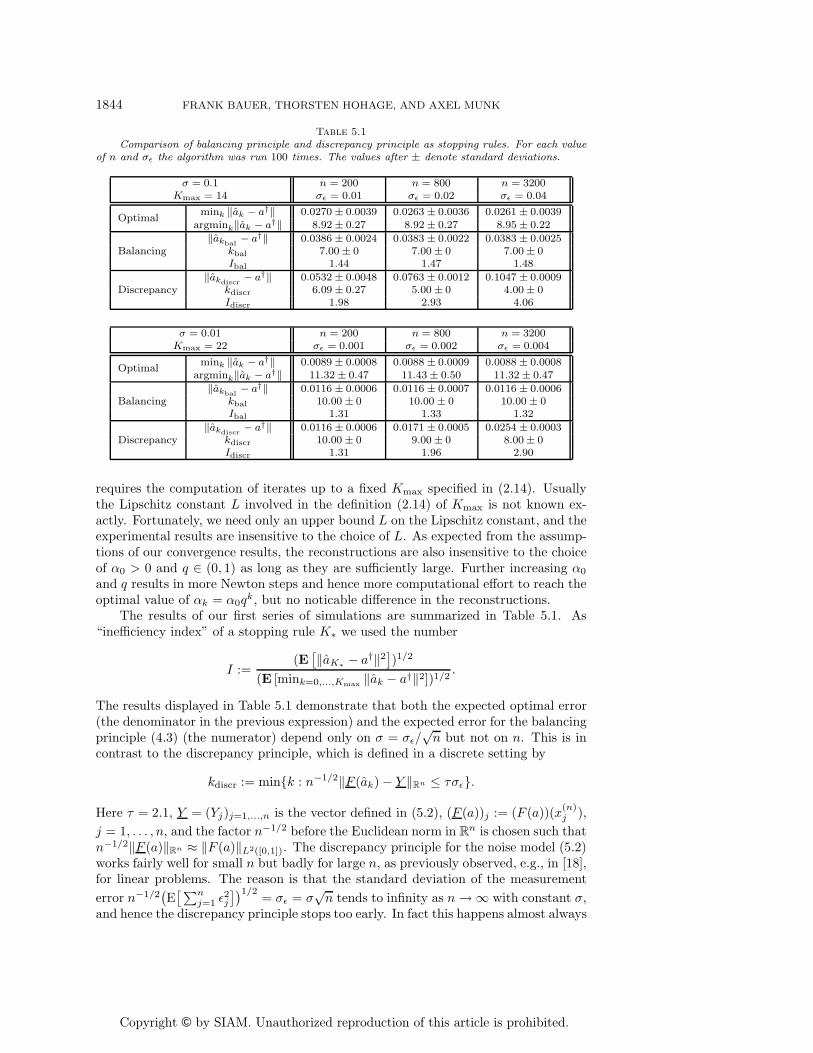
Table 5.1

Comparison of balancing principle and discrepancy principle as stopping rules. For each valueof n and σε the algorithm was run 100 times. The values after ± denote standard deviations.

σ = 0.1 n = 200 n = 800 n = 3200Kmax = 14 σε = 0.01 σε = 0.02 σε = 0.04

mink ‖ak − a†‖ 0.0270 ± 0.0039 0.0263 ± 0.0036 0.0261 ± 0.0039Optimal

argmink‖ak − a†‖ 8.92 ± 0.27 8.92 ± 0.27 8.95 ± 0.22

‖akbal − a†‖ 0.0386 ± 0.0024 0.0383 ± 0.0022 0.0383 ± 0.0025Balancing kbal 7.00 ± 0 7.00 ± 0 7.00 ± 0

Ibal 1.44 1.47 1.48

‖akdiscr − a†‖ 0.0532 ± 0.0048 0.0763 ± 0.0012 0.1047 ± 0.0009Discrepancy kdiscr 6.09 ± 0.27 5.00 ± 0 4.00 ± 0

Idiscr 1.98 2.93 4.06

σ = 0.01 n = 200 n = 800 n = 3200Kmax = 22 σε = 0.001 σε = 0.002 σε = 0.004

mink ‖ak − a†‖ 0.0089 ± 0.0008 0.0088 ± 0.0009 0.0088 ± 0.0008Optimal

argmink‖ak − a†‖ 11.32 ± 0.47 11.43 ± 0.50 11.32 ± 0.47

‖akbal − a†‖ 0.0116 ± 0.0006 0.0116 ± 0.0007 0.0116 ± 0.0006Balancing kbal 10.00 ± 0 10.00 ± 0 10.00 ± 0

Ibal 1.31 1.33 1.32

‖akdiscr − a†‖ 0.0116 ± 0.0006 0.0171 ± 0.0005 0.0254 ± 0.0003Discrepancy kdiscr 10.00 ± 0 9.00 ± 0 8.00 ± 0

Idiscr 1.31 1.96 2.90

requires the computation of iterates up to a fixed Kmax specified in (2.14). Usuallythe Lipschitz constant L involved in the definition (2.14) of Kmax is not known ex-actly. Fortunately, we need only an upper bound L on the Lipschitz constant, and theexperimental results are insensitive to the choice of L. As expected from the assump-tions of our convergence results, the reconstructions are also insensitive to the choiceof α0 > 0 and q ∈ (0, 1) as long as they are sufficiently large. Further increasing α0

and q results in more Newton steps and hence more computational effort to reach theoptimal value of αk = α0q

k, but no noticable difference in the reconstructions.The results of our first series of simulations are summarized in Table 5.1. As

“inefficiency index” of a stopping rule K∗ we used the number

I :=(E[‖aK∗ − a†‖2

])1/2

(E [mink=0,...,Kmax ‖ak − a†‖2])1/2.

The results displayed in Table 5.1 demonstrate that both the expected optimal error(the denominator in the previous expression) and the expected error for the balancingprinciple (4.3) (the numerator) depend only on σ = σε/

√n but not on n. This is in

contrast to the discrepancy principle, which is defined in a discrete setting by

kdiscr := min{k : n−1/2‖F (ak) − Y ‖Rn ≤ τσε}.

Here τ = 2.1, Y = (Yj)j=1,...,n is the vector defined in (5.2), (F (a))j := (F (a))(x(n)j ),

j = 1, . . . , n, and the factor n−1/2 before the Euclidean norm in Rn is chosen such that

n−1/2‖F (a)‖Rn ≈ ‖F (a)‖L2([0,1]). The discrepancy principle for the noise model (5.2)works fairly well for small n but badly for large n, as previously observed, e.g., in [18],for linear problems. The reason is that the standard deviation of the measurementerror n−1/2

(E[∑n

j=1 ε2j

])1/2 = σε = σ√n tends to infinity as n→ ∞ with constant σ,

and hence the discrepancy principle stops too early. In fact this happens almost always

Copyright © by SIAM. Unauthorized reproduction of this article is prohibited.

A REGULARIZED NEWTON METHOD WITH RANDOM NOISE 1845

at the first step for n sufficiently large, whereas the optimal stopping index, whichasymptotically depends only on σ, but not on n, may be arbitrarily large for small σ.

Finally we tested the rates of convergence with the balancing principle for thethree curves a† shown in the right panel of Figure 5.1. We always chose n = 128 andvaried σε. For each value of σ and each of the three curves a† we performed 50 runsof the iteratively regularized Gauss–Newton method. The triangles in the left panelshow the rates σ1/6, σ3/8, and σ7/12, which are obtained by neglecting the logarithmicfactor in (4.16) and setting c = 5

8 and μ = 18 ,

38 ,

78 following the discussion above. Note

that the experimental rates agree quite well with these predicted rates even for thefirst two functions, which are not smooth enough to be covered by our theory.

In summary we have demonstrated that the performance of the balancing principleis independent of the sample size n, whereas the discrepancy principle works well forsmall n, but becomes more and more inefficient as n→ ∞. Moreover, for the balancingprinciple the empirical rates of convergence match the theoretical rates very well.

Appendix. Exponential inequality for Gaussian noise. In this appendixwe will prove the exponential inequality (2.8c) for the case that the noise process ξ in(1.2a) is Gaussian.

Let us consider the random variable V = ‖Λξ‖2 for an arbitrary linear operatorΛ : Y → X such that E

[‖Λξ‖2]< ∞. Since CovΛξ = ΛMΛ∗ with M := Covξ, the

operator ΛMΛ∗ is trace class; i.e., the eigenvalues λ1 ≥ λ2 ≥ · · · of ΛMΛ∗ satisfy∑∞i=1 λi = E [V ] <∞. Note that M−1/2ξ is a Gaussian white noise process; i.e., the

random variables ξi :=⟨M−1/2ξ, ϕi

⟩are i.i.d. standard normal for any orthonormal

system {ϕi} in Y. In particular, if {ϕi} is a system of left singular vectors of ΛM1/2,then V =

∑∞i=1 λiξ

2i . The random variables ξ2i are i.i.d. χ2

1 with Laplace transform

E[exp(tξ2i)]

= (1 − 2t)−1/2, 0 < t <12.

Then it holds that

P

⎛⎝ ∞∑i=1

λi(ξ2i − 1) ≥ η

√√√√2∞∑i=1

λ2i

⎞⎠ ≤ exp(

18− η

4

)(A.1)

for any η > 0 (see [11, 25]).Theorem A.1. Under the above conditions we have for any τ ≥ 1 that

P (V ≥ τE [V ]) ≤ exp(

18− C

4(τ − 1)

),(A.2)

where C := 2−1/2∑∞

i=1 λi/(∑∞

i=1 λ2i )

1/2.Proof. Rewrite

{V ≥ τE [V ]} =

{ ∞∑i=1

λiξ2i ≥ τ

∞∑i=1

λi

}=

⎧⎨⎩∞∑i=1

λi(ξ2i − 1) ≥ η

√√√√2∞∑i=1

λ2i

⎫⎬⎭ ,where η = (τ − 1)C, and apply (A.1).

Since λi ≥ 0, we have∑∞

i=1 λ2i ≤ (

∑∞i=1 λi)

2, and hence C ≥ 2−1/2 for anyeigenvalue sequence (λi). Therefore, choosing Λ := gα(F ′[a]∗F ′[a])F ′[a]∗, we obtain(2.8c) with c1 = exp(1

8 + 14√

2) and c2 = 1

4√

2.

Copyright © by SIAM. Unauthorized reproduction of this article is prohibited.

1846 FRANK BAUER, THORSTEN HOHAGE, AND AXEL MUNK

A variation of the proof in [25] allows in principle an extension for more general(non χ2) random variables under proper growth conditions on the Laplace transformof the ξ2i . This would again give an exponential bound of the form (2.8c).

REFERENCES

[1] A. B. Bakushinskiı, The problem of the convergence of the iteratively regularized Gauss-Newton method, Comput. Math. Math. Phys., 32 (1992), pp. 1353–1359.

[2] A. B. Bakushinskiı and M. Y. Kokurin, Iterative Methods for Approximate Solution of In-verse Problems, Springer, Dordrecht, The Netherlands, 2004.

[3] F. Bauer and T. Hohage, A Lepskij-type stopping rule for regularized Newton methods, In-verse Problems, 21 (2005), pp. 1975–1991.

[4] N. Bissantz, T. Hohage, and A. Munk, Consistency and rates of convergence of nonlinearTikhonov regularization with random noise, Inverse Problems, 20 (2004), pp. 1773–1791.

[5] N. Bissantz, T. Hohage, A. Munk, and F. Ruymgaart, Convergence rates of general regu-larization methods for statistical inverse problems and applications, SIAM J. Numer. Anal.,45 (2007), pp. 2610–2636.

[6] B. Blaschke, A. Neubauer, and O. Scherzer, On convergence rates for the iteratively reg-ularized Gauss-Newton method, IMA J. Numer. Anal., 17 (1997), pp. 421–436.

[7] T. T. Cai and M. G. Low, Nonparametric estimation over shrinking neighborhoods: Superef-ficiency and adaptation, Ann. Statist., 33 (2005), pp. 184–213.

[8] E. Candes, Modern statistical estimation via oracle inequalities, Acta Numer., 15 (2006),pp. 257–325.

[9] L. Cavalier, G. K. Golubev, D. Picard, and A. B. Tsybakov, Oracle inequalities for inverseproblems, Ann. Statist., 30 (2002), pp. 843–874.

[10] R. Cont and P. Tankov, Retrieving Levy processes from option prices: Regularization of anill-posed inverse problem, SIAM J. Control Optim., 45 (2006), pp. 1–25.

[11] R. Dahlhaus and W. Polonik, Nonparametric quasi-maximum likelihood estimation forGaussian locally stationary processes, Ann. Statist., 34 (2006), pp. 2790–2824.

[12] H. W. Engl, M. Hanke, and A. Neubauer, Regularization of Inverse Problems, KluwerAcademic Publishers, Dordrecht, Boston, London, 1996.

[13] T. Hohage, Fast numerical solution of the electromagnetic medium scattering problem andapplications to the inverse problem, J. Comput. Phys., 214 (2006), pp. 224–238.

[14] T. Hohage and M. Pricop, Nonlinear Tikhonov regularization in Hilbert scales for inverseboundary value problems with random noise, Inverse Probl. Imaging, 2 (2008), pp. 271–290.

[15] B. Kaltenbacher, Some Newton-type methods for the regularization of nonlinear ill-posedproblems, Inverse Problems, 13 (1997), pp. 729–753.

[16] B. Kaltenbacher, A posteriori parameter choice strategies for some Newton type methods forthe regularization of nonlinear ill-posed problems, Numer. Math., 79 (1998), pp. 501–528.

[17] J.-M. Loubes and C. Ludena. Penalized estimators for nonlinear inverse problems, ESAIMProbab. Stat., to appear.

[18] M. A. Lukas, Comparison of parameter choice methods for regularization with discrete noisydata, Inverse Problems, 14 (1998), pp. 161–184.

[19] P. Mathe, The Lepskiı principle revisited, Inverse Problems, 22 (2006), pp. L11–L15.[20] P. Mathe and S. Pereverzev, Geometry of ill-posed problems in variable Hilbert scales,

Inverse Problems, 19 (2003), pp. 789–803.[21] P. Mathe and S. Pereverzev, Regularization of some linear ill-posed problems with dis-

cretized random noisy data, Math. Comp., 75 (2006), pp. 1913–1929.[22] W. K. Newey and J. L. Powell, Instrumental variable estimation of nonparametric models,

Econometrica, 71 (2003), pp. 1565–1578.[23] F. O’Sullivan, Convergence characteristics of methods of regularization estimators for non-

linear operator equations, SIAM J. Numer. Anal., 27 (1990), pp. 1635–1649.[24] S. Prossdorf and B. Silbermann, Numerical Analysis for Integral and Related Operator

Equations, Birkhauser, Basel, 1991.[25] A. Rohde and L. Dumbgen, Confidence Sets for the Optimal Approximating Model—Bridging

a Gap between Adaptive Point Estimation and Confidence Regions, 2008; available onlineat http://arxiv.org/abs/0802.3276.

[26] A. Tsybakov, On the best rate of adaptive estimation in some inverse problems, C. R. Acad.Sci. Paris Ser. I Math., 330 (2000), pp. 835–840.