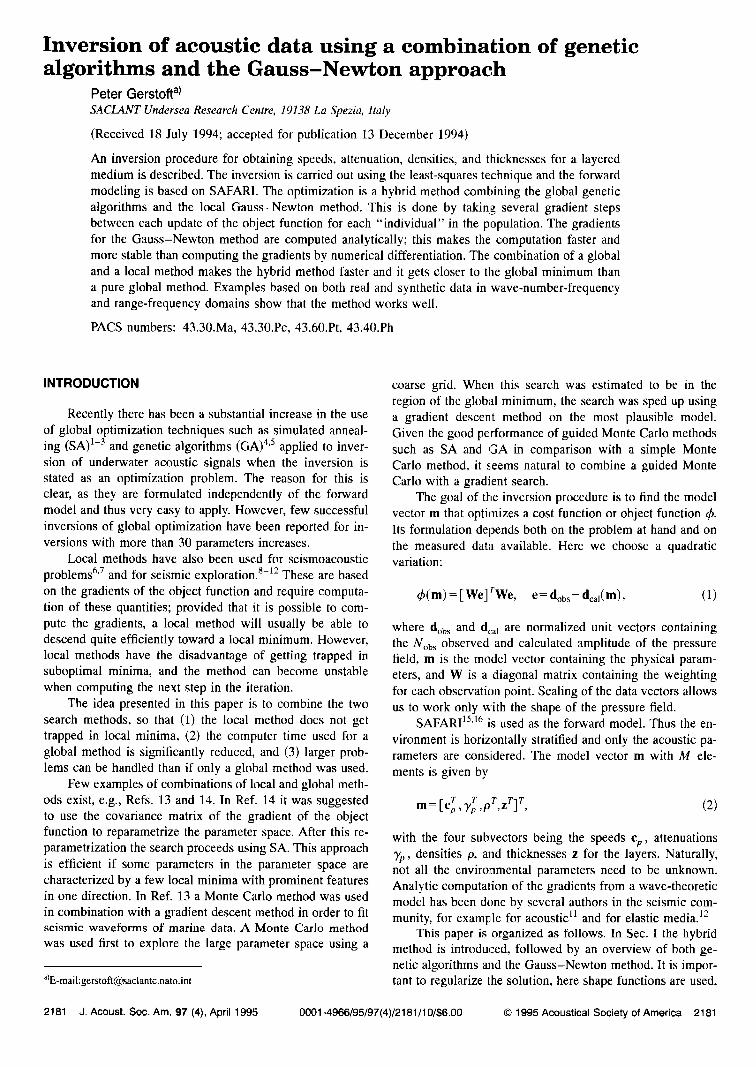
Inversion of acoustic data using a combination of genetic algorithms and the Gauss-Newton approach

Peter Gerstoft a) SACLANT Undersea Research Centre, 19138 La Spezia, Italy

(Received 18 July 1994; accepted for publication 13 December 1994) An inversion procedure for obtaining speeds, attenuation, densities, and thicknesses for a layered medium is described. The inversion is carried out using the least-squares technique and the forward modeling is based on SAFARI. The optimization is a hybrid method combining the global genetic algorithms and the local Gauss-Newton method. This is done by taking several gradient steps between each update of the object function for each "individual" in the population. The gradients for the Gauss-Newton method are computed analytically; this makes the computation faster and more stable than computing the gradients by numerical differentiation. The combination of a global and a local method makes the hybrid method faster and it gets closer to the global minimum than a pure global method. Examples based on both real and synthetic data in wave-number-frequency and range-frequency domains show that the method works well. PACS numbers: 43.30.Ma, 43.30.Pc, 43.60.Pt, 43.40.Ph

INTRODUCTION

Recently there has been a substantial increase in the use of global optimization techniques such as simulated anneal- ing (SA) •-3 and genetic algorithms (GA) 4'5 applied to inver- sion of underwater acoustic signals when the inversion is stated as an optimization problem. The reason for this is clear, as they are formulated independently of the forward model and thus very easy to apply. However, few successful inversions of global optimization have been reported for in- versions with more than 30 parameters increases.

Local methods have also been used for seismoacoustic

problems 6'7 and for seismic exploration. 8-•2 These are based on the gradients of the object function and require computa- tion of these quantities; provided that it is possible to com- pute the gradients, a local method will usually be able to descend quite efficiently toward a local minimum. However, local methods have the disadvantage of getting trapped in suboptimal minima, and the method can become unstable when computing the next step in the iteration.

The idea presented in this paper is to combine the two search methods, so that (1) the local method does not get trapped in local minima, (2) the computer time used for a global method is significantly reduced, and (3) larger prob- lems can be handled than if only a global method was used.

Few examples of combinations of local and global meth- ods exist, e.g., Refs. 13 and 14. In Ref. 14 it was suggested to use the covariance matrix of the gradient of the object function to reparametrize the parameter space. After this re- parametrization the search proceeds using SA. This approach is efficient if some parameters in the parameter space are characterized by a few local minima with prominent features in one direction. In Ref. 13 a Monte Carlo method was used in combination with a gradient descent method in order to fit seismic waveforms of marine data. A Monte Carlo method

was used first to explore the large parameter space using a

•E-mail:gcrstofi@saclantc.nato.int

coarse grid. When this search was estimated to be in the region of the global minimum, the search was sped up using a gradient descent method on the most plausible model. Given the good performance of guided Monte Carlo methods such as SA and GA in comparison with a simple Monte Carlo method, it seems natural to combine a guided Monte Carlo with a gradient search.

The goal of the inversion procedure is to find the model vector tn that optimizes a cost function or object function ,;b. Its formulation depends both on the problem at hand and on the measured data available. Here we choose a quadratic variation:

qb(m) = [we]rWe, e= dou •- dcal(m), (1)

where dot,s and dca I are normalized unit vectors containing the Nob s observed and calculated amplitude of the pressure field, m is the model vector containing the physical param- eters, and W is a diagonal matrix containing the weighting for each observation point. Scaling of the data vectors allows us to work only with the shape of the pressure field.

SAFARI 15'•6 is used as the forward model. Thus the en- vironment is horizontally stratified and only the acoustic pa- rameters are considered. The model vector m with M ele-

ments is given by

T T T T T m=[%,yp,p ,z ] , (2)

with the four subvectors being the speeds %, attenuations y•,, densities p, and thicknesses z for the layers. Naturally, not all the environmental parameters need to be unknown. Analytic computation of the gradients from a wave-theoretic model has been done by several authors in the seismic com- munity, for example for acoustic • and for elastic media?

This paper is organized as follows. In Sec. I the hybrid method is introduced, followed by an overview of both ge- netic algorithms and the Gauss-Newton method. It is impor- tant to regularize the solution, here shape functions are used,

2181 J. Acoust. Soc. Am. 97 (4), April 1995 0001-4966/95/97(4)/2181/10/$6.00 ¸ 1995 Acoustical Society of America 2181

and this is also described in Sec. I. In Sec. II the approach is applied to the inversion of geoacoustic parameters for both real and synthetic data.

I. THE HYBRID APPROACH

A crucial point in deciding if a global or local method is most efficient for a given object function is the number of local minima in the search space. By a global method we mean a method, such as SA or GA, which does not use gradients. If there are only a few local minima a local method with a few random starting points is more efficient than a global method, because a global method is very inef- ficient in descending, as the gradients are not used. For noisier data the object function will show several suboptimal minima. For this scenario the global method will become more efficient as it will not get stuck in each of the minima. Finally, if the data becomes too noisy then only an exhaus- tive search will find the solution.

For a large class of inverse problems it is believed that the number of local minima in the search space is small. Here an efficient approach would be to find the local minima by a gradient method and then use a global method to choose between these local minima. This is what the hybrid method should do.

The hybrid approach states quite simply that for each new child generated by the GA, in addition to the crossover and mutation operator, Ng Gauss-Newton steps are applied to the child in order to increase the fitness. The choice of Ng is problem dependent. For a local problem it is optimal to use a large Ng so that the minimum is reached quickly. How- ever, if the minimum is not reached during the first set of iterations, it can be reached in the next with little extra com- putational cost. For very noisy data it is optimal not to per- form any Gauss-Newton steps. Experimentally, we found the Ng=5 seems to be a good choice. A. Genetic algorithms

Genetic algorithms (GA) are based on an analogy with biological evolution. While these have already provided promising results in the seismic community, 17-•9 an applica- tion to ocean acoustic problems has only recently been published. 4 The basic principle of GA is simple: From all possible model vectors, an initial population size of q mem- ber is selected. The fitness of each member is computed based on the fit between the observed and computed data. Then through a set of evolutionary steps the initial popula- tion evolves in order to become fitter. An evolutionary step consists of selecting a parental distribution from the popula- tion based on the individual's fitness. The parents are then combined in pairs and operators are applied to them to form a set of children. Traditionally the crossover and mutation operators have been used, but for the hybrid method the "Gauss-Newton" operator is also applied. Finally, the chil- dren replace part of the population to get a fitter population.

The environment is discretized into M parameters in a model vector m. Each parameter m j, j= 1 ..... M, has a bi- nary parameter string of length nj and can take 2nJ discrete values according to an a priori probability distribution (Gaussian, rectangular or based on a priori information).

I l = =nj--1 =nl-2 ß ø•3 c(2 0 = 0 0 0 0 0 m rain

I

1 = 0 0 0 0 1 mmin+ 1 Am I

2 = 0 0 0 1 0 m rain 2 Am j + 3= 0 0 0 1 1 mjmln+ 3 A m

2nj -1 = 1 1 1 1 1 mj m'ax

FIG. 1. Binary coding of model parameters. nj is the number of bits.

Here a rectangular distribution between a lower and upper bound min max [mj ,rnj ] is used. We have (see Fig. 1)

i rnin ß =mj +tj Arnj ij=0,1,2 ..... 2"J--1 (3) rnj , , where

max rnin

rnj - mj (4) Am j- 2n• - 1 A major difference between SA and GA is that GA uses

q model vectors at the same time, where q is the population size, while SA uses only one. GA consists essentially of three operators: Selection, crossover, and mutation.

Selection: In order to establish the next generation, a subset of the current population must be selected as parents. Selection is based on the fitness of the individual models.

The probability that the kth member is selected as parent is made according to a normalized Boltzmann distribution:

exp[- qb(mk)/T] Pk=x•=• exp[-qb(mt)/T] ' k=l ..... q. (5) The introduction of temperature T, as in SA, gives us the

opportunity to stretch the probability and to improve the per- formance of the algorithm? Indeed, at the first stage of the procedure, by stretching the fitness we avoid choosing as parents only those members with the better fit, which would otherwise tend to dominate the population; later in the opti- mization this stretching leads to better discrimination be- tween models with close fitness. As with SA, the choice of the temperature T is difficult. It must neither be too high nor too low. A good compromise is a temperature of the same magnitude as the object function, here T=min[•mn)]. Dur- ing the optimization, the fitness increases and the tempera- ture decreases.

Crossover: For each set of parents, each consisting of a model vector, two children are constructed. For each param- eter in the model vector each child may either be a direct copy of one parent, with probability 1-px, or it can be a bit crossover of the two parents with crossover probability p•, see Fig. 2. The crossover point is chosen randomly in the interval [1,N-1], where N is the number of bits used in the coding. Different techniques are available to perform this crossover of the population. Two of these are single-point crossover where the entire chromosome is used once, and multiple-point crossover (as used here) where the chromo- some is divided into genes related to each parameter on which the crossover is applied.

2182 J. Acoust. Soc. Am., Vol. 97, No. 4, April 1995 Peter Gerstoft: Inversion of acoustic data 2182

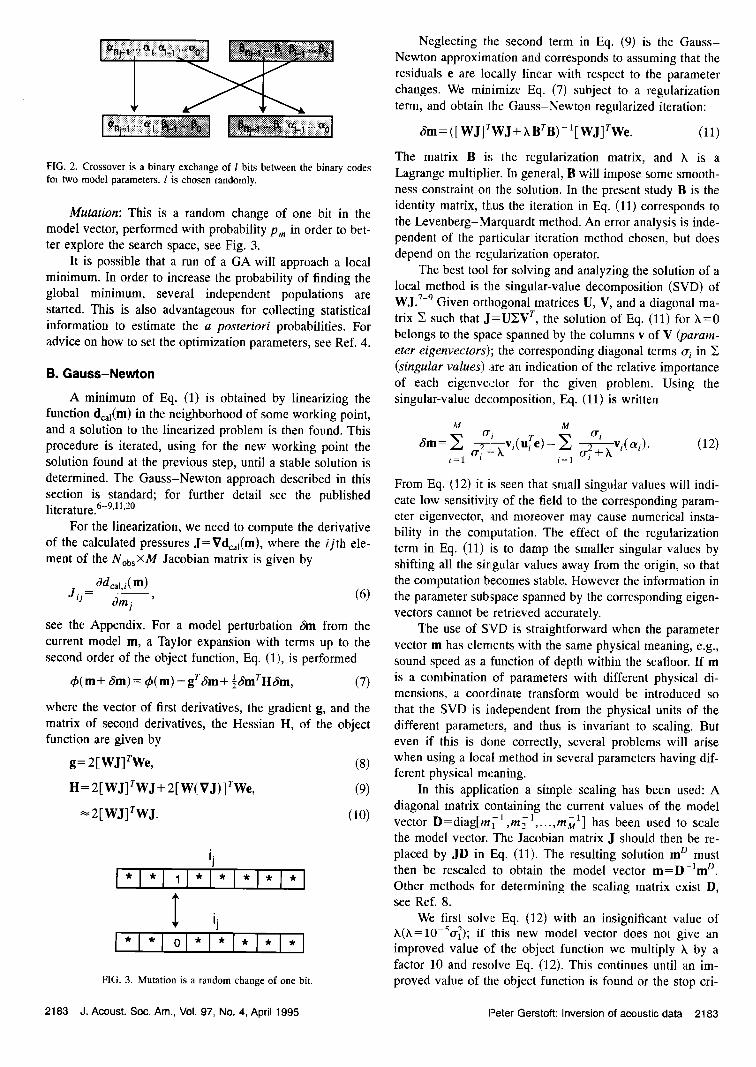
FIG. 2. Crossover is a binary exchange of 1 bits between the binary codes for two model parameters. l is chosen randomly.

Mutation: This is a random change of one bit in the model vector, performed with probability Pm in order to bet- ter explore the search space, see Fig. 3.

It is possible that a run of a GA will approach a local minimum. In order to increase the probability of finding the global minimum, several independent populations are started. This is also advantageous for collecting statistical information to estimate the a posteriori probabilities. For advice on how to set the optimization parameters, see Ref. 4.

B. Gauss-Newton

A minimum of Eq. (1) is obtained by linearizing the function dcal(m ) in the neighborhood of some working point, and a solution to the linearized problem is then found. This procedure is iterated, using for the new working point the solution found at the previous step, until a stable solution is determined. The Gauss-Newton approach described in this section is standard; for further detail see the published literature.6-9,n. 20

For the linearization, we need to compute the derivative of the calculated pressures J=Vdeal(m), where the ijth ele- ment of the NobsXM JacobJan matrix is given by

Odcal,i(m) Jij - 8mj ' (6)

see the Appendix. For a model perturbation ,fro from the current model m, a Taylor expansion with terms up to the second order of the object function, Eq. (1), is performed

•(m+ •Sm)= •(m)+ gr6m+ «smrH6m, (7) where the vector of first derivatives, the gradient g, and the matrix of second derivatives, the Hessian H, of the object function are given by

g = 2 [ W J] rwe, (8) H= 2[W J] rwj + 2[W(?j)]rwe, (9)

•2[WJ]rWJ. (10)

i i

FIG. 3. Mutation is a random change of one bit.

Neglecting the second term in Eq. (9) is the Gauss- Newton approximation and corresponds to assuming that the residuals e are locally linear with respect to the parameter changes. We minimize Eq. (7) subject to a regularization term, and obtain lhe Gauss-Newton regularized iteration:

•Sm= ([WJ]7WJ+ XBTB) - l[wj] rwe. (11) The matrix B is the regularization matrix, and X is a Lagrange multiplier. In general, B will impose some smooth- ness constraint on the solution. In the present study B is the identity matrix, thus the iteration in Eq. (11) corresponds to the Levenberg-Marquardt method. An error analysis is inde- pendent of the particular iteration method chosen, but does depend on the regularization operator.

The best tool for solving and analyzing the solution of a local method is the singular-value decomposition (SVD) of WJ. 7-9 Given orthogonal matrices U, V, and a diagonal ma- trix •; such that J=UY•V r, the solution of Eq. (11) for h=0 belongs to the space spanned by the columns v of V (param- eter eigenvectors); the corresponding diagonal terms o' i in •; (singular values) ::tre an indication of the relative importance of each eigenvector for the given problem. Using the singular-value decomposition, Eq. (11) is written

M M

i=10'i -•' •k '= O.i-•'•Vi(Oli). (12) From Eq. (12) it is seen that small singular values will indi- cate low sensitivit:y of the field to the corresponding param- eter eigenvector, and moreover may cause numerical insta- bility in the computation. The effect of the regularization term in Eq. (11) is to damp the smaller singular values by shifting all the singular values away from the origin, so that the computation becomes stable. However the information in the parameter subspace spanned by the corresponding eigen- vectors cannot be retrieved accurately.

The use of SVD is straightforward when the parameter vector m has elements with the same physical meaning, e.g., sound speed as a function of depth within the seafloor. If m is a combination of parameters with different physical di- mensions, a coordinate transform would be introduced so that the SVD is independent from the physical units of the different parameters, and thus is invariant to scaling. But even if this is done correctly, several problems will arise when using a local method in several parameters having dif- ferent physical meaning.

In this application a simple scaling has been used: A diagonal matrix containing the current values of the model vector D=diag[mi-l,m, • ..... m• 1] has been used to scale the model vector. The Jacobian matrix J should then be re- placed by JD in Eq. (11). The resulting solution m ø must then be rescaled to obtain the model vector m=D-•m ø. Other methods for determining the scaling matrix exist D, see Ref. 8.

We first solve Eq. (12) with an insignificant value of h(•.=10-5o-•1); if this new model vector does not give an improved value of the object function we multiply )t by a factor 10 and resolve Eq. (12). This continues until an im- proved value of the object function is found or the stop cri-

2183 d. Acoust. Soc. Am., Vol. 97, No. 4, April 1995 Peter Gerstoft: Inversion of acoustic data 2183

terion is satisfied. The stop criterion is that the maximum number of iterations is reached or that for all parameters i=I,...,M:

•Srni< Arni• , (13) where •=0.2 and Am i is the discretization step size given by Eq. (4).

An important step in obtaining a solution by a local method is the determination of the derivatives of the pressure field with respect to the model parameters. These can be computed in three ways: •2 finite difference, adjoint state technique, and analytical differentiation.

The adjoint state is based directly on the differential equation, see Reft 20.

For the finite difference method, the main problem is to determine the step size. This should be determined by some adaptive method in order to get a stable result. It is also computationally demanding; for a problem of M parameters a finite difference solution requires at least M+I forward models. This is in contrast to both adjoint and analytical differentiation where the computation of derivatives does not increase the computer time significantly. Thus finite differ- ence should only be used for small problems. In addition, finite difference will have problems in obtaining stable de- rivatives; it cannot easily be automated.

Analytic differentiation has been used in seismic reflec- tivity modeling in the frequency-wave-number domain by Refs. 11 and 12 for seismic exploration problems, but for each formulation of the forward model the analytic differen- tiation is different.

In the present application we derive analytical expres- sions for the gradient using the direct global matrix method (DGM) as implemented in SAFARI. These are essential in getting a Gauss-Newton method to work and are developed in the Appendix.

C. Regularization Experience with synthetic and real data 5'2• had shown

that it is advantageous to regularize the solution in order to have a priori well-behaved solutions. Regularization is intro- duced via shape functions:

Ms

m= '• laihi, (14) i

where h i is the /the shape function or basis function, /.t i is the coefficient associated with the shape function, and M s is the number of shape functions used. The advantages of shape functions are (1) To constrain the solution to belong to a certain class of expected profiles. (2) To describe the varia- tion of the parameters with fewer coefficients and in so doing to reduce the number of unknowns. This can also constrain

the solution to be more physically correct. By linking the velocities in the sediment together we can describe them by a smoother function and, further, the number of unknowns is reduced. (3) To link correlated parameters. For example the source of receiver depth is often specified in depth from the surface. Alternatively, using shape functions they can be specified from the bottom.

TABLE I. Comparison of inversion results for the three examples. CPU time is for a DEC-3000/800 workstation.

CPU Model calls New individuals

Case Obj fn (rain) ( X 10 3) ( X 10 3) A1-GA 0.003 14 50 50

Al-hy 0.0001 0.6 1 0.2 A1-GN 0.006 0.03 0.022 ... A2-GA 0.0003 14 50 50

A2-hy 0.000007 9 10 1 B-G^ 0.56 40 10 10

B-hy 0.62 14 1 0.2

Regularization using shape functions may decrease the correlation between parameters and this would improve the inversion results. This was done in Ref. 5 where we inverted

for the slope and the offset of the water sound speed instead of inverting for the absolute sound speed at discrete points.

II. EXAMPLES

The examples will compare the hybrid approach in both wave number or range domain on both synthetic and real data to the classical genetic algorithms and Gauss-Newton methods.

For the GA the "standard" parameters 4'5 were used: Population size 32, crossover rate 0.8, mutation probability 0.05, and reproduction size 0.5. A full GA run will consist of several parallel populations each with 2000 forward models. For the hybrid method, a run will consist of one population with 1000-5000 forward models and five Gauss-Newton iterations or five forward models for each new individual.

This corresponds to evaluating 200-1000 new individuals. The examples will show comparisons between GA and

the hybrid method. The main findings are summarized in Table I. The basis for comparison of the two methods is how fast the final estimate is obtained. How well the final esti-

mate fits the data is expressed through the value of the object function, Eq. (1). How fast the solution is obtained is best expressed through the CPU-time, which depends on the ac- tual implementation of the code. It could also be expressed by the number of forward modeling calls, but because the GN also needs a gradient the forward modeling calls are more CPU intensive for this method (about a factor 2-5 depending on the number of gradients to be computed). Fi- nally, the speed can also be expressed as number of new individuals. For the hybrid method, computation of a new individual requires Ng forward models; using Ng=5 makes a new individual a factor 5X2=10 more intensive than the simple GA. This extra effort is often well spent.

It is instructive to bear in mind some limiting cases: (1) For a purely local problem GN is faster than the hybrid method which is faster than GA. The GN does not waste any time exploring the model space. (2) If the GA and hybrid method have the same number of new individuals the hybrid will always outperform the GA because it does additional GN steps which will give better or at worst the same fitness. (3) On very noisy data the hybrid method will just waste time computing gradients.

2184 d. Acoust. Soc. Am., Vol. 97, No. 4, April 1995 Peter Gerstoft: Inversion of acoustic data 2184

60

100

150

a)

1600 2000 2400 2800

Sound speed (m/s)

50

100

150

1600 2000 2400 2800

Sound speed (m/s)

50

100

150

c)

600 2000 2400 2800

Sound speed (m/s)

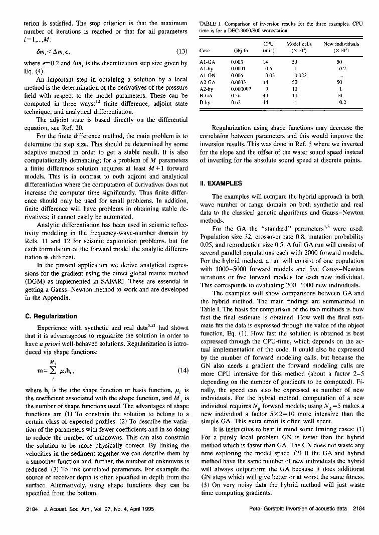
FIG. 4. The inversion result (dashed line) for the sound-speed profile using (a) GA, (b) Gauss-Newton, and (c) the hybrid method. The true solution is the solid line.

A. Inversion in wave-number domain

In order to describe the approach we first invert for the sound-speed profile given the simple environmental model given in Table II, which is similar to the environment given in Ref. 4 except that we have no shear. The bottom is param- etrized into 10 layers, each 10 m thick, plus a basement layer; in total 11 layers. In order to obtain maximum re- sponse from the bottom, both the source and the receivers are placed on the seabed. The source frequency is 100 Hz and the magnitude of the horizontal wave-number spectrum is computed at 64 points equally spaced in the phase velocity range from 1200 to 3000 m/s. The amount of information available to retrieve the parameters here is rather limited in order to make the inversion more difficult. These examples are purely synthetic. Thus there is no consideration of how we should obtain the input data from actual experiments. For a discussion of how to transform real data to wave-number domain, see Refs. 11 and 12.

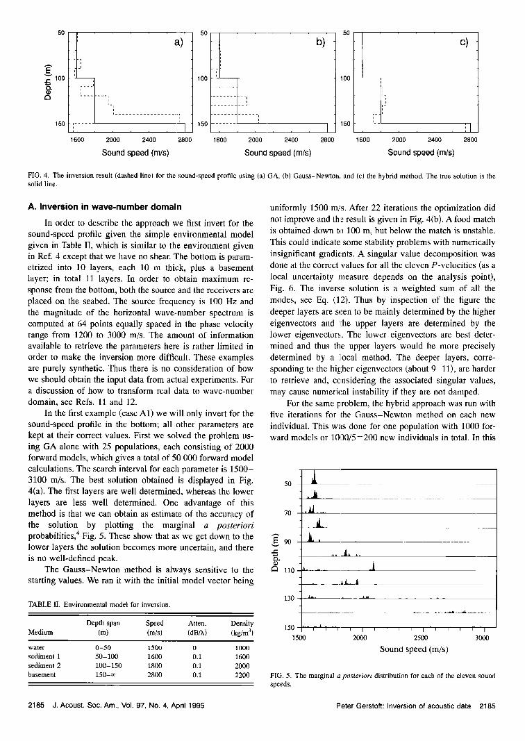
In the first example (case A1) we will only invert for the sound-speed profile in the bottom; all other parameters are kept at their correct values, First we solved the problem us- ing GA alone with 25 populations, each consisting of 2000 forward models, which gives a total of $0 000 forward model calculations. The search interval for each parameter is 1500- 3100 m/s. The best solution obtained is displayed in Fig. 4(a). The first layers are well determined, whereas the lower layers are less well determined. One advantage of this method is that we can obtain as estimate of the accuracy of the solution by plotting the marginal a posterJori probabilities, 4 Fig. 5. These show that as we get down to the lower layers the solution becomes more uncertain, and there is no well-defined peak.

The Gauss-Newton method is always sensitive to the starting values. We ran it with the initial model vector being

TABLE 11. Environmental model for inversion.

Depth span Speed Atten. Density Medium (m) (m/s) (dB/k) (kg/m 3) water 0-50 1500 0 1000

sediment 1 50-100 1600 0.1 1600 sediment 2 100-150 1800 0.1 2000 basement 150-• 2800 0.1 2200

uniformly 1500 m/s. After 22 iterations the optimization did not improve and the result is given in Fig. 4(b). A food match is obtained down to 100 m, but below the match is unstable. This could indicate some stability problems with numerically insignificant gradients. A singular value decomposition was done at the correct values for all the eleven P-velocities (as a local uncertainty measure depends on the analysis point), Fig. 6. The inverse solution is a weighted sum of all the modes, see Eq. (12). Thus by inspection of the figure the deeper layers are seen to be mainly determined by the higher eigenvectors and 'Ihe upper layers are determined by the lower eigenvectors. The lower eigenvectors are best deter- mined and thus the upper layers would be more precisely determined by a ]local method. The deeper layers, corre- sponding to the higher eigenvectors (about 9-11), are harder to retrieve and, cc•nsidering the associated singular values, may cause numerical instability if they are not damped.

For the same problem, the hybrid approach was run with five iterations for the Gauss-Newton method on each new

individual. This was done for one population with 1000 for- ward models or 1000/5=200 new individuals in total. In this

50

70

• 90

• ]]0

130

150 "' '-'•' ; '-' ' I • ' ' ' I ' • " ' f" '1 ]500 2000 2500 3oo0

Sound speed (m/s)

FIG. 5. The marginal a posteriori distribution for each of the eleven sound speeds.

2185 J. Acoust. Soc. Am., Vol. 97, No. 4, April 1995 Peter Gerstoft: Inversion of acoustic data 2185

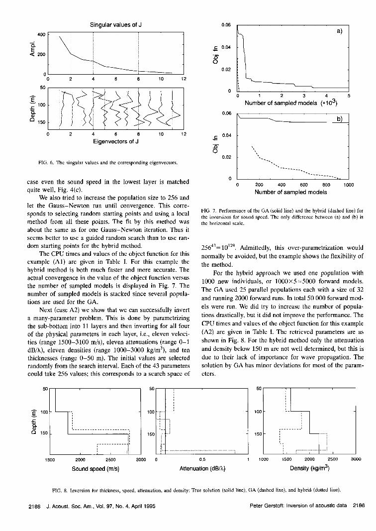
Singular values of J

•,. 400 t 200 t

0 ß 0

5O

v 100 ..1:

o_

15o

2 4 6 8 10 12

0 2 4 6 8 10 12

Eigenvectors of J

F[G. 6. The singular values and the corresponding eigenvectors.

case even the sound speed in the lowest layer is matched quite well, Fig. 4(c).

We also tried to increase the population size to 256 and let the Gauss-Newton run until convergence. This corre- sponds to selecting random starting points and using a local method from all these points. The fit by this method was about the same as for one Gauss-Newton iteration. Thus it

seems better to use a guided random search than to use ran- dom starting points for the hybrid method.

The CPU times and values of the object function for this example (A1) are given in Table I. For this example the hybrid method is both much faster and more accurate. The actual convergence in the value of the object function versus the number of sampled models is displayed in Fig. 7. The number of sampled models is stacked since several popula- tions are used for the GA.

Next (case A2) we show that we can successfully invert a many-parameter problem. This is done by parametrizing the sub-bottom into 11 layers and then inverting for all four of the physical parameters in each layer, i.e., eleven veloci- ties (range 1500-3100 m/s), eleven attenuations (range 0-1 dB/M, eleven densities (range 1000-3000 kg/m3), and ten thicknesses (range 0-50 m). The initial values are selected randomly from the search interval. Each of the 43 parameters could take 256 values; this corresponds to a search space of

0.02

0.06

0.04

0.02

a)

0 1 2 3 4 5

Number of sampled models (.10 3 )

b)

200 400 600 800 1000

Number of sampled models

FIG. 7. Performance of the GA (solid line) and the hybrid (dashed line) for the inversions for sound speed. The only difference between (a) and (b) is the horizontal scale.

25643=10129. Admittedly, this over-parametrization would normally be avoided, but the example shows the flexibility of the method.

For the hybrid approach we used one population with 1000 new individuals, or 1000x5=5000 forward models. The GA used 25 parallel populations each with a size of 32 and running 2000 forward runs. In total 50 000 forward mod- els were run. We did try to increase the number of popula- tions drastically, but it did not improve the performance. The CPU times and values of the object function for this example (A2) are given in Table I. The retrieved parameters are as shown in Fig. 8. For the hybrid method only the attenuation and density below 150 m are not well determined, but this is due to their lack of importance for wave propagation. The solution by GA has minor deviations for most of the param- eters.

50

'•' lOO v

CI 150

1500 2000 2500

Sound speed (m/s)

ooo

50 ,

150 1 •" 0 0.5

Attenuation (dB/k)

50

100

150

1000 1500 2000 2500 3000

Density (kg/m 3)

FIG. 8. Inversion for thickness, speed, attenuation, and density: True solution (solid line), GA (dashed line), and hybrid (dotted line).

2186 J. Acoust. Soc. Am., Vol. 97, No. 4, April 1995 Peter Gerstoft: Inversion of acoustic data 2186

FleceJvers

Ballast

Data transmission

i Source

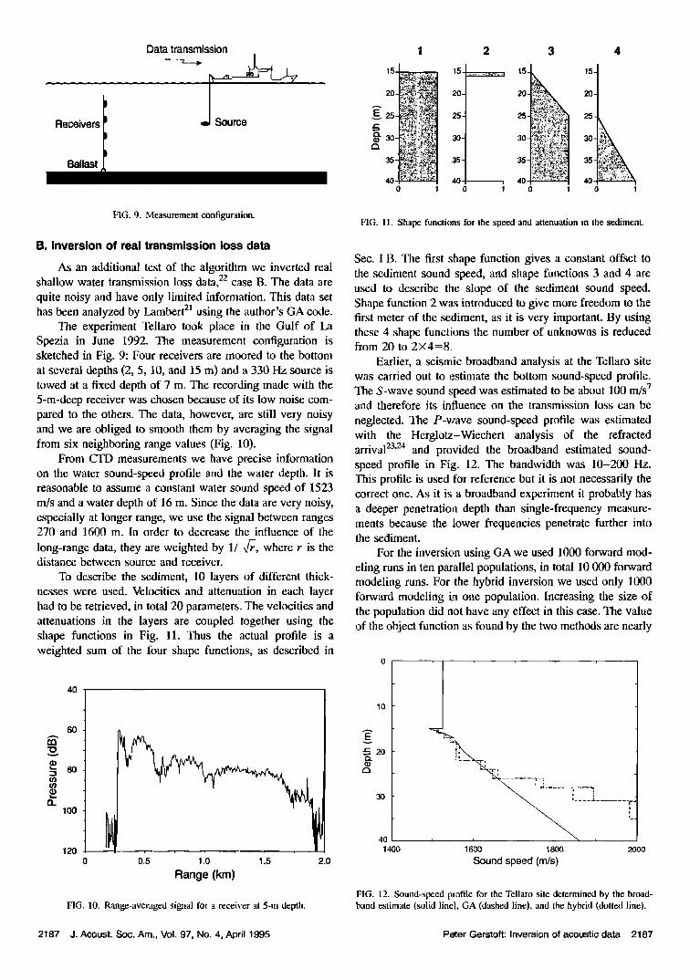
FIG. 9. Measurement configuration.

B. Inversion of real transmission loss data

As an additional test of the algorithm we inverted real shallow water transmission loss data, 22 case B. The data are quite noisy and have only limited information. This data set has been analyzed by Lambert 2t using the author's GA code.

The experiment Tellaro took place in the Gulf of La Spezia in June 1992. The measurement configuration is sketched in Fig. 9: Four receivers are moored to the bottom at several depths (2, 5, 10, and 15 m) and a 330 Hz source is towed at a fixed depth of 7 m. The recording made with the 5-m-deep receiver was chosen because of its low noise com- pared to the others. The data, however, are still very noisy and we are obliged to smooth them by averaging the signal from six neighboring range values (Fig. 10).

From CTD measurements we have precise information on the water sound-speed profile and the water depth. It is reasonable to assume a constant water sound speed of 1523 m/s and a water depth of 16 m. Since the data are very noisy, especially at longer range, we use the signal between ranges 270 and 1600 m. In order to decrease the influence of the

long-range data, they are weighted by 1/ ,/•, where r is the distance between source and receiver.

To describe the sediment, 10 layers of different thick- nesses were used. Velocities and attenuation in each layer had to be retrieved, in total 20 parameters. The velocities and attenuations in the layers are coupled together using the shape functions in Fig. 11. Thus the actual profile is a weighted sum of the four shape functions, as described in

4O

6O

lOO

0 0.5 1.0 1.5

Range (km)

FIG. 10. Range-averaged signal for a receiver at 5-m depth.

2.0

1 2 3

•'30 30 30

40 0 1 0 ! 0 1

4

15-

20-

25-

35-

40 !

FIG. ll. Shape functions for the speed and attenuation in the sediment.

Sec. I B. The first shape function gives a constant offset to the sediment sound speed, and shape functions 3 and 4 are used to describe the slope of the sediment sound speed. Shape function 2 was introduced to give more freedom to the first meter of the sediment, as it is very important. By using these 4 shape functions the number of unknowns is reduced from 20 to 2X4=8

Earlier, a seismic broadband analysis at the Tellaro site was carried out to estimate the bottom sound-speed profile. The S-wave sound speed was estimated to be about 100 m/s 7 and therefore its influence on the transmission loss can be

neglected. The P-wave sound-speed profile was estimated with the Herglotz-Wiechert analysis of the refracted arrival 2324 and provided the broadband estimated sound- speed profile in Fig. 12. The bandwidth was 10-200 Hz. This profile is used for reference but it is not necessarily the correct one. As it is a broadband experiment it probably has a deeper penetration depth than single-frequency measure- ments because the lower frequencies penetrate further into the sediment.

For the inversion using GA we used 1000 forward mod- eling runs in ten parallel populations, in total 10 000 forward modeling runs. For the hybrid inversion we used only 1000 forward modeling in one population. Increasing the size of the population did not have any effect in this case. The value of the object function as found by the two methods are nearly

10

3o

40 1400 1600 1800 2000

Sound speed (m/s)

FIG. 12. Sound-speed profile for the Tellaro site determined by the broad- band estimate (solid line}, GA (dashed line). and the hybrid (dotted line}.

2187 J. Acoust. Soc. Am., Vol. 97, No. 4, April 1995 Pe:er Gerstoft: Inversion of acoustic data 2187

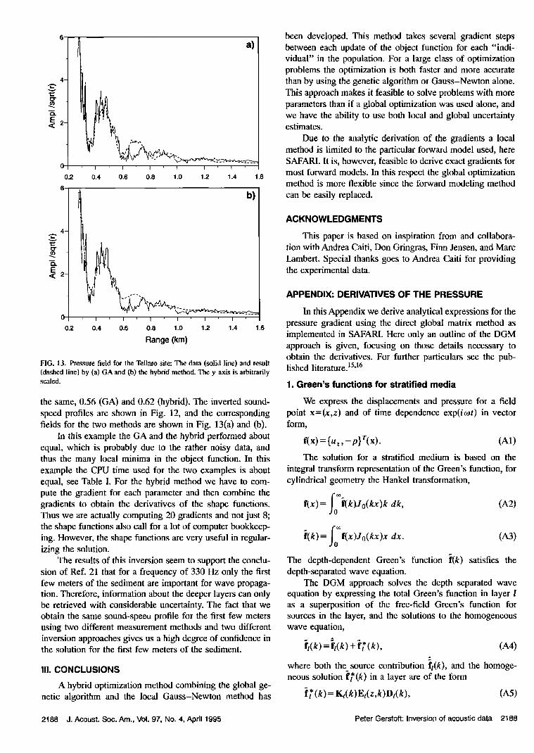
o

0.2

6

a)

0.4 0.6 0.8 1.0 12 1.4 1.6

4

E • 2-

o

0.2

b)

Range (krn)

FIG. 13. Pressure field for the Tellaro site: The data (solid line) and result (dashed line} by (a) GA and (b) the hybrid method. The y axis is arbitrarily scaled.

the same, 0.56 (GA) and 0.62 (hybrid). The inverted sound- speed profiles are shown in Fig. 12, and the corresponding fields for the two methods are shown in Fig. 13(a) and (b).

In this example the GA and the hybrid performed about equal, which is probably due to the rather noisy data, and thus the many local minima in the object function. In this example the CPU time used for the two examples is about equal, see Table I. For the hybrid method we have to com- pute the gradient for each parameter and then combine the gradients to obtain the derivatives of the shape functions. Thus we are actually computing 20 gradients and not just 8; the shape functions also call for a lot of computer bookkeep- ing. However, the shape functions are very useful in regular- izing the solution.

The results of this inversion seem to support the conclu- sion of Ref. 21 that for a frequency of 330 Hz only the first few meters of the sediment are important for wave propaga- tion. Therefore, information about the deeper layers can only be retrieved with considerable uncertainty. The fact that we obtain the same sound-speeu profile for the first few meters using two different measurement methods and two different inversion approaches gives us a high degree of confidence in the solution for the first few meters of the sediment.

III. CONCLUSIONS

A hybrid optimization method combining the global ge- netic algorithm and the local Gauss-Newton method has

been developed. This method takes several gradient steps between each update of the object function for each "indi- vidual" in the population. For a large class of optimization problems the optimization is both faster and more accurate than by using the genetic algorithm or Gauss-Newton alone. This approach makes it feasible to solve problems with more parameters than if a global optimization was used alone, and we have the ability to use both local and global uncertainty estimates.

Due to the analytic derivation of the gradients a local method is limited to the particular forward model used, here SAFARI. It is, however, feasible to derive exact gradients for most forward models. In this respect the global optimization method is more flexible since the forward modeling method can be easily replaced.

ACKNOWLEDGMENTS

This paper is based on inspiration from and collabora- tion with Andrea Caiti, Don Gringras, Finn Jensen, and Marc Lambert. Special thanks goes to Andrea Caiti for providing the experimental data.

APPENDIX: DERIVATIVES OF THE PRESSURE

In this Appendix we derive analytical expressions for the pressure gradient using the direct global matrix method as implemented in SAFARI. Here only an outline of the DGM approach is given, focusing on those details necessary to obtain the derivatives. For further particulars see the pub- lished literature. ]s']6

1. Green's functions for stratified media

We express the displacements and pressure for a field point x=(x,z) and of time dependence exp(itot) in vector form,

f(x) ={uz,-p}r(x). (A1) The solution for a stratified medium is based on the

integral transform representation of the Green's function, for cylindrical geometry the Hankel transformation,

f{x) = f(k)Jo(kx)k dk, (A2)

ilk)= r(x)J0(kx)x ax. (A3)

The depth-dependent Green's function •(k) satisfies the depth-separated wave equation.

The DGM approach solves the depth separated wave equation by expressing the total Green's function in layer l as a superposition of the free-field Green's function for sources in the layer, and the solutions to the homogeneous wave equation,

[l(k) = }l(k) + •? (k), (A4) where both the source contribution ft(k), and the homoge- neous solution [•(k) in a layer are of the form

•? ( k ) = Kl( k )El(z,k )Dl( k ), (A5)

2188 J. Acoust. Soc. Am., Vol. 97, No. 4, April 1995 Peter Gerstoff: Inversion of acoustic data 2188

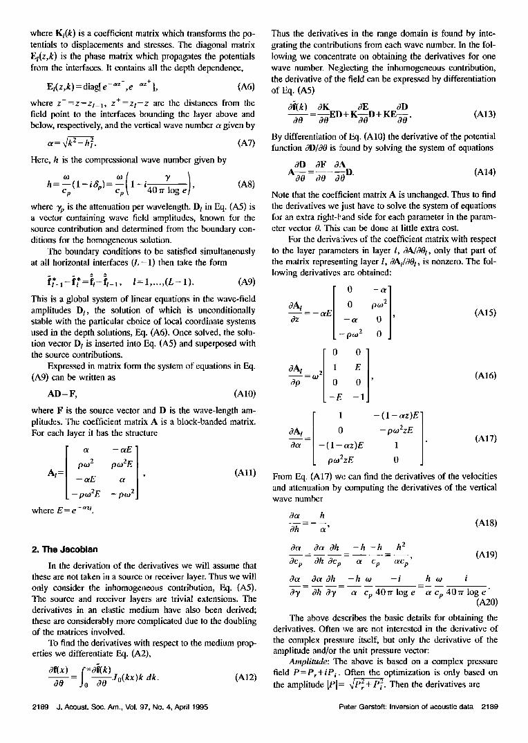
where Kt(k ) is a coefficient matrix which transforms the po- tentials to displacements and stresses. The diagonal matrix El(z,k) is the phase matrix which propagates the potentials from the interfaces. It contains all the depth dependence,

Et(z,k ) = diag[e- •Z-,e • + ], (A6) where z-=z-zt_•, z+=zt-z are the distances from the field point to the interfaces bounding the layer above and below, respectively, and the vertical wave number ot given by

= (^7) Here, h is the compressional wave number given by

h= •p(1-iSp)= 1-t407r log e , where ¾p is the attenuation per wavelength. D t in Eq. (A5) is a vector containing wave field amplitudes, known for the source contribution and determined from the boundary con- ditions for the homogeneous solution.

The boundary conditions to be satisfied simultaneously at all horizontal interfaces (L- 1) then take the form

?Ll--??=}l--}l_i, /=1 ..... (L- 1). (A9) This is a global system of linear equations in the wave-field amplitudes Dr, the solution of which is unconditionally stable with the particular choice of local coordinate systems used in the depth solutions, Eq. (A6). Once solved, the solu- tion vector D t is inserted into Eq. (A5) and superposed with the source contributions.

Expressed in matrix form the system of equations in Eq. (A9) can be written as

AD=F, (^10)

where F is the source vector and D is the wave-length am- plitudes. The coefficient matrix A is a block-banded matrix. For each layer it has the structure

po• 2

-- p •o2E where E = e- azt.

pro:E , -p(o2J

2. The Jaaobmn

In the derivation of the derivatives we will assume that these are not taken in a source or receiver layer. Thus we will only consider the inhomogeneous contribution, Eq. (A5). The source and receiver layers are trivial extensions. The derivatives in an elastic medium have also been derived; these are considerably more complicated due to the doubling of the matrices involved.

To find the derivatives with respect to the medium prop- erties we differentiate Eq. (A2),

x ) O' /O •-• - Jo -•--So(kx) dk. (A12)

Thus the derivatives in the range domain is found by inte- grating the contributions from each wave number. In the fol- lowing we concentrate on obtaining the derivatives for one wave number. Neglecting the inhomogeneous contribution, the derivative of the field can be expressed by differentiation of Eq. (A5)

c•(k) OK OE 80 - 'j•ED + K•-•D + KE•-•. (A13)

By differentiation of Eq. (A10) the derivative of the potential function JD/00 is •ound by solving the system of equations

8D 8F 8A

A• :•- saD. (A14) Note that the coefficient matrix A is unchanged. Thus to find the derivatives we just have to solve the system of equations for an extra right-hand side for each parameter in the param- eter vector 0. This can be done at little extra cost.

For the defiva'ives of the coefficient matrix with respect to the layer parameters in layer l, a•aOt, only that part of the matrix representing layer l, aAt/aO t, is nonzero. The fol- lowing derivatives are obtained:

aA• _ 0 p•2

•z•E :j, (A15) __ p•2

8A 1 = 1 op o : -E 1

(A16)

1 -(1- otz)E'

8A t 0 - pro2zE = (A17)

3a - ( 1 - az)E 1 pro2zE 0

From Eq. (A17) we can find the derivatives of the velocities and attenuation by computing the derivatives of the vertical

ho• i

(A18)

(A19)

wave number

0a h

Oh or'

0ot Oa Oh -h-h h 2

Ocp c)h OCp Ol Cp OlCp ' Oa 0ot Oh - h o - i

83, Oh 83, a cp 40rr log e a c•, 40w log e' (A20)

The above dcscribes the basic details for obtaining the derivatives. Often we are not interested in the derivative of the complex pressure itself, but only the derivative of the amplitude and/or the unit pressure vector:

Amplitude: The above is based on a complex pressure field P=Pr+iPi. Often the optimization is only based on

d -• q_ -• the amplitude [PI= •F7- F{. Then the derivatives are

2189 J. Acoust. Soc. Am., Vol. 97, No. 4, April 1995 Pater Gerstoft: Inversion of acoustic data 2189

Unit-pressure vector: The unit pressure is defined as

P

0 = (prp)m- (A22) The derivative is

(A23)

- J Re{fi (p•}, (A24) (prp) v2 • r J where the superscript T indicates conjugate transpose.

M.D. Collins, W. A. Kuperman, and H. Schmidt, "Nonlinear inversion for ocean-bottom properties," J. Acoust. Soc. Am. 92, 2770-2783 (1992).

"C. E. Lindsey and N. R. Chapman, "Matched field inversion for geophys- ical parameters using adaptive simulated annealing," IEEE J. Oceanic Eng. 18, 224-231 (1993).

3S. E. Dosso, M. L. Yeremy, J. M. Ozard, and N. R. Chapman, "Estimation of ocean bottom properties by matched-field inversion of acoustic field data," IEEE J. Oceanic Eng. 18, 232-239 (1993).

4p. Getstort, "Inversion of seismoacoustic data using genetic algorithms and a posterJori probability distributions." J. Acoust. Soc. Am. 95, 770- 782 (1994}.

Sp. Gerstoft, "Global inversion by genetic algorithms for both source po- sition and environmental parameters," J. Comp. Acoust. 2, 251-266 (1994}.

6S. D. Rajah, J. E Lynch, and G. V. Frisk, "Perturbative inversion methods for obtaining bottom geoacoustic parameters ia shallow water," J. Acous- t. Soc. Am. 82, 998-1017 (1987).

•A. Caiti, T. Akal, and R. D. Stoll, "Estimation of shear wave velocity in shallow marine sediments," IEEE J. Oceanic Eng. 19, 58-72 (1994).

SL. R. Lines and S. Treitel, "A review of least squares inversion and its application to geophysical problems," Geophys. Prosp. 32, 159-186 (1984).

0j. A. Scales, E Dochcny, and A. Gcrsztenkom, "Rcgularisation of nonlin- ear inverse problems: imaging the near-surface weathering layer," Inverse Problems 6, 115-131 (1990).

1øF. Komendi and M. Dietrich, "Nonlinear waveform inversion of plane- wave seismogram in stratified elastic media," Geophysics 56, 664-674 (1991).

nL Amundsen and B. Ursin, "Frequcney-wavenumber inversion of acous- tic data," Geophysics 56, 1027-1039 (1991).

12H. Zhao, B. Ursin, and L. Amundsen, "Frequency-wavenumber elastic inversion of marine seismic data," Geophysics 59, 1868-1881 (1994).

13p. W. Cary and C. H. Chapman, "Automatic 1D waveform inversion of marine seismic refraction data," Geophys. J. 93, 527-546 (1988).

•4L. Fishman and M.D. Collins, "Characterizing parameter spaces," in Second European Conference on Underwater Acoustics, edited by L. Bj•m• (European Commission, Brussels, Belgium, 1994).

15H. Schmidt and E B. Jensen, "A full wave solution for propagation in multilayered viscoelastic media with application to Gaussian beam reflec- tion at fluid-solid interfaces," J. Acoust. Soc. Am. 77, 813-825 0985).

16H. Schmidt and G. Tango, "Efficient global matrix approach to the com- putation of synthetic seismograms," Geophys. J. R. Astron. Soc. 84, 331- 359 (1986).

17p. L. Stoffa and M. K. Sea, "Multiparameter optimization using genetic algorithms: Inversion of plane wave seismograms," Geophysics 56, 1794-1810 (1991).

lsj. A. Scales, M. L. Smith, and T. L Fisher, "Global optimization methods for highly nonlinear inverse problems," J. Comp. Physics 103, 258-268 (1992).

•9 M. Sambridge and G. Drijkoningen, "Genetic algorithms in seismic wave- form inversion," Geophys. J. lat. 109, 323-343 (1992).

•øA. Tarantola, Inverse Problem Theory: Methods for Data Fitting and Model Parameter Estimation (Elsevier, Amsterdam, 1987).

21M. Lambert, "Inversion of seismo-acoustic real data using genetic algo- rithms," SM-276, SACLANT Undersea Reseamh Centre, La Spezia, Italy (1994).

22The transmission loss data were taken by the Seafloor Acoustics Group at SACLANTCEN; the broadband estimate was done by Andrea Caiti.

23K. Aki and P. G. Richards, Quantitative Seisinology: Theory and Methods (Freeman, San Francisco, 1980).

2aT. Akal, A. Caiti, and R. D. Stoll, "Remote sensing in shallow-water marine sediments," in Acoustic Classification and Mapping of the Seabed (Institute of Acoustics, Bath, UK, 1993).

2190 J. Acoust. Soc. Am., Vol. 97, No. 4, April 1995 Peter Getstort: Inversion of acoustic data 2190