arX

iv:1

311.

0718

v3 [

hep-

th]

10

Feb

2014

Preprint typeset in JHEP style - HYPER VERSION

Holographic thermalization with a chemical potential in

Gauss-Bonnet gravity

Xiao-Xiong Zeng

School of Science, Chongqing Jiaotong University, Chongqing, 400074, China

xxzeng@mail.bnu.edu.cn

Xian-Ming Liu

Department of Physics, Hubei University for Nationalities, Enshi, 445000, Hubei, China

liuxianming1980@163.com

Wen-Biao Liu

Department of Physics, Beijing Normal University, Beijing, 100875, China

wbliu@bnu.edu.cn

Abstract: Holographic thermalization is studied in the framework of Einstein-Maxwell-

Gauss-Bonnet gravity. We use the two-point correlation function and expectation value of

Wilson loop, which are dual to the renormalized geodesic length and minimal area surface

in the bulk, to probe the thermalization. The numeric result shows that larger the Gauss-

Bonnet coefficient is, shorter the thermalization time is, and larger the charge is, longer the

thermalization time is, which implies that the Gauss-Bonnet coefficient can accelerate the

thermalization while the charge has an opposite effect. In addition, we obtain the functions

with respect to the thermalization time for both the thermalization probes at a fixed charge

and Gauss-Bonnet coefficient, and on the basis of these functions, we obtain the thermalization

velocity, which shows that the thermalization process is non-monotonic. At the middle and

later periods of the thermalization process, we find that there is a phase transition point, which

divides the thermalization into an acceleration phase and a deceleration phase. We also study

the effect of the charge and Gauss-Bonnet coefficient on the phase transition point.

Contents

1. Introduction 1

2. Charged Vaidya AdS black branes in Gauss-Bonnet gravity 3

3. Holographic thermalization 5

3.1 Renormalized geodesic length 6

3.2 Minimal area surface 8

4. Numerical results 9

5. Conclusions 18

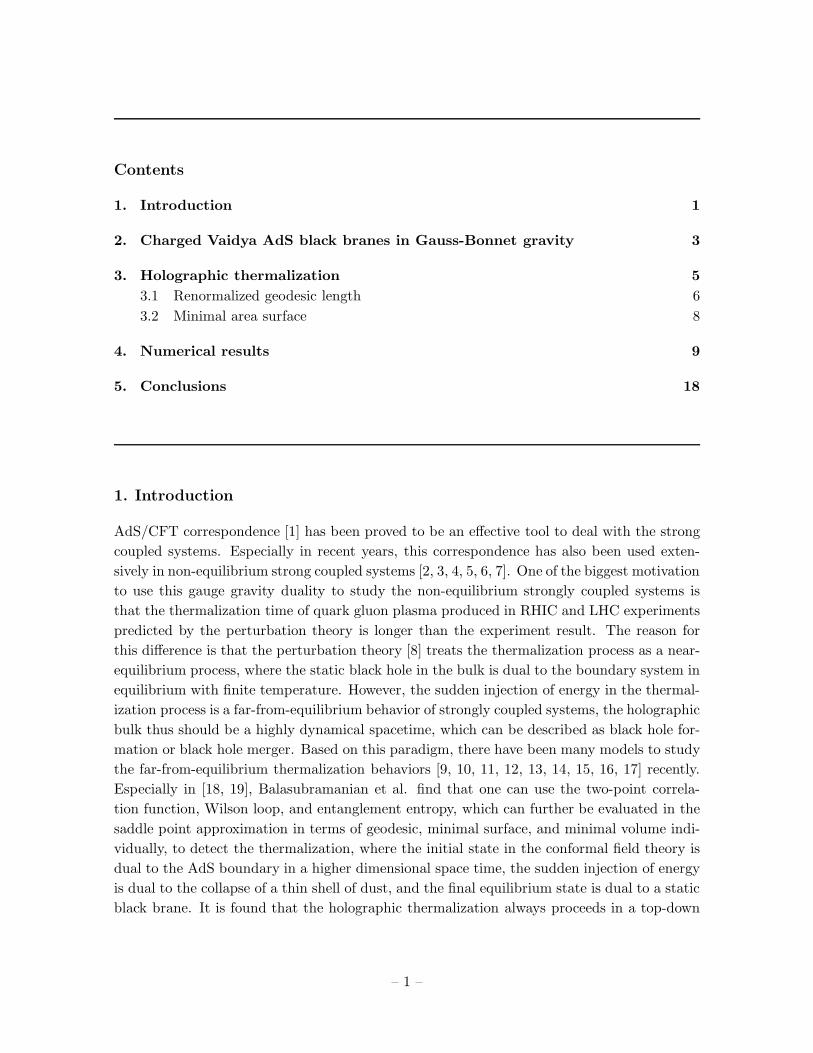
1. Introduction

AdS/CFT correspondence [1] has been proved to be an effective tool to deal with the strong

coupled systems. Especially in recent years, this correspondence has also been used exten-

sively in non-equilibrium strong coupled systems [2, 3, 4, 5, 6, 7]. One of the biggest motivation

to use this gauge gravity duality to study the non-equilibrium strongly coupled systems is

that the thermalization time of quark gluon plasma produced in RHIC and LHC experiments

predicted by the perturbation theory is longer than the experiment result. The reason for

this difference is that the perturbation theory [8] treats the thermalization process as a near-

equilibrium process, where the static black hole in the bulk is dual to the boundary system in

equilibrium with finite temperature. However, the sudden injection of energy in the thermal-

ization process is a far-from-equilibrium behavior of strongly coupled systems, the holographic

bulk thus should be a highly dynamical spacetime, which can be described as black hole for-

mation or black hole merger. Based on this paradigm, there have been many models to study

the far-from-equilibrium thermalization behaviors [9, 10, 11, 12, 13, 14, 15, 16, 17] recently.

Especially in [18, 19], Balasubramanian et al. find that one can use the two-point correla-

tion function, Wilson loop, and entanglement entropy, which can further be evaluated in the

saddle point approximation in terms of geodesic, minimal surface, and minimal volume indi-

vidually, to detect the thermalization, where the initial state in the conformal field theory is

dual to the AdS boundary in a higher dimensional space time, the sudden injection of energy

is dual to the collapse of a thin shell of dust, and the final equilibrium state is dual to a static

black brane. It is found that the holographic thermalization always proceeds in a top-down

– 1 –

pattern, namely the UV modes thermalize firstly, followed by the IR modes 1. They also

find that there is a slight delay in the onset of thermalization and the entanglement entropy

thermalizes slowest, which sets a timescale for equilibration. Later, such an investigation is

generalized to the bulk geometry with electrostatic potential [20, 21, 22] and high curvature

corrections [23, 24, 25] to see how the chemical potential and correction parameter affect the

thermalization time in the boundary field theory, other extensions on this topic please see

[26, 27, 28, 29]. Made by Balasubramanian et al., there are further some elegant extensions

on holographic thermalization very recently. Firstly the time-dependent spectral functions

in conformal field is found to be tractable[30]. With it, many quantities of interest in the

thermalization process, e.g., the time dependence of the occupation number of field modes in

the boundary gauge theory, can be calculated. Secondly, the holographic thermalization is

extended to the inhomogeneous case by considering an AdS4 weak field inhomogeneous col-

lapse [31, 32]. It is found that the AdS description of the early time evolution is well-matched

by free streaming, and the stress tensor approaches that of second order hydrodynamics near

the end of the early time interval.

The purpose of this paper is to investigate holographic thermalization in the bulk with

curvature corrections and a gauge potential. By holography, curvature correction corresponds

to 1N

or 1λcorrection [33, 34] to the boundary field theory 2, and the gauge potential corre-

sponds to a chemical potential in the boundary field theory. In Einstein gravity, there have

been some works to study the effect of the chemical potential on the thermalization [20, 21].

And there are also some works to study the effect of correction parameter of the high order

curvature on the thermalization [23, 24, 25]. Here we want to explore whether the chemical

potential and the correction parameter have the same effect on the thermalization time. If

not, our model will provide theoretically a wider range of the thermalization time. To observe

the thermalization process in the dual conformal field theory, we take the two-point corre-

lation function and expectation value of Wilson loop as thermalization probes to study the

thermalization behavior 3. According to the AdS/CFT correspondence, this process equals

to probing the evolution of a shell of charged dust that interpolates between a pure AdS and

a charged Gauss-Bonnet AdS black brane by making use of the renormalized geodesic length

and minimal area surface. Concretely we first study the motion profile of the geodesic and

1On the weakly coupled side classical calculations have shown that the thermalization process is of the

bottom-up type, i.e. low energetic modes reach thermal equilibrium first [8].2According to the AdS/CFT correspondence, it is well known that IIB string theory on AdS5 ×S5 back-

ground is dual to D = 4 N = 4 SU(Nc) super Yang-Mills theory. In the limits of large Nc and large ’t Hooft

coupling, the SYM theory is dual to IIb supergravity which is low energy effective theory of superstring theory.

So the higher curvature terms in the bulk theory can arise as next to leading order corrections in the 1/N(large

N) expansion of the boundary CFTs in the strong ’t Hooft coupling limit.3Usually, one also can use the entanglement entropy to detect the thermalization process. Recently there

have been many works to study holographic entanglement entropy in higher derivative gravitational theories

[35, 36, 37, 38, 39, 40, 41]. Especially in [25], the author found that the entanglement entropy has simi-

lar behavior as the other observables during the thermalization process. For simplicity, we will not study

entanglement entropy in this paper.

– 2 –

minimal area, and then the renormalized geodesic length and minimal area surface in the

charged Gauss-Bonnet Vaidya AdS black brane. When we study the effect of the gauge po-

tential on the thermalization process, the Gauss-Bonnet coefficient is fixed and when we are

interested in the effect of Gauss-Bonnet coefficient, the gauge potential is fixed. Our result

shows that larger the Gauss-Bonnet coefficient is, easier the dual boundary system thermal-

izes, while larger the charge is, harder the dual boundary system thermalizes. That is, the

Gauss-Bonnet coefficient have an opposite effect on the thermalization time compared with

the gauge potential. In addition, we also obtain the analytical functions of the renormalized

geodesic length with respect to the thermalization time as well as the renormalized minimal

area surface with respect to the thermalization time. Based on the functions, we get the

thermalization velocity. Our result shows that the velocity is negative at the initial time and

positive at the middle and later periods, which indicates that the thermalization process is

non-monotonic. We find that there is a phase transition point for the thermalization velocity

at a fixed Q and α, which divides the thermalization process into an acceleration phase and

a deceleration phase. Effect of Q and α on the phase transition points is also studied.

The remainder of this paper is organized as follows. In the next section, we shall pro-

vide a brief review of the charged Vaidya AdS black brane in Gauss-Bonnet gravity. Then

the holographic setup for non-local observables will be explicitly constructed in Section 3.

Especially, we show that the relation between the renormalized length and the two-point

correlation function is still valid in the Gauss-Bonnet gravity. Resorting to numerical calcu-

lation, we perform a systematic analysis of how the Gauss-Bonnet coefficient and chemical

potential affect the thermalization time and thermalization velocity in Section 4. We end up

with some discussions in the last section.

2. Charged Vaidya AdS black branes in Gauss-Bonnet gravity

The D(D ≥ 5) dimensional Einstein-Maxwell theory with a negative cosmological constant

and a Gauss-Bonnet term 4 representing a quadratic curvature correction is given by

I =1

16πGD

∫

M

dDx√−g (R− 2Λ− 4πGDFµνF

µν + αLGB) , (2.1)

where GD is the D-dimensional gravitational constant, R is the Ricci scalar, Λ is the negative

cosmological constant, α is the Gauss-Bonnet coefficient, and Fµν = ∂µAν − ∂νAµ,

LGB = R2 − 4RµνRµν +RµνστR

µνστ . (2.2)

From the action in Eq.(2.1), many exact solutions have been found [44, 45, 46, 47, 48, 49, 50,

51], here we are interested in the D-dimensional charged black brane solution

ds2 = −F (r)dt2 + F (r)−1dr2 +r2

l2dx2n, (2.3)

4The action in Eq.(2.1) is not a consistent truncation of an effective higher derivative gravitational action,

it is one special case where the higher order corrections of the Maxwell field have vanishing coefficients. One

also can take into account the corrections to the Maxwell field such as in [42, 43].

– 3 –

where

F (r) =r2

2α[1−

√

1− 4α

l2(1− Ml2

rD−1+

Q2l2

r2D−4)], (2.4)

in which ℓ =

√

− (D−1)(D−2)2Λ , α = (D − 3)(D − 4)α, M and Q are related to the ADM black

hole mass M0 and charge Q0 as follows

M0 =(D − 2)MVn

16πGD

,

Q20 =

2π(D − 2)(D − 3)Q2

GD

, (2.5)

where Vn is the volume of the unit radius sphere SD−2. The U(1) gauge potential reads

At = − Q

4π(D − 3)(r3−D

h − r3−D) = u(1− rD−3h

rD−3), (2.6)

in which rh is the event horizon radius that is characterized by F (rh) = 0 and u is the

electrostatic potential, which can be identified with the chemical potential of the dual field

theory. The Hawking temperature of the charged Gauss-Bonnet AdS black brane reads

T =∂rF (r)

4π|rh =

(D − 1)rh − (D − 3)Q2ℓ2r5−2Dh

4πℓ2, (2.7)

which can be viewed as the temperature of the dual conformal field theory on the AdS

boundary. On the other hand, as r approaches to infinity, one can see the above black brane

metric changes into

ds2 → r2

ℓ2eff(−dt2 + dx2n) +

ℓ2effr2

dr2, (2.8)

where

xn =ℓeffℓ

xn, ℓ2eff =

2α

1−√

1− 4αℓ2

. (2.9)

Thus this black brane solution is asymptotically AdS with AdS radius ℓeff .

To get a Vaidya type evolving black brane, we would like first to make the coordinate

transformation z = ℓ2

r, in this case the black brane metric in Eq.(2.3) can be cast into

ds2 =ℓ2

z2[−F (z)dt2 + F−1(z)dz2 + dx2n], (2.10)

where

F (z) =ℓ2

2α

[

1−√

1− 4α

ℓ2(1−MzD−1ℓ4−2D +Q2z2D−4ℓ10−4D)

]

. (2.11)

Then by introducing the Eddington-Finkelstein coordinate system, namely

dv = dt− 1

F (z)dz, (2.12)

– 4 –

Eq.(2.10) changes into

ds2 =ℓ2

z2[

−F (z)dv2 − 2dz dv + dx2n]

. (2.13)

Now the charged Gauss-Bonnet Vaidya AdS black brane can be obtained by freeing the mass

parameter and charge parameter as arbitrary functions of v[52, 53, 54]. This black brane is

a solution of the equations of motion of the total action

Itotal = I + Imatter, (2.14)

where Imatter is the action for external matter fields. As one can show, such a metric is

sourced by the null dust with the energy momentum tensor flux and gauge flux [52, 53, 54]

8πGDTmatterµν = zD−2(

D − 2

2M(v) − (D − 2)zD−3Q(v)Q(v))δµvδνv,

8πGDJµmatter =

√

(D − 2)(D − 3)

2zDQ(v)δµz , (2.15)

where the dot stands for derivative with respect to coordinate v, M(v) and Q(v) are the mass

and charge of a collapsing black brane5. It is obvious that for the charged Vaidya AdS black

branes in Gauss-Bonnet gravity, the energy-momentum tensor depends on not only M(v) but

also Q(v). In this case, Eq. (2.13) describes the collapse of a thin-shell of charged dust from

the boundary toward the bulk interior of asymptotically anti-de Sitter spaces as M and Q

are substituted by M(v) and Q(v).

3. Holographic thermalization

In this section, we are going to investigate the thermalization process of a class of strongly

coupled system. According to the AdS/CFT correspondence, the rapid injection of energy

on the boundary corresponds to the collapse of a black brane in the AdS space. So to

describe the thermalization process holographically, one should choose the mass M(v) and

charge Q(v) properly so that it can describe the evolution of the charged dust. It was found

that this properties can be achieved by setting the mass parameter and charge parameter as

M(v) = Mθ(v), Q(v) = Qθ(v) [20, 21], where θ(v) is the step function. In this case, in the

limit v → −∞, the background corresponds to a pure AdS space while in the limit v → ∞, it

corresponds to a charged Gauss-Bonnet AdS black brane. For the convenience of numerical

calculations, M(v) and Q(v) are usually chosen as the smooth functions

M(v) =M

2

(

1 + tanhv

v0

)

, (3.1)

Q(v) =Q

2

(

1 + tanhv

v0

)

, (3.2)

5For more information about the energy condition in the time dependent background, please see [55]

– 5 –

where v0 represents a finite shell thickness.

Having the construction of a model that describes the thermalization process on the dual

conformal field theory, we have to choose a set of extended non-local observables 6 in the bulk

which allow us to evaluate the evolution of the system. In this paper, we shall focus mainly

on the two-point correlation function at equal time and expectation value of rectangular

space-like Wilson loop, which in the bulk correspond to the renormalized geodesic length and

minimal area surface respectively. For simplicity but without loss of generality, we shall set

the unit such that ℓ = 1 and rh = 1 in the later discussions. In addition, from Eq.(2.11), we

know that the mass and the charge have the relation M = 1 +Q2, in this case we only need

to change the charge to adjust the mass parameter during the numerical process.

3.1 Renormalized geodesic length

The relation between the renormalized geodesic length and two-point correlation function at

equal time has been discussed extensively [19, 56]. Here we will give a review of the relation

to check whether it is still valid in the Gauss-Bonnet gravity.

Start with the action of a complex scalar field of mass m in the bulk background gravi-

tational field gab

S = −1

2

∫

dd+1X√−g[gab∇aφ∇bφ+m2φφ], (3.3)

which gives rise to the bulk propagator

G(x, y) = 〈φ(x)φ(y)〉 = 〈x| 1

iH|〉y =

∫

∞

0dT 〈x|e−iHT |y〉, (3.4)

where H = −12 [∇a∇a − m2] can be thought of as the Hamiltonian of a fictitious quantum

mechanical model with T the proper time 7. With this in mind, one can reformulate this

quantum mechanical model in terms of path integral over the worldlines of a massive particle.

In particular, the above bulk propagator can be expressed as

G(x, y) =

∫

∞

0dTDXeis

= N∫

∞

0dT

∏

τ

∫

DX(τ)√

−g(τ)ei∫ T0 dτ [ 1

2(gµν

dXµ

dτdXν

dτ−m2)+R

6]

= N∫

∞

0dT

∏

τ

∫

DX(τ)√

−g(τ)ei∫ 10 dτ [ 1

2(T−1gµν

dXµ

dτdXν

dτ−Tm2)]

(3.5)

with X(0) = y, X(T ) = x, and m2 = m2 − R3 . In the saddle point approximation, i.e.,

T =

√

−gµνdXµ

dτdXν

dτ

m, (3.6)

6Because the local observables such as the energy-momentum tensor and its derivatives can not explore

deviations from thermal equilibrium in detail though it provides valuable information about the applicability

of viscous hydrodynamics.7For the derivation of the Hamiltonian, please see appendix.

– 6 –

the bulk propagator can be evaluated as

G(x, y) ∝ ei∫ 10 dτ(−m

√

−gµνdXµ

dτdXν

dτ), (3.7)

with Xµ(τ) the classical trajectory satisfying the above equation of motion. Obviously

Eq.(3.7) is consistent with the formulation in [19, 56]

〈O(t0,x)O(t0,x′)〉 ≈ e−∆Lren , (3.8)

where ∆ is the conformal dimension of scalar operator O, which is similar to m in Eq.(3.7),

and Lren indicates the renormalized length of the bulk geodesic between the points (t0, xn)

and (t0, x′n) on the AdS boundary. In other words, the Gauss-Bonnet coefficient has not effect

on the dual relation between the renormalized geodesic length and the two-point correlation

function. In what follows, we will make use of Eq.(3.8) to explore how the Gauss-Bonnet

coefficient and gauge potential affect the thermalization time. The reason that we use the

renormalized geodesic length Lren in Eq.(3.7) is that the geodesic length is divergent near the

boundary, which is related to the divergent part as

Lren = L+ 2ℓeff ln z0. (3.9)

where L =√−dS2 is the geodesic length between the points (t0, xn) and (t0, x

′n) on the AdS

boundary and z0 is the IR radial cut-off. Next, we are concentrating on studying L. Taking

into account the spacetime symmetry of our Vaidya type black brane, we can simply let (t0, xn)

and (t0, x′n) have identical coordinates except x1 = −ℓeff

l2 ≡ − l

2 and x′1 = −ℓeffl2 ≡ − l

2 with

l the separation between these two points on the boundary. In order to make the notation as

simple as possible, we would like to rename this exceptional coordinate x1 as x and employ

it to parameterize the trajectory such that the proper length in the charged Gauss-Bonnet

Vaidya AdS black brane can be given by

L =

∫ l2

−l2

dx

√

1− 2z′(x)v′(x)− F (v, z)v′(x)2

z(x), (3.10)

where the prime denotes the derivative with respect to x and

F (v, z) =1

2α

[

1−√

1− 4α (1−M(v)zD−1 +Q(v)2z2D−4)

]

. (3.11)

Note that the integrand in Eq.(3.10) can be thought of as the Lagrangian L of a fictitious

system with x the proper time. Since the Lagrangian does not depend explicitly on x, there

is an associated conserved quantity

H = L − v′(x)∂L

∂v′(x)− z′(x)

∂L∂z′(x)

=1

z(x)√

1− 2z′(x)v′(x)− F (v, z)v′(x)2. (3.12)

– 7 –

In addition, based on the Lagrangian L of the system, we obtain

∂L∂z

=−v′(x)2∂zF (z, v)H

2− 1

z(x)3H , (3.13)

∂

∂x

∂L∂z′

= −v′′(x)H. (3.14)

So the equation of motion for z(x) can be written as

0 = 2− 2v′(x)2F (v, z) − 4v′(x)z′(x)− 2z(x)v′′(x) + z(x)v′(x)2∂zF (v, z). (3.15)

Similarly, the equation of motion for v(x) can be solved as

0 = v′(x)z′(x)∂zF (v, z) +1

2v′(x)2∂vF (v, z) + v′′(x)F (v, z) + z′′(x), (3.16)

in which

∂zF (z, v) =(D − 1)M(v)zD−2 − (2D − 4)Q2(v)z2D−5

√

1− 4α(1−M(v)zD−1 +Q2(v)z2D−4),

∂vF (z, v) =M ′(v)zD−1 − 2Q(v)Q′(v)z2D−4

√

1− 4α(1−M(v)zD−1 +Q2(v)z2D−4). (3.17)

Next, we turn to studying the equations of motion in Eq.(3.15) and Eq.(3.16). Considering

the reflection symmetry of our geodesic, we will use the following initial conditions

z(0) = z∗, v(0) = v∗, v′(0) = z′(0) = 0. (3.18)

As z(x) and v(x) are solved, we can get the IR radial cut-off and thermalization time by the

boundary conditions as follows

z(l

2) = z0, v(

l

2) = t0, (3.19)

In addition, with the help of Eq.(3.12) and Eq.(3.18), the proper length of geodesic in Eq.(3.10)

can be simplified as

L = 2

∫ l2

0dx

z∗z(x)2

, (3.20)

which will be more convenient for us to obtain the renormalized geodesic length.

3.2 Minimal area surface

In this section, we are going to study the minimal area surface, which in the dual conformal

field theory corresponds to the Wilson loop operator. Wilson loop operator is defined as

a path ordered integral of gauge field over a closed contour, and its expectation value is

approximated geometrically by the AdS/CFT correspondence as [19, 57]

〈W (C)〉 ≈ e−Aren(Σ)

2πα′ , (3.21)

– 8 –

where C is the closed contour, Σ is the minimal bulk surface ending on C with Aren its

renormalized minimal area surface, and α′ is the Regge slope parameter. In the Gauss-Bonnet

gravity, we will assume Eq.(3.21) is still valid as that between the renormalized geodesic length

and the two-point correlation function.

Here we are focusing solely on the rectangular space-like Wilson loop. In this case, the

enclosed rectangle can always be chosen to be centered at the coordinate origin and lying on

the x1 − x2 plane with the assumption that the corresponding bulk surface is invariant along

the x2 direction. This implies that the minimal area surface can be expressed as

A =

∫ l2

l2

dx

√

1− 2z′(x)v′(x)− F (v, z)v′(x)2

z(x)2, (3.22)

where we have set the separation along x2 direction to be one and the separation along x1 to

be l with x2 renamed as y and x1 renamed as x. As before, from Eq.(3.22) we also can get a

Lagrangian L and with it we can find a conserved quantity, i.e.,

H =1

z(x)2√

1− 2z′(x)v′(x)− F (v, z)v′(x)2, (3.23)

which can simplify our equations of motion as

0 = 4− 4v′(x)2F (v, z) − 8v′(x)z′(x)− 2z(x)v′′(x) + z(x)v′(x)2∂zF (v, z),

0 = v′(x)z′(x)∂zF (v, z) +1

2v′(x)2∂vF (v, z) + v′′(x)F (v, z) + z′′(x). (3.24)

Similarly, with the initial conditions as in (3.18) and the regularization cut-off as in (3.19),

the renormalized minimal area surface can be cast into

Aren = 2

∫ l2

0dx

z2∗z(x)4

− 2

z0. (3.25)

Next, we will investigate the evolution of the renormalized minimal area surface with respect

to the thermalization time to explore how the gauge potential and Gauss-Bonnet coefficient

affect the thermalization process.

4. Numerical results

In this section, we will solve the equations of motion of geodesic length and minimal area

surface numerically, and then explore how the chemical potential and Gauss-Bonnet coefficient

affect the thermalization time. Since there have been many works to study the effect of the

space time dimensions and boundary separation on the thermalization probes [18, 19, 20, 21],

to avoid redundancy, we mainly discuss the case D = 5 and a fixed boundary separation in

this paper. During the numerics, we will take the shell thickness and UV cut-off as v0 = 0.01,

z0 = 0.01 respectively.

– 9 –

According to the AdS/CFT correspondence, we know that the electromagnetic field in

the bulk is dual to the chemical potential in the dual quantum field theory, so we will use

the electromagnetic field defined in Eq.(2.6) to explore the effect of the chemical potential

on the thermalization process in the AdS boundary. However, as stressed in [20, 58, 59], the

chemical potential has energy units in the dual field theory ([u] = 1/[L]) while Aµ as defined

in Eq.(2.1) is dimensionless, thus one has to redefine the electromagnetic field as Aµ = Aµ/p,

where p is a scale with length unit that depends on the particular compactification. In this

case, Aµ and u have the same unit and the chemical potential can be expressed as

u = limr→∞

Aµ =Qr3−D

h

4πp(D − 3). (4.1)

In addition, due to the conformal symmetry on the boundary, the quantity which is physically

meaningful is the ratio of u/T in asymptotically charged AdS space time, namely the chemical

potential measured with the temperature as the unit. Therefore, through this paper we will

use the following ratio

u

T=

Q

p(D − 3)[(D − 1)rD−2h − (D − 3)Q2r3−D

h ], (4.2)

to check the effect of the chemical potential on the thermalization time. Obviously, for the case

rh = 1, Eq.(4.2) shows that u/T changes from 0 → ∞ provided Q changes from 0 →√

D−1D−3 .

In other words, to adjust the change of the ratio u/T in all the range, we only need to change

Q from 0 →√

D−1D−3 . For the case D = 5 in this paper, we will choose Q = 0.00001, 0.5, 1 in

our numerical result. On the other hand, we will also consider the effect of the Gauss-Bonnet

coefficient on the thermalization time, as in [23] we will take α = −0.1, 0.0001, 0.08 as the

constraint of causality of dual field theory on the boundary is imposed8.

As the boundary conditions in Eq.(3.18) is adopted, the equations of motion of the

geodesic in Eq.(3.15) and Eq.(3.16) for different α and different Q can be solved numeri-

cally. When we are interested in the effect of Q on the motion profile of the geodesic, the

Gauss-Bonnet coefficient α is fixed, and when we are interested in the effect of Gauss-Bonnet

coefficient α, the charge Q is fixed. Since different initial time v⋆ corresponds to different stage

of the motion of the geodesics, we also discuss the effect of v⋆ on the motion profile. Figure (1)

and Figure (2) plot the motion profile of the geodesic at the initial time v⋆ = −0.856,−0.456

respectively for different charge and Gauss-Bonnet coefficient. In both figures, the horizontal

direction is the motion profile of the geodesics for different Gauss-Bonnet coefficients while the

vertical direction is the motion profile of the geodesics for different charges. From Figure (1)

and Figure (2), we know that as the initial time increases, the shell of the dust approaches to

the horizon of the charged Gauss-Bonnet black brane, which means that for the larger initial

time, the thermalization has been behaved longer. For different initial time, we also keep a

8As α is dialed beyond the causality bound but within the Chern-Simons limit, it has not effect on the

thermalization process. One can see the thermalization curves plotted in [25].

– 10 –

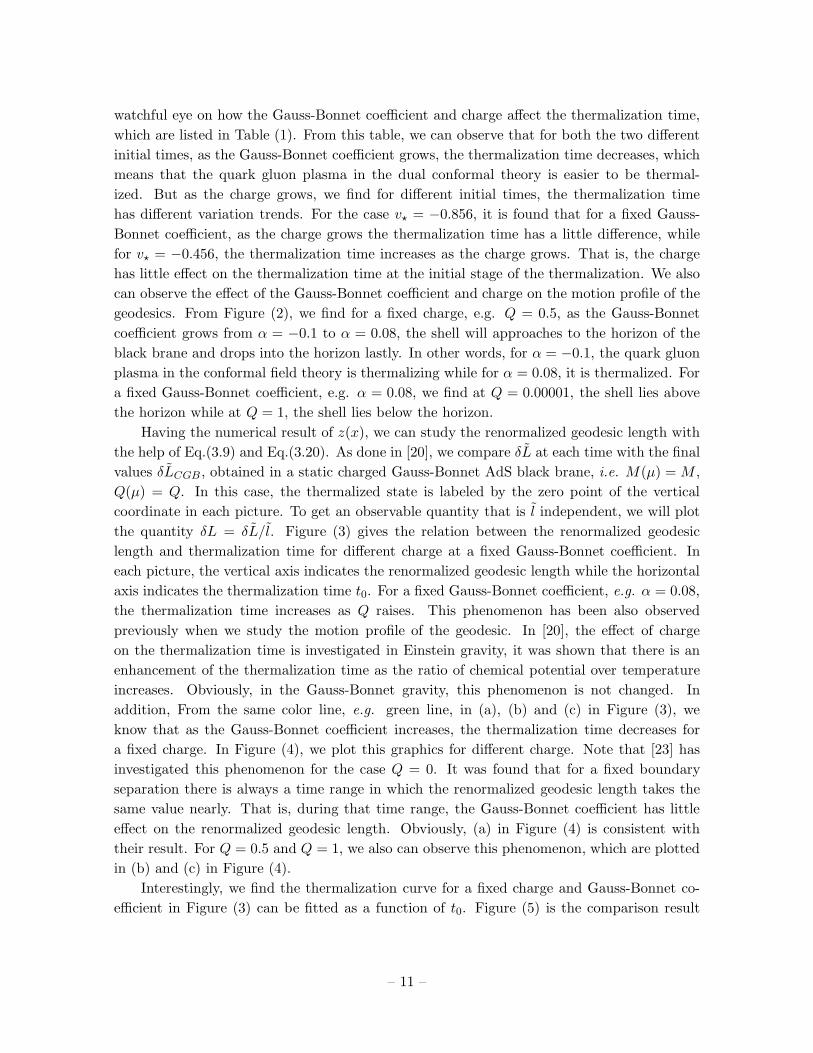
watchful eye on how the Gauss-Bonnet coefficient and charge affect the thermalization time,

which are listed in Table (1). From this table, we can observe that for both the two different

initial times, as the Gauss-Bonnet coefficient grows, the thermalization time decreases, which

means that the quark gluon plasma in the dual conformal theory is easier to be thermal-

ized. But as the charge grows, we find for different initial times, the thermalization time

has different variation trends. For the case v⋆ = −0.856, it is found that for a fixed Gauss-

Bonnet coefficient, as the charge grows the thermalization time has a little difference, while

for v⋆ = −0.456, the thermalization time increases as the charge grows. That is, the charge

has little effect on the thermalization time at the initial stage of the thermalization. We also

can observe the effect of the Gauss-Bonnet coefficient and charge on the motion profile of the

geodesics. From Figure (2), we find for a fixed charge, e.g. Q = 0.5, as the Gauss-Bonnet

coefficient grows from α = −0.1 to α = 0.08, the shell will approaches to the horizon of the

black brane and drops into the horizon lastly. In other words, for α = −0.1, the quark gluon

plasma in the conformal field theory is thermalizing while for α = 0.08, it is thermalized. For

a fixed Gauss-Bonnet coefficient, e.g. α = 0.08, we find at Q = 0.00001, the shell lies above

the horizon while at Q = 1, the shell lies below the horizon.

Having the numerical result of z(x), we can study the renormalized geodesic length with

the help of Eq.(3.9) and Eq.(3.20). As done in [20], we compare δL at each time with the final

values δLCGB , obtained in a static charged Gauss-Bonnet AdS black brane, i.e. M(µ) = M ,

Q(µ) = Q. In this case, the thermalized state is labeled by the zero point of the vertical

coordinate in each picture. To get an observable quantity that is l independent, we will plot

the quantity δL = δL/l. Figure (3) gives the relation between the renormalized geodesic

length and thermalization time for different charge at a fixed Gauss-Bonnet coefficient. In

each picture, the vertical axis indicates the renormalized geodesic length while the horizontal

axis indicates the thermalization time t0. For a fixed Gauss-Bonnet coefficient, e.g. α = 0.08,

the thermalization time increases as Q raises. This phenomenon has been also observed

previously when we study the motion profile of the geodesic. In [20], the effect of charge

on the thermalization time is investigated in Einstein gravity, it was shown that there is an

enhancement of the thermalization time as the ratio of chemical potential over temperature

increases. Obviously, in the Gauss-Bonnet gravity, this phenomenon is not changed. In

addition, From the same color line, e.g. green line, in (a), (b) and (c) in Figure (3), we

know that as the Gauss-Bonnet coefficient increases, the thermalization time decreases for

a fixed charge. In Figure (4), we plot this graphics for different charge. Note that [23] has

investigated this phenomenon for the case Q = 0. It was found that for a fixed boundary

separation there is always a time range in which the renormalized geodesic length takes the

same value nearly. That is, during that time range, the Gauss-Bonnet coefficient has little

effect on the renormalized geodesic length. Obviously, (a) in Figure (4) is consistent with

their result. For Q = 0.5 and Q = 1, we also can observe this phenomenon, which are plotted

in (b) and (c) in Figure (4).

Interestingly, we find the thermalization curve for a fixed charge and Gauss-Bonnet co-

efficient in Figure (3) can be fitted as a function of t0. Figure (5) is the comparison result

– 11 –

v⋆=-0.856 v⋆= -0.456

α=-0.1 α=0.0001 α=0.08 α=-0.1 α=0.0001 α=0.08

Q=0.00001 0.691064 0.625561 0.560275 1.01538 0.949617 0.887499

Q=0.5 0.690223 0.624786 0.559595 1.02213 0.958193 0.897744

Q=1 0.687522 0.622449 0.557604 1.03968 0.981075 0.925744

Table 1: The thermalization time t0 of the geodesic probe for different Gauss-Bonnet coefficient α

and different charge Q at v⋆ = −0.856,−0.456 respectively.

of the numerical curve and function curve. At a fixed α, one can get the function of the

thermalization curve for different charge. For example, at α = 0.0001, the thermalization

curve for Q = 0.00001, 0.5, 1 can be expressed respectively as 9

g1 = −0.132319 − 0.015338t0 + 0.132916t20 − 0.393653t30 + 0.560646t40 − 0.190989t50 − 0.0210284t60

g2 = −0.140525 − 0.0101622t0 + 0.101997t20 − 0.348701t30 + 0.626571t40 − 0.324671t50 + 0.033151t60

g3 = −0.166815 − 0.00146773t0 + 0.0355258t20 − 0.209675t30 + 0.691328t40 − 0.54898t50 + 0.129204t60(4.3)

For small time, the function is determined by the lower power of t0, while for large time it

is determined by the higher power of t0. With the function, we can get the thermalization

velocity, which is plotted in Figure (6). From this figure, we can observe two interesting

phenomena for the thermalization process. One is that the thermalization velocity is negative

at the initial time while it is positive at the middle and later periods, which means that the

thermalization process is non-monotonic. In fact, this non-monotonic behavior has also been

observed in [21]. The reason for this behavior is that at the initial time the thermalization

is “quantum” while at the later periods, it is “classical”. The author in [21] further argued

that at the “quantum” stage the slope of the thermalization curve, namely the thermalization

velocity, is negative and at the “classical” stage the slope is positive. Obviously, our result

plotted in Figure (6) confirms their argument. The other is that there is a phase transition

point for the thermalization velocity, which divides the thermalization into an acceleration

phase and a deceleration phase. (a) and (b) in Figure (6) represent respectively the effect of

Q and α on the phase transition points. From both figures, we know that the phase transition

points vary for different Q and α. Especially in (b), we can observe clearly that as α increases,

the phase transition points shift left. At a fixed Q and α, we can get the value of the phase

transition point. For the case Q = 0.5 and α = 0.0001, it is easy to find that in the time range

0 < t0 < 1.04978, the thermalization is an acceleration process while for t0 > 1.04978 it is a

deceleration process before it approaches to the equilibrium state. Surely as the slope of this

velocity curve is produced, we also can get the values of the acceleration and deceleration.

Adopting similar strategy, we also can study the motion profile of minimal area as well

9For higher order power of t0, we find it has few contributions to the thermalization, including the phase

transition point which will be discussed next.

– 12 –

-2 -1 0 1 20.0

0.5

1.0

1.5

2.0

x�

zHxL

(a) Q = 0.00001, α = −0.1

-2 -1 0 1 20.0

0.5

1.0

1.5

2.0

x�

zHxL

(b) Q = 0.00001, α = 0.0001

-2 -1 0 1 20.0

0.5

1.0

1.5

2.0

x�

zHxL

(c) Q = 0.00001, α = 0.08

-2 -1 0 1 20.0

0.5

1.0

1.5

2.0

x�

zHxL

(d) Q = 0.5, α = −0.1

-2 -1 0 1 20.0

0.5

1.0

1.5

2.0

x�

zHxL

(e) Q = 0.5, α = 0.0001

-2 -1 0 1 20.0

0.5

1.0

1.5

2.0

x�

zHxL

(f) Q = 0.5, α = 0.08

-2 -1 0 1 20.0

0.5

1.0

1.5

2.0

x�

zHxL

(g) Q = 1, α = −0.1

-2 -1 0 1 20.0

0.5

1.0

1.5

2.0

x�

zHxL

(h) Q = 1, α = 0.0001

-2 -1 0 1 20.0

0.5

1.0

1.5

2.0

x�

zHxL

(i) Q = 1, α = 0.08

Figure 1: Motion profile of the geodesics in the charged Gauss-Bonnet Vaidya AdS black brane. The

separation of the boundary field theory operator pair is ℓ = 3 and the initial time is v⋆ = −0.856.

The black brane horizon is indicated by the yellow line. The position of the shell is described by the

junction between the dashed red line and the green line.

as the change of the renormalized minimal area surface to thermalization time. Based on

the motion equations in (3.24) and the boundary conditions in (3.18), the numerical solution

of z(x) can be produced. In this case, we can get the motion profile of minimal area for

different charge Q and Gauss-Bonnet coefficient α, which is shown in Figure (7). From this

figure, we know that for a fixed charge, e.g. the first row, as the Gauss-Bonnet coefficient

increases, the shell surface approaches to the horizon surface step by step, which means the

thermalization is faster. For a fixed Gauss-Bonnet coefficient, e.g. the third column, as the

charge increases, the shell surface is removed from the horizon surface step by step, which

means the thermalization is slower. The thermalization time for different α and Q have been

listed in Table (2). It is shown that for a fixed charge the thermalization time decreases as

α becomes larger, while for a fixed α, the thermalization time increases as Q becomes larger.

That is, the charge has an inverse effect compared with the Gauss-Bonnet coefficient on the

thermalization time. This phenomenon is similar to that of the geodesics.

– 13 –

-2 -1 0 1 20.0

0.5

1.0

1.5

2.0

x�

zHxL

(a) Q = 0.00001, α = −0.1

-2 -1 0 1 20.0

0.5

1.0

1.5

2.0

x�

zHxL

(b) Q = 0.00001, α = 0.0001

-2 -1 0 1 20.0

0.5

1.0

1.5

2.0

x�

zHxL

(c) Q = 0.00001, α = 0.08

-2 -1 0 1 20.0

0.5

1.0

1.5

2.0

x�

zHxL

(d) Q = 0.5, α = −0.1

-2 -1 0 1 20.0

0.5

1.0

1.5

2.0

x�

zHxL

(e) Q = 0.5, α = 0.0001

-2 -1 0 1 20.0

0.5

1.0

1.5

2.0

x�

zHxL

(f) Q = 0.5, α = 0.08

-2 -1 0 1 20.0

0.5

1.0

1.5

2.0

x�

zHxL

(g) Q = 1, α = −0.1

-2 -1 0 1 20.0

0.5

1.0

1.5

2.0

x�

zHxL

(h) Q = 1, α = 0.0001

-2 -1 0 1 20.0

0.5

1.0

1.5

2.0

x�

zHxL

(i) Q = 1, α = 0.08

Figure 2: Motion profile of the geodesics in the charged Gauss-Bonnet Vaidya AdS black brane. The

separation of the boundary field theory operator pair is ℓ = 3 and the initial time is v⋆ = −0.456.

The black brane horizon is indicated by the yellow line. The position of the shell is described by the

junction between the dashed red line and the green line.

0.0 0.5 1.0 1.5 2.0-0.30

-0.25

-0.20

-0.15

-0.10

-0.05

0.00

t0

∆L-∆LCGB

(a) α = −0.1

0.0 0.5 1.0 1.5 2.0-0.30

-0.25

-0.20

-0.15

-0.10

-0.05

0.00

t0

∆L-∆LCGB

(b) α = 0.0001

0.0 0.5 1.0 1.5 2.0-0.30

-0.25

-0.20

-0.15

-0.10

-0.05

0.00

t0

∆L-∆LCGB

(c) α = 0.08

Figure 3: Thermalization of the renormalized geodesic lengths in a charged Gauss-Bonnet Vaidya

AdS black brane for different charge Q at a fixed Gauss-Bonnet coefficient α. The separation of the

boundary field theory operator pair is ℓ = 3. The green line, red line and purple line correspond to

Q = 0.00001, 0.5, 1 respectively.

Substituting the numerical result of z(x) into (3.25), we can get the renormalized minimal

area surface. Similar to the case of geodesic, we will plot δA − δACGB , where δA = δA/l

– 14 –

0.0 0.5 1.0 1.5 2.0-0.30

-0.25

-0.20

-0.15

-0.10

-0.05

0.00

t0

∆L-∆LCGB

(a) Q = 0.00001

0.0 0.5 1.0 1.5 2.0-0.30

-0.25

-0.20

-0.15

-0.10

-0.05

0.00

t0

∆L-∆LCGB

(b) Q = 0.5

0.0 0.5 1.0 1.5 2.0-0.30

-0.25

-0.20

-0.15

-0.10

-0.05

0.00

t0

∆L-∆LCGB

(c) Q = 1

Figure 4: Thermalization of the renormalized geodesic lengths in a charged Gauss-Bonnet Vaidya

AdS black brane for different Gauss-Bonnet coefficients α at a fixed charge Q. The separation of the

boundary field theory operator pair is ℓ = 3. The green line, red line and purple line correspond to

α = −0.1, 0.0001, 0.08 respectively.

0.5 1.0 1.5 2.0

-0.15

-0.10

-0.05

(a) α = −0.1

0.2 0.4 0.6 0.8 1.0 1.2 1.4

-0.15

-0.10

-0.05

(b) α = 0.0001

0.2 0.4 0.6 0.8 1.0 1.2

-0.15

-0.10

-0.05

(c) α = 0.08

Figure 5: Comparison of the function in Eq.(4.3) with the numerical result in Figure 3.

0.2 0.4 0.6 0.8 1.0 1.2 1.4t0

0.05

0.10

0.15

0.20

dH∆L-∆LCGBL�dt0

(a) α = 0.0001 and ℓ = 3

0.2 0.4 0.6 0.8 1.0 1.2 1.4t0

0.05

0.10

0.15

0.20

0.25

dH∆L-∆LCGBL�dt0

(b) Q = 1 and ℓ = 3

Figure 6: Thermalization velocity of the renormalized geodesic lengths in a charged Gauss-Bonnet

Vaidya AdS black brane. The green line, red line and purple line in (a) correspond to Q =

0.00001, 0.5, 1 and the black line, blue line and yellow line in (b) correspond to α = −0.1, 0.0001, 0.08

respectively.

and δACGB is the renormalized minimal area surface for a charged Gauss-Bonnet AdS black

brane. The relation between the renormalized minimal area surface and thermalization time

for different charge Q is given in Figure (8) for a fixed Gauss-Bonnet coefficient α, in which

the vertical axis indicates the renormalized minimal area surface while the horizontal axis

indicates the thermalization time t0. For a fixed α, we find larger the charge Q is, longer

the thermalization time is. That is to say, as the chemical potential in the dual field theory

increases, the thermalization time rises too, which is the same as that obtained by studying

– 15 –

-0.5

0.0

0.5

x

-0.5

0.0

0.5

y

0.0

0.5

1.0

(a) Q = 0.00001, α = −0.1

-0.5

0.0

0.5

x

-0.5

0.0

0.5

y

0.0

0.5

1.0

(b) Q = 0.00001, α = 0.0001

-0.5

0.0

0.5

x

-0.5

0.0

0.5

y

0.0

0.5

1.0

(c) Q = 0.00001, α = 0.08

-0.5

0.0

0.5

x

-0.5

0.0

0.5

y

0.0

0.5

1.0

(d) Q = 0.5, α = −0.1

-0.5

0.0

0.5

x

-0.5

0.0

0.5

y

0.5

1.0

(e) Q = 0.5, α = 0.0001

-0.5

0.0

0.5

x

-0.5

0.0

0.5

y

0.5

1.0

(f) Q = 0.5, α = 0.08

-0.5

0.0

0.5

x

-0.5

0.0

0.5

y

0.5

1.0

(g) Q = 1, α = −0.1

-0.5

0.0

0.5

x

-0.5

0.0

0.5

y

0.0

0.5

1.0

(h) Q = 1, α = 0.0001

-0.5

0.0

0.5

x

-0.5

0.0

0.5

y

0.5

1.0

(i) Q = 1, α = 0.08

Figure 7: Motion profile of the minimal area in the charged Gauss-Bonnet Vaidya AdS black brane.

The boundary separation along the x direction is 1.5, and along the y direction is 1, the initial time is

v∗ = −0.252. The yellow surface is the location of the horizon. The position of the shell is described

by the junction between the white surface and the green surface.

the motion profile of the minimal area. In addition, for a fixed charge, we also study the

effect of the Gauss-Bonnet coefficient on the thermalization time, which is shown in Figure

(9). It is obvious that larger the Gauss-Bonnet coefficient is, shorter the thermalization time

is, which means that the quark gluon plasma is easier to thermalize. This behavior is similar

to that of the geodesic which is given in Figure (3). As the case of the renormalized geodesic

length, we find there is also an overlapped region for the case Q = 0.00001, 0.5, 1 respectively

in Figure (9). We also can get the functions of the renormalized minimal area surface with

respect to the thermalization time. At α = 0.08, the functions of the thermalization curve

– 16 –

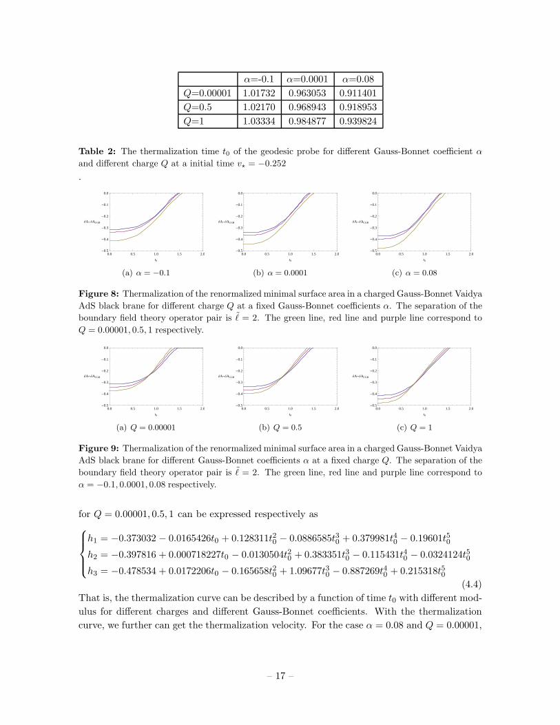
α=-0.1 α=0.0001 α=0.08

Q=0.00001 1.01732 0.963053 0.911401

Q=0.5 1.02170 0.968943 0.918953

Q=1 1.03334 0.984877 0.939824

Table 2: The thermalization time t0 of the geodesic probe for different Gauss-Bonnet coefficient α

and different charge Q at a initial time v⋆ = −0.252

.

0.0 0.5 1.0 1.5 2.0-0.5

-0.4

-0.3

-0.2

-0.1

0.0

t0

∆A-∆ACGB

(a) α = −0.1

0.0 0.5 1.0 1.5 2.0-0.5

-0.4

-0.3

-0.2

-0.1

0.0

t0

∆A-∆ACGB

(b) α = 0.0001

0.0 0.5 1.0 1.5 2.0-0.5

-0.4

-0.3

-0.2

-0.1

0.0

t0

∆A-∆ACGB

(c) α = 0.08

Figure 8: Thermalization of the renormalized minimal surface area in a charged Gauss-Bonnet Vaidya

AdS black brane for different charge Q at a fixed Gauss-Bonnet coefficients α. The separation of the

boundary field theory operator pair is ℓ = 2. The green line, red line and purple line correspond to

Q = 0.00001, 0.5, 1 respectively.

0.0 0.5 1.0 1.5 2.0-0.5

-0.4

-0.3

-0.2

-0.1

0.0

t0

∆A-∆ACGB

(a) Q = 0.00001

0.0 0.5 1.0 1.5 2.0-0.5

-0.4

-0.3

-0.2

-0.1

0.0

t0

∆A-∆ACGB

(b) Q = 0.5

0.0 0.5 1.0 1.5 2.0-0.5

-0.4

-0.3

-0.2

-0.1

0.0

t0

∆A-∆ACGB

(c) Q = 1

Figure 9: Thermalization of the renormalized minimal surface area in a charged Gauss-Bonnet Vaidya

AdS black brane for different Gauss-Bonnet coefficients α at a fixed charge Q. The separation of the

boundary field theory operator pair is ℓ = 2. The green line, red line and purple line correspond to

α = −0.1, 0.0001, 0.08 respectively.

for Q = 0.00001, 0.5, 1 can be expressed respectively as

h1 = −0.373032 − 0.0165426t0 + 0.128311t20 − 0.0886585t30 + 0.379981t40 − 0.19601t50

h2 = −0.397816 + 0.000718227t0 − 0.0130504t20 + 0.383351t30 − 0.115431t40 − 0.0324124t50

h3 = −0.478534 + 0.0172206t0 − 0.165658t20 + 1.09677t30 − 0.887269t40 + 0.215318t50(4.4)

That is, the thermalization curve can be described by a function of time t0 with different mod-

ulus for different charges and different Gauss-Bonnet coefficients. With the thermalization

curve, we further can get the thermalization velocity. For the case α = 0.08 and Q = 0.00001,

– 17 –

0.5 1.0 1.5

-0.4

-0.3

-0.2

-0.1

(a) α = −0.1

0.2 0.4 0.6 0.8 1.0 1.2 1.4

-0.4

-0.3

-0.2

-0.1

(b) α = 0.0001

0.2 0.4 0.6 0.8 1.0 1.2 1.4

-0.4

-0.3

-0.2

-0.1

(c) α = 0.08

Figure 10: Comparison of the function in Eq.(4.4) with the numerical result in Figure 8.

0.2 0.4 0.6 0.8 1.0 1.2 1.4t0

0.1

0.2

0.3

0.4

0.5

dH∆A-∆ACGBL�dt0

Figure 11: Thermalization velocity of the renormalized minimal surface area in a charged Gauss-

Bonnet Vaidya AdS black brane for Q = 0.00001 and α = 0.08.

the thermalization velocity is plotted in Figure (11). From this figure, we also can observe the

non-monotonic behavior and phase transition point of the thermalization process, which is

similar to that of the renormalized geodesic length. We also can obtain the acceleration phase

and deceleration phase for this case. By the slope of the thermalization velocity, we know

that the acceleration range is 0 < t0 < 1.106 and the deceleration range is 1.106 < t0 < 1.481.

Adopting the same strategy, we also can get the phase transition points for other Q and α.

5. Conclusions

Effect of the chemical potential and correction parameter on the thermalization in the dual

boundary field theory is investigated by considering the collapse of a shell of charged dust

that interpolates between a pure AdS and a charged Gauss-Bonnet AdS black brane. The

two-point function and expectation values of Wilson loop are chosen as the thermalization

probes, which are dual to the renormalized geodesic length and minimal area surface in the

bulk. We first study the motion profiles of the geodesic and minimal surface and find that

larger the Gauss-Bonnet coefficient is, shorter the thermalization time is, and larger the charge

is, longer the thermalization time is. At the initial stage of the thermalization, we find that

the charge has little effect on the thermalization time. We reproduce this result by studying

– 18 –

the relation between the renormalized geodesic length and time as well as the renormalized

minimal surface area and time respectively.

In addition, we also find the functions of the thermalization probes with respect to the

thermalization time by fitting the numerical result. Though this is a naive test, we still can

get some useful information. Firstly, we get the thermalization velocity for a fixed charge and

Gauss-Bonnet coefficient. From the velocity curve, on one hand, we know that the thermal-

ization process is non-monotonic, and on the other hand we find there is a phase transition

point, which divides the thermalization into an acceleration phase and a deceleration phase.

Secondly according to the slope of the velocity curve, we also get the acceleration and decel-

eration of the thermalization. Thus our investigation provides a more accurate description of

the thermalization process. Note that in our naive test, we can not see how the charge and

Gauss-Bonnet coefficient affect the thermalization quantificationally since the coefficients of

the functions are not determined. In future, we expect to find an analytical formulism to

study the thermalization so that we can get more useful information on the thermalization

process.

Acknowledgements

We would like to give great thanks to the anonymous referee for his helpful suggestions about

this paper. Xiao-Xiong Zeng would like to thank Hongbao Zhang for his encouragement

and various valuable suggestions during this work. This work is supported in part by the

National Natural Science Foundation of China (Grant Nos. 11365008, 61364030). It is also

supported by the Natural Science Fund of Education Department of Hubei Province (Grant

No. Q20131901)

Appendix: Derivation of the Hamiltonian from the Lagrangian

Suppose that there exists a Hamiltonian H such that

U(x, y;T ) = 〈x|e−iHT |y〉 = N∏

τ

∫

dd+1X(τ)√

−g(τ)ei∫ T0 dτL(τ) (5.1)

with X(0) = y, X(T ) = x, and the Lagrangian L = 12(gµν

dXµ

dτdXν

dτ−m2). Then we have

i∂

∂TU(x, y;T ) = HU(x, y;T ), (5.2)

and

U(x, y;T ) = N

∫

dd+1X√

−g(X)

ei2ǫ

gµν(x+X

2)(x−X)µ(x−X)ν− i

2ǫm2

U(X, y;T − ǫ), (5.3)

– 19 –

where ǫ is a small quantity, to be taken to go to zero in the later calculation. Now for

convenience, we would like to resort to the Rienmann normal coordinate at x, where the

behavior of metric is simplified as

gµν(x) = ηµν , ∂ρgµν(x) = 0, ∂ρ∂σgµν(x) = −1

3[Rµρνσ(x) +Rµσνρ(x)]. (5.4)

So by Taylor expanding all the involved functions at x and T , Eq.(5.3) gives rise to

U(x, y;T ) = N

∫

dd+1X√

−g(x)[1− 1

6Rρσ(x)(x−X)ρ(x−X)σ + · · ·]

ei2ǫgµν(x)(x−X)µ(x−X)ν (1− i

2ǫm2 + · · ·)

[1− (x−X)ρ∂ρ +1

2(x−X)ρ(x−X)σ∂ρ∂σ + · · ·]

(1− ǫ∂

∂T+ · · ·)U(x, y;T ).

(5.5)

Here we only keep those terms up to the first order of ǫ after the Gaussian integral, where the

normalization constant N can be fixed by the zero order equation and H can be determined

by the first order equation as

H = −1

2[∇a∇a −m2] +

1

6R. (5.6)

Similarly, if the Lagrangian is given by

L =1

2(gµν

dXµ

dτ

dXν

dτ−m2) +

1

6R, (5.7)

then the corresponding Hamiltonian will be shifted to

H = −1

2[∇a∇a −m2]. (5.8)

References

[1] J. M. Maldacena, The Large N limit of superconformal field theories and supergravity, Adv.

Theor. Math. Phys.2, 231 (1998) [hep-th/9711200].

[2] J. Sonner, A. G. Green, Hawking Radiation and Non-equilibrium Quantum Critical Current

Noise, Phys. Rev. Lett. 109, 091601 (2012).

[3] W. J. Li, Y. Tian, H. Zhang, Periodically Driven Holographic Superconductor, JHEP 07,

030(2013) [arXiv:1305.1600 [hep-th]].

[4] K. Murata, S. Kinoshita, N. Tanahashi, Non-equilibrium Condensation Process in a

Holographic Superconductor, JHEP 1007, 050 (2010) [arXiv:1005.0633[hep-th]].

[5] A. Mukhopadhyay, Non-equilibrium fluctuation-dissipation relation from holography, Phys.

Rev. D 87, 066004 (2013) [arXiv:1206.3311[hep-th]].

– 20 –

[6] K. Arnab, K. Sandipan, Steady-state Physics, Effective Temperature Dynamics in Holography,

arXiv:1307.6607[hep-ph].

[7] N. Shin, Nonequilibrium Phase Transitions and a Nonequilibrium Critical Point from Anti-de

Sitter Space and Conformal Field Theory Correspondence, Phys. Rev. Lett. 109, 120602 (2012)

[arXiv:1204.1971[hep-th]].

[8] R. Baier, A. H. Mueller, D. Schiff, D. Son, Bottom up thermalization in heavy ion collisions,

Phys. Lett. B 502, 51 (2001) [hep-ph/0009237].

[9] D. Garfinkle and L. A. Pando Zayas, Rapid Thermalization in Field Theory from Gravitational

Collapse, Phys. Rev. D 84, 066006 (2011) [arXiv:1106.2339 [hep-th]].

[10] D. Garfinkle, L. A. Pando Zayas and D. Reichmann, on Field Theory Thermalization from

Gravitational Collapse, JHEP 1202, 119 (2012) [arXiv:1110.5823 [hep-th]].

[11] A. Allais and E. Tonni, holographic evolution of the mutual information, JHEP 1201 102

(2012) [arXiv:1110.1607 [hep-th]].

[12] S. R. Das, Holographic Quantum Quench, J. Phys. Conf. Ser. 343, 012027 (2012)

[arXiv:1111.7275 [hep-th]].

[13] D. Steineder, S. A. Stricker and A. Vuorinen, probing the pattern of holographic

thermalization with photons, arXiv:1304.3404 [hep-ph].

[14] B. Wu, on holographic thermalization and gravitational collapse of massless scalar fields,JHEP

1210, 133 (2012)[arXiv:1208.1393 [hep-th]].

[15] X. Gao, A. M. Garcia-Garcia, H. B. Zeng, H. Q. Zhang, Lack of thermalization in holographic

superconductivity, arXiv:1212.1049 [hep-th].

[16] A. Buchel, L. Lehner, R. C. Myers and A. van Niekerk, Quantum quenches of holographic

plasmas, JHEP 1305, 067 (2013) [arXiv:1302.2924[hep-th]].

[17] V. Keranen, E. Keski-Vakkuri, L. Thorlacius, Thermalization and entanglement following a

non-relativistic holographic quench, Phys. Rev. D 85, 026005 (2012) [arXiv:1110.5035[hep-th]].

[18] V. Balasubramanian et al., Thermalization of Strongly Coupled Field Theories, Phys. Rev.

Lett. 106, 191601 (2011) [arXiv:1012.4753 [hep-th]].

[19] V. Balasubramanian et al., Holographic Thermalization, Phys. Rev. D 84, 026010 (2011)

[arXiv:1103.2683 [hep-th]].

[20] D. Galante and M. Schvellinger, Thermalization with a chemical potential from AdS spaces,

JHEP 1207, 096 (2012) [arXiv:1205.1548 [hep-th]].

[21] E. Caceres and A. Kundu, Holographic Thermalization with Chemical Potential, JHEP 1209,

055 (2012) [arXiv:1205.2354 [hep-th]].

[22] E. Caceres, A. Kundu, D. L. Yang, Jet Quenching and Holographic Thermalization with a

Chemical Potential, arXiv:1212.5728 [hep-th].

[23] X. X. Zeng and W. Liu, Holographic thermalization in Gauss-Bonnet gravity, Phys. Lett. B

726, 481 (2013) [arXiv:1305.4841[hep-th]].

– 21 –

[24] W. H. Baron and M. Schvellinger, Quantum corrections to dynamical holographic

thermalization: entanglement entropy and other non-local observables, arXiv:1305.2237

[hep-th].

[25] Y. Z. Li, S. F. Wu, G. H. Yang, Gauss-Bonnet correction to Holographic thermalization:

two-point functions, circular Wilson loops and entanglement entropy, arXiv:1309.3764 [hep-th].

[26] W. Baron, Damian Galante and M. Schvellinger, Dynamics of holographic thermalization,

arXiv:1212.5234 [hep-th].

[27] I. Arefeva, A. Bagrov, A. S. Koshelev, Holographic Thermalization from Kerr-AdS,

arXiv:1305.3267 [hep-th].

[28] V. E. Hubeny, M. Rangamani, E.Tonni, Thermalization of Causal Holographic Information,

arXiv:1302.0853 [hep-th].

[29] I. Y. Arefeva, I. V. Volovich, On Holographic Thermalization and Dethermalization of

Quark-Gluon Plasma, arXiv:1211.6041 [hep-th].

[30] V. Balasubramanian et al., Thermalization of the spectral function in strongly coupled two

dimensional conformal field theories, arXiv:1212.6066 [hep-th].

[31] V. Balasubramanian et al., Inhomogeneous holographic thermalization,

arXiv:1307.7086[hep-th].

[32] V. Balasubramanian et al., Inhomogeneous Thermalization in Strongly Coupled Field

Theories, arXiv:1307.1487[hep-th].

[33] P. Candelas, G. T. Horowitz, A. Strominger and E. Witten, Vacuum configurations for

superstrings, Nucl. Phys. B 258 (1985) 46.

[34] S. Nojiri and S. D. Odintsov, Brane-world cosmology in higher derivative gravity or warped

compactification in the next-to-leading order of AdS/CFT correspondence, JHEP 07 (2000)

049.

[35] J. de Boer, M. Kulaxizi, A. Parnachev, Holographic Entanglement Entropy in Lovelock

Gravities, JHEP 1107, 109 (2011)[arXiv:1101.5781].

[36] L. Y. Hung, R.C. Myers, M. Smolkin, On Holographic Entanglement Entropy and Higher

Curvature Gravity, JHEP 1104 (2011) 025 [arXiv:1101.5813].

[37] A. Bhattacharyya, A. Kaviraj, A. Sinha, Entanglement entropy in higher derivative

holography, JHEP 1308, 012 (2013).

[38] X. Dong, Holographic Entanglement Entropy for General Higher Derivative Gravity,

arXiv:1310.5713 [hep-th].

[39] Y. Z. Li, S. F. Wu, Y. Q. Wang, G. H. Yang, Linear growth of entanglement entropy in

holographic thermalization captured by horizon interiors and mutual information, JHEP 09,

057 (2013) [arXiv:1306.0210 [hep-th]].

[40] W. Z. Guo, S. He, J. Tao, Note on Entanglement Temperature for Low Thermal Excited States

in Higher Derivative Gravity, arXiv:1305.2682 [hep-th].

[41] A. Bhattacharyya, M. Sharma, A. Sinha, On generalized gravitational entropy, squashed cones

and holography, arXiv:1308.5748 [hep-th].

– 22 –

[42] R. C. Myers, S. Sachdev, A.Singh, Holographic Quantum Critical Transport without

Self-Duality, Phys. Rev. D 83, 066017 (2011)[arXiv:1010.0433 [hep-th]].

[43] D. Anninos, G. Pastras, Thermodynamics of the Maxwell-Gauss-Bonnet anti-de Sitter Black

Hole with Higher Derivative Gauge Corrections, JHEP 0907, 030 (2009) [arXiv:0807.3478

[hep-th]].

[44] R. G. Cai, Gauss-Bonnet black holes in AdS spaces, Phys. Rev. D 65, 084014 (2002)

[arXiv:hep-th/0109133].

[45] S. Cremonini, K. Hanaki, J. T. Liu and P. Szepietowski, Black holes in five-dimensional gauged

supergravity with higher derivatives, JHEP 0912, 045 (2009) [arXiv:0812.3572 [hep-th]].

[46] D. Anninos and G. Pastras, Thermodynamics of the Maxwell-Gauss-Bonnet anti-de Sitter

Black Hole with Higher Derivative Gauge Corrections, JHEP 0907, 030 (2009)

[arXiv:0807.3478 [hep-th]].

[47] D. Astefanesei, N. Banerjee, S. Dutta,(Un)attractor black holes in higher derivative AdS

gravity, JHEP 0811, 070 (2008) [arXiv:0806.1334 [hep-th]].

[48] X. O. Camanho, J. D. Edelstein, Causality constraints in AdS/CFT from conformal collider

physics and Gauss-Bonnet gravity, arXiv:0911.3160[hep-th].

[49] X. O. Camanho, J. D. Edelstein, Causality in AdS/CFT and Lovelock theory, arXiv:0912.1944

[hep-th].

[50] A. Buchel et al., Holographic GB gravity in arbitrary dimensions, JHEP 1003, 111 (2010)

[arXiv:0911.4257 [hep-th]].

[51] X. H. Ge, Y. Ling, Y. Tian and X. N. Wu, Holographic RG flows and transport coefficients in

Einstein-Gauss-Bonnet-Maxwell theory, JHEP 1112, 051 (2012) [arXiv:1112.0627[hep-th]].

[52] A. E. Dominguez, Emanuel Gallo, Radiating black hole solutions in Einstein-Gauss-Bonnet

gravity, Phys. Rev. D 73, 064018 (2006) [arXiv:gr-qc/0512150].

[53] T. Kobayashi, A Vaidya-type radiating solution in Einstein-Gauss-Bonnet gravity and its

application to braneworld, Gen. Rel. Grav. 37, 1869 (2005) [arXiv:gr-qc/0504027].

[54] H. Maeda, Effects of Gauss-Bonnet term on the final fate of gravitational collapse, Class.

Quant. Grav. 23, 2155 (2006) [arXiv:gr-qc/0504028].

[55] E. Caceres, A. Kundu, J. F. Pedraza, W. Tangarife, Strong Subadditivity, Null Energy

Condition and Charged Black Holes, arXiv:1304.3398 [hep-th].

[56] V. Balasubramanian and S. F. Ross, Holographic particle detection, Phys. Rev. D 61, 044007

(2000) [arXiv:hep-th/9906226].

[57] J. M. Maldacena, Wilson loops in large N field theories, Phys. Rev. Lett. 80, 4859 (1998)

[arXiv:hep-th/9803002].

[58] R. C. Myers, M. F. Paulos and A. Sinha, Holographic Hydrodynamics with a Chemical

Potential, JHEP 0906, 006 (2009) [arXiv:0903.2834 [hep-th]].

[59] Y. Ling, C. Niu, J. P. Wu and Z. Y. Xian, Holographic Lattice in Einstein-Maxwell-Dilaton

Gravity, arXiv:1309.4580[hep-th].

– 23 –