Holographic Wave Functions of the Universe - CORE
150
ARENBERG DOCTORAL SCHOOL Faculty of Science Holographic Wave Functions of the Universe Gabriele Conti Dissertation presented in partial fulfillment of the requirements for the degree of Doctor of Science (PhD): Physics November, 2017 Supervisor: Prof. dr. T. Hertog
-
Upload
khangminh22 -
Category
Documents
-
view
0 -
download
0
Transcript of Holographic Wave Functions of the Universe - CORE

ARENBERG DOCTORAL SCHOOLFaculty of Science
Holographic Wave Functionsof the Universe
Gabriele Conti
Dissertation presented in partialfulfillment of the requirements for the
degree of Doctor of Science (PhD):Physics
November, 2017
Supervisor:Prof. dr. T. Hertog


Holographic Wave Functions of the Universe
Gabriele CONTI
Examination committee:Prof. dr. T. Van Riet, chairProf. dr. T. Hertog, supervisorProf. dr. A. Van ProeyenProf. dr. E. CarlonProf. dr. A. Castro(UVA - Universiteit van Amsterdam)
Prof. dr. S. Detournay(ULB - Universitè Libre de Bruxelles)
Dissertation presented in partialfulfillment of the requirements forthe degree of Doctor of Science(PhD): Physics
November, 2017

© 2017 KU Leuven – Faculty of ScienceUitgegeven in eigen beheer, Gabriele Conti, Celestijnenlaan 200D, B-3001 Leuven (Belgium)
Alle rechten voorbehouden. Niets uit deze uitgave mag worden vermenigvuldigd en/of openbaar gemaakt wordendoor middel van druk, fotokopie, microfilm, elektronisch of op welke andere wijze ook zonder voorafgaandeschriftelijke toestemming van de uitgever.
All rights reserved. No part of the publication may be reproduced in any form by print, photoprint, microfilm,electronic or any other means without written permission from the publisher.

Aknowledgements
Working at KU Leuven has been a great honor. I would like to thank everysingle person who made these five years unforgettable. Everyone who supportedme on a professional and personal level. Without all of you, this thesis wouldhave been impossible.
First of all I want to thank Thomas Hertog, for being my supervisor and forgiving me the opportunity to do this PHD. I want to thank you for all theinteresting, nice and advanced projects you gave me. It was a great opportunityfor me to work with you on these topics, and I am really grateful for that. Youalso gave me the opportunity to travel a lot during my PHD, in order to attendconferences, schools, workshops, etc. This gave me the opportunity to grow upa lot both on a professional and personal level, as well as the opportunity toknow many new colleagues. I am really grateful to you for all of this.
Secondly, I would like to thank my PHD committee: Enrico Carlon, Antoine(Toine) Van Proeyen, Alejandra Castro, Stephan Detournay and Thomas VanRiet. Thanks for the time you dedicated to the reading of my manuscript andfor the valuable comments.
A special thanks to Thomas Van Riet. I really appreciated the useful discussionswe had about dS/CFT. Those discussions stimulated me a lot. I have alsoenjoyed when we were going to some missions together, in particular the one inMadrid. Further, your door is always open when PHD students need to talkabout professional or personal issues. This is very important for all us, and itmean a lot to me!
A special thanks to Alejandra Castro. Even if we met only during conferencesand schools, I have really appreciated talking with you about my and your work.It has been an honour knowing you. Thank you for giving me the opportunityto give a talk in Amsterdam and to have agreed on being in my PHD committee.
A special thanks to Frederick Denef. It was a pleasure to know you and to have
i

ii AKNOWLEDGEMENTS
been your teaching assistant during my first year as a PHD student. It was alsovery nice to meet with you during conferences or workshop. I really appreciatedall the time we talk and we updated each other with our recent works.
I also want to thank all the ITF members. Nikolay Bobev for the stimulatingdiscussions. Christian Maes for all his skepticism. I know it sounds weird, butthose discussions help us (phd students) a lot. They push us to give our bestall the time, and I really appreciate that.
A very special thanks to Ellen Van der Woerd for sharing this experience withme. I am really happy to have started my PHD with you. We had so manydiscussions both from a professional and a personal level. I am deeply gratefulto have met not only a colleague but also a friend like you during these years.
Thanks to all the ones who shared the office with me during these years:Frederick Coomans, Alessio Marrani, and Yannick Vreys. We spent a lot oftime in the same room, and without you it would have been different.
I am also really grateful to all the persons I met at ITF during these years.Thanks to Federico, Alice and Marius for driving me to the office or back home.Thanks to Anneleen for being so professional and nice with everybody. Withoutyou the work at ITF would be way more complicated. Thanks to Filip for beingso helpful everytime we needed to fix issues on our computers. Thanks to MattWilliams, it was nice to meet you and to have so many fruitful discussions withyou. Thanks to Marjoree, I really enjoyed conversations with you and with yourhusband. I wish the best luck to both of you. A special thanks to Jesse. I metyou only during my final year, but it was really nice, and I wish we would havespent more time together. Thanks for the Dutch translation of the abstract.Thanks also to Edoardo. It was always very nice and pleasant to talk with you.I wish you good luck for your work and your life. Finally, Pablo, Juan, Gabriele,Brecht, Bert, Marco, Fridrik, Vincent, Bert, Ruben, and all the people whoshared time with me at ITF, thanks a lot. It was a pleasure to meet with all ofyou.
Thanks to all the people I met during these years. Blagoje, Jules, Laura, MarcoF., Marco S., Teresa, it was really nice to know all of you and I really liked tomeet with you during schools or conferences. A special thank also to all thepeople who shared time with me in Brussels: Marco, Jo, Adolfo, Marianna. Ireally had a lot of fun with all of you and I will always bring very good memoryfor the time we spent together.
Thanks to my parents, my sister and my niece. You are always there when Ineed. You are supporting me every day, and you are a motivation for me togive my best. You are always a light even when everything is dark. You arealways a landmark for me.

AKNOWLEDGEMENTS iii
A special thanks to all my friends in Italy. I am so lucky to have you therealways. My life would be boring without you. It is really great to know I cancount on all of you everytime I need. You always give me valuable suggestionsfor my life and you always support me when I need. I really appreciate that.
Thanks to Carole for reading my manuscript and for spotting English mistakes.
Last but not least, the best thanks to my beloved Juliette. My life in Brusselshad a turn around when I met you. There are no words I can use to describehow much I am grateful for the chance I had to know you and for the privilegeto share my life with you. You give a meaning to every single day. You give ameaning to my life. You were always there to comfort me, to support me, tostimulate me day after day. You were there when I was happy. You were therewhen I was sad. You were there when I was angry. You were there when I wassick. You have always found the right words and gave me the right motivationsto go on, to move on, to follow my dreams. Thank you for your never endingbelieve in me. Without you, this work and my PHD would have not beenpossible. Thanks!


Abstract
It is a central goal of theoretical high-energy physics to develop a unifiedtheoretical framework that describes Nature on all scales. A common approachto this involves merging quantum theory and General Relativity into a unifiedtheory of quantum gravity. A theory of this kind has the potential to putcosmology on firm theoretical footing.
String theory is a promising candidate for a unified theory. The second stringtheory revolution in the ’90s has consolidated the role of holography in quantumgravity in the form of a duality between quantum gravity with anti-de Sitter(AdS) boundary conditions and Conformal Field Theories (CFTs) defined on theconformal boundary of AdS. However observations indicate that our universe isasymptotically de Sitter (dS). Together these developments mean it is importantto understand whether holographic ideas can be developed and used in a dScontext to construct a quantum gravitational model of cosmology.
A central role in quantum cosmology is played by the wave function of theuniverse. There are several indications indeed that the application of holographyto cosmology enables a new formulation of the wave function of the universe interms of the partition function of Euclidean deformed CFTs defined on the futureconformal boundary. However many fundamental questions about the technicaland conceptual nature of holographic cosmology or dS/CFT remain open. Inthis thesis we study and explore a number of features of dS/CFT duality. Inone particular example, AdS/CFT implies an explicit realization of dS/CFT,which relates Vasiliev’s higher spin theory of gravity to the O(N) vector modelof interacting scalars. This example will serve throughout this thesis as a usefultoy model with which we will explore and test various developments of theduality more generally.
In the first part of this thesis we develop dS/CFT for Vilenkin’s tunnelingwave function and contrast its behaviour with that of the Hartle-Hawking wavefunction. We evaluate the holographic tunneling wave function in the O(N)
v

vi ABSTRACT
vector toy model in the presence of a mass deformation and compare this withits behaviour predicted in the usual bulk saddle pont approximation.
In the second part of this thesis we explore the dS/CFT correspondence withS1×S2 future boundary conditions. In this context it has been argued that theprobability measure is badly defined, both in the O(N) vector toy model and inEinstein gravity, in the limit where the radius of the S1 goes to zero. We analyzethis using quantum cosmology techniques to elucidate the interpretation of thewave function in this domain. We show that the divergent behaviour of the(bulk and boundary) measures occurs in a regime where the wave function doesnot describe asymptotically classical, Lorentzian histories and hence admitsno clean probabilistic interpretation. We also exhibit the strikingly differentbehaviour of the tunneling and no-boundary wave function in this regime. Theformer appears to select this quantum realm whereas the latter predicts theuniverse is everywhere in the semiclassical domain.
The third part of this thesis consists of a digression into AdS/CFT. In the bulkwe consider a consistent truncation of M-Theory compactified on AdS4 × S7
consisting of Einstein gravity minimally coupled to a single scalar field with anegative exponential potential. We numerically find a three parameter familyof new Euclidean solutions of this theory that asymptote to a locally AdS spacewith a (double) squashed sphere as conformal boundary configuration. Oursolutions are generalization of the AdS Taub-NUT/Bolt solutions to include asecond squashing and scalar matter. We study their thermodynamic behaviouras a function of the three boundary parameters and show this qualitativelyreproduces that of the free O(N) vector model defined on a double squashedsphere and deformed by a mass term.
This sets the scene for the final part of this thesis where we consider complexgeneralizations of the above solutions, starting from the same theory, withasymptotically dS boundary conditions. These specify the saddle point wavefunction in a minisuperspace model of anisotropic deformations of dS with scalarmatter driving a regime of eternal inflation. We initiate a holographic explorationof eternal inflation by computing the partition function of the interacting O(N)vector model as a function of the three asymptotic parameters. We find that theamplitude is low for conformal boundary surfaces far from the round conformalstructure. This is in line with general field theory expectations and lendssupport to the conjecture that the exit from eternal inflation is reasonablysmooth, producing universes that are relatively regular on the largest scaleswith globally finite surfaces of constant density.

Beknopte samenvatting
Het is een centrale doelstelling van de theoretische hoge energie fysicaom een verenigd theoretisch kader te ontwikkelen dat de natuur op alleschalen beschrijft. Een belangrijk onderdeel hiervan is het unificeren vande kwantummechanica met de algemene relativiteitstheorie van Einstein, toteen zogenaamde kwantumzwaartekracht. Een dergelijke theorie heeft ondermeerde potentie om kosmologie op stevige theoretische basis te zetten. in de jaren’90, heeft door middel van holografie kwantummechanica zwaartekracht in devorm van een dualiteit tussen kwantumzwaartekracht met anti-de Sitter (AdS)randvoorwaarden en Conforme veldentheorieën (CFT’s) gedefinieerd op deconforme grens van AdS. Observaties wijzen er echter op dat ons universumasymptotisch de Sitter (dS) is en niet AdS. Het is een interessant vraagstuk ofde holografische ideeen van AdS ook toegepast kunnen worden op dS ruimtes.Dit zou dan leiden tot een kwantum-gravitatiemodel van de kosmologie. Eencentrale rol in de kwantumkosmologie wordt gespeeld door de golffunctie vanhet universum en zal ook in deze thesis een belangrijke rol hebben.
Er zijn inderdaad verschillende aanwijzingen dat de toepassing van holografiein kosmologie een nieuwe formulering van de golffunctie van het universumkan opleveren door middel van andere voorwaarden van de verdelingsfunctievan Euclidsch-vervormde CFT’s gedefinieerd voor de toekomstige conformegrens. Veel fundamentele vragen over de technische en conceptuele aard vanholografische kosmologie en dS/CFT blijven echter nog altijd open. In ditproefschrift bestuderen en onderzoeken we een aantal kenmerken van de dS/CFTdualiteit. In een specifiek voorbeeld impliceert AdS/CFT een expliciete realisatievan dS/CFT, welke Vasiliev’s hogere spintheorie van zwaartekracht relateertaan een O(N) vectormodel interagerende waarmee we verschillende aspectenvan de dualiteit zullen verkennen en testen.
In het eerste deel van dit proefschrift ontwikkelen we dS/CFT voor deVilenkin tunneling-en contrasteren het gedrag met dat van de Hartle-Hawking-golffunctie. We evalueren de holografische tunneling-golffunctie in het O(N)
vii

viii BEKNOPTE SAMENVATTING
vectormodel, in aanwezigheid van een massavervorming, en vergelijken dit methet gedrag voorspeld in de gebruikelijke benadering van bulkzadel-punten. Inhet tweede deel van dit proefschrift onderzoeken we de dS/CFT-correspondentiemet S1 × S2 als toekomstige randvoorwaarden. In dit verband is betoogddat de waarschijnlijkheidsmaat slecht is gedefinieerd, zowel in het O (N)-vectormodel als in de zwaartekrachttheorie, in de limiet waar de straalvan de S 1 naar nul gaat. Wij analyseer dit fenomeen met behulp vantechnieken uit de kwantumkosmologie om de interpretatie van de golffunctiete verduidelijken. We laten zien dat het afwijkende gedrag van de (bulk engrens) maten plaats vindt in een regime waar de golffunctie asymptotische geenklassieke, Lorentziaanse, geschiedenissen beschrijft en daarom geen fatsoenlijkeprobabilistische interpretatie toelaat. We tonen ook een opvallend andersgedrag aan van de tunneling en "no-boundary"golffuncties in dit regime. Deeerstgenoemde lijkt het kwantumrijk te selecteren, terwijl dat laatste hetuniversum voorspelt in een semiklassiek domein.
Het derde deel van dit proefschrift bestaat uit een studie naar AdS/CFT. In debulk beschouwen we een consistente truncatie van M-Theory gecompactificeerdop AdS 4 × S 7 bestaande uit Einstein-zwaartekracht minimaal gekoppeldaan een scalair veld met een negatieve, exponentiële, potentiaal. Door gebruikte maken van numerieke technieken vinden we een familie aan Euclidischeoplossingen met drie parameters, die asymptotisch naar een lokale AdS-ruimtegaan met een (dubbele) geplette bol als conforme grens. Onze oplossingenzijn generalisaties van de AdS Taub-NUT / Bolt-oplossingen die een tweedevervorming van de sfeer toelaten, met scalaire materie. We bestuderen hunthermodynamisch gedrag in functie van de drie familie-parameters en laten ziendat dit kwalitatief het vrije O (N) -vectomodel reproduceert, gedefinieerd opeen dubbel geplette bol met een massaterm vervorming.
Dit schetst de setting voor het laatste deel van dit proefschrift, waarin we heteen complexe veralgemening beschouwen van de bovengenoemde oplossingen,uitgaande van dezelfde theorie, met asymptotisch dS randvoorwaarden. Dezespecificeren de zadelpunt-golffunctie in een minisuperspace-model met anisotropevervormingen van dS en met scalaire materie dat een regime van eeuwige inflatieaandrijft. We initiëren een holografische verkenning van eeuwige inflatie doorde verdelingsfunctie van het interagerende O (N) vectormodel te berekenen alseen functie van de drie asymptotische parameters die de familie aan oplossingendefiniëren. We vinden dat de de amplitude laag is voor conforme grensvlakkenver van de ronde, conforme, structuur. Dit is in lijn met verwachtingen uitde veldentheorie en geeft steun aan het vermoeden dat de uitweg uit eeuwigeinflatie relatief glad is, en dat er universa geproduceerd kunnen worden dieop grote schaal regulier zijn met globaal eindige oppervlakken van constantedichtheid.

Contents
Abstract v
Contents ix
1 Holography For Cosmology 1
1.1 Introduction . . . . . . . . . . . . . . . . . . . . . . . . . . . . . 1
1.2 A Semiclassical Cosmological Measure . . . . . . . . . . . . . . 7
1.2.1 Tunneling Wave Function . . . . . . . . . . . . . . . . . 10
1.2.2 No-Boundary Wave Function . . . . . . . . . . . . . . . 12
1.2.3 No-Boundary Vs Tunneling . . . . . . . . . . . . . . . . 19
1.2.4 Issues . . . . . . . . . . . . . . . . . . . . . . . . . . . . 19
1.3 Beyond Semiclassicality: A Holographic Cosmological Measure 20
1.4 From Quantum to Classical . . . . . . . . . . . . . . . . . . . . 24
1.4.1 Lorentzian Histories . . . . . . . . . . . . . . . . . . . . 25
1.5 Open Questions . . . . . . . . . . . . . . . . . . . . . . . . . . . 26
1.5.1 Free O(N) Vector Model Massed . . . . . . . . . . . . . 27
1.5.2 Critical O(N) Vector Model . . . . . . . . . . . . . . . . 28
1.5.3 Free O(N) Vector Model Squashed . . . . . . . . . . . . 29
1.5.4 U(N) Vector Model . . . . . . . . . . . . . . . . . . . . . 29
ix

x CONTENTS
1.6 Outline of the Thesis . . . . . . . . . . . . . . . . . . . . . . . . 30
2 Holographic Tunneling Wave Function 33
2.1 Introduction . . . . . . . . . . . . . . . . . . . . . . . . . . . . . 33
2.2 The Tunneling Wave Function . . . . . . . . . . . . . . . . . . . 34
2.3 Representations of Complex Saddle Points . . . . . . . . . . . . 36
2.4 Homogeneous Minisuperspace . . . . . . . . . . . . . . . . . . . 37
2.4.1 dS representation of saddle points . . . . . . . . . . . . 38
2.4.2 AdS representation of saddle points . . . . . . . . . . . 40
2.5 General Saddle points . . . . . . . . . . . . . . . . . . . . . . . 41
2.6 Holographic tunneling wave function . . . . . . . . . . . . . . . 43
2.7 Testing the duality . . . . . . . . . . . . . . . . . . . . . . . . . 45
2.7.1 Minimal O(N) vector model . . . . . . . . . . . . . . . . 45
2.7.2 Critical O(N) vector model . . . . . . . . . . . . . . . . 47
2.8 Discussion . . . . . . . . . . . . . . . . . . . . . . . . . . . . . . 48
3 Two Wave Functions and dS/CFT on S1 × S2 51
3.1 Introduction . . . . . . . . . . . . . . . . . . . . . . . . . . . . . 51
3.2 Asymptotic Tunneling Wave Function . . . . . . . . . . . . . . 52
3.3 Asymptotic Hartle–Hawking Wave Function . . . . . . . . . . . 57
3.4 Wave Functions in the Classically Forbidden Regime . . . . . . 59
3.5 Predictions in the Classical Domain . . . . . . . . . . . . . . . 63
3.6 Holographic Wave Functions . . . . . . . . . . . . . . . . . . . . 68
3.7 Discussion . . . . . . . . . . . . . . . . . . . . . . . . . . . . . . 73
4 A digression into AdS/CFT 75
4.1 Introduction . . . . . . . . . . . . . . . . . . . . . . . . . . . . . 75
4.2 Scalar Excitations of Squashed AdS Taub-NUT/Bolt . . . . . 77

CONTENTS xi
4.3 A CFT comparison . . . . . . . . . . . . . . . . . . . . . . . . . 81
4.4 Discussion . . . . . . . . . . . . . . . . . . . . . . . . . . . . . . 85
5 A Holographic Measure on Eternal Inflation 87
5.1 Introduction . . . . . . . . . . . . . . . . . . . . . . . . . . . . . 87
5.2 Anisotropic inflationary minisuperspace . . . . . . . . . . . . . 89
5.2.1 Anisotropic inflationary histories . . . . . . . . . . . . . 94
5.2.2 Classical Lorentzian evolution. . . . . . . . . . . . . . . 97
5.3 A Holographic Measure . . . . . . . . . . . . . . . . . . . . . . 98
5.4 Discussion . . . . . . . . . . . . . . . . . . . . . . . . . . . . . . 101
6 Discussion 103
6.1 Summary and conclusion . . . . . . . . . . . . . . . . . . . . . 103
6.2 Outlook . . . . . . . . . . . . . . . . . . . . . . . . . . . . . . . 105
A Appendix 107
A.1 Basis change. . . . . . . . . . . . . . . . . . . . . . . . . . . . . 107
A.2 Anisotropic Euclidean AdS solutions. . . . . . . . . . . . . . . . 108
A.2.1 Equations of motion . . . . . . . . . . . . . . . . . . . . 108
A.2.2 Solutions . . . . . . . . . . . . . . . . . . . . . . . . . . 109
A.2.3 Evaluating the numerical action . . . . . . . . . . . . . 115
A.2.4 Euclidean Action . . . . . . . . . . . . . . . . . . . . . . 115
A.3 Anisotropic dS solutions. . . . . . . . . . . . . . . . . . . . . . . 117
Bibliography 119


Chapter 1
Holography For Cosmology
1.1 Introduction
Our knowledge of the underlying physical mechanisms of Nature underwent arevolutionary advance in the first part of the last century. Einstein’s theory ofgeneral relativity perfectly describes the behaviour of a weak gravitational fieldat large scales. Quantum mechanics describes with an incredible accuracy theeffects of non-gravitational forces on small scales. However one would expectgravity to behave fundamentally quantum mechanically, with the classicalEinsteinian theory emerging as a limiting case under appropriate circumstances.
There is much evidence that a quantum theory of gravity is needed to describeour own universe. In 1929 Hubble discovered that the universe is not static,but is expanding, [1]. Back in time the universe must have been very small, apoint source containing all the matter, a point with an infinite density. Froma theoretical point of view, classical general relativity cannot describe suchscenario. Classical general relativity admits solutions with singularities, but thePenrose – Hawking singularity theorems state that our universe is geodesicallyincomplete in the past if treated classically. General relativity must break downat least at the Planck time and perhaps more broadly. Hence general relativitycannot be used to describe the region close to a singularity, and a quantummodel of gravity is needed.
In 1965 Penzias and Wilson accidentally discovered that the entire universeis filled with a background radiation, [2], a sort of echo of a primordial event.This radiation is called cosmic microwave background (CMB) and it is anelectromagnetic type of radiation. It is the leftover of an event which occurred
1

2 HOLOGRAPHY FOR COSMOLOGY
Figure 1.1: The most detailed image of the CMB radiation, released byPlanck, [12, 13, 14, 15]. Different color represent different temperatures. Thesefluctuation are the seeds of galaxy and star formations.
at an early phase of the universe. At the very beginning, the universe wasextremely dense and even photons were scattering. In this period the universewas completely opaque. With the expansion, the temperature cooled down andthe density dropped down. At a certain time, photons were free to propagate.This period is often referred as surface of last scattering, and the CMB radiationis the visual image of that event. The CMB is in a certain sense a "relicradiation", the earliest image of the universe we can have through electromagneticradiation. The CMB is almost isotropic everywhere, but there are some tiny,crucial fluctuations (at the part per million level) seed for the galaxy and starformations, [3, 4, 5]. Understanding the CMB radiation is therefore of crucialimportance. In the past years, an enormous amount of observations have beendone, improving the definition and the details of this primordial image. Amongthese observations, we have to cite the results of: COBE [6], WMAP [7, 8, 9],ALMA [10, 11], Planck [12, 13, 14, 15], and others [16, 17]. In figure 1.1 weshow the picture of the CMB radiation with the highest definition we havetoday, released by the Planck mission in 2013.
The discovery of the CMB posed further questions. In classical cosmology the hotbig bang model successfully describes many, but not all the futures we observe inthe universe. For example, it does not explain flatness, absence of horizons andthe origin of the density fluctuations we observe in the CMB. Theorists suggestedthat the universe expanded at an exponential rate at the very beginning. Thismodel is called inflation and provides a solution to the flatness and the horizonproblem, and one can obtain the spectrum of density perturbation by requiringthat the matter fields started in a particular quantum state [18, 19]. Inflation

INTRODUCTION 3
is driven by a quantized scalar field that (slowly) rolls down a potential hill andstops at a positive minima of the potential which is the cosmological constant wemeasure today. Many different types of inflationary models have been proposedin the past years [20, 21, 22, 23, 24, 25, 26, 27, 28]. We refer to [29, 30, 31, 32]for a review. Inflation suggests that the universe cannot be originated fromany initial state (i.e. one could choose initial conditions such that inflationdoes not occur at all). Understanding the observed state of the universe istherefore related to the problem of initial conditions. As often occurs, a newdiscovery lead to new mysteries. If inflation is eternal, the inflationary phase ofthe universe’s expansion lasts forever in different fractal regions of the universe.Eternal inflation, therefore, produces a hypothetically infinite multiverse, andonly in a small volume of the universe inflation come to an end. Eternal inflationappears to be generic, [20], and appears to be the likely outcome of inflation,[18]. If inflation is eternal, whatever can happen, will happen, and it will happennot only once but an infinite numbers of time, with the only requirement thatthe fundamental law of physics are not violated. Classical gravity itself is notable to describe this scenario, and a quantum gravity theory is needed.
Once we have a model of quantum gravity at our disposal, we need a wayto test it. Quantum gravity effects are expected to be relevant at very highenergy, and we expect to be able to observe these effects directly as we approachthe Planck length (1.62× 10⁻³⁵m or equivalently 1.22× 10¹⁶TeV). The mostpowerful high energy particle accelerator (LHC) can probe events at around14TeV, a scale far smaller to the one needed to directly test a quantum theoryof gravity. A lab on earth is not the only way we might have to test such atheory. If quantum gravity effects took place during the early phase of ouruniverse, they might have left a fingerprint on present observations. The earlyuniverse might be the best laboratory (and maybe the only one) where to testa model of quantum gravity. Understanding the effects of a quantum theory ofgravity in cosmology is therefore of crucial importance. In 2016 the observationof gravitational waves, [33], opened a new window in this scenario. We cannotuse electromagnetic waves to observe the universe before CMB time, but wemight use gravitational waves to directly observe quantum gravity effects atan earlier phase of the universe. A quantum gravity theory for cosmology istherefore fundamental in these days of important observations.
Recently, astrophysicists realized that the universe is expanding at anaccelerating rate. The acceleration is driven by a tiny but crucially positivecosmological constant Λ ∼ 10−52m−2, [34, 35, 36, 37, 38]. The positivity of thecosmological constant rises many issues.
These issues do not represent a motivation for a quantum gravity theory, ratherthey are problems one needs to face up when dealing with a quantum gravitymodel in a universe dominated by a positive cosmological constant.

4 HOLOGRAPHY FOR COSMOLOGY
The d+ 1 dimensional pure de Sitter (dS) geometry is a maximally symmetricsolution of the Einstein’s field equation with a positive cosmological constant Λ
Gµν = Rµν −12gµνR+ Λgµν = 0 . (1.1)
The geometry of dSd+1 space can be viewed as the induced metric on thehyperboloid
−X20 +
d+1∑i,1
X2i = 3
Λ ≡1H2 , (1.2)
embedded in d + 2 dimensional Minkowski space. We can describe dS spacewith different coordinate patches, which cover the whole hyperboloid or part ofit.
The so called global patch, is described by the line element
ds2 = −dt2 + 1H2 cosh2(Ht)dΩ2
d . (1.3)
A surface of constant t is a three-sphere. The sphere shrinks from a maximumsize at t = −∞, a surface called I−, to a minimum size at t = 0. Then itbounces to a maximum size at t =∞, a surface called I+. A single observercannot access the whole global space. Rather, s/he can only access the regiondescribed by the so called static patch, with metric
ds2 = −(1− r2H2)dt2 + (1− r2H2)−1dr2 + r2dΩ2d−1 . (1.4)
The surface r = 1/H ≡ ldS is a null surface that surrounds an observer at alltimes (the cosmological horizon). The coordinate ranges are: r ∈ [0, ldS ] andt ∈ R.
We show the Penrose diagram of dS space in figure 1.2. The whole square iscovered by the global patch (1.3) only. A physical observer can only access thequarter of the whole square containing the NP (or the SP). One can use othercoordinate patches, but we do not discuss them here. We refer to [39] for anexhaustive discussion.
If this expansion persists the fate of our universe might be a cold and "empty"universe. An observer in the far future would observe a universe governed bythermal and quantum fluctuations at a Hawking temperature of ∼ 10−29K. Themain source of energy will be the cosmological constant, which today alreadyconstitutes ∼ 70% of the total energy. Obviously no physical person can observesuch scenario, hence what is the meaning of an observer or, more in general,of any observable in the far future? That is not the only problem. A featureof the dS universe is the presence of a cosmological horizon, which is observer

INTRODUCTION 5
r=0
I+
I-
SP NP
r=ldS
Figure 1.2: Penrose diagram of a dS universe.
dependent. An observer (like us) does not have access to data of the wholeuniverse (in particular, data outside the cosmological horizon). In particular,an observer does not ordinarily have access to the spatial slice at infinite future,I+. The physical meaning of infinite future itself and, more in general, of dataoutside the cosmological horizon is a big challenge in theoretical physics (for anoverview we refer to [40, 41]). The mystery persists. A cosmological horizon hasa gravitational entropy which scales as the area of the horizon, S = A/4G, whichis a similar behaviour as the gravitational entropy for black holes, [42]. Can wehave a micro-canonical description of this gravitational entropy? How can wetake into account for the vast number of microstates, 1010120 , coming from theGibbons-Hawking entropy [43] of the cosmological horizon? A quantum gravitydescription of dS space needs to face up with all these issues. For a completereview we refer to [39, 44, 45].
Eventually, inflation came to an end, followed by the CMB and the formationof large scale structures we observe today. A quantum theory of gravity shouldadmit cosmological solutions that predict a universe originated from a quantumevent and evolved to a classical four-dimensional inflationary Lorentzian universewhich is asymptotic de Sitter space. In short, a quantum gravity theory seemsto be needed, and it must predict the cosmological observations we see in theclassical limit (when the universe expands).
The quantum cosmology program tries to address these questions. In quantumcosmology one assigns a measure to the likelihood of a boundary configuration ata given time, which can be related to the outcome of cosmological observations.

6 HOLOGRAPHY FOR COSMOLOGY
The key object of interest in quantum cosmology is the wave function of theuniverse,
Ψ[hij(x), χ(x), B] , (1.5)where hij(x) is the space-like section of the universe on a closed surface B, andχ(x) is the scalar field 1 configuration on this surface.
The square of the wave function gives a measure, in terms of probabilistic weightfor that particular configuration,
P[hij(x), χ(x), B] = |Ψ[hij(x), χ(x), B]|2 . (1.6)
The value of the boundary fields generically depends on their location onthe entire manifold, whose coordinates are denoted by x. The space of allthe possible values of the boundary geometry and matter field configurations(hij(x), χ(x)) is called superspace. The superspace can be thought of thespace where the classical dynamics take place, it is infinite dimensional butwith a finite number of coordinates (hij(x), χ(x)) at every point x on theboundary-surface.
Superspace is an infinite dimensional configuration space, so the full formalismis extremely challenging. A more practical way to proceed is to reduce thesuperspace to a finite-dimensional space, i.e. if we consider only those fields thatare homogeneous. This reduced version of superspace is called minisuperspace.This restriction is achieved by setting most of the field modes and their momentato zero. In this way we exclude many geometries that might give a non-trivial contribution. We should not think to a minisuperspace model as anapproximation of the full theory, but rather as a toy model that shares someaspects of the full theory. We study certain features of the full theory in isolationwith the rest.
To determine (1.5), we need three elements: initial conditions, dynamics andinterpretations. The equations the wave function must satisfy admit moresolutions, and we need to impose initial conditions by hand to specify onlyone. To evaluate the wave function we need to consider a dynamic theory ofgravity which describes the dynamic of the universe. Finally, we need a schemeto interpret our results and find what type of universe is predicted by the wavefunction.
The outline of this chapter is as follows. In section 1.2 we introduce theequations the wave function must satisfy, we discuss semiclassical solutions andthe different proposals of boundary conditions which lead to different measuresand different predictions. In section 1.3 we review the wave function approachto the dS/CFT correspondence. We provide an alternative way to compute the
1One can also consider vector fields configurations, [46].

A SEMICLASSICAL COSMOLOGICAL MEASURE 7
full cosmological measure (1.6). In section 1.4 we discuss what is the outcomeof the wave function. We will describe how classical solutions emerge from thequantum theory and what we interpret as a prediction. In section 1.5 we give alist of results that were already known and provided a motivation for this thesiswork. Finally, in section 1.6 we give an outline of the remainder of the thesis.
1.2 A Semiclassical Cosmological Measure
In this section we will describe the equations that the wave function must satisfy,and we will discuss semiclassical solutions. In short, we review the formalism ofquantum cosmology. We refer to [47, 48, 49, 50, 51, 52, 53] for an exhaustivediscussion.
In minisuperspace model2 the wave function is a solution of the quantum versionof the Hamiltonian constraint of general relativity, which can be obtained bygeneralizing the Dirac quantization procedure to minisuperspace models,
HΨ(qA) =(−1
2GABπAπB + U(qA)
)Ψ(qA) ≡
(−∇2 + U(qA)
)Ψ(qA) = 0 ,
(1.7)where we have collected the coordinates qA ≡ hij(x), χ(x), with A = 1, 2.The superpotential is
U(q) =√h(−3R+ 2Λ + V (χ)
), (1.8)
and the momenta are defined as
πA = −i δ
δqA. (1.9)
while GAB = G(ij)(kl), with
Gijkl = h−12 (hikhjl + hilhjk − hijhkl) . (1.10)
The boundary Ricci scalar 3R is evaluated on the surface hij , and V (χ) is thepotential of the asymptotic scalar field profile χ. Equation (1.10) provides ametric on superspace and Gijkl is called the deWitt metric, [52]. GAB providesa metric on minisuperspace.
Some important properties of this metric are2In superspace models there is also a second constraint, called momentum constraint. In
minisuperspace this constraint is automatically satisfied by the minisuperspace ansatz.

8 HOLOGRAPHY FOR COSMOLOGY
• the signature of the deWitt metric is independent of the signature ofspacetime;
• the signature of the deWitt metric is hyperbolic at every point x.
The latter property arises from the fact that the coefficient of the momentain the Hamiltonian constraint (1.7) is regarded as a metric of a 6-dimensionalhyperbolic Riemannian manifoldM. When hij is positive definite (as it is fora spacelike hypersurface)M has the hyperbolic signature −+ + + ++. Thisproperty was pointed out by deWitt himself in [52].
Equation (1.7) is called Wheeler-deWitt (WdW) equation, and it is the quantumversion of the classical constraint of general relativity. It reminds the zero-energySchröedinger equation of ordinary quantum mechanics. The WdW equation(1.7) describes the dynamic of the wave function in minisuperspace. The volumeof the three-metric
√h is the label of time in the superspace coordinates 3.
The minisuperspace metric GAB depends on qA. This leads to an operatorordering issue in the kinetic term and in (1.7) a particular choice was made.The superspace metric has indefinite signature and the potential term in (1.7) isnot positive definite. We have to consider generically complex functional Ψ(qA)to solve (1.7).
In quantum mechanics one can find approximate solutions to the Schröedingerequation, [54, 55]. One needs to expand the wave function as a power seriesin ~ and to solve the Schröedinger equation order by order. The procedure iscalled WKB approximation, and can be generalized to minisuperspace models[56, 57].
We expand the wave function as a power series in ~, and we keep track ofits real and imaginary components. To simplify the notation we collect theminisuperpsace coordinates, q ≡ qA. We look for WKB solutions in the form
Ψ(q) = e−IR(q)/~+iS(q)/~ +O(~−2) , (1.11)
where IR and S are real. We use the wave function (1.11) in equation (1.7).The result is a set of two equations,
−12(∇IR)2 + 1
2(∇S)2 + U(q) = 0 ,
∇IR · ∇S = 0 .(1.12)
3It corresponds to the minus sign in the hyperbolic signature of the superspace metric.

A SEMICLASSICAL COSMOLOGICAL MEASURE 9
Solutions to the first equation clearly depends on the sign of U(q). In the regionof minisuperspace where U(q) > 0 we have WKB solutions in the form
Ψ(1)± (q) = exp
(±1~
∫ q√U(q′)dq′
). (1.13)
When U(q) < 0 we have WKB solutions in the form
Ψ(2)± (q) = exp
(± i~
∫ q√−U(q′)dq′ ∓ iπ
4
), (1.14)
where the last term arises from the Airy function and it is needed to match thetwo approximate results in the proximity of U(q) = 0.
In the first regime the wave function (1.13) shows an exponentially decaying (orgrowing) behaviour. In ordinary quantum mechanics this regime is related to aquantum behaviour of the wave function (i.e. the tunneling through a potentialbarrier). The region of minisuperspace where the wave function shows thisbehaviour is called classically forbidden region. In analogy with quantummechanics the wave function of the universe is also tunneling through a potentialbarrier, U(q), and in this regime quantum effects are considered non-negligible.
When U(q) < 0 the wave function (1.14) shows an oscillatory behaviour. Inquantum mechanics an oscillatory wave function is related to a classical regime.Further, if
|∇S| |∇IR| , (1.15)
is satisfied, the wave function oscillates with an almost conserved amplitude.The condition (1.15) is called classicality condition, and it is of central role inquantum cosmology. The wave function (1.11) shows a classical behaviour whenis in the form e±iS(q).
Mathematical consistency alone does not lead to a unique solution of theWheeler-deWitt equation, as deWitt himself pointed out already in 1967, [52].Unfortunately, though many progress have been done, this is still an openquestion. One needs to specify boundary conditions that selects only one ofthe possible solutions. That is, we choose only one wave function from themany that the dynamic allows. Many proposals have been advanced in thepast years, mainly guided by analogies with ordinary quantum mechanics,simplicity, naturalness and predictions in line with experimental data. Withthe advancement of our knowledge and mathematical techniques, we hope thatone day the theory alone will select only one solution as the only wave functionthat better describes our own universe. In this thesis work we will explore thisquestion from an holographic prospective, but now we first review the two mainproposals of initial conditions.

10 HOLOGRAPHY FOR COSMOLOGY
1.2.1 Tunneling Wave Function
A proposal for the wave function of the universe was postulated by Vilenkin[56, 57]. In his point of view the quantum origin of the universe is similar to atunneling event in ordinary quantum mechanics.
In ordinary quantum mechanics one can expand solutions to the Klein-Gordonequation in terms of mode functions eip·x. These modes can be classified aspositive or negative frequency mode in respect to the timelike Killing vector−i∂/∂t. The solutions are eigenfunctions of this Killing vector and we canclassify the solutions by looking at the sign of the eigenvalues. Negative andpositive frequency modes are related to the sign of the timelike component, J0,of the conserved current,
J = i
2 (Ψ∗ 5Ψ−Ψ5Ψ∗) , 5 · J = 0 . (1.16)
In an analogous manner, Vilenkin tried to classify the solutions of the WdWequation. A similar definition is immediately problematic. A mathematicalproperty of superspace is that it has no Killing vectors at all, so that positiveand negative frequency mode cannot be defined in this way. Nevertheless, wecan make progress if we restrict ourselves to certain regions of superspace suchas when we are close to its boundary. The boundary of superspace consists ofconfigurations that are in some sense singular. This includes regions where h1/2
is zero or infinite, or where χ or (∂iχ) are infinite. The boundary consists ofregions where the four-geometry is also singular and regions where it is regular.For example, at the north or south pole of a four sphere h1/2 vanishes whilethe four geometry is perfectly regular but, when h1/2 is infinite also the fourgeometry is infinite. We can divide the boundary in two regions. The partof the boundary where the four-geometry is regular is called the non-singularboundary of superspace. The part of the boundary where the four-geometry issingular (i.e. when h1/2 is infinite) is called the singular boundary.
If the wave function is oscillatory close to the singular boundary one expectssolutions to the WdW equation to be well approximated by the WKB modes(1.14). For each mode we can define a current
J = −|C|2∇S , (1.17)
where |C| is related to the amplitude of the wave function. This mode is definedto be outgoing at the boundary if −∇S points outwards there, while it is definedto be ingoing if −∇S points inward.
Vilenkin’s proposal for the Tunneling wave function ΨT can be summarized as :
A SEMICLASSICAL COSMOLOGICAL MEASURE 11
ΨT is the solution to the WdW equation that is bounded everywhere and consistssolely of outgoing modes at singular boundaries of superspace.
In this way we select only one WKB solution in (1.14). We take a linearcombination of the two WKB modes in (1.13) and we define the Tunneling wavefunction as, [56, 57],
ΨT |U(q)>0(q) = Ψ(1)+ (q)− i
2Ψ(1)− (q) , (1.18)
andΨT |U(q)<0(q) = Ψ(2)
− (q) . (1.19)
The second term in (1.18) is negligible except in the proximity of the regionwhere U(q) ∼ 0, [57].
A mode that is outgoing to the boundary of superspace describes an expandinguniverse. Hence, the Tunneling wave function cannot describe data located I−.
Vilenkin definition can be viewed as the analogue of the propagator in ordinaryquantum mechanics. The propagator of the wave function can be regarded asa Lorentzian functional integral, with weight eiSL , where SL is the Lorentzianaction. Schematically the Tunneling wave function can be defined as a Lorentzianpath integral
ΨT (hij(x), χ(x), B) =∑M
∫DgµνDΦeiSL(gµν,Φ)/~ . (1.20)
In this case one needs to consider a class of Lorentzian four metrics gµν . TheLorentzian action for this model is
SL = 12κ
∫Md4x√−g((R− 2Λ)− (∇Φ)2 − 2V (Φ)
)+ 1κ
∫∂M
d3x√hK ,
(1.21)where κ = 8πG and where h and K are respectively the induced metric on theasymptotic boundary and its extrinsic curvature, and where we have rescaledthe scalar field. The wave function defined in this way is not a solution to thewhole WdW equation, rather it should be regarded as the Green function ofthe WdW operator [56, 57]. The Tunneling wave function in the semiclassicalapproximation can be written as
ΨT [q] ≈ 2 cosh[IR[q]/~]exp(iS[q]/~) , (1.22)
where IR and S are respectively the real and the imaginary parts of iSL, withSL given in (1.21).

12 HOLOGRAPHY FOR COSMOLOGY
1.2.2 No-Boundary Wave Function
Hartle and Hawking, in their original paper [58], provided a definition for theno-boundary measures in terms of a path integral. In quantum field theory theground state can be defined in terms of a Euclidean path integral. In a similarway they defined the wave function of the universe as a Euclidean path integral,over four-geometries and field configurations, with weight e−IE , where IE is theEuclidean action. Schematically, the no-boundary wave function is defined as
ΨHH (hij(x), χ(x), B) =∑M
∫DgµνDΦe−IE(gµν ,Φ)/~ . (1.23)
The sum is over a class of four-manifolds M for which ∂M is part of theirboundary, and over some class of euclidean four-metrics gµν and matter fieldconfigurations Φ which induce the three-metric hij and matter field configurationχ on the boundary. In this thesis work we consider four-dimensional Einsteingravity minimally coupled to a scalar field in a given potential. The Euclideanaction for this model is
IE = − 12κ
∫Md4x√g((R− 2Λ)− (∇Φ)2 − 2V (Φ)
)− 1κ
∫∂M
d3x√hK .
(1.24)
We write the line element of a closed three-geometry as
hijdxidxj = b2hijdx
idxj , (1.25)
where the volume of hij is fixed to be one and b plays the role of a scale factorand is real. Superspace is therefore spanned by b and hij(x), and the boundaryconfiguration χ(x) of the scalar field Φ. Thus Ψ = Ψ(b, hij , χ).
The Hartle-Hawking prescription is to set the initial three-surface volume hij tozero, ensuring the closure of the four-geometry, and the regularity of the fields.The no-boundary proposal naturally selects only one mode in (1.13). Hartle andHawking required that the wave function is at a minima when the three-surfacevolume is zero and it grows exponentially in the classically forbidden region. Interms of WKB modes the no-boundary wave function can be defined as,
ΨHH |U(q)>0(q) = Ψ(1)− (q) , (1.26)
andΨHH |U(q)<0(q) = Ψ(2)
+ (q) + Ψ(2)− (q) . (1.27)
In the classically allowed region the no-boundary wave function consists ofa linear combination of two complex conjugated WKB modes. Hence, theHartle-Hawking wave function is real.

A SEMICLASSICAL COSMOLOGICAL MEASURE 13
In the path integral quantization one can construct semiclassical solutions byfollowing the path that extremize the actions (1.24). These have to be complexin order to have a convergent path integral and to have an oscillatory wavefunction and a classical behaviour. The prescription is to consider complexsaddle point of the action, described by the line element
ds2 = σ2 (N2(λ)dλ2 + a2(λ)dΩ23), (1.28)
where σ2 = 2G/(3π) = κ/(12π2) is a normalization factor, chosen for laterconvenience. In this thesis work we will work in units where κ = 1. We locatethe South pole at λ = 0 and the boundary of the manifoldM at λ = 1, wherethe scale factor matches a real boundary value b = a(1), and the scalar fieldmatches the real boundary value χ = Φ(1). The coordinates λ and xi are real,while N , a and Φ are complex functions. Variation of the action with respectof N(λ) leads to the Hamiltonian constraint, while variations of it with respectof the fields lead the equation of motion for a(λ) and Φ(λ). Different choices ofN(λ) give different representations of the same saddle point. It is convenient tointroduce the function τ(λ) defined as
τ(λ) ≡∫ λ
0dλ′N(λ′) . (1.29)
In this way different choices of N(λ) are equivalent to different contours in thecomplex τ plane. A contour starts from the SP at λ = τ = 0 and ends at theboundary λ = 1 with τ(1) ≡ v. Each contour that connects τ = 0 to τ = v istherefore a different representation of the same complex saddle point. In termsof τ the geometry is
ds2 = σ2 (dτ2 + a2(τ)dΩ23). (1.30)
The scale factor a(τ) and the scalar field Φ(τ) are solutions of the equations ofmotion
a2 + 1−H2a2 − a2Φ2 − 2a2V = 0 ,
Φ + 3 aa
Φ + dV
dΦ = 0 .(1.31)
Solutions are the functions a(τ) and Φ(τ) in the complex τ -plane. We considerthe contour C(0, υ) which connects the SP at τ = 0 to a point υ where a(υ)and Φ(υ) take the real values b and χ respectively. For any such contour theon-shell action is given by
IE = 3π2
∫C(0,υ)
dτa[a2 (H2 + 2V (Φ)
)− 1]. (1.32)

14 HOLOGRAPHY FOR COSMOLOGY
The asymptotic behaviour of the fields is better understood if we introducethe variable u ≡ e−Hτ ≡ e−H(y+iz). In term of this variable, the large volumeregime corresponds to the large y limit. The asymptotic behaviour of the fieldscan be written in powers of u,
a(u) = c
u
[1 + u2
4c2H2 −34 α
2u2δ− + · · · − 2m2αβ
3H2 u3 + · · ·], (1.33)
Φ(u) = uδ−(α+ α1u+ · · · ) + uδ+(β + β1u+ · · · ), (1.34)
where δ± ≡ 32 ±
√94 −
m2
H2 . This factor is real if 0 ≤ m2 ≤ 9H2/4. Thisis called the Strominger bound and is a generalizations to dS space of theBreitenlohner-Freedman bound in Anti-de Sitter space, [59, 60].
The complex asymptotic solutions are locally determined in terms of theargument of the wave function, i.e. the ‘boundary values’ c2γij and α, upto the u3 term in (1.33) and to order uδ+ in (1.34). The further coefficients inthe expansions encode information about the detailed physics of the matter(the shape of the potential), the interior of the saddle point geometry and theboundary condition of regularity at the SP. We now use this complex asymptoticstructure to identify and relate two different geometric representations of thesaddle points.
dS Representation
A classical real configuration corresponds to a curve in the complex τ planewhere both the scale factor and the scalar field are real. The location of thesecurves can be seen from the asymptotic expansions (1.33) and (1.34), which toleading order in u can be written as
a(u) = c
u= |c|eiθc+iHxT+Hy , Φ(u) = αuδ− = |α|eiθα−iδ−HxT−δ−Hy ,
(1.35)where c, α are constants not determined by the asymptotic equations. Theasymptotic form of the solution (1.35), is called Starobinski expansion [61], andis the dS analogue of the Fefferman-Graham expansion in a AdS background,[62, 63].
The fields are real along the curve
xT = −θcH
= θαδ−H
. (1.36)
The existence of such a tuning and its compatibility with the regularity conditiondoes not follow from this analysis, and in general it is not guaranteed that these

A SEMICLASSICAL COSMOLOGICAL MEASURE 15
dS
xSP
AdS
2Hπ/
π/2
τ
y τυ
H||
VV V
' '%(
8<
: :E
Figure 1.3: Different contours in the complex τ plane leading to differentrepresentations of the complex saddle points.
types of saddle points actually exist. It will highly depend on the choice of thescalar field potential and on the initial values of the fields at the SP. In [64]authors describe different sets of initial conditions for the fields that admit thetuning (1.36), and other sets where this does not occur.
An example of this contour is provided by the contour CD in Fig. 1.3.
Along the x = xT curve we have
ds2 ≈ −dy2 + |c|2e2HydΩ23, Φ ≈ αe−δ−Hy. (1.37)
Hence, along this contour, y acts as a time coordinate and the metric representsan asymptotic Lorentzian de Sitter universe with a slowly decaying scalar fieldprofile. The asymptotic contribution to the saddle point action is given by theintegral (1.32) along the curve x = xT . It is immediate that there will be nocontribution to the amplitude of the wave function from this part of the contour:the integrand in (1.32) is real as dτ = idy. Instead, this part of the contouryields a large negative contribution to the phase of the wave function, requiredfor classicality. Thus ΨHH oscillates rapidly with an approximately constantamplitude and describes an expanding, inflationary history.

16 HOLOGRAPHY FOR COSMOLOGY
In the neighbourhood of the SP at τ = 0 the saddle point solutions take theform
Φ(0) ≈ φ0eiθ, a(τ) ≈
coth[√
VΛ(φ0)τ]
√VΛ(φ0)
, (1.38)
where VΛ = V + Λ. If we consider xT ≈ iπ/(2√VΛ(φ0)) and if we define a
contour CD that first runs from τ = 0 to τ = xT along the x-axis and thenalong the y-axis we get a geometric representation of the saddle points in whichan approximately Euclidean four sphere is smoothly joined onto a classical,expanding Lorentzian dS universe. This dS representation is illustrated in Fig1.3.
The action integral over the Euclidean regime determines the amplitude of thecorresponding classical history and is approximately given by [57]
IR ≈ −3π
2VΛ(φ0) . (1.39)
We can only write this explicitly in terms of the minisuperspace coordinates,when an analytic solution is known along the entire contour. For example whenthe scalar field is relatively small at the SP and moves in a quadratic potentialwe have the analytic solution [64],
Φ = χ2F1[δ−, δ+, 2, (1 + i sinhHτ)/2]
2F1[δ−, δ+, 2, (1 + i sinh[cosh−1(Hb)])/2], (1.40)
where 2F1 is the hypergeometric function. This specifies a relation φ0 = Cχbδ− ,where C is a constant which depends on H, δ− and δ+ . In this case theamplitude of the wave function is given by
IR '3π
2H2 −3πm2|C|2χ2b2δ−
2H4 +O(χ4). (1.41)
To find the measure, we split the extremizing actions (1.24) into a real IR, andimaginary S, components. On the extremizing path, the Hartle Hawking wavefunction can be written as, [65],
ΨHH [q] ≈ 2exp[−IR[q]/~] cos(S[q]/~) . (1.42)
In the classical regime the wave function consists of two modes, one ingoing andthe other outgoing the boundary of superspace, and IR independent on q andgiven by (1.41). These modes describe respectively a contracting and expandingphase of the universe. The no-boundary wave function naturally have access todata both at I+ and I−.

A SEMICLASSICAL COSMOLOGICAL MEASURE 17
AdS Representation
The dS representation is not the only useful representation of the saddle points.The saddle point action is given by the integral (1.32) and can be evaluatedalong any contour C(0, υ) connecting the SP to the endpoint υ. Consider nowthe contour CA shown in Fig. 1.3. This contour gradually moves away from theCD as the scalar field rolls down the hill. For large values of y the two contoursare separated asymptotically by π/(2H). At the point υa it turns and runshorizontally towards the endpoint υ. This contour has the same endpoint υ,the same action, and makes the same predictions as CD, but the saddle pointgeometry is different. The fact that the two contours are shifted by π/(2H)implies that, along CA, the asymptotic behaviour of the field can be obtainedfrom (1.35) by replacing u with −iu. Since a was real along the xT curve itwill be imaginary along the xT − π/(2H) curve, and therefore the asymptoticbehaviour of the scale factor along CA can be obtained from (1.35) by replacinga(u) with ia(u). Along the CA the asymptotic form of the metric (2.5) is
ds2 ≈ −dy2 − |c|2e2HydΩ23, (1.43)
and the asymptotic form of the scalar field is
φ(y) ≈ |α|e−iδ−Hπ/2e−δ−Hy ≡ αe−δ−Hy. (1.44)
The behaviour of the fields along this part of the contour resembles the form ofthe asymptotic solutions in an AdS background which is given by the Feffermann-Graham expansion, [62, 63]. The saddle point geometry along this part of thecontour is that of an asymptotically AdS, spherically symmetric domain wallwith a complex scalar field profile in the radial direction y. The negativesignature means that, along this part of CA, the action (1.32) acts as that ofEinstein gravity coupled to a negative cosmological constant −Λ and a negativepotential −V , which explains why the AdS behaviour emerges. Eq. (1.44)shows that the asymptotic phase of the scalar field along CA of the contour isuniversal and determined by the boundary condition that it is asymptoticallyreal along the xT curve.
In figure 1.4 we give a visual image of the two different representations of thecomplex saddle point.
Along the AdS contour, the action (1.24) is minus the action of Euclidean AdS,and therefore contains the usual diverging term due to the infinite volume ofAdS space. In standard AdS/CFT usually one adds specific counterterms toextract the finite regular part, [66]. The counterterms are expressed in terms ofthe boundary geometry hij , and the boundary scalar field χ, and are given in

18 HOLOGRAPHY FOR COSMOLOGY
Figure 1.4: deSitter (left) and Anti-deSitter (right) representation of the complexsaddle points.
four dimensions by
Sct = −∫∂M
d3x√h(2 +
3R
2 + χ2
2 +O(χ3)) , (1.45)
where 3R is the Ricci scalar evaluated on the boundary geometry hij . Weclearly have
Ia(0, va) = −IregDW + Sct +O(e−Hya) , (1.46)
where −IregDW is the constant contribution to the action as the boundary ispushed to infinity, and it is equivalent to the regularized domain wall actiontypical of AdS/CFT.
The contribution to the saddle point action from the horizontal closing of thecontour regulates the divergences. This follows immediately from the fact thatthe amplitude of ΨHH along the horizontal part of the dS contour tends to aconstant. Therefore, the contribution from the horizontal closing of the contourmust cancel the divergences appearing along CA, and it must provide the phaseof the wave function. Therefore, we must have
Re[Ih(va, v)] = −Sct +O(e−Hya) , (1.47)
and soRe[I(v)] = −IregDW (va) , (1.48)
hence,I(v) = −IregDW + iSct(v) +O(e−Hya) . (1.49)
To summarize, the real part of the action evaluated over complex dS saddlepoints is equal to the regularized AdS action. Further, the horizontal part ofthe contour regulates the volume divergences of AdS space and provides thephase needed for classicality.

A SEMICLASSICAL COSMOLOGICAL MEASURE 19
Figure 1.5: Qualitative behaviour of the tunneling wave function ΨT (left) andthe Hartle-Hawking wave function ΨHH (right). The blue dashed curve shows aslice of the superpotential U in the presence of a positive cosmological constant.
1.2.3 No-Boundary Vs Tunneling
There are many qualitative and quantitative difference between the two proposals.A representative behaviour of the two wave functions is depicted in figure 1.5,where we considered the no-scalar field case. In this case the superspace isone-dimensional spanned by the coordinate b and the wave function is a functionof b only.
When we introduce a scalar field, we can see from equation (1.39) that theno-boundary wave functions predicts higher probability for histories with asmaller potential, so with lower amount of inflation. This is in contrast withobservations which suggest around sixty e-folds of inflation. Nevertheless, ifwe sum only over histories that contain our observational data at least once,we get a shift of the peak of the probability and the wave function predicts asufficient amount of inflation, [67]. In contrast, the Tunneling wave functionappears to be peaked around larger potential, and therefore naturally favoursinflationary models.
1.2.4 Issues
As we have discussed above, the equations that specify the dynamic of the wavefunction in superspace admit more than one solution, and one needs to selectonly one by imposing initial conditions. The full cosmological measure specifiedby the Tunneling wave function or the no-boundary wave function are definedrespectively in (1.20) and (1.23).
Once we have specified the measure, there are further issues. The sum overfour manifolds is already difficult to define, and one usually considers each

20 HOLOGRAPHY FOR COSMOLOGY
admissible four-manifold separately. Further, the gravitational action is notbounded from below. The path integral does not converge if integrated over realEuclidean or Lorentzian metrics. To achieve convergence one needs to integrateover complex four-metrics gµν . In this sense, even the terms "Euclidean" or"Lorentzian" are not properly correct, since they refer to complex geometries.The relation between the two wave functions is more subtle than a simple Wickrotation. We need to refer to (1.23) and (1.20) as two distinct objects, withdifferent properties and therefore different predictions, which provides differentprobability measures for a given boundary configuration. An other issue is thatthe outcome of the path integral highly depends on the choice of the end-pointsin the complex plane.
So far we have specified solutions at the semiclassical level only. To uncover themysteries of eternal inflation, we need a way to compute the full cosmologicalmeasure, in the hope that a theory of quantum gravity provides a smoothexit from eternal inflation, with a finite a reasonably smooth universe as theoutcome. We will discuss this at the end of this thesis, while now we providean alternative way to compute the full cosmological measure.
1.3 Beyond Semiclassicality: A Holographic Cos-mological Measure
At the end of the last century, theorists realized that a property of stringtheory, and a supposed property of quantum gravity, is that the description of avolume of space can be thought of as encoded on a lower-dimensional boundaryof the region. This idea is named "holographic principle" and was proposedoriginally by ’t Hooft, [68], and subsequently Susskind gave a precise stringtheory interpretation, [69]. A first concrete example of this duality was proposedin 1997 by Maldacena [70], who conjectured that a gravity theory in d + 1-dimensions, defined on AdS space, can be described in terms of a ConformalField Theory which lives on the d-dimensional boundary. In particular, heshowed that N = 4 Super Yang Mills, with a SU(N) gauge group, in fourdimensions is dual to string theory in Euclidean AdS5 × S5. A year later,Witten elaborated this idea and proposed a precise correspondence betweenfield theory observables and those of supergravity, [71].
The AdS/CFT correspondence specifies how the parameters on the two sidesof the duality are related to each other. On the string theory side we havetwo dimensionless parameters, the string coupling gs and the curvature scale instring units, lAdS/ls, where lAdS =
√−3/Λ and ls is the string length. On the
gauge theory side we have the rank of the gauge group, N , and the Yang-Mills

BEYOND SEMICLASSICALITY: A HOLOGRAPHIC COSMOLOGICAL MEASURE 21
coupling gYM . The relation between these quantities is given by
lAdSls
= (4πgsN)1/4 =(g2YMN
)1/4. (1.50)
There is an interesting limit, known as ’t Hooft limit, when we consider N →∞while keeping g2
YMN ≡ λ fixed. The solutions describe classical gravity whenlAdS is large in string units, which translates to λ 1 or, in other words, astrongly coupled field theory. On the other hand, stringy corrections of thegeometry become important when lAdS is very small in string units, whichtranslates to λ 1 (a weakly coupled dual field theory).
Further, a normalizable bulk field in AdS which falls off as shown in Eq. (1.44),corresponds to an operator O with scaling dimension 3
2 −√
94 + l2AdSm
2, andwith expectation value < O >= α. When the mass of the bulk scalar field ism2 = −2/l2AdS , then the scaling dimension of the dual operator and its vacuumexpectation value are integers, respectively one and two.
The statement that the gravitational and the field theory are equivalent is betterunderstood in terms of the equivalence between the partition functions of thetwo theories,
ZO[hij , α]QFT = ZAdS [hij , α] . (1.51)The power of this correspondence is that it is a weak/strong duality, as we havediscussed above. One can study a weakly coupled field theory (where we dohave control of calculations) to get information about a strongly coupled gravitytheory and vice versa. For example, if we consider the gravity theory in thesemiclassical approximation (i.e. large N limit of the duality), the dictionaryreduces to
ZO[hij , α]QFT ≈ e−IregDW
[hij ,α]/~ . (1.52)The opposite is also true. A weakly coupled field theory can be regarded as astrongly coupled gravity theory, i.e. which includes quantum gravity effects.
This duality is very well understood in bulk theories whose background isAdS. There are many reasons why this is the case. String theory more directlydescribes AdS geometries in the holographic limit, and more elaborate techniquesneed to be employed to uplift the AdS vacuum to dS. An other reason is thatAdS has only one spacelike boundary where the dual theory might live.
Observations suggest that we live in a universe with a positive cosmologicalconstant. Therefore it is natural to ask whether the holographic principle canbe extended and understood in gravity theory whose background is dSd+1. Thisis not an easy task, since many problems arise immediately. First of all, dSspace has two timelike boundaries. A second issue is that dS space has an eventhorizon. A physical observer in this space is not able to see the entire universe,

22 HOLOGRAPHY FOR COSMOLOGY
in particular does not have access to the entire boundary. Any known attemptto incorporate de Sitter space in string theory leads to a deSitter space which ismetastable [72, 73, 74, 75, 76]. If so, there might not be any future boundaryat all. One of the key questions for asymptotically dS universe is whether wecan define precise observables encoded on its boundary, [77, 78].
Many argued that there might not exist any dS/CFT correspondence after all andthat this might be a fundamental property of string theory. Other theorists triedto derive the dS/CFT correspondence from string theory, employing differenttypes of dualities, [79, 80]. Any attempt to define the dS/CFT correspondencehas to do with some sort of derivation from the better known AdS/CFTcorrespondence.
In this way we can use standard AdS/CFT, deformed by complex operators,to evaluate the probability measure for a classical Lorentzian dS history. Thedictionary can be written schematically as
ΨHH [hij , χ] = 1ZQFT [hij , α]
exp (iSct[hij , χ]/~) , (1.53)
where the sources hij , α are locally related to the asymptotic behaviour of thefields along the AdS part of the contour in Figure 1.3. To make the comparisonmore explicit one can write the wave function (1.5) in terms of the asymptoticvariables α or β. The procedure is similar to the Fourier transformation ofordinary quantum mechanics, and the results can be found in the AppendixA.1. For more details we refer to [81].
The duality (1.53) has been shown to be valid at the semiclassical level only, butit has been conjectured to be valid also beyond the saddle point approximation.If that is the case, and if we have a model where the AdS/CFT dual is knownexplicitly, we might have a concrete realization of the dS/CFT duality whichprovides an alternative way to compute the full cosmological measure. Aconcrete example of this duality is provided by ABJM theory which admitsAdS4 vacuum solutions in the large N limit, [82]. The dictionary (1.53) statesthat we can evaluate the probability for a dS inflationary universe directly fromthe partition function of ABJM in the presence of certain relevant complexdeformations. Unfortunately, an explicit form of the partition function of ABJMis not feasible at the moment, and we need to proceed in a different way.
In ordinary AdS/CFT, the Vasiliev theory of higher spin is dual to the O(N)vector model of interacting scalars. This duality is suggested by the fact thatthe O(N) vector model has a singlet sector (in the large N factorization) withconserved currents of the form: Jµ1....µs = Φi∂(µ1...∂µs)Φi for integer spinss, which is precisely the spectrum of massless higher spin fields in minimalbosonic higher spin gravity in 4D. In particular, according to the general rules of

BEYOND SEMICLASSICALITY: A HOLOGRAPHIC COSMOLOGICAL MEASURE 23
AdS/CFT, conserved currents in a CFT are dual to corresponding gauge fieldsin AdS. Hence, a conserved spin 1 current is dual to a spin gauge field in thebulk. The conserved stress tensor is dual to the graviton. And this generalizeto all spins. One can show, [84], that the dual to the free O(N) vector modelmust have a cubic graviton coupling (which is different from Eintein gravity butcan be obtained by adding higher derivative terms to the Einstein action, whichis indeed a feature of Vasiliev theory, which therefore suggests the duality).
Recently Anninos et al. [83] have put forward a precise realisation of dS/CFTthat is potentially valid beyond the semiclassical approximation. Their proposalrelates Vasiliev’s theory of higher spin gravity in four-dimensional de Sitter spaceto a Euclidean, three dimensional conformal field theory with anti-commutingscalars and Sp(N) ≡ O(−N) symmetry. A typical problem with dS/CFT isthat one naively has operators with complex weights. It is not the case of theSp(N) vector model (and thus of Vasiliev theory) because an operator in thefree theory of this model has conformal dimension 2, and expectation value< O >= 1. This is very special since, as previously discussed in this section, itcorresponds to a bulk scalar field with mass m2 = 2/l2dS . Any different choiceof the bulk scalar field mass would lead to a generically complex weights (and adifferent field theory dual). In this sense Vasiliev theory and the Sp(N) vectormodel represent a very special case. Further, the bulk scalar field mass is notarbitrary, but constrained by the holographic dual. We will use this particularvalue of the scalar field mass in Chapters 4 and 5.
The work of Anninos et al. [83] has made possible the first precise holographiccalculations of the wave function of a Vasiliev universe, by evaluating thepartition function of the Sp(N) CFT as a function of various deformations.It was found however that the resulting measure exhibits several divergencesthat are unexpected in well-defined, stable theories [85, 86]. This includesdivergences associated with mass deformations in the dual on S3 and with thetopological complexity on more complicated future boundaries.
We will compare our results with these field theories dual to Vasiliev higherspin theory of gravity. A comparison between Einstein gravity with the dualof Vasiliev’s gravity, might appear odd for most, but it can be interestingfor two reasons. It is crucial to understand if the divergences found in theSp(N) ≡ O(−N) model are also present in Einstein gravity, and what is theirphysical implication on classical cosmology. The second reason is that, if the twotheories share some similarities, we can have access to a qualitative behaviourof the wave function of the universe beyond the saddle point approximation.

24 HOLOGRAPHY FOR COSMOLOGY
Χ
Χ
Figure 1.6: Pictorial representation of the classical evolution of boundary dataon a surface Σ at t = tΣ, and their evolution at a subsequent instant of time.
1.4 From Quantum to Classical
A quantum system is regarded as classical when the wave function is stronglypeaked about one or more classical configurations. In the latter case, a classicalbehaviour is achieved if the quantum mechanical interference between thosestates is negligible (those states should decohere), [54, 55].
The way we interpret the wave function in quantum cosmology is to regard astrong peak of the wave function as a prediction, [87, 88, 64]. The wave functionis peaked about some correlation between coordinates and momenta when itis in the form eiS . A classical history is predicted whenever the evolution ofthe three-geometry and scalar field configurations in time is governed by theclassical Lorentzian Einstein equations, where time is only defined in context ofthat specific history.
Classical gravity can be described in terms of data living on a space-likesurface Σ. The Einstein’s equations (1.1) determine their evolution in time. Inminisuperspace models, the data (hij , χ) only depend on the location in timeof the surface. Say we measure hij and χ at a given time t = tΣ. A dynamictheory, such as general relativity, gives their value at a subsequent instant oftime t = tΣ + δt.
In figure 1.6, we give a pictorial representation of this construction. If we evolvethe Einstein’s field equations (1.1) in time, we find a set of values for the fieldsqA ≡ (hij , χ), with A = 1, 2. In minisuperspace models, this class of paths issubjected to a single constraint. The underlined theory, general relativity, is a

FROM QUANTUM TO CLASSICAL 25
parametrized theory, in the sense that "time" is already contained amongst thedynamical variables hij , χ and for this reason the wave function (1.5) does notdepend on the time coordinate label t, but only on the boundary fields hij , χ.Since the three-surfaces are compact, their intrinsic geometry fixes their locationon the four-manifold, [89, 90, 91, 92]. This leads to the classical Hamiltonianconstraint, [52],
H = 12GABπ
AπB + U(q) = 0 , (1.54)
where the classical momenta are defined as
πA = δ
δqA, (1.55)
In the region of superspace where the classicality condition (1.15) holds, theWDW equation (1.7) reduces to the classical Lorentzian Hamilton-Jacobiequation of the classical theory, (1.54). A wave function in the form Ψ ∼ eiS is asolution of the classical Hamiltonian constraint (1.54). In this region, the wavefunction rapidly oscillates with a conserved probability measure. A classicalhistory of the universe is not something that is imposed by hand, rather it ispredicted.
1.4.1 Lorentzian Histories
How to interpret the classical spacetime and field configuration predicted bythe wave function? What is the physics encoded in the phase of the wavefunction? To answer these questions, we evaluate the classical Hamilton-Jacobifield equation, (1.54), for a wave function in the form eiS . We use the value ofthe boundary field configurations b, χ as boundary conditions and we evaluatethe equations back in time.
To summarize: we evaluate the semiclassical probability measure over complexsaddle points of the Einstein-Hilbert action, by looking for those regions ofminisuperspace where the wave function shows a classical behaviour. Thecoordinates of minisuperspace, of this region, provide a set of boundary fieldconfigurations b, χ that we use as a set of boundary conditions to solve theclassical Lorentzian equation of motion back in time. These are in the form
− b2 + 1−H2b2 + b2χ2 − 2b2V = 0 ,
− χ− 3 bbχ+ dV
dχ= 0 ,
(1.56)

26 HOLOGRAPHY FOR COSMOLOGY
where f = df/dt, and t is the Lorentzian time defined on that particular history.Classical Lorentzian dS space in the global patch, (1.3), provides a solution toequation (1.56) in the no-scalar field case.
Hence, complex saddle points defining the wave function provide a semiclassicalmeasure for a given history which is encoded in the phase of the wave. Thebehaviour of that history can be evaluated by evaluating the equations ofmotion along the vertical part of the dS contour depicted in figure 1.3, which isequivalent to solve (1.56).
There are several key points, [64]:
• A Lorentzian history might be bouncing in the past or have an initial (orfinal) singularity.
• Singularities in the classical history should not be regarded as a signal ofthe breaking down of the quantum theory. Rather they should be thoughtas a breaking down of the approximation.
• The wave function predicts probabilities for Lorentzian histories and notfor their initial data. In a certain sense, we can say that the wave functionresolves classical singularities.
• The classical histories should not be confused with the saddle points thatprovide the steepest descents approximation to the integral defining thewave functions. The classical histories are real and Lorentzian, while thesaddle points are generally complex. The Lorentzian histories may bouncein the past, for example they can have a period of contraction from aninfinity in the past, bounce and re-expand to another one in the future.The saddle points have only one infinity.
We should look at the wave function of the universe as an object that givesprobabilistic weight to the possible histories of a quantum universe.
1.5 Open Questions
In the course of this thesis we will use the O(N) vector model of interactingscalar fields in 3-dimensions. This model is conjectured to be dual to Vasiliev’shigher spin gravity with asymptotically AdS4 boundary. We will considerdifferent types of deformations. Here, we review the main ingredients and wewill show more details in the next chapters.

OPEN QUESTIONS 27
2
>
Figure 1.7: |Zfree|−2 as a function of the mass deformation.
1.5.1 Free O(N) Vector Model Massed
We consider the free O(N) vector model on a Euclidean three sphere of radiusr, and a finite constant mass deformation µ2. The action for this model is, [93],
S = 12
∫d3x√g
[(∇~Φ)2 + R
8~Φ2 + µ2~Φ2
], (1.57)
where ~Φ is an N -component field which transforms as a vector under O(N)rotations, R is the Ricci scalar and ∇ is the covariant Laplacian operator of S3.
The partition function of this model is known explicitly [94],
logZfree[µ2] =
− N
48π2
6π2(1− 4r2µ2) log
(1− e−iπ
√1−4r2µ2
)+ 12Li3
(e−iπ√
1−4r2µ2)
+ iπ√
1− 4r2µ2[π2(1− 4r2µ2) + 12Li2
(e−iπ√
1−4r2µ2)]
.
(1.58)
In figure 1.7 we show the inverse squared of the partition function of the freemodel sourced by a mass deformation of conformal dimension two, related tothe holographic no-boundary probability. The holographic probability measurediverges for negative mass deformation.
The mass deformation µ2 has conformal dimension two, and therefore it isrelated to the wave function expressed in terms of an operator of conformaldimension δ+ = 2, (i.e. wave function in the β basis). The dictionary relatesµ2 ∝ −β. Even if the dual of this model is Vasiliev’s higher spin theory ofgravity, [93], the divergence appearing at negative mass deformations risesthe question whether or not this divergence can be observed in the context

28 HOLOGRAPHY FOR COSMOLOGY
of Einstein’s gravity and, if so, what is its interpretation and implication onthe Lorentzian histories. In the final chapters of this work we will address thisquestion.
1.5.2 Critical O(N) Vector Model
One can consider the free theory and deform it with a relevant double tracedeformation λ(~Φ · ~Φ)2/(8N), where λ is a constant of conformal dimension one,whose action is [95, 96]
S = 12
∫d3x√g
[(∇~Φ)2 +
(18R+ λσ
)~Φ2 + λ(~Φ · ~Φ)2
2N
]. (1.59)
In the limit rλ→∞ and N →∞ the partition function of this model is relatedto the partition function of the free theory by a Fourier type transformation [85].One introduces an auxiliary field Nµ = ~Φ · ~Φ, and the action can be rewrittenin terms of single trace operators
S = 12
∫d3x√g
[(∇~Φ)2 +
(18R+ λσ + λµ
)~Φ2 − Nλµ2
2
]. (1.60)
Integrating out the ~Φ field one obtains
Zcrit[σ] = eNλ2
∫dΩ3σ
2∫Dµ2 exp
[N
∫dΩ3
(µ4
2λ − σµ2)]
Zfree[µ2] , (1.61)
where µ2 ≡ λσ+ λµ. The first factor on the r.h.s. in (1.61) is local. At large None can evaluate the integral (1.61) in the saddle point approximation. Using(1.58) the saddle point equation reduces to
16πr2µ2
rλ+ 16πrσ =
√1− 4r2µ2 cot
(π2√
1− 4r2µ2). (1.62)
In the large rλ regime the first term vanishes and the saddle point equationcan be solved analytically for small deformations σ. The result can be foundin [85, 94], and we will provide a more detailed discussion in the next chapter.The partition function of this model does not show any divergence. Thedeformation is of conformal dimension one and therefore is dual to a gravitytheory with a source of dimension δ− = 1, i.e. wave function in the α basis.The dictionary relate σ ∝ −iα. This model is dual to Vasiliev’s gravity, [95, 96],nevertheless a comparison with Einstein gravity might give some insights on thenon-perturbative description of the wave function. We will explore this later.

OPEN QUESTIONS 29
1.5.3 Free O(N) Vector Model Squashed
The free O(N) vector model can be defined on a (double) squashed background.The squashing introduce a geometrical deformation. The squashed geometry isdescribed by the line element
ds2 = r204
((σ1)2 + 1
1 +A(σ2)2 + 1
1 +B(σ3)2
), (1.63)
where
σ1 = − sinψdθ + cosψ sin θdφ ,
σ2 = cosψdθ + sinψ sin θdφ ,
σ3 = dψ + cos θdφ ,
(1.64)
are group invariant differential forms of the round sphere. If we consider thesquare of the same σi, as in equation (1.63), we have SU(2)× SU(2) = SO(4)isometry, i.e. a round sphere. Cross products between the σi, i.e. σ1σ2 wouldbreak this symmetry to SU(2)×U(1). Further, off-diagonal terms might give ametric that might not even be continuously deformed to a round sphere. Thesewere the reasons why the authors of [98] considered only the ansatz (1.63), andfor the same reasons we will consider only this ansatz in chapters 4 and 5. Therange of the coordinates in equation (1.64) are, 0 ≤ θ ≤ π, 0 ≤ φ ≤ 2π and0 ≤ ψ ≤ 4π. The factors A and B parametrize the squashing.
The free energy of this model was shown to be peaked around the round spherecase when a single squashing is applied [85, 97, 98, 99, 100]. At negativesquashing, there is an interesting regime where the boundary Ricci scalarchanges sign and becomes negative. This will be the subject of chapter 4 and 5.
1.5.4 U(N) Vector Model
The O(N) theory can be modified to a U(N), if we consider the backgroundgeometry to be S1 × S2, with metric
ds2 = Θ2dλ2 + dΩ22 , (1.65)
where Θ is the relative size of the two sphere, and λ has periodicity one. Thepartition function is dependent on Θ. There are interesting regimes. When1/Θ
√N , the partition function is, [101],
logZfree[Θ] = −N2 log 2 , (1.66)

30 HOLOGRAPHY FOR COSMOLOGY
and when 1/Θ√N the partition function reduces to, [101],
logZfree[Θ] = 4ζ(3)NΘ2 . (1.67)
This field theory partition function suggested that dS and AdS are not in generalrelated by analytic continuation at the nonperturbative level, though they mightbe in many cases in perturbation theory, [85].
1.6 Outline of the Thesis
In the remainder of this thesis, we will address some of the problems we havediscussed so far. We will explore in more details several properties of the wavefunctions of the universe and its holographic interpretation. We now give anoutline of this thesis work with a brief revision of the main topics and resultsdiscussed through the thesis. Every chapter is based on a personal researchwork of the author.
In chapter 2 we provide a holographic formulation for the Tunneling wavefunction. In analogy with the Hartle-Hertog proposal for the no-boundary wavefunction, we write the Tunneling amplitude in terms of the partition functionof field theories usually employed in the context of AdS/CFT. We compare theTunneling measure in different field basis with the partition functions (1.58)and (1.61). We perform a perturbative calculation and we explore whethera diverging behaviour similar to (1.58) can be found in Einstein gravity. Wediscuss the holographic interpretation of the two wave functions in the hope thatholography might give some insights on which wave function better describesour own universe.
In chapter 3, we analyze a divergence appearing in Einstein gravity similar tothe one observed in (1.67). In Einstein gravity a similar divergence was found inthe case of saddle points predicting Lorentzian histories that are Schwarzschildde Sitter black holes [85]. We will analyze this diverging behaviour in thecontext of the Hartle-Hawking state, and of the Tunneling state. We studythe Lorentzian histories predicted by these saddle points, and the physicalinterpretation of these divergences, and we resolve it.
In chapter 4 and 5, we explore in further details the comparison of the divergencefound in (1.58) and Einstein gravity. The relation between the source and thevacuum expectation value of the dual theory defines the potential for the scalarfield in the gravity model, [102]. We find this potential and we study the solutions.We also introduce two squashing parameters and we generalize what we havediscussed in section 1.5.3. The analysis in chapter 4 is standard AdS/CFT and

OUTLINE OF THE THESIS 31
with this analysis we can study a generalization of the Taub-NUT/Bolt phasetransition in the presence of scalar hairs and a further squashing. We combinethe squashing and the massive deformation and we study the behaviour ofthe partition function and of the O(N) vector model in this three-dimensionalportrait. The presence of the squashing introduces a region in configurationspace where the boundary Ricci scalar changes sign and becomes negative. Inchapter 5 we focus on the cosmological solutions that we can construct fromthis model. We study the Lorentzian histories of these solutions which are of amixmaster universe in the presence of a scalar field in a non-trivial potential,and we evaluate their semiclassical probability in the no-boundary state. Finally,we evaluate the full cosmological probability by looking at the holographic dual.This provides a toy model to support the Hartle-Hawking conjecture about asmooth exit from eternal inflation [103].


Chapter 2
Holographic Tunneling WaveFunction
2.1 Introduction
The dS/CFT proposal [104, 105, 106, 107] conjectures that ‘the’ wave functionof the universe with asymptotic de Sitter (dS) boundary conditions is givenin terms of the partition function of a Euclidean CFT deformed by variousoperators. But which wave function of the universe does the CFT select?Alternatively dS/CFT may be able to accommodate different wave functions.Some evidence for this comes from the explicit higher spin version of dS/CFT[83] where the partition functions appear to exhibit certain features reminiscentof the Hartle-Hawking wave function in Einstein gravity [85], whereas otherproperties have a natural interpretation in the tunneling state [65].
The potential in the Wheeler-DeWitt (WDW) equation in an asymptoticallyAdS context is everywhere positive. Generic solutions Ψ thus have a growingand a decaying branch in the large volume regime. A closer look at the behaviorof the Hartle-Hawking wave function in its AdS domain shows it correspondsto a very special, decaying wave function in AdS [108, 109]. This is closelyconnected to the fact that the holographic Hartle-Hawking measure involvesthe inverse of the AdS/CFT dual partition function [110].
In this chapter we investigate whether there are reasonable quantum states incosmology corresponding to the growing branch of AdS wave functions. In asense one might argue such states have a cleaner holographic interpretation,
33

34 HOLOGRAPHIC TUNNELING WAVE FUNCTION
because the dual theory in AdS/CFT most directly computes the growingbranch of bulk wave functions only. Indeed, the local surface terms one usuallyadds to the bulk action to extract information essentially eliminate the decayingbranch.
We find that Vilenkin’s tunneling wave function [57, 56], in the semiclassicalapproximation and up to local surface terms, is equivalent to the growing branchof the most natural wave function in AdS, in which the amplitudes of boundaryconfigurations are specified by the partition function of a dual CFT with certainfinite deformations. To show this we again exploit the complex structure ofthe bulk saddle points. This allows us to establish a relation between thetunneling wave function with asymptotic dS boundary conditions and an AdSwave function which we interpret in the context of AdS/CFT. As a first testof our proposal for a holographic tunneling state we compute the partitionfunction of the O(N) vector model on the round three sphere as a function of ahomogeneous, finite mass deformation. We do this both for the critical and forthe minimal model. We find the partition functions in both cases qualitativelyagree with the behaviour of the minisuperspace tunneling wave function inEinstein gravity coupled to a positive cosmological constant and a massivescalar field, and we interpret this as evidence in favour of our proposal.
As solutions to the WDW equation the tunneling and Hartle-Hawking wavefunctions obey different boundary conditions. As a consequence they specify adifferent cosmological measure, which translates into different predictions forwhat we should expect to observe1. A controversial feature of the tunnelingwave function has been whether it actually predicts that the amplitude ofinhomogeneous fluctuations is suppressed, as required by observation. In orderfor this to be the case the fluctuation action must enter in the wave functionwith a different sign than the action for the background histories. This signchange has been motivated on the basis of regularity of the wave function[57, 112, 113]. We revisit this point in the Discussion below and conclude thereis no evidence for this from a holographic viewpoint.
2.2 The Tunneling Wave Function
We consider Einstein gravity coupled to a positive cosmological constant Λand a scalar field moving in a positive potential V . A quantum state of theuniverse in this model is given by a wave function Ψ on the superspace of allthree-metrics hij(~x) and field configurations χ(~x) on a closed spacelike surfaceΣ. It is described by the wave functional (1.5).
1See e.g. [111] for a sharp illustration of this.

THE TUNNELING WAVE FUNCTION 35
All wave functions must satisfy an operator implementation of the classicalconstraints. These include the Wheeler-DeWitt (WDW) equation HΨ = 0. Tosolve the WDW equation one must specify boundary conditions on Ψ. A choiceof boundary conditions specifies a quantum state of the universe, which togetherwith the dynamics provides a predictive framework of cosmology.
In the tunneling approach to quantum cosmology [56, 57], the boundarycondition on the wave function is that ΨT in the large three-volume regime ofsuperspace should include only outgoing waves, describing expanding universes.Physically this boundary condition implements the idea that our expandingclassical universe originated in a quantum tunneling event. The motivation forthis comes from an analysis in homogeneous isotropic minisuperspace wherethe WDW equation has a potential U(b) of the form (cf. Fig. 1.5)
U(b) = b2 − b4VΛ(χ), (2.1)
with b the scale factor and VΛ(χ) ≡ Λ/3 + V (χ). The WDW equation thereforehas growing and decaying solutions in a classically forbidden region 0 < b < bcunder the barrier, where bc = 1/
√VΛ(χ), but it has outgoing and ingoing wave
solutions - corresponding to expanding and contracting universes - for b ≥ bc.One can thus envision a tunneling process from b = 0, or ‘nothing’, to a closeduniverse of radius bc which then subsequently expands. This selects the outgoingsolution at large scale factor. In the semiclassical approximation and at largevolume the resulting wave function will then oscillate rapidly and be of the form(1.22). The tunneling probabilities are approximately given by [57]
P ∼ exp(−2∫ bc
0db√U(b)
)≈ exp
(−3πVΛ(φ0)
), (2.2)
where φ0 is the absolute value of the scalar at the b = 0 boundary (cf.Section 2.4). Once a universe nucleates it evolves classically and expandsin an inflationary manner. The boundary condition that the wave functionshould include only outgoing waves in the large volume limit implies it is a linearcombination of the growing and decaying solutions in the classically forbiddenregion2. However the nucleation probabilities (2.2) are specified by the decayingsolution under the barrier [57].
This is in sharp contrast with the Hartle-Hawking boundary conditions whichselect the growing solution under the barrier. This yields a real linearcombination of ingoing and outgoing waves in the large volume region, describinga time-symmetric ensemble of contracting and expanding universes. Relative
2A more formal definition of the tunneling wave function in terms of a Lorentzian pathintegral was put forward in [114]. However this can only be evaluated in the semiclassicallimit we discuss here.

36 HOLOGRAPHIC TUNNELING WAVE FUNCTION
probabilities in the Hartle-Hawking state are specified by the amplitude of thegrowing solution when it emerges from the classically forbidden region. Asa result both wave functions differ in their predictions: the tunneling wavefunction (2.2) favours universes in which the scalar field starts high up itspotential, leading to a long period of inflation, whereas the Hartle-Hawkingwave function favours histories with a low amount of inflation [58].
In the semiclassical approximation both wave functions can be evaluated usingsaddle points. These are complex solutions of the Einstein equation, discussedin more detail below, which interpolate between ‘nothing’ at the South Pole ofan approximate four-sphere of radius ∼ 1/
√V (φ0) to a Lorentzian, classical,
inflationary universe. The saddle points specifying ΨT are the same as thosedefining the semiclassical Hartle-Hawking wave function. However they areweighted differently in both wave functions, because they behave very differentlyunder the barrier. The Hartle-Hawking probabilities are of the form |ΨHH |2 ∼exp(−2IE), where IE ≈ −3π/|VΛ(φ0)| is the real part of the Euclidean saddlepoint action.
It is subtle, however, to implement the tunneling boundary condition in the fullsuperspace. A naive extension of the above framework to include perturbationsaround homogeneous isotropic configurations does not yield a normalizableprobability distribution for perturbations. For this reason it has been argued[57, 112, 113] that the probabilities for perturbations in the tunneling state aregiven by the growing branch of the wave function under the barrier, as in theHartle-Hawking state. One motivation for our work is to revisit this point froma holographic perspective. We return to this in the Discussion.
2.3 Representations of Complex Saddle Points
We briefly review the saddle point geometries defining the semiclassical tunnelingwave function. This construction is equivalent to the one discussed in Sec. 1.2.2in the case of the no-boundary wave function, and here we highlight the maindifferences.
The Lorentzian action SL of our model is given in (1.21).
We consider the line element of a closed three-geometry as the one given inequation (1.25). Hence, ΨT = ΨT (b, hij , χ).
The compact saddle point geometries that specify the semiclassical approxima-tion to the wave function are of the form
ds2 = −N2(λ)dλ2 + gij(λ, ~x)dxidxj , (2.3)
HOMOGENEOUS MINISUPERSPACE 37
where λ, xi are four real coordinates on the real manifoldM. We take λ = 0to locate the South Pole (SP) of the saddle point, where the geometry caps-off,and λ = 1 to locate the boundary Σ ofM. Regularity at the SP together withthe boundary condition that the geometry and field matches the real boundaryconfiguration (b, hij , χ) on Σ mean that the saddle points are generally complexsolutions of the Einstein equation.
The Einstein equation can be solved for gij(λ, ~x), φ(λ, ~x) for any complexN(λ) that is specified. As for the no-boundary wave function, different choicesof N(λ) yield different geometric representations of the same saddle point. Ifwe define the complex variable
τ(λ) ≡∫ λ
0dλ′N(λ′) + τ0, (2.4)
then different choices of N(λ) correspond to different contours in the complexτ -plane. Contours begin at the SP at λ = 0, with τ(0) ≡ τ0, and end at theboundary λ = 1, with τ(1) ≡ υ. Each contour that connects τ0 to υ yields adifferent representation of the same complex saddle point. This freedom in thechoice of contour gives physical meaning to a process of analytic continuation— not of the Lorentzian histories themselves — but of the saddle points thatdefine their probabilities.
In the next section we recall that this can be used to identify two differentuseful representations of all saddle points corresponding to asymptoticallylocally de Sitter, classical, Lorentzian histories. In one representation (dS) theinterior saddle point geometry behaves as if the cosmological constant and thescalar potential were positive. In the other (AdS) the Euclidean part of theinterior geometry behaves as if these quantities were negative, and specifies anasymptotically locally AdS space. Asymptotically Lorentzian de Sitter universesand Euclidean anti-de Sitter spaces are thereby connected in the semiclassicalwave function.
The action of a saddle point is an integral of its complex geometry and fields,which includes an integral over complex time τ . Different contours for this timeintegral each yield the same amplitude of the boundary configuration the saddlepoint corresponds to. This provides the basis for the holographic form of ΨT aswe now discuss.
2.4 Homogeneous Minisuperspace
We are interested in the tunneling wave function at large volume. In this regimethe semiclassical approximation to the WDW equation holds and implies an

38 HOLOGRAPHIC TUNNELING WAVE FUNCTION
asymptotic expansion of the wave function which is essentially equivalent tothe asymptotic expansion of solutions to the Einstein equation with asymptoticdS boundary conditions [108, 109]. We can therefore work directly with theasymptotic saddle point equations to study the asymptotic structure of ΨT .
We begin by considering O(4) invariant saddle points for which hij(~x) is fixedto be the metric of a round unit three sphere γij . Homogeneous and isotropicminisuperspace is thus spanned by the scale factor b and the homogeneous valueof the scalar field χ, and Ψ = Ψ(b, χ).
The line element of the four-geometries that contribute to the minisuperspacewave function can be written as
ds2 = −dτ2 + a2(τ)γijdxidxj (2.5)
and the saddle point equations implied by the action (1.21) become (1.31).
Solutions specify functions a(τ) and φ(τ) in the complex τ -plane. A contourC(τ0, υ) representing a saddle point connects the SP at τ0 to a point υ wherea(υ) and φ(υ) take the real values b and χ respectively. For any such contourthe on-shell action is given by
SL = −3π2
∫C(τ0,υ)
dτa[a2 (H2 + 2V (φ)
)− 1]. (2.6)
In terms of the variable u ≡ e−Hτ ≡ e−H(y+iz) the large volume regimecorresponds to the large y limit. The asymptotic expansions in powers of u ofthe scale factor and field are the same as for the no-boundary wave functionand are given by (1.33), and (1.34).
2.4.1 dS representation of saddle points
At large volume the wave function predicts an ensemble of classical, Lorentzianhistories. Classical histories correspond to curves in the complex τ -plane alongwhich both the scale factor and field are real. It was found in [64] that in theabove parameterisation all curves corresponding to classical histories asymptoteto a constant value zf 3.
3In [64] these curves were found by starting at the SP with a complex value of the scalarfield φ(τ0). By tuning the phase of φ(τ0) together with the value of zf they found allasymptotically vertical curves z = zf along which a and φ are both real and the classicalityconditions satisfied. There is one such curve, defining one classical Lorentzian history, foreach value |φ(τ0)| ≡ φ0. In a single field potential this yields a one-parameter family ofhomogeneous and isotropic, asymptotically de Sitter, classical Lorentzian histories.

HOMOGENEOUS MINISUPERSPACE 39
This can also be seen from the asymptotic expansions (1.33) and (1.34), whichto leading order in u can be written as (1.35).
The condition that a and φ are both real in the large volume limit along aconstant value zf requires that
θc = −Hzf , θα = δ−Hzf . (2.7)Then along the z = zf curve we have
ds2 ≈ −dy2 + |c|2e2Hyγijdxidxj , φ ≈ αe−δ−Hy. (2.8)
Hence along this contour y acts as a time coordinate and the metric representsan asymptotic Lorentzian de Sitter universe with a slowly decaying scalar field.The asymptotic contribution to the saddle point action is given by the integral(2.6) along the curve z = zf . It is immediate that there will be no contributionto the amplitude A of the wave function from this part of the contour: Theintegrand in (2.6) is real as is dτ = dy. Instead this part of the contour yields alarge negative contribution to the phase of the wave function, as required bythe outgoing tunneling boundary conditions. Thus ΨT oscillates rapidly withan approximately constant amplitude and describes an expanding, inflationaryhistory.
It does not follow from the above analysis that the tuning (2.7) is possible withregularity conditions at the origin and therefore that the saddle points actuallyexist. However [64] have shown they do. In the neighbourhood of the SP atτ = τ0 the O(4) invariant saddle point solutions take the form (1.38).
Taking τ0 ≈ iπ/(2√VΛ(φ0)) and defining a contour CD that first runs from
τ0 to zf = 0 along the z-axis and then along the y-axis yields a geometricrepresentation of the saddle points in which an approximately Euclidean foursphere is smoothly joined onto a classical, expanding Lorentzian dS universe.This dS representation is illustrated in Fig 2.1(a).
The action integral over the Euclidean regime determines the amplitude A ofthe corresponding classical history and is approximately given by [57]
logA ≈ − 3π2VΛ(φ0) . (2.9)
We can only write this explicitly, when an analytic solution is known along theentire contour. For example when the scalar field is relatively small at the SPand moving in a quadratic potential we have the analytic solution discussedin equation (1.40). In the present case the amplitude of the Tunneling wavefunction is given by
logA ' − 3π2H2 + 3πm2|C|2χ2b2δ−
2H4 +O(χ4). (2.10)

40 HOLOGRAPHIC TUNNELING WAVE FUNCTION
Figure 2.1: The dS contour CD (left) and the AdS contour CA (right) inthe complex τ -plane yield two distinct geometric representations of the samecomplex saddle point.
2.4.2 AdS representation of saddle points
The contour CD is not the only useful representation of the saddle points. Thesaddle point action is given by the integral (2.6) and can be evaluated alongany contour C(τ0, υ) connecting the SP to the endpoint υ. Consider now thecontour CA shown in Fig. 2.1(b). In the neighbourhood of the SP the contourlies along
za(y) ' π
2√|VΛ(φ(y))|
. (2.11)
Hence the first branch (a) gradually moves away from the dS contour as thescalar field rolls down the hill. For large values of y the contour asymptotesto za = π/(2H). At the point υa ≡ iπ/(2H) + yυ it turns and runs verticallydown along (b) towards the endpoint υ. This contour has the same endpoint υ,the same action, and makes the same predictions as CD, but the saddle pointgeometry is different. Eq.(1.44) shows that the displacement from the real axisto za replaces u by −iu and therefore a(u) by ia(u), to leading order. Since awas real along the real axis it will be imaginary along z = za. The asymptoticform of the metric (2.5) along z = za is (1.43) and the asymptotic form of thescalar field along the z = za curve is given by (1.44).
Hence the saddle point geometry along this part of the contour is that of anasymptotically AdS, spherically symmetric domain wall with a complex scalarfield profile in the radial direction y. This construction is analogue as the onediscussed in Sec. (1.2.2) in the case of the no-boundary wave function.
The contribution iSL(a) to the saddle point action iSL coming from the integralalong (a) is equal to minus the Euclidean AdS action of the domain wall solutionand therefore exhibits the usual volume divergences associated with AdS. Inthis AdS domain the tunneling wave function thus behaves as the growing wavefunction familiar from AdS/CFT. This is in sharp contrast with the Hartle-

GENERAL SADDLE POINTS 41
T
HH
b
Figure 2.2: Qualitative behavior of ΨT and ΨHH in the AdS regime of the saddlepoints along branch (a) of the contour CA. The tunneling state corresponds tothe usual growing wave function in AdS familiar from AdS/CFT whereas ΨHH
is a decaying wave function in its AdS regime. The blue dashed line shows thesuperpotential U .
Hawking wave function which behaves as a decaying wave function in its AdSdomain [110]. We illustrate this difference in Fig.2.2.
The contribution to the saddle point action from the vertical closing of thecontour (b) regulates the divergences. This follows immediately from the factthat the amplitude of ΨT along the horizontal part of the dS contour tends toa constant. The contribution from (b) therefore must cancel the divergencesfrom (a), and also provide much of the phase of the wave function.
There remains the relation between the finite ‘regulated’ action iSregL(a) = −IregDW
on (a), where IregDW is the usual regulated Euclidean AdS action of the domainwall, and the amplitude A of the wave function evaluated at the endpointυ. This connection is supplied by the action integral (2.6) along (b). In thenext section we show that for all asymptotically locally de Sitter saddle points,i.e. including those corresponding to inhomogeneous final configurations, thevertical branch (b) does not contribute to the amplitude.
2.5 General Saddle points
The above discussion is not restricted to minisuperspace. It extends to saddlepoints corresponding to general boundary configurations specified by complexmetrics of the form (2.3). In terms of the variable u the large volume expansion

42 HOLOGRAPHIC TUNNELING WAVE FUNCTION
of the general complex solution of the Einstein equation is given by [110]
gij(u, ~x) = c2
u2
[h
(0)ij (~x) + h
(2)ij (~x)u2 + h
(−)ij (~x)u2δ− + · · ·+ h
(3)ij (~x)u3 + · · ·
],
(2.12)
φ(u, ~x) = uλ−(α(~x) + α1(~x)u+ · · · ) + uλ+(β(~x) + β1(~x)u+ · · · ), (2.13)
where h(0)ij (~x) has unit volume. As in the homogeneous case, the asymptotic
solutions are specified by the asymptotic equations in terms of the boundaryfunctions c2hij and α, up to the u3 term in (2.12) and to order uδ+ in (2.13).Beyond this the interior dynamics and the boundary condition of regularity onM become important.
In saddle points associated with asymptotically classical histories the phases atthe origin are tuned so that gij and φ become real for small u along the horizontalpart of a contour CD at z = zf . Since the expansions are analytic functions ofu that means there is again an alternative contour CA that asymptotically runsat za = zf + π/(2
√|VΛ|) along which the metric gij is also real, but with the
opposite signature. Thus we recover more generally the same story as in thehomogeneous and isotropic example.
Furthermore, it was shown in [110] that the asymptotically finite contributionto iSL coming from the first branch of CA is the same as the logarithm of thesaddle point amplitude at the endpoint υ. To see this one can evaluate theaction integral along the vertical branch (b) of the contour connecting (a) to υ,order by order in u. The on-shell action integral along the vertical part is givenby
SL(b)(υa, υ) = − 18π
∫ zf
za
dz
∫d3x√−g[6H2 − 3R+ 12V (φ) + 6(~∇φ)2
],
(2.14)where 3R is the scalar three curvature of gij . As shown in [110] the asymptoticEinstein equation implies this does not contribute to the amplitude of the wavefunction in the large yυ limit. This means iSL(b) only regulates the divergencesof the action from (a) and supplies the phase necessary for classicality at υ. Inparticular one has
iSL(b)(υa, υ) = (i− 1)(I1 + I2 + Iφ)(υa) +O(e−Hyυ ), (2.15)
where I1 and I2 are the familiar (real) gravitational counterterms and Iφ areadditional (complex) scalar field counterterms which cancel the divergencesarising from the slow fall-off of φ for large yυ [110]. Hence for sufficiently large

HOLOGRAPHIC TUNNELING WAVE FUNCTION 43
yυ the combination
iSL(a)(υa)− (I1 + I2 + Iφ)(υa)→ −IregDW . (2.16)
Summing the contributions from (a) and (b) yields
iSL[b, hij(~x), χ(~x)] = −IregDW [hij(~x), α(~x)] + iSct[b, hij(~x), α(~x)] +O(e−Hyυ ),
(2.17)where iSct ≡ (I1 + I2 + Iφ)(υ).
In this expression α is determined by the argument of the wave function asdescribed in Eq.(1.44). Thus we find that in the limit of large scale factorthe tunneling probabilities for all Lorentzian, asymptotically locally de Sitterhistories with scalar matter are specified by the action of an ensemble ofEuclidean AdS domain wall saddle points with a complex scalar field profile.This result leads directly to a holographic form of ΨT as we discuss next.
2.6 Holographic tunneling wave function
The AdS representation of the saddle points provides a natural connectionbetween ΨT in the large volume limit and Euclidean AdS/CFT. In thesupergravity approximation the Euclidean AdS/CFT dictionary states that
exp(−IregDW [hij(~x), α(~x)]) = ZQFT [hij , α(~x)] ≡ 〈exp∫d3x√hα(~x)O〉QFT ,
(2.18)where the dual QFT lives on the conformal boundary represented here by thethree-metric hij . For radial domain walls this is the round three-sphere, but ingeneral α and hij are arbitrary functions of all boundary coordinates ~x.
Applying (2.18) to (2.17) yields the following holographic formulation of theasymptotic tunneling wave function,
ΨT [h, χ] = ZQFT [h, α]eiSct[h,χ], (2.19)
in which the probabilities of boundary configurations in the large volume limitare given by the partition function of CFTs defined on the AdS boundary anddeformed by certain operators4.
As discussed above the sources (h, α) of ZQFT in (2.19) are locally related tothe argument (h, χ) of the wave function. The dependence of the field theory
4It has been suggested that the wave function at finite scale factor can be obtained froman RG flow in the dual [115].

44 HOLOGRAPHIC TUNNELING WAVE FUNCTION
partition function on the sources gives a measure on different asymptoticallylocally de Sitter configurations. For sufficiently small values of the mattersources and sufficiently mild deformation of the round three sphere geometryone expects the integral defining the partition function to converge.
Eq. (2.19) is an example of a dS/CFT duality, albeit at the semiclassical levelonly. By this we mean that the derivation leading to (2.19) is based on thesaddle point approximation of the bulk wave function, and hence concerns thelarge N limit of any dual field theory. It is an important open question whethera dS/CFT duality like (2.19) holds when loop corrections in the bulk are takeninto account.
A concrete dynamical model to which the duality (2.19) applies is provided byN = 8 gauge supergravity in four dimensions, which admits an AdS4 vacuumsolution and is dual to ABJM theory in the large N limit. The bulk theorycontains negative mass scalars and admits several consistent truncations to AdSgravity coupled to one or more m2/H2 = −2 scalars. These scalars act as light,positive mass scalars in the dS regime of the bulk saddle points and thus candrive inflation in the corresponding Lorentzian history. The (complex) sourcesin the boundary theory that correspond to those scalars turn on finite, relevantdeformations of the CFT. The duality (2.19) states that the large N ABJMpartition function as a function of those particular sources yields a dual way tocompute the tunnelling measure in this model.
We should note, however, that the space of field theory deformations thatare allowed is rather restricted. This is because one can only turn on thosesources that preserve the asymptotic dS structure. This excludes in particularall irrelevant deformations corresponding to positive mass scalars in the AdStheory since these act as tachyonic scalars on the dS branch of the contourwhich, when turned on, destroy the asymptotic dS structure. Even scalars indS with positive masses larger than +9H2/4 are difficult to incorporate. This isbecause if they don’t decay they can form stable bound halos, slowing or evenreversing the expansion in local regions of the universe thereby again altering theasymptotic structure. In the AdS regime such fields behave as tachyonic scalarswith masses below the Breitenlohner-Freedman bound. Any AdS theory withsuch scalars would admit bubble solutions that describe the decay of the AdSvacuum, consistent with the absence of a well-defined asymptotic dS structure.
In summary, the asymptotic dS structure which is a prerequisite in anydS/CFT proposal acts as a final condition that strongly constrains the possibledeformations and therefore the dynamics.

TESTING THE DUALITY 45
2.7 Testing the duality
It is not feasible at present to compute the partition function for deformedCFTs on S3 that are dual to Einstein gravity. To gain intuition and support forthe duality (2.19) we therefore consider the simpler Klebanov-Polyakov versionof the correspondence wherein the large N field theory is tractable [95]. Thisconjectures a duality between a higher spin gravity in AdS4 and the singletsector of the critical O(N) vector model at large N in three dimensions. Inthe spirit of [96, 85] we will compare exact results on the field theory sidewith properties of the bulk wave function in Einstein gravity, and interpret aqualitatively similar behavior as a positive test of the above conjectured duality.
Specifically we consider the partition function of small but finite, constant massdeformation of the critical O(N) vector model on S3. Since the operator thatis sourced has dimension two we take the bulk to be four dimensional Einsteingravity theory coupled to a positive cosmological constant and a scalar field ofmass m2 = 2H2. Along the AdS branch of the saddle points the asymptoticexpansion of the scalar field is then
φ = αe−Hy + βe−2Hy, (2.20)
where α = iα and β = −β. We will compare the partition function as afunction of a mass deformation of the critical O(N) model sourced by α withthe asymptotic bulk wave function in the field basis as a function of the scalarboundary value α/(2Hb).
Before doing so, however, we first consider a mass deformation of the simpler,minimal O(N) vector model. The partition function of this is related to thatof the critical model by a double trace RG flow [93, 83]. In the minimalmodel a mass deformation is sourced by β multiplying an operator of conformaldimension one. In the bulk this means one adopts the alternative quantisationin which β is the source, corresponding to calculating the bulk wave function ina different basis. Given the subtleties with the signs of the coefficients in thecomplex saddle points it is instructive to illustrate how the duality works inboth bases, and thus to consider both the critical and the minimal model.
2.7.1 Minimal O(N) vector model
First we consider the action of the minimal O(N) vector model on a threesphere of radius r and a finite constant mass deformation µ2, given by [93], andwritten in (1.57).

46 HOLOGRAPHIC TUNNELING WAVE FUNCTION
The free energy of this model is
− F = logZmin[µ2] = −N2 log det[−+ R
8 + µ2
ε2
](2.21)
where ε is an arbitrary dimensionful constant, interpreted as a slidingrenormalization scale. The functional determinant can be calculated usinga zeta function regularization scheme. This yields to (1.58).
For small r2µ2 the partition function becomes
logZmin[µ2] ∼ −N8
[log 4− 3ζ(3)
π2
]+ N
16r4π2µ4 +O(r6µ6). (2.22)
The first term is the partition function of the massless O(N) vector model onS3. The second term is the change in the partition function induced by a smallbut finite mass term that deforms the theory away from its r2µ2 = 0 fixedpoint.
To show that Zmin exhibits the same behaviour as ΨT we first perform acanonical transformation to write ΨT as a function of β. It suffices for ourpurposes here to consider the small scalar field regime described at the end ofSection 2.4.1. We write the asymptotic scalar profile as
φ = α
2Ha−1 + β
4H2 a−2 ≡ αa−1 + βa−2. (2.23)
The general form of a canonical transformation at the level of the action is
Πdφ−H(φ,Π, λ) = Bdβ −K(β, B, λ) + dG(φ, β)dt
, (2.24)
where Π = φa3 is the conjugate momentum of φ, and B = αH is the conjugatemomentum of β. Also, H and K are the respective Hamiltonians and G isthe generating function. This formulation is derived by requiring that thetransformed action gives the same equations of motion. That is, the variationof both actions is the same up to a total derivative.
We are interested in a canonical transformation of the form(φΠ
)=(a−2 H−1a−1
−2Ha −a2
)(βB
). (2.25)
To find the generating function we evaluate∫Πdφ =
∫ [(3H2a−1β2 + 4HβB + 3
2aB2)dλ+Bdβ
]
+[−Ha−1β2 − 2βB − 1
2H−1aB2
]BD
.
(2.26)

TESTING THE DUALITY 47
The boundary term is the generating function G, when expressed as a functionof β and χ only. The wave functions in different bases are thus related by
ΨT (β, b) =∫dχ exp
[3πiH
4 (χ2b3 + 2βχb− β2b−1)]
ΨT (χ, b). (2.27)
We showed in section 2.4.1 that the scalar part of ΨT (χ, b) is given by5
ΨT (χ, b) = exp[
3π4(−iHχ2b3 + χ2b2
)]. (2.28)
Hence we find
ΨT (β, b) =∫dχ exp
[3π4 (χ2b2 + 2iHβχb+O(b−1))
]. (2.29)
A steepest descent approximation of the integral yields the relation χ =−iHβb−1. The amplitude of ΨT in terms of β is thus given by
logA[β] = − 3π2H2 + 3πβ2
64H2 +O(β4). (2.30)
Remarkably this is qualitatively similar to the behavior of Zmin in (2.22), sincethe holographic dictionary relates N ∼ H−2 and µ2 ∼ β = −β. We concludethat logZmin[µ2] ' logA[β], in agreement with our general result (2.19).
2.7.2 Critical O(N) vector model
We now proceed to compute the partition function of the critical O(N) vectormodel. This model can be obtained from the free theory by deforming it witha relevant double trace deformation λ(~Φ · ~Φ)2/(8N), where λ is a constant ofconformal dimension one, and taking the dimensionless coupling rλ→∞. Weinclude an additional single-trace deformation ~Φ · ~Φ with coefficient λσ, whereσ corresponds to the asymptotic bulk coefficient α. The action is [95, 96]
S = 12
∫d3x√g
[(∇~Φ)2 +
(18R+ λσ
)~Φ2 + λ(~Φ · ~Φ)2
2N
]. (2.31)
In the limit rλ → ∞ the partition function of this model is related to thepartition function of the minimal model by a basis transformation [85], similarto the transformation of ΨT above. To compute this one introduces an auxiliary
5Here we use that C = 1/(2iH) for m2 = 2H2, with C defined above eq.(2.10).

48 HOLOGRAPHIC TUNNELING WAVE FUNCTION
field Nµ = ~Φ · ~Φ, such that the action can be rewritten in terms of single traceoperators
S = 12
∫d3x√g
[(∇~Φ)2 +
(18R+ λσ + λµ
)~Φ2 − Nλµ2
2
]. (2.32)
Integrating out the ~Φ field one obtains
Zcrit[σ] = eNλ2
∫dΩ3σ
2∫Dµ2 exp
[N
∫dΩ3
(µ4
2λ − σµ2)]
Zmin[µ2] , (2.33)
where µ2 ≡ λσ + λµ. The equivalence with Eq.(2.27) shows that both modelsare indeed related by a Fourier type transformation. The first factor on the r.h.s.in (2.33) is local. As we discussed this is canceled by the contribution to theaction integral along the second, vertical part of the saddle point contour. Atlarge N one can evaluate the integral (2.33) in the saddle point approximation.Using (1.58) the saddle point equation reads
16πr2µ2
rλ+ 16πrσ =
√1− 4r2µ2 cot
(π2√
1− 4r2µ2). (2.34)
In the large rλ regime the first term vanishes and the saddle point equation canbe solved analytically. For small dimensionless deformations rσ 1 eq.(2.34)implies that r2µ2 1, which then yields
logZcrit[σ] ∼ −N8
[log 4− 3ζ(3)
π2
]−Nπ2r2σ2 +O(r3σ3). (2.35)
On the other hand, the amplitude of ΨT in the field basis in this regime is givenby (cf. (2.10))
logA[α] = − 3π2H2 + 3πα2
16H2 +O(α4), (2.36)
where we used that C = 1/(2iH) for m2 = 2H2 and χ = α/(2Hb). SinceN ∼ H−2 and σ ∼ α = iα we again find qualitative agreement between thebulk and boundary calculations.
2.8 Discussion
We have shown that the complex structure of the bulk saddle points specifyingthe semiclassical tunneling wave function in cosmology allows one to useEuclidean AdS/CFT to derive a dual formulation of ΨT . In this, the relativeprobabilities of asymptotically locally de Sitter configurations in the tunneling

DISCUSSION 49
state are given in terms of the partition function of AdS/CFT duals defined onthe conformal boundary and deformed by certain relevant operators.
Our derivation applies to general, inhomogeneous boundary configurations. Itis therefore legitimate and interesting to ask whether the holographic formof ΨT predicts fluctuations away from homogeneity are damped as requiredby observation. It is immediately clear from (2.19) that this is not the case,because the two point functions of the AdS/CFT dual operators are positive [106].Hence holography indicates that the tunneling state does not yield a well-defined,normalisable cosmological measure beyond minisuperspace. Independently ofany application to cosmology our analysis shows that in the WKB approximation,ΨT and ΨHH can also be viewed as wave functions with asymptotic AdSboundary conditions. This is because their complex saddle points have ageometric representation in which their interior geometry is locally AdS. Thetunneling wave function corresponds to the usual growing wave function in itsAdS domain that features in AdS/CFT applications. By contrast the Hartle-Hawking wave function is a decaying wave function in its AdS domain. Atthe semiclassical level the probability distributions they predict are inverselyrelated to each other. Indeed in [110] the Hartle-Hawking measure involves theinverse of the AdS/CFT dual partition function. But this simple symmetry isunlikely to hold beyond tree level; there is no reason why the loop correctionsto both wave functions should be inversely related to each other. Instead onewould expect that a complete dS/CFT framework for Einstein gravity thatis rooted in Euclidean AdS/CFT will require a direct understanding of thedecaying branch of the bulk wave function in AdS/CFT. Having said this,a somewhat similar inverse relation shows up in the higher spin realisationof dS/CFT, where the partition function of the Sp(N) model as a functionof certain deformations (often) is the inverse of the original O(N) partitionfunction. Yet recent calculations of finite N partition functions in this contextdo not conclusively settle whether the field theory describes ΨHH , ΨT or yetanother state. In fact they hint at the possibility that different choices ofboundary conditions on the fermions in the dual may provide the freedomneeded to model different bulk wave functions. Our results clarify at least thebulk side of this question.

Chapter 3
Two Wave Functions anddS/CFT on S1 × S2
3.1 Introduction
Current models of the wave function of the universe such as Vilenkin’s tunnelingstate [56, 57] or the Hartle-Hawking wave function [58] successfully predictthat our classical universe emerged in an early period of inflation. In theirpresent form however they are based on a weighting of four-geometries that isdifficult to define beyond the semiclassical leading order in ~ approximation. Itis an important goal of quantum gravity to obtain a precise formulation of thequantum state that can be used to reliably calculate the probability measurebeyond the saddle point approximation.
Results of Anninos et al. [85, 97], showed that Vasiliev’s theory of higher spingravity in four-dimensional de Sitter space exhibit several divergences. Evidentlyit is important to understand what this means and whether these divergencesalso occur in other theories of gravity in asymptotic de Sitter space1. If so thispotentially undermines the very notion of a wave function of the universe inquantum gravity. To elucidate these questions we perform a careful analysis ofboth the tunneling and the Hartle-Hawking wave function on S1×S2 boundariesin Einstein gravity2. In [85] a similar divergence was found in the small S1 limitboth in a bulk calculation in Einstein gravity and in a boundary calculation
1At least some of the divergences discussed in the context of Vasiliev gravity appear to bepresent also in Einstein gravity[85, 116, 86].
2See e.g. [117] for early work on the Hartle-Hawking wave function on S1 × S2.
51

52 TWO WAVE FUNCTIONS AND DS/CFT ON S1 × S2
in the dual to Vasiliev gravity. Here we identify the former divergence in thetunneling state, but we find that the Hartle-Hawking measure converges atsmall S1.
However we then analyse in detail the classical predictions of both wavefunctions and show that the divergence in the tunneling state is connectedwith the contribution of an unphysical branch of saddle points associated withnegative mass black holes in de Sitter space. There are strong arguments thatconfigurations describing negative mass black holes must be excluded fromthe physical configuration space in quantum gravity in order for the theoryto be well-defined and stable. We show that discarding the correspondingsaddle points branches renders both the tunneling and the Hartle-Hawkingwave function in Einstein gravity on S1 × S2 well-behaved. Whether this is thecorrect approach in Vasiliev gravity, which may or may not be stable, remainsto be seen.
The outline of this chapter is as follows: In Section 3.2 we compute the tunnelingwave function on S1 × S2 in the large overall volume limit, as a function ofthe relative size of S1 and S2. We rediscover the divergence in the small S1
limit discussed in [85, 86]. In Section 3.3 we compute the Hartle-Hawkingwave function on S1 × S2 and find it converges at small S1. In Section 3.4 weevaluate the wave functions at finite volume and, in particular, in the classicallyforbidden region. We show that classical evolution emerges only at exceedinglylarge overall volumes in the small S1 limit. In Section 3.5 we derive the classicalpredictions of the asymptotic wave functions on S1 × S2. We demonstrate thatthe divergence in the tunneling wave function is associated with a branch ofsaddle points describing negative mass Schwarzschild-de Sitter black holes. InSection 3.6 we derive a holographic formulation of the semiclassical Hartle-Hawking wave function on S1 × S2 and clarify its connection with a EuclideanAdS wave function.
3.2 Asymptotic Tunneling Wave Function
In quantum cosmology in the semiclassical approximation the state of theuniverse is given by a wave function Ψ defined on the superspace of all possiblethree-geometries and matter field configurations. All wave functions must satisfythe operator implementation of the classical Hamiltonian constraint knownas the Wheeler-DeWitt (WDW) equation HΨ = 0, where H is a differentialoperator on superspace. To solve the WDW equation one has to specify a setof boundary conditions on Ψ. This is the analogue in quantum cosmology ofspecifying the initial conditions for the universe.

ASYMPTOTIC TUNNELING WAVE FUNCTION 53
Vilenkin has proposed [56, 57] that Ψ consists of outgoing waves only at singularboundaries of superspace. The physical idea behind this proposal is that theuniverse originates in a non-singular quantum tunneling event. Vilenkin’stunneling proposal can be implemented as a boundary condition on the WDWequation. In the semiclassical approximation in which the wave function iswritten as a sum of terms of the form
ΨT =∑n
AneiSnL , (3.1)
the tunneling boundary condition amounts to a positivity condition on theconserved current Jn = i
2Ψ∗T↔∇ ΨT = −|An|2∇SnL associated with WDW
evolution.
In a cosmological context, for spherical boundaries and in a minisuperspaceapproximation, the semiclassical tunneling wave function predicts an ensembleof classical, expanding universes with an early period of inflation [56, 57]. Herewe are interested in ΨT on S2 × S1 boundaries in four dimensional Einsteingravity coupled to a positive cosmological constant Λ. The Lorentzian action ofthis model is given by3
SL = 116π
∫Md4x√−g (R− 2Λ) + 1
8π
∫∂M
d3x√hK . (3.2)
To find ΨT we evaluate the action on regular solutions with a boundary geometryof the form4
R2cγijdx
idxj = R2c
((Θdθ2π
)2+ dΩ2
2
). (3.3)
Hence the minisuperspace of this model is the two-dimensional manifold 0 ≤Rc ≤ ∞, 0 ≤ Θ ≤ ∞. The four-dimensional ‘saddle point’ solutions that matchonto boundaries of this form are complex generalizations of Schwarzschild – deSitter space. They can be written as
ds2 = −ρ2(χ)dλ2 + dχ2 +R2(χ)dΩ22 , (3.4)
where χ is a complex variable that runs from χ0 at the ‘South Pole’ (SP) ofthe saddle points, where the geometry closes off, to χc at the boundary whereR(χc) = Rc and ρ(χc) = ρc. To match the periodicity of the S1 at the boundary(3.3) the variable λ must be periodic with a period λ0 given by
λ0 = ΘRc√−ρ2
c
. (3.5)
3We use Planck units where ~ = G = c = 1.4Our calculations in this Section closely follow [85, 86].

54 TWO WAVE FUNCTIONS AND DS/CFT ON S1 × S2
The equations of motion for the scale factors ρ(χ) and R(χ) are
ρ
ρR+ R+ ρ
ρR+ ΛR = 0
2RR+ R2 − 1 + ΛR2 = 0
R2 + 2 ρρRR− 1 + ΛR2 = 0
where R ≡ ∂χR.
We concentrate on solutions where the S1 shrinks to zero size at the SouthPole, at a nonzero value of the S2 radius R(χ0) = R0. This class of solutionsdetermines the Θ-dependence of ΨT , which is our main focus in this paper5.Regularity of the solutions at the SP implies
λ0 = ± 2πiρ(χ0) = ± 4πiR0
1− ΛR20. (3.6)
The second equality follows from the equations of motion (3.6) which admit afirst integral of the form
ρ2 = R2 = 1− ν
R− Λ
3R2 , (3.7)
where the constant of integration ν = R0 − (Λ/3)R30. Evaluating the action
(3.2) on these solutions yields
SL = −λ0
12(9R0 − ΛR3
0 − 12Rc + 4ΛR3c
). (3.8)
The boundary value Rc is real and positive of course, but R0 is in generalcomplex. The latter can be used to label the different saddle points. Combining(3.6) with (3.5) and using (3.7) yields the following quintic equation for R0 interms of the argument (Θ, Rc),
− 16π2R20
(− 1R2c
+R0 − Λ
3R30
R3c
+ Λ3
)= Θ2(1− ΛR2
0)2 . (3.9)
We discuss the solution of this equation for general values of the argument(Θ, Rc) in Section 3.4. Here we concentrate on the classical region of superspace
5When the S2 shrinks to zero size regularity at the SP implies that the saddle point is aquotient of de Sitter space with an amplitude that is independent of Θ. Hence this class ofsolutions merely accounts for an overall normalisation factor.

ASYMPTOTIC TUNNELING WAVE FUNCTION 55
IVIII
II I
-1.5 -1.0 -0.5 0.0 0.5 1.0 1.5-1.5
-1.0
-0.5
0.0
0.5
1.0
1.5
Re@R0D
Im@R0
D
Figure 3.1: The saddle points can be labeled by the complex value R0 of theoverall scale factor R at the South Pole. They are naturally divided in fourclasses corresponding to values R0 in different quadrants of the complex R0-plane.For each boundary configuration (Rc,Θ) in the classical region of superspacethere is one saddle point in each quadrant that potentially contributes to thewave function. We show the behavior of R0 as a function of Θ (along the curvesin each quadrant), for a number of values of the overall boundary radius Rcin the classical region of superspace. As Θ→∞ we have R0 → ±1/
√Λ, and
Λ = 3 here. In the Rc →∞ limit the four curves lie on the imaginary axis forΘ ≤ 2π/
√3 and on the circle at radius |R0| = 1/
√Λ for larger Θ.
Rc 1/√
Λ. In this region there are four classes of solutions corresponding tovalues R0 in different quadrants of the complex R0-plane. For each boundaryconfiguration (Rc,Θ) there is one saddle point in each quadrant. Figure 3.1shows the behavior of R0 as a function of Θ in each quadrant, for a number ofvalues of the overall boundary radius Rc in the classical region of superspace.
In the Rc →∞ limit the four curves tend to curves that run along the imaginaryaxis for Θ ≤ 2π/
√3 and along a circle of radius |R0| = 1/
√Λ for larger values
of Θ. In this limit (3.9) reduces to a quartic equation which can be solvedanalytically [85, 86], yielding
R0 = − 2πΘΛ
(ρc/Rc ±
√(ρc/Rc)2 + Θ2
4π2Λ
)+O
(1Rc
). (3.10)
The equations of motion together with the boundary conditions (3.6) at the

56 TWO WAVE FUNCTIONS AND DS/CFT ON S1 × S2
SP imply that ρc/Rc → −i√
Λ/3 in the large Rc regime if Im[R0] > 0 andρc/Rc → +i
√Λ/3 for saddles with Im[R0] < 0. Hence (3.10) describes the
limiting (large Rc) behaviour of the four classes of solutions shown in Fig. 3.1.In the large Rc regime eq. (3.5) becomes
λ0 = Θ√Λ/3
(1 + 3
2ΛR2c
− 3ν2ΛR3
c
)+O
(1R4c
). (3.11)
Substituting this in the action (3.8) yields
iSL = −i Θ√Λ/3
(Λ3R
3c −
12Rc + 1
4R0(1 + Λ3R
20))
+O(
1Rc
), (3.12)
with R0 given by (3.10). Hence the action obeys the positivity condition on theconserved current6 in the Lorentzian regime for all four classes of saddle points.It would therefore seem they all contribute to the tunneling wave function ΨT .
At large overall volume the semiclassical wave function can be elegantly expressedin terms of a universal phase factor - which accounts for the ‘counterterms’ inholographic discussions - multiplied by a sum of asymptotically finite ‘regularized’saddle point actions. From (3.12) we obtain
ΨT [Θ, Rc] ∝12e
iSct(cosh(I1
R)eiSR + cosh(I2R)e−iSR
)(3.13)
whereiSct(Θ, Rc) = −i Θ√
Λ/3
(Λ3R
3c −
12Rc
), (3.14)
and
iSR(Θ) = −i((
Θ2 − 4π2)3/29ΛΘ2
)(3.15)
if Θ > 2π/√
3, and iSR = 0 otherwise. The amplitudes in eq. (3.13) are givenby
I1R(Θ) = −I4
R(Θ) = 4π2
9Θ2ΛRe[(−1 +
√1− 3Θ2
4π2
)(3Θ2
2π − π + π
√1− 3Θ2
4π2
)]
I2R(Θ) = −I3
R(Θ) = 4π2
9Θ2ΛRe[(
1 +√
1− 3Θ2
4π2
)(−3Θ2
2π + π + π
√1− 3Θ2
4π2
)](3.16)
6See discussion below Eq. (1.17)

ASYMPTOTIC HARTLE–HAWKING WAVE FUNCTION 57
where the superscript on IR in (3.16) corresponds to the label of the quadrantin Fig 3.1.
For Θ > 2π/√
3 we have I1R = I2
R with imaginary part given by (3.15) and realpart given by
I1R(Θ) = −
(π
Λ −8π3
9ΛΘ2
), (3.17)
which tends to the well known Nariai amplitude −π/Λ as Θ→∞. Even thoughthe phase of the wave function is dominated by the universal iSct factor atlarge overall volume, we will see in Section 3.5 that the imaginary part of theregularized actions (3.17) plays a crucial role on the classical predictions of thewave function.
For Θ 6 2π/√
3 the solutions R0 are purely imaginary. The regularized actions(3.16) are all real in this regime, but there is no obvious relation between I1
R
and I2R. Indeed in the Θ→ 0 limit,
I1R → 0 , I2
R = 16π3
9ΛΘ2 →∞ . (3.18)
The second class of solutions gives rise to a diverging amplitude as observed in[85, 86]. Here we have found that this divergence emerges as a feature of thetunneling wave function. We return to its interpretation below, but we firstevaluate the Hartle–Hawking wave function on S1 × S2.
3.3 Asymptotic Hartle–Hawking Wave Function
A different proposal for boundary conditions on the Wheeler-de Witt equation isdue to Hartle and Hawking [58] who have suggested, inspired by the Euclideanconstruction of the ground state wave function in field theory, that the wavefunction of the universe is given in terms of an appropriately defined Euclideanpath integral. In the semiclassical approximation the Hartle–Hawking (HH)wave function is thus given by
ΨHH(ξ) '∑n
e−InE [ξ] (3.19)
where InE is the Euclidean action of a compact, regular - and therefore generallycomplex - saddle point solution that matches the real boundary data ξ on itsonly boundary. The sum over saddle points is such that the resulting wavefunction is real.

58 TWO WAVE FUNCTIONS AND DS/CFT ON S1 × S2
The Euclidean action of the model we consider here reads
IE = − 116π
∫Md4x√g (R− 2Λ)− 1
8π
∫∂M
d3x√hK . (3.20)
To evaluate the HH wave function on S1 × S2 boundaries (3.3) we considerEuclidean four-geometries of the form
ds2 = dχ2 + ρ2 (χ) dω2 +R2 (χ) dΩ22 . (3.21)
where, as before, the variable χ goes from χ0 at the SP where the S1 smoothlycaps off and R(χ0) = R0, to χc at the boundary where R(χc) = Rc. In orderfor the circle in (3.21) to match the periodicity of the S1 at the boundary (3.3)we must have
ω0 = ΘR(χc)ρ(χc)
. (3.22)
The Euclidean action evaluated on solutions of the form (3.21) is given by
IE = ω0
12(9R0 − ΛR3
0 − 12Rc + 4ΛR3c
). (3.23)
Smoothness at the SP requires ω to be periodic with periodicity
ω(χ0) ≡ ω0 = 2πρ(χ0) = 4πR0
1− ΛR20, (3.24)
where the last equality follows from the equations of motion. Combining thiswith (3.22) yields again the quintic equation (3.9) for R0 as a function of Rcand Θ. Hence we obtain the same set of saddle points in the large Rc-limit asbefore, specified by the solutions (3.10). Their relative weighting however willbe different as we see below.
It follows from (3.24) that saddle points specified by complex conjugate values ofR0 have complex conjugate ω0. Using (3.22) this means that complex conjugateR0 go together with complex conjugate values ρ(χc) (since Θ and Rc are realand positive). Expanding (3.22) for large Rc thus gives
ω0 = ±i Θ√Λ/3
(1 + 3
2ΛR2c
− 3ν2ΛR3
c
)+O
(1R4c
), (3.25)
where the overall plus sign corresponds to saddles with Im[R0] > 0 and viceversa. Substituting this in the Euclidean action (3.23) yields
IE = ±i Θ√Λ/3
(Λ3R
3c −
12Rc + 1
4R0(1 + Λ3R
20))
+O(
1Rc
), (3.26)
WAVE FUNCTIONS IN THE CLASSICALLY FORBIDDEN REGIME 59
where the overall plus sign again corresponds to saddle points with Im[R0] > 0.Summing the contributions of all four saddle points yields the following resultfor the semiclassical HH wave function evaluated on S1 × S2,
ΨHH [Θ, Rc] ∝ e−I1R cos[Sct + SR] + e−I
2R cos[Sct − SR] (3.27)
where Sct and SR are given by (3.14) and (3.15), and I1R and I2
R are given by(3.16).
The semiclassical HH wave function (3.27) is manifestly real as expected. Itsbehaviour in the regime Θ > 2π/
√3 follows directly from (3.17). The usual
Nariai limit in which I1R = I2
R = −π/Λ emerges as Θ → ∞. At the criticalvalue Θ ≡ Θc = 2π/
√3 the amplitude of both terms in (3.27) is given by
IR = −π/(3Λ). At low Θ the HH wave function behaves very differently fromthe tunneling wave function (3.13). Whereas ΨT diverges in this limit, the HHwave function is manifestly well-behaved since I1
R → 0 and I2R →∞ as Θ→ 0.
3.4 Wave Functions in the Classically ForbiddenRegime
We now proceed to evaluate ΨT and ΨHH for all values of Rc and in particularin the classically forbidden region of superspace 0 ≤ Rc ≤ 1/
√Λ where the
superpotential, (1.8),
U (Rc,Θ) = RcΘ(1− ΛR2c) (3.28)
is positive. This is the regime where the wave functions don’t oscillate - andhence cannot be interpreted in terms of (an ensemble of) classical histories -but where they either grow or decay. This is also where the difference betweenthe boundary conditions on ΨT and ΨHH becomes most manifest.
The semiclassical tunneling wave function is specified by the boundary conditionthat the wave function consists of outgoing modes only in the classical regionof superspace Rc 1/
√Λ. Therefore to evaluate ΨT at finite values of Rc and
in particular in the classically forbidden region we start from its large Rc form(3.13) and solve (3.9) numerically to find the wave function at smaller values ofRc.
For each value of Θ this yields four curves R0(Rc) in the complex R0-plane,corresponding to four families of saddle points. As Rc increases the curves tendto two pairs of complex conjugate values R0 that define ΨT in the Rc →∞ limitas discussed above. Fig. 3.2 shows several examples of saddle point trajectoriesR0(Rc) in the complex R0-plane, for a number of different values of Θ.

60 TWO WAVE FUNCTIONS AND DS/CFT ON S1 × S2
1.5 1.0 0.5 0.0 0.5 1.0 1.51.5
1.0
0.5
0.0
0.5
1.0
1.5
Re R0
ImR
0
[ ]
[
]
1.5 1.0 0.5 0.0 0.5 1.0 1.51.5
1.0
0.5
0.0
0.5
1.0
1.5
Re R0
ImR
0
[ ]
[
]Figure 3.2: The trajectories in the complex R0-plane that specify the four saddlepoints contributing to ΨT as a function of the boundary value Rc, for a numberof different values of Θ. The left panel shows the four solutions R0(Rc) forthree values of Θ, when this is small Θ ≤ 2π/
√3. In this regime R0 tends to a
purely imaginary value as Rc → ∞. The right panel shows R0(Rc) for threevalues of Θ when this is large, Θ > 2π/
√3. In this case the four curves tend to
a point on the circle |R0| = 1/√
Λ in the Rc →∞ limit.
As before we can clearly distinguish a low - and a high temperature regime.If Θ ≤ 2π√
3 the trajectories start out somewhere on the imaginary axis in theRc →∞ limit. At a critical boundary radius Rc ∼ 1/
√Λ each pair of complex
conjugate solutions tends to a real solution7. The latter then becomes a pair ofreal solutions as Rc decreases further, with R0 → ±
√3/Λ and R0 → 0 in the
Rc → 0 limit.
If Θ > 2π√3 the trajectories start out somewhere on the circle in Fig. 3.1. Other
than this their behaviour is rather similar to the low Θ regime, except that thebranch of solutions with Re[R0] > 0 is specified by complex R0 over the entirerange of radii Rc.
To find ΨT (Rc,Θ) we evaluate the action (3.8) on the above solutions R0(Rc,Θ)and sum over the different saddle points. As eq. (3.13) shows in the large Rcregime this yields a superposition of two outgoing waves. Each wave receivescontributions from a set of saddle points with complex conjugate R0.
At the boundary of the classical region - or more precisely, at the critical valueof the boundary radius Rc where the saddle points become real - we use the
7The precise value of Rc at which the transition from complex to real saddle points occursslightly depends on Θ and on the branch.

WAVE FUNCTIONS IN THE CLASSICALLY FORBIDDEN REGIME 61
Figure 3.3: The semiclassical tunneling wave function evaluated on S1 × S2 asa function of the overall scale factor Rc, for two different (representative) valuesof the relative size Θ, i.e. Θ = 1.6 (left) and Θ = 15 (right). As Θ decreasesthe amplitude of the asymptotic classical configuration increases.
WKB connection formulae to find the wave function under the barrier. Thelatter takes the form [57]
ΨT (Rc,Θ) =∑j=1,2
(Ψj
+(Rc,Θ)− i
2Ψj−(Rc,Θ)
). (3.29)
Here the index j labels the individual terms (waves) in (3.13). That is, thelinear combinations in (3.29) are matched, for each j, onto an outgoing wave inthe classical region. The subscript +/− refers to the leading/subleading saddlepoint under the barrier. The solutions Ψ± in the classically forbidden regionare approximately real.
We illustrate the resulting behaviour of the tunneling wave function in Fig.3.3for two representative values of Θ, namely Θ = 1.6 as an example in the hightemperature regime and Θ = 15 as an example at low temperature. One clearlysees that the oscillatory behaviour characteristic of the classical WKB regimeonly emerges at sufficiently large boundary values Rc 1/
√Λ - well inside the
classical region of superspace. The amplitude of the outgoing wave increases fordecreasing Θ, and diverges for Θ→ 0 as we discussed above. In the classicallyforbidden region the wave function grows under the barrier in a way reminiscentof the tunneling wave function on S3 boundaries in a cosmological context [57].
We now turn to the Hartle–Hawking Wave Function in the classically forbiddenregion. A defining feature of ΨHH is the boundary condition that the wavefunction decays in the Rc → 0 limit. In the saddle point approximation thisselects the branches of saddle points for which R0 → 0 as Rc → 0. In terms ofthe wave function, this selects only the Ψj
− WKB components under the barrier.
Therefore to find the Hartle-Hawking wave function at finite nonzero valuesof Rc we numerically solve (3.9) and select the branches of solutions which

62 TWO WAVE FUNCTIONS AND DS/CFT ON S1 × S2
1.5 1.0 0.5 0.0 0.5 1.0 1.51.5
1.0
0.5
0.0
0.5
1.0
1.5
Re R0
ImR
0
[ ]
[
]
1.5 1.0 0.5 0.0 0.5 1.0 1.51.5
1.0
0.5
0.0
0.5
1.0
1.5
Re R0
ImR
0
[ ]
[
]Figure 3.4: The trajectories in the complex R0-plane that specify the saddlepoints contributing to ΨHH as a function of the boundary value Rc, for anumber of different values of Θ. The left panel shows the solutions R0(Rc)for three values of Θ in the regime Θ ≤ 2π/
√3 in which R0 tends to a purely
imaginary value as Rc →∞. The right panel shows R0(Rc) for three values ofΘ in the regime Θ > 2π/
√3 in which the curves tend to a point on the circle
|R0| = 1/√
Λ in the Rc →∞ limit.
yield a semiclassical wave function that obeys the above boundary conditionas Rc → 0. As expected from the form of the superpotential (3.28) we findΨHH decays under the barrier and oscillates with an approximately constantamplitude given by (3.27) in the region Rc 1/
√Λ.
The wave function also depends on Θ. As before we can clearly distinguisha low - and a high temperature regime. For Θ ≤ 2π/
√3 the Hartle-Hawking
boundary condition selects two saddle point solutions in the small Rc regimewhich are specified by real values of R0. At a critical boundary radius Rcaround 1/
√Λ each real solution splits8 in a pair of saddle points specified by
complex conjugate values of R0. We use the WKB matching conditions at thatpoint to obtain the wave function at larger values of Rc where we recover theoscillating wave function (3.27) in the region Rc 1/
√Λ.
We show the saddle point trajectories R0(Rc) in the complex R0-plane in Fig.3.4(a), for four values of Θ ≤ 2π/
√3. The trajectories of course tend to two
pairs of complex conjugate points on the imaginary axis as Rc → ∞. In theΘ → 0 limit the limiting points have |R0| → ∞ for one pair of solutions and|R0| → 0 for the second pair.
8The exact value of Rc at which this happens depends on Θ and on the branch.

PREDICTIONS IN THE CLASSICAL DOMAIN 63
Figure 3.5: The semiclassical Hartle–Hawking wave function evaluated on S1×S2
as a function of the overall scale factor Rc, for two different (representative)values of the ‘temperature’ Θ, i.e.Θ = 1.6 (left) and Θ = 15 (right). Thewave function oscillates when Rc 1/
√Λ where it predicts an ensemble of
Lorentzian, classical Schwarzschild - de Sitter spaces with relative probabilitiesgiven by the amplitude of the wave.
The behaviour of R0(Rc) in the low temperature regime Θ > 2π√3 is summarised
in Fig. 3.4(b). The trajectories of the branch that starts out at R0 < 0 forsmall Rc tend to a point on the |R0| = 1/
√Λ circle away from the imaginary
axis as Rc →∞. The second pair of solutions has complex R0 for all values ofRc > 0, except at Rc = 0 and at Rc = 1/
√Λ when R0 = 1/
√Λ.
To find ΨHH(Rc,Θ) we evaluate the Euclidean action (3.23) on the abovesolutions R0(Rc,Θ) and sum over the different saddle points. The resultingwave function is shown in Fig. 3.5 for two representative values of Θ, namelyΘ = 1.6 as an example in the high temperature regime and Θ = 15 as anexample at low temperature. One clearly sees that the oscillatory behaviourcharacteristic of the classical WKB regime only emerges at sufficiently largeboundary values Rc 1/
√Λ - well inside the classical region of superspace.
The asymptotic amplitude of ΨHH increases with increasing Θ and tends tothe Nariai amplitude e πΛ in the Θ→∞ limit. For boundary values Rc < 1/
√Λ
in the classically forbidden region the wave function is given by a sum ofapproximately real saddle points. As expected it does not oscillate but generallyexhibits a growing behaviour. A transition region around Rc ∼ 1/
√Λ connects
both regimes.
3.5 Predictions in the Classical Domain
In the previous sections we saw that ΨT and ΨHH oscillate fast in the largeoverall volume region. This is the realm of superspace where we expect both

64 TWO WAVE FUNCTIONS AND DS/CFT ON S1 × S2
wave functions to predict a set of real classical histories that are solutions ofthe Lorentzian Einstein equations [64]. In this section we compute this classicalensemble.
Classical evolution emerges at large Rc because both wave functions take aWKB form (more specifically, a sum of such forms)
Ψ[Θ, Rc] ≈ A(Θ, Rc) exp±iS(Θ, Rc)/~, (3.30)
where S varies rapidly over the region and A varies slowly [64]. That is9, eachterm satisfies
|∇ΘA/A| |∇ΘS|, |∇RcA/A| |∇RcS| (3.31)
with A = exp±InR and S = Sct ± SR.
Under these circumstances the WDW equation implies that S satisfies to agood approximation the classical Hamilton-Jacobi equation [64]. In a suitablecoarse-graining the only histories that have a significant probability are then theclassical histories corresponding to the integral curves of S. This is analogousto the prediction of the classical behavior of a particle in a WKB state innon-relativistic quantum mechanics.
Integral curves are found by integrating the classical relations relating momentato derivatives of the action,
pΘ = ∇ΘS, pRc = ∇RcS. (3.32)
The solutions Θ(t) and Rc(t) of (3.32) are curves in superspace that define aset of classical, Lorentzian histories of the form
ds2 = −dt2 +R2c(t)
((Θ(t)dθ
2π
)2+ dΩ2
2
). (3.33)
The relations between superspace coordinates and momenta (3.32) mean thatto leading order in ~, and at any one time, the classical histories predicted by awave function of the universe do not fill classical phase space. Rather, they lieon a surface within classical phase space of half its dimension.
The relative probabilities of the individual coarse-grained classical histories inthe ensemble are given by A. They are constant along the integral curves as aconsequence of the Wheeler-DeWitt equation (cf [64]). Hence they give the treelevel measure of different possible universes in the classical ensemble predictedby a particular wave function.
9We assume for now that Θ is not too small and return to the Θ→ 0 limit in Section 3.4.

PREDICTIONS IN THE CLASSICAL DOMAIN 65
The classical predictions of ΨT and ΨHH evaluated on S1 × S2 in the largeRc limit can be obtained from their asymptotic form (3.27) and (3.13). Itis immediately clear that both wave functions predict the same ensemble ofclassical histories, albeit with different relative probabilities10. The asymptoticclassical ensemble comprises two distinct sets of histories. For Θ ≤ 2π/
√3,
where R0 is purely imaginary at large Rc, the saddle points are associated withclassical histories that are simply quotients of de Sitter space. This is becausein this region the phase of both wave functions is given entirely by the universalfactor Sct given by (3.14).
By contrast, if Θ > 2π/√
3 then the ‘renormalised’ actions (3.17) contribute aphase factor ±SR to the wave function given by (3.15). In this regime we have
±∇ΘSR = −12√
3/ΛRe[ν] , (3.34)
and the integral curves specified by
Rc = 1√Λ/3
(Λ3Rc −
12Rc
+ Re[ν]2R2
c
)
Θ = Θ√Λ/3
(1R2c
− 3Re[ν]2R3
c
).
(3.35)
Eq. (3.35) is nothing but the Lorentzian version of the large Rc expansion ofthe first integral (3.7). The asymptotic solutions are
R(t) ≡ Rc(t) = exp[√
Λ3 t]
+O(1/R2), Θ = Θ∞ +O(1/R2) (3.36)
where Θ∞ is a constant of integration that specifies the asymptotic relative sizeof S1 and S2. Using the first integral (3.35) and defining an S1 scale factorρ ≡ ˙
R the asymptotic Lorentzian solutions (3.33) with R and Θ given by (3.36)can be written as
ds2 = − dR2
−1 + 2MR
+ Λ3 R
2+(−1 + 2M
R+ Λ
3 R2)dx2 + R2dΩ2
2 , (3.37)
where the mass M is given by
M = 12Re[ν] = 1
2Re[R0 −Λ3R
30] (3.38)
and we have introduced hats to distinguish the real variable R that enters in theclassical, Lorentzian histories from the complex variable R that describes the
10The lack of a divergence as Θ→ 0 in ΨHH is just one manifestation of this.

66 TWO WAVE FUNCTIONS AND DS/CFT ON S1 × S2
saddle point geometries. Therefore at low Θ both wave functions predict (twocopies of) an ensemble of Schwarzschild-de Sitter spaces. The black holes havepositive mass M in histories associated with saddle points that have Re[R0] > 0.By contrast Re[R0] < 0 saddle points correspond to negative mass black holes.For a quantum gravity theory to be well-defined and stable, configurations likenegative mass black holes should be excluded from the physical configurationspace [118]. In the context we consider here this means the contributions tothe wave function of the corresponding branches of saddle points should bediscarded. This also eliminates the divergence of ΨT in the small Θ limit,which (cf. eq. (3.18)) is associated with the saddle point branch in the secondquadrant in Fig. 3.1.
Only part of the Lorentzian geometry is directly (geometrically) connectedto the complex saddle points. However one can classically extrapolate theasymptotic solutions using the Lorentzian Einstein equations to obtain otherparts of the Lorentzian histories, such as the region inside the horizons whereR behaves as a radial direction and x becomes the time direction. To whatextent a classical extrapolation beyond the horizon is justified will be discussedelsewhere [119].
Finally let us return to the Θ→ 0 regime. In the Θ→ 0 limit the ratio of thegradients (3.31) with respect to Θ is given by
|∇ΘIR|/|∇ΘS| ∼ 1/Θ3R3c . (3.39)
This suggests that classical evolution may not be predicted by the wave functionsas Θ → 0, even at large values of Rc. We illustrate this in Figure 3.6 wherewe show ΨHH(Rc) for Θ = 0.1. One sees that the classical, oscillatory WKBbehaviour emerges at boundary radii Rc that are much larger than the radii atwhich the quantum/classical transition occurs in the wave function evaluatedat the larger values of Θ shown in Fig. 3.5.
It is interesting that neither ΨT nor ΨHH appears to predict classical evolutionin this limit. Moreover this is independent of the inclusion of the divergentbranch in ΨT in this limit. This is because the breakdown of the classicalityconditions as Θ → 0 is not so much due to large variations in the amplitudebut rather to slow variations of the phase.
The fact that the classicality conditions fail in the Θ→ 0 limit need not itself bean indication of an instability. However in regions of superspace where the wavefunction does not predict classical evolution it is difficult to interpret, becauseprobabilities in quantum cosmology are generally assigned to four-dimensional,decoherent classical histories only.
We have seen that the real Lorentzian histories are not the same as the complexsaddle points that determine their probabilities. There is however a convenient

PREDICTIONS IN THE CLASSICAL DOMAIN 67
Figure 3.6: Classical evolution only emerges at large boundary radii when Θ issmall.
l
e
Figure 3.7: Contour in the complex χ-plane along which the geometry of saddlepoints in the fourth quadrant of Fig. 3.1 consists of a complex, approximatelyEuclidean geometry smoothly joined onto a Lorentzian, classical, Schwarzschild-de Sitter space.
geometric representation of the saddle points in which their connection withasymptotically classical histories is explicit [64, 110]. This is obtained byrepresenting the complex solutions ρ(χ) and R(χ) along an appropriate contourin the complex χ-plane, starting from χ0 at the SP to χc at the boundary. Anexample of such a contour for a saddle point in the fourth quadrant of Fig. 3.1is shown in Fig. 3.7, where we have chosen χ0 = 0 without loss of generality.Writing χ = x + iy the contour first runs along the real x-axis to a turningpoint xT from where it goes vertically. The turning point is chosen so that as

68 TWO WAVE FUNCTIONS AND DS/CFT ON S1 × S2
Q
Figure 3.8: The turning point xT as a function of Θ for saddle points in the 1stand 4th quadrant of fig. 3.1. From top to bottom Λ = 2, 3, 4. For Θ ≤ 2π/
√3
the turning point is independent of Θ and given by xT = π/2H with H =√
Λ/3as expected.
y →∞,Re[ρ(y)]→ 0 , Im[R(y)]→ 0 (3.40)
along the contour. A vertical curve of this kind exists in the complex R0-planeprovided R0 is a solution of (3.9). The value of the turning point xT dependson the boundary data Θ and Λ. This is illustrated in Figure 3.8 where we plotxT (Θ) for three different values of Λ.
If the conditions (3.40) hold then the complex saddle point geometry (3.21)smoothly tends to a real, Lorentzian four-geometry along the vertical part ofthe contour, of the form
ds2 = −dy2 + ρ2dω2 + R2dΩ22 , (3.41)
where ρ(y) ≡ Im[ρ], R(y) ≡ Re[R] and ω ≡ Im[ω0]. This agrees with theclassical histories obtained from the integral curves of the phase of the saddlepoint action. Indeed using the Lorentzian version of the first integral it isstraightforward to write the solution (3.41) in the form (3.37).
3.6 Holographic Wave Functions
In this section we derive a holographic form of both wave functions on S1 × S2
by generalising the results in [110] for the Hartle-Hawking wave function on

HOLOGRAPHIC WAVE FUNCTIONS 69
topologically spherical boundaries.
In [110] it was shown that in the large volume limit, the complex saddle points ofthe Hartle–Hawking wave function on S3 in cosmological models with a positivecosmological constant and a positive scalar potential have a representation inwhich the geometry consists of a regular Euclidean AdS domain wall that makesa smooth transition to a Lorentzian, inflationary universe that is asymptoticallyde Sitter. In this representation, the complex transition region between AdSand dS regulates the volume divergences of the AdS action and accounts forthe universal phase factor of the wave function. The approximately EuclideanAdS region in turn encodes the information about the state and provides thetree level measure. Specifically the action of all saddle points in this model canbe written as
IE(φ, a) = −IregAdS(φ) + iSct(φ, a) +O(1/a) (3.42)
where a and φ are the boundary values of the scale factor and field, and φis a complex intermediate value in the asymptotic AdS region that is fullydetermined by φ [110].
Eq. (3.42) directly leads to a dual formulation of the semiclassical Hartle–Hawking measure in which ΨHH is given in terms of the partition function onS3 of (complex) deformations of the same CFTs that occur in AdS/CFT [110].
We now show that this result generalises to the Hartle-Hawking wave functionevaluated on S1 × S2. Further, since the semiclassical tunnelling wave functioninvolves the same saddle points - albeit weighted differently - a similar derivationalso yields a holographic form of the tunnelling wave function.
The action of a saddle point is an integral of its complex geometry that includesan integral over time χ. Different complex contours11 for this time integralyield different geometric representations of the saddle point, without changingthe action. This freedom in the choice of contour gives physical meaning to aprocess of analytic continuation — not of the Lorentzian histories themselves —but of the saddle points that through their action define the probability measureon the classical ensemble.
The contour we considered in Section 3.4 and shown in Fig. 3.7 was particularlyuseful to exhibit a geometric connection between the complex saddle points andthe real, Lorentzian histories. But it is not the only useful representation ofthe saddle points. Consider the contour shown in Fig. 3.9, for a solution withIm[R0] > 0. This has the same endpoints, the same action, and makes the samepredictions. But the geometry is different. The contour can be divided in a part
11This should not be confused with the choice of contours of path integrals that determineswhich saddle points to include. We are talking here about different representations of a givensaddle point.

70 TWO WAVE FUNCTIONS AND DS/CFT ON S1 × S2
Figure 3.9: The saddle point representation in which the saddle point geometryis Euclidean Schwarzschild-AdS along the vertical part (a) of the contour. Thisrepresentation serves as a guide in the derivation of a holographic formulationof the Hartle-Hawking wave function in terms of a field theory defined on theconformal boundary geometry.
(e) along the horizontal axis from the SP at χ0 = 0 to χe = xa = xT − π/2,a part (a) that runs vertically to an intermediate point χa = xa + iya whereR ≡= iRc and a part (h) along the horizontal branch connecting χa to theendpoint χc = xT + iyc.
The geometry along part (a) is especially interesting. Along this part of thecontour
Im[ρ]→ 0 , Re[R]→ 0 , Re[ω]→ 0. (3.43)Hence for sufficiently large ya the saddle point can be conveniently written interms of approximately real variables,
ds2 = −dy2 − ρ2dω2 − R2dΩ22 (3.44)
where R ≡ −iR and ω = −iω. Using the first integral (3.7) this becomes
ds2 = − dR2
1− 2MR− ΛAdS
3 R2−(
1− 2MR− ΛAdS
3 R2)dω2 − R2dΩ2
2 . (3.45)
This is Euclidean Schwarzschild – AdS with ΛAdS = −Λ and mass
M ≡ − i2ν = − i2(R0 + ΛAdS3 R3
0) = 12(R0 −
ΛAdS3 R3
0) (3.46)

HOLOGRAPHIC WAVE FUNCTIONS 71
with R0 given by (3.10).
Fig. 3.1 shows that the AdS black hole mass is real and positive in the largevolume limit for Θ ≤ 2π/
√3 whereas it is complex for larger Θ. This is expected
since there is a critical temperature Tc =√
Λ/(2π) below which there are no(real!) AdS black holes [120]. Evaluating eq. (3.22) in the large Rc limit showsthat Θ = 2π/
√3 precisely corresponds to Tc. The saddle point branch outside
the |R0| = 1/√
Λ circle in Fig. 3.1 corresponds to the large black holes that arethermodynamically stable in AdS.
A similar AdS representation can be found for saddle points with Im[R0] < 0.In this case the vertical part (a) of the contour runs down to negative values ofy. The Schwarzschild-AdS geometry (3.45) of these saddle points can be madeexplicit in terms of the radial variable R ≡ iR which is real and positive alongthe AdS part of the contour. The black hole mass M = + i
2ν which is againgiven by the right hand side of (3.46) and positive.
It remains to compute the action along the AdS contour of Fig. 3.9, in the largevolume limit Rc 1/
√Λ. The total action integrated along the first two legs
of the contour is given by
I(e)+(a)E (Θ, Rc) = − Θ√
Λ/3
(ΛAdS
3 R3c −
12 Rc −
i
4R0(1− ΛAdS3 R2
0))
+O(
1Rc
)(3.47)
As expected the action along (a) exhibits the usual volume divergences inthe Rc → ∞ limit that are characteristic of the action of asymptoticallyAdS spaces. The divergent terms are universal and account for what areknown as the counterterms (3.14) in holographic discussions [66, 121]. Theasymptotically finite contribution to the action along (a) is not universal andencodes information about the state and the dynamics. It is closely related tothe regularised AdS action which in terms of the natural radial AdS variable Rreads
IregAdS(Θ) = Θ
4√
Λ/3R0(1 + ΛAdS
3 R20) . (3.48)
Substituting this in (3.47) yields
I(e)+(a)E (Θ, Rc) = −Ireg
AdS(Θ) + Sct(Θ, Rc) +O(1/Rc
), (3.49)
where the counterterms Sct are given by (3.14) evaluated on the boundary(Θ, Rc). The action along the horizontal leg of the contour is given by
I(h)E (Θ, Rc, Rc) = −Sct(Θ, Rc)− iSct(Θ, Rc) . (3.50)
Hence this part of the contour merely regulates the volume divergences andsupplies the universal phase factor of the wave function. Taken together this

72 TWO WAVE FUNCTIONS AND DS/CFT ON S1 × S2
means the saddle point actions in the large volume limit can be written as
IE(Θ, Rc) ≈ −IregAdS(Θ)− iSct(Θ, Rc) . (3.51)
Therefore the requirement that a configuration on the final boundary behavesclassically, with constant IR, automatically regulates the volume divergencesassociated with the action of the Euclidean AdS regime of the saddle point. Thisimplies that the leading order in ~ probabilities of the classical Schwarzschild-deSitter histories can be calculated either from the dS representation of the saddlepoints or from their representation as Euclidean Schwarzschild-AdS spaces.
Eq. (3.51) provides a natural connection between ΨHH on S1 × S2 boundariesin pure de Sitter gravity and Euclidean AdS/CFT. The Euclidean AdS/CFTcorrespondence relates Ireg
AdS(Θ) in turn to minus the logarithm of the largeN limit of the partition function ZCFT [Θ] of a dual conformal field theorydefined on the conformal boundary γ (cf. eq. (3.3)). This yields a dualformulation of the semiclassical NBWF – and hence a concrete realization of asemiclassical dS/CFT duality – in terms of one of the known, unitary dual fieldtheories familiar from AdS/CFT [110]. In this dual description, the semiclassicalHartle-Hawking wave function (3.27) is of the form
1ZCFT (Θ) cos[Sct(Θ, Rc)] . (3.52)
Hence the argument Θ of the wave function in the large volume limit enters as anexternal source in the dual partition function. The dependence of the partitionfunction on the value of Θ then gives a dual Hartle-Hawking probability measureon the space of classical asymptotic configurations.
The semiclassical tunnelling wave function (3.13) involves the same complexsaddle points as the HH wave function but weighted differently. Therefore(3.51) can also be used to put forward a holographic form of ΨT in the largeRc-regime [94]. Substituting (3.51) in (3.13) yields the following holographicrepresentation of the growing branch of ΨT ,
ΨT ∼ ZCFT (Θ)eiSct(Θ,Rc). (3.53)
In principle one can use the holographic expressions (3.52) and (3.53) to comparesemiclassical bulk results for the wave functions with the predictions of a dualboundary theory. At this point explicit boundary calculations with scalarsources are feasible only for the Sp(N) or O(N) conformal field theories whichare conjectured to be dual to Vasiliev’s higher-spin gravity, respectively inasymptotic de Sitter space [83] and in AdS [95].

DISCUSSION 73
Nevertheless the partition functions of those models might qualitatively capturecertain aspects of the behaviour of wave functions in Einstein gravity. This wasthe approach pursued in [85, 86] in the context of the dS/CFT proposal of [83],where it was found that the partition function of the Sp(N) model on S1 × S2
exhibits a divergence in the small S1 limit that is of the same form as thebehaviour of ΨT in Einstein gravity, provided the second branch is included12.
The holographic form of the wave functions we derived above differs somewhatfrom the dS/CFT proposal [83] used in [85, 86] in that it (again for Vasilievgravity) involves the AdS dual O(N) model rather than the Sp(N) model. Thisis because we have used the complex analytic structure of the saddle points torelate the semiclassical wave functions in asymptotic dS to (Euclidean) AdSrather than taking N → −N in the dual to ‘continue’ from AdS to dS. Howeverthe net result at this level of comparison is the same. Indeed the partitionfunction of the bosonic O(N) vector model at large temperature is [101]
logZCFT = 4ζ(3)N/Θ2 . (3.54)
Substituting this in (3.53) one sees this qualitatively reproduces the behaviour(3.18) of ΨT along the divergent branch in the small S1 limit.
It follows from (3.52) that the dual partition function (3.54) also qualitativelyreproduces the behaviour of ΨHH along the same branch. In the Hartle-Hawkingstate however this is a subleading branch of the wave function. It is an importantopen problem in holographic cosmology and in holography in general to accessthe second branch of bulk wave functions from a dual boundary theory.
3.7 Discussion
We have evaluated the semiclassical tunneling and Hartle-Hawking wavefunctions on S1 × S2 in Einstein gravity coupled to a positive cosmologicalconstant. Over most of superspace there are four branches of complex saddlepoints that can contribute to the wave functions. In the classical region ofsuperspace – at large overall volume – the wave functions predict an ensembleof real Lorentzian histories. Asymptotically the wave functions are functionsof the relative size of S1 and S2. When the S1 is sufficiently large (relative tothe S2) the real, asymptotic classical histories that correspond to the complexsaddle points are Schwarzschild-de Sitter black holes. Two branches describeblack holes with positive mass whereas the remaining two are associated with
12In [85, 86] the divergence in the Sp(N) model was associated with a divergence of theHartle-Hawking wave function in Einstein gravity. However Section 2 of this paper illustratesthat the calculations in [85, 86] actually compute the tunnelling wave function.

74 TWO WAVE FUNCTIONS AND DS/CFT ON S1 × S2
negative mass black holes. The latter branches give rise to a divergence in thetunneling state at small S1. By contrast the Hartle-Hawking wave functionappears to be well-behaved in this regime. Singularities associated with negativemass black holes are not expected to be ‘resolved’ in quantum gravity. This isbecause the resolution of such singularities would yield regular solutions withnegative energy and thus lead to a theory without a stable ground state [118].Configurations like negative mass black holes with naked, timelike singularitiesshould therefore be excluded from the physical configuration space. This ispossible if they lie in a separate ‘superselection’ sector of the theory. In thequantum cosmological context considered here the most natural way to do thisis to discard the contribution 13 to the wave function of the branches of saddlepoints associated with negative mass black holes at large S1. We have shownthis also resolves the problem of the divergence of the tunneling state in Einsteingravity in the small S1 limit.
Whether this is the correct procedure in Vasiliev gravity remains an openquestion, because Vasiliev gravity may not be a stable theory. At present mostof what we know about Vasiliev gravity is based on calculations in the boundarytheory. One might argue that our results in the context of an Einstein gravitybulk support the interpretation [85, 86] that the divergences indicate Vasilievgravity is unstable, because we have shown they are associated with negativemass black holes in de Sitter space.
13In a holographic calculation of the wave function the analogous restriction amounts toa choice of (periodic) boundary conditions on the fermions in the dual. This would be thecorrect procedure to evaluate the wave function if Vasiliev gravity in de Sitter space werestable.

Chapter 4
A digression into AdS/CFT
4.1 Introduction
The analysis of the behaviour of field theories on a curved background is veryfruitful and leads to many interesting insights into the structure of quantum fieldtheory. Deformations away from the flat metric can reveal universal propertiesin CFTs itself, but also on the gravity side of the duality. The boundary of AdSis usually taken to be flat Euclidean space or the round sphere since the twoare related by a conformal transformation. Any geometrical deformation awayfrom this conformally flat class is related to a new bulk geometry which is adeformation of AdS.
Another type of deformation of the field theory is provided by the addition ofoperators with a given conformal dimension. These are related to scalar fieldprofiles in the bulk theory. In this chapter we will focus on deformations ofconformal dimension one and on deformations of conformal dimension two. Thestandard AdS/CFT dictionary [122, 123] states that a dual field theory in thepresence of one or the other type of deformation are both interpreted as bulkgravity solution with a non-trivial scalar field profile with mass m2 = −2. Thisyields to a bulk partition function that can be written in different basis [94, 81].The two flavours of the partition function can be viewed as the generalization inquantum cosmology of the position and momentum space in ordinary quantummechanics, and are related by a basis change transformation, [81]. This is seenin the dual theory as well where, in certain limits the partition function ofthe field theory with deformations of conformal dimension one can be relatedthrough a basis change transformation to a field theory deformed by an operator
75

76 A DIGRESSION INTO ADS/CFT
of conformal dimension two, [97].
In this chapter we investigate the effects of these type of deformations onboth sides of the duality. We consider CFTs and their holographic duals on atwo-parameter family of squashed three spheres whose metric can be written as(1.63). In particular we evaluate the partition function of the free O(N) vectormodel as a function of the two squashing parameters A and B in (1.63). In thelimit when one of the squashing parameters vanishes we recover the results of[85].
We analyze the O(N) vector model, which is well-known to be dual to Vasilievhigher-spin gravity in AdS4 [124, 95, 125]. Here we will not consider higher-spingravitational theories directly. Instead we will aim for a qualitative comparisonbetween the physics of the O(N) model on the squashed sphere in (1.63) andEinstein gravity with AdS boundary conditions. We first construct new solutionsof general relativity with a negative cosmological constant that are everywhereregular and have a double squashed sphere of the form (1.63) as their boundary.Our solutions are generalisations of the well known AdS Taub-NUT and Taub-Bolt solutions [126, 127], and fall into the type IX Bianchi classification. Westudy the thermodynamic properties of these new solutions with the partitionfunction of the free O(N) model as a function of the two squashing parametersA and B and as a function of different type of deformations. We find that bothsystems exhibit a qualitatively similar behaviour over the entire configurationspace of boundary geometries. On the other hand they differ in specific featuressuch as the NUT to Bolt transition at large positive values of the squashingparameters, which is evidently absent in the free dual theory, and a shift of thelocal peak of the field theory partition function as sources are turned on.
One of the main interest of this chapter is provided by the background geometry(1.64). In general the Ricci scalar of a double squashed three sphere of the form(1.63) is given by
R = 6 + 8A+ 8B + 2AB(6−AB)(1 +A)(1 +B) , (4.1)
which is symmetric in A and B. For B = 0 there is a single region A < −3/4where R is negative. Adding a second squashing, however, leads to an additionalR < 0 region associated with large positive values of both A and B. This isillustrated in Figure 4.1.

SCALAR EXCITATIONS OF SQUASHED ADS TAUB-NUT/BOLT 77
-1 0 1 2 3 4 5
-1
0
1
2
3
4
5
A
B
Figure 4.1: The shaded blue region is where the Ricci scalar, R, becomesnegative. For one squashing there is only one place where R changes sign,but away from these points there are for given A or B two regions where R isnegative.
4.2 Scalar Excitations of Squashed AdS Taub-NUT/Bolt
We consider the real ‘AdS domain’ of the wave function evaluated on squashedspheres of the form (1.63). In the semiclassical approximation in the bulk thisis specified by four-dimensional solutions of general relativity with a negativecosmological constant with action
IE = − 116πG
∫Md4x√g(R− (∇Φ)2 − 2V (Φ))− 1
8πG
∫∂M
d3x√hK , (4.2)
where h and K are respectively the induced metric on the asymptotic boundary(1.63) and its extrinsic curvature. For reasons that will become clear belowwe consider the consistent truncation of M-theory on AdS4 × S7 consisting ofgravity coupled to a single scalar Φ with potential
V (Φ) = −2− cosh(√
2Φ) (4.3)
in units where Λ = −3 and hence l2AdS = 1. For Φ = 0 and a single squashing,i.e. B = 0 in (1.63), the solutions that asymptotically tend to (1.63) arewell-known and can be thought of as generalizations of the asymptoticallyflat Taub-NUT and Taub-Bolt solutions [126, 127, 66]. These are two sets oftopological distinct solutions that are asymptotically AdS. The NUT solutionshave a zero-dimensional fixed point set, the NUT, around which the solutions

78 A DIGRESSION INTO ADS/CFT
are topologically R4. The second set, the Bolt solutions, have a two-dimensionalfixed point set, the Bolt. These solutions are locally R2×S2 in the neighbourhoodof the Bolt.
The metric of solutions that have the same NUT/Bolt topology in the interiorand that asymptote to the squashed sphere (1.63) with two non-vanishingsquashing parameters A and B can be written in the following form,
ds2 = l0(r)2dr2 + l1(r)2σ21 + l2(r)2σ2
2 + l3(r)2σ23 , (4.4)
together with a radial scalar profile Φ(r).
Plugging this Ansatz into the equations of motion derived from the action(4.2) one finds a system of non-linear second order differential equations for themetric functions la(r) and the scalar Φ(r) which are given in Appendix A.2.Numerical solutions to this system with the scalar set to zero were found in [98].Here we generalize these by including a scalar excitation and its backreactionon the geometry.
We start by considering an expansion at large values of r which, employingholographic terminology, we call UV expansion. The UV expansion is of theFefferman-Graham type and the same for both the NUT and Bolt solutionssince in both cases the non-trivial information is encoded in the interior of thesolutions, i.e. in the IR. The leading order terms in the metric for large r aregiven by
ds2 = dr2 + e2r (A0σ21 +B0σ
22 + C0σ
23). (4.5)
Notice that we have implemented the gauge l0(r) = 1. The next terms in theUV expansion of the solutions read
l1(r) = A0er +Ake
(1−k)r ,
l2(r) = B0er +Bke
(1−k)r ,
l3(r) = C0er + Cke
(1−k)r
(4.6)
Φ(r) = α
2(A0B0C0)1/3 e−r + β
4(A0B0C0)2/3 e−2r +Dke
−(2+k)r (4.7)
where the sum over k goes over all positive integers.
We plug the series expansions (4.6)-(4.7) into the Einstein equations andsolve them order by order in powers of er. The results of this procedure aresummarized in Appendix A.2. The important upshot is that the UV expansionis controlled by seven independent parameters A0, B0, C0, A3, B3, α, β. Itturns out that the Einstein equations are invariant under constant shifts of r

SCALAR EXCITATIONS OF SQUASHED ADS TAUB-NUT/BOLT 79
which we use to eliminate one of the parameters, setting A0 = 14 . Comparing
the asymptotic form of the metric with the metric (1.63) on the double squashedsphere one can find the following relation between the squashing parameters Aand B and the leading order coefficients B0 and C0
A = 14C0
− 1 , B = 14B0
− 1 . (4.8)
The leading coefficients B0, C0 and α specify the asymptotic values of metricand field. As we discuss in Appendix A.2 the values of the subleading coefficients(A3, B3 and β) are fixed by imposing regularity conditions (either on a NUT ora Bolt) in the bulk of the full solution of the nonlinear equations of motion.
In practice we use the IR expansions (cf. (A.8) and (A.11)) as initial conditionsto integrate the equations of motion numerically to the UV. This yields a three-parameter family of solutions that are controlled by two coefficients specifyingthe IR behavior of the scale factors la(r) and by the initial value Φ0 of thescalar field. There are two distinct classes of solutions. The first class consistsof regular solutions for which the metric functions la(r) grow exponentially,the scalar field gradually decays and the boundary metric is a sphere with twonon-trivial squashing parameters as in (1.63). A representative example of aNUT solution of this kind is shown in Fig. 4.2. We also find a class of singularsolutions for which one or more of the metric functions la(r) vanish at somefinite value of r, leading to a curvature singularity. We will ignore the secondclass of solutions since they do not contribute to the wave function in the largethree-volume regime.
1 2 3 4 5r
0.1
0.2
0.3
0.4
0.5
ϕ
1 2 3 4 5r
10
20
30
40
50
60
li
Figure 4.2: A typical solution with a NUT in the IR and with a non-trivialscalar profile in the radial direction, which asymptotes to a double squashedsphere boundary geometry.
The Bolt solutions only exist for sufficiently large, positive squashings. In thisregime there is often more than one combination of IR parameters that yieldsthe same values of the leading asymptotic parameters A, B and α.
The regularity condition on the scalar field in the interior yields a relation β(α)between the coefficients of its UV profile which depends on the squashings and
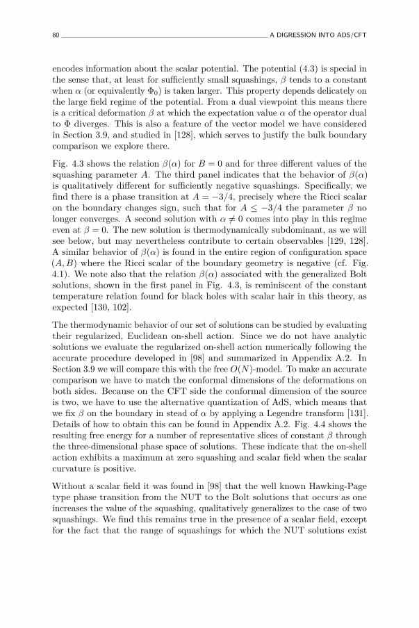
80 A DIGRESSION INTO ADS/CFT
encodes information about the scalar potential. The potential (4.3) is special inthe sense that, at least for sufficiently small squashings, β tends to a constantwhen α (or equivalently Φ0) is taken larger. This property depends delicately onthe large field regime of the potential. From a dual viewpoint this means thereis a critical deformation β at which the expectation value α of the operator dualto Φ diverges. This is also a feature of the vector model we have consideredin Section 3.9, and studied in [128], which serves to justify the bulk boundarycomparison we explore there.
Fig. 4.3 shows the relation β(α) for B = 0 and for three different values of thesquashing parameter A. The third panel indicates that the behavior of β(α)is qualitatively different for sufficiently negative squashings. Specifically, wefind there is a phase transition at A = −3/4, precisely where the Ricci scalaron the boundary changes sign, such that for A ≤ −3/4 the parameter β nolonger converges. A second solution with α 6= 0 comes into play in this regimeeven at β = 0. The new solution is thermodynamically subdominant, as we willsee below, but may nevertheless contribute to certain observables [129, 128].A similar behavior of β(α) is found in the entire region of configuration space(A,B) where the Ricci scalar of the boundary geometry is negative (cf. Fig.4.1). We note also that the relation β(α) associated with the generalized Boltsolutions, shown in the first panel in Fig. 4.3, is reminiscent of the constanttemperature relation found for black holes with scalar hair in this theory, asexpected [130, 102].
The thermodynamic behavior of our set of solutions can be studied by evaluatingtheir regularized, Euclidean on-shell action. Since we do not have analyticsolutions we evaluate the regularized on-shell action numerically following theaccurate procedure developed in [98] and summarized in Appendix A.2. InSection 3.9 we will compare this with the free O(N)-model. To make an accuratecomparison we have to match the conformal dimensions of the deformations onboth sides. Because on the CFT side the conformal dimension of the sourceis two, we have to use the alternative quantization of AdS, which means thatwe fix β on the boundary in stead of α by applying a Legendre transform [131].Details of how to obtain this can be found in Appendix A.2. Fig. 4.4 shows theresulting free energy for a number of representative slices of constant β throughthe three-dimensional phase space of solutions. These indicate that the on-shellaction exhibits a maximum at zero squashing and scalar field when the scalarcurvature is positive.
Without a scalar field it was found in [98] that the well known Hawking-Pagetype phase transition from the NUT to the Bolt solutions that occurs as oneincreases the value of the squashing, qualitatively generalizes to the case of twosquashings. We find this remains true in the presence of a scalar field, exceptfor the fact that the range of squashings for which the NUT solutions exist

A CFT COMPARISON 81
(a) A = 40.0 (b) A = 0 (c) A = −0.85
(d) A = 40.0 (e) A = 0 (f) A = −0.85
Figure 4.3: On the first line the relation β(α) that characterizes the asymptoticscalar profile is shown for B = 0 and three different values of the squashingparameter A. On the second line, the free energy as a function of β for thesame values of the squashing A. The blue curves correspond to NUT solutions,which exist for all three values of squashings, while the red curves in panel (a)represent the two branches of Bolt solutions.
gradually shrinks and becomes centered around zero squashing for large valuesof Φ0. At the same time the minimum squashing required for Bolt solutions toexist increases for increasing Φ0, leading to a critical value above which there isa regime of squashings in which no regular solutions exist.
4.3 A CFT comparison
The study of the holographic dual field theory description of the gravitationalsolutions described in the previous two sections is a non-trivial problem. Oneapproach would be to embed these solutions as backgrounds in M-theory andto identify a dual CFT. One can for instance think of the NUT/Bolt solutionsas deformations of the AdS4 × S7 solution of eleven-dimensional supergravity.In this case the dual field theory is the ABJM SCFT and we are faced withthe problem of evaluating the partition function of supersymmetry breakingdeformations of this theory at strong coupling. This is a formidable problemwhich we will not attempt to solve here. Instead, we will focus on a simplified

82 A DIGRESSION INTO ADS/CFT
-1 1 2 3 4A
0.5
1.0
1.5
IE
(a) β = 0.0
-1 1 2 3 4A
0.5
1.0
1.5
IE
(b) β = −0.85-0.4 -0.2 0.0 0.2 0.4 0.6 0.8
A
-1.0
-0.8
-0.6
-0.4
-0.2
IE
(c) β = −2.22
10 12 14 16 18 20A
-0.4
-0.2
0.0
0.2
0.4
IE
(d) β = 0.0 (e) β = −0.85
20 40 60 80 100 120A
-12
-10
-8
-6
-4
-2
IE
(f) β = −2.22
Figure 4.4: The free energy as a function of the squashing for different valuesof the UV deformation parameter β. The blue (red) curves represent the NUT(Bolt) solutions. In the top row the behavior around zero squashing is shown,while in the bottom row the transition from NUT to Bolt is highlighted.
(a) β = −1.4
Figure 4.5: The free energy as a function of the squashing for β = −1.4. Theblue line is given by the solutions with NUT boundary conditions. The redlines are given by the Bolt solutions. The bolt and the nut solutions overlap ata single point at this critical value of the scalar field.
model of this setup where we consider a vector-like theory on the double-squashedsphere in (1.63) in the presence of a homogeneous mass deformation.
The O(N) vector models with complex deformations in three dimensions areconjectured to be described holographically by a higher-spin Vasiliev theory inAdS4 with certain specific boundary conditions [124, 95, 125]. Through (1.53)they are also dual at the semiclassical level to Vasiliev theory in dS4 [110, 83].These higher-spin theories are very different from pure Einstein gravity with acosmological constant. Despite this difference it has been found that there are

A CFT COMPARISON 83
many qualitative similarities between the behaviour of the free energy of theO(N) vector models and the action of Einstein gravity solutions as a functionof squashings and mass deformations [96, 94, 98, 85]. We calculate the partitionfunction of the free mass deformed O(N) vector model on a double squashedsphere, the mass deformed free model partition function as
Zfree[m2] =∫Dφe−Ifree+
∫d3x√gm2O(x) , (4.9)
where Ifree is the action of the conformal, free O(N) model,
Ifree = 12
∫d3x√g
(∂µφa∂
µφa + Rφaφa
8
). (4.10)
Here φa are components of an N -component field transforming as a vectorunder O(N) rotations and R is the Ricci scalar of the boundary geometry onwhich the dual is defined.
Evaluating the Gaussian integral in (4.9) amounts to computing the followingdeterminant
− logZfree = F = N
2 log(det[−∇2 +m2 + R
8Λ2
]), (4.11)
where Λ is a cutoff that we will use to regularise the UV divergences in thistheory. For a single squashing the eigenvalues of the operator in (4.11) can befound in closed analytic form and read [132]
λn,q = n2 +A(n− 1− 2q)2 − 14(1 +A) +m2 ,
q = 0, 1, . . . , n− 1, n = 1, 2, . . . .(4.12)
To find the eigenvalues on double squashed spheres we apply the numericaltechniques developed in [132, 98] which enable us to determine the spectrumnumerically to (in principle) any desired accuracy.
To regularise the infinite sum in (4.11) one may be tempted to use an analyticapproach like ζ-function regularisation. However this method is not well-adaptedto situations where the spectrum of the Laplacian is known only numerically.Therefore we use a heat-kernel type regularisation which can be implementednumerically and was discussed in detail in [85, 98].
Using a heat-kernel the sum over eigenvalues divides in a UV and an IR part.The latter converges and can readily be done numerically whereas the formercontains all the divergences and should be treated with care. We regularize

84 A DIGRESSION INTO ADS/CFT
this numerically by verifying how the sum over high energy modes changesif we vary the energy cutoff. From a numerical fit we then deduce the non-divergent part which we add to the sum over the low energy modes to givethe total renormalized free energy. The resulting determinant after heat-kernelregularisation captures all modes with energies lower than the cutoff Λ. Thecontribution of modes with eigenvalues above the cutoff is exponentially small.For more details on this procedure we refer to our earlier work [98, 99].
In Figure 4.6 we show a two-dimensional slice of the resulting free energy as afunction of the squashing A and a real mass deformation m2. This intermediateresult can be compared with the action of the real asymptotically locally AdSsolutions shown in Figure 4.4.
An important features of this model is that the free energy diverges whenR/8 +m2 becomes zero. This is a generalization to mass deformed theories ofthe divergences found in [98]. To understand this we have to inspect the IRbehaviour of the free energy, which is given by a sum over upper incompletegamma functions Γ(0, λL,kδ) where λL,k are the eigenvalues and δ. From thedefinition of these, one can see that if λ approaches 0 then Γ(0, λL,kδ) diverges.Since the lowest eigenvalue of the Laplacian ∇2 always vanishes, the firsteigenvalue λ1 of the operator in (4.11) becomes zero when the Ricci scalarvanishes. This explains the sharp features in the function F (A,B) in Figure4.6.1 There is no corresponding divergence in the gravitational on-shell action.We believe that this discrepancy is entirely due to the fact that so far we areconsidering a free CFT. Indeed we will see in Chapter 5 the large N analysis ofthe free energy of the interacting three-dimensional O(N) vector model thatthis divergence in the free energy is removed (see also [96]).
Differentiating the partition function with respect to the source m2 yields theone-point function of the dual operator O as a function of the deformation m2.This is shown in the right panel of Figure 4.6 for three different values of asingle squashing A. The gravitational counterpart of this, plotted in Figure4.3, is remarkably similar. Given the latter depends delicately on the details ofthe scalar potential, this provides a strong motivation to choose this particularpotential in our comparison with the boundary theory.
1We should note that there are also “higher order" divergences which are less pronounced.These happen when any of the higher eigenvalues of the Laplacian cancels R/8 +m2 6= 0 togive another zero eigenvalue of the operator in (4.11). These divergences always appear inthe regions of the (A,B) plane where the Ricci scalar R in (4.1) is negative.

DISCUSSION 85
(a) In function of both A and m2
1 2 3 4 5⟨⟩
-1.0
-0.5
0.5
1.0
m2
(b) m2 in function of 〈O〉 for A = 0(in blue), A = −0.85 (in green) and forA = 40 (in red)
-1 1 2 3A
-3.0
-2.5
-2.0
-1.5
-1.0
-0.5
F
(c) m2 = 0.0
-1 1 2 3A
-3.0
-2.5
-2.0
-1.5
-1.0
-0.5
F
(d) m2 = −0.4
-1 1 2 3A
-3.0
-2.5
-2.0
-1.5
-1.0
-0.5
F
(e) m2 = −0.8
Figure 4.6: In all these figures the free energy as a function of the squashing isgiven for different mass deformations.
4.4 Discussion
We have evaluated real Euclidean saddle point in Einstein gravity coupled to anegative cosmological constant, on a (double) squashed sphere, in the presenceof a scalar field profile in a non trivial potential. Our results include a largeclass of geometries such as the round sphere, the Taub-NUT/Bolt, and thegeneralization with two squashing. This type of geometries is interesting for thepresence of a phase transition at large squashing and the presence of a negativecurvature boundary geometry at small squashing2. The type of potential wehave considered is interesting in the context of AdS cosmologies, [128]. It hasthe peculiarity that below a minimum value βmin there are no regular solutions.Further, it tends to a constant βc when α diverges. Between βmin and βc theβ(α) curve is double valued. The solution with lower α is thermodynamicallydominant.
We found that the Taub-NUT/Bolt phase transition occurs at larger values2In the double squashed case there is also a negative curvature region at large squashing.

86 A DIGRESSION INTO ADS/CFT
of the squashing when we apply a scalar deformation. Above a critical valueof β, there is no longer a phase transition, but regular solutions can be foundin some regions of superspace. The free energy is globally peaked around thesphere and the no-scalar case. The negative curvature region is an unstableregime, and it highly affect the β(α) curve. In this regime the scalar field profilediverges in both α and β and the latter changes sign. The divergence occurs ina thermodynamically sub-dominant branch.
In the O(N) vector model there are some similarities and differences. Thefree energy is globally peaked around the round sphere case, but the relativepeak shifts as we apply a mass deformation. The vev as a function of themass deformation show a similar behaviour seen in Einstein gravity, with theimportant difference that the mass deformation is never double valued. Thenegative curvature regime manifests itself leading to a positive, but constant,mass deformation.
Chapter 5
A Holographic Measure onEternal Inflation
5.1 Introduction
Slow roll eternal inflation [20, 22] occurs when the effective potential V isextremely flat. The condition for eternal inflation is that ε ≤ V , where ε ≡V 2,φ/V
2. Since the variance of the wave function of fluctuation modes is of order∼ V/ε, evaluated at horizon crossing, this means that quantum fluctuations inthe energy density of the inflaton are large in eternal inflation. Stochastic modelsof the evolution of these fluctuations indicate that their backreaction leads tolarge amplitudes for universes with exceedingly large and infinite constantdensity surfaces [133, 134].
This means the usual theory of inflation based on semiclassical gravity breaksdown in eternal inflation. It is therefore natural to describe eternal inflationusing gauge-gravity duality. In this chapter we study a holographic toy modelof eternal inflation in the no-boundary quantum state [58].
The partition functions ZQFT in (1.53) are complex deformations of EuclideanAdS/CFT duals. This form of dS/CFT reduces in minisuperspace toformulations based on analytic continuation [106, 135, 136] and agrees toleading order with the higher-spin realization [83] where the Sp(N) and O(N)partition functions are inversely related. It is tempting indeed to view EuclideanAdS/CFT and dS/CFT as two real domains of a single complexified theory[137, 108, 109, 79, 138, 139]. In this view any wave function that satisfies the
87

88 A HOLOGRAPHIC MEASURE ON ETERNAL INFLATION
Wheeler-DeWitt equation has an AdS and a dS domain. The former involvesat the semiclassical level everywhere real saddle points, whereas the latter isspecified by asymptotically real dS saddle points with a complex Euclidean AdSinterior. We adopt this viewpoint in the remainder of this chapter.
The dual field theory partition function in (1.53) automatically treats bulkbackgrounds and fluctuations in a unified manner. It is therefore ideally suitedto describe eternal inflation where the separation between both breaks down.A dual description of eternal inflation plausibly involves a weakly coupledEuclidean field theory defined e.g. on the surface at the threshold of eternalinflation [103]. In realistic cosmologies this would involve an IR CFT [115]. Herewe consider a simplified cosmology in which the early phase of (eternal) inflationtransitions directly to an asymptotic Λ-dominated regime. This permits usto study eternal inflation directly in the UV of the dual. In fact many of theknown AdS/CFT duals naturally describe a regime of eternal inflation in thedS domain of the theory because the Breitenlohner-Freedman stability boundon scalars in AdS corresponds precisely to the condition ε ≤ V in dS.
Equation (1.53) shows that dS/CFT relates the argument of the wave functionof the universe to external sources in the dual partition functions that turn ondeformations of the CFT. The dependence of the partition function on the valuesof the sources, which include the background geometry, yields a holographicmeasure on the space of asymptotically locally de Sitter universes. Generalfield theory results imply that the holographic amplitude of the undeformedCFT on the round S3 is a local maximum with respect to scalar deformations[140, 93] and deformations of the geometry [99, 141]. Furthermore one expectsthe holographic measure strongly suppresses conformal backgrounds far from theround conformal structure and in particular conformal classes with a metric ofnegative scalar curvature. This is because the lowest eigenvalue of the conformalLaplacian on this background is negative. Hence the partition function of aweakly coupled CFT likely diverges [71], which would lead to zero amplitudefor such configurations [103].
General holographic considerations therefore immediately lead to a very differentperspective on the global structure of the universe in eternal inflation thanthe picture emerging from semiclassical gravity. Indeed Hawking and Hertogrecently argued that the holographic description of eternal inflation providesevidence against the idea that eternal inflation typically leads to a highlyirregular universe with a mosaic structure of bubble like patches separated byinflationary domains.
It is the purpose of this chapter to support this intuition with explicit calculationsin a toy model in which the partition function can be evaluated. Specifically,we compute the partition function of the interacting O(N) vector model on

ANISOTROPIC INFLATIONARY MINISUPERSPACE 89
a two-parameter family of squashed three spheres in the presence of a massdeformation. The latter turns on a bulk scalar satisfying the conditions foreternal inflation, and the asymptotic squashings mean we consider the Hartle-Hawking wave function in a minisuperspace model consisting of anisotropiccosmologies.
The O(N) vector theory conjectured to be dual to higher-spin Vasiliev gravityin four dimensions [124, 95, 125, 83]. Higher-spin theories are very differentfrom pure Einstein gravity. However, ample evidence [96, 85, 98] suggests thattheir partition functions sourced by scalar, vector and spin-2 deformationsqualitatively capture the behavior of duals to Einstein gravity with AdS or dSboundary conditions. Motivated by this we view these vector theories as dualtoy models for eternal inflation in Einstein gravity and aim for a qualitativeunderstanding only.
The extended minisuperspace model we consider includes histories with constantdensity surfaces with negative curvature. These can be viewed as toy models ofbubble like patches thought to be produced in eternal inflation. We computethe probability distribution over histories in this model, which turns out tobe normalizable and globally peaked at the round three sphere. Moreover thetotal probability of negative Ricci scalar boundary surfaces turns out to beexponentially small. This behavior confirms the general properties discussedearlier and therefore lends support to the conjecture put forward in [103].
We also compare the holographic measure with the saddle point no-boundarymeasure in minisuperspace in an Einstein gravity model of eternal inflationbased on a consistent truncation of M-theory compactified on AdS4 × S7. Inthe dS domain these saddle points admit a regime of scalar field driven eternalinflation in the neighbourhood of the potential minimum and therefore accessiblein the UV. We find the anisotropic cosmologies in this model and numericallyregularize their action in order to evaluate the semiclassical wave function.
5.2 Anisotropic inflationary minisuperspace
In Chapter 4 we considered real, asymptotically locally AdS solutions, withreal radial scalar field profiles. These solutions specify the AdS domain of thesemiclassical Hartle-Hawking wave function. The wave function is real andexponentially decaying in this domain, and hence does not predict classical,Lorentzian cosmological evolution.
We now turn to the de Sitter domain of the wave function. At the semiclassicallevel this is specified by complex solutions of the same theory, given by the

90 A HOLOGRAPHIC MEASURE ON ETERNAL INFLATION
action (4.2), that asymptotically tend to real, Lorentzian, locally de Sitterspace. The asymptotically Lorentzian behavior of this set of solutions providesa large imaginary contribution to their Euclidean action. This means the wavefunction in the de Sitter domain describes an ensemble of asymptotically classical,cosmological histories [64]. In this section we evaluate the wave function in ananisotropic minisuperspace model with a scalar field using semiclassical bulkmethods. In the next Section we compare our results in this approximationwith a dual field theory computation of the wave function.
Complex saddle points
We consider the same minisuperspace model as before, consisting of squashedsphere boundary surfaces (1.63) with spatially homogeneous scalar fieldconfigurations. The metric of the interior saddle point solutions can thusagain be written in the form (4.4), but now with complex scale factors la and acomplex scalar field profile Φ.
rSP
y
υC′
C
π/2
τ
Figure 5.1: Two representations in the complex τ -plane of the same no-boundarysaddle point associated with an inflationary universe. Along the horizontalpart of the AdS contour C the geometry is an asymptotically AdS, sphericallysymmetric domain wall with a complex scalar field profile. Along the horizontalbranch of the dS contour C′ the saddle point behaves as a Lorentzian, inflationaryuniverse.
To represent the solutions it is useful to introduce a complex time coordinateτ(r) defined by
τ(r) ≡∫ r
0dr′l0(r′) . (5.1)

ANISOTROPIC INFLATIONARY MINISUPERSPACE 91
In terms of the variable τ the asymptotically dS domain of the wave function isto be found along the asymptotically horizontal line τ = t+ iπ/2 in the complexτ -plane. Along this line the leading order Fefferman - Graham - Starobinskyexpansion of the metric (4.5) becomes
ds2 = dt2 − e2t (A0σ21 +B0σ
22 + C0σ
23). (5.2)
Here A0, B0, C0 are real constants specifying the degree of asymptotic anisotropy.The Lorentzian signature of the asymptotic metric means the original scalefactors li defined in (4.4) are to leading order purely imaginary in the dSdomain. Their subleading behavior can be deduced from an asymptotic analysisof the equations of motion and is given in Appendix A. We illustrate therepresentation of the saddle point solutions in the complex τ -plane in Fig. 5.1.The semiclassical AdS domain of the wave function is specified by solutionsthat are regular in the IR and real along the real τ = r axis. The semiclassicaldS domain, by contrast, involves everywhere regular complex geometries thattend to asymptotically real, Lorentzian solutions along the τ = t+ iπ/2 line.The AdS contour shown in Fig. 5.1 provides a geometric representation of thesecomplex solutions in which their interior geometry consists of a Euclidean AdSdomain wall that makes a smooth (but complex) transition to a Lorentzianasymptotically dS universe. The signature of the asymptotic metric (5.2) meansthat the potential (4.3) in the original Euclidean action (4.2) acts in the dSregime as a positive effective potential
V dSeff (Φ) = −V = 2 + cosh(√
2Φ) (5.3)
0.5 1.0 1.5 2.0 2.5 3.0ϕ
10
20
30
40
VeffdS(ϕ )
0.5 1.0 1.5 2.0 2.5 3.0ϕ
-2.5
-2.0
-1.5
-1.0
VeffAdS(-iϕ )
Figure 5.2: Left panel:The effective potential in the dS domain that givescosmological relevant solutions. Right panel: The effective potential that givesrelevant cosmological solutions in the AdS domain.
The argument of the wave function is real. This means that in order for theabove complex solutions to be valid saddle points specifying the semiclassicalwave function, the scalar field must also become real along the same line in the

92 A HOLOGRAPHIC MEASURE ON ETERNAL INFLATION
τ -plane. The UV expansion (4.7) shows this requires its leading coefficient α tobe imaginary, which in turn means that the scalar profile is imaginary all alongthe AdS part of the contour C shown in Fig. 5.1. The interior region of thesaddle points specifying the Lorentzian dS domain of the wave function thusinvolves complex generalizations of Euclidean AdS domain walls. The effectivepotential in this AdS domain wall regime is therefore
V AdSeff (Φ) = −2− cos(√
2Φ), (5.4)
where Φ ≡ iΦ, and is illustrated in the right panel of Fig. 5.2. This shows thatthe asymptotic dS domain of the wave function corresponds to a finite domainof IR values Φ0 of the scalar field bounded by |Φ0| <
√2π/2 ≡ Φc. From
an AdS perspective this is simply a consequence of the shape of the effectivepotential governing the inner AdS region of the saddle point solutions. Froma dS perspective this bound signals the boundary of the inflationary regimeof the effective potential (5.3) in the dS domain. The potential (5.3) clearlyadmits inflationary solutions near its minimum. For large values of the scalarfield however it is too steep. The IR regularity condition of the Hartle-Hawkingsaddle points selects those patches of scalar potentials where the conditionsfor inflation hold [64]. The semiclassical wave function has no support outsidethese inflationary patches.
To determine for which real boundary conditions in the asymptotic dS domainregular complex solutions exist we must numerically solve the complex equationsof motion derived from the action (4.2). The regularity conditions on geometryand field in the IR, either at a NUT or a Bolt, leave three free parameters; twoassociated with the IR behavior of the scale factors and one for the complexvalue Φ0 of the scalar field. Varying these and numerically integrating theEinstein equation in the complex τ -plane to the asymptotic dS regime in theUV yields a three-parameter family of complex solutions whose action specifiesthe semiclassical no-boundary wave function in the dS domain. Details of thisprocedure are given in Appendix A.2.1 Fig. 5.3 shows a representative exampleof a solution with two squashings and the scalar field turned on, along a contourC along which the solution exhibits an inner Euclidean AdS domain wall region.
The regularity condition on the scalar field in the interior yields a relation β(α)between the coefficients of its asymptotic profile. We show this for three differentcombinations of squashings in the left panel of Fig. 5.4. A characteristic featureof this model is that β is imaginary over the entire range of parameter space.The dual interpretation of this suggests that the corresponding cosmologicalhistories behave only approximately classically in the large volume regime [81].This may seem surprising but is perhaps related to the fact that the potential
1The same method was already employed in [142] to find anisotropic saddle points of theno-boundary wave function for a different potential.

ANISOTROPIC INFLATIONARY MINISUPERSPACE 93
2 4 6 8λ
0.02
0.04
0.06
0.08
0.10
Re(ϕ)
2 4 6 8λ
-0.5
-0.4
-0.3
-0.2
-0.1
Im(ϕ)
2 4 6 8λ
100
200
300
400
Re(li)
2 4 6 8λ
2
4
6
Im(li)
Figure 5.3: A representative example of a complex solution with a NUT inthe interior and a scalar field profile, that is asymptotically locally dS with adouble squashed sphere future spatial boundary. The solution is shown herealong a contour C like the one depicted in Fig. 5.1 consisting of three segments.The top panels show the evolution of the real and imaginary components of thescalar field along this contour. The bottom panels show the real and imaginarycomponents of the three scale factors. The values of the IR parameters areφ0 = 1/2, β4 = −1/6 and γ4 = −11/60.
(Α)
(Α)
Figure 5.4: The behaviour of β as a function of α (left) and behaviour of α asa function of φ0 (right). All the curves are for B = 0. The blue curve is forA = 0, the red for A = −0.85 and the green for A = 40. When φ0 approachesφc, α starts to diverge.
V dSeff (Φ) describes a regime of eternal inflation and not slow roll inflation. Onemight have thought that the boundedness of the range of values Φ0 in the IRwould mean the semiclassical wave function has support over a limited range ofvalues α in the UV. This is not the case. The right panel of Fig. 5.4 plots α

94 A HOLOGRAPHIC MEASURE ON ETERNAL INFLATION
as a function of Φ0 for three different combinations of squashings. One sees αdiverges as Φ0 → Φc.
5.2.1 Anisotropic inflationary histories
The Euclidean action (4.2) of the above solutions specifies the semiclassicalno-boundary wave function in the asymptotic dS domain. The complex natureof the solutions means that in the large three-volume region of superspace thewave function takes the form
Ψ[a,A,B, χ] ≈ exp(−IR[a,A,B, χ] + iS[a,A,B, χ])/~. (5.5)
where a ≡ et is the overall volume scale factor. Here IR[a,A,B, χ] and−S[a,A,B, χ] are the real and imaginary parts of the Euclidean action IE ofthe regular complex saddle point solution that matches the real boundary data(a,A,B, χ), with (A,B) the squashing parameters and χ ≈ −iα/2a(A0B0C0)1/3.In the large volume regime the phase factor S varies rapidly compared to IR,
|~∇IR| |~∇S| . (5.6)
Hence the wave function predicts the boundary configuration evolves classically[64]. This is analogous to the prediction of the classical behavior of a particle ina WKB state in non-relativistic quantum mechanics. Thus the NBWF in the dSdomain predicts an ensemble of classical, asymptotically locally de Sitter historiesthat are the integral curves of S in superspace, with relative probabilities thatare proportional to exp[−2IR(A,B, χ)]. The latter are conserved under scalefactor evolution as a consequence of the Wheeler-DeWitt equation [64].
0.5 1.0 1.5 2.0 2.5t
-3.0
-2.5
-2.0
-1.5
-1.0
-0.5
0.5
ϕ
-4 -2 2 4t
-1.0
-0.5
0.5
ϕ
Figure 5.5: Left panel: An asymptotically classical history that is initiallyclassically singular, for Φ0 = 0.5, A = 2.3 and B = 0. Right panel: Anasymptotically classical history with a bounce in the semiclassical domain, forΦ0 = 0.5, A = 0.16 and B = 0.

ANISOTROPIC INFLATIONARY MINISUPERSPACE 95
The classical ensemble consists of a three-parameter family of inflationaryhistories that are asymptotically dS and have a certain degree of anisotropy,parameterized by (A,B) on the future boundary. The histories in this model donot exhibit a phase of reheating and slowing expansion. Instead they transitionfrom a phase of scalar field driven inflation to a phase of accelerated expansiondriven by the cosmological constant. The potential is such that the scalar fieldinflation is of the type of slow roll eternal inflation. Hence if one were to includeinhomogeneous fluctuations, one would find that the wave function becamebroadly distributed, predicting an ensemble of histories with exceedingly largeor even infinite constant scalar density surfaces [133, 134].
Within the minisuperspace model the classical extrapolation of the historiesbackwards in time is justified as long as the classicality conditions (5.6) hold.We find two distinct classes of past evolutions. For reasonably small values(A,B, χ) the classical extrapolation backwards exhibits a de Sitter like bounce toapproximately the same (time reversed) history on the other side. By contrast,for large values (A,B, χ) the histories are classically past singular. Fig. 5.5shows a representative example in each class. The classical extrapolations ofall Bolt saddle points, which only exist for large squashings, are past singular.The range of squashings (A,B) for which the classical histories bounce in thepast decreases for increasing χ. This is in line with our expectations for thisparticular scalar potential, which becomes too steep at large Φ to sustaininflation. We illustrate this in the left panel of Fig. 5.6 where we show theregion in the (A,B) phase space for three different values of χ within which theclassically extrapolated histories bounce.
0.2 0.4 0.6 0.8 1.0iΑ
0.1
0.2
0.3
0.4
PHBounceL
Figure 5.6: Left panel: The total probability for a semiclassical bounce as afunction of α. Right panel: The three contours bound the region in the (A,B)plane for which an approximately classical bounce occurs for (from small tolarge) resp. α = 3/4i, α = i/2 and α = 0.
The relative probabilities of the individual histories in the classical ensemble arefully specified by the regularized action of the interior AdS domain wall regime

96 A HOLOGRAPHIC MEASURE ON ETERNAL INFLATION
of the saddle points. Specifically in the large three-volume region we have [110]
IR[a,A,B, χ] = −IregAdS [A,B, αf ] (5.7)
where αf ≡ α(χ) is defined in the AdS regime of the saddle points (cf. (4.7))and purely imaginary for real boundary values χ in the dS domain [110]. Tocompute the regularized action one can perform the regularization procedurenumerically as detailed in the Appendix for the real AdS solutions. Howeverit is more convenient to consider the complex saddle points along a differentcontour, indicated with C′ in Fig. 5.1. This yields a geometric representation ofthe solutions in which a Euclidean deformed four sphere gradually transitionsto a Lorentzian asymptotically locally de Sitter space. The Lorentzian behaviorof the solution along the second leg of C′ means the real part of the Euclideanaction stabilizes automatically along C′ [64].
Figure 5.7: The probability distribution over anisotropic minisuperspace as afunction of the squashing A and the amount of scalar field inflation parameterizedby iα.
We show a two-dimensional slice P (A,α) of the probability distribution in Fig.5.7. As expected the distribution is normalizable and peaks at the pure deSitter history with a round sphere boundary and zero scalar field. In Fig. 5.8we show slices of constant α of this distribution P (A) for three different valuesof the coefficient α specifying the asymptotic scalar profile. The Bolt solutionsprovide the dominant contribution to the probabilities at large squashings A.This is the dS counterpart of the Hawking-Page like phase transition in the AdSdomain of the wave function. The total probability of histories associated withBolt saddle points is small however and decreases for increasing scalar field.

ANISOTROPIC INFLATIONARY MINISUPERSPACE 97
The probability distribution over the classical ensemble can also be used tocompute the total probability in this model that an asymptotically classicaluniverse emerges form a regular bounce in the past and therefore lies in thequasiclassical realm throughout its entire history. This is obtained by integratingthe probability distribution over the domain in the (A,B)-plane shown in theleft of Fig. 5.6. This corresponds, for a given scalar value χ on a constant asurface, to bouncing histories when classically extrapolated backwards. We plotthe probability Pbounce as a function of α in the right panel of Fig. 5.6, wherewe restriced to a single squashing. This shows that the total probability of anon-singular origin is significant in this model when the scalar field is everywhererelatively small. However, it sharply decreases outside this regime and vanishesfor histories in the large field regime near the edge of the inflationary regime ofthe potential.
A
A
(a) P(A) for α = 0
A
A
(b) P(A) for α = i
A
A
(c) P(A) for α = 2i
Figure 5.8: Slices of the probability distributions for B = 0 for three differentvalues of α. The blue curves show the NUT contributions whereas the dominantBolt contribution is given in red.
5.2.2 Classical Lorentzian evolution.
It is interesting to understand the influence of the negative curvature regime onthe classsical Lorentzian evolution. To achieve this we introduce the Lorentzianboundary variables β± such that, [143, 144, 145],
log l1(t) = β+(t) +√
3β−(t),
log l2(t) = β+(t)−√
3β−(t),
log l3(t) = −2β+(t) ,
(5.8)
where t is the time defined on a particular history. The Lorentzian action inthis new boundary squashing parameters shows a "gravitational" potential
V (β+, β−) = 4e−2β+ cosh 2√
3β− − 2e−8β+ + e4β+(
1− cosh 4√
3β−). (5.9)

98 A HOLOGRAPHIC MEASURE ON ETERNAL INFLATION
Figure 5.9: An example of the Lorentzial evolution of the anisotropy parametersβ+ and β−. As time increase they both decrease to a more isotropicconfiguration.
If we look at the Lorentzian evolution of the anisotropy parameters β±, we seethat the evolution of the squashing bounce against the equipotential lines, asa ball in a billiard. This is the typical behaviour of the mixmaster universe.Whether they approach a more isotropic or a more squashed configurationcrucially depends on the sign of the potential (5.9). An example of a historywhose evolution is towards a more isotropic configuration is shown in figure 5.9.
In terms of this parametrization the boundary scalar Ricci curvature is 3R ∝− 1
2V (β+, β−), [143]. The sign of the boundary Ricci scalar crucially influencesthe anisotropic evolution of the Lorentzian histories. When 3R is positive thepotential V (β+, β−) < 0 and the Lorentzian classical universe evolves to a moreisotropic configuration in the future. On the contrary, when 3R is negative thepotential V (β+, β−) > 0 and the Lorentzian classical universe evolve to an evenmore anisotropic configuration. In this regime, the squashing parameters A andB reach the critical value −1 in a finite time.
5.3 A Holographic Measure
In the holographic form (1.53) the NBWF amplitude of configurations on Σf
is specified by the partition function of deformations of Euclidean AdS/CFTduals. The arguments of the wave function enter as sources in the dual. Forthe geometry this means we must evaluate the dual partition function on the

A HOLOGRAPHIC MEASURE 99
double-squashed sphere (1.63). The bulk scalar sources a scalar deformation byan operator O of dimension one with coupling α. This is a relevant operatorwhich in our dual O(N) vector toy model induces a flow from the free to thecritical O(N) model. The coefficient α is imaginary in the dS domain of thewave function as discussed above. Hence we are led to evaluate the partitionfunction, or free energy, of the critical O(N) model as a function of the twosquashing parameters A and B and an imaginary mass deformation α ≡ m2.
The deformed, critical O(N) model is obtained from a double trace deformationf(φ · φ)2/(2N) of the free model with in addition a source ρfm2 turned on forthe single trace operator O ≡ (φ · φ). By taking f →∞ the theory flows fromits unstable UV fixed point where the source has dimension one to its criticalfixed point with a source of dimension two [95]. To see this, we consider (4.9)and we introduce an auxiliary variable m2 = m2
ρf + Oρ . This yields to
Zfree[m2] =∫DφDm2e−Ifree+N
∫d3x√g[ρfm2O− f2O
2− 12f (m2−ρfm2)2] . (5.10)
which can be written as
Zfree[m2] =∫Dm2e−
N2f
∫d3x√g(m2−ρfm2)2
Zcrit[m2] , (5.11)
with
Zcrit[m2] =∫Dφe−Ifree+N
∫d3x√g[ρfm2O− f2O
2] . (5.12)
Inverting (5.11) yields Zcrit as a function of Zfree:
Zcrit[m2] = eNfρ2
2
∫d3x√gm4
∫Dm2e
N∫d3x√g(m42f −ρm
2m2)Zfree[m2] . (5.13)
The value of ρ can be determined by comparing two point functions in the bulkwith those in the boundary theory [85]. For the O(N) model this implies ρ = 1,which agrees with the transformation from critical to free in [97].2
To compute Zcrit(A,B, α) we use the partition function, (4.9), of the free massdeformed O(N) vector model on a double squashed sphere and then evaluate(5.13) in a large N saddle point approximation. We substitute our result forZfree in (5.13) and evaluate the integral in a large N saddle point approximationto compute the partition function of the critical model.
The first factor outside the path integral in (5.13) diverges in the large f limit,which we cancel by adding the appropriate counterterms. The saddle point
2The above calculation can be repeated for the Sp(N) model by putting ρ = −i[85].

100 A HOLOGRAPHIC MEASURE ON ETERNAL INFLATION
equation then becomes, for homogeneous deformations∫d3x√g
(m2
f− m2
)= −∂ logZfree[m2]
∂m2 , (5.14)
where the first term on the left hand side vanishes for large f . Solving this form2 and inserting the result in (5.13) yields Zcrit[m2].
Because α is imaginary we also have to plug in an imaginary value for m2. Thesaddle point equation has infinitely many solutions for a fixed imaginary valuem2
0. There is always one greater than −R/8 and the rest is smaller than thisvalue. To make sure we include all the relevant solutions, we need to do acareful study of the m2-plane to determine where the steepest descent contourfor m2 lies. For the single squashed sphere this was already discussed in detailin [85], in which it was found3 that the relevant steepest-descent contour couldalways be deformed to pass through the saddle point that lies to the right ofthe point where m2 = −R/8.
To apply this procedure to our model with one squashing, we first calculate ZFreeas a function of (complex) m2 using the numerical techniques described aboveand we then numerically invert (5.14) to find the behaviour of the complexdeformation m2 as a function of imaginary m2. The relation between these twodeformations is shown in Figure 5.10, where the real and imaginary parts of m2
are plotted as a function of im2 for three different values of A. Notice that m2
is restricted to be larger than −R/8, as can be seen from the plot of the realpart of m2 where it is clear that for large im2, m2 → −R/8. From the left plotwe also see that the imaginary part of m2 tends to zero whenever im2 becomeslarge.
-0.4 -0.2 0.2 0.4ⅈ m 2
-0.5
0.5
Rem2
-0.4 -0.2 0.2 0.4ⅈ m 2
-0.6
-0.4
-0.2
0.2
0.4
0.6
Imm2
Figure 5.10: The real and imaginary solutions of the saddle point equation (5.14)are shown for three different values of a single squashing, i.e. A = −0.8 (blue),A = 0 (red) and A = 2.06 (green). For large im2 we have Re(m2)→ −R/8.
3It was also found that for the Sp(N) model the saddle point contour is ill-defined suchthat the non-perturbative (in N), critical Sp(N) model does not exist.

DISCUSSION 101
Inserting the saddle point relation m2(m2) in (5.13) yields the partitionfunction Zcrit[A,B, m2] which we illustrate in Figure 5.11, where we plot atwo-dimensional slice of the holographic probability distribution in anisotropicminisuperspace as a function of the mass deformation corresponding to theasymptotic scalar profile and of one squashing parameter. The distributionhas a global maximum at zero squashing and zero deformation correspondingto the pure de Sitter history, in agreement with the result based on a bulkcalculation. When the scalar is turned on however, the local maximum shiftstowards positive values of A - a feature which is absent in the bulk result -which we illustrate in Figure 5.12 where we plot three one-dimensional slices ofthe distribution for three different values of m2.
As anticipated the sharp features associated with the divergences of the freeenergy in the free O(N) model discussed above have disappeared, resulting in asmooth and normalizable distribution over the entire configuration space. Weshould emphasize however that in our calculation of Zcrit starting from Zfree wehave taken in account only the regions of configuration space for which the freetheory is not manifestly unstable. This restriction appears to be born out bythe natural measure on configuration space and selects the region of parameterspace where R/8 ≥ m2. By contrast, the distribution defined by Zcrit extendsover boundary configurations where this inequality does not hold and includes,in particular, boundary geometries with negative curvature. Remarkably, thedistribution is well defined in this regime of superspace also. In fact it is evidentfrom Figure 5.11 that the total probability of R < 0 histories is exponentiallysmall.
5.4 Discussion
Holographic cosmology provides a radically new perspective on eternal inflation.We have initiated an exploration of its implications in the toy model contextgiven by the interacting O(N) vector model defined on a two-parameter familyof squashed three spheres and deformed by a mass term. We have evaluated itspartition function as a function of the three asymptotic parameters. ThroughdS/CFT this specifies a holographic measure on a minisuperspace of anisotropicdeformations of dS with scalar field matter in the regime of eternal inflation, inhigher-spin gravity. We find that the amplitude is low for conformal boundarysurfaces far from the round conformal structure. This is in line with generalfield theory expectations and lends support to the conjecture that the exit frometernal inflation is reasonably smooth, producing universes that are relativelyregular on the largest scales with globally finite surfaces of constant density.

102 A HOLOGRAPHIC MEASURE ON ETERNAL INFLATION
Figure 5.11: A two-dimensional slice of the holographic probability distributionin anisotropic minisuperspace as a function of the mass deformation m2
corresponding to the asymptotic scalar profile and one squashing A thatparameterizes the amount of asymptotic anisotropy.
0 5 10 15 20 25 30A
0.5
1.0
1.5
2.0
1
Z 2
(a) m2 = 0.00 10 20 30 40
A
0.02
0.04
0.06
0.08
0.10
0.12
1
Z 2
(b) m2 = 0.05i0 10 20 30 40
A
0.002
0.004
0.006
0.008
1
Z 2
(c) m2 = 0.1i
Figure 5.12: Three one-dimensional slices of the probability distribution inanisotropic minisuperspace for three different values of m2. The local maximumshifts towards larger values of the asymptotic anisotropy in histories with morescalar field inflation.
A reliable theory of eternal inflation is important to sharpen the predictions ofslow roll inflation. This is because the dynamics of eternal inflation specifiesthe prior over the zero modes, or bulk slow roll backgrounds, which in turndetermines the predictions of the precise spectral properties of CMB fluctuationson observable scales [111]. The generic features of the pattern of fluctuations inholographic models of inflation were extensively studied [135, 146, 147, 148, 149].A well-defined measure on eternal inflation will sharpen these predictions byselecting a specific subset of RG flows or slow roll backgrounds.

Chapter 6
Discussion
6.1 Summary and conclusion
A quantum gravity description of de Sitter space appears to be needed if we wantto understand the intimate nature of our own universe. Holography appearsto be a property of quantum gravity theories and, therefore, it is crucial tounderstand how this principle can be incorporated in cosmology. This wouldlead to the so called dS/CFT correspondence, which relates the wave functionof the universe to the partition function of a dual field theory defined on theboundary.
A quantum gravity theory of dS space is affected by several issues, and ourunderstanding is limited. The theory accommodates multiple definition ofthe wave function of the universe and, therefore, different measures. Further,the existence of two different asymptotic boundaries and the presence of acosmological horizon pose conceptual problems that need to be understood.
In addition, there is the problem that we do not know the partition functionof ABJM theory, which is dual to AdS4 solution of Einstein gravity, and canbe used to compute the full cosmological measure. To explore the quantumversion of dS space we proceeded only qualitatively. In this thesis work wehave compared our bulk results with the partition function of the model dualto Vasiliev higher spin theory of gravity. That is the O(N) vector model inthe presence of different type of complex deformations. Under certain type ofdeformations the theory is known to be affected by divergences. We exploredthese divergences in the context of Einstein gravity, and we resolved them inthe sense that we have found they correspond to a non-classical behaviour of
103

104 DISCUSSION
the wave function.
In this research work we have explored all these issues. In Chapter 2 wehave found the holographic form of the Tunneling wave function, and we havecompared it with certain relevant small perturbations of the O(N) vectormodel. In this chapter we have found that the growing behaviour of thepartition function in AdS familiar from Euclidean AdS/CFT is equivalent tothe amplitude of the Tunneling wave function in cosmology. The way theTunneling wave function is defined, naturally selects boundary observables onlyat future infinity. In contrast the no-boundary wave function have access toboth boundaries (past and future infinity). This can already be seen in thesemiclassical form of the two wave functions, (1.22) and (1.42). The modes,and thus the expanding or contracting phases of the universe are encoded inthe phases of the wave functions, and thus do not have any influence on theirholographic probabilities.
In Chapter 3 we have analyzed the behaviour of the divergence found in the U(N)vector model. We have shown that, in Einstein gravity, a similar divergenceappears in the presence of saddle points predicting Lorentzian histories that areSchwarzschild de Sitter black hole with negative mass. The diverging behaviourcorresponds to a vanishing probability measure of the Hartle-Hawking state,and to an un-physical diverging probability measure for the Tunneling state.This divergence occurs in a configuration where the classicality condition is notsatisfied, so that the solutions do not predict any classical Lorentzian history.Configurations like negative mass black holes should be excluded from thephysical configuration space, and we should discard their contribution to thefull measure.
The Sp(N) vector model is known to diverge at negative mass deformations.Further, if we deform the round S3 sphere along two independent directions,we can explore a regime with negative boundary curvature. We have exploredthese types of deformations in chapter 4 in the context of standard AdS/CFTcorrespondence, and in chapter 5 in the context of cosmology. We showedthat in Einstein gravity a divergence similar to the one observed in the Sp(N)vector model, appears in saddle point solutions predicting tachyonic scalar fieldprofile on the future boundary. These saddle points do not predict any classicalbehaviour of the wave function. Our results of chapter 4, are a generalization ofthe AdS-Taub NUT/Bolt deformed by a second squashing and in the presence ofnon-trivial scalar field profile. We showed that the NUT/Bolt phase transitiondo not occur for sufficiently large scalar deformations. This phase transitioncannot be seen in Vasiliev theory, nevertheless this provides an important tool toexplore a quantum description of dS space, at least qualitatively. The results ofchapter 5 are relevant in cosmology. We have analyzed the Lorentzian historiesthat are of a mixmaster universe. Depending on the boundary values of the

OUTLOOK 105
squashing and of the scalar field the histories might bounce or be singular inthe past. We have evaluated the probability measure for these histories and wehave compared it with the partition function of the O(N) vector model in thepresence of a critical complex deformation. In this way we got an holographicmeasure of eternal inflation.
In this thesis work we pushed our understanding of the dS/CFT correspondencea step further. We have analyzed how holography selects either the tunnelingor the no-boundary state. We have explored similarities and the differencesbetween Einstein and Vasiliev theories. It is tempting to conjecture that adivergence in the latter can be traced to a wave function, defined in Einsteingravity, in a non-classical regime. With this comparison in our hands, we haveanalyzed the full probability measure for different kinds of inflationary universes.
6.2 Outlook
We have already discussed some possible future work in this direction, in thediscussion of every single chapter. Here we present a more general overview. Afirst step can be done once we will a feasible form of the partition function ofABJM. In this way we will have a concrete way to compute the full cosmologicalmeasure.
One day astrophysicist will be able to refine their observations and providemore restrictions on cosmological observables. This might exclude one of thetwo wave functions proposal. Now that we have a way to compute the fullcosmological measure (at least qualitatively), and that we know how holographyselects either one or the other wave function, we might test the theory againstobservations.
The Hartle-Hertog proposal has been shown in the semiclassical approximationonly. A further direction is to explore this correspondence also beyond thesemiclassical level, i.e. by including loop corrections, or by employing differenttechniques to evaluate it, [150, 151, 152, 153, 154, 155]. This would push theHartle-Hertog proposal a step further.
Another insight is to explore the nature of the two boundaries of dS space.In recent years, the so called ER=EPR conjecture [156, 157], lead to a betterunderstanding of the entanglement in field theory, and to a better understandingof quantum gravity itself. In this new description entanglement in field theorycan be described by a wormhole that connects two observers on different (orsame) boundaries. A future direction is to understand if the ER=EPR conjecture

106 DISCUSSION
can be translated to dS space, to analyze the role of the two boundaries and ofthe cosmological horizon in a holographic scenario.
Finally there are still many open questions that might be answered throughholography. We still do not have a microcanonical description of the entropy ofthe cosmological horizon. We have not answered yet to the question on whatis the meaning of boundary data that are casually disconnected to a physicalobserver covered by an horizon. We do not have a good understanding on howto incorporate this holographic set-up in a deeper theory, i.e. string theory.We know that string theory has an infinite spectrum of higher spin massivefields. If a suitable limit where their masses disappear is explored, one mighthope to recover the same spectrum observed in Vasiliev theory. This is theso called tensionless limit, and might provide a suitable path to connect ourresults with a deeper theory such as string theory. In that case we might havea stringy description of the dS/CFT correspondence. String theory predicts avast number of dS vacua, and the holographic wave function of the universemight provide a measure to select them.

Appendix A
Appendix
A.1 Basis change.
The wave function can be written in terms of the new asymptotic variables.The details of this basis change can be found in [81], and here we summarizethe results.
α basis.
ΨHH [γij , α, η] =∫dχe
∫d3xG(γij ,α,hij ,χ,η)ΨHH [hij , χ] , (A.1)
where the generating function is
G(γij , α, hij , χ, η) =√γ
κη3
(1 + η2
(γijhij +
R(γ)
2
))
−σ2 η−σα2γ3/2σ + ση−λ+αγλ+/2σ −
λ+√γ
2η3 χ2 .
(A.2)
β basis.
ΨHH [γij , β, η] =∫dχe
∫d3xG(γij ,β,hij ,χ,η)ΨHH [hij , χ] , (A.3)
107

108 APPENDIX
where the generating function is
G(γij , β, hij , χ, η) =√γ
κη3
(1 + η2
(γijhij +
R(γ)
2
))
+σ
2 ησβ2γ3/2σ − ση−λ−βγλ−/2σ −
λ−√γ
2η3 χ2 .
(A.4)
A.2 Anisotropic Euclidean AdS solutions.
The goal of these appendices is to give the technical details associated with thephysics of gravitational theories that have a squashed sphere boundary. Firstwe start with the equations of motion and afterwards the UV and IR expansionsof the fields are given. Afterwards we give our method to numerically calculatethis action.
A.2.1 Equations of motion
The equations of motion can be obtained by substituting the metric (4.4) intothe action (4.2) and by varying this respectively with respect to l0, l1, l2, l3and Φ,

ANISOTROPIC EUCLIDEAN ADS SOLUTIONS. 109
l02l3
2
l12l2
2 + l02l2
2
l12l3
2 + l02l1
2
l22l3
2 −2l02
l12 −
2l02
l22 −
2l02
l32 + 4l20V (φ) + 4l1′l2
′
l1l2+ 4l1′l3
′
l1l3
+ 4l2′l3′
l2l3− 2φ′2 = 0 ,
− 4l0′l1′
l0l1− 4l0′l3
′
l0l3− l0
2l32
l12l2
2 + 3l02l22
l12l3
2 −l0
2l12
l22l3
2 −2l02
l12 + 2l02
l22 −
2l02
l32
+ 4l02V (φ) + 4l1′′
l1+ 4l1′l3
′
l1l3+ 4l3′′
l3+ 2φ′2 = 0 ,
− 4l0′l2′
l0l2− 4l0′l3
′
l0l3− l0
2l32
l12l2
2 −l0
2l22
l12l3
2 + 3l02l12
l22l3
2 + 2l02
l12 −
2l02
l22 −
2l02
l32
+ 4l02V (φ) + 4l2′′
l2+ 4l2′l3
′
l2l3+ 4l3′′
l3+ 2φ′2 = 0 ,
− 4l0′l1′
l0l1− 4l0′l2
′
l0l2+ 3l02l3
2
l12l2
2 −l0
2l22
l12l3
2 −l0
2l12
l22l3
2 −2l02
l12 −
2l02
l22 + 2l02
l32
+ 4l02V (φ) + 4l1′′
l1+ 4l1′l2
′
l1l2+ 4l2′′
l2+ 2φ′2 = 0 ,
l02 ∂V (φ)
∂φ+ l0
′φ′
l0− l1
′φ′
l1− l2
′φ′
l2− l3
′φ′
l3− φ′′ = 0
(A.5)
These equations of motion are valid for both the AdS and dS domain of thewave function, for this reason the variables are understood to be a function of τ ,defined in (5.1) and ′ means a derivative with respect to τ . The AdS equationsof motion (discussed in Chapter 3) get retrieved by setting τ = r, and theLorentzian dS solutions (discussed in Chapter 4) lie along the line τ = t+ iπ/2.
A.2.2 Solutions
IR NUT
For the NUT solutions we know that around the NUT, denoted here by τ∗, themetric should look like R4
ds2 = dτ2 + (τ − τ∗)2
4 (σ21 + σ2
2 + σ23) . (A.6)

110 APPENDIX
Therefore we can expand the fields around τ = τ∗ with the following AnsatzΦ(τ) = Φ0 + Φk(τ − τ∗)k,
l1(τ) = 12(τ − τ∗) + βk+1(τ − τ∗)k+1 ,
l2(τ) = 12(τ − τ∗) + γk+1(τ − τ∗)k+1 ,
l3(τ) = 12(τ − τ∗) + δk+1(τ − τ∗)k+1 , (A.7)
where k runs from 1 to ∞. By plugging in this Ansatz into the equations ofmotion (A.5) we get the following leading order terms
l1(τ) = 12(τ − τ∗) + β3(τ − τ∗)3 + 1
1920
(− 4V (Φ0)2 − 576V (Φ0)γ3
− 6912γ32 + 144V (Φ0)β3 − 6912γ3β3 + 4608β3
2
− 3(∂V (Φ0)∂Φ0
)2)(τ − τ∗)5 +O
((τ − τ∗)7) ,
l2(τ) = 12(τ − τ∗) + γ3(τ − τ∗)3 + 1
1920
(− 4V (Φ0)2 + 144V (Φ0)γ3
+ 4608γ32 − 576V (Φ0)β3 − 6912γ3β3 + 6912β3
2
− 3(∂V (Φ0)∂Φ0
)2)(τ − τ∗)5 +O
((τ − τ∗)7) ,
l3(τ) = 12(τ − τ∗)−
(112V (Φ0) + β3 + γ3
)(τ − τ∗)3 + 1
1920
(16V (Φ0)2
+ 624V (Φ0)γ3 + 4608γ32 + 624V (Φ0)β3 + 16128γ3β3 + 4608β3
2
− 3(∂V (Φ0)∂Φ0
)2)(τ − τ∗)5 +O
((τ − τ∗)7) ,
Φ(τ) = Φ0 + 18∂V (Φ0)∂Φ0
(τ − τ∗)2 +(
1288V (Φ0)∂V (Φ0)
∂Φ0
+ 1192
∂V (Φ0)∂Φ0
∂2V (Φ0)∂Φ2
0
)(τ − τ∗)4 +O
((τ − τ∗)6) .
(A.8)

ANISOTROPIC EUCLIDEAN ADS SOLUTIONS. 111
This expansion is controlled by the three real parameters β3, γ3 and Φ0 whichare ultimately related to the two squashing parameters A and B together withthe coefficients A3 and B3 of the subleading terms and the two free parametersin the UV expansion of the scalar field α and β, at the asymptotic boundary.
IR Bolt
We can do the same thing for the Bolt solutions. In this case we know that themetric should look like R2 × S2 around the Bolt position τ∗, that is
ds2 = dτ2 + (τ − τ∗)2
4 σ21 + β2
0σ22 + γ2
0σ23 . (A.9)
Therefore we take the following Ansatz for the expansion of the fields aroundτ = τ∗,
Φ(τ) = Φ0 + Φk(τ − τ∗)k, l1(τ) = β0 + βk(τ − τ∗)k ,
l2(τ) = γ0 + γk(τ − τ∗)k , l3(τ) = 12(τ − τ∗) + δk+1(τ − τ∗)k+1 , (A.10)

112 APPENDIX
with k going from 1 to ∞. If we solve the equations of motion (A.5) with thisAnsatz, we get
l1(τ) = γ0 +(
14γ0− V (Φ0)γ0
4
)(τ − τ∗)2
−(
11192γ03 −
V (Φ0)24γ0
+ γ4 + γ0
32
(∂V (Φ0)∂Φ0
)2)(τ − τ∗)4
+O((τ − τ∗)6) ,
l2(τ) = γ0 +(
14γ0− V (Φ0)γ0
4
)(τ − τ∗)2 + γ4(τ − τ∗)4 +O
((τ − τ∗)6) ,
l3(τ) = 12(τ − τ∗)− (τ − τ∗)3
12γ02
+(V (Φ0)2
160 + 531920γ04 −
V (Φ0)40γ02 −
1320
(∂V (Φ0)∂Φ0
)2)(τ − τ∗)5
+O((τ − τ∗)7) ,
Φ(τ) = Φ0 + 14∂V (Φ0)∂Φ0
(τ − τ∗)2
+ 1192γ2
0
∂V (Φ0)∂Φ0
(−4 + 3γ0
2(2V (Φ0) + ∂2V (Φ0)∂Φ2
0))
(τ − τ∗)4
+O((τ − τ∗)6) .
(A.11)
We chose to parametrize this expansion by the three independent real parametersγ0, γ4 and Φ0 which are again mapped to the squashing parameters A, B andα, β in the UV. Notice that to get the NUT or Bolt double squashing resultswithout scalar field we have to put Φ0 = 0 and V (Φ) = Λ in the initial conditionsabove, effectively reducing the above expansions and equations of motion tothe ones discussed in [98].

ANISOTROPIC EUCLIDEAN ADS SOLUTIONS. 113
UV
The asymptotic solutions are the same for both the NUT and the bolt. To findthem, we look at the asymptotic form of the metric
ds2 = dτ2 + e2τ (A0σ21 +B0σ
22 + C0σ
23) . (A.12)
If we use that the scalar field potential around Φ = 0 behaves as V (Φ) ∼ Λ−Φ2,we can make the Ansatz of a Fefferman-Graham expansion
Φ(τ) = αe−τ + βe−2τ + . . . , l1(τ) = A0eτ +Ake
(1−k)τ ,
l2(τ) = B0eτ +Bke
(1−k)τ , l3(τ) = C0eτ + Cke
(1−k)τ , (A.13)
where the sum over k goes over all positive integers. The constants aredetermined by solving the equations of motion (A.5), order by order, giving thefollowing consistent series expansion
l1(τ) = A0eτ + 1
16A0B02C0
2
(− 5A0
4 + 2A02B0
2 + 3B04 + 2A0
2C02
− 6B02C0
2 + 3C04 − 2A0
2B02C0
2α2)e−τ +A3e
−2τ +O(e−3τ ) ,
l2(τ) = B0eτ + 1
16A0B02C0
2
(3A0
4 + 2A02B0
2 − 5B04 − 6A0
2C02
+ 2B02C0
2 + 3C04 − 2A0
2B02C0
2α2)e−τ +B3e
−2τ
+O(e−3τ ) ,
l3(τ) = C0eτ + 1
16A0B02C0
2
(3A0
4 − 6A02B0
2 + 3B04 + 2A0
2C02 + 2B0
2C02
− 5C04 − 2A0
2B02C0
2α2)e−τ −
(A3C0
A0− B3C0
B0− 2
3C0αβ
)e−2τ
+O(e−3τ ) ,
Φ(τ) = α
2(A0B0C0)1/3 e−τ + β
4(A0B0C0)2/3 e−2τ +O(e−3τ ) .
(A.14)
We have performed this expansion up to eight order and have verified that it iscontrolled by the seven parameters A0, B0, C0, A3, B3, α, β. The coefficients

114 APPENDIX
α and β appearing in the expansion of Φ are undetermined by the equationsof motion, here we rescaled them to the most convenient convention makingsure it is conform with the literature. Notice that when we are deep into thedS domain τ = t+ iπ/2, which makes the scale factors imaginary, giving theLorentzian metric from (5.2).
Since the equations of motion (A.5) are invariant under constant shifts of theradial coordinate, one can set A0 = 1
4 by an appropriate shift of τ . One cannow identify B0 and C0 with the squashing parameters in (1.63) as follows
A = 14C2
0− 1 , B = 1
4B20− 1 . (A.15)
The parameters A3, B3 and β are independent from the point of view of theUV expansion but are ultimately fixed in terms of A, B and α by the regularityconditions that we imposed for the numerical solutions of the full nonlinearequations of motion.
From IR to UV
It is worth discussing how we constructed the numerical solutions of the fullnonlinear equations of motion in (A.5). Let us start with the AdS-Taub-NUTsolutions. For these we picked real values for the parameters a3, b3 and φ0 inthe IR expansion (A.8). For each such value we then numerically integratedthe equations of motion from r = r∗ to some large value of rc. If the resultingnumerical solution does not exhibit a singularity at an intermediate value ofthe radial coordinate r we declared the solution to be regular and read of theasymptotic parameters B0, C0 and α and β in (A.14) which we then relate tothe squashing parameters A and B using (A.15). As expected we find thatthere are no restrictions on the parameters A and B, i.e. as we vary a3 andb3 for a fixed φ0 we can explore the whole (A,B) plane. If we take a non-zerovalue for φ0 we will reach the same conclusion with the only difference that theregion in the (a3, b3) plane that gives valid UV solutions shifts to higher valuesof a3 and b3 when φ0 increases as can be seen in Figure A.1.
The procedure we used to construct the AdS-Taub-Bolt solutions is again verysimilar. We start with the IR expansion in (A.11), vary the parameters γ0 andγ4 and integrate numerically the equations of motion. Finally, we read off theasymptotic parameters B0 and C0 from the behaviour of the numerical solutionsat large r and deduce the corresponding values of A and B using the relation in(A.15). However, there is an important difference between these solutions andthe AdS-Taub-NUT solutions. For a fixed value of B there are critical valuesof A below/above which there are no AdS-Taub-Bolt solutions. This leads

ANISOTROPIC EUCLIDEAN ADS SOLUTIONS. 115
Γ
Β
Γ
Β
Γ
Β
Figure A.1: Initial conditions for a3 and b3 that give rise to non-singularsolutions. From left to the right we took φ0 = 0, 1, 2.
to curves in the (A,B) plane and the AdS-Taub-Bolt solutions exist only forvalues of the squashing parameters that are below or above these critical curves.Furthermore for every value of (A,B) for which Bolt solutions exist there aretwo possible solutions of the equations of motion which we dub “positive” and“negative” branch. All of these features are extensions of the familiar behaviourof the analytically known AdS-Taub-Bolt solutions with B = 0 discussed in[158, 66] and for which more details can be found in [98].
A.2.3 Evaluating the numerical action
A.2.4 Euclidean Action
To evaluate the action, it is easiest to use the on-shell version of (4.2):
IE =− 2π∫dτ l1(τ)l2(τ)l3(τ)V (Φ(τ))
− 2π(l2(τ)l3(τ)l′1(τ) + l1(τ)l3(τ)l′2(τ) + l1(τ)l2(τ)l′3(τ)
)τ=τc
(A.16)
where τc is the cut-off radius at which we take the boundary ∂M.
It is interesting to focus on the evaluation of the action for our AdS solutions(thus assuming that τ = r, the radial AdS coordinate). Namely, these leadto the thermodynamical properties that were discussed in Section 4. Asusual for asymptotically locally AdS space, the value of the on-shell actiondiverges, and one needs to implement a regularization procedure. We applythe usual tools of holographic renormalization which were used for the singlesquashed AdS-NUT/Bolt solutions in [66]. This procedure amounts to addinginfinite counterterms to the action in (A.16) that make it finite on-shell. Thesecounterterms are universal for a given gravitational theory and thus we can

116 APPENDIX
simply apply the results of [66] to our setup. The counterterms are given by
Sct = 18π
∫∂M
d3x√h
(2 + R2 + Φ2
2
), (A.17)
where R is the scalar curvature of the boundary metric hij . Evaluating thiscounterterm action yields
Sct = π2(l12l2
2 + l22l3
2 + l12l3
2) + 2l12l22l3
2(4 + Φ2)− l14 − l24 − l34
2l1l2l3.
(A.18)
Substituting our asymptotic expansions of the functions li(τ) and the scalarfield (A.14) gives1
Sct = π
(4A0B0C0ε
3τ − 14A0B0C0
(A4
0 +B40 + C4
0 − 2B20C
20 − 2A2
0B20
− 2A20C
20 + 2(A0B0C0)4/3α2
)ετ − 2
3αβ +O(ε−τ ))τ=τc
. (A.19)
The asymptotic form of the original on-shell gravitational action in (A.16) reads
IE = −π(
4A0B0C0ε3τ − 1
4A0B0C0
(A4
0 +B40 + C4
0 − 2B20C
20 − 2A2
0B20
− 2A20C
20 + 2(A0B0C0)4/3α2
)ετ +O(1)
)τ=τc
. (A.20)
As expected the sumIrenE = IE + Sct , (A.21)
remains finite in the τ = τc →∞ limit and thus this sum can serve as a goodregularized on-shell action.
Since our gravitational solutions are constructed numerically, evaluating theregularized on-shell action Sren is tricky. The difficulty comes from the factthat one has to add a large positive and a large negative number and this couldlead to numerical instabilities. To remedy this, we found it useful to employthe following strategy. From (A.20) we know how the on-shell action divergesat large values of τ . We can thus evaluate numerically this on-shell action atlarge but finite values of r and fit the resulting values to the function
f = De3τc + Ee2τc + Feτc +G+He−τc + Ie−2τc . (A.22)1Notice that to expand the scalar field, we have to assume that it rolled down its potential
such that the potential is approximated by V (Φ) ≈ Λ− Φ2 + . . ..

ANISOTROPIC DS SOLUTIONS. 117
We can then read of the coefficients D, E, and F and use the first three termsin (A.22) as our numerical counterterm action that should be added to S toproduce a finite result. If there is no scalar field, the value of G is the finalvalue for the renormalized action.
In the case of the AdS theories we considered we have to do some more workif there is a non-zero scalar field. Because in the free O(N) model we wantto analyse the deformation by an operator of dimension ∆ = 1, the scheme ofalternate quantization comes into play and we have to evaluate the action interms of β. To achieve this we have to perform a Legendre transform by addingthe following term [131, 159]
S− = −∫∂M
d3x√hΦπΦ , (A.23)
where πΦ is the canonical momentum of Φ at the boundary
πΦ = 1√h
δ(IE + Sct)δΦ = ∂τΦ + Φ . (A.24)
After plugging in the asymptotic expansions in this term, we get
S− = 2παβ +O(e2τ ) . (A.25)
Thus to get the complete action, we have to add to G the constant parts from(A.19) and (A.25). The procedure is equivalent to the one discussed in A.1.
As a consistency check of our numerical results we should find that the coefficientE in (A.22) is approximately 0. We found that this value usual was of the orderof O(10−10), but became bigger, up to order O(10−4), for squashings close to-1.
To evaluate the dS actions it is sufficient to evaluate the action along the path C′in the complex τ plane, see Fig. 5.1. Due to the properties of the dS solutionsthe real part of the action will tend to a constant along the Lorentzian part ofthe contour, while all the divergent terms are encapsulated by the imaginarypart of the action.
A.3 Anisotropic dS solutions.
The method to find the dS-Taub-NUT solutions is very similar to the AdS case,except that we now have to evaluate the equations of motion along a contourin the complex τ -plane. Due to the special nature of the potential chosen here[64, 81], the classical solutions all lie along a horizontal line at τ = iπ/2 + t.

118 APPENDIX
Γ
Β
Γ
Β
Γ
Β
Figure A.2: Initial conditions for a3 and b3 that give rise to non-singularsolutions. From the left to the right φ0 = 0, 1/2i, 3/4i.
Evaluating the equations of motion along this line for large τ will learn us ifthe initial conditions give valid solutions that do not evolve into a singularity.The initial conditions (β3, γ3) that give valid solutions are just minus the onesfrom the AdS solutions without a scalar field. However, when φ0 gets increased,the initial conditions do not change significantly in this case.
The dS counterpart of the Bolt solutions can be found by making the AdS initialconditions imaginary. The other properties of the AdS-Bolt solutions carry overin a straightforward way, e.g. there is only a limited region in parameter spacewere these solutions exist, and there is always a positive and negative branch.
From IR to UV
In the double squashed case the initial conditions giving regular asymptoticsolutions, resemble a triangular shape also in this case. The only difference isthat increasing φ0 does not significantly alter the behaviour of the dS initialconditions. This can be seen in figure A.2, for a choice of φ0 = 0, 1/2i, 3/4i.
The dS counterpart of these Bolt solutions and the numerical calculation of theaction is a straightforward generalization of the discussion of Appendix A.2.

Bibliography
[1] Edwin Hubble. A relation between distance and radial velocity amongextra-galactic nebulae. Proc. Nat. Acad. Sci., 15:168–173, 1929.
[2] Arno A. Penzias and Robert Woodrow Wilson. A Measurement of excessantenna temperature at 4080-Mc/s. Astrophys. J., 142:419–421, 1965.
[3] Alexei A. Starobinsky. Spectrum of relict gravitational radiation and theearly state of the universe. JETP Lett., 30:682–685, 1979. [Pisma Zh.Eksp. Teor. Fiz.30,719(1979)].
[4] Viatcheslav F. Mukhanov and G. V. Chibisov. Quantum Fluctuationsand a Nonsingular Universe. JETP Lett., 33:532–535, 1981. [Pisma Zh.Eksp. Teor. Fiz.33,549(1981)].
[5] Viatcheslav F. Mukhanov and G. V. Chibisov. The Vacuum energy andlarge scale structure of the universe. Sov. Phys. JETP, 56:258–265, 1982.[Zh. Eksp. Teor. Fiz.83,475(1982)].
[6] C. L. Bennett, A. Banday, K. M. Gorski, G. Hinshaw, P. Jackson,P. Keegstra, A. Kogut, George F. Smoot, D. T. Wilkinson, andE. L. Wright. Four year COBE DMR cosmic microwave backgroundobservations: Maps and basic results. Astrophys. J., 464:L1–L4, 1996.
[7] Eiichiro Komatsu et al. Results from the Wilkinson Microwave AnisotropyProbe. PTEP, 2014:06B102, 2014.
[8] G. Hinshaw et al. Nine-Year Wilkinson Microwave Anisotropy Probe(WMAP) Observations: Cosmological Parameter Results. Astrophys. J.Suppl., 208:19, 2013.
[9] C. L. Bennett et al. Nine-Year Wilkinson Microwave Anisotropy Probe(WMAP) Observations: Final Maps and Results. Astrophys. J. Suppl.,208:20, 2013.
119

120 BIBLIOGRAPHY
[10] J. Dunkley et al. The Atacama Cosmology Telescope: CosmologicalParameters from the 2008 Power Spectra. Astrophys. J., 739:52, 2011.
[11] Jonathan L. Sievers et al. The Atacama Cosmology Telescope:Cosmological parameters from three seasons of data. JCAP, 1310:060,2013.
[12] P. A. R. Ade et al. Planck 2013 results. XXII. Constraints on inflation.Astron. Astrophys., 571:A22, 2014.
[13] P. A. R. Ade et al. Planck 2013 results. XVI. Cosmological parameters.Astron. Astrophys., 571:A16, 2014.
[14] P. A. R. Ade et al. Planck 2013 results. XV. CMB power spectra andlikelihood. Astron. Astrophys., 571:A15, 2014.
[15] P. A. R. Ade et al. Planck 2013 results. I. Overview of products andscientific results. Astron. Astrophys., 571:A1, 2014.
[16] D. J. Fixsen. The Temperature of the Cosmic Microwave Background.Astrophys. J., 707:916–920, 2009.
[17] M. J. Reid, J. A. Braatz, J. J. Condon, K. Y. Lo, C. Y. Kuo, C. M. V.Impellizzeri, and C. Henkel. The Megamaser Cosmology Project: IV. ADirect Measurement of the Hubble Constant from UGC 3789. Astrophys.J., 767:154, 2013.
[18] Alan H. Guth. The Inflationary Universe: A Possible Solution to theHorizon and Flatness Problems. Phys. Rev., D23:347–356, 1981.
[19] Andrei D. Linde. A New Inflationary Universe Scenario: A PossibleSolution of the Horizon, Flatness, Homogeneity, Isotropy and PrimordialMonopole Problems. Phys. Lett., B108:389–393, 1982.
[20] Alexander Vilenkin. The Birth of Inflationary Universes. Phys. Rev.,D27:2848, 1983.
[21] Andrei D. Linde. Chaotic Inflation. Phys. Lett., B129:177–181, 1983.
[22] Andrei D. Linde. Eternally Existing Selfreproducing Chaotic InflationaryUniverse. Phys. Lett., B175:395–400, 1986.
[23] Andrei D. Linde. Fast roll inflation. JHEP, 11:052, 2001.
[24] Renata Kallosh, Andrei Linde, and Alexander Westphal. Chaotic Inflationin Supergravity after Planck and BICEP2. Phys. Rev., D90(2):023534,2014.

BIBLIOGRAPHY 121
[25] Fedor L. Bezrukov and Mikhail Shaposhnikov. The Standard Model Higgsboson as the inflaton. Phys. Lett., B659:703–706, 2008.
[26] A. O. Barvinsky, A. Yu. Kamenshchik, and A. A. Starobinsky. Inflationscenario via the Standard Model Higgs boson and LHC. JCAP, 0811:021,2008.
[27] J. L. F. Barbon and J. R. Espinosa. On the Naturalness of Higgs Inflation.Phys. Rev., D79:081302, 2009.
[28] Katherine Freese, Joshua A. Frieman, and Angela V. Olinto. Naturalinflation with pseudo - Nambu-Goldstone bosons. Phys. Rev. Lett., 65:3233–3236, 1990.
[29] David H. Lyth and Andrew R. Liddle. The primordial density perturbation:Cosmology, inflation and the origin of structure. 2009.
[30] Leonardo Senatore. TASI 2012 Lectures on Inflation. In Proceedings,Theoretical Advanced Study Institute in Elementary Particle Physics:Searching for New Physics at Small and Large Scales (TASI 2012):Boulder, Colorado, June 4-29, 2012, pages 221–302, 2013.
[31] Daniel Baumann. Inflation. In Physics of the large and the small, TASI09, proceedings of the Theoretical Advanced Study Institute in ElementaryParticle Physics, Boulder, Colorado, USA, 1-26 June 2009, pages 523–686,2011.
[32] William H. Kinney. TASI Lectures on Inflation. 2009.
[33] B. P. et al Abbott. Observation of gravitational waves from a binary blackhole merger. Phys. Rev. Lett., 116:061102, Feb 2016.
[34] S. Perlmutter et al. Measurements of the cosmological parameters Omegaand Lambda from the first 7 supernovae at z>=0.35. Astrophys. J.,483:565, 1997.
[35] S. Perlmutter et al. Discovery of a supernova explosion at half the age ofthe Universe and its cosmological implications. Nature, 391:51–54, 1998.
[36] S. Perlmutter et al. Measurements of Omega and Lambda from 42 highredshift supernovae. Astrophys. J., 517:565–586, 1999.
[37] Adam G. Riess et al. Observational evidence from supernovae for anaccelerating universe and a cosmological constant. Astron. J., 116:1009–1038, 1998.

122 BIBLIOGRAPHY
[38] Adam G. Riess et al. A Redetermination of the Hubble Constant with theHubble Space Telescope from a Differential Distance Ladder. Astrophys.J., 699:539–563, 2009.
[39] Dionysios Anninos. De Sitter Musings. Int. J. Mod. Phys., A27:1230013,2012.
[40] Steven Weinberg. The cosmological constant problem. Rev. Mod. Phys.,61:1–23, Jan 1989.
[41] Lee Smolin. Quantum gravity with a positive cosmological constant. 2002.
[42] S. W. Hawking. Black holes and thermodynamics. Phys. Rev. D, 13:191–197, Jan 1976.
[43] G. W. Gibbons and S. W. Hawking. Cosmological Event Horizons,Thermodynamics, and Particle Creation. Phys. Rev., D15:2738–2751,1977.
[44] Marcus Spradlin, Andrew Strominger, and Anastasia Volovich. LesHouches lectures on de Sitter space. In Unity from duality: Gravity,gauge theory and strings. Proceedings, NATO Advanced Study Institute,Euro Summer School, 76th session, Les Houches, France, July 30-August31, 2001, pages 423–453, 2001.
[45] Raphael Bousso. TASI Lectures on the Cosmological Constant. Gen. Rel.Grav., 40:607–637, 2008.
[46] James B. Hartle, S.W. Hawking, and Thomas Hertog. Vector Fields inHolographic Cosmology. JHEP, 1311:201, 2013.
[47] Don N. Page. Lectures on quantum cosmology. pages 135–170, 1990.
[48] S. W. Hawking. Lectures on Quantum Cosmology. In Quantum Gravityand Cosmology, Proceedings, 8th Summer Institute, Kyoto, Japan, May7-11,1985, pages 170–206, 1986.
[49] David L. Wiltshire. An Introduction to quantum cosmology. In Cosmology:The Physics of the Universe. Proceedings, 8th Physics Summer School,Canberra, Australia, Jan 16-Feb 3, 1995, pages 473–531, 1995.
[50] Jonathan J. Halliwell. Introductory Lectures on Quantum Cosmology. In7th Jerusalem Winter School for Theoretical Physics: Quantum Cosmologyand Baby Universes Jerusalem, Israel, 27 December 1989 - 4 January1990, pages 159–243, 1990.
[51] Gianluca Calcagni. Classical and Quantum Cosmology. Graduate Textsin Physics. Springer, 2017.

BIBLIOGRAPHY 123
[52] B. S. DeWitt. Quantum theory of gravity. in the canonical theory. Phys.Rev., 160:1113–1148, Aug 1967.
[53] Carlo Rovelli. Notes for a brief history of quantum gravity. In Recentdevelopments in theoretical and experimental general relativity, gravitationand relativistic field theories. Proceedings, 9th Marcel Grossmann Meeting,MG’9, Rome, Italy, July 2-8, 2000. Pts. A-C, pages 742–768, 2000.
[54] J.J. Sakurai and J. Napolitano. Modern Quantum Mechanics. Addison-Wesley, 2011.
[55] Steven Weinberg. Lectures on Quantum Mechanics. Cambridge UniversityPress, 2 edition, 2015.
[56] A. Vilenkin. Boundary conditions in quantum cosmology. Phys. Rev. D,33:3560–3569, Jun 1986.
[57] A. Vilenkin. Quantum cosmology and the initial state of the universe.Phys.Rev., D37:888, 1988.
[58] J.B. Hartle and S.W. Hawking. Wave Function of the Universe. Phys.Rev.,D28:2960–2975, 1983.
[59] Peter Breitenlohner and Daniel Z. Freedman. Stability in GaugedExtended Supergravity. Annals Phys., 144:249, 1982.
[60] Peter Breitenlohner and Daniel Z. Freedman. Positive Energy in anti-DeSitter Backgrounds and Gauged Extended Supergravity. Phys. Lett.,B115:197–201, 1982.
[61] Alexei A. Starobinsky. Isotropization of arbitrary cosmological expansiongiven an effective cosmological constant. JETP Lett., 37:66–69, 1983.
[62] Charles Fefferman and C. Robin Graham. Conformal invariants. AstériqueNuméro hors série ’The mathematical heritage of Élie Cartan (Lyon,1984)’ (1985) 95–116, 1985.
[63] Charles Fefferman and C. Robin Graham. The ambient metric. 2007.
[64] J. Hartle, S.W. Hawking, and T. Hertog. The Classical Universes of theNo-Boundary Quantum State. Phys.Rev., D77:123537, 2008.
[65] Gabriele Conti and Thomas Hertog. Two Wave Functions and dS/CFTon S1 × S2. 2014.
[66] Roberto Emparan, Clifford V. Johnson, and Robert C. Myers. Surfaceterms as counterterms in the ads-cft correspondence. Phys. Rev. D,60:104001, Oct 1999.

124 BIBLIOGRAPHY
[67] J. B. Hartle, S.W. Hawking, and T. Hertog. No-Boundary Measure of theUniverse. Phys.Rev.Lett., 100:201301, 2008.
[68] Gerard ’t Hooft. Dimensional reduction in quantum gravity. In Salamfest1993:0284-296, pages 0284–296, 1993.
[69] Leonard Susskind. The World as a hologram. J. Math. Phys., 36:6377–6396, 1995.
[70] Juan Martin Maldacena. The Large N limit of superconformal fieldtheories and supergravity. Int. J. Theor. Phys., 38:1113–1133, 1999. [Adv.Theor. Math. Phys.2,231(1998)].
[71] Edward Witten. Anti-de Sitter space and holography. Adv. Theor. Math.Phys., 2:253–291, 1998.
[72] Eva Silverstein. (A)dS backgrounds from asymmetric orientifolds. InStrings 2001: International Conference Mumbai, India, January 5-10,2001, 2001.
[73] Raphael Bousso and Joseph Polchinski. Quantization of four form fluxesand dynamical neutralization of the cosmological constant. JHEP, 06:006,2000.
[74] Shamit Kachru, Renata Kallosh, Andrei D. Linde, and Sandip P. Trivedi.De Sitter vacua in string theory. Phys. Rev., D68:046005, 2003.
[75] Alexander Maloney, Eva Silverstein, and Andrew Strominger. De Sitterspace in noncritical string theory. In Workshop on Conference on theFuture of Theoretical Physics and Cosmology in Honor of Steven Hawking’s60th Birthday Cambridge, England, January 7-10, 2002, pages 570–591,2002.
[76] Ulf H. Danielsson, Sheikh S. Haque, Paul Koerber, Gary Shiu, ThomasVan Riet, and Timm Wrase. De Sitter hunting in a classical landscape.Fortsch. Phys., 59:897–933, 2011.
[77] Raphael Bousso. Bekenstein bounds in de Sitter and flat space. JHEP,04:035, 2001.
[78] T. Banks, W. Fischler, and S. Paban. Recurrent nightmares? Measurementtheory in de Sitter space. JHEP, 12:062, 2002.
[79] C. M. Hull. Timelike T duality, de Sitter space, large N gauge theoriesand topological field theory. JHEP, 07:021, 1998.
[80] Michael Gutperle and Andrew Strominger. Space - like branes. JHEP,04:018, 2002.

BIBLIOGRAPHY 125
[81] Thomas Hertog, Ruben Monten, and Yannick Vreys. Lorentzian Conditionin Holographic Cosmology. 2016.
[82] Ofer Aharony, Oren Bergman, Daniel Louis Jafferis, and Juan Maldacena.N=6 superconformal Chern-Simons-matter theories, M2-branes and theirgravity duals. JHEP, 0810:091, 2008.
[83] Dionysios Anninos, Thomas Hartman, and Andrew Strominger. HigherSpin Realization of the dS/CFT Correspondence. 2011.
[84] Simone Giombi. Higher Spin — CFT Duality. In Proceedings, TheoreticalAdvanced Study Institute in Elementary Particle Physics: New Frontiersin Fields and Strings (TASI 2015): Boulder, CO, USA, June 1-26, 2015,pages 137–214, 2017.
[85] Dionysios Anninos, Frederik Denef, and Daniel Harlow. Wave function ofVasiliev’s universe: A few slices thereof. Phys.Rev., D88(8):084049, 2013.
[86] Shamik Banerjee, Alexandre Belin, Simeon Hellerman, Arnaud Lepage-Jutier, Alexander Maloney, Djordje Radicevic, and Stephen Shenker.Topology of Future Infinity in dS/CFT. JHEP, 11:026, 2013.
[87] J. J. Halliwell and S. W. Hawking. Origin of structure in the universe.Phys. Rev. D, 31:1777–1791, Apr 1985.
[88] J. J. Halliwell. Correlations in the wave function of the universe. Phys.Rev. D, 36:3626–3640, Dec 1987.
[89] Peter W. Higgs. Integration of Secondary Constraints in QuantizedGeneral Relativity. Phys. Rev. Lett., 1:373–374, 1958. [Erratum: Phys.Rev. Lett.3,66(1959)].
[90] C. J. Isham and K. V. Kuchar. Representations of Space-timeDiffeomorphisms. 1. Canonical Parametrized Field Theories. AnnalsPhys., 164:288, 1985.
[91] C. J. Isham and K. V. Kuchar. Representations of Space-timeDiffeomorphisms. 2. Canonical Geometrodynamics. Annals Phys., 164:316,1985.
[92] Karel V. Kuchař. Canonical geometrodynamics and general covariance.Foundations of Physics, 16(3):193–208, 1986.
[93] Igor R. Klebanov, Silviu S. Pufu, and Benjamin R. Safdi. F-Theoremwithout Supersymmetry. JHEP, 1110:038, 2011.
[94] Gabriele Conti, Thomas Hertog, and Ellen van der Woerd. HolographicTunneling Wave Function. JHEP, 12:025, 2015.

126 BIBLIOGRAPHY
[95] I.R. Klebanov and A.M. Polyakov. AdS dual of the critical O(N) vectormodel. Phys.Lett., B550:213–219, 2002.
[96] Sean A. Hartnoll and S. Prem Kumar. The O(N) model on a squashedS3 and the Klebanov-Polyakov correspondence. JHEP, 0506:012, 2005.
[97] Dionysios Anninos, Frederik Denef, George Konstantinidis, and EdgarShaghoulian. Higher Spin de Sitter Holography from FunctionalDeterminants. JHEP, 1402:007, 2014.
[98] Nikolay Bobev, Thomas Hertog, and Yannick Vreys. The NUTs and Boltsof Squashed Holography. JHEP, 11:140, 2016.
[99] Nikolay Bobev, Pablo Bueno, and Yannick Vreys. Comments on Squashed-sphere Partition Functions. 2017.
[100] Gabriele Conti, Thomas Hertog, and Yannick Vreys. Holographic Measureon Eternal Inflation. pages –, 2017.
[101] Stephen H. Shenker and Xi Yin. Vector Models in the Singlet Sector atFinite Temperature. 2011.
[102] Thomas Hertog and Gary T. Horowitz. Designer gravity and field theoryeffective potentials. Phys. Rev. Lett., 94:221301, 2005.
[103] S. W. Hawking and Thomas Hertog. A Smooth Exit from Eternal Inflation.2017.
[104] Vijay Balasubramanian, Jan de Boer, and Djordje Minic. Mass, entropyand holography in asymptotically de Sitter spaces. Phys.Rev., D65:123508,2002.
[105] Andrew Strominger. The dS / CFT correspondence. JHEP, 10:034, 2001.
[106] Juan Martin Maldacena. Non-Gaussian features of primordial fluctuationsin single field inflationary models. JHEP, 0305:013, 2003.
[107] Edward Witten. Quantum gravity in de Sitter space. 2001.
[108] James B. Hartle, S.W. Hawking, and Thomas Hertog. AcceleratedExpansion from Negative Λ. 2012.
[109] James B. Hartle, S.W. Hawking, and Thomas Hertog. QuantumProbabilities for Inflation from Holography. JCAP, 1401(01):015, 2014.
[110] T. Hertog and J. Hartle. Holographic No-Boundary Measure. JHEP,1205:095, 2012.

BIBLIOGRAPHY 127
[111] Thomas Hertog. Predicting a Prior for Planck. JCAP, 1402:043, 2014.
[112] Tanmay Vachaspati and Alexander Vilenkin. On the Uniqueness of theTunneling Wave Function of the Universe. Phys.Rev., D37:898, 1988.
[113] J. Garriga and A. Vilenkin. In defense of the “tunneling” wave functionof the universe. Phys. Rev. D, 56:2464–2468, Aug 1997.
[114] Alexander Vilenkin. Approaches to quantum cosmology. Phys.Rev.,D50:2581–2594, 1994.
[115] Andrew Strominger. Inflation and the dS / CFT correspondence. JHEP,0111:049, 2001.
[116] Alejandra Castro and Alexander Maloney. The Wave Function of Quantumde Sitter. JHEP, 11:096, 2012.
[117] R. Bousso and S.W. Hawking. Lorentzian condition in quantum gravity.Phys.Rev., D59:103501, 1999.
[118] Gary T. Horowitz and Robert C. Myers. The value of singularities.Gen.Rel.Grav., 27:915–919, 1995.
[119] James Hartle and Thomas Hertog. Quantum transitions between classicalhistories. Phys. Rev., D92(6):063509, 2015.
[120] S.W. Hawking and Don N. Page. Thermodynamics of Black Holes inanti-De Sitter Space. Commun.Math.Phys., 87:577, 1983.
[121] Kostas Skenderis. Lecture notes on holographic renormalization.Class.Quant.Grav., 19:5849–5876, 2002.
[122] Vijay Balasubramanian, Per Kraus, and Albion E. Lawrence. Bulk versusboundary dynamics in anti-de Sitter space-time. Phys. Rev., D59:046003,1999.
[123] Vijay Balasubramanian, Per Kraus, Albion E. Lawrence, and Sandip P.Trivedi. Holographic probes of anti-de Sitter space-times. Phys. Rev.,D59:104021, 1999.
[124] E. Sezgin and P. Sundell. Massless higher spins and holography. Nucl.Phys., B644:303–370, 2002. [Erratum: Nucl. Phys.B660,403(2003)].
[125] Simone Giombi and Xi Yin. Higher Spin Gauge Theory and Holography:The Three-Point Functions. JHEP, 09:115, 2010.
[126] A. H. Taub. Empty space-times admitting a three parameter group ofmotions. Annals of Mathematics, 53(3):472–490, 1951.

128 BIBLIOGRAPHY
[127] E. Newman, L. Tamubrino, and T. Unti. Empty space generalization ofthe Schwarzschild metric. J. Math. Phys., 4:915, 1963.
[128] Adam Bzowski, Thomas Hertog, and Marjorie Schillo. Cosmologicalsingularities encoded in IR boundary correlations. JHEP, 05:168, 2016.
[129] Juan Martin Maldacena. Eternal black holes in anti-de Sitter. JHEP,04:021, 2003.
[130] Thomas Hertog and Gary T. Horowitz. Holographic description of AdScosmologies. JHEP, 04:005, 2005.
[131] Igor R. Klebanov and Edward Witten. AdS / CFT correspondence andsymmetry breaking. Nucl. Phys., B556:89–114, 1999.
[132] B. L. Hu. Scalar Waves in the Mixmaster Universe. I. The HelmholtzEquation in a Fixed Background. Phys. Rev. D, 8:1048–1060, Aug 1973.
[133] Andrei D. Linde, Dmitri A. Linde, and Arthur Mezhlumian.Nonperturbative amplifications of inhomogeneities in a selfreproducinguniverse. Phys. Rev., D54:2504–2518, 1996.
[134] James Hartle, S. W. Hawking, and Thomas Hertog. The No-BoundaryMeasure in the Regime of Eternal Inflation. Phys. Rev., D82:063510, 2010.
[135] Paul McFadden and Kostas Skenderis. Holography for Cosmology.Phys.Rev., D81:021301, 2010.
[136] Juan Maldacena. Einstein Gravity from Conformal Gravity. 2011.
[137] Kostas Skenderis, Paul K. Townsend, and Antoine Van Proeyen. Domain-wall/cosmology correspondence in adS/dS supergravity. JHEP, 08:036,2007.
[138] Robbert Dijkgraaf, Ben Heidenreich, Patrick Jefferson, and Cumrun Vafa.Negative Branes, Supergroups and the Signature of Spacetime. 2016.
[139] E. A. Bergshoeff, J. Hartong, A. Ploegh, J. Rosseel, and Dieter Van denBleeken. Pseudo-supersymmetry and a tale of alternate realities. JHEP,07:067, 2007.
[140] Daniel L. Jafferis, Igor R. Klebanov, Silviu S. Pufu, and Benjamin R.Safdi. Towards the F-Theorem: N=2 Field Theories on the Three-Sphere.JHEP, 06:102, 2011.
[141] Sebastian Fischetti and Toby Wiseman. On Universality of HolographicResults for (2+1)-Dimensional CFTs on Curved Spacetimes. 2017.

BIBLIOGRAPHY 129
[142] Sebastian F. Bramberger, Shane Farnsworth, and Jean-Luc Lehners.Wavefunction of anisotropic inflationary universes with no-boundaryconditions. Phys. Rev., D95(8):083513, 2017.
[143] Kazuya Fujio and Toshifumi Futamase. Appearance of classical MixmasterUniverse from the No-Boundary Quantum State. Phys. Rev., D80:023504,2009.
[144] Stephen W. Hawking and Julian C. Luttrell. The Isotropy of the Universe.Phys. Lett., B143:83, 1984.
[145] W. A. Wright and I. G. Moss. The Anisotropy of the Universe. Phys.Lett., B154:115–119, 1985.
[146] P. Binetruy, E. Kiritsis, J. Mabillard, M. Pieroni, and C. Rosset.Universality classes for models of inflation. JCAP, 1504(04):033, 2015.
[147] Jaume Garriga, Kostas Skenderis, and Yuko Urakawa. Multi-field inflationfrom holography. JCAP, 1501(01):028, 2015.
[148] Adam Bzowski, Paul McFadden, and Kostas Skenderis. Holography forinflation using conformal perturbation theory. JHEP, 04:047, 2013.
[149] Niayesh Afshordi, Claudio Coriano, Luigi Delle Rose, Elizabeth Gould,and Kostas Skenderis. From Planck data to Planck era: Observationaltests of Holographic Cosmology. Phys. Rev. Lett., 118(4):041301, 2017.
[150] Hideo Kodama. Holomorphic wave function of the universe. Phys. Rev.D, 42:2548–2565, Oct 1990.
[151] T. Thiemann. Quantum spin dynamics (QSD). Class. Quant. Grav.,15:839–873, 1998.
[152] T. Thiemann. Quantum spin dynamics (qsd). 2. Class. Quant. Grav.,15:875–905, 1998.
[153] H. Garcia-Compean, O. Obregon, and C. Ramirez. Noncommutativequantum cosmology. Phys. Rev. Lett., 88:161301, 2002.
[154] J. Ambjorn, J. Jurkiewicz, and R. Loll. Reconstructing the universe. Phys.Rev., D72:064014, 2005.
[155] Jan Ambjorn, Jerzy Jurkiewicz, and Renate Loll. The self-organizingquantum universe. Sci. Am., 299N1:42–49, 2008.
[156] M. van Raamsdonk. Building up Space-Time with Quantum Entanglement.International Journal of Modern Physics D, 19:2429–2435, 2010.

130 BIBLIOGRAPHY
[157] J. Maldacena and L. Susskind. Cool horizons for entangled black holes.Fortschritte der Physik, 61:781–811, September 2013.
[158] Andrew Chamblin, Roberto Emparan, Clifford V. Johnson, and Robert C.Myers. Large N phases, gravitational instantons and the nuts and boltsof AdS holography. Phys. Rev., D59:064010, 1999.
[159] Ioannis Papadimitriou. Multi-Trace Deformations in AdS/CFT: Exploringthe Vacuum Structure of the Deformed CFT. JHEP, 05:075, 2007.

List of publications
1. G. Conti, T. Hertog. Two wave functions and dS/CFT on S1 × S2. JHEP10.1007/JHEP06(2015)101. hep-th/1412.3728.
2. G. Conti, T. Hertog, E. van der Woerd. Holographic Tunneling WaveFunction. JHEP 10.1007/JHEP12(2015)025. hep-th/1506.07374.
3. G. Conti, T. Hertog, Y. Vreys. Holographic Measure on Eternal Inflation.hep-th/1708.xxxx.
131


FACULTY OF SCIENCEDEPARTMENT OF PHYSICS AND ASTRONOMY
INSTITUTE FOR THEORETICAL PHYSICSCelestijnenlaan 200D
B-3001 Leuvenhttp://www.fys.kuleuven.be/itf