Rochester Institute of Technology Rochester Institute of Technology

RIT Scholar Works RIT Scholar Works

Theses

8-15-2006

Modeling holographic grating imaging systems using the angular Modeling holographic grating imaging systems using the angular

spectrum propagation method spectrum propagation method

Thomas Blasiak

Follow this and additional works at: https://scholarworks.rit.edu/theses

Recommended Citation Recommended Citation Blasiak, Thomas, "Modeling holographic grating imaging systems using the angular spectrum propagation method" (2006). Thesis. Rochester Institute of Technology. Accessed from

This Thesis is brought to you for free and open access by RIT Scholar Works. It has been accepted for inclusion in Theses by an authorized administrator of RIT Scholar Works. For more information, please contact ritscholarworks@rit.edu.

CHESTER F. CARLSON CENTER FOR IMAGING SCIENCE

ROCHESTER INSTITUTE OF TECHNOLOGY

ROCHESTER, NEW YORK

CERTIFICATE OF APPROVAL

______________________________________________________________

M.S. DEGREE THESIS

______________________________________________________________

The M.S. Degree Thesis of Thomas C. Blasiak has been examined and approved by the thesis committee

as satisfactory for the thesis requirement of the Master of Science degree

__________________________________Dr. Roger Easton

__________________________________Dr. Zoran Ninkov

__________________________________Dr. Michael Kotlarchyk

Date

ii

Modeling Holographic Grating Imaging Systems Using

The Angular Spectrum Propagation Method

by Thomas Blasiak

Submitted to the

Chester F. Carlson Center for Imaging Science

in partial fulfillment of the requirements

for the Master of Science Degree at the

Rochester Institute of Technology

Abstract

The goal of this research was to describe the angular spectrum propagation method for the

numerical calculation of scalar optical propagation phenomena. The angular spectrum propagation

method has some advantages over the Fresnel propagation method for modeling low F# optical

systems and non-paraxial systems. An example of one such system was modeled, namely the

diffraction and propagation from a holographic diffraction grating. To accomplish this goal

MATLAB® code was developed to implement the angular spectrum propagation method. Some

classical imaging problems such as diffraction from a rectangular aperture, Talbot imaging, focal

shift for converging beam illumination, and two beam interference were described in detail in order

to demonstrate the capabilities of this method. Results from modeling the image formation of a

holographic diffraction grating were compared to a ZEMAX® ray trace model.

iii

Acknowledgements

I would like to acknowledge my wife Tina Bray for encouraging me at all of the critical junctures,

and my daughter Riley Bray Blasiak who inspires me.

I must also acknowledge Sue Chan in the Chester F. Carlson Center for Imaging Science for cutting

red tape, and my advisor Professor Roger Easton who taught me everything I know about linear

systems and who was extremely patient with me along the way.

I want to acknowledge my committee, Roger Easton, Zoran Ninkov and Michael Kotlarchyk who

were always knowledgeable and personable.

I would also like to acknowledge my employer Newport Corporation and its predecessors who have

supported me in my education and the various managers I have had along the way who allowed me

the freedom to pursue my interests.

Lastly, I want to dedicate this work to my father Leon Blasiak who worked as an electrical engineer

for his entire career and has now forgotten more than I know, and to my mother Adele Blasiak who

has always been there for him.

iv

Contents

1 Introduction ................................................................................................................... 1 1.1 Background ........................................................................................................................6 1.2 Physical optics propagation models ...................................................................................7

1.2.1 Fresnel propagation...................................................................................................8

1.2.2 Angular spectrum propagation................................................................................14 1.3 Diffraction gratings ..........................................................................................................21 1.4 Imaging properties of holographic gratings......................................................................24 1.5 Geometrical ray trace models ...........................................................................................29

2 Approach ..................................................................................................................... 39 2.1 Plane-wave propagation modeling with the Angular Spectrum .......................................41

2.2 Comparison between the Fresnel method and the ASPM for aperture diffraction modeling ..........................................................................................................................................54

2.3 The application of the Angular Spectrum Propagation Method to Talbot imaging..........64 2.4 Two-beam interference with polarized light described using a modification to the ASPM. ..........................................................................................................................................67 2.5 Axial focal shift for converging beam illumination prediction using the ASPM .............73 2.6 ASPM applied to modeling off-axis converging beam illumination with high NA .........76

3 Results ......................................................................................................................... 78 3.1 Moiré fringe phenomenon description and modeling using the Angular Spectrum Propagation Method ..........................................................................................................................................78 3.2 Holographic diffraction grating image formation predicted using the ASPM..................84

4 Conclusions and discussion ......................................................................................... 99

5 Appendix I ................................................................................................................. 101 5.1 Zemax Lens Data entry for modeling a holographic grating..........................................101

6 Appendix II................................................................................................................ 102 6.1 Matlab® code for calculating phase from a complex number array...............................102 6.2 Matlab® code for unwrapping phase .............................................................................103

7 Appendix III .............................................................................................................. 104 7.1 Matlab® code for calculating the image from a two-dimensional square aperture ........104 7.2 Matlab® code for plotting two-dimensional gray scale image.......................................108

8 References ................................................................................................................. 109

v

List of Figures

Figure 1.1. Typical optical system layout showing the traveling wavefront incident on the exit pupil, the exit pupil, and the image plane. The wavefront at the exit pupil is sampled and propagated to the image plane...........................................................................................................3

Figure 1.2. Sampling of the exit pupil wavefront. Nyquist sampling would require two samples per minimum spatial period. Practical sampling may require from five to ten samples per minimum spatial period to reduce numerical artifacts..........................................................................4

Figure 1.3. Geometry for Fresnel propagation. The input plane is on the left, and the image plane is on the right. Z is the distance between the two parallel planes, and r is the distance between a point on plane 1 and a point on plane 2. ......................................................................................10

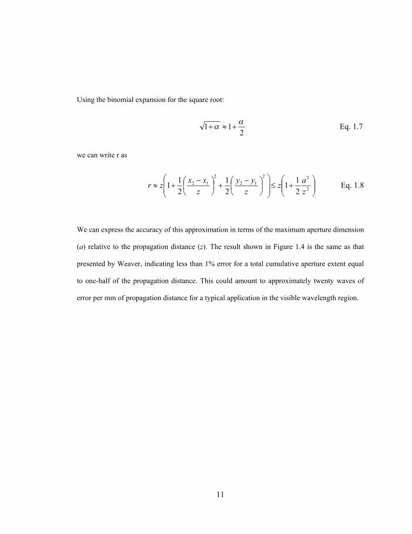
Figure 1.4. Relative accuracy for the binomial expansion of the propagation distance r. The value “a” is the sum of the maximum dimensions in the two planes. When this value is half of the propagation distance, the estimate for r can be off by %.6.0≈ This explains why the Fresnel approximation is limited to systems with large F#’s, generally near the axial zone. ..........................................................................................12

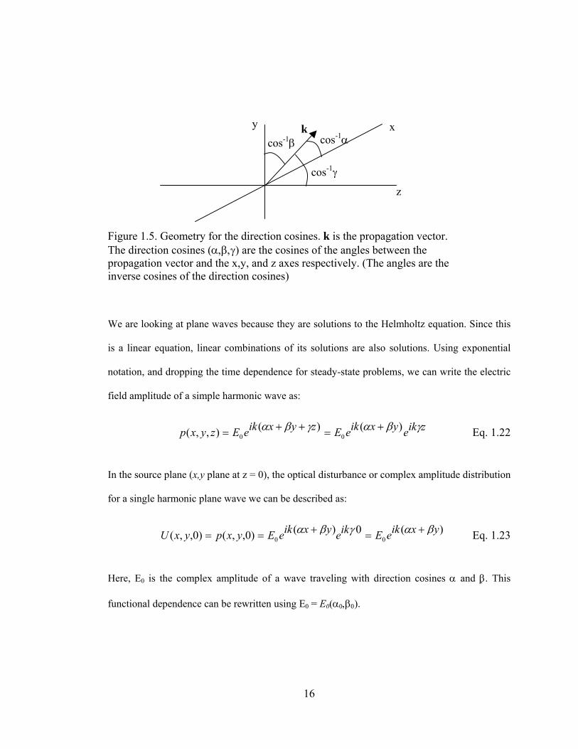
Figure 1.5. Geometry for the direction cosines. k is the propagation vector. The direction cosines (α,β,γ) are the cosines of the angles between the propagation vector and the x,y, and z axes respectively. (The angles are the inverse cosines of the direction cosines)......................................16

Figure 1.6. Classical ruled diffraction grating construction on a concave surface. During the ruling process, the diamond tool travels very smoothly in the direction perpendicular to the plane of the drawing, while the grating carriage moves very precisely to the right, traveling the distance of one groove for each stroke of the diamond tool. For this type of grating, the grooves are straight and parallel in a plane that is tangent to the grating surface...................................................................22

Figure 1.7. Holographic diffraction grating construction. A fringe field is formed by the interference of two coherent light sources; the intensity pattern at the grating surface exposes a photosensitive material in which the groove structure is produced....................................................................23

vi

Figure 1.8. Hologram geometry from Champagne (1967). This geometry is used to describe the positions of the recording sources and the reconstruction geometry. The subscript q is replace by each of (C,O,R,I) to represent the reConstruction , Object, Reference and Image points. ...........................................................................................26

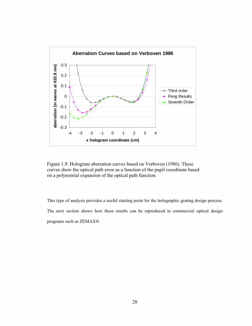
Figure 1.9. Hologram aberration curves based on Verboven (1986). These curves show the optical path error as a function of the pupil coordinate based on a polynomial expansion of the optical path function..........................28

Figure 1.10. Optical layout for holographic grating described by Verboven. The grating is at the left of the figure, and the image plane is on the right. Three wavelengths are shown, 732.8 nm at the top of the figure coming to focus before the image plane, 632.8 nm in the middle coming to focus at the image plane, and 532.8 nm focusing beyond the image plane........................................................................................30

Figure 1.11. ZEMAX Ray Fan Diagram for the Verboven holographic grating showing the aberrations as a function of the pupil coordinate. The plot shows the y-pupil coordinate on the left, and the x-pupil coordinate on the right. The aberrations are given in waves of optical path length at 632.8 nm. Note the agreement with the seventh-order aberrations plotted in Figure 1.9.................................................................................31

Figure 1.12. ZEMAX Merit Function Entry Screen. The rms spot size was chosen as the value to be optimized. Selection of “Ignore Lateral Color” indicates that each wavelength is included independently in the ray trace and optimization process. ...................................................33

Figure 1.13. Ray Fan diagram for holographic grating optimized in ZEMAX®. The image on the left is for the y-pupil coordinate, this has been improved over the original planar hologram described by Verboven. The image on the right is for the x-pupil coordinate, this is slightly worse than the original design because this design considers three wavelengths, not just one.........................................................................35

Figure 1.14. Optical layout for the holographic grating after optimization in ZEMAX®. Note that all three wavelengths come to a good focus at the image plane. The Zero order reflected beam is shown for reference, this beam comes to focus because the substrate is a concave reflector....................................................................................................36

Figure 1.15. Spot diagram at 532.8 nm for holographic grating optimized with ZEMAX®................................................................................................37

vii

Figure 1.16. Spot diagram at 632.8 nm for holographic grating optimized with ZEMAX®................................................................................................38

Figure 1.17. Spot diagram at 732.8 nm for holographic grating optimized with ZEMAX®................................................................................................38

Figure 2.1. Phase change for plane-wave propagation showing that a plane wave propagating along the z-axis will have π units of phase change as it advances one-half a wave. .......................................................................44

Figure 2.2. Unwrapped phase for tilted plane-wave propagation from under sampled direction-cosine spectrum. In this case, the tilt angle did not correspond to the sampling interval in direction-cosine space................45

Figure 2.3. Direction cosine spectrum of a plane wave having a direction cosine of 1.0−=α . Since the sampling interval is very coarse in the direction cosine space, this plane-wave is under-sampled. .....................46

Figure 2.4. Direction cosine spectrum for a plane wave having a direction cosine of 1.0−=α 226. This corresponds exactly to the sampling interval. ......47

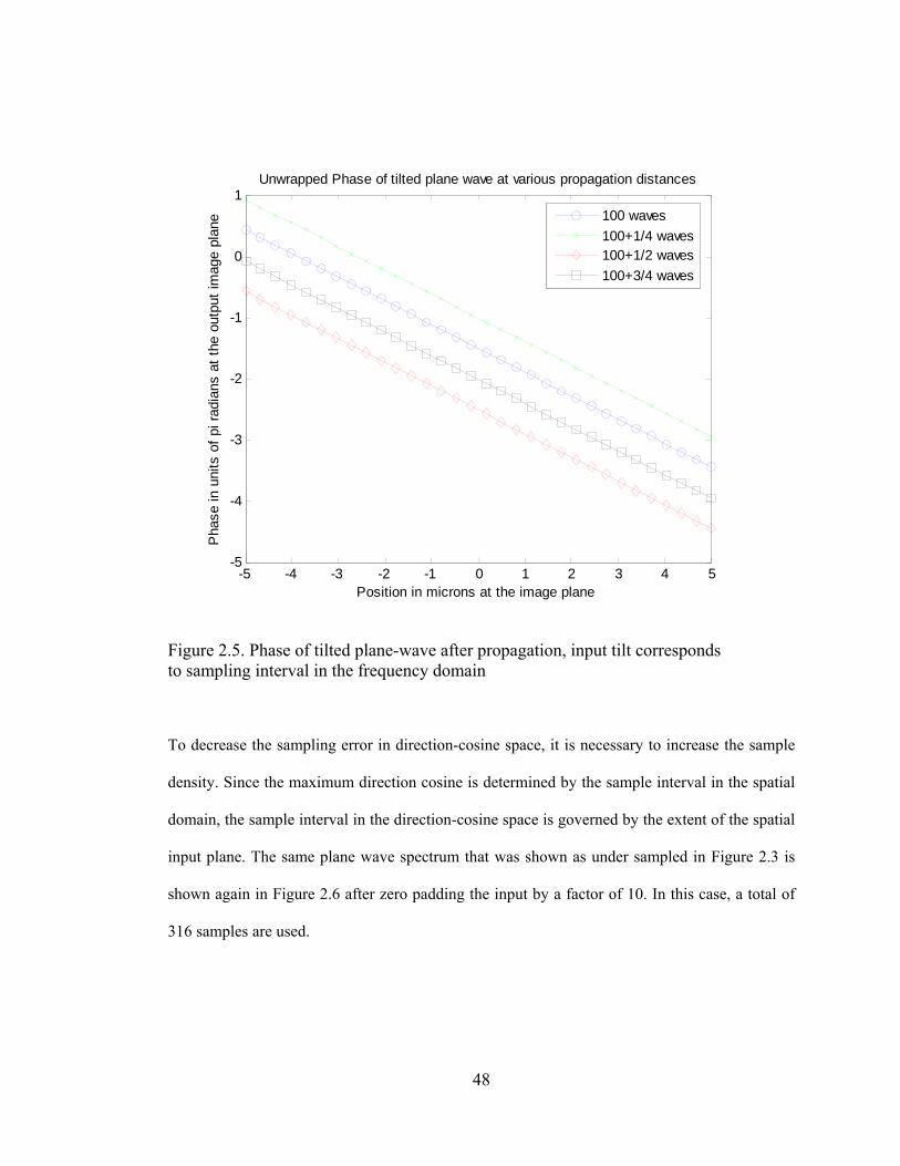
Figure 2.5. Phase of tilted plane-wave after propagation, input tilt corresponds to sampling interval in the frequency domain .............................................48

Figure 2.6. Discrete direction cosine spectrum for plane wave having direction cosine of 1.0−=α with 316 samples in the direction-cosine space over the range from 0.1to0.1 +=−= αα .........................................49

Figure 2.7. Phase error metric based upon a difference between the predicted unwrapped phase and a linear fit to the predicted phase for a 100 wave propagation distance. Initial ra merit value is .1257 radians, and initial rms merit value is .0409 squared radians. Increasing the input window size also increases the sampling density in the direction-cosine space. ............................................................................................50

Figure 2.8. Same a Figure 2.7 but for a propagation distance of 10mm. Initial ra merit value is .1101 radians, and initial rms merit value is .0172 squared radians. .......................................................................................52

Figure 2.9. Direction-cosine estimate based upon the slope parameter for the best-fit model to the unwrapped phase. This figure shows that a penalty of a 2 percent error in the estimate for the direction cosine can be obtained for insufficient sampling in direction-cosine space. This figure is from the propagation of a linear phase sampled and fitted over a 100um window, propagated a distance of 10mm as in Figure 2.8. ...........................................................................................................53

viii

Figure 2.10. Fresnel propagation for a 1mm rectangular aperture at 632.8 nm following Weaver (1983). The curves at 50 and 500mm are offset from zero by –2mm and plus 2mm respectively for visibility. ...............55

Figure 2.11. Fresnel propagation for a 1mm wide 1-D aperture showing intensity rescaled by a factor of z. The integrals under all three curves are the same. ........................................................................................................56

Figure 2.12. Angular Spectrum Propagation for a 1mm wide 1-D aperture compared with the Fresnel propagation method for the configuration. Note, that all images are in fact centered at zero, but they are shown offset for visibility. The ASPM images are offset at –3mm and +3mm for the 50mm and 500mm propagation distances respectively. ..............57

Figure 2.13. A close up for the 100mm propagation distance for a one-dimensional slit shows that both the ASPM and the Fresnel methods produce essentially identical results ........................................................58

Figure 2.14. Angular spectrum propagation for a 1mm square aperture showing central slices through the intensity at the image plane. Note the peak intensity increase at the 500mm propagation distance. The three images are shown offset from one another for visibility. ........................60

Figure 2.15. Two-dimensional image from a 1mm square aperture at a propagation distance of 500mm. The image is shown in a gray scale that is proportional to the log of the image intensity. The plot at the right is a central slice profile of the image intensity................................61

Figure 2.16. Two-dimensional image from a 1mm square aperture at a propagation distance of 100mm. The image is shown in a gray scale that is proportional to the log of the image intensity. The plot at the right is a central slice profile of the image intensity................................62

Figure 2.17. Two-dimensional image from a 1mm circular aperture at a propagation distance of 100mm. The image is shown in a gray scale that is proportional to the log of the image intensity. The plot at the right is a central slice profile of the image intensity. Note that the central intensity drops to near zero..........................................................63

Figure 2.18. Talbot Imaging using ASPM showing the Talbot image at 39.5mm, the phase-reversed Talbot image at 43.5mm, and the Talbot subimage at 41.5mm from a 20 groove per millimeter amplitude grating illuminated with a plane wave at 632.8 nm. The images are periodic with propagation distance with the pattern repeating at a distance of L2/λ where L is the spatial period of the grating. ....................................65

ix

Figure 2.19. Talbot Imaging using ASPM for a phase grating showing the Talbot image at 41.5mm and the phase-reversed Talbot image at 45.4mm. The phase grating has a period of 20 groove per millimeter with a phase depth of .2 waves. The grating is illuminated with a plane wave at 632.8 nm. The images are periodic with propagation distance with the pattern repeating at a distance of L2/λ where L is the spatial period of the grating............................................................................................66

Figure 2.20. E-field orientation for two-beam interference in TE case; the fields are perpendicular to the plane of incidence, and are parallel to each other so they add directly.........................................................................68

Figure 2.21. E-field orientation for two-beam interference in TM case; the incident fields E1 and E2 are in the plane of incidence and are shown with x and z vector components at some instant of time.........................68

Figure 2.22. Direction cosine diagram on the left for a plane wave traveling at an angle θ relative to the z axis. The diagram on the right shows the same k vector together with E-field for the TM case. .............................69

Figure 2.23. Original and cosine weighted direction-cosine spectrum for two-beam interference in the TM case. The magnitude of the x-component of the E-field is found multiplication with an angle dependent weighting function given by Eq. 2.15......................................................71

Figure 2.24. Two-beam interference at 632.8 nm with ±30° incident beams showing the reduced fringe contrast for the TM case as compared to the TE case. Note that the average intensity is the same for the two cases.........................................................................................................72

Figure 2.25. Optical layout for converging wave illumination of a circular aperture used to model the axial focal shift with the ASPM. .................73

Figure 2.26. Axial focal shift for a 40-wave diameter circular aperture in a converging beam......................................................................................74

Figure 2.27. Axial focal shift based on results by Sheppard (2003) .........................75

Figure 2.28. Off-axis converging illumination through a rectangular aperture.........77

Figure 3.1. Illumination pattern from a diffraction grating illuminated with λ=488 nm using a super-gaussian beam..................................................80

Figure 3.2. Optical layout used for producing a Moiré fringe pattern with a diffraction grating as a beam combiner. ..................................................82

Figure 3.3. Moiré pattern from a diffraction grating illuminated with 488 nm.........83

x

Figure 3.4. Model of a groove pattern on a 2mm square patch of the grating surface shown with 100x horizontal scale magnification in order enhance the visibility of the groove structure. The groove depth was normalized to be .1-wave deep at 632.8 nm. Note how the groove pattern is curved, this is what leads to the focusing properties of holographic diffraction gratings. .............................................................86

Figure 3.5. Rms spot radius for ZEMAX optimized planar holographic grating that was modeled using the ASPM. This plot represents the merit function variable that was given equal weighting at all three wavelengths. The result is that the imaging is pretty good at the central wavelength and equally bad at the two extremes ........................88

Figure 3.6. Optical Layout for ZEMAX optimized planar holographic grating hologram. The grating is shown at the left, the image plane is parallel to the grating surface at a distance of 30mm away. Three wavelengths are shown 600 nm, 632.8 nm, and 665.6 nm along with the zero order reflection that does not come to focus. The grating has a nominal groove frequency of 403.5 grooves per millimeter at the center.............90

Figure 3.7. Through focus spot diagram for ZEMAX optimized holographic grating indicating a plus or minus two millimeter shift in the image plane position is required to bring the extreme wavelengths into focus.........................................................................................................91

Figure 3.8. Spot diagram at 632.8 nm in the image plane for the planar hologram. .92

Figure 3.9. Image intensity at 632.8 nm at the focal plane using 10mm wide sample window (2x zero padding) and four time Nyquist sampling. The image position is not correct and is aliased because the image falls outside of the sampling window. .....................................................93

Figure 3.10. Image intensity at 632.8 nm at the focal plane for the grating hologram showing the image position at 9.54mm away from the optical axis. This agrees with the geometric ray trace model..................94

Figure 3.11 Image intensity for best focus at 600 nm, 2mm beyond the nominal image plane. Note the image width of almost 400um at the 30mm propagation distance. This is in agreement with the results from the ZEMAX ray trace. ...................................................................................95

Figure 3.12. Image intensity at 665.6nm at the focal plane and plus 2mm...............96

Figure 3.13. Image intensity at 665.6 nm at the focal plane distance of 30mm........97

Figure 3.14. Image intensity at 665.6 nm, 2mm inside the focal plane corresponding to the best focus for this wavelength. ..............................98

xi

List of Tables

Table 1.1. Number of samples required for the angular spectrum propagation method for a variety of combinations of minimum spatial period, sampling density, and zero padding. Note that the number of required samples can become intractably large, even for some reasonably small systems.......................................................................................................5

Table 1.2. Hologram geometry based on Verboven (1986). The Reference and Object points are the locations of diverging spherical waves used to record the hologram with 488 nm light. The substrate is a planar surface illuminated with a plane wave arriving from the direction given by the reConstruction coordinates. The image at 632.8 nm is formed at position indicated by the Image coordinates. ..........................27

Table 1.3. Grating parameters for the holographic grating after optimization in ZEMAX. The substrate is a concave reflector with a radius of curvature of 580.81mm............................................................................34

Table 3.1. Diffraction efficiencies calculated in PC Grate for a perfectly conducting 205 groove per mm grating in second order Littrow at 488 nm ............................................................................................................81

Table 3.2. Grating parameters for planar hologram for modeling using the ASPM .87

Table 5.1. Summary of surface data for the Verboven holographic grating. This data is entered into the ZEMAX Lens Data Editor. Note that the surface type for the holographic grating is the ZEMAX standard HOLOGRAM1 surface type..................................................................101

xii

1 Introduction The angular spectrum propagation method (ASPM) has been well known for nearly 40 years.

(Goodman, 1968) (Lalor, 1968). This technique has recently been applied to modeling micro-

optical systems including diffraction gratings (Kurzweg, 2001), and to the design of diffractive

optical elements (Mellin, 2001). Other scalar optical propagation models such as Fresnel

propagation have recently been used in such novel areas as phase reconstruction (Fienup, 1999)

and micro-electrical mechanical device inspection (Furlong, 2003). This thesis describes the

angular spectrum propagation method for the numerical modeling of holographic gratings.

The angular spectrum propagation method offers some distinct advantages over the Fresnel

propagation method. In particular the ASPM is not limited to small angles around the paraxial

zone, is able to accommodate very short propagation distances, and maintains the same sample

spacing in both the input and output planes. The downside is that the ASPM may require very

large data arrays to model real systems. This thesis provides examples of how the ASPM can be

applied to modeling some well-known optical phenomena including two-dimensional diffraction

from square and circular apertures, two-beam interference, and Talbot imaging from a

diffraction grating. The goal of this thesis is to apply the ASPM to model the image formation

process from a holographic diffraction grating, and to compare these results to a geometric ray

trace for the same component modeled in ZEMAX®.

1

Throughout this thesis, the numerical calculations using the angular spectrum propagation

method were performed in Matlab®. This approach provided the required flexibility to change

the model parameters. It is informative, however, to briefly discuss other commercial sources

that may have some similar computational capabilities. Discrete computation using the angular

spectrum propagation method is available in ASAP™ from Breault Research Organization. This

program and FRED from Photon Engineering, LLC utilize the Gaussian beam decomposition

technique as their primary method for modeling scalar wave propagation. DECAD is a freeware

program which has implemented the angular spectrum method for modeling diffractive optics.

ZEMAX® from Zemax Development Corporation and GLAD from Applied Optics Research

have implemented an angular spectrum propagation algorithm with an approximation that limits

the utility of the method to the axial region. Code V® from Optical Research supports a beam

propagation option that uses either the angular spectrum or the Fresnel propagation technique,

dependent upon the system geometry. Many of these applications, plus OSLO from Lambda

Research Corporation, can calculate the wavefront at the exit pupil of an optical system from the

geometrical ray trace. The constructed wavefront is then sampled and propagated to the image

plane of the system by various algorithms, usually a Fourier transform or a Fresnel

approximation. Figure 1.1 shows the layout of a typical optical system that is discussed. The

wavefront at the exit pupil is sampled and propagated to the image plane using the numerical

algorithm.

2

Propagation

Image plane Traveling Wavefront

Exit aperture or Exit pupil

Figure 1.1. Typical optical system layout showing the traveling wavefront incident on the exit pupil, the exit pupil, and the image plane. The wavefront at the exit pupil is sampled and propagated to the image plane.

The sampling of the wavefront is a critical step. In many typical applications there is an implicit

assumption that the exit wavefront is a smooth function of the exit pupil spatial coordinate. This

allows for small sampling arrays and very fast calculations. For the case of a diffraction grating

system such as we are interested in, the angular spectrum method may require high-density

spatial sampling of the optical field immediately after the diffractive component. For example, if

we want to model a diffraction grating with 100 grooves per mm, the groove spacing is 10um. If

we assume a smooth groove structure and we sample at the Nyquist limit, we would need one

sample every 5um. Figure 1.2 shows how the phase of the wavefront might look immediately

after a diffraction grating in a typical system. Table 1.1 summarizes how some real world

problems that require dense sampling of the wavefront at the exit pupil may become numerically

intractable even with today’s powerful desktop computers. In this context, “zero padding” refers

to the extension of the input sampling window, i.e. a 1mm input region window that is 4 times

3

zero padded, is really a 4 mm wide input window, usually extended to the new size by adding

zeros to the sampling array.

Exit pupil wavefront phase

1

2

3

4

5

6

Minimum spatial period for sampling

N

Sample number

Figure 1.2. Sampling of the exit pupil wavefront. Nyquist sampling would require two samples per minimum spatial period. Practical sampling may require from five to ten samples per minimum spatial period to reduce numerical artifacts.

4

Table 1.1 Number of samples per area Minimum

spatial period in microns

Sampling* Zero Padding 1mm

linear 1 Χ 1mm square

10 Χ 10mm square

10 Nyquist None 200 40,000 4 Χ 106

10 Practical None 1,000 1 Χ 106 1 Χ 108

10 Nyquist 4 times 1,000 1 Χ 106 1 Χ 108

10 Practical 4 times 5,000 25 Χ 106 25 Χ 108

5 Practical 4 times 10,000 1 Χ 108 1 Χ 1010

* Practical sampling in this context is five times Nyquist or ten samples per minimum spatial period.

Table 1.1. Number of samples required for the angular spectrum propagation method for a variety of combinations of minimum spatial period, sampling density, and zero padding. Note that the number of required samples can become intractably large, even for some reasonably small systems.

In order to accurately describe real-world signals, Weaver (1983) suggests the requirement for

using sampling frequencies larger than Nyquist so that the sampling density is eight to ten times

the minimum spatial period. Since the angular spectrum method has the same spatial sampling

interval in both the input and output planes, it is necessary to consider the minimum spatial

period in both planes. For example in a low F# system that produces a small focused spot, the

minimum feature dimension might occur in the output image plane, and these image features

would dictate the required sampling density. Leseberg (1992) indicates that dense sampling may

be required along only one axis for many real diffractive systems. For example, dense sampling

may be required in the spectral direction (perpendicular to the groove pattern of the diffraction

grating), and fewer samples would be required along the groove direction. For some of the

examples in this thesis, only one-dimensional calculations were performed in order to avoid the

intractably large data sets associated with two-dimensional problems.

5

Later in this Chapter, (Section 1.2) the theoretical framework for the Fresnel propagation and

the angular spectrum propagation methods are developed in some detail. Afterwards, some

background concerning diffraction gratings is reviewed so as to establish a terminology base. A

description of grating aberration theory is given to provide an historical framework. Also, a

method for modeling and optimizing a holographic grating using the ZEMAX® geometric ray

trace program is discussed. This method was used to establish the design parameters for the

holographic grating that is modeled in Chapter 3 and this method is used to provide a

comparative basis for the results in Chapter 3.

In Chapter 2, a variety of simple systems are modeled with the angular spectrum propagation

method (ASPM) in order to demonstrate the application and capabilities of the method. In

Chapter 3, the ASPM is used to model moiré fringe phenomenon from a linear diffraction

grating, which cannot be predicted directly from a geometric ray trace model. Lastly, the image

formation process is modeled for a holographic diffraction grating with curved grooves on a

planar surface and the results are compared to ZEMAX simulations.

1.1 Background Diffractive optics, holographic optical elements, binary optics, computer generated holograms,

holographic diffraction gratings, and concave diffraction gratings are perhaps only a subset of

possible names for a class of optical components that are routinely used to manipulate the

propagation of light. Like a simple lens, whose phase and amplitude transmittance function is

6

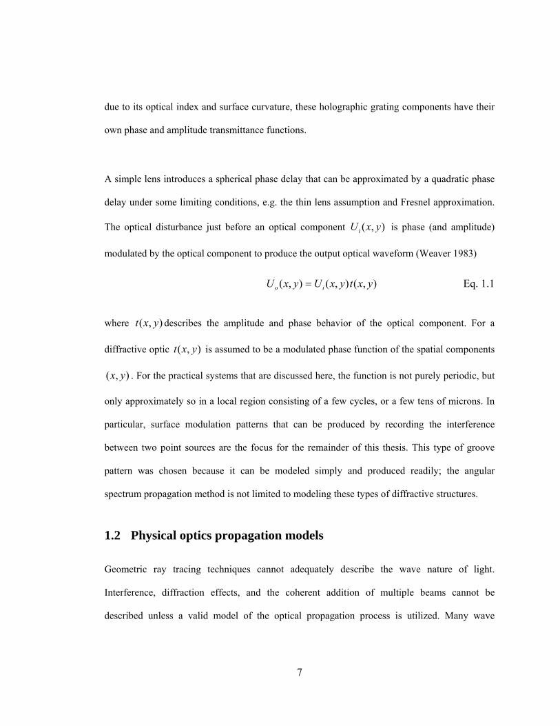
due to its optical index and surface curvature, these holographic grating components have their

own phase and amplitude transmittance functions.

A simple lens introduces a spherical phase delay that can be approximated by a quadratic phase

delay under some limiting conditions, e.g. the thin lens assumption and Fresnel approximation.

The optical disturbance just before an optical component is phase (and amplitude)

modulated by the optical component to produce the output optical waveform (Weaver 1983)

),( yxUi

),(),(),( yxtyxUyxU io = Eq. 1.1

where describes the amplitude and phase behavior of the optical component. For a

diffractive optic is assumed to be a modulated phase function of the spatial components

. For the practical systems that are discussed here, the function is not purely periodic, but

only approximately so in a local region consisting of a few cycles, or a few tens of microns. In

particular, surface modulation patterns that can be produced by recording the interference

between two point sources are the focus for the remainder of this thesis. This type of groove

pattern was chosen because it can be modeled simply and produced readily; the angular

spectrum propagation method is not limited to modeling these types of diffractive structures.

),( yxt

),( yxt

),( yx

1.2 Physical optics propagation models Geometric ray tracing techniques cannot adequately describe the wave nature of light.

Interference, diffraction effects, and the coherent addition of multiple beams cannot be

described unless a valid model of the optical propagation process is utilized. Many wave

7

phenomena can be described even after extensive simplifications to the underlying set of

Maxwell’s equations. One common set of simplifying assumptions to the problem of optical

propagation is the scalar approximation, together with the monochromatic assumption. These

assumptions include propagation in homogeneous, non-conducting, non-magnetic and source

free media. This gives rise to the Helmholtz equation that has the equation for a plane wave as

its solution.

1.2.1 Fresnel propagation

The Fresnel propagation integral is used to approximate an optical field in one plane based upon

the field in some other plane. A good starting point is to describe the optical field.

Weaver (1983) describes an optical disturbance function V(x;t) as a solution to the three-

dimensional scalar wave equation that results from solving Maxwell’s equations for propagation

in a dielectric, such as free space. The three-dimensional scalar wave equation is:

2

2

22 );(1);(

ttV

ctV

∂∂

=∇xx Eq. 1.2

This represents either the magnetic or the electric component of the propagating field. The

power density or energy transfer per unit area (in units of watts/meter2) is proportional to the

squared modulus of V. For imaging applications this is the primary value of interest.

8

Assuming a separable function of space and time we can write:

tiettUtV νπϕϕ 2)(where)()();( == xx Eq. 1.3

The time dependence assumes monochromatic light. Together, these assumptions give rise to

the three-dimensional Helmholtz equation that must be satisfied for any optical disturbance

function U.

λππν 22where0)()( 22 ===+∇

ckUkU xx Eq. 1.4

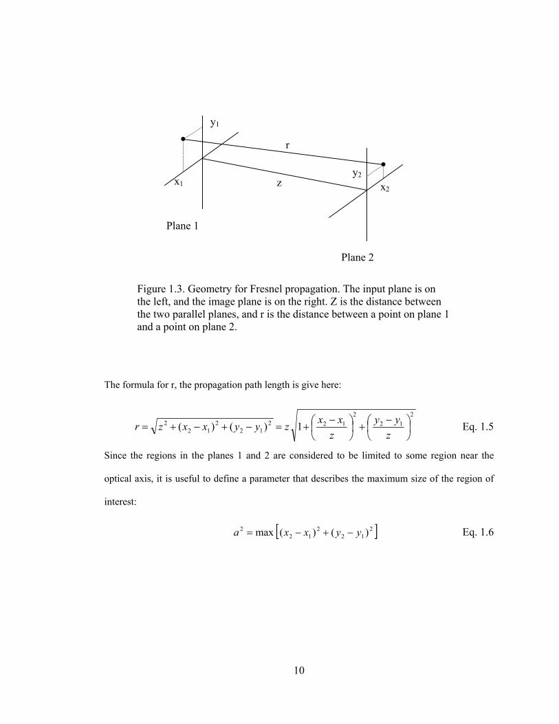
The geometry for Fresnel propagation is shown in Figure 1.3 where the input is in plane 1 at z =

0 with spatial coordinates (x1,y1) and the output is in plane 2 with spatial coordinates (x2,y2).

The distance between planes is z, and r represents the distance between a point in plane 1 and a

point in plane 2.

9

y1

x1 x2

y2

r

z

Plane 1 Plane 2

Figure 1.3. Geometry for Fresnel propagation. The input plane is on the left, and the image plane is on the right. Z is the distance between the two parallel planes, and r is the distance between a point on plane 1 and a point on plane 2.

The formula for r, the propagation path length is give here:

212

2122

122

122 1)()( ⎟

⎠⎞

⎜⎝⎛ −

+⎟⎠⎞

⎜⎝⎛ −

+=−+−+=z

yyz

xxzyyxxzr Eq. 1.5

Since the regions in the planes 1 and 2 are considered to be limited to some region near the

optical axis, it is useful to define a parameter that describes the maximum size of the region of

interest:

[ ]212

212

2 )()(max yyxxa −+−= Eq. 1.6

10

Using the binomial expansion for the square root:

211 αα +≈+ Eq. 1.7

we can write r as

⎟⎟⎠

⎞⎜⎜⎝

⎛+≤⎟

⎟⎠

⎞⎜⎜⎝

⎛⎟⎠⎞

⎜⎝⎛ −

+⎟⎠⎞

⎜⎝⎛ −

+≈ 2

2212

212

211

21

211

zaz

zyy

zxxzr Eq. 1.8

We can express the accuracy of this approximation in terms of the maximum aperture dimension

(a) relative to the propagation distance (z). The result shown in Figure 1.4 is the same as that

presented by Weaver, indicating less than 1% error for a total cumulative aperture extent equal

to one-half of the propagation distance. This could amount to approximately twenty waves of

error per mm of propagation distance for a typical application in the visible wavelength region.

11

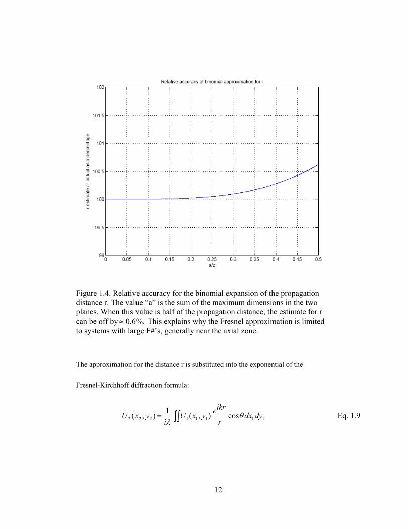
Figure 1.4. Relative accuracy for the binomial expansion of the propagation distance r. The value “a” is the sum of the maximum dimensions in the two planes. When this value is half of the propagation distance, the estimate for r can be off by This explains why the Fresnel approximation is limited to systems with large F#’s, generally near the axial zone.

%.6.0≈

The approximation for the distance r is substituted into the exponential of the

Fresnel-Kirchhoff diffraction formula:

11111222 cos),(1),( dydxr

ikreyxUi

yxU θλ ∫∫= Eq. 1.9

12

For propagation distances that are large relative to the aperture sizes zr ≈ so we can replace r

in the denominator by z, and cosθ with 1 leading to Equation 1.10.

11

212

212

111222

21

211

1),(1),( dydxz

yyz

xxikze

zyxU

iyxU ∫∫

⎥⎥⎦

⎤

⎢⎢⎣

⎡⎟⎠⎞

⎜⎝⎛ −

+⎟⎠⎞

⎜⎝⎛ −

+

=λ

Eq. 1.10

After removing the z terms from the integral, we have

( ) ( )[ ]11

212

212

1112222),(),( dydx

yyxxz

ik

eyxUzi

ikzeyxU ∫∫−+−

=λ

Eq. 1.11

If we expand the exponent and remove the x2 and y2 terms from of the integral, we have

( ) ( ) ( )11

21212

12

1

111

22

22

2222),(2),( dydx

yyxxzik

eyx

zik

eyxUyx

zik

ezi

ikzeyxU+

−++

= ∫∫λ

Eq. 1.12

which can be simplified by defining the leading intensity and phase factor as K:

( )22

22

21 yx

zi

e

zi

ezi

K+

= λπ

λπ

λ Eq. 1.13

Leaving:

( )11

21

21

21

21

111222

2),(),( dydxz

yyz

xxie

yxz

i

eyxUKyxU⎟⎠⎞

⎜⎝⎛ +−+

= ∫∫ λλπ

λπ

Eq. 1.14

13

This is the Fresnel propagation formula and consists of the Fourier transform of the product of

the input optical disturbance and a quadratic phase term, along with a leading intensity and

phase factor. Note that the output spatial coordinates (x2,y2) can be recovered from the

frequency domain variables ⎟⎠⎞

⎜⎝⎛

zy

zx

λλ22 , by multiplying by λz.

We are left with a result that requires a different output spatial sampling frequency for every

propagation distance z. Also, this result is restricted in terms of the size of the apertures and the

propagation distances that can be modeled. The next section will develop the angular spectrum

propagation method, which does not suffer from these shortcomings, although it may be more

numerically intensive

1.2.2 Angular spectrum propagation

The angular spectrum propagation method is not limited by the small angle approximation, and

the spatial sampling frequency is the same in both input and output planes. These factors

contribute to making the angular spectrum the method of choice for numerical simulations. This

method also has some shortcomings, including larger numerical arrays for long propagation

distances, as pointed out by Veerman (2004) who proposed a direct integration method. Zhang

(2005) uses the method of stationary phase to address the numerical issues associated with the

propagation of non-paraxial gaussian beams.

14

A scalar plane wave can be described as a function of position and time, and its form is not

changed by propagation. These waves are solutions to the Helmholtz equation, and therefore are

an important starting point for understanding the angular spectrum propagation method. The

equation for a scalar plane wave is given by:

)cos(),,,( 00 φω +−++= tzkykxkEtzyxp zyx Eq. 1.15

where kx, ky , and kz are components of the propagation vector:

kjik ˆˆˆzyx kkk ++=

r Eq. 1.16

This wave is periodic with the period defined by the wavelength λ along the direction of

propagation. The magnitude of the propagation vector is

2222zyx kkkk ++===

λπk Eq. 1.17

The normalized components of k along the principal axes are the direction cosines defined as:

kkx=α Eq. 1.18

kk y=β Eq. 1.19

kkz=γ Eq. 1.20

1therefore 222 =++ γβα Eq. 1.21

15

y x

z

kcos-1α

cos-1γ

cos-1β Figure 1.5. Geometry for the direction cosines. k is the propagation vector. The direction cosines (α,β,γ) are the cosines of the angles between the propagation vector and the x,y, and z axes respectively. (The angles are the inverse cosines of the direction cosines)

We are looking at plane waves because they are solutions to the Helmholtz equation. Since this

is a linear equation, linear combinations of its solutions are also solutions. Using exponential

notation, and dropping the time dependence for steady-state problems, we can write the electric

field amplitude of a simple harmonic wave as:

zikeyxikeEzyxikeEzyxp γβαγβα )()(),,( 00+=++= Eq. 1.22

In the source plane (x,y plane at z = 0), the optical disturbance or complex amplitude distribution

for a single harmonic plane wave we can be described as:

)(0)()0,,()0,,( 00yxikeEikeyxikeEyxpyxU βαγβα +=+== Eq. 1.23

Here, E0 is the complex amplitude of a wave traveling with direction cosines α and β. This

functional dependence can be rewritten using E0 = E0(α0,β0).

16

A general optical disturbance in the source plane is a linear combination of any number of plane

waves with each plane wave traveling in a different direction.

∑ +=N

n

nnnnn

yxikeEyxU )(),()0,,( βαβα Eq. 1.24

Goodman (1968) describes the optical disturbance in the x,y plane at z = 0 as an inverse Fourier

transform of the angular spectrum A(ε,η) where [ ]1−F is the inverse Fourier transform operator.

[ ] ∫∫+== − ηξηξπηξηξ ddyxieAAyxU )(2),(),()0,,( 1F Eq. 1.25

Goodman equates the complex amplitude coefficients E(α,β) of the plane wave (in units of volts

per meter) to the value inside the integral of Eq. 1.25, therefore, the angular spectrum A(ξ,η)

must have units of volt-meters.

[ ] [ ] [ ]1-1 mmmV),(mV),( ηξηξβα ddAE −⋅=⎥⎦

⎤⎢⎣⎡ Eq. 1.26

Here, the direction cosines are related to the frequency variables through the relations:

λξα = Eq. 1.27a

ληβ = Eq. 1.27b

( ) ( )221 ληλξγ −−= Eq. 1.27c

The angular spectrum is found by rearranging Equation 1.25 and is the Fourier decomposition of

the optical field in the input plane where F [ ] is the forward Fourier transform.

17

[ ] ∫∫ +−== dydxyxieyxUyxUA )(2)0,,()0,,()0;,( ηξπηξ F Eq. 1.28

For a position further along the optical axis at z, we can write the angular spectrum as the

Fourier decomposition of the optical disturbance at this plane.

[ ] ∫∫ +−== dydxyxiezyxUzyxUzA )(2),,(),,();,( ηξπηξ F Eq. 1.29

Lastly, the inverse Fourier transform that describes the optical disturbance function at the plane

z is:

[ ] ∫∫ +== − ηξηξπηξηξ ddyxiezAzAzyxU )(2);,();,(),,( 1F Eq. 1.30

The optical disturbance function U must satisfy the Helmholtz equation:

022 =+∇ UkU Eq. 1.31

The intermediate result after applying the Helmholtz equation to the expression inside the

integral of Eq. 1.30 is:

0)(2);,()(2);,(

)(2);,()2()(2);,()2(

22

2

22

=+++

++−+−

yxiezAkyxiedz

zAd

yxiezAyxiezA

ηξπηξηξπηξ

ηξπηξπηηξπηξπξ Eq. 1.32

After canceling the exponential terms, we obtain the simple relation

0])()(1[);,();,( 2222

2

=−−+ ληλξηξηξ zAkdz

zAd Eq. 1.33a

18

0);,();,( 222

2

=+ zAkdz

zAd ηξγηξ Eq. 1.33b

An elementary solution to this differential equation is:

zikeAzA γηξηξ )0;,();,( = Eq. 1.34

where γ is given in equation 1.27c as the z component of the propagation vector. For plane

waves traveling in the positive z-direction, we have

22222 1)()(1 βαληλξγ −−=−−= Eq. 1.35

1when1and 2222 <+−−= βαβαγ Eq. 1.36

Recall from Eq. 1.28 that the angular spectrum at z = 0 can be written as a Fourier transform of

the input field, so by combining this with Eq. 1.34 we can write the angular spectrum in the

output plane as a function of the input field:

[ ] zikedydxyxieyxUzikeyxUzikeAzA γηξπγγηξηξ ⎥⎦⎤

⎢⎣⎡ +−=== ∫∫ )(2)0,,()0,,()0;,();,( F

Eq. 1.37

With this result and Eq. 1.30, we can show that the optical disturbance in the output plane is a

function of the optical disturbance in the input plane and of the propagation distance z:

[ ] ∫∫ +=⎥⎦⎤

⎢⎣⎡= − ηξηξπγηξγ ddyxiezikeAzikeyxUzyxU )(2)0;,()0,,(),,( 1 FF

Eq. 1.38

19

We are left with a very powerful and simple result: given the optical disturbance function in the

plane z = 0, we can compute the angular spectrum there, multiply that spectrum by a linear

phase term, and use the inverse Fourier transform to find the optical disturbance in a new plane

at distance z away from the input plane.

A comment is in order here with regard to the implementation of this method in the GLAD and

ZEMAX commercial software programs. Both sources have approximated the square root in Eq.

1.36 via Eq. 1.7:

211

2222 βαβαγ +

−≈−−= Eq. 1.39

In place of equation 1.34, they arrive at the following approximate form:

( ) ( ) ⎟⎠⎞

⎜⎝⎛⎟⎟

⎠

⎞⎜⎜⎝

⎛+−

≈+−

=22

22

)0,,()0,,();,(ηξπλ

ηξληλξ

λπ

ηξηξzi

eAzi

eikzeAzA

Eq. 1.40

This approximation limits the applicability to the paraxial zone and this approximation will not

be used here. Instead, we will use Eq. 1.36 directly to compute the z-direction cosine without

any approximation.

Harvey (2003) suggested using dimensionless spatial variables by normalizing all of the spatial

coordinates by the wavelength as follows:

20

λxx =ˆ Eq. 1.41a

λyy =ˆ Eq. 1.41b

λzz =ˆ Eq. 1.41c

Therefore we can write the dimensionless angular spectrum as the direction cosine spectrum:

( ) ( )[ ] ∫∫⎟⎠⎞⎜

⎝⎛ +−

== ydxdyxi

eyxUyxUS ˆˆˆˆ2

)0,ˆ,ˆ(0,ˆ,ˆ0;,βαπ

βα F Eq. 1.42

And the optical disturbance in the normalized output plane as

( ) ( )[ ] ( ) ( ) βαβαππγβαπγ ddyxiezieSzieyxUzyxU ˆˆ2ˆ20;,ˆ20,ˆ,ˆˆ,ˆ,ˆ 1 +=⎥⎦⎤

⎢⎣⎡= ∫∫− FF

Eq. 1.43

These results are applied in discrete form to some practical problems in Chapter 2.

1.3 Diffraction gratings The classical method for producing a diffraction grating involves burnishing a metal coating

with a diamond tool using a high-precision machine called a ruling engine, as shown in Figure

1.6 (Hutley, 1982) (Loewen, 1997). This method forms straight, equally spaced grooves in a

plane. The groove structure of the diffraction grating gives rise to its dispersive properties,

21

where the propagation direction for an incident wavefront after interaction with the surface

depends upon the wavelength. Gratings also may be formed on surfaces other than plane as

shown in Figure 1.6. This type of concave ruled diffraction grating has both image formation

properties (due to the substrate curvature), and dispersive properties (due to the groove pattern).

Diamond tool Diamond carriage

Grating surface

Grating carriage

Figure 1.6. Classical ruled diffraction grating construction on a concave surface. During the ruling process, the diamond tool travels very smoothly in the direction perpendicular to the plane of the drawing, while the grating carriage moves very precisely to the right, traveling the distance of one groove for each stroke of the diamond tool. For this type of grating, the grooves are straight and parallel in a plane that is tangent to the grating surface.

A holographic grating can be produced with curved grooves by using diverging wavefronts as

the recording sources. This type of grating has both focusing properties due to the curvature and

placement of the grooves, as well as dispersive properties due to the spacing of the grooves.

This type of grating is considered for the remainder of this thesis. The method of production

derives its name from classical holography, where the interference pattern between two coherent

22

wavefronts is recorded in a photosensitive material. In the simplest arrangement, as shown in

Figure 1.7, two plane waves form a standing wave pattern of straight and equally spaced fringes

in the region where they overlap. This type of grating is sometimes called a “ruled equivalent

holographic grating”, since the positions of the grating grooves on the surface are the same as

would be obtained by a ruling engine. This pattern can be recorded in a photosensitive material.

Some materials, such as photographic emulsions, record the intensity modulation of the fringes

as a variation in the optical density of the material. These are called “amplitude gratings.” Other

materials such as photoresist, allow for removal of the exposed areas. This process forms a

surface relief pattern called a “phase grating.” The photoresist process forms a grating that can

be coated with a reflective metal layer and used in reflection. This thesis does not investigate the

nature of the complex behavior of the optical fields at the metal-dielectric interface of the

grating surface. The primary concern is the image position and relative image intensity, not the

absolute intensity of the images that are formed.

Grating surface

αR αO

Object wave Reference wave

Fringe field

Figure 1.7. Holographic diffraction grating construction. A fringe field is formed by the interference of two coherent light sources; the intensity pattern at the grating surface exposes a photosensitive material in which the groove structure is produced.

23

A very simple view of the phase surface is as a height function h(x,y). For example, a surface

that has a 0.1um surface height variation and a sinusoidal period of 10um in the x direction has a

height function given by Eq. 1.44. This function is constant over all values of y for any value of

x.

( ) ⎥⎦⎤

⎢⎣⎡ +

=2

)10/2sin(11.0),( xyxh π Eq. 1.44

To obtain the complex phase reflection function for this surface we multiply the height function

h(x,y) by a factor of two in order to account for the doubled path length upon reflection from the

surface, and insert it into a complex exponential to represent the optical phase.

( )λπ2kwhere,21),( == yxhikeyxt Eq. 1.45

This result can be inserted into Eq. 1.1 to find the optical waveform immediately after the

diffraction grating component assuming that the input optical disturbance is known.

1.4 Imaging properties of holographic gratings

The imaging characteristics of simple holograms were described by Champagne (1967). He

considers point source holograms recorded on planar surfaces where the object is a point source

and the reference wavefront is a spherical wave. Plane waves are considered as spherical waves

with infinite radius. Peng (1986) and Verboven (1986) described the imaging characteristics of

curved surface holograms. In these studies, the imaging characteristics are described in terms of

aberrations, or deviations from a spherical wave converging toward an image point or a point of

24

reference as a function of the pupil position. This imaging theory provides a valuable tool for

the design and analysis of grating imaging systems; see for example the work by Vila, et al.

(1988).

Noda, Namioka and Seya (Noda, 1974 – three references) investigated in detail the geometric

theory of the grating, ray tracing through holographic gratings and the design of holographic

concave gratings based upon geometric theory. These papers did not reference the work of

Champagne and they offer a different approach to the same problem of describing the image

formation process in terms of aberration functions.

The nomenclature in the field of holography described by Champagne is adopted here. An

object wavefront and a reference wavefront interfere to form an interference pattern that is then

recorded. In digital holography, this recording may be in electronic form only (Kreis, 2005).

For interference to occur, the object and reference waves must have a defined coherence

relationship, and for the remainder of this paper, a laser source with a long coherence length

(such as a commercial ion laser) is assumed to provide monochromatic illumination for the

object and reference waves.

In traditional holography, the object is illuminated by the coherent source. The light that travels

from the object to the recording surface forms the object wavefront. Without loss of generality,

only spherical wavefronts originating from a point source are used for both the object and

25

reference wavefronts. In practice, the functional equivalent of this is obtained by utilizing a

good spatial filter.

In addition to the object and reference wavefronts, Champagne describes the reconstruction

wavefront and the image wavefront. Given a hologram located at z=0 in the x-y plane, he

defines a coordinate geometry for each of the four points, reConstruction, Object, Reference and

Image represented by the set (C,O,R,I). Figure 1.5 shows this geometry relative to a coordinate

axis where the subscript q is replaced by one of (C,O,R,I) to represent each of the four points.

Q(xq, yq, zq) rq (x,y)

Rq z

x

y

Figure 1.8. Hologram geometry from Champagne (1967). This geometry is used to describe the positions of the recording sources and the reconstruction geometry. The subscript q is replace by each of (C,O,R,I) to represent the reConstruction , Object, Reference and Image points.

26

An example from Verboven (1986) has the following characteristics:

Recording wavelength = 488 nm Reconstruction wavelength = 632.8 nm u =1 for diverging source, -1 for converging source, 0 for source at infinity Q = X (mm) Y (mm) Z (mm) u Reference (R) -250.655 0.0 2450.212 1 Object (O) 55.785 0.0 331.296 1 reConstruction (C) -173648 0.0 984808 0 (plane wave) Image (I) 52.091 0.0 295.448 1

Table 1.2. Hologram geometry based on Verboven (1986). The Reference and Object points are the locations of diverging spherical waves used to record the hologram with 488 nm light. The substrate is a planar surface illuminated with a plane wave arriving from the direction given by the reConstruction coordinates. The image at 632.8 nm is formed at position indicated by the Image coordinates.

Based upon this information alone, it is possible to generate aberration curves from a

polynomial expansion of the optical path difference function that describe the propagating

wavefront as a deviation from a perfect spherical wavefront. Verboven has done this and his

results for the above hologram (or holographic grating) are reproduced in Figure 1.9. The fifth-

order polynomial expansion result given by Peng (1986) is included in Figure 1.9.

27

Aberration Curves based on Verboven 1986

-0.3

-0.2

-0.1

0

0.1

0.2

0.3

-4 -3 -2 -1 0 1 2 3 4

x hologram coordinate (cm)

aber

ratio

n (in

wav

es a

t 632

.8 n

m)

Third orderPeng ResultsSeventh Order

Figure 1.9. Hologram aberration curves based on Verboven (1986). These curves show the optical path error as a function of the pupil coordinate based on a polynomial expansion of the optical path function. This type of analysis provides a useful starting point for the holographic grating design process.

The next section shows how these results can be reproduced in commercial optical design

programs such as ZEMAX®.

28

1.5 Geometrical ray trace models The most practical method to evaluate the performance of holographic gratings is to use

geometrical ray trace techniques. This capability is a standard feature of commercial software

packages such as ZEMAX®, Code V®, and OSLO®. These programs are also well suited to

calculating the ray aberrations as described in the previous section.

This section describes how ZEMAX is used to enter, model, and optimize a holographic grating.

The starting point is the same holographic grating described previously. The grating is then

optimized and some typical output metrics are presented. Later, in section 3, the same design

and analysis features of ZEMAX are used to describe a similar grating component, and those

results are compared to results of the angular spectrum propagation method.

Table 5.1 in Appendix I shows a summary view of data that was entered into the ZEMAX lens

data editor in order to reproduce the hologram component described by Verboven. In this case

the grating component is being used in reflection.

The optical layout for the holographic grating is shown in Figure 1.10, with the grating on the

left and the image plane on the right. Three wavelengths are shown, λ=532.8 nm at the bottom,

632.8 nm in the center and 732.8 nm at the top. The central wavelength λ=632.8 nm represents

the optimized wavelength as chosen by Verboven. This grating has 548.8 grooves per mm at the

central portion of its surface.

29

Image plane

Grating

x

z

Figure 1.10. Optical layout for holographic grating described by Verboven. The grating is at the left of the figure, and the image plane is on the right. Three wavelengths are shown, 732.8 nm at the top of the figure coming to focus before the image plane, 632.8 nm in the middle coming to focus at the image plane, and 532.8 nm focusing beyond the image plane.

The Optical Path Difference (OPD) Fan diagram in Figure 1.11 shows the wavefront aberration

in waves as a function of the pupil position. The image in the right of the figure shows the OPD

aberration function as a function of the x-pupil coordinate. This result agrees quantitatively to

the results shown in Figure 1.9 as presented by Verboven for seventh-order aberrations. (Here

30

the image is inverted with respect to Figure 1.9) The image on the left is for the pupil coordinate

along the y-axis which runs parallel to the grooves at the center of the holographic grating.

Figure 1.11. ZEMAX Ray Fan Diagram for the Verboven holographic grating showing the aberrations as a function of the pupil coordinate. The plot shows the y-pupil coordinate on the left, and the x-pupil coordinate on the right. The aberrations are given in waves of optical path length at 632.8 nm. Note the agreement with the seventh-order aberrations plotted in Figure 1.9. The example described above is optimized for only a single wavelength. The fact that this

grating is on a planar substrate makes it very difficult to optimize the imaging performance at

more than one wavelength since only the curvature of the recording wavefronts contribute to the

focusing properties of the grating element. With ZEMAX it is possible to set up a merit function

to optimize the surface geometry and the hologram recording geometry simultaneously. Figure

31

1.12 shows the Default Merit Function Generator in ZEMAX. It has been found though trial and

error that choosing the rms spot size for the optimization merit function produces more stable

optimization results than choosing the rms wavefront for the optimization merit function.

Note the box at the bottom of Figure 1.9 there is a box for “Relative X Wgt:” (Weight). This

option allows for preferential optimization of the spectral resolution over the spatial resolution.

This option is useful when wavelength resolution is more important than spatial resolution. Note

that the option for “Ignore Lateral Color” is selected. This allows for optimization of each

wavelength independently. Since we want our holographic grating to separate different colors

and bring them each to a tight focus, we need to select the “Ignore Lateral Color” option.

Though ZEMAX includes options for preferentially weighting some wavelengths more than

others during optimization, this was not done and all wavelengths were given an equal

weighting.

32

Figure 1.12. ZEMAX Merit Function Entry Screen. The rms spot size was chosen as the value to be optimized. Selection of “Ignore Lateral Color” indicates that each wavelength is included independently in the ray trace and optimization process.

The parameters that were free to vary during optimization included the substrate spherical radius

of curvature, the hologram recording source points, and the image plane position (including the

tilt of the image plane.) The incident beam was not changed, and the distance to the image plane

was maintained at 300mm. The results for the optimization are shown in Table 1.3 and Figures

1.13 through 1.17. In this case, the grating has 270 grooves per mm at the center, and the best

focus is much closer to the grating normal. Note that by allowing for a concave substrate, much

better imaging was attained at the extreme wavelengths.

33

Recording wavelength = 488 nm Reconstruction wavelength = 632.8 nm u =1 for diverging source, -1 for converging source, 0 for source at infinity Substrate radius 580.81 Q X (mm) Y (mm) Z (mm) u R Reference -34.72 0.0 554.18 1 O Object 40.22 0.0 579.19 1 C reConstruction -173648 0.0 984808 0 (plane-wave) I Image -8.933 0.0 299.867 1

Table 1.3. Grating parameters for the holographic grating after optimization in ZEMAX. The substrate is a concave reflector with a radius of curvature of 580.81mm

The OPD Fan diagram for the central wavelength is shown in Figure 1.13, note that this device

performs slightly worse at the central wavelength than the original example along the x-pupil

coordinate, and slightly better along the y-pupil coordinate as evident from the scale of the OPD

diagram in Figure 1.13 which now extends to ±1 wave. This grating is slightly worse along the

x-pupil direction for the central wavelength because it was optimized to work over three

wavelengths. This grating it is slightly better over the y-pupil because the curved surface for the

optimized component adds a beneficial focusing characteristic.

34

Figure 1.13. Ray Fan diagram for holographic grating optimized in ZEMAX®. The image on the left is for the y-pupil coordinate, this has been improved over the original planar hologram described by Verboven. The image on the right is for the x-pupil coordinate, this is slightly worse than the original design because this design considers three wavelengths, not just one.

35

The new layout is shown in Figure 1.14 with the position of the zero-order reflected beam

shown for reference. Note that the zero order comes to a focus because the substrate is a

concave reflector. Also note that the optimal position for the image plane is tilted with respect to

the grating substrate.

Zero Order reflected beam

Figure 1.14. Optical layout for the holographic grating after optimization in ZEMAX®. Note that all three wavelengths come to a good focus at the image plane. The Zero order reflected beam is shown for reference, this beam comes to focus because the substrate is a concave reflector.

The spot diagrams for the three wavelengths included in the optimization process are shown in

Figures 1.15 - 1.17, each point represents a ray that has been traced through the system. Note

36

that all three wavelengths focus with spot sizes very close to the diffraction limit expressed as

the diameter of the Airy disk shown by the circles in the spot diagrams.

Figure 1.15. Spot diagram at 532.8 nm for holographic grating optimized with ZEMAX®

37

Figure 1.16. Spot diagram at 632.8 nm for holographic grating optimized with ZEMAX®.

Figure 1.17. Spot diagram at 732.8 nm for holographic grating optimized with ZEMAX®

38

2 Approach To apply the angular spectrum propagation method (ASPM) to model a holographic grating

component, we first start with a few simple cases to demonstrate the mechanics of the process.

This section will describe some well-known optical propagation effects such as edge diffraction,

and interference, that cannot be predicted using ray trace techniques. In Chapter 3 we will model

the moiré fringe phenomena and a planar holographic diffraction grating with imaging

properties.

Throughout this section, we will discuss some of the specific numerical considerations including

the sampling interval in the spatial domain, the sample window size, and the sampling interval

in the direction cosine space.

First, we can demonstrate analytically that this method correctly predicts that a plane wave is

not changed by the propagation, and that this method correctly describes the increase in phase of

a plane wave. Some investigation is made with regard to the numerical stability of the ASPM

technique by looking at how consistently a linear phase term is predicted. Next, in Section 2.2,

the effect of an aperture is described and compared to results that have been presented by

Weaver (1983), where he used the Fresnel propagation method. 1-D and 2-D calculations will

also be compared.

39

In Section 2.3, we take a brief look at an interesting characteristic of diffraction gratings, namely

the Talbot imaging effect. Talbot imaging is the periodic intensity variations that are formed

when a periodic structure is illuminated with monochromatic light. This effect will be modeled

to demonstrate that the ASPM can accurately describe some aspects of diffraction gratings and

the diffraction process.

Section 2.4 will briefly investigate whether the ASPM is suitable for modeling some

polarization properties by looking at the case of two-beam interference.

Section 2.5 will demonstrate that the ASPM correctly predicts the axial focal shift for a

converging beam propagating through a circular aperture.

Lastly we will look at a case that is clearly beyond the limits of the restrictions of the Fresnel

propagation method, where a converging spherical beam with a low F# is propagated to an off-

axis position in the focal plane.

40

2.1 Plane-wave propagation modeling with the Angular Spectrum

In the general case for all of these propagation problems, we will start from the x-y plane at z =

0, here we know the field and the aperture function t(x,y). The input Ui(x,y) to the system will be

multiplied by this function to describe the output Uo(x,y), or the optical disturbance due to the

component at z = 0.

),(),(),( yxtyxUyxU io = Eq. 2.1

This function is then propagated to the output plane using the angular spectrum propagation

method. For simplicity we can assume separable functions and treat only a single spatial axis.

)()()( xtxx io ψψ = Eq. 2.2

In the simple case of a unit-amplitude plane wave normally incident (with the x-direction cosine

α=0) on the source plane, and a perfectly transparent (no object) transmittance function where

t(x) = 1 we can write:

xiexUxU io

02

1)()( λπ

== Eq. 2.3

The spectrum of a unit-amplitude plane wave is a delta function, and if the plane wave is

traveling along the z direction, then the spectrum is a 1-D delta function at zero frequency as

shown in Eq. 2.4.

)()0,( ξδξ =A Eq. 2.4

41

Because γ = 1 = 22 )(11 λξα −=− , Eq. 2.5

the effect of propagation on the plane-wave is simply a change in phase of the constant spectrum

which is a constant that depends only on the propagation distance z and the direction cosine γ:

( )ziezA

2)(12

)();(λξ

λπ

ξδξ−

= Eq. 2.6

Therefore the plane-wave simply changes phase as it propagates:

( )∫

−= ξξπλξ

λπ

ξδ dxiezi

ezxU )(2)(12

)(),(2

Eq. 2.7

By using the sifting property of the Dirac delta function we can recover our original plane wave

with a phase shift that depends on the propagation distance as shown in Eq. 2.8. Here 1(x) is the

Fourier transform of the delta function indicating a value of one for all values of x.

)0(212

)(1),( xiezi

exzxU πλπ

= Eq. 2.8

The same mechanics will be used throughout the remainder of this thesis, except that the

transforms will be performed numerically instead of analytically. To facilitate the numerical

analysis, the spatial coordinates will be normalized using Eq. 1.41 to become dimensionless as

described previously, (Harvey, 2003). With this substitution, the direction cosines (α,β) are the

Fourier space coordinates in place of (ξ,η).

42

The first point to be made clear regarding the numerical sampling can be understood by starting

with the definition of the z-direction cosine in Eq. 1.36, 221 βαγ −−= . This value must be

positive for a plane-wave traveling in the positive z-direction. Therefore, . If

then γ is imaginary and the propagation transfer function

122 <+ βα

122 >+ βα zie ˆ2πγ is an

exponentially decaying function representing an evanescent wave, (Kowarz, 1995). We will not

consider these solutions since they do not represent propagating waves. For a treatment of these

evanescent waves using angular spectrum decomposition see Choi et al., (2005). The limits on α

and β are directly related to the sampling interval in the spatial domain. We know that the

maximum frequency is given by the Nyquist limit:

x̂2

1)max(∆

=α Eq. 2.9

So if a maximum value of unity is desired for α, then the sampling interval in the spatial domain

must be half of the wavelength ⎟⎠⎞

⎜⎝⎛ =∆

21x̂ . Recall that we are using dimensionless units (of

waves) in the spatial axis where the spatial dimension is divided by the wavelength.

Figure 2.1 shows the results for the numerical calculation for the plane wave propagation

problem. A region of 2mm in size and padded with zeros to 8mm was sampled every .3164um,

for a total of 25284 samples. Note that the symbols on the plot do not depict the sampling

interval. The expected phase shift of π radians is obtained when propagated a distance of an

43

integer number of waves plus a half a wave. Appendix II shows the Matlab® function for

calculating the phase from the real and imaginary portions of the scalar field.

-4 -3 -2 -1 0 1 2 3 4

-0.4

-0.2

0

0.2

0.4

0.6

0.8

1

Unwrapped Phase of plane wave at various propagation distances

Position in mm at the image plane

Pha

se in

uni

ts o

f pi r

adia

ns a

t the

out

put i

mag

e pl

ane

100 waves100+1/4 waves100+1/2 waves100+3/4 waves

Figure 2.1. Phase change for plane-wave propagation showing that a plane wave propagating along the z-axis will have π units of phase change as it advances one-half a wave.

There is another consideration for a tilted plane wave, namely that the tilt of the plane wave may

not correspond to the sampling interval in direction-cosine space. Figure 2.2 shows the result of

a calculation for a 10um region sampled every .3164um for a total of 32 samples. Figure 2.3

shows the frequency or direction-cosine spectrum. Note that the input plane wave has a

44

direction cosine of 1.0−=α , but since the sampling interval in the direction cosine space is

very large, this plane wave is not accurately represented.

-5 -4 -3 -2 -1 0 1 2 3 4 5-5

-4

-3

-2

-1

0

1Unwrapped Phase of a tilted plane wave at various propagation distances

Position in microns at the image plane

Pha

se in

uni

ts o

f pi r

adia

ns a

t the

out

put i

mag

e pl

ane 100 waves

100+1/4 waves100+1/2 waves100+3/4 waves

Figure 2.2. Unwrapped phase for tilted plane-wave propagation from under sampled direction-cosine spectrum. In this case, the tilt angle did not correspond to the sampling interval in direction-cosine space.

45

-1 -0.8 -0.6 -0.4 -0.2 0 0.2 0.4 0.6 0.8 10

0.1

0.2

0.3

0.4

0.5

0.6

0.7

direction cosine

Frequency content of the input (magnitude/N2)

Vol

ts/m

eter

Figure 2.3. Direction cosine spectrum of a plane wave having a direction cosine of 1.0−=α . Since the sampling interval is very coarse in the direction cosine space, this plane-wave is under-sampled.

Figure 2.4 shows another spectrum for a tilted plane wave, this time the tilt corresponds exactly

to the sampling interval in direction-cosine space. Figure 2.5 shows the resulting phase after

propagation.

46

-1 -0.8 -0.6 -0.4 -0.2 0 0.2 0.4 0.6 0.8 10

0.1

0.2

0.3

0.4

0.5

0.6

0.7

0.8

0.9

1

direction cosine

Frequency content of the input (magnitude/N2)

Vol

ts/m

eter

Figure 2.4. Direction cosine spectrum for a plane wave having a direction cosine of 1.0−=α 226. This corresponds exactly to the sampling interval.

47

-5 -4 -3 -2 -1 0 1 2 3 4 5-5

-4

-3

-2

-1

0

1Unwrapped Phase of tilted plane wave at various propagation distances

Position in microns at the image plane

Pha

se in

uni

ts o

f pi r

adia

ns a

t the

out

put i

mag

e pl

ane 100 waves

100+1/4 waves100+1/2 waves100+3/4 waves

Figure 2.5. Phase of tilted plane-wave after propagation, input tilt corresponds to sampling interval in the frequency domain

To decrease the sampling error in direction-cosine space, it is necessary to increase the sample

density. Since the maximum direction cosine is determined by the sample interval in the spatial

domain, the sample interval in the direction-cosine space is governed by the extent of the spatial

input plane. The same plane wave spectrum that was shown as under sampled in Figure 2.3 is

shown again in Figure 2.6 after zero padding the input by a factor of 10. In this case, a total of

316 samples are used.

48

-1 -0.8 -0.6 -0.4 -0.2 0 0.2 0.4 0.6 0.8 10

0.1

0.2

0.3

0.4

0.5

0.6

0.7

0.8

0.9

1

direction cosine

Frequency content of the input (magnitude/N2)

Vol

ts/m

eter

Figure 2.6. Discrete direction cosine spectrum for plane wave having direction cosine of 1.0−=α with 316 samples in the direction-cosine space over the range from 0.1to0.1 +=−= αα

In order to assess how the number of samples in direction-cosine space influences the numerical

accuracy of the predictions, a simple numerical experiment was performed. The same tilted

plane wave propagation example that was the subject of Figure 2.2 was modeled with a variety

of sampling intervals in direction-cosine space and propagated a distance of 100 waves. This

was accomplished by extending the range of the spatial sampling window to 100um, and

reviewing how closely the unwrapped phase matches a straight line over a 100um range at the

output plane. Then the range of the input plane was increased in 100um steps up to 3mm. This

49

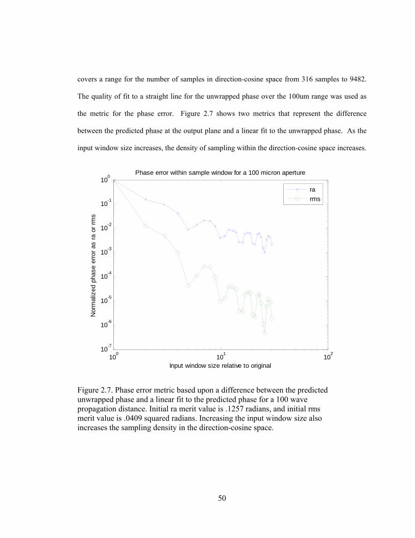
covers a range for the number of samples in direction-cosine space from 316 samples to 9482.

The quality of fit to a straight line for the unwrapped phase over the 100um range was used as

the metric for the phase error. Figure 2.7 shows two metrics that represent the difference

between the predicted phase at the output plane and a linear fit to the unwrapped phase. As the

input window size increases, the density of sampling within the direction-cosine space increases.

100 101 10210-7

10-6

10-5

10-4

10-3

10-2

10-1

100

Input window size relative to original

Nor

mal

ized

pha

se e

rror a

s ra

or r

ms

Phase error within sample window for a 100 micron aperture

rarms

Figure 2.7. Phase error metric based upon a difference between the predicted unwrapped phase and a linear fit to the predicted phase for a 100 wave propagation distance. Initial ra merit value is .1257 radians, and initial rms merit value is .0409 squared radians. Increasing the input window size also increases the sampling density in the direction-cosine space.

50

The definitions for the quality of fit metrics are given in Equations 2.10 and 2.11 where p is the

predicted (unwrapped) phase at the output plane and pmodel is the value of the unwrapped phase

from the best-fit model. The best-fit model is from a linear least squares regression using the

slope and intercept as the model parameters. N is the number of sample points within the 100um

range of interest.

N

ppN

el∑ −=

mod

ra Eq. 2.10

( )

N

ppN

el∑ −=

2mod

rms Eq. 2.11

Figure 2.8 shows the same example using a propagation distance of 10mm instead of 100

waves.

51

100 101 10210-6

10-5

10-4

10-3

10-2

10-1

100

101

102

Input window size relative to original

Nor

mal

ized

pha

se e

rror a

s ra

or r

ms

Phase error within sample window for a 100 micron aperture

rarms

Figure 2.8. Same a Figure 2.7 but for a propagation distance of 10mm. Initial ra merit value is .1101 radians, and initial rms merit value is .0172 squared radians.

Note that the improvement with increasing frequency domain sampling density is not as rapid in

this case. This can be explained in part because the z-term is in the exponential for the

propagation transfer function zie ˆ2πγ which causes a rapidly varying phase term for large

propagation distances. Figure 2.9 shows the value of the slope for the fitted linear phase. Note

that this unstable at the 1% level until the sample window is increased to beyond 2.5 mm in this

case.

52

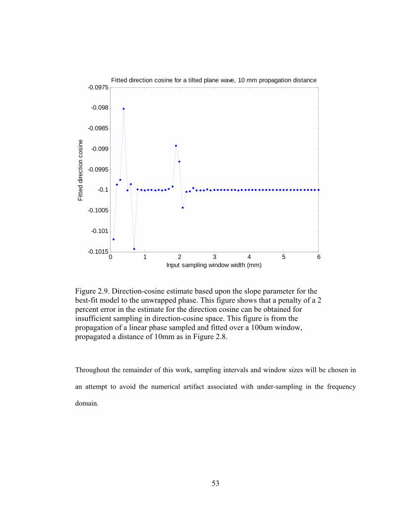
0 1 2 3 4 5 6-0.1015

-0.101

-0.1005

-0.1

-0.0995

-0.099

-0.0985

-0.098

-0.0975Fitted direction cosine for a tilted plane wave, 10 mm propagation distance

Fitte

d di

rect

ion

cosi

ne

Input sampling window width (mm)

Figure 2.9. Direction-cosine estimate based upon the slope parameter for the best-fit model to the unwrapped phase. This figure shows that a penalty of a 2 percent error in the estimate for the direction cosine can be obtained for insufficient sampling in direction-cosine space. This figure is from the propagation of a linear phase sampled and fitted over a 100um window, propagated a distance of 10mm as in Figure 2.8.

Throughout the remainder of this work, sampling intervals and window sizes will be chosen in

an attempt to avoid the numerical artifact associated with under-sampling in the frequency

domain.

53

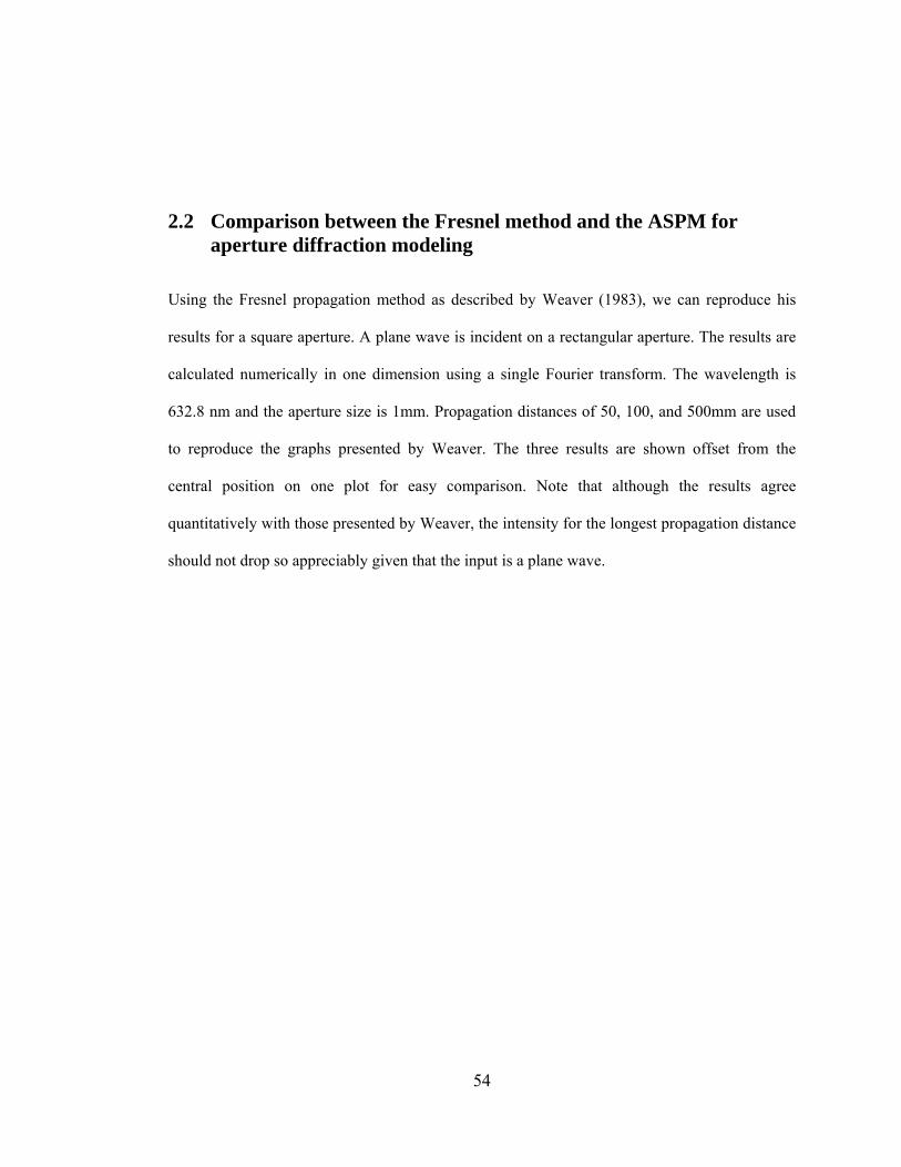
2.2 Comparison between the Fresnel method and the ASPM for aperture diffraction modeling

Using the Fresnel propagation method as described by Weaver (1983), we can reproduce his

results for a square aperture. A plane wave is incident on a rectangular aperture. The results are

calculated numerically in one dimension using a single Fourier transform. The wavelength is

632.8 nm and the aperture size is 1mm. Propagation distances of 50, 100, and 500mm are used

to reproduce the graphs presented by Weaver. The three results are shown offset from the

central position on one plot for easy comparison. Note that although the results agree

quantitatively with those presented by Weaver, the intensity for the longest propagation distance

should not drop so appreciably given that the input is a plane wave.

54

-4 -3 -2 -1 0 1 2 3 40

0.1

0.2

0.3

0.4

0.5

0.6

0.7

0.8

0.9

1 Intensity at 50mm 100mm 500mm propagation distances

Position in mm at the image plane (offset)

Imag

e In

tens

ity re

lativ

e un

its 50mm100mm500mm

Figure 2.10. Fresnel propagation for a 1mm rectangular aperture at 632.8 nm following Weaver (1983). The curves at 50 and 500mm are offset from zero by –2mm and plus 2mm respectively for visibility.

The explanation for this error is in the method that is used to scale the Fourier transform in the

Fresnel calculation. For each new propagation distance, a new spatial coordinate is required. In

fact the spatial coordinate x2 is given by ξλz where ξ is the spatial frequency in the Fourier

domain; z

xλ

ξ 2= . At larger propagation distances (larger z) the output spatial plane has fewer

samples for a given unit length.To compensate for this change in sampling, the intensity needs

to be rescaled by a factor of z. The result of this rescaling is shown in Fig. 2.11.

55

-4 -3 -2 -1 0 1 2 3 40

1

2

3

4

5

6

7

8 Intensity at 50mm 100mm 500mm propagation distances

Position in mm at the image plane (offset)

Imag

e In

tens

ity re

lativ

e un

its 50mm100mm500mm

Figure 2.11. Fresnel propagation for a 1mm wide 1-D aperture showing intensity rescaled by a factor of z. The integrals under all three curves are the same.

The same problem of propagation from a one-dimensional rectangular aperture can be solved

with good agreement using the angular spectrum propagation method (ASPM). The graphical

result showing how the beam profile evolves along the propagation axis is shown in Figure 2.12

together with the results obtained using the Fresnel method. Note that the ASPM method

provides the relative intensities directly, without rescaling. Although the ASPM requires two

Fourier transforms for each propagation problem, in practice there is an advantage over the

Fresnel method if multiple propagation distances are to be investigated. For the ASPM the first

Fourier transform of the input waveform and then one Fourier transform for each propagation

56

distance is needed. Each output plane will have the same sampling interval on the spatial

coordinate. The Fresnel propagation method requires one Fourier transform operation for each

propagation distance, but the sampling interval will be different for every result. If the image

plane is tilted, both methods require Fourier transform operations at each of many propagation

distances in order to determine the structure of the image field along the propagation axis.

-8 -6 -4 -2 0 2 4 6 8 100

0.2

0.4

0.6

0.8

1

1.2

1.4

1.6

1.8

2 Comparison between ASPM and Fresnel at various propagation distances

Position in mm at the image plane (offset for visibility)

Imag

e In

tens

ity re

lativ

e un

its

50 mm ASPM50 mm Fresnel100 mm ASPM100 mm Fresnel500 mm ASPM500 mm Fresnel

Figure 2.12. Angular Spectrum Propagation for a 1mm wide 1-D aperture compared with the Fresnel propagation method for the configuration. Note, that all images are in fact centered at zero, but they are shown offset for visibility. The ASPM images are offset at –3mm and +3mm for the 50mm and 500mm propagation distances respectively.

57

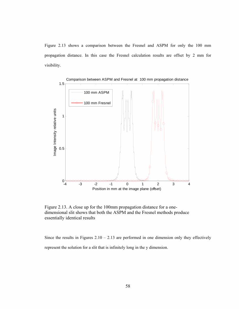
Figure 2.13 shows a comparison between the Fresnel and ASPM for only the 100 mm

propagation distance. In this case the Fresnel calculation results are offset by 2 mm for

visibility.

-4 -3 -2 -1 0 1 2 3 40

0.5

1

1.5 Comparison between ASPM and Fresnel at 100 mm propagation distance

Position in mm at the image plane (offset)

Imag

e In

tens

ity re

lativ

e un

its

100 mm ASPM100 mm Fresnel100 mm Fresnel

Figure 2.13. A close up for the 100mm propagation distance for a one-dimensional slit shows that both the ASPM and the Fresnel methods produce essentially identical results

Since the results in Figures 2.10 – 2.13 are performed in one dimension only they effectively

represent the solution for a slit that is infinitely long in the y dimension.

58

A comparable result is obtained for a two-dimensional square aperture of size 1mm square and

is shown in Figure 2.14. Note the correct prediction of the enhanced intensity at the central zone

for the 500mm propagation distance where edge diffraction from all four aperture edges

contributes to the intensity maximum. The integrals for predicted intensities at both the 100mm

and 500mm propagation distances were found to be equal. The complete two-dimensional

image intensity maps are shown for the 500mm and 100mm propagation distances in Figures

2.15 and 2.16 using a logarithmic gray scale. Figure 2.17 shows the image for a 1mm diameter

circular aperture at a propagation distance of 100mm. The Matlab® code for producing the

image in Figure 2.16 is included in Appendix III.

59

-4 -3 -2 -1 0 1 2 3 40

0.5

1

1.5

2

2.5

3

3.5

4 Intensity at 50 mm 100 mm 500 mm propagation distances

Position in mm at the image plane (offset)

Imag

e In

tens

ity a

rbitr

ary

units

50 mm50 mm100 mm100 mm500 mm500 mm

Figure 2.14. Angular spectrum propagation for a 1mm square aperture showing central slices through the intensity at the image plane. Note the peak intensity increase at the 500mm propagation distance. The three images are shown offset from one another for visibility.

60

mm

alo

ng y

mm along x

Scaled Image Intensity

-2 -1 0 1 2-2

-1.5

-1

-0.5

0

0.5

1

1.5

2

0 2 4-2

-1.5

-1

-0.5

0

0.5

1

1.5

2

Intensity

Figure 2.15. Two-dimensional image from a 1mm square aperture at a propagation distance of 500mm. The image is shown in a gray scale that is proportional to the log of the image intensity. The plot at the right is a central slice profile of the image intensity.

61

mm

alo

ng y

mm along x

Scaled Image Intensity

-1 -0.5 0 0.5 1-1

-0.8

-0.6

-0.4

-0.2

0

0.2

0.4

0.6

0.8

1

0 1 2-1

-0.8

-0.6

-0.4

-0.2

0

0.2

0.4

0.6

0.8

1

Intensity

Figure 2.16. Two-dimensional image from a 1mm square aperture at a propagation distance of 100mm. The image is shown in a gray scale that is proportional to the log of the image intensity. The plot at the right is a central slice profile of the image intensity.

62

mm

alo

ng y

mm along x

Scaled Image Intensity

-1 -0.5 0 0.5 1-1

-0.8

-0.6

-0.4

-0.2

0

0.2

0.4

0.6

0.8

1

0 1 2-1

-0.8

-0.6

-0.4

-0.2

0

0.2

0.4

0.6

0.8

1

Intensity

Figure 2.17. Two-dimensional image from a 1mm circular aperture at a propagation distance of 100mm. The image is shown in a gray scale that is proportional to the log of the image intensity. The plot at the right is a central slice profile of the image intensity. Note that the central intensity drops to near zero.

63

2.3 The application of the Angular Spectrum Propagation Method to Talbot imaging

The Talbot effect or Talbot imaging is the formation of periodic images that result from the

coherent illumination of a periodic structure, (Lohmann, et al. 1986). A grating structure is re-

imaged at various propagation distances away, some of the images are phase reversed where

dark lines in the image correspond to regions where light transmits through the grating structure.

In order to demonstrate the utility of the angular spectrum propagation method, the Talbot

image formation from an amplitude grating was modeled. Goodman (1996 p.87) presents the

analytical solution for Talbot image formation form an amplitude grating. An amplitude grating

has a periodic variation in the amount of light transmittance. Figure 2.18 shows the Talbot

image, the Talbot subimage, and the phase-reversed Talbot image, for an amplitude grating

having a period of 50um. The propagation distances correspond to the locations of the Talbot

images. In this case, the wavelength =λ 632.8 nm and the distance z = 39.5mm. This distance

corresponds to the tenth Talbot image occurring at multiples of the grating period squared

divided by the wavelength: ( ) mm 39.5mm05.102

=× λ . Figure 2.19 shows the result from

modeling a phase grating using the ASPM. The grating period and wavelength are the same as

described above, but in this case, the entire grating is transparent and the optical depth of the

sinusoidal grating grooves is .2 waves. This result demonstrates that the ASPM has utility for

modeling this type of grating where an analytical solution is not easily attained. It is interesting

64

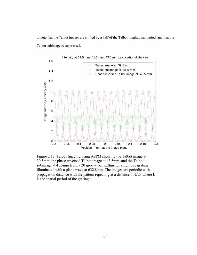
to note that the Talbot images are shifted by a half of the Talbot longitudinal period, and that the

Talbot subimage is suppressed.

-0.2 -0.15 -0.1 -0.05 0 0.05 0.1 0.15 0.20

0.2

0.4

0.6

0.8

1

1.2

1.4

1.6 Intensity at 39.5 mm 41.5 mm 43.5 mm propagation distances

Position in mm at the image plane

Imag

e In

tens

ity a

rbira

ry u

nits

Talbot image at 39.5 mmTalbot subimage at 41.5 mmPhase-reversed Talbot image at 43.5 mm

Figure 2.18. Talbot Imaging using ASPM showing the Talbot image at 39.5mm, the phase-reversed Talbot image at 43.5mm, and the Talbot subimage at 41.5mm from a 20 groove per millimeter amplitude grating illuminated with a plane wave at 632.8 nm. The images are periodic with propagation distance with the pattern repeating at a distance of L2/λ where L is the spatial period of the grating.

65

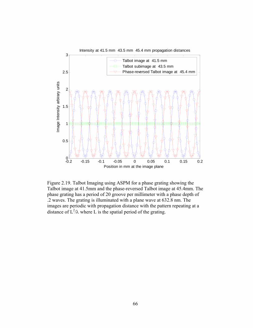
-0.2 -0.15 -0.1 -0.05 0 0.05 0.1 0.15 0.20

0.5

1

1.5

2

2.5

3 Intensity at 41.5 mm 43.5 mm 45.4 mm propagation distances

Position in mm at the image plane

Imag

e In

tens

ity a

rbira

ry u

nits

Talbot image at 41.5 mmTalbot subimage at 43.5 mmPhase-reversed Talbot image at 45.4 mm

Figure 2.19. Talbot Imaging using ASPM for a phase grating showing the Talbot image at 41.5mm and the phase-reversed Talbot image at 45.4mm. The phase grating has a period of 20 groove per millimeter with a phase depth of .2 waves. The grating is illuminated with a plane wave at 632.8 nm. The images are periodic with propagation distance with the pattern repeating at a distance of L2/λ where L is the spatial period of the grating.

66

2.4 Two-beam interference with polarized light described using a modification to the ASPM

Two-beam interference due to the interaction of two coherent beams is another interesting

phenomenon to investigate using the angular spectrum propagation method. Since this method is

capable of handling non-paraxial systems, some care must be given when considering scalar

fields, which do not directly consider the effects of polarization. By investigating a two-beam

interference problem, we can see how the ASPM might be modified to handle the case of

polarized interference.

The basic problem that we will consider is two beams incident on a plane ±30° of the surface

normal. The fringe spacing of the interference field can easily be calculated using Eq. 2.12

( )( ) λλλθ

λ==

°==

5.230sin2sin2d Eq. 2.12

We will consider two cases: (1) where the electric field is perpendicular to the plane of

incidence (TE), and (2) the electric field is in the plane of incidence (TM). The analytical

results for these cases are given in a recent paper by Fan, et al., (2005). For the TE case, the E-

field is in the same plane as the image plane, and the scalar theory handles the one-dimensional

problem properly. For the TM case, the E-field has a component in the image plane as well as

another component perpendicular to the image plane. These two cases are shown in Figures 2.20

and 2.21.

67

Figure 2.20. E-field orientation for two-beam interference in TE case; the fields are perpendicular to the plane of incidence, and are parallel to each other so they add directly.

E1 E2

x

E1

E2

E1z

E2z

E1xE2x

x

Figure 2.21. E-field orientation for two-beam interference in TM case; the incident fields E1 and E2 are in the plane of incidence and are shown with x and z vector components at some instant of time.

To compute the x and z components for the electric field, it is convenient to recall the

definitions for the direction cosines shown in Eq. 2.14.

68

( )θ−°== 90coskkα x Eq. 2.14a

( )θcoskkγ x == Eq. 2.14b

With reference to the Figure 2.22, we can see how the direction cosines may be convenient to

have at our disposal.

x

k

θ kz

kx

z

k

θ

kx

kz

θ E

z

Ex

Figure 2.22. Direction cosine diagram on the left for a plane wave traveling at an angle θ relative to the z axis. The diagram on the right shows the same k vector together with E-field for the TM case.

Using the direction cosines we can decompose the electric field components according to Eq.

2.15.

( ) γθ EEEx == cos Eq. 2.15a

( ) αθ EEE =−°= 90cosz Eq. 2.15b

69

This formula basically amounts to a cosine-weighting factor for the x component of the E-field.

The original and weighted direction-cosine spectrum is shown in Figure 2.23. The z-component

spectrum is the sine complement according to Eq. 2.15b. Both the x and z components are then

propagated to the image plane according to the rules described previously. The image intensity

is computed by the incoherent addition of the x and z components:

**zzxx EEEEI += Eq. 2.16

where is the complex conjugate of .

*xE xE

70

-1 -0.8 -0.6 -0.4 -0.2 0 0.2 0.4 0.6 0.8 10

0.2

0.4

0.6

0.8

1

1.2

direction cosine

Frequency content for two plane waves at 30 degees TM case (magnitude/N2)

Vol

ts/m

eter

Original SpectrumSpectrum of x - componentWeighting Function

Figure 2.23. Original and cosine weighted direction-cosine spectrum for two-beam interference in the TM case. The magnitude of the x-component of the E-field is found multiplication with an angle dependent weighting function given by Eq. 2.15.

Figure 2.24 shows the result for both the TE and the TM case. As expected, the TM case shows

the same fringe period with reduced modulation. For the calculations shown in Figure 2.24, the

sampling interval was 16 samples per wave in the spatial domain to provide for good fringe

visualization. A total of 12,642 samples were used. This was enough to give good numerical

results in the sense that the output still retained good uniform intensity across the field of

calculation even if the propagation direction did not coincide exactly with the sample spacing in

the frequency domain

71

Figure 2.24. Two-beam interference at 632.8 nm with ±30° incident beams showing the reduced fringe contrast for the TM case as compared to the TE case. Note that the average intensity is the same for the two cases.

Although this result demonstrates the capability of the ASPM to handle polarization

calculations, this capability was not used in the remainder of this work.

72

2.5 Axial focal shift for converging beam illumination prediction using the ASPM

Axial focal shift, where there is a difference between the position of the focus as predicted by

scalar optical propagation models and geometric ray trace techniques, was described by

Osterberg, et al. (1961) and Sheppard, et al. (2003). This can be modeled quite well using the

ASPM since this is a scalar optical propagation problem. In Figure 2.25, a forty-wave diameter

circular aperture occludes a converging beam. The angle between the axial line and the line

extending from the geometric focus point to the edge of the aperture is 10 degrees (NA=.174).

The ASPM correctly predicts an axial focal shift of 10 waves towards the aperture from the

geometric focus position as shown in Figure 2.26.

Propagation distance z

= 74 microns or almost120 waves

40 waves diameter aperture

Output image plane

Edge diffraction

Converging beam input

At F# about 3, this system can not be modeled with the Fresnel method

Figure 2.25. Optical layout for converging wave illumination of a circular aperture used to model the axial focal shift with the ASPM.

73

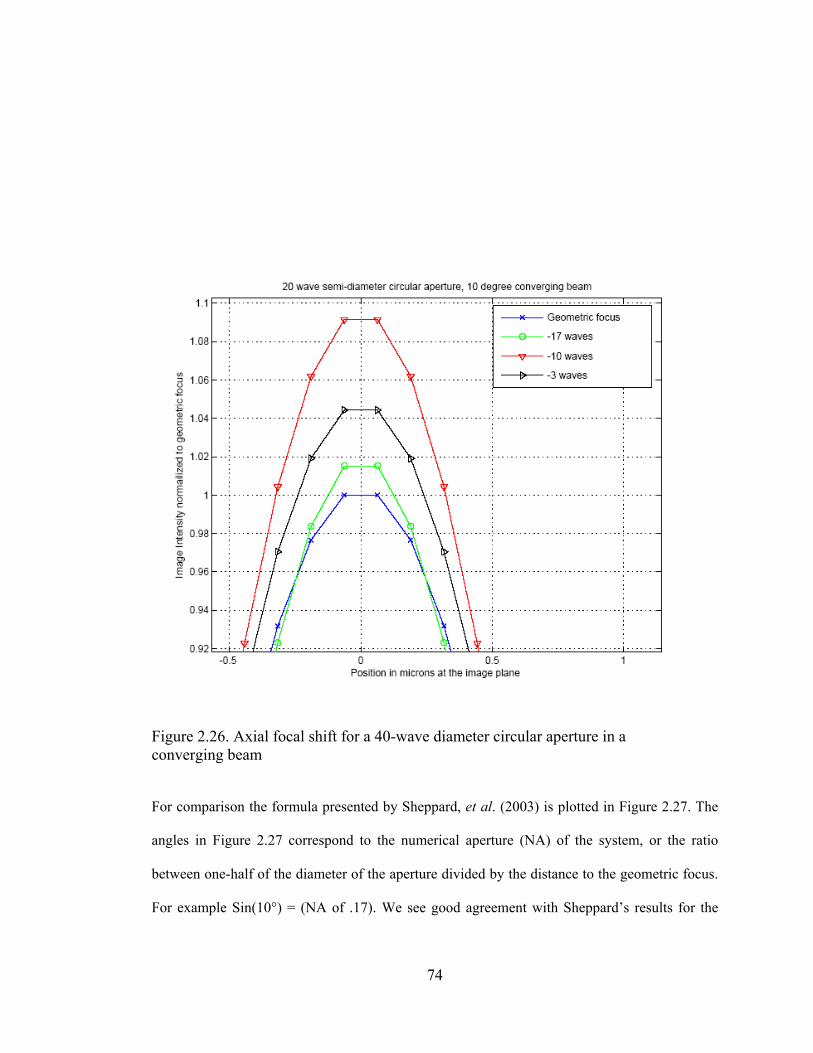
Figure 2.26. Axial focal shift for a 40-wave diameter circular aperture in a converging beam

For comparison the formula presented by Sheppard, et al. (2003) is plotted in Figure 2.27. The

angles in Figure 2.27 correspond to the numerical aperture (NA) of the system, or the ratio

between one-half of the diameter of the aperture divided by the distance to the geometric focus.

For example Sin(10°) = (NA of .17). We see good agreement with Sheppard’s results for the

74

position and the intensity of the predicted focus by noting the peak for the 10 degree curve in

Figure 2.27 occurs at 10 waves inside of the geometric focus with an intensity 10 percent higher

than the geometric focus. This is expected since the ASPM represents a numerical solution to

the scalar diffraction equation.

Figure 2.27. Axial focal shift based on results by Sheppard (2003)

75

2.6 ASPM applied to modeling off-axis converging beam illumination with high NA

To further demonstrate the power of the ASPM for computing imaging problems, an off- axis

converging spherical beam was used to illuminate a 1-D rectangular aperture. The aperture

width was 8mm and the propagation distance about 10mm, having an off-axis angle of 45°, the

working F# is about 2.5. Illumination wavelength λ=632.8nm should place the first 1-D Airy

minimum at 1.58um.

microns 1.582.5*.6328 F# MinimumAiryFirst === λ Eq. 2.17

Since our image position is 45° off the optical axis, the effective F# is increased by .7 as is the

first Airy minimum. Figure 2.28 shows this predicted result for the central image at a

propagation distance of 10mm.

If we wanted to know the image structure on a tilted plane perpendicular to the central ray

propagation direction, we would need to calculate the image at many propagation distances in

order to sample the image at many positions on the tilted image plane. The example in Figure

2.28 shows the image plane at three different propagation distances; 9.9mm, 10mm and

10.005mm. Many authors (Leseberg, 1992) (Tommasi, et al., 1992) (Delen, et al., 2001)

(Kurzweg, et al.. 2001), (Matsushima, et al., 2003), and (De Nicola, et. al., 2005) have

investigated the possibility of rotating the direction-cosine space by using simple coordinate

transforms to find the propagated fields on tilted planes. Due to the fact that the coordinate

rotation transformation operation is not linear, it is not possible to use a Fourier transform to

recover the output field. Matsushima et al. (2003) suggests a cubic-spline interpolation to

recover the samples at equal spacing in the Fourier domain. For the remainder of this work, we

76

deal only with parallel input and output planes. If the desired output plane is tilted with respect

to the input plane, it is necessary to perform the calculation for many propagation distances and

extract the data for the tilted plane from the larger dataset.

9980 9985 9990 9995 10000 10005 10010 10015 10020

0

200

400

600

800

1000

1200

1400

1600

1800

Intensity at 9.990 mm 10.000 mm 10.005 mm propagation distances

Position in microns at the image plane

Imag

e In

tens

ity a

rbitr

ary

units

9.99 mm10 mm10.005mm

Figure 2.28. Off-axis converging illumination through a rectangular aperture.

77

3 Results In this section, the angular spectrum propagation method is used to model the image formation

from diffraction gratings. In the first case, a simple planar grating is illuminated with two beams

and the moiré Fringe phenomenon is predicted. In the second case, a planar grating structure

with imaging characteristics such as can be produced using the holographic method is placed in

the aperture plane. The field immediately after the aperture plane is propagated to the image

plane located 30mm away. The resulting image is compared to spot diagrams generated from

ray trace results for the same grating component modeled in ZEMAX.

3.1 Moiré fringe phenomenon description and modeling using the Angular Spectrum Propagation Method

Moiré fringes can be understood by thinking of the diffraction grating as a beam combiner. Two

beams incident on a diffraction grating can be made to propagate along the same direction after

diffraction. By only having a small difference in propagation direction for the two beams, an

interference pattern will result giving rise to a coarse fringe pattern. Soares (1979) described this

technique for repositioning holograms.

In our case, we will use a grating with 205 groove/mm illuminated with a super-gaussian beam

with an aperture diameter of roughly 10mm. Using the Littrow grating equation in second order

and an illumination wavelength of 488 nm:

78

( )( )( ) 1.2

205.488.2sin2

=== αλd

m Eq. 3.1

Using the same incident angle we can propagate the first order in the direction normal to the

surface of the grating.

( )( ) 01.205.488.sinsin =−==− βαλd

Eq. 3.2

Figure 3.1 shows the result of propagating a single beam from the diffraction grating. The

propagation distance was chosen to be 120mm to avoid overlap between the various propagating

orders.

79

Zero

order

First

orderSecond

order

Littrow

Figure 3.1. Illumination pattern from a diffraction grating illuminated with λ=488 nm using a super-gaussian beam.

It is interesting to note the relative intensities of the diffracted orders in Figure 3.1. PC-Grate, a

commercial program that is capable of calculating diffraction efficiency was used to model the

same grating in the same geometry, using TE polarization (electric vector parallel to the

grooves) and perfect conductivity for the surface (No Fresnel reflection losses.) The results of

this calculation are shown in Table 3.1 with the diffraction efficiencies normalized to the zero

order diffraction efficiency to enable direct comparison to Figure 3.1. Though there is generally

80

good agreement between the two results, no claims are made here with regard suitability of

ASPM for calculating diffraction efficiencies for real diffraction gratings.

Order PC Grate Absolute

PC Grate Normalized From Figure3.1

2 (Littrow) 0.04 0.12 0.12 1 0.28 0.86 0.86 0 0.33 1.00 1.00 -1 0.28 0.85 0.85

Table 3.1. Diffraction efficiencies calculated in PC Grate for a perfectly conducting 205 groove per mm grating in second order Littrow at 488 nm

Starting with the same geometry described above, with a second illumination beam approaching

from the opposite side of the grating surface normal will produce two beams propagating in the

direction normal to the surface as shown in Figure 3.2. Each beam is displaced in angle by .1%,

or one part in one thousand, for a difference of two parts per thousand for the two co-

propagating beams. This angular misalignment is observed in the fringe pattern of Figure 3.3 by

noting that there are two moiré fringes in 5mm, a period that spans 1000 grooves on the surface.

For these calculations, one sample per wave was used in the spatial dimension with an 80mm

sample window, or approximately 164,000 samples. This example demonstrates the utility for

the ASPM to predict diffraction effects that cannot be modeled using geometric ray trace

techniques.

81

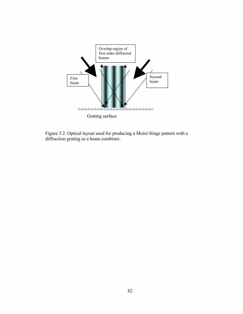
Second beam

First beam

Overlap region of first order diffracted beams

Grating surface

Figure 3.2. Optical layout used for producing a Moiré fringe pattern with a diffraction grating as a beam combiner.

82

Figure 3.3. Moiré pattern from a diffraction grating illuminated with 488 nm

83

3.2 Holographic diffraction grating image formation predicted using the ASPM

The holographic diffraction grating with imaging properties will be described according to the

same method discussed previously. Two diverging spherical waves will interfere to form a

groove pattern on a planar substrate. Typically the substrate is coated with a photoresist that can

be developed after exposure to produce a structured pattern on the surface. We will assume a

perfectly linear development response to the intensity modulation. The spherical wave from

each point source is:

r

ikreErE o=)( Eq. 3.3

The time dependence has been suppressed and the two sources are assumed to have a fixed

phase relationship so the light is coherent. The variable r represents the distance between the

source point and each point on the surface. The two values of E(r) (one from each source) are

combined coherently to compute the intensity on the surface, the asterisks indicates the complex

conjugate.

( )( )*2121 EEEEI ++= Eq. 3.4

To find the intensity modulation on the surface, the average intensity is found first by combining

the same two beams incoherently

( )( ) ( )( )*22

*11 EEEEI avg += Eq. 3.5

The modulation is found by subtracting the average intensity from the modulated intensity.

84

( )avgIII −=mod Eq. 3.6

This value is scaled to produce a surface height function that ranges from zero to one. A

resulting groove pattern is shown in Figure 3.4. A synthetic wavelength of 100 times the

recording wavelength was used to generate the plot in Figure 3.4 in order to produce a readable

plot. The groove spacing is seen from the plot to be four grooves per millimeter. At the actual

recording wavelength of 488 nm, the real groove frequency at the center is 403.5 grooves per

mm. Note that the groove pattern is curved; this is what produces the focal properties of the

hologram. A region of only 2mm x 2mm is shown. The actual ZEMAX calculations were based

on a 5x5 mm square region. The ASPM modeling was only performed for the 5-mm-wide 1-D

grating in the dimension perpendicular to the grooves.

85

Gro

ove

heig

htin

wav

es

Figure 3.4. Model of a groove pattern on a 2mm square patch of the grating surface shown with 100x horizontal scale magnification in order enhance the visibility of the groove structure. The groove depth was normalized to be .1-wave deep at 632.8 nm. Note how the groove pattern is curved, this is what leads to the focusing properties of holographic diffraction gratings.

Table 3.2 summarizes the specification for the grating hologram component including the

construction and reconstruction geometry. A plane wave was chosen as the reconstruction

source to make the problem similar to the component that was described previously in sections

1.4 and 1.5. The ASPM technique is equally capable of modeling other than plane-wave inputs.

The geometry in Table 3.2 is the result of an optimization process in ZEMAX where the

86

Reference and Object points were allowed to vary to produce a minimum rms spot size in the

focal plane at all three wavelengths of 600, 632.8 and 665.6 nm. All three wavelengths will be

modeled using both ZEMAX and the ASPM.

Table 3.2

Recording wavelength = 488 nm Reconstruction wavelength = 632.8 nm u =1 for diverging source, -1 converging source, 0 source at infinity Q X (mm) Y (mm) Z (mm) u R Reference 11.190 0.0 36.341 1 O Object 51.901 0.0 530.464 1 C reconstruction 476196 0.0 9988660 0 (plane-wave) I Image 9.543 0.0 30 1

Table 3.2. Grating parameters for planar hologram for modeling using the ASPM

Figure 3.5 shows the result of the ZEMAX optimization for the rms spot radius. In this case an

equal weighting was given to all three wavelengths during the optimization process. After

optimization, the rms spot radius is best at the center wavelength, and larger but nearly equal at

the two extreme wavelengths. This result is qualitatively similar to the result of the planar

hologram described in section 1.5. It is not possible to obtain good imaging at multiple

wavelengths on a plane that is parallel to the hologram for a planer hologram produced with

spherical waves.

87

Figure 3.5. Rms spot radius for ZEMAX optimized planar holographic grating that was modeled using the ASPM. This plot represents the merit function variable that was given equal weighting at all three wavelengths. The result is that the imaging is pretty good at the central wavelength and equally bad at the two extremes

88

The optical layout is shown in Figure 3.6 where the zero-order reflection is shown for reference.

Note that the central wavelength of 632.8 nm comes to a tight focus at the image plane, the short

wavelength (600 nm) comes to focus beyond the image plane, and the long wavelength (665.6

nm) comes to focus in front of the image plane. Once again, this is very similar to the results for

a planar hologram described in section 1.4.

We can find the position of the 632.8 nm wavelength in the focal plane by using the grating

equation with the central-order groove frequency of 403.5 grooves/mm to find the diffraction

angle when the incident angle is (–2.73) degrees.

( )( ) 3030.)73.2sin(4035.6328.sinsin =°−−=−= αλβd

Eq. 3.7

To find the image position, we can take the tangent of this angle and multiply by the

propagation distance of 30mm to obtain 9.54mm.

89

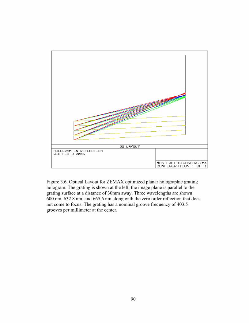
Figure 3.6. Optical Layout for ZEMAX optimized planar holographic grating hologram. The grating is shown at the left, the image plane is parallel to the grating surface at a distance of 30mm away. Three wavelengths are shown 600 nm, 632.8 nm, and 665.6 nm along with the zero order reflection that does not come to focus. The grating has a nominal groove frequency of 403.5 grooves per millimeter at the center.

90

The through-focus spot diagram in Figure 3.7 indicates a shift of ±2mm for the position of the

image plane for best focus at the extreme wavelengths.

Figure 3.7. Through focus spot diagram for ZEMAX optimized holographic grating indicating a plus or minus two millimeter shift in the image plane position is required to bring the extreme wavelengths into focus.

91

The spot diagram at the central wavelength of 632.8 nm is shown in Figure 3.8. Note the total

spread is approximately 20um and that the image appears to have a coma aberration.

Figure 3.8. Spot diagram at 632.8 nm in the image plane for the planar hologram.

To model this grating component using the ASPM, a 5-mm-wide slice in the direction

perpendicular to the grooves was chosen. Given a grating groove period of 2.5um, Nyquist

sampling would be 1.25um, four times Nyquist would be approximately two samples per wave

92

at 632 nm. The result with this spatial frequency sampling and two times zero padding (31,606

samples total) is shown in Figure 3.9.

Figure 3.9. Image intensity at 632.8 nm at the focal plane using 10mm wide sample window (2x zero padding) and four time Nyquist sampling. The image position is not correct and is aliased because the image falls outside of the sampling window.

Note that the image does not appear in the correct position in Figure 3.9. The output spatial

sampling window is too narrow.

93

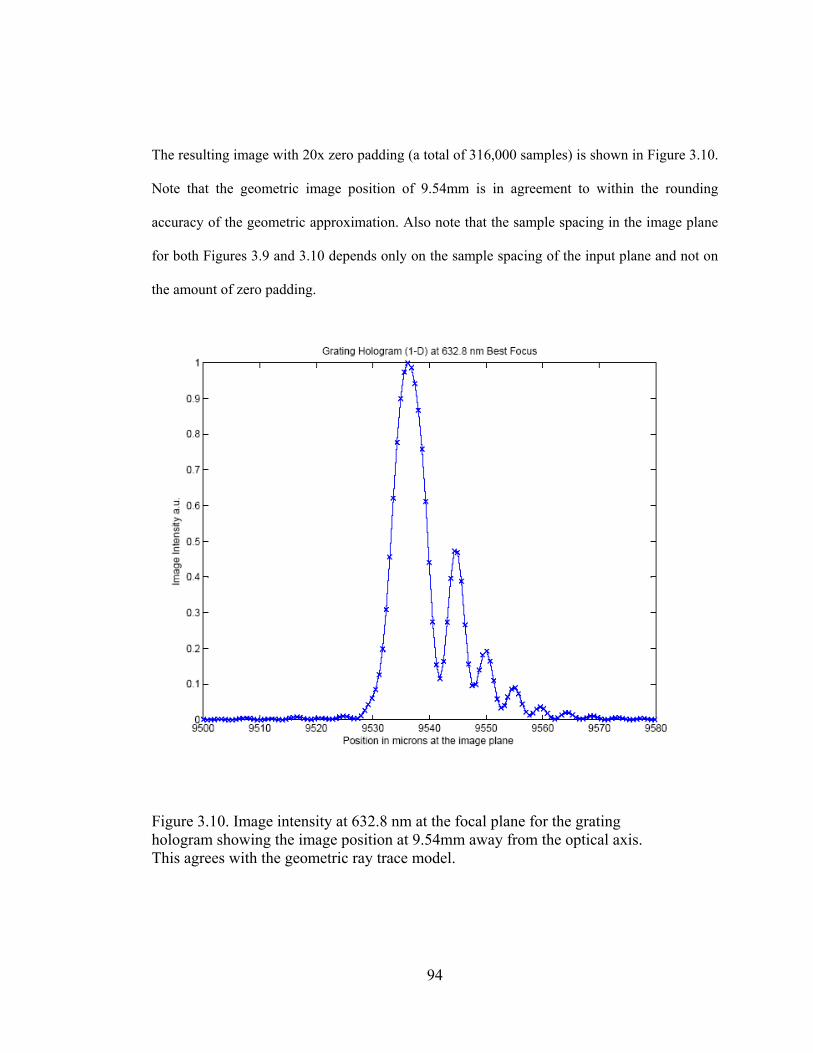
The resulting image with 20x zero padding (a total of 316,000 samples) is shown in Figure 3.10.

Note that the geometric image position of 9.54mm is in agreement to within the rounding

accuracy of the geometric approximation. Also note that the sample spacing in the image plane

for both Figures 3.9 and 3.10 depends only on the sample spacing of the input plane and not on

the amount of zero padding.

Figure 3.10. Image intensity at 632.8 nm at the focal plane for the grating hologram showing the image position at 9.54mm away from the optical axis. This agrees with the geometric ray trace model.

94

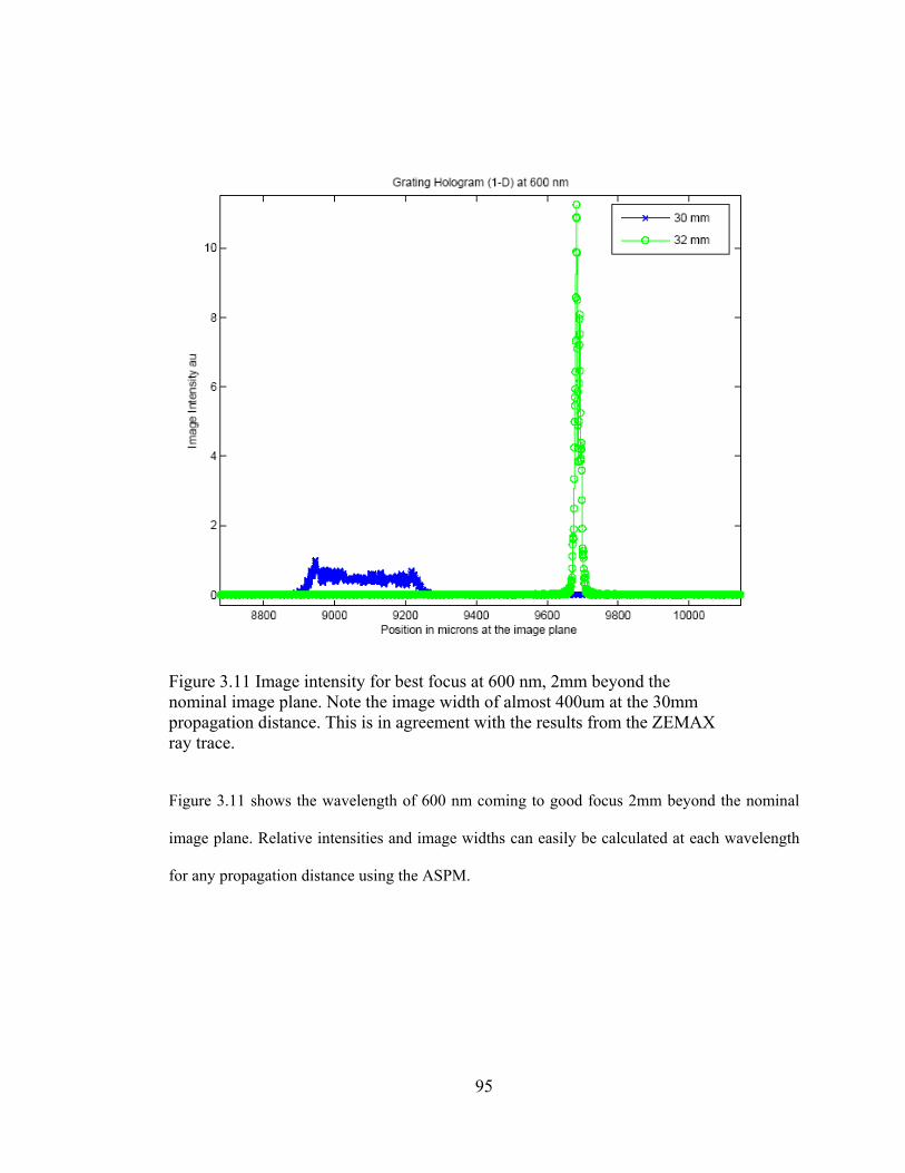
Figure 3.11 Image intensity for best focus at 600 nm, 2mm beyond the nominal image plane. Note the image width of almost 400um at the 30mm propagation distance. This is in agreement with the results from the ZEMAX ray trace.

Figure 3.11 shows the wavelength of 600 nm coming to good focus 2mm beyond the nominal

image plane. Relative intensities and image widths can easily be calculated at each wavelength

for any propagation distance using the ASPM.

95

Figure 3.12. Image intensity at 665.6nm at the focal plane and plus 2mm

A similar result is seen in Figure 3.12 for the 665.6nm wavelength where the approximate best

focus is now 2mm before the nominal image plane at a propagation distance of 28mm.

96

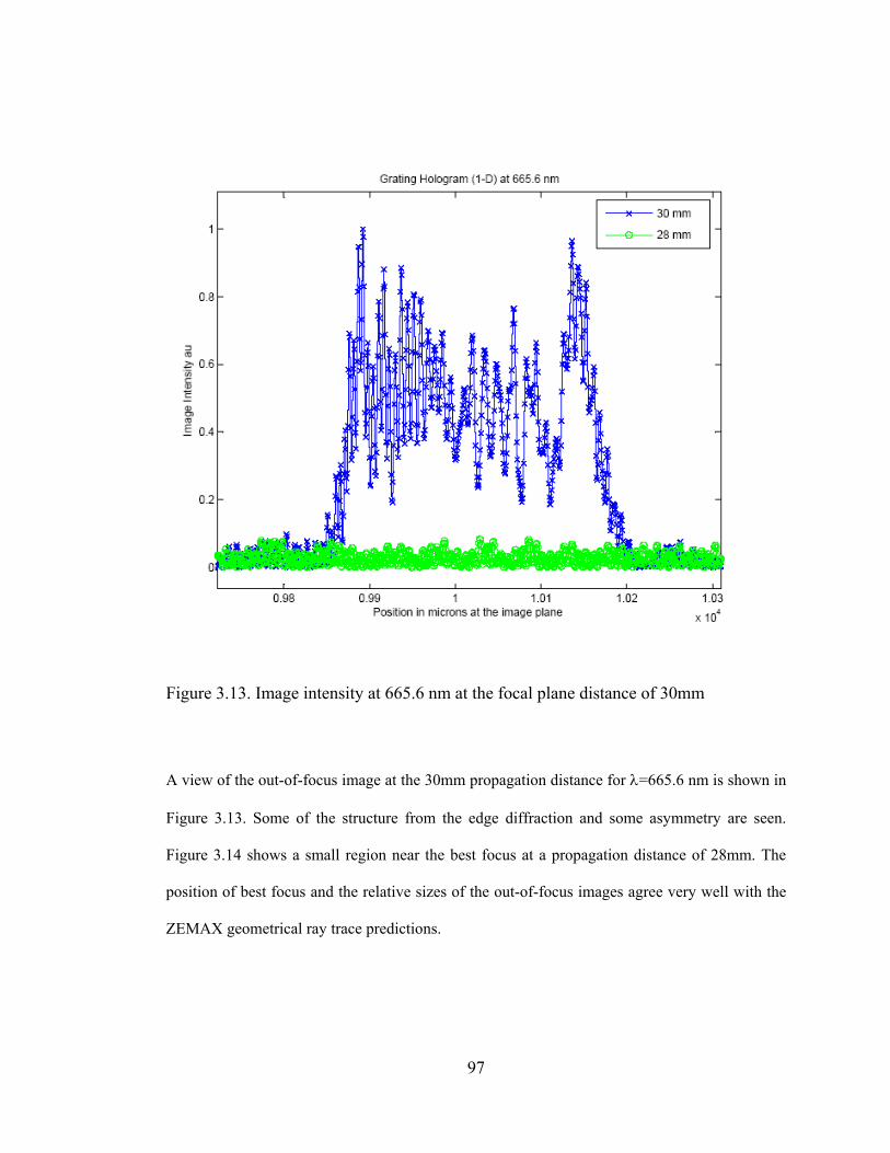
Figure 3.13. Image intensity at 665.6 nm at the focal plane distance of 30mm

A view of the out-of-focus image at the 30mm propagation distance for λ=665.6 nm is shown in

Figure 3.13. Some of the structure from the edge diffraction and some asymmetry are seen.

Figure 3.14 shows a small region near the best focus at a propagation distance of 28mm. The

position of best focus and the relative sizes of the out-of-focus images agree very well with the

ZEMAX geometrical ray trace predictions.

97

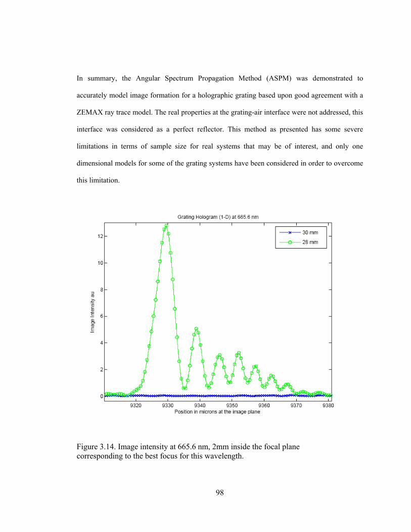
In summary, the Angular Spectrum Propagation Method (ASPM) was demonstrated to

accurately model image formation for a holographic grating based upon good agreement with a

ZEMAX ray trace model. The real properties at the grating-air interface were not addressed, this

interface was considered as a perfect reflector. This method as presented has some severe

limitations in terms of sample size for real systems that may be of interest, and only one

dimensional models for some of the grating systems have been considered in order to overcome

this limitation.

Figure 3.14. Image intensity at 665.6 nm, 2mm inside the focal plane corresponding to the best focus for this wavelength.

98

4 Conclusions and discussion The analytical angular spectrum propagation method was presented for scalar optical fields to

model imaging systems that use holographic gratings. The key factors and assumptions that

allow for this analysis are that plane waves are solutions to the linear Helmholtz equation and

that the Helmholtz equation adequately describes scalar optical fields. Furthermore, we assumed

that physical optical fields could be decomposed using Fourier analysis into plane-wave

components with complex amplitude coefficients. This technique is able to accurately predict

many scalar optical propagation and diffraction phenomena that cannot be accurately predicted

using geometric ray trace techniques.

Discrete numerical computations using the discrete and fast Fourier transform were developed

in Matlab® to implement the angular spectrum propagation method. Special care needs to be

given to the sampling interval in the spatial domain to accurately sample the smallest features of

the input field, such as those features produced by diffraction gratings. A sampling interval of a

half wave was found to be adequate for all propagating waves. Evanescent wave fields were not

considered. Also, the sampling interval in the direction-cosine space (spatial frequency domain)

needs to be sufficiently fine to accurately describe the propagating wave fields. An rms fit

metric was investigated to determine whether a sufficient amount of sampling was selected.

Sufficient sampling was achieved by padding the input array in the spatial domain with zeros

and observing the effect on the calculated propagated fields.

99

Comparisons were also made to the Fresnel propagation algorithm and it was found that the

angular spectrum propagation method has some desirable features. The angular spectrum

propagation method has the ability to accurately model high-numerical-aperture non paraxial

systems, and the spatial sampling intervals are the same in the input and output planes. Both

features indicate that the ASPM is desirable in some applications. It was also found that the

numerical algorithms for the ASPM in GLAD® and ZEMAX® utilize limiting approximations

that are only valid in the paraxial zone and do not follow the angular spectrum method outlined

by Goodman.

One limitation of this method is that very large arrays may be required to fully model some real

systems. In the example, a 5mm square diffraction grating with nominally 400 grooves per

millimeter could not be modeled in two dimensions using the standard features of a single

processor desktop computer. A one dimensional model of this system was compared with the

geometric ray trace results produced in ZEMAX® and the two methods agreed in all significant

respects with the ASPM predicting some aperture diffraction effects that could not be modeled

using geometric ray trace techniques.

100

5 Appendix I

5.1 Zemax Lens Data entry for modeling a holographic grating This appendix contains a table that describes the ZEMAX lens data entry for modeling and

optimizing the holographic gratings described in Section 1.5.

Table 5.1

Surface # Type Thickness (mm) Glass Semi-Diameter Tilt (degrees)0 STANDARD Infinity 1 COORDBRK -10.00 2 HOLOGRM1 MIRROR 40 3 COORDBRK 300 9.99 4 COORDBRK 5 STANDARD 0.24 Hologram Recording Coordinates X1 55.785 Y1 0 Z1 331.296 X2 -250.655 Y2 0 Z2 2450.212 Recording Wavelength 488 nm Diffraction Order 1 Table 5.1. Summary of surface data for the Verboven holographic grating. This data is entered into the ZEMAX Lens Data Editor. Note that the surface type for the holographic grating is the ZEMAX standard HOLOGRAM1 surface type.

101

6 Appendix II

6.1 Matlab® code for calculating phase from a complex number array

This Matlab® code segment to compute the phase of a complex number

If the input complex number is an array of 1 x n, then the output will also be 1 x n.

function p = myphase(U) % This function to calculate the phase of the input % return values in the range of - pi to pi % % Input U complex scalar field % % Output p = phase of the input signal % Separate the real and imaginary parts ru = real(U); iu = imag(U); % sr is the sign of the real part sr = sign(ru); % only adjust in Q2 or Q3 when the real part is negative sr(find(sr==1))=0; % add pi if the imaginary part is positive si = sign(iu); % nz is the index to the non-zero elements of % the real part nz=find(ru~=0); % zi is the index to the zero elements of the real part zi=find(ru==0); % Compute the phase for the elements where the % real part is non-zero. p(nz) = atan(iu(nz)./ru(nz)) - sr(nz).*si(nz)*pi; % if the real part is zero, then the phase is % either +/- pi/2 p(zi) = sign(iu(zi))*pi/2;

102

6.2 Matlab® code for unwrapping phase

This Matlab® code segment to unwrap phase

The input and outputs are arrays of size 1 x n.

function u = myunwrap(p) % This function to calculate unwrap the phase % given by the input % % Input p = phase of the input signal range % from -pi to pi % % Output u = unwrapped phase % % compute the difference between each array value d = diff(p); % find the index for the declining values where % the phase step is greater than pi didx = find(d>pi); % note length of the input array lp = length(p); % copy the input u = p; % subtract 2pi starting at each declining index to the % end of the array for n=1:length(didx) u(didx(n)+1:lp)=u(didx(n)+1:lp)-2*pi; end % find the index for the increasing values where % the phase step is less than pi iidx = find(d<-pi); % add 2pi starting at each increasing index to the end % of the array for n=1:length(iidx) u(iidx(n)+1:lp)=u(iidx(n)+1:lp)+2*pi; end

103

7 Appendix III This appendix includes the Matlab® code for calculating the diffraction and propagation form a square aperture using the angular spectrum propagation method.

7.1 Matlab® code for calculating the image from a two-dimensional square aperture

% asmethodf.m % angular spectrum, plane wave propagation % % This code written by Thomas Blasiak % copyright Thomas Blasiak 2006 % copyright Rochester Institue of Technology 2006 % define constants two_pi = 2*pi; lambda=.6328; % in microns HeNe red wavelength %1 mm normalized aperture dimension appdia = 1000/lambda; % zero padding in the spatial plane zero_pad=16; % dimensionless spatial extent of the input plane x_size = appdia*zero_pad; % samples per wave % a value of two here corresponds to % a direction cosine of one % since this is a paraxial problem the frequency % domain is centered around zero (+/- .025) samps_per_wave = .05; % find the integer number of samples nsamp=floor(x_size*samps_per_wave); % make the number of samples even in the case % when it is not already even if(mod(nsamp,2)==1) nsamp = nsamp+1; end % make the problem symmetric nsampx = nsamp; nsampy = nsamp; % set up the spatial sampling on the input plane %

104

% note that x is dimensionles % to obtain microns,multiply by lambda xa = ((0:(nsamp-1))/(nsamp-1)-.5)*x_size; % this is a two-D array of sample locations % symmetric in this case [x,y] = meshgrid(xa,xa); %This is the sampling frequency in the dimensionless % patial variable dx = x(1,2)-x(1,1); dy = y(2,1)-y(1,1); % report the value in microns dx*lambda dy*lambda % find the nyquist limit based upon the padded sample width nqx = nsampx/2; nqy = nsampy/2; % and the frequency step freq_stepx = 1/(nsampx*dx); freq_stepy = 1/(nsampy*dy); % The frequency goes from the nyquist limits equally spaced fx = (-nqx:(nqx-1))*freq_stepx; fy = (-nqy:(nqy-1))*freq_stepy; % make this a two-D array as well % note that % fxa is the alpha direction cosine % fya is the beta direction cosine [fxa,fya]=meshgrid(fx,fy); % compute the z direction cosine (also gamma) fz = sqrt(1-fxa.^2-fya.^2); % define the field at the input plane % rectangular aperture with normally incident plane wave up1 = rect2(x/appdia,y/appdia).*exp(-two_pi*0*x); % if you want to see the input uncomment the following %figure %surf(x*lambda/1000,y*lambda/1000,up1.*conj(up1)) %title('This is the input') %xlabel('x in mm') %ylabel('y in mm') % s1 is the angular spectrum of the input s1 = fftshift(fft2(up1)); % show a slice of the real part of the spectrum

105

figure stem(fx,real(s1(nsampx/2,:))); xlabel('direction cosine') title('This is a central slice frequency content of the input') % prepare for the next plot figure % Colors for plotting cp=['b','g','r','k','c'] % v is an array of propagation distances in waves v = ([500000,100000])/lambda; for n = 1:length(v) zprop=v(n); % band limit the propagation transfer function prop = exp(i*two_pi*zprop*fz).*(abs(fxa.^2+fya.^2)<1); % this is the output angular spectrum oas1 = s1.*prop; % compute the output by inverse fourier transform % ui1 represents the optical disturbance at the image ui1 = ifft2(fftshift(oas1)); % compute a value proportional to the intensity Inten = ui1.*conj(ui1); % Show a slice through the result % offset each value plot(x(nsampx/2+1,:)*lambda/1000+2*n-4,... Inten(nsampx/2+1,:),strcat(cp(n),'-')) % Overlay all the plots if n==1 hold % and add the title title_string = sprintf('%5.0f mm',v*lambda/1000) title_string = strcat(' Intensity at',...

title_string,' propagation distances') title(title_string) % and the axis labels xlabel('Position in mm at the image plane (offset)') ylabel('Image Intensity arbitrary units') % show a limited region axis([-4 4 0 4]) end

106

end % show the intensity result for the last value % in log grayscale m = myplotgray(xa/1000,xa/1000,Inten,2) % compute the discrete intensity inegral sum(sum(Inten))

107

7.2 Matlab® code for plotting two-dimensional gray scale image Matlab® code segment for plotting a two dimensional intensity map in log gray scale. function m=myplotgray(cx,cy,lni,cl) % this funtion to plot a gray scale image % % Inputs % cx,cy = 1-d coordinate arrays for plotting % lni = Intensity map % cl = coodinate limits for plotting % % output m not used, just a place holder %make the lowest value unity so the log will go to zero lni=lni-min(min(lni))+1; %take the log and make the range 0:255 lni=log(lni); lni=lni*255/max(max(lni)); % show the image figure image(cy,cx,lni') % Invert the plotting axes axis xy % label it ylabel('mm along y') xlabel('mm along x') grid title('Scaled Image Intensity') % set the graph limits axis([-cl cl -cl cl]) %make a grayscale colormap (intensity weighted) cm=(0:255)/255; cm=exp(-5*cm); a=[cm' cm' cm']; colormap(a); % output assignment m=1;

108

8 References [Abramowitz, 1969] Abramowitz, I.A., “Evaluation of hologram imaging by ray

tracing”, Applied Optics, Volume 8, Number 2, February 1969, pp403-410

[Bracewell, 1986] Bracewell, Ronald N., “The Fourier transform and its applications”, McGraw-Hill , 1986

[Champagne, 1967] Champagne, Edwin B., “Nonparaxial Imaging, Magnification, and Aberration Properties in Holography”, Journal of the Optical Society of America, Volume 57 No. 1, January 1967, pp51-55

[Choi, et al. 2005] Choi,Kyongsik, Kim,Hwi, Lim,Yongjun, Kim,Seyoon, Lee,Byoungho, “Analytic design and visualization of multiple surface plasmon resonance excitation using angular spectrum decomposition for a gaussian input beam”,Optics Express, Volume 13 Number 22, October 2005, pp8866-8874.

[Delen, 2001] Delen, Nuri, Hooker, Brian, “Verification and comparison of fast Fourier transform-based full diffraction method for tilted and offset planes”, Applied Optics, Volume 40 Number 21, July, 2001 pp3525-3531

[De Nicola, et al., 2005] De Nicola, S., Finizio, A., Pierattini,G., Ferraro, P., Alfieri, D.,”Angular spectrum method with correction of anamorphism for numerical reconstruction of digital holograms on tilted planes” , Optics Express Volume 13, Number 24, November 2005, pp. 9935-9940.

[Fan, 2005] Fan, Y., Bourov, A., Zavyalova, L., Zhou, J., Estroff, A., Lafferty, N., Smith, B.W., "ILSim - A compact simulation tool for interferometric lithography", Proc. SPIE 5754, (2005)

[Fienup, 1999] Fienup,J.R. “Phase retrieval for undersampled broadband images”, Journal of the Optical Society of America Vol 16 1999 pp 1831-1839.

[Furlong, et al., 2003] Furlong, C, Pryputniewicz,R.J. “Optoelectronic characterization of shape and deformation of MEMS accelerometers used in transportation applications”, Optical Engineering, Vol 42 No 5, 2003 pp1223-1231.

[Goodman, 1968] Joseph W. Goodman, “Introduction to Fourier Optics” McGraw- Hill, First Edition, 1968

[Goodman, 1996] Joseph W. Goodman, “Introduction to Fourier Optics” McGraw- Hill, Second Edition, 1996

[Harvey, et al.,2003] Harvey, James E., Bogunovic, Dijana, Krywonos, Andrey, “Aberrations of diffracted wave fields: distortion”, Applied Optics, Vol 42, Number 7, March 1, 2003, pp1167-1174

109

[Hutley, 1982] Hutley, M.C., Diffraction gratings, Academic Press, 1982

[Kowarz, 1995] Kowarz, Marek W., “Homogeneous and evanescent contributions in scalar near-field diffraction” Applied Optics, Volume 34, Number 17, 1995, pp3055-3063

[Kurzweg, et al., 2001] Kurzweg, Timothy P., Levitan, Steven P., Martinez, Jose A., Kahrs, Mark, Chiarulli. Donald M., “An Efficient Optical Propagation Technique for MEM Simulation” Nanotech, Volume 1, 2001, pp352-355

[Kurzweg, 2002] Kurzweg, Timothy P, “Optical Propagation Methods for System Level Modeling of Optical MEM Systems”, Phd Dissertation, University of Pittsburg, Electrical Engineering, 2002

[Kreis, 2005] Kreis,Thomas, Handbook of Holographic Interferometry, Wiley-VCH 2005

[Lalor, 1968] Lalor, Eamon, “Conditions for the Validity of the Angular Spectrum of Plane Waves” Journal of the Optical Society of America, Vol. 58 No.9, September 1968, pp 1235-1237

[Latta , 1971] Latta, J. N. “Fifth-Order Hologram Aberrations”, Applied Optics, Volume 10, No.3, March 1971, p666-667

[Leseberg, 1992] Leseberg, Detlef, “Computer-generated three-dimensional image holograms” Applied Optics Volume 31 Number 2 January 1992 pp223-229

[Loewen et al., 1997] Loewen, Erwin G., Popov, Evgeny, Diffraction Gratings and Applications, Marcel Dekker, 1997

[Lohmann, et al., 1989] Lohmann, Adolf, Marathay, Arvind, “About periodicities in 3-D wavefields”, Applied Optics Volume 28, Number 20 October 1989, pp4419-4423.

[Matsushima et al. 2003] Matsushima, Kyoji, Schimmel, Hagen, Wyrowski, Frank, “Fast calculation method for optical diffraction on tilted planes by use of the angular spectrum of plane waves”, Journal of the Optical Society of America, Volume 20, Number 9, September 2003, pp 1755-1762

[Mellin, et al., 2001] Mellin, Stephen D., Nordin, Gregory P., “Limits of scalar diffraction theory and an iterative angular spectrum algorithm for finite aperture diffractive optical element design”, Optics Express Volume 8, Number 13, June 2001, pp705-722.

[Noda et al. 1974] Noda, H., Namioka, T., Seya, M., “Geometric theory of the grating”, Journal of the Optical Society of America, Volume 64,Number 8, August 1974, pp1031-1036

110

[Noda et al. 1974] Noda, H., Namioka, T., Seya, M., “Ray tracing through holographic gratings”, Journal of the Optical Society of America, Volume 64,Number 8, August 1974, pp1037-1042

[Noda et al. 1974] Noda, H., Namioka, T., Seya, M., “Design of holographic concave gratings for Seya-Namioka monochrometers”, Journal of the Optical Society of America, Volume 64,Number 8, August 1974, pp1043-1048

[Osterberg, et al., 1961] Osterberg, Harold, Smith, Luther, “Closed solutions of Rayleigh’s diffraction integral for axial points”, Journal of the Optical Society of America, Volume 51, Number 10, Ocotober 1961,pp 1050-1054

[Peng et al., 1986] Peng, Ke-Ou, Frankena, Hans, “Nonparaxial theory of curved holograms”, Applied Optics, Volume 25, Number 8 April 1986 pp1319-1326

[Rebordao, 1984] Rebordao, J.M., “General form for aberration coefficients in holography”, Journal of the Optical Society of America A, Volume 1 No. 7, July 1984 p788-790

[Sheppard, et al., 2003] Sheppard, Colin, Török, Peter, “Focal shift and the axial optical coordinate for high aperture systems of finite Fresnel number”, Journal of the Optical Society of America A, Volume 20, Number 11, November 2003, pp 2156-2162

[Soares, 1979] Soares, O.D.D. “Hologram repositioning by an interferometric technique” Applied Optics Vol. 18 No. 22, November 1979, pp 3838-3840

[Tommasi et al., 1992] Tommasi, Tullio, Bianco, Bruno, Optics Letters, Volume 17 Number 8, April 15,1992 pp 556-558

[Veerman, et al.,2004] Veerman, Jan, Rusch, Jurgen, Urbach, H. Paul,”Calculation of the Rayleigh-Sommerfeld diffraction integral by exact integration of the fast oscillating factor”, Journal of the Optical Society of America A. Volume 22, Number 4, April 2005, pp 636-646.

[Verboven, et al., 1986] Verboven, P.E., Lagasse, P.E., “Aberration coefficients of curved holographic optical elements”, Applied Optics, Volume 25, Number 22, November 1986, pp4150-4154

[Vila, et al., 1988] Vila, Rafeal, de Frutos, Angel, Mar, Santiago,”Design of Aberration balanced high-efficiency focusing holographic gratings”, Applied Optics, Volume 27, Number 14 July 1988 pp3013-3019

[Weaver 1983] Weaver, Joseph H., Application of Discrete and Continuous Fourier Analysis, John Wiley and Sons, 1983.

[Zhang, 2005] Zhang, Yaoju, “Nonparaxial propagation of elliptical Gaussian beams diffracted by a circular aperture”, Optics Communications 248 (2005) pp 317-326.

111

Software References

[ASAP] ASAP software program, Breault Research Organization, Inc., 6400 East Grant Road, Suite 350, Tuscon, AZ 86715, www.breault.com

[Code V] Code V Optical design, Optical Research Associates, 3280 East Foothill Boulevard Pasadena, California 91107, www.opticalres.com

[DECAD] Dr. Olivier MAGNIN www.diffractive.optics.free.fr

[GLAD] GLAD laser and Physical Optics Software, Applied Optics Research, 1087 Lewis River Rd. #217, Woodland, WA 98674, www.aor.com

[Matlab] MATLAB® The Mathworks, Inc. 3 Apple hill Drive, Natick, MA 01760-2098, www.mathworks.com

[PC-Grate] PCGrate-S 6.1, International Intellectual Group, Inc., 2080 Fairport Nine Mile Point Road, P.O. Box 335, Penfield, New York 14526, www.pcgrate.com

[Zemax] ZEMAX® Optical design program, Zemax Development Corporation, 4901 Morena Blvd, Suite 207, San Diego, CA 92117-7320. www.zemax.com

112