arX

iv:1

212.

5728

v1 [

hep-

th]

22

Dec

201

2UTTG-11-12

Jet Quenching and Holographic Thermalization with a Chemical Potential

Elena Caceres1,2, Arnab Kundu2, Di-Lun Yang3

1Facultad de Ciencias, Universidad de Colima, Bernal Diaz del Castillo 340, Colima, Mexico.

2Theory Group, Department of Physics, University of Texas at Austin, Austin, TX 78712, USA.

3Department of Physics, Duke University, Durham, North Carolina 27708, USA.

We investigate jet quenching of virtual gluons and thermalization of a strongly-coupled plasma

with a non-zero chemical potential via the gauge/gravity duality. By tracking a charged shell falling

in an asymptotic AdSd+1 background for d = 3 and d = 4, which is characterized by the AdS-

Reissner-Nordstrom-Vaidya (AdS-RN-Vaidya) geometry, we extract a thermalization time of the

medium with a non-zero chemical potential. In addition, we study the falling string as the holo-

graphic dual of a virtual gluon in the AdS-RN-Vaidya spacetime. The stopping distance of the

massless particle representing the tip of the falling string in such a spacetime could reveal the jet

quenching of an energetic light probe traversing the medium in the presence of a chemical poten-

tial. We find that the stopping distance decreases when the chemical potential is increased in both

AdS-RN and AdS-RN-Vaidya spacetimes, which correspond to the thermalized and thermalizing

media respectively. Moreover, we find that the soft gluon with an energy comparable to the ther-

malization temperature and chemical potential in the medium travels further in the non-equilibrium

plasma. The thermalization time obtained here by tracking a falling charged shell does not exhibit,

generically, the same qualitative features as the one obtained studying non-local observables. This

indicates that –holographically– the definition of thermalization time is observer dependent and

there is no unambiguos definition.

PACS numbers:

I. INTRODUCTION

The AdS/CFT correspondence, a duality between the type IIB supergravity and the N = 4

SU(Nc) super Yang-Mills theory (SYM) at large ’t Hooft coupling in the large Nc limit[1–4], has

been widely studied to investigate the properties of strongly coupled systems. At finite temperature,

the spacetime metric in the gravity dual is governed by the AdS-Schwarzschild geometry, in which

the temperature is characterized by the Hawking temperature of a black hole[5]. The holographic

2

dual description can be regarded as an analogue of the strongly-coupled quark gluon plasma (QGP)

generated in the relativistic heavy ion collisions. On the other hand, the QGP also carries a non-

vanishing chemical potential. In the gravity dual, the chemical potential is encoded in the AdS-

Reissner-Nordstrom (AdS-RN) spacetime[6, 7] which carries a non-vanishing gauge field.

One of the interesting aspects of the heavy ion physics is the thermalization process of the medium

after the collisions of the two nuclei. In the gravity dual, this scenario should correspond to the grav-

itational collapse and the formation of a black hole. The issue was studied by implementing various

approaches in the literature. In [8–19] the collisions of gravitational shock waves are introduced to

mimic the colliding nuclei in the relativistic collisions. In [20, 21] time-dependent and boost-invariant

metrics, associated with the plasma undergoing Bjorken expansion, were investigated and further

generalized in [22] with a chemical potential. Moreover, the authors in [23, 24] introduced anisotropic

and time-dependent boundary conditions, which lead to the thermalization of an anisotropic plasma.

Alternatively, the gravitational collapse can be characterized by a collapsing shell, which results in

the isotropic thermalization[25–31]. Note that, such first principle computations are generally diffi-

cult and thus a more phenomenological approach allows us to probe the physics with more ease.

We also note that the background metric generated by a time-varying weak dilaton field produces

AdS-Vaidya-type background[27] and provides a very good quantitative approximation in the thin-

shell limit. In [32–34], various non-local operators have been studied in the AdS-Vaidya spacetime

to probe aspects of thermalization of the medium; and generalized in the presence of a charged

shell where the spacetime is represented by AdS-RN-Vaidya metric[35, 36]. As shown in [37], a

thermalization time which is independent of the length scales of non-local operators can be extracted

from an alternative approach.

Another salient issue in the heavy ion collisions is the jet quenching of hard probes traversing

the medium. Much effort has been made towards studying this phenomenon in the thermalized

medium via holographic methods. In general, the heavy probes such as heavy quarks are assumed

to constantly travel through the infinite medium. In [38, 39], jet quenching of heavy quarks is

characterized by the drag force caused by the interaction with the medium, which can be derived

from the dynamics of a trailing string in the gravity dual. Furthermore, the jet quenching parameter,

3

which encodes the momentum broadening of hard probes, can also be extracted from the computation

of the light cone Wilson loop in the curved spacetime[40–42]. However, for light probes such as light

quarks and gluons, they may finally dissipate in the medium. According to [43–49], the gravity

dual of light probes may have various candidates. The maximum stopping distance of the light

probes can, nevertheless, be derived from the null geodesic of a massless particle falling in the dual

geometry. There are only a handful of studies on the influence of a non-equilibrium medium on

the jet quenching of hard probes[37, 50, 51]. Some work on the influence of thermalization on

electromagentic probes can be found in [52–54]. In [37], it is indicated that jet quenching of light

probes with energy much greater than the temperature of the thermal medium remains unaffected

by the non-equilibrium processes. This situation may change when the probes carry finite energy

comparable with other soft scales of the medium.

In this paper, we will follow the previous studies in [35, 37] to investigate thermalization of the

medium with a chemical potential and jet quenching of light probes in such a non-equilibrium plasma.

Our work is organized in the following order. In section II, we analyze the AdS-RN-Vaidya metric

in Poincare coordinate and extract a thermalization time by tracking the position of the falling shell

in the thin-shell limit. We compare our results with the ones obtained from non-local observables

[35] and argue that these two prescriptions can only be compared when the length scale of the

non-local operators is roughly the size of the future horizon. In section III following [44], we study

jet quenching of a virtual gluon traveling in the medium, which is characterized by a double string

falling in the gravity dual background. First we compute the stopping distance of a gluon in the

thermalized medium with non-zero chemical potential. Then we set up the initial conditions of the

falling string in the AdS-RN-Vaidya geometry and the matching condition when the tip of the string

penetrates the shell. Towards the end of the section, we evaluate stopping distances for both hard

and soft gluons in the non-equilibrium medium with a chemical potential. We conclude with a brief

summary and discussions. Some technical details are presented in two appendices.

4

II. FALLING SHELL IN ADS-RN-VAIDYA SPACETIME

In this section, we will extract the thermalization time of the non-equilibrium plasma with a

non-zero chemical potential by tracking the position of the falling shell in Poincare patch of AdS-

RN-Vaidya geometry. The approach is different from studying non-local operators in Eddington-

Finkelstein (EF) coordinates as carried out in [35, 36]. Since we can define thermalization time to

be the time when the shell almost coincides with the future horizon, it is independent of the length

of the operators. We will observe that with increasing chemical potential, this thermalization time

decreases.

We begin with the AdS-RN-Vaidya[57] metrics in EF coordinates with d = 3 and d = 4, respec-

tively. For d = 3, we have

ds2 =1

z2(

−f(v, z)dv2 − 2dvdz + dx2i

)

, Av = q(v)(zh − z) , (1)

where f(v, z) = 1−m(v)z3 + 12q(v)2z4. For d = 4, we have

ds2 =1

z2(

−f(v, z)dv2 − 2dvdz + dx2i

)

, Av = q(v)(z2h − z2) , (2)

where f(v, z) = 1 − m(v)z4 + 23q(v)2z6. Here we have set the AdS curvature radius L = 1. The

coordinates xi represent the d-dimensional spatial directions. Also, v denotes the EF time coordinate

and z denotes the radial direction. The boundary is located at z = 0 and zh denotes the future

horizon. In the equations above, m(v) and q(v) represent the mass and electric charge of the shell.

The charge is related to the time component of the vector potential, which generates an R-charge

chemical potential in the gauge theory side via

µ = limz→0

Av(v, z) . (3)

5

For simplicity, we are interested in the thin-shell limit of the interpolating mass function

m(v) =M

2

(

1 + tanh

(

v

v0

))

(4)

with v0 → 0. We can make the same choices as [35] by taking q(v)2 = Q2m(v)4/3 and q(v)2 =

Q2m(v)3/2 for d = 3 and d = 4, respectively. The values of zh are determined by

f(v > v0, zh) = 1−Mz3h +1

2M4/3Q2z4h = 0 , for d = 3 , (5)

f(v > v0, zh) = 1−Mz4h +2

3M3/2Q2z6h = 0 , for d = 4 . (6)

We assume the shell falls from the boundary at t = 0 and thus µ is a constant since v = t ≥ 0 on

the boundary. On the other hand, the thermalization temperature is given by

T = − 1

4π

d

dzf(v > v0, z)|zh . (7)

The entropy can be determined by the area of the black hole,

S =Ah

4πG, (8)

where Ah represents the area of the black hole and G denotes the Newtonian constant.

Before proceeding further, a few comments are in order. Since the underlying theory is conformal,

the only relevant parameter is the ratio T/µ. Thus we define

χd =1

4π

(µ

T

)

, (9)

which we will consider throughout the paper.

Now, we would like to convert the metric into Poincare coordinates. By taking

dv = g(t, z)dt− 1

f(v, z)dz , (10)

6

where g(t, z) is a hitherto unknown function, the metric in EF coordinates can be rewritten as

ds2 =1

z2

(

−f(v, z)g(t, z)2dt2 +dz2

f(v, z)+ dx2

i

)

. (11)

The function g(t, z) can now be identified with the redshift factor. In the thin-shell limit we can

ignore the compression of the shell as indicated in [37] and therefore separate the space-time into

the following two regimes: exterior and interior. For the exterior geometry, g(t, z < z0) = 1 where

z0 denotes the position of the shell. This is because the exterior of the shell is described by an AdS-

RN geometry. For the interior of the shell, g(t, z > z0) = f(v > v0, z0), where f(v, z) in different

dimensions are shown below (1) and (2). We will refer to this as the quasi-AdS (qAdS) background.

Thus we get:

ds2 =

1z2

(

−F (z)dt2 + dz2

F (z)+ dx2

)

if v > 0 (z < z0) ,

1z2(−F (z0)

2dt2 + dz2 + dx2) if v < 0 (z > z0) ,

(12)

where

F (z) =

1−Mz3 + (1/2)M4/3Q2z4 for d = 3 ,

1−Mz4 + (2/3)M3/2Q2z6 for d = 4 .

(13)

Since the falling velocities of the upper and lower surfaces are the same in the thin-shell limit, the

position of the falling shell is given by

t(z0) =

∫ z0

0

dzs1

F (zs). (14)

Given that the shell never coincides with the future horizon exactly in the Poincare coordinates, we

approximate the thermalization time as τ = t(z0)|z0=0.99zh , which is shown in Fig.1 and Fig.2 with

different values of chemical potential measured in the unit of temperature for d = 3 and d = 4,

7

respectively. When increasing the chemical potential, the thermalization time decreases. We should

comment here that the specific choice of z0 = 0.99zh does not affect the qualitative feature as far as

the thermalization time is concerned, any other choice yields a similar behavior. Also, for very large

value of χd the thermalization time vanishes asymptotically.

The qualitative behaviors here are distinct from those found by studying non-local operators in

the AdS-RN-Vaidya metric[35]. However, we should notice that the definitions of the thermalization

time in these two approaches are different. For example, if we introduce a spacelike geodesic with

two ends fixed on the boundary, the thermalization time can be defined as the time when the shell

grazes the bottom of the geodesic in the bulk. After that, the whole geodesic will reside in the

AdS-RN spacetime, which matches the result derived in the thermalized medium. Therefore, in

this situation, the thermalization time of non-local operators are recorded by the position of the

falling shell. Nevertheless, when the separation on the boundary of the spacelike geodesic is too

large such that the bottom of it penetrates the future horizon, the geodesic can never fully reside

in the AdS-RN spacetime even when the shell asymptotically reaches the future horizon. In other

words, the maximum thermalization time in Poincare coordinates should be the time when the shell

almost reaches the future horizon. For the non-local operators with much larger lengths can never

thermalize in Poincare coordinates or the definition of the thermalization time in such a case should

be modified. Thus, thermalization times extracted from two approaches can only be compared when

the length scale of non-local operators introduced in EF coordinates is about the size of the future

horizon.

1 2 3 4Χ3

0.25

0.30

0.35

0.40

0.45

ΤT

FIG. 1: The thermalization time τ with different values ofchemical potential in d = 3.

0.2 0.4 0.6 0.8 1.0Χ4

0.35

0.40

0.45

0.50

0.55ΤT

FIG. 2: The thermalization time τ with different values ofchemical potential in d = 4.

8

III. THE JET QUENCHING OF VIRTUAL GLUONS

Let us also study thermalization of light probes traversing the non-equilibrium medium. In this

section, we will follow the approach in [44] to compute the maximum stopping distance led by the

falling massless particle characterizing the tip of a double string with two ends fixed at an infrared

scale in the 5-dimensional AdS-RN-Vaidya spacetime. In the gauge theory dual, this double string

corresponds to a virtual gluon, in which its energy is encoded by the position of the tip of the string.

The computation in the 4-dimensional spacetime can be carried out in the same manner. A similar

computation investigating the stopping distance of a massless particle propagating in the bulk as the

holographic dual of a R-charged current diffusing on the boundary and the falling string scenario in

the AdS-Vaidya spacetime is shown in [37].

A. Stopping distance in the AdS-RN spacetime

Before proceeding with the non-equilibrium medium, we may begin by investigating the thermal

medium with a non-zero chemical potential, which is described by the AdS-RN geometry. When

the particle moves in the spacetime metric which only depends on the z coordinate, the energy and

spatial momentum of the particle should be conserved. The null geodesic can thus be written as [47]

dxi

dz=

√gzz

gijqj(−qkqlgkl)1/2

, (15)

where gij is the spacetime metric and qi = (−ω, |~q|, 0, 0) for i = 0, 1, 2, 3 is defined as the conserved

4-momentum of the particle. Here we define the momentum of the particle by using qµ = gµνdxν/dλ,

λ being the affine parameter, in which case we can write down qz in terms of qi and z. In this note,

we will use Roman indices and Greek indices to represent 4-dimensional and 5-dimensional spacetime

9

directions, respectively, unless otherwise mentioned. In the AdS-RN spacetime, (15) leads to

dx1

dz=

1(

ω2

|~q|2− F (z)

)1/2,

dt

dz=

1

F (z)(

1− F (z) |~q|2

ω2

)1/2. (16)

The first equation in (16) allows us to study the stopping distance of the light probe in the thermalized

medium with a non-zero chemical potential. The stopping distance is given by

x1s =

∫ zh

zI

dz(

ω2

|~q|2− F (z)

)1/2, (17)

which only depends on the ratio |~q|/ω and the initial position of the tip of the string zI . The ratio

|~q|/ω roughly represents the ratio to the spatial momentum and energy of the virtual gluon and zI can

be associated with its initial energy. More comprehensive discussions over the physical interpretation

of these two quantities can be found in [37]. Even though determining the ratio of |~q| to ω entails the

initial string profile close to the tip, which could depend on the geometry of the thermalized medium,

we may choose the straight string as the simplest setup As shown in [38, 39], the profile of a moving

string obtained from extremizing the Nambu-Goto action in the AdS geometry is a straight string.

Although the physical solution in the AdS-Schwarzschild geometry corresponds to a trailing profile,

where the profile in the presence of a chemical potential could be more complicated, we will make

the same straight-string setup in the thermalized case for comparison. This assures that the gluons

traveling in the thermalized medium with different values of chemical potential carry the same initial

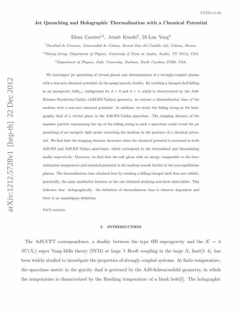
energy and momentum and as well the same ratio to |~q| and ω. The ratio of the stopping distance

with a non-zero chemical potential to that with zero chemical potential at the same temperature is

shown in Fig.3 and Fig.4 for both d = 3 and d = 4. It turns out that the stopping distance of the

light probe decreases when the chemical potential increases, which has the same qualitative feature

compared to the thermalization of the medium.

Physically, by increasing the chemical potential, we actually increase the number of states. From

10

(8), the entropy density of the plasma in d + 1 dimension is given by 4Gs = z−(d−1)h . As illustrated

in Fig.5 and Fig.6, the entropy density increases when the chemical potential is increased. The

medium thus becomes denser, which results in the enhanced scattering for the light probe and a

smaller stopping distance. On the other hand, the medium also thermalizes faster because of the

same effect. Although the holographic correspondence of the falling shell in the gauge theory side is

unknown, the falling shell could be characterized by the collective motion of massless particles with

large virtuality in the gravity dual since a null shell is homogeneous along spatial directions and it

falls along a null geodesic. Each particle as a component of the shell may as well be influenced by

the backreaction to the spacetime metric caused by the falling shell; hence it should qualitatively

behave in the same manner as the light probe traversing the medium. Since the component particles

of the shell carry large virtuality, the enhanced scattering led by increasing chemical potential would

be more pronounced, which reduces the thermalization time of the medium. By comparing Fig.5

with Fig.6, the entropy density for d = 4 increases more rapidly than that for d = 3, which also

manifests the steeper drop of the thermalization time of both the probe and the medium for d = 4

when increasing the chemical potential by comparing Fig.1 with Fig.2 and Fig.3 with Fig.4.

To avoid a naked singularity in the AdS-RN spacetime, there exists a maximum value of Q such

that the position of the horizon is given by F (z) = 0. By taking M = 1, the maximum values are

Qmax = (27/32)1/6 and Qmax = 3−1/4 for d = 3 and d = 4, respectively. Given that the derivative of

F (z) vanishes at the horizon, the temperature of the medium then vanishes. The corresponding zero

temperature black hole is known as the extremal black hole. However, this does not correspond to

the vacuum since it carries a non-zero entropy given by a non-vanishing area of the extremal black

hole horizon. In this situation, we see that the dimensionless parameter χ4(3) diverges. Also, the

stopping distances with a non-zero chemical potential in the unit of temperature, x1s(T, µ) shown in

Fig.3 and Fig.4, become zero; we hence lose the ability to make a comparison between the observables

in the media with and without a chemical potential in this particular situation.

11

0.2 0.4 0.6 0.8 1.0Χ3

0.2

0.4

0.6

0.8

1.0x`s

1HT,ΜLx`s

1HT,0L

FIG. 3: The ratio to the stopping distances with and withoutchemical potential in the unit of temperature for d = 3,where x1

s = x1sT . Here we set M = 1, zI = 0, and |~q| =

0.99ω.

0.1 0.2 0.3 0.4 0.5 0.6 0.7Χ4

0.2

0.4

0.6

0.8

1.0x`s

1HT,ΜLx`s

1HT,0L

FIG. 4: The ratio to the stopping distances with and withoutchemical potential in the unit of temperature for d = 4,where x1

s = x1sT . Here we set M = 1, zI = 0, and |~q| =

0.99ω.

0.2 0.4 0.6 0.8 1.0 1.2 1.4Χ3

20

40

60

80

4GsT2

FIG. 5: The entropy density with different values of thechemical potential for d = 3. Here we set M = 1.

0.2 0.4 0.6 0.8 1.0Χ4

200

400

600

800

4GsT3

FIG. 6: The entropy density with different values of thechemical potential for d = 4. Here we set M = 1.

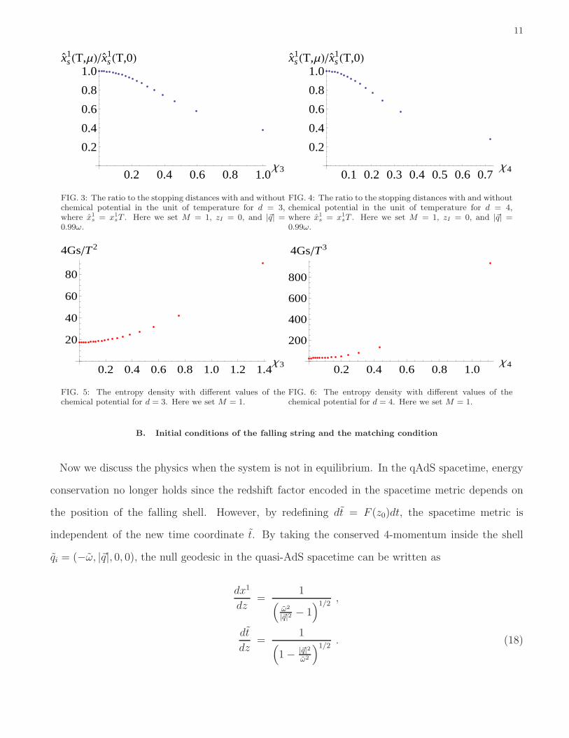
B. Initial conditions of the falling string and the matching condition

Now we discuss the physics when the system is not in equilibrium. In the qAdS spacetime, energy

conservation no longer holds since the redshift factor encoded in the spacetime metric depends on

the position of the falling shell. However, by redefining dt = F (z0)dt, the spacetime metric is

independent of the new time coordinate t. By taking the conserved 4-momentum inside the shell

qi = (−ω, |~q|, 0, 0), the null geodesic in the quasi-AdS spacetime can be written as

dx1

dz=

1(

ω2

|~q|2− 1

)1/2,

dt

dz=

1(

1− |~q|2

ω2

)1/2. (18)

12

Now ω and ω are two conserved energies defined in the AdS-RN spacetime and the quasi-AdS

spacetime, respectively.

When the string fully resides in the quasi-AdS spacetime, the string profile obtained from extrem-

izing the Nambu-Goto action by choosing the redshift time coordinate t and z as the worldsheet

coordinates should be a straight string[37]: x1 = vt. The momentum density and momentum of the

corresponding string take the form:

π0µ =

∂L∂xµ

= (π0t , π

0x1, π0

x2 , π0x3, π0

z) =−1

2πα′z2√1− v2

(1,−v, 0, 0, 0) ,

pµ = 2

∫ ∞

zI

dzπ0µ =

1

πα′zI√1− v2

(−1, v, 0, 0, 0) , (19)

where xµ = (dxµ/dt) and zI represents the initial position of the tip of the string. It is argued in

[37] that the 4-momentum of the massless particle should be proportional to the 4-momentum of

the string since the falling string here behaves approximately as a null string. We thus have the

following relation,

qiq0

=pip0

= −v. (20)

As pointed out in [37], the part of a falling string outside the shell could be distorted and bears an

unknown profile, while the part inside the shell should remain straight. Nevertheless, the detailed

structure of the string profile should not affect the maximum stopping distance.

Next, when the tip of the string penetrates the shell and falls in the AdS-RN geometry, we have

to find the matching condition to connect the ω and ω defined in two spacetimes at the collision

point zc. As shown in [37], such a condition can be derived by requiring the momentum conservation

along the spacetime direction tangent to the shell, which results in

ω

ω=

1

2(1−√1− δ2)

[2F (zc)(1−√1− δ2) + δ2(1− F (zc))], , (21)

where δ = |~q|/ω. The ratios are illustrated in Fig.7 and Fig.8 for both d = 3 and d = 4, respectively.

The same matching condition can also be derived in a different setup by using the continuity of the

13

wave function of the massless particle in the WKB approximation [37].

0.2 0.4 0.6 0.8 1.0zczh

0.7

0.8

0.9

1.0ΩΩ

FIG. 7: The red, blue, and green solid curves represent theenergy ratios for Q = 0 with |~q| = 0.99, 0.9, and 0.5ω, re-spectively. The case for Q = 0.9 are showed by the dashedcurves. Here we set M = 1 and d = 3

0.2 0.4 0.6 0.8 1.0zczh

0.7

0.8

0.9

1.0ΩΩ

FIG. 8: The red, blue, and green solid curves represent theenergy ratios for Q = 0 with |~q| = 0.99, 0.9, and 0.5ω, re-spectively. The case for Q = 0.7 are showed by the dashedcurves. Here we set M = 1 and d = 4

C. Stopping distance in the AdS-RN-Vaidya spacetime

Now, we may follow the approach in [37] to compute the stopping distance in the thin-shell limit

in Poincare coordinates. We will also eject the shell and massless particle at the same time. The

computation involves tracking the shell and the massless particle simultaneously and finding the first

collision point zc. For simplicity, here we only show the general expression for the stopping distance,

x1s =

∫ zc

zI

dz(

ω2

|~q|2− 1

)1/2+

∫ zb

zc

dz(

ω2

|~q|2− F (z)

)1/2, (22)

where the second collision point zb is approximately equal to zh since the shell falls with the speed of

light. Similar to the study in the AdS-Vaidya spacetime [37], the stopping distance of the massless

particle falling from the boundary is not affected by the gravitational collapse in the AdS-RN-Vaidya

geometry. In our setup, when we set the initial position of the tip of the string on the boundary,

the corresponding virtual gluon on the gauge theory side carries infinite energy as shown in (19). As

indicated in [37], when the hard probe has the energy much larger than any other scale such as the

thermalization temperature or the chemical potential of the system, the thermalization of the probe

would be insensitive to the thermalization of the medium. However, for the soft probe carrying

energy comparable to other scales of the system, we may envision an influence of the thermalization

14

process on the jet quenching phenomenon, which is also explored in [37] for a zero chemical potential.

This scenario is shown in Fig.9 and Fig.10, where we eject the massless particle below the boundary,

which corresponds to the soft gluon with a finite energy. As a result of thermalization, stopping

distance of light probes increases.

Finally, we illustrate this behaviour for different values of chemical potential in AdS-RN and

AdS-RN-Vaidya spacetimes in Fig.11 and Fig.12. The results can be reproduced by solving geodesic

equations directly in EF coordinates, which are presented in Appendix A; the latter approach can be

further applied beyond the thin-shell limit. As shown in Fig.11 and Fig.12, the stopping distances

scaled by the thermalization temperature in both the AdS-RN-Vaidya and AdS-RN geometries

decrease when the values of χd are increased and will drop to zero when the values of χd reach

infinity.

In general, we find that the probe gluon travels further in the non-equilibrium plasma with a

non-zero chemical potential compared to the thermal background. Increasing the magnitude of the

chemical potential decreases the stopping distances in both equilibrium and non-equilibrium plasmas.

0.2 0.4 0.6 0.8 1.0 1.2 1.4z

0.5

1.0

1.5

2.0

x1

FIG. 9: The red and blue curves represent the trajectoriesof the massless particles moving in AdS-RN and AdS-RN-Vaidya spacetimes for d = 3 and χ3 = 4.47, respectively.The red and blue dashed lines denote the first collision pointand the position of the future horizon. Here we take zI = 0.4,M = 1, and |~q|/ω = 0.99 as the initial conditions in bothspacetimes.

0.2 0.4 0.6 0.8 1.0 1.2z

0.5

1.0

1.5

2.0

x1

FIG. 10: The red and blue curves represent the trajectoriesof the massless particles moving in AdS-RN and AdS-RN-Vaidya spacetimes for d = 4 and χ4 = 1.1, respectively. Thered and blue dashed lines denote the first collision point andthe position of the future horizon. Here we take zI = 0.4,M = 1, and |~q|/ω = 0.99 as the initial conditions in bothspacetimes.

15

0.2 0.4 0.6 0.8 1.0 1.2 1.4Χ3

0.050.100.150.200.250.300.35

xsT

FIG. 11: The red and blue points represent the stoppingdistances with different values of chemical potential in AdS-RN and AdS-RN-Vaidya for d = 3, respectively. Here we setM = 1, zI = 0.4, and |~q|/ω = 0.99 as the initial conditionsin both spacetimes.

0.2 0.4 0.6 0.8 1.0Χ4

0.1

0.2

0.3

0.4

0.5

xsT

FIG. 12: The red and blue points represent the stoppingdistances with different values of chemical potential in AdS-RN and AdS-RN-Vaidya for d = 4, respectively. Here we setM = 1, zI = 0.4, and |~q|/ω = 0.99 as the initial conditionsin both spacetimes.

IV. SUMMARY AND DISCUSSIONS

In this paper we have investigated thermalization of a non-equilibrium plasma with a non-zero

chemical potential by tracking a thin shell falling in the AdS-RN-Vaidya spacetime. We found the

thermalization time of the medium decreases when the chemical potential is increased. We have also

studied the jet quenching of a virtual gluon traversing such a medium by computing the stopping

distance of a falling string, in which the tip of the string falls along a null geodesic. In both the

thermalized or thermalizing medium with a non-zero chemical potential, the stopping distance of

the probe gluon decreases when the chemical potential is increased. On the other hand, for a soft

gluon with finite energy comparable to the thermalization temperature of the medium, its stopping

distance in the thermalizing medium is larger than that in the thermalized case.

In section II, we briefly discussed the difference between the thermalization time obtained from

our approach and that derived in [35]; we will further elaborate on this here. When the medium

carries no chemical potential, the position of the horizon is about the inverse of the temperature.

As indicated in [37], the thermalization times obtained from two approaches in the AdS-Vaidya

geometry approximately match when the length scale of the nonlocal operators is about the inverse

of the temperature. However, for the medium with a non-zero chemical potential, the temperature

does not linearly depend on z−1h . To compare the thermalization times obtained from two approaches,

we have to investigate the thermlization time for a nonlocal operator with the length scale about

16

the size of the horizon in the AdS-RN-Vaidya spacetime. As shown in Fig.13, thermalization time

obtained by analyzing non-local observables with a length-scale ls = 1.71zh[35] do exhibit similar

qualitative feature as the one we have encountered here. Note that the number ls/zh bears no possible

physical significance other than being an order one number where we have found a visibly pleasant

matching. As far as the thermalization time of the medium is concerned, we conclude that our

approach by tracking the falling shell close to the horizon seems consistent with that by probing the

thermalizing medium with nonlocal operators, when the length scale of the operators approximately

equals the size of the horizon. In addition, the thermalization times from both approaches starts to

drop more rapidly when µ & T .

For the light probe traversing the medium with a non-zero chemical potential, the decrease of the

stopping distance when increasing the chemical potential is expected due to the enhanced scattering

with the increasing density of the medium. In [55, 56], it is found that the jet quenching parameter

and the drag force of a trailing string in the charged SYM plasma both increase when the chemical

potential is increased, which is again consistent with our general observations here.

0.2 0.4 0.6 0.8 1.0Χ4

0.200.25

0.350.400.450.500.55ΤT

FIG. 13: The blue and red points represent the thermalization times scaled by the temperature obtained from our approachand that from analyzing non-local observables, respectively. Here we take M = 1 in the both cases.

V. ACKNOWLEDGEMENT

The authors thank A. Guijosa, B. Muller and S. Das for useful discussions. This material is based

upon work supported by DOE grants DE-FG02-05ER41367, de-sc0005396 (D. L. Yang), National

Science Foundation under Grant Number PHY-0969020 (EC and AK), CONACyT grant CB-2008-

17

01- 104649 (EC) and a Simons postdoctoral fellowship awarded by the Simons Foundation (AK).

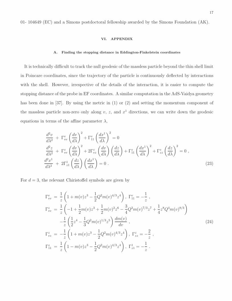
VI. APPENDIX

A. Finding the stopping distance in Eddington-Finkelstein coordinates

It is technically difficult to track the null geodesic of the massless particle beyond the thin shell limit

in Poincare coordinates, since the trajectory of the particle is continuously deflected by interactions

with the shell. However, irrespective of the details of the interaction, it is easier to compute the

stopping distance of the probe in EF coordinates. A similar computation in the AdS-Vaidya geometry

has been done in [37]. By using the metric in (1) or (2) and setting the momentum component of

the massless particle non-zero only along v, z, and x1 directions, we can write down the geodesic

equations in terms of the affine parameter λ,

d2v

dλ2+ Γv

vv

(

dv

dλ

)2

+ Γv11

(

dx1

dλ

)2

= 0

d2z

dλ2+ Γz

vv

(

dv

dλ

)2

+ 2Γzvz

(

dv

dλ

)(

dz

dλ

)

+ Γz11

(

dx1

dλ

)2

+ Γzzz

(

dz

dλ

)2

= 0 ,

d2x1

dλ2+ 2Γ1

z1

(

dz

dλ

)(

dx1

dλ

)

= 0 . (23)

For d = 3, the relevant Chiristoffel symbols are given by

Γvvv =

1

z

(

1 +m(v)z3 − 1

2Q2m(v)4/3z4

)

, Γv11 = −1

z,

Γzvv =

1

z

(

−1 +1

2m(v)z3 +

1

2m(v)2z6 − 3

4Q2m(v)7/3z7 +

1

4z8Q4m(v)8/3

)

−1

z

(

1

2z4 − 1

3Q2m(v)1/3z5

)

dm(v)

dv, (24)

Γzvz = −1

z

(

1 +m(v)z3 − 1

2Q2m(v)4/3z4

)

, Γzzz = −2

z,

Γz11 =

1

z

(

1−m(v)z3 − 1

2Q2m(v)4/3z4

)

, Γ1z1 = −1

z.

18

For d = 4,

Γvvv =

1

z

(

1 +m(v)z4 − 4

3Q2m(v)3/2z6

)

, Γv11 = −1

z,

Γzvv =

1

z

(

−1 +m(v)2z8 +2

3Q2m(v)3/2z6 − 2Q2m(v)5/2z10 +

8

9Q4m(v)3z12

)

− 1

2z

(

z5 −Q2z7m(v)1/2) dm(v)

dv, (25)

Γzvz = −1

z

(

1 +m(v)z4 − 4

3Q2m(v)3/2z6

)

, Γzzz = −2

z,

Γz11 =

1

z

(

1−m(v)z4 +2

3Q2m(v)3/2z6

)

, Γ1z1 = −1

z.

In addition to these, the mass function is defined as

m(v) =M

2

(

1 + tanh

(

v

v0− 1

2

))

, (26)

where the shift in the hyperbolic-tangent function is to fit the setup illustrated in Fig.14. In the

thin-shell limit, the mass function defined here will degenerate to the expression in (4). The mo-

mentum along the x1 direction q1 = |~q| = z−2 dx1

dλfrom the definition qµ = gµν

dxν

dλis conserved in EF

coordinates. Thus, we may rewrite the geodesic equations in terms of the derivative with respect to

x1,

dxµ

dλ=

dxµ

dx1

dx1

dλ= z2|~q|x′µ ,

d2xµ

dλ2= |~q|2z2(x′′µz2 + 2zz′x′µ) , (27)

where the prime denotes the derivative with respect to x1. By inserting (27) into the geodesic

equations, we find the last equation in (23) is automatically satisfied due to the conservation of

momentum along x1. We then have to introduce proper initial conditions to solve other two geodesic

equations in (23). Even though the energy of the particle is not conserved in the AdS-RN-Vaidya

spacetime, initially the gravitational effect led by the falling shell is negligible. Therefore, we may

write down the initial conditions as a massless particle falling in the pure AdS metric. For a particle

19

ejected from zI , we have

z|x1=0 = zI , v|x1=0 = t|x1=0 − z|x1=0 = −zI ,

v′|x1=0 = (t′ − z′)|x1=0 =ω0

|~q| −√

ω20 − |~q|2|~q| ,

z′|x1=0 =

√

ω20 − |~q|2|~q| , (28)

where ω0 and ~q represent the initial energy and momentum of the massless particle in Poincare

coordinates. The stopping distance obtained in EF coordinates is shown in Fig.15 for d = 4 in the

thin-shell limit, where we also make a comparison with the result illustrated in Fig.12 with the same

initial conditions. The results match and cannot be distinguished from the plot. This holds for d = 3

as well. We can also evaluate the stopping distance with the thick shell in EF coordinates, it turns

out that the deviation from the thin shell is negligible.

z

tt = 0 v0

qAdS

AdS −RN

shell

zI

FIG. 14: The scenario of a massless particle ejecting fromthe boundary as the shell starts to fall, where v0 denotesthe thickness of the shell and the solid red curves and thedashed red curve represent the surfaces and the center of theshell, respectively. Here the blue dashed line represents themasselss particle ejected from zI .

0.2 0.4 0.6 0.8 1.0Χ4

0.1

0.2

0.3

0.4

0.5

xsT

FIG. 15: The green points represent the stopping distances inAdS-RN-Vaidya spacetime in EF coordinates, which matchthose derived in Poincare coordinates as shown by the bluepoints. Here the initial conditions are the same as those inFig.12 and we take v0 = 0.0001.

20

B. The dyonic black hole

Here we will summarize some properties of the dyonic black hole in d = 3. The action we consider

is the following

S0 =1

8πGN

(

1

2

∫

d4x√−g(R− 2Λ)− 1

4

∫

d4xF 2

)

, (29)

which results in the following eom

Rµν −1

2(R − 2Λ) gµν = gαρFρµFαν −

1

4gµνF

2 , (30)

∂ρ[√−gF ρσ

]

= 0 , ∂ρ[√−g(⋆F )ρσ

]

= 0 , (31)

where (⋆F ) is the Hodge dual of F . In (3 + 1)-bulk dimensions, the Hodge dual of the bulk electro-

magnetic field is another two form. Thus it is possible for a black hole to possess both electric and

magnetic charges. Such a dyonic black hole is given by

ds2 =L2

z2

(

−fdt2 +dz2

f+ d~x2

)

, Λ = − 3

L2, (32)

f(z) = 1−Mz3 +1

2L2

(

Q2e +Q2

m

)

z4 , (33)

F = Qedz ∧ dt+Qmdx ∧ dy , (34)

where Qe and Qm denote the electric and the magnetic charges respectively.

In the extremal case, the function f can be written as

f(z) = 1− 4

(

z

zH

)3

+ 3

(

z

zH

)4

, (35)

where zH is the location of the event-horizon. It is easy to check that the temperature is given by

4πT = − df

dz

∣

∣

∣

∣

zH

= 0 . (36)

21

Therefore for the extremal case, we can write

z3H =4

M, Q2

e +Q2m =

6

L2

1

z4H. (37)

We can now find the corresponding Vaidya-type background sourced by appropriate matter field

S = S0 + κSext . (38)

This will give the following equations of motion

Rµν −1

2(R− 2Λ) gµν − gαρFρµFαν +

1

4gµνF

2 = (16πGNκ)Textµν , (39)

∂ρ[√−gF ρσ

]

= (8πGNκ) Jσe , (40)

∂ρ[√−g(⋆F )ρσ

]

= (8πGNκ) Jσm . (41)

Here Je denotes the electric current and Jm denotes the magnetic current. The dyonic-Vaidya

background takes the following form

ds2 =L2

z2(

−fdv2 − 2dvdz + d~x2)

, f(z, v) = 1−m(v)z3 +1

2L2

(

qe(v)2 + qm(v)

2)

z4 , (42)

with the following vector fields

Fzv = qe(v) , Fxy = qm(v) . (43)

The above background is sourced by the following stress-energy tensor

2κT extµν =

z2

L2

(

L2dm

dv− z

(

qedqedv

+ qmdqmdv

))

δµvδνv . (44)

The electric and magnetic sources are given by

κJµe =

dqedv

δµv , κJµm =

dqmdv

δµv . (45)

22

The extremal limit is now obtained by considering

zH(v)3 =

4

m(v), qe(v)

2 + qm(v)2 =

6

L2

1

zH(v)4. (46)

Once m(v) is chosen, we can pick the electric and magnetic charge functions according to the above

formula. An obvious such choice is given by

qe(v)2 =

3

4L2

(

m(v)√2

)4/3

= qm(v)2 . (47)

[1] O. Aharony, S. S. Gubser, J. M. Maldacena, H. Ooguri, and Y. Oz, Phys.Rept. 323, 183 (2000), hep-th/9905111.

[2] S. Gubser, I. R. Klebanov, and A. M. Polyakov, Phys.Lett. B428, 105 (1998), hep-th/9802109.

[3] E. Witten, Adv.Theor.Math.Phys. 2, 253 (1998), hep-th/9802150.

[4] J. M. Maldacena, Adv.Theor.Math.Phys. 2, 231 (1998), hep-th/9711200.

[5] E. Witten, Adv.Theor.Math.Phys. 2, 505 (1998), hep-th/9803131.

[6] A. Chamblin, R. Emparan, C. V. Johnson, and R. C. Myers, Phys.Rev. D60, 064018 (1999), hep-th/9902170.

[7] M. Cvetic and S. S. Gubser, JHEP 9904, 024 (1999), hep-th/9902195.

[8] D. Grumiller and P. Romatschke, JHEP 0808, 027 (2008), 0803.3226.

[9] S. S. Gubser, S. S. Pufu, and A. Yarom, Phys.Rev. D78, 066014 (2008), 0805.1551.

[10] J. L. Albacete, Y. V. Kovchegov, and A. Taliotis, JHEP 0807, 100 (2008), 0805.2927.

[11] L. Alvarez-Gaume, C. Gomez, A. Sabio Vera, A. Tavanfar, and M. A. Vazquez-Mozo, JHEP 0902, 009 (2009), 0811.3969.

[12] S. Lin and E. Shuryak, Phys.Rev. D79, 124015 (2009), 0902.1508.

[13] J. L. Albacete, Y. V. Kovchegov, and A. Taliotis, JHEP 0905, 060 (2009), 0902.3046.

[14] S. S. Gubser, S. S. Pufu, and A. Yarom, JHEP 0911, 050 (2009), 0902.4062.

[15] Y. V. Kovchegov and S. Lin, JHEP 1003, 057 (2010), 0911.4707.

[16] Y. V. Kovchegov, Prog.Theor.Phys.Suppl. 187, 96 (2011), 1011.0711.

[17] P. M. Chesler and L. G. Yaffe, Phys.Rev.Lett. 106, 021601 (2011), 1011.3562.

[18] I. Y. Aref’eva, A. Bagrov, and L. Joukovskaya, JHEP 1003, 002 (2010), 0909.1294.

[19] I. Y. Aref’eva, A. Bagrov, and E. Pozdeeva, JHEP 1205, 117 (2012), 1201.6542.

[20] M. P. Heller, R. A. Janik, and P. Witaszczyk (2011), 1103.3452.

[21] M. P. Heller, R. A. Janik, and P. Witaszczyk (2012), 1203.0755.

23

[22] T. Kalaydzhyan and I. Kirsch, JHEP 1102, 053 (2011), 1012.1966.

[23] P. M. Chesler and L. G. Yaffe, Phys.Rev.Lett. 102, 211601 (2009), 0812.2053.

[24] P. M. Chesler and L. G. Yaffe, Phys.Rev. D82, 026006 (2010), 0906.4426.

[25] S. B. Giddings and A. Nudelman, JHEP 0202, 003 (2002), hep-th/0112099.

[26] S. Lin and E. Shuryak, Phys.Rev. D78, 125018 (2008), 0808.0910.

[27] S. Bhattacharyya and S. Minwalla, JHEP 09, 034 (2009), 0904.0464.

[28] D. Garfinkle and L. A. Pando Zayas, Phys.Rev. D84, 066006 (2011), 1106.2339.

[29] D. Garfinkle, L. A. Pando Zayas, and D. Reichmann, JHEP 1202, 119 (2012), 1110.5823.

[30] J. Erdmenger and S. Lin, JHEP 1210, 028 (2012), 1205.6873.

[31] B. Wu, JHEP 1210, 133 (2012), 1208.1393.

[32] V. Balasubramanian, A. Bernamonti, J. de Boer, N. Copland, B. Craps, et al., Phys.Rev.Lett. 106, 191601 (2011),

1012.4753.

[33] V. Balasubramanian, A. Bernamonti, J. de Boer, N. Copland, B. Craps, et al., Phys.Rev. D84, 026010 (2011), 1103.2683.

[34] I. Y. Arefeva and I. Volovich (2012), 1211.6041.

[35] E. Caceres and A. Kundu, JHEP 1209, 055 (2012), 1205.2354.

[36] D. Galante and M. Schvellinger, JHEP 1207, 096 (2012), 1205.1548.

[37] D. Vaman, B. Muller, and D.-L. Yang (in preparation).

[38] S. S. Gubser, Phys.Rev. D74, 126005 (2006), hep-th/0605182.

[39] C. Herzog, A. Karch, P. Kovtun, C. Kozcaz, and L. Yaffe, JHEP 0607, 013 (2006), hep-th/0605158.

[40] H. Liu, K. Rajagopal, and U. A. Wiedemann, JHEP 0703, 066 (2007), hep-ph/0612168.

[41] H. Liu, K. Rajagopal, and U. A. Wiedemann, Phys.Rev.Lett. 97, 182301 (2006), hep-ph/0605178.

[42] F. D’Eramo, H. Liu, and K. Rajagopal, Phys.Rev. D84, 065015 (2011), 1006.1367.

[43] Y. Hatta, E. Iancu, and A. H. Mueller, JHEP 05, 037 (2008), 0803.2481.

[44] S. S. Gubser, D. R. Gulotta, S. S. Pufu, and F. D. Rocha, JHEP 10, 052 (2008), 0803.1470.

[45] P. M. Chesler, K. Jensen, A. Karch, and L. G. Yaffe, Phys. Rev. D79, 125015 (2009), 0810.1985.

[46] P. Arnold and D. Vaman, JHEP 10, 099 (2010), 1008.4023.

[47] P. Arnold and D. Vaman, JHEP 1104, 027 (2011), 1101.2689.

[48] P. Arnold, P. Szepietowski, and D. Vaman, JHEP 1207, 024 (2012), 1203.6658.

[49] B. Muller and D.-L. Yang (2012), 1210.2095.

[50] M. Spillane, A. Stoffers, and I. Zahed, JHEP 1202, 023 (2012), 1110.5069.

[51] A. Stoffers and I. Zahed (2011), 1110.2943.

[52] R. Baier, Nucl. Phys. A715, 209 (2003), hep-ph/0209038.

24

[53] R. Baier, S. A. Stricker, O. Taanila, and A. Vuorinen, JHEP 1207, 094 (2012), 1205.2998.

[54] D. Steineder, S. A. Stricker, and A. Vuorinen (2012), 1209.0291.

[55] E. Caceres and A. Guijosa, JHEP 0612, 068 (2006), hep-th/0606134.

[56] E. Caceres and A. Guijosa, JHEP 0611, 077 (2006), hep-th/0605235.

[57] For d = 3, the Hodge dual of the bulk electro-magnetic field is another two-form. Thus we can also introduce a magnetic

charge in the AdS-Vaidya type background: such a background should be dubbed as AdS-dyon-Vaidya background. By

adjusting the values of the electric and magnetic charge in the system, the final temperature of the medium can be fine-

tuned to zero, which corresponds to an electro-magnetic quench phenomenon. More discussion on the dyonic background

can be found in Appendix B.