DEBRIS BED QUENCHING UNDER BOTTOM FLOOD ...

..

. - .

:*-

}REG /CR-3850

L-NUREG-51788

DEBRIS BED QUENCHING

UNDER BOTTOM FLOOD CONDITIONS

[lN-VESSEL DEGRADEDCORE COOLING PHENOMEN0 LOGY)

N.K. Tutu. T. Ginsberg, J. Klein J. Klages, and C.E. Schwarz

Date Published - July 1984

DEPARTMENT OF NUCLEAR ENERGY, BROOKHAVEN NATIONAL LABORATORY

UPTON.LONG ISLAND NEW YORK 11973

Prepared for

--U S. Nuclear Regulatory Comrnission

am Washington, D.C. 20555

}j * }'j [)N j/ [d El $

k b} [d ; [/7 f $? ~ , M

5

!

8411130622 841031-38 R PDR

._ . _ . . .- _. __ .

--

-

NUREG/CR 3850BNL-NUREG-51788

AN. R-7

DEBRIS BED QUENCHING UNDER BOTTOM FLOOD CONDITIONS

[lN-VESSEL DEGRADED CORE COOLING PHENOMENOLOGY)

N.K. Tutu. T. Ginsberg, J. Klein, J. Klages, and C.E. Schwarz===,e

~

ii-:[l@ :;.. ;:Di? ,.:+Fqis. .-;. |:$;w,

Manuscript Completed - May 1984 3NDate Published - July 1984 f.ji:~

g;.i:?U;; ;

*

~ f;,,.

ye-

EXPERIMENTAL MODELING GROUP

DEPARTMENT 0F NUCLEAR ENERGY

BROOKHAVEN NATIONAL LABORATORY

UPTON, LONG ISLAND, NEW YORK 11973

.

Prepared for

.

05FICE OF NUCLEAR REGULATORY RESEARCH'

U.S. NUCLEAR REGULATORY COMMISSIONWASHINGTON, D.C. 20555 -

UNDER INTERAGENCY AGREEMENT DE AC02-76CH00016

NRC FIN NO. A 3024

. . . .

-wa

- _ _ _ _ _ _ _ _ _ _ _ .. _ _ _ _ . . _ _

p. f

-|, >

;. .

->'

>

v

N

- -

.

r.

d. t. -

'

, _

>

A

.

w

,*

,.

-

J

a

a

L

'

-<

.

_

- ,

E

NOTICE

This report was prepared as an account of work sponsored by an agency of the UnitedStates Government. Neither the United States Government nor any agency thereof,or

'any of their employees, makes any warranty, expressed or implied, or assumes any- legal liability or responsibility for any third party's use, or the results of such use, ofany information, apparatus, product or process disclosed in this report,or representsf

bt its use by such third party would not infringe privately owned rights.- The views expressed in this report are not necessarily those of the U.S. Nuclear

l>guistory Commission.

Available from.

' GPO Sales Program -Division of Technical Infonnation and Document Control

- U.S. Nuclear Regulatory CommissionWashington, D.C. 20655

andNational Technical Information Service

- Springfield, Virginia 22161

. .. ... . . . . . . . . ..

.

.

|

ABSTRACT

This report is directed towards development of an understanding of thetransient quenching of in-vessel debris beds, located in the reactor core re-is injected from below. Specifi-gion, under conditions where the coolantcally, the objective is to develop and experimentally verify analytical modelsfor the prediction of tne temperature distribution and the steam generationrate during the transient quenching of superheated debris beds by coolingwater supplied from the bottom of the debris bed.

Experiments involving the quenching of superheated debris beds formedWater at saturation tem-with 3.18 mm stainless steel spheres were performed.

perature was injected from below at a constant rate to initiate the quenchingMeasurements were made of the instantaneous heat flux, and thermo-process.

various locations within the bed. Time dependentcouple temperatures attraces of these parameters are presented for various initial debris bed tem-Both the average heatperatures and water injection superficial velocities.flux and the maximum heat flux are observed to increase with increasing water

For a water injection superficial velocity of only 7.4 mm/s,injection rate.we measure heat fluxes that are an order of magnitude larger than those ob-served under conditions where the water is supplied from above (top-flooding).

The experimental data suggest that for small liquid supply rate and lowinitial particle temperature the bed quench process is a one-dimensionalfrontal phenomenon. A quasi-steady one-dimensional model for the quenchingprocess is developed for this " deep bed" regime. The model assumes the exis-tence of a planar liquid quench front traveling upwards with a constant speed.For very low values of the water injection rate, the model shows good agree-ment with the experimental results. For large liquid supply rate and highinitial bed temperature, the bed quench process is a complex, multi-dimension-al phenomenon. A simplified transient model of coolant-debris interaction wasdeveloped to characterize this " shallow bed" regime. Numerical computationsshow that model predictions are very sensitive to the local heat transfercoefficients used, and that reasonable agreement between the measurements andmodel predictions can be obtained with proper choice of the parameters de-scribing the local heat transfer coefficients.

- iii -

||

-. _. _ _ _ _ _

- ---

CONTENTS

Pag.e

A BS T R ACT . . . . . . . . . . . . . . . . . . . . . . . . . . . . . . . . iii

CONTENTS . . . . . . . . . . . . . . . . . . . . . . . . . . . . . . . . vviLIST OF FIGURES ............................

LIST OF TABLES . . . . . . . . . . . . . . . . . . . . . . . . . . . . . viiiN0MENCLATURE . . . . . . . . . . . . . . . . . . . . . . . . . . . . . . ix

11. INTRODUCTION ...........................1.1 Background . . . . . . . . . . . . . . . . . . . . . . . . 1.

1.2 Fuel Distribution and Superheated Debris Beds in the CoreRegion . . . . . . . . . . . . . . . . . . . . . . . . . . . . 1

1.3 Objectives and Related Work 2.................

52. ANALYSIS .............................2.1 General ID Conservation Equations 5..............

2.2 A Quasi-Steady 1-D Model for Debris Bed Quenching withConstant Rate Injection of the Coolant from Below 9......

2.2.1 I nt eg ral Anal ys i s . . . . . . . . . . . . . . . . . . . 9

2.2.2 The Structure of the Heat Transfer Layer 11.......

2.2.2.1 General Mathematical Development . 11......

2.2.2.2 Zeroeth Order Approximation to ObtainQualitative Solution . . . . . . . . . . . . . 15

2.3 Modeling of Interfacial Drag Terms . . . . . . . . . . . . . . 17

and hst . . . 182.4 Modeling of Local Heat Transfer Coefficients hsv2.4.1 Modeling of hsv . . . . . . . . 19

2.4.2 Modeling of hst.................... 202.5 Results of Solution for the Heat Transfer Layer Structure

21for Some Simple Cases ....................

2.6 A Simplified Transient Model for Heat Transfer26Sensitivity Studies .....................

293. EXPERIMENTAL APPARATUS AND PROCEDURE ...............

334. RESULTS AND DISCUSSION ......................4.1 Transient Temperature Traces . . . . . . . . . . . . . . . . . 334.2 Quench Front Propagation Plots . . . . . . . . . . . . . . . . 394.3 Instantaneous and Average Heat Flux at Bed Top . . . . . . . . 44

4.4 Predictions from the Transient Model . . . . . . . . . . . . . 48

4.4.1 Solution Procedure .................. 494.4.2 Modeling of the Heat Transfer Coefficient hst . . . - 494.4.3 Results . . . . . . . . . . . . . . . . . . . . . . . . 50

5. APPLICATIONS TO SEVERE ACCIDENT SITUATIONS ............ 61

5.1 General Observations . . . . . . . . . . . . . . . . . . . . . 615.2 Preliminary Recommendations for the SCDAP Code . . . . . . . . 62

6. CONCLUDING REMARKS .......... ............ 63

657. REFERENCES ..................... -

-v-

I,

- - -

. - - - ._

FIGURES

PageFigure

1 Schematic of 1-D Two-Phase F1ow Through a Porous Bed 6. . . . . . .

62 En ergy Ex ch ang e Model . . . . . . . . . . . . . . . . . . . . . . .

3 Detennination of Boiling Relation . . . . . . . . . . . . . . . . . 8

4 The Quasi-Steady State Debris Bed Quench Model 10. . . . . . . . . .

5 Defi ni ti o n Ske tc h . . . . . . . . . . . . . . . . . . . . . . . . . 12

6 Separated Flow Model for Evaluating Area-Averaged HeatTransfe r Coeffici ent s . . . . . . . . . . . . . . . . . . . . . . . 19

7 Temperature and Void Fraction Profiles within the Heat23Transfer Layer ..........................

8 Temperature and Void Fraction Profiles within the HeatTransfer Layer .......................... 24

9 Temperature and Void Fraction Profiles within the Heat24Transfer Layer ..........................

10 Temperature and Void Fraction Profiles within the Heat 25Transfer layer ..........................

11 Pressure Gradient Profile within the Heat Transfer Layer 25. . . . .

12 Schematic of the Core-Debris Heat Transfer Facility . . , 30. . .

13 Schenatic of the Test Section . . . . . . . . . . . . . . . . . . 31

14 Transient Temperature Traces along the Bed centerline . . . . . . . 33

15 Transient Temperature Traces in the Wall Region . . . . . . . . . . 34

16 Transient Temperature Traces along the Bed Centerline . . . . . . . 35





- vi -

-

FIGURES (Continued)

PageFigure

21 Transient' Temperature Traces in the Wall . Region . . . . . . . . . . 37



24 Quench Front Propagation Plot . . . . . . . . . . . . . . . . . . . 39

25 Quench Front Propagation Pl ot . . . . . . . . . . . . . . . . . . . 40

26: Quench Front Propagation Pl ot . . . . . . . . . . . . . . . . . . . 40


28- Quench Front Propagation Pl ot . . . . . . . . . . . . . . . . . . . 41

29 Quench Front Propagation Plot . . . < . . . . . . . . . . . . . . . . 42



32. Instantaneous Heat Flux Leaving the Debris Bed 45. . . . ......

33- Instantaneous Heat Flux Leaving the Debris Bed 46. . . . ......

~

47- 34 Instantaneous Heat Flux Leaving the Debris Bed . . . . ......

'35 Average Heat Flux Per Unit Water Injection Superficial48Velocity Per Unit Temperature Difference . . . . . . . ......

36 Calculated Instantaneo'us Steam Flux Leaving the Debris Bed. . . . . 51

37 Effect of Minimum Film Boiling Temperature on the Calculated-Steam Flux ............................ 52

38' Sensitivity of Calculated Steam Flux to the Parameter Cf 53.....

39 Sensitivity of Calculated Steam Flux to the Parameter C r . . . . . 55t

40 Instantaneous Steam Flux at Top of the Debris Bed . . . . . . . . . 56

- vii -

._ _ _ _ _ _ _ _ _ -________ _ ____ _ _ _ _ _ _ _ _ _ _ _ _ _ _ ._ .

. . . . . . .. .. ..

_ _ _ _ _ _ _ _ _ _ _ _ __

FIGURES (Continued)

PayeFigure

41 Calculated Instantaneous Void Fraction at Five Axial57

Locations . . . . . . . . . . . . . . . . . . . . . . . . . . . . .

42 Calculated Instantaneous Solid Temperature at Five Axial58

Locations . . . . . . . . . . . . . . . . . . . . . . . . . . . . .

43 Variation of the Heat Transfer Coefficient Multiplier DuringFilm Boiling with Void Fraction a for Cf = 0.16 . . . .-. . . . . . 60

44 Calculated Instantaneous Steam Flux at the Top of the Debris60Bed f or Four Experimental Cases . . . . . . . . . . . . . . . . . .

- 45 Schematic of Coolant Flow Through a Partially Degraded Core . . . . 62

. . . . .. . . . 6246 -1-0 Coolant Flow Through a Uniformly Degraded Core

TABLES

Page]BddJe

1 Calculated V'alues of L ...................... 26

2 Calculated Valuss of Time Scale T . ................ 26

313 Experimental Parameters . . . . . . . . . . . . . . . . . . . . . .

4 - Calculated Values of D/L and H/L ................. 44

-viti-

_ - _ _ _ _ _ _ _ _ _ _ _ _ _ _ _ _ - _ _ _ _ - _ - _ _ _ _ _ _ _

NOMENCLATURE

A Cross-sectional area of the debris bedC r,Cf Parameters used in the modeling of heat transfert

coefficientse Specific heat of the solids

c Specific heat of vapor at constant pressurep

cV Specific heat of vapor at constant volume

el Specific heat of liquidD Inside diameter of test vesseld Diameter of particles constituting the porous bed

Fs Drag per unit volume of free space on the liquid phase dueLto solid particles within the debris bed

Fs Vapor solid drag per unit volume of free spaceyI

F Interfacial drag on the vapor phase due to the liquid phaseL-per unit volume of free space

g- Acceleration due to gravityH Debris bed height'

hfb Saturated film boiling heat transfer coefficient for a sin-gle sphere

h Radiative heat transfer coefficient for a single spherer

h*fg E + 0.5 c (Ts - T at)p s

hsL Solid-liquid heat transfer coefficient per unit volume ofsolid.

h Solid-vapor heat transfer coefficient per unit volume ofsvsolid

h*L Heat transfer coefficient for an isolated sphere in an in-s finite liquid medium

j Superficial velocity of vapor = volumetric flow rate /Ay

JL Superficial velocity of liquid

J[ Liquid injection superficial velocity at the bottom of thedebris bed

- kL Thermal conductivity of the liquid phasek Themal conductivity of the vapor phasey

k Effective thermal conductivity of the porous mediums! L Thickness of the heat transfer layer

E Latent heat of vaporization1 = K /O

m -Superficial vapor mass flux at the top of the debris bedy

- ix -

Nu' Nusselt number

P- Pressure

P at Pressure at saturation temperatures

'PO Injection pressure at the bottom of the bed

P" Pressure at bed exitq" Heat flux leaving the debris bed E heat lost by the entire

bed per unit cross-sectional area per unit time

fh" Bed heat flux per . un,it . injection [) velocity per unittem-

3-T }perature difference = q"/{J (TR Gas. constant for the vapor

- Re = p j t/py, Reynolds numberyy

Mass of vapor generated per unit time per unit superficials yvolume (total bed volume)

T Solid temperatures

TL Liquid temperatureT Vapor. temperaturey

.T[ Liquid temperature at injection at the bottom of the bed

Tsat Saturation temperature,

T] Initial debris bed temperature

T Time taken by a thermocouple to quench after the bottomq thermocouple has quenched

AT[ =T Ts sat

AT =Ts - T ats s

'AT =Ty-Tsaty

ATmf Particle superheat at minimum film boiling temperature

t Time

u Internal energy per unit mass for the vapor phase

-V. Quench front propagation speedVertical coordinate in the coordinate system moving with thex

_ quench front

z Vertical coordinate in the stationary coordinate system

Greek Symbols

Void fractiona

c Bed porosity

q Emittance of the liquid-vapor interfacee Emittance of the solids

3= dc / {1.75(1-c) }n_x-

..

. .

'23= d c /{150(1-c)2} specific permeability of the porous bedK

uy Dynamic viscosity of the vapor phaseW . Dynamic viscosity of the liquid phhseL

'L. Density of the liquid phaseDensity of the vapor phasepy

Density of the solid phaseos*p- Density of the vapor phase at the top of the heat transfer

layer

o Liquid-vapor surface tension ~

oB Stefar.-Boltzman constants

T Time' scale = L/V

,

e

- xi -

_. . _ _ _ _ _ _ _

1. INTRODUCTION

1.1 Background

Results of examination of the Three-Mile Island Unit 2 reactor suggestthat a portion of the reactor core was fragmented into a solid debris bed [1].The observed severe core damage has led the U.S. NRC to reconsider the role ofdegraded core accidents in the process of licensing of light-water reactors.A major research effort has been developed [2] to quantify the risks to thepublic associated with such severe accidents.

Knowledge of the geometric and thermal state of the damaged core caring asevere accident is crucial from two points of view. From the accident manage-ment viewpoint, the state of the core wo"1d guide decisions regarding the ad- '

visability, timing and rate of coolant injection during the accident. Second,from the radiation release point of view, the timing and release rate of fis-sion products from the fuel are needed for estimates of radioactive releaserates from containment during the accident sequence.

1.2 Fuel Disruption and Superheated Debris Beds in the Core Region

Disruption of a dried-out fuel bundle may occur as a result of materialmelting ' or by fragmentation. It has been suggested [3] that fuel elementfragmentatica could occur as a result of thernial shock caused by rapid quench-ing following reintroduction of cooling water to the uncovered reactor core.The process of disruption could lead to a particulate core debris bed locatedin the region of the undamaged core (in-vessel). The fragmented core couldstill have significant stored thermal energy. If, moreover, the flow of cool-ing water is interrupted subsequent to fragmentation, the debris bed would re-heat until coolant flow is restored. It is possible, therefore, that fuel 4

disruption would lead to development of regions of liot fragmented debris with-in the original core volume. The debris would continue to reheat until cool-ing capability is restored. Henry [4] has suggested that such a sequenceoccurred in the TMI-2 accident.

Reactor operator action could lead to reestablishment of some fraction ofnominal primary system flow. If flow paths into the bottcm of the core areavailable, i.e., total blockages do not develop, then the hot debris would bereflooded by coolant flow from beneath the bed. The large specific surfacearea of the fragmented core suggests that large steam generation rates arepossible upon reflood of the debris. Stm geaeration during the bottom re-flood quench process could lead to presturi stirm of the primary system. The

extent of the threat to the primary ';n n it be evaluated.

Calculations of primary system uress scation as a result of reflood ofan in-core debris bed were presented in the Zion PRA [4]. Here it was assumedthat a complete lower . blockage exists, and that the water flows around thedamage and subsequently refloods from the top. The heat removal was consid-ered as a countercurrent reflood process. Calculations indicate that thesteam generation rate can adequately be relieved via the pressurizer safetyval ves.- Thus, overpressurization would not be a problem ;ccording to this ;

scenario.

-1-

I

. -

-

If, on the other hand, blockages do not exist or are incomplete, thenwater would reflood the core from below. Since the countercurrent flow limit-ing mechanism is not operative in this case, the heat transfer rates and hencethe steam generation rates could be radically different from the top-floodcase. Ginsberg et al. [5] have experimentally observed that the heat transferrates under bottom reflood conditions are at least an order of magnitude larg-er than those typical of the top-flood case. The order-of-magnitude increasein steam generation rate that this result suggests would challenge the pres-sure relief capability of a PUR primary system during a core-wide refloodsequence.

1.3 Objectives and Related Work

The objective of the work described here is to develop and experimentallyverify analytical models for prediction of the heat transfer and steam genera-

' tion during the transient quench of superheated core debris by cooling watersupplied from below the debris bed.

Analytical methods are being developed to predict the progression of coredamage during severe accidents [6,7]. These methods are designed to predictthe heatup, fragnentation and neltdowr, of the reactor core and surroundingstructures and to follow the relocation of core material from the originalcore location through the breach of the primary vessel. The SCDAP code [6]'contains a description of the transition from intact fuel bundles to fragment-ed rubble beds. The code also contains a thermal-hydraulic model for flow andheat transfer processes within the debris bed. In principle, therefore, theSCDAP code is designed to pennit transient debris bed quench calculations.The work described here is designed to support development and evaluation ofthe two-phase debris bed thermal-hydraulic models required for debris quenchcalculations.

Numerous investigations dealing with the heat removal from debris bedshave been undertaken. Most of the work, however, has been done in the area ofdetermining the dryout heat flux during steady-state decay heat removal underboth top-flood and bottom-flood ccnditions [8,9,10,11]. Recently, studies of

L quenching of debris beds under top-flood conditions have been reported [12].( Until recently almost no work had been done in the area of transient quenching

of core debris under bottom reflood conditions. Excluding the preliminary ex-| periments referred to above [5], the authors are aware of only one other paper

dealing with the subject. Tung and Dhir [13] used stainless steel spheres toform the debris bed and Freon 113 served as the coolant. The maximum bed tem-perature was 588 K. Their experimental effort was limited to seven experi-mental runs. They observed the average heat flux to be 5.5 times the heat fluxthat would be predicted under top-flood conditions.

The experimental and analytical work described in subsequent chapters wasdeveloped to study the transient quenching of one-dimensional debris bedsunder conditions of constant volumetric rate of coolant injection from below.The effects of constant head injection and multidimensional debris bed charac-teristics will be considered separately.

-2-

_ _ _ - - _ _ _ - _ _ - _ _ _ _ _ _ _ _ _ _ _

__ _ _ _ _ _ _

,

|I

Chapter 2 presents the mathematical modeling of the bed quench process.1-0"A " quasi-steady 1-D" model applicaole to deep beds, and a " transient

model, applicable to both shallow and deep beds, are discussed. The experi-mental apparatus and procedure are discussed in Chapter 3. Experimentalresults are presented in Chapter 4, and are compared with solutions obtainedfrom the analytical models. Chapter 5 discusses the relation between the workreported here and the development of- analytical tools required for degradedcore analyses. Concluding remarks are presented in Chapter 6. In order tobetter appreciate the development of mathematical models presented in Chapter2, some readers might find it advantageous to first glance through Chapters 3and 4, which will give the reader a feeling for the physical phenomena underconsideration.

-3-

.

J A

V

2. - ANALYSIS

2.1 - General ID Conseryation Equations

..

Let us consider an unsteady one-dimensional flow of liquid-vapor mixturethrough a superheated porous bed of constant cross-sectional area A and con-

~

_ :stant porosity c flowing upwards against gravity. ~ As shown in Figure 1, letJjy and L be the local vapor and -liquid superficial velocities, respec-

tively. The' continuity equations for.the liquid and vapor phases are given- by:

.

0 (1)c [(1-a)p ] * (# jL l) + s'=

Ly

ch(ap)+h(pj)-s'y 0. (2)=y yy

.

Here z :is the _ vertical coordinate upwards and s is the local mass genera-y- tion rate 'of vapor per unit total volume. Conservation of linear momentum

across' a'section dz of the bed yields the following momentum equations foreach of the two phases:

- 2 -

k(pLL)'+ + E(I-")P g + c(1-a) h + c FLs - c FkLd -a) L

0 (3)+ =g

(p j )'+ + cap g + ca h + cF + cFk gyy y vs ) (4 )0[ .

=

1

iwhere-FyL is the interfacial drag per unit volume of free space in the bedon the vapor phase due to the presence of liquid, F s is the force per unitvvolume of free space on the vapor phase due to the solid particles in the bed,

,

L and1F s is the drag force per unit volume of free space on the liquid phaseL1due to solids. All drag forces are positive when acting downwards.

To derive the energy equations for the solid and. fluid phases we shalluse the.-energy exchange model depicted schematically in Figure 2. The liquid:can . exchange energy with the solid directly and indirectly via the vaporphase. . This ' total energy exchange between the solid and liquid phase per unitvolume of solid per unit time per unit degree temperature difference is denot-

-ed. by ' the heat transfer coefficient hsl. The remaining energy exchange be-tween the solid and vapor phase per unit volume of solid per unit time per

: unit : degree temperature difference is denoted by h v and goes into super-sheating the vapor (see Section 2.4 for a more detailed discussion). Thus no

!

-5-

!

|_.

_ . _ _ _ _ _ _ _ . " _ _ _

1130000000000!!O000000000000000000000000000000000<30000000000000000000000000000000000000000000000C30000000000000000000000000000000000000000000000C30000000000000000000000000000000000000000000000(

if 7mmnnnnnnnnnnnnnnnnnnnnn00000000000C00000000000<300000000000000000000000ZtdZ 00000000000000000000000c3oooOOOooOOOOOooOOOoooOOcomanococcoanoconnoonnnc

sk 20000 00000 00000000s Jk 3OOOOC Jk 8000(jV j L 000<3000 if30000 00000

00004 3COOOC -

30000 00000 3000 900000000000000000000C30<30000000000 11 conococoon

if

Z

w.

Figure 1. Schematic of 1-D Two-Phase Flow Through a Porous Bed.

____ _ _ _ ______

______

1 Lioulo |

_ _ _ _ _____ _ _ _

__

VAPOR/" |hit

h e,

SOLID

Figure 2. Energy Exchange Model.

-6-

- _ _ . . .

. _ _ _ _ _ _ _ .

separate energy exchange between the vapor and liquid phase need be modeled.In the absence of any internal energy sources, the energy equation for thesolid phase can now easily be derived to be:

23Th(p'ss) k' -hsL(T -T)-hsv(T -T) (5)T =

s L s ys 2az

where k' is the " effective" themal conductivity of the porous medium.

The energy balance for each of the liquid and vapor phases across asection dz of the bed can ue described by:

" Rate of change of - ~ Net enthalpy" ~ Net molecular-

flux of + conduction throughinternal energy =

of phase i in the phase i phase i_ control volume Adz_ _

IN __ IN _

Energy transfer- - Enthalpy lost or~

as heat from gained due to mass+ other phases to + transfer from other

phases across inter-phase i_

_ facial boundaries _

.

Thus the energy equations for the liquid and vapor phases can be written as:

ch[(1-a)pL'LLTl+ Pd TLL+LL

23T (6)L

k c(1-a) 2+hsL(1-c)(T -T)-sl u+=l s L y( v>Bz

'ch(apu)+h pj I u+y yy

2_ i v l- (7)

3T r 3

= k ca 2+hsv(1-c)(T -T)+s Iu+fiy s y yaz ( v/

where u is the internal energy per unit mass for the vapor, and is given by

VcL sat + E + c (T -Tsat) - R Tsat + (8)Tu = y y

-7-

_ - - _ _ - - - - - - - - _ _ _ -

... . .

_ - _ _ _ _ _ - _ - _ _ _ _

|:

Here weLare assuming the vapor to behave as a perfect gas with a specific gasconstant'R.

In addition to the ~above conservation equations we need a relation toevaluate .the local vapor generation rate. We shall assume that all the heat. transferred from solid to . liquid via hst is _ used in evaporation of theliquid if TL> the saturation - temperature, and that no evaporation takesplace if the local liquid temperature is 'less than the saturation temperature.The temperature of. vapor produced during boiling has a value intennediate be-tween the solid temperature and the saturation temperature. Now, by defini-tion T 'is the local cross-sectionally averaged vapor temperature, which isythe average of the temperature of vapor being produced and the temperature ofvapor already present at that axial location. For simplicity, therefore, weshall assume that the vapor is produced at the local vapor temperature T .yThis is' schematically shown in Figure 3. So we have

at . .T(1-c)hsL(T -Tsat) " E + ' v(T -Tse) +s v p y L 1Tgl

i =0. ;Tg<Tsaty

Of course, the energy balance expressed above in Equation (9) implies that theliquid temperature will never exceed the saturation temperature.

Vapor Out (Enthalpy Out)

(i at T ) s(u+h)y yy

, + V

i I

(1-c)hsL(T -Tsat)HEAT -* s*IN ~ (HEAT IN) :

,

'Liquid In k(c sat + }L,

(s at Tsat) (Enthalpy In)y

Figure 3. Determination of Boiling Relation.

-8-

I

- - - - - _ _ _ _ _ _ _ _ _ _ . . _ _

h v, and theNow if the local heat transfer coefficients hst and sinterfacial drag terms FL F} and F can be modeled in terms of theotherunknowns, Equations},)thr,ough(9} scan be solved for the unknowns j ,1

T, T, and s. The modeling of these terms will bea, P, T,j(, L y ysdiscussed later.

2.2 A Quasi-Steady 1-D Model for Debris Bed Quenching with Constant RateInjection of the Coolant from Below

Let us consider the transient quenching of a superheated debris bed inwhich the liquid coolant is injected from below at a constant mass flow rate.We postulate the existence of a quench front, and assume that at any instangthe debris bed consists of three distinct regions; a liquid filled quenchedregion at the bottom, a heat transfer layer which includes the two-phase re-gion adjacent to the quenched region, and finally the superheated vapor re-gion on the top where the vapor and solid debris are in thennal equilibrium.This is schematically shown in Figure 4. Furthermore, we also assume thatduring the quenching process the quench front travels upwards with a constantvelocity V, and that the thickness of the heat transfer layer remains con-stant.

2.2.1 Integral Analysis

The front pr.opagation speed V and the vapor flux (per unit time per unittotal bed am) m at the top of the debris bed can be calculated from theyintegral mass and erergy balance across the entire debris bed. We shall as-sume the liquid to be at saturation temperature Tsat at the liquid front (AB_ig Fig. 4). The liquid enters the bott9 of the, debris bed at a temperatureFL with a constant superficial velocity J -L

From the mass balance of coolant for the control volume PQRS shown inFigure 4, we get:

*

P J[ - cV(PL #v) (10)ni =Ly

*

where P is the density of the vapor at the top of the heat transfer layery(CD in Fig. 4). As the heat transfer layer moves up the debris bed, the ab-solute pressure within it will keep decreasing if the top of the debris bedexperiences a constant pressure. In obtaining the above equation we haveneglected the rate of change of vapor mass within the heat transfer layer dueto this changing pressure.

*It is implied that we also assume the liquid front to coincide with thequench front. Solid particles are considered quenched when T =Tsat-s

-9-

ME ., M

(Vapor Out)b at T", P"y

R S g

Superheated'

Vapor Region

T = T"s

T =Ty saE1

H

Dq"yC - - - - - - - - - - - -

m

Heat Transfer qL Layer i

Osa11A -B"

Liquid FilledQuenched Region a

a50,

J at T

(Liquid In)

Figure 4. The Quasi-Steady State Debris Bed Quench Model.

Let Ts be the initial temperature of the debris bed. Then, energybalance for the control volume PQRS gives:

:

~ Rate of change of internal energy" " Net Enthalpy Flux-into PQRSof solid, liquid, and gas =

. phases within PQRS _ _ _

or,

*

-(1-c)Vp 's(T"- T ) + cVpL LT- cVp [u]at T"ss y

" p(d I cTU+ 1- h {{ulat T= + RT"}y

- 10 -

l

O.where u is given by - Equation (8), and P is the injection press-ure at thebottom of the debris bed. This leads to

plJ ([ - P /pl)(11)V =

(1-c)ps s(T"- T ) + cpl - cp RTs

where,

=cL(Tat-T[)+E+cf(T"-Tat)+ Pat (12)* /PL.t s s s

This expression for the quench front propagation speed is similar though notidentical to the one obt..ined independently by Tung and Dhir [13]. The majordifference is the absence of the vapor superheat term in Equation (12). ,"Nowthe heat --lost by the debris bed per unit time per unit total bed area, q isgiven_by

V(1-c)P c (T -T[).~

q" = ss

The bed heat loss can also be expressed as heat flux pgr unit injectionvelocity per unit temperature difference. Denoting this by Q", we have

6"=q"/(J(T"-T[)}t.

'

Substituting for q" and V, we get

pl( - P /pl).

(13)Q" = .*

(T" - T ) + (cp I - CP*v R T")/{p c (I-C)}O

L ss

The above expression is independent of the injection velocity of the coolant.

It should now be noted that the bed heat flux, the vapor flux at bed top,and the quench front propagation velocity are independent of the details ofthe heat transfer mechanisms. The heat transfer coefficients simply determinethe structure and length of the heat transfer layer.

2.2.2 The Structure of the Heat Transfer Layer

2.2.2.1. General Mathematical Development

To simplify the problem, we make the following assumptions within theheat transfer layer:

- 11 -

_ __

(i) Compared to boiling and convective heat transfer, molecular con-duction through solid, liquid and vapor is negligible.

(ii) The liquid temperature is constant and equals the saturation tem-perature at the liquid / quench front (TL = T at)-s

(iii) The density of the liquid phase pL and the latent heat of vapor-ization I are constants.

(iv) The vapor is a perfect gas with constant specific heats.

(v) Quench front propagation speed V is a constant.

,

(vi) The structure of the heat transfer layer does not change as itmoves up the bed.

As shown in Figure 5, let us now consider a moving coordinate system(x,t) with origin at the bottom of the heat transfer layer and moving upwards

:

z

n

X

h

----- - - - - '

" Heat TransferV Layer

v]L " ' " * -

,

Tiii?~ E:f= - . -

E=F=-~ EVt 2~ _5-

x=z-Vtu

Figure 5. Definition Sketch,

with a constant velocity V. Then, the last assumption above implies that inthe moving reference frame (x,t), all the dependent variables are independentof time t. Thus, transformation from the fixed coordinate system (z,t) to themoving coordinate system (x,t) gives:

- 12 -

~ _ - - _ _ _ _ _ _ _ _ _ _ _ _ _ _ _ _ _ _ _ . __ . _ _ _ _ ._ _____- ___ _- _ ___ _ _________ _ --- _ -_ _ ______ __ _ __ -___

*..

f

fgh ,

l E.0E ,

j x.

fg\ ^ f g \. ,

I g)l -V I g / t= |m ,

( Z l

~ fa\ fa\=g g'.

t

The conservation' Equations (1) through (7), when transformed in the moving,

coordinates,;then become: '

a. -Liquid Continuity,

dh(ptjl)+CVOL ,g (14), y

'-b. Vapor Continuity

.d- g {p jyy-cgV} = s (15)y y,

c. . Liquid Momentum

- V h (pL L) + c(1-a)ptg + c(1-a) $dgy c )

0 (16)+ cFLs - cF L+c - )=

- d. Vapor Momentum

(pj)+copg+cah+cF + cFfL c )=0- (17)# -V yy y . ys -eg

:e.. Solid Energy Balance>

V h (p c T ) hsL(T - T ) + h v(T -T) (18)=t s s ysss s,

.

- 13 - r

, .. , . - - - . .. _. . --- . ._

._ .- ____ _ _ _ _ _ - _ _ _ _ _ _ _ _ _ _ _ _ _ _ _ _ _ _ _ _ _ _ _ _ _ _ - _ _

f. Vapor Energy Balance

hsv(1-c)(T - T ) + RT s' - h(p j ) (19)-(p j c -cVapc()V V = .

s y y y yyyp y

Since we are~ assuming the liquid temperature to be a constant equal to T ateswe need not consider the liquid energy Equation (6). If we neglect the termP/P - in comparison to the sensible heat of the liquid phase, this equationLreduces to the liquid continuity equation. Adding Equations (14) and (15) wehave:

d {p jy y , pL l + cVa(PL-Pv)}d 0.=g

Now jy = a = 0 and jL = J at x = 0; therefore

(20)pjy y + ptjL + cVa(PL-P) .PdLl."v

Adding Equations (16) and (17) gives the following expression for the pressuregradient:

-h=g{ap (1-a)pL} + FLs + F+ A s -

vs y 2y

2VpL L+ Y (P-da P Pj 2 Yp j d 2v L yy

2 ca c(1-a) L~P)+E~ 22+ c (1-a)2 +~

vca

2dp j 2 Vj

~ "Y {2y v,

+ dx 2+ c (21)~

*

ac-

Eliminating the pressure gradient between Equations (16) and (17) gives the| following equation for the void fraction gradient:

| ((1-a)pj 2(1-a)p j V 2apL LdY "P d2 yy Ll | da2 + '"Y (P ~P ) ~y

.

f ca+ P 'Y +~

2 v L v a (1-0 c(1-a)2 | E

( }J'"(I'") DIP ~P ) - caFLs+cFkV~Y~ ~

c a) L v)+=sy c

2drJ-(1-a)jy 2

vs + dx |V + 2(1-a)j V - ca(1-a)V+ c(1-a)F (22)-

ac y

- 14 -

i

, . _ __ __ . _ . . = _ .- __ _ .

L . 2.2.2.2 Zeroeth Order Approxim' ation to Obtain Qualitative Solution

' As.'we can see from Equation (18), the solid-fluid heat transfer coef-4

_ ficients are mainly responsible for the solid temperature distribution within~

the heat transfer layer. Since the heat transfer coefficients should be func--- .tions of void fraction, they are thergfore indirectly dependent upon the in-

terfacial drag tems F s* f s, and FvL . - As discussed in Sections 2.3 andcients' and Fpnt there L

y ;

2.4, at pres are no models available for the heat transfer coeffi- :. -

.Since we. are therefore forced to make an ad-hoc assumptionabout the hen transfer coefficients, we feel that at present we can only ob-

.

,

tain > qualitative solutions to the temperature distribution within the heattransfer layer. Therefore, for the purpose of obtaining a qualitative solu-

Etion, instead of solving the above set of equations exactly we make the fol-lowing assumption in order to simplify the problem.

1

' We assume that the pressure gradient generated within the bed exactlybalances all the drag and body forces on a liquid element, and therefore re-sults in null acceleration of a liquid element. In other words, we assume

d }=0.'

d L(23)E co-a) }

i.

Since at x=0, a=0, and jl=J , integrating the above equation we get:,

.

(I-")J (24)j " ,

L L

At moderate pressure the density of the vapor phase is negligible as com-pared to the density of the liquid phase. We shall now consider simplifica-

are neglected in com-.tions in the above equations when terms of order Py'parison to' tems of order P -L

The.' maximum value of the front ropagation speed V corresponds to thecasewhenthebediscoldandequalsJf/c. ThusV-0(J[). Also, c ~ 0(1) anda~ 0(1). Thus from Equation (20), we get

jy ~ PL 0(J[) .V

Now Equations (21) and (15) can be simplified by neglecting tems of orderunity in' comparison to terms.of order 9 /#v. This gives:L

- h = (1-a)pLg + Ft3 + F +8 V (25)- -

ys v ac ca at

I1

- 15 -

|- . _ - _ _ _.._. __ _ __ _ - - _ _ .._ . - _ _ _ - _ _ _ _ _ . _ , _ . _ ._._. ~ _-

- _ _ _ _ _ _ - _ _ _ _

h {p j } = s (26).yy y

Equation (19) then reduces to:

dTj e* d

y ( ,g)( )=Py v ,,

Substituting Equation (24) in Equation (20) yields an expression for the voidfraction a in terms of the vapor superficial velocity:

VV (28)a = .

P (U - 'Y)L

The vapor density p and the pressure P are related by the equation ofystate:

p RT (29)P = y y .

Substituting Equation (29) in Equation (25) gives:

(1-")P g + FLs + F- 1- +* -

2 L vs 2

2pj dTV+ (30)2 dx .

ac Ty

Neglecting P/pl in comparison to the latent heat of vaporization L ,Equations (9), (11), and (12) simplify to:

s {f + cp(Ty - T at)} (31)(1-c)hsL(Ts - T at) = y ss

PJr*L(32)V =

| (1-c)p c (T" - T ) + cpLf*

ss

VE* cL(Tat-T)+t+cfT"-Tsat) (33)=

s .

- 16 -

, . -. - - - . . ._ -. -. . . . . - - -

t

4 . . , .

.'. Thus Equations ' (18) (with .TL E Tsat), . (24)L and -(26) through (33) cany, , a, P, P, T, andbe.- solved - simultaneously for--the unnknowns j jl

...

y yT . The-initial conditions are:

_ s,

j =0e y

T '= T ats s~At x -= 0 ,-

.

<'

l T = T at-y s~ .P. = P" + a-

n

is a constant equal to the' ^ | where P" is" the: pressure at bed exit and_- aoestimated pressure drop ^ from the quench front : to the bed exit. Since the

can be found byF . solution yields the actual value of this pres;ure. drop, ao:an iterative procedure. - Of course since - the liquid front is continuously

,

moving up, a is a-function of time. . Therefore, one might- have to ' solve theo

above set of equations for many time- steps. However, it should be noted that'

: equations governing the dependent variables j , j , a, T, and T do.

yl

y s*

E not ' involve the pressure P explicitly. ' The pressure dependence enters onlyvia its effect on the density of the vapor . phase P . So, .for problems' :ywhere - a /P" . << 1, a can essentially be considered to - be independent oftime.-

'

oo -

.

'2.3 ' Modeling of . Interfacial Drag Terms

~ Before the gener61 e nservation equations can be solved, interfacial drag ;

vapor-liquid drag : term . F pentin tems of other depeF s,-.and F L :must be. modeled- tems F s.

'

Ly. . vL in; variables. No . models or the interfacial

debris beds are available in the literature.. It has been customary to either -'- : neglect it [10] or assume it..to be included in the relative . permeabilities;

. g

and - F s [8]. However recent . measurements of - FvL ' . byF'used ' to model LTutu et' al . [14] yshaveclearlydemonstratedthatnoneoftgetwoassumptionsis

,

valid: for - high pemepility porous beds (K > 4x10-8 m ). More hasic ex-.

- perimental data for FvL are needed . before a reliable model for F)L can bet

i . developed.7 In. view of its apparent success- [15], we shall use the Lipinski-model,

..[15,16] for Fvs and FLs- -Thus:r,

IP dvv+Pv @)-F " "ys- Ke nn, y y

, 2 .

- hM dL l + ~P d ,I LLl-

M.(1-8)I. ". ts gg nn -

where.

|

- 17 -.

4

, m.- -,ww.,-., .,w , r -w.-,-,.--.we ,- -..-- -mw,.-?s- -,-,--% y.----g+-s--gr,,e-, v m e-y-* y w w-g g,>+--y *w*,,,,vy,.tv-,wr~~

____-_ .

(l.,gff)3 'K = g K =,

(36)>

(1-a ff N j" Seff, nL ==y a e

a/(1-S ), when 0 < a < (1-S ) )a ff=

r re(37)

a > (1-S ) b'1 when=a ff re ,

The residual saturation S is given by [16]r

0.264_1_ (1-c)2 a cose

3 ,-- r 22 3dc

_L9

_

where e is the wetting contact angle between the liquid and the particle and dis the diameter of the particles within the debris bed.

:

2.4 Modeling of Local Heat Transfer Coefficients h v and hsLs

The modeling of the local heat transfer coefficients is perhaps the mostimportant factor which determines the ultimate accuracy of detailed predic-

: tions of any one dimensional debris bed quenching model where the coolant isinjected at a constant rate from below. Unfortunately, however, at presentthere are no basic experimental data or theoretical models available for thelocal heat transfer coefficients during a two-phase flow through a porous med-ium. We are looking for general relationships of the fonn:

h hsv(j > J , , T , T , T , fluid properties, solid properties)=sv y L s y t

hst sL(dv J , a, T , T , T , fluid properties, solid properties)h=L s y L<

In the absence of such relationships, for the present, we must use an alterna-tive approach.

Heat transfer coefficient correlations exist for the flow of a single-phase fluid through a porous medium [17]. We are concerned here, however,with modeling h and hst within the two-phase region (or heat transfersvlayer of Section 2.2). For this purpose we shall assume a separated flow

..

model as depicted in Figure 6. The coefficient hst is evaluated within the" liquid-filled" boiling region and then averaged over the total cross section.Similarly, h is evaluated in the " vapor region" a and then averanad oversvthe total cross section.

:

- 18 -

Ii-

Boiling -- Vapor -Region Superheated

______ __

_ . - _ _ _ _ - -_ _ _ _ _ _ _ _ _

_ 1-a _a --

Figure 6. Separated Flow Model for Evaluating Area AveragedHeat Transfer Coefficients.

2.4 .1 Modeling of h vs

For a single-phase flow through a porous medium, Choudhury and El-Wakilvolumetric heat transfer[17] recommend the following correlation for the

coefficient between the solid and fluid.

- -1.33Re .65 1( t in meters0Nu = ,

5,

where t = K/n. For a porous bed consisting of spheres of diameter d andporosity c=0.4, this reduces to:

Re .65 (10.145 d)1.33 d in meters .0Nu = ,

Applying this correlation to the supesteated vapor region of the bed (see Fig-ure 6), we get:

(10.145 d)1.33=

v

- 19 -

- - - ~ ' ' - - - " - - - _ _ _ _ _ _ _ . . _ _ _ _

_

c

c

'

where hy is the volumetric heat transfer coefficient within the superheatedregion only. The area averaged heat transfer coefficient h (per unit totalyvolume) is therefore given by:

"s

h ah=y y

or.

2hE r 0.65(10.145 d)1.33 0.35

Re .65(10.145 d)1.33 (38)0= a , 3

_

_ The heat transfer coefficient per unit volume of the solid, hsy, can now becalculated at:

h /(1 c) (39)} hsv = y .

2.4. 2 Modeling of hsl

We assume the following model for hsL:

(40)b (1-a)hslhst =o

'

where h sL is the heat transfer coefficient for an isolated sphere in an infi-=

nite liquid medium, b is an empirical function to take into account theofact that the solid is not an isolated sphere but a part of the debris bed,

'_ and the factor (1-a) corresponds to the separated flow model shown in Figure- 6. Due to a lack of experimental data, for now we shall assume bo = 1.y Thus, results from calculations perfonned with this value of b can only beo

considered as qualitative in nature.

Depending upon the particle superheat AT , an isolated sphere in an'

infinite liquid medium can be in one of the following three regimes: nucleate.

boiling, transition region and film boiling. We shall consider the nucleateboiling region to end when the heat flux equals thg critical heat flux. As anexample, we use the following model to calculate hst in the three regimes:

(a) Given the particle size d and the liquid properties, we first calcu-_

late the critical heat flux [18]. Starting with AT =0, we use the Rohsenows[19] nucleate pool boiling correlation until the heat flux equals the criticalheat flux.

_

For 3.175 m spheres in water at 373 K, we get:_

3h L= 1.8468(T 3 - Tsat) /d kW/m K 0 1 AT si 17.83 K . (41)

_

~

~ 20 -

--

^

-

---

-

:

(b) Since we are assuming the liquid to be at saturation temperaturewithin the heat transfer layer, following Dhir and Purohit [20], the particlesuperheat at minimum film boiling temperature is 101 K. In the film boiling

region we shall use the correlation recommended by Farahat and El Halfawy [21]when the radiation and subcooling effects are small. Since in our case sub-cooling effects are zero, we get:

*

h{hfb + 0.75 h } ATs }_ 101 K (42)hsL"

r ,

where

* 3 0.25k h d p (p _ p )gy fg

h 0.75=fb T k u (T - T )

*

I + 0.5 c (T -Tsd)h =fg p s

-TsB ath =

r T -T-._ + _1_ _ 1 _ s sat1

C C_

L s

The vapor properties in the above expressions are to be calculated at the" film temperature" which equals the average of solid temperature and the satu-ration temperature.

(c) In the inteymediate transition range 17.83 K < ATs <ferature differ-101 K, we as-

sume the heat flux hslaTs to be a linear function of tee temience AT . Since the end points are calculated from Equations (41) and (42),

shsL can easily be interpolated in this regime.

It must be emphasized once again that this model for hsL can only beconsidered qualitative in nature, and merely serves to illustrate the essen-tial features of the heat transfer layer when incorporated into the quasi-steady debris bed model described in Section 2.2.2. Results from sample cal-culations perfonned using the interfacial drag tenn models of Section 2.3 andthe heat transfer coefficient models of Section %.4 are discussed in the nextsection.

2.5 Results of Solution for the Heat Transfer Layer Structurefor Some Sample Cases

Having discussed the modeling of Fvs(33hs,imuktaneous1"y for the tempera-and h* , we can now solvef h sEquations (18), (24), and (26) through sture, void fraction and superficial velocity distribution within the heat

- 21 -

_ _ _ _ _ _ _ - _ _

- - _ _ ________-___

transfer layer. These equations were solved using the fourth-order Runge-Kutta process due to Gill. To start the calculation procedure, it wasnecessary to assume a finite value of (T -T at) at x=0; a value of 2 K wass schosen. In accordance with our experimental conditions (to be described inthe next chapter), we have chosen the following parameters for these samplecalculations:

Particle material : stainless steelParticle diameter : = 3.175 mm (sphere)Liquid : waterInlet liquid temperature T : =Tsat = 373 KBed porosity c: : = 0.4 .

Since the expression for the vapor temperature gradient (Equation (27)) issingular at j =0, the calculation procedure forces h v=0 in the domain 01y sjy I V.

Figures 7, 8 and 9 show the dimensionless distributions of solid tempera-ture, vapor temperature and void fraction within the heat transfer layer forthree different initial solid temperatures. The heat transfer layer thicknessL appearing in these figures has arbitrarily been defined to be the distancebetween 5% and 95% values of the dimensionless solid temperature profile AT /sAT . The sharp jump in the solid temperature and void fraction profiles nearsthe quench front is due to the high heat transfer rates in the nucleate andtransition boiling regimes. As expected, the vapor temperature lags the solidtemperature. Figure 10 shows the results for a lower value of water injectionrate. A comparison with Figure 8 reveals only a small change in the dimen-sionless solid temperature and void fraction profiles. However, the vaportemperature rises much more slowly. This is to be expected because at a lowerwater injection rate, the vapor velocity is lower and therefore the vapor-solid heat transfer coefficient is lower.

Figure 11 shows the calculated pressure gradient within the two-phaselayer. The expression for the pressure gradient includes the sum of the terms

F s. As we can see from Equations (34 ) through (37), Fs isFs and L yya ff=1. Thus, the calculatedsingular at a ff=0 and FLs is singular at ee

pressure gradient will go to infinity at these points. Initial calculationsshowed that these singularities are rather broad. These singularities were

F s=0 foro ff < 0.1 andF s=0 forartificially suppressed by forcing Ley0 1s stilla f f > 0.8. As can be seen from Figure 11, the peak at a ff= implicite e

not suppressed completely. This indicates that our assumption inEquation (23) does a poor job of predicting the void fraction near the quenchfront.

Table 1 shows the computed values of the heat transfer layer thickness Lfor various water injection superficial velocities and initial debris bed tem-peratures. As one might expect, it is observed that L increases both with in-creasing J and increasing TT. We also see that at high initial bed tempera-tures and igh water injection rates, the thickness of the heat transfer layer

- 22 -

- _ _ _ _ - _

!I

can be rather large. Let us define a characteristic time scale T =L/V. Thiswould correspond to the time scale of a temperature transient experienced by asolid particle as the heat transfer layer passed across it. If such a measure-ment is available from experiments, a comparison with calculated value wouldbe a - test for the modeling of heat transfer coef ficients hst and hsv-Calculated values of T for a f cases are given in Table 2. It is seen thatT is only a weak function of J .

.

l.O . i i - --i i _,i

__

,OJ = 7.4 mm/s

-

g 0.8 ,J--

-

8" - t2 TI= Sl2K -

.

3>

hO.6-

-

g> -

4 -

O.4 -

.

8m __

-

. O.2 -

_< _

s I I l l i. . i i

.O O.4 OB l.2 l.6 2.0

x/L

Figure 7. Temperature and Void Fraction Profiles within theHeat Transfer Layer. 1: Void Fraction; 2: SolidTemperature; 3: Vapor Temperature.

- 23 -

_. ____-____ _______

... . - - _ _ _ _ _ _

|

1.0 , . .i i ,.

*-

J[ = 7.4 mm/s~

-

6 ' O.8 - - -'<

'Tf= 594 K _

/e' - /H /

4 0.6 - |'/ -

*g _f .

4g ;;, 0.4 _ 2 _

F 3 __

p* O.2 - - -

4_ _

I I ' IO.0 ' ' ' ' ' '

O.O O.4 0.8 1.2 1.6 2.0x/L

Figure 8. Temperature and Void Fraction Profiles within theHeat Transfer Layer. -1: Void Fraction; 2: SolidTemperature; 3: Vapor Temperature.

1.0 . ; ; ,, ,, , ,

.

*~

/ J[ = 7.4 mm/s~

$ O.8 - ,e -

/ T7= 775 K _g;; -

f

k O.6 - [ _

Q*- / _

,- O.4 I--

k ~t -

F" O.2 -

3-

<

I l l l0.0 ' i i i i

QO O.4 0.8 1.2 f.6 2.0x/L

.


- 24 -

_ _ - _ _ _ _ - _ _ __

. l.O ,, ,, , ,

. - /,,''J[= 1.01mm/s ~

.

g O.8 /-

// T7= 594 K _'9"

- - 1/ 2 3.F40.6 : _.

7* /Q 'I

-

g ;, 0.4 - - __

.F- .g

s" O.2 - - _

<_

O.0 "'

l l I l' ' i ' '

O.O O.4 0.8 1.2 1.6 2.0x/L


G90 . , .i i i.

_ J[ = 7.4 mm/s ,

a72 - 77= 775 K __

E

k O.54-

3.-

0.36 --

-

0.se -

. . i. . ..,OD O.5 1.0 1.5 2.0

z/L

Figure 11. Pressure Gradient Profile within theHeat Transfer Layer.

- 25 -

..

Table 1 Calculated Values of L

d = 3.175 m, T8 = Tsat = 373 K, L in om

J (mm/s)T"(K) 1.01 1.98 4.42 7.4

512 19.35 36.58 81.93 137.4594 30.41 57.97 128. 203.6775 36.47 68.32 144.8 228.

Table 2 Calculated Values of Time Scale T

d = 3.175 mm, T[ = Tsat = 373 K, T in seconds

J[(mm/s)T.(K) 1.01 1.98 4.42 7.4

s

512 10.28 9.91 9.94 9.96594 18 . 17 17.67 17.48 16.61775 26.24 25.06 23.8 22.37

2.6 A Simplified Transient Model for Heat Transfer Sensitivity Studies

The quasi-steady 1-D model developed in Section 2.2 is valid only afterthe heat transfer layer has been formed and has begun to propagate at a con-stant speed. From the moment of coolant injection until this time, the modelis invalid, and the model becomes invalid again once the top of the heattransfer layer reaches the top of the debris bed. For deep beds (L/H u 1),this initial and final quench period is only a small part of the total quenchduration, and if details of the initial period are not required, the quasi-steady model is quite adequate. However, when the heat transfer layer thick-ness is of the same order as the bed height (shallow bed), the quasi-steadyassumption is likely to break down for most of the quench duration. In thiscase the partial di fferential equations presented in Section 2.1 must besolved directly. To reduce the numerical computation time and yet retain theessential physics of themal interaction , we shall now make a few additionalassumptions and present a simpler set of equations that can be used to approx-inately solve the general problem. This is being done primarily to integretour experimental results and to demonstrate the main features of the problem.It must be emphasized that we are still considering the problem where theliquid is being injected at a constant rate from below.,

- 26 -

I

We make the following assumptions:

(i) the liquid enters at Tsat and remains at Tsats

(ii) the solid-vapor heat transfer is neglected (hsv E 0) ,

(iii) molecular heat conduction through the solid is negligible comparedto the boiling heat transfer,

(iv) the absolute liquid velocity of a liquid element within the bedremains constant,

(v) the vapor is produced at the film temperature, (Ts + Tsat)/2.

The second assumption is primarily being made to simplify the problem. Thiscan be expected to result in errors of the order of

V0.5 c (Ts - Tsat)/( I + c (Ts - TsatU -

p p

For our experiments at the maximum debris bed temperature of 775 K, this cor-responds to an error of 13%. The fourth assumption is discussed in Section2.2.2.2 and results in considerable simplification in the mathematical formu-lation of the problem. Considering the extremely large uncertainty in model-ing of heat transfer coefficients and interfacial solid-fluid drag terms, wefeel this assumption is justified if we are only looking for the qualitativenature of the quenching process. This assumption implies (see Section*

2.2.2.2):~

J~ ~ d ~

3 L 3 L 0=

5t + c(1-a) iz c(1-a)_

:

or

(1-a)J (43)jL = .,

Substituting this in the liquid continuity relation (Equation (1)) gives

OJ J

h(jL) $ (44)(d ) ~ col

" ~L V '

The energy equation for the solid phase, Equation (5) reduces to.

*This model has since been extended to include the full fluid momentum equa-tions. Preliminary computations show that the qualitative nature of the re-sults is similar to results obtained when assumption (iv) is used.

- 27 -

. . . _ _ .

.. - . . . . . ..

t

'

ps s (Is-Tsat) (45)(Ts)' " - .

c

Since the vapor is assumed to be produced at the " film temperature," the vaporgeneration rate iy is given byL

I

sy' i E + 0. 5 c p( Ts - Tsat) } . (46)'

(1 r)hsL(Ts - T at) =s

'

Thus, Equations (43) through (46) can be solved simultaneously to yield jl.a and Ts as functions of z and t. The initial and boundary conditions are:

fTs T=s

At t = 0, z > 0

0 hjt =

jL d< "

At z = 0 for al l t> .

TsathT =s

|

Since the instantane'ous vapor flux leaving the top of the debris bed, my, ismeasured experimentally, it is useful to derive an expression for it. A massbalance across the entire debris bed gives:

U*

pJ'~ P e(1-a) dz - plId ILg* (47)in =y gL L

( *o J

.The above set of equations were solved numerically for several conditions cor-responding to our experimnts. The solution and results are discussed in Sec-tion 4.4.

,

:

M

4

- 28 -

.

Q . p A 7 : f. Q j f g g . .,.. f c y.t ? . - Q j p, . J, f ,.f ;. " . , ~y _.

,.

i

3. EXPERIMENTAL APPARATUS AND PROCEDURE

A schematic of the experimental facility designed to perform debris bedquench experiments is shown in Figure 12. The test section consists of a 108mm inside diameter stainless steel tube in which the debris bed is formed.Due to the high pressure in the reactor vessel (and consequently small super-ficial velocity of steam that is generated), it is unlikely that the debriswould get fluidized in the reactor vessel during the quenching process. To

simulate this, the particle bed was constrained between two fixed screens toprevent fluidization. Before beginning an experimental run, the two butterflyvalves are closed. The debris bed is then brought to its initial temperatureby circulating hot air through it and by energizing the heater coils surround-ing the test section (not shown in Figure 12). The test section is insulatedon the outside and the power to wall heaters is adjusted to minimize the radi-al and axial temperature gradients within the debris bed. To prevent possiblecondensation of steam leaving the top of the debris bed (during the experi-mental run) before it can be measured by a turbine flowmeter, the stainlesssteel piping above the test section is insulated and preheated to saturationtemperature by circuliting steam through it.

Water, which serves as a coolant during the quenching process, is heatedin an insulated tank above the test section. The dcwncomer walls are electri-cally heated and insulated to maintain water close to the desired temperature.For the present series of experiments, water was heated to the saturation tem-perature of 373 K. A Hydroflo Model CD1T1014-0401 positive displacement pumpwas used to inject water into the test section at a constant flow rate. An

accumulator (Pulsatrol 76-SS-V-76) and a back pressure valve (ECO BPV-6A-1) onthe downstream side of the pump were used to dampen the flow pulsations and tomaintain a constant discharge pressure irrespective of the instantaneous pres-sure drop across the bed.

The locations of various thermocouples and pressure taps within the testsection are shown in Figure 13. In addition, four thermocouples along thetest section wall are used to monitor the wall temperature during the quench-ing process. All thermocouples are the Chromel-Alumel type.

To start an experimental run, the hot air flow to the test section andsteam flow to the neighboring sections are shut off. The two butterfly valvesare opened, and other flow control valves are set to the appropriate states.Next, the data acquisition program is started and then the quench is initiatedby turning on the pump. During an experimental run, signals from various the-rmocouples and pressure transducers, as well as a signal proportional to thesteam flow rate at the top of the bed, are recorded. A NEFF system 623 and HP1000 computer were used to digitize, acquire and process the data. The sig-nals were sampled at 25 Hz and low pass filtered at 10 Hz prior to sampling toprevent aliasing. A pair of Cox turbine flowmeters were used to measure thesteam flow rate. The experimental parameters are listed in Table 3.

- 29 -

- - -- -- - - - . _ . _ _ _ _ __

. - . ..

-

4.s

STEAM ' ' "'

BYPASS FURNACEFg HOT

WATERTANK

d bFLOWMETER

kTOP INJECTION

?R_*

@ POSITIVE ODISPLACEMENT WPUMP, FLOW - NDAMPENER, AND

O-

BACK PRESSURE M. VALVE E

RSTEAM

HOT'

[ AIREXHAUST

BLEED. PACKEDPARTICLE

(.{}- '. BEDHOT-AIR -

% 0 :|N +

STEAM >.,.

COILS - T _#

Figure 12.' ~ Schematic of the Core-Debris Heat Transfer Facility.-

- 30 -

i

.

||

I.

FIXED SCREEN g i 6j1 .

PTI--* [.

=* ''

35.8'

|22. 9 108i

PT2 - | 21. e 8 ' =,

|

|

108, ,

; ..

PT3 - i 20. e 7 i

STAINLESS |

24* * 27 ; 108 zSTEEL PIPE N!. o

,

|19' # 6 iPT4 -!'

!~D+ 108|

PTS- i 18'e 5 '

; g ,4;_ ____.

!! 103mmFIXED SCREEN-

:- 108 --|| |

Figure 13. Schematic of the Test Section. 9, G: Thermocouple Locations;5,6,7,8,9,27: Thennocouples Along the Bed Centerline; 18,19,20,21,22,24: Thermocouples 12.7 mm from the Wall.

Table 3 Experimental Parameters

Particle material Stainless steel 302Particle diameter 3.175 mmBed height 422 mmBed porosity 0.39Vessel diameter 108 mmCoola nt WaterCoolant supply temperature 373 KSystem pressure 0.1 MPaInitial bed temperature 512 K, 594 K, 775 KWater inlet superficial

velocity, J { 1.01, 1.98, 4.42, 7.4 mm/s

- 31 -

I 41

4. RESULTS AND DISCUSSION

4.1 Transient Temperature Traces

For experiments conducted with the smallest water injection superficialOvelocity J = 1.01 mm/s, a typical temperature trace from thermocouples with-lin the bed is shown in Figure 14. The temperature remains constant or changes

very slowly, decreases slowly for a few seconds (~ 10 seconds), and then dropssharply to the saturation temperature and remains constant thereafter. Thetime at which the temperature is reduced to the saturation temperature isdefined as the " quench time," and it is assumed that this is also the timewhen a small neighborhood of the debris bed surrounding the thermocouple isquenched. Figures 14 and 15 show the temperature traces for one of the exper-imental runs with ATs = 429 K. The numbers on the traces correspond to thermo-couple numbers shown in Figure 13. Except for small fluctuations, we observethat temperature decreases monotonically. Once a thermocouple has quenched,no temperature recovery is observed. We notice that thermocouples quench insequence from bottom to top. Excluding the bed top, we also note that thethermocouples along the bed center line quench at about the same time as thethermocouples in the wall region. This indicates a frontal type quench withan approximately flat quench front travelling up the bed. Similar qualitativebehavior was observed for experiments conducted at different initial bed tem-peratures as long as the water injection superficial velocity remained thesame (1.01 mm/s).

850 .. , . . . i'- RUN 7

J[ = l.Olmm/s

g . -

E 650 - -

u

{ - 5 6 7 8 9 -

{550 - -

W - -

450 - -

- -

' i ' '' '350O 100 200 300 400

TIME (s)

Figure 14. Transient Temperature Traces along the Bed Centerline.1 Numbers 5 Through 9 Correspond to Thermocouple Locations

Shown in Figure 13.

|

- 33 -

:

| 850 , , ,

, , i,

| -

- RUN 7 .

750 - 4 ' 'O' **''-g . _

g 650 - k -

$ ..

y 21 22

3 550-

18 19 20-

*_

_

450 --

--

'' ' ' ''350 -

o too 200 300 400

TIMF. (s)

Figure 15. Transient Temperature Traces in the Wall Region.Numbers 18 through 22 Correspond to ThemocoupleLocations Shown in Figure 13.

When the water injection superficial velocity was increased to 1.98 mm/s,we observed similar behavior only when the initial debris bed temperature waslow (AT = 142 K). At higher initial debris bed temperatures (ATs = 228 K ,395 K),sseveral differences in behavior were observed, as can be seen fromFigures 16 through 19. Sme of the themoccuples exhibit a substantial tem-perature recovery subsequent to an initial quench. Nevertheless, the thermo-couples finally quench in sequence from bottom to top. The " quench times" forthermocouples in the wall region are substantially different from the quenchtimes of center line themocouples. For Run 6, the data indicate that thewall region quenches much faster than the central region of the bed. Figures18 and 19 show the results for another nin. Here we observe that it is thecentral portion of the bed that quenches ahead of the wall region.

Experiments conducted at higher water injection rates indicate that thethemocouples quench out of sequence. Figure 20 shows an example where ther-mocouple 27 quenches ahead of the upstream thermocouple 6. This figure andFigures 21 through 23 show the temperature traces for two runs at water injec-tion superficial velocities of 4.42 and 7.4 mm/s. In general, for these waterflow rates, the wall region of the bed quenched faster than the central por-tion of the debris bed.

- 34 -

___ _ _ _ _ _ _ _ _ _ _ _ _ _ _ _ _ _ _ .

850 i i i i, y ,RUN 6

JO . l.98 mm/s ""_,____s_

m_

750 - -

-

2 n

~.a 650 -' #

. / !-

$ 1 g

tg I i -

5 l I

| 7f 8|I 550 - 5 6 9 -

\ 'N | | 1- I g 1

-

L Je

450 - -

i i !.--

.

t i tL t

' I 'I i* ' '

35050 11 0 170 230 290

TIME (s)

Figure 16. Transient Temperature Traces along the Bed Centerline.

:

850 i i; ;,

RUN 6--

o . l.98 mm/sJ

_____.--

,-s.

\ 'i-

5 650 - \ '\ -

y \R - )\\ -

E i \-E 550 - 18 19 20 21 i,,

5 \. -s- .~

,'

450 - -

22e: ; -

I ' ' ''35050 110 t70 230

TIVE (s) TIME (s)

Figure 17. Transient Temperature Traces in the Wall Region.

- 35 -

..

650 , i; g.

RUN13 Jf . l.98 mm/s. -

590 -

_ -

->

y 530 - l -

?~

E~

S 6 7 8

T2 470 - -

U_ g -

410 - -

- E _-

' I' '350 '

30 70 110 150

TIME (s)


650 . , ,

, i i.

RUN13,

_

J0 = 1.98 mm/s^ - - - - - - - - - - -

590 - N I,22 -

E -)i -

-

i

{-g28wg 530 -

I h'|1

-

kD _'

,

a r4-

$ 470 - 18 is 20 [ h -'

l 'I -U- ,\ ' |,.

II / t| -'410 - .e 1,

- 1

' ' '' ' '350 '

30 70 11 0 150 19 0

TIME (s)

Figure 19. Transient Temperature Traces in the Wall Reginn.

- 36 -

I

l|

850

_Run 5, JO = 4.42 mm/s

_.......6.,750 . _ . . - ,;

_ s ,3,u -

\.m

R eso -

n'N ', ,-< s.

5 -

I\

a i

3550 -

| 3'

-

\,9" 7 8_

5 27|

450 - I I.| | |- L |__ I i ,

' ' 'yo ye'350 go 120g

TIME (4)


85o yo .i4.4 2 mm/s

i '

RUN 5 J.

-

75o -

3-

~ NE ) L \g eSo - i N -

a i N5 - 1. \5 is isi gI 550 - I "

U | 20\ -

- ,' l

450 -ri 22

'

--

_- _ o'

b'''

35 so sooTIME (s)

Figure 21. Transient Temperature Traces in the llall Region.

,

- 37 -

., .. . . - - - _ _ _ _ _ - _ _

O

650 , , i ,, ,

syf-. l___________ JO . 7,4 mm/s~

'

590 -

| -

- - i

E %I.

Ig 530 - \g -

h. - I' ) _

g

470 -!

m | A-

Y - f; I y -

I -!410 - i

i h,,9

1Jy !! l -L-- w u <

I I 135o . . . .

16 32 48 64 80

TIME (s)


650 , , , ,

IRUN 23 J[ * 7.4 mm/s

,

. -

590 -

- --b_ ,-

} g221

g . ..

530 - -

Ib - 18 19 20 El

| 1 I

-

r # 470 - |-

I. -

410 - -

A - +.. p

' ' '

350

TIME (s)

Figure 23. Transient Temperature Traces in the llall Region.

- 38 -

. _ _ -

t

4.2 Quench Front Propagation Plots

Data for the thermocouple quench times, together with the thermocouplelocations, can be used to construct quench front propagation plots. Figures

Here z is the axial distance as measured from the bottom thermoc[ouple 18 (see24 through 26 show these plots for experiments conducted with J = 1.01 mm/s.

-

Figure 13) and To .is the time to quench measured with respect to the time ofarrival of the qu6nch front at the bottom thermocouple 18. The initial debrisbed temperature Ts indicated in these figures is a nominal .value averaged overseveral experimental runs. Since V is the theoretical front propagation speedas calculated from Equation (32), the quasi-steady 1-D debris bed quenchingmodel as discussed in Section 2.2 would predict the quench front propagationplot to be given by z = T V. This corresponds to the solid lines in theqabove-mentioned figures. The data show that the actual quench front propaga-tion speed is ig reasonable agreement with the prediction for experimentsconducted with J L = 1.01 mm/s.

At- higher water injection rates, there was only one case (JL = 1.98 mm/s,.Ts = 512 K) where the quenching could be considered to be by front oropaga-tion. This is shown in Figure 27, and the agreement with the predicted frontpropagation speed ' is poor. As the . discussion of temperature traces in theprevious section shows, for the remaining cases we observed some two-dimensional (2-D) effects. Different quenching rates are observed in the wallregion and central region, and substantial temperature recovery of some thermo-couples upon initial quench is also observed. While a well-defined quenchfront does not exist for these cases, it is nevertheless instructive to plotthe quench front propagation curves for these cases based upon the finalquench time of thermocouples. This at.least allows us to compare the actualglobal time scale of the problem to the predicted one. Some of these plotsare shown in Figures 28 through 31, and we make the observations discussedbel ow.

125 , , , , , , , , ,

- Jf . l.oi m m/s-

ioo - 7*. sia n -

- .

75 - -

5- ~

|-so -

-

25 - -

I-. -

' ' ' ' ' ' '

o zs so 7s ioo izs

T,V/d

Figure 24. Quench Front Propagation Plot.C: Centerline, Run 16; Q: Wall Region,

(12.7 m from Wall), Run 16; a: Centerline,Run 17; V: Wall Region (12.7 mm from Wall),Run 17.

- 39 -

. _ _ - - . - - ,

,.-. . .-

O

.

12 5 . . . , , , , , ,

- Jf a l.Olmm/s-

*ioo - 17 3,4 x -

- -

7S - -

R - -

50 - -

- -

-25 - -

-. -

0 ' ' ' ' ' ' ' ' =

0 25 So 75 10 0 125

T V/dg

Figure 25. Quench Front Propagation Plot.O: Centerline, Run 10; Q:-Wall. Region,Run10;A: Centerline,' Run 11; V: Wall Region, Run 11.

i2s , , . . , , . . .

- J[ * l.04 mm/s-

ioo -

17 77su-

.-

75 --

R -

so --

.-

25 --

--

, , , , , , . . .',

O 25 SO 75 t00 125

T V/de

. Figure 26. Quench Front Propagation Plot.'

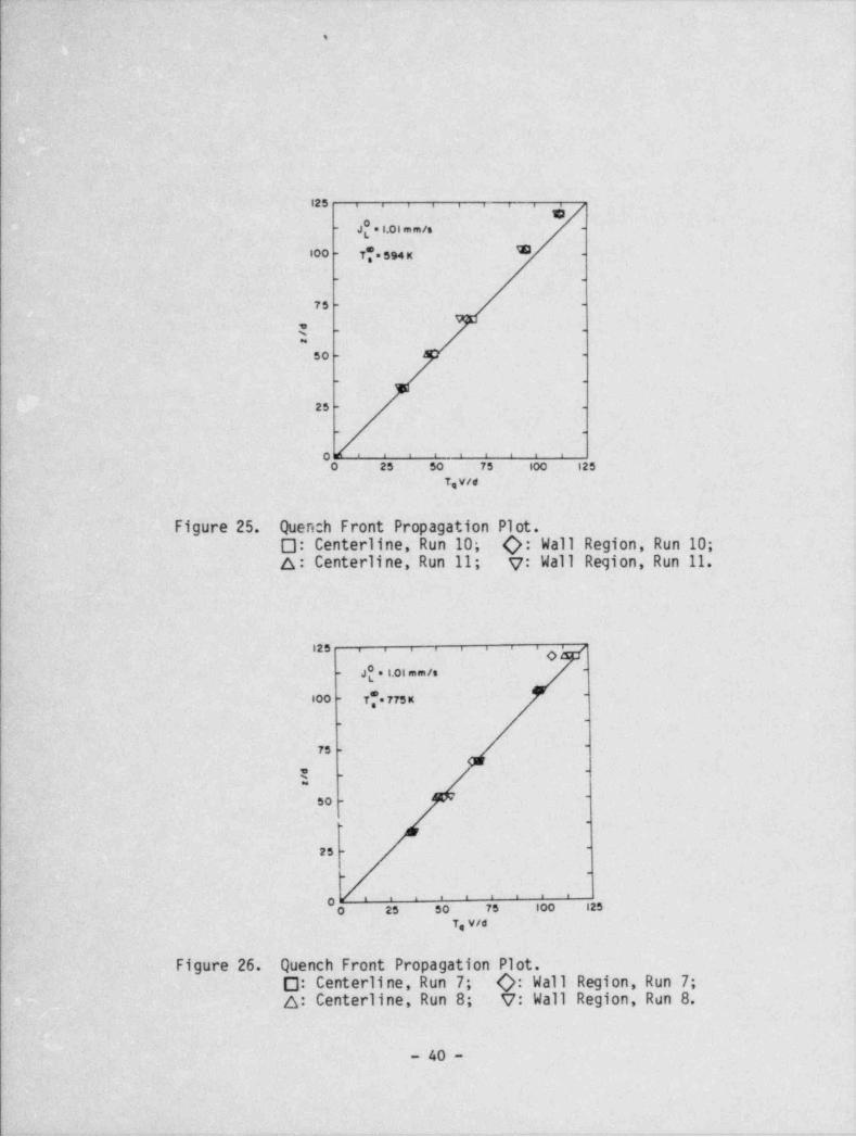
0: Centerline, Run 7; Q: Wall Region, Run 7;A: Centerline, Run 8; V: Wall Region, Ron 8.

- 40 -

. -- - . _. . . .

-

. . . . . .. ... . .. . . . ..

. .

'

.e

'

,.. ,.

hh , a , B B a 5 1 a

@- J e 1.98 mm/s ~

* -i0o .

17.Si2 x. -

75 -

-

Q3. -

50 -' -

.-

25 - -

. -

' ' ' ' ' ' ' ' '0O 25 SO . 7S 800 i25

T V/de

Figure 27. Quench Front Propagation Plot.'

O Centerline, Run 18; Q: Wall Region, Run 18.

i.S , , , , , ,,,

~ f . l.90 mm/s~

J-

13 2 - tie 775K.-

.o v a o.

,, .av a o -

.-

.. . cm a o -

. -

33 - E -

.

, . . . . . . . .o0 33 64 99 132 ISS

T,V/d

Figure 28. Quench Front Propagation Plot.O: Centerline, Run 4; Q: Wall Region, Run 4;a: Centerline, Run 6; g: Wall Region, Run 6.

- 41 -

_ _ _ _ _ -

-.. ~ ~ ' ~ ~ . ,

~l|

l

$D g I 5 5 4 5 I 3 '

-

J[= 7.4 mm/s-

*140 -

T, = 512 K-

- vo a c-105 - y o ~ m

-

3 .-

7o - 50 m2-

- 1D d)-

35 - S Ao -

"

r .-

E i E E E I I I I

00 35 70 105 190 175

T,V/d

'

- Figure 29. Quench Front Propagation Plot.O: Centerline, Run 21;- Q: Wall Region, Run 21;a : Centerline, Run 22; v: Wall Region, Run 22

too . . . , , , , , ,

. Jf = 7.4 mm/s .

160 -T"=594K _

. .

120 - o o -

3 . o a .

80 - -

o o. .

o a4o .

g.

. .

-' ' ' ' ' ' ' ' '0O 40 80 12 0 160 200

T, V/d

Figure 30. Quench Front Propagation Plot.O: Centerline, Run 23; Q: Wall Region, Run 23.

- 42 -

__ - .-. . _ - . -__

_

.

.

i7s . . . . . . . . . ..

-J 7.4 m m /s-

MO . T" * 775K -

- ov-

10 5 - Qv a O"

: --

.6

70 - y Q 0 4

- ova -

ss - o a -

.-

~'^53 do '' ' ' '0 7o ios i7so

T, V/d

Figure 31. Quench Front Propagation Plot.0: Centerline, Run 24; Q: Wall Region, Run 24;a: Centerline, Run 25; V: Wall Region, Run 25.

t = 1.98 mm/s and T" = 775 K, the data lie in a broad bandFor Jaround the predicted straight line.s When JL = 7.4 mm/s and T" = (512 K, 594K), we observe the wall region to quench faster than the predicted rate andtge central region to quench slower than the predicted rate. Finally, for

= 775 K, the data lie in a broad band around the pre-J g = 7.4 m/s and T sdicted value.

To summarize, we find that the larger the water injection rate and theinitial bed temperature, the more apparent are the two-dimensional effects.Of course, 2-D effects are partly responsible for the instances where somedownstream region of the bed quenches ahead of the upstream region. This canhappen as follows. When the wall region quenches faster than the central re-gion of the bed, a pool of water is formed on the bed top, and from that mo-ment the bed can also quench from top to bottom. Apart from understanding thephysical reasons for the origi.) of these 2-D effects, one would also like toformulate dimensionless parameters to predict if 2-D effects are important ina given situation. If D is the test vessel diameter (5 debris bed diameter),H the bed height and L the thickness of the heat transfer layer as discussed '^

in Section 2.5, then D/L seems to be the suitable parameter. D/L is the "as- -

pect ratio" of the heat transfer layer, and if this is much larger than unity,2-D effects would presumably be small. Table 4 shows the values of this pa-

rameter for the various experimental cases. Here the calculated values of Lfrom Table 1 of Section 2.5 have been used. As discussed before, for the

first four cases, we did not observe any 2-D effects from the temperature

- 43 -

_.. .

e nii. is

W

traces or quench front plots; for these cases Table 1 shows that D/L .2 3.For cases 5 through 12, we observed some 2-D effects, for these D/L < 2.Thus, Table 4 shows that even though the particle diameter d remains un--

-changed, at higher water injection rates and at higher initial debris bedtemperatures, we must correspondingly increase the vessel diameter D to keepthe 2-D effects small. - This puts the discrepancy between the actual and pre-dicted quench front. plots for these cases in proper perspective.

|

Table 4 Calculated Values of D/L and H/L_

J[(mm/s) Ts (K) D/L H/LCase No.

1 1.01 512 5.58 21.81

2 1.01 594 3.55 13.88

3 1.01 775 2.96 11.57

4 1.98 512 2.95 11.54

5 1.98 594 1.86 7.286 1.98 775 1.58 6.187 4.42 512 1.32 5.158 4.42 594 0.844 3.39 4.42 775 0.746 2.91

10 7.4 512 0.786 3.07

11 7.4 594 0.53 2.07

12 7.4 775 0.4 74 1.851

|

4.3 Instantaneous and Average Heat Flux at Bed Top

From the measurements of instantaneous steam flow rate leaving the top ofthe debris bed, one can calculate the instantaneous heat flux at bed top dur-ing the experiment. Figure 32 shows the results for the cases where the nomi- 1

nal initial debris bed temperature was 512 K. The quasi-steady 1-D model dis- i

gussed in Section P 2 would, of course, predict a constant value of heat flux )gq" = V(1-c)Ps c (T s - Tsat). This value, which was obtained by calculatingsV from Equation (32), is indicated by the horizontal dashed lines in this fig-ure. When J L = 1.01 mm/s, the agreement between the actual heat flux and themodel prediction is very good. At higher water injection rates the actualheat flux is no longer constant during the quenching period and the agreement

- 44 -

. - .. . ._-- _ _ _ - -

- - - - - - - - - - - - - - -

IQ5 i i i i i i i i i

- (T -Tsot) = 139K-

s_N

-

{ 8.4 - J " 7'4 **/*L

3 -

2 -

-

hE3-

-

-

Q -

m,, ___ __

-

!;[ 4.2 -,

Oy _ J =4.42mm/s -

_- -- -_- O' J =1.98mm/s _

2.1 - LOJ =l.ol mm/s _--

- - - - ----_

- - - - - - - - - - - --.------:-----

o 50 10 0 iso 200 250

TIME (s)

Figure 32. Instantaneous Heat Flux Leaving the Debris Bed.: Data ; - - - : Quasi-Steady ID Model Prediction.

becomes progressively worse. Figures 33 and 34 show that the results for thecases with nominal initial debris bed temperatures of 594 K and 775 K arequalitatively similar. As discussed in the previous section, if significant2-D effects are present, one should expect a discrepancy between the actualheat flux and the 1-D model prediction. Besides the parameter D/L, the param-eter H/L would determine the duration during which the instantaneous heat fluxcould be expected to be a constant. If no 2-D effects were present (D/L >> 1),a rough estimate of the fractional quench time during which the heat flux isconstant is (H/L-2)/(H/L). Table 4 lists the values of D/L and H/L for vari-

The small values for both of these parameters for cases 5 throughous cases.12 are consistent with the discrepancy between the actual and predicted in-stantaneous heat fluxes shown in Figures 32, 33 and 34.

Integrating the heat flux plots of the previous figures, we can now ob-tain heat flux values averaged over the quench period. Figure 35 shows theobserved average heat flux per unit water injection superficial velocity perunit temperature difference as a function of the initial debris led tempera-ture. The solid line in this figure is the model prediction. Considering the

- 45 -

_.

._

- _ - _ _ _

scatter in the data, the agreenent is reasonable. Thus, despite significant2-D effects at large injection velocities and large initial debris bed temper-atures, the average heat flux is reasonably predicted by the model.

As a final note on heat flux measurements, we observe that (see Figures32-34) the heat flux is a strong function of both the water injection rate andthe initial debris bed tenperature. Since the heat flux for an identical de-bris bed during top flood conditions is about 1 MW/m2 [5,12], we also note

j that depending upon the water injection rate, the heat flux during bottomflood can be an order of magnitude larger than that during the top flood.

15.0

( T*-T ot ) = 221 Ks s

g(- O12.0 - J = 7.4mm/s

SE2 -

-

' 9.0 i

O-

O,} J = 4.42 mm/sL@ -

m .. g ____

Q 6.0 -

|.,x

h ~ - b -j.. - - ------'

$ .0 - [ '\ o3 J =l.98mm/s/. -_ 5.___ J2 =1.Olmm/s

s

y_

'

_ .--- _ .- -- - - - - -

-----_____g_.---~~ -_

_

O> ' ' ' ' ' ' ' ' ' '

O 50 10 0 150 200 250

TIME (s)

Figure 33. Instantaneous Heat Flux Leaving the Debris Bed.: Data ; - - - : Data, . Quasi-

Steady 1D Model Prediction.

- 46 -

-____________ - ____ - _________________________________________ - ______ ___-

.. .

- _ _ _ . _.

.

2OO i i i i i i i i i

OJ ,7,4,,f, _^ -

3 L (T -T~ sat) = 402 K -sg 16.0 -

)1 -

- -..nS IRO -

-

-

kOg- _.p_ -

__

!i 3,0 f -_

_f=4.42 mm/s _} J__ __

,

@ . 4.0-i J =l.98mm/s-

~(-=1.Ol mm/s--- --- ---r^_ w _ _. nn--_ x _ _ _ _ --- --

' ' ' ' ' ' ' 'OO 75 150 225 300 375

TIME (s)

Figure 34. Instantaneous Heat Flux Leaving the Debris Bed.: Data ; . _ . ...: Data , . Quasi-Steady

1D Model Prediction.

- 47 -

_ _ _ _ _ _ _ _ _ _ _ _ _ _ _ _ - _-__

, _ .

f'

'

' 7. 5 , , , , , , , , ,

- - j

-a6.0 - $ -

# - a 8* _

u 43.4.5 - V g

-

e- -

E |,., 3.0 - g

2 ap. - -

*CF

l.5 - -

- -

' ' ' ~' ' ' ' ' '0.0 ,

11 0 170 230 290 350 410

ATf (K)

-Figure 35. Average Heat Flux Per Unit Water Injection SuperficialVelocity Per Unit Temperature Difference.O: JE = 1.01 mm/s; Q: JE = 1.98 mm/s;

J[ = 4.42 m/s;- V: J[ = 7.4 m/s.A:g

: Quasi-Steady 1-0 Model Prediction, Equation (13).

4.4 Predictions from the' Transient Model

The instantaneous heat flux measurements discussed in the previous sec-tion have shown that the quasi-steady model cannot be used for most of our ex-perimental conditions to predict the details of the quenching process. This

- is because the necessary condition of a deep bed (H/L >> 1) is not being sat-isfied by these runs. To interpret these results, therefore, it is necessaryto solve the transient problem. ' We shall now use the simplified transientmodel presented in Sectign 2.6 to predict the instantaneous vapor flux at the- top of the debris bed (my) and compare it to the experimental measurements.While the quasi-steady model could predict this global quantity independent ofthe solid-fluid. heat transfer coefficient (Equation 10), such is not the casewith ~ the transient model (Equation 47). The instantaneous vapor flux at bedtop is strongly coupled to the heat transfer coefficient because the detailsof the' heat transfer determine both the period of formation of the heat trans-.fer layer and its thickness. As discussed in Section 2.4, at present there

- 48 -

:r

. . ., _ _ , . . . , , . . . , . . - . . , , - . _ _ - . . _ . , , .

_ _ . .

= 4

- m.

-

:

h are no models available for the local solid-liquid heat transfer coefficient:- during a two-phase flow through a debris bed. Therefore, we can only do a ,

; parametric study to detennine the sensitivity of the solution to the heat 4transfer coefficient.

'~

4.4.1 Solution Procedure -

-;

In order to predict j as functions of space and time, partial -

differential equations (44)L and Tand (45), together with Equations (43) and (46), _

s-

must be solved simultaneously. To do that, the debris bed was divided into -

,

;- 421 spatial nodes - 1 mm apart. Since the solution is known at t=0, the right--

_hand side of Equations (44) and (45), representing the time derivatives of

-

- JL and T, respectively, could be detennined at every node. The spatial -

sderivative of jL was evaluated using the backward difference approximation:-

to improve the numerical stability. Next, the standard fourth-order Runge- -"

- Kutta process due to Gill was used to evaluate jL and T at the next timesstep at at every node. The procedure was continued until the top of the ;

_

debris bed quenched. The following relation between the node spacing az and-'

.

time step at was used:-

0.22 (az/J[) .'

at =

i_

- 4.4.2 Modeling of the Heat Transfer Coefficient hsL_

-

-

-

In Section 2.4.2 we assumed the following model for hsL: :

,

b (1-a)h*L -- hst =

o s i

F .

E 2

[ where for lack of experimental data, the empirical function b was chosen to-

op be unity. The boiling hegt transfer coefficient for an isolated sphere in an

"

infinite liquid medium, hst , was evaluated according to the applicable heat _

,- transfer regime. Equation (41) was used in the nucleate boiling regime and ?-

Equation (42) was used in the film boiling regime. The solid superheat at"

i minimum film boiling temperature, ATmf, was assumed to be a constant equal it_ tg 101 K. In the intermediate transition range, we assumed the heat flux :

h AT to be a linear function of the temperature difference AT -{ sL s s -

h Here, we shall use the same model for hst with the following changes: $

$ (i) the solid superheat at minimum film boiling temperature, ATmf' E

_

will be used as a parameter, 3_

(ii) during the nucleate t, oiling region and the transition region, jbo = C r, and !{ t

T (iii) during the film boiling regime 2

2Cf + (1 - C )a (48)b =f ,o

=--

m

E- 49 -

!_ ,

.

_

where C r and Cf will be used as parameters. Stevens and Witte [22], whotstudied the instability of the vapor film boiling around spheres by quenchinga single sphere in water, have clearly demonstrated that for a fixed watertemperature, the transition temperature is a function of the initial spheretemperature. In other words, the transition does not occur at a fixed sphere |temperature. Thus, the choice of ATmf as a parameter is quite justified. |The functional fonn of bo, used in Equation (48) is rather arbitrary and was |

suggested by the qualitative nature of the measurements of the instantaneoussteam flux leaving the debris bed. In reality, b is likely to be a func-otion of j , jL, a, T,T fluid and solid properties. So, it must bey semphasized that this modelfn,g of hst merely serves the role of illuminatingthe qualitative features of the problem. It would also demonstrate the neces-sity (or lack thereof) of determining the heat transfer coefficients accurate-ly. )

4.4.3 Results

We shall now present the calculated values of the instantaneous vapor Iflux leaving the debris bed, as obtained from Equation (47), and solution of |the transient model for various cases. '

. Figure 36 shows the results for AT" = 402 K and various water injectionsuperficial velocities. In these calcdlations we have used a heat transfercoefficient model identical to the one used in Section 2.4.2, i.e. , ATmf =101 K, Cg=Cf 1.0. If we assume the steam exit temperature to be=

equal to T g 2 would correspond to a heat flux ofabout 20 Mh/m'. steam flux _ of 6.5 kg/smThus, these calculated values of steam flux can be compareddirectly to experimental heat flux measurements shown in Figure 34. As ex-

Opected, the agreement is good for J 1.01 mm/s. However, the agreement is=

very poor for the other three cases. It is suggested that the heat transfercoefficient assumed by the. model is not realistic. To show that this isindeed possible, we shall first determine the sensitivity of the solution forone case (J 7.4 mm/s -- the case with the smallest value of H/L) to thethree parameker=s in the heat transfer coefficient. Next, we shall try to finda combination of the parameters that would give reasonable qualitative agree-ment between the calculations and the data.

Figure 37 shows the sensitivity of, results to the minimum film boilingtemperature. Starting with time t=0, m increases at a rate determined byy

the film boiling heat transfer coefficient (for a given J[the bed)r,eaches theand T" and henceby Cf in our model. Once the liqu,id-filled portion ofminimum film boiling temperature, m experiences a sharp jump due to theysudden increase in the heat transfer coefficient during the transition regime.Therefore, as ATmf is increased, this sharp jump will occur at earliertimes, and consequently, the total amount of liquid within the bed at transi-tion would be less. The magnitude of this jump is proportional to the amountof liquid within the bed at this time and the remaining thermal energy in thepartially quenched portion of the bed. While the former is inversely propor-tional to ATmf, the latter is proportional to ATmf. Thus, the magnitudeof the peak may not be sensitive to ATmf if other parameters are fixed. As

- 50 -

_- ._ . - . _ ._ . . -- - -- _. ..

_ .

-

6.5

E 5.2 -EN '

3% 3.9-E j

,

XDg 2.6-2<La ,

.y;P-w h ; .Q %n'

m.e er & -a - w--- erwe+%0.0 =, -~~

-

--

> .

-5.0 70.0 14 5.0 220.0 295.0 370.0

TIME (s)

Figure 36. Calculated Instantaneous Steam Flux Leaving the Debris Bed.

ATs "o402 K, ATmf = 101 K, C r = Cf = 1.0,-e ; J{1.01 mm/s.= 7.4 m/s ,

t

-O-: JL = 4.4 2 nn/ s , -e: J[ = 1.98 mm/s,-5-: JL=

is evident from Figure 37, this is indeed the case. We also note that thesteam flux profile becomes flatter with increasing ATmf. This happens

increases, the average heat transfer coefficient experiencedbecause as ATmfby the solid particles also increases, and therefore, both the formation timeand the thickness of the heat tFansfer layer Will be reduced.* This cffec-tively increases the H/L ratio and brings the debris bed closer to the " deepbed" condition, and hence, closer to the " ideal" constant steam flux for thiscase as predicted by the quasi-steady model.

The sensitivity of results to the para.neter Cf is shown in Figure 38.is reduced, the film boiling heat transfer coefficient is reduced, andAs Cfthis reduces the rate of rise of the vapor flux. For Cf = 0.25, water reach-

es the top of the debris bed at approximately t=23 seconds. Since the top of

the debris bed is open in our model, both water and steam are allowed to es-cape. Therefore, the steam flux decreases beyond this point until a portionof the bed goes into the transition boiling regime, thus resulting in thesecond peak.

*A simple order of magnitude analysis of Equation (18) shows that L is in-versely proportional to hst-

- 51 -|

:

_ -__

5.0

N{ - 4.0-N ' ~

g o( - u

> 3.0 - /"~

.E / -

\~

XU \j 2.0 -

s sb$ l .0- \

o o <,

0.0 e:: :. . ,

0.0 14.0 28.0 42.0 56.0 70.0TIME (s)

Figure 37. Effect of Minimum Film Boiling Temperatureon the Calculated Steam Flux.

aT[=402K,J = 7.4 mm/s, C r = Cf = 1. 0,t

4: AT,7 = 101K, e.: AT,7 = 165 K,

e: AT,f= 225 K, -a.: AT,7 = 300 K.

- 52 -

_ _ _ _ _ _

- _ _ . . .

- s

-

,

_

_

=_

5 -

--

-_

5._ .-

:

E 6.0 m

.?-n

s^

, w 4.8- * . - -- E g.,\ I-

,

- <. ,o % i..

'3.6- g y>,

*-

-

_ x__

o 2

J 2.4 -* -=- u. =_

1-

-

I .2 -

r T

E-t '

_ O.O . . . .: 1

- 0.0 14.0 28.0 42.0 56.0 70.0 _s; TIME (s) kw

-

-' 1_.

b Figure 38. Ser.sitivity of Calculated Steam Flux to the Parameter C .-

f

h AT} = 402 K, JL = 7.4 m/s, ATmf = 101 K, C r= 1.0, 'h_t

5- t: Cf = 1.0,-e-: Cf = 0. 5, -a: Cf = 0.25. $.-e

3-

E ?-

y,

m

' *

v.

E __

^

_

_

= e'

- 53 --

__

... _-

r-

Figure 39 shows the results of varying the parameter C r. As C ist tr- reduced, the heat transfer coefficient during transition is reduced, and this

reduces the rate 'of rise of vapor flux upon transition. However, the peaksteam flux remains about the same.

. Figure 40 shows_ the results of choosing a . set of values for the threeCr and Cf by trial and error to give the best agree- i- parameters ATmf, t

ment with the data for one of the- experimental runs. As can be seen, the l

agreement is qualitatively reasonable and demonstrates both the effectivenessof the simple model, and more importantly, the value of modeling the heattransfer coefficients accurately. For a given run, we have treated the param-eters ATmf, C and Cf as constants, but in reality these are likely to it

-

be functions of local variables and be stochastic in nature. This would )smooth out the sharp changes in the computed steam flux, and agreement with '

the data is likely to be better. |To help. understand the physical reasons for the shape of the calculated

steam flux in Figure 40, we have plotted the calculated time history of voidfraction and solid temperature at five different axial locations within thebed in Figures 41 and 42, respectively. Starting from time t = 0, until theliquid reaches a given axial location, the void fraction remains unity and thesolid debris remains at its initial temperature. When the liquid which isbeing injected from the bottom of the debris bed at a constant rate reaches a.given location, void fraction drops sharply to a certain value and the parti-cles go into film boiling. As we can see from Figure 41, the value of voidfraction' attained during this period is an increasing function of the verticaldistance from the bottom of the debris bed. Since the heat transfer rate dur-ing film boiling-is low, the solid tenperature decreases slowly (see Figure42) and the local J. team generation rate is low. Thus the local void fraction

- during this period is primarily determined by the total vapor flux. Since thetotal vapor flux crossing a given location keeps increasing as we move up thebed, the void fraction should increase as we move up the bed. When the soildparticles go into the transition boiling regime,'the local steam generationrate increases sharply and therefore the void fraction increases sharply. Atthe bottom of the bed where water is readily available, particles are quenched

,

quickly after entering the transition regime, and the void fraction drops tozero as the voids are filled up with the water. This is seen for the curvesfor z = 25 mm in Figures 41 and 42. As the bottom portions of the bed startto quench, the availability of liquid to the top regions of the bed is reduced(or delayed) because now part of the injected water must be used in filling upthe voids in the quenched bottom regions. Thus the temperature and void frac-tion traces in the top regions of the bed behave differently after undergoingtransition. Let us consider the void fraction and temperature traces for z =350 mm in Figures 41 and 42. Upon transition, the temperature drops quicklyas the surrounding liquid is evaporated, and since no liquid is available from

i below, the void fraction quickly rises to unity (dryout). Until liquid be-

comes available to this region once more, dryout persists (a=1) and the parti-cle temperature remains constant. When liquid reaches this location again,.

its supply is- not interrupted this time because most of the debris bed belowthis level has quenched and has been filled up with the liquid. Thereforeboth.the void fraction and temperature drop quickly as the solid particles arequenched.

- 54 -

s

|

_____m__ _. m.._. __A --__________m _ - m + -_ --ei w - - - --,,--c----w - - + - , , - - - - - - - " -

_ _ - _

.

5.0

k5

4.0 -^

E k ._'

d. 3.0 -> "

e N.

X

32.0-u.2

'

<t

N 1.0 -m o

' O r .: :0.0 . . .

0.0 14.0 28.0 42.0 56.0 70.0

TIME (s)

Figure 39. Sensitivity of Calculated Steam Flux to the Parameter C r-t

AT" = 402 K, J = 7.4 mm/s, ATmf = 300 K, Cf = 1.0,

C r = 0.25.C r = 0. 5, -e :C r = 1.0,-e : t9-: tt

,

- 55 -

_ _ _ _ _ - _ _ _ _ _ _ - _ _ _ _ .

r

7.5

NE 6.0-

%6 i

> 4.5- !E |x' o \D c i

d 3.0- j [1 on . - -

'# N,$ i,v> i.5-

' i

!!'--O.0 '

0.0 14.0 28.0 42.0 56.0 70.0TIME (s)

Figure 40. Instantaneous Steam Flux at Top of the Debris Bed.

AT[ = 402 K, J = 7. 4 m/ s ,: Data, Run 24

---o --: Calculated from the Transient Model, ATmf = 260 K,Ctr = 1.0, Cf = 0.16.

- 56 -

. -. . _ . . . . . . . . . . . . . . . . .--

_

-

1.o:: = = =,= = =,= , = = =

ho "n 'o oo.8 - , _

>

e-

U || O*"z o i ,

"" " "o 0.6 -

H 1

_

O Nog si

% Nw n n _% 0.4 - 0'

81 D.9 %"S- % g"

o.2 ~ _

o88 % o

0.0 'e = =3 L_ _1 _ u_ !_ __

o.o io.o 20.0 30.0 40.0 50.0 so.o

TIME (s) w

Figure 41. Calculated Instantaneous Void Fraction at Five Axial Locations.

AT[ = 402 K, J = 7. 4 m/ s , ATmf = 260 K , yC r = 1.0, Cf = 0.16, jet '

-E-: z = 25 m , -4- : z = 134 m, -o-: z = 242 m,

-0- : z = 350 m, -e-: z = 404 m._

z = 0 and 420 m Corres.cond to the Bottom and Top of Debris yBed, Respectively. ;

N,

-

=

7-

gi

- 57 - 1,sui

1

M

1.O :: : = =i : : : : i i i

O.8 -- -

~

|

8. 0.6 - - |-

k - - - - \N

!='

0.4 - -

)1

0.2 - a o o U " - |

O.0 ' ' " s-s d': = e: e =4 : r eO 10 20 30 40 50 60

TIME (s)

Figure 42. Calculated Instantaneous Solid Tenperature at Five AxialLocations.

AT" = 402 K, J = 7.4 mm/s, AT = 260 K, C = 1.0, Cf = 0.16,g tr-3-: z = 25 mi, -+-: z = 134 m, -o-:z = 242 m,

-O-: z = 350 m, -e-: z = 404 m..

~

Let us now go back to the calculated steam flux trace of Figure 40. Fromtime t = 0 to about t = 17 seconds, the calculated steam flux rises slowly be-cause steam is being generated via film boiling. As the bottom of the bedgoes into transition boiling, the steam generation rate rises sharply. Beyondthis point two competing effects try to stabilize the steam generation rate.Since the portion of t.he bed undergoing transition (" transition layer") ini-tially increases, this tends to increase the steam generation rate. However,once the bottom of the bed starts to quench, the growth of the " transitionlayer" is slowed or arrested. The rate of rise of the steam flux is, there-fore, reduced. The quench process near the bottom of the bed also reduces theavailability of water to the unquenched portion of the bed, since water isneeded to fill up the vc. ids in the quenched region. This also acts to reduce

i . the steam flux. At about t = 23 seconds, water has reached the top of thedebris bed. Beyond th'es point the net mass of unquenched particles can onlydecrease. This effect tends to lower the steam flux leaving the debris bed.

<

- 58 -

..

v.~ e

, .,~ , , ,

The loss of water from the top of the bed * and the use of injected water infilling up the voids in the quenched region of the 'ed leads, at about 35seconds, to dryout in the top portion of the bed (see Figure 41). This re-sults in a sharp reduction in the steam flux until water becomes available tothese regions. As Figure 42 shows, these regions are partially quenched andclose to the transition temperature. Consequently, upon rewetting the localsteam generation rate is large enough to compensate for the fact that only asmall portion of the bed is producing steam. Thus, the steam flux levels offand a secondary " heat transfer layer" is fonned and begins to travel up thebed. Since this region of the bed is at.a lower temperature and losing heatat a high' rate due to transition boiling, the thickness of this secondary heattransfer layer is small and reaches a quasi-equilibrium state quickly. Thus,it appears that the approximately constant steam generation rate during thelast 10 seconds is due to the fact that the thin heat transfer layer istraveling up the bed at approximately constant speed. The steam generationrate drops off rapidly as the heat transfer layer crosses the top of the bed.

It must be emphasized once again that the modeling of hst used heremust be treated only as an example and is yet to be placed on a solid founda-tion. As a final note on the heat transfer coefficient used here, Figure 43shows the variation of the multiplier b (1-a) with a during the film boilingoregime that is used to obtain the debris bed heat transfer coefficient fromthe single sphere heat transfer coefficient.

Although we realize that the parameters in the heat transfer coefficient -

are likely to be different for different experimental conditions, it is never-theless interesting to see the results of using the same set of p"arameters(that gave us reasonable agreement for the case with Jg = 7.4 mm/s, T = 775 Kas shown in Figure 40) for several experimental condhtions. Figure 44 showss

the results for four different water injection rates. These should be com-pared with calculations with a different set of parameters shown in Figure 36and the experimental, data of Figure 34. The importance of the choice of heattransfer coefficients is self-evident from these figures. Since the same setof parameters does not result in good agreement with the data for all the cas-es, it is clearjthat' heat transfer coefficients must be modeled in tenns ofother (besides Ts,and a) local dynamic variables as well.

<

b

*The model assumes that water crossing the upper boundary of the debris bed islost. A water pool above the bed is not allowed to fonn.

- 59 -

. .. - . .. . . .. ..

o.20 i i i i i i i i i

--

o.is-

'B-i _

y 0.12 --

_-

u

6 o.os --

t _-

o.o4 --

_

i i I I l I i I I000

0.o o.2 0.4 0.6 o.s 1.0

a

Figure 43. Variation of the Heat Transfer Coefficient MultiplierDuring Film Boiling with Void Fraction a for Cf = 0.16.

6.5

E 5.2- fN

Cy o

~> 3.9- "E

x'ba '

d 2.6- 0

u a o

A'i 3-en/ I %8Tl

O.0'

:.

-5.0 70.0 145.0 220.0 295.0 370.0TIME (s)

Figure 44. Calculated Instantaneous Steam Flux at the Top of the Debris Bedfor Four Experimental Cases.

= oATs = 402 K, JL = 7.4 m/s, ATmf = 260 K, Ctr = 1.0, C f = 0.16,+ : J[ = 7.4 m/s, -O-: J[ = 4.42 m/s,

J[ = 1.98 m/s, -5-: JL = 1.01 m/ s .-- S :

- 60 -

I

5. APPLICATIONS TO SEVERE ACCIDENT SITUATIONS

5.1 General Observations

The experimental results described in the last chapter have demonstratedthat the steam generation rate during the quenching of a superheated debrisbed under bottom reflood conditions is proportional to the liquid supply rate.Even at the relatively low liquid supply rates, we have observed heat fluxes(and hence the steam generation rates) that are an order of magnitude largerthan those observed under top flood conditions. Steam generation resultingfrom quenching of a superheated fragmented core could lead to significant pri-mary system pressurization if fragmentation is extensive and if flow to thedamaged regions of the core is sustained. However, the actual liquid flowthrough the damaged regions of the core, and hence the actual magnitude of thesteam spike, would be a strong function of the damage-state of the core. Letus consider two possibilities.

In the first case, as shown in Figure 45, only a small portion of thecore is in the degraded debris bed state. In this case most of the forcedflow will bypass through the surrounding undamaged portion of the core becauseit would offer least resistance to the flow. The steam generation rate inthis situation is likely to be small and the associated primary system pres-sure rise would be small. However, as shown in Figure 46, if the entire core(or most of it) is in the degraded debris bed state, much of the liquid in-jected from below is likely to pass througn the debris bed. (In principle,one would also have to consider the liquid bypass adjacent to the core bar-rel .) In such a situation, the results of our experiments suggest that thevolume of steam generated could be quite large if liquid flow to the damagedcore is sustained. For this case, the water injection rate during reflood iscrucial. Consideration should be given to control of the water injection rateso that the primary system pressure rise would be tolerable. Detailed analy-sis of this scenario would require models for the steam generation rate aswell as a water injection model based upon the difference in pressure betweenthe water source and the primary system.

In order to analyze various accident scenarios involving the quenching ofin-vessel debris beds a general analytical model is needed. The quasi-steady1-D model and the simple transient model developed in Chapter 2 represent thefirst steps in this direction. Further changes in these models would be therelaxation of the assumption of zero acceleration of the liquid phase and in-clusion of decay heat, hydrogen generation, finite conductive heat fluxthrough a single particle and extension to high prototypic pressures and tem-peratures. In order to simulate the quenching of partially degraded cores thetransient model must obviously be extended to two dimensions. This extensionto two dimensions and the development of accurate models for the local heattransfer coefficients are perhaps the most important and challenging problems

-that must be solved.

|

- 61 -

|

m

k

r

], - UNDAMAGED| CORE|I, DEBRIS BED

\-

/ ooo ) ???SSSSSSSSESSc

/]],EbEf/_L EEEEESES$$EEia a a a ua a

oolAUcoolant

Figure 45. Schenatic of Coolant Flow Figure 46. 1-D Coolant Flow ThroughThrough a Partially De- a Unifomly Degradedgraded Core. Core.

5.2 Prelininary Recommendations for the SCDAP Code

EG&G, under the sponsorship of the U.S. NRC, is developing the SevereCore Damage Analysis Package (SCDAP) computer code [23] to simulate severedisruption of LWR cores under various accident scenarios. Fuel bundle frag-mentation and debris behavior during and following reflood is one of the situ-ations that is being modeled by the SCDAP code [23,243 However, the debrisbed-coolant themal interaction model that is presently incorporated in theSCDAP code [24] deals only with the quasi-steady removal of internal heat gen-eration. A transient quench model that simulates the removal of sensible heatfrom the superheated debris by the flowing coolant is yet to be incorporatedin the code. As discussed in the previous section, we need to solve many

. problems before an accurate, general, two-dimensional model for the transientquenching of a debris bed can be developed. However, based on the encouragingresults that were obtained from the simple transient model developoed in Sec-tion 2.6, it is felt that an extension of this one-dimensional model which in-cludes the fluid momentum equations can be incorporated in the current versionof the SCDAP code.

- 62 -

I

m--m-- m umi-umm-

- . .

.

6. CONCLUDING REMARKS

Experiments involving the quenching of fixed * superheated debris bedsformed with 3.18 mm stainless steel spheres were performed. After the debrisbed was heated to iLs initial temperature, water at saturation temperature wasinjected from below at a constant rate to initiate the quenching process.Measurements were made of the instantaneous heat flux, and thennocouple tem-peratures at various locations within the bed. Time dependent traces of theseparameters are presented for various initial debris bed temperatures and waterinjection superficial velocities. Both the average heat flux and the maximumheat flux are observed to increase with increasing water injection rate. Fora water injection superficial velocity of only 7.4 mm/s we measure heat fluxesthat are an order of magnitude larger than those observed under top-flood con-ditions.

The experimental data suggest that for small liquid supply rate and lowinitial particle temperature, the bed quench process is a one-dimensionalfrontal phenomenon. The bed heat flux is constant during most of the durationof the quench period. The range of conditions which display one-dimensionalfrontal cooling characteristics is identified as the " deep bed" (defined be-low) regime of bed quenching, and a limiting mathematical model was developedto describe the observed behavior. For large liquid supply rate and high ini-tial bed temperature, the bed quench process is a complex, multi-dimensionalphenomenon. Under these conditions, the bed heat flux displays a non-uniformtime dependence. In order to characterize this " shallow bed" regime, it wasnecessary to develop a detailed transient model of the coolant-debris interac-tion. This model, while developed for the " shallow bed" regime, also appliesto the " deep bed" regime.

Based upon the experimental observations described above, a one-dimen-sional " deep bed" model for the quenching process was developed. The modelassumes the existence of a planar liquid quench front traveling upwards with aconstant speed. The debris bed is divided into three regions: (1) theliquid-filled quenched region, (2) the heat transfer layer of thickness L, and(3) the superheated vapor region in thermal equilibrium with the debris. Then.odel is valid only for those cases where the bed height H is much larger thanthe thickness L of the heat transfer layer. To predict the bed heat flux andthe quench front propagation speed, no knowledge of the solid-fluid heattransfer coefficient is required. However, the structure of the heat transferlayer in terms of its thickness and the distribution of solid temperature,vapor temperature, void fraction, and superficial vapor velocity within it, isstrongly coupled to the solid-fluid heat transfer coefficients. For the ex-perimental cases where the " deep bed" condition (H/L>>1) is satisfied (mostlyat the lowest water injection rate), thermocouple temperature traces withinthe debris bed did indicate a frontal propagation type quench. The observedfront propagation speed was close to the predicted value. Also, in agreementwith the model, the instantaneous heat flux was approximately constant (inde-pendant of time) for most of the quench duration.

*The debris bed was constrained between two fixed screens, and therefore couldnot fluidize.

- 63 -.

.

" '' -- -- u. wiw iu .. mb ,, I g h ,

For most of the experimental runs, the " deep bed" condition was apparent-ly not being satisfied. A simplified transient model was developed to inter-pret the experimental results. This transient model, which is valid for boththe shallow bed and deep bed regimes, integrates the governing transient con-servation equations directly. A detailed knowledge of the local heat trans-fer rates is essential in this case. Numerical computations show that theresults are very sensitive to the heat transfer coefficients used. With prop-er choice of the parameters describing the local heat transfer coefficients,reasonable agreement between the measured instantaneous steam flux and thepredicted steam flux is obtained. These results clearly demonstrate theimportance of developing a general reliable model for the solid-fluid heattransfer coefficients, and therefore significant effort must - be directedtowards this goal .

Work is now in progress to include the full fluid momentum equations inthe one-dimensional transient model. This should lead to more reliable voidfraction predictions, and would therefore help us to properly evaluate themodeling of heat transfer coefficients.

:

i

$#

- 64 -

.. -

7. REFERENCES

1. Owen , D. A. , et al . , "THI-2 Core Damage: A Summary of Present Knowl-edge," Proceedings of International Meeting on Light Water Reactor SevereAccident Evaluation, p. 1.5-1, Cambridge, MA, August 28 - September 1,1983.

2. Larkins, J. T. and M. A. Cunningham, " Nuclear Power Plant Severe AccidentResearch Plan," U. S. Nuclear Regulatory Commission, NUREG-0900 January1983.

3. Cook, B. A., " Fuel Rod Material Behavior During Test PCM-1," NUREG/CR-0757, TREE-1333, June 1979.

4. " Zion Probabilistic Risk Assessment," Commonwealth Edison, Illinois,

1981.

5. Ginsberg, T. , et al . , " Core Debris Quenching Heat Transfer Rates UnderTop- and Bottom-Reflood Conditions," Proceedings International Meeting onLWR Severe Accident Evaluation, TS-18.7, Cambridge, MA, August 28 -September 1, 1983.

6. Allison, C. M. , et al., "SCDAP: A Computer Code for Analyzing LightWater Reactor Severe Core Damage," Proceedings International Meeting onLWR Severe Accaant Evaluation, TS-5.1, Cambridge, MA, Augustg 28 -

September 1, 1983.

7. Young M. F. et al ., "MELPROG Ccfde Development and Methods," ProceedingsInternational Meeting on LWR Severe Accident Evaluation, TS-2.8, Cam-bridge, MA, August 28 - September 1,1983.

8. Lipinski , R. J., "A Model for Boiling and Dryout in Particle Beds,"NUREG/CR-2646, SAND 82-0765, 1982.

9. Gabor, J. D., et al., " Status Report on Limiting Heat Fluxes in DebrisBeds," Argonne National Laboratory Report No. ANL/ RAS 80-21, September1980.

10. Naik, A. S. and Dhir, V. K., " Forced Flow Evaporative Cooling of a Volu-metrically Heated Porous layer," Int. J. Heat Mass Transfer, Vol. 25, No.4, pp. 541-552, 1982.

11. Tsai, F. P., et al., "On Dryout Heat Flux of an Inductively Heated Heter-ogeneous Bed," Proceedings International Meeting on LWR Severe AccidentEvaluation, TS-18.3, Cambridge, MA, August 28 - September 1,1983,

12. Ginsberg, T., et al., " LWR Steam Spike Phenomenology: Debris Bed Quench-ing Experiments," NUREG/CR-2857, BNL-NUREG-51571, June 1982.

- 65 -

.-_ - _ _ _ _ _ _ _ _ _ _ _ _ _ _ _ _ - . _

b

l_-

b13. Tung, V. X. and Dhir, V. K., " Quenching of a Hot Particulate Bed by Bot- ~

tom Flooding,"* School of Engineering and Applied Science, University of PCalifornia, Los Angeles, CA 90024. g

14 Tutu, N. K. , et al ., "Interf acial Drag for Two-Phase Flow Through High EPermeability Porous Beds," Interfacial Transport Phenomena, ASME HTD-Vol. E23, pp. 37-44, 1983. Also to appear in Journal of Heat Transfer. 7

I15. Lipinski, R. J., "A Review of Debris Coolability Models," Proceedings In- [_

ternational Meeting on LWR Severe Accident Evaluation, TS-18.2, Cam-bridge, MA, August 28 - September 1,1983.

-

L

16. Lipinski, R. J. , "A Coolability Model for Postaccident Nuclear Reactor -

c

Debris," Nuclear Technology, Vol. 65, pp. 53-66,1984. --

?17. Choudhury, W. U. and El-Wakil, M. M., " Heat Transfer and Flow Character- k

istics in Conductive Porous Media with Energy Generation," Proceedings 54th International Heat Transfer Conference, Versailles, France, 1970; 2-

paper CT 3.2, A.I.Ch.E. , New York. -

18. Two-Phase Flow and Heat Transfer in the Power and Process Industries, [Bergles, A. E., et al., Hemisphere Publishing Corporation, pp. 210-213, i1981.

-

-

19. Rohsenow, W. M., "A Method of Correlating Heat Transfer Data for Surface --

Boiling of Liquids," Trans. ASME, H , p. 969, 1952.~

20. Dhir, V. K. and Purohit, G. P., "Subcooled Film Boiling Heat Transfer;from Spheres," Nuclear Engineering and Design, E, pp. 49-66, 1978. --

21. Farahat, M. M. and El Halfawy, F. Z., " Film Boiling Heat Transfer from-

Spherical Particles to Subcooled Liquids," Atomkernenergie (ATKE) Bd. 26,Lfg. 4, pp. 235-241,1975. ;

22. Stevens, J. W. and Witt , L. C., "Destabilization of Vapor Film Boiling _

Around Spheres," Int. J. Heat Mass Transfer, Vol.16, pp. 669-678,1973

23. Allison, C. M., et al., " Severe Core Damage Analysis Package (SCDAP) Code-

Conceptual Design Report," EGG-CDAP-5397, EGAG Idaho, Inc., Idaho 83415, -

April 1981.-

a

24. Hsieh, T. S., " Debris Bed Characterization and Thermal Behavior Models -

_

for SCDAP," EGG-CDD-5728, EG&G Idaho, Inc., Idaho 83415, January 1982.-

:_

-r

-

* Source not available, copy may be obtained from Professor V. K. Dhir._

.-

-66- _

-

..

- -- - - _ _ _ _ _ .

:

/" " "### ##

\.S. NUCLEAR REGUL ATORY COMMISSION NUREC/CR-3850U, '" * "

%IBLIOGRAPHIC DATA SHEET BNL-NUREG-5f788

or me No.. ef sopewreste) y ggy,e gi,g; y4 TITLE AND SutlTITLE (Ad uY

Debris Bed Quenching,Under Bottom Flood Conditions(In-Vessel Degraded e Cooling Phenomenology) 3. RECIPIENT'S ACCESSION NO.

[ / AUTHORtSI N. K. Tutu, T.TGinsberg, J. Klein, S. o ATE REPORT COMPLE TEo

| vE anJ.KlagesandC'.kE. Schwartz uomisMay 1984

5 s

1 PkHFoHMING ORGANIZATION NAME ANO(MAILING ADDRESS (Jaciudr 2,0 Codel DATE REPORT ISSUED

.

Brookhaven National Laboratory uomys [vEAnDepartment of Nuclear Energy % July 1984*

- Upton, Long Island, New York 11973 ..

s neue umasg

R B ILee.e Nehl

k t/ VoNh0HING OHGANI/AiloN N AME AN~) M AILING ADOMESS finesude le Codel

Division of Accident Evaluation \ p- Office of Nuclear Regulatory Research \ f , ,, gg go.

U.S. Nuclear Regulatory Commission (= ,

- Washington, DC 20555 \_

vFE RIOD Cove RE O (facius,ve dentsJ'' IJ S YPt oF HLPOHT h'6Formal Technical Report s

,4 ft,,, u,,j- Ib. SUPPLEMENTAHY NOTES

1;.m

;$ 14 ABSTH ACT (200 woms or sent

This report is directed towards development of an understanding of the transient_ quenchingofin-vesseldebrisbeds,locatedin}thereactorcoreregion,underconditions

~

Specifically, the objective is to develop and; where the ccalant is injected from below.experimentally verify analytical models for-the prediction of the temperature distributionand the steam generation rate during the transient quenching of superheated debris beds by=

cooling water supplied from the bottom of the debris bed. ' Experiments involving the quench-yL f d

ing of superheated debris beds formed with' 3.18 tr.m stainlesQteel spheres were per orme .rate to initiate the--

Water at saturation temperature was injected from below at a tonstantMeasurements were made of the instantaneous, heat flux, and thermocouplequenching precess.

temperatures at various locations within the bed. The experimehtal data suggest that forsmall liquid supply rate and low initial particle temperature thaibed quench process is a

~-

,

one-dimensional frontal phenomenon. ,A quasi-steady one-dimensionni,mocel for the quenchingFor large liquidisupply rate and highy

process is developed for this " deep. bed" regime.?initial bed ten.perature, the bed quench process is a complex, multiklimensional phenomenon.

' A simplified transient model of coolant-debris interaction was developed to characterize-

this " shallow-bed" regime. %i.

,

f

'

IT KEY WORDS AND DOCUMENT AN ALYSIS / 1 74 DE SC RIP TORS

( Debris-bed, Quenching, Core-Debris, Transient, Bottom-Reflood,%Debris-Coolant, Thermal Interaction, Model

W . }

?T-

,

Em+

"

li

_ iii. nw u nt n HS.on s t NiA u TE HMS '>_

.

-

'

18 AV AIL ABILITY ST ATEMENT 19 SECURITY CLASS ITos eeports 11 NO Of PAGE SUnclassified5

30 SE CUM TV CLASS f f764 ps*/ M CEUnlimited- ~.c. _ m I,,,,

4U.8. GOVERNMENT PRINflNG OFFICE: 1984 717 032 10012,.

:m_

g -: - ' :;+v:.,

,

. ,

*) ,.

.

-

n

-

b.

<

..

W

L20555078677 L LANIR7US NRCADM-DIV OF TIDCPOL'CY E PUB MGT OR-POR NUREGW- 501 OC 2GS95'n A SH I flG T ON

._

5-

'

.,

.

"E 6

- 9m .7 - ,- - . _ , 4=,. m . , ,,

DEBRIS BED QUENCHING UNDER BOTTOM FLOOD ...

Documents

Transcript of DEBRIS BED QUENCHING UNDER BOTTOM FLOOD ...