
Debris-Flow Protection Systems for Mountain Torrents
281
56
-
Upload
khangminh22 -
Category
Documents
-
view
0 -
download
0
Transcript of Debris-Flow Protection Systems for Mountain Torrents

Debris-Flow Protection Systems for Mountain Torrents Basic Principles for Planning and Calculation of Flexible Barriers
Corinna Wendeler
Swiss Federal Institute for Forest, Snow and Landscape Research WSL, CH-8903 Birmensdorf
Heft 44, 2016
WSL BerichteISSN 2296-3456


PublisherSwiss Federal Institute for Forest, Snow and Landscape Research WSLCH-8903 Birmensdorf
Heft 44, 2016
WSL BerichteISSN 2296-3456
Debris-Flow Protection Systems for Mountain Torrents Basic Principles for Planning and Calculation of Flexible Barriers
Corinna Wendeler

Responsible for the publication of this seriesProf. Dr. Konrad Steffen, Director WSL
Responsible for this issueDr. Manfred Stähli, Head unit Mountain Hydrology and Mass Movements
Managing Editor: Sandra Gurzeler, WSLLayout: Dr. Axel Volkwein, WSLTranslation from German: itl Institut für technische Literatur AG, CH-8280 Kreuzlingen
ContactSwiss Federal Research Institute WSL Dr. Axel VolkweinZürcherstrasse 111CH-8903 BirmensdorfE-Mail: [email protected]
Citation Wendeler, C., 2016: Debris-Flow Protection Systems for Mountain Torrents – Basic Principles for Planning and Calculation of Flexible Barriers. WSL Ber. 44: 279 pp.PDF download www.wsl.ch/publikationen/pdf/15501.pdf
ISSN 2296-3448 (Print)ISSN 2296-3456 (online)
Photos coverSide view of a filled debris flow barrier in Illgraben VS, May 2006Numerical simulation of debris flow barrierDebris flow frontPhysical modelling of debris flow barriers in laboratory
Source directory of figuresRickli C., WSL 2.1 rightIshikawa (Japan) 2.10 leftDep. for Natural Hazards, Ct. Berne 1.1, 2.10 right, 2.13McArdell B., WSL 2.11Graf C., WSL 4.3Geobrugg AG 3.1, 3.2 right, 3.3 left, 3.4,3.9 right, 3.10, 3.12Gwerder C., WSL 4.15 rightGubler A., WSL 5.24, 5.25,5.26, 6.9Schatzmann M. 5.5 rightSchlickenrieder M., FH Munich 6.3
© Swiss Federal Institute for Forest, Snow and Landscape Research WSL, 2016

Preface
This WSL report is a word-by-word translation of the doctoral dissertation of CorinnaWendeler that has been elaborated at WSL and submitted to the Swiss Federal Instituteof Technology (ETHZ) in Zurich in 2008, as part of the requirements for her degree. Thethesis won the Swiss PLANAT research award 2008. The original thesis has been writtenin German. Since its publication the WSL received numerous requests for an Englishversion of this work, clearly indicating that the thesis and the underlying project is ofinternational interest. Meanwhile several articles and reports based on the thesis alreadyhave been published in the scientific literature (see next page). But there is still significantinterest for more data and the contents of the Ph.D. thesis to warrant having it translatedinto English, hence the production of the present WSL report. However, it must be clearthat this report is a direct translation only. No changes have been made to the contentthat was originally written eight years ago as part of Dr. Wendeler’s doctoral dissertation.Therefore, we strongly recommend that the reader compare the content of the thesis withthe newest publications listed on the next page (and to be published in the near future).
This thesis is an outcome of a joint research project between Geobrugg AG and theSwiss Federal Institute for Forest, Snow and Landscape Research (WSL), in order toinvestigate the use of flexible ring net barriers to retard or stop debris flows. The projectwas generously supported by the Commission for Technology and Innovation (CTI) ofthe Federal Office for Professional Education and Technology (OPET), which was led atthe WSL by Dr. Axel Volkwein. The supervision of the Ph.D. thesis within the projectwas led by Prof. Dr. Mario Fontana, Institute of Structural Engineering, Swiss FederalInstitute of Technology ETHZ. Additional supervision at the WSL was primarily throughDr. Axel Volkwein, with significant support provided by Dr. Perry Bartelt.
Other WSL staff collaborated and helped secure the success of the project. We particu-larly thank our measurement technician Bruno Fritschi and the representatives of WSLin the Canton of Valais, Francois Dufour and Dr. Alexandre Badoux. Pat Thee performedthe topographic surveys in rough terrain and Julia Kowalski helped with the analysis ofdebris-flow data. The WSL debris-flow team, i.e. Dr. Brian McArdell and Christoph Grafwith support of Dr. Dieter Rickenmann are responsible for all the background researchin Illgraben that allowed the installation and investigation of a fully instrumented flexi-ble protection system. The project also benefitted from academic projects by universitystudents, including Florian Kaineder, Andreas Gubler, Philipp Franke and MagdalenaSchlickenrieder. After completion of the thesis, Dr. Wendeler left the WSL and joinedGeobrugg AG to further pursue applications of ring-net barriers to help mitigate debrisflows and other natural hazard processes.
Zurich, April 2016 Manfred Stahli
i

Publications originating from the doctoral thesis of C. Wendeler:
Wendeler, C.; McArdell, B.; Bartelt, P.; Volkwein, A., 2016: Load model for designingflexible steel barriers for debris flow mitigation. Submitted to Canadian GeotechnicalJournal.
Wendeler, C.; Volkwein, A., 2015: Laboratory tests for the optimization of mesh size forflexible debris-flow barriers. Nat. Hazards Earth Syst. Sci. 15, 12: 2597-2604.
Volkwein, A.; Wendeler, C.; Stieglitz, L.; Lauber, G., 2015: New approach for flexible de-bris flow barriers. In: IABSE Conference Geneva, 2015 - Structural Engineering: Provid-ing Solutions to Global Challenges. Report. September 23-25 2015, Geneva, Switzerland.Zurich, IABSE. 248-255.
Volkwein, A.; Baumann, R.; Rickli, C.; Wendeler, C., 2015: Standardization for flexibledebris retention barriers. In: Lollino, G.; Giordan, D.; Crosta, G.B.; Corominas, J.; Azzam,R.; Wasowski, J.; Sciarra, N. (eds) Engineering Geology for Society and Territory - Volume2. Landslide Processes. London, Taylor & Francis. 193-196.
Volkwein, A., 2014: Flexible debris flow barriers - Design and application WSL Bericht.18: 29 pp.
Volkwein, A.; Wendeler, C.; Guasti, G., 2011: Design of flexible debris flow barriers.In: Genevois, R.; Hamilton, D.L.; Prestininzi, A. (eds) 5th International Conference onDebris-Flow Hazard. Mitigation. Mechanics, prediction and assessment. Padua, Italy, 14-17 June 2011. Rome, Casa Editrice Universita La Sapienza. 1093-1100.
Wendeler, C.; McArdell, B.; Volkwein, A.; Denk, M.; Groner, E., 2008: Debris flow miti-gation with flexible ring net barriers - field tests and case studies. WIT Trans. Eng. Sci.60: 23-31.
ii WSL Berichte, Heft 44, 2016

Summary
In mountainous regions throughout the world, debris flows constitute a threat to humanlives and infrastructure. Debris flows are often caused by heavy rainfall. They consist ofdebris containing mud and coarse sediment that flows downhill towards the valley bottom.This study investigates a new system of protection against debris flows, ring net barriers.
Existing approaches to describe the load applied by debris flows are discussed in a his-torical context. The range of application of these approaches is also given. New resultsfrom full-scale field tests at the Illgraben debris-flow observation station in Canton Valais,Switzerland, and scaled laboratory tests led to the development of a new load approachdescribed below.
The hydrostatic load during the stopping process of a debris flow depends on the massdensity and the flow depth. The associated dynamic load depends on the square of theimpact velocity, the density, and a flow- and material-dependent coefficient. The pressurecoefficients of watery debris flows tend to be smaller than those of granular debris flows,for which friction is more important.If the first impact of the debris flow is stopped by the ring net barrier, the subsequentfilling process can be discretized over time by a stepwise applied pressure model. Thisallows for the calculation of the total pressure distribution on the ring net. If the barrieris completely filled, the load approaches that of the active earth pressure. This is due tothe continual draining of water from the stopped material, which in turn is due to theextra load caused by the overflowing debris flow.
Field and laboratory tests have confirmed a new friction theory that takes into accountthe flow-process variables involved in debris flows. This law contradicts the common as-sumption that the Mohr-Coulomb friction law with a constant friction parameter alsodescribes debris-flow friction.
A software tool called FARO, which was originally developed for simulating rockfall-protection systems with flexible ring net barriers, was adapted for the area load of im-pacting debris flows to facilitate calculation of the structural behavior of the barriers.The software tool CARAT is recommended for the form-finding studies of the soft andflexible, membrane-like structure of the barriers. The design of the support structure isnot considered herein and should be dimensioned during the planning phase.
In practice, the first steps for a safety concept should supplement the design of the ring netbarriers. An example is given to illustrate the step-by-step approach, which is summarizedin a flowchart, to calculation.
iii

Contents
1 Introduction 11.1 Flexible Ring Net Barriers for Debris-flow Protection . . . . . . . . . . . . 21.2 Classification and Outline of the Present Work . . . . . . . . . . . . . . . . 31.3 Procedures to Determine the Load Model . . . . . . . . . . . . . . . . . . . 4
1.3.1 Field Tests . . . . . . . . . . . . . . . . . . . . . . . . . . . . . . . . 41.3.2 Laboratory Tests . . . . . . . . . . . . . . . . . . . . . . . . . . . . 51.3.3 Historical Concepts and Pressure-Surge Approach . . . . . . . . . . 51.3.4 Numerical Modeling . . . . . . . . . . . . . . . . . . . . . . . . . . 51.3.5 Formulation of the Design Concept . . . . . . . . . . . . . . . . . . 6
2 Debris flows 72.1 Gravitational Mass Movements . . . . . . . . . . . . . . . . . . . . . . . . 72.2 The Debris-flow Process . . . . . . . . . . . . . . . . . . . . . . . . . . . . 11
2.2.1 Initiation . . . . . . . . . . . . . . . . . . . . . . . . . . . . . . . . 112.2.2 Flow Process . . . . . . . . . . . . . . . . . . . . . . . . . . . . . . 12
2.2.2.1 Simplified Equations of Motion . . . . . . . . . . . . . . . 142.2.2.2 Two-Phase Model . . . . . . . . . . . . . . . . . . . . . . 162.2.2.3 Rheology and Laws of Friction . . . . . . . . . . . . . . . 18
2.2.3 Energy Balance . . . . . . . . . . . . . . . . . . . . . . . . . . . . . 202.2.3.1 Random Energy . . . . . . . . . . . . . . . . . . . . . . . 22
2.3 Protective Measures . . . . . . . . . . . . . . . . . . . . . . . . . . . . . . 242.3.1 Diversion Dams . . . . . . . . . . . . . . . . . . . . . . . . . . . . . 242.3.2 Retaining Structures . . . . . . . . . . . . . . . . . . . . . . . . . . 252.3.3 Debris-flow Screen Racks and Brakes . . . . . . . . . . . . . . . . . 262.3.4 Flow-Guiding Structures . . . . . . . . . . . . . . . . . . . . . . . . 26
2.4 Protection Concepts . . . . . . . . . . . . . . . . . . . . . . . . . . . . . . 272.4.1 The 2005 Flooding . . . . . . . . . . . . . . . . . . . . . . . . . . . 272.4.2 Implementation in Brienz . . . . . . . . . . . . . . . . . . . . . . . 292.4.3 Implementation in village of Hasliberg . . . . . . . . . . . . . . . . 31
3 Flexible Barriers for Debris-flow Protection 333.1 History of Net Barriers . . . . . . . . . . . . . . . . . . . . . . . . . . . . . 33
3.1.1 Net barriers in torrent controls . . . . . . . . . . . . . . . . . . . . 333.1.2 Snow Nets . . . . . . . . . . . . . . . . . . . . . . . . . . . . . . . . 343.1.3 Rockfall Nets . . . . . . . . . . . . . . . . . . . . . . . . . . . . . . 34
3.2 Flexible Debris-flow Barriers . . . . . . . . . . . . . . . . . . . . . . . . . . 353.2.1 Structure . . . . . . . . . . . . . . . . . . . . . . . . . . . . . . . . 36
v

Contents
3.2.2 Structural Elements and Components . . . . . . . . . . . . . . . . . 383.2.2.1 Support Ropes . . . . . . . . . . . . . . . . . . . . . . . . 383.2.2.2 Winglet and Border Ropes . . . . . . . . . . . . . . . . . . 393.2.2.3 Brake Elements . . . . . . . . . . . . . . . . . . . . . . . . 393.2.2.4 Anchoring . . . . . . . . . . . . . . . . . . . . . . . . . . . 403.2.2.5 Ring Net . . . . . . . . . . . . . . . . . . . . . . . . . . . 423.2.2.6 Abrasion Protection . . . . . . . . . . . . . . . . . . . . . 42
3.2.3 Construction . . . . . . . . . . . . . . . . . . . . . . . . . . . . . . 443.2.4 Maintenance . . . . . . . . . . . . . . . . . . . . . . . . . . . . . . . 463.2.5 Emptying and Dismantling . . . . . . . . . . . . . . . . . . . . . . . 473.2.6 Use of Resources and Ecological Aspects . . . . . . . . . . . . . . . 48
3.3 Mode of Action . . . . . . . . . . . . . . . . . . . . . . . . . . . . . . . . . 503.4 Ring Net Barriers as Multilevel Barriers . . . . . . . . . . . . . . . . . . . 51
3.4.1 Hydraulic Principles from Hydraulic Engineering . . . . . . . . . . 513.4.2 Mode of Action of Multilevel Structures . . . . . . . . . . . . . . . 533.4.3 Practical Example, Merdenson . . . . . . . . . . . . . . . . . . . . . 563.4.4 Sample Calculation, Multilevel Barriers . . . . . . . . . . . . . . . . 61
4 Illgraben Research Barrier Field Tests 674.1 Catchment Area . . . . . . . . . . . . . . . . . . . . . . . . . . . . . . . . . 684.2 Measurement Equipment . . . . . . . . . . . . . . . . . . . . . . . . . . . . 69
4.2.1 Shear wall . . . . . . . . . . . . . . . . . . . . . . . . . . . . . . . . 714.2.2 Debris-flow Balance . . . . . . . . . . . . . . . . . . . . . . . . . . . 714.2.3 Instrumentation of the Research Barrier . . . . . . . . . . . . . . . 72
4.2.3.1 Triggering of Measurement Equipment . . . . . . . . . . . 724.2.3.2 Video Camera and Spotlight . . . . . . . . . . . . . . . . . 734.2.3.3 Flow Depth and Fill Level Measurement . . . . . . . . . . 744.2.3.4 Force Measurement . . . . . . . . . . . . . . . . . . . . . . 744.2.3.5 Data Acquisition . . . . . . . . . . . . . . . . . . . . . . . 76
4.3 Barrier Development . . . . . . . . . . . . . . . . . . . . . . . . . . . . . . 774.3.1 2005 Barrier . . . . . . . . . . . . . . . . . . . . . . . . . . . . . . . 774.3.2 2006 Barrier . . . . . . . . . . . . . . . . . . . . . . . . . . . . . . . 784.3.3 2007 Barrier . . . . . . . . . . . . . . . . . . . . . . . . . . . . . . . 80
4.4 Measurement Results, Debris-flow Balance and Shear Wall . . . . . . . . . 824.4.1 Energy Balances . . . . . . . . . . . . . . . . . . . . . . . . . . . . 83
4.5 Measurement Results of the Test Barriers . . . . . . . . . . . . . . . . . . . 884.5.1 2006 Filling Event Measured Values . . . . . . . . . . . . . . . . . . 884.5.2 2005, 2006 Overflow Event Measured Values . . . . . . . . . . . . . 884.5.3 Geometry and Retention Volume of the Barriers . . . . . . . . . . . 90
4.6 Analysis and Interpretation . . . . . . . . . . . . . . . . . . . . . . . . . . 944.6.1 Debris-flow Data Observation Station . . . . . . . . . . . . . . . . . 944.6.2 Test Barrier Data . . . . . . . . . . . . . . . . . . . . . . . . . . . . 944.6.3 Analysis of Net Details . . . . . . . . . . . . . . . . . . . . . . . . . 954.6.4 Analysis of Barrier Geometric Data . . . . . . . . . . . . . . . . . . 98
5 Physical Modeling 101
vi WSL Berichte, Heft 44, 2016

Contents
5.1 Laws Applicable to the Model . . . . . . . . . . . . . . . . . . . . . . . . . 1015.1.1 Dimensional Analysis . . . . . . . . . . . . . . . . . . . . . . . . . . 103
5.2 Laboratory Tests . . . . . . . . . . . . . . . . . . . . . . . . . . . . . . . . 1065.2.1 Experimental Equipment . . . . . . . . . . . . . . . . . . . . . . . . 106
5.2.1.1 Topographic System . . . . . . . . . . . . . . . . . . . . . 1065.2.1.2 Laser Measurements . . . . . . . . . . . . . . . . . . . . . 1075.2.1.3 Measuring Sledge . . . . . . . . . . . . . . . . . . . . . . . 1085.2.1.4 High-Speed Camera . . . . . . . . . . . . . . . . . . . . . 1095.2.1.5 Data Acquisition . . . . . . . . . . . . . . . . . . . . . . . 109
5.2.2 Barriers . . . . . . . . . . . . . . . . . . . . . . . . . . . . . . . . . 1095.2.3 Debris-Flow Materials . . . . . . . . . . . . . . . . . . . . . . . . . 110
5.2.3.1 Origin of the Materials . . . . . . . . . . . . . . . . . . . . 1115.2.3.2 Grain-Size Distribution Curves . . . . . . . . . . . . . . . 1115.2.3.3 Density Determination . . . . . . . . . . . . . . . . . . . . 1125.2.3.4 Viscosity Determination . . . . . . . . . . . . . . . . . . . 1125.2.3.5 Friction Angle . . . . . . . . . . . . . . . . . . . . . . . . 114
5.2.4 Test Procedure . . . . . . . . . . . . . . . . . . . . . . . . . . . . . 1155.2.4.1 Preparation of the Debris-Flow Mixture . . . . . . . . . . 1155.2.4.2 Experimental Procedure . . . . . . . . . . . . . . . . . . . 116
5.3 Results . . . . . . . . . . . . . . . . . . . . . . . . . . . . . . . . . . . . . . 1175.3.1 Visual Observations . . . . . . . . . . . . . . . . . . . . . . . . . . . 1175.3.2 Determination of Relevant Scaling Factors . . . . . . . . . . . . . . 118
5.3.2.1 Evaluation . . . . . . . . . . . . . . . . . . . . . . . . . . 1225.3.3 Flow Velocities and Flow Depths . . . . . . . . . . . . . . . . . . . 1235.3.4 Material Retention . . . . . . . . . . . . . . . . . . . . . . . . . . . 1235.3.5 Force Measurement . . . . . . . . . . . . . . . . . . . . . . . . . . . 126
5.3.5.1 Maximum Load . . . . . . . . . . . . . . . . . . . . . . . . 1275.3.5.2 Static Load . . . . . . . . . . . . . . . . . . . . . . . . . . 131
5.3.6 Drainage . . . . . . . . . . . . . . . . . . . . . . . . . . . . . . . . . 1335.4 Numerical Modeling of the Laboratory Tests . . . . . . . . . . . . . . . . . 136
5.4.1 Coefficients of Friction . . . . . . . . . . . . . . . . . . . . . . . . . 1365.4.1.1 Friction Parameters in the Laboratory Tests . . . . . . . . 136
5.4.2 Modeling of the Tests using Material from the Illgraben . . . . . . . 1405.5 Interpretation of the Laboratory Tests . . . . . . . . . . . . . . . . . . . . 147
5.5.1 Applying the Model to Reality . . . . . . . . . . . . . . . . . . . . . 1475.5.2 Transferability of the Flow Process . . . . . . . . . . . . . . . . . . 1475.5.3 Interaction between Debris Flow and Barrier . . . . . . . . . . . . . 1485.5.4 Validity of the Simulation . . . . . . . . . . . . . . . . . . . . . . . 149
6 Basic Principles for the Design of Debris-flow Nets 1516.1 Previous Load Approaches for Rigid Structures . . . . . . . . . . . . . . . 151
6.1.1 Kherkheulidze’s Approach . . . . . . . . . . . . . . . . . . . . . . . 1516.1.2 Lichtenhahn’s Approach . . . . . . . . . . . . . . . . . . . . . . . . 1526.1.3 Coussot’s Approach . . . . . . . . . . . . . . . . . . . . . . . . . . . 1526.1.4 Armanini and Scotton’s Approach . . . . . . . . . . . . . . . . . . . 1536.1.5 Hubl and Holzinger’s Approach . . . . . . . . . . . . . . . . . . . . 155
WSL Berichte, Heft 44, 2016 vii

Contents
6.1.6 Cantonal Building Insurances (GBV) . . . . . . . . . . . . . . . . . 1556.1.7 Swiss Construction Standard SIA . . . . . . . . . . . . . . . . . . . 1566.1.8 German Industry Standard DIN . . . . . . . . . . . . . . . . . . . . 1576.1.9 Evaluation of Load Approaches for Rigid Barriers . . . . . . . . . . 158
6.2 Approaches for Flexible Barriers . . . . . . . . . . . . . . . . . . . . . . . . 1616.2.1 Comparison between Effects of Rockfall and Debris flow . . . . . . 1616.2.2 Back-calculation of Measured Rope Forces to the Effects . . . . . . 162
6.2.2.1 Mechanical Properties of Ropes . . . . . . . . . . . . . . . 1626.2.2.2 Rope Equation . . . . . . . . . . . . . . . . . . . . . . . . 1626.2.2.3 Approximate Solution of the Rope Equation . . . . . . . . 1646.2.2.4 Back-calculation with Measurement Data from 2006 Fill-
ing Event . . . . . . . . . . . . . . . . . . . . . . . . . . . 1666.2.3 Ring Net Flow Resistance . . . . . . . . . . . . . . . . . . . . . . . 1676.2.4 Energy-based Approach According to Rickenmann . . . . . . . . . . 1696.2.5 Earth Pressure Approach . . . . . . . . . . . . . . . . . . . . . . . . 170
6.2.5.1 Development of the Earth Pressure Approach . . . . . . . 1716.2.5.2 Back-calculation of 2006 Illgraben Filling Event Measure-
ment Data . . . . . . . . . . . . . . . . . . . . . . . . . . 1716.2.6 Evaluation of Load Approaches for Flexible Barriers . . . . . . . . . 172
6.3 Load Model with Pressure Surges . . . . . . . . . . . . . . . . . . . . . . . 1756.3.1 Pressure Surges on Ring Net Barriers . . . . . . . . . . . . . . . . . 1756.3.2 Load comparison: granular front - muddy front . . . . . . . . . . . 1796.3.3 Application to the Values Measured in the Illgraben . . . . . . . . . 1806.3.4 Reverse Calculation Based on Rope Forces . . . . . . . . . . . . . . 181
6.3.4.1 Filling stage 1 . . . . . . . . . . . . . . . . . . . . . . . . . 1816.3.4.2 Filling stage 2 . . . . . . . . . . . . . . . . . . . . . . . . . 1826.3.4.3 Filling stage 3 . . . . . . . . . . . . . . . . . . . . . . . . . 1836.3.4.4 Completely Filled . . . . . . . . . . . . . . . . . . . . . . . 1836.3.4.5 Overflowing . . . . . . . . . . . . . . . . . . . . . . . . . . 183
6.3.5 Evaluation of the Pressure-Surge Approach . . . . . . . . . . . . . . 1846.4 Discussion . . . . . . . . . . . . . . . . . . . . . . . . . . . . . . . . . . . . 187
6.4.1 Methods to Compare Barriers of Varying Stiffness . . . . . . . . . . 1876.4.2 Discussion of the Different Load Models . . . . . . . . . . . . . . . 1906.4.3 Selection of the Pressure-Surge Model . . . . . . . . . . . . . . . . . 192
7 Numerical Modeling 1937.1 FARO Software for Simulating Rockfall-protection Structures . . . . . . . . 193
7.1.1 Non-linear Dynamic Analysis . . . . . . . . . . . . . . . . . . . . . 1937.1.2 Static Analysis . . . . . . . . . . . . . . . . . . . . . . . . . . . . . 1947.1.3 Carrying out the Calculation . . . . . . . . . . . . . . . . . . . . . . 195
7.2 Simulation of Debris-flow Protection Structures using FARO . . . . . . . . 1967.2.1 Area Loads . . . . . . . . . . . . . . . . . . . . . . . . . . . . . . . 1967.2.2 Model Generation and Simulation of the 2006 Barrier in the Illgraben197
7.2.2.1 General Simulation Parameters . . . . . . . . . . . . . . . 1977.2.2.2 Element Nodes . . . . . . . . . . . . . . . . . . . . . . . . 1977.2.2.3 Element Input . . . . . . . . . . . . . . . . . . . . . . . . 198
viii WSL Berichte, Heft 44, 2016

Contents
7.2.2.4 Load Input . . . . . . . . . . . . . . . . . . . . . . . . . . 1997.2.3 Influence of Modeling Details . . . . . . . . . . . . . . . . . . . . . 200
7.2.3.1 Hydrostatic Pressure Distributed Linearly or Uniformly . . 2007.2.3.2 Dynamic Pressure According to Variant 1 or Variant 2 . . 2017.2.3.3 Influence of Load Increase . . . . . . . . . . . . . . . . . . 2057.2.3.4 Influence of Damping Ratio . . . . . . . . . . . . . . . . . 2057.2.3.5 Influence of Time Step Size . . . . . . . . . . . . . . . . . 2077.2.3.6 Deformations . . . . . . . . . . . . . . . . . . . . . . . . . 2077.2.3.7 Static Calculation . . . . . . . . . . . . . . . . . . . . . . 207
7.3 Form Finding . . . . . . . . . . . . . . . . . . . . . . . . . . . . . . . . . . 2117.3.1 Definition of Term Form Finding . . . . . . . . . . . . . . . . . . . 2117.3.2 CARAT Software . . . . . . . . . . . . . . . . . . . . . . . . . . . . 2127.3.3 Basic Form Finding Equations . . . . . . . . . . . . . . . . . . . . . 2137.3.4 General Modeling Details . . . . . . . . . . . . . . . . . . . . . . . 2147.3.5 Model of Ring Net Barrier with Membrane Elements . . . . . . . . 2177.3.6 Structural Design . . . . . . . . . . . . . . . . . . . . . . . . . . . . 220
7.4 Interpretation . . . . . . . . . . . . . . . . . . . . . . . . . . . . . . . . . . 2277.4.1 FARO for Simulating Debris-flow Barriers . . . . . . . . . . . . . . 2277.4.2 CARAT for Form-finding Analysis of Debris-flow Barriers . . . . . . 2277.4.3 Comparison of Both Procedures and Outlook . . . . . . . . . . . . 227
8 Debris-flow Barrier Design Example 2298.1 Topographic Conditions and Choice of Location . . . . . . . . . . . . . . . 2298.2 Input Data . . . . . . . . . . . . . . . . . . . . . . . . . . . . . . . . . . . 2318.3 Design Concept . . . . . . . . . . . . . . . . . . . . . . . . . . . . . . . . . 232
8.3.1 Distinction from Existing Standards . . . . . . . . . . . . . . . . . . 2338.3.2 Intensity . . . . . . . . . . . . . . . . . . . . . . . . . . . . . . . . . 2348.3.3 Probability of Occurrence . . . . . . . . . . . . . . . . . . . . . . . 2348.3.4 Probability of Failure . . . . . . . . . . . . . . . . . . . . . . . . . . 235
8.4 Corrosion Protection . . . . . . . . . . . . . . . . . . . . . . . . . . . . . . 2388.5 Course of the Design Process . . . . . . . . . . . . . . . . . . . . . . . . . . 2408.6 Use of Design Procedure for an Example Barrier . . . . . . . . . . . . . . . 241
8.6.1 Topographic and Geological Situation . . . . . . . . . . . . . . . . . 2418.6.2 Louwenenbach Debris-flow Input Data . . . . . . . . . . . . . . . . 2428.6.3 Safety Concept . . . . . . . . . . . . . . . . . . . . . . . . . . . . . 2428.6.4 Calculation of Occurrent Debris-flow Loads . . . . . . . . . . . . . . 2428.6.5 Calculation of Occurrent Snow Loads . . . . . . . . . . . . . . . . . 2448.6.6 Design of the Barrier . . . . . . . . . . . . . . . . . . . . . . . . . . 244
8.6.6.1 Dimensioning the Winglet Rope . . . . . . . . . . . . . . . 2458.6.6.2 Study of an Individual Impact . . . . . . . . . . . . . . . . 246
8.6.7 Determining the Retention Volume . . . . . . . . . . . . . . . . . . 2468.6.8 Cost-benefit Analysis of Planned Series of Barriers . . . . . . . . . . 247
8.6.8.1 Outlay for Protective Measures with Ring Net Barriers . . 2498.6.8.2 Comparison of Concrete Barrier and Ring Net Barrier Costs249
8.7 Notes and Limits of Application . . . . . . . . . . . . . . . . . . . . . . . . 2518.7.1 Accompanying Notes . . . . . . . . . . . . . . . . . . . . . . . . . . 251
WSL Berichte, Heft 44, 2016 ix

Contents
8.7.2 Limits of Application . . . . . . . . . . . . . . . . . . . . . . . . . . 251
9 Summary and Outlook 2539.1 Summary . . . . . . . . . . . . . . . . . . . . . . . . . . . . . . . . . . . . 253
9.1.1 Debris-flow Process . . . . . . . . . . . . . . . . . . . . . . . . . . . 2539.1.2 Load Model . . . . . . . . . . . . . . . . . . . . . . . . . . . . . . . 2549.1.3 The Obstruction Side . . . . . . . . . . . . . . . . . . . . . . . . . . 2549.1.4 Numerical Simulation . . . . . . . . . . . . . . . . . . . . . . . . . . 2549.1.5 Design Concept . . . . . . . . . . . . . . . . . . . . . . . . . . . . . 255
9.2 Future Prospects . . . . . . . . . . . . . . . . . . . . . . . . . . . . . . . . 2559.2.1 Loads . . . . . . . . . . . . . . . . . . . . . . . . . . . . . . . . . . 2559.2.2 Additional Areas of Application . . . . . . . . . . . . . . . . . . . . 256
Bibliography 257
x WSL Berichte, Heft 44, 2016
1 Introduction
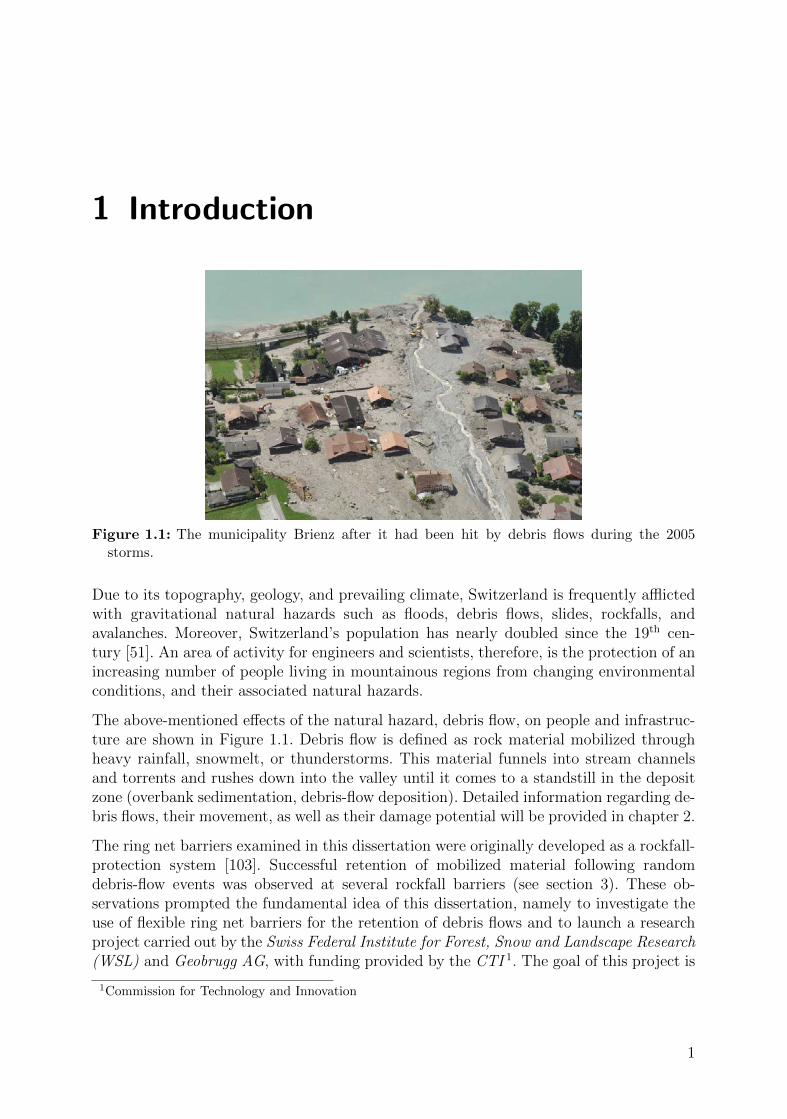
Figure 1.1: The municipality Brienz after it had been hit by debris flows during the 2005storms.
Due to its topography, geology, and prevailing climate, Switzerland is frequently afflictedwith gravitational natural hazards such as floods, debris flows, slides, rockfalls, andavalanches. Moreover, Switzerland’s population has nearly doubled since the 19th cen-tury [51]. An area of activity for engineers and scientists, therefore, is the protection of anincreasing number of people living in mountainous regions from changing environmentalconditions, and their associated natural hazards.
The above-mentioned effects of the natural hazard, debris flow, on people and infrastruc-ture are shown in Figure 1.1. Debris flow is defined as rock material mobilized throughheavy rainfall, snowmelt, or thunderstorms. This material funnels into stream channelsand torrents and rushes down into the valley until it comes to a standstill in the depositzone (overbank sedimentation, debris-flow deposition). Detailed information regarding de-bris flows, their movement, as well as their damage potential will be provided in chapter 2.
The ring net barriers examined in this dissertation were originally developed as a rockfall-protection system [103]. Successful retention of mobilized material following randomdebris-flow events was observed at several rockfall barriers (see section 3). These ob-servations prompted the fundamental idea of this dissertation, namely to investigate theuse of flexible ring net barriers for the retention of debris flows and to launch a researchproject carried out by the Swiss Federal Institute for Forest, Snow and Landscape Research(WSL) and Geobrugg AG, with funding provided by the CTI 1. The goal of this project is
1Commission for Technology and Innovation
1
1 Introduction
to develop an design model of the interaction between debris flow and a flexible ring netbarrier through a comprehensive testing programme with field and laboratory tests, and toapply the model within the context of the discete-element software FARO [103], originallydeveloped for the implementation of rockfall barriers. The understanding gained throughfield and laboratory tests of these processes will enable the development of potential newand optimized protective structures.
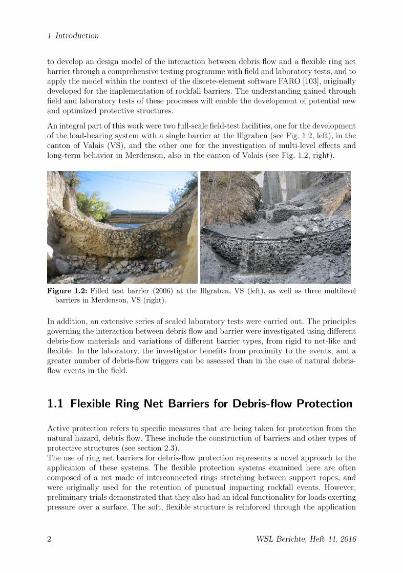
An integral part of this work were two full-scale field-test facilities, one for the developmentof the load-bearing system with a single barrier at the Illgraben (see Fig. 1.2, left), in thecanton of Valais (VS), and the other one for the investigation of multi-level effects andlong-term behavior in Merdenson, also in the canton of Valais (see Fig. 1.2, right).
Figure 1.2: Filled test barrier (2006) at the Illgraben, VS (left), as well as three multilevelbarriers in Merdenson, VS (right).
In addition, an extensive series of scaled laboratory tests were carried out. The principlesgoverning the interaction between debris flow and barrier were investigated using differentdebris-flow materials and variations of different barrier types, from rigid to net-like andflexible. In the laboratory, the investigator benefits from proximity to the events, and agreater number of debris-flow triggers can be assessed than in the case of natural debris-flow events in the field.
1.1 Flexible Ring Net Barriers for Debris-flow Protection
Active protection refers to specific measures that are being taken for protection from thenatural hazard, debris flow. These include the construction of barriers and other types ofprotective structures (see section 2.3).The use of ring net barriers for debris-flow protection represents a novel approach to theapplication of these systems. The flexible protection systems examined here are oftencomposed of a net made of interconnected rings stretching between support ropes, andwere originally used for the retention of punctual impacting rockfall events. However,preliminary trials demonstrated that they also had an ideal functionality for loads exertingpressure over a surface. The soft, flexible structure is reinforced through the application
2 WSL Berichte, Heft 44, 2016

1.2 Classification and Outline of the Present Work
of so-called brake elements, which act as built-in energy dissipators within the supportropes. The individual components of the ring net barriers used for debris-flow protectionwill be discussed in chapter 3.
The advantage of ring net barriers lies in their light support structure, which can betransported by helicopter into difficult-to-access alpine regions. There they can be installedwithin a short period of time. A service road is recommended in cases where emptyingfollowing an event is desired.The net barriers’ filigree appearance, in comparison to massive structures, is easier toincorporate into the natural scenery of regions where tourism often plays an importantrole. The barrier itself constitutes a relatively minor ecological interference for the torrentsystem.
In principle, the flexible net barriers can be subdivided according to two possible areasof application. The empty net structure, generally positioned into the river channel justabove the normal discharge, provides a retention space in case of debris-flow events. Inaddition, the ring net barriers are well suited for enlarging the retention spaces of alreadyexisting structures. When several barriers are arranged consecutively, the retention vol-ume can be increased accordingly.The second area of application is as a permanently-filled structure within the streambedfor the purpose of bed stabilization and the creation of acheck dam. In this case, the struc-tural design and shape of the barrier must be carefully setup in order to minimize abrasiveand corrosive processes. Additional protection from abrasion for the upper support ropesis indispensable for this application (see section 3.2.2.6).
1.2 Classification and Outline of the Present Work
Relatively few approaches to calculate the load applied by debris flows exist to date. Ex-isting approaches are usually based solely on experimental data from scaled laboratorytests [8]. Because of the difficult conditions and procedures, very few debris-flow loadshave been measured in natural debris-flow channels [8].A measurement technique tailored specifically to these requirements recorded rope forcesduring debris-flow events that filled and overflew different ring net barriers at the Illgraben.The results were classified and interpreted in combination with additional measured vari-ables. Further, pressure distributions across the flow depth during a debris-flow event weremeasured for the first time. A model based on the flow laws of fluids was derived fromthis data to describe the stopping process and the interaction between debris flow and aring net barrier.
The laws of friction prevailing during the flow process of debris flows have not been studiedextensively to date [6]. The present work uses data gathered in field and laboratory tests todemonstrate that the friction parameters cannot be considered constant (Mohr-Coulomb),as frequently assumed to date. These friction parameters depend on the instantaneous flowvelocities as well as on the water content and the random energy (granular temperature)being released; they ultimately also influence the pressure coefficient during the dynamicimpact onto a barrier. For granular, friction-dominated debris flows, the derived pressure
WSL Berichte, Heft 44, 2016 3

1 Introduction
coefficient for the amplification of the dynamic load remains to be verified through fieldmeasurements.
Due to the lack of measurement data from debris-flow impacts onto retaining structuresto date, few standards for a safety concept for debris-flow loads have been published [98].Thus, there is a continued need for action to implement the future design of debris-flowprotection systems according to their respective requirements. An initial proposal for asafety concept to be selected for the dimensioning of ring net barriers will be presentedwithin the framework of the present work.
First practical applications of the presented barriers (see section 2.4.3) show an increasingdemand for future-oriented protective systems, which, with intelligent planning and engi-neering, will ensure the continued safe use of residential and recreational areas in alpineregions for years to come.
1.3 Procedures to Determine the Load Model
In order to develop a realistic load model for the design of the ring net barriers, severaldifferent steps (topics) were required, according to which the present work is structured.These are, first and foremost, the field tests, which are complemented by the requiredlaboratory tests and numerical modeling. Taken together, they result in a load model onwhich the design concept for dimensioning net barriers for debris-flow retention is based.
1.3.1 Field Tests
The development, optimization, and measurement instrumentation of the test barrier willbe described in detail in chapter 4; the same chapter contains the detailed description ofthe debris-flow observation station, which the WSL has been operating at the Illgrabensince 2000. Supplemental test results from the so-called debris-flow balance, which wasused to determine the average velocity of the debris flow, will be presented. The dataobtained at the shear wall installed in 2006 complement primarily the load approach bymeans of the effective force profile measured in the debris flow across the flow depth.The results obtained at the test barrier, such as rope force and fill level, will be presented indetail. Additional field measurements to determine geometric parameters such as retentionvolume, channel slope in the filled space, and remaining barrier height of a filled ring netbarrier are illustrated in the process.Though the experiences in the field are essential for determining and optimizing structuralbehavior, they are first and foremost crucial for the study and refinement of specific detailsof the load-bearing system.
4 WSL Berichte, Heft 44, 2016
1.3 Procedures to Determine the Load Model
1.3.2 Laboratory Tests
The projected laboratory tests and their results, which complement the field tests, will bediscussed in chapter 5. The chapter will be introduced by a dimensional analysis allowingfor the scaled adaptation of the results to real-life dimensions. Dimensionless numbers rel-evant to the process description will be presented in detail and factored into the analysis.A total of four different debris-flow material mixtures were used and their effects on debris-jam characteristics, velocity development, friction parameters, and the impact forces dur-ing the filling process examined in order to ensure the experiments are applicable to avariety of different debris-flow channels.Modeling of the laboratory tests with the process-dependent laws of friction within thesoftware AVAL-1D complements the chapter, confirming the obtained measurements.
1.3.3 Historical Concepts and Pressure-Surge Approach
Chapter 6 provides a historical outline, subdivided into approaches to rigid barriers andthe few approaches to flexible barriers, and summarizes the current state of research. Theadvantages and disadvantages of each approach will be described in detail. A load model,which reflects the filling behavior and the loads arising during the filling process of a ringnet barrier, will be developed based on the results from the field and laboratory tests.
1.3.4 Numerical Modeling
The load model developed in chapter 6 will be revisited in chapter 7 and implemented inthe discrete-element program FARO. Different areas of influence of the load application,selection of time steps, and damping ratio will be examined by means of example simu-lations using the 2006 barrier system. The results will be calibrated and validated usingresults from the field tests.
In the case of flexible support structures made of mesh material, the final deformed con-figuration plays an important role in their load-transfer behavior. Hence, a supplementalform-finding analysis using the software CARAT was performed in order to investigatethe ring net barriers’ deformation behavior. A simplified model of a ring net barrier withmembrane elements is shown in Figure 1.3. During the form-finding analysis, the deformedconfiguration is modeled as a function of the preliminary tension of the ring net, and itsbehavior in response to the quasi-static debris-flow load is examined. The required ropelengths and cut of the ring net can be deducted subsequently in order to achieve thedesired final deformed configuration.A comparison between the advantages and disadvantages of the two simulation programsconcludes chapter 7 on numerical modeling.
WSL Berichte, Heft 44, 2016 5

1 Introduction
Figure 1.3: Simulation of the 2006 test barrier using FARO (left) and a simplified model of aring net barrier with membrane elements in CARAT (right).
1.3.5 Formulation of the Design Concept
The final chapter 8 compiles the key points for barrier design and implements them aspart of a model calculation of a barrier in the Hasliberg area of the Bernese Oberland(see also section 2.4.3). The first steps for a design concept will be outlined and discussedwith respect to the standards established to date. Building on this, a cost-benefit analysisof the barriers in the Hasliberg area illustrates the fundamental procedure for planningprotective measures against natural hazards while taking financial considerations intoaccount.
6 WSL Berichte, Heft 44, 2016

2 Debris flows
From a geomorphological perspective, debris flows are a type of gravitational mass move-ment [69]. Different types will be discussed in the first section and will be subdividedaccording to their respective prevailing processes. Subsequently, the debris-flow processitself will be described by means of flow equations, rheology, and energy analyses, whichwill be of critical relevance for further investigations and analyses (see section 2.2).A section about the protective measures existing to date as well as their functionalitiesand procedures for debris-flow retention illustrates the state of currently available tech-nologies. The last part of this chapter will discuss the damage potential of debris flowsand the resulting required protection concepts, using the damages recorded following the2005 flooding [9] as an example.
2.1 Gravitational Mass Movements
The classification of the processes underlying different types of mass movements fre-quently used for engineering purposes is shown in Table 2.1. Mass movements due to iceand snow such as icefall, avalanches, and snow slides do not fall within the scope of thepresent work, which focuses on the mass movements of soil and rock materials. They are,however, classified similarly to the types of mass movements in Table 2.1.
Table 2.1: Classification of mass movements according to Varnes [102].
Process Material
Bedrock Soil and sediment
Falls Rock-/blockfall Soilfall
Slides Rock-/blockslide Debris slide
Flows Rock fragment flow (dry) Debris flow and mudflow (wet)
Gravitational mass movements occur due to changes in the equilibrium of forces, i.e. therelationship between decelerating and accelerating forces, which are a result of physicaland/or chemical processes [17]. Water generally plays a decisive role, as it reduces thestability, i.e. the internal friction and cohesion of the material, by means of a variety ofprocesses. The term ”mass movement” is more commonly used than the frequently-usedterm ”landslide,” as the latter does not include the falling, toppling, and slower processes,such as creeps and spreads [19].
7
2 Debris flows
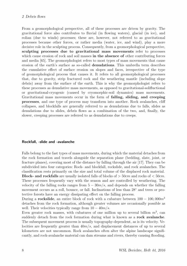
From a geomorphological perspective, all of these processes are driven by gravity. Thegravitational force also contributes to fluvial (in flowing waters), glacial (in ice), andeolian (due to winds) processes; these are, however, not referred to as gravitationalprocesses because other forces, or rather media (water, ice, and wind), play a moredecisive role in the sculpting process. Consequently, from a geomorphological perspective,sculpting processes due to gravitational mass movements refer to processeswhich cause erosion of rock and soil masses in the absence of other contributing forcesand media [65]. The geomorphologist refers to most types of mass movements that causeerosion of the earth’s surface as so-called denudations. This umbrella term describesthe cumulative effect of surface erosion on slopes and faces, irrespective of the typeof geomorphological process that causes it. It refers to all geomorphological processesthat, due to gravity, strip fractured rock and the weathering mantle (including slopedebris) away from the surface of the earth. This is why the geomorphologist refers tothese processes as denudative mass movements, as opposed to gravitational-solifluctionalor gravitational-cryogenic (caused by cryomorphic-soil dynamics) mass movements.Gravitational mass movements occur in the form of falling, sliding, and creepingprocesses, and one type of process may transform into another. Rock avalanches, cliffcollapses, and blockfalls are generally referred to as denudations due to falls, slides asdenudations due to slides, debris flows as a combination of the two, and, finally, theslower, creeping processes are referred to as denudations due to creeps.
Rockfall, -slide and -avalanche
Falls belong to the fast types of mass movements, during which the material detaches fromthe rock formation and travels alongside the separation plane (bedding, slate, joint, orfracture planes), covering most of the distance by falling through the air [17]. They can besubdivided into four categories: Rock- and blockfall, rockslide, and rock avalanches. Theclassification rests primarily on the size and total volume of the displaced rock material.Block- and rockfalls are usually isolated falls of blocks of > 50cm and rocks of < 50cm.These processes frequently vary with the season and are controlled by weathering. Thevelocity of the falling rocks ranges from 5 − 30m/s, and depends on whether the fallingmovement occurs as a roll, bounce, or fall. Inclinations of less than 28◦ and trees or pro-tective forests have an energy dissipating effect on the falling process.During a rockslide, an entire block of rock with a cubature between 100 − 100, 000m3
detaches from the rock formation, although greater volumes are occasionally possible aswell. Their velocities typically range from 10− 40m/s.Even greater rock masses, with cubatures of one million up to several billion m3, cansuddenly detach from the rock formation during what is known as a rock avalanche.The subsequent movement process is usually topography-dependent, as is its velocity. Ve-locities are frequently greater than 40m/s, and displacement distances of up to severalkilometers are not uncommon. Rock avalanches often alter the alpine landscape signifi-cantly, and rock-avalanche material can dam streams and rivers, thereby causing flooding.
8 WSL Berichte, Heft 44, 2016
2.1 Gravitational Mass Movements
Slides
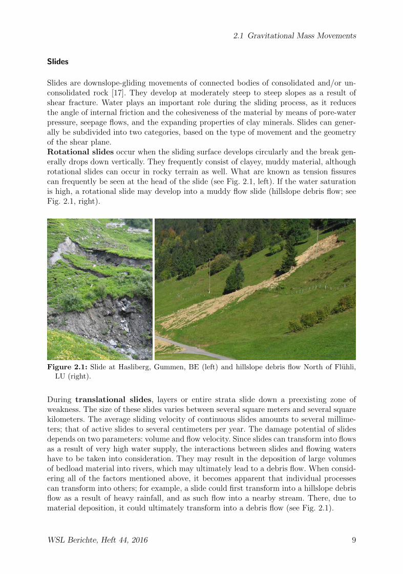
Slides are downslope-gliding movements of connected bodies of consolidated and/or un-consolidated rock [17]. They develop at moderately steep to steep slopes as a result ofshear fracture. Water plays an important role during the sliding process, as it reducesthe angle of internal friction and the cohesiveness of the material by means of pore-waterpressure, seepage flows, and the expanding properties of clay minerals. Slides can gener-ally be subdivided into two categories, based on the type of movement and the geometryof the shear plane.Rotational slides occur when the sliding surface develops circularly and the break gen-erally drops down vertically. They frequently consist of clayey, muddy material, althoughrotational slides can occur in rocky terrain as well. What are known as tension fissurescan frequently be seen at the head of the slide (see Fig. 2.1, left). If the water saturationis high, a rotational slide may develop into a muddy flow slide (hillslope debris flow; seeFig. 2.1, right).
Figure 2.1: Slide at Hasliberg, Gummen, BE (left) and hillslope debris flow North of Fluhli,LU (right).
During translational slides, layers or entire strata slide down a preexisting zone ofweakness. The size of these slides varies between several square meters and several squarekilometers. The average sliding velocity of continuous slides amounts to several millime-ters; that of active slides to several centimeters per year. The damage potential of slidesdepends on two parameters: volume and flow velocity. Since slides can transform into flowsas a result of very high water supply, the interactions between slides and flowing watershave to be taken into consideration. They may result in the deposition of large volumesof bedload material into rivers, which may ultimately lead to a debris flow. When consid-ering all of the factors mentioned above, it becomes apparent that individual processescan transform into others; for example, a slide could first transform into a hillslope debrisflow as a result of heavy rainfall, and as such flow into a nearby stream. There, due tomaterial deposition, it could ultimately transform into a debris flow (see Fig. 2.1).
WSL Berichte, Heft 44, 2016 9

2 Debris flows
Debris flows
Debris flows are fast-flowing mixtures of water, debris, sediment, and wood, with a highconcentration of solids of about 30 − 70 % [16]. They occur primarily in alpine regions,where substrates susceptible to erosion provide much unconsolidated rock material. Inaddition, they require channel slopes steeper than 25 − 30%, depending on the frictionangle of the material. Furthermore, large volumes of water, for example those resultingfrom heavy rainfall or snowmelt, are needed as an initiator, mobilizing the unconsolidatedsolid material. Once the material of a debris flow is mobilized, it can reach velocities ofup to 15m/s and densities between 1600−2300kg/m3. The volumes displaced by a debrisflow can grow up to several hundred thousand cubic meters. Debris-flow deposition occurswhen a debris flow leaks out of the streambed or breaks out laterally at the embankment,due to great erosive forces (deposition area of a debris flow in Fig. 2.2). Further detailsregarding the debris-flow process will be provided in section 2.2.
Figure 2.2: Deposition zone of a debris flow with a width of several kilometers in the Himalaya,Nepal, Langtang region.
A subcategory of debris flows includes what are known as hillslope debris flows, alsoreferred to as flow slides. A superficial mixture of unconsolidated solids (primarily soiland plant canopy) and water characterize this form of mass movement [17]. Hillslopedebris flows develop primarily on relatively steep slopes (above 30◦), although a clearsliding surface is not present. The mobilized volume is usually limited, and reaches up to20, 000m3. Their movement speed, much like that of debris flows, depends heavily on watercontent, but usually ranges from 1 to 10m/s. If a hillslope debris flow flows into flowingwater, it can transform into a debris flow, and provides the material for the subsequentprocess.
10 WSL Berichte, Heft 44, 2016
2.2 The Debris-flow Process
2.2 The Debris-flow Process
2.2.1 Initiation
In the Alps, the events initiating debris flows are primarily of hydrological nature. How-ever, debris flows can also be triggered by earthquakes and volcanic eruptions. An analysisof triggering conditions for debris flows in Switzerland revealed the following, fundamen-tally different, causes [120]:
• Short, thundery rainfalls
• Long periods of rainfall
• Extensive snow- and icemelt
• Dam failure and lake outbursts
The first two elements are referred to as precipitation-dependent events. The last two el-ements can also occur during periods of dry weather conditions. Precipitation-dependentevents include what is known as incident precipitation, which is defined as the rainfallthat fell constantly until the point at which the debris flow was triggered. These couldbe short rainfalls, lasting between 1 and 4h, primarily thunderstorms, or long periods ofrainfall lasting between 12 and 48h. Long periods of rainfall that trigger debris flows occurprimarily in the inner Alps and at the South side of the Alps, while thunderstorms triggerdebris-flow activity primarily at the foothills of the Alps and in the Alps themselves.Figure 2.3 shows three demarcation lines, which illustrate the critical precipitation inten-sity I [mm/h] required to trigger a debris flow as a function of duration D [h]. Abovethese demarcation lines, debris-flow activity can - but doesn’t have to - occur. Belowthem, only a flooding event usually occurs. A global boundary illustrating what is gener-ally considered to be required for the triggering of a debris flow or a hillslope debris flowis indicated based on [18]. According to [120], a critical precipitation lasting one hour atapproximately 40mm/h is applicable for the Swiss Alpine region. The minimum precipi-tation requirement during a 24h long rainfall amounts to approximately 2.5mm/h, or atotal amount of precipitation of 60mm. As an example from the region, the precipitationintensity required to trigger a debris flow in the Illgraben (an active debris-flow channelin Canton of Valais, Switzerland, and debris-flow observation station of the WSL [68, 69])is
I = 10 ·D−0.85 (2.1)
whereD is the duration of the precipitation event and I the average precipitation intensity.Full particulars about the Illgraben and the local debris-flow research will be provided inchapter 4.
The limiting curve for precipitation intensity in the Illgraben is lower than the othertwo curves in Figure 2.3, indicating that the Illgraben responds much faster than otherdebris-flow systems. Above the indicated limiting curve, a debris-flow event occurs in theIllgraben with 50% probability.Aside from adequate water saturation, sufficient amounts of weathering and unconsoli-dated solid material are also required; additionally, enough potential energy is needed,
WSL Berichte, Heft 44, 2016 11

2 Debris flows
Figure 2.3: Average precipitation intensity required for debris-flow events globally, regionally,and locally. Legend: mittlere Niederschlagsintensitat = average precipitation intensity; DauerD des Regenereignisses = duration D of rainfall event; regionaler Datensatz fur SchweizerAlpen = regional data set in Swiss Alps; lokaler Datensatz = local data set; globaler Datensatz= global data set.
which subsequently transforms into kinetic energy by means of the mobilization of thematerial (see section 2.2.3). The following three parameters constitute the requirementsfor the triggering of a debris-flow event.
2.2.2 Flow Process
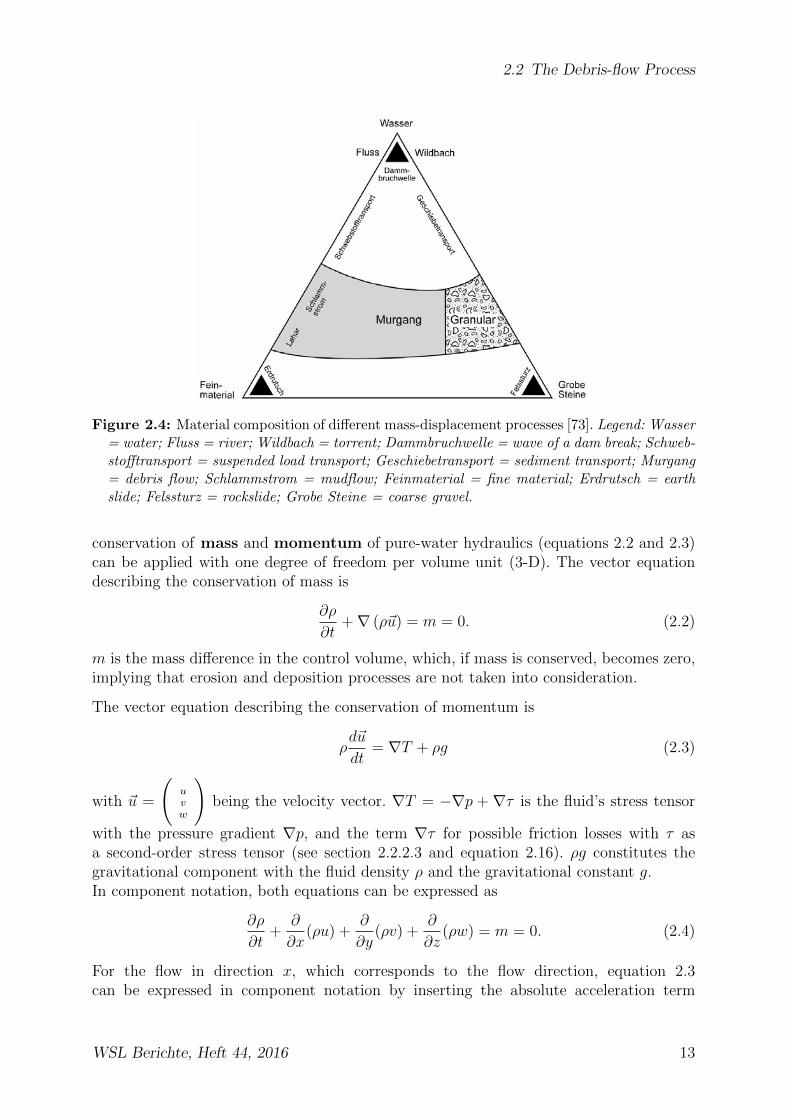
In order to describe the flow process in more detail, the debris flows will have to besubdivided further. Here, according to [73], material composition plays an important role(see Fig. 2.4).
If the debris flow consists almost exclusively of fine material, it is referred to as a mudflow(or lahar). If rocks and blocks are the prevailing materials, it is referred to as a granulardebris flow. The density of a mudflow usually ranges from 1600 to 1900kg/m3, whereasthe density of a granular debris flow is higher, ranging from 1900kg/m3 to 2300kg/m3
(for determination of debris-flow density, see chapter 4.2.2). An exact boundary for thetransition from mudflow to granular debris flow cannot be determined. It is also not un-usual for hybrid forms to occur during a debris-flow event. In fact, granular fronts, whichoften carry large blocks and whose ensuing debris-flow tails frequently are mudflow-like,are relatively common (see also section 4.5).As can be seen in Figure 2.4, water content and grain size distribution play an impor-tant role in the flow behavior of the material. Several approaches to further characterizethe flow behavior already exist to date. The simplest approaches treat the debris flowsas homogeneous fluids with specific physical properties. As a result, the known laws of
12 WSL Berichte, Heft 44, 2016
2.2 The Debris-flow Process
Figure 2.4: Material composition of different mass-displacement processes [73]. Legend: Wasser= water; Fluss = river; Wildbach = torrent; Dammbruchwelle = wave of a dam break; Schweb-stofftransport = suspended load transport; Geschiebetransport = sediment transport; Murgang= debris flow; Schlammstrom = mudflow; Feinmaterial = fine material; Erdrutsch = earthslide; Felssturz = rockslide; Grobe Steine = coarse gravel.
conservation of mass and momentum of pure-water hydraulics (equations 2.2 and 2.3)can be applied with one degree of freedom per volume unit (3-D). The vector equationdescribing the conservation of mass is
∂ρ
∂t+∇ (ρ~u) = m = 0. (2.2)
m is the mass difference in the control volume, which, if mass is conserved, becomes zero,implying that erosion and deposition processes are not taken into consideration.
The vector equation describing the conservation of momentum is
ρd~u
dt= ∇T + ρg (2.3)
with ~u =
(uvw
)being the velocity vector. ∇T = −∇p +∇τ is the fluid’s stress tensor
with the pressure gradient ∇p, and the term ∇τ for possible friction losses with τ asa second-order stress tensor (see section 2.2.2.3 and equation 2.16). ρg constitutes thegravitational component with the fluid density ρ and the gravitational constant g.In component notation, both equations can be expressed as
∂ρ
∂t+
∂
∂x(ρu) +
∂
∂y(ρv) +
∂
∂z(ρw) = m = 0. (2.4)
For the flow in direction x, which corresponds to the flow direction, equation 2.3can be expressed in component notation by inserting the absolute acceleration term
WSL Berichte, Heft 44, 2016 13

2 Debris flows
ρd~udt
= ρ(∂~u∂t
+ u∂~u∂x
+ v ∂~u∂y
+ w ∂~u∂z
). Therefore, the conservation of momentum in direction
x expressed in component notation is
ρ
(∂u
∂t+ u
∂u
∂x+ v
∂u
∂y+ w
∂u
∂z
)= ρgx −
∂p
∂x+∂τxx∂x
+∂τyx∂y
+∂τzx∂z
(2.5a)
and in directions y and z
ρ
(∂v
∂t+ u
∂v
∂x+ v
∂v
∂y+ w
∂v
∂z
)= ρgy −
∂p
∂y+∂τyy∂y
+∂τxy∂x
+∂τzy∂z
(2.5b)
ρ
(∂w
∂t+ u
∂w
∂x+ v
∂w
∂y+ w
∂w
∂z
)= ρgz −
∂p
∂z+∂τzz∂z
+∂τxz∂x
+∂τyz∂y
. (2.5c)
The friction components ∂τxx∂x
+ ∂τyx∂y
+ ∂τzx∂z
etc. will be discussed in section 2.2.2.3. Equa-tions 2.4 and 2.5 are three-dimensional equations of motion for a volume element. Theseequations still have many unknowns, such as the pressure p, the single velocity com-ponents u, v, w, and the shear stresses τij. With respect to this problem, the followingsimplifications of the flow equations are applied in fluid mechanics [22].
• One-dimensional flow models still consider the velocity at every point in itsdirection, and in incompressible flows (∂ρ
∂t= 0) as constant. In essence, this approach
can be reduced to a flow line. Velocities, flow depths, and pressures are taken intoaccount in the form of average values perpendicular to the direction of motion. Thisusually works by means of an averaged integration of two-dimensional equations ofmotion over the flow depth z (equations 2.4 and 2.5 without the y components).The channel width can then also be taken into account by means of a width factor.
• In two-dimensional flow models, the flow lines must flow in parallel, so as toalways yield rectangular flow regions of equal width b (see also Fig. 2.5). However,the width of the entire cross section must be constant. These widths are basedon 3-D equations, which are either integrated over the averaged flow depth h andinclude the insertion of the free surface and channel bottom boundary conditions, orthey are additionally integrated over the averaged width. These models are appliedprimarily in channel hydraulics.
• Three-dimensional flows no longer require a segmentation of the associated flowfunction into constant widths (see Fig. 2.5). Three-dimensional flow conditions exist,for instance, when air conditioners blow out air, or in flow processes in torrents. Allcomponents of equations 2.4 and 2.5 are taken into account.
2.2.2.1 Simplified Equations of Motion
The simplified model for granular flows along a plane with an inclination Θ accordingto [87] makes the following assumptions. The flow sliding downslope is considered to bea continuum with several particles distributed across the height H = hmax, suggesting
14 WSL Berichte, Heft 44, 2016

2.2 The Debris-flow Process
Low velocity
High velocity High velocity
Low velocity b = const
b ≠ const
Figure 2.5: Two-dimensional and axially-symmetric flow model according to [22]. The axialsymmetry of the model assumption in Figure 2.5 is actually a special case of three-dimensionalflow.
that the relation HL� 1 applies. Due to the incompressibility, the density is assumed to
be constant across the height z ( ∂ρ∂h
= 0). Furthermore, velocity is not assumed to varyacross the flow depth h and is considered to be uniformly distributed in the flow directionx. Velocities perpendicular to the direction of motion (in y- and z- direction, v and w)are not taken into consideration. This leads to a hydrostatic pressure distribution in thez-direction (∂p
∂z= ρgz(z − h)).
Figure 2.6: Geometry of a granular mass on an inclined plane.
In [7], the equations of mass and momentum are, as in the shallow-water approximationwith height averaging, integrated over the flow depth h of the granular flow:
U =1
h
∫ h
0
udz. (2.6)
However, a fixed profile function (which will not be discussed further within the contextof this derivation) has to be assumed for every parameter to be integrated [62]. Forρ = const., the following equations of motion for a granular mass moving in direction xon an inclined plane emerge
∂h
∂t+
∂
∂x(hU) = 0 (2.7)
and for the conservation of momentum
∂U
∂t+ U
∂U
∂x= gx −
1
ρ
∂p
∂x+
1
ρhτzx|0. (2.8)
WSL Berichte, Heft 44, 2016 15
2 Debris flows
Inserting the pressure gradient p/∂x = −ρgz ∂h∂x into equation 2.8 yields the universallyvalid equation of momentum for a granular mass on an inclined plane
∂U
∂t+ U
∂U
∂x= gx − gz
∂h
∂x+
1
ρhτzx|0 (2.9)
with τzx|0 being the effective shear stress on the ground. The shear-stress term∫ h
0∂τzx∂z
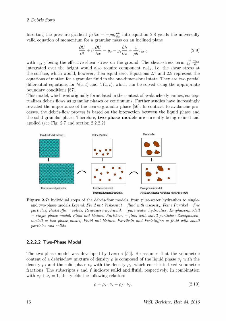
integrated over the height would also require component τzx|h, i.e. the shear stress atthe surface, which would, however, then equal zero. Equations 2.7 and 2.9 represent theequations of motion for a granular fluid in the one-dimensional state. They are two partialdifferential equations for h(x, t) and U(x, t), which can be solved using the appropriateboundary conditions [87].This model, which was originally formulated in the context of avalanche dynamics, concep-tualizes debris flows as granular phases or continuums. Further studies have increasinglyrevealed the importance of the coarse granular phase [56]. In contrast to avalanche pro-cesses, the debris-flow process is based on the interaction between the liquid phase andthe solid granular phase. Therefore, two-phase models are currently being refined andapplied (see Fig. 2.7 and section 2.2.2.2).
Figure 2.7: Individual steps of the debris-flow models, from pure-water hydraulics to single-and two-phase models.Legend: Fluid mit Viskositat = fluid with viscosity; Feine Partikel = fineparticles; Feststoffe = solids; Reinwasserhydraulik = pure water hydraulics; Einphasenmodell= single phase model; Fluid mit kleinen Partikeln = fluid with small particles; Zweiphasen-modell = two phase model; Fluid mit kleinen Partikeln und Feststoffen = fluid with smallparticles and solids.
2.2.2.2 Two-Phase Model
The two-phase model was developed by Iverson [56]. He assumes that the volumetriccontent of a debris-flow mixture of density ρ is composed of the liquid phase νf with thedensity ρf and the solid phase νs with the density ρs, which constitute fixed volumetricfractions. The subscripts s and f indicate solid and fluid, respectively. In combinationwith νf + νs = 1, this yields the following relation:
ρ = ρs · νs + ρf · νf . (2.10)
16 WSL Berichte, Heft 44, 2016

2.2 The Debris-flow Process
Moreover, Iverson assumes that grain sizes of less than 0.05mm, i.e. clays and silts, per-manently remain in suspension and are, therefore, part of the liquid phase. Grain sizesabove 0.05mm, such as sand and gravel, are part of the solid phase of the debris flow.Based on these assumptions, different physical properties can be inferred for the solidand the liquid phase. Coulomb’s friction law (equation 2.20) applies to both dry, solidmaterial, as well as to water-saturated, debris-flow material. The laws of friction for fluidsapply to the liquid phase (see section 2.2.2.3). Therefore, the equations of motion areformulated separately for each phase.
Two-Phase Equations of Motion
The conservation of mass for the liquid and solid phases are described in 2.11a and 2.11b.
Conservation of mass (solids)∂(ρsνs)
∂t+∇ · (ρsνs~us) = ms (2.11a)
Conservation of mass (liquids)∂(ρfνf )
∂t+∇ · (ρfνf~uf ) = mf (2.11b)
With ~us and ~uf being the velocities of the liquid and the solid phase, respectively, and ms
and mf being the mass of the liquid and solid phase, respectively, per volume unit. Theequations 2.11a and 2.11b are coupled via νf +νs = 1 (see equation 2.10). This ultimatelyleads to equation 2.12, which describes the conservation of mass in a debris flow
∂ρ
∂t+∇ · (ρu) = mf +ms. (2.12)
Iverson assumes a shared velocity u, which is defined in
u = (ρsνsus + ρfνfuf )/ρ. (2.13)
Additional important assumptions are that no change in mass (ms + mf = 0) occursduring the process and that both phases are incompressible. This results in
∂ρ
∂t+∇ · (ρu) = 0. (2.14)
The equations for the conservation of momentum are, therefore:
ρsνs
(∂us∂t
+ us · ∇us)
= ∇ · Ts + ρsνsg + f −msvs (2.15a)
ρfνf
(∂uf∂t
+ uf · ∇uf)
= ∇ · Tf + ρfνfg + f −mfvf (2.15b)
Ts and Tf are the stress tensors of the liquid and the solid phase, and f represents theinteraction force, which results from the exchange of momentum between the fluid andsolid particles. If the change in mass is again not taken into consideration, the terms msvsand mfvf do not apply.Compared to single-phase models, equations 2.12 and 2.15 have the advantage of having
WSL Berichte, Heft 44, 2016 17
2 Debris flows
two stress tensors for the liquid phase Tf and the solid phase Ts, which can be consideredseparately. The stress tensor Ts of the solid phase incorporates, among others, the Mohr-Coulomb friction law (see equation 2.20). For the derivation of the stress tensor Tf of afluid with internal friction (viscosity), the following conditions apply:
• In nonviscous cases, the stress tensor decreases to the scalar pressure p.
• The liquid is incompressible.
• The frictional forces are proportional to the first derivatives of the velocity (Newto-nian fluid, see section 2.2.2.3).
Tf = −pI + 2νfηfD︸ ︷︷ ︸viscous stress tensor τi,j
(2.16)
p is the pressure and I the identity tensor, which together form the pressure term. Thesecond part of the equation describes the viscous stress tensor τi,j = 2νfηfD. ηf is theviscosity of the fluid, which is multiplied by the liquid fraction νf , andD is the deformationtensor of a fluid
Di,j =1
2
(∂ui∂xj
+∂uj∂xi
). (2.17)
Di,j characterizes the shear of a fluid, and, as a result, Di,j = Dj,i applies. The deformationtensor D is, therefore, symmetrical. If the rotation of the fluid particles is not takeninto account, the diagonal elements Di,i of the deformation tensor result from the strain(Dxx = ∂u
∂x, Dyy = ∂v
∂y, and Dzz = ∂w
∂z). The interaction between the two phases can
thereby be characterized as well. Moreover, the momentum balance takes the force f(which expresses the exchange of momentum via the interaction between both the grainsand the fluid as well as between themselves) into account [56]. The implementation of thistwo-phase model and its equations into a flow model is described in [62].
2.2.2.3 Rheology and Laws of Friction
Although the simplified equations for granular media and the stress tensors Ts and Tfhave, as of yet, only taken friction losses into consideration in the form of term fr = ∇τor as 1
ρτzx∂z
, they have not been characterized in more detail. With respect to the friction
term, the material law of the fluid (and that of the solids in the case of two-phase models)is incorporated into the equations.A number of fluids and their flow behaviors (rheology) can be differentiated, generallybased on the Herschel-Bulkley model [22]:
τ = τy + η
(du
dz
)b. (2.18)
For Newtonian fluids, the constant η corresponds to the dynamic viscosity, and theexponent b becomes one, i.e. a linear material behavior occurs. In the case of pure water,an example of a Newtonian fluid, b = 1, η = 1, and τy = 0 applies. The function ofequation 2.18 is simplified to a straight line through the origin (Fig. 2.8). An exponent b
18 WSL Berichte, Heft 44, 2016
2.2 The Debris-flow Process
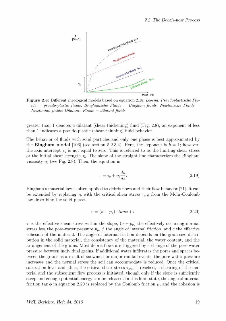
Figure 2.8: Different rheological models based on equation 2.18. Legend: Pseudoplastische Flu-ide = pseudo-plastic fluids; Binghamsche Fluide = Bingham fluids; Newtonsche Fluide =Newtonian fluids; Dilatante Fluide = dilatant fluids.
greater than 1 denotes a dilatant (shear-thickening) fluid (Fig. 2.8); an exponent of lessthan 1 indicates a pseudo-plastic (shear-thinning) fluid behavior.
The behavior of fluids with solid particles and only one phase is best approximated bythe Bingham model [106] (see section 5.2.3.4). Here, the exponent is b = 1; however,the axis intercept τy is not equal to zero. This is referred to as the limiting shear stressor the initial shear strength τb. The slope of the straight line characterizes the Binghamviscosity ηb (see Fig. 2.8). Then, the equation is
τ = τb + ηbdu
dz. (2.19)
Bingham’s material law is often applied to debris flows and their flow behavior [21]. It canbe extended by replacing τb with the critical shear stress τcrit from the Mohr-Coulomblaw describing the solid phase.
τ = (σ − pp) · tanφ+ c (2.20)
τ is the effective shear stress within the slope, (σ − pp) the effectively-occurring normalstress less the pore-water pressure pp, φ the angle of internal friction, and c the effectivecohesion of the material. The angle of internal friction depends on the grain-size distri-bution in the solid material, the consistency of the material, the water content, and thearrangement of the grains. Most debris flows are triggered by a change of the pore-waterpressure between individual grains. If additional water infiltrates the pores and spaces be-tween the grains as a result of snowmelt or major rainfall events, the pore-water pressureincreases and the normal stress the soil can accommodate is reduced. Once the criticalsaturation level and, thus, the critical shear stress τcrit is reached, a shearing of the ma-terial and the subsequent flow process is initiated, though only if the slope is sufficientlysteep and enough potential energy can be released. In this limit state, the angle of internalfriction tanφ in equation 2.20 is replaced by the Coulomb friction µ, and the cohesion is
WSL Berichte, Heft 44, 2016 19

2 Debris flows
neglected.
τ = τcrit + ηbdu
dz= (σ − p)µ︸ ︷︷ ︸
Mohr−Coulombfriction
+ ηbdu
dz︸ ︷︷ ︸viscous friction
(2.21)
In this equation, the Mohr-Coulomb friction represents the dry friction, and the viscousfriction represents the velocity-dependent or internal friction.
2.2.3 Energy Balance
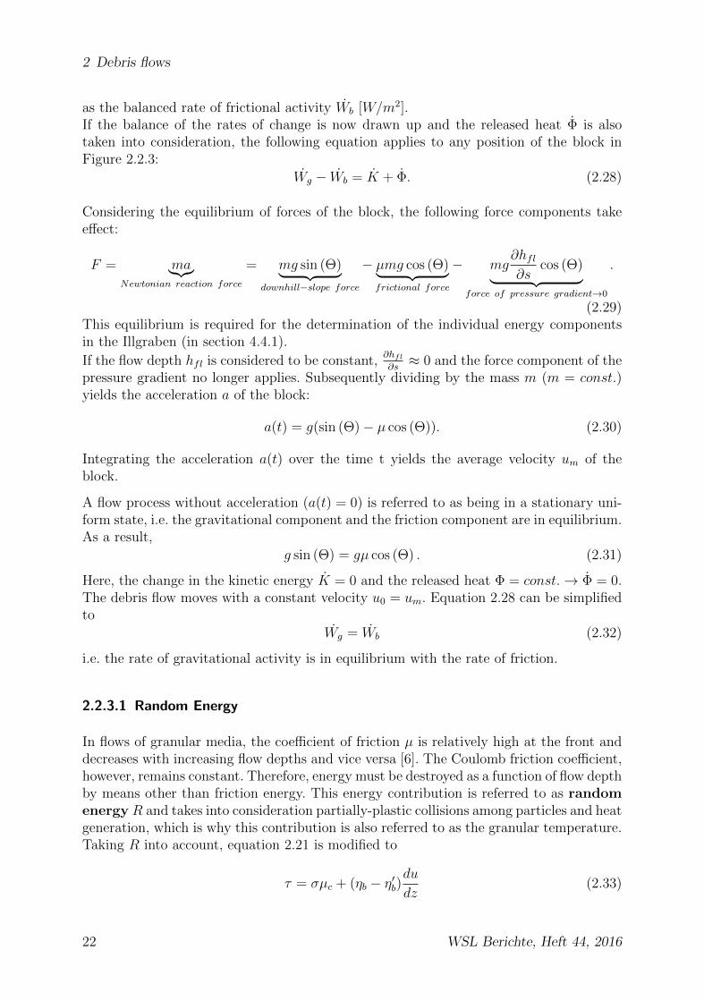
Single-phase models, such as the previously discussed Bingham model (see equation 2.19),have limitations with respect to the energy balance. The momentum-flux balance primarilydescribes the loss of energy due to viscous shear stress. However, it does not take intoaccount the loss of energy due to grains colliding with each other (what Bartelt [5] refers toas random energy). Therefore, a further development of hydraulic models for debris flowsis based on an explicit consideration of the physical processes underlying the conservationof mass, the conservation of momentum, and the conservation of energy, as well as onthe individual losses during the process [56]. The equations for the conservation of massand momentum have already been discussed in the previous sections. What remains to bediscussed are the equations for the conservation of energy within the physical flow process.These are of critical importance for the ability to predict if a global failure will occurfollowing the initiation phase of a debris flow, i.e. if potential energy will be convertedto kinetic energy. Furthermore, energy analyses are required to predict how decelerationand acceleration processes develop within the debris flow. This information, in turn, isnecessary for the ability to plan protection concepts and the appropriate measures.Therefore, conservation-of-energy analyses for debris flows will be derived and establishedin this section by means of a simplified model. In addition, they will be supported withfield and laboratory data for debris flows with material from the Illgraben (in sections 4.2.2and 5.4.1). In the simplified model of our energy analyses, we characterize the debris flowby means of the flow depth hfl as a block of mass m, which slides down an inclined planewith the angle Θ = dH/ds.
According to the conservation-of-energy principle
∆Epot + ∆K + ∆Einternal = 0 (2.22)
with Epot = mgH being the potential, i.e. the gravitational energy at the beginning ofthe process. H is the initial height and ∆H is the vertical difference between position 1and position 2 within the complete system. During the flow process, the initial potentialenergy Epot is converted into a residual fraction ∆Epot−∆H , the kinetic energy K, andthe internal energy (see Fig. 2.9 and equation 2.22).For the other balances, the term work rate is introduced. It refers to the change in therespective form of energy, i.e. the change of energy occurring in a debris flow with an areaof one square meter and with a flow depth hfl over the course of time t. The mass mof the block over one m2 then becomes m = ρhfl = σ
g cos(Θ)in weight per m2 [kg/m2]. σ
[N/m2] is the effective normal force, which is measured in section 4.2.2 for debris flowsin the Illgraben (see chapter 4). All components of the work rate will be written with a
20 WSL Berichte, Heft 44, 2016

2.2 The Debris-flow Process
Figure 2.9: Debris flow modeled as a sliding block on a plane. Legend: innere = internal.
period ”·” in the following sections. The work rate of the potential energy is then referredto as Wg(t) [W/m2] and is equal to
Wg(t) = gρhflgds
dt= ρhflg
sin (Θ) s
dt= ρhflg sin (Θ)um = σ tan (Θ)um (2.23)
with um = ds/dt as the average velocity over the flow depth hfl.
The kinetic energy K is then equal to
K =1
2ρhflu
2m =
1
2
σ
g cos (Θ)u2m (2.24)
and its rate of change K [W/m2] being
K =1
2
(dσ
dt
)u2m
g cos (Θ)+ um
(dumdt
)σ
g cos (Θ). (2.25)
The change of mass m = ddt
σg cos(Θ)
and, accordingly, dσdt
, is considered to be small, i.e.erosion and deposition processes are not considered in these balances. The first term12
(dσdt
)u2m
g cos(Θ)→ 0 is neglected. K then becomes
K = um
(dumdt
)︸ ︷︷ ︸
am
σ
g cos (Θ)= umam
σ
g cos (Θ)= umamρhfl. (2.26)
The last component of the energy balance is the internal energy Einternal. In our simplifiedmodel of a block on an inclined plane, it includes only the basal friction energy Wb, which isgenerated by the shear stress on a rough substrate. All other internal losses are neglected,i.e. Einternal = Wb applies with
Wb = τum (2.27)
WSL Berichte, Heft 44, 2016 21
2 Debris flows
as the balanced rate of frictional activity Wb [W/m2].If the balance of the rates of change is now drawn up and the released heat Φ is alsotaken into consideration, the following equation applies to any position of the block inFigure 2.2.3:
Wg − Wb = K + Φ. (2.28)
Considering the equilibrium of forces of the block, the following force components takeeffect:
F = ma︸︷︷︸Newtonian reaction force
= mg sin (Θ)︸ ︷︷ ︸downhill−slope force
− µmg cos (Θ)︸ ︷︷ ︸frictional force
− mg∂hfl∂s
cos (Θ)︸ ︷︷ ︸force of pressure gradient→0
.
(2.29)This equilibrium is required for the determination of the individual energy componentsin the Illgraben (in section 4.4.1).
If the flow depth hfl is considered to be constant,∂hfl∂s≈ 0 and the force component of the
pressure gradient no longer applies. Subsequently dividing by the mass m (m = const.)yields the acceleration a of the block:
a(t) = g(sin (Θ)− µ cos (Θ)). (2.30)
Integrating the acceleration a(t) over the time t yields the average velocity um of theblock.
A flow process without acceleration (a(t) = 0) is referred to as being in a stationary uni-form state, i.e. the gravitational component and the friction component are in equilibrium.As a result,
g sin (Θ) = gµ cos (Θ) . (2.31)
Here, the change in the kinetic energy K = 0 and the released heat Φ = const.→ Φ = 0.The debris flow moves with a constant velocity u0 = um. Equation 2.28 can be simplifiedto
Wg = Wb (2.32)
i.e. the rate of gravitational activity is in equilibrium with the rate of friction.
2.2.3.1 Random Energy
In flows of granular media, the coefficient of friction µ is relatively high at the front anddecreases with increasing flow depths and vice versa [6]. The Coulomb friction coefficient,however, remains constant. Therefore, energy must be destroyed as a function of flow depthby means other than friction energy. This energy contribution is referred to as randomenergy R and takes into consideration partially-plastic collisions among particles and heatgeneration, which is why this contribution is also referred to as the granular temperature.Taking R into account, equation 2.21 is modified to
τ = σµc + (ηb − η′b)du
dz(2.33)
22 WSL Berichte, Heft 44, 2016

2.2 The Debris-flow Process
with µc as the Coulomb friction coefficient and η′b as the viscous shear-thinning as afunction of the random energy R. The generation of R is proportional to the rate ofgravitational activity Wg (see equation 2.23). The change in R over time t is proportionalto the current random energy. This yields
R(t) = αWg(t)︸ ︷︷ ︸random−energy generation
− βR(t)︸ ︷︷ ︸particlecollision → heat
. (2.34)
This equation can be explained visually by means of what is known as a reciprocal thwart-ing effect, i.e. the more that the grains collide with each other at high random energy, thefaster the grains come back to rest due to the partially-plastic impacts.Taking the random energy into account as an additional component of the internal energyyields
Wb = Φ + R (2.35)
with Φ being the heat released as a result of basal friction and R as the random-energycontribution. Then, the overall energy balance, including the random-energy contribution,is
Wg − Wb = K + Φ + R. (2.36)
For a more detailed explanation of random energy and its effect on the coefficient offriction µ, see [46] and chapter 5.4.1.
WSL Berichte, Heft 44, 2016 23

2 Debris flows
2.3 Protective Measures
Protective measures are required in order to protect people and infrastructure from nat-ural hazards. Gravitational natural hazards are generally dealt with using a stepwiseapproach [17]. The first step is the identification of hazards and their documentation, sothat information can be provided as to whether an area is at risk. This is followed by thesecond step, which examines how much an area is at risk. In particular, this step includesthe process of hazard mapping. Both the risk map and hazard map function together as abasis for the assessment of the damage potential. The final step is action planning, whichincludes the protective measures. During the action-planning process, passive measuresshould be considered first. These include, for example, an adapted use of and, as a result,primarily new building-permit phases in critical areas. Active measures actively intervenein the course of events. Here, probabilities and intensities, as well as the expected damagepotential, are taken into account in the assessment (see also section 8.3). Active measuresalso include debris-flow protection concepts, which will be described in more detail inthe remainder of this section. Furthermore, there are also emergency measures, intendedto function primarily as backups in case of the failure of the protection concepts. Theseinclude early-warning systems, evacuation procedures, and rapid disaster relief, since anyprotective measure can fail in exceptional circumstances.Active debris-flow protection consists of four different approaches, which may also occuras hybrid forms:
• Diversion
• Retention
• Drainage
• Passing through
2.3.1 Diversion Dams
Diversion dams are a concept taken from avalanche protection, for which they have longproven to be of value. They are massive structures made of thrown blocks or naturally-deposited material, with or without additional fasteners. They are usually placed abovethe infrastructure to be protected and, should a debris-flow event occur, are intended toredirect the debris flow in a controlled manner in flow direction, so that it comes to astandstill in a safe area. In practice, such a diversion dam has been implemented in theTrachtbach near Brienz (see section 2.4.2). Other examples include the diversion dam inTasch, VS,1 in the Mattertal, and in Pontresina, GR,2.A diversion dam should be selected as a protective measure if there is enough spaceabove the object to be protected, so that the dam can be built in an area where thedebris flow flows downslope in a tangible manner. In terms of its visual appearance,this protective measure significantly interferes with the surrounding nature. Therefore,
1Canton of Valais2Canton of Graubunden
24 WSL Berichte, Heft 44, 2016
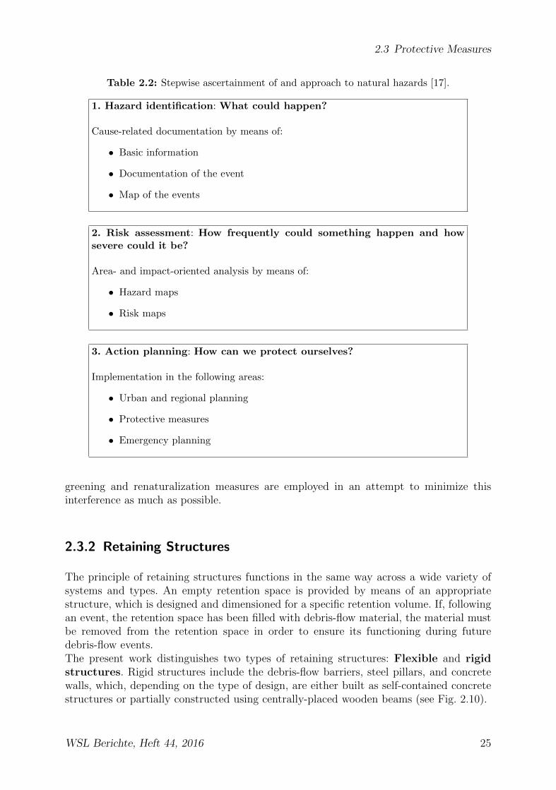
2.3 Protective Measures
Table 2.2: Stepwise ascertainment of and approach to natural hazards [17].
1. Hazard identification: What could happen?
Cause-related documentation by means of:
• Basic information
• Documentation of the event
• Map of the events
2. Risk assessment: How frequently could something happen and howsevere could it be?
Area- and impact-oriented analysis by means of:
• Hazard maps
• Risk maps
3. Action planning: How can we protect ourselves?
Implementation in the following areas:
• Urban and regional planning
• Protective measures
• Emergency planning
greening and renaturalization measures are employed in an attempt to minimize thisinterference as much as possible.
2.3.2 Retaining Structures
The principle of retaining structures functions in the same way across a wide variety ofsystems and types. An empty retention space is provided by means of an appropriatestructure, which is designed and dimensioned for a specific retention volume. If, followingan event, the retention space has been filled with debris-flow material, the material mustbe removed from the retention space in order to ensure its functioning during futuredebris-flow events.The present work distinguishes two types of retaining structures: Flexible and rigidstructures. Rigid structures include the debris-flow barriers, steel pillars, and concretewalls, which, depending on the type of design, are either built as self-contained concretestructures or partially constructed using centrally-placed wooden beams (see Fig. 2.10).
WSL Berichte, Heft 44, 2016 25

2 Debris flows
Figure 2.10: Retaining structure combined with steel pillars in Japan (left) and sediment trapmade of concrete in Bonigen, BE (right).
The flexible structures include the ring net barriers made of high-tensile steel, whichthe present work examines in greater detail. They provide favorable filling conditionsfor the debris flow because they can accommodate large deformations. In addition, theirinstallation is often faster and easier compared to rigid barriers (see chapter 3).The effectiveness of the debris-flow stopping mechanism can be optimized using what isknown as the drainage principle. Here, the debris-flow material is retained by the ringnet, and the water can drain towards the front. The thus-halted debris-flow front forms asolid earth-fill dam in conjunction with the barrier, thus bringing the subsequent materialto a halt.
2.3.3 Debris-flow Screen Racks and Brakes
Other protective measures for debris flows that are based on the principle of drainageinclude debris-flow brakes. A steel grate is installed in the channel bed, leaving a basalopening underneath. Now, if a debris flow were to move across the grate, water would getdetracted, and the debris flow would come to a halt. As a result of the front stalling, thematerial that follows should also comes to a standstill. An example of an implementeddebris-flow brake is located in the Dorfbach in Tasch, VS. Here, a steel grate of 19min length and 12m in width was installed in the streambed (Fig. 2.11. Downstream thebrake, a suitable deposition basin was constructed, which is sealed by a dam. In sum, thisyields a retention volume of 15,000m3, protecting the road and railway bridges furtherbelow to the greatest possible extent [44].
2.3.4 Flow-Guiding Structures
Another protective measure for debris flows is based on a principle that differs fromthat of the other mechanisms. Flow-guiding structures are intended to route a particulardebris-flow channel through an endangered area, in a controlled manner and without
26 WSL Berichte, Heft 44, 2016

2.4 Protection Concepts
complications. To this end, a non-eroding shell of thrown concreted blocks is usuallyconstructed, which then ensures a defined flow through its cross section. Usually, thistype of protective measure is used in combination with other methods, as is the case,for example, with the so-called flow-guiding shell in Brienz, BE3 (see chapter 2.4.2). Interms of planning and structural engineering, flow-guiding structures are a sensible choiceonly if a guaranteed retention space is available following the area that the flow is beingguided through. In the case of Brienz, this is Lake Brienz, which is where the shell of theTrachtbach terminates.
Figure 2.11: Diversion dam in Pontresina, GR (left) and debris-flow brake in the Dorfbachnear Tasch, VS (right).
2.4 Protection Concepts
This chapter will present two real-life examples - from Brienz and Hasliberg - of thedamage potential of debris flows, in order to illustrate the damages occurred and thesubsequently-developed protection concepts. Only a coordinated concept, based on a com-bination of a variety of measures in different locations along the vulnerable streams, willbe able to prevent damages (such as those from the flood year 2005) in the future.
2.4.1 The 2005 Flooding
The 2005 flooding was triggered by a trough, the center of which was located south ofthe Alps and which remained largely stable over a longer period of time. This lead tointense rainfalls, primarily on August 21 and 22, 2005, covering extensive areas on thenorth side of the Alps: from the Bernese Alps over Central Switzerland and parts ofGrisons, to Austria and Southern Bavaria. In all of Switzerland, the damage amountedto approximately 3 billion Francs, with the damage being most extensive in the BerneseOberland (see Fig. 2.12). Moreover, most of the damage was caused by debris flows, alsoin the Bernese Oberland, and more specifically, around Lake Brienz.
3BE, Canton of Bern
WSL Berichte, Heft 44, 2016 27

2 Debris flows
In the Hasliberg area Gummen, 13,000m3 of schistous material were mobilized andflowed in several surges into the valley, thus flooding the municipalities of Meiringenand Hasliberg. During this process, the debris flow eroded another 25,000m3 along itsflow path, so that the total volume amounted to almost 40,000m3 [71]. Thankfully, theseevents neither resulted in personal injuries nor fatalities.
Figure 2.12: Main types of damage by canton as in [9]. Legend: ubrige Kantone = other can-tons; Schaden = damage; private Schaden = private damage; Infrastrukturschaden = damageon infrastructure.
Tthis was not the case in the municipality of Brienz, where the events at the riversTrachtbach and Glyssibach resulted in, among other damages, personal injuries. Thedebris flow in the Trachtbach was triggered by a slide in the forest Ritzwald, which flowedinto the Trachtbach carrying about 60,000m3, thus providing enough material for thedebris flow that followed. The landslide material in the Trachtbach is very cohesive andrequires prolonged soaking in order to begin to flow. This requirement was met in August2005. The first 5000m3 could easily be transported along the shell, a specially-designedstreambed which functions as a flow-guiding structure with increased drainage capacity,into Lake Brienz. However, due to its high viscosity and the high sea-level, the materialbecame stuck shortly after, thus damming and filling the shell from the lake upwards. Asa result, the capacity of the shell was exhausted, and the debris flow broke out of theshell on the left and the right, thus overflowing Brienz. According to [75], approximately76,000m2 of the village were affected, whereas the estimated cubature of solids amountedto approximately 5000 to 7000m3. A similar event occurred in the Glyssibach, where adebris flow transported approximately 30,000m3 of material into the valley. This debrisflow was also triggered by a slide down to 1200m above sea level, near the village of Balen.
28 WSL Berichte, Heft 44, 2016

2.4 Protection Concepts
Figure 2.13: Brienz after the 2005 storms, and debris-flow damage to a residential building inBrienz.
2.4.2 Implementation in Brienz
In Brienz, the canton immediately ordered an analysis of the events, which formed thebasis for the newly-developed protection concept and the projected structural measures.This new protection concept for the river Trachtbach will be discussed in detail below [76].First, it is necessary to estimate the magnitude of future events. This estimation is basedprimarily on an assessment of the slide area in the forest Ritzwald. Elaborated measure-ment techniques now regularly observe the slide area at several measuring points andprovide estimates of possible events (Table 2.3).
Table 2.3: Basic scenarios for events in the river Trachtbach.
Frequency Volume in m3 reaching the villageVery often 5,000Every 30 years 9,000Every 100 years 30,000Every 300 years 50,000Extreme event > 100,000
Based on this event analysis, it became apparent that the village of Brienz is not ad-equately protected. There is a high to medium probability that a debris-flow event willlead to an overflow situation within the village. Moreover, around 60 buildings are locatedwithin the red and blue danger zones (red indicates high risk, blue indicates medium risk).The events in 2005 made clear that debris-flow events of high intensity may lead to per-sonal injuries and fatalities due to the destruction of buildings. Therefore, the followingprotection concept was developed according to Table 2.4, with measures devised for threedifferent areas: maintenance, urban and regional planning, and structural measures [76].
The action plan for Brienz illustrates the need for different measures in different locations.In order to develop an effective protection concept, the most suitable measure needs tobe identified for each location. The overall concept is designed to ensure that a centennial
WSL Berichte, Heft 44, 2016 29

2 Debris flows
Table 2.4: Protection concept Brienz.
1. MaintenanceMaintenance of watersMaintenance of forests (slope stability)Minimizing the amount of wood in the channel
2. Urban and regional planningClearing of deposition basins and basal openingsProtection measures (hazard map, zoning plan, building regulations)
3. Structural measuresInstallation of a drainage system at the slide area in the forest RitzwaldRing net barrier at the front of the Ritzgraben cutConcrete barrier at the rear end of the Ritzgraben cutDevelopment of road access to the front and the rear end of the Ritzgraben cutRing net at the river TrachtbachExtension of the protection dam RauenhagProtection dam at the Wellenberg bridgeWalls along the shell (increasing the size of the cross section)Removal of the wall along the quay (debris can flow into the lake more efficiently)
50,000m3
slide 10,000m3
slide
5000m3
Channel erosion
4000m3
Retention at the anterior cleft
14,000m3
Barrier
6000m3
Shell
10,000m 3
Lake
5,000m3
Quay
6000m3
Retention within the channel with 3 barriers
65,000m3
Bedload supply
24,000m3
Retention within the channel
29,000m3
System capacity
Settlement area 8,000m3
Settlement
Figure 2.14: Quantity of solids (red/dashed) and planned retention structures (black/solid) atthe river Trachtbach Brienz, BE [76].
event of 30,000m3 (see Table 2.3) causes only minimal damage within the village. More-over, one of the unique measures in the action plan for Brienz is that, for the first time inSwitzerland, buildings were forcibly relocated, i.e. partially-damaged buildings could notbe rebuilt in the same location.
30 WSL Berichte, Heft 44, 2016

2.4 Protection Concepts
The remainder of the present work will not include further specific discussion of theplanning and dimensioning of the 4 ring net barriers in the Trachtbach. However, a samplecalculation in chapter 8 illustrates the procedure. The remaining measures will not beindividually described in detail, although more detailed information can be found in [76].
2.4.3 Implementation in village of Hasliberg
The 2005 events in the valley Haslital were also analyzed in detail. and lead to the develop-ment of a comprehensive concept of structural measures [50]. The present work, however,will only discuss the concept of structural measures in the case of ring net barriers, locatedin the Gummen area.Here, schist material capable of forming debris flows is already retained in the catchmentarea by means of 13 flexible ring net barriers. The overall retention volume of the barriersamounts to approximately 12,000m3. Two landfill sites together accommodate approxi-mately 40,000m3. Because the Gummen region is difficult to access, the nets are idealfor this location; they can be flown to the area by helicopter and installed using a smallwalking excavator. Moreover, because tourism plays an important role for the Gummenregion, the nets were also chosen as a visually pleasing alternative to massive concretebarriers. In addition, because the return period of the events is estimated to lie between10 and 15 years, ring nets are considered to be an ideal solution (provided that the netsare maintained regularly). The mesh size and the height of the basal opening were deter-mined in laboratory tests at the WSL (refer to section 5.3.4 and [109]). Furthermore, thenets were dimensioned for debris-flow loads, and one net for snow and avalanche loads(see chapter 8 and [85]).
Deposit area "Hubel"
Deposit area "oberer Staffel"
Ring net series
Figure 2.15: Staggered bedload retention in the catchment area Gummen with 13 flexiblebarriers and two landfill sites.
WSL Berichte, Heft 44, 2016 31

2 Debris flows
32 WSL Berichte, Heft 44, 2016

3 Flexible Barriers for Debris-flowProtection
Before flexible nets were used for protection from debris flows, they were used to retaindriftwood, snow and rockfalls. Their advantage lies in their simple, lightweight structureof few components, which can even be installed in difficult-to-access, mountainous regions.This section outlines the history of the nets and cable barriers (only cables, no nets) andtheir development into flexible net barriers for debris-flow protection. The mode of actionof filled flexible barriers in the streambed is described in more detail in the section onmulti-level barriers.
3.1 History of Net Barriers
A wide variety of net and cable barriers were being used as protective structures againstalpine natural hazards already fifty years ago. Historical use for each field of use is outlinedbelow.
3.1.1 Net barriers in torrent controls
Nets were first used in the natural hazards field as early as 1953 in torrent control [64].Permeable structures were intended to retain only coarse bedload and allow the waterthrough. To this end, very large mesh sizes of up to a meter were selected, or even singleropes were stretched across the streambed. Owing to a lack of experience in the design ofthe cable ropes and about their long-term behavior, the cable barriers were only used as anemergency measure if an event occurred. Bedload and driftwood was usually successfullyretained.Some rope net barriers were erected in East Tyrol in the 1970s [83]. These were usuallyconstructed from vertical supports consisting of steel profiles, with support ropes stretchedin between. One of the first barriers of this type was erected in the river Griesbach inEast Tyrol in 1964. This has successfully retained driftwood and bedload ever since. Thedriftwood is removed every 3 to 5 years, and the bedload is emptied by subsequent floodingevents. This barrier previously had no repairs at all except for one broken support rope.The main consideration for using nets to retain driftwood is that the wood is held bythe net close to the water surface, whereas the flood water including the bedload canpass through under the net. However, observations have shown that the flow velocity isreduced by the dammed-up wood and therefore the bedload is often also deposited at the
33

3 Flexible Barriers for Debris-flow Protection
net barrier. This still produces a spatial separation of wood and bedload, which makesthe emptying process much easier [83].
3.1.2 Snow Nets
Avalanche protection systems consisting of wire rope nets have proven effective in difficult-to-access terrain owing to their simple and lightweight structure. The structures, whichconsist of rope nets and steel wire mesh and are stretched between posts, provide a sup-port area transverse to the slope as far as the snow surface. Snow nets have less of a visualeffect on the natural scenery in the avalanche initiation zone than traditional steel snowbridges [79]. The disadvantages of snow nets compared with conventional rigid avalanchecontrol structures have previously been the material costs, although these can be com-pensated for by lower installation costs. Also, snow retention in the case of powder snowavalanches can be somewhat poorer because mesh sizes are too large. Snow retention canbe greatly improved by a secondary meshwork extended additionally over the wire netsand further optimized by an offset arrangement in the terrain.Rockfall nets and debris-flow nets can also become ”snow nets” as a result of snow ac-cumulation and snow slides (see Fig. 3.2). The area of application for flexible protectivestructures cannot usually be differentiated clearly, and therefore debris-flow nets situatedbelow an avalanche initiation zone must also be suitable for avalanche pressures and snowslides or must be dismantled and stored in the winter (see section 8.6). The first net struc-tures for avalanche protection were used in 1951 on the Schafberg in Pontresina. Thesewere diagonal nets with rectangular mesh, which were stretched directly on the posts.The posts were initially made of wood, later steel posts were used.
Figure 3.1: Snow net structure (left) and rigid structure with snow bridge (right).
3.1.3 Rockfall Nets
Avalanche control structures were frequently exposed to rockfalls during the snow-freeseason and withstood them successfully. This observation resulted in the net structuresalso being used for rockfall protection.
34 WSL Berichte, Heft 44, 2016
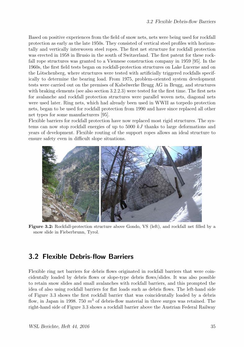
3.2 Flexible Debris-flow Barriers
Based on positive experiences from the field of snow nets, nets were being used for rockfallprotection as early as the late 1950s. They consisted of vertical steel profiles with horizon-tally and vertically interwoven steel ropes. The first net structure for rockfall protectionwas erected in 1958 in Brusio in the south of Switzerland. The first patent for these rock-fall rope structures was granted to a Viennese construction company in 1959 [95]. In the1960s, the first field tests began on rockfall-protection structures on Lake Lucerne and onthe Lotschenberg, where structures were tested with artificially triggered rockfalls specif-ically to determine the bearing load. From 1975, problem-oriented system developmenttests were carried out on the premises of Kabelwerke Brugg AG in Brugg, and structureswith braking elements (see also section 3.2.2.3) were tested for the first time. The first netsfor avalanche and rockfall protection structures were parallel woven nets, diagonal netswere used later. Ring nets, which had already been used in WWII as torpedo protectionnets, began to be used for rockfall protection from 1990 and have since replaced all othernet types for some manufacturers [95].Flexible barriers for rockfall protection have now replaced most rigid structures. The sys-tems can now stop rockfall energies of up to 5000 kJ thanks to large deformations andyears of development. Flexible routing of the support ropes allows an ideal structure toensure safety even in difficult slope situations.
Figure 3.2: Rockfall-protection structure above Gondo, VS (left), and rockfall net filled by asnow slide in Fieberbrunn, Tyrol.
3.2 Flexible Debris-flow Barriers
Flexible ring net barriers for debris flows originated in rockfall barriers that were coin-cidentally loaded by debris flows or slope-type debris flows/slides. It was also possibleto retain snow slides and small avalanches with rockfall barriers, and this prompted theidea of also using rockfall barriers for flat loads such as debris flows. The left-hand sideof Figure 3.3 shows the first rockfall barrier that was coincidentally loaded by a debrisflow, in Japan in 1998. 750 m3 of debris-flow material in three surges was retained. Theright-hand side of Figure 3.3 shows a rockfall barrier above the Austrian Federal Railway
WSL Berichte, Heft 44, 2016 35

3 Flexible Barriers for Debris-flow Protection
Figure 3.3: Rockfall barriers loaded with debris flows, in Aobandani, Japan in 1998 (left) andin St. Anton, Tyrol in 2005 (right).
in St. Anton, Tyrol, which was loaded by a debris flow following extreme precipitationin 2005. Here, almost 150 m3 of debris-flow material was retained and therefore did notreach the train tracks.After rockfall barriers had successfully retained smaller slides and debris flows, attemptswere made to use ring net barriers to protect from debris flows as well. Initial experi-ments with small debris flows took place in 1996 at the USGS1 flume in Oregon in theUSA [23, 35]. The 2m-wide and 95m-long channel has an inclination of 30◦, and the start-ing volume can be up to 20m3. Six experiments with diagonal and ring nets were carriedout in total. The mesh sizes were between 10 and 30cm, a secondary meshwork withsmaller mesh or a synthetic fleece being stretched over the nets to retain fine sediment.The nets extended between two support ropes. The support ropes contained load cellsto determine the exact force profile during the filling process. These tests showed thatdebris-flow volumes of up to 10m3 and impact velocities of up to 10m/s can be stoppedsuccessfully with flexible barriers. The nets with the secondary meshwork had very goodretention, and the nets with the fleece retained almost all the material. Load peaks of upto 45 kN occurred in the support ropes, which were measured at the same time as themaximum deformation of the barriers.The first 1:1 field tests on ring net barriers for protection from debris flows then began in2005 in Illgraben, Valais, Switzerland (see section 4.3.1).
3.2.1 Structure
The load-bearing system of flexible debris-flow barriers currently consists of support ropesthat extend transversely to the streambed and are anchored in the sides of the channel.Rope anchors or self-drilling anchors are used as anchor systems (see section 3.2.2.4). Thering net is shackled between the support ropes and transfers the load areally to them.There are two types of debris-flow barrier, depending on the valley shape. The VX systemmanufactured by Geobrugg (see Fig. 3.4a) is suitable for V-shaped channel cross sectionsand is used for spans up to 15m. The UX system is suitable for wide cross sectionsand spans up to 30m (see Fig. 3.4b). In the UX system, one or more posts, over which
1United States Geological Survey, http://www.usgs.gov
36 WSL Berichte, Heft 44, 2016

3.2 Flexible Debris-flow Barriers
a)
b)
L < 15m
3 - 4m
1.5 - 2m
1.5 - 2m
0.5 - 1m
Figure 3.4: a) UX system with posts for wide spans, b) VX system without posts for narrowerspans.
the support ropes run, are provided along the structure, in a similar manner to rockfall-protection nets. The posts are anchored with retaining ropes and provided with a concretefoundation, depending on the type of ground. These ensure that the remaining heighth′b after the filling process remains as large as possible, to achieve the largest possibleretention volume (see section 4.5.3).
WSL Berichte, Heft 44, 2016 37

3 Flexible Barriers for Debris-flow Protection
3.2.2 Structural Elements and Components
Abrasion-protection
Brake elements Ring net
Winglet rope
Support ropes Border rope
Basal opening
Anchor
Figure 3.5: Schematic Construction of a Flexible Debris-flow Barrier.
Most of the individual components of ring net barriers for debris flows have been takenfrom rockfall barriers and are therefore described only briefly in this paper (for a detaileddescription, see [103, 45]). Only components that have been recently developed or arespecifically relevant for debris-flow barriers are described in detail. Fig. 3.5 shows theindividual components of a debris-flow barrier.
3.2.2.1 Support Ropes
The support ropes extend from one bank to the other and usually have one or morebrake elements integrated in them (see section 3.2.2.3). The relevant dimensions of theGeobinex 22mm ropes used in the test barriers are listed in Table 3.1. These ropes areround strand ropes. Round strand ropes are stranded twice: the wires are stranded toform strands and then the strands are stranded to form the rope. This type of strandinghas the advantage that round strand ropes react less sensitively to transverse pressurethan conventionally straight-stranded ropes.
The calculated breaking force of a rope Fr is calculated from the metallic cross sectionAm multiplied by the nominal wire strength βN to produce Fr = Am · βN . It is alwayshigher than the minimum breaking force Fmin calculated by the manufacturer. This mustbe achieved or exceeded in the entire rope when it breaks. Fmin = Fr · k. The strandingfactor k is a reduction factor that is produced by the stranding of the wires and theadditional stresses produced thereby [40].The ropes are each coated with an aluminum-zinc coating to protect against corrosion.For the calculation of the rope forces using the occurrent loads, see section 6.2.2.
38 WSL Berichte, Heft 44, 2016

3.2 Flexible Debris-flow Barriers
Table 3.1: Geobinex 22mm support rope parameters.
Parameter [−] Value
Nominal diameter d [mm] 22Metallic cross section Am [mm2] 255.5Mass per meter [kg/m] 2.16Min. breaking force acc. to rope manufacturer [kN ] 400Calculated breaking force Fr [kN ] 500Nominal wire strength βN [N/mm2] 1960
3.2.2.2 Winglet and Border Ropes
The winglet rope (see Fig. 3.5) is a structural rope, which extends from the top anchoron one bank to the other top anchor on the other bank. It is usually routed at an angle ofapproximately 30◦ to the upper support rope and fixed there with a clamp. The wingletsare thereby formed on both sides of the debris-flow barrier. When the barrier is full, thewinglets should ensure that the debris-flow stream is kept to the greatest possible extentin the center of the barrier, so that lateral erosion of the bank is avoided. The settlingbehavior of the barrier during the filling process is also controlled by means of the wingletrope and the number of brakes installed in it (see section 4.6.4). The abrasion protectionsystem is usually mounted on the winglet rope (see section 3.2.2.6).A further structural rope is formed by the border rope as a lateral termination of thering net barrier (see Fig. 3.5). It runs from the top to the bottom anchor on each bank.It usually runs through the flexible head (see section 3.2.2.4) of the central support ropeanchor. The ring net is fastened to each side of this border rope with shackles.
3.2.2.3 Brake Elements
Figure 3.6: Unloaded brake element (left) and pulled brake element after loading (right).
So called brake elements are integrated in the support ropes. These brake elementsconsist of a tube bent in a circle, through which the support rope runs. The tube is heldtogether by a clamp. When the support rope is loaded, the brakes reduce in diameter andbecome longer. The rope length l0 thereby increases by the displacement of the brakes lbr.During this process, energy is absorbed by the plastic deformation of the tube and by the
WSL Berichte, Heft 44, 2016 39
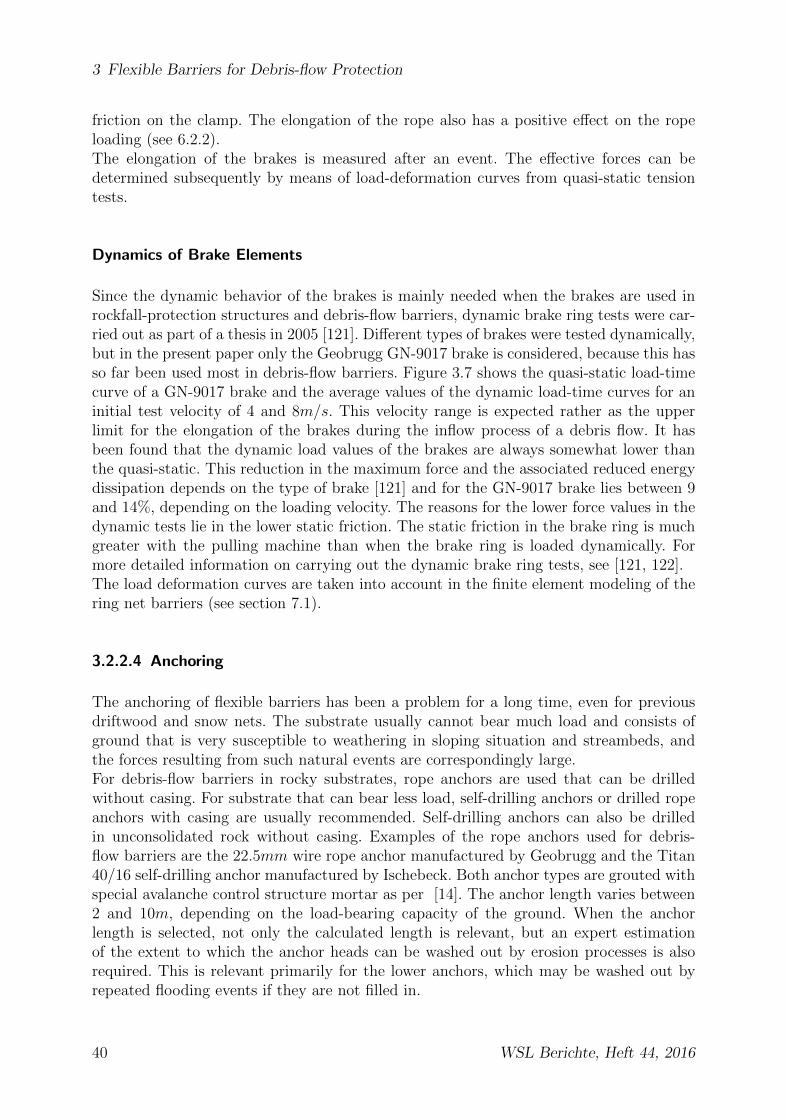
3 Flexible Barriers for Debris-flow Protection
friction on the clamp. The elongation of the rope also has a positive effect on the ropeloading (see 6.2.2).The elongation of the brakes is measured after an event. The effective forces can bedetermined subsequently by means of load-deformation curves from quasi-static tensiontests.
Dynamics of Brake Elements
Since the dynamic behavior of the brakes is mainly needed when the brakes are used inrockfall-protection structures and debris-flow barriers, dynamic brake ring tests were car-ried out as part of a thesis in 2005 [121]. Different types of brakes were tested dynamically,but in the present paper only the Geobrugg GN-9017 brake is considered, because this hasso far been used most in debris-flow barriers. Figure 3.7 shows the quasi-static load-timecurve of a GN-9017 brake and the average values of the dynamic load-time curves for aninitial test velocity of 4 and 8m/s. This velocity range is expected rather as the upperlimit for the elongation of the brakes during the inflow process of a debris flow. It hasbeen found that the dynamic load values of the brakes are always somewhat lower thanthe quasi-static. This reduction in the maximum force and the associated reduced energydissipation depends on the type of brake [121] and for the GN-9017 brake lies between 9and 14%, depending on the loading velocity. The reasons for the lower force values in thedynamic tests lie in the lower static friction. The static friction in the brake ring is muchgreater with the pulling machine than when the brake ring is loaded dynamically. Formore detailed information on carrying out the dynamic brake ring tests, see [121, 122].The load deformation curves are taken into account in the finite element modeling of thering net barriers (see section 7.1).
3.2.2.4 Anchoring
The anchoring of flexible barriers has been a problem for a long time, even for previousdriftwood and snow nets. The substrate usually cannot bear much load and consists ofground that is very susceptible to weathering in sloping situation and streambeds, andthe forces resulting from such natural events are correspondingly large.For debris-flow barriers in rocky substrates, rope anchors are used that can be drilledwithout casing. For substrate that can bear less load, self-drilling anchors or drilled ropeanchors with casing are usually recommended. Self-drilling anchors can also be drilledin unconsolidated rock without casing. Examples of the rope anchors used for debris-flow barriers are the 22.5mm wire rope anchor manufactured by Geobrugg and the Titan40/16 self-drilling anchor manufactured by Ischebeck. Both anchor types are grouted withspecial avalanche control structure mortar as per [14]. The anchor length varies between2 and 10m, depending on the load-bearing capacity of the ground. When the anchorlength is selected, not only the calculated length is relevant, but an expert estimationof the extent to which the anchor heads can be washed out by erosion processes is alsorequired. This is relevant primarily for the lower anchors, which may be washed out byrepeated flooding events if they are not filled in.
40 WSL Berichte, Heft 44, 2016
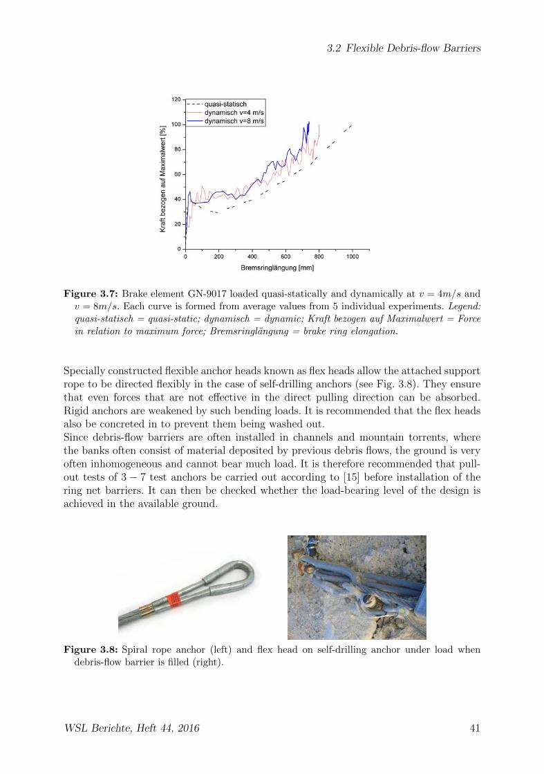
3.2 Flexible Debris-flow Barriers
Figure 3.7: Brake element GN-9017 loaded quasi-statically and dynamically at v = 4m/s andv = 8m/s. Each curve is formed from average values from 5 individual experiments. Legend:quasi-statisch = quasi-static; dynamisch = dynamic; Kraft bezogen auf Maximalwert = Forcein relation to maximum force; Bremsringlangung = brake ring elongation.
Specially constructed flexible anchor heads known as flex heads allow the attached supportrope to be directed flexibly in the case of self-drilling anchors (see Fig. 3.8). They ensurethat even forces that are not effective in the direct pulling direction can be absorbed.Rigid anchors are weakened by such bending loads. It is recommended that the flex headsalso be concreted in to prevent them being washed out.Since debris-flow barriers are often installed in channels and mountain torrents, wherethe banks often consist of material deposited by previous debris flows, the ground is veryoften inhomogeneous and cannot bear much load. It is therefore recommended that pull-out tests of 3 − 7 test anchors be carried out according to [15] before installation of thering net barriers. It can then be checked whether the load-bearing level of the design isachieved in the available ground.
Figure 3.8: Spiral rope anchor (left) and flex head on self-drilling anchor under load whendebris-flow barrier is filled (right).
WSL Berichte, Heft 44, 2016 41

3 Flexible Barriers for Debris-flow Protection
3.2.2.5 Ring Net
The ring net of the debris-flow barriers under study consists of wire rings having a diam-eter of 30cm or 35cm. However, other diameters are also possible depending on the areaof application and are used e.g. in Japan and the USA (see Fig. 3.9). In the commerciallyavailable ROCCO net manufactured by Geobrugg, each ring has four adjacent rings (seeFig. 3.9). Each ring consists of a wire, bent to form a certain number of windings. Forexample, the ROCCO 16/3/300 has 16 windings per individual ring, with a wire diameterof 3mm and a ring diameter of 300mm. The windings of an individual ring are fixed bysteel clamps at 2− 3 points. The wire used for the ring nets is a high-tensile spring steelwire with a nominal strength of 1770 N/mm2 according to EN 10264-2 [36].A eutectic aluminum-zinc coating of 5% aluminum and 95% zinc is used for corrosion pro-tection. There is not yet any long-term experience of the erosion rate of the zinc-aluminumlayer by debris flows. For rockfall barriers, an erosion rate in a moist environment of ap-proximately 8g/m2 per year is assumed [39]. This empirical value can certainly be appliedto debris-flow barriers that are arranged above the streambed as a preventative retentionspace. The water washes over them only briefly after an event, and they are then emptiedand reinstalled (see section 3.2.5).If the debris-flow barriers are installed in the streambed for bed stabilization or step ef-fect (see section 3.4.3), there are not yet any long-term empirical values relating to theerosion rates of the coating. The water in mountain torrents and debris-flow channels isoften very rich in sediment and therefore highly abrasive. Abrasion tests on ROCCO ringsshowed that after three large debris flows the aluminum-zinc coating decreased by 75%from 220g/m2 to 60g/m2 [25]. This shows that the corrosion protection of the ring netmust be achieved structurally (see also sections 8.4 and 7.3.6).
Figure 3.9: Pulling up the ring net like a curtain during installation (left) and alternative meshsizes at Gaviota Pass, CA.
3.2.2.6 Abrasion Protection
To protect the upper support rope and the winglet rope, a special abrasion protectionsystem has been developed. This becomes relevant as soon as the flexible barrier has
42 WSL Berichte, Heft 44, 2016

3.2 Flexible Debris-flow Barriers
Figure 3.10: Abrasion protection 2005 without slots for shackling (left) and developedabrasion-protection 2006 and 2007 with slots (right).
filled up and the rest of the debris flow that cannot be retained flows over the barrier.The abrasion protection system is then in direct contact with the shearing and additionalload of the overflowing debris flow. Therefore, the abrasion protection system mustmeet particular demands in terms of robustness. In the first field barriers in 2005 (seesection 4.3.1) a relatively weak angled profile with two shackles for fastening to the uppersupport rope was used (see Fig. 3.10 left). Even after the first debris flow it was foundthat the profile was very bent and individual segments had twisted around the supportrope, producing free spaces (see Fig. 3.11). The profile was enlarged in 2006 to form areinforced angled profile, which had larger sides and also a greater sheet thickness. Largerfastening shackles were also used to avoid pressure points on the upper support rope asa result of the abrasion protection (see section 4.3.1). To prevent the abrasion protectionsystem sliding apart during the filling process, slots were made at both profile ends,so that the individual profiles can be connected to each other with shackles (see Fig. 3.11).
Figure 3.11: Pulled-apart abrasion protection in 2005 (left) and abrasion protection shackledwith slots in 2007 (right).
Galvanization of the abrasion-protection is less suitable for corrosion protection owing tothe highly abrasive effect of the debris-flow material flowing over them. ”Sacrificial steel”is the only option here, that is, making the sheet as thick as possible in order to provide a
WSL Berichte, Heft 44, 2016 43

3 Flexible Barriers for Debris-flow Protection
large amount of steel for abrasion and corrosion (see section 8.4) and replacing the abrasionprotection from time to time as wear parts when necessary (see also section 3.2.4). It isalso possible to produce the abrasion-protection from stainless steels (see section 4.6.3).
3.2.3 Construction
The construction of ring net barriers can be divided into the following four parts:
• Drilling and Foundations: Drilling takes the most construction work time, de-pending on the bank strength. A drill and self-drilling anchors are shown in Fig-ure 3.12. The self-drilling anchors are drilled with disposable drill bits and simul-taneously grouted by injection through the anchor tube. The disposable drill bitmeans that drilling does not need to be carried out with casing. The flex heads,which ensure the flexible load transference direction, are then mounted onto theself-drilling anchors. The injected mortar is capable of full force transmission after28 days. However, the tensioning of the support ropes can start after about 7 days,because the injected mortar has achieved 80 to 90% of its maximum compressivestrength by this time.If the construction is a UX system, the foundations of the posts are created at thesame time that the anchors are drilled. If the UX system has only one post, it shouldbe ensured when the retaining rope anchors are drilled that they are not createddirectly in the streambed, otherwise the risk of the anchor head being eroded byflooding events and debris flows is increased. If there is more than one post, it is of-ten not possible to avoid drilling the retaining rope anchors directly in the channel.In this case, if the bed level is variable owing to instable bed material, it is recom-mended that the retaining rope anchors with the flex head be additionally concretedin. The risk of retaining rope anchors being washed out can then be minimized.
Figure 3.12: Titan 40/16 self-drilling anchors with tubular cross section for injecting the mor-tar (left) and drill for setting the self-drilling anchors (right).
• Installing and Tensioning the Support Ropes: First, the upper and lowersupport ropes are stretched transversely over the streambed from anchor to anchorand, after being deflected around the flex head, fastened with wire rope clampsaccording to EN 13411-5 [37] (see Fig. 3.13). In the case of the previously usedGeobinex 22mm support rope, 10 wire rope clamps should be arranged according
44 WSL Berichte, Heft 44, 2016

3.2 Flexible Debris-flow Barriers
to the manufacturer’s recommendations. The winglet rope, which is fastened tothe upper support ropes, is tensioned last (see also Fig. 4.31 and section 4.6). Thesupport ropes are pre-tensioned with approximately 10 kN .In UX systems with posts, the lower and upper support ropes are mounted andtensioned first. Then the posts are placed with the aid of either a helicopter or awalking crane. The upper support rope must then be laid carefully around the topof each post in order to avoid transverse pressures arising from the transverse forceof the post. Lastly, the retaining ropes are stretched from the top of the post to theretaining rope anchors.
Figure 3.13: Tensioned support ropes with brake rings (left) and fixing the support ropes withrope clamps (right).
• Shackling the Ring Net: An additional mounting rope, on which the ring netis suspended for mounting, is stretched from winglet rope anchor to winglet ropeanchor. The ring net can be hoisted on the mounting rope like a curtain and thenshackled to the support ropes (see Fig. 3.14). When the ring net is shackled, it isimportant to ensure that only the rings from one ring net row are used. Once thenet is shackled to the support ropes, the excess rings are cut off.
Figure 3.14: Ring net prepared for shackling, hung on iron rods (left) and ring net hoisted onthe mounting rope for shackling (right).
• Positioning and Shackling the Abrasion Protection System: After the shack-led ring net has been cut to size and the auxiliary rope has been removed, the
WSL Berichte, Heft 44, 2016 45

3 Flexible Barriers for Debris-flow Protection
abrasion protection system is mounted. The simplest method is to raise the angledprofile sheets piece by piece with the aid of an excavator, position them and shacklethem to the winglet rope (see Fig. 3.15). The profiles are then shackled to each otherwith a ring of the ring net, so that they hold each other together (see Fig. 3.11).
Figure 3.15: Mounting the abrasion protection system with an excavator.
In principle, a barrier can be constructed by one person and the appropriate equipment,such as a walking crane and equipment for drilling the anchors. However, it is advantageousto have several people present for the installation. In this case, the general time neededto construct a ring net barrier including drilling is easily a week. The drilling equipment,the walking crane and the material can be flown to the installation site by helicopter. Thering nets can then in principle be installed without access roads. However, any cleaningand emptying work must be considered when planning the installation, if the barriers areto be continuously available as a retention space for debris-flow material. An access roadwould probably be necessary for this anyway, so that the material can be brought fromthe barrier to the landfill site provided for it (see section 2.4.3).
3.2.4 Maintenance
Maintenance is divided into two parts depending on the intended use of the ring netbarriers:
• Use of the ring net barrier for preventive debris-flow retention, i.e. the barrier re-mains unfilled just above the water surface most of the time. In this case it isassumed that the barrier is partially or completely filled only from time to time byan event. The barrier is then emptied immediately in order to make the retentionspace available again. If an excavator enters the channel above the filled barrier, itis usually not necessary to open the ring net. However, it is often only possible toempty the filled barriers from below, because it is only possible for the excavatorand transport vehicles to approach from there (see section 3.2.5). When a barrier isemptied from below, it must be opened, which usually means that brakes, support
46 WSL Berichte, Heft 44, 2016

3.2 Flexible Debris-flow Barriers
ropes and even the ring net must be replaced during reinstallation. However, it isnot necessary to drill the anchors again.
• Use of the filled ring net barrier as a permanent step in the channel (see sec-tion 3.4.3): Most of the maintenance work is taken up by replacing the abrasion-protection if it is bent too much or too much steel has been worn away. The remainingcapacity of the brakes must also be checked, so that the stability of the barrier isensured if there is a subsequent event. Furthermore, the regions of the ring net thatare permanently exposed to the water flow should be monitored for corrosion. Thereis still too little long-term experience of this for ring net barriers used permanentlyin the filled state.
3.2.5 Emptying and Dismantling
Only emptying from below the barrier is described here, because excavating from aboveis not a technical problem. The following different methods are conceivable:
• Relieving the barrier of load with rope tensioning devices, so that the support ropescan be opened in a controlled manner and the ring net can be removed. This isdone using a rope tensioning device, which is mounted on the upper support ropeand anchor head and is tensioned there. Then the rope clamps should be releasedfor controlled opening of the upper support rope. This is then done with the othersupport ropes after the material in question has been removed, as far as the lowersupport ropes. Then the barrier is reinstalled.This method is often not possible if the support ropes are not freely accessible. Afterthe filling process, they are often jammed under the abrasion protection system ordifficult to access owing to solidified debris-flow material. In this case the only optionis to cut or maybe even to blast the ring net.
• Blasting part of the net or ropes by means of controlled explosive charges. This isfollowed by emptying and reinstallation.
• Cutting through the ring net and/or the support ropes using a welding torch withan extension, i.e. operating the welding torch or cutter from an excavator bucket,because the ring net is under great tension when filled and this requires a safetydistance.
• Shackles have been developed that can be opened even under great load.
The third method was used to dismantle the Illgraben barrier in 2006 (see sec-tion 4.3.2) [24]. It was not possible to let down the net in a controlled manner owingto the high tensions. Blasting could not be carried out either because of the risk to nearbywindow panes. So only the third variant remained and this turned out to be very sensi-ble. First, an excavator bucket with welding equipment was used to cut a series of ringsvertically from top to bottom. It was possible to do this without any risks, because the Ill-graben has only a shallow gradient, so the excavator was not endangered by any materialfalling out. A large amount of material containing large blocks, which was situated directlybehind the net, immediately broke away (see Fig. 3.16). The material was excavated as
WSL Berichte, Heft 44, 2016 47

3 Flexible Barriers for Debris-flow Protection
well as possible through the opening. As soon as the lower support rope was relieved ofload, it was cut and then one half of the net was pulled out of the debris-flow materialusing the excavator. Then this part of the net was cut away by cutting the central andupper support ropes. The barrier could then be emptied first on one side of the net, thenon the other.It should generally be taken into account that stopped debris-flow material is usually com-pressed behind the barriers in a similar manner to concrete. The grain-size distribution ofdebris flows almost always has a large fine fraction, which results in a cohesive final stateof the stopped material (see section 5.2.3.2).In conclusion, it is not easily possible to empty a debris-flow barrier from below withoutdestroying the net and the ropes.
Figure 3.16: Dismantling the ring net barrier in Illgraben in 2006: the whole net is relieved ofload by cutting open the ring net and removing material with an excavator (left) and thenthe upper support rope is cut (right).
3.2.6 Use of Resources and Ecological Aspects
In purely visual terms, it is perhaps already obvious that the structure of a ring net barrieris much lighter than a solid concrete barrier. Nevertheless, the weight of a ring net barrierwith two support ropes, one at the top and one at the bottom, a winglet rope, and twoborder ropes is listed in detail in Table 3.2 and then compared with a concrete barrier togive an impression of the use of resources of both support systems. The density of steelis assumed to be ρsteel = 7850kg/m3.
48 WSL Berichte, Heft 44, 2016
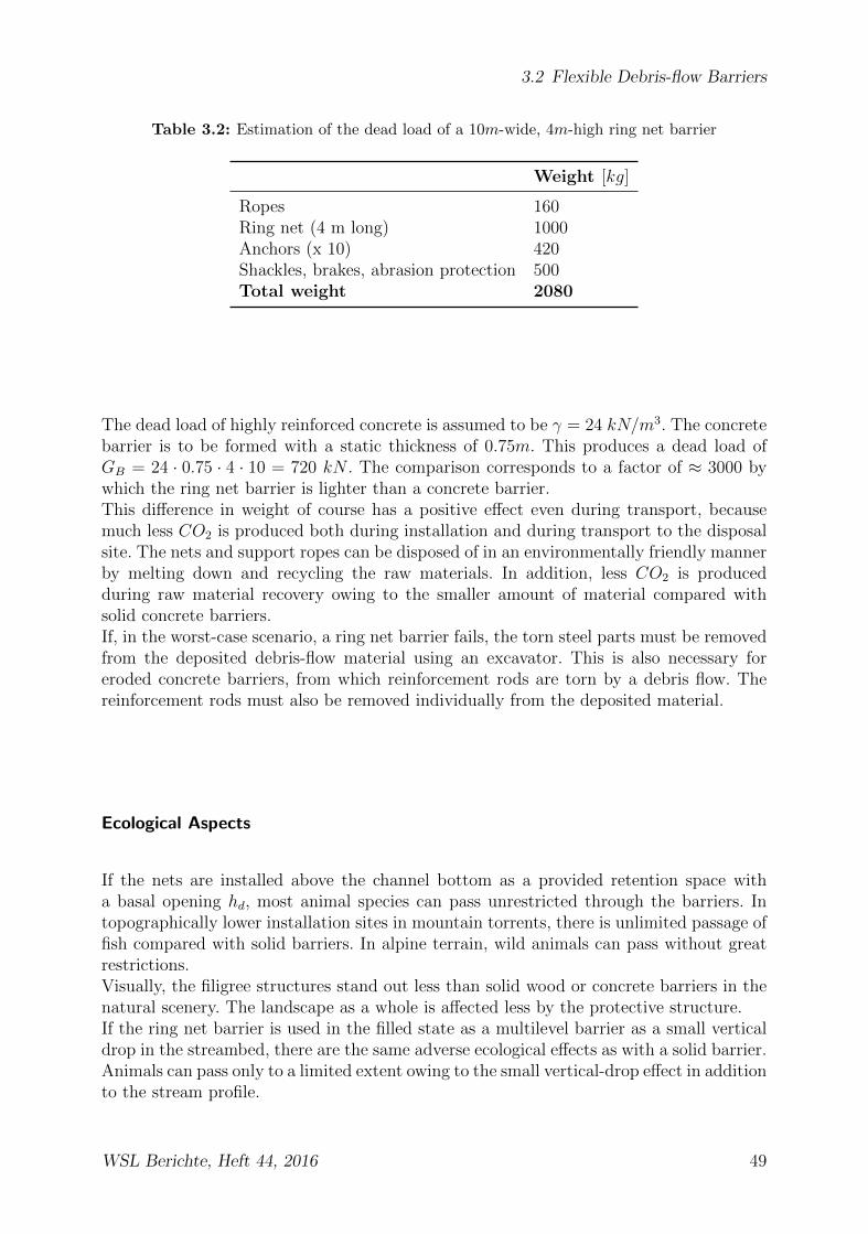
3.2 Flexible Debris-flow Barriers
Table 3.2: Estimation of the dead load of a 10m-wide, 4m-high ring net barrier
Weight [kg]
Ropes 160Ring net (4 m long) 1000Anchors (x 10) 420Shackles, brakes, abrasion protection 500Total weight 2080
The dead load of highly reinforced concrete is assumed to be γ = 24 kN/m3. The concretebarrier is to be formed with a static thickness of 0.75m. This produces a dead load ofGB = 24 · 0.75 · 4 · 10 = 720 kN . The comparison corresponds to a factor of ≈ 3000 bywhich the ring net barrier is lighter than a concrete barrier.This difference in weight of course has a positive effect even during transport, becausemuch less CO2 is produced both during installation and during transport to the disposalsite. The nets and support ropes can be disposed of in an environmentally friendly mannerby melting down and recycling the raw materials. In addition, less CO2 is producedduring raw material recovery owing to the smaller amount of material compared withsolid concrete barriers.If, in the worst-case scenario, a ring net barrier fails, the torn steel parts must be removedfrom the deposited debris-flow material using an excavator. This is also necessary foreroded concrete barriers, from which reinforcement rods are torn by a debris flow. Thereinforcement rods must also be removed individually from the deposited material.
Ecological Aspects
If the nets are installed above the channel bottom as a provided retention space witha basal opening hd, most animal species can pass unrestricted through the barriers. Intopographically lower installation sites in mountain torrents, there is unlimited passage offish compared with solid barriers. In alpine terrain, wild animals can pass without greatrestrictions.Visually, the filigree structures stand out less than solid wood or concrete barriers in thenatural scenery. The landscape as a whole is affected less by the protective structure.If the ring net barrier is used in the filled state as a multilevel barrier as a small verticaldrop in the streambed, there are the same adverse ecological effects as with a solid barrier.Animals can pass only to a limited extent owing to the small vertical-drop effect in additionto the stream profile.
WSL Berichte, Heft 44, 2016 49
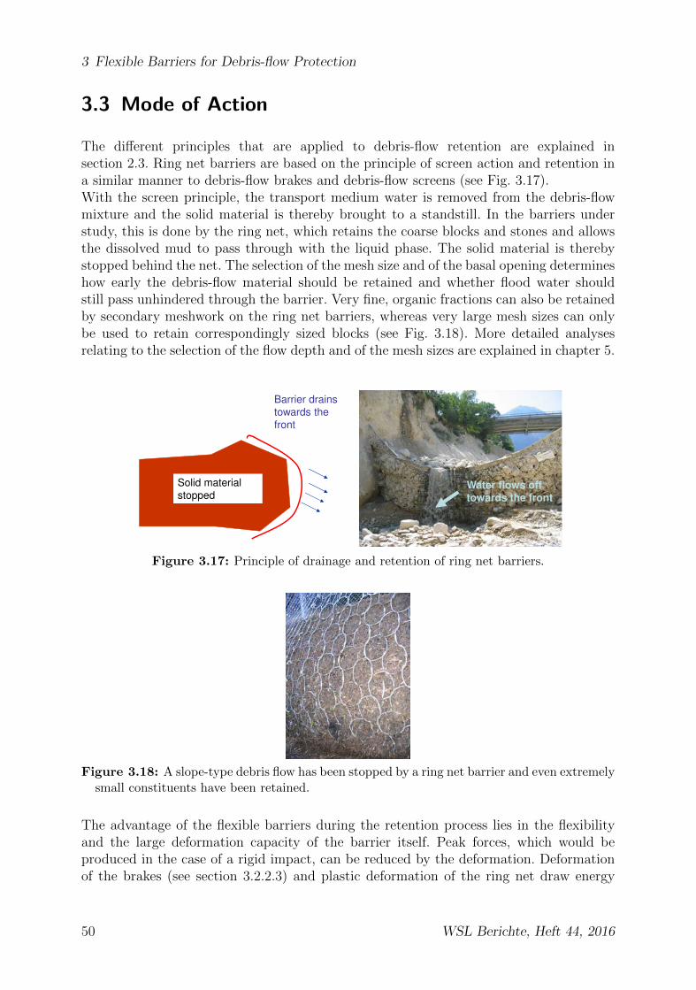
3 Flexible Barriers for Debris-flow Protection
3.3 Mode of Action
The different principles that are applied to debris-flow retention are explained insection 2.3. Ring net barriers are based on the principle of screen action and retention ina similar manner to debris-flow brakes and debris-flow screens (see Fig. 3.17).With the screen principle, the transport medium water is removed from the debris-flowmixture and the solid material is thereby brought to a standstill. In the barriers understudy, this is done by the ring net, which retains the coarse blocks and stones and allowsthe dissolved mud to pass through with the liquid phase. The solid material is therebystopped behind the net. The selection of the mesh size and of the basal opening determineshow early the debris-flow material should be retained and whether flood water shouldstill pass unhindered through the barrier. Very fine, organic fractions can also be retainedby secondary meshwork on the ring net barriers, whereas very large mesh sizes can onlybe used to retain correspondingly sized blocks (see Fig. 3.18). More detailed analysesrelating to the selection of the flow depth and of the mesh sizes are explained in chapter 5.
Solid material
stopped
Barrier drains
towards the
front
Water flows off
towards the front
Figure 3.17: Principle of drainage and retention of ring net barriers.
Figure 3.18: A slope-type debris flow has been stopped by a ring net barrier and even extremelysmall constituents have been retained.
The advantage of the flexible barriers during the retention process lies in the flexibilityand the large deformation capacity of the barrier itself. Peak forces, which would beproduced in the case of a rigid impact, can be reduced by the deformation. Deformationof the brakes (see section 3.2.2.3) and plastic deformation of the ring net draw energy
50 WSL Berichte, Heft 44, 2016

3.4 Ring Net Barriers as Multilevel Barriers
from the impacting debris flow and thereby reduce the maximum loads that occur (seesection 6.3.2). Force and deformation curves from the experiments on the USGS flumeshow that the force increases linearly with the deformation of the barrier [23]. The slowdeformation process of the barrier during the filling process results in a slower increasein load up to the maximum load of the structure. At the same time, the load in thesupport ropes is again slightly reduced repeatedly by the jerky deformation of the brakes(see Fig. 4.5.2). The maximum load occurs when the barrier has reached its maximumdeformation.With rigid barriers that cannot deform on impact, the increase in load to maximum loadtakes place very rapidly [49]. These structures lack the energy dissipation by means ofthe deformation process of individual components.If the barrier is planned to be a permanent barrier for bed stabilization in the streambedwhen filled, its mode of action is described in more detail in the following sections.
3.4 Ring Net Barriers as Multilevel Barriers
3.4.1 Hydraulic Principles from Hydraulic Engineering
In order to understand the mode of action and purpose of vertical drop structures inchannels better, some hydraulic principles will be introduced and explained first.First, the flow regime in mountain torrents and debris-flow streams will be consideredand analyzed in more detail. Most mountain torrents generally have a non-uniformstreamflow. Uniform streamflow usually only occurs in prismatic channels with ashallow bed inclination and without obstructions such as steps, boulders or barriers. Linearmovement without acceleration and delay is characteristic of uniform streamflow, i.e. theaverage velocity um remains constant along the flow path. The pressure distribution istherefore hydrostatic. The following applies: ∂p
∂z= ρgz(z − hfl) where z is parallel to the
flow depth hfl. Therefore, um is constant and as a result so is the average velocity heightu2m2g
, and the energy line runs parallel to the surface line and parallel to the bed line [34].The same flow depth always prevails. The following applies:
IS = IW = IR (3.1)
where IS is the bed inclination, IW is the inclination of the water surface and IR is theinclination of the energy line.In the case of mountain torrents, this ideal does not exist owing to the non-uniformstreamflow. Another method is therefore necessary. The channel discharge is reduced asan approximation of a flow tube, i.e. the continuity equation
u =Q
A(3.2)
applies, where Q is the average discharge and A is the cross section of the channel. Wealso consider the discharge in the channel as a bundle of flow lines. A flow line is a
WSL Berichte, Heft 44, 2016 51
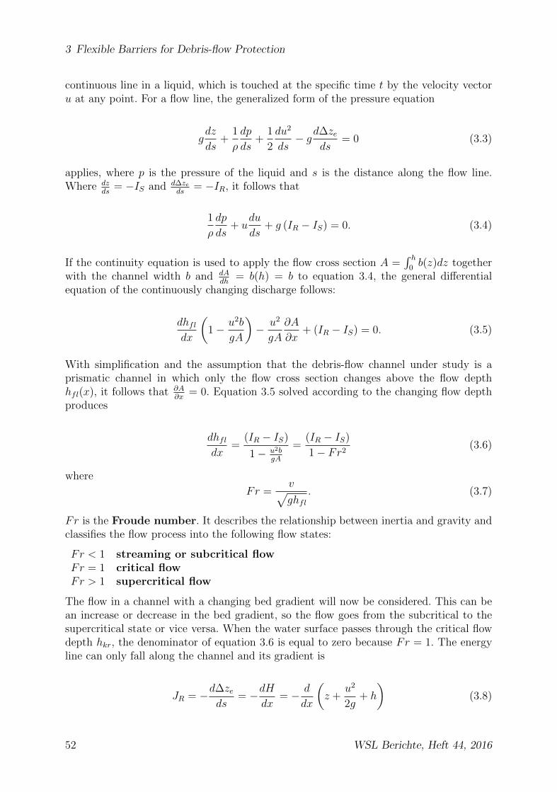
3 Flexible Barriers for Debris-flow Protection
continuous line in a liquid, which is touched at the specific time t by the velocity vectoru at any point. For a flow line, the generalized form of the pressure equation
gdz
ds+
1
ρ
dp
ds+
1
2
du2
ds− gd∆ze
ds= 0 (3.3)
applies, where p is the pressure of the liquid and s is the distance along the flow line.Where dz
ds= −IS and d∆ze
ds= −IR, it follows that
1
ρ
dp
ds+ u
du
ds+ g (IR − IS) = 0. (3.4)
If the continuity equation is used to apply the flow cross section A =∫ h
0b(z)dz together
with the channel width b and dAdh
= b(h) = b to equation 3.4, the general differentialequation of the continuously changing discharge follows:
dhfldx
(1− u2b
gA
)− u2
gA
∂A
∂x+ (IR − IS) = 0. (3.5)
With simplification and the assumption that the debris-flow channel under study is aprismatic channel in which only the flow cross section changes above the flow depthhfl(x), it follows that ∂A
∂x= 0. Equation 3.5 solved according to the changing flow depth
produces
dhfldx
=(IR − IS)
1− u2bgA
=(IR − IS)
1− Fr2(3.6)
where
Fr =v√ghfl
. (3.7)
Fr is the Froude number. It describes the relationship between inertia and gravity andclassifies the flow process into the following flow states:
Fr < 1 streaming or subcritical flowFr = 1 critical flowFr > 1 supercritical flow
The flow in a channel with a changing bed gradient will now be considered. This can bean increase or decrease in the bed gradient, so the flow goes from the subcritical to thesupercritical state or vice versa. When the water surface passes through the critical flowdepth hkr, the denominator of equation 3.6 is equal to zero because Fr = 1. The energyline can only fall along the channel and its gradient is
JR = −d∆zeds
= −dHdx
= − d
dx
(z +
u2
2g+ h
)(3.8)
52 WSL Berichte, Heft 44, 2016

3.4 Ring Net Barriers as Multilevel Barriers
where H is the height of the energy line in the system. At the point of flow change, thespecific energy passes through a minimum, i.e. the energy line must go through its lowestpoint Hmin at this point [34]. During critical flow, therefore
Hmin = z +u2kr
2g+ hkr. (3.9)
z
Water level
River bed
Reference height
E.L.
H = Hmin
u2k/2g Hmin
hkr
Figure 3.19: Curve of an energy minimum along a channel.
The following applies:
dHmin
dx= −IR =
dhkrdx
(1− Fr2
kr
)− IS (3.10)
Frkr = 1 produces IR = IS and therefore the numerator of equation 3.6 is also zero andtherefore the change in flow depth and the inclination of the free surface is undefined(dhfldx
= 00). The limit values can be determined using L’Hopital’s rule [34]. This shows that
the transition from the subcritical to the supercritical state is constant, but the transitionfrom the supercritical to the subcritical state takes place discontinuously. For the flow pro-cess of a stream, this means that the transition from subcritical flow to supercritical flowtakes place continuously and no energy dissipation takes place. In contrast, the transitionfrom supercritical flow to subcritical flow takes place by means of a discontinuity, whatis known as a hydraulic jump, and energy is dissipated in the process (see section 3.4.4).
3.4.2 Mode of Action of Multilevel Structures
Multilevel structures are generally intended to stabilize and raise the channel bottom inorder to prevent the streambed becoming deeper and deeper owing to vertical erosion.Vertical erosion occurs during floods as a result of high flow velocities and an associatedhigh bedload transport rate, and as a result of debris flows and debris-flow surges, whicherode the streambed. When multilevel structures are filled, there is a shallower inclina-tion angle I ′S behind the structure as seen in the flow direction (see section 4.5.3 andsection 4.6.4). Moreover, bedload and debris-flow material is retained behind the struc-ture, depending on the available retention volume Vr.There are the following principles of energy dissipation:
WSL Berichte, Heft 44, 2016 53

3 Flexible Barriers for Debris-flow Protection
a) Energy dissipation by bed gradient reduction (see Fig. 3.20)In this case there is a transition from IS > I ′S. The flow depth hfl is less than thecritical flow depth hkr. In this case the debris flow is in supercritical flow (Fr > 1).If IS from equation 3.6 becomes smaller owing to the barrier backwater of themultilevel structure, the flow depth increases (h2 > h1 and
dhfldx
> 0 ). The flowvelocity is thereby reduced and the debris flow becomes slower (see Fig. 3.20a). Theenergy line thus becomes shallower for a smaller bed gradient.
b) Energy dissipation by bed gradient reduction and subsequent hydraulic jump (tran-sition from supercritical flow to subcritical flow) (see Fig. 3.20b)If the flow depth increases to hkr in supercritical flow (owing to shallower bed incli-nation I ′S), a hydraulic jump is produced after the change in gradient and the flowchanges from supercritical to subcritical. The energy minimum of the energy line isachieved (see equation 3.9) and in addition energy is dissipated during the hydraulicjump ∆IW . After the hydraulic jump, the flow process continues as subcritical flow(Fr < 1).
c) Energy dissipation by overflow and possible hydraulic jump after passing over a dam(see Fig. 3.20c)If the flow approaching the dam is subcritical (a hydraulic jump has been formedpreviously by the change in gradient), critical flow (Hkr) is achieved at the damcrest of the filled barrier. In subcritical flow, a backwater curve is formed upstream.At the dam overflow itself, the flow velocity increases greatly, the flow depth falls tohkr and the streamflow continues as supercritical flow after the dam. If the gradientI ′S is shallower again owing to the next filled barrier, another hydraulic jump canoccur shortly after the dam, if hfl increases to hkr (see process under b). Energy isthen dissipated again by the hydraulic jump IW .If the flow approaching the dam is supercritical (hfl < hkr), the water flows over thedrop with unchanged depth. The free spray pattern can be calculated as a type oftrajectory [34]. There is no significant energy dissipation owing to the small vertical-drop effect. Turbulence occurs only when the spray drops into the stream and mayalso result in abrosion processes, depending on the intensity. A small amount ofenergy is dissipated thereby.
54 WSL Berichte, Heft 44, 2016

3.4 Ring Net Barriers as Multilevel Barriers
a)
b)
E.L.
IR1 > IR2
h1
u21/2g
u1 > u2 > ukr
h1 < h2 < hkr
Is > I ′s
u22/2g
h2
I ′s
Is
IR1
IR2
c)
I ′s
Ish1
E.L.
IR1u1 > u2
h1 < hkr < h2
IR1 > IR2
Is > I ′s
△IwIR2
h2hkr
E.LI1
v21/2g
I2
hkr
h1
△IW
Figure 3.20: a) Energy dissipation principles in multilevel barriers, in supercritical flow withouthydraulic jump, b) in supercritical flow with hydraulic jump, and c) when plunging over adam.
A detailed model calculation for energy dissipation in multilevel barriers is shown in sec-tion 3.4.4 at the end of this chapter.The objective of multilevel structures is therefore to achieve a change in flow from su-percritical to subcritical by means of a hydraulic jump by changing the gradient at thestart of the series of structures. The flow then approaches the dam of the first barrier insubcritical flow and a backwater curve forms in front of the overflow (see Fig. 3.20c). The
WSL Berichte, Heft 44, 2016 55

3 Flexible Barriers for Debris-flow Protection
overflow takes place in supercritical flow. If the subsequent backwater gradient of the nextbarrier is shallow enough, a hydraulic jump is formed again, followed by another changein flow before the next overflow. The series of flow changes and energy jumps extends asfar as the last structure, according to this model.A further objective of multilevel structures is certainly also the increased retention spaceof several structures in series. Of course, continuous emptying of the structures is assumedin this case.
3.4.3 Practical Example, Merdenson
The Merdenson (municipality of Vollege, Valais) was chosen as the site for a multileveltest barrier. Like the Illgraben (see chapter 4), the Merdenson is one of the most activedebris-flow channels in the Swiss Alps and is therefore an ideal location for researchingthe small vertical-drop effect as well as the long-term behavior of the barriers.In December 2006, all the permits had been obtained from the municipality and canton,and three barriers were installed in series (see Fig. 3.21, left). For more information on theproject and location as well as the construction work and safety on site, see the Merdensonsafety guidelines [115].Before construction started, the channel was measured precisely in order to be able tocalculate the exact volumes retained following a debris-flow event by means of another,subsequent measurement (see also section 4.5.3).The barriers were filled by a debris flow on January 1st, 2007. A further, much larger debrisflow took place on March 3rd, 2007. The pictures show the filled state during the inspectionon March 5th (see Fig. 3.21, right). The analysis of the retained volumes from the twomeasurements produced almost 800 m3 of retained debris-flow material (see Fig. 3.22).
Figure 3.21: Installed series of three nets in the Merdenson in the unfilled (left) and filled state(right).
The channel slope changed from an average of IS = 20% before barrier installation toI ′S ≈ 13%. The channel is steeper only behind the top barrier, barrier 1, owing to a shortdistance from a gravity wall to the first net. This distance was selected to be so small inorder to protect the foot of the gravity wall from scouring (see Fig. 3.24). A free backwater
56 WSL Berichte, Heft 44, 2016
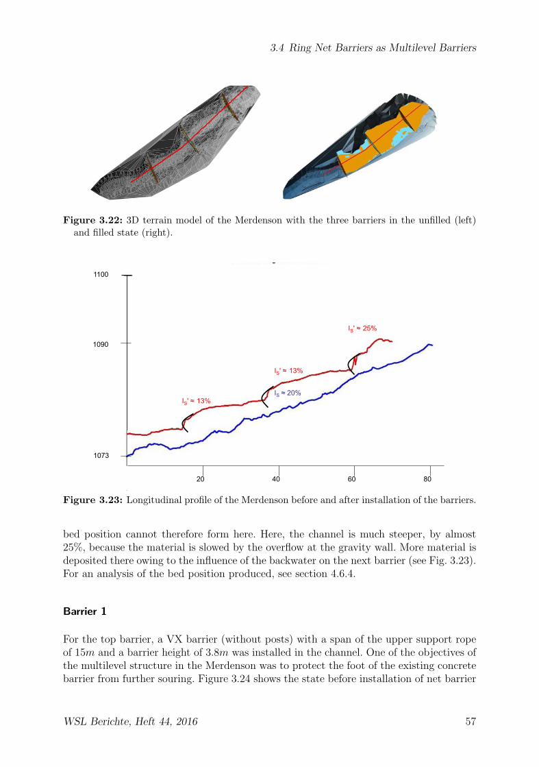
3.4 Ring Net Barriers as Multilevel Barriers
Figure 3.22: 3D terrain model of the Merdenson with the three barriers in the unfilled (left)and filled state (right).
20 40 60 80
1100
1073
1090
IS ≈ 20% IS' ≈ 13%
IS' ≈ 13%
IS' ≈ 25%
Figure 3.23: Longitudinal profile of the Merdenson before and after installation of the barriers.
bed position cannot therefore form here. Here, the channel is much steeper, by almost25%, because the material is slowed by the overflow at the gravity wall. More material isdeposited there owing to the influence of the backwater on the next barrier (see Fig. 3.23).For an analysis of the bed position produced, see section 4.6.4.
Barrier 1
For the top barrier, a VX barrier (without posts) with a span of the upper support ropeof 15m and a barrier height of 3.8m was installed in the channel. One of the objectives ofthe multilevel structure in the Merdenson was to protect the foot of the existing concretebarrier from further souring. Figure 3.24 shows the state before installation of net barrier
WSL Berichte, Heft 44, 2016 57

3 Flexible Barriers for Debris-flow Protection
1 on the left and the state with the filled barrier and the concrete wall in the backgroundon the right.
Figure 3.24: Scoured out old concrete barrier (left) and filled barrier 1 as an anti-scouringmeasure for the old concrete barrier (right).
The net achieved the objective of providing scouring protection for the existing concretewall. It shows that impoundment of debris-flow material can specifically be achieved witha flexible barrier. For example, it is possible to use ring net barriers to implement bedstabilization, energy minimization in the channel by means of changes in inclination andanti-scouring measures in hydraulic engineering.The height of the upper support rope was 4.5m before the filling process, the basal openingwas 0.7m. After the filling process, the lowest point of the upper edge of the barrier h′bwas 3.2m (see Fig. 3.25).
Barrier 2
Here, a UX type with a post in the middle and a length at the top of approx. 18m and aheight of 3.3m was installed. This barrier was also completely filled (see Fig. 3.26). Theshape of barrier 2, with a post initially slightly inclined in the flow direction, proved usefulin terms of the overflow crest produced as corrosion protection for the ring net (see alsosection 7.3.6).
The initial height hb with basal opening for barrier 2 was 3.6m. As a result of the fillingprocess, it settled to a remaining height of 2.6m (see Fig. 3.27). Approaches for calculatingthe remaining height are shown in section 4.6.4.
58 WSL Berichte, Heft 44, 2016

3.4 Ring Net Barriers as Multilevel Barriers
Figure 3.25: Net edge of filled barrier 1 in comparison with the anchor position. The horizontalline shows the position of the upper support rope. Legend: Netzpunkte = points on upper netedge; Anker = anchors; Hohe Netzpunkte = height of net edge points; Netzlange = positionalong the net.
Figure 3.26: Filled barrier 2 (left) and its overflow crest (right).
Barrier 3
The installed type is a VX system like the first barrier; the length of the upper supportrope is 13.5m and the barrier height is 2.9m. The filled state of barrier 3 can be seen inthe foreground of Figure 3.21.The line of the upper support rope was approximately 3m above the channel bed. Afterthe filling process, the barrier subsided to a remaining height h′b of 2.2m (see Fig. 3.28).
WSL Berichte, Heft 44, 2016 59

3 Flexible Barriers for Debris-flow Protection
Figure 3.27: Net edge of filled barrier 2 in comparison with the anchor position. The horizontalline shows the position of the upper support rope. Legend: Netzoberkante = points on uppernet edge; Anker = anchors; Hohe Netzpunkte = height of net edge points; Netzlange = positionalong the net.
Figure 3.28: Net edge of filled barrier 3 in comparison with the anchor position. The horizontalline shows the position of the upper support rope. Legend: Netzoberkante = points on uppernet edge; Anker = anchors; Hohe Netzpunkte = height of net edge points; Netzlange = positionalong the net.
Summary
The first multilevel structure consisting of flexible barriers has been realized successfullyin the Canton of Valais and filled by a debris-flow event. The WSL now further studiesand analyzes the long-term behavior of such filled barriers. Evaluations of the long-termbehavior are not made in this thesis.
60 WSL Berichte, Heft 44, 2016

3.4 Ring Net Barriers as Multilevel Barriers
In addition, the multilevel barrier subproject in the Merdenson serves a practical purposein the channel. It was possible to protect the existing concrete barrier from further abrosionby barrier 1. The debris flow loses most of its energy by flowing over the concrete barrier,and therefore the impact into the first barrier and the subsequent barriers takes placemore or less gently. This is confirmed by the brake elements in the support ropes of thebarriers, which were only activated a little. Therefore, there remains a high load-bearingcapacity for subsequent events that flow over the barriers during the long-term study.Moreover, this project has also shown that the principle of multilevel structures with ringnets can be used both as a retention-type protective measure for larger volumes and as asmall vertical-drop effect when filled.
3.4.4 Sample Calculation, Multilevel Barriers
For the sample calculation, three filled nets in series are considered and the energydissipation as a result of the small vertical-drop effect is determined as pure-water flow(see section 3.4.2). In section 2.2.2 it was shown that debris flows can be describedapproximately with equations from pure-water hydraulics.
Geometry and Channel Properties
The barrier height in the empty state hb is approx. 5.3m. The channel width is setconstantly to b ≈ 10m. The bed gradient before installation of the nets is Is ≈ 30% andinitially has a channel roughness of kst = 20 (for mountain torrents according to [55]).The Strickler coefficient kst is set after filling to kst = 7, since the roughness increasesowing to the coarse debris-flow material. Values for roughnesses for debris-flow materialscan be defined according to [82]. The inclination of the channel after filling is calculatedaccording to section 4.6.4 to give I ′s = 2/3 · Is = 20% with a remaining height of thebarriers of h′b = 4/3 · h′b = 4m.
The exact position of the barriers in the channel can be determined using an equationsystem with three equations and three unknowns. The following relationship arises fromthe geometry in Figure 3.29:
∆H = 3 · 4 m+ 0.2 · 3 · l′ (3.11a)
3 · l′ = L (3.11b)
∆H/L = 0.3 (3.11c)
From this follows that ∆H = 36m, L = 120m and the horizontal single spacing of thebarriers at l′ = 40m. Consequently, ∆h = 12m. This results in a barrier spacing alongthe channel bottom of l = 41.7m. The minimum barrier spacing of l = 10m accordingto [11, 8] is therefore fulfilled.
WSL Berichte, Heft 44, 2016 61

3 Flexible Barriers for Debris-flow Protection
∆h=4m
∆h=4m
∆h=4m
Is=30%
Is'=20%
Is'=20%
cst=20
kst=7
Is'=20%
kst=7
kst=7
l'
∆h
∆h
∆h
l'
l'
∆H
L
1 2 3 4
Barrier 1
Barrier 2
Barrier 3
Figure 3.29: Topographic position of three nets installed in series.
Flow Regime at the Knickpoint
If the debris flow is considered as a pure-water flow, the following approach for calculatingthe flow regime is produced (see section 3.4.2):
• Flow regime on approach: The approaching average debris-flow discharge Q is50 m3/s, kst = 20 and the channel slope Is = 30%. The normal flow depth, assumingthat the channel is approximately rectangular, is calculated iteratively as follows
Q = kstA5/3
U2/3I
1/2R (3.12)
where IR = Is with uniform flow, the perimeter U = 2hn + b of the channel andthe flow cross section A = b · hn. This gives the normal flow depth in section 1 ofhn,1 = 0.65m. The flow velocity is calculated from the condition of continuity to beun,1 = 7.69m/s. The Froude number in section 1 is Fr = 7.69√
9.81·0.65= 3.04, i.e. the
approaching flow is supercritical.
• Flow regime in the backwater area behind the barrier: The approachingaverage debris-flow discharge is Q = 50 m3/s, the Strickler coefficient is kst = 7and the channel slope is Is = 20%. The normal flow depth is calculated iterativelyaccording to equation 3.12 to give hn,2 = 1.5m with a velocity un,2 = 3.44m/s. TheFroude number in this region is then Fr = 0.89, i.e. the flow is subcritical.
• A hydraulic jump for energy dissipation must take place between supercritical andsubcritical flow.
• Calculating the hydraulic jump: The flow depth on the right-hand side hn,r(subcritical region, see Fig. 3.13) is equal to normal flow with hn,r = 1.5m. The flowdepth on the left-hand side shortly before the hydraulic jump is calculated to be
hn,l =hn,r2
√1 + 8Fr2 − 1. (3.13)
62 WSL Berichte, Heft 44, 2016

3.4 Ring Net Barriers as Multilevel Barriers
The individual variables are shown in Figure 3.30.
hn,r
hl
Lw
Hydraulic jump Supercritical flow
Subcritical flow
Is
IR>Is
IR=Is∆Iw
Figure 3.30: Schematic diagram of a hydraulic jump with subsequent normal flow.
The flow depth before the hydraulic jump with a Froude number of Fr = 0.89 and aflow depth hn,r = 1.5m is hl = 1.14m with a flow velocity of ul = 4.38m/s. Therefore,energy is already dissipated in the supercritical region before the hydraulic jumpowing to the change in inclination and roughness.
• Classifying the hydraulic jump: The Froude number before the hydraulic jumpis Fr = 1.33. Owing to the very small Froude number, according to [55] a wave-shaped jump forms, which does not result in very large energy conversions.
• Length of the hydraulic jump: An approximate length of the hydraulic jump iscalculated, derived from experimental investigations according to [55], to be
LW = 6.0 · hr (3.14)
where hr is the flow depth after the hydraulic jump. The length Lw is in this case9m.
Flow Regime on Overflow
In the subcritical region, calculations must be made upstream to determine the energyheads. The boundary condition for this is the free overflow at the first barrier, where thereis critical flow with the flow depth hkr and the flow velocity ukr (see Fig. 3.19).
• Calculating critical flow depth: The flow depth hkr at the overflow crest iscalculated to be
hkr = 3
√q2
g(3.15)
where q = Q/b. The critical flow depth hkr does not occur exactly at the overflowpoint because the pressure in the bed region is reduced to atmospheric pressureby the supply of air in the overflow. Therefore, the flow paths are curved close tothe drop. The velocity has a downward vertical component owing to this curvature.Therefore, the flow depth hkr also deviates slightly from the calculated value owing
WSL Berichte, Heft 44, 2016 63

3 Flexible Barriers for Debris-flow Protection
to the curvature of the flow paths; an approximation for rectangular cross sectionsis hreal = 0.7 · hkr [55]. However, the assumption of hkr directly at the overflow issufficiently accurate for the calculation made here. The flow depth is calculated tobe hkr = 1.36m.
• Calculating the backwater curve: Upstream, the flow depth increases fromhkr = 1.36m to hn = 1.5m. The length of influence of the backwater curve canbe determined with the Boss method according to [100] by averaging the energylines IR and the hydraulic radii R to give
∆x =hr +Kr − hl −Kl
Is − IR,m(3.16)
where the kinetic energies Kr = u2r2·9.81
and Kl =u2l
2·9.81and the average of the energy
gradient IR,m
IR,m =u2m
k2stR
4/3m
. (3.17)
where um is the average velocity from ul and ur and Rm is the average value of thehydraulic radii on the left and right. For the values calculated above, the averageenergy line inclination IR,m = 0.22 and consequently the backwater curve length∆x = 3.15m.
• Calculating the supercritical section before the hydraulic jump: In super-critical flow, the Boss method must be used upstream in an analogous manner to theprevious point from flow depth hn,1 = 0.65m to flow depth hl = 1.14m. A length ofthe energy dissipation region before the hydraulic jump of ∆x = 17.22m is producedfor an average energy gradient of IR,m = 0.29.
• Total length of processes in the backwater area: This can be determinedto be lprocess = 17.22m + 9m + 3.15m = 29.46m ≈ 30m and is therefore shorterthan the existing geometric length l = 41.7m. That is, the individual stages ofenergy dissipation before the hydraulic jump, of the hydraulic jump itself and ofthe subsequent backwater curve before the overflow can easily be formed on theexisting backwater length. This means that the barrier location, the barrier heightand the associated backwater area have been projected correctly. An overview ofthe individual energy stages in sections 1 and 2 is provided in Figure 3.31.
• Weir overflow: Here, the flow changes back from subcritical to supercritical. Theenergy balance is calculated according to Bernouilli assuming a loss value ξ at theback of the dam (ring net barrier bulge) of ξ = 10%. The flow velocity below thedam is replaced by the condition of continuity. The following balance is producedaccording to Figure 3.32
Hmin + ∆h = hu +u2u
2 · g + ∆e. (3.18)
Where uu = Qhub
and ∆e = ξ u2u
2·g :
hkr +u2kr
2 · g + ∆h =Q2
b2h2u2 · g
+ ξu2u
2 · g . (3.19)
64 WSL Berichte, Heft 44, 2016

3.4 Ring Net Barriers as Multilevel Barriers
∆h=4m
Is=30%
Is'=20%
l = 40m
∆h = 12m
IR=Is
IR=Is
IR>Is
∆I w= 0.02m
IR>Is
hn,1= 0.65m
hl = 1.14m hn,2= 1.5m
hkr= 1.36m
Super-critical flowSupercritical flow Subcritical flow
K1= 3.01m
Kl= 0.97m
Barrier
Figure 3.31: Water surface profile IW and energy line profile IR as far as the drop at the firstbarrier; for the drop and the behavior there, see Figure 3.32.
∆Iw
h l = 1.14m
Hydraulic jump IR>Is
IR>Is
∆e=ξu2/(2g)
Hmin = 2.04m
∆h = 4m
∆h = 4m
hu = 0.5m
hkr = 1.36m
Figure 3.32: Water surface profile IW and energy line profile IR for overflow and subsequenthydraulic jump.
The flow depth after the dam can be determined from this to be hu = 0.5m witha velocity uu = 10m/s. The Froude number is Fr = 4.51, therefore the flow issupercritical.Since the normal water depth in the shallow, dammed area is hn = 1.5m and the flowvelocity is un = 3.44m/s (Fr = 0.89, subcritical flow), another hydraulic jump musttake place for the flow transition. The same process occurs as for the first barrier,since all three barriers have the same distance from each other. The backwatercurve upstream of the overflow (subcritical flow) is again calculated using the Bossmethod according to equation 3.16. The distance between the flow depth after thedam hu and the flow depth shortly before the hydraulic jump hl is calculated usingthe same method downstream. Again, the hydraulic jump lies in between. The samecalculation method is also necessary for the area behind barrier 3. The flow overthis barrier is then supercritical again. There is no hydraulic jump in the steep area
WSL Berichte, Heft 44, 2016 65

3 Flexible Barriers for Debris-flow Protection
(Is = 30%) behind barrier 3 owing to the normal water depth of hn,4 = 0.65m,un,4 = 7.69m/s and a Froude number of Fr = 3.04.
Energy Loss at the Hydraulic Jump
The energy loss height ∆Iw[m] at the hydraulic jump is calculated to be [63]
∆Iw =(hr − hl)3
4hlhr(3.20)
where hr is the flow depth right of the hydraulic jump and hl is the flow depth left of it.The mechanical work performed Pw can be calculated according to [63] to give
Pw = γQ∆e. (3.21)
For the sample calculation, this gives an energy loss height ∆Iw per hydraulic jump of∆Iw = 0.007m and therefore, for the average discharge Q = 50m/s and an assumeddebris-flow specific weight of γ = 22000N/m2, a performed work of Pw = 7480 J/s.If the work performed at the hydraulic jump is compared with the total energy of adebris-flow event, a duration of 15 min produces a work performed per hydraulic jump ofE = 7480 W · 900 s = 6732 kJ .As comparative energy, the debris flow is considered a block with the potential work atthe start of the multilevel structure according to Figure 2.9 in section 2.2.3. The averagedischarge Q and a duration of 15 min produce a launch volume of V = 45, 000 m3.With a density of 2200kg/m3 the potential energy in relation to the structure height of∆H = 36m is Epot = mg∆H = 45, 000 · 2200 · 9.81 · 36 = 3.49 · 107kJ . Three hydraulicjumps as a result of three barriers produce a total loss of Ew = 3 · 13.5 = 40.5 kJ , whichcorresponds to an energy dissipation rate of 0.056%, in relation to the potential energy ofthe debris flow in this section. However, other losses as a result of internal energies, suchas friction and particle collision, have been omitted in this calculation. In addition, theloss as a result of the dam overflow has not been taken into account in this comparison.
66 WSL Berichte, Heft 44, 2016

4 Illgraben Research Barrier Field Tests
The Illgraben in Valais is one of the most active debris-flow channels in Switzerland.At least one debris-flow event can be expected every year. For this reason, it is verysuitable for observing flow characteristics of debris flows and for developing protectionconcepts. Since 2000, WSL has been running a debris-flow observation station there, withvarious measurement equipment and instrumentation. The Illgraben is therefore an idealtest region for the development of flexible ring net barriers, because data from historicalevents recorded by the observation station as well as current data can be used. In addition,its high level of debris-flow activity makes it a good testing grounds for testing the barriersunder extreme effects. A further advantage was the existing infrastructure at the end ofthe Illgraben, close to the Rhone, where there was good accessibility to the site and also apower supply for the measurement equipment. For more information on the location as wellas the existing infrastructure and safety on site, see the Illgraben safety guidelines [114].
Catchment area
Deposition zone
Measurementinstrumentation
along the channel
Test barrier
Rhone
Illbach
Switzerland
Figure 4.1: Geographical location of the Illgraben in Switzerland (left) and detailed map ofthe Illgraben region (right).
67

4 Illgraben Research Barrier Field Tests
4.1 Catchment Area
The catchment area of the Illgraben measures 10.5 km2 and extends from the peakof the Illhorn (2790 m above sea level) to the debouchure of the river Illbach into theriver Rotten (French name Rhone, 610 m above sea level). The geology in the catchmentarea consists of quartzites, calcareous deposits and dolomite. Continuous erosion occursespecially in the south-western part of the catchment area, where calcareous deposits anddolomite main occur (see Fig. 4.2). Dolomite is particularly susceptible to weathering andproduces a large amount of silty material owing to its brittle surface. The debris flowsin the Illgraben normally consist of a muddy mass, made up mainly of the weathereddolomite material, and blocks of quartzite or calcite, which often form the granular front.However, mudflow-like debris flows can also form, in which only isolated larger blocks aretransported. Both mudflows and granular debris flows occur mostly in surges and movedownhill as waves. An event therefore usually consists of several debris-flow surges. Anoverview of the measured debris flows from 2005 and 2006 is shown in Table 4.1.
Figure 4.2: Catchment area of the river Illbach (left) looking SW and weathered material in ascree gully (right).
On the basis of the measured values, defined ranges for the individual physical parametersof the debris flows in the Illgraben can be specified (see Table 4.2). The angle of internalfriction and the viscosity of the liquid phase were each determined in the laboratorywith deposited debris-flow material (see section 5.2.3.4 and 5.2.3.5). For the viscositymeasurement, samples of the debris-flow material were mixed with water again and theviscosity was determined for different concentrations of solids. The division into liquidphase and solid phase was made according to Iverson’s theory (see section 2.2.2.2). Theseindividual physical variables will play an important role later in the design of the ring netbarriers in section 8.2.
68 WSL Berichte, Heft 44, 2016

4.2 Measurement Equipment
Table 4.1: Measured debris flows in the Illgraben, 2005 to 2006.
Date Volume Average Max. Front Remarksfront density flow depth 1 velocity
[m3] [kg/m3] [m] [m/s]
02.08.2005 6800 2100 1.0 6.0 Granular front18.08.2005 4400 2200 0.8 0.7 Granular front18.05.2006 15,000 1600 1.1 2.9 Mudflow24.06.2006 50,000 2000 2.7 6.0 Granular front/
watery end27.06.2006 55,000 2000 2.6 4.9 Granular front/
watery end18.07.2006 10,800 1900 2.5 7.9 Mudflow28.07.2006 18,000 2100 1.5 2.1 Granular front03.10.2006 10,000 2050 1.5 1.6 Granular front
1 Flow depth at barrier
Table 4.2: Physical variables for the Illgraben and debris flows characteristics.
Physical variable Symbol Order of magnitude
Solid materialDensity [kg/m3] ρs 2650Internal friction angle [◦] φ′ 35 - 43Liquid phaseDensity [kg/m3] ρf 1000-1200Viscosity [Pa · s] µ 0.5 -100Debris-flow mixtureSolid fraction νs 0.4 -0.8Liquid fraction νf 0.2 -0.6Density of debris flow [kg/m3] ρ 1600 - 2300Basal friction angle [◦] φbas 25 - 35
4.2 Measurement Equipment
In the catchment area there are three precipitation measurement devices for reconstructingthe precipitation that leads to a debris-flow event (see Fig. 4.3). Six geophones along thechannel measure the ground movements that are generated by the passing debris flows.Two of the geophones also act as trigger units for further measurement instruments. Thetrigger signal is also transmitted by GSM as an SMS message to mobile telephones and asa fax message to WSL. All the other measurement devices in the lower part of the channelare operated synchronously, so that it is possible to calculate the debris-flow velocitiessection by section and to compare measurement data simultaneously. Three radar andlaser measuring devices determine the flow depth of the debris flow at points with auniform channel cross section (e.g. concrete barrier) and thereby also allow the discharge
WSL Berichte, Heft 44, 2016 69

4 Illgraben Research Barrier Field Tests
Figure 4.3: Instrumentation along the river Illbach. Legend: Kamera = camera; Geo = geo-phone; Murgangwaage = debris flow balance; Bruckenkopf = bridgehead; Echolot = ultra-sonicdistance measurement; Regenmesser = rain gauge; Staumauer = concrete dam.
Q(t) to be calculated. Video cameras at two different sites provide visual informationabout the shape and type of debris flow and its flow process. In 2004, a debris flowbalance was also installed under the road bridge in the lower part of the channel (seesection 4.2.2). The measurement data from the balance can be used to determine thedensity of a debris flow and also the water content by means of the pore-water pressure(for more detail on pore-water pressure measurements, see [62]). Since 2006 there has alsobeen a shear wall, which provides information on the velocity profile and the forces overthe flow depth of a debris flow flowing past (see section 4.2.1).A test barrier is installed in the channel downstream of the shear wall and debris-flowbalance. Here, close to the debouchure of the Illgraben into the river Rhone, all themeasurement devices above can be used to determine the debris-flow data. If damageoccurs, there is also no risk to the neighboring infrastructure, because the mobilizedmaterial is transported directly into the river Rhone (see Fig. 4.3).
70 WSL Berichte, Heft 44, 2016

4.2 Measurement Equipment
4.2.1 Shear wall
The shear wall is a solid concrete wall, which was designed according to guidelines of thecantonal building insurance [60] to withstand impact loads and pressures of debris flows(see section 6.1.6). An approx. 9m-long guide wall with an angle of 20◦ to the flow isfollowed in the flow direction by the flow-parallel part of the wall. In order to avoid flowseparation phenomena at the wall knickpoint or to avoid measuring their influence, themeasurement area was arranged approx. 1.8m after the transition in the parallel regionof the wall (see Fig. 4.4). The measurement area comprises three rows of six geophoneseach and one row of six force measurement plates distributed over a height of 1.8m.The purpose of the measurement arrangement is to gain information on the vertical ve-locity profile and also on the force distribution in a debris flow. The force measurementplates measure the effective force per plate face, from which the compressive force can bedirectly derived.
Figure 4.4: Schematic diagram of the shear wall with measurement equipment (left) andshear wall in the Illgraben (right). Legend: Leitwand = guide wall; Geophone = geophones;Kraftmesszellen = load cells.
4.2.2 Debris-flow Balance
Shear- & normal-force measurement
2.0m 4.0m
Steel plate
Figure 4.5: Debris-flow balance viewed counter to the flow direction (left) and detailed diagrambefore installation (right).
WSL Berichte, Heft 44, 2016 71

4 Illgraben Research Barrier Field Tests
The debris-flow balance (see Fig. 4.5) consists of a 2m-long, 4m-wide steel plate integratedin the channel bottom at a barrier, with built-in load cells in the horizontal and verticaldirections. Above the plate, a laser measuring device records the current flow depth h(t).The density ρ(t) of the debris flow can thereby be determined using the vertical load. Thehorizontal load cells indicate the current shear stress τ(t). The vertical load σ(t) and theshear stress τ(t) can then be used to calculate the coefficient of friction µ(t) = τ(t)/σ(t)(see [69]).
4.2.3 Instrumentation of the Research Barrier
There is more measurement equipment at the installed research barrier almost 100 mbelow the debris-flow balance (Fig. 4.6), which is described in this section. A map of theindividual measurement devices at the research barrier is shown in Fig. 4.7.
a) b)
c)
d)
Figure 4.6: Research barrier with measurement equipment: a) video camera, b) spotlight,c) laser measurement system and d) load cells in the support ropes.
4.2.3.1 Triggering of Measurement Equipment
Several hundred meters upstream there are two geophones (Nos. 24 and 27 in Fig. 4.3).If a debris flow passes the geophones, the earth movements occurring are measured as
72 WSL Berichte, Heft 44, 2016
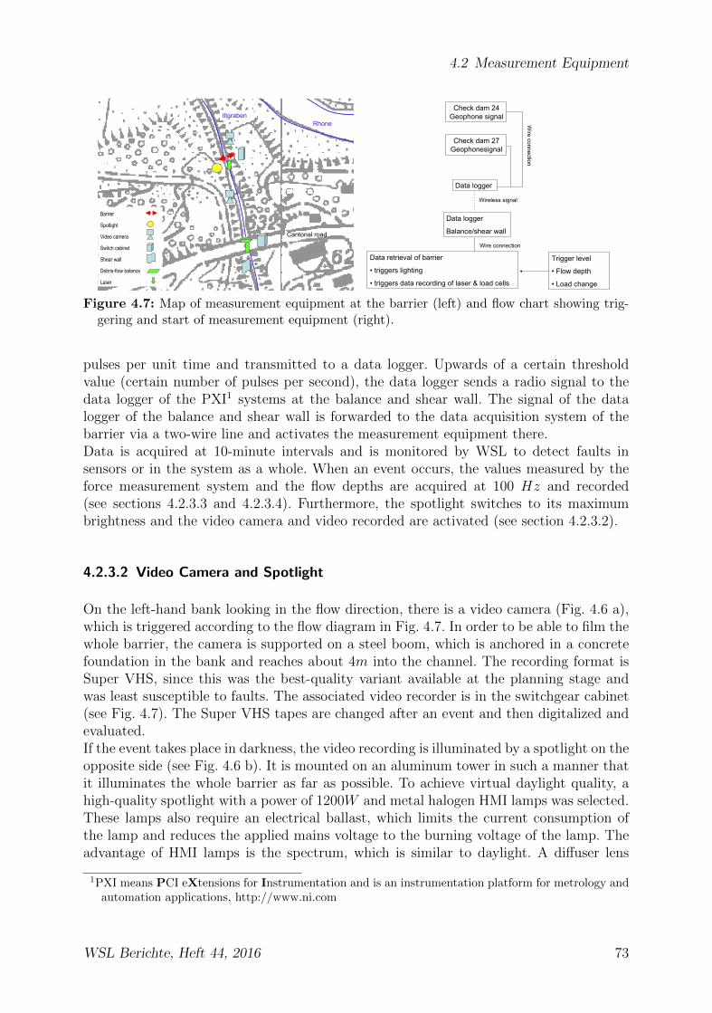
4.2 Measurement Equipment
Cantonal road
Rhone
Barrier
Spotlight
Video camera
Switch cabinet
Shear wall
Debris-flow balance
Laser
Illgraben Check dam 24
Geophone signal
Check dam 27 Geophonesignal
Data loggerW
ire connection
Data logger
Balance/shear wall
Wireless signal
Data retrieval of barrier
• triggers lighting
• triggers data recording of laser & load cells
Trigger level
• Flow depth
• Load change
Wire connection
Figure 4.7: Map of measurement equipment at the barrier (left) and flow chart showing trig-gering and start of measurement equipment (right).
pulses per unit time and transmitted to a data logger. Upwards of a certain thresholdvalue (certain number of pulses per second), the data logger sends a radio signal to thedata logger of the PXI1 systems at the balance and shear wall. The signal of the datalogger of the balance and shear wall is forwarded to the data acquisition system of thebarrier via a two-wire line and activates the measurement equipment there.Data is acquired at 10-minute intervals and is monitored by WSL to detect faults insensors or in the system as a whole. When an event occurs, the values measured by theforce measurement system and the flow depths are acquired at 100 Hz and recorded(see sections 4.2.3.3 and 4.2.3.4). Furthermore, the spotlight switches to its maximumbrightness and the video camera and video recorded are activated (see section 4.2.3.2).
4.2.3.2 Video Camera and Spotlight
On the left-hand bank looking in the flow direction, there is a video camera (Fig. 4.6 a),which is triggered according to the flow diagram in Fig. 4.7. In order to be able to film thewhole barrier, the camera is supported on a steel boom, which is anchored in a concretefoundation in the bank and reaches about 4m into the channel. The recording format isSuper VHS, since this was the best-quality variant available at the planning stage andwas least susceptible to faults. The associated video recorder is in the switchgear cabinet(see Fig. 4.7). The Super VHS tapes are changed after an event and then digitalized andevaluated.If the event takes place in darkness, the video recording is illuminated by a spotlight on theopposite side (see Fig. 4.6 b). It is mounted on an aluminum tower in such a manner thatit illuminates the whole barrier as far as possible. To achieve virtual daylight quality, ahigh-quality spotlight with a power of 1200W and metal halogen HMI lamps was selected.These lamps also require an electrical ballast, which limits the current consumption ofthe lamp and reduces the applied mains voltage to the burning voltage of the lamp. Theadvantage of HMI lamps is the spectrum, which is similar to daylight. A diffuser lens
1PXI means PCI eXtensions for Instrumentation and is an instrumentation platform for metrology andautomation applications, http://www.ni.com
WSL Berichte, Heft 44, 2016 73
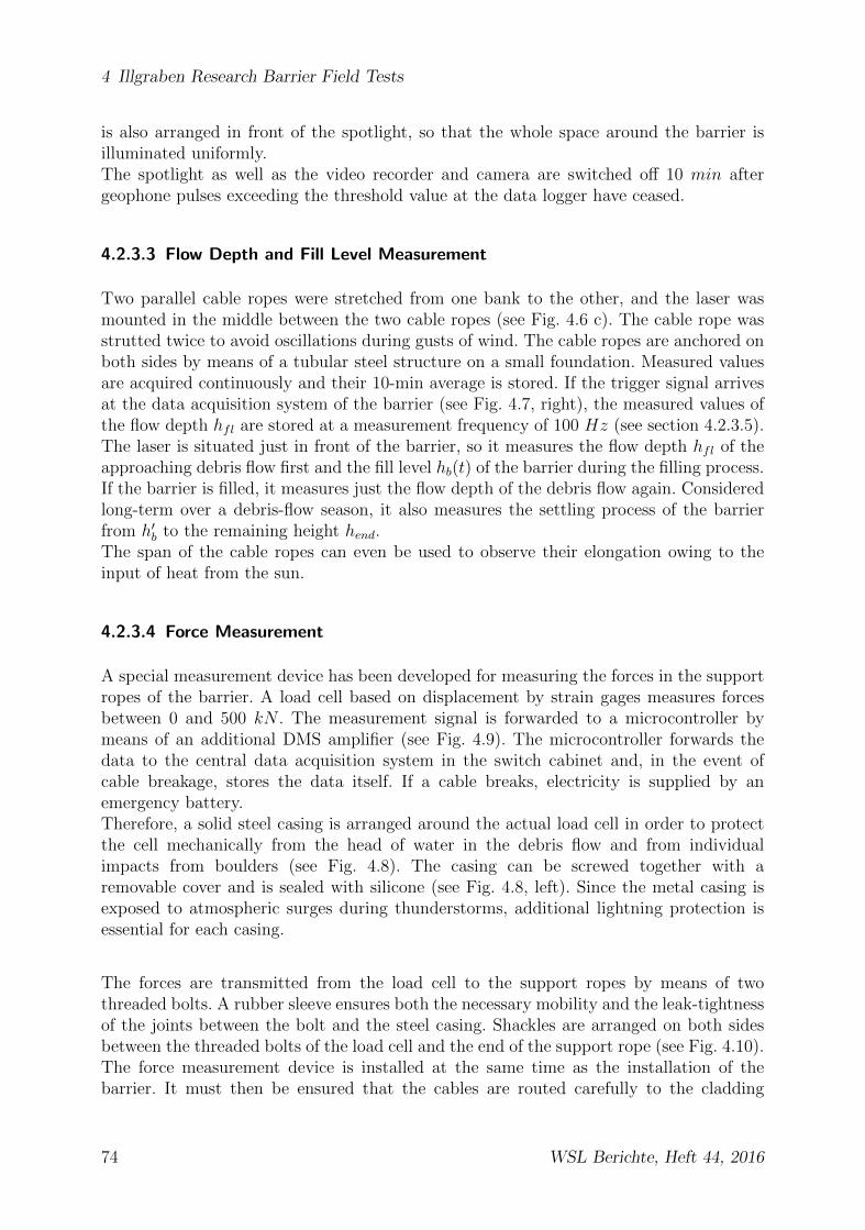
4 Illgraben Research Barrier Field Tests
is also arranged in front of the spotlight, so that the whole space around the barrier isilluminated uniformly.The spotlight as well as the video recorder and camera are switched off 10 min aftergeophone pulses exceeding the threshold value at the data logger have ceased.
4.2.3.3 Flow Depth and Fill Level Measurement
Two parallel cable ropes were stretched from one bank to the other, and the laser wasmounted in the middle between the two cable ropes (see Fig. 4.6 c). The cable rope wasstrutted twice to avoid oscillations during gusts of wind. The cable ropes are anchored onboth sides by means of a tubular steel structure on a small foundation. Measured valuesare acquired continuously and their 10-min average is stored. If the trigger signal arrivesat the data acquisition system of the barrier (see Fig. 4.7, right), the measured values ofthe flow depth hfl are stored at a measurement frequency of 100 Hz (see section 4.2.3.5).The laser is situated just in front of the barrier, so it measures the flow depth hfl of theapproaching debris flow first and the fill level hb(t) of the barrier during the filling process.If the barrier is filled, it measures just the flow depth of the debris flow again. Consideredlong-term over a debris-flow season, it also measures the settling process of the barrierfrom h′b to the remaining height hend.The span of the cable ropes can even be used to observe their elongation owing to theinput of heat from the sun.
4.2.3.4 Force Measurement
A special measurement device has been developed for measuring the forces in the supportropes of the barrier. A load cell based on displacement by strain gages measures forcesbetween 0 and 500 kN . The measurement signal is forwarded to a microcontroller bymeans of an additional DMS amplifier (see Fig. 4.9). The microcontroller forwards thedata to the central data acquisition system in the switch cabinet and, in the event ofcable breakage, stores the data itself. If a cable breaks, electricity is supplied by anemergency battery.Therefore, a solid steel casing is arranged around the actual load cell in order to protectthe cell mechanically from the head of water in the debris flow and from individualimpacts from boulders (see Fig. 4.8). The casing can be screwed together with aremovable cover and is sealed with silicone (see Fig. 4.8, left). Since the metal casing isexposed to atmospheric surges during thunderstorms, additional lightning protection isessential for each casing.
The forces are transmitted from the load cell to the support ropes by means of twothreaded bolts. A rubber sleeve ensures both the necessary mobility and the leak-tightnessof the joints between the bolt and the steel casing. Shackles are arranged on both sidesbetween the threaded bolts of the load cell and the end of the support rope (see Fig. 4.10).The force measurement device is installed at the same time as the installation of thebarrier. It must then be ensured that the cables are routed carefully to the cladding
74 WSL Berichte, Heft 44, 2016
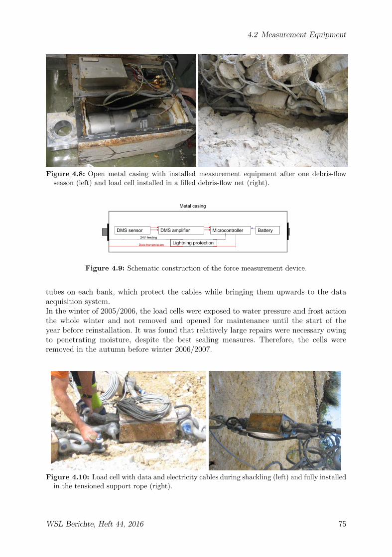
4.2 Measurement Equipment
Figure 4.8: Open metal casing with installed measurement equipment after one debris-flowseason (left) and load cell installed in a filled debris-flow net (right).
Data transmission
DMS sensor DMS amplifier Microcontroller Battery 24V feeding
Metal casing
Lightning protection
Figure 4.9: Schematic construction of the force measurement device.
tubes on each bank, which protect the cables while bringing them upwards to the dataacquisition system.In the winter of 2005/2006, the load cells were exposed to water pressure and frost actionthe whole winter and not removed and opened for maintenance until the start of theyear before reinstallation. It was found that relatively large repairs were necessary owingto penetrating moisture, despite the best sealing measures. Therefore, the cells wereremoved in the autumn before winter 2006/2007.
Figure 4.10: Load cell with data and electricity cables during shackling (left) and fully installedin the tensioned support rope (right).
WSL Berichte, Heft 44, 2016 75

4 Illgraben Research Barrier Field Tests
4.2.3.5 Data Acquisition
The barrier measurement data is acquired at a PC in the switch cabinet (see Fig. 4.11).The video camera for the camera and a screen are also situated there. The measurementdata from the load cells and the laser arrive as analogue data at the PC and are con-verted into binary 12-bit data by a data acquisition card (type NI AT-MIO-64E-32). Themeasurement data are displayed graphically on the screen with Labview 3 (see Fig. 4.11,right). The measured values are finally stored as ASCII data and can be retrieved fromWSL by means of a GSM modem. The video cassette in the video recorder must be ex-changed manually after every event.Both the PC and the video recorder are protected from brief interruptions in the powersupply with a UPS (uninterruptible power supply).The measurement results are discussed in sections 4.5 and 4.6.
Figure 4.11: Data acquisition with monitor, emergency battery and video recorder (left) anddisplay of support rope forces on the monitor in the switch cabinet (right).
2http://sine.ni.com3Labview stands for Laboratory Virtual Instrumentation Engineering Workbench and is a graphical
programming system produced by National Instruments, http://www.ni.com/labview
76 WSL Berichte, Heft 44, 2016

4.3 Barrier Development
4.3 Barrier Development
Three different barrier designs were tested in the Illgraben as field barriers during theproject. The field barrier acts as a 1 : 1 experiment to study the load-transference behav-ior of the barriers. Aspects of the form finding, the long-term behavior during the barrierservice life and the suitability of individual components, such as those for abrasion protec-tion, were also studied. To this end, the barriers were analyzed precisely after every eventover the service periods and suggestions for improving the next barrier arrangement weredeveloped. Before construction, the barriers were simulated with the load approach ac-cording to Rickenmann [82] using the software FARO (see chapter 7.1). The experimentalbarriers in the Illgraben are generally always VX barriers (see section 3.2.1). The differentbarrier designs and the respective developments are described in the sections below.
4.3.1 2005 Barrier
In 2005, the first ring net barrier was installed in the Illgraben. Two support ropes wereinstalled in each case at the top, in the middle and at the bottom. The upper supportropes each had 2 brake rings offset to one side, the middle and lower support ropes eachhad only one brake ring. A winglet rope was intended to hold the stream or debris-flowstream in the middle of the barrier owing to its shape and thereby prevent bank erosion.The winglet rope ran from the central anchor to the upper anchor and was deflectedthere and then routed at an angle of ≈ 30◦ to the upper support rope, where it wasfastened with a clamp and routed from there to the middle anchor on the other side ofthe stream in a mirror-symmetrical manner (see Fig. 4.12, dotted line). A brake ring wasarranged between the central anchor and the upper anchor. The border rope ran from thelower anchor to the upper anchor on each bank and did not have any brakes (dashed linein Fig. 4.12). The shackled ring net formed the barrier between the support ropes. Anabrasion protection system (see section 3.2.2.6) in the form of an L-profile was mountedalong the winglet rope.For a detailed description of the components used, see section 3.2.2.The basal opening between the net and the channel bottom was selected to be relativelysmall owing to the lack of experience.
The following structural details were found to be negative after the first debris-flow season:
• The relatively small basal opening filled the barrier with a bedload event before thefirst ”real” debris flow of the season. The geophone signal was too weak to triggerthe measurement equipment (see section 4.2.3.1). Therefore, there are no measuredvalues from the filling process (see section 4.5).
• The winglet rope was loaded by transverse pressure during an overflow event owingto its deflection point at the upper anchor. In addition, the brakes of the wingletrope were arranged after the deflection, as a result of which they were not able toextend properly. The winglet rope broke after the first overflow event.
• The abrasion protection system in the form of the L-profile rotated after the first
WSL Berichte, Heft 44, 2016 77
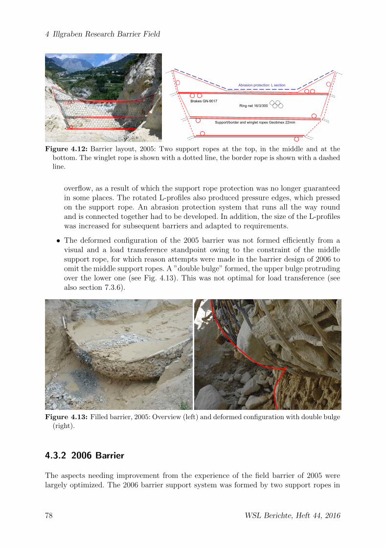
4 Illgraben Research Barrier Field Tests
Brakes GN-9017Ring net 16/3/300
Support/border and winglet ropes Geobinex 22mm
Abrasion protection: L section
Figure 4.12: Barrier layout, 2005: Two support ropes at the top, in the middle and at thebottom. The winglet rope is shown with a dotted line, the border rope is shown with a dashedline.
overflow, as a result of which the support rope protection was no longer guaranteedin some places. The rotated L-profiles also produced pressure edges, which pressedon the support rope. An abrasion protection system that runs all the way roundand is connected together had to be developed. In addition, the size of the L-profileswas increased for subsequent barriers and adapted to requirements.
• The deformed configuration of the 2005 barrier was not formed efficiently from avisual and a load transference standpoint owing to the constraint of the middlesupport rope, for which reason attempts were made in the barrier design of 2006 toomit the middle support ropes. A ”double bulge” formed, the upper bulge protrudingover the lower one (see Fig. 4.13). This was not optimal for load transference (seealso section 7.3.6).
Figure 4.13: Filled barrier, 2005: Overview (left) and deformed configuration with double bulge(right).
4.3.2 2006 Barrier
The aspects needing improvement from the experience of the field barrier of 2005 werelargely optimized. The 2006 barrier support system was formed by two support ropes in
78 WSL Berichte, Heft 44, 2016

4.3 Barrier Development
each case at the top and bottom, the upper support ropes each having two brakes on oneside, and the lower support ropes each having only one brake. In addition, the middlesupport rope was replaced by 8 so-called DIMO elements, which engage in the net likefingers. DIMO elements are weak brake elements, which respond to slight loading and arerouted directly from the ring net to a fixed point (anchor). Type GS-8002 brakes, whichhave a low response load, are used for DIMO elements. The winglet rope was routeddirectly to the opposite anchor without a deflection point at the upper anchor, with onebrake on each side (see Fig. 4.14). The border rope ran in each case from the bottom tothe top anchor on both sides. The abrasion protection system was reinforced by selectinga larger L-profile, which was also shackled from profile to profile (see also section 3.2.2.6).This prevents the profiles from rotating relative to each other and sliding away from eachother. The fastening shackles that grasp the upper support rope were enlarged to avoidcompression and pressure points on the upper support rope.The basal opening was made much larger than the previous year, with a height of 0.5m.
Improved abrasion protection: Reinforced L section
Ring net 16/3/300
Support/border and winglet ropes: Geobinex 22mm
Brakes GN-9017
DIMO elements GS-8002
Figure 4.14: Barrier layout, 2006: Two support ropes at the top and bottom, winglet ropeshown with dotted lines, border rope shown with dashed lines.
The following further findings were produced:
• The rope routing of the 2006 barrier produced the finding that the brake elementsshould be arranged on each side of each support rope, otherwise the effective forcesmust be transmitted over the entire rope length from the load point to the nextbrake. One brake on each side of the support rope is better than two brakes in serieson one side.
• Brake elements in the lower support rope must be fixed upwards when installed onthe ring net, otherwise stones become wedged in the brake elements, even when flowis passing under the barrier, and can thereby block the brakes.
• The DIMO elements engaged in the net were not pulled during the filling process.Furthermore, they caused severe ring net deformations, as a result of which pressurepoints were produced within the barrier. The use of DIMO elements in debris-flowbarriers was therefore found to be impractical.
• Abrasion protection by means of the larger L-profile was very suitable. The profilethickness was increased by 3mm, as a result of which it did not deform as much.The increase in the sheet thickness of the abrasion profiles also serves for corrosionprotection, since the zinc coating of the profiles is worn away after one overflow
WSL Berichte, Heft 44, 2016 79

4 Illgraben Research Barrier Field Tests
process (see section 8.4). The shackling of the individual profiles to each otherprevented them from rotating relative to each other and sliding apart from eachother and ensures uniform protection of the upper support rope. The larger fasteningshackles are also advantageous for the course of the upper support rope and that ofthe winglet rope, since this results in a uniform arrangement of the abrasion profilesalong the rope course without pressure points.
• Without the middle support rope, the deformed configuration appeared uniform inaccordance with the occurrent debris-flow pressure during the filling process (seeFig. 4.15).
• It was observed for the first time in the middle of the debris-flow season in Augustthat the discharge of the barrier was not flowing over it, but rather that the waterwas seeping down before the overflow and exiting again at the foot of the barrier(see Fig. 4.15, right). However, this effect occurred only briefly when there was verylittle flow in the river Illbach.
Seepage
Water drainage
Figure 4.15: 2006 after the filling event (left) and new discharge route owing to seepage inAugust 2006 (right).
4.3.3 2007 Barrier
The design of the 2007 barrier arose from the form finding (see section 7.3.6). Theanchors of the upper support rope were moved one meter forward in the flow direction.The forward anchor position should cause the bulge in the barrier when in the filled stateto move further forward in the upper region. The forward overflow crest of the barriershould mean that the water does not flow away over the ring net (see Fig. 7.33 in chapter7.3). The corrosion on the ring net can then be reduced by the shape.The rope course of the upper support ropes is adjusted to that of the earlier wingletrope, and there is only one horizontal support rope instead of the upper support ropes.This rope routing was selected owing to the large support load in the winglet rope (seemeasured values 4.5.2). Furthermore, a middle auxiliary rope (shown with dotted lines inFig. 4.16) was introduced to control the deformed configuration in the flow direction. It
80 WSL Berichte, Heft 44, 2016
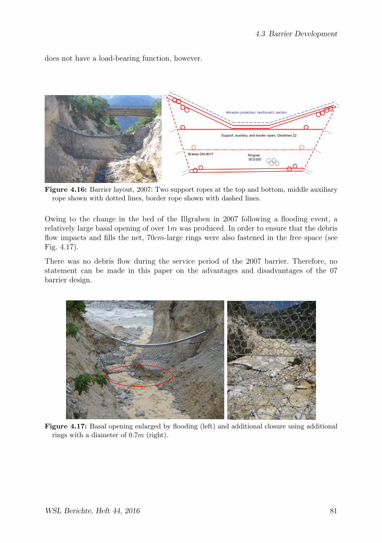
4.3 Barrier Development
does not have a load-bearing function, however.
Abrasion protection: reinforced L section
Ringnet 16/3/300
Support, auxiliary, and border ropes: Geobinex 22
Brakes GN-9017
Figure 4.16: Barrier layout, 2007: Two support ropes at the top and bottom, middle auxiliaryrope shown with dotted lines, border rope shown with dashed lines.
Owing to the change in the bed of the Illgraben in 2007 following a flooding event, arelatively large basal opening of over 1m was produced. In order to ensure that the debrisflow impacts and fills the net, 70cm-large rings were also fastened in the free space (seeFig. 4.17).
There was no debris flow during the service period of the 2007 barrier. Therefore, nostatement can be made in this paper on the advantages and disadvantages of the 07barrier design.
Figure 4.17: Basal opening enlarged by flooding (left) and additional closure using additionalrings with a diameter of 0.7m (right).
WSL Berichte, Heft 44, 2016 81

4 Illgraben Research Barrier Field Tests
4.4 Measurement Results, Debris-flow Balance andShear Wall
Figure 4.18: Pressure profiles at different times during the debris flow on October 3rd, 2006.The y axis shows the number of the load cell by height. The value 6 on the y axis is the topcell, the value 2 is the 2nd lowest cell. Legend: nach Frontankunft = after arrival of front;Nummer der Kraftmessplatte = number of force plate; Hohe = height; Druck auf Platte =pressure on single force plates.
In the case of the shear wall measurement data, only the results of the force measurementplates that are relevant within this thesis will be discussed. The geophone data are notdiscussed. Fig. 4.18 shows measured values at certain times during the event of October3rd, 2006.Cell No. 1 is omitted because it was already silted up at the start of the debris flow.The values of cell 2 are also lower than the measured values of cell 3. This also suggestsa partial silting-up of cell 2. The first pressure distribution curve one second after thearrival of the front has a hyperbolic appearance. This suggests that not much materialwas deposited yet before cell 2, because the measured values of cell 2 and cell 3 are stillrelatively close to each other. The flow depth is in the process of rising, i.e. the top cell 6was still not affected at all (see Fig. 4.19). The front lasted for approximately 8s accord-ing to the video recording and was followed by a rather muddy-looking part of the debrisflow. The pressure distribution 12s after the arrival of the front is hydrostatic except forthe silted-up load cells 1 and 2. This suggests a homogeneous mixture of the solids withthe liquid phase, which is also confirmed by the video. At this point it shows a uniformlypasty, homogeneous liquid. The same applies for the point in time 24 s after the arrival
82 WSL Berichte, Heft 44, 2016
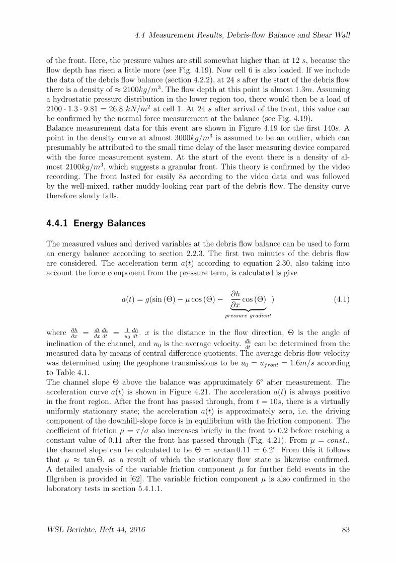
4.4 Measurement Results, Debris-flow Balance and Shear Wall
of the front. Here, the pressure values are still somewhat higher than at 12 s, because theflow depth has risen a little more (see Fig. 4.19). Now cell 6 is also loaded. If we includethe data of the debris flow balance (section 4.2.2), at 24 s after the start of the debris flowthere is a density of ≈ 2100kg/m3. The flow depth at this point is almost 1.3m. Assuminga hydrostatic pressure distribution in the lower region too, there would then be a load of2100 · 1.3 · 9.81 = 26.8 kN/m2 at cell 1. At 24 s after arrival of the front, this value canbe confirmed by the normal force measurement at the balance (see Fig. 4.19).Balance measurement data for this event are shown in Figure 4.19 for the first 140s. Apoint in the density curve at almost 3000kg/m3 is assumed to be an outlier, which canpresumably be attributed to the small time delay of the laser measuring device comparedwith the force measurement system. At the start of the event there is a density of al-most 2100kg/m3, which suggests a granular front. This theory is confirmed by the videorecording. The front lasted for easily 8s according to the video data and was followedby the well-mixed, rather muddy-looking rear part of the debris flow. The density curvetherefore slowly falls.
4.4.1 Energy Balances
The measured values and derived variables at the debris flow balance can be used to forman energy balance according to section 2.2.3. The first two minutes of the debris floware considered. The acceleration term a(t) according to equation 2.30, also taking intoaccount the force component from the pressure term, is calculated is give
a(t) = g(sin (Θ)− µ cos (Θ)− ∂h
∂xcos (Θ)︸ ︷︷ ︸
pressure gradient
) (4.1)
where ∂h∂x
= dtdx
dhdt
= 1u0
dhdt
. x is the distance in the flow direction, Θ is the angle of
inclination of the channel, and u0 is the average velocity. dhdt
can be determined from themeasured data by means of central difference quotients. The average debris-flow velocitywas determined using the geophone transmissions to be u0 = ufront = 1.6m/s accordingto Table 4.1.The channel slope Θ above the balance was approximately 6◦ after measurement. Theacceleration curve a(t) is shown in Figure 4.21. The acceleration a(t) is always positivein the front region. After the front has passed through, from t = 10s, there is a virtuallyuniformly stationary state; the acceleration a(t) is approximately zero, i.e. the drivingcomponent of the downhill-slope force is in equilibrium with the friction component. Thecoefficient of friction µ = τ/σ also increases briefly in the front to 0.2 before reaching aconstant value of 0.11 after the front has passed through (Fig. 4.21). From µ = const.,the channel slope can be calculated to be Θ = arctan 0.11 = 6.2◦. From this it followsthat µ ≈ tan Θ, as a result of which the stationary flow state is likewise confirmed.A detailed analysis of the variable friction component µ for further field events in theIllgraben is provided in [62]. The variable friction component µ is also confirmed in thelaboratory tests in section 5.4.1.1.
WSL Berichte, Heft 44, 2016 83
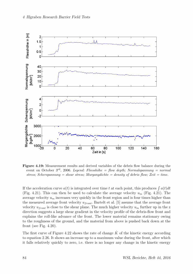
4 Illgraben Research Barrier Field Tests
Figure 4.19: Measurement results and derived variables of the debris flow balance during theevent on October 3rd, 2006. Legend: Fliesshohe = flow depth; Normalspannung = normalstress; Scherspannung = shear stress; Murgangdichte = density of debris flow; Zeit = time.
If the acceleration curve a(t) is integrated over time t at each point, this produces∫a(t)dt
(Fig. 4.21). This can then be used to calculate the average velocity um (Fig. 4.21). Theaverage velocity um increases very quickly in the front region and is four times higher thanthe measured average front velocity ufront. Bartelt et al. [5] assume that the average frontvelocity ufront is close to the shear plane. The much higher velocity um further up in the zdirection suggests a large shear gradient in the velocity profile of the debris-flow front andexplains the roll-like advance of the front. The lower material remains stationary owingto the roughness of the ground, and the material from above is pushed back down at thefront (see Fig. 4.20).
The first curve of Figure 4.22 shows the rate of change K of the kinetic energy accordingto equation 2.26. It shows an increase up to a maximum value during the front, after whichit falls relatively quickly to zero, i.e. there is no longer any change in the kinetic energy
84 WSL Berichte, Heft 44, 2016
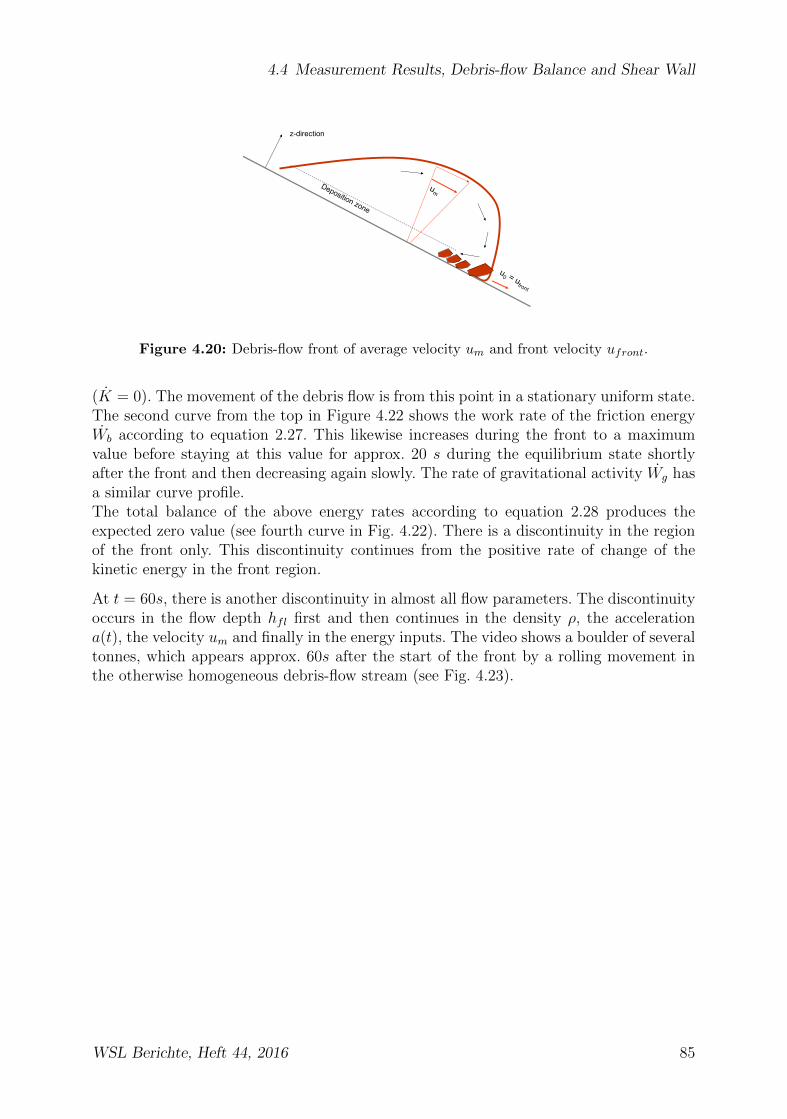
4.4 Measurement Results, Debris-flow Balance and Shear Wall
z-direction
Figure 4.20: Debris-flow front of average velocity um and front velocity ufront.
(K = 0). The movement of the debris flow is from this point in a stationary uniform state.The second curve from the top in Figure 4.22 shows the work rate of the friction energyWb according to equation 2.27. This likewise increases during the front to a maximumvalue before staying at this value for approx. 20 s during the equilibrium state shortlyafter the front and then decreasing again slowly. The rate of gravitational activity Wg hasa similar curve profile.The total balance of the above energy rates according to equation 2.28 produces theexpected zero value (see fourth curve in Fig. 4.22). There is a discontinuity in the regionof the front only. This discontinuity continues from the positive rate of change of thekinetic energy in the front region.
At t = 60s, there is another discontinuity in almost all flow parameters. The discontinuityoccurs in the flow depth hfl first and then continues in the density ρ, the accelerationa(t), the velocity um and finally in the energy inputs. The video shows a boulder of severaltonnes, which appears approx. 60s after the start of the front by a rolling movement inthe otherwise homogeneous debris-flow stream (see Fig. 4.23).
WSL Berichte, Heft 44, 2016 85

4 Illgraben Research Barrier Field Tests
Figure 4.21: Movement of the debris-flow front: acceleration a, a integrated over time andaverage velocity um. Legend: Reibungskoeffizient = coefficient of friction; Beschleunigung =acceleration; Beschleunigung integriert uber die Zeit = acceleration integrated over time; Mit-tlere Geschwindigkeit = average velocity; Zeit = time.
86 WSL Berichte, Heft 44, 2016

4.4 Measurement Results, Debris-flow Balance and Shear Wall
Figure 4.22: Work rates K, Wg and Wb of a debris flow and their total balance. Legend:Anderungsrate kin. Energie = change rate of kinetic energy; Anderungsrate Reibungsenergie =change rate of frictional energy; Gravitationsarbeitsrate = change rate of gravitational energy;Energiebilanz = energy balance; Zeit = time.
Figure 4.23: A boulder rolls over the debris flow balance. The images were digitalized at dif-ferent times from the video recording of October 3rd, 2006.
WSL Berichte, Heft 44, 2016 87

4 Illgraben Research Barrier Field Tests
4.5 Measurement Results of the Test Barriers
Table 4.1 at the start of the chapter gives an overview of the individual debris flows inthe Illgraben within the duration of the project. In this section, the occurring debris flowsare divided into filling events and overflow events, in order to show the effect of thedebris flow on the barrier. Measured filling events only occurred in the 2006 debris-flowseason, because the flooding event of 2005 meant that there was no geophone signal toactivate the measurement equipment and the barrier was filled without measured values.
4.5.1 2006 Filling Event Measured Values
During the filling event on May 18th, 2006 (see Table 4.1), a watery debris flow with adensity of 1600kg/m3 and a flow velocity of ufront = 3m/s reached the barrier at 18:40h. Few large blocks were transported in the front wave, as a result of which the net wasnot blocked for 7min, and the flow, which rather resembled a flood, flowed through underthe net. A blockage at the lower support ropes did not occur until time 18:47, followedby a very slow filling process of more than 90s duration (see Fig. 4.24). As can be seenclearly on the video recording, the solid material is retained behind the barrier and thewater flows forward through the ring net. During the filling process, the load of almost230kN at the lower support ropes is much higher than the load at the upper supportropes, which is maximum 150kN . Figure 4.24 does not show the load in the winglet rope,the maximum value of which is 160kN during the filling process. Figure 4.24 also showsbrief reductions in load and force, which are attributable to the sudden elongations of thebrakes. The measured values of the laser indicate the flow depth hfl of the debris flowbefore blockage and the fill level hb after blockage. The flow depth in the first wave beforefilling was almost 1m.
The corresponding data of the debris flow balance are shown in Figure 4.25. The start ofthe filling process at the balance was t = 230s. A relatively large debris-flow wave with aflow depth of almost 1.5m can also be seen in the measurement data of the balance. Thebalance data are mainly relevant for the overflow loading condition in section 6.3.4.5. Inthat case, shear stress τ and normal stress σ from the measured data of the balance havea direct effect on the filled barrier.The retention volume is discussed as part of the measurement data in section 4.5.3.
4.5.2 2005, 2006 Overflow Event Measured Values
Debris flows flowed over the filled debris flow barriers several times. Since the events eachprovided similar measurement data, only one overflow event per debris-flow season willbe discussed in detail in this thesis. For the barrier layout of 2005, the overflow forces ofthe event of August 2nd are considered (see Fig. 4.26).According to Table 4.1, this is a granular debris flow with a density of 2100kg/m3 anda maximum flow depth of around 1m. The flow velocity of 6m/s was relatively highcompared with other events in the Illgraben. One of the load cells in the lower support
88 WSL Berichte, Heft 44, 2016

4.5 Measurement Results of the Test Barriers
Brake elongation
Figure 4.24: Measured forces in the lower and upper support ropes Frope during the 2006 fillingevent. The flow depth is shown on the right-hand y axis [112]. Legend: oberes Tragseil = uppersupport rope; unteres Tragseil = lower support rope; Fliesshohe = flow depth; Fullstandshohe= filling height; Belastung Tragseil = Load in support rope; Zeit = time.
rope failed owing to a technical defect. The measured value of the other load cell in thelower support rope is very small at 45kN , because the lower region of the barrier wasdammed in after the last event. The middle support ropes were loaded with 10kN moreduring the overflow. The upper support ropes are loaded directly by the vertical load σand the shear stress τ of the debris flow owing to the debris-flow process. Their load levelwas changed by almost 20kN thereby. At the time 13:50:25, a boulder approx. 1m indiameter was entrained, which is shown by an increase in load in the upper support ropesand in the measured flow depth hfl. At the same time, this boulder can also be seen inthe video recordings.
A further overflow event occurred in the 2006 debris-flow season on June 27th (see Ta-ble 4.1). It was also a debris flow with a granular front and a density of 2000kg/m3. Theflow depth was 2.7m and was somewhat above average. The increase in load during thefront was 30kN at the lower support ropes and 100kN at the upper support ropes, whichwere directly affected. The winglet rope underwent a large increase in load with a loadpeak of just under 200kN (see Fig. 4.27). Since the winglet rope was always fastenedto the upper support ropes with a clamp, one of the upper support ropes was subjectedto constraints and transverse pressure owing to the large overflow load. The introducedtransverse force component of the fastened winglet rope was too great. This happenedbecause the brakes on both sides of the winglet rope were able to elongate, whereas theupper support ropes each had brakes on only one end of the rope. As a result, a transversepressure developed at the other rope end owing to the lack of brake elongation and thetransverse tensile component of the fastened winglet rope, and one of the upper support
WSL Berichte, Heft 44, 2016 89
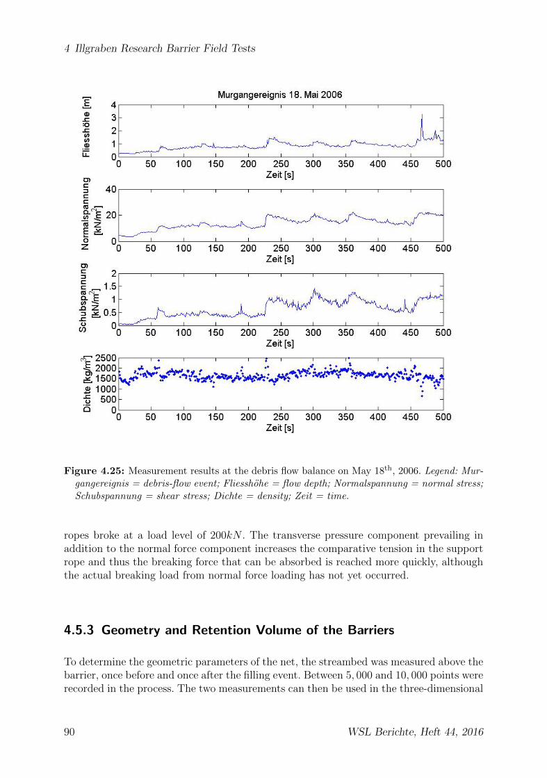
4 Illgraben Research Barrier Field Tests
Figure 4.25: Measurement results at the debris flow balance on May 18th, 2006. Legend: Mur-gangereignis = debris-flow event; Fliesshohe = flow depth; Normalspannung = normal stress;Schubspannung = shear stress; Dichte = density; Zeit = time.
ropes broke at a load level of 200kN . The transverse pressure component prevailing inaddition to the normal force component increases the comparative tension in the supportrope and thus the breaking force that can be absorbed is reached more quickly, althoughthe actual breaking load from normal force loading has not yet occurred.
4.5.3 Geometry and Retention Volume of the Barriers
To determine the geometric parameters of the net, the streambed was measured above thebarrier, once before and once after the filling event. Between 5, 000 and 10, 000 points wererecorded in the process. The two measurements can then be used in the three-dimensional
90 WSL Berichte, Heft 44, 2016

4.5 Measurement Results of the Test Barriers
Large
stone
Figure 4.26: Measured forces in the support ropes Frope during the overflow event on August2nd, 2005. The flow depth is shown on the right-hand axis. Legend: Belastung Tragseil =load in support rope; Fliesshohe = flow depth; oberes Tragseil = upper support rope; mittlerestragseil = middle support rope; unteres Tragseil = lower support rope; Zeit = time.
terrain model in ArcGis4 to determine the differential volume, which corresponds to theretention volume. For the filling event on May 18th, 2006, the retained volume Vr = 960m3
was determined in this manner (see Fig. 4.28).
From a hydraulic engineering standpoint, the bed inclination produced in the filled stateof the barrier also forms an interesting component of the study. An overview of the changein the bed position between the initial installation of a barrier in 2005 and before andafter filling in May 2006 is shown in Figure 4.29.
A clear flattening of the bed owing to the barrier installation in the streambed is seen ifthe bed inclination before the initial barrier installation in 05 is compared with the bedinclination after the already installed barrier in 06 (see Fig. 4.29).In addition, the remaining barrier height after the filling process h′b and the deformationof the barrier in the flow direction f are of interest for later dimensioning. The top of thenet at different times is shown in Figure 4.30. It depends on the number and intensity ofoverflow events and on the elongation of the brakes in the winglet rope and in the uppersupport ropes.
The maximum deformation of the bulge in the flow direction is also dependent on thenumber of overflow processes. After the filling event in 2006, the maximum deformationin the flow direction was 2.5m. At the end of the debris-flow season, the maximum de-formation in the flow direction was 3.25m. This means that, as long as the brakes in thesupport ropes are not yet fully extended after the filling process, the net barriers deform
4Commercial software for displaying geographical information: http://www.esri.com/software/arcgis
WSL Berichte, Heft 44, 2016 91

4 Illgraben Research Barrier Field Tests
Figure 4.27: Measured forces in the support ropes Frope during the overflow event on June27th, 2006. The flow depth is shown on the right-hand y axis. Legend: Flugelseil = wingletrope; oberes Tragseil = upper support rope; unteres Tragseil = lower support rope; Fliesshohe= flow depth; Belastung Tragseil = load in support rope; Zeit = time.
Figure 4.28: 3D terrain model of the empty streambed with the measured anchor points of thebarrier marked by crosses (left) and 3D model of the filled barrier and measured net points(right).
further in the flow direction during subsequent overflow events owing to the effective shearstress τ of the overflowing debris flow.The measured values are based only on the observation period of one debris-flow seasonsand on one filling process, because no more difference measurements could be made owingto the lack of a filling event in 2007.
92 WSL Berichte, Heft 44, 2016
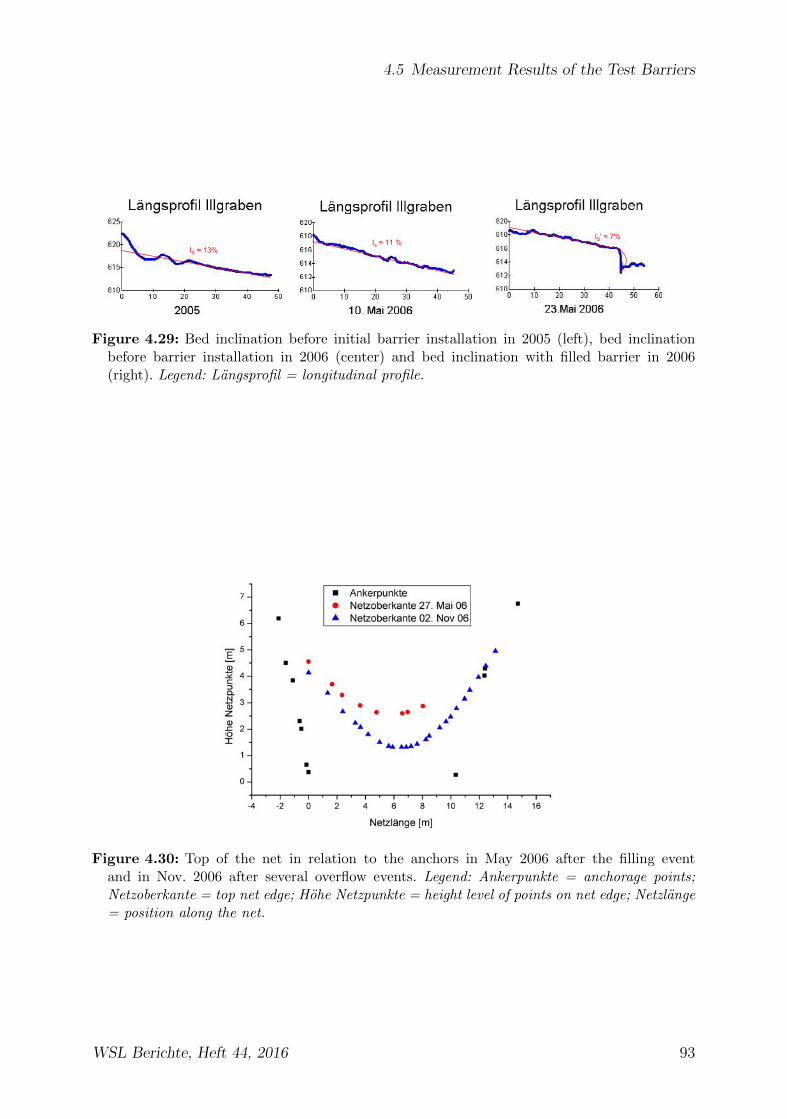
4.5 Measurement Results of the Test Barriers
IS ≈ 13% Is ≈ 11 %
IS' ≈ 7%
Figure 4.29: Bed inclination before initial barrier installation in 2005 (left), bed inclinationbefore barrier installation in 2006 (center) and bed inclination with filled barrier in 2006(right). Legend: Langsprofil = longitudinal profile.
Figure 4.30: Top of the net in relation to the anchors in May 2006 after the filling eventand in Nov. 2006 after several overflow events. Legend: Ankerpunkte = anchorage points;Netzoberkante = top net edge; Hohe Netzpunkte = height level of points on net edge; Netzlange= position along the net.
WSL Berichte, Heft 44, 2016 93

4 Illgraben Research Barrier Field Tests
4.6 Analysis and Interpretation
4.6.1 Debris-flow Data Observation Station
In the course of the studies, it was found that the site of the test barrier in the Illgrabenwas an ideal choice. The measurement instruments and the debris-flow data of thedebris-flow observation station already present formed ideal conditions for a completedebris-flow evaluation. The following findings came to light:
• The measured values of the shear wall have a hyperbolic pressure profile within thefront and a hydrostatic pressure profile in the subsequent, well-mixed debris-flowtail. The measured values of the hydrostatic pressure profile were also confirmed atthe same time by the vertical load measurement at the balance.
• A precise energy analysis of the balance data allows the individual energy contribu-tions in the debris-flow process, which play a role in the subsequent load approach,to be estimated (see section 6.2.4).
• If all the measurement equipment in the Illgraben is taken into consideration, theflow depth hfl, the shear stress τ , the normal stress σ, the average front velocityufront and the lateral pressure distribution over the flow depth can be measured asdirect parameters for further dimensioning the barriers. From these, further derivedvariables can be determined, such as the density ρ, the acceleration a, the averagevelocity um, the rates of change of the kinetic energy K, gravitational force Wg andthe friction energy Wb.
• A newly developed measurement technique for acquiring the barrier data works inan almost error-free manner and acquires the parameters around the debris-flownet that are important for barrier design. The flow depth hfl directly in front ofthe barrier, the fill level hb of the barrier, the rope forces in the barrier Frope and avideo recording of the events are recorded. Furthermore, geometric variables can bedetermined before and after the filling process, such as fill volume Vr, bed inclinationbefore and after the filling process Is and I ′s and the barrier height after the fillingprocess h′b.
4.6.2 Test Barrier Data
Both the barrier layout of 2005 and that of 2006 were able to provide evidence that thesupport system of the flexible ring net barriers functions as a whole. It can withstand adebris flow without restrictions and retain some of the debris-flow stream. The drainageprinciple owing to the permeability of the ring net causes the flowing stream to stopbehind the net and effects continuous filling from the streambed to the set net heighth′b (see section 4.5.1). It has only been possible so far to measure one, rather muddyfilling event. This filling event showed that the greatest loads occur in the lower supportropes during the filling process. The maximum rope loads here were 230kN , whereas
94 WSL Berichte, Heft 44, 2016

4.6 Analysis and Interpretation
the maximum loads in the upper support ropes were only ≈ 60% of the lower supportropes, with a maximum of 150kN . A back calculation of the measured rope loads tothe effective debris-flow pressure is made in section 6.2.2. The force measurement ofthe filling event also confirmed that the occurrent rope forces during the filling processof a muddy event are well below the maximum breaking force of the support ropes of400kN (see Table 3.1). However, measured values of the rope loads in the case of agranular debris-flow front are still not available, because it has not yet been possible tomeasure a granular filling event. If necessary, these loads can be calculated using theapproach according to Rickenmann [82] in section 6.3.2, or taken into account with ahigher pressure coefficient in the dynamic fraction (see section 6.3.2).The elongation of the brakes and the associated energy absorption can clearly be seenduring the filling process by a noticeable reduction in the load level in all support ropeswith brakes. The point in time at which the brakes elongate can also be seen in closeanalysis of the video recording and coincides with that of the data recording.The filling time was rather long at timp = 90s, because it was a very muddy event andsmaller stones and a lot of mud continued to flow through the barrier during the fillingprocess. The experimental data of the USGS flume in Oregon [23] previously gave fillingtimes of timp = 1− 4s [82]. This value is significantly lower and occurs rather during thefilling process of a granular debris-flow front. The dynamic dependence over the fillingtime timp alone indicates that there will be two types of design method for the fillingprocess, depending on the type of debris flow. For the design approach to mudflow-likeevents and that for granular debris flows, see section 6.3.2.The measurements of the overflow processes relate to both types of debris flow, bothmudflow and debris flows with granular fronts, that flowed over the barrier and weremeasured. The measured values of the overflow events show that the increase in loadduring the overflow mainly takes place in the upper support ropes and in the wingletrope. The size of the increase in load in the upper support ropes and in the winglet ropewas maximum ∆Frope = 100kN , in the lower support ropes only 30kN . The increase inload in the upper support ropes is therefore 3 times greater than in the lower supportropes. It depends on the effective normal stress σ and shear stress τ of the overflowingdebris flow (for calculation, see section 6.3.4.5).Individual blocks do not produce large load peaks, either during the filling process orduring overflow. Although they can be seen in the measurement data by a brief increasein load of up to 10kN , this was well below the increases in load of the entire debris-floweffect during filling or overflowing, with only 5% of the maximum force.Ropes did not break because they reached their maximum breaking force, but ratherowing to badly realized structural details. It was necessary to test and improve thesestructural details over the service period of the barriers in the field and by means of threedifferent barrier designs.
4.6.3 Analysis of Net Details
The following structural barrier details were developed and improved:
WSL Berichte, Heft 44, 2016 95

4 Illgraben Research Barrier Field Tests
• Brakes should be arranged on both sides of support ropes so that the tensile forcedoes not have to be transmitted through the entire length of the rope when thebrakes respond. If the support rope is loaded on the side where there is no brake,the brake can be prevented from elongating by the rope friction, which builds upalong the entire length of the rope. With such a constraint, the rope can breakbefore the brake can elongate. If the brakes are arranged on both sides, only halfthe friction distance has to be overcome before the brake responds.
• On the lower support ropes, it is important to tie the brakes upward with a piece ofwire during installation. This prevents the brakes being blocked by stones or piecesof wood becoming jammed in them when a flood flows under the net.
• Deflection points for support ropes must be avoided as far as possible. This wasdiscovered with the 2005 barrier, in which the winglet rope was deflected at theupper anchor. Deflection points reduce the rope force that can be absorbed owingto transverse pressure forces, depending on the deflection radius. According to [121]the reduced breaking force RBF [%] is calculated according to the following rule ofthumb
RBF = 0.0035α +δ
D3.66 +
0.1 static loads
0.3 dynamic loads(4.2)
where α is the deflection angle in ◦, δ is the wire diameter, and D is the sum ofthe deflection diameter and half the rope diameter d. According to [121], this ruleof thumb applies to static deflection experiments; for dynamic loads, the last valuechanges from 0.1 to 0.3.No deflection experiments have been carried out yet for Geobinex 22mm supportropes (see section 3.2.2.1). However, there is some data from rope breakages causedby deflection for rockfall barriers (see [121]). These can be used to make the fol-lowing estimations in relation to breaking force minimization. The wire diameter is≈ 1.2mm. If the deflection point of the winglet rope of nominal diameter d = 22mmfrom the 2005 barrier is considered, the rope was deflected by ≈ 45◦ at the flex head,which has a diameter of ≈ 35mm. According to formula 4.2, there is a reductionin the breaking force RBP of 55% for dynamic load and 35% for static load. Ifone assumes the maximum breaking force of 400kN and reduces this by 55%, thisproduces 220kN . This load could quite easily have occurred in the winglet ropeduring the overflow of the event on June 27th, 2006 (see Fig. 4.27), which explainsthe breakage of the winglet rope in 2005.
• Pressure points caused by clamps, insufficiently large shackles etc. should be avoidedwhen designing the ring net barrier. This was demonstrated by the breakage in theupper support rope, to which the winglet rope was fastened with a clamp. Thetransverse tensile component of the winglet rope was too great for the support rope.In addition to the existing transverse pressure, frictional forces presumably occurredwithin the clamp and therefore heat caused by the friction. The cold-twisted wiresof the support ropes undergo an additional minimization of bearing load as a resultof heat [121]. Therefore, the rope broke at the clamp at a measured rope load of≈ 200kN . Such pressure points should generally be avoided when designing the
96 WSL Berichte, Heft 44, 2016
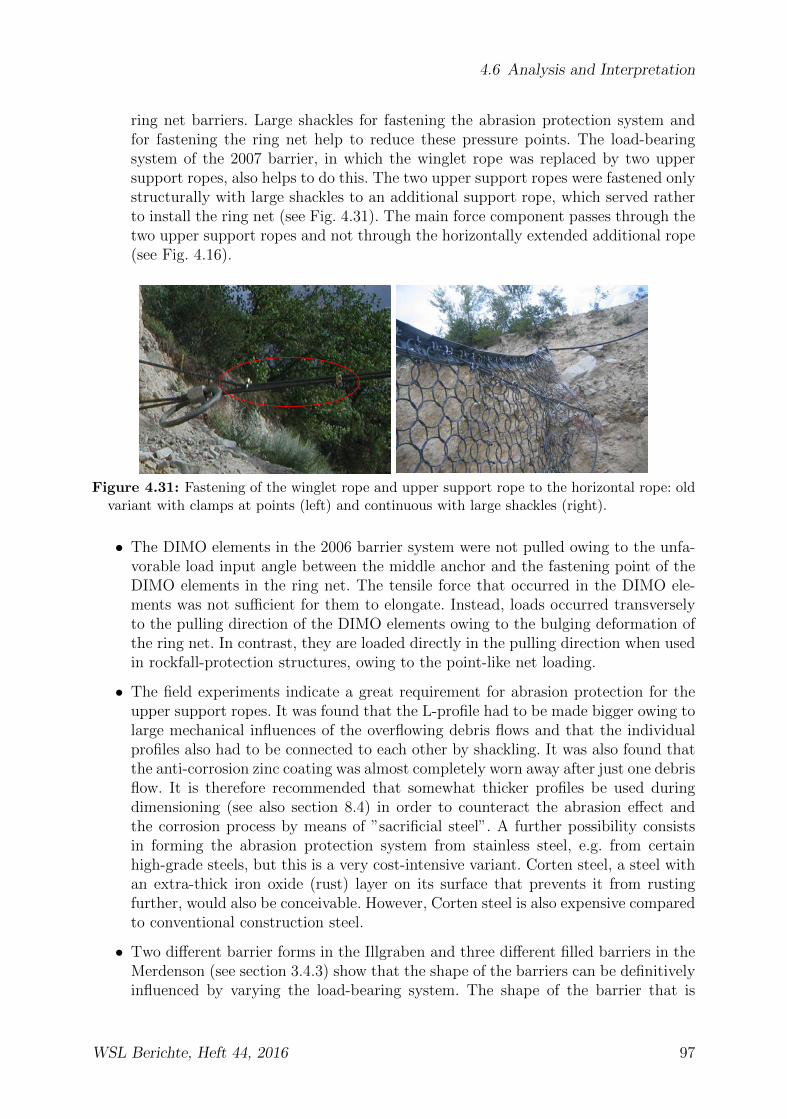
4.6 Analysis and Interpretation
ring net barriers. Large shackles for fastening the abrasion protection system andfor fastening the ring net help to reduce these pressure points. The load-bearingsystem of the 2007 barrier, in which the winglet rope was replaced by two uppersupport ropes, also helps to do this. The two upper support ropes were fastened onlystructurally with large shackles to an additional support rope, which served ratherto install the ring net (see Fig. 4.31). The main force component passes through thetwo upper support ropes and not through the horizontally extended additional rope(see Fig. 4.16).
Figure 4.31: Fastening of the winglet rope and upper support rope to the horizontal rope: oldvariant with clamps at points (left) and continuous with large shackles (right).
• The DIMO elements in the 2006 barrier system were not pulled owing to the unfa-vorable load input angle between the middle anchor and the fastening point of theDIMO elements in the ring net. The tensile force that occurred in the DIMO ele-ments was not sufficient for them to elongate. Instead, loads occurred transverselyto the pulling direction of the DIMO elements owing to the bulging deformation ofthe ring net. In contrast, they are loaded directly in the pulling direction when usedin rockfall-protection structures, owing to the point-like net loading.
• The field experiments indicate a great requirement for abrasion protection for theupper support ropes. It was found that the L-profile had to be made bigger owing tolarge mechanical influences of the overflowing debris flows and that the individualprofiles also had to be connected to each other by shackling. It was also found thatthe anti-corrosion zinc coating was almost completely worn away after just one debrisflow. It is therefore recommended that somewhat thicker profiles be used duringdimensioning (see also section 8.4) in order to counteract the abrasion effect andthe corrosion process by means of ”sacrificial steel”. A further possibility consistsin forming the abrasion protection system from stainless steel, e.g. from certainhigh-grade steels, but this is a very cost-intensive variant. Corten steel, a steel withan extra-thick iron oxide (rust) layer on its surface that prevents it from rustingfurther, would also be conceivable. However, Corten steel is also expensive comparedto conventional construction steel.
• Two different barrier forms in the Illgraben and three different filled barriers in theMerdenson (see section 3.4.3) show that the shape of the barriers can be definitivelyinfluenced by varying the load-bearing system. The shape of the barrier that is
WSL Berichte, Heft 44, 2016 97

4 Illgraben Research Barrier Field Tests
produced in the filled state can influence the load-transference behavior and thestructural corrosion protection of the ring net. Therefore, further experiments werecarried out using simulations (see chapter 7.3).
4.6.4 Analysis of Barrier Geometric Data
With regard to the geometric measurement data of the barrier, the following assumptionsaccording to [82] were confirmed:
• For the channel slope after the filling process behind the barrier I ′S, it was foundthat it became shallower by a factor of 2/3 compared with the original channel slope(I ′S = 2
3IS). The channel slope was 11% before installation of the net in 2006, on
May 10th, and 7% after the filling process on May 23rd, 2006 (see Fig. 4.29). Inaddition, the bed in the Illgraben rose after initial installation of the net and at thesame time the original bed inclination decreased from 13% (in 2005, before initialinstallation) to 11% after one net season (see Fig. 4.29). The measured values fromthe Merdenson multilevel structure also confirm the factor of 2/3 of the original bedinclination (see section 3.4.3). Jaeggi in [57] also mentions a flattening of the bedas a result of a multilevel structure. He mentions a practical example from the ValVaruna, where the bed inclination was reduced from 37% to 22% by the arrangementof several concrete barriers, which corresponds to a slightly larger factor of 3/5 butis similar to that of 2/3.
• It was also found that the remaining height of the barrier after initial filling wash′b = 3
4·hb (see Fig. 4.30). The settling of the net edge owing to filling of the barrier
was already predicted by Rickenmann [82] with a factor of 3/4. This was confirmedusing field measurements. The original height of the barrier without winglets was4m, after the filling process it was almost 3m. This settling value of approximately1m can also be calculated using the displacement of the brakes in the winglet rope.The upper support ropes are not decisive for the settling of the barrier, becausetheir anchors are arranged lower down than the winglet rope anchors. They rathercontrol the distance f , i.e. the deformation of the barrier in the flow direction (seealso section 6.2.2 and 7.3.6). Using the measurement points, an angle of 39◦ wasproduced between the winglet rope and the anchor line after the first filling event inMay. The vertical displacement of the brake is then calculated as lbr,v = cos 39◦ · lbr.The average value of the two brake elongations in the winglet rope during the fillingevent was ≈ 53cm on each side. This results in a vertical deformation of 82cm. Thisvalue is somewhat smaller than that measured, because vertical deformations fromthe flex heads under load and also measurement inaccuracies are included. However,the order of magnitude for the settling behavior of the barrier can be determinedby means of the winglet rope using this procedure.
• After several overflow processes, the barrier sank to a remaining height of 1.5m (seeFig. 4.30). Therefore, it sank again by half the remaining height h′b after initial fillingand depending on the starting height hb to hend = 3
8· hb. However, this significant
settling on repeated overflow events was also because both brakes in the winglet
98 WSL Berichte, Heft 44, 2016
4.6 Analysis and Interpretation
rope were pulled as far as they could go by several intensive overflow events (seeTable 4.1). Reinforcement was thereupon provided by a second winglet rope withnew brakes, which of course gave the barrier more room to settle owing to the newbrakes.With UX barriers (see section 3.2.1), maintenance of the remaining height is ensuredin the case of large spans by the posts. If spans are large, large rope extensions andbrake elongations occur in the whole system, and therefore the remaining height ofthe barrier must be controlled with posts.
The analysis of the geometric parameters I ′S and h′b of the filled debris-flow barrier inthe Illgraben forms a basis for the design of the available retention volume Vr of planneddebris-flow barriers.In addition, the change in the bed position as a result of the installation of nets isimportant in terms of hydraulic engineering. A flatter bed results in a slower flow regimein mountain torrents and thus to lower transport of bedload. The flow process of debrisflows is lower in energy owing to the lower flow velocity and results in a braking processin the channel with or without additional protective measures. The principle of bedposition change for energy dissipation is also important for multilevel structures (see alsosection 3.4.2).
WSL Berichte, Heft 44, 2016 99

4 Illgraben Research Barrier Field Tests
100 WSL Berichte, Heft 44, 2016

5 Physical Modeling
In order to investigate the barriers’ structural behavior in response to loads applied by adebris flow under laboratory conditions, 70 tests using four different debris-flow materialsfrom four different catchment areas were conducted at WSL. These tests are more cost-effective compared to field tests, and specific parameters can be observed in a targetedmanner. In addition, it is possible to observe a greater number of events than during fieldmeasurements, because of the limited number of naturally-occurring debris flows. More-over, the observer’s proximity to the events during the laboratory tests allows for a moredetailed examination of the occurring processes. The examination of processes occurringin the field rests primarily on post-hoc analyses of videos of the events. A targeted selec-tion of tests, which accompanies the events observed in the field, allows for an efficientestimation of the occurrent loads.One of the challenges associated with laboratory tests is scaling and the associated trans-ferability of the results to real-life situations. As a result, this chapter will first derive thelaws applicable to the experiments and will then develop important scaling parameterswithin the framework of a dimensional analysis.A detailed description of the tests will be followed by a discussion of the results and theirsignificance. Based on the detailed analysis and interpretation of the results, a represen-tative load model will be developed in the following chapter (see chapter 6).Modeling of the laboratory tests in the finite-element program AVAL-1D1, a simulationprogram for granular media, is intended to provide additional confirmation of the specificdebris-flow parameters measured in the tests.The subsequent interpretation highlights the transferable aspects of the tests and intro-duces the thus-derived design concept.
5.1 Laws Applicable to the Model
The first section attempts to identify similarity criteria for the performed laboratory tests.Based on a dimensional analysis, dimensionless quantities allowing for a comparison ofthe laboratory tests to real-life events will be derived. This will be followed by a criticalanalysis and consideration of the laboratory tests’ limits of transferability.A physical model, which aims to reproduce natural processes as faithfully as possible,should meet the criteria of geometric, kinematic and dynamic similarity [55]. The require-ment for geometric similarity is met by means of a constant ratio Ls between the naturallengths Ln (n = natural) and the lengths of the model Lm (m = model). Ls (s = scaling)then corresponds to the model scale. Kinematic similarity is achieved when temporal
1AVAL-1D is a one-dimensional simulation program for avalanche dynamics, http://www.slf.ch/aval-1d
101

5 Physical Modeling
sequences are consistent, for example the duration of the naturally-occurring filling pro-cess timp,n and the filling time in the model timp,m. Kinematic similarity generally requiresthat the ratios between time intervals, velocities, and accelerations all be of about equalsize. Dynamic similarity requires an approximately equal balance of occurring forces. As aresult, the laboratory test should aim to achieve approximately the same balance of forcesover the course of the process as the prototypical, naturally-occurring process. However,complete dynamic similarity for all forces occurring in the flow is not possible using thesame fluids in the model as in nature [55].For processes that are primarily controlled by gravity and have a free surface, dynamicsimilarity can be achieved using Froude’s law of comparison. In order to do so, theFroude number (according to equation 3.7) in the model must match that of the naturally-occurring prototype, which leads to the following equation:
um√gmLm
=un√gnLn
. (5.1)
If this condition is met, the second condition, which requires equal Reynolds numbersaccording to Reynolds’ law, should be met as well. The Reynolds number is a quantitythat provides information about flow behavior, indicating whether a flow is laminar orturbulent. It is defined as
Re =uLρ
η(5.2)
where u is the flow velocity, L is the geometric length of the current, ρ is the density of thefluid, and η is the dynamic viscosity according to equation 5.17. According to Weber, theflow behavior of a debris flow is laminar for Reynolds numbers of Re < 600 and turbulentfor Reynolds numbers of Re > 1600 [106]. In hydraulics, laminar flow is defined as flowingin even, parallel layers without disruptions. Turbulence is present once the flow lines areno longer parallel, leading to swirls and discontinuity of the fluid particles. With respectto Reynolds similitude, the following equation applies:
umLmρmηm
=unLnρnηn
. (5.3)
Since acceleration due to gravity is the same in the model as in nature, Froude’s modelus =
√gsLs from equation 5.1 can be inserted into Reynolds’ similitude model with
gs = 1[−], resulting in
Ls =
(ηsρs
)2/3
(5.4)
with υs = ηsρs
being the ratio of the kinematic viscosity in naturally-occurring conditionsto the kinematic viscosity in the model. As a result, equation 5.4 has only one degreeof freedom. If a scale of length is now defined, the ratio of the fluid viscosities in thenaturally-occurring and model conditions is invariably set.However, the identification and use of fluids with proportionately different viscosities isgenerally not feasible. Therefore, it is reasonable to draw solely upon Froude’s law ofsimilitude and to neglect Reynolds similitude. However, this results in viscosities beingtoo high in the model (for Reynolds numbers that are too small). For a simulated debrisflow with free-surface flow and gravitational forces which outweigh viscous forces, thissimplification seems justified.
102 WSL Berichte, Heft 44, 2016
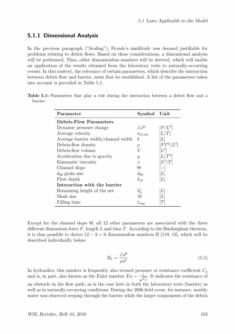
5.1 Laws Applicable to the Model
5.1.1 Dimensional Analysis
In the previous paragraph (”Scaling”), Froude’s similitude was deemed justifiable forproblems relating to debris flows. Based on these considerations, a dimensional analysiswill be performed. Thus, other dimensionless numbers will be derived, which will enablean application of the results obtained from the laboratory tests to naturally-occurringevents. In this context, the relevance of certain parameters, which describe the interactionbetween debris flow and barrier, must first be established. A list of the parameters takeninto account is provided in Table 5.1.
Table 5.1: Parameters that play a role during the interaction between a debris flow and abarrier.
Parameter Symbol Unit
Debris-Flow ParametersDynamic pressure change 4P [F/L2]Average velocity ufront [L/T ]Average barrier width/channel width b [L]Debris-flow density ρ [FT 2/L4]Debris-flow volume V [L3]Acceleration due to gravity g [L/T 2]Kinematic viscosity υ [L2/T ]Channel slope Θ [−]d90 grain size d90 [L]Flow depth hfl [L]Interaction with the barrierRemaining height of the net h′b [L]Mesh size M [L]Filling time timp [T ]
Except for the channel slope Θ, all 12 other parameters are associated with the threedifferent dimensions force F , length L and time T . According to the Buckingham theorem,it is thus possible to derive 12− 3 = 9 dimensionless numbers Π [119, 13], which will bedescribed individually below:
Π1 =4Pρu2
(5.5)
In hydraulics, this number is frequently also termed pressure or resistance coefficient Cpand is, in part, also known as the Euler number Eu = 1√
Cp. It indicates the resistance of
an obstacle in the flow path, as is the case here in both the laboratory tests (barrier) aswell as in naturally-occurring conditions. During the 2006 field event, for instance, muddywater was observed seeping through the barrier while the larger components of the debris
WSL Berichte, Heft 44, 2016 103

5 Physical Modeling
flow were retained (see section 4.5.1).
Π2 =ghflu2
=1
Fr2=⇒ Fr (5.6)
1Fr2
represents the Froude number Fr, which describes the ratio of inner to gravitationalforces. It subdivides flow conditions into ”streams” (subcritical) and ”rapid flows” (su-percritical), and thus indicates the conformation the flow takes in the channel (see alsosection 3.4.1). This number is taken into account during scaling for almost all problemsinvolving open-channel drainage.
Π3 =υ
uhfl=
1
Re=⇒ Re (5.7)
The Reynolds number Re indicates the ratio of inertial to viscous forces in a fluid, andsubdivides its flow into laminar or turbulent flow regimes. This number can never beconsidered at the same time as the Froude number if the same fluid with the same viscosityis used in the laboratory tests. The problems that can arise when estimating the magnitudeof the Reynolds number relate to the determination of the viscosity of the debris-flowmixture (see section 5.2.3.4).
Π4 =timpu
h′b(5.8)
Π4 is the only relation which takes the filling time of the barriers into account. Therefore,this number also reflects the dynamics of the filling process. It represents a characteristiclength L of the contributing debris-flow material behind the filled barrier.
Π5 =V
h2flb
(5.9)
Π5 describes the standardized length of a debris-flow wave, thereby providing an estimateof the debris-flow surge’s duration. V is the volume of the debris-flow wave filling thebarrier, which can usually be determined only by means of prognostic values and estimates.hfl to width b indicates the cross section of the first wave‘s impact on the barrier.
Π6 =d90
hfl(5.10)
Π6 indicates the grain distribution across the flow depth. It is important for the consid-eration of geometric parameters, such as mesh size, and the basal opening. However, it isgenerally difficult to detect d90 grain sizes in a debris-flow mixture.
Π7 =h′bhfl
(5.11)
Π7 indicates the ratio of net height remaining after filling h′b to flow depth hfl. It specifiesthe number of surges required to reach the top of the net, and thus, the completely filledstate (see also section 6.3).
Π8 =M
d90
(5.12)
104 WSL Berichte, Heft 44, 2016
5.1 Laws Applicable to the Model
Π8 indicates the ratio of mesh size to d90 grain size and is used to scale the mesh size frommodel to laboratory tests.
Π9 = tan Θ (5.13)
In steady flows, Π9 is equal to the friction parameter µ and is, therefore, important forenergy analyses in which friction energy, or the rate of frictional activity, plays a role. Inaddition, the ratio of the rate of gravitational to the rate of frictional activity indicateswhether a debris flow is accelerating, or, should frictional forces predominate, decelerating(see sections 2.2.3 and 4.4).The orders of magnitude of the selected dimensionless numbers and an assessment of thetransferability of the test results will be the subject of section 5.3.
Physical Limits
Every dimensional analysis also illustrates physical limits. For example, Froude’s simili-tude and Reynolds similitude can never be achieved simultaneously using the same mate-rial in both the model and naturally-occurring conditions. Therefore, the Reynolds numberhas been neglected entirely in the current case, and viscous forces are also not taken intoconsideration, even though they also play a role during the debris-flow process (for therheology of debris flows, see section 2.2.2.3). In addition, there is considerable uncertaintyin debris-flow models regarding the magnitude of a number of debris-flow parameters inthe field data, such as, for example, the viscosity of the debris-flow mixture, the surgevolume V , or the d90 grain in a debris flow. These uncertainties prompt further ques-tions in the interpretation of the dimensional analysis. In addition, other factors, such asthe stiffness ratio between the model and naturally-occurring conditions, are not usuallyreproduced correctly. Considering, for example, the stiffness ratio of the barriers in themodel km and in the field kn
kmAmfm
ρmu2m
=knAnfn
ρnu2n
. (5.14)
with Am being the barrier surface in the model and An the barrier surface in the field,as well as fm being the maximum deformation of the barrier in the model and fn themaximum deformation in the field. km/Am and kn/An are referred to as relative stiffness.Since identical material with the same water content is used, ρm = ρn applies. Instead ofvelocities, the Froude numbers with u2 = Fr2ghfl and Frm = Frn are used. It followsthat
kmfmAmhfl,m
=knfnAnhfl,n
. (5.15)
The average deformation of a soft barrier was fm ≈ 0.1m in the laboratory and fn ≈ 2.5min the field. This yields a ratio of ≈ 1/25. The flow depths correspond to the length scaleLs and, according to [46], then average between 20 and 30 at ≈ 25. The ratio of the barriersurfaces Am/An is ≈ 1/400. It follows that, for the stiffness ratios,
km =1
400kn (5.16)
WSL Berichte, Heft 44, 2016 105

5 Physical Modeling
i.e., the stiffness modulus of the laboratory barriers km must be 400-times softer thanthat of the ring net barriers in the field. This factor can only be roughly approximated byselecting soft nets (barriers used in section 5.2.2, e.g. cat nets and safety nets for boats).Here therefore, the physical limits of scaled laboratory tests become apparent.Nevertheless, the dimensional analysis demonstrated that the experiments apply to real-life scenarios in many respects. The results of the laboratory tests discussed in the re-mainder of this chapter confirm this conclusion in most cases, indicating that the loadmodel to be developed later can draw upon numerous findings from the laboratory tests.
5.2 Laboratory Tests
5.2.1 Experimental Equipment
The test channel at WSL was designed by Daniel Weber [106] and equipped for hisexperiments investigating the erosion behavior of debris flows (see Fig. 5.1 and 5.2). Inorder to carry out the laboratory experiments for the present work, the test channel wasadapted to the new requirements and modified accordingly.The upper part of the channel with the launch container, the subsequent accelerationtrack, and the cross section of the measuring channel (with a width of 30cm) were notmodified (see Fig. 5.1). The launch container and the acceleration track together measureabout 3m in length and have a smooth surface made of steel. Hereafter, the actual debris-flow wave is created, which then flows into the measuring channel. Flint from the Illgrabenwith a grain size of 1cm is glued to the channel floor, which provides the streambed withthe roughness required for the generation of a debris-flow front. The inclinations of thelaunch container, the acceleration track, as well as the measuring channel can be adjustedindependently of one another to measure between 0 and 55%. The existing topographicsystem to determine the retention volume was preserved along the 3.70m long measuringtrack (see section 5.2.1.1). The existing ultrasonic sensors designed to determine flowvelocity and flow depth were replaced by more accurate laser measuring devices. Thearrangement of the laser measuring devices is shown in Figure 5.1.A specially-designed measuring sledge allows for the installation of different barrier typesand the measurement of impact and frictional forces in flow direction (see section 5.2.1.3).A front view of the filling process in the tests was recorded using a high-speed camera. Aspotlight placed above the channel ensures adequate lighting.A concrete-silo container was used to insert the material into the launch container. Usinga crane, this container was lifted up to the launch container, where it emptied its content.A mobile bulk container was placed at the end of the channel to collect the material.
5.2.1.1 Topographic System
The topographic system is used to determine the deposition volume (located behind thebarrier and along the channel) produced by a laboratory debris flow. To accomplish this,
106 WSL Berichte, Heft 44, 2016

5.2 Laboratory Tests
θ
Launch container
Net
Hatch
A
A
A-A cut
0.3m
0.3m
Laser
Force measurement
Camera
0.3m 0.75mrough smooth
Figure 5.1: Layout of the WSL’s debris-flow channel: cross section of the measuring track,lateral view of the channel and top view.
a measuring laser moves along two tracks on the right- and left-hand side of the channel,scanning its profile based on a grid of 0.75cm on the x-axis (flow direction) and 0.75cmon the y-axis (channel width) and measuring, at each point, the height z. The raster dataof the thus-generated ASCII file can then be converted to topographic contour lines usingsuitable software (e.g., ArgGIS or MATLAB). Based on this data, the deposited volumecan be calculated.
5.2.1.2 Laser Measurements
Four laser devices are used to measure distance (see Fig. 5.1). A thin beam of light allowsfor the precise determination of the flow depth. With a scanning frequency of 2.2kHz,fast-moving objects can be recorded as well.The average front velocity ufront is calculated based on the time difference between mea-surements of flow depth and distance traveled between two lasers.The first laser spike was chosen as the point of origin of the time scale. At this point, thefront has reached the laser. This point, however, is not always identical, since splashesof water or individual stones can trigger the laser before the actual front. Therefore, thelaser measurements were also aligned with the high-speed videos.
WSL Berichte, Heft 44, 2016 107
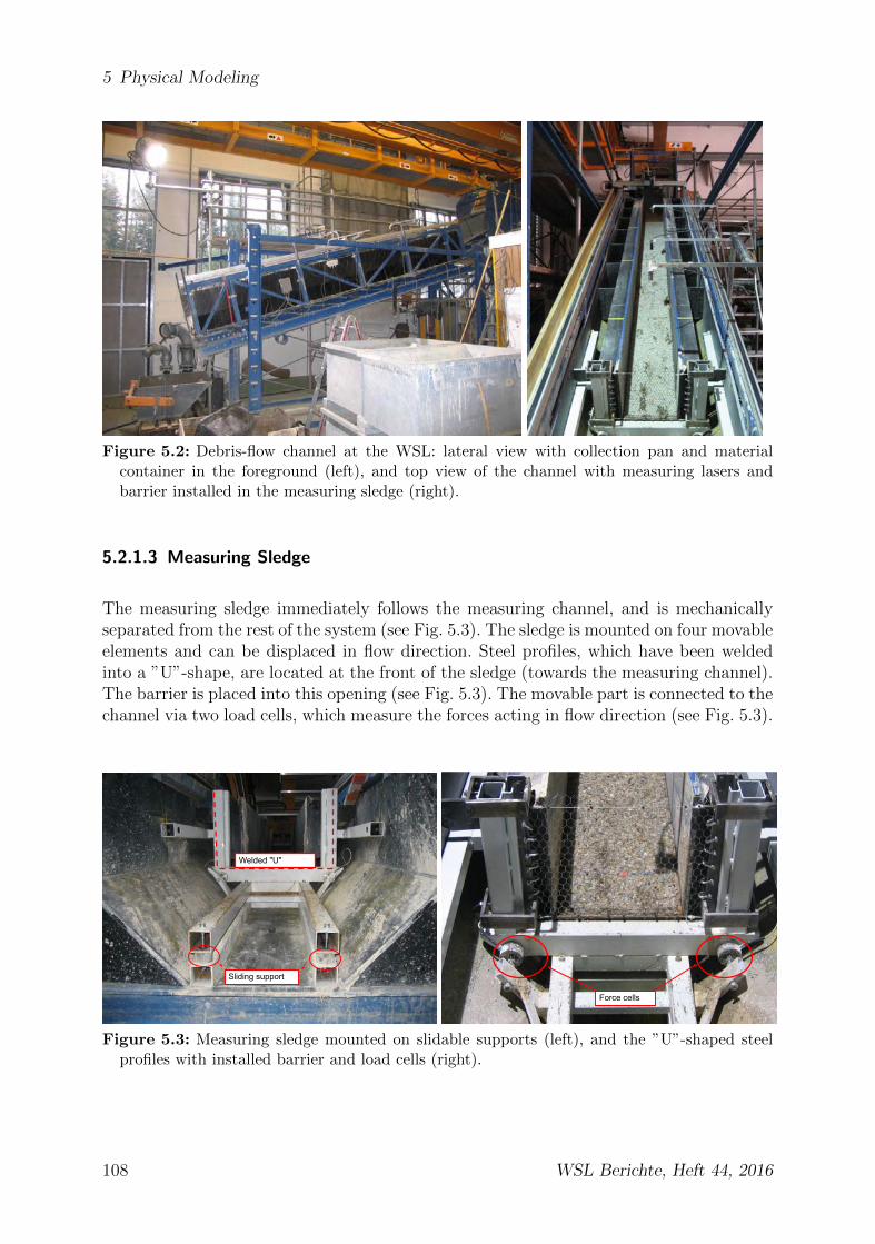
5 Physical Modeling
Figure 5.2: Debris-flow channel at the WSL: lateral view with collection pan and materialcontainer in the foreground (left), and top view of the channel with measuring lasers andbarrier installed in the measuring sledge (right).
5.2.1.3 Measuring Sledge
The measuring sledge immediately follows the measuring channel, and is mechanicallyseparated from the rest of the system (see Fig. 5.3). The sledge is mounted on four movableelements and can be displaced in flow direction. Steel profiles, which have been weldedinto a ”U”-shape, are located at the front of the sledge (towards the measuring channel).The barrier is placed into this opening (see Fig. 5.3). The movable part is connected to thechannel via two load cells, which measure the forces acting in flow direction (see Fig. 5.3).
Sliding support
Welded "U"
Force cells
Figure 5.3: Measuring sledge mounted on slidable supports (left), and the ”U”-shaped steelprofiles with installed barrier and load cells (right).
108 WSL Berichte, Heft 44, 2016

5.2 Laboratory Tests
5.2.1.4 High-Speed Camera
At the end of the channel and facing the measuring sledge, a high-speed camera recordsthe barrier’s filling process at 125 frames per second. Based on two markings on the chan-nel floor, the velocity of the impact on the barrier can be determined, which serves as acontrol for the laser measurements.During some of the tests, the camera was placed above the channel. This perspectiveprovides a recording of the two different filling processes (see section 5.3.1). This set-upalso allows for a second velocity alignment, based on the markings on the channel floor.A spotlight with an additional transformer is mounted above the channel (see sec-tion 4.2.3.2).
5.2.1.5 Data Acquisition
Once the launch hatch is opened, the laser and force measurements start, and the high-speed camera begins to record. The data from the laser and force measurements aretransferred to PC via a measuring board (see section 4.2.3.5). Steering is controlled, justlike in the field tests, using the software Labview, which ultimately generates an ASCIIdata set.The video recorded with the high-speed camera can then be evaluated using a suitableviewer software (Redlake Motion Scope Media Player2).
5.2.2 Barriers
The following barriers were used according to Table 5.2 to investigate their differentproperties. They differ, for example, not only in terms of mesh size, but also in termsof the properties of their materials, such as elasticity and deformability. In addition,rigid barriers were simulated using wood and Plexiglas panels. With respect to materialretention, these can be considered impermeable.
2MotionPlayer is a Microsoft-Windows based software for imagewise analysis of video recordings,http://www.redlake.com
WSL Berichte, Heft 44, 2016 109

5 Physical Modeling
Table 5.2: Barriers used in the tests and their mesh sizes.
Barrier/Net Properties Mesh Size [cm] Material
elastic net flexible, elastic 2 rubber-mounted netcat net flexible, inelastic 2, 3 rope netsafety net for boats flexible, inelastic 4, 6 rope netsquare grid rigid 0.5 wire meshchicken wire rigid 1.2, 1.6, 2 wire meshTECCOmeshwork rigid 3 wire meshrigid plate rigid/impermeable - wood and synthetic materials
The nets and barriers used do not represent real models of ring nets. Material parameters,such as the stiffness modulus k of the ring net, can be rarely reproduced in the model,due to the different stiffness ratios in nature and in the model. The stiffness reproducedin the model is always too rigid (see section 5.1.1). Therefore, the barriers in the modelhave to be considerably more flexible than in nature. While the flexible nets remain amajor simplification of actual ring net barriers, they nonetheless can simulate, more orless faithfully, geometric properties (such as mesh size and the basal opening) by meansof a factor or a dimensional analysis (see section 5.1).
5.2.3 Debris-Flow Materials
Weber already observed in [106] that, when using natural materials, a near-naturalreproduction can only be achieved if either the maximum grain size dmax is adapted tochannel width or the grain-size distribution is identical to that of natural debris-flowmaterials. It is practically impossible to meet both of these requirements at the sametime; i.e. they are mutually exclusive. The highest possible maximum grain size corre-sponds to approximately one-tenth of the width of the channel. In the end, the followingcompromise was made:Natural debris-flow materials were collected from deposit zones in the channels andscreened to a maximum grain size of 3cm. While the removed fractions change thegrain-size distribution within the debris-flow mixture, the ratios between grain sizes ofd < 3cm remain the same. Indeed, the rheological properties of debris flows stronglydepend on water content and the prevailing fine fraction of clays and silts up to agrain size of 0.06mm [106]. These components are not affected by the screening process;only their percentages within the grain-size distribution curve change. By removing thecoarser components, the grain-size distribution curve is shifted towards the smaller grainsizes on the left. This is taken into account during scaling by means of the d90 grain-sizeratio between model and nature (see section 5.1).Since the fine fraction cannot be entirely recovered following each completed test (becauseit gets lost in cracks and gaps along the channel), used debris-flow material cannot bereused in other tests.
110 WSL Berichte, Heft 44, 2016

5.2 Laboratory Tests
5.2.3.1 Origin of the Materials
A total of four different debris-flow materials were used. Two of these were collectedfrom torrents in Merdenson, and in the Illgraben (canton Valais). These two sources wereselected because of the test barriers present at these locations, and because they allowfor a comparison of the measured properties with those observed in the field. The twoother materials used were collected from torrents in the Bernese Oberland (the Alpbachin Haslital and the Trachtbach near Brienz). These two collection sites were selectedbecause they are planning to use ring nets as debris-flow protection structures; usingmaterial collected directly from them allowed for the best possible investigation of theeffect of mesh size and the basal opening by means of laboratory tests (see [109, 110]).Moreover, good accessibility is an important factor for the selection of collection sites.The collection sites in Merdenson and the Illgraben were accessible either by car or onfoot. The materials from Gummen and the Trachtbach had to be flown down into thevalley by helicopter. As a result, only a limited number of tests using these two materialscould be carried out. For the majority of the tests, material from the Illgraben was used.
5.2.3.2 Grain-Size Distribution Curves
Grain size d (mm)
Mas
s fr
actio
n of
gra
ins
<d
0.001 0.01 0.1 1 10 1000.0
0.2
0.4
0.6
0.8
1.0Clay Silt Sand Gravel Stone
AlpbachIllgrabenIllgraben sieved Trachtbach
Figure 5.4: Grain-size distribution in debris-flow materials from the Illgraben, the Alpbach,and the Trachtbach (dashed line), as well as the grain-size distribution curve of the materialfrom the Illgraben from a previous collection (solid line).
The grain-size distributions of the materials used are shown in Figure 5.4. A fine fractionof clay and silt of at least 10% is characteristic of all debris-flow materials (see Fig. 5.4
WSL Berichte, Heft 44, 2016 111

5 Physical Modeling
and [106, 99]). Particularly striking is the large fine fraction in the material from theTrachtbach, with grain sizes of d < 0.06mm making up almost 40% of the material,whereas they make up only about 20% of the other materials. According to [99], thissuggests a very viscous flow behavior of the Trachtbach material. Viscous debris flowshave a much higher proportion of fine materials of d < 0.06mm.
5.2.3.3 Density Determination
In the context of Gubler’s work [46], the solid-substance densities were determined inthree of the four debris-flow materials. Here, the material from the Trachtbach was notexamined, since it is very cohesive and loamy, which made the analysis too difficult. Thedetermined material densities are shown in Table 5.3.
Table 5.3: Bulk densities determined as in [46] in the debris-flow materials used.
Collection Site Dry-Material Density [kg/m3]
Alpbach 2533Illgraben 2693Merdenson 2696Trachtbach 2000 (estimate)
5.2.3.4 Viscosity Determination
Figure 5.5: Ball viscometer for the determination of the viscosity of the liquid debris-flow phaseand its schematic structure (right).
The viscosity in the material from the Illgraben was determined. in cooperation withKowalski [62] at the Institute for Nutritional Sciences of the ETH Zurich. The measure-ments were performed using a ball viscometer as in [88] (see Fig. 5.5). The ball viscometerconsists of a round container with a radius of Rs = 57.5mm, which is hs = 48cm high. Aball with a diameter of d = 12mm is moved through the suspension with the rotational
112 WSL Berichte, Heft 44, 2016
5.2 Laboratory Tests
velocity ω. The dynamic viscosity can be determined based on the shear stress τ and theshear rate γ, so that
η =τ
γ. (5.17)
For further information about the conversion of the measured values into shear stress τand shear rate γ, please refer to [88]. The sediment concentration of the solution Cv iscalculated as in [88]. Therefore,
Cv =Cs,DFCs,DC
1 + Cs,DF (1− Cs,DC)(5.18)
with Cs,DF being the volumetric sediment concentration in the debris flow and Cs,DCbeing the percentage of the grain-size distribution curve the utilized grain sizes accountfor. Fine screenings of the Illgraben material, as in [62], demonstrated that grain sizes ofd < 2mm accounted for 36.6% of the screened material, and that grain sizes of d < 4mmaccounted for 50% (see Fig. 5.4, Illgraben).The material was dried, screened, and its weight determined with one-gram accuracy.Subsequently, the amount of water required to achieve the appropriate volumetric watercontent was added. At this point, it became apparent that a mixture of d < 4mm andw = 20% is too viscous for the viscometer. The subsequent addition of water distortedthe resulting associated water content and the examined suspension volume.Three measurements were taken per shear rate and then averaged. A shear thinning effectcould be observed during all measurements. This means that the highest viscosities weremeasured at the slowest shear velocity of γ = 0.1[1/s], whereas the lowest viscosities weremeasured at γ = 30[1/s]. The resulting average viscosities are shown in Table 5.4.
For the flow process of the debris flow, the shear-thinning behavior of the Illgraben ma-terial implies that the material itself offers less resistance once high flow velocities arereached (or occur). Moreover, it displays a higher viscosity with a larger grain size andidentical water content. This seems plausible and, thus, transferable to the naturally-occurring process.Assuming a linear velocity profile, the shear rates occurring during a flow process can beapproximated based on the flow depth hfl. For a debris flow with flow depth hfl = 1m andan average front velocity of 3m/s, for example, the shear rate γ in the debris flow wouldequal approximately 3[1/s]. Assuming that particles of d < 2mm remain in suspension,the viscosity of the liquid phase η equals approximately 5Pas at a water content of 30%.With respect to the measured shear stresses across shear rates, the measurements confirmthe assumptions of the Bingham model concerning fluids with particles (in section 2.2.2.3in equation 2.19). A fluid with particles of d < 2mm, a water content of 30%, and asediment concentration Cv = 0.46, for instance, exhibits the Bingham-model property asshown in Figure 5.6. Here, the initial shear strength τb equals approximately 5.5N/m2,and the Bingham viscosity ηb ≈ 0.45 amounts to a correlation coefficient R2 of the best-fitline of 0.97.
Unfortunately, viscosity measurements for larger grain sizes are currently not possible. The
WSL Berichte, Heft 44, 2016 113

5 Physical Modeling
Table 5.4: Average viscosities determined by ball viscometer according to [88].
Water Content [%] Cv[−] d [mm] Shear Velocity γ [1/s] Viscosity [Pas]
0.2 0.59 < 2 0.1 2500.2 0.59 < 2 1 17.40.2 0.59 < 2 10 2.60.2 0.59 < 2 30 1.5
0.3 0.46 < 2 0.1 760.3 0.46 < 2 1 60.3 0.46 < 2 10 1.00.3 0.46 < 2 30 0.6
0.2 ≈ 0.68 < 4 too viscous not measurable0.3 0.54 < 4 0.1 171.80.3 0.54 < 4 1 260.3 0.54 < 4 10 2.60.3 0.54 < 4 30 1.2
largest viscometer can be utilized for grain sizes up to 2cm [21]. The viscosity of an entiredebris flow, therefore, can only be estimated and interpolated hypothetically. Thus, thevalues of these measurements serve only as a reference point for an order of magnitude, tobe used for the determination of the ring net’s resistance during the mudflow percolationin section 6.2.3.
5.2.3.5 Friction Angle
The angle of internal friction, according to Coulomb’s friction law in equation 2.20 insection 2.2.2.3, was determined only in the material from the Illgraben. Here, the angle ofinternal friction was relevant for the design of the field barrier and the reverse calculationof the field data.Samples of d < 20mm were used in the tests, carried out at the department of soilmechanics of the TU Munich, to determine the angle of internal friction. Because thematerial from the Illgraben consists of very cohesive soil (which cannot be compactedperfectly - even with great effort - unless the material has the ideal water content), fourcompaction tests were performed (according to DIN 18127 [29]). The ideal water contentfor the maximum bulk density of ρd = 2225kg/m3 was determined to be w = 5.9%.This water content was used as the initial water content for the subsequent triaxial test(according to DIN 18137, part 2 [30]). A CU-test was performed consolidated with σ1 =σ3 = 50kN/m2 and undrained, during which pore-water drainage is inhibited and theresulting pore-water pressure p is measured. σ3 is kept constant, and σ1 is increased untilfailure. A state of failure is depicted schematically in Figure 5.7 (right). The test revealedthat the Illgraben material has an effective angle of internal friction of φ′ = 42.9◦ with acohesion of c′ = 20.5kN/m2.
114 WSL Berichte, Heft 44, 2016
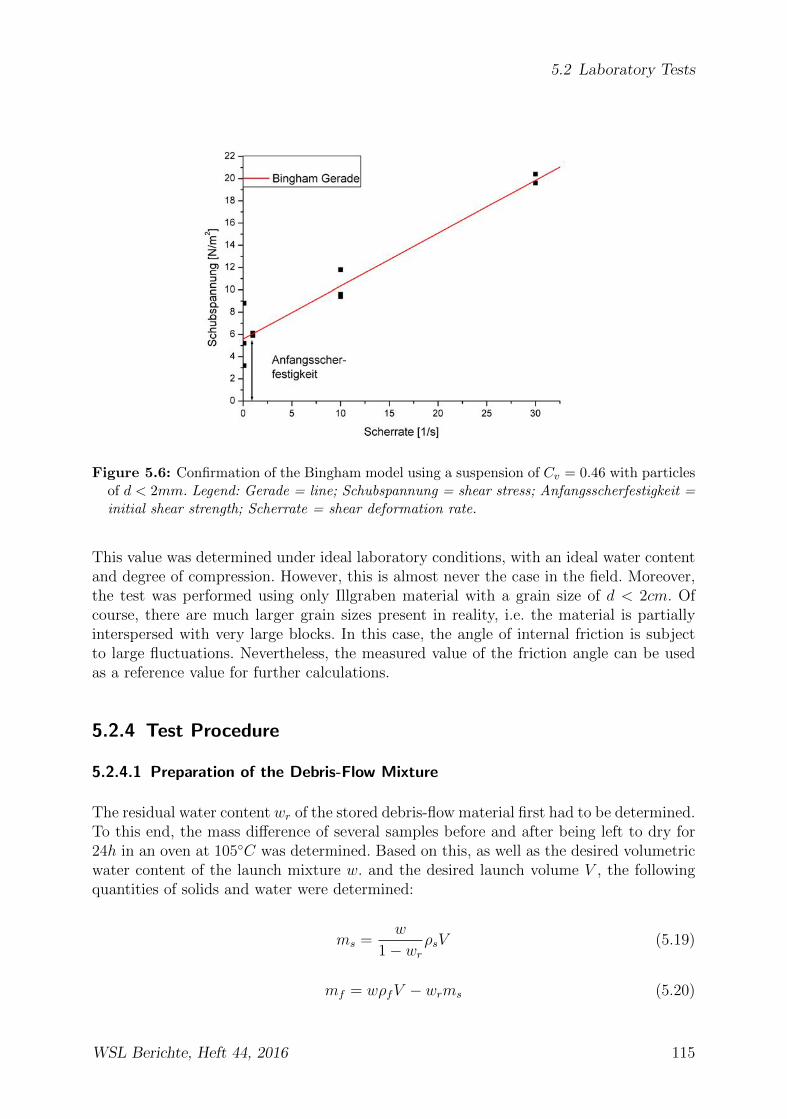
5.2 Laboratory Tests
Figure 5.6: Confirmation of the Bingham model using a suspension of Cv = 0.46 with particlesof d < 2mm. Legend: Gerade = line; Schubspannung = shear stress; Anfangsscherfestigkeit =initial shear strength; Scherrate = shear deformation rate.
This value was determined under ideal laboratory conditions, with an ideal water contentand degree of compression. However, this is almost never the case in the field. Moreover,the test was performed using only Illgraben material with a grain size of d < 2cm. Ofcourse, there are much larger grain sizes present in reality, i.e. the material is partiallyinterspersed with very large blocks. In this case, the angle of internal friction is subjectto large fluctuations. Nevertheless, the measured value of the friction angle can be usedas a reference value for further calculations.
5.2.4 Test Procedure
5.2.4.1 Preparation of the Debris-Flow Mixture
The residual water content wr of the stored debris-flow material first had to be determined.To this end, the mass difference of several samples before and after being left to dry for24h in an oven at 105◦C was determined. Based on this, as well as the desired volumetricwater content of the launch mixture w. and the desired launch volume V , the followingquantities of solids and water were determined:
ms =w
1− wrρsV (5.19)
mf = wρfV − wrms (5.20)
WSL Berichte, Heft 44, 2016 115

5 Physical Modeling
She
ar s
tress
τ'
r=(σ
1'-σ 3
')/2
[kN
/m2 ]
M=(σ1'+σ3')/2 [kN/m2]
c' σ'3 σ'1
φ'
σ1
σ3
τ
α
τ
σ
α
P
Sliding plane in triaxial test Shear plane
Figure 5.7: Triaxial shear-test apparatus to determine the angle of internal friction (left), andmode of operation illustrated based on the Mohr-Coulomb theory (right).
with ρs being the solid-material density according to Table 5.3 and ρf being the densityof the water. The water contents typically used for individual materials and the resultingdebris-flow densities are shown in Table 5.5.
Table 5.5: Volumetric water content w of the test mixture and the resulting density ρ of themixture.
Material Water Content [%] Debris-Flow Density [kg/m3]
Alpbach 54 1700Illgraben 30 2200Merdenson 57 1700Trachtbach 52 1500
The required solids and water are then weighed and mixed using a concrete mixer, untila homogeneous phase has formed.
5.2.4.2 Experimental Procedure
The subsequent procedures will be described only briefly; a more detailed discussion ofmethods and their implementation is provided in [59].
116 WSL Berichte, Heft 44, 2016

5.3 Results
Following the installation of the barrier, the correct functioning of the load cells was con-firmed using a spring balance. This control is essential in order to calibrate it to zeroand to ensure a uniform response. Subsequently, the frame of the high-speed camera wasverified with the spotlight on. If the channel is filmed from above using a scaffold, it isimportant to adjust the frame so that the entire retained debris-flow cone is pictured. Ifthe camera is placed in front of the barrier, the entire barrier should be within the frame,as well as the two measuring marks for verifying the impact velocity.Shortly before inserting the debris-flow material into the launch container, the channelwas irrigated to simulate a saturated streambed and to improve the flow characteristicsof the debris flow.The debris-flow material should only be inserted into the launch container when every-thing else has been prepared and is ready to go. If the material is left in the launchcontainer for too long, the solid material slowly begins to settle, which results in phaseseparation and causes the flow characteristics of the thus-generated debris-flow wave tochange significantly.Once the measurement instrumentation was activated, the hatch was opened. The ma-terial then flows in a rolling motion, which resembles a debris-flow front, towards thebarrier, and fills it.
5.3 Results
A total of 66 laboratory tests were performed; 42 of which used material from the Illgraben.Table 5.6 provides an overview of the materials used, water contents, launch volumes, andinclinations.
Table 5.6: Overview according to [46] showing the materials used in the tests, water contents,launch volumes, and inclinations.
Material Inclination Launch Volume Water Content Total
25% 40% 50% 50 l 100 l 150 l (volumetric [%])
Alpbach 9 9 54 9Illgraben 7 11 24 13 23 6 30 42Trachtbach 11 10 1 52 11Merdenson 4 3 (1× 75 l) 57 4
5.3.1 Visual Observations
During the tests and on the video recordings, the following characteristics (typical fordebris flows) were observed. A flow resembling a front, with large rocks in the front anda more liquid part composed of the fine fraction trailing behind, was observed during thetests using material from the Illgraben. The grain distribution is clearly recognizable, even
WSL Berichte, Heft 44, 2016 117

5 Physical Modeling
Figure 5.8: Front and top-down view of a net filled with debris-flow material (test using Ill-graben material with a launch volume of 50l and an inclination of 25%).
after filling of the net (as shown in Figure 5.8). It decreases significantly with increaseddistance from the net, and the water content increases. However, the tests using materialfrom the Alpbach appeared muddier, with a poorly-developed front. This is desired, andachieved by means of increased water content, since debris flows in the Alpbach are rathermuddy (densities of ρ ≈ 1800 − 1900kg/m3 according to [50]). The debris flows usingmaterial from the Trachtbach exhibited a very viscous flow due to the extremely cohesivematerial. Nevertheless, in all tests, the large stones accumulated at the front during theflow, whereas the smaller ones trailed behind along with the water. As a result, a debrisjam already begins to form at the net during the impact of the front (containing thestones). The few videos that filmed the Illgraben tests with an inclination of 25% fromabove showed a type of reverse-flow wave, which occurred shortly after the debris jamand flowed towards the liquid mud upstream of the net (see Fig. 5.9). The filling processcan be subdivided into three stages: (1) the impact of the front, (2) a small verticaldeflection or filling of the barrier, and (3) the wave reflected upstream (see Fig. 5.11,left). The formation of the reverse-flow wave confirms the load approach developed laterin section 6.3.Furthermore, an upward deflection of the debris-flow stream was observed with greaterlaunch volumes or more liquid mixtures, and the associated higher front velocity (seeFig. 5.10, left), suggesting a vertical spread, i.e. a spread perpendicular to the directionof the flow and parallel to the barrier [3]. First, the front hits the barrier and, with higherflow velocities, it is reflected vertically and then flows over the barrier. The remainingretention volume behind the barrier is then filled completely by the material that follows(see Fig. 5.10, right). This effect is more pronounced with rigid barriers. For a detailedoverview and evaluation of the video analyses, see [46].
5.3.2 Determination of Relevant Scaling Factors
To achieve an ideally constructed model, all 9 numbers in the model should correspondto those in nature. However, since this can never be achieved in reality (as discussedwith respect to the Froude and Reynolds numbers, for example, in section 5.1), the mostsignificant numbers need to be identified and interpreted. Table 5.7 lists the dimensionless
118 WSL Berichte, Heft 44, 2016

5.3 Results
Figure 5.9: Reverse-flow wave formed shortly after the debris jam at the net at time pointst1 = 2860, t2 = 3320, t3 = 3740, and t4 = 4030ms in a 50l test using Illgraben material at aninclination of 25%.
numbers for the values of typical debris flows (consisting of all materials used in thisproject) that have been observed in the field (see section 5.1), and contrasts them withthose observed in the laboratory (field data Illgraben see Table 4.1). The last columnshows estimates of the dimensionless numbers relative to the process in consideration, aswell as their importance, where a = relevant, b = less relevant, and c = not relevant.
WSL Berichte, Heft 44, 2016 119
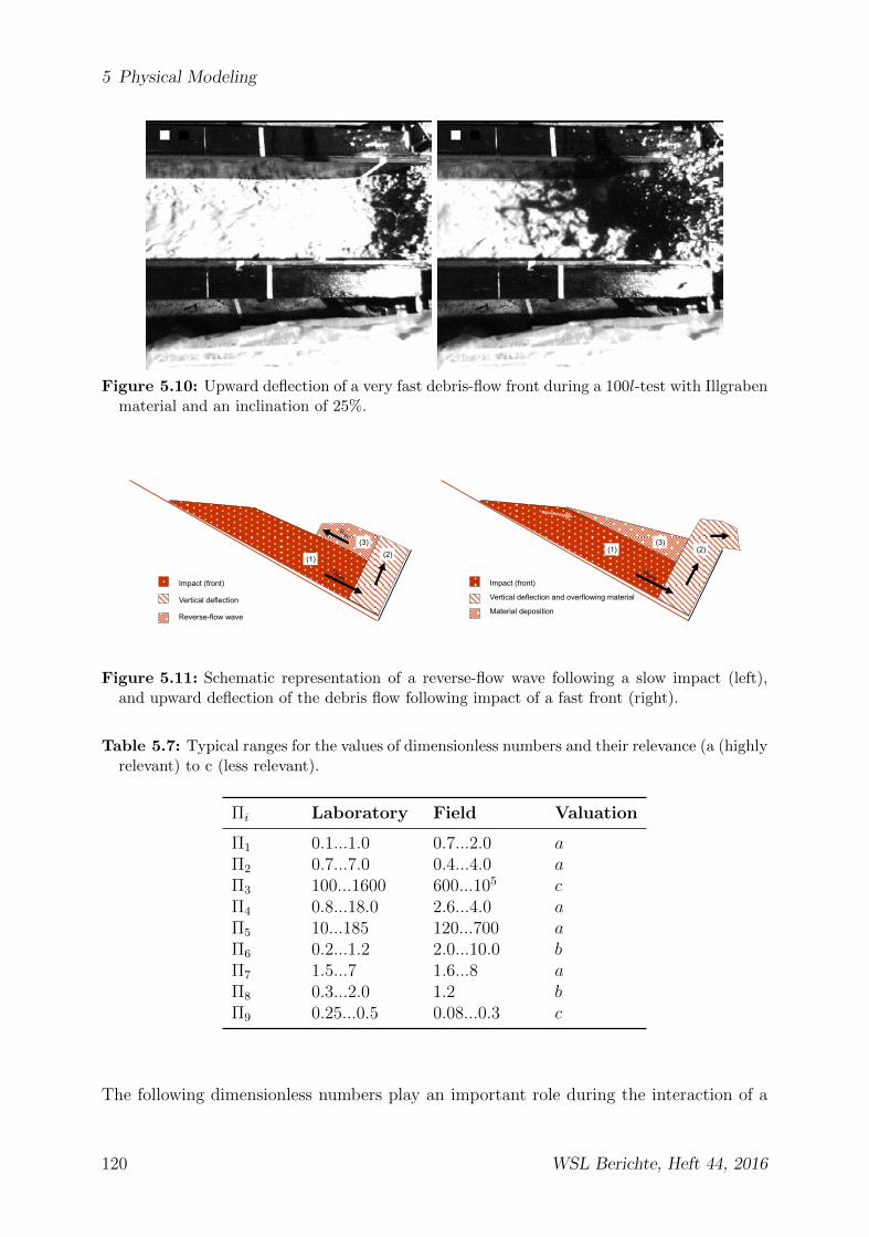
5 Physical Modeling
Figure 5.10: Upward deflection of a very fast debris-flow front during a 100l-test with Illgrabenmaterial and an inclination of 25%.
Impact (front)
Vertical deflection
Reverse-flow wave
(1) (2) (3)
Impact (front)
Vertical deflection and overflowing material
Material deposition
(1) (2)(3)
Figure 5.11: Schematic representation of a reverse-flow wave following a slow impact (left),and upward deflection of the debris flow following impact of a fast front (right).
Table 5.7: Typical ranges for the values of dimensionless numbers and their relevance (a (highlyrelevant) to c (less relevant).
Πi Laboratory Field Valuation
Π1 0.1...1.0 0.7...2.0 aΠ2 0.7...7.0 0.4...4.0 aΠ3 100...1600 600...105 cΠ4 0.8...18.0 2.6...4.0 aΠ5 10...185 120...700 aΠ6 0.2...1.2 2.0...10.0 bΠ7 1.5...7 1.6...8 aΠ8 0.3...2.0 1.2 bΠ9 0.25...0.5 0.08...0.3 c
The following dimensionless numbers play an important role during the interaction of a
120 WSL Berichte, Heft 44, 2016
5.3 Results
debris flow and a barrier:
• Π1 indicates how much the dynamic pressure ∆P of the debris flow increases duringimpact on the barrier. Since both the density ρ as well as the velocity ufront aretaken into account, it is a material-dependent, dimensionless number, and formsa link between the forces measured in the laboratory and those measured in thefield. For the field events, Π1 was set to 0.7 for muddier debris flows with littleviscosity and to 2.0 for granular, very viscous debris flows, in accordance with theapproaches by Armanini [3] (see section 6.3).
• Π2 is the Froude number, which is usually used as a scaling basis for problemsinvolving natural inclines. As a result, it is a scaling factor that also appears toapply to debris flows, since - in this case - gravitational forces also outweigh viscousforces [106]. The flow velocity ufront and the flow depth hfl are both importantparameters with respect to the loads that occur when a debris flow flows into abarrier (see section 6.3).
• Π4 describes the length of the stopped debris flow relative to the fill level of thebarrier h′b, and is the only number which takes the filling time timp into account.Π4 generally is an important parameter for the assessment of the dynamics of thefilling process. A value of 90s for timp, based on the very muddy debris flow fromMay 18, 2006, is the only value for timp based on actual field events currentlyknown. According to [82, 23], this value appears to be quite large for granulardebris flows. The USGS flume experiments revealed impact times of 1-4s. Thesetimes were adopted for the determination of Π4 in the field data, as shown inTable 5.7. This demonstrates a common range of Π4, in spite of the uncertaintyconcerning the impact time due to missing data.
• Π5 describes the typical length of a debris-flow surge. The volume parameter Vfor the first debris-flow surge is an estimate and a prognostic value associatedwith significant uncertainty. In the Illgraben, for instance, this value can onlybe determined approximately using the average flow Q and the time t, theduration of the debris-flow wave as assessed visually based on video data. Valuesregarding the size of debris-flow surges have almost never been provided in literature.
• Π7 is the ratio of the remaining height of the net h′b to the flow depth hfl. Thisdirectly indicates the duration of a filling process if this filling process is subdividedinto individual surges with a flow depth hfl, which are then stacked vertically untilthe final fill level h′b is reached (see also section 6.3 and Fig. 6.12). Therefore, Π7 isan important parameter for the entire filling process and the ensuing loads.
There are two other dimensionless parameters that are taken into consideration, but thesedo not need to/cannot be consistently identical. For these numbers, the uncertainties in
WSL Berichte, Heft 44, 2016 121
5 Physical Modeling
the determination of the parameters taken into consideration are subject to very largefluctuations:
• Π6 and Π8 form ratios between geometric parameters relative to the d90 grain sizes.Here, the uncertainty in both numbers lies in the estimation of the d90 grain size.Only values for the Illgraben are currently available, as provided in [69], where avisual assessment yielded a grain size of 25cm. This value was used as the d90 grainsize for the field values of Π6 and Π8 in Table 5.7. In order to scale the mesh size,the d90 grain size is absolutely essential (see [46, 109, 110]).
Π3 and Π9 do not play a significant role in the interaction process examined below:
• Due to the contradiction with the Froude scaling derived in equation 5.4, theReynolds number Re = Π3 is not taken into account. As a result, viscous forces areneglected in this model. Moreover, the dynamic viscosity η can only be determinedfor small grain sizes, and statements concerning the viscosity of an entire debris-flowmixture are, therefore, difficult to make and often erroneous (see section 5.4).
• Π9 influences the debris-flow process itself rather than the interaction betweena debris flow and a barrier. The channel slope plays an important role in theacceleration of a debris flow and is thus indirectly taken into account by Π1, Π2,and Π4.
5.3.2.1 Evaluation
The dimensionless numbers Π1, Π2, and Π7 generally exhibit good agreement, as shownin Table 5.7. This suggests good transferability of the laboratory tests to the data mea-sured in the field. A more detailed analysis of dimensionless numbers relative to individualdebris-flow materials is provided in [46]. In the laboratory, the Froude numbers generallywere rather too high compared to the field tests, and the launch volumes rather too small.However, neither could be improved due to the pre-existing conditions at the test chan-nel. It has not been possible to reproduce even slower debris flows, since the shallowerslopes required for these prohibit the debris flows from reaching the barrier. In addition,the launch volume of the thus-generated debris-flow wave is limited to 150l, due to thecapacity of the launch container.Π4 and Π5 describe the characteristic length of the debris flow. Π4 describes the length ofthe debris flow acting behind the filled barrier, and Π5 the length of the entire debris-flowsurge. Π5 was usually greater in the data measured in the field than in the laboratory,due to the launch volume being too small in the laboratory tests [46]. Only those labora-tory tests using material from the Trachtbach, in which a surge volume of V ≈ 5000m3
was predicted, exhibited good agreement with the dimensionless volume. However, thelaunch volume of 50-150l in the laboratory tests is generally too small in comparison tothe debris-flow volumes of an actual, real-life surge.The quotient Π4/Π5 indicates the percentage of the retained length relative to the total
122 WSL Berichte, Heft 44, 2016
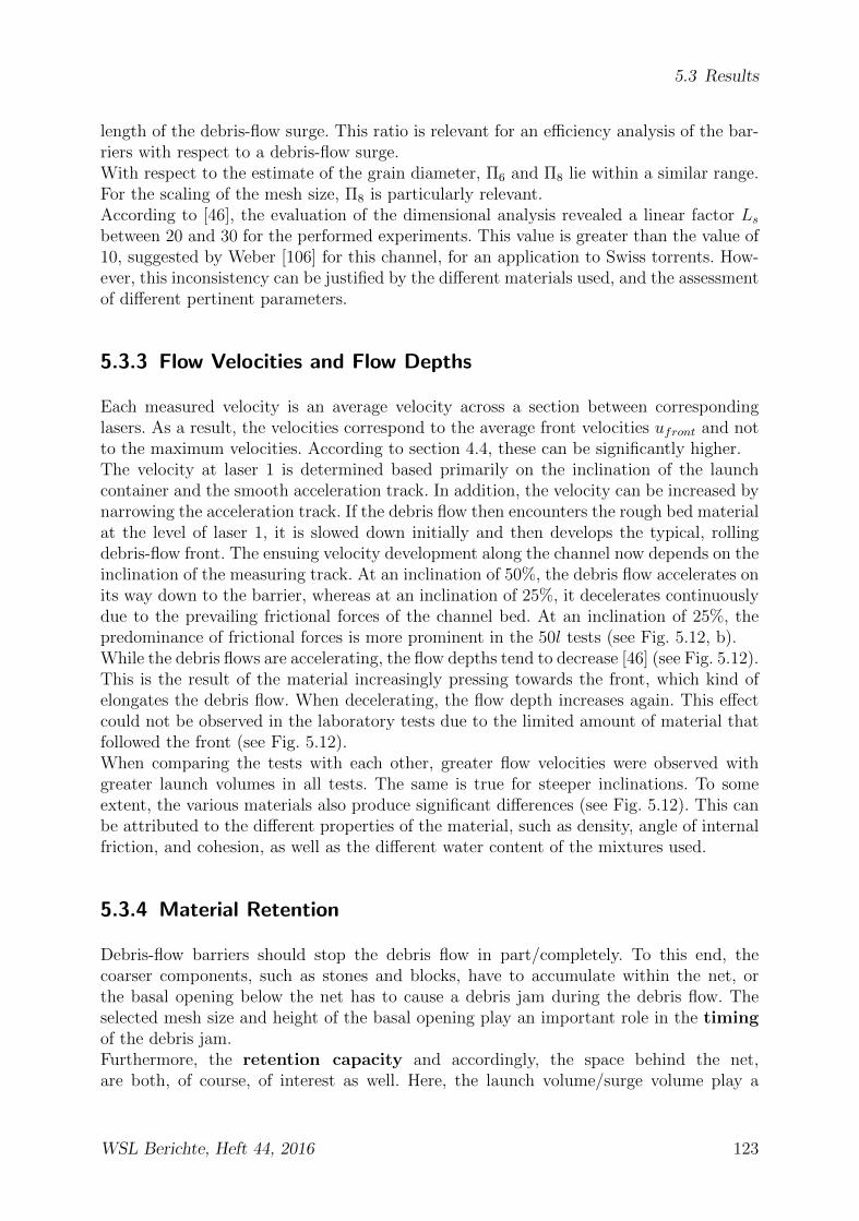
5.3 Results
length of the debris-flow surge. This ratio is relevant for an efficiency analysis of the bar-riers with respect to a debris-flow surge.With respect to the estimate of the grain diameter, Π6 and Π8 lie within a similar range.For the scaling of the mesh size, Π8 is particularly relevant.According to [46], the evaluation of the dimensional analysis revealed a linear factor Lsbetween 20 and 30 for the performed experiments. This value is greater than the value of10, suggested by Weber [106] for this channel, for an application to Swiss torrents. How-ever, this inconsistency can be justified by the different materials used, and the assessmentof different pertinent parameters.
5.3.3 Flow Velocities and Flow Depths
Each measured velocity is an average velocity across a section between correspondinglasers. As a result, the velocities correspond to the average front velocities ufront and notto the maximum velocities. According to section 4.4, these can be significantly higher.The velocity at laser 1 is determined based primarily on the inclination of the launchcontainer and the smooth acceleration track. In addition, the velocity can be increased bynarrowing the acceleration track. If the debris flow then encounters the rough bed materialat the level of laser 1, it is slowed down initially and then develops the typical, rollingdebris-flow front. The ensuing velocity development along the channel now depends on theinclination of the measuring track. At an inclination of 50%, the debris flow accelerates onits way down to the barrier, whereas at an inclination of 25%, it decelerates continuouslydue to the prevailing frictional forces of the channel bed. At an inclination of 25%, thepredominance of frictional forces is more prominent in the 50l tests (see Fig. 5.12, b).While the debris flows are accelerating, the flow depths tend to decrease [46] (see Fig. 5.12).This is the result of the material increasingly pressing towards the front, which kind ofelongates the debris flow. When decelerating, the flow depth increases again. This effectcould not be observed in the laboratory tests due to the limited amount of material thatfollowed the front (see Fig. 5.12).When comparing the tests with each other, greater flow velocities were observed withgreater launch volumes in all tests. The same is true for steeper inclinations. To someextent, the various materials also produce significant differences (see Fig. 5.12). This canbe attributed to the different properties of the material, such as density, angle of internalfriction, and cohesion, as well as the different water content of the mixtures used.
5.3.4 Material Retention
Debris-flow barriers should stop the debris flow in part/completely. To this end, thecoarser components, such as stones and blocks, have to accumulate within the net, orthe basal opening below the net has to cause a debris jam during the debris flow. Theselected mesh size and height of the basal opening play an important role in the timingof the debris jam.Furthermore, the retention capacity and accordingly, the space behind the net,are both, of course, of interest as well. Here, the launch volume/surge volume play a
WSL Berichte, Heft 44, 2016 123

5 Physical Modeling
Section + distance
v(m
/s)
1 2 3 40 1.5 2.5 3.5 m
1
2
3
4
●
●
●●
●
●
●
●
●
●
●●
●
●
●
Illgraben 150 lIllgraben 100 lIllgraben 50 lAlpbach 50 l
Section + distance
v(m
/s)
1 2 3 40 1.5 2.5 3.5 m
1
2
3
4
●●
●
●
● ●
●
●
●
●
Illgraben 100 lIllgraben 50 lTrachtbach 50 lMerdenson 50 l
a) Velocities at an inclination of 50% b) at an inclination of 25%
Section + distance
h(c
m)
1 2 3 40 1.5 2.5 3.5 m
0
10
20
30●
●
●
●
●
●
●
●
●
●●
●
●
●
●
Illgraben 150 lIllgraben 100 lIllgraben 50 lAlpbach 50 l
Section + distance
h(c
m)
1 2 3 40 1.5 2.5 3.5 m
0
10
20
30
●
●
●
●
● ● ●
●
●
Illgraben 100 lIllgraben 50 lTrachtbach 50 lMerdenson 50 l
c) Flow depths at an inclination of 50% d) at an inclination of 25%
Figure 5.12: Mean values according to [46] of the series of tests examining flow velocities ofthe debris-flow front and maximum flow depths.
particularly important role. If the retention volume is exhausted, the remainder of thedebris flow overflows the barrier.
Blockage of the Net
All mesh sizes smaller than or equal to 4cm produce good blockage and nearly-completeretention of the material. Mesh sizes larger than 4cm only partially retain the material (fora comparison of material retention as a function of mesh size using Hasliberg material, seeFig. 5.13). With basal openings of 4cm or less, a debris jam and net filling always occur.If larger basal openings are selected, net filling does not occur. In tests using drainagechannels of 3 and 4cm, debris jams generally occurred at a later point in time comparedto tests which did not use a basal opening. Initially, material flows through underneaththe net (before the filling process is initiated).Further details regarding the effects of mesh size and the basal opening for the Trachtbachand Alpbach material specifically are provided in [109, 110].
124 WSL Berichte, Heft 44, 2016
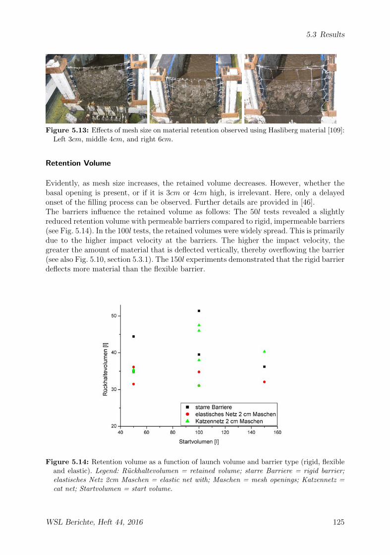
5.3 Results
Figure 5.13: Effects of mesh size on material retention observed using Hasliberg material [109]:Left 3cm, middle 4cm, and right 6cm.
Retention Volume
Evidently, as mesh size increases, the retained volume decreases. However, whether thebasal opening is present, or if it is 3cm or 4cm high, is irrelevant. Here, only a delayedonset of the filling process can be observed. Further details are provided in [46].The barriers influence the retained volume as follows: The 50l tests revealed a slightlyreduced retention volume with permeable barriers compared to rigid, impermeable barriers(see Fig. 5.14). In the 100l tests, the retained volumes were widely spread. This is primarilydue to the higher impact velocity at the barriers. The higher the impact velocity, thegreater the amount of material that is deflected vertically, thereby overflowing the barrier(see also Fig. 5.10, section 5.3.1). The 150l experiments demonstrated that the rigid barrierdeflects more material than the flexible barrier.
Figure 5.14: Retention volume as a function of launch volume and barrier type (rigid, flexibleand elastic). Legend: Ruckhaltevolumen = retained volume; starre Barriere = rigid barrier;elastisches Netz 2cm Maschen = elastic net with; Maschen = mesh openings; Katzennetz =cat net; Startvolumen = start volume.
WSL Berichte, Heft 44, 2016 125
5 Physical Modeling
Summary
With reference to the dimensional analysis carried out, the mesh and drainage-channelsize can be considered in relation to the d90 grain size used. Here, the relevant parameteris Π8 = M/d90. Unfortunately, the specification of a d90 grain size of 25cm is based onone field event as described in [69]. This yields Π8 = 1.2 for a mesh size of M = 30cmfor the field barrier. The mesh sizes in the laboratory varied between 3 and 4cm withΠ8 = 1.0− 1.3. These values show good accordance, although they should be interpretedwith caution due to the field data. In any case it is evident that most material is retainedwith mesh sizes equal to the d90 grain diameter, and that this applies to field barriers aswell. This was confirmed in 2005 and 2006 for the barriers in the Illgraben, with a meshsize of M = 30cm and good material retention (see section 4.5).According to [46], the following applies to the basal opening: If the basal opening is thesame size as the d90 diameter, a debris jam always occurs. If it is twice the size of thed90 grain, no debris jams occur in the laboratory (at a drainage-channel height of 6cm).Here, the flow depth hfl now plays the decisive role. Sufficient accordance between theflow depth and the height of the basal opening is required, so that the debris flow strikesagainst the lower support rope and begins to chock. The laboratory tests demonstratedthat the factor hfl = 1.3 ·hd was still not high enough. Field tests in the Illgraben showedthat a ratio of hfl = 1.5 · hd is sufficient.When selecting basal openings for mountain torrents, the type of channel bed also needsto be taken into consideration. If the bed consists of solid rock, the bed level in the channeldoes not fluctuate much, whereas if the channel bed consists of loose deposit materials, thebed level can rapidly sink. Therefore, each flooding event can quickly flush out materialunderneath the barrier, thereby increasing the size of the basal opening (see section 4.3.3).The effects of the barrier type on retention volume exhibit only a small material-dependentcomponent. Approximately identical amounts of material are retained by rigid barriers asby flexible or elastic ones. However, there is a greater vertical deflection of the material dur-ing the initial impact onto rigid barriers than onto flexible ones. This vertically-deflectedmaterial is then directed over the barrier. Nonetheless, this does not lead to a significantdeficit in material retention due to the material that follows. The values measuring theretained volume are thus subject to natural variations.
5.3.5 Force Measurement
Force measurement is one of the key elements of the performed laboratory tests. As previ-ously described in section 5.2.1.3, the force was measured in parallel to the flow directionby means of the measuring sledge and two load cells. Hereafter, the occurrent total loadwill always correspond to the sum of both load cells.The performed laboratory tests demonstrated two different force effects. One is the dy-namic load of the debris flow during the flow, which the barrier has to withstand foronly a short amount of time. In the load curve, this load is referred to as the maximumload Fmax (see Fig. 5.15). Once the net has been filled, the force measured then returnsto the static value Fstat.
126 WSL Berichte, Heft 44, 2016

5.3 Results
Time (s)
Forc
e (N
)
0 2 4 6 8
0
250
500
750
maximum Load Fmax
static load Fstat
Figure 5.15: Load acting on the net as a function of time, illustrating the maximum and thestatic load as in [46].
This section will describe and interpret the occurrent maximum and static loads basedon laws relevant to the model.
5.3.5.1 Maximum Load
The maximum load consists of two types of loads. One is the dynamically-acting loadresulting from the stopping process of the debris flow (change in momentum). The otheris the hydrostatic load of the debris-flow material streaming in (hydraulic pressure). Here,two different types of filling process have been observed in the laboratory tests:
• Case 1 Tests with Fr > 2: The first wave determines Fmax during the debris-flowimpact (see Fig. 5.16, top). At the time of Fmax, the flow depths and fill levels at laser4 on the barrier still show the flow depth hfl of the first wave. Here, the flow forceresulting from the hydrostatic pressure acts only through hfl, i.e. Fhyd = 1
2ρgbh2
fl.This value is low relative to Fmax and can be neglected.
• Case 2 Tests with Fr < 2: The filling process begins upon impact of the first wave,i.e. the hydraulic pressure already applies across the entire fill level hfill at Fmax (seeFig. 5.18). The hydrostatic flow force Fhyd = 1
2ρgbh2
fill cannot be neglected.The same applies to rigid barriers without basal openings. Here, the static hydraulicpressure also applies across the entire fill level at Fmax. In this case too, the hydraulicpressure must be taken into account (see Fig. 5.18, bottom).
As a result, the hydraulic pressure did not contribute significantly to Fmax in most tests(case 1). The calculation of the dynamic pressure increase ∆P = Pdyn = Fmax
bhfillis based
directly on Fmax. In case 2, the hydrostatic pressure across the fill level was taken intoaccount for the calculation of Pdyn. Evidently, Pdyn directly depends on the velocity u2 (seeFig. 5.19). This points to the hydraulic problem of flow resistance. Here, Fdyn = 1
2cdρAu
2,
Fdyn/A = Pdyn, Π1 =Pdynρu2
= 12cd, and cd = 2Π1 apply. Therefore, Π1 = Pdyn/ρu
2 is
WSL Berichte, Heft 44, 2016 127

5 Physical Modeling
Figure 5.16: At the time of Fmax, only the first wave exerts hydraulic pressure. Legend:Fliesshohe = flow depth; Kraftmessung = force measurement; Zeit = time.
directly taken into account as a dimensionless number in Figure 5.19 and represented bythe Froude number Π2. The Π1 values were higher in tests that used material from theTrachtbach, which is very cohesive. However, a higher Π1 value was also observed in onetest that used material from the Illgraben. However, this outlier can be explained by thematerial used in the test, which had not been properly mixed and, thus, contained clumps.These clumps then behave like cohesive material (see Trachtbach) or larger grain sizes,differentiating this debris flow from those in the other tests.Low Π1 values can also be observed in very slow tests with Fr < 2. This can be explaineddirectly based on the definition of Π1 = ∆P/ρu2. For lower velocities, the dynamic pres-sure ∆P is also lower.A very low Π1 value was observed with a rigid barrier at a relatively high Froude numberof Fr ≈ 5. This value can be attributed to the significant vertical deflection with rigidbarriers at high Froude numbers. As a result, the dynamic load ∆P is reduced.
The analysis of the maximum loads in the laboratory tests generally demonstrates thefollowing points:
• The dynamic pressure increase ∆P depends on the velocity u2. Therefore, largerimpact velocities result in greater loads acting on the structure.
128 WSL Berichte, Heft 44, 2016

5.3 Results
Fr < 2 Rigid barriers
Figure 5.17: Fmax with and without hydraulic pressure Fhyd.
• The interaction with the barrier is a hydraulic problem, namely the flow aroundan obstacle. The barrier’s resistance to the flow is expressed by a resistance valuecd, which can also be expressed as the dimensionless number Π1 = 1
2cd. Since the
barriers have a relatively similar cd value once they are blocked with stones, onlythe debris-flow material itself plays a significant role.
• Furthermore, Π1 is material-dependent. Higher Π1 values can be observed with verycohesive materials. This suggests that a material parameter αm can be introducedin addition to the pressure coefficient cd of the barrier. It follows that
Π1 =∆P
ρu2=
1
2cdαm → ∆P =
1
2cdαm︸ ︷︷ ︸cp
ρu2 (5.21)
with cd being the resistance value of the barrier, αm a material-specific factor ofthe debris-flow material, ρ the density of the debris flow, and u the average frontvelocity. 1
2cdαm is integrated into the value cp, a specific pressure coefficient. This
approach is in line with the calculation methods previously recommended in theguidelines for protection against gravitational natural hazards [60] as well as withthe approaches of Coussot [21] and Armanini [3] (see section 6.1).
• Rigid barriers in the flow path of high-velocity flows have a low dynamic pressurecoefficient cp. This is because the debris-flow stream is directly deflected verticallyupwards by the impact side of the barrier. Occasionally, this phenomenon can alsobe observed with flexible barriers in the flow path of very high velocity debris flows(see Fig. 5.10). The vertical deflection reduces the load acting on the barrier and,thereby, also the ∆P and cp values. However, it is important to consider that thefull hydrostatic pressure already acts during the impact of the debris flow onto an
WSL Berichte, Heft 44, 2016 129
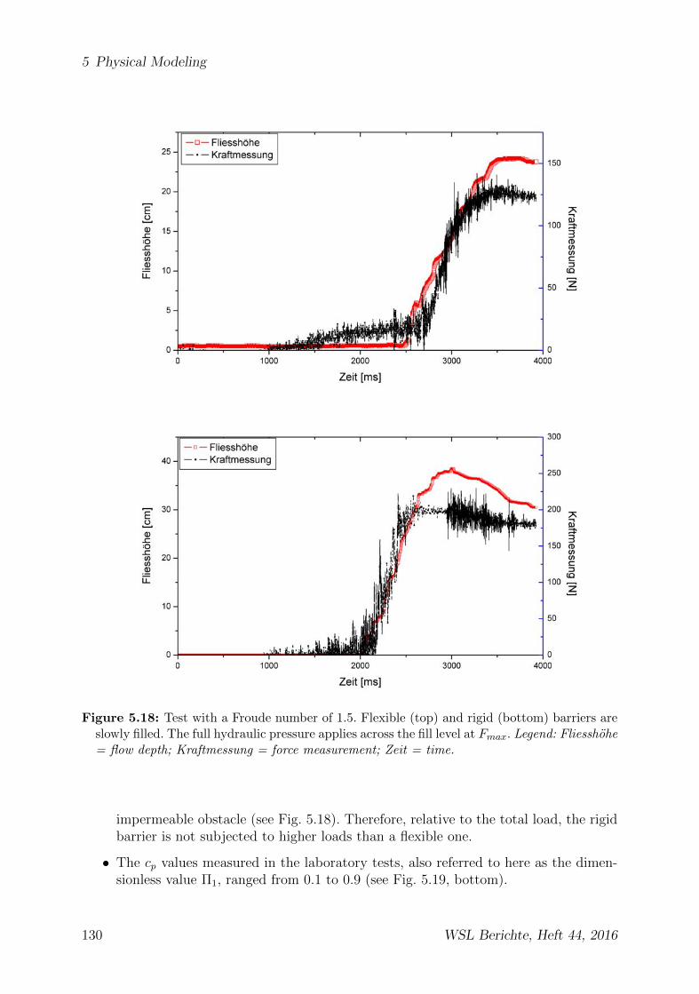
5 Physical Modeling
Figure 5.18: Test with a Froude number of 1.5. Flexible (top) and rigid (bottom) barriers areslowly filled. The full hydraulic pressure applies across the fill level at Fmax. Legend: Fliesshohe= flow depth; Kraftmessung = force measurement; Zeit = time.
impermeable obstacle (see Fig. 5.18). Therefore, relative to the total load, the rigidbarrier is not subjected to higher loads than a flexible one.
• The cp values measured in the laboratory tests, also referred to here as the dimen-sionless value Π1, ranged from 0.1 to 0.9 (see Fig. 5.19, bottom).
130 WSL Berichte, Heft 44, 2016
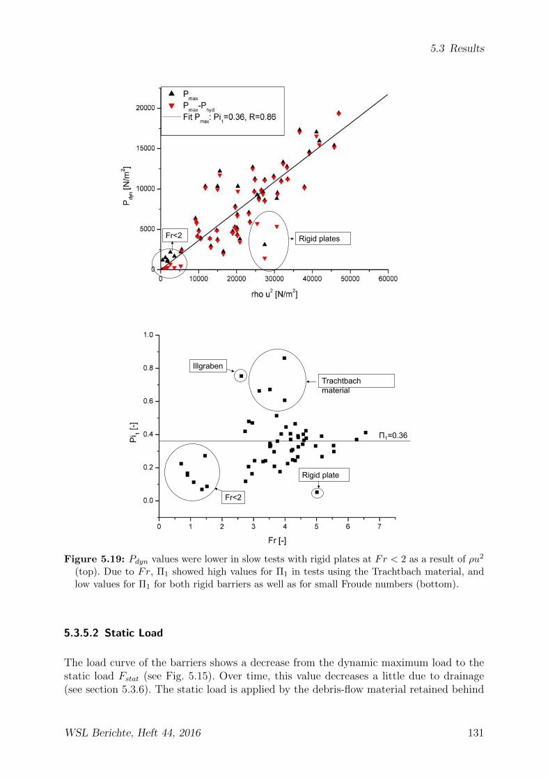
5.3 Results
Rigid plates Fr<2
Rigid plate
Trachtbach material
Illgraben
Π1=0.36
Fr<2
Figure 5.19: Pdyn values were lower in slow tests with rigid plates at Fr < 2 as a result of ρu2
(top). Due to Fr, Π1 showed high values for Π1 in tests using the Trachtbach material, andlow values for Π1 for both rigid barriers as well as for small Froude numbers (bottom).
5.3.5.2 Static Load
The load curve of the barriers shows a decrease from the dynamic maximum load to thestatic load Fstat (see Fig. 5.15). Over time, this value decreases a little due to drainage(see section 5.3.6). The static load is applied by the debris-flow material retained behind
WSL Berichte, Heft 44, 2016 131

5 Physical Modeling
the barrier directly after the flow at
Fstat =
∫ hfill
0
Phyd(h)bdh =1
2ρgh2
fillb. (5.22)
If the debris cone has almost completely drained, the static load slowly approaches theactive earth pressure at
Fstat t→∞ =
∫ hfill
0
Phyd(h)bdh =1
2Ka,hγh
2fillb (5.23)
with Ka,h being the factor of the active earth pressure
Ka,h =cos2(φ+ α)
cos2(α)(
1 +√
sin(φ+δ) sin(φ−β)cos(α−δ) cos(α+β)
)2 . (5.24)
A definition of the angle is provided in Figure 5.20.
Figure 5.20: Definition of the angle during active earth pressure according to [47].
According to section 5.2.3.5, a friction angle of φ′ ≈ 40◦ then yields a coefficient ofKa,h = 0.2. The line in Figure 5.21 indicates the active earth pressure for fill levelshfill < 28cm relative to Fstat immediately following the tests.Figure 5.21 confirms that Fstat depends on h2
fill. However, a prominent increase of Fstatin tests using fill levels hfill > 28cm, or h2
fill > 784cm2, was observed. Here, the valuesdeviated significantly from the linear relationship to h2
fill. This is due to the overflowprocess that occurred in these tests. While the filling process was ongoing, additionaloverflowing occurred in all tests with hfill > 28cm. As a result, the density ρ of thematerial retained behind the barrier was increased. This occurred because the verticalload of the overflowing debris flow compressed the grains. In this case, what is referred toas the pack size of the debris-flow material within the cone is increased. As a result, Fstatincreases as well.According to [46], the increase in Fstat is caused by the higher velocities in the testswith hfill > 28cm. These tests show that, for hfill > 28cm, Fstat depends on u2. Athigher velocities, the grains directly behind the net are compressed as well, resulting inan increase of Fstat.
132 WSL Berichte, Heft 44, 2016

5.3 Results
Figure 5.21: Fstat as a function of fill level h2fill for tests with hfill < 28cm (no overflowing)
and tests with hfill > 28cm (overflowing). The line indicates the active earth pressure at afriction angle of φ = 40◦. Legend: mit Uberstromen = with overflow; ohne Uberstromen =without overflow; mit aktivem Erddruck = with active earth pressure; Steigung = slope angle.
5.3.6 Drainage
In order to determine an approximate permeability value kf for a stopped debris-flow conewith Illgraben material, water drainage across time t was assessed immediately followingthe test. The recorded water drainage was highest immediately after the test and thenrapidly decreased at an exponential rate (see Fig. 5.22). Increased water drainage wasobserved in the 100l test depicted in Figure 5.22, due to the higher retention volumeof V = 57.4l behind the barrier compared to the retention volumes of V = 31.7l andV = 32.7l in the 50l tests. The two 50l tests resembled each other with respect to theapproximated exponential function. Drainage in test no. 65 was q = 12 + 216e−t/10.91 andq = 12 + 243e−t/20.78 in test no. 66, each with a coefficient of determination of R2 = 0.99.The slightly increased drainage in test 66 compared to test 65 can be explained by theincreased afflux length of the retention cone.
In order to determine an approximate value for the permeability kf , the debris-jam conemust be considered as a porous medium. To this end, a calculation method from the do-main of groundwater hydraulics was used [101]. The conditions are described by means ofthe differential equation for an unconfined aquifer, according to the approximate solutionby Dupuit, i.e.
∂2(h2)
∂x2= 0 (5.25)
with h(x) being the line of the water surface, which is still visible on the cone shortly afterthe test (see Fig. 5.23). Integrating the equation 5.25 twice and inserting the boundary
WSL Berichte, Heft 44, 2016 133

5 Physical Modeling
Figure 5.22: Measured water drainage over time in two 50l tests, and one 100l test usingIllgraben material and a water content of w = 30%. Legend: Versuch = test; Funktion =function; Abfluss = drainage; Zeit = time.
hfill
zxL
Debris flow coneh(x)
Figure 5.23: Water level in the retention cone immediately following the test (left), andschematic representation of the retention cone for the determination of flow (right).
conditions hx=0 = hfill for hx=L = 0 yields
h2 =−h2
fill
Lx+ h2
fill = h2fill
(1− x
L
)(5.26)
According to Darcy’s law, it follows for flow and drainage q per meter width that
qx = hvx = −kfhh
dx=−kf
2
d(h2)
dx(5.27)
If equation 5.26 is now inserted into equation 5.27 and the channel width b = 0.3m is
134 WSL Berichte, Heft 44, 2016
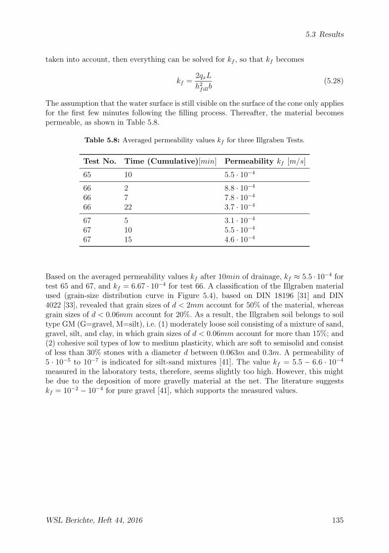
5.3 Results
taken into account, then everything can be solved for kf , so that kf becomes
kf =2qxL
h2fillb
(5.28)
The assumption that the water surface is still visible on the surface of the cone only appliesfor the first few minutes following the filling process. Thereafter, the material becomespermeable, as shown in Table 5.8.
Table 5.8: Averaged permeability values kf for three Illgraben Tests.
Test No. Time (Cumulative)[min] Permeability kf [m/s]
65 10 5.5 · 10−4
66 2 8.8 · 10−4
66 7 7.8 · 10−4
66 22 3.7 · 10−4
67 5 3.1 · 10−4
67 10 5.5 · 10−4
67 15 4.6 · 10−4
Based on the averaged permeability values kf after 10min of drainage, kf ≈ 5.5 · 10−4 fortest 65 and 67, and kf = 6.67 · 10−4 for test 66. A classification of the Illgraben materialused (grain-size distribution curve in Figure 5.4), based on DIN 18196 [31] and DIN4022 [33], revealed that grain sizes of d < 2mm account for 50% of the material, whereasgrain sizes of d < 0.06mm account for 20%. As a result, the Illgraben soil belongs to soiltype GM (G=gravel, M=silt), i.e. (1) moderately loose soil consisting of a mixture of sand,gravel, silt, and clay, in which grain sizes of d < 0.06mm account for more than 15%; and(2) cohesive soil types of low to medium plasticity, which are soft to semisolid and consistof less than 30% stones with a diameter d between 0.063m and 0.3m. A permeability of5 · 10−5 to 10−7 is indicated for silt-sand mixtures [41]. The value kf = 5.5 − 6.6 · 10−4
measured in the laboratory tests, therefore, seems slightly too high. However, this mightbe due to the deposition of more gravelly material at the net. The literature suggestskf = 10−2 − 10−4 for pure gravel [41], which supports the measured values.
WSL Berichte, Heft 44, 2016 135

5 Physical Modeling
5.4 Numerical Modeling of the Laboratory Tests
5.4.1 Coefficients of Friction
The conservation-of-energy analysis from section 2.2.3 also applies to the laboratorytests. When a debris flow is triggered, potential energy is converted into kinetic energyand possible internal energy losses (see equation 2.22). According to equation 2.33, theinternal losses are subdivided into the Mohr-Coulomb friction (dry friction), the viscousfriction, and the losses due to what is known as random energy. These loss processesprevent debris flows from accelerating continuously, and cause them to halt – at somepoint – of their own accord.In section 4.4, the friction parameter µ = τ/σ is determined based on the values measuredfor the normal stress σ and the shear stress τ , obtained with the debris-flow balance forfield events in the Illgraben.For comparison, the orders of magnitude µ and individual influencing factors for thelaboratory tests are indicated; this was done in order to subsequently implement thederived friction law into the simulation of the laboratory tests in AVAL-1D. A moredetailed description of the development of the friction parameters for the laboratory testsis provided in [46].
5.4.1.1 Friction Parameters in the Laboratory Tests
During the field tests, the time course of µ was measured at the balance. In the laboratorytests, µ could be determined only as an average value, based on the conservation of energyat three different sections, for each test. Since the kinetic energy K is identified basedon the average front velocity ufront, each determined µ value applies to the front. Thehighest velocities occur in the area with the highest flow depths hfl,max. This area appearsshortly after the front; hence umax ≈ ufront applies. As a result, µ (determined based onthe energy balance with ufront) is comparable to Wg (determined based on equation 2.23with hfl,max).Based on Figure 2.9, the laboratory debris flow was simplified to a block of mass m. Assuggested in [46], the energy balance for a block of mass according to equation 2.22 yieldsµ for the respective section measured, so that
µ = tan (Θ)− u21 − u2
2
2g cos (Θ) s(5.29)
with Θ as the channel slope. u1 and u2 are the average flow velocities of the respectivelaser sections of length s. µ can either be determined for individual sections between thelasers or as an average value for the entire length of the channel. The following influencingfactors for the coefficient of friction µ of the laboratory tests were observed [46]:
• Material With identical launch volumes and inclinations, the material from theAlpbach exhibited significantly lower values for µ(t) than the material from theIllgraben. This was due to the higher water content of the Alpbach material (see
136 WSL Berichte, Heft 44, 2016
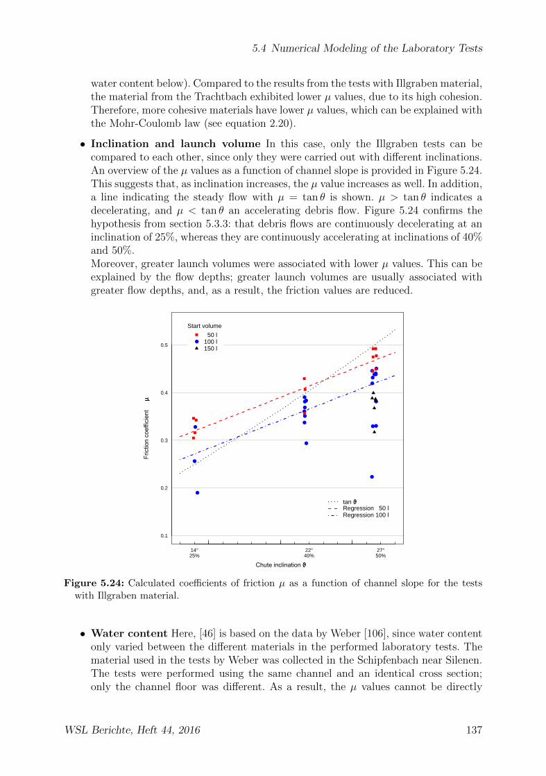
5.4 Numerical Modeling of the Laboratory Tests
water content below). Compared to the results from the tests with Illgraben material,the material from the Trachtbach exhibited lower µ values, due to its high cohesion.Therefore, more cohesive materials have lower µ values, which can be explained withthe Mohr-Coulomb law (see equation 2.20).
• Inclination and launch volume In this case, only the Illgraben tests can becompared to each other, since only they were carried out with different inclinations.An overview of the µ values as a function of channel slope is provided in Figure 5.24.This suggests that, as inclination increases, the µ value increases as well. In addition,a line indicating the steady flow with µ = tan θ is shown. µ > tan θ indicates adecelerating, and µ < tan θ an accelerating debris flow. Figure 5.24 confirms thehypothesis from section 5.3.3: that debris flows are continuously decelerating at aninclination of 25%, whereas they are continuously accelerating at inclinations of 40%and 50%.Moreover, greater launch volumes were associated with lower µ values. This can beexplained by the flow depths; greater launch volumes are usually associated withgreater flow depths, and, as a result, the friction values are reduced.
Chute inclination ϑϑ
Fric
tion
coef
ficie
ntµµ
14° 22° 27°25% 40% 50%
0.1
0.2
0.3
0.4
0.5
●
●
●
●●
●●
●●
●
●
●
●
●
●
●
●
●
●
●
●
●
●
Start volume
50 l100 l150 l
tan ϑϑRegression 50 lRegression 100 l
Figure 5.24: Calculated coefficients of friction µ as a function of channel slope for the testswith Illgraben material.
• Water content Here, [46] is based on the data by Weber [106], since water contentonly varied between the different materials in the performed laboratory tests. Thematerial used in the tests by Weber was collected in the Schipfenbach near Silenen.The tests were performed using the same channel and an identical cross section;only the channel floor was different. As a result, the µ values cannot be directly
WSL Berichte, Heft 44, 2016 137

5 Physical Modeling
compared to the tests in the present work. However, there is a clear trend, whichdemonstrates that a higher water content in the debris flow is associated with lowercoefficients of friction µ (see Fig. 5.25). Furthermore, these tests also confirm thatµ is greater for steeper slopes (see Fig. 5.25).
Volumetric water content
µµ
0.4 0.6 0.8 1.0
0.0
0.1
0.2
0.3
0.4
0.5
●
●
●
●
●●
●
●
●
●
●
●
● 40% slope 25% angle
Figure 5.25: Calculated coefficients of friction µ for the tests by Weber [106] with the materialfrom the river Schipfenbach at inclinations of 40% and 50% and a launch volume of 100l.
• Rate of gravitational activity Wg In order to calculate Wg using equation 2.23,the flow velocities and maximum flow depths were averaged across the entire lengthof the channel. Figure 5.26 shows a trend towards lower µ values for higher workrates Wg.
• Time course The evolution of µ along the channel during the flow process willbe discussed here. According to [46], lower µ values should be observed at thebeginning of the channel than for sections further along the channel. As shown inFigure 5.12, this is a consequence of the flow-depth development along the channel;the flow depths continually decrease as the debris flow moves down the channel,thus increasing the µ values. For a more detailed description of the µ values acrossthe sections between lasers, see [46].Variable µ values have also been observed in the test results from the Illgraben(see section 4.4). In these tests, µ was higher at the front of debris flows thanin the following debris-flow tail. This could also be observed during the event ofOctober 3, 2006, among others. At this front, µ values ranged from 0.12 to 0.15,whereas they immediately decreased to 0.1 right after the front (see Fig. 5.27).Unfortunately, relatively few µ values have been measured for the front here aswell, since it was very steep and very short. For further results concerning µ during
138 WSL Berichte, Heft 44, 2016

5.4 Numerical Modeling of the Laboratory Tests
μc + viscous friction
μc + viscous friction
25%
40%
50%
Figure 5.26: Coefficients of friction µ as a function of rate of gravitational activity Wg forthe tests using Illgraben material, with adjusted curves for equation 5.33 for the differentinclinations. Legend: Neigung = slope inclination.
field events and their analysis and interpretation, see [62].
The field of avalanche dynamics revealed the following dependency for µ [6]
µ = µ1 + (µ2 − µ1)e−k′Wg (5.30)
with µ1 =(τσ
)h→∞ as a tangent to the µ values measured for high flow depths. µ2 =
(τσ
)h→0
is the tangent for lower flow depths. For a definition of µ1 and µ2, see Fig. 5.27 in [6].The parameters for equation 5.30 have been reliably estimated for Illgraben materialwith different inclinations using MATLAB (cftool function). The curves are shown inFigure 5.26. However, due to missing data points, the determination of µ according toequation 5.30 is very vague and, therefore, should be interpreted with caution. For adetailed description of the proceedings and the statistical background, see [46].µ decreases as the rate of gravitational activity increases as a result of the additionalinternal contribution to losses due to random energy (see equation 2.34). As Wg increases,the random energy increases as well. As the random-energy contribution increases, thedry-friction contribution decreases µ (see equation 2.33). The differential equation forrandom energy (equation 2.34) can be solved for Wg = const., so that
R(t) =α
βWg
(1− e−βt
)+R0e
−βt (5.31)
WSL Berichte, Heft 44, 2016 139

5 Physical Modeling
μ2=0.12
μ2=0.1
Normal stress [kN/m2]
Shear stress [kN
/m2]
Figure 5.27: µ values measured for the Illgraben event on October 3, 2006 (left), and definitionof µ1 and µ2 according to [6] (right).
with R0 = R(0), i.e. the random energy R at time point zero. For Wg 6= const., thecourse of R(t) can be calculated numerically, and for high values of β (compared to thecalculation steps for ∆t), the equation 2.34 can be simplified to
R(t) ≈ α
βWg(t) for Wg(t) 6= const. and β � ∆t. (5.32)
Inserting equation 5.32 into equation 5.30 yields
µ = µ1 + (µ2 − µ1)e−kR (5.33)
with k = α/β, i.e. the friction parameter µ directly depends on the random energy R.Unfortunately, this cannot be measured directly.Furthermore, the best-fit curves in Figure 5.26 show a shift of the curves for differentinclinations. Gentler inclinations result in lower flow velocities and lower values for µ, andsteeper inclinations in higher flow velocities and larger µ values. This, then, indicates thevelocity-dependent viscous friction component from equation 2.33, which shifts the curvesvertically in combination with µc. This effect is not taken into account in equation 5.33.For µmod, derived from equation 2.33, arises
µmod =τ
σ= µc︸︷︷︸
Coulomb friction
+u2
hfl cos Θξ︸ ︷︷ ︸viscous friction
− 2λ′√Wg︸ ︷︷ ︸
random energy
(5.34)
with σ = ρghfl cos Θ, µc as the friction value for the Coulomb friction, ξ as the coefficient
of viscous friction, and λ′ =λ√
αβ
ρhflgas the coefficient accounting for the random-energy
contribution. In equation 5.32, random energy is expressed as R(t) = αβWg(t).
This derived friction law will be used in the modeling of the laboratory tests below.
5.4.2 Modeling of the Tests using Material from the Illgraben
Only tests with an inclination of 25% will be considered and modeled in AVAL-1D. Thechange of the friction parameter during the flow process is described by equation 5.34.
140 WSL Berichte, Heft 44, 2016

5.4 Numerical Modeling of the Laboratory Tests
For λ′ = 0, equation 5.34 describes the Voellmy model used in avalanche dynamics [7]. Anoverview of the dimensions of the parameters µc, ξ, and λ′ is provided in Table 5.9. Thechannel is subdivided into the acceleration track, made of steel, and the measuring track,with a channel floor consisting of rough pebbles. The values in Table 5.9 refer to the testsusing the Illgraben material and an inclination of 25%. With other materials, such as thematerial from the Trachtbach, for example, the ξ value was significantly higher (ξ = 106)and the λ value significantly lower (λ′ = 0.01). This material, which acts rather viscously,can be described approximately using the Voellmy model; the material from the Illgraben,however, cannot be adequately described by this model (see Fig. 5.28).
Table 5.9: Dimensions of the friction parameters, used in the AVAL-1D model, for Illgrabenmaterial at an inclination of 25%.
Channel section µc[−] ξ[m/s2] λ′[
kg√Ws2
]Steel 0.2 10.0 105 0.2Measuring channel 0.37 4.0 105 0.4
Modeling of the Barrier
The available geometric input functions are well-suited to represent the geometry of thechannel. However, despite the acceleration track’s S-shape, it can only be representedlinearly (see Fig. 5.1). Furthermore, reproduction and modeling of the installed barrieris difficult. Here, the only possible solution is to model the barrier as a rigid geometricaldiscontinuity, with a 90◦ angle perpendicular to the direction of the streambed. Conse-quently, the stiffness of the simulated barrier more closely resembles the stiffness of rigidbarriers, and not that of flexible nets. Furthermore, the energy-dissipation behavior ofthe layer in the simulation model cannot exactly reproduce the behavior of the barriers(particularly of the flexible ones).
50l Tests
The 50l Illgraben tests at an inclination of 25% will be discussed first. As shown in Fig-ure 5.28, the following velocity developments were observed. The Voellmy model for λ′ = 0was also included in the figure.This demonstrated that the performed debris-flow tests cannot be described using theVoellmy model, i.e. with only a dry and a turbulent friction component. This also proves
that the last component (2λ′√Wg) from equation 5.34 influences the flow process signif-
icantly. These observations suggest that significant energy losses during the debris-flowprocess can be attributed to random energy. The model seems to adequately reproduce thevelocity development along the channel and the flow-depth development (see Fig. 5.29).
WSL Berichte, Heft 44, 2016 141

5 Physical Modeling
Figure 5.28: Velocity development in the laboratory tests using Illgraben material, an incli-nation of 25%, and a launch volume of 50l compared to simulation values in AVAL-1D formodified friction parameters for granular media. Legend: Mittlere Geschwindigkeit = averagevelocity; Versuch = test; Mittelwert der Versuche = test average; Modellierung with = modeledwith; Nr = no.
In addition, the deposition behavior of the simulated 50l tests was compared to the depo-sition behavior in the actual channel (see Fig. 5.30). Good agreement of the debris-flowcones was observed. The extent of the deposition zone was approximately identical tolcone ≈ 100cm, as was the impounding depth. Furthermore, in the channel, very littlematerial was deposited behind the cone; this was true both in the model as well as inthe tests using Illgraben material. In the 50l tests with an inclination of 25%, 1 − 3l ofmaterial were already deposited along the channel behind the cone. This occurred a littlemore in the simulation of ≈ 10 l, although in these cases, the deposition behavior behindthe barrier was described relatively well nonetheless.
Figure 5.31 shows the development of flow depths at each laser measuring point for testno. 63, as an example of the 50l tests. It should be noted that the flow depth cannotbe represented correctly immediately after the acceleration track. It is much too low inthe simulation. However, the values measured at the second laser in the laboratory testcorrespond exactly to the simulation, bringing the test and simulation back into coherence.Laser 3 and 4 correspond relatively well in terms of spike timing, due to the concordantvelocity developments in the laboratory test and simulation (see Fig. 5.28). Nevertheless,the flow depths in the simulation are slightly lower at these points.
142 WSL Berichte, Heft 44, 2016

5.4 Numerical Modeling of the Laboratory Tests
Figure 5.29: Flow-depth development in the laboratory tests using Illgraben material, an in-clination of 25%, and a launch volume of 50l compared to simulation values in AVAL-1D formodified friction parameters for granular media. Legend: Versuch = test; Rinne war nichtbewassert = chute has not been spayed before test; Mittelwert Versuche = test average; Mod-ellierung with = modeled with; Fliesshohe = flow depth; Nr = no.
100l Tests
The velocity development in the 100l tests was somewhat more scattered - both betweenand within individual tests - than in the 50l tests (see Fig. 5.32). Test no. 62 is an outlierbecause the material remained in the launch container for 5min, causing the phases toseparate. The velocities at lasers 3 and 4 in the simulation were somewhat lower towardsthe end than in the laboratory tests. In contrast, the 100l tests accelerated downwardsagain. This effect cannot be represented using the friction-parameter model according toequation 5.34.However, the flow-depth development again demonstrated good agreement between thesimulation and the performed tests (see Fig. 5.33).A figure indicating deposition will not be shown for the 100l tests, since it looks verysimilar to that of the 50l tests. Compared to the 50l tests, a small portion of the 100loverflowed the installed barrier in both the simulation and laboratory tests. However, thecones formed during these tests were, aside from a slightly longer afflux length lcone in the100l tests, comparable to those in the 50l tests.The flow-depth development along the channel in test no. 61 is shown in Figure 5.34.It demonstrates a generally good agreement between the simulation and laboratory test.Once again, the flow depth immediately after the acceleration track was too low in thesimulation, a result which may be due to an inaccurate reproduction of the accelerationtrack in the simulation.
WSL Berichte, Heft 44, 2016 143

5 Physical Modeling
h_fill=21.3cm
Icone≈ 105cm
[cm]
[cm]
Longitudinal profile of chute
Cross section of chute
hfill = 20 cm
lcone =100 cm
Figure 5.30: Deposition behavior in laboratory tests using Illgraben material at an inclinationof 25% and with a launch volume of 50l (top), compared to simulation values in AVAL-1D(middle and bottom).
144 WSL Berichte, Heft 44, 2016

5.4 Numerical Modeling of the Laboratory Tests
Figure 5.31: Development of flow depths directly at the lasers for test no. 63 with 50l and aninclination of 25%, and for the simulation of the test in AVAL-1D. Legend: Versuch = test;Modell = model; Fliesshohe = flow depth; Zeit = time.
Figure 5.32: Velocity development in the laboratory tests using Illgraben material, an incli-nation of 25%, and a launch volume of 100l, compared to simulation values in AVAL-1D formodified friction parameters for granular media. Legend: Geschwindigkeit = velocity; Mittel-wert Versuche = test average; Versuch = test; Modellierung mit = modeled with.
WSL Berichte, Heft 44, 2016 145

5 Physical Modeling
Figure 5.33: Flow-depth development in the laboratory tests using Illgraben material at aninclination of 25% and with a launch volume of 100l, compared to simulation values in AVAL-1D for modified friction parameters for granular media. Legend: Fliesshohen = flow depths;Versuch = test; Mittelwert Versuche = test average; Modellierung mit = modeled with; Nr. =no.
Figure 5.34: Flow-depth development directly at the lasers for test no. 61 with 100l and aninclination of 25%, as well as for the simulation of the test in AVAL-1D. Legend: Versuch =test; Modell = model; Fliesshohe = flow depth; Zeit = time.
146 WSL Berichte, Heft 44, 2016

5.5 Interpretation of the Laboratory Tests
5.5 Interpretation of the Laboratory Tests
5.5.1 Applying the Model to Reality
The performed dimensional analysis and examination of the dimensionless numbers con-firmed that the experiments are applicable to certain areas of reality. They demonstratedgood agreement between relevant dimensionless numbers from the performed laboratorytests and those from naturally-occurring debris flows. In addition, the dimensionalanalysis confirmed that the launch volumes in the experiments were too low compared tothe typical surge volumes in nature. Furthermore, the Froude numbers obtained in thelaboratory tests were slightly too high. Neither of these two problems can be solved atthe same time as the other. At the minimum inclination (25%), lower Froude numberscan only be achieved by reducing the launch volume.However, visual observations revealed a distinct debris-flow front during the flow process.This suggests that the front area of the model debris flow is very similar to those ofnaturally-occurring debris flows. Only the subsequent debris-flow tail was too short in thelaboratory, a result which can be attributed to the lower launch volumes. Nevertheless,the front is far more relevant for the interaction between debris flow and barrier and fora description of the filling process than the subsequent tail, which merely overflows thebarrier afterwards.
5.5.2 Transferability of the Flow Process
The flow development of the laboratory debris flows along the channel exhibited, similarlyto debris flows in the field, decreasing flow velocities with gentle inclinations and higherfriction losses. Smaller launch volumes also resulted in friction-dominated, deceleratingdebris flows. When a debris flow is decelerating, its flow depth increases, and vice versa.This effect occurs because the material of an accelerating debris flow gets pulled apart,which decreases the flow depth, and, in order to fulfill the condition of continuity Q = uA,hfl has to decrease with higher u and identical cross-section width. The opposite effectoccurs in friction-dominated flow regimes.A closer examination of the friction parameters reveals that µ did not act uniformlyalong the measuring track. This confirms Bartelt’s assumption [5] that, in granular media,µ decreases as flow depths increase, and increases again with decreasing flow depths.Moreover, µ strongly depends on the water content of the debris flow. µ decreases aswater content decreases, i.e. more grains rub against each other, since fewer intersticesare filled with water. The loss of friction due to random energy could only be demonstratedvaguely due to the low number of applicable experiments. Nevertheless, a trend emergedsuggesting that µ values were lower at higher rates of gravitational activity Wg due to therandom-energy contribution. The finding that the value of µ does not remain constantthroughout the flow process of a debris flow is important for the modeling of the tests.
WSL Berichte, Heft 44, 2016 147

5 Physical Modeling
5.5.3 Interaction between Debris Flow and Barrier
The prevailing flow velocity of the debris flow during impact on the barrier influences pri-marily the filling process and the applied load. The maximum load Fmax and its dynamiccomponent Fmax−Fhyd is proportional to the velocity u2. Fmax in very rapid debris flowswas shown to result primarily from the dynamic load of the debris-flow wave, whereasthe hydrostatic pressure was shown to exert an effect solely via the flow depth of the firstwave. In contrast, Fmax in very slowly-flowing debris flows was shown to occur almostsimultaneously with the maximum fill level of the barrier. In this case, the hydrostaticpressure is significantly higher. A distinct difference between impacts of very fast- andslowly-flowing debris flows can also be observed visually. Debris flows with Froude num-bers of Fr > 2 generally get deflected vertically at the barrier and overflow the barrierinitially, before the material that follows can fill it (for a schematic representation, seeFig. 5.11, right). Physically, this effect can be explained by means of the impoundingdepth himp = u2/(2g). It provides an additional contribution to the impact level hw of thedebris flow, since hw = hfl +himp. Since the impounding depth is calculated based on thekinetic energy and the squared velocity, the contribution of himp is significantly greater athigh velocities. As a result, the debris flow is deflected upwards/stretches out verticallydue to its increased area of effect hw. A discussion of himp is also provided in [60, 3] inchapter 6. This component remained small in slow debris flows, and there was hardlyany visible vertical deflection. Instead, a kind of reverse-flow wave developed and flowedupstream (schematic representation in Fig. 5.11, left). Both types of filling processes areof critical importance for the subsequent load model (in chapter 6).
An examination of the pressure coefficient and the dimensionless number Π1 revealedthat the pressure coefficient is clearly material-dependent. With identical barriers, i.e.with identical drag coefficients cd, higher Π1 values were observed in experiments usingTrachtbach material. This material is very viscous and cohesive. It became apparent thatan additional, material-dependent factor αm was needed to describe the occurrent debris-flow pressure forces, reflecting their increase in cohesive, viscous materials. This factor,however, can be combined with the width-dependent cd value into a specific pressureparameter cp = αm · cd. The cp value then corresponds to the dimensionless number Π1
in the laboratory tests. In the performed tests, its values ranged from 0.1 to 0.9. Thisrange of values is at the lower end of the spectrum for application to naturally-occurringdynamic debris-flow loads (see chapter 6). Other load approaches indicate larger valuesfor the dynamic amplification, with maximum values of up to 2− 15 [2, 20].
The type of barrier also plays an important role during occurrent debris-flow loads. Thecontribution of the dynamic component of the debris-flow load was smaller during impactonto rigid, impermeable barriers; this was due to the added vertical-deflection effect. Inthis case, the full hydraulic pressure of the debris flow was applied across the fill levelinstead. As a result, the total load applied to rigid barriers was not smaller than thatacting on flexible barriers. No definitive conclusions regarding the retaining capacities ofrigid and flexible barriers could be reached.
With respect to geometric properties, such as mesh size and basal opening, the followingobservations were made: At a mesh size of M = d90 grain size, the material properties
148 WSL Berichte, Heft 44, 2016

5.5 Interpretation of the Laboratory Tests
were conducive to debris jams. With respect to the basal opening, the experimentsdemonstrated that its dimensions depend on the overlap between the flow depth andthe bottom part of the barrier. With a basal opening of hd < 2/3hfl, there was a highprobability of the material causing a debris jam. In this case, only the timing of thedebris jam played a significant role. If the drainage channel is somewhat larger (nearthe threshold value of hd = 2/3hfl), the debris jam occurs later than with smaller basalopenings, which cause blockage earlier and, thus, lead to faster filling of the barrier.These processes are very similar in nature, and the test results are, therefore, directlytransferable. The geometric parameters used in the laboratory tests, such as meshsize M and basal opening hd, can be scaled up to ideal field dimensions based on thedimensionless numbers Π6 and Π8 (see [109, 110]).
5.5.4 Validity of the Simulation
The simulation in AVAL-1D confirmed the laws known to date for granular media. Thecurrent Voellmy model was modified by means of code adjustments to include an ad-ditional energy contribution: random energy. The velocity development, the flow depths,and the deposition behavior of the laboratory debris flows could not be described in termsof dry and viscous friction (Voellmy model) alone. The parameters of the model, µc for dryfriction, ξ for the viscous-friction component, and λ′ as the random-energy contribution,were determined for Illgraben material by means of two simulated experiments.The results of the simulation correspond well to the results of the laboratory tests. How-ever, the acceleration track cannot easily be reproduced due to its S-shaped geometry;consequently, the flow depths measured at the first laser were too low in the simulation.Nevertheless, the flow depths at subsequent lasers again correspond well to those in the ex-periments. The deposition behavior along the channel and at the simplified model barriercan be modeled accurately in the simulation, although the simulation barrier can neverreproduce the actual energy-dissipation principles of the barriers used in the laboratory.The simulation offers an additional opportunity to validate the model of process-dependent friction parameters in a debris flow. With respect to debris-flow modeling,these findings serve as a reminder that the model of a simplified block on an inclinedplane with µ = const. does not describe problems involving flowing debris flows accu-rately.In addition, the performed laboratory tests and their results could be validated with thehelp of a software tool. This confirms the transferability of the test results both to actualdebris-flow properties and to the load model described in the following chapter.
WSL Berichte, Heft 44, 2016 149

5 Physical Modeling
150 WSL Berichte, Heft 44, 2016

6 Basic Principles for the Design ofDebris-flow Nets
This chapter provides a brief overview of current approaches to the dimensioning of rigidstructures. Because flexible barriers represent a new approach to debris-flow retention,very few design approaches are available to date. Therefore, the following section willhighlight different design options for flexible structures and discuss their applicability andlimitations. A new load model, resulting from data obtained in field tests, laboratorytests, and a combination of hydraulic events, will be developed as a design basis, andconfirmed by means of measurement data. A subsequent discussion compares the previousapproaches to the newly-developed design approach, and draws conclusions for the futuredesign of flexible barriers.
6.1 Previous Load Approaches for Rigid Structures
The work of Schlickenrieder [89] includes a detailed overview of previous calculation meth-ods for debris-flow loads, and a comparison of their results based on an example debrisflow. This section will briefly present only the most common and most relevant approaches(for the design) from this work.
6.1.1 Kherkheulidze’s Approach
Kherkheulidze’s approach represents a method to calculate impact loads of muddy debrisflows [61]. It is one of the first approaches to calculating debris-flow loads, which alreadyexhibit density and velocity dependence. Kherkheulidze proposes the following equationfor the calculation of muddy debris-flow loads (static and dynamic)
P = 0.1γc(5h+ u2) (6.1)
with P [t/m2] being the debris-flow load averaged over height h, γc[t/m3] being the
density of the debris flow, and u being the average velocity. He specifies that this formulaapplies to debris-flow densities between 1.6 − 2.3t/m3, flow depths up to 11m, andaverage velocities of u = 14 − 22m/s. The specified range of velocities clearly indicatesthat the scope includes mudflows. However, the density range specified would also allowthis approach to apply to granular debris flows.
151

6 Basic Principles for the Design of Debris-flow Nets
6.1.2 Lichtenhahn’s Approach
In his work regarding the calculation of check dams, Lichtenhahn [66] indicates that thehydrostatic water pressure is 7− 10 times higher during a debris-flow surge. In practice,this approach is often used for the design of protective structures for mountain torrents [8].Water pressure is highest at the channel bed and, therefore, the debris-flow load amountsto
Pli = kρwghfl (6.2)
with k = 7 − 10 according to [66] (k values in practice: k = 3 − 11). ρw being the bulkdensity of water.This approach is based entirely on flow depth hfl as the debris-flow parameter and is,therefore, also referred to as a static approachwith dynamic amplification, as flow velocitiesare not taken into account. This approach also does not take the density of the debrisflow explicitly into account.
6.1.3 Coussot’s Approach
Coussot subdivides debris-flow loads according to the kinds of debris flows [20]. He dis-tinguishes between muddy and granular debris flows (for classification, see section 2.2.2).He proposes the following method of calculation for muddy debris flows
F =1
2ρgh2
fl cos (Θ) b+ ρu2hflb (6.3)
with ρ being the density of the debris flow, hfl being the flow depth, Θ being the channelslope, u being the impact velocity, and b being the width of the river or the structure.This calculation method is subdivided into a hydrostatic and a dynamic component. Theflow velocity u can also be expressed using the Froude number with u = Fr
√gh. As a
result, equation 6.3 can be expressed as
F =1
2ρgh2
flb(1 + 2Fr2) (6.4)
without taking angle impact cos Θ ≈ 1 into account. This transformation demonstratesthat - with a Froude number of 2 - the dynamic debris-flow load is already eight timeshigher than the hydrostatic component. Therefore, in practice, the hydrostatic componentdoes not need to be taken into account when the Froude numbers are even higher.
For granular debris flows, Coussot proposes the following approach:
F = ρζu2hflb (6.5)
with ζ being the coefficient, which depends on grain density at the front and the brakingtime t. Here, Coussot specifies values for ζ = 5 − 15. For the impact/braking time, heindicates values between 0.03 − 2s. The hydrostatic debris-flow load is then ignored forthe amplification of ζ for granular debris flows.
152 WSL Berichte, Heft 44, 2016

6.1 Previous Load Approaches for Rigid Structures
6.1.4 Armanini and Scotton’s Approach
Prior to calculating the impact load of a debris flow onto a rigid structure, the dynamics,i.e. the flow process, of the debris flow has to be examined in greater detail [3]. According toSavage/Hutter’s approach [87], the problem can be reduced to the one-dimensional, depth-integrated, simplified model (see section 2.2.2.1). The transport equations 2.7 and 2.9from section 2.2.2.1 apply. These equations can, for example, be solved for the boundaryconditions of a bursting dam. Here, a disturbance with the wave velocity c =
√gh cos Θ is
assumed and inserted in the two equations. Θ is the channel slope. As a result, the frontvelocity ufront = 2c = 2
√gh cos Θ can be determined.
For the flow processes of debris flows, it must be assumed that the front velocity and theflow velocity in the debris flow itself deviate from the above equation (see section 4.4),depending on whether the debris flow is currently accelerating or decelerating due toprevailing frictional forces. According to Armanini [3], the following difference in pressuredistribution develops on impact with a rigid structure:
a) if the debris flow is accelerating (a > 0), i.e. if the rate of gravitational activity isgreater than the rate of frictional activity (Wg > Wb), a vertical spread or deflectiondevelops following the impact with a rigid obstacle. The hydrostatic pressure Pstatand the dynamic pressure4P generated by the flow momentum act on the structure(see Fig. 6.1, a). The dynamic force of the debris flow is calculated based on theconservation of momentum
F = ρQ(u1 − u2) (6.6)
with u1 being the impact velocity in flow direction and u2 being the velocity followingthe braking process. In the case of impact loads of debris flows u1 = ufront andu2 = 0. Q can be replaced by equation 3.2 with Q = uA, thus resulting in totaldynamic momentum
4F = ρu2A bzw. 4P = ρu2. (6.7)
4P is the dynamic-pressure increase. In this approach, Armanini neglected thetemporal change of the conservation of momentum in the control volume Vc becauseit is relatively small. Moreover, he neglected the spread of4P over4h (see Fig. 6.1).
b) if the rate of frictional activity is greater, i.e. Wb > Wg, the debris flow is de-celerating. This is usually the case with granular fronts, with which the flow depthcontinuously decreases. Upon impact, a reflection of the pressure wave occurs, whichrepresents a greater strain on the structure (see observations concerning pressuresurges from the laboratory studies in section 5.3.1). In open channels, a form of pres-sure surge develops (see Fig. 6.1, b). A disturbance propagates upstream. Accordingto [3], the dynamic pressure can then be calculated approximately using
4P = ρu(u+ c) (6.8)
with c being the wave velocity of the reverse-flow wave, considered to be a hydraulicproblem of the surge barrage [86]. The wave velocities of uplift waves in deep waterscan be calculated using
c =√gh (6.9)
WSL Berichte, Heft 44, 2016 153
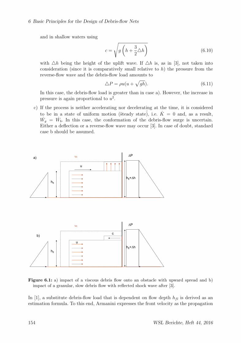
6 Basic Principles for the Design of Debris-flow Nets
and in shallow waters using
c =
√g
(h+
3
24h)
(6.10)
with 4h being the height of the uplift wave. If 4h is, as in [3], not taken intoconsideration (since it is comparatively small relative to h) the pressure from thereverse-flow wave and the debris-flow load amounts to
4P = ρu(u+√gh). (6.11)
In this case, the debris-flow load is greater than in case a). However, the increase inpressure is again proportional to u2.
c) If the process is neither accelerating nor decelerating at the time, it is considered
to be in a state of uniform motion (steady state), i.e. K = 0 and, as a result,Wg = Wb. In this case, the conformation of the debris-flow surge is uncertain.Either a deflection or a reverse-flow wave may occur [3]. In case of doubt, standardcase b should be assumed.
∆P
hfl
hfl+∆h
u
Vc a)
∆P
hfl
hfl+∆h u
Vc
c b)
Figure 6.1: a) impact of a viscous debris flow onto an obstacle with upward spread and b)impact of a granular, slow debris flow with reflected shock wave after [3].
In [1], a substitute debris-flow load that is dependent on flow depth hfl is derived as anestimation formula. To this end, Armanini expresses the front velocity as the propagation
154 WSL Berichte, Heft 44, 2016

6.1 Previous Load Approaches for Rigid Structures
of the disturbance of the dam-breaking wave ufront = 2c = 2√gh cos Θ. He inserts this
(amplified by 2) as the dynamic debris-flow load [2]
∆P = 2ρu2front = 4ρghfl cos Θ (6.12)
in addition to a hydrostatic partPstat = γhfl. (6.13)
This results in a force ofPAr = 5ρghfl (6.14)
or the substitute force
FAr = Fdyn + Fstat = 4ρgh2fl +
1
2γh2
fl = 4.5γh2fl. (6.15)
By means of this derivation, a complex load approach was turned into a static approach,which in turn can be used as an approximate value for an estimation of debris-flow loads.
6.1.5 Hubl and Holzinger’s Approach
Hubl and Holzinger [49, 53] derive a pressure formula for debris flows on the basis oflaboratory tests. In order to characterize the flow behavior, they rely on Froude numbers,and to describe the occurring maximum pressures, they define what they refer to aspressure factors, which describe hydrostatic and dynamic pressure. Taken together, thisleads to the following formula
pmax = 4.5ρu0.8(ghfl)0.6 (6.16)
with pmax being the maximum debris-flow load (static and dynamic), ρ being the densityof the debris flow, u being the flow velocity, and hfl being the flow depth of the debrisflow. [8] also suggest this formula for the dimensioning of protective structures in torrents.This formula can be derived by means of the introduction of a pressure factor Kp = pmax
ρv2.
Following calibration with the laboratory tests, this yields Kp = 4.5Fr−1.2 [49], whichin [53] was originally Kp = 5.0Fr−1.2. Kp corresponds to a factor similar to the Π1 = 4P
ρu
defined in this work. This factor takes the dynamic component 4P , as opposed to themaximum load, into consideration (see section 5.3.5.1).Equation 6.16 yields pressure values Kp significantly higher than one for slow Froudenumbers (Fr < 2).
6.1.6 Cantonal Building Insurances (GBV)
Due to a lack of technical design requirements regarding approaches to debris-flow loads,the Swiss cantonal building insurances have issued guidelines for planners and engi-neers [60]. These are based on the previously tested and published guidelines of St.Gallen’s building insurance. The version for all of Switzerland’s cantons takes into ac-count the latest standards for support structures issued by the SIA. However, there is no
WSL Berichte, Heft 44, 2016 155

6 Basic Principles for the Design of Debris-flow Nets
official mandate requiring that the guidelines be followed.The approach to debris-flow loads in the cantonal building insurance GBV’s guidelines issimilar to that of Coussot [20], and can be derived from the flow dynamics of avalanches.The pressure resulting from the dynamic load depends on the flow velocity u, the densityρ, and a dynamic factor a. This yields the formula for the debris-flow load
qf = aρu2 (6.17)
where a = 2 for granulitic debris flows, and a = 4 for granular debris flows.
Figure 6.2: Debris-flow impact on a building. qf is the dynamic debris-flow load, qe is thequasi-static equivalent load of the individual impact, and qf,r is the frictional force acting onthe side walls [60]. Legend: Grundriss = horizontal projection.
In equation 6.17, the hydrostatic debris-flow load also needs to be taken into account.Furthermore, according to [60], the impact of individual blocks also needs to be considered.For the calculation of the resulting concentrated load and its influencing factors - as wellas their spatial distribution across the structure - see [60] on page 81. The analysis of anindividual impact on a support rope of a ring net barrier has been studied as part of thedesign example in section 8.6.6.2.With respect to load distribution, the debris-flow load is distributed uniformly across theheight hfl and is estimated linearly based on the dynamic pressure himp = u2/(2g) (seeFig. 6.2). The concentrated load is to be calculated for the least favorable location. Thefrictional force of the debris flow on structures standing parallel to its flow path will not bediscussed in this work (for full particulars, see [60]). This force component is not relevantfor the design of debris-flow barriers perpendicular to the flow direction.
6.1.7 Swiss Construction Standard SIA
Generally, there are no specific construction standards for debris-flow loads, neitherin Switzerland (SIA) nor in Germany (DIN, see section 6.1.8). The guidelines by the
156 WSL Berichte, Heft 44, 2016

6.1 Previous Load Approaches for Rigid Structures
Cantonal insurances [60] described in the previous section extend the scope of the SwissSIA standard.In SIA 261/1 [93], debris flows are referred to as extraordinary impacts. These aregenerally recorded by means of hazard and intensity maps, according to Confederationrecommendations and guidelines. They are based on recurrence periods of 30, 100, and300 years. SIA 261/1 subdivides debris flows into two levels of intensity - medium andstrong. A debris flow of medium intensity is associated with flow depths of hfl < 1m andflow velocities of u < 1m/s; both the flow velocities and flow depths are higher thanthese threshold values for debris flows of strong intensity.Based on SIA 260 [91] and the GBV, the following design concept with the appropriatesafety factors was devised and is shown in Table 6.1.
Table 6.1: Safety factors for the impact of debris-flow loads according to the GBV [60] basedon SIA 260 [91]
Recurrence Period Safety Factor γf Impact
1 - 30 years γf = 1.5 Fd1
30 - 100 years γf = 1.3 Ad2
More than 100 years γf = 1.2 Ad2
1 Normal impact Fd according to paragraph 4.4.2.1 SIA 2602 Extraordinary impact Ad according to paragraph 3.2.2.8
SIA 260
The rated value of an impact Fd or an extraordinary impact Ad is then calculated asfollows:
Fd = γfFrep or. Ad = γfArep (6.18)
with Frep being the representative intensity and Arep being the extraordinary intensityof the debris-flow impact. The debris-flow impact has to be determined according to theload approach of the GBV’s guidelines.The design concept proposed by the GBV contradicts SIA 261/1 [92], which states thatdebris flows should always be categorized as extraordinary impacts. As a result, accordingto Table 6.1, only recurrence periods greater than 30 years with γf = 1.3 and γf = 1.2would be taken into consideration. Chapter 8 provides further information regarding aproposed design concept for the ring net barriers, which is followed by a critical analysisof the safety factors proposed in the GBV (on the basis of the SIA). Moreover, the questionconcerning the required safety parameters represents a potential future prospect for thiswork.
6.1.8 German Industry Standard DIN
Debris-flow loads are not explicitly considered in the German DIN standards. In Germany,check dams are designed using the load approach by Lichtenhahn [89], according to the
WSL Berichte, Heft 44, 2016 157

6 Basic Principles for the Design of Debris-flow Nets
Bavarian Office for the Environment (see section 6.1.2).The safety factors on the impact side depend on whether the debris flow is defined as anextraordinary impact Ad or as an unfavorable, variable impact (working load).
• According to DIN 1055-9 [28], extraordinary impacts usually have a short durationof action and a low probability of occurrence. Here, Ad = γAAk with γA = 1.0 appliesto the impact (according to DIN 1055-100 [27]). In addition, the continuous strainresulting from the dead load has to be taken into account in the form of γG = 1.0and combined with the extraordinary load.
• If the debris-flow impact is not considered to be an extraordinary impact, and insteadis classified as a variable impact, the safety factor changes to γQ = 1.5. Here, thepermanent loads need to be taken into account using γG = 1.35.
6.1.9 Evaluation of Load Approaches for Rigid Barriers
The load approaches for debris flows generally can be subdivided into three different types.
• Static approaches Only the flow depth of the debris flow is considered as a de-pendent variable in the calculation (see Lichtenhahn’s approach [66]). Density andflow velocities are not explicitly taken into account. The dynamic debris-flow load isthen calculated based on an amplification of the static water pressure with a factorof 3− 11.
• Mixed approaches Here, both the hydrostatic as well as the dynamic debris-flowloads are taken into account in the form of discrete variables (approaches accordingto Kherkheulidze [61], Armanini/Scotton [3], and the mudflow approach accordingto Coussot [20]). Because this latter mixed-approach method considers both com-ponents (static and dynamic) separately, it is based on the laws of physics. Withrespect to the dynamic component, all approaches incorporate the squared velocity,thus indicating the kinetic energy.
• Dynamic approaches These methods usually calculate only the dynamic compo-nent of the debris-flow load. The static component needs to be either consideredseparately (see the GBV’s approach [60]) or ignored due to the high amplificationof the dynamic component (see Coussot’s approach for granular debris flows [20]).Furthermore, some approaches take both into account because they are based onmaximum pressures recorded, such as the approach according to Hubl/Holzinger [8].
Figure 6.3 provides a comparison of the results of the load approaches for rigid barriers.Here, it becomes apparent that - starting at a certain range of velocities (u > 10m/s)- all static approaches yield lower results than the mixed and dynamic approaches. Ofthe approaches that depend on velocity (mixed and dynamic), Kherkheulidze’s approachyields the lowest results. By far the largest loads are obtained using the GBV’s approach, inwhich α = 4 is applied. Within the context of guidelines for the protection of objects [60],this value is probably on the reasonably safe side.As of yet, Coussot’s approach [20] has not been included in the comparison. He proposes a
158 WSL Berichte, Heft 44, 2016
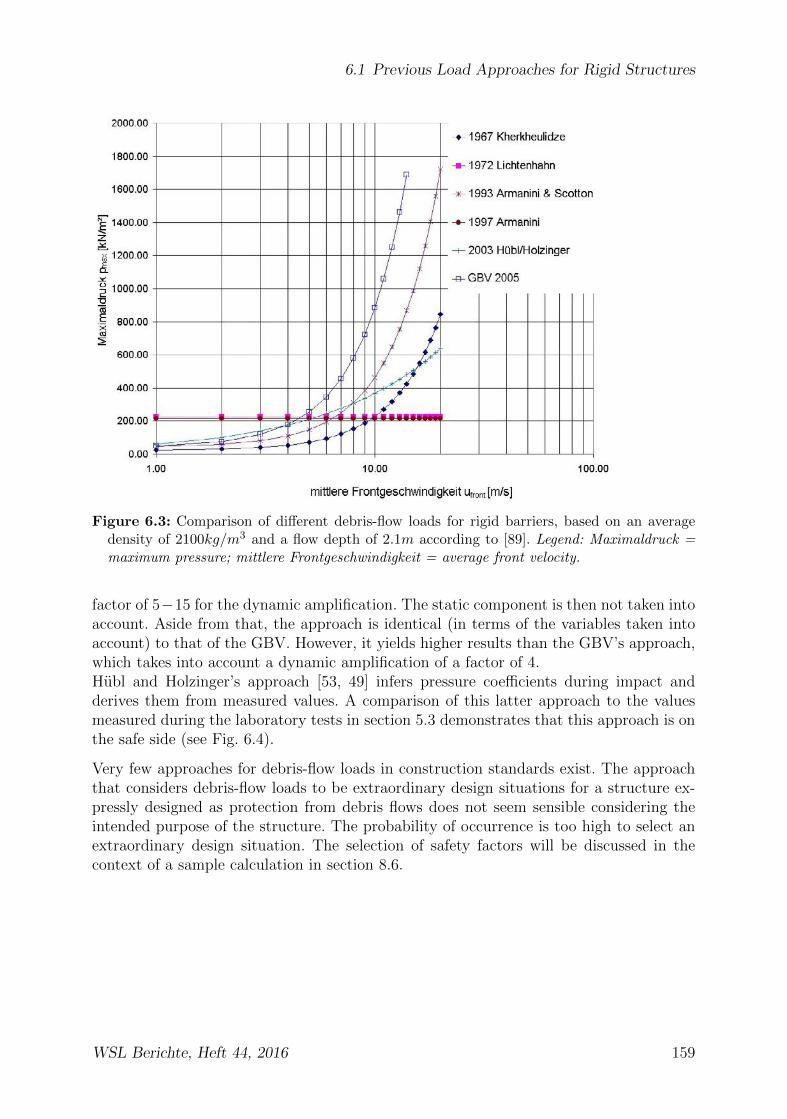
6.1 Previous Load Approaches for Rigid Structures
Figure 6.3: Comparison of different debris-flow loads for rigid barriers, based on an averagedensity of 2100kg/m3 and a flow depth of 2.1m according to [89]. Legend: Maximaldruck =maximum pressure; mittlere Frontgeschwindigkeit = average front velocity.
factor of 5−15 for the dynamic amplification. The static component is then not taken intoaccount. Aside from that, the approach is identical (in terms of the variables taken intoaccount) to that of the GBV. However, it yields higher results than the GBV’s approach,which takes into account a dynamic amplification of a factor of 4.Hubl and Holzinger’s approach [53, 49] infers pressure coefficients during impact andderives them from measured values. A comparison of this latter approach to the valuesmeasured during the laboratory tests in section 5.3 demonstrates that this approach is onthe safe side (see Fig. 6.4).
Very few approaches for debris-flow loads in construction standards exist. The approachthat considers debris-flow loads to be extraordinary design situations for a structure ex-pressly designed as protection from debris flows does not seem sensible considering theintended purpose of the structure. The probability of occurrence is too high to select anextraordinary design situation. The selection of safety factors will be discussed in thecontext of a sample calculation in section 8.6.
WSL Berichte, Heft 44, 2016 159

6 Basic Principles for the Design of Debris-flow Nets
Figure 6.4: Comparison of the cD value according to Hubl and Holzinger’s approach to thatof the laboratory tests. In contrast to Figure 5.19, here, Pmax is used for Π1 instead of ∆P .Legend: Kurve = curve; Messdaten Laborversuche = measured data from laboratory tests.
160 WSL Berichte, Heft 44, 2016

6.2 Approaches for Flexible Barriers
6.2 Approaches for Flexible Barriers
Only a few approaches exist to date for debris-flow load on flexible barriers [82]. If theproblem is considered precisely, it must be solved with an FSI1 calculation [104, 107].The ring net barrier deforms during the filling process and then forms a new equilibriumcondition for the inflowing fluid with each time step ∆t. This relatively laborious calcu-lation process is circumvented in the following load approaches and calculation methodsby determining a quasi-static equivalent load.
6.2.1 Comparison between Effects of Rockfall and Debris flow
The definitive difference in the effect of a debris flow on a ring net is that the load formedby the inflow of the debris flow is effective over a wide area. In addition, the durationof action and filling time are longer and less dynamic than the duration of contact of arockfall with a flexible barrier. These aspects have been confirmed by corresponding dropexperiments, which are described in more detail in the work of Franke [42]. An overviewof the differences between rockfall and debris-flow loads on flexible barriers is providedin Table 6.2.
Table 6.2: Comparison between rockfall and debris-flow effects on flexible barriers.
Rockfall Debris flow
Effect Concentrated load Distributed load: debris-flow loadConcentrated load: Individual impact of a block
Duration of action 0.2− 0.5 s 1− 90 s
Process Single impact Filling in surges
Deformation 5− 12m 2− 3m
The individual impact of a stone is not taken into account in the load approaches below,because this has already been researched thoroughly in ring net barriers used as rockfallbarriers. Many studies and applications have shown that an individual impact of a stonecan be arrested within the provided energy class of ring nets [103, 45]. With ring nets forretaining wood, individual impact experiments with tree trunks have shown that kineticenergies of up to 2500 J can be retained in the ring net and of up to 700 J can be retaineddirectly at the support rope [83]. For the approach of an equivalent load for the individualimpact of a stone in the debris flow, the approach of the GBV [60] can be used, based onthe kinetic energy (mass m and flow velocity u of the stone). An individual impact of ablock at the support rope is discussed as part of the design example in section 8.6.6.2.
1Fluid-structure interaction calculation
WSL Berichte, Heft 44, 2016 161

6 Basic Principles for the Design of Debris-flow Nets
6.2.2 Back-calculation of Measured Rope Forces to the Effects
In this section, the mechanical properties of cable ropes are described and the backgroundof the rope equation and its approximate solution are explained. For different forms ofeffective load (uniformly-distributed load, parabolic load and triangular load), their re-sulting rope loads and deformations are determined and compared with the measuredvalues (see section 4.5.3).
6.2.2.1 Mechanical Properties of Ropes
For cable ropes, it is assumed that they are ideally flexible and therefore can only absorbtensile forces. Although there is a slight bending stiffness, this is very small comparedwith the axial stiffness and is disregarded [72].Ropes exhibit the following deformation behavior under load:
• elastic strain, which is reversible after the load is removed,
• plastic strain, which is irreversible after loading,
• rheological strain, which occurs as a result of creep under long-term loading.
The plastic strain after initial loading is of great importance for steel stranded ropes.This occurs owing to interstices between the individual wires, which become aligned oninitial loading and thus result in plastic strain. The typical stress-strain curve of ropes istherefore non-linear on initial loading. A linear stress-strain relationship is only producedafter repeated loading. For this region, the rope modulus of elasticity is definedeither as a tangent modulus or as a secant modulus [40]. For the further calculationsin this paper, an E-modulus of 1.28 · 1011 N/m2 is used for the stranded ropes. It doesnot matter exactly which load range this has been determined for, owing to the largeelongations as a result of the brake elements in the support ropes, because the elasticstrains are very small in comparison. In addition, the ropes are generally not pre-loadedbefore installation.The assumed rope slack is also an important variable in the installation of the ropes.Rope slacks ld between l/30 and l/50 of the span l were assumed [39]. Then the differenceof both values on the resulting load was studied. Here it was found that the elongationof the brakes in the support rope was more decisive for the rope load than the initial slack.
6.2.2.2 Rope Equation
There is a rope under an arbitrary load q(x) with axial stiffness EA. The followingrelationships exist between the individual rope lengths in the initial and end stages
162 WSL Berichte, Heft 44, 2016

6.2 Approaches for Flexible Barriers
s length of rope in end states0 = l + ld length of rope in initial state, l is the span,
ld = l/50..l/30 the slack∆s elastic change in length of rope∆st elongation of rope as a result of temperature change
The bearing forces F and H are equal on both sides (see Fig. 6.5). The assumption thatthe bending moment M is zero in each part of the rope means that
M −Hy = 0. (6.19)
FropeF
l
Frope
H
φ H
φ q(x)
x
y ds
φ f
φ
S
H ds
S+ds
dx
q(x)ds
H
Rope element (section):
F
Figure 6.5: Rope under the effect of an arbitrary, uniformly-distributed load and forces and adetail of a rope element.
At the point of max. slack f,
f =maxM
H. (6.20)
The sagitta f is however often unknown before loading. Therefore, the geometric lengthof the rope s0 and s before and after loading must be derived as well. If the rope elementds (Fig. 6.5) is considered, then [72]
ds =√dx2 + dy2 = dx
√1 + y′2. (6.21)
ds, integrated over the entire rope length, produces
s =
∫ l
0
√1 + y′2dx =
∫ l
0
√1 +
(1dM
Hdx
)2
dx. (6.22)
WSL Berichte, Heft 44, 2016 163
6 Basic Principles for the Design of Debris-flow Nets
dM/dx can be replaced by the transverse force Q and results in
s =
∫ l
0
√1 +
(Q
H
)2
dx. (6.23)
The elastic deformation of the rope ∆s can then be calculated from
∆s =
∫ s
0
εds =
∫ l
0
H
EA cosφ
√1 + y′2dx =
H
EA
∫ l
0
(1 + y′2)dx =H
EA
∫ l
0
(1 +
Q2
H2
)dx.
(6.24)The elongation of the rope as a result of temperature is calculated to be
∆st = αt∆ts0 (6.25)
where αt is the temperature strain value for steel and ∆t is the temperature difference.Everything inserted into s = s0 + ∆s+ ∆st produces∫ l
0
√1 +
(Q
H
)2
dx = s0(1 + αt∆t) +H
EA
∫ l
0
(1 +
Q2
H2
)dx. (6.26)
This equation is the generally valid exact rope equation. It includes any desired loads andrope slacks of any size.However, the solution of this equation presents some problems, because it is only possibleusing numerical integration. To carry out practical calculations, an approximate solutionmust be derived. The brake elongation, which is relevant in the case of ropes for ring netbarriers, is also implemented in the equation.
6.2.2.3 Approximate Solution of the Rope Equation
If equation 6.22 is approached using a Taylor series, then
s =
∫ l
0
(1 +
1
2y′2 − 1
8y′4 +
1
16y′6...
)dx. (6.27)
For small rope slacks, a restriction can be made to the first two terms, therefore
s ≈∫ l
0
(1 +
1
2y′2)
=
∫ l
0
(1 +
1
2
Q2
H2
)dx. (6.28)
The elastic change in length can also be approximated to be
∆s ≈ Hs0
EA. (6.29)
The rope equation overall can then be simplified to
1 +1
2H2
∫ l
0
Q2dx = s0(1 + αt∆ts0) +Hs0
EA. (6.30)
164 WSL Berichte, Heft 44, 2016

6.2 Approaches for Flexible Barriers
This equation can be rearranged to
H3 +H2EA
[1− 1
s0
(l − αt∆ts0)
]=EA
2s0
∫ l
0
Q2dx. (6.31)
This equation can be solved iteratively by substituting H. It corresponds to the formH3 + bH2 − c = 0 and only has a real solution for H [72].As a first approximate solution for the first iteration, H is calculated for EA → ∞ togive
H = H1 =
√ ∫ l0Q2dx
2(s0(1 + αt∆t)− l). (6.32)
The brake elongation is then introduced and the first iteration is carried out again for theretaining force H. The elastic rope strain ∆s is also included withH1,corr. stot = s0+∆s+lbris inserted instead of s0(1+αt∆t); the temperature strain is disregarded in this case. Thisyields
H1,corr =
√ ∫ l0Q2dx
2(stot − l). (6.33)
If H1,corr is known, the next steps are determined using a Newton method. For the secondapproximation of H,
H2 =2H3
1,corr + bH21,corr + c
3H21,corr + 2bH1,corr
(6.34)
where b = EA(
1− l−lbrs0
)and c = EA
∫ l0 Q
2dx
2s0. The same procedure applies to the i-th
iteration, 2 − 3 iterations usually being sufficient in practice. Different loads and theireffect in terms of rope force and deformation are studied below. Here it is necessaryto determine the integral
∫ l0Q2dx and calculate the max. deformation values from the
moment line (see Table 6.3).
Table 6.3: Effective load q with bearing force,∫ l
0 Q2dx and max. deformation f
Load q Bearing force F∫ l
0Q2dx max f = maxM
h
q(x) 12ql 1
12q2l3 ql2
8H
q(x)14ql 7
240q2l3 ql2
12H
q(x) 14ql q2l3
18.535ql2
48H
The sagitta f of the rope deformation is always dependent on the direct span l, becausethe max. deformation f is derived from equation 6.19. To include the brake elongation inthe horizontal deformation of the rope, the procedure according to Figure 6.6 is followed:First, the vertical deflection f1 is determined for the direct span l and the iterated retaining
WSL Berichte, Heft 44, 2016 165
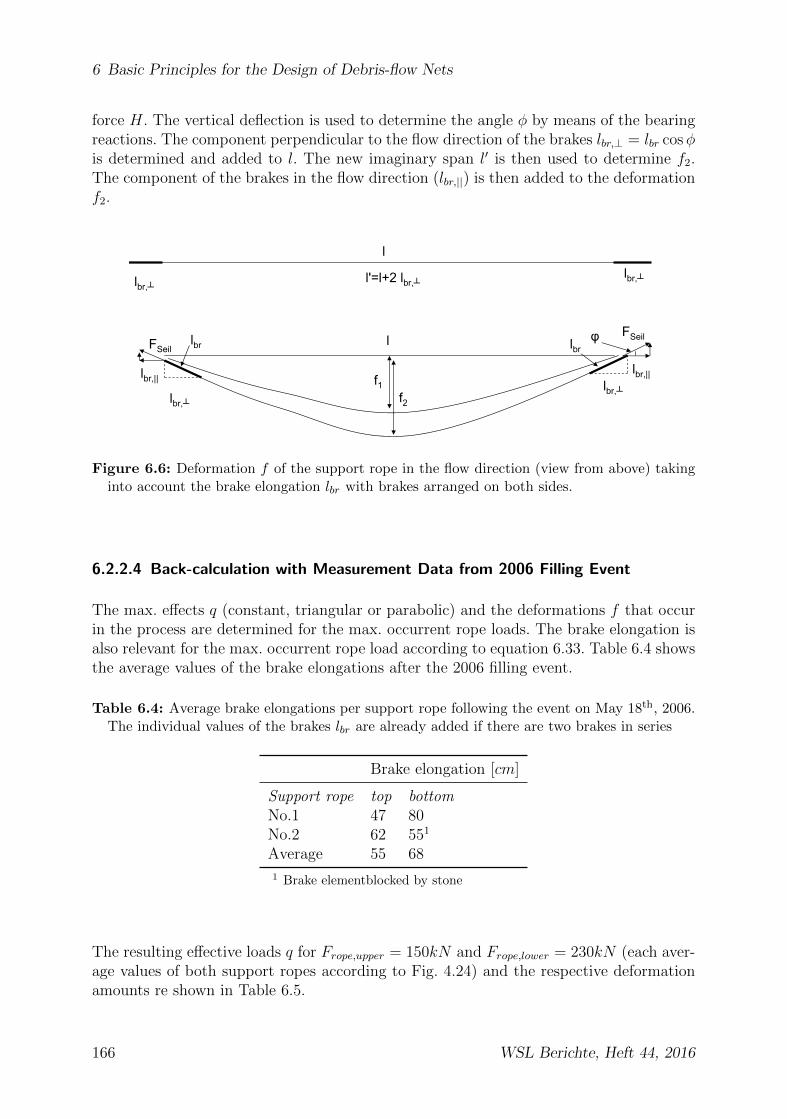
6 Basic Principles for the Design of Debris-flow Nets
force H. The vertical deflection is used to determine the angle φ by means of the bearingreactions. The component perpendicular to the flow direction of the brakes lbr,⊥ = lbr cosφis determined and added to l. The new imaginary span l′ is then used to determine f2.The component of the brakes in the flow direction (lbr,||) is then added to the deformationf2.
lbr,||
lbr,┴lbr,┴
l
l'=l+2 lbr,┴
FSeil
lbr,||
FSeil
lbr,┴
lbr
lbr,┴
lbr
f2
l
f1
φ
Figure 6.6: Deformation f of the support rope in the flow direction (view from above) takinginto account the brake elongation lbr with brakes arranged on both sides.
6.2.2.4 Back-calculation with Measurement Data from 2006 Filling Event
The max. effects q (constant, triangular or parabolic) and the deformations f that occurin the process are determined for the max. occurrent rope loads. The brake elongation isalso relevant for the max. occurrent rope load according to equation 6.33. Table 6.4 showsthe average values of the brake elongations after the 2006 filling event.
Table 6.4: Average brake elongations per support rope following the event on May 18th, 2006.The individual values of the brakes lbr are already added if there are two brakes in series
Brake elongation [cm]
Support rope top bottomNo.1 47 80No.2 62 551
Average 55 68
1 Brake elementblocked by stone
The resulting effective loads q for Frope,upper = 150kN and Frope,lower = 230kN (each aver-age values of both support ropes according to Fig. 4.24) and the respective deformationamounts re shown in Table 6.5.
166 WSL Berichte, Heft 44, 2016
6.2 Approaches for Flexible Barriers
Table 6.5: Effective rope load q and calculated deformation values for equal, triangular orparabolic load and effective total load for an initial slack of ld = l/50 and the measured brakeelongations according to Table 6.4
Equal, triangular, parabolic load
q [kN/m] on upper support rope 21 38 28.2q [kN/m] on lower support rope 48 90 63.1
f ′ [m] 1.91 2.25 1.88φ [◦] 28.2 25.1 24.6f [m] 2.20 2.48 2.02
Total load Ftot [kN ] 780.6 722.6 689.4
The effective loads for the initial slack ld = l/30 are almost 3% higher than the valuesfrom Table 6.5 for ld = l/50. The total load Ftot is calculated from q [kN/m] distributedto the respective rope length of the upper and lower support ropes (lupper = 13.4m andllower = 10.4m).The deformation calculations show the best results for the triangular distribution of theload q, because the max. bulge of the barrier was f ≈ 2.5m (see Table 6.5). Nevertheless,the occurrent loads q are assumed to be evenly distributed in the further calculations,because this assumption is on the safe side for the effective total load (see Table 6.5).
Several simplifications are made when inferring the effective load q with the approximaterope equation. Firstly, there is an inaccuracy from the exact rope equation in the ap-proximate solution for large deformations f . According to [72], for a calculated sagittaf = 2.5m with a span l = 10.4m the error for the ratio f/l = 0.24 with retaining force His 3% and with deformation f is 7%. The error therefore mainly has an effect on the cal-culated sagitta, whereas the retaining force is reproduced virtually correctly. In addition,the calculated rope lengths with the implemented brake elongation are also only approx-imations, because on the one hand the brake elongations cannot be measured exactly atthe time of peak load and on the other hand other variables in the length of the rope suchas slack, elastic strain etc. must be estimated. The calculations are however still usefulfor an approximate calculation of the effective load q.After the analysis of the rope resistance, the resistance of the ring net while the debrisflow flows through is considered in detail below.
6.2.3 Ring Net Flow Resistance
If debris-flow events are very muddy with small grain sizes, most of the material flowsthrough the ring net barrier before isolated stones become wedged and the ring net fillsup. The hydraulic pressure exerted on the ring net in the process serves as the lower limitfor the load model of the ring net barriers in this section.To be able to calculate the flow resistance of the whole ring net, an individual ring is
WSL Berichte, Heft 44, 2016 167

6 Basic Principles for the Design of Debris-flow Nets
considered first. An individual ring with 16 windings according to section 3.2.2.5 has anapproximate wire bundle diameter of dring,∅ ≈ 1.7cm. If flow arrives at this ring accordingto Figure 6.7 at ufront = 3m/s (front velocity of mudflow event on May 18th, 2006; seesection 4.5.1) and with a density ρ = 1600kg/m3, the Reynolds number of the incomingflow is
Re =ufront · dring,∅ · ρ
η=
3.0 · 0.017 · 1600
5...11= 7.5...16. (6.35)
ufront
dRingquerschnitt
x
ydRing
Figure 6.7: Debris-flow flowing into an individual ring at ufront during a muddy event. Legend:Ringquerschnitt = cross-sectional area of net ring
The viscosity of the debris-flow mud is estimated using the shear velocity for a linearvelocity profile at flow depth h = 1m to give γ = 3m/s
1m= 3[1/s]. For the shear velocity
γ = 3[1/s], an average viscosity (linearly interpolated) of η ≈ 5Pas was measured for asuspension with particles d < 2mm and η ≈ 11Pas for a suspension with particles d <4mm. The solids concentration Cv of the solutions was 0.54 and 0.59 with a water contentof w = 30% (for viscosity determinations, see section 5.2.3.4). The solids concentrationis rather high for a mudflow, but this is only the viscosity of the debris-flow matrix withparticles less than 2 and 4mm. Much larger particles are present in the mudflow itself.As an order of magnitude, the viscosity measurements are sufficient for classifying theReynolds number range. For the determined Reynolds number range from 7.5...16, a pairof vortices forms immediately after the flow passes around a cylinder (Karman vortexstreet). At a Reynolds number Re = 4, it would still be a creeping flow without vortexformation [55]. Pressure coefficients of cw = 3.5 − 4 result (see Fig. 6.8). The resultingflow force on the ring cross section is calculated from
FD =1
2cwρu
2dring,∅. (6.36)
The force of the flow around the whole ring is then
Fring = UringFD = πdringFD (6.37)
where Uring is the circumference of an individual ring.If the overlapping rings, where the rings interconnect in the ring net, are disregardedbelow, and the pressure load of a ring around which flow passes is multiplied by the
168 WSL Berichte, Heft 44, 2016
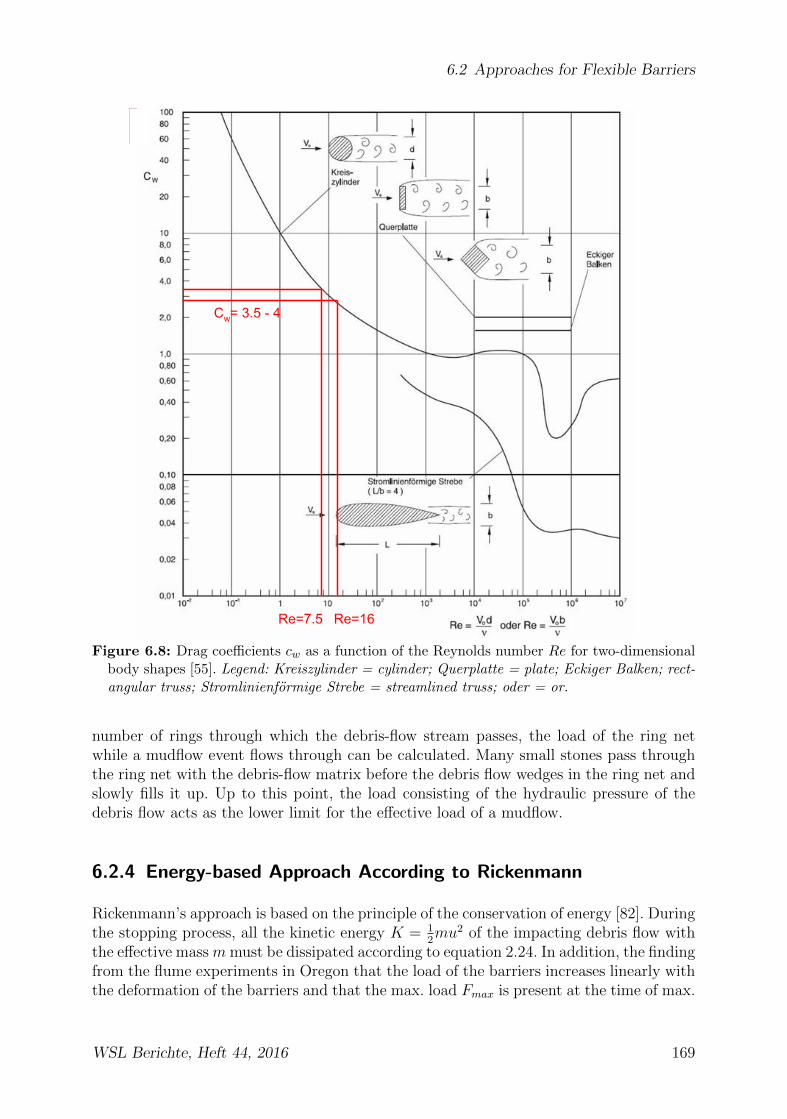
6.2 Approaches for Flexible Barriers
Re=7.5 Re=16
Cw= 3.5 - 4
Figure 6.8: Drag coefficients cw as a function of the Reynolds number Re for two-dimensionalbody shapes [55]. Legend: Kreiszylinder = cylinder; Querplatte = plate; Eckiger Balken; rect-angular truss; Stromlinienformige Strebe = streamlined truss; oder = or.
number of rings through which the debris-flow stream passes, the load of the ring netwhile a mudflow event flows through can be calculated. Many small stones pass throughthe ring net with the debris-flow matrix before the debris flow wedges in the ring net andslowly fills it up. Up to this point, the load consisting of the hydraulic pressure of thedebris flow acts as the lower limit for the effective load of a mudflow.
6.2.4 Energy-based Approach According to Rickenmann
Rickenmann’s approach is based on the principle of the conservation of energy [82]. Duringthe stopping process, all the kinetic energy K = 1
2mu2 of the impacting debris flow with
the effective mass m must be dissipated according to equation 2.24. In addition, the findingfrom the flume experiments in Oregon that the load of the barriers increases linearly withthe deformation of the barriers and that the max. load Fmax is present at the time of max.
WSL Berichte, Heft 44, 2016 169

6 Basic Principles for the Design of Debris-flow Nets
deformation, is also addressed [23, 35]. The linear increase of the force F , plotted overthe deformation f , produces the energy/work from the area under the curve F(t) to give
W =
∫ f
0
F (t)df =Ff
2(6.38)
where f is the deformation of the barrier in the flow direction.If the two equations W = K are equated as occurrent energies and solved according tothe force F , this yields
F =mu2
f(6.39)
where u is the impact velocity of the debris flow and m is the effective mass of the stoppeddebris flow. The size of the stopped mass of the debris flow behind the net is the unknownquantity in this approach. It is approximated in this case as the volume behind the barrierand thereby estimated from the average discharge Q with the density ρ during the impactperiod timp to give m = Q · timp ·ρ. Inserting the effective mass m into equation 6.39 yields
F =ρQtimpu
2
f. (6.40)
The occurrent total load according to this approach is therefore also dependent on theimpact velocity u2. Difficult-to-estimate variables such as the filling time or impact timetimp or the effective mass m are also included.It is not practical to use this approach to design barriers for muddy debris flows, whichhave a long filling time timp and during which a large proportion of the debris flow flowsthrough the ring net as it fills up. The effective loads are overestimated (see section 6.4.2).
6.2.5 Earth Pressure Approach
There are also approaches for debris-flow loads based on an amplification of the static load(see section 6.1.2 and [66]). Building on this, this section investigates whether the ringnet barriers can be calculated by a dynamic amplification of the static loading condition.If the active earth pressure is calculated for a specific weight γ = 23kN , a fill level hfill =3m (see section 4.5.3) and a width b as an average value between the two rope lengthsbm = 10.4 + 13.4 = 11.9m, this gives the following calculation according to equation 5.23assuming a linear earth pressure: Fstat = 1
2Ka,hγh
2fillb = 1
20.3 · 23 · 32 · 11.9 = 370kN with
Ka,h = 0.3 (φ = 33◦).If the effective load q is determined by back-calculation of the occurrent rope forces whenthe barrier is filled, this yields a total load of ≈ 300kN (see Table 6.6). In this case, eachof the upper support ropes are loaded with 100kN and one of the two lower support ropesis loaded with 150kN . The other one is broken during the filling event; the load cell stillmeasures 50kN by means of the clamped rope end.Assuming a tensile force of 15kN in the DIMO elements from the FARO simulation of thebarrier (see section 7.1), a component in the flow direction of 15 · 8 DIMOs · sin(28◦) =56kN is added. This yields a total load of the barrier in the filled state of 356kN .
The calculations for the active earth pressure therefore correspond well to the back-calculation of the measured values from the rope loads.
170 WSL Berichte, Heft 44, 2016

6.2 Approaches for Flexible Barriers
Table 6.6: Effective load q from a simplified rope equation according to section 6.2.2.
Effective load
Upper support ropes 14 kN/mLower support ropes 11 kN/m (one broken support rope)Total load Ftot 302kN
6.2.5.1 Development of the Earth Pressure Approach
Here, the calculation of the dynamic load from the static load is investigated, based on theapproach according to Lichtenhahn [66]. According to [46], laboratory tests indicated adependence of the quotient Fmax/Fstat on the squared velocity u, since influencing factorssuch as different densities and masses cancel each other out in the quotient. A steeperregression curve was found for the material from the Trachtbach than for all the othermaterials. The following functional dependency is produced
ln
(FmaxFstat
)= βu2 (6.41)
where β = 0.144 for Trachtbach material and β = 0.070 for Illgraben, Alpbach and Mer-denson with R2 = 0.9. The Trachtbach material also had a higher pressure coefficient cdin the laboratory tests, which explains the steeper curve in Figure 6.9 (see section 5.3.5.1).
6.2.5.2 Back-calculation of 2006 Illgraben Filling Event Measurement Data
If one takes the active earth pressure as a given as the static load and defines for thefront velocity of ufront = 3m/s (see section 4.5.1) the ratio Fmax/Fstat according to equa-tion 6.41, this yields an amplification of the static load of Fmax/Fstat = 1.88. The loadfrom the active earth pressure Eah is Fstat ≈ 370kN , and with the calculated factor am-plified, this yields Fdyn = 1.88 · 370 = 690kN . This value lies in the lower range of thecalculated total load on the barrier according to Table 6.5 at 690−780kN (without takinginto account the installed dimo elements).Back-calculations and simulations with FARO (see section 7.1) have shown that the loaddistribution must also be modified for dynamic amplification (see Fig. 6.10). If the dis-tribution of the active earth pressure is amplified with the dynamic factor (assuming itis distributed linearly) and these loads are used to calculate the rope forces, this yieldsan excessively large load in the lower support ropes and an excessively small load in theupper ones.With a linear earth pressure distribution, the vertical load and the surge component ofthe overflowing debris flow are also missing. As a result, the initially assumed distributionis shifted from Pdyn to Pdyn,corr. (see also Fig. 6.20). At the same time, the load in thelower region must be reduced. This is done by taking into account the supporting forceof the backwater on the barrier caused by the overflow of the debris flow (see Fig. 6.11).
WSL Berichte, Heft 44, 2016 171

6 Basic Principles for the Design of Debris-flow Nets
5
4
I.L
I.L
2
1
0
0
Material
x Alpbs.ch • 11 l!graben+ trv�eirdenson
Tradhtbach
+ . __ ... .
+ ... ··�-�-�
- :I:_.
.... ,.
,,
0
I
0 I
.... ,·
,..
�
.. +-"'
x
• 1,0
0 I
I
I
I
t
a. , J
• x
,/'
I
•
Q ,,
• ,
x• ,,. Oo 0
,,. , O(oQ) 0 0 10
0 0 (0
•'0 0
0
'to rO
0
--------------------------------
2 3
Regressi:on Tradhtbach Regressi:on others
4
Velocity before impact 1(m/s)
Figure 6.9: Relationship between the maximum and static load depending on the impact ve-locity u. The regression is based on experiments with a mesh size of 3cm. Experiments withother mesh sizes are indicated with an empty symbol.
Eah
dyn. factor
Pdyn
Pdyn,corr.
Figure 6.10: Amplification of the active earth pressure to the dynamic debris-flow pressureand modification of the dynamic debris-flow pressure (dashed line).
6.2.6 Evaluation of Load Approaches for Flexible Barriers
The comparison between rockfall and debris-flow load shows that the debris flow is ef-fective over an area rather than at points like the rockfall and is at the same time lessdynamic. Section ”Back-calculation of Rope Forces” (see section 6.2.2) serves to deter-mine the effective load q from the measured rope forces, but should not be understood asa load approach for the calculation of barriers and should not be used as such.
172 WSL Berichte, Heft 44, 2016
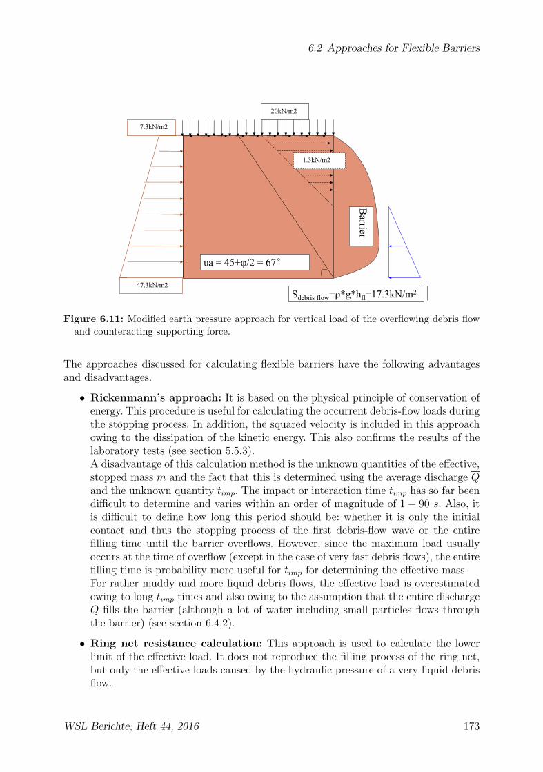
6.2 Approaches for Flexible Barriers
υa = 45+φ/2 = 67°
Barrier
20kN/m2
1.3kN/m2
7.3kN/m2
47.3kN/m2 Sdebris flow=ρ*g*hfl=17.3kN/m2
Figure 6.11: Modified earth pressure approach for vertical load of the overflowing debris flowand counteracting supporting force.
The approaches discussed for calculating flexible barriers have the following advantagesand disadvantages.
• Rickenmann’s approach: It is based on the physical principle of conservation ofenergy. This procedure is useful for calculating the occurrent debris-flow loads duringthe stopping process. In addition, the squared velocity is included in this approachowing to the dissipation of the kinetic energy. This also confirms the results of thelaboratory tests (see section 5.5.3).A disadvantage of this calculation method is the unknown quantities of the effective,stopped mass m and the fact that this is determined using the average discharge Qand the unknown quantity timp. The impact or interaction time timp has so far beendifficult to determine and varies within an order of magnitude of 1− 90 s. Also, itis difficult to define how long this period should be: whether it is only the initialcontact and thus the stopping process of the first debris-flow wave or the entirefilling time until the barrier overflows. However, since the maximum load usuallyoccurs at the time of overflow (except in the case of very fast debris flows), the entirefilling time is probability more useful for timp for determining the effective mass.For rather muddy and more liquid debris flows, the effective load is overestimatedowing to long timp times and also owing to the assumption that the entire dischargeQ fills the barrier (although a lot of water including small particles flows throughthe barrier) (see section 6.4.2).
• Ring net resistance calculation: This approach is used to calculate the lowerlimit of the effective load. It does not reproduce the filling process of the ring net,but only the effective loads caused by the hydraulic pressure of a very liquid debrisflow.
WSL Berichte, Heft 44, 2016 173

6 Basic Principles for the Design of Debris-flow Nets
• Earth pressure approach and amplification by Fmax/Fstat: The earth pressureapproach is used for calculation of the static load of a ring net barrier. It demon-strates here that the filled ring net barrier can be calculated by means of a linearlydistributed earth pressure.The limits of this approach lie in the fine distribution of the effective load. In thiscase it is shown that the upper support ropes are also directly loaded during over-flow. Also, the lower support ropes are highly loaded when the linearly effectiveearth pressure is amplified. In this case the load can only be reduced with a sup-porting force approach on the opposite side of the barrier.Owing to the highly material-dependent, unknown friction angle φ, the static loadFstat is difficult to estimate. If this is increased further by an amplification factor,errors in the calculation have a great effect on the result. The definition of theamplification factor from the squared impact velocity also quickly results in under-or overestimation of the load if the velocity inputs are incorrect. Also, force rear-rangements must be defined, which require a lot of engineering experience in theestimation of the effective vertical load and the supporting force of the overflowingdebris flow.
Overall, all approaches have their justification and their area of effectiveness. Nevertheless,a model will be presented in the next section of this paper that can minimize or solvesome of the previous problems and therefore should be used as a new calculation modelfor flexible debris-flow barriers.
174 WSL Berichte, Heft 44, 2016

6.3 Load Model with Pressure Surges
6.3 Load Model with Pressure Surges
The following observations, made in the laboratory (see chapter 5) and in the field tests(see chapter 4), confirm Armanini’s assumptions (see section 6.1.4):
• The dynamically-measured maximum force is proportional to the impact velocityu2 (statements a) and b) in section 6.1.4).
• In very slowly-flowing debris flows, for example in the laboratory debris flows (atan inclination of 25%), a reverse-flow wave was observed (assumption b) in sec-tion 6.1.4).
• With liquid and thus faster debris flows, an upward deflection of the debris-flowstream was observed at the barrier (assumption case a) in section 6.1.4). In addition,the friction coefficient µ for more liquid debris flows are lower (see chapter 5).
• Greater launch volumes lead to more rapid debris flows, during which frictionalforces play a less significant role. In these cases, an upward deflection of the debrisflow occurred upon impact onto the barrier as well.
• At the shear wall in the Illgraben, a hydrostatic pressure distribution in debris flowscould be measured and confirmed (see section 4.4). In this case, the dynamic loadapplied by the momentum of the flow can be neglected, since the measurementinstrumentation at the shear wall is located perpendicularly to the direction offlow. Therefore, the velocity component u⊥ perpendicular to flow direction equalsapproximately zero.
6.3.1 Pressure Surges on Ring Net Barriers
First, it is assumed that a debris flow of flow depth hfl strikes against the lower supportropes, causing the first part of the front to stop (see Fig. 6.12, a). As a result, the hydro-static debris-flow load Pstr and the momentum ∆P are acting on the lower support rope.The impacting load per meter width can be calculated as
F =1
2γ(hfl +4h)2︸ ︷︷ ︸
hydrostatic component
+
ρhflu2 for muddy fronts
ρhflu(u+√ghfl) for granular fronts︸ ︷︷ ︸
hydrodynamic component
(6.42)
γ = ρg is the specific weight of a debris flow with the density ρ.
WSL Berichte, Heft 44, 2016 175

6 Basic Principles for the Design of Debris-flow Nets
hfl
Ring net
illin st e 1
Phyd
P
Variant 1
P
Variant 2
hflh=hfl
∆P/2∆P
illin st e 2
Ring net
hfl
Material stopped, draining
u
Phyd
Upper support rope moves diagonally towards the front
Variant 1 Variant 2
hfl
Lower support rope moves downwards
h
illin st e 3
Material stopped nd
ein dr ined
u
hfl
Phyd
P P/3
Variant 1 Variant 2
hfl
h
Figure 6.12: Filling stage 1: Debris-flow load during impact on the lower support rope; fillingstage 2: Debris-flow load following stopping of the first part; filling stage 3: Predicted subse-quent filling process and reduction of the hydrostatic debris-flow load due to drained debriscone (dotted line). Two conceivable ways the dynamic debris-flow load can be distributed areindicated.
With respect to the subsequent filling process, two different filling scenarios are conceiv-able:
176 WSL Berichte, Heft 44, 2016
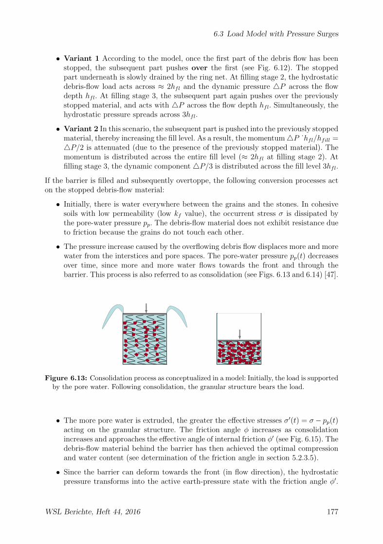
6.3 Load Model with Pressure Surges
• Variant 1 According to the model, once the first part of the debris flow has beenstopped, the subsequent part pushes over the first (see Fig. 6.12). The stoppedpart underneath is slowly drained by the ring net. At filling stage 2, the hydrostaticdebris-flow load acts across ≈ 2hfl and the dynamic pressure 4P across the flowdepth hfl. At filling stage 3, the subsequent part again pushes over the previouslystopped material, and acts with 4P across the flow depth hfl. Simultaneously, thehydrostatic pressure spreads across 3hfl.
• Variant 2 In this scenario, the subsequent part is pushed into the previously stoppedmaterial, thereby increasing the fill level. As a result, the momentum4P ˙hfl/hfill =4P/2 is attenuated (due to the presence of the previously stopped material). Themomentum is distributed across the entire fill level (≈ 2hfl at filling stage 2). Atfilling stage 3, the dynamic component 4P/3 is distributed across the fill level 3hfl.
If the barrier is filled and subsequently overtoppe, the following conversion processes acton the stopped debris-flow material:
• Initially, there is water everywhere between the grains and the stones. In cohesivesoils with low permeability (low kf value), the occurrent stress σ is dissipated bythe pore-water pressure pp. The debris-flow material does not exhibit resistance dueto friction because the grains do not touch each other.
• The pressure increase caused by the overflowing debris flow displaces more and morewater from the interstices and pore spaces. The pore-water pressure pp(t) decreasesover time, since more and more water flows towards the front and through thebarrier. This process is also referred to as consolidation (see Figs. 6.13 and 6.14) [47].
Figure 6.13: Consolidation process as conceptualized in a model: Initially, the load is supportedby the pore water. Following consolidation, the granular structure bears the load.
• The more pore water is extruded, the greater the effective stresses σ′(t) = σ− pp(t)acting on the granular structure. The friction angle φ increases as consolidationincreases and approaches the effective angle of internal friction φ′ (see Fig. 6.15). Thedebris-flow material behind the barrier has then achieved the optimal compressionand water content (see determination of the friction angle in section 5.2.3.5).
• Since the barrier can deform towards the front (in flow direction), the hydrostaticpressure transforms into the active earth-pressure state with the friction angle φ′.
WSL Berichte, Heft 44, 2016 177

6 Basic Principles for the Design of Debris-flow Nets
pp
t
∆pp=∆σ
t0
pp
t
σ' = σ - pp
t0
∆σ
σ'
Figure 6.14: Consolidation process with development of pore-water pressure pp and the effec-tive stress σ′ over time t.
σ
τ
Overall slip circle
Effective slip circle
σ3' σ3 σ1' σ1∆pp ∆pp
φu
φ' cu c'
Figure 6.15: Effects of pore-water pressure on the angle of internal friction φ′. At first, theinitial shear strength cu exhibits almost no internal friction (low φu or φu = 0). The initialshear strength cu, due to the apparent cohesion of the Van der Waals forces of the watermolecules, is greater than the effective cohesion c′, due to the attraction of the capillaryforces [47].
For the time period between these two load cases,
1
2Ka,hγh
2fill < Fstr <
1
2γh2
fill (6.43)
applies, with Ka,h as the active earth-pressure factor (see section 5.3.5.2). Howquickly the drained debris-flow cone approaches the active earth-pressure statedepends primarily on the composition of the debris-flow material. If the debris-flowmaterial has a very high fine fraction (grain sizes of d < 0.06mm constitute morethan 20%), it usually has a low kf value, and accordingly, the consolidation processtakes longer. If the material is more gravelly and contains larger blocks, drainage
178 WSL Berichte, Heft 44, 2016

6.3 Load Model with Pressure Surges
takes significantly less time, and the active earth pressure is reached sooner.The transitional stage is depicted as a dotted line in Figure 6.12, filling stage 3 (seealso section 6.3.5).
The load distribution across the support ropes is a structural problem concerning theinvolved ring-net areas. In this case, the different pressure distributions in variants 1and 2, which are examined in section 6.3.3, need to be taken into account.
6.3.2 Load comparison: granular front - muddy front
The following section will compare data from a muddy debris-flow event with those from agranular event with respect to the previously-discussed pressure distributions. The impactvelocities are estimated at ufront = 3m/s and 5m/s at flow depths of 1m. For muddy debrisflows, the density is set to ρ = 1600kg/m3 and for granular debris flows to 2000kg/m3.This yields the following loads impacting onto the barriers, as in Table 6.7.
Table 6.7: Load comparison between granular debris flows and mudflows based on the approachaccording to [3]
Muddy debris flow Granular debris flowufront[m/s] Fstr[kN/m] Fdyn[kN/m] Fstr[kN/m] Fdyn[kN/m]
Filling stage 1 3 8 14.4 10 24.7Filling stage 2 3 32 14.4 40 24.7Filling stage 3 3 72 14.4 90 24.7
Filling stage 1 5 8 40 10 50Filling stage 2 5 32 40 40 50Filling stage 3 5 72 40 90 50
For the calculation of the impacting forces in Table 6.7, 4P was set to 4P = ρu2 formuddy debris flows, and to 4P = ρu(u +
√ghfl) for granular events, corresponding to
the developing reverse-flow wave. For muddy events with very low densities and high flowvelocities, Armanini et al. [2] set the dynamic pressure component to 4P ≈ 0.7ρu2. Forgranular debris flows, which flow more slowly because frictional forces predominate, thedynamic amplification 4P = 2ρu2 was selected. As a result, the difference between theforces acting during muddy and granular debris flows increases (see Fig. 6.16).
As shown in Figure 6.16, the forces acting during granular debris flows are approximately70% greater than those acting during muddy debris flows, according to the approach byArmanini. If Armanini’s prefactors are not taken into consideration, the forces actingduring granular debris flows are approximately 50% greater.
WSL Berichte, Heft 44, 2016 179
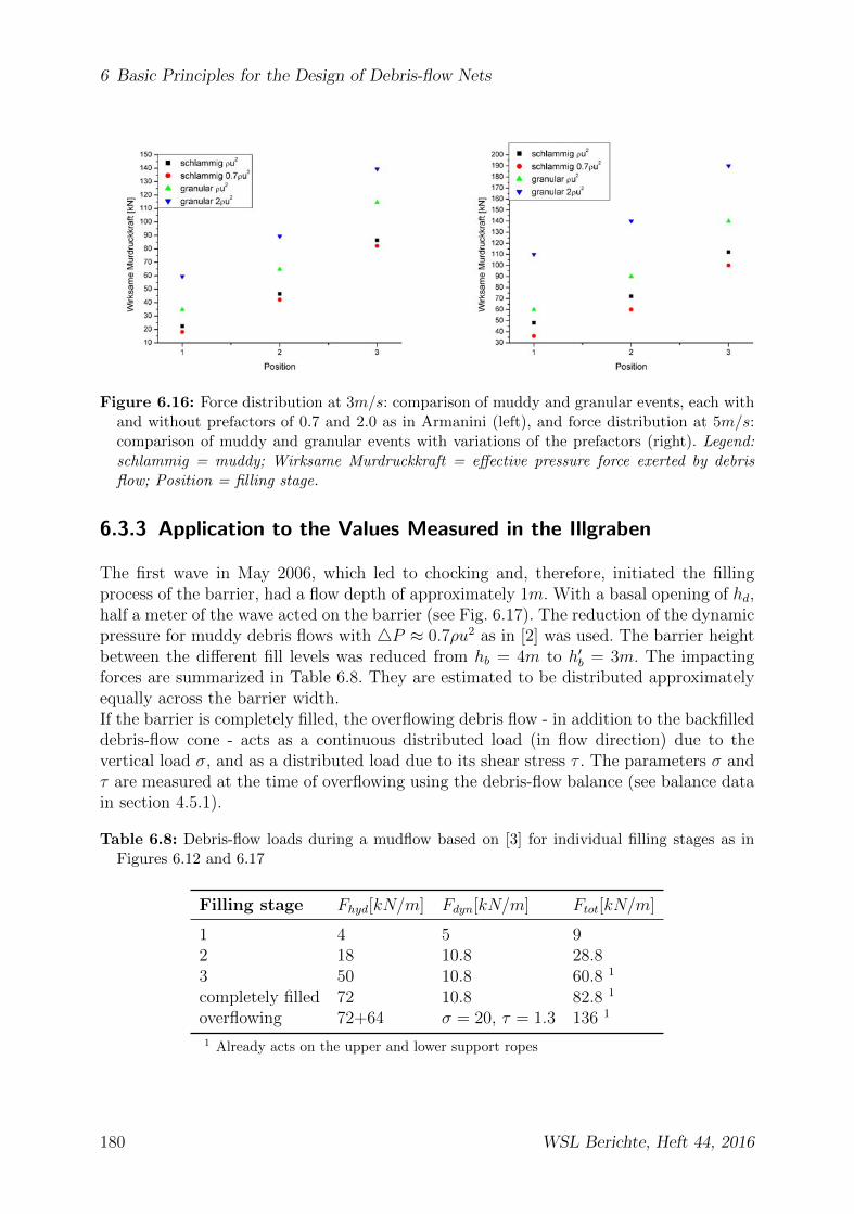
6 Basic Principles for the Design of Debris-flow Nets
Figure 6.16: Force distribution at 3m/s: comparison of muddy and granular events, each withand without prefactors of 0.7 and 2.0 as in Armanini (left), and force distribution at 5m/s:comparison of muddy and granular events with variations of the prefactors (right). Legend:schlammig = muddy; Wirksame Murdruckkraft = effective pressure force exerted by debrisflow; Position = filling stage.
6.3.3 Application to the Values Measured in the Illgraben
The first wave in May 2006, which led to chocking and, therefore, initiated the fillingprocess of the barrier, had a flow depth of approximately 1m. With a basal opening of hd,half a meter of the wave acted on the barrier (see Fig. 6.17). The reduction of the dynamicpressure for muddy debris flows with 4P ≈ 0.7ρu2 as in [2] was used. The barrier heightbetween the different fill levels was reduced from hb = 4m to h′b = 3m. The impactingforces are summarized in Table 6.8. They are estimated to be distributed approximatelyequally across the barrier width.If the barrier is completely filled, the overflowing debris flow - in addition to the backfilleddebris-flow cone - acts as a continuous distributed load (in flow direction) due to thevertical load σ, and as a distributed load due to its shear stress τ . The parameters σ andτ are measured at the time of overflowing using the debris-flow balance (see balance datain section 4.5.1).
Table 6.8: Debris-flow loads during a mudflow based on [3] for individual filling stages as inFigures 6.12 and 6.17
Filling stage Fhyd[kN/m] Fdyn[kN/m] Ftot[kN/m]
1 4 5 92 18 10.8 28.83 50 10.8 60.8 1
completely filled 72 10.8 82.8 1
overflowing 72+64 σ = 20, τ = 1.3 136 1
1 Already acts on the upper and lower support ropes
180 WSL Berichte, Heft 44, 2016
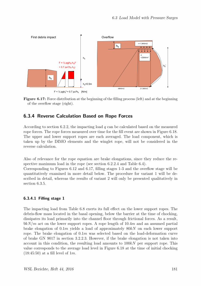
6.3 Load Model with Pressure Surges
hfl
First debris imp t
hd=0.5m
F = ½ ρghfl2 + 0.7 ρu2hfl [N/m]
F = ½ ρg(hfl-hd)2
+ 0.7 ρu2(hfl-hd)
hb
Overflow
hfl
τ=1.3kN/m2
48kN/m2
hb'
21.3kN/m2
σ =20kN/m
Figure 6.17: Force distribution at the beginning of the filling process (left) and at the beginningof the overflow stage (right).
6.3.4 Reverse Calculation Based on Rope Forces
According to section 6.2.2, the impacting load q can be calculated based on the measuredrope forces. The rope forces measured over time for the fill event are shown in Figure 6.18.The upper and lower support ropes are each averaged. The load component, which istaken up by the DIMO elements and the winglet rope, will not be considered in thereverse calculation.
Also of relevance for the rope equation are brake elongations, since they reduce the re-spective maximum load in the rope (see section 6.2.2.4 and Table 6.4).Corresponding to Figures 6.12 and 6.17, filling stages 1-3 and the overflow stage will bequantitatively examined in more detail below. The procedure for variant 1 will be de-scribed in detail, whereas the results of variant 2 will only be presented qualitatively insection 6.3.5.
6.3.4.1 Filling stage 1
The impacting load from Table 6.8 exerts its full effect on the lower support ropes. Thedebris-flow mass located in the basal opening, below the barrier at the time of chocking,dissipates its load primarily into the channel floor through frictional forces. As a result,9kN/m act on the lower support ropes. A rope length of 10.4m and an assumed partialbrake elongation of 0.1m yields a load of approximately 80kN on each lower supportrope. The brake elongation of 0.1m was selected based on the load-deformation curveof brake GN 9017 in section 3.2.2.3. However, if the brake elongation is not taken intoaccount in this condition, the resulting load amounts to 100kN per support rope. Thisvalue corresponds to the average load level in Figure 6.18 at the time of initial chocking(18:45:50) at a fill level of 1m.
WSL Berichte, Heft 44, 2016 181
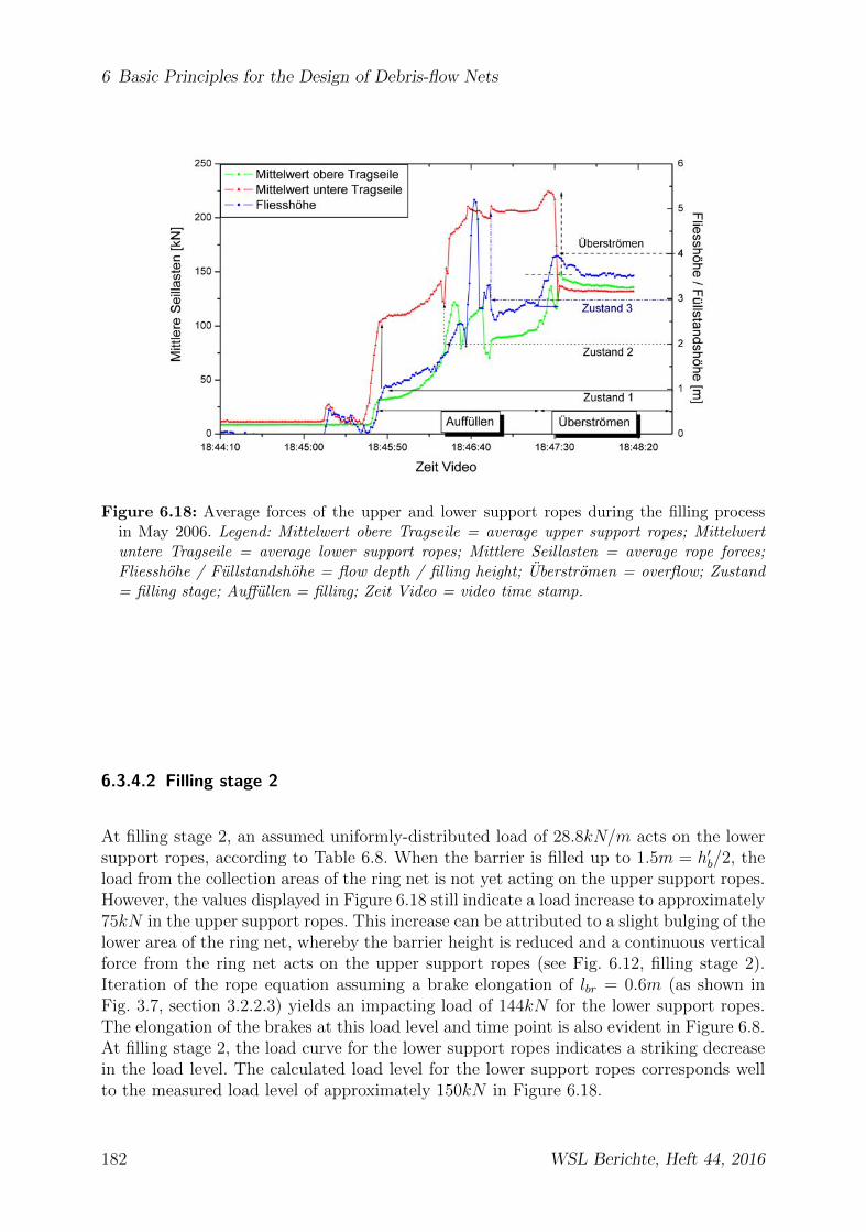
6 Basic Principles for the Design of Debris-flow Nets
Figure 6.18: Average forces of the upper and lower support ropes during the filling processin May 2006. Legend: Mittelwert obere Tragseile = average upper support ropes; Mittelwertuntere Tragseile = average lower support ropes; Mittlere Seillasten = average rope forces;Fliesshohe / Fullstandshohe = flow depth / filling height; Uberstromen = overflow; Zustand= filling stage; Auffullen = filling; Zeit Video = video time stamp.
6.3.4.2 Filling stage 2
At filling stage 2, an assumed uniformly-distributed load of 28.8kN/m acts on the lowersupport ropes, according to Table 6.8. When the barrier is filled up to 1.5m = h′b/2, theload from the collection areas of the ring net is not yet acting on the upper support ropes.However, the values displayed in Figure 6.18 still indicate a load increase to approximately75kN in the upper support ropes. This increase can be attributed to a slight bulging of thelower area of the ring net, whereby the barrier height is reduced and a continuous verticalforce from the ring net acts on the upper support ropes (see Fig. 6.12, filling stage 2).Iteration of the rope equation assuming a brake elongation of lbr = 0.6m (as shown inFig. 3.7, section 3.2.2.3) yields an impacting load of 144kN for the lower support ropes.The elongation of the brakes at this load level and time point is also evident in Figure 6.8.At filling stage 2, the load curve for the lower support ropes indicates a striking decreasein the load level. The calculated load level for the lower support ropes corresponds wellto the measured load level of approximately 150kN in Figure 6.18.
182 WSL Berichte, Heft 44, 2016

6.3 Load Model with Pressure Surges
6.3.4.3 Filling stage 3
In this filling stage, the upper support ropes play an important part as well. Based on theimpacting distributed loads, the total load divides into 18.8kN/m acting on the uppersupport ropes, and 42kN/m acting on the lower support ropes. The elongation of thebrakes in the lower support ropes is still assumed to be lbr = 0.6m, since no further brakeelongation is apparent in Figure 6.18. The brakes of the upper support ropes extend bytheir measured maximum value of lbr = 0.55m. The reverse calculation yields a load of200kN for the lower support ropes, and a load of 135kN for the upper support ropes.The measured forces of the lower support ropes amounted to approximately 200kN , andthose of the upper support ropes to approximately 130kN (see Fig. 6.18).
6.3.4.4 Completely Filled
The last impinging debris-flow surge fills the barrier up to the lower edge, and the over-flowing process begins. 28.8kN/m act on the upper support ropes and 54kN/m on thelower support ropes. At lbr = 0.55m, this yields a rope load of 200kN on the upper sup-port ropes, and of 260kN on the lower support ropes. These values are higher than thevalues measured for this fill level, 150kN for the upper and 200kN for the lower supportropes. In addition, the bulge of the barrier is now almost fully developed and, as a result,the barrier has deformed towards the front and downwards, due to the dead load of thedebris-flow material. The load is now also acting on both the winglet rope and the DIMOelements. According to the simulation of the 2006 barrier in FARO (see section 7.1),30kN are acting on each DIMO element. The rope deformation (see section 6.2.2) allowsfor the determination of the rope angle φrope based on the holding force in the rope Hand the iterated rope force Frope, which yields an angle of φrope = 27.7◦ (see Fig. 6.5). Itis assumed that the angle of the DIMO elements, between the horizontal line of the bar-rier and the tangent in the plane of the DIMO elements, is approximately identical whenthe bulge is filled. For the 8 DIMO elements, this results in a total force component ofFD,fl = 30 · sin(27.7◦) · 8 = 108.9kN in flow direction. Dividing the reducing load compo-nent of the DIMO elements equally between the upper and lower rope forces yields a reduc-tion of 55kN/13.4m = 4.1kN/m for the upper, and 55kN/10.4m = 5.3kN/m for the lowersupport ropes. The DIMO elements reduce the rope load to q = 28.8kN/m− 4.1kN/m =24.7kN/m and q = 54kN/m − 5.3kN/m = 48.7kN/m, which results in a load of 170kNon the upper support ropes, and 240kN on each lower support rope.Due to its deformed configuration, which is similar to a vertical catenary, the winglet ropedoes not significantly dissipate load in flow direction. The winglet rope is primarily actedupon by the dead load of the barrier.The determined loads are 20− 30% greater than the measured loads.
6.3.4.5 Overflowing
During overflowing, the barrier is completely filled, and the debris flow flows across thebarrier with the flow depth hfl (see Fig. 6.17, right). The vertical load σ and the shear
WSL Berichte, Heft 44, 2016 183

6 Basic Principles for the Design of Debris-flow Nets
Ring net (view from above)
Deformed ring net Dimo element
φrope=φD
FD
FD,fl
Figure 6.19: Loading direction on the DIMO elements in filled stage.
stress τ act on the retained debris-flow volume. According to Figure 6.17, this results inan impacting load of 86kN/m on the lower and 50kN/m on the upper support ropes.These loads, minus the DIMO elements, yield rope loads of 300kN in the upper and360kN in the lower support ropes. These rope loads are clearly too high for the overflowloading condition. A short, significant load peak in the support ropes of 150kN and230kN occurs during the first overflowing wave; however, it only lasts for a duration of10s. Nevertheless, the load determined with the load approach is 50 − 60% too high.Following the short maximum load, the rope loads decrease to 140kN during overflowing.The partially-progressed consolidation of the material appears to play a role, and thetransition to active earth pressure seems to come slowly into effect.
6.3.5 Evaluation of the Pressure-Surge Approach
As shown in Table 6.9, variant 2 underestimates the forces acting on the upper supportropes. In contrast, variant 1 represents both the upper and the lower support ropes
184 WSL Berichte, Heft 44, 2016

6.3 Load Model with Pressure Surges
Overflow
hfl
hb'
7.8kN/m2 22.8kN/m2
1.3kN/m2
11.4kN/m2
θa=45°+φ/2
Figure 6.20: Forces active during overflow with application of the active earth pressure forφ = 26◦.
Table 6.9: Comparison of loads measured during the May 18, 2006 mudflow, with loads deter-mined for the respective fill levels for variant 1 and variant 2 using the design approach
Forces in the Support Ropes[kN ] Measured Var. 1 Var. 2
Filling stage 1Top 0 0 0Bottom 100 90 90
Filling stage 2Top 75 0 0Bottom 125-150 144 125
Filling stage 3Top 130 135 81Bottom 200 200 220
Completely filledTop 150 170 130Bottom 230 240 250
correctly. The conceptual model of a debris-flow front that pushes itself across thepreviously stopped material appears to correspond more to reality than the idea that thedebris-flow front pushes into the previously stopped cone, thus raising the fill level. Theconfirmation of variant 1 also indicates that the underlying material is already completelystopped, and therefore no longer contributes to the subsequent front’s exchange ofmomentum. It is consolidated and slightly compressed by the subsequent front pushingitself across the material. However, the consolidation is not taken into account in themodel of the front pushing across the stopped material, since the subsidence of theunderlying material lies within the scope of the accuracy measurements and prognoses ofthe occurrent flow depths.Starting with filling stage 3, variant 1 begins to generally overestimate the occurrentloads, which can be attributed to the progressing consolidation of the debris-flow
WSL Berichte, Heft 44, 2016 185
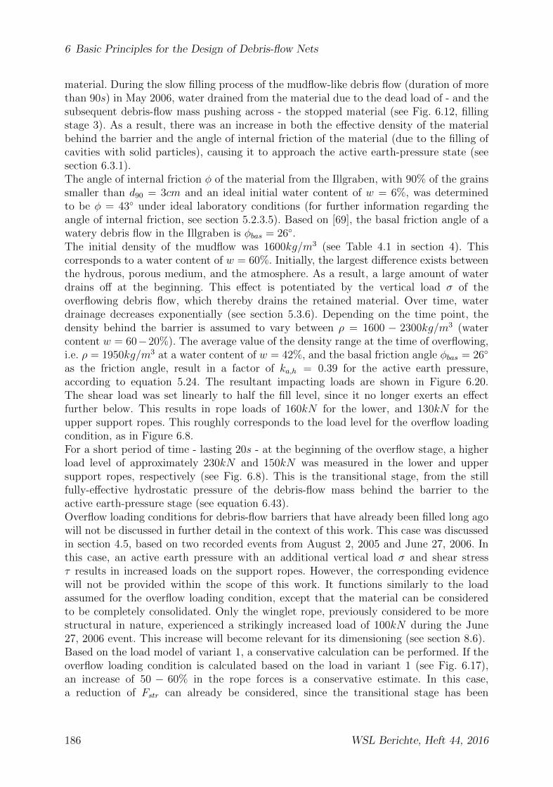
6 Basic Principles for the Design of Debris-flow Nets
material. During the slow filling process of the mudflow-like debris flow (duration of morethan 90s) in May 2006, water drained from the material due to the dead load of - and thesubsequent debris-flow mass pushing across - the stopped material (see Fig. 6.12, fillingstage 3). As a result, there was an increase in both the effective density of the materialbehind the barrier and the angle of internal friction of the material (due to the filling ofcavities with solid particles), causing it to approach the active earth-pressure state (seesection 6.3.1).The angle of internal friction φ of the material from the Illgraben, with 90% of the grainssmaller than d90 = 3cm and an ideal initial water content of w = 6%, was determinedto be φ = 43◦ under ideal laboratory conditions (for further information regarding theangle of internal friction, see section 5.2.3.5). Based on [69], the basal friction angle of awatery debris flow in the Illgraben is φbas = 26◦.The initial density of the mudflow was 1600kg/m3 (see Table 4.1 in section 4). Thiscorresponds to a water content of w = 60%. Initially, the largest difference exists betweenthe hydrous, porous medium, and the atmosphere. As a result, a large amount of waterdrains off at the beginning. This effect is potentiated by the vertical load σ of theoverflowing debris flow, which thereby drains the retained material. Over time, waterdrainage decreases exponentially (see section 5.3.6). Depending on the time point, thedensity behind the barrier is assumed to vary between ρ = 1600 − 2300kg/m3 (watercontent w = 60−20%). The average value of the density range at the time of overflowing,i.e. ρ = 1950kg/m3 at a water content of w = 42%, and the basal friction angle φbas = 26◦
as the friction angle, result in a factor of ka,h = 0.39 for the active earth pressure,according to equation 5.24. The resultant impacting loads are shown in Figure 6.20.The shear load was set linearly to half the fill level, since it no longer exerts an effectfurther below. This results in rope loads of 160kN for the lower, and 130kN for theupper support ropes. This roughly corresponds to the load level for the overflow loadingcondition, as in Figure 6.8.For a short period of time - lasting 20s - at the beginning of the overflow stage, a higherload level of approximately 230kN and 150kN was measured in the lower and uppersupport ropes, respectively (see Fig. 6.8). This is the transitional stage, from the stillfully-effective hydrostatic pressure of the debris-flow mass behind the barrier to theactive earth-pressure stage (see equation 6.43).Overflow loading conditions for debris-flow barriers that have already been filled long agowill not be discussed in further detail in the context of this work. This case was discussedin section 4.5, based on two recorded events from August 2, 2005 and June 27, 2006. Inthis case, an active earth pressure with an additional vertical load σ and shear stressτ results in increased loads on the support ropes. However, the corresponding evidencewill not be provided within the scope of this work. It functions similarly to the loadassumed for the overflow loading condition, except that the material can be consideredto be completely consolidated. Only the winglet rope, previously considered to be morestructural in nature, experienced a strikingly increased load of 100kN during the June27, 2006 event. This increase will become relevant for its dimensioning (see section 8.6).Based on the load model of variant 1, a conservative calculation can be performed. If theoverflow loading condition is calculated based on the load in variant 1 (see Fig. 6.17),an increase of 50 − 60% in the rope forces is a conservative estimate. In this case,a reduction of Fstr can already be considered, since the transitional stage has been
186 WSL Berichte, Heft 44, 2016

6.4 Discussion
completed. However, the determination of the consolidation time point and the associatedtransition to active earth pressure requires a solid background in soil mechanics. Tothis end, material parameters such as grain-size distribution, cohesion, density, and theangle of internal friction play an important role. In addition to these parameters, thereare also debris-flow characteristics, such as water content, density, viscosity, and thedrainage behavior of the mixture. In short, many material- and process-specific variablesinfluence the conversion process behind the barrier. In practice, however, engineers andplanners are frequently unable to precisely characterize these variables when planningand designing debris-flow protection concepts.
6.4 Discussion
6.4.1 Methods to Compare Barriers of Varying Stiffness
The approach described in the pressure-surge model does not explicitly take the flexibilityof the barrier into account. This section, therefore, will outline the effects of barrierstiffness during impact, in order to subsequently determine if approaches for rigid barriersalso apply to flexible structures and vice versa.The ring net barrier’s deformation behavior during the filling process, as evident in thevideo recordings, suggest the following stiffness progression in the 2006 barrier system(see Fig. 6.21, bottom). Initially, and up to a deformation of about 1.2m in flow direction,stiffness does not play a significant role during the filling process, since the entire structurebehaves flexibly. Assuming a rope load of q = 9kN/m (see section 6.3.3, Table 6.8) duringthe first impacting wave of the 2006 filling event, the sagitta of the rope amounts tof ≈ 1.5m (see section 6.2.2.4). A rope load of approximately 100kN then triggers thebrakes. The stiffness increases linearly. Once the majority of the flexible features havesubsequently been exhausted, i.e. when most brake elements have been applied and therings have plastically deformed, the entire structure gets progressively stiffer (see [42])until it reaches a specific value and begins to approach a constant stiffness (see Fig. 6.21,bottom).
In order to compare different barrier systems to each other, a different approach is re-quired, which explicitly takes the deformation of the structure into account. Unlike inFSI calculations2, deformation will not be calculated and factored in for each time step,but instead will be used for the time point of initial impact of the debris-flow wave (seeFig. 6.12, filling stage 1). To this end, energy-conservation principles are applied to anequivalent mechanical model, in which the deformation of the structure is represented bythe displacement of a spring, and the stiffness of the structure functions as the equivalentspring constant (see Fig. 6.21, top).The initial impact of the debris-flow wave is simplified by assuming that the entire ki-netic energy is converted into the potential energy of the spring, i.e. dissipated via thedeformation of the barrier, and by neglecting other possible occurring losses, such as, for
2Fluid-structure interaction calculation
WSL Berichte, Heft 44, 2016 187

6 Basic Principles for the Design of Debris-flow Nets
Net barrier
f
ufront
Equivalent model
^ = m
ufront kn
Displacement f
Stiffness
kn
Spring model:kn=const.
Estimated actual development of kn
1.5m 1.2m
Figure 6.21: Strongly simplified spring model representing the flexible ring net barrier (top),and stiffness of the model compared to the estimated actual stiffness of the ring net barrier(bottom).
example, friction energy. As a result,
K =1
2mu2
front =1
2knf
2 = Epot (6.44)
with K being the kinetic energy of the debris flow according to equation 2.24, m beingthe stopped mass following initial impact, ufront being the front velocity, kn being theequivalent stiffness of the field barrier, and f being the deformation of the barrier duringinitial impact. However, it is difficult to estimate the contributing mass during impact.To this end, it is assumed that the length of the impact l = hfl/tan(φ) can be calculatedby way of the friction angle’s area of effect. The friction angle is assumed to be the basalfriction angle of the debris flow φbas = 26◦. Based on this, the contributing debris-flow masscan be estimated. If the mass m is known, the equivalent stiffness kn can be determinedfor different deformations using equation 6.44. Based on the principles of Hooke’s law, theimpacting load
Fmax = knf (6.45)
can be thus inferred. This law shows a linear increase in force relative to displacement,a result that was also observed partially in the slide experiments in Oregon [23, 35].Nonetheless, this principle is greatly simplified, since the force acting on the net increasesslowly at the beginning of the filling process, and significantly faster shortly before theactual stopping process of the debris flow. The constant value for kn also represents a sim-plification, since the stiffness of the ring net barrier does not remain constant throughoutthe entire filling process (see Fig. 6.21, bottom).
188 WSL Berichte, Heft 44, 2016

6.4 Discussion
Calculating the equivalent stiffness according to the Timoshenko beam theory (uniformly-distributed load q on a single-span beam), as an additional reference value, yields [48]
kn =76.8EI
l3(6.46)
with EI being the flexural stiffness and l being the span width of the single-span beam.In order to compare the results of the conservation of energy according to equation 6.44for a rigid system, the stiffness according to the Timoshenko theory (equation 6.46) wasdetermined for an HEB 180 steel profile and a wood cross section, 0.3m in height and0.3m thick, each with a span width of 10.4m (span width of the lower support rope). Thesame procedure was also performed for the ring net barrier. Based on the deformation ofthe lower support rope of approximately 1.5m at an impacting load of q = 9kN/m duringfilling stage 1, an equivalent flexural stiffness EIbarrier and, consequently, the equivalentstiffness kn can be determined. Figure 6.22 shows these results alongside the results of theenergy equation. These results suggest that stiffness based on the conservation of energydoes not apply to very small deformations, since the stiffness kn rapidly approaches infinitydue to the exponential slope of the curve. Furthermore, the stiffness based on the modelof the Timoshenko beam is lower than the stiffness calculated based on the conservationof energy. The energy equation yields a barrier stiffness of kn ≈ 133kN/m (deformation off = 1.5m), assuming a contributing mass m ≈ 33t and a front velocity of ufront = 3m/s(see filling event on May 18, section 4.5.1). The equivalent stiffness of the Timoshenkomodel yields a barrier stiffness of kn ≈ 63kN/m for a deformation of 1.5m and, therefore,is lower than that of the conservation-of-energy equation, albeit in the same order ofmagnitude by a factor of 2.
Kn of barrier with Timoshenko beam theory
Kn wooden board b=30cm, l=10.4m
Kn HEB 180 steel profile, l=10.4m
Figure 6.22: Barrier stiffness kn as a function of displacement f , based on the conservation ofenergy in the equivalent spring system. The stiffness of a steel and a wood cross section, aswell as the stiffness of the ring net barrier, calculated as a Timoshenko beam, are also shown.
Using the respective stiffness, the occurrent load can be calculated based on Hooke’s lawfor the displacement of a spring Fmax = f · kn. The results for different deformations
WSL Berichte, Heft 44, 2016 189
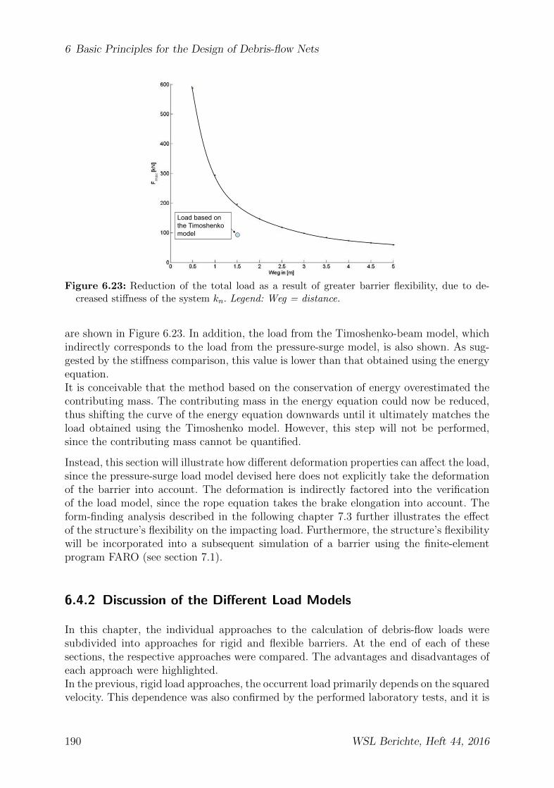
6 Basic Principles for the Design of Debris-flow Nets
Load based on the Timoshenko model
Figure 6.23: Reduction of the total load as a result of greater barrier flexibility, due to de-creased stiffness of the system kn. Legend: Weg = distance.
are shown in Figure 6.23. In addition, the load from the Timoshenko-beam model, whichindirectly corresponds to the load from the pressure-surge model, is also shown. As sug-gested by the stiffness comparison, this value is lower than that obtained using the energyequation.It is conceivable that the method based on the conservation of energy overestimated thecontributing mass. The contributing mass in the energy equation could now be reduced,thus shifting the curve of the energy equation downwards until it ultimately matches theload obtained using the Timoshenko model. However, this step will not be performed,since the contributing mass cannot be quantified.
Instead, this section will illustrate how different deformation properties can affect the load,since the pressure-surge load model devised here does not explicitly take the deformationof the barrier into account. The deformation is indirectly factored into the verificationof the load model, since the rope equation takes the brake elongation into account. Theform-finding analysis described in the following chapter 7.3 further illustrates the effectof the structure’s flexibility on the impacting load. Furthermore, the structure’s flexibilitywill be incorporated into a subsequent simulation of a barrier using the finite-elementprogram FARO (see section 7.1).
6.4.2 Discussion of the Different Load Models
In this chapter, the individual approaches to the calculation of debris-flow loads weresubdivided into approaches for rigid and flexible barriers. At the end of each of thesesections, the respective approaches were compared. The advantages and disadvantages ofeach approach were highlighted.In the previous, rigid load approaches, the occurrent load primarily depends on the squaredvelocity. This dependence was also confirmed by the performed laboratory tests, and it is
190 WSL Berichte, Heft 44, 2016
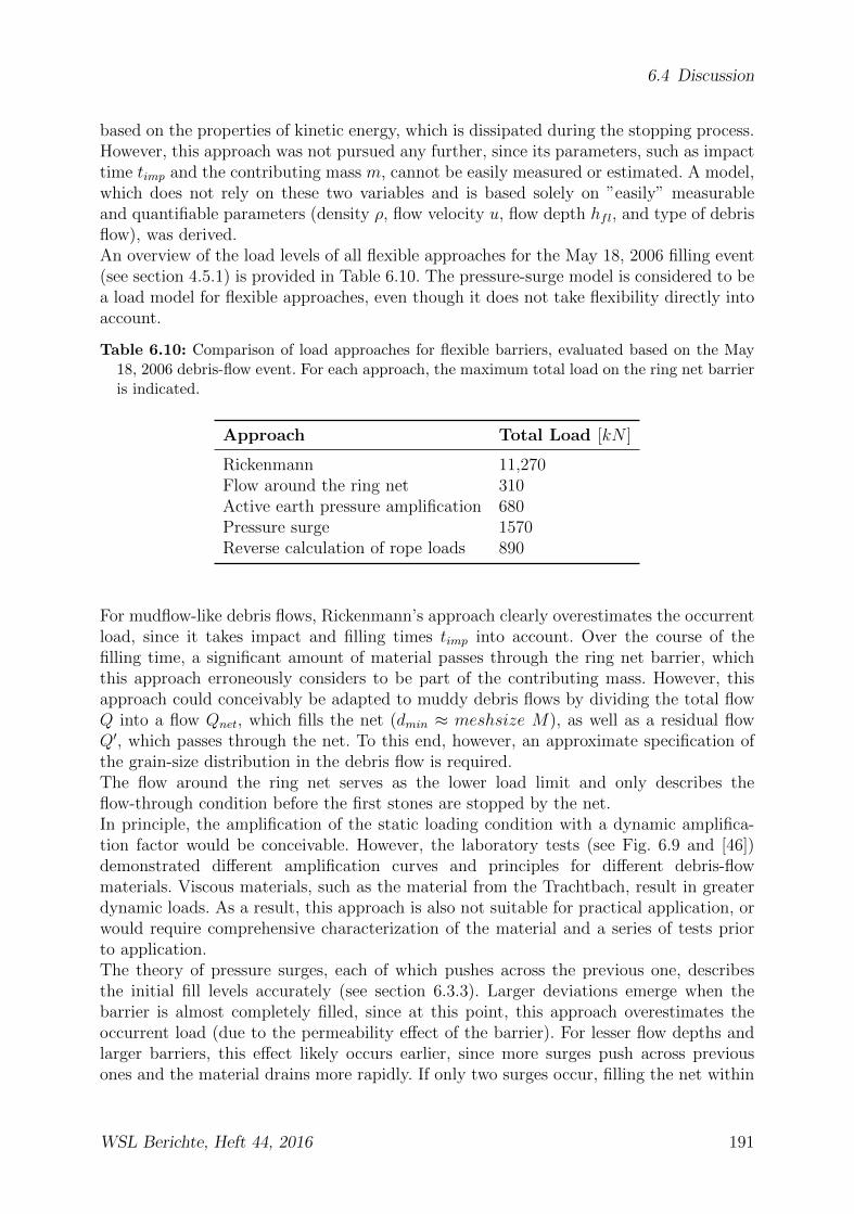
6.4 Discussion
based on the properties of kinetic energy, which is dissipated during the stopping process.However, this approach was not pursued any further, since its parameters, such as impacttime timp and the contributing mass m, cannot be easily measured or estimated. A model,which does not rely on these two variables and is based solely on ”easily” measurableand quantifiable parameters (density ρ, flow velocity u, flow depth hfl, and type of debrisflow), was derived.An overview of the load levels of all flexible approaches for the May 18, 2006 filling event(see section 4.5.1) is provided in Table 6.10. The pressure-surge model is considered to bea load model for flexible approaches, even though it does not take flexibility directly intoaccount.
Table 6.10: Comparison of load approaches for flexible barriers, evaluated based on the May18, 2006 debris-flow event. For each approach, the maximum total load on the ring net barrieris indicated.
Approach Total Load [kN ]
Rickenmann 11,270Flow around the ring net 310Active earth pressure amplification 680Pressure surge 1570Reverse calculation of rope loads 890
For mudflow-like debris flows, Rickenmann’s approach clearly overestimates the occurrentload, since it takes impact and filling times timp into account. Over the course of thefilling time, a significant amount of material passes through the ring net barrier, whichthis approach erroneously considers to be part of the contributing mass. However, thisapproach could conceivably be adapted to muddy debris flows by dividing the total flowQ into a flow Qnet, which fills the net (dmin ≈ meshsize M), as well as a residual flowQ′, which passes through the net. To this end, however, an approximate specification ofthe grain-size distribution in the debris flow is required.The flow around the ring net serves as the lower load limit and only describes theflow-through condition before the first stones are stopped by the net.In principle, the amplification of the static loading condition with a dynamic amplifica-tion factor would be conceivable. However, the laboratory tests (see Fig. 6.9 and [46])demonstrated different amplification curves and principles for different debris-flowmaterials. Viscous materials, such as the material from the Trachtbach, result in greaterdynamic loads. As a result, this approach is also not suitable for practical application, orwould require comprehensive characterization of the material and a series of tests priorto application.The theory of pressure surges, each of which pushes across the previous one, describesthe initial fill levels accurately (see section 6.3.3). Larger deviations emerge when thebarrier is almost completely filled, since at this point, this approach overestimates theoccurrent load (due to the permeability effect of the barrier). For lesser flow depths andlarger barriers, this effect likely occurs earlier, since more surges push across previousones and the material drains more rapidly. If only two surges occur, filling the net within
WSL Berichte, Heft 44, 2016 191

6 Basic Principles for the Design of Debris-flow Nets
a short period of time (high flow depths hfl), the impact of permeability will certainlyemerge more slowly. The overflow loading condition during the 2006 event was alsooverestimated, due to the impact of the previously drained material. In this case, areduction of the load due to the advanced consolidation of the material is conceivable,although this requires a thorough understanding of the debris-flow material and itsdrainage behavior. Therefore, the design concept realized in chapter 8 will not take thisreduction into account, and will be based on a conservative load model instead. A moreprecise calculation based on the reduction due to the already self-supporting, stoppedsoil aggregate yields the occurrent rope loads (see section 6.3.5).
6.4.3 Selection of the Pressure-Surge Model
The pressure-surge model has yielded verifiable results for the mudflow event in May 2006.The results of the laboratory tests and field measurements also confirm many respectsof this model (see section 6.3). Furthermore, the model’s parameters can be estimatedrelatively ”easily”. The dynamic component is taken into account via the conservation ofmomentum, irrespective of the impact times. Up until this point, the pressure factor cp forthe dynamic momentum of granular debris flows could be derived based on specificationsby Armanini et al. [2]. This factor has yet to be confirmed in 1:1 field measurements.The pressure coefficient of the dynamic component in the laboratory tests fell between0.1−0.9 and, therefore, correspond to the pressure coefficient of a mudflow. Based on theliterature, a value cp = 2 is recommended for granular debris flows. As a result, a calcu-lation method using the appropriate pressure coefficient allows for the design for muddyand granular debris flows. If both types of debris flows occur within the same channel,factor cp = 2 must be used.Due to the reduction of the ”overflow” stage, the pressure-surge model takes the perme-ability of the barriers into account via the earth-pressure approach. The flexibility of thesystem, however, is not taken into consideration. Section 6.4.1 demonstrated that a precisedetermination of the system’s stiffness (e.g. using FSI and form finding; see section 7.3)may allow for improved consideration of flexibility. Furthermore, parameters that cannotcurrently be measured, such as the contributing mass, need to be further characterizedby means of targeted experiments.By selecting the pressure-surge model, the present work adopts a conservative approach,and flexibility, therefore, will not be taken into consideration. While the design examplecalculated in FARO does take flexibility into account on the structural side, it is neglectedon the load side (see section 8).
192 WSL Berichte, Heft 44, 2016

7 Numerical Modeling
The numerical modeling of protective structures is advantageous because it saves on thenecessary, time- and cost-intensive 1:1 field tests. Furthermore, a better knowledge of themodel formation allows an optimization of the dimensioning of existing barrier systemsand at the same time the development of new load-bearing systems.The barriers are first simulated using the software FARO, which was originally produced tosimulate flexible rockfall barriers [103]. The necessary modeling details will be explained,as well as the new software components necessary for debris-flow barriers. Subsequentexample simulations of the 2006 filling event explain the influences of certain parameterson model generation and at the same time validate the measured field forces.In the second section of this chapter, the form-finding analyses necessary for flexiblestructures will be discussed. A simplified model is used to carry out a quick back-of-the-envelope calculation of a form-finding analysis, which is integrated into the structuralimplementation in practice. Supplementary calculations for the necessary installation stateof the individual components are made within the structural design.A comparison of the results of the two related programs in terms of their area of applicationand limits is included in the subsequent discussion.
7.1 FARO Software for Simulating Rockfall-protectionStructures
The simulation program, which is based on the finite element method, was developedspecifically for the numerical modeling of flexible rockfall-protection structures and wascalibrated and validated using the results of 1:1 field tests (rockfall tests) with flexiblestructures. The individual structure components such as posts, ring net, ropes, and brakesare simulated true to the model by specific, discrete elements in accordance with theirproperties. The numerical analysis is written in C++, whereas the graphical interface andthe visualization are programmed in Java and Java3D.
7.1.1 Non-linear Dynamic Analysis
In contrast to a static, linear, finite element analysis, the occurrent inertial forces of thetransported masses must be included in dynamic calculations. Therefore, the followingequation of motion must be solved numerically:
Ma+ Cu+K(x) = F (7.1)
193
7 Numerical Modeling
where M is the mass matrix of the individual nodes, C is the damping matrix, and K isthe stiffness matrix of the whole system. K(x) stands for the element-internal forces thatoccur during the simulation period, while F is the load vector of the external loads. a isthe acceleration, which can also be expressed as a = x, u is the velocity, the integral ofthe acceleration (u = x), and finally x is the distance variable.Owing to the large non-linearities expected in the dynamic simulation and the short sim-ulation period of Ttot ≈ 0.5 s for rockfalls, an explicit time integration method with veryshort time steps is recommended for the numerical solution of the equation of motion [103].The new velocities and displacements at time step t+ ∆t are calculated directly from thecurrent accelerations. These are assumed to be constant over a very short time step ∆t.A problem with the explicit method is the selection of an excessively long time step, asa result of which the assumption of constant acceleration is no longer valid and thereforethe result deviates from the real value.Another possibility would be an ”implicit” method that, in contrast to the explicit method,forms the equilibrium again and solves the non-linear equation system again for each timestep ∆t. However, in the case of large non-linearities this results in many iteration cyclesand consequently in long computing times, despite the much longer time steps that canbe selected.For this reason, the time integration algorithm in FARO is based on an explicit timeintegration according to the finite difference method [103]. It calculates the velocity atthe new time point t = t0 + ∆t to give
v(t+ ∆t) = v(t) + a∆t (7.2)
assuming that a = const. during this time step. The displacement variables are calculatedfrom the velocity u in the same manner. The algorithm itself always moves betweentime steps t−∆t and t + ∆t based on the central difference quotients. Within this timeinterval, the corresponding accelerations, velocities, displacements and energy contents areconstant. At time point t = 0 s, the following starting conditions apply to the respectivesystem nodes: ut=0 = ut = −∆t and xt=0 = x0. The velocities and displacements are theneach updated according to equation 7.2 from time step t to time point t+ ∆t
ut+∆t = ut +f
m∆t (7.3)
xt+∆t = xt + ut∆t (7.4)
where f = m · a (Newton) is the matrix of the effective forces on the system points andm is the matrix of the respective point masses.An order of magnitude of between ∆t = 10−4 − 10−6s is suggested for selecting the timestep. Smaller time steps result in undesirably longer computing times and larger timesteps result in numerical instabilities and large deviations in the results.
7.1.2 Static Analysis
The static equilibrium of a structure is found in conventional FE programs directly bysolving a (non-)linear equation system of the node equilibrium. The explicit method im-
194 WSL Berichte, Heft 44, 2016
7.1 FARO Software for Simulating Rockfall-protection Structures
plemented in FARO for reproducing dynamic processes is also used for calculating quasi-static equilibrium states. An explicit calculation method can even be recommended forvery large deformations.With quasi-static calculations, it is important to keep the occurrent node velocities aslow as possible in order to minimize undesirable inertial forces here. All mass points havethe velocity u = 0m/s at the start and, although they are accelerated by the quasi-staticforce fstat, this acceleration is reduced again by relatively high damping in the next timestep and thus the velocity is kept low. This method is carried out until the differencein the kinetic energy from one time step to the next has reached a predefined minimum(u → 0). For values for the damping ratio to be specified and for the threshold value ofthe kinetic energy, see [103].
7.1.3 Carrying out the Calculation
The model is input into FARO using a text file. The syntax diagram for the input can befound in [103]. When variables that have units (distance, force and velocity) are input,consistent use of the SI units m, kg, s must be ensured.After the model has been successfully generated, the simulation itself must be startedvia the graphical interface or by means of command lines (for ”batch operation”). Theindividual steps of the model generation are presented and explained in the followingsection using a debris-flow barrier.
WSL Berichte, Heft 44, 2016 195

7 Numerical Modeling
7.2 Simulation of Debris-flow Protection Structuresusing FARO
Since debris flows act on the structure over an area, as already shown in Table 6.2,a procedure has been developed for inputting area loads into FARO. Also, the nodegeneration previously used for rockfall-protection systems has been expanded from therectangular ring nets more usual for rockfalls to trapezoidal cross sections. A graphicalimplementation of the load Debris flow in the FARO software will visually animate thisloading condition. A sample calculation of the 2006 ring net barrier in the Illgraben belowshows the procedure for model generation and the associated modeling details.
7.2.1 Area Loads
Area loads and pressures are often converted to node forces in finite element formulations.Therefore, there are two conceivable possibilities for modeling the debris-flow loads in agenerated model structure in FARO:
• Accelerated masses Here, each loaded system node i is assigned a starting velocityand an additional mass mi. This corresponds to equivalent node loads according toNewton’s law of Fi = miai (see Fig. 7.1, left).
• Node forces The effective total load is distributed uniformly over the node situatedin the loaded area (see Fig. 7.1, right).
Node mass = mi
ufront
Accelerated point masses
Node force Fi
Individual node loads
Figure 7.1: Both variants of load input, with moving point masses on the left and with indi-vidual node loads on the right.
The procedure of assigning masses to each loaded node requires an estimation of theeffective total mass. The overall ”dynamics” in the system are retained, whereas theyare omitted in the quasi-static equivalent load. The node starting velocity used can beequated with the inflowing velocity of the debris flow ufront. However, if each node is
196 WSL Berichte, Heft 44, 2016

7.2 Simulation of Debris-flow Protection Structures using FARO
slowly braked to u = 0 based on the resistance of the barrier, the loaded structure of thebarrier collapses and no longer has a real deformed configuration. A final, filled state ofthe barrier cannot therefore be formed with this method.
In contrast, the individual node load procedure produces a nice deformed configurationof the loaded structure, but the question arises of the size and type (distribution overtime t) of the effective forces.
If the effective masses and forces are estimated correctly, both procedures should producethe same result. Owing to the selected load approach, based on pressures of the effectivedebris-flow front, the individual node load procedure is selected for the calculation shown.In addition, this produces a verification of the developed load approach in terms of theoccurrent rope loads of the barrier structure. However, a sufficiently accurate estimationof the effective masses during the stopping process is not possible, because there is onlyone available measurement result for the filling process.
7.2.2 Model Generation and Simulation of the 2006 Barrier in theIllgraben
7.2.2.1 General Simulation Parameters
For an approximate duration of the individual surges (see section 6.3), the simulationtime point tsim = 1s is placed at time point treal = 1 min after blockage of the net. Forthe calculations, the time step size is set to ∆t = 5 · 10−6s, the damping ratio is set toα = 1 [103].
7.2.2.2 Element Nodes
For the model generation, the node groups net nodes, bearing nodes, and braking nodesaccording to Figure 7.2 above and [103] must be entered. The coordinate system is selectedwith the z axis pointing upward (according to the usual topographic coordinate systems).The bearing nodes are assigned the corresponding boundary condition for non-displaceablemounting. All the nodes in the 2006 barrier are in one plane, although in reality this isnot entirely the case in a ring net barrier structure.When the loads are entered, nodes are determined that lie in the respective loaded area of asurge (surges 1, 2, 3 or 4; see Fig. 7.2, bottom). Dividing the ring net nodes into individualgroups in the input file allows direct access to the respective node for the correspondingload part. Load surges 1− 3 correspond to the fill stages 1− 3 from section 6.3. Surge 4is the last surge, which results in complete filling and overflow.
WSL Berichte, Heft 44, 2016 197
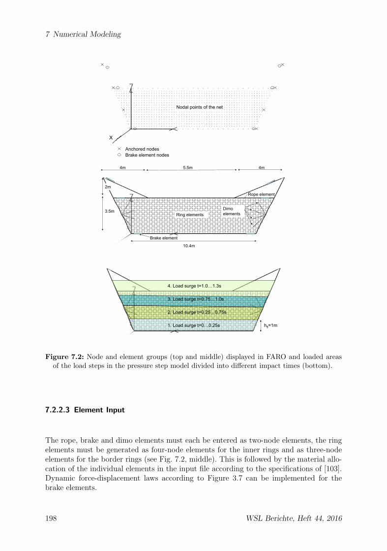
7 Numerical Modeling
Nodal points of the net
n ored nodesBrake element nodes
X
Ring elements Dimo elements
Rope element
Brake element
2m
3.5m
10.4m
5.5m 4m4m
hfl=1m 1. Load surge t=0…0.25s
2. Load surge t=0.25…0.75s
3. Load surge t=0.75…1.0s
4. Load surge t=1.0…1.3s
Figure 7.2: Node and element groups (top and middle) displayed in FARO and loaded areasof the load steps in the pressure step model divided into different impact times (bottom).
7.2.2.3 Element Input
The rope, brake and dimo elements must each be entered as two-node elements, the ringelements must be generated as four-node elements for the inner rings and as three-nodeelements for the border rings (see Fig. 7.2, middle). This is followed by the material allo-cation of the individual elements in the input file according to the specifications of [103].Dynamic force-displacement laws according to Figure 3.7 can be implemented for thebrake elements.
198 WSL Berichte, Heft 44, 2016

7.2 Simulation of Debris-flow Protection Structures using FARO
7.2.2.4 Load Input
The loads are input by applying concentrated loads. With a constant pressure distribu-tion, these are calculated from the pressure multiplied by the area divided by the numberof nodes. If the load is constant over the barrier height, this can then be distributeduniformly over all the nodes. In the case of a linear pressure distribution, the load for eachseries of nodes must be averaged over the height and multiplied by the correspondingwidth (see Fig. 7.4). The loads are each increased linearly from the previously effectiveto the next maximum value over the effective period.Table 7.1 shows the procedure for variant 2 according to section 6.3 for the loads ofMay 18th, 2006 from section 6.3.3. In this case, the dynamic and hydrostatic pressure isdistributed uniformly over the current fill level. With variant 1, however, the dynamicpressure is in each case applied only over the flow depth of the last load surge. Thisprocedure results in a more laborious input than variant 2. In each case, the averagewidth of the dynamic load surge or, in the case of the hydrostatic pressure, the averagewidth of the filled net area is applied as the average width for calculating the individualnode loads from pressures.
Table 7.1: Effective load q [kN/m] from pressure surge calculation distributed over the entireloaded area of the fill level and respective increase of the load over the filling time of theimpact for variant 2
EinwirkungsdauerState/step 1 2 3 4 Overflow
Load q [kN/m] 9.0 28.8 60.8 82.8 601
bm [m] 10.83 11.26 11.68 11.9 11.9Number of nodes [−] 258 538 840 902 902Node load [N ] 377 602 845 1092 792Simulation time [s] 0-0.25 0.25-0.75 0.75-1.0 1.0-1.3 1.3-1.6
1 Active earth pressure approach with φ = 26◦
Dead Load
The dead load of the barrier and the retained material is relevant mainly for dimension-ing the winglet rope, since this transfers the dead load of the bulge (for chain line, seesection 8.6.6.1). In addition, the dead load affects the deformation of the barrier in thevertical direction.The dead load of the filled ring net in the negative z-direction is estimated by thefollowing approximate calculation (see Fig. 7.3). The deformed configuration of thering net is approximately triangular according to section A-A in Figure 7.3 and isassumed to be constant over the width. The parts missing owing to the approxima-tion as a triangular profile are compensated to some extent by the assumption of thedeformation as constant. Loading owing to dead load is therefore calculated to give
WSL Berichte, Heft 44, 2016 199

7 Numerical Modeling
Fg = 0.5 · g · f · h′b · bm · ρ = 0.5 · 9.81 · 2.5 · 3 · 11.9 · 1950 = 853kN with a density ρof the retained material of 1950kg/m3 (see section 6.3.4.5).Loading owing to dead load is increased to the maximum value at the end of load surge 4(barrier completely filled).
Anchor
Lower support ropes
hb'
Upper support ropes
Section A-A:
Anchor
Topview:
f
A
A
Unloaded barrier
bm
Calculated volume
Retained volume
G
f
Filled barrier
Figure 7.3: Approximation of the volume of the debris-flow bulge to determine the dead load.
7.2.3 Influence of Modeling Details
The following definitive influencing variables are investigated in the simulations:
• Hydrostatic pressure distributed constantly or linearly
• Dynamic pressure according to variant 1 or variant 2 (see section 6.3)
• Variation of time step size
• Variation of damping ratio
• Chronological variation of the load increase up to full load
The results of the varied influencing factors are presented in the following sections.
7.2.3.1 Hydrostatic Pressure Distributed Linearly or Uniformly
The static pressure of stationary liquids or of debris-flow material increases linearly withdepth (see section 4.4). For reasons of simpler modeling, a uniformly distributed pressureis also conceivable instead of the triangular pressure distribution (see Fig. 7.4). There-fore, the hydrostatic pressure is modeled with a linearly increasing and with a uniformdistribution (see Fig. 7.4).
200 WSL Berichte, Heft 44, 2016

7.2 Simulation of Debris-flow Protection Structures using FARO
Linear hydro-static pressure
Phyd
∆h∆h
Continuous pressure
∆h ∆h
Phyd / 2
Figure 7.4: Modeling of a linear pressure distribution compared with a constant one.
Table 7.2: Comparison of the simulated maximum forces with the linear or constant load dis-tribution of the hydrostatic component in relation to the measured rope forces (the percentagedeviation is in brackets in each case)
Meas. rope forces Phyd linear Phyd const.
Upper support ropes [kN ] 150 151 (≈ 0 %) 166 (+10 %)Lower support ropes [kN ] 230 242 (+5 %) 200 (−15 %)
The maximum loads of the upper and lower support ropes are shown as average valuesin Table 7.2.This makes it clear that the linear hydrostatic pressure distribution corresponds moreto reality and reproduces the measured rope forces better. The main difference appearsin the loading of the lower support ropes. Here, the load per support rope is 242kNwith a linear pressure distribution, whereas it is underestimated at 200kN with uniformdistribution. The upper support ropes are overestimated with the distribution.It is therefore sensible to assume that the hydrostatic pressure is linearly distributed.In the example of the 2006 filling event, it plays a greater role in the lower dynamicloads owing to the very liquid debris flow. If the dynamic fraction dominates for granulardebris flows, a constant hydrostatic pressure distribution can however still be used forthe calculation.
7.2.3.2 Dynamic Pressure According to Variant 1 or Variant 2
The dynamic component of the effective debris-flow load can act either in a uniformlydistributed manner over the fill height or only in the upper, newly filled region (seesection 6.3). Therefore, variant 1 and variant 2 are compared with each other according
WSL Berichte, Heft 44, 2016 201

7 Numerical Modeling
to Figure 7.5.
2. s ariant 1
2. s ariant 2
PdynPhyd Phyd Pdyn
Figure 7.5: Load distribution over the ring net nodes according to variants 1 and 2 using step2 as an example.
To investigate the influence of the distribution of the dynamic pressure, the hydrostaticpressure distribution is assumed to be distributed uniformly over the height, because thedynamic component is the critical one for debris flows with high flow velocities and there-fore the influence of the correct modeling of the hydrostatic pressure is of less importance.
The simulation results for variants 1 and 2 show small differences. Owing to the distri-bution of Fdyn over the respectively upper surge with an increase of 0 to Fdyn, variant 1exhibits more oscillations in the load-time curves than variant 2 (see Fig. 7.6). The maxi-mum load of the upper and lower support ropes is reproduced slightly better by variant 1(see Table 7.3). This is an additional confirmation of the model from section 6.3.5 of thepressure surges pushing over each other.
Table 7.3: Comparison of the simulated maximum forces with pressure variants 1 and 2 inrelation to the measured rope forces (percentage deviation in brackets). The static pressurehas been assumed to be uniformly distributed
Meas. rope forces Variant 1 Variant 2
Upper support ropes [kN ] 150 150 (0 %) 141 (−6.5 %)Lower support ropes [kN ] 230 212 (−8.5 %) 202 (−14 %)
The difference in forces between variants 1 and 2 according to Table 7.3 is greater in thesimulation if the dynamic component is proportionately greater, e.g. in the case of granularfronts or fast-flowing debris flows. Variant 1 is therefore recommended for the input ofarea loads. For the muddy filling process during the filling event of 2006, the difference in
202 WSL Berichte, Heft 44, 2016

7.2 Simulation of Debris-flow Protection Structures using FARO
Figure 7.6: Simulated forces in the upper (top) and lower (bottom) support ropes in the indi-vidual fill stages according to variants 1 and 2. Legend: Zustand = stage; vollstandige Fullung= completely filled; Beginn Uberstromen = start of overflow; Seilkrafte = rope forces; ObereTragseile = upper support ropes; untere Tragseile = lower support ropes; Variante = variant;Simulationszeit = simulation time.
the effective range of variants 1 and 2 plays less of a role, for which reason the load inputof variant 2 is sufficient for reasons of simplicity (see Table 7.3). Simulation deviations ofup to 14% deviation are generally within a good range for the calculated support ropeloads. It should however be noted that the occurrent loads are underestimated in thiscase.
The variation in the different load distributions shows that the correct simulation resultsare achieved with variant 1 for dynamic load and with a linear distribution for hydrostaticload. The rope forces of the lower support ropes are 244kN , those of the upper support
WSL Berichte, Heft 44, 2016 203

7 Numerical Modeling
ropes are 180kN (see Fig. 7.7). They overestimate the measured rope forces by max. 20%.This load input is chosen for the rest of the study.
Figure 7.7: Simulated forces of the upper and lower support ropes according to variant 1 andlinear static pressure distribution. Legend: Seilkrafte = rope forces; untere Tragseile = lowersupport ropes; obere Tragseile = upper support ropes; Simulationszeit = simulation time.
The following individual results were also produced:
• Winglet rope: In Figure 7.8, the load of the winglet rope is also entered in eachcase. This was not taken into account in the load approach in section 6.3, because itwas assumed that it transfers the dead load of the filled barrier only in the verticaldirection. The size of the load in the simulation is also highly dependent on the sizeof the dead load of the bulge of the barrier acting in the negative z direction. Inthe simulations a load of 150kN was reached, in the field the measured value was160kN (see section 4.5.1). In this case too, simulations and real measured valuesare close together.
• DIMO elements: The support load components of the DIMO elements have notbeen shown so far. The maximum value of 60kN occurred in each case in the DIMOelements fastened horizontally in the net, whereas smaller loads occur in the upperand lower oblique DIMO elements. These are not arranged parallel to the main loaddirection, as a result of which they receive a smaller load (see section 4.6.3). Theaverage value of the load level of all 8 DIMO elements is approximately 35kN .
204 WSL Berichte, Heft 44, 2016

7.2 Simulation of Debris-flow Protection Structures using FARO
Figure 7.8: Simulated forces in the winglet rope in the individual fill stages according to vari-ants 1 and 2. Legend: Zustand = stage; vollstandige Fullung = completely filled; BeginnUberstromen = start of overflow; Seilkrafte = rope forces; Flugelseil = winglet ropes; Variante= variant; Simulationszeit = simulation time.
7.2.3.3 Influence of Load Increase
In the simulation results shown so far, the load was always increased up to a simulationtime of tsim = 1.3s before the overflow loads were applied between tsim = 1.3− 1.6s. Forcomparison, the individual load surges are now each increased in 1/10 of the previoussimulation time tsim up to the maximum load. This means that the barrier is alreadycompletely filled at tsim = 0.13s. The following simulations are carried out with dampingratio α = 10. Figure 7.9 shows the results of these calculations for the lower and uppersupport ropes.
It can be seen that brief load peaks occur with the rapid increase in load owing to the rapidloading of the structure. This is followed with the rapid increase in load by a constantloading, which corresponds approximately to the loading of the normal, slower increasein load. The normal loading speed is therefore sufficient. Only the upper support ropeshave a 14% higher load level with the rapid increase in load than with the medium andslower increases in load.Excessively rapid increases in load should be avoided owing to the fast reaction of thestructure with large load peaks. In case of doubt, the sensitivity of the structure in relationto the rate of load increase must be determined first in a numerical simulation.
7.2.3.4 Influence of Damping Ratio
With the variation in damping ratio, a load increase time of t = 1.3s and a time step sizeof ∆t = 5 · 10−6 are used. It can be seen in Figure 7.10 that the maximum load becomes
WSL Berichte, Heft 44, 2016 205

7 Numerical Modeling
Figure 7.9: Rope forces of the upper and lower support ropes at a rapid 0.13s, a normal 1.3s,and a slow 13s load increase. Legend: obere Seilkrafte = upper rope forces; untere Seilkrafte =lower rope forces; langsam = slow; schnell = fast; mit = with; Simulationszeit = simulationtime.
smaller during the simulation for larger values of α (α = 50, α = 100). The maximumexcursions are damped for larger values of α, so the curves seem more uniform than forlower damping values of α = 1 and α = 10. In addition, the maximum values of theload are reached later in time in the simulation for higher damping ratios, although theincrease in load is the same (see Fig. 7.10).
Figure 7.10: Rope forces of the upper and lower support ropes for a variation in the dampingratio of α = 1, 10, 50, 100. Legend: obere Seilkrafte = upper rope forces; untere Seilkrafte =lower rope forces; Simulationszeit = simulation time.
If the damping ratios are too high, however, there is a risk of underestimating the maxi-mum occurrent load because load peaks are damped out. In addition, the maximum loadlevel for higher damping ratios is not reached until later in the simulation, as a result ofwhich there is a risk that the simulation is ended prematurely before the maximum loadlevel has even been reached.
206 WSL Berichte, Heft 44, 2016

7.2 Simulation of Debris-flow Protection Structures using FARO
7.2.3.5 Influence of Time Step Size
The time step ∆t is varied from 1.0 · 10−6s to 30 · 10−6s, because the structure (ring net)numerically fails at a time step of ∆t > 3.0 ·10−5. The maximum values of the rope forcesare shown in Table 7.4. The utilization in the ring net is also shown, because the ring net isthe definitive component in the increase in the time step. In previous simulations, the ringnet was not critically utilized, which is why it was not included in previous considerations.
Table 7.4: Comparison of maximum loads in the support ropes and rings with variation of thetime step
Time step size [s] 1.0 · 10−6 5 · 10−6 10 · 10−6 20 · 10−6 30 · 10−6
Upper support ropes [kN ] 182 188 180 181 1801
Lower support ropes [kN ] 244 242 244 246 2501
Rings [utilization %] 31 32 33 37 701
1 Threshold time step before numerical time integration becomes instable
It can therefore be determined that the time integration is no longer stable at a time stepof ∆t > 3.0 ·10−5s. The time step size ∆t = 1.0 ·10−5s, with which most simulations werecarried out, provides correct load sizes in the individual components and should also beused for the following simulations.
7.2.3.6 Deformations
The individual load surges can be recognized easily in the bulging during deformationsof the barrier (see Fig. 7.11). The deformation of the barrier as a whole also correspondsqualitatively well with the individual stages according to the video analysis of the fillingprocess. However, the quantitative maximum deformations of the bulge in FARO arereproduced slightly too large, for which reason FARO should not be used to calculatemaximum deformations for area load effects. The maximum deflection of the bulge in thecompletely filled state is in this case approximately 3m, whereas it was 2.5m after thefirst filling process in the field (see section 4.5.3). This problem results from the fact thatFARO was originally written for the point loads of rockfalls, i.e. the numerical model ofthe ring net has been optimized rather for a multidirectional linear load transference fromthe impact point to the support system and less for a uniform loading over an area.
7.2.3.7 Static Calculation
Although the static calculation of ring net barriers is often not definitive from a designstandpoint, it should still be included in the investigation, particularly for very highbarriers. It can also be necessary to investigate any definitive partial or complete snow
WSL Berichte, Heft 44, 2016 207
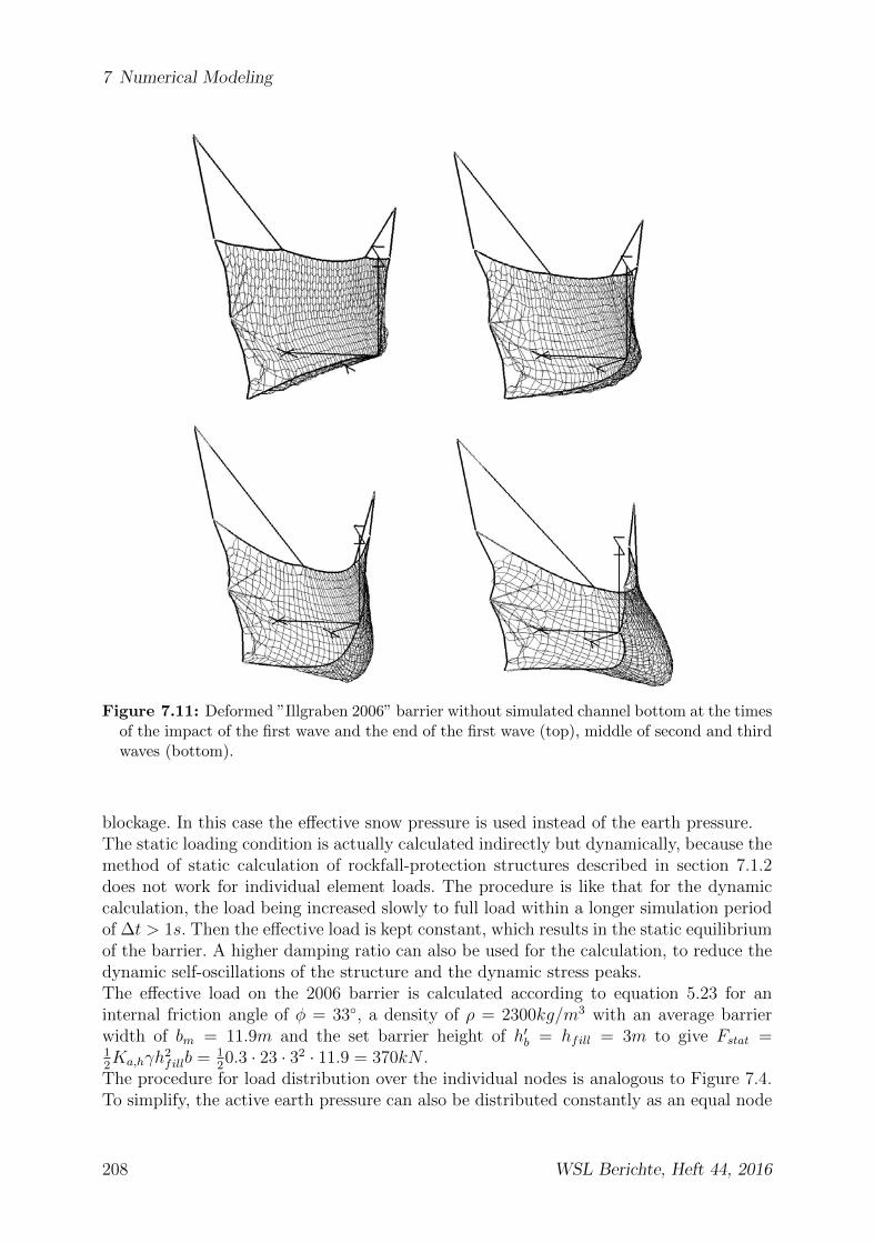
7 Numerical Modeling
Figure 7.11: Deformed ”Illgraben 2006” barrier without simulated channel bottom at the timesof the impact of the first wave and the end of the first wave (top), middle of second and thirdwaves (bottom).
blockage. In this case the effective snow pressure is used instead of the earth pressure.The static loading condition is actually calculated indirectly but dynamically, because themethod of static calculation of rockfall-protection structures described in section 7.1.2does not work for individual element loads. The procedure is like that for the dynamiccalculation, the load being increased slowly to full load within a longer simulation periodof ∆t > 1s. Then the effective load is kept constant, which results in the static equilibriumof the barrier. A higher damping ratio can also be used for the calculation, to reduce thedynamic self-oscillations of the structure and the dynamic stress peaks.The effective load on the 2006 barrier is calculated according to equation 5.23 for aninternal friction angle of φ = 33◦, a density of ρ = 2300kg/m3 with an average barrierwidth of bm = 11.9m and the set barrier height of h′b = hfill = 3m to give Fstat =12Ka,hγh
2fillb = 1
20.3 · 23 · 32 · 11.9 = 370kN .
The procedure for load distribution over the individual nodes is analogous to Figure 7.4.To simplify, the active earth pressure can also be distributed constantly as an equal node
208 WSL Berichte, Heft 44, 2016

7.2 Simulation of Debris-flow Protection Structures using FARO
Figure 7.12: Deformed barrier without simulated channel bottom in final state during overflow,from the front and from the side.
load over all the nodes. It is then not possible to reproduce the measured rope forces inthe Illgraben precisely, because the lower rope forces have a load that is too small and theupper rope forces have one that is too large. To verify the measured static rope forces inthe Illgraben, a load that is distributed linearly over the height is therefore chosen for thesimulation example. This yields the rope forces according to Figure 7.13. A comparison
Figure 7.13: Rope forces of the filled barrier loaded by active earth pressure. Legend: Seilkrafte= rope forces; untere Tragseile = lower support ropes; obere Tragseile = upper support ropes;Simulationszeit = simulation time.
of the simulated rope forces with the measured values for the filled state of the barrierwithout vertical loads (only daytime flow) is shown in Table 7.5.
WSL Berichte, Heft 44, 2016 209
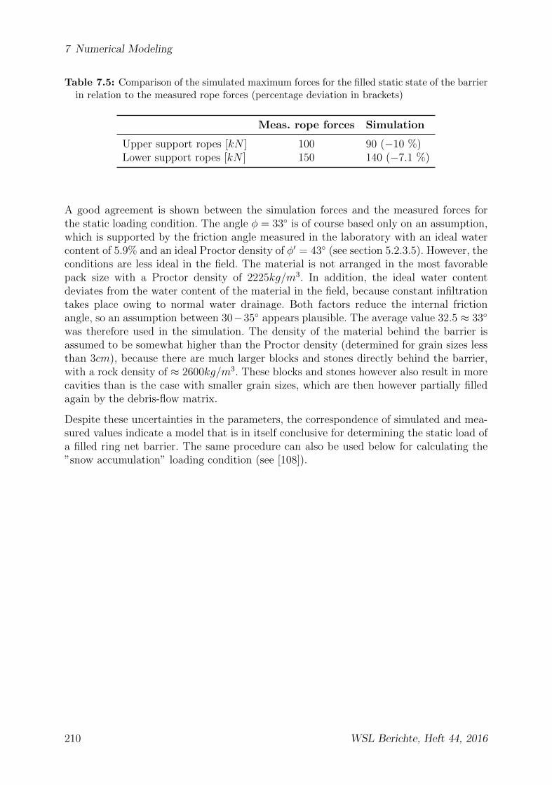
7 Numerical Modeling
Table 7.5: Comparison of the simulated maximum forces for the filled static state of the barrierin relation to the measured rope forces (percentage deviation in brackets)
Meas. rope forces Simulation
Upper support ropes [kN ] 100 90 (−10 %)Lower support ropes [kN ] 150 140 (−7.1 %)
A good agreement is shown between the simulation forces and the measured forces forthe static loading condition. The angle φ = 33◦ is of course based only on an assumption,which is supported by the friction angle measured in the laboratory with an ideal watercontent of 5.9% and an ideal Proctor density of φ′ = 43◦ (see section 5.2.3.5). However, theconditions are less ideal in the field. The material is not arranged in the most favorablepack size with a Proctor density of 2225kg/m3. In addition, the ideal water contentdeviates from the water content of the material in the field, because constant infiltrationtakes place owing to normal water drainage. Both factors reduce the internal frictionangle, so an assumption between 30−35◦ appears plausible. The average value 32.5 ≈ 33◦
was therefore used in the simulation. The density of the material behind the barrier isassumed to be somewhat higher than the Proctor density (determined for grain sizes lessthan 3cm), because there are much larger blocks and stones directly behind the barrier,with a rock density of ≈ 2600kg/m3. These blocks and stones however also result in morecavities than is the case with smaller grain sizes, which are then however partially filledagain by the debris-flow matrix.
Despite these uncertainties in the parameters, the correspondence of simulated and mea-sured values indicate a model that is in itself conclusive for determining the static load ofa filled ring net barrier. The same procedure can also be used below for calculating the”snow accumulation” loading condition (see [108]).
210 WSL Berichte, Heft 44, 2016

7.3 Form Finding
7.3 Form Finding
With flexible barriers, large deformations of the structure occur as they are filled by adebris flow. The end deformation plays an important role in the dimensioning and use ofthe barrier in practice owing to geometric conditions and long-term behavior. Therefore,this chapter will describe and carry out an approach for controlling the shape of softstructures - the form-finding analysis - using the example of a simplified model of the ringnet barrier.First, the necessary theoretical principles of the form-finding problem are briefly intro-duced and explained in the following sections. The model calibration is described usingthe ring net experiments on the CTI test stand [45]. The developed modeling details arethen implemented in a three-dimensional, simplified model of a typical structure using thesoftware CARAT (see section 7.3.2). The model shows a possible ideal deformed configu-ration for the barrier to be able to transfer the debris-flow loads in an efficient manner.The results of the form-finding calculation are then interpreted from a structural stand-point of practicability, i.e. which deformations are technically sensible and feasible toachieve a reasonable outlay on materials and costs. Back-of-envelope calculations for thenecessary installation state of the support ropes and of the ring net are introduced. Inaddition, the aspect of durability plays an important role in the shaping of the ring netbarriers and must be taken into account. All three factors - bearing-load-specific shap-ing, economical feasibility and structurally necessary shaping - play an important role inthe numerical modeling even in the planning phase and should be agreed and taken intoaccount as well as possible.
Figure 7.14: Equilibrium form after form-finding analysis for an intended maximum end de-formation f of 1m.
7.3.1 Definition of Term Form Finding
Form finding means the search for the load-bearing geometry that balances the prioritiesof magnitude and orientation taking into account the geometric boundary conditions, ropeforces and external loads [104]. Form finding is relevant to membrane and rope supportstructures that allow large deformations while neglecting the bending stiffness, whichresults in a link between the stress state and the geometry. It also has great importancein the membrane-oriented design of bowl-type structures.Form finding is generally difficult from a numerical standpoint because it is an inverse
WSL Berichte, Heft 44, 2016 211

7 Numerical Modeling
problem. With inverse problems, causes are sought for observed, measured or intendedeffects and solutions. This is the exact opposite of direct problems, where the resultingeffect of the causes is investigated using a defined system with basic equations and givenparameters.In this case, the ideal shape of a ring net barrier for load-transference behavior is sought,i.e. the barrier is in equilibrium for the predefined starting load and preliminary tensionof the ropes. In other words, how must the individual components such as ropes andanchors be arranged and pre-tensioned so that a uniform load distribution in the supportstructure occurs during and after the filling process.The present work mainly considers barriers in one plane. The preliminary tension of theropes and of the ring net were varied in order to achieve a controlled end deformation ofthe bulge after filling. A support system that already has an initial spatial configurationwhen in the unloaded state is not considered in this paper.First, a net membrane, shown in cross section as a rope strand, is modeled under variablepreliminary rope tension in CARAT in a highly simplified, two-dimensional model (seesection 7.3.2). The model and the results for a variable preliminary rope tension are shownin Figure 7.15. It shows how different preliminary tension values affect the maximumdeformation f of the barrier.
5kN/m 4kN/m 3kN/m 2kN/m 1kN/m
Figure 7.15: 2-D model of the ring net and the maximum deformations f when the preliminaryrope tension is reduced in stages from 5 kN/m to 1 kN/m. Legend: Ankerpunkt = anchor;Stich = arch rise; Ausgangskonfiguration = start configuration; Gleichgewichtskonfiguration= euquilibrium state.
The form-finding analysis is followed by the cut calculation. This means determining thegeometry of the associated unloaded initial structure, i.e. the construction specificationfor the flat, unfilled barrier.
7.3.2 CARAT Software
For a long time, the experimental approach to the form-finding problem was the onlypossibility of solving the complex issue of form finding. A small-format, physical modelof the membrane structures was laboriously produced to obtain information about thecut and the final form of membrane support structures. In the meantime, numerical formfinding has become established by the development of different methods for overcomingthe numerical difficulties associated with inverse problems. The CARAT finite-elementprogram was developed at the Institute for Structural Mechanics at the University ofStuttgart [10]. The name CARAT stands for ”Computer Aided Research Analysis Tool”.
212 WSL Berichte, Heft 44, 2016
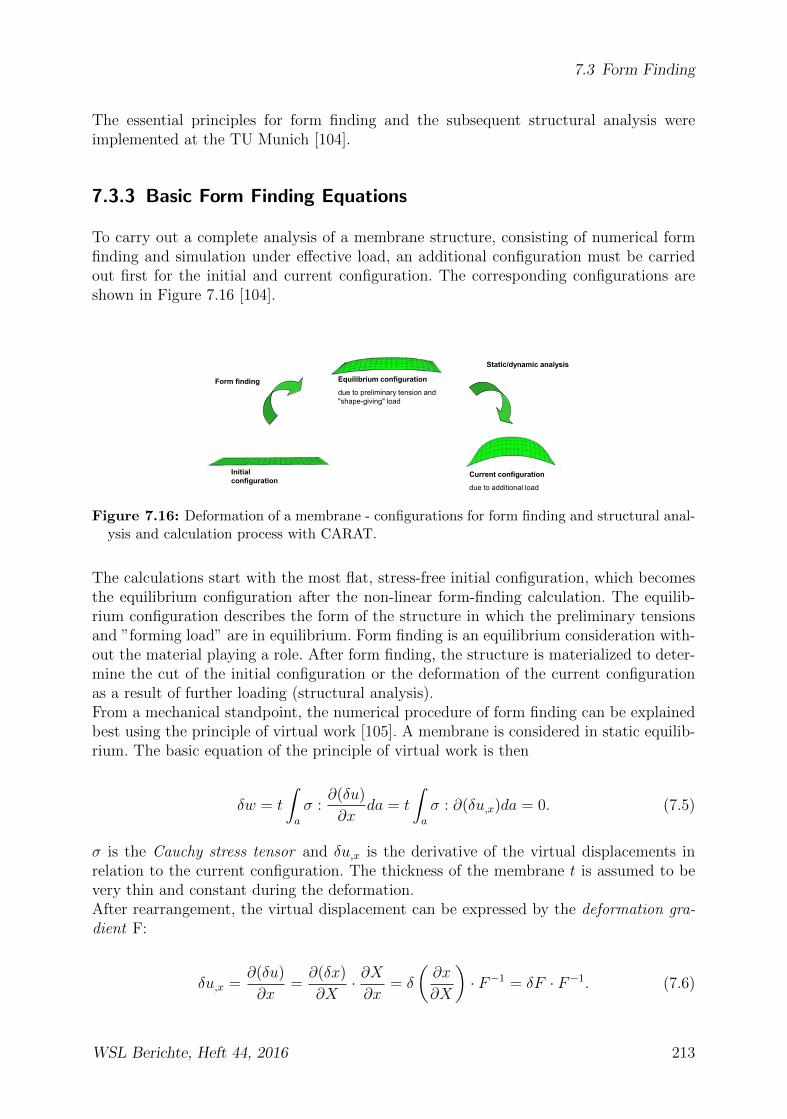
7.3 Form Finding
The essential principles for form finding and the subsequent structural analysis wereimplemented at the TU Munich [104].
7.3.3 Basic Form Finding Equations
To carry out a complete analysis of a membrane structure, consisting of numerical formfinding and simulation under effective load, an additional configuration must be carriedout first for the initial and current configuration. The corresponding configurations areshown in Figure 7.16 [104].
Form finding
Current configuration
due to additional load
Initial configuration
Equilibrium configuration
due to preliminary tension and "shape-giving" load
Static/dynamic analysis
Figure 7.16: Deformation of a membrane - configurations for form finding and structural anal-ysis and calculation process with CARAT.
The calculations start with the most flat, stress-free initial configuration, which becomesthe equilibrium configuration after the non-linear form-finding calculation. The equilib-rium configuration describes the form of the structure in which the preliminary tensionsand ”forming load” are in equilibrium. Form finding is an equilibrium consideration with-out the material playing a role. After form finding, the structure is materialized to deter-mine the cut of the initial configuration or the deformation of the current configurationas a result of further loading (structural analysis).From a mechanical standpoint, the numerical procedure of form finding can be explainedbest using the principle of virtual work [105]. A membrane is considered in static equilib-rium. The basic equation of the principle of virtual work is then
δw = t
∫a
σ :∂(δu)
∂xda = t
∫a
σ : ∂(δu,x)da = 0. (7.5)
σ is the Cauchy stress tensor and δu,x is the derivative of the virtual displacements inrelation to the current configuration. The thickness of the membrane t is assumed to bevery thin and constant during the deformation.After rearrangement, the virtual displacement can be expressed by the deformation gra-dient F:
δu,x =∂(δu)
∂x=∂(δx)
∂X· ∂X∂x
= δ
(∂x
∂X
)· F−1 = δF · F−1. (7.6)
WSL Berichte, Heft 44, 2016 213

7 Numerical Modeling
Figure 7.17: Tangential stress state of a membrane [105].
If equation 7.6 is now inserted into equation 7.5 and integrated over the initial area A,the following equation results:
δw = t
∫A
σ : (δF · F−1)detFdA = t
∫A
detF (σ · F−T ) : δFdA = 0. (7.7)
Finally, the 2nd Piola-Kirchhoff stress tensor S = detFF−1 · σ · F−T is introduced. TheCauchy stress tensor relates to the current configuration, while the 2nd Piola-Kirchhoffstress tensor relates to the reference or initial configuration. σ and S are identical if currentand initial configuration are the same, which is the case in the equilibrium configurationand thus in the form finding solution.The theory of form finding is not discussed in any more detail in this paper. For a moredetailed description of the derivation of the principle of virtual displacements and thenumerical implementation for the finite element calculation of the form-finding analysis,see [104].
7.3.4 General Modeling Details
Two modeling types were studied for the ring net in CARAT. One consists in reproducingthe ring net as a membrane that can reproduce the properties of the reproduction as wellas possible. The material property of the membrane elements of only being able to transfertensile stresses is well suited to this (see Fig. 7.18, left). However, with an isotropic materiallaw of the membrane elements, the shear modulus cannot be influenced separately fromthe E-modulus and Poisson’s ratio [104]. This results in contradictory material behaviorbetween the model and the ring net, because the ring net itself cannot absorb shear forces.
In modeling terms, the problem of shear stiffness can be circumvented by selecting an or-thotropic material law. With this material behavior, the shear modulus can be minimizedseparately. Because the ring net has the same material properties in different directions,the fiber directions are each allocated the same material characteristic values.A particular property of membranes is that they can only transfer tensile force. If com-pression occurs, they attempt to evade it perpendicular to their plane. Wrinkling occurs,which result in numerical instabilities in the simulation. Wrinkling can be understood
214 WSL Berichte, Heft 44, 2016

7.3 Form Finding
Figure 7.18: Pulled 8-ring arrangement of ROCCO 19/3/300 (red) and the determined bendingand tensile stiffness kb and kt of it [45].
in structural engineering terms as a local stability problem. There are two different ap-proaches to this problem.The first and simplest option, which is however hardly useful in practice, is to changethe discretization. Coarser discretizations calculate beyond the wrinkle problems and”smooth” them, in a manner of speaking. The great disadvantage of this approach is thatthe calculation accuracy rapidly decreases with coarser discretization, and this method isless practical as a result.It is better to model the structure with specific membrane elements that have implementedthe wrinkling and thereby resolve and calculate wrinkled regions with normal discretiza-tion fineness. This procedure does not require a coarse or very fine discretization, whichresults in inaccuracies or very long calculation times, and the convergence behavior is alsostable [104].
Figure 7.19: Model of an individual ring with truss elements and generated rope net with trusselements.
Alternatively to an orthotropic, flat membrane, the ring net can be reproduced as a ropenet. In this case the ring net is reproduced with truss elements, which interconnect toform a rope net. An individual ring is discretized by four truss elements. The node pointsof the individual elements then form the overlap region of the rings. The biggest modelingerror that can occur in this case is caused by the contact points of the individual rings
WSL Berichte, Heft 44, 2016 215

7 Numerical Modeling
in the nodes being reproduced rigidly, whereas in reality these can slide freely [103]. Inaddition, this method entails additional time and effort in model generation compared tomodeling with membrane elements, owing to the large number of elements with a complexelement-node assignment.
Figure 7.20: Test stand used for calibration. Legend: instrumentierter Wurfkorper = instru-mented impact body.
Figure 7.21: Comparison between membrane and rope net model deformations of the tensionedring net in the test stand.
Both modeling approaches are calibrated with the aid of the experimental data of the CTIframe (see Fig. 7.20). In the frame experiments, an 820kg experimental ball was placedinto the ring net shackled in the frame and the static slack was measured. The model ofthe membrane elements and the model of the rope net were then calibrated to these de-formation values. With the membrane elements, the problem of wrinkling occurred in thecorner regions with the four-sided mounting produced from the experimental arrangementin the frame. This wrinkling was intensified by the central load point of the subsequentlymodeled ball, the load from the ball being assumed to be distributed over half the ball sur-face. It was possible to overcome the wrinkling in the model with orthotropic membrane
216 WSL Berichte, Heft 44, 2016
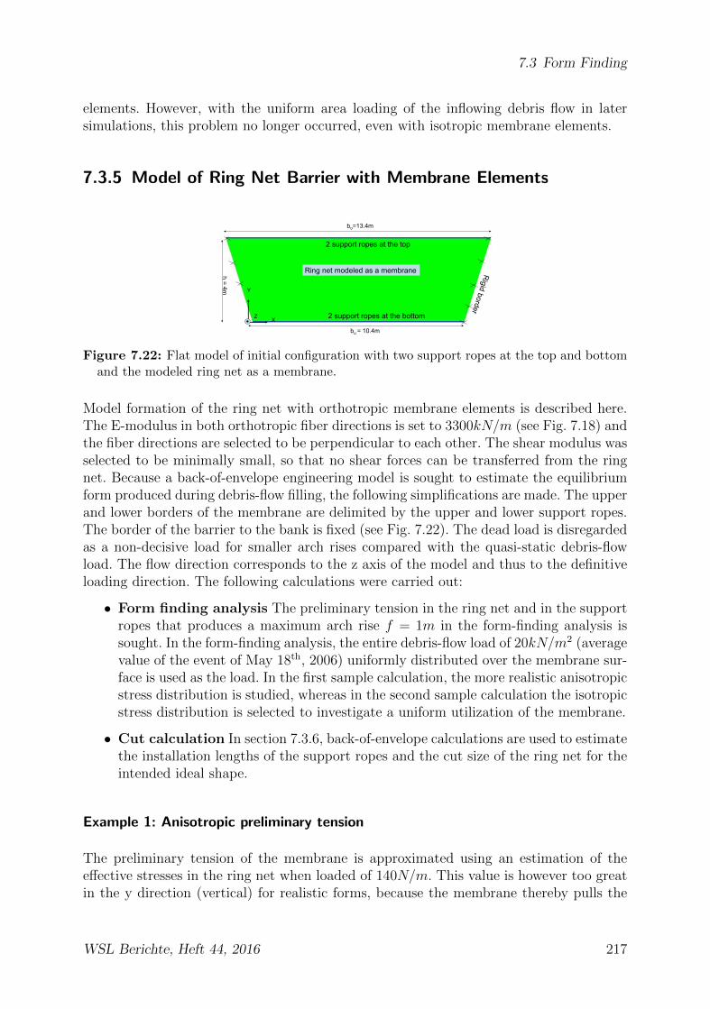
7.3 Form Finding
elements. However, with the uniform area loading of the inflowing debris flow in latersimulations, this problem no longer occurred, even with isotropic membrane elements.
7.3.5 Model of Ring Net Barrier with Membrane Elements
2 support ropes at the top
2 support ropes at the bottom
Ring net modeled as a membrane
X
Y
Z
bo=13.4m
bu = 10.4m
h = 4m
Figure 7.22: Flat model of initial configuration with two support ropes at the top and bottomand the modeled ring net as a membrane.
Model formation of the ring net with orthotropic membrane elements is described here.The E-modulus in both orthotropic fiber directions is set to 3300kN/m (see Fig. 7.18) andthe fiber directions are selected to be perpendicular to each other. The shear modulus wasselected to be minimally small, so that no shear forces can be transferred from the ringnet. Because a back-of-envelope engineering model is sought to estimate the equilibriumform produced during debris-flow filling, the following simplifications are made. The upperand lower borders of the membrane are delimited by the upper and lower support ropes.The border of the barrier to the bank is fixed (see Fig. 7.22). The dead load is disregardedas a non-decisive load for smaller arch rises compared with the quasi-static debris-flowload. The flow direction corresponds to the z axis of the model and thus to the definitiveloading direction. The following calculations were carried out:
• Form finding analysis The preliminary tension in the ring net and in the supportropes that produces a maximum arch rise f = 1m in the form-finding analysis issought. In the form-finding analysis, the entire debris-flow load of 20kN/m2 (averagevalue of the event of May 18th, 2006) uniformly distributed over the membrane sur-face is used as the load. In the first sample calculation, the more realistic anisotropicstress distribution is studied, whereas in the second sample calculation the isotropicstress distribution is selected to investigate a uniform utilization of the membrane.
• Cut calculation In section 7.3.6, back-of-envelope calculations are used to estimatethe installation lengths of the support ropes and the cut size of the ring net for theintended ideal shape.
Example 1: Anisotropic preliminary tension
The preliminary tension of the membrane is approximated using an estimation of theeffective stresses in the ring net when loaded of 140N/m. This value is however too greatin the y direction (vertical) for realistic forms, because the membrane thereby pulls the
WSL Berichte, Heft 44, 2016 217

7 Numerical Modeling
upper and lower support ropes together too much and too much of the barrier’s height(h′b << hb) is lost. Consequently, an anisotropic preliminary tension was selected thatonly has 140kN/m preliminary tension in the x direction and 20kN/m in the verticaldirection (y direction). The ropes are pre-tensioned with 50kN .
Figure 7.23: Vertical deformations of the equilibrium configuration of the barrier (anisotropi-cally pre-tensioned) modeled for a desired maximum arch rise f of 1m.
Figure 7.24: Horizontal deformations of the equilibrium configuration of the barrier (anisotrop-ically pre-tensioned) modeled for a desired maximum arch rise f of 1m.
Figure 7.25: Ring net stresses in the equilibrium configuration of the ring net barrier for amaximum arch rise f of 1m with anisotropic preliminary tension of the membrane.
The deformation amounts of the ”ideal shape” in the vertical and horizontal directions areshown in Figures 7.23 and 7.24. A feasible shape (equilibrium configuration) was foundfor the ring net barrier with an intended target deformation of f = 1m.The von Mises stresses are relevant for the utilization of the ring net (see Fig. 7.25). Theycorrespond to the required preliminary tension value (target condition of the form-findinganalysis); stress peaks only occur along the support rope. These can be explained by thefixed mounting of the membrane on the support ropes, which prevents the membraneslipping on the support ropes.Because a uniform stress distribution is usually the aim for flat support structures, anisotropic preliminary stress state is studied in the next sample calculation.
218 WSL Berichte, Heft 44, 2016

7.3 Form Finding
Example 2: Isotropic preliminary tension
In the barrier below, the membrane is pre-tensioned isotropically with 40kN/m and thesupport ropes are pre-tensioned with 100kN/m. The isotropic preliminary tension is re-duced accordingly to avoid excessively reducing the membrane area owing to the lessdominant load transference direction (h′b << hb). Therefore, the preliminary tension inthe support ropes is also increased.
Figure 7.26: Vertical deformations of the equilibrium configuration of the barrier modeled fora desired maximum arch rise f of 1m (isotropically pre-tensioned).
Figure 7.27: Horizontal deformations of the equilibrium configuration of the barrier modeledfor a desired maximum arch rise f of 1m (isotropically pre-tensioned).
A realistic equilibrium form of the form-finding calculation is observed here too. Thedefined target deformation f = 1m is achieved. The vertical deformations in the uppersupport ropes (middle of the barrier) are also in the acceptable range at 1.4m. With regardto the intended ring net stress of 40kN/m2, it can be seen in Figure 7.28 that this orderof magnitude is achieved in the border region of the barrier. Greater von Mises stressesoccur in the middle region owing to the direct vertical load transference direction to thesupport ropes.
Figure 7.28: Ring net stresses in the equilibrium configuration of the ring net barrier for amaximum arch rise f of 1m (isotropically pre-tensioned).
In summary, both calculations have achieved their equilibrium form and thus form amodel for an approximate determination of the ”ideal form” of a ring net barrier for a
WSL Berichte, Heft 44, 2016 219
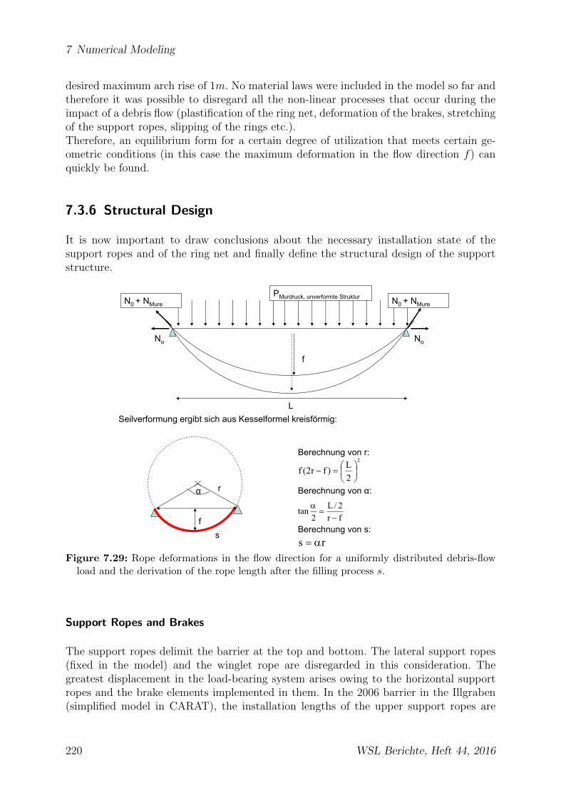
7 Numerical Modeling
desired maximum arch rise of 1m. No material laws were included in the model so far andtherefore it was possible to disregard all the non-linear processes that occur during theimpact of a debris flow (plastification of the ring net, deformation of the brakes, stretchingof the support ropes, slipping of the rings etc.).Therefore, an equilibrium form for a certain degree of utilization that meets certain ge-ometric conditions (in this case the maximum deformation in the flow direction f) canquickly be found.
7.3.6 Structural Design
It is now important to draw conclusions about the necessary installation state of thesupport ropes and of the ring net and finally define the structural design of the supportstructure.
f
No No
PMurdruck, unverformte StrukturN0 + NMure N0 + NMure
L
rα
sf
Berechnung von r:2
2L)fr2(f ⎟⎠⎞
⎜⎝⎛=−
rs α=
Berechnung von α:
Berechnung von s:fr2/L
2tan
−=
α
Seilverformung ergibt sich aus Kesselformel kreisförmig:
Figure 7.29: Rope deformations in the flow direction for a uniformly distributed debris-flowload and the derivation of the rope length after the filling process s.
Support Ropes and Brakes
The support ropes delimit the barrier at the top and bottom. The lateral support ropes(fixed in the model) and the winglet rope are disregarded in this consideration. Thegreatest displacement in the load-bearing system arises owing to the horizontal supportropes and the brake elements implemented in them. In the 2006 barrier in the Illgraben(simplified model in CARAT), the installation lengths of the upper support ropes are
220 WSL Berichte, Heft 44, 2016
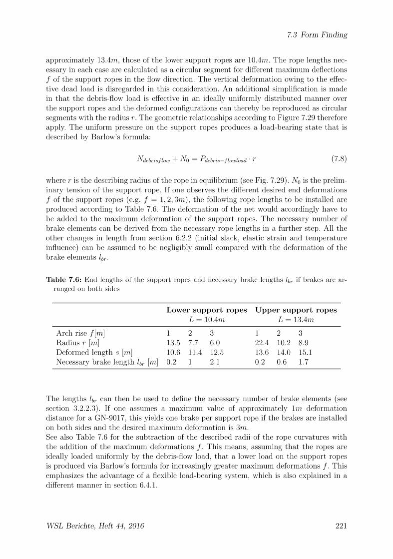
7.3 Form Finding
approximately 13.4m, those of the lower support ropes are 10.4m. The rope lengths nec-essary in each case are calculated as a circular segment for different maximum deflectionsf of the support ropes in the flow direction. The vertical deformation owing to the effec-tive dead load is disregarded in this consideration. An additional simplification is madein that the debris-flow load is effective in an ideally uniformly distributed manner overthe support ropes and the deformed configurations can thereby be reproduced as circularsegments with the radius r. The geometric relationships according to Figure 7.29 thereforeapply. The uniform pressure on the support ropes produces a load-bearing state that isdescribed by Barlow’s formula:
Ndebrisflow +N0 = Pdebris−flowload · r (7.8)
where r is the describing radius of the rope in equilibrium (see Fig. 7.29). N0 is the prelim-inary tension of the support rope. If one observes the different desired end deformationsf of the support ropes (e.g. f = 1, 2, 3m), the following rope lengths to be installed areproduced according to Table 7.6. The deformation of the net would accordingly have tobe added to the maximum deformation of the support ropes. The necessary number ofbrake elements can be derived from the necessary rope lengths in a further step. All theother changes in length from section 6.2.2 (initial slack, elastic strain and temperatureinfluence) can be assumed to be negligibly small compared with the deformation of thebrake elements lbr.
Table 7.6: End lengths of the support ropes and necessary brake lengths lbr if brakes are ar-ranged on both sides
Lower support ropes Upper support ropesL = 10.4m L = 13.4m
Arch rise f [m] 1 2 3 1 2 3Radius r [m] 13.5 7.7 6.0 22.4 10.2 8.9Deformed length s [m] 10.6 11.4 12.5 13.6 14.0 15.1Necessary brake length lbr [m] 0.2 1 2.1 0.2 0.6 1.7
The lengths lbr can then be used to define the necessary number of brake elements (seesection 3.2.2.3). If one assumes a maximum value of approximately 1m deformationdistance for a GN-9017, this yields one brake per support rope if the brakes are installedon both sides and the desired maximum deformation is 3m.See also Table 7.6 for the subtraction of the described radii of the rope curvatures withthe addition of the maximum deformations f . This means, assuming that the ropes areideally loaded uniformly by the debris-flow load, that a lower load on the support ropesis produced via Barlow’s formula for increasingly greater maximum deformations f . Thisemphasizes the advantage of a flexible load-bearing system, which is also explained in adifferent manner in section 6.4.1.
WSL Berichte, Heft 44, 2016 221

7 Numerical Modeling
Cutting the Ring Net to Size
To be able to define the necessary number of rings and the size of the ring net when in-stalled, the deformation of the rings from the round (elastic) state to the angular (plastic)state according to Figure 7.30 must first be taken into account. The plastic strain of therings themselves is disregarded, as a result of which the edge length of the ring a thathas been deformed into a square shape can be calculated from the circumference of thering to give a = 2 · π · r/4 = 2 · π · 0.15/4 = 0.23m for a ring diameter of d = 30cm(see Fig. 7.30). The spacing of the main rows of rings is estimated using the deformedgeometry in Figure 7.30 to give a/2.The maximum bulge in the center of the ring net according to Figure 7.27 is decisive forthe number of necessary horizontal rows of rings. In reality, the maximum arch rise of thering net tends to be in the lower half of the barrier owing to the additionally effectivedead load and the (usually trapezoidal) debris-flow load distribution that varies over theheight, but the necessary number of rings remains the same for the structural design.
Main row Main row
a/2
a
Figure 7.30: Deformed ring net and the approximation of the ring as a square with a sidelength a.
As shown in Figure 7.27 the simplified model in CARAT produced for the equilibriumform a 30cm larger maximum deformation f in the ring net than in the support ropeswith a total deformation of approximately 1.1m. For a radius of r = 16.6m, this yields anet length snet,h of 12.2m, if the deformed ring net is projected into a plane. This meansthat the necessary number of main ring rows with a distance between two rows of ≈ a/2according to Figure 7.30 is N = 12.2/(0.23 + 0.23/2) = 36 main ring rows.
If the number of main rings to be installed is compared with the number of main ring rowsthat is recommended by the manufacturer per meter of net area [39], a recommendationof 2.8 rings per meter with an average barrier span of 11.9m gives a main ring number of33 rings. Therefore, 3 additional ring rows are necessary in the central net region.The same calculation is carried out for the vertical rings. In this case, the lowering of thenet from hb = 4 to h′b = 4− 1.4− 0.7 = 1.9m remaining height according to Figure 7.26 istaken into account. For 30cm maximum deformation of the ring net in the flow direction,this yields a necessary vertical net length of snet,v = 2.09m. This is half the installationlength of the net at 4m. So, only the structural number of rings from [39], which is specified
222 WSL Berichte, Heft 44, 2016

7.3 Form Finding
as 21 (main and secondary rings) for a height of 4m and a ring diameter of d = 30cm, isdecisive for the vertical length of the net owing to settling of the barrier.Because additional distance in the rings becomes free during vertical deformation, itwould be conceivable that additional main rows do not have to inserted in the horizontaldirection either. The rings can deform in a more rectangular manner with the larger axisin the horizontal direction (x direction), which also supports the main transfer directionin the horizontal direction (x direction) (see Fig. 7.32).The diagonals at the sides are added by means of additional cuts or the rings that havebeen cut off in the lower net region (see Fig. 7.31).
10.4m
13.4m
Number of main rows = 36 installed across 11.9mNum
ber of main row
s: 10
Cutting line ring net
4m
Figure 7.31: Required ring rows and cuts from form-finding calculation.
Figure 7.32: Ring net that has deformed in a rectangular manner with a larger deformation ofthe rings in the horizontal direction, which supports the horizontal load transference directionof the membrane.
Structural Details
There are other important points to take into account in the form finding of the barriersin addition to the maximum deformation and the ring net shape. The final form of thebarrier has a big influence e.g. on the behavior of the barrier with respect to durability. Ifwater containing sediment flows continuously over the deformed bulge of the barrier, the
WSL Berichte, Heft 44, 2016 223
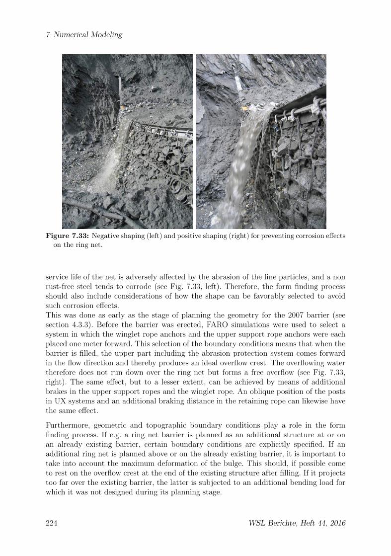
7 Numerical Modeling
Figure 7.33: Negative shaping (left) and positive shaping (right) for preventing corrosion effectson the ring net.
service life of the net is adversely affected by the abrasion of the fine particles, and a nonrust-free steel tends to corrode (see Fig. 7.33, left). Therefore, the form finding processshould also include considerations of how the shape can be favorably selected to avoidsuch corrosion effects.This was done as early as the stage of planning the geometry for the 2007 barrier (seesection 4.3.3). Before the barrier was erected, FARO simulations were used to select asystem in which the winglet rope anchors and the upper support rope anchors were eachplaced one meter forward. This selection of the boundary conditions means that when thebarrier is filled, the upper part including the abrasion protection system comes forwardin the flow direction and thereby produces an ideal overflow crest. The overflowing watertherefore does not run down over the ring net but forms a free overflow (see Fig. 7.33,right). The same effect, but to a lesser extent, can be achieved by means of additionalbrakes in the upper support ropes and the winglet rope. An oblique position of the postsin UX systems and an additional braking distance in the retaining rope can likewise havethe same effect.
Furthermore, geometric and topographic boundary conditions play a role in the formfinding process. If e.g. a ring net barrier is planned as an additional structure at or onan already existing barrier, certain boundary conditions are explicitly specified. If anadditional ring net is planned above or on the already existing barrier, it is important totake into account the maximum deformation of the bulge. This should, if possible cometo rest on the overflow crest at the end of the existing structure after filling. If it projectstoo far over the existing barrier, the latter is subjected to an additional bending load forwhich it was not designed during its planning stage.
224 WSL Berichte, Heft 44, 2016

7.3 Form Finding
Figure 7.34: Geometrically constrained selection of the boundary conditions in the addition ofa net barrier to an already existing structure, Illgraben VS, Barrier 25.
If an addition is made to the side of a concrete barrier, as in the case of Barrier 25 inthe Illgraben, the boundary conditions of the barrier, such as anchor position and roperouting, are largely already defined by the old structure. The obliquely arranged secondbarrier, which is situated above the first net barrier, acts to divert the debris-flow streamover the actual concrete barrier (see Fig. 7.34). Indirect form finding was also conductedin this case.
Shaping from a Construction Standpoint
If the two other aspects of form finding - durability and geometric conditions - fromsection 7.3.6 are included in the structural design, this means that first the horizontaldeformation of the barrier in the flow direction must be estimated or calculated to decidethe location at which the net should be installed. It is then necessary to analyze thegeometric conditions on site for the selection of the anchors and where necessary revisethe model if the anchors cannot be drilled according to the model created.Barlow’s formula in equation 7.8 shows that large maximum deformations have a morefavorable load-transference behavior for the debris-flow load. Here, however, the deadload of the retained debris-flow material must be taken into account. If the ring netprojects far beyond the line of the support ropes, very high loads quickly arise from thedead load with large bulges. These loads must be transferred accordingly via the supportstructure. The same caution should be exercised with a larger bulge in the upper barrierpart, which is better suited for structural reasons to improving corrosion problems, butrepresents a large additional load on the whole system, especially during the overflowprocess.In addition, the intended purpose of the barrier must be taken into consideration.Is the barrier planned to provide debris-flow retention or as a barrier that remainspermanently full to create a small vertical-drop effect in the streambed? In the lattercase, additional measures are required for durability. The selection of upper anchorsthat are brought forward and deviate from the vertical system line is recommended forthis (see section 4.3.3). This necessarily results in a deformed configuration that comesfurther forward horizontally in the flow direction at the upper support ropes. Direct
WSL Berichte, Heft 44, 2016 225

7 Numerical Modeling
contact between the overflowing water and the net can thereby largely be avoided andconsequently corrosion can be prevented.
Form finding in this field ultimately consists in weighing up, in engineering terms,which deformation is needed for uniform load transference in the system and to whatextent this shaping can be realized from the geometric conditions on site to take intoaccount at the same time the structural aspects of durability.
226 WSL Berichte, Heft 44, 2016

7.4 Interpretation
7.4 Interpretation
7.4.1 FARO for Simulating Debris-flow Barriers
The simulations of the ring net barrier with the finite-element program FARO show satis-factory results on the structural side of the structure. The component-specific calibrationof the individual elements from rockfalls also prove advantageous when used for the calcu-lation of debris-flow barriers. The choice of model generation with individual node loadsto verify the pressure step model meant that rope loads could be calculated in the sim-ulations with less than 20% deviation from the measured loads of the field barriers. Thedeformations of the structure during the filling process seem plausible and coincide withthe observations from the analyzed video recording.The static loads can likewise be reproduced in a satisfactory manner by a dynamic cal-culation with an increase up to maximum load and a subsequent constant load level.
7.4.2 CARAT for Form-finding Analysis of Debris-flow Barriers
In the process of designing the flexible barriers, it is important that the shape is madefeasible even at the early stage of selecting the boundary conditions, such as anchor pointsand preliminary tension of the ropes and ring net. Therefore, a form-finding analysis withCARAT is carried out in addition to the structural calculation with FARO. In the pro-cess, a simplified model of the ring net barrier is created with membrane elements andthe equilibrium form obtained is studied for feasibility and practicability.The aspect of structural design was supplemented by a back-of-envelope engineering cal-culation for the necessary installation lengths of the support ropes and the necessary cutsof the ring net.
Owing to the simplified model of the ring net barrier in CARAT by means of membraneelements that reproduce the ring net and duplicate support rope routing at the top andbottom and fixed borders at the side, it was not possible to simulate the occurring loadsexactly. To do this, specific calibration calculations would first have to be carried out tosimulate the structure-specific components, as was the case with the calibration of theFARO software. For realistic modeling, specific adaptations would have to be made inCARAT, e.g. for rings, support rope brakes etc., which would in principle be possible infuture. The first step was basically a calibration of the membrane element with the staticvalues of the ring net tensioned in the test stand in order to obtain a rough estimation ofthe necessary material parameters for the element.
7.4.3 Comparison of Both Procedures and Outlook
In the structural calculation with FARO, a non-linear, dynamic calculation was usedto directly calculate the occurrent load distribution of the barrier. The non-linearanalysis changes the undeformed ring net barrier of the initial configuration into thedeformed state, the current configuration (see Fig. 7.35). This required an existing,
WSL Berichte, Heft 44, 2016 227
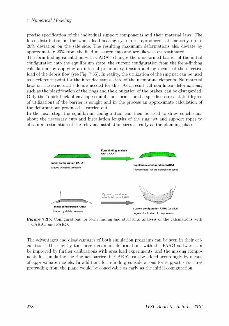
7 Numerical Modeling
precise specification of the individual support components and their material laws. Theforce distribution in the whole load-bearing system is reproduced satisfactorily up to20% deviation on the safe side. The resulting maximum deformations also deviate byapproximately 20% from the field measurements and are likewise overestimated.The form-finding calculation with CARAT changes the undeformed barrier of the initialconfiguration into the equilibrium state, the current configuration from the form-findingcalculation, by applying an internal preliminary tension and by means of the effectiveload of the debris flow (see Fig. 7.35). In reality, the utilization of the ring net can be usedas a reference point for the intended stress state of the membrane elements. No materiallaws on the structural side are needed for this. As a result, all non-linear deformations,such as the plastification of the rings and the elongation of the brakes, can be disregarded.Only the ”quick back-of-envelope equilibrium form” for the specified stress state (degreeof utilization) of the barrier is sought and in the process an approximate calculation ofthe deformations produced is carried out.In the next step, the equilibrium configuration can then be used to draw conclusionsabout the necessary cuts and installation lengths of the ring net and support ropes toobtain an estimation of the relevant installation sizes as early as the planning phase.
Form finding analysis with CARAT
Initial configuration CARAT
loaded by debris pressureEquilibrium configuration CARAT
("ideal shape" for pre-defined stresses)
Dynamic, non-linear simulation with FARO
Current configuration FARO (detailed
degree of utilization of components)
Initial configuration FARO
loaded by debris pressure
Figure 7.35: Configurations for form finding and structural analysis of the calculations withCARAT and FARO.
The advantages and disadvantages of both simulation programs can be seen in their cal-culations. The slightly too large maximum deformations with the FARO software canbe improved by further calibrations with area load experiments, and the missing compo-nents for simulating the ring net barriers in CARAT can be added accordingly by meansof approximate models. In addition, form-finding considerations for support structuresprotruding from the plane would be conceivable as early as the initial configuration.
228 WSL Berichte, Heft 44, 2016

8 Debris-flow Barrier Design Example
In chapter 6, the historical approaches to designing debris-flow barriers were outlined anda new load model was developed from the previously acquired findings from field and lab-oratory tests. This model based on pressure surges (see section 6.3) is now implementedin an example of use.First, the parameters relevant for the implementation are defined and estimated and thenecessary topographic conditions for erecting a ring net barrier are included in the choiceof location. A section on the subject of ”corrosion” also provides possibilities for solvingthis problem.The basic procedure for determining decisive safety factors, to be carried out for a compre-hensive series of measured debris-flow load data gathered over a long period, is describedbelow. Because there is not yet sufficient measurement data for this work, the recom-mended safety factors from building insurance [60] are used, although these should beclassed as critical for the problem of debris-flow load on ring net barriers, from the view-point of risk and safety experts1. However, the circle of practitioners and engineers whoare the users must be provided with some sort of guidelines for a design concept, becausethe implementation of the nets in practice has already begun (see section 2.4.3 and 2.4.2),and moreover the safety factors in the guidelines from cantonal insurers are on the sideof caution.A critical assessment of the limits of use of flexible ring net barriers forms the conclusionof this chapter.
8.1 Topographic Conditions and Choice of Location
In principle, any debris-flow channel or mountain torrent is suitable for the installationof flexible ring net barriers, as long as its width is less than 25m and appropriate bankslopes are present for anchoring the load-bearing system. It must be considered as earlyas the planning stage where the most favorable location for the respective structure is,because the area of application of the barriers depends decisively on this.
• Use as an available retention volume In this case, an installation of the barrieror a number of barriers in the catchment area or directly below already known slidesand instabilities is recommended, since only this can prevent even more materialbeing mobilized along the channel during the flow process (see implementation inBrienz and Hasliberg, section 2.4).
• Use in the filled state as a barrier or bed stabilization In this case, the struc-
1Personal communication with Dr. Jochen Kohler, Department of Risk and Safety, ETH Zurich
229

8 Debris-flow Barrier Design Example
tures should be sited where the greatest energy loss can be achieved or where energyis to be removed from the flow process of the debris flow or from the flood discharge.If there is a series of structures, the spacing between the barriers must also be consid-ered, so that the desired hydraulic jump formation and thus the energy-dissipationprocess takes place (see section 3.4.2). Guide values for the barrier spacing l in anechelon of barriers are specified as l > 10m or as twice the scour length lk [11, 8].
Other points that are relevant for choosing the location of barriers are:
• Accessibility If the barrier is planned as a debris-flow retention space, good ac-cessibility must be ensured for any emptying necessary. If possible, an access roadshould be provided above the structure, so that the barrier does not have to beopened, as is the case with access from below (see section 3.2.5). The routes tothe respective landfill site should ideally be passable with trucks and have a shortdistance.
• Winglet stability The structure should generally be planned for where the bankslopes capable of bearing the most load are. The necessary anchor length and num-ber of anchors can then be minimized. In general, temporary deposition regions,which mostly consist of ground that can bear little load and is very susceptible toweathering, should be avoided.
• Channel slope The gentler the slope of the channel at the location of the barrier,the greater the retention volume. In addition, the debris flow flows more slowly insections of more gradual inclines, as a result of which the occurrent loads on thestructure become smaller.
• Channel cross section The cross-section width at the location of the barriershould not exceed 25m, because ring net barriers are not suitable for a larger spanowing to the load-bearing system (see section 8.7.2). In addition, the bank heightsat the cross-sectional profile should be at least as high as the planned barrier heightin order to be able to anchor the upper support ropes. It is of course better if theupper edges of the bank slopes are much higher than the planned upper edge of thenet, in order to prevent the debris flow bursting its banks and overflowing.
• Composition of the channel bottom A solid stream bottom consisting of arocky substrate would also be advantageous, since the basal opening can then beadapted reliably to the discharge depth of the decisive flood discharge without thebed being washed out under the barrier and the basal opening being undesirablywidened (see section 4.3.3).
• Avoidance of avalanche chutes Avalanche chutes should generally be avoidedwhen selecting the location, because the pressures of impacting avalanches are toogreat for the load-bearing system of a ring net barrier.
230 WSL Berichte, Heft 44, 2016

8.2 Input Data
8.2 Input Data
To calculate the occurrent load, the following debris-flow parameters are of critical im-portance:
• Density ρ
• Maximum front velocity u
• Flow depth hfl
• Dry density ρs, angle of internal friction φ′ (only for precise calculation of ”overflow”loading condition)
If individual variables for the dimensioning are not directly known, a useful approximationis made by an engineering evaluation or by empirical approaches.The following variables are geometrically relevant for the barrier to be planned:
• Decisive debris-flow volume or volume of a debris-flow surge V
• Planned retention volume of barrier Vr
• Channel slope Is
• Average channel width b at barrier location
For empirical estimation of the occurrent velocities, the maximum possible dischargesQmax during a debris-flow event must first be estimated. Two approaches according toMizuyama et. al [70] are used for this: one approach for muddy debris flows and one forgranular debris flows
Qmud = 0.0188V 0.79 (8.1)
Qgranular = 0.135V 0.78 (8.2)
where V is the decisive debris-flow volume. For further approaches to calculating thedischarge of debris flows, see [89].The velocity development of debris flows is estimated with
u = 2.1Q0.34I0.2s (8.3)
according to Rickenmann [81] or based on the flow approach of Manning-Strickler [77] togive
u =1
nh
2/3fl I
0.5s (8.4)
where n = 5.5 − 10 is the Strickler value depending on the channel roughness. Thereare further approaches to estimating the flow velocity, which are presented and compared
WSL Berichte, Heft 44, 2016 231

8 Debris-flow Barrier Design Example
with each other in [89]. For the dimensioning of the barriers, the two above calculationmethods are sufficient to determine the velocity, because they cover most events withadequate reliability (see [89]).
8.3 Design Concept
A safety concept is generally used to ensure the stability of a structure in the context ofload-bearing ability, fitness for purpose, and durability. This safety concept purelyformally mentions limit states, the exceeding of which means that the specified require-ments are no longer met. With regard to the ring net barriers, therefore, the followingdocumentation should be provided in the limit state of load-bearing ability:
• State of failure of support ropes and brakes owing to excessive tensile and transverseforce effects
• Breakage of ring net as a result of excessive loads
• Breakage of anchors or flex heads (cross section failure)
• Failure of anchors on pulling out (shaft friction).
The limit state of fitness for purpose comprises the following criteria:
• Documentation of maximum deformations (form-finding analysis)
• Remaining height (necessary retention volume)
and in the case of an event to ensure the retention function
• Necessary emptying (if desired)
• Necessary repairs (brake replacement, replacement of damaged support ropes).
Durability includes the following points:
• Correct structural design and shaping to avoid corrosion and abrasion (see sec-tion 7.3.6)
• Corrosion protection of the structure generally (for any cross section impact, seesection 8.4)
• Erosion of foundations and anchors.
For conventional issues of impact and resistance in construction, safety sub-factors aredefined in the new safety concept for the loading (impact) γF and for the capacity towithstand loads (resistance) γR on the basis of probabilistic methods (see new DIN 1055-100 [27], DIN 1045 [26], DIN 18800 [32], SIA 260 [91], SIA 261 [93]). In contrast to this,previous standards had only one global safety factor that covers both sides (e.g. 1045-1edition 7.88, DIN 18800-1 edition 3.83).
232 WSL Berichte, Heft 44, 2016

8.3 Design Concept
8.3.1 Distinction from Existing Standards
Because the safety factors of the above standards relate to specific, problem-related studiessuch as the probability of a building failing under the effect of wind and snow, they are nottransferable to the subject of debris-flow barriers. Specific safety factors must be derivedprecisely for the problem of ring net barriers under debris-flow load. The probability offailure used here results from an optimization of the incurred costs of the measure and theextent of the damage reduced thereby. This produces the question of a cost-benefit anal-ysis (see also section 8.6.8). Although a smaller probability of breakage can be achievedwith a greater number or greater dimensions of nets, this also results in much higher costsfor the building measures.In previous planning processes (e.g. Hasliberg and Brienz in section 2.4.3 and 2.4.2) thenumber of nets was determined from the predicted debris-flow volumes of a specifiedrecurrence interval. The volume reduction of the debris-flow event with protective mea-sures means that the occurring damage potential is reduced correspondingly (see alsosection 8.6.8).
In SIA 261/1 (see section 6.1.7), debris flows are always referred to as extraordinary loadson a structure. A debris flow generally acts as a temporary load. Whether it is declared anextraordinary or normal impact depends on the probability of occurrence of the loadingcondition. Because a debris-flow protection structure has a greater probability of beingloaded by a debris flow during its service life, a debris flow cannot be an extraordinaryloading condition, because DIN 1055-9 specifies an annual probability of occurrence ofp = 10−4 for this [28], which corresponds to the probability of a debris flow occurringevery 10, 000 years. In SIA 261, the extraordinary loading condition is only describedwith a low probability of occurrence and no concrete values are given for the probabilityof occurrence [92].In Table 6.1 (taken from [60]), based on the SIA, debris flows with short recurrence periods(1 − 30 years) are declared a normal impact and those with longer recurrence intervals(> 30 years) are declared an extraordinary impact.
The recurrence period or frequency of occurrence is always an important influencing vari-able for the basis of a safety concept. The occurrent intensities of the load are also signif-icant.SIA 261/1 [93] subdivides debris flows into medium and strong intensities (see sec-tion 6.1.7). The SIA is also based on hazard maps, which classify debris flows into thefollowing levels of hazard: Considerable risk, moderate risk, low risk, residual risk and norisk. These hazard maps also include the recurrence period, which is subdivided into 30,100 and 300 years.
WSL Berichte, Heft 44, 2016 233

8 Debris-flow Barrier Design Example
8.3.2 Intensity
The basic procedure for creating a safety concept for debris-flow loads on ring net barriersis presented below.The pressure exerted on a barrier by a debris flow is influenced by the following inputparameters and the associated uncertainties:
• Density of debris-flow material This can only be estimated as an average value.The density also influences the decisive pressure coefficient cd, which is greater forgranular debris flows than for muddy ones.
• Flow depth hfl This is assigned as a characteristic value to a certain quantile. Thequantile depends on the recurrence period.
• Impact velocity This is estimated from the average front velocity and is likewisedefined as a quantile value depending on the recurrence period.
The statistical variability of the above parameters requires a stochastic description ofthe debris-flow load acting on the barrier. The individual influencing factors can all bedescribed by certain distribution functions (e.g. normal, log-normal, Weibull distributionetc.), which are superimposed when the debris-flow load is calculated. This then yields anew distribution function, which describes the frequency of occurrence of certain debris-flow loads (density distribution). These can also be derived directly from the maximumdebris-flow loads over a certain time series given a sufficient amount of measurement dataand statistically checked accordingly [52]. Because only the extreme events are decisivefor the design, the debris-flow load distribution can be described over an extreme valuedistribution, e.g. Weibull, Gumbel or Frechet distribution [38] (see Fig. 8.1).
8.3.3 Probability of Occurrence
In addition to the occurrent intensity, the expected frequency of the events over time isrelevant. This time-dependent component is usually acquired with a power law (Pareto)distribution for flood distributions, rockfall events and slides [97, 96]: P = a · f−b. Thisdistribution is an approximation of the tail of the density function using a power law.Therefore, it only reproduces the frequencies of extreme events in the right-hand area ofthe density function (see Fig. 8.1). Parameters a and b are defined according to the profileof the debris-flow load distribution.
The density function of debris-flow loads can be used to define the characteristic debris-flow loads for certain specified quantile values. If longer recurrence periods and also greaterexpected intensities are included, the distribution shifts correspondingly to the right, sofor example the 95% quantile value of the 1-year event ultimately corresponds to the 50%quantile value of the 50-year event.
234 WSL Berichte, Heft 44, 2016

8.3 Design Concept
Yearlong series of measurements
50% quantile Recurrence every 50 years
Frequency
Debris-flow load per flow height [kN/m]
95% quantile
e.g. Gumbel distribution
Power Law: P=a f-b
Figure 8.1: Example of a density function of debris-flow loads and their distribution for longerdebris-flow recurrence intervals.
8.3.4 Probability of Failure
Based on DIN 1055-9 [28] for extraordinary loads, debris flows can also be described us-ing risk scenarios. The scope of the studies depends on the consequences to be expected.These consequences should be estimated taking into account the risk to people, the en-vironmental consequences and the economic damage to society. A division into hazardcategories, which are listed in Table 8.1, is also conceivable. The damage potential affectsthe decisive probability of failure that is accepted in a safety concept. Proceeding fromtypical probabilities of failure in construction of between pf = 10−3− 10−6 [58], these areassigned to the damage potential as follows: For a significant risk to human life in hazardcategory 3, pf = 10−6 is presumed, pf = 10−5 for hazard category 2, and finally pf = 10−3
for hazard category 1.The accepted probabilities of failure for debris-flow protective structures are takenfrom [98], these also being guided by the DIN standards (e.g. DIN 1055-100 [27]) forthe structural engineering of buildings. The accepted probability of failure is ultimatelyan optimization problem of the costs incurred by the measure and the damage reductionproduced (see section 8.6.8). Alternatively, according to [78], the accepted risk of failureis produced from the costs of reducing the risk, ethical principles and comparison withfurther risks. This boundary must therefore be located and defined accordingly for debris-flow protection structures, which should be understood as a prompt for further work inthe field of natural hazard management.
The probability of failure of a structure in structural engineering is calculated with theprobabilistic approach (frequency distributions with average value and standard devia-tions) from the difference between the resistance distribution R and the impact side Saccording to Figure 8.2 to yield
pf = P (R− S < 0) = P (M < 0). (8.5)
WSL Berichte, Heft 44, 2016 235
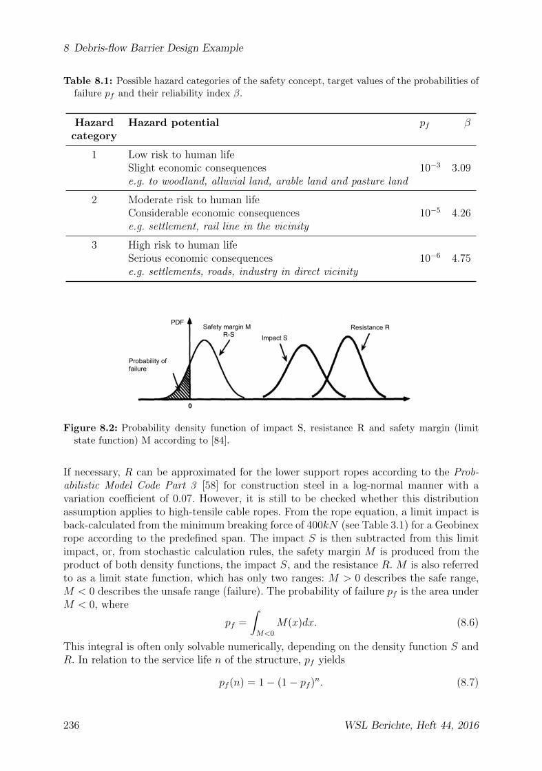
8 Debris-flow Barrier Design Example
Table 8.1: Possible hazard categories of the safety concept, target values of the probabilities offailure pf and their reliability index β.
Hazard Hazard potential pf βcategory
1 Low risk to human life10−3 3.09Slight economic consequences
e.g. to woodland, alluvial land, arable land and pasture land
2 Moderate risk to human life10−5 4.26Considerable economic consequences
e.g. settlement, rail line in the vicinity
3 High risk to human life10−6 4.75Serious economic consequences
e.g. settlements, roads, industry in direct vicinity
Resistance R
Impact S
Safety margin MR-S
Probability of failure
Figure 8.2: Probability density function of impact S, resistance R and safety margin (limitstate function) M according to [84].
If necessary, R can be approximated for the lower support ropes according to the Prob-abilistic Model Code Part 3 [58] for construction steel in a log-normal manner with avariation coefficient of 0.07. However, it is still to be checked whether this distributionassumption applies to high-tensile cable ropes. From the rope equation, a limit impact isback-calculated from the minimum breaking force of 400kN (see Table 3.1) for a Geobinexrope according to the predefined span. The impact S is then subtracted from this limitimpact, or, from stochastic calculation rules, the safety margin M is produced from theproduct of both density functions, the impact S, and the resistance R. M is also referredto as a limit state function, which has only two ranges: M > 0 describes the safe range,M < 0 describes the unsafe range (failure). The probability of failure pf is the area underM < 0, where
pf =
∫M<0
M(x)dx. (8.6)
This integral is often only solvable numerically, depending on the density function S andR. In relation to the service life n of the structure, pf yields
pf (n) = 1− (1− pf )n. (8.7)
236 WSL Berichte, Heft 44, 2016

8.3 Design Concept
The reliability index β is defined as a measure of safety [84]. This depends on the distri-bution of the limit state function by pf = Φ−1(−β). For a normal distribution of M , thetarget values of β are given in Table 8.1 for the specified probabilities of failure pf . Thenecessary safety factors on the material and impact sides for the corresponding impactcombination (in this case debris-flow load and dead load of the ring net barrier) can bederived from this reliability index. The safety factors ultimately determine the preciseposition of the impact density function and the resistance density function in relation toeach other and therefore the overlap region (failure).
If the probability of occurrence and intensity as well as the hazard potential and theassociated accepted probability of failure under the structure are taken into account, thesafety parameters according to Table 8.2 can be recommended.
Table 8.2: Safety factor γF on the impact side taking into account the probability of occurrenceand the expected damage potential, based on cantonal building insurance [60]
Recurrence period Hazard category
1 - 30 years
30 - 100 years
Over 100
years
1
1.0
1.0
1.0
2
1.3
1.3
1.2
3
1.5
1.3
1.2
Smaller safety parameters are produced for smaller probabilities of occurrence or largerunderlying debris-flow loads, and correspondingly larger safety parameters are producedfor lower accepted risks. The magnitude of the selected parameters was specified based onSIA 261/1 [93] and cantonal building insurance [60], where debris flows are divided intotwo intensity classes (see section 6.1.7). The medium intensity for debris flows (hfl < 1mand u < 1m/s) is generally very quickly exceeded, which is demonstrated by the valuesmeasured in the Illgraben (see Table 4.1). With the classification according to SIA 261/1,therefore, the intensity will mostly be high for a protective measure with ring net barriers.A simpler protective measure is sufficient and more cost-effective for medium intensity.Because it has not been possible to carry out a detailed risk analysis for ring nets un-der debris-flow impact, these values should be regarded only as a recommendation andreference point for engineers in practice. The recommended safety parameters from thecantonal building insurance are rather on the safe side for property protection guidelines,although they were not explicitly determined for the use of ring net barriers under debris-flow load.On the resistance side of the high-tensile support ropes, the safety factor γR = 1.35 fromavalanche protection [15] could be used. However, this was likewise not determined inan explicitly probabilistic manner for the problem of high-tensile support ropes underdebris-flow load.
WSL Berichte, Heft 44, 2016 237

8 Debris-flow Barrier Design Example
The suggested safety factors were not derived based on a risk-based analysis for theproblem of ring net barriers under debris-flow loads. Such an analysis should be carriedout in the future on the basis of concrete measured values (see section 9.2)2.
The assessment of the decisive safety concept in this paper does not yet include an eval-uation of the quality of the input parameters for determining the debris-flow loads. Howcertainly can these parameters be specified to obtain meaningful values? It would beconceivable to take account of this uncertainty in the parameters with an addition or re-duction. This would mean that a reduction of the safety factor by 0.9 ·γF could be carriedout if input parameters were good owing to long-term observation of the debris flows inthe field. If knowledge of the parameters were rather poor, it would be conceivable toincrease γF by the value 1.1 · γF .
A reduction of the safety factor in the case of a series of barriers in the streambed is likewiseconceivable. If e.g. the first structure acts as a debris-flow breaker and is dimensioned forthe maximum loading condition (”overload condition”), a safety factor of γF = 1.0 makessense. However, this is also produced based on the hazard category, since the hazardpotential does not lie directly below the barrier for the first structure of a series (hazardcategory 1, γF = 1.0).
8.4 Corrosion Protection
From a visual standpoint, the aspect of corrosion should rather be placed on the side ofdurability, as long as no reduction in load-bearing capacity occurs as a result of excessivecross-sectional thinning. To ensure stability, it is proposed that the effect of corrosionbe taken into account generally by means of an increase in the necessary design crosssection. This means that corrosion on the barriers is in principle allowed and possible,since a certain sacrifice in cross section has been calculated for this purpose. Although inpurely visual terms it does not look nice when steel on a protective structure corrodes, thisprocedure of cross-sectional sacrifice is also used for steel avalanche protection structures.An addition to the cross section depending on the expected service life of the protectivestructure would also be conceivable. Table 8.3 shows the additions divided into envi-ronmental conditions. Structures in the filled state, which serve for bed stabilization inthe channel, are assigned to direct impact. Protective structures that act as an availableretention space above the water surface are assigned to indirect impact. In addition, com-ponents that are directly exposed to the abrasive effect of overflowing water, such as theabrasion protection system, should always be classified as directly affected.
The percentage increases owing to corrosion losses have been estimated. Field tests withsteel cross sections in debris-flow channels under long-term observation are necessary toenable precise statements on wear rates resulting from corrosion.As part of this project, abrasion tests were carried out to study the abrasion behaviorof zinc coatings. To this end, different galvanized steel cross sections were mounted on abarrier in the Illgraben, over which debris flows directly flowed (see Fig. 8.3, left). After
2Personal communication with Dr. Jochen Kohler, Department of Risk and Safety, ETH Zurich
238 WSL Berichte, Heft 44, 2016

8.4 Corrosion Protection
Table 8.3: Cross-sectional increases to ensure load-bearing ability in corrosive environments.
Impact Service life [years] Cross-sectional increase [%]
direct 1
10 515 1020 15
indirect 2
10 015 520 10
1 Abrasive effect and water impact directly present2 No direct water impact
only three large debris flows (total volume ≈ 135, 000m3), rust was visible on steel profiles,because the zinc layer had decreased by 75% (see Fig. 8.3, right).
Figure 8.3: Galvanized steel profiles on barrier 28 in the Illgraben after the first debris flow(left) and baseplate of a post after three debris flows (right).
Zinc-coating of the steel parts of filled ring net barriers that are directly in the channel isnot absolutely necessary for this reason. A suitable alternative coating that uncondition-ally withstands the abrasive behavior of sediment water and debris flows has not yet beendeveloped. An alternative to coatings would be to use stainless steel or corten steel tomake certain components that are directly exposed to the abrasive wear and overflowingof sediment-rich water. However, this is then also a question of cost.A further option includes shaping the barrier during the planning stage such that over-flowing water cannot directly affect the load-bearing components (ring net, ropes) (seesection 7.3.6).
WSL Berichte, Heft 44, 2016 239

8 Debris-flow Barrier Design Example
8.5 Course of the Design Process
The flow chart for the design of flexible ring net barriers is shown in Figure 8.4. It showsthe procedure for dealing with the decisive loading condition of debris flow on the left andthe other loading conditions on the right. This flow chart should be followed step by stepwhen dimensioning flexible barriers and is implemented in the following section using asample calculation.
Granular
(ρ = 2000-2300 kg/m3)
Cd= 2.0
Select barrier site according to topographic conditions
Specify parameters
V, Vr, ρ, u, hfl, ρs, γ'
Specify safety concept
Frequency, hazard category, quality of parameters, number of structures
Specify barrier geometry
hb, bo, bu, bm, hd, support structure
Design with pressure surges
Number of surges hb/hfl
Muddy
(ρ = 1600-1900 kg/m3)
Cd= 0.7-1.0
Dimensioning Number of support ropes, brakes, anchors, nets
System feasible
• Number of ropes OK
• Anchoring possible
Retention volume Vr satisfied
Construction of barrier
Check fitness for purpose
• Form finding (max. deformations,
corrosion protection, remaining barrier height hb')
• Corrosion protection (cross-sectional load?)
Specify different geometry
OK
OK
Definitive debris-flow load
Specify different location
not
not
OK
OK
Other decisive loads: Snow slides, avalanches,
earth pressure, single impacts
Definitive load qk(t) on flexible, permeable structure: γR, γF, qd(t) (with safety factor)
Numerical simulation (e.g. FARO)
Figure 8.4: Procedure for designing flexible ring net barriers for debris-flow retention.
240 WSL Berichte, Heft 44, 2016

8.6 Use of Design Procedure for an Example Barrier
8.6 Use of Design Procedure for an Example Barrier
8.6.1 Topographic and Geological Situation
The design example describes a barrier that is planned as a part-measure of a barrierseries of several nets in the Hasliberg area Gummen. The recurrence period of the debrisflows in the Louwenenbach is 10-15 years. The average channel slope in the Louwenenbachis about 30◦.The barriers are installed in the catchment area to retain already mobilized materialbefore it mobilizes further material during the flow process. The location for all the netsmust be selected such that as many points from section 8.1 as possible apply, and alsosuch that the retention volume of the nets is maximal.To demonstrate all relevant loading conditions, the example barrier stands at an angle of≈ 10◦ to the inflowing direction of an expected avalanche with a recurrence interval of10-15 years.
Avalanche track
Example barrier
10°
Figure 8.5: Location of the example barrier below the avalanche slope (left) and schistousmaterial in the streambed of the Louwenenbach (right).
The bank slope material consists mainly of Alenien schist in beds running parallel to theslope, which is particularly susceptible to weathering (see Fig. 8.5, right). Its weatheringdebris consists of clayey, very silty/sandy fine to medium gravel with lots of stones andboulders and at the same time forms the available debris-flow material. In the dry state,the slope debris has a friction angle of φ′ = 25−28◦ with a low cohesion of c′ = 0−3kN/m2.In the wet state, the angle of internal friction can quickly fall to below 15◦, as a result ofwhich the whole mass can be mobilized as a debris flow.Precise knowledge of the ground material is also important in the dimensioning of theanchor lengths, which must be confirmed by additional pull-out tests.
An access road and a landfill site are planned in the direct vicinity for the necessaryemptying and maintenance (see Fig. 2.15 in section 2.4.3). There are two landfill sites forthe whole retaining system of all the barriers, one at the start of the series and one at theend, of 15, 000m3 and 25, 000m3.
WSL Berichte, Heft 44, 2016 241
8 Debris-flow Barrier Design Example
After the location has been decided and all the topographic conditions have been takeninto account, the input parameters necessary for the calculation are specified.
8.6.2 Louwenenbach Debris-flow Input Data
The 2005 debris flows in the Hasliberg area were classified as viscous mudflows [71]. Thefollowing debris-flow characteristic data are used as the basis for the design example:
• Surge size V = 5000m3
• Debris-flow density ρ = 1600− 2200kg/m3
• Maximum discharge Qmax = 60− 100m3/s, overload condition Qmax = 150m3/s
• Debris-flow velocity u = 6− 9m/s
• Flow depths hfl = 1.5− 2.0m.
Therefore, all the debris-flow parameters relevant for the design are known; an estimationor determination of missing parameters is not necessary. Moreover, for the design for theloading condition of full accumulation of snow and loading by an avalanche, the followingparameters are provided by the responsible forestry office of the Canton of Bern on thebasis of the avalanche guidelines [15]:
• 10-year event with full snow accumulation with a snow thickness of 5m and a glidefactor of 2.4 yields an applicable snow pressure of 30kN/m.
• Applied avalanche pressure with perpendicular impact 120kN/m2 with a recurrenceinterval of 10-15 years. A previous snow accumulation of 2.5m is assumed beforethe avalanche impacts the barrier with an assumed flow depth of 2.5m at an acuteangle (10◦).
8.6.3 Safety Concept
Because a recurrence period of the expected debris-flow events was estimated to be 10-15years and because the infrastructure to be protected lies some distance away (approx.2 km below), a safety factor of γF = 1.3 would be necessary on the load side accordingto Figure 8.2 for hazard category 2. However, because this is a barrier series with 13protective nets and the sample calculation relates to one of the first barriers, the safetyfactor is reduced to γF = 1.0, because several other structures are available for retentionin the event of damage. The safety factor on the material side γR is set to 1.05, the usualvalue for steel according to SIA [94].
8.6.4 Calculation of Occurrent Debris-flow Loads
The pressure surge design concept proposed in section 6.3 is used. Because the debrisflows in the Hasliberg occur as viscous mudflows, the pressure factor cd for calculating the
242 WSL Berichte, Heft 44, 2016

8.6 Use of Design Procedure for an Example Barrier
dynamic fraction is assumed to be cd = 1.0. For fast, watery mudflows, however, cd = 0.7is set (see section 6.3.2). For the impacting surges, the following two loading conditionsare studied:
1. Fast-flowing mudflow at u = 9m/s but a low density of ρ = 1600kg/m3 and a lowflow depth of hfl = 1.5m (lower flow depth follows from condition of continuity)
2. Slow-flowing, thick, viscous mudflow at u = 6m/s,ρ = 2200kg/m3 and max. flow depth hfl = 2.0m
To be on the safe side, no reduction in debris-flow energy owing to the multilevel structureis taken into account. A system diagram of the planned barrier in the cross section of thestreambed is shown in Figure 8.6.
1714 m
1712 m
1710 m
10 m 20 m 30 m0 m
Upper support ropes, l=24 m
Middle support ropes, l=14 m
Retention ropes
hd=0.5m
l=8 m
Lower support ropes, l=6 m
Figure 8.6: Cross section and system diagram of the example barrier.
The fill levels and load surges derived according to section 6.3 are considered. Althoughthere is a different distribution of load surges until the completely filled state comparedwith the 2006 event in the Illgraben owing to the different flow depths, the procedure is thesame. The occurrent debris-flow loads are shown in Table 8.4 for both loading conditions.
The loads of the overflow loading condition have been calculated without reductions bymeans of a transition state to active earth pressure (see section 6.3.4.5). The full hydro-static debris-flow load acts on the barrier. The distribution of the load onto the individualsupport ropes takes place via the collection areas of the ring net. Table 8.5 shows the ef-fective decisive loads on the support ropes for the respective fill level (series of structures→ γF = 1.0).
In each case, therefore, the loads of loading condition 1 are decisive for the lower and uppersupport ropes and those of loading condition 2 are decisive for the middle support ropes.These load values are used to carry out a FARO simulation for the dynamic design, whichis not described further in this design example (see section 7.1). It is no longer possibleto design the rope forces by means of the iterated rope line owing to the geometry of thebarrier with posts, because the rope has one bearing point on each post.
WSL Berichte, Heft 44, 2016 243

8 Debris-flow Barrier Design Example
Table 8.4: Debris-flow loads in the Louwenenbach according to section 6.3 for the individualfilling stages according to Figure 6.12 and 6.17
Condition Fhyd[kN/m] Fdyn[kN/m] Ftot[kN/m]
Loading condition 1Level 1 8 91 99Level 2 50 136 186 1
Level 3/completely filled 130 136 266 2
Overflowed 224 σ = 24, τ = 2.4 227 2
Loading condition 2Level 1 44 158 202 1
Level 2/completely filled 223 198 421 2
Overflowed 351 σ = 44, τ = 4.4 355 2
1 Acts on middle and lower support ropes2 Acts on all support ropes
Table 8.5: Decisive load of the support ropes for the respective fill level as a rated valueqd[kN/m].
Lower Middle Upper support ropes Condition
qd,max[kN/m] 106 - - Loading condition 1, level 1qd,max[kN/m] 32 154 - Loading condition 1, level 2qd,max[kN/m] 59 108 100 Loading condition 1, level 3qd,max[kN/m] 121 179 58 Loading condition 2, overflowing
8.6.5 Calculation of Occurrent Snow Loads
The 2.5m-high snow accumulation results in a snow pressure of 10kN/m on the lowerpart of the barrier (middle, lower support ropes). The remaining 2m of the barrier heightare loaded by the inflowing avalanche, which impacts the barrier at an angle of 10◦. Thedecisive avalanche pressure is reduced to PLaw = 120kN/m2 · sin(10◦) ≈ 21kN/m2. Thisaffects the middle and upper support ropes and, at a flow depth of 2.5m, produces animpacting load of 53kN/m.The avalanche impact loading condition is not decisive owing to the impact angle of ≈ 10◦
and is covered by the debris-flow loading condition (see Table 8.5).
8.6.6 Design of the Barrier
The simulation in FARO with the occurrent debris-flow loads according to Table 8.5produced the following number of Geobinex 22mm support ropes (see section 3.2.2.1):
244 WSL Berichte, Heft 44, 2016

8.6 Use of Design Procedure for an Example Barrier
Table 8.6: Required number of support ropes (Geobinex 22mm) and their loading.
Number Load per rope[kN ]
Lower support ropes 3 150Middle support ropes 3 200Upper support ropes 3 175Border ropes 2 (per side) 200Retaining ropes 4 (per post) 200
A GN-9017 brake is arranged on both sides of each of the lower support ropes. Thearrangement on both sides was found to be practical from the field tests in the Illgraben(see section 4.6.3). In the middle and upper support ropes, two of these brakes areinstalled in series on each side to allow the barrier to deform correspondingly. Theretaining ropes each have one brake to prevent excessive give in the flow direction(smaller retention volume). In general, the number of brakes is defined by the shape, andthe size of the brakes is defined by the occurrent load in the support rope and by thegeneral system stiffness.An HEB 220 profile was selected for the two posts on the basis of a compressive forceof 600kN and a buckling length of sk = 4.5 · 1.5 = 7m. The mounting of the posts isarticulated at the post foot and is not assumed to be completely free (travel-limitingspring) at the top owing to the upper support ropes running through and to the retentionof the retaining ropes, for which reason the factor for the buckling length of β = 2.0 isreduced to β = 1.5.A ring net with 19 windings and a mesh size of 30cm is selected (FARO simulation).Owing to the required number of support ropes, 26 anchors are required in total (e.g.Titan 40/16, permissible load 300kN with safety factor η = 1.75). The shaft frictioncan be determined using the method according to Ostermayer [12], based on empiricalvalues. A cohesive ground (clay and silt, moderately plastic, semi-solid), with an assumedforce application length (corresponding approximately to the anchoring length) of 8m,produces a shaft friction of τM ≈ 300kN/m2 (with subsequent grouting). From this, thelimit force Fcrit on pulling out can be calculated, with an anchor length l0 of ≈ 8m anda diameter d of the Titan 40/16 of 40mm to give Fcrit = 8 · 0.04 · π · 300 ≈ 300kN . Themax. present tensile force per anchor is ≈ 200kN (see Table 8.6), resulting in a safetyof η = 300/200 = 1.5. The load-bearing capacity of the anchors must be checked withadditional pull-out tests (see section 3.2.2.4).
8.6.6.1 Dimensioning the Winglet Rope
The winglet rope was not explicitly taken into account in the FARO simulations and in thedesign of the rope forces before, because only the occurrent load in the flow direction wasstudied for the debris-flow loads. However, the winglet rope transfers the dead load of thebarrier mainly in a vertical line (catenary). To dimension it, the rope line of section 6.2.2
WSL Berichte, Heft 44, 2016 245

8 Debris-flow Barrier Design Example
is taken into consideration.The dead load of the projecting barrier bulge is determined by the approximate solutionof Figure 7.3 and is transferred for simplification as a uniformly-distributed load to thewinglet rope. The remaining height is assumed to be h′b = 3/4 · hb = 3/4 · 4 = 3m, themaximum deflection of the barrier owing to the large span and the two brakes on each sideis assumed to be f = 3m, the density of the retained debris-flow material is assumed to be2000kg/m3. This yields Fg = 0.5·g ·f ·h′b ·bm ·ρ = 0.5·9.81·3·3·(25+6)/2·2000 = 1370kN .This produces a uniform load of q = 1370/25 = 55kN/m on the winglet rope in the verticaldirection. A brake with a maximum elongation of lbr = 1m is assumed on each side. Thesolution of the rope equation for these values produces a rope force of Frope,d = 1043kN(see section 6.2.2). Three support ropes are therefore necessary for a minimum breakingload of ≈ 400kN (see section 3.2.2.1, Table 3.1).
8.6.6.2 Study of an Individual Impact
The individual impact of a block directly onto a support rope is decisive, because thereis already evidence for the impact onto the ring net from rockfall barriers [45, 103]. If ablock of mass m directly impacts a support rope at velocity u, all the kinetic energy of theblock is converted into rope strain energy [83]. In addition, some of the energy is absorbedby the brakes, which is difficult to quantify. The rope strain energy can be determined tobe
Epot,rope =1
2k∆L2 (8.8)
where k = EA/L is the spring constant of the rope (elastic component) and ∆L is theelastic strain of the rope (equation 6.24) for a rope length L. If the rope spring constantk is replaced with Hooke’s law k = Frope/∆L and the rope strain energy is also equatedwith the kinetic energy, the rope force during an individual impact can be calculated togive
Frope =
√mu2EA
L(8.9)
with the simplification that the same spring constant k prevails over the rope length andthe absorption energy of the brakes is disregarded.In the design example, if one assumes a block of mass m = 500kg, which impactsthe lower support rope at a debris-flow velocity of u = 9m/s, the rope force Frope =√
500·92·1.28·1011·2.56·10−4
6= 470kN with an assumed modulus of elasticity of the support rope
of Erope = 1.28·1011 N/m2 (see section 6.2.2) and a nominal cross section A = 2.56·10−4m2
(see Table 3.1). Because there are three lower support ropes, the occurrent impact loadis divided by three to give a load peak of 170kN per support rope and can therefore beaccepted.
8.6.7 Determining the Retention Volume
The rope routing in Figure 8.6 produces a barrier height hb = 4m and thereby h′b =3/4·hb ≈ 3m, the width bo = 24.0m and bu = 6.0m with a channel slope of Θ ≈ 30◦ = 57%,
246 WSL Berichte, Heft 44, 2016
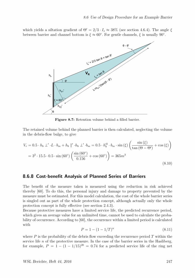
8.6 Use of Design Procedure for an Example Barrier
which yields a siltation gradient of Θ′ = 2/3 · Is ≈ 38% (see section 4.6.4). The angle ξbetween barrier and channel bottom is ξ ≈ 60◦. For gentle channels, ξ is usually 90◦.
θ
hb
hb'
θ'
θ - θ'
VR
ξ ≈ 60°
hb┴'
hb║'
Figure 8.7: Retention volume behind a filled barrier.
The retained volume behind the planned barrier is then calculated, neglecting the volumein the debris-flow bulge, to give
Vr = 0.5 · hb ⊥′ ·L · bm + hb ‖′ ·hb ⊥′ ·bm = 0.5 · h′2b · bm · sin (ξ)
(sin (ξ)
tan (Θ−Θ′)+ cos (ξ)
)= 32 · 15.5 · 0.5 · sin (60◦)
(sin (60◦)
0.156+ cos (60◦)
)= 365m3
(8.10)
8.6.8 Cost-benefit Analysis of Planned Series of Barriers
The benefit of the measure taken is measured using the reduction in risk achievedthereby [60]. To do this, the personal injury and damage to property prevented by themeasure must be estimated. For this model calculation, the cost of the whole barrier seriesis singled out as part of the whole protection concept, although actually only the wholeprotection concept is fully effective (see section 2.4.3).Because protective measures have a limited service life, the predicted recurrence period,which gives an average value for an unlimited time, cannot be used to calculate the proba-bility of occurrence. According to [60], the occurrence within a limited period is calculatedwith
P = 1− (1− 1/T )n (8.11)
where P is the probability of the debris flow exceeding the recurrence period T within theservice life n of the protective measure. In the case of the barrier series in the Hasliberg,for example, P = 1 − (1 − 1/15)20 = 0.74 for a predicted service life of the ring net
WSL Berichte, Heft 44, 2016 247

8 Debris-flow Barrier Design Example
barriers of 20 years [39] and a recurrence period of 15 years. Periods of 30, 100, 300 yearsare considered discrete recurrence periods but only act as an auxiliary construct.The amounts of damage have been defined by Bern Highways Department using previousempirical values from past flooding events; the values are shown in Table 8.7. Thevalues for the damage after the protective measure are produced from the effect of thedebris-flow nets, by which it is assumed that a previous 30-year event with the samedamage would only occur with a 100-year event. Also, a 30-year event would cause muchless damage of 10 million Swiss Francs owing to the nets. The reduction in damage isthen formed from the difference between in the damage without the measure and theresidual damage with the measure.
Table 8.7: Determination of the extent of damage R for the debris flows in the municipalitiesof Hasliberg and Meiringen.
Recurrence period T 30 100 300
Previous extent of damage [CHF ] 65 million 69 million 73 millionExtent of damage afterwards [CHF ] 10 million 65 million 69 million
Reduction in damage Sm[CHF ] 55 million 4 million 4 million
Probability P 0.49 0.18 0.064Probability ∆P 0.31 0.116 0.064Benefit N [CHF ] 26.95 million 0.464 million 0.256 millionBenefit Nyear [CHF/year] 1.34 million 23, 200 12, 800Extent of damage R [CHF/year] 1.34 million 1.37 million 1.38 million
For the occurrent probability of the event within the service life of the nets P , the averagevalue ∆Pi = Pi − Pi+1 is formed in each case, wherein the 300-year event, being thegreatest possible event, directly receives the probability of occurrence P . The occurrentprobabilities ∆Pi and the decisive reduction in damage can be used to calculate the benefitof the measure as follows: Ni = ∆Pi · Sm,i. The benefit per year is then Nyear = Ni/20for a 20-year service life of the nets. The actual extent of damage R is then in this casecalculated from the sum of all the annual benefits to give R =
∑Ni,year.
Other methods, such as the Wilhelm or Borter methods (used by FOEN3 in cost-benefitanalyses) for calculating the occurrent extent of damage R are described in [80]. However,these are not suitable for this specific case owing to the probability of occurrence duringthe service life of the protective measure, which is why the procedure according to thecantonal building insurance [60] was chosen instead.
Protection against a hundred-year flooding event should therefore incur costs no higherthan 1.37 million Swiss Francs per year. The installed protective nets can completelyretain a 15-year event at most and correspondingly minimize a 30-year event by partialretention. The damage for the short recurrence periods can therefore be minimized.
3FOEN=Federal Office for the Environment
248 WSL Berichte, Heft 44, 2016
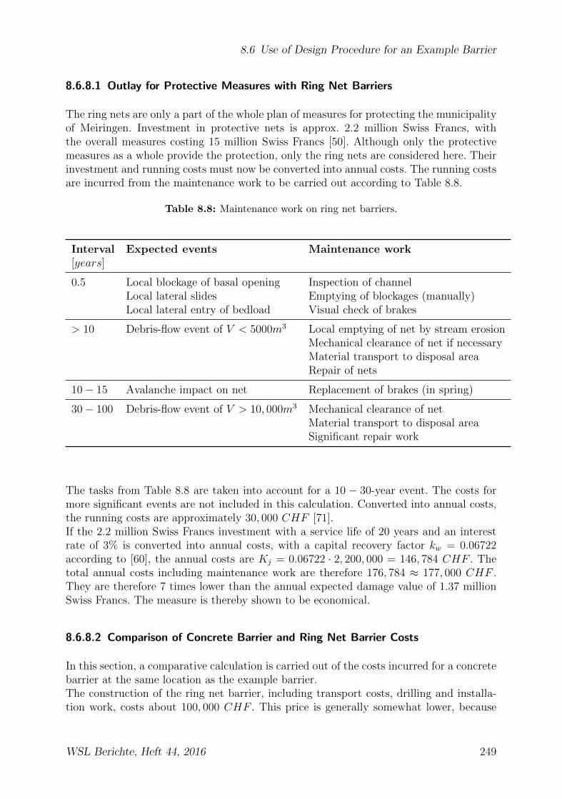
8.6 Use of Design Procedure for an Example Barrier
8.6.8.1 Outlay for Protective Measures with Ring Net Barriers
The ring nets are only a part of the whole plan of measures for protecting the municipalityof Meiringen. Investment in protective nets is approx. 2.2 million Swiss Francs, withthe overall measures costing 15 million Swiss Francs [50]. Although only the protectivemeasures as a whole provide the protection, only the ring nets are considered here. Theirinvestment and running costs must now be converted into annual costs. The running costsare incurred from the maintenance work to be carried out according to Table 8.8.
Table 8.8: Maintenance work on ring net barriers.
Interval Expected events Maintenance work[years]
0.5 Local blockage of basal opening Inspection of channelLocal lateral slides Emptying of blockages (manually)Local lateral entry of bedload Visual check of brakes
> 10 Debris-flow event of V < 5000m3 Local emptying of net by stream erosionMechanical clearance of net if necessaryMaterial transport to disposal areaRepair of nets
10− 15 Avalanche impact on net Replacement of brakes (in spring)
30− 100 Debris-flow event of V > 10, 000m3 Mechanical clearance of netMaterial transport to disposal areaSignificant repair work
The tasks from Table 8.8 are taken into account for a 10 − 30-year event. The costs formore significant events are not included in this calculation. Converted into annual costs,the running costs are approximately 30, 000 CHF [71].If the 2.2 million Swiss Francs investment with a service life of 20 years and an interestrate of 3% is converted into annual costs, with a capital recovery factor kw = 0.06722according to [60], the annual costs are Kj = 0.06722 · 2, 200, 000 = 146, 784 CHF . Thetotal annual costs including maintenance work are therefore 176, 784 ≈ 177, 000 CHF .They are therefore 7 times lower than the annual expected damage value of 1.37 millionSwiss Francs. The measure is thereby shown to be economical.
8.6.8.2 Comparison of Concrete Barrier and Ring Net Barrier Costs
In this section, a comparative calculation is carried out of the costs incurred for a concretebarrier at the same location as the example barrier.The construction of the ring net barrier, including transport costs, drilling and installa-tion work, costs about 100, 000 CHF . This price is generally somewhat lower, because
WSL Berichte, Heft 44, 2016 249

8 Debris-flow Barrier Design Example
the construction involves a whole series of barriers and therefore the costs for setting upa building site etc. are shared by several barriers. If it were a single structure of this size,the total price would be about 110, 000 CHF . But the order of magnitude should sufficefor a model calculation.A solid concrete barrier at this site with the same retention volume would have an ap-proximate concrete volume of 4m · 15.5m · 1m = 62m3 excluding the foundation and dambase. If a foundation of 1m width, 6m length and a thickness of ≈ 0.5m is added, thisyields 65m3 of concrete. The reinforcement content of such a concrete barrier is assumedto be ≈ 100kg/m3. This produces approximate construction costs including formwork andcasting of approximately 200, 000 CHF . If the transport costs for the necessary helicopterflights of ≈ 38, 000 CHF are also included, this adds up to approximately 238, 000 CHFfor the construction of a solid concrete barrier. The reinforcement estimations and con-struction costs have been estimated using the previous construction costs of the shearwall in the Illgraben (see section 4.2.1) and an assumed inflation rate of 5% (offer threeyears old).This yields a cost ratio of ring net barrier to solid concrete barrier of 110, 000/238, 000 =0.46. This is approximately half the cost.This ratio still depends indirectly on the location, because the transport costs for theconcrete barrier are much higher for inaccessible locations than when the structure canbe erected in the valley with good access conditions.
250 WSL Berichte, Heft 44, 2016

8.7 Notes and Limits of Application
8.7 Notes and Limits of Application
8.7.1 Accompanying Notes
The planning of the barriers must still be balanced with the hazard potential below thestructures in each individual case (see section 8.3). Most of all, the topographic conditionsin the mountain torrent must be suitable for erecting a ring net barrier, and the geometricparameters such as location of the barrier, height of the structure, span, anchoring andthe planned retention volume must be specified carefully. Owing to the widely varyingboundary conditions in debris-flow channels and therefore the parameters that are some-times very uncertain (density of debris flow, flow depth, flow velocities), the experienceof experts on site during planning is indispensable.Erected barriers also require regular checking of the fill level and the general conditionof the barrier. In barriers that are used as a small vertical-drop effect in the streambed,regular maintenance of the abrasion protection system and of the brakes (remaining brakecapacity) is required.
8.7.2 Limits of Application
The previous section has already referred to the suitability of the topographic conditionsin a mountain torrent for a ring net barrier. This point is also one of the most importantlimits of application for the retention system. Spans of more than 25m are not practicalowing to the significant settling behavior of the barriers (hb = 3/4 · h′b) and the resultingconstantly decreasing retention volume. The remaining barrier height h′b for a span of≈ 25m can be largely guaranteed by means of two additional posts as a UX system. Foreven larger spans, further posts would be necessary, and then the load-bearing systemwould at some point be exhausted owing to the large forces that must be transferred.In principle, a quadruple support rope design could be constructed, but this would nolonger be feasible owing to the arrangement of the ropes at deflection points, and also itwould not be possible to shackle the ropes to the ring net.The limiting geometric factor of the span also indirectly means a limit on the retentionvolume. Ring net barriers are suitable for retaining volumes up to ≈ 1000− 1500m3. Forgreater retention volumes, only a series of nets or consequently a solid concrete structureare possible, with which a large retention volume can be created at once.If the bank slope and winglet strengths in the channel are moderate owing to temporarydeposition material, the load-bearing system of a ring net barrier is not suitable becauseanchoring in the embankment winglets is not possible. The risk that the barrier will failas a result of washed-out anchors is too great with instable embankment winglets. Inthis case, a suitable retention space would be better created with a gravity wall, whichconducts its loads via the foundation into the channel floor as compression.The developed load approach also demonstrates that at high flow velocities, very fast,very high dynamic forces occur when a debris flow impacts a barrier structure and evendouble in the case of granular fronts. If very high debris-flow velocities of more than10− 12m/s are expected in very steep mountain torrents, the retention system of flexible
WSL Berichte, Heft 44, 2016 251

8 Debris-flow Barrier Design Example
ring net barriers is therefore not recommended, because the occurrent loads rapidly reacha possible limit load for the load-bearing system. At the same time the question shouldgenerally be asked whether a retaining structure is practical at all in an extremely steepterrain, owing to the high dynamic forces during the filling process and to the smallretention volume, or whether the barrier structure would be better relocated to theshallower runout zone. The ”permanently-filled barrier” as a small vertical-drop effect inthe steep streambed is the appropriate solution in this case. It may then be possible tocounteract the large dynamic loads by previous filling with soil aggregate.The retention system of flexible ring net barriers for debris-flow protection is generallysuitable for small to medium debris flows with an expected surge volume of max.V = 5000m3, low to moderate flow velocities of max. 10 − 12m/s and an expecteddischarge of no more than 100m3/s. The planned retention space Vr can be ensured betterover several barriers in series than with one large barrier, which may reach the limit ofthe expected retaining capacity owing to excessive settling behavior with large spans.In general, an alternative solution should be considered for high expected debris-flowenergies.
252 WSL Berichte, Heft 44, 2016

9 Summary and Outlook
9.1 Summary
Adapting flexible ring net barriers, originally designed as rockfall-protection structures,for debris-flow retention may prove to be an efficient alternative to conventional debris-flow retention measures. The foundations of the load-bearing system of these barriers,their further development, and design were optimized through field and laboratory tests.The resulting load model was implemented using the simulation software FARO.New insights into the debris-flow process were gained using different energy analyses,advancing the general understanding of the interaction between debris flow and barrier.The results will be summarized in short paragraphs below:
9.1.1 Debris-flow Process
Different energy analyses performed as part of field and laboratory tests confirm a newtheory regarding friction processes within debris flows. Friction parameters of debris flowsduring the flow process cannot be regarded as material-dependent constants because theyare influenced by additional parameters, such as water content, rate of gravitational ac-tivity, and flow velocity. The variable friction parameters could be demonstrated usingfield and laboratory measurements.The non-determinable variable, random energy, which is the result of partially-plastic im-pacts of the grains among one another, plays an important role in the energy analyses ofdebris flows. It is an additional internal contribution to losses due to frictional work. Itscontribution to the applicable law of friction is determined by the proportionality to therate of gravitational activity (see section 5.4.1.1).A detailed analysis of the balance data demonstrated that the average velocity in a debrisflow is greater than the measured front velocity ufront. As a result, the rolling motion ofa granular front develops due to the large shear gradient. In the front, the floating, fastmaterial, often consisting of large blocks, gradually gets pushed underneath the slower-flowing material closer to the ground. However, the average front velocity ufront continuesto be used for the dimensioning of the nets because it is the only one that can be measuredin practice.
253

9 Summary and Outlook
9.1.2 Load Model
A comprehensive compilation and comparison of historical approaches reveal large dis-crepancies between the results of different debris-flow load calculations.Due to the dearth of approaches to flexible barriers, a load model was developed basedon field and laboratory measurements. This model serves as a procedural method for thedesign of flexible ring net barriers. It is based on easily-estimated parameters (density ρ,flow depth hfl, and flow velocity u) and draws upon basic principles of physics, assum-ing a hydrostatic pressure distribution and a suddenly-occurring change of momentumduring the stopping process of the debris flow (see section 6.3). Measurement data fromboth portions were analyzed as part of individual experiments. To date, the flexibility ofthe structure during the influx process has been explicitly considered only as part of thesubsequent simulation or by means of an approximate solution to the rope equation.
9.1.3 The Obstruction Side
A load-bearing system to efficiently dissipate the emerging loads toward the embankmentwinglets was developed by means of comprehensive full-scale field tests, which used differ-ent load-bearing systems on the barrier side. Structural details, such as protection fromabrasion and the winglet rope, were successfully refined and resolved. Questions concern-ing the required mesh size M and the size of the basal opening hd could be answeredusing field as well as scaled laboratory tests.A succession of three barriers in Merdenson demonstrates the application as a multilevelbarrier to enlarge the retention space. In addition, these barriers illustrate a further areaof application: a permanent, small vertical drop in mountain torrents to allow for thetargeted protection of the dam base from further erosion and scouring.
9.1.4 Numerical Simulation
The implementation of the load approach in the simulation software FARO allows forsimple and time-saving dimensioning of the barriers in the future. The results of thesimulation were calibrated with data measured in the field. Furthermore, they confirmthe developed pressure-surge load model. With respect to specific aspects, such as thedynamic force-displacement law of the brake elements, the scope of the software couldbe broadened with the help of additional dynamic component tests based on the workof [103, 45].The use of a simplified model of the barrier as part of the form-finding analysis producesgood results for the desired maximum deformation of the barrier’s bulge of 1m. Duringthe subsequent calculation of the cut, the required number of brakes and rows of ring netwere determined for this equilibrium form. In the case of these flexible structures, however,form finding should not solely serve the calculation of the maximum sagitta f . Rather,it should already be included during the planning phase in order to achieve an accuratestructural design of the load-bearing system, which in turn would prevent corrosion andachieve efficient load-bearing behavior.
254 WSL Berichte, Heft 44, 2016

9.2 Future Prospects
9.1.5 Design Concept
A design concept for dimensioning the barriers was proposed on the basis of SIA (SwissSociety of Engineers and Architects) 260, 261 [92, 91], the GBV (Cantonal Building Insur-ance) [60], as well as DIN standards 1055-9 and 1055-100 [28, 27] to guarantee maximumsecurity for present and future structures during the difficult-to-determine debris-flowloading condition. A detailed, risk-based analysis of the debris-flow loading condition onring net barriers has not yet been performed due to the low amount of available field data.
All these individual elements made the development of this new method of using flexiblering net barriers for the retention of debris flows possible. Their low weight and fastinstallation have proven ring net barriers beneficial in alpine terrain. In addition, they area visually pleasing and ecologically justifiable alternative to concrete structures, especiallyfor small- to medium-sized debris flows (with surge volumes of up to 5000m3). As a resultof their implementation, people and infrastructure can be protected from the naturalhazard, debris flow, in a targeted manner, even in times of climate change. This in turnwould allow the settlement areas of alpine regions to be maintained to a reasonable extent.
9.2 Future Prospects
Potential users already began demonstrating great interest in the application of the newprotection concept, flexible barriers, while the project was ongoing. The goal of developinga method for the design of debris-flow barriers was realized as part of the present workby examining a variety of different subtopics.However, new ideas leading to a refinement of the load approach, which in turn resultedin a more efficient design, had already emerged during the realization of this project. Inaddition, a number of other areas of application of these barriers are conceivable. Theseapplications are already being confirmed in a follow-up project examining the use of ringnets for hillslope debris flows.
9.2.1 Loads
To date, the developed load approach has been validated for a recorded mudflow event.It unfortunately was not possible to measure a granular debris-flow event prior to thecompletion of this work. As a result, it was necessary to rely on data from past literature todetermine the pressure coefficient of the dynamic component of a granular debris flow [2].This gap will have to be filled by means of further field tests using flexible ring net barrierswith built-in measuring cells.
Moreover, to date these field studies have only been conducted in two debris-flow channels(Merdenson, Illgraben), and they have been extended by the use of additional materialsduring the laboratory tests. For global application of this barrier system, additional ex-periments in other debris-flow channels with different material compositions would be ofgreat benefit. These further results would allow for the assessment of the measurements’
WSL Berichte, Heft 44, 2016 255

9 Summary and Outlook
transferability and the better quantification of their material-dependent effects.
A pan-European standard procedure regarding debris-flow loads on protective structuresand a corresponding risk-based safety concept would be desirable, although it may notbe possible on a transnational level in the near future due to the differences betweenthe actual processes and material compositions. However, a risk-based analysis based ondifferent catchment areas and locations for protective structures within Switzerland maybe feasible in order to provide engineers and practical users substantiated guidelines forhandling debris-flow loads on protective structures.
An additional task is the refinement of special simulation programs, which specificallydescribe the structural side of protective structures while simultaneously reproducing thefluid (debris flow) with the requisite accuracy.The present work describes a simulation tool (FARO), which models the structure withquasi-static equivalent loads based on the developed design concept, and delivers plausibleresults for the dimensioning of flexible ring net barriers. The next step would be thecoupling of both physical processes, i.e. the process occurring between the inflowing fluidand the flexible ring net barrier (structural side) relative to an FSI1 calculation. All this,for example, could be achieved by developing an interface between FARO, the tool usedfor fluid and structure to date, and the newly developed flow code for debris flows inRAMMS2.
To date, load-bearing systems have been projected and implemented primarily in theplane. Further form-finding calculations with more complicated support structures pro-truding from the plane and the curvature – possibly predetermined - of the ring netbarrier, could achieve additional retention space and a more efficient load transference.
9.2.2 Additional Areas of Application
If the barriers provide protection from debris flows, they are, in principle, also suitable forthe protection from hillslope debris flows. Very similar to debris flows in terms of process(see section 2.1), hillslope debris flows exhibit, to some extent, significantly higher flowspeeds of up to 15m/s in steep terrain. Hillslope debris-flow triggers are not bound tostreambeds but can occur anywhere - in steep grass as well as woodlands -with slopessteeper than 30◦. If the risk of hillslope debris-flow activity in a particular location ispredictable, for example due to previous landslides, a ring net barrier for the targetedprotection of structures is conceivable.
Ring net barriers also could possibly be used as snow-slide protection measures by situ-ating them above the infrastructures they are intended to protect (see [108]). Due to thesignificant forces that arise during avalanche events, the filigree load-bearing system prob-ably will continue to be unsuitable in the future as a fully-fledged avalanche-protectionsystem.
1FSI = fluid-structure interaction2RAMMS = Rapid Mass Movements
256 WSL Berichte, Heft 44, 2016

Bibliography
[1] Armanini, A.: On the dynamic impact of debris flows . In Recent Developments onDebris Flows, Lecture Notes in Earth Sciences 64 . Springer, 1997.
[2] Armanini, A., M. Lachner, B. Majone, R. Rigon, G. Benedetti, andM. Hideaki: Restoration of the basins quebrada san jose de galipan and quebradael cojo. International Workshop on the debris flow disaster of December 1999 inVenezuela, 2000.
[3] Armanini, A. and P. Scotton: On the impact of a debris flow on structures . InProceedings of XXV Congress of International Association for Hydraulic Research,Tokyo, 1993. IAHR.
[4] Baillifard, M. A.: Interaction between snow avalanches and catch dams . PhDthesis, Swiss Federal Institute of Technology ETH, Zurich, 2007.
[5] Bartelt, P., O. Buser, and K. Platzer: Fluctuation-dissipation relations forgranular snow avalanches . Journal of Glaciology, 62:631–643, 2006.
[6] Bartelt, P., O. Buser, and K. Platzer: Starving avalanches: Frictional mech-anisms at the tails of finite-sized mass movements . Geophysical Research Letters,34, 2007. L20407, doi:10.1029/2007/GL031352.
[7] Bartelt, P. and U. Gruber: Development and calibration of a Voellmy-fluiddense snow avalanche model based on a finite element method . Internal technicalreport, Swiss Federal Research Insitute SLF, Davos, Switzerland, 1997.
[8] Bergmeister, K., J. Suda, J. Hubl und F. R. Miklau: Schutzbauwerke gegenWildbachgefahren. Techncal report, Betonkalender, 2008.
[9] Bezzola, G. R. und C. Hegg (Hrsg.): Ereignisanalyse Hochwasser 2005, Teil1 Prozesse, Schaden und erste Einordnung . Federal Office for the EnvironmentFOEN, Federal Research Institute WSL, 2007.
[10] Bletzinger, K.-U.: CARAT = Computer Aided Research Analysis Tool . Institutefor Structural Mechanics, University Stuttgart.
[11] Boll, A.: Wildbach und Hangverbau. Report Nr. 343, Federal Research InstituteWSL, Birmensdorf, Switzerland, 1997.
[12] Braunlich, M.: Pfahle mit kleinem Durchmesser - Technik, Anwendung, Tragver-halten, 2002. Diploma thesis, University Weimar.
257

Bibliography
[13] Buckingham, E.: Model experiments and the form of empirical equations . Trans.ASME, 37:263–296, 1915.
[14] Federal Office for the Environment FOEN: Typenliste Ankermortel,Ankermortel die fur den Lawinenverbau und Steinschlagverbau zugelassen sind ,2004.
[15] Federal Office for the Environment FOEN, Federal Research In-stitute WSL: Lawinenverbau im Anbruchgebiet - Technische Richtlinie als Vol-lzugshilfe, 2007.
[16] Bundesamt fur Umwelt, Wald und Landschaft (BUWAL),Bundesamtfur Wasserwirtschaft (BWW),Bundesamt fur Raumplanung (BRP):Berucksichitigung der Hochwassergefahren bei raumwirksamen Tatigkeiten, 1997.
[17] Bundesamt fur Umwelt, Wald und Landschaft (BUWAL),Bundesamtfur Wasserwirtschaft (BWW),Bundesamt fur Raumplanung (BRP):Berucksichitigung der Massenbewegungsgefahren bei raumwirksamen Tatigkeiten,1997.
[18] Caine, N.: The rainfall intensity - duration control of shallow landslides and debrisflows . Geografiska Annaler, Series A, 62:23–27, 1980.
[19] Cornforth, D.: Landslides in Practice. John Wiley and Sons, 1996.
[20] Coussot, P.: Les laves torrentielles - Connaissances a l’usage du practicien.Etudes equipements pour l’eau et l’environnement No 23, Cemagref Editions,France, 1996.
[21] Coussot, P. and J.-M. Piau: A large-scale field coaxial cylinder rheometer for thestudy of the rheology of natural coarse suspensions . Journal of Rheology, 39(1):105–124, 1994.
[22] Daugherty, R. L. and J. B. Franzini: Fluid Mechanics with Enineering Appli-cations . McGraw-Hill Kogakusha, LTD, 1977.
[23] DeNatale, J. S., R. M. Iverson, J. J. Major, R. G. LaHusen, G. L.Fliegel, and J. D. Duffy: Experimental testing of flexible barriers for contain-ment of debris flow . Technical report, U.S. Geological Survey, 1999.
[24] Denk, M.: Abbau Versuchssperre Illgraben. Internal technical report, Fatzer AG,2006.
[25] Denk, M.: Bericht zum Abrasionsprojekt . Internal technical report, Fatzer AG,2006.
[26] DIN 1045-1: Tragwerke aus Beton, Stahlbeton und Spannbeton - Bemessung undKonstruktion, Juli 2001.
[27] DIN 1055-100: Einwirkung auf Tragwerke - Grundlagen der Tragwerksplanung -Sicherheitskonzept und Bemessungsregeln, 2001.
258 WSL Berichte, Heft 44, 2016

Bibliography
[28] DIN 1055-9: Einwirkung auf Tragwerke - Aussergewohnliche Einwirkungen, Au-gust 2003.
[29] DIN 18127.: Baugrund - Untersuchung von Bodenproben - Proctorversuch, Novem-ber 1997.
[30] DIN 18137–2: Baugrund, Versuche und Versuchsgerate; Bestimmung der Scher-festigkeit; Triaxialversuch, Dezember 1990.
[31] DIN 18196: Erd- und Grundbau - Bodenklassifikation fur bautechnische Zwecke,Juni 2006.
[32] DIN 18800-1: Bemessung und Konstruktion, November 1990.
[33] DIN 4022–1: Benennung und Beschreibung von Boden und Fels , September 1987.
[34] Dracos, T.: Hydraulik . Verlag der Fachvereine Zurich, 1990.
[35] Duffy, J. D. and J. S. DeNatale: Debris flow mitigation using flexible barriers .In Proc. of the 47th Annual Highway Geology Symposium, pp. 243–252, 1996.
[36] European Commitee for Standardization: Steel wire and wire products -Steel wire for ropes - Part 2: Cold drawn non alloy steel wire for ropes for generalapplications , March 2002.
[37] European Commitee for Standardization: EN13411 - 5. Terminations forsteel wire ropes. Safety. U-bolt wire rope grips , September 2003.
[38] Faber, P. D. M.: Statistics and Probability Theory . Lehrstuhl fur Risiko undSicherheit, Eidg. Technische Hochschule Zurich, 2007.
[39] Fatzer AG: Schutzsysteme Steinschlagschutz , 2004.
[40] Feyrer, K.: Drahtseile - Bemessung, Betrieb, Sicherheit . Springer, 2000.
[41] Floss, R.: Umdrucke zur Vorlesung Bodenmechanik . Lehrstuhl fur Grundbau,Bodenmechanik und Felsmechanik, TU-Munchen, 2001.
[42] Franke, P.: Erarbeitung der Wirkungsweise von flachig einwirkenden Belastungenauf flexible Ringnetze, 2008. Diploma thesis, ZHAW.
[43] Geotechnical Engineering Office GEO, Hong Kong, China: Review of nat-ural terrain landslide debris-resisting barrier design, 2000.
[44] Graf, C. und B. Mc.Ardell: Die Murgangbeobachtungsstation Randa. Techn.Ber., Eidgenossische Forschungsanstalt WSL, Birmensdorf, Schweiz, 2005.
[45] Grassl, H. G.: Experimentelle und numerische Modellierung des dynamischenTrag- und Verformungsverhaltens von hochflexiblen Schutzsystemen gegen Stein-schlag . Doktorarbeit, Eidgenossische Technische Hochschule Zurich, 2002.
WSL Berichte, Heft 44, 2016 259
Bibliography
[46] Gubler, A.: Physikalische Modellierung flexibler Barrieren zum Schutz vorMurgangen, 2007. Diplomarbeit Eidgenossische Technische Hochschule Zurich.
[47] Gudehus, G.: Bodenmechanik . Ferdinand Enke Verlag, Stuttgart, 1981.
[48] Hauger, W., W. Schnell und D. Gross: Technische Mechanik 3 - Kinetik .Springer, Berlin, 1989.
[49] Hubl, J. und G. Holzinger: Kleinmassstabliche Modellversuche zur Wirkung vonMurbrechern. WLS Report 50 / Band 3, Universitat fur Bodenkultur, Wien, Oct2003.
[50] Herzog, B.: Lokale losungsorientierte Ereignisanalyse LLE Hasliberg-Milibach.Project report, Herzog Ingenieure ETH/SIA, Davos, Oktober 2006.
[51] Hilker, N., C. Hegg und M. Zappa: Unwetterschaden in der Schweiz 1972-2007mit besonderer Betrachtung des August-Hochwassers 2005 . In: Proc. of Int. Symp.Interpraevent, Dornbirn, Austria, Band 1 , S. 99–110, 2008.
[52] Hoffmann, C. W.: WSL-Kurs Einfuhrung in die Statistik . Eidg. Forschungsan-stalt WSL.
[53] Holzinger, G. und J. Hubl: Belastung eines Murbrechers: Abgeleitet aus La-borversuchen. In: Internationales Symposium Interpraevent 2004 , S. VII/131–139,Riva/Trient, 2004. Interpraevent.
[54] Hutchinson, J. N.: Morphological and geotechnical parameters of landslides inrelation to geology and hydrogeology . In: Proceedings 5th International Symposiumon Landslides in Lausanne, S. 3–35. Balkema, 1988.
[55] Institut fur Hydromechanik Universitat Karlsruhe: Hydromechanik ,1998.
[56] Iverson, R. M.: The physics of debris flows . Rev. Geophysics, 35(3):245–296,1997.
[57] Jaeggi, M. N. and S. Pellandini: Torrent check dams as a control measure fordebris flows . In Recent Developments on Debris Flows , pp. 186 – 207. Springer,1997.
[58] Joint Comitee of Structural Safety JCSS: Probabilistic Model Code, 2001.http://www.jcss.ethz.ch.
[59] Kaineder, F.: Praxisbericht . Internal technical report, Fedral Research InstituteWSL, 2006.
[60] Kantonale Gebaudeversicherung: Objektschutz gegen gravitative Naturgefah-ren, 2005.
[61] Kherkheulidze, I. I.: Estimation of basic characteristics of mudflow . Hydrome-terological Research Institute Tbilisi, UDSSR, 1956.
260 WSL Berichte, Heft 44, 2016

Bibliography
[62] Kowalski, J.: Two-Phase Modeling of Debris Flows . PhD thesis, EidgenossischeTechnische Hochschule Zurich, 2008.
[63] Kozeny, J.: Hydraulik . Springer, Wien, 1953.
[64] Kronfellner-Kraus, G.: Uber offene Wildbachsperren. Techn. Ber. 88, Mittei-lungen der forstlichen Bundes-Versuchsanstalt Wien, 1970.
[65] Leser, H.: Geomorphologie. Westermann Schulbuchverlag GmbH, 2003.
[66] Lichtenhahn, C.: Die Berechnung von Sperren in Beton und Eisenbeton. Kollo-quium, Mitteilungen der forstlichen Bundesversuchsanstalt Wien, 1973.
[67] Major, J. and T. C. Pierson: Debris flow rheology: Experimental analysis offine-grained slurries . Water resources research, 28:841–857, 1994.
[68] McArdell, B. and A. Badoux: Analysis of debris flows triggering rainfall eventsin the illgraben. Journal of Geophysical Research, 2008. in preparation.
[69] McArdell, B., P. Bartelt, and J. Kowalski: Field observations of basal forcesand fluid pore pressure in a debris flow . Geophysical Research Letters, 34(L07406),2007.
[70] Mizuyama, T., S. Kobashi, and G. Ou: Prediction of debris flow peak discharge.In Proc. of Int. Symp. Interpraevent, Bern, Switzerland, Band 4 , pp. 99–108, 1992.
[71] Monney, J., B. Herzog, M. Wenger, C. Wendeler und A. Roth: Einsatzvon flexiblen Stahlbarrieren als Murgangruckhalt . Wasser Energie Luft, 3:255–259,2007.
[72] Palkowski, S.: Statik der Seilkonstruktionen. Springer, 1990.
[73] Philips, C. J. and T. R. H. Davies: Determing rheological parameters of debrisflow material . Geomorphology, 4:101–110, 1991.
[74] Plattform Naturgefahren der Alpenkonvention(PLANALP): Doku-mentation von Naturereignissen Feldanleitung , 2006.
[75] Pozzi, A., P. Sieber, D. Zimmermann und M. Zimmermann: Lokalelosungsorientierte Ereignisanalyse Trachtbach. Techn. Ber., NDR Consulting Zim-mermann und Niederer + Pozzi Umwelt AG und Tiefbauamt des Kantons Bern,2006.
[76] Pozzi, A., P. Sieber, D. Zimmermann und M. Zimmermann: Projekt fur dieVerbauung des Trachtbaches 2007 . Techn. Ber., Tiefbauamt des Kantons Bern Ober-ingenieurkreis I, 2006.
[77] PWRI: Technical standard for measures against debris flow (draft). Technical Me-morandum of PWRI, No. 2632, Ministry of Construction, Japan, 1988.
[78] Ragetz, T.: Integrales Naturgefahrenmanagement in einem Gebirgskanton.Schweizerische Zeitung fur Forstwesen, 153:263–267, 2002.
WSL Berichte, Heft 44, 2016 261

Bibliography
[79] Rammer, L., E. Rainer und P. Holler: Anforderungen fur Schneenetze, BFW-Praxisinformation 8/2005, 9 - 10.
[80] Richli, B.: Hochwasserschutzmassnahmen Hasliberg-Meiringen nach dem Unwet-ter 2005 - Begleitstudie zur Wirtschaftlichkeit und planerischen Auswirkungen, 2007.Diplomarbeit Departement Bau, Umwelt und Geomatik.
[81] Rickenmann, D.: Empirical Relationships for Debris Flows . Natural Hazards,19:47–77, 1999.
[82] Rickenmann, D.: Estimation of debris flow impact on flexible wire rope barri-ers . Internal technical report, Swiss Federal Research Insitute WSL, Birmensdorf,Switzerland, 2001.
[83] Rimbock, A.: Schwemmholzruckhalt in Wildbachen. Doktorarbeit, Technische Uni-versitat Munchen, 2003.
[84] Roth, A.: Zuverlassigkeit von flexiblen Steinschlagschutzsystemen, 2001. Diplom-arbeit Eidgenossische Technische Hochschule Zurich.
[85] Roth, A., M. Denk und T. Zund: Technischer Bericht und Bemessung, MilibachMeiringen, Murgangruckhalt Louwenenbach. Techn. Ber., Fatzer AG, 2006.
[86] Rossert, R.: Hydraulik im Wasserbau. Oldenbourg, Munchen, 1999.
[87] Savage, S. B. and K. Hutter: The motion of a finite mass of granular materialdown a rough incline. Journal of Fluid Mechanics, 199:177–215, 1989.
[88] Schatzmann, M.: Rheometry for large particle fluids and debris flows . PhD thesis,Eidgenossische Technische Hochschule Zurich, 2005.
[89] Schlickenrieder, M.: Ansatze fur Lastannahmen und Berechnungen vonMursperren, 2008. Diplomarbeit Fachbereich 02 Bauingenieurwesen.
[90] Sharpe, C. F. S.: Landslides and Related Phenomena, Columbia University Press,1938.
[91] SIA 260 (Swiss standard): Grundlagen der Projektierung von Tragwerken, 2003.
[92] SIA 261 (Swiss standard): Einwirkungen auf Tragwerke, 2003.
[93] SIA 261/1 (Swiss standard): Einwirkungen auf Tragwerke - Erganzende Festle-gungen, 2003.
[94] SIA 263 (Swiss standard): Stahlbau, 2003.
[95] Spang, R. M. und R. Bollinger: Vom Holzzaun zum Hochenergienetz - DieEntwicklung des Steinschlagschutzes von den Anfangen bis zur Gegenwart . FatzerAG, 2001.
[96] Stark, C. and N. Hovius: The characterization of landslide size distributions .Geophysical Research Letters, 28(6):1091–1094, 2001.
262 WSL Berichte, Heft 44, 2016

Bibliography
[97] Straub, D. and M. Schubert: Modeling and managing uncertainties in rock-fallhazards . Georisk, 2:1–15, 2008.
[98] Suda, J., A. Strauss, F. Rudolf-Miklau, and J. Huebl: Safety Assesssmentof Barrier Structures . Structure and Infrastructure Engineering SIE, in Review.
[99] Takahashi, T.: Debris Flow - Mechanics, Prediction and Countermeasures . Taylor& Francis, 2007.
[100] Valentin, F.: Einfuhrung in die Hydromechanik . Lehrstuhl fur Hydraulik undGewasserkunde, TU-Munchen, 2000.
[101] Valentin, F.: Grundwasserhydraulik . Lehrstuhl fur Hydraulik undGewasserkunde, TU-Munchen, 2002.
[102] Varnes, D. J.: Landslide types and processes . Highway Research Board, 29:20–47,1958. Special Report.
[103] Volkwein, A.: Numerische Simulation von flexiblen Steinschlagschutzsystemen.PhD thesis, Eidgenossische Technische Hochschule Zurich, 2004.
[104] Wuchner, R.: Mechanik und Numerik der Formfindung und Fluid-Struktur-Interaktion von Membrantragwerken. PhD thesis, Technische Universitat Munchen,2006.
[105] Wuchner, R. and K.-U.Bletzinger: Stress-adapted numerical form finding ofpre-stressed surfaces by the updated reference strategy . International Journal ForNumerical Methods in Engineering, 64:143–166, 2005.
[106] Weber, D.: Untersuchungen zum Fliess- und Erosionsverhalten granularerMurgange. Dissertation, Eidgenossische Forschungsanstalt fur Wald, Schnee undLandschaft WSL, Birmensdorf, 2004.
[107] Wendeler, C.: Fluid-Struktur-Interaktion mit ANSYS/Multiphysics - Fragen derModellbildung und Beispiele, 2003. Diplomarbeit.
[108] Wendeler, C.: Berechnungen von Steinschlagverbauungen auf Schneelasten mitFARO . Internal technical report, Federal Research Institute WSL, 2006.
[109] Wendeler, C.: Bericht Laborversuche Murgangruckhalt Gummen. Techn. Ber.,Federal Research Institute WSL, 2006.
[110] Wendeler, C.: Bericht Laborversuche Murgangruckhalt Trachtbach. Techn. Ber.,Federal Research Institute WSL, 2007.
[111] Wendeler, C.: Forschungsprojekt KTI-Murgang-Mehrstufige Netzverbauung Mer-denson: Bericht zum Fullereignis . Techn. Ber., Federal Research Institute WSL,2007.
[112] Wendeler, C.: Gelandeschutz – Wie viel tragen sie wirklich? . Metall, 608:26–29,2008.
WSL Berichte, Heft 44, 2016 263

Bibliography
[113] Wendeler, C., B. W. McArdell, D. Rickenmann, A. Volkwein, A. Roth,and M. Denk: Testing and numerical modeling of flexible debris flow barriers . InZhang, M. and H. Wang (eds.): Proc. of the sixth International Conference onPhysical Modeling in Geotechnics , pp. 1573–1578. Balkema, 2006.
[114] Wendeler, C. und A. Volkwein: Sicherheitsrichtlinie Illgraben. Federal Rese-arch Institute WSL, 2005.
[115] Wendeler, C. und A. Volkwein: Sicherheitsrichtlinie Merdenson. Federal Re-search Institute WSL, 2005.
[116] Wendeler, C., A. Volkwein und M. Denk: Flexible Schutzsysteme gegenMurgange. Der Bauingenieur, 3:48–52, 2007.
[117] Wendeler, C., A. Volkwein, A. Roth, M. Denk, and S. Wartmann: Fieldmeasurements used for numerical modelling of flexible debris flow barriers . In Proc.of the 4th. International Conferences on Debris-Flow Hazards Mitigation, pp. 681–690, 2007.
[118] Wendeler, C., A. Volkwein, A. Roth, B. Herzog, N. Hahlen, andM. Wenger: Hazard prevention using flexible muli-level debris flow barriers . InProc. of Int. Symp. Interpraevent, Dornbirn, Austria, Band 1 , pp. 547–554, 2008.
[119] Yalin, M.: Theory of Hydraulic Models . Macmillan, London, 1971.
[120] Zimmermann, M., P. Mani, and P. Gamma: Murganggefahr und Klimaanderung- ein GIS-basierter Ansatz . Hochschulverlag AG, 1997.
[121] Zund, T.: Analyse des Verhaltens massgebender Tragelemente von flexiblen Stein-schlagschutzsystemen, 2005. Diplomarbeit Eidgenossische Technische HochschuleZurich.
[122] Zund, T., W. Gerber, M. Sennhauser und A. Muller: Dynamsiche Testsvon Bremsringen. Techn. Ber., Federal Research Institute WSL und Fatzer AG,2006.
264 WSL Berichte, Heft 44, 2016
List of symbols
Symbol Description UnitA Channel width, i.e. flow width as a function of hfl(x) m2
α Deflection angle of a cable rope ◦
αm Material-dependent debris-flow load factor −b Stream-channel width mRBF Reduced breaking force of a support rope during deflection %bm Average barrier width mbo Barrier width at the upper support ropes mbu Barrier width at the lower support ropes mβ Impact angle at which the debris flow strikes an obstacle ◦
c Cohesiveness of solid materials Nm2
cp Pressure coefficient of a dynamic debris-flow load −cd Drag coefficient of an object in the flow path −Cv Sediment concentration in a suspension sample −Cs,DF Volumetric sediment concentration in a debris flow −Cs,DC Proportion of a particular grain size within the grain-size distribu-
tion curve−
d90 90% of the grain sizes are smaller than this value mmdmax Maximum grain size in a debris-flow mixture mmdring Ring diameter of the ring net mdring,∅ Wire-bundle diameter of a single ring mδ Wire diameter of a single wire in a strand mmηb Bingham viscosity Pas
η Dynamic viscosity , safety factor Pas
f Maximum deformation of the barrier in flow direction, force matrix mFrope Rope force of a barrier support rope kNg Gravitational constant m
s2
γ Shear rate during viscosity measurements 1/shb Fill level of the barrier mh′b Height of the barrier following the filling process mhd Height of the basal opening between the lowermost support rope
and the stream bedm
hend Height of the barrier following several overflowing processes mhfl Flow depth of the debris flow mhfill Fill level of the barrier used primarily in the laboratory tests mhn Normal water drainage mhimp Impounding pressure of the debris flow mhw Theoretical impact level of the debris flow m
265
List of Symbols
Symbol Description UnitIR Inclination of the energy line in the open stream channel -IS Inclination of the streambed in the open stream channel -I ′S Inclination of the streambed behind a filled flexible barrier -IW Inclination of the water surface in the open stream channel -∆Iw Energy head dissipation during the hydraulic jump mkf Permeability coefficient (permeability) m/skm Stiffness modulus of the model barriers N/mkn Stiffness modulus of the ring net used N/m
kst Strickler coefficient indicating channel roughness m1/3
s
l Distance between individual barriers of a multilevel barrier mlbr Rope elongation due to the braking distance mlk Length of scouring due to barrier overflow mLm Characteristic length in nature (prototype) mLn Characteristic length in the model mLs Model-scaling factor based on Ln/Lm −LW Hydraulic-jump distance mM Mesh size of the ring net mµ Effective coefficient of friction -µc Coulomb-friction (dry-friction) coefficient -νs Concentration of solids with d > 0.05mm in the debris flow
(definition according to Iverson)-
νf Liquid-phase fraction in the debris flow + particles with d <0.05mm
-
p Fluid pressure Nm2
pp Pore-water pressure in the debris flow Nm2
∆P Dynamic debris-flow load increase Nm2
φ Angle of internal friction ◦
φ′ Effective angle of internal friction ◦
φbas Basal friction angle ◦
Q Average flow m3/sQ′ Flow passing the net m3/sQnet Flow filling the net m3/sq Specific flow m2/sR Average hydraulic radius in the debris-flow channel m
ρ Density of the debris flow kgm3
ρf Density of the liquid phase kgm3
ρs Density of the solid phase kgm3
σ Normal stress Nm2
τ Shear stress Nm2
τcrit Limiting shear stress during state of failure Nm2
timp Duration of impact on the barrier stsim Current barrier simulation time in FARO sΘ Channel slope ◦
Θ′ Channel slope behind a filled barrier ◦
266 WSL Berichte, Heft 44, 2016

List of Symbols
Symbol Description UnitU Channel diameter of a torrent mu Debris-flow velocity m
s
~u Debris-flow velocity vector ms
ufront Average front velocity of the debris flow ms
υ Kinematic viscosity m2/sV Relevant volume of a debris-flow surge m3
Vr Available retention volume behind a flexible barrier m3
w Relative water content in the debris flow %wr Relative water content in moist debris-flow material %
WSL Berichte, Heft 44, 2016 267