THESIS

LEVERAGING STRUCTURAL-CONTEXT SIMILARITY

OF WIKIPEDIA LINKS TO PREDICT TWITTER USER LOCATIONS

Submitted by

Chuanqi Huang

Department of Computer Science

In partial fulfillment of the requirements

For the Degree of Master of Science

Colorado State University

Fort Collins, Colorado

Fall 2017

Master’s Committee:

Advisor: Sangmi Lee Pallickara

Shrideep Pallickara

Stephen C. Hayne

Copyright by Chuanqi Huang 2017

All Rights Reserved

ABSTRACT

LEVERAGING STRUCTURAL-CONTEXT SIMILARITY

OF WIKIPEDIA LINKS TO PREDICT TWITTER USER LOCATIONS

Twitter is a widely used social media service. Several efforts have targeted understanding the

patterns of information dissemination underlying this social network. A user’s location is one of

the most important information items relative to analyzing content. However, location information

tends to be unavailable because most users do not (want to) include geo-tags in their tweets. To

predict a user’s location, existing approaches require voluminous training data sets of geo-tagged

tweets. However, some of the characteristics of tweets, such as compact, non-traditional linguistic

expressions, have posed significant challenges when applying model-fitting approaches. In this

thesis, we propose a novel framework for predicting the location of a social media user by leverag-

ing structural-context similarity over Wikipedia links. We measure SimRanks between pages over

the Wikipedia dump dataset and build a knowledge base, mapping location information (e.g., cities

and states) to related vocabularies along with the likelihood for these mappings. Our results evolve

as the users’ tweet stream grows. We have implemented this framework using Apache Storm to

observe real-time tweets. Finally, our framework provides a list of ranked "probable" cities based

on the distances between candidate locations and their weights. This thesis includes empirical

evaluations that demonstrate performance that is in line with current state-of-the-art location pre-

diction approaches.

Key words: SimRank, Wikpedia, Apache Storm, Location Prediction, timeline, Social Media,

Twitter

ii

TABLE OF CONTENTS

ABSTRACT . . . . . . . . . . . . . . . . . . . . . . . . . . . . . . . . . . . . . . . . . . . ii

Chapter 1 Introduction . . . . . . . . . . . . . . . . . . . . . . . . . . . . . . . . . . . 1

1.1 Usage Scenarios . . . . . . . . . . . . . . . . . . . . . . . . . . . . . . . 2

1.1.1 Research Challenges . . . . . . . . . . . . . . . . . . . . . . . . . . . 2

1.1.2 Research Questions . . . . . . . . . . . . . . . . . . . . . . . . . . . . 3

1.2 Thesis Contributions . . . . . . . . . . . . . . . . . . . . . . . . . . . . . 3

1.3 Thesis Organization . . . . . . . . . . . . . . . . . . . . . . . . . . . . . 4

Chapter 2 Related Works . . . . . . . . . . . . . . . . . . . . . . . . . . . . . . . . . . 5

Chapter 3 Generating Knowledge Base Using SimRank . . . . . . . . . . . . . . . . . 9

3.1 Basic Graph Theory . . . . . . . . . . . . . . . . . . . . . . . . . . . . . 9

3.2 Structural Similarity . . . . . . . . . . . . . . . . . . . . . . . . . . . . . 9

3.2.1 Structural Similarity in SimRank . . . . . . . . . . . . . . . . . . . . . 10

3.3 Basic SimRank Equations . . . . . . . . . . . . . . . . . . . . . . . . . . 11

3.4 SimRank Matrix . . . . . . . . . . . . . . . . . . . . . . . . . . . . . . . 12

3.4.1 Matrix Representation of SimRank . . . . . . . . . . . . . . . . . . . . 12

3.4.2 SimRank Matrix Calculation . . . . . . . . . . . . . . . . . . . . . . . 13

3.5 Extract Relevant Words . . . . . . . . . . . . . . . . . . . . . . . . . . . 14

3.5.1 Wikipedia . . . . . . . . . . . . . . . . . . . . . . . . . . . . . . . . . 14

3.5.2 Dataset . . . . . . . . . . . . . . . . . . . . . . . . . . . . . . . . . . . 15

3.5.3 Preprocessing . . . . . . . . . . . . . . . . . . . . . . . . . . . . . . . 15

3.6 Distributed Computing Framework . . . . . . . . . . . . . . . . . . . . . 18

3.6.1 Parallel Computing . . . . . . . . . . . . . . . . . . . . . . . . . . . . 18

3.6.2 Large Matrix Multiplication With Mapreduce . . . . . . . . . . . . . . 18

Chapter 4 Estimating Location . . . . . . . . . . . . . . . . . . . . . . . . . . . . . . . 20

4.1 Sliding Window Algorithm . . . . . . . . . . . . . . . . . . . . . . . . . 20

4.2 Applying Sliding Window Algorithm to Estimating Location . . . . . . . . 20

4.3 Increasing The Coverage Area Of A City . . . . . . . . . . . . . . . . . . 21

Chapter 5 Overall Framework . . . . . . . . . . . . . . . . . . . . . . . . . . . . . . . 23

Chapter 6 Evaluation . . . . . . . . . . . . . . . . . . . . . . . . . . . . . . . . . . . . 24

6.1 Dataset . . . . . . . . . . . . . . . . . . . . . . . . . . . . . . . . . . . . 24

6.1.1 Obtain Users’ Tweets . . . . . . . . . . . . . . . . . . . . . . . . . . . 24

6.1.2 Dataset Filtering . . . . . . . . . . . . . . . . . . . . . . . . . . . . . . 25

6.2 Evaluation Mechanism . . . . . . . . . . . . . . . . . . . . . . . . . . . . 26

6.3 Result . . . . . . . . . . . . . . . . . . . . . . . . . . . . . . . . . . . . . 26

6.3.1 Accuracy and Confusion matrix . . . . . . . . . . . . . . . . . . . . . . 26

6.3.2 Selecting Overlays using IDW . . . . . . . . . . . . . . . . . . . . . . 27

iii

6.3.3 Receiver Operating Characteristic . . . . . . . . . . . . . . . . . . . . 30

6.3.4 Comparison Of Proximal And Distal Confusion Matrices . . . . . . . . 31

Chapter 7 Conclusions and Future Work . . . . . . . . . . . . . . . . . . . . . . . . . . 34

7.1 Conclusions . . . . . . . . . . . . . . . . . . . . . . . . . . . . . . . . . 34

7.2 Future Work . . . . . . . . . . . . . . . . . . . . . . . . . . . . . . . . . 34

References . . . . . . . . . . . . . . . . . . . . . . . . . . . . . . . . . . . . . . . . . . . . 36

iv

Chapter 1

Introduction

With the ongoing rapid advancement and development of information technology, Internet use

has become central to the lives of many people. According to the United Nations agency that

oversees international communications, more than 3 billion people are using the Internet as of

2015 [1]. Furthermore, a new report from the International Telecommunication Union states that

the number of Internet users has increased from 738 million in 2000 to 3.2 billion in 2015 [1].

The dramatic increase of internet usage has led to the rapid development of Social networking.

The most recent social media statistics on consumer adoption and usage of social networks, dated

April 2017, indicate that more than 10073 million active users are using popular social networks;

this is close to one-third of the total number of people using the Internet in 2015 [2]. The increasing

popularity of social networks has led to an exciting phenomenon that is related to communicating

information. Compared to the earlier predominance of sharing information verbally (person-to-

person), sending information through a social network where posted items win public attention

and comments has increasingly become a preferred choice. A more interesting element of this

phenomenon is that focusing on social networking, generally, is likely to yield more extensive

information about what is happening around the world in real time than reading newspapers and

accessing news broadcasts (online or otherwise). Communication between humans is not restricted

to face-to-face interactions. People talk to others via email, telephone, and networks, exchanging

information and enhancing relationships. Furthermore, people in modern society are more inclined

to speak publicly, and they post what they want to say in large social media networks, such as

Twitter, Facebook, and Weibo, communicating with others through replies. Usually, this kind

of communication is more publicly oriented than personal communications, and it is also more

accessible with no direct intrusion on privacy. We can obtain the latest and most intense real-time

events by focusing on social networking; however, we are not "gossip reporters." What we are

concerned about is what is currently happening and what we can do for it. Location is one of

1

most important elements of unfolding events; however, most people do not disclose their location

information. Therefore, we have designed and developed a system to predict the locations of people

who have posted text messages on social networking. If we can position someone who has posted

messages on social networking, in cases of emergency, we can give our help rapidly. Moreover, we

can obtain the local weather conditions and do some weather forecasting. Certainly, these scenarios

will be explored in our future work, but the emphasis of this article is on how to predict location

information. For this thesis study, we have designed and developed a scalable, real-time location

prediction system that leverages structural-context similarity over Wikipedia links. This system

uses SimRank [3] as a basic algorithm to construct a customized classification knowledge base

and applies a sliding window prediction model to classify users’ locations based on their tweets

history. In our system, Apache Storm is used to access a real-time data stream from twitter [4],

and Apache Hadoop is used to accomplish distributed computing for core algorithms [5].

1.1 Usage Scenarios

Location prediction based on social media activity can be seen as a classification problem.

Various popular social media platforms use much different ways to draw users’ attention. Twitter

focuses on tweets, which involves expressing information by text, often supplemented with pic-

tures. Instagram focuses on the feature of no prohibited images; users can post what they want

without any limits (photo-based, text, or combinations). Facebook is relatively comprehensive.

Our system is focused on analyzing users’ text messages and predicting location based on the con-

tent of posts. Therefore, any social media that is based on text content can supply most of the

information that is used in our system. In this paper, we focus on twitter messages, tweets.

1.1.1 Research Challenges

Text-based location prediction could be summarized as basic text classification; however, com-

pared with traditional text classification, text posted on social media is more concise and more

2

colloquial. Furthermore, considering that we are focused on location prediction, more geographic

location-related words should be included. In this respect, we face a few quite critical challenges:

• A very small portion of social media messages contain geospatial location information.

• The amount of data is very large.

• Most of the conversations do not include geospatial context.

1.1.2 Research Questions

Location prediction based on social media has been researched frequently, but several questions

remain relative to meeting this challenge, and some of these questions are addressed in this paper:

• What methods for selecting and weighting text information that can be used to identify lo-

cation are effective?

• How can we approximate the location based on geospatially neighboring locations?

• How can we perform the data processing and mining algorithm efficiently with a large dataset

(Big Data)?

1.2 Thesis Contributions

This thesis study demonstrates that it is reasonable to use the SimRank algorithm to build a lo-

cation prediction system, and we propose a novel method for extracting location vocabulary related

to specific cities from Wikipedia links. Using Wikipedia to create an independent knowledge base

reduces the influence of the dataset itself on the results. Secondly, this paper introduces readers

to a new way to think about how to obtain a large enough dataset from current data to accomplish

prediction instead of using existing datasets or data from old versions of applications, which has

been common in previous research. In this respect, the analysis presented in this paper will be

more confident. At last, the SimRank algorithm is well-known to be a very expensive algorithm

because it requires continuous iterative calculations, especially when the amount of data is large,

3

and this cost is particularly alarming. This paper introduces readers to a novel idea, which is to use

SimRank properties to extract the most relevant data for our research, greatly reducing the cost of

computing.

1.3 Thesis Organization

The remainder of this thesis is organized as follows: the next chapter presents other work

related to location prediction and the most recent important developments, providing a general idea

of how to overcome our research challenges. Chapter 3 introduces our core algorithm, SimRank,

and how to use the algorithm to build an independent knowledge base. Chapter 4 is a presentation

of the location estimation method used with the created knowledge base. Chapter 5 will show an

overall framework of our prediction system. In Chapter 6, we discuss and analyze our results and

present the evaluation our location prediction system. Finally, we give the conclusion about our

system, talk about our future work and how to improve our prediction system.

4

Chapter 2

Related Works

Location is one of the basic pieces of information we can get from social media messages.

Sometimes, people disclose their location openly, and their posts or replies contain lots of place

names. However, this is usually not the case. People who do not want disclose their locations will

avoid using any place name, or they just use abbreviations of places in posts and replies. Location

prediction is a research area that focuses on identifying users’ locations through social media, and

this area is currently receiving attention from numerous researchers. The most common method

of estimating user location is based on the content of posts [6] [7] [8] combined with machine

learning methods [9]. This approach is much like text classification, but it is more complicated.

The objective is to classify users’ posts into different locations, but it is difficult to get enough

terms from their posts because posts are usually very short, sometimes containing only a few

words. Therefore, to increase the content of a user’s post, Chandra, Khan, and Muhaya found a

way to combine a post with its reply and define them as a conversation. The basic assumption

of this approach is that the topic of a conversation remains constant throughout the relevant reply

messages, so every reply of a post will greatly expand its content. This method is called the Reply

Based Probability Distribution Mode(RBPDM) [7]. However, researchers don’t want to calculate

the probability distribution for every term that appears in a post; actually, most of them are some

type of stop word, and half of the remaining terms are not meaningful for location prediction.

Therefore, researchers focus on finding location-indicative words to decrease computational costs.

Bo, Cook, and Baldwin used an approach that artificially classifies terms that appear in a post into

three sets: local words, semi-local words, and common words. Then, Information Retrieval and

Data Mining technology is applied to these sets, including calculating TF-ICF and Information

Gain Ratio. Afterwards, maximum entropy modeling is used to predict location [8].

Moving beyond content-based approaches to location prediction, some researchers base pre-

dictions on the relationship between humans in social media. The Facebook model, developed

5

by Backstrom, begins by observing from an intuitive theoretical perspective that the probability

of friendship is roughly inversely proportional to distance. This model calculates the probabil-

ity that a user lives at a given location based on that user’s friends’ locations and then calculates

this probability at each of the locations of a user’s friends [10]. Typically, the result of the cal-

culations is the center of the cluster of the user’s friends; however, if users have a lot of media

friends, such as news services (e.g. CNN), the location will deviate with their influence. McGee,

Caverlee, and Cheng introduced an approach to location prediction that incorporates evidence of

social tie strength to improve the Facebook model. To determine a user’s social media graph, they

construct a decision tree to classify edges (relationships between users and their friends) as lo-

cal or non-local, assign different weights to the edges, then put these weights into the Facebook

model to improve the accuracy of prediction [11]. Also, researchers tend to develop their own

prediction models through the existing authoritative repository. Kapanipathi, Kapanipathi, Sheth,

and Thirunarayan used Wikipedia to generate their knowledge base and do location prediction. In

their approach, they find a city’s Wikipedia page and define every hyperlink in the city’s page as

a local entity of that city. The next step in this approach is to calculate each local entity’s weight

to generate the knowledge base using three Information Retrieval technologies-Pointwise Mutual

Information, Betweenness Centrality, and Semantic Overlap Measures. This knowledge base is

then used to predict users’ locations [12].

Many methods are created and modeled for location prediction, however, even with a perfect

model two problems remain relative to predicting location using social media posts,. One is the

nature of the dataset, and the other is computing costs. Every day, tens of millions of people

are using different kinds of social media, resulting in hundreds of millions of data points that are

continuously produced, so data selection is a challenge. Also, even though we can obtain huge

amounts of data, the efficient use of the data is another challenge.

Apache Storm is a distributed stream processing computation framework written predomi-

nantly in the Clojure programming language, originally created by Nathan Marz and the team

at BackType. Apache Storm was initially released on September 17, 2011 [13]. Storm lets pro-

6

grammers construct their own pipeline to process data, called "topology." In a topology, data is

passed around between spouts that emit data streams as immutable sets of key-value pairs called

tuples and bolts that transform those streams (count, filter etc.). Bolts themselves can optionally

emit data to other bolts down the processing pipeline, making distributed data processing, espe-

cially streamed data, more effective [14]. Also, Storm supports a wide range of uses, including

real-time analytics, machine learning, continuous computation, and more. It is also extremely fast,

with the ability to process over a million records per second per node on a modestly sized cluster.

Another advantage is that Storm has close ties with twitter. The Storm project was open sourced

after being acquired by twitter, and Storm offers the easiest way to interact with the twitter applica-

tion program interface (API). This feature makes getting and processing real-time twitter steaming

data convenient and effective.

For the real-time IoT sensor data analytics, Granules and Neptune provide support for low

latency processing and analytics datastreams [15] [16]. In addition to these features, Granules

leverages the NaradaBrokering framework in order to disseminate data streams in cluster and grid

settings [17] [18]. Kachikaran et al. proposed workflow engine that accounts for the data availabil-

ity in the spatiotemporal sensor environment [19].

Apache Hadoop is an open-source software framework for distributed storage and distributed

processing of very large data sets on computer clusters built from commodity hardware. All the

modules in Hadoop are designed with the fundamental assumption that hardware failures are com-

mon and should be automatically handled by the framework. Since Hadoop2.0, Apache Hadoop is

composed of four different modules: Hadoop Common, Hadoop Distributed File System (HDFS),

Hadoop YARN, and Hadoop MapReduce. As one of the most popular distributed computing

frameworks in the world, using Hadoop is the most convenient and economical way to do big data

processing and calculation. Furthermore, most methods in location prediction complete complex

operations using the MapReduce framework [20] to process statistics problems such as TF-IDF,

transition matrix generation, and huge matrix multiplications effectively.

7

Recently, [21], [22]proposed a framework that explores statistical ensemble and learning meth-

ods for predictive analytics. This framework uses dimensionality reduction and ensemble tech-

niques to improve the performance and accuracy of forecasting models generated in a distributed

environment. Moreover, a variety of methodologies and query-based frameworks have been intro-

duced to perform large scale analyticsover a distributed environment. There have been approaches

based on ad hoc queries that allow users to achieve latency with reasonable accuracy [23] [24].

Optionally, the query can be spatially constrained [25]. Supporting anomaly detection based on

spatiotemporal characteristics is also available [26].

Combining Storm and Hadoop is a wise choice. With the explosion of data sources in recent

years, many Apache Hadoop users have recognized the need to process data in real time while

maintaining traditional batch and interactive data workflows. Apache Storm fills that real-time

role and offers tight integration with many of the tools and technologies commonly found in the

Hadoop ecosystem.

8

Chapter 3

Generating Knowledge Base Using SimRank

3.1 Basic Graph Theory

In our approach, we focus on the directed graph, so we will model the objects and relationships

of a directed graph as G = (V,E), where V is all nodes in the graph that represent objects of

a domain, and E is all edges in the graph that represent relationships between different objects.

When we apply the model to the web pages, each node will represent a webpage, and if there is

a directed edge from node p to node q in the graph, it will represent an existing hyperlink from

webpage p to webpage q. Consider a large and complicated page structure like Wikipedia. Some

pages have a lot of hyperlinks to other pages, but some pages may not. If there is a page without

any hyperlinks to other pages and without any in-links from other pages, we call it a dead page in

our approach, and in the directed graph, it is a dead node. Dead nodes can exist in our model. Even

if a node doesn’t have any edge linked with the graph, it still exists in the node set V , but that node

will not have any effect on our calculations. In our model of the graph, a directed edge from node

p to q is denoted by edg(p, q), and the edge weights will be used to represent the similarity score

of two nodes, denoted by sim(p, q).

Relative to our purposes, for a node v in the model, we denote I(v) as the set of in-neighbor

nodes of v, and O(v) as the set of out-neighbor nodes of v, and we donate by Ii(v) and Oi(v) as

individual in-neighbors and out-neighbors of v, respectively. Finally, every graph can be repre-

sented as its adjacent matrix, so we denote adj(G) as the adjacent matrix of a directed graph G,

and denote ide(G) as the identity matrix for adj(G).

3.2 Structural Similarity

Structural similarity is similarity in the topological structure of information, such as web links,

through the network map that measures the degree of similarity between objects of the universal

9

model, and it has been widely applied in the field of information retrieval to processes such as

search engine optimization, collaborative filtering recommendation, and document aggregation

classification. In 2002, Jeh and Widom of MIT presented a new model for location prediction

based on web link structure to evaluate the similarity between any two objects in the network graph,

the SimRank model [3]. Common sense implies that if there is an edge between two nodes in a

graph, these two nodes are similar, and SimRank gives a new conceptualization of the similarity

of two nodes in a graph. Jeh and Widom argue that if two nodes are pointed to by similar nodes

in the graph, then they are similar, which is a type of recursive thought process, and the initial

condition for recursive definition is that each node is most similar to itself. SimRank can compare

the similarity between any two nodes of a graph, but Google PageRank [27] can only measure the

importance of each node. In 2014, Kapanipathi, Kapanipathi, Sheth, and Thirunarayan proposed

using Wikipedia as a knowledge base for location prediction [12]. These researchers use the words

that are the hyperlinks of a city’s Wikipedia article as similar words to that city, and they then

apply Pointwise Mutual Information, Betweenness Centrality, and Semantic Overlap Measures to

generate a knowledge base for weighting text information. In our system, we use SimRank as

a basic model, a completely different approach, to generate our knowledge base and accomplish

location prediction.

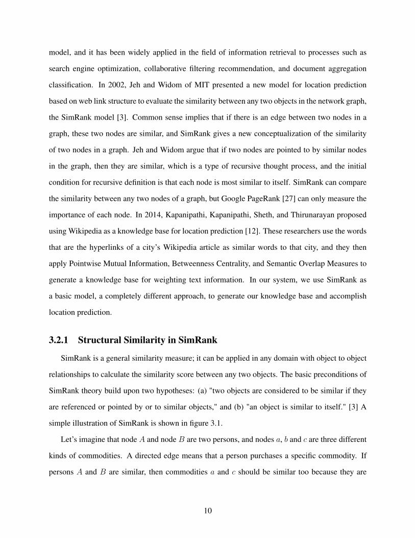
3.2.1 Structural Similarity in SimRank

SimRank is a general similarity measure; it can be applied in any domain with object to object

relationships to calculate the similarity score between any two objects. The basic preconditions of

SimRank theory build upon two hypotheses: (a) "two objects are considered to be similar if they

are referenced or pointed by or to similar objects," and (b) "an object is similar to itself." [3] A

simple illustration of SimRank is shown in figure 3.1.

Let’s imagine that node A and node B are two persons, and nodes a, b and c are three different

kinds of commodities. A directed edge means that a person purchases a specific commodity. If

persons A and B are similar, then commodities a and c should be similar too because they are

10

Figure 3.1: A bipartite graph sample explaining similarity in SimRank, where A and B are persons, and a,

b, and c are commodities.

purchased by (referenced by) similar people. Conversely, if a and c are similar commodities, then

we can draw the conclusion that persons A and B should be similar because they both purchased

commodity b and similar commodities a and c. Furthermore, the similarity of persons A and B

depends on the similarity of commodities a and c. A more straightforward example is that if

commodity b is flour, commodity a is eggs, and commodity c is meat, we can suppose that both

persons A and B want to cook something. A may want to make a cake, and B may want to make

some dumplings, but both A and B may be chefs.

3.3 Basic SimRank Equations

Based on the example mentioned above, we can conclude the following:

• People are similar if they purchase similar commodities, and

• Commodities are similar if they are purchased by similar people.

Here, similarity of people and similarity of commodities are mutually-reinforcing. Now, we want

to know the similarity of two nodes in our model graph, so let’s denote them as A and B, and

according to basic common sense, 0 <= sim(A,B) <= 1. Based on the rationale of our example

mentioned above, the similarity of nodes A and B depend on the similarity of the nodes that

have in links from (purchased by) A and B, which can be represented by I(A) and I(B). Now,

our problem is to calculate the similarity of all individual nodes, Ii(A), that belong to I(A) and

11

individual nodes lj(B) that belong to I(B). For this step, we just need to calculate each similarity

score of Ii(A) and Ij(B), sum them all, and normalize. Then, we can get the resulting similarity

of nodes A and B. The following is the recursive equation for SimRank:

sim(A,B) =C

|I(A)||I(B)|

|I(A)|∑

i=1

|I(B)|∑

j=1

sim(Ii(A), Ij(B)) (3.1)

Also, based on the mutually-reinforcing notions, similarity between commodities can be write at:

sim(A,B) =C

|O(A)||O(B)|

|O(A)|∑

i=1

|O(B)|∑

j=1

sim(Oi(A), Oj(B)) (3.2)

Ignoring C for the moment, equation (1) means that the similarity between A and B equals the

average similarity between any two nodes where each node is referenced by A and B, respectively.

Equation (2) means the similarity between A and B equals the average similarity between any two

nodes where each node points to A and B, respectively. Depending on the domain and application,

SimRank can be calculated by either or a combination of these two equations.

Now considering the constant, let’s imagine that there is a graph with only three nodes, A, B,

and C and two edges, edg(A,C) and edg(A,B). Based on the SimRank rationale, sim(B,C) =

sim(A,A), and the similarity of A to itself is 1. However, we don’t want to conclude that

sim(B,C) = sim(A,A) = 1 because two different nodes cannot be totally same, so we use a

constant (C) where 0 < C < 1, yielding sim(B,C) = C ∗ sim(A,A), which means that we are

less confident about the similarity between B and C.

3.4 SimRank Matrix

3.4.1 Matrix Representation of SimRank

The basic SimRank equation is in an iterative computation formula. To calculate simk+1(A,B),

we need to know simk(A,B), so the iteration equation can be written as

12

sim0(A,B) =

0 ifA 6= B

1 ifA = B

simk+1(A,B) =

C|I(A)||I(B)|

∑|I(A)|i=1

∑|I(B)|j=1 simk(Ii(A), Ij(B)) ifA 6= B

1 ifA = B

(3.3)

We can found that it is difficult to expand parallel computing using equation 3.3. The compu-

tation time and space are very expensive even when processing only a slightly larger number of

data graphs (e.g., hundreds of thousands) on a single machine. However, we can deduce the ma-

trix representation of SimRank based on the iterative equation, which makes it easy to do parallel

computing[14]. The equation for this process is written as follows:

sim0 = In

simk+1 = C ∗ (Q ∗ simk ∗QT ) + In

(3.4)

where In is an identity matrix, Simk is the similarity matrix whose entry [Simk]a,b denotes the

similarity score Simk(a, b), and Q is the column normalized adjacency matrix.

3.4.2 SimRank Matrix Calculation

As the core algorithm used for this thesis study, SimRank is a quite good method for calcu-

lating the weight score for every Wikipedia article. However, SimRank is also a very expensive

algorithm; its continuous iterative operation results in a great deal of computing consumption.

Even if the matrix format of SimRank is reduced to simplify the interpretation of the iterative

pattern [28], a substantial amount of matrix multiplication is still essential. Generally speaking,

to calculate the weight sore with SimRank, we need to create a matrix of a graph in which the

number of rows is equal to the number of columns, equating the total number of nodes in the graph

and then complete at least ten replications of iterative multiplication. As we know, if we need to

calculate an nxn size matrix with self-multiplication, we will temporarily generate n2 intermediate

data. So, if the matrix is not very large, we can calculate a SimRank score for each entity easily,

13

but we can’t calculate a matrix that is 5, 332, 092 ∗ 5, 332, 092 in size. Therefore, to deal with such

a huge dataset, we need frameworks for processing big data and reducing the size of the dataset

appropriately. In this paper, we will use the SimRank algorithm to significantly reduce the num-

ber of articles we choose from the Wikipedia dump, and the following sections provide a detailed

description of the process.

3.5 Extract Relevant Words

3.5.1 Wikipedia

If we use different locations as categories and obtain enough social media messages from each

location, the direct way to predict location is using a machine learning method. This involves

putting all of these messages into a machine learning model and running training and testing analy-

ses. Ostensibly, we can get a location prediction system quite easily using this approach. However,

social media messages are not traditional normative text. They use words more freely and more

colloquially, and social media messages are more networked. Only a very small portion of social

media messages contain geospatial locations, and datasets associated with social media are very

large. Therefore, traditional machine learning methods cannot provide adequate efficiency and ac-

curacy. We need to build our own knowledge base to select and weight social media messages for

use in location prediction.

Wikipedia is a multilingual encyclopedia collaboration program based on wiki technology and

a network encyclopedia written in multiple languages. Currently, the English Wikipedia alone

has over 5, 332, 092 articles that may be of any length. The English Wikipedia contains over 2.9

billion words. Moreover, different articles in Wikipedia are not completely independent of each

other. There are numerous wikilinks on each Wikipedia article that give hyperlinks from the article

page to another article page that contains the title or key words of the page shown in the original

article. Because of this interesting feature of Wikipedia, articles have formed a large network

graph, and through the wikilinks, even two articles that are completely unrelated are able to have

some connection. If we are just concerned about the title of the article, we can construct a large

14

graph of the Wikipedia knowledge network. The vertices of graph are representative of the titles

of articles, and the edges among different vertices of the graph represent the existence of one or

more hyperlinks from one article to another. Using this large Wikipedia knowledge graph, we can

obtain our own geospatial knowledge base through the core algorithm SimRank.

3.5.2 Dataset

Our data graph comes from Wikipedia; each line of the dataset begins with a page and follows

with its hyperlink pages, like page1 : page2, page3, page4, ... , pagen.

(a) Wikipedia hyperlink data (b) Page title sorted dataset

Figure 3.2: (a) Snapshot of the structure of Wikipedia Links used in our system. Each page title is repre-

sented by an ordered number, which is stored in a page title file (b) as shown above. The total size of the

dataset is around 5.7 million rows, and the file size is around 1.1GB.

3.5.3 Preprocessing

Although the dataset does not seem particularly large for parallel computing, based on the

SimRank matrix equation, we need to create a matrix wherein every word is included in both a row

and a column, which means that we have 5.7 million different rows in our dataset. So to calculate

every words’ SimRank, we need to create a 5.7million*5.7million matrix. Calculations are further

complicated in that we need to do iterative multiplication on this matrix at least 5 times, generating

a tremendous amount of intermediate data. For our experiment, at least 10TB of intermediate data

were generated to obtain the final result, and the running time was over 36 hours. With respect

15

to this challenge, the dataset dump from general Wikipedia browsing contains mostly article titles

are obviously irrelevant for location predictions based on common sense, and many articles contain

some stop words, such as obscure vocabulary or foul language. Moreover, the dataset also includes

some languages other than English, which is not considered by our system. These issues make it

necessary to preprocess the dataset.

Extract Relevant Words Base On SimRank Theory

Based on the random surfer-pairs model mentioned in the original SimRank paper [3], the

SimRank score for two nodes a and b in the same graph, sim(a, b), can be measured by how soon

the two nodes are expected to meet at the same node if they randomly walked the graph. So, we can

calculate the similarity score of two random nodes in the same graph by summing the probability

that these two nodes follow random paths and arrive at the same node in the same steps. So, we

can get the equation for the SimRank score, sim′(a, b), with the following equation:

sim′(a, b) =∑

t:(a,b)→(x,x)

P [t]cl(t) (3.5)

where t can be the path of node a to node x in n steps or the path of node b to node x in n steps,

and c is a constant belonging to (0, 1). The cl(t) means if there is no path from node a or b to node

x, we can make a "teleport", jump over some small probability edges and reach a random node in

the graph to create a path for them. Also, the SimRank paper shows us the process of developing

this equation from SimRank equation 3.2.

So, based on the random surfer-pairs model, we can extract the relevant words by fixing the

path in three steps. We show our relevant word extraction method in figure 3.3. First, beginning

with a certain city, our Wikipedia dataset gives hyperlinks of the specific city directly; let’s denote

them as city out links, CO1 to COn. Second, we convert our out-link dataset to the in-link dataset,

and based on this dataset, we select all page titles that are direct in-link pages to all CO1 to COn,

and we denoted these page titles as ’One Step Word.’ Third, we identify the out-link pages of CO1

to COn and denote them as CO1O1...CO1On to COnO1...COnOn, later selecting all pages that

16

Figure 3.3: Selection of words relevant to a certain city in two steps:(1) one step words are page titles that

have hyperlinks directly to city’s hyperlinked web page, and (2) two step words are page titles that need to

travel through two hyperlinks to arrive at a city’s hyperlinked web page.

are direct in-link pages to CO1O1...CO1On to COnO1...COnOn. At last, we can see all pages that

are in-link pages to the pages selected in step 3 and denote them as ’Two Step Word.’ According

to the random surfer-pairs model and our selection method, the specific city and ’One Step Words’

must meet at one page among CO1 to COn in step one, and a specific city’s ’Two Step Words’

must meet at one page among CO1O1...CO1On to COnO1...COnOn in step two. Compared to

other procedures where we cannot determine whether nodes can meet on the same city’s page,

this method not only excludes most unrelated pages but also saves the most relevant pages, greatly

reducing the amount of data. We can get the Wikipedia articles that are most relevant to the chosen

city by combining step one words, step two words, and step three words. As our experiment

shows, step two included 20 thousand pages, and if we go for three steps, the extraction process

will include almost all pages of the dataset. This being the case, we also need some method to

reduce the number of pages we select.

Reducing Number of Pages Selected

Based on the random surfer-pairs model, in step one, the similarity between a certain city, C,

and one of its ’One Step Words’ (let’s say OSW) can be calculated by:

sim(C,OSW ) =∑ 1

O(C) ∗O(OSW )(3.6)

17

where O(C) and O(OSW ) are the number of out-links of C and OSW, respectively.On the other

hand, based on the matrix representation of SimRank, step one similarity between these two page

titles can be calculated by summarizing the value of 1I(page)2

, where Page is a page that C and OSW

can reach in one step. Theoretically speaking, these two similarities should be equal:

sim(C,OSW ) =N

O(C) ∗O(OSW )=

1

I(page1)2+

1

I(page2)2+ ...+

1

I(pagen)2(3.7)

Let’s consider the best case, where O(OSW ) = 1, which means this page has only one out-link

directly to one of C’s out-link pages. This makes us choose the best OSW page for our system.

Then we deduce the following:

I(page1) =√

O(C) (3.8)

Consider that step three of our relevant word extraction method will include almost all pages of

the dataset, so we apply a selection condition on our selection method that limits the dataset to

pages where the number of in-links is less than√

O(C). This page reduction method significantly

reduces the size of the dataset generated with our step three words, making it possible to add step

three words to our system.

3.6 Distributed Computing Framework

3.6.1 Parallel Computing

As an iterative algorithm, SimRank is quite compute intensive, and even when the dataset is

slightly large, the turnaround time becomes extremely long. In our approach, we leveraged the

Hadoop MapReduce framework to achieve scalability of computation by means of parallelizing

computing over the large dataset.

3.6.2 Large Matrix Multiplication With Mapreduce

We use two MapReduce jobs to do matrix multiplication. Say we have two matrices, A and B,

in the first MapReduce job. For each of the data items(i, j, v), if the item comes from matrix A, we

18

output key value pairs (j, (A, i, v)), and if the item comes from matrix B, we output intermediate

key value pairs (i, (B, j, v)). Then, the jth column of matrix A and the ith row of matrix B will

be processed by the same reduce nodes if value i equals value j. On the reduce side, we store the

data from A and B to listA[i] and listB[j] respectively, and then multiply each entry of listA[i]

and each entry of listB[j] as ((i, j), listA[i] ∗ listB[j]). In the second MapReduce job, we just

need to summate using the same key from the first MapReduce job. Here gives the pseudocode for

the first mapreduce job:

Algorithm 1 First MapReduce

1: procedure MAP

2: input← Matrix value[i, j, v]

3: if input ∈ A then

4: Pair < key, value >← (j, (A, i, v))5: else

6: Pair < key, value >← (i, (B, j, v))

7: procedure REDUCE

8: input← Pair < key, value >

9: if input ∈ A then

10: list[A]← value

11: else

12: list[B]← value

13: output← ((i, j), list[A]× list[B])

19

Chapter 4

Estimating Location

4.1 Sliding Window Algorithm

Given a large integer buffer or array (say size, x), window size (say, n) and a number (say,

k), a sliding window starts from the first element and keeps shifting right by one element. The

objective is to find the minimum k numbers present in each window. This is commonly solved

using a sliding window algorithm.

4.2 Applying Sliding Window Algorithm to Estimating Loca-

tion

Generally, a sliding window algorithm is used to find the minimum number in an array; how-

ever, we can use the same type of algorithm in our system for location estimation. We need to

calculate the SimRank score for each user based on their tweets history, so the basic idea is to

create a sliding window that is the same size (or length) as the extracted words or phrase of one

location term in our knowledge base. This window starts from the first character of the user’s

tweets and keeps shifting right by one word. Because the length of different words varies, so does

the window size, but we can base the window size on how many spaces the sliding window passes

to make sure the number of words in the window is fixed. Then, based on this method, we can get

the SimRank score equation for user tweets as follows:

SimRankScore(C,U) =n

∑

i=1

Sim(C, ti) ∗ Freqti (4.1)

where C is the city name, U is the user’s twitter screen name, ti is the word or phrase found from

the user’s tweets, Freqti is the number of times that the word or phrase appears in that user’s

tweets, and sim(C, ti) represents the SimRank score between the word or phrase ti and different

20

cities in our knowledge base. Based on the equation above and our knowledge, we can calculate

the SimRank score between the user and different cities that we have chosen, compare the value of

SimRank scores, and the city with the biggest SimRank score will be the user’s predicted location.

4.3 Increasing The Coverage Area Of A City

Common sense suggests that there is no strict border between adjacent cities. Especially for

densely populated clusters of cities, we can hardly tell to which city a person belongs if the indi-

vidual lives at the junction of the city. The dataset we collected is based on twitter’s IP detection

of active users, and we default to the users living in the city center. However, using the city as a

reference point to carry out user classification yields a much too harsh classification. There will be

error in the assessment of a large number of marginal city users. A reasonable idea is to expand the

city’s coverage area appropriately so that the city can cover the central area of other cities, calculate

the classification contribution of covered cities to the sample city, and find the best coverage for

our system. Inverse distance weighting (IDW) is a nonlinear interpolation technique for estimating

the value of an attribute at unknown locations based on the weighted average of the attribute values

from nearby location sample points. IDW can be calculated with the following equation:

IDW (City) =

∑ Wci

D2ci

∑

1D2

ci

(4.2)

Equation 4.2 Calculates the IDW value for a certain city, where Wci is the true classification value

of our system for covered cities, and Dci is the distance between a sample city and a covered city.

IDW is a good way for us to realize the idea of increasing the coverage area of specific city. In

general, the IDW value for a particular location point, assigned during the averaging calculation

of sampled points, depends on the distance from these points to the particular point. As shown

in figure 6.3 below, the blue cities represent known samples and the red city point is an unknown

location. The attribute values of known samples are shown in red next to the samples, and the

distances between the unknown location and the known samples are shown in black text next to

21

edges. Using equation, we can estimate the unknown location’s attribute value, and we can also

understand the influence of the distance on the estimated value; closed points have a greater effect

on the estimated value than distant points.

Figure 4.1: An example of inverse distance weighting.

The equation that lay side on the right of the figure is used to calculate IDW, is shown below.

The IDW value is obtained by summing the city weights divided by the square of the distances and

dividing by the summed reciprocals of the squares of the distances

22

Chapter 5

Overall Framework

Figure 5.1: Framework of prediction system

Figure 5.1 illustrates the framework of our location prediction system. In general, our sys-

tem consists of three parts: The blue part is how we connect to twitter servers and collect our

dataset. The red part is how we generate our knowledge base with the structural-context similarity

of Wikipedia links and the SimRank algorithm. The green parts combine the result of blue and red

stages, using the sliding window algorithm to predict the maximum probability of the city where

the user is located.

23

Chapter 6

Evaluation

6.1 Dataset

In order to obtain a reasonable data counts and geospatial coverage, we choose California as

our dataset acquisition location. Based on the Wikipedia statistics of the largest California cities

by population, we chose the 20 cities with largest populations.

6.1.1 Obtain Users’ Tweets

Now, we have the 20 cities needed to obtain a sufficient dataset, but there are not any ready-

made records of tweets categorized by city recently, so we need to obtain this dataset by ourselves.

Twitter provides API for developers to connect with twitter, and Apache Storm offers allows the

users to use real-time stream data without additional middleware. By combining the two, we can

get the tweet stream contains various information including post time, hashtag, text content, post

location, and so on. The information we are most concerned about is location and text content,

where location is automatically detected by twitter based on the user’s IP address. In twitter, if

users willing to show up their location information, users must opt-in to use the Tweeting With

Location feature (turn location "on") and must give explicit permission for their exact location to

be displayed with their Tweets, few of them are faked [29]. So we can use them with confidence.

Also, when we focus on users’ tweets, we can identify users’ posted tweets and retweeted tweets

based on the tag clearly. On the other hand, users’ tweets are always short and simple; very few

people will post a long story on twitter. One tweet from a user cannot confidently predict the

correct location, so we try to get as many tweets as possible by going back over the tweets history

from that user. This method allows us to obtain multiple tweets from one user, improving the

accuracy of the prediction.

24

6.1.2 Dataset Filtering

Obviously, not every dataset we get from twitter is useable. First, we need a twitter user who

is active because we get these tweets based on the real-time stream. All users post their tweets

at the time we obtain them, so we can say every twitter user we have in the dataset is active.

Second, we need to exclude some public twitter numbers, such as those for advertising, news, and

so on. These twitter users tend to post numerous tweets in the same day, but these tweets are

totally useless for our prediction purposes. Third, the users who have posted regular tweets are the

most representative users for our prediction system, so we filter most of our dataset by selecting

the users who have posted at least 50 pages of tweets on their timeline, and in our estimation

process, every page includes 10 tweets on the average. At last, we review our knowledge base.

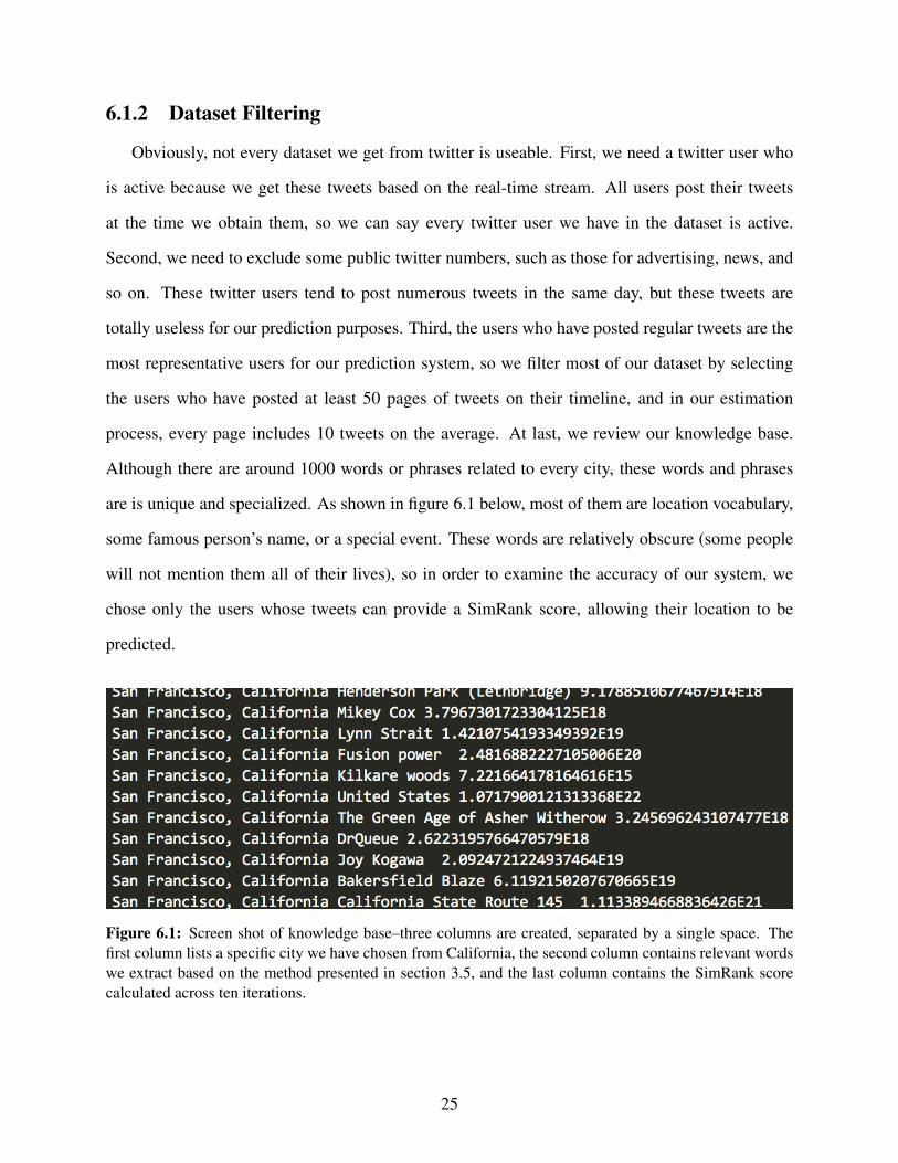
Although there are around 1000 words or phrases related to every city, these words and phrases

are is unique and specialized. As shown in figure 6.1 below, most of them are location vocabulary,

some famous person’s name, or a special event. These words are relatively obscure (some people

will not mention them all of their lives), so in order to examine the accuracy of our system, we

chose only the users whose tweets can provide a SimRank score, allowing their location to be

predicted.

Figure 6.1: Screen shot of knowledge base–three columns are created, separated by a single space. The

first column lists a specific city we have chosen from California, the second column contains relevant words

we extract based on the method presented in section 3.5, and the last column contains the SimRank score

calculated across ten iterations.

25

6.2 Evaluation Mechanism

Practically speaking, accuracy gives the most obvious and straightforward indication of the

performance of our system, and it is the baseline for our evaluation. However, as classification

problem model, a confusion matrix is a more effective and unambiguous way to present the pre-

diction results. A confusion matrix, also known as an error matrix, is a specific table layout that

provides a visualization of the performance of an algorithm. Given a specific city, say C1, a con-

fusion matrix gives us four classes to show the performance of our system: True positives, which

means actual C1 users were correctly classified as C1; false negatives, which means C1 users were

incorrectly marked as being located in a different city, say Cn; false positives, which means users

from a different city, say Cn, were incorrectly labeled as C1; and true negatives, which means all

users except users from C1 were correctly classified as non-C1 users.

6.3 Result

We have collected a group of datasets based on different cities and stored them in the different

cities’ files, respectively. We selected two different datasets for our evaluation. The first one is

around 500 users that come from the same city, and the second one is a mixed file dataset which

includes information around 1000 users from 20 different cities.

6.3.1 Accuracy and Confusion matrix

Because the populations and the number of active twitter users vary among cities, the size of

the datasets that we obtained is quite disparate. To present the results for the overall accuracy of

our method, we chose Los Angeles, which has the largest population in California [30] (Table 6.1).

Accuracy is the most intuitive way to show the performance of a prediction system, it can be

calculated by TP+TNP+N

, where TP is the true positive, TN is the true negative, P is the positive sample

totally and N is the negative sample totally. As table 6.1 show us above, the accuracy of the sample

city(Los Angeles here) can be calculated by the system’s prediction of number of users who belong

to this city divid by the total number of users. It is 28.4%. Based on the prediction result, except

26

Table 6.1: In the first row, cities are listed in decreasing order, sorted on population estimates provided by

the United States Census Bureau around July 1, 2015 [30]. City codes are shown below. The second row

of the table shows prediction results for over 500 users that all come from Los Angeles. For each user, we

collected at least 75 pages of tweets(around 300 to 500 tweets totally) from their timeline, which included

their tweets and retweets.

A: Los Angeles, B: San Diego, C: San Jose, D: San Francisco, E: Fresno, F: Sacramento, G: Long Beach,

H: Oakland, I: Bakersfield, J: Anaheim, K: Santa Ana, L: Riverside, M: Stockton, N: Chula Vista, O: Irvine,

P: Fremont, Q: San Bernardino, R: Modesto, S: Fontana, T: Oxnard

City A B C D E F G H I J K L M N O P Q R S T

PredNum 142 21 20 19 11 13 29 14 10 27 34 26 17 12 26 8 24 14 18 15

the sample city, the predictions of other cities are basically distributed randomly, population diff

of each city didn’t give enough impact on our accuracy result.

To make sure the distribution of test users, we selected 50 users from each city who published

the longest tweets, labeling them, and putting them into the same file. Running our system on this

file generated the confusion matrix of these 20 cities, as shown below in figure 6.2. This matrix

gives us an overview of our system’s performance, and it will be discussed in further detail below.

6.3.2 Selecting Overlays using IDW

As introduced earlier, inverse distance weighting (IDW) is a nonlinear interpolation technique

used for estimating an attribute at an unknown location based on the weighted average of the

attribute values from nearby location sample points. Here, we can apply IDW value to select a

better overlay for a sample city in our system.

In order to include a sufficient number of cities in our calculations, we chose Los Angeles as our

sample city for two reasons: The high population of Los Angeles is useful for collecting available

datasets, and eight cities of our twenty-city dataset are quite close to Los Angeles geospatially. It

is more meaningful to use nearby cities to calculate IWD values because geospatially closed points

have a greater effect on the estimated value than distant points.

As figure 6.3 shows, we selected a relatively small area (black dotted box), and if we magnify

this area, we can obtain the straight-line distance between each of the selected cities and Los

Angeles, which are listed at the bottom right corner of the figure. Then, if we make Los Angeles

27

Figure 6.2: Confusion matrix of twenty cities. For each city, we chose fifty users for our evaluation dataset.

The colored vertical bar on the right side indicates the accuracy present in color format. The X-axis and

Y-axis cities are sorted by the size of the dataset we collected at the same time, and to a certain extent, the

matrix represents the number of twitter users in each city.

the center of a circle and use the distance listed as the radius, we can get several overlays that

cover different numbers of cities one by one. For each of overlay, we consider Los Angeles as

an unknown location point, and calculate the IDW values of Los Angeles based on other cities

in the same overlay. Finally, Los Angeles’s prediction result and each overlay’s IDW value are

respectively summed to get the final sensitivity result, which means we can expand the coverage

area of Los Angeles to observe changes in sensitivity. The results are shown in figure 6.4.

IDW values were calculated based on the city covered by a specific area. The second value of

IDW is not considered in our experiment because when the overlay covers only one known weight

value city, the value of IDW is always equals to this city’s weight value. The last two columns are

28

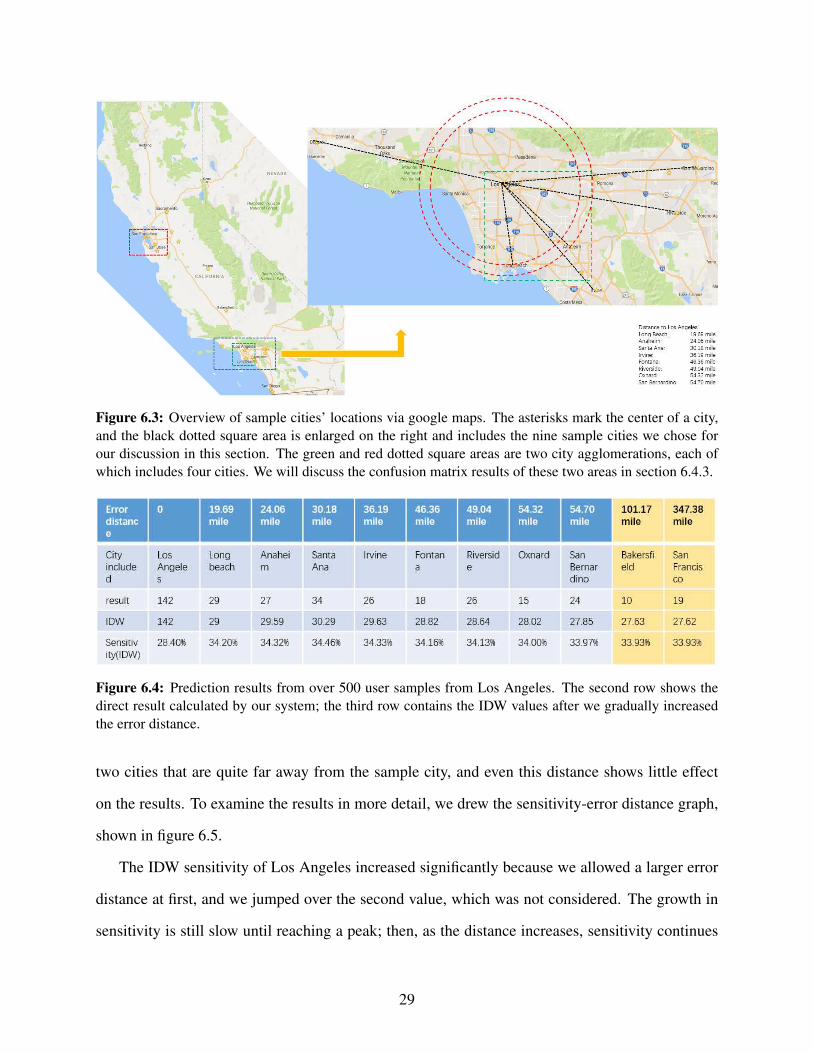
Figure 6.3: Overview of sample cities’ locations via google maps. The asterisks mark the center of a city,

and the black dotted square area is enlarged on the right and includes the nine sample cities we chose for

our discussion in this section. The green and red dotted square areas are two city agglomerations, each of

which includes four cities. We will discuss the confusion matrix results of these two areas in section 6.4.3.

Figure 6.4: Prediction results from over 500 user samples from Los Angeles. The second row shows the

direct result calculated by our system; the third row contains the IDW values after we gradually increased

the error distance.

two cities that are quite far away from the sample city, and even this distance shows little effect

on the results. To examine the results in more detail, we drew the sensitivity-error distance graph,

shown in figure 6.5.

The IDW sensitivity of Los Angeles increased significantly because we allowed a larger error

distance at first, and we jumped over the second value, which was not considered. The growth in

sensitivity is still slow until reaching a peak; then, as the distance increases, sensitivity continues

29

Figure 6.5: sensitivity-Error Graph for Los Angeles

to decrease. As we saw in figure 6.5, the IDW sensitivity increases at the beginning, and after it

reaches a peak value, it begins a slow, continuous decline.

Compare this result with existing approach of twitter location prediction. Typically, most of

previous approaches predict users’ location on nationwide, they always give a large error distance

between the actual location of the user and the estimated location by their algorithm. Cheng et

al. got 51% sensitivity rate on average error distance at 535.564 miles [6], Krishnamurthy et

al. also use wikipedia to create knowledgebase and got 54.48% sensitivity rate on average error

distance at 429 miles [12]. Purely from the numerical point, their approach seems better than our

approach, however, consider that our approach is doing location prediction on citywide, we can

get a relatively good sensitivity result when gives a much smaller error distance.

6.3.3 Receiver Operating Characteristic

A receiver operating characteristic curve, i.e. ROC curve, is a graphical plot that illustrates the

diagnostic ability of a binary classifier system as its discrimination threshold is varied. For our

30

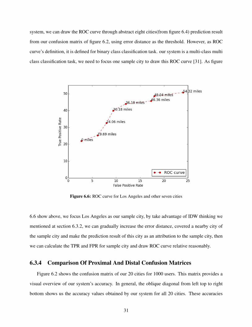
system, we can draw the ROC curve through abstract eight cities(from figure 6.4) prediction result

from our confusion matrix of figure 6.2, using error distance as the threshold. However, as ROC

curve’s definition, it is defined for binary class classification task. our system is a multi-class multi

class classification task, we need to focus one sample city to draw this ROC curve [31]. As figure

Figure 6.6: ROC curve for Los Angeles and other seven cities

6.6 show above, we focus Los Angeles as our sample city, by take advantage of IDW thinking we

mentioned at section 6.3.2, we can gradually increase the error distance, covered a nearby city of

the sample city and make the prediction result of this city as an attribution to the sample city, then

we can calculate the TPR and FPR for sample city and draw ROC curve relative reasonably.

6.3.4 Comparison Of Proximal And Distal Confusion Matrices

Figure 6.2 shows the confusion matrix of our 20 cities for 1000 users. This matrix provides a

visual overview of our system’s accuracy. In general, the oblique diagonal from left top to right

bottom shows us the accuracy values obtained by our system for all 20 cities. These accuracies

31

fluctuate within a range from 18.5% to 27.4%. Dividing the matrix into two parts on the diagonal,

calling the bottom part the left and the top part the right, the average color of the grids from the

left (bottom) is brighter than the color of grids that come from the right (top). This situation means

our system tends to place twitter users in cities that have more active twitter users (false negative

and false positives). So, compared to table 1, in which cities are sorted by population and results

displayed are relatively average, the actual number of active twitter users has more influence on

the results than the baseline population. For a deeper examination of the confusion matrix, we

extracted specific areas to reorganize the matrix, and the results are shown in figure 6.7.

Figure 6.7: This confusion matrix is extracted from the overall matrix according to two relatively separate

city agglomerations. The sample size for each city is still 50, but the false negative and false positive values

just correspond to the selected cities.

We extracted four cities from the green dotted boxed area in figure 6.3 as one city group, and

the other four cities were drawn from the red dotted box as a second city group. We extracted

confusion matrix data related just to these eight cities and reorganized the data based on the two

32

groups. The resulting matrix, figure 6.7, using the center of the graph as a point of reference,

can be divided into four parts: left top, left bottom, right top, and right bottom. We find that the

color of the left top and right bottom parts are lighter than the left bottom and right top parts.

This is because, even if the wrong classification is made, the system is more inclined to classify

users to nearby cities than to distant cities. On the other hand, the first and the fifth columns of

the matrix are lighter in color than the following three columns. Obviously, this is caused by a

lack of balance between population and number of active twitter users. According to the data we

collected, Los Angeles, as expected, has the highest population density and the most twitter users.

However, when we consider San Francisco and San Jose, San Jose has a larger population than San

Francisco, but we can only get one-third of the number of active users from San Jose than we get

from San Francisco in the same time frame. Furthermore, Los Angeles and San Francisco have the

largest number of active twitter users of the eight cities, and our location prediction system prefers

to assign more users to these two cities than to the others. Certainly, the flow of the population, the

difference between place of residence and workplace in prosperous cities, and frequent movement

are likely to have a strong influence on our experimental results, and such factors have had some

unpredictable effects on our system. Future studies will be directed at finding and overcoming

these types of challenges.

33

Chapter 7

Conclusions and Future Work

7.1 Conclusions

For this thesis, we constructed a location prediction system for twitter users by using the

structural-context similarity of Wikipedia links as a basis for data collection and applying the

SimRank algorithm to create an independent knowledge base for predicting a twitter user’s loca-

tion with reasonable accuracy. The use of Apache Storm allowed access to real-time data, making

it possible to use the latest user information. We have proposed a novel method to for extracting

relevant words, greatly reducing the amount of calculation required for the system. The extraction

method was combined with the MapReduce framework in Apache Hadoop, improving the effi-

ciency of the core algorithm for analyzing our data base significantly. Finally, the presented results

and discussion show that our system produces an acceptable level of prediction accuracy for the

20 sample cities chosen from California.

7.2 Future Work

There are many improvements and extensions to this system to pursue. First, the population and

number of active twitter users of a specific city have a huge influence on our prediction results. If

we expand the distributed scale and extend the tweets collection time, we could get more data about

the distribution of twitter users across different cities, which would be conducive to normalizing

our dataset and improving prediction accuracy. Second, in large tourist cities like San Francisco

and Los Angeles, the number of active twitter users will change dramatically based on different

time intervals. Furthermore, all data generated by foreign travelers is inappropriate for our system

because our system analyzes tweets history to predict location. So in the future, our system should

exclude the data obtained from these visitors.

34

Location prediction should not be the final goal; it is only a means of getting users’ potential

information. Our system should also have broader applications. We could filter incoming messages

with key words that are of interest, such as weather conditions. For example, if we filter using the

word rain, then our system will give places where it is currently raining. If we are concerned

with tweets that reflect sentiments regarding an event, we just need to extract sentiment-related

words from Wikipedia and reconstruct our knowledge base; then, our system will show sentiments

for different cities. Certainly, twitter is only one of popular social media platforms. However,

relatively speaking, there are more Facebook and Instagram users than twitter users, and there are

many studies on location prediction using these social media platforms [8] [10]. We expect that our

system can deal with different kinds of social media, and combined with different recommended

systems on the market like Yelp, it is possible to build a more powerful prediction framework.

35

References

[1] Jacob Davidson. Here’s how many internet users there are, 2015.

[2] Dave Chaffey. Global social media research summary 2017, 2016.

[3] Glen Jeh and Jennifer Widom. Simrank: a measure of structural-context similarity. Proceed-

ings of the Eighth ACM SIGKDD Enternational Conference on Knowledge Discovery and

Data Mining, pages 538–543, 2002.

[4] Ankit Toshniwal, Siddarth Taneja, Amit Shukla, Karthik Ramasamy, ..., and Dmitriy Ryaboy.

Storm@ twitter. Proceedings of the 2014 ACM SIGMOD International Conference on Man-

agement of Data, pages 147–159, 2014.

[5] Hadoop. Apache hadoop and yarn, 2006.

[6] Zhiyuan Cheng, James Caverlee, and Kyumin Lee. You are where you tweet: A content-

based approach to geo-locating twitter users. Proceedings of the 19th ACM International

Conference on Information and Knowledge Management, pages 759–768, 2010.

[7] Swarup Chandra, Latifur Khan, and Fahad Bin Muhaya. Estimating twitter user location

using social interactions âAS a content based approach. Privacy, Security, Risk and Trust

(PASSAT) and 2011 IEEE Third International Conference on Social Computing (SocialCom),

pages 838–843, 2011.

[8] HAN Bo, Paul COOK, and Timo thy BALDW IN. Geolocation prediction in social media

data by finding location indicative words. Proceedings of COLING, pages 1045–1062, 2012.

[9] Theodoros Anagnostopoulos, Christos Anagnostopoulos, and Stathes Hadjiefthymiades. An

adaptive machine learning algorithm for location prediction. International Journal of Wire-

less Information Networks, 18(2):88–99, 2011.

36

[10] Lars Backstrom, Eric Sun, and Cameron Marlow. Find me if you can: improving geographi-

cal prediction with social and spatial proximity. Proceedings of the 19th International Con-

ference on World Wide Web, pages 61–70, 2010.

[11] Jeffrey McGee, James Caverlee, and Zhiyuan Cheng. Location prediction in social media

based on tie strength. Proceedings of the 22nd ACM international conference on Information

and Knowledge Management, pages 459–468, 2013.

[12] Revathy Krishnamurthy, Pavan Kapanipathi, Amit P. Sheth, and Krishnaprasad Thirunarayan.

Location prediction of twitter users using wikipedia. The Ohio Center of Excellence in

KnowledgeEnabled Computing, 2014.

[13] Nathan Marz. Storm: Distributed and fault-tolerant realtime computation, 2013.

[14] Tony Siciliani. Streaming big data: Storm, spark and samza.

[15] S. Pallickara, J. Ekanayake, and G. Fox. Granules: A lightweight, streaming runtime for

cloud computing with support, for map-reduce. Cluster Computing and Workshops, 2009.

CLUSTERâAZ09. IEEE International Conference on, pages 1–10, 2009.

[16] T. Buddhika and S. Pallickara. Neptune: Real time stream processing for internet of things

and sensing environments. Parallel and Distributed Processing Symposium, 2016 IEEE In-

ternational, pages 1143–1152, 2016.

[17] S. Pallickara and G. Fox. On the matching of events in distributed brokering systems. ITCC,

pages 68–76, 2004.

[18] G. Fox, S. Pallickara, and X. Rao. Towards enabling peer-to-peer grids. Concurrency and

Computation: Practice and Experience, 17(7–8):1109–1131, 2005.

[19] Johnson Charles Kachikaran Arulswamy and Sangmi Lee Pallickara. Columbus: Enabling

scalable scientific workflows for fast evolving spatio-temporal sensor data. Proceedings of

the 14th IEEE International Conference of Service Computing, 2017.

37

[20] Jeffrey Dean and Sanjay Ghemawat. Mapreduce: simplified data processing on large clusters.

Communications of the ACM, 51(1):107–113, 2008.

[21] W. Budgaga, M. Malensek, S. Pallickara, F. J. Breidt N. Harvey, and S. Pallickara. Predictive

analytics using statistical, learning, and ensemble methods to support real-time exploration

of discrete event simulations. Future Generation Computer Systems, 56:360–374, 2016.

[22] Walid Budgaga, Matthew Malensek, Sangmi Lee Pallickara, and Shrideep Pallickara.

A framework for scalable real-time anomaly detection over voluminous, geospatial data

streams. Concurrency and Computation: Practice and Experience, 29(12):1–16, 2017.

[23] M. Malensek, S. Pallickara, and S. Pallickara. Fast, ad hoc query evaluations over multidi-

mensionalgeospatial datasets. IEEE Transactions on Cloud Computing, 2015.

[24] M. Malensek, S. Pallickara, and S. Pallickara. Analytic queries over geospatial time-series

data using distributed hash tables. IEEE Transactions on Knowledge and Data Engineering,

28(6):1408–1422, 2016.

[25] M. Malensek, S. Pallickara, and S. Pallickara. Evaluating geospatial geometry and proximity

queries using distributed hash tables. Computing in Science and Engineering, 16(4):53–61,

2014.

[26] W.Budgaga, M. Malensek, S. Lee Pallickara, and S. Pallickara. A framework for scalable

real-time anomaly detection over voluminous, geospatial data streams. Concurrency and

Compu-tation: Practice and Experience, 29(12), 2017.

[27] Larry Page and Sergey Brin. The pagerank citation ranking: bringing order to the web. 1998.

[28] Weiren Yu, Xuemin Lin, and Jiajin Le. A space and time efficient algorithm for simrank

computation. Proceedings of the 12th International Asia-Pacific Web Conference, pages 164–

170, 2010.

[29] Twitter. Geo guidelines.

38

[30] Wikipedia. List of largest california cities by population.

[31] Tom Fawcett. An introduction to roc analysis. Pattern Recognition Letters, 27(8):861–874,

2006.

39