METHODOLOGY FOR THE SELECTION AND TIMING OF WATER RESOURCES

PROJECTS to Promote National Economic Development

by

Wendim-Agegnehu Lemma

AUGUST 1975

77

.·

METHODOLOGY FOR THE SELECTION AND TIMING OF WATER RESOURCES PROJECTS To Promote National Economic Development

August 1975

by Wendim-Agegnehu Lemma *

•

HYDROLOGY PAPERS COLORADO STATE UNIVERSITY

FORT COLLINS, COLORADO 80523

No. 77

•Formerly Ph.D. graduate student, Colorado State University, Civil Engineering Department, Fort Coll ins, Colo rado. Presently with Bechtel, Inc., P.O. Box 3965, San Francisco, California 94119

Chapter

TABLE OF CONTENTS

.-NOTATIONS USED IN THE MATHEMATICAL HODEL

ACKNOWLEDGMENTS

ABSTRACT

INTRODUCTION

II ECONOMIC DEVELOPHENT AND PLANNING

Economic Development and Underdevelopment Planning for National Economic Devel opment

III SURVEY OF PRESENT PRACTICES OF PROJECT SELECTION AND TIMING

IV METHODOLOGY FOR THE SELECTION AND TIMING OF WATER RESOURCES PROJECTS

Rationale, Objectives , and Crit eria . Component Procedures of the Methodo l ogy ~

Simulation of the Economy . . . . . Assessment of Demands . . . . . . . Assessment of Resource Capabilities Opt imal Selection and Timing . . . . Feedback : Testing, Analysis, and Adjustment

V ILLUSTRATIVE EXAMPLE

Statement of the Problem Basic Data .. . Assessment of Production Requirements Sel ection and Timing of Projects ..

VI SUMMARY, CONCLUSIONS, AND RECOMMENDATIONS

REFERENCES

APPENDIX A: COMPUTER PROGRAM AND OUTPUTS OF INPUT-OUTPUT PROJECTION AND DETERMINATION OF PRODUCTI ON REQUIREMENTS

APPEND IX B: COMPUTER PROGRAM . . . .

APPENDIX C: RESULTS OF SELECTION FOR A SINGLE AND MULTIPLE (IN THIS CASE 2) TIME PERIODS

iii

Paae

iv

v ~ t

v

1

2

2 6

9

12

i 2 16 17 20 22 2.5 27

28

28 28 34 34

38

39

42

so

60

8

c

c

c T

D T

g

i

J(

1 • 1, 2, ... , n

s

5

NOT A TIONS USED IN THE MATHEMATICAL MODEL

Value of average annual production

Present value of benefits

Yearly cost

Present value of costs

Allocated budget for plan period T

The total production demands vector at the beginning of plan period T

Average annual growth rate of GNP

Annual discount rates

Project number

Total number of projects

TYPe of project output (irrigation water, hydropower, etc.)

Vector of projected imports at plan period T

k-th project

Set of projects selected for implementation at the beginning of plan period T

Yearly cash flow

Net present worth

iv

t • 1, 2, ..• , T Number of years

T Project life

v • 1, 2, ... , V Number of projects going out of use (vanishing)

w T

y T

v

p

,. • 1, 2, ... , N

Vector of projected intermediate demands T

Vector of projected final demands T

The i ncrement i n total production levels between two successive plan peri~s

The vector of target levels of out­puts to be met by new projects

Length of construction (or project maturity) period of the k- th project

Topscript indicating target levels of outputs to b~ met by new projects

Number of years in each development plan period; f ive years is the span most commonly adopted by developing countries

Number of development plan period

Subscript used to indicate reference to the base year

ACKNOWLEDGMENT

I highly appreciate the. Graduate Research Assistantship granted Colorado State University whlch made it possible for me to pursue this study was supported by AID 2ll(d) Water Resources Institutional Grant. the Civil Engineering Department.

me by the Civil Engineering Department of last phase of my graduate studies. The Ftmds for computer usage were provided by

I am deeply indebted to my academic program committee for their invaluable suggestions, discussions, and guidance generously rendered to me throughout the course of my work. Special gratitude is due to Dr. Maurice L. Albertson, Centennial Professor of Civil Engineering and chairman of the committee, who not only offered guidance in conducting this study and edited the manuscript, but also took keen interest and helped shape my academic and professional training.

I particularly appreciate the large amount of time and effort which Dr. S. Lee Gray, Associate Professor of Economics, devoted to discussion and suggestions on the economic aspects of the study. Drs. John Labadie, Assistant Professor of Civil Engineering, and WilliamS. Duff, Assistant Professor of Mechanical Engineering were very helpful in the mathematical modeling and solution of the problea. Professor Henry P. Caulfield, Jr., Professor of Political Science, helped in the area of public decision making. Dr. Warren A. Hall, Director of the Office of Water Resources Research, helped at the initial stage in formulating an~ struct uring of the research problem and later reviewed the manuscript. In addition , I am grateful to Charles J. Palmer, Economic Research Service of the U.S. Department of Agriculture, for his help in developing the computer code for the input-output projection.

Wendim-Agegnehu Lemma

ABSTRACT

The methodology developed in this paper is designed to facilitate the selection and timing of water resources projects to optimally achieve "a priori" specified national economic development through desired strategies. The methodology is composed of several analytical procedures.

The input-output model is used to simulate the national economy thus further facilitating consistent pro­jections of the elements of final demands in accordance with the national economic development objectives and strategies , and assessing the total and incremental requirements for sectorar outputs of goods and services at designated future time periods. A mathematical model for the selection and timing of water resources projects for their implementation, in other words for the formulation of an optimal national water resources development program, has been developed and its application demonstrated on an elt8.111ple problem. The model incorporates important factors such as economic efficiency of projects , demand targets for project outputs of goods and services necessary to achieve desired national economic growth, resources capabilities and limitations , and project interrelationships. Incorporation of these and other related factors makes the model reflective of the real world problem it is intended to aid in solving.

The application on an example problem convincingly indicates it to be a very useful tool indeed in the national economic planning process. This exercise also reveals the avenues for further research and improvem.ent.

v

I'

Chapter 1 INTRODUOION

: Despite the fact that more and more countries are

exercising some form of economic planning, and despite the fact that the literature on planning and project evaluation for developing countries is literally mush­rooming, work concerning the extremely vital subject of project selection and timing for implementation to enhance national economic development is disappoint­ingly meager and incomplete. After all, the culmina­tion of t he plan formulation process is the selection of a recommended plan of action--a fact recognized by many.

Furthermore, most of the works on project evalua­tion, and selection, under conditions associated with de­veloping countries end up using the competitive market model (by virtue of the implied assumptions underlying the choice of such parameters as interest rates and se­lection criteria) which does not accurately represent the real situation in these countries (even though this is usually acknowledged at the beginning) at all.

The objective of this study is to develop a meth­odology composed of rigorous analytical procedures based on sound optimization techniques for the selec­tion and timing of the implementation of water re­sources p·rojects to enhance national economic develop­ment. "Project selection and timing" is understood in this study as the decision-making process of determin­ing which projects should actually be implemented and when. The irreversibility of such decisions coupled with the resource intensiveness of water resources projects, and hence the costliness of a wrong decision, make the selection and timing of water resources pro­jects a crucial matter in the entire process of national economic development planning.

In this paper the major elements relevant to the selection and timing of water resources projects are studied and a methodology composed of analytical pro­cedures for making such decisions directed to achiev­ing national economic development goals and targets

l

within its resources capabilities is developed. Even though the methodology may prove to be useful in both economies where the operative policy is either indica­tive or directive planning, it shoul d be most useful in the latter.

The results of the study are presented in the following chapters. Chapter II exhaustively discusses the need for central planning to ensure balanced and sustained national economic growth and articulates the place of project selection and timing in the planning process. A survey of the present practices of project selection and timing given in Chapter II I, while point­ing out the merits of some of the leading works, ar­ticulates the necessary features of the real world to be depi cted in the decision making that these studies are lacking. The suggested methodology is presented in Chapter IV. An illustrative example, wherethemechan­ics and the workability of the methodology are demon­strated, is given in Chapter V. Conclusions and recom­mendations for further research, as well as reflections on relevant l essons learned, are given in Chapter VI.

The scope of the study is limited to considering only "the enhancement of national economic devel opment" out of the three major objectives of water resoures development (Chapter IV). This is mainly because of the fact that the valuation of benefits and costs (primarily benefits) pertaining to the other two ob­jectives is yet an unresol ved issue, and those sug­gested so far are noncommensurate with that of the basic and conventional development objective.

Furthermore, due to the unavailability of the necessary data in the appropriate form and kind, ap­plication of the methodol ogy could not be demonstrated on an actual case of a given country. However, the example problem set up is as good, if not better, for it has more detail because separate parts of the data used represent actual cases whi ch have been pulled out of documents of several countries.

'iit"'

Chapter II ECONOMIC DEVELOPMENT AND PLANNING

The overall purpose of this chapter is to indi­cate the need for and the appropriate place of the methodology, suggested in the present study, for the selection and timing of water resources projects. The methodology could find application in almost any place; yet, it would be especially useful where simul­taneous development of numerous sectors is to be car­ried out according to a long-range perspective plan that specifies the desired goals for the entire econo­my. Among possible other uses that the methodology may have, in addition to selecting and timing of water re­sources projects, is that it could help indicate areas where projects may be lacking and hence the need to initiate projects in such specific areas.

In this chapter, the general features of underde­velopment of countries and the reasons for the need of accelerated economic development in these countries is briefly discussed. Also the type of development plan­ning adopted by most of these countries and its merits are elaborated.

Economic Development and Underdevelopment

A clear understanding of the differences between economic underdevelopment and development is vital in the formulation and implementation of meaningful and effective programs to bring about necessary and desir­able transformation. An understanding of the process of development and a knowledge of the ways and means of activating , controlling and maintaining the process are equally vital. This section is intended to aid in such under standing.

Di fferences Between Development and Underdevelopment

Development is a relative concept. Underdevelop­ment is a comparative and essentially negative concept. Underdeveloped countries are basically areas of radical scarcity where the inadequacy of the means of liveli ­hood (social welfare) is the primary distinguishina feature. While more developed (also known as advanced or afflu~nt) countries possess a number of common characteristics by which they can be positi vely iden­tified (e.g ., i ndustrial ized production systems; rela­tively high per capita gross national products; rela­tively high adult literacy; high per capita energy , calorie and protein consumption, high per capita in ­come, etc.}, the same cannot be said of underdeveloped countries. Such a positive identification of underde­veloped countries is impossible because it embraces diversified civilizations and societies, as wel l oa the less affluent regions of the developed countrle~. In other words, underdevelopment is a notion thmt characterizes that which societies are not, i.e . , tlo· veloped, but does not characterize positively what In fact they are. Nevertheless, it is of interest to no to that so many different observer s and scholars hnvo come up with very similar l ists of characteri stics of the underdeveloped countries, despite the fact thmt there are often vast differences in the poli t ic3 l Dnd cultural aspects, available information and record keeping of the various underdeveloped countries.

Characteristics of Underdeveloped Areas

Perhaps the most comprehensive list of characte r ­istics of underdeveloped countries is given by l.clbon­stein (1957) who divided them into four major •:ato~&Or • ies: economic, demographic and health, technoloal ca l,

and cultural and political characteristics. These characteristics are given below primarily as Leiben­stein presented them with minor changes and updating .

Economic

a. General

1. A ver y high proportion of the popula­tion is in agriculture , usually 70 to 90 percent.

2. Evidence of considerable "disguised un­employment" and a l ack of employment opportunities outside agriculture. "Absolute overpopulation" in agricul­ture, i.e . , it would be possible tore­duce the number of workers in agricul­ture and still obtain the same total output .

3: Very little capital per head.

4. Lo~ income per capita and, as a conse­quence , existence is near the "subsi s­tence" level. (Per capita income ranges from $48 to $192 per year. )

S. Practically zero savings for the large mass of the people as well as low capi­tal formation--the rate of investment as a percentage of the national produc~ devoted to capital formatiorr in the less developed countries is 5 to 6 percent as opposed to 12 to 15 percent or more in developed economies (Millikan , 1973). Whatever savings do exist are usually ach ieved by a landholding class whose val ues are not conducive to investment in industry or commerce.

6. The primary industries , that is, agri­culture, forestry, ~d mining, are usu­a lly the residual employment categoric~

7. The output in agriculture is made up mostly of cereals and primary raw ma­terials, with relatively low output of protein foods. The reason for this is the conversion ratio between cereals and meat products ; that is, if 1 acre of cereals produces a certain number of calories , it would take bet ween 5 and 7 acres to produce the same number of calor ies if meat products were produced

~ . Major proportion of expenditures are on . food and necessities.

9 . Exports are mainly foodstuffs and raw mater ials (primary goods).

10 . Low volume of trade per capita .

11. Poor credit and marketing facilities . .

12. Poor housing.

1.l. Under-utilization of production factor s .

...

b. Agriculture

1.

2.

3.

Although there is low capitalization on the land, there is simultaneously an uneconomic us~ of whatever capital ex­ists due to the small size of holdings and the existence of exceedingly small plots.

Exceedingly low agricultural technology with l imited and primitive tools. The methods of production for the domestic market are generally old- fashioned and inefficient, resulting in little surplus for marketing. This is usually true irrespective of whether the cultivator owns the land, has tenancy rights, or is a sharecropper.

Low yields per unit area.

.4. Even where there are big landowners, the openings for modernized agricultur­al production are limited by difficul­ties of transport and the absence of a·~ sizable demand in the local market. It is significant that in many underdevel­oped countries a modernized type of ag­riculture is confined to production for sale in foreign markets.

s.

6.

7.

There is an inability of the small landholders and peasants to weather even a short- term crisis, and, as a consequence, attempts are made to get the highest possible yields from the soil, which leads to soil depletion.

There is a widespread prevalence of high i ndebtedness relative to assets and income .

A most pervasive aspect is · a feeling of land hunger due to the exceedingly small size of holdings and small diversified plots. The reason for this is that holdings are continually subdivided as the population on the land increases.

Demographic

1. High fertility rates, usually above 40 per thousand.

2. High mortality rates and low expectation of life at birth.

3. Inadequate nutrition and dietary deficiencies.

4. Rudimentary hygiene, public health, and san­itation.

S. Rural overcrowding.

Cultural and Political

1. Rudimentary education and usually a high degree of illiteracy among most of the people (80 to 90 percent). This l eads to inadequate . man20wer resources which is the key to de­velapment above all else (Albertson, 1972).

2. E.xtensive prevalence of child labor.

3. General weakness or absence of the middle class.

3

4. Inferiority of women's status and position.

s. Traditionally determined behavior and role for the bulk populace.

Technological and Miscellaneous

..

1. Inadequate manpower resources--both in quality and quantity.

2.

3 .

4.

s.

Facilities for the training of technicians, engineers, and others needed as manpowe·r re­sources for development are absent or inade­quate at best.

I

Inadequate infrastructure.

Crude technology.

Dualism-existence of large metropolitan cities with modern civic amenities on the one hand and on the other, poor, unhygienic and back­ward rural areas. Similar dualism is found in the field of production and transpo·rt so that the hand loom exists side by side with the automatic loom, the bullock cart with the jet plane, and so on.

A close study of the foregoing characteristics would inevitably lead to· the conclusion that underde­veloped countries are areas of acute scarc1t1es and inadequacies. This particular impression, more . than any elaborate theory, reveals the social aim and pur­pose for development, i.e., substitute scarcities and inadequacies with adequacy and plentifulness.

The Development Process

Understanding the development process requires a clear conceptualization of what is meant by dev·elop­ment as well as a knowledge of the ends, the means, the measures, and the· aims of development.

What is development? Development is basically a process of transformation , i.e., it is a process by which underdeveloped countries rid themselves of the foregoing negative characteristics and acquire certain characteristics of today's affluent nations: adequacy, plentifulness and more self-sufficiency.

The development process has been explained and analyzed in varied ways by different indivi duals at different times from different points of view. A com­prehensive treatment of the development process based on a conceptual model called 'The Development Wheel' (Fig. Il-l) is given by Albertson (1972). Using the Development Wheel, he explains and concludes that man­power is " ... alpha and omega," " ... the beginning and the end of the development process," and that "devel­opment is accomplished by man."

The wheel is explained by Albertson as follows:

"The model shown in Fig. 1 depends upon man's knowledge and his motivation to use this knowledge to create and work through the necessary insti­tutions. Man's motivation depends upon his values--both individual values and the values of the groups and the institutions that he creates and uses as vehicles. He uses the natural re­sources and the infrastructure to produce the goods, services, and information which can be used by man for consumption or for further devel- . opment--in other words, for capital."

Among other things, an important bertson's approach is the implicit

aspect of Al­suggestion that

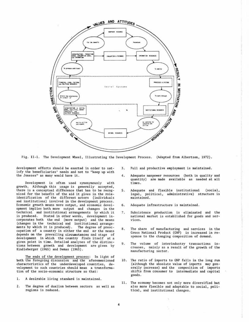
Fig. Il-l. The Development Wheel, Illustrating the Development Process. (Adapted from Albertson, 1972).

development efforts should be exerted in order to sat­isfy the beneficiaries' needs and not to "keep up with the Joneses" as many would have it.

Development is often used synonymously with growth. Although this .usage is generally accepted, there is a conceptual difference that has to be recog­nized for the benefit of the aid it gives in the role­identification of the different actors (individuals and institutions) involved in the development process. Economic growth means more output, and economic devel­opment implies both more output and changes i n the technical and institutional arrangements by which it is produced. Stated in other words, development in­corporates both the end (more output) and the means (changes in the technical and institutional arrange­ments by which it is produced) . The degree of preoc­cupation of a country in either the end or the means depends on the prevailing cir cumstances and stage of development in which the country finds itself at a given point in time. Detailed analyses of the distinc­tions between growth and development are given by Kindleberger (1965) and Demas (1965).

The ends of the development process: In light of both the foregoing discussion and the aforementioned characteristics of the underdeveloped countries, de­velopment to such countries should mean a transforma­t ion of the socio-economic structure so that:

1. A desirable living standard is maintained.

2. The degree of dualism between sectors as well as regions is reduced.

4

3. Full and productive employment is maintained.

4. Adequate manpower resources (both in quality and quantity) are made available as needed at all times.

5. Adequate and flexible institutional (social, legal, political, administrative) structure is maintained.

6. Adequate infrastructure is maintained.

7. Subsistence production is eliminated and the national market is established for goods and ser­vices.

8. The share of manufacturing and services in the Gross National Product (GNP) is increased in re­sponse to the changing composition of demand.

9. The volume of interindustry transactions in­creases, mainly as a result of the growth of the manufacturing sector.

10. The ratio of i mports to GNP falls in the long run (although the absolute value of imports may gen­erally increase) and the composition of imports shifts from consumer to intermediate and capital goods.

11. The economy becomes not only more diversified but also more flexible and adaptable to social, poli­tical , and institutional changes.

The means of the development process: The devel­opment process, in tHo achievement of i ts purposes, i nvolves either new combinations of existing factors at a given technical l evel or the introduction of technical innovation. Furtanno (1964) defines as being fully developed at a given moment, those regions in which, in conditions of full employment of factors , i t is possible to incr ease productivity (real production per capita) only by introducing technical innovations; and those regions whose productivity is i ncreasing, or could be increased by t he mere . introduction of alr eady known techniques, as displaying various degrees of un­derdevelopment. The growth of a developed economy is, then, a matter of accumulating new scientific knowl­edge and of advancing the technological application of such knowledge. On the other hand, the growth of un­derdeveloped economies for the most part is a matter of assimilating techniques already existing. Contrary to the school of thought that expertise and know-how could be imported analogous to cases where physical resources are inadequate, the past experience clearly shows that an adequate i ndigenous manpower resour ce is a prerequisite for sustained development to materialize.

The measure of economic development: Generally, t he level of i ncome and the rate of increase of income are used as the approximate measures of the state of and the r ate of economic developr~nt (Kindleberger, 1965). Actually, indicators of economic deve lopment (Albertson, 1972) and their measurements are much more complex and wider in scope than Kindleberger suggests and than will be used in this study (growth of GNP over time). They should include all the variables (composed of the f actors and actors) involved in the entire process. Economic development occurs when de­sirable changes take place over a given period of t ime in the separate, and in the sum results (both i n qual­ity and quantity) of activities carried out in the areas of industrial and commercial enterprises, admi nistra­tive and legal i nsti tutions, manpower and physical (natura l and man-made) resources, social (both private and community at large) amenit ies , etc. For the eval­uation of economic development over a given period of time, simplificat ions and approximations of the mea­surements are made necessary due to the fact that a valuation system applicable to all t he indicators is not available at the present time.

Economic gr owth (as distinct from economic devel ­opment) occurs when key economic variables become l arger from one period of time to the next in a sys­tematic way. In this regard (Furtando, 1944), devel­opment consists basi cal ly of an increase i n the f l ow of real income, i.e., an increase in the quantity of goods and services at the disposal of a given communi­ty per time period.

..

A more important characteristic of the developed economies (nations) which distinguishes them from the less developed ones, and from which most of the ot her economi c distinctions logically follow, is the fact that they have exhibited over a period of several de­cades a capacity of sustained, built-in, and reasonably steady annual growth in per capita economic output amounting for, on the average , 2 to 3 percent age points per year (Millikan, 1973). Although i t had been learned that during the past decade the less devel oped countries as a group have achieved an average per cap­i ta economic growth of nearly 2 per cent (Millikan, 1973)", this has not been self-sustained, this is evi ­denced by a significant portion of the resources (both capital and manpower) that have made this possible having been supplied by the developed nations in the form of some type of foreign aid.

5

The aims of national economic development: From the multitude of actual economic development plans adopted by some nations, as well as from the enormous scholastic works available, it is very clear that the aim of development is the achievement of regular long­term, built-in, sustained growth without external sub­sidy.

This is a very realistic and worthwhile aim for the less developed countries to have. Whi le self­sustained, steady economic growth will not in itself necessarily bring with i t adequate progress toward all the other goals that less developed countries seek i n their development programs , it wi ll facilitate achiev­ing them. In the absence of such growth, significant progress toward most of these goals is impossible.

A significant manifestation of this aim as the key to the development issue is the fact that i n 1961 the General Assembly of the United Nations re­solved that the 1960 ' s would be termed the "Development Decade." In this period, the world community would devote itself to the problem of generating a process oi accelerated economic growth that could in time lift the world' s less affluent (which constitutes two­thirds of the world's population) out of grinding poverty and provide the wherewithal for a marked improvement i n the quality of life of the mass of the world's peoples. The quantitative target set was an annual average growth rate of the economic output or gross national product (GNP) of the less developed world of 5 percent (Millikan, 1973). On October 24, 1970, the twenty-fifth anniversary of the founding of the United Nations, the General Assembly voted unani­mously to proclaim the 1970's ' 'The Second Interna­tional Development Decade" and to adopt the Interna­tional Development Strategy which set the annual average rate of growth of GNP for the less developed countries to be at least 6 percent (U.N., 1970).

Development Pol icies and Strategies

Development strategi es: While self-sustained growth is a common aim shared by most , if not all , de­veloping nations , the policies and strategies that such countries adopt are diverse, depending on circum­stances pr eval ent in the given country and on the stage of economic development that i t has reached . Some of t he priority strategies may be categorized as follows:

1. The allocation of investment r esources among major economic sectors such as agriculture; manu­facture of consumer goods; production of interme­diate and capital production of intermediate and capit al goods; in1provement of infrastructure such as transportation, communication , and power. In­correct allocation can sharpl y reduce the average productivity of capital.

2. The adoption of technologies appropriate to the country' s resources base. For example, if, as in many less developed countries , capital is very scarce and labor is in abundant supply, produc­tivit y can be increased by adopting labor inten­sive and capital -saving technologies .

3. Research--for instance in agriculture, to develop new technologies particularly suited to the con~ ditions prevailing in the country.

4. An appropriate balance between activities de­signed to replace imports with domestic produc­tion on the one hand and those intended to gener­ate exports on the other.

,, I~ ,,

. .

1

s.

6.

Education, training, and the development of man­power resources, which is the moving force of de­velopment .

The creation, promotio~, and improvement of in­st itutions, public and private, whose smooth functioning is important to the development pro­cess.

7. The right balance between excessive governmental efforts to regulate, control, and manage economic activity and inadequate attention to such regula­tion and contr~l in areas where it is important.

8. The provision of a framework for capital resources management, tax and fiscal policy and the control of markets that will maximize incentives to pro­ductivity improvements.

Obstacles to economic development: The selection and adoption of anyone or groups of the various mea­sures to promote sustained economic growth categorized above, as well as the setting of priority among them, is the responsibility of the government of a country. Of course, the adoption or even a pledge of cdmmitment for concentrated effort for implementation of develop­ment policies and strategies, at best, could be only the beginnin~ to the long and arduous process of eco­nomic development which is jammed full of obstacles and surprises. Some of the potential obstacles to economic devel opment of underdeve loped countries pub­lished by the United Nations in 1951 include (U.N., 1951): lack of adequate manpower resource; lack of an experimental outl ook encouraged by education; preva­lence of other worldly philosophies and a high prefer­ence for leisure; existence of avenues to social pres­tige easier than via achievement; prevalence of mot i­vations and values that inhibit rather than induce and accelerate development; lack of enterprise and entre­preneurship; absence of a broadly based credit struc­ture; prevalence of foreign owned enterprises operat­ing under terms that are not favorable to the local economy; weak or arbitrary government; extended fami­lies; defect of the law; legal or customary barriers to innovation; lack of information; low social mobility and horizontal resource mobility; monopolies; concen­tration of power into too few hands; deficient leader­ship; as well as many others.

A desire to eliminate or minimize the effects of these obstacles , among other reasons to be discussed in the following section, is one of the primary rea­sons for the almost universal adoption of development planning by the less developed countries.

Planning for National Economic Development

Among other things, planning for National Econom­ic Development (NED) is the task of government. The purpose of planning is succinctly stated by Colm and Gieger (1965): " ... the purpose of planning is to enable governments to deliberately influence economic pro­cesses in order to supplement, reinforce. support, and guide the market process of decision making and activ­ity. More specifically, planning seeks directly or indirectly to infl uence those factors believed to de­termine the rate and direction of development." In this section the need for planning, t he types of plans and their component parts are presented.

The Need for Planning for NED

The major reasons why pl anning for national eco­nomic development is considered to be necessary are changing trends and preference of government interven­tion over ' l aissez-faire ' economy.

Changing trends: Planning for economic policy, and particularly planning for national economic devel ­opment by government, is increasingly faining prefer­ence over the 'laissez-faire' doctrine. In the past , except in the SQcialist count ries, planning for eco­nomic policy was a temporary exercise launched as a remedial measure in times of war, depression, or crises of one kind or another that involves some economic bottlenecks. The increased tendency towards planned economic policy (development) as opposed to the 'laissez-faire' doctrine are based, as explained by Tinbergen (1967) and summarized here, on three major concepts, which themselves reflect a change in human conceptions:

1.

.. 2'

3.

The tendency of being more and more conscien­tious--the conscious introduction of looking ahead

The grpwing awareness of the interconnection be­tween various economic factors--resulting in the new effort to integrate different parts of eco­nomic policy.

The changing tendency in views about the aims of state intervention, i . e ., whereas state interven­tion in the past was aimed at alleviating econom­;c bottlenecks or crises, it is now increasingly regarded as an activity that fits cl osely into the whole economic development process and is aimed far more at bringing about sound economic development t han at curing economic ills .

These three concepts yield the three chief ele­ments of planning for national economic development-­

. looking ahead (predicting or forecasting) , coordina­tion, and attainment of desired aim.

The foregoing concepts , especially the third (in light of effecting accelerated economic growth in­stead of letting the economic system take its natural pace, and not so much that of the acceptance of an ideological principle of state ownership of means of production), provide the major reasons for the almost universal acceptance of central (state) development planning in the l ess developed countries. In other words, central planning is adopted by the developing countries not as a result of endorsing the ideology and joining the camp which believes that "egalite" would be best accomplished if the means of production is owned by the state (and hence it should do the planning) . On the contrary, it is rather because of the growing awareness of the fact that intervention and control is best effected by the state rather than the market mechanism in order to bring the aim of ac- · celerated economic growth--i.e., the improved welfare of the society. This leads into a new arena where the case for and against pl anned economic development is debated primarily by economists.

Preference among market control and state inter­vention: Currently, there does not appear to be anyone . who believes in absolute ' laissez-faire' (market con­trolled economy) since most economists who are propo­nents of the market controlled economy acknowledge

11.aissez-faire: doctrine of nonintervention by government.

6

several departures {r~ the competitive market norms which justify public intervention . Broadly, these in­clude the following:2

1. To set, modify and enforce rules under which in­dividuals and society must operate.

2. Direct intervention in the development and man­agement of public and merit goods where the ex­clusion of individuals from consumption of goods and service due to consumption by others is not applicable (e. g. public goods, nonmarketable goods, etc.).

3. Intervention in order to correct certain failures in the market mechanism such as:

a. product and factor indivisibilities b. externalities c. monopolies d . extreme scarcity of goods.

Thus,the proponents of market controlled economic policy say that, except for the foregoing areas, the control should be left to the market. Although this ' issue has been a subject of controversy between the proponents of the two principles (laisse~-faire versus planned economic policy) and r emains an unsettled question, a detailed comparative analysis will not be made here since in situations where accelerated growth is the aim (which means intervention is necessary),the extremely fragile assumptions that underlie the com­petitive market model simply will not exist--besides, the case for planned development has already been made on more realistic and fundamental grounds.

Nevertheless, a brief note on the major points against each policy is in order for the sake of com­pleteness of presentation. For further details see Bator (1958) and Lewis (1961). The major arguments against completely centrally planned and coordinated policy are its inflexibility since revision involves complex r e l ations; its incapability to quick response and adjustment to changes; its liability of imperfect fulfillment due to its inflexibility and the realism of uncertainty in such decision making; mistakes are bound to be costly since they would inflict a chain of wrong decisions.

The major arguments against a market controlled economy are its inadequacy for fair income distribu­tion, for handling of foreign trade, for coping with major changes (slow effect to speed or slow mobility of resource in response to changes); and its being un­stable (which is the main reason for constant state intervention in western markets today) and wasteful. The most important argument against the market control policy is the fact that the merits of the market de­pend on the existence of perfect competition, and that perfect competition is rare if not absent. Lewis (1961) asserts that nothing in the market mechanism establishes or maintains competition and that only state action can assure competition. Indeed, the market cannot function adequately without positive support from the state.

Thus, the point that should be clearly understood is that the choice, as learned from past and present situations, is not one of an either/or case , but that of a mix. The area, scope and level of state interven­tion (planned development) may vary from one country to another. The less developed the economy, the higher the

desired rate of development, and the less competitive the market mechanism; consequently, the higher the level, the wider and deeper the scope, and the larger the area of state intervention required--for a policy of nonintervention here would be inadequate. In other words, the need for the adoption of a planned develop­ment policy is dependent on the degree of underdevel­opment of a country.

Types of Planning

Depending on the criterion used, planning could be classified into several types. According to the institutional arrangement, planning could be classified into centralized (planning by government) and decen­tralized. There have been cases, although rare, where departmental planning (planning done by individual de­partments independently--without a central organ to coordinate their activities) are practiced.

In character, plans could be classified into in­dicative and directive. Indicative planning is con­ducted for the purpose of pointing out the desired direction for further advancement and implementation i~ primarily based on persuasion. Implementation is made imperative by the state in the case of directive planning.

In scope, planning 'could be multisectoral, sec­toPal, or functional (U.S. National Water Commission , 1972). Multisectoral planning is a comprehensive co­ordinated planni ng for all sectors of public endeavor. Sectoral planning is integrated planning for all func­tions (purposes) within one sector, such as water re­sources. Functional planning is planning to meet a specific need within a sector, such as flood con.trol or the like.

The major and most common classification of plan­ning is the one based on the time span covered by the plan. There are three broad categories in which plans are usually c lassified in terms of their duration. These are known as perspective or long-term, medium­term, and short-term plans. Perspective plans cover a span of one or two decades. These plans depict the general course to be taken by the national economy. Medium-term plans extend anywhere from 4 to 6 years. Although a span of 5 years is the duration adopted by a large number of developing countries for their medium-term plans, the precise length is often deter­mined by administrative and political requirements (such as terms of elected executives and legislators) in conjunction with making the necessary allowance for the maturation of major projects. The short-term plans incl ude plans of 3, 2 and/or 1 year duration. Of these, the annual plans, as reflected by the govern­ment budgets over the fiscal year of a country, are the most detailed and popular i n use.

A development plan of a coun'try should include each of the three major categories depending upon the stage of plan formulation and type of influence the particular program is to cause on the overall economy. Measures aimed at counteracting i nfluences on the country's economy caused by unforeseen incidental mat­ters,as well as those aimed at adjusting to conditions caused by unpredictable fluctuations ,are to be covered in the short-term plans of annual duration. On the other hand, undertakings that cause long-term influ­ence on the economy due to factors such as long-term investments or far-reaching institutional changes are covered in the long-term or perspective plans. Almost

2For d.etailed discussion of these failures see Friedman (1962), Herber (1968), and Bator (1958}.

7

all major water r esources development projects· oelong to the latter category since they involve large amounts of expenditures over long periods of time '(Hall and Dracup, 1970). It is desirable for J>lanning in a country to cover each of the ~ain categories, for it would then be possible to build up detailed projects within a sui table framework.

Major Components of Planning for NED

The process of development planning involves a large number of activities which may be distinguished and carried out as logical phases or steps (Colm and Geiger, 1965; Timbergen , 1964). For convenience these activities are identified i n this study as: goal ident ification and specification, inventory of re­sources, program formul ation, and provision for imple­mentation. These activities are not necessarily to be carried out in chronological order.

Goal identification and specification: This in­volves the definition of the purpose(s) for which de ­velopment is being undertaken--which is usually done in three levels of specificity .

The first level is a statement of the general ob­ject ive of the plan. For example, the purpose of the plan may be to raise the standard of living , to elimi­nate dependency on foreign assistance, to diversify the economy, to improve defense capabilities or a combination of these and ot her objectives simiiar in nature.

At the next level, these objectives are expressed in terms of specific goals such as i ncreases in pro­duction, savings , investment , consumption , foreign trade and other aggregative variabl es that are felt to be needed to be used as instruments (strategies) that help accomplish the general objectives of the plan.

Finally, targets are established. Here, precise measures and quantitative levels that each sector of the economy must achieve are specified. Of course all three level s must be related to a time frame for their accomplishment.

Inventory of r esour ces: This is determination of resource capabil ities avai lable for achieving the spe­cific goals and targets of the development plan. Re­sources i nclude the necessary production inputs as well as the capital requi red to utilize existing ma­terial and human resources and to develop additional ones.

Prog~am formulation: This is the central activity around whlch all the others revolve. It involves the formulation of specific programs within the general plan framework. Programs embody final decisions about targets, setting of prior ities, selection of individual i nvestment projects, and timing within particular sec­tors of the economy; and also specific regions within the country as well as related specifi c matter s .

Each program includes not only a description of specific targets to be achieved, but also an inventor y of resource requirements and the phasing of the pro­gram over t ime. Although this has been miss~ng in most existing development plans , ideally each program should be refined to the point where i t lists the in­dividual projects which must be undertaken as well as their phasing over time. In addition, the program should specify the means whereby the resources are mo­bil ized for achieving the goals of the program. This latter part overlaps with, and very much depends upon, decisions to be made in the next phase of the planning process.

3For more details refer to Chapter IV

8

Provision for implementation : The necessary ar­rangements for implementation of the plan are too of­ten neglected entirely or are inadequate in today's development planning. These arrangements include (Colm and Geiger, 1965) : the organizati on of the planning function and its administrative relationships with the chief executive, the legislature, and the J>Olicymaking and operating departments of the government; the as­signment of responsibilities for carr ying out the com­ponent programs of the plan; the relationship of the plan to the national budget ; the roles of the fi scal and monetary author ities ; the provisions for progress reporting and evaluation; and the selection and train­ing of planning personnel. This phase should also in­c lude the selection of the means whereby resources can be mobil ized to achieve the specified goals and tar­gets.

The task of the private and public sectors, as well as the instruments to be used by the government in order to induce all concerned to carry out the plan, must be scrupulously studied and decided upon. A gov­ernment has at i t s disposal various types of policies and measures for directly or indirectly bringi ng about the desired development. These include direct public investment; making publ ic funds available in various ways to the private sector; different kinds of ai d ob­tained from foreign governments and international or­ganizations; encouragement of private foreign invest­ments; fiscal and monetary policies to limit consump­tion, augment savings , and stimulate and channel in­digenous private investment; and other instruments at the disposal of t he national governm.ent (Clifford and Osmond, 1971). The particular combination of means (measures) that the government select s depends on the particular needs, administrative capabilities and l im­itations , and past experiences of the country con­cerned.

The planning process is not one of carrying the activities described i n a strict chronological order; rather, it is an iterative process involving the JDOdi­fication and updating of conclusions and results de­rived at the end of each step in the light of knowledge acquired and i nformation gathered in carrying out sub­sequent steps. All figures should be revised when new data become avai lable.

The Place of Pro ject Selection and Timing

In this study "project selection and t i ming" re­fers to the decision- making process of determining which projects s hould actually be implemented and when The criteria that are to be used in such decision making wi ll be e laborated in Chapter IV .

Another aspect to be specified is that a c lear distinction is made between "project selection and timing" and "project evaluation." The first expression is understood to mean what is stated above, while "project evaluation" is associated with the decision­making process usually carried out for the purpose of determining economic and financial feasi bil ity of a project. Thus , project evaluation is carried out for the purpose of determining the economic efficiency of individual projects as investment entities, while pro­ject selection and timing i s performed for the purpose of determining "the best mix of projects"3 that are available to meet plan objectives and sectoral goals and targets during a specific time schedule.

Project evaluation is done at the project formu­lation l evel while project selection and timing is done at the program formulation phase of the planning process for the entire economy.

Chapter Ill SURVEY OF PRESENT PRACTICES OF PROJECT SELECTION AND TIMING

.· A sur vey of the available liter ature in the gen­

eral ar ea of project analysisl would i nvar iably lead to the deduction that a tremendous amount of work is done wit h respect to project evaluation, while the work done with respect to project selection is meager and i ncompl ete . Some avoid the issue by stating that the selection of projects is outside their scope of work whi l e others give i ndications of implicit use of the evaluation methods for project selection as well. In t his chapter, an assessment is made of the major works related to selection and timing of projects in general as well as their relevance to, and necessary improve­ments to make them applicable to the selection and timing of water resources projects intended to promote acceler ated, yet bal anced2 national economic growth in a centr ally planned and coordinated framework . For convenience the works will be subgrouped under the following categories : guidelines and methodologies used by the federal agencies of the United States of America, guidelines and manual s recommended for use by international agencies and organizations, and recent developments and recommendations from academic and re­search institutions . Incidentally, it may be well to point out at the outset t hat the relevance to and the adequacy of the various methodologies found in the foregoing categories , for their application for the selection and ti~ing of water resources projects, im­proves as one moves down the list.

Federal Agencies of the United States of America (U.S.A.)

Since the economy of the U.S.A. is pr imarily based on a competitive market whose development is to be controlled by the relevant market forces, such as con­sumer sovereignty and the laws of supply and demand, the areas where the federal government engages itsel f in direct investment and management are very limited. ln fact, except in times of economic crisis or war, it would not be a gross mistake to state that the federal government is limited t o the bare minimum areas of state intervention accepted br the proponents of ' laissez-faire ' economic pol icy. Consequently, there has not been call for proj ect selection, and hence for the methodology , to achieve balanced and coordinated national economic devel opment.

On the other hand, there seem to be developments that suggest changing trends toward planned and coor­dinat ed devel opment at least in the area of water and related land resources. The primary means used by the

United States Government to achieve its economic ob­jectives is through control effected by the appropria­tion mechanism of federal funds. Since the federal agencies, and the projects for which they seek federa l funding, are numerous (and yet the federal agency that is charged with the responsibility of evaluating the project s is only one, Bureau of the Budget) it has been necessary to develop a standard method for the evalua­tion of projects by the various federal agencies. This, among other reasons,4 has resulted in the formu­lation and adoption (into law) of the Federal Register Volume 38, No. 174, Part lli, in September 1973 which has been in effect since October 25 , 1973. This docu­ment establishes the principles and standards for planning water and related land resources (U.S. Water Resources Council, 1973) . The entire document, when completed, is to be composed of three major component parts: Principles, Standards, and Procedures for water a~ related land resources planning.

The Principles reflect major public policy and public investment theory. They provide "the broad policy framework for planning activities and include t he conceptual basis for planning." The Standards present the best available techniques for the applica­tion of Principles. They provide for "uniformi ty and consistency in comparing, measuring, and judging bene­ficial and adverse effects of alternative plans." The Procedures consist of detailed methods for the appli­cation of the Principles and Standards. They provide "more detailed methods for carrying out the various levels of planning activities, including the selection of objectives, the measurement of beneficial and ad­verse effects, and the comparison of alternative plans for action. Procedures are developed within the frame­work of Principles and the uniformity of Standards but will vary with the level of planning, the type of pro­gram, and the state-of-the-art of planning."

According to the foregoing description of the major parts of the document, methodology for the se­lecti on and timing of water resources projects should be included i n the Procedures which is yet to be de­veloped and approved . s The document publ ished in June 1969 (U.S. Water Resources Council, 1969), which actu­ally is a preliminary draft developed by the Special Task Force on evaluation procedures, covers in detail concepts and techniques of evaluating and measuring ben­efits and costs of water resources projects. However, it does not give any specific methodology for either the selection or the timing of projects.

1Project analysis: includes and is not limited to the processes of project inception, formulation, evaluation, selection, timing, and impact assessment.

2Balanced growth: The situation where simultaneous i nvestment in a number of projects (sectors) {the so-called horizontal dependence in consumption demand) is planned and coordinated by the government so that thus generated income will create inducement for further investment ( ' supply creates its own demand •). The government al·so moni t or s the expansion of the supply of all outputs in accor dance to that of the demand for t hem (the so-called vertical structure of products) so that bottl enecks may not hold back the rate of growth (Mathur, 1971).

3Refer to Chapter II , p. 21. 4For detailed account of the long-term developments that took place in the creation and evolution of federal guidelines for water resources project evaluation refer to Caulfield (1973) .

5I t is accurately not ed in t he "Guidelines for Implementing Principles and Standards for Multiobjective Planning of Water Resources" (U.S . Bureau of Reclamat ion, December 1972) t hat: "The approach to be followed in sel ecting plans or alternative plans for large ar eas is not specificall y addressed in t he Principles and St andards . "

9

I··'

I'

.il

In the 1960's, in accord with procedures of the "Policy, Program and Budgets System (PPBS) , " analyses of priorities for project funding within a budgetary constraint were made within the Executive Branch. The Corps of Engineers , for example, made intensive analy­ses in this regard. More recently, the Water Resources Council has established an administrative system for "prioritizing" data collection, planning efforts, and project selection leading to presentation of priori­tics to the Office of Management and Budget. These efforts are directed toward the same concerns of this paper, 'but they have not yet advanced very far i n terms og use of rigorous analytical tools in decision making.

Concern with this matter is reflected in Sec. 201 (b) (3) of the Water Resources Planning Act of 1965 (P.L. 89-80) which provides that· Federal-State river basin commissions established under the terms of the Act shall "recommend l ong-range schedules of priori ties for the collection and analyses of basic data and for i nvestigation, planning and construction of projects (U .S. Congress, 1965} .

The need for a methodology for the selection of projects and plans is strongly expressed i n a more re­cent report, "Guidelines for Implementing Principles and Standards for Multiobjective Planning of Water Re­sources," that was developed by a multiagency task force under the leadership of the Bureau of Reclama­tion (U.S. Bureau of Reclamation, 1972). Here , "the se­lection of a recommended plan of action" is recognized as "the culmination of the plan formulation process" and a rather detailed conceptualization is presented on the selection process. While it is suggested that plans be selected on the basis of maximizing net na­tional economic development benefits, hope is expressed that employment of better methodologies will be possi­ble as modeling procedures using systems analysis and operations research techniques are developed. It is the express hope of this researcher that the result of the present study will be a positive contribution i n this direction.

Recommendations by International Organizat i ons and Agencies

Manuals and guidelines in the general area of project analysis have been prepared by three major or­ganizations who play leading roles in international development efforts. These are the United Nations In­dustrial Development Organization (UNIDO), the Organi­zation for Economic Cooperation and Development (OECD), and the International Bank for Reconstruction and De­velopment (IBRD).

The World Bank (IBRD) recommends and uses the "internal rate of return" as the measure of performance for economic and financial analysis as well as for t he selection (ranking) of projects from among possible choices . The formal evaluation criterion for the "in­ternal rate of return" measure of project worth is to accept all projects having an internal rate of return equal to or greater than the opportunity cost of capi­tal and projects are ranked in order of the value of their internal rate of return (Gittinger, 1972) .

The UNIDO Guidelines (U .N., 1972) and the OECD Manual (OECD, 1972) are concerned in the main, with industrial projects; yet the principles are said to be equally applicable to all investment undertakings. Although the approaches given by the two organizations

have distinct differing points (most of which are not relevant to the theme of this paper) , they may be con­sidered similar with respect to matters significant to this study. Both recommend the use of net present value as the correct criterion in judging projects. They both recommend the use of shadow prices instead of mar­ket prices for the evaluation of social benefits and costs. The one difference that should be mentioned is that they use different numeraire (measure) . However, this does not make any difference to the outcome of project evaluation (Dasgupta, 1972).

The UNIDO Guidelines recommends measuring bene­fits and costs in terms of consumption, while the OECD uses investment (expressed in free foreign exchange terms) as the unit of measurement. Thus in the UNIDO approach aggregate net benefits expressed in terms of consumption are discounted whereas in the OECD approach the net benefits expressed in terms of investable re­sources are discounted . The choice as to which numer­aire to use is a matter of convenience. What is im­portant is that, as Dasgupta' s rather lengthy and thorough analysis of the differences between the two approaches concludes: " ... it ought to make no differ­ence to one ' s judgment about the desirability of a project." Nevertheless, both approaches recommend the use of net present worth as the basis for project evaluation . The formal criterion in these approaches is to accept all projects which have positive net present worth.

The UNIDO Guidelines does not recommend a speci­fic procedure for project selection , yet the procedure recommended for project evaluation coupled with the assumed point of view of the decision maker (a firm ' s point of view) woUild implicitly lead to a similar pro­cedure as t hat recommended by the OECD Manual. The OECD Manual recommends that projects be selected and ranked according to their profitability. Although i t prefers to .. use a so-called 'profitability ratio' (in case of limited borrowing capacity), it recognizes the net present worth of a project as an important measure of profitability.

All the foregoing procedures, although they may differ among themselves in some specific point(s) of detailed nature, have one feature of major importance in common. Although not always clearly specified, they all have "maximization of profit" as the primary , if not the only, objective to be adhered to in selecting projects.

It is apparent, t herefore, that the decision is being made from a firm ' s point of view in a competi­tive market framework .

The three criteria often used in project evalua­tion exercises are: benefit cost ratio greater than or equal to unity (B/C > 1), positive net present worth (NPW > 0) , internal rate of return greater than or equal to the social opportunity cost of capital (r ~ i ). All these criteria are criteria that indicate the profita­bility of a project. Thus, they show the economic ef­ficiency of the given project. In plain language, t he satisfaction of any one of the foregoing efficiency criteria by a project means that it will produce bene­fits equal to or greater than the cost of the project. Thus, satisfaction of such criteria by a project should mean just and only that it is economically feasib le. Ranking or authorization of projects for implementa­tion may be based on such efficiency criteria only in very special cases- -such as when projects are authorized

6Interview with Professor Henry P. Caulfield, Jr . , of Colorado State University, July 3, 1974.

10

in isolation and/or when there is no budgetary con­straint and the repayment capability of a project is the only concern. Ranking or selecting water resources projects for their · implemen~ation in order to promote accelerated and balanced national economic development in the less developed countries solely on the basis of economic efficiency criteria is inappropriate, "inter alia," for the following reasons:

1. Water resources development in less developed countries in this era involves multipurpose means for achieving multiple objectives of various lev­els. This is a much more complex situation than that of a firm concerned with a single enterprise of a given type of output.

2. Water r esources development in almost all devel­oping countries is a public (state) undertaking, hence the selection of projects cannot be done solely from the private investors' point of view, who selects projects only according to rates of profit.

3. A public program in a given sector or subsector will consist of some selection of individual projects from among a large number of possible projects. This entails possible incompatibilities and interdependencies among projects which cannot be handled with a singl e efficiency criterion alone.

4. In a centrally planned and coordinated economy where the doctrine of balanced growth is adopted, the state intervention goes as far as making s i­multaneous investments in numerous projects and sectors as well as monitoring the rate of growth of supply (project outputs) in accordance with the demands for them. Therefore, not only is it inappropriate to rank projects according to a single efficiency criterion (which is what happens when one accepts projects up to a specified cut­off point as the present recommendations hold). but it is wrong to speak of ranking of p<ojects, per se. The truth of the matter is that one can only select projects, and select not only to max­imize profit, but select also in compliance to all relevant considerations--in this case , a pri­ori set levels of project outputs which are pro­jected demands necessary for a balanced growth.

5. Availability of funds limit the volume of public expenditure which create budgetary constraints and do not allow building every project that meets efficiency criteria.

When all these considerations are taken together, it is evident that the pure efficiency criterion can neither be adequate nor dominant in the proces s of se­lection and timing of projects to formulate an optimum water resources development program that will promote national economic development.

It should not be misunderstood that an abandon­ment of the use of efficiency criteria in project se­lection is being recommended. On the contrary, because of the innate insensitivity of government (in contrast to a firm) to the lures of profit and the threats of

bankruptcy, economic efficiency must , and does, have a special role which warrants due treatment, but it is within limits establ ished by all the pertinent factors that depict the situation. It is in recognition of its relative importance that the researcher considers and recommends that the satisfaction of economic efficiency criteria by a project (economic feasibility of a proj­ect) be a necessary condition in the selection process. The sufficient condition is the meeting of the other constraints that depict the pertinent dimensions of the decision space .7 Developing a mathematical deci­sion model based on t he foregoing concept, using sys­tems analysis and operations research techniques as the nucleus of the methodology to be developed in this paper, is the primary challenge in this study.

Developments in Research and Academic Institutions

Althoufth there have been some publications in areas other than resource allocation and capital bud­geting, the question of selection and t iming of proj­ects has, in the main, been most extensively studied in these two major areas. It was Lorie and Savage who

.pioneered in articulating the major dimensions of capi-tal budgeting problems (since known by the pseudonym "the Lorie-Savage problems") (Lorie and Savage, 1955) . This marked the beginning of a vigorous and intensive work which resulted in the much more complete works of Weingartner (1963), Oakford (1970) , and Duff (1971). Leaving the details and sequence of improvements brought about by these and other scholars in the fiel~ the major aspects relevant to the topic of the current study are as follows.

The major positive features that the literature on capital budgeting offer and which constitute a better reflection of realism, in contrast t~ the manuals and guidelines discussed in the previous section, arc:

1. Recognition of capital rationing and project se­lection as the rule, rather than the exception , contrary to the usual disregard on the grounds that rationing ought not to exist when firms be­have rational l y, which in turn is a basic assump­tion in the theory of firm and market behavior (Weingartner, 1966).

2 . Provide for capital constraint considerations.

3. Provide techniques for handling project interre­lationships.

Even though these are improvements of paramount importance, selection and timing models presented in the capital budgeting literature do not reflect in full the aspects of the real world. In particular, they do not provide techniques for handling consider­ations stipulated under numbers 1 and 4 in the fore­going section. These are legitimate considerations that make a real difference in the outcome of the selection and timing of water resources projects and even more so in situations laid out in Chapter II.

The mathematical model to be developed as part of the methodology for selection and timing of water re­sources projects worked out in this paper includes provisions to reflect these important aspects.

7For further details of this aspect , refer to Chapter IV. 8 Examples of such works include: Steiner, 1959; Reiter, 1963; Butcher et al., 1969; Morin and Esogbue, 1971.

11

Chapter IV METHODOLOGY FOR THE SELECTION AND TIMING OF WATER RESOURCES PROJECTS

.· "Planning by itself is a fruitless activity: The

purposes of planning are to assure the proper choice of projects and to achieve their efficient implementa­tion." (Solomon, 1970)

~~king the proper choice of project s and deciding when to implement them is the concern of this paper. Such decisions are important and criti cal in certain respects. It is even more so when the selection and timing for implementation involves water resources proj­ects. The relatively highly irreversible nature of decisi ons to implement water resources projects, coupled with the large magnitude of necessary resource inputs, and hence the implicit costliness of a wrong decision, are but a few of the many reasons why the selection and timing of water resources projects for their implemen­tation is one of the most important and critical as­pects of planning for national economic development.

Therefore, such decisions should be based on sound rationale and be assisted by systematic and rig­orous analytical procedures augmented by informed j udgJDent.

Rationale, Objectives, and Criteria

Rationale for Project Selection

The rationale for project sel ection must be the optimal achievement of "a priori" specified ends. Water resources projects should not be implemented for their own sake and they should not be considered an end in themselves; rather, they are part of a series of chains of means used to achieve a wider range of socio-economic objectives.

In a system of interrelated sectors, activities in each sector should be directed and monitored in order to fulfill the share of the particular sector. Sectors are further disaggregated into subsectors and projects. Accordingly, the national economic develop­ment objectives must be specified as targets for the sectors and subsectors to meet in a given time frame­work. Thus . projects must be implemented in order to achieve such targets with the optimal resource alloca­tion directives--efficiently and economically, and their selection must be based on their effective esti­mated contribution to the targets.

Rationale for Timing

The outputs and services of water r esources proj ­ects, by and large, are intermediate commodities needed by other sectors as their inputs. This means, for sectors that use the outputs of goods and services of water resources projects as inputs to· meet their re­spective targets by a given point in time, the water resources projects that produce the needed inputs should already be in existence and operating. There­fore, implementation of water resources projects should be timed such that it is completed by the be­ginning of the respective overall plan period .

Objectives of Water Resources Development

The development, exploitation , and maintenance of the resources of a nation have the aims and goals stated in Chapter II as their objectives--in a nut­shell , promote the quality of life (national welfare).

12

The objectives of water resources development, however stated, are rooted in these overall goals. Although a national development plan may list sev~ral overall ob­jectives in varied specificities, the objectives of water resources development can be grouped into three major ones:

1. To enhance national economic development (NED)-­mainly achieved by increasing the value of the nation ' s outputs of goods and services and i m­proving national economic efficiency.

2. To enhance social well-being--mainly by providing and maintaining such social amenities as securit~ health, education, employment , etc.

3. To enhance the quality of the environment--mainly by the management, conservation, preservation, creation, r estoration, or improvement of the quality of certain natural and cultural resources and ecological syst ems . This grouping may be considered as a compromise

version of those stipulated by Senate Document 97 (U.& Water Resources Council, 1962) and the Federal Regis­ter (U.S. Water Resources Council, 1973) which in turn is a further articulation and refinement of the former.

Because the purpose of this paper is to develop a methodology for the selection and timing of water re­sources projects for national economic development, the last two objectives are not considered further, except to point out the following. Mainly because of the fact that it had been impossible so far to have a valuation system of the benefits and costs (mainly the benefits) in a quantitative form commensurate with that used for the valuation of the conventional pri­mary objective, economic development, the evaluation of projects and programs with respect to these objec­tives could not be carried out by the use of rigor ous analytical procedures. Such goals are traditionally assumed to be achieved through measures such as taxa­tion, subsidies , special isolated projects and pro­grams, etc . This is an area where research is overdue. Hopefully, the work presently being undertaken by the Water Resources Centers of the Thirteen Western States will have positive results in this respect.

The National Economic Development (NED) Objective

'7he national economic development objective is enhanced by increasing the value of the nation's out­put of goods and services and improving national eco­nomic efficiency." (U. S. Water Resources Council , 1973)

From this statement, it is clear that the objec­tive of NED can be translated into measurable quanti­tative indicators, namely:

1. Value of output of goods and services.

2. Economic efficiency.

Implementation of water resources projects re­sults in increased production of goods and services which can be measured in terms of their values. Mea­surements of both of the foregoing components of the NED objective are well known (U. S. Water Resources Council, 1973; Young and Gray, 1972; U. N., 1972; Gittinger, 1972).

Gross national product (GNP), expressed in market values, is the measure' customarily used to express the current or projected national outputs of goods and services. Furthermore, GNP js the aggregate sum of market values of outputs of goods and services of in­dividual sectors and industries of the whole economy. With respect to the water resources sector, the sec­toral component of the GNP is in turn the aggre­gate sum of the values of the outputs of goods and/or services of individual water resources projects. For convenience the water resources sector may be disag­gregated into subsectors (industries--in input-output analysis parlance) according to the following tradi­tional water resources project purposes and treated as a sector of the national economy:

1. Municipal, domestic, and industrial (M&I) water supply.

2.

3.

4.

5.

6.

Melioration--irrigation, drainage and reclamation.

Hydroelectric power.

Navigation--inland waterways and appurtenances.

River regulation--flood control, low flow augmen­tation.

Recreation and conservation.

The Standard Industrial Classification Manual (U.S. Bureau of the Budget, 1967) does not distinguish or provide for ~ separate water resources division (sector) composed of the operating, administrative and auxiliary establishments engaged in the production of outputs of goods and services by projects and programs involving water and related resources. The rather ob­vious use to be made of and benefits to be gained J;rom such classification and incorporation of the same in the national record keeping and accounting system jus­tify its adoption.

The foregoing classification not only complies with the general principles for classification given in the manual, but also satisfies ful l y the purposes of such classification (U. S. Bureau of the Budget, 1967):

"The Standard Industrial Classification was for use in the classification of establishments by type of activity in which engaged: for pur­poses of facilitating the collection, tabulation, presentation and analysis of data relating to es­tablishments: and for promoting uniformity and comparability in the presentation of statistical data collected by various agencies ... ".

Furthermore, such a provision would facil itate better water and related resources development plan­ning and balanced growth . It facilitates the mainte­nance and accurate tracing of objectives (depending on the planning strategy) through hierarchical levels of planning, thus avoiding what McKean (1958) termed as an "inherent danger" of suboptimization--disaggregated analysis of a large system. It enables more direct and reliable assessment of current and future demands for water resources outputs. It . also enables relatively earlier and easier detection of bottlenecks providing ample time to carry out the necessary corrective mea­sure. Thus, the creation of a separate water resources sector is desirable in more ways than one; it provides a readily available information source, facilitates better planning, enables prompt and appropriate action based on informed judgment for better end results, all of which are for economic development.

13

Getting back to tho main point of this section, GNP, the aggregate sum of the market value of outputs of goods and services of all the sectors of the econ­omy, both public and private, is the measure adopted to express the values of the nations ' outputs of goods and services and hence serve as the indicator of the first component of the NED objective. The indicator to the second component of the NED objective, as well as the exact form of the criteria for the selection of water resources projects, is elaborated in the next section.

The NED objective is formally expressed as a per­centage rate increase of GNP over specified plan peri­ods. This is further broken down into target l evels or increases in values of sectoral outputs of goods and services and expressed in scalar quantities for operational purposes.

Criteria for the Selection of Water Resources Projects

Objectives stat ed in the terms given in Chapter II may become meaningless or confusing and certainly are not operational . They become meaningful and oper­ational only when expressed as indicators in more spe­cific and quantitative forms. For purposes of select­ing and timing of projects for their implementation via rigorous analytical procedures of systems analysis, objectives have to be further specified and expressed in terms of criteria.

The methodology proposed in this paper in­corporates a series of procedures as well as a mathe­matical model. The mathematical model is the analyti­cal tool by which the actual selection of the projects for the optimal achievement of the NED objectives is carried out. The usefulness of a mathematical model is highly dependent upon the degree of approximation of the real case by the model. The more aspects and phe­nomena (interrelationship) of the actual case depicted by a model the better it represents the case under consideration and the more useful it is for purposes of study, analysis and subsequent inferences to be made. In general, mathematical models have four major components (Au and Stelson , 1969).

1. A set of decision variables.

2. A set of constraints.

3. An objective function.

4. An optimal solution.

The first three elements are the vital means through which the analyst must try to depict the real situation during the problem formulation and model building. In this regard, the most effective use of these elements requires a good know-how of both the art and the science of systems engineering as well as a thorough knowledge of the system--physical or other­wise. Thus in determining the criteria for the selec­tion of projects, the appropriate relationship between the NED object.ives and the means of the physical sys­tem (water resources projects) should be depicted by the major el ements of the selection model.

Criter ia are operational means of j udging prefer­ence of alternative choices in light of a given objec­tive(s). They may also be seen as approximations to measure objectives. Yet, the fact that the NED objec­tive is translated into two indicators may be a poten­tial problem of a conceptual nature in the use of a mathematical optimizing model. According to the "Zeroth law of ,Opet:ations ·,Research" (Morel-Seytoux,

t I I ,!

I! It d

li

1973), one can opt1m1ze only one objective at a t ime. In other words, one cannot maximize benefits and mlnl­mize costs simultaneously. An important point of rel ­evance t hat needs to be menti6ned here and must be kept in mind is that although maximization of economic efficiency does invariably lead to maximization of outputs and services , in circumstances where the poli­cy of ba lanced growth is the operating framework, it is not the ~aximization of the aggregate GNP that is sought as much as it is that of the attainment of a priori i dentified and specified levels of outputs and services.

Furthermore, it was resolved earlier (Chapter III) that the economic feasibility of a project (satisfac­tion of econo~ic efficiency criteria by a. project) be a necess.ary condition in the selection of projects. "Necessary" and "sufficiency'' shall be understood as defined in the report by the Technical Committee of the Water Resour ces Centers of the Thirteen Western States (the Office of Water Resources Research, 1971). A "nece ssary" condition is described as one in whose absence an effect cannot occur, and a "sufficient" condition (or set of cond.itions) as one that insures the production of an effect. Thus, the designation of the efficiency criteria as the necessary condition is appr opr iately justified since in its absence, which would be a case of waste and loss, the over all objec­tive of NED cannot materialize. The other part of the NED objective--"increasing the value of the nations' output of goods and services" may be considered as the sufficient condition (or par t of a set of such condi­tions). Such designation is even more plausible in the framework of balanced gr owth for here the values of subsectoral outputs and services necessary for the an­ticipated gr owth are identified and given in scalar target forms. Meeting these targets insures national economic development , hence (according to the. forego­ing definition) this aspect is a sufficient condition i n the se l ect ion of projects. Therefore, to effect NED throuah project implementation, satisfying the effi­ciency c r iteria is a necessary condition without which real NED cannot occur; whil e meeting the subsectoral target l evels of outputs of goods and services, as a sufficient condition, insures the realization of the desired NED.

On the other hand, criteria can take the form of indices and/or constraints. An index is a scoring system for measuring the desirability of an alterna­t ive , while a constraint is a limitation on the activi­ty pertaining to an input (cost of project), an output (demand), or a relationship. Thus the necessary con­dition of economic efficiency may be expressed as an index and made the objective function of the mathemat­ical model.

The Economic Eff iciency Criterion to be Used

Due t o the fact that outlays and benefits of water res'ources projects stretch over long spans of time and because of the inherent time value of money (social time pr eference) , the index or measure used to reflect pr eferability of projects with respect to eco­nomic effi ciency must be a discounted measure. There are thr ee such measures that are most commonly used at present- -the benefit-cost ratio, the net present wort~ and internal rate of return. Although each can be de­termined in several differ ent ways in pr actice, they can be expressed formally as follows:

Benefit-cost ratio B c"

Net present worth • S

T

~ t=l

b (l+i) -t t

Internal rate of return is that discount rate that S • 0 , i.e.,

r •

in which

T i, s.t. L (b -c) (l+i)-t ,. 0

t=l . t t

bt • benefits in each year

ct • costs (outlays) in each year

i interest (discount) rate

(4-1)

(4-2)

r such

t • 1, 2, . . . , T. number of years (T • life of project).

In the absence of financial limitations and when the opportunity cost of capital (or social time pref­erence rate) is used for discounting, use of all the three measures leads to the selection of a unique set of projects since the formal criteria for acceptance of all the three measures (Chapter II I) say nothing more than to accept all projects whose benefits offset their costs.l Unfortunately, the real worl d presents a much more complex situation of scarcity, and diverse interest rates are in use simultaneously.

Use of the B/C ratio for ranking purposes may lead to error since it discriminates against projects that have high gross returns and operating costs even though they may possess higher net worth (and hence mean more production and growth) than projects ·with rela­tivel y higher 8/C ratios (McKean , 1958) . Although the internal rate of return· may successfully be used in ranking projects. it is also liable to cause erroneous choice when mutually exclusive or inter related proj­ects are involved in the choice. Another negative feature of the internal rate of return is that some­times it is possible to find more than .one interest rate that will make the present worth of benefits equal to the present worth of costs. This may haFpen in cases where costs of relatively high magnitude (comparable to investment) occur later in the project life (e .g., due to replacements of major parts or machinery).

The net present worth (NPW), being an · absolute value and not a relative measure, cannot be used for ranking acceptable alternative projects. Yet, it is the most s t raightforward, discounted cash flow measure of project worth in terms of concept and calculat ion.

As stated in the previous chapter, when balanced economic growth is being pursued, ranking of proj ects on the basis of only an efficiency criterion is i nap­propriate. Also in such a case , a measure that i ndi­cates the net worth (value) in absolute terms (rather than in some potentially misleading relative terms) is mor e relevant, easily comprehensible, and more refl ec­tive of the overal l NED objective. Fur thermore, as

1This is assuming that there are no proposals for which more than one internal rate of r eturn (roots) makes S=O.

14

de Neufville and Stafford (1971) concluded, the net present worth is the single best criterion in situa­tions where the capital resources are limited and must be allocated to the most produ~tive projects, which is the rationale stipulated earlier for the selection of projects . Consequently, the NPW will be the index used to assess the efficiency of projects. The objective function of the aatheaatical model for the optimal se­lection of projects for implementation will be to max­iaize the total net present worth. A case in point is that all the projects that are being considered for iapleaentation are economicaily feasible. The model is i ntended to select that aix of pTojects which, as a prograa, has maximua economic efficiency while satis­fying the de .. nd levels for subsectoral outputs of goods and services deemed necessary for the antici­pated economic growth.

In using the net present worth, as is the case for all discounted measures and apparent from '.Eqs. (4-1) and {4-2), as a criterion for project analysis, the discount rate and the length of the project life are paraaeters of cardinal importance. Past experi­ences have shown a drastic change in the number of feasible projects for r e latively slight change in the value of these parameters. Studies by Fox and Herfin­dahl {1964) indicated that out of the number of proj­ects authorized for construction by the CoYps of Engi­neers in 1962 evaluated at an average discount rate of 2-5/8 percent; 9, 64, and 80 percent of them showed negative net present worths when evaluated at 4, 6, and 8 percent, respectively. The subject of what dis­COWlt rate to use in sel ecting water resources proj­ects in situations prevalent in developing countries {Chapters II and III) are briefly treated in the fol­lowing section. For more detail, as well as differing points of view, Tefer to U.N. (1972); Maass (1962); U. S. Joint Econoaic Committee (1969); U. S. Water Re­sources Council (1973).

The Disco\Dlt Rate and Period of Analysis

The choice of the discount rate and of the life of the project are clearly major determinants of the relative merit of projects. This is especially true and of particular importance with regard to large­scale engineering (infrastructure) projects since it is typical of these works for their relatively high investment costs to come in the very early time period and the relatively small benefit stream to· come in the distant future . The discounting procedure is as biased as the human nature that devised it in that it attach­es higher preference for present or near future dol­lars and hence gives them higher weights and less weight and preference for dollars to come in the dis­tant future. This, of course , is incongruent to the acquired instinct of mankind for the aspiration of a brighter tomorrow.

The relative preference and thus gTeater weight for present and immediate future consumption of the discount procedure, when coupled with high discount rate, favors projects that yield profits in the imme­diate future (i.e., short-term and small projects) and leads to the exclusion of large-scale projects with long gestation periods, which is characteristic of wa­ter resources and infrastructure types of projects that are absolute necessities for meaningful and sus­tained economic development of any nation. Neverthe­less, use of too low discount rates should be guarded against for they will mean inefficient use of resources as scarce as capital resources. Certainly, the diffi­culty in determining the appropriate discount rate can hardly be underestimated. One possible way of handling it is presented .in this section.

The discount rate: The different reco-.endations for the determination of the appropriate discount rate to be used in the evaluation of public projects (coa­monly known as the social rate of discount ) seea to be rooted primarily in one of three bases, or SOlie cOII­bination thereof. They are:

1. Opportunity cost of capital;

2. Time preference of society;

3. Cost of capital.

Recommendations based on {1) suggest that " . .. the correct discount rate for the evaluation of a rovern­ment project is the percentage rate of return that the resources utilized would otherwise provide in the pri­vate sector" (Baumol, 1969) . This statement ass~mes existence of an economy with perfect coapetitive mar­ket and high level of employment as well as a profit maximization objective as the single criterion for in­vestment decisions. Based on the foregoing assuaptions, Baumol observes the discount rate to be the arbiter of

, th' allocation of resources between private and public enterprise. Such observation and recommendation ai&ht well be correct and appropriate given the entire scope of assumptions and objectives intact; yet, as elabor­ated in Chapter II, neither the market conditions nor the objective of the economic activities of aost de­veloping countries, if not that of all, are the s .. e as stated above ; and therefore the concept aay be in­applicable if not inoperative in these countries.

15

The establ ishment of a discount rate for public projects that would reflect the time preference of so• ciety is inoperative for two reasons. First, it is practically impossible to arrive at a single interest rate that all members of a society would agTee to as being the value of their preference to forego consump­tion at present for one at a specified future tiae merely because of the simple fact that even a unit of money at present has different real value to different people. This leads to the second reason and what would seem as a natural way to solve the dilelllllla faced in the first reason; i .e., let the government decide the dis­count rate based on what it knows or thinks to be the time preference of society. In reality this would aean to leave it to the whims of some civil servant or a group of bureaucrats. This clearly would not reflect the actual time preference of the society.

The most operative procedure which is applicable to conditions prevalent in developing countries is to deter­ment the discount rate based on the cost of capital used for ~ublic projects. The cost of capital resource used for investment by the government in the developaent of water and related resources is not a unique value even for a given year since the govert~~~ent' s sources of capital are several. Furthermore, even if matters are simplified by considering the amount of investment of a given project to have come from general public fund, the fact remains that the government acquires its funds at different costs and in different amounts from an~ number of sources available to it. A typical list of possible sources of capital resources available to most of the developing countries would include govern­ment bonds and securities; different types of taxes and' tariffs; loans from foreign countries, foreicn banks, and local banks; etc. Therefore, the interest rate to be used in project analysis for discoWlting future costs and benefits, or otherwise converting the same to a common time base, should be based on .the weighted average rate of cost of capital available to the government for investment purposes. This, of course, should be the lower bound for the value of the

I "I'' 1;. ·~ '

'j'Ji ,I ''

I

·i I I

• i l ~

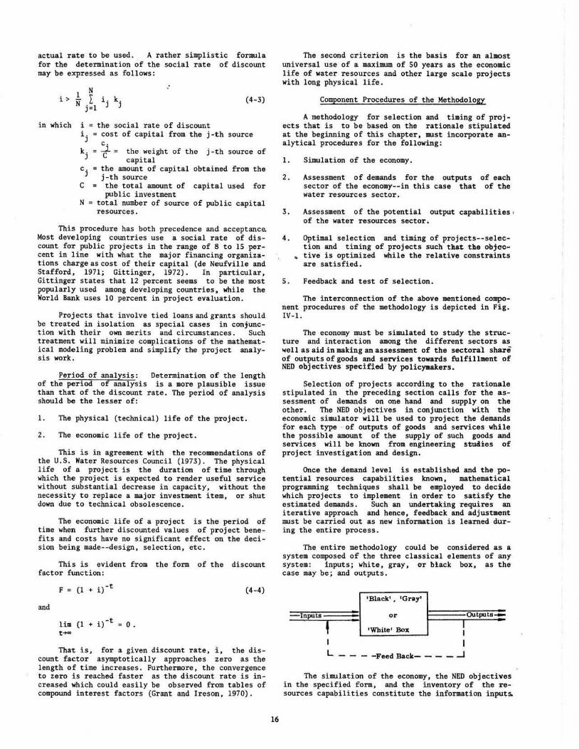
actual rate to be used. A rather simplistic formula for the determination of the social rate of discount may be expressed as follows:

i > 1 N N L iJ. kJ.

j•l

.. (4-3)

in which i = the social rate of discount ij = cost of capital from the j-th source

c. k . = .....l. =

J c the weight of the j -th source of capital

c. • the amount of capital obtained from the J j-th source

C the total amount of capital used for public investment

N = total number of source of public capital resources.

This procedure has both precedence and acceptance Most developing countries use a social rate of dis­count for public projects in the range of 8 to 15 per­cent in line with what the major financing organiza­tions charge as cost of their capital (de Neufville and Stafford, 1971; Gittinger, 1972). In particular, Gitt.inger states that 12 percent seems to be the most popularly used among developing countries. while the World Bank uses 10 percent in project evaluation.

Projects that involve tied loans and grants should be treated in isolation as special cases in conjunc­tion with their own merits and circumstances. Such treatment will minimize complications of the mathemat­ical modeling problem and simplify the project analy­sis work.

Period of analysis: Determination of the length of the period of analysis is a more plausible issue than that of the discount rate. The period of analysis should be the lesser -of:

1. The physical (technical) life of the project .

2. The economic life of the project.

This is in agreement with the recommendations of the U.S. Water Resources Council (1973). The physical life of a project is the duration of time through which the project is expected to render useful service without substantial decrease i n capacity, without the necessity to replace a major investment item, or shut down due to technical obsolescence.

The economic life of a project is the period of time when further discounted values of project bene­fits and costs have no significant effect on the deci­sion being made--design, selection, etc.

This is evident from the form of the discount factor function:

and

F = (1 + i) -t

liD (1 + i) -t 0 . t-

(4-4)

That is, for a given discount rate, i , the dis­count factor asymptotically approaches zero as the length o·f time increases. Furthermore, the convergence to zero is reached faster as the discount rate is in­creased which could easily be observed from tables of compound interest factors (Grant and Ireson, 1970).

16

The second criterion is the basis for an almost universal use of a maximum of 50 years as the economic life of water resources and other larg.e scale projects with long physical life •

Component Procedures of the Methodology

A methodology for selection and timing of proj­ects that is to be based on the rationale stipulated at t he beginning of this chapter, must incorporate an­alytical procedures for the following:

1. Simulation of the economy.

2. Assessment of demands for the outputs of each sector of the economy--in this case that of the water resources sector.

3. Assessment of the potential output capabilities • of the water resources sector,

4. Optimal selection and timing of projects--selec­tion and timing of projects such that t he objcc•

• tive is optimized while the relative constraints are satisfied ..

5. Feedback and test of selection.

The interconnection of the above mentioned compo­nent procedures of the methodology is depicted in Fig. IV-1.

The economy must be simulated to study the struc­ture and interaction among the different sectors as well as aid in making an assessment of the sectoral shari of outputs of goods and services towards fulfill111ent of NED objectives specified' by policyaakers.

~election of projects according to the rationale stipulated in the preceding section calls for the as­sessment of demands on one hand and supply on the other. The NED objectives in conjunction with the economic simulator will be used to project the demands for each type ·of outputs of goods and services while the possible amoun.t of the supply of such goods and services will be known from engineering s~udies of project investigation and design.

Once the demand level is established and the po­tential resources capabilities known, mathematical programming techniques shall be employed to decide which projects to· implement in order to satisfy the estimated demands. Such an undertaking requires an iterative approach. and hence, feedback and adjust•ent must be carried out as new information is learned dur­ing the entire process.

The entire methodology could be considered as a system composed of the three classical elements of any system: inputs; white, gray, or biack box, as the case may be; and outputs.

Inputs

' =

I L

'Black' • •Gny'

or

'White• Box l I

-Feed Back- - - - ....I

The simulation of the economy, the NED objectives i n the specified form, and the inventory of the re­sources capabilities constitute the information input~

;

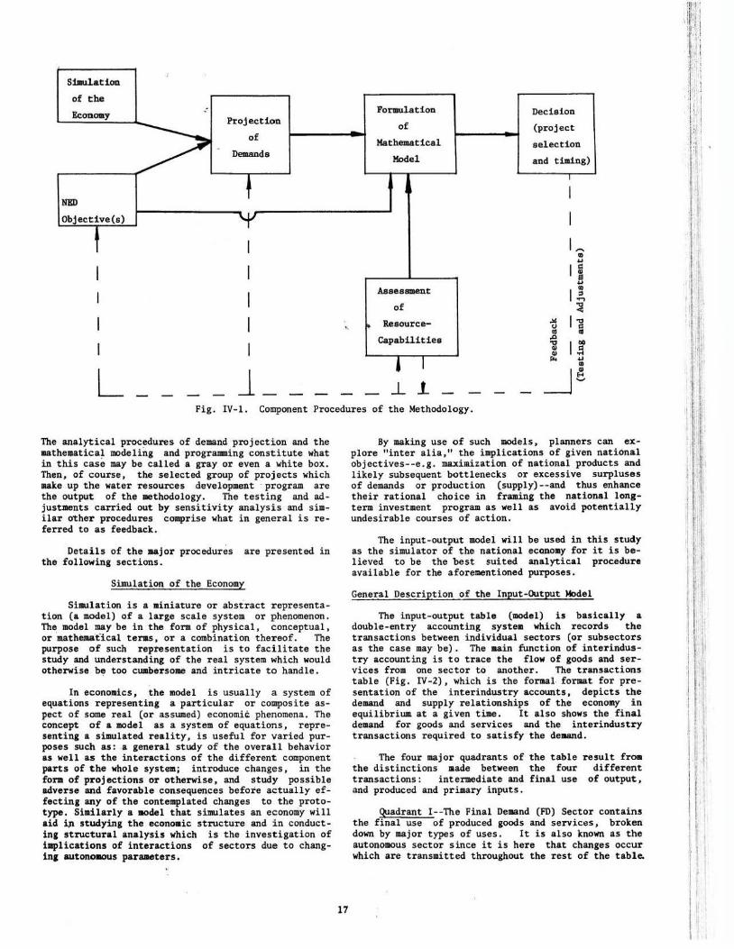
S illlul.ation

of the

Economy .: Formulation Decision

/ Projection of (project

of Hathe~~~atical selection .

Demands Model and tilll1ng)

t I

NED I

Obj ect ive(s) I

' I '" ID ... I I 1e

B I I

Assessment ll of ~

I I Resource- "' '1 ... C) as

Capabilities .0

I I .,

I ! Ql Ql

j I lr< ... ID Ql

L l_ j_ j_

Fig. IV-1. Component Procedures of the Methodology.

The analytical procedures of demand projection and the aathematica~ modeling and programming constitute what in this case may be called a gray or even a white box. Then, of course, the selected group of projects which make up the water resources development · program are the output of the methodology. The testing and ad­just ments carried out by sensitivity analysis and sim­ilar other procedures coBprise what in general is re­ferred to as feedback.

Detail s of the aajor procedures are presented in the following sections.

Simulation of the Economy

Simulation is a miniature or abstract representa­tion (a model) of a large scale system or phenomenon. The model may be in the form of physical, conceptual, or aatheJUtical tel'IIS, or a combination thereof. The purpose of such representation is to facilitate the study and understanding of the real system which would otherwise be too cumber some and intricate to handle.

In economics , the ~odel is usually a system of equations representing a particular or composite as­pect of some real (or assumed) economi~ phenomena. The concept of a model as a system of equations, repre­senting a simulated reality, is useful for varied pur­poses such as: .a general study of the overall behavior as well as the interactions of the different component parts of the whole system; introduce changes, in the fora of projections or otherwise, and study possible adverse and f avorabl e consequences before actually ef­fecting any of the contemplated changes to the proto­type. Si•il arly a model that simulates an economy will aid i~ studying t he econoaic structure and in conduct­ing st ructural analysis which is the investigation of iBplicat ions of interactions of sectors due to chang­ing aut ono.aus para.eters.

17

By making use of such models, planners can ex­plore "inter alia," the implications of given national objectives--e.g. maximization of national products and likely subsequent bottlenecks or excessive surpluses of demands or production (supply)--and thus enhance their rational choice in framing the national long­term investment program as well as avoid potentially undesirable courses of action.

The input-output model will be used in this study as the simulator of the national econo•y for it is be­lieved to be the best suited analytical procedure available for the a£orementioned purposes.

General Description of the Input-Output Model

The input-output table (model) is basically a double-entry accounting system which records the transactions between individual sectors (or subsectors as the case may be) . The aain function of interindus­try accounting is to trace the flow of goods and ser­vices from one sector to another. The transactions table (Fig. IV -2), -which is the formal. fonaat for pre­sentation of the interindustry accounts, depicts the demand and supply relationships of the economy in equilibrium at a given time . It also shows the final demand for goods and services and the inter industr y transactions required to satisfy the deaand.

The four major· quadrants of the table result f ro• the distinctions aade between the four different transactions: intermediate and final use of output , and produced and pr imary inputs.

Quadrant 1--The Final Deaand (FD) Sector contains the final use of produced goods and services, broken down by major types. of uses. It is also known as the autonomous sector since it is here that changes occur which are transmitted throughout the rest of the tabl e

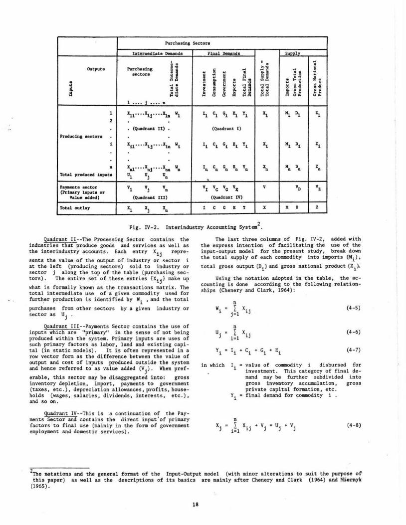
Purchaetna Sectora

InterMdiate Demanda Final Demands Supply

I I • ~ .. . Output• Purchaaina j]

>-'1:1 " " ..... ~j

..... 0 ... 0 .. .. .. " .. aectore " ..

I .!l go ... 0 .. ~

... 0 .. :;~ .. ! • "' " II) • ..... • ... 31 .. ... u .. ..... .. • .. ...... .. . " . " &. .. ... .. • .. 0 • • 0 n . ...

... .:s ~ " 8 i ..... Q, 0 0 a 8 ~& ~~ ,!1 .... .... {?..., ... u ... u ...

1 ••.. j •• •• 11

1 ~l····~j· · ··Jtn wl I1 c1 ql ~ Tl ~ '\ D1 z1 2 .

. (Quadreot II) • (Qu•drant I)

Producin& eector e

1 xu··· ·xiJ " .. xiD wi Ii ci Gi Bi Ti 11 M1 Di zi . .

11 xu.l .... xnJ •••• x011 wn I c Gil Bn yll I M o .. z

n Q ll 11 ll

Total pr oduced 111pute 01 oJ 0 ll ..

Pa,....ta .. ctor vl vJ v VI vc VG v, v VD vz (Priooary 111putl or ll

Value added) (Quadrant Ill) (Quadnnt IV)

Total out lay ~ xJ xn I c G B T X M D z

Fig. IV-2. 2 Interindustry Accounting System

Quadrant 11--The Processing Sector contains the industries that produce. goods a.nd services as well as the interindustry accounts. Each entry Xij repre-

sents the value of the output of industry or sector i at the left (producing sectors) sold to industry or sector j along the top of the table (purchasing sec­tors). The entire set of these entries {Xij } make up

what is formally known as the transactions matrix. The total intermediate use of a given commodity used for furt~er production is identified by wi • and the total

purchases from other sectors by a given industry or sector as Uj

quadrant I II--Payments Sector contains the use of inputs which are "primary" in the sense of not being produced within the system. Primary inputs are uses of such primary factors as labor, land and existing capi­tal (in stat ic models). It is often represented in a row vector form as the difference b~tween the value of output and cost of inputs produced outside the system and hence referred to as value added (Vj). When pref-

erable, t his sector may be disaggregated into: gross inventory depletion, import , payments to government (taxes, etc.), depreciation allowances, pl'ofits , house­holds (wages , salaries, dividends, intere·sts, etc.), and so on.

quadrant IV--This is a continuation of the Pay­ments Sector and contains the direct input'of primary factors to final use (mainly in the form of government employment and domestic ser vices).

The last three columns of Fig. IV-2, added with the express intention of facil itating the use of the input-output model for the present study, break down the total supply of each commodity into imports Q4i) '

total gross output (01) and gross national product (Zi).

Using the notation adopted in the table, the ac­counting is done according to the following relation­ships (Chenery and Clark, 1964):

n w.

1 • r x. j

j=l 1 (4-S)

n

uj .. r X .. (4-6) i • l lJ

Y. l "' I. l

+ c. l

+ G. + l

E. 1

(4-7)

in which I. 1

value of commodity i di sbursed for investment. This category of final de­mand may be further subdivided into gross inventory accumulation, gross pri vate capital formation, etc.

Yi • final demand for commodity i .

(4-8)

2The notations and the general format of the this paper) as well as the descriptions of

(1965).

Input-Output model (with minor alterations to suit the purpose of its basics are mainly after Chenery and Clark (1964) and Mi•rnyk

18

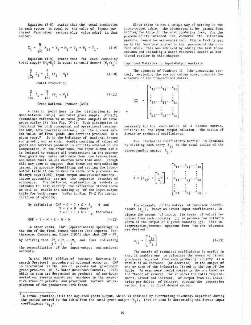
Equation (4·8) states that the total production in each sector is equal to the value of inputs pur­chased from other sectors plus value added in that sector:

x .• ~

n ~ X .• + Y.

l) l (4-9)

Equation (4-9) states that for each commodity total supply (Mi+Di) is equal to total demand (W1+Yi).

n

I i=l

D. = 1

-Total Production

z. = 1

n I (Y i . Mi)

i=l

-Gross National Product (GNP)

(4-10)

( 4-11)

A case in point here is the distinction to be ~ made between GNP(Z) and total gross supply (TGS)(X) (sometimes referred to as total gross output) or total gross outlay (X) (see Fig. IV-2). Such distinction is important for both conceptual and operational reasons. The GNP·, more precisely defined, is "the current mar­ket value of final goods and services produced in a given year." It is the indicator of national income and growth, and as such, double counting of values of goods and services produced is strictly avoided in its computation. On the other hand, the input-output table is designed to measure all transactions in the economy. Some goods may enter into more than one transaction, and hence their values counted more than once. Though this may seem to suggest that these are contradicting issues, by properly identifying and setting the input­output table it can be made to serve both purposes. As Miernyk says (1965), input-output analysis and national­income acco~ting are not two separate branches of economics . The following explanation in symbols is intended to help clarify the difference stated above as well as enable the setting up of the input-output table for both usages (refer to Fig. IV-2 for identi­fication of symbols).

By definition GNP c + I + G + E - M and X y • w where x y c • 1 + G + Ex' therefore

GNP = Y - M "' X • w - M (4-12)

In other words, GNP (operationally speaking) is the sum of the final demand vectors less imports. Fur· thermore, Chcnery and Clark (1964) show that GNP • l:V .

J by deriving that l:V. = l:Y. - l:M. and thus indicating

j) il il the reconciliation of the input-output and national accounts.

In the OBERS (Office of Business Economic Re­search Services) procedure of national accounts, GNP is determined as the sum of private and government gross products (U. S. Water Resources Council , 1972) which in turn are determined as products of man-hours worked and average output per man-hour in the respec­tive areas of pr ivate and government sectors of em­ployment of the productive work force.

Since there is not a unique way of setting up the input-output t&ble, the advantages to be gained from setting the table in the most conducive form, for the purpose of its intended use, whenever the situation permits, cannot be overemphasized. Figure IV-3 is set up in the form best suited to the purpose of the cur­rent study. This was achieved by adding the last three columns and including a water resources sector as men­tioned earlier in this chapter.

Important Matrices in Input-Output Analysis

The elements of Quadrant II (the processing sec­tor), excluding the row and column sums, comprise the elements of the transactions matrix:

[X)

necessary for the calculation of a second matrix, critical to the input-output solution, the matrix of direct or technical coefficients.

The "technical coefficients matrix" is obtained by dividing each entry Xij by the total outlay of the

corresponding sector Xj ;

The elements of the matrix of technical coeffi­cients (aij)' known as direct input coefficients, in-

dicate the amount of inputs (in terms of value) re­quired from each industry (i) to produce one dollar's worth of the output of a given industry (j). This in­terpretation beco~es apparent from how the elements are derived.3

(4-13)

The matrix of technical coefficients is useful in that it enables one to calculate the amount of direct purchases required from each producing industry as a result of an increase (or decrease) in the output of one or more of the industries listed at the top of the table. An even more useful matrix is the one known as the "Leontief inverse" for it shows the total require­ments, direct and indirect, of output from all indus­tries per dollar of delivery outside the processing sector, i.e., to final demand sector.

3In actual practice, it is the adjusted gross output, which is obtained by subtracting inventory depletion during the period covered by the table from the total gross output (X.), that is used in determining the direct input coefficients (a .. ). J

1)

19

.. '!

I I

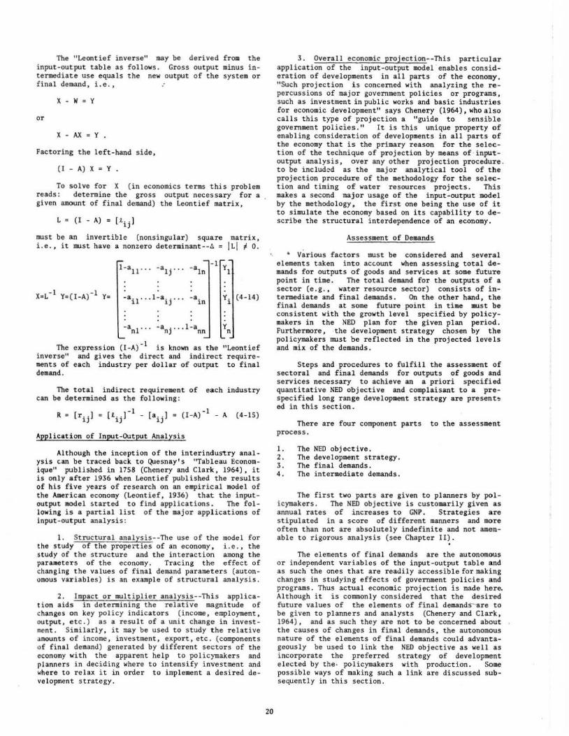
The "Leontief inverse" may be derived from the input-output table as follows. Gross output minus in­termediate use equals the new output of the system or final demand, i.e.,

X - W = Y

or

X-/1\X=Y.

Factoring the left-hand side,

(I - A) X = Y •

To solve for X (in economics terms this problem reads: determine the gross output necessary for a given amount of final demand) the Leontief matrix,

L "' (I - A) = [ R.ij)

must be an invertible (nonsingular) square matrix, i.e., it must have a nonzero determinant--~= ILl ~ 0.

-a ln

-a. 1n

The expression (1 -A)-l is known as the inverse" and gives the direct and indirect ments of each industry per dollar of output demand.

yi (4-14)

"Leontief require­to final

The total indirect requirement of each industry can be determined as the following :

R = (r .. ) = [t .. )-l - (a . . ) = (1-A)-l -A (4-15) l) lJ lJ

Application of Input-Output Analysis

Although the inception of the interindus~ry anal­ysis can be traced back to Quesnay' s ·~ableau Econom­ique" published in 1758 (Chenery and Clark, 1964), it is only after 1936 when Leontief puulished the results of his five years of research on an empirical model of the American economy (Leontief, 1936) that the input­output eodel started to find applications. The fol­lowing is a partial list of the major appl ications of input-output analysis:

1. Structural analysis--The use of the model for the study of the propexties of an economy. i.e., the study of the structure and the interaction among the parameters of the economy. Tracing the effect of changing the values of final demand parameters (auton­umous variables) is an example of structural analysis.

2. Impact or multiplier analysis--This applica­tion aids in determining the relative magnitude of changes on key policy indicators (income, employment, output, etc.) as a result of a unit change in invest­mont. Similarly, it may be used to study the relative amounts of income, investment, export, etc. (components of final demand) generated by different sectors of the oconomy with the apparent help to policymakers and planners in deciding where to intensify investment and where to relax it in order to implement a desired de­velopment strategy.

20

3. Overall economic projection--This particular application of the input-output model "enables consid­eration of developments in all parts of the economy. "Such projection i s concerned with analyzing the re­percussions of major government policies or programs, such as investment in public works and basic industries for economic development" says Chenery (1964), who also calls this type of projection a "guide to sensible government policd.es." It is this unique property of enabling consideration of developments in all parts of the economy that is the primary reason for the selec­tion of the technique of projection by means of input­output analysis, over any other projection procedure . to be includ~d as the major analytical tool of the projection procedure of the methodology for the selec­tion and timing of water resources projects. This makes a second major usage of the input-output model by the methodology, the first one being the use of it to simulate the economy based on its capability to de­scribe the structural interdependence of an economy.

Assessment of Demands

• Various factors must be considered and several elements taken into account when assessing total de­mands for outputs of goods and services at some future point in time. The total demand for the outputs of a sector (e .g., water resource sector) consists of in­termediate and final demands. On the other hand, tl1e final demands at some future point in time must be consistent with the growth level specified by policy­makers in the NED plan for the given plan period. Furthermore, the development strategy chosen by the policymakers must be reflected in the projected levels and mix of the demands.

Steps and procedures to fulfill the assessment of sectoral and final demands for outputs of goods and services necessary to achieve an a priori specified quantitative NED objective and complaisant to a pre­specified long range development strategy are present~ ed in this section.

There are four component parts to the assessment process .

1. The NED objective. 2. The development strategy. 3. The final demands. 4. The intermediate demands.

The first two parts are given to planners by pol­icymaker s. The NED objective is customarily given as annual rates of increases to GNP. Strategies are stipulated in a score of different manners and more often than not are absolutely indefinite and not amen­able to rigorous analysis (see Chapter II).

The elements of final demands are the autonomous or independent variables of the input-output table and as such the ones that are readily accessible for making changes in studying effects of governn1ent policies and programs. Thus actual economic projection is made here. Although it is commonly considered that the desired future values of the elements of final demands-are to be given to planners and analysts (Chenery and Clark, 1964), and as such they are not to be concerned about the causes of changes in final demands, the autonomous nature of the elements of final demands could advanta­geously be used to link the NED objective as well as incorporate the preferred strategy of development elected by the· policymakers with production. Some possible ways of making such a link are discussed sub­sequently in this section.

The intermediate demands are the direct and in­direct demands by the processing sectors necessary to produce both final and intermediate goods and.services. These are dependent endogenous variables. . They are dependent on the technology and the level of total final demands.

The assessment of total demands for goods and services of the economy of a country is best done by input-output projection. The primary reason for pre­ferring input-output projection over other procedures is that it is a consistent projection, i.e., when an input-output table is projected, the output of each in­dustry is consistent with the demands for its products (Miernyk, 1965). The importance of this feature in the planning and pursuit of balanced economic growth, which is the reality of most developing countries (Chapter 11), cannot be overemphasized .

The assessment of total demands that deploy input­output projection is carried out in three major steps:

1. Projection of final demands . 2. Computation of inte·rmediate demands. 3. Computation of total production requirements.

Projection of Final Demands (FDJ.

This is done by projecting each element in the final demands sector of the input-output table. The sum of the rows of the projected elements fo~ the new final demands vector. Any one or a combination of a number of approaches may be deployed in making the projection of individual or groups of the components of the final demands. Some of them are briefly pre­sented in the following paragraphs.

Empirical relationships: The different components of the FD are estimated as a continuation of past trends by either some form of extrapolation or fitting some mathematical function. This approach is readily applicable to elements that are regressible with re­spect to some demographic variables--the elements of the household consumption column are perfect examples. Another exampl e is the Moore-Peterson employment mul­tiplier estimation procedure which uses an employment­production function that measures the relationship be­tween total employment (in man-years) i n each industry and the gross output of the industry expressed in mil­lions of dollars (Miernyk, 1965).

Empirical relationships of diverse nature are used, where available, in projecting the entries of the FD sector. Although their usefulness in facili­tating such projections is undisputed, their use is limited since there are very few, if any, established relationships for use in even the most cursory type of projection. This is largely because of the fact that such relationships lack .univer sality, and have to be developed (and be constantly updated) on a case by case basis for each country , and the prohibitive na­ture of data acquisition involved.

Disaggregation of GNP: In this method, the new level of GNP is disaggregated into sectoral components and then dispersed horizontally backwards into the elements of FD according to historical patterns of distribution or some other basis. This approach as­sumes continuation of past trends and no change in the structure of the industrial system and their share in production. Such an approach may be more appropriate for use ln mature economies than for developing ones.

21

Disaggregation of GNP into sectoral component parts based on strategic reasons such as desired com· position of diversification and designating the ele­ments of the FD to ramify the chosen strategy, an ap­proach employed by several countries, is much more suitable to underdeveloped countries than one based on past pattern.

The scarce-factor approach: Priority is given to sectors and industries that either economize scarce factors (mainly capital) or use large amounts of abun­dant ones (labor intensive) . Activities in such sec­tors are intensif ied and corresponding elements of the FD increased while those of capital intensive sectors are deferred. The apparent difficulty of delineating the sectors into the foregoing categories hinders the widespread usage of this approach. Multiplier analysis in conjunction with informed judgment can be used to assist in such i dentification. For example, large en­tries in the household row of the matrix of technical coefficients of a closed input-output table with re­spect to the household ' s sector indicates that the purchasing sector at the top is a labor intensive one.

.. Key sectors approach: Sector s that are key to the

economic development .are identified and the corre­sponding entries in FD are projected according to some guidelines. This is the approach mostly followed by strategists and planners who are proponents of the school of thought that investment in social and public overhead and basic {heavy) industries is the prime mover and an absolute necessity for accelerated and sustained economic development. The usual procedure followed in this approach is one of analogy. A country with an economy of the desired structure and level is selected and the major components of its FD are adopt­ed with some adjustments. This method is very popular among the developing countries because of its simplic­ity in application and coherence of the approach to the planning on long range bases adopted by these countries.

None of the foregoing approaches can be uniformly applied to arrive at the projected values of each and all entries of the PO sector. Rather, they can be used in combinations or one at a time, depending on the suitability of the approach to the nature of the par­ticular entry and column under ·consideration , to iden­tify the sectors and columns of the FD that are in­strumental to effect the elected strategy. After such sectors and columns are identified the exact level to which an entry of the FD should be projected can be determined by an iterative process that seeks the con­vergence of the difference between the final demands and imports vectors to the projected (target) GNP llevel where the latter is the control.

This is the most viable approach that can be rec­ommended at the present time to link the overal l NED objective, development strategy, and production of goods and services . lt will enable the assessment of total production of goods and ~ervices necessary to meet the NED objective targets via an elected develop­ment strategy.

A point that needs mention here is that an exper­ienced economist should be consulted in identifying key sectors for the given strategy. The expertise of an experienced economist in this area should be sought and the need for it cannot be overemphasized. Although there is no dispute as to the importance and necessity of such expertise all along the selection and timing

I· L

' L

I

of projects for NED, i t is acutely indispensable in t he phase of identifying key sectors relative to spe­cific development strategies .

Computation of Intermediate Demands (Projection of the Processing Sector)

This computation is carried out to find the transact i ons by t he processing sectors necessary to sustain the newly projected leve l of final demands . A well established procedure exists to perform such a computation and i ts steps are given below (Miernyk, 1965).

l.

2.

3.

4.

5.

6.

Obtain the projected final demands vector as the row sums of the projected component elements of t he final demands sector including projected im­ports.

Compute adjusted projected final demand by f irst multiplying the projected final demand by the ratio of inventory depletion to final demand in the base year, and then subtract ing t his amount from the projected final demand.

Post multiply the transpose of the Leont ief i n­verse matrix, [L] -1 , by t he adjusted projected final demands vector . The product is the new ad­justed total gross output for each i ndustry.

Multiply each element in t he i - th column of the t echnical coefficient matrix by the i-th element of the transposed adjusted total gross outputs vector obtained in step 3. The r esult is the processing sector of the projected transactions table. The row sums of this matrix form the ele­ments of the new intermediate demands vector .

To obtain t he total gross output vector, add the appropriate inventory adjustment which was sub­tracted in step 2 to the adjusted total gross outputs found in step 3. 4

Set up the new proj ected transactions table by entering the computed values of its components in the foregoing' s t eps in their appropriate slots of the tabulation.

Total Production Requirement

The total production requirement is the amount of goods and services that the producing sector has to deliver to both final and i ntermediat e users . The new total production requirement is the sum of the pro­jected i ntermediate and f inal demands less proj ect ed imports.

Recapitulation

In this section of the paper, a procedure that uses input-output projection in conjuncti.on wit h the overall NED objective and development strategy to for ecast the economic transactions and predict the total production r equi r ements for the outputs of goods and services of the individua l sector (and subsector) of the economy has been presented. It is preferable to Jo the projection in constant prices for the kind of planning and level of decision making that the method­ology suggested is addressed to.

The major s teps of the projection procedure are as follows:

1.

2.

3.

4.

Obtain the overall NED object ive in an appropri­ate form for the planning period(s) under consid­eration.

Obtain the elected strategy f or the economic de­velopment for t he planning period(s) .

Identify key sectors and elements of final de­mands that are instrumental i n i mplementing the elected strategy.

Project the identified elements of the final de­mands sector consist ent with the policy objective and strategy as per 1 and 2 along with all other f inal demands necessary for-continued growth.

5 . Compute transactions of the processing sector and int ermediate demands consistent with the proj ect­ed level of fina l demands .

6 . , Compute the total production requi red from the producing sectors to satisfy the new demand lev­els for both the final and intermediate uses .

The foregoing projection procedure helps deter­mine the total production of outputs of goods and ser­vices necessary to achieve a desired growth level a priori specified by policymakers . The deployment of the i nput-output projection procedure endows signifi­cant advantage in that it enables determination of both direct and indirect requirements to sustain a given leve l of final demands. The ability to determine al l required demands is in turn very important for it will improve the cert ainty of meeting demands by se­l ected pro jects and programs and hence attain the as­pired level of growth. More importantly, it provides production targets, and near realistic ones, for proj­ect selection and program f ormulation on the aptness of which the warrantee to the aspired growth lies. The selection of projects to meet such targets is to be accomplished through the use of mathematical program­ming techniques which is presented in the section after the following .

In t he next section , assessment of resource capa­bilities , an apparent prerequisite to project selec­tion and plan formulation, is presented.

Assessment of Resource Capabilities

In order t o formu l ate a program that will meet the projected future demand levels , i t i s necessary . to know the resources capabilit ies that can readily be empl oyed to satisfy the estimated production require­ments . After all, the core issue of the subject of project sel ection is one of satisfying demand by lit­eral l y matching supply to demand. Of course it is the output capabi lity of the projects that constitute the avai l able supply .

Assessment of resources capabilities in the area of water resources development involves an ext ensive and relativel y detailed inventory of the quantity and characteristics of water and related resources , ap­praisal of opportunities for their beneficial use, de­termination of ways and means of their management and

4The appropriate "inventory adjustment" refers t o the application of t he inventory adjustment referred to in ~top 2 to the Leontief i nverse matrix so t hat both the direct and indirect effects of t he adjustment are ac­commodated in the new total g:oss output vector .

22

exploitation, as well as identification of possible limitations to their full utilization and ways of mit­igating such l imitations.

The scope and procedures of the investigations necessary for water resources development project­designs and plan- formulations are presented in suffi ­cient detail in publications of the U.N. (1964) and the U.S. Bureau of Reclamation (1972). Thus, presentation of the same here is omitted.

The data necessary in the selection of water re­sources projects include estimates of: net economic values of project outputs ·of goods and services; costs of construction, operation, maintenance and replace­ments; length of,project construction period; project life; capital and other resources available for proj­ect implementation, etc. The quality of these data must be of high reliability in order to assure the ability of the development program to produce at least the values estimated and that it will be implemented at no more than the estimated costs. Data of such quality are produced as a result of studies conducted at the project-feasibility-study levels. •

From the foregoing paragraph, it is evident that assessment of resources capabilities up to and i nclud­ing project-feasibility-studies is a forerunner ~nder­taking to project selection for imple~ntation. Fur­thermore, project selection involves two or more proj ­ects. It is logical that the larger the number of projects to select from the greater the possibility of selecting a set with higher performance (whatever the measure of performance may be). It is also a kno~t fact that such project i nvestigations are expensive ventures and require long ranges of time. It seems one is faced with a dilemma.

In actuality, the cost of investigation is negli­gible compared to investment costs in water resources development. Therefore, despite the seeming dilemma, water resources project investigation and project for­mulation up to the economic feasibility level should be carried out on a continuous basis , especially in countries where long range development planning is adopted. In this way, the inefficient (and expensive in the long run) piecemeal approach of s olving prob­lems by seeking solutions after problems of critical nature have risen can be avoided. The situation in the countries of the Sahel regi on of North Africa i nvolv­ing pro·blems caused by drought in 1973-74 should be more than enough evidence to serve as a lesson and grounds for the justification of continuous resources capabilities assessments.

The appropriate format for the presentation of the data for use in the selection and timing of water resources projects should be similar to that used for the example problem (Chapter V).

Optimal Selection and Timing5

"Optimal selection" in this study refers to se­lection of a set of projects that optimize a given ob­jective function, while satisfying all pertinent con­straints in the areas of available resources, project relationships, etc. Another dimension of optimality is the t imely provision of the water resources project outputs for use by the other sectors of the economy. Specific ways to handle the aforementioned aspects are presented in the present section.

5For notations used in this section refer top. iv.

As stipulated earlier, water r esources projects should be t imed such that project outputs are avail­able for use by other sectors over the ensuing plan­ning per iod. This is necessary since most output s of water resources projects are i ntermediate goods and as such required by other sectors in the production of their respective outputs.

In light of the foregoing condition for project timing, there may be an inherent problem in cases where a selected set of projects contains one or more projects with necessary construction period longer than the time available between the time its output is scheduled to be made available for use and the time the selection is made. Such possible contradictions could be eliminated by one of two ways.

One way is to check and make the necessary ad­justment as a separate exercise after the select ion in the feedback and adjustment phase (Fig. IV-1) of the

,.entire process.

23

The second, and more expedient way, is to include an expression i n the body of the mathematical model that would exclude the projects with construction pe­riods in excess of that available.

System Decomposition

Since project selection and formulation of devel­opment programs covering the entire economy of any country is a rather large problem, it would be expedi­tious and advantageous i n more ways than one to decom­pose the problem and tackle it in parts.

The water resources sector, as with most other sec­tors, is a small enough part compared to the entire economic system, and yet complete and diverse within itself, to be treated as a relatively separate and com­plete subsystem. Geoffrion (1972) calls such subdivi sion of large problems into subproblems a "solution strat­egy," in contrast to "problem manipulations," which are ~ays of simplification mainly by restatement of the dual of a linear programming problem.

The additive nature of the input-output model , used to simulate the whole economy, is a positive fea­ture in this regard since the concept of "the whole being the sum of its component parts," which is one of the rationale basis of decomposition and resynthesis of large systems, is built into the input-output modeL

However, the stage at which a large system is de­composed and the subsystems treated . separately is important and may lead to erroneous decisions if done at a stage different from the appropriate one. In the methodology given herein, decomposition is effected only after the total production requirements have been assessed. This is crucial because the production tar­get should include all final and intermediate, direct and indirect demands, lest there be bottlenecks result­ing from unsatisfied demands.

Once the production requirements are computed (given in the immediately preceding section), the problem of the selection and timing of projects to meet these requir~ments can be carried out on a sector by sector basis . Such decomposition decreases the size

I: I'

I' i· ·I

r I I. r i

I ·f

' l i

I

.lc

·I I

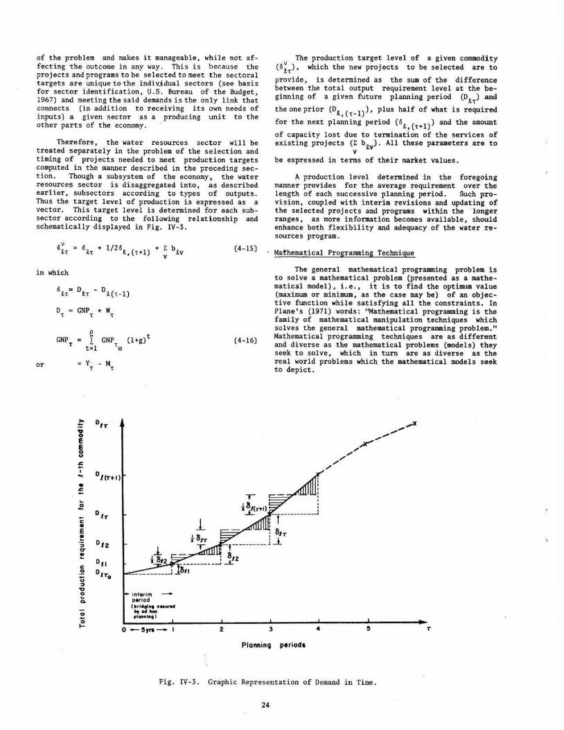
of the problem and makes it manageable, while not af­fecting the outcome in any way. This is because the projects and programs to be selected to meet the sectoral targets are unique to the indiv..i.dual sectors (see basi s for sector identification, U.S. Bureau of the Budget, 1967) and meeting the said demands is the only link that connects (in addition to receivi ng its own needs of inputs) a given sector as a producing unit to the other parts of the economy . ·

Therefore, the water resources sector will be treated separately in the problem of the selection and timing of projects needed to meet production targets computed in the manner described in the preceding sec­tion. Though a subsystem of the economy, the water resources sector is disaggregated into, as described earl ier, subsectors according to types of outputs. Thus the target level of production is expressed as a vector. This target level is determined for each sub­sector according to the following relationship and schematically displayed in Fig. IV-3.

6v h

in which

6 = h

D T

GNP T

or

6h + 1/261,(1"+1) + ~ btv

D - D h 1(1"-1)

GNP + w T T

p

L GNP t=l

Y·: T M T

~ o,T . ~ 0 E

~ .. :

To (l+g) t

.!. 0Jtr+l )

• .f! --c • E .~ :;)

'C7

:! c .2 u :;)

'0 0 ~

Q.

interim ptriocl (•rldtl ... ONurM ..,"" ..... •••flint)

0 --5yrs-

(4-15)

( 4-16)

_L

2

The productio·n target level of a given commodity (6~T), which the new projects to be selected are to

provide, is determined as the sum of the difference between the total output requirement level at the be­ginning of a given future planning period (D1T) and

the one prior (D1, (T-l)), plus half of what is required

for the next planning period (6R.,{T+l)) and the amount

of capacity lost due to termination of the services of existing projects (E b1v). All these parameters are to

v be expressed in terms of their market values.

A production level determined in the foregoing manner provides for the average requirement over the length of each successive planning period. Such pro­vision, coupled with interim revisions and updating of the selected projects and programs within the ' longer ranges, as more information becomes available, should enhance both flexibility and adequacy of the water re­sources program.

Mathematical Programming Technique

The general mathematical programming problem is to solve a mathematical problem (presented as a mathe­matical model), i.e., it is to find the optimum value (maximum or minimum, as the case may be) of an objec­tive function while satisfying all the constraints . In Plane ' s (1971) words: "Mathematical programming is the family of mathematical manipulation techniques which solves the general mathematical programming problem." Mathematical programming techniques are as different and diverse as the mathematical problems (models) they seek to solve , which in turn are as diverse as the real world problems which the mathematical models seek to depict.

1'

Plannin9 periods

Fig. IV-3. Graphic Representation of Demand in Time.

24

The selection of the programming technique de­pends upon several factors such as: nature of the real world problem to be programmed, the form of the objec­tive and constraint functions, the form of the avail­able data, available or kno~ technique to the pro­grammer, and other similar aspects.

The programming technique employed for tackling the selection and timing of water resources projects

. is the zero-one integer linear programming technique. Zero-one integer linear programming is the best suited technique for the problem that this study is addressed to for the following reasons:

· l. The objective and constraint functions are linear.

2.

3.

4.

s.

The selection of a set of . projects is a process characterized by a combinatorial phenomenon.

The indivisibility of the water resource projects (i.e., in the selection of projects for implemen­tation, a project is selected as a whole unit or rejected). In other words, it is meaningless to have fractions of projects as the solutions to the mathematical model.

It has comparatively less dimensionality problem when considering multipurpose, multiproject, and multiple time frame. This would be a problem in particular, if dynamic programming were to be used (Butcher, Haimes, and Hall, 1969).

The relatively readily availability of computer codes.

The strength and scope of application of zero-one i nteger linear programming are given extensive cover­age in the literature in the works of Balinski (1965) , Pritsker et al. (1968 (b] , [c]), Watters (1968), Pl&ne and McMillan (1971), and others. ·

In zero-one integer programming, the decision var iable takes either of the binary values of 0 and 1. Thus in the present study

{

1 if project number k is selected for P = implementation by the beginning of kt plan period T

0 otherwise.

Mathematical Model

The main aspects of mathematical modeling are the identification of the relevant variables (parameter i dentification) and formulation of the functional re­lationships of the variables required to model the situation under study. Thus, a mathematical model is a representation of the relationships of the pertinent parameter s of a real world problem i n the form of an objective function and constraints. The logical basis and the steps of constructing mathematical models are elaborated at length by Pritsker et al. (1968 [a]) and will not be repeated here.

The overall objective of this paper is to develop a methodology for the optimal selection of water re­sources projects that will enhance economic develop­ment. In the foregoing s ections, procedures for making projections of outputs of goods and services consis­tent with NED objectives have been presented . Further­more, what is to constitute the objective and con­straint functions have been delineated and stipulated; i n explicit terms and in full for the former and in part for the l atter. Here, the mathematical model for the optimal selection of water resources projects will be presented in a more complete form.

The specific problem to be translated into a matehmatical model is:

The

Sel~ct a set of water resources projects {p} , for implementation by the planning period number t , out of a given set of economically feasible p~oj­ects K , that maximize economic efficiency (as measured by net present worth of projects) while satisfying the production requirement levels and without exceeding a given budgetary limitation, as well as other constraints pertinent to the situation.

PrinciEal Mathematical Model

N K Maximize I l: 5kt Pkt

pkT •=1 k.il ( 4-16a)

Subject to:

1. Satisfaction of production targets

T 1,2, .. . , N (4-17) .t • 1, 2, ... , n

· 2. Budgetary constraints

25

K ~ c p < c L kT kt - T

]< .. 1 T•l,Z, ... ,N

3. Bivalency (zero-one) constraint

0 or 1

(4-18)

(4-19)

4. Nonexceedence of length of available time by project construction time (or project maturity time)

Observance of the above stated condition can be brought about in several other ways such as the fol ­lowing:

a. forced exclusion of projects until the neces­sary construction and maturity time has elapsed. This concept i s in effect the con­verse of consideration 9 stated further belo~ The expression to be used is the following:

(4-21)

in which J is the set of projects being ex­cluded;

b. another way would be to create dummy project~ with zero costs and benefits, and require their implementation at such time when the length of construction and maturity time of their real counterparts has elapsed while making the real projects contingent upon the corresponding dummy ones (see considerations 7 and 9 below).

S. Non repetitive selection of any given project

(4-22)

I I' I

I I I • I I I I

I I I I

SkT and CkT in (4-16a) and (4-18), respectively,

are defined as follows:

T sk-r • ~ s'kT (l+i) t .. ( 4-23)

t=l 0

T

skTo " B - c ~ ( . ) -t kT k1:0

skt l +l. 0 t=O

T n T ~ ~ . -t ~ -t b.tkt ( l+l.) - ckt(l+i) (4-24)

t=O 9.• 1 t=O

T ck-r • ~ c (l+i) - t (4-25)

t=l kTO

T ckT L

-t (4- 26) ckt (1 +i) 0 t "O

Note: Since it has been suggested that the projection of the input-output model , and hence , that of the total production level, be done in constant ~rices, the value of average project out put s, b.tkt and not discounted value of benefits should

be used i n (4-17) at subsequent plan period (T • 1, 2, ... ,N).

Additional Considerations

In addition to the constraints stated as part of the principal model , appropriate express ions that will take into account pertinent relationships particular to the situation at hand must be included in order to ensure a sound decision. These are mainly cases of project relationships and matters such as ensur ing in­clusion of an isolated project deemed necessary ·for reasons other than those incorporated in t he mathemat­ical model. Mathematical expressions for incorporating some of the cases that may frequently be encountered in the selection and timing of water resources proj­ects are given below as cont i nuation of the body of constraints of the entire mathematical model.

6. Mutually exclus ive projects--These are a set of projects {L} out of which only one can be select­ed, i.e., acceptance of one project precludes ac­ceptance of al l others in the set. Such project s are encountered in water resources when there are two or more alternate project designs for a given site or in the case when there ar e a number of impoundment projects on sites located at very close range to each other that only one site could be used. One equation of the following type should be added for each set {L} of mutually ex­clusive projects.

( 4 - 27)

7. Con.tingent projects--When acceptance o f a project (k) is dependent on the acceptance of another project (s) (j), thus making the first project con­tingent on the acceptance of the l atter. This is also a rather frequent reality . among water re­sources projects. The following type of rela­tionship should be added for each pair of conti n­gent p;rojects.

26

8.

9 .

T

pkt- ~ pjt! 0 , T. 1, 2, ... , N t =l

(4-28)

Compulsory precedence--When the acceptance of a project (k) may be possible only after the pas­sage of a given number of periods of time ' (o) a fter the acceptance of pr oject (j) . Such a con­dition can be imposed by the following relation­ship.

-r-o pkt - ~ pjt < 0 , T. 1, 2, ... , N

t :ol (4- 29)

Compulsory acceptance--This is a situation when implementation of a proj ect (k) is deemed neces­sary for reasons other than i ncorporated in the mathematical model. To insure inclusion of su ch a project in the selected set of projects, the following expression should be added for each such project .

(4-30)

Compulsor y deferment is expressed by making the right-hand side equal to zero.

A special case would be when the implementation of project k is desired to take place at t ime T " y. In this case expression (4-30) takes t he following form.

(4-31}

Independent projects, those projects whose accep­tance is not affected by ,the inclusion of others , do not require special treatments. The principal model is adequate for their selection. Another case that needs to be mentioned here, although its treatment is almost apparent, is the case when a project can be im­plemented in stages. This case may be handled by con­sideri ng each possible successive stage as a separate project and by inc luding in the model the appxopr i ate contingency compulsory precedence and mutually exclu­sivity constrai nts . For example , a project that can be impl emented i n (n) s tages may be represented as (n + 1) separate alternative proposals and the set can be included in the mathematical model by making appro­priate use of expressions given under 6, 7 , and 8.

An Alternative Problem

The foregoing mathematical moclel is formulated for a situation where the budgetary ceilings are· a priori specified.

More often, in the real world, officials responsi­ble for the development of the water and related re­sources of a country are charged not only with the task of formulating and carrying out programs consis ­t ent with the NED objectives stipulated in the period­ic national development plans, but must also submit re­quests for appropriation of funds necessary to imple­ment the programs.

In such cases the problem ·may be f ormulated as follows: ·

Which are the projects to be water resources program as part

i ncluded in the of the overall

action program o~ the long range national devel­opment plan and what is the least amount of in­vestment necessary to . be appropriated from the national treasury? ·

The mathematical model for this problem is the following:

Minimize l: l: C,_ P,_ T k .. t .. -r

(4-32)

subject to all the constraints of the other model ex­cept the budgetary constraint.

Feedback: Testing, Analysis, and Adjustment

This section is included to stress the need of learning by gathering new information as well as by conducting tests on the decisions arrived at and mak­ing the necessary adjustment i n order to achieve bet­ter end results. Such activities include "inter alia" i nfeasibilit y analysis , sensitivity analysis, and so on.

Infeasibility

Infeasibility of solution to the mathematical programming problem may be caused, among other reasons, due to infeasibility of the development program.

The primary reasons for infeasibility caused by the devel opment proaram are by and large related to inade­quacy in resources necessary to carry out the desired level of growth. Specifically, this may be either in­sufficient capital resource to fund all projects nec­essary to meet the production target or lack of water resource sector capabilities in the sense that the outputs of the known pr ojects are short of meeting the target demand levels.

On the other hand, the NED policy adopted might have been unrealistically ambitious and was made with­out consideration of the nation's resources base.

By relaxing each type of constraint, one at a time, the decision maker (or the analyst) may learn the bot­tleneck area and, using additional information and in­formed judgment , recommend measures to alleviate the bottleneck, thereby hopefully converging to a feasible solution. Some possible steps that may be recommended to alleviate the aforementioned causes of program in­feasibilities are:

1. Seek and secure additional capital resources . This is in the case when t he violation of the capital resource constraint is responsible for the solution infeasibility.

2. Lower the level of the NED objective to some ac­ceptable level wit hout jeopardizing the long­range growth.

3. Initiate a crash pr ogram of identification and study of potential water r esources projects.

4 . Seek administrative policy measures that may be used to alleviate the bottleneck .

Furthermore, other measures based on informed judgment by interdisciplinary groups should be sought and the model as well as the decision subsequently up­dated and read j usted . It should be well remembered that the selection process, as any other major part of development planning, is an iterative process and the mathematical model can only hel p the process by en­abling easier detection of bottlenecks and expediting the analysis of alternative policy trials. Of course , as a better informat ion base develops the number of such iterations should decrease.

Sensitivity Analysis

Sensitivity analysis is a technique used to ana­lyze the sensitivity of the optimal solution to changes or uncertainty in the input data . There are several

~questions to which sensitivity analysis may be em­ployed t o gain insights. Certainly it is also an inval­uable means of improving the quality of diverse kinds of decisions. The many techniques and l•Ses of ~ensi­tivity analysis are adequately presented by Dantzig (1963) , Wilde and Beight ler (1967), de Neufville and Stafford (1971), and i n almost all books in the field of Operations Research (e.g., Hiller and Lieberman; 1969).

27

As the parameters used in the selection model (water resources capabil ities, capital and other re­lated resource availabilities, as well as the produc­tion requirement levels) are seldom known with a reli­able degree of accuracy, as they are only estimates, the planner or t he analyst must coupl e the optimal project selection with an investigation of the sensi­tivity of the optimum selection to possible changes in these parameters. Such sensitivity analysis is an in­evitable feature of project selection exercises, espe­cially in light of the possible repercussions and consequences inherent in an overall progr am being for­mulated to effect balanced and coordinated economi c development.

The most important types of sensitivity analysis to be conducted when carrying out optimal project se­lection using a zero-one integer linear programming technique are those concerned with variation of the constraint vector--mainly the elements of the target levels in the case of the present study. This type of sensitivity anal ysis is known in the literature as "specification sensitivity analysis" (de Neufvi l le and Stafford, 1971). Analysis of the effect on the optimal solution of perturbations in the elements of the con­straint vectors would help determine the sensitivity of the selection to inaccuracies in the projection of demand levels. lt may also aid in detecting bottle­necks mentioned in the foregoing section and hinting ways of alleviating them.

I'

I'·

Chapter V ILLUSTRATIVE EXAMPLE

In this chapter an example problem based on hypo­thetical data is set up to illustrate the application and to demonstrate the workability of the methodology developed in Chapter IV.

Due to the unavailability of the necessary data in the appropriate form, application of the methodolo­gy could not be demonstrated on an actual case of a given country. However, separate par ts of the data used in the example problem represent actual cases since they have been taken from documents of several countries. Thus, while the example probl em is not concerning a particular country, it is conceivable that there could have been a country with the given economy, NED objectives and strategies, as well as the resources used in this example problem. Besides, the purpose to be served here is not so much to conduct a case study as it is t o i llustrate the mechanics of the application of the methodology. It is also hoped that using semi-hypothetical data (as opposed to one using entirely hypothet ical data) will make it evident that the necessary data could be processed and made avail ­able in form and kind appropriate for usage in the methodology upon its acceptance as a standar d practice

Statement of the Problem

The overall problem may be posed as fol lows:

Given

l.

2 .

The economic structure of a country by way of an input-output table,

Its long-r ange national economic development (NED) objectives and strategies,

3. The pot ential capabilities (and limitations) of its water and related resources (including capi­tal );

select the water resources projects to be i mplemented during subsequent plan periods for the optimal reali­zation of the stated objectives .

Basic Data

Economic Structure of the Country

The input- output tables for Pakistan economy for the years 1954 and 1963/64 prepared by G. Rasul (1964) and W. Tims (1965) , respectively, were used in con­junction with other census material (Government of Pakistan, 1968 [a, b) , 1970) to produce the input-output t able depicted in Table V-1 and used as the simulator of the economy of the country of the example problem.

A water resources sector, disaggr egat ed into t hree major subsectors, is added to the conventional input-output table. This is done in order to facili­tate the assessment of the direct and indirect demands for the outputs of water resources projects. Census and other Government publications (Government of Paki­stan, 1965, 1968 · [a,b] 1970) have been used in the es­timation of the transactions of the water resources sector wi'th the other sectors of the economy.

Notice the absence of a separate government col­umn in the Final Demands Sector (for identification of notations see Fig. IV-2) . Thi s is characteristic of

28

developing countries where, by virtue of the fact that the government is involved in almost all sectors to a l arge extent, separate record keeping is practically impossible .

NED Objectives and Strategies

Here agai~ the long range (20 years) objecti ves and strategies of the Pakistani Government as stated in its "Long-Term Perspective Plan" and reproduced in its Third Five Year Plan (1965-70) (Government of Pa­kistan, 1965 [b)) is adopted to be the NED objectives and strategies of the example country.

The NED objectives: spective Plan are:

The objectives of the Per-

l. , A quadrupling of the Gross National Product;

2. Provision of full empl oyment to the entire labor force by about the middle of the Perspective Plan period;

3. Pari ty i n per capita income between regions ;

4. Universal literacy; and

s. Elimination of dependence on foreign assistance.

The main instrument for achieving the foregoing objectives is stated to be a fast rate of increase in Gross National Product--an average growth rate of 7 . 2 percent over the plan period. The basic framework of t he long-term growth is gi ven in Tabl e V- 2.

Growth strategies: The major strategi es chosen are: moder ate increases in gross investment ; decrease in investments requiring foreign assistance; substan­tial increase in exports; and considerable import sub­stitution in capital goods and intermediate products whose domestic production is projected to increase at the rate of 10.0 and 13.7 percent per annum, respec­tively.

The entire strategy in general , and the proj ec­tion of increased production of capital goods and in­ter mediate products at such a very high level in par­ticular , is intended t o effect significant s t ructural changes ·of the economy of the country--from basically agricultural to one that is diversified, from one of net capital importing to self supporting.

A quantitative breakdown of the strategies is given in Tables V-3 and V-4 while the desired struc ­tural changes ar e stipulated i n Table V-5. For further details refer to the long-term Perspective Plan in the Third Five Year Plan of Pakistan (Government of Paki­stan , 1965).

The guidelines stated in Tables V-2 through V-5 wer e used i n projecting the final demand and import levels given in Tables V-6 and V-7, respectively, for further use in t he assessment of total demands and de­t ermination of incremental production requirements in successive plan periods (Appendix A) . The aggregate sectors specified in Tables V-2 through V-5 are inter­pr eted and disaggregated in terms of the sector s used in the input-output tabl e .

.·

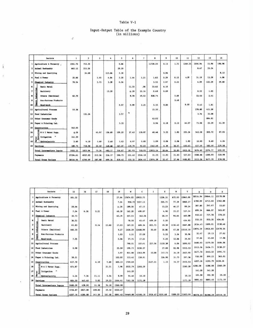
Seeton I

I Acrtculture " ror .. ti'J , ISSJ. 7)

l AAIMJ. IIoobeMry 662.12

~ IUD1Aa Mil ~rrylac

4 r-1 6 r...r 3).00

' - ull- t n 71.36

6 ... .1c. MIIW

7 11 Ma.c:ht•• ry

·13 Oc ... :re (h.ltU.e ) 62.70

' I l oa-P•Hou• hodu,ct•

10 i --·k ll Acrtculhnl......_ ''·" 1.2 , ... l ... trh•

13 Otlooi .,.._. Goo4o

14 r.,_. 6 Pdat. .... U...

u -. .......... su.os

16 ~I K ' I .... .. s.,.. o. U

17 SJ lrrtaact.oa " 141.20

18 i ... roelec.t --ric ).60

" S.TricH I"·"

Tou.l bt•r.4i 41t::41 ta.uu l3U. ll

,.,..u 271,.,61

Total ,, ... o..~ .. "''"·''

S.Cte u IS

I Aarlc u.ltv.r• ' tonUTJ 101.31

J AAS...l lu• ltudry

) tu:a.1aa Mid Qu.ury i1lt 21.46

4 P.,.l 6 Powr 7.54

' a..&lul t Nu.cn )},7)

• . . ...lc fteW 36.SI

7 ~ IVthiMU 63.13

• ! Oda.r• (Saitbl .. ) 460.)3

' E Noe.· •t rrw• Product•

10 ~ Wood-work 7.05

II Aa;rtt-.lt\I ... J. Proce ..

12 r0011 ,_.~ut .. 0.91

13 Other C.OU.~r ~·

ll , ... 1' l PriatlQI tad. Jt,21

IS Coa.n ructioo 617.70 . 16 t N 6 1 Wn u lu.pp . 011.11

u g .

!3 lrril"t.10Q

II f l ....... l .. u-1• 4.24

It S.rwitM 604.)0

Tou.l b~...,.,.ht-• 1.-uu 2480,29

•• ,..t. 1726.17

To tal Crou_~_tUn 4207.16

Table V- 1

Input-Output Table of the Example Country (in mi llions)

z ) 6 ' 6 7 • 9

7Sl. ,, 0.16 11721.20 0 . 1)

211.$6 21.2t

)6 ,61 113.66 2.39 0.96

1.4.S 6. 14 2. 20 1. .. 1.21 I.U 0.29

).73 '·" 0.36 '·" 1.t7

11.33 .16 23.U 6.lt

1).29 o.ZI )2.16 0.61 0.09

9 . ·70 69.01 131.70

0.97 0.99 2.ZJ '·" 0.13

"·" . 131.24 l .H •

4).02

),)) 0. 9. 0.1&

45.97 116.69 109.20 37. 63 llf.l7 ..... ,,,

4.10 1.69 2.U 1.63 0.97 o.u l.O"' 0.06

lll.tl 12.40 IU . .. I 7.n7 • U .lt fl . • "6' 64 .... IU3,,. 75.24 41),17 '"·" lll.tl 111.n llts3.14 20.64

6U7.0S 111.S6 2Jl.l1 )00,7) )]1.42 2)Jl.ll u.u ll.fl

67to.n 217.80 ...... 111.42 )3), , 21]4.6) 1lt16.M )2.67

.. 17 II It v c I • :7.64 !7674.05 109)3." 1236.)1

7.04 uo. 72 1)57.13 20S. ' '

o.26 188. S6 n.u 11.21

6.26 0.21 ... , 162.20 491. 07 4. 100

6J,)II lS7. Sl )42.06 21.19

)1.)0 4S.47 609. 11 0.20

0.14 JS,60 17.0) 167.Sl 61t.l4 122.73 ll.lt

9.27 1656. 29 12401.99 )0.69 30.86

1.03 1.51 27.09 O.Sl

0.06 27 . 74 17.61 0.2)

7to.Ol )]7.~1 227.06 IUO.Jt

u.so 19t.73 SilO. S7 27.00

),t7 ISI.IO 236).99 10.00 ~17.73

10l.t2 333.42 231.91 l26.to

4.10 5.60 600.1) 1769.60 14)7.01 1.15

)1.21 7.16 202). 79 2260.29

141.20 I

7.)4 ! 1.11 4.54 .. , 91.00 10. 10

443, 60 s.u 19.23 1444.41 7111.21 1171.19

6)9. 00 ll.ll 76.11 2361.tl

)127.01 109.12 zs.u 6312.07

0216.01 161. 20 IOI,SO 1891.45 3 .... 1.11 4!110.10 39».67 1231.61

29

10 II 12 13 14

I. 7Z 1149.25 20S~.94 IS.to 116.,.

8.67 )),26

1.15

o.u 4Jf I )l.lt 1J.S9 4.16

o.u 6.09 111.29 )9.01

I I

o.n I.U

0.69 :Zl .Ol 2.41

o.oa I 1.00 0.4] 1.11

na.eci 41lt.SO

).76 )3,01

-·" 0.12 44.07 73.91 zs.n 41.19

1.1.2 193.)4 SOl.SI 203.72 17.9)

0.06 I.U 10.90 9.69 4.26

"'·" 6 .... , U7.4t SU, 6t 22J.SI

)),1) IUl.lO 167i.IO 1176.71 602.00

21.13 S27.U 1136.66 uoo.n )21 .91

37.66 2UO.tl SS1l.Z6 3477 .70 1)0.91

K t X D z

672.83 12142.19 30514.94 29844.11 12170.06

77.39 , .. 0 .21 6790." 6711.60 S7•U.II

•6. 17 tt.26 287.80 141.6~ 53.07

)).27 Sl7.U 499.)4 666 .07 )0),17

90.64 460. " III.U 727.71 l70.2S

6)4. 13 Sll.JS ,n,n 4S4.15

1136.62 266'-.11 2UA.4l IUI.OI .,,., .. 47 . 36 12311.10 1)974. 39 13926.13 12470.34

3.)4 lO.t6 32.47 29. 13 27.62

12.06 29.92 )1.66 4).60 17.16

6.06 1490.92 2 .. 0.9) 2)79,)0 1U4.16

12.t6 5)1).5) 3313.26 )4)4. 71 )2)0.37

)4.11 2ns.to )417.70 , .. 3.)2 2n1.12

)I. 7S ,,,,. 930. 91 19t.2l S6S.II

14.37 24S2.Sl 4207.16 4192.79 24),, 16

2260.29 4216.01 4216.01 2260.29

161. 20 U l .20

10.10 IOI.SO IOI.SO 10.10

1171.19 1191.43 ""·" 1171.19

2219.00 5160).06 16~76.0~ 84196.09 Ull4.16

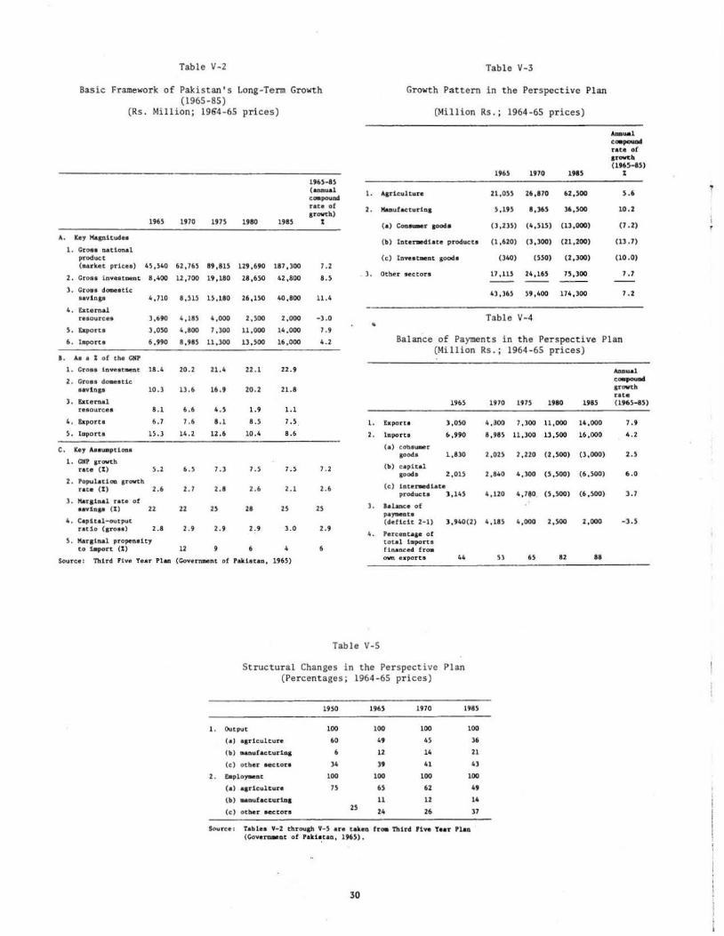
Table V-2

Basic Framework of Pakistan's Long-Term Growth (1965-85)

(Rs. Million; 1964-65 prices)

A. Key Hasnituclu

1 . Croe• national product

196S 1970 1975 1980 198S

(•nket pr1c .. ) 45,540 61,765 89,815 119, 690 187,300

1. Grou lnvest ... nt 8,400 12,700 19,180 28,650 42 ,800

3. Cron dOO>Oat1c aavinp 4. 710 8 ,HS 15,180 26,150 40,800

4 .. Extero•l reaource• 3.690 4,18S 4,000

5. lt><poru 3,050 4,800 7,300

1965-U (afQ'Iu&l coapound rat• or arovth)

%

7.1

8 . 5

11.4

Table V-3

Grow~h Pattern in the Perspective Plan

(Million Rs.; 1964-65 prices)

1965 1970 l98S

I. Aar1cu1ture 21,055 26,S70 62,500

2. 1\aoufacturina 5,195 8,365 36,500

(a) eo..-r aood• (3,235) ( 4,515) (13,000)

( b) Intenod1ate producto (1 , 620) (3,300) (21,200)

(c) InvootMnt good• (340) (SSO) (2,300)

3. Other aecton 11 ,115 24,165 75,300

43,365 59,400 174,300

Table V-4

ADI>ua1 coapouo4 rate of arovth (1965-.,)

%

5.6

10.2

(7 .2)

(13.7)

(10.0)

7. 7

7.2

6. I•poru 6. 990

I . Aa a % oC the GNP

8 , 985 U,JOO

2,500

11,000

13,500

2,000

14.000

16,000

-3.0

7.9

4.2 Balance of Payments in the Perspective Plan (Million Rs.; 1964-65 prices)

1. Cro.ea S.nveat.-aent 18 .. 4

2. Croea d<HM:atic. aavlnp 10.3

3. txterna1 reaoureea

4 . txporca

S. Import a

C. Kay Au\dlpt1ono

l. CNP arovth rate ( %)

2. Populatioo arovth

8.1

6.7

15.3

S.2

rate (%) 2.6

l. Karaia.al rat.e of oavtaaa ( %) 22

4. Capital-output rot1o <sroasl 2.8

5. llaralna1 propena1ty to 1•port (%)

20.2

13.6

6 .6

7.6

14.1

6.5

2.7

22

2.9

12

21.4

16.9

4 .s 8.1

11.6

7 .J

2.8

2.9

22.1

10.1

1.9

8 .s 10.4

7.5

2.6

2a

2.9

22.9

21.8

1.1

1.5 ' 8.6

7.5

2.1

25

).0

7.2

2.6

25

2.9

1. Export•

2. l•porta

(a) cohau.aer goode

(b) oapita1 coodo

1965

3,050

6,990

l,8l0

Z,OlS

(o) lnto<Mdiata produc.ta l ,l4S

l. lalanc.e of payeeoto

1970 1975 1980 1985

4,300 7 ,)00 ll,OOO 14,000

8. 98S 11,300 13,500 16,000

2,025 2,220 (2,500) (3,000)

2,840 4,300 (5,500) (6,500)

4,120 4, 7$0. (5 ,500) (6 ,500)

(dofioit 2-1) ),940(2) 4,185 4,000 2,500 2,000

4. Percenta&e of total i•porta

Source: Third Five Yea r Plan (GovernMnt of Pakistan, 1965)

financed. fro. ovn. exports 44 53 65 82 88

Table V-5

Structural Changes in the Perspective Plan (Per centages; 1964-65 prices)

1950 1965 1970 1985

1. Output

(o) aar1cu1turo

(b) aanufaccurlna

(c) other HCtOrl

2. Eap1o,.ont

( a ) oarlcu1tura

(b) uouCacturina

(c) other •ector•

100

60

34

100

75

25

100

49

l2

39

100

65

ll

24

100

45

14

41

100

62

12

26

100

36

2l

43

100

49

14

37

Sou reo : Tab1u V-2 throuah V-5 au takaa froe Third five Tan P1aa (Govenment of Pakio.tao, 1965).

30

Aanual c-Dd arovth rat• (1965-85)

7.9

4.2

2.5

6 .0

3.7

-3.5

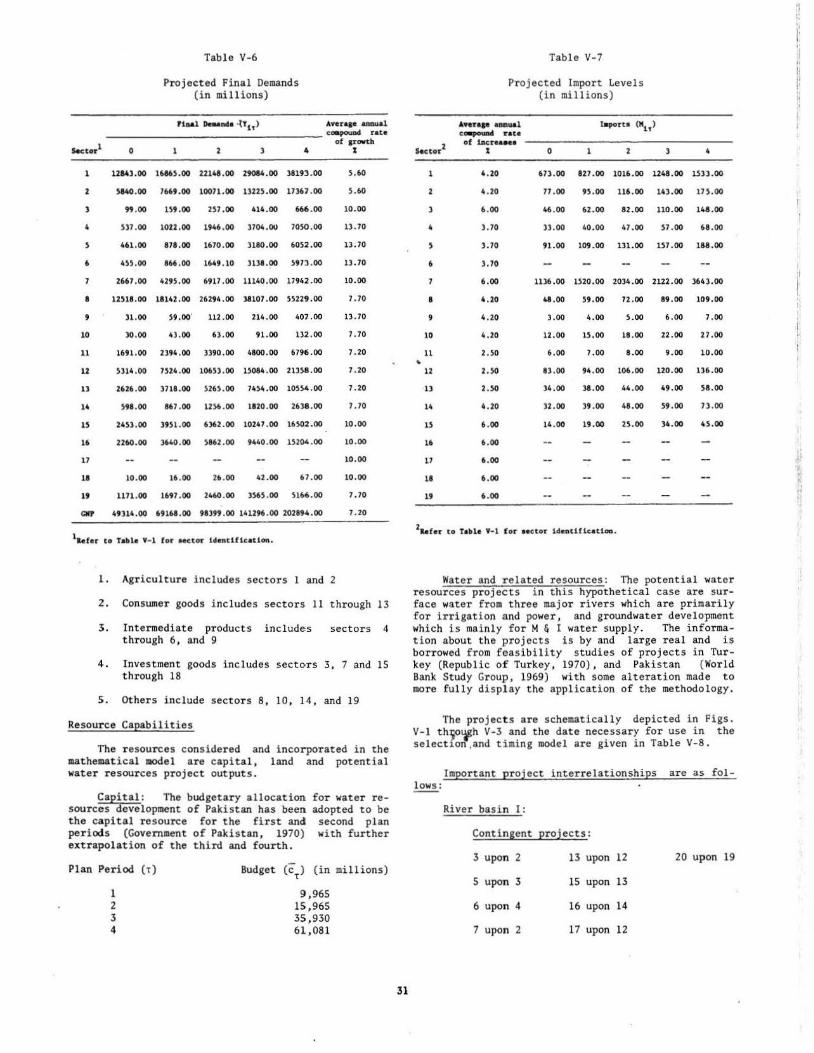
Table V-6

Projected Final Demands (in millions)

fba1 Dnando ·tth) AnraJ• aruwol ------------------------------------c~ rot•

of rrowtb Seetor1 0 3 4 I

2

4

6

10

11

12

ll

14

1S

16

17

18

19

12143.00 16865.00 22141.00 2-...oo 38193.00

5140.00 7669.00 10011.00 13225.00 11367.00

99.00 lS9.00 257.00 414 .00 666.00

5)1.00 1021.00 1946.00 3704.00 7050.00

461 .00

455.00

878.00 1670.00 3180.00 6052.00

866.00 1649.10 3138.00 5973.00

2667.00 429S.OO 6917.00 11140.00 11942.00

U518 .00 18141.00 26294.00 38107.00 55229.00

31.00 59.00" 112.00 214.00 407.00

30.00 43.00 63.00 91.00 132.00

1691.00 2394 . 00 3390.00 4800.00 6796 .00

5314 . 00 7S24.00 10653.00 15084. 00 2llS8.00

2626.00 3718.00 5265.00 7454.00 10554.00

591.00 867.00 1256.00 1820. 00 2638 . 00

245) .00 3951.00 6)62 .00 10247. 00 16S02 .00

2260.00 )640.00 )862.00 9440.00 15204.00

10.00 16.00 26.00 42.00 67.00

1111.00 1697.00 2460.00 3565 .00 5166.00

49314.00 6916*.00 91399 .00 141296.00 202894.00

5.60

5.60

10.00

13.70

13.70

13.70

10.00

7.70

13.70

7.70

7.20

7.20

7.20

7.70

10.00

10.00

10.00

10.00

7.70

7.20

1a.tor to Tab1• v- 1 f or oector ldontlflcotlon.

1.

2.

3.

4.

Agriculture includes sectors I and 2

Consumer goods includes sectors 11 through 13

Intermediate products includes through 6, and 9

sectors 4

Investment goods includes sectors 3, 7 and 15 through 18

5. Others include sectors 8, 10, 14, and 19

Resource Capabilities

The resources considered and incorporated in the mathematical model are capital, land and potential water resources project outputs.

Capital: The budgetary allocation sources development of Pakistan has been the capital resource for the first and periods (Government of Pakistan, 1970) extrapolation of the third and fourth.

for water re­adopted to be

second plan with further

Plan Period (t)

1 2 3 4

Budget (c) (in millions) T

9,965 15,965 35 , 930 61,081

31

•

3

6

• 9

10

11

12

ll

14

1S

16

11

l8

19

Table V-7

Projected Import Levels (in millions)

4ftUP&Dili&01

c_.... nco of bet~• -----------------------------------

%

4.20

4 .20

6.00

3.70

3.70

).70

6.00

4.20

4.20

4 . 20

2.SO

2.50

2.SO

4.20

6.00

6.00

6.00

6.00

6.00

0 l 4

613.00 827.00 1016.00 1241.00 1533.00

77.00 95.00 116.00 143.00 175.00

46 . 00 62.00 82.00 110.00 148.00

33.00 40.00 47.00 57.00 68.00

91.00 109.00 131.00 157.00 188.00

1136.00 1520.00 2034.00 2122.00 3643.00

48.00 59.00 72.00 89.00 109.00

3.00 4.00 5.00 6.00 7.00

12.00 15.00 18.00 22.00 27.00

6.00 7.00 8.00 9.00 10.00

83.00 94.00 106.00 120.00 136.00

34.00 38.00 44.00 49.00 58.00

)2.00 39.00 48 .00 59.00 73.00

14.00 19.00 25.00 34.00 45.00

2a.ter to Toble V- 1 for o•ctor 1dentlf1cat1oa.

Water and related resources: The potential water resources projects in this hypothetical case are sur­face water from three major rivers which are primarily for irrigation and power, and groundwater development which is mainly for M & I water supply . The informa­tion about the projects is by and large real and is borrowed from feasibility studies of projects in Tur­key (Republic of Turkey, 1970), and Pakistan (World Bank Study Group, 1969) with some alteration made to more fully display the application of the methodology.

The projects are schematically depicted in Figs. V-1 th~o~h V-3 and the date necessary for use in the selectlon .and timing model are given in Table V-8.

Important project interrelationships are as fol­lows:

River basin I:

Contingent projects:

3 upon 2

5 upon 3

6 upon 4

7 upon 2

13 upon 12

15 upon 13

16 upon 14

17 upon 12

20 upon 19

j, II !

I ,, ., ,.

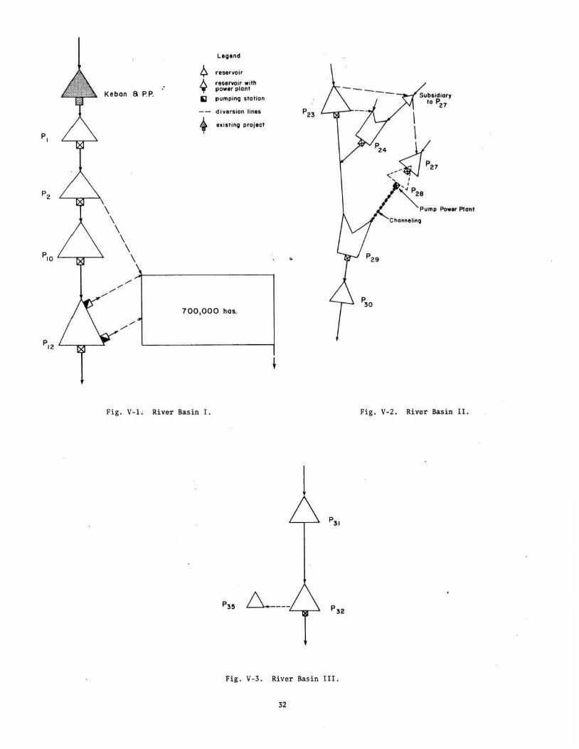
Legend

~ .-eservoir

~ reservoir with _. power plant

Kebon a P.P. I;) pumping station

diversion linea p23

t existing project

P,

p2

\ \ \ \

PIO \ \ .. \

700,000 has.

Fig. V-1; River Basin I.

j

Fig. V-3 . River Basin III.

32

I I

--~" <;,. I

' '.J p

~a Pump Power Plant

Fig. V-2. River Basin II.

tk

1

·-.... ..... DiiKrlptiooe ....... ...

2 ' •

2.1 ~~h

2.1.1 ... htuS -..... to r2 b' .... tn ... u-

2.2 '2 • '3 ,_..,...

2. 1.2 ""lalo' bu. to r 3

6 2.2.1 - lalo' bu. to t 4

10

II

2.1.3 ... 7.tol "'" · to t 2

2.3 r 2 I r 7 c~~

lliPT_.,_

'- l:ollrof

U 12. I t- I&<Oio&M

u 12.1.1 ... latuS"""· to t 12

14 12.2 r12 • 'u ,_._.

u 12.1.2 . ""' 4.to' "'"· to r 13

1i 12.2.1 ... 4do5 .... to ,14

17 12.1. ) .., 7.to5 t.&o. to t 12

11 12.1 r12

• r17

,_._.

19 19.1 IIU4lo rar.-

20 19.1.2 ... ?alaS to ,19

l1 u.2 'u • 'IO ,_,_ 22 lliPI&t-

23

24 14.1

u 24.1.1

26

27

21

29

30

31

Low c.r-1a1a (.U. nor .. • f,_Tukla)

w.. 'u U:..,~ <r24 ''25

x.ot • •"- (aU. lt01'qe , .... Tarbala)

'Pic tar

32 32.1 ~~ucla

3:J 32.1.2 lalu r32

36

S1

31

39

40

41

42

64

4S

loUl .. <th

Pooj ... .ilolo&oi&

-J .. ....

Iori S,-ploooo M•.

Table V-8

Data on Water Resources Projects

Val~aM of Projact outpuu

(i.c.J.Uioul AY ,. .. .......,

"'-~· ...... "" b1

4

1451

2500

2740

78

78

1500

340

610

306

341

900

301

lrrtp-tloD 1t

2

'

60-'

604

Ul

451

1055

947

947

453

453

604

604

1051

1057

1057

224

123

201

52

216

123

12J

16

26

II

II

,_. Toe.! Total J !let b, -.J'lto eoeu c s

6

347

173

171

7

4924

2462

1546

11008

6424

8

224J

1669

SIN

64155

5176

6424 Sl76

14970 11062

172 17432

443 19735

91

399

121

12l

ll70

1911~

1748

642l

8170

1600 -

12731

11~97

"' 11806

1476

4616

6092

UOl

4701

15021 9317

124 16770 10793

177 Ul8 19"

16 15233 9127

19) 17751. 11106

261 17191 11338

53 3353

16 1600

21 1725

213 3250

209 3200

54 21051

1115

1200

1045

2102

2500

10996

T '

2611

793

3360

41Sl

541

8338

• 6412

1.309

269

1106

2071

31199

3899

nos 5977

539

6106

6645

5153

1468

400

12l3

675

700

JOSI3 20983 96001

33530 18150 14610

21

54

1600

1715

3315

1135

lOOt

3417

8131

302J

180

111

1150

1040

2050

9240

6116

1465

5701

812

Ill

102

33

1415

615

1275

9110

2323

1952

3136

2191

76

Proj.et

-turatl0111

TS.O

T ,... .. 10

10

10

CotipouDd aoUD.ta of con• aad llet voTtha

of ProjfiCU n the b•llaiq of pla period• OH

'u I al

3296

2452

7120

10072

1634

1634

162'3

-•u

u

3147

1165

4tl7

6102

805

5733

6907

1002

" · .. "k• I

u l

4142

3603

11166

14799

12615

12615

23UI

27414

1415

11706

16746

1011

26162 1923 38440

216t

&712

8951

6907

6907

3U

2654

3053

572t

3164

9965

IS !52

10141

10141

. "kJ "1.4 I •u

14 1;T 6

5652 7115

1712 5294 2515

7H4 16450 10651

11966 21744 13173

1731 1183 11639

1113

3424

10149

taooo

1472

2126

Sll

3899

416

1417

4817

11639 1738

3501t 12377

40383

)6151

2113

4612

14641

1U24

14912

14912

149U

26441

2163

4152

ISS

57~

U91

U:161

12368

13689 1312 20114 1231i 29553 11096

151st 1712 23300 12903 34235 11959

2901 792 ua 1164 6277 1110

13410 1972 19704 13112 21951 19368

16311 976! 23976 14346 3522f 21011

166$9 - 24477 12636 35964 11566

2770

1763

1535

3713

3613

16156

308!0

27666

1690

1521

3012

U576

106

2177

3703

96

1001

2153

1712

122l

163

150

2157

587

1797

992

1029

4069

2591

2256

5559

Slt7

14173 23739

31" 864

1461

1457

1511

21707

3315

1168

7UO

4656

12"

21.57

2141

2l20

34879 311M

14105 U2H 2(1725 66551 30451

21569 40694

2112

1006

1173

13385

128

1116

5069

285

341l

2168

4608

3219

101

112

2483

2245

4426

us

4080

140

1411

3163

1515

1766

240

220

31692

3206

1479

2733

19667

181

3109

419

5015

4214

6170

4730

149

166

59792 46565

3641

1m

6503

4710

217l

,309 21197

221

5995

,,3 106

2176

4647

3695

2639

352

324

276

4561

10943

615

219

241

I I

' I '

!

' i,

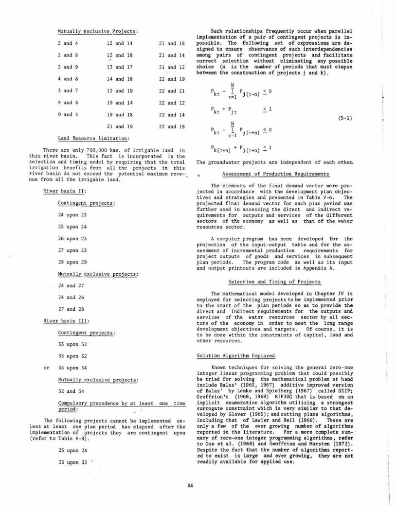
Mutualll Exclusive Projects:

2 and 4 12 and 14 21 and 18

2 and8 12 and 18 21 and 14 :

2 and 9 13 and 17 21 and 12

4 and 8 14 and 18 22 and 19

3 and 7 12 and 19 22 and 21

9 and 8 19 and 14 22 and 12

9 and 4 19 and 18 22 and 14

21 and 19 22 and 18

Land Resource Limitation:

Ther e are only 700,000 has. of i rrigable l and i n this river basin. This fact is incorporated i n the selection and timing model by r equiring that the total irrigation benefits from all the projects in this river basin do not exceed the potential maximum reve- , nue from all the irrigab1e land.

River basin II:

Contingent 12rojects :

24 upon 23

25 upon 24

26 upon 23

27 upon 23

28 upon 29

Mutual1r exc lusive Eroj ect s:

24 and 27

24 and 26

27 and 28

River basin III:

Contingent 12r ojects:

33 upon 32

35 upon 32

or 35 upon 34

~~tually exclusive projects:

32 and 34

ComEulsory precedence by at least one t ime period:

The following projects cannot be implemented un­less at least one plan period has elapsed after the i mplementation of projects they are contingent upon (refer to Table V-8).

25 upon 24

33 upon 32 ~

34

Such relationships frequently occur when parellel implementation of a pair of contingent projects is im­possible. The following set of expressions are de­signed to ensure observance of such interdependencies among pairs of contingent projects and facilitate correct selection wi thout eliminating any possible choice (n is the number of periods that must elapse between the construction of projects j and k).

< 1

(5-l) N

pkT til Pj(t+n) < 0

P + P. < 1 k(t+n) J (T+n) -

The groundwater projects are i ndependent of each othe~

.. Assessment of Production Requirements

The elements of the final demand vector were pro­jected in accordance with the development plan objec­tives and strategies and presented in Tabl e V-6. The projected final demand vector for each plan period was further used in assessing the direct and indirect re­quirements for outputs and services of the different sectors of tffe economy as well as that of the water r esources sector.

A computer program has been developed for the projection of the input-output table and for the as­sessment of incremental production requirements for project outputs of goods and services in subsequent plan periods. The progra.m code as well as its input and output printouts are included in Appendix A.

Select ion and Timing of Project s

The mathematical model developed in Chapter rv is employed for selecting projects to be implemented prior to the start of t he plan periods so as to provide the direct and indirect requirements for the outputs and services of the water resources sector by all sec­tors of the economy in order to meet the long range development objec~ives and targets. Of course , it is to be done within the constraints of capital, land and other resources .

Solution Algorithm EmElored

Known techniques for sol ving the general zero-one integer linear progr amming problem that could possibly be tried for solving the mathematical problem at hand include Salas' (1965 , 1967) additive improved version of Balas' by Lemke and Spielberg (1967) called DZ.IP; Geoffrion's (1968, 1969) RIP30C that is based on an implicit enumeration algor ithm utilizing a strongest surrogate constraint which is very similar to that de­veloped by Glover (1965); and cutting plane algoritllms, including that of Lawler and Bell (1966). These are only a few of the ever growing number of algorithms reported in the literature. For a more complete sum- · mary of zero-one i nteger programming algorithms, refer to Gue et al. (1968) and Geoffrion and Marsten (1972). Despite the f act that the number of algorithms report­ed to exist is large and ever growing, they are not readily available for applied use.

Of the many algorithms developed for solving zero-one integer (all or mixed) programming problems , most of the reports on computational experience (Peterson, 1967; Trauth and Woolsey, 1969; Gue et al., 1968; Geoffrion and Marsten, 1972; Pettway, 1973) show that Geoffrion ' s enumerative al~orithm with surrogate constraints is superior to all the others for the range of problems to which they were applied.

• Pettway' s study (1973) led to the conclusion that of the more available integer linear programming al­gorithms . enumerative (implicit) types converged faster than the cutting plane types and that the algorithms of Lemke and Spielberg (1967) and Geoffrion (1968) were the best of those studied by him--mainly small size problems of which the largest was 25 x 28. The other studies (Gue et al., 1968; Geoffrion, 1969; Geoffrion and Marsten, 1972) firmly conclude, based on studies involving greater numbers and larger problems than used by Pettway, that Geoffrion's RIP30C is su­perior to all as the fastest converging algorithm and assert that the necessary solution time has a polyno­mial relationship with the number of variables while this is an exponential relationship in the other al­gorithms.

The studies made so far do not make an exhaustive inquiry into computer s torage requirements as related to the size of problems and algorithms used. This is a matter that deserves investigation since in an n­variable zero-one problem there may be as many as 2n possible solutions. Furthermore, the consensus among experimenters is that these algorithms are character­ized by large computer space requirements and that there is little hope of solving problems with more than 100 variables in a reasonable amount of machine time. This concern is strongl y expressed in the arti­cle by Gue et al. (1968) . They also hold the view that Geoffrion's algorithm is the most promising for han­dling large problems with possibly some further im­provement s.

Therefore, since all evidences seem to indicate that Geoffrion' s algorithm RIP30C, is the best, it is chosen for solving the problem in this study.

Necessary problem manipulations: ten to solve integer linear programs form:

mini mize ex subject to Ax + b > 0

x. ,. 0 or 1 J

RIP30C is writ­of the following

in which c and x are N-dimensional vectors, b is an M-dimensional vector, and A is an MxN matrix.

Any bounded integer program can be reformulated to conform to the given form using elementary manipu­lations such as the following.

The objective function: If the problem is a max­imization problem, which is the case of the example problem, the objective function (but not the con­~raints) must be multiplied by -1. This follows from the fact that the maximum of any function f is the minimum of -f.

The constraints: The algorithm requires that all the elements of [A) as well as the constraint vector b be put on the left side of the inequality sign.

Inequalities of the sense gi ~ 0 are changed to gi S 0 by multiplying by -1.

Equality constraints must be r eplaced by two i n­equality constraints of different sense and the one with the sense of gi ~ 0 multiplied by -1. That is , given gi = 0, proceed as follows:

r' > 0

{'' > 0

{" > 0

g .• 0 •> •> • > 1

gi < 0 -gi > 0 gj > 0

in which gj A = -gi

Results and Anallsis

In order to ensure global optimality of the solu­tion to the foregoing problem, it should be treated in its entirety, i.e., in~lude all the variables (45) and fo~ the entire number of plan periods (4). The solu­tion then will represent an optimum water resources program that is tailored to ensure a sustained national economic development for a future time span of twenty years according to the desired rate and strategy given in the national long-range development plan .

But, as if designed to substantiate Messrs . Gue and associates ' fear that the algorithms require large storage space and may be impossible to be used in sol v­ing large problems (Gue et al., 1968) , it turned out that the presently formulated problem is too large for the CDC6400 computer available at Colorado State Uni­versity, with an operating core space of 140,0008 . The size of the constraint matrix is 244 x 180 and it is much larger than what the algorithm had been applied to, according to available information. The problem became excessively large , even though the number of decision variables are only 45, for two fundamental reasons: 1) It is a combinatorial problem. 2) Imbedded in its linear appearance, it has dynamic aspects ac­counting for several time periods by replicate con­straints (see Table V-9).

Table V-9

Effect of Dynamic Aspect of the Selection and Timing Problem in its Size

No. of No. of No. of Plan Periods Variables Possible Solutions

1 45 3.5 X 1013

2 90 1.2 X 1027

4 180 1.5 X 1054

The problem can be made amenable for solution by employing a suitable solution strategy technique. 3 At this moment the most suitable technique appears to be the Dantzig-Wolfe decomposi t ion technique which is

3"Solution strategy" techniques reduce an opumuation problem to a related sequence of simpler optimization problems as opposed to "problem manipulation" techniques which are devices for restating a given problem i n an alternative form that is apt to be more amenable to solution. (For detailed explanation refer to Geoffrion, 1969).

35

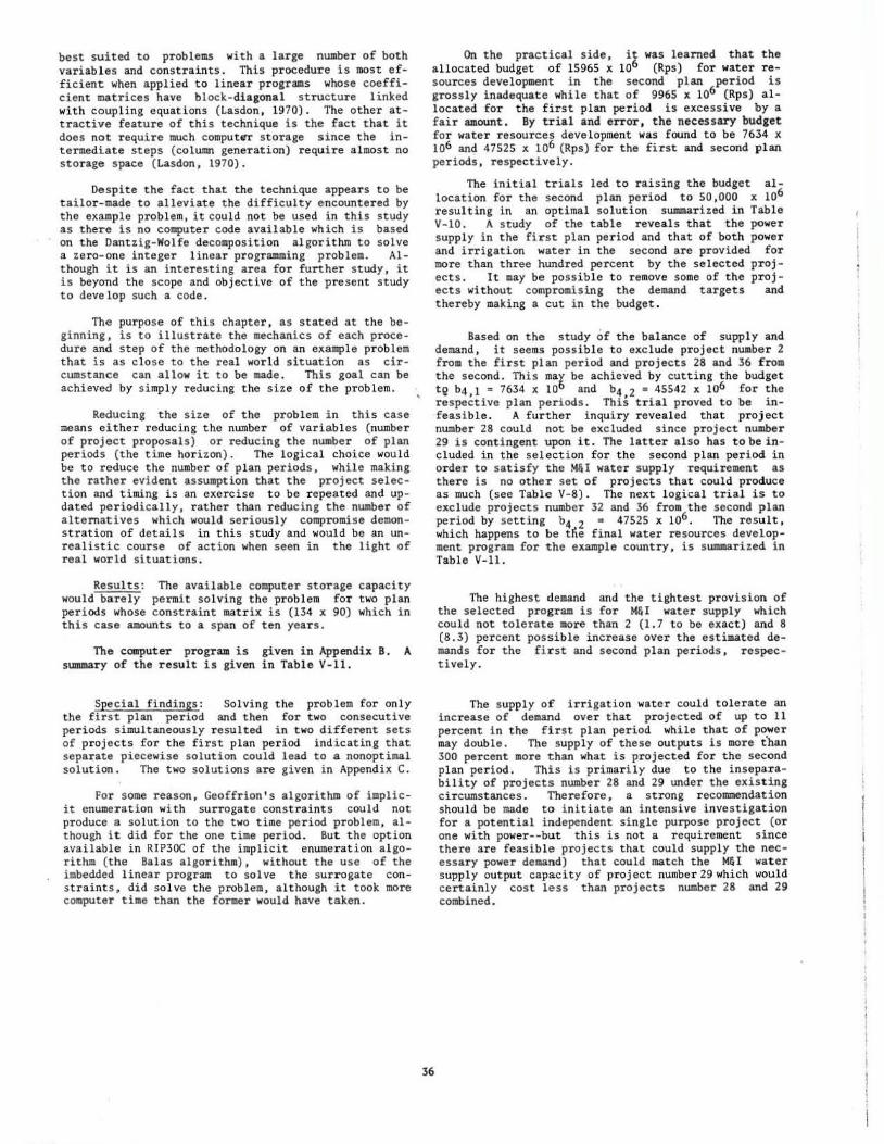
best suited to problems with a large number of both variabl es and constraints. This procedure is most ef­ficient when applied to linear programs whose coeffi­cient matrices have block-diagonal structure linked with coupling equations (Lasdon, 1970). The other at­tractive feature of this technique is the fact that it does not require much computeT storage since the in­termediate steps (column generation) require almost no storage space (Lasdon, 1970).

Despite the fact that the technique appears to be tailor-made to allevi ate the difficulty encountered by the example problem, it could not be used in this study as there is no computer code available which is based on the Oantzig-Wolfe decomposition algorithm to solve a zero-one integer linear programming problem. Al­though it is an interesting area for further study, it is beyond the scope and objective of the present study to develop such a code.

The purpose of this chapter, as stated at the be­ginning, is to illustrate the mechanics of each proce­dure and step of the methodology on an example problem that is as close to the real world situation as cir­cumstance can allow it to be made. This goal can be achieved by simply reducing the size of the problem.

Reducing the size of the problem in this case means either reducing the number of variabl es (number of project proposals) or reducing the number of plan periods (the time horizon). The logical choice would be to reduce the number of plan periods, while making the rather evident assumption that the project selec­tion and timing is an exercise to be repeated and up­dated periodically, rather than reducing the number of alternatives which would seriously compromise demon­stration of details in this study and would be an un­realistic course of action when seen in the light of real world situations.

Results: The available computer storage capacity would barely permit solving the problem for two plan periods whose constraint matrix is (134 x 90) which in this case amounts to a span of ten years.

The computer program is given in Appendix B. A summary of the result is given in Table V-11.

Special findings: Solving the problem for only the first plan period and then for two consecutive periods simultaneously resulted in two different sets of projects for the first plan period indicating that separate piecewise solution could lead to a nonoptimal solution. The two solutions are given in Appendix C.

For some reason, Geoffrion ' s algorithm of implic­it enumeration with surrogate constraints could not produce a solution to the two time period problem, al­though it did for the one time period. But the option available in RIP30C of the implicit enumeration algo­rithm (the Balas algorithm), without the use of the imbedded linear program to solve the surrogate con­straints, did solve the problem, although it took more computer time than the former would have taken.

On the practical side, it was learned that the allocated budget of 15965 x 106 (Rps) for water re­sources development in the second plan period is grossly inadequate while that of 9965 x 106 (Rps) al­located for the first plan period is excessive by a fair amount. By trial and error, the necessary budget for water resources development was found to be 7634 x 106 and 47525 x 106 (Rps) for the first and second plan periods, respectively.

The initial trials led to raising the budget al­location for the second plan period to 50,000 x 106 resulting in an optimal solution summarized in Table V-10. A study of the table reveals that the power supply in the first plan period and that of both power and irrigation water in the second are provided for more than three hundred percent by the selected proj­ects. It may be possible to remove some of the proj ­ects without compromising the demand targets and thereby making a cut in the budget .

Based on the study of the balance of supply and demand, it seems possible to exclude project number 2 from the first plan period and projects 28 and 36 from the second. This may be achieved by cutting the budget tQ b4,1 ~ 7634 x 10° and b4 2 • 45542 x 106 for the respective plan periods. This trial proved to be in­feasible . A further inquiry revealed that proj ect number 28 could not be excluded since project number 29 is contingent upon it. The latter also has to be in­cluded in the selection for the second plan period in order to satisfy the M&I water supply requirement as there is no other set of projects that could produce as much (see Table V-8) . The next logical trial is to exclude projects number 32 and 36 from the second plan period by setting b4 2 • 47525 x 106. The result, which happens to be t~e final water resources develop­ment program for the example country, is summar ized in Table V-11.

36

The highest demand and the t i ghtest provision of the selected program is for M&l water supply which could not tolerate more than 2 (1.7 to be exact) and 8 (8.3) percent possible increase over the estimated de­mands for the first and second plan periods, respec­tively.

The supply of irrigation water could tolerate an increase of demand over that projected of up to 11 percent in the first plan period while that of power may double. The supply of these outputs is more than 300 percent more than what is projected for the second plan period. This is primarily due to the insepara­bility of projects number 28 and 29 under the exist ing circumstances. Therefore, a strong recommendation should be made to initiate an intensive investigation for a potential independent single purpose project (or one with power--but this is not a requirement since there are feasible projects that could supply the nec­essary power demand) that could match the M&I wat er supply output capacity of project number 29 which would certainly cost less than projects number 28 and 29 combined.

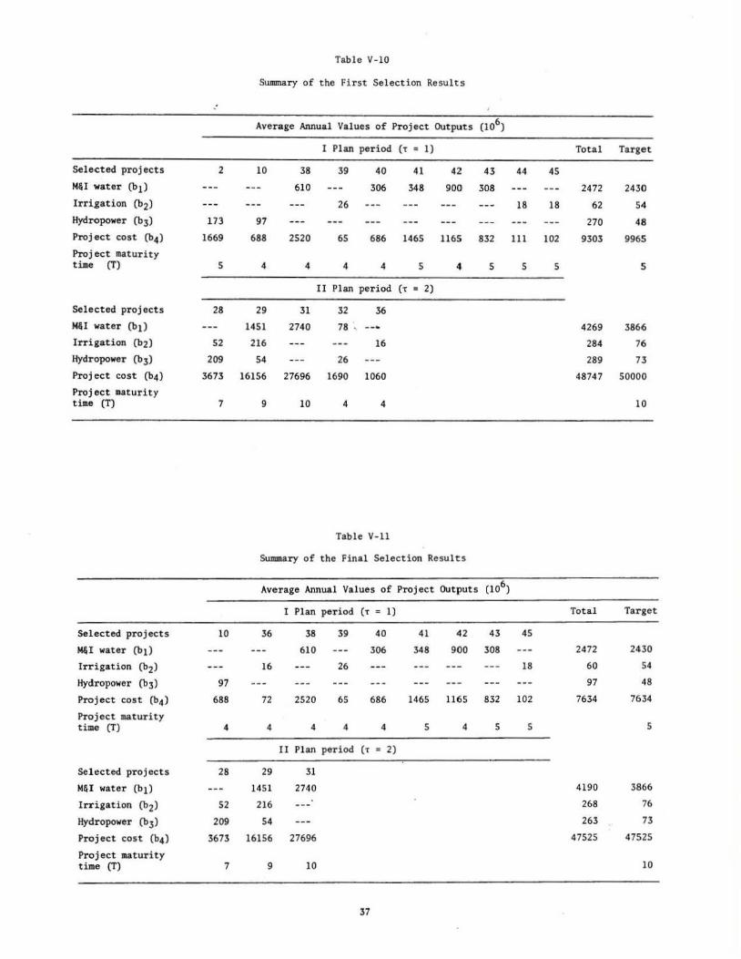
Table V-10

Summary of the First Selection Results

.. Average Annual Values of Project Outputs (106)

I Plan period (T = 1) Total Target

Sele~ted projects 2 10 38 39 40 41 42 43 44 45

M&I water (b1) 610 306 348 900 308 2472 2430

Irrigation (b2) 26 18 18 62 54 Hydropower (b3) 173 97 270 48 Project cost (b4) 1669 688 2520 65 686 1465 1165 832 111 102 9303 9965 Project maturity time (T) 5 4 4 4 4 5 4 5 5 5 5

II Plan period (T = 2)

Selected projects 28 29 31 32 36

M6I water (b1) 1451 2740 78 . __ ..

4269 3866

Irrigation (bz) 52 216 16 284 76

Hydropower (b3) 209 54 26 289 73

Project cost (b4) 3673 16156 27696 1690 1060 48747 50000

Project maturity time (T) 7 9 10 4 4 10

Table V-ll

Summary of the Final Selection Results

Average Annual Values of Project Outputs (106)

I Plan period (T = 1) Total Target

Selected projects 10 36 38 39 40 41 42 43 45

MU water (b1) 610 306 348 900 308 2472 2430

Irrigation (b2) 16 26 18 60 54

Hydropower (b3) 97 97 48

Project cost (b4) 688 72 2520 65 686 1465 1165 832 102 7634 7634

Project maturity time (T) 4 4 4 4 4 5 4 5 5 5

II Plan period (T "' 2)

Selected projects 28 29 31

MU water {bl) 1451 2740 4190 3866

Irrigation (bz) 52 216 268 76

Hydropower (b3) 209 54 263 73

Project cost (b4) 3673 16156 27696 47525 47525

Project maturity time (T) 7 9 10 10

37

/

Chapter VI SUMMARY, CONCLUSIONS, AND RECOMMENDATIONS

The case has been made .:that central planning is most desirable for balanced, accelerated, and sus­tained national economic development (NED) to take place . It is even inevitable if the ever widening gap between the developing and developed nations is to start closing.

Furthermore, projects that compr ise sectoral pro­grams, which in turn are subsets of the entire NED plan, should be selected on the basis of their contri­butions to t he attainment of NED objectives and tar­gets. Such pragmatic program formulation requires a methodology that utilizes quantitative anal ytical pro­cedures to carry out the selection of projects that best accomplish the NED goals without overlooking available options and within the resource capabilities of a nation. Developing such a methodology has been t he objective of this study. This objective has been fully achieved.

A methodol ogy that pr ovides for ample measures to •· incorporate all relevant considerations which are characteristic of water resources projects selection and timing to promote balanced and sus tained economic devel opment i n centrally planned and coordinated frame­work (for details of the major consi deration refer to p. III-3, Chapter III) has been developed. This makes the methodology far super ior to present techniques.

The methodology is composed of several analytical procedures. The input-output model is used to simu­late the economy of the country, in making consistent projections of t he elements of final demands in ac­cordance with NED objectives and strategies, and in assessing total and incremental requirements for sec­toral outputs of goods and services in subsequent plan periods. A mathematical model is developed and zero­one integer linear programming is employed to make the sel ection of projects that yield an opti mal water re­sources development program for the number of planning periods under consideration.

38

Application of the methodology on the example problem as a whole, and the points discussed under "Special findings" (Chapter V) in particular, i ndicate the capacity of the methodology to incorporate details and enable the performance of rigorous anal ysis which cer tainly makes it a very useful tool in the process of NED planning. Thus , applied carefully and j udi­ciously it will improve t he insight gained and hence the final decision reached regarding the selection and timing for implementation of water resources projects to promote NED. Furthermore , the methodology could i n principle be applied to similar decision making in t he other sectors of the economy provided that the neces­sary data in t he appropriate kind and form are made available .

The only limitation on extended use of the meth­odology learned from the computational experience is t~e rather large computer storage requirement which becomes prohibitive when the selection and timing problem invol·ves a large number of projects and sever­al time periods. Further research efforts should be directed in developing new a l gorithms (or adopt exist­ing ones such as the Dant zig-Wolfe decomposition a l go­rithm) with efficient computer codes that use solution strategy techniques for abetting the dimensionality problems associated with large size problems.

Concomitant to the adoption of the methodology as a standard procedure in the national economic develop­ment planning pr ocess is the reorganization of the format and scope of the data collection and processing on national resources base and economic transactions . Water resources should be classified as a separate economic sector and included in the i nput-output table of the economy. Water resources project identifica­tion and studies up to and including feasibility re­ports should be carried out on a continuous basis .

/

REFERENCES

Albertson, Maurice L., 1972: The Development Process. East-West Center, TechnQlogy and Development Cen­ter, Honolulu, Hawaii.

Au , Tung and Thomas E. Stelson , 1969: Introduction to Systems Engineering, Deterministic Models. Addison-Wesley, Menlo Park, California.

Balas, E., 1965: An Additive Algorithm for Solving Linear Programs with Zero-One Variables. Opera­tions Research, Vol. 13, No. 4, July-August, pp. 517-546.

--..,.,--.' 1967: Discrete Programming by the Filter Method. Operations Research, Vol. 15, No . . 5, September-October, pp. 915-957.

Balinski, M.L., 1965: Integer Programming: Methods, Uses, Computations. Management Science, Vol. 12, No. 3, November, pp. 253-313.

Bator, F.M., 1958: The Anatomy of Market Failure. Quarterly Journal of Economics, Vol. ·LXXII, No. 3, pp. 351-379, August.

Baumol, William J., 1969: On the Discount Rate for Public Projects. In the Analysis and Evaluation of Public Expenditures: The PPB System--A Com­pendium of Papers Submitted to the Subcommittee on Economy in Government of the Joint Economic Committee, Congress of the United States, U. S. Government Printing Office, Washington, D. C., Vol. I, pp. 489-503.

Butcher, WilliamS., Yakov Y. Haimes and Warren A.Hal~ 1969: Dynamic Progr3llllling for the Optimal Se­quencing of Water Supply Projects. Water Re­sources Research, Vol. 5, No. 6, December, pp. 1196-1204.

Caulfield, Henry P., Jr., 1973: Federal Guidelines for Water Resource Project Evaluation. Chapter 20 in Environmental Impact on Rivers (River Mechanics Vol. III) edited by H.W. Shen, Fort Collins, Colorado.

Chenery, Hollis B. and Paul G. Clark, 19·64: Interin­dustry Economics. John Wiley and Sons, Inc., New York.

Colm, Gerhard and Theodore Geiger, 1965 : Country Pro­gramming as a Guide to Development. In Develop­ment of the Emerging Countries- -An Agenda for Re­search, The Brookings Institution, Washington, D. C., Fourth Printing, March 1965.

Dantzig, G.B., 1963: Linear Programming and Extension~ Princeton University Press, Princeton, New Jersey.

Dasgupta, Partha, 197?: A Comparative Analysis of the UNIDO Guidelines and .t .he OECD Manual. Oxford University Institute of Economics and Stat~ Bulletin, Vol. 34, No. 1, February 1972.

Demas, William G., 1965: The Economics of Development in Small Countries with Special Reference to the Caribbean; Center for Developing-Area Studies. McGill University, Montreal.

de Neufville, Richard and Joseph H. Stafford, 1971: Systems Analysis for Engineers and Managers. McGraw-Hill, Inc., New York.

39

Duff, William S., 1971: The Application of Dynamic Programming to the Selection and Timing of Inter­related Proposals in a Stochastic Environment. Doctoral Dissertation, Department of Industrial Engineering , Stanford University, August, 1971. Also published as SRI Report No. 86053102- AII, Research Institute, Menlo Park, Cal ifornia, August.

Fox, Irving and Orris Herfindahl, 1964: Attainment of Efficiency in Satisfying Demands for Water Re­sources. American Economic Review, Vol. 54, No. 3, May, pp. 198-206.

Friedman, Milton, 1962: Capitalism and Freedom. The University of Chicago Press, Chicago, Illinois.

Furtando, Celso, 1964: Development and Underdevelop­ment. Translated by Ricardo W. De Aguiar and Eric Charles Drysdale , University of California Press, Berkeley and Los Angeles.

Geoffrion , A.M. and A.B. Nelson, 1968: User ' s Instruc­tions for 0-l Integer Linear Programming. Code RIP30C, Memo. RM-5627-PR, The ~~ Corporation, Santa Monica, California.

Geoffrion, A.M., 1969: An Improved Implicit Enumera­tion Approach for Integer Programming. Operations Research, Vol. 17, No. 3, May-June, pp. 437-454.

---.----:-' 1969: Elements of Large-Scale Mathematical Programming. A Report Prepared for the U.S. Air Force Project RAND, The RAND Corporation, Santa Monica, California.

--~-and R.E. Marsten, 1972: Integer Programming Algorithms: A Framework and State-of-the-Art Survey. Management Science , Vol . 18, No . 9, May, pp. 465-491.

Gittinger, J. Price, 1972: Economic Analysis of Agri­cultural Projects. The Johns Hopkins University Press, Baltimore.

Glover, F. , 1965: A Multiphase-Dual Algorithm for the Zero-One Integer Programming Problems . Operations Research, Vol. 13, No. 6, November-December, pp. 879-919.

Government of Pakistan, Central Statistics Office , Economic Affairs Division, 1965: Census of Elec­tricity Undertakings 1962-63. Government of Pakistan Press, Karachi.

---..,-' 1968 (a): Pakistan Statistical Yearbook 1965 and 1966. Government of Pakistan Press, Karachi.

---=--'' 1968(b) : Pakistan Statistical Yearbook 1967. Government of Pakistan Press, Karachi.

--~-· 1970: Pakistan Statistical Yearbook 1968. Government of Pakistan Press, Karachi.

Government of Pakistan, Planning Commission, 1970: The Fourth Five Year Plan 1970-75.

----• 1965 (b): The Third Five Year Plan, 1965-70 .

Grant, Eugene L. and W. Grant Ireson, 1970 : Principles of Engineering Economy. Fifth Edition, The Ronald Press Company, New York.

Gue, R.L., J.C. liggett and K.C. of Algorithms for Zero-One Communications of the ACM, December, pp. 838-844.

Cain, 1968: Analysis Programming Problems. Vol. 11, No. ·12,

Hall, Warren A. and John A .. Dracup, 1970: Water Re­sources Systems Engineerlng. McGraw- Hill Company, New York.

Herber, Bernard P., 1968: Modern Public Finance. The Irwin Series in Economics, 4th Edition, .Richard D. Irwin, Inc., Homewood, Illinois.

Hiller, F.S. and G.J. Lieberman, 1969: Introduction to Operations Research. Holden-Day, Inc., San Fran­cisco.

Kindleberger, Charles P., 1965: Economic Development. McGraw-Hill , New York.

Lasdon, leon S. , 1972: Optimization Theory for Large Systems. The MacMillan Company, New York.

Lawler, E.L. and M.D. Bell, 1966: A Method for Solving Discrete Optimization Problems. Operations Re­search, Vol. 14, No. 4, pp. 699-719.

Leibenstein, Harvey, 1957: Economic Backwardness and Economic Growth. John Wiley and Sons, Inc., New York.

Lemke, C.E. and K. Spielberg, 1967: Direct Search Al­gorithm for Zero-One and Mixed-Integer Program­ming. Operations Research, Vol. 15, No. 5, September-October, pp. 892-914.

Leontief, W., 1936: Quantitative Input-Output tions in the Economic System of the United Review of Economics and Statistics , IVIII, August, pp. 105-125.

Rela­States. No. 3,

Lewis, W. Arthur, 1961: The Principle of Economic Planning. George Allen and UNWIN Ltd. -

Lorie, James H. and Leonard J. Savate, 1955: Three Problems in Rationing Capital. The Journal of Business, Vol. XXVI II, No. 4, October, pp. 229-239.

Mathur, Ashok, 1971: Balanced vs. Unbalanced Growth: A Reconciliatory View in Developing the Underde­veloped Countries. Edited by Alan B. Mountjoy, Chapter 9, Wiley-lnterscience Divisi-on of John Wiley and Sons, Inc., New York, pp. 142-161.

McKean, Roland N., 1958: Efficiency in Government Through Systems Analysis--With Emphasis on Water Resources Development . RAND Corporation Research Study No. 3, the RAND Corporation, Santa Monica, California .

Miernyk, William H., Output Analysis .

1965: The Elements of Input-Random House, New York.

Millikan, Max F., 1973: A Strategy of Development. In the Case for Development, Six Studies, United Nations Center for Economic and Social Informa­tion, Preager Publishe~s. New York.

Morel-Seytoux, H.J., 1972: Foundation of Engineering Optimization--Lecture Notes. Department of Civil Engineering, Colorado State University, Fort Collins, Colorado.

40

Morin, Thomas L. and Augustine M.O. Esogbue, 1971: Some Efficient Dynamic Programming Algorithms for the Optimal Sequencing and Scheduling of Water Supply Projects. Water Resources Research, Vol. 7, No. 3, June , pp. 479-484 .

Oakford, Robert V., 1970: Capital Budgeting--A Quan­titative Evaluation of Investment Alternatives. The Ronald Press Company, New York .

Organization for 'Economic Cooperation and Development, Paris, 1972: Manual of Industrial Project Analy­sis in Developing Countries. Vols. I and II.

Petersen, C.C., 1967: Computational Experience With Variants of the Balas Algorithm Applied to the Selection of R and D Projects. Management Sci­~· Vol. 13, No. 9, May, pp. 736-750.

Peterson, D.F., 1971: Water Resources Planning and Social Goals: Conceptualization Toward a New Methodology. Prepared for the Office of Water Resources Research, U.S. Department of the Inte­rior, Utah State University, logan, Utah.

Pettway, R.H., 1973: Integer Programming in Capital Budgeting: A Note on Computational Experience . Journal of Financial and quantitative Analysis, Vol. VII, No. 4.

Plane, Donald R. and Claude McMillan , J r. , 1971: Dis­crete Optimization--Integer Programming and Net­work Analysis for Management Decisions . Prentice- _ Hall, Inc., Englewood Cliffs, New Jersey.

Pritsker, A.A.B., L.J. Watters and P.M. Wolfe, 1968(a): Mathematical Formulation: A Problem in Design. The RAND Corporation, P-3790.

----~~· 1968(b): A Zero-One Programming Approach to Scheduling with Limited Resources. The RAND Cor­poration, RM-5561-PR.

----;-;:-' 1968(c): Multiproject Scheduling with Lia ­ited Resources: A Zero-One Programming Approach. The RAND Corporation, Report 3800.

Rasul, G., 1964: stan, 1954.

Input-Output Relationships in Paki­Rotterdam University Press.

Reiter, S., 1963: Choosing an Investment Program Among Interdependent Projects. Review of Economic Studies, February, pp. 32-36.

Republic of Turkey, Ministry of Energy and Natural Resources--General Directorate of State Hydraulic Works, 1970: Lower Firat Project--Feasibility Report. Prepared by Electo-Watt Engineering Ser ­vices, Ltd . , Tipton and Kalmbach, Inc., Societe General Poure L'Industrie, and Gizbili Consulting Engineers.

Steiner, Peter 0., 1959: Choosing Among Alternative Public Investments in the Water Resource Field. The American Economic Review, Vol. XLIX, No .. 5, December , pp. 893-916.

Subcommittee on Benefits and Costs, Federal Inte~ Agency River Basin Committee , 1950: Proposed Practices for Economic Analysis of RiVer Basin · Projects ("The Green Book"). U. S. Goverruaent Printing Office, Washington, D.C.

Subcommittee on Evaluation Standards, Inte·r -Agency Committee on Water Resources, 1958: Proposed Practices for Economic Analysis of River· Basin Projects (''The Green Book"). u. S. Govermae.nt Printing Office, Washington, .D.C.

Tims, Wouter, 1965: The Methodology of Estimating Im­port Requirements. Government of Pakistan, Plan­ning Commission, International Economics Section, March.

Tinbergen, Jan, 1964 : Central Planning. Yale Univer­sity Press .

--...,.,...-• 1967: Development Plaming. Translated from the Dutch by N.D. Smith, McGraw-Hill, New York.

Trauth, C.A., Jr. and R.E. Woolsey, 1969: Integer Linear PrograDIJIIing: A Study in Computational Ef­ficiency. Management Science , Vol . 15, No. 9, May, pp. 481-493.

United Nations, Department of Economic A.ffairs, 1951: Measures for the Economic Development of Under­Developed Countries . Report by a group of experts appointed by the Secretary-General of the United Nations, New York, May.

United Nations Economic Commission for Asia and the Far East, 1964: Manual of Standards and Criteria for Planning Water Resource Projects. Water Re­sources Series No. 26 , New York.

United Nations, Industrial Development Organization, Geneva, 1972: Project Formulation and Evaluation Series No. 2, Guidelines for Project Evaluation, New York.

United Nations Office of Public · Information, 1970: Assembly Decisions on Economic Questions, U.N. Monthly Chronicle, January, Vol . VII, No. 1,~ 150-lSl.

U.S. Bureau of the Budget, 1952: Circular A-47, Wash­ington, D.C., December 31.

--~-· 1967: Manual.

Standard Industrial Classification

U.S. Bureau of Reclamation, Special Task Force, 1972: Guidelines for Implementing Principles and Stan­dards for Multiobjective Planning of Water Re­sources. Review Draft, December .

U.S. Congress, 1965: Public Law 89-80: Water Resources Planning Act, 89th Congress, S.21, U.S. Government Printing Office, Washington, D.C.

41

U.S. National Water Resources Commission, Report by Consulting Panel on Wate~ Resources Planning, 1972: Water Resource Planning. PB-211-921, June; Distributed by National Technical Information Service , U.S. Department of Commerce, 5285 Port Royal Road, Springfield, Virginia 22151.

U. S. Subcommittee on Economy in Government of the Joint Economic Committee , Congress of the United States , 1969: The Analysis and Evaluation of Public Expenditures: The PPB System. Vols. I, II, and III, U. S. Government Printing Office, Washington, D.C.

U. S. Water Resources Council, 1962: Policies, Stan­dards and Procedures in the Formulation, Evalua­tion and Review of Plans for Use and Development of Water and Related Land Resources: Senate Doc­ument 97, 87th Congress, 2nd Session. U. S. Gov­ernment Printing Office, Washington, D.C.

, Special Task Force, 1969: ---;;E.,.-v"""'aluation of Water and Related

Projects (''The !Hue Book"). June. '

.. Procedures for Land Resource

, 1972: OBERS Projections--Economic Activity ---~i-n-the United States. U. S. Government Printing

Office, Washington, D.C. 20402.

----~~·· 1973: Federal Register, Establishment of Principles and Standards for Planning Water and Related Land Resources. Vol. 3B, No . 174, Sep­tember 10, 1973.

----~~·· 1973: Federal Register, Establishment of Principles and Standards for Planning Water and Related Land Resources, No. 174-Pt.III-1, Sep­tember, Washington, D.C.

Weingatner , Martin H., 1963: Mathematical Programming and the Analysis of Capital Budgeting Problems. 1962 Award Wi nner of the Ford Foundation Doctoral Dissertation Series, Prentice-Hall, Inc., Engle­wood Cliffs, New Jersey.

---=--· 1966: Capital Budgeting of Interrelated Projects: Survey and Synthesis. Management Sci­~· Vol. 12, No. 7, March, pp. 485-516.

White, Gilbert F., 1971: Strategies of American Water Management . The University of Michigan Press.

World Bank Study Group Headed by Pieter Lieftinck, 1969:. Water and Power Resources of West Pakistan-­A Study in Sector Planning. Vols. I , II and III, The Johns Hopkins Press, Baltimore, Maryland 21218.

Young, Robert A. and S. Lee Gray, 1972: Economic Value of Water- -Concepts and Empirical Estimates Colorado State University, March.

I~

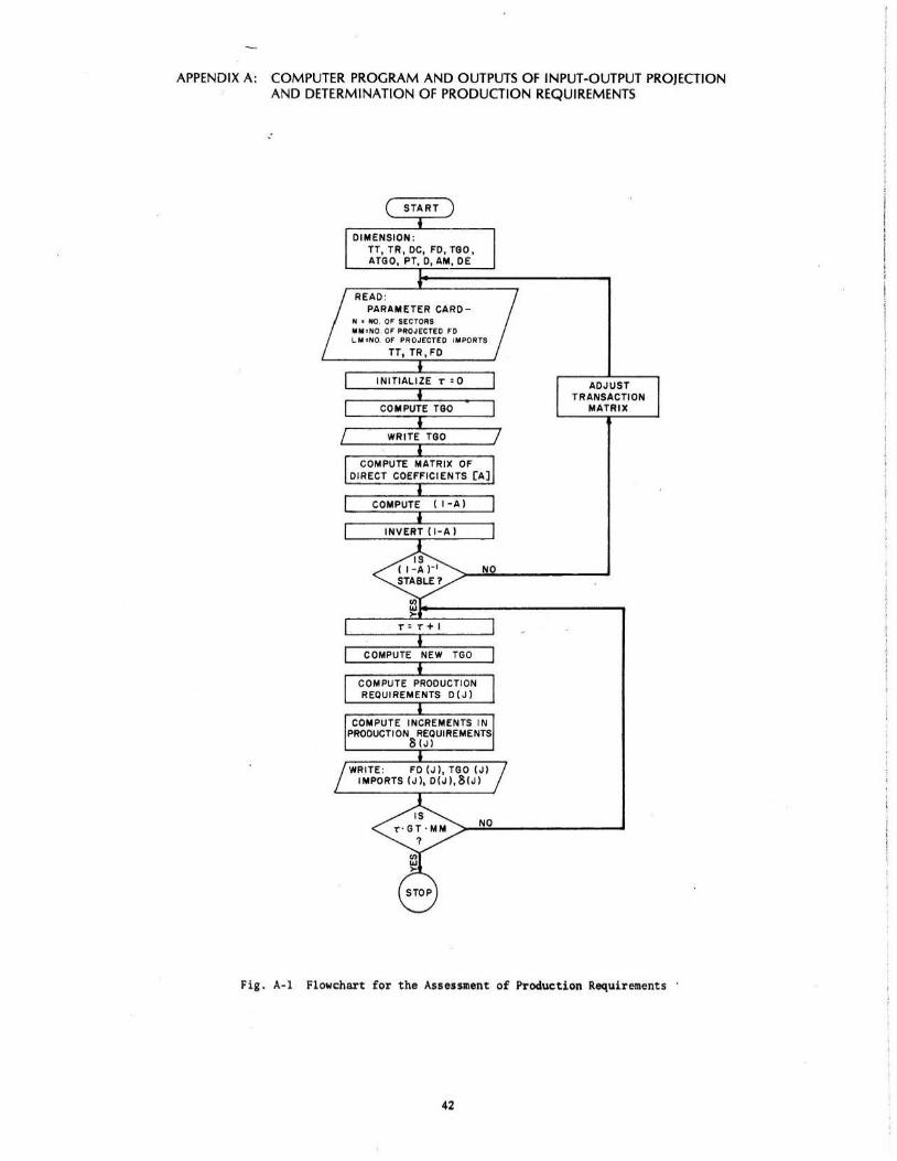
APPENDIX A: COMPUTER PROGRAM AND OUTPUTS OF INPUT-OUTPUT PROJECTION AND DETERMINATION O F PRODUCTION REQUIREMENTS

.·

N • NO, OF S£CTOAS MM• NO. Of P~OJECT£0 FO L M •NO. Of PROJECTED IIIIPORTS

TT, TR,FD

NO

ADJUST TRANSACTION

MATRIX

Fig. A-1 Flowchart for the Assessment of Production Requirements ·

42

PROGRAM 10 CINPUToOUT~UTtlAPES=tNPUToTAPE6•0U IPUTl c C NOTES C N•NUMdEW Of S~CTORS C HH=NUH~EK Of ~HOJECTlUN P~RlODS OH NUMdER Of fD VECTORS C ~H• IHPO HTS C TT•t •dLE TITLES C TR•THAN SACT ION~ MATRIX C DC= DIRECT COEff iCIENTS C TGO=TOTAL ~HODOCTIOH ~EGUIREHENTS

c C DATA C CARD l•NoHHoLH C PARAHETEMS CAKO START AT COLUMN 1 C CAAD Z-TITLE OF TA&LES ~0 COLUMNS C CA~D ) fORMAT Of TRANSACTIONS t 8 Cf LO oZl C CA~D • NO, OF TRANSACTIONS CAkOS TO BE READ C CARD S - FORMAT Of FD CHF10 . ZI C DATA CARDS C di.ANK CARD c

DIMENSION TTIIOlt TRC40o40lt DCC40 o401t FDC401r TGO I40lt ATGOI40lt 1 PTC40t401r 0 140lt AHC401r DEI40)

RE AD 15r1381 N~HH,LH

c

L•O READ 15tll9l ITTCiltl=ltlOI MEAD 1Stl391 fMT DO 101 1• 1tN

101 HEAD IStfMTl ITPiltJl,J•ltNI ~EAO I So 1391 fMT AEAD IStfHTl tFDillti• ItNI

C CALCULATE TOTA~ OUTPUTS c

DO 102 l =lo N TGO I ll•fi)( IJ

DO 102 J•loN 102 TGOI II •TGOil i•TRCloJI ..

If CLH,NEoll 60 TO 104 READ CSofHTI (AMClloi=1•Nl DO 103 l•l,N

103 DC li • TGO ili-AHitl 104 IN•N/ 10

lf I IIO•lNl.EUoJNI GO TO lOS c C WHITE OUT TRANSACTIONS TABLE c

IN•tN•1 lOS IH• l

lf llNol. Toll ll'hl 00 I n7 Kl$•ltiN

• RITE Ct> tlotU WWITE Ct>ol-11 KKoiN •IH T! Ct,.lot21 KC•KK•lO If CKC.GT,Nt KC•N WKITE CbolltJI Cloi=IHoKC I 00 106 1 " ltN

106 w~ITE Cbol44l J,CTRilo J ),J• (H,KCI W>ll TE 16tl.,21 IH•KC•l

107 CONTINUE WRITE ·Cbt1461 DO 10~ l•loN

109 wRITE 16tl~tSI FOIII oTGOcl l c C COMPUTE DIRECT COEFFICIENTS c;

00 10'1 J•lt N DO l OCJ l•l,N

109 DC CitJI•TRCitJ I / TGOIJI c C WAITE DIRECT COEffiCIENTS c

110 {N•N/ 10 If I CIO•INI.EQoiNl GO TO 111 IN• IN• I

Ill 111"1 If llNoL T • It lH:o l DO 115 I<K•loiN

IF IL.EOoll GO TO 11Z WRITE Ct,. l,.7) GO TO 113

l ll WRITE 16 ol4e) Ill •RITE l~olotll KKolN

WRITE 16 •l.,Z) KC•KK•IO IF CKCoGToNJ I<C&N WRIT[ Cbolot31 ll•I~IHoKCI

oo u• l•ltN

43

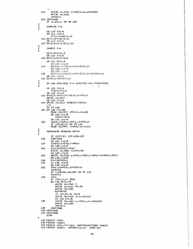
c c c

c c c

c c c

c

114

ll!>

li t.

117

!18

u~

llO

l l! i

IU

123

12 ..

wHITE lb ol491 loiDCIIoJioJ•IHoKCI WRITE 16o l421 IM=KC•I

CONTINUE If ILo£Uoll GO TO 12'

COMPUTE I-A

DO ltb• l•loN 00 I to Js lo •~

Pf II oJhOC I! , J) OCIJ,JI 2-UC iloJI 00 II 7 I" J, N OCIIoii:Io O• OCII•II

INVEHl I-A

0Cil,N•11at,O 00 ll!l l•loN DC 11•1• '~•11 =0 ·0 DO 121 Kt<=t •N

00 ll~ J= I•N OC CN•Io JI:uC C1•J•li/UCilo11 00 120 I =~ · N 00 120 .o~ ), N

OCI I -I •JI=UCII •J•li-OC IIo1l~uciN•l o JI

oo 1?. 1 J =i· ' ' OCCN,JI =OC CN•1• JI

OC ~OW CONT~INS I-A INVERTED ANO TRANSPOSED

00 122 l " lo N ATG01 1l =O oll

00 l l Z J : t , N ATGU I I I ::A l uO C I I oi)C II oJI • F'D CJI WHITE lb t l SOI 00 123 l=ltN wRITE I o, 1511 ATGO II I • TGO I[) L'" l GO TO 110 oo 136 1=1·""

RE AO (5,F'HTI tFOIJ) ,J• 1oNI 00 125 L=ltN

TGUILI"=II . O 00 125 J • 1•N

..

125 TGOILI =TGOILI•OCILoJl•FOCJI IF CL~.NEoll GO TO ill READ IS,FHTI ((AHCLitL=loNil

C TEHHINATE REAOING DATTA c

I F IEOF1511 ll7ol26t 137 126 CONTINUE

00 127 L=loN 121 ATGOILI : TGOCLI-AHCLI

DO 128 L• loN 12K OILI=ATGOILI-Oill

Wot!TE lbt l521 CloK=loSl UO 129 L" loN

!29 WRITE 16tl53l L•FOILioTGOILi oAHCLioATGO ILI•Oill 00 130 L=loN

130 Olll • AT GO CLI I l l 00 132 J•l oN

00 132 l=l oN 132 TRILoJlaPTILoJI•TGOIJl

IN•N/10 IF CllO•INl, (O,JNI GO TO I ll IN=1N•1

Ill 114•1 I F Cll"oLlol l IN•1 00 ll'!> KK=!ofN

•"ITE loo!S•H 1 wRITE IO tl41) KKo iN IIIRITE lt.,J42l KC•KK•lO If" IKC.GT ,Nl KC =N WIH TE 16, \loll ILtL•IHti\C I 00 134 L''l tN

13" WWITE lbol44) loiTRILo J I .J•IMtKCI wHITE lbt l lo2l IH• I(C•l

135 CONTINUE 136 CONTINuE !37 CONTINUE

S l OP

l l il FO~HAT 13121 139 FORMAT ClOA~I 1"0 F~RH~T C1H1,///,10~• 18HTRANSACTIONS TAijl£1 1"1 FOH~AT 11001. • 4HPAG£ o1Zo1Xo 2HOFoiZI

44

I l I ! I I

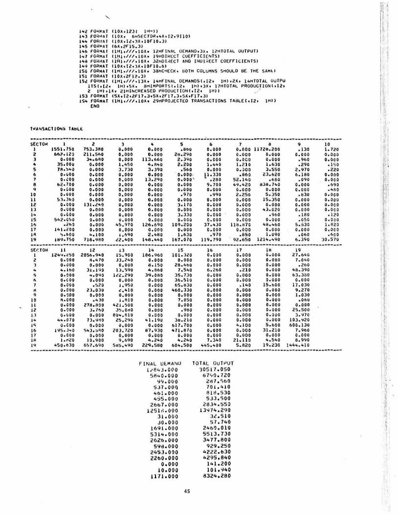
l~l fO~~AT 110Xo1231 JH-11 1~3 FOR~AT 11 0Xo 6HSECTO~t4Xtl2o91101 144 FORMAT 1!0Xt l l • lXt 10fl0.31 145 fORMAT 16X,2f l 5 . 31 146 FOR~AT IIHlo///,lOX• 12HflNAL 0£MAN0t3Xt l2HTOTAL OUTPUT) 1~7 FORMAT 11H1ol//tl0Xt 19HOI~~CT COEfflCI ENTSI 148 FORMAT 11~1,///olOX• 32HOI~ECT AND INUl~ECT COEFFIC IENTSI 1~~ FORMAT 110Xtl2t3XtlOF10.61 ISO fORMAT 11Hl,///olOX• 38HCHECKo 60TH COLUMNS SHOULD BE THE SAHtl lSI FORH4T C10X92f1?.. 31 152 fO~HAT 11Hlo///ol3X• l4Hf 1NAL DEHANOSCtl2• 1Hit 2X o l4HTOTAL OUTPU

lTSCtl2• lHloSXo 8HlMPORTSi ol2o 1Hit3X• 17HTOTAL PROOUCt10Nitl2• ~ 1Hit1Xt 21HINCREASED PROOUC II0N iol2 t IHII •

153 FORMAT C5X, I2•2f17.3t5X o2f17 , 3 t 5Xtf17o31 154 FORMAT CIH1o///,10Xt 29HPRO~ECT~D TRANSACTIONS TABLECol2• IHII

END

l,.A~SACTIO~S lAblf

-·------------------·-------------------------------------------------------------------------------------SEC TO,. 1 2 3 4 s 6 7 1:1 9 10 1 1551.150 753.3110 o. ooo o . ooo . llt>O o.ooo o. ooo 11721!. 200 .130 1.720 2 6f>('o12:J 2llo5f>O o.ooo o.ooo 2!l.290 o. ooo o . ooo o.ooo o . ooo o.ooo l o. ooo 3to.6110 o . ooo 11.3. 660 2 . 390 o.ooo o . ooo o.ooo ,960 o.ooo .. 35.0011 o. ooo 1,450 "tofl40 2.200 1,440 1.210 1.630 .290 . 1';;0 5 711.!141) o.ooo 3 . 730 .3,390 ,560 o.ooo O, ·JOO 3.550 2.970 .220 6 O•iiOO o.ooo o . ooo o . ooo 0 .ooo. ll. 330 .860 23.620 6,180 o.ooo 7 o. ~oo o.ooo o.ooo 13.290 o . ooo ' .. . 280 S2.140 . 680 .090 o.ooo 8 b2o100 Oo\100 o.ooo o .ooo o . ooo 9.700 4~.420 !l38.740 o.ooo . 690 q o. ooo o.ooo o.ooo o.ooo o . ooo o. ooo o.ooo o.ooo o.ooo .480

10 o.uoo o.ooo o.ooo o.ooo .970 .990 2.250 S.3SO . 830 o.ooo 11 !>3.J60 o. ooo o.ooo o.ooo o . ooo o.ooo o . ooo 15. 350 o.ooo o . ooo 12 o. ooo 131 . 240 o.ooo o . ooo 3.170 o.ooo o.ooo o. ooo o.ooo o.ooo ll o.ooo o.ooo o.ooo o.ooo o.ooo o.ooo o.ooo 43.020 o.ooo o.ooo I'+ o .~oo o. ooo o.ooo o . ooo 3. 330 o.ooo o.ooo .960 .180 .120 IS S42.G!>O o.ooo o.ooo o . ooo o.ooo o.ooo o.ooo o.ooo .oso o.ooo II, .2t>~ OoOU(I 4S,970 126. 690 109.200 37. 430 llll. 87() 48.460 5.:>30 1.820 17 l41.coo o.ooo o . ooo 0 . 0(10 o.ooo o.ooo o.ooo o.ooo o.ooo o.ooo ~~ ... 1100 ~.100 J,690 2.480 1.630 ,970 .8so 1.1!90 .060 .600 19 .1!9.750 718.980 ~2.400 148.440 167. 070 119.790 ' 92.650 1214.490 6.390 )0.570

----------------------------------------------------------------------------------------------------------SEr.TOH II 12 13 14 15 16 17 11! 19 I 124'<ocSO 20So.9<t0 1';;,900 186.960 101.320 o.ooo o.ooo o.ooo 27.640 2 o.ooo 8.470 33.240 .o.ooo o.ooo o . ooo o.ooo o . ooo 7.040 ) o.~oo o.ooo o.ooo 8.150 28.400 o.ooo o.ooo o . ooo .260 ~ 4.11>0 31.190 13.590 4.860 7.S40 6 . 260 .210 o.ooo 48.390 5 o.~oo ... 090 1a.290 3'9.060 3S. 730 o.ooo o.ooo o.ooo 63.3oo , o .~oo o.ooo o.ooo o.ooo 36.51() o.ooo o.ooo o.ooo o.ooo 1 o.ooo . 520 1.950 •0. 000 65.1!30 o.ooo .140 15. bOO 17.030 tl o.ooo 23.030 £,410 •0.000 460.330 o.ooo o.ooo o . ooo 9.270 9 o. ~.00 o.ooo o.ooo ·0.000 o . ooo o.ooo o.ooo o.ooo 1.030

10 'h000 ,4)0 1. 1110 o.ooo 7 , 050 o.ooo o.ooo o.ooo .060 11 o.ooo 278.800 421 . 500 o.ooo o.ooo o.ooo o.ooo o.ooo o.ooo 12 o. ooo 3.760 3S , Ot10 ·O. 000 .960 o.ooo o.ooo o.ooo 2S.500 1.1 0·~00 o. ooo 80~.810 o. ooo o.ooo o.ooo o.ooo o . ooo 3.970 I~ ~ ... o1o 73. 9110 25.29(1 41.1 90 3!l . 210 o.ooo o.ooo o.ooo 103,920 j<; o.coo o.ooo ii.OOO o.ooo 617. 700 o.ooo 4.100 5 . 600 600.130 16 19S. J .. o ':;43. :.110 203.720 67 . 930 471 . 870 o.ooo o.ooo 31.210 7,960 17 o.ooo o.ooo o.ooo o.ooo o.ooo o . ooo o.ooo o.ooo o.ooo lA 1. 11c0 10 . 900 9,690 4.240 4,240 7.340 21.110 4.S40 8,9<,10 19 450 . 630 6!.7 . 690 Sl:l5,490 22'9.580 604.500 445. 400 S. 820 19.230 1444, 410

----------------------------------------------------------------------------------------------------------FINAL Uf.MANU

ttf!4J.O(IO SA40 . 000

94.0(10 S .H. OOQ 461 . 000 4~5.000

2ob7.ooo 12Sli~ .ooo

31 . 000 Jo.ooo

1691 . 000 5314 . 000 262b.OOO s~a.ooo

2453.000 22oo . ooo

o.ooo 10.000

1171 . 000

45

TOlAL UUTi'UT 305 l"T.OSO

6740.720 2iH ,S60 701.410 13Hl . 530 SJJ , SOO

2834 .!;i5i) 13~74.290

3£.510 57.740

246'J.Ol0 5513.730 3477.800

929.250 4222. 630 4295 . 840

141.200 101.940

8324.280

·'' "Iii;

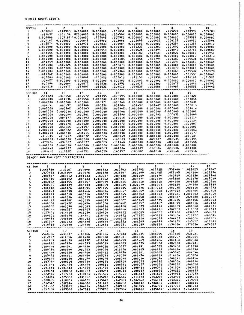
OI~ECI COEffiCIENTS

--------~----~--------------------------------------------------------------------------------------------Sfr.TU~ 2 3 4 5 b 1 II 9 10

1 .O'iOil,.~ .llOQ,.3 o.oooooo o.oooooo .001051 o.oooooo o.oooooo .839270 .ooj999 .029769 2 .uzt~oH .,)Jil5 .. 0";0(10000 o.oooooo .0345b2 o.oooooo o.oooooo o.oooooo o.oooooo o.oooooo 3 o.oooooo .005 107 •· o.oooooo .162045 .002920 o.oooooo o.oooooo o.oooooo .029529 0.000000 .. .OJ1l47 o.oooooo .ooc;o42 .006900 .00261:18 .00.!699 .000427 .000117 .008'120 .oo2S9o

i c; .oo2S74 o.oooooo . 012971 .004833 .00~684 o.oooooo o. oooooo .000254 .091357 .003810 b u.oooooo o.oooooo o.oooooo o.oooooo o.oooooo .021237 .000303 .001690 .19009!> o.oooooo 1 o.oooooo o . oooooo o.oooooo .018948 o.oooooo . ooo52!:i .018394 .000049 .002768 o.oooooo

I R .uo~<J '.)'j 0.000000 o.oooooo o.oooooo o.oooooo .018182 .017435 .01>0020 o.oooooo • Oll9SO 'I o.oooooo o.oooooo o.uooooo o.oooooo 0. 00000(1 o . oooooo o.oooooo o.oooooo o.oooooo .OObJIJ

10 o.oouooo o.oooooo o.ooouoo o.oooooo .oollt!S . 001856 . 000794 . 000.38) .025531 o.oooo oo 11 .oo114'1 o.oooooo o .oooooo o. oooooo o.oooooo o.oooooo o . oooooo . 001098 o . oooooo o.oooooo ! !l o.oooooo ·01'1321> o . oooooo o .-oooooo ·003873 o.oooooo o . oooooo o.oooooo o . oooooo o.oooooo

I l1 o.oooooo o.oooooo o.uooooo o.oooooo o.oooooo o.oooooo 0·000000 .003079 o.oooooo o.oooooo 14 o.oo ooo~ o.oooooo o.oooooo o.oooooo .004061:1 o.oooooo o.oooo oo .000069 .oo5SJ7 .002078 l'i . • 0 1771>2 o.oooooo o.oooooo o.oooooo o.oooooo o . oooooo 0 · 000000 o . oooooo .0015311 o.oooooo 111 ·00000'>1 o.oooooo •IS9862 .1801:>22 .1 33410 .o7o159 ·041936 ·003468 .1701 02 .o31521 l 17 -~0 .. '>27 o.oooooo o.oooooo o.oooooo o . oooooo o . oooooo o.oooooo o.oooooo o.ooooo o o.oooo oo , Ill oOOOIII4 ·00060 .. ·00'>877 ·003536 ·001991 ·00Hil8 ·000300 .000078 .oo1o41:> .010391 E ~~ .ooo~la ·10-::>!!77 .077d97 ·211631 .204UO .224531:> o03l686 .081>909 .1 ~6555 .52'i442 i --------------------------------------------------------------------------------------------------------- I ~ErT0!-1 11 12 13 14 15 }() 17 18 19 • ~

I . 507<!23 .37Jo'i8 .004'572 .2Ci1195 .023995 o.oooooo o.oooooo o.oooooo . 003320 2 1).000000 .001 511> .00955o o.oooooo o.oooooo o.oooooo o.oooooo o. oeoooo .000846 J o.oooooo o.oooooo 0.000000 .008771 . 00 1:> 740 o.oooooo o.oooooo o.oooooo .000031 4 . 0011>'>~1 . ooSo'i7 • oo:wob .005230 .0017t!6 .001457 .001487 o.oooooo .005813 ') o. oooooo .oo0742 .035 163 • 042055 .00841>2 .. o.oouooo o . oooooo 0 . 000000 .0076l<t b o.oooooo o.oooooo o.oooooo o.oooooo .008646 o.oouooo o.oooooo O.OOOCiOO o . oooooo 7 o.oooooo .0000'1 .. .000561 o.oooooo .015590 o.oooooo .. 000992 .153031 .00204() II u.oooooo .004117 .ooo~><t3 o.oooooo .1 09015 o. oooooo o.oooooo 0.000000 .001114 Q o.oooooo o.oooooo o.oooooo o .oooooo o.oooooo o.oooooo o.oooooo o . oooooo . 000 124

11) .u~3z r,<! .000078 . 000520 o.oooooo .001670 o.oooooo o.oooooo o.oooooo .000007 II o.oooooo .o5o5&S .1211'17 o.oooooo o.oooooo 0.000000 o.oooooo o.oooooo o.oooooo 12 o.ooooou .oo~6R2 .Cii OOfl7 o. oooo·oo . 000232 o . oooooo o.oooooo 0 . 000000 .003063 13 o.oooooo o.oooooo • .!31414 o.oooooo o.cooooo o.oooooo o.oooooo o . oooooo • 0004 77 14 .~17'11S • 0 1)417 • 007272 .044326 .009049 0.000000 o.oooooo o. oooooo .012484 } <; ~. 000000 . o.oooooo o.oooooo o.oooooo • h6283 o.oooooo .029037 . 054934 • 0720'14 111 .07'1401> .OYt!Stl7 .05A5 77 .094625 .111748 o.oooooo o.oooooo . 30o l60 . o oo-t~b

11 o. oooooo o . oouooo o.uooooo o.oooooo o.oooooo 0.000000 o.oooooo Q.OOOOOO o.oooooo In .ouo7 .. o .oo1<t77 .002711() .004563 . 001004 • 001709 .14<;504 .044536 .001080 19 .1 8Jiti2 .1192112 .11>11351 .247059 .143157 .103682 .041218 .1dbb40 .1735 1b

-------------------------------------------------------------------------------------·----------------01-<t:C I ANO l~UIWECT COlfflCIENT<;

----------------------------------------------------------------------------------------------------------SEr.TUH 1 i! 1 " 5 b 7 1:1 9 · 10 1 1. 01>2'1211 .1331 S7 .002690 .oot.723 .0}3943 .023792 • 017925 .952460 . 018623 .057267 ~ • •)?3~33 I.03SJ<;9 .OOOb 1b • 000778 .036367 . 0!>0899 . 00 0465 .0211>45 . 0041 61> . 002270 3 .ooosn .oo5~>12 1.001133 .163937 . 004121! .001009 .OOOI7Q .000709 .0 :14:236 .001948 .. .OOI<ol!> .c;Oll~2 .006133 1.010052 .004731 .00 .. 774 .00i)83Q .002155 . 01.0676 . 007•0011 '; .0031U • 00 17>;5 . 0141 57 .009t!39 1.0035h . 0028 10 . 0005 18 .oo .. z9o . 095725 .010940 to .oooc21 .ooo139 . 00010) .000259 .ooo22~t 1.021979 .ooo3~3 .002129 .194590 .0021 £19 1 .ooO«>Ia .oo072t. .001594 . 021445 .001505 .oo~o76 1. 019013 .001075 .00511~ .004372 ~ .oo:i1 .. o .007.2'1" .OOl,.bb .003914 . 003247 .023259 .01 9558 l. CI:>'< b l l • OOUS4 .0206Gtl 9 .ooOOOJ ·000018 .ooool6 . 000039 .000045 .oooos3 .000013 . 000021 l . OOOi:6J .O Otl3 ')19

l() .OOOO!:>J .0000]6 .0000)9 .000079 .001237 . 001 951! • 00082b .000487 .026080 1.000347 II •'JOI!!~S ·001lt12 ·000039 · 000093 ·000327 .000149 ·OOC075 .003415 .ooo 1~& .oo0293 12 .oooS3t! o0Z0472 .ooo454 .001020 .oo5462 .000957 ·0001()7 .0001:199 .001 1> 16 .oo2 172 n .uouo n . oooo<ta .000063 ·000210 .OOOlllB .oo~279 ·000110 .00431>9 .0002&b .OOOSOI 14 .oouS<!H •OOllZ7 .oot8o3 o00 .. 399 . 0082b4 .oo .. 2o3 · 000711 .002263 .011 5211 . oll b77 l'i . cz3~31 •01 .. '111:! ·011024 .026904 .024232 .026005 ·004b52 .031420 .034227 • 05d 920 1o .01)4100 .oo5o7'i ol of-74 1 . 2 }1>441> .140 732 .0771!32 .o .. 3923 o00'llo54 . 211 752 .04B67b 17 •<'0 .. '1 111 .01)01:>16 . ooool2 .oooo31 _..oooo~>5 .00011 0 .ooo083 . 004'+07 ·000086 .oo~26:;

18 .ooiOb" •OOtG62 · 001.675 .oo5574 -~ .oo2832 .OOl549 •00049R .001235 . o ~3952 . oll991 19 . 0\1:171 5 ol4c? 788 . 1( 4786 . 312670 . 28 1331 . 30008 <,) . 050259 .1341>84 • 376334 .67 .. 187

---------------------------------------------------------------------------------------------------------Sfr.TOR 11 12 13 14 15 11> 17 lli 1<;. I .541:1~21> . 435207 oiO<l76 1:> .231264 .15941:13 .002634 . c o8355 .017825 .025021 z . ot21:>t!7 .o111>r,t:. .017400 .007201:1 .004281 .000216 .oo0330 .000 797 .002064 3 . OOllb9 .OO}bj~ .001932 .OIOQ98 .008959 .000'+69 .000764 .001128 .002200 4 .00 .. 1112 .00773 .. .00<~093 .008319 . 00421!3 .002275 .002338 .002630 • 00770 I 5 .0041>1>4 .004) 41 .04Qil36 .048055 .013337 .001191 .001 385 .003460 .011 290 0 • oou ll•> .000244 .000303 .000330 .0101128 • 000105 .000493 .00091 .. . 000990 7 .1)01 .. ~4 .001528 .00?'100 .002412 . 0199711 .000801 .026565 . 165S42 . 0046'11>

~ .. • 00~452 .OOt!bOl .OO'i454 .oo5on .140039 . 001474 .0068 19 .014404 .013920

! ~ .oooc,;~ .oooo26 .000054 .000045 .000049 .000016 .000014 .000041 .ooo1 ~1> 10 . ooJ324 .000300 .oo131~> .000121> . 002109 . 000023 .000116 .000304 .000216 1l 1.001041 .o5 t .. 30 .15111>60 .000511 .000561 .000037 .000051 .000128 .000358 12 .~01061 1.oots u .014736 .001425 .001208 .000411 .000349 .001004 .003~32 ll .ooot•H .ooo1c;2 1.301327 .000241 .000721 .000087 . 000093 .000250 .0001:128 1 .. .ozz~84 .o177~>3 .011!13 .. 1.051594 .01479() . 001817 .001897 .004978 .017371:1 I S .01J347 .025333 .031922 .035243 1.196564 .011163 .053200 . OYJ'I95 .105740 1'> . OBt!092 ·110839 .106035 .l15t>72 .142)81 1.002892 .056181 . 340379 .01924() 11 .oo2~40 .oo2014 .ooosos .001070 .000738 . 000012 1.000039 .000082 . 000116 11§ .oo1 -.5o • OOJOQS .0041124 .006090 .002188 .001979 .1567910 1. 047796 .001743 19 .2'.)7134 .18~588 .Jto7011 • 355286 .257334 .13002d .105669 . .310237 1.244605

------·---------------·-----------------------------------------------------------·---------------------46

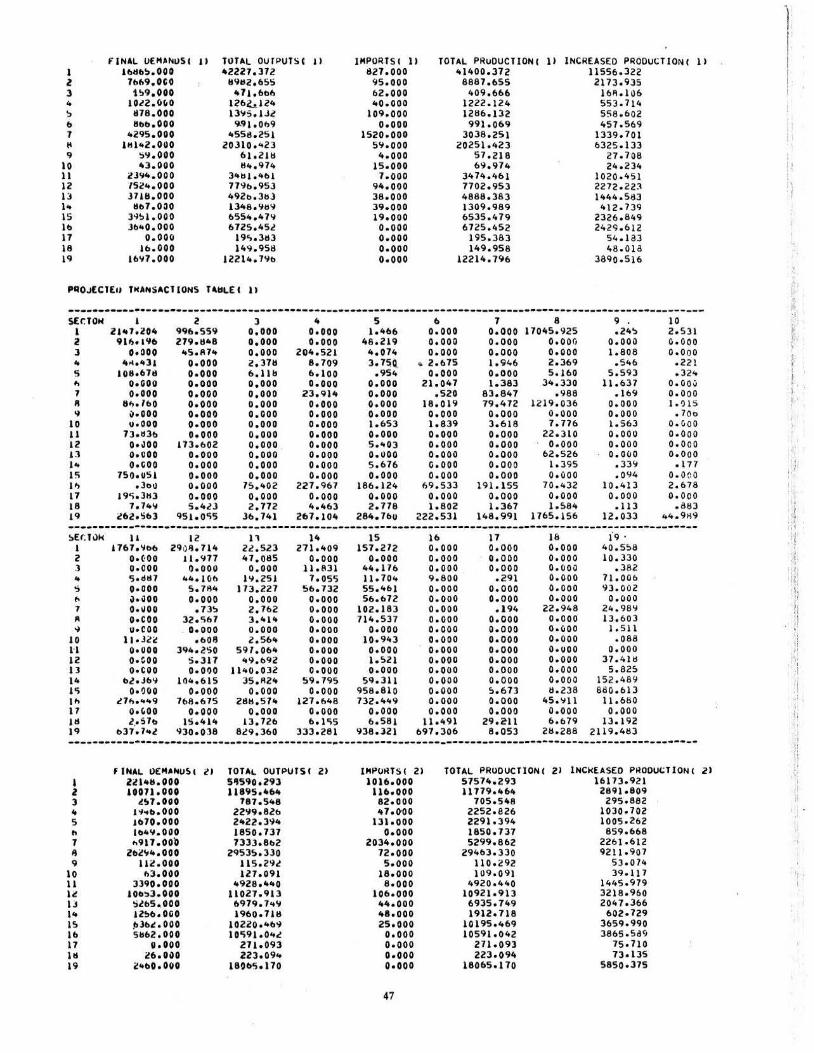
1 l 3 4

~

b 1 II 9

10 11 12 ll 1 .. 15 1tl 17 18 19

fiNAL OEHANOSC 1• 1btlb!).000

7t>f>9.0CO i;9.000

u.n.c.r.o 1178 . 000 llt.b.OOO

to29S.OOO 1111to2.000

~9.000 43.000

21~.ooo

'ISi!to.OOO J1lii.OOO 111>7.0~0

3~!>1.000 l tltoO.OOO

o.ooc. 1b.OOO

1697.000

TOTAL OUIPUTSC 11 4U27.372

ll'i112.6SS 471.601!>

126a.,124 139S.1Jl 9.9}.0f>9

.. 5ss.ZS1 20310 . .. 23

61.2111 ll<t.97<o

3"b'·'""' 77'lb.95J 492bo3bJ 1348.9119 6554.479 6725.45.!

19').3113 149.958

12214.7Yt.

PltOJECTEU TNA .. SACllONS HilLE I 11

1MPORTSI 11 1127.000

95.000 62.000 40.000

109.000 o.ooo

152o.ooo 59.000 ~t.ooo

15.000 7.ooo

94.000 38.000 39.000 19.000

o . ooo o.ooo o.ooo o. ooo

TOTAL PRuOUCTIONC 41400.372

8887.655 409 . 666

1222.124 12116.1).2 991.069

3038.2!;} 20251.423

5 7.218 69.974

3474.'t61 7702.953 4888. 38.3 1309.989 6535.47'9 6725.452

195.383 149.958

12214.796

II INCREASED PRODUCTION( 1• 11556.322 2173.935

1611 .106 553.714 558 . 602 457.569

1339.701 6325.133

27.708 24.23<t

1020 . 451 2272.22:\ 1444.583 412.7) 9

2326 . 849 2429.612

54 .1 83 48.018

3890 . 516

------·---------------------------------------------------------------------------------------------------SEC: TON 1 z J .. 5 ,., 1 ,. 9

10 11 1Z 1l , .. 15 I'> 17 18 J9

~Er: Tuk J 2 .l 4 'j

to 1 A 'i

10 1'1 12 ll 14 J<; 1" 17 111 19

1 2tU.l!04

91f)o1Y6 o. ooo

4>1.to3J 10IIo6711

o.ooo o.ooo

ltl>olbO ;,.ooo u.ooo

73oll3b o. ~oo o.ooo o.coo

750oU51 .Joo

19'>.3113 1 . 7to9

l6lo':ib3

ll &767.':106

o.~oo o. ooo 'iodtl7 0·000 oh ~OO o.uoo o.coo U•COO

ll.Jli! 0• 000 o. coo o.coo

tlloJb9 0·~00

~71) ... 49 o.c.oo l .• S 1to

b37. 7 .. l

2 991>.559 279. 11•8 .. 5.117<o

o.ooo o.ooo o . ooo o.ooo o.ooo o.ooo o.ooo o.ooo

113.602 o.ooo o.ooo o.ooo o.ooo o.ooo S.4lJ

qs, .oo;s

12 29:)11. 714

11.917 o.ooo

..... JOb 5.7~4

o.ooo .73~

32. 567 . o. 000

.608 3'14. lSO

s.311 o.ooo

104.615 o.ooo

766.675 o.ooo

15 .414 930.038

3 o.ooo o.ooo o.ooo 2 .3711 6 .11 11 o .ooo o.ooo o .ooo o.ooo o.ooo o.ooo o.ooo . o.ooo o.ooo o.ooo

7:>.<t02 o.ooo 2. 772

Jb,741

11 U.S23 "1 .oa5

o.ooo 1'1.251

173.227 o.ooo 2.762 3.411t o.ooo 2 . 564

597.064 <o9.b'il

1 h0.032 35.112<t

o.ooo 288.57<t

o.ooo 13.726

829.360

4 o.ooo o.ooo

204.521 8. 709 6.100 o . ooo

23.911t o.ooo o.ooo o.ooo o.ooo o. ooo o.ooo o.ooo o.ooo

227.967 o.ooo 4.463

267. 104

14 271.409

o.ooo .11.831 1.oss

56.732 o.ooo o.ooo o.ooo o.ooo o.ooo o. ooo o.ooo o.ooo

59.795 o.ooo

127.6to8 o.ooo 6. 1<;5

333. 281

5 1.466

48.219 4.074 3.75,~

. 954 o.ooo o.ooo o.ooo o.ooo 1.653 o.ooo S.to03 o.uoo 5.676 o.ooo

186.124 o.ooo 2 . 778

284.7611

15 157.272

o.ooo 44.176 11.70't 55.1tb1 56.o72

102.183 714.537

o.ooo 10.91t3

o.ooo 1.521 o.ooo

59.311 958.81 0 732.1t49

o.ooo 6 . 581

938.)21

b o.ooo o.ooo o.ooo

.. 2.675 o.ooo

21.047 .520

18.0 19 o.ooo 1.839 o.ooo o.ooo o-.ooo G. ooo o . ooo

69.533 o.ooo 1.802

222.531

16 o.ooo o.ooo o.ooo 9.800 o.ooo o.ooo o.ooo o.ooo o.ooo o.ooo o.ooo o.ooo o.ooo o.ooo o.ooo o.ooo o.ooo

11 .491 b97.306

7 o.ooo o.ooo o.ooo 1.946 o.ooo 1.383

83.847 79.472 o.ooo 3. 618 o.ooo o.ooo o.ooo o . ooo o . ooo

191. 155 o.ooo 1. 31>7

148.991

17 o.ooo o.ooo o.ooo

. 291 o.ooo o.ooo .194

o.ooo o.ooo o.ooo o.ooo o . ooo o . ooo o. ooo 5 . 673 o.ooo o . ooo

29.211 8.053

8 17045.925

o.oor, o.ooo 2 . 369 5.160

34.330 .988

1219.036 o.ooo 7. 716

22.310 o.ooo

62.526 1.395 o. ooo

70.<t32 o.ooo 1.584

1765.156

18 o.ooo o.ooo o.ooo o.ooo o.ooo o.ooo

22 . 948 o.ooo o.c.oo o.ooo o.uoo o.ooo o.ooo o.ooo 11.238

45. '11 1 o.ooo 6 .t.79

211.288

9 .24~

o.ooo 1.808

. 546 5.593

11.637 .1 b9

o.ooo o.ooo 1.563 o . ooo o.ooo o. auo

.33'1

.094 10.413

o.ooo .1 13

12.033

19 . 40.558 10 . 330

.382 71 . 00b 93. 002

o.ooo 24.989 13. 603 l.Sll .o8a

o.ooo 37.4111

5.825 152.489 880.b13

11.660 o.ooo

13.1 92 2119.483

10 2.531 o.ooo o .ooo

. 221

. 324 o . ooo o.ooo 1. 015

• 70o o . c. oo o. ooo o.ooo o.ooo

. 177 o. ooo 2.678 o. ooo

. Bt13 4't. 9H9

-------~---·---------------------------------------------------------------------------------------------

f IHAL U£ .. MIIUSI l l TOUt. OUTPUTS ! 2• IMPU~TSI 2l TOTAL PRUDUCTIONC Zl lNCHEASEO P~ODUCTlONI

' Zi!ltoii.OOO 511590.293 1016.000 5757~.293 16173.921 2 uou.ooo 11895.46 .. 116. 000 11779o46<o 289& .809 3 l!t7.000 787.51t8 82.ooo 705.548 295.882 4 1-i.,o.OOO 2299.8lb to1.0'00 2252.826 1030.702 5 !b70.000 21t22.3'J<o 131 . 000 2291.394 1005.262

" lbto'I.OOO 1850.737 o.ooo 1850 .737 859.668 1 ... 917.00~ 733J.8t12 2034.000 5299.862 2261.612 II Zlli!Y4.000 2953!>.330 12· 000 29463.330 9211·907 9 u z .ooo 115.29~ 5.ooo 11 0 . 292 53 . 074

10 t>l.OOO 127.091 18.000 109.091 39 .117 11 3390.000 .. 928.4110 a.ooo 4920 . 440 1445 .979 ll tob~l.OOO 11027.913 106·000 10921.9 13 3218 . 960 IJ S.!b5 •. 000 6979. h'l 44.000 6935.749 2047.366 1• J2!tb.OOO 1960 . 7111 48.000 1912.118 602.729 15 l!lbt.OOO 10220 · '-b'l 25.000 10195.469 3659 .990 111 51162.000 uo;91.o .. ~ o.ooo 10591. ~42 3865 . Sa9 11 u.ooo 271.093 o.ooo 211.093 75.710 111 26.000 223.094 o.ooo 223.09~ 73.135 19 l"t10.0(10 180b5.l70 o.ooo 18065 .170 585o. J 75

47

z•

1 I I I

i'

.,

• J . ,,·r '

·I 1 · 11

•l ';

i't !

i ,.,

·.1 :!

!( .

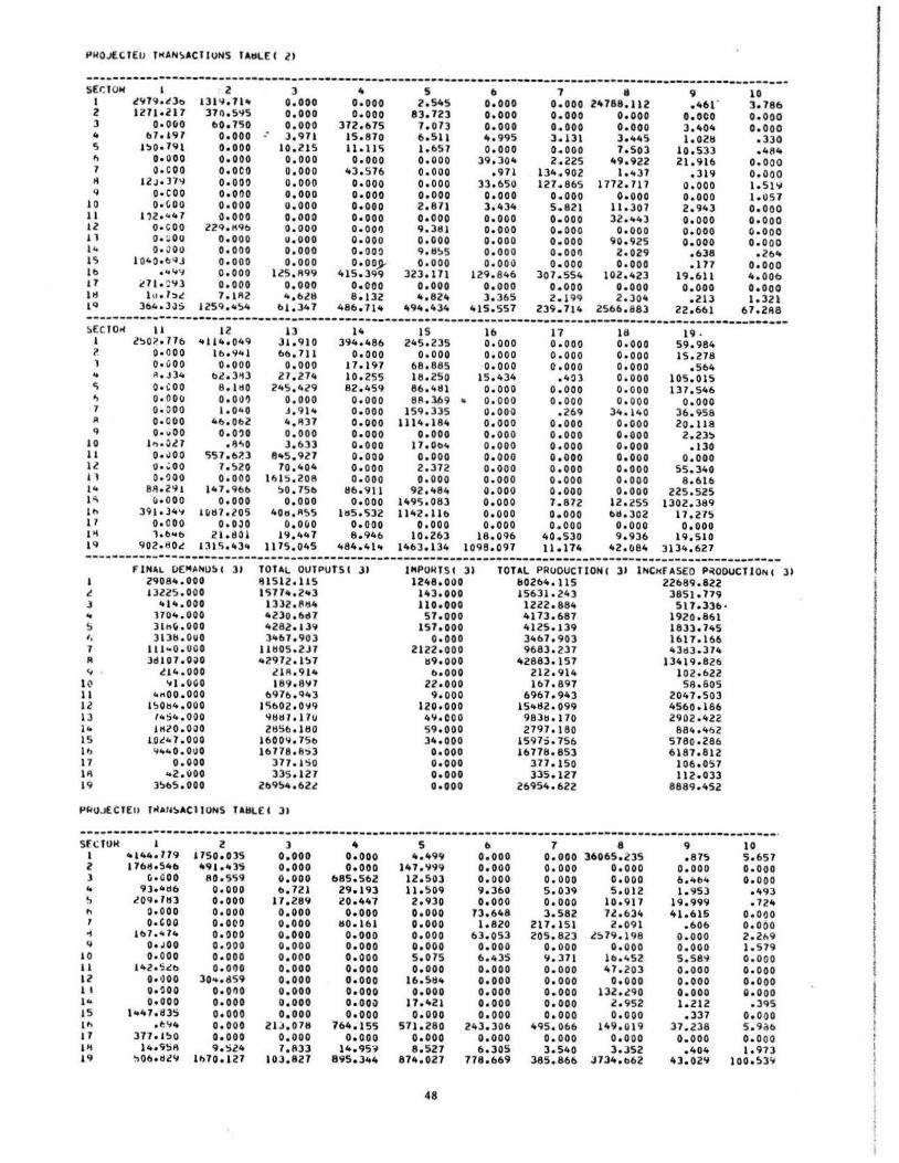
PWOJECTEU THAN~ACTIONS TA~LEI 21

----------------------------------------------------------------------------------------------------------SEt; TOW I 2 3

" 5 ~

7 14 Cj

10 11 12 !l ... I S 1b t1 l d l q

1 <!'179. c!lb 127lo2l7

o. ooo b7ol97 1~0. 7'11

o.ooo o.coo

12JoJN o. coo o. ,oo

l n · '-"1 O•COO o.~oo 0· ;)011

10'-0· bQJ . 4'-1~

~7 1 . ~ '13

l u o1':><! 36,t..3olS

l 131<~.7 1-3711 .5'15

f>0.750 o. 000 •• o.ooo o. ooo o.oco o.ooo o.ooo o.ooo o.ooo

22'1.1i'lb o.ooo o.ooo o.ooo o.ooo o.ooo 7.1112

1 25'1.4~4

3 o.ooo o.ooo o.ooo 3.971

10.2 15 o.ooo o.ooo o.ooo o.ooo o.ooo o.ooo o.ooo u.ooo o.ooo o.ooo

l l5.A99 o.ooo ... bl8

bl .347

4 o.ooo o.ooo

372.f>75 15.870 11.115 o.ooo

43.576 o.ooo o.ooo o. ooo o.ooo o. ooll o.ooo O.OO!l o.oo_p..

415. 399 o.ooo 8 . 132

48b.71<t

5 2.545

83.723 7 .on 6.511 l.b57 o.ooo o.ooo o.ooo o. ooo 2 . 871 o.ooo 9.3111 o.ooo 9.11!>5 o. ooo

323.171 o. ooo ... 824

494.434

f> o.ooo o.ooo o. ooo lt. 995 o.ooo

39.304 .971

JJ. bSII o.ooo 3.434 o.ooo o. ooo o.ooo o.ooo o. ooo

129.846 o.ooo 3.365

1t1S. 557

7 o.ooo o.ooo o.ooo 3.131 o.ooo 2.225

134 . 902 127.865

o.ooo 5.821 o. ooo o. 000 o. ooo o. oon o. ooo

307.554 o.ooo 2.199

239.71 4

• 21t788. 112 o.ooo o.ooo 3o41t5 7o503

lt9.922 1.437

1772.717 o.ooo

11.3o 1 32 . .. 43 o.ooo

90.925 2.029 o.ooo

102. 423 o.ooo 2 . 304

2566.883

9 olo61 ·

o.oco 3.404 1 . 0211

10.533 21.916

. 3 19 o.ooo o.ooo 2.943 o.ooo o.ooo o.ooo

. 638

.177 19.611 o.ooo

.213 22. 661

10 3. 786 o. ooo o.ooo .330 .484

o.ooo o.ooo 1.51'11 lo057 o.ooo o.ooo o.ooo o.ooo

. 2f)4 o.ooo 4. 0oo o.ooo 1o32l

67 . 2'18

----------------------------------------------------------------------------------------------------------!>ECTO,. 1 ?. l .. c; ., 7 A q

10 11 1l 11 1" I '> 1h 17 1'1 19

11 2':>0?. · 176

o.ooo OoGOO AoJ34 o. -:oo o. oou o. ooo o. ooo o . .. oo

l '> · ~l1 o • .>oo 11 · ~00 Oo? OO

811. 2'11 ~.ooo

391.34'1 o.ooo l.b .. b

902otl0<!

12 .. 111o.Qio9

1b o94 1 o.ooo

bl o3>13 8 .1110 o. o\l? 1. 040

41). 062 0.0?0 .~'>0

557.6?.3 7. 520 o.ooo

l<t7.96b o.ooo

HtH.205 o. oJo

2 1.1!0 I !31 5 .1o)4

13 3 1.910 btl . 711 o.ooo

27 .27/o 245 ,429

o.ooo J . 91 .. to.ll37 o.ooo 3. 633

8<t5.927 70 .40't

16 15 . 206 !10.756 o. ooo

loOo. ASS o.ooo

19.to47 1175,045

llo 394 .1o86

o.ooo 17.197 10.255 62.1o59 o.ooo o. ooo o.ooo o.ooo o.ooo o. ooo o.ooo o.ooo

116.911 o.ooo

1115.532 o.ooo 6.946

484.41'+

I S 245.235

o. ooo 68.885 18 . 250 86.4111 811 . 369 ..

159.335 1114.184

o.ooo 17 • Ob4 o.ooo 2.372 o.ooo

16 o.ooo o.ooo o.ooo

15 .434 o.ooo o. ooo o.ooo o.ooo o.ooo o.ooo o.ooo o.ooo o.ooo o.ooo o.ooo o.ooo o.ooo

92. 484 149S.083 lllo2 .1lb

o.ooo 1o.263

1463 .134 18.0'16

1098.097

17 o.ooo o.ooo o.ooo

.403 o.ooo o.ooo

. 269 o. ooo o.ooo o.ooo o.ooo o.ooo o.ooo o.ooo 7 .• 872 o.ooo o.ooo

40.530 11 .174

111 o.ooo o.ooo o.ooo o.ooo o.ooo o.ooo

34.11o0 o. ooo o.ooo o.ooo o.ooo o.ooo o.ooo o.ooo

12.255 611. 302 o.ooo 9. 936

42.084

19 . 59.984 15 . 278

. 564 105.015 137.5<t6

o.ooo 36. 958 20. 118 2.23~

.130 o.ooo

55. 340 8.61b

225.525 1302,389

17.275 o.ooo

19.510 3134.627

---------------------------------------------------------------------------------------------------------I l J .. , '· 1 A ..

1(1 II 12 13 14 IS 11> 17 I ll 19

F INAL OEM~NU;( )I 2'108<t.OOO I JUS.OOO

414.000 1704.000 Jlhli .OOO 31311. 0110

111 .. 0 . 000 3dl07 . 0i)0

<!lto . OOO .. I . OGO

4!<00.000 I!>Ob4 . 000

, .. 54.000 1Kl0 . 000

1.0<!<•7 . 000 li"40.01)0

o.ooo .. 2 . \100

3!>1>5 .000

TOTAL OUTPUTS! 31 ~1512.115 1577 ... 2 .. 3 1 332 . tl~4 lo230 . 6d7 '-282.139 31o67 . 903

l1t105. 2J7 .. 2972 .1!>7

l111 . 9 14 189o8Y7

6976.'143 1S602.0Y9

98117 .17V 21!56 .1110

16009 . 751> 16778.8S3

317 . 150 335.127

Z69S<o.62l

l'kOJECTEII foiAI4~.ACllON5 TAHL( I 31

IMPOWTSI 31 1248 . 000 143.000 110.000

57. 000 157.000

o.ooo 2 122.000

119.000 t..ooo

22.000 9.000

120·000 49oOOO 59. 000 34. 000 o.ooo o.ooo o.ooo o.ooo

TOTAL PROOUCTIONI 110264.115 15631.243

1222 . 884 4173 . 687 4125 .139 3467. 903 9683 . 237

lt2883. 157 212 . 914 ib7 . 897

6967. 943 1541!2.099

98311 .170 2797 . 180

1597:i . 756 16778.853

377 .ISO 335. 127

26954.622

31 lNC~F.ASEO P~OOUCTIONI 31 22!189.822

3851 .779 5 17 . 33b.

1920 . 861 1833.745 1617.166 lt3d3.371o

13419.826 102 .622

58. 605 2047.503 4560 .186 2902 .422

884.4f>2 5780 - 286 6 187 . 812

106 . 057 112.033

8889 .1o52

---------------------------------------------------------------------------------------------------------· Sft:TOH 1 2 ) lo !> , , oj

(j

10 II 12 1 I 14 I S l h I 7 ,,. 19

I 4 144.779 l761lo51ob

r..ooo 9).1o ll6

l0'1o7tl) o.ooo o.coo

H>7.474 O•JOO o.ooo

142o':ilb O• •JOO o .~oo o.ooo

}41t7oll3S . ~ .... 377. 150 }4.9'511

!>06otll'l

2 1750.035

491 ... 3'5 80. 559 o.ooo o.ooo o.ooo o.ooo o.ooo o . ~oo o.ooo 0.01)0

30 ... t!59 o.ono o.ooo o.ooo o.ooo o.ooo 9.Sl4

1b70. 127

3 o.ooo o.ooo o.ooo b . 721

l7 . 28CJ o.ooo o.ooo o.ooo o.ooo o.ooo o. ooo o. ooo o.ooo o.ooo o.ooo

2D. 0711 o.ooo 7.833

I 03.827

4 o.ooo o.ooo

085. 562 29.193 20 .447 o.ooo

110.161 o.ooo o.ooo o.ooo o.ooo o.ooo o.ooo o.oo~ o.ooo

761t.l55 o.ooo

1<t.95'j 895.3<tlo

5 to.499

147.11\19 12.503 11.509

2. 930 o. ooo o.ooo o.ooo o. ooo 5.075 o.ooo

16 . 51!1t o.ooo

17.1t2 1 o. ooo

571 . 280 o. ooo 8.527

874.027

48

b o.ooo o. ooo o. ooo 9.360 o.ooo

73.648 1.820

63.053 o. ooo 6.435 o.ooo o.ooo o.ooo o.ooo o. ooo

243. 306 o.ooo 6.305

778.669

7 o.ooo o.ooo o.ooo 5.039 o. ooo 3.582

217.15 1 205. 823

o.ooo 9. 371 o.ooo o.ooo o.ooo o.ooo o.ooo

495. 066 o.ooo 3.540

385.866

8 36065.235

o.ooo o.ooo 5 . 0 12

10 . 917 7l.634

2.091 l579.198

o.ooo 1b.<o52 lt7. 203 o.ooo

132.l90 .2.952 o.ooo

149. 019 o.ooo 3.352

J731t.b62

9 .875

o.ooo 6 .464 1.953

19.999 lt1 . 615

.606 o.ooo o.ooo 5.58'1 o.ooo o. ooo o.ooo 1.212

.337 37 . 238 o. ooo

. 404 lt3.029

10 5 .657 o.ooo o. ooo

o't93 .724

o.ooo o.ooo 2. 2t.9 1.579 o.ooo o.ooo o. ooo o.ooo

.3'15 o.ooo 5 .9a6 o. ooo 1.973

100 . 53'1

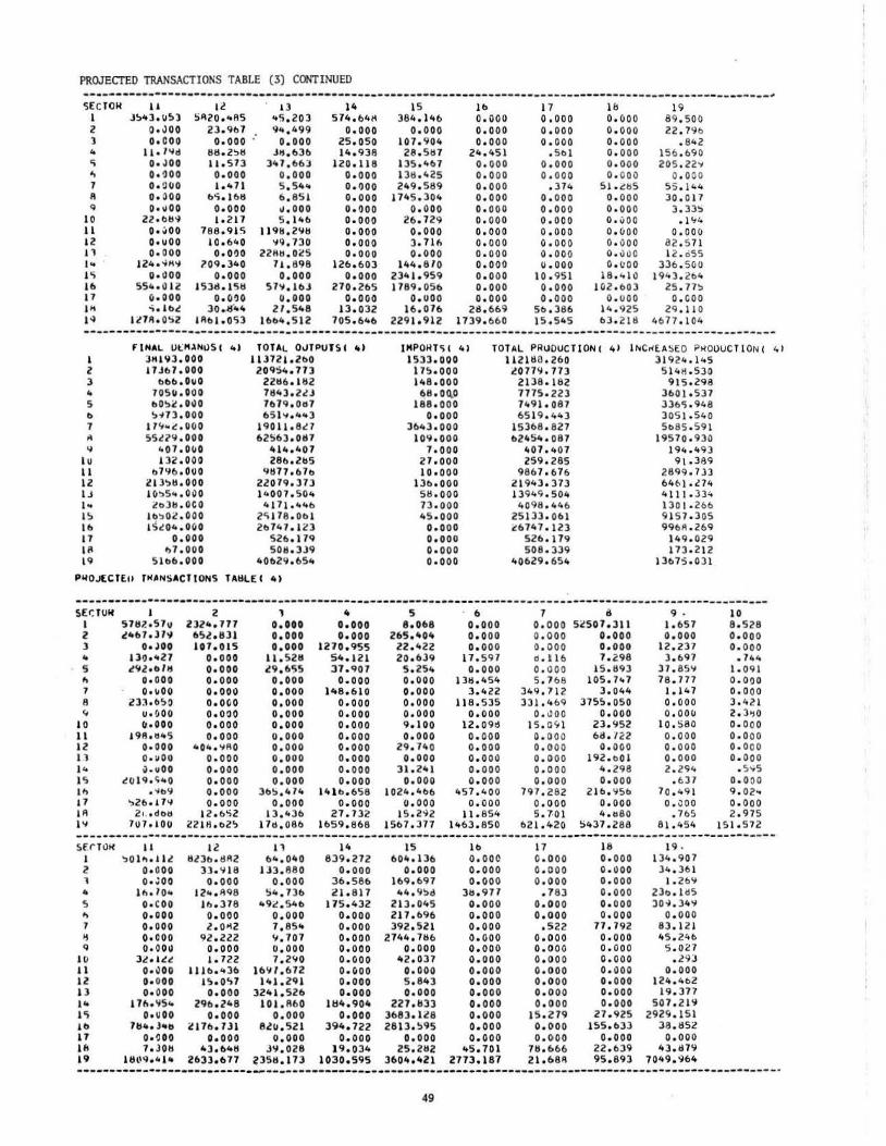
PROJECTED TRANSACTIONS TABLE (3) CONTINUED

--·------------------------------------------------------------------------------------------------------; SECT OW 1 2 l .. 'i ., 7 ft q

10 11 12 11 14 1'; lb 17 IH I~

ll l!><tl.\1!1)

o.JOO o.coo

11· 7'-ld o. JOO Oe'lOO o. ~~~o

o.ooo 0 · ~00

l!Z·bll~ o.;,oo 0·1100 o.ooo

12iedll'l O· llOO

554.1) 12 (1 . 000 "ielb~

1l111.o~2

ll !iA20e41\5

23. 9t>7 o.ooo :

tlt1.2~tl

11.51) o. ooo ··-71 b'i.1btl o.ooo 1·2 17

788.915 10.640 0.0')0

?09. Jie0 o.ooo

15311.l<;tJ o.O'lO

3o • .S~oie 1At>l.05l

I )

.. 5 . 203 9 ... '-99 o. ooo

Jll.63b 3ie7.b6:t

o.ooo 5 . 5'-" 6 . 851 .... ooo 5 .146

119t1.2Ytl 119.730

221111 . 0~5 71.898 o.ooo

57\l .lbJ o.ooo

21.5'-8 16t>ie.512

14 574.64~

o. ooo 25.050 14.938

120.118 o.ooo 0.1)00 o.ooo o.ooo o. ooo o.ooo o.ooo o.ooo

126. 603 o.ooo

270.2b5 o. ooo

13.032 705.6'-6

I S 384 .1«6

o.ooo 107.904

28 . StJ7 135.467 131!.425 249. 589

1745.304 o. ooo

26. 729 o.ooo 3.71f> o.ooo

144.810 23'-1 . 959 1789.056

o.uoo 16.076

2291.912

1b O.i)QO o.ooo o.ooo

24.451 o. ooo o.ooo o.ooo o.ooo o.ooo o.ooo o.ooo o.ooo o.ooo o.ooo o.ooo o.ooo o.ooo

28.669 1139. 660

17 o.ooo o. ooo o.ooo

. St> 1 o.ooo o. ooo

.374 o.ooo o.ooo o.ooo o.ooo o. ooo o.ooo u.ooo

10.95 1 o.ooo o.ooo

St>.386 15.545

1& o.ooo o.ooo o.ooo o.ooo o.ooo o. ooo

51.i::t15 o.ooo o.ooo 0.1)00 o.ooo o.voo 0 . 1)1)0 o.uoo

18.411) 102 . 603

o.uoo 14.925 b3.218

19 89. 500 22 . Nl)

. 842 156.690 205.22'1

o.ooo 55 . 144 30 . 0 17 3 . 33~

.1'14 o.oou

82 . 571 12 . d55

336.5uo 1943. 21)4

25 . 7h o. ooo

29 .1 10 4677.104

----------------------------------------------------------------------------------------------------------1 2 3 4

5 I)

7 A 'I

1u 11 12 lJ 1'+ 1!> 16 17 II\ 19

FINAL U~M~N~S C 41 JKI93.000 17 J6 7 . 000

bb6.0110 705(1.01)0 bO!>~.OilO !>.0) . 000

17 .... ~.000 S5UY . OOO

.. 07 . 0\10 !32 . 000

b7'16.0UO lll~ti.OOO 1(1!>5 ... 0 1)0

<!o3ti.OCO lt>':>O~ . ooo IS~04 .0CIO

o.ooo ~7 . 000

51t>6 .000

TOTAL OuTPUJ5 1 ~~ 11 J12t.2t>O Z09S4. 773

22t16.ltl2 7~43.UJ 7b79.0d7 bSl-, . .... 3

190 11.80 62S6J.OI!7

~14.407

286. 2115 YtH7 . 67t>

Z2079.373 . .. 007.504

4 171 ... 46 2'il78.0bl 2t>747 .1 ~3

526.179 5011. 3.)9

4062Y.65ie

IMPOHTSC 4 ) 1533.000

17!1.000 1~8.000 68.0~0

188.000 o.ooo

3643.000 lOY.OOO

1.ooo 27 . 000 to.ooo

l3b.OOO 5ti.OOO n . ooo 45 . 000 o.ooo o.ooo o. ooo o. ooo

TOTAL PRUOUCTIONI 112180.260 l077'1.77J

2138.182 7715.223 7491.087 6519. 44)

15368 . 827 62454 . 087

407 . 407 259. 285

9867 . 676 2191e3. 373 13949.504

4098 . 446 25133.061 ~6747.1 23

526.179 508. 339

40629. 654

41 1NC"EASEO P~OUUCTlON( ~) 31924.145 5 14H.530

915.298 3601.537 336';.948 3051. 540 5o85 . 591

19570.930 194.493 9t . 389

2899 .7J3 64~j.l74

"Ill .33" 1301 · 266 9157 . 305 99611 . 269

149.029 173 . 212

13675 . 031

-------------------------·--------------------------------------------------------------------------------5Et: TUif I 2 3 .. 5 , 7 8 ...

10 11 12 1l 1 .. IS I I> 17 lA lY

l

• 5 .. 1 ~ 9

J U 11 12 13 14 l 'i lb 17 lfl 19

I 57117.o57u l~b7 .JN

OoJOO 131) . .. 27 ~Yl..bltj

o.ooo o . ~oo

l3:lob!>O u.ooo (1.000

1911.11"5 o.ooo o.~oo

~-uOO ~0 19.~'>0

. ~09

'>26oiN e,>,,.doo

1o1 . 10u

11 '>0 l~> . ll.l

o.ooo o . ~oo

11>. 10 .. o.coo o.ooo o.ooo o.ooo o.ooo

34! .1~~

OoolOO o.ooo o.ooo

17ft. Y5" 0·~00

7ti ... Jooo o.~oo 7.JOtl

lf:lllq,4 lOO

2 232 ... 777 65l..8ll 107.015

o.ooo o. ooo o. ooo o.oo11 o.ooo o.ooo o. ooo o. ooo

'-04. '1110 o.ooo o.ooo o.ooo o.ooo o.ooo

12.6!i2 22i ll.t>2':>

12 lll36.1!f\2

)).'118 o. ooo

12 .. . 1198 11>.378 o. ooo l.OH2

92.222 o.ooo 1.722

ll1b ... 36 1">.0'>7 o.ooo

296.2'-8 o.ooo

2l7fl. 7J1 o.ooo

4).6411 2633.677

l o.ooo o. ooo o.ooo

11.5211 4!9.655 o.ooo o.ooo o.ooo o.ooo o.ooo o. ooo o. ooo o.ooo o.ooo o.ooo

365.ie74 o. ooo

13 . 436 l7d.086

n 64.040

lJ3.880 o.ooo

S4. 736 " 9.l,5ie6

o.ooo 7. 85 .. Y. 707 o. ooo 7,2'10

16111.672 l41.2'H

3241.526 10l.A60

o. ooo 8.!(1 . 521

o. ooo .JY.028

~358 , 173

(t

o. ooo o.ooo

1270.955 51eo12l 37.907 o.ooo

148.610 o.ooo o.ooo o.ooo o.ooo o. ooo o.ooo o. ooo o.ooo

14 l t> . 658 o.ooo

27.732 1659.868

14 839. 272

o.ooo 36.586 21.817

175. 432 o. ooo o. ooo o.ooo o.ooo o.c.oo o.ooo o. ooo o. ooo

lH4 . 904 o.ooo

394.722 o. ooo

19.034 1030.595

5 8. 068

265.404 22.422 20.6)9 5.254 o.ooo o.ooo o.ooo o.ooo 9.1 00 o.ooo

29.740 o.ooo

31 . 241 o. ooo

1024.4b6 o. ooo 15.2~2

1567.377

15 60ie. 136

o.ooo 169.697 .. 4.'1!>d

213.045 217.696 392.521

2744.7116 o.ooo

42.037 o.ooo 5.843 o. ooo

227. 1133 3683.ll8 2813. ~95

o.ooo 25. 2tJ2

3604.421

49

6 o. ooo o. ooo o. ooo

17.597 o.ooo

131:1 . 454 3 .422

11 a. 535 o. ooo

12.09d o. ooo o.ooo o. ooo o. ooo o.ooo

457.400 o. ooo

11.854 1463.850

1b o. ooo o.ooo o. ooo

311.971 o. ooo o. ooo o.ooo o. ooo o.ooo o.ooo o.ooo o. ooo o.ooo o.ooo o.ooo o.ooo o.ooo

45 . 701 2773.187

7 o.ooo o.ooo o. ooo cs .l16 o. ooo 5 . 768

349 . 712 331.469

o.ooo 15.G<;.1 o.ooo o.ooo o.ooo o. ooo o. ooo

797 . 282 o. ooo 5 . 7-01

621.4o20

17 o. ooo o.ooo o.ooo

. 783 o. ooo o.ooo

. 522 o.ooo o. ooo o.ooo o.ooo o. ooo o.ooo o.ooo

15.279 o.ooo o.ooo

711 . 666 21.68A

II 5~507 .311

o. ooo o.ooo 7.298

15.1:193 105.7<o7

3.044 3755. 050

o.ooo 23. 952 6<1./22 o.ooo

192.oOl 4.298 o.ooo

21b.95b o.ooo 4 . 1180

!i437 . Z88

18 o.ooo o.ooo o. ooo o. ooo o.ooo o. ooo

77 . 792 o.ooo o.ooo o.ooo o.ooo o. ooo o.ooo o.ooo

27.925 l!>S.b33

o. ooo 22.b39 95. 89)

9. 1.657 o.ooo

12.237 3.b97

37. 85<; 78.777

1.147 o. ooo o.ooo

10 . 580 o.ooo o.ooo o. ooo 2. 2<;4

. 637 70 . 491 0 . ~00 .765

a 1.454

19' 134.907

3 ... J61 1.2t><;

23o . ld5 3H. 34<;

o. ooo 83.12 1 45.24b

5 . 027 . 29J

o. ooo 124 ... 1)2

19.371 507.219

29Z'i.ISI 38. 1!52 o.ooo

43.1179 7049 . 964

10 8 . 528 o.ooo o. ooo

.744 1.09 1 o. ooo o. ooo 3 .4 21 2oJ'l0 o.o oo o.o oo o.ooo o. ooo

. s-.5 o . o~o 9 . o2 .. o. ooo 2 . 975

151 . 572

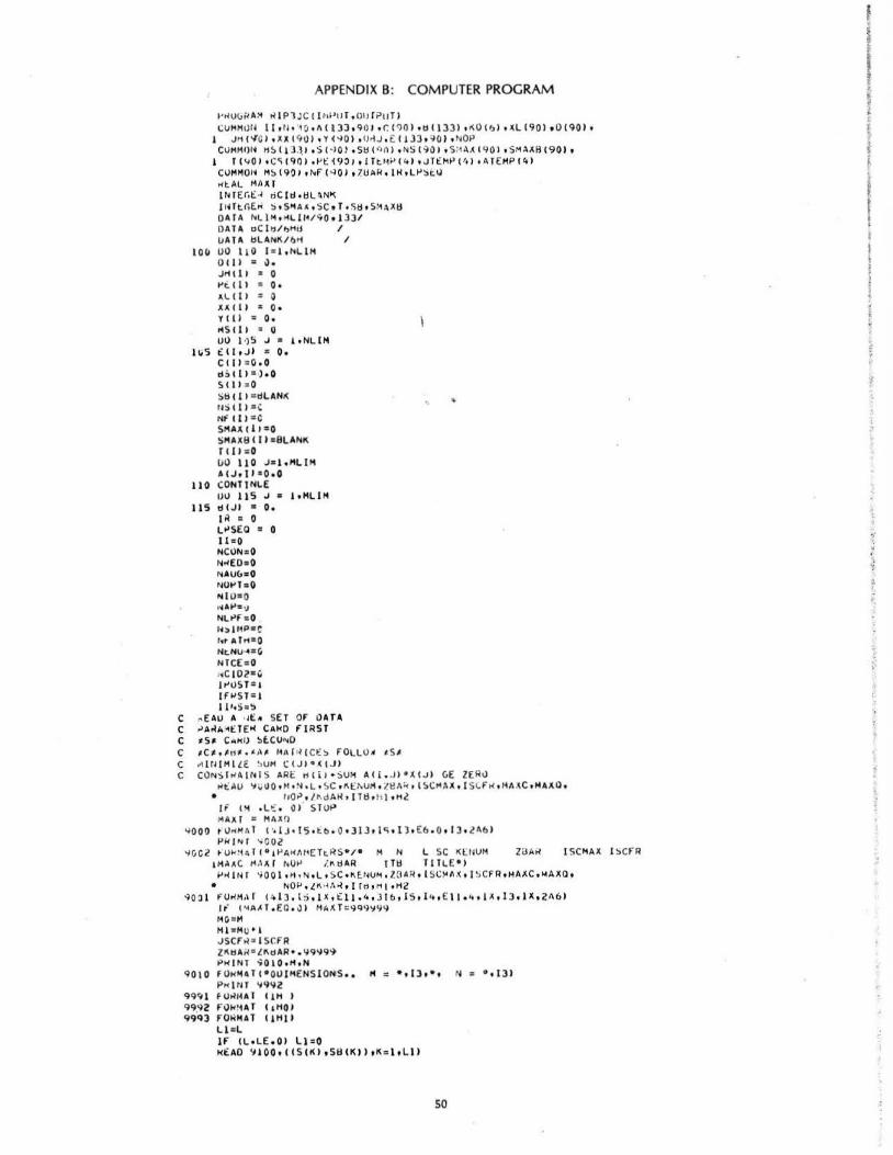
APPENDIX B: COMPUTER PROGRAM

I'>Wu~A~ KIPl.:C! IM'liT,OIJ ri>IITI CUMHt)f~ II , flo ' It/ oil I I 33 , 9 1) I • t. ( 9 0 I ·~ I 133 I , ~0 l t;, I • ~L I 90 I t O I 90 I •

I J>1( '1'\JI , ~Xl91)J o Y ('-I Q J, IJ<iJ , t: IIJ3 o 'IO Jo NOI'

CUMHI)I'i t1!> 1)3.1,1 o$( ·10 ) oSl:li"OI oNSI'iOI , S :·tA ,< ! 9 01 , $MAX8190J • I Tl <iO io C<; !901o l't::i 9~1tiTt.t~;.> (<tloJTt::I<I'I'•I• ATEfo!PCC.J

10 (1

110

115

CUHfo!O~ H!> I901 ,NFI~Ol o lUA~ olKoLI'~~~

><tAL MilA I INTEG£~ riC !d•l:lL~N~ JHTtnE~ S • SMAAoSC oTo Sl:l t S~AXl:l OATA NL)M,MLI~/90 •1 331 OAT A aC lls/I)Hil I liATA l:lLANK/b>1 UU 11 0 ! a:J,hL IH 0 l II " ,) , J >1 ! I I ~ 0 l't. l I I a Oo ALI I I G XX (I I " 0 • Till " O, >~S ll I " U UU 1 15 J • l oNLIH t: II oJ I ., Oo CliJ : O. O d311 I " ·l•O S I II : 0 Sl:l CII =dLANI( liS Ill •C Nf III •C SHA.\(11=0 SM.AX I:Ili 1•8LANK Till : 0 UU 110 J a i,ML IH .acJ.ti • O· O CONTTNLE UU 1 15 J • l oHLIH d(JI • O. lil = 0 LI'SEQ " 0 11:0 NCUNaO No<EO• O NAUC.:O NOI'T:O r;IU•O , ....... . J

NLI'f : O l<:>lf1P•{' ,, . ATH•O Nt.NU·4"G NTCE=O .• c IDZ•v I>'UST = t lf~'ST= I

ll 1oS• !:>

/

C ~EAU A •It:• S ET Of OATA C ~AKA~t:TEo< CAMO fiRS T C tS• CAMU ~lCVNO C ,c~.~~~·· •A~ r<nr~ rCE~ fOLLU A ~S# C ~ IH!MilE ~UH CIJ I•((JI

..

C CllNS i tiAINI $ ARC: t1liJ • SUH A((, .JI • X(JI C.E ZEHu ~t::AO '-I ~OO •~•N•L• &C o~t:~UHo Z~II~ •I !>CHAX o l S~ftl o HAACoHA.\0 ,

• ltO.>o/1\dAK o !Ttl , h ) oHl If 1!'1 . LO:: . 0,- STUI-' MAXI = Mil A()

~000 t U><HA I l> I J •I S otb . 0 •31Jo l~ ol l o E6 . 0 o l3o lll6 1 PkiNT -.coz

'-I GCZ ~Uk~4ll 0 1 PA><IIHET~RS•t• M N L SC KENUM ZaA~ 1 5CHAX l ~CFR tMAA t MIXI NOP l~ l:l AR ! Ttl TITLE0 1 l'ti (IH 'IOO loM oN o L , S.C o l\ ~tlUM , Z[IA~l o l SC~A~ o i ~,CFR oMAXC,I.4AXQ,

• NOP , lK~A~ol f"•HloH2

90~ 1 FUo<H~I c- l J , I S oi XoEli • 4o ll6 ol S ,l 4 oEI I o4oiAol3 olX oZA6) If l ~AAI,£0 , J) HAXT~999~~'1

HO =M MI ,.Hu•l .JSCf~:o ! SC:fR Z~tiA~·L~dAR•.'I9~9~ PHINT 9 0l0o11 oN

9010 f UMMlT I 0 0UIHENS l ONS,, 11 • oiJo • o N"' 0 ol31 PK l tl f '19'12

99"4 1 fUKIUl (1H I 9 992 f01<'1A T ( 1HOI 99.93 fO .. IUT IIHII

Ll cL IF IL• LE.OI Ll=O Ht:AO 'HOO t ( (S(KJ oSIHK I I ol'i= loLU

so

, I . t. i f

I

~100 fOkM~f ll~ll4oAlll Jf ILoGE,Ol GO TO 130 L:zO lfkST=J

lJO COI'ITINUE >~EAO 'lcOOtiCI J I oJ=Itl'll

c••••••••••~•••••••••••••••••••• 9200 fO~MATIE!Oolo5El2o3l

IF ( I~AilC.EOo~l GO TO 141 oo 1 .. 0 .J= loN

140 CIJI=-CI.Jl l<tl CONTINuE

wE AO ~200oldiiloi:zloHl 2~0 AEAO 9400oiiiTEHPt~l,JTEMP(KloATEHPIKll•~=lo4l

9400 fOwMAT I412IJoElOo3tlXll ENO=O•O 00 250 K=lolt K 1=1 TI:) IP II'. I I(J:Jft:l'!,> (10

If IKI.t:v.OI GO TO 250 If IKJ. t::w.Cl ·GO TO 250

c••••••••••••••••••••••••••••••• It (~AAC,N£,CI ATE~P(Kl=-ATEMP(Kl AIK),KJ) :ATt::~P (K)

E,_u= l• ·: 2~0 CONTIHIJE

It IEh~oNE,O.OI GO TO 200 Pw )•4T <,020

90?0 fU><HATI*OlNITIAL SOLUTION•! Pw!NT ~SOOoiiSIKloSdiKIIoKaloLI

9~00 ~UN~AT (14( JX ol4 tA! II ;>~ PH ..;OJO lf ( ~A~C .GT. 01 PRJ"T 90~0

10JO fu~N• II*~COST CUfffiCI(Nf~V) <.lo)4~ • U~I1A r I v • w, ~AX , •--'il (,l~S CliANGt:O• l

f>"'lNT ·obOOt!C (JI ,.J:z},tll Pwii'H ~0~0

90~0 ~u~MAT!*OLON~THAINT CON~TANlS* l f'k[tiT -lbOOoi•JI !lol =l , Ml ..... ! Nr .;obo

;~~0 r U"H~It*UCONST~ANT MATRIX, BY ~OwS•l if' ('1AAC oGl, Ol PRINT 90•o0 v\i <:~l I : I.M ~~INT ~bOOo!A I(oJl,J=l•~l

f'wiNT \lC)Y I ~:'> l CONT(Nl.E

l>~ltH <;<.192 C ALL UATA kEA~ fOR THIS RUN C PE~fO~M CHANGE OF VARIABLES NOW If NECESSAHY

()U c';:i .J= loN CS I.J JZC (.Jl ll' t CI.JI .C:.Eo\1,1}1 GO TO <!<;<; CIJJ:-C!.Jl 00 2'53 I =!<H tllll:u tlJ+A(( oJI A(J ,.Jl =-AtloJI CONTINIJE FO~HAlll~•lOE I ?. oSl IF !llf~t(.uT.O.Ol GO TO 300 ZI:IAI(: Q,O O<l 2 75 .J=IoN

275 ldAH%LdA~•CI J l .100 z:.=o.o

00 32~ 1=1.~ 3?5 dS! ll =cl! ll

UO :130 J • loN 330 -.SIJI=J

If !LofO,QJ GO TO 400 00 375 l(:loL .Jl=SII\1 Kl• lAI:IS IJll NSIKli • O Jr l.J l oLE.ol GO TO 37~ ZS:zZS•C !.Jil 110 350 l • l+M

JSO l:l~lll=dS ill +AIIoJtl J75 CONT!NIJE <oOO CONTINUE

It ('11/•lSCI<!A~.GT.MLIMl I SCMA.< :: HUM - MO ll>~Mv•ISCMAX CALL :OC:CUNOITOI 11 "' Til Tc!•Tll TJ " TO

C JNlTlALilATlON CO~PLETE NO•, START fiRST lfE~ATION GU TO 1 ~10

C P"EPARE T~ COM~UTE SU~AOGATl CONST~AlNT lOOO c.;UNTIN"'f

51

,, .

:·.

IF cst . EO. o l GO TO 2400 .JSCF R".JSCF R •I If Ct SCfR.GT • .JSCfRI GO TO 2400 HL:N-L If CHL.LE.Il GO TO 2400 .JSCfR2 0

IOSO UO 10~0 .J=l•N IOoO • HS C.JJ "0

NSIMP=" SIMP•t I~CL.E~ oOI GO TO 1076 00 1 ~ 7 '5 I =I•L

.J:fAtiS CSIIII 1075 HSC.JI =- S CII

If CNO~ . NE.OI GO TO 1076 I'Rlf.IJ " 070

9070 FOWHAlc•oCUH~£NT PARTIAL ~OLUTION•I I'~ INT Jt>OO • C CS (KI •Stl CKII•K=l • LI

C SOL~E T~~ !HdEOOE~ LINEAR PROGRAM 11)76 CALL SIHt>LE

If I~UI',NE . O I GO TO 10 77 PRINT ~080 • OB.J t ZtlAR

9080 FO~H-I C • OB.J •ZdAR•2E15·~1 1077 CONTINIJE

ll• ll• lPOST C ' KOitl £0 0 MEAN~ Otl.J LESS ThAN ZBAR, EO 2 MEANS INFINITY, EO 4 MEANS C TROUtlLE, EO ~ MEANS Oo.J GE ZBAR

If IKOC lloEU.ZI GO TO 3~00 IF co<OC 1J.EU.41 GO TO 100 If Co<OC 1),£0,61 GO TO 1500 VLPS:-Od.J H' CVLo>S.LE. c-ZBARIIGO TC>-l<t9Cil 0 0 llSO Js lotN IF CO ili.NE.AINTCOClll·AN~.NSC II.NEoOI GO TO 1500

I JSO CONTI NliE 00 1.,50 .J: t•N If C"S C.JI.EO.OI GO TO l<tSO l •.J L• L•I NSC.JI"'O Sd iLl"t:oCitl If (I) Cll .NE.O.OI GO TO 1~00 S CL.Ia-.J uO TO 1450

hOO S ILl = .J ZS•ZS•CC.JI LIO 1.:.25 ll• l•M

1~25 tlS CIII=oS iltl•ACl1•.JI C NATU~AL OIJAL I NTEGEq SOLUTION fOUNO

l<tSO CUNTINIJE NIU"'" l ~;• i GO TO 2320

1*99 KU II I•o C COHPV fl Ntw Sv~ROGATE CONST~AINT

1500 If IISCHA~.LE ,Ol GO TO 1 ~99 dHI"ialdAH uo ISO:) 1•1 •"'0

1505 tiMPiadMPt•~L.Ctl•dCll If C~oSCt!HPI-dCMII.LE. O•OOOSI GO TO 159~ H CH•"'O . LT.I !>CHAI\ 1 GO Tv IS?II 1)1.) 1<; 1.; I=H lo H tl C II ::d C 1•1 I t!SC II •th l l •II uO I o; 1 J .J~< I • N

1 ~ 10 AlltJl=ACl• l •Jl M~M-1

l 'f>i!O d CH•II ~tlMP I u u l'f>'>' .J:o:l • "~ Z .J~ : A.AI.Jl If (.JH(.JJ,Gt .C-Nll l.JHe-ZJH If IJHC.JJ . c. r . ell ZJH:I),

1~50 AIM+ltJJ•lJ~ M:.;, • I tl 'i tMI " Il 1141 oo l 'i '/!;> ll:=tol 1<1 :!:> cro I F l~ t. LE o O I GO TO 1575 t151 Mi etiSCHI•ACMtKII

1575 CONTINUE If CNUP , NE.OI GO TO 1599 PRINT J:i98,-'4 P~INT 9oOO.;AIHtJioJ:},NJ, d1M itdSCMI

1 59~ FO~H4T IZIHOSURROGATE CONSTRAINT,zx ,I41 1599 I f I~Vtl i·EU.61 GO TO 3400

C CHlCK THE ROVNOEO DUAL SOLUTION FOR FEASI BI LITY 1-.011 CONTINuE

rv•. s "01) F• ZS

l'l =tl'i CHI '105 t)O 9 10 J:1,N

I~ INSI.JioEU.?I GO TO 910

52

I ~

~

I t l

I 1

I I

If It) C.JJ .LT . llJI GO TO 910 f=f•CIJI • fl =fi•AIMtJI

~Ill CO,.,TINvE If lf·~~.ZSARI GO TO 2400 li .(fi,Gt:.Q.OI GO TO Q20

'itS Go ' To <!400 920 00 910 (z},MO

f.?=::IS HI OU 'J?.'S J=l t N IF l t~SIJt ,£U,(il Go ' 'To 9.?5 It' IOIJI,LT.TDI GO TO 925 F"2=F2•A ( l •JI

Q25 CONT iNI.I£ lf lf2.LT.o.GI GO TO 915

\1 30 CVNTINIJ( C ~OUNu~O OvAL SOLUTION fEASl&L£

Q)j NC!Ol•hClOZ•I 9)2 NOI-'T:zNili'T•i

C~LL. :.t.CONO 0 3 1 lt' c~.~U.MOI GO TO 940 ou 9J'S '"'"1 •" ij(ll=~lll•f-Z~~AR-Z~AR

935 oSIII•cS III•f-ZKdAR-L~AR

~~0 ldAw:f•ZKdA~ ou ~ .. s J • t,L SHAXd iJI •SijiJI

)45 SMAXtJI•SIJI K=L UV 950 J : {,N • If l ~iS IJJ,£U,_OI GO TO 9'SO K:K•l SHA Xtl I K I :ijLANI< SMAX(KI • J If' ( t) (JJ ·,LToTOI SHAXIKI =-.1

950 cum t"'uE If 1'<\li-',NE . OI vO TO 9t.O

1 PwtNT 33tO·f PklNT 3oOOtiiSHAXCJit SMAX~(JlltJ= I•N)

~Oil CU"' T I NI.IE "'OtlJ=UdJ ZOtlJ: N\JijJ It' IUdJ.NE,lOHJI Z0ljJ:ZUdJ•l·O If (f,( U, LOdJI GO TO 3500 Gil TO .!400

C 8£GINNIN6 OF AN llt~ATION. MAKE CHEAP ATTEMPT TO ~AlHUH l~l~ IJK=O . 1~20 CUNT{NUE

Ir tzS ,GE.ZllAHI GO TO 3100 1)0 1'150 ll"'l•MO I~ C'l5(III.LT.o.ol GO TO !980

1~50 CUNTIIIIIJE GU TO 232()

C SEE If ANY VA~IAbL(S MUST bE 0 19'<0 ( Ut•TINUE

DO 2000 J= I •Ill If INSIJI,£0,01 GO TO 2000 lr l lS• CI.JI .LT . ZrlARI GO TO 2000 NSIJI =~

L=L•i SdiLI=dCilj S ILl =·J

2000 CONT!IIIuE K{NS:O If 11JK,£U,il GO TO 2300 If C IJK,£0, ~1 GO TO 1000 lJK=i If IMol.f,Mll GO TO 2025 "'SC:o { jsMj J~:zi-1

1,;0 TO ~050 2025 MSC= i

11=1 I~=·~c

C ~[wtuwM diNAWY r (ASidlLITY TEST 20~0 ou 2~2~ l:li •ll

U• rlS I 1 I uo ~100 J•!oll If t ;•SIJI.( U,QI GO TO 2100 If (AIItJI.I>T .o.OJ U=O•Ail ,Jl

2100 CUNTINUE 2110 1~· (•loi..T.O.OI GO TO 3000

C SEE lf ANY Fk£E VARIA~I.E MuST BE 0 OR llD ~lOtl .Jl = t , N . I f tA.II•Jll .('l• o.Ol. GO 10 2 200 It INSIJil ,[Gl .OI GO lO 220 <1

.!120 If (Q,G(,A~S(A(l,Jj))l Gil TO 2200 IIISIJtl ~ ll

L"'L •I

53

s .. lu=cC£H [t' I ~II•Jili•GT .O.OI GO TO 2l~O S IU =-JI Gu TO 2200

21 50 S ILI =Jl l~=ZS•C I.Jll IN 21 '1'!; L9= 1•11

2175 d~ll9l =bS II~l•Ail9tJII

t< lNS -::IIlNS +I 2200 CONTINuE ?300 CONT ! Nl.E

H liiiNS.GC: .IINSJ GO TO 1 9~0 If I~I~S.GE.IINSI GO TO 1920

?.220 I:UNTINUE If I~SC,£0,01 GO TO 2025 IF lt<l~S.EO.ul GO TO 1000 ! JK=.? GO Tu l~lO

C A dETfER FE~SidLE SOLUTION HAS SEEN FOUND 2320 CONTINUE

IF l"lot:u.M!ll GO TO 2340 C kEVISE dill ANO BSill USING ~E~ ZS

l)u 232'> f =M ioM ~lil:diiJ•lS-ZKdAR-ZBAR

?.325 dSI!l=~S<II•ZS-ZKdAR-Z8A~ 2340 ZdAR:LS-ZIIBAR

()0 ?.1SO .J=1•N 2J50 511A~IJI=SIJI

GO TO 3300 C AUGMENTATION STEP ~

2400 Kl"O If ISC.EU,OI GO TO 2415 If llf~ST.NE.OI GO TO 241~ HHST2 1 DO 241 Q J=1•N IF INSIJI,£U,Ol GO TO 2410 J1=0 IF ( l)l .. d ,£u,1.0I J1:oJ If IOI.JI , EU.OoOI J1=-J If IJ1,£Q,Ol GO TO 2410 L=L•l ;~S IJI ='.l SILI=.JI IF I J I•LT.QI GO TO 2,.10 Z~=ZS•C I.JI uu 2 .. o!:i 1 "I•"'

2~05 dSilJ=cSili•AIIoJI 2410 CONTINUE . 2415 cvr•Tl Nut:

If I I Tt:t.t::O,OI GO TO 2425 If I JSCfR, NE oOI GO TO 24cS uo 24~C .1•1•!11 If l'<Sl.JI , f.ll.O I GO TO 2420 If 1\ll J I .t:O.IIHIT IUIJI l I r,o TO 2420 1\1 =111•1 TlKll=J

7..,7.0 CUN!INUE l;~· TO c5()5

z.,cs C.:lNTtNVE UU 2<;00 J=1•N If I•ISI.JI ,[U,QI GO TO 2SOO ~1 =1<1•1

1 f IK 1 I:..; Gv TO 2-50~

2'•'>v t:ONT !NOJE 2'>00 CONTiNUE 25J:i cO,..T!NVE

II' O< 1 • .;:a, !ll GO TO 3200 NAI' =NAP+i 1-'=-l.OC:::l() DO 257S K=1•1<1 J:T (I< I f'i=O .O u\l ?.SSG 1 =I o>l P~=dS lll "All •JI !F lP2.GE . O. OI GO TO 2550 Pi=Pt•Pl

2550 CONTINlJE If lP1.LEePI GO TO 2575 P=PI Jl=J

25 75 COrH I NVE NSIJ11 =0 L=L•l SlLl:J1 lS,.zS•C I .Jll (}0 261>0 1•1·"'

21>00 dSilJ=t:SCli•AIIt.Jll <.iv TO 1~10

C f ATHOMED DUE TO BINARY INFEASIBLE CONSTRAINT

54

l

I ' I

3000 ~CON:NCON• l GU TO 3500

3&00 Nllfl)slf~ED•t Gu · To· Jsoe

C fA THOMEO OUE TO LACK Of fREE VARIA~LES 3200 NAVG:NA\JG+l

Gu TO 3500 3300 NUPTcNUPT;l

CALL ~f.CONOIT31 If INU~oNEoOI GO TO 3~00 P~INT 33&Q olS ~W INT 3~00o i iS IKioS~IKII tKsloL I

3310 tUK~I T 123HO BETTER SOLUTION FOUNOt5~o2HZ=olPE15.81 GO TU 3500

3 .. oo NLt>f'=~"'" ' GU TO 3500

C ~ACKTHACK STEP 3<;00 CIJIH t :~l.E

NEhUto~•hENU .. • l If IN(hUHoLToKENVHI GO TO 3530 NENUH=O

3505 CONTINUE ENUH=O· O 0\J 3<;1;) K=l oN

3510 If C S~IKJ,F.O.~CI~ I ENUH=ENUH•,S••K CALL St:CCNOil21 Elll = T2 - TO El.r2 = ll - Tl Tl'•Tl If lf.LTl HA,II.fs -1 GO TO 3517

3Sl 5 CONTINUE

.LT .MAltl) GO TO 3515

If IHUP, NE,OI GO TO 37 00 3:'>17 CUNTIN\JE

~RINT J5ZOoENUHo ELT loEL Tlo L

..

3!>20 FOIIHAT (.lHOoF'lOo5o3aH Of THE SOLUTIONS HAVE BEEN ENUHERATEI>.S.Xo • ISHTIME IN SECONUSt2Xo5HTOTAl of8 o3o2X o7HELAPSEOof8o3o • 5Xt2HL•ol31

3.;30 CONTINliE If I~A~T . GE. Ool GO TO 3700 PRINT 9090

9090 F'UHHATc•OfiNAL PARTIAL SOLUTION•) PAINT 1~00tiCSCKi t SS IKIIoK=ltLI

3600 fUkHA T ll512Xtl .. tAl)) uO TO 3738

3700 NFATH=NfATH• I 3710 If ll oEUo 01 GO TO 3738

If I S~ILI , (Q, dLANK ) GO TO 3900 .J•UB!.IS ILII NSI.JJ=.J tr IS ILI.LToOI GO TO 3735 ZS•ZS- CI.JI uv 37ZS 1"'1•H

3725 ~S II I•~SC I I-Ai lo.JI 3735 Solll • dLANK

S lli ,.O L:.L-1 If ILoGT oOI GO TQ 3710

C FINISHED NOW. PREPARE ANO GIVE FINAL OUTPUTo 3738 CONTINUE

PWINT l7J9oHi oH2 3739 fOIIHAT llHltSX oZA~I

00 37 .. 0 .J•lor-1 37,.0 SIJI=O

00 374Z .J•& • N K•JAttSISHAJII.JI) IF' IKo(YoOI GO TO 3744

37 .. 2 SIKi s l 37 .... OU 37 .. ~ ~· I•N

If ISIKI,NEoO) GO TO 374b SMAA(.JI•-K J•J• I

3Tio6 Cul'tliNUE CALL SiCUNOITZI ELTl = To! - TO If IMUT,LTo OI GO TU 37!>Z I'ICl"T J7SO ollll

37SO fOICHAl IJOHOIM .. LIClT ENUM~HAliON COMPLET! o ~X ollHJO rAL T1H~=·f~o31 GO TO 31SH

J75Z "R INT l7SSoELTI l7~<; fOk~AT 11 .. ~0TIHE (JIC(€0E0,5X•llHfOTAL TIHE=of8o3) J 758 CONTINUE

'"AR .. o.o uO 3'13'> .Js &oN K• IArt~ISMAX'(.J) I IF' ICSIKi oLT.Q,OI SHAXI.JI :•SMAXI.JI If ISHAXI.Ji oC.T,OI Z~AR=l~AIC•CS I~I

) Hl5 CONTtN\JE P~lNT -d<o\) • L~AR

55

38•0 fU~M~T « "O~OLUT IO~ ~EfO~( VA~IAHLE CHANGt YCJI a l • XCJI If CCJI I IS NtGAI!VE •• •I• LEAST l = • ,!PE17.81

3d00 UO 3d 1~ K= l• N 3R IO Til\ I : 0

00 3il:O K'= l tN Kl =IAdS CSHAXl KII

3~<:0 It t <;IIAXPII . GT,OI T!Kl) : 1(1 P~ ll·~·r 90 11

9011 FO~MAT«• VAR!A13LES SET TO OtlE*I t',jiNT 3830 • «TIKI tK"1tNI

3~30 ~ORHA T IIS I4Xtllll ELT3 = Tl ·fl) NITER=~fATH+NFATH·I t'~lNT JKSO,NOPTtN~EOoNCON,NAUG tNAP tN!O ,NCI02 t',jiNT JdS I•NLPF tNSIHP,NITER , ELTJ

3850 fOHHAT 123H0NO, FEASl&LE SOLUT I O~S .IS/ • llH ZS r.E ZdAH tiS . ~H TIMES/ • Z2H CONS T~AINT I NF(ASldLE t iSt6H TlHES/ • / 4H AUGMENTATION 1Ht'0SSIULE ti St6H TlHES/ • 22H AUGMENTATION POSSidLEt!St6H TIMES/ • 14H I NTEGER OUALS ·I~ .~H TIMES/ • 26H NO. OF ~OUNU~O INT. OUALStlSJ

lA~ l FO~MAT lilH LP FATHOMEOtl~tbH TIMES/ • tOH LP CALLEOt i S , ~H TIMES/ * i SH "-0. ITt~ATION<; tiS/ * l6H LAST FEASIBLE SOLUTION ATtFb.3o9H SECONOSI

C END OF FINAL OUTPUT. LOOK FOR ANOTHE~ PROBLEM NOw, (,0 TO 100

C COH~L~H(NT AND UNDERSCORE LAST REMAINING ENTRY IN S, BvO Sd Ill =ttCltl

S lll a • S ILI J•IAdSISILII IF ISILJ,UToOJ GO TO 3950 ZS•ZS•CIJJ uo 39ZS 1• 1•"

39?5 tiSi l taaS III•ACloJI GO TO 1'110

3~50 ZS•ZS• CIJI IJU ) •17:5 1•1•M

3~75 8SC1t •dS I11•AII•JI l::i•U ~Ub~UUTINE ~ IHPLE

..

C AU TOMATIC SIM~LEX R~UU~DANT lUUATlONS CAUSE INFEASiijiLITY

c

c

100

COMHON INfLAG tMX oNNoAIIJ3 • ?0I •CI~O I t bl133ltKOibl,~bl901tPC~Oio 1 JI11--~I.AI'iO!oYC90l,OtlJ tc 11JJ• 'iO i t NOt>

CUHHUN d51 1J31t S C 90 lo ~d i 90 itNS I 901 t SHAXI~Oit SH~A8(901o 1 .T 1901 oC!> 1110 I , t>E 1901 ,[f£MPI•l t JTt:MP 141,4 lt:.MP 1 .. 1

COHHON H~ I ~O I•NFC90io ZUAM.IRt~PSt:O t:uu l VALENCE (XXt~L) ~OGlCAI. T~IG·VER

LOGICAL fiNV•FrHZ tSCH SET · INITIAL VALUES t SET CONSTANT VALUES

F'I NV " orAL~E. THIG '" . FALSE, I Tt:IC • 0 LI'SEO " Lt'SEO• t NUHVR • '0 NUHPV :a 0 H • MA N • NN TEXP •5**16 NVER = H/2 5 NCUT 4*H • 10 IF IINfLAu,EO . OJ GO TO 1•10

!~.,USE CORRECT TEMPERATURE ON ROWS f"FRZ • .TMUEo I. • 1

If IHSCI.J,(O,NFILI) GU TO 1955 IFIHSILI*NFILI•GT.o,OR.IMSIL I.EO.O,ANDoXILI.GE,O.Il GO TO 1950 , .. ~ If CNFILI • NE.Ol GO TO 1925 IF IJHilloGT,OI GO T'l 1Q30 1920

c tf JH DI SAGREES WIT11 ~S 00 SPECIAL P IVOT IF IHSILloGT.O •• NO,JHILioGE.I·HI) GO TO 1950 If IHSILioLT .OoANO.JHI~I.LT oi•Hll GO TO 1950

C SPEC IAL I'IVOTt SWITCH SlNGLtTONS 1925 IJO I._Zb J•l•H

c 11110

PIJJ • o'(,JI • ECI,JI ECI,JI • •ECitJI

CONTINUE OBJ • OttJ • XCU XCII " - X CII JHL " J111LI lf C~HL.GE.C-Mil JMIL) " - L·M lf IJHL.t.l .C-MI) JI11LJ = •L GO TV 1~<;0

DO FULL l'lVOT ON SlNGLET~N JT • -t coc;T " I' I II IF IHS CII.GToOl GO TO 1Q)l .JT • .JT•M cosT • 1.-cosr

56

l l

J

I i ~

HJl

c 1~32

1 ~35

c 1Y:J6

19J7

1-.42 1945

c 14!'>0 1955

l'1b0

c• 1410

1400

1401 c•

ll20

ll:il

1111

1113

10101

c 1114

1104

1105 1119

c

1199

110Z

EN " l• GO TO bJO

GET COLVMNC.JTI SC>i "' ,fALSE . IF ICOST,GT . Ool GU TO 1938 uO TO 1000

c;ELt::Cl ~OWCIAI If lli-!,NEo.>.OH, SCHI GO TO 1 '~40

SCrl :,JHcJEo t.N =-EN 00 B37 J=l tM

YIJl : -YCJI CONTINUE uO TO 1~35 lf!I SCHoANO.AdSCCOSTI.GT . TPIVl.OR.tA. £0.0) GO TO 1980 If IEN,GJ , Q, J GU TO 1945 oo a-..,z J =1 •"

y (oJ) " -YIJJ CO:-.T U.iuE vO TO 901

l'l~OTIIH , JTI NF ILl " MS Ill lFCJHC~I.LT o O l GO TO 1~~0 IA:.J"ILJ 118 I liii•L

CONT INIJE L " L • I IF IL oLE o HI GO TO 100 H 'IH = .F'ALSE, GO TO 910

STAHl WITH SINGLETON BASIS ' 00 140i! .J=I•N

KIH.JI : 0 CONTINUE F'f'HZ : , f'ALSt:: . OQ h 01 1 = 1 , H

JHCll "-1 Nf' C I I • 145 C I I

..

If INf'lll oLT.~.OR . (NfllJ,£0,0 .ANO.BilloLT.O . ll JH tll=-I-14 CONTtNU£

CHEATt:: INVERSE FRUH -KB' ANO 'JH' llf.H::: . TRUE. INIIC " 0 NUHIIR a NUH\IA •1 nciG " ofALSE. OtSJ ,. ll• uu 1113 1 s a.~

00 115 1 Ja 1o14 F.'(J oll • Oo

CONTl t-IUE If IJHClloLT.C-MII GO TO 1111 If CJHCIIoGT.OI J~ C il • 0 E I !til a lo "I II = o. Alii "' Hill 1>0 10 Ill 3 tll•U = -a. t>III • •I • OdJ "' O&J • dill X I 11 " - oi C II

C\INTINUE .JT " 1

If llldiJTI.EO.OJ GO hl 1102 uO TV bOO C.E T CULUHN I JT I TY = lt>IV IH = 0 COST " CIJT l uu 11 0 4 I = lt 14 COST = COST • AIJT ol l • o>cll

CSTEP 71

tfiJHili,Nt.. Q, OH,XII J,NE . o • • OH ,ABS!Yi lll .LE·TYl GO TO 110~ TY: A\!~ll'!lll !H = I

CONTINUE If ll~.NEoOJ GO ro 1119 r v = .o. LlO II 0';; I = t. tl

tf!JHIII.N(,Q,OH , XtiJ,(O.Oo oOA.ARSIYI Ill.LEoTPIVJ GQ TO 1105 tf I AbSIYilJJ ,LE,TY•~RSIXI Il ll GO TO 1105 lY = ABSIYili/XCl)l ~~ ;o I

CONTINUE If IIR.NE.OI GO TO 900 PlvOT!lH, JTJ flN\1 "' oTRUE o

IF CNv~.F.O,OJ PRINT 1199oLPS£0 FO~MATI15HO INVERT FAIL LPoJ~) GO TO 1410

CONTtNuE JT • JT • I If CJT •LE. Nl GO TO 10101

57

·, ! '

t:~~ I) I'• ,, ., ~ l

I.

I.

I

C* PERFORM A ~IMP~EX ITERATION 1200 ~E~ ; .FA~SE. 500 00 503 I : 1 • 14

IF l~fllloEO. O . ANO.XCIJ.LToOol 503 CONTINUE

c• fiND KINIHUH WEDUCEO COST 599 J~ " 0

30)

lld o.o 1)0 7C 1 J =l•N

If' ll<tHJI.NE.OI OT 3 CCJJ 00 3?3 I o: ltM

GO TO 70 1

UT = OT • AIJoii•Ptll CONTINUE If IOT . GE.SSJ uO TO 701 dl:l ·= OT JT = J

701 CONTINUE uO 71)c! I=ioM

If IJH<IIoLT.OJ GO TO 702 If ll'llJ.LT . Bcsl GO TO 703 If 111.-PIJIJ.GEoth:!J GO TO 102 ~a= 1o•PI IJ

71)3

Jl .. - 1-14 GO TO 702 dd="'lll JT ,. ·I

,02 CONTINUE CvST :a l:ld 1f IJT oEU.OJ GO TO 203 If IITEH.GEoNCUTJ GO TO 160 ITER = ITER •1

..

X II) =0•

!STEP 31

c• MU~T tPLV INVERSE Tl~ES AlooJTl 15TEP 41 If IJT .~T•O' GO TO 630

C ~EGIN SucskOUTINE GET CO~UMNIJT I 6 00 UU 610 I= lo~

11ll = o.o 6 10 CVNTINIJE

OV buS . I = 1 •M ~IJT = AIJ T, IJ IF l.tiJT .t.o .o,J <.iO TO bOS 00 &Ob J = 1oM

YIJI = 11~1 • AIJT*EIJol l &06 CONTINUE 605 CONTINUE

Gil TO 640 b30 JTZ = •JT

t:,M = lo ' lt IJTZ .~E .MI GO TO 631 JT2 = JT2 - H EH = -t.

6 31 00 632 I =ltH VII I = EM*EIIoJT2J

632 CONTINIJE b40 VMAX :: 0.

00 6?0 I = l•M YMAX = AHAX11 A~SIY IIJJ,YMAX

6211 CONTINUE T .. iV YMAX • TEXP

C fliU OF GET CUl.UHN If !FfRZJ GO TO 1932 IF' IVEI< J GO TO 1114 RCOST = l'MAX/8d IF' ITRIG .ANO. Sa.GE.I·TP1V JI GO TO 203 THIG=I:Id.GE.I-T .. I VI

c• SELECT P IVOT RO~ !STEP 5 1 1000 AA " TPIV

I t< "' 0 1002 uo 1003 I = 1oM

If l~lll.Ne.Q. ,OR.YIII.~E.AA.OR,NF'IIJ,NE .QJ GO TO 1003 AA "' Y Ill IR = 1

1003 CONTINUE If' ll~•Nf•Ol GO TO 1020 AA : 0. DO 101~ I "' 1oM

I F l~f'llJ.Nf.O oORoYill. LE•TPlV.ORoVCli.~E.AA•XCIJl GO TO 1010 AA = YllJ/X Ill lk • 1

1010 CONT INU£ lulO If IFF'"ZI GO TO 1936

If cJj;,f:I.I.OJ GO TO 207 c• ~lVOT ON ClRoJT) ISTEP 6)

~'>l lA • ..I,.CH<l h' llAoGT.OI KSilAI • 0

C oEGl~ SUaROUTINE PlVOTClHoJTl 1011 NUMPV • tluMPV 1

J..,CIRI • JT If IJT.GTeOI KdiJTl • IH

58

i

I ! '

I l ' .

i . l

Yl ., - YIIRI VIIRI "' - 1.11 00 90.. j = ''"

XY ., E IIRtJIIYl If C~Y .EO o O~I GO TO 90• ~ CJI • P CJI • COST. • XV t:: CI~•JI " Oo uo 9Jtl 1 = 1•!'1

E CitJI • ECltJI • XY" VIII 906 CON I I NUE <i.J4 CONTINIJE

.XV = -.XCIRI I Yl 0~ 90~ 1 • l • H

XOLO • JI.C 11 XII I = XOLO • XV • VIII

90a CONTIN\JE YIIRI =·-Yl itCIRI = -XY

C ENO Of PIVOT Ot!J = OdJ • xv•cos T If IVERI GO TO 1102

C EXCH•NGE ~OWS If SLACK Pl VOTEU IN WRONG ROW If CJT.GT.O,OR.JT2oE0.1~1 GO TO 907 XY "' X<lRI ltCIRI = XIJT21 ltiJTZI = XV oo 9,)9 1 • 1• 14

XY = iiiR•ll EllRtll ., ECJTZtll EIJTZt ll • /I.Y

9(;9 CONTIN\IE U : J., IJ T21 JI11JT21 • JT Jf'1ClRI = U Kd iiU s 1R

907 1NVC • lNVC •1 C TO SIEP 1 It NOT INVERTING, TO STEP 7 If INVERT I NG

If CffAZI GO TO 1950 If COdJ.GE. laARI GO TO 18n II' IFUWI GO TO 1200

910 If CINVC,GE. NVERI GO TO 1120 GO TO 1200

C• ENO Of ALGOWITHH, SET EXIT VALUES ••• 207 IF CRCOST. LE,C-1000.11 GO TO 203

C INFINITE SOLUTION I( • 2 GO TO ZSO

1110 IC•tl GO TO 250

C P~UdLEH I S CYCLING ~ERHAPS UoO I< • <t

I>K INT lb1oLI-'SEO lb1 f0~M~I t3 1 HOITE"AT10N LIMIT EXCEEOtO ON LPtl41

GU TO 2!>(• C fEASibLE OR lNFEAS idL[ •SOLUTlON

~OJ t< • 0 2 50 00 1399 J • 1oN

AX 0o0 Kt!J Kd (JI If IKdJ. NEoO I XX XIKHJI KdCJI = LL

1399 CONTI NUE t<OCl l K ICOCZ I ITER KU'I31 s INVC ICOI"I " NUM'IR 110151 NUHPV 1<~16 1 " J T If CNUP . N~ . ,)J· HETURN I'RINT Ho.?,"LPSEOt (t<O(Ji tl•l•bl

162 FO~MAT !JH L~•I St 6H 110 t 6161 I'W INT 19~2

19~2 F0kH~T C21HG l JH NF HS tPtYtXtdlllt l DO 19113 1=1•i4 PWINT 19a4,ltJH CIItNFC i l tMS CiltPC lltYilltXIIIt81ll

191'3 CUNTI NIJE 19P" FO~Hlii1Xt4l lt4F12o61

WE. TURN 19"0 If CNOP,[U,OI PRINT 198 ltLPSE0tL t iR,SCHtCOST 19~1 FUW"ATI 3HOLP ,I4t1ZH FAIL, SLAC~ tllt4H l RzlJtSH SCH•L1t3H C•f19obl

If IIA• N£o01 GO TO 1941 GO TO 1410

[NO

59

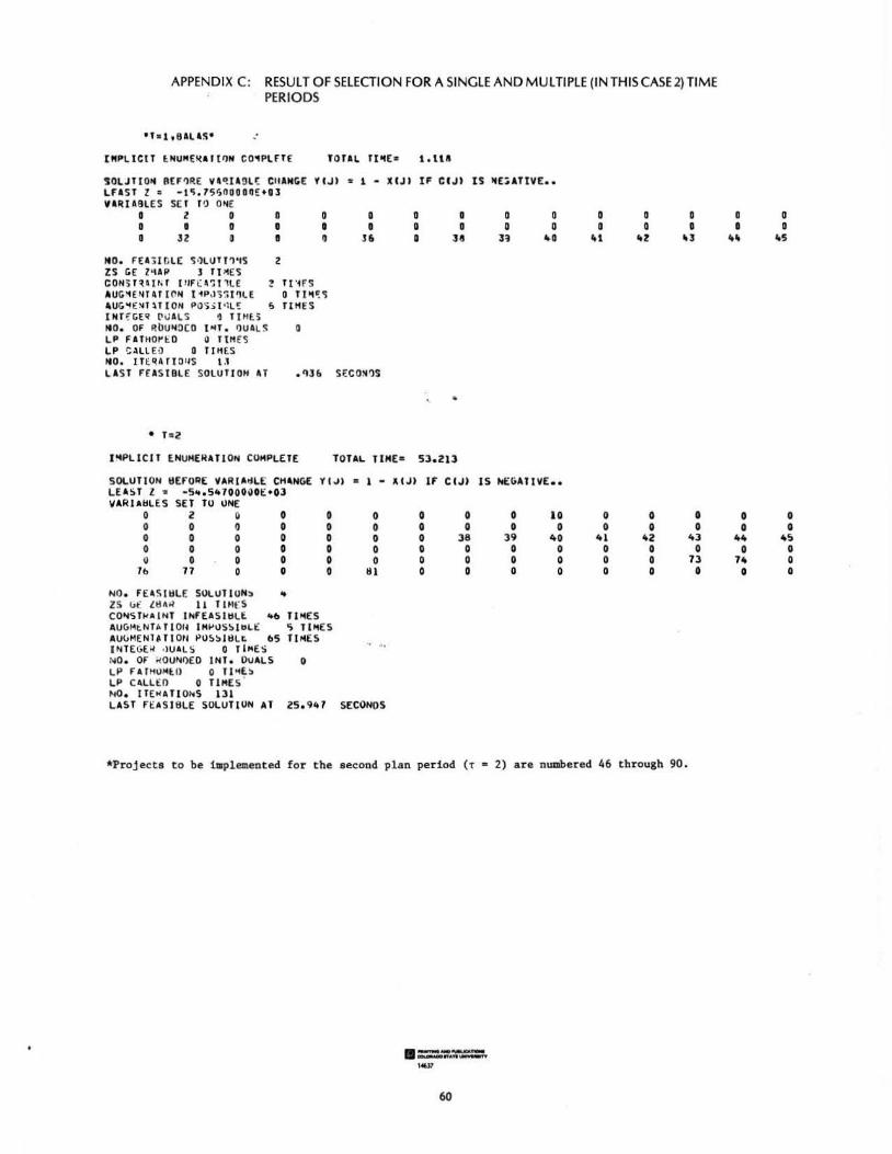
APPENDIX C: RESULT OF SELECTION FOR A SINGLE AND MULTIPLE (IN THIS CASE 2) TIME PERIODS

•f• 1 , 81LA!>• :

[MPLlCIT ~NUME~AJ{QN CO"'PlfTE TOTAL Ti llE• t.lU

~OLJTIOit IIEF'lRE Vl~U!Il~ CIIAICGE YCJI t 1 • XCJI IF CCJI IS NE:aTtVE •• LFASf Z = -t~.7s~oooon:+al VUIA!IlES SET T'.l O~E

0 z 0 0 0 0 0 0 0 0 0 0 0 0 • 0 0 • 0 II 0 II 0 0 0 0 0 3Z ~ e 0 l6 D l8 l~ 11.0 Itt Ill Ill

MD. FEAi iCLE S~lUTT1~S z ZS GE Z'\AP' J JI>IES CON;J~4IIH [liF t: 4'> 1 1l E z T t'1 f'S AUG"'E~T4Tl 0~ [1PJ3~l'llE 0 TI 'ICCS AUG"'E~J~TJON PQ~jl ~L! 6 TlHES INT;;GEQ [1\JALS ~ Tl HlS ItO. OF P.bUN!>(O l04T • 'lUALS 0 LP F ITHOI' I:: O ~ TIHtS LP C.\lLE\J 0 TIHlS ItO. IT~qAftO •IS \ .1 LAST F£AS l8lE SOlUTION AT , qJ& SF.CO~?S

•

• T=2

I~PLICIT ENUMERATION COMPLETE TOTAL TIME• 53. 213

SOLUTION ~EFORE ~&RIA~LE CHANGE YCJI • l - ACJI If CCJI IS l'ft::GATI ~E. o

LEA~T l " -s~.S47000ij0£ •03 VARIA~LES SET TO UN£

0 2 0 0 0 0 0 0 0 10 0 0 0 0 0 I) 0 0 0 0 0 0 0 0 0 0 0 0 0 0 0 0 0 38 39 40 41 42 lo3 0 0 0 0 0 0 0 0 0 0 0 0 0 I) 0 0 0 0 0 0 0 0 0 0 0 73

7b 77 0 0 0 Ill 0 0 0 0 0 0 0

NO. FElSI~LE SOLUTION~ ~

zs ut: ill ~~ ll T Hit'S CONST.-AINT INFElSII!Lt:. .. f> TI'1£S AUGMtNTA TIO~ IH~US~IbLE S TI'IES AUl>MENTHtOtl PO~~l lllt. 65 TIMES INTEGE~ ·lUALS 0 TlMES NO, Or kOUN~EO INT. DUALS 0 I.P FlTHOMt.l) 0 Tl04~~ LP CIILLt:O 0 TIMES 1'10. Il(HA TlONS 131 LAST Ft:ASIOLE SOI.UTION AT ZS,91t7 SECONDS

*Projects to be iwplemented for the second plan period (T • 2) are numbered 46 through 90 .

60

0 0 0 0 .... lo5

0 0 0 0

"" ~~~ 0 0

74 0 0 0

KEY WORDS: Water resources projects, timing of water pro­jects, selection of water proj ects, economic development, efficiency of projects, demand targets, services:

Abstract: The methodology developed in this paper is de­signed to facilitate the selecti on and timing of water re­sources projects to optimally achieve "a priori" specified national economic development through desired strategies. The methodology is composed of several analytical procedures.

The input- output model is used to simulate the national economy thus further facilitating consistent projections of the elements of final demands in accoxdance with the national economic development objectives and strategies, and assess­ing the total and incremental requi rements for sectoral out­puts of goods and services at designated future time periods, A mathematical model for the selection and timing of water

KEY WORDS: Water resources projects, timing of water pro­jects, selection of water projects, economic development, efficiency of projects, demand targets, services:

Abstract: The methodology developed in this paper is de­signed to facilitate the selecti on and timing of water re­sources projects to optimally achieve "a priori" specified national economic development through desired strategies. The methodology is composed of several analytical procedures.

The input-output model is used to simulate the nat ional economy thus further facilitating consistent projections of the elements of final demands in accoxdance with the nat ional economic development objectives and strategies, and assess­ing the t otal and incremental requirements for sectoral out­puts of goods and services at designated future time periods . A mathematical model for the selection and t iming of water

KEY WORDS: Water resources projects, timing of water pro­jects, selection of water projects, economic development, efficiency of projects, demand targets, services:

Abstr act: The methodology developed in this paper is de­signed to fac ilitate the selection and timing of water re­sources projects to optimally achieve "a priori" spec ified. national economic development through desired strategies. The methodology is composed of several analytical procedures.

The input-output model is used to simulate the national economy thus further facilitating consistent projections of the elements of final demands in acco~dance with the national economic development objectives and strategies, and assess­ing t he total and incremental requirements for sectoral out­puts of goods and services at designated future time periods . A mathematical model for the selection and timing of water

KEY WORDS: Water resources projects , timing of water pro­jects, selection of water projects, economic development, efficiency of projects, demand targets, services:

Abstract: The methodology developed in this paper is de­signed to facilitate the selection and timing of water re­sources project s to optimally achieve "a priori" specified national economic development through desired strategies. The methodology is composed of several analytical procedures.

The input-output model is used to simulate t he national economy thus furt her faci litating consistent projections of the elements of final demands in accoxdance with the nat ional economic development object ives and strategies , and assess­ing the total and incremental requirements for sectoral out­puts of goods and services at designated future t ime periods . A mathematical model for the selection and timing of water

/

resources projects for their implementation, in other words for the formulation of an optimal national water resources development program, has been developed and its applica­tion demonstrated on an example problem. The model incor­PQrates important factors such as economic efficiency of projects, demand targets for project outputs of goods and services necessary to achieve desired national economic growth, resources capabilities and limitations, and project interrelationships. Incorporation of these and other re­lated factors makes the model reflective of the real world problem it is intended to aid' in -solving.

Reference : Lemma, Wendim-Agegnehu, Colorado State University paper No. 77 (September 1975) "Methodology for the Selection and Timing of Water Resources Projects

resources projects for their implementation, in other words for the formulation of an optimal national water resources development program, has been developed and its applica­tion demonstrated on an example problem. The model _incor­porates important factors such as economic efficiency of proj ects, demand targets for project outputs of goods and services necessary to achieve desired national economic growth, resources capabilities and limitations, and project interrelationships. Incorporation of these and other re­lated factors makes the model reflective of the real world problem it is intended to aid in solving.

Reference: Lemma, Wendim-Agegnehu, Colorado State University paper No. 77 (September 1975) "Methodology for the Selection and Timing of Water Resources Projects

.,.., ,.. _ ,_ ---~ ....::~< ;~;~i!: .¢-. ''!1 ...

\

·")-~ ..

resources projects for their implementation, in other words for the formulation of an optimal national water resources development program, has been developed and its applica­tion demonstrated on an example problem. The model incor­porates important factors such as economic efficiency of projects, demand targets for project outputs of goods and services necessary to achieve desired national economic '• growth, resources capabilities and limitations, and project interrelationships. Incorporation of these and other re­lated factors makes the model reflective of the real world problem it is intended to aid in solving.

Reference: Lemma, Wendim-Agegrtehu, Colorado State University paper No. 77 (September 1975) "Methodology for the Selection and Timing of Water Resources Projects

•

resources projects for t heir implementation , in other words for the formulation of an optimal national water resources development program, has been developed and its applica­tion demonstrated on an example problem. The model incor­porates important factors such as economic efficiency of projects, demand targets for project outputs of goods and services necessary to achieve desired national economic growth, resources capabilities and limitations, and project interrelationships. Incorporation of these and other re­lated factors makes the model reflective of the real world problem it is intended to aid in solving.

Reference: Lemma, Wendim-Agegnehu, Colorado State University paper No. 77 (September 1975) "Methodology for the Selection and Timing of Water Resources Projects