The Holographic Principle and the Emergence of Spacetime ...

The Holographic Principle and the Emergence of Spacetime

by

Vladimir Rosenhaus

A dissertation submitted in partial satisfaction of the

requirements for the degree of

Doctor of Philosophy

in

Physics

in the

Graduate Division

of the

University of California, Berkeley

Committee in charge:

Professor Raphael Bousso, Chair

Professor Lawrence Hall

Professor Alex Filippenko

Spring 2014


Copyright 2014

by

Vladimir Rosenhaus

1

Abstract


by

Vladimir Rosenhaus

Doctor of Philosophy in Physics

University of California, Berkeley

Professor Raphael Bousso, Chair

Results within string theory and quantum gravity suggest that spacetime is notfundamental but rather emergent, with the fundamental degrees of freedom living on aboundary surface of one lower dimension than the bulk. This thesis is devoted to studyingthe holographic principle and its realization for spacetimes with both negative and positivecosmological constant.

The holographic principle is most explicitly realized in the context of the AdS/CFTcorrespondence. We examine the extent to which AdS/CFT realizes the holographic prin-ciple and study the UV/IR relation. We study aspects of how bulk locality emerges withinAdS/CFT. To this effect, we study how to reconstruct the bulk from boundary data. Westudy how such a reconstruction procedure is sensitive to large changes in the bulk geom-etry. We study if it is possible to reconstruct a subset of the bulk from a subset of theboundary data. We explore both local and nonlocal CFT quantities as probes of the bulk.One nonlocal quantity is entanglement entropy, and to this effect we construct a frameworkfor computing entanglement entropy within the field theory.

The most ambitious application of the holographic principle would be finding theholographic dual to the multiverse. We investigate properties of this putative duality. Weextend the UV/IR relation of AdS/CFT to the multiverse, with the UV cutoff of the theoryon future infinity being dual to a late time cutoff (measure) in the bulk. We compare variousmeasure proposals and examine their predictions.

i

Contents

List of Figures v

List of Tables xiv

1 Introduction 1

I Emergent Spacetime with Λ < 0: AdS/CFT 6

2 Holography for a Small World 92.1 Introduction . . . . . . . . . . . . . . . . . . . . . . . . . . . . . . . . . . . . . . . 92.2 UV/IR . . . . . . . . . . . . . . . . . . . . . . . . . . . . . . . . . . . . . . . . . . 11

2.2.1 Review of UV/IR . . . . . . . . . . . . . . . . . . . . . . . . . . . . . . . 112.2.2 Comments on Scale/Radius . . . . . . . . . . . . . . . . . . . . . . . . . 11

2.3 Oscillating Particle . . . . . . . . . . . . . . . . . . . . . . . . . . . . . . . . . . . 122.4 Scalar Field Solutions . . . . . . . . . . . . . . . . . . . . . . . . . . . . . . . . . 14

2.4.1 Relativistic Wave Packet . . . . . . . . . . . . . . . . . . . . . . . . . . . 142.4.2 Non-relativistic Mode . . . . . . . . . . . . . . . . . . . . . . . . . . . . . 172.4.3 General Solution . . . . . . . . . . . . . . . . . . . . . . . . . . . . . . . . 18

2.5 Precursors . . . . . . . . . . . . . . . . . . . . . . . . . . . . . . . . . . . . . . . . 192.6 A Proposal for Finding the States . . . . . . . . . . . . . . . . . . . . . . . . . . 20

2.6.1 Proposal . . . . . . . . . . . . . . . . . . . . . . . . . . . . . . . . . . . . . 212.6.2 Ultraboosted states . . . . . . . . . . . . . . . . . . . . . . . . . . . . . . 22

2.7 Conclusion . . . . . . . . . . . . . . . . . . . . . . . . . . . . . . . . . . . . . . . . 232.8 Equations for Energy Shell . . . . . . . . . . . . . . . . . . . . . . . . . . . . . . 23

3 Light-sheets and AdS/CFT 253.1 Introduction . . . . . . . . . . . . . . . . . . . . . . . . . . . . . . . . . . . . . . . 253.2 The Causally Connected Region C . . . . . . . . . . . . . . . . . . . . . . . . . 293.3 The Light-sheet Region L . . . . . . . . . . . . . . . . . . . . . . . . . . . . . . . 30

3.3.1 Spacelike Holography vs Light-Sheets . . . . . . . . . . . . . . . . . . . 313.3.2 Bounds on the Holographic Domain . . . . . . . . . . . . . . . . . . . . 33

3.4 Proof that L = C . . . . . . . . . . . . . . . . . . . . . . . . . . . . . . . . . . . . 363.5 Covariant Renormalization Group Flow . . . . . . . . . . . . . . . . . . . . . . 393.6 Nonlocal Operators and the Bulk Dual . . . . . . . . . . . . . . . . . . . . . . . 41

ii

3.7 Quantum Gravity Behind Event Horizons . . . . . . . . . . . . . . . . . . . . . 463.8 Light-sheets from the conformal boundary of AdS . . . . . . . . . . . . . . . . 47

4 Null Geodesics, Local CFT Operators, and AdS/CFT for Subregions 494.1 Introduction . . . . . . . . . . . . . . . . . . . . . . . . . . . . . . . . . . . . . . . 494.2 The Reconstruction Map . . . . . . . . . . . . . . . . . . . . . . . . . . . . . . . 52

4.2.1 General Formulas . . . . . . . . . . . . . . . . . . . . . . . . . . . . . . . 524.2.2 Global AdS . . . . . . . . . . . . . . . . . . . . . . . . . . . . . . . . . . . 544.2.3 AdS-Rindler . . . . . . . . . . . . . . . . . . . . . . . . . . . . . . . . . . 554.2.4 Poincare Patch . . . . . . . . . . . . . . . . . . . . . . . . . . . . . . . . . 584.2.5 Poincare-Milne . . . . . . . . . . . . . . . . . . . . . . . . . . . . . . . . . 594.2.6 AdS-Rindler Revisited . . . . . . . . . . . . . . . . . . . . . . . . . . . . 62

4.3 A Simple, General Criterion for Continuous Classical Reconstruction: Cap-turing Null Geodesics . . . . . . . . . . . . . . . . . . . . . . . . . . . . . . . . . 624.3.1 Unique Continuation, Null Geodesics, and RG Flow . . . . . . . . . . 644.3.2 The Diagnostic in Other Situations . . . . . . . . . . . . . . . . . . . . 65

4.4 Arguments for an AdS-Rindler Subregion Duality . . . . . . . . . . . . . . . . 674.4.1 Probing the Bulk . . . . . . . . . . . . . . . . . . . . . . . . . . . . . . . 674.4.2 Hyperbolic Black Holes . . . . . . . . . . . . . . . . . . . . . . . . . . . . 68

4.5 Discussion . . . . . . . . . . . . . . . . . . . . . . . . . . . . . . . . . . . . . . . . 69

5 AdS Black Holes, the Bulk-Boundary Dictionary, and Smearing Func-tions 715.1 Introduction . . . . . . . . . . . . . . . . . . . . . . . . . . . . . . . . . . . . . . . 715.2 Smearing functions . . . . . . . . . . . . . . . . . . . . . . . . . . . . . . . . . . . 735.3 Solving the wave equation . . . . . . . . . . . . . . . . . . . . . . . . . . . . . . 775.4 Black hole smearing functions and large angular momentum modes . . . . . 79

5.4.1 Asymptotic behavior of the wave equation . . . . . . . . . . . . . . . . 805.4.2 Large angular momentum and WKB . . . . . . . . . . . . . . . . . . . 81

5.5 Smearing functions for other spacetimes . . . . . . . . . . . . . . . . . . . . . . 825.5.1 Static spherically symmetric spacetimes . . . . . . . . . . . . . . . . . . 835.5.2 Trapped null geodesics . . . . . . . . . . . . . . . . . . . . . . . . . . . . 86

5.6 Conclusions . . . . . . . . . . . . . . . . . . . . . . . . . . . . . . . . . . . . . . . 88

6 Scanning Tunneling Macroscopy, Black Holes, and AdS/CFT Bulk Local-ity 906.1 Introduction . . . . . . . . . . . . . . . . . . . . . . . . . . . . . . . . . . . . . . . 906.2 Bulk reconstruction in Minkowski space . . . . . . . . . . . . . . . . . . . . . . 92

6.2.1 Success with propagating modes . . . . . . . . . . . . . . . . . . . . . . 926.2.2 Reality with evanescent modes . . . . . . . . . . . . . . . . . . . . . . . 946.2.3 Ignoring evanescent modes . . . . . . . . . . . . . . . . . . . . . . . . . . 946.2.4 Dealing with evanescent modes . . . . . . . . . . . . . . . . . . . . . . . 956.2.5 Window function . . . . . . . . . . . . . . . . . . . . . . . . . . . . . . . 966.2.6 Conclusions . . . . . . . . . . . . . . . . . . . . . . . . . . . . . . . . . . . 97

6.3 Bulk reconstruction in AdS space . . . . . . . . . . . . . . . . . . . . . . . . . . 97

iii

6.3.1 Local CFT operators as boundary data . . . . . . . . . . . . . . . . . . 986.3.2 Bulk reconstruction near the boundary . . . . . . . . . . . . . . . . . . 996.3.3 Bulk reconstruction deeper in . . . . . . . . . . . . . . . . . . . . . . . . 104

6.4 Evanescence in CFT Dual . . . . . . . . . . . . . . . . . . . . . . . . . . . . . . 1096.5 Discussion . . . . . . . . . . . . . . . . . . . . . . . . . . . . . . . . . . . . . . . . 1116.6 Evanescent Optics . . . . . . . . . . . . . . . . . . . . . . . . . . . . . . . . . . . 111

7 Entanglement Entropy: A Perturbative Calculation 1157.1 Introduction . . . . . . . . . . . . . . . . . . . . . . . . . . . . . . . . . . . . . . . 1157.2 General framework . . . . . . . . . . . . . . . . . . . . . . . . . . . . . . . . . . . 116

7.2.1 Geometric perturbations . . . . . . . . . . . . . . . . . . . . . . . . . . . 1187.2.2 Relevant perturbations . . . . . . . . . . . . . . . . . . . . . . . . . . . . 121

7.3 Perturbations of a planar entangling surface . . . . . . . . . . . . . . . . . . . 1227.3.1 Calculation . . . . . . . . . . . . . . . . . . . . . . . . . . . . . . . . . . . 124

7.4 Perturbations of a spherical entangling surface . . . . . . . . . . . . . . . . . . 1267.4.1 Geometric perturbations . . . . . . . . . . . . . . . . . . . . . . . . . . . 1287.4.2 Calculation . . . . . . . . . . . . . . . . . . . . . . . . . . . . . . . . . . . 129

7.5 Notation . . . . . . . . . . . . . . . . . . . . . . . . . . . . . . . . . . . . . . . . . 1317.6 Foliation of M in the vicinity of the entangling surface . . . . . . . . . . . . . 1327.7 Intermediate calculations for Sec. 7.3 . . . . . . . . . . . . . . . . . . . . . . . 134

II Emergent Spacetime with Λ > 0 135

8 Boundary Definition of a Multiverse Measure 1378.1 Introduction . . . . . . . . . . . . . . . . . . . . . . . . . . . . . . . . . . . . . . . 1378.2 New light-cone time . . . . . . . . . . . . . . . . . . . . . . . . . . . . . . . . . . 141

8.2.1 Probabilities from light-cone time . . . . . . . . . . . . . . . . . . . . . 1418.2.2 A gauge choice for the conformal boundary . . . . . . . . . . . . . . . . 1428.2.3 The multiverse in Ricci gauge . . . . . . . . . . . . . . . . . . . . . . . . 144

8.3 Properties of new light-cone time . . . . . . . . . . . . . . . . . . . . . . . . . . 1478.3.1 Rate equation . . . . . . . . . . . . . . . . . . . . . . . . . . . . . . . . . 1478.3.2 Attractor solution . . . . . . . . . . . . . . . . . . . . . . . . . . . . . . . 1508.3.3 Event counting . . . . . . . . . . . . . . . . . . . . . . . . . . . . . . . . . 150

8.4 The probability measure . . . . . . . . . . . . . . . . . . . . . . . . . . . . . . . 1528.4.1 Probabilities from the new light-cone time cut-off . . . . . . . . . . . . 1528.4.2 Equivalence to the old light-cone time cut-off . . . . . . . . . . . . . . 1538.4.3 Equivalence to the new causal patch measure . . . . . . . . . . . . . . 1548.4.4 Equivalence to the old causal patch measure . . . . . . . . . . . . . . . 155

8.5 The general case . . . . . . . . . . . . . . . . . . . . . . . . . . . . . . . . . . . . 1568.5.1 Perturbative inhomogeneities . . . . . . . . . . . . . . . . . . . . . . . . 1568.5.2 Singularities in the boundary metric . . . . . . . . . . . . . . . . . . . . 1588.5.3 Inhomogeneities . . . . . . . . . . . . . . . . . . . . . . . . . . . . . . . . 160

8.6 Conformal factor for a homogeneous bubble universe . . . . . . . . . . . . . . 161

iv

9 Testing measures 1669.1 Introduction . . . . . . . . . . . . . . . . . . . . . . . . . . . . . . . . . . . . . . . 1669.2 Counting Observations . . . . . . . . . . . . . . . . . . . . . . . . . . . . . . . . 1699.3 Open FRW universes with cosmological constant . . . . . . . . . . . . . . . . . 1719.4 The causal patch cut-off . . . . . . . . . . . . . . . . . . . . . . . . . . . . . . . . 173

9.4.1 Positive cosmological constant . . . . . . . . . . . . . . . . . . . . . . . 1739.4.2 Negative cosmological constant . . . . . . . . . . . . . . . . . . . . . . . 179

9.5 The apparent horizon cutoff . . . . . . . . . . . . . . . . . . . . . . . . . . . . . 1819.5.1 Definition . . . . . . . . . . . . . . . . . . . . . . . . . . . . . . . . . . . . 1819.5.2 Positive cosmological constant . . . . . . . . . . . . . . . . . . . . . . . 1849.5.3 Negative cosmological constant . . . . . . . . . . . . . . . . . . . . . . . 186

9.6 The fat geodesic cutoff . . . . . . . . . . . . . . . . . . . . . . . . . . . . . . . . 1889.6.1 Positive cosmological constant . . . . . . . . . . . . . . . . . . . . . . . 1899.6.2 Negative cosmological constant . . . . . . . . . . . . . . . . . . . . . . . 190

10 Future inextendability and non-decoupling of the regulator 19310.1 Non-decoupling of the regulator . . . . . . . . . . . . . . . . . . . . . . . . . . . 19310.2 The probability to encounter the cutoff . . . . . . . . . . . . . . . . . . . . . . 19710.3 Objections . . . . . . . . . . . . . . . . . . . . . . . . . . . . . . . . . . . . . . . . 199

10.3.1 The cutoff can not be encountered in a late-time limit . . . . . . . . . 19910.3.2 Hitting the cutoff is an artifact . . . . . . . . . . . . . . . . . . . . . . . 201

10.4 The Guth-Vanchurin paradox . . . . . . . . . . . . . . . . . . . . . . . . . . . . 20310.5 Discussion . . . . . . . . . . . . . . . . . . . . . . . . . . . . . . . . . . . . . . . . 203

10.5.1 Assumptions . . . . . . . . . . . . . . . . . . . . . . . . . . . . . . . . . . 20410.5.2 Observation . . . . . . . . . . . . . . . . . . . . . . . . . . . . . . . . . . . 20510.5.3 Interpretation . . . . . . . . . . . . . . . . . . . . . . . . . . . . . . . . . 206

11 Conclusion 209

Bibliography 211

v

List of Figures

2.1 The interior of the larger cylinder represents AdS. The vertical direction istime and the radial direction is ρ. The CFT lives on the boundary (R×Sd−1)which is at ρ = π/2. In order for AdS/CFT to fully realize the holographicprinciple, some theory which has a Hilbert space of dimension exp(A/4ld−1

pl ),where A is the area of the sphere at ρ = π/2 − δ, must be extracted from theCFT. This theory would live on the sphere at ρ = π/2−δ (inner cylinder) andwould need to be able to fully describe the interior: 0 < ρ < π/2 − δ. . . . . . . 10

2.2 (a) A relativistic particle following a radial geodesic inside of AdS. Its closestapproach to the boundary is ρ = π/2 −m/E. (b) The sphere shown is theSd−1 of the CFT (it is represented as an S2; in (a) we were only able todraw the boundary as an S1). On the CFT the particle is represented by athin shell of ⟨Tµν⟩. This shell is shown at multiple instances of time. As theparticle starts near the boundary, the shell is small and near the right poleof the sphere. The shell grows as the particle falls towards smaller ρ. As theparticle passes through ρ = 0 the shell wraps the entire Sd−1. As the particlemoves out again to larger ρ, the shell contracts. Crucially, the thickness ofthe shell is m/E. . . . . . . . . . . . . . . . . . . . . . . . . . . . . . . . . . . . . 13

2.3 (a) The profile of a localized wave packet (2.10) traveling away from theboundary (q0 = 106, σx = σz = 10−3) shown at time t = 10−2. It is composedof modes highly oscillatory in the z direction, of wavenumber peaked aroundq0. (b) The CFT image ⟨O(x)⟩ at this time (given by (2.20)). . . . . . . . . . 14

2.4 A plot of the radial modes f0l(ρ) in (2.21) for fixed l (l = 100) and several dif-ferent choices of ∆ (∆ = 10, 100, 500, in colors red, green, blue, respectively).The variable on the horizontal axis is the radial coordinate r/L = tanρ. Theplot shows that increasing ∆ leads to stronger confinement to the center ofAdS. To violate UV/IR we choose a mode with ∆ ≫ l≫ 1/δ. . . . . . . . . . 17

2.5 A highly boosted state for which the center of mass energy, and hence back-reaction, is small. In order for the theory on the sphere to only have a finitenumber of states, we must exclude this state. A plausible reason is that anyattempt to probe it would form a black hole that is much larger than thesphere. . . . . . . . . . . . . . . . . . . . . . . . . . . . . . . . . . . . . . . . . . 22

vi

3.1 (a) The Poincare patch of AdS, with the usual time slicing in the coordinatesof Eq. (1.1). (b) Time slices of an arbitrary bulk coordinate system thatcovers the same near-boundary region as the Poincare patch but a differentregion far from the boundary. This illustrates that there is no preferredcoordinate system that would uniquely pick out a region described by theboundary, particularly if the bulk is not in the vacuum state. . . . . . . . . . 26

3.2 The boundary of AdS; the dashed lines should be identified. Examples ofglobally hyperbolic subsets b are shown shaded. A causal diamond is a setof the form I−(q) ∪ I+(p), where q is boundary event in the future of theboundary event p. Let τ be the time along a geodesic from p to q in theEinstein static universe of unit radius (ds2 = −dt2 + dΩ2

d−1). With τ = 2π, thecausal diamond is the boundary of the Poincare patch. A causal diamondwith τ < 2π (τ > 2π) is called “small” (“large”). An open interval (t1, t2)with t2 − t1 < π (t2 − t1 > π is called “short strip” (“tall strip”). . . . . . . . . 27

3.3 The four null hypersurfaces orthogonal to a spherical surface B in Minkowskispace. The two cones F1, F3 have negative expansion and hence correspondto light-sheets. The covariant entropy bound states that the entropy of thematter on each light-sheet will not exceed the area of B. The other twofamilies of light rays, F2 and F4, generate the skirts drawn in thin outline.Their cross-sectional area is increasing, so they are not light-sheets, and theentropy of matter on them is unrelated to the area of B. . . . . . . . . . . . . 30

3.4 Penrose diagram of a collapsing star (shaded). At late times, the area of thestar’s surface becomes very small (B). The enclosed entropy in the spatialregion V stays finite, so that the spacelike entropy bound is violated. Thecovariant entropy bound avoids this difficulty because only future directedlight-sheets are allowed by the nonexpansion condition. L is truncated bythe future singularity; it does not contain the entire star. . . . . . . . . . . . . 31

3.5 (a) A square system in 2+1 dimensions, surrounded by a surface B of almostvanishing length A. The entropy in the enclosed spatial volume can exceedA. (b) [Here the time dimension is projected out.] The light-sheet of B inter-sects only with a negligible (shaded) fraction of the system, so the covariantentropy bound is satisfied. . . . . . . . . . . . . . . . . . . . . . . . . . . . . . . 32

3.6 An AdS-Schwarzschild black hole. A sphere on the regulated boundary en-closes an infinitely large spatial region that extends all the way to the second,disconnected conformal boundary on the far side of the black hole. . . . . . . 33

vii

3.7 The union of all future directed light-sheets, L+(b), coming off the usualslicing of the boundary Minkowski space (left) covers precisely the Poincarepatch (the wedge-shaped region that lies both in the future of the boundarypoint A and in the past of D). On the right, we show a a different timeslicing of the same boundary region. One of these slices is shown in bluein the bulk Penrose diagram (center); it curves up at B and down at C.The future-directed light-sheet coming off the portion of the slice near C isnearly the same as the future lightcone of C (shown in red/short-dashed),which reaches far beyond the Poincare patch to the far side of AdS. The bulkregion covered by L+(b) will thus be nearly two Poincare patches, consistingof the points that lie in the future of A but not in the future of D (long-dashed). 35

3.8 Consider an arbitrary boundary region b (enclosed by the solid line), and apoint P in the bulk region C(b) (orthogonal to the page). The causal futureof P , J+(P ), intersected with b is shown hatched. Roughly, the strategyof the proof is to demonstrate that there exists a time slice st∗(P ) on theboundary that is tangent to the lower boundary of future of P in b. We showthat st∗(P ) is the earliest time slice that has any intersection with the futureof P , and that P lies on the past light-sheet of st∗(P ). . . . . . . . . . . . . . . 37

3.9 The covariant bulk RG flow presented here reproduces the standard bulkRG flow in certain coordinate systems. Here we illustrate the constructionin global coordinates of Anti-de Sitter space. For a given coordinate timecutoff δ, the union over t of the intersection surfaces sδt = `−t+δ/2 ∩ `

+t−δ/2 form

a timelike hypersurface bδ in the bulk (left). The cross-sectional area of agiven light-sheet will be greater on the surface bδ than on bδ

′

(right). Thedifference (A −A′)/4 bounds the entropy on the red light-sheets going frombδ to bδ

′

, meaning that the bound applies to the entire darkly shaded wedgebetween them. The lightly shaded region between the hypersurfaces bδ

′

andbδ is covered by such wedges. . . . . . . . . . . . . . . . . . . . . . . . . . . . . . 39

3.10 A cross-section of Anti-de Sitter space, showing a short strip region S cen-tered around τ = 0 on the boundary, and the bulk region S(S) spacelikeseparated from S. A local operator at the origin of the bulk can be writtenin terms of local operators on the boundary smeared over the boundary re-gion spacelike-related to the origin, within the green wedges. This region ismuch larger than S (red thick line), stretching from τ = −π/2 to τ = +π/2. . . 42

3.11 According to the Hamiltonian on the boundary strip S, no source acts at theorigin in the bulk, so the expectation value of φ vanishes everwhere. At thetime τ0 outside the strip, a source term for the nonlocal boundary operatordual to φ(0,0) can be added to the boundary Hamiltonian. This causes theexpectation value of φ to be nonzero in the future of (0,0), in contradictionwith the earlier conclusion about the same bulk points. Thus, unless wepossess information about the exterior of S on the boundary guaranteeingthat such operators do not act, the bulk interpretation of regions outsideH(S) = C(S) is potentially ambiguous. . . . . . . . . . . . . . . . . . . . . . . 44

viii

3.12 The shaded region shows bulk points spacelike related to a global boundaryCauchy surface σ. The union of all such sets over the collection of boundaryCauchy surfaces which do not intersect S has an ambiguous bulk interpre-tation when the boundary Hamiltonian is allowed to vary outside of S. Theunambiguous region, H(S), is the complement of this union. In this example,we see that H(S) = C(S). . . . . . . . . . . . . . . . . . . . . . . . . . . . . . . 45

4.1 Here we show the AdS-Rindler wedge inside of global AdS, which can bedefined as the intersection of the past of point A with the future of point B.The asymptotic boundary is the small causal diamond defined by points Aand B. The past lightcone of A and the future lightcone of B intersect alongthe dashed line, which is a codimension-2 hyperboloid in the bulk. There isa second AdS-Rindler wedge, defined by the points antipodal to A and B,that is bounded by the same hyperboloid in the bulk. We refer to such a pairas the “right” and “left” AdS-Rindler wedges. . . . . . . . . . . . . . . . . . . 50

4.2 Here we depict Poincare-Milne space, together with an AdS-Rindler spacethat it contains. The bulk of Poincare-Milne can be defined as the intersectionof the past of point A with the future of line BE. Clearly this region containsthe AdS-Rindler space which is the intersection of the past of A and the futureof B. Furthermore, the asymptotic boundary of the Poincare-Milne space andthe AdS-Rindler space is identical, being the causal diamond defined by Aand B on the boundary. . . . . . . . . . . . . . . . . . . . . . . . . . . . . . . . . 60

4.3 This is one of many null geodesics which passes through AdS-Rindler spacewithout reaching the AdS-Rindler boundary. The four highlighted pointson the trajectory are (bottom to top) its starting point on the near sideof the global boundary, its intersection with the past Rindler horizon, itsintersection with the future Rindler horizon, and its endpoint on the far sideof the global boundary. . . . . . . . . . . . . . . . . . . . . . . . . . . . . . . . . 63

4.4 On the left we show the effective potential for a null geodesic in a sphericalblack hole, and on the right the same for a planar black brane. In the caseof a spherical black hole, there is a potential barrier which traps some nullgeodesics in the r < 3GNM region. Therefore continuous reconstruction fromthe boundary is not possible for the region r < 3GNM . In the planar case,there are null geodesics reach arbitrarily large finite r without making itto the boundary. Hence there is no bulk region which can be continuouslyreconstructed from the boundary data. . . . . . . . . . . . . . . . . . . . . . . . 66

4.5 The geometry defining the Hartle-Hawking state for AdS-Rindler. Half ofthe Lorentzian geometry, containing the t > 0 portion of both the left andright AdS-Rindler spaces, is glued to half of the Euclidean geometry. Theleft and right sides are linked by the Euclidean geometry, and the result isthat the state at t = 0 is entangled between the two halves. . . . . . . . . . . . 68

4.6 The Penrose diagram for a hyperbolic black hole. In the µ = 0 case, regionsI and IV become the right and left AdS-Rindler wedges. In this case, thesingularity is only a coordinate singularity, so the spacetime can be extendedto global AdS. . . . . . . . . . . . . . . . . . . . . . . . . . . . . . . . . . . . . . . 69

ix

5.1 To construct the bulk operator Φ(B), the CFT operator O(b′) is smearedwith the smearing function K(B∣b′) as indicated in (5.7). (a) The supportof the pure AdS smearing function K(B∣b′) is all boundary points b′ space-like separated from B (hatched region). (b) Had the AdS-Rindler smearingfunction existed, it would have only made use of the boundary region thatoverlaps with J+(q) ∩ J−(p) (the intersection of the causal future of q andcausal past of p), where q and p are chosen so that J+(q)∩J−(p) just barelycontains B. Any changes outside this bulk region J+(q) ∩ J−(p) would havebeen manifestly irrelevant for computing Φ(B). . . . . . . . . . . . . . . . . . 76

5.2 The wave equation can be recast as a Schrodinger equation (5.18). We plotthe global AdS4 potential (5.21) for l = 3 for a massless field. The plot onthe left is in terms of the radial coordinate r appearing in the AdS metric(5.20). The plot on the right is in terms of the tortoise coordinate r∗, and isthe one relevant for solving (5.18). The two are related through r = tan r∗.The tortoise coordinate has the effect of compressing the potential at large r,while leaving small r unaffected. The AdS barrier occurs at r∗ very close toπ/2; its narrowness allows the modes to decay only as a power law: φ ∼ r−∆. 78

5.3 A plot of the AdS4-Schwarzschild (r0 = 1) potential (5.23) as a function ofthe radial coordinate r. The plot on the left is for l = 4, and the one on theright for l = 10. Unlike for pure AdS, ω is not bounded from below by l; for afixed ω, l can be arbitrarily high. The barrier an ω mode must pass throughgrows as l increases. This results in the ω ≪ l modes having exponentialbehavior in l. Intuitively, these modes become ever more confined near thehorizon with increasing l. . . . . . . . . . . . . . . . . . . . . . . . . . . . . . . 79

5.4 We are interested in finding for which static spherically spacetimes withouthorizons a smearing function exists. The smearing function involves the sum(5.31) over modes, which can be grouped into 3 different regimes. Only Aposses a threat to the convergence of (5.31). At large r the metric, andconsequently the potential (5.19), looks like that of pure AdS (5.38). Atsmaller r, in regime A the angular momentum l is so large that all terms inthe potential except for the centrifugal barrier (5.40) are irrelevant. . . . . . 83

5.5 The wave equation can be recast as a Schrodinger equation (5.18) with apotential V (r) and an energy ω2. Here we sketch a possible potential (5.19)for which a smearing function doesn’t exist. At large r, r > R, the thepotential looks like that of pure AdS (the figure has been compressed; thedistance between r2 and R is really much larger). At smaller r the potential,for large l, is approximated by (5.40). If f(r)/r2 ever has positive slope, asshown above, some of the modes ω (dashed line) will have to tunnel throughthe barrier. Consequently, the sum (5.31) will diverge for r < r2. . . . . . . . 84

x

5.6 The equation for a null geodesic is that of a particle traveling in a 1-d potential(5.44). The potential is plotted for (a) pure AdS and (b) AdS-Schwarzschild(M = 1 in AdS4). In pure AdS all null geodesics have an endpoint on theboundary, as can be seen from the figure on the left. This is in contrastto spacetime with horizons (right figure) which have some null geodesicswhich are trapped as a result of the potential U vanishing at the horizon.More generally, whenever there are trapped null geodesics, then there is nosmearing function for some points in the bulk. . . . . . . . . . . . . . . . . . . 87

6.1 The setup of bulk reconstruction in (2+1)-dimensional Minkowski half-spaceR2,1+ . We have a bulk field φ(x, t, z) obeying the wave equation, which we

wish to reconstruct from the data φ(x, t,0) on a timelike hypersurface at z = 0. 926.2 The bulk profile of the modes is found from solving the Schrodinger equation

in the above effective potential V (z). Modes with ω2 > k2 are propagating,whereas those with ω2 < k2 are evanescent. In pure AdS space, evanescentmodes are forbidden due to their exponential divergence at large z. However,evanescent modes become allowed if there is a change in the effective potentialin the large z interior so as to cause the potential to dip below k2. . . . . . . 101

6.3 (a) The effective potential (6.45) for a small AdS black hole. The boundary ofAdS space is at tortoise coordinate r∗ = π/2, while the horizon is at r∗ = −∞.Evanescent modes arise if the potential ever drops below the value at the localminimum present in the pure AdS space (∼ l2). Here, this occurs becausethe potential approaches zero at the horizon. (b) The effective potential forpure global AdS space. . . . . . . . . . . . . . . . . . . . . . . . . . . . . . . . . 105

6.4 The effective potential for a large black as a function of the tortoise coor-dinate. Note that with tortoise coordinates the region near the boundary(large r) gets compressed near π/2. Thus, the top corner of the plot is theonly portion of the potential that is similar to a portion of the pure AdSpotential (Fig. 6.3(b)). Here, the modes are mostly those of type (1) thatpropagate into the black hole horizon, and type (4) that have low energy andhence are evanescent. . . . . . . . . . . . . . . . . . . . . . . . . . . . . . . . . . 107

6.5 The effective potential for the wave equation in a medium that undergoes ajump in its index of refraction. . . . . . . . . . . . . . . . . . . . . . . . . . . . . 112

6.6 Light is shined from the source (z1), interacts with the sample (z0), and isreceived at z = 0. . . . . . . . . . . . . . . . . . . . . . . . . . . . . . . . . . . . 113

6.7 The evanescent modes can be converted into propagating modes by placing,for example, a piece of glass near them. . . . . . . . . . . . . . . . . . . . . . . 114

7.1 Abstract sketch of the two dimensional transverse space to the entanglingsurface Σ. C± are the two sides of the cut C where the values φ± of the fieldφ are imposed. . . . . . . . . . . . . . . . . . . . . . . . . . . . . . . . . . . . . . 117

7.2 A sketch of a slightly deformed entangling surface (curved line) in threedimensions. (x1, x2) span the transverse space to Σ , while y parametrizes Σ.The foliation (7.9) is designed to capture the geometry of the neighborhoodof a given entangling surface Σ. . . . . . . . . . . . . . . . . . . . . . . . . . . . 122

xi

7.3 Transverse space to the entangling surface in the analytically continued space-time. Σ is located at the origin. The reduced density matrix is given by apath integral (7.1) with fixed boundary conditions φ+ (φ−) on the upper(lower) dashed blue lines. . . . . . . . . . . . . . . . . . . . . . . . . . . . . . . 123

7.4 We conformally transform between H (left) and Rd (right). We first mapfrom the σ ≡ u+ iτ coordinates of H to e−σ (middle); here the origin is u =∞and the boundary circle is u = 0. We then map via (7.53) to Rd. Dashedlines on the left represent τE = 0+, β− slices of H that are mapped through anintermediate step onto t = 0± sides of the cut throughout the interior of thesphere r = R on the right . . . . . . . . . . . . . . . . . . . . . . . . . . . . . . . 126

7.5 We show the constant τE slices (blue) and constant u slices (red) in the (r, tE)plane (7.56). The sphere is located at r/R = 1, tE = 0 and corresponds tou→∞. The vertical line (r = 0) corresponds to u = 0. . . . . . . . . . . . . . . 127

8.1 Constant light-cone size on the boundary defines a hypersurface of constant“light-cone time” in the bulk. The green horizontal lines show two examplesof such hypersurfaces. They constitute a preferred time foliation of the mul-tiverse. In the multiverse, there are infinitely many events of both type 1and type 2 (say, two different values of the cosmological constant measuredby observers). Their relative probability is defined by computing the ratio ofthe number of occurrences of each event prior to the light-cone time t, in thelimit as t→∞. . . . . . . . . . . . . . . . . . . . . . . . . . . . . . . . . . . . . . 138

8.2 Conformal diagram of de Sitter space with a single bubble nucleation. Theparent de Sitter space is separated from the daughter universe by a domainwall, here approximated as a light-cone with zero initial radius (dashed line).There is a kink in the diagram where the domain wall meets future infinity.This diagram represents a portion of the Einstein static universe, but theRicci scalar of the boundary metric is not constant. . . . . . . . . . . . . . . . 139

8.3 (a) The parent de Sitter space with the future of the nucleation event removedand (b) the bubble universe are shown as separate conformal diagrams whichare each portions of the Einstein static universe. After an additional confor-mal transformation of the bubble universe (shaded triangle), the diagramscan be smoothly matched along the domain wall. The resulting diagram (c)has a round S3 as future infinity but is no longer a portion of the Einsteinstatic universe. . . . . . . . . . . . . . . . . . . . . . . . . . . . . . . . . . . . . . 146

8.4 Conformal diagram of de Sitter space containing a bubble universe with Λ = 0 158

xii

9.1 The probability distribution over the timescales of curvature and vacuumdomination at fixed observer timescale log tobs, before the prior distributionover log tc and the finiteness of the landscape are taken into account. Thearrows indicate directions of increasing probability. For Λ > 0 (a), the dis-tribution is peaked along the degenerate half-lines forming the boundarybetween regions I and II and the boundary between regions IV and V. ForΛ < 0 (b), the probability distribution exhibits a runaway toward the smalltc, large tΛ regime of region II. The shaded region is is excluded becausetobs > tf = πtΛ is unphysical. . . . . . . . . . . . . . . . . . . . . . . . . . . . . . 175

9.2 The causal patch can be characterized as the union of all past light-cones(all green lines, including dashed) of the events along a worldline (verticalline). The apparent horizon cutoff makes a further restriction to the portionof each past light-cone which is expanding toward the past (solid green lines).The dot on each light-cone marks the apparent horizon: the cross-section ofmaximum area, where expansion turns over to contraction. . . . . . . . . . . 182

9.3 Conformal diagrams showing the apparent horizon cutoff region. The bound-ary of the causal patch is shown as the past light-cone from a point onthe conformal boundary. The domain wall surrounding a bubble universe isshown as the future light-cone of the bubble nucleation event. The regionselected by the cutoff is shaded. For Λ > 0 (a), the boundary of the causalpatch is always exterior to the apparent horizon. For Λ < 0 (b), the appar-ent horizon diverges at a finite time. Because the apparent horizon cutoff isconstructed from light-cones, however, it remains finite. The upper portionof its boundary coincides with that of the causal patch. . . . . . . . . . . . . . 183

9.4 The probability distribution from the apparent horizon cutoff. The arrowsindicate directions of increasing probability. For Λ > 0 (a), the probabilityis maximal along the boundary between regions IV and V before a priordistribution over log tc is included. Assuming that large values of tc aredisfavored, this leads to the prediction log tΛ ∼ log tc ∼ log tobs. For Λ < 0(b), the distribution is dominated by a runaway toward small tc and large tΛalong the boundary between regions II and III. . . . . . . . . . . . . . . . . . . 185

9.5 The probability distribution computed from the scale factor (fat geodesic)cutoff. The arrows indicate directions of increasing probability. For Λ > 0 (a),the probability distribution is maximal along the boundary between regionsIV and V; with a mild prior favoring smaller log tc, this leads to the predictionof a nearly flat universe with log tc ∼ log tΛ ∼ log tobs. For Λ < 0 (b), theprobability distribution diverges as the cosmological constant increases to avalue that allows the observer timescale to coincide with the big crunch. . . 190

xiii

10.1 A multiverse populated by infinitely many observers (vertical line segments)who first see 1 o’clock (at events labeled “1”) and then 2 o’clock (“2”). Ageometric cutoff selects a finite set of events, whose relative frequency definesprobabilities. Events that are not counted are indicated by dashed lines. Theleft figure shows a global cutoff: all events prior to the time t0 (curved line)are counted and all later events ignored. (The global time has nothing todo with the observers’ clocks, which come into being at a rate dictated bythe dynamics of eternal inflation.) The right figure shows the causal patchcutoff, which restricts to the causal past of a point on the future boundary.In both figures, the cutoff region contains observers who see 1 o’clock butnot 2 o’clock. Their number, as a fraction of all observers who see 1 o’clockbefore the cutoff, defines the probability of reaching the end of time between1 and 2 o’clock. . . . . . . . . . . . . . . . . . . . . . . . . . . . . . . . . . . . . . 194

xiv

List of Tables

8.1 Equivalences between measures. The new light-cone time cut-off is equivalentto probabilities computed from three other measure prescriptions (double ar-rows). This implies that all four measures shown on this table are equivalentin the approximation described at the beginning of Sec. 2.3. (See Ref. [44]for a more general proof of the equivalence between the old light-cone timecut-off and the old causal patch measure.) . . . . . . . . . . . . . . . . . . . . . 152

xv

Acknowledgments

I am grateful to many for discussions. I would like to especially thank my advisorRaphael Bousso, as well as Ben Freivogel, Stefan Leichenauer, Soo-Jong Rey, and MishaSmolkin.

1

Chapter 1

Introduction

One of the outstanding problems in theoretical physics has been how to quantizegravity. Early attempts at quantizing gravity tried to quantize the gravitational field usingthe same procedure that had been successfully used to quantize all other fields. Theseattempts failed for a number of technical and conceptual reasons. The reason for this failureis now understood at a much more basic level: the gravitational field is not fundamental.Quantizing gravity is like trying to quantize sound waves in a fluid - one is quantizing thewrong thing. What has been learned is that spacetime is an emergent concept. The purposeof this thesis is to further our understanding of how spacetime emerges.

Early Hints of the Holographic Principle

That spacetime is not fundamental but rather emergent is a radical idea and onewhich emerged after decades of studies of black holes and string theory. In normal contexts,gravity is weak and so our lack of an understanding of quantum gravity is not a hindrance.However, in situations when matter is made sufficiently dense, gravity can become strong.The most dramatic signature of gravity is a black hole. A black hole forms when an objectbecomes sufficiently dense to induce complete gravitational collapse. Hence, it is the arenaof black holes that can be expected to reveal some of quantum gravity’s central features.

The study of the quantum properties of black holes developed rapidly in the 1970s.Hawking’s area theorem [92] demonstrated that the area of a black hole never decreases,giving a resemblance to the second law of thermodynamics in which the entropy neverdecreases. Going further, Bardeen, Carter and Hawking [8] developed the four laws ofblack hole thermodynamics, demonstrating a striking analogy between the behavior of ablack hole and a thermodynamic system. At a mathematical level, it appeared that if oneidentified the black hole’s horizon area with entropy and the inverse mass of the black holeas temperature, then Einstein’s equations for the black hole’s behavior could be recast asthe standard equations for the laws of thermodynamics. At this point, as the name suggests,a black hole was believed to be black. Consequently, it was thought it had no temperatureand no entropy, and that the analogy with thermodynamics was purely a mathematical one.

At the same time, Bekenstein [10, 11, 12, 13] was disturbed that as a result ofa black hole the concept of the second law of thermodynamics would lose its operationalmeaning. A black hole gave one a mechanism to destroy entropy - one simply drops it into

2

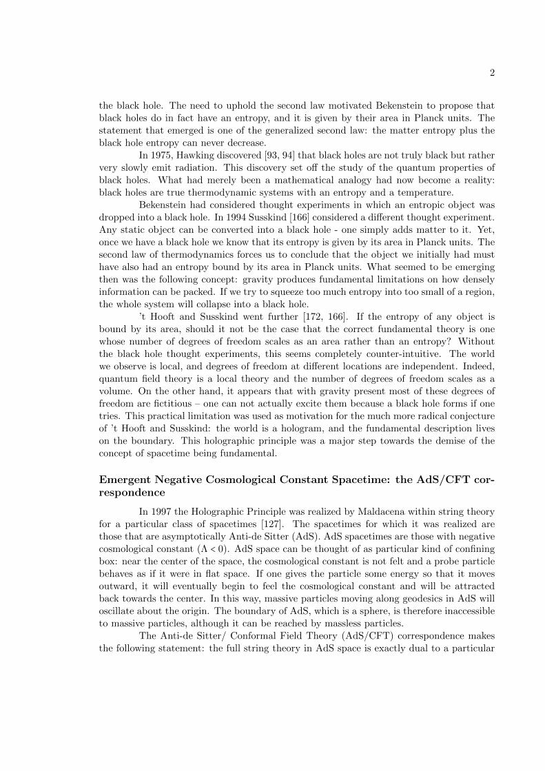
the black hole. The need to uphold the second law motivated Bekenstein to propose thatblack holes do in fact have an entropy, and it is given by their area in Planck units. Thestatement that emerged is one of the generalized second law: the matter entropy plus theblack hole entropy can never decrease.

In 1975, Hawking discovered [93, 94] that black holes are not truly black but rathervery slowly emit radiation. This discovery set off the study of the quantum properties ofblack holes. What had merely been a mathematical analogy had now become a reality:black holes are true thermodynamic systems with an entropy and a temperature.

Bekenstein had considered thought experiments in which an entropic object wasdropped into a black hole. In 1994 Susskind [166] considered a different thought experiment.Any static object can be converted into a black hole - one simply adds matter to it. Yet,once we have a black hole we know that its entropy is given by its area in Planck units. Thesecond law of thermodynamics forces us to conclude that the object we initially had musthave also had an entropy bound by its area in Planck units. What seemed to be emergingthen was the following concept: gravity produces fundamental limitations on how denselyinformation can be packed. If we try to squeeze too much entropy into too small of a region,the whole system will collapse into a black hole.

’t Hooft and Susskind went further [172, 166]. If the entropy of any object isbound by its area, should it not be the case that the correct fundamental theory is onewhose number of degrees of freedom scales as an area rather than an entropy? Withoutthe black hole thought experiments, this seems completely counter-intuitive. The worldwe observe is local, and degrees of freedom at different locations are independent. Indeed,quantum field theory is a local theory and the number of degrees of freedom scales as avolume. On the other hand, it appears that with gravity present most of these degrees offreedom are fictitious – one can not actually excite them because a black hole forms if onetries. This practical limitation was used as motivation for the much more radical conjectureof ’t Hooft and Susskind: the world is a hologram, and the fundamental description liveson the boundary. This holographic principle was a major step towards the demise of theconcept of spacetime being fundamental.

Emergent Negative Cosmological Constant Spacetime: the AdS/CFT cor-respondence

In 1997 the Holographic Principle was realized by Maldacena within string theoryfor a particular class of spacetimes [127]. The spacetimes for which it was realized arethose that are asymptotically Anti-de Sitter (AdS). AdS spacetimes are those with negativecosmological constant (Λ < 0). AdS space can be thought of as particular kind of confiningbox: near the center of the space, the cosmological constant is not felt and a probe particlebehaves as if it were in flat space. If one gives the particle some energy so that it movesoutward, it will eventually begin to feel the cosmological constant and will be attractedback towards the center. In this way, massive particles moving along geodesics in AdS willoscillate about the origin. The boundary of AdS, which is a sphere, is therefore inaccessibleto massive particles, although it can be reached by massless particles.

The Anti-de Sitter/ Conformal Field Theory (AdS/CFT) correspondence makesthe following statement: the full string theory in AdS space is exactly dual to a particular

3

field theory that can be thought of as living on the sphere that is at the boundary of AdS.AdS/CFT is perhaps the simplest and cleanest way to realize holography. An importantquestion is to what extent AdS/CFT has fully realized the holographic principle. In par-ticular, the holographic principle states that the theory describing the interior of a spherelives on the surface of the sphere and also has a Hilbert space dimension set by the areaof the sphere. AdS/CFT has clearly realized the first of these conditions because the CFTlives on the boundary. On the other hand, the later condition is more difficult since theboundary of AdS space has infinite area. This is consistent with the CFT having an infinitedimensional Hilbert space, but not very informative for trying the match the number ofdegrees of freedom. In chapter 2 we address this question of to what extent AdS/CFT hasfully realized holography.

Before the AdS/CFT correspondence, string theory provided a quantum theoryof gravity, but only in the perturbative regime. To address many of the fundamentalquestions in quantum gravity, one needs to know the nonperturbative structure of theory.The AdS/CFT correspondence both provided this nonperturbative definition, and at thesame time realized and confirmed the Holographic Principle.

Although AdS/CFT was discovered 15 years ago, many aspects of the dictionaryrelating bulk observables to boundary observables have remained elusive. It will be our goalto make progress in filling in this dictionary. In particular, one of the central mysteries ofholography is if spacetime is emergent and not fundamental, how does it do such a goodjob of emerging so that we perceive a local world?

One way to make progress towards understanding how the bulk emerges is to posethe question: is it the case that the CFT on some subset of the boundary is dual to somesubregion of the bulk? This question is intimately tied to the question of how nonlocalholography is. An affirmative answer to our question is not guaranteed, but if it were thecase that portions of the boundary could be associated with portions of the bulk in someway, it would not only provide an important ingredient in the bulk-boundary dictionary,but would also give us clues for how to apply holography in other contexts. In chapter 3 wefirst establish what the candidate bulk and boundary subregions would actually be. Then,in chapter 4 we try to establish to what extent the subregion duality can be realized.

An even more elementary question is how mysterious is holography. In particular,can one give a simple prescription for which CFT quantities encode the various aspects ofthe bulk? One can ask: if we consider a family of bulk observers in AdS who are nearthe boundary, can they do experiments to reconstruct the bulk? A priori, it is unclear ifthe answer should be positive or negative. By the nature of the AdS/CFT dictionary, theextent to which these observers can reconstruct the bulk is the same as the question ofthe extent to which local CFT operators are enough to reconstruct the bulk. One shouldrecall that a field theory has many quantities which are inherently nonlocal (for instance,entanglement entropies or Wilson loops). Consequently it is important to establish whenlocal CFT operators are sufficient to reconstruct the bulk, and when these more exoticnonlocal objects need to be used. In chapter 5 and 6 we turn to this question. Finally, incontexts that local CFT operators are not sufficient to reconstruct the bulk, one would liketo understand which nonlocal objects one should use instead. Entanglement entropy hasemerged as a particularly good candidate due to the work of Ryu and Takayanagi [154, 104]

4

relating boundary entanglement entropy to the area of extremal bulk curves. If the Ryu -Takayanagi conjecture is true, it gives a remarkable way in which to probe the bulk. Totest their conjecture one needs to know how to compute entanglement entropy within theCFT, and this is what we turn to in chapter 7.

Emergent Positive Cosmological Constant Spacetime

While AdS/CFT is a beautiful realization of holography, the spacetime we inhabithas a positive cosmological constant rather than a negative one. What we would really likethen would be to have a holographic description of a de Sitter spacetime (dS). This is a farmore challenging task. Indeed, it is even unclear where the holographic theory should live,as the full de Sitter space is itself spatially closed. Although, a natural possibility is thehologram lives on the spatial sphere at future infinity.

The main difficulty, however, to understanding emergent Λ > 0 spacetimes is thedifficulty of realizing them in string theory. In particular, the same arguments leading tothe AdS/CFT correspondence are not applicable to a putative dS/CFT correspondence[163, 164, 186, 131]. Nevertheless, one could conjecture there exists a CFT dual to de Sitterspace and then try to understand this correspondence without knowing the details of whatthe actual boundary theory is. Unfortunately, it is unclear if such a correspondence can berealized [168].

The potential absence of a holographic duality for pure stable de Sitter space maymean we must directly find the holographic dual of the full multiverse. It is believed thatthe effective potential within string theory is one with an enormous number of metastableminima. One therefore has not just one universe, but an infinite number of them. One canstart with a region that is de Sitter, yet tunneling events will cause it to decay to otheruniverses which can have either positive of negative Λ. The structure of the theory on futureinfinity is therefore a fractal rather than just a sphere. One is forced to define a theory onthis fractal. In chapter 8 we take some first steps towards doing this.

Unlike the case of AdS/CFT where we know the theory that is dual to string theoryin AdS space, we do not yet know what the theory is that is dual to the multiverse. At thisstage, one of the hopes is to extract pieces of the bulk-boundary mapping in AdS/CFT andapply them to the multiverse context. Concretely, in AdS/CFT (as discussed in chapter2) when comparing bulk quantities with CFT quantities one must typically impose an IRregulator in the bulk and correspondingly a UV regulator on the boundary. The AdS/CFTdictionary relates these regulators. In the context of a multiverse duality, a UV regulatoron the theory on future infinity would correspond to a late time regulator in the bulk.

The most basic question that needs to be answered is how to relate this boundaryUV regulator to a bulk late time regulator. In the context of the multiverse, the question ofthe late time regulator is known as the measure problem, and predates holography. While inthe context of the multiverse we do not have a theory telling us what the correct regulatoris, we instead have experimental observations. The hope then is to work in the reversedirection - we guess a bulk measure and see what predictions it gives us. The requirementthat predictions match observation then gives us clues about what the correct analog ofUV/IR is for the multiverse. In chapter 9 we test various measure proposals to see how welltheir predictions match observation. Finally, in chapter 10 we point out a serious difficulty

5

that is encountered with measures in the multiverse - the bulk late time regulator (measure)never decouples. As a field theory statement for the putative theory on future infinity, thismeans the UV cutoff never decouples.

6

Part I

Emergent Spacetime with Λ < 0:AdS/CFT

7

In this first part we study the holographic principle as realized in the AdS/CFTcorrespondence. This part is devoted to studying to what extent AdS/CFT realizes holog-raphy, what the dictionary is between the bulk theory and the boundary theory, and inwhat way bulk locality emerges. This part is organized as follows.

In chapter 2, based on [152], we study to what extent AdS/CFT has realized theholographic principle. The holographic principle asserts that the complete description ofthe interior of a sphere is a theory which not only lives on the surface of the sphere, but alsohas A/4 binary degrees of freedom. In this context we revisit the question of UV/IR thatwas initially studied by Susskind and Witten [165]. We construct states which are localizeddeep in the interior yet are encoded on short scales in the CFT, seemingly in conflict withthe UV/IR prescription. We make a proposal to address the more basic question of whichCFT states are sufficient to describe physics within a certain region of the bulk.

In chapter 3, based on [40], we ask whether the CFT restricted to a subset b of theAdS boundary has a well-defined dual restricted to a subset H(b) of the bulk geometry. ThePoincare patch is an example, but more general choices of b can be considered. We proposea geometric construction of H. We argue that H should contain the set C of causal curveswith both endpoints on b. Yet H should not reach so far from the boundary that the CFThas insufficient degrees of freedom to describe it. This can be guaranteed by constructinga superset L of H from light-sheets off boundary slices and invoking the covariant entropybound in the bulk. The simplest covariant choice is L = L+∩L−, where L+ (L−) is the unionof all future-directed (past-directed) light-sheets. We prove that C = L, so the holographicdomain is completely determined by our assumptions: H = C = L. In situations wherelocal bulk operators can be constructed on b, H is closely related to the set of bulk pointswhere this construction remains unambiguous under modifications of the CFT Hamiltonianoutside of b. Our construction leads to a covariant geometric RG flow. We comment on thedescription of black hole interiors and cosmological regions via AdS/CFT.

In chapter 4, based on [31], we investigate the nature of the AdS/CFT dualitybetween a subregion of the bulk and its boundary. In global AdS/CFT in the classicalGN = 0 limit, the duality reduces to a boundary value problem that can be solved byrestricting to one-point functions of local operators in the CFT. We show that the solution ofthis boundary value problem depends continuously on the CFT data. In contrast, the AdS-Rindler subregion cannot be continuously reconstructed from local CFT data restricted tothe associated boundary region. Motivated by related results in the mathematics literature,we posit that a continuous bulk reconstruction is only possible when every null geodesic in agiven bulk subregion has an endpoint on the associated boundary subregion. This suggeststhat a subregion duality for AdS-Rindler, if it exists, must involve nonlocal CFT operatorsin an essential way.

In chapter 5, based on [118], we study more generally the bulk - boundary map-ping. In Lorentzian AdS/CFT there exists a mapping between local bulk operators andnonlocal CFT operators. In global AdS this mapping can be found through use of bulkequations of motion and allows the nonlocal CFT operator to be expressed as a local oper-ator smeared over a range of positions and times. We argue that such a construction is notpossible if there are bulk normal modes with exponentially small near boundary imprint.We show that the AdS-Schwarzschild background is such a case, with the horizon intro-

8

ducing modes with angular momentum much larger than frequency, causing them to betrapped by the centrifugal barrier. More generally, we argue that any barrier in the radialeffective potential which prevents null geodesics from reaching the boundary will lead tomodes with vanishingly small near boundary imprint, thereby obstructing the existence ofa smearing function. While one may have thought the bulk-boundary dictionary for lowcurvature regions, such as the exterior of a black hole, should be as in empty AdS, ourresults demonstrate otherwise.

In chapter 6, based on [149], we further study the bulk -boundary dictionary andbulk reconstruction from boundary data. We establish resolution bounds on reconstructinga bulk field from boundary data on a timelike hypersurface. If the bulk only supportspropagating modes, reconstruction is complete. If the bulk supports evanescent modes, localreconstruction is not achievable unless one has exponential precision in knowledge of theboundary data. Without exponential precision, for a Minkowski bulk, one can reconstructa spatially coarse-grained bulk field, but only out to a depth set by the coarse-grainingscale. For an asymptotically AdS bulk, reconstruction is limited to a spatial coarse-grainingproper distance set by the AdS scale. AdS black holes admit evanescent modes. We studythe resolution bound in the large AdS black hole background and provide a dual CFTinterpretation. Our results demonstrate that, if there is a black hole of any size in thebulk, then sub-AdS bulk locality is no longer well-encoded in boundary data in terms oflocal CFT operators. Specifically, in order to probe the bulk on sub-AdS scales using onlyboundary data in terms of local operators, one must either have such data to exponentialprecision or make further assumptions about the bulk state.

In chapter 7, based on [153], we would like to start using the entanglement entropyas a probe of bulk geometry. We therefore develop a framework for computing entanglemententropy for the CFT. We provide a framework for a perturbative evaluation of the reduceddensity matrix. The method is based on a path integral in the analytically continued space-time. It suggests an alternative to the holographic and ‘standard’ replica trick calculationsof entanglement entropy. We implement this method within solvable field theory examplesto evaluate leading order corrections induced by small perturbations in the geometry of thebackground and entangling surface. Our findings are in accord with Solodukhin’s formulafor the universal term of entanglement entropy for four dimensional CFTs.

9

Chapter 2

Holography for a Small World

2.1 Introduction

The spherical entropy bound [14, 15] gives a remarkable bound on the number ofstates contained within a sphere of area A. The holographic principle [172, 166, 20, 23]builds on it to make the far more extraordinary assertion that there exists a theory thatlives on the sphere and describes all of physics within the sphere, and accomplishes this featwhile only having a Hilbert space of dimension exp(A/4l2pl).

AdS/CFT has only partially realized the holographic principle. The CFT doeslive on the boundary of AdS, but its Hilbert space is infinite-dimensional. The boundary ofthe region described has an area which is also infinite, and comparing two infinities is notmeaningful.

To confirm the holographic principle in AdS we must extract from the CFT atheory of the appropriate dimension that is capable of fully describing the innermost regionof AdS, out to a sphere of area A (see Fig. 2.1). The CFT on a lattice is a natural candidate,and was the basis of the UV/IR proposal of Susskind and Witten [165]. However, the UV/IRproposal is known to have some limitations, motivating us to analyze its validity in a rangeof contexts.

In the first part of this chapter we will construct certain states which explicitlyviolate UV/IR; the bulk states will be within the sphere of area A, yet their boundaryimage will have features on scales far smaller than the lattice spacing. Our examples willdemonstrate UV/IR is violated for both particles which stay inside the sphere and thosewhich enter and leave; for particles that are both relativistic and non-relativistic; for bothstatic states and dynamic states.

In the second part of the chapter we start afresh in looking for the correct theorydescribing the interior of the sphere of area A. We make a proposal for an answer to thequestion: what CFT states should this theory contain? This is a much easier question thanconstructing a full theory; a full theory requires having not only the states, but also theobservables and a way of doing time evolution. It is, however, a more difficult question thanfinding just the states confined within the sphere that the Bekenstein bound specializes to.If the interior of the sphere is truly a holographic image, the hologram must be able todescribe relativistic particles which enter and leave the sphere. We will discuss how our

10

"

"

(a)

Figure 2.1: The interior of the larger cylinder represents AdS. The vertical direction is timeand the radial direction is ρ. The CFT lives on the boundary (R×Sd−1) which is at ρ = π/2.In order for AdS/CFT to fully realize the holographic principle, some theory which has aHilbert space of dimension exp(A/4ld−1

pl ), where A is the area of the sphere at ρ = π/2 − δ,must be extracted from the CFT. This theory would live on the sphere at ρ = π/2− δ (innercylinder) and would need to be able to fully describe the interior: 0 < ρ < π/2 − δ.

proposal avoids the difficulties UV/IR encountered. We also comment on the necessity ofexcluding ultraboosted states from the description.

The chapter is organized as follows. In Sec. 2.2.1 we review the UV/IR proposal.In Sec. 7.2 we review the well-known example of a relativistic particle oscillating insideof AdS. The boundary image of the bulk gravitational field induced by the particle is theenergy-momentum tensor concentrated to a thin shell, and consequently strongly violatingUV/IR. In Sec. 2.4.1 we begin our study of scalar field wave packets. We construct a welllocalized and highly relativistic wave packet which goes inside the bulk IR cutoff, yet onthe boundary the expectation value of the CFT operator dual to the scalar field is localizedto a region well below the lattice spacing. In Sec. 7.4 we consider a scalar field with largemass (in AdS units), and consider a mode with angular momentum much larger than theinverse of the lattice spacing but much smaller than the mass. The mode is localized withinthe central AdS radius, yet the boundary image is on scales below the lattice spacing. InSec. 2.4.3 we consider a general solution of the Klein-Gordon equation and show that inorder for the CFT to not lose information about it when placed on a lattice would requirea lattice spacing far smaller than the one prescribed by UV/IR. In Sec. 2.5 we discuss thepossibility that the information contained in local CFT operators which went missing whena UV cutoff was placed is in fact retained in some other “precursor” operators. In Sec. 2.6we present our proposal for which CFT states are sufficient to fully describe the interior ofthe sphere of area A.

The question of the validity of the “scale/radius” relation is related but somewhat

11

different from the question of the validity of the UV/IR proposal. As a side note, inSec. 2.2.2 we comment that scale/radius does not follow from the rescaling isometry of thePoincare patch metric, nor is it generally valid. Our example in Sec. 2.4.1 explicitly violatesscale/radius.

2.2 UV/IR

2.2.1 Review of UV/IR

In this section we review the UV/IR proposal [165]. Consider AdS in globalcoordinates

ds2 = L2

cos2 ρ(−dτ2 + dρ2 + sin2 ρ dΩ2

d−1). (2.1)

The CFT lives on the boundary of AdS, at ρ = π/2, on a sphere that has been conformallyrescaled to have radius 1. The UV/IR prescription seeks to provide a theory that candescribe the interior of AdS for all ρ < π/2−δ, where δ ≪ 1. The full CFT is of course capableof doing this, however it has an infinite-dimensional Hilbert space and the holographicprinciple tells us a finite-dimensional Hilbert space should suffice.

In many computations in AdS/CFT, a bulk quantity that is IR divergent is dual toa CFT quantity that is UV divergent. For instance, the divergence of the length of a stringending on the boundary is dual to the divergent self-energy of a quark. This observationmotivated [165] to propose that the theory we are looking for is the CFT placed on a lattice.Since the CFT is an SU(N) gauge theory, [165] wanted to count N2 degrees of freedomper lattice site. The lattice spacing is then fixed by having the number of CFT degrees offreedom match the area in Planck units of the sphere at ρ = π/2 − δ:

1

ld−1pl

(Lδ)d−1

. (2.2)

Using the relation N2 = (L/lpl)d−1, we see that the lattice size is fixed to be δ.Since each of these degrees of freedom has, like a harmonic oscillator, an infinite-

dimensional Hilbert space, [165] needed to further impose that each oscillator can only beexcited to the first few energy levels. This amounts to imposing an energy density cutoffof (1/δ)d. The energy density cutoff will not be important for us since UV/IR will facedifficulties already at the stage of the spatial lattice.

We should note that the terminology “UV/IR” is used in a range of contexts. Forus, UV/IR will mean the specific proposal reviewed above of how to truncate the CFT andstill be able to describe the portion of the interior, 0 < ρ < π/2 − δ.

2.2.2 Comments on Scale/Radius

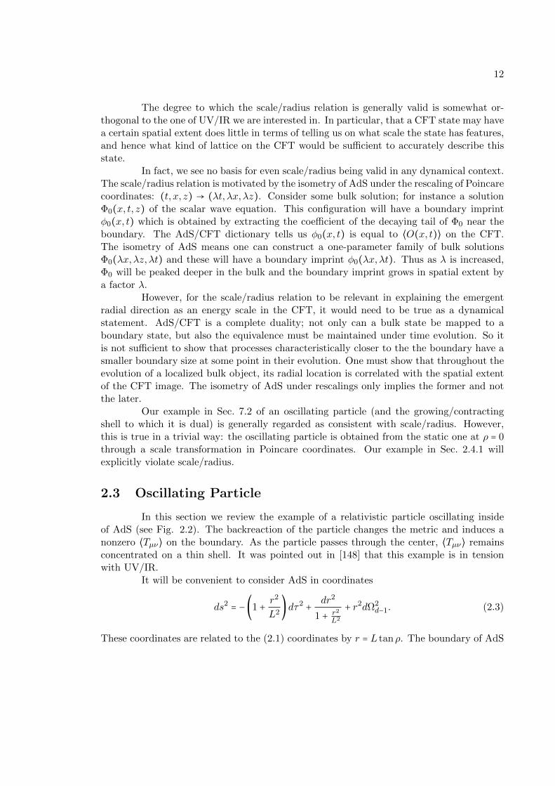
In this section we include a few comments on the “scale/radius” relation and howit relates to UV/IR. The scale/radius relation is the statement that an object close to theboundary should be dual to a CFT state with small spatial extent, whereas an object deepin the bulk should be dual to a CFT state of large spatial extent.

12

The degree to which the scale/radius relation is generally valid is somewhat or-thogonal to the one of UV/IR we are interested in. In particular, that a CFT state may havea certain spatial extent does little in terms of telling us on what scale the state has features,and hence what kind of lattice on the CFT would be sufficient to accurately describe thisstate.

In fact, we see no basis for even scale/radius being valid in any dynamical context.The scale/radius relation is motivated by the isometry of AdS under the rescaling of Poincarecoordinates: (t, x, z) → (λt, λx, λz). Consider some bulk solution; for instance a solutionΦ0(x, t, z) of the scalar wave equation. This configuration will have a boundary imprintφ0(x, t) which is obtained by extracting the coefficient of the decaying tail of Φ0 near theboundary. The AdS/CFT dictionary tells us φ0(x, t) is equal to ⟨O(x, t)⟩ on the CFT.The isometry of AdS means one can construct a one-parameter family of bulk solutionsΦ0(λx,λz, λt) and these will have a boundary imprint φ0(λx,λt). Thus as λ is increased,Φ0 will be peaked deeper in the bulk and the boundary imprint grows in spatial extent bya factor λ.

However, for the scale/radius relation to be relevant in explaining the emergentradial direction as an energy scale in the CFT, it would need to be true as a dynamicalstatement. AdS/CFT is a complete duality; not only can a bulk state be mapped to aboundary state, but also the equivalence must be maintained under time evolution. So itis not sufficient to show that processes characteristically closer to the the boundary have asmaller boundary size at some point in their evolution. One must show that throughout theevolution of a localized bulk object, its radial location is correlated with the spatial extentof the CFT image. The isometry of AdS under rescalings only implies the former and notthe later.

Our example in Sec. 7.2 of an oscillating particle (and the growing/contractingshell to which it is dual) is generally regarded as consistent with scale/radius. However,this is true in a trivial way: the oscillating particle is obtained from the static one at ρ = 0through a scale transformation in Poincare coordinates. Our example in Sec. 2.4.1 willexplicitly violate scale/radius.

2.3 Oscillating Particle

In this section we review the example of a relativistic particle oscillating insideof AdS (see Fig. 2.2). The backreaction of the particle changes the metric and induces anonzero ⟨Tµν⟩ on the boundary. As the particle passes through the center, ⟨Tµν⟩ remainsconcentrated on a thin shell. It was pointed out in [148] that this example is in tensionwith UV/IR.

It will be convenient to consider AdS in coordinates

ds2 = −(1 + r2

L2)dτ2 + dr2

1 + r2

L2

+ r2dΩ2d−1. (2.3)

These coordinates are related to the (2.1) coordinates by r = L tanρ. The boundary of AdS

13

(a) (b)

Figure 2.2: (a) A relativistic particle following a radial geodesic inside of AdS. Its closestapproach to the boundary is ρ = π/2 −m/E. (b) The sphere shown is the Sd−1 of the CFT(it is represented as an S2; in (a) we were only able to draw the boundary as an S1). Onthe CFT the particle is represented by a thin shell of ⟨Tµν⟩. This shell is shown at multipleinstances of time. As the particle starts near the boundary, the shell is small and near theright pole of the sphere. The shell grows as the particle falls towards smaller ρ. As theparticle passes through ρ = 0 the shell wraps the entire Sd−1. As the particle moves outagain to larger ρ, the shell contracts. Crucially, the thickness of the shell is m/E.

is at r →∞. In this limit the metric (2.3) asymptotes to

ds2 = r2 (−dτ2

L2+ dΩ2

d−1) . (2.4)

The metric of the Sd−1 ×R on which the CFT lives is obtained by conformally rescaling(2.4) by a factor of 1/r2, giving a sphere of radius equal to 1.

A particle of mass m oscillating in AdS (Fig. 2.2a) satisfies the geodesic equation

r2 = (Em

)2

− 1 − ( rL)

2

, (2.5)

where E is the energy of the particle with respect to the timelike Killing field,

E/m = (1 + r2/L2)τ . (2.6)

The proper energy of the particle at the center of AdS is equal to E, and the CFT energy ofthis state is EL. The largest r the particle reaches is rmax ≈ LE/m, where we have assumedE ≫ m. In terms of coordinates (2.1), ρmax = π/2 − α, where we defined α ≡ m/E. Sincethe particle is relativistic, α≪ 1.

The computation of ⟨Tµν⟩ for this state was done by Horowitz and Itzhaki [99], andwe collect their results in Appendix 2.8. In Fig. 2.2b we have sketched how ⟨Tµν⟩ evolves.The energy of the CFT state is concentrated on a shell of thickness α. As the particle fallsinto the bulk the shell expands, reaching a maximum size when the particle reaches r = 0.The shell then contracts as the particle moves out towards larger r. Crucially, the thicknessof the shell is equal to α.

14

0

0.005

0.01Z

-0.01

0

0.01

X

0

0.005

0.01Z

(a)

-0.01 0.01X

<OHxL>

(b)

Figure 2.3: (a) The profile of a localized wave packet (2.10) traveling away from the bound-ary (q0 = 106, σx = σz = 10−3) shown at time t = 10−2. It is composed of modes highlyoscillatory in the z direction, of wavenumber peaked around q0. (b) The CFT image ⟨O(x)⟩at this time (given by (2.20)).

UV/IR tells us that the CFT on a lattice with spacing δ should describe the bulkout to ρ = π/2 − δ. Thus, it must describe the oscillating particle which goes through ρsmaller than the cutoff. Yet, if we choose α≪ δ, then the shell has a width far smaller thanthe lattice spacing. The extent to which the cutoff CFT fails to describe the particle can bemade arbitrarily large by making α small. The extreme case would be a massless particletraveling through the bulk. Its boundary dual is a shell that is completely localized on thelightcone θ = τ .

2.4 Scalar Field Solutions

The example in Sec. 7.2 of an oscillating particle presents a constraint on imposingany kind of lattice on the CFT. However, this example is a bit special and we would like tohave a larger set of examples to test UV/IR. That is what we do in this section. Instead ofworking with the gravitational field, we will consider a free scalar field φ,

(◻ +m2)φ = 0. (2.7)

The CFT operator O is dual to φ. Throughout this section we will consider some solutionsof (2.7) and look at ⟨O⟩ for these states. We will be interested in solutions of (2.7) whicheither at some time, or for all time, are contained within the bulk region ρ < π/2− δ. In ourexamples we will construct states that do this and also have ⟨O⟩ that is concentrated onscales much less than δ.

2.4.1 Relativistic Wave Packet

In this section we would like to construct a wave packet that travels from near theboundary of AdS into the bulk. We would like this packet to remain well concentrated and

15

have negligible spread as it propagates into the bulk. It is familiar from wave physics thatpackets with large momentum in one direction have, for a long period of time, negligiblespreading in the transverse directions. In AdS we can construct packets with a similarproperty (shown in Fig. 2.3a). For these packets we will want to find how ⟨O⟩ evolves withtime. Near the boundary (ρ ≈ π/2), the field value will decay as (cosρ)∆. The AdS/CFTdictionary tell us that the coefficient in front of this term determines ⟨O⟩. So to find ⟨O⟩we need to find the behavior of the tail of the wave packet at ρ ≈ π/2. It should be pointedout that just because the peak of the packet in the bulk has negligible transverse spreaddoes not yet imply the tail will also have negligible spread with time; although we will seethis is what occurs in AdS.

The packets we will construct can be used to violate UV/IR by arbitrarily largeamounts. For some given lattice spacing δ, we make a packet with transverse spread muchless than δ. We then make it sufficiently energetic so that it doesn’t spread for a long time.On the CFT, ⟨O⟩ remains concentrated to a region much less than δ, even when the packetis at ρ < π/2 − δ.

To construct the packets it will be convenient to use Poincare coordinates, whichare a good approximation to global coordinates near the boundary and for small angularspread. Inserting ρ = π/2 − z into (2.1) gives

ds2 = L2

z2(−dt2 + dz2 + dx2) , (2.8)

where the angular coordinate is now x and the time coordinate has been relabeled t = τ . Inthese coordinates the mode solutions to (2.7) are

ϕqk(x, t, z) = zd/2Jν(qz)eikx−iωqkt, (2.9)

where 0 < q <∞, the energy is ω2qk = q2 + k2, and ν = ∆ − d/2. The conformal dimension ∆

is taken to be of order 1, and is related to the mass m through ∆(∆ − d) =m2L2.We now construct our packet out of the modes (2.8) peaked around a large q = q0

with spread in q of σ−1z , and peaked around k = 0 with spread in k of σ−1

x :

Φ(x, t, z) = ∫ dq dk√q ϕqk(t, x, z) e−k

2σ2x/4 e−(q−q0)

2σ2z/4, (2.10)

where q0 ≫ σ−1z , σ

−1x ≫ 1. To verify the packet has the behavior we desire, we make some

simplifications to allow us to evaluate the integrals in (2.10). First we notice that particlesin AdS only behave differently from those in Minkowski space when they get close enoughto the boundary such that the gravitational potential energy becomes comparable to theirkinetic energy. In terms of the modes (2.9) this is reflected in the the z component:

Jν(qz) ∼1

√qzeiqz, for qz ≫ ν . (2.11)

This means we can think of q as a kind of radial momentum. From the form of (2.10) we seethat q is peaked around q0 with spread σ−1

z which is much less than q0. Thus for z ≫ ν/q0

we can approximate (2.10) by

Φ(x, t, z) ≈ z(d−1)/2∫ dq dk eiqz e−k2σ2x/4 eikx e−(q−q0)

2σ2z/4 e−iωqkt. (2.12)

16

Aside from the uninteresting power of z in front, (2.12) is of the same form as a packetpropagating in the z direction in Minkowski space. Since in (2.12), k ≲ σ−1

x ≪ q0, weapproximate

ωqk =√q2 + k2 ≈ q + k2

2q0. (2.13)

This allows us to separate the q and k integrals in (2.12), and easily evaluate the integralover q,

Φ(x, t, z) = z(d−1)/2 ψ(x, t) e−(z−t)2/σ2z eiq0(z−t), (2.14)

where

ψ(x, t) = ∫ dk eikx e−k2σ2x/4 e

−i k2t

2q0 . (2.15)

We have dropped constants and have labeled the transverse spread as ψ because, as canbe seen from the energy (2.13), it satisfies the non-relativistic Schrodinger equation for aparticle of mass q0. Evaluating (2.15) thus gives the familiar answer,

ψ(x, t) = 1

σx√

1 + 2itσ2xq0

exp⎛⎝− x2

σ2x(1 + 2it

σ2xq0

)⎞⎠, (2.16)

showing the packet’s spread with time is the expected,

σx(t) = σx

¿ÁÁÀ1 + ( 2t

q0σ2x

)2

. (2.17)

This shows that the transverse spread is negligible for times t ≲ q0σ2x.

We would now like to evaluate ⟨O(x, t)⟩. Noting that for small z the Bessel functioncan be approximated as

Jν(qz) ∼ (qz)ν for qz < ν , (2.18)

we obtain ⟨O(x, t)⟩ from the z → 0 limit of z−∆Φ(x, t, z). Using (2.10) we find,

⟨O(x, t)⟩ = ∫ dq dk qν+1/2 e−k2σ2x/4 eikx e−(q−q0)

2σ2z/4 e−iωqkt . (2.19)

We now perform the same simplifications we used on (2.10), separating the integrals over qand k, and finding

⟨O(x, t)⟩ = e−iq0tψ(x, t), (2.20)

where ψ(x, t) is given by the same expression as (2.15) before, and we have ignored termsthat are independent of x, t. Eq. 2.20 shows that ⟨O(x, t)⟩ remains localized within ∣x∣ ≲ σxfor a time t ≲ q0σ

2x, as well as being highly oscillatory with time.1 A wave packet and its

1Since our interest is the CFT defined on the sphere of the global AdS boundary, our equations shouldonly be used for small times, t≪ 1, where the approximation of the Poincare patch metric is valid. To followthe packet deeper into the bulk we would need to use the true global AdS evolution. Since it will take thepacket a time of π/2 to reach the center of AdS, we expect its transverse spread even at the center to remaincomparable to σx (with a sufficiently large choice of q0). It is interesting to consider what would happen ifwe were actually interested in the CFT theory on the Minkowski boundary of the Poincare patch. Then asthe packet moves towards the Poincare horizon located at infinite z, the CFT profile would spread over theentire x axis. This is not surprising; in this case the packet is traveling for an infinite amount of Poincaretime.

17

1 2 3 4 5 6 7

r

L

f0,l

Figure 2.4: A plot of the radial modes f0l(ρ) in (2.21) for fixed l (l = 100) and severaldifferent choices of ∆ (∆ = 10, 100, 500, in colors red, green, blue, respectively). Thevariable on the horizontal axis is the radial coordinate r/L = tanρ. The plot shows thatincreasing ∆ leads to stronger confinement to the center of AdS. To violate UV/IR wechoose a mode with ∆ ≫ l≫ 1/δ.

dual ⟨O⟩ at an instant of time are shown in Fig. 2.3. We see that the UV/IR prescriptioncan be violated by arbitrarily large amounts with this example. To decrease the boundarysize, σx, we simply need to increase q0 in order to maintain q0 ≫ σ−1

x .Since we are taking q0 to be large, one might worry that if there is other matter

around then gravitational effects might invalidate the use of the free wave equation (2.7).However, any such effects would occur on scales set by the Planck scale. The Planck scaleis related to the AdS scale by a power of 1/N . Crucially, the lattice size on the boundarythat UV/IR prescribes is independent of N , allowing us to take N as large as we want.

2.4.2 Non-relativistic Mode

In Sec. 7.2 and Sec. 2.4.1 we considered relativistic particles with large momentumin the radial direction. In this section we go to the other extreme of a non-relativisticparticle with angular momentum. The radial location of the particle is determined by twocompeting forces. AdS is confining, and the more massive the particle, the more it is confinedto the center of AdS. On the other hand, the centrifugal barrier from the particle’s angularmomentum pushes it out to larger radius. We will see that in order for the boundary imageto have features on small scales, the particle needs to be given large angular momentum.By dialing the particle’s mass to be sufficiently large, we make the particle well-confined tothe center of AdS, and hence violate UV/IR.

As in the previous section, we consider a scalar field and for simplicity our equa-tions are in AdS3. The mode solutions of the Klein-Gordon equation (2.7) in global coor-dinates (2.1) are given by,

ϕnl(ρ, τ, θ) = fnl(ρ)eilθe−iωnlτ . (2.21)

The energy ωnl = ∆+2n+ l, where ∆ ≈mL for large mass, and the radial part fnl(ρ) is somehypergeometric function whose explicit form we have suppressed. For small ρ AdS looks

18

like Minkowski space in spherical coordinates, and the radial modes reduce to the familiarspherical Bessel functions.

Consider a bulk solution that consists of just a single mode, (2.21). On the bound-ary, the expectation value of O for this state is simply proportional to (2.21) with the radialportion removed,

⟨O(θ, τ)⟩∝ eilθe−iωnlτ . (2.22)

Let us now put the CFT on a lattice of size δ. Since the CFT lives on a circle of radius1, this amounts to restricting to modes with l ≲ δ−1. Thus, to violate UV/IR we simplyneed to consider a bulk solution ϕ0l with l≫ δ−1 and take the mass of the field sufficientlylarge to have this mode confined near the center. In other words, ∆ ≫ l ≫ δ−1. Since thisexample consists of an energy eigenstate, it illustrates that UV/IR is insufficient even fordescribing static bulk physics which remains confined within ρ < π/2 − δ.

2.4.3 General Solution

We have seen examples of both relativistic and non-relativistic wave packets thatcause difficulties for UV/IR. But perhaps these examples are special and for a generic bulkfield configuration, the UV regulated CFT will be able to describe it fairly well. This is thequestion we address in this section.

Consider some solution Φ(ρ, τ, θ) of the wave equation (2.7). Expanding Φ interms of modes (2.21),

Φ(ρ, τ, θ) =∑n,l

cnl fnl(ρ) eilθ−iωnlτ . (2.23)

Assuming the modes are normalized with respect to the standard bulk Klein-Gordon norm,near the boundary fnl(ρ) takes the form dnl(cosρ)∆, where

dnl = (−1)n¿ÁÁÀΓ(∆ + n + ∣l∣)Γ(∆ + n)

n!Γ(∆)2Γ(n + ∣l∣ + 1) . (2.24)

We can now find the boundary imprint of this solution,

⟨O(τ, θ)⟩ =∑n,l

cnl dnl eilθ−iωnlτ . (2.25)

The question now is: for a solution Φ relevant to the region ρ < π/2 − δ, are theimportant features of the corresponding ⟨O⟩ on scales larger than δ? On the boundary, aspatial lattice of size δ is equivalent to cutoff on l of δ−1. In order to be able to truncate thesum in (2.25) to l < δ−1, it would need to be the case that cnl is suppressed at these large l.However, this is clearly not generally true. At any fixed ρ in the bulk we need a completebasis of modes in the angular direction, which requires retaining modes of arbitrarily highl.

To be more precise, since we don’t expect local field theory to be valid in thebulk below the Planck scale, the highest l we would actually need in order to describe r < Rwould be R/lpl. However, this would require a lattice spacing on the CFT that is far smallerthan in the UV/IR prescription: in AdSd+1/CFTd, the lattice we would need to describeρ < π/2 − δ would need to have a spacing of δ/N2/(d−1).

19

2.5 Precursors

We have seen examples of states for which the CFT would lose some of the infor-mation contained in ⟨O⟩ if it were placed on a lattice. However, perhaps all the informationabout the state is still present in the CFT on a lattice, but instead of being containedin ⟨O⟩ is contained in the expectation value of some other operators? Without a betterunderstanding of the AdS/CFT dictionary this remains a possibility, but one that is dif-ficult to test. In this section we will just make two comments. The first is that we seeno compelling reason why upon placing the CFT on a lattice, ⟨O⟩ would lose informationwhile these other operators retain it. The second is that if this possibility is realized, thenthe UV/IR regulated version of AdS/CFT may not be very useful since the aspects of thebulk-boundary dictionary that we knew in the full AdS/CFT would not be applicable tothe regulated version.

To discuss how the CFT encodes the bulk it is useful to ask the following question:how would a collection of CFT observers reconstruct some bulk field configuration Φ(ρ, τ, θ)?Expanding Φ in terms of modes ϕnl as in (2.23), the goal of the CFT observers would beto determine all the coefficients cnl. Measuring the expectation value of O over the wholesphere at one instant of time, ⟨O(θ, τ0)⟩, would give them some of the information, but notall of it. In particular, since the boundary imprint in ⟨O⟩ of a single mode is proportionalto exp(ilθ − iωnlτ0), the CFT observers would be able to distinguish among the differentl quantum numbers. However, all the modes ϕnl of a fixed l but differing n would givethe same imprint in ⟨O(θ, τ0)⟩. By measuring ⟨O(θ, τ)⟩ over a range of times, the CFTobservers could start distinguishing the modes with different n. Having ⟨O(θ, τ)⟩ for all θand a time of ∆τ = π would allow for a full reconstruction of Φ.

If AdS/CFT is complete then there should be a faster way of reconstructing thebulk; there should exist some CFT operators, named “precursors” in [148], which can bemeasured at one instant of time and immediately fully determine Φ. The precursor operatorsare expected to be highly nonlocal and their actual form has remained a mystery. In certaindynamical contexts precursors are essential. For instance, if two wave packets collide in thecenter of AdS, it takes a time of π/2 before causality allows the result of the collision topropagate to the boundary and become encoded in ⟨O⟩. During that π/2 interval of time,the result of the collision is encoded exclusively in the precursors.

These considerations lead us to believe that if we were to consider the CFT onsome subset of the boundary, R × Sd−1, that does not contain the full time direction, thenthe only way to reconstruct some portions of the bulk would be by measuring precursors.However, this is not the situation UV/IR presents: the UV regulated CFT in UV/IR stilllives on the full time direction.2 Thus it would be unclear why precursors are essential inthe UV/IR regulated version of AdS/CFT in contexts where they were not needed in thefull AdS/CFT.

Nevertheless, it may be that precursors save UV/IR. In this case, we should askwhat the bulk-boundary dictionary would be for the UV/IR regulated AdS/CFT. In the

2In UV/IR an energy density cutoff is prescribed for the CFT in addition to the spatial lattice. Theenergy cutoff can be regarded as making the time direction into a lattice. Thus, if in our examples UV/IRhad failed due to the energy density cutoff, then the need for precursors might have been a good explanation.However, UV/IR failed already at the stage of imposing the spatial lattice.

20

full AdS/CFT one can construct a mapping, perturbatively in 1/N , between local bulkoperators φ(ρ, τ, θ) and the CFT operator O smeared over space and time with some kernel.To leading order in 1/N , this takes the form

φ(ρ, τ, θ) = ∫ dτ ′dθ′ K(ρ, τ, θ∣τ ′, θ′) O(τ ′, θ′). (2.26)

The actual form of K was worked out in [90, 89], where the authors also pointed out thata UV cutoff on the CFT would destroy the mapping (2.26). Namely, [90] showed that thedivergence in the two-point function of φ at coincident points can only occur from the UVdivergence of the two-point function of O. Thus, if the theory dual to the inner portion ofAdS is the CFT with a UV cutoff, then the only way to express the bulk operators φ interms of CFT operators is directly in terms of the precursors.

2.6 A Proposal for Finding the States

We are interested in finding a theory which is capable of describing all the physicsthat can occur in the interior of a sphere of area A in AdS, while having a Hilbert space ofthe appropriate dimension. The proposal the UV/IR prescription gave is that the theorydescribing the interior ρ < π/2−δ is the CFT on a lattice of size δ. We have seen in previoussections that this proposal faces difficulties. In this section we initiate a new search for thedesired theory.

Finding such a theory is a difficult problem, and we will only try to address amore elementary question: what are the CFT states that this theory would contain? Inother words, what is the set of CFT states that are sufficient to cover everything that couldpossibly happen in the region 0 < ρ < ρ0?

We need to know what CFT states are dual to a chair in the center of AdS, or astar, or any object contained within ρ < ρ0. But we also need much more than that. Thesphere at ρ = ρ0 that we are discussing is imaginary; we aren’t literally putting a shell there.So a particle can fly in and out of the region ρ < ρ0, or two particles can come in, collide,and leave. We must include the CFT states dual to these processes. This is an essentialpoint: if this “small world” consisting of ρ < ρ0 is truly a holographic image, every physicalprocess which occurs inside should be encoded in the hologram. The difficult part is thatwe should choose carefully which CFT states we are keeping, since the holographic principleonly allows us to include exp(A/4ld−1

pl ) independent states. We should note that there isno guarantee the question being posed has an answer. It may just be that one really needsmore states, even an infinite number, and there is no hologram for a small world.

We begin this section by reviewing the Bekenstein bound. We then make ourproposal for what the CFT states are that we want, and discuss how it passes the testsof the previous sections that UV/IR struggled with. We then discuss a puzzling aspect ofour proposal, and indeed any proposal which keeps a finite number of states: ultraboostedstates which pass through ρ < ρ0 must be excluded from the description.

21

2.6.1 Proposal

Consider some weakly gravitating object that has energy E and can be enclosedin a sphere of radius R.3 For instance, the object could be a planet, or a gas inside of aspherical cavity with reflecting walls. The Bekenstein bound gives a bound on the entropyof the object,

S ≤ 2πER . (2.27)

The requirement that the object not be within its Schwarzschild radius requires E < R/2l2pl,and transforms (2.27) into

S ≤ A

4l2pl. (2.28)

Eq. (2.28) can be interpreted as saying that if we have a spherical box with enclosing walls,then specifying A/4l2pl numbers is sufficient to completely specify what is inside the box.

We now return to AdS, and consider placing one of these bound systems insideof AdS. Since AdS is confining, placing the system anywhere except the center will incuran energy cost. If we do place it in the center then in order for it to not undergo gravi-tational collapse, its energy must be bound by its size. These considerations motivate ourproposal for the answer to the question of what CFT states are in the holographic theory.In coordinates (2.1), with the AdS radius L, and with the CFT living on a sphere of radius 1,

Proposal: The CFT states sufficient to fully describe the bulk for all ρ < ρ0 arethose with CFT energy less than ML, where M is the mass of a black hole of radius ρ0.

Let us discuss a few aspects of our proposal. First, we would like to make sure itcovers all the states we considered in previous sections. The non-relativistic particle withangular momentum (Sec. 7.4) stays confined within ρ < ρ0 and so is the kind of boundstate the Bekenstein bound includes, and is easily covered. In Sec. 7.2 and Sec. 2.4.1 weconsidered a relativistic particle which enters and leaves our sphere. UV/IR had difficultywith it even in the case the particle’s energy is measured in AdS units, regardless of howsmall lpl is. In our proposal, the energy cutoff is in Planck units, and so these relativisticparticles are included.

We also need to verify that our proposal has the correct number of states prescribedby the holographic principle. This follows from consistency of AdS/CFT. On the CFT sidewe want to count the number of states with energy less than ML. This will be dominatedby states with energy close to ML, and up to order 1 factors, can be calculated from thestandard thermodynamics of a free gas of N2 species. For CFT4 for large M , the log of thenumber of such states is of order N1/2(ML)3/4. We need to compare this with the area inPlanck units of a large AdS5 black hole of mass M . This is given by (Ml3plL

2)3/4/l3pl. Using

the relation N2 = (L/lpl)3, we see they are equal.4

3In this paragraph we are in 4-dimensional Minkowski space.4Although our proposal should be applicable even for small spheres with sub-AdS radius, it is not partic-

ularly useful in this case since the number of CFT states is larger than what we want. In particular, therewill be states which are dual to graviton energy eigenstates that are delocalized over the entire central AdSregion.

22

Figure 2.5: A highly boosted state for which the center of mass energy, and hence backre-action, is small. In order for the theory on the sphere to only have a finite number of states,we must exclude this state. A plausible reason is that any attempt to probe it would forma black hole that is much larger than the sphere.

We note that our proposal is more concrete than the heuristic statement that CFTstates of low energy are associated with bulk regions of small ρ and states of high energyare associated with the near boundary region, ρ ≈ π/2. In particular, we are not proposingthat CFT states of high energy are sufficient to describe the portion of the bulk that is nearthe boundary. This would obviously be wrong; a relativistic particle oscillating in AdS, likethe one in Sec. 7.2, transverses nearly all of AdS while having constant energy. All we aresaying is that the low energy states may be sufficient to completely describe the small ρregion.

2.6.2 Ultraboosted states

Having discussed the successes of our proposal, in this section we push it to thebrink of failure. Namely, our proposal excludes the high energy states (those with energygreater than ML), and we need to know if this is valid. It is certainly justified to excludea state if it has large backreaction, and this is the first avenue we pursue. Our discussionwill focus on the two different frames of reference that are relevant: that of the sphere onwhich the theory lives, and the center of mass frame.

Consider the state inside the sphere at some instant of time as an object is passingthrough. The energy, E, with respect to the reference frame of the sphere is the energythat appears in our proposal as the cutoff energy determining which states are kept. Thereis also the center of mass reference frame, and we will let ECM denote the energy in thisframe. The backreaction, as characterized by curvature invariants, can be computed in anyframe of reference and is easiest to analyze in the center of mass frame.

There are therefore two different possibilities: (a) E and ECM are comparable.(b) E ≫ ECM . In Case (a) our proposal does well, since the states of large energy also have

23

large center of mass energy ECM and consequently collapse into a black hole larger thanour sphere. On the other hand, Case (b) (see Fig. 2.5) is more interesting. By taking somesystem of small energy and boosting it by an enormous amount, its energy E can be madearbitrarily large. By going to sufficiently large boost, we can make states which the theoryliving on the sphere can no longer describe.

Although it appears odd that sufficiently energetic states are invisible to the theoryon the sphere, it is perhaps reasonable. The observables of the theory should correspond tosome kind of physical probe of the interior. For instance, the sphere theory could send inparticles to probe the interior. These probes will naturally be of low energy, as measuredin the sphere reference frame. Now consider the state of an ultraboosted object passingthrough the interior. Any attempt to probe it in this way will form a large black hole, ofradius much larger than where the sphere theory was living. So, in a physical sense, thereis no way for the hologram to be able to describe these states.

2.7 Conclusion

Our goal has been to see the extent to which UV/IR gives us a theory, withA/4ld−1

pl degrees of freedom, that can fully describe the central AdS region out to a sphereof area A. We presented some examples which are in tension with UV/IR. We thereforetook a step back, turning to the more basic question of which CFT states are sufficientto describe the interior of the sphere. The states of lowest energy seem like a promisingcandidate, which passes the tests UV/IR struggled with. Interestingly, an ultraboostedparticle passing through would be invisible to the theory on the sphere.

One may wonder: is there any reason a region of spacetime should be describedby a holographic theory with so few degrees of freedom? The most straightforward inter-pretation of entropy bounds would be that they do nothing more than quantify the simpleobservation that information requires energy, and too much energy confined to too small of aregion leads to gravitational collapse. From this perspective, the holographic principle is anunbelievable extrapolation. And yet, AdS/CFT has partially realized the holographic prin-ciple; so perhaps it fully realizes it. Or, perhaps it doesn’t and there only exist hologramswith infinite information content.

2.8 Equations for Energy Shell

In this appendix we collect several equations from [99] relevant for finding ⟨Tµν⟩for the oscillating particle in Sec. 7.2. The result was already sketched in Fig. 2.2 b.

To find ⟨Tµν⟩ we need to first find the gravitational field caused by the oscillatingparticle. The tail of this field at large r will then be proportional to ⟨Tµν⟩. Horowitz andItzhaki [99] did this calculation in a more elegant way. They first found ⟨Tµν⟩ for a stationaryparticle at r = 0 and then applied a boost. Their answer is presented in Poincare patchcoordinates, since in these coordinates a boost is just a dilatation and easy to implement.The Poincare patch metric is

ds2 = L2

z2(−dt2 + dx2 + dz2) . (2.29)

24

Defining u = t −√x2 and v = t +

√x2, the result of [99] for AdS5/CFT4 is

⟨Tuu⟩ = 8mα4

3π2

1

(α2 + u2)3(α2 + v2) (2.30)

⟨Tvv⟩ = 8mα4

3π2

1

(α2 + v2)3(α2 + u2) (2.31)

⟨Tuv⟩ = 4mα4

3π2

1

(α2 + u2)2(α2 + v2)2. (2.32)

In Poincare patch coordinates, the particle starts at z = α at t = 0 and then falls towardslarger z. For fixed v, ⟨Tµν⟩ can be seen to be peaked on the lightcone (u = 0) with width oforder α.

Since our real interest is in the boundary theory on R × S3, we need to do aconformal transformation and coordinate change to get from R3,1 to R×S3. The Minkowskimetric is

ds2 = −dudv + (v − u)2

4dΩ2

2. (2.33)

Conformally rescaling by a factor of 14(1+ v

2)(1+u2) and changing coordinates: u = tanU ,v = tanV , where U = 1

2(τ − θ) and V = 12(τ + θ) gives the desired

ds2 = −dτ2 + (dθ2 + sin2 θdΩ22). (2.34)

Applying these transformations to theR3,1 stress tensor (2.30) gives theR×S3 stress tensor:

⟨TUU ⟩ = 2mα4

3π2

(1 + u2)3(1 + v2)(α2 + u2)3(α2 + v2) (2.35)

⟨TV V ⟩ = 2mα4

3π2

(1 + v2)3(1 + u2)(α2 + v2)3(α2 + u2) (2.36)

⟨TUV ⟩ = mα4

3π2

(1 + u2)2(1 + v2)2

(α2 + u2)2(α2 + v2)2, (2.37)

where u and v were written above in terms of τ and θ. If we are interested in the energycomponent, then this is given by

⟨Tττ ⟩ =1

4(⟨TUU ⟩ + 2⟨TUV ⟩ + ⟨TV V ⟩). (2.38)

25

Chapter 3

Light-sheets and AdS/CFT

3.1 Introduction

In the study of the Lorentzian AdS/CFT correspondence [127, 185, 6, 89, 91],one may consider the boundary theory defined on a proper subset of the global conformalboundary. In this case, it is natural to expect that the bulk dual spacetime manifold maybe extendible. That is, the theory on the subset should describe less than the maximallyextended global bulk solution.

The most common example is the CFT on Minkowski space, Rd−1,1, which is dualto the Poincare patch of the bulk, with metric

ds2 = R2−dt2 + dx2d−1 + dz2

z2. (3.1)

These bulk and boundary regions are shown as subsets of global AdS in Fig. 3.1a. ThePoincare patch seems a “natural” choice for the bulk, at least in the above warped-productcoordinate system, where the boundary corresponds to z = 0 and the Poincare patch toz > 0. However, there is nothing special about this choice of coordinates. One could easilywrite down coordinates that cover a larger or smaller portion of the bulk that is boundedby the same portion of the conformal boundary as z → 0 (see Fig. 3.1b). So what selectsthe Poincare patch as the bulk dual of the CFT on Minkowski space?

The bulk dual region should be well-defined not only in the vacuum, but forarbitrary states in the semiclassical regime, perturbatively in 1/N . Deep in the bulk, themetric will not be that of empty AdS space. In general all Killing symmetries will be broken,so they cannot be used to pick out a preferred bulk region. For example, consider a globalbulk solution corresponding to a pair of neutron stars orbiting around the origin of thestandard global coordinates. At what time (say, along its worldline) does each star enterand exit the bulk region dual to the CFT on Rd−1,1?

Another well-known example is the maximally extended Schwarzschild-AdS blackhole. The global conformal boundary consists of two disconnected copies of R × Sd−1. Inthe Hartle-Hawking state (the Euclidean vacuum), the two components can be thought ofas slices in a single complex manifold and are related by analyticity. However, one canconsider more general states, for example by adding neutron stars near the left boundary

26

(a) (b)

Figure 3.1: (a) The Poincare patch of AdS, with the usual time slicing in the coordinatesof Eq. (1.1). (b) Time slices of an arbitrary bulk coordinate system that covers the samenear-boundary region as the Poincare patch but a different region far from the boundary.This illustrates that there is no preferred coordinate system that would uniquely pick outa region described by the boundary, particularly if the bulk is not in the vacuum state.

(far from the black hole), and white dwarfs near the right boundary. Restricting attentionto the CFT living on the left boundary, one would expect it to encode the nearby neutronstars, but not the white dwarfs on the far side of the black hole. But what is the basisof this expectation? And where does the reach of the left theory end: at the black holehorizon, or somewhere inside the black hole/white hole regions? Again, there should be ananswer to this question that does not rely on special bulk symmetries or coordinate choices.

There are many other possible choices of subsets b of the global boundary, someof which are shown in Fig. 3.2.1 Let us suppose that the CFT on b describes some portionH(b) of the bulk. We will call H(b) the holographic domain of b. It should be possible toconstruct this bulk region geometrically from b. The goal of this paper is to provide such aconstruction. 2

1We consider only subsets b which, viewed as manifolds in their own right, are globally hyperbolic andhave the same number of spacetime dimensions as the global boundary. Otherwise the initial value problemof the CFT would be ill-defined. If b is a proper subset of the global boundary, then it is not obvious thatthe CFT on b must have a bulk dual, and we do not set out to prove this or establish under which conditionsa bulk dual exists. The question we seek to address is: if b did have a bulk dual region, what would itbe? In all cases, a semiclassical bulk dual can be assigned only to some subset of CFT states (excluding,for example, the equal superposition of two global CFT states corresponding to different bulk metrics), andonly perturbatively in 1/N . In the case of a small diamond, the bulk dual is the AdS-Rindler patch, so onewould expect the geometric states to have a thermal character.

2In the special case that b is a diamond, motivated by the Ryu- Takayanagi proposal [154, 173, 68] forcomputing holographic entanglement entropy, one could try constructing H(b) out of minimal surface whichstart and end on b. We will not explore this approach here, however it would be interesting to study how itrelates to our construction. We will note however that Ryu - Takayanagi only applies for static situations;

27

tall strip

small diamond

(a)

Minkowskispace

de Sitter space

(b)

short strip

largediamond

(c)

Figure 3.2: The boundary of AdS; the dashed lines should be identified. Examples ofglobally hyperbolic subsets b are shown shaded. A causal diamond is a set of the formI−(q) ∪ I+(p), where q is boundary event in the future of the boundary event p. Let τbe the time along a geodesic from p to q in the Einstein static universe of unit radius(ds2 = −dt2 + dΩ2

d−1). With τ = 2π, the causal diamond is the boundary of the Poincarepatch. A causal diamond with τ < 2π (τ > 2π) is called “small” (“large”). An open interval(t1, t2) with t2 − t1 < π (t2 − t1 > π is called “short strip” (“tall strip”).

Outline Our strategy will be to bound the bulk dual region H(b) by a subset C(b) anda superset L(b):

C(b) ⊂H(b) ⊂ L(b) . (3.2)

We choose C(b) to be the minimum region the CFT needs to describe to be consistent withbulk causality and locality properties near the boundary. The set L(b) will be constructedfrom light-sheets in a way that ensures that the bulk dual does not have more degreesof freedom (higher maximum entropy) than the CFT. We will then show that under someadditional assumptions on L(b), all three sets are equal. This fully determines H(b) subjectto the stated assumptions.

In Sec. 3.2, we propose a lower bound on the holographic domain. We argue thatH(b) ⊃ C(b), where C(b) = J+(b) ∩ J−(b) is the set of bulk points which lie both in thecausal past and in the causal future of the conformal boundary region b. Otherwise, theboundary would fail to describe regions that can be explored by a bulk observer localizednear the boundary.

In Sec. 3.3, we propose an upper bound on the holographic domain: H(b) ⊂ L(b),

for time dependent situations one must use the proposal [104] of (minimal) extremal surfaces, which hasbeen less well established. Additionally, as we will find in Section 6, allowing sufficient modifications ofthe boundary theory makes the bulk ambiguous in large regions. In this sense, the bulk dual naturallyconstructed from extremal surfaces would generally be too large.

28

determined by the requirement that the boundary theory should contain enough degrees offreedom to describe the bulk. The number of CFT degrees of freedom is controlled by thearea A of the regulated boundary [165]. In order to ensure that the CFT can describe theholographic domain H, H must be contained in a bulk region that satisfies an entropy boundS ≲ A. In Sec. 3.3.1, we review the covariant entropy bound, which states that the relevantentropy lies on light-sheets emanating from the boundary area. There are no generally validbounds on the entropy at equal time, so light-sheets should play a preferred role in anyholographic duality. A light-sheet is a null hypersurface generated by nonexpanding lightrays orthogonal to a codimension two surface.

The boundary is of codimension one, so the construction of a bulk region out oflight-sheets off the boundary first requires a foliation of the boundary b into time slices(which are codimension two surfaces from the bulk viewpoint). In Sec. 3.3.2, we examinewhether it is nevertheless possible to define a covariant, slicing-independent upper boundL(b) from light-sheets.3

Given a boundary time slicing, one may consider the union L+(b) of all future-directed light-sheets (one from each slice), or the union L−(b) of all past-directed light-sheets. However, both of these sets depend on the slicing of b, and the same is true for theunion L+(b) ∪L−(b). Thus, neither defines an upper bound on H(b) covariantly.

We then consider the intersection L(b) ≡ L+(b)∩L−(b) as a candidate for an upperbound on H(b). There are two apparent problems with this choice. The first is that L(b),too, would appear to depend on the time slicing of the boundary set b. Secondly, it is easyto see that L(b) ⊂ C(b). This would conflict with our expectation that C(b) ⊂H(b) ⊂ L(b),unless it can be shown that L(b) = C(b). That is, the consistency of our arguments requiresthat any point that lies on a causal curve that begins and ends on the boundary region bmustalso lie on both a past and a future-directed light-sheet emanating from b, independentlyof the time slicing of b.

We prove this nontrivial result in Sec. 3.4. As a corollary, the slicing independenceof C(b) implies the slicing independence of L(b). Assuming this is the correct choice ofL(b), it follows that the holographic domain H(b) is completely determined:

H(b) = C(b) = L(b) . (3.3)

The description of H(b) in terms of light-sheets allows us to define a holographicbulk RG flow, and the equivalence with C(b) makes the RG flow manifestly covariant.Combining the focussing theorem with the covariant entropy bound guarantees that thenumber of degrees of freedom is strictly nonincreasing along the flow. We discuss thisconstruction in Sec. 3.5.

In Sec. 3.6 we consider natural definitions of the bulk dual region from the perspec-tive of the field theory, which contains nonlocal operators that can probe deeply into thebulk. This approach is less general than our geometric approach, because the construction

3Light-sheets were used in Ref. [42] to determine the holographic domain of (effectively) half of theglobal boundary. This region is not globally hyperbolic and the theorem of Sec. 3.4 does not apply; butthe division of the boundary selects for a preferred slicing. Recently, Hubeny has examined which bulkregions are explored by extremal surfaces of various dimensions in static situations; she finds, as we do forthe holographic domain H, that black hole interiors are never included [101].

29

of such operators is not known for arbitrary b. In cases where it is known we find thata region H, very similar to H(b), is picked out as the region with an unambiguous bulkinterpretation.

Sec. 3.7 is largely independent of the rest of this paper. We consider the extent towhich AdS/CFT adds to our understanding of quantum gravity in regions with dominantself-gravity, such as black hole interiors and cosmological regions. We describe a thought-experiment involving the formation and evaporation of (smaller) black holes in such regions,and we argue that its description requires a nonperturbative bulk theory.

3.2 The Causally Connected Region C

In this section, we argue that the CFT on the boundary portion b must at leastdescribe the set C(b) of bulk points that are both in the past and in the future of b:H(b) ⊃ C(b).

Consider a bulk excitation very close to the boundary, e.g. at π2 − ρ = ε ≪ 1 in

global coordinates,

ds2 = R2

cos2 ρ(−dτ2 + dρ2 + sin2 ρdΩ2

d−1) . (3.4)

Such an excitation is represented on the boundary by excitations with support on a regionof size ε, at the same transverse position [165]. Here we take the boundary theory to liveon a unit sphere, but this property is essentially local. It holds in Poincare as well as globalcoordinates. One expects, therefore, that it should hold for any boundary region b, as longas ε is much smaller than the characteristic temporal and spatial size of b. This impliesthat the boundary theory on b must describe at least the state and the dynamics of a bulkregion sufficiently close to b. We will exploit the fact that this near-boundary region, inturn, is causally connected to the larger bulk region C(b) to show that the CFT must atleast describe C(b).

Consider now a family of bulk observers localized at π2 − ρ = ε ≪ 1. They will

require a finite proper acceleration of order R−1, where R is the AdS curvature radius. Theproper time for which this acceleration must be maintained is

∆tproper =R

ε∆τ . (3.5)

This diverges in the limit as ε → 0, but we will only need to consider the case of smallbut finite ε. Thus there appears to be no obstruction, in principle, to the existence of suchbulk observers. What region can they explore? We will treat the observers as a collective,imagining that they densely fill Cauchy surfaces of the boundary b, moved into the bulkby ε. Such observers can receive signals from the causal past of b in the bulk, and theycan send signals to the causal future of b. However, they cannot determine the state in theentirety of either of these regions without making additional assumptions.

The only region that can be actively explored and manipulated by observers nearthe boundary is the intersection of the past and the future of b,

C(b) ≡ J+(b) ∩ J−(b) . (3.6)

30

F1

F3

B

2F

4F

time

Figure 3.3: The four null hypersurfaces orthogonal to a spherical surface B in Minkowskispace. The two cones F1, F3 have negative expansion and hence correspond to light-sheets.The covariant entropy bound states that the entropy of the matter on each light-sheet willnot exceed the area of B. The other two families of light rays, F2 and F4, generate the skirtsdrawn in thin outline. Their cross-sectional area is increasing, so they are not light-sheets,and the entropy of matter on them is unrelated to the area of B.

This region can be probed by preparing local probes at an early time, allowing them totravel deeper into the bulk and then back to the observer at a late time. The outcomeof such an experiment is completely determined by the state in C(b), by causality. Andconversely, local fields at any point in C(b) can be manipulated by such an experiment.Since the experiments of these near-boundary observers are described by the CFT, then fora consistent duality to hold the CFT must describe at least the region C(b):

C(b) ⊂H(b) . (3.7)

If the near boundary region can both probe and be affected by C(b), then the same mustbe true for the boundary theory itself.

By contrast, knowledge of the state in J−(b)−J+(b), say, is not necessary in orderto compute the dynamics near the boundary or in any region that can be explored from theboundary. It is sufficient to specify initial conditions on the past boundary of C(b) in thebulk. Conversely, since its past boundary need not be a Cauchy surface for J−(b) − J+(b),the state in J−(b) − J+(b) is not determined by the state in the region C(b) which can beexplored from the boundary.

3.3 The Light-sheet Region L

In this section we construct a region L(b) which is guaranteed to be encodablein the CFT on the boundary portion b, in the sense that holographic entropy boundsguarantee that the maximum entropy of matter in L(b) does not exceed the number ofdegrees of freedom of the CFT on b. For an exact duality to hold, H(b) must be containedin some region with this property, and we will conjecture that H(b) ⊂ L(b).

The holographic principle [172, 166, 21, 22] is a universal relation between area andquantum information. This relation manifests itself empirically as the Covariant Entropy

31

L

event horizon

null

infinityapparenthorizon

VB

singularity

star

Figure 3.4: Penrose diagram of a collapsing star (shaded). At late times, the area of thestar’s surface becomes very small (B). The enclosed entropy in the spatial region V staysfinite, so that the spacelike entropy bound is violated. The covariant entropy bound avoidsthis difficulty because only future directed light-sheets are allowed by the nonexpansioncondition. L is truncated by the future singularity; it does not contain the entire star.

Bound [21]: Let A be the area of an arbitrary (open or closed) codimension-two surface B,and let S be the entropy of the matter on any light-sheet ` of B:

S[`(B)] ≤ A4. (3.8)

At the core of the covariant entropy bound is the notion of a light-sheet (Fig. 3.3).Light-sheets are null hypersurfaces generated by nonexpanding light rays orthogonal to thesurface B. There are four orthogonal directions at every point, since the surface has twosides and we can consider past and future directed light rays. If the null energy conditionis satisfied, at least two of these directions will have nonpositive expansion and thus giverise to light-sheets. The covariant entropy bound holds separately on each light-sheet. (Fora review, see Ref. [23].)

3.3.1 Spacelike Holography vs Light-Sheets

The holographic principle is not the statement that the entropy in any spatialregion V is limited by the area of the surface bounding that region. This “spacelike”entropy bound follows from the covariant bound in certain special cases [21], but in generalit is false. Counterexamples are easily found in cosmology, inside black holes, and evenin weakly gravitating systems [23]. As a general statement valid in all spacetimes, onemust not think of holography as effectively projecting out a spacelike direction. Holographyprojects along a null direction, just as it does in a conventional hologram.

To illustrate the falsehood of any spacelike notion of holography, consider thesurface area of a collapsing star (Fig. 3.4). The area approaches zero near the singularity,but the entropy of the star starts out finite and cannot decrease. Thus, S(V ) ≫ A at latetimes: a violation of the spacelike entropy bound. However, a light-sheet off of a late-timesurface will not penetrate the whole star, so the covariant bound, Eq. (3.8), is upheld.

Another example is shown in Fig. 3.5: It is possible to surround any matter systemwith a surface of arbitrarily small area. (For weakly gravitating systems the surface will

32

x

t

y

(a) (b)

Figure 3.5: (a) A square system in 2+1 dimensions, surrounded by a surface B of almostvanishing length A. The entropy in the enclosed spatial volume can exceed A. (b) [Herethe time dimension is projected out.] The light-sheet of B intersects only with a negligible(shaded) fraction of the system, so the covariant entropy bound is satisfied.

consist of elements that are highly boosted with respect to the rest frame.) Thus, thespacelike entropy bound is violated. By contrast, the light-sheets off of such surfaces do notcontain most of the system, evading violation of the covariant entropy bound. Details andfurther examples are given in Ref. [23].

Notice that the above counterexamples to a spacelike entropy bound can easilybe embedded into an asymptotically AdS spacetime. In particular, consider a timelikehypersurface that is a direct product, b = R × S2. (For definiteness, we consider AdS4 butour arguments hold in any number of dimensions.) In the limit where the spatial two-spheresare large, b encloses a very large spacetime region. We can think of b as a regulated versionof the conformal boundary. The bulk spacetime it encloses is described by a conformal fieldtheory living on b, with a UV cutoff on a length scale comparable to the AdS curvatureradius [165].

Yet, the hypersurface b can also be foliated into two-dimensional slices which havearbitrarily small area; and each such slice bounds a global bulk slice. With this slicing, anaive “spacelike” interpretation of holography would seem to imply that the bulk can bedescribed by a theory with an arbitrarily small Hilbert space. This interpretation is clearlyincorrect, as the bulk can have arbitrarily large entropy in the limit where b approaches theboundary.

Another example is furnished by the eternal Schwarzschild-AdS black hole solution.Let us again consider the regulated global boundary given by the direct product of timewith a sphere of fixed radius larger than the black hole, b = R × S2. As shown in Fig. 3.6,this sphere encloses an infinitely large spatial region that extends all the way to the second,disconnected conformal boundary on the far side of the black hole. This region containsarbitrarily large entropy: for example, a dilute gas of n → ∞ photons can be added nearthe second boundary with negligible backreaction. Of course, our intuition tells us that theCFT that lives on the second boundary should be “responsible” for those photons. Theonly problem is that spacelike holography does not tell us this. In fact, it cannot possiblytell us any such thing. Black hole event horizons are global objects; for example, if wedecide much later to add mass to the black hole, this will affect the location of the horizon

33

Figure 3.6: An AdS-Schwarzschild black hole. A sphere on the regulated boundary en-closes an infinitely large spatial region that extends all the way to the second, disconnectedconformal boundary on the far side of the black hole.

at all earlier times. Thus, there is no local criterion that can prevent us from extending aspacelike holographic domain to the far side of the black hole.

As the above examples illustrate, the light-like nature of the holographic relationbetween entropy and area is crucial for making sense of AdS/CFT as a manifestation ofthe holographic principle. This relation is captured by the geometric construction of light-sheets.

3.3.2 Bounds on the Holographic Domain

As shown by Susskind and Witten [165], the CFT with a UV cutoff δ has amaximum entropy equal to the proper area of the spatial boundary of AdS in standardglobal coordinates. The latter is considered to be located in the bulk, a coordinate distanceδ away from the true conformal boundary. This observation tells us that the CFT manifestlyhas the correct number of degrees of freedom demanded by the holographic principle, givenby the area of the boundary, not by the size of the enclosed volume.

In this argument one assumes, of course, that the CFT describes no more and noless than the spacetime region “enclosed” in the regulated boundary. This is plausible inthe case of global AdS with the standard slicing of the boundary into round spheres. Theanalysis of the previous subsection has shown, however, that this assumption is coordinate-dependent at best, and that it is ill-defined for cases such as the Poincare patch, where theboundary slices do not “enclose” any particular region.

In order to claim more generally that the CFT uses an area’s worth of degrees of

34

freedom to describe the bulk, we must characterize some relevant bulk region, given theboundary. Note that the UV/IR connection is not the issue; by construction, the Susskind-Witten argument suffices to ensure that the maximum entropy on the CFT agrees with thearea of the regulated boundary. This remains true for arbitrary foliations of the boundary,as long as the short-distance regulator in the CFT is imposed with respect to the chosentime-slices. We can always remove the UV cutoff at the end and think of the CFT as livingon the true conformal boundary.

The nontrivial question is how far from the boundary (how deep into the bulk)the CFT description is valid. If this region is taken to extend too far from the boundary,then the bulk entropy might be larger than the boundary area, and thus larger than themaximum entropy of the CFT. In that case, the CFT Hilbert space would be too small tocapture the bulk physics. The only way to ensure that the bulk entropy is sufficiently smallis to appeal to the covariant entropy bound. This is why the relevant bulk region must berelated to the boundary by light-sheets. We will now explore possible concrete proposalsfor this relation.

Consider a timelike hypersurface b embedded in an asymptotically AdS and afoliation into spacelike hypersurfaces. We may view b as a spacetime in its own right, withone less spatial dimension than the AdS spacetime it is embedded in. In order for the theoryliving on b to be well-defined, we require that b be globally hyperbolic and that each timeslice be a Cauchy surface. Most relevant for the present discussion is the limiting case whereb lies on the conformal boundary of global AdS: b ⊂ I. (b can be a proper subset of I, forexample if b is the boundary of the Poincare patch of AdS.) In this case, the metric of b isdefined only up to conformal transformations. We will be interested only in situations whereeach time slice of b is “normal”, i.e, each slice t admits both a past-directed light-sheet `−tand a future-directed light-sheet `+t . This is automatically the case for b ⊂ I, as we show inappendix 3.8.

Let us consider the regions L+(b) and L−(b). L+(b) is defined as the union over tof the future-directed light-sheets `+t of each slice. Similarly, L−(b) is the union of all past-directed light-sheets. Two natural looking possible bounds on the holographic domain areH(b) ⊂ L+(b) and H(b) ⊂ L−(b). At the fundamental level, there is no distinction betweenthe past and the future, so L+(b) and L−(b) should play a symmetric role as bounds on theholographic domain. Let us therefore consider the candidate bounds H(b) ⊂ L+(b)∪L−(b),and H(b) ⊂ L+(b)∩L−(b). The former bound guarantees that every point in L+(b)∪L−(b)lies either on a future-directed or a past-directed light-sheet from some time slice of b. Thelatter bound is stronger: if H(b) ⊂ L+(b) ∩L−(b), then every point in H(b) lies on at leastone past- and one future-directed light-sheet.

The choice of time slicing on b is a coordinate choice and so cannot have funda-mental significance. Remarkably, the set L(b) ≡ L+(b)∩L−(b) is indeed independent of howb is foliated, even though L+(b) and L−(b) individually do depend on the time slicing ofb. In the following section we will prove a stronger theorem: L(b) = C(b). (Recall thatC(b) ≡ J+(b)∩J−(b) is the region causally connected to b, which we discussed in the previ-ous section.) The fact that L(b) is slicing-independent follows as a corollary, since C(b) isslicing-independent by construction. The simplicity and slicing-independence of L(b) makeit especially attractive, and we will see in Sec. 3.5 that it also leads to a useful formulation

35

A

B C

D

Figure 3.7: The union of all future directed light-sheets, L+(b), coming off the usual slicingof the boundary Minkowski space (left) covers precisely the Poincare patch (the wedge-shaped region that lies both in the future of the boundary point A and in the past of D).On the right, we show a a different time slicing of the same boundary region. One of theseslices is shown in blue in the bulk Penrose diagram (center); it curves up at B and down atC. The future-directed light-sheet coming off the portion of the slice near C is nearly thesame as the future lightcone of C (shown in red/short-dashed), which reaches far beyondthe Poincare patch to the far side of AdS. The bulk region covered by L+(b) will thus benearly two Poincare patches, consisting of the points that lie in the future of A but not inthe future of D (long-dashed).

of holographic RG flow.The other set that we were led to consider, the union L+(b) ∪ L−(b), is slicing-

dependent (see Fig. 3.7). This disqualifies it from further consideration, if we insist, as we doin this paper, that a unique upper bound on the holographic domain should be constructedfrom light-sheets off a single, arbitrary slicing of the boundary region b.

It is important to note that there are other, more complicated ways of constructinga bulk region covariantly from light-sheets. We will not analyze such sets here, but wemention some of them for completeness and future consideration. For example, to treat thepossible time-slicings in a democratic way, one could form the union, or the intersection,over all possible time-slicings T , of the sets L+(b) ∪ L−(b): L′(b) = ⋂T (L+(b) ∪ L−(b))and L′′(b) = ⋃T (L+(b) ∪ L−(b)). Clearly, L(b) ⊂ L′(b) ⊂ L′′(b). However, the restrictionH(b) ⊂ L′′(b) seems too weak to ensure that the boundary theory has enough degrees offreedom to describe the bulk. For a given time slicing, it may not be the case that a givenpoint in L′′(b) lies on any light-sheet emanating from a slice. Worse, there may not existany choice of time slicing for which all of L′′(b) is covered by the light-sheets from the slices.The stronger bound H(b) ⊂ L′(b) (which however is weaker than the bound we examinehere) does ensure these properties, and we intend to investigate it further in future work.

In summary, the requirement that the bulk have no more degrees of freedom than

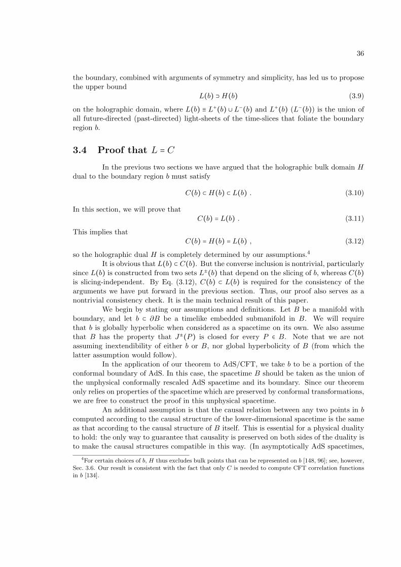
36

the boundary, combined with arguments of symmetry and simplicity, has led us to proposethe upper bound

L(b) ⊃H(b) (3.9)

on the holographic domain, where L(b) ≡ L+(b) ∪ L−(b) and L+(b) (L−(b)) is the union ofall future-directed (past-directed) light-sheets of the time-slices that foliate the boundaryregion b.

3.4 Proof that L = C

In the previous two sections we have argued that the holographic bulk domain Hdual to the boundary region b must satisfy

C(b) ⊂H(b) ⊂ L(b) . (3.10)

In this section, we will prove thatC(b) = L(b) . (3.11)

This implies thatC(b) =H(b) = L(b) , (3.12)

so the holographic dual H is completely determined by our assumptions.4

It is obvious that L(b) ⊂ C(b). But the converse inclusion is nontrivial, particularlysince L(b) is constructed from two sets L±(b) that depend on the slicing of b, whereas C(b)is slicing-independent. By Eq. (3.12), C(b) ⊂ L(b) is required for the consistency of thearguments we have put forward in the previous section. Thus, our proof also serves as anontrivial consistency check. It is the main technical result of this paper.

We begin by stating our assumptions and definitions. Let B be a manifold withboundary, and let b ⊂ ∂B be a timelike embedded submanifold in B. We will requirethat b is globally hyperbolic when considered as a spacetime on its own. We also assumethat B has the property that J±(P ) is closed for every P ∈ B. Note that we are notassuming inextendibility of either b or B, nor global hyperbolicity of B (from which thelatter assumption would follow).

In the application of our theorem to AdS/CFT, we take b to be a portion of theconformal boundary of AdS. In this case, the spacetime B should be taken as the union ofthe unphysical conformally rescaled AdS spacetime and its boundary. Since our theoremonly relies on properties of the spacetime which are preserved by conformal transformations,we are free to construct the proof in this unphysical spacetime.

An additional assumption is that the causal relation between any two points in bcomputed according to the causal structure of the lower-dimensional spacetime is the sameas that according to the causal structure of B itself. This is essential for a physical dualityto hold: the only way to guarantee that causality is preserved on both sides of the duality isto make the causal structures compatible in this way. (In asymptotically AdS spacetimes,

4For certain choices of b, H thus excludes bulk points that can be represented on b [148, 96]; see, however,Sec. 3.6. Our result is consistent with the fact that only C is needed to compute CFT correlation functionsin b [134].

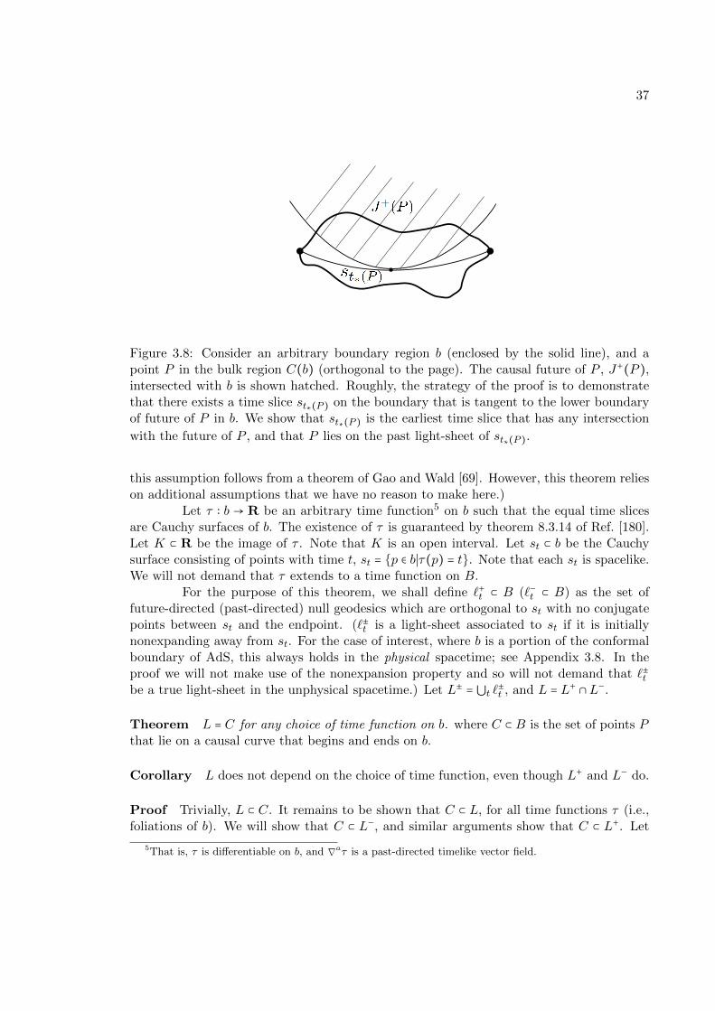
37

Figure 3.8: Consider an arbitrary boundary region b (enclosed by the solid line), and apoint P in the bulk region C(b) (orthogonal to the page). The causal future of P , J+(P ),intersected with b is shown hatched. Roughly, the strategy of the proof is to demonstratethat there exists a time slice st∗(P ) on the boundary that is tangent to the lower boundaryof future of P in b. We show that st∗(P ) is the earliest time slice that has any intersection

with the future of P , and that P lies on the past light-sheet of st∗(P ).

this assumption follows from a theorem of Gao and Wald [69]. However, this theorem relieson additional assumptions that we have no reason to make here.)

Let τ ∶ b → R be an arbitrary time function5 on b such that the equal time slicesare Cauchy surfaces of b. The existence of τ is guaranteed by theorem 8.3.14 of Ref. [180].Let K ⊂ R be the image of τ . Note that K is an open interval. Let st ⊂ b be the Cauchysurface consisting of points with time t, st = p ∈ b∣τ(p) = t. Note that each st is spacelike.We will not demand that τ extends to a time function on B.

For the purpose of this theorem, we shall define `+t ⊂ B (`−t ⊂ B) as the set offuture-directed (past-directed) null geodesics which are orthogonal to st with no conjugatepoints between st and the endpoint. (`±t is a light-sheet associated to st if it is initiallynonexpanding away from st. For the case of interest, where b is a portion of the conformalboundary of AdS, this always holds in the physical spacetime; see Appendix 3.8. In theproof we will not make use of the nonexpansion property and so will not demand that `±tbe a true light-sheet in the unphysical spacetime.) Let L± = ⋃t `±t , and L = L+ ∩L−.

Theorem L = C for any choice of time function on b. where C ⊂ B is the set of points Pthat lie on a causal curve that begins and ends on b.

Corollary L does not depend on the choice of time function, even though L+ and L− do.

Proof Trivially, L ⊂ C. It remains to be shown that C ⊂ L, for all time functions τ (i.e.,foliations of b). We will show that C ⊂ L−, and similar arguments show that C ⊂ L+. Let

5That is, τ is differentiable on b, and ∇aτ is a past-directed timelike vector field.

38

P ∈ C (and P is not contained in b) .Definition. Let K+(P ) be the subset of the real numbers consisting of all t such

that st ∩ I+(P ) is not empty. That is, st∣t ∈K+(P ) is the set of all time slices on b whichcontain endpoints of future-directed timelike curves from P .

Lemma A. K+(P ) is nonempty. Proof. Since P ∈ C, there is a point p ∈ b ∩J+(P ). All points in b∩I+(p) are necessarily in I+(P ) (corollary following theorem 8.1.2 ofRef. [180]). Since K is an open interval, there exists t ∈K with t > τ(p). Any inextendibletimelike curve passing through p intersects st because st is a Cauchy surface, which showsthat st ∩ I+(p), and consequently b ∩ I+(P ), is nonempty. Therefore K+(P ) is nonempty.

Lemma B. For any t ∈ K+(P ), the set At = b ∩ J+(P ) ∩ J−(st) is compact. Proof.Since P ∈ C, b ∩ J−(P ) is not empty. Let q ∈ b ∩ J−(P ). Let j+(q) be the causal futureof q within the spacetime b, and define j−(st) similarly. Then j+(q) ∩ j−(st) is compact(theorem 8.3.12 of Ref. [180]). But because the causal relation between points in b is thesame whether we treat them as events in the spacetime b or the spacetime B, we alsohave that j+(q) ∩ j−(st) = b ∩ J+(q) ∩ J−(st). Since this set is compact, it is closed as asubset of B. J+(P ) is a closed subset of J+(q), and it follows that b ∩ J+(P ) ∩ J−(st) =J+(P )∩(b∩J+(q)∩J−(st)) is a closed subset of b∩J+(q)∩J−(st). Therefore b∩J+(P )∩J−(st)is compact.

Definition. Let t∗(P ) = inft∈K+(P ) t.Lemma C. For any t ∈ K+(P ), t∗(P ) = minp∈At τ(p). In particular, this means

that there is a surface st∗(P ) and that st∗(P )∩J+(P ) is not empty. Proof. By Lemma B, Atis compact and hence τ(p) attains a minimum value τmin. Consider a point p ∈ sτmin∩J+(P )and an inextendible future-directed timelike curve γ in b starting at p. All points on γ otherthan p are necessarily in b ∩ I+(P ) (corollary following theorem 8.1.2 of Ref. [180]), and γnecessarily intersects st′ for every t′ ∈K with t′ > τmin because st′ is a Cauchy surface. Thisimplies that all such times t′ are in K+(P ), and hence τmin ≥ t∗(P ). If τmin > t∗(P ), thenthere is some t′ ∈ K+(P ) with τmin > t′. Then t > t′, and so st′ ∩ At is not empty by thedefinition of At. But then τmin ≤ t′ by the definition of τmin, which contradicts τmin > t′.Therefore we conclude that τmin = t∗(P ).

Lemma D. K+(P ) is an open subset of the real numbers. This implies that st∗(P )∩I+(P ) is empty. Proof. Let γp be an inextendible timelike curve in b which passes througha point p ∈ b ∩ I+(P ). We can choose to parametrize γp by the time function τ , whichmeans that γp ∶ K → b is a continuous function satisfying τ(γp(t)) = t. Since I+(P ) isopen, it follows that the inverse image γ−1

p [I+(P )] is open in K, and therefore open in R

because K is an open interval. By applying τ γ, we see that γ−1p [I+(P )] ⊂ K+(P ). Then

⋃p∈b∩I+(P ) γ−1p [I+(P )] is an open subset of R equal to K+(P ).

Proof of theorem. Lemma C and Lemma D together demonstrate that there isa surface st∗(P ) such that st∗(P ) ∩ I+(P ) is empty while st∗(P ) ∩ J+(P ) is nonempty. Letp ∈ st∗(P ) ∩ J+(P ). By the corollary following theorem 8.1.2 of Ref. [180], there is a nullgeodesic connecting p to P . Furthermore, since st∗(P ) ∩ I+(P ) is empty, this null geodesiccannot be deformed to a timelike curve connecting st∗(P ) to P . Then by theorem 9.3.10of Ref. [180], this null geodesic must be orthogonal to st∗(P ) and have no conjugate pointsbetween P and p. This shows that P ∈ `−t∗(P ) ⊂ L

−.

39

3.5 Covariant Renormalization Group Flow

We repeatedly made use of the UV/IR connection [165] in motivating our con-structions. Entropy bounds play a very important role in UV/IR: the bulk region withinthe IR cutoff must have entropy limited by the area in Planck units of a time slice on thecutoff surface. However, as we have stressed, this only holds true for very special time slicesand the covariant entropy bound must be used in general to bound the bulk entropy. Holo-graphic renomalization group flows [5, 52, 61, 98] aim to refine UV/IR, but in all standardapproaches manifest covariance is lost and the status of entropy bounds is unclear. Herewe outline an approach which reproduces the standard results and remedies both of theseproblems. Our construction gives an improved bulk radial flow, however it does not addressthe open question of finding a precise field theory RG representation of the bulk flow.

Figure 3.9: The covariant bulk RG flow presented here reproduces the standard bulk RGflow in certain coordinate systems. Here we illustrate the construction in global coordinatesof Anti-de Sitter space. For a given coordinate time cutoff δ, the union over t of theintersection surfaces sδt = `−t+δ/2 ∩ `

+t−δ/2 form a timelike hypersurface bδ in the bulk (left).

The cross-sectional area of a given light-sheet will be greater on the surface bδ than on bδ′

(right). The difference (A−A′)/4 bounds the entropy on the red light-sheets going from bδ

to bδ′

, meaning that the bound applies to the entire darkly shaded wedge between them.The lightly shaded region between the hypersurfaces bδ

′

and bδ is covered by such wedges.

Choose a time function τ on b. Then for any t1, t2 the set b[t1, t2] = p ∈ b∣t1 <τ(p) < t2 satisfies the conditions of our theorem and we can associate to it the regionH(b[t1, t2]). Now introduce a cutoff timescale δ to the theory. In the bulk, we shouldremove the union (over t) of the sets H(b[t − δ/2, t + δ/2]) from H(b). The remaining bulkregion, Hδ, is the region described by the cutoff CFT. This prescription is similar to theconstruction of [26], where it was shown that the IR cutoff surface as normally defined can

40

be reproduced using only causality.Denote the boundary of Hδ by bδ. The time function on b automatically induces a

time function on bδ:6 By construction, bδ is the union of sets of the form sδt = `−t+δ/2 ∩ `+t−δ/2,

which we can take as time slices on bδ. The maximum proper time in bδ between sδt andsδt+δ will be of order the AdS time. More generally, we can let δ depend on t.

To change the cutoff from δ to δ′, we have two equivalent options: First, we canreturn to the true boundary b and repeat the construction with δ′ in place of δ. Second,we can use the surface bδ, together with its induced time function, as the starting pointfor the construction, with cutoff δ′ − δ. The geometry is the same either way, because thelight-sheets from bδ are continuations of the light-sheets from b.

By the definition of the L, and since H = L, all time slices of bδ are normal. Thatis, their orthogonal light-rays are everywhere nonexpanding in the direction of the bulk RGflow. A generic time slicing on bδ will not admit ingoing past- and future-directed light-sheets at all points on all time-slices; only the slicing induced by the flow has this property.And generic hypersurfaces other than those induced by the flow may not admit any slicingwith this property. Note that this property is inherited from the remarkable property ofthe conformal boundary described in the Appendix: any slicing of the conformal boundaryis everywhere normal in the physical metric.

The fact that all time slices of bδ are normal is highly nontrivial. It leads to twoadditional, attractive features that distinguish this geometric flow from, say, the flow alongspacelike geodesics:

Entropy bounds hold for both the UV and the IR regions.

These bounds guarantee that the effective number of degrees of freedom is nonincreas-ing along the flow.

Consider first the IR region. The covariant entropy bound guarantees that anyfuture- or past-directed light-sheet from any slice sδt has entropy less than the area of thatslice, in Planck units. Since the area of the light-sheet is nonincreasing as it moves awayfrom the boundary, the number of degrees of freedom is nonincreasing along the RG flow.

Now consider the UV region, i.e., follow the light-sheet from sδ′

t backward to somecutoff δ < δ′ closer to the true boundary. The cross-sectional area will be larger on bδ andwe can consider the area difference A −A′. A generalized version of the covariant entropybound [65] implies that the entropy on the partial light-sheet between A and A′ is boundedby (A−A′)/4. Note that this bound applies to both light-sheets bounding the wedge-shapedregion between the slices sδt+(δ′−δ)/2 and sδt−(δ′−δ)/2 on bδ and sδ

′

t on bδ′

, and hence to the

entire information content of the regions that are integrated over in the RG flow.7

RG flows are normally defined in terms of proper distances, times, or energies,whereas the above construction is in terms of an arbitrary coordinate time. To define

6This will be true for sufficiently well-behaved time functions t; the precise conditions will be investigatedelsewhere.

7In general, the area A(t) of different slices on bδ will not be independent of t. It seems likely thatrequiring this independence will lead to preferred choices of δ(t) and thus for the flow. Also, while the areaswill be automatically finite at finite δ in the case of the global boundary, they will be infinite in general andmust be regulated.

41

proper distances on the boundary, one has to choose a conformal frame, and the choice oftime function in our construction is analogous. Heuristically, one can imagine choosing theconformal factor so that τ becomes proper time, which means that it is conjugate to energy.

We have emphasized the geometric aspects of the RG flow, i.e., the bulk side. Thequestion of what precisely the removal of near-boundary regions corresponds to in the CFTremains subtle, and it will be interesting to revisit it in light of the geometric flow we havedescribed. In particular, it would be nice to understand whether a duality holds for thewedge-shaped regions associated with thin boundary strips, and for the Rindler portion ofthe bulk dual to small causal diamonds on the boundary.

As the example of the global boundary (Fig. 3.9) illustrates, the description ofthe bulk region H(b[t − δ/2, t + δ/2]), for small time intervals δ, cannot involve the fullset of CFT degrees of freedom, since approximately exp(A/4) CFT states correspond tobulk states localized to the interior of the bulk hypersurface bδ . If a duality exists, theCFT degrees of freedom relevant for H(bδ) will not involve certain nonlocal operators thatoccupy scales larger than δ.

3.6 Nonlocal Operators and the Bulk Dual

We constructed a candidate for a bulk region H(b) dual to b geometrically, usingconsiderations of causality and holographic entropy bounds. Except for appealing to theUV/IR relation [165], we did not make use of detailed properties of the AdS/CFT dualityor the boundary theory. In this section we will explore a different approach to this question,namely the use of nonlocal operators in the CFT to probe deeply into the bulk region. Wewill examine the relationships between this approach and the geometric one. Note thatthe operator approach is available only for choices of b where the construction of boundaryduals to local bulk operators is known, so it is less general than our geometric construction.

The methods of the operator approach were recently discussed by Heemskerk,Marolf, and Polchinski [96], and we refer the reader to that work for further details. Theproblem is to identify a subset of operators φ(x) within the set of all operators in theCFT on b, indexed by a position x in a semiclassical spacetime of higher dimension, whichcan be identified as local bulk operators. An important point is that the definition of thelocal bulk operators depends on the background metric. Our analysis below pertains tothe case where this metric is held fixed up to perturbative corrections in 1/N , so this issueshould not pose difficulties.

The CFT definition of φ(x) will involve nonlocal CFT operators known as precur-sors [148, 171, 66]. An (in principle) explicit construction is available in the case of globalAdS, and the resulting operators make use of an entire Cauchy surface of the global bound-ary. For this reason, and also for simplicity, we will spend most of this section focused onthe case of a short strip b = S,

S = (−τ0, τ0) × Sd, with τ0 ≪ 1 , (3.13)

which we normally think of as being embedded in the global boundary (see Fig. 3.10), usingthe coordinates of Eq. 3.4. From the global point of view, the set of operators on the Cauchy

42

surface τ = 0 of the boundary is complete, and so in particular contains the operator φ(x)for every point x in the entire global bulk.

=0

=/2

Figure 3.10: A cross-section of Anti-de Sitter space, showing a short strip region S centeredaround τ = 0 on the boundary, and the bulk region S(S) spacelike separated from S. Alocal operator at the origin of the bulk can be written in terms of local operators on theboundary smeared over the boundary region spacelike-related to the origin, within the greenwedges. This region is much larger than S (red thick line), stretching from τ = −π/2 toτ = +π/2.

Now consider modifications of the CFT Hamiltonian H outside b, and let us defineH as the largest bulk region such that operators φ(x) for x ∈ H can be represented interms of CFT operators in b in an unambiguous way. There are some modifications of theCFT Hamiltonian which continue to yield a well-defined bulk Hamiltonian. For instance,we can insert a local source in the CFT whose effect in the bulk is to cause a particle topropagate causally inward from the boundary. As we discuss below, certain modificationsof the CFT Hamiltonian which make use of nonlocal operators can lead to ambiguitiesin the bulk Hamiltonian. In the case where we allow only those modifications leading towell-defined bulk Hamiltonians, we identify a region S on which the operators φ(x) haveunambiguous CFT representations in b. In the more general case of modifications whichlead to an ambiguous bulk Hamiltonian, we will identify H as the subset of S for whichφ(x) still has an unambiguous CFT representation in b. We will note that H is closelyrelated to H.

The region S The only known construction of φ(x) in the boundary theory consists oftwo steps and applies either in global AdS or the Poincare patch. In the first step, one

43

writes a local bulk operator φ(x) as a smeared local operator on the boundary:

φ(x) = ∫ dy′K(x∣y′)O(y′) +O(1/N) . (3.14)

Here y′ denotes a boundary coordinate, while x is the bulk coordinate.8 The smearingfunction K(x∣y) is not unique, but a convenient choice is nonzero if and only if y spacelike-related to x [90, 89, 107]. One can think of K(x∣y) as providing the solution to the equationof motion for φ(x) given boundary data on the asymptotic boundary; this is a spacelikeanalogue of the standard initial value problem. Note that for any choice of x in globalAdS, the boundary support of K(x∣y) is larger than the region S. The second step of theconstruction uses unitary evolution in the CFT to write all of the local CFT operatorsO(y′) appearing in Eq. 3.14 in terms of nonlocal operators defined at τ = 0 (or some othertimeslice within the short strip S).

Now let us identify a subset S(S) of the bulk such that the above construction ofthe CFT operator φ(x) is independent of modifications of the boundary Hamiltonian outsideb,9 provided that these modifications continue to lead to a well-defined bulk Hamiltonian.In Ref. [96], it was shown that S consists of the bulk points that are neither in the causalfuture of the future boundary of S, nor in the causal past of its past boundary. We willrefer to such points somewhat loosely as being “spacelike-related” to S (see Fig. 3.10).

At first, this result may seem surprising, so it is worth reviewing the argumentfor it [96]. First, fix a fiducial CFT Hamiltonian H over the entire global boundary, andfollow the above procedure to construct an operator O satisfying φ(x) = O, for some xspacelike-related to S (the special case x = 0 is pictured in Fig. 3.10). But there is anotherway we can produce the operator O: We can use causal bulk evolution to write φ(x) interms of φ(x′) for points x′ in the future of the x:

φ(x) = ∫Σdx′ [φ(x′)∇Gadv(x∣x′) −∇φ(x′)Gadv(x∣x′)] +O(1/N) , (3.15)

where Σ consists of a bulk Cauchy surface and, possibly, a portion of the global boundary.We can use Eq. 3.14 to write the φ(x′) appearing here in terms of operators on the boundary.By evolving φ(x) sufficiently far forward into the future, the y′-support of K(x′∣y′) will liein the region τ > 0 for every x′ appearing in Eq. 3.15. Now we evolve this new smearedoperator back to τ = 0 to obtain a second operator O′. However, O′ = φ(x) = O, and sothese two procedures actually give the same answer. Now suppose we modify the CFTHamiltonian from our fiducial choice H to H, and we stipulate that H only differs fromH for τ < 0. We can repeat the procedure to compute new operators O and O′, whichare equal to each other and to φ(x). The claim is that, since the calculations of O′ andO′ refer only to the τ > 0 region of the bulk and boundary, and H = H in that region,the computations are identical and so manifestly we have O′ = O′. Therefore O = O, andthe change in fiducial Hamiltonian did not change the operator assignment. An analogousargument can be made for modifications to the CFT Hamiltonian for τ > 0.

8The presence of a source will modify this equation in the appropriate way given by Green’s identity.9We impose the boundary condition that the boundary state at τ = 0 remain unchanged.

44

J=o

Figure 3.11: According to the Hamiltonian on the boundary strip S, no source acts at theorigin in the bulk, so the expectation value of φ vanishes everwhere. At the time τ0 outsidethe strip, a source term for the nonlocal boundary operator dual to φ(0,0) can be addedto the boundary Hamiltonian. This causes the expectation value of φ to be nonzero in thefuture of (0,0), in contradiction with the earlier conclusion about the same bulk points.Thus, unless we possess information about the exterior of S on the boundary guaranteeingthat such operators do not act, the bulk interpretation of regions outside H(S) = C(S) ispotentially ambiguous.

The region H The above argument relied crucially on the existence of a well-definedbulk Hamiltonian. However, there are reasonable modifications of the CFT Hamiltonian Hfor which this will not be the case (see Fig. 3.11). At the time τ0 on the boundary, let usadd to H a source for the nonlocal CFT operator O dual to a local bulk operator at theorigin, φ(τ = 0, ρ = 0):

H →H + Jδ(τ − τ0)O (3.16)

We are working perturbatively, so the operator O is the one constructed using the abovemethod and the unmodified Hamiltonian H. In the bulk, this source acts completely locallyas a source for φ at the origin at τ = 0. Note that this bulk point is spacelike related to theboundary slice τ0.

Now let us compute the expectation value of the bulk operator φ at the origin, atsome infinitesimal time ε after the source acts. This operator can be constructed by theusual methods, but those methods require a knowledge of the bulk Hamiltonian in the regionS(S). This Hamiltonian is ambiguous: from the viewpoint of the strip S, the source doesnot act, since it acts in the CFT only at τ0. Then the bulk evolution should be computedfrom the usual bulk Hamiltonian without source, and we obtain ⟨φ(ε,0)⟩ = 0. From the

45

viewpoint of the CFT at the time τ0, the bulk region near (0,0) contains a source. Thenthe bulk evolution should take this source into account and we obtain ⟨φ(ε,0)⟩ ≠ 0. Thus,there is no unique assignment of a bulk field value at (ε,0). In this sense, (ε,0) should notbe considered a bulk point dual to the strip.

Let us now consider a general boundary region b and construct a bulk region H suchthat the interpretation of what happens in H is unambiguous (Fig. 3.12). The ambiguitieswe discussed arise from inserting nonlocal CFT operators into the Hamiltonian on Cauchysurfaces of the boundary which do not intersect the region b. A modification of the CFTHamiltonian on such a Cauchy surface σ can lead to an ambiguous bulk Hamiltonian in theregion S(σ) spacelike-related to σ. Thus we find that H is the compliment of the union of allS(σ), where σ is any Cauchy surface for the global boundary which lies in the complementof b.

Figure 3.12: The shaded region shows bulk points spacelike related to a global boundaryCauchy surface σ. The union of all such sets over the collection of boundary Cauchy surfaceswhich do not intersect S has an ambiguous bulk interpretation when the boundary Hamil-tonian is allowed to vary outside of S. The unambiguous region, H(S), is the complementof this union. In this example, we see that H(S) = C(S).

The region H is closely related to C(b) and hence to H(b). It is easy to see thatH = C ⊂ H. The study of a number of examples suggests that H ≠ H if and only if an eventhorizon is present in the bulk. It would be nice to study H and its relation to H further.The discussion in the following section may be relevant.

46

3.7 Quantum Gravity Behind Event Horizons

In this section we discuss an issue that is somewhat orthogonal to the main subjectof this paper: the degree to which the reconstruction of bulk regions, perturbatively in1/N , allows us to claim that AdS/CFT provides a full quantum gravity theory for regionsbehind event horizons, such as the interior of a black hole, or cosmological regions. We willconstruct an experiment behind the horizon whose outcome is known but not captured bysuch methods.

The CFT provides a full quantum gravity theory for observers near the boundary.10

It completely settles the issue of whether the formation and evaporation of a black hole is aunitary process. It is crucial for this argument that the time evolution is carried out on theboundary, where it is manifestly unitary; the duality is used only at early and late times inorder to recover the in and out states in the bulk [167, 146, 78, 64].

To what extent can we regard the CFT also as a full quantum gravity theory foran observer falling into the black hole? Perhaps, by reordering the degrees of freedom, onecould interpret the CFT as providing a nonperturbative definition of quantum gravity forthe infalling observer? This would require that the bulk dual region is ambiguous, at thenonperturbative level. This may be the case, but the dictionary that would provide thisdefinition is not known at the required level of precision.

The black hole interior is clearly encoded in the CFT if one makes use of bulkequations of motion to evolve the infalling data back out of the black hole and to theboundary. But in the same approximation, we can also generate a xeroxing paradox [169]:at the semiclassical level, there is no manifest obstruction to evolving to global bulk slicesthat contain both the black hole interior and the Hawking cloud.

Perhaps we should restrict the bulk evolution by hand to the causal patch of aninfalling observer, and settle for this approximate description of the black hole interior? Thefiniteness of entropy bounds inside black holes imply that there cannot be exact observablesassociated with the infalling observer at late times. Thus, the description of the infallingobserver should be less precise that that of the observer near the boundary, who has accessto exact observables. Perhaps the need to use bulk evolution is simply a reflection of thisintrinsic limitation?

In fact, however, it is clear that the infalling observer requires a theory that goes be-yond semiclassical bulk evolution. This can be seen from the following thought-experiment.Consider an infalling observer who performs scattering experiments inside a Schwarzschild-AdS black hole of radius R, after crossing the event horizon. The scattering occurs at highenough energy to produce a (smaller) black hole of mass m, which then evaporates. We arefree to choose parameters so that the scattering effectively takes place in flat space:

RAdS ≫ R≫ f(m) ≫ 1 , (3.17)

where f(m) is at least the evaporation timescale of the black hole (md in d spatial bulkdimensions). For sufficiently large but finite R/f(m), the infalling observer can confirm

10Note that all observers that remain outside the black hole have the same causal diamond, consisting ofthe exterior of the black hole. The covariant RG flow we described in Sec. 3.5 can be thought of as movingthe observers deeper into the bulk, but note that the flow never enters the black hole.

47

the unitarity of black hole formation and evaporation to any required precision. But thisconflicts with the result that would be obtained from the semiclassical analysis (Hawking’scalculation).

We conclude that the proper description of an infalling observer requires a quantumgravity theory beyond the semiclassical approximation. The CFT on the boundary doesnot provide us with that theory, since its application to the infalling observer relies onsemiclassical bulk evolution. No other way of relating local operators inside the black hole toboundary operators is known; therefore, we cannot replace this bulk evolution by boundaryevolution, as we did in the case of scattering experiments performed by a near-boundaryobserver.

Of course, in the limit used in the thought-experiment, one could imagine “cuttingout” the spacetime region of size f(m) that contains the scattering experiment. One couldembed this region in an asymptotically AdS spacetime with RAdS ≫ f(m) and use the flatspace S-matrix, which can be computed using AdS/CFT [167, 146, 78, 64]. In fact, thisargument is what gives us confidence that the process is indeed unitary. But how wouldthis prescription generalize? A theory of the infalling observer that relied on this type ofcutting and pasting would not be applicable to the highly dynamical regions deeper insidethe black hole, nor to the spacelike singularity, which cannot be so transplanted.

An exact version of this cut-and-paste process is available if the black hole isformed by sending in a spherical null shell from the boundary of AdS [100]. By causality,the bulk region in the past of the shell is the same no matter whether we decide to sendin the shell or not. If we do send in the shell, then this region includes a portion w of theblack hole interior. If we do not, then the same bulk region w is dual to operators on theboundary, which can be evolved to nonlocal operators W on a single global boundary timeslice preceding the insertion of the shell. This illustrates that cut-and-paste is well-definedprecisely in the limit where it yields no information about regions that could only exist inthe interior of black holes, such as singularities and a highly dynamical geometry.

The absence (so far) of an intrinsic bulk theory at the nonperturbative level appearsto impose crucial limitations on our ability to describe black hole interiors and cosmologicalregions11 via AdS/CFT, beyond what follows from the approximate methods that werealready available to generate bulk evolution.

3.8 Light-sheets from the conformal boundary of AdS

In this appendix we show that the light-rays orthogonal to any spacelike slice ofthe conformal boundary of AdS have nonpositive expansion into the bulk in the physi-cal metric, and thus generate light-sheets. This is an important property of light-sheetsin asymptotically AdS spacetimes. It guarantees that the maximum entropy of the bulkholographic domain H is nonincreasing under the covariant RG flow described in Sec. 3.5.

11A similar conclusion [75] applies to the interior of other event horizons, such as an FRW universe [128].In this case there are two natural choices of conformal frame on the boundary [7]: one in which the CFT iswell-behaved, and another in which the coefficient of a relevant operator diverges in finite time. It is temptingto interpret this violent behavior in terms of an infalling observer hitting the big crunch singularity behindthe horizon, but it can be understood more simply as the arrival of the bulk domain wall on the boundary.

48

In Poincare coordinates, the AdS metric is:

ds2 = 1

z2(dz2 + ηµνdxµdxν) , (3.18)

where ηµν is the metric for d dimensional Minkowski space. Consider the conformallyrescaled metric

ds2 = dz2 + ηµνdxµdxν , (3.19)

which is d + 1 dimensional Minkowski space. Take some small region of the boundary andlet θ be the expansion of some congruence of infinitesimally neighboring light rays in thisspace. That is

θ = d log Adλ

, (3.20)

where A is the infintesimal area spanned by the light rays and λ is the affine parame-ter. In order for the null geodesics to remain affinely parameterized after the conformaltransformation, the affine parameter must transform as (Appendix D of [180])

dλ

dλ= cz2 , (3.21)

where c is a constant and z2 is the conformal factor. The area will transform as

A = Azd−1

. (3.22)

Using (3.20), (3.21), and (3.22) we find that the expansion in the AdS spacetime(3.18) is

θ = cz2θ − c(d − 1)zkz , (3.23)

where

kz = dzdλ

.

Since both θ and kz are defined in d + 1 dimensional Minkowski space using a congrueneceof null rays orthogonal to a spacelike (and hence nowhere null) foliation, they are finite.Thus, at the boundary (z = 0), we have θ = 0.

49

Chapter 4

Null Geodesics, Local CFTOperators, and AdS/CFT forSubregions

4.1 Introduction

The AdS/CFT correspondence [127, 185] provides an important tool for obtaininginsight into quantum gravity. Yet even today, the seemingly basic question of how bulklocality is encoded in the boundary theory—in other words, which CFT degrees of freedomdescribe a given geometrical region in the bulk—has resisted a simple, precise answer.

In this chapter, we investigate the related question of AdS/CFT subregion duali-ties. That is, we consider the possibility that a CFT restricted to a subset of the full AdSboundary is dual to a geometric subset of the AdS bulk. There is no obvious reason that ageometric region on the boundary has to correspond to a geometric region in the bulk, butthere are strong arguments for such a subregion duality in certain simple cases [48], andintriguing hints [165, 154, 104] that it may be true more generally.

The problem of precisely what bulk region should be associated with a givenboundary region is complicated and has been explored recently by [40, 51, 103]. We willnot propose or adopt a rule for constructing such an association. Instead, we focus onone nice feature of the global AdS/CFT duality which does not generalize to arbitrarysubregions, namely the ability to reconstruct the bulk using local CFT operators in theclassical limit [90, 89, 107, 96]. Specifically, we will emphasize the role of continuity of thebulk reconstruction, and propose a simple geometric diagnostic testing whether continuousreconstruction holds for a given subregion.

To motivate our investigation, first consider the full global AdS/CFT duality. Wewill work in Lorentzian signature and fix the Hamiltonian of the CFT, which correspondsto fixing all the non-normalizable modes in the bulk. Now take the GN → 0 limit in thebulk; the bulk theory reduces to solving classical field equations in a fixed background.The non-normalizable modes are fully determined and non-dynamical, but there are stillmany allowed solutions because of the normalizable modes. CFT data on the boundaryshould be sufficient to specify a particular bulk solution. Normalizable modes in the bulk

50

A

B

Figure 4.1: Here we show the AdS-Rindler wedge inside of global AdS, which can be definedas the intersection of the past of point A with the future of point B. The asymptoticboundary is the small causal diamond defined by points A and B. The past lightcone ofA and the future lightcone of B intersect along the dashed line, which is a codimension-2 hyperboloid in the bulk. There is a second AdS-Rindler wedge, defined by the pointsantipodal to A and B, that is bounded by the same hyperboloid in the bulk. We refer tosuch a pair as the “right” and “left” AdS-Rindler wedges.

approach zero at the boundary, but a nonzero boundary value can be defined by strippingoff a decaying factor,

φ(b) ≡ limz→0

z−∆Φ(b, z) , (4.1)

where z is the usual coordinate that approaches zero at the boundary, b stands for theboundary coordinates, and Φ is a bulk field. We will also use the notation B = (b, z) whereconvenient. By the “extrapolate” version of the AdS/CFT dictionary [6], these boundaryvalues are dual to expectation values of local operators,

φ(b) = ⟨O(b)⟩ . (4.2)

We can now ask a classical bulk question: do the boundary values φ determine the bulk solu-tion everywhere? This is a nonstandard type of Cauchy problem, because we are specifyingdata on a surface that includes time.

In a simple toy model where the bulk contains only a single free field with arbitrarymass, Hamilton et al. [90, 89] showed explicitly that this boundary data does specify thebulk solution completely in global AdS. The fact that the boundary data specifies thebulk solution can be considered the classical, non-gravitational limit of AdS/CFT. It is anontrivial fact that expectation values of local CFT operators are sufficient to reconstructthe bulk field in this case.

A proposed subregion duality must pass the same test. Is the CFT data in aboundary subregion sufficient to reconstruct the bulk solution within the corresponding

51

bulk subregion? In principle, the CFT data is quite complicated. The simplification thatoccurred in global AdS/CFT, that expectation values of local boundary operators weresufficient, may or may not carry over to other cases, and our task is to properly account forwhen it does. This is a problem in the theory of classical differential equations which we canhope to solve. Simple examples show that the problem is subtle, however, and to properlycapture the physics of the problem we need to differentiate between bulk reconstruction andcontinuous bulk reconstruction.

The simplest illustration comes from AdS-Rindler space, which can be describedas follows. In the global duality, the CFT is formulated on a sphere cross time and theassociated bulk is global AdS. Let us divide the boundary sphere at some time across theequator. In the bulk, the extremal surface ending on the boundary equator is a hyperboloid,and we can use Rindler-type coordinates in AdS so that this extremal surface is a Rindlerhorizon. The northern hemisphere on the boundary extends naturally into a small causaldiamond on the boundary, namely the region determined by time evolution of the datain the northern hemisphere. The corresponding bulk region is a Rindler wedge, shown inFig. 4.1, which we will call AdS-Rindler space.

Does the global boundary data, restricted to the small boundary diamond, deter-mine the bulk solution in the corresponding AdS-Rindler wedge? Hamilton et al. [89] alsoaddressed this question. They determined that a particular analytic continuation of theboundary data was necessary to reconstruct the bulk. Here we provide a different answerthat does not rely on analytic continuation of the boundary data. We claim that there is adirect map from the boundary data to the bulk field, but that the map is not continuous.This leaves the physical interpretation open to doubt.

There are two reasons to focus on the question of continuity. First, if the subre-gion duality is correct, we would expect that measuring boundary data to finite precisionshould determine the bulk data to a corresponding precision. This is only true if the bulksolution depends continuously on the boundary data. Second, the question of continuousreconstruction seems to be mathematically robust; we will be able to make heuristic contactwith nice mathematical theorems about when continuous reconstruction is possible.

Continuous reconstruction fails because there are finite excitations in the bulkRindler wedge with an arbitrarily small imprint on the boundary data. The physics ofthese excitations is simple: there exist null geodesics that pass through the bulk Rindlerwedge, but avoid the boundary diamond. One can construct solutions where geometricoptics is an arbitrarily good approximation and the energy is concentrated along such anull geodesic. In this way, we can construct solutions that are finite in the bulk but havearbitrarily small boundary data in the Rindler wedge.

We can also ask a slightly different mathematical question, which is closely relatedto bulk reconstruction from the boundary data but simpler to analyze: the question ofunique continuation. Suppose we are given the bulk solution in some region near theboundary, and we want to continue the solution further into the bulk. In the AdS context,evolution inward is roughly dual to RG flow in the CFT. This question is closely related tothe previous one, and again can be diagnosed with null geodesics [174]. In the case of thebulk Rindler wedge we find that unique continuation fails as well. We cannot evolve thesolution radially inward in this case.

52

Given the connection to continuity and local reconstruction, as well as geometricalsimplicity, we are motivated to propose a diagnostic for continuous bulk reconstruction fromlocal CFT operators:

Does every null geodesic in the bulk subregion have an endpoint on the corre-sponding boundary subregion?

Despite the failure of this diagnostic for AdS-Rindler, there are good reasons tothink that this particular subregion duality actually holds. The Rindler wedge can bethought of as an eternal black hole with a hyperbolic horizon. This suggests that a dualityholds, by analogy with the ordinary eternal black hole: the CFT in the Hartle-Hawkingstate may be restricted to one boundary component, and the resulting thermal state is dualto one of the two exterior region of an eternal AdS-Schwarzschild black hole [48].

Since continuous reconstruction from CFT one-point functions fails for this subre-gion, we learn that nonlocal boundary operators must play an important role in the dualityeven in the classical limit. Generalizing this result, we learn that nonlocal CFT opera-tors [148, 171] are important when subregions are small enough that the boundary regionno longer captures all null rays passing through the bulk.

The remainder of the chapter is organized as follows. In Section 4.2 we reviewthe general procedure for reconstructing the bulk solution from boundary data which wasemployed by Hamilton et al. in their work. We also show how to determine continuity ofthe reconstruction map. The general method is applied to global AdS, AdS-Rindler space,the Poincare patch, and Poincare-Milne space. In Section 4.3 we formulate the geometricdiagnostic of capturing null geodesics and relate it to continuity of the reconstruction map,making contact with results in the mathematics literature. We apply the diagnostic tothe black hole geometries, as well, without finding an explicit reconstruction map. InSection 4.4, we exhibit arguments that a subregion duality does exist for AdS-Rindlerspace. In Section 4.5, we note that this can be reconciled with the failure of continuousreconstruction from local fields if the duality involves nonlocal boundary operators in anessential way.

4.2 The Reconstruction Map

4.2.1 General Formulas

We begin this section by reviewing the procedure for obtaining a bulk solutionfrom boundary data using eigenmodes of the wave equation, generalizing the approach ofRef. [89]. A classical, free bulk field Φ can be expanded in terms of orthonormal modes Fkwhich depend on a collection of conserved quantities k:

Φ(B) = ∫ dk akFk(B) + c.c. (4.3)

53

Near the boundary, the modes Fk have the asymptotic form Fk(B) ∼ r−∆fk(b). Thus wefind the boundary field φ = limr→∞ r∆Φ has the expansion

φ(b) = ∫ dk akfk(b) + c.c. (4.4)

Given φ(b), we can ask whether it is possible to reconstruct Φ(B). Recall that φ(b) is dualto a one-point function in the CFT, hence this is equivalent to asking whether the bulk fieldis determined by CFT one-point functions. This is possible when the ak can be extractedfrom φ through an inner product of the form

ak =Wk ∫ db f∗k (b)φ(b) , (4.5)

where Wk is a weighting factor. Equivalently, the boundary mode functions should satisfythe orthogonality relation

∫ db f∗k (b)fk′(b) =W −1k δk,k′ . (4.6)

There is no guarantee that a relation such as (4.6) will hold in general. We will see bothpossibilities in the examples below.

Given (4.5), it is a simple matter to solve for Φ(B):

Φ(B) = ∫ dk [Wk ∫ db f∗k (b)φ(b)]Fk(B) + c.c. (4.7)

We emphasize that at this stage (4.7) is, in principle, a recipe for computing the bulk fieldin terms of the boundary field.

However, there is an important simplification when the order of integration overk and b can be exchanged. Then we have

Φ(B) = ∫ db K(B∣b)φ(b) , (4.8)

whereK(B∣b) = ∫ dk Wkf

∗k (b)Fk(B) + c.c. (4.9)

This is a nontrivial simplification which does not occur in all cases. We will see belowthat when the order of integration is illegitimately exchanged, as in the example of theAdS-Rindler wedge, the integral over k in (4.9) does not converge [89].1

Non-convergence of the integral in (4.9) is due to growth of the eigenmodes atlarge k. The large k behavior of the modes is closely related to the question of continuity ofthe reconstruction map, φ(b)↦ Φ(B). To examine continuity, we need to adopt definitionsfor the bulk and boundary norms. On the boundary, we will follow Ref. [9] and use thenorm

∣∣φ∣∣2b = ∫ db ∣∇bφ∣2 + ∣φ∣2 . (4.10)

Here ∣∇bφ∣2 is positive-definite, not Lorentzian, even though we are in a Lorentzian space-time. In other words, the norm looks like an integral of an energy density (over both space

1With certain extra assumptions on the fields, however, [89] is able to construct a complexified smearingfunction.

54

and time), not an action. We will leave its exact form unspecified here, but will be explicitin the examples below. The correct norm to choose is an open question, and a differentchoice may affect the answer. Our choice is motivated by related results in the mathematicsliterature, but it may not be a natural choice for this problem. For now, this norm willserve to illustrate the possible answers to the continuity question. Because of (4.6), we willfind that ∣∣φ∣∣2b ∝ ∫ p(k)W −1

k ∣ak∣2, where p(k) is a quadratic polynomial in the conservedmomenta.

In the bulk, a convenient and natural norm is given by the energy of the solution.Adopting the standard Klein-Gordon normalization for the modes Fk(B), the energy isgiven by

∣∣Φ∣∣2B = E[Φ] = ∫ dk ∣ω(k)∣∣ak∣2 , (4.11)

where ω(k) is the frequency written as a function of the conserved quantities (one of whichmay be the frequency itself). The reconstruction map is continuous if and only if there isa constant C > 0 such that

∣∣Φ∣∣2B ≤ C ∣∣φ∣∣2b . (4.12)

That is, a bulk solution of fixed energy cannot have arbitrarily small imprint on the bound-ary. Equivalently, by going to momentum space, the product ω(k)Wk/p(k) must be boundedfrom above. In the remainder of this section we apply these general formulas to severalspecific cases to find smearing functions and check continuity. We restrict ourselves to a2+1-dimensional bulk for simplicity.

4.2.2 Global AdS

The AdS2+1 metric in global coordinates is

ds2 = − 1

cos2 ρdt2 + 1

cos2 ρdρ2 + tan2 ρdθ2 . (4.13)

The Klein-Gordon equation in these coordinates reads

− cos2 ρ∂2t Φ + cos2 ρ

tanρ∂ρ (tanρ∂ρΦ) + 1

tan2 ρ∂2θΦ =m2Φ . (4.14)

The normalizable solutions are

Fnl = Nnle−iωteilθ cos∆ ρ sin∣l∣ ρFnl(ρ) (4.15)

where

Nnl =¿ÁÁÀΓ(n + ∣l∣ + 1)Γ(∆ + n + ∣l∣)

n!Γ2(∣l∣ + 1)Γ(∆ + n) , (4.16)

Fnl(ρ) = 2F1(−n,∆ + n + ∣l∣, ∣l∣ + 1, sin2 ρ) , (4.17)

and the frequency is ω = ∆ + 2n + ∣l∣. The boundary modes are

fnl = limρ→π/2

cos(ρ)−∆Fnl = (−1)neilθ−iωt¿ÁÁÀΓ(∆ + n + ∣l∣)Γ(∆ + n)

n!Γ2(∆)Γ(n + ∣l∣ + 1) . (4.18)

55

Following the general procedure outlined above, we can compute the smearingfunction

K(θ, t, ρ∣θ′, t′) =∑n,l

1

4π2

Γ(∆)Γ(n + ∣l∣ + 1)Γ(∆ + n) (−1)ne−iω(t−t′)eil(θ−θ′) cos∆ ρ sin∣l∣ ρFnl(ρ) + c.c.

(4.19)This can be summed to obtain the result of Ref. [89].

The boundary norm in this case is given by2

limT→∞

1

T∫

T /2

−T /2dtdθ ((∂tφ)2 + (∂θφ)2 + φ2) = 4π2∑

nl

(ω2 + l2 + 1)Γ(∆ + n + ∣l∣)Γ(∆ + n)n!Γ2(∆)Γ(n + ∣l∣ + 1) ∣anl∣2 .

(4.20)The reconstruction map is continuous if and only if the following quantity is bounded:

ωWnl

1 + ω2 + l2 = ω

4π2(1 + ω2 + l2)n!Γ2(∆)Γ(n + ∣l∣ + 1)

Γ(∆ + n + ∣l∣)Γ(∆ + n) . (4.21)

This ratio clearly remains finite for all values of n and l, thus proving continuity.

4.2.3 AdS-Rindler

We now turn to the AdS-Rindler wedge, which in 2+1 dimensions has the metric

ds2 = 1

z2

⎡⎢⎢⎢⎢⎢⎣−(1 − z

2

z20

)dt2 + dz2

1 − z2

z20

+ dx2

⎤⎥⎥⎥⎥⎥⎦. (4.22)

The Rindler horizon is located at z = z0, while the AdS boundary is at z = 0. The Klein-Gordon equation is

− z2

1 − z2/z20

∂2t Φ + z3∂z (

1

z(1 − z

2

z20

)∂zΦ) + z2∂2xΦ =m2Φ . (4.23)

The normalizable solutions are

Fωk = Nωke−iωteikxz∆ (1 − z

2

z20

)−iω/2

2F1 (∆ − iω − ik

2,∆ − iω + ik

2,∆,

z2

z20

) (4.24)

where ω = ωz0, k = kz0, and

Nωk =1√

8π2∣ω∣

RRRRRRRRRRRR

Γ(∆+iω+ik2 )Γ(∆+iω−ik

2 )Γ(∆)Γ(iω)

RRRRRRRRRRRR. (4.25)

The boundary modes are then

fωk = limz→0

z−∆Fωk = Nωkeikx−iωt . (4.26)

2In global coordinates, the norm in position space is properly defined as an average over time. This isrelated to the fact that the frequencies are discrete.

56

We can attempt to construct the smearing function following Eq. 4.9, but, as discussedbelow that equation, we will find that the integral over k does not converge:

K(x, t, z∣x′, t′) = (4.27)

1

4π2 ∫ dkdω eik(x−x′)e−iω(t−t

′)z∆ (1 − z2

z20

)−iω/2

2F1 (∆ − iω − ik

2,∆ − iω + ik

2,∆,

z2

z20

)

(4.28)

=∞ . (4.29)

This divergence is due to the exponential growth in k of the hypergeometric function whenk ≫ ω [89],

2F1 (∆ − iω − ik

2,∆ − iω + ik

2,∆,

z2

z20

) ∼ exp[k sin−1(z/z0)] . (4.30)

The boundary norm is given by

∫ dtdx ((∂tφ)2 + (∂xφ)2 + φ2) = ∫ dωdk 4π2N2ωk(1 + ω2 + k2)∣aωk∣2 . (4.31)

We see that the ratio which must be bounded in order that continuity hold is

ωWnl

1 + ω2 + k2= 2ω2

1 + ω2 + k2

RRRRRRRRRRRR

Γ(∆)Γ(iω)Γ(∆+iω+ik

2 )Γ(∆+iω−ik2 )

RRRRRRRRRRRR

2

. (4.32)

This ratio remains bounded for fixed k, but when k ≫ ω it grows like exp(πk) . So we findboth that the smearing function does not exist and that continuity fails.

Physical Interpretation In this case, the problem with reconstructing the bulk solutionoccurs regardless of the bulk point we are interested in. The discontinuity can be understoodphysically. At first, it is surprising that modes with ω < k are even allowed; in the Poincarepatch, obtained as the z0 →∞ limit of AdS-Rindler, they are not.3 Near the Rindler horizonfrequency is redshifted relative to its value at infinity, while momentum is unaffected. Soa local excitation with proper frequency comparable to its proper momentum appears atinfinity as a mode with ω < k. The modes with ω < k are confined by a potential barrier thatkeeps them away from the boundary; for large k the height of the barrier is proportional tok2. This causes the boundary data to be suppressed relative to the bulk by a WKB factorexp(− ∫

√V ) ∼ exp(−πk).

We have seen that there is no smearing function in this case because a divergenceat large momentum prevents us from exchanging the order of integration. To understand thephysical meaning of this divergence, we can ask about computing a more physical quantity,which will regulate the divergence. Instead of trying to find an expression for the bulk field

3In Ref. [162], in the context of the BTZ black hole, it is suggested that these modes are connected withfinite temperature effects, and the associated exponential factors are interpreted as Boltzmann weights. Weconsider this to be very suggestive, but have not found a concrete connection to this work.

57

at a specified bulk point, consider instead a bulk field smeared with a Gaussian function ofsome width σ in the transverse direction,

Φσ(t, x, z) ≡ ∫ dx′ exp(−(x′ − x)2

σ2)Φ(t, x′, z) . (4.33)

We only smear in the x direction because the only divergence is in k, and we drop variousnumerical factors and polynomial prefactors that will be unimportant for our conclusion.We will also set z0 = 1 (which is always possible by an appropriate scaling of coordinates)for the remainder of this section.

The smeared field has a perfectly fine expression in terms of local boundary fields.We can use symmetries to place the bulk point at t = x = 0; then

Φσ(0,0, z) = ∫ dt′dx′Kσ(0,0, z∣x′, t′)φ(x′, t′) (4.34)

with

Kσ(0,0, z∣x′, t′) =

∫ dωdk eiωt′ − kx′ − k2σ2

(1 − z2)−iω/2 2F1 (∆ − iω − ik

2,∆ − iω + ik

2,∆, z2) . (4.35)

The important question is the large k behavior of this function. To get a feeling for it,replace the hypergeometric function by its large k limit,

2F1 ≈ g(ω,∆, z)k∆−1 cosh(2kθ) (4.36)

where θ depends on the distance from the boundary, sin θ = z, and g a function that does notdepend on k. We ignore the polynomial prefactor and focus on the exponential dependence.Performing the integral, we get

Kσ(0,0, z∣x′, t′) “ = ” g(t,∆, z) exp( θ2

σ2− x

′2

σ2− 2i

θ

σ2x′) (4.37)

where the quotation marks indicate that this is only a cartoon of the correct answer thatcaptures the large momentum behavior of the smearing function. Now we can write thesmeared bulk field in terms of the boundary values,

Φσ(0,0, z) = ∫ dx′dt′Kσ(0,0, z∣x′, t′)φ(x′, t′) . (4.38)

What is the behavior of this function as we localize the bulk field by taking thewidth small, σ → 0? Kσ is strongly dependent on σ: the maximum value of Kσ is exponen-tially large at small σ, Kmax

σ = exp(θ2/σ2), where again θ is related to the distance fromthe horizon, ranging from θ = π/2 at the horizon to θ = 0 at the boundary. It varies rapidly,with characteristic wavenumber θ/σ2, and has a width set by σ.

The physical length over which the bulk point is smeared is σphys = σ/z, and upto an order-one factor we can approximate θ ≈ z. Restoring factors of the AdS radius L, we

58

find that the smeared smearing function Kσ is a rapidly oscillating function with maximumvalue

Kmaxσ ∼ exp

⎛⎝L2

σ2phys

⎞⎠. (4.39)

Note that the dependence on the radial location has disappeared upon writing things interms of the physical size. Attempting to measure the bulk field at scales smaller than theAdS radius requires exponential precision in the boundary measurement, because we aretrying to compute an order-one answer (the bulk field value) by integrating an exponentiallylarge, rapidly oscillating function multiplied by the boundary field value.

We note here an interesting technical feature of this construction. We chose tocompute a bulk operator smeared with a Gaussian profile in the transverse direction. Nor-mally, the exact form of a smeared operator is not physically relevant. In particular, we canask whether it is possible to construct an analogous function K for smeared bulk operatorswhich have smooth but compact support in the transverse direction. Unfortunately this isimpossible. In order to overcome the exponential divergence at large k in the mode func-tions, we had to smear against a bulk profile which dies off at least exponentially fast at largek. Such a function is necessarily analytic in x, and hence will not have compact support.Therefore we cannot truly localize our smeared bulk operators in the above construction;some residual leaking to infinity is required.

4.2.4 Poincare Patch

The Poincare patch is the canonical example of a subregion duality that works.With our chosen norms, we will find that continuity actually fails in the Poincare patch,even though a smearing function exists. This suggests that the Poincare patch may alreadyreveal subtleties that we claim exist in the AdS-Rindler case. However, we will see that thenature of the discontinuity is very different from that of the AdS-Rindler wedge. Later, inSection 4.3, we will argue that this discontinuity may be a harmless relic of our choice ofnorm, and that a more reliable answer is given by the geometric criterion presented there.

The metric of the Poincare patch is

ds2 = dz2 − dt2 + dx2

z2, (4.40)

and the Klein-Gordon equation in these coordinates reads

−z2 ∂2t Φ + z3∂z (

1

z∂zΦ) + z2∂2

xΦ =m2Φ . (4.41)

In this case we label the eigenmodes by k and q, with q > 0. The frequency is given byω =

√q2 + k2. Properly normalized, the modes are Fqk = (4πω)−1/2eikxz

√qJν(qz). We have

introduced the notation ν = ∆ − 1 =√

1 +m2. Then the boundary modes are

fqk = limz→0

z−∆Fqk =qν+

12

2νΓ(∆)ei(kx−ωt)√

4πω. (4.42)

59

The smearing function can easily be computed,

K(x, t, z∣x′, t′) = ∫ dqdk2νΓ(∆)

4π2qν−1ωeik(x−x

′)e−iω(t−t′)zJν(qz) + c.c. , (4.43)

and this matches with the result of Ref. [89].The boundary norm is

∫ dtdx ((∂tφ)2 + (∂xφ)2 + φ2) = ∫ dqdkπq2ν

4νΓ2(∆)(1 + ω2 + k2)∣aqk∣2 . (4.44)

The ratio which must remain bounded for continuity to hold is

ωWqk

1 + ω2 + k2= 4νΓ2(∆)ωπq2ν(1 + ω2 + k2) . (4.45)

For large q, k this remains bounded, but as q → 0 it does not. The physics of the problem isthe following. Starting with any solution, we can perform a conformal transformation thattakes

z → λz, x→ λx, t→ λt . (4.46)

For large λ, this moves the bulk solution towards the Poincare horizon and away from thePoincare boundary, resulting in a small boundary imprint. Under this scaling, q → λ−1q, soit is exactly the small q behavior above that allows for such an “invisible” solution.

As stated above, we believe that this discontinuity may merely be a problem ofthe choice of norm. In particular, this is an “infrared” discontinuity, and the difficulties ofthe AdS-Rindler wedge were “ultraviolet” in character. The smearing function seems to besensitive only to the ultraviolet discontinuities, which suggests that those are more trouble-some. Furthermore, in Section 4.3 we will see that the Poincare patch (marginally) passesthe geometric test of continuity while the AdS-Rindler wedge clearly fails. A remainingproblem for future work to provide a more concrete connection between “ultraviolet” and“infrared” discontinuities and the existence or non-existence of a smearing function.

4.2.5 Poincare-Milne

Poincare-Milne space is the union of the collection of Milne spaces at each value of zin the Poincare patch. It is useful to contrast the Poincare-Milne case with the AdS-Rindlercase considered above. The reason is that the conformal boundary of Poincare-Milne spaceis identical to that of the AdS-Rindler wedge, but the Poincare-Milne bulk is larger, asshown in Fig. 4.2.4 We expect that the boundary theory of the AdS-Rindler boundary isdual to the AdS-Rindler bulk space and not more [40, 51, 103], and so it is an importantcheck on our methods that they do not provide false evidence for a Poincare-Milne subregionduality. While we have no proof that the free theory constructions we have considered sofar cannot be extended to Poincare-Milne, we can show that the most obvious constructionbreaks down in a very curious way.

4For definiteness we discard the future light cone of the point E in the figure, so that the boundary isexactly AdS-Rindler, with no extra null cone.

60

A

B

C

D

E

Figure 4.2: Here we depict Poincare-Milne space, together with an AdS-Rindler space thatit contains. The bulk of Poincare-Milne can be defined as the intersection of the past ofpoint A with the future of line BE. Clearly this region contains the AdS-Rindler spacewhich is the intersection of the past of A and the future of B. Furthermore, the asymptoticboundary of the Poincare-Milne space and the AdS-Rindler space is identical, being thecausal diamond defined by A and B on the boundary.

The metric of Poincare-Milne space is

ds2 = dz2 − dt2 + t2dx2

z2, (4.47)

where we restrict to t > 0. The Klein-Gordon equation in these coordinates reads

−z2t−1∂t(t∂tΦ) + z3∂z (1

z∂zΦ) + z2t−2∂2

xΦ =m2Φ . (4.48)

The z-dependence and x-dependence of the normalizable eigenmodes are identical to thePoincare patch case, and the t-dependence comes from solving the equation

−t−1∂t(t∂tψ) − t−2k2ψ = q2ψ . (4.49)

The general solution to this equation is a linear combination of Hankel functions, ψ =AH

(1)ik (qt) +BeπkH(2)

ik (qt) = AH(1)ik (qt) +B[H(1)

ik (qt)]∗.As we will demonstrate, no equation like 4.6 can hold for solutions to this equation.

To see this, it is convenient to define ψ = (qt)1/2ψ. Then we have

−∂2t ψ −

k2 + 1/4t2

ψ = q2ψ . (4.50)

This is a Schrodinger equation for a scattering state in an attractive 1/t2 potential. Tosimplify the calculation, we will normalize the solutions so that A = 1 always. The standard

61

expectation from quantum mechanics is that B is then completely determined as a functionof q, and in particular we will only have a single linearly independent solution for a givenvalue of q. However, from the bulk point of view there should always be two solutions forany q, corresponding to the positive and negative frequency modes. Indeed, the coefficientB is usually determined by the boundary condition ψ(0) = 0, but here that is triviallysatisfied for all B. Hence B is a free parameter. We will now demonstrate another strangefact about this potential, that eigenmodes with different values of q are not orthogonal,which shows that Eq. 4.6 does not hold.

To see this, consider two solutions ψ1 and ψ2 corresponding to q1 and q2. We have

(q21 − q2

2)∫∞

0dt ψ∗1 ψ2 = ψ∗1∂tψ2 − ∂tψ∗1ψ2∣

∞0. (4.51)

We can compute the inner product once we know the asymptotic behavior of the solutionsnear t =∞ and t = 0.

First, we use the large argument asymptotic form of the Hankel function,

H(1)ik (qt) ≈

√2

πqtei(qt−π/4)ekπ/2 , (4.52)

so that

ψi ≈√

2

πekπ/2 (ei(qit−π/4) +Bie−i(qit−π/4)) . (4.53)

Then we find

limt→∞

1

q21 − q2

2

(ψ∗1∂tψ2 − ∂tψ∗1 ψ2) = 2eπk (1 +B∗1B2) δ(q1 − q2) , (4.54)

where we have used the fact that limx→∞ e−iqx/q = πδ(q) and δ(q1 + q2) = 0 when q1 and q2

are both positive. The result is proportional to a δ-function, as it had to be. For large t thesolution approaches a plane wave, and plane waves of different frequencies are orthogonal.

Near t = 0 we use the small argument expansion

H(1)ik (qt) ≈ 1 + cothπk

Γ(1 + ik) (qt2)ik

− Γ(1 + ik)πk

(qt2)−ik

, (4.55)

so thatψi ≈ Citik+1/2 +Dit

−ik+1/2 , (4.56)

where Ci and Di are determined in terms of Bi and qi. Then we have

limt→0

ψ∗1∂tψ2 − ∂tψ∗1 ψ2 = 2ik (C∗1C2 −D∗

1D2) . (4.57)

In order to ensure orthogonality, this combination has to vanish for arbitrary choices ofthe parameters. This is clearly not the case. We note in passing that imposing an extraconstraint of the form D = eiδC, with δ a new independent parameter, will make thewavefunctions orthogonal. Tracing through the definitions, one can see that this also fullydetermines B in terms of q and δ, and that ∣B∣ = 1 as expected by unitarity. The choice of δ

62

corresponds to a choice of self-adjoint extension, necessary to make the quantum mechanicswell-defined (for additional discussion of this point see Ref. [59], and see references thereinfor more on the 1/t2 potential in quantum mechanics). As we pointed out above, however,such a prescription is not relevant for our current task, as it would eliminate a bulk degreeof freedom.

4.2.6 AdS-Rindler Revisited

We would like to emphasize that the above analysis of Poincare-Milne space isnot a no-go theorem. As an example, we now show that AdS-Rindler space, analyzed in acertain coordinate system, suffers from the same pathologies. By a change of coordinates,one can show that the AdS-Rindler wedge can be written in a way that is precisely analogousto Poincare-Milne:

ds2 = dz2 − x2dt2 + dx2

z2, (4.58)

where we restrict to the region x > 0. Using this coordinate system, and following the usualprocedure, we encounter problems very similar to those of Poincare-Milne space discussedabove. The x-dependence of the eigenmodes is found by solving

−x−1∂x(x∂xψ) − x−2ω2ψ2 = −q2ψ . (4.59)

This is equivalent to a Schrodinger equation in the same potential as before, except now weare finding bound states instead of scattering states. The analysis is completely analogousto the Poincare-Milne case. There is a continuous spectrum of bound states (unusual forquantum mechanics!), and they are not generically orthogonal. Thus we cannot carry outthe program of mapping boundary data to bulk solutions. In this scenario, the choice of aself-adjoint extension would involve quantizing the allowed values of q, and by restrictingq correctly we can find a set of orthogonal states. While that is appropriate for quantummechanics, here the bulk physics is well-defined without such a restriction.

4.3 A Simple, General Criterion for Continuous Classical Re-construction: Capturing Null Geodesics

In this section, we propose a general, geometric criterion for classical reconstruc-tion of the bulk from the boundary. To our knowledge, the case of AdS has not beenanalyzed explicitly. However, mathematicians such as Bardos et al. [9] have analyzed theanalogous situation in flat spacetime: Consider a field that solves the classical wave equa-tion in some region Ω of Minkowski space with a timelike boundary ∂Ω, with Neumannboundary conditions everywhere on the boundary. Now suppose the boundary value of thefield is given in some region R ⊂ ∂Ω of the boundary. When is this sufficient to determinethe bulk field everywhere in Ω?

The central result is that every null geodesic in Ω should intersect R in orderfor continuous reconstruction to be possible. The basic intuition is that if there is somenull geodesic that does not hit R, then by going to the geometric optics limit we canconstruct solutions that are arbitrarily well localized along that geodesic. These solutions

63

Figure 4.3: This is one of many null geodesics which passes through AdS-Rindler spacewithout reaching the AdS-Rindler boundary. The four highlighted points on the trajectoryare (bottom to top) its starting point on the near side of the global boundary, its intersectionwith the past Rindler horizon, its intersection with the future Rindler horizon, and itsendpoint on the far side of the global boundary.

are “invisible” to the boundary observer who only can observe φ in the region R, in thesense that the boundary imprint can be made arbitrarily small while keeping the energyfixed.

It is not surprising that capturing every null geodesic is a necessary condition forcontinuous reconstruction, and this will be the important point for us. In many situations,however, the null geodesic criterion is actually sufficient. As long as every null geodesichits R, the entire bulk solution can be reconstructed. (The theorems are quite a bit moregeneral than we have described here, applying to general second-order hyperbolic partialdifferential equations, and generalizing to nonlinear problems.)

We propose to extrapolate this condition to AdS and its asymptotic boundary, andsubregions thereof. The statement is that continuous reconstruction of a bulk subregion isonly possible if every null geodesic in that subregion reaches the asymptotic boundary ofthat subregion. Applying this to a small diamond on the boundary, we conclude that there isno bulk region for which boundary data on the small diamond can be continuously mappedto a bulk field. As shown in Fig. 4.3, it is possible to find a null geodesic through any bulkpoint that does not intersect a small diamond on the AdS boundary.

A rigorous generalization of the null geodesic criterion to the case of AdS is desir-able. In global AdS, at least for the special case of the conformally coupled scalar field, thetheorems of Ref. [9] are already strong enough in their current form to ensure continuity.That is because the problem is equivalent to a particular wave equation in a (spatially)compact region with boundary, i.e., the Penrose diagram. And indeed, there we found thatthe reconstruction was continuous in the way predicted by the theorems.

As stated above, a subtlety arises for the Poincare patch. From the point ofview of null geodesics, the Poincare patch is a marginal case. In the Penrose diagram, theboundary of the Poincare patch seems to be just barely large enough to capture all nullgeodesics passing through the bulk. Why, then, did we find that the reconstruction map isdiscontinuous, in apparent violation of the theorems of Ref. [9]? In fact, the Poincare patch

64

just barely fails the criterion because the boundary region is not an open set, as requiredby the theorem that guarantees continuous reconstruction. We believe this may explain the“infrared” discontinuity we found, and we also believe that a different choice of norm couldcure the problem. The existence of an explicit smearing function shows that the problemsof the Poincare patch are not fatal.

AdS-Rindler space is of an entirely different character. As we mentioned above,it is clear that there are null geodesics which pass through the bulk and do not intersecteven the closure of the boundary. We believe that this is why the discontinuity is in the“ultraviolet,” and also why the smearing function does not exist.

4.3.1 Unique Continuation, Null Geodesics, and RG Flow

There is another important physical question which brings null geodesics to thefore, and it is less subtle than continuity. The trouble with continuity, as we have seen, isthat precise statements depend on a choice of boundary norm, and we have been unableto specify a natural choice for this problem. However, even without a boundary norm, wecan ask the bulk question of unique continuation of a solution in the radial direction. InAdS/CFT, the radial evolution of the fields is related to a renormalization group flow ofthe CFT [5, 52, 61, 98]. Let r be a radial coordinate such that r = ∞ is the boundary,which represents the UV of the CFT. In the CFT, the IR physics is determined by the UVphysics, which suggests that a bulk field configuration near r = ∞ can be radially evolvedinward and determine the field configuration for all r. This intuition can be checked for anygiven proposed subregion duality.

It is a well-studied problem in mathematics to take a classical field, which solvessome wave equation, specified in the region r > r∗ and ask if it can be uniquely continuedto the region r < r∗. If we ask the question locally, meaning that we only ask to continuein a neighborhood of r = r∗, then the answer is simple and apparently very robust: thecontinuation is unique if and only if all null geodesics that intersect the surface r = r∗ enterthe known region r > r∗. (This is usually stated by saying that the extrinsic curvaturetensor of the surface, when contracted with any null vector, should have a certain sign.)The intuition here is the same as with continuous reconstruction: if a null geodesic grazesthe surface but does not enter the region where we are given the solution, then we canconstruct geometric optics type solutions that are zero in the known region, but nonzeroinside [174].

By this same reasoning, one might conclude that reconstruction from the boundaryis not unique when there are null geodesics which avoid the boundary, as opposed to thereconstruction being merely discontinuous as stated previously. The resolution has to dowith the technical definitions behind the phrasing, which differ slightly between the twoquestions. In the present context, the non-uniqueness of the solution comes from going allthe way to the geometric optics limit along some geodesic which does not enter r > r∗.But this is a singular limit, and one might wish to exclude such configurations from beingsolutions to the equation. That is the choice we implicitly made in previous sections whenwe talked about continuity. Continuity is broken because of the same type of geometricoptics solutions with a singular limit, but we do not have to include the limiting case itself;continuity only depends on the approach to the limit. So the null geodesic criterion, and

65

the reasoning behind it, is the same even though certain technical aspects of the descriptionchange based on convenience for the particular question being asked. The point of discussingunique continuation at all is that the boundary is not involved in the question, and so aboundary norm need not be chosen.

For the case of the AdS-Rindler wedge, the same analysis of null geodesics as aboveindicates that unique continuation fails as well. Knowing the solution for r > r∗ does notdetermine the solution for smaller r. Furthermore, the Poincare patch is again a marginalcase for this question. Using the standard z coordinate, then for any z∗ there are nullgeodesics which do not deviate from z = z∗.

4.3.2 The Diagnostic in Other Situations

To get a sense for how seriously to take our diagnostic, we can apply it to a varietyof familiar situations to test its implications.

AdS black hole formed in a collapse Suppose we begin at early times with matternear the AdS boundary, and then at some later time it collapses to make a large black hole.In this case, every null geodesic reaches the boundary. For a given geodesic, just follow itback in time: at early times there is no black hole and no singularity, and we know that allnull geodesics in AdS hit the boundary. So for a black hole formed in a collapse, every nullgeodesic is captured by the boundary, and it is likely that continuous reconstruction of thebulk is possible, both inside and outside the horizon.

Eternal AdS black holes and black branes In the case of an eternal black hole, thereare some null geodesics that never reach the boundary; they go from the past singularityto the future singularity. The bulk can be continuously reconstructed from the boundarydata only outside r = 3GNM . (3 is the correct numerical factor in 3+1 dimensions. Moregenerally, the bulk can be reconstructed down to the location of the unstable circular orbit.)

We will show this explicitly, focusing initially on a spherical black hole in 3+1dimensions. The metric is

ds2 = −f(r)dt2 + dr2

f(r) + r2dΩ2

2 (4.60)

with f(r) = 1 + r2/L2 − 2GNM/r. The null geodesics are extrema of the action

S = ∫ dλgµν xµxν = ∫ dλ (f t2 − r

2

f− r2Ω2) . (4.61)

Identifying the conserved quantities E = f t and l = r2Ω, the equation of motioncan be read off from the condition that the worldline is null:

0 = gµν xµxν =E2

f− r

2

f− l2

r2. (4.62)

This derivation leads to a simple equation for null geodesics,

r2 + Veff(r) = E2 with Veff = fl2

r2. (4.63)

66

Veff (r) Veff (r)

rr

Figure 4.4: On the left we show the effective potential for a null geodesic in a sphericalblack hole, and on the right the same for a planar black brane. In the case of a sphericalblack hole, there is a potential barrier which traps some null geodesics in the r < 3GNMregion. Therefore continuous reconstruction from the boundary is not possible for theregion r < 3GNM . In the planar case, there are null geodesics reach arbitrarily large finite rwithout making it to the boundary. Hence there is no bulk region which can be continuouslyreconstructed from the boundary data.

The effective potential has a maximum at r = 3GNM , independent of l (see Fig. 4.4). Sonull geodesics that begin outside this radius will inevitably reach the boundary, either inthe past or the future. But there are null geodesics that exit the past horizon, bounce offthe potential barrier, and enter the future horizon. Because of these, it will be impossibleto reconstruct the bulk region near the horizon.

In this case, rather than conclude that there is anything wrong with the corre-spondence, the natural interpretation is that our classical analysis is breaking down. The“lost” null geodesics are being lost because they fall into the singularity. To recover thisinformation, we will need to go beyond the classical approximation and resolve the singu-larity.

We can also ask about unique continuation. Starting with the data at large r, wecan try to integrate in to find the solution at smaller r. This process will work fine downto r = 3GNM . However, trying to continue the solution across 3GNM will be impossible.

In the case of a black brane with a planar horizon in AdSD, the effective potentialfor the null geodesics becomes

Veff = a − b

rD−1(4.64)

where a and b are positive constants. Unlike the spherical black hole, there is no localmaximum in the effective potential. For every value of r, there are null geodesics which exitthe past horizon, travel to that value of r, then exit the future horizon. So there is no bulkregion that can be continuously reconstructed from the boundary data.

General conclusion about black hole reconstruction In the cases of eternal blackholes and black branes, the presence of singularities led to the existence of null geodesicswhich did not reach the boundary, and consequently regions of the bulk which could not

67

be reconstructed from the boundary data. This is not a sign that AdS/CFT is breakingdown, but rather an indication that our classical reconstruction procedure is not valid.We know that classical physics breaks down in the neighborhood of the singularity, butthe null geodesic criterion suggests that there is a problem even in low-curvature regions.Since the problematic null geodesics begin and end on singularities, it is possible that thephysics of singularities needs to be resolved before this question can be answered. A secondpossibility is that nonlocal boundary operators in the CFT encode the physics of the missingbulk regions. As we emphasize in Section 4.4, this latter possibility is the expected outcomefor AdS-Rindler space, where we believe there is an exact duality between particular bulkand boundary subregions.

4.4 Arguments for an AdS-Rindler Subregion Duality

In this section we exhibit several arguments in favor of a subregion duality forAdS-Rindler space, despite the failure of continuous reconstruction from local boundaryfields.

4.4.1 Probing the Bulk

In the previous section, we asked whether we could classically reconstruct thebulk field Φ(B) from data on the boundary φ(b). In essence, we restricted ourselves toconsidering only one point functions ⟨O(b)⟩ on the boundary, and sought to reconstructbulk fields from integrals of these local boundary operators. However, from an operationalstandpoint, there is no reason to expect this to be the most efficient way of reconstructing thebulk in general. The boundary theory is equipped with many inherently nonlocal operators.For instance, higher point correlation functions such as ⟨O(b1)O(b2)⟩ could provide a muchbetter probe of the bulk than one point functions.5

From a physical standpoint, basic properties of AdS/CFT and causality [165,42] are enough to argue that the theory on the boundary diamond should be capable ofreconstructing, at the very least, the AdS-Rindler bulk [40, 51, 103]. Consider a bulkobserver Bob who lives near the boundary. The boundary theory should be able to describeBob, and thus it would be inconsistent for Bob to have information about the bulk whichthe boundary theory does not. Since Bob can send and receive probes into regions of thebulk which are in the intersection of the causal future and causal past of his worldline,he can probe the entire bulk diamond. Thus, it should be the case that the entire bulkdiamond can reconstructed from data on the boundary.

The question of classical reconstruction—restricting to one-point functions on theboundary—amounts to only allowing Bob to make measurements of the field value at hislocation. If the value of the field decays rapidly near the boundary, Bob would need ex-tremely high resolution to resolve the field. Allowing higher point functions on the boundaryamounts to allowing Bob to send and receive probes into the bulk which directly measure

5It may be the case that higher point functions, which can be obtained by solving classical bulk equationsof motion with quantum sources, encounter similar obstructions in the classical limit. However the boundarytheory also contains many additional nonlocal operators, such as Wilson loops, which we expect to behavedifferently in this regime.

68

Figure 4.5: The geometry defining the Hartle-Hawking state for AdS-Rindler. Half of theLorentzian geometry, containing the t > 0 portion of both the left and right AdS-Rindlerspaces, is glued to half of the Euclidean geometry. The left and right sides are linked bythe Euclidean geometry, and the result is that the state at t = 0 is entangled between thetwo halves.

the field away from the boundary. This could potentially be a far more efficient way ofreconstructing the bulk.

4.4.2 Hyperbolic Black Holes

A CFT dual for AdS-Rindler arises as a special case of the AdS/CFT dualityfor hyperbolic black holes. The conformal boundary of AdS-Rindler can be viewed as theRindler patch of Minkowski space, by Eq. 4.58. The CFT vacuum, when restricted to theRindler patch, appears as a thermal Unruh state, indicating the presence of a thermal objectin the bulk. Indeed, the AdS-Rindler metric in Eq. 4.22 with the replacement z = 1/r isexactly the µ = 0 case of the metric of the hyperbolic black hole studied in Ref. [57]:

ds2 = −( r2

L2− 1 − µ

rd−2)dt2 + ( r

2

L2− 1 − µ

rd−2)−1

dr2 + r2dH2d−1 , (4.65)

where the spatial hyperbolic plane has the metric

dH2d−1 =

dξ2 + dx2i

ξ2. (4.66)

A CFT dual for hyperbolic black holes follows from an adaptation of Maldacena’sanalysis of the eternal AdS black hole [130], which generalizes easily to the hyperboliccase. In particular, hyperbolic black holes have a bifurcate Killing horizon, allowing fora definition of a Hartle-Hawking state from a Euclidean path integral (Fig. 4.5). Theboundary consists of two disconnected copies of R ×Hd−1 (the boundary diamonds). Theboundary Hartle-Hawking state is defined through a Euclidean path integral performed onIβ/2×Hd−1, where Iβ/2 is an interval of length β/2 and β is the inverse Rindler temperature.

69

I

II

III

IV r = ∞r = ∞

singularity

singularity

Figure 4.6: The Penrose diagram for a hyperbolic black hole. In the µ = 0 case, regions Iand IV become the right and left AdS-Rindler wedges. In this case, the singularity is onlya coordinate singularity, so the spacetime can be extended to global AdS.

(Of course, the Hartle-Hawking state for AdS-Rindler is equivalent to the global vacuum.This follows since Iβ/2 ×Hd−1 is conformal to a hemisphere, which is half of the boundaryof Euclidean AdS.) The right and left wedges, regions I and IV in Fig. 4.6, are entangled:

∣ψ⟩ =∑n

e−βEn/2 ∣En⟩R ∣En⟩L . (4.67)

Restricting to only region I or IV therefore yields a thermal density matrix.Excitations above the Hartle-Hawking vacuum can be constructed through op-

erator insertions in the Euclidean geometry. In these states, all particles that enter andleave region I through the Rindler/hyperbolic black hole horizon will be entangled withparticles in region IV. One may therefore question to what extent region I can be recon-structed without access to region IV. Small excitations above the Hartle-Hawking vacuum,with energy below the temperature 1/2πL, will appear as an indiscernible fluctuation in thethermal noise when restricted to region I. More energetic states, however, are Boltzmann-suppressed. The density matrix in I will, to a good approximation, accurately register thepresence of particles with energy above 1/2πL. Hence, the boundary theory of region I, i.e.,its density matrix, should encode at least the high-energy states in the bulk region I [50].

4.5 Discussion

If an AdS/CFT duality to is to make sense physically, it should be the case that aphysicist with a large but finite computer can simulate the CFT and learn something aboutthe bulk. Knowing particular boundary observables to some accuracy should determine thebulk to a corresponding accuracy. In the case of global AdS/CFT, Hamilton et al. [89]found simple boundary observables—local, gauge invariant operators—which are sufficientto reconstruct the bulk. We have shown that this reconstruction is continuous, meaningthat it is a physical duality in the above sense.

70

In the case of the proposed AdS-Rindler subregion duality, we have seen thatthese operators are not sufficient to perform the same task. We have shown that, givenEq. 4.10 as our choice of boundary norm, the classical reconstruction map in AdS-Rindleris not continuous. This indicates that we must specify the boundary theory to arbitraryprecision to learn anything about the bulk, signaling a breakdown in the physicality of thecorrespondence.

It is true that our argument for the breakdown depends on the specific boundarynorm we choose. We are always free to pick a different norm, for instance one which betterrespects the symmetries of the boundary theory, and it may be useful to investigate thispossibility further. However, the null geodesic criterion gives a simple and intuitive pictureof the failure of classical reconstruction, and we would find it surprising if a natural choiceof norm could cure the difficulties.

The failure of our diagnostic does not necessarily signal the death of a AdS-Rindlersubregion duality. The crucial point is that besides taking the classical limit, we addition-ally assumed that bulk operators could only be expressed as integrals of local boundaryquantities. By removing this extra assumption, a full duality may be recovered—and itwould seem surprising if, in general, local boundary quantities were always sufficient forclassical reconstruction in all situations. The CFT contains many nonlocal operators, suchas complicated superpositions of Wilson loops [148, 171], in addition to local ones. Ourresults suggest that these additional operators are necessary to see locality in the bulk,even in the classical limit.

71

Chapter 5

AdS Black Holes, theBulk-Boundary Dictionary, andSmearing Functions

5.1 Introduction

The Lorentzian AdS/CFT [127, 185, 79] dictionary in extrapolate form gives asimple relation between a bulk operator close to the boundary, and a boundary operator.If Φ(B) is a bulk operator, where B denotes a bulk coordinate B = (r, t,Ω), and b is aboundary coordinate b = (t,Ω), then [6, 78, 91]

limr→∞

r∆Φ(B) = O(b). (5.1)

This relates a local bulk operator at large r to a local boundary operator. But what is theCFT dual of Φ(B) at finite r? A natural proposal is

Φ(B) = ∫ db′ K(B∣b′)O(b′) +O(1/N), (5.2)

where K(B∣b′) is some smearing function.There is no reason a dictionary as simple as (5.2) has to be true. Our goal in

this chapter will be to make progress on establishing when a mapping like (5.2) is and isn’tpossible. In pure global AdS, the smearing function K(B∣b′) was found in [89]. We willshow a smearing function as in (5.2) does not exist in AdS-black hole backgrounds, for anybulk point B.

Eq. 5.2 is in some ways an extraordinary statement. It allows us to express ann-point function of bulk operators Φ in terms of smeared n-point functions of boundaryoperators O. Thus it says that the entire bulk state is encoded in terms of operators O.Yet, the operators O are special: they are related via (5.1) to the large r limit of local bulkoperators. Most field theory operators, for instance Wilson loops, are not of this form.1

1One should keep in mind that in (5.2) we are smearing on the boundary over both space and time; if onewere to use the CFT Hamiltonian to evolve the right side of (5.2) to a single time then one would generatean operator with Wilson loops. Nevertheless, the ability to avoid Wilson loops if one is allowed to computecorrelation functions of the O for different times is in itself nontrivial.

72

Having the precise form of the smearing function K(B∣b′) is an important compo-nent of the AdS/CFT dictionary. For any bulk point B, K(B∣b′) will presumably have mostof its support on some subregion of the boundary. Thus, K(B∣b′) would tell us, independentof the state, which subregion [40, 51, 103] of the global AdS boundary is “responsible” fora bulk point B.2

As a result of (5.1), Eq. 5.2 has a purely bulk interpretation. It states that a bulkoperator at point B can be expressed in terms of smeared bulk operators at large radius.Alternatively, in the Schrodinger picture it states that the bulk wavefunction restricted toa large but fixed r = R and provided for some sufficient time extent, completely encodes thebulk state for all r < R. It is not obvious if this is a true or false statement. If a particleis sitting at the center of AdS, its wavefunction at large r will be small but nonvanishing;perhaps that is enough to determine the wavefunction everywhere? Or perhaps there aresome states for which the wavefunction has vanishingly small support at r = R, making(5.2) impossible?

While (5.2) is an operator statement, determining K(B∣b′) is a classical field the-ory problem: Given ϕ(b′) ≡ Φ(r = R, t′,Ω′), how does one reconstruct Φ(B)? This isa nonstandard boundary value problem, with data being specified on a timelike surface.However, having a smearing function is a more stringent requirement than simply havingan algorithm for deterimining Φ(B) for any given ϕ(b′). For instance, it may be the casethat for any particular bulk solution, even if ϕ(b′) is extremely small, one can pick anappropriate resolution so as to see it and reconstruct Φ(B). However, it could be thatno matter how good a resolution one picks, there always exist field configurations havinga near boundary imprint ϕ(b′) that is below the resolution scale. In such a case therewouldn’t be a smearing function; for a smearing function implies a state-independent wayof reconstructing. In a sense one has to pick the resolution beforehand without knowledgeof which field configurations will be under consideration. As a CFT statement, the absenceof a smearing function means that certain aspects of the bulk are not well encoded in thesmeared CFT operators O(b′), but rather in the more general Wilson loops.

Constructing a smearing function is straightforward in static, spherically symmet-ric spacetimes. One solves the bulk equations of motion through a mode decomposition:Φωlm(r, t,Ω) = φωl(r)Ylm(Ω)e−iωt. The bulk is reconstructed mode by mode, using theboundary imprint to extract the coefficient of each mode. In some cases this can be usedto construct a smearing function. However in other cases, for reasons discussed above andwhich we will make precise in Sec. 5.2, the candidate smearing function is a divergent sum.Pure AdS falls into the first category, while AdS-black holes are in the second.

In AdS, just like in flat space, at small r there is a centrifugal barrier which reflectsthe modes. However, black holes have the property that at a finite distance from the horizonthe centrifugal barrier peaks and the potential dies off as the horizon is approached. Unlikein pure AdS, modes with ω ≪ l become admissible, and are trapped behind the centrifugalbarrier. As l is increased with ω kept constant, the barrier grows, and the imprint of themodes at large r decays exponentially in l.

In Sec. 5.2 we review the mode sum approach to obtaining a smearing function.In Sec. 5.3 we rewrite the Klein-Gordon equation for a scalar field in a static, spherically

2We should note that in general K(B∣b′) will not be unique.

73

symmetric background as a Schrodinger equation. For large l, the potential has roughlytwo competing terms: the centrifugal barrier and the AdS barrier ∼ r2. For any radius r, nomatter how large, there is an l sufficiently high so that the centrifugal barrier dominates.In Sec. 5.4 we use WKB to show that in AdS-black hole backgrounds this effect gives riseto the exponential behavior in l for the modes.

It may seem surprising that our ability to describe the bulk at large r, wherethe metric is well approximated by pure AdS, could be affected by the presence of asmall black hole deep in the bulk. In Sec. 5.4.1 we show that while it is true the be-havior of the modes near the boundary is always well approximated by Bessel functionsr−d/2Jν(

√ω2 − l(l + d − 2)/r), the relation between ω and l depends on the entire bulk ge-

ometry. In pure AdS, ω is quantized as ωn = 2n + l + ∆, while in the AdS-black hole ω iscontinuous and independent of l. As a result, ω ≪ l is allowed for AdS-black holes, leadingthe Bessel function to have imaginary argument and correspondingly exhibit exponentialgrowth.

In Sec. 5.5 we take the first steps towards generally establishing for which asymp-totically AdS spacetimes a smearing function exists. In Sec. 5.5.1 we consider a static,spherically symmetric spacetime and argue that only the behavior of the high l modes isrelevant for this question. We find in this limit the potential in the Schrodinger-like equa-tion describing the modes simplifies significantly. We find that any barrier in the large lpotential leads to exponential behavior in l of the modes and prevents a smearing function.Here the appropriate limit leading to an exponentially suppressed tail involves sending ωto infinity as well sending l to infinity, while keeping the ratio ω/l constant. Thus, we willfind that even a small, dense star in AdS can prevent a smearing function from existing forsome bulk points. However, unlike the black hole, we are not necessarily prevented fromconstructing a smearing function at large r in general. In Sec. 5.5.2 we consider generalspacetimes and examine the possibility of the existence of trapped null geodesics (geodesicswith neither endpoint on the boundary) as a proxy for the smearing function not existing.We find that in static spherically symmetric spaces the null geodesic equation is that ofa classical point particle moving in a potential identical to the one found in Sec. 5.5.1 asbeing relevant for the smearing function question. Therefore a smearing function does notexist if there are trapped null geodesics.

5.2 Smearing functions

We work in Lorentzian AdSd+1/CFTd with fixed boundary Hamiltonian, and cor-respondingly all nonnormalizable bulk modes turned off. We let B denote a bulk coordinate,B = (r, t,Ω), and b a boundary coordinate b = (t,Ω). If we consider a scalar field Φ(B)in the bulk, then excited states are obtained by acting with Φ(B) on the vacuum. As theboundary is approached, Φ(r → ∞) will decay to 0. However, we can extract the leadingterm ϕ in the decay, Φ(B)→ ϕ(b)/r∆, where the conformal dimension ∆ = d/2+

√d2/4 +m2.

The extrapolate version of the AdS/CFT dictionary instructs us to identify ϕ with a localboundary operator: ϕ(b)↔ O(b).

As a result we can construct a relation between Φ(B) and the CFT operatorsO(b) by relating the tail ϕ of Φ at the boundary to Φ(B) through use of bulk equations

74

of motion. This is a nonstandard boundary value problem where the data is specified on atimelike surface. Unlike usual time evolution where the field at point is determined by thefield in the causal past of that point, here we have little intuition about which portion ofthe boundary is needed to determine Φ(B).

Smearing function as a mode sum

In the limit of infinite N , the bulk field operator Φ(B) obeys the free wave equationand its reconstruction from boundary data can be implemented through Fourier expansion.Letting Φk(B) be the orthogonal solutions to the Klein-Gordon equation (where k is acollective index), we do a mode expansion of Φ(B) in terms of creation and annihilationoperators ak,

Φ(B) = ∫ dk akΦk(B) + h.c. (5.3)

Taking B to the boundary and letting ϕk = Φkr∆ gives

O(b) = ∫ dk akϕk(b) + h.c. (5.4)

In some cases the boundary mode functions ϕk(b) are orthogonal. If they are we can invert(5.4)

ak = ∫ db O(b)ϕ∗k(b), (5.5)

where we have with hindsight chosen to normalize the modes Φk so that ϕk are orthonormal.3

Inserting (9.12) into (5.4) gives

Φ(B) = ∫ dk [∫ db′ ϕ∗k(b′)O(b′)]Φk(B) + h.c. (5.6)

Exchanging the integrals over k and b gives

Φ(B) = ∫ db′ K(B∣b′)O(b′), (5.7)

whereK(B∣b′) = ∫ dk Φk(B)ϕ∗k(b′) + h.c. (5.8)

Potential divergences of the smearing function

Eq. 6.6 is the equation for a smearing function and will be the focus of the restof the chapter. In all the cases we will consider, (9.12) will exist, but the integral in (6.6)may or may not converge. In the limit of infinite N the question of the existence of asmearing function in some background can therefore be equivalently stated as the questionof convergence of the integral in (6.6).4 In cases when a smearing function exists in the

3One is of course free to choose any normalization for the Φk; however if the ϕk are not orthonormal,(6.6) will get modified by the appropriate factor.

4There is a potential loophole. The smearing function could exist without the integral (6.6) converging.If this were the case, the smearing function would have to be a function whose Fourier transform is notwell-defined.

75

N =∞ limit, one can then include corrections to (5.7) perturbatively in 1/N [107, 96]. Wewill only be concerned with the smearing function at infinite N .

The bulk modes Φk that appear in (6.6) need to be normalized so that the boundarymodes ϕk they asymptote to are orthonormal. This is at the heart of the problem ofconstructing smearing functions. When we decompose some bulk solution Φ(B) in termsof modes, we generally don’t expect each mode to be weighted equally. Rather, there aresome modes which may have small coefficients. However, the smearing function is stateindependent and has no way of knowing which modes will get small weight.

When working in a general background, not all modes are equal. Some modesmay need to pass through enormous barriers in the potential on their way to the boundaryand consequently suffer a huge damping. All the modes Φk are normalized so that theϕk ≡ Φkr

∆ they asymptote to on the boundary are orthonormal. As a result, modes thathad to pass through a large barrier will be extremely large at small r. For any particularsolution this wouldn’t bother us, as these modes would have a small expectation value ofak. As a result, (5.6) would converge. However, without having the small ak to dampen themodes at small r, the integral (6.6) appearing in (5.7) might diverge. As we will see later,this is precisely what happens in AdS-Rindler and in AdS-Schwarzschild.

Pure AdS smearing function

The metric for global AdSd+1 can be written as

ds2 = −(1 + r2)dt2 + dr2

1 + r2+ r2dΩ2

d−1. (5.9)

The smearing function K(B∣b′) was constructed in [89] (see also [16, 90]).5 Notably, ithas support on boundary points b′ that are spacelike (or null) seperated from B (shown inFig. 5.1). It takes a different form in even and odd dimensions, and is simpler when d + 1is even:

K(B∣b′) = [√

1 + r2 cos(t − t′) − r cos(Ω −Ω′)]∆−d

. (5.10)

The spacelike support of K(B∣b′) gives it some peculiar features. If one usesK(B∣b′) to construct Φ(B) through (5.7) and considers the limit of taking B to the bound-ary, it is not manifest that Φ(B) → r−∆O(b). In fact, UV/IR [165] seems to suggest oneshould only need some compactly supported portion of the boundary to construct Φ(B)if B is close to the boundary. However, the smearing function (5.10) does not reflect thisintuition. Indeed, the limit of (5.10) when B is close to the boundary,

K(r →∞, t,Ω ∣b′)→ r∆−d [cos(t − t′) − cos(Ω −Ω′)]∆−d(5.11)

is not at all peaked at small t − t′ and Ω −Ω′.

5To avoid any potential confusion, we note that in Lorentzian AdS/CFT the smearing function problemis distinctly different from the one Witten’s bulk-boundary propagator [185] addressed in Euclidean space.The Lorentzian version of Witten’s bulk-boundary propagator is a bulk Green’s function with one pointtaken to the boundary (as a result, unlike (5.10) it does manifestly approach a delta function for coincidentpoints). However, it is a smearing function for the nonnormalizable modes, which are dual to sources forthe CFT; whereas we are interested in a smearing function for normalizable modes.

76

B

(a)

B

p

q

(b)

Figure 5.1: To construct the bulk operator Φ(B), the CFT operator O(b′) is smeared withthe smearing function K(B∣b′) as indicated in (5.7). (a) The support of the pure AdSsmearing function K(B∣b′) is all boundary points b′ spacelike separated from B (hatchedregion). (b) Had the AdS-Rindler smearing function existed, it would have only made useof the boundary region that overlaps with J+(q) ∩ J−(p) (the intersection of the causalfuture of q and causal past of p), where q and p are chosen so that J+(q)∩J−(p) just barelycontains B. Any changes outside this bulk region J+(q)∩J−(p) would have been manifestlyirrelevant for computing Φ(B).

AdS-Rindler smearing function

Perhaps the smearing function (5.10) is not optimal and uses more boundary datathan actually necessary? The minimal possible boundary region (shown in Fig. 5.1b) can befound by picking boundary points p, q such that B is just barely contained in the intersectionof the causal future of q with the causal past of p, J+(q)∩J−(p). The intersection of J+(q)∩J−(p) with the boundary yields the smallest boundary region allowed by causality [26]. Aconvenient coordinate system to use which covers only this region is AdS-Rindler, which inAdS3 takes the form

ds2 = −(r2 − 1)dt2 + dr2

r2 − 1+ r2dx2. (5.12)

In Ref. [89] construction of a smearing function of this form was attempted, but theprocedure fails. The solution for the modes in terms of a hypergeometric function is [112]

Φωk(r, t, x) = r−∆ (r2 − 1

r2)−iω/2

F (∆ − iω − ik2

,∆ − iω + ik

2,∆,

1

r2) ei(kx−ωt). (5.13)

For k ≫ ω the modes have an exponential growth in k. As a result, the integral (6.6) doesn’tconverge. Note that although AdS-Rindler asymptotes to the Poincare Patch at large r,modes with k ≫ ω are forbidden in Poincare Patch but allowed in AdS-Rindler.

Had an AdS-Rindler smearing existed, it would have guaranteed a smearing func-tion for points B in the large r region of any asymptotically AdS geometry. The field andmetric at any point outside of J+(q) ∩ J−(p) would have been manifestly irrelevant. In theabsence of an AdS-Rindler smearing function, all we have is the global smearing function.

77

Since it makes use of the entire spacelike separated region from B, changes to the field any-where in the bulk could potentially have an impact on reconstruction of Φ(B). While wewouldn’t expect a small perturbation of the metric at the center of AdS to have a significantimpact on the form of the smearing function, a black hole in the center is a major changeto metric and the existence of a smearing function is no longer guaranteed.

Our goal will be to understand in which circumstances the smearing function doesand doesn’t exist; when (6.6) does and doesn’t converge. In the following section we analyzethe bulk modes in an AdS-Schwarzschild background.

5.3 Solving the wave equation

In this section we rewrite the wave equation for a scalar field in the form of aSchrodinger equation, allowing us to easily analyze the solutions.

We consider a scalar field Φ(B) in a static, spherically symmetric background,


h(r) + r2dΩ2

d−1. (5.14)

To leading order in 1/N the field Φ satisfies the free wave equation

1√g∂µ(

√ggµν∂νΦ) −m2Φ = 0. (5.15)

Separating Φ as

Φ(r, t,Ω) = φ(r)Y (Ω)e−iωt (5.16)

gives for the radial field φ(r),

ω2

fφ + 1

rd−1

√h

f∂r(

√fhrd−1∂rφ) −

l(l + d − 2)r2

−m2φ = 0. (5.17)

Letting φ(r) = u(r)/r d−12 and changing variables to a tortoise-like coordinate dr∗ = dr/

√fh

turns (5.17) into a Schrodinger-like equation

d2u

dr2∗+ (ω2 − V (r))u = 0, (5.18)

with a potential

V (r) = f [(d − 1)4r

(fh)′f

+ (d − 1)(d − 3)4

h

r2+ l(l + d − 2)

r2+m2] . (5.19)

We examine the form of the potential in global AdS and AdS-Schwarzschild:

78

1 8r

20

100

V

(a)

0.2 1 Π

2

r*20

100

300

V

(b)

Figure 5.2: The wave equation can be recast as a Schrodinger equation (5.18). We plot theglobal AdS4 potential (5.21) for l = 3 for a massless field. The plot on the left is in terms ofthe radial coordinate r appearing in the AdS metric (5.20). The plot on the right is in termsof the tortoise coordinate r∗, and is the one relevant for solving (5.18). The two are relatedthrough r = tan r∗. The tortoise coordinate has the effect of compressing the potential atlarge r, while leaving small r unaffected. The AdS barrier occurs at r∗ very close to π/2;its narrowness allows the modes to decay only as a power law: φ ∼ r−∆.

Global AdS

Global AdSd+1 has the metric

ds2 = −(1 + r2)dt2 + dr2

1 + r2+ r2dΩ2

d−1, (5.20)

and correspondingly a potential

VGlobal(r) = (1 + r2) [d2 − 1

4+m2 + (d − 1)(d − 3) + 4l(l + d − 2)

4r2] . (5.21)

The potential for global AdS is plotted in Fig. 5.2. The potential is dominated atsmall r by the angular momentum barrier l(l + d− 2)/r2, and at large r by the AdS barrierproportional to r2. At intermediate radius, these terms balance and the potential attains aminimum set by the angular momentum l. The minimum of the potential, which at large lis approximately l(l + d − 2), sets the lower bound on ω.

AdS-Schwarzschild

AdS- Schwarzschild is of the form

ds2 = −(1 + r2 − (r0

r)d−2

)dt2 + dr2

1 + r2 − ( r0r)d−2

+ r2dΩ2d−1. (5.22)

giving a potential

VBH(r) = [1 + r2 − (r0

r)d−2

] [d2 − 1

4+m2 + (d − 1)2

4

rd−20

rd+ (d − 1)(d − 3) + 4l(l + d − 2)

4r2] .

(5.23)

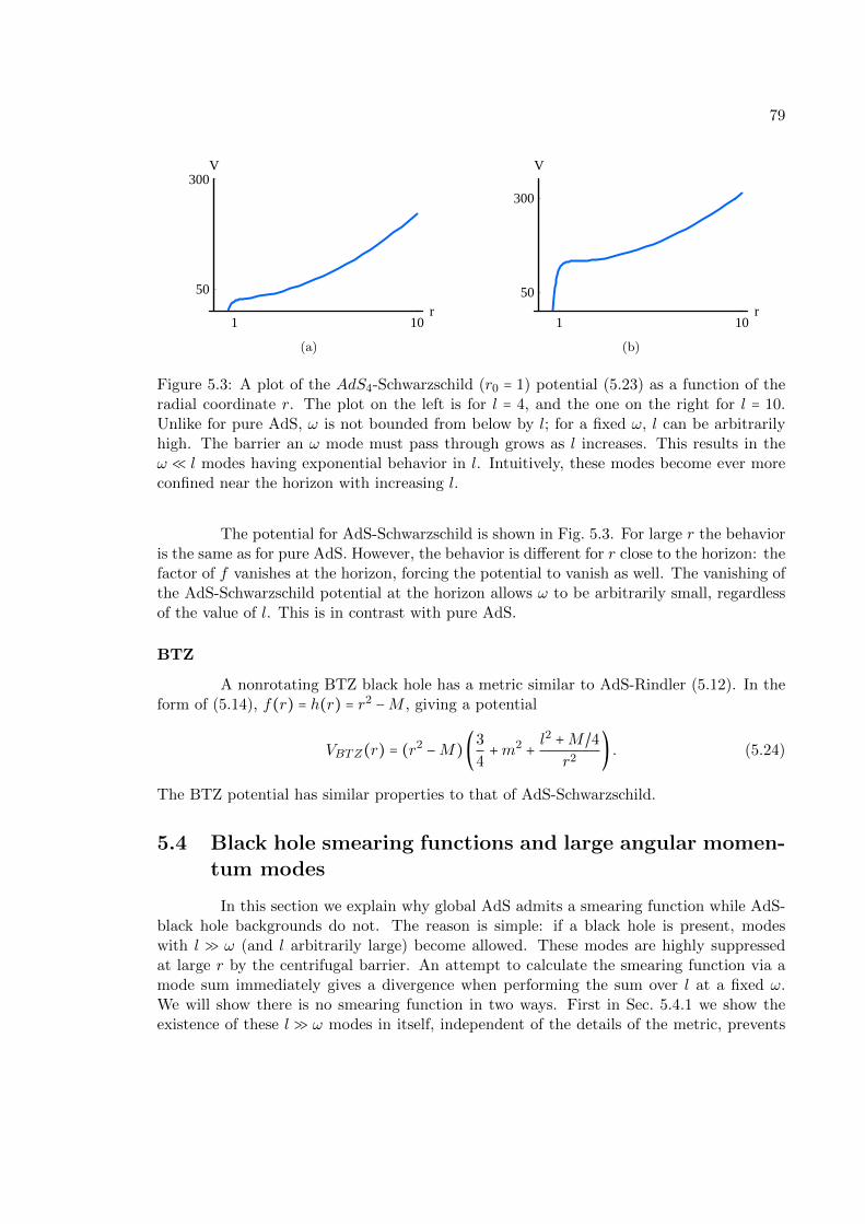
79

1 10r

50

300V

(a)

1 10r

50

300

V

(b)

Figure 5.3: A plot of the AdS4-Schwarzschild (r0 = 1) potential (5.23) as a function of theradial coordinate r. The plot on the left is for l = 4, and the one on the right for l = 10.Unlike for pure AdS, ω is not bounded from below by l; for a fixed ω, l can be arbitrarilyhigh. The barrier an ω mode must pass through grows as l increases. This results in theω ≪ l modes having exponential behavior in l. Intuitively, these modes become ever moreconfined near the horizon with increasing l.

The potential for AdS-Schwarzschild is shown in Fig. 5.3. For large r the behavioris the same as for pure AdS. However, the behavior is different for r close to the horizon: thefactor of f vanishes at the horizon, forcing the potential to vanish as well. The vanishing ofthe AdS-Schwarzschild potential at the horizon allows ω to be arbitrarily small, regardlessof the value of l. This is in contrast with pure AdS.

BTZ

A nonrotating BTZ black hole has a metric similar to AdS-Rindler (5.12). In theform of (5.14), f(r) = h(r) = r2 −M , giving a potential

VBTZ(r) = (r2 −M)(3

4+m2 + l

2 +M/4r2

) . (5.24)

The BTZ potential has similar properties to that of AdS-Schwarzschild.

5.4 Black hole smearing functions and large angular momen-tum modes

In this section we explain why global AdS admits a smearing function while AdS-black hole backgrounds do not. The reason is simple: if a black hole is present, modeswith l ≫ ω (and l arbitrarily large) become allowed. These modes are highly suppressedat large r by the centrifugal barrier. An attempt to calculate the smearing function via amode sum immediately gives a divergence when performing the sum over l at a fixed ω.We will show there is no smearing function in two ways. First in Sec. 5.4.1 we show theexistence of these l ≫ ω modes in itself, independent of the details of the metric, prevents

80

a smearing function for bulk points at large r. In Sec. 5.4.2 we use WKB to directly solvefor the modes, showing there is no smearing function for any bulk point B. We should notethat there are other cases where a smearing function fails to exist, even without a horizonand the associated l≫ ω modes, as we will show in Sec. 5.5.

In Sec. 5.4.1 we review how in pure AdS modes oscillate as eiqz where z = 0 is theboundary and q2 = ω2 − l(l + d − 2). If modes existed with q2 < 0, then they would growexponentially as eκz where κ2 = −q2. Since black hole backgrounds asymptotically approachpure AdS, their q2 < 0 modes will display this exponential behavior in l. Connecting withthe discussion in Sec. 5.2, this means the sum in (6.6) will not converge, and hence thesemodes forbid a smearing function for bulk points near the boundary.

In Sec. 5.4.2 we show that in the limit of high l, the potential (5.19) considerablysimplifies, with only the centrifugal barrier remaining. Using WKB we solve to find themodes. The result shows an exponential behavior in l for these l ≫ ω modes, for any bulkpoint. Thus we find there is no smearing function for any point in any static sphericallysymmetric spacetime with a horizon.

5.4.1 Asymptotic behavior of the wave equation

For an asymptotically AdS space, at large r the f(r), h(r) in (5.14) have the limitf(r), h(r)→ r2. Changing variables to z = 1/r, we write the metric as

ds2 = −dt2 + dz2 + dΩ2

z2. (5.25)

For small angles (5.25) resembles the metric of the Poincare Patch. The wave equation forthe radial modes is

z2φ′′ − z(d − 1)φ′ + (z2q2 −m2)φ = 0, (5.26)

where q2 = ω2 − l(l + d − 2). Substituting φ(z) = zd/2ψ(z) yields

z2ψ′′ + zψ′ + (z2q2 − ν2)ψ = 0, (5.27)

where we defined ν2 =m2 + d2/4. For ω2 > l(l + d − 2) this gives ψ(z) = Jν(qz) and hence

φ(z) = zd/2Jν(qz), (5.28)

which resembles the usual solution in the Poincare Patch.6 Modes with ω2 < l(l + d − 2)have negative q2. Of course these modes don’t exist in pure AdS, but they do in AdS-Schwarzschild. Defining κ2 = −q2, we get ψ(z) = Jν(iκz) ≡ eiνπ/2Iν(κz).7 Since the Besselfunction Jν(x) oscillates, Iν(x) grows exponentially. We can see the exponential growth

directly. Letting φ(z) = z d−12 u(z), (5.26) becomes

6The other solution, Yν(qz), is discarded because it doesn’t have the correct behavior φ → z∆ near theboundary that is expected of a normalizable mode.

7In the context of Euclidean AdS/CFT in the Poincare Patch one has this scenario of q2 < 0. Thereare two solutions: Iν(κz) and Kν(κz). The Kν(κz) solution is kept while the Iν(κz) is discarded preciselybecause of its exponential growth in the bulk. Of course, for us Kν(κz) cannot be kept since it growsexponentially as the boundary is approached and so is nonnormalizable.

81

u′′ − [κ2 + ν2 − 1/4z2

]u = 0 . (5.29)

In the limit of z ≫√ν2 − 1/4/κ, Eq. 5.29 is solved by u = eκz. Thus, we see that for large l

and l≫ ω the modes behave asφ(z) = z

d−12 elz. (5.30)

Our use of the pure AdS metric is justified for sufficiently small z. However forany z > 0, there exists an l sufficiently large such that z ≫

√ν2 − 1/4/κ is satisfied. Since

computing a smearing function involves summing over l arbitrarily large, we are guaranteedto reach regime (5.30) at sufficiently high l.

Smearing function for static spherically symmetric spacetimes

In the case of static spherically symmetric spacetimes, the solutions (5.16) can beinserted into the smearing function (6.6), giving

K(r, t,Ω∣t′,Ω′) = ∫ dωeiω(t−t′) ∑l,mi

φω,l(r)Ylmi(Ω)Y ∗lmi

(Ω′) , (5.31)

where mi denotes all the angular quantum number, m1, ...,md−2, and we have normalizedthe time dependent piece with respect to the boundary Klein-Gordon norm. The radialmodes φω,l are solutions to the radial wave equation (5.18) and should be normalized sothat φωl → r−∆ as r →∞. For AdS-Schwarzschild, the energies ω are continuous and so wehave written an integral over ω; for global AdS this would be replaced by a discrete sumover n as ωn = 2n + l +∆.

If only modes with ω >√l(l + d − 2) are allowed then, as we saw above, the near

boundary solution (5.28) is, when properly normalized,

φωl(r) = 2νΓ(ν + 1)Jν(q/r)rd/2qν

. (5.32)

Inserting the φωl(r) into (5.31), we see the sum converges. On the other hand, for modeswith ω <

√l(l + d − 2), and in particular the high l ones with solution (5.30), the sum over

l in (5.31) is hopelessly divergent.

5.4.2 Large angular momentum and WKB

Our goal here is to directly show the exponential behavior in l of the modes φωl(r)for large l and l ≫ ω for any bulk point. The smearing function doesn’t exist due to themodes with arbitrarily large l, which is why this is a sufficient limit to consider. We will alsosee how the details of the metric become irrelevant in the large l limit, with the centrifugalbarrier dominating the potential (5.19).

Modes with energy ω have a turning point at r = rt which satisfies V (rt) = ω2. Inthe limit of l ≫ ω, the turning point approaches the horizon, rt ≈ rh. For r > rt the modesalways have ω2 < V and thus decay. For r > rt, we can use WKB:

82

u(r) = 1√p

exp(−∫r

rtp dr∗), (5.33)

where p2 = V − ω2.We will only be interested in the exponential term, so we drop the 1/√p prefactor.

As discussed in Sec. 5.2, in order to compute the smearing function we need to normalizeall the bulk modes so that their boundary limit (upon stripping off r∆) is normalized withrespect to the boundary norm. In terms of u(r), we need its coefficient to approach 1 asr →∞. Thus,

u(r) = exp⎛⎝∫

∞

r

dr′√f(r′)h(r′)

√V (r′) − ω2

⎞⎠, (5.34)

where we used the relation between the radial coordinate and the tortoise coordinate, dr∗ =dr/

√fh.

The key point is that for any point outside the horizon, r > rh, there is an lsufficiently large such that the potential (5.19) can be approximated by

V (r) = f l2

r2, (5.35)

where for simplicity we used l(l + d − 2) ≈ l2. In (5.34) it is sufficient to only integrate forsome finite distance δ away from r to see the exponential behavior in l,

u(r) > exp⎛⎝∫

r+δ

r

dr′√f(r′)h(r′)

√V (r′) − ω2

⎞⎠. (5.36)

For any δ we want, there is an l sufficiently large such that the potential (5.19) can beapproximated by (5.35) for all radii between r and r + δ. Thus, using the approximatepotential (5.35) and neglecting ω2 we get,

u(r) > exp⎛⎝l∫

r+δ

r

dr′

r′√h(r′)

⎞⎠. (5.37)

This demonstrates the exponential growth in l of the modes. This is true for any bulk pointr; the only difference is the larger r, the greater the l before the exponential growth (5.37)sets in.

In the limit of large r we can approximate f(r) ≈ h(r) ≈ r2. This yields u(r) →el/r. Recalling φ = u/r(d−1)/2, this reproduces (5.30). Additionally, (5.37) matches theexponential growth in l of the exact hypergeometric function solution (5.13) found in [112]for the BTZ black hole.

5.5 Smearing functions for other spacetimes

We have seen if there is a horizon the potential (5.19) vanishes at the horizon andconsequently any frequency ω > 0 is allowed. The arguments of the previous section show

83

A

B

C

(a)

Figure 5.4: We are interested in finding for which static spherically spacetimes withouthorizons a smearing function exists. The smearing function involves the sum (5.31) overmodes, which can be grouped into 3 different regimes. Only A posses a threat to theconvergence of (5.31). At large r the metric, and consequently the potential (5.19), lookslike that of pure AdS (5.38). At smaller r, in regime A the angular momentum l is so largethat all terms in the potential except for the centrifugal barrier (5.40) are irrelevant.

there is no smearing function. In this section we examine more generally when a smearingfunction exists. In Sec. 5.5.1 we consider a general static spherically symmetric spacetime(5.14), and find a simple criteria on the metric (5.41) which gaurantees there will be modeswith exponential behavior in l for high l, and hence there will not be a smearing functionfor some bulk points. In Sec. 5.5.2 we examine the possibility of trapped null geodesics as aproxy for a smearing function not existing for an arbitrary spacetime. In the special case ofstatic spherically symmetric spacetimes we demonstrate that the existance of trapped nullgeodesics prevents a smearing function.

5.5.1 Static spherically symmetric spacetimes

In this section we examine the existence of a smearing function for spacetimes ofthe form (5.14) which do not possess horizons.

The question of the existance of a smearing function is the question of the conver-gence of the sum (5.31) over ω and l at a given value of r. To answer this question, we willneed to estimate the size of each mode with a given ω and l, for every ω that is allowed. Itis convenient to divide the (ω, l)-plane into three regions, shown in Fig. 5.4, according tothe sizes of ω and l relative to certain large values ω0 and l0 which depend only on f andh and will be defined carefully below. Region A consists of all modes with l > l0, region Bconsists of all modes with ω > ω0 and l < l0, and region C consists of the remaining modeswith ω < ω0 and l < l0.

84

l(l+d-2)

(a)

Figure 5.5: The wave equation can be recast as a Schrodinger equation (5.18) with apotential V (r) and an energy ω2. Here we sketch a possible potential (5.19) for which asmearing function doesn’t exist. At large r, r > R, the the potential looks like that of pureAdS (the figure has been compressed; the distance between r2 and R is really much larger).At smaller r the potential, for large l, is approximated by (5.40). If f(r)/r2 ever has positiveslope, as shown above, some of the modes ω (dashed line) will have to tunnel through thebarrier. Consequently, the sum (5.31) will diverge for r < r2.

Approximating the potential

To aid our calculation, we will approximate the behavior of the potential for large,small, and intermediate values of r.

Large rSince the metric approaches pure AdS at large r, we can approximate f(r) ≈

h(r) ≈ r2 for r > R, where R is some sufficiently large radius that depends on f and h. Thepotential for r > R thus takes the form

V (r) ≈ l(l + d − 2) + (d2 − 1

4+m2) r2, r > R. (5.38)

Small rAs r → 0, h(r)→ 1 to avoid a conical singularity, and f(r)→ f0 > 0. Thus we can

find some small ε > 0 such that

V (r) ≈ f0 (l(l + d − 2) + (d − 1)(d − 3)/4

r2) , r < ε. (5.39)

Note that the form of the potential implies that ω is quantized. Aside from the constantf0, the potential for r < ε does not depend on the details of the geometry.

Intermediate rFor ε < r < R it will be useful to do a separate analysis for modes lying in the three

different (ω, l)-regions shown in Fig. 5.4.A: Since f , h, and their derivatives are bounded functions for r < R, we can find

an l0 sufficiently large so that for all l > l0 all terms in the potential (5.19) except thecentrifugal barrier are irrelevant for all r < R,

V (r) ≈ f(r) l(l + d − 2)r2

, r < R and l > l0. (5.40)

85

This potential agrees with our small-r approximation above when r < ε. Note that thepotential in this region has an overall scaling with l.

B: We choose an ω0 sufficiently large such that ω20 ≫ V (r) for all ε < r < R and

l < l0. For modes in region B the potential is negligible at intermediate values of r.C: For modes in region C all of the details of the potential are important, and

there is no useful approximation.

Convergence of sum for smearing function

Since ω and l are quantized, there are only a finite number of modes in regionC, so that part of the sum (5.31) converges. In region B the modes experience the samepotential as in pure AdS (aside from an inconsequential scaling of f0 at small r), so thatpart of the sum will converge as well. This only leaves region A to analyze.

Let us suppose the potential (5.40) has positive slope for some range of r,

d

dr(f(r)r2

) > 0 for some r. (5.41)

We will now show if this occurs then there is no smearing function for some bulk points dueto an exponential divergence in region A. In Fig. 5.5 we sketch an example of potential forwhich (5.41) occurs. Consider the limit of large ω and large l. This is the classical limit ofthe Schrodinger equation (5.18), as can be seen from the fact that the range of r∗ is finiteand fixed, while the potential V (r) and energy ω are getting large. Thus, it is guaranteedthat there exists a mode ω lying within any classically allowed energy interval. If (5.41) issatisfied in a neighborhood of r = r1, then that neighborhood consists of classical turningpoints for an interval of possible values of ω. Let r2 > r1 be any point in the classicallyforbidden region for these values of ω.8 Then the field at any r in the range r1 < r < r2 (orany r in the classically allowed region r < r1) is larger than that at r2 by a WKB factor of

exp(∫r2

r

dr√fh

√V − ω2) = exp

⎛⎝l∫

r2

r

dr√fh

√f

r2− (ω

l)

2⎞⎠. (5.42)

There is a subtlety here: in addition to this decaying solution, there is also anexponentially growing solution and the eigenstate will in general be a linear combinationof the two if there is a second classically allowed region when r > r2 (as in the scenario ofFig. 5.5). If both solutions contribute with comparable coefficients, then the eigenstate willnot be exponentially larger at r than it is at r2 as we have claimed. That phenomenon occurs,for instance, in the symmetric double well potential familiar from quantum mechanics.However, that kind of behavior is special to the symmetric, degenerate case. As long as theenergy differences between approximate eigenstates localized on either side of the barrier islarger than the exponentially small tunneling factor, the true eigenstates of the system willbe exponentially well localized on one side of the barrier, and we can restrict attention tothose localized in the r < r1 region.

8We treat r1 and r2 as if they are less than R for the puprose of approximating the potential. However,if they are larger than R it makes little difference. In the large-l limit the extra terms in (5.38) becomeirrelevant for r < r2.

86

It is clear that (5.42) can be made arbitrarily large by making l large. Speficially,let α = ω/l where ω and l are the modes considered above which are suppressed and givebehavior (5.42). Now consider the portion of the sum (5.31) concentrated on the line offixed α. Thus, (5.31) will not converge and there will not be a smearing function for pointsr < r2. We should note that unlike the black hole case considered earlier, which did not havea smearing function for any bulk point, for a potential like in Fig. 5.5 there is a smearingfunction for bulk points at large r.

A remaining question is the converse of our statement: if f(r)/r2 has non-positiveslope for all r, is the smearing function guaranteed to exist? In this case there are no turningpoints at intermediate values of r, and hence no opportunity for exponential WKB factors.However, it is possible that the magnitude of the slope of f(r)/r2 is small for some rangeof r, and then the 1/√p factor in (5.33) can become large. It is conceivable that one couldstill make sense of (5.31), despite power law growth in the summand, through regulationand analytic continuation. This requires further analysis, and is something we intend toinvestigate in subsequent work.

5.5.2 Trapped null geodesics

We have established a smearing function does not exist in a black hole background.In a general static spherically symmetric spacetime, we have shown that it does not existif the metric has the property (5.41). In a more general spacetime without a high degreeof symmetry, the mode sum approach to constructing a smearing function is inapplicable.This motivates us to search for a simply proxy for the existence of a smearing function.In this section we explore the following proposal: there is a smearing function iff all nullgeodesics have at least one endpoint on the boundary.

A smearing function allows one to make the statement (5.2) about the mappingbetween bulk and boundary operators. However, finding a smearing function is a classicalfield theory problem. At the level of individual modes we saw a smearing function fora point B in the bulk fails if there are modes whose imprint on the regulated boundaryis exponentially small compared to their value B. Throughout this chapter we held theboundary imprint fixed and saw the value at B grow arbitrarily large, causing (6.6) todiverge. Keeping the field value at B fixed, this would correspond to modes with boundaryimprint becoming arbitrarily small.

Since field configurations are built out of modes, we can state this as: a smearingfunction fails to exist if there are bulk field solutions Φ(B) with arbitrarily small boundaryimprint. When one takes the geometric optics limit, field solutions become arbitrarily welllocalized along null geodesics. At a heuristic level, this motivates the simple criterion oftrapped null geodesics, which we will now explore quantitatively..9

9In [9, 174] it was shown for a large class of hyperbolic differential equations that the diagnostic ifreconstruction of a bulk field depends on boundary data continuously (for a particular choice of boundarynorm) is that there not be any trapped null geodesics. In [31] null geodesics were explored in the context ofsubregion dualities due to these results and with the motivation of establishing if a collection of boundaryobserves can physically reconstruct the bulk field in a subregion of AdS. This question is of secondary concernto us here; our interest is rather in the nature of the bulk-boundary dictionary (if (5.2) is possible).

87

r

U

(a)

r

U

(b)

Figure 5.6: The equation for a null geodesic is that of a particle traveling in a 1-d potential(5.44). The potential is plotted for (a) pure AdS and (b) AdS-Schwarzschild (M = 1 inAdS4). In pure AdS all null geodesics have an endpoint on the boundary, as can be seenfrom the figure on the left. This is in contrast to spacetime with horizons (right figure)which have some null geodesics which are trapped as a result of the potential U vanishingat the horizon. More generally, whenever there are trapped null geodesics, then there is nosmearing function for some points in the bulk.

Geodesic equation

To find the motion of null geodesics in the spacetime (5.14), we note that thetimelike Killing vector gives the conserved quantity E = f t, and the Killing vector in one ofthe angular directions, θ, gives L = r2θ. Here we are using the notation xµ ≡ dxµ/dλ whereλ is the affine parameter.

The geodesic equation can be written as

f

hr2 +L2 f

r2= E2. (5.43)

This is just the Newtonian energy conservation equation for a particle with position-dependent mass moving in a potential

U = L2 f

r2. (5.44)

In black hole backgrounds the potential (5.44) vanishes at the horizon, leading to trappednull geodesics. More generally, (5.44) tells us there are no trapped geodesics iff U ′ < 0 forall r.

It is interesting to note that even a small dense star in AdS can have trapped nullgeodesics. All the star needs is to have a radius R which lies in the range 2M < R < 3M .The metric for r >R is described by the Schwarzschild metric. Since for the Schwarzschildmetric U ′(r) > 0 for r < 3M , null geodesics will get trapped at small r.

Trapped null geodesics ⇒ no smearing function

In 5.1 we saw that for the question of the existence of a smearing function, onlythe behavior of the high l modes was relevant. In this regime (labeled A in Fig. 5.4)

88

the potential in the Schrodinger equation for the modes was well approximated by (5.40).Yet this is exactly the same as the classical particle potential (5.44) for a null geodesic.Our condition for a smearing function not existing (5.41) is the same as the condition forthe existence of trapped null geodesics. Thus we conclude that if there are trapped nullgeodesics, then a smearing function does not exist.

We note that since null geodesics are only sensitive to the local metric, trappednull geodesics cannot tell us for which regions of the bulk there is no smearing function. If anull geodesic is confined to r < rt, this indicates there is no smearing function for r < rt, butit says nothing about a smearing function for r > rt. The existence of a smearing functionfor r > rt depends, as we explained above, on the existence of additional classically allowedregions with V (r) < ω2 for r > rt. A classical null geodesic confined to r < rt cannot probethese aspects of the potential.

5.6 Conclusions

In this chapter we have further explored one of the approaches to establishingthe dictionary between bulk and boundary operators. In this approach, a bulk operator isexpressed in terms of bulk operators at asymptotically large radius, which are then mappedto local boundary operators through (5.1). While this approach works in pure global AdS,we have argued it can fail if there are bulk modes which have an arbitrarily small tail at largeradius. We have shown that AdS-Schwarzschild backgrounds are a case where this smearingfunction approach fails as a result of modes with arbitarily high angular momentum l, butfixed boundary energy, ω.

Understanding in general when a spacetime has a region for which a bulk operatorcannot be expressed in terms of smeared local boundary operators remains an importantfuture problem. We have shown that for static, spherically symmetric spacetimes, this ques-tion can be answered by considering the behavior of modes with large ω and large l. Thesemodes satisfy a Schrodinger-like equation with a potential that is the same as the potentialexperienced by classical null geodesics. These results suggest that a smearing function maynot exist for some bulk points in any spacetime which has trapped null geodesics .

The extent to which the absence of a smearing function modifies the bulk-boundarydictionary remains to be seen. It is possible one can obtain an approximate smearingfunction by imposing a cutoff in the bulk and excluding high l and high ω modes from thesum (5.31) defining the smearing function. Additionally, as we discussed, the existance of asmearing function is a more stringent requirement than simply being able to reconstruct abulk field solution given some particular boundary data. To this extent, even though (5.7)may not exist, (5.6) exists at N =∞. However, unlike a smearing function, it is unclear that(5.6) can be generalized to situations with broken spherical and time-translation symmetry,and so may be of limited use. Another option would be to try to construct a smearingfunction which uses the complexified boundary, as done in [89] for AdS-Rindler, and perhapsthis would gives clues as to what the real spacetime representation of the bulk-boundarymap is.

When a smearing function does exist, it means that bulk data provided at largeradius for a sufficient time extent completely determines the bulk everywhere. In a way, it

89

makes holography seem less powerful; a spatial direction has just been replaced by a timedirection. Of course, the power of AdS/CFT is due to the CFT Hamiltonian which onecan use to evolve the right side of (6.6) to a single time. The resulting operator is highlynonlocal and known as a precursor [148]: an operator which encodes what happened deepin the bulk long before casuality allows a local operator O(b) to know about it.

The absence of a smearing function makes the holographic dictionary more elusive.Bulk evolution combined with boundary evolution are not even in principle sufficient toanswer the question of what the precursers are. Other methods must be developed to findthe dictionary between bulk operators and nonlocal boundary operators.

90

Chapter 6

Scanning Tunneling Macroscopy,Black Holes, and AdS/CFT BulkLocality

6.1 Introduction

This chapter concerns reconstructing the state of the anti-de Sitter (AdS) bulkfrom the conformal field theory (CFT) boundary. Finding which CFT quantities encodethe bulk and, if so, in what ways has been actively pursued recently, e.g. [106, 97, 152,111, 116, 60, 58, 102, 4, 31, 118, 110]. One standard approach is to start with local CFTdata and use bulk equations of motion to evolve radially inward. The questions we seekto answer are: under what circumstances is this evolution possible, how deep into the bulkcan we evolve, on what scales can the bulk be reconstructed, and what assumptions aboutthe bulk state must be made?

We first address these questions in a simpler context: the electromagnetic field inMinkowski spacetime. Given boundary field data on a timelike codimension-1 hypersurface(z = 0), can the electromagnetic field be determined everywhere (z > 0)? Suppose thebulk is filled with homogeneous air. The only solutions to the wave equation consistentwith translation symmetries are traveling waves, and reconstruction is trivially achieved.On the other hand, suppose that the bulk is filled with air for 0 ≤ z < zg and with glassfor z > zg. The translation symmetry being broken, there is now a new class of solutions:waves which are traveling for z > zg but evanescent for 0 ≤ z < zg. Evanescent modesare solutions with imaginary momentum. While legitimate solutions of the wave equation,these modes are forbidden in vacuo because of exponential growth at large z and hence non-normalizability. The presence of glass at finite z cuts off this unboundedness and rendersthe mode permissible. Reconstructing the field inside the glass from measurements at z = 0is hopeless; a small mistake will get exponentially amplified. It would be like trying tomeasure the electromagnetic field inside a waveguide while standing a kilometer away. Infact, even reconstruction of the field for 0 ≤ z < zg from the boundary data at z = 0 isno longer straightforward. If we do not measure the evanescent modes (in the absence ofassumptions on the form of the solution), we can not reconstruct the field anywhere. We

91

can, however, measure the evanescent modes at z = 0 to some extent without resorting toexponential precision. If we do then the field, coarse-grained in x over a scale σ, can bereconstructed, but only for z < σ.

We next address the reconstruction question in the context of the AdS/CFT cor-respondence: we consider a free scalar field in a fixed asymptotically AdS background. Abackground which is pure AdS, or a perturbation thereof, is like the electromagnetic field inthe vacuum - exact reconstruction using boundary data is possible. Thus, local CFT opera-tors give a probe of the bulk on the shortest of scales. A background with a small AdS blackhole is like putting in a region with glass. The geometry in the black hole atmosphere, theregion from 2M to 3M , changes the boundary conditions and permits evanescent modes.Analogously to the case with glass, reconstructing the field in the atmosphere is hopeless.Reconstructing the field far from the black hole is possible to some extent, and like in thecase of the electromagnetic field, requires measuring the evanescent data. The conditionz < σ translates into the ability to resolve the bulk on AdS scales and no shorter. The mea-surement of evanescent modes forms the basis of the functioning of a Scanning TunnelingMicroscope (STM). In this sense, the CFT is acting like an STM for macroscopic scales.

It may seem puzzling that a small black hole deep in the bulk should have anyimpact on our ability to reconstruct the bulk close to the boundary. One may pretendthe evanescent modes don’t exist and work only with the propagating modes. This mightbe a good approximation for some states and for regions close to the boundary, but itis one that is violated by legitimate finite energy solutions having a significant coefficientfor an evanescent mode. Even in the Hartle-Hawking vacuum, the CFT Green’s functionG2(ω,k) ( given by the Fourier transform of the finite temperature two-point correlator⟨O(t,x)O(0,0)⟩T ) is nonzero but exponentially small ∼ exp(−α∣k∣/T ) in the evanescentregime k ≫ ω. The evanescent modes are part of the spectrum of states, so even if onemight opt to ignore them for two-point correlators, they necessarily contribute to any finite-temperature n−point function as intermediate states.

We have organized the chapter as follows. In Section 6.2, we formulate in Minkowskispacetime the problem of spacelike reconstruction from timelike boundary data. We showthat reconstruction is exact in situations with only propagating modes but requires expo-nential precision in situations with evanescent modes. In the latter situation, reconstructionwithout exponential precision is possible but only at the cost of averaging over directionsparallel to the boundary, and only out to a distance set by this averaging scale. In Section6.3, we formulate the reconstruction problem in AdS space and demonstrate that the situ-ation is exactly parallel to the Minkowski spacetime counterpart. In pure AdS, all modesare propagating and the reconstruction is exact. In an AdS black hole background, evanes-cent modes open up near the black hole horizon and reconstruction requires exponentialprecision. Here again, reconstruction without exponential precision is possible but only atthe cost of an AdS scale averaging over directions parallel to the boundary. In Section6.4, via the AdS/CFT correspondence, we discuss the impact of evanescent modes on bulkreconstruction from the CFT viewpoint. We show that in general precise determination ofa Green’s functions at finite temperature requires exponential precision. In the Appendix6.6 we review evanescent modes in optics, the principles of a microscope, and scanningtunneling (optical) microscopy (STM).

92

t

x

z

Figure 6.1: The setup of bulk reconstruction in (2 + 1)-dimensional Minkowski half-spaceR2,1+ . We have a bulk field φ(x, t, z) obeying the wave equation, which we wish to reconstruct

from the data φ(x, t,0) on a timelike hypersurface at z = 0.

6.2 Bulk reconstruction in Minkowski space

In this section we pose the question: for a field φ(x, t, z) satisfying the wave equa-tion in (2+ 1)-dimensional Minkowski spacetime 1, is the boundary data φ(x, t,0) specifiedat a timelike hypersurface z = 0 sufficient to reconstruct the field φ(x, t, z) everywhere?(See the setup shown in Fig. 6.1.) The wave equation admits solutions with both realand complex momentum. The solutions with real momentum are the propagating waves,e±ikzz. If the space is everywhere homogeneous, such as pure Minkowski space, then theseare the only admissible delta-function normalizable modes. In this case, reconstruction ofφ(x, t, z) from the boundary data φ(x′, t′,0) works perfectly — we show in Sec. 6.2.1 thatthe smearing function K(x, t, z∣x′, t′) whose convolution with φ(x′, t′,0) yields φ(x, t, z) iswell-defined everywhere in the bulk. On the other hand, if the space is inhomogeneous by,for instance, having a spatially varying index of refraction, then modes with imaginary mo-mentum can become permissible. Instead of propagating, these modes grow exponentiallyin the z direction: e±κzz. They are known as “evanescent modes”. Our goal is to pointout that the evanescent modes cause serious difficulties in reconstructing the field anywherefrom given boundary data.

6.2.1 Success with propagating modes

We consider the wave equation in (2 + 1)-dimensional Minkwoski spacetime R2,1:

(−∂2t + ∂2

x + ∂2z) φ(x, t, z) = 0. (6.1)

We will be interested in reconstructing φ(x, t, z) from boundary data φ(x, t,0) specified ona timelike hypersurface b at z = 0. To accomplish this, we decompose the solutions to (6.1)in terms of the propagating wave basis:

φ(x, t, z) = ∫ ∫ dkx dω φ(kx, ω) e−ikxx−ikzz−iωt, (6.2)

1Extension to higher dimensions is straightforward and does not reveal any new physics.

93

where the delta-function normalizability condition puts

kz ≡√ω2 − k2

x ∈ R+ → ∣ω∣ ≥ ∣kx∣. (6.3)

We chose kz to be positive, as we will for simplicity assume there are only left-movers.2

The decomposition (6.2) is slightly nonstandard as ω is one of the independent variablesas opposed to kz. This is a convenient choice here as the boundary data is specified on atimelike hypersurface. The Fourier transform of φ(x, t, z = 0) yields

φ(kx, ω) = ∫ ∫bdx′dt′ eikxx

′+iωt′φ(x′, t′,0). (6.4)

Inserting (6.4) into (6.2),

φ(x, t, z) = ∫ ∫bdx′dt′ K(x, t, z∣x′, t′)φ(x′, t′,0). (6.5)

Here, K is the smearing function given by

K(x, t, z∣x′, t′) = ∫∞

−∞dω∫∣kx∣≤∣ω∣

dkx e−iω(t−t′)e−ikx(x−x

′)e−i√ω2−k2

x z

= ∫∞

−∞dkx∫∣ω∣≥∣kx∣

dω e−iω(t−t′)e−ikx(x−x

′)e−i√ω2−k2

x z. (6.6)

The integral in (6.6) is convergent, so (6.5) realizes our goal of reconstructing φ(x, t, z) interms of the boundary data φ(x, t,0). This is not surprising, as for every mode the field atsome value of z is related to the field at z = 0 by the phase-factor eikzz associated with thetranslation, where kz is given by (6.3).

It will be useful for later to first reconstruct per each monochromatic ω mode andthen combine them together. We then use

φω(x,0) ≡ ∫∞

−∞dt eiωt φ(x, t, z = 0) (6.7)

to reconstruct φω(x, z),

φω(x, z) = ∫∞

−∞dx′ Kω(x, z∣x′) φω(x′,0) (6.8)

whereKω(x, z∣x′) = ∫∣kx∣≤∣ω∣

dkx e−ikx(x−x′)e−i

√ω2−k2

x z. (6.9)

The full smearing function is then recovered through the spectral sum

K(x, t, z∣x′, t′) = ∫∞

−∞dω Kω(x, z∣x′)e−iω(t−t

′). (6.10)

2Assuming there are only left-movers allows us to connect more directly with the analogous problemin AdS space. The more general case in Minkowski space for which right-movers are also included is astraightforward extension and requires specifying ∂zφ(x, t, z = 0) in addition to φ(x, t, z = 0) at the boundaryb.

94

6.2.2 Reality with evanescent modes

In the above discussion we restricted kz to be real-valued as a consequence of thedelta-function normalizability condition for the modes. If one were to consider kx > ω suchthat kz is imaginary: kz ≡ iκz, a mode would take the form

e−ikxxe−iωteκzz. (z ≥ 0) (6.11)

This solution diverges at large z, and is therefore not admissible. We were thus correctto discard it. However, if the Minkowski space is inhomogeneous in the z-direction, oftensolutions such as (6.11) become admissible. In Appendix 6.6, we give two situations whichgenerate evanescent modes: (1) a wave traveling in a medium with a z dependent index ofrefraction, and (2) a wave scattering off a material that has an x-dependent transmissioncoefficient and is located at some fixed z.

If evanescent modes are present, then they pose a serious challenge for reconstruct-ing the field from the z = 0 boundary data. Unlike propagating modes, evanescent modeswill have an exponentially suppressed imprint on the z = 0 boundary compared to theirvalue at z > 0. This exponential behavior renders the reconstruction procedure of Sec. 6.2.1inapplicable: the smearing function K (6.6) is ill-defined because of the divergence from thekx ≫ ω region of integration. For the rest of this section, we simply assume that evanescentmodes are present and do not inquire as to their origin. An exemplary situation to keepin mind is the one where the index of refraction of the background changes at some largevalue of z > 0. For simplicity, we will assume the change made at large z is such that allpossible evanescent modes are produced so that the mode solutions now contain all valuesof kx regardless of ω. We would like to understand the impact this has on reconstructingthe field from boundary data.

We can take two approaches in dealing with evanescent modes. We may ignorethe modes from the outset, contending that they are not propagating. Or we may includethe modes. We now argue that in both cases we will face unavoidable limitations on theresolving power of the reconstruction.

6.2.3 Ignoring evanescent modes

Consider first the approach of ignoring the evanescent mode data at the boundary:we will not try to extract their coefficient from the boundary data provided at z = 0. Inthe procedure of Sec. 6.2.1, we are now in the situation that the Fourier decompositionof φ(x, t, z) (6.2) extends over all kx and ω, but we truncate the Fourier decomposition ofthe smearing function K in (6.6) to ∣ω∣ ≥ ∣kx∣ . Reconstruction of φ(x, t, z) can be donemonochromatically per each frequency ω, first reconstructing φω(x, z) and then combiningthem to get φ(x, t, z). Reconstruction of φω(x, z) is the same problem as the one encounteredin optics when one tries to resolve features of a sample by shining monochromatic light onit. (For those who need to refresh optics, consult Appendix 6.6.) Ignoring the evanescentmodes is the standard assumption in optical microscopy: the detector (playing the role ofthe boundary) is far from the sample, so the magnitude of the evanescent modes at thescreen is exponentially small and is zero for all practical purposes. For this reason, we onlyhave knowledge of features of the sample, T (kx), for ∣kx∣ ≤ ∣ω∣. This is the standard result

95

we would expect: detecting light of frequency ω, we can probe the features of a sample butonly on scales larger than the resolution power set by ω−1.

Specifically, we assume the boundary data specified at the z = 0 hypersurfacetells us nothing about the coefficients φω(kx) for ∣kx∣ ≥ ∣ω∣. Clearly, we can then nothope to confidently reconstruct φω(x, z), as the coefficient φω(kx) for the large kx couldbe arbitrarily large. To ameliorate this, we may ask for reconstructing the field φω(x, z)coarse-grained over x with the Gaussian window function of resolution scale σ. We denotethis coarse-grained field as φσω(x, z):

φσω(x, z) = ∫∞

−∞dx′ e−(x−x

′)2/σ2

φω(x′, z) . (6.12)

We would expect that reconstructing φσω(x, z) should only require knowledge of modes with∣kx∣ ≲ ∣σ∣−1. To verify this, we rewrite (6.12) as

φσω(x, z) = ∫ dkx φω(kx, z) e−k2xσ

2

e−ikxx. (6.13)

Unless φω(kx, z) grows exponentially in k2x for large kx, its value is irrelevant for ∣kx∣ ≳ ∣σ∣−1.

Therefore, if we are only interested in reconstructing the field φω(x, z) coarse-grained overx with resolution scale σ, then we can reconstruct it using only the propagating mode dataat the z = 0 boundary as long as ∣ω∣ ≳ 1/σ (and provided a reasonable assumption is madeabout the behavior of the ∣kx∣ ≫ ∣ω∣ modes).

All seems well, but there is a problem. To reconstruct φσ(x, t, z) for all time t, weneed φσω(x, z) for all ω. Yet, there is no σ for which this condition will be satisfied: for anyσ, there is an interval of missing ω, ∣ω∣ < 1/σ. This means that, with the assumption wemade that we ignore the evanescent mode data at z = 0, we can not possibly reconstruct thetemporal evolution of the field at any z location, regardless of how large a coarse-grainingresolution σ in x we are willing to compromise for. In short, for reconstruction relying onlyon propagating mode data, coarse-graining over x achieved reconstructability over z butsacrificed reconstructability over t.

6.2.4 Dealing with evanescent modes

Consider next the approach of retaining all the evanescent mode data at the bound-ary. If we wish to resolve the field on a scale ∣∆x∣ ≃ σ, we expect to require knowledge of thefield profile with kx ≲ σ−1. But then, evanescent modes with ω = 0 and kx = σ−1 behave likeez/σ, and we would expect we can determine φσ(x, t, z) only for z ≲ σ. At bulk locations zlarger than σ, the evanescent modes grow exponentially large compared to what we haveaccess to on the boundary. We will show below that one would require exponential accuracyin the knowledge of the z = 0 boundary data to reconstruct the field at bulk regions as deepas z ≫ σ. To foreshadow considerations in Sec. 6.3 for AdS space, let us mention thatthe criterion z ≲ σ will turn into σproper(z) ≳ LAdS[1 + ε(z)], where σproper(z) is the properdistance at a bulk location z corresponding to the coordinate distance σ, up to a correctionfactor ε that depends on details of the bulk.

We now redo the computation of Section 6.2.1 but with evanescent modes takeninto account. The monochromatic field φω(x, z) is expressed in terms of φω(x,0) through

96

Kω of (6.9). In the expression (6.9) for Kω, we must integrate over all ∣kx∣ < ∞. Wesplit this integral into contributions of the propagating modes and the evanescent modes,respectively,

Kω(x, z∣x′) = ∫ω

−ωdkx e

−ikx(x−x′)e−i√ω2−k2

x z + ∫∣kx∣>ωdkx e

−ikx(x−x′) e√k2x−ω2 z. (6.14)

The second integral is badly divergent. Thus, the evanescent modes have obstructed ourability to reconstruct the field in the bulk. As before, we instead ask for reconstructing themore physical quantity: the field coarse-grained over x with a Gaussian window function.We have

φσω(x, z) = ∫bdx′ Kσ

ω(x, z∣x′) φω(x′,0) (6.15)

whereKσω(x, z∣x′) = ∫

bdx e−(x−x)

2/σ2

Kω(x, z∣x′) . (6.16)

Inserting (6.9) into (6.16) yields

Kσω(x, z∣x′) = ∫ dkx e

−ikx(x−x′) e−i√ω2−k2

x z e−k2xσ

2

. (6.17)

Asking for the field smeared over σ in the x direction thus amounts to coarse-graining thesmearing function (6.14) over momentum kx with the Gaussian window function exp(−k2

xσ2)

to suppress large kx. The kx ≫ ω part of the integral in (6.17) gives

[e−2i(x−x′)z/σ2 ⋅ ez2/σ2] e−(x−x′)2/σ2

. (6.18)

Having smeared out in the x-direction, let’s examine the behavior in the bulk z-direction.As measured at deeper bulk regions z ≫ σ, this function oscillates rapidly in phase andgrows exponentially in amplitude. So, to determine the σ−grained field at a z greaterthan σ, one needs to measure the boundary data φω(x, z = 0) with exponential precision. Inshort, for reconstruction retaining evanescent mode data, coarse-graining over x amelioratedreconstructability over z, for a depth of order the coarse-graining scale or so.

6.2.5 Window function

In both approaches to dealing with evanescent modes, bulk reconstruction requiresa choice of a window function for the x-direction to regularize the divergence in (6.14). In(6.17), we chose a Gaussian window function to achieve the regularization. What aboutother choices? One might try a hard-wall window function, Θ(σ−1−∣kx∣), which gives perfectregularization, and whose x-space window function takes the form

sin (x−x′σ )x − x′ . (6.19)

One might also try a Laplace window function, e−kxσ, but this function would be insufficientto regulate the divergence. Details of reconstruction certainly depend on the choice of thewindow function, but the fact we are limited by resolution bounds do not depend on thechoice.

97

The choice of the window function is also a practical matter for the ScanningTunneling Microscopy (STM). The basis of STM is the measurement of evanescent modes.In the problem of resolving the features of a sample (Appendix 6.6), the location of thesample is held fixed and bringing the STM probe needle a distance σ close to the sampleallows image resolution on a scale σ. From the optics perspective, determining the spatialfeatures of a sample regardless of the frequency with which it is illuminated, as an STMallows, is an enormous achievement. We have shown that the ability to do this in the STMcontext translates into our ability to reconstruct the bulk field φσ(x, t, z) for z < σ fromboundary data. While the precise depth to which reconstruction is possible would certainlydepend on the chosen window function, the fact that the STM probes to a depth set by theimage resolution scale, is independent of the choice.

One should note that the coarse-grained smearing function, for any coarse grainingother than the hard wall choice (6.19), makes little distinction between σ less than or greaterthan 1/ω. This appears in tension with the standard assumption (reviewed in Sec. 6.2.3)that for σ > 1/ω, reconstruction should still be possible even while ignoring the evanescentmodes. However, regardless of ω, Kσ

ω has the same behavior coming from kx ≫ ω andleading to the same complications with reconstruction for z ≳ σ. The resolution is that thesmearing function makes no assumption regarding the high kx behavior of the field we aimto reconstruct, whereas our previous argument that modes with kx > σ are not needed forthe σ-grained field relied on a (very reasonable) assumption about the high kx behavior ofthe field.

6.2.6 Conclusions

Let’s summarize what we have learned so far. Our question of interest has beenwhether we can reconstruct the field φ(x, t, z) using the data φ(x, t, z = 0) at the z = 0timelike hypersurface. We assumed we can do this reconstruction monochromatically, re-constructing φω(x, z) from φω(x,0). If the medium is homogeneous and only propagatingmodes are present, then the reconstruction works flawlessly and is given by (6.5, 6.6).If, however, the medium is inhomogeneous and evanescent modes are present, then recon-structing φ(x, t, z) point by point in the bulk is not achievable. We could instead reconstructφω(x, z) coarse-grained in x with a σ-sized resolution, φσω(x, z). This reconstruction can bedone, while not measuring any of the evanescent modes, but only for σ ≳ 1/ω. Since recon-structing φσ(x, t, z) for all time t requires reconstructing φσω(x, z) for all ω, we are unableto reconstruct φσ(x, t, z) for any z. If, on the other hand, we do include the evanescentmodes, the reconstruction of φσ(x, t, z) can be done but only for the bulk depth z ≲ σ. Thisis because reconstructing for z ≳ σ would require exponential accuracy in measuring thevalue of φ(x, t,0).

6.3 Bulk reconstruction in AdS space

We now turn to AdS space and repeat the bulk reconstruction analysis. In short,we will find that the conclusion is exactly the same as in the flat Minkowski space case,except that we now need to understand the resolving power in proper distances. In Sec. 6.3.1

98

we make some general remarks regarding the relation between restricting the boundary datato local CFT operators and reconstructing a bulk AdS field from this data. In Sec. 6.3.2 wefocus on reconstruction in the near-boundary region of the bulk. In Sec. 6.3.3, we considerevolving deeper into the bulk and find how the resolving power is modified.

6.3.1 Local CFT operators as boundary data

The AdS/CFT dictionary in extrapolate form [6] relates the boundary limit of abulk operator φ to a local CFT operator O:

limz→0 z−∆ φ(x, t, z) = O(x, t). (6.20)

Hereafter, the only boundary CFT data we will consider is that of local CFT operators.We also hold the CFT Hamiltonian fixed, corresponding to the restriction that all non-normalizable modes of the bulk field φ are turned off. So, different states of the bulk field φcorrespond to exciting different normalizable modes. The CFT operator O(x, t) dual to thebulk field φ has a scaling dimension ∆ set by the mass of the bulk field φ, ∆(∆ − d) =m2.In non-vacuum states, the CFT operators acquire nonzero expectation values.

Defining the boundary tail through limz→0φ(x, t, z) = φ0(x, t)z∆, one would liketo express the field φ(x, t, z) in the bulk in terms of the boundary tail φ0(x′, t′). Thisquestion is a nonstandard boundary-value problem of evolving boundary hyperbolic data ata timelike hypersurface into the bulk along a spacelike ‘radial’ direction. This is preciselythe sort of problem we addressed in section 6.2 in the simpler context of flat Minkowskispace. In normal Cauchy evolution of an initial-value problem, we take a Fourier transformwith respect to the spatial direction x, z of elliptic data on the t = 0 Cauchy surface toobtain their spectral initial values. Here, we must work with hyperbolic data on the z = 0timelike hypersurface. So, as in section 2, instead of doing a Fourier transform with respectto z, we do one with respect to boundary time t and obtain spectral boundary values.

Suppose complete reconstructability of the bulk is possible. Then, the bulk op-erator φ(x, t, z) at a bulk location z is a linear combination of the CFT operator O(x, t),smeared over the boundary hypersurface b:

φ(x, t, z) = ∫bdx′ dt′K(x, t, z∣x′, t′) O(x′, t′) +⋯ , (6.21)

where the ellipses refer to nonlinear interactions in the bulk. Although (6.21) is an operatorstatement, as a result of (6.20), finding K is reduced to a classical field theory problem. Inthe limit of weakly interacting bulk dynamics (corresponding to arbitrarily large CFT cen-tral charge), the nonlinear bulk interactions denoted by the ellipses in (6.21) are negligibleand the reconstruction can be done mode by mode. In what follows, we will only be inter-ested in the leading-order term of (6.21). In the bulk, we then have a fixed background onwhich the non-interacting bulk field φ(x, t, z) evolves according to the AdS wave equation.

Indeed, we can construct a smearing function for pure AdS space, as was donein [90, 89]. Using perturbation theory, we can also construct a smearing function for anasymptotically AdS space connected perturbatively to pure AdS space (such as one with aplanet). In cases when a smearing function exists, through (6.21), the operators O provideus with a probe of bulk locality on as short of scales as the semiclassical equations of motion

99

are valid. In cases when a well-defined smearing function K can be constructed, (6.21) canbe used to express bulk n-point correlators of φ in terms of boundary CFT correlators ofO.

We stress that having a well-defined smearing function is a more stringent require-ment than simply having an algorithm for determining the bulk field φ(x, t, z) from givenconformal boundary data φ0(x′, t′). For instance, one might suppose that for any particularbulk solution, even if φ0(x′, t′) is extremely small, one can pick an appropriate resolution forone’s measuring device so as to see it and reconstruct φ(x, t, z). However, it could be thatno matter how good a resolution one picks, there always exist field configurations havinga near-boundary imprint φ0(x′, t′) that is below the resolution power of one’s measuringapparatus. In such a case, one does not have a well-defined smearing function as its ex-istence implies a state-independent way of reconstruction. In a sense, one has to pick apriori the resolution power without preconceived knowledge of which field configurationswill be under consideration. Indeed, in some cases, there is no smearing function [118]. Ablack hole background is such a case – there are modes with ω ≪ l (where l is the linear orangular momentum measured in units of the AdS-scale) whose relative boundary imprinte−l is arbitrarily small.

A remark is in order regarding our working assumption on the boundary data.Nothing we have said so far regarding reconstruction has made use of there actually existinga dual CFT, except that we assumed from the outset that the boundary conformal data isspanned by the set of local CFT operators. We can consider a collection of near-boundaryobservers who reconstruct the bulk field, their limitation of being confined to z = 0 isovercome by making measurements over an extended period of time. This setup is theequivalent of the statement that a complete set of local CFT operators O(x, t) smearedover space and time is sufficient to reconstruct the bulk. It is important to note thatthis is a working assumption. The CFT is equipped with many quantities that local near-boundary observers are not. For instance, one could reconstruct the bulk by measuringCFT Wilson loops [150, 129, 148] or entanglement entropy [154]. An important questionis in what situations data provided by expectation values of local CFT operators O(x, t)is not sufficient to reconstruct the bulk and these other CFT quantities must be invoked.In situations when local operators O(x, t) are insufficient to exactly probe bulk locality,we would like to understand if the O(x, t)’s are at least sufficient to probe the bulk fieldscoarse-grained over some scale.

6.3.2 Bulk reconstruction near the boundary

Our goal is to study bulk reconstructability for general bulk spacetimes thatasymptote to pure AdS space near the timelike boundary. Let’s first consider the caseof reconstructing the bulk field at locations close to the boundary. There, the metric is ap-proximated by that of pure AdS space, so we should be able to make universal statementsconcerning the reconstruction. The mode solutions on a general asymptotic AdS space canbe classified into propagating and evanescent, depending on whether the the bulk radialmomentum-like quantum number is real or imaginary. If the bulk supports only propagat-ing modes such as in pure AdS space, one can show that φ(x, t, z) can be reconstructedexactly. On the other hand, if somewhere in the bulk there is a significant change in the

100

geometry, then evanescent modes may become admissible.In this section, in situations where evanescent modes are present, we will show

that: (1) if we completely ignore boundary data from the evanescent modes, the bulkcan not be reconstructed anywhere or on any scale, and (2) if we include boundary datafrom the evanescent modes, but not to exponential precision, we are able to reconstruct thebulk, but only on AdS-size scales and not shorter; viz. we can reconstruct φσ(x, t, z) forσproper > LAdS.

AdS smearing function

Let’s first work out the explicit functional form of the smearing function. Considerthe massive scalar wave equation

1√g∂µ(

√ggµν∂νφ) −m2φ = 0, (6.22)

in the Poincare patch of (d + 1)-dimensional AdS space 3 :

ds2 = −dt2 + dx2 + dz2

z2. (6.23)

The modes areφω,kx = 2νΓ(ν + 1)q−ν zd/2 e−ikxx−iωt Jν(qz), (6.24)

where q =√ω2 − k2

x is like a bulk radial momentum and ν2 = m2 + (d/2)2. In (6.24),we normalized the modes so that they approach plane waves of unit amplitude near theboundary:

z−∆φω,kx → e−ikxx−iωt as z → 0 . (6.25)

We would like to express the bulk field φ(x, t, z) in terms of the conformal boundarydata φ0(x, t) at the z = 0 hypersurface b,

φ(x, t, z) = ∫bdx′dt′ K(x, t, z∣x′, t′) φ0(x′, t′) . (6.26)

This equation is essentially identical to the one used in the context of reconstruction inMinkowski space (6.5). The only difference is that since in AdS space all modes universallydie off near the boundary, on the right of (6.26), we used the conformal data of the fieldφ0(x′, t′) ≡ limz→0z

−∆φ(x′, t′, z). We construct the smearing function K in the same wayas in Sec. 6.2.1: a Fourier transform of the hyperbolic boundary b allows us to extractfrom φ0(x, t) the boundary amplitudes of all modes. This yields the smearing functionK(x, t, z∣x′, t′) given by

K(x, t, z∣x′, t′) = ∫∞

−∞dω Kω(x, z∣x′)e−iω(t−t

′), (6.27)

whereKω(x, z∣x′) = 2νΓ(ν + 1)∫

∞

−∞dkx e

−ikx(x−x′)zd/2 q−νJν(qz) . (6.28)

We reemphasize that (6.28) is the counterpart of (6.9), except that AdS modes have differentbehavior in the radial z-direction (6.24) as compared to Minkowski modes. The smearingfunction (6.28) accounts for this difference.

3Hereafter, we shall suppress the AdS scale LAdS, and reinstate it in some of the final expressions.

101

3 2 1 0

k2

V

Figure 6.2: The bulk profile of the modes is found from solving the Schrodinger equationin the above effective potential V (z). Modes with ω2 > k2 are propagating, whereas thosewith ω2 < k2 are evanescent. In pure AdS space, evanescent modes are forbidden due totheir exponential divergence at large z. However, evanescent modes become allowed if thereis a change in the effective potential in the large z interior so as to cause the potential todip below k2.

Propagating modes

Let’s analyze in what circumstances the smearing function is well-defined. Wewill find that, as in the Minkowski space analysis of section 2, the AdS smearing function(6.28) is well-defined if there are only propagating modes. From (6.22), we see that the

z-component of the AdS modes, φωkx = u(z)zd−12 e−ikxx−iωt, satisfies

−d2u(z)dz2

+ V (z)u(z) = ω2u(z), (6.29)

where

V (z) = k2x +

ν2 − 1/4z2

. (6.30)

The effective potential is plotted in Fig. 6.2. Toward the z = 0 boundary, the potentialis confining. Toward z → ∞, the potential becomes flat and we recover the behavior ofMinkowski modes. Indeed, in (6.24), the Bessel function asymptotes for qz ≫ ν to a planewave:

Jν(qz) ∼1

√qzeiqz. (6.31)

It now remains to understand when the radial z-component of the momentum, q, isreal-valued. In pure AdS space, the effective potential is bounded from below V (z) ≥ k2

x, sothe frequency is bounded by ω2 ≥ k2

x. This translates into the statement that q2 = ω2−k2x ≥ 0.

We find that, as for homogeneous Minkowski space, pure AdS space has only propagatingmodes. If the bulk space deviates from the AdS space, so long as the effective potentialV (z) > k2

x for all z, there can only exist propagating modes. With propagating modes only,the integrals that define the smearing function (6.28) and (6.10) are convergent and thereconstruction is perfect. We conclude the the simple criteria for exact reconstruction ofthe bulk near the boundary is that there are only propagating modes.

102

At this point, we point out the need to exercise caution. While the reconstructionfor the near-boundary region appears independent of the geometry deep in the bulk, this isactually incorrect. For instance, as we will see below, the presence of a black hole deep inthe bulk drastically modifies our ability to reconstruct the field anywhere in the bulk. Thisis a consequence of the black hole changing the boundary conditions deep in the bulk andpermitting evanescent modes to appear.

Evanescent modes

Let us now assume that there is a change in the potential deep inside the bulksuch that the effective potential dips to V (z) < k2

x and evanescent modes can occur. Forinstance, if there is a black brane in the bulk of the Poincare patch AdS space, then theeffective potential V (z) will vanish at the horizon and a continuum of evanescent modeswill be present just outside the black brane horizon. We will discuss in Sec. 6.3.3 if thereare other geometries for which evanescent modes can occur. For now, we simply assumethat evanescent modes are present and study their impact on the reconstruction.

Choosing kx > ω leads the z-component of the modes (6.24) to become

Jν(qz) = Jν(iκzz) = eiνπ/2Iν(κzz), (6.32)

where κz ≡√k2x − ω2. For large κzz,

Iν(κzz) ∼ eκzz, (6.33)

and so this solution is precisely an evanescent mode. It is clear that the monochromaticsmearing function (6.28) is divergent if evanescent modes are included, and we can no longerexactly reconstruct the field. This situation is completely analogous to what happened inthe context of Minkowski space in Sec. 6.2.3.

The reader may find it confusing that we can not reconstruct a local field evenclose to the boundary, where the bulk asymptotes to pure AdS space. Indeed, the AdS/CFTdictionary (6.20) tells us that knowledge of the local CFT operator O(x, t) should give thelocal bulk field φ(x, t, z) at the boundary z → 0. If we were to regulate this expression atz = ε so as to say that O(x, t) = ε−∆φ(x, t, ε), then we would appear to have a contradiction.The resolution is that the proximity to the boundary, in the sense of the z-location at whichmodes encounter the confining barrier of the AdS space, depends on the momentum of themode. We see from (6.31) that the mode at z ≫ νq−1 behaves as if it is in flat space,while the mode at z ≲ νq−1 experiences the AdS confining barrier and decays as z∆. It isthe latter region for which (6.20) applies. In other words, the ε for which (6.20) starts tobecome applicable is momentum-dependent.

AdS locality

If the evanescent modes are present, the spectral integral for the smearing function(6.28) is divergent and we can not reconstruct φ(x, t, z). The best we can hope for isto reconstruct a coarse-grained bulk field. As in the Minkowski case, we would like to

103

reconstruct the field coarse-grained in the x-direction with resolution scale σ (6.12). Thus,we should compute the σ-grained smearing function

Kσω(x, z∣x′) = ∫

bdx e−(x−x)

2/σ2

Kω(x, z∣x′) , (6.34)

where Kω appearing in the integrand is given by (6.28). Hence,

Kσω(x, z∣x′) = 2νΓ(ν + 1)∫

∞

−∞dkx e

−ikx(x−x′) zd/2q−νJν (√ω2 − k2

x z) e−k2xσ

2

. (6.35)

In the evanescent regime (kx > ω) and at bulk radial position z ≳ ν/√k2x − ω2, the Bessel

function undergoes exponential growth (6.33). Since ν is assumed to be of order 1, evalu-ating (6.35) leads to the same behavior as in the analogous expression for the Minkowskicase (6.18). Thus, we conclude that we can only reconstruct the σ-grained field in the bulkto the depth

σ ≳ z . (6.36)

Going to a bulk coordinate distance z deeper than σ would require exponential precision inthe measurements of φ0(x, t) at the timelike boundary hypersurface (z = 0).

So far, the conclusions are qualitatively the same as for the Minkowski spaceproblem. In AdS space, we need to go one step further and express the resolution boundsin proper distances. The distance σ in which we have coarse-grained in the x-direction isa coordinate distance, natural from the viewpoint of boundary data of the dual CFT. Theproper distance between two points (z1, x1, t1) and (z2, x2, t2) in AdS space is given by

(∆s)2 = 1

z1z2[(z1 − z2)2 + (x1 − x2)2 − (t1 − t2)2] . (6.37)

So, converting the coordinate distance resolution ∆x = σ to the proper one, we have theproper coarse-graining scale at bulk location z

σproper(z) = σLAdS

z. (6.38)

Thus, (6.36) translates at radial depth z to a proper resolution bound:

σproper(z) ≳ LAdS. (6.39)

This is one of our main results: with our assumptions, in an asymptotically AdS spacewhich gives rise to evanescent modes, we can not reconstruct the bulk field any better thanthe AdS scale. Moreover, the right-hand side of (6.39) being independent of z, we are ableto reconstruct the AdS bulk without limits on the depth, at least for the near-boundaryregion.4

We derived the proper resolution bound (6.39) from analysis of the near-boundaryregion of the bulk. For regions deeper in, the bound may be further modified. For instance,for AdS black holes, the bound could also depend on the black hole horizon scale RBH as

4The result (6.39) was anticipated in [31] in the context of AdS-Rindler.

104

well as the bulk depth z. On general grounds, we expect that the resolution bound takesthe form

σproper(z) ≳ LAdS [1 + ε(z,RBH)] , (6.40)

where ε is background-specific correction factor at the bulk depth z. In the next section,we shall extract this correction for a large AdS black hole.

Once again, we have a clear analogy with Scanning Tunneling Microscopy (STM).The invention of STM revolutionized microscopy: by placing a needle at a distance σ froma sample, some of the evanescent modes could be captured, allowing resolution on a scaleσ. Remarkably, in AdS space, the resolution in the bulk is set by the AdS scale and thereconstruction can be done to arbitrary bulk depth.

6.3.3 Bulk reconstruction deeper in

In this section we evolve deeper into the bulk. Specifically, we take an AdS-Schwarzschild background and classify the types of modes present, and identify criteria forthe presence of evanescent modes in other backgrounds. We also find the correction ε in(6.40) that the resolution bound (6.39) receives at locations deeper in the bulk.

Effective potential for modes

Consider a scalar field φ in a general spherically symmetric background thatasymptotes to AdS space,


f(r) + r2dΩ2

d−1. (6.41)

The field φ satisfies the wave equation (6.22). Separating φ as

φ(r, t,Ω) = ϕ(r)Y (Ω)e−iωt (6.42)

gives for the radial field ϕ(r),

ω2

fϕ + 1

rd−1∂r(f rd−1∂rϕ) −

l(l + d − 2)r2

ϕ −m2ϕ = 0. (6.43)

Letting ϕ(r) = u(r)/r d−12 and changing variables to the tortoise coordinate dr∗ = f−1dr

turns (6.43) into a Schrodinger-like equation

d2u

dr2∗+ (ω2 − V (r))u = 0, (6.44)

with the effective potential

V (r) = f [(d − 1)2

f ′

r+ (d − 1)(d − 3)

4

f

r2+ l(l + d − 2)

r2+m2] . (6.45)

105

-0.5 0.5 Π

2

r*

V

(a)

0 Π

2

r*

V

(b)

Figure 6.3: (a) The effective potential (6.45) for a small AdS black hole. The boundary ofAdS space is at tortoise coordinate r∗ = π/2, while the horizon is at r∗ = −∞. Evanescentmodes arise if the potential ever drops below the value at the local minimum present inthe pure AdS space (∼ l2). Here, this occurs because the potential approaches zero at thehorizon. (b) The effective potential for pure global AdS space.

Small AdS-Schwarzschild Black Hole

The AdS- Schwarzschild black hole metric is given by:

ds2 = −(1 + r2 − (r0

r)d−2

)dt2 + dr2

1 + r2 − ( r0r)d−2

+ r2dΩ2d−1. (6.46)

Here, we will be interested in a small black hole, so r0 ≪ LAdS and r0 ≈ 2M . In Fig. 6.3(a),we plotted the effective potential (6.45) for a small black hole. There are four kinds ofmodes, and can be classified depending on the ratio of ω to l. We characterize the modesgoing from high ω to low ω.

1. ω ≳ lr0

. These modes are higher than the angular momentum barrier and propagateinto the black hole; they correspond to throwing φ particles into the black hole.

2. l ≲ ω ≲ lr0

. These modes are directly related to the modes in the pure AdS space(plotted in Fig. 6.3 (b)). They correspond to the particles having sufficient angularmomentum so that they stay far away from the black hole and do not notice itspresence. They do differ from the pure AdS modes in that they have exponentiallysuppressed tails which are propagating near the black hole.

3. l ≲ ω ≲ lr0

. This is the same regime as type 2 modes, but these modes are the ones thathave most of their support close to the black hole and only an exponentially smallamplitude in the asymptotic region. We will call these modes trapped modes.

4. ω ≲ l. These are the evanescent modes. All possible evanescent modes, with any ω forany value of l, are present as a result of the potential dropping to zero at the horizon.

As discussed in Sec. 6.3.2, it is only the evanescent modes which inhibit reconstructionof the region near the boundary. The trapped modes inhibit reconstruction of the field,

106

but only for regions close to the black hole (r < 3r0/2). Recall that we normalize all themodes so that their boundary limit is φωlr

∆ → 1. The trapped modes are propagating inmost of the AdS bulk. Only when they encounter r ∼ 3r0/2, and have to pass under thecentrifugal barrier, do these modes begin to undergo exponential growth. Neither modes oftype (1) or (2) are problematic for reconstruction as they never undergo exponential growthas compared to their boundary value.

We should emphasize that the difficulties with reconstruction in a black hole back-ground are not due to the presence of the horizon, per se. One might think there shouldbe difficulties with reconstruction because there are now things which fall into the blackhole and so can’t be seen from the boundary (in other words, that modes of type (1) causedifficulties). However, the case of pure Poincare Patch is a counter-example. There, every-thing falls into the Poincare horizon, yet as we showed in Sec. 6.3.2, there are no difficultieswith bulk reconstruction. The only necessary criteria the modes need to satisfy for the bulkreconstruction is that their magnitude at the bulk point of interest is not exponentiallylarger than their boundary value.

It is interesting to ask in which backgrounds, aside from the AdS black hole, arethe trapped modes (type 3) present. For a static, spherically symmetric spacetime,


g(r) + r2dΩ2, (6.47)

one could write down an effective potential (similar to (6.45)) and see if it has a barrier (alocal maximum). For the question of reconstruction, we are most interested in modes withlarge l: if there are trapped/evanescent modes it is these that will be hardest to reconstruct.So, we can simplify the analysis by taking the large l limit of the effective potential. Forany given r, in the large l limit, the effective potential simplifies to

V = f l2

r2, (6.48)

and the criterion for having trapped modes is that

d

dr( fr2

) > 0 (6.49)

for some value of r. In [118] it was shown that (6.49) implies that there is no smearingfunction for some region in the bulk. The condition (6.49) can be achieved by having asufficiently dense planet so that its radius is less than 3M .

It is also interesting to ask in which backgrounds, aside from the AdS black hole,are the evanescent modes (type 4) present. The criterion for having evanescent modes isthat the effective potential has a new global minimum, different from the one present inpure AdS space which has the value ∼ l2. From (6.48), this means that

f

r2< 1 (6.50)

for some value of r. Outside the planet, r > R, the metric takes the form (6.46). Letting rhdenote the would-be horizon of the planet, (6.50) translates into the following condition on

107

0 0.5 Π

2

r*

V

Figure 6.4: The effective potential for a large black as a function of the tortoise coordinate.Note that with tortoise coordinates the region near the boundary (large r) gets compressednear π/2. Thus, the top corner of the plot is the only portion of the potential that is similarto a portion of the pure AdS potential (Fig. 6.3(b)). Here, the modes are mostly those oftype (1) that propagate into the black hole horizon, and type (4) that have low energy andhence are evanescent.

the radius R of the planet:

R − rh <rhd − 2

( rhLAdS

)2

. (6.51)

Since rh/LAdS ≪ 1 by assumption, it is nontrivial for physical matter to be so dense. Inparticular, if one assumes the density is nonnegative and a monotone decreasing function,then a general argument [180] gives that one must have R − rh > rh/8 (for 4 spacetimedimensions).

Large AdS-Schwarzschild black hole

We would like to find corrections to the reconstruction resolution bound σproper >LAdS for locations deeper in the bulk, where the geometry is no longer pure AdS space. Tofind this, we need to solve for the radial profile of the evanescent modes. The evanescentmodes will grow exponentially as one moves from the boundary into the bulk. The distanceinto the bulk that we can evolve is set by the rate of the growth: when the coefficient inthe exponential becomes of order one, we are unable to evolve deeper in.

We focus on a large AdS black hole, which is similar to a black brane. In the limitthat the black hole is large, r0 ≫ 1, the metric (6.46) can be simplified by dropping the 1as it is small relative to r2, so that f(r) = r2 − (r0/r)d−2. If in addition to this we also zoomin on a small portion of the solid angle, this yields the black brane metric,

ds2 = −(r2 − (r0

r)d−2

)dt2 + dr2

r2 − ( r0r)d−2

+ r2dx2. (6.52)

The horizon location, rh, and temperature, T , are given by

rdh = rd−20 , T = d rh

4π. (6.53)

108

The equation for the effective potential satisfied by the radial modes is given by (6.45) withl(l + d − 2) replaced by k2

x,

V = f [d2 − 1

4+m2 + (d − 1)2

4

rd−20

rd+ k

2x

r2] . (6.54)

To solve for the radial profile of the modes, we use the WKB approximation, only keepingthe exponential factor

u(r) = exp(∫∞

r

dr′

f(r′)√V (r′) − ω2) . (6.55)

We are interested in the mode which is the most evanescent, and this is the one with ω = 0.Thus, for (6.55), we have

u(r) = exp⎛⎜⎝∫

∞

r

dr′√r′2 − rdh/r′d−2

√ν2 + k2

x

r′2+ (d − 1)2

4(rhr′

)d⎞⎟⎠, (6.56)

where we defined ν2 = m2 + (d2 − 1)/4. Since rh/r < 1 and ν is of order 1, we can drop thelast term in (6.56). Converting to the z-coordinate, z = 1/r, and setting σ ≡ k−1, (6.56)becomes

u(z) = exp⎛⎝∫

z

0

dz′√1 − (z′/zh)d

√1

σ2+ ν2

z′2⎞⎠. (6.57)

In the case of pure AdS space, we have (6.57) but with zh = ∞. In that case, we arguedthat for small z (such that z ≪ σ), we can drop the 1/σ2 term in in the square root andfind that u(z) has power law behavior consistent with the conformal scaling, z∆, of the fieldnear the boundary. For z ≳ σ, we instead drop the ν2/z2 term in the square root, leadingto the behavior

u(z) = exp( zσ) . (6.58)

With an AdS black hole present, this behavior receives only minor corrections. Since

1√1 − (z/zh)d

> 1 , (6.59)

u(z) has a faster growth in an AdS black hole background than in pure AdS space. We canfind the field at z = zh and in the limit σ ≪ zh. This gives5,

u(zh) = exp⎛⎝

1

σ∫

zh

σ

dz√1 − (z/zh)d

⎞⎠. (6.60)

Evaluating the integral gives

u(zh) = exp(α zhσ

) , (6.61)

5Here, we set the lower limit of integration to be σ since this is around where the approximation ofdropping the ν2/z2 term becomes invalid. For z ≲ σ, one should instead drop the 1/σ2 term. However, sinceby assumption σ/zh ≪ 1, one can just as well set the lower limit of integration to 0.

109

where

α =√π Γ[1 + 1/d]Γ[2 + 1/d] . (6.62)

The value of α is larger than 1: for instance, in d = 4, α ≈ 1.3, only slightly larger than1. This fits with our expectation, since if we had been in pure AdS space, then we wouldhave had u(z) = exp(z/σ). The exponent α is universal in that it depends only on d butnot on other details of the AdS black hole; it can be considered a nontrivial prediction fora strongly coupled CFT at finite temperature.

Comparing with (6.40), we now obtain the correction factor ε to the resolutionbound at the horizon:

ε(zh) = α − 1 =√π Γ[1 + 1/d]Γ[2 + 1/d] − 1 ≤ 0.7⋯. (6.63)

In the next section, we will find the physical interpretation of the correction factor ε at thehorizon as a nonperturbative effect in the thermal Green’s functions in the CFT dual.

6.4 Evanescence in CFT Dual

In this section, we turn to the CFT dual of the AdS space and pose the question:how do evanescent modes manifest themselves in the CFT? The first question is whetherthe evanescent modes are part of the CFT spectrum. To be specific, consider the largeAdS black hole we studied in the last section. The black hole is the holographic dual ofthe CFT at a high temperature T that equals the black hole’s Hawking temperature. TheT = 0 vacuum is now changed to the T > 0 ground state (this ground state is created outof the vacuum by OBH). Now, the T > 0 spectrum includes the continuous, evanescentspectrum in addition to the discrete spectrum. In effect, the continuous spectrum increasesthe dimension of the Hilbert space.

One might object that the evanescent states do not propagate to the AdS boundaryand need not to be included. However, they do contribute to CFT correlators at finitetemperature and should be included. For instance, consider the 4-point CFT correlator G4,as computed holographically in a large AdS black hole background:

G4(1,2,3,4) ≡ ⟨T ∣O1O2O3O4∣T ⟩CFT

= ∫ ∫B

dxdy GBb(1, x)GBb(2, x)K2(x, y)GBb(3, y)GBb(4, y) . (6.64)

The point is that the integrals over the bulk x and y in the region close to the black holehorizon contain contributions from evanescent modes. This is because the evanescent modesare genuine propagating modes in this region and the bulk-to-bulk propagator K2(x, y)contains these modes. More generally, propagating modes from or to the AdS boundarywould couple to the evanescent modes whose wave function is localized near the black holehorizon. This implies that, in the dual CFT, we should expect a new class of 3-pointcorrelators that involve two local CFT operators O1,O2 and one effective operator ETassociated with the heat bath:

⟨O1O2ET ⟩ ∼ ⟨T ∣O1O2∣T ⟩. (6.65)

110

To see (6.65) explicitly, we compute the CFT 2-point function in the evanescent regimeby computing a bulk 2-point function and taking its boundary limit. Let us canonicallyquantize the bulk scalar field φ(x, t, z) and expand in terms of modes φωk ,

φ = ∫ ∫ dωdk (φωk aωk + φ∗ωk aωk) , (6.66)

where the creation operators satisfy the usual commutation relation. Here, we normalizethe modes differently from Sec. 6.3 and use the bulk Klein-Gordon normalization, which ismore natural in the present context. 6

The bulk 2-point function can thus be written as: 7

⟨φ(x2, t2, z2)φ(x1, t1, z1)⟩ = ∫ dω dk φωk(x2, t2, z2) φ∗ωk(x1, t1, z1) (6.67)

Writing the modes asφωk(x, t, z) = fωk(z)e−ikx+iωt , (6.68)

and using the AdS/CFT dictionary (6.20), we get

⟨T ∣O(x2, t2)O(x1, t1)∣T ⟩ = limz→0∫ ∫ dω dk z−2∆∣fωk(z)∣2e−ik(x2−x1)+iω(t2−t1). (6.69)

Let us focus on the portion of the 2-point function (6.69) coming from the evanescent regimeω ≪ k. Since the Klein-Gordon normalization roughly corresponds to having the mode beof order 1 at the horizon, to find the z → 0 limit of ∣fωk(z)∣2, we just need the WKB factorgiving the relative suppression at the boundary. This factor was computed in (6.61). Wethus find that, in the regime ω ≪ k and k ≫ T , the bulk 2-point function has the behavior(ignoring prefactors),

G(ω, k) = e−αkT . (6.70)

Here, α is a constant factor given by α = (d/2π)α, where α was found in (6.62).8 The result(6.70) is not surprising. At zero temperature, there is no evanescent mode with ω < k andso such a correction should vanish. So, at finite temperature, the evanescent modes mustgenerate a contribution which vanishes in the zero temperature limit. This explains theBoltzmann suppression (6.70) of the evanescent mode contribution.

In the previous sections, we argued that a black hole in the bulk changes theboundary conditions so as to permit evanescent modes and that a small error in determiningtheir coefficient will get exponentially amplified when reconstructing the bulk. Here, we havejust taken the ground state for the large black hole background and found the boundaryimprint of the evanescent modes through CFT 2-point correlators at finite temperature. If

6In Sec. 6.3, in for instance (6.24), we normalized the modes so that when rescaled by z−∆, their z-component approaches 1 at the boundary. This was a natural normalization in that context since we neededto use the boundary limit of the field to then do a Fourier transform over space and time on the boundaryto extract the coefficients of the modes. Here, we normalize with respect to the bulk Klein-Gordon norm sothat (6.67) takes a simple form.

7Note that we are taking the bulk state to be the Hartle-Hawking vacuum.8In [162] the imaginary part of the retarded Green’s function was found in the evanescent regime through

an alternate method. Their result for d = 4 agrees with (6.70).

111

the bulk state is a slight deviation from this ground state, then to determine it near thehorizon one must make a boundary measurement precise enough to detect something assmall as (6.70). Of course, we can have an excited state in the black hole background thathas a much larger coefficient for an evanescent mode.

6.5 Discussion

The AdS resolution bound we have found in this chapter has an important impacton the dual CFT. The first question concerns the boundary CFT data. We showed that,in an AdS black hole background, bulk fields have evanescent modes. These modes areexponentially suppressed near the boundary. Translated into the CFT description, thismeans that we are unable to reconstruct the bulk on sub-AdS scales if we only have localCFT data, ⟨O⟩, and do not have it to exponential precision. The next question is whatCFT data naturally encodes the evanescent modes.

Much in the same way as the evanescent modes trapped to a material are regardedas “part” of the material, the evanescent modes in an AdS black hole background arenaturally part of the semiclassical black hole. Thus, a speculative possibility is that thereexists a theory which describes the near-horizon atmosphere of a black hole and, as asubsector of the CFT, can be thought of as living on the black hole horizon. 9

An extremal Reissner-Norstrom AdS black hole is a particularly concrete settingin which to explore this, as the near horizon limit is AdS2 × Sd−1. From the perspective ofthe AdS2, the evanescent modes of the underlying AdS black hole are propagating modesof AdS2. Furthermore, AdS2×Sd−1 should be dual to multiple copies of a CFT1. We wouldtherefore conjecture that the bulk of the AdS extremal black hole could be reconstructed bya combination of local operator data coming from both the boundary CFTd and the towerof horizon CFT1 ’s. 10

6.6 Evanescent Optics

In this appendix, we summarize some central principles of optics that make usevanescent modes.

Total Internal Reflection

To see how evanescent waves can be generated if homogeneity is broken, considerthe wave equation in a background which has a z-dependent speed of light,

(− 1

c(z)2∂2t + ∂2

x + ∂2z) φ = 0. (6.71)

9Note that the black hole horizon would be used as a holographic screen to describe the black holeatmosphere; we are not discussing anything about the black hole interior.

10AdS2 × Sn has been argued to be problematic [132, 1]. This would not be a problem for us, as we donot fully take the near horizon limit. The complete near horizon limit would correspond to keeping onlythe ω = 0 modes, while we are interested in small but finite ω modes. Alternatively, one could consider ourconstruction for a black p-brane for which the quoted issues are absent.

112

z

V(z)

Figure 6.5: The effective potential for the wave equation in a medium that undergoes ajump in its index of refraction.

The modes areφ(x, t, z) = e−iωt−ikxx uω,k(z), (6.72)

where u(z) satisfies a Schrodinger-like equation

−u′′ + V (z)u = 0 (6.73)

with an effective potential

V (z) = k2x −

ω2

c2(z) . (6.74)

As a simple scenario which generates evanescent modes, we take

c(z) = c1 z > z1

c0 z ≤ z1.(6.75)

The potential (6.74) for this choice of c(z) is shown in Fig. 6.5. We see that modes with

ω2

c21

< k2x <

ω2

c20

are evanescent for z < z1. Indeed, the lower limit kx = ω/c1 is precisely the well-knowncritical angle for total internal refraction: sin θc = n1. Here θc is the angle between theincoming wave at z > z1 and the normal in the z direction and n1 is the index of refractionof the material, n1 = c0/c1.

Microscopes

Another context in which evanescent modes appear is in the use of a microscope.The microscope is trying to resolve the spatial features of a sample which is thin andlocated at z0 (see Fig. 6.6). The sample is projected with monochromatic light of frequencyω coming from a source at z1 > z0. The sample has some space-dependent transmissioncoefficient T (x), which then determines the wave profile that is received at the detector at

113

z z 01 o

Sample T(x)

Source

Detector

Figure 6.6: Light is shined from the source (z1), interacts with the sample (z0), and isreceived at z = 0.

z = 0. As long as the sample has spatial features on scales smaller than ω−1, evanescentwave which are trapped near the sample will be generated.

The field consists of a monochromatic wave with frequency ω, φω(x, z), which wewill simply denote by E(x, z). We wish to relate the field at the source to the field receivedat the detector, and see how the transmission coefficient enters this expression.

The field at the source is denoted by Esource(x, z1), and the generated wave prop-agates freely from z1 to z0,

Esource(qx, z0) = Esource(qx, z1)e−iqz(z1−z0), (6.76)

where qz =√ω2 − q2

x. The effect of the sample is to modify the wave at z = z0 by thetransmission coefficient. After passing through the sample the field becomes

Esample(x, z0) = T (x)Esource(x, z0), (6.77)

In Fourier space (6.77) becomes the convolution

Esample(kx, z0) = ∫ dqx T (kx − qx) Esource(qx, z0). (6.78)

From the sample the wave propagates freely to the detector at z = 0,

Edetector(kx,0) = Esample(kz, z0) e−ikzz0 . (6.79)

Combining (6.76), (6.78), and (6.79) yields

Edetector(x,0) = ∫ dkx dqx Esource(qx, z1)e−iqz(z1−z0) T (kx − qx) e−ikzz0 e−ikxx. (6.80)

Eq. 6.80 is the relation we had been seeking between the emitted field at the source, Esource

at z = z1, and the received field at the detector, Edetector at z = 0.From (6.80) we see that the sample serves to convert the waves impinging on it

with x momentum qx to those with momentum kx, with the conversion amplitude given byT (px) where px ≡ kx − qx. The incident waves on the sample are propagating; thus ∣qx∣ < ω.

114

Figure 6.7: The evanescent modes can be converted into propagating modes by placing, forexample, a piece of glass near them.

For the converted waves to be propagating they need ∣kx∣ < ω. Thus, unless the sample hasno features on any spatial scale smaller than ω−1 (so that T (px) vanishes for all ∣px∣ > ω),there will be evanescent modes at z < z0. Indeed, to generate evanescent modes one needonly choose a sample which is a reflecting metal sheet with a hole. In this case T (x) hascompact support, requiring T (px) to be nonzero at arbitrarily large px.

Scanning Tunneling Optical Microscope

We have found that the frequency ω of the wave shined on the sample sets thelimit of the scale on which the sample can be resolved: modes with kx > ω are evanescentand too suppressed at the detector location to be measurable. For a long time this wasbelieved to set a fundamental limit on the best achievable resolution of a material [136].11

The way to resolve the structure on scales shorter than ω−1 would be to detectthe evanescent modes. Since their magnitude is exponentially small at the location of thedetector, one must instead detect them close to the sample or equivalently, covert them intopropagating waves. This can be achieved by placing some object near the material so asto change the index of refraction. A sketch is shown in Fig. 6.7. The near-field detectionof evanescent waves is the basis of how an STOM functions. In an STOM, a pointer isbrought close to the sample and some of the evanescent waves hitting it are converted intopropagating waves, which are then able to reach the detector.

Suppose we wish to resolve the sample on a scale σ ≪ ω−1. This requires detectingevanescent modes with kx ∼ σ−1, and corresponding kz =

√ω2 − k2

x ≈ −ikx. Since theevanescent modes decay exponentially (6.11), the pointer tip must be placed no furtherthan a distance ∆z ∼ σ from the sample. Thus, an STOM allows resolution of features onarbitrarily short scales σ, regardless of ω. However, the new limitation is set by the distanceof the pointer tip from the sample. To resolve on a scale σ requires placing the tip no morethan a distance σ away from the sample so as to capture the evanescent modes.

11It may appear this hindrance can be overcome by simply using waves of arbitrarily high frequency.However, sufficiently high frequency waves will damage the sample.

115

Chapter 7

Entanglement Entropy: APerturbative Calculation

7.1 Introduction

Entanglement entropy is a rapidly developing technique in condensed matter physics[113, 46] and holography [154]. One of the main theoretical gaps that substantially limitsits studies is the paucity of computational tools. In this chapter we construct a perturbativeframework for computing entanglement entropy of the vacuum purely within the context ofquantum field theory (QFT).

As of today the existing tools for computing entanglement entropy include: thereplica trick, conifolds, and the elegant prescription of Ryu and Takayanagi [154]. Thereplica trick, and its generalizations, is the only generic approach to calculating entangle-ment entropy within field theory [46, 47]. It rests on evaluating the partition function onan n-folded cover of the background geometry where a cut is introduced throughout theexterior of the entangling surface. However, evaluation of the partition function on a repli-cated manifold can only be carried out in a limited number of cases. On the other hand,the Ryu-Takayanagi prescription is much easier to implement. It plays a central role incharacterizing new properties of holographic field theories, e.g., [114], and provides newinsights into the quantum structure of spacetime [60]. Recently, the generalized replicatrick was successfully implemented in the bulk AdS space to provide strong evidence for theRyu-Takayanagi conjecture [119]

In [48] Casini, Huerta and Myers showed that the reduced density matrix for spher-ical entangling surfaces in flat space is conformally equivalent to a thermal state on the hy-perbolic geometry, and that the entanglement entropy equals the thermodynamic entropyof this thermal state. This observation provided an alternative derivation of the holographicentanglement entropy for spherical regions in flat space. However, their construction tightlyrelies on the conformal symmetry of the boundary CFT and on the (spherical) geometry ofthe entangling surface. Hence, their work raises a natural question: how does one accommo-date small disturbances of their framework within a perturbative approach? In this chapterwe propose a Euclidean path integral formalism that addresses this question. In particular,our method paves the way for an alternative approach to calculating entanglement entropy

116

within quantum field theory.In Section 7.2 we set aside holography, the replica trick, and other existing methods

of calculating entanglement entropy and begin with the ‘standard’ Euclidean path integraldefinition of the reduced density matrix. Next, we foliate spacetime in the vicinity of theentangling surface in such a way as to encode both the geometric structure of the surfaceand the geometry of the background. This choice of coordinates is one of the central aspectsof our approach, as any deformation can be now thought of as a background deformation.As a result, a perturbative framework around systems with known reduced density matricesis established.

In Section 7.3 we consider the entanglement entropy obtained by dividing the fieldtheory into two (semi-infinite) regions with a single flat plane separating them. In thiscase the entanglement entropy for any QFT equals the thermal entropy observed by anaccelerating Rindler observer [108]. We apply our general formalism to calculate leadingorder corrections induced by either slight curvature of the background or mild deformationsof the flat wall separating the two subsystems. In particular, we evaluate the universaldivergence of the entanglement entropy induced by these modifications in four dimensionalspacetimes. The results are in complete agreement with the structure of the universal termsin entanglement entropy of 4D conformal field theories originally proposed by Solodukhin[161].

The main focus of Section 7.4 is the analysis of perturbations around sphericalentangling surfaces. The unperturbed case in the context of QFT was studied in [48],whereas in this work we implement our formalism to investigate consequences of smallperturbations. The resulting corrections to the universal divergence of entanglement entropyin 4D match known results in the literature [161].

7.2 General framework

We start with a general quantum field theory that lives on a d-dimensional Eu-clidean manifoldM equipped with a Riemannian metric gµν . The action of the field theoryis given by I0(φ, gµν), where φ collectively denotes all the QFT fields. We assume that thesystem resides in the vacuum state1. The entangling surface is chosen to be some general(d − 2)-dimensional surface Σ. Our notation for the rest of the chapter is summarized inAppendix 7.5.

The degree of entanglement between the QFT degrees of freedom inside and outsideof Σ is encoded in the reduced density matrix ρ0 that can be written as a path integral overM with a (d − 1)-dimensional cut C, such that ∂ C = Σ

[ρ0]φ−φ+ ≡ ⟨φ−∣ρ0∣φ+⟩ = ∫φ(C+)=φ+φ(C−)=φ−

Dφe−I0(φ,gµν) , (7.1)

where C± are the two sides of the cut and φ± are some fixed field configurations (see Fig. 7.1).

In general, evaluation of the above path integral is not a tractable problem, butthere are exceptions, e.g., planar and spherical surfaces in Rd that we are going to explore

1For entanglement entropy of excited states in the holographic context see, [104].

117

Ʃ

Figure 7.1: Abstract sketch of the two dimensional transverse space to the entangling surfaceΣ. C± are the two sides of the cut C where the values φ± of the field φ are imposed.

later. For the rest of this section the details of ρ0 are not crucial, we only need to assume thatit is known, since the main purpose is to get a closed form expression for small perturbationsof ρ0 as a consequence of slight deformations of the background metric gµν and entanglingsurface Σ, or perturbations of the QFT by, e.g., a relevant operator.

We start with the normalized density matrix,

ρ0 =ρ0

Trρ0. (7.2)

The corresponding modular Hamiltonian, K0, and the entanglement entropy, S0, are givenby

K0 = − log ρ0 ,

S0 = −Trρ0 log ρ0 . (7.3)

Now let us consider perturbation of ρ0 by a small amount δρ,

ρ = ρ0 + δρ , (7.4)

The new density matrix ρ is assumed to be normalized, and therefore Tr δρ = 0. The cor-responding modular Hamiltonian, K, and the entanglement entropy, S, can be constructedperturbatively provided that ρ0 and δρ are known

K = − log ρ = K0 − ρ−10 δρ + 1

2(ρ−1

0 δρ)2 +O(δρ3) ,

S = −Trρ log ρ = S0 +Tr(δρ K0) −1

2Tr(δρ ρ−1

0 δρ) +O(δρ3) . (7.5)

In those examples that we are going to consider, it is possible (but not alwaysnecessary) to implement a conformal transformation that maps the background M, andhence the path integral (7.1), onto S1 ×Hd−1 which we will denote as H. Of course, weimplicitly restrict our consideration here to CFTs. Remarkably, under this transformationthe entangling surface Σ is mapped onto the conformal boundary of Hd−1 while fixed states

118

∣φ±⟩ are mapped onto constant slices τE = 0 and τE = β ( see Fig 7.4). The latter conditionensures that under this map the reduced density matrix ρ0 transforms into a normalizedthermal density matrix ρT on H. In particular, S1 plays the role of Euclidean time, τE, andits period is identified with the inverse temperature β. Additionally,

ρT = U ρ0 U−1 , (7.6)

where U is a unitary CFT operator that implements the conformal transformation. Forexample, the primary spinless operators, O, of the CFT locally transform as2

OH = Ω∆ U OM U−1 , (7.7)

where ∆ is the scaling dimension of O and Ω is the conformal factor that relates the metricson the two manifolds

ds2M = Ω2ds2

H . (7.8)

In what follows we consider separately perturbations of the QFT action, and perturbationsassociated with either slight changes in the background geometry or mild deformations ofthe entangling surface Σ.

7.2.1 Geometric perturbations

In general, the modular Hamiltonian depends on the background geometry aswell as on the geometry of the entangling surface. The same is true about conformaltransformations of M onto H that relate the density matrices as in (7.6). Such mappingsare sensitive to changes in the background geometry as well as to deformations of theentangling surface Σ. While the former sensitivity is obvious, the latter follows from thefact that (7.6) is valid if and only if the field configurations φ+ and φ− are mapped ontoconstant slices τE = 0 and τE = β, respectively. Therefore the mapping, if it exists, certainlydepends on the details of Σ.

These observations lead us to construct a special foliation ofM that encodes boththe background geometry as well as the structure of the entangling surface. Such a foliationfor a genericM and Σ can only be found perturbatively in the distance from the entanglingsurface. Sufficiently far from Σ caustics may be encountered and our coordinate system willbreak down. However, this region is not relevant for us. We present here the final answerfor the foliation, with the details relegated to Appendix 7.6. To second order in the distancefrom Σ, the metric on M is given by

ds2M = (δab −

1

3Racbd∣Σxcxd)dxadxb + (Ai +

1

3xbεdeRibde∣Σ)εac xadxcdyi

+ (γij + 2Kaij xa + xaxc(δacAiAj +Riacj ∣Σ +Kc ilK

la j))dyidyj +O(x3) ,

(7.9)

where yid−2i=1 and xa2

a=1 parametrize Σ and the 2-dimensional transverse space, respec-tively. The entangling surface Σ is located at xa = 0 and γij is the corresponding induced

2The subscript on O indicates on which manifold the operator has support.

119

metric, εac is the volume form of the transverse space, whereas Rµναβ and Kaij are the back-

ground and extrinsic curvatures, respectively. Finally, Ai is the analog of the Kaluza-Kleinvector field associated with dimensional reduction over the transverse space. Note that byconstruction the structure of Σ is built into the above ansatz.

The ansatz for the metric with a slightly perturbed background and mildly mod-ified entangling surface Σ can be obtained by varying (7.9) around the unperturbed back-ground. In particular, the metric will take the following form

gµν = gµν + hµν , (7.10)

where gµν is the unperturbed metric of the form (7.9) with known coefficients, while hµνcontains all the information about perturbations that occurred in the background and en-tangling surface geometries.

If Σ is everywhere a small deformation of the original entangling surface, e.g., ifit is a plane everywhere except that in some localized region there is a small “bump”, thenperturbative analysis applies globally on Σ. However, hµν does not necessarily even needto be small everywhere on the entangling surface. If, for example, the surface does notglobally look like a plane by having a low curvature but long turn, then we can implementa cut and paste procedure suggested in [17]. We cut the surface along regions which aresufficiently flat, compute the entanglement entropy for each section, and then paste theresults together. Of course, this cut and paste procedure is not straightforward and thereare potential computational subtleties that need to be addressed.

Substituting decomposition (7.10) into the path integral representation of the den-sity matrix, (7.1), and expanding the result around gµν yields,

[ρ]φ−φ+ = 1

N ∫φ(C+)=φ+φ(C−)=φ−

Dφe−I0(φ,gµν+hµν)

= 1

N ∫φ(C+)=φ+φ(C−)=φ−

Dφe−I0(φ,gµν)(1 + 1

2∫M TµνMhµν + . . . ) , (7.11)

where TµνM is the energy-momentum tensor of the QFT on the unperturbed Euclideanmanifold M

TµνM = − 2√g

δI0

δgµν. (7.12)

The normalization constant N appearing in (7.11) is given by

N = ∫ Dφ0∫φ(C+)=φ(C−)=φ0


2∫M TµνMhµν + . . . )

= N0 (1 + 1

2∫M⟨TµνM ⟩0hµν + . . .) , (7.13)

where ⟨TµνM ⟩0 is the expectation value of the stress tensor in the state ρ0, while N0 is thenormalization constant of the unperturbed density matrix ρ0,

N0 = ∫ Dφ0∫φ(C+)=φ(C−)=φ0

Dφ e−I0(φ,gµν) . (7.14)

120

If the path integral representation of ρ0 is symmetric under rotations in the trans-verse space around the entangling surface, then it is convenient to think of it as an effectiveevolution from the slice C+ to the slice C− [108, 18, 177]. In this case, based on (7.11), (7.13)and (7.14), one can write

[δρ]φ−φ+ = ⟨φ−∣δρ∣φ+⟩ =1

2∫M⟨φ−, θf ∣U(θf , θ) TµνM (θ) U(θ, θi)∣φ+, θi⟩hµν

− 1

2[ρ0]φ−φ+ ∫M⟨TµνM ⟩0hµν(θ) , (7.15)

where we have used the definition δρ = ρ − ρ0, θ is the polar angle around the entanglingsurface such that θi and θf equal 0 and 2π respectively, and U is the angular evolutionoperator given by,

U(θ2, θ1) = exp ( − θ2 − θ1

2πK0) . (7.16)

Because of rotational symmetry the expectation value ⟨TµνM ⟩0 is independent of θ. Moreover,the above formula for δρ can be written as

δρ = 1

2∫M U(θf , θ) (T

µνM (θ) − ⟨TµνM ⟩0)U(θ, θi)hµν . (7.17)

Now using eqs.(7.17) and (7.5) we get the following correction to the modular Hamiltonian,

K = K0 −1

2∫M U(θi, θ)(T

µνM (θ) − ⟨TµνM ⟩0)U(θ, θi)hµν + . . . . (7.18)

The entanglement entropy across Σ can be evaluated by substituting (7.17) into (7.5). Thisgives

S = S0 +1

2∫M⟨TµνM K0⟩c hµν + . . . , (7.19)

where ⟨. . .⟩c is the connected two point function in the state ρ0. We should note that ourresults (7.18), (7.19) are valid for a general field theory, and not necessarily restricted to aCFT.

Moreover, if we restrict our consideration to conformal field theories, then it ispossible to generalize the above results to include the case when the state undergoes aconformal mapping as in (7.6), (7.8). We first recall the rule for conformal transformationof the energy-momentum tensor,

TµνM = Ω−d−2 ∂xµ

∂Xα

∂xν

∂Xβ(TαβH +Aµν) , (7.20)

where Xµ are coordinates on H, xµ collectively denotes (xa, yi) and Aµν is the higherdimensional analog of the Schwarzian derivative. Hence, from (7.11) we obtain

[U ρ U−1]φ+φ− =1

N ∫ φ(τE=0)=φ+

φ(τE=β)=φ−


2∫HΩ−2(TµνH +Aµν)hµν + . . .) , (7.21)

where φ± are the conformally transformed field configurations φ±,

∣φ±⟩ = U ∣φ±⟩ . (7.22)

121

Also note that the normalization constant N in (7.13) can be rewritten as

N = N0 (1 + 1

2∫HΩ−2⟨TµνH ⟩Thµν +

1

2∫HΩ−2Aµνhµν + . . .) , (7.23)

where ⟨TµνH ⟩T is the thermal expectation value of the stress tensor on H. Combining eqs.(7.28) and (7.23), yields

Uδρ U−1 = 1

2∫H UT (β, τE)(TµνH (τE) − ⟨TµνH ⟩T )UT (τE,0)Ω−2hµν , (7.24)

where we used the transformation rule (7.6), and UT is the evolution operator on H,

UT (τE, τE) = exp ( − (τE − τE) H) , (7.25)

where H is the Hamiltonian that generates τE translations. It is related to the modularHamiltonian on M by K0 = U−1βHU .

Since the von Newman entropy is invariant under unitary transformations, theentanglement entropy across Σ can be evaluated using the density matrix onH. Substituting(7.24) into (7.5), yields

S = ST +β

2∫HΩ−2⟨TµνH H⟩c hµν + . . . , (7.26)

where ST is the thermal entropy of the CFT in the state ρT , while ⟨. . .⟩c is the (thermal)connected two point function on H. This result is simply a conformal transformation (7.8)of (7.19), accompanied by the rule (7.20). Finally, using eqs.(7.5) and (7.24), we get thefollowing correction to the modular Hamiltonian,

K = K0 −1

2U−1 (∫H UT (0, τE)(TµνH (τE) − ⟨TµνH ⟩T )UT (τE,0)Ω−2hµν) U + . . . . (7.27)

7.2.2 Relevant perturbations

The main goal of this subsection is to investigate the consequences of small per-turbations of the QFT by, e.g., relevant operators. The general form of the reduced densitymatrix (7.11) that undergoes such a perturbation is

[ρ]φ+φ− = 1

N ∫φ(C+)=φ+φ(C−)=φ−

Dφe−I0(φ,gµν)+g ∫MO

= 1

N ∫φ(C+)=φ+φ(C−)=φ−

Dφe−I0(φ,gµν) (1 + g∫MO + g2

2(∫MO

)2 + . . .) , (7.28)

where g is the coupling constant, the scaling dimension of O is ∆ < d, and we assume thatthe effect of the deformation is small, e.g., the theory sits sufficiently close to the UV fixedpoint. The normalization constant this time is given by

N = N0 (1 + g∫M⟨O⟩0 +g2

2∫M∫M⟨OO⟩0 + . . .) , (7.29)

122

x1

x2

y

Figure 7.2: A sketch of a slightly deformed entangling surface (curved line) in three dimen-sions. (x1, x2) span the transverse space to Σ , while y parametrizes Σ. The foliation (7.9)is designed to capture the geometry of the neighborhood of a given entangling surface Σ.

where the expectation values are taken in the vacuum state. Following now the same stepsas in the previous subsection, we obtain the leading order correction to S0,

δS = g∫M⟨OK0⟩c . (7.30)

If the unperturbed theory is a CFT then the leading correction to S0 vanishessince K0 ∼ Tµν and therefore ⟨K0O⟩c = 0. Hence, we have to resort to the second orderperturbation. Using (7.5) yields,

δS = g2

2∫M∫M (⟨K0OO⟩c − ⟨OO⟩c) , (7.31)

where certain caution should be taken before evaluating the expectation value of the twopoint function in the above expression, since according to (7.5) this correlator is evaluatedusing a path integral with an effective interval of evolution that has to be three times biggerthan the interval of evolution used to compute the three point function in (7.31).

We finish this section with a comment that it would be interesting to compareholographic predictions made in [105] with the results based on (7.31), and we hope toreport on this in a forthcoming publication.

7.3 Perturbations of a planar entangling surface

In this section we explore the leading order correction (7.19) in the case of smallperturbations of a planar entangling surface in flat space. These perturbations could arisefrom the entangling surface being slightly deformed (see Fig. 7.2), or if the backgroundgeometry is weakly curved. For simplicity we restrict our discussion to four spacetime di-mensions and evaluate the logarithmic divergence of entanglement entropy. This divergenceis universal since it is independent of the regularization scheme.

The entanglement entropy of the unperturbed plane in flat space is closely relatedto the Unruh effect observed by a uniformly accelerating observer in Minkowski space.Indeed, the reduced density matrix for the vacuum for the semi-infinite domain x1 > 0 isobtained by tracing out the region x1 < 0 on a constant zero Minkowski time slice. This is

123

x1

x2

ɸ+

ɸ_

Figure 7.3: Transverse space to the entangling surface in the analytically continued space-time. Σ is located at the origin. The reduced density matrix is given by a path integral(7.1) with fixed boundary conditions φ+ (φ−) on the upper (lower) dashed blue lines.

precisely the region hidden by Rindler horizon and the resulting reduced density matrix has athermal interpretation in the sense of Unruh [177, 108] with a space dependent temperaturethat scales as x−1

1 . A Rindler observer who is confined to the right wedge, and who is passingthrough x1 at t = 0, finds himself immersed in a thermal bath of Unruh radiation. The sumof thermal entropies observed by all Rindler observers is the entanglement entropy, and thedivergence of the temperature as x1 → 0 gives rise to the UV divergence of entanglemententropy.

Analytic continuation of the Rindler wedge to Euclidean signature maps it ontothe entire Euclidean space with a puncture at the origin. In Minkowski signature, this punc-ture corresponds to the Rindler horizon. Furthermore, the analytically continued RindlerHamiltonian, HR , becomes the generator of rotations in the transverse space to Σ, and asshown in [108] the path integral (7.1) can be written as

[ρ0]φ+φ− = ⟨φ−∣e−2πHR ∣φ+⟩ . (7.32)

In particular, we immediately deduce that the modular Hamiltonian is proportional to theRindler Hamiltonian, K0 = 2πHR, which plays the role of the angular evolution operator inthe transverse space to Σ. (see Fig. 7.3)

What we have said so far is the standard story for flat space. In a general spacetime,since any region locally looks flat, we expect the leading divergence of the entanglmententropy will be insensitive to the background, in so much as that it scales as an area.The subleading terms of the entanglement entropy are dominated by the region near theentangling surface but have sensitivity to regions slightly away from it as well.

Far away from the surface corrections to the background metric induced by per-turbations of the system may be large. However, the further away some region is fromthe surface, the less relevant it is for the entanglement entropy. Stated in the language ofaccelerated observers: those who are highly accelerated and close to the Rindler horizonare unlikely to notice a large deviation from a thermal spectrum, while those with smallacceleration who are far away find little Unruh radiation and the thermal effect is practicallyzero.

124

7.3.1 Calculation

The leading order correction to the entanglement entropy of a flat plane is givenby (7.19),

δS = π∫R4

⟨TµνHR⟩hµν . (7.33)

Here HR is the Rindler Hamiltonian in the unperturbed spacetime3,

HR = −∫ATµνξ

µnν , (7.34)

where A = x ∈ R4 ∣x2 = 0, x1 > 0, ξ = x1∂2 − x2∂1 is the Killing vector field associated withrotational symmetry around the plane at xa = 0, while n = ∂2 is normal to A. Thus,

HR = −∫Ady dx1 x1 T22 . (7.35)

Substituting HR into (7.33) gives

δS = −π∫Ad2x d2y dx1 d

2y x1 hµν(x, y) ⟨Tµν(x, y)T22(x, y)⟩ . (7.36)

Here the coordinates are xµ = (xa, yi) where xa with a = 1,2 are orthogonal to the entanglingsurface (see Fig. 7.3) and yi with i = 1,2 are along the entangling surface. Also, x2 = 0. From(7.9) we find that there are two terms in hµν that are responsible for the logarithmicallydivergent contribution to δS. They are

hij = xaxcRiacj (7.37)

hab = −1

3Racbdxcxd . (7.38)

Note that the δγij term in (7.9) is not relevant as it contributes to the ‘area law’ correction.Also, the cross terms dxdy will give vanishing contributions. Finally, terms proportionalto the extrinsic curvatures contribute at second order within our perturbative expansion(since the extrinsic curvature of the plane is zero and the contribution of the linear termvanishes identically).

The connected 2-pt function for the stress tensor for a CFT is given in [139],

⟨Tµν(x, y)T22(x, y)⟩ =CT Iµν,22

((x − x)2 + (y − y)2)4(7.39)

where

Iµν,22 = Iµ2Iν2 −δµν

4, (7.40)

with

Iµ2 = δµ2 −2(x − x)µ x2

(x − x)2 + (y − y)2. (7.41)

3The minus sign appears due to the definition (7.12) of the energy-momentum tensor in Euclideansignature.

125

In Appendix 7.7 we preform the integral (7.36) and find

δS = c

6π∫ d2y (δacδbdRabcd + δijδacRiacj) log(`/δ) . (7.42)

Here ` is the characteristic scale of the perturbations, δ is the UV cut-off, and CT = 40c/π4

with c being the central charge of the CFT defined by the trace anomaly,

⟨Tµµ⟩ =c

16π2 ∫MCµνρσCµνρσ − a

16π2 ∫ME4 , (7.43)

where Cµνρσ is the Weyl tensor and E4 is the Euler density,

E4 = RµνρσRµνρσ − 4RµνRµν +R2 . (7.44)

Our correction (7.42) should be compared with Solodukhin’s formula [161] for theuniversal part of entanglement entropy in the case of a four dimensional CFT,

SCFT = 1

2π∫

Σ[c (δacδbdCabcd +Ka

ijKija − 1

2KaKa) − aRΣ] log(R/δ) , (7.45)

where RΣ is the intrinsic curvature of the entangling surface. Of course, for the case of aplanar surface in flat space SCFT vanishes identically.

Varying (7.45) around the flat plane embedded in Rd, we obtain to linear order insmall perturbations

δSCFT = c

2π∫

ΣδacδbdCabcd log(R/δ) = c

6π∫

Σ(δacδbdRabcd + γijδacRiacj + γijγklRikjl) ,

(7.46)where in the second equality we used the definition of the Weyl tensor. This expressionmatches (7.42) since the last term is a total derivative in this case, and therefore its integralvanishes. Indeed, the first variation of the Gauss-Codazzi relation (7.89) around the flatplane embedded in flat space gives

γijγklRikjl∣Σ = ∂i(∂jδγij − γmn∂i δγmn) , (7.47)

where we have used the general variational rule

δRΣ = −RijΣ δγij +∇i(∇jδγij − γmn∇i δγmn) , (7.48)

where ∇i is covariant derivative compatible with the unperturbed induced metric γij .Before closing this section let us make a couple of comments. First, we note

that (7.42) and (7.46) are independent of the central charge a. This is a straightforwardconsequence of the fact that RΣ is the Euler density of a two-dimensional manifold, andtherefore the last term in (7.45) is a topological invariant that does not change under smoothdeformations of the entangling surface and background, i.e.,

δ∫ΣRΣ = ∫

Σ(1

2γijRΣ −RijΣ) δγij = 0 , (7.49)

126

R r

tE

Figure 7.4: We conformally transform between H (left) and Rd (right). We first map fromthe σ ≡ u + iτ coordinates of H to e−σ (middle); here the origin is u =∞ and the boundarycircle is u = 0. We then map via (7.53) to Rd. Dashed lines on the left represent τE = 0+, β−

slices of H that are mapped through an intermediate step onto t = 0± sides of the cutthroughout the interior of the sphere r = R on the right

where by assumption the deformed and original setups approach each other at infinity andwe used the fact that Σ is a two-dimensional manifold.

Second, it should be noticed that terms in (7.45) that are quadratic in extrinsiccurvature do not contribute to the leading order correction to the entanglement entropysince Ka

ij of a flat plane vanishes. To see the effect of extrinsic curvatures one has to studysecond order perturbations within our formalism and this will be addressed in a forthcomingpublication. In order to see the effect of extrinsic curvatures at first order, we now turn tospherical entangling surfaces.

7.4 Perturbations of a spherical entangling surface

In this section the background manifold M will be identified with Rd, and theentangling surface Σ will be a sphere, Sd−2, of radius R. We first show that there is aconformal map that transforms between Euclidean path integral representations of ρ0 andρT and then apply the analysis of Sec. 7.2 to compute the first order corrections to theentanglement entropy due to slight deformations of Rd and Sd−2.

Let us recall that the partition function on H ≡ S1 ×Hd−1 can be evaluated by apath integral on the Euclidean background

ds2H = dτ2

E +R2 (du2 + sinh2udΩ2d−2) , (7.50)

where the Euclidean time coordinate has period ∆τE = β = 2πR. In the following, it will beconvenient to introduce complex coordinates:

σ = u + iτE/R and ω = r + itE , (7.51)

where the latter will be used below to describe a conformally mapped geometry. Note thatboth u and r are radial coordinates, and we must have Re(σ) = u > 0 and Re(ω) = r > 0.

127

1 2 3

r

R

-4

-2

2

4

tE

Figure 7.5: We show the constant τE slices (blue) and constant u slices (red) in the (r, tE)plane (7.56). The sphere is located at r/R = 1, tE = 0 and corresponds to u → ∞. Thevertical line (r = 0) corresponds to u = 0.

With the first of these new coordinates, the above metric (7.50) can be written as

ds2H = R2 (dσ dσ + sinh2(σ + σ

2) dΩ2

d−2) . (7.52)

Now we make the coordinate transformation

e−σ = R − ωR + ω . (7.53)

Since we are considering d ≥ 3 there is no guarantee that this holomorphic change of coordi-nates will result in a conformal transformation. However, one can readily verify the abovemetric (7.52) becomes

ds2H = Ω−2 [dω dω + (ω + ω

2)

2

dΩ2d−2]

= Ω−2 [dt2E + dr2 + r2 dΩ2d−2 ] , (7.54)

where

Ω−1 = 2R2

∣R2 − ω2∣ = cosh u + cos(τE/R) . (7.55)

Hence, after eliminating the conformal factor Ω−2 in the second line of (7.54), we recognizethat the final line element is simply the metric on d-dimensional flat space. Written explicitlyin terms of real coordinates, (7.53) takes the form (see Fig. 7.5)

r = Rsinhu

coshu + cos(τE/R) ,

tE = Rsin(τE/R)

coshu + cos(τE/R) . (7.56)

Note that (7.56) can be obtained by analytic continuation to Euclidean time of the conformalmapping between causal domain of a sphere in Minkowski space and Lorentzian H [48].Under this analytic continuation the boundary of the causal domain shrinks to a sphere of

128

radius R while its interior spans the rest of Euclidean space. Note also that the conformalfactor (7.55) is everywhere regular on the Euclidean space excluding the sphere of radiusR.

Eq. (7.56) implements a simple bijection between H and Rd. Furthermore, theconformal boundary of the hyperbolic space Hd−1 is mapped onto a (d − 2)-dimensionalsphere of radius R sitting on a tE = 0 slice of Rd. Finally, constant time slices τE = 0+ andτE = β− are mapped respectively onto tE = 0− and tE = 0+ of the cut C = xµ ∈ Rd ∣0 ≤ r <R , tE = 0. Hence we have shown that the conformal map (7.53) transforms between thethermal state on H and the entangled state ρ0 for a spherical region in Rd.

7.4.1 Geometric perturbations

The metric on M is given by

ds2M = dt2E + dr2 + r2 dΩ2

d−2 . (7.57)

We rewrite it as

ds2M = dx2

1 + dx22 + (1 + 2

Rx2 +

x22

R2) ds2

Σ , (7.58)

where we defined a new set of coordinates tE = x1 , r = R + x2 with −R ≤ x2 <∞, and ds2Σ

is the line element on a sphere of radius R

ds2Σ = R2dΩ2

d−2 . (7.59)

The extrinsic curvatures of Σ in this case are given by

K 1ij = 0 , K 2

ij =γij

R, (7.60)

where γij is the induced metric on a sphere of radius R.We assume that the background curvature, induced metric, and extrinsic curva-

tures acquire corrections Rµναβ , δγij and δKcij parametrized by some infinitesimal param-

eter εR2Rµναβ ∼ RδKc

ij ∼ δγij ∼ ε (7.61)

As a result, the slightly perturbed metric can be expressed in the form of (7.10), where gµνis given by (7.58), while hµν takes the form

hµνdxµdxν = −1

3Racbd∣Σxcxddxadxb + (Ai +

1

3xbεdeRibde∣Σ)εac xadxcdyi

+ (δγij + 2 δKaij xa + xaxc(Riacj ∣Σ +

2

Rδ2c δKa ij − δ2

aδ2c

δγij

R2))dyidyj +O(ε2) .

(7.62)

Here yi are just the standard spherical angles multiplied by R. In what follows we use theunperturbed induced metric γij to raise and lower the indices on the entangling surface.

To use (7.26) we need the connected correlator ⟨TµνH H⟩c. Since the Hamiltonianis conserved and hyperbolic space is maximally symmetric, the correlator is insensitive to

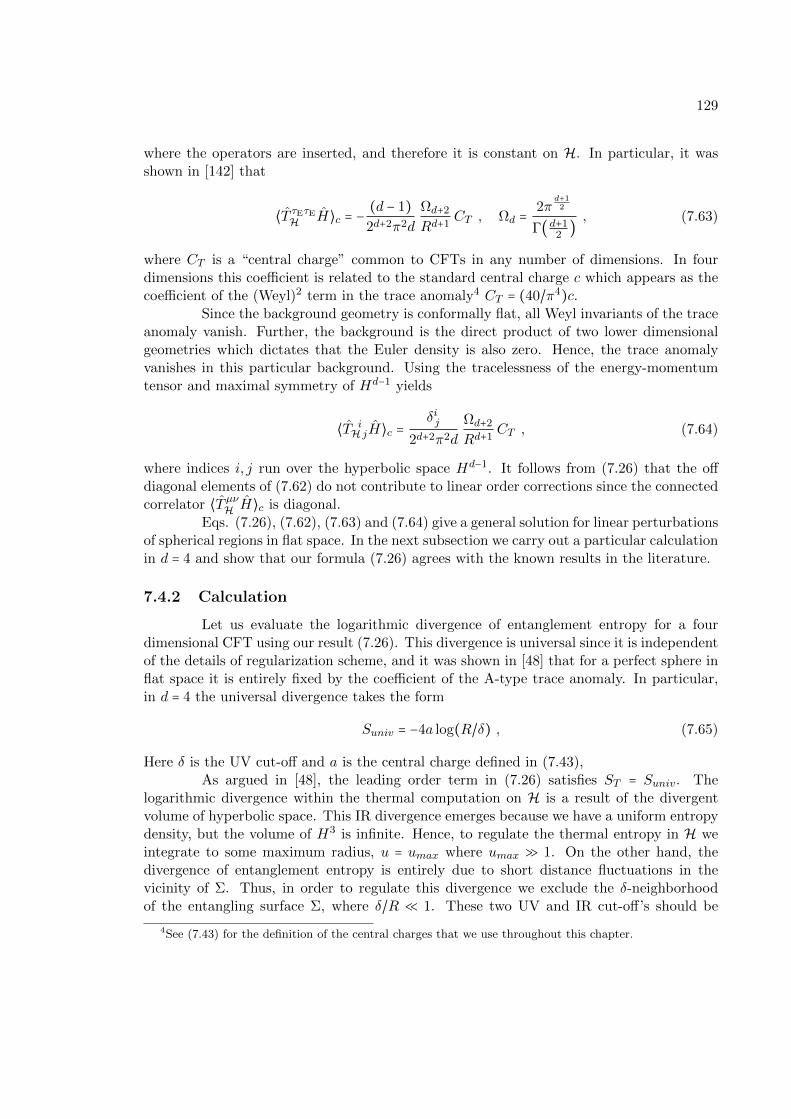
129

where the operators are inserted, and therefore it is constant on H. In particular, it wasshown in [142] that

⟨T τEτEH H⟩c = −(d − 1)2d+2π2d

Ωd+2

Rd+1CT , Ωd =

2πd+12

Γ(d+12

), (7.63)

where CT is a “central charge” common to CFTs in any number of dimensions. In fourdimensions this coefficient is related to the standard central charge c which appears as thecoefficient of the (Weyl)2 term in the trace anomaly4 CT = (40/π4)c.

Since the background geometry is conformally flat, all Weyl invariants of the traceanomaly vanish. Further, the background is the direct product of two lower dimensionalgeometries which dictates that the Euler density is also zero. Hence, the trace anomalyvanishes in this particular background. Using the tracelessness of the energy-momentumtensor and maximal symmetry of Hd−1 yields

⟨T iH jH⟩c =

δij

2d+2π2d

Ωd+2

Rd+1CT , (7.64)

where indices i, j run over the hyperbolic space Hd−1. It follows from (7.26) that the offdiagonal elements of (7.62) do not contribute to linear order corrections since the connectedcorrelator ⟨TµνH H⟩c is diagonal.

Eqs. (7.26), (7.62), (7.63) and (7.64) give a general solution for linear perturbationsof spherical regions in flat space. In the next subsection we carry out a particular calculationin d = 4 and show that our formula (7.26) agrees with the known results in the literature.

7.4.2 Calculation

Let us evaluate the logarithmic divergence of entanglement entropy for a fourdimensional CFT using our result (7.26). This divergence is universal since it is independentof the details of regularization scheme, and it was shown in [48] that for a perfect sphere inflat space it is entirely fixed by the coefficient of the A-type trace anomaly. In particular,in d = 4 the universal divergence takes the form

Suniv = −4a log(R/δ) , (7.65)

Here δ is the UV cut-off and a is the central charge defined in (7.43),As argued in [48], the leading order term in (7.26) satisfies ST = Suniv. The

logarithmic divergence within the thermal computation on H is a result of the divergentvolume of hyperbolic space. This IR divergence emerges because we have a uniform entropydensity, but the volume of H3 is infinite. Hence, to regulate the thermal entropy in H weintegrate to some maximum radius, u = umax where umax ≫ 1. On the other hand, thedivergence of entanglement entropy is entirely due to short distance fluctuations in thevicinity of Σ. Thus, in order to regulate this divergence we exclude the δ-neighborhoodof the entangling surface Σ, where δ/R ≪ 1. These two UV and IR cut-off’s should be

4See (7.43) for the definition of the central charges that we use throughout this chapter.

130

related by the conformal mapping between the two spaces. If we focus on the tE = 0 slice(or equivalently the τE = 0 slice), then (7.56), yields the following relation [48]

1 − δ

R= sinhumax

coshumax + 1⇒ umax ≃ log(R/δ). (7.66)

To get corrections to the leading order result we substitute eqs. (7.62), (7.63) and (7.64)into (7.26) and use eqs. (7.50), (7.55) and (7.56) to carry out the integrals. The final answerfor the logarithmically divergent part of the integrals is given by

δSuniv =c

6π∫

Σ( δγR2

− 2

Rδ2c δK

c + γijδacRiacj ∣Σ + δacδbdRabcd) log(R/δ) , (7.67)

where Σ is a sphere of radius R, δγ and δKc are the traces of the perturbations δγij andδKc

ij , and we used (7.56) to evaluate the components of hµν in coordinates (7.50),

huu = −R2 Ω4

6δacδbdRabcd e−2u sin2(τE/R) ,

hτEτE = −R2 Ω4

6δacδbdRabcd (1 + e−u cos(τE/R))2

,

huτE = R2 Ω4

24δacδbdRabcd e−u sin(τE/R)(1 + e−u cos(τE/R)) . (7.68)

Let us now compare (7.67) with Solodukhin’s formula (7.45). For the case of asphere in flat space, this formula reduces to (7.65). Corrections to (7.65) can be evaluatedby varying (7.45) around sphere of radius R embedded into Rd. Provided that variationsare small and satisfy (7.61), we get (7.46) again. The latter is not a coincidence, it is astraightforward consequence of the fact that (7.45) is Weyl invariant while the two setups(a plane and a sphere in flat space) are conformally equivalent. To see it explicitly, let uswrite the metric around flat plane as follows

ds2 = dr2 + r2dθ2 + δijdyidyj =r2

R2(dτ2

E +R2

r2(dr2 + δijdyidyj)) , (7.69)

where we have defined τE = Rθ and used polar coordinates in the transverse space to theplane. Stripping off conformal factor on the right hand side of this expression leaves uswith the metric on H in Poincare patch. Note that conformal factor is everywhere regularin the punctured Euclidean space (or analytically continued Rindler wedge), and the planeat r = 0 is mapped onto conformal boundary of H.

Hence, we have shown that two setups are conformally equivalent to H with entan-gling surfaces being mapped onto conformal boundary of the hyperbolic space. Thereforethey are conformally equivalent to each other. In particular, it follows that quadratic inextrinsic curvatures term of (7.45),

I = ∫Σ(Ka

ijKija − 1

2KaKa) , (7.70)

does not contribute to the first variation of entanglement entropy around spherical region.This claim can be verified by direct computation, however there is a simple argument based

131

on the Weyl symmetry inherent to the problem. Indeed, this term is separately Weylinvariant and its first variation vanishes in the planar case, therefore the same is true forconformally equivalent spherical region in flat space. In our forthcoming publication weare going to explore the second order perturbation theory to uncover the effect of extrinsiccurvatures on the entanglement entropy.

Let us now show that (7.46) agrees with (7.67). Varying the Gauss-Codazzi relation(7.89) around the unperturbed sphere of radius R embedded in flat space gives

γijγklRikjl∣Σ = 1

R2δγ − 2

Rδ2c δK

c +∇i(∇jδγij − γmn∇i δγmn) , (7.71)

where we have used the variational rule (7.48). Substituting this result into (7.46) gives(7.67)5.

7.5 Notation

In this appendix we explain our notation and conventions. Greek indices run overthe entire background, whereas Latin letters from the ‘second’ half of the alphabet i, j, . . .represent directions along the entangling surface.

There is a pair of independent orthonormal vectors which are orthogonal to Σ,we denote them by nµa (with a = 1,2), where the letters from the beginning of the Latinalphabet are used to denote the frame or tangent indices in the transverse space. Thendelta Kronecker δab = nµanνbgµν is the metric in the tangent space spanned by these vectorsand δab is the inverse of this metric.

We also have tangent vectors tµi to Σ, which are defined in the usual way withtµi = ∂xµ/∂yi, where xµ and yi are the coordinates in the full embedding space and alongthe surface, respectively. The induced metric is then given by γij = tµi tνj gµν . It can also

be defined as a bulk tensor with γµν = gµν − g⊥µν , where g⊥µν = δabnaµnbν is the metric in thespace transverse to Σ. The second fundamental forms are defined for the entangling surfacewith Ka

ij = tµi t

νj∇µnaν , where ∇µ is covariant derivative compatible with gµν . We use this

definition to construct the bulk vector Kµij = n

µaK

aij .

Next we define the volume form in the tangent space spanned by the normal vectors

εab = −εba , ε12 = 1 ,

εab = δacδbdεcd = εab . (7.72)

Using this definition the volume form in the transverse space can be written as εµν = εabnaµnbν .We use g⊥µν to raise and lower the indices in the transverse space, while indices along thedirection of the entangling surface are raised and lowered with the induced metric γµν . Notethat the following useful identity holds,

εµνερσ = g⊥µρg⊥νσ − g⊥µσg⊥νρ . (7.73)

Finally, our convention for the curvature tensor is given by

Rµνρσ =1

2(gµσ,νρ + gνρ,µσ − gµρ,νσ − gνσ,µρ) + Γνρ,χΓχµσ − Γνσ,χΓχµρ . (7.74)

5The total derivative in (7.71) does not contribute since Σ in our case has no boundaries.

132

7.6 Foliation of M in the vicinity of the entangling surface

In this appendix we build a particular foliation of M in the vicinity of Σ. First,we choose some parametrization yid−2

i=1 for the entangling surface Σ, then for a given pointO ∈ Σ we fill the transverse space with geodesics radiating orthogonally out from O. Foreach point p on the resulting two-dimensional manifold, TO, we find a geodesic that connectsit to O, such that p lies a unit affine parameter from O. Tangent vector to such a geodesic atO can be expanded in terms of a chosen two-dimensional basis nµa . We give its componentsthe names xa and choose them as coordinates on TO. Together yi, xa parametrize M inthe vicinity of Σ.

Note that we keep the parametrization of the entangling surface unspecified andtherefore the final answer for entanglement entropy will be symmetric with respect toreparametrizations of Σ. On the other hand, choosing a particular foliation of the trans-verse space does not destroy general covariance of the entanglement entropy since the finalanswer is obtained by integrating out this space.

By construction, the following relations hold

naµ = δaµ , tµi = δµi , g⊥µν = δac δaµ δcν , gia = 0 on Σ . (7.75)

In particular, δac plays the role of the transverse metric in this foliation and one can readilyevaluate the extrinsic curvatures of Σ,

Kaij = ∇inaj ∣Σ = 1

2δac∂c gij ∣Σ . (7.76)

Hence,gij = γij + 2Kaij x

a +O(x2) . (7.77)

Furthermore, geodesics radiating orthogonally out from a given point y ∈ Σ take the formxa(τ) = vaτ , where va belongs to the two-dimensional tangent space spanned by two normalvectors at y. Substituting this parametrization into the geodesic equation yields

Γµacvavc = 0 ⇒ Γµac = 0 at O . (7.78)

This identity can be further generalized by differentiating the geodesic equation n timeswith respect to τ and setting τ = 0. This gives

∂(d1∂d2⋯∂dnΓµ

ac) = 0 at O , (7.79)

where as usual (⋯) denotes symmetrization with respect to the indices within the paren-thesis. This result (7.79) with index µ in the transverse space can be used to derive theexpansion of the metric on Ty,

gab(x, y) = δab −1

3Racbd(y)xcxd −

1

6∂eRacbd(y)xcxdxe +O(x4) . (7.80)

Moreover, it follows from Γiac∣Σ = ∂(dΓiac)∣Σ = 0 that Taylor expansion of gic in the vicinityof Σ can be written as follows

gic = (Ai +1

3xbεdeRibde∣Σ)xaεac +O(x3) , (7.81)

133

where we have introduced a vector field that lives on Σ

Ai =1

2εac∂agic∣Σ , (7.82)

and used the following identity that holds for our foliation

Ribac∣Σ = ∂b∂[a gc]i∣Σ , (7.83)

where [⋯] denotes antisymmetrization with respect to the indices inside the square brackets.We only need to compute O(x2) term in (7.77) to get the expansion of the full

metric to second order in the distance from the entangling surface. We first note thatChristoffel symbols with at least one index in the transverse space are given by

Γµac∣Σ = 0 , Γaic∣Σ = −εacAi , Γaij ∣Σ = −Kaij , Γjia∣Σ =Kj

a i . (7.84)

Now using (7.74), we obtain

Riajb∣Σ = 1

2εbaFij −

1

2∂a∂bgij ∣Σ + δabAiAj +Kb ilK

la j , (7.85)

where Fij = ∂iAj − ∂jAi is the field strength. Symmetrizing this expression with respect toa and b, yields

1

2∂a∂bgij ∣Σ =Ri(ab)j ∣Σ + δabAiAj +

1

2(Kb ilK

la j +Ka ilK

lb j) , (7.86)

where (⋯) means symmetrization with respect to the indices inside the parenthesis. Hence(7.77) to second order in xa takes the form

gij = γij + 2Kaij xa + xaxc(δacAiAj +Ri(ac)j ∣Σ) + xaxcKc ilK

la j +O(x3) . (7.87)

Altogether eqs. (7.80), (7.81) and (7.87) correspond to the second order expansion of thefull metric gµν in the vicinity of Σ. To linear order in the distance from Σ this metric takesthe simple form,

ds2 = δacdxadxc + 2Aiεac xadxc dyi + (γij + 2Kaij x

a)dyidyj +O(x2) . (7.88)

Note that using the definition (7.74) and (7.84), one can evaluate various com-ponents of the Riemann tensor that were not necessary so far. For instance, consideringdirections along the entangling surface Σ yields the well known Gauss-Codazzi identity

Rijkl∣Σ =RΣijkl +Ka

jkKa il −KajlKa ik , (7.89)

where RΣijkl is the intrinsic curvature tensor on Σ.Furthermore,

Rijab∣Σ = εbaFij +Kb ilKla j −Ka ilK

lb j , (7.90)

This identity can be used to express the field strength in terms of the background curvatureand extrinsic geometry of Σ.

Finally,

Rijla∣Σ = ∇iKajl −∇jKail + 2 εbaA[iKbj]l ,

Rabcd∣Σ = RTabcd∣Σ , (7.91)

where ∇i is the covariant derivative compatible with the induced metric on Σ and RTabcd isthe intrinsic curvature tensor of the transverse space, Ty, at a given point y ∈ Σ.

134

7.7 Intermediate calculations for Sec. 7.3

In this Appendix we evaluate the integral (7.36) appearing in the calculation of thefirst order correction to the entanglement entropy for a deformed plane in a weakly curvedbackground. First we consider the contribution of the metric perturbation with indices inthe direction of the entangling surface, i.e., hij = xaxcRiacj . In this case (7.40) is given by,

Iij,22 =4 x2

2 (y − y)i(y − y)j((x − x)2 + (y − y)2)2

− 1

4δij (7.92)

We begin evaluating (7.36) by first doing the integral over y through a change of variablesy → y + y giving

δS1 = −π2

10CT ∫

x1>0d2xd2y dx1 x1

δij hij

((x1 − x1)2 + x22)3

( x22

(x1 − x1)2 + x22

− 5

6). (7.93)

Next, we carry out the x1 integral and introduce polar coordinates in the transverse space,x1 = r cos θ, x2 = r sin θ,

δS1 =π2

240CT ∫ d2y dθ

dr

r3δij hij , (7.94)

As expected, the integral over r exhibits logarithmic divergence close to the entanglingsurface at r = 0. Hence, we introduce a UV cut off, δ, to regularize divergence and integrateover r and θ

δS1 =c

6π∫ d2y δijδacRiacj log(`/δ) , (7.95)

where ` is characteristic scale of small perturbations, and we used the value of CT = (40/π4)cin four spacetime dimensions.

Next we calculate the contribution of perturbations in the transverse space, i.e.,hab = −1

3Racbdxcxd. Using Iab,22 from (7.40) and performing the integral over y in (7.36)

yields

δS2 = −π2CT ∫x1>0

d2x d2y dx1 x1 hab(x, y)

×⎛⎝

1

3

δa2δb2 − δab/4((x1 − x1)2 + x2

2)3− x2(x − x)b δa2

((x1 − x1)2 + x22)

4+ 4

5

x22 (x − x)a(x − x)b((x1 − x1)2 + x2

2)5

⎞⎠

As before, we preform the x1 integral, introduce polar coordinates in the transverse space,substitute hab, carry out θ integral, and finally get

δS2 =c

6π∫ d2y δacδbdRabcd log(`/δ) (7.96)

Combined with (7.95), we have thus recovered (7.42).

135

Part II

Emergent Spacetime with Λ > 0

136

In this second part we turn to the harder question of finding the holographic dualto the multiverse. As the correct theory is not yet known, we seek to make progress byextracting general lessons about holography from AdS/CFT. We make a proposal for howto implement the analog of the UV/IR prescription for the mulitverse context so as todefine a bulk measure. We then test our measure and others in the literature to see howwell they match with observation. Finally, we point out a serious difficulty encountered byall measure proposals. This part of the thesis is organized as follows.

In chapter 8, based on [28], we propose to regulate the infinities of eternal inflationby relating a late time cut-off in the bulk to a short distance cut-off on the future boundary.The light-cone time of an event is defined in terms of the volume of its future light-cone onthe boundary. We seek an intrinsic definition of boundary volumes that makes no referenceto bulk structures. This requires taming the fractal geometry of the future boundary,and lifting the ambiguity of the conformal factor. We propose to work in the conformalframe in which the boundary Ricci scalar is constant. We explore this proposal in the FRWapproximation for bubble universes. Remarkably, we find that the future boundary becomesa round three-sphere, with smooth metric on all scales. Our cut-off yields the same relativeprobabilities as a previous proposal that defined boundary volumes by projection into thebulk along timelike geodesics. Moreover, it is equivalent to an ensemble of causal patchesdefined without reference to bulk geodesics. It thus yields a holographically motivated andphenomenologically successful measure for eternal inflation.

In chapter 9, based on [29], we test different measures. We show that the geometryof cutoffs on eternal inflation strongly constrains predictions for the timescales of vacuumdomination, curvature domination, and observation. We consider three measure proposals:the causal patch, the fat geodesic, and the apparent horizon cutoff, which is introduced herefor the first time. We impose neither anthropic requirements nor restrictions on landscapevacua. For vacua with positive cosmological constant, all three measures predict the doublecoincidence that most observers live at the onset of vacuum domination and just before theonset of curvature domination. The hierarchy between the Planck scale and the cosmologicalconstant is related to the number of vacua in the landscape. These results require only mildassumptions about the distribution of vacua (somewhat stronger assumptions are requiredby the fat geodesic measure). At this level of generality, none of the three measures aresuccessful for vacua with negative cosmological constant. Their applicability in this regimeis ruled out unless much stronger anthropic requirements are imposed.

Finally, in chapter 10, based on [30], we point out a difficulty with all existingmeasures. Present treatments of eternal inflation regulate infinities by imposing a geometriccutoff. We point out that some matter systems reach the cutoff in finite time. This impliesa nonzero probability for a novel type of catastrophe. According to the most successfulmeasure proposals, our galaxy is likely to encounter the cutoff within the next 5 billionyears.

137

Chapter 8

Boundary Definition of aMultiverse Measure

8.1 Introduction

String theory gives rise to an enormous multiverse where the constants of natureare locally constant but vary over extremely large distance scales [41, 109]. In this context,it is natural to make predictions by counting. The relative probability of two events (forexample, two different outcomes of a cosmological or laboratory measurement) is definedby their relative abundance,

p1

p2= N1

N2, (8.1)

where N1 is the expectation value of the number of times an event of type 1 occurs in themultiverse.

There is ambiguity in computing the ratio N1/N2: naively, both numbers are infi-nite. Starting from finite initial conditions, eternal inflation produces an infinite spacetimevolume in which everything that can happen does happen an infinite number of times. Aprocedure for regulating this divergence is called a measure. Different measures can lead todifferent relative probabilities starting from an otherwise identical theory.

A number of measures have been proposed, including [125, 123, 71, 72, 70, 76, 179,178, 24, 121, 122, 141, 73, 182, 183, 184, 126, 26], but over the past several years a vigorousphenomenological effort (e.g., [77, 62, 145, 63, 159, 157, 37, 43, 137, 33, 158, 38, 140, 53, 34,155, 35, 144, 39, 87]) has focused attention on a few simple proposals that remain viable. Inthis chapter, we will focus on the light-cone time cut-off, which arises from an analogy withthe AdS/CFT correspondence. Given a short-distance cut-off on the boundary conformalfield theory, the radial position of the corresponding bulk cut-off [165] can be obtained fromcausality alone [42], without reference to the details of the bulk-boundary correspondence.In the multiverse, the time of a bulk event can similarly be defined in terms of a scaleon the future boundary of the multiverse [73]. The simplest causal relation is to associateto each bulk event a boundary scale given by the volume of its future light-cone on theboundary [26] (see Fig. 8.1).1

1A different bulk-boundary relation was proposed in Ref. [73]. One of us (RB) has argued that this relation

138

22

22

2

2

1

1 1

1 1 11

1 1 1

1

11

1 11

11

1

111

1

1

1

1

1

1

1

11

2

22

2

2

2

2 2

2

2

2

2 2

2

2

22

2

2

2 2 22

22

2

22

22

22

22

22

22

22 22

22

222

2222

22

22 2

2 22 22 2 2 2 222 22 22 222

22 2 2 22

22 2

1

11

1

1

1

1 1

11

1

11

11

1

1

1

1

1

1

11

2

22

2

2

2

2

2 2

222

2

2 22

2

22 2

2

22

21

2

22

2

222

Figure 8.1: Constant light-cone size on the boundary defines a hypersurface of constant“light-cone time” in the bulk. The green horizontal lines show two examples of such hy-persurfaces. They constitute a preferred time foliation of the multiverse. In the multiverse,there are infinitely many events of both type 1 and type 2 (say, two different values ofthe cosmological constant measured by observers). Their relative probability is defined bycomputing the ratio of the number of occurrences of each event prior to the light-cone timet, in the limit as t→∞.

There is a remaining ambiguity: how is the volume of the future light-cone to bedefined? Near the future boundary, physical distances diverge in inflating regions and goto zero near singularities. Ref. [26] defined boundary volumes by erecting a congruence ofgeodesics orthogonal to a fixed, fiducial bulk hypersurface and projecting future infinity ontothe fiducial hypersurface along the geodesics. The definition of Ref. [26] is quite robust2; inparticular, it does not matter whether geodesics expand or collapse or cross.

We would like to find an alternative definition of the boundary volume which doesnot rely on such an elaborate bulk construction. The geodesics used to project the light-cone onto the fiducial hypersurface do only one thing for us: they define boundary volumes.Yet they encode an enormous amount of geometric bulk information (the exact path of eachgeodesic, the expansion and shear of nearby geodesics, etc.), most of which is never usedfor any purpose. They bear no apparent relation to any physical system; for example, theydo not represent the worldlines of actual particles. Moreover, the construction takes anabsurdly classical viewpoint of the bulk geometry: because of the exponential expansion ofde Sitter vacua, the projection of a late time light-cone onto the fiducial hypersurface hassubplanckian volume.

There is another reason why it would be nice to eliminate bulk geodesics from thedefinition of the measure. Ultimately, one expects that a fundamental description of the

is less well-defined than light-cone time and is not analogous to the UV/IR relation of AdS/CFT [26]. Theseconcerns aside, it could be combined with the metric we construct on the future boundary. The resultingmeasure would be different from the one obtained here.

2In this respect, the definition of volumes explored here remains inferior, for now, since it is completelywell-defined only for homogeneous bubble universes. However, for the reasons stated below, it may ultimatelyprove to be more fundamental.

139

Figure 8.2: Conformal diagram of de Sitter space with a single bubble nucleation. Theparent de Sitter space is separated from the daughter universe by a domain wall, hereapproximated as a light-cone with zero initial radius (dashed line). There is a kink in thediagram where the domain wall meets future infinity. This diagram represents a portion ofthe Einstein static universe, but the Ricci scalar of the boundary metric is not constant.

multiverse will involve its boundary structure in some way. This was a key motivation forseeking a multiverse analogue of the UV/IR relation of AdS/CFT in the first place. Theequivalence of the causal patch and light-cone time cut-off, along with their phenomeno-logical successes, encourages us to take seriously the motivations behind the two measures.In particular, we would like to define the light-cone time cut-off, to the greatest extentpossible, in terms of quantities that are intrinsic to the boundary.

In this chapter we will propose an intrinsic definition of volumes on the futureboundary of the multiverse, and we will explore the resulting time foliation and measure.Like in AdS, we will render the boundary finite by a conformal rescaling of the bulk metric.However, we face two difficulties that have no direct analogue in AdS/CFT.

The boundary of the multiverse is naturally a fractal. In the bulk, bubbles ofdifferent vacua keep being produced at later and later times, leading to boundary featureson arbitrarily small scales. If the bulk evolution exhibits attractor behavior (this is commonto many global foliations of the multiverse, though the attractor itself depends on thefoliation), then the boundary will exhibit self-similarity in the short-distance limit. Becauseof the abundance of short-distance structure, the boundary must be constructed first onlarge scales, and then refined to better and better resolution, corresponding to evolvingthe bulk to later and later times. The details of this procedure have not been carefullyformulated and will concern us greatly.

The fractal structure leads to a number of difficulties for defining a metric on thefuture boundary:

Generically, when a new bubble forms at late times in the bulk, one would like to

140

include this information on the boundary, for example by coloring a small disk on theboundary which is enclosed by this bubble. But the new vacuum will also change themetric in the bulk, and thus, the shape of the conformal diagram. In other words,generically, the boundary metric will keep changing as we increase the resolution. Thisis worse than the behavior of most fractals we are familiar with, which are defined bycoloring points on a fixed background metric.

A natural way of constructing a conformal diagram depicting the formation of a bubbleuniverse in de Sitter space leads to a future boundary with a “sharp edge” (see Fig. 2),where the first derivative of the induced boundary metric is discontinuous. With moreand more bubbles forming at late times, such edges would appear on arbitrarily smallscales.

The shape of the boundary is defined only up to finite conformal transforma-tions. Because the boundary metric is obtained from the bulk spacetime by a conformalrescaling, it is only defined up to a finite conformal factor. The shape of many conformaldiagrams can be changed by a conformal transformation. The resulting diagram is just aslegitimate as the original one, but its boundaries may have a different geometry.

In the multiverse, this ambiguity in the boundary metric leads to an ambiguity in thebulk foliation. Unlike in AdS, which is asymptotically empty, this leads to a potentialambiguity in the measure. For example, a different choice of conformal factor maychange the predicted probability distribution for the cosmological constant.

Outline We introduce the concept of light-cone time in Sec. 8.2.1, emphasizing that itrequires a definition of the volume of any future light-cone. In Sec. 8.2.2, we propose that thevolume should be defined as the volume enclosed by the light-cone on the future conformalboundary of the multiverse. Moreover, we propose choosing the conformal factor so thatthe boundary metric has constant scalar curvature,

R = constant , (8.2)

where R is the Ricci scalar of the boundary metric3 A recent result in mathematics—the solution to the Yamabe problem—guarantees that a suitable conformal transformationcan always be found and is essentially unique on the boundary. This proposal defineswhat we shall refer to as “new light-cone time”. In Sec. 9.3, we apply our proposal to asimplified landscape model. We approximate bubble universes as homogeneous open FRWcosmologies, we assume that they all have nonzero cosmological constant, and we neglectbubble collisions. Despite these simplifications, all of the difficulties listed above arise inthis model, and we show that our proposal succeeds in addressing them. We constructthe conformal diagram iteratively, making sure that the boundary condition R = const.

3Garriga and Vilenkin [74] defined the metric on future infinity by foliating the spacetime by surfaceswhose induced metric has R = 0. In general spacetimes this is different from our proposal, and bulk R = 0surfaces do not always exist. However, in the special case we focus on of homogeneous de Sitter bubbles,their boundary metric is the same as ours.

141

is satisfied each time a new bubble universe is included in the bulk. We find that thisprocedure leads to a fixed, everywhere smooth boundary metric that can be taken to be aunit three-sphere.

The boundary metric picked out by the condition R = const. defines new light-conetime. In Sec. 8.3, we present some of the most important properties of this time foliation.In Sec. 10.2, we derive rate equations that govern the distribution of vacua. We emphasizethe boundary viewpoint, in which bubble universes correspond to topological disks on theboundary three-sphere. In Sec. 8.3.2, we find the solution of the rate equations. The latetime attractor behavior in the bulk corresponds to a universal ultraviolet scaling of thedistribution of disks on the boundary. In Sec. 8.3.3, we derive the crucial expression thatunderlies the probability measure: the number of events of arbitrary type, as a function oflight-cone time.

In Sec. 8.4, we analyze the probability measure. In Sec. 8.4.2, we show that newlight-cone time yields the same measure as old light-cone time, i.e., both cut-offs predict thesame relative probabilities for any two types of events in our simplified landscape model.In particular, this implies that our “new” light-cone time shares the phenomenologicalsuccesses of the old one, and of the causal patch measure dual to it.

In Sec. 8.5, we discuss how our approach may extend to the general case, whereinhomogeneities, collisions, and vacua with Λ = 0 are included. We also consider the (likely)possibility that the landscape contains vacua of different dimensionality. In defining a uniqueboundary metric, several difficulties arise in addition to the ones listed above, and a moregeneral method of implementing Eq. (8.2) is needed. We discuss what phenomenologicalproperties may be expected of the resulting measure. In particular, we expect that in thecontext of inhomogeneous universes, a boundary definition of light-cone volume will addressa problem pointed out by Phillips and Albrecht [144].

8.2 New light-cone time

In this section, we define new light-cone time, and we construct the surfaces ofconstant light-cone time in a simple multiverse.

8.2.1 Probabilities from light-cone time

Given a time foliation of the multiverse, the relative probability of events of typeA and B (e.g., two different outcomes of an experiment) can be defined by

pApB

= limt→∞

NA(t)NB(t) , (8.3)

where NA(t) is be the number of times an event of type A has occurred prior to the timet. This measure depends strongly on the choice of t. In this chapter, we focus exclusivelyon the case where t is of the form

t ≡ −1

3log

V (E)4π/3 . (8.4)

142

Here, V (E) is the (suitably defined) volume of the causal future of E, I+(E). Any timevariable of this form will be referred to as light-cone time.

To complete the definition of light-cone time, and thus of the measure, one mustdefine V (E). One such definition, which results in what we shall refer to as old light-cone time, was given in Ref. [26]: consider a family of geodesics orthogonal to a fiducialhypersurface in the bulk, and let V (E) be the volume occupied on the fiducial hypersurfaceby the geodesics that eventually enter I+(E). In this chapter we will explore a differentdefinition, new light-cone time.

Often, we will find it convenient to work instead with the variable

η = e−t = (V (E)4π/3 )

1/3, (8.5)

which is naturally interpreted as a boundary distance scale. Since hypersurfaces of constantη are hypersurfaces of constant t, they define the same bulk foliation, and thus, the samemeasure. In the bulk, η decreases towards the future and vanishes on the boundary; tincreases towards the future and diverges at the boundary.

8.2.2 A gauge choice for the conformal boundary

Physical distances diverge in the asymptotic future of an eternally inflating multi-verse, except inside black holes and vacua with negative cosmological constant, where theyapproach zero. Such behavior is found in many other spacetimes, such as (Anti-)de Sitterspace or the Schwarzschild solution. However, in many cases a boundary of finite volumecan be defined by a conformal transformation.

To a physical spacetime M , with metric gµν , we associate an unphysical spacetimeM with metric gµν which satisfies a number of conditions. There must exist a conformalisometry ψ ∶M → ψ[M] ⊂ M such that

gµν = Ω2(x)ψ∗gµν = e2φ(x)ψ∗gµν (8.6)

in ψ[M]. Note that Ω should be nowhere-vanishing on ψ[M], and we demand that Ωbe sufficiently smooth (say, C3 [95]) in ψ[M] and extend to a continuous function on theclosure, ψ[M]. We will refer to both Ω and φ = log Ω as the conformal factor. Hereafterwe will identify M with its image ψ[M] (called “the bulk”), and refer to the physical (gµν)and unphysical (gµν = Ω2gµν) metrics defined on M , eliminating ψ from the notation.

As a set, the boundary of M is defined as those points in the closure of M ⊂ Mwhich are not contained in M itself: ∂M = M −M . By the “boundary metric”, Gab, wemean the unphysical metric induced on ∂M viewed as a subset of M . The key property wewill require of the unphysical spacetime is that for any E ⊂M , the volume of I+(E) ∩ ∂Mbe finite in the boundary metric. (Below we will define V (E) to be this volume.) Notethat for those cases where the physical volumes and distances diverge as one approachesthe boundary, this implies that the conformal factor Ω approaches zero on ∂M , or that φdiverges. We will return in Sec. 8.5 to the question of which bulk metrics can be conformallyrescaled so that the boundary metric is finite and nonsingular.

143

There is an ambiguity in the boundary metric which is related to an ambiguity inchoosing the conformal factor that makes the rescaled bulk spacetime finite. Consider anadditional Weyl rescaling with a conformal factor that is bounded on the boundary:

Gab = e2φ(x)Gab , (8.7)

with ∣φ(xµ)∣ < K for some real number K. This will produce a new unphysical spacetimewhose boundary still has finite volume, and which we could have obtained directly from theoriginal spacetime via the conformal factor φ + φ. So the requirement of finiteness is notsufficient to fix the boundary metric completely.

We propose to fix the ambiguity by demanding that the conformal transformationyield a boundary metric of constant scalar curvature:

R = constant . (8.8)

Here, R is the Ricci scalar computed in the boundary metric, not the bulk Ricci scalarrestricted to the boundary. The value of the constant is arbitrary. (It can be changed byan overall rescaling of the unphysical spacetime; this shifts light-cone time by a constantbut leaves the foliation, and thus the probability measure, invariant.) At a naive level ofcounting degrees of freedom, these conditions fix the metric.

At a more refined level, the question of whether an arbitrary metric on a smooth,compact manifold can be brought to a metric with constant scalar curvature is a difficultproblem in mathematics known as the Yamabe problem. The Yamabe problem has beensolved in the affirmative [156], [117]. For a smooth compact Riemannian manifold (Mn,G

′)of dimension n ≥ 3, there exists a metric G conformal to G′ such that the Ricci scalar of G isconstant. The problem of finding the appropriate conformal transformation G = φ4/(n−2)G′

amounts to solving the differential equation

4(n − 1)n − 2

∇2φ +R′φ = Rφn+2n−2 , (8.9)

with R a constant. This is nontrivial since the solution φ must be smooth and strictlypositive, and must exist globally.

Yamabe [187] attempted to solve the problem by noting that (8.9) can be writtenas the Euler-Lagrange equation for a certain functional of the metric. This functional isclosely related to the average scalar curvature of the metric over the manifold. Since theminimum occurs for the metric with constant curvature, the solution focuses on showingthat the minimum of this functional is realized. Yamabe’s original proof was later shownto be valid only in certain cases [176]. The proof was extended to other cases in [3] andcompleted in 1984 by Richard Schoen [156]. A unified and self-contained proof of theYamabe problem is given in [117].

Having shown that a constant curvature metric exists, can we be sure that it isunique? Generically it is [2]: there is an open and dense set U in the space of conformalclasses of metrics such that each element [G] ∈ U has a unique unit volume metric withconstant scalar curvature. In simple cases with symmetries, however, there may be a few-parameter family of solutions to the Yamabe problem. For example, the round three-sphere

144

has an ambiguity given by the global conformal group SO(4,1). However, this ambiguitycan only be used to fix the locations of a few points. We will ultimately be interested inthe behavior on the shortest scales where this ambiguity has no effect.

We can now define V (E) in Eq. (8.4) as follows. Let L(E) be the portion of theboundary in the causal future of E, i.e., the intersection of I+(E) with the boundary. LetV (E) be the volume of L(E), measured using the metric Gab obtained by the (essentiallyunique) conformal transformation that achieves constant Ricci scalar on the boundary:

V (E) ≡ ∫L(E)

d3y√G , (8.10)

where G is the determinant of Gab. With this choice of V , Eq. (8.4) defines the newlight-cone time, t, and Eq. (8.3) defines a probability measure for the multiverse, the newlight-cone time cut-off.

8.2.3 The multiverse in Ricci gauge

In this section, we carry out the construction of future infinity with R = const,subject to the following approximations and assumptions:

All metastable de Sitter vacua are long-lived: κα ≪ 1, where κα = ∑κiα is the totaldimensionless decay rate of vacuum α, and κiα = ΓiαH

−4α , where Γiα is the decay

rate from the de Sitter vacuum α to the arbitrary vacuum i per unit four volume,and Hα = (3/Λα)1/2 is the Hubble constant associated with the asymptotic de Sitterregime of vacuum α.4

Bubble collisions are neglected. This is equivalent to setting all decay rates to zero inthe causal past of a bubble.

Each bubble is a homogeneous, isotropic, open universe; the only exception are bubblesnucleating inside bubbles, which spontaneously break this symmetry. On a large scale,this assumption essentially follows from the previous two approximations, since a largesuppression of the decay implies a large suppression of fluctuations that break theSO(3,1) symmetry of the Coleman-de Luccia geometry. But on a small scale, thisassumption implies that we suppress any structure formation that results from smallinitial perturbations; we treat the bubble universe as completely homogeneous andisotropic.

All bubbles have the same spacetime dimension, D = 3 + 1.

No vacua with Λ = 0 are produced. This ensures that the boundary contains no nullportions or “hats”, where the boundary metric would be degenerate.

The above assumptions allow us to take an iterative approach to the construction of theconformal diagram, while satisfying the gauge condition (8.2). We will now describe thisconstruction step by step.

4We denote vacua with Λ > 0 by indices α,β, . . . and vacua with Λ ≤ 0 by indices m,n, . . .. If no particularsign of Λ is implied, vacua are denoted by i, j, . . ..

145

The universe begins in some metastable vacuum (it will not matter which one).Our initial step is to construct a conformal diagram satisfying R = const. for this de Sittervacuum, as if it were completely stable. We will refer to this spacetime as the zero-bubblemultiverse. The metric is

ds20 =

−dη2 + dΩ23

H20 sin2 η

, (8.11)

where dΩ23 = dξ2 + sin2 ξ(dθ2 + sin2 θdφ2) is the metric on the unit three-sphere. (Since an

infinitely old metastable de Sitter space has zero probability, let us restrict to η ≤ π/2,5 as ifthe universe came into being at the time η = π/2.) Multiplying this metric by the conformalfactor e2φ =H2

0 sin2 η, one obtains a conformally rescaled metric

ds20 = −dη2 + dΩ2

3 , (8.12)

which can be viewed as a portion of an Einstein static universe [95]. The future boundarycorresponds to the points with η = 0, which were not part of the physical spacetime. Itsinduced metric is that of a round three-sphere with unit radius. Thus, it satisfies the gaugecondition we impose, that the three-dimensional Ricci scalar be constant.

The second step is to construct light-cone time in the 1-bubble multiverse. Con-sider the causal future I+ of an arbitrary event E with coordinates (η, ξ, θ, φ) in the physicalspacetime. We note that conformal transformations map light-cones to light-cones, and thatthe unphysical metric, Eq. (8.12), is spatially homogeneous. Therefore, the volume V oc-cupied by I+(E) on the future boundary can only depend on the η coordinate of the eventE, and not on its spatial coordinates; it is given by

V = ∫η

04π sin2 ηdη . (8.13)

The light-cone time is t ≡ −13 log V

4π/3 . At late times, V = 4π3 η

3, so t = − log η.The next step is to consider the first bubble that nucleates inside this vacuum,

i.e., the nucleation event with the earliest light-cone time. (The time and place of thisnucleation is of course governed by quantum chance; as we add more and more bubbles,we shall ensure that on average, their nucleation rate per unit four-volume conforms tothe rates Γαm dictated by the landscape potential.) We then replace the causal future ofthe nucleation event with the new bubble, i.e., with an open FRW universe, which mayhave positive or negative cosmological constant, and may contain matter and radiation.Aside from this one nucleation event, we treat both the parent and the daughter vacuum ascompletely stable, so we do not modify the spacetime in any other way. We thus obtain aphysical spacetime consisting of a parent de Sitter vacuum and one bubble universe with adifferent vacuum, which we refer to as the one bubble multiverse. Now we construct a newconformal diagram for this spacetime, as follows (see Fig. 8.2.3):

The conformal diagram is left unchanged outside the future light-cone of the nu-cleation event, where the physical spacetime is also unchanged. That is, we shall use thesame conformal factor as before for this region.

5In naming the time coordinate in Eq. (8.11) η, we are anticipating the result below that η = constantwill define hypersurfaces of constant light-cone time in accordinance with the definition of η in Eq. (8.5).Since this definition requires η to take positive values which decrease towards the future boundary, we shalltake η to have a positive range in Eq. (8.11). Thus, η ≥ π/2 corresponds to times after η = π/2.

146

(a) (b) (c)

Figure 8.3: (a) The parent de Sitter space with the future of the nucleation event removedand (b) the bubble universe are shown as separate conformal diagrams which are eachportions of the Einstein static universe. After an additional conformal transformation ofthe bubble universe (shaded triangle), the diagrams can be smoothly matched along thedomain wall. The resulting diagram (c) has a round S3 as future infinity but is no longera portion of the Einstein static universe.

The future of the nucleation event is an open FRW universe, which either crunches(if Λ < 0) or becomes asymptotically de Sitter in the future (if Λ > 0). We show in Ap-pendix 8.6 that this spacetime can be conformally mapped to a finite unphysical spacetimewith the following properties:

The conformal factor is smooth (Cn, with n arbitrarily large) in the physical spacetimeand continuous when extended to the future boundary.

The induced metric along the future light-cone of the nucleation event agrees withthe induced metric on the same hypersurface in the outside portion of the diagram,which was left unchanged.

The future boundary is identical to the piece of the future boundary that was removedfrom the old diagram.

(Note that this portion of the unphysical spacetime will not be a portion of the Einsteinstatic universe, nor is there any reason to demand that it should be.)

Because of the above properties, we are able to combine the remainder of the oldPenrose diagram with the new portion covering the interior of the bubble. This results in asingle Penrose diagram which is smooth everywhere6 in the physical spacetime, and whosefuture boundary is a round three-sphere of unit radius. Thus, it satisfies the condition wehave imposed, that the Ricci scalar of the boundary metric be constant.

We can now simply iterate this procedure. Complete the following sequence ofoperations, starting with i = 0 (or really with i = 1 since we have already gone through oneiteration, above):

6There is enough freedom in the choice of the conformal factor in the bulk to ensure that the conformalfactor is not only continuous but arbitrarily differentiable at the seam where the FRW bubble and theold de Sitter parent are matched, while maintaining the round three-sphere metric of the future boundary.Thick-wall bubbles and non-zero initial bubble radii can similarly be accommodated.

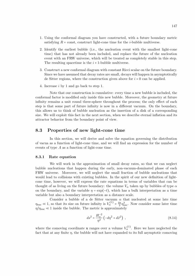
147

1. Using the conformal diagram you have constructed, with a future boundary metricsatisfying R = const, construct light-cone time for the i-bubble multiverse.

2. Identify the earliest bubble (i.e., the nucleation event with the smallest light-conetime) that has not already been included, and replace the future of the nucleationevent with an FRW universe, which will be treated as completely stable in this step.The resulting spacetime is the i + 1-bubble multiverse.

3. Construct a new conformal diagram with constant Ricci scalar on the future boundary.Since we have assumed that decay rates are small, decays will happen in asymptoticallyde Sitter regions, where the construction given above for i = 0 can be applied.

4. Increase i by 1 and go back to step 1.

Note that our construction is cumulative: every time a new bubble is included, theconformal factor is modified only inside this new bubble. Moreover, the geometry at futureinfinity remains a unit round three-sphere throughout the process; the only effect of eachstep is that some part of future infinity is now in a different vacuum. On the boundary,this allows us to think of bubble nucleation as the insertion of a disk of a correspondingsize. We will exploit this fact in the next section, when we describe eternal inflation and itsattractor behavior from the boundary point of view.

8.3 Properties of new light-cone time

In this section, we will derive and solve the equation governing the distributionof vacua as a function of light-cone time, and we will find an expression for the number ofevents of type A as a function of light-cone time.

8.3.1 Rate equation

We will work in the approximation of small decay rates, so that we can neglectbubble nucleations that happen during the early, non-vacuum-dominated phase of eachFRW universe. Moreover, we will neglect the small fraction of bubble nucleations thatwould lead to collisions with existing bubbles. In the spirit of our new definition of light-cone time, however, we will express the rate equations in terms of variables that can bethought of as living on the future boundary: the volume Vα taken up by bubbles of type αon the boundary, and the variable η = exp(−t), which has a bulk interpretation as a timevariable but also a boundary interpretation as a distance scale.

Consider a bubble of a de Sitter vacuum α that nucleated at some late timeηnuc ≪ 1, so that its size on future infinity is V

(1)α = 4π

3 η3nuc. Now consider some later time

η/ηnuc ≪ 1 inside the bubble. The metric is approximately

ds2 = H−2α

η2(−dη2 + dx2) , (8.14)

where the comoving coordinate x ranges over a volume V(1)α . Here we have neglected the

fact that at any finite η, the bubble will not have expanded to its full asymptotic comoving

148

volume, and that the bubble is not exactly de Sitter but may contain matter and radiation.Both of these corrections decrease like powers of η/ηnuc; in particular, most of the physicalvolume at small η/ηnuc will be empty de Sitter space.

The above metric is valid at zeroth order in the decay rate expansion: we haveneglected all decays that might have already taken place in the bubble by the time η. Wewill now include decays at first order. The proper three-volume of the bubble at the time

η is H−3α V

(1)α /η3. One Hubble volume occupies proper volume 4π

3 H−3α , so that the number

of Hubble volumes is

n(1)α = V

(1)α

4π3 η

3= η

3nuc

η3. (8.15)

We note the relation Hαdtprop = dt = −dη/η between the proper time, tprop, light-cone time,t, and η. We also recall the definition that κiα is the rate at which i-bubbles are nucleatedinside the α-vacuum, per Hubble volume and Hubble time. In a single bubble of type α,therefore, the total number of bubbles of type i that are produced during a time dη is

dN(1)iα = κiαn(1)

α dt = −dη4π3 η

4κiαV

(1)α . (8.16)

The total number of bubbles of type i produced inside α-bubbles during the time dη isobtained by summing over all α-bubbles:

dNiα =−dη4π3 η

4κiαVα(η) , (8.17)

where Vα(η) is the total volume taken up at future infinity by α bubbles nucleated prior toη.

Now consider the total volume dV +i taken up at future infinity by all the i-bubbles

produced (in any vacuum) during the time dη. Since we are neglecting bubble collisions,this is equal to the number of bubbles produced, times the volume taken up by each bubble:

dV +i = 4π

3η3∑

α

dNiα . (8.18)

Though some vacua with Λ ≤ 0 can decay, this effect is not important and will also beneglected. Thus the sum runs only over de Sitter vacua, whereas i denotes a vacuum of anytype.

As a result of decays into other vacua, the total boundary volume taken up by thede Sitter vacuum α decreases during the time dη, by a volume 4π

3 η3 per decay:

dV −α = −4π

3η3∑

i

dNiα . (8.19)

Focussing now on de Sitter vacua alone, we can find that the total rate of change of theboundary volume occupied by α-bubbles, dVα = dV +

α +dV −α , by combining the previous three

equations:

dVα =−dηη∑β

MαβVβ , (8.20)

149

whereMαβ ≡ καβ − καδαβ . (8.21)

This is the rate equation for the volume occupied by metastable de Sitter vacuaon the boundary . We derived this equation using bulk dynamics, which we understand atthe semi-classical level. But we have expressed it in terms of variables that are definedon the boundary: Vα is a boundary volume and η is a boundary scale. In this form, therate equation can be naturally interpreted in terms of the boundary dynamics we seek. Ineffect, we have derived a procedure for constructing the boundary fractal, working fromthe largest bubbles to the smallest. Begin with the boundary sphere all in one “color”,corresponding to the initial metastable de Sitter vacuum in the bulk. Now use the bubbledistribution (8.16) to include new bubbles, one by one, corresponding to disks of differentcolors. The disks are smaller and smaller (of radius η) as we progress to smaller scales η.Just as there will be a finite number of bubbles prior to the time t in the bulk, there willbe a finite number of disks on the boundary for any UV cut-off η. Their distribution willobey Eq. (8.20).

Eq. (8.16) specifies how many i-disks of a given size should be inserted in an α-disk, but we also should specify where they should be inserted. Since the nucleation rate ishomogeneous in the bulk metric, Eq. (8.14), new bubbles be inserted with equal probabilityin any infinitesimal volume occupied by the α-disk. We have excluded bubble collisions;this can be incorporated from the boundary point of view by forbidding the addition of anynew disk whose boundary would overlap with an existing disk. This amounts to excludinga zone of width η neighboring all existing disk boundaries. As we discussed in the previoussection, the solution to the Yamabe problem on the sphere is not unique, and we still havethe freedom to act with the group of global conformal transformations SO(4,1). However,this has no effect on Eq. (8.16), which is conformally invariant.

This completes our discussion of the boundary interpretation of the rate equation.The boundary process we have described should emerge from a more general boundarytheory that remains to be discovered, and one would expect Eq. (8.20) to constrain theconstruction of such a theory. Meanwhile, in order to compare our result to the rateequation for “old” light-cone time, we would like to rewrite it using bulk variables. In termsof light-cone time, Eq. (8.20) becomes

dVαdt

=∑β

MαβVβ . (8.22)

We can use Eq. (8.15) to eliminate Vα, the volume taken up by α-disks on the boundarywith UV-cutoff η = exp(−t), in favor of the number of horizon volumes of type α in the bulkat the time t:

Vα(t) = nα(t)4π

3exp(−3t) . (8.23)

Thus, we obtain the bulk rate equation

dnαdt

= (3 − κα)nα +∑β

καβnβ . (8.24)

150

This is identical to the rate equation for old light-cone time, Eq. (36) in Ref. [44]. Thus, atthis level of approximation, the two definitions of light-cone time yield precisely the samerate equations.

8.3.2 Attractor solution

The solutions to the above rate equation exhibit attractor behavior at late times(η → 0):7

Vα(η) = Vαηq +O(ηq) ; (8.25)

or, in terms of bulk variables,

nα(t) = nαe(3−q)t +O(e(3−q)t) . (8.26)

Here −q is the largest eigenvalue of the matrix Mαβ, Vα is the corresponding eigenvector,and nα ≡ Vα/4π

3 ; −q is the second-largest eigenvalue, and 0 < q < q [76, 44].At short distances on the boundary (late times in the bulk), the distribution

of disks (Hubble volumes) is governed by the “dominant eigenvector”, Vα, which can bethought of as the linear combination of de Sitter vacua that decays most slowly. In arealistic landscape, this eigenvector will have almost exclusive support in a single vacuum,which we shall denote by a star:

Vα ≈ vδα∗ . (8.27)

This dominant vacuum is the slowest-decaying de Sitter vacuum of the landscape [159]. Thenormalization, v, of the eigenvector depends on the infrared boundary configuration (initialconditions in the bulk).

8.3.3 Event counting

So far we have discussed only de Sitter vacua; and even in asymptotically de Sitterbubbles, we have neglected any initial, transitory period during which the bubble universemight have been dominated by, say, matter, radiation, or slow-roll inflation. This was suffi-cient for deriving the rate equation and the asymptotic attractor distribution for de Sittervacua. As we now turn to the question of counting events in the multiverse, we must includeall bubbles and regimes within them.

Let A be some type of event (e.g., a supernova occurs, or the microwave backgroundtemperature is found to be between 2.5 K and 3 K by some experiment). Let NA(η) be thenumber of times an event of type A has occurred in the bulk prior to the cut-off η. (On theboundary, we expect that this is the number of times it has been encoded in modes of sizegreater than η. For now, we will use the bulk definition since we know how to compute it.)

To compute NA(η), we substitute the asymptotic distribution of de Sitter vacua,Eq. (8.25), into our result for the number of bubbles of type i produced per unit time dη,

7See Eq. (37) of Ref. [76], who analyzed its solutions. Although our Eq. (8.22) takes the same mathe-matical form, it should be noted that it is for a different physical variable: the boundary volume fractionoccupied by α-disks, which by Eq. (8.23) corresponds to a fraction of Hubble volumes in the bulk. (InRef. [76], the relevant variable was the fraction of proper bulk volume occupied by vacuum α.)

151

Eq. (8.17):

dNi =−dη

4π3 η

4−q ∑α

κiαVα ; (8.28)

then we sum over all bubbles and nucleation times:

NA(η) =∑i∫i η

η0

(dNA

dNi)η/ηn

(dNi

dη)ηn

dηn , (8.29)

where dNA/dNi is the expected number of events of type A that have occurred by the timeη in a single bubble of type i nucleated at the time ηn. The lower limit of integration, η0,is an arbitrary early-time cut-off (an infrared cut-off on the boundary) that will drop outof the limit in Eq. (8.3).

At late times, all bubbles of type i are statistically equivalent, because they areproduced locally in an empty de Sitter region. Therefore, dNA/dNi depends only on theratio

ζ ≡ η/ηn . (8.30)

To avoid overcounting, the integral should run only over a single bubble of vacuum i,excluding regions of other vacua nucleated inside the i bubble; this restriction is denotedby index i appearing on the upper left of the integration symbol.

Combining the above results, and changing the integration variable from ηn to ζ,

NA(η) =1

4π3 η

3−q ∑i∑α

NAiκiαVα . (8.31)

Here we have assumed for simplicity that A cannot occur in the dominant vacuum, ∗(otherwise, see Ref. [44]); and we have defined

NAi ≡ ∫i 1

0(dNA

dNi)ζζ2−qdζ . (8.32)

The lower limit of integration in Eq. (8.32) should strictly be ζ = η/η0, so this result isvalid only at late times (η → 0), but this is the only regime relevant for computing relativeprobabilities.

The quantity (dNAdNi)ζ

depends on the details of the bubble universe i and on how

the cut-off surface η intersects this bubble. It can be written as

(dNA

dNi)ζ= ∫

i 1

ζdζ ′ d3x

√g ρAi(ζ ′,x) . (8.33)

where ρAi be the density of events of type A per unit four-volume in a bubble i, and g isthe determinant of the metric. The integral is over the interior of a single bubble of typei, from its nucleation up to a light-cone time a factor ζ after nucleation. Substituting intoEq. (8.32) and exchanging the order of integration, we obtain an alternative expression forNAi:

NAi = ∫i 1

0dζ ′∫ d3x

√g ρAi(ζ ′,x)∫

ζ′

0dζ ζ2−q (8.34)

= 1

3 − q ∫ d4x√g ρAi(x) ζ(x)3−q , (8.35)

152

use boundary use geodesics

Global measures: New Light Cone Time ⇔ Old Light Cone Time

Local measures: New Causal Patch Old Causal Patch

Table 8.1: Equivalences between measures. The new light-cone time cut-off is equivalent toprobabilities computed from three other measure prescriptions (double arrows). This impliesthat all four measures shown on this table are equivalent in the approximation described atthe beginning of Sec. 2.3. (See Ref. [44] for a more general proof of the equivalence betweenthe old light-cone time cut-off and the old causal patch measure.)

where the integral is over the entire four-volume of a single i-bubble, with the exclusion ofnew bubbles nucleated inside it.

8.4 The probability measure

In Sec. 4.1 we derive the probability measure defined by the new light-cone timecut-off. In the following subsections, we show that it is equivalent to probabilities computedfrom three other measure prescriptions (see Table 8.4.1).

8.4.1 Probabilities from the new light-cone time cut-off

The relative probability of two events A and B is defined by

pApB

= limη→0

NA(η)NB(η) . (8.36)

By substituting Eq. (8.31), we find that the probability of an event of type A is given by

pA ∝ NA ≡∑i∑α

NAiκiαVα . (8.37)

[We recall here that Vα is the eigenvector with largest eigenvalue of the matrix Mαβ givenin Eq. (8.21); κiα is the dimensionless nucleation rate of i-bubbles in the de Sitter vacuumα, and NAi can be computed from Eqs. (8.32) or (8.35); below we shall discover a simplerway of computing it, from Eqs. (8.39) and (8.44).] This expression is not normalized, butratios can be taken to obtain relative probabilities.

We should go on to compute some probability distributions of interest. We shouldverify that catastrophic predictions such as Boltzmann brains, the youngness paradox(“Boltzmann babies”), and the Q-catastrophe are absent. If so, we should then move on tocompute probability distributions over certain quantities of interest, such as the cosmolog-ical constant, the primordial density contrast, the spatial curvature, and the dark matterfraction, and we could verify that observed values are not unlikely under these distributions(say, in the central 2σ). Instead, we will now demonstrate that the new light-cone timecut-off is equivalent to other measures that have already been studied.

153

8.4.2 Equivalence to the old light-cone time cut-off

Probabilities computed from the old light-cone time cut-off are also of the generalform (8.37) [44]. We will now show that they are in fact identical, under the assumptionsmade in the previous sections.

We consider each factor appearing inside the sum in Eq. (8.37) in turn. The decayrate κiα is a property of the landscape vacua unrelated to the definition of light-cone time.Moreover, we have shown that new light-cone time gives rise to the same rate equation andattractor solution as old light-cone time [26, 44], assuming that all metastable de Sittervacua are long-lived. This implies that the eigenvector Vα is the same, whether old or newlight-cone time is used. Therefore any difference between the two measures would have tocome from the quantity NAi. However, if we approximate bubble interiors as homogeneous,isotropic, open universes, with metric of the form

ds2 = −dτ2 + a(τ)2(dχ2 + sinh2 χdΩ22) . (8.38)

then no such difference arises. At this level of approximation, old and new light-cone timedefine the same probability measure.

To demonstrate this, let us rewrite NAi, starting from Eq. (8.35). Homogeneityimplies that ρAi depends only on the FRW time, τ . Therefore, we can write

NAi =1

3 − q ∫∞

0dτ σAi(τ)Vc(τ) , (8.39)

where σAi(τ) ≡ ρAi(τ)a(τ)3 is the density of events of type A per FRW time and per unitcomoving volume, and

Vc(τ) ≡ ∫ dΩ3 ζ(τ, χ)3−q . (8.40)

Stricly, the integral should exclude comoving regions that have already decayed. But sincethe decay probability is homogeneous, we may absorb these excisions into a decrease ofthe comoving density σAi and let the integral run over the entire unit hyperboloid, dΩ3 =4π sinh2 χdχ. The integral converges because the factor ζ3−q rapidly vanishes at large χ.Thus, Vc(τ) can be thought of as an effective comoving volume whose events contribute toNAi at the time τ .

Since q is the decay rate of the longest-lived vacuum, we can assume that it isexponentially small in a realistic landscape, so it can be neglected in Eq. (8.40). Moreover,from the definition of light-cone time in terms of volumes V on the future boundary, itfollows that

ζ3 = e−(t−tn) = V (t)/V (tn) . (8.41)

Note that these equalities can be taken to hold by definition, no matter how the volumeon the future boundary is defined. We will now abandon the particular definition made inSec. 8.2.2 and consider a general metric Gµν(y) on the future boundary of the multiverse.We shall find that Vc, and thus NAi, is independent of this choice of metric if the bubble ishomogeneous.

Upon substitution of Eq. (8.41), the integrand in Eq. (8.40) is the boundary volumeof the future light-cone L(τ, χ) of each point, which we may in turn write as an integral

154

over the region of the boundary enclosed by the light-cone:

Vc(τ) = V (tn)−1∫ dΩ3∫L(τ,χ)

d3y√G (8.42)

= V (tn)−1∫L(0,χ)

d3y√G∫

CP (y,τ)dΩ3 . (8.43)

In the second line, we exchanged the order of integration. The ranges of integration are thecrucial point here. The union of the future light-cones from all points on the hyperboloidcovers precisely the entire disk corresponding to the bubble universe at future infinity.Hence, the outer integral ranges over this disk, which we have written as the region enclosedby the future light-cone of the bubble nucleation event, L(0, χ). But each boundary pointis covered by many future light-cones of bulk points. Correspondingly, the inner integralranges over all points on the FRW slice whose future light-cone includes the boundary pointy. But this is simply the set of points in the intersection of the τ = const. slice with thecausal past of y, i.e., the portion of the constant FRW time slice that lies in the causalpatch whose tip is at y. By homogeneity, its volume is independent of y and will be denotedV CPc (τ). Thus, the two integrals factorize. Since ∫L(0,χ) d3y

√G = V (tn) by definition, we

obtainVc(τ) = V CP

c (τ) . (8.44)

With this result, Eq. (8.39) becomes manifestly independent of the definition of boundaryvolume. Thus, the quantity NAi will be the same for any type of “light-cone time”, if thebubbles of type i are homogeneous FRW universes.

This is a remarkably general result, so let us state it very clearly. From Eq. (8.32),NAi would appear to depend on the definition of ζ, which in turn depends on the definitionof the scale η associated with a bulk point E as V (E) = 4π

3 η3, where V is the volume taken

up by the causal future of E on the future boundary. This volume, of course, can be definedin different ways: for example, in Ref. [26] it was defined by projecting onto a fiducial bulkhypersurface, whereas in the present chapter it was defined in terms of the induced metricof the boundary in a conformal frame with R = const. These different definitions of Vgenerically do lead to different values of ζ, η, and light-cone time t at the event E. Whatwe have shown is that they cannot lead to any difference in NAi.

In the homogeneous FRW approximation, then, different definitions of light-conetime can only lead to a different probability measure if they lead to different rate equations.This can certainly happen in principle. However, we have shown earlier that the twodefinitions given so far—“old” and “new” light-cone time—yield the same rate equations.We conclude that they also lead to the same probability measure, if bubble universes areapproximated as homogeneous open FRW universes.

8.4.3 Equivalence to the new causal patch measure

Consider an ensemble of causal patches whose tips are distributed over the futureboundary of the multiverse, at constant density δ with respect to the boundary metricdefined in Sec. 8.2.2. The probability for an event of type A, according to the causal patchmeasure, is proportional to the ensemble average of the number of times an event of type

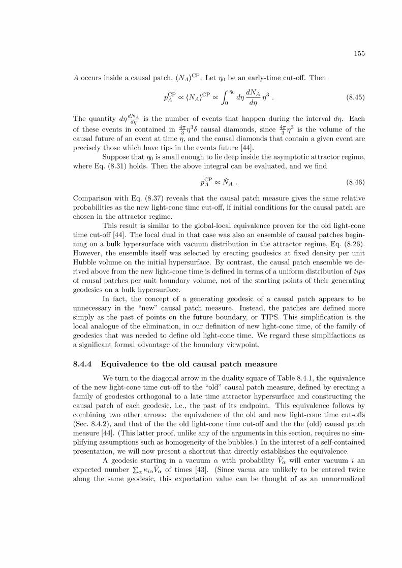
155

A occurs inside a causal patch, ⟨NA⟩CP. Let η0 be an early-time cut-off. Then

pCPA ∝ ⟨NA⟩CP ∝ ∫

η0

0dη

dNA

dηη3 . (8.45)

The quantity dη dNAdη is the number of events that happen during the interval dη. Each

of these events in contained in 4π3 η

3δ causal diamonds, since 4π3 η

3 is the volume of thecausal future of an event at time η, and the causal diamonds that contain a given event areprecisely those which have tips in the events future [44].

Suppose that η0 is small enough to lie deep inside the asymptotic attractor regime,where Eq. (8.31) holds. Then the above integral can be evaluated, and we find

pCPA ∝ NA . (8.46)

Comparison with Eq. (8.37) reveals that the causal patch measure gives the same relativeprobabilities as the new light-cone time cut-off, if initial conditions for the causal patch arechosen in the attractor regime.

This result is similar to the global-local equivalence proven for the old light-conetime cut-off [44]. The local dual in that case was also an ensemble of causal patches begin-ning on a bulk hypersurface with vacuum distribution in the attractor regime, Eq. (8.26).However, the ensemble itself was selected by erecting geodesics at fixed density per unitHubble volume on the initial hypersurface. By contrast, the causal patch ensemble we de-rived above from the new light-cone time is defined in terms of a uniform distribution of tipsof causal patches per unit boundary volume, not of the starting points of their generatinggeodesics on a bulk hypersurface.

In fact, the concept of a generating geodesic of a causal patch appears to beunnecessary in the “new” causal patch measure. Instead, the patches are defined moresimply as the past of points on the future boundary, or TIPS. This simplification is thelocal analogue of the elimination, in our definition of new light-cone time, of the family ofgeodesics that was needed to define old light-cone time. We regard these simplifactions asa significant formal advantage of the boundary viewpoint.

8.4.4 Equivalence to the old causal patch measure

We turn to the diagonal arrow in the duality square of Table 8.4.1, the equivalenceof the new light-cone time cut-off to the “old” causal patch measure, defined by erecting afamily of geodesics orthogonal to a late time attractor hypersurface and constructing thecausal patch of each geodesic, i.e., the past of its endpoint. This equivalence follows bycombining two other arrows: the equivalence of the old and new light-cone time cut-offs(Sec. 8.4.2), and that of the the old light-cone time cut-off and the the (old) causal patchmeasure [44]. (This latter proof, unlike any of the arguments in this section, requires no sim-plifying assumptions such as homogeneity of the bubbles.) In the interest of a self-containedpresentation, we will now present a shortcut that directly establishes the equivalence.

A geodesic starting in a vacuum α with probability Vα will enter vacuum i anexpected number ∑α κiαVα of times [43]. (Since vacua are unlikely to be entered twicealong the same geodesic, this expectation value can be thought of as an unnormalized

156

probability of entering i.) By the assumed homogeneity, all causal patches with tips in thesame FRW bubble have statistically identical content, which, by Eq. (8.39), is given by(3 − q)NAi. Thus, the probability of an event of type A, according to the the “old” causalpatch measure, is

pold CPA ∝∑

i∑α

NAiκiαVα , (8.47)

which agrees with the probability computed from the new light-cone time cut-off, Eq. (8.37).

8.5 The general case

At first sight, it seems that our prescription is well-defined for any bulk spacetime.Simply find a conformal transformation which makes the bulk spacetime finite, and thenuse the constant scalar curvature condition to fix the ambiguity in the boundary metric.The Yamabe theorem would seem to guarantee that this can always be done. But thisprocess is not as simple as it sounds once we go beyond the approximation of homogeneousFRW universes stated in Sec. 9.3.

In this section, we will discuss the additional challenges that arise in the generalcase, how they might be addressed, and what they may imply for the phenomenology of newlight-cone time. We first discuss perturbative inhomogeneities which complicate the storybut do not obviously lead to a pathology. Then we discuss situations where the boundarymetric is singular. These situations require a generalization of our prescription which weoutline, but whose details we leave for the future. Finally, we argue that the probabilitiesderived from new and old light-cone time will differ in the presence of inhomogeneities, withnew light-cone time being favored phenomenologically.

8.5.1 Perturbative inhomogeneities

No bubble universe will be exactly homogeneous and isotropic. Gravitationalwaves will perturb the metric and break spherical symmetry. Modes will leave the horizonduring slow roll inflation and become frozen. We expect that such perturbations will affectthe future boundary. Indeed, any metric of the form

ds2 = −dt2 + e2Htaij(xk)dxidxj , (8.48)

is a solution to Einstein’s equation with positive cosmological constant in the limit t →∞,where aij is an arbitrary 3-metric that depends only on the spatial coordinates xk.8 (Thisresult is attributed to Starobinski in Ref. [19].) In terms of conformal time, the metric is

ds2 = 1

η2(−dη2 + aijdxidxj) , (8.49)

and the future boundary is the surface η = 0. Rescaling by the conformal factor Ω = η, weobtain a (preliminary) boundary metric

ds2 = aijdxidxj . (8.50)

8There are global constraints at finite time that may restrict the form of the boundary metric. Thoughit seems to us implausible, we cannot rule out that such restrictions may prevent the appearance of smallerand smaller geometric features on the boundary.

157

Recall that aij is arbitrary, so any metric is possible on future infinity. If Eq. (8.48) describesthe late time limit of a de Sitter bubble universe, aij will need to be further conformallyrescaled to finite volume and matched to the outside portion of the boundary. The conditionR = const. can then be achieved by a third conformal transformation. But because not everymetric aij is conformal to a portion of the round S3, in general the future boundary will notbe a round S3, and its geometry will contain features on the scale of the future light-coneof any perturbation.

Bubble nucleations occur at arbitrarily late times, corresponding to small sizes onthe boundary. As a result, the boundary metric is perturbed on arbitrarily small scales.The boundary geometry is a fractal. It is important to understand the distinction we aredrawing here to the homogeneous case. In this case, too, a fractal develops on the futureboundary, but that fractal describes the disks corresponding to different vacua distributedover a fixed background metric (a round S3). This is similar to the kind of fractal we arefamiliar with. What we are finding in the general case is that in addition, the geometryitself becomes a fractal. It exhibits self-similar features such as curvature on arbitrarilysmall scales.

By itself, the fractal curvature presents no serious obstacle. It just forces usto construct the background geometry of the boundary the same way we constructed its“matter content” (say, the disks representing different vacua): by starting in the infraredand refining it step by step as we move to short distances.

However, there are additional problems. Suppose we would like to include somebulk perturbation, such as the formation of a new bubble universe, on the boundary. Inthe simplified multiverse we studied in Sec. 9.3, the conformal transformation that achievedconstant Ricci scalar acted nontrivially only in the future of the nucleation event; it didnot change the conformal transformation outside the future light-cone. But the Yamabeproblem cannot generally be solved subject to such strong boundary conditions. Thus, weexpect that for general bulk perturbations, the boundary metric with R = constant will bemodified in regions that are outside the lightcone of the perturbation. So the nucleation ofan inhomogeneous bubble generically changes the lightcone time of every event, even eventsout of causal contact with the nucleation.

In the homogeneous approximation, if we are given some finite region of the bulkspacetime, we have enough information to compute the surfaces of constant light-cone timein that region because adding bubbles outside the region, even in its future, will not changethe size of future lightcones. If we had a computer simulating the bulk evolution, we couldwrite a simple algorithm for generating the entire bulk spacetime underneath the cutoffsurface. But in the inhomogeneous case, we do not have a simple prescription for the sizeof a bulk event on the boundary. Events in the future, or even in causally disconnectedregions, will change the boundary metric, and thus could change the size of “old” futurelight-cones on the boundary. So given a computer which can simulate the bulk evolution,we do not have an algorithm for computing the bulk spacetime up to the cutoff, because itis unclear which events will turn out to occur at times after the cutoff.

This poses a challenge to the iterative construction of light-cone time, in Sec. 9.3.This procedure relied on moving forward along an existing light-cone time foliation, thei-bubble multiverse, and including the first new bubble nucleation reached in this manner

158

Figure 8.4: Conformal diagram of de Sitter space containing a bubble universe with Λ = 0

to compute the i + 1-bubble multiverse. In this algorithm, the light-cone time was nevermodified for events prior to the new bubble nucleation. Thus, we could be sure at eachstage that we have a final version of the foliation up to the i + 1-th bubble nucleation. Asa result, a UV cut-off on the boundary had a simple bulk translation: bubble nucleationsafter a certain time should be ignored.

In fact, it is unclear whether a discrete iterative process remains a viable approxi-mation scheme in the general case. We were able to focus on bubble nucleation events only,since by our assumptions no other events had the potential to modify the future boundary.In general, one expects that all spacetime events, or at least all events in regions that arenot empty de Sitter space, will affect the future boundary. This is a continuous set.

While it is possible that some or all of the above effects are quantitatively neg-ligible, they raise interesting conceptual issues. If we had a boundary description of thetheory, presumably it would be well defined to go down to shorter and shorter scales. Whatis missing at this point is a simple bulk prescription once we go beyond the approximationof homogeneous FRW universes. The fact that the boundary geometry becomes fractalonce one includes all of the expected bulk dynamics means that defining volumes on theboundary is trickier. What is needed is a way to construct the UV-cutoff version of theboundary geometry, which is not a fractal. This can perhaps be done by beginning with thehomogeneous approximation and then perturbing around it, but we have not attempted todo this.

8.5.2 Singularities in the boundary metric

There is a more severe pathology that can arise in constructing the boundarymetric. What if the bulk spacetime does not lead to a boundary metric which is nonsingularand 3 + 1 dimensional everywhere? There are several ways this can happen. Perhaps thesimplest is the nucleation of a Λ = 0 bubble. Future infinity will now contain a “hat” as

159

shown in Fig. 8.5.2. The induced metric will be degenerate because the “hat” is a null cone.The null portion of the boundary metric is

ds2 = r2dΩ22 , (8.51)

which is not 3-dimensional. So a bulk spacetime that includes Λ = 0 asymptotic regions willhave a singular boundary metric. It is then unclear how to define volumes on the boundary.

Another example of a bulk spacetime that leads to a singular boundary metric is aSchwarzschild black hole in de Sitter space. The metric for Schwarzschild-de Sitter in staticcoordinates is

ds2 = −(1 − 2m

r− r

2

l2)dt2 + 1

1 − 2mr − r2

l2

dr2 + r2dΩ22 . (8.52)

If we continue the metric behind the cosmological horizon and let r → ∞, the metricapproaches pure de Sitter space. For large r, the metric is

ds2 = − l2

r2dr2 + r2 ( 1

l2dt2 + dΩ2

2) . (8.53)

The boundary is r →∞; conformally rescaling the factor of r2 gives the boundary metric

ds2 = 1

l2dt2 + dΩ2

2 . (8.54)

The r =∞ part of the future boundary is a spatial cylinder. This is conformal to a sphere,aside from two missing points at the poles.

What about the other part of future infinity, the black hole singularity? Here wetake the opposite limit r → 0 to obtain the metric

ds2 = − r

2mdr2 + 2m

r(dt2 + r3

2mdΩ2

2) . (8.55)

As r → 0, the t direction blows up while the S2 becomes small. Therefore, if we do theconventional conformal rescaling to keep the t direcion finite, the S2 will have zero size onthe boundary, and the boundary metric will be one-dimensional,

ds2 = dt2 . (8.56)

So the boundary metric for a Schwarzschild-de Sitter black hole can be thought of as asphere with a string coming out from the north pole. This is not a 3-dimensional manifoldand it is not clear how to generalize our construction to this case.

Bubbles with negative cosmological constant end in a spacelike singularity. In thehomogeneous approximation these big crunches actually do not deform the boundary awayfrom the round S3. However, we know that the homogeneous approximation breaks downat late times. Instead of a homogeneous collapse, any small region near the singularitywill be of the Kasner form, with two contracting and one expanding direction, much likethe singularity of the Schwarzschild black hole discussed above. The boundary metric willbe one-dimensional. The Kasner behavior is uncorrelated between different parts of the

160

singularity: which direction is expanding changes from place to place. Therefore we expectthat the boundary geometry for a big crunch is something like a fishnet.

One might expect that the light-cone time cut-off (and by extension, the causalpatch) is simply inapplicable to portions of the multiverse that are in the domain of de-pendence of future singularities or hats [26], since the analogy with AdS/CFT breaks downentirely in such regions. In this case, the measure may still give a good approximation tothe correct probabilities in regions such as ours, which are in the eternally inflating domain(roughly, the de Sitter regions). Assuming that a smoothing procedure can be found alongthe lines of the previous subsection, one can ignore singularities while they are smaller thanthe UV cut-off and, if one accepts that the measure is meant to apply only to eternallyinflating regions, one can stay away from the singularities once they are larger than the UVcut-off.

However, there is another way in which the boundary can have portions of differentdimensionality. In a realistic landscape, one expects that there will be de Sitter vacua withdimension smaller or greater than 3 + 1. For example, in a landscape that includes both 4-dimensional and 6-dimensional de Sitter vacua, some regions of the future boundary will be3-dimensional while others will be 5-dimensional. We would need some way of generalizingthe construction to boundaries with a variety of dimensionalities.

8.5.3 Inhomogeneities

From the previous subsections we conclude that two things are needed to make ourprescription well-defined in a realistic multiverse. We must be able to allow the boundaryto change dimensionality from place to place, and we need a procedure for smoothing thefractal nature of the boundary geometry. We will now assume that this can be achievedand turn to the phenomenological implications of giving up the assumption of homogeneity.

In Sec. 8.4.2 we established the equivalence of old and new light-cone time inthe homogeneous approximation. It is precisely when homogeneity is broken that old andnew light-cone time differ. We will find it convenient to analyze this difference in the localversion of each measure, the old and new causal patch measures. A causal patch is alwaysthe same type of region: the past of a point on the future boundary. But the old and newcausal patch measure consider different ensembles of causal patches, and probabilities arecomputed as an ensemble average.

In the old causal patch measure, the ensemble is defined by erecting timelikegeodesics orthogonal to an initial hypersurface in the dominant vacuum, and following theirevolution until they reach a crunch. The resulting patches will contain different decoherenthistories. If a geodesic enters a bubble universe like ours, it quickly becomes comoving [33].With probability presumably of order one, it will become bound to a galaxy or galaxycluster. After the cosmological constant begins to dominate, at the time τΛ, it may wellremain bound to this structure for a time much greater than τΛ, until it is either ejectedby some process or falls into a black hole, or the structure disintegrates. As a consequence,it may be the case that typical causal patches in the old ensemble do not become emptyat late times but contain a single bound structure or black hole [144]. This could haveimportant consequences for some probability distributions.

For example, consider a class of observers that live at a FRW time τobs. (Nothing

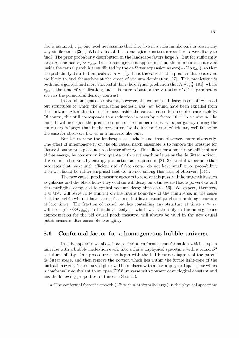
161

else is assumed, e.g., one need not assume that they live in a vacuum like ours or are in anyway similar to us [36].) What value of the cosmological constant are such observers likely tofind? The prior probability distribution in the landscape favors large Λ. But for sufficientlylarge Λ, one has τΛ ≪ τobs. In the homogeneous approximation, the number of observersinside the causal patch is then diluted by the de Sitter expansion as exp(−

√3Λτobs), so that

the probability distribution peaks at Λ ∼ τ−2obs. Thus the causal patch predicts that observers

are likely to find themselves at the onset of vacuum domination [37]. This predictions isboth more general and more successful than the original prediction that Λ ∼ τ−2

gal [181], whereτgal is the time of virialization; and it is more robust to the variation of other parameterssuch as the primordial density contrast.

In an inhomogeneous universe, however, the exponential decay is cut off when allbut structures to which the generating geodesic was not bound have been expelled fromthe horizon. After this time, the mass inside the causal patch does not decrease rapidly.Of course, this still corresponds to a reduction in mass by a factor 10−11 in a universe likeours. It will not spoil the prediction unless the number of observers per galaxy during theera τ ≫ τΛ is larger than in the present era by the inverse factor, which may well fail to bethe case for observers like us in a universe like ours.

But let us view the landscape as a whole and treat observers more abstractly.The effect of inhomogeneity on the old causal patch ensemble is to remove the pressure forobservations to take place not too longer after τΛ. This allows for a much more efficient useof free energy, by conversion into quanta with wavelength as large as the de Sitter horizon.If we model observers by entropy production as proposed in [24, 37], and if we assume thatprocesses that make such efficient use of free energy do not have small prior probability,then we should be rather surprised that we are not among this class of observers [144].

The new causal patch measure appears to resolve this puzzle. Inhomogeneities suchas galaxies and the black holes they contain will decay on a timescale that is power-law andthus negligible compared to typical vacuum decay timescales [56]. We expect, therefore,that they will leave little imprint on the future boundary of the multiverse, in the sensethat the metric will not have strong features that favor causal patches containing structureat late times. The fraction of causal patches containing any structure at times τ ≫ τΛ

will be exp(−√

3Λτobs), so the above analysis, which was valid only in the homogeneousapproximation for the old causal patch measure, will always be valid in the new causalpatch measure after ensemble-averaging.

8.6 Conformal factor for a homogeneous bubble universe

In this appendix we show how to find a conformal transformation which maps auniverse with a bubble nucleation event into a finite unphysical spacetime with a round S3

as future infinity. Our procedure is to begin with the full Penrose diagram of the parentde Sitter space, and then remove the portion which lies within the future light-cone of thenucleation event. The removed piece will be replaced with a new unphysical spacetime whichis conformally equivalent to an open FRW universe with nonzero cosmological constant andhas the following properties, outlined in Sec. 9.3:

The conformal factor is smooth (Cn with n arbitrarily large) in the physical spacetime

162

and continuous when extended to the future boundary.

The induced metric along the future light-cone of the nucleation event agrees withthe induced metric on the same hypersurface in the outside portion of the diagram,which was left unchanged.

The future boundary is identical to the piece of the future boundary that was removedfrom the old diagram.

(Note that the new portion of the unphysical spacetime will not be a portion of the Einsteinstatic universe, nor is there any reason to demand that it should be.)

We will accomplish this mapping in three steps. First, we will show that any FRWuniverse with non-zero vacuum energy is conformally equivalent to a portion of de Sitterspace. Second, we will show that this portion of de Sitter space can be conformally mappedto a portion of the Einstein static universe whose future boundary is identical to the pieceof the future boundary removed from the parent de Sitter diagram. Third, we show thatthis portion of the Einstein static universe is conformally equivalent to a new unphysicalspacetime which satisfies all of the above properties (and is not a portion of the Einsteinstatic universe).

An open FRW universe, such as the one following the nucleation event, has themetric

ds2FRW = a2(T )(−dT 2 + dH2

3) , (8.57)

where T is the conformal time, a is the scale factor, and

dH23 = dχ2 + sinh2 χdΩ2

2 . (8.58)

All bubble nucleation events are followed by a period of curvature domination in the bubbleuniverse, and hence conformal time is unbounded toward the past. Furthermore, as longas Λ ≠ 0, conformal time is finite toward the future. We are thus free to choose the rangeof T to be −∞ < T ≤ 0 for every FRW universe under consideration. The open slicing of deSitter space (with unit de Sitter length) is one special case of this metric:

adS(T ) = −1

sinhT. (8.59)

Any other FRW universe is conformally equivalent to the de Sitter open slicing, and theconformal factor is given by

Ω1 = −1

a(T ) sinhT. (8.60)

The second step is to map the open slicing of de Sitter space into a portion of theEinstein static universe whose future boundary is identical to the piece removed from theparent vacuum. Recall that the Einstein static universe has a metric given by Eq. 8.12,

ds20 = −dη2 + dΩ2

3 , (8.61)

and that the Penrose diagram of the parent de Sitter space consists of the region 0 > η > −π.We write the S3 metric as

dΩ23 = dξ2 + sin2 ξdΩ2

2 . (8.62)

163

In these coordinates the nucleation event can be taken to be at η = ηnuc and ξ = 0, so thatthe portion of future infinity we need to reproduce in the bubble universe is the portion ofthe round S3 with 0 < ξ < −ηnuc.

9

The open slicing coordinates (T,χ) are not convenient for this task, so first we willchange coordinates to (ηin, ξin), in terms of which the metric Eq. 8.57, with a = adS, lookslike

ds2 = 1

sin2 ηin

(−dη2in + dΩ2

3) , (8.63)

where we need to ensure that 0 < ξin < −ηnuc when ηin = 0. Then we can simply rescale bysinηin to finish the job. Now we turn to the task of finding the transformation (T,χ) →(ηin, ξin) .

Let X0, X1, X2, X3, X4 of be the coordinates of 4+1-dimensional Minkowskispace, in which de Sitter space is the hyperboloid

−X20 +

3

∑i=1

X2i +X2

4 = 1 . (8.64)

The relationship between the coordinates (ηin, ξin) and the Xµ is

X0 = cotηin (8.65)

Xi = − 1

sinηinsin ξin ni

X4 = − 1

sinηincos ξin,

where ni are unit vectors whose sum equals 1. We need to specify how the (χ,T ) coordinatesof Eq. 8.57 relate to the Xµ. The standard open slicing of de Sitter space is given by

X0 = − 1

sinhTcoshχ (8.66)

Xi = − 1

sinhTsinhχ ni

X4 = − cothT ,

but this is not what we want to do. We have to remember that the nucleation event isat χ = 0, T = −∞, which would be equivalent to ηin = −π/2 and ξin = 0 if we used thisprescription. To fix the problem, we use the 4+1-dimensional boost symmetry, which is anisometry of the de Sitter space, to move the nucleation event to another position. Let Xµ

be given by

X0 = coshβX0 + sinhβX4 (8.67)

X4 = sinhβX0 + coshβX4

Xi = Xi, 1 ≤ i ≤ 3 , (8.68)

9In this appendix only, we will find it more convenient for η to take negative values and increase towardsthe future boundary. The η defined in the main body of the chapter is ηmain = ∣ηappendix∣.

164

and then define the open coordinates (T,χ) by

X0 = − 1

sinhTcoshχ (8.69)

Xi = − 1

sinhTsinhχ ni

X4 = − cothT .

Now the nucleation event is at ηin = ηnuc and ξin = 0, where cotηnuc = − sinhβ . We canwrite the relationship between (T,χ) and (ηin, ξin) directly in terms of ηnuc as

sinhχ

sinhT= sin ξin

sinηin(8.70)

− cotηin = 1

sinηnuc

coshχ

sinhT+ cotηnuc cothT .

Now the metric is in the form Eq. 8.63, and 0 < ξin < −ηnuc when ηin = 0. Hence we canconformally rescale by

Ω2 = sinηin , (8.71)

to map the bubble universe into a portion of the Einstein static universe with future bound-ary identical to the piece cut out of the old diagram.

The product Ω1Ω2 succeeds in mapping our original FRW universe to a portionof the Einstein static universe with the correct future boundary. Now we will act with onefinal conformal rescaling, Ω3, which must change the induced unphysical metric along thefuture light-cone of the nucleation event to match the one in the old de Sitter diagram,thus ensuring that the total conformal transformation is continuous. We must also demandthat Ω3 = 1 on the future boundary ηin = 0, since we have already fixed that part of theunphysical spacetime.

The induced metric on the future light-cone of the nucleation event has a similarform in both the unphysical bubble coordinates (ηin, ξin) and the unphysical parent coor-dinates, which we will now denote as (ηout, ξout). In both cases it merely comes from theEinstein static universe metric:

ds2light−cone = sin2 ξin/out dΩ2

2 , (8.72)

where ξin/out = ηin/out − ηnuc. Hence the conformal factor evaluated along the light-cone is

Ω3 =sin ξout

sin ξin. (8.73)

We just need to find out how ξout and ξin are related. We can do this by demanding thatthe induced physical metrics also be identical on the light-cone.

The induced physical metric on the light-cone from the parent de Sitter space isfound by restricting Eq. 8.11 to the relevant surface:

ds20 →

sin2 ξout

H20 sin2 ηout

dΩ22 , (8.74)

165

where again ηout − ξout = ηnuc.In terms of the χ and T coordinates inside the bubble, the relevant light-cone is

given by χ →∞, T → −∞, χ + T = const. In terms of ηin and ξin, the light-cone is given byηin − ξin = ηnuc. One can see that a fixed value of χ + T is equivalent to a fixed value of ξin.Since a(T )→ Ce−T for some constant C as T → −∞, we have from Eq. 8.57 that

ds2FRW → Ce2(χ+T )dΩ2

2 = Csin2 ξin

sin2 ηin

dΩ22 . (8.75)

We must determine the constant C, which is related to our convention that T = 0 on futureinfinity. This constant is easily determined by considering the particular light-cone given byχ+T = 0. This is the event horizon of the FRW universe, and its area is given by AEH, whichdepends on the detailed form of a(T ). So C = AEH/4π. Finally we have our relationshipbetween the in-coordinates and out-coordinates on the bubble wall hypersurface:

√AEH

4π

sin (ηin − ηnuc)sinηin

= 1

H0

sin (ηout − ηnuc)sinηout

. (8.76)

Notice that ηin and ηout coincide at the nucleation event (both equal to ηnuc) and at futureinfinity (both equal to zero).

We are free to extend Ω3 into the rest of the bubble universe in any continuous waywe please, so long as it restricts to 1 on future infinity and sin ξout/ sin ξin on the boundarylight-cone. One might worry about the fact that Ω3 is multivalued at the point where thebubble wall meets future infinity. This is not a concern, though, because the only functionwhich need be well defined is the product

Ω = Ω1Ω2Ω3 = −sinηin

a(T ) sinhTΩ3 . (8.77)

In this formula, ηin = ηin(χ,T ) as determined by Eqs 8.70 . From here it is easy to see thatas we approach the point χ = ∞ along any slice of fixed T , including both T = 0 (futureinfinity) and T = −∞ (domain wall), we arrive at Ω = 0 so long as Ω3 remains finite.

Thus we have accomplished our initial task. The function Ω3 is very ambiguous,as we have only fixed its behavior at the boundaries of the spacetime. We can use thisadditional freedom to make Ω arbitrarily smooth at the interface between the parent andthe bubble universe. Additionally, one could impose that Ω3 be identically equal to 1 notjust on the future boundary, but in the entire region T > T0 for some particular T0. Inparticular, we can choose T0 to be the time of vacuum domination in the bubble universe.

166

Chapter 9

Testing measures

9.1 Introduction

String theory appears to contain an enormous landscape of metastable vacua [41,109], with a corresponding diversity of low-energy physics. The cosmological dynamics ofthis theory is eternal inflation. It generates a multiverse in which each vacuum is producedinfinitely many times.

In a theory that predicts a large universe, it is natural to assume that the relativeprobability for two different outcomes of an experiment is the ratio of the expected numberof times each outcome occurs. But in eternal inflation, every possible outcome happensinfinitely many times. The relative abundance of two different observations is ambiguousuntil one defines a measure: a prescription for regulating the infinities of eternal inflation.

Weinberg’s prediction [181] of the cosmological constant [151, 143] was a stunningsuccess for this type of reasoning. In hindsight, however, it was based on a measure thatwas ill-suited for a landscape in which parameters other than Λ can vary. Moreover, themeasure had severe phenomenological problems [27]. This spurred the development of morepowerful measure proposals in recent years [125, 123, 71, 72, 70, 76, 179, 178, 24, 121, 122,141, 73, 182, 183, 184, 126, 26, 28, 160]. Surprisingly, some of these measures do far morethan to resolve the above shortcomings. As we shall see in this chapter, they obviate theneed for Weinberg’s assumption that observers require galaxies; and they help overcomethe limitation of fixing all parameters but one to their observed values.

In this chapter we will analyze three different measure proposals. Each regulatesthe infinite multiverse by restricting attention to a finite portion. The causal patch mea-sure [24] keeps the causal past of the future endpoint of a geodesic; it is equivalent to aglobal cutoff known as light-cone time [26, 44]. The fat geodesic measure [34] keeps a fixedphysical volume surrounding the geodesic; in simple situations, it is equivalent to the globalscale factor time cutoff [53]. We also introduce a new measure, which restricts to the interiorof the apparent horizon surrounding the geodesic.

From little more than the geometry of these cutoffs, we are able to make remark-able progress in addressing cosmological coincidence and hierarchy problems. Using eachmeasure, we will predict three time scales: the time when observations are made, tobs, thetime of vacuum energy domination, tΛ ≡

√3/∣Λ∣, and the time of curvature domination,

167

tc.1 We work in the approximation that observations occur in nearly homogeneous FRW

universes so that these time scales are well defined.We will allow all vacuum parameters to vary simultaneously. Parameters for which

we do not compute probabilities are marginalized. We will not restrict attention to vacuawith specific features such as baryons or stars. We will make some weak, qualitative as-sumptions about the prior distribution of parameters in the landscape. We will assume thatmost observers are made of something that redshifts faster than curvature. (This includesall forms of radiation and matter but excludes, e.g., networks of domain walls.) But wewill not impose any detailed anthropic requirements, such as the assumption that observersrequire galaxies or complex molecules; we will not even assume that they are correlated withentropy production [24, 37, 36]. Thus we obtain robust predictions that apply to essentiallyarbitrary observers in arbitrary vacua.

The probability distribution over all three variables can be decomposed into threefactors, as we will explain further in Sec. 9.2:

d3p

d log tobs d log tΛ d log tc=

d2p

d log tΛ d log tc×M(log tobs, log tc, log tΛ) × α(log tobs, log tc, log tΛ) . (9.1)

Here p is the probability density that a bubble with parameters (log tΛ, log tc) is producedwithin the region defined by the cutoff. Its form can be estimated reliably enough for ourpurposes from our existing knowledge about the landscape. The factorM(log tobs, log tΛ, log tc)is the mass inside the cutoff region at the time tobs. This is completely determined by thegeometry of the cutoff and the geometry of an FRW bubble with parameters (log tΛ, log tc),so it can be computed unambiguously. The last factor, α(log tobs, log tc, log tΛ), is the onewe know the least about. It is the number of observations per unit mass per logarithmictime interval, averaged over all bubbles with the given values (log tΛ, log tc).

A central insight exploited in this chapter is the following. In bubbles with positivecosmological constant, the calculable quantity M so strongly suppresses the probability inother regimes that in many cases we only need to know the form of α in the regime whereobservers live before vacuum energy or curvature become important, tobs ≲ tΛ, tc. Undervery weak assumptions, α must be independent of tΛ and tc in this regime. This is becauseneither curvature nor vacuum energy play a dynamical role before observers form, so thatneither can affect the number of observers per unit mass. Thus, for positive cosmologicalconstant α is a function only of tobs in the only regime of interest. The success of themeasures in explaining the hierarchy and coincidence of the three timescales depends onthe form of this function. We will that the causal patch and apparent horizon cutoff succeed

1In regions where curvature will never dominate, such as our own vacuum, tc is defined as the time whencurvature would come to dominate if there were no vacuum energy. Since our observations are consistent witha flat universe, we can only place a lower bound on the observed value of tc. We include tc in our analysisbecause bubble universes in the multiverse are naturally very highly curved, so the absence of curvaturerequires an explanation. Moreover, we shall see that some measures select for high curvature in vacua withwith negative cosmological constant. This effect is partly responsible for the problems encountered in thisportion of the landscape.

168

well in predicting the three timescales already under very weak assumptions on α. The fatgeodesic cutoff requires somewhat stronger assumptions.

For negative cosmological constant, however, the geometric factor M favors theregime where tobs is not the shortest time scale. Thus, predictions depend crucially onunderstanding the form of α in this more complicated regime. For example, we need to knowon average to what extent early curvature domination disrupts the formation of observers.What is clear from our analysis is that all three measures are in grave danger of predictingthat most observers see negative Λ, in conflict with observation, unless the anthropic factorα takes on rather specific forms. Assuming that this is not the case, we must ask whetherthe measures can be modified to agree with observation. Both the causal patch measureand the fat geodesic measure are dual [34, 44] to global time cutoffs, the lightcone time andthe scale factor time cutoff, respectively. These global cutoffs, in turn, are motivated by ananalogy with the UV/IR relation in AdS/CFT [73]. But this analogy really only appliesto positive Λ, so it is natural to suspect that the measure obtained from it is inapplicableto regions with Λ ≤ 0 [26]. (Indeed, the causal patch does not eliminate infinities in Λ = 0bubbles [24]. We do not consider such regions in this chapter.)

Outline and summary of results In Sec. 9.2, we will describe in detail our method forcounting observations. We will derive an equation for the probability distribution over thethree variables (log tΛ, log tc, log tobs). We will explain how simple qualitative assumptionsabout α(log tobs, log tc, log tΛ), the number of observations per unit mass per unit logarithmictime interval, allow us to compute probabilities very generally for all measures.

We work in the approximation that observations in the multiverse take place innegatively curved Friedmann-Robertson-Walker (FRW) universes. In Sec. 9.3, we will ob-tain solutions for their scale factor, in the approximation where the matter-, vacuum-, andpossibly the curvature-dominated regime are widely separated in time.

In Secs. 9.4–9.6, we will compute the probability distribution over (log tΛ, log tc, log tobs),using three different measures. For each measure we consider separately the cases of positiveand negative cosmological constant. As described above, the results for negative cosmolog-ical constant are problematic for all three measures. We now summarize our results for thecase Λ > 0.

In Sec. 9.4, we show that the causal patch measure predicts the double coincidencelog tc ≈ log tΛ ≈ log tobs. We find that the scale of all three parameters is related to thenumber of vacua in the landscape. This result is compatible with current estimates of thenumber of metastable string vacua. Such estimates are not sufficiently reliable to put ourprediction to a conclusive test, but it is intriguing that the size of the landscape may be theorigin of the hierarchies we observe in Nature (see also [147, 24, 25, 35, 39, 36]. We havepreviously reported the result for this subcase in more detail [30].

Unlike the causal patch, the new “apparent horizon measure” (Sec. 9.5) predictsthe double coincidence log tc ≈ log tΛ ≈ log tobs for any fixed value tobs. When all param-eters are allowed to scan, its predictions agree with those of the causal patch, with mildassumptions about the function α. The apparent horizon measure is significantly moreinvolved than the causal patch: it depends on a whole geodesic, not just on its endpoint,and on metric information, rather than only causal structure. If our assumptions about α

169

are correct, this measure offers no phenomenological advantage over its simpler cousin andmay not be worthy of further study.

The fat geodesic cutoff, like the apparent horizon cutoff, predicts the double co-incidence log tc ≈ log tΛ ≈ log tobs for any fixed value of tobs. However, it favors small valuesof all three timescales unless either (a) an anthropic cutoff is imposed, or (b) it is assumedthat far more observers form at later times, on average, than at early times, in vacua wherecurvature and vacuum energy are negligible at the time tobs. (Qualitatively, the other twomeasures also require such an assumption, but quantitatively, a much weaker prior favoringlate observers suffices.) In the latter case (b), the results of the previous two measures arereproduced, with all timescales set by the size of the landscape. In the former case (a), thefat geodesic would predict that observers should live at the earliest time compatible withthe formation of any type of observers (in any kind of vacuum). It is difficult to see whythis minimum value of tobs would be so large as to bring this prediction into agreement withthe observed value, tobs ∼ 1061.

9.2 Counting Observations

In this section, we explain how we will compute the trivariate probability distri-bution over (log tobs, log tc, log tΛ). We will clarify how we isolate geometric effects, whichcan be well-computed for each cutoff, from anthropic factors; and we explain why very fewassumptions are needed about the anthropic factors once the geometric effects have beentaken into account.

Imagine labelling every observation within the cutoff region by (log tobs, log tc, log tΛ).We are interested in counting the number of observations as a function of these parame-ters. It is helpful to do this in two steps. First, we count bubbles, which are labelled by(log tc, log tΛ) to get the “prior” probability distribution

d2p

d log tΛ d log tc. (9.2)

This p is the probability density to nucleate a bubble with the given values of the parametersinside the cutoff region.

The next step is to count observations within the bubbles. A given bubble ofvacuum i will have observations at a variety of FRW times. In the global description ofeternal inflation, each bubble is infinite and contains an infinite number of observations ifit contains any, but these local measures keep only a finite portion of the global spacetimeand hence a finite number of observations. We parameterize the probability density forobservations within a given bubble as

dNi

d log tobs∼M(log tobs, log tc, log tΛ)αi(log tobs) , (9.3)

where M is the mass inside the cutoff region, and αi is the number of observations perunit mass per logarithmic time interval inside a bubble of type i. In this decomposition, Mcontains all of the information about the cutoff procedure. For a given cutoff, M dependsonly on the three parameters of interest. Because we are considering geometric cutoffs,

170

the amount of mass that is retained inside the cutoff region does not depend on any otherdetails of the vacuum i. On the other hand, αi depends on details of the vacuum, such aswhether observers form, and when they form; but it is independent of the cutoff procedure.

Since we are interested in analyzing the probability distribution over three vari-ables, we now want to average αi over the bubbles with a given (log tΛ, log tc), to get theaverage number of observations per unit mass per logarithmic time α. With this decompo-sition, the full probability distribution over all three variables is

d3p

d log tobs d log tΛ d log tc= d2p

d log tΛ d log tcM(log tobs, log tc, log tΛ)α(log tobs, log tc, log tΛ) .

(9.4)To recap, p is the probability for the formation of a bubble with parameters (log tΛ, log tc)inside the cutoff region; M(log tobs, log tΛ, log tc) is the mass inside the cutoff region at theFRW time tobs in a bubble with parameters (log tΛ, log tc); and α(log tobs, log tc, log tΛ) isthe number of observations per unit mass per logarithmic time interval, averaged over allbubbles with parameters (log tΛ, log tc).

This is a useful decomposition because the mass M inside the cutoff region can becomputed exactly, since it just depends on geometrical information. We will assume thatd2p/d log tΛ d log tc can be factorized into contribution from tΛ and a contribution from tc.Vacua with Λ ∼ 1 can be excluded since they contain only a few bits of information in anycausally connected region. In a large landscape, by Taylor expansion about Λ = 0, the priorfor the cosmological constant is flat in Λ for Λ ≪ 1, dp/dΛ = const. Transforming to thevariable log tΛ, we thus have

d2p

d log tΛd log tc∼ t−2

Λ g(log tc) . (9.5)

The factor g(log tc) encodes the prior probability distribution over the time of curvaturedomination. We will assume that g decreases mildly, like an inverse power of log tc. (Assum-ing that slow-roll inflation is the dominant mechanism responsible for the delay of curvaturedomination, log tc corresponds to the number of e-foldings. If g decreased more strongly,like an inverse power of tc, then inflationary models would be too rare in the landscape toexplain the observed flatness.) The detailed form of the prior distribution over log tc willnot be important for our results; any mild suppression of large log tc will lead to similarresults.

With these reasonable assumptions, the probability distribution becomes

d3p

d log tobs d log tΛ d log tc= t−2

Λ M(log tobs, log tc, log tΛ)g(log tc)α(log tobs, log tc, log tΛ) .(9.6)

Because α depends on all three variables, it is very difficult to compute in general. However,it will turn out that we can make a lot of progress with a few simple assumptions about α.First, we assume that in the regime, tobs ≪ tΛ, α is independent of tΛ. Similarly, we assumethat in the regime, tobs ≪ tc, α is independent of tc. By these assumptions, in the regimewhere the observer time is the shortest timescale, tobs ≲ tΛ, tc, the anthropic factor α willonly depend on log tobs:

α(log tobs, log tc, log tΛ) ≈ α(log tobs) for tobs ≲ tΛ, tc . (9.7)

171

These assumptions are very weak. Because curvature and Λ are not dynamically importantbefore tc and tΛ, respectively, they cannot impact the formation of observers at such earlytimes. One could imagine a correlation between the number of e-foldings and the timeof observer formation even in the regime tobs ≪ tc, for example if each one is tied tothe supersymmetry breaking scale, but this seems highly contrived. In the absence of acompelling argument to the contrary, we will make the simplest assumption.

Second, we assume that when either tobs ≫ tc or tobs ≫ tΛ, α is not enhancedcompared to its value when tobs is the shortest timescale. This is simply the statementthat early curvature and vacuum domination does not help the formation of observers.This assumption, too, seems rather weak. With this in mind, let us for the time beingoverestimate the number of observers by declaring α to be completely independent of log tΛand log tc:

α(log tobs, log tc, log tΛ) ≈ α(log tobs) . (9.8)

This is almost certainly an overestimate of the number of observations in the regime wheretobs is not the shortest time scale. However, we will show that the predictions for positivecosmological constant are insensitive to this simplification because the geometrical factorM , which we can compute reliably, suppresses the contribution from this regime. We willreturn to a more realistic discussion of α when we are forced to, in analyzing negativecosmological constant.

With these assumptions and approximations, the three-variable probability distri-bution takes a more tractable form,

d3p

d log tobs d log tΛ d log tc= t−2

Λ g(log tc)M(log tobs, log tΛ, log tc)α(log tobs) . (9.9)

This is the formula that we will analyze in the rest of the chapter. The only quantity thatdepends on all three variables is the mass, which we can compute reliably for each cutoffusing the geometry of open bubble universes, to which we turn next.

9.3 Open FRW universes with cosmological constant

In this section, we find approximate solutions to the scale factor, for flat ornegatively curved vacuum bubbles with positive or negative cosmological constant. Thelandscape of string theory contains a large number of vacua that form a “discretuum”, adense spectrum of values of the cosmological constant [41]. These vacua are populated byColeman-DeLuccia bubble nucleation in an eternally inflating spacetime, which producesopen Friedmann-Robertson-Walker (FRW) universes [49]. Hence, we will be interested inthe metric of FRW universes with open spatial geometry and nonzero cosmological constantΛ. The metric for an open FRW universe is

ds2 = −dt2 + a(t)2(dχ2 + sinh2 χdΩ22) . (9.10)

The evolution of the scale factor is governed by the Friedmann equation:

( aa)

2

= tca3

+ 1

a2± 1

t2Λ. (9.11)

172

Here tΛ =√

3/∣Λ∣ is the timescale for vacuum domination, and tc is the timescale for cur-vature domination. The term ρm ∼ tc/a3 corresponds to the energy density of pressurelessmatter. (To consider radiation instead, we would include a term ρrad ∼ t2c/a4; this wouldnot affect any of our results qualitatively.) The final term is the vacuum energy density,ρΛ; the“+” sign applies when Λ > 0, and the“−” sign when Λ < 0.

We will now display approximate solutions for the scale factor as a function ofFRW time t. There are four cases, which are differentiated by the sign of Λ and the relativesize of tc and tΛ. We will compute all geometric quantities in the limit where the three timescales t, tc, and tΛ are well-separated, so that some terms on the right hand side of Eq. (9.11)can be neglected. In this limit we obtain piecewise solution for the scale factor. We willnot ensure that these solutions are continuous and differentiable at the crossover times.This would clutter our equations, and it would not affect the probability distributions wecompute later. Up to order-one factors, which we neglect, our formulas are applicable evenin crossover regimes.

If tc ≫ tΛ, curvature never comes to dominate. (One can still define tc geometri-cally, or as the time when curvature would have dominated in a universe with Λ = 0.) Inthis limit the metric can be well approximated as that of a perfectly flat FRW universe,and so becomes independent of tc. We implement this case by dropping the term tc/a3 inEq. (9.11).

Positive cosmological constant We begin with the case Λ > 0 and tc ≪ tΛ. By solvingEq. (9.11) piecewise, we find

a(t) ∼⎧⎪⎪⎪⎪⎨⎪⎪⎪⎪⎩

t1/3c t2/3 , t < tct , tc < t < tΛtΛe

t/tΛ−1 , tΛ < t .(9.12)

If tc ≫ tΛ, there is no era of curvature domination, and the universe can be approximatedas flat throughout. The scale factor takes the form

a(t) ∼⎧⎪⎪⎨⎪⎪⎩

t1/3c t2/3 , t < tΛt1/3c t

2/3Λ et/tΛ−1 , tΛ < t .

(9.13)

Negative cosmological constant For Λ < 0, the scale factor reaches a maximum andthen begins to decrease. The universe ultimately collapses at a time tf , which is of ordertΛ:

tf ≈ πtΛ . (9.14)

The evolution is symmetric about the turnaround time, tf/2 ≈ πtΛ/2.Again, we consider the cases tΛ ≫ tc and tΛ ≪ tc separately. For tc ≪ tΛ, the scale

factor is

a(t) ∼⎧⎪⎪⎪⎪⎨⎪⎪⎪⎪⎩

t1/3c t2/3 , t < tctΛ sin(t/tΛ) , tc < t < t′ct1/3c (t′)2/3 , t′c < t .

(9.15)

We have defined t′ ≡ tf − t.

173

There is no era of curvature domination if tc ≳ tf/2. For tc ≫ tf/2, we treat theuniverse as flat throughout, which yields the scale factor

a(t) ∼ t2/3Λ t1/3c sin2/3(πt/tf) , (9.16)

where tf here takes on a slightly different value compared to the curved case:

tf = 2πtΛ/3 . (9.17)

At a similar level of approximation as we have made above, this solution can be approxi-mated as

a(t) ∼⎧⎪⎪⎨⎪⎪⎩

t1/3c t2/3 , t < tf/2t1/3c (t′)2/3 , tf/2 < t .

(9.18)

where again t′ ≡ tf − t .

9.4 The causal patch cut-off

With all our tools lined up, we will now consider each measure in turn and derivethe probability distribution. We will treat positive and negative values of the cosmologicalconstant separately. After computing M , we will next calculate the bivariate probabilitydistribution over log tΛ and log tc, for fixed log tobs. In all cases this is a sharply peakedfunction of the two variables log tΛ and log tc, so we make little error in neglecting theprobability away from the peak region. Then we will go on to find the full distributionover all three parameters. In this section, we begin with the causal patch measure [24, 32],which restricts to the causal past of a point on the future boundary of spacetime. Thecausal patch measure is equivalent [44] to the light-cone time cutoff [26, 28], so we will notdiscuss the latter measure separately.

We may use boost symmetries to place the origin of the FRW bubble of interestat the center of the causal patch. The boundary of the causal patch is given by the pastlight-cone from the future end point of the comoving geodesic at the origin, χ = 0:

χCP(t) = ∫tf

t

dt′

a(t′) . (9.19)

If Λ < 0, tf is the time of the big crunch (see Sec. 9.3). For long-lived metastable de Sittervacua (Λ > 0), the causal patch coincides with the event horizon. It can be computed asif the de Sitter vacuum were eternal (tf → ∞), as the correction from late-time decay isnegligible.

9.4.1 Positive cosmological constant

We begin with the case Λ > 0, tc < tΛ. Using Eq. (9.12) for a(t), we find

χCP(tobs) ∼⎧⎪⎪⎪⎨⎪⎪⎪⎩

1 + log(tΛ/tc) + 3 [1 − (tobs/tc)1/3] , tobs < tc1 + log(tΛ/tobs) , tc < tobs < tΛe−tobs/tΛ , tΛ < tobs .

. (9.20)

174

The comoving volume inside a sphere of radius χ is π(sinh 2χCP − 2χCP). Weapproximate this, dropping constant prefactors that will not be important, by χ3 for χ ≲ 1,and by e2χ for χ ≳ 1:

VCP ∼ exp(2χCP) , tobs < tΛχ3

CP , tΛ < tobs .(9.21)

The mass inside the causal patch is MCP = ρa3VCP = tcVCP.

MCP ∼⎧⎪⎪⎪⎨⎪⎪⎪⎩

t2Λ/tc , tobs < tc < tΛ It2Λtc/t2obs , tc < tobs < tΛ II

tce−3tobs/tΛ , tc < tΛ < tobs III

(9.22)

Next, we consider the case Λ > 0, tΛ < tc. The above caclulations can be repeatedfor a flat universe, which is a good approximation for this case:

MCP ∼ tΛ , tobs < tΛ V

tΛe−3tobs/tΛ , tΛ < tobs IV

(9.23)

The same result could be obtained simply by setting tc = tΛ in (9.22).The full probability distribution is given by multiplying the mass in the causal

patch by the prior distribution and the number of observations per unit mass per unit timeto give

d3pCP

d log tc d log tΛd log tobs∼ gα ×

⎧⎪⎪⎪⎪⎪⎪⎪⎪⎪⎪⎪⎪⎪⎪⎪⎪⎪⎪⎪⎪⎪⎨⎪⎪⎪⎪⎪⎪⎪⎪⎪⎪⎪⎪⎪⎪⎪⎪⎪⎪⎪⎪⎪⎩

1

tc, tobs < tc < tΛ I

tct2obs

, tc < tobs < tΛ II

tct2Λ

exp(−3tobs

tΛ) , tc < tΛ < tobs III

1

tΛexp(−3tobs

tΛ) , tΛ < tobs, tc IV

1

tΛ, tobs < tΛ < tc V

(9.24)

Recall that g(log tc) is the prior distribution on the time of curvature domination, and α isthe number of observations per unit mass per logarithmic time interval.

We will first analyze this probability distribution for fixed log tobs. As explainedin the introduction, we will for the time being overestimate the number of observers inthe regime where tobs is not the shortest timescale by assuming that α is a function oflog tobs only. We will find that the overestimated observers do not dominate the probabilitydistribution, so this is a good approximation. With these approximations, α is independentof log tΛ and log tc and can be ignored for fixed log tobs.

The probability distribution we have found for log tc and log tΛ is a function ofpowers of tc and tΛ, i.e., exponential in the logarithms. Therefore the distribution will bedominated by its maximum. A useful way of determining the location of the maximum isto follow the gradient flow generated by the probability distribution. In the language ofRef. [88, 35], this is a multiverse force pushing log tΛ and log tc to preferred values. We

175

I

II

III

IV

V

log tobslog tc

log tobs

log tL

(a) Λ > 0

I

II

IIIIV

V

log tobslog tc

log tobs

log 2tobs

log t f

(b) Λ < 0

Figure 9.1: The probability distribution over the timescales of curvature and vacuum dom-ination at fixed observer timescale log tobs, before the prior distribution over log tc and thefiniteness of the landscape are taken into account. The arrows indicate directions of increas-ing probability. For Λ > 0 (a), the distribution is peaked along the degenerate half-linesforming the boundary between regions I and II and the boundary between regions IV andV. For Λ < 0 (b), the probability distribution exhibits a runaway toward the small tc, largetΛ regime of region II. The shaded region is is excluded because tobs > tf = πtΛ is unphysical.

could use our formulas to determine the precise direction of the multiverse force, but thiswould be difficult to represent graphically, and it is not necessary for the purpose of findingthe maximum. Instead, we shall indicate only whether each of the two variables prefersto increase or decrease (or neither), by displaying horizontal, vertical, or diagonal arrowsin the (log tc, log tΛ) plane (Fig. 9.1). We ignore the prior g(log tc) for now since it is notexponential.

We consider each region in (9.24) in turn. In region I, tobs < tc < tΛ, the probabilityis proportional to t−1

c . Hence, there is a pressure toward smaller tc and no pressure on tΛ.This is shown by a left-pointing horizontal arrow in region I of the figure. In region II(tc < tobs < tΛ), the probability is proportional to tct

−2obs. This pushes toward larger log tc

and is neutral with respect to log tΛ. (Recall that we are holding log tobs fixed for now.)In region III (tc < tΛ < tobs), the probability goes like tct

−2Λ e−3tobs/tΛ . Since the exponential

dominates, the force goes toward larger log tΛ; log tc is pushed up as well. In region IV(tΛ < tobs, tΛ < tc) the exponential again dominates, giving a pressure toward large log tΛ.In region V (tobs < tΛ < tc), the distribution is proportional to t−1

Λ , giving a pressure towardsmall log tΛ. The dependence of the probability on log tc lies entirely in the prior g(log tc)in these last two regions because the universe is approximately flat and hence dynamicallyindependent of log tc.

Leaving aside the effect of g(log tc) for now, we recognize that the probabilitydensity in Fig. 9.1 is maximal along two lines of stability, log tΛ = log tobs and log tc =log tobs, along which the probability force is zero. These are the boundaries between regionsIV/V and I/II, respectively. They are shown by thick lines in Fig. 9.1. The fact that the

176

distribution is flat along these lines indicates a mild runaway problem: at the crude level ofapproximation we have used thus far, the probability distribution is not integrable. Let usconsider each line in turn to see if this problem persists in a more careful treatment.

Along the line log tΛ = log tobs, the prior distribution g(log tc) will suppress largelog tc and make the probability integrable, rendering a prediction for log tc possible. (Witha plausible prior, the probability of observing a departure from flatness in a realistic futureexperiment is of order 10% [67, 54]; see also [39]. See [133, 45] for different priors.) We willfind the same line of stability for the other two measures in the following section, and it islifted by the same argument.

The line log tc = log tobs looks more serious. The prior on log tΛ follows from verygeneral considerations [181] and cannot be modified. In fact, the probability distributionis rendered integrable if, as we will suppose, the landscape contains only a finite numberN of vacua. This implies that there is a “discretuum limit”, a finite average gap betweendifferent possible values of Λ. This, in turn, implies that there is a smallest positive Λ inthe landscape, of order

Λmin ∼ 1/N . (9.25)

This argument, however, only renders the distribution integrable; it does not suffice tobring it into agreement with observation. It tells us that log Λ is drawn entirely at randomfrom values between log Λmin and log t−2

obs, so at this level of analysis we do not predict thecoincidence log tobs ≈ log tΛ.

Even though we do not predict a coincidence for observers living at a fixed arbitrarylog tobs, it could still be the case that after averaging over the times when observers couldlive most observers see log tobs ∼ log tΛ. To address this question, we need to allow log tobs

to vary. For fixed log tobs, the maximum of the probability with respect to log tc and log tΛis obtained along the boundary between region I and region II, as discussed above. Alongthis line, the probability is

dp

d log tobs∼ g(log tobs)

tobsα(log tobs) . (9.26)

Having maximized over log tΛ and log tc, we can now ask at what log tobs the probabilityis maximized. Note that since the distribution is exponential, maximizing over log tΛ andlog tc is the same as integrating over them up to logarithmic corrections coming from thefunction g.

The location of the maximum depends on the behavior of α(log tobs). Let usassume that

α ∼ t1+pobs , with p > 0 . (9.27)

(We will justify this assumption at the end of this section, where we will also describe whathappens if it is not satisfied.) Then the maximum is at the largest value of log tobs subjectto the constraint defining regions I and II, log tobs < log tΛ. It follows that the maximum ofthe three-variable probability distribution is at

log tobs ≈ log tc ≈ log tΛ ≈ log tmaxΛ . (9.28)

Therefore, in a landscape with p > 0 and vacua with Λ > 0, the causal patch predicts thatall three scales are ultimately set by log tmax

Λ , and thus, by the (anthropic) vacuum with

177

smallest cosmological constant. This, in turn, is set by the discretuum limit, i.e., by thenumber of vacua in the landscape [24, 37, 35, 36], according to

tmaxΛ ∼ N 1/2 . (9.29)

This is a fascinating result [30]. It implies that the remarkable scales we observe in Nature,such as the the vacuum energy and the current age of the universe, are not only mutuallycorrelated, but that their absolute scale can be explained in terms of the size of the land-scape. If current estimates of the number of vacua [41, 55] hold up, i.e., if log10N is oforder hundreds,2 then Eq. (9.28) may well prove to be in agreement with the observed valuetΛ ∼ 1061.

Let us go somewhat beyond our order-of-magnitude estimates and determine howprecisely log tobs and log tΛ can be expected to agree. To that end, we will now calculatepCP(f−1tΛ < tobs < ftΛ) as a function of f , i.e., the probability that log tobs lies withinan interval log f of log tΛ. The probability distribution of Eq. 9.24 is dominated near theboundary of regions IV and V, and the probability in region IV is exponentially suppressed.So we will neglect all regions except region V. (Ignoring region IV means we are eliminatingthe possibility that log tobs > log tΛ.)

The probability density in region V is

dp

d log tobs d log tc d log tΛ∝t1+pobs

tΛg(log tc) . (9.30)

We will further restrict to tc > tmaxΛ , which is reasonable if tobs is pushed to large values and

g(log tc) does not strongly prefer small values of log tc. Since we are computing a probabilitymarginalized over log tc, this restriction on the range of log tc means that the exact form ofg will not affect the answer. The quantity

∫∞

log tmaxΛ

d log tc g(log tc) (9.31)

will factor out of our computations, and hence we will ignore it. Having eliminated thelog tc dependence, we continue by computing the normalization factor Z for log tΛ > log tobs:

Z = ∫log tmax

Λ

0d log tobs∫

log tmaxΛ

log tobs

d log tΛt1+pobs

tΛ≈ (tmax

Λ )pp(1 + p) . (9.32)

In the last line we have dropped terms negligible for tmaxΛ ≫ 1.

Now we will calculate the unnormalized probabilty for f−1tobs < tΛ < ftobs. Wewill split the integration region into two subregions according to whether tobs < f−1tmax

Λ orf−1tmax

Λ < tobs < tmaxΛ . It turns out that each of these subregions is important. First we do

2The number of anthropic vacua, N , may be smaller by dozens or even hundreds of orders of magnitudethan the total number of vacua, N , for low-energy reasons that are unrelated to the cosmological constantor curvature and so are not included in out analysis. Hence, log10N ∼ O(1000) may be compatible withEq. (9.28).

178

tobs < f−1tmaxΛ :

∫log(f−1tmax

Λ )

0d log tobs∫

log(ftobs)

log tobs

d log tΛt1+pobs

tΛ(9.33)

≈ (tmaxΛ )pp

(f−p − f−1−p) (9.34)

= Z(1 + p)(f−p − f1−p) . (9.35)

Finally we calculate the case f−1tmaxΛ < tobs < tmax

Λ :

∫log tmax

Λ

log(f−1tmaxΛ )

d log tobs∫log tmax

Λ

log tobs

d log tΛt1+pobs

tΛ(9.36)

= (tmaxΛ )p [1 − f−p

p− 1 − f−1−p

1 + p ] (9.37)

= Z [1 − (1 + p)f−p + pf−1−p)] . (9.38)

Adding together the unnormalized probabilities and dividing by the factor Z wefind the result

pCP(f−1tobs < tΛ < ftobs) ≈ 1 − f−1−p . (9.39)

In addition to being independent of g(log tc), this result is independent of tmaxΛ , but the

validity of our approximation depends on both. In particular, region V contributes moreto the probability for larger tmax

Λ , so the approximation gets better as tmaxΛ increases. How-

ever, even for tmaxΛ = 1060 the result is only off by a few percent compared to a numerical

integration.Let us now return to discussing our assumption, Eq. (9.27). If p were not positive,

that is, if α increased at most linearly with tobs, then the maximum of the probabilitydistribution would be located at the smallest value of tobs compatible with observers. Inthis case the causal patch would predict tΛ ≫ tobs. This would be in conflict with observationexcept under the extremely contrived assumption that tmax

Λ ∼ tminobs .

However, the assumption that p > 0 is quite plausible [30]. Recall that we are onlydiscussing the form of α in the regime where tobs is the shortest time scale, tobs ≲ tc, tΛ, sowe do not have to worry that later observations may be disrupted by curvature or vacuumenergy. Recall, moreover, that α is defined by averaging over many vacua, so we mustconsider only how this average depends on tobs. In particular, this means that we shouldnot imagine that in moving from one value of tobs to another, we need to hold fixed thevacuum, or even restrict to only one or two parameters of particle physics and cosmology.Typical vacua with most observers at one value of tobs are likely to differ in many detailsfrom vacua in which most observers arise at a different time.

With this in mind, we note two general effects that suggest that α(log tobs) in-creases monotonically. First, the spontaneous formation of highly complex structures suchas observers relies both on chance and, presumably, on a long chain of evolutionary processesbuilding up increasing complexity. The later the time, the more likely it is that such a chainhas been completed. Secondly, for larger tobs, the same amount of mass can be distributedamong more quanta, of less energy each. Therefore, less mass is necessary to construct a

179

system containing a given number of quanta, such as a system of sufficient complexity tofunction as an observer. These arguments make it very plausible that α grows. Moreover,while they do not prove that it grows more strongly than linearly with tobs, they do makethis type of behavior rather plausible.

9.4.2 Negative cosmological constant

We turn to negative values of the cosmological constant, beginning with the caseΛ < 0, tc ≪ tΛ. From Eqs. (9.15) and (9.19), we find that the comoving radius of the causalpatch is given by

χCP(t) ∼⎧⎪⎪⎪⎪⎨⎪⎪⎪⎪⎩

3 − 2 log(tc/2tΛ) + 3 [1 − (t/tc)1/3] , t < tc3 − log tan(t/2tΛ) + log tan(t′c/2tΛ) , tc < t < t′c3 ( t′tc )

1/3, t′c < t .

(9.40)

Recall that a prime denotes time remaining before the crunch: t′ ≡ tf − t. To better showthe structure of the above expressions, we have kept some order-one factors and subleadingterms that will be dropped below. We will approximate log tan(t′c/2tΛ) = − log tan(tc/2tΛ) ≈− log(tc/2tΛ).

The mass inside the causal patch at the time tobs is

MCP = ρa3VCP[χCP(tobs)] ∼ tcVCP . (9.41)

We will again approximate the comoving volume inside a sphere of radius χ by χ3 for χ ≲ 1and by e2χ for χ ≳ 1, giving

MCP ∼⎧⎪⎪⎪⎨⎪⎪⎪⎩

t4Λ/t3c , tobs < tc It2Λt

−1c tan−2(tobs/2tΛ) , tc < tobs < t′c II

t′obs, t′c < tobs III(9.42)

Now let us consider the case tc ≳ tf/2. The comoving radius of the causal patch isgiven by using Eqs. (9.18) and (9.19):

χCP(t) ∼ (t′)1/3t−1/3c , tf/2 < t

2(tf/2tc)1/3 − (t/tc)1/3 , t < tf/2 .(9.43)

The mass in the causal patch is then given by, up to order one constant factors,

MCP ∼ t′obs , tf/2 < tobs IVtf , tobs < tf/2 V

(9.44)

Now we can combine all of the above information to obtain the full probability

180

distribution,

d3pCP


⎧⎪⎪⎪⎪⎪⎪⎪⎪⎪⎪⎪⎪⎪⎪⎪⎪⎪⎪⎪⎪⎪⎪⎨⎪⎪⎪⎪⎪⎪⎪⎪⎪⎪⎪⎪⎪⎪⎪⎪⎪⎪⎪⎪⎪⎪⎩

t2Λt3c

, tobs < tc < tΛ I

1

tc tan2(tobs/2tΛ), tc < tobs < t′c , tc < tΛ , II

t′obs

t2Λ, t′c < tobs , tc < tΛ III

t′obs

t2Λ, tf/2 < tobs < tc IV

1

tΛ, tobs < tf/2 < tc V

(9.45)

The analysis of the probability “forces” proceeds as in the positive cosmologicalconstant case discussed in the previous subsection, by identifying and following the direc-tions along which the probability grows in each distinct region of the (log tΛ, log tc) plane.The result, however, is rather different (Fig. 9.1b). For fixed log tobs, the unnormalizedprobability density diverges in the direction of small log tc and large log tΛ (region II) liket2Λt

−1c . The discrete spectrum of Λ bounds log tΛ from above, and the Planck scale is a lower

limit on log tc. Recall that so far, we have approximated the rate of observations per unitmass α as independent of (log tc, log tΛ). However, if tc ≪ tobs (tΛ ≪ tobs), then curvature(or vacuum energy) could dynamically affect the processes by which observers form. Onewould expect that such effects are generally detrimental.

Here, for the first time, we find a distribution that peaks in a regime where tc ≪tobs. This means that the detailed dependence of α on log tc is important for understandingthe prediction and must be included. We do not know this function except for special classesof vacua.

Instead of letting log tc → 0 so that tc becomes Planckian, we will only allow tc tofall as low as tmin

c . We do this because it does not make our analysis any more difficult, andit may capture some aspects of anthropic selection effects if we choose to set log tmin

c to besome positive quantity.

Thus, within our current approximations the causal patch predicts that most ob-servers in vacua with negative cosmological constant measure

log tc → log tminc , log tΛ → log tmax

Λ , (9.46)

where tmaxΛ ≡ ∣Λ∣−1/2

min ∼ N 1/2 is the largest achievable value of tΛ in the landscape. Ourresult reveals a preference for separating the curvature, observer, and vacuum timescales:a hierarchy, rather than a coincidence.

What happens if log tobs is also allowed to vary? After optimizing log tΛ and log tc,the probability distribution over log tobs is

dp

d log tobs∼ ( t

maxΛ

tobs)

2

α(log tobs)g(log tmin

c )tminc

. (9.47)

If α grows faster than quadratically in tobs, then large values of log tobs are predicted:log tobs ∼ log tΛ ∼ log tmax

Λ , log tc ∼ log tminc , with the maximum probability density given

181

by α(log tmaxΛ )g(log tmin

c )/tminc . Otherwise, a small value of log tobs is predicted: log tΛ ∼

log tmaxΛ , log tobs ∼ log tmin

obs , log tc ∼ log tminc , with maximum probability

(tmaxΛ /tmin

obs )2α(log tminobs )g(log tmin

c )/tminc .

(Here we have introduced log tminobs in an analogous way to log tmin

c . The point here is thattypical observers live at the earliest possible time.)

Do these predictions conflict with observation? Not so far: We are observers in avacuum with Λ > 0, so the relevant probability distribution over (log tΛ, log tc) is the onecomputed in the previous subsection. This led to the predictions that log tΛ ∼ log tobs andlog tc ≳ log tobs, both of which agree well with observation; and that the scale of log tΛ iscontrolled by the number of vacua in the landscape, which is not ruled out.

However, we do get a conflict with observation if we ask about the total probabilityfor each sign of the cosmological constant. The total probability for positive cosmologicalconstant is approximately given by the value of the distribution of the maximum. Withour assumption about α (Eq. 9.27), this is p+ ∼ g(log tmax

Λ )α(log tmaxΛ )/tmax

Λ . The totalprobability for negative Λ is also controlled by the probability density at the maximum ofthe distribution; as mentioned earlier, it is given by α(log tmax

Λ )g(log tminc )/tmin

c if p > 1, andby (tmax

Λ /tminobs )2α(log tmin

obs )g(log tminc )/tmin

c for p < 1.Dividing these, we find that a negative value of Λ is favored by a factor

p−p+

= tmaxΛ g(log tmin

c )tminc g(log tmax

Λ ) for p > 1 . (9.48)

We know that tmaxΛ must be at least as large as the observed value of tΛ, which is of order

tobs: tmaxΛ > tobs ∼ 1061. Furthermore, we expect that g(log tmax

Λ ) < g(log tminc ). It follows

that p+ < tminc /tmax

Λ : the observed sign of the cosmological constant is extremely unlikelyaccording to the causal patch measure in our simple model unless tmin

c is rather close totobs. The situation is similarly bad if p < 1.

We regard this result as further evidence [155, 39] that the causal patch cannotbe applied in regions with nonpositive cosmological constant, or more generally, in thedomains of dependence of future spacelike singularities and hats. This is plausible in lightof its relation to the light-cone time cutoff [26, 28], which is well-motivated [73] by ananalogy to the UV/IR relation [165] of the AdS/CFT correspondence [127], but only ineternally inflating regions.

9.5 The apparent horizon cutoff

This section is structured like the previous one, but we now consider the apparenthorizon cutoff, which is introduced here for the first time.

9.5.1 Definition

To define this cutoff, let us begin with a reformulation of the causal patch. Wedefined the causal patch as the causal past of a point on the future boundary of spacetime.But it can equivalently be characterized in terms of a worldline that ends on that point: the

182

Figure 9.2: The causal patch can be characterized as the union of all past light-cones(all green lines, including dashed) of the events along a worldline (vertical line). Theapparent horizon cutoff makes a further restriction to the portion of each past light-conewhich is expanding toward the past (solid green lines). The dot on each light-cone marksthe apparent horizon: the cross-section of maximum area, where expansion turns over tocontraction.

causal patch is the union of the past lightcones of all events that constitute the worldline.By the past light-cone we mean the null hypersurface that forms the boundary of the causalpast.

Each past light-cone can be uniquely divided into two portions. Beginning atthe tip, the cross-sectional area initially expands towards the past. But along each nullgeodesic generator of the light-cone, the expansion eventually becomes negative, and thecross-sectional area begins to decrease. This turnaround does not happen in all spacetimes,but it does happen in any FRW universe that starts from a big bang (Fig. 9.2) or by bubblenucleation in a vacuum of higher energy. The point along each null geodesic where theexpansion vanishes and the area is maximal is called the apparent horizon [23]. The causalpatch consists of both portions of the past light-cone. The apparent horizon cutoff entailsa further restriction: it consists only of the portion of each light-cone which is expandingtowards the past.

Our motivation for considering this cutoff comes from the preferred role playedby the apparent horizon in understanding the holographic properties of cosmological space-times. In the terminology of Refs. [21, 22], the apparent horizon is a preferred holographicscreen: it possesses two light-sheets going in opposite spacetime directions, which togetherform an entire light-cone. The covariant entropy bound states that any light-sheet off of asurface of area A contains matter with entropy S ≤ A/4. Since the past light-cone consistsof two different light-sheets off of the same surface of area AAH, the entropy on it cannot ex-ceed AAH/4+AAH/4 = AAH/2. Both the causal patch cutoff and the apparent horizon cutoffcan be thought of as a restriction to the information contained on the preferred holographic

183

(a) Λ > 0 (b) Λ < 0

Figure 9.3: Conformal diagrams showing the apparent horizon cutoff region. The boundaryof the causal patch is shown as the past light-cone from a point on the conformal boundary.The domain wall surrounding a bubble universe is shown as the future light-cone of thebubble nucleation event. The region selected by the cutoff is shaded. For Λ > 0 (a), theboundary of the causal patch is always exterior to the apparent horizon. For Λ < 0 (b),the apparent horizon diverges at a finite time. Because the apparent horizon cutoff isconstructed from light-cones, however, it remains finite. The upper portion of its boundarycoincides with that of the causal patch.

screen. The causal patch keeps information about both sides of the screen; the apparenthorizon cutoff only about one side.

The above definition of the apparent horizon cutoff applies to arbitrary worldlinesin general spacetimes. To obtain a definite ensemble of cutoff regions that can be averaged,let us specify that we follow geodesics orthogonal to an initial hypersurface specified accord-ing to some rule, for example, a region occupied by the longest lived de Sitter vacuum in thelandscape [76, 43]. When a geodesic enters a new bubble, it quickly becomes comoving [34].

For a comoving geodesic in an FRW universe, it is convenient to restate the cutoffby specifying what portion of each FRW time slice should be included. The apparent horizonat equal FRW time is defined as the sphere centered on the geodesic whose orthogonalfuture-directed ingoing light-rays have vanishing expansion. This sphere exists at the FRWtime t if and only if the total energy density is positive, ρ(t) > 0. Its surface area is givenby [21]

AAH(t) = 3

2ρ(t) , (9.49)

from which its comoving radius can easily be deduced. The apparent horizon cutoff consistsof the set of points that are both within this sphere (if it exists), and within the causalpatch. The former restriction is always stronger than the latter in universes with positivecosmological constant, where the apparent horizon is necessarily contained within the causalpatch [22]. In universes with Λ < 0, there is an FRW time t∗ when the apparent horizoncoincides with the boundary of the causal patch. If tobs < t∗, we restrict our attention toobservers within the apparent horizon; otherwise we restrict to observers within the causalpatch (see Fig. 9.3).

184


We begin with the case Λ > 0, tc ≪ tΛ. The scale factor a(t) is given by Eq. (9.12).The energy density of the vacuum, ρΛ ∼ Λ ∼ t−2

Λ , begins to dominate over the density ofmatter, ρm ∼ tc/a3, at the intermediate time

ti ∼ t1/3c t2/3Λ . (9.50)

Note that tc ≪ ti ≪ tΛ if tc and tΛ are well-separated. Thus we can approximate Eq. (9.49)by

AAH(t) = 3

2(ρm(t) + ρΛ)∼ ρ−1

m (t) , t < tiρ−1

Λ , t > ti. (9.51)

The comoving area of the apparent horizon, AAH/a2, is initially small and grows to aboutone at the time tc. It remains larger than unity until the time tΛ and then becomes smallagain. The proper volume within the apparent horizon is VAH ∼ aAAH when the comoving

area is large and VAH ∼ A3/2AH when it is small. The mass within the apparent horizon is

MAH = ρmVAH ∼ tcVAH/a3. Combining the above results, we find

MAH ∼⎧⎪⎪⎪⎨⎪⎪⎪⎩

tobs , tobs < ti < tΛ Itct

2Λ/t2obs , ti < tobs < tΛ II

tce−3(tobs/tΛ−1) , ti < tΛ < tobs III

(9.52)

For the case Λ > 0, tΛ ≲ tc, the mass can be obtained by setting tc ∼ ti ∼ tΛ in theabove result:

MAH ∼ tobs , tobs < tΛ < tc V

tΛe−3(tobs/tΛ−1) , tΛ < tobs, tc IV

(9.53)

The full probability distribution is obtained as before by multiplying by tobsα(log tobs)and dividing by t2Λ to get

d3pAH


⎧⎪⎪⎪⎪⎪⎪⎪⎪⎪⎪⎪⎪⎪⎪⎪⎪⎪⎪⎪⎪⎪⎨⎪⎪⎪⎪⎪⎪⎪⎪⎪⎪⎪⎪⎪⎪⎪⎪⎪⎪⎪⎪⎪⎩

tobs

t2Λ, tobs < ti < tΛ I

tct2obs

, ti < tobs < tΛ II

tct2Λ

exp [−3( tobs

tΛ− 1)] , ti < tΛ < tobs III

1

tΛexp [−3( tobs

tΛ− 1)] , tΛ < tobs, tc IV

tobs

t2Λ, tobs < tΛ < tc V

(9.54)

The probability forces are shown in Fig. 9.4. The boundary between regions I andII is given by log ti = log tobs, which corresponds to log tΛ = 3

2 log tobs− 12 log tc. In region I, the

probability is proportional to t−2Λ , corresponding to a force toward smaller log tΛ. In region

II there is a force toward large log tc. In region III, the exponential dominates the log tΛ

185

I

II

III

IV

V

log tobslog tc

log tobs

log tL

(a) Λ > 0

I

II

III

IV V

VI

VII

log tobslog tc

log tobs

log 2tobs

log 2tobs Β

log t f

(b) Λ < 0

Figure 9.4: The probability distribution from the apparent horizon cutoff. The arrowsindicate directions of increasing probability. For Λ > 0 (a), the probability is maximalalong the boundary between regions IV and V before a prior distribution over log tc isincluded. Assuming that large values of tc are disfavored, this leads to the predictionlog tΛ ∼ log tc ∼ log tobs. For Λ < 0 (b), the distribution is dominated by a runaway towardsmall tc and large tΛ along the boundary between regions II and III.

dependence, giving a preference for large log tΛ; the tc prefactor provides a force towardslarge log tc. In regions IV and V the probabilities are independent of log tc except for theprior g(log tc). The force is towards large log tΛ in region IV, while in region V small log tΛis preferred.

Following the gradients in each region, we find that the distribution peaks on theboundary between regions IV and V. Along this line, the probability density is constantexcept for g(log tc). As discussed in Sec. 9.4.1, this degeneracy is lifted by a realistic priorthat mildly disfavors large values of log tc. Thus, the apparent horizon cutoff predicts thedouble coincidence

log tobs ∼ log tΛ ∼ log tc . (9.55)

This is in good agreement with observation.What if the observer time scale is allowed to vary? After optimizing log tΛ and

log tc, the probability distribution over log tobs is

dp

d log tobs∼ g(log tobs)

α(log tobs)tobs

. (9.56)

We have argued in Sec. 9.4.1 that α grows faster than tobs; under this assumption, all threetimescales are driven to the discretuum limit:

log tobs ≈ log tc ≈ log tΛ ≈ 1

2log N . (9.57)

186


We turn to the case Λ < 0, tc ≪ tΛ. The scale factor is given by (9.15). The totalenergy density becomes negative at the intermediate time

ti ∼ t1/3c t2/3Λ , (9.58)

when the positive matter density is sufficiently dilute to be overwhelmed by the negativevacuum energy, ρΛ ∼ −t−2

Λ . As discussed in Sec. 9.5.1, the apparent horizon exists on theFRW timeslice t only if the total density at that time is positive. By Eq. (9.49), the apparenthorizon diverges when the density vanishes. Slightly earlier, at the time t∗ = (1 − ε)ti, theapparent horizon intersects the boundary of the causal patch. For t < t∗, the apparenthorizon and defines the cutoff; for t > t∗, the causal patch does (see Fig. 9.3).

To compute t∗, notice that tc ≪ tΛ and Eq. (9.58) imply tc ≪ ti ≪ tΛ. This impliesthat the scale factor can be well approximated by a(t) ≈ tΛ sin(t/tΛ) ≈ t in a neighborhoodof ti. This range includes the time t∗ if ε is small. We will assume this approximation fornow, and we will find that ε≪ 1 follows self-consistently. By Eq. (9.49), the proper area ofthe apparent horizon at the time ti(1 − ε) is AAH(t) = t2Λ/2ε. From Eq. 9.40, we find thatthe causal patch has proper area 16πe3t4Λ/t2c +O(ε2). Equating these expressions, we find

ε = 1

32πe3

t2ct2Λ

, (9.59)

which is much less than unity.For times t < t∗, we compute the mass within the apparent horizon. When t ≲ tc

we use that VAH ∼ A3/2AH, while for tc ≲ t < t∗, we have VAH ∼ aAAH. For times t > t∗ we use

the results for the causal patch from Sec. 9.4.2.

MAH ∼

⎧⎪⎪⎪⎪⎪⎪⎪⎨⎪⎪⎪⎪⎪⎪⎪⎩

tobs, tobs < tc I

tobs (1 − ( tobs

ti)3)

−1, tc < tobs < t∗ II

t2Λt−1c tan−2(tobs/2tΛ), t∗ < tobs < t′c III

t′obs , t′c < tobs IV

, (9.60)

Finally, we consider the case Λ < 0, tf/2 < tc, for which the universe can beapproximated as spatially flat at all times. The scale factor is given by Eq. (9.16). Thearea of the apparent horizon, AAH ∼ t2Λ tan2(πt/tf), diverges at the turnaround time. Soat a time t∗ < tf/2, the apparent horizon and causal patch are equal in size, and after thattime we must use the causal patch as our cutoff. The area of the causal patch is ACP ∼ t2Λaround this time, so the apparent horizon interesects the causal patch at

tflat∗ ≈ β tf

2(9.61)

for β some order one number less than one.The comoving size of the apparent horizon is given by χ ∼ (t/tc)1/3 for t < tflat

∗ ; fort > tflat

∗ we use our formulas from the causal patch in the previous section to obtain

MAH ∼⎧⎪⎪⎪⎨⎪⎪⎪⎩

t′obs, tf/2 < tobs < tc V

tf , tflat∗ < tobs < tf/2 < tc V I

tobs , tobs < tflat∗ < tc V II

, (9.62)

187

We can now write the full probability distribution for the apparent horizon cutoff withnegative cosmological constant,

d3pAH


⎧⎪⎪⎪⎪⎪⎪⎪⎪⎪⎪⎪⎪⎪⎪⎪⎪⎪⎪⎪⎪⎪⎪⎪⎪⎪⎪⎪⎪⎪⎪⎪⎪⎪⎪⎪⎨⎪⎪⎪⎪⎪⎪⎪⎪⎪⎪⎪⎪⎪⎪⎪⎪⎪⎪⎪⎪⎪⎪⎪⎪⎪⎪⎪⎪⎪⎪⎪⎪⎪⎪⎪⎩

tobs

t2Λ, tobs < tc < tΛ I

tobs

t2Λ [1 − ( tobs

ti)

3], tc < tobs < t∗ < tΛ II

1

tc tan2( tobs

2tΛ), t∗ < tobs < t′c III

t′obs

t2Λ, t′c < tobs < tf IV

t′obs

t2Λtf/2 < tobs < tc V

1

tΛ, tflat

∗ < tobs < tf/2 < tc V I

tobs

t2Λ, tobs < tflat

∗ < tc V II

(9.63)

The probability force diagram is shown in Fig. 9.4. Just looking at the arrows, it isclear that the maximum of the probability distribution lies somewhere in region III, perhapsat the boundary with region II. Although the formula in region III is already reasonablysimple, there is a simpler form that is correct at the same level of approximation as the restof our analysis,

t2Λtct2obs

α(log tobs)g(log tobs) . (9.64)

This is a good approximation for tobs ≪ tΛ, but it is only wrong by an order one factorthrougout region III, so we will go ahead and use this.

For fixed log tobs, it is clear that log tΛ wants to be as large as possible, and log tcas small as possible, but we must remain in region III. The condition t∗ < tobs boundingregion III is equivalent to

log tc + 2 log tΛ < 3 log tobs . (9.65)

If log tobs is big enough so that tminc (tmax

Λ )2 < t3obs, then the maximum of the distribution isat log tΛ = log tmax

Λ and log tc = log tminc , with probability given by

(tmaxΛ )2

tminc t2obs


If log tobs is smaller, then the maximum is given by log tc = log tminc and 2 log tΛ = 3 log tobs −

log tminc , with probability

tobs

(tminc )2


In either case, we are driven to tc ≪ tobs.

188

Note that, as in the case of the causal patch cutoff with Λ < 0, the distributionis peaked in a regime where tc ≪ tobs. So there is some uncertainty in our result comingfrom the dependence of α on log tc when log tc < log tobs. We do not know the form of thisfunction, which depends on details of the nature of observers, and as before we will justcontinue to assume that α is independent of log tc.

Now we allow log tobs to vary. For small log tobs such that (9.67) is valid, log tobs

wants to grow given very mild assumptions about α. Eventually log tobs becomes largeenough that we leave the small log tobs regime. For larger log tobs such that (9.66) is valid,log tobs is driven up to log tmax

Λ if α increases faster than quadratically with tobs. In thiscase we predict log tΛ ∼ log tobs. If α grows more slowly with log tobs, then we predictlog tobs ≪ log tΛ.

Let us compare the total probability for negative Λ to the total probability forpositive Λ, assuming the form (9.27) for α. For negative Λ, we will assume that the largelog tobs regime is the relevant one, so that the correct probability distribution over tobs is(9.66). Note that this is the the same as (9.47), the result for negative Λ in the causal patch.Additionally, (9.56) is identical to (9.26), the result for positive Λ in the causal patch. Sothe total probabilities are identical to those we found previously for the causal patch. Thena negative value of Λ is favored by a factor

p−p+

= tmaxΛ g(log tmin

c )tminc g(log tmax

Λ ) for p > 1 , (9.68)

and a similar result for p < 1.

9.6 The fat geodesic cutoff

In this section, we compute probabilities using the fat geodesic cutoff, which con-siders a fixed proper volume ∆V near a timelike geodesic [34]. To compute probabilities, oneaverages over an ensemble of geodesics orthogonal to an initial hypersurface whose detailswill not matter. As discussed in the previous section, geodesics quickly become comovingupon entering a bubble of new vacuum. By the symmetries of open FRW universes, we maypick a fat geodesic at χ = 0, without loss of generality.

In the causal patch and apparent horizon measure, the cutoff region is large com-pared to the scale of inhomogeneities, which average out. The definition of the fat geodesic,however, is rigorous only if ∆V is taken to be infinitesimal. Thus, in this section, we shallneglect the effects of local gravitational collapse. We shall approximate the universe asexpanding (and, for Λ < 0 after the turnaround, contracting) homogeneously. Since thephysical 3-volume, ∆V , of a fat geodesic is constant, the mass within the cutoff region isproportional to the matter density:

MFG ∝ ρm ∼ tca3

. (9.69)

The fat geodesic cutoff is closely related to the scale factor time cutoff, but it ismore simply defined and easier to work with. Scale factor time is defined using a congruenceof timelike geodesics orthogonal to some initial hypersurface in the multiverse: dt ≡ Hdτ ,

189

where τ is the proper time along each geodesic and 3H is the local expansion of the con-gruence. This definition breaks down in nonexpanding regions such as dark matter halos;attempts to overcome this limitation (e.g., Ref. [53]) remain somewhat ad-hoc. In regionswhere the congruence is everywhere expanding, scale factor time is exactly equivalent tothe fat geodesic cutoff with initial conditions in the longest lived de Sitter vacuum [34].


We begin with the case Λ > 0, tc ≪ tΛ. Combining Eqs. (9.69) and (9.12), weobtain

MFG ∼⎧⎪⎪⎪⎨⎪⎪⎪⎩

1/t2obs, tobs < tc < tΛ Itc/t3obs, tc < tobs < tΛ II

(tc/t3Λ)e−3tobs/tΛ , tc < tΛ < tobs III

. (9.70)

For the flat universe (Λ > 0, tc > tΛ), we obtain

MFG ∼ 1/t2obs, tobs < tΛ V

(1/t2Λ)e−3tobs/tΛ , tΛ < tobs IV. (9.71)

This leads to the probability distribution

d3pFG


⎧⎪⎪⎪⎪⎪⎪⎪⎪⎪⎪⎪⎪⎪⎪⎪⎪⎪⎪⎪⎪⎪⎪⎨⎪⎪⎪⎪⎪⎪⎪⎪⎪⎪⎪⎪⎪⎪⎪⎪⎪⎪⎪⎪⎪⎪⎩

1

t2Λt2obs

, tobs < tc < tΛ I

tct3obst

2Λ

, tc < tobs < tΛ II

tct5Λ

exp [−3tobs

tΛ] , tc < tΛ < tobs III

1

t4Λexp [−3

tobs

tΛ] , tΛ < tobs, tc IV

1

t2obst2Λ

, tobs < tΛ < tc V

(9.72)

The probability force diagram is shown in Fig. 9.5. The result is the same as forthe apparent horizon cutoff: the distribution peaks on the entire line separating regions IVand V, up to the effects of g(log tc). A realistic prior that mildly disfavors large values oflog tc will tend to make log tc smaller. Thus, the fat geodesic cutoff predicts the doublecoincidence

log tobs ∼ log tΛ ∼ log tc , (9.73)

in good agreement with observation.What if we allow log tobs to scan? Optimizing (log tΛ, log tc), we find the probability

distribution over log tobs:

dp

d log tobs∼ α(log tobs)g(log tobs)

t4obs

. (9.74)

The denominator provides a strong preference for log tobs to be small. To agree with obser-vation, α must grow at least like the fourth power of tobs for values of tobs smaller than the

190

I

II

III

IV

V

log tolog tc

log to

log tL

(a) Λ > 0

III

III

IV

log tobslog tc

log tobs

log 2tobs

log t f

(b) Λ < 0

Figure 9.5: The probability distribution computed from the scale factor (fat geodesic) cutoff.The arrows indicate directions of increasing probability. For Λ > 0 (a), the probabilitydistribution is maximal along the boundary between regions IV and V; with a mild priorfavoring smaller log tc, this leads to the prediction of a nearly flat universe with log tc ∼log tΛ ∼ log tobs. For Λ < 0 (b), the probability distribution diverges as the cosmologicalconstant increases to a value that allows the observer timescale to coincide with the bigcrunch.

observed value tobs ∼ 1061. We cannot rule this out, but it is a much stronger assumptionthan the ones needed for the causal patch and apparent horizon cutoffs.

The preference for early log tobs in the fat geodesic cutoff can be traced directlyto the fact that the probability is proportional to the matter density. This result has aninteresting manifestation [34] in the more restricted setting of universes similar to our own:it is the origin of the strong preference for large initial density contrast, δρ/ρ, which allowsstructure to form earlier and thus at higher average density.


For Λ < 0, tc ≪ tΛ, we use Eq. (9.15) for the scale factor. The mass in the cutoffregion is

MFG ∼⎧⎪⎪⎪⎨⎪⎪⎪⎩

1/t2obs, tobs < tc I(tc/t3Λ) sin−3(tobs/tΛ), tc < tobs < t′c II1/t′2obs, t′c < tobs III

. (9.75)

(Recall that a prime denotes the time remaining before the crunch, t′ ≡ tf − t.) For the flatuniverse case, Λ < 0 and tc > tf/2, we use Eq. (9.16) for the scale factor and find

MFG ∼ t−2Λ sin−2(πtobs/tf), tf/2 < tc IV. (9.76)

191

The probability distribution is then

d3pFG


⎧⎪⎪⎪⎪⎪⎪⎪⎪⎪⎪⎪⎪⎪⎪⎪⎪⎪⎨⎪⎪⎪⎪⎪⎪⎪⎪⎪⎪⎪⎪⎪⎪⎪⎪⎪⎩

1

t2Λt2obs

, tobs < tc < tΛ I

tc

t5Λ sin3(tobs/tΛ), tc < tobs < t′c II

1

t2Λ(t′obs)2, t′c < tobs III

1

t4Λ sin2(πtobs/tf), tf/2 < tc IV

(9.77)

The probability force diagram is shown in Fig. 9.5. At fixed log tobs, the scalefactor measure predicts that observers exist just before the crunch (log t′obs → log tmin

obs′).

Recall that tminobs was introduced as a proxy for more detailed anthropic selection effects.

The point is that the measure provides a pressure which favors observers living as close aspossible to the crunch.

We can now find the probability distribution over tobs. In the previous sections,up to logarithmic corrections it did not matter whether we optimized or marginalized over(tΛ, tc) because the distribution near the maximum was exponential. Here, we will getdifferent answers for the two procedures, so we choose to marginalize over (log tΛ, log tc),leaving log tobs to scan. The resulting distribution is

dp

d log tobs∼ t−3

obs α(log tobs) . (9.78)

There is no geometric pressure on log tc in region III, where Eq. (9.75) peaks, so the valueof log tc will be determined by the prior distribution and anthropic selection. Assumingthat the prior favors small values of log tc, it seems likely that expected value of log tc ismuch less than log tobs. As in the apparent horizon and causal patch measures for Λ < 0,this complicates the computation of α. However, the situation here is not the same. Thedifference is that here we have observers forming late in the recollapse phase of a crunchinguniverse, where the dominant contribution to the energy density actually comes from matter.The fact that the universe is in a recollapse phase makes it very hard to say what the formof α will be, whether or not there is an era of curvature domination.

Regardless of the form of α, the first factor in Eq. (9.78) has a preference forlog tobs to be small. If α it grows faster than t3obs, then it is favorable for log tobs to be largeand log tobs → log tmax

Λ . Otherwise, log tobs → log tminobs , which means that some anthropic

boundary determines the expected value.Now we will estimate the preference for negative values of Λ over positive by inte-

grating the distributions in Eqs. (9.78) and (9.74). As mentioned above, to get agreementwith the observed value of Λ we need to assume α grows like a fourth power of tobs. Thenfor both positive and negative Λ, the distribution is sharply peaked at tobs ∼ tmax

Λ . Then wefind

p−/p+ ∼ tmaxΛ . (9.79)

So negative values of the cosmological constant are favored.

192

Finally, for Λ < 0 it is worth noting the behavior of the probability distributionover log tobs for fixed log tΛ, using for instance Eq. (9.76) and neglecting for simplicity thefactor α. Depending on whether tobs is larger or smaller than tf/2, log tobs will be driveneither to log tmin

obs′

or to log tminobs . The former case is reproduced by our above procedure of

fixing log tobs and letting log tΛ vary. The latter case is the time-reversed case (and we knowthat the fat geodesic measure respects the time-reversal symmetry of a crunching universe).When both log tΛ and log tobs are allowed to vary, we are driven to log tΛ ∼ log tobs ∼ log tmin

obs

regardless of the order of scanning.Recall that the fat geodesic cutoff is equivalent to the scale factor measure in

simple situations. However, our negative conclusions about negative Λ differ from theanalyis of the scale factor measure in [53] which found no conflict with observation. Thereare two reasons for this discrepancy. First, the fat geodesic measure differs from the detailedprescription given in [53] in the recollapsing region. Second, the analysis of [53] made anunjustified approximation [34], computing the scale factor time in the approximation of ahomogeneous FRW universe. It remains to be seen if there is a precise definition of thescale factor cutoff that will give the result computed in [53]. The fat geodesic is our bestattempt to define a simple measure in the spirit of [53].

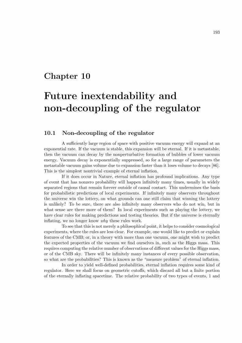
193

Chapter 10

Future inextendability andnon-decoupling of the regulator

10.1 Non-decoupling of the regulator

A sufficiently large region of space with positive vacuum energy will expand at anexponential rate. If the vacuum is stable, this expansion will be eternal. If it is metastable,then the vacuum can decay by the nonperturbative formation of bubbles of lower vacuumenergy. Vacuum decay is exponentially suppressed, so for a large range of parameters themetastable vacuum gains volume due to expansion faster than it loses volume to decays [86].This is the simplest nontrivial example of eternal inflation.

If it does occur in Nature, eternal inflation has profound implications. Any typeof event that has nonzero probability will happen infinitely many times, usually in widelyseparated regions that remain forever outside of causal contact. This undermines the basisfor probabilistic predictions of local experiments. If infinitely many observers throughoutthe universe win the lottery, on what grounds can one still claim that winning the lotteryis unlikely? To be sure, there are also infinitely many observers who do not win, but inwhat sense are there more of them? In local experiments such as playing the lottery, wehave clear rules for making predictions and testing theories. But if the universe is eternallyinflating, we no longer know why these rules work.

To see that this is not merely a philosophical point, it helps to consider cosmologicalexperiments, where the rules are less clear. For example, one would like to predict or explainfeatures of the CMB; or, in a theory with more than one vacuum, one might wish to predictthe expected properties of the vacuum we find ourselves in, such as the Higgs mass. Thisrequires computing the relative number of observations of different values for the Higgs mass,or of the CMB sky. There will be infinitely many instances of every possible observation,so what are the probabilities? This is known as the “measure problem” of eternal inflation.

In order to yield well-defined probabilities, eternal inflation requires some kind ofregulator. Here we shall focus on geometric cutoffs, which discard all but a finite portionof the eternally inflating spacetime. The relative probability of two types of events, 1 and

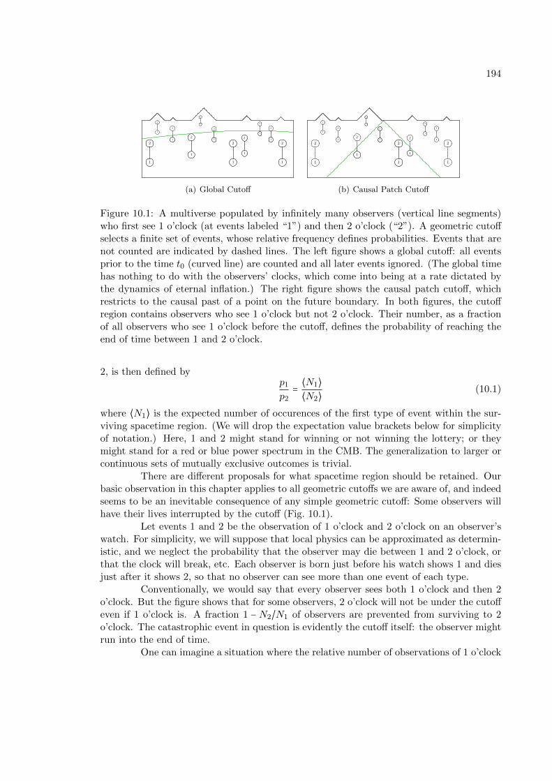
194

1

2

1

2

1

2

1

2

1

2

1

2

1

2

1

2

1

2

1

2

1

2

(a) Global Cutoff

1

2

1

2

1

2

1

2

1

2

1

21

2

1

2

1

2

1

2

1

2

(b) Causal Patch Cutoff

Figure 10.1: A multiverse populated by infinitely many observers (vertical line segments)who first see 1 o’clock (at events labeled “1”) and then 2 o’clock (“2”). A geometric cutoffselects a finite set of events, whose relative frequency defines probabilities. Events that arenot counted are indicated by dashed lines. The left figure shows a global cutoff: all eventsprior to the time t0 (curved line) are counted and all later events ignored. (The global timehas nothing to do with the observers’ clocks, which come into being at a rate dictated bythe dynamics of eternal inflation.) The right figure shows the causal patch cutoff, whichrestricts to the causal past of a point on the future boundary. In both figures, the cutoffregion contains observers who see 1 o’clock but not 2 o’clock. Their number, as a fractionof all observers who see 1 o’clock before the cutoff, defines the probability of reaching theend of time between 1 and 2 o’clock.

2, is then defined byp1

p2= ⟨N1⟩

⟨N2⟩(10.1)

where ⟨N1⟩ is the expected number of occurences of the first type of event within the sur-viving spacetime region. (We will drop the expectation value brackets below for simplicityof notation.) Here, 1 and 2 might stand for winning or not winning the lottery; or theymight stand for a red or blue power spectrum in the CMB. The generalization to larger orcontinuous sets of mutually exclusive outcomes is trivial.

There are different proposals for what spacetime region should be retained. Ourbasic observation in this chapter applies to all geometric cutoffs we are aware of, and indeedseems to be an inevitable consequence of any simple geometric cutoff: Some observers willhave their lives interrupted by the cutoff (Fig. 10.1).

Let events 1 and 2 be the observation of 1 o’clock and 2 o’clock on an observer’swatch. For simplicity, we will suppose that local physics can be approximated as determin-istic, and we neglect the probability that the observer may die between 1 and 2 o’clock, orthat the clock will break, etc. Each observer is born just before his watch shows 1 and diesjust after it shows 2, so that no observer can see more than one event of each type.

Conventionally, we would say that every observer sees both 1 o’clock and then 2o’clock. But the figure shows that for some observers, 2 o’clock will not be under the cutoffeven if 1 o’clock is. A fraction 1 −N2/N1 of observers are prevented from surviving to 2o’clock. The catastrophic event in question is evidently the cutoff itself: the observer mightrun into the end of time.

One can imagine a situation where the relative number of observations of 1 o’clock

195

and 2 o’clock is relevant to predicting the results of an experiment. Suppose that theobservers fall asleep right after seeing 1 o’clock. They wake up just before 2 o’clock withcomplete memory loss: they have no idea whether they have previously looked at theirwatches before. In this case, they may wish to make a prediction for what time they willsee. Since N2 < N1, by Eq. (10.1), p2 < p1: the observation of 2 o’clock is less probable thanthat of 1 o’clock. This is possible only if some observers do not survive to 2 o’clock.

The conclusion that time can end obtains whether or not the observers have mem-ory loss. Consider an observer who retains her memory. She is aware that she is about tolook at her watch for the first time or for the second time, so the outcome won’t be a surpriseon either occasion. But this does not contradict the possibility that some catastrophic eventmay happen between 1 and 2 o’clock. The figure shows plainly that this event does happento a nonzero fraction of observers. The only thing that changes when considering observerswho remember is the type of question we are likely to ask. Instead of asking about twoalternative events (1 or 2), we may find it more natural to ask about the relative probabilityof the two different possible histories that observers can have. One history,“1−” , consistsof seeing 1 o’clock and running into the cutoff. The alternative, “12”, consists of seeing 1o’clock and then seeing 2 o’clock. From Fig. 10.1 we see that N12 = N2 and N1− = N1 −N2.Since N1 > N2, we have p1− > 0: there is a nonzero probability for the history in which theobserver is disrupted by the end of time.

Outline and Frequently Asked Questions The probability for the end of time isnonzero for all geometric cutoffs. Its value, however, depends on the cutoff. In Sec. 10.2 wecompute the probability, per unit proper time, that we will encounter the end of time.

A number of objections may be raised against our conclusion that time can end.

Q: Can’t I condition on the end of time not happening?1

A: Certainly. This is like asking what the weather will be tomorrow, supposing thatit will not rain. It is a reasonable question with a well-defined answer: The sun willshine with probability x, and it will snow with probability 1 − x. But this does notmean that it cannot rain. If the end of time is a real possibility, then it cannot beprevented just by refusing to ask about it.

Q: In some measures, the cutoff is taken to later and later times. In this limit, theprobability to encounter the end of time surely approaches 0?

A: No. In all known measures of this type, an attractor regime is reached where thenumber of all types of events grows at the same exponential rate, including observers

1In the above example, this would force us to ask a trivial question (“What is the relative probabilityof seeing 1 or 2, for an observer whose history includes both 1 and 2?”), which yields the desired answer(p2/p1 = 1). For a more interesting example, consider an experiment that terminates at different timesdepending on the outcome, such as the Guth-Vanchurin paradox described in Sec. 10.4, or the decay of aradioactive atom. In such experiments it is tempting to propose that the experiment should be regardedto last for an amount of time corresponding to the latest possible (conventional) outcome, regardless ofthe actual outcome; and that any outcome (other than the end of time) should be counted only if theexperiment has been entirely completed before the cutoff, in the above sense. This proposal is not only futile(as described in the answer), but also ill-defined, since any event in the past light-cone of the event P canbe regarded as the beginning of an experiment that includes P .

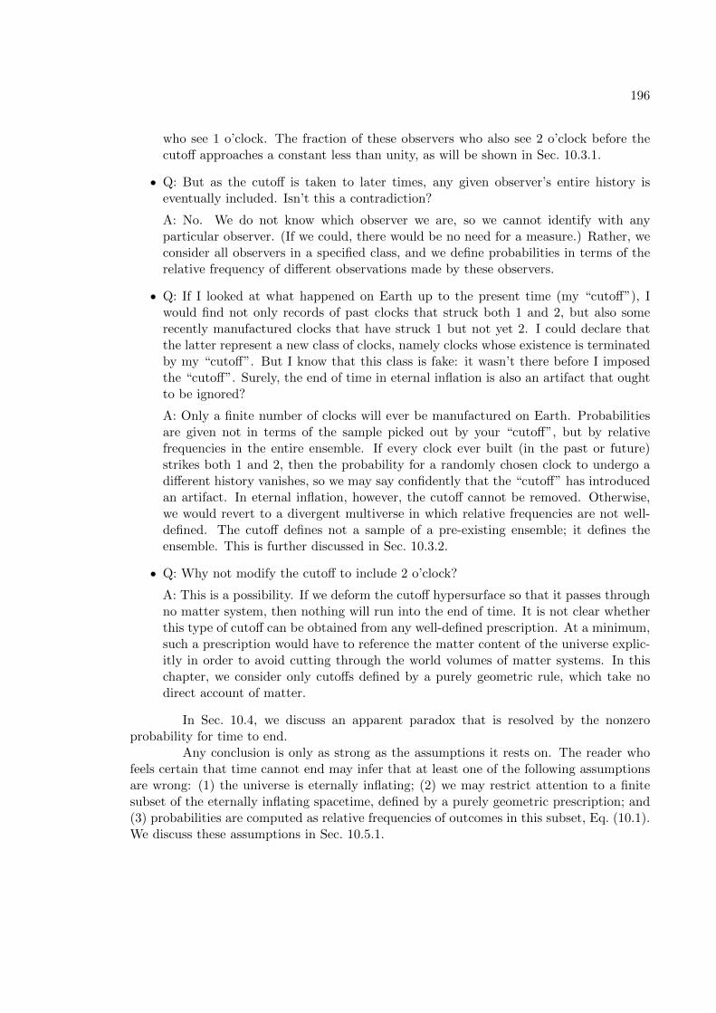
196

who see 1 o’clock. The fraction of these observers who also see 2 o’clock before thecutoff approaches a constant less than unity, as will be shown in Sec. 10.3.1.

Q: But as the cutoff is taken to later times, any given observer’s entire history iseventually included. Isn’t this a contradiction?

A: No. We do not know which observer we are, so we cannot identify with anyparticular observer. (If we could, there would be no need for a measure.) Rather, weconsider all observers in a specified class, and we define probabilities in terms of therelative frequency of different observations made by these observers.

Q: If I looked at what happened on Earth up to the present time (my “cutoff”), Iwould find not only records of past clocks that struck both 1 and 2, but also somerecently manufactured clocks that have struck 1 but not yet 2. I could declare thatthe latter represent a new class of clocks, namely clocks whose existence is terminatedby my “cutoff”. But I know that this class is fake: it wasn’t there before I imposedthe “cutoff”. Surely, the end of time in eternal inflation is also an artifact that oughtto be ignored?

A: Only a finite number of clocks will ever be manufactured on Earth. Probabilitiesare given not in terms of the sample picked out by your “cutoff”, but by relativefrequencies in the entire ensemble. If every clock ever built (in the past or future)strikes both 1 and 2, then the probability for a randomly chosen clock to undergo adifferent history vanishes, so we may say confidently that the “cutoff” has introducedan artifact. In eternal inflation, however, the cutoff cannot be removed. Otherwise,we would revert to a divergent multiverse in which relative frequencies are not well-defined. The cutoff defines not a sample of a pre-existing ensemble; it defines theensemble. This is further discussed in Sec. 10.3.2.

Q: Why not modify the cutoff to include 2 o’clock?

A: This is a possibility. If we deform the cutoff hypersurface so that it passes throughno matter system, then nothing will run into the end of time. It is not clear whetherthis type of cutoff can be obtained from any well-defined prescription. At a minimum,such a prescription would have to reference the matter content of the universe explic-itly in order to avoid cutting through the world volumes of matter systems. In thischapter, we consider only cutoffs defined by a purely geometric rule, which take nodirect account of matter.

In Sec. 10.4, we discuss an apparent paradox that is resolved by the nonzeroprobability for time to end.

Any conclusion is only as strong as the assumptions it rests on. The reader whofeels certain that time cannot end may infer that at least one of the following assumptionsare wrong: (1) the universe is eternally inflating; (2) we may restrict attention to a finitesubset of the eternally inflating spacetime, defined by a purely geometric prescription; and(3) probabilities are computed as relative frequencies of outcomes in this subset, Eq. (10.1).We discuss these assumptions in Sec. 10.5.1.

197

In Sec. 10.5.2, we discuss whether, and how, the nonzero probability for the end oftime may be observed. We point out that known predictions of various measures actuallyarise from the possibility that time can end. On the problematic side, this includes thefamous youngness paradox of the proper time cutoff; on the successful side, the predictionof the cosmological constant from the causal patch cutoff.

In Sec. 10.5.3, we discuss how the end of time fits in with the rest of physics. Thisdepends on the choice of cutoff. With the causal patch cutoff, there may be a relativelypalatable interpretation of the end of time which connects with the ideas of black holecomplementarity. The boundary of the causal patch is a kind of horizon, which can betreated as an object with physical attributes, including temperature. Matter systems thatencounter the end of time are thermalized at this horizon. This is similar to an outsideobserver’s description of a matter system falling into a black hole. What is radically new,however, is the statement that we might experience thermalization upon crossing the blackhole horizon.

This work was inspired by discussions with Alan Guth, who first described to usthe paradox mentioned in section 10.4. We understand that Guth and Vanchurin will bepublishing their own conclusions [85]. In taking seriously the incompleteness of spacetimeimplied by geometric cutoffs, our conclusion resembles a viewpoint suggested earlier by KenOlum [138].

10.2 The probability to encounter the cutoff

The phenomenon that time can end is universal to all geometric cutoffs. But therate at which this is likely to happen, per unit proper time τ along the observer’s worldline,is cutoff-specific. We will give results for five measures.

Causal patch The causal patch cutoff [24] restricts attention to the causal past of theendpoint of a single worldline (see Fig. 10.1). Expectation values are computed by averagingover initial conditions and decoherent histories in the causal patch. The end of time, in thiscase, is encountered by systems that originate inside the causal patch but eventually exitfrom it.

Our universe can be approximated as a flat FRW universe with metric

ds2 = −dτ2 + a(τ)2(dχ2 + χ2dΩ2) . (10.2)

Observers are approximately comoving (dχ/dτ = 0). We assume that the decay rate of ourvacuum, per unit four-volume, is much less than t−4

Λ . Then the decay can be neglectedentirely in computing where the boundary of the causal patch intersects the equal timesurfaces containing observers. The boundary is given by the de Sitter event horizon:

χE(τ) = ∫∞

τ

dτ ′

a(τ ′) . (10.3)

We consider all observers currently within the horizon: χ < χE(τ0), with τ0 = 13.7Gyr. This corresponds to a comoving volume Vcom = (4π/3)χE(τ0)3. Observers located at

198

χ leave the patch at a time τ ′ determined by inverting Eq. (10.3); in other words, theyreach the end of time at ∆τ ≡ τ ′ − τ0 from now. An (unnormalized) probability distributionover ∆τ is obtained by computing the number of observers that leave the causal patch atthe time τ0 +∆τ :

dp

d∆τ∝ 4πχE(τ0 +∆τ)2

a(τ0 +∆τ) . (10.4)

We compute a(τ) numerically using the best-fit cosmological parameters from the WMAP5data combined with SN and BAO [115]. From the distribution (10.4), we may obtain boththe median and the expectation value for ∆τ . We find that the expected amount of propertime left before time ends is

⟨∆τ⟩ = 5.3 Gyr . (10.5)

Time is unlikely to end in our lifetime, but there is a 50% chance that time will end withinthe next 3.7 billion years.

Light-cone time The light-cone time of an event is defined in terms of the volume ofits future light-cone on the future boundary of spacetime [26, 44, 28]. The light-cone timecutoff requires that we only consider events prior to some light-cone time t0; then the limitt0 →∞ is taken. It can be shown that the light-cone time cutoff is equivalent to the causalpatch cutoff with particular initial conditions [44]. Thus, the probability for an observer toencounter the end of time is the same as for the causal patch cutoff.

Fat geodesic The fat geodesic cutoff considers a fixed proper volume 4πd3/3 near atimelike geodesic [34]. To compute probabilities, one averages over an ensemble of geodesicsorthogonal to an initial hypersurface whose details will not matter. One can show that thegeodesics quickly become comoving after entering a bubble of new vacuum. Since ourvacuum is homogeneous, we may pick without loss of generality a fat geodesic at χ = 0.We shall neglect the effects of local gravitational collapse and approximate the universe asexpanding homogeneously. Equivalently, we take the proper distance d to be small comparedto the present curvature scale of the universe but large compared to the scale of clusters.These approximations are not essential, but they will simplify our calculation and save uswork when we later consider the scale factor cutoff.

We should only consider observers who are currently (τ0 = 13.7 Gyr) within thefat geodesic, with χ < d/a(τ0). An observer leaves the geodesic a time ∆τ later, withχ = d/a(τ0 +∆τ). The unnormalized probability distribution over ∆τ is

dp

d∆τ∝ 4π

d3(da/dτ)τ0+∆τ

a(τ0 +∆τ)4. (10.6)

From this distribution, we find numerically that the expected amount of proper time leftbefore the end of time is 5 Gyr. There is a 50% chance that time will end within the next3.3 billion years.

While the result is similar, there is an important formal difference between thefat geodesic and causal patch cutoffs. The boundary of the fat geodesic is a timelike hy-persurface, from which signals can propagate into the cutoff region. Boundary conditions

199

must therefore be imposed. When a system leaves the fat geodesic, time ends from itsown point of view. But an observer who remains within the cutoff region continues to seethe system and to communicate with it. The image of the system and its response to anycommunications are encoded in data specified on the timelike boundary. In practice, thesimplest way to determine these boundary conditions is to consider the global spacetimeand select a fat geodesic from it. This means that the fat geodesic is not a self-containeddescription. The content of the causal patch, by contrast, can be computed from its owninitial conditions without reference to a larger spacetime region.

Scale factor time Scale factor time is defined using a congruence of timelike geodesicsorthogonal to some initial hypersurface in the multiverse: dt ≡ Hdτ , where τ is the propertime along each geodesic and 3H is the local expansion of the congruence. This definitionbreaks down in nonexpanding regions such as dark matter halos; attempts to overcomethis limitation (e.g., Ref. [53]) remain somewhat ad-hoc. Here we use for H the Hubblerate of a completely homogeneous universe whose density agrees with the average densityof our universe. This does not yield a precise and general cutoff prescription, but it allowsus to compute an approximate rate at which we are likely to encounter the cutoff: in aneverywhere-expanding timelike geodesic congruence, the scale factor time cutoff is equivalentto the fat geodesic cutoff [34]. Hence it gives the same rate for time to end as the fat geodesiccutoff.

Proper time In the proper time cutoff, the characteristic timescale is the shortest Hubbletime of all eternally inflating vacua. In a realistic landscape, this is microscopically short,perhaps of order the Planck time [33]. Thus, time would be overwhelmingly likely to endin the next second:

dp

d∆τ≈ t−1

Pl . (10.7)

This is the famous “youngness paradox” in a new guise. The cutoff predicts that our obser-vations have superexponentially small probability, and that most observers are “Boltzmannbabies” who arise from quantum fluctuations in the early universe. Thus, this measure isalready ruled out phenomenologically at a high level of confidence [124, 81, 82, 83, 175, 122,84, 33].

10.3 Objections

Our intuition rebels against the conclusion that spacetime could simply cease toexist. In the introduction, we answered several objections that could be raised against theend of time. In this section, we will discuss two of these arguments in more detail.

10.3.1 The cutoff can not be encountered in a late-time limit

In some measure proposals, such as the proper time cutoff [120, 121], the scalefactor time cutoff [53], and the light-cone time cutoff [26], a limit is taken in which the

200

cutoff region is made larger and larger as a function of a time parameter t0:

p1/p2 = limt0→∞

N1(t0)/N2(t0) . (10.8)

Naively one might expect the cutoff observers to be an arbitrarily small fraction of allobservers in the limit t0 →∞. This turns out not to be the case.

One finds that the number of events of type I that have occurred prior to the timet is of the form

NI(t) = NI exp(γt) +O(σt) , (10.9)

with σ < γ ≈ 3. Thus, the growth approaches a universal exponential behavior at latetimes [76, 33, 44], independently of initial conditions. The ratio N1/N2 appearing inEq. (10.1) remains well-defined in the limit t0 →∞, and one obtains

p1

p2= N1

N2

. (10.10)

The constants NI , and thus the relative probabilities, depend on how the time variable isdefined; we will discuss some specific choices below.

Suppose that observers live for a fixed global time interval ∆t. Then a person diesbefore time t if and only if he was born before t−∆t. Therefore the number of births Nb isrelated to the number of deaths Nd by

Nd(t) = Nb(t −∆t) (10.11)

Using the time dependence of Nb given in (10.9), this can be rewritten

Nd(t)Nb(t)

≈ exp(−γ∆t) , (10.12)

up to a correction of order e(σ−γ)t which becomes negligible in the late time limit. Thus,the fraction of deaths to births does not approach unity as the cutoff is taken to infinity.The fraction of observers whose lives are interrupted by the cutoff is

Nc

Nb= 1 − exp(−γ∆t) (10.13)

where Nc = Nb −Nd is the number of cutoff observers.Since (10.13) is true for any time interval ∆t, it is equivalent to the following

simple statement: any system has a constant probability to encounter the end of time givenby

dp

dt= γ ≈ 3 (10.14)

This result can be interpreted as follows. Due to the steady state behavior of eternalinflation at late times, there is no way to tell what time it is. The exponential growth (10.9)determines a t0-independent probability distribution for how far we are from the cutoff,given by (10.14).

201

10.3.2 Hitting the cutoff is an artifact

Could it be that observers who run into the cutoff are an artifact, not to be takenseriously as a real possibility? Certainly they would not exist but for the cutoff. Yet, weargue that cutoff observers are a real possibility, because there is no well-defined probabilitydistribution without the cutoff; in particular, only the cutoff defines the set of allowed events.In order to convince ourselves of this, it is instructive to contrast this situation with onewhere a cutoff may introduce artifacts. We will consider two finite ensembles of observers,without reference to eternal inflation. We then restrict attention to a portion of eachensemble, defined by a cutoff. We find that this sample looks the same in both ensembles,and that it contains observers that run into the cutoff. In the first ensemble, these observersare an artifact of sampling; in the second, they are real. We will then explain why eternalinflation with a cutoff is different from both examples.

A cutoff on a finite ensemble defines a sample Consider a civilization which beginsat the time t = 0 and grows exponentially for a finite amount of time. (We will make noreference to a multiverse in this example.) Every person is born with a watch showing 1o’clock at the time of their birth, when they first look at it. One hour later, when theylook again, the watch shows 2 o’clock; immediately thereafter the person dies. After thetime t∗ ≫ 1 hour, no more people are born, but whoever was born before t∗ gets to liveout their life and observe 2 o’clock on their watch before they die. In this example, thereis a well-defined, finite ensemble, consisting of all observers throughout history and theirobservations of 1 and 2. The ensemble contains an equal number of 1’s and 2’s. Everyobserver in the ensemble sees both a 1 and a 2, each with 100% probability. No observermeets a premature demise before seeing 2.

Now suppose that we do not know the full ensemble described above. Instead, weare allowed access only to a finite sample drawn from it, namely everything that happenedby the time t, with 1 hour ≪ t < t∗. This sample contains many observers who died beforet; each of them will have seen both 1 and 2. We refer to these as “histories” of type 12.It also contains observers (those who were born after t − 1 hour) who are still alive. Eachof them has seen 1 but not yet 2, by the time t, which we refer to as a history of type1−. What do we say about these observers? Should we declare that there is a nonzeroprobability that an observer who sees 1 does not live to see 2? In fact, a finite sampleof a larger, unknown ensemble allows us to draw no conclusion of this kind, because wehave no guarantee that our sampling of the ensemble is fair. The true set of outcomes,and their relative frequency, is determined only by the full ensemble, not by our (possiblyunfaithful) sample of it. Similarly, if we had a considered a more complicated system, suchas observers with watches of different colors, etc., the relative frequency of outcomes in anysubset need not be the same as the relative frequency in the full ensemble, unless we makefurther assumptions.

If we examined the full ensemble, we could easily verify that every observer whosees 1 also lives to see 2. Thus we would learn that 1− was an artifact of our sampling:imposing a cutoff at fixed time produced a new class of events that does not exist (or moreprecisely, whose relative frequency drops to zero) once we take the cutoff away. Armed withthis knowledge, we could then invent an improved sampling method, in which the 1− cases

202

are either excluded, or treated as 12 events.As our second example, let us consider a civilization much like the previous one,

except that it perishes not by a sudden lack of births, but by a comet that kills everyoneat the time t∗. This, too, gives rise to a finite, well-defined ensemble of observations. Butunlike in the previous example, there is a larger number of 1’s than 2’s: not every observerwho sees a 1 lives to see a 2. Thus, the probabilities for the histories 12 and 1− satisfyp1− > 0, p12 < 1. Indeed, if we choose parameters so the population grows exponentially ona timescale much faster than 1 hour, most people in history who see 1 end up being killedby the comet rather than expiring naturally right after seeing 2; that is, p12 = 1 − p1− ≪ 1in this limit.

Again, we can contemplate sampling this ensemble, i.e., selecting a subset, byconsidering everything that happened prior to the time t < t∗. Note that this sample willlook identical to the finite-time sample we were given in the previous example. Again, wefind that there are apparently events of type 1−, corresponding to observers who have seen1 but not 2 by the time t. But in this example, it so happens that (i) events of type 1−actually do exist in the full ensemble, i.e., have nonzero true relative frequency; and (ii)assuming exact exponential growth, our sample is faithful: the relative frequency of 1− vs.12 in the sample (observers prior to t) is the same as in the full ensemble (observers in allhistory, up to t∗).2

We learn from the above two examples that a subset of an ensemble need not yieldreliable quantitative information about the relative frequencies of different outcomes, oreven qualitative information about what the allowed outcomes are. All of this informationis controlled only by the full ensemble. In both examples, the set of events that occuredbefore the time t < t∗ contain events of type 1−. But in the first example, these eventsare a sampling artifact and their true probability is actually 0. In the second example, 1−corresponds to a real possibility with non-zero probability.

The cutoff in eternal inflation defines the ensemble Now let us return to eternalinflation. In order to regulate its divergences, we define a cutoff that picks out a finitespacetime region, for example the region prior to some constant light-cone time t. Naively,this seems rather similar to the examples above, where we sampled a large ensemble byconsidering only the events that happened prior to a time t < t∗. But we learned that suchsamples cannot answer the question of whether the histories of type 1− are real or artifacts.To answer this question, we had to look at the full ensemble. We found in the first examplethat 1− was real, and in the second that 1− was an artifact, even though the sample lookedexactly the same in both cases. In eternal inflation, therefore, we would apparently need to“go beyond the cutoff” and consider the “entire ensemble” of outcomes, in order to decidewhether 1− is something that can really happen.

But this is impossible: the whole point of the cutoff was to define an ensemble.An infinite set is not a well-defined ensemble, so the set we obtained by imposing a cutoff isthe most fundamental definition of an ensemble available to us. We can argue about whichcutoff is correct: light-cone time, scale factor time, the causal patch, etc. But whatever

2Actually it is faithful only in the limit as t is much greater than the characteristic growth timescale ofthe civilization, because of the absence of any observers prior to t = 0.

203

the correct cutoff is, its role is to define the ensemble. It cannot be said to select a samplefrom a larger ensemble, namely from the whole multiverse, because this larger ensemble isinfinite, so relative abundances of events are not well-defined. If they were, we would havehad no need for a cutoff in the first place.

10.4 The Guth-Vanchurin paradox

Another way to see that the end of time is a real possibility is by verifying that itresolves a paradox exhibited by Guth and Vanchurin [80]. Suppose that before you go tosleep someone flips a fair coin and, depending on the result, sets an alarm clock to awakenyou after either a short time, ∆t ≪ 1, or a long time ∆t ≫ 1. Local physics dictates thatthere is a 50% probability to sleep for a short time since the coin is fair. Now supposeyou have just woken up and have no information about how long you slept. It is naturalto consider yourself a typical person waking up. But if we look at everyone who wakes upbefore the cutoff, we find that there are far more people who wake up after a short nap thana long one. Therefore, upon waking, it seems that there is no longer a 50% probability tohave slept for a short time.

How can the probabilities have changed? If you accept that the end of time is areal event that could happen to you, the change in odds is not surprising: although thecoin is fair, some people who are put to sleep for a long time never wake up because theyrun into the end of time first. So upon waking up and discovering that the world has notended, it is more likely that you have slept for a short time. You have obtained additionalinformation upon waking—the information that time has not stopped—and that changesthe probabilities.

However, if you refuse to believe that time can end, there is a contradiction. Theodds cannot change unless you obtain additional information. But if all sleepers wake, thenthe fact that you woke up does not supply you with new information.

Another way to say it is that there are two reference classes one could consider.When going to sleep we could consider all people falling asleep; 50% of these people havealarm clocks set to wake them up after a short time. Upon waking we could consider theclass of all people waking up; most of these people slept for a short time. These referenceclasses can only be inequivalent if some members of one class are not part of the other.This is the case if one admits that some people who fall asleep never wake up, but not ifone insists that time cannot end.

10.5 Discussion

Mathematically, the end of time is the statement that our spacetime manifold isextendible, i.e., that it is isometric to a proper subset of another spacetime. Usually, it isassumed that spacetime is inextendable [180]. But the cutoffs we considered regulate eternalinflation by restricting to a subset of the full spacetime. Probabilities are fundamentallydefined in terms of the relative abundance of events and histories in the subset. Then thefact that spacetime is extendible is itself a physical feature that can become part of anobserver’s history. Time can end.

204

10.5.1 Assumptions

We do not know whether our conclusion is empirically correct. What we haveshown is that it follows logically from a certain set of assumptions. If we reject the conclu-sion, then we must reject at least one of the following propositions:

Probabilities in a finite universe are given by relative frequencies of events orhistories This proposition is sometimes called the assumption of typicality. It forces usto assign a nonzero probability to encountering the end of time if a nonzero fraction ofobservers encounter it.

Even in a finite universe one needs a rule for assigning relative probabilities toobservations. This need is obvious if we wish to make predictions for cosmological obser-vations. But a laboratory experiment is a kind of observation, too, albeit one in which theobserver controls the boundary conditions. A comprehensive rule for assigning probabilitiescannot help but make predictions for laboratory experiments in particular. However, wealready have a rule for assigning probabilities in this case, namely quantum mechanics andthe Born rule, applied to the local initial conditions prepared in the laboratory. This mustbe reproduced as a special case by any rule that assigns probabilities to all observations [33].A simple way to achieve this is by defining probabilities as ratios of the expected numberof instances of each outcome in the universe, as we have done in Eq. (10.1).

Probabilities in an infinite universe are defined by a geometric cutoff Thisproposition states that the infinite spacetime of eternal inflation must be rendered finiteso that the above frequency prescription can be used to define probabilities. Moreover, itstates that a finite spacetime should be obtained by restricting attention to a finite subsetof the infinite multiverse.3 It is possible that the correct measure cannot be expressed ina geometric form. Imagine, for instance, a measure that makes “exceptions” for mattersystems that come into existence before the cutoff, allowing all events in their world volumeto be counted. A purely geometric prescription would have chopped part of the historyoff, but in this measure, the cutoff surface would be deformed to contain the entire historyof the system. Such a cutoff would depend not only on the geometry, but also on thematter content of spacetime.4 A more radical possibility is that the measure may notinvolve any kind of restriction to a finite portion of spacetime. For example, Noorbalaand Vanchurin [135], who exhibit a paradox similar to that described in Sec. 10.4, but donot allow for the possibility that time can end, advocate a nongeometric type of measure.If such a prescription could be made well-defined and consistent with observation (which

3We have considered measures in which the cutoff is completely sharp, i.e., described by a hypersurfacethat divides the spacetime into a region we keep and a region we discard. In fact this is not essential. Onecould smear out the cutoff by assigning to each spacetime event a weight that varies smoothly from 1 to 0over some region near the cutoff surface. There would still be a finite probability for time to end.

4We have not attempted to prove this statement, so it should be considered an additional assumption.Because the metric has information about the matter content, we cannot rule out that a geometric measurecould be formulated whose cutoff surfaces never intersect with matter. It seems unlikely to us that such acutoff could select a finite subset of the multiverse. A related possibility would be to define a global timecutoff such that typical observers live farther and farther from the cutoff in the limit as t→∞. This wouldinvalidate our analysis in Sec. 10.3.1, which assumed exponential growth in t.

205

seems unlikely to us), then one might escape the conclusion that time can end. Similarly,Winitzki [182, 183, 184] defined a measure where only finite spacetimes are considered, andin this measure there is no novel catastrophe like the end of time.

The universe is eternally inflating To prove this proposition wrong would be a dra-matic result, since it would seem to require a kind of fundamental principle dictating thatNature abhors eternal inflation. After all, eternal inflation is a straightforward consequenceof general relativity, assuming there exists at least one sufficiently long-lived field theoryvacuum with positive vacuum energy (a de Sitter vacuum). This assumption, in turn, seemsinnocuous and is well-motivated by observation: (1) The recent discovery of accelerated ex-pansion [151, 143], combined with the conspicuous lack of evidence that dark energy isnot a cosmological constant [115], suggests that our own vacuum is de Sitter. If this isthe case, the universe must be eternally inflating. (2) Slow-roll inflation solves the horizonand flatness problems. Its generic predictions agree well with the observed CMB powerspectrum. But slow-roll inflation requires a sufficiently flat scalar field potential. Eternalinflation requires only a local minimum and so is less fine-tuned. How could we considerslow-roll inflation, but exclude eternal inflation? — There are also theoretical motivationsfor considering the existence of de Sitter vacua: (3) In effective field theory, there is nothingspecial about potentials with a positive local minimum, so it would be surprising if theycould not occur in Nature. (4) String theory predicts a very large number of long-livedde Sitter vacua[41, 109, 55], allowing for a solution of the cosmological constant problemand other fine-tuning problems.

10.5.2 Observation

If we accept that time can end, what observable implications does this have?Should we expect to see clocks or other objects suddenly disappear? In measures such asscale factor time or light-cone time, the expected lifetime of stable systems is of order 5billion years right now, so it would be very unlikely for the end of time to occur in, say, thenext thousand years. And even if it did occur, it would not be observable. Any observerwho would see another system running into the end of time is by definition located to thecausal future of that system. If the cutoff surface is everywhere spacelike or null, as isthe case for the light-cone time cutoff and the causal patch cutoff, then the observer willnecessarily run into the cutoff before observing the demise of any other system.

Though the end of time would not be observable, the fact that time has not endedcertainly is observable. If a theory assigns extremely small probability to some event, thenthe observation of this event rules out the theory at a corresponding level of confidence.This applies, in particular, to the case where the event in question is time-not-having-ended.For example, Eq. (10.7) shows that the proper time measure is thus falsified.

An observation which indirectly probes the end of time is the value of the cos-mological constant. For definiteness consider the causal patch measure, which predicts acoincidence between the time when the observers live and the time when the cosmologicalconstant beings to dominate the expansion of the universe, tΛ ∼ tobs. This represents themost important phenomenological success of the measure, and we will now argue that it istied intimately to the end of time.

206

The most likely value of the cosmological constant is the one which leads to themost observers inside the causal patch. We will assume that there are a constant number ofobservers per unit mass, and will imagine scanning the possible values of tΛ ∼ 1/

√Λ with tobs

held fixed. It’s most useful to think of the distribution of values of log tΛ, where the preferredvalue is largely determined by two competing pressures. First, since the prior probability isflat in Λ, there is an exponential pressure in log tΛ toward lesser values. Second, if tΛ < tobs

there is an exponential pressure in tΛ (superexponential in log tΛ) toward greater values.This is a simple consequence of the fact that all matter is expelled from the causal patch atan exponential rate after vacuum domination begins. These two pressures lead to tobs ∼ tΛ.

The end of time is implicitly present in this argument. Suppose there are twogenerations of observers, one living at tΛ and another at 10tΛ. Even if local physics saysthat there are the same number of observers per unit mass in each generation, the sec-ond generation must be atypical, and hence have fewer members, if the prediction for thecosmological constant is to remain valid. Where are the missing members of the secondgeneration? The answer is that time has ended for them. They are not counted for thepurposes of any calculation, and so they do not exist. Clearly, the setup is identical to theobservers who see 1 o’clock and 2 o’clock discussed above.

In this chapter, we have considered sharp geometric cutoffs. However, intuitionfrom AdS/CFT [73, 26, 28] suggests that the cutoff should not be a completely sharp surface,but should be smeared out over a time of order tΛ. If the cutoff is smeared, there could beobservable consequences of approaching the end of time; the details would depend on theprecise prescription for smearing the cutoff.

10.5.3 Interpretation

The notion that time can come to an end is not completely new. Space and timebreak down at at singularities, which are guaranteed to arise in gravitational collapse [95].But our conclusion is more radical: the world can come to an end in any spacetime region,including regions with low density and curvature, because spacetime is incomplete.

One might speculate that semiclassical gravity breaks down on very large timescales, say t3Λ, the evaporation time for a large black hole in de Sitter space, or exp(πt2Λ),the recurrence time in de Sitter space. But in the most popular measures, we are likelyto encounter the end of time on the much shorter timescale tΛ. Perhaps one could inventa new cutoff that would push the end of time further into the future. But there is nowell-motivated candidate we are aware of, and, as we have discussed, one would be likely tolose some of the phenomenological success of the measures in solving, e.g., the cosmologicalconstant problem.

How can we make sense of our conclusion? Is there a way of thinking about it thatwould make us feel more comfortable about the end of time? Does it fit in with somethingwe already know, or is this a completely new phenomenon? The answer to this questionturns out to depend somewhat on which cutoff is used.

All measures One way to interpret the end of time is to imagine a computer just powerfulenough to simulate the cutoff portion of the eternally inflating spacetime. The simulationsimply stops at the cutoff. If the measure involves taking a late time limit, then one can

207

imagine building larger and larger computers that can simulate the spacetime until a latercutoff. These computers can be thought of as the definition of the cutoff theory, much inthe same way that lattice gauge theory is used. There is no physical significance to anytime after the cutoff.5 This is an interesting rephrasing of the statement of the end of time,but it does not seem to mitigate its radicality.

Causal patch only Our result appears to admit an intriguing interpretation if the causalpatch measure is used. The original motivation for the causal patch came from blackhole complementarity [170]. Consider the formation and evaporation of a black hole inasymptotically flat space. If this process is unitary, then the quantum state describing thecollapsing star inside the black hole is identical to the state of the Hawking radiation cloud.Since these two states are spacelike separated, two copies of the quantum state exist atthe same time. But before the star collapsed, there was only one copy. This amounts to“quantum xeroxing”, which is easily seen to conflict with quantum mechanics.

A way around this paradox is to note there is no spacetime point whose past light-cone contains both copies. This means that no experiment consistent with causality canactually verify that xeroxing has taken place. Thus, the paradox can be regarded as anartifact of a global viewpoint that has no operational basis. A theory should be capableof describing all observations, but it need not describe more than that. Geometrically, thismeans that it need not describe any system that cannot fit within a causal patch. What thexeroxing paradox teaches us is that we must not describe anything larger than the causalpatch if we wish to avoid inconsistencies in spacetimes with black holes.

But once we reject the global description of spacetime, we must reject it whetheror not black holes are present. In many cosmological solutions, including eternal inflation,the global spacetime is not accessible to any single experiment. This motivated the use ofthe causal patch as a cutoff to regulate the infinities of eternal inflation [32, 24].

Let us return to the black hole spacetime and consider the causal patch of anoutside observer. This patch includes all of the spacetime except for the interior of theblack hole. As Susskind has emphasized, to an outside observer, the causal patch is aconsistent representation of the entire world. The patch has a boundary, the stretchedhorizon of the black hole. This boundary behaves like a physical membrane, endowed withproperties such as temperature, tension, and conductivity. When another observer falls intothe black hole, the outside observer would say that he has been thermalized at the horizonand absorbed into the membrane degrees of freedom. Later the membrane evaporates andshrinks away, leaving behind a cloud of radiation.

It is very important to understand that this really is the unique and completedescription of the process from the outside point of view; the black hole interior does notcome into it. The process is no different, in principle, from throwing the second observerinto a fire and watching the smoke come out. Any object is destroyed upon reaching thehorizon. Yet, assuming that the black hole is large, the infalling observer would not noticeanything special when crossing the horizon. There is no contradiction between these two

5Ken Olum has pointed out for some time that one way to interpret a geometric cutoff is that “we arebeing simulated by an advanced civilization with a large but finite amount of resources, and at some pointthe simulation will stop.” The above interpretation adopts this viewpoint (minus the advanced civilization).

208

descriptions, since they agree as long as the two observers remain in causal contact. Oncethey differ, it is too late for either observer to send a signal to the other and tell a conflictingstory.

The end of time in the causal patch is an effect that fits well with the outsideobserver’s description. When the infalling observer enters the black hole, he is leaving thecausal patch of the outside observer. In the language of the present chapter, the outsideobserver defines a particular causal patch, and the inside observer encounters the end of timewhen he hits the boundary of this patch. We now see that there is a different, more satisfyinginterpretation: the inside observer is thermalized at the horizon. This interpretation invokesa relatively conventional physical process to explain why the inside observer ceases to exist.Time does not stop, but rather, the observer is thermalized. His degrees of freedom aremerged with those already existing at the boundary of the causal patch, the horizon.

If this interpretation is correct, it can be applied to black holes that form in theeternally inflating universe, where it modifies the theory of the infalling observer. It is nolonger certain that an infalling observer will actually make it to the horizon, and into theblack hole, to perish only once he hits the future singularity. Instead, time might end beforehe enters the black hole. How is this possible?

In the traditional discussion of black hole complementarity, one picks an observerand constructs the associated causal patch. It is impossible, by construction, for an observerto leave his own patch. In other words, time cannot end if we live in a causal patch centeredon our own worldline. In eternal inflation, however, one first picks a causal patch; thenone looks for observers in it. Some of these observers will be closer to the boundary andleave the patch sooner than others, who happen to stay in the patch longer. Equivalently,suppose we do want to begin by considering observers of a given type, such as an observerfalling towards a black hole. To compute probabilities, we must average over all causalpatches that contain such an observer. In some patches the observer will be initially farfrom the boundary, in others he will hit the boundary very soon. This yields a probabilitydistribution for the rate at which time ends.

Suppose, for example, that we attempted to jump into a black hole of mass m inour own galaxy (and neglect effects of gravitational tidal forces, matter near the black hole,etc.). Using the ensemble of causal patches defined in Ref. [44], one finds that time wouldprobably end before we reach the horizon, with probability 1 −O(m/tΛ). This probabilityis overwhelming if the black hole is much smaller than the cosmological horizon.

209

Chapter 11

Conclusion

We live in a universe with a positive cosmological constant. In terms of the fulleffective potential, we are sitting at a local minimum. There is little reason to believe thatthe effective potential contains only one local minimum. Indeed, string theory tells us thatthe effective potential contains an enormous number of minima. Therefore, there is strongreason to believe that our vacuum is metastable: we are in a local minimum, but not a globalone. From the perspective of some geodesic, our vacuum will eventually decay, nucleatingnew bubble universes. The nucleated universes will themselves decay, and the process willcontinue repeating until a universe with negative cosmological constant is created. Thisparticular geodesic will terminate at the big crunch singularity. However there will be othergeodesics that followed a different route and that are still in regions that are expanding. Inthis way, inflation is eternal and gives rise to an infinite multivere. In this thesis we haveattempted to take some steps towards finding a theory describing the multiverse.

As we have discussed, there is strong reason to believe that the complete theoryis not a local one. Rather, the theory lives on a codimension 1 surface. In the context ofthe multiverse, the natural place for the theory to live is on a spacelike equal time slice onfuture infinity. In the absence of knowledge of what this theory is, we have tried to makeprogress by trying to ascertain properties of this theory from contexts in which there existsa complete understanding of quantum gravity.

The case in which an in-principle full understanding of string theory is known isfor a stable spacetime with a negative cosmological constant (AdS space). For AdS space,the boundary lives on a timelike hypersurface. The complete nonperturbative descriptionof the bulk is given by a conformal field theory living on the boundary. This AdS/CFT cor-respondence realizes the holographic principle: the idea that spacetime is not fundamental,but rather emergent. In the context of AdS space, we know what the fundamental degreesof freedom are: they are the degrees of freedom of the CFT. In the context of the multiversewe lack this knowledge.

The first task needed for doing computations in the multiverse is to introducea late time cutoff (a measure). This cutoff is analogous to the large radius IR cutoff inAdS space. In AdS/CFT, the UV/IR relation is generally regarded as providing a relationbetween the bulk IR cutoff and the CFT cutoff. In chapter 8 we implemented a similarkind of cutoff in the context of the multiverse so as to define a measure which we called new

210

light-cone time. In chapter 9 we computed some of the predictions this measure gives. Theset of quantities that we can at this time compute is limited, as there are few quantities forwhich we know the prior probability distribution. Nevertheless, the cosmological constantis a notable exception since regardless of the precise form of the effective potential, nearany point Taylor expansion should be valid and doing this around values close to 0 givesa flat prior for the cosmological constant. Our results are encouraging, with the measureitself providing an explanation of the coincidence problem (the coincidence between the erawhen we are living and the onset of vacuum energy domination). It is notable that in theframework of chapter 9, the value of the cosmological constant is not set by the requirementthat it be sufficiently small so as to not disrupt galaxy formation [181]. Rather, the effectis due entirely to the measure. At the same time, in chapter 10 we found that all currentmeasures, including ours, face a serious difficulty: the late time cutoff does not decouple.Thus, our successful explanation of the cosmological constant comes at the expense of someother less palatable and more cataclysmic predictions about our future fate.

These difficulties were in part the motivation to reexamine the UV/IR relation.In chapter 2 we found that in fact a UV cutoff CFT would not appear to be sufficientto describe the portion of the bulk AdS out to some radius cutoff. Indeed, any attemptof this kind to decompose the CFT into different tensor factors does not lend itself to ageometric decomposition of the bulk. Perhaps then, this goes some way towards explainingwhy the analog of UV/IR that we implemented in the multiverse encountered difficultiesin chapter 10. For future work, it would therefore seem appropriate to first gain a betterhandle on constructing a regulated version of AdS/CFT before trying to apply it to themultiverse. One possibility, that we explored to some extent in chapter 2, is to replaceUV regularization of the CFT with something else so as to achieve full description of thedesired bulk region. Another possibility is to try to understand what it is in the bulk thata UV regulated CFT can describe. In the context of the multiverse, this would translateinto using a nongeometric measure.

In the other chapters in Part 1 we tried to make progress in addressing how thebulk is encoded in the CFT. To this effect, in chapters 3 and 4 we studied if it is possiblethat there is a duality between a subregion of the boundary and a subregion of the bulk.In chapters 5 and 6, we went on to consider how to reconstruct the bulk from boundarydata in the form of local operators. It would be interesting to apply these ideas to themultiverse and ask the analogous question of how would one use the data on future infinityto reconstruct the spacetime.

211

Bibliography

[1] Ahmed Almheiri and Joseph Polchinski. Models of AdS2 Backreaction and Hologra-phy. arXiv:1402.6334, 2014.

[2] M. Anderson. On uniqueness and diferentiability in the space of Yamabe metrics.Comm. Contemp. Math, 7:299–310, 2005.

[3] T. Aubin. Equations diferentielles non lineaires et probleme de Yamabe concernantla courbure scalaire. J. Math. Pures Appl., 55:269–296, 1976.

[4] Vijay Balasubramanian, Borun D. Chowdhury, Bartlomiej Czech, Jan de Boer, andMichal P. Heller. A hole-ographic spacetime. arXiv:1310.4204, 2013.

[5] Vijay Balasubramanian and Per Kraus. Spacetime and the holographic renormaliza-tion group. Phys. Rev. Lett., 83:3605–3608, 1999.

[6] Tom Banks, Michael R. Douglas, Gary T. Horowitz, and Emil J. Martinec. AdSdynamics from conformal field theory. hep-th/9808016, 1998.

[7] J.L.F. Barbon and E. Rabinovici. AdS Crunches, CFT Falls And Cosmological Com-plementarity. JHEP, 1104:044, 2011.

[8] J. M. Bardeen, B. Carter, and S. W. Hawking. The four laws of black hole mechanics.Commun. Math. Phys., 31:161, 1973.

[9] Claude Bardos, Gilles Lebeau, and Jeffrey Rauch. Sharp Sufficient Conditions forthe Observation, Control, and Stabilization of Waves from the Boundary. SIAM J.Control Optim., 30(5):1024–1065, 1992.

[10] J. D. Bekenstein. Black holes and the second law. Nuovo Cim. Lett., 4:737–740, 1972.

[11] Jacob D. Bekenstein. Black holes and entropy. Phys. Rev. D, 7:2333, 1973.

[12] Jacob D. Bekenstein. Generalized second law of thermodynamics in black hole physics.Phys. Rev. D, 9:3292, 1974.

[13] Jacob D. Bekenstein. Statistical black-hole thermodynamics. Phys. Rev. D, 12:3077,1975.

[14] Jacob D. Bekenstein. A universal upper bound on the entropy to energy ratio forbounded systems. Phys. Rev. D, 23:287, 1981.

212

[15] Jacob D. Bekenstein. Do we understand black hole entropy? 1994. Presented at the7th Marcel Grossmann Meeting on General Relativity.

[16] Iosif Bena. On the construction of local fields in the bulk of AdS(5) and other spaces.Phys.Rev., D62:066007, 2000.

[17] Eugenio Bianchi and Robert C. Myers. On the Architecture of Spacetime Geometry.2012. arXiv:1212.5183.

[18] J.J Bisognano and E.H. Wichmann. On the Duality Condition for a Hermitian ScalarField. J.Math.Phys., 16:985–1007, 1975.

[19] W. Boucher and G. W. Gibbons. Cosmic Baldness. Presented at 1982 Nufeld Work-shop on the Very Early Universe, Cambridge, England, Jun 21 - Jul 9, 1982.

[20] Raphael Bousso. A covariant entropy conjecture. JHEP, 07:004, 1999.

[21] Raphael Bousso. A covariant entropy conjecture. JHEP, 07:004, 1999.

[22] Raphael Bousso. Holography in general space-times. JHEP, 06:028, 1999.

[23] Raphael Bousso. The holographic principle. Rev. Mod. Phys., 74:825, 2002.

[24] Raphael Bousso. Holographic probabilities in eternal inflation. Phys. Rev. Lett.,97:191302, 2006.

[25] Raphael Bousso. TASI Lectures on the Cosmological Constant. Gen. Rel. Grav.,40:607–637, 2008.

[26] Raphael Bousso. Complementarity in the Multiverse. Phys. Rev., D79:123524, 2009.

[27] Raphael Bousso and Ben Freivogel. A paradox in the global description of the multi-verse. JHEP, 06:018, 2007.

[28] Raphael Bousso, Ben Freivogel, Stefan Leichenauer, and Vladimir Rosenhaus. Bound-ary definition of a multiverse measure. Phys.Rev., D82:125032, 2010.

[29] Raphael Bousso, Ben Freivogel, Stefan Leichenauer, and Vladimir Rosenhaus. Ageometric solution to the coincidence problem, and the size of the landscape as theorigin of hierarchy. Phys. Rev. Lett., 106:101301, 2011.

[30] Raphael Bousso, Ben Freivogel, Stefan Leichenauer, and Vladimir Rosenhaus. Eternalinflation predicts that time will end. Phys. Rev., D83:023525, 2011.

[31] Raphael Bousso, Ben Freivogel, Stefan Leichenauer, Vladimir Rosenhaus, and ClaireZukowski. Null Geodesics, Local CFT Operators and AdS/CFT for Subregions.Phys.Rev., D88:064057, 2013.

[32] Raphael Bousso, Ben Freivogel, and I-Sheng Yang. Eternal inflation: The inside story.Phys. Rev. D, 74:103516, 2006.

213

[33] Raphael Bousso, Ben Freivogel, and I-Sheng Yang. Boltzmann babies in the propertime measure. Phys. Rev., D77:103514, 2008.

[34] Raphael Bousso, Ben Freivogel, and I-Sheng Yang. Properties of the scale factormeasure. Phys.Rev., D79:063513, 2009.

[35] Raphael Bousso, Lawrence J. Hall, and Yasunori Nomura. Multiverse Understandingof Cosmological Coincidences. Phys. Rev., D80:063510, 2009.

[36] Raphael Bousso and Roni Harnik. The Entropic Landscape. Phys. Rev., D82:123523,2010.

[37] Raphael Bousso, Roni Harnik, Graham D. Kribs, and Gilad Perez. Predicting thecosmological constant from the causal entropic principle. Phys. Rev. D, 76:043513,2007.

[38] Raphael Bousso and Stefan Leichenauer. Star Formation in the Multiverse. Phys.Rev.,D79:063506, 2009.

[39] Raphael Bousso and Stefan Leichenauer. Predictions from Star Formation in theMultiverse. Phys.Rev., D81:063524, 2010.

[40] Raphael Bousso, Stefan Leichenauer, and Vladimir Rosenhaus. Light-sheets andAdS/CFT. Phys.Rev., D86:046009, 2012.

[41] Raphael Bousso and Joseph Polchinski. Quantization of four-form fluxes and dynam-ical neutralization of the cosmological constant. JHEP, 06:006, 2000.

[42] Raphael Bousso and Lisa Randall. Holographic domains of Anti-de Sitter space.JHEP, 04:057, 2002.

[43] Raphael Bousso and I-Sheng Yang. Landscape predictions from cosmological vacuumselection. Phys. Rev. D, 75:123520, 2007.

[44] Raphael Bousso and I-Sheng Yang. Global-Local Duality in Eternal Inflation. Phys.Rev., D80:124024, 2009.

[45] Brandon Bozek, Andreas Albrecht, and Daniel Phillips. Curvature Constraints fromthe Causal Entropic Principle. Phys. Rev., D80:023527, 2009.

[46] Pasquale Calabrese and John L. Cardy. Entanglement entropy and quantum fieldtheory. J.Stat.Mech., 0406:P06002, 2004.

[47] Jr. Callan, Curtis G. and Frank Wilczek. On geometric entropy. Phys.Lett., B333:55–61, 1994.

[48] Horacio Casini, Marina Huerta, and Robert C. Myers. Towards a derivation of holo-graphic entanglement entropy. JHEP, 05:036, 2011.

[49] S. Coleman and F. De Luccia. Gravitational effects on and of vacuum decay. Phys.Rev. D, 21:3305–3315, 1980.

214

[50] Bartlomiej Czech, Joanna L. Karczmarek, Fernando Nogueira, and Mark Van Raams-donk. Rindler Quantum Gravity. Class.Quant.Grav., 29:235025, 2012.

[51] Bartlomiej Czech, Joanna L. Karczmarek, Fernando Nogueira, and Mark Van Raams-donk. The Gravity Dual of a Density Matrix. Class.Quant.Grav., 29:155009, 2012.

[52] Jan de Boer, Erik P. Verlinde, and Herman L. Verlinde. On the holographic renor-malization group. JHEP, 08:003, 2000.

[53] Andrea De Simone, Alan H. Guth, Michael P. Salem, and Alexander Vilenkin. Pre-dicting the cosmological constant with the scale-factor cutoff measure. Phys.Rev.,D78:063520, 2008.

[54] Andrea De Simone and Michael P. Salem. The distribution of Omegak from thescale-factor cutoff measure. Phys.Rev., D81:083527, 2010.

[55] Frederik Denef and Michael R. Douglas. Distributions of flux vacua. JHEP, 05:072,2004.

[56] Freeman Dyson. Time without end: Physics and biology in an open universe. Rev.Mod. Phys., 51:447–460, 1979.

[57] Roberto Emparan. AdS / CFT duals of topological black holes and the entropy ofzero energy states. JHEP, 9906:036, 1999.

[58] Netta Engelhardt and Aron C. Wall. Extremal Surface Barriers. 2013.arXiv:1312.3699.

[59] Andrew M. Essin and David J. Griffiths. Quantum mechanics of the 1/x2 potential.American Journal of Physics, 74:109, 2006.

[60] Thomas Faulkner, Monica Guica, Thomas Hartman, Robert C. Myers, and MarkVan Raamsdonk. Gravitation from Entanglement in Holographic CFTs. JHEP,1403:051, 2014.

[61] Thomas Faulkner, Hong Liu, and Mukund Rangamani. Integrating out geometry:Holographic Wilsonian RG and the membrane paradigm. JHEP, 08:051, 2011.

[62] Brian Feldstein, Lawrence J. Hall, and Taizan Watari. Density perturbations and thecosmological constant from inflationary landscapes. Phys. Rev. D, 72:123506, 2005.

[63] Brian Feldstein, Lawrence J. Hall, and Taizan Watari. Landscape Predictions for theHiggs Boson and Top Quark Masses. Phys. Rev., D74:095011, 2006.

[64] A.Liam Fitzpatrick and Jared Kaplan. Scattering States in AdS/CFT. 2011.arXiv:1104.2597.

[65] Eanna E. Flanagan, Donald Marolf, and Robert M. Wald. Proof of classical versionsof the Bousso entropy bound and of the Generalized Second Law. Phys. Rev. D,62:084035, 2000.

215

[66] Ben Freivogel, Steven B. Giddings, and Matthew Lippert. Toward a theory of pre-cursors. Phys.Rev., D66:106002, 2002.

[67] Ben Freivogel, Matthew Kleban, Maria Rodriguez Martinez, and Leonard Susskind.Observational consequences of a landscape. JHEP, 03:039, 2006.

[68] Mitsutoshi Fujita, Tadashi Takayanagi, and Erik Tonni. Aspects of AdS/BCFT.JHEP, 11:043, 2011.

[69] Sijie Gao and Robert M. Wald. Theorems on gravitational time delay and relatedissues. Class. Quant. Grav., 17:4999–5008, 2000.

[70] Juan Garcıa-Bellido and Andrei Linde. Stationary solutions in Brans-Dicke stochasticinflationary cosmology. Phys. Rev. D, 52:6730–6738, 1995.

[71] Juan Garcıa-Bellido, Andrei Linde, and Dmitri Linde. Fluctuations of the gravita-tional constant in the inflationary Brans-Dicke cosmology. Phys. Rev. D, 50:730–750,1994.

[72] Juan Garcıa-Bellido and Andrei D. Linde. Stationarity of inflation and predictions ofquantum cosmology. Phys. Rev., D51:429–443, 1995.

[73] J. Garriga and A. Vilenkin. Holographic Multiverse. JCAP, 0901:021, 2009.

[74] J. Garriga and A. Vilenkin. Holographic Multiverse. JCAP, 0901:021, 2009.

[75] Jaume Garriga. Holographic description of vacuum bubbles. Prog. Theor. Phys.Suppl., 190:261–273, 2011.

[76] Jaume Garriga, Delia Schwartz-Perlov, Alexander Vilenkin, and Sergei Winitzki.Probabilities in the inflationary multiverse. JCAP, 0601:017, 2006.

[77] Jaume Garriga and Alexander Vilenkin. Anthropic prediction for Lambda and the Qcatastrophe. Prog. Theor. Phys. Suppl., 163:245–257, 2006.

[78] Steven B. Giddings. The Boundary S matrix and the AdS to CFT dictionary.Phys.Rev.Lett., 83:2707–2710, 1999.

[79] S. S. Gubser, I. R. Klebanov, and A. M. Polyakov. Gauge theory correlators fromnoncritical string theory. Phys. Lett., B428:105, 1998.

[80] Alan Guth and Vitaly Vanchurin. Private communication.

[81] Alan H. Guth. Inflation and eternal inflation. Phys. Rep., 333:555, 1983.

[82] Alan H. Guth. Inflationary models and connections to particle physics. 2000. astro-ph/0002188.

[83] Alan H. Guth. Inflation. 2004. astro-ph/0404546.

[84] Alan H. Guth. Eternal inflation and its implications. J. Phys., A40:6811–6826, 2007.

216

[85] Alan H. Guth and Vitaly Vanchurin. Eternal Inflation, Global Time Cutoff Measures,and a Probability Paradox. 2011. arXiv:1108.0665.

[86] Alan H. Guth and Erick J. Weinberg. Could the universe have recovered from a slowfirst-order phase transition? Nucl. Phys., B212:321–364, 1983.

[87] Lawrence J. Hall and Yasunori Nomura. Evidence for the Multiverse in the StandardModel and Beyond. Phys.Rev., D78:035001, 2008.

[88] Lawrence J. Hall and Yasunori Nomura. Evidence for the Multiverse in the StandardModel and Beyond. Phys. Rev., D78:035001, 2008.

[89] Alex Hamilton, Daniel N. Kabat, Gilad Lifschytz, and David A. Lowe. Holographicrepresentation of local bulk operators. Phys.Rev., D74:066009, 2006.

[90] Alex Hamilton, Daniel N. Kabat, Gilad Lifschytz, and David A. Lowe. Local bulkoperators in AdS/CFT: A Boundary view of horizons and locality. Phys.Rev.,D73:086003, 2006.

[91] Daniel Harlow and Douglas Stanford. Operator Dictionaries and Wave Functions inAdS/CFT and dS/CFT. 2011. arXiv:1104.2621.

[92] S. W. Hawking. Gravitational radiation from colliding black holes. Phys. Rev. Lett.,26:1344–1346, 1971.

[93] S. W. Hawking. Black hole explosions. Nature, 248:30–31, 1974.

[94] S. W. Hawking. Particle creation by balck holes. Commun. Math. Phys., 43:199, 1975.

[95] S. W. Hawking and G. F. R. Ellis. The large scale stucture of space-time. CambridgeUniversity Press, Cambridge, England, 1973.

[96] Idse Heemskerk, Donald Marolf, Joseph Polchinski, and James Sully. Bulk and Tran-shorizon Measurements in AdS/CFT. JHEP, 1210:165, 2012.

[97] Idse Heemskerk, Donald Marolf, Joseph Polchinski, and James Sully. Bulk and Tran-shorizon Measurements in AdS/CFT. JHEP, 1210:165, 2012.

[98] Idse Heemskerk and Joseph Polchinski. Holographic and Wilsonian RenormalizationGroups. JHEP, 06:031, 2011.

[99] Gary T. Horowitz and N. Itzhaki. Black holes, shock waves, and causality in theAdS/CFT correspondence. JHEP, 02:010, 1999.

[100] Veronika E. Hubeny. Precursors see inside black holes. Int. J. Mod. Phys., D12:1693–1698, 2003.

[101] Veronika E. Hubeny. Extremal surfaces as bulk probes in AdS/CFT. 2012.

[102] Veronika E. Hubeny and Henry Maxfield. Holographic probes of collapsing blackholes. 2013. arXiv:1312.6887.

217

[103] Veronika E. Hubeny and Mukund Rangamani. Causal Holographic Information.JHEP, 1206:114, 2012.

[104] Veronika E. Hubeny, Mukund Rangamani, and Tadashi Takayanagi. A covariantholographic entanglement entropy proposal. JHEP, 07:062, 2007.

[105] Ling-Yan Hung, Robert C. Myers, and Michael Smolkin. Some Calculable Contribu-tions to Holographic Entanglement Entropy. JHEP, 1108:039, 2011.

[106] Daniel Kabat and Gilad Lifschytz. Decoding the hologram: Scalar fields interactingwith gravity. 2013. arXiv:1311.3020.

[107] Daniel Kabat, Gilad Lifschytz, and David A. Lowe. Constructing local bulk observ-ables in interacting AdS/CFT. Phys.Rev., D83:106009, 2011.

[108] Daniel N. Kabat and M.J. Strassler. A Comment on entropy and area. Phys.Lett.,B329:46–52, 1994.

[109] Shamit Kachru, Renata Kallosh, Andrei Linde, and Sandip P. Trivedi. De Sitter vacuain string theory. Phys. Rev. D, 68:046005, 2003.

[110] Cynthia Keeler, Gino Knodel, and James T. Liu. What do non-relativistic CFTs tellus about Lifshitz spacetimes? JHEP, 1401:062, 2014.

[111] William R. Kelly and Aron C. Wall. Coarse-grained entropy and causal holographicinformation in AdS/CFT. 2013. arXiv:1309.3610.

[112] Esko Keski-Vakkuri. Bulk and boundary dynamics in BTZ black holes. Phys.Rev.,D59:104001, 1999.

[113] Alexei Kitaev and John Preskill. Topological entanglement entropy. Phys.Rev.Lett.,96:110404, 2006.

[114] Igor R. Klebanov, David Kutasov, and Arvind Murugan. Entanglement as a probe ofconfinement. Nucl.Phys., B796:274–293, 2008.

[115] E. Komatsu et al. Five-Year Wilkinson Microwave Anisotropy Probe (WMAP) Ob-servations: Cosmological Interpretation. Astrophys.J.Suppl., 180:330–376, 2009.

[116] Nima Lashkari, Michael B. McDermott, and Mark Van Raamsdonk. GravitationalDynamics From Entanglement ”Thermodynamics”. 2013. arXiv:1308.3716.

[117] J.M. Lee and T. H. Parker. The Yamabe Problem. Bull Amer. Math Soc.., 17:37–81,1987.

[118] Stefan Leichenauer and Vladimir Rosenhaus. AdS black holes, the bulk-boundarydictionary, and smearing functions. Phys.Rev., D88(2):026003, 2013.

[119] Aitor Lewkowycz and Juan Maldacena. Generalized gravitational entropy. JHEP,1308:090, 2013.

218

[120] A. Linde. Eternally existing selfreproducing chaotic inflationary universe. Phys. Lett.,B175:395–400, 1986.

[121] Andrei Linde. Sinks in the landscape, Boltzmann Brains, and the cosmological con-stant problem. JCAP, 0701:022, 2007.

[122] Andrei Linde. Towards a gauge invariant volume-weighted probability measure foreternal inflation. JCAP, 0706:017, 2007.

[123] Andrei Linde, Dmitri Linde, and Arthur Mezhlumian. From the big bang theory tothe theory of a stationary universe. Phys. Rev. D, 49:1783–1826, 1994.

[124] Andrei Linde, Dmitri Linde, and Arthur Mezhlumian. Nonperturbative amplificationsof inhomogeneities in a self-reproducing universe. Phys. Rev. D, 54:2504–2518, 1996.

[125] Andrei Linde and Arthur Mezhlumian. Stationary universe. Phys. Lett., B307:25–33,1993.

[126] Andrei Linde, Vitaly Vanchurin, and Sergei Winitzki. Stationary Measure in theMultiverse. JCAP, 0901:031, 2009.

[127] Juan Maldacena. The large N limit of superconformal field theories and supergravity.Adv. Theor. Math. Phys., 2:231, 1998.

[128] Juan Maldacena. Vacuum decay into Anti de Sitter space. 2010. arXiv:1012.0274.

[129] Juan Martin Maldacena. Wilson loops in large N field theories. Phys.Rev.Lett.,80:4859–4862, 1998.

[130] Juan Martin Maldacena. Eternal black holes in anti-de Sitter. JHEP, 0304:021, 2003.

[131] Juan Martin Maldacena. Non-Gaussian features of primordial fluctuations in singlefield inflationary models. JHEP, 0305:013, 2003.

[132] Juan Martin Maldacena, Jeremy Michelson, and Andrew Strominger. Anti-de Sitterfragmentation. JHEP, 9902:011, 1999.

[133] John March-Russell and Francesco Riva. Signals of Inflation in a Friendly StringLandscape. JHEP, 0607:033, 2006.

[134] Donald Marolf. States and boundary terms: Subtleties of Lorentzian AdS/CFT.JHEP, 05:042, 2005.

[135] Mahdiyar Noorbala and Vitaly Vanchurin. Geocentric cosmology: a new look at themeasure problem. 2010. arXiv:1006.4148.

[136] Lukas Novotny and Bert Hecht. Principles of Nano-Optics. Cambridge UniversityPress, Cambridge, 2012.

[137] Ken D. Olum and Delia Schwartz-Perlov. Anthropic prediction in a large toy land-scape. JCAP, 0710:010, 2007.

219

[138] Ken. Olum. Private Communication.

[139] H. Osborn and A.C. Petkou. Implications of conformal invariance in field theories forgeneral dimensions. Annals Phys., 231:311–362, 1994.

[140] Don N. Page. Return of the Boltzmann brains. 2006.

[141] Don N. Page. Cosmological Measures without Volume Weighting. JCAP, 0810:025,2008.

[142] Eric Perlmutter. A universal feature of CFT Renyi entropy. 2013. arXiv:1308.1083.

[143] S. Perlmutter et al. Measurements of Omega and Lambda from 42 high-redshiftsupernovae. Astrophys. J., 517:565–586, 1999.

[144] Daniel Phillips and Andreas Albrecht. Effects of Inhomogeneity on the Causal En-tropic prediction of Lambda. Phys.Rev., D84:123530, 2011.

[145] Levon Pogosian and Alexander Vilenkin. Anthropic predictions for vacuum energyand neutrino masses in the light of WMAP-3. JCAP, 0701:025, 2007.

[146] Joseph Polchinski. S matrices from AdS space-time. 1999. hep-th/9901076.

[147] Joseph Polchinski. The cosmological constant and the string landscape. 2006. hep-th/0603249.

[148] Joseph Polchinski, Leonard Susskind, and Nicolaos Toumbas. Negative energy, super-luminosity and holography. Phys.Rev., D60:084006, 1999.

[149] Soo-Jong Rey and Vladimir Rosenhaus. Scanning Tunneling Macroscopy, Black Holes,and AdS/CFT Bulk Locality. 2014. arXiv:1403.3943.

[150] Soo-Jong Rey and Jung-Tay Yee. Macroscopic strings as heavy quarks in large Ngauge theory and anti-de Sitter supergravity. Eur.Phys.J., C22:379–394, 2001.

[151] Adam G. Riess et al. Observational evidence from supernovae for an acceleratinguniverse and a cosmological constant. Astron. J., 116:1009–1038, 1998.

[152] Vladimir Rosenhaus. Holography for a small world. 2013. arXiv:1309.4526.

[153] Vladimir Rosenhaus and Michael Smolkin. Entanglement Entropy: A PerturbativeCalculation. 2014. arXiv:1403.3733.

[154] Shinsei Ryu and Tadashi Takayanagi. Holographic derivation of entanglement entropyfrom AdS/CFT. Phys. Rev. Lett., 96:181602, 2006.

[155] Michael P. Salem. Negative vacuum energy densities and the causal diamond measure.Phys.Rev., D80:023502, 2009.

[156] R. Schoen. Conformal deformation of a Riemannian metric to constant scalar curva-ture. J. Diff. Geom., 20:479–495, 1984.

220

[157] Delia Schwartz-Perlov. Probabilities in the Arkani-Hamed-Dimopolous-Kachru land-scape. J.Phys., A40:7363–7374, 2007.

[158] Delia Schwartz-Perlov. Anthropic prediction for a large multi-jump landscape. JCAP,0810:009, 2008.

[159] Delia Schwartz-Perlov and Alexander Vilenkin. Probabilities in the Bousso-Polchinskimultiverse. JCAP, 0606:010, 2006.

[160] Delia Schwartz-Perlov and Alexander Vilenkin. Measures for a TransdimensionalMultiverse. JCAP, 1006:024, 2010.

[161] Sergey N. Solodukhin. Entanglement entropy, conformal invariance and extrinsicgeometry. Phys.Lett., B665:305–309, 2008.

[162] Dam T. Son and Andrei O. Starinets. Minkowski space correlators in AdS / CFTcorrespondence: Recipe and applications. JHEP, 0209:042, 2002.

[163] Andrew Strominger. The dS/CFT correspondence. JHEP, 10:034, 2001.

[164] Andrew Strominger. Inflation and the dS/CFT correspondence. JHEP, 11:049, 2001.

[165] L. Susskind and E. Witten. The holographic bound in Anti-de Sitter space. 1998.

[166] Leonard Susskind. The world as a hologram. J. Math. Phys., 36:6377–6396, 1995.

[167] Leonard Susskind. Holography in the flat space limit. pages 98–112, 1998. Pre-sented at General relativity and relativistic astrophysics. Proceedings: 8th CanadianConference, Montreal.

[168] Leonard Susskind. The anthropic landscape of string theory. 2003. hep-th/0302219.

[169] Leonard Susskind and Larus Thorlacius. Gedanken experiments involving black holes.Phys. Rev., D49:966–974, 1994.

[170] Leonard Susskind, Larus Thorlacius, and John Uglum. The stretched horizon andblack hole complementarity. Phys. Rev. D, 48:3743, 1993.

[171] Leonard Susskind and Nicolaos Toumbas. Wilson loops as precursors. Phys.Rev.,D61:044001, 2000.

[172] G. ’t Hooft. Dimensional reduction in quantum gravity. 1993. gr-qc/9310026.

[173] Tadashi Takayanagi. Holographic Dual of BCFT. Phys. Rev. Lett., 107:101602, 2011.

[174] Daniel Tataru. Unique continuation problems for partial differential equations. InGeometric Methods in Inverse Problems and PDE Control, volume 137 of The IMAVolumes in Mathematics and its Applications. Springer, 2004.

[175] Max Tegmark. What does inflation really predict? JCAP, 0504:001, 2005.

221

[176] N. Trudinger. Remarks concerning the conformal deformation of Riemannian struc-tures on compact manifolds. Ann. Scuola Norm. Sup. Pisa, 22:265–274, 1968.

[177] William G. Unruh and Nathan Weiss. Acceleration Radiation in Interacting FieldTheories. Phys.Rev., D29:1656, 1984.

[178] Vitaly Vanchurin. Geodesic measures of the landscape. Phys. Rev. D, 75:023524,2007.

[179] Vitaly Vanchurin and Alexander Vilenkin. Eternal observers and bubble abundancesin the landscape. Phys.Rev., D74:043520, 2006.

[180] Robert M. Wald. General Relativity. The University of Chicago Press, Chicago, 1984.

[181] Steven Weinberg. Anthropic bound on the cosmological constant. Phys. Rev. Lett.,59:2607, 1987.

[182] Sergei Winitzki. A volume-weighted measure for eternal inflation. Phys. Rev.,D78:043501, 2008.

[183] Sergei Winitzki. Reheating-volume measure for random-walk inflation. Phys. Rev.,D78:063517, 2008.

[184] Sergei Winitzki. Reheating-volume measure in the landscape. Phys. Rev., D78:123518,2008.

[185] Edward Witten. Anti-de Sitter space and holography. Adv. Theor. Math. Phys., 2:253,1998.

[186] Edward Witten. Quantum gravity in de Sitter space. 2001. hep-th/0106109.

[187] H. Yamabe. On a deformation of Riemannian structures on compact manifolds. OskaMath J.., 12:21–37, 1960.

The Holographic Principle and the Emergence of Spacetime ...

Documents

Transcript of The Holographic Principle and the Emergence of Spacetime ...