arX

iv:h

ep-p

h/96

0620

8v2

25

Aug

199

7

INFLATON DECAY IN DE SITTER SPACETIME

D. Boyanovsky(a), R. Holman(b), S. Prem Kumar(b)

(a) Department of Physics and Astronomy, University of Pittsburgh, PA.15260,U.S.A.

(b) Department of Physics, Carnegie Mellon University, Pittsburgh, PA.15213, U.S.A.

Abstract

We study the decay of scalar fields, in particular the inflaton, into lighter

scalars in a De Sitter spacetime background. After providing a practical def-

inition of the rate, we focus on the case of an inflaton interacting with a

massless scalar field either minimally or conformally coupled to the curvature.

The evolution equation for the expectation value of the inflaton is obtained to

one loop order in perturbation theory and the decay rate is recognized from

the solution. We find the remarkable result that this decay rate displays an

equilibrium Bose-enhancement factor with an effective temperature given by

the Hawking temperature H/2π, where H is the Hubble constant. This con-

tribution is interpreted as the “stimulated emission” of bosons in a thermal

bath at the Hawking temperature. In the context of new inflation scenarios,

we show that inflaton decay into conformally coupled massless fields slows

down the rolling of the expectation value. Decay into Goldstone bosons is

also studied. Contact with stochastic inflation is established by deriving the

Langevin equation for the coarse-grained expectation value of the inflaton field

to one-loop order in this model. We find that the noise is gaussian and cor-

related (colored) and its correlations are related to the dissipative (“decay”)

kernel via a generalized fluctuation-dissipation relation.

Typeset using REVTEX

1

I. INTRODUCTION

Non-equilibrium processes play a fundamental role in cosmological scenarios motivatedby particle physics models. Processes such as thermalization, reheating and particle decayare important ingredients in most theoretical scenarios that attempt a description of earlyuniverse cosmology [1–4]. An important ingredient underlying most attempts at a descrip-tion of inflationary cosmologies is that of equilibration, which is tacitly assumed wheneverquasi-equilibrium methods are invoked in their study, such as effective potentials and finitetemperature field theory.

The concept of quasi-equilibrium during an inflationary stage requires a careful under-standing of two different time scales. One is the expansion time scale tH = H−1, whereH is the Hubble parameter, while the other is the field relaxation time scale, tr. A quasi-equilibrium situation obtains whenever tr << tH since in this case particle physics processesoccur much faster than the Universe expands allowing fields to respond quickly to any changesin the thermodynamic variables.

Can the inflaton of inflationary cosmologies be treated as being in quasi-equilibrium?The answer to this question depends crucially on the various processes that contribute tothe dynamical relaxation of this field. Some of these processes are the decay of the inflatoninto lighter scalars or fermions, as well as collisions that, while they leave the total numberof particles fixed, will change the phase space distribution of these particles.

In this paper we wish to understand the effects of coupling the inflaton to lighterscalars during the inflationary era. Single particle decay of the inflaton into lighter scalarsor fermions in the post-inflationary era, when space-time can be well approximated by aMinkowski metric, is by now fairly well understood within the context of the “old-reheating”scenario [6–9], but it is much less understood during the early stages of inflation.

In saying this, we have to distinguish between the various models of inflation. In “old” or“extended” inflation [10], the inflaton is trapped in a metastable minimimum, from which itexits eventually via the nucleation of bubbles of the true vacuum phase. A critical parameterin these models is the nucleation rate, which is typically calculated assuming that the fieldis equilibrated [3,4,11]. Such an assumption will only be justified if the relaxation time ofthe inflaton in the metastable phase, i.e. in De Sitter space, is much smaller than the timescale for nucleation of a critical bubble.

In “new” or “chaotic” inflationary scenarios [7], the supraluminal expansion of the uni-verse is driven by the so-called “slow-roll” dynamics of the inflaton. Typically, this is studiedvia the zero or finite temperature effective potential. In doing this, the assumption of quasi-equilibrium is made, in that one can replace the actual field dynamics, by that given bya static quantity, the effective potential. This assumption must be checked, and one wayof doing that is by considering the evolution of the inflaton in the presence of couplings toother fields and computing the field relaxation rate. In particular, if dissipative processesassociated with the “decay” of the inflaton field into lighter scalars are efficient during theslow-roll stage in new or chaotic inflationary scenarios, then these may result in a furtherslowing down of the inflaton field as it rolls down the potential hill.

2

Finally, there is the stochastic inflation approach advocated by Starobinskii [12]. In thisscenario, inflationary dynamics is studied with a stochastic evolution equation for the inflatonfield with a gaussian white noise that describes the microscopic fluctuations. As pointed outby Hu and collaborators [13] and Habib and Kandrup [14,15], noise and dissipation arerelated via a fundamental generalized fluctuation-dissipation theorem and must be treatedon the same footing.

In this article we study the process of relaxation of the inflaton field via the decay intomassless scalar particles in De Sitter space-time with the goal of understanding the modifi-cations in the decay rates and the relevant time scales as compared to those in Minkowskispace-time. Our study focuses on the description of these processes within “old/extended” and “new” inflationary scenarios. Within “old” inflation we study the situation in whichthe inflaton field oscillates around the metastable minimum (before it eventually tunnels)and decays into massless scalars. In the case of “new” inflation, we address the situation ofthe inflaton rolling down a potential hill, near the maximum of the potential, to understandhow the process of “decay” introduces dissipative contributions to the inflaton evolution.

We also establish contact with stochastic inflation by deriving the Langevin (stochastic)equation for the inflaton field, and analyzing the generalized fluctuation-dissipation relationbetween the dissipation kernel resulting from the “decay” into massless scalars and thecorrelations of the stochastic noise.

At this point we would like to make precise the meaning of “decay” in a time dependentbackground. The usual concept of the transition rate in Minkowski space, i.e. the transitionprobability per unit volume per unit time for a particular (in) state far in the past toan (out) state far into the future is no longer applicable in a time dependent background.Relaxing this definition to finite time intervals ( for example by obtaining the transitionprobability from some ti to some tf) would yield a time dependent quantity affected by theambiguities of the definition of particle states. In Minkowski space-time the existence oftime translational invariance allows a spectral representation of two-point functions and thetransition rate (or decay rate) is related to the imaginary part of the self-energy on shell.Such a correspondence is not available in a time dependent background. Furthermore thetime evolution of a scalar field is damped because of the red-shifting of the energy due to theexpanding background even in the absence of interactions. In particular in De Sitter spacethis damping is exponential and any other exponential damping arising from interactionswill be mixed with the gravitational red-shift.

We propose to define the “decay rate” as the contribution to the exponential damping ofthe inflaton evolution due to the interactions with other fields, which is clearly recognizedthrough the dependence on the coupling to these fields. This practical definition then arguesthat in order to recognize such a “decay rate” we must study the real-time dynamics of thenon-equilibrium expectation value of the inflaton field in interaction with other fields, andthe identification of this rate should transpire from the actual evolution of this expectationvalue.

Although the methods presented in this article can be generalized to arbitrary spatiallyflat FRW cosmologies and include decay of a heavy inflaton into lighter scalars, we study

3

the simpler but relevant case of inflaton decay into massless scalars in De Sitter space-time.This case affords an analytic perturbative treatment that illuminates the relevant physicalfeatures.

The article is organized as follows: in section II we present a brief pedagogical review ofthe closed time path formalism and the derivation of the non-equilibrium Green’s functionsfor free fields in De Sitter spacetime. In section III the model is defined and the methodsto obtain the evolution equation are summarized. Here we study several cases, includingminimal and conformal coupling and the slow-roll regime. We obtain the remarkable resultthat the decay rate can be understood from stimulated emission in a bath at the Hawkingtemperature. In section IV we study the effect of Goldstone bosons on the inflaton evolution,pointing out that Goldstone bosons are necessarily always minimally coupled. In section Vwe make contact with stochastic inflation, derive the stochastic Langevin equation for theinflaton zero mode and obtain the dissipative kernel and the noise correlation function,which are related by a generalized fluctuation-dissipation theorem. The resulting noise isgaussian but colored. In section VI we summarize our results and propose new lines ofstudy. An appendix is devoted to a detailed derivation, establishing the consistency of theflat-space limits of the analytic structure of the dissipative kernel in De Sitter space-time,with Minkowskian calculations.

II. NON-EQUILIBRIUM FIELD THEORY

A. The Closed Time Path Formalism

As mentioned in the introduction we will be studying the real-time evolution of the zeromode of the inflaton in a universe with a time-dependent background metric. Furthermore,we will restrict our investigations to perturbative phenomena in theories in which the inflatoninteracts with other matter fields in a De Sitter universe. We will be primarily concerned withdefining and calculating quantities such as the perturbative “decay rate” of the inflaton. Forstudies of non-perturbative particle production in non-equilibrium situations see [19] (andreferences therein). Calculation of particle production in curved spacetime has also beendone using the Boguliubov transformations; see for e.g [23]

The tools required for studying time-dependent phenomena in quantum field theories havebeen available for quite some time, and were first used by Schwinger [16] and Keldysh [17].There are many articles in the literature using these techniques to study time-dependentproblems [18,19]. However, these techniques have not yet become an integral part of theavailable methods for studying field theory in extreme environments. We thus present aconcise pedagogical introduction to the subject for the non-practitioner.

The non-equilibrium or time dependent description of a system is determined by the timeevolution of the density matrix that describes it. This is in turn described by the Liouvilleequation (in the Schrodinger picture):

ih∂ρ(t)

∂t= [H(t), ρ(t)]. (2.1)

4

Here we have allowed for an explicitly time dependent Hamiltonian which is in fact the casein an expanding universe. The formal solution of the Liouville equation is,

ρ(t) = U(t)ρiU−1(t) (2.2)

where ρi is the initial density matrix specified at some initial time t = 0. The time dependentexpectation value of an operator is then easily seen to be,

〈O〉(t) = Tr[ρiU−1(t)OU(t)]/Tr[ρi] (2.3)

In most cases of interest the initial density matrix is either a thermal one or a pure statecorresponding to the ground state of some initial Hamiltonian. In either case,

ρi = e−βHi (2.4)

Hi = H(t < 0). (2.5)

The ground state of Hi can be projected out by taking the β → ∞ limit. To study stronglyout of equilibrium situations it is usually convenient to introduce a time-dependent Hamilto-nian H(t) such that H(t) = Hi for −∞ ≤ t ≤ 0 and H(t) = Hevol(t) for t > 0 where Hevol(t)is the evolution hamiltonian that determines the dynamics of the theory.

For thermal initial conditions, eq (2.3) can be written in a more illuminating form bychoosing an arbitrary time T < 0 for which U(T ) = exp[−iTHi] so that we may writeexp[−βHi] = exp[−iHi(T−iβ−T )] = U(T−iβ, T ). Inserting the identity U−1(T )U(T ) = 1,commuting U−1(T ) with ρi and using the composition property of the evolution operator,we get

〈O〉(t)= Tr[U(T − iβ, t)OU(t, T )]/Tr[U(T − iβ, T )] (2.6)

= Tr[U(T − iβ, T )U(T, T ′)U(T ′, t)OU(t, T )]/Tr[U(T − iβ, T )] (2.7)

where we have introduced an arbitrary large positive time T ′. The numerator now representsthe process of evolving from T < 0 to t, inserting the operator O, evolving to a large positivetime T ′, and backwards from T ′ to T and down the imaginary axis to T − iβi. Eventuallyone takes T → −∞;T ′ → ∞. This method can be easily generalised to obtain real timecorrelation functions of a string of operators.

As usual, an operator insertion may be achieved by introducing sources into the timeevolution operators, and taking a functional derivative with respect to the source. Thus weare led to the following generating functional, in terms of time evolution operators in thepresence of sources

Z[J+, J−, Jβ] = Tr[U(T − iβ, T ; Jβ)U(T, T ′; J−)U(T ′, T ; J+)] (2.8)

with T → −∞;T ′ → ∞. One can obtain a path integral representation for the generatingfunctional [16–21] by inserting a complete set of field eigenstates between the time evolutionoperators,

5

Z[J+, J−, Jβ] =∫

DΣDΣ1DΣ2

∫

DΣ+DΣ−DΣβei∫ T ′

TL[Σ+,J+]−L[Σ−,J−] × (2.9)

ei∫ T−iβ

TL[Σβ ,Jβ ].

The above expression for the generating functional is a path integral defined on a complextime contour. Since this path integral actually represents a trace, the field operators at theboundary points have to satisfy the following conditions:

Σ+(T ) = Σβ(T − iβ) = Σ, (2.10)

Σ+(T ′) = Σ−(T ′) = Σ2,

Σ−(T ) = Σβ(T ) = Σ1.

The superscripts (+) and (−) refer to the forward and backward parts of the time contour,while the superscript (β) refers to the imaginary time part of the contour. In the limitT → −∞ it can be shown that cross-correlations between fields defined at real times andthose defined on the imaginary time contour, vanish due to the Riemann−Lebesgue lemma.The fact that the density matrix is thermal for t < 0 shows up in the boundary conditionon the fields and the Green’s functions. Thus the generating functional for calculating realtime correlation functions simplifies to:

Z[J+, J−] = exp

i∫ T ′

Tdt[Lint(−iδ/δJ+) −Lint(iδ/δJ−)]

×

exp

i

2

∫ T ′

Tdt1

∫ T ′

Tdt2Ja(t1)Jb(t2)Gab(t1, t2)

(2.11)

with a, b = +,−. We will now proceed to a calculation of the non-equilibrium Green’sfunctions in De Sitter spacetime

B. Non-equilibrium Green’s Functions In De Sitter

To obtain the non-equilibrium Green’s functions we focus on a free scalar field Σ inan FRW background metric [20]. The generating functional of non-equilibrium Green’sfunctions is written in terms of a path integral along the closed time path (CTP) (2.11) witha free Lagrangian density, L0(Σ

±) given by

L0(Σ±) =

1

2[a3(t)Σ+2 − a(t)(~∇Σ+)

2 − a3(t)(M2 + ξR)Σ+2] (2.12)

−[+ −→ −]

where R = 6(a/a+ a2/a2).We prepare the system such that it is thermal for t < 0 with temperature 1/β. At t = 0,

we switch the interactions on and follow the resulting time evolution of the coupled fields.

6

As seen in the previous section, the CTP formulation of non-equilibrium field theory imposescertain boundary conditions on the fields (2.10).

Rewriting the Lagrangian as a quadratic form in Σ± we obtain the Green’s functionequation,

[∂2

∂t2+ 3

a

a

∂

∂t− ∇2

a2+ (M2 + ξR)]G(x, t; x′, t′) =

δ4(x− x′)

a3/2(t)a3/2(t′). (2.13)

We use spatial translational invariance to define,

Gk(t, t′) =

∫

d3xei~k·~xG(x, t; 0, t′), (2.14)

so that the spatial Fourier transform of the Green’s function obeys,

[d2

dt2+ 3

a

a

d

dt+k2

a2+ (M2 + ξR)]Gk(t, t

′) =δ(t− t′)

a3/2(t)a3/2(t′). (2.15)

The solution can be cast in a more familiar form by writing

Gk(t, t′) =

fk(t, t′)

a3/2(t)a3/2(t′), (2.16)

so that the function fk(t, t′) obeys the second order differential equation,

[d2

dt2− (

3a

2a+

3a2

4a2) +

k2

a2+ (M2 + ξR)]fk(t, t

′) = δ(t− t′). (2.17)

The general solution of this equation is of the form

fk(t, t′) = fk

>(t, t′)Θ(t− t′) + fk<(t, t′)Θ(t′ − t), (2.18)

where fk> and fk

< are solutions to the homogeneous equation obeying the appropriateboundary conditions. They can be expanded in terms of normal mode solutions to thehomogeneous equation:

fk>(t, t′) = A>Uk(t)U

∗k (t

′) +B>Uk(t′)U∗

k (t), (2.19)

fk<(t, t′) = A<Uk(t)U

∗k (t

′) +B<Uk(t′)U∗

k (t).

The choice of mode functions can be made unique for a given ξ and M by requiring that,

limk→∞

Uk(t) ∼ e−ikt, (2.20)

or,

limH→0

Uk(t) ∼ e−iωkt,

ωk =√k2 +M2.

7

Here H ≡ ˙a(t)/a(t) is the Hubble parameter. Stated simply, these conditions require that wemust necessarily recover the rules of field theory in Minkowski space when we take the flat-space or the short distance (k → ∞) limits. These boundary conditions are similar to thoseinvoked by Bunch and Davies [22,23]. For the De Sitter space case, with a(t) = exp(Ht),the mode functions are the Bessel functions [23], J±ν(ke

−Ht/H) provided ν is not an integer,where

ν = i

√

M2

H2+ 12ξ − 9

4. (2.21)

For the values of ξ and M for which ν becomes real these Bessel functions become manifestlyreal and the solutions that fulfill the boundary conditions (2.20) are obtained as linearcombinations of these functions. In order to obtain the full Green’s functions the constantsA>, B>, A<, B< (2.19) are determined by implementing the following boundary conditions[18–20] :

f>k (t, t) = f<k (t, t) (2.22)

f>k (t, t) − f<k (t, t) = 1

f>k (T − iβ, t) = f<k (T, t)

The first two conditions are obtained from the continuity of the Green’s function and thejump discontinuity in its first derivative. The third boundary condition is just a consequenceof the periodicity of the fields in imaginary time, which followed from the assumption thatthe density matrix is that of a system in thermal equilibrium at time T < 0. Althoughwe allowed for a thermal initial density matrix, we will focus only on the zero temperaturecase, since during the De Sitter era the temperature is rapidly red-shifted to zero. The mostgeneral case for the Green’s function can be found in [20]. Implementing these conditionsfor the case of imaginary ν and zero temperature (β → ∞) we find :

G>k (t, t′) =

−πJν(z)J−ν(z′)2Hsin(πν)e3Ht/2e3Ht′/2

(2.23)

G<k (t, t′) =

−πJ−ν(z)Jν(z′)2Hsin(πν)e3Ht/2e3Ht′/2

,

z = ke−Ht

H, z′ = k

e−Ht′

H(2.24)

and ν is given by (2.21).In the case of interest for this article, that of a massless scalar field either conformally or

minimally coupled to the curvature, the Bessel functions in the above expressions must bereplaced by the corresponding Hankel functions.These two cases correspond to:

(i)M = 0, ξ = 0, ⇒ Uk(t) = H(1)3/2(ke

−Ht/H), (2.25)

(ii)M = 0, ξ =1

6, ⇒ Uk(t) = H(1)

1/2(ke−Ht/H), (2.26)

8

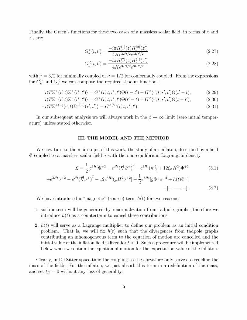
Finally, the Green’s functions for these two cases of a massless scalar field, in terms of z andz′, are:

G>k (t, t′) =

−iπH (1)ν (z)H(2)

ν (z′)

4He3Ht/2e3Ht′/2(2.27)

G<k (t, t′) =

−iπH (2)ν (z)H(1)

ν (z′)

4He3Ht/2e3Ht′/2(2.28)

with ν = 3/2 for minimally coupled or ν = 1/2 for conformally coupled. From the expressionsfor G>

k and G<k we can compute the required 2-point functions:

i〈TΣ+(~r, t)Σ+(~r′, t′)〉 = G>(~r, t;~r′, t′)Θ(t− t′) +G<(~r, t;~r′, t′)Θ(t′ − t), (2.29)

i〈TΣ−(~r, t)Σ−(~r′, t′)〉 = G>(~r, t;~r′, t′)Θ(t′ − t) +G<(~r, t;~r′, t′)Θ(t− t′), (2.30)

−i〈TΣ+(−)(~r, t)Σ−(+)(~r′, t′)〉 = G<(>)(~r, t;~r′, t′). (2.31)

In our subsequent analysis we will always work in the β → ∞ limit (zero initial temper-ature) unless stated otherwise.

III. THE MODEL AND THE METHOD

We now turn to the main topic of this work, the study of an inflaton, described by a fieldΦ coupled to a massless scalar field σ with the non-equilibrium Lagrangian density

L =1

2[e3HtΦ+2 − eHt(~∇Φ+)

2 − e3Ht(m2Φ + 12ξΦH

2)Φ+2 (3.1)

+e3Htσ+2 − eHt(~∇σ+)2 − 12e3HtξσH

2σ+2] +1

2e3Ht[gΦ+σ+2 + h(t)Φ+]

−[+ −→ −]. (3.2)

We have introduced a “magnetic” (source) term h(t) for two reasons:

1. such a term will be generated by renormalization from tadpole graphs, therefore weintroduce h(t) as a counterterm to cancel these contributions,

2. h(t) will serve as a Lagrange multiplier to define our problem as an initial conditionproblem. That is, we will fix h(t) such that the divergences from tadpole graphscontributing an inhomogeneous term to the equation of motion are cancelled and theinitial value of the inflaton field is fixed for t < 0. Such a procedure will be implementedbelow when we obtain the equation of motion for the expectation value of the inflaton.

Clearly, in De Sitter space-time the coupling to the curvature only serves to redefine themass of the fields. For the inflaton, we just absorb this term in a redefinition of the mass,and set ξΦ = 0 without any loss of generality.

9

To study the time evolution of the expectation value of the inflaton field we invoke thetadpole method(see Ref. [19] and references therein) to obtain its equation of motion. Thisis implemented by first shifting Φ by its expectation value in the non-equilibrium state asfollows :

Φ±(~x, t) = φ(t) + ψ±(~x, t) ; φ(t) = 〈Φ±(~x, t)〉 (3.3)

and then enforcing the tadpole condition which is simply a consequence of (3.3)

〈ψ±(~x, t)〉 = 0. (3.4)

φ(t) being the spatially homogeneous inflaton zero mode that drives inflation. We alsorequire that 〈σ±(~x, t)〉 = 0 to all orders, which means that the σ field does not acquire anexpectation value. After the shift of the inflaton field (3.3), the non-equilibrium action reads:

S =∫

d3xdt

L0(ψ+) + L0(σ

+) + ψ+e3Ht[

−φ− 3Hφ−m2Φφ]

+ e3Htg

2φ(σ+)2 (3.5)

+e3Htg

2ψ+(σ+)2 + e3Ht

h

2ψ+ − (+ → −)

where L0 represents the free theories for the ψ and σ fields. The tadpole condition (3.4) isimplemented by calculating the expectation value of the field operator ψ± by inserting it intothe non-equilibrium path integral and expanding in powers of g, about the free theory andsetting the resulting expression to zero. In particular we evaluate the following expressionto order g2 in perturbation theory:

〈ψ+(~x, t)〉 =∫

D[ψ±]D[σ±]ei(S0[+]−S0[−]) × ψ+(~x, t) × (3.6)

exp

∫

d3x′dt′[

e3Ht′[

−φ− 3Hφ−m2Φφ]

ψ+ + e3Ht′ g

2φ(σ+)2 + e3Ht

′ g

2ψ+(σ+)2 + e3Ht

′ h

2ψ+

− (+ → −)]= 0

The equation of motion is obtained by independently setting the coefficients of 〈ψ+(x)ψ+(x′)〉and 〈ψ+(x)ψ−(x′)〉 to zero. This is justified because these two correlators are independentfunctions. It is easily seen that the condition 〈ψ−〉 = 0 yields exactly the same equations.

This procedure gives rise to an equation of motion for the zero mode φ(t) and is in factequivalent to extremizing the one-loop effective action which incorporates the equilibriumboundary conditions at t < 0.

It is worth noting that this scheme, referred to as amplitude expansion, also assumes thatthe amplitude of the zero-mode φ(t) is “small” so that terms such as gφ(t)σ2 may be treatedperturbatively.

To one-loop order (O(g2)) we obtain the following form of the equation of motion.

10

φ+ 3Hφ+m2Φφ− g

2〈σ2〉(t) − i

g2

4π2

∫ t

−∞dτK(t, τ)φ(τ) − h(t)

2= 0, (3.7)

K(t, τ) =∫ ∞

0k2dk[G>2

k (τ, t) −G<2k (τ, t)]e3Hτ , (3.8)

Spatial translational invariance guarantees that 〈σ2〉 is only time dependent. We can combinethe φ independent contributions to the equation of motion into a single function:

h(t) =h(t)

2+g

2〈σ2〉(t). (3.9)

If the σ is conformally coupled to the curvature 〈σ2〉 represents a quadratically divergent piecewhich must be subtracted away by a renormalization of the “magnetic field” h. On the otherhand if σ is minimally coupled, one obtains the well known linearly growing contribution [3]after subtracting away the divergence leading to a modified inhomogeneous term in the zeromode equation of motion:

h(t) =gH3t

8π2+h(t)

2. (3.10)

We will, however, show explicitly in the next section that this term does not enter in thecalculation of the perturbative “decay rate” in this theory.

We use h(t) as a Lagrange multiplier to enforce the constraint that for t < 0, φ(t) =φi, φ(t) = 0 is a solution of the effective equation of motion for the expectation value. Inthis manner, we define an initial value problem with Cauchy data on a space-like surface forthe dynamics in which the expectation value of the inflaton field is “released” from someinitial value at time t = 0. For t > 0 the equation of motion becomes

φ(t) + 3Hφ(t) +m2Φφ(t) − i

g2

4π2

∫ t

0dτK(t, τ)φ(τ) = h(t) (3.11)

φ(t = 0) = φi , φ(t = 0) = 0 (3.12)

with the kernel given by (3.8).We now proceed to study the solution to this equation of motion in the cases of conformal

and minimal coupling.

A. Conformally coupled massless σ:

For a conformally coupled massless scalar, the Green’s functions are given by (2.27,2.28)with the Hankel functions as in (2.26).

The kernel has a particularly simple form in this case:

K(t, τ) = −i∫ ∞

0dk

sin[2k(e−Hτ − e−Ht)/H ]

2e2Hte−Hτ. (3.13)

11

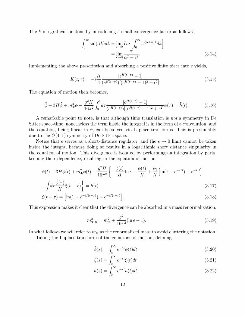
The k-integral can be done by introducing a small convergence factor as follows :

∫ ∞

0sin(αk)dk = lim

ǫ→0Im

[∫ ∞

0ei(α+iǫ)kdk

]

= limǫ→0

α

α2 + ǫ2. (3.14)

Implementing the above prescription and absorbing a positive finite piece into ǫ yields,

K(t, τ) = −iH4

[eH(t−τ) − 1]

(eH(t−τ))[(eH(t−τ) − 1)2 + ǫ2]. (3.15)

The equation of motion then becomes,

φ+ 3Hφ+m2Φφ− g2H

16π2

∫ t

0dτ

[eH(t−τ) − 1]

(eH(t−τ))[(eH(t−τ) − 1)2 + ǫ2]φ(τ) = h(t). (3.16)

A remarkable point to note, is that although time translation is not a symmetry in DeSitter space-time, nonetheless the term inside the integral is in the form of a convolution, andthe equation, being linear in φ, can be solved via Laplace transforms. This is presumablydue to the O(4, 1) symmetry of De Sitter space.

Notice that ǫ serves as a short-distance regulator, and the ǫ → 0 limit cannot be takeninside the integral because doing so results in a logarithmic short distance singularity inthe equation of motion. This divergence is isolated by performing an integration by parts,keeping the ǫ dependence, resulting in the equation of motion

φ(t) + 3Hφ(t) +m2Φφ(t) − g2H

16π2

−φ(t)

Hln ǫ− φ(t)

H+φiH

[

ln(1 − e−Ht) + e−Ht]

+∫

dτφ(τ)

Hξ(t− τ)

= h(t) (3.17)

ξ(t− τ) =[

ln(1 − e−H(t−τ)) + e−H(t−τ)]

. (3.18)

This expression makes it clear that the divergence can be absorbed in a mass renormalization,

m2Φ,R = m2

Φ +g2

16π2(ln ǫ+ 1). (3.19)

In what follows we will refer to mΦ as the renormalized mass to avoid cluttering the notation.Taking the Laplace transform of the equations of motion, defining

φ(s) =∫ ∞

0e−stφ(t)dt (3.20)

ξ(s) =∫ ∞

0e−stξ(t)dt (3.21)

h(s) =∫ ∞

0e−sth(t)dt (3.22)

12

and using the initial condition φ(t = 0) = 0, we find

s2φ(s) − sφi + 3H(sφ(s) − φi) +m2Φ,Rφ(s) +

g2

16π2Σ(s)φ(s) = h(s) (3.23)

Σ(s) = −s∫ ∞

0dte−st[ln(1 − e−Ht) + e−Ht] = −sξ(s) (3.24)

B. The Gibbons-Hawking Temperature

It is well known that fields in De Sitter space can be thought of, in some contexts, asbeing embedded in a thermal bath at a temperature H/2π, the so-called Gibbons-Hawkingtemperature [24]. How do we see these effects in the context of our calculation?

First we notice that the Green’s functions(2.23,2.24, 2.27,2.28) and the kernels (3.15,3.18) in (3.17) obey the periodicity condition in imaginary time

K(t− τ) = K(t− τ +2πi

H). (3.25)

These kernels can be analytically continued to imaginary time t− τ = −iη and expanded ina discrete series in terms of the Matsubara frequencies

ωn =2πn

βH,

1

βH= TH =

H

2π(3.26)

TH is recognized as the Gibbons-Hawking temperature in this space-time [23]. Then as afunction of imaginary time (3.18) can be written as

ξ(η) =1

βH

∞∑

n=−∞eiωnηΞ(ωn) (3.27)

Ξ(ωn) =∫ βH

0dηe−iωnηξ(η) (3.28)

We find

Ξ(ωn) = −βH(H

ωn− δn,1

)

, n ≥ 1. (3.29)

¿From this expression, Σ(s) can be obtained at once:

Σ(s) = −sξ(s) =∞∑

1

H(1

nH− 1

s+ nH) − s

s+H. (3.30)

This Laplace transform has simple poles at minus the Matsubara frequencies correspondingto the Hawking temperature.

Finally we obtain the solution for the Laplace transform

13

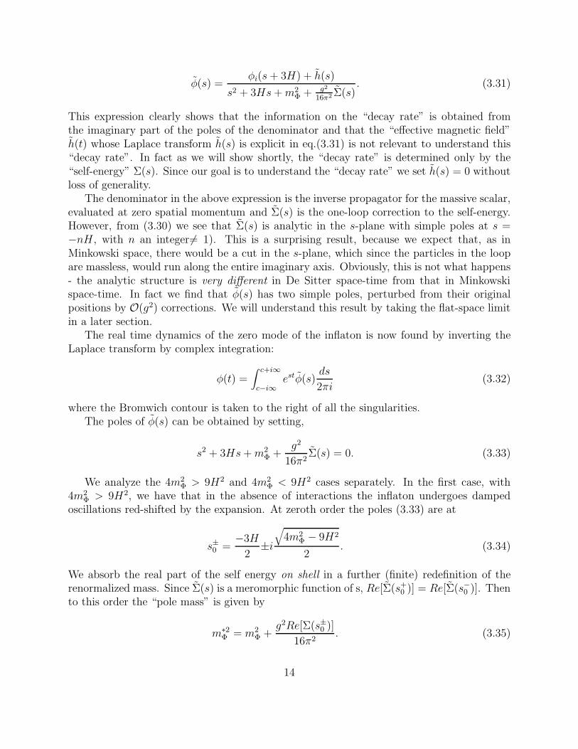
φ(s) =φi(s+ 3H) + h(s)

s2 + 3Hs+m2Φ + g2

16π2 Σ(s). (3.31)

This expression clearly shows that the information on the “decay rate” is obtained fromthe imaginary part of the poles of the denominator and that the “effective magnetic field”h(t) whose Laplace transform h(s) is explicit in eq.(3.31) is not relevant to understand this“decay rate”. In fact as we will show shortly, the “decay rate” is determined only by the“self-energy” Σ(s). Since our goal is to understand the “decay rate” we set h(s) = 0 withoutloss of generality.

The denominator in the above expression is the inverse propagator for the massive scalar,evaluated at zero spatial momentum and Σ(s) is the one-loop correction to the self-energy.However, from (3.30) we see that Σ(s) is analytic in the s-plane with simple poles at s =−nH , with n an integer6= 1). This is a surprising result, because we expect that, as inMinkowski space, there would be a cut in the s-plane, which since the particles in the loopare massless, would run along the entire imaginary axis. Obviously, this is not what happens- the analytic structure is very different in De Sitter space-time from that in Minkowskispace-time. In fact we find that φ(s) has two simple poles, perturbed from their originalpositions by O(g2) corrections. We will understand this result by taking the flat-space limitin a later section.

The real time dynamics of the zero mode of the inflaton is now found by inverting theLaplace transform by complex integration:

φ(t) =∫ c+i∞

c−i∞estφ(s)

ds

2πi(3.32)

where the Bromwich contour is taken to the right of all the singularities.The poles of φ(s) can be obtained by setting,

s2 + 3Hs+m2Φ +

g2

16π2Σ(s) = 0. (3.33)

We analyze the 4m2Φ > 9H2 and 4m2

Φ < 9H2 cases separately. In the first case, with4m2

Φ > 9H2, we have that in the absence of interactions the inflaton undergoes dampedoscillations red-shifted by the expansion. At zeroth order the poles (3.33) are at

s±0 =−3H

2±i√

4m2Φ − 9H2

2. (3.34)

We absorb the real part of the self energy on shell in a further (finite) redefinition of therenormalized mass. Since Σ(s) is a meromorphic function of s, Re[Σ(s+

0 )] = Re[Σ(s−0 )]. Thento this order the “pole mass” is given by

m∗2Φ = m2

Φ +g2Re[Σ(s±0 )]

16π2. (3.35)

14

Obviously this mass is independent of the renormalization scheme. We also define the sub-tracted self energy Σ∗(s) = Σ(s)−Re[Σ(s+

0 )], and at this stage it is convenient to introducethe “effective mass”

M2Φ = m∗2

Φ − 9H2

4. (3.36)

in terms of which, to order g2, we find

s± =−3H

2±i√

M2Φ +

g2

16π2Σ∗(s+)

=−3H

2±iMΦ±i

g2ImΣ(s±0 )

32π2MΦ+ O(g4) (3.37)

The Bromwich countour for the inverse Laplace transform can now be deformed bywrapping around the imaginary axis and picking up the poles [19]. The resulting expressionhas the Breit-Wigner form of a sharp resonance centered at the “pole mass” that is verynarrow in the weak coupling limit, leading to the time evolution of the inflaton given by

φ(t) = Zφie−3Ht/2e−Γt/2 cos(MΦt+ α) (3.38)

where,

Z2 = 1 +9H2

4M2Φ

− 2g2B′

32π2MΦ− 12g2HB

128π2M3Φ

− 18g2H2B′

128π2M3Φ

(3.39)

α = arctan

[

− 3H

2MΦ+

g2

16π2[A′

2MΦ+

9H2A′

8M3Φ

− 18H2B

16M4Φ

]

]

B = Im[

Σ∗(s)]

s=−3H2

+iMΦ

A′ = Re

[

∂Σ∗(s)

∂s

]

s=−3H2

+iMΦ

B′ = Im

[

∂Σ∗(s)

∂s

]

s=−3H2

+iMΦ

.

The most interesting of these quantities is the damping rate, given by

Γ =g2ImΣ∗(s+

0 )

16π2MΦ. (3.40)

The imaginary part of the self-energy in the above expression, can be evaluated using stan-dard sum formulas (these sums also appear finite temperature field theory [25,26]) and isfound to be

15

Γ =

g2 tanh

βH

√

m∗2Φ

− 9H2

4

2

32π√

m∗2Φ − 9H2

4

=g2 tanh

(βHMΦ

2

)

32πMΦ(3.41)

This expression for Γ is a monotonically increasing function of H . When H = 0, it matcheswith the flat-space decay rate

ΓMinkowski =g2

32πmΦ. (3.42)

We thus obtain the result that the inflaton decay proceeds more rapidly in a De Sitterbackground than in Minkowski space-time.

The rate (3.41) can be written in a more illuminating manner as

Γ =g2 coth

(βHω0

2

)

32πMΦ

=g2 [1 + 2nb(ω0)]

32πMΦ

(3.43)

ω0 = −is+0 ; nb(ω0) =

1

eβHω0 − 1(3.44)

This is a remarkable result - the decay rate is almost the same as that in Minkowski space, butin a thermal bath at the Hawking temperature [19,27]. Habib [15] has also found an intriguingrelationship with the Hawking temperature in the probability distribution functional in hisstudies of stochastic inflation.

If we now look at the 4m2Φ < 9H2 case, we see that the inflaton ceases to propagate, i.e.

its Compton wavelength approaches the horizon size and there is no oscillatory behavior inthe classical evolution of the zero mode:

φ(t) = (9H2

4m2Φ

− 1)−1/2φie−3Ht/2 sinh (|MΦ|t+ β) (3.45)

tanh β =2|MΦ|3H

.

The one loop contribution is the same as in the previous case but now the poles of φ(s) lieon the real axis:

s±0 =−3H

2±√

9H2 − 4m2Φ

2. (3.46)

s± =−3H

2±√

9H2 − 4m2Φ − 4 g2

16π2 Σ(s±)

2

We define

Σ(s±0 ) = C±D (3.47)

16

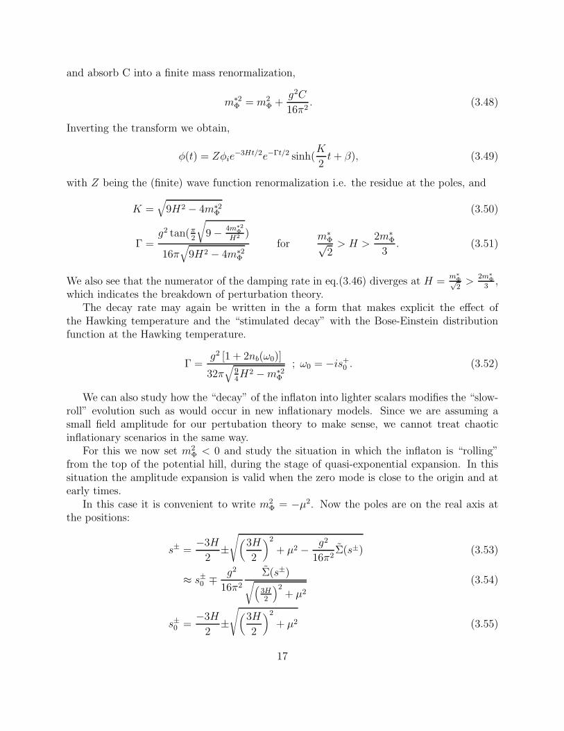
and absorb C into a finite mass renormalization,

m∗2Φ = m2

Φ +g2C

16π2. (3.48)

Inverting the transform we obtain,

φ(t) = Zφie−3Ht/2e−Γt/2 sinh(

K

2t+ β), (3.49)

with Z being the (finite) wave function renormalization i.e. the residue at the poles, and

K =√

9H2 − 4m∗2Φ (3.50)

Γ =g2 tan(π

2

√

9 − 4m∗2Φ

H2 )

16π√

9H2 − 4m∗2Φ

form∗

Φ√2> H >

2m∗Φ

3. (3.51)

We also see that the numerator of the damping rate in eq.(3.46) diverges at H =m∗

Φ√2>

2m∗

Φ

3,

which indicates the breakdown of perturbation theory.The decay rate may again be written in the a form that makes explicit the effect of

the Hawking temperature and the “stimulated decay” with the Bose-Einstein distributionfunction at the Hawking temperature.

Γ =g2 [1 + 2nb(ω0)]

32π√

94H2 −m∗2

Φ

; ω0 = −is+0 . (3.52)

We can also study how the “decay” of the inflaton into lighter scalars modifies the “slow-roll” evolution such as would occur in new inflationary models. Since we are assuming asmall field amplitude for our pertubation theory to make sense, we cannot treat chaoticinflationary scenarios in the same way.

For this we now set m2Φ < 0 and study the situation in which the inflaton is “rolling”

from the top of the potential hill, during the stage of quasi-exponential expansion. In thissituation the amplitude expansion is valid when the zero mode is close to the origin and atearly times.

In this case it is convenient to write m2Φ = −µ2. Now the poles are on the real axis at

the positions:

s± =−3H

2±√(

3H

2

)2

+ µ2 − g2

16π2Σ(s±) (3.53)

≈ s±0 ∓ g2

16π2

Σ(s±)√(

3H2

)2+ µ2

(3.54)

s±0 =−3H

2±√(

3H

2

)2

+ µ2 (3.55)

17

For g = 0 the pole that is on the positive real axis, s+0 , is the one that dominates the

evolution of the inflaton down the potential hill (the growing mode). Since s+0 > 0 we find

that

Σ(s+0 ) =

∞∑

2

s+0

n(s+0 + nH)

> 0, (3.56)

and we conclude that, to this order, the pole on the positive real axis is shifted towardsthe origin. Therefore the rate of growth of the growing mode is diminished by the decayinto lighter scalars and the “rolling” is slowed down. This is physically reasonable, sincethe “decay” results in a transfer of energy from the inflaton to the massless scalars and therolling of the field down the potential hill is therefore slowed down by this decay process.

C. Minimally coupled massless σ:

Now we turn to the ξσ = 0 case. The Green’s functions are given by (2.27,2.28) with theHankel functions (2.25). There are many features in common with the previous case: thekernel is translationally invariant in time and periodic in imaginary time with periodicityβH . Thus it can again be expanded in terms of Matsubara frequencies and the Laplacetransform carried out in a straightforward manner. However, for minimal coupling we finda new logarithmic infrared divergence in the kernel along with the ultraviolet logarithmicsingularity of the conformally coupled case. Therefore, the k-integral in the kernel must beperformed with an infrared cutoff µ. The logarithmic ultraviolet divergence is handled in asbefore, and after this subtraction we find the self-energy to be:

Σ(s) =

ξσ=1/6︷ ︸︸ ︷∞∑

1

H(1

nH− 1

s+ nH) − s

s+H−4H

3

∞∑

1

1

n(

1

s+ nH− 1

s+ 3H + nH) (3.57)

+(1

s− 1

s+ 3H)[

4H

3ln 2 − 2H(

2

3ln(H/µ) +

14

9)]

+4H

3(

1

s+H− 1

s+ 2H) +

4H2

3[1

s2− 1

(s+ 3H)2].

We notice that the self-energy for the conformally coupled case is contained in the aboveexpression. It is also interesting to note that the imaginary part of the self-energy, on-shell,receives no contribution from the infrared divergent piece, which only contributes to a furtherrenormalization of the “pole mass” m∗2

Φ . We now focus on the case 4m2Φ − 9H2 > 0.

The expression for the decay rate is obtained by evaluating the imaginary part of theself-energy at the pole s+

0 (see eq. (3.40) and found to be

Γ =

ξσ=1/6︷ ︸︸ ︷

g2

32π[[1 + 2nb(ω0)]

MΦ

(

1 +4H2

m∗2Φ

)

+8H3

πm∗4Φ

]. (3.58)

18

with (3.44). The qualitative behaviour of the decay rate as a function of H is similar to thatin the conformally coupled case. We see that, Γ(ξσ = 0) > Γ(ξσ = 1/6) > Γ(Minkowski).

D. Analytic structure of the self-energy

As mentioned earlier, the analytic structure of the self-energy in the De Sitter backgroundis drastically different from what one would expect in flat space-time. We find that the self-energy for the case where Φ is unstable does not display cuts in the s-plane. Though thereason for this strange behaviour is not clear at present, we can try to understand it bytaking the flat-space limit i.e. the H → 0 limit. In this limit, it suffices to look at Σ(s) forξσ = 1/6. It is easily shown that the additional terms in (3.25) are vanishingly small in theH → 0 limit. We thus obtain,

limH→0

Σ(s) = limH→0

[∞∑

1

H(1

nH− 1

s + nH) − s

s+H]

(3.59)

=∫ ∞

H(1

x− 1

s+ x)dx− 1

(3.60)

= ln(s/m) + ln(m/H) − 1

where m is a mass scale that serves as an infrared regulator. Hence,

φ(s) =sφi

s2 + (m2Φ + g2

16π2 ln(m/H) − 1) + g2

16π2 ln(s/m). (3.61)

The above expression has a cut which can be chosen to run from 0 to −∞, so that it is tothe left of the Bromwich contour. The discrete singularities of the self-energy at s = −nHhave merged into a continuum in the small H limit to give a cut along the negative realaxis in the s-plane. In addition, there are two simple poles in the first Riemann sheet at±imΦ + O(g2). Inverting the transform yields,

φ(t) = Zφie−Γt/2 cos(mΦt+ α)

− φig2

16π2

∫ ∞

0dω

ωe−ωt

(ω2 +m2Φ + g2

16π2 ln(ω/m))2 + ( g2

16π)2. (3.62)

We see here, a Breit-Wigner form plus contributions from across the cut.A flat-space analysis with mσ 6= 0, carried out in a previous work [19] reveals a very

different picture. In particular, we find two cuts extending from s = ±2imσ to ±i∞ and twosimple poles which move off into the second Riemann sheet above the two-particle thresholdwhen mΦ > 2mσ. However, upon inverting the transform and taking mσ → 0, we obtain

φ(t) = φig2

16π2

∫ ∞

0dω

ω cosωt

(ω2 −m2Φ − g2

16π2 ln(ω/m))2 + ( g2

32π)2. (3.63)

19

A deformation of the contour of integration shows that eqs.(3.62) and (3.63) are in factidentical and hence we have consistency (see the Appendix). Although the limits H → 0and mσ → 0 do not commute insofar as the analytic structure in the s-plane is concerned,the time evolution obtained from the inverse Laplace transform is unambiguously the same.

IV. THE O(2) MODEL AND GOLDSTONE BOSONS

While the inflaton is typically taken to be a singlet of any gauge or global symmetry, thereis no reason that it could not transform non-trivially under a continuous global symmetry.If this occurs, and the symmetry is broken spontaneously, the interesting possibility arisesof dissipation of energy into Goldstone bosons. Even if the inflaton is a singlet, one couldask about the evolution of fields that belong to multiplets of a global continous symmetry,during inflation. Our primary motivation, however, is to study dissipative processes of theinflaton via the decay into Goldstone bosons in De Sitter space-time as new non-equilibriummechanisms.

The effect may be studied in the O(2) linear sigma model, in which the inflaton is partof the O(2) doublet, with Lagrangian density

L =1

2[e3HtΦ2 − eHt(~∇Φ)

2+ e3Htπ2 − eHt(~∇π)

2] (4.1)

+1

2e3Ht(µ2 − 12ξH2)(Φ2 + π2) − e3Ht

λ

4!(Φ2 + π2)2 + h(t)Φ.

Assuming that µ2 > 12ξH2, in the symmetry broken phase the field Φ acquires a VEV

〈Φ〉 =

√

6(µ2 − 12ξH2)

λ, (4.2)

and the Goldstone bosons are left with no mass terms, and hence are massless, minimallycoupled fields in De Sitter space-time [28]; this is a fairly well known result.

We now write

Φ(x, t) =

√

6(µ2 − 12ξH2)

λ+ φ(t) + ψ(x, t) (4.3)

and use the tadpole method to impose:

〈ψ(x, t)〉 = 0, (4.4)

〈π(x, t)〉 = 0.

Using eq.(4.3) it is easy to see that couplings of the form ψπ2, are automatically induced inthe Lagrangian. Carrying out the same analysis as before and keeping only terms up to firstorder in φ(t), we find the following equation of motion

20

φ+ 3Hφ+m2(t)φ− i3λµ2

2π2

∫ t

0dτ [Kφ(t, τ) +

1

9Kπ(t, τ)]φ(τ) = h(t), (4.5)

where, K(t, τ) =∫ ∞

0k2dk[G>2

k (τ, t) −G<2k (τ, t)]e3Hτ .

Here m2(t) is given by the tree-level mass term 2µ2 plus contributions proportional tothe tadpole 〈π2〉(t). Since the Goldstone boson is always minimally coupled to the curvature〈π2〉(t) will grow linearly with time and result in a non-trivial time-dependence for the massof the massive mode φ. In this case the methods of the earlier section are not applicable,and the definition of a “decay rate” will be plagued by time-dependent ambiguities.

Such a time-dependence will, however, be absent in a De Sitter space that exists forever, inwhich case the contribution from the tadpole will simply be a divergence that is renormalisedthrough a redefinition of the mass. In such a situation, the contribution to the decay ratefrom the massive mode would be subdominant due to the kinematics and the Goldstonemodes would provide the dominant contribution to the decay rate. Thus, neglecting Kφ(t, τ)the equation of motion has exactly the same form as eq.(3.5). The subsequent analysis andresults would be identical to those obtained above in the section on minimally coupled fields.

V. THE LANGEVIN EQUATION

Our results allow us to make contact with the issue of decoherence and the stochasticdescription of inflationary cosmology [12–15].

Decoherence is a fundamental aspect of dissipational dynamics and in the description ofnon-equilibrium processes in the early universe [13–15]. The relationship between fluctuationand dissipation as well as a stochastic approach to the dynamics of inflation can be exploredby means of the Langevin equation.

This section is devoted to obtaining the corresponding Langevin equation for the non-equilibrium expectation value of the inflaton field (zero mode) in the one loop approximationwithin the model addressed in this article.

The first step in deriving a Langevin equation is to determine the ‘system’ and ‘bath’variables, and subsequently integrate out the ‘bath’ variables to obtain an influence functionalfor the ‘system’ degrees of freedom [13–15].

We first separate out the expectation value and impose the tadpole conditions as follows:

Φ± = φ± + ψ± ; 〈Φ±(~x, t)〉 = φ±(t) ; 〈σ±(~x, t)〉 = 0. (5.1)

The non-equilibrium effective action is defined in terms of the Lagrangian given by equa-tion(3.2) as,

eiSeff =∫

Dψ+Dψ−Dσ+Dσ−eiS0[φ+]−S0[φ−]eiS0[ψ+]−S0[ψ−]

eiS0[σ+]−S0[σ−]eiSint[ψ+,φ+,σ+]−Sint[ψ

−,φ−,σ−]

21

where S0 represents the action for free fields, and Sint contains all the remaining parts of theaction. The effective action for the zero modes is obtained by tracing out all the degrees offreedom corresponding to the non-zero modes (or the ‘bath’ variables), in a consistent loopexpansion. It is useful to introduce the center of mass (φ(t)) and relative (R(t)) coordinatesas

φ±(t) = φ(t) ± R(t)

2(5.2)

Remembering the definitions of the Green’s functions in eqs.(2.29 - 2.31), we expandexp(iSint) up to order g2 and consistently impose the tadpole condition to obtain the ef-fective action per unit volume (because the expectation value is taken to be translationallyinvariant),

SeffΩ

=∫

dt(

L0(φ+) − L0(φ

−))

(5.3)

− ig2

16π3

∫ ∞

−∞dt∫ t

−∞dt′∫

d3ka3(t)a3(t′)R(t)φ(t′)[

G>2k (t, t′) −G<2

k (t, t′)]

− ig2

32π3

∫ ∞

−∞dt∫ ∞

−∞dt′∫

d3ka3(t)a3(t′)R(t)R(t′)[

G>2k (t, t′) +G<2

k (t, t′)]

+ h(t)R(t) + terms independent of φ

As before h(t) results from subtracting the φ-independent contribution of the tadpolefrom h(t).

Now, it is not difficult to verify that the non-equilibrium Green’s functions given byeqn.(2.16, 2.19) and obeying the boundary conditions (2.22) have the property,

G>k (t, t′) = [G<

k (t, t′)]∗. (5.4)

This property guarantees that the second term in the effective action is real, while the thirdterm is pure imaginary. The imaginary, non-local, acausal part of the effective action givesa contribution to the path-integral that may be written in terms of a stochastic field as

exp[ − 1

2

∫

dt∫

dt′R(t)K(t, t′)R(t′)]∝∫

DξP[ξ] exp[i∫

dtξ(t)R(t)] (5.5)

P[ξ] = exp[−1

2

∫

dt∫

dt′ξ(t)K−1(t, t′)ξ(t′)]

with

K(t, t′) = − g2

16π3

∫

d3ka3(t)a3(t′)[G>2k (t, t′) +G<2

k (t, t′)] (5.6)

The non-equilibrium path integral now becomes

22

Z∝∫

DφDRDξP[ξ] exp i[Sreff(φ,R) +∫

dtξ(t)R(t)] (5.7)

with Sreff [φ,R] being the real part of the effective action and with P[ξ] the gaussian prob-ability distribution for the stochastic noise variable.

The Langevin equation is obtained via the saddle point condition [13]

δSreffδR(t)

|R=0 = ξ(t) (5.8)

leading to

φ+ 3Hφ+m2Φφ+ i

g2

16π3

∫ t

−∞dt′∫

d3ka3(t′)[G>2k (t, t′) −G<2

k (t, t′)]φ(t′) − h(t) =ξ(t)

a3(t)(5.9)

where the stochastic noise variable ξ(t) has gaussian, but colored correlations:

<< ξ(t) >>= 0; << ξ(t)ξ(t′) >>= K(t, t′) (5.10)

The double brackets stand for averages with respect to the gaussian probability distributionP[ξ]. The noise is coloured and additive. Due to the properties of the Green’s functions (5.4),the noise kernel (which contributes to the imaginary part of the effective action) is simplythe real part of G>2

k (t, t′). The dissipative kernel (which gives rise to the non-local termin the Langevin equation) on the other hand is given by the imaginary part of G>2

k (t, t′).Consequently, the fluctuation− dissipation theorem is revealed in the Hilbert transformrelationship between the real and imaginary parts of the analytic function G>2

k (t, t′). Theequation of motion (3.11) is now recognized to result from (5.9) by taking the average overthe noise.

One could now obtain the corresponding Fokker-Planck equation that describes the evo-lution of the probability distribution function for φ [12,29].

We must emphasize here, that all the results discussed so far in this section, are inde-pendent of the specifics of the FRW background spacetime, the masses of the fields, and thetemperature of the initial thermal state. The importance of the Langevin equation residesat the fundamental level in that it provides a direct link between fluctuation and dissipationincluding all the memory effects and multiplicative aspects of the noise correlation functions.

In particular in stochastic inflationary models it is typically assumed [12] that the noiseterm is gaussian and white (uncorrelated). This simplified stochastic description, in termsof gaussian white noise, leads to a scale invariant spectrum of scalar density perturbations[12]. Although this description is rather compelling, within the approximations made inour analysis we see that for a σ field with an arbitrary mass and arbitrary couplings tothe curvature there is no regime in which the correlations of the noise term (5.10) can bedescribed by a Markovian delta function in time [13]. One could speculate that some othercouplings or higher order effects, or perhaps some peculiar initial states could lead to agaussian white noise, but then one concludes that gaussian white noise correlations are byno means a generic feature of the microscopic field theory.

23

We can speculate that our result of gaussian but correlated noise could have implica-tions for stochastic inflation. In particular it may lead to departures from a scale invariant(Harrison-Zel’dovich) spectrum of primordial scalar density perturbations, that can now becalculated within a particular microscopic model using the non-equilibrium field-theoreticaltools described in this work. Of course this requires further and deeper study, which isbeyond the scope of this article.

VI. CONCLUSIONS AND FURTHER QUESTIONS

In this article we have studied the decay of inflatons into massless scalars in De Sitterspace. The motivation was to understand the non-equilibrium mechanisms of inflaton relax-ation during the stage of quasi-inflationary expansion in early universe cosmology, in old,new and stochastic inflationary scenarios. Chaotic inflation models cannot be treated withinour approximation scheme since the field will typically start at values that are large enoughso that the amplitude expansion is not valid. Having recognized the inherent difficulties indefining a decay rate in a time dependent background, we have given a practical definitionthat requires understanding the real-time evolution of the inflaton interacting with lighterfields. This led us to a model in which an inflaton interacts with massless scalars via atrilinear coupling, allowing for both minimal and conformal coupling to the curvature.

We obtained a decay rate at one loop order that displays a remarkable property. Withsome minor modifications it can be interpreted as the stimulated decay of the inflaton in athermal bath at the Hawking temperature. This decay rate is larger than that of Minkowskispace because of the Bose-enhancement factors associated with the Hawking temperature.The decay rate of the minimally coupled case is larger than that of the conformal case whichin turn is larger than the Minkowski rate. We have shown explicitly that in the case of newinflation, the dissipation of the inflaton energy associated with the decay into conformallycoupled massless scalars slows down further the rolling of the inflaton down the potentialhill. We have also studied decay into Goldstone bosons.

To establish contact with the stochastic inflationary scenario, we derived the Langevinequation for the coarse-grained expectation value of the inflaton field to one loop order.We find that this stochastic equation has a gaussian but correlated (colored) noise. Thetwo point correlation function of the noise and the dissipative kernel fulfill a generalizedfluctuation-dissipation relation.

There are several potentially relevant implications of our results for old, new and stochas-tic inflation. In the case of old inflation we see that dissipative processes in the metastablemaximum can contribute substantially to the “equilibration” of the inflaton oscillations, andmore so because of the enhanced stimulated decay for large Hubble constant. In the case ofnew inflation, we have seen that these dissipative effects help slow the rolling of the inflatonfield down the potential hill, possibly extending the stage of exponential expansion.

Within the context of stochastic inflation, our results point out to the possibility ofincorporating deviations from a scale invariant spectrum of primordial scalar density pertur-bations by the noise correlations, which manifest the underlying microscopic correlations of

24

the field theory. This is a possibility that is worth exploring further.Our results also point to further interesting questions:

1. Is it possible to understand at a more fundamental level the connection between thedecay rate and the Hawking temperature of a bath in equilibrium? In particular, isthis connection maintained at higher orders?

2. Is it possible to relate the “decay rate” to the rate of particle production via theinteraction? Such a relation in Minkowski space-time is a consequence of the existenceof a spectral representation for the self-energy but such a representation is not availablein a time dependent background.

Answers to these questions will undoubtedly offer a much needed deeper understandingof non-equilibrium processes in inflationary cosmology.

ACKNOWLEDGMENTS

D.B would like to thank H. J. de Vega for useful references and illuminating discussions,and NSF for support through grant award No: PHY-9302534. D. B. and S. P. K. would liketo thank Salman Habib for illuminating conversations and comments.

S. Prem Kumar and R.Holman were partially supported by the U.S. Dept. of Energyunder Contract DE-FG02-91-ER40682.

VII. APPENDIX

In this appendix, we show explicitly, that (3.62) and (3.63) are in fact identical expres-sions. The behaviour of φ(t) in Minkowski (given by (3.57)) was obtained in reference [19]where mσ was allowed to have non-zero values. Now, the results from this reference mustobviously coincide with the flat-space limits (H → 0) derived in this paper. To see this,consider eqn.(3.63):

φ(t) = φig2

16π2

∫ ∞

0dω

ω cosωt

(ω2 −m2Φ − g2

16π2 ln(ω/m))2 + ( g2

32π)2

=φiπRe[

∫ ∞

0− idω(ωeiωt)[

1

ω2 −m2Φ − g2

16π2 ln(ω/m) − i g2

32π

− 1

ω2 −m2Φ − g2

16π2 ln(ω/m) + i g2

32π

]].

The branch cut due to the logarithm in the denominator runs from 0 to +∞, and the contourof integration may be chosen to run from 0 to +∞ on the first sheet. It is easy to see thatthe integrand has 4 simple poles, one in each quadrant. In particular, the pole in the firstquadrant is at

25

ω1 = mΦ +g2

32π2mΦln(mΦ/m) + i

g2

64πmΦ. (7.1)

Furthermore, the exponential is well behaved at infinity in the first quadrant. We cantherefore deform the contour of integration so that it runs ¿from 0 to +i∞, picking up theresidue from one simple pole. Writing ω = iz, and noticing that the logarithm picks up animaginary part iπ/2 we now have,

φ(t) =φiπRe[

∫ ∞

0dz(ize−zt)[

1

−z2 −m2Φ − g2

16π2 ln(z/m) − i g2

16π

− 1

−z2 −m2Φ − g2

16π2 ln(z/m)] + Res[

−iωeiωtω2 −m2

Φ − g2

16π2 ln(ω/m) − i g2

32π

]|ω=ω1].

=φiπ

[− g2

16π

∫ ∞

0dz

ze−zt

(z2 +m2Φ + g2

16π2 ln(z/m))2 + ( g2

16π)2

+ 2πRe[ limω→ω1

(ωeiωt(ω − ω1)

ω2 −m2Φ − g2

16π2 ln(ω/m) − i g2

32π

)]]

Absorbing the real part of the self-energy on-shell as an additional mass renormalization,and going through the subsequent algebra we obtain our result,

φ(t) = φ(0)(1 +g2

32π2mΦ2)e

− g2t

64πmΦ cos(mΦt)

−φig2

16π2

∫ ∞

0dz

ze−zt

(z2 +m2Φ + g2

16π2 ln(z/m))2 + ( g2

16π)2.

26

REFERENCES

[1] A. Guth, Phys. Rev. D 15, 347 (1981); A. H. Guth and E. J. Weinberg, Nucl. Phys.B212,321 (1983).

[2] For early reviews on the inflationary scenario see for example: R. H. Brandenberger,Rev. of Mod. Phys. 57, 1 (1985); Int. J. Mod. Phys. A2, 77 (1987); L. Abbott and S. Y.Pi, Inflationary Cosmology, World Scientific, 1986; A. D. Linde, Rep. Prog. Phys. 47,925 (1984).P. J. Steinhardt, Comm. Nucl. Part. Phys. 12, 273 (1984).

[3] A. D. Linde, Particle Physics and Inflationary Cosmology, Harwood, Chur, Switzer-land, 1990; Lectures on Inflationary Cosmology, in Current Topics in AstrofundamentalPhysics, ‘The Early Universe’, Proceedings of the Chalonge Erice School, N. Sanchezand A. Zichichi Editors, Nato ASI series C, vol. 467, 1995, Kluwer Acad. Publ.

[4] E. Kolb and M. S. Turner, The Early Universe, Addison-Wesly, Redwood city, 1990.[5] A. Vilenkin and L. H. Ford, Phys. Rev. D26, 1231 (1982); A. Linde, Phys. Lett. 108B,

389 (1982); A. Vilenkin, Nucl. Phys. B226, 527 (1983); E. Mottola, Phys. Rev. D31, 754(1985); F. Cooper and E. Mottola, Mod. Phys. Lett. A, 2, 635 (1987); B. Allen, Phys.Rev. D32, 3136 (1985).

[6] A. D. Dolgov and A. D. Linde, Phys. Lett. 116B, 329 (1982).[7] A. D. Linde, Phys. Lett. 129B, 177 (1983).[8] L. F. Abbott, E. Farhi and M. B. Wise, Phys. Lett. 117B, 29 (1982).[9] A. D. Dolgov and D. P. Kirilova, Sov. J. Nucl. Phys. 51, 273 (1990).

[10] D. La and P.J. Steinhardt. Phys. Rev. Lett. 62, 376 (1989); Phys. Lett. B 220, 375(1989).

[11] See also R. Brandenberger and A. Linde in reference [2].[12] A. A. Starobinskii, in Field Theory, Quantum Gravity and Strings, ed. by H. J. de

Vega and N. Sanchez (Springer, Berlin 1986). J. M. Bardeen and G. J. Bublik, Class.Quan. Grav. 4, 473 (1987); S. J. Rey, Nucl. Phys. B284, 706 (1987); D. Polarski andA. Starobinskii, Class. Quant. Grav. 13, 377 (1996); A. Starobinskii and J. Yokohama,Phys. Rev. D50, 6357 (1994).

[13] B. L. Hu, J. P. Paz and Y. Zhang, Phys. Rev. D45, 2843 (1993) ; ibid 47,1576 (1993).E. Calzetta and B. L. Hu, Phys. Rev. D49, 6636 (1994); ibid 52, 6770 (1995). B. L. Huand A. Matacz, Phys. Rev. D51, 1577 (1995); A. Matacz, “A new theory of stochasticinflation”, gr-qc-9604022.

[14] S. Habib and H. E. Kandrup, Phys. Rev. D39, 2871 (1989); ibid 46, 5303 (1992).[15] S. Habib, Phys. Rev. D46, 2408 (1992).[16] J. Schwinger, J. of Math. Phys. 2, 407 (1961).[17] L. V. Keldysh, Sov. Phys. JETP 20, 1018 (1965).[18] see for example:E. Calzetta and B. L. Hu, Phys. Rev. D35, 495 (1988); ibid D37,

2838 (1988); J. P. Paz, Phys. Rev. D41, 1054 (1990); ibid D42, 529 (1990); B. L. Hu,Lectures given at the Canadian Summer School For Theoretical Physics and the ThirdInternational Workshop on Thermal Field Theories (Banff, Canada, 1993) (to appearin the proceedings) and in the Proceedings of the Second Paris Cosmology Colloquium,

27

Observatoire de Paris, June 1994, p.111, H. J. de Vega and N. Sanchez Editors, WorldScientific, 1995, and references therein.

[19] D. Boyanovsky, H. J. de Vega, R. Holman, D.-S. Lee and A. Singh, Phys. Rev. D51,4419 (1995). See for a review, D. Boyanovsky, H. J. de Vega and R. Holman, in theProceedings of the Second Paris Cosmology Colloquium, Observatoire de Paris, June1994, p. 127-215, H. J. de Vega and N. Sanchez Editors, World Scientific, 1995; D.Boyanovsky, M. D’Attanasio, H. J. de Vega, R. Holman and D. S. Lee, Phys. Rev. D52,6805 (1995); D. Boyanovsky, M. D’Attanasio, H. J. de Vega and R. Holman, hep-ph-9602232 (to appear in Phys. Rev. D) and references therein.

[20] G. Semenoff and N. Weiss, Phys. Rev. D31, 689;699 (1985); H. Leutwyler and S. Mallik,Ann. of Phys. (N.Y.) 205, 1 (1991); A. Ringwald, Ann. of Phys. (N.Y.) 177, 129 (1987);Phys. Rev. D 36, 2598 (1977); I. T. Drummond, Nucl. Phys. B190[FS3], 93 (1981).

[21] P. M. Bakshi and K. T. Mahanthappa, J. of Math. Phys. 4, 1 (1963); ibid. 12. ; L. V.Keldysh, Sov. Phys. JETP 20, 1018 (1965); R. Mills, “Propagators for Many ParticleSystems”; A. Niemi and G. Semenoff, Ann. of Phys. (N.Y.) 152, 105 (1984); Nucl. Phys.B [FS10], 181, (1984); E. Calzetta, Ann. of Phys. (N.Y.) 190, 32 (1989); R. D. Jordan,Phys. Rev. D33, 444 (1986); N. P. Landsman and C. G. van Weert, Phys. Rep. 145, 141(1987); R. L. Kobes and K. L. Kowalski, Phys. Rev. D34, 513 (1986); R. L. Kobes, G.W. Semenoff and N. Weiss, Z. Phys. C 29, 371 (1985).

[22] T. S. Bunch and P. C. W. Davies, Proc. R. Soc. A 360, 117 (1978).[23] N. D. Birrell and P.C. W. Davies, Quantum Fields in Curved Space, (Cambridge Univ.

Press, Cambridge, England, 1982); S. A. Fulling, Aspects of Quantum Field Theory inCurved Space Time, (Cambridge Univ. Press, England, 1989).

[24] G.W. Gibbons and S. W. Hawking, Phys. Rev D15, 2738 (1977).[25] L. Dolan and R. Jackiw, Phys. Rev. D9, 2904 (1974); ibid 3320.[26] J. I. Kapusta, Finite Temperature Field Theory, Cambridge Monographs on Mathemat-

ical Physics, Cambridge Univ. Press, 1989.[27] There is a subtle difference in this expression compared to the finite temperature

Minkowski space result in terms of MΦ. In Minkowski space the argument of the Bose-Einstein occupation factor is MΦ/2 [19], which can be understood from the spectralrepresentation of the self-energy in a perturbative expansion. The lowest order correc-tion corresponds to an an intermediate two particle state, each particle carries half theenergy of the external scalar leg. In De Sitter space-time (as in any time dependentbackground) there is no possibility of writing a spectral representation. The similaritybetween De Sitter and finite temperature field theory in Minkowski space is thereforenot an equivalence.

[28] M.B. Voloshin and A.D. Dolgov,Sov. J. Nucl. Phys. 35, 120 (1982); V. Faraoni, astro-ph/9602111 (to appear in PRD).

[29] F. R. Graziani, Phys. Rev. D39, 3630 (1989); A. Linde, D. Linde and A. Mezhlunmian,Phys. Rev. D49, 1783 (1994).

28