Electric Flux Density, Gauss' Law, and Divergence
41
ELECTRIC FLUX DENSITY, GAUSS’ LAW, AND DIVERGENCE
-
Upload
khangminh22 -
Category
Documents
-
view
0 -
download
0
Transcript of Electric Flux Density, Gauss' Law, and Divergence

ELECTRIC FLUX DENSITY, GAUSS’ LAW, AND DIVERGENCE

About 1837, the Director of the Royal Society in London, Michael Faraday, was interested in static electric fields and the effect of various insulating materials on these fields.
This is the lead to his famous invention, the electric motor. He found that if he moved a magnet through a loop of wire, an electric current flowed
in the wire. The current also flowed if the loop was moved over a stationary magnet. ► Changing magnetic field produces an electric field.
Electric Flux Density Chapter 3 Electric Flux Density, Gauss’s Law, and Divergence
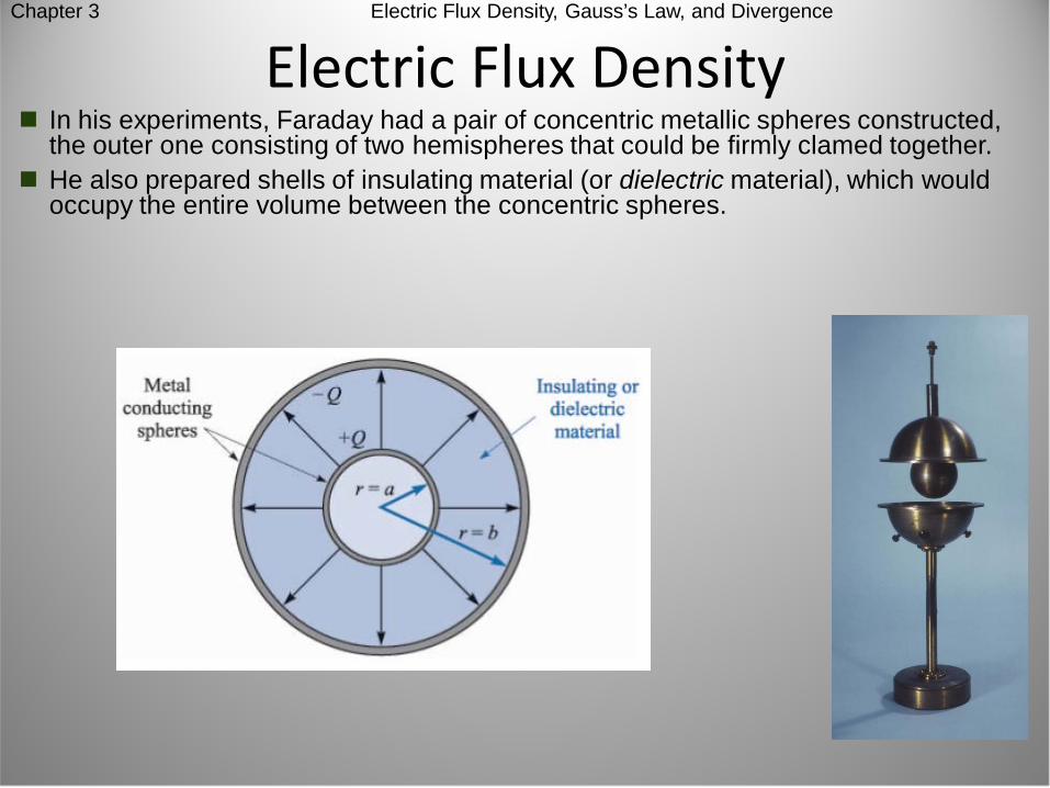
Electric Flux Density In his experiments, Faraday had a pair of concentric metallic spheres constructed,
the outer one consisting of two hemispheres that could be firmly clamed together. He also prepared shells of insulating material (or dielectric material), which would
occupy the entire volume between the concentric spheres.
Chapter 3 Electric Flux Density, Gauss’s Law, and Divergence

Electric Flux Density Chapter 3 Electric Flux Density, Gauss’s Law, and Divergence
Faraday found out, that there was a sort of “charge displacement” from the inner sphere to the outer sphere, which was independent of the medium.
We refer to this flow as displacement, displacement flux, or simply electric flux.
ψ Q=
Where ψ is the electric flux, measured in coulombs, and Q is the total charge on the inner sphere, also in coulombs.

Electric Flux Density Chapter 3 Electric Flux Density, Gauss’s Law, and Divergence
At the surface of the inner sphere, ψ coulombs of electric flux are produced by the given charge Q coulombs, and distributed uniformly over a surface having an area of 4πa2 m2.
The density of the flux at this surface is ψ/4πa2 or Q/4πa2 C/m2.
The new quantity, electric flux density, is measured in C/m2 and denoted with D. The direction of D at a point is the direction of the flux lines at that point. The magnitude of D is given by the number of flux lines crossing a surface normal to
the lines divided by the surface area.

Electric Flux Density Chapter 3 Electric Flux Density, Gauss’s Law, and Divergence
Referring again to the concentric spheres, the electric flux density is in the radial direction :
At a distance r, where a ≤ r ≤ b,
2 (inner sphere)4 rr a
Qaπ=
=D a
2 (outer sphere)4 rr b
Qbπ=
=D a
24 rQ
rπ=D a
If we make the inner sphere smaller and smaller, it becomes a point charge while still retaining a charge of Q. The electrix flux density at a point r meters away is still given by:
24 rQ
rπ=D a

204 r
Qrπε
=E a
Electric Flux Density Chapter 3 Electric Flux Density, Gauss’s Law, and Divergence
0ε=D E
2vol04
vR
dvR
ρπε
= ∫E a
2vol 4v
RdvR
ρπ
= ∫D a
Comparing with the previous chapter, the radial electric field intensity of a point charge in free space is:
Therefore, in free space, the following relation applies:
For a general volume charge distribution in free space:

Electric Flux Density Chapter 3 Electric Flux Density, Gauss’s Law, and Divergence
Example Find the electric flux density at a point having a distance 3 m from a uniform line
charge of 8 nC/m lying along the z axis in free space.
02L
ρρ
πε ρ=E a
2L
ρρπρ
⇒ =D a98 10
2 ρπρ
−×= a
921.273 10 C mρρ
−×= a
For the value ρ = 3 m,
91.273 103
−×=D 10 24.244 10 C mρ
−= × a 20.424 nC mρ= a

Electric Flux Density Example Calculate D at point P(6,8,–10) produced by a uniform surface charge density with ρs
= 57.2 μC/m2 on the plane x = 9.
Chapter 3 Electric Flux Density, Gauss’s Law, and Divergence
02s
Nρε
=E a2
sN
ρ⇒ =D a
657.2 102 N
−×= a 228.6 C mN µ= a
At P(6,8,–10),
N x−a = a 228.6 C mx µ⇒ = −D a

Gauss’s Law The results of Faraday’s experiments with the concentric spheres could be summed
up as an experimental law by stating that the electric flux passing through any imaginary spherical surface lying between the two conducting spheres is equal to the charge enclosed within that imaginary surface.
Chapter 3 Electric Flux Density, Gauss’s Law, and Divergence
Faraday’s experiment can be generalized to the following statement, which is known as Gauss’s Law:
“The electric flux passing through any closed surface is equal to the total charge enclosed by that surface.”
ψ Q=
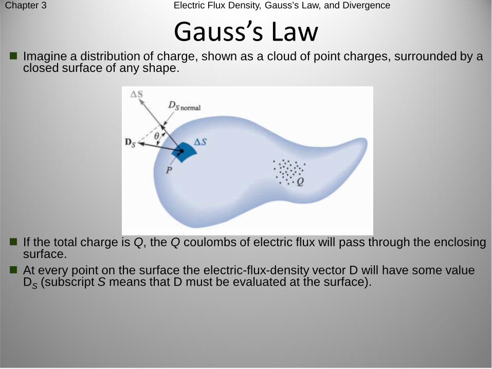
Gauss’s Law Imagine a distribution of charge, shown as a cloud of point charges, surrounded by a
closed surface of any shape.
Chapter 3 Electric Flux Density, Gauss’s Law, and Divergence
If the total charge is Q, the Q coulombs of electric flux will pass through the enclosing surface.
At every point on the surface the electric-flux-density vector D will have some value DS (subscript S means that D must be evaluated at the surface).
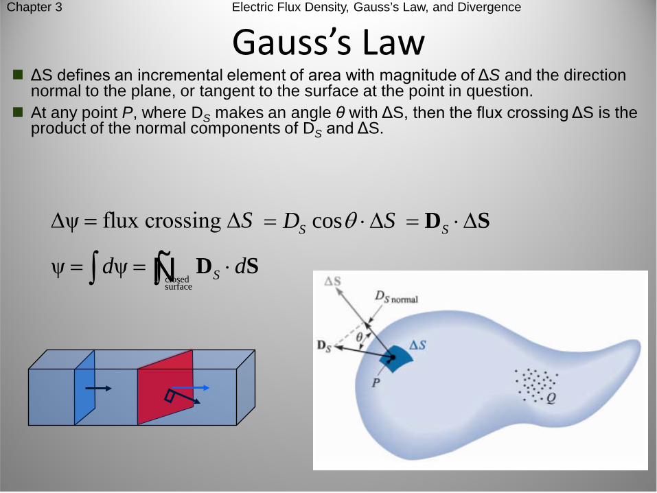
Gauss’s Law ΔS defines an incremental element of area with magnitude of ΔS and the direction
normal to the plane, or tangent to the surface at the point in question. At any point P, where DS makes an angle θ with ΔS, then the flux crossing ΔS is the
product of the normal components of DS and ΔS.
Chapter 3 Electric Flux Density, Gauss’s Law, and Divergence
ψ flux crossing S∆ = ∆ cosSD Sθ= ⋅∆ S= ⋅∆D S
closedsurface
ψ ψ Sd d= = ⋅∫ ∫ D SÑ

Gauss’s Law The resultant integral is a closed surface integral, with dS always involves the
differentials of two coordinates ► The integral is a double integral.
We can formulate the Gauss’s law mathematically as:
Chapter 3 Electric Flux Density, Gauss’s Law, and Divergence
ψ charge enclosedS
S d Q= ⋅ = =∫ D SÑ
nQ Q= ∑ LQ dLρ= ∫ SSQ dSρ= ∫ vvol
Q dvρ= ∫
The charge enclosed meant by the formula above might be several point charges, a line charge, a surface charge, or a volume charge distribution.

Gauss’s Law Chapter 3 Electric Flux Density, Gauss’s Law, and Divergence
We now take the last form, written in terms of the charge distribution, to represent the other forms:
volSS vd dvρ⋅ =∫ ∫D SÑ
Illustration. Let a point charge Q be placed at the origin of a spherical coordinate system, and choose a closed surface as a sphere of radius a.
The electric field intensity due to the point charge has been found to be:
204 r
Qrπε
=E a
0ε=D E 24 rQ
rπ⇒ =D a

Gauss’s Law Chapter 3 Electric Flux Density, Gauss’s Law, and Divergence
24S rQaπ
=D a
2 sin rd a d dθ θ φ=S a
22 sin sin
4 4S r rQ Qd a d d d da
θ θ φ θ θ φπ π
⋅ = ⋅ =D S a a
At the surface, r = a,
2
00
cos4Q π
π
φθ
θ θπ =
=
= −
ψS
S d= ⋅∫ D SÑ2
0 0sin
4 r a
Q d dπ π
φ θθ θ φ
π= ==
= ∫ ∫
Q=

Application of Gauss’s Law: Some Symmetrical Charge Distributions
Chapter 3 Electric Flux Density, Gauss’s Law, and Divergence
Let us now consider how to use the Gauss’s law to calculate the electric field intensity DS:
SSQ d= ⋅∫ D SÑ
The solution will be easy if we are able to choose a closed surface which satisfies two conditions:
1. DS is everywhere either normal or tangential to the closed surface, so that DS⋅dS becomes either DSdS or zero, respectively.
2. On that portion of the closed surface for which DS⋅dS is not zero, DS is constant.
For point charge ► The surface of a sphere. For line charge ► The surface of a cylinder.

Application of Gauss’s Law: Some Symmetrical Charge Distributions
Chapter 3 Electric Flux Density, Gauss’s Law, and Divergence
Dρ ρ=D a
From the previous discussion of the uniform line charge, only the radial component of D is present:
The choice of a surface that fulfill the requirement is simple: a cylindrical surface.
Dρ is every normal to the surface of a cylinder. It may then be closed by two plane surfaces normal to the z axis.

Application of Gauss’s Law: Some Symmetrical Charge Distributions
Chapter 3 Electric Flux Density, Gauss’s Law, and Divergence
SSQ d= ⋅∫ D SÑ
sides top bottom 0z z z z
zz LD dS D dS D dSρ ρ
ρ ρ′= === + +∫ ∫ ∫
2
0 0
L
zD d dz
π
ρ φρ φ
= == ∫ ∫
2D Lρ πρ=
2QD
Lρ πρ⇒ =
We know that the charge enclosed is ρLL,
2LDρ
ρπρ
=
02LEρ
ρπε ρ
=

Chapter 3 Electric Flux Density, Gauss’s Law, and Divergence
Application of Gauss’s Law: Some Symmetrical Charge Distributions
The problem of a coaxial cable is almost identical with that of the line charge.
Suppose that we have two coaxial cylindrical conductors, the inner of radius a and the outer of radius b, both with infinite length.
We shall assume a charge distribution of ρS on the outer surface of the inner conductor.
Choosing a circular cylinder of length L and radius ρ, a < ρ < b, as the gaussian surface, we find:
2SQ D Lπρ=
The total charge on a length L of the inner conductor is: 2
0 02
L
S SzQ ad dz aL
π
φρ φ π ρ
= == =∫ ∫ S
SaD ρρ
⇒ =

Chapter 3 Electric Flux Density, Gauss’s Law, and Divergence Application of Gauss’s Law: Some Symmetrical Charge Distributions
For one meter length, the inner conductor has 2πaρS coulombs, hence ρL = 2πaρS,
2L
ρρπρ
=D a
Everly line of electrix flux starting from the inner cylinder must terminate on the inner surface of the outer cylinder:
outer cyl ,inner cyl2 SQ aLπ ρ= −
,outer cyl ,inner cyl2 2S SbL aLπ ρ π ρ= −
,outer cyl ,inner cylS Sab
ρ ρ= −
If we use a cylinder of radius ρ > b, then the total charge enclosed will be zero. ► There is no external field,
0SD =
• Due to simplicity, noise immunity and broad bandwidth, coaxial cable is still the most common means of data transmission over short distances.

Example A 50-cm length of coaxial cable has an inner radius of 1 mm and an outer radius of 4
mm. The space between conductors is assumed to be filled with air. The total charge on the inner conductor is 30 nC. Find the charge density on each conductor and the expressions for E and D fields.
Chapter 3 Electric Flux Density, Gauss’s Law, and Divergence
Application of Gauss’s Law: Some Symmetrical Charge Distributions
inner cyl ,inner cyl2 SQ aLπ ρ=
inner cyl,inner cyl 2S
QaL
ρπ
⇒ =9
3
30 102 (10 )(0.5)π
−
−
×=
29.55 C mµ=
outer cyl ,outer cyl inner cyl2 SQ bL Qπ ρ= = −
inner cyl,outer cyl 2S
QbL
ρπ
−⇒ =
9
3
30 102 (4 10 )(0.5)π
−
−
− ×=
×22.39 C mµ= −
Chapter 3 Electric Flux Density, Gauss’s Law, and Divergence
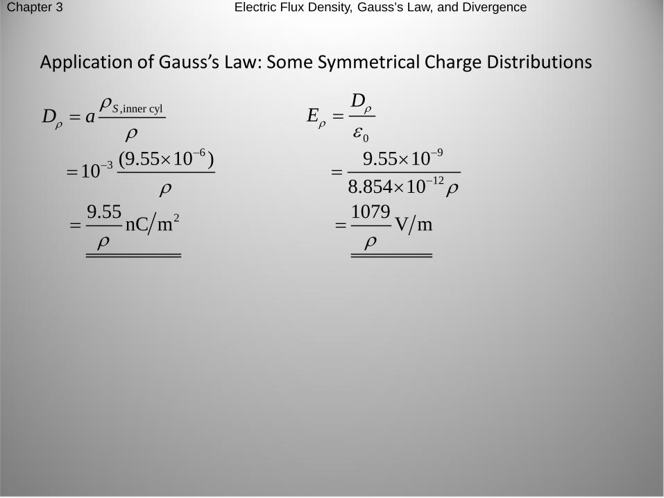
Application of Gauss’s Law: Some Symmetrical Charge Distributions
,inner cylSD aρ
ρρ
=
63 (9.55 10 )10
ρ
−− ×
=
29.55 nC mρ
=
0
DE ρ
ρ ε=
9
12
9.55 108.854 10 ρ
−
−
×=
×1079 V m
ρ=

Application of Gauss’s Law: Differential Volume Element Chapter 3 Electric Flux Density, Gauss’s Law, and DIvergence
We are now going to apply the methods of Gauss’s law to a slightly different type of problem: a surface without symmetry.
We have to choose such a very small closed surface that D is almost constant over the surface, and the small change in D may be adequately represented by using the first two terms of the Taylor’s-series expansion for D.
The result will become more nearly correct as the volume enclosed by the gaussian surface decreases.

0x
0( )f x
0x x x= + ∆
0( ) ( )f x x f x+ ∆ =
0( ) ( )f x f x x= + ∆
20 0 00
( ) ( ) ( )( ) ( ) ( ) ( )1! 2! !
nnf x f x f xf x f x x x x
n′ ′′
= + ∆ + ∆ + + ∆L
A point near x0
Only the linear terms are used for the linearization
Chapter 3 Electric Flux Density, Gauss’s Law, and DIvergence
Taylor’s Series Expansion

Application of Gauss’s Law: Differential Volume Element
Chapter 3 Electric Flux Density, Gauss’s Law, and DIvergence
Consider any point P, located by a rectangular coordinate system.
The value of D at the point P may be expressed in rectangular components:
0 0 0 0x x y y z zD D D= + +D a a a
We now choose as our closed surface, the small rectangular box, centered at P, having sides of lengths Δx, Δy, and Δz, and apply Gauss’s law:
Sd Q⋅ =∫ D SÑ
front back left right top bottomSd⋅ = + + + + +∫ ∫ ∫ ∫ ∫ ∫ ∫D SÑ

Chapter 3 Electric Flux Density, Gauss’s Law, and DIvergence
Application of Gauss’s Law: Differential Volume Element
We will now consider the front surface in detail. The surface element is very small, thus D is
essentially constant over this surface (a portion of the entire closed surface):
front frontfront⋅ ∆∫ D SB
front xy z⋅∆ ∆D aB
,frontxD y z∆ ∆B The front face is at a distance of Δx/2 from P, and therefore:
,front 0 rate of change of with 2x x xxD D D x∆
+ ×B
0 2x
xDxDx
∂∆+
∂B

Chapter 3 Electric Flux Density, Gauss’s Law, and DIvergence
We have now, for front surface:
Application of Gauss’s Law: Differential Volume Element
0front
2x
xDxD y zx
∂∆ + ∆ ∆ ∂ ∫ B
In the same way, the integral over the back surface can be found as:
back backback⋅∆∫ D SB
back ( )xy z⋅ −∆ ∆D aB
,backxD y z− ∆ ∆B
,back 0 2x
x xDxD Dx
∂∆−
∂B
0back
2x
xDxD y zx
∂∆ − + ∆ ∆ ∂ ∫ B

If we combine the two integrals over the front and back surface, we have:
Chapter 3 Electric Flux Density, Gauss’s Law, and DIvergence
Application of Gauss’s Law: Differential Volume Element
front back xD x y z
x∂
+ ∆ ∆ ∆∂∫ ∫ B
right left yD
y x zy
∂+ ∆ ∆ ∆
∂∫ ∫ B
top bottom zD z x y
z∂
+ ∆ ∆ ∆∂∫ ∫ B
Repeating the same process to the remaining surfaces, we find:
These results may be collected to yield:
S
yx zDD Dd x y z
x y z∂ ∂ ∂
⋅ + + ∆ ∆ ∆ ∂ ∂ ∂ ∫ D S BÑ
S
yx zDD Dd Q v
x y z∂ ∂ ∂
⋅ = + + ∆ ∂ ∂ ∂ ∫ D S BÑ

Chapter 3 Electric Flux Density, Gauss’s Law, and DIvergence
Charge enclosed in volume yx zDD Dv v
x y z∂ ∂ ∂
∆ + + × ∆ ∂ ∂ ∂ B
Application of Gauss’s Law: Differential Volume Element The previous equation is an approximation, which becomes better as Δv becomes
smaller. For the moment, we have applied Gauss’s law to the closed surface surrounding the
volume element Δv, with the result:

Chapter 3 Electric Flux Density, Gauss’s Law, and DIvergence
Application of Gauss’s Law: Differential Volume Element
Example Let D = y2z3 ax + 2xyz3 ay + 3xy2z2 az pC/m2 in free space.
(a) Find the total electric flux passing through the surface x = 3, 0 ≤ y ≤ 2, 0 ≤ z ≤ 1 in a direction away from the origin. (b) Find
|E| at P(3,2,1). (c) Find the total charge contained in an incremental sphere having a radius of 2 μm centered at P(3,2,1).
ψ SSd= ⋅∫ D S(a)
( ) ( )1 2 2 3 3 2 2
0 0 32 3 x y z xz y x
y z xyz xy z dydz= = =
= + + ⋅∫ ∫ a a a a
1 2 2 3
0 0y z dydz= ∫ ∫
2 11 13 43 40 0
y z=23 pC=
Chapter 3 Electric Flux Density, Gauss’s Law, and DIvergence
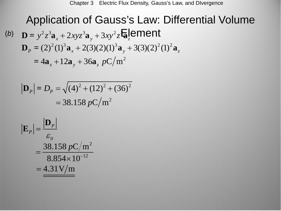
Application of Gauss’s Law: Differential Volume Element (b) 2 3 3 2 22 3x y zy z xyz xy z+ +D = a a a
2 3 3 2 2(2) (1) 2(3)(2)(1) 3(3)(2) (1)P x y z+ +D = a a a24 12 36 C mx y z p+ += a a a
2 2 2(4) (12) (36)P PD = + +D =238.158 C mp=
0
PP ε
=D
E
2
12
38.158 C m8.854 10
p−=
×4.31V m=

Chapter 3 Electric Flux Density, Gauss’s Law, and DIvergence
Application of Gauss’s Law: Differential Volume Element (c) yx z
DD DQ vx y z
∂ ∂ ∂+ + ∆ ∂ ∂ ∂
B
yx zP
P
DD DQ vx y z
∂ ∂ ∂+ + ∆ ∂ ∂ ∂
B
( ) 43 2 3 6 3 33 321
0 2 6 pC m (2 10 ) mxyz
xz xy z π −===
+ + × ×B
( ) 43 2 6 330 2(3)(1) 6(3)(2) (1) (2 10 ) Cpπ −+ + ×B
272.61 10 C−×B

We shall now obtain an exact relationship, by allowing the volume element Δv to shrink to zero.
Divergence Chapter 3 Electric Flux Density, Gauss’s Law, and DIvergence
Syx zdDD D Q
x y z v v
⋅∂ ∂ ∂+ + = ∂ ∂ ∂ ∆ ∆
∫ D SB Ñ
0 0lim limSyx zv v
dDD D Qx y z v v∆ → ∆ →
⋅∂ ∂ ∂+ + = = ∂ ∂ ∂ ∆ ∆
∫ D SÑ⇓
The last term is the volume charge density ρv, so that:
0lim Syx z
vv
dDD Dx y z v
ρ∆ →
⋅∂ ∂ ∂+ + = = ∂ ∂ ∂ ∆
∫ D SÑ

Divergence Chapter 3 Electric Flux Density, Gauss’s Law, and DIvergence
Let us no consider one information that can be obtained from the last equation:
0lim Syx zv
dDD Dx y z v∆ →
⋅∂ ∂ ∂+ + = ∂ ∂ ∂ ∆
∫ D SÑ
This equation is valid not only for electric flux density D, but also to any vector field A to find the surface integral for a small closed surface.
0lim Syx zv
dAA Ax y z v∆ →
⋅∂ ∂ ∂+ + = ∂ ∂ ∂ ∆
∫ A SÑ

Divergence Chapter 3 Electric Flux Density, Gauss’s Law, and DIvergence
This operation received a descriptive name, divergence. The divergence of A is defined as:
0Divergence of div lim S
v
d
v∆ →
⋅= =
∆∫ A S
A A Ñ
“The divergence of the vector flux density A is the outflow of flux from a small closed surface per unit volume as the volume shrinks to zero.”
A positive divergence of a vector quantity indicates a source of that vector quantity at that point.
Similarly, a negative divergence indicates a sink.

Divergence Chapter 3 Electric Flux Density, Gauss’s Law, and DIvergence
div yx zDD D
x y z∂∂ ∂
= + +∂ ∂ ∂
D
1 1div ( ) zD DDz
φρρ
ρ ρ ρ φ∂ ∂∂
= + +∂ ∂ ∂
D
22
1 1 1div ( ) (sin )sin sinr
Dr D D
r r r rφ
θθθ θ θ φ
∂∂ ∂= + +
∂ ∂ ∂D
Rectangular
Cylindrical
Spherical

Divergence Chapter 3 Electric Flux Density, Gauss’s Law, and DIvergence
Example If D = e–xsiny ax – e–x cosy ay + 2z az, find div D at the origin and P(1,2,3)
div yx zDD D
x y z∂∂ ∂
= + +∂ ∂ ∂
D sin sin 2x xe y e y− −= − + + 2=
Regardles of location the divergence of D equals 2 C/m3.
Maxwell s First Equation (Electrostatics)
Chapter 3 Electric Flux Density, Gauss’s Law, and Divergence:
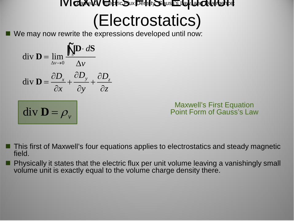
We may now rewrite the expressions developed until now:
div yx zDD D
x y z∂∂ ∂
= + +∂ ∂ ∂
D
0div lim S
v
d
v∆ →
⋅=
∆∫ D S
D Ñ
div vρ=DMaxwell’s First Equation
Point Form of Gauss’s Law
This first of Maxwell’s four equations applies to electrostatics and steady magnetic field.
Physically it states that the electric flux per unit volume leaving a vanishingly small volume unit is exactly equal to the volume charge density there.

Chapter 3 Electric Flux Density, Gauss’s Law, and DIvergence
The Vector Operator ∇ and The Divergence Theorem
Divergence is an operation on a vector yielding a scalar, just like the dot product. We define the del operator ∇ as a vector operator:
x y zx y z∂ ∂ ∂
∇ = + +∂ ∂ ∂
a a a
( )x y z x x y y z zD D Dx y z
∂ ∂ ∂∇ ⋅ = + + ⋅ + + ∂ ∂ ∂
D a a a a a a
yx zDD D
x y z∂∂ ∂
∇ ⋅ = + +∂ ∂ ∂
D
Then, treating the del operator as an ordinary vector, we can write:
div yx zDD D
x y z∂∂ ∂
∇ ⋅ + +∂ ∂ ∂
D = D =

The Vector Operator ∇ and The Divergence Theorem
Chapter 3 Electric Flux Density, Gauss’s Law, and DIvergence
We shall now give name to a theorem that we actually have obtained, the Divergence Theorem:
vol volSvd Q dv dvρ⋅ = = = ∇ ⋅∫ ∫ ∫D S DÑ
volSd dv⋅ = ∇ ⋅∫ ∫D S D Ñ
The first and last terms constitute the divergence theorem:
“The integral of the normal component of any vector field over a closed surface is equal to the integral of the divergence of this vector field throughout the volume enclosed by the closed surface.”

The Vector Operator ∇ and The Divergence Theorem Chapter 3 Electric Flux Density, Gauss’s Law, and DIvergence
Example Evaluate both sides of the divergence theorem for the field
D = 2xy ax + x2 ay C/m2 and the rectangular parallelepiped fomed by the planes x = 0 and 1, y = 0 and 2, and z = 0 and 3.
volSd dv⋅ = ∇ ⋅∫ ∫D S D Ñ
3 2 3 2
0 10 0 0 03 1 3 1
0 20 0 0 0
( ) ( ) ( ) ( )
( ) ( ) ( ) ( )
SS x x x x
y y y y
d dydz dydz
dxdz dxdz
= =
= =
⋅ = ⋅ − + ⋅
+ ⋅ − + ⋅
∫ ∫ ∫ ∫ ∫∫ ∫ ∫ ∫
D S D a D a
D a D a
Ñ
0 2( ) ( )y y y yD D= ==0( ) 0,x xD = =
3 2
10 0( )
SS x xd D dydz=⋅ =∫ ∫ ∫D SÑ
3 2
0 02ydydz= ∫ ∫ 12 C=
But
Divergence Theorem