Generalized Jensen-Shannon Divergence Lossfor Learning with Noisy Labels

Erik EnglessonKTH

Stockholm, Swedenengless@kth.se

Hossein AzizpourKTH

Stockholm, Swedenazizpour@kth.se

Abstract

Prior works have found it beneficial to combine provably noise-robust loss functionse.g., mean absolute error (MAE) with standard categorical loss function e.g. crossentropy (CE) to improve their learnability. Here, we propose to use Jensen-Shannondivergence as a noise-robust loss function and show that it interestingly interpolatebetween CE and MAE with a controllable mixing parameter. Furthermore, wemake a crucial observation that CE exhibits lower consistency around noisy datapoints. Based on this observation, we adopt a generalized version of the Jensen-Shannon divergence for multiple distributions to encourage consistency arounddata points. Using this loss function, we show state-of-the-art results on bothsynthetic (CIFAR), and real-world (e.g. WebVision) noise with varying noise rates.

1 Introduction

Labeled datasets, even the systematically annotated ones, contain noisy labels [1]. Therefore,designing noise-robust learning algorithms are crucial for the real-world tasks. An important avenueto tackle noisy labels is to devise noise-robust loss functions [2, 3, 4, 5]. Similarly, in this work, wepropose two new noise-robust loss functions based on two central observations as follows.

Observation I: Provably-robust loss functions can underfit the training data [2, 3, 4, 5].Observation II: Standard networks show low consistency around noisy data points 1, see Figure 1.

We first propose to use Jensen-Shannon divergence (JS) as a loss function, which we crucially showinterpolates between the noise-robust mean absolute error (MAE) and the cross entropy (CE) thatbetter fits the data through faster convergence. Figure 2 illustrates the CE-MAE interpolation.Regarding Observation II, we adopt the generalized version of Jensen-Shannon divergence (GJS) toencourage predictions on perturbed inputs to be consistent, see Figure 3. Notably, Jensen-Shannondivergence has previously shown promise for test-time robustness to domain shift [6], here we furtherargue for its training-time robustness to label noise. The key contributions of this work2 are:

• We make a novel observation that a network predictions’ consistency is reduced for noisy-labeled data when overfitting to noise, which motivates the use of consistency regularization.

• We propose using Jensen-Shannon divergence (JS) and its multi-distribution generaliza-tion (GJS) as loss functions for learning with noisy labels. We relate JS to loss functions thatare based on the noise-robustness theory of Ghosh et al. [2]. In particular, we prove that JSgeneralizes CE and MAE. Furthermore, we prove that GJS generalizes JS by incorporatingconsistency regularization in a single principled loss function.

• We provide an extensive set of empirical evidences on several datasets, noise types and rates.They show state-of-the-art results and give in-depth studies of the proposed losses.

1we call a network consistent around a sample (x) if it predicts the same class for x and its perturbations (x̃).2implementation available at https://github.com/ErikEnglesson/GJS

35th Conference on Neural Information Processing Systems (NeurIPS 2021).

0 100 200 300 400Epochs

0

20

40

60

80

100

Valid

atio

n Ac

cura

cy(%

)0%20%

40%60%

(a) Validation Accuracy

0 100 200 300 400Epochs

0

20

40

60

80

100

Cons

isten

cy(%

)

0%20%

40%60%

(b) Consistency Clean

0 100 200 300 400Epochs

0

20

40

60

80

100

Cons

isten

cy(%

)

20% 40% 60%

(c) Consistency Noisy

Figure 1: Evolution of a trained network’s consistency as it overfits to noise using CE loss. Herewe plot the evolution of the validation accuracy (a) and network’s consistency (as measured by GJS)on clean (b) and noisy (c) examples of the training set of CIFAR-100 for varying symmetric noiserates when learning with the cross-entropy loss. The consistency of the learnt function and theaccuracy closely correlate. This suggests that enforcing consistency may help avoid fitting to noise.Furthermore, the consistency is degraded more significantly for the noisy data points.

2 Generalized Jensen-Shannon DivergenceWe propose two loss functions, the Jensen-Shannon divergence (JS) and its multi-distributiongeneralization (GJS). In this section, we first provide background and two observations that motivateour proposed loss functions. This is followed by definition of the losses, and then we show thatJS generalizes CE and MAE similarly to other robust loss functions. Finally, we show how GJSgeneralizes JS to incorporate consistency regularization into a single principled loss function. Weprovide proofs of all theorems, propositions, and remarks in this section in Appendix C.

2.1 Background & Motivation

Supervised Classification. Assume a general function class3 F where each f ∈ F maps aninput x ∈ X to the probability simplex ∆K−1, i.e. to a categorical distribution over K classesy ∈ Y = {1, 2, . . . ,K}. We seek f∗ ∈ F that minimizes a risk RL(f) = ED[L(e(y), f(x))], forsome loss function L and joint distribution D over X×Y, where e(y) is a K-vector with one at indexy and zero elsewhere. In practice, D is unknown and, instead, we use S = {(xi, yi)}Ni=1 which areindependently sampled from D to minimize an empirical risk 1

N

∑Ni=1 L(e(yi), f(xi)).

Learning with Noisy Labels. In this work, the goal is to learn from a noisy training distributionDη where the labels are changed, with probability η, from their true distribution D. The noiseis called instance-dependent if it depends on the input, asymmetric if it dependents on the truelabel, and symmetric if it is independent of both x and y. Let f∗η be the optimizer of the noisydistribution risk RηL(f). A loss function L is then called robust if f∗η also minimizes RL. The MAEloss (LMAE(e(y), f(x)) := ‖e(y) − f(x)‖1) is robust but not CE [2].

Issue of Underfitting. Several works propose such robust loss functions and demonstrate theirefficacy in preventing noise fitting [2, 3, 4, 5]. However, all those works have observed slowconvergence of such robust loss functions leading to underfitting. This can be contrasted with CEthat has fast convergence but overfits to noise. Ghosh et al. [2] mentions slow convergence of MAEand GCE [3] extensively analyzes the undefitting thereof. SCE [4] reports similar problems for thereverse cross entropy and proposes a linear combination with CE. Finally, Ma et al. [5] observe thesame problem and consider a combination of “active” and “passive” loss functions.

Consistency Regularization. This encourages a network to have consistent predictions for differentperturbations of the same image, which has mainly been used for semi-supervised learning [7].

Motivation. In Figure 1, we show the validation accuracy and a measure of consistency duringtraining with the CE loss for varying amounts of noise. First, we note that training with CE losseventually overfits to noisy labels. Figure 1a, indicates that the higher the noise rate, the moreaccuracy drop when it starts to overfit to noise. Figure 1(b-c) shows the consistency of predictionsfor correct and noisy labeled examples of the training set, with the consistency measured as theratio of examples that have the same class prediction for two perturbations of the same image, see

3e.g. softmax neural network classifiers in this work

2

0.0 0.2 0.4 0.6 0.8 1.0Probability in given class

0

1

2

3

4

Loss

val

ue

JS, 1 = 0.01JS, 1 = 0.1JS, 1 = 0.3JS, 1 = 0.5CE

JS, 1 = 0.7JS, 1 = 0.9JS, 1 = 0.99JS, 1 = 0.999999MAE

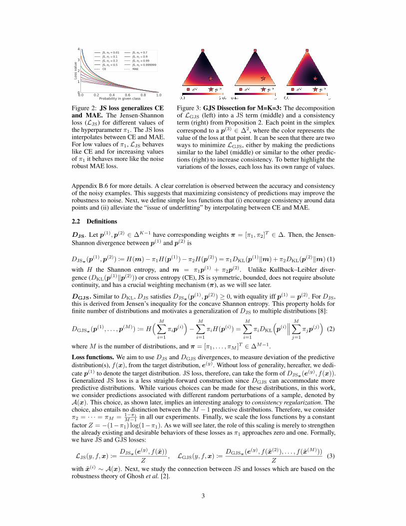
Figure 2: JS loss generalizes CEand MAE. The Jensen-Shannonloss (LJS) for different values ofthe hyperparameter π1. The JS lossinterpolates between CE and MAE.For low values of π1, LJS behaveslike CE and for increasing valuesof π1 it behaves more like the noiserobust MAE loss.

Figure 3: GJS Dissection for M=K=3: The decompositionof LGJS (left) into a JS term (middle) and a consistencyterm (right) from Proposition 2. Each point in the simplexcorrespond to a p(3) ∈ ∆2, where the color represents thevalue of the loss at that point. It can be seen that there are twoways to minimize LGJS, either by making the predictionssimilar to the label (middle) or similar to the other predic-tions (right) to increase consistency. To better highlight thevariations of the losses, each loss has its own range of values.

Appendix B.6 for more details. A clear correlation is observed between the accuracy and consistencyof the noisy examples. This suggests that maximizing consistency of predictions may improve therobustness to noise. Next, we define simple loss functions that (i) encourage consistency around datapoints and (ii) alleviate the “issue of underfitting” by interpolating between CE and MAE.

2.2 Definitions

DJS. Let p(1),p(2) ∈ ∆K−1 have corresponding weights π = [π1, π2]T ∈ ∆. Then, the Jensen-Shannon divergence between p(1) and p(2) is

DJSπ (p(1),p(2)) := H(m)− π1H(p(1))− π2H(p(2)) = π1DKL(p(1)‖m) + π2DKL(p(2)‖m) (1)

with H the Shannon entropy, and m = π1p(1) + π2p

(2). Unlike Kullback–Leibler diver-gence (DKL(p(1)‖p(2))) or cross entropy (CE), JS is symmetric, bounded, does not require absolutecontinuity, and has a crucial weighting mechanism (π), as we will see later.

DGJS. Similar to DKL, DJS satisfies DJSπ (p(1),p(2)) ≥ 0, with equality iff p(1) = p(2). For DJS,this is derived from Jensen’s inequality for the concave Shannon entropy. This property holds forfinite number of distributions and motivates a generalization of DJS to multiple distributions [8]:

DGJSπ (p(1), . . . ,p(M)) := H( M∑i=1

πip(i))−

M∑i=1

πiH(p(i)) =

M∑i=1

πiDKL

(p(i)∥∥∥ M∑j=1

πjp(j))

(2)

where M is the number of distributions, and π = [π1, . . . , πM ]T ∈ ∆M−1.

Loss functions. We aim to use DJS and DGJS divergences, to measure deviation of the predictivedistribution(s), f(x), from the target distribution, e(y). Without loss of generality, hereafter, we dedi-cate p(1) to denote the target distribution. JS loss, therefore, can take the form of DJSπ (e(y), f(x)).Generalized JS loss is a less straight-forward construction since DGJS can accommodate morepredictive distributions. While various choices can be made for these distributions, in this work,we consider predictions associated with different random perturbations of a sample, denoted byA(x). This choice, as shown later, implies an interesting analogy to consistency regularization. Thechoice, also entails no distinction between the M − 1 predictive distributions. Therefore, we considerπ2 = · · · = πM = 1−π1

M−1 in all our experiments. Finally, we scale the loss functions by a constantfactor Z = −(1−π1) log(1−π1). As we will see later, the role of this scaling is merely to strengthenthe already existing and desirable behaviors of these losses as π1 approaches zero and one. Formally,we have JS and GJS losses:

LJS(y, f,x) :=DJSπ (e(y), f(x̃))

Z, LGJS(y, f,x) :=

DGJSπ (e(y), f(x̃(2)), . . . , f(x̃(M)))

Z(3)

with x̃(i) ∼ A(x). Next, we study the connection between JS and losses which are based on therobustness theory of Ghosh et al. [2].

3

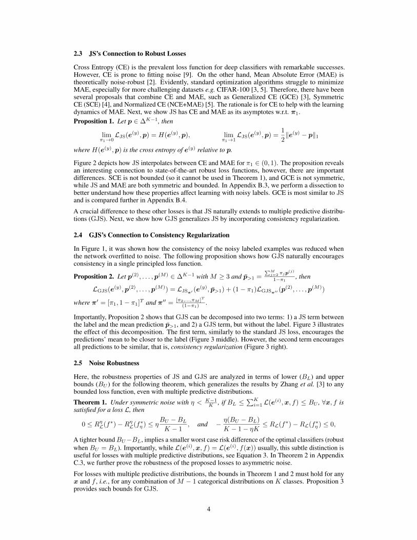
2.3 JS’s Connection to Robust Losses

Cross Entropy (CE) is the prevalent loss function for deep classifiers with remarkable successes.However, CE is prone to fitting noise [9]. On the other hand, Mean Absolute Error (MAE) istheoretically noise-robust [2]. Evidently, standard optimization algorithms struggle to minimizeMAE, especially for more challenging datasets e.g. CIFAR-100 [3, 5]. Therefore, there have beenseveral proposals that combine CE and MAE, such as Generalized CE (GCE) [3], SymmetricCE (SCE) [4], and Normalized CE (NCE+MAE) [5]. The rationale is for CE to help with the learningdynamics of MAE. Next, we show JS has CE and MAE as its asymptotes w.r.t. π1.Proposition 1. Let p ∈ ∆K−1, then

limπ1→0

LJS(e(y),p) = H(e(y),p), limπ1→1

LJS(e(y),p) =1

2‖e(y) − p‖1

where H(e(y),p) is the cross entropy of e(y) relative to p.

Figure 2 depicts how JS interpolates between CE and MAE for π1 ∈ (0, 1). The proposition revealsan interesting connection to state-of-the-art robust loss functions, however, there are importantdifferences. SCE is not bounded (so it cannot be used in Theorem 1), and GCE is not symmetric,while JS and MAE are both symmetric and bounded. In Appendix B.3, we perform a dissection tobetter understand how these properties affect learning with noisy labels. GCE is most similar to JSand is compared further in Appendix B.4.

A crucial difference to these other losses is that JS naturally extends to multiple predictive distribu-tions (GJS). Next, we show how GJS generalizes JS by incorporating consistency regularization.

2.4 GJS’s Connection to Consistency Regularization

In Figure 1, it was shown how the consistency of the noisy labeled examples was reduced whenthe network overfitted to noise. The following proposition shows how GJS naturally encouragesconsistency in a single principled loss function.

Proposition 2. Let p(2), . . . ,p(M) ∈ ∆K−1 with M ≥ 3 and p̄>1 =∑Mj=2 πjp

(j)

1−π1, then

LGJS(e(y),p(2), . . . ,p(M)) = LJSπ′ (e(y), p̄>1) + (1− π1)LGJSπ′′ (p

(2), . . . ,p(M))

where π′ = [π1, 1− π1]T and π′′ = [π2,...,πM ]T

(1−π1) .

Importantly, Proposition 2 shows that GJS can be decomposed into two terms: 1) a JS term betweenthe label and the mean prediction p̄>1, and 2) a GJS term, but without the label. Figure 3 illustratesthe effect of this decomposition. The first term, similarly to the standard JS loss, encourages thepredictions’ mean to be closer to the label (Figure 3 middle). However, the second term encouragesall predictions to be similar, that is, consistency regularization (Figure 3 right).

2.5 Noise Robustness

Here, the robustness properties of JS and GJS are analyzed in terms of lower (BL) and upperbounds (BU ) for the following theorem, which generalizes the results by Zhang et al. [3] to anybounded loss function, even with multiple predictive distributions.

Theorem 1. Under symmetric noise with η < K−1K , if BL ≤

∑Ki=1 L(e(i),x, f) ≤ BU , ∀x, f is

satisfied for a loss L, then

0 ≤ RηL(f∗)−RηL(f∗η ) ≤ ηBU −BLK − 1

, and − η(BU −BL)

K − 1− ηK≤ RL(f∗)−RL(f∗η ) ≤ 0,

A tighter boundBU−BL, implies a smaller worst case risk difference of the optimal classifiers (robustwhen BU = BL). Importantly, while L(e(i),x, f) = L(e(i), f(x)) usually, this subtle distinction isuseful for losses with multiple predictive distributions, see Equation 3. In Theorem 2 in AppendixC.3, we further prove the robustness of the proposed losses to asymmetric noise.

For losses with multiple predictive distributions, the bounds in Theorem 1 and 2 must hold for anyx and f , i.e., for any combination of M − 1 categorical distributions on K classes. Proposition 3provides such bounds for GJS.

4

Proposition 3. GJS loss withM ≤ K+1 satisfiesBL ≤∑Kk=1 LGJS(e(k),p(2), . . . ,p(M)) ≤ BU

for all p(2), . . . ,p(M) ∈ ∆K−1, with the following bounds

BL =

K∑k=1

LGJS(e(k),u, . . . ,u), BU =

K∑k=1

LGJS(e(k), e(1), . . . , e(M−1))

where u ∈ ∆K−1 is the uniform distribution.Note the bounds for the JS loss is a special case of Proposition 3 for M = 2.Remark 1. LJS and LGJS are robust (BL = BU ) in the limit of π1 → 1.

Remark 1 is intuitive from Section 2.3 which showed that LJS is equivalent to the robust MAE in thislimit and that the consistency term in Proposition 2 vanishes.

In Proposition 3, the lower bound (BL) is the same for JS and GJS. However, the upper bound (BU )increases for more distributions, which makes JS have a tighter bound than GJS in Theorem 1 and 2.In Proposition 4, we show that JS and GJS have the same bound for the risk difference, given anassumption based on Figure 1 that the optimal classifier on clean data (f∗) is at least as consistent asthe optimal classifier on noisy data (f∗η ).Proposition 4. LJS and LGJS have the same risk bounds in Theorem 1 and 2 ifEx[Lf

∗

GJSπ′′(p(2), . . . ,p(M))] ≤ Ex[Lf

∗η

GJSπ′′(p(2), . . . ,p(M))], where LfGJSπ′′

(p(2), . . . ,p(M)) isthe consistency term from Proposition 2.

3 Related Works

Interleaved in the previous sections, we covered most-related works to us, i.e. the avenue of identifica-tion or construction of theoretically-motivated robust loss functions [2, 3, 4, 5]. These works, similarto this paper, follow the theoretical construction of Ghosh et al. [2]. Furthermore, Liu&Guo [10] use“peer prediction” to propose a new family of robust loss functions. Different to these works, here, wepropose loss functions based on DJS which holds various desirable properties of those prior workswhile exhibiting novel ties to consistency regularization; a recent important regularization technique.

Next, we briefly cover other lines of work. A more thorough version can be found in Appendix D.

A direction, that similar to us does not alter training, reweights a loss function by confusion matrix [11,12, 13, 14, 15]. Assuming a class-conditional noise model, loss correction is theoretically motivatedand perfectly orthogonal to noise-robust losses.

Consistency regularization is a recent technique that imposes smoothness in the learnt function forsemi-supervised learning [7] and recently for noisy data [16]. These works use different complexpipelines for such regularization. GJS encourages consistency in a simple way that exhibits otherdesirable properties for learning with noisy labels. Importantly, Jensen-Shannon-based consistencyloss functions have been used to improve test-time robustness to image corruptions [6] and adversarialexamples [17], which further verifies the general usefulness of GJS. In this work, we study suchloss functions for a different goal: training-time label-noise robustness. In this context, our thoroughanalytical and empirical results are, to the best of our knowledge, novel.

Recently, loss functions with information-theoretic motivations have been proposed [18, 19]. JS, withan apparent information-theoretic interpretation, has a strong connection to those. Especially, the latteris a close concurrent work studying JS and other divergences from the family of f-divergences [20].However, in this work, we consider a generalization to more than two distributions and study the roleof π1, which they treat as a constant (π1 = 1

2 ). These differences lead to improved performance andnovel theoretical results, e.g., Proposition 1 and 2. Lastly, another generalization of JS was recentlypresented by Nielsen [21], where the arithmetic mean is generalized to abstract means.

4 Experiments

This section, first, empirically investigates the effectiveness of the proposed losses for learningwith noisy labels on synthetic (Section 4.1) and real-world noise (Section 4.2). This is followed byseveral experiments and ablation studies (Section 4.3) to shed light on the properties of JS and GJSthrough empirical substantiation of the theories and claims provided in Section 2. All these additionalexperiments are done on the more challenging CIFAR-100 dataset.

5

Table 1: Synthetic Noise Benchmark on CIFAR. We reimplement other noise-robust loss functionsinto the same learning setup and ResNet-34, including label smoothing (LS), Bootstrap (BS),Symmetric CE (SCE), Generalized CE (GCE), and Normalized CE (NCE+RCE). We used samehyperparameter optimization budget and mechanism for all the prior works and ours. Mean testaccuracy and standard deviation are reported from five runs and the statistically-significant topperformers are boldfaced. The thorough analysis is evident from the higher performance of CE in oursetup compared to prior works. GJS achieves state-of-the-art results for different noise rates, types,and datasets. Generally, GJS’s efficacy is more evident for the more challenging CIFAR-100 dataset.

Dataset MethodNo Noise Symmetric Noise Rate Asymmetric Noise Rate

0% 20% 40% 60% 80% 20% 40%

CIFAR-10

CE 95.77 ± 0.11 91.63 ± 0.27 87.74 ± 0.46 81.99 ± 0.56 66.51 ± 1.49 92.77 ± 0.24 87.12 ± 1.21BS 94.58 ± 0.25 91.68 ± 0.32 89.23 ± 0.16 82.65 ± 0.57 16.97 ± 6.36 93.06 ± 0.25 88.87 ± 1.06LS 95.64 ± 0.12 93.51 ± 0.20 89.90 ± 0.20 83.96 ± 0.58 67.35 ± 2.71 92.94 ± 0.17 88.10 ± 0.50SCE 95.75 ± 0.16 94.29 ± 0.14 92.72 ± 0.25 89.26 ± 0.37 80.68 ± 0.42 93.48 ± 0.31 84.98 ± 0.76GCE 95.75 ± 0.14 94.24 ± 0.18 92.82 ± 0.11 89.37 ± 0.27 79.19 ± 2.04 92.83 ± 0.36 87.00 ± 0.99NCE+RCE 95.36 ± 0.09 94.27 ± 0.18 92.03 ± 0.31 87.30 ± 0.35 77.89 ± 0.61 93.87 ± 0.03 86.83 ± 0.84JS 95.89 ± 0.10 94.52 ± 0.21 93.01 ± 0.22 89.64 ± 0.15 76.06 ± 0.85 92.18 ± 0.31 87.99 ± 0.55GJS 95.91 ± 0.09 95.33 ± 0.18 93.57 ± 0.16 91.64 ± 0.22 79.11 ± 0.31 93.94 ± 0.25 89.65 ± 0.37

CIFAR-100

CE 77.60 ± 0.17 65.74 ± 0.22 55.77 ± 0.83 44.42 ± 0.84 10.74 ± 4.08 66.85 ± 0.32 49.45 ± 0.37BS 77.65 ± 0.29 72.92 ± 0.50 68.52 ± 0.54 53.80 ± 1.76 13.83 ± 4.41 73.79 ± 0.43 64.67 ± 0.69LS 78.60 ± 0.04 74.88 ± 0.15 68.41 ± 0.20 54.58 ± 0.47 26.98 ± 1.07 73.17 ± 0.46 57.20 ± 0.85SCE 78.29 ± 0.24 74.21 ± 0.37 68.23 ± 0.29 59.28 ± 0.58 26.80 ± 1.11 70.86 ± 0.44 51.12 ± 0.37GCE 77.65 ± 0.17 75.02 ± 0.24 71.54 ± 0.39 65.21 ± 0.16 49.68 ± 0.84 72.13 ± 0.39 51.50 ± 0.71NCE+RCE 74.66 ± 0.21 72.39 ± 0.24 68.79 ± 0.29 62.18 ± 0.35 31.63 ± 3.59 71.35 ± 0.16 57.80 ± 0.52JS 77.95 ± 0.39 75.41 ± 0.28 71.12 ± 0.30 64.36 ± 0.34 45.05 ± 0.93 71.70 ± 0.36 49.36 ± 0.25GJS 79.27 ± 0.29 78.05 ± 0.25 75.71 ± 0.25 70.15 ± 0.30 44.49 ± 0.53 74.60 ± 0.47 63.70 ± 0.22

Experimental Setup. We use ResNet 34 and 50 for experiments on CIFAR and WebVision datasetsrespectively and optimize them using SGD with momentum. The complete details of the trainingsetup can be found in Appendix A. Most importantly, we take three main measures to ensure a fairand reliable comparison throughout the experiments: 1) we reimplement all the loss functions wecompare with in a single shared learning setup, 2) we use the same hyperparameter optimizationbudget and mechanism for all the prior works and ours, and 3) we train and evaluate five networks forindividual results, where in each run the synthetic noise, network initialization, and data-order aredifferently randomized. The thorough analysis is evident from the higher performance of CE in oursetup compared to prior works. Where possible, we report mean and standard deviation and denotethe statistically-significant top performers with student t-test.

4.1 Synthetic Noise Benchmarks: CIFAR

Here, we evaluate the proposed loss functions on the CIFAR datasets with two types of syntheticnoise: symmetric and asymmetric. For symmetric noise, the labels are, with probability η, re-sampled from a uniform distribution over all labels. For asymmetric noise, we follow the standardsetup of Patrini et al. [22]. For CIFAR-10, the labels are modified, with probability η, as follows:truck→ automobile, bird→ airplane, cat↔ dog, and deer→ horse. For CIFAR-100, labels are,with probability η, cycled to the next sub-class of the same “super-class”, e.g. the labels of super-class“vehicles 1” are modified as follows: bicycle→ bus→ motorcycle→ pickup truck→ train→ bicycle.

We compare with other noise-robust loss functions such as label smoothing (LS) [23], Boot-strap (BS) [24], Symmetric Cross-Entropy (SCE) [4], Generalized Cross-Entropy (GCE) [3], and theNCE+RCE loss of Ma et al. [5]. Here, we do not compare to methods that propose a full pipelinesince, first, a conclusive comparison would require re-implementation and individual evaluation ofseveral components and second, robust loss functions can be considered orthogonal to them.

Results. Table 1 shows the results for symmetric and asymmetric noise on CIFAR-10 and CIFAR-100. GJS performs similarly or better than other methods for different noise rates, noise types, anddata sets. Generally, GJS’s efficacy is more evident for the more challenging CIFAR-100 dataset.For example, on 60% uniform noise on CIFAR-100, the difference between GJS and the secondbest (GCE) is 4.94 percentage points, while our results on 80% noise is lower than GCE. We attributethis to the high sensitivity of the results to the hyperparameter settings in such a high-noise ratewhich are also generally unrealistic (WebVision has ∼20%). The performance of JS is consistently

6

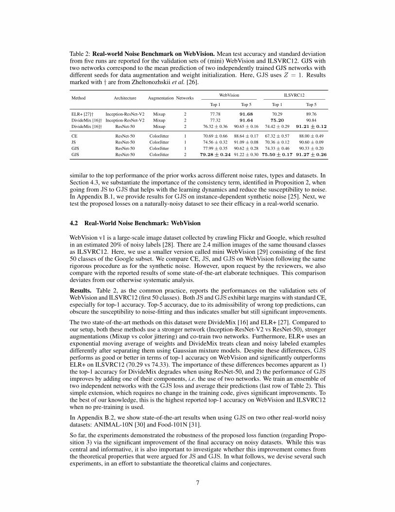
Table 2: Real-world Noise Benchmark on WebVision. Mean test accuracy and standard deviationfrom five runs are reported for the validation sets of (mini) WebVision and ILSVRC12. GJS withtwo networks correspond to the mean prediction of two independently trained GJS networks withdifferent seeds for data augmentation and weight initialization. Here, GJS uses Z = 1. Resultsmarked with † are from Zheltonozhskii et al. [26].

Method Architecture Augmentation NetworksWebVision ILSVRC12

Top 1 Top 5 Top 1 Top 5

ELR+ [27]† Inception-ResNet-V2 Mixup 2 77.78 91.68 70.29 89.76DivideMix [16]† Inception-ResNet-V2 Mixup 2 77.32 91.64 75.20 90.84DivideMix [16]† ResNet-50 Mixup 2 76.32± 0.36 90.65± 0.16 74.42± 0.29 91.21 ± 0.12

CE ResNet-50 ColorJitter 1 70.69± 0.66 88.64± 0.17 67.32± 0.57 88.00± 0.49JS ResNet-50 ColorJitter 1 74.56± 0.32 91.09± 0.08 70.36± 0.12 90.60± 0.09GJS ResNet-50 ColorJitter 1 77.99± 0.35 90.62± 0.28 74.33± 0.46 90.33± 0.20GJS ResNet-50 ColorJitter 2 79.28 ± 0.24 91.22± 0.30 75.50 ± 0.17 91.27 ± 0.26

similar to the top performance of the prior works across different noise rates, types and datasets. InSection 4.3, we substantiate the importance of the consistency term, identified in Proposition 2, whengoing from JS to GJS that helps with the learning dynamics and reduce the susceptibility to noise.In Appendix B.1, we provide results for GJS on instance-dependent synthetic noise [25]. Next, wetest the proposed losses on a naturally-noisy dataset to see their efficacy in a real-world scenario.

4.2 Real-World Noise Benchmark: WebVision

WebVision v1 is a large-scale image dataset collected by crawling Flickr and Google, which resultedin an estimated 20% of noisy labels [28]. There are 2.4 million images of the same thousand classesas ILSVRC12. Here, we use a smaller version called mini WebVision [29] consisting of the first50 classes of the Google subset. We compare CE, JS, and GJS on WebVision following the samerigorous procedure as for the synthetic noise. However, upon request by the reviewers, we alsocompare with the reported results of some state-of-the-art elaborate techniques. This comparisondeviates from our otherwise systematic analysis.

Results. Table 2, as the common practice, reports the performances on the validation sets ofWebVision and ILSVRC12 (first 50 classes). Both JS and GJS exhibit large margins with standard CE,especially for top-1 accuracy. Top-5 accuracy, due to its admissibility of wrong top predictions, canobscure the susceptibility to noise-fitting and thus indicates smaller but still significant improvements.

The two state-of-the-art methods on this dataset were DivideMix [16] and ELR+ [27]. Compared toour setup, both these methods use a stronger network (Inception-ResNet-V2 vs ResNet-50), strongeraugmentations (Mixup vs color jittering) and co-train two networks. Furthermore, ELR+ uses anexponential moving average of weights and DivideMix treats clean and noisy labeled examplesdifferently after separating them using Gaussian mixture models. Despite these differences, GJSperforms as good or better in terms of top-1 accuracy on WebVision and significantly outperformsELR+ on ILSVRC12 (70.29 vs 74.33). The importance of these differences becomes apparent as 1)the top-1 accuracy for DivideMix degrades when using ResNet-50, and 2) the performance of GJSimproves by adding one of their components, i.e. the use of two networks. We train an ensemble oftwo independent networks with the GJS loss and average their predictions (last row of Table 2). Thissimple extension, which requires no change in the training code, gives significant improvements. Tothe best of our knowledge, this is the highest reported top-1 accuracy on WebVision and ILSVRC12when no pre-training is used.

In Appendix B.2, we show state-of-the-art results when using GJS on two other real-world noisydatasets: ANIMAL-10N [30] and Food-101N [31].

So far, the experiments demonstrated the robustness of the proposed loss function (regarding Propo-sition 3) via the significant improvement of the final accuracy on noisy datasets. While this wascentral and informative, it is also important to investigate whether this improvement comes fromthe theoretical properties that were argued for JS and GJS. In what follows, we devise several suchexperiments, in an effort to substantiate the theoretical claims and conjectures.

7

0 100 200 300 400Epochs

0

20

40

60

80

Valid

atio

n Ac

cura

cy(%

)

10.10.50.9

(a) JS, η = 20%

0 100 200 300 400Epochs

0

20

40

60

80

Valid

atio

n Ac

cura

cy(%

)

10.10.50.9

(b) JS, η = 60%

0 100 200 300 400Epochs

0

20

40

60

80

Valid

atio

n Ac

cura

cy(%

)

10.10.50.9

(c) GJS, η = 20%

0 100 200 300 400Epochs

0

20

40

60

80

Valid

atio

n Ac

cura

cy(%

)

10.10.50.9

(d) GJS, η = 60%

Figure 4: Effect of π1. Validation accuracyof JS and GJS during training with symmetricnoise on CIFAR100. From Proposition 1, JS be-haves like CE and MAE for low and high valuesof π1, respectively. The signs of noise-fitting forπ1 = 0.1 on 60% noise (b), and slow learning ofπ1 = 0.9 (a-b), show this in practice. The GJSloss does not exhibit overfitting for low values ofπ1 and learns quickly for large values of π1 (c-d).

2 3 4 5 6 7 8Number of distributions(M)

60.0

62.5

65.0

67.5

70.0

72.5

75.0

77.5

80.0

Valid

atio

n Ac

cura

cy(%

)

0%20%

40%60%

Figure 5: Effect of M. Validation accuracy forincreasing number of distributions (M ) and dif-ferent symmetric noise rates on CIFAR-100 withπ1 = 1

2 . For all noise rates, using three insteadof two distributions results in a higher accuracy.Going beyond three distributions is only help-ful for lower noise rates. For simplicity we useM = 3 (corresponding to two augmentations)for all of our experiments.

4.3 Towards a Better Understanding of the Jensen-Shannon-based Loss FunctionsHere, we study the behavior of the losses for different distribution weights π1, number of distributionsM , and epochs. We also provide insights on why GJS performs better than JS.

How does π1 control the trade-off of robustness and learnability? In Figure 4, we plot thevalidation accuracy during training for both JS and GJS at different values of π1 and noise rates η.From Proposition 1, we expect JS to behave as CE for low values of π1 and as MAE for larger valuesof π1. Figure 4 (a-b) confirms this. Specifically, π1 = 0.1 learns quickly and performs well for lownoise but overfits for η = 0.6 (characteristic of non-robust CE), on the other hand, π1 = 0.9 learnsslowly but is robust to high noise rates (characteristic of noise-robust MAE).

In Figure 4 (c-d), we observe three qualitative improvements of GJS over JS: 1) no signs of overfittingto noise for large noise rates with low values of π1, 2) better learning dynamics for large values of π1

that otherwise learns slowly, and 3) converges to a higher validation accuracy.

How many distributions to use? Figure 5 depicts validation accuracy for varying number ofdistributions M . For all noise rates, we observe a performance increase going from M = 2 to M = 3.However, the performance of M > 3 depends on the noise rate. For lower noise rates, having morethan three distributions can improve the performance. For higher noise rates e.g. 60%, having M > 3degrades the performance. We hypothesise this is due to: 1) at high noise rates, there are only a fewcorrectly labeled examples that can help guide the learning, and 2) going from M = 2 to M = 3 addsa consistency term, while M > 3 increases the importance of the consistency term in Proposition 2.Therefore, for a large enough M, the loss will find it easier to keep the consistency term low (keeppredictions close to uniform as at the initialization), instead of generalizing based on the few cleanexamples. For simplicity, we have used M = 3 for all experiments with GJS.

Is the improvements of GJS over JS due to mean prediction or consistency? Proposition 2decomposed GJS into a JS term with a mean prediction (p̄>1) and a consistency term operatingon all distributions but the target. In Table 3, we compare the performance of JS and GJS to GJSwithout the consistency term, i.e., LJSπ′ (e

(y), p̄>1). The results suggest that the improvement ofGJS over JS can be attributed to the consistency term.

Figure 4 (a-b) showed that JS improves the learning dynamics of MAE by blending it with CE,controlled by π1. Similarly, we see here that the consistency term also improves the learningdynamics (underfitting and convergence speed) of MAE. Interestingly, Figure 4 (c-d), shows thehigher values of π1 (closer to MAE) work best for GJS, hinting that, the consistency term improvesthe learning dynamics of MAE so much so that the role of CE becomes less important.

8

Table 3: Effect of Consistency. Validation ac-curacy for JS, GJS w/o the consistency term inProposition 2, and GJS for 40% noise on theCIFAR-100 dataset. Using the mean of two pre-dictions in the JS loss does not improve perfor-mance. On the other hand, adding the consis-tency term significantly helps.

Method Accuracy

LJS(e(y),p(2)) 71.0LJS

π′(e(y), p̄>1) 68.7

LGJS(e(y),p(2),p(3)) 74.3

Table 4: Effect of GJS. Validation accuracywhen using different loss functions for clean andnoisy examples of the CIFAR-100 training setwith 40% symmetric noise. Noisy examples ben-efit significantly more from GJS than clean ex-amples (74.1 vs 72.9).

Method π1

Clean Noisy 0.1 0.5 0.9

JS JS 70.0 71.5 55.3GJS JS 72.6 72.9 70.2JS GJS 71.0 74.1 68.0

GJS GJS 71.3 74.7 73.8

Is GJS mostly helping the clean or noisy examples? To better understand the improvementsof GJS over JS, we perform an ablation with different losses for clean and noisy examples, seeTable 4. We observe that using GJS instead of JS improves performance in all cases. Importantly,using GJS only for the noisy examples performs significantly better than only using it for the cleanexamples (74.1 vs 72.9). The best result is achieved when using GJS for both clean and noisyexamples but still close to the noisy-only case (74.7 vs 74.1).

How is different choices of perturbations affecting GJS? In this work, we use stochastic augmen-tations for A, see Appendix A.1 for details. Table 5 reports validation results on 40% symmetric andasymmetric noise on CIFAR-100 for varying types of augmentation. We observe that all methodsimprove their performance with stronger augmentation and that GJS achieves the best results inall cases. Also, note that we use weak augmentation for all naturally-noisy datasets (WebVision,ANIMAL-10N, and Food-101N) and still get state-of-the-art results.

How fast is the convergence? We found that some baselines (especially the robust NCE+RCE)had slow convergence. Therefore, we used 400 epochs for all methods to make sure all had time toconverge properly. Table 6 shows results on 40% symmetric and asymmetric noise on CIFAR-100when the number of epochs has been reduced by half.

Is training with the proposed losses leading to more consistent networks? Our motivation forinvestigating losses based on Jensen-Shannon divergence was partly due to the observation in Figure 1that consistency and accuracy correlate when learning with CE loss. In Figure 6, we compare CE, JS,and GJS losses in terms of validation accuracy and consistency during training on CIFAR-100 with40% symmetric noise. We find that the networks trained with JS and GJS losses are more consistentand has higher accuracy. In Appendix B.7, we report the consistency of the networks in Table 1.

Summary of experiments in the appendix. Due to space limitations, we report several importantexperiments in the appendix. We evaluate the effectiveness of GJS on 1) instance-dependent syntheticnoise (Section B.1), and 2) real-world noisy datasets ANIMAL-10N and Food-101N (Section B.2).We also investigate the importance of 1) losses being symmetric and bounded for learning with noisylabels (Section B.3), and 2) a clean vs noisy validation set for hyperparameter selection and the effectof a single set of parameters for all noise rates (Section B.5).

Table 5: Effect of Augmentation Strategy. Val-idation accuracy for training w/o CutOut(-CO) orw/o RandAug(-RA) or w/o both(weak) on 40%symmetric and asymmetric noise on CIFAR-100.All methods improves by stronger augmentations.GJS performs best for all types of augmentations.

MethodSymmetric Asymmetric

Full -CO -RA Weak Full -CO -RA Weak

GCE 70.8 64.2 64.1 58.0 51.7 44.9 46.6 42.9NCE+RCE 68.5 66.6 68.3 61.7 57.5 52.1 49.5 44.4GJS 74.8 71.3 70.6 66.5 62.6 56.8 52.2 44.9

Table 6: Effect of Number of Epochs. Vali-dation accuracy for training with 200 and 400epochs for 40% symmetric and asymmetricnoise on CIFAR-100. GJS still outperformsthe baselines and NCE+RCE’s performanceis reduced heavily by the decrease in epochs.

MethodSymmetric Asymmetric

200 400 200 400

GCE 70.3 70.8 39.1 51.7NCE+RCE 60.0 68.5 35.0 57.5GJS 72.9 74.8 43.2 62.6

9

0 100 200 300 400Epochs

0

20

40

60

80

100

Val A

ccur

acy(

%)

CE JS GJS

(a) Validation Accuracy

0 100 200 300 400Epochs

0

20

40

60

80

100

Cons

isten

cy(%

)

CE JS GJS

(b) Consistency Clean

0 100 200 300 400Epochs

0

20

40

60

80

100

Cons

isten

cy(%

)

CE JS GJS

(c) Consistency Noisy

Figure 6: Evolution of a trained network’s consistency for the CE, JS, and GJS losses. We plotthe evolution of the validation accuracy (a) and network’s consistency on clean (b) and noisy (c)examples of the training set of CIFAR-100 when learning with 40% symmetric noise. All losses usethe same learning rate and weight decay and both JS and GJS use π1 = 0.5. The consistency ofthe learnt function and the accuracy closely correlate. The accuracy and consistency of JS and GJSimprove during training, while both degrade when learning with CE loss.

5 Limitations & Future Directions

We empirically showed that the consistency of the network around noisy data degrades as it fits noiseand accordingly proposed a loss based on generalized Jensen-Shannon divergence (GJS). While weempirically verified the significant role of consistency regularization in robustness to noise, we onlytheoretically showed the robustness (BL = BU ) of GJS at its limit (π1 → 1) where the consistencyterm gradually vanishes. Therefore, the main limitation is the lack of a theoretical proof of therobustness of the consistency term in Proposition 2. This is, in general, an important but understudiedarea, also for the literature of self- or semi-supervised learning and thus is of utmost importance forfuture works.

Secondly, we had an important observation that GJS with M > 3 might not perform well under highnoise rates. While we have some initial conjectures, this phenomenon deserves a systematic analysisboth empirically and theoretically.

Finally, a minor practical limitation is the added computations for GJS forward passes, however thisapplies to training time only and in all our experiments, we only use one extra prediction (M = 3).

6 Final Remarks

We first made two central observations that (i) robust loss functions have an underfitting issue and (ii)consistency of noise-fitting networks is significantly lower around noisy data points. Correspondingly,we proposed two loss functions, JS and GJS, based on Jensen-Shannon divergence that (i) interpolatesbetween noise-robust MAE and fast-converging CE, and (ii) encourages consistency around trainingdata points. This simple proposal led to state-of-the-art performance on both synthetic and real-worldnoise datasets even when compared to the more elaborate pipelines such as DivideMix or ELR+.Furthermore, we discussed their robustness within the theoretical construction of Ghosh et al. [2]. Bydrawing further connections to other seminal loss functions such as CE, MAE, GCE, and consistencyregularization, we uncovered other desirable or informative properties. We further empirically studieddifferent aspects of the losses that corroborate various theoretical properties.

Overall, we believe the paper provides informative theoretical and empirical evidence for the useful-ness of two simple and novel JS divergence-based loss functions for learning under noisy data thatachieve state-of-the-art results. At the same time, it opens interesting future directions.

Ethical Considerations. Considerable resources are needed to create labeled data sets due to theburden of manual labeling process. Thus, the creators of large annotated datasets are mostly limitedto well-funded companies and academic institutions. In that sense, developing robust methods againstlabel noise enables less affluent organizations or individuals to benefit from labeled datasets sinceimperfect or automatic labeling can be used instead. On the other hand, proliferation of such harvesteddatasets can increase privacy concerns arising from redistribution and malicious use.

Acknowledgement. This work was partially supported by the Wallenberg AI, Autonomous Systemsand Software Program (WASP) funded by the Knut and Alice Wallenberg Foundation.

10

References[1] Lucas Beyer, Olivier J Hénaff, Alexander Kolesnikov, Xiaohua Zhai, and Aäron van den Oord.

Are we done with imagenet? arXiv preprint arXiv:2006.07159, 2020.

[2] Aritra Ghosh, Himanshu Kumar, and PS Sastry. Robust loss functions under label noise for deepneural networks. In Proceedings of the Thirty-First AAAI Conference on Artificial Intelligence,pages 1919–1925, 2017.

[3] Zhilu Zhang and Mert Sabuncu. Generalized cross entropy loss for training deep neural networkswith noisy labels. In Advances in neural information processing systems, pages 8778–8788,2018.

[4] Yisen Wang, Xingjun Ma, Zaiyi Chen, Yuan Luo, Jinfeng Yi, and James Bailey. Symmetriccross entropy for robust learning with noisy labels. In Proceedings of the IEEE InternationalConference on Computer Vision, pages 322–330, 2019.

[5] Xingjun Ma, Hanxun Huang, Yisen Wang, Simone Romano, Sarah Erfani, and James Bailey.Normalized loss functions for deep learning with noisy labels, 2020.

[6] Dan Hendrycks, Norman Mu, Ekin D. Cubuk, Barret Zoph, Justin Gilmer, and Balaji Lakshmi-narayanan. Augmix: A simple data processing method to improve robustness and uncertainty.In International Conference on Learning Representation, 2020.

[7] Avital Oliver, Augustus Odena, Colin Raffel, Ekin D Cubuk, and Ian J Goodfellow. Realisticevaluation of deep semi-supervised learning algorithms. arXiv preprint arXiv:1804.09170,2018.

[8] Jianhua Lin. Divergence measures based on the shannon entropy. IEEE Transactions onInformation theory, 37(1):145–151, 1991.

[9] Chiyuan Zhang, Samy Bengio, Moritz Hardt, Benjamin Recht, and Oriol Vinyals. Understandingdeep learning requires rethinking generalization, 2017.

[10] Yang Liu and Hongyi Guo. Peer loss functions: Learning from noisy labels without knowingnoise rates. In Hal Daumé III and Aarti Singh, editors, Proceedings of the 37th InternationalConference on Machine Learning, volume 119 of Proceedings of Machine Learning Research,pages 6226–6236. PMLR, 13–18 Jul 2020.

[11] Nagarajan Natarajan, Inderjit S Dhillon, Pradeep K Ravikumar, and Ambuj Tewari. Learningwith noisy labels. In Advances in neural information processing systems, pages 1196–1204,2013.

[12] Sainbayar Sukhbaatar, Joan Bruna, Manohar Paluri, Lubomir Bourdev, and Rob Fergus. Trainingconvolutional networks with noisy labels. In Proceedings of the international conference onlearning representation, 2015.

[13] Giorgio Patrini, Alessandro Rozza, Aditya Krishna Menon, Richard Nock, and Lizhen Qu.Making deep neural networks robust to label noise: A loss correction approach. In Proceedingsof the IEEE Conference on Computer Vision and Pattern Recognition, pages 1944–1952, 2017.

[14] Bo Han, Jiangchao Yao, Gang Niu, Mingyuan Zhou, Ivor Tsang, Ya Zhang, and MasashiSugiyama. Masking: A new perspective of noisy supervision. In Advances in Neural InformationProcessing Systems, pages 5836–5846, 2018.

[15] Xiaobo Xia, Tongliang Liu, Nannan Wang, Bo Han, Chen Gong, Gang Niu, and MasashiSugiyama. Are anchor points really indispensable in label-noise learning? In Advances inNeural Information Processing Systems, pages 6838–6849, 2019.

[16] Junnan Li, Richard Socher, and Steven CH Hoi. Dividemix: Learning with noisy labels assemi-supervised learning. In International Conference on Learning Representation, 2020.

[17] Jihoon Tack, Sihyun Yu, Jongheon Jeong, Minseon Kim, Sung Ju Hwang, and Jinwoo Shin.Consistency regularization for adversarial robustness, 2021.

11

[18] Yilun Xu, Peng Cao, Yuqing Kong, and Yizhou Wang. L_dmi: A novel information-theoreticloss function for training deep nets robust to label noise. In Advances in Neural InformationProcessing Systems, pages 6225–6236, 2019.

[19] Jiaheng Wei and Yang Liu. When optimizing f-divergence is robust with label noise. InInternational Conference on Learning Representation, 2021.

[20] I. CSISZAR. Information-type measures of difference of probability distributions and indirectobservation. Studia Scientiarum Mathematicarum Hungarica, 2:229–318, 1967.

[21] Frank Nielsen. On the jensen–shannon symmetrization of distances relying on abstract means.Entropy, 21(5), 2019.

[22] Giorgio Patrini, Alessandro Rozza, Aditya Menon, Richard Nock, and Lizhen Qu. Making deepneural networks robust to label noise: a loss correction approach, 2017.

[23] Michal Lukasik, Srinadh Bhojanapalli, Aditya Krishna Menon, and Sanjiv Kumar. Does labelsmoothing mitigate label noise? In International Conference on Machine Learning, 2020.

[24] Scott Reed, Honglak Lee, Dragomir Anguelov, Christian Szegedy, Dumitru Erhan, and AndrewRabinovich. Training deep neural networks on noisy labels with bootstrapping. arXiv preprintarXiv:1412.6596, 2014.

[25] Yikai Zhang, Songzhu Zheng, Pengxiang Wu, Mayank Goswami, and Chao Chen. Learningwith feature-dependent label noise: A progressive approach, 2021.

[26] Evgenii Zheltonozhskii, Chaim Baskin, Avi Mendelson, Alex M. Bronstein, and Or Litany.Contrast to divide: Self-supervised pre-training for learning with noisy labels, 2021.

[27] Sheng Liu, Jonathan Niles-Weed, Narges Razavian, and Carlos Fernandez-Granda. Early-learning regularization prevents memorization of noisy labels, 2020.

[28] Wen Li, Limin Wang, Wei Li, Eirikur Agustsson, and Luc Van Gool. Webvision database:Visual learning and understanding from web data, 2017.

[29] Lu Jiang, Zhenyuan Zhou, Thomas Leung, Jia Li, and Fei-Fei Li. Mentornet: Learningdata-driven curriculum for very deep neural networks on corrupted labels. In ICML, 2018.

[30] Hwanjun Song, Minseok Kim, and Jae-Gil Lee. SELFIE: Refurbishing unclean samples forrobust deep learning. In ICML, 2019.

[31] Kuang-Huei Lee, Xiaodong He, Lei Zhang, and Linjun Yang. Cleannet: Transfer learning forscalable image classifier training with label noise. In Proceedings of the IEEE Conference onComputer Vision and Pattern Recognition (CVPR), 2018.

[32] Ekin D. Cubuk, Barret Zoph, Jonathon Shlens, and Quoc V. Le. Randaugment: Practicalautomated data augmentation with a reduced search space, 2019.

[33] Terrance DeVries and Graham W. Taylor. Improved regularization of convolutional neuralnetworks with cutout, 2017.

[34] Junnan Li, Yongkang Wong, Qi Zhao, and Mohan Kankanhalli. Learning to learn from noisylabeled data, 2019.

[35] Duc Tam Nguyen, Chaithanya Kumar Mummadi, Thi Phuong Nhung Ngo, Thi Hoai PhuongNguyen, Laura Beggel, and Thomas Brox. Self: Learning to filter noisy labels with self-ensembling. In International Conference on Learning Representation, 2019.

[36] Curtis G Northcutt, Tailin Wu, and Isaac L Chuang. Learning with confident examples: Rankpruning for robust classification with noisy labels. arXiv preprint arXiv:1705.01936, 2017.

[37] Daiki Tanaka, Daiki Ikami, Toshihiko Yamasaki, and Kiyoharu Aizawa. Joint optimizationframework for learning with noisy labels. In Proceedings of the IEEE Conference on ComputerVision and Pattern Recognition, pages 5552–5560, 2018.

12

[38] Arash Vahdat. Toward robustness against label noise in training deep discriminative neuralnetworks. In Advances in Neural Information Processing Systems, pages 5596–5605, 2017.

[39] Ahmet Iscen, Giorgos Tolias, Yannis Avrithis, Ondrej Chum, and Cordelia Schmid. Graphconvolutional networks for learning with few clean and many noisy labels. In Proceedings ofthe European Conference on Computer Vision, 2020.

[40] Paul Hongsuck Seo, Geeho Kim, and Bohyung Han. Combinatorial inference against labelnoise. In Advances in Neural Information Processing Systems, pages 1173–1183, 2019.

[41] Christian Szegedy, Vincent Vanhoucke, Sergey Ioffe, Jon Shlens, and Zbigniew Wojna. Re-thinking the inception architecture for computer vision. In Proceedings of the IEEE conferenceon computer vision and pattern recognition, pages 2818–2826, 2016.

[42] Takeru Miyato, Shin-ichi Maeda, Masanori Koyama, and Shin Ishii. Virtual adversarial training:a regularization method for supervised and semi-supervised learning. IEEE transactions onpattern analysis and machine intelligence, 41(8):1979–1993, 2018.

[43] David Berthelot, Nicholas Carlini, Ian Goodfellow, Nicolas Papernot, Avital Oliver, and Colin ARaffel. Mixmatch: A holistic approach to semi-supervised learning. In Advances in NeuralInformation Processing Systems, pages 5049–5059, 2019.

[44] Antti Tarvainen and Harri Valpola. Mean teachers are better role models: Weight-averagedconsistency targets improve semi-supervised deep learning results. In Advances in neuralinformation processing systems, pages 1195–1204, 2017.

Checklist

1. For all authors...(a) Do the main claims made in the abstract and introduction accurately reflect the paper’s

contributions and scope? [Yes](b) Did you describe the limitations of your work? [Yes] See Section 6.(c) Did you discuss any potential negative societal impacts of your work? [Yes] See

Section 6.(d) Have you read the ethics review guidelines and ensured that your paper conforms to

them? [Yes]2. If you are including theoretical results...

(a) Did you state the full set of assumptions of all theoretical results? [Yes](b) Did you include complete proofs of all theoretical results? [Yes] See Section C in the

Appendix.3. If you ran experiments...

(a) Did you include the code, data, and instructions needed to reproduce the main experi-mental results (either in the supplemental material or as a URL)? [Yes] See footnote onthe first page.

(b) Did you specify all the training details (e.g., data splits, hyperparameters, how theywere chosen)? [Yes] See Section A in the Appendix.

(c) Did you report error bars (e.g., with respect to the random seed after running experi-ments multiple times)? [Yes] See main experiments in Table 1 & 2.

(d) Did you include the total amount of compute and the type of resources used (e.g., typeof GPUs, internal cluster, or cloud provider)? [Yes] See Section A.

4. If you are using existing assets (e.g., code, data, models) or curating/releasing new assets...(a) If your work uses existing assets, did you cite the creators? [Yes](b) Did you mention the license of the assets? [N/A](c) Did you include any new assets either in the supplemental material or as a URL? [Yes](d) Did you discuss whether and how consent was obtained from people whose data you’re

using/curating? [N/A]

13

(e) Did you discuss whether the data you are using/curating contains personally identifiableinformation or offensive content? [N/A]

5. If you used crowdsourcing or conducted research with human subjects...(a) Did you include the full text of instructions given to participants and screenshots, if

applicable? [N/A](b) Did you describe any potential participant risks, with links to Institutional Review

Board (IRB) approvals, if applicable? [N/A](c) Did you include the estimated hourly wage paid to participants and the total amount

spent on participant compensation? [N/A]

14