Consequence Relations - arXiv
358
arXiv:2106.10966v2 [math.LO] 7 Jul 2021 Consequence Relations An Introduction to the Tarski-Lindenbaum Method A. Citkin and A. Muravitsky
-
Upload
khangminh22 -
Category
Documents
-
view
3 -
download
0
Transcript of Consequence Relations - arXiv

arX
iv:2
106.
1096
6v2
[m
ath.
LO
] 7
Jul
202
1
Consequence Relations
An Introduction to the Tarski-Lindenbaum Method
A. Citkin and A. Muravitsky

From one perspective, all intellectual and artisticpursuits are efforts to understand the world, includingourselves and our relation to the rest of the world. Ifsuccessful, they would not ‘leave everything as it is’but bring about some, however slight, desired changeof the world in the form of modifications of oursurroundings or our consciousness.
Hao Wang, Beyond Analytic Philosophy (1981)
Foreword
When Tarski introduced the concept of a consequence operation in his 1930 pa-per ‘Fundamentale Begriffe der Methodologie der deduktiven Wissenschaften I’,readers could have been forgiven if they thought that it was just ‘abstract nonsense’reflecting an insistence, characteristic of the Lvov-Warsaw school of mathematics,on always striving for the highest possible level of generality. In effect, Tarski tookthe already quite abstract notion of a closure operation that had been introducedinto topology by Kuratowski, and noticed that if we omit two of its conditions (thatthe closure of the empty set is empty and that closure distributes over unions), thenwe have an important instantiation in logic: the set of all logical consequences ofa set of propositions satisfies the remaining conditions for closure operations. Yet,despite this abstractness, in the following decades the notion became a versatileinstrument in the logician’s tool-box.
In the process, it underwent some subtle refinements, of which we mention two.Although in his initial intuitive explanations Tarski used the language of relationssaying, for example, that “The set of all consequences of the set A of sentences ishere denoted by the symbol ‘Cn(A)’”, both the official definition and its formaldevelopment were carried out in the language of operations. It was not until the1970s, following remarks of Scott, that it became standard practice to treat thetwo as trivially inter-definable and, in some accounts, to focus principally on therelational presentation.
Again, in his 1930 paper Tarski quickly moved from consequence operationsthemselves to the ‘deductive or closed systems’ that they determine. Given a con-sequence operation Cn, a deductive system with respect to Cn is any set A ofpropositions such that A = Cn(A). Since A is not in general closed under substi-tution then, so long as it is fixed, substitution plays little part in the investigation.However, if we direct attention to the consequence operations themselves – oreven to those deductive systems that are of the kind Cn(∅), which is typical forthe theorem-sets of formal logic — then the picture changes. As Łoś and Suzko
i
ii
emphasized in 1958, in that context it becomes natural to consider the case that Cn
itself is closed under substitution, i.e. that �(Cn(A)) ⊆ Cn(�(A))) for any suitablydefined substitution function � on the underlying language. The term ‘structural’was introduced for this condition on consequence operations or relations (not tobe confused with a quite different sense of the same term that is current in proof-theory in the tradition of Gentzen).
By the 1960s the first books making free use of the notion of structural conse-quence relations began to appear. The present writer vividly remembers comingacross Rasiowa & Sikorski’s celebrated volume The Mathematics of Metamathe-matics as a graduate student in 1963, the year of its publication, and the profoundinfluence that it had on him. In the 1970s Rasiowa followed up with her AlgebraicApproach to Non-Classical Logic, which widened the selection of non-classicallogics under consideration. In both volumes, consequence relations were used inassociation with another basic concept of algebra, also going back to Tarski andLindenbaum as far as its application to logic is concerned – quotient structures.Under suitable conditions, satisfied in classical logic and many of its non-classicalvariants, we can define an equivalence relation on formulae of the language thatis well-behaved with respect to all its logical connectives, thus forming a quotientstructure of equivalence classes of formulae that is equipped with algebraic oper-ations corresponding to the connectives; this is now known as a Lindenbaum (orLindenbaum-Tarski) algebra for that logic. The construction allows one to applyto logic powerful techniques of universal algebra, and to lift Tarski’s consequenceoperations/relations to the quotient level.
However, it seems fair to say that for Rasiowa and Sikorski, center stage wasoccupied by quotient structures and their algebraic manipulations, while conse-quence operations were rather auxiliary. In particular, the Łoś-Suzko condition ofstructurality was not considered at all. It was in 1988 that Wójcicki’s Theory ofLogical Calculi gave consequence a central place in the story, reflected in the sub-title Basic Theory of Consequence Operations, with particular attention accordedto those consequence operations that are generated by ‘logical matrices’, especiallythose matrices with a single ‘designated element’ (cf. the masterly review by Bullin Studia Logica 1991 50:623-629).
The present text of Citkin & Muravitsky continues in the tradition of these au-thors, taking into account advances that have been obtained since the publicationof Wójcicki’s study but hitherto available only in the journals. One such advance,due to Muravitsky in a paper of 2014, is the concept of a ‘unital’ consequence op-eration (or relation). This is a very broad class of structural consequence relationsover the language of a propositional logic (or, indeed, first-order logic) that can
iii
be used to define Lindenbaum-Tarski quotient algebras. It includes several othersuch classes in the literature, notably those of ‘implicative’ and ‘Fregean’ conse-quence relations. The quotient structures can then be used to obtain results aboutthe logic, particularly negative results to the effect that certain kinds of formulaeare not theorems of certain logical systems, or are not consequences of certain setsof formulae.
Advanced undergraduate students in mathematics, and graduate students inphilosophy, with a solid course in classical logic as well as some exposure to abit of model theory and basic ideas of computability, should be able to understandand benefit from this text. May it serve them as well as did Rasiowa and Sikorskiin my own youth and Wójcicki in following years.
David MakinsonLondon, UK

iv
Contents
1 Introduction 1
1.1 Overview of the key concepts . . . . . . . . . . . . . . . . . . . . 11.2 Overview of the contents . . . . . . . . . . . . . . . . . . . . . . 8
2 Preliminaries 11
2.1 Preliminaries from set theory . . . . . . . . . . . . . . . . . . . . 112.2 Preliminaries from topology . . . . . . . . . . . . . . . . . . . . 152.3 Preliminaries from algebra . . . . . . . . . . . . . . . . . . . . . 17
2.3.1 Subalgebras, homomorphisms, direct products and subdi-rect products . . . . . . . . . . . . . . . . . . . . . . . . 17
2.3.2 Class operators . . . . . . . . . . . . . . . . . . . . . . . 222.3.3 Term algebra, varieties and quasi-varieties . . . . . . . . . 242.3.4 Hilbert algebras . . . . . . . . . . . . . . . . . . . . . . . 292.3.5 Distributive lattices . . . . . . . . . . . . . . . . . . . . . 302.3.6 Brouwerian semilattices . . . . . . . . . . . . . . . . . . 312.3.7 Relatively pseudo-complemented lattices . . . . . . . . . 322.3.8 Boolean algebras . . . . . . . . . . . . . . . . . . . . . . 332.3.9 Heyting algebras . . . . . . . . . . . . . . . . . . . . . . 35
2.4 Preliminaries from model theory . . . . . . . . . . . . . . . . . . 392.5 Preliminaries from computability theory . . . . . . . . . . . . . . 44
2.5.1 Algorithmic functions and relations on ℕ . . . . . . . . . 462.5.2 Word sets and functions . . . . . . . . . . . . . . . . . . 532.5.3 Effectively enumerable sets . . . . . . . . . . . . . . . . . 54
3 Sentential Formal Languages 57
3.1 Sentential Formal languages . . . . . . . . . . . . . . . . . . . . 573.2 Semantics of sentential formal language . . . . . . . . . . . . . . 72
3.2.1 The logic of a two-valued matrix . . . . . . . . . . . . . . 78
v
vi CONTENTS
3.2.2 The Łukasiewicz logic of a three-valued matrix . . . . . . 803.2.3 The Łukasiewicz modal logic of a three-valued matrix . . 813.2.4 The Gödel n-valued logics . . . . . . . . . . . . . . . . . 823.2.5 The Dummett denumerable matrix . . . . . . . . . . . . . 823.2.6 Two infinite generalizations of Łukasiewicz’s Ł3 . . . . . 83
3.3 Historical notes . . . . . . . . . . . . . . . . . . . . . . . . . . . 85
4 Logical Consequence 91
4.1 Consequence relations . . . . . . . . . . . . . . . . . . . . . . . 914.2 Consequence operators . . . . . . . . . . . . . . . . . . . . . . . 954.3 Realizations of abstract logic . . . . . . . . . . . . . . . . . . . . 101
4.3.1 Defining new abstract logics from given ones by substitution1024.3.2 Consequence operator via a closure system . . . . . . . . 1034.3.3 Defining abstract logic semantically: a general approach . 1054.3.4 Consequence relation via logical matrices . . . . . . . . . 1094.3.5 Consequence relation via inference rules . . . . . . . . . . 114
4.4 Abstract logics defined by modus rules . . . . . . . . . . . . . . . 1264.4.1 General characterization . . . . . . . . . . . . . . . . . . 1264.4.2 Abstract logics ⋆ . . . . . . . . . . . . . . . . . . . . . 1284.4.3 The class of -models . . . . . . . . . . . . . . . . . . . 1294.4.4 Modus rules vs. non-finitary rules . . . . . . . . . . . . . 131
4.5 Extensions of abstract logics . . . . . . . . . . . . . . . . . . . . 1334.6 Historical notes . . . . . . . . . . . . . . . . . . . . . . . . . . . 138
5 Matrix Consequence 147
5.1 Single-matrix consequence . . . . . . . . . . . . . . . . . . . . . 1475.2 Finitary matrix consequence . . . . . . . . . . . . . . . . . . . . 1565.3 The conception of separating tools . . . . . . . . . . . . . . . . . 1605.4 Historical notes . . . . . . . . . . . . . . . . . . . . . . . . . . . 162
6 Unital Abstract Logics 165
6.1 Unital algebraic expansions . . . . . . . . . . . . . . . . . . . . . 1656.2 Unital abstract logics . . . . . . . . . . . . . . . . . . . . . . . . 168
6.2.1 Definition and some properties . . . . . . . . . . . . . . . 1686.2.2 Some subclasses of unital logics . . . . . . . . . . . . . . 170
6.3 Lindenbaum-Tarski algebras . . . . . . . . . . . . . . . . . . . . 1726.3.1 Definition and properties . . . . . . . . . . . . . . . . . . 1726.3.2 Implicational unital logics . . . . . . . . . . . . . . . . . 177

CONTENTS vii
6.3.3 Examples of Lindenbaum-Tarski algebras . . . . . . . . . 1796.3.4 Rieger-Nishimura algebra . . . . . . . . . . . . . . . . . 190
6.4 Examples of application of Lindenbaum-Tarski algebras . . . . . . 2046.4.1 Glivenko’s theorem . . . . . . . . . . . . . . . . . . . . . 2046.4.2 Completeness . . . . . . . . . . . . . . . . . . . . . . . . 2056.4.3 Admissible and derivable structural inference rules . . . . 2056.4.4 Classes of algebras corresponding and fully correspond-
ing to a calculus . . . . . . . . . . . . . . . . . . . . . . 2076.5 An alternative approach to the concept of Lindenbaum-Tarski algebra2096.6 Historical notes . . . . . . . . . . . . . . . . . . . . . . . . . . . 210
7 Equational Consequence 213
7.1 Language for equalities and its semantics . . . . . . . . . . . . . 2137.2 Equational consequence . . . . . . . . . . . . . . . . . . . . . . . 2157.3 as a deductive system . . . . . . . . . . . . . . . . . . . . . . . 2227.4 Lindenbaum-Tarski matrices for logic . . . . . . . . . . . . . . 2277.5 Mal’cev matrices . . . . . . . . . . . . . . . . . . . . . . . . . . 2307.6 Equational consequence based on
implicational logic . . . . . . . . . . . . . . . . . . . . . . . . . 2377.6.1 Abstract logic B . . . . . . . . . . . . . . . . . . . . . . 2407.6.2 Abstract logic H . . . . . . . . . . . . . . . . . . . . . . 240
7.7 Philosophical and historical notes . . . . . . . . . . . . . . . . . 241
8 Equational L-Consequence 247
8.1 Equational L-consequence . . . . . . . . . . . . . . . . . . . . . 2478.2 L as a deductive system . . . . . . . . . . . . . . . . . . . . . . 2508.3 Lindenbaum-Tarski matrices for logic L . . . . . . . . . . . . . . 2538.4 Interconnection between and L . . . . . . . . . . . . . . . . . 2568.5 L-models . . . . . . . . . . . . . . . . . . . . . . . . . . . . . . 2578.6 Examples of logics L . . . . . . . . . . . . . . . . . . . . . . . . 2588.7 L-Equational consequence based on
implicational logic . . . . . . . . . . . . . . . . . . . . . . . . . 2598.8 Historical notes . . . . . . . . . . . . . . . . . . . . . . . . . . . 262
9 -Consequence 265
9.1 -Languages . . . . . . . . . . . . . . . . . . . . . . . . . . . . 2659.2 Semantics of . . . . . . . . . . . . . . . . . . . . . . . . . . . 2709.3 -Consequence . . . . . . . . . . . . . . . . . . . . . . . . . . . 278
viii CONTENTS
9.3.1 -consequence defined by -matrices . . . . . . . . . . . 2799.3.2 -consequence defined via inference rules . . . . . . . . . 280
9.4 Lindenbaum -matrices . . . . . . . . . . . . . . . . . . . . . . 2889.5 Lindenbaum-Tarski -structures . . . . . . . . . . . . . . . . . . 2909.6 Three -matrix consequences . . . . . . . . . . . . . . . . . . . 2929.7 Historical notes . . . . . . . . . . . . . . . . . . . . . . . . . . . 301
10 Decidability 305
10.1 Abstract logics defined by finite atlases . . . . . . . . . . . . . . . 30610.1.1 Indistinguishable formulas . . . . . . . . . . . . . . . . . 30710.1.2 Matrix equivalences. . . . . . . . . . . . . . . . . . . . . 30910.1.3 Restricted Lindenbaum matrices and atlases . . . . . . . . 311
10.2 Enumerating procedure . . . . . . . . . . . . . . . . . . . . . . . 31710.3 Solution to Problem (m.1) . . . . . . . . . . . . . . . . . . . . . 31810.4 Solution to Problem (m.2) . . . . . . . . . . . . . . . . . . . . . 32110.5 Solution to Problem (m.3) . . . . . . . . . . . . . . . . . . . . . 32310.6 Historical notes . . . . . . . . . . . . . . . . . . . . . . . . . . . 324
Bibliography 327
Subject Index 343
Chapter 1
Introduction
1.1 Overview of the key concepts
This book is devoted to the study of the concept of a consequence relation in formallanguages. The idea of an argument that allows one to draw conclusions from pre-determined premises goes back to Aristotle. French historian J-P. Vernant writesabout this turning point in the development of argumentation in ancient Greekculture,
“Historically, rhetoric and sophistry, by analysing the forms of dis-course as the means of winning the contest in the assembly and thetribunal, opened the way for Aristotle’s inquiries, which in turn de-fined the rules of proof along with the technique of persuasion, andthus laid down a logic of the verifiably true, a matter of theoreticalunderstanding, as opposed to the logic of the apparent or probable,which presided over the hazardous debates on practical questions.”(Cf. (Vernant, 1982), chapter 4.)
Based on his observations of the public debate and pedagogical practice of thetime, Aristotle called an argument dialectical if it was presented as an argumentthat begins with predetermined, possibly conditional, premises and leads to a def-inite conclusion.1 On the contrary, the conclusion of a demonstrative, or didactic,
1W. Kneale and M. Kneale write, “In its earliest sense the word ‘dialectic’ is the name of themethod of argument which is characteristic of metaphysics. It is derived from the verb διαλέγεσθαι,which means ‘discuss’, and, as we have already seen, Aristotle thinks of a dialectic premiss as onechosen by a disputant in an argument.” Cf. (Kneale and Kneale, 1962), chapter 1, section 3.
1

2 CHAPTER 1. INTRODUCTION
argument was made from self-evident judgments, regarded as axioms. W. Knealeand M. Kneale explain the difference between the two types of reasoning as fol-lows.
“In demonstration, we start from true premisses and arrive with ne-cessity at a true conclusion: in other words, we have proof. In dialec-tical argument, on the other hand, the premisses are not known to betrue, and there is no necessity that the conclusion be true. If thereis an approach to truth through dialectic, it must be more indirect.”((Kneale and Kneale, 1962), chapter 1, section 1)
The notion of a consequence relation is mainly associated with dialectical rea-soning, in which demonstrative reasoning is considered as a special case.
Most languages that we will deal with, although not all of them, fall into thecategory of propositional;2 however, sometimes we will use first-order language inour discussion. The concept of logical consequence in formal languages was intro-duced by A. Tarski in the 1930s; cf. (Tarski, 1930b; Tarski, 1930a; Tarski, 1936b).Carnap’s earlier attempts to define logical consequence were, as Tarski rightlynotes, “connected rather closely with the particular properties of the formalizedlanguage which was chosen as the subject of investigation.” (Cf. (Tarski, 1936a);quoted from (Tarski, 1983), p.414.) According to Carnap, a sentence � followslogically from a set X of sentences if X and the negation of � together generate acontradictory class.3
Tarski defines logical consequence in terms of consequence operators, not interms of consequence relations; however, as was explicitly stated by D. Scott (Scott, 1974a),section 1, (see also (Scott, 1971), section II, and (Shoesmith and Smiley, 2008),pp. 19–21), the two concepts can be used interchangeably. Thus, we have twonotions for expressing the same conception of logical consequence. This promptsus to introduce a unifying term, abstract logic, so that fixing an abstract logic ,we can use both the consequence relation ⊢ and the consequence operator Cn
in the same context.
2In justification, we remind the reader of the judgment of Łukasiewicz: “The logic of proposi-tions is the basis of all logical and mathematical systems.” Cf. (Łukasiewicz, 1934).
3Regarding this definition, Tarski writes, “The decisive element of the above definitionobviously is the concept ‘contradictory’. Carnap’s definition of this concept is too compli-cated and special to be reproduced here without long and troublesome explanations.” (quotedfrom (Tarski, 1983), p. 414.)
1.1. OVERVIEW OF THE KEY CONCEPTS 3
Tarski regarded the notion of consequence operator as primitive, governed byaxioms. In his exposition, this also concerned a non-empty set, S, (of meaningfulsentences) of cardinality less than or equal to ℵ0, which is fixed for consideration.From our point of view, Tarski’s axioms for the consequence operator still giveyou space to develop, to a large extent (see, e.g., (Tarski, 1930a)), the conceptof logical consequence, but the absence of any structure in the set of meaningfulsentences is not so good. That is why, from the very beginning, we distinguishatomic and compound well-formed sentences, or formulas (as we prefer to callTarski’s “meaningful sentences”) and impose structural characteristics on the setS of all formulas so that S is not merely an infinite set but becomes a formulaalgebra F, where is a formal language that is fixed over consideration. Thisleads us directly to the Lindenbaum method, one of the main lines of our exposition,to which Chapter 4 and all subsequent chapters are devoted.
One of the properties of the Tarski consequence operator is that the set of con-sequences can increase, but never decreases with an increase in the set of premises.Such consequence operators are called monotone, in contrast to non-monotoneconsequence operators. Accordingly, the abstract logic and the consequence rela-tion both associated with a monotone consequence operator are also called mono-tone, for monotonicity is one of the conditions of the consequence relation. In thisbook, we deal only with monotone abstract logics.
Another property, finitarity, marked by Tarski makes an important distinctionbetween finitary and non-finitary abstract logics. On the other hand, one impor-tant property, structurality, was missing in Tarski’s axiomatization of logical con-sequence. Only in 1958, the concept of a structural consequence operator wasintroduced in (Łoś and Suszko, 1958). Accordingly, the abstract logic and the con-sequence operator both associated with a structural consequence operator are alsocalled structural. In this book, we deal with structural and non-structural abstractlogics.
Given an abstract logic and a set X ∪ {�} of formulas, the two mutually ex-clusive results are possible —X ⊢ � orX ⊢ �. Tarski’s intended interpretationof the former is expressed in (Tarski, 1930a) as follows.
“Let A be an arbitrary set of sentences of a particular discipline. Withthe help of certain operations, the so-called rules of inference, newsentences are derived from the set A, called the consequences of theset A.” (quoted from (Tarski, 1983), p. 63)
This view of Tarski on how to define the relation of logical consequence,namely in a purely syntactic form, was probably obtained from his observation of

4 CHAPTER 1. INTRODUCTION
how all deductive sciences could be constructed if their scientific languages werecompletely formalized.4 In contrast to this view, J. Łukasiewicz and A. Tarskishowed in (Łukasiewicz and Tarski, 1930) a different way of doing this. Namely,they gave the definition of logical matrix and formulated the notion of the systemgenerated by a logical matrix. Moreover, which is important for the purposes ofthis book, they first formulated the Lindenbaum theorem in print, which laid thefoundation for the Lindenbaum method.
If Cn is the consequence operator of an abstract logic , then, by definition,Cn(∅) consists of all -theorems. A logical matrix, whose algebra is the for-mula algebra and whose logical filter (that is the set of designated elements) isCn(∅), is a Lindenbaum matrix. The Lindenbaum theorem reads: Given an ab-stract logic , the Lindenbaum matrix is an adequate logical matrix for the set of-theorems, assuming that the last set is closed under formula substitution. Thus,we see that Lindenbaum matrix is a universal tool for separating -theorems fromthose formulas which are not -theorems. The Lindenbaum method has evolvedin the further development of this idea.
The first step in this direction is to allow any set Cn(X) = {� | X ⊢ �},the -theory generated by X, to be a logical filter (and it is here that we need thestructurality of Cn). The updated Lindenbaum matrix in this way is denoted byLin[X]. It turns out that Lin[X] is an adequate matrix for all and only thoseformulas � that X ⊢ �. Thus, given an structural abstract logic , the set of allmatrices Lin[X], known as a bundle, gives one a means to solve the problem:either X ⊢ � or X ⊢ �, for any set X ∪ {�} of formulas.
The Lindenbaum method opens up two perspectives in the field of abstractlogic. We will consider them separately.
First, an immediate consequence of Lindenbaum’s theorem is that any struc-tural abstract logic is determined by a class of logical matrices, which provides an-other alternative for defining a logical consequence, and not just by inference rules.Such a logical consequence is called a matrix consequence. A special cases of amatrix consequence is a single-matrix consequence when an abstract logic is deter-mined by a single matrix. The criterion for the latter case was discovered by J. Łośand R. Suszko in terms of the concept of uniformity; cf. (Łoś and Suszko, 1958).However, as R. Wójcicki noticed in (Wójcicki, 1970), Łoś and Suszko’s argumentis valid only for finitary abstract logics. Further, Wójcicki managed to establishin (Wójcicki, 1988) a criterion for a single-matrix consequence in terms of unifor-mity and the concept of couniformity.
4We would like to draw the reader’s attention to the title of (Tarski, 1930a).
1.1. OVERVIEW OF THE KEY CONCEPTS 5
What is striking in the formulations of both criteria is essential that the cardi-nality of the set of variables of the object language , , must be greater than orequal to ℵ0. It seems unlikely that the validity of both theorems depends on thecardinality of the set of variables. Therefore, it would be interesting to drop thecondition that card() ≥ ℵ0, or to show that without this condition the theoremsare invalid.
This brings us back to the restriction imposed by Tarski on the cardinality ofthe set of formulas. This restriction can be satisfied even if the set of propositionalvariables is finite while keeping the set of formulas infinite.
The second perspective of Lindenbaum method is related to the second alter-native in ‘X ⊢ � or X ⊢ �’. Namely, while ‘X ⊢ �’ can be established usinginference rules, other means will be required to establish ‘X ⊢ �’. A. Kuznetsovproposed in (Kuznetsov, 1979) a broad conception of separating tools which alsocovers our problem. His approach he explained in the following words:
“[...] let us consider those of them [objects], the use of which is basedon a special relation R between formulas and these objects, which ispreserved under the rules of inference [postulated] in a given calculus[...] If such a relation R is fixed and an object � stands in the rela-tion R to each of given formulas (axioms, hypotheses), but a formulaA does not, we say that � separates (module R) the formula A fromthe given formulas. [...] Objects of this kind, with such a relationR to formulas and so agreed with the rules of inference of the calcu-lus under consideration, we call separating tools.” (our translation;comp. (Muravitsky, 2014a))
Although in case of structural abstract logic , a Lindenbaum matrix Lin[X]
is a separating tool to decide whether X ⊢ �, however, the algebra of this matrixcan be very complex; therefore, the direct application of Lin[X] can be difficultto implement, if at all possible. The way out of this difficulty may lie in narrowingthe class of structural abstract logics in the hope of obtaining more manageableLindenbaum matrices.
This perspective prompted A. Muravitsky to introduce in (Muravitsky, 2014a)a class of unital abstract logics, that is, the structural abstract logics with theproperty: for every setX of formulas, the logical filter Cn(X) of the LindenbaummatrixLin[X] is a congruence class with respect to the congruence on the algebraofLin[X], generated by the set Cn(X)×Cn(X). As shown in (Muravitsky, 2014a),the class of unital logics properly contains the class of implicative logics intro-duced by H. Rasiowa (Rasiowa, 1974), among which we find classical proposi-

6 CHAPTER 1. INTRODUCTION
tional logic, intuitionistic propositional logic, modal logic S4 and many others,and the class of Fregean logics introduced in (Czelakowski and Pigozzi, 2004).
The quintessence of the Lindenbaum method is the concept of a Lindenbaum-Tarski algebra. Although the Lindenbaum–Tarski algebra can be defined for anyabstract logic and for each-theory, as, for example, in (Citkin and Muravitsky (originators), 2013)and (Citkin and Muravitsky, 2016), we apply this definition exclusively for unitallogic, since for some specifications of unital logic, such as implicational unitallogic, the Lindenbaum-Tarski algebra exhibits good universal properties, at bestbeing a free algebra over some varieties and quasi-varieties. It is in this capacitythat the Lindenbaum-Tarski algebra is useful for finding separating tools.
The discussion above applies to propositional languages. Next, we move on toformal languages that do not contain quantifiers but contain the equality sign ‘≈’,interpreted as an equality relation, that is, as the diagonal of the Cartesian square ofthe carrier of an algebra. Replacing the logical filter of the logical matrix with thediagonal of the Cartesian square of the carrier of the latter, we obtain an E-matrix.Adapting the notion of a matrix consequence to this new type of logical matrixleads to the concept of an equational consequence. If not all E-matrices are used,but only those that belong to a class of E-matrices, we have an -consequence,which is denoted by ⊢ . Similar to the notion of a matrix consequence, the notionof an E-consequence is based on the notion of valuation of equalities in an E-matrix. The equational consequence is the formalization of, perhaps, one of theoldest forms of mathematical reasoning, especially in algebra.
With the introduction of the concepts of an E-matrix and equational conse-quence, the concept of a Lindenbaum-Tarski matrix for relative to X, symboli-callyLT [X], plays the same role for the equational consequence as the Lindenbaum-Tarski algebra does for the matrix consequence. Yet, given a setX∪{�} of equali-ties with the condition that the variables occurring in the equality � are contained inthe set of the variables occurring in the equalities ofX, a more effective tool to de-termine whether X ⊢ � is a special E-matrix related to the set X, which is calleda Mal’cev matrix and denoted by Mal[X]. In the context of separating tools, thealgebra of any E-matrix valuating the equalities of X is a homomorphic image ofthe algebra of Mal [X]; and if the class [] of all algebras of the matrices of is a quasi-variety, then the algebra of each Mal [X] belongs to [].
We arrive at a different type of consequence relation associated with a class of E-matrices if, instead of relying on the notion of valuation, we base thenew definition on the notion of validation of equalities in an E-matrix. Givena nonempty class of E-matrices, this new consequence relation is called equa-tional L-consequence associated with , or L-consequence for short. The abstract
1.1. OVERVIEW OF THE KEY CONCEPTS 7
logic associated with L-consequence is denoted by L. If the class [] is a va-riety, the set CnL
(∅) is called the equational logic (relative to ). In particular,
if is the class of all E-matrices of a certain signature, CnL(∅) is known as the
Birkhoff equational logic.
The treatment of consequence relations changes when the formal language ofthe subject matter changes. This is evident in the transition from sentential lan-guages to quantifier-free languages with equality. Even more radical changes arerequired when we deal with first-order languages, which include generalized quan-tifiers. The consequence relation for such languages is called -consequence. Themost difficult task in formulating the notion of -consequence is the definition ofa new semantics. Thus, -structures and -matrices replace algebras and logi-cal matrices for sentential languages, as well as algebras and E-matrices for lan-guages without quantifiers with equality. The most radical part of the new seman-tics is the presence of infinite operations that interpret the quantifiers. Moreover,these operations may be partial. Nevertheless, there is a similarity with the matrixconsequence, and the notion of a Lindenbaum -matrix plays a role in the -consequence relations analogous to one the notion of a Lindenbaum matrix playsin the matrix consequence relations.
Effective decidability (or computability) problems associated with matrix con-sequence, require new concepts specific to the field. In particular, we introduce therelation of formula indistinguishability associated with a given algebra. Since eachrelation of formula indistinguishability is an equivalence on a formula algebra, it isimportant to be able to construct effectively a complete set of representatives of allequivalence classes with respect to this relation. In addition, since computabilityconcerns limited resources, a key player here is the concept of a restricted Linden-baum matrix.
Thus, the book is devoted to the study of the field of application of the method,which arose from the concept of the Lindenbaum matrix by A. Lindenbaum andthe Lindenbaum theorem, within the framework of the concept of a consequencerelation by A. Tarski and in the context of the conception of separating tools byA. Kuznetsov. The unifying term Tarski-Lindenbaum method is intended to referto the first two headings as the key topics of this study. Our implementation ofthe Tarski-Lindenbaum method aims to emphasize the role of the conception ofseparating tools.
8 CHAPTER 1. INTRODUCTION
1.2 Overview of the contents
Chapter 2: Preliminaries contains concepts and facts from the areas of set the-ory, topology, universal algebra, model theory, and computability theory that willbe used in this book. We expect the reader to refer to this chapter as needed.
Chapter 3: Formal Languages introduces the type of formal language that isused in Chapters 2–6 and 10 of the book. This sentential schematic language isillustrated by a number of examples. Also in this chapter, we define the operationof uniform (or simultaneous) substitution and the semantics for this language byintroducing the concept of a logical matrix. The latter concept is also illustratedby a number of examples.
Chapter 4: Logical Consequence explains the central concept of this book —the concept of consequence relation, as well as its counterpart, that of consequenceoperator. We prove the main properties of these concepts. In addition, we showseveral ways in which consequence relations can be defined and modified. Wepay special attention to the determination of consequence relations using logicalmatrices and inference rules.The first way leads to the Lindenbaum method andthe Lindenbaum theorem. The second method is very natural, and we considerseveral of its options. In particular, we discuss in some detail the definition ofconsequence relations defined by modus rules. We also discuss in this chapter theidea of completeness.
Chapter 5: Matrix Consequence is devoted to matrix consequence. We espe-cially focus on the single-matrix consequence. Namely, we prove the Łoś-Suszko-Wójcicki theorem, the Wójcicki theorem, and the Shoesmith-Smiley theorem; allthese theorems are about when a structural abstract logic (a unifying term for thestructural consequence relation and structural consequence operator) has an ade-quate logical matrix. We conclude this chapter with two discussions — on finitarymatrix consequence and on the conception of separating tools.
Chapter 6: Unital Abstract Logics introduces the concept of unital abstractlogic. We illustrate this concept with a number of well-known examples of logicalconsequence, as well as some classes of logical consequence, such as implicativelogics and Fregean logics. The quintessence of this chapter is the concept of aLindenbaum-Tarski algebra. Also in this chapter, we are developing a technique
1.2. OVERVIEW OF THE CONTENTS 9
that allows us to consider the Lindenbaum-Tarski algebra as a separating tool, orat least as a starting point for creating such a means. As illustrative examples,we give a detailed description of the Lindenbaum-Tarski algebras with one andtwo variables of the classical propositional calculus and the Lindenbaum-Tarskialgebra with one variable of the intuitionistic propositional calculus, the so-calledRieger-Nishimura algebra. We also include some applications of Lindenbaum-Tarski algebras.
Chapter 7: Equational Consequence develops a theory of the consequencerelation for a schematic language of terms with equality. This consequence re-lation, called the equational consequence, is determined in a semantic way bymeans of E-matrices, as well as syntactically by inference rules, and their equiva-lence is established as a completeness theorem. We also define the concept of theLindenbaum-Tarski matrix and the concept of the Mal’cev matrix for the equa-tional consequence. Further, we prove an analog of the Mal’cev first and secondtheorems, as well as analogs of the Dick and Tietze theorems for the equationalconsequence. The equational consequence based on implication logic is illustratedby two examples: the class of Boolean algebras with equality and the class of Heyt-ing algebras with equality.
Chapter 8: Equational L-Consequence While the equational consequence ofChapter 7 is a direct application of the concept of matrix consequence to E-matrices,the concept of equational L-consequence is an extension of Birkhoff’s “equationallogic”; namely, in contrast to the equational logic, we assume that the equationalL-consequence can be defined for any nonempty set of E-matrices. Also in thischapter, we show the connection between the equational consequence and theequational L-consequence and illustrate the latter concept with two examples: theclass of Boolean algebras with equality and the class of Heyting algebras withequality. In addition, we define the Lindenbaum-Tarski matrices for the equationalL-consequence and demonstrate the usefulness of this concept.
Chapter 9: -Consequence The topic of this chapter is the treatment of a con-sequence relation in the framework of predicate languages with generalized quan-tifiers, which is called in this book -consequence. We discuss two patterns of-consequence: one is defined by -structures and the other, for specified lan-guages, through deductive systems. Since the former is largely related to matrixconsequence, we employ the Lindenbaum method for its characterization. Then,

10 CHAPTER 1. INTRODUCTION
this method is used to consider models of the three kinds of -consequence givendeductively. Completeness results are given for three -consequence relations,but only for a limited case, which, however, includes the subcase of all formaltheorems.
Chapter 10: Decidability This chapter discusses the effective decidability ofproblems related to finite logical matrices and finite atlases. Among these ques-tions is the problem of the triviality of the logic of a given finite matrix, the problemof weak equivalence of two given finite matrices, and also the question of whethertwo given finite atlases determine the same consequence relation.

Chapter 2
Preliminaries
2.1 Preliminaries from set theory
In this book, we adhere to a naıve version of the Zermelo-Fraenkel axiomatic sys-tem with the Axiom of Choice, ZFC. In this context and essentially throughoutthe book, the understanding of the word ‘naıve’ differs from its use in colloquialspeech as ‘simple’ and ‘inexperienced’. Rather, the language of set theory, whichincludes membership ∈, inclusion⊆, proper inclusion ⊂ and some other relations,including functions, as well as Cartesian products based on them, is employed touse the results of a strict axiomatic theory, namely ZFC. The words ‘class’, ‘fam-ily’, etc. will be used as synonyms of the word ‘set’.
In addition to the notation above, we use the following concepts and their no-tation.
• The set with no elements, the empty set, is denoted by ∅.
• We use the set-roster notation to define a set whose elements can be explicitlypresented; for example, a set whose elements are a, b, c, will be written as{a, b, c}.
• A set that can be defined by a predicate, say P (x), applied to the elements ofa given set A, will be written by the set-builder notation as {x ∈ A | P (x)};givenA and P (X), the existence of that set in ZF is guaranteed by the Axiomof Comprehension.
• Given a set X, the power set of X is defined as follows:
(X) ∶= {Y | Y ⊆ X};
11
12 CHAPTER 2. PRELIMINARIES
the existence of (X) is guaranteed in ZF by the Axiom of Power Set.
• Given sets X and Y , ‘X ⋐ Y ’ denotes that X is a finite (perhaps empty)subset of Y .
• Given setsX and Y , X ∩ Y , X ∪ Y , X ⧵ Y stand for the union, intersection
of X and Y , and the difference by subtracting Y from X, respectively; thefirst two operations are generalized to any family {Xi}i∈I and denoted by⋂
i∈I{Xi}i∈I and⋃
i∈I{Xi}i∈I , respectively.
• Given entities x and y (in ZFC, x and y are sets, but we can treat them aselements of any nature), (x, y) denotes the set {x, {x, y}} which is called anordered pair; the characteristic property of this notion is the following:
(x1, y1) = (x2, y2) ⟺ x1 = x2 and y1 = y2.
• The Cartesian (or direct) product of two sets (not necessarily distinct) Xand Y (in this order) is the set
X × Y ∶= {(x, y) | x ∈ X and y ∈ Y }.
• R is a binary relation on a set X if R ⊆ X × X; if R is coincident withthe equality relation on X, it is denoted by ΔX and called the diagonal ofX ×X, that is
ΔX ∶= {(x, x) | x ∈ X};
if a set X is fixed over a context, we write simply Δ; partially ordered andlinear relations will be used explicitly, while well-ordered relations on or-dinal and cardinal numbers only implicitly.
• Given relations R and S on a set X, the composition of R and S, symboli-cally R◦S, (in this order) is the following binary relation on X:
R◦S ∶= {(x, y) | there exists z ∈ X such that (x, z) ∈ R and (z, y) ∈ S}.
• f is a function (or map) from a set X into (or to) a set Y , in symbols f ∶
X ⟶ Y , if f ⊆ X × Y and for every x ∈ X, there exists a unique y ∈ Ysuch that (x, y) ∈ f ; the set of all functions from X to Y is denoted by Y X ;instead of ‘(x, y) ∈ f ’, we write ‘f (x) = y’ or ‘f ∶ x ↦ y’; a functionf ∶ X ⟶ Y is one-to-one, or injective, if f (x1) = f (x2) implies x1 = x2;
2.1. PRELIMINARIES FROM SET THEORY 13
f is onto, or surjective, if for any y ∈ Y , there is an x ∈ X such thatf (x) = y. Note that composition (as defined above) of two functions is afunction.
• The Cartesian product of a family {Xi}i∈I is denoted by∏
i∈I{Xi}, or sim-ply by
∏i∈I Xi, and is defined as the set of all such functions f from I
into⋃
i∈I{Xi} such that f (i) ∈ Xi; as customary, we call the elements of∏i∈I Xi sequences; if x ∈
∏i∈I Xi, we write xi rather than x(i).
• If f ∈ Y X and A ⊆ X, then we denote
f (A) ∶= {y ∈ Y | there is x ∈ A suth that f (x) = y};
and if B ⊆ Y , we denote
f−1(B) ∶= {x ∈ X | f (x) ∈ B}.
• Given functions f ∈ Y X and g ∈ ZY , a composite function g◦f ∶ X ⟶
Z (in this order) is defined as usual
g◦f (x) ∶= g(f (x)).
Ordinals are sets that are generated from the empty set ∅ by means of theoperations of successor, X′ ∶= X ∪ {X}, and union. All ordinals can be well-ordered by ∈; in relation to ordinals, this relation is denoted by <. The finiteordinals are: 0 ∶= ∅, 1 ∶= 0 ∪ {0}, etc.
The Axiom of Infinity states that the collection consisting of 0, 1,… is a set. Itis denoted by ℕ; that is,
ℕ ∶= {0, 1,…}.
Arranging the elements of ℕ by <, we obtain a well-ordered set of type !,which is the least infinite ordinal.
The Axiom of Choice
All the concepts mentioned above can be defined in ZF. However, they will not beenough to develop the reasoning that we need in this book. We need the Axiom ofChoice.
The Axiom of Choice is the following statement.
For any nonempty collection X of sets, there is a function ffrom X to
⋃X such that for any nonempty Y ∈ X, f (Y ) ∈ Y .
(AC)
14 CHAPTER 2. PRELIMINARIES
The function f in the above statement is called a choice function for X.The following statements proved to be equivalent to (AC) in ZF.
(a) Every set can be well-ordered.
(b) The Cartesian product of a nonempty set of nonempty sets is nonempty.
(c) In any nonempty partially ordered set, if any chain of this set has the greatestelement, then this set contains a maximal element. (Zorn’s Lemma)
(c∗) In any nonempty partially ordered set, if any chain of this set has the great-est element, then any element of this set is less than or equal to a maximalelement. (Zorn’s Lemma)
Sets X and Y are said to have the same cardinality if there is an injectivefunction from X onto Y ; and the cardinality of X is less than the cardinality of Yif there is an injective function from X into Y , but not vice versa.
Employing (AC), we define the cardinal of a set as follows. Given a set X, itscardinal, symbolically card(X), is the least ordinal � such that � and X have thesame cardinality. That the cardinal of a set always exists follows from the property(a) above, as well as from the facts that every well-ordered set is isomorphic tosome ordinal and that all ordinals are well-ordered. The first property is equivalentto (AC), but the last two properties are proven in ZF. Thus, two sets, say X and Y ,have the same cardinality if, and only if, card(X) = card(Y ).
We denote:ℵ0 ∶= card(ℕ).
If there is an injective function from X into Y but card(X) ≠ card(Y ), wewrite ‘card(X) < card(Y )’. As customary, we use the notation:
card(X) ≤ card(Y )df
⟺ card(X) < card(Y ) or card(X) = card(Y ).
A set X is said to be infinite if there is no injective function from X onto oneof the elements of ℕ. If there is an injection from X onto a proper subset of X,then X is called Dedekind infinite. It can be proven in ZF that a set is Dedekindinfinite if, and only if, it contains a subset of the cardinality of ℕ. Therefore, anyDedekind infinite set is infinite. However, it can only be proven in ZFC that a setis Dedekind infinite if, and only if, it is infinite. Thus one can prove in ZFC that aset X is infinite (or equivalently Dedekind infinite) if, and only if, card(X) ≥ ℵ0.
2.2. PRELIMINARIES FROM TOPOLOGY 15
References
1. (Fraenkel et al., 1973)
2. (Halmos, 1974)
3. (Johnstone, 1987)
4. (Kuratowski and Mostowski, 1976)
2.2 Preliminaries from topology
In this book, we use some well-known facts from general topology.
A topological space (or simply space) is a pair (X,) (perhaps both X and
with subscripts), where ⊆ (X) and such that
1◦ ∅ ∈ and X ∈ ;
2◦ for any U1,… , Un ∈ , U1 ∩… ∩ Un ∈ ;
3◦ for any {Ui}i∈I ⊆ ,⋃{Ui}i∈I ∈ .
In a topological space (X,), X is called the carrier of the space and is thetopology of the space. The elements of are called the open sets of the space.The complement of an open set is called closed. The topology is called discrete
if = (X). In our applications, we will be assuming thatX ≠ ∅. IfX is a finiteset, any space (X,) is called finite.
It is customary to apply the term space (or topological space) to X, meaningthat X is endowed with a family of subsets of X satisfying the conditions 1◦–3◦. It must be clear that X can be endowed with different families of open sets.Slightly abusing notation, we write X = (X,).
A family {Ui}i∈I ⊆ is called an open cover of a space X = (X,) if⋃{Ui}i∈I = X. Any subfamily {Ui}i∈I0 with I0 ⊆ I is called a subcover of the
cover {Ui}i∈I if⋃{Ui}i∈I0 = X. A subcover is called finite if I0 is a nonempty
finite set.A topological space is called compact if each open cover has a finite subcover.The following observation is obvious.
Proposition 2.2.1. Any finite discrete topological space is compact.

16 CHAPTER 2. PRELIMINARIES
Let X be a nonempty set. Suppose we have a family B0 ∶= {Yi}i∈I ⊆ (X).Suppose that we want to define a topology on X such that sets Yi are open in Xendowed with this topology.
First we form all finite intersections Yi1 ∩ … ∩ Yin collecting them in a set B.Then, we define all unions
⋃j∈J{Zj | Zj ∈ B} collecting them in a set , to
which we add ∅ and X (if they are not yet there). The sets of the resulting set we announce open and define the space X ∶= (X,). It is not difficult to checkthat the conditions 1◦–3◦ are satisfied. The family B0 is called a subbase of thespace X, and the set B is a base of X. It is obvious that all sets of the subbase B0
are open in X.
Now we employ this way of introducing topology on a set to define the carte-sian product of topological spaces. Assume that we have a collection {Xi}i∈I oftopological spaces Xi ∶= (Xi,i), where i ∈ I . First, we define the cartesianproduct of the sets Xi; that is
P ∶=∏i∈I
Xi.
An arbitrary element x of P will be denoted by (xi)i∈I ; that is x ∶= (xi)i∈I . Givenan i ∈ I , a projection �i ∶ P ⟶ Xi is defined by the mapping �i ∶ x ↦ xi. Nowwe define:
B0 ∶= {�−1i (U ) | U ∈ i and i ∈ I}.
Finally, B0 is employed as a subbase to define a product topology (aka Ty-
chonoff topology) on P. Denoting the product topology on P by , we call thetopological space (P,) a cartesian product of the collection {(Xi,i)}i∈I .
From the definition of the product topology, we see that its base B constitutedby the sets of the form
�−1i1 (Ui1) ∩ … ∩ �−1ik (Uik),
where Ui1 ∈ i1,… , Uik ∈ ik
. This means that the sets of this base can berepresented as follows: ∏
i∈I
Zi, (2.1)
where for some I0 ⋐ I , if i ∈ I0, then Zi is an arbitrary set from i, and if i ∉ I0,thenZi = Xi. In particular, if eachXi in the cartesian product P is a finite discretespace, then in each representation (2.1), there is a set I0 ⋐ I such that if i ∈ I0,then Zi is an arbitrary subset of Xi, and if i ∉ I0, then Zi = Xi.
In our application of cartesian products (Section 5.2) the following propositionis essential.
2.3. PRELIMINARIES FROM ALGEBRA 17
Proposition 2.2.2 (Tychonoff theorem). The cartesian product of a collection ofcompact topological spaces is compact relative to the product topology.
Corollary 2.2.2.1. The cartesian product of a collection of discrete spaces is com-pact relative to the product topology.
References
1. (Bourbaki, 1998)
2. (Kelley, 1975)
2.3 Preliminaries from algebra
2.3.1 Subalgebras, homomorphisms, direct products and sub-
direct products
Let A = ⟨A; , ⟩ be an algebra of type , where A, called the carrier, or theuniverse, of A, is a nonempty set, and and are operations on A of arity n > 0
and arity n = 0, respectively. The operations of ∪ are called the fundamental
operations of A. We also denote the carrier of an algebra A by |A|. We denote byΔ
A(or by Δ
A) the diagonal of |A|×|A|; if an algebra A is fixed over consideration,
we write simply Δ.Assume that a nonempty set B ⊆ A is such that for any F ∈ of arity n and
any b1,… , bn ∈ B, Fb1 … bn ∈ B, and ⊆ B. Then the algebra B = ⟨B; , ⟩ iscalled a subalgebra of the algebra A.
Given an algebra, the intersection of any set of subalgebras of this algebra,providing that the intersection of the carriers is nonempty, is a subalgebra of thealgebra.
Let A be an algebra and ∅ ≠ X ⊆ |A|. It is clear that the set of the subalgebrasof A that include X is nonempty; for instance, A itself is such a subalgebra (ofitself). The least (in the sense of ⊆) subalgebra of A that contains X exists and isdenoted by [X]
A. If the set ≠ ∅, then conditionX ≠ ∅ can be dropped, for then
the algebra [∅]A
will be the least subalgebra of A that contains . The algebra[X]
Ais called the subalgebra (of A) generated by the set X, where the elements
of the latter set are called generators.

18 CHAPTER 2. PRELIMINARIES
Proposition 2.3.1 ((Cohn, 1981), chapter II, proposition 5.1, (Grätzer, 2008), §9,lemma 3). Let A = ⟨A; , ⟩ be an algebra of type . Also, let ∅ ≠ X ⊆ |A|.Then the carrier of [X]
Aconsists of the elements �[a1,… , an], where � is an -
formula with n variables (see Chapter 3) and a1,… , an ∈ X.
Let A and B be algebras of type . A map f ∶ |A| ⟶ |B| is called ahomomorphism if the following permutability conditions (for each F ∈ ofarity n and any a1,… , an ∈ |A|) are satisfied:
f (Fa1 … an) = Ff (a1)… f (an), (2.2)
and for each c ∈ ,f (c) = c, (2.3)
where the left-hand occurrence of ‘c’ in the above equality is an element of |A|,and the right-hand occurrence of ‘c’ is an element of |B|.
From an algebraic point of view, it is convenient to regard constants as 0-aryoperations, which we will do in what follows.
An ‘onto’ homomorphism is called an epimorphism. A one-one homomor-phism is called an embedding.
Let A be an algebra of type . An equivalence on |A| is called a congru-
ence if the following preservation conditions (for each F ∈ of arity n and anya1,… , an ∈ |A|) are satisfied:
(a1, b1),… , (an, bn) ∈ � ⟹ (Fa1 … an, F b1 … bn) ∈ �.
Given a congruence � on an algebra A and X ⊆ |A|, we denote:
[X]� ∶= {x ∈ |A| | (x, y) ∈ �, for some y ∈ X}
and call [X]� the congruence class on A modulo a congruence �, generated by
the classX ×X. X is called a generating set. If X = {x}, we write [x]� (or x∕�)instead of [{x}]�. A∕�(X) is a quotient algebra relative to the congruence �(X).
Let � be a congruence on an algebra A. It is well known that the map x ↦ x∕�is a homomorphism. This homomorphism is called natural; we denote it by n�.
Let f ∶ X ⟶ Y be an arbitrary map of X to Y . A relation
ker(f ) ∶= {(x, y) ∈ X ×X | f (x) = f (y)}
is called the kernel of f .

2.3. PRELIMINARIES FROM ALGEBRA 19
A Bf
A∕ker(f )
nker(f ) g
Figure 2.1: Illustration of Proposition 2.3.4
Proposition 2.3.2. Let f ∶ A ⟶ B be a homomorphism. Then ker(f ) is acongruence on A.
Let A be an algebra of type and � be a congruence on A. Fix a set X ⊆ |A|.We denote a special congruence on A as follows:
�(X) ∶=⋂
{� ∈ Con A | X ×X ⊆ �}.
We note that
X ⊆ Y ⊆ |A| ⟹ �(Y ) ⊆ �(X) (2.4)
Proposition 2.3.3. The homomorphic image of an algebra A under a homomor-phism into an algebra B is a subalgebra of B.
The following proposition is called the “first isomorphism theorem” in (Cohn, 1981),theorem II.3.7, and the “Homomorphism Theorem” in (Burris and Sankappanavar, 1981),theorem 6.12, and in (Grätzer, 2008), §11, theorem 1.
Proposition 2.3.4. Let A and B be algebras of type and f ∶ A ⟶ B bea homomorphism. Then the map g ∶ a∕ker(f ) ↦ f (a), where a ∈ A, is anisomorphism of A∕ker(f ) onto the image of A under f such that f = g◦nker(f ).(See Figure 2.1.)
The following proposition is the first part of theorem II.3.11 (third isomor-phism theorem) in (Cohn, 1981).
Proposition 2.3.5. Let � and � be congruences on an algebra A with � ⊆ �. Thenthe map a∕� ↦ a∕�, where a ∈ |A|, defines an epimorphism of A∕� onto A∕�.

20 CHAPTER 2. PRELIMINARIES
Let � and � be congruences on an algebra A with � ⊆ �. We define:
�∕� ∶= {(a∕�, b∕�) | (a, b) ∈ �}. (2.5)
It is well known that�∕� is a congruence on A∕�; cf. (Burris and Sankappanavar, 1981),lemma 6.14.
The next proposition is called “Second Isomorphism Theorem” in (Burris and Sankappanavar, 1981),theorem 6.15.
Proposition 2.3.6. Let � and � be congruences on an algebra A with � ⊆ �. Thenthe map (a∕�)∕(�∕�) ↦ a∕� is an isomorphism of (A∕�)(�∕�) onto A∕�.(See Figure 2.2.)
Algebra
.........................
.........................
.........................
...
...
...
...
...
...
...
...
.
...
...
...
...
...
...
...
...
.
...
...
...
...
...
...
...
...
.doted and dashed lines for
equivalence classes of �
dashed lines forequivalence classes of �
A
Quotients
A∕� (A∕�)∕(�∕�)
Figure 2.2: Illustration of Proposition 2.3.6
The following proposition could be regarded as a reverse of Proposition 2.3.6.
Proposition 2.3.7. Let � be a congruence on A. Then for any congruence � onA∕�, there is a congruence � on A such that � ⊆ � and the map (a∕�)∕� ↦ a∕�is an isomorphism of (A∕�)∕� onto A∕�.
Proof. First of all, we note that the map (a∕�)∕� ↦ a∕�, where a ∈ |A|, isdefined correctly. For, for any congruence � on A with � ⊆ �, if a∕� = b∕�, forsome a, b ∈ |A|, then a∕� = b∕�.
2.3. PRELIMINARIES FROM ALGEBRA 21
Now we aim to define �. It can be done as follows.
(a, b) ∈ �df
⟺ (a∕�, b∕�) ∈ �.
It is easily seen that � is a congruence on A and � ⊆ �. Also, it is not difficultto see that the map (a∕�)∕� ↦ a∕� is an isomorphism.
Let {Ai}i∈I be a family of algebras of type . We denote by
A ∶=∏i∈I
Ai
the direct product of the algebras Ai, which is an algebra of type , whose carrier|A| is the Cartesian product of {|Ai|}i∈I and each n-ary operation f is definedpointwise: for any x1,… , xn ∈ |A|,
f (x1,… , xn) ∶= (f ((x1)i,… , (xn)i))i∈I ,
and each -constant c ∶= (ci)i∈I .If all Ai are isomorphic to one another, we call A a direct power.
Proposition 2.3.8 (comp. (Burris and Sankappanavar, 1981), chapter II,theorem7.9). Given two sets {Ai}i∈I and {Aj}j∈J of algebras of type with I ∩ J = ∅,the algebras
∏i∈I Ai ×
∏j∈J Aj and
∏k∈I∪J Ak are isomorphic with respect to
the map f (a, b) = (ck)k∈I∪J , where ck = ak, if k ∈ I , and ck = bk, if k ∈ J .
A subalgebra B of the direct product A =∏
i∈I Ai is called a subdirect product
of the family {Ai}i∈I if each projection pi ∶ x ↦ xi is an epimorphism of B ontoAi. If an isomorphic image of B is a subalgebra of
∏i∈I Ai, we speak of a subdirect
embedding.An algebra A is subdirectly irreducible if A is trivial or Con A ⧵ {Δ} has a
least congruence. It is equivalent to say that A is subdirectly irreducible if, andonly if, for any subdirect embedding f ∶ A ⟶
∏i∈I Ai, there is i ∈ I such that
pi◦f ∶ A ⟶ Ai is an isomorphism. Next we define a map ℎ ∶ x ↦ (f (x), g(x)),for any x ∈ |B|. It is clear that ℎ is a homomorphism from B into
∏i∈I Ai × A.
Proposition 2.3.9 (Birkhoff). Every algebra of type is isomorphic to a subdirectproduct of subdirectly irreducible algebras of type .
We denote by the abstract class1 of all subdirectly irreducible algebras oftype .
1The term abstract class (of algebras) is defined in the next subsection.
22 CHAPTER 2. PRELIMINARIES
References
1. (Burris and Sankappanavar, 1981)
2. (Cohn, 1981)
3. (Grätzer, 2008)
2.3.2 Class operators
Given a class of algebras of type , we employ the following class operators:
• A ∈ I if, and only if, A is an isomorphic image of some algebra of ;
• A ∈ S if, and only if, A is isomorphic to a subalgebra of some algebra of;
• A ∈ H if, and only if, A is a homomorphic image of some algebra of ;
• A ∈ P if, and only if, A is isomorphic to the direct product of a nonemptyset of algebras in ;
• A ∈ Ps if, and only if, A is a subdirect product of a nonempty set of
algebras in ;
• A ∈ Pr if, and only if, A is isomorphic to a reduced product2 of a nonempty
set of algebras in ;
• A ∈ Pu if, and only if, A is isomorphic to an ultraproduct3 of a nonempty
set of algebras in .
A class is called abstract if, along with each algebra in it, contains itsisomorphic images; in other words, I = . We note that, applying any of theabove operators to , we obtain an abstract class.
In the sequel, we will find useful another class operator. Proposition 2.3.9induces the following definition.
Given a class of algebras of type ,
A ∈ Hsidf
⟺ there is B ∈ and there is 0 ⊆ such that A ∈ 0
and B is a subdirect product of all algebras of 0.
2The notion of reduced product is defined in Section 2.4.3The notion of ultraproduct is defined in Section 2.4.

2.3. PRELIMINARIES FROM ALGEBRA 23
In terms of operators Ps
and Hsi, Proposition 2.3.9 can be reformulated as fol-lows.
Proposition 2.3.10. Given a class of algebras of type , ⊆ PsHsi.
Proof. Let A ∈ . In virtue of Proposition 2.3.9, there is a set {Ai}i∈I ⊆ suchthat A is a subdirect product of {Ai}i∈I . By definition, {Ai}i∈I ⊆ Hsi.
For any class operators O1 and O2, we denote
O1 ≤ O2
df⟺ for any class , O1 ⊆ O2.
Proposition 2.3.11 ((Burris and Sankappanavar, 1981), chapter II, lemma 9.2 ).The following inequalities hold: SH ≤ HS, PS ≤ SP, PH ≤ HP, and P
s≤ SP.
Also, HH = H, SS = S, and PP = P.
There is a simple characterization of the class operator Hsi. In fact, it collectsall subdirectly irreducible homomorphic images of any algebra of a given class .
Proposition 2.3.12. Let be a class of algebras of type . Then Hsi = (H) ∩
.
Proof. Suppose A ∈ Hsi. Then, by the definition of the Hsi operator and by thedefinition of subdirect products, the algebra A is subdirectly irreducible and is ahomomorphic image of an algebra from .
Now assume that A ∈ (H) ∩ . This implies that there is an algebra B
such that A is a homomorphic image with respect to an epimorphism g ∶ B ⟶
A. Further, in virtue of Proposition 2.3.13, there is a set {A}i∈I of subdirectlyirreducible algebras and a subdirect embedding f ∶ B ⟶
∏i∈I Ai. In virtue of
Proposition 2.3.8, the map
ℎ ∶∏i∈I
Ai ×A →∏
{A′ | A′ ∈ {Ai}i∈I ∪ {A}}
where ℎ(a, b) = (c)k∈I∪{j} with j ∉ I , ck = ck, if k ∈ I , and ck = b, if k = j, is anisomorphism.
Next we define a map:
f ∗ ∶ x ↦ (f (x), g(x)),
for any x ∈ |B|. It is clearly seen that the map ℎ◦f ∗ is a subdirect embedding ofB into
∏{A′ | A′ ∈ {Ai}i∈I ∪ {A}}.
24 CHAPTER 2. PRELIMINARIES
References
1. (Burris and Sankappanavar, 1981)
2. (Grätzer, 2008)
2.3.3 Term algebra, varieties and quasi-varieties
Below we give algebraic characterizations of equational classes and of implica-tional classes of algebras of the same type. These characterizations require for-mulas of first-order. We defer the definition of a first-order formula to Section 2.4.Here we use the first-order formulas of two special kinds.
If we want to represent the signature of the algebras of type symbolically,we introduce for each operation from and for each constant from the symbols,usually denoted by the same letters, corresponding to those operations and con-stants. Thus we generate the set of function symbols and the set of constantsymbols . In addition, we introduce a nonempty set of (individual) variables.Using these categories of symbols, we generate the set of terms, by including inthe latter all variables and constants, as well as the strings that are obtained ac-cording to the following rule: if t1,… , tn are terms and F is a functional symbolof arity n, then F t1 … tn is a term. The last procedure can be regarded as an oper-ation on the set of terms with the constant symbols as 0-ary operations. Thus weobtain an algebra of type , which is called a term algebra and denoted by F.The specificity of the term algebra of type is that, given any algebra A of type and an arbitrary map f ∶ ⟶ |A|, f can be extended to a homomorphismf ∶ F ⟶ A. It is customarily to denote the initial map f and its extension f bythe letter f . The property just described is called a universal mapping property
of algebra F relative to the class of all algebras of type . Below we will seethat some algebras have the universal property relative to special subclasses of theclass of all algebras of type .
In this section, we describe first-order languages with equality and withoutadditional predicate symbols. More information about first-order languages andtheir semantics can be found in the references at the end of Section 2.4. We use aunifying notation ‘FO’ to denote first-order languages which are discussed in thissubsection and in Section 2.4. In Chapter 9, we will deal with first-order languagesof a different grammar, called there -languages.
Any FO consists of a set of individual variables, logical constants ‘∧∧∧’, ‘∨∨∨,‘→→→’, ‘¬¬¬’, and quantifiers ‘∀∀∀’ and ‘∃∃∃’, as well as parentheses ‘(’ and ‘)’.
2.3. PRELIMINARIES FROM ALGEBRA 25
The formal language of terms is an integral part of FO. In this subsection,we use a simplified version of FO, which is not reflected in the notion of a termbut is reflected in the notion of a formula.
If t and s are -terms, then t ≈ s, where ≈ is regarded as the only (binary)predicate symbol (of this version of FO), is a first-order formula; we also callany such formula an equality. If A and B are first-order formulas, then:
(1) (A∧∧∧ B) is a first-order formula;
(2) (A∨∨∨ B) is a first-order formula;
(3) (A→→→ B) is a first-order formula;
(4) ¬¬¬A is a first-order formula;
(5) ∀∀∀xA, where x ∈ , is a first-order formula;
(6) ∃∃∃xA, where x ∈ , is a first-order formula.
Only equalities and the formulas that can be built according to (1)–(6) are first-order formulas (or FO-formulas or simply formulas) of (this simplified versionof) FO.
A formula of the form (5) or (6) can be a constituent of a larger formula.Whether a formula of the form (5) or (6) is considered individually of as a con-stituent of a larger formula, A is called the scope of the quantifier ∀∀∀ or of thequantifier ∃∃∃, respectively; and the variable x following the quantifier, as well anyoccurrence of x in A is called bound. The occurrences of variables that are notin the scope of any quantifier with the equal variable are called free. If an FO-formula is closed, it is called an FO-sentence. A formula which does not containquantifiers is called quantifier-free.
Let A be a formula, all free variables of which constitute a set {x1,… , xn}.The formula ∀x1 …∀ xnA is called a universal closure of A. It should be clearthat if the formula A has more than one free variable, it has more than one univer-sal closures. However, from a semantic viewpoint, all these closures have equaltruth values in all interpretations.4 Thus, at least semantically, they are indistin-guishable. Therefore, we use the term the universal closure of a formula A, whichmay have several instances. We denote the universal closure of A by ∀∀∀…∀∀∀A. In
4This is explained in Section 2.4.
26 CHAPTER 2. PRELIMINARIES
particular, the universal closure ∀∀∀…∀∀∀ � ≈ � of an equality � ≈ � is called anidentity. A formula of the form
(�1 ≈ �1 ∧∧∧…∧∧∧ �n ≈ �n)→→→ � ≈ �, (∗)
where n ≥ 0, is called a quasi-equality, and its universal closure
∀∀∀…∀∀∀((�1 ≈ �1 ∧∧∧…∧∧∧ �n ≈ �n)→→→ � ≈ �)
a quasi-identity. In particular, each equality is a quasi-equality, and each identityis a quasi-identity, with n = 0 in both cases.
Given an FO-equality � ≈ � and an algebra A of type , we say that � ≈ �is valid in A, symbolically A ⊧ � ≈ �, if for any homomorphism v ∶ F ⟶ A,v[�] = v[�].
Similarly, a quasi-equality, say (∗), is valid in A, symbolically
A ⊧ ((�1 ≈ �1 ∧∧∧…∧∧∧ �n ≈ �n)→→→ � ≈ �),
if for any v, v[�] = v[�], whenever all the equalities v[�i] = v[�i], where 1 ≤ i ≤ n,hold.
Remark 2.3.1. In Section 2.4, we will introduce a relation ⟨A,Δ⟩ ⊧ ∀∀∀…∀∀∀A,where ⟨A,Δ⟩ is an expansion of an algebra A and ∀∀∀…∀∀∀A is an identity of quasi-identity. From our explanation there, it will be clear that
A ⊧ A ⟺ ⟨A,Δ⟩ ⊧ ∀∀∀…∀∀∀A.
This is supposed to show a relationship between equalities and identities, on theone hand, and quasi-equalities and quasi-identities, on the other.
Let Σ be a nonempty set of equalities or quasi-equalities. We write
A ⊧ Σ
if A ⊧ A, for all A ∈ Σ.
A nonempty class of -algebras is an equational class if there is a set Σ ofidentities such that
A ∈ ⟺ A ⊧ Σ. (∗∗)
There is a very well-known and useful characterization of equational classesdue G. Birkhoff.
2.3. PRELIMINARIES FROM ALGEBRA 27
Proposition 2.3.13 (Birkhoff, cf. (Mal’cev, 1973), § 13, theorem 1). Let be anonempty class of algebras of type . Then is an equational class if, and onlyif, the following conditions are satisfied:
(a) S ⊆ ;
(b) H ⊆ ;
(c) P ⊆ .
A class is called a variety if the closures (a)–(c) of Proposition 2.3.13 hold.Thus for a class to be equational and to be a variety are two equivalent conditions.
Proposition 2.3.14 (Tarski, cf. (Mal’cev, 1973), § 13, theorems 2). The smallestvariety containing a class equals HSP.
Given a class of algebras of type, the varietyHSP is said to be generated
by , or one can also say that generates this variety.Here is another useful characterization.
Proposition 2.3.15 ((Burris and Sankappanavar, 1981), chapter II, theorem 11.12).Let be a class of algebras of type . Then HSP = HP
s
We conclude our discuss about equational classes with the following importantproperty formulated in terms of variety.
Proposition 2.3.16. Let be a class of algebras of type . Then the varietygenerated by coincides with the variety generated by Hsi, that is, HSP =
HSPHsi.
Proof. Our starting point is the inclusion ⊆ PsHsi which is true in virtue of
Proposition 2.3.10. Then, we continue:
⊆ PsHsi ⟹ ⊆ SPHsi [by Proposition 2.3.11]
⟹ P ⊆ PSPHsi ⊆ SPPHsi = SPHsi [by Proposition 2.3.11]⟹ SP ⊆ SSPHsi = SPHsi [by Proposition 2.3.11]⟹ HSP ⊆ HSPHsi.
To prove the other inclusion, we show that Hsi ⊆ HSP. In proving the lastinclusion, we have to remember that the last class is a variety and therefore, it isclosed under the operator H. (Proposition 2.3.13)
Assume A ∈ Hsi. Then there is an algebra B ∈ and a set {Ai}i∈I ⊆
such that B is a subdirect product of {Ai}i∈I and A = Ai, for some i ∈ I . SinceA is a homomorphic image of B, A ∈ HSP.
Finally, applying the second part of Proposition 2.3.13, we conclude thatHSPHsi ⊆HSP.

28 CHAPTER 2. PRELIMINARIES
Now we turn to implicative classes, or quasi-varieties.A nonempty class of -algebras is an implicative class, or quasi-variety if
there is a set Σ of quasi-equalities such that the equivalence (∗∗) holds.The following characterization is due to A. Mal’cev.
Proposition 2.3.17 ((Mal’cev, 1973), § 11, theorem 2). Let be a nonempty ab-stract class of algebras of type . Then is a quasi-variety if, and only if, thefollowing conditions are satisfied:
(a) a trivial (degenerate) -algebra belongs to ;
(b) S ⊆ ;
(c) P ⊆ ;
(d) Pu ⊆ .
For any nonempty class of algebras of type and any setX ⊆ , we define:
�(X) ∶=⋂
{� ∈ ConF | X2 ⊆ � and F∕� ∈ IS}.
This gives rise for the following definition of algebra F∕�(X) with the gen-erators X ∶= {x∕�(X) | x ∈ X}. This algebra will also be denoted by F(X).
Proposition 2.3.18 ((Burris and Sankappanavar, 1981), theorem 10.10 and corol-lary 10.11). Given a nonempty class of algebras of type , for any set X ⊆ ,the algebra F(X) has the universal mapping property relative to the class .
Moreover, given an algebra A ∈ , for sufficiently large X ⊆ , A ∈ HF(X).
The following proposition is a generalization of theorem 10.12 of (Burris and Sankappanavar, 1981).
Proposition 2.3.19. Let be a nonempty class of algebras of type . Then thealgebra F∕�(X) belongs to the class SP. Hence, if S ⊆ and P ⊆ , inparticular if is a quasi-variety, then F∕�(X) belongs to .
Proof. First we note that
F∕�(X) ∈ Ps{F∕� | X ⊆ � and F∕� ∈ S};
see (Burris and Sankappanavar, 1981), §8, exercise 11. This implies that
F∕�(X) ∈ PsP.
Using Proposition 2.3.11, we obtain that F∕�(X) ∈ SP.

2.3. PRELIMINARIES FROM ALGEBRA 29
Given a variety (or quasi-variety) of algebras of type and X ⊆ , thealgebra F(X) is called a free algebra relative to . It is well-known that, givenX ∪ Y ⊆ , if card(X) = card(Y ), then the algebras F(X) and F(Y ) areisomorphic. Then, if � = card(X), then the algebra F(X) is also denoted byF(�) and call the free algebra of rank � relative to .
References
1. (Burris and Sankappanavar, 1981)
2. (Mal’cev, 1973)
2.3.4 Hilbert algebras
An algebra A = ⟨A;→, 1⟩, where → is a binary operation and 1 (the unit) a 0-ary operation (or a constant), is called a Hilbert algebra5 if for arbitrary elementsx, y, z ∈ A, the following conditions are satisfied:
(d1) x → 1 = 1,(d2) x → (y→ x) = 1,(d3) (x → (y→ z)) → ((x→ y) → (x→ z)) = 1,(d4) (x → y = 1 and y→ x = 1) ⟺ x = y.
In any Hilbert algebra the following hold:
x → x = 1,
and(x = 1 and x→ y = 1) ⟹ y = 1. (2.6)
The relation ≤ defined as
x ≤ ydf
⟺ x → y = 1 (2.7)
is a partial ordering on A and, hence, 1 is the greatest element with respect to ≤.
5The notion of a Hilbert algebra was introduced in (Diego, 1962); see also (Diego, 1966).In (Rasiowa, 1974) Hilbert algebras are called positive implication algebras. Diego also proved(see (Diego, 1966), theorem 3) that the Hilbert algebras form an equational class.

30 CHAPTER 2. PRELIMINARIES
References
1. (Diego, 1962)
2. (Rasiowa, 1974)
2.3.5 Distributive lattices
An algebra A = ⟨A; ∧,∨⟩ of type ⟨2, 2⟩, where ∧ (meet) and ∨ (join) are binaryoperations, is called a distributive lattice if the following equalities hold in A forarbitrary elements x, y and z of A:
(l1) i) x ∧ y = y ∧ x, ii) x ∨ y = y ∨ x,(l2) i) x ∧ (y ∧ z) = (x ∧ y) ∧ z, ii) x ∨ (y ∨ z) = (x ∨ y) ∨ z,(l3) i) (x ∧ y) ∨ y = y, ii) x ∧ (x ∨ y) = x,(l4) i) x ∧ (y ∨ z) = (x ∧ y) ∨ (x ∧ z), ii) x ∨ (y ∧ z) = (x ∨ y) ∧ (x ∨ z).
In any distributive lattice the following identities hold:
x ∧ x = x and x ∨ x = x (idempotent laws)
Indeed, for any x, y ∈ L,
x = x ∧ (x ∨ y)= (x ∧ x) ∨ (x ∧ y) [according to (l4–i)]= ((x ∧ y) ∨ x) ∧ ((x ∧ y) ∨ x) [in virtue of (l1–ii) and (l4–ii)]= x ∧ x. [according to (l3–i)]
The second idempotent law can be proven in a similar fashion.
If in the definition of a distributive lattice, we replace the laws (l4) with theidempotent laws, we receive the definition of a lattice. In this book, we will mostlydeal with distributive lattices. However, some laws below are true for any lattice.
We observe that if A is a lattice, then for any x, y ∈ A,
x ∧ y = x ⟺ x ∨ y = y.
Indeed, assume that x ∧ y = x. Then we have: x ∨ y = (x ∧ y) ∨ y = y.On the other hand, if x ∨ y = y, then x ∧ y = x ∧ (x ∨ y) = x.
2.3. PRELIMINARIES FROM ALGEBRA 31
The last equivalence induces the following definition. Given a lattice A, wedefine a binary relation on A as follows:
x ≤ ydf
⟺ x ∧ y = x. (2.8)
According to the last equivalence, we have:
x ≤ y ⟺ x ∨ y = y.
Further, we notice that ≤ is a partial ordering on A and, according to this order-ing, x ∧ y is the greatest lower bound and x ∨ y is the least upper bound of {x, y},respectively. This, in particular, implies that the operations ∧ and ∨ are monotonewith respect to ≤. Namely,
x ≤ y⟹ (x ∧ z ≤ y ∧ z and x ∨ z ≤ y ∨ z).
A lattice A is complete if for any subset X ⊆ A, there are a greatest lowerbound of X, symbolically
⋀X, and a least upper bound of X, symbolically
⋁X,
with respect to ≤.
References
1. (Rasiowa, 1974)
2. (Rasiowa and Sikorski, 1970)
2.3.6 Brouwerian semilattices
An algebra A = ⟨A; ∧,→, 1⟩ is a Brouwerian semilattice (aka relatively pseudo-complemented semilattice or implicative semilattice) if ⟨A;→, 1⟩ is a Hilbert al-gebra and ⟨A; ∧⟩ is a meet semilattice, that is, the properties (l1–i) and (l2–i) aresatisfied; in addition, the following equalities hold:
(s1) (x ∧ y) → x = 1,(s2) (x → y) → ((x → z) → (x → (y ∧ z))) = 1.
In any Brouwerian semilattice the equivalence
x ∧ y = x ⟺ x → y = 1.
32 CHAPTER 2. PRELIMINARIES
is true. This implies that the relations defined by (2.7) and (2.8) coincide. Thus weemploy one symbol, ≤, for this relation and use (2.6) and (2.8) either as a definingequivalence or as a property.
The following properties hold in any Brouwerian semilattice:
x ≤ y→ z ⟺ x ∧ y ≤ z (2.9)
andx ∧ y = 1 ⟺ (x = 1 and y = 1). (2.10)
References
1. (Köhler, 1981)
2. (Nemitz, 1965)
2.3.7 Relatively pseudo-complemented lattices
An algebra A = ⟨A; ∧,∨,→, 1⟩ is a relatively pseudo-complemented lattice if⟨A; ∧,∨⟩ is a distributive lattice and ⟨A; ∧,→, 1⟩ is a Bouwerian semilattice; inaddition, the following equalities hold:
(p1) x → (x ∨ y) = 1,(p2) (x → z) → ((y → z) → ((x ∨ y) → z)) = 1.
In fact, there is no need to require ⟨A; ∧,∨⟩ to be distributive. The distributivityfollows from (2.9).
Also, in virtue of (2.9), in any relatively pseudo-complemented lattice,
x ≤ y→ y;
that is, for any element y, y → y is the greatest element with respect to ≤, that is,y→ y = 1.
References
1. (Rasiowa, 1974)
2. (Rasiowa and Sikorski, 1970)
2.3. PRELIMINARIES FROM ALGEBRA 33
2.3.8 Boolean algebras
Boolean algebras belong to the class of distributive lattices.A Boolean algebra is an algebra A = ⟨A; ∧,∨,¬, 1⟩, where ∧ and ∨ are the
operations of a distributive lattice, that is, they satisfy the equalities (l1)–(l4) above,¬ (complementation) is a unary operation and 1 is a 0-ary operation, if (b1)–(b2)
below are satisfied in A for arbitrary elements x, y and z of A:
(b1) i) x ∧ 1 = x, ii) x ∨ 1 = 1,(b2) i) (x ∧ ¬x) ∨ y = y, ii) (x ∨ ¬x) ∧ y = y.
If we apply the definition (2.8) for a Boolean algebra A, we realize that 1 is thegreatest element and ¬1 the least element in A, respectively. Indeed, the formercomes from (b1–i) and the latter, with the help of (b2–i) and (b1–i), can be obtainedas follows:
x = (1 ∧ ¬1) ∨ x = ¬1 ∨ x.
Denoting0 ∶= ¬1, (2.11)
we observe that for any x ∈ B, ¬x is a unique element y such that x ∧ y = 0
and x ∨ y = 1. The element ¬x is called a complement of x. Thus any Booleanalgebra is a distributive lattice with a greatest element 1, a least element 0 anda complementation ¬x. This implies that, in view of commutativity of ∧ and ∨
(the equalities (l1)), we can say the x is the complement of ¬x, which immediatelyimplies the equality
¬¬x = x. (2.12)
We also observe that
1 = x ∨ ¬x and 0 = x ∧ ¬x, (2.13)
for an arbitrary element x ∈ A.We denote:
x → y ∶= ¬x ∨ y.
andx ↔ y ∶= (x→ y) ∧ (y→ x).
The just defined implication x→ y satisfies all the laws of the relatively com-plemented lattice. Thus a Boolean algebra can be defined as an expansion of a rela-tively complemented lattice with a new unary operation ¬ which satisfies (b1)–(b2)
34 CHAPTER 2. PRELIMINARIES
and the identity x → y = ¬x ∨ y. This allows one to consider a Boolean algebrain the signature ⟨∧,∨,→,¬, 1⟩.
It is well known that given a Boolean algebra A = ⟨A; ∧,∨,¬, 1⟩, the algebra⟨A; ∧,∨,→, 1⟩ is a relatively pseudo-complemented lattice; cf. (Rasiowa and Sikorski, 1970),theorem II.1.1, or (Rasiowa, 1974), theorem VI.1.2. Then, with the help of (2.10),we immediately obtain:
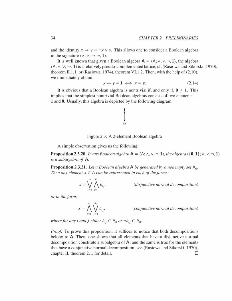
x↔ y = 1 ⟺ x = y. (2.14)
It is obvious that a Boolean algebra is nontrivial if, and only if, 0 ≠ 1. Thisimplies that the simplest nontrivial Boolean algebras consists of two elements —1 and 0. Usually, this algebra is depicted by the following diagram.
∙
∙1
0
Figure 2.3: A 2-element Boolean algebra
A simple observation gives us the following.
Proposition 2.3.20. In any Boolean algebra A = ⟨A; ∧,∨,¬, 1⟩, the algebra ⟨{0, 1}; ∧,∨,¬, 1⟩is a subalgebra of A.
Proposition 2.3.21. Let a Boolean algebra A be generated by a nonempty set A0.Then any element x ∈ A can be represented in each of the forms:
x =
m⋁i=1
ni⋀j=1
bij, (disjunctive normal decomposition)
or in the form:
x =
m⋀i=1
ni⋁j=1
bij, (conjunctive normal decomposition)
where for any i and j either bij ∈ A0 or ¬bij ∈ A0.
Proof. To prove this proposition, it suffices to notice that both decompositionsbelong to A. Then, one shows that all elements that have a disjunctive normaldecomposition constitute a subalgebra of A; and the same is true for the elementsthat have a conjunctive normal decomposition; see (Rasiowa and Sikorski, 1970),chapter II, theorem 2.1, for detail.
2.3. PRELIMINARIES FROM ALGEBRA 35
Proposition 2.3.22 ((Burris and Sankappanavar, 1981), corollary 1.9). Up to iso-morphism, there is only one subdirectly irreducible Boolean algebra, a 2-elementBoolean algebra.
As we will see below (Proposition 2.3.23), the class of Boolean algebras canbe regarded as a subclass of a larger class of Heyting algebras which are discussedin the next subsection. Therefore, many properties related to Heyting algebras areapplicable to Boolean algebras. For example, the properties that are discussedbelow in Proposition 2.3.24 for Heyting algebras (Section 2.3.9) can be applied toBoolean algebras as well.
References
1. (Burris and Sankappanavar, 1981)
2. (Rasiowa, 1974)
3. (Rasiowa and Sikorski, 1970)
2.3.9 Heyting algebras
A Heyting algebra (aka pseudo-Boolean algebra) is an algebra A = ⟨A; ∧,∨,→,¬, 1⟩ of type ⟨2, 2, 2, 1, 0⟩, where ∧ and ∨, → (relative pseudo-complementation)are binary operations, ¬ (pseudo-complementation) is a unary operation and 1 (theunit) is a 0-ary operation, if, besides the equalities (l1)–(l2) and (b1) (Section 2.3.8),the following equalities are satisfied for arbitrary elements x, y, z of H:
(h1) x ∧ (x→ y) = x ∧ y,(h2) (x→ y) ∧ y = y,(h3) (x→ y) ∧ (x → z) = x → (y ∧ z),(h4) x ∧ (y→ y) = x,(h5) ¬1 ∨ y = y,(h6) ¬x = x→ ¬1.
It is customary to denote:
x ↔ y ∶= (x→ y) ∧ (y→ x).
As in the case of Boolean algebras, in Heyting algebras, in virtue of (b1), theelement 1 is a greatest element in Heyting algebra. The property (h4) implies that
x → x = 1. (2.15)

36 CHAPTER 2. PRELIMINARIES
Using the notation (2.11) and the property (h5), we conclude that 0 is a leastelement in Heyting algebra. According to (h6), we have:
¬x = x → 0.
Thus, the last identity and (h1) imply the following:
x ∧ ¬x = 0. (2.16)
The following property characterizes pseudo-complementation:
x ≤ y→ z ⟺ x ∧ y ≤ z. (2.17)
Indeed, assume first that x ≤ y → z. Then, in view of (l1–i), the monotonicityof ∧ with respect to ≤ and (h1), we have:
x ∧ y ≤ y ∧ (y → z) = y ∧ z ≤ z.
Conversely, suppose that x ∧ y ≤ z, that is x ∧ y = x ∧ y ∧ z. Then, in virtueof (h2), (h4), (h3), we obtain:
x ≤ y→ x = (y→ x) ∧ (y→ y) = y→ (x ∧ y) = y→ (x ∧ y ∧ z)= (y→ (x ∧ y)) ∧ (y→ z) ≤ y → z.
Using (2.17), we receive immediately:
x ≤ y ⟺ x → y = 1; (2.18)
which in turn implies:x = y ⟺ x ↔ y = 1.
Proposition 2.3.23. Let A = ⟨A; ∧,∨,→,¬, 1⟩ be a Heyting algebra. Then itsrestriction B = ⟨A; ∧,∨,¬, 1⟩ is a Boolean algebra if the identity x → y = ¬x ∨
y holds in A. Conversely, if B = ⟨B; ∧,∨,¬, 1⟩ is a Boolean algebra. Then itsexpansion A = ⟨B; ∧,∨,→,¬, 1⟩, where x→ y ∶= ¬x ∨ y, is a Heyting algebra.
Proof. Let A be a Heyting algebra in which x → y = ¬x ∨ y. We observe that,because of (2.16), the identity (b2–i) is true in A. The identity (b2–ii) is also true,for we have:
(x ∨ ¬x) ∧ y = (x→ x) ∧ y = y.

2.3. PRELIMINARIES FROM ALGEBRA 37
Now assume that A is an expansion of a Boolean algebra B, where, by defini-tion, x → y = ¬x ∨ y. We aim to show that all the properties (h1)–(h6) are validin A. Indeed, we obtain:
x ∧ (x→ y) = x ∧ (¬x ∨ y) = (x ∧ ¬x) ∨ (x ∧ y) = x ∧ y;(x → y) ∧ y = (¬x ∨ y) ∧ y = y;(x → y) ∧ (x → z) = (¬x ∨ y) ∧ (¬x ∨ z) = ¬x ∨ (y ∧ ¬x) ∨ (¬x ∧ z) ∨ (y ∧ z)
= ¬x ∨ (y ∧ z) = x→ (y ∧ z);x ∧ (y→ y) = x ∧ (¬y ∨ y) = x;¬x = ¬x ∨ 0 = ¬x ∨ ¬1 = x→ ¬1.
Corollary 2.3.23.1. Let A = ⟨A; ∧,∨,¬, 1⟩ be a Boolean algebra. Then for anarbitrary x ∈ A, ¬¬x → x = 1, where the operation x → y is understood as¬x ∨ y.
Proof. Augmenting A with → defined as above, we receive a Heyting algebra.Then we use (2.15) and (2.12).
It should be clear that the simplest nontrivial Boolean algebra (Fig. 2.3.8) isalso the simplest non-generate Heyting algebra.
We will be using Heyting algebras as a basic semantics for the intuitionisticpropositional logic (Section 6.3.3). For this purpose, in the sequel, we will needthe following propertied of Heyting algebras.
Proposition 2.3.24. Let A = ⟨A; ∧,∨,→,¬, 1⟩ be a Heyting algebra. For arbi-trary elements x, y and z of H the following properties hold:
(a) x ≤ y→ x,(b) x→ y ≤ (x → (y→ z)) → (x → z),(c) x ≤ y→ (x ∧ y),(d) x ∧ y ≤ x,(e) x ≤ x ∨ y,(f) x→ z ≤ (y → z) → ((x ∨ y) → z),(g) x→ y ≤ (x → ¬y) → ¬x,(h) x ≤ ¬x→ y.
Proof. We obtain successively the following.

38 CHAPTER 2. PRELIMINARIES
(a) follows straightforwardly from (h2).To prove (b), using (2.17), we have:
(x → y) ∧ (x → (y→ z)) ∧ x = (x → y) ∧ x ∧ (y→ z)= x ∧ y ∧ (y → z) = x ∧ y ∧ z ≤ z.
Then, we apply (2.17) again twice to get (b).We derive (c) immediately from x ∧ y ≤ x ∧ y.(d) and (e) are obvious.To prove (f), we first have:
(x → z) ∧ (y→ z) ∧ (x ∨ y) = ((x→ z) ∧ (y → z) ∧ x) ∨ ((x → z) ∧ (y→ z) ∧ y)= (x ∧ z ∧ (z → y)) ∨ (y ∧ z ∧ (x → z))= (x ∧ z) ∨ (y ∧ z) = (x ∨ y) ∧ z ≤ z.
Then, we apply (2.17) twice.To prove (g), applying (2.17) twice, we have:
(x → y) ∧ (x→ ¬y) ∧ x = x ∧ y ∧ ¬y = x ∧ 0 ≤ 0,
which implies that
(x → y) ∧ (x → ¬y) ≤ x→ 0 = ¬x.
It remains to apply (2.17).Finally, we obtain (h) as follows:
x ∧ ¬x = 0 ≤ y.
Then, we apply (2.17).
Two obvious ways to obtain new Heyting algebras from old ones are the for-mation of subalgebras and homomorphic images. For instance, given a nontriv-ial Heyting algebra ⟨A; ∧,∨,→,¬, 1⟩, the algebra ⟨{0, 1}; ∧,∨,→,¬, 1⟩, where0 ∶= ¬1, the smallest subalgebra of the first algebra.
The following method is very useful for obtaining homomorphic images of agiven Heyting algebra.
Let A = ⟨A; ∧,∨,→,¬, 1⟩ be a nontrivial Heyting algebra and b ∈ A. We con-sider the algebra Ab = ⟨{x ∈ A | x ≤ b}; ∧b,∨b,→b,¬b, 1b⟩, where, by definition:
x ∧b y ∶= x ∧ y;x ∨b by ∶= x ∨ y;x→b y ∶= (x→) ∧ b;¬bx ∶= (¬x) ∧ b;1b ∶= b.

2.4. PRELIMINARIES FROM MODEL THEORY 39
It turns out that Ab is a homomorphic image of A with respect to the homo-morphic map x↦ x∧b. See (Rasiowa and Sikorski, 1970), chapter IV, § 8, wherethe formation of Ab is called relativization.
References
1. (Rasiowa, 1974)
2. (Rasiowa and Sikorski, 1970)
2.4 Preliminaries from model theory
Let a first-order language FO consist of a set of individual variables, logicalconstants ‘∧∧∧’, ‘∨∨∨, ‘→→→’, ‘¬¬¬’ and quantifiers ‘∀∀∀’ and ‘∃∃∃’, as well as parentheses ‘(’and ‘)’. Moreover, a signature of FO includes a set of functional symbols ofarity greater than or equal to 1, a set of individual constants which are treatedas 0-ary functional symbols.
We continue to call the terms of FO -terms.Any FO must have a nonempty set of predicate symbols; some have equal-
ity ≈, some don’t. We will be assuming that the arity of each predicate symbolP ∈ is greater or equal to 1.
The notion of a formula is similar to the one given in Section 2.3.3 with achange in the clause for atomic formulas: if P ∈ of arity n and t1,… , tn are-terms, then P (t1,… , tn) is an (atomic) FO-formula. The other clauses are thesame as (1)–(6) on p. 25. Thus defined formulas we call FO-formulas, or simplyformulas; the latter is used in the contexts where confusion is unlikely.
If an FO-formula is closed, it is called an FO-sentence. As in Section 2.3.3,a formula which does not contain quantifiers is called quantifier-free.
Models of FO (FO-models for short, or simply models) which we use inChapters 4–8 of this book, where we apply some of the results of model theory,have one of the following two forms:
(a) ⟨A;, , D⟩ or (b) ⟨A;, , �⟩, (2.19)
where and are the sets of interpreted functional symbols and constants ofFO, D is a unary predicate and �, the interpretation of ≈ in A, is the diagonalof A × A; usually, ⟨A;, ⟩ is called an algebra of the corresponding model. If

40 CHAPTER 2. PRELIMINARIES
M is a model, its algebra is denoted by [M]. For a class of models, []
denotes the class of their algebras. Given a model M, we denote by |M| its carrier.The models of type (2.19–b) we call e-models.Further, let v be a map of the set of individual variables into |M|. We will be
using (a well-known) satisfactory relation of a first-order formulaA in a model M,saying that M satisfies A at v, symbolically (M, v) ⊧ A or M ⊧v A.6 A model M
satisfies ', or ' is satisfiable in M, if there is such a valuation v of the individualvariables in M that (M, v) ⊧ '.
We write M ⊧ A if M ⊧v A, for any valuation v in M, and say that M validates
A. Given a model M and a quantifier-free formula A, the following equivalencemust be clear:
M ⊧ ∀∀∀…∀∀∀A ⟺ M ⊧ A. (2.20)
It must be clear that any identity, say ∀∀∀…∀∀∀ (� ≈ �), and the quasi-identity∀∀∀…∀∀∀ (p ≈ p→→→ � ≈ �) are validated by the same FO-models.
Definition 2.4.1. Let Σ be a set of FO-sentences and let be a nonempty classof FO-models. We say that Σ is satisfiable in if there a model A ∈ , whichsatisfies all sentences of Σ.
Let be a nonempty class of e-models. The set of equalities validated by allmodels from is called the equational theory of ; this equational theory willbe denoted by EQ[]. Now, we define:
ModEQ() ∶= {M | M ⊧ EQ[]}.
It is clear that [ModEQ()] (of algebras) is an equational class (or variety)
generated by the class [].
Proposition 2.4.1 ((Burris and Sankappanavar, 1981), (Grätzer, 2008), (McKenzie et al., 2018)).Let be a nonempty class of models of the form (2.19–b). Then EQ[] =
EQ[ModEQ()]. Furthermore,[ModEQ
()] = HSP[] = HSPHsi[].
Remark 2.4.1. The last conclusion of Proposition 2.4.1 follows from Proposi-tion 2.3.13, Proposition 2.3.11 and Proposition 2.3.16.
6Other utterances of this relation are: ‘v satisfies ' in M’ ((Bell and Slomson, 1969), chapter 3,§ 2); ‘' is true of v in M’ ((Hodges, 1993), section 1.3); ‘M satisfies ' with v’ ((Enderton, 2001),section 2.2); ‘(M, �) satisfies '’ or ‘M is a model for ' with respect to v’ ((Rautenberg, 2010),section 2.3); ‘' is satisfied by a sequence v ∶ ⟶ A in M’ or ‘a sequence v ∶ ⟶ A
satisfies ' in M ((Chang and Keisler, 1990), definition 1.3.12).
2.4. PRELIMINARIES FROM MODEL THEORY 41
Let M = ⟨A;, , �⟩ be a model of type (2.19–b). We define:
{M}si ∶= {⟨B;, , �⟩ | ⟨B;, ⟩ ∈ [M]si}
Proposition 2.4.2. Given a model M of type (2.19–b), EQ[M] = EQ[{M}si].
Proof. We prove that for any identity ∀∀∀…∀∀∀�,
M ⊧ ∀∀∀…∀∀∀� ⟺ {M}si ⊧ ∀∀∀…∀∀∀�.
Indeed, suppose M ⊧ ∀∀∀…∀∀∀� and N ∈ {M}si. Since [N] is a homomorphicimage of [M], in virtue of Proposition 2.4.6–a, N ⊧ ∀∀∀…∀∀∀�.
Conversely, assume that {M}si ⊧ ∀∀∀…∀∀∀�. By definition, there is a set {Mi}i∈I ⊆{M}si such that the algebra [M] is subdirectly embedded into
∏i∈I [Mi]. Ac-
cording to Proposition 2.4.6–b, ⟨∏i∈I [Mi], �⟩ ⊧ ∀∀∀…∀∀∀� and hence, in virtue ofProposition 2.4.6–c, M ⊧ ∀∀∀…∀∀∀�.
In the sequel, we will use the following fact.
Proposition 2.4.3. There are only two varieties of Boolean algebras — the trivialvariety and the variety of all Boolean algebras.
Proof. Let us consider a nontrivial variety. And let us take any nontrivial alge-bra in it. According to Proposition 2.3.20, a 2-element algebra is a subalgebra ofthe latter. Hence, according to Proposition 2.3.13, this 2-element algebra belongsto the variety. By the same proposition, any direct power of the 2-element alge-bra belongs to the variety. However, any Boolean algebra is isomorphic to somedirect power of a 2-element Boolean algebra ((Burris and Sankappanavar, 1981),corollary IV.1.12). Therefore, any Boolean algebra belongs to any nontrivial vari-ety.
Let {Mi}i∈I be a family of FO-models. Also, let ∇ be a filter over I . We fixthe direct product
M ∶=∏i∈I
Mi
and define:
x ≡∇ ydf
⟺ {i ∈ I | xi = yi} ∈ ∇.
It is well known that ≡∇ is congruence relation on the algebra A = ⟨A, , ⟩.We denote by A∕∇ the quotient algebra with respect to this congruence. To obtain
42 CHAPTER 2. PRELIMINARIES
a model, A∕∇, we have to expand A∕∇ with an interpretation of ≈ in this algebra.Let us denote (temporarily) this interpretation by �D. By definition, we have:
(x∕∇, y∕∇) ∈ �∇
df⟺ {i ∈ I | (xi, yi) ∈ �i} ∈ ∇.
Since each �i is a diagonal, we observe that
(x∕∇, y∕∇) ∈ �∇ ⟺ x∕∇ = y∕∇.
This means that �∇ is the diagonal of |A∕F | × |A∕F |; we denote it simply by �,if no confusion arises.
We denote ∏∇
Mi ∶= ⟨A∕∇, �⟩
and call the last model a reduced product of the family {Ai}i∈I with respect to thefilter ∇. If ∇ be an ultrafilter over I , we call
∏∇ Mi an ultraproduct with respect
to the ultrafilter ∇.In case if each Mi = ⟨Ai, Di⟩, where Di is a unary predicate on |Ai|, then, by
definition, we have: ∏∇
Mi ∶= ⟨A∕∇, D⟩, (2.21)
where
x∕∇ ∈ Ddf
⟺ {i ∈ I | xi ∈ Di} ∈ ∇.
Let be a nonempty class of models of the form (2.19–b). The set of quasi-identities validated by all models from is called the quasi-equational theory
of ; this quasi-equational theory will be denoted by QE[]. Now, we define:
ModQE() ∶= {M | M ⊧ QE[]}.
The class [ModQE()] (of algebras) is obviously an implicative class (or a
quasi-variety) generated by the class [].
Proposition 2.4.4 ((Burris and Sankappanavar, 1981), theorem V.2.25, (Gorbunov, 1998),corollary 2.3.4). Let be a nonempty class of e-models. Then QE[] =
QE[ModQE()]. Furthermore, [ModQE
()] = SPPu[].
Remark 2.4.2. The last conclusion of Proposition 2.4.4 follows from Proposi-tion 2.3.17 and Proposition 2.3.11.
2.4. PRELIMINARIES FROM MODEL THEORY 43
In the sequel, we will need the following refined variant of compactness theo-rem.
Proposition 2.4.5 ((Bell and Slomson, 1969), (Chang and Keisler, 1990)). Let Σbe a set of FO-sentences and let be a nonempty class of FO-models closedunder ultraproducts. Then Σ is satisfiable in if, and only if, every finite subsetof Σ is satisfiable in .
Proof. Suppose Σ is satisfiable in ; that is, there is a model M ∈ , whichsatisfies all sentences of Σ. Then, obviously, A satisfies any subset, in particularany finite subset, of Σ.
Conversely, let I denote the set of all finite subsets of Σ. By premise, foreach i ∈ I , there is a model Mi which satisfies i. According to Corollary 4.1.11of (Chang and Keisler, 1990), there is an ultrafilter ∇ over I such that the ultra-product
∏∇ Mi satisfies Σ. By premise, this model belongs to . Hence, Σ is
satisfiable in .
A first-order formula A is said to be preserved:
• under homomorphisms if for any homomorphism f of a model M into amodel N and any valuation v in M,
(M, v) ⊧ �⟹ (N, vf ) ⊧ �,
where vf is a valuation in N such that vf [p] = f (v[p]), for any individualvariable p;
• under direct products if for any class {Mi}i∈I of FO-models and any val-uation v in M =
∏i∈I Mi, whenever (Mi, vi) ⊧ �, for every i ∈ I , where
vi[p] is the projection of v[p] on Mi, then (M, v) ⊧ �,
Proposition 2.4.6.
(a) Any equality and any identity is preserved under homomorphisms.(b) Any equality and any identity, as well as any quasi-equality and any quasi-identity,
are preserved under direct products.(c) Both identities and quasi-idenities are preserved on subalgebras.
Proof. (a) is part of the proof of theorem 3.2.4 of (Chang and Keisler, 1990). (b)is covered by theorem 1 of (Mal’cev, 1973), chapter III, § 7. For the proof of (c),see, e.g., (Mal’cev, 1973), § 7, theorem 1.
44 CHAPTER 2. PRELIMINARIES
References
1. (Bell and Slomson, 1969)
2. (Burris and Sankappanavar, 1981)
3. (Chang and Keisler, 1990)
4. (Enderton, 2001)
5. (Gorbunov, 1998)
6. (Grätzer, 2008)
7. (Hodges, 1993)
8. (Mal’cev, 1973)
9. (McKenzie et al., 2018)
10. (Rautenberg, 2010)
2.5 Preliminaries from computability theory
In this section, we outline some ideas of computability and strive to prepare areader unfamiliar with these ideas for reading Chapter 10. Thus we intend to in-troduce the reader to the idea of an effective method or algorithm. From the verybeginning, we need to make a few warnings.
First of all, we do not assume any aesthetic load in the term ‘effective method’.Secondly, although different levels of effectiveness can be distinguished in com-putability theory, in this book we deal mainly with the lowest. Even at this level,we will prove that certain problems have positive solutions in the sense that thereis a desirable effective method or algorithm that decides this problem. Such prob-lems are called decidable. The problems (from a certain category of problems) forwhich any algorithm does not produce a desirable result are called undecidable.This distinction requires a rigorous definition of the concept of an effective method.In this book, we however deal only with decidable problems. Thus, the purposeof this section is to discuss the concept of decidability from the point of view ofan effective method without going into rigorous detail, that is, without giving anexact explication of an effective method as a computable function. The reader can

2.5. PRELIMINARIES FROM COMPUTABILITY THEORY 45
find a precise definition of a computable function, decidability, and undecidabilityin the references at the end of this section.
Suppose a set A is a subset of a set U . It is customary to think of U as a‘universal’ set. Then the problem arises: Is there an effective method for any xin U to decide whether x lies in A? For simplicity, let us assume that U = ℕ,where ℕ is the set of nonnegative integers introduced in Section 2.1 We wouldanswer the above question in the affirmative, if we could find an effective function�A ∶ ℕ ⟶ {0, 1} such that
�A(x) =
{1 if x ∈ A
0 if x ∉ A.(2.22)
The function �A is called the characteristic function of A. If we succeed infinding an effective (or algorithmic) �A, we state that
A = {x ∈ ℕ | �A(x) = 1}
and, hence, can claim that the set A is decidable.The situations that we will meet in Chapter 10 are a little more complex. Roughly
speaking, we will consider situations when U ⊂ ℕ and is decidable and then askthe question whether a set A ⊆ U is decidable relative to U , that is, whether analgorithm exists for any x ∈ U to decide if x ∈ A.
Let us define for the last decidability procedure a function �A|U ∶ U ⟶
{0, 1}:
�A|U (x) ∶=
{1 if x ∈ A
0 if x ∈ U ⧵ A.(2.23)
The function �A|U is partial, since it is undefined on ℕ ⧵ U . We agree that ef-fective method can be implemented as a partial function, and later in Section 2.5.1,we will give the rationale for this view. However, even in this case, the set A isdecidable as soon as the characteristic functions �U and �A|U are realized as algo-rithms.
Indeed, we define a function � ′A ∶ ℕ ⟶ {0, 1} as follows:
� ′A(x) ∶=
⎧⎪⎨⎪⎩
1 if �U (x) = 1 and �A|U (x) = 1
0 if �U (x) = 1 and �A|U (x) = 0
0 if �U (x) = 0.
46 CHAPTER 2. PRELIMINARIES
It is clear that for any x ∈ ℕ,
x ∈ A ⟺ � ′A(x) = 1.
Next in this section, we discuss the idea of an effective method or algorithmthat is implemented by a function, possibly partial, from ℕ ×… × ℕ
⏟⏞⏞⏞⏟⏞⏞⏞⏟n
, where n ≥ 1,
or its proper subset into ℕ. Along with such functions, we also consider relationsR ⊆ ℕ ×… × ℕ
⏟⏞⏞⏞⏟⏞⏞⏞⏟n
such that their characteristic function �R ∶ ℕ ×… × ℕ⏟⏞⏞⏞⏟⏞⏞⏞⏟
n
⟶
{0, 1} is effective. We call such functions and relations effective or algorithmic ifthey can be defined in ‘a purely mechanical way’. (This phrase will be discussed inthe following subsection.) After that, we discuss the idea of algorithmic functionsand relations that are defined on other domains.
2.5.1 Algorithmic functions and relations on ℕ
It is not surprising that we start with functions of any finite number of variablesdefined on ℕ, taking into account the historical fact, which E. Beth expressed inwords:
“At any rate, the fascination inspired by the art of computation ex-plains why, at a certain moment, a properly scientific interest in num-bers developed.” ((Beth, 1962), section 25)
What functions can be considered executable in accordance with an effectivemethod? The last example of the last subsection suggests that to avoid the processof relative effectiveness ad infinitum, it must be agreed that some functions areeffective for granted. By agreement, the following functions form the basis ofeffective functions:
• the successor function s ∶ n↦ n + 1, where n ∈ ℕ;
• the zero functions: on ∶ x ↦ 0, where x ∈ ℕ ×… × ℕ⏟⏞⏞⏞⏟⏞⏞⏞⏟
n
and n ∈ ℕ; in
particular, o0 is just 0;
• and the projections: �nm(x1,… , xn) = xm, where each xi ∈ ℕ and 1 ≤ m ≤ n.
2.5. PRELIMINARIES FROM COMPUTABILITY THEORY 47
We argue that the basis functions can be performed in ‘a purely mechanicalway’. Before moving on to this, we need consensus. The consensus is that anynatural numbersm and n can be identified ‘purely mechanically’ as different or thesame. This needs to be explained.
To facilitate our discussion of the ‘purely mechanical method’, let us assumethat there is a device, a computer, which is capable of performing such ‘mechani-cal’ actions. Our first assumption about this device is that it takes a finite number ofconstructive objects as input and returns the constructive object as output. This iswhat V. Uspensky and A. Semenov write about the notion of a constructive object:
“This notion can be regarded not only as a basic notion but also asa primary one. Strictly speaking it belongs not to the theory of al-gorithms but to the introduction to it. As one old textbook says: “Asubject of an introduction to a science usually contains preliminarynotions, i.e. notions that can not be included into the science itself butare essential for it and are assumed by it”.
All attempts to define the notion of a constructive object (includingours) either are very abstract and vague or define specific classes ofconstrictive objects. As all primitive notions it can be understood byexamples.” ((Uspensky and Semenov, 1993), section 1.0.0)
Perhaps the main feature of the constructive object is that it can be representedby a word in a certain alphabet. For instance, using the decimal symbols ’0’, ‘1’,. . . , ’9’, digits, any natural number can be written as a finite sequence of digits,providing that only one such a sequence starts with ‘0’, that is the one which doesnot have more digits. The examples of such sequences are:
0, 1, 2, 31, 502.
Another way to depict natural numbers as words is the following. Any positivenumber is written as a sequence of occurrences of ‘|’, and 0 is depicted as an emptyword, for which one can use any symbol different from ‘|’, for example, ‘�’. Thuswe obtain that 0 is depicted by ‘�’, 1 by ‘|’, 2 by ‘||’, etc.
More general setting of depicting constructive objects will be discussed in thenext subsection.
Now it should be clear that the computer, using the two numbers m and n inone of the representations presented above, can decide ‘purely mechanically’, thatis, without resorting to intelligence in any reasonable sense of the word, whetherthey are represented by the same string of elementary characters.
48 CHAPTER 2. PRELIMINARIES
We note that the equality relation ‘=’ defined for the output of the same ordifferent algorithms is a more general relation than the equality of two strings ofsymbols representing natural numbers in one of the above notations. As we willsee below, the relation = between two algorithmic functions is also decidable in a‘purely mechanical way’.
It is generally accepted that in order to be qualified as algorithmic, a methodmust have the following characteristics:
• the algorithmic method is deterministic; in other words, when implemented,the algorithm works like a function;
• the algorithmic method is independent of a single input, but can be appliedto a data set;
• as a function, the algorithm may be partial; but if it is defined for input, itcompletes its work with a certain result.
A. A. Markov claims something similar as follows:
“The following three features are characteristic of algorithms and de-termine their role in mathematics;a) the precision of the prescription, leaving no place to arbitrariness,and its universal comprehensibility — the definiteness of the algo-rithm;b) the possibility of starting out with initial data, which may varywithin given limits — the generality of the algorithm;c) the orientation of the algorithm toward obtaining some desired re-sult, which is indeed obtained in the end with proper initial data, —the conclusiveness of the algorithm.” ((Markov, 1962), introduction;cp. (Markov, 1960), section 1.)
Returning to the functions of the basis, we argue that the procedure for ob-taining for a given natural number n the number s(n) in any of the aforementionedrepresentations can be regarded as purely mechanical, as well as the procedurefor returning 0 from any natural argument or from nothing. Also, the projections�nm ∶ ℕ ×… × ℕ
⏟⏞⏞⏞⏟⏞⏞⏞⏟n
⟶ ℕ can be performed purely mechanically, given that the
parameters m and n are predefined.Thus in this context, we can understand ℕ as an effectively generated infinite
list of numerals:0, s(0), s(s(0)),…; (2.24)
2.5. PRELIMINARIES FROM COMPUTABILITY THEORY 49
We observe that, given a numeral n of (2.24), which is not coincident with 0,the computer can determine the (nearest) predecessor of n, that is, such a numeralm that s(m) is coincident with n. This leads to the recursive definitions7 of effectivefunctions.
Recursion allows you to define a new function using one or two given functionsby recursion equations. There are two types of recursion equations. The first typeuses one given function, say f , and defines a new function of one variable, say ℎ,by the following equations:
{ℎ(0) = a
ℎ(s(x)) = f (x, ℎ(x)),
where a is a given number.The second type uses two given functions, say f (x1,… , xn−1) and g(x1,… , xn+1),
and defines a function of n variables with n ≥ 2:
{ℎ(x1,… , xn−1, 0) = f (x1,… , xn−1)
ℎ(x1,… , xn−1, s(x)) = g(x1,… , xn−1, x, g(x1,… , xn−1, x))
Using basis functions as initial functions, many other functions can be definedin a finite number of steps, using substitution (or composition) and suitable recur-sion equations. The functions obtained from the basis functions by a finite numberof applications of substitution and recursion equations form the class of primitiverecursive functions.
There is a strong argument that a recursive definition whose recursion equa-tions employ effective functions defines an effective function; cf. (Cutland, 1980),section 4.4, (Davis et al., 1994), section 3.3, (Davis, 1958), section 3.1, or (Mal’cev, 1970),section 12.3. In addition, this argument states that the basis functions are effectiveand, therefore, all primitive recursive functions are effective or algorithmic. Theargument, known as the Church thesis, goes even further, claiming that a certainextension of the class of primitive recursive functions, among which some func-tions are partial, contains exactly all effective functions.8 In Section 2.5.3 we givean example and demonstrate the usefulness of partial effective functions.
7See about recursive definitions (or definitions by recursion) in (Cutland, 1980), section2.4, (Davis, 1958), section 3.3, (Davis et al., 1994), section 3.2, or (Mal’cev, 1970), section 2.2
8About the Church thesis, see, e.g., (Uspensky and Semenov, 1993), section 1.2.4, and refer-ences therein.

50 CHAPTER 2. PRELIMINARIES
The inclusion of partial functions is important. For illustration, let us considertwo computable functions, f (x) and g(x), where f (x) is partial and g(x) is to-tal. If however f (x) is defined on all outputs of g(x), then the composite functionf◦g(x), obtained by substitution, f (g(x)), is a total computable function.
Below we demonstrate that some functions and predicates defined on ℕ and onCartesian products of ℕ are effective, providing that the Church thesis is accepted.
For each function below, we first give a meaningful definition of the function,and then define it using recursion equations.
sg(x) ∶=
{0 if x is coincident with 0
1 if otherwise;
These are recursion equations for sg.
{sg(0) = o0
sg(s(x)) = s(o1(x)).
pd(x) ∶=
{0 if x is coincident with 0
the predicessor of x if otherwise.{
pd(0) = o0
pd(s(x)) = �11(x).
Using the last function, we define:
x ∸ y ∶=
{x if y is coincident with 0
pd(x ∸ pd(y)) if otherwise;
and now this function by recursion equations:
{x ∸ 0 = �1
1(x)
x ∸ s(y) = pd(x ∸ y).
Next we define for the numerals (2.24) the following relations:
x ≤ ydf
⟺ 1 ∸ sg(x ∸ y) is coincident with 1
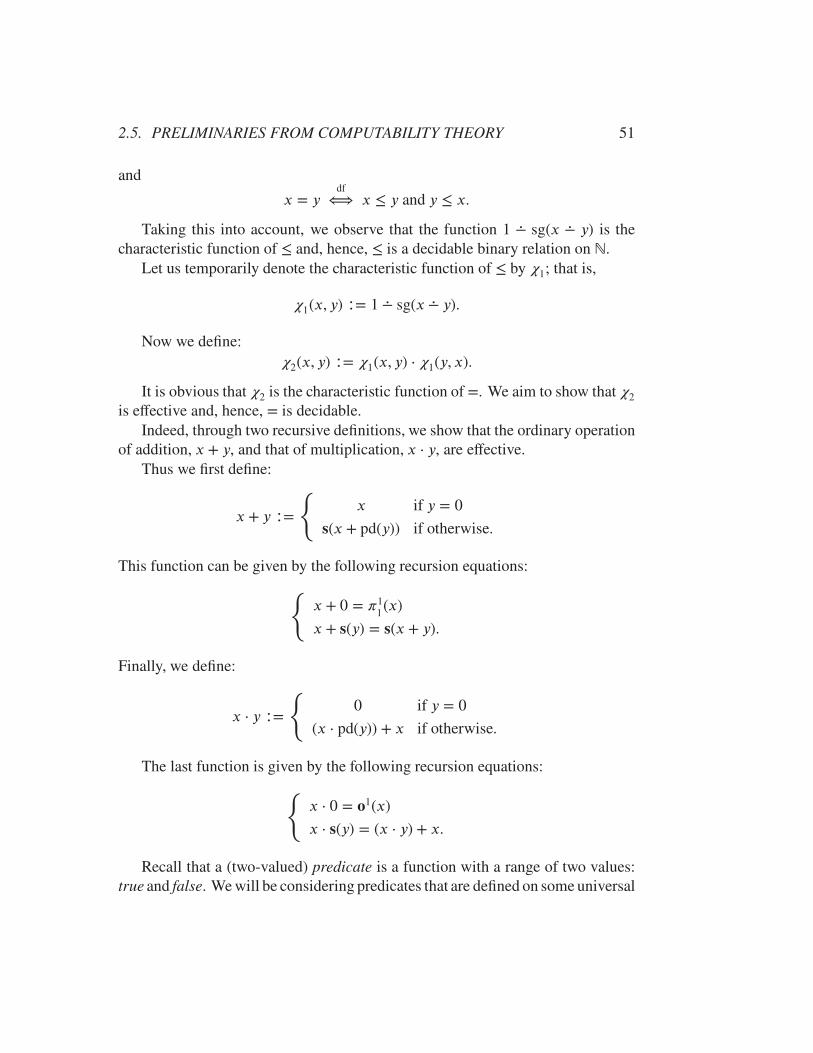
2.5. PRELIMINARIES FROM COMPUTABILITY THEORY 51
and
x = ydf
⟺ x ≤ y and y ≤ x.
Taking this into account, we observe that the function 1 ∸ sg(x ∸ y) is thecharacteristic function of ≤ and, hence, ≤ is a decidable binary relation on ℕ.
Let us temporarily denote the characteristic function of ≤ by �1; that is,
�1(x, y) ∶= 1 ∸ sg(x ∸ y).
Now we define:�2(x, y) ∶= �1(x, y) ⋅ �1(y, x).
It is obvious that �2 is the characteristic function of =. We aim to show that �2
is effective and, hence, = is decidable.Indeed, through two recursive definitions, we show that the ordinary operation
of addition, x + y, and that of multiplication, x ⋅ y, are effective.Thus we first define:
x + y ∶=
{x if y = 0
s(x + pd(y)) if otherwise.
This function can be given by the following recursion equations:
{x + 0 = �1
1(x)
x + s(y) = s(x + y).
Finally, we define:
x ⋅ y ∶=
{0 if y = 0
(x ⋅ pd(y)) + x if otherwise.
The last function is given by the following recursion equations:
{x ⋅ 0 = o1(x)
x ⋅ s(y) = (x ⋅ y) + x.
Recall that a (two-valued) predicate is a function with a range of two values:true and false. We will be considering predicates that are defined on some universal
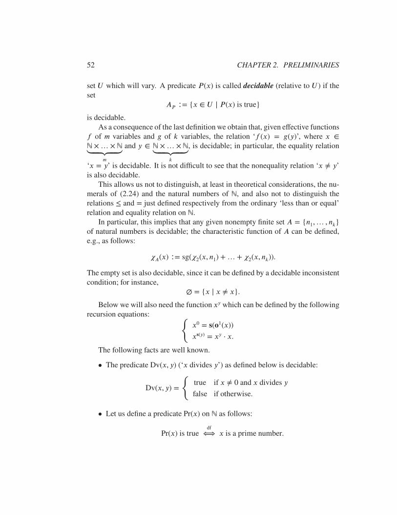
52 CHAPTER 2. PRELIMINARIES
set U which will vary. A predicate P (x) is called decidable (relative to U ) if theset
AP ∶= {x ∈ U | P (x) is true}
is decidable.As a consequence of the last definition we obtain that, given effective functions
f of m variables and g of k variables, the relation ‘f (x) = g(y)’, where x ∈
ℕ ×… × ℕ⏟⏞⏞⏞⏟⏞⏞⏞⏟
m
and y ∈ ℕ ×… × ℕ⏟⏞⏞⏞⏟⏞⏞⏞⏟
k
, is decidable; in particular, the equality relation
‘x = y’ is decidable. It is not difficult to see that the nonequality relation ‘x ≠ y’is also decidable.
This allows us not to distinguish, at least in theoretical considerations, the nu-merals of (2.24) and the natural numbers of ℕ, and also not to distinguish therelations ≤ and = just defined respectively from the ordinary ‘less than or equal’relation and equality relation on ℕ.
In particular, this implies that any given nonempty finite set A = {n1,… , nk}of natural numbers is decidable; the characteristic function of A can be defined,e.g., as follows:
�A(x) ∶= sg(�2(x, n1) + …+ �2(x, nk)).
The empty set is also decidable, since it can be defined by a decidable inconsistentcondition; for instance,
∅ = {x | x ≠ x}.
Below we will also need the function xy which can be defined by the followingrecursion equations: {
x0 = s(o1(x))
xs(y) = xy ⋅ x.
The following facts are well known.
• The predicate Dv(x, y) (‘x divides y’) as defined below is decidable:
Dv(x, y) =
{true if x ≠ 0 and x divides y
false if otherwise.
• Let us define a predicate Pr(x) on ℕ as follows:
Pr(x) is truedf
⟺ x is a prime number.
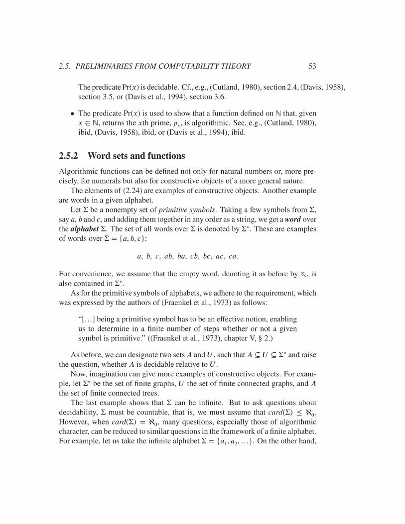
2.5. PRELIMINARIES FROM COMPUTABILITY THEORY 53
The predicate Pr(x) is decidable. Cf., e.g., (Cutland, 1980), section 2.4, (Davis, 1958),section 3.5, or (Davis et al., 1994), section 3.6.
• The predicate Pr(x) is used to show that a function defined on ℕ that, givenx ∈ ℕ, returns the xth prime, px, is algorithmic. See, e.g., (Cutland, 1980),ibid, (Davis, 1958), ibid, or (Davis et al., 1994), ibid.
2.5.2 Word sets and functions
Algorithmic functions can be defined not only for natural numbers or, more pre-cisely, for numerals but also for constructive objects of a more general nature.
The elements of (2.24) are examples of constructive objects. Another exampleare words in a given alphabet.
Let Σ be a nonempty set of primitive symbols. Taking a few symbols from Σ,say a, b and c, and adding them together in any order as a string, we get a word overthe alphabet Σ. The set of all words over Σ is denoted by Σ∗. These are examplesof words over Σ = {a, b, c}:
a, b, c, ab, ba, cb, bc, ac, ca.
For convenience, we assume that the empty word, denoting it as before by �, isalso contained in Σ∗.
As for the primitive symbols of alphabets, we adhere to the requirement, whichwas expressed by the authors of (Fraenkel et al., 1973) as follows:
“[…] being a primitive symbol has to be an effective notion, enablingus to determine in a finite number of steps whether or not a givensymbol is primitive.” ((Fraenkel et al., 1973), chapter V, § 2.)
As before, we can designate two setsA and U , such thatA ⊆ U ⊆ Σ∗ and raisethe question, whether A is decidable relative to U .
Now, imagination can give more examples of constructive objects. For exam-ple, let Σ∗ be the set of finite graphs, U the set of finite connected graphs, and Athe set of finite connected trees.
The last example shows that Σ can be infinite. But to ask questions aboutdecidability, Σ must be countable, that is, we must assume that card(Σ) ≤ ℵ0.However, when card(Σ) = ℵ0, many questions, especially those of algorithmiccharacter, can be reduced to similar questions in the framework of a finite alphabet.For example, let us take the infinite alphabet Σ = {a1, a2,…}. On the other hand,
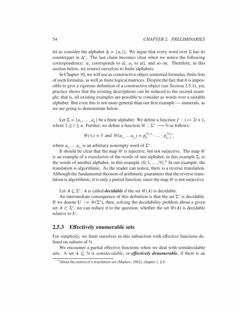
54 CHAPTER 2. PRELIMINARIES
let us consider the alphabet Δ = {a, |}. We argue that every word over Σ has itscounterpart in Δ∗. The last claim becomes clear when we notice the followingcorrespondence: a1 corresponds to a|, a2 to a||, and so on. Therefore, in thissection below, we restrict ourselves to finite alphabets.
In Chapter 10, we will use as constructive object sentential formulas, finite listsof such formulas, as well as finite logical matrices. Despite the fact that it is impos-sible to give a rigorous definition of a constructive object (see Section 2.5.1), yet,practice shows that the existing descriptions can be reduced to the second exam-ple; that is, all existing examples are possible to consider as words over a suitablealphabet. But even this is not more general than our first example — numerals, aswe are going to demonstrate below.
Let Σ = {a1,… , an} be a finite alphabet. We define a function f ∶ i ↦ 2i+1,where 1 ≤ i ≤ n. Further, we define a function @ ∶ Σ∗ ⟶ ℕ as follows:
@(�) = 3 and @(ai1 … aik) = pf (i1)0
⋅… ⋅ pf (ik)k−1
,
where ai1 … aik is an arbitrary nonempty word of Σ∗.It should be clear that the map @ is injective, but not surjective. The map @
is an example of a translation of the words of one alphabet, in this example Σ, tothe words of another alphabet, in this example {0, 1,… , 9}.9 In our example, thetranslation is algorithmic. As the reader can notice, there is a reverse translation.Although the fundamental theorem of arithmetic guarantees that the reverse trans-lation is algorithmic, it is only a partial function, since the map @ is not surjective.
Let A ⊆ Σ∗. A is called decidable if the set @(A) is decidable.An intermediate consequence of this definition is that the set Σ∗ is decidable.
If we denote U ∶= @(Σ∗), then, solving the decidability problem about a givenset A ⊂ Σ∗, we can reduce it to the question, whether the set @(A) is decidablerelative to U .
2.5.3 Effectively enumerable sets
For simplicity, we limit ourselves in this subsection with effective functions de-fined on subsets of ℕ.
We encounter a partial effective functions when we deal with semidecidablesets. A set A ⊆ ℕ is semidecidable, or effectively denumerable, if there is an
9About the notion of a translation see (Markov, 1962), chapter 1, § 6.

2.5. PRELIMINARIES FROM COMPUTABILITY THEORY 55
effective function function 'A such that
'A(x) =
{1 if x ∈ A
undefined if x ∉ A.
The ground for the first name is obvious, and for the second — the following(well-known) theorem.
A set A is effectively enumerable if, and only if, A = ∅ or A is therange of a total effective function.
(Cf. (Cutland, 1980), chapter 7, section 2, (Davis, 1958), chapter 5, section 4,or (Davis et al., 1994), chapter 4, section 4.)
If a set is decidable, it is also semidecidable, but the converse is not necessarilytrue. It is usually simpler to show the semidecidability of a set than to prove thatthe set is decidable. The following theorem is very useful for establishing thedecidability of sets.
(Post) A set A is decidable if, and only if, both A and ℕ ⧵A are effec-tively enumerable.
(Cf. ibid.)The last theorem is based on the previous one, and can be illustrated as follows.Suppose both A and ℕ ⧵ A are effectively enumerable and unequal to ∅. For
convenience, we denote: B ∶= ℕ ⧵A. In virtue of the first theorem, there are twoeffective total functions, A and B, such that A = A(ℕ) and B = B(ℕ). Thenit is clear that any given n ∈ ℕ is among the members of the following sequence:
A(0), B(0), A(1), B(1),…
If n is a value of A, then n ∈ A; if n is a value of B in this sequence, then n ∉ A.The described procedure is effective, since it is based on the effective functions Aand B and on the decidable relation =.
Another decidability procedure uses a different criterion for effectively enu-merable sets.
A setA is effectively enumerable if, and only if, there is a total effectivefunction �A(x, y) (with two variables) such that for any n ∈ ℕ, n ∈ Aif, and only if, the equation �A(x, n) = 0 has a solution.
56 CHAPTER 2. PRELIMINARIES
(Cf. (Cutland, 1980), ibid, (Mal’cev, 1970), section 4.2.)Indeed, if given sets A and B are as above and if we know functions A and
�B, then for a given n ∈ ℕ, we effectively create the sequence:
A(0), �B(0, n), A(1), �B(1, n),… (2.25)
Thus, if n is a value of A, then n ∈ A; if one of the values of �B in this sequencetakes 0, then n ∉ A. It is clear that one of these options should happen.
The situation is not too complicated if we have a universal decidable setU ⊂ ℕ
and all effective procedures are executed relative to U . It is also not more difficultwhen in Chapter 10 we will work with words in a fixed alphabet, and not with num-bers, where a function such as @ will be implied, but behind the scenes. Namely,the sequence (2.25) will be implemented there on word sets.
References
1. (Cutland, 1980)
2. (Davis, 1958)
3. (Davis et al., 1994)
4. (Mal’cev, 1970)
5. (Markov, 1960)
6. (Markov, 1962)
7. (Uspensky and Semenov, 1993)
Chapter 3
Sentential Formal Languages and
Their Interpretation
3.1 Sentential Formal languages
It is commonly accepted that formal logic is an enterprise, in the broad sense ofthe word, which is characterized, first of all, by the use, study and development offormal languages. One of the grounds for this characterization is that formal lan-guage ensures the codification of accepted patterns of reasoning. From the outset,we have to admit that such a representation of the train of thought in argumenta-tion confines it to a framework of the discrete rather than the continuous. From thisviewpoint, an explicit argument is represented in a formal language by a sequenceof discrete units.
It is also commonly accepted that logic, formal or otherwise, deals with theconcept of truth. Each unit in a formally presented reasoning is assumed to beartruth-related content. Yet, the use of formal language for the codification of theunits of truth-related contents does not make logic formal; only the realizationthat the discrete units, called words, of a formal language, constituting a deduc-tion chain, are codes of forms of judgments rather than “formulations of factual,contingent knowledge” (Carnap) does.1
Thus we arrive at a twofold view on the units of formal language, which areused to form the codes of formally presented deductions. On the one hand, theyare words of a given formal language, satisfying some standard requirements; on
1Compare with the notion of elementary propositional functionin (Whitehead and Russell, 1997), section A ∗ 1.
57
58 CHAPTER 3. SENTENTIAL FORMAL LANGUAGES
the other, they are forms that do not possess any factual content but are intendedto represent it. Moreover, the content that is meant to be represented by meansof a formal unit is intended to generate an assertion, not command, exclamation,question and the like. Having this in mind, we will be calling these formal units(sentential) formulas or terms, depending on which role they play in our analysis.
Concerning formal deduction, or formal reasoning, we will make a distinction,and emphasize it, between what is known in philosophy of logic as the theory ofconsequence, or dialectic argument, which is rooted in Aristotle’s Analytica Pri-ora, where the central question is ‘What follows from what?’, and what philosophyof logic calls the theory of demonstration, which can be traced to Analytica Poste-riora, where the main question is ‘What can be obtained from known (accepted)premises?’. The formulas qualifying to be answers to the latter question will becalled theses or (formal) theorems. We note that the class of such theses dependson the set of premises, as well as on the means of the deduction in use. The the-ory of consequence will be analyzed in terms of a binary relation between the setsof formulas of a given formal language and the formulas of this language. As to“the means of the deduction in use,” it will be our main focus throughout the book.
After these preparatory remarks, we turn to definition of a formal language.Here we face an obstacle. Since each formal language depends on a particular setof symbols, in order to reach some generality, we are to deal with a schematic lan-guage which would contain all main characteristics of many particular languagesthat are in use nowadays; many other languages of this category can be defined inthe future. All our formal languages in focus, with the exception of the ones we dis-cuss in Chapters 7–9, are sentential, that is, they are intended to serve for definingsentential logical systems.2 However, for technical purposes, we will occasionallybe employing predicate languages, which will be introduced as needed.
The schematic language we define in this section will not be the only one weare going to deal with. In order to advance Lindenbaum method, as we understandit, to the limits we are able to envisage, we will discuss it in the framework of somefragments of first order language as well.
A sentential schematic language is assumed to contain symbols of the fol-lowing pairwise disjoint categories:
• a nonempty set of sentential (or propositional) variables; we will refer to
2E. Beth rightly notes in (Beth, 1965), chapter IV, section: “The sentential logic begins with theobservation that not only single terms or concepts but also complete sentences can be consideredas the content of a sentence.”
3.1. SENTENTIAL FORMAL LANGUAGES 59
the elements of as p, q, r,…, using subscripts if needed;
• a set of sentential (or propositional) connectives is nonempty; we will re-fer to the elements of as F0, F1,… , F ,…, where is any ordinal; for eachconnective Fi, there is a natural number #(Fi) called the arity of the connec-tive Fi. We will be omitting index and write simply F , if confusion is un-likely; the cardinality of is not bounded from above; that is, 0 < card( ).The connectives of arity 0, if any, are called sentential (or propositional)constants. The constants form a set denoted by (maybe empty). We willrefer to the elements of as a, b, c,…, using subscripts if necessary.
We repeat: the sets , , and , each consisting of symbols, are pairwise dis-joint, and assume also that the elements of each of these sets are distinguishable insuch a way that a concatenation of a number of these symbols can be read uniquely;that is, given a word w of of the length 1, one can decide whether w ∈ orw ∈ or w ∈ ; if the word w has the length greater than 1, then, we assume, itis possible to recognize each symbol of w in a unique way.
Thus gives space for defining many specific languages. To denote a languagedefined by a specification within we will be using subscripts or other marksattached to .
The most important concept within a language is that of formula. To refer toformulas formed by the means of , we use the letters �, �, ,… (possibly withsubscripts or other marks), calling them -formulas. Specifically, these symbolsplay a role of informal metavariables for -formulas. For specified languages wereserve the right to employ other notations, about which the reader will be advised.For a special purpose (to deal with structural inference rules), we introduce formalmetavariables as well.
Given two sentential languages, ′ and ′′ with ′ ⊆ ′′, ′ ⊆ ′′ and ′ ⊆ ′′, ′′ is called an extension of ′ and the latter is a restriction of the former. Anextension ′′ of a language ′ is called primitive if ′ = ′′ and ′ = ′′, that is,when ′′ is obtained only by adding new variables, if any, to ′.
Definition 3.1.1 (-formulas). The set Fm of -formulas is formed inductivelyaccording to the following rules∶
(a) ∪ ⊆ Fm; if � ∈ ∪ , � is called atomic;
(b) if �1,… , �n ∈ Fm and F ∈ with #(F ) = n, then F�1 … �n ∈ Fm;
(c) the -formalas are only those -words which can be obtainedsuccessively according to the rules (a) and (b).
60 CHAPTER 3. SENTENTIAL FORMAL LANGUAGES
When we deal with more than one language in one and the same context, say′ and ′′, which are differ only by their sets of variables, ′ and ′′ respectively,we denote their sets of formulas by Fm′
and Fm′′, respectively.
We will find useful the notion of the degree of a (given) formula �, accordingto the following clauses:
(a) if � ∈ ∪ , then its degree is 0;(b) if � = F�1 … �n, then the degree of � is the sum of
the degrees of all �i plus 1.
It is easy to see that the degree of a formula � equals the number of occurrencesof the sentential connectives that are contained in �.
As can be seen from the last definition, the degree of a formula is an estimateof its “depth.” Also, in the last definition, it is assumed that if � = Fi�1 … �n, thatis if � ∉ ∪ , it begins with some sentential connective (F with #(F ) = n inour case). But then, the words �1,… , �n must be recognizable as formulas. Thusit is important to note that for any given wordw of the language , one can decidewhether w is an -formula or not. One of the ways, by which it can be done, isthe construction of a formula tree for the formula in question.
Technically, it is convenient to have the notion of metaformula associated witha given language .
Definition 3.1.2 (-metaformulas). Given a language, the set Mf of-metaformulasis defined inductively by the clauses∶
(a) Mv ∪ ⊆ Mf; where Mv is a set of metavariables �, �, ,…;
(with or without subscripts) with card(Mv) = card(Fm) and such thatMv ∩ = ∅ and Mv ∩ = ∅;
(b) if �1,… , �n ∈ Mf and F ∈ with #(F ) = n, then F�1 …�n ∈ Mf;
(c) the -metaformalas are only those formal words which can be obtainedsuccessively according to the items (a) and (b).
The notion of the degree of metaformula is similar to that of formula.The intended interpretation of metavariables is -formulas.
Now we turn again to formulas. We will be using the following notation: Givenan -formula �,
(�) is the set of variables that occur in �.
3.1. SENTENTIAL FORMAL LANGUAGES 61
It will be assumed that the set is decidable and the sets and are decidablewhen they are countable; that is, for any -word w of the length 1, there is aneffective procedure which decides whether w ∈ , whether w ∈ , or whetherw ∈ . In this case, it is also effectively decidable whether any -word is an-formula or not.
The cardinality of a language, symbolically card(), is card(Fm). We willbe using both notations. It can be observed that for any language , card() ≥ ℵ0.
The notion of a subformula of a (given) formula is defined inductively throughthe notion of the set Sub(�) of all subformulas of a (given) formula � as follows:
(a) if � ∈ ∪ , then Sub(�) = {�};(b) if � = F�1 … �n, then Sub(�) = {�} ∪ Sub(�1) ∪ … ∪ Sub(�n).
A subformula � of a formula � is called proper if � ∈ Sub(�) and � ≠ �.A useful view on a subformula of a formula is that the former is a subword of
the latter and is a formula itself.The following observation will implicitly be used in the sequel.
Proposition 3.1.1. For each formula � that does not belong to ∪ , there is afunctional symbol F of arity n and a unique sequence �1,… , �n of formulas suchthat � = F�1 … �n.
Proof can be found in (Rosenbloom, 1950), chapter IV, section 1.
The formula tree for a formula � is a finite directed edge-weighted labeledtree where each node is labeled by a subformula of the initial formula �. Thenode labeled by � is the root of the tree; that is its indegree equals 0. Supposea node is labeled by � ∈ Sub(�). If � ∈ ∪ , we call this node a leaf ; itsoutdegree equals 0. Now assume that � = Fi�1 … �n, that is #(Fi) = n. Thenoutdegree of this node is n. Since � may have more than one occurrence of asubformula �, all nodes labeled by the last formula will have outdegree equal to#(Fi). Then, n directed edges will connect this node to n nodes labeled by thesubformulas �1,… , �n, wherein the weight i is assigned to the edge connecting �with �i. These n nodes are distinct from one another even if some of �1,… , �nmay be equal. We note that each occurrence of every subformula of � is a label ofa formula tree for �. Also, we observe that the degree of each �i is less than thedegree of �. A formula tree for a given formula � is completed if each completepath from the root ends with a leaf. This necessarily happens, for the degree of aformula is a nonnegative integer.

62 CHAPTER 3. SENTENTIAL FORMAL LANGUAGES
We note that we use weighted edges only in order to identify a (unique) pathfrom the root of a tree to a particular node.
It should be obvious that all formula trees for a given formula are isomorphicas graphs. So one can speak of the formula tree for a given formula.
Let us illustrate the last definition for the formulaFiFjappwith #(Fi) = #(Fj) =2. Below we identify the nodes with their labels.
FiFjapp1
zz✉✉✉✉✉✉✉✉✉
2
""❊❊
❊❊❊❊
❊❊❊
Fjap1
}}⑤⑤⑤⑤⑤⑤⑤⑤ 2
%%❏❏
❏❏❏❏
❏❏❏❏
p
a p
Figure 3.1: The formula tree for FiFjapq
It should be clear that the formula tree for an initial formula allows us to workwith each occurrence of every subformula of this formula separately and also tofollow through the subformula relation even within a designated occurrence of asubformula of the initial formula. This observation will be used in the operationof replacement below.
Let us consider any leaf of the formula tree of Figure 3.1, say the one labeled bya. We observe that the nodes of the path from the root to the selected leaf consistof all subformulas of the initial formula which contain a as their subformula. Nowlet us color the first occurrence of p in red and the second in blue so that we obtain
FiFjapp. (initial formula)
We use color only for the sake of clarity to identify the path we are workingwith at the moment (see below); we could use weights of edges instead.
Next we consider the two paths: the first,
FiFjapp1
⟶ Fjap2
⟶ p, (red)
corresponds to the red occurrence of p in the sense that its nodes constitute allsubformulas of the initial formula, which contain this red occurrence of p; thesecond path,
FiFjapp1
⟶ p, (blue)
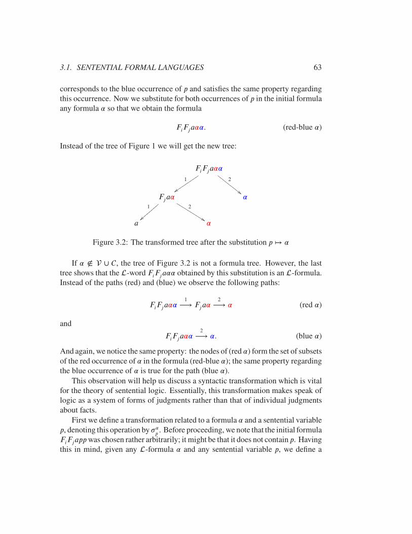
3.1. SENTENTIAL FORMAL LANGUAGES 63
corresponds to the blue occurrence of p and satisfies the same property regardingthis occurrence. Now we substitute for both occurrences of p in the initial formulaany formula � so that we obtain the formula
FiFja��. (red-blue �)
Instead of the tree of Figure 1 we will get the new tree:
FiFja��1
zz✉✉✉✉✉✉✉✉✉
2
""❋❋
❋❋❋❋
❋❋❋
Fja�1
}}④④④④④④④④ 2
%%❑❑
❑❑❑❑
❑❑❑❑
�
a �
Figure 3.2: The transformed tree after the substitution p↦ �
If � ∉ ∪ , the tree of Figure 3.2 is not a formula tree. However, the lasttree shows that the -word FiFja�� obtained by this substitution is an -formula.Instead of the paths (red) and (blue) we observe the following paths:
FiFja��1
⟶ Fja�2
⟶ � (red �)
and
FiFja��2
⟶ �. (blue �)
And again, we notice the same property: the nodes of (red �) form the set of subsetsof the red occurrence of � in the formula (red-blue �); the same property regardingthe blue occurrence of � is true for the path (blue �).
This observation will help us discuss a syntactic transformation which is vitalfor the theory of sentential logic. Essentially, this transformation makes speak oflogic as a system of forms of judgments rather than that of individual judgmentsabout facts.
First we define a transformation related to a formula � and a sentential variablep, denoting this operation by ��p . Before proceeding, we note that the initial formulaFiFjappwas chosen rather arbitrarily; it might be that it does not contain p. Havingthis in mind, given any -formula � and any sentential variable p, we define a
64 CHAPTER 3. SENTENTIAL FORMAL LANGUAGES
unary substitution ��p ∶ Fm ⟶ Fm as follows:
∙ if � ∈ ∪ and � ≠ p, then ��p (�) = �;∙ if � = p, then ��p (�) = �;∙ if � = Fi�1 … �n, then ��p (�) = Fi�
�p (�1)… ��p (�n).
At first sight, it may seem that unary substitution is not powerful enough. Forexample, let us take a formula FiFjapq, where connectives Fi and Fj have the arityequal to 2. Assume that we want to produce a formula FiFja��. Suppose we firstobtain:
��p (FiFjapq) = FiFja�q.
And we face a problem if � contains q, for then we get
��q (FiFja�q) = FiFja��q (�)�,
which is not necessarily equal to FiFja��. To overcome this difficulty, we selecta variable which occurs neither in � nor in the initial formula FiFjapq. Supposethis variable is r. Then, we first produce:
�rq(FiFjapq) = FiFjapr.
Now the desirable formula can be obtained in two steps:
��p (FiFjapr) = FiFja�r,��r (FiFja�r) = FiFja��.
Thus we observe:��r ◦�
�p◦�
rq(FiFjapq) = FiFja��.
This leads to the conclusion that the composition of two and more unary sub-stitutions may result in substitution of a different kind; namely, we can obtain theformula FiFja�� from the formula FiFjapq by substituting simultaneously theformulas � and � for the variables p and q, respectively. Thus we arrive at thefollowing definition.
Definition 3.1.3 (substitution). Given a formal language , a syntactic transfor-mation � ∶ Fm ⟶ Fm is called a uniform (or simultaneous) substitu-
tion (or simply a substitution or -substitution) if it is an extension of a map�0 ∶ ⟶ Fm, satisfying the following conditions ∶
(a) if � ∈ , then �(�) = �;(b) if � = Fi�1 … �n, then �(�) = Fi�(�1)… �(�n).

3.1. SENTENTIAL FORMAL LANGUAGES 65
Given a substitution � and a formula �, �(�) is called a substitution instance of�. The set of -substitutions is denoted by Sbs.
For a set X of -formulas and an -substitution �, we denote:
�(X) ∶= {�(�) | � ∈ X} and �−1(X) ∶= {� | �(�) ∈ X}.
Thus, for any substitution �,
�(∅) = ∅ and �−1(∅) = ∅. (3.1)
Also, we observe:
i) �(�−1(X)) ⊆ X and ii) X ⊆ �−1(�(X)). (3.2)
(Exercise 3.1.2)We leave for the reader to prove that, given a fixed formula �, any simultaneous
substitution applied to � results in the composition of singular substitutions appliedto �. (See Exercise 3.1.3.)
Proposition 3.1.2. For any map �0 ∶ ⟶ Fm, there is a unique substitution� ∶ Fm ⟶ Fm extending �0.
Proof is left to the reader. (Exercise 3.1.4.)
The last proposition allows us to think of a substitution simply as a map � ∶
⟶ Fm, which will be convenient when we want to define a particular substi-tution. On the other hand, the property (b) of Definition 3.1.3 allows us to look atany substitution as a mapping satisfying a special algebraic property, which willalso be convenient when we want to use this property.
For now, we want to note that composition of finitely many substitutions is asubstitution. Moreover, for any substitutions �1, �2 and �3,
�1◦(�2◦�3) = (�1◦�2)◦�3 (3.3)
(We leave this property for the reader; see Exercise 3.1.5.) This implies that the setof all substitutions, related to a language , along with composition ◦ constitute amonoid with the identity element
�(p) = p, for any p ∈

66 CHAPTER 3. SENTENTIAL FORMAL LANGUAGES
which will be calling the identity substitution. It must be clear that for any formula�,
�(�) = �.
Because of (3.3), any grouping in
�1◦… ◦�n
leads to the same result. For this reason, parentheses can be omitted, if we do wantto be specific.
We will call a set F ⊆ Fm closed under substitution if for any -formula �and substitution �,
� ∈ F ⟹ �(�) ∈ F .
We have already noted that the tree of Figure 3.2 is not a formula tree if � ∉
∪ . However, we can build the formula tree for �. It does not matter how itlooks; so we depict it schematically as follows:
�
�O�O�O
◦◦◦
Figure 3.3: The formula tree for �
Attaching two copies of the last tree to the tree of Figure 3.2, we obtain the treefor FiFja��.
FiFja��1
zz✉✉✉✉✉✉✉✉✉
2
$$❍❍
❍❍❍❍
❍❍❍❍
Fja�1
}}④④④④④④④④ 2
%%❑❑
❑❑❑❑
❑❑❑❑
�
�O�O�O
a �
�O�O�O
◦◦◦
◦◦◦
Figure 3.4: The formula tree for FiFja��

3.1. SENTENTIAL FORMAL LANGUAGES 67
We will call one copy of the formula tree for � the tree for red � and the othercopy the tree for the blue �.
Now let us take any formula � and construct the formula tree for it depicted asfollows:
�
�O�O�O
∙ ∙ ∙
Figure 3.5: The formula tree for �
Now in the path
FiFja��1
⟶ Fja�2
⟶ �
of the tree of Figure 3.4, we replace all red occurrences of � by � and replace the
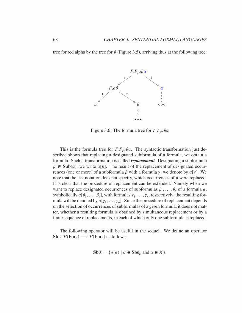
68 CHAPTER 3. SENTENTIAL FORMAL LANGUAGES
tree for red alpha by the tree for � (Figure 3.5), arriving thus at the following tree:
FiFja��1
zz✉✉✉✉✉✉✉✉✉
2
$$❍❍
❍❍❍❍
❍❍❍❍
Fja�1
~~⑤⑤⑤⑤⑤⑤⑤⑤ 2
$$❏❏
❏❏❏❏
❏❏❏❏
�
�O�O�O�O
a �
�O�O�O
◦◦◦
∙ ∙ ∙
Figure 3.6: The formula tree for FiFja��
This is the formula tree for FiFja��. The syntactic transformation just de-scribed shows that replacing a designated subformula of a formula, we obtain aformula. Such a transformation is called replacement. Designating a subformula� ∈ Sub(�), we write �[�]. The result of the replacement of designated occur-rences (one or more) of a subformula � with a formula , we denote by �[ ]. Wenote that the last notation does not specify, which occurrences of � were replaced.It is clear that the procedure of replacement can be extended. Namely when wewant to replace designated occurrences of subformulas �1,… , �n of a formula �,symbolically �[�1,… , �n], with formulas 1,… , n, respectively, the resulting for-mula will be denoted by �[ 1,… , n]. Since the procedure of replacement dependson the selection of occurrences of subformulas of a given formula, it does not mat-ter, whether a resulting formula is obtained by simultaneous replacement or by afinite sequence of replacements, in each of which only one subformula is replaced.
The following operator will be useful in the sequel. We define an operatorSb ∶ (Fm) ⟶ (Fm) as follows:
SbX = {�(�) | � ∈ Sbs and � ∈ X}.

3.1. SENTENTIAL FORMAL LANGUAGES 69
Proposition 3.1.3. The following properties hold:
(a) X ⊆ SbX;
(b) Sb(X ∪ Y ) = SbX ∪ SbY ;(c) Sb(X ∩ Y ) = SbX ∩ SbY ;(d) X ⊆ Y ⟹ SbX ⊆ SbY ;(e) for any � ∈ Sbs, �(SbX) ⊆ SbX;
(f) Sb(SbX) = SbX.
Proof. (a) follows from the observation that �(X) = X. (b), (c) and (d) are obvious.(e) follows from the fact that a compositions of two (and more) substitutions is asubstitution. (f) follows from (a) and (e).
Before going over examples of some sentential languages, we discuss how anymetaformula can be seen in the light of the notion of substitution. It must be clearthat the intended interpretation of any metaformula � is the set of formulas of aparticular shape.
Similar to Definition 3.1.3, any map �0 ∶ Mv ⟶ Fm can uniquely beextended to � ∶ Mf ⟶ Fm. We will call both �0 and its extension � arealization, or instantiation, of metaformulas in . The following observationwill be useful in the sequel. An instantiation � is called simple if it is the extensionof �0 ∶ Mv ⟶ .
Proposition 3.1.4. Let � be an -metaformula and Σ� be the class of all instanti-ations of �. Then for any -substitution � and any -formula �,
� ∈ Σ� ⟹ �(�) ∈ Σ�.
Proof is leaft to the reader. (Exercise 3.1.6)
Below we give examples of languages that are specifications of the schematiclanguage . All these languages include a denumerable set as the set of senten-tial variables.
A: In this language, there is no sentential constants; there are four (assertoric)logical connectives: ∧ (conjunction),∨ (disjunction),→ (implication or con-ditional), and ¬ (negation), having the arities #(∧) = #(∨) = #(→) = 2 and#(¬) = 1. It is customary to use an infix notation for this language; however,the use of infix notation for this language requires two additional symbols:‘(’ and ‘)’ called the left and right parenthesis, respectively. Accordingly,

70 CHAPTER 3. SENTENTIAL FORMAL LANGUAGES
the definition of formula will be different: (� ∧ �), (� ∨ �), (� → �) and¬� are formulas, whenever � and � are. The parentheses do not apply toatomic formulas and negations. Sometimes, we will not employ all the con-nectives of A but some of them, continuing to call this restricted languageA. Sometimes, A is considered in its extended version, when a connective↔ is added; if not, then the last connective is used as an abbreviation:
� ↔ � ∶= (� → �) ∧ (� → �).
B: This language extends A by adding to it two constants: ⊤ (truth or verum)and ⊥ (falsehood or falsity or falsum or absurdity). Sometimes, only one ofthese constants will be employed. The parentheses do not apply to atomicformulas, negations and to the constants ⊤ and ⊥. We will call all thesevariants by B, indicating every time the list of constants.
C: This language extends eitherA orB with two sentential connectives (modal-ities): □ (necessity) and ◊ (possibility) both of the arity 1, that is #(□) =
#(◊) = 1. In addition to the corresponding requirements above, the paren-theses do not apply to the formulas that start with the modalities □ and ◊.Sometimes, when only one of these modalities is employed, we continue tocall this language C .
In the sequel we will employ more formal languages, which do not fit the pro-posed framework but closely related to it.

3.1. SENTENTIAL FORMAL LANGUAGES 71
Exercises 3.1
1. Here we give another definition of a formula tree. This new definition isconvenient when we deal with an algorithmic problem, in which case the sets , and are regarded countable and effectively decidable. One of suchproblems will be raised below as an exercise. We note that in this definitiona designated path can be identified exclusively by the nodes it comprises.
The formula tree for a formula � is a finite directed labeled tree where eachnode is labeled with a pair ⟨n, �⟩, where n is a natural number and � is asubformula of �.
There is a unique node, called the root, labeled by ⟨p0, �⟩, the ingdegree ofwhich is 0.3 The ingdegree of all other nodes of the tree, if any, equals 1.Let a node v be labeled with ⟨n, �⟩, where � ∈ ∪. Then the outdegree ofv is always 0. Such nodes are called leaves. (As the reader will see below,leaves are always present in a formula tree.) Thus if � ∈ ∪ , the formulatree of � consists of only one node, the root, which is also a leaf. Assumethat � = F�1 … �k with F ∈ is a proper subformula of � and a nodev is labeled with ⟨n, �⟩. Suppose that pj is the greatest prime number thatdivides n. Then the outdegree of v is #(F ), that is in our case, equals k. Andthen v will be connected via k edges to k different nodes, v1,… , vk. (Thedirection of each such edge is from v to vi.) We label vi with ⟨n ⋅ pj+i, �i⟩.Thus, if �i = �j , then the two distinct nodes, vi and vj , will be labeled withlabels distinct in their first place and equal in the second. Also, we note thatthe degree of each �i is less than the degree of �.
Use the new definition of formula tree to prove the following.
There is a mechanical procedure (an algorithm) which, given alist of pairs ⟨n1, �1⟩,… , ⟨nk, �k⟩, where each ni is a positive in-teger, can assemble a formula tree, where the pairs are regardedas the nodes of the tree, or states that such a tree does not exist.
2. Prove the inclusions (3.2).
3. Prove that (a) for any fixed formula � and any fixed substitution �, there areunary substations �1,… , �n such that �(�) = �1◦… ◦�n(�); however, (b) forany fixed substitution �, there is no finitely many fixed unary substitutions�1,… , �n such that for any formula �, �(�) = �1◦… ◦�n(�).
3We remind the reader that p0, p1, p2,… is the sequence of prime numbers.

72 CHAPTER 3. SENTENTIAL FORMAL LANGUAGES
4. Prove Proposition 3.1.2.
5. Prove (3.3).
6. Prove Proposition 3.1.4.
3.2 Semantics of sentential formal language
One of our concerns in this book is to show how truth can be transmitted throughformulas of a formal language by formally presented deduction. Calling a formulatrue, we will mean a kind of truth which does not depend on any factual content.Moreover, sharing the view of the multiplicity of the nature of truth, we will bedealing rather with degrees of truth, calling them truth values. Then, the idea oftruth will find its realization in the idea of validity.
Concerning the independence of any factual, contingent content in relation totruth values, let us consider the following two sentences — ‘Antarctica is large’and ‘Antarctica is large or Antarctica is not large’. If our formal language containsa symbol for the grammatical disjunction “…1 or …2”, say “…1 ∨…2” (as in thelanguagesA–C of Section 3.1), and a symbol for creating the denial of sentence,say “¬…” (also as in A–C), we can write in symbolic form the first sentenceas p and the second as p ∨ ¬p. From the viewpoint of Section 3.1, both formalexpressions are formulas of the language A. Now, depending on familiarity withgeography, as well as of personal experience, one can count p true or false. Thesecond formula p∨¬p, however, in some semantic systems takes steadily the truthvalue true, regardless of any personal relation towards p. The universality of thiskind will be stressed in the idea of validity.
From the last example, it should be clear the distinction between the statements,the truth value of which (understood as the degree of trust or that of informative-ness) is dependent on the contingency of facts, the level of knowledge or personalbeliefs, and the formal judgments, which obtain their logical status or meaningdetermined by semantic rules. These rules will allow us to interpret the formaljudgments of a language in abstract structures, reflecting the structural characterof these judgments, as well as the universal character of their validity, therebyunderstanding their invalidity as the failure to satisfy this universality.
In this book, semantics will play pragmatic rather than explanatory role;4 namelywe will be stressing the use of semantic structures as separating tools. This will be
4However, since we state validity conditions for formal judgments, these conditions generate themeanings of the judgments, according to the point of view that has been emphasized by Wittgen-
3.2. SEMANTICS OF SENTENTIAL FORMAL LANGUAGE 73
explained in Section 5.3. Moreover, we want to emphasize that in our approach tosemantics we adhere to the relativistic position, according to which a single formaljudgment can be valid according to one semantic system and invalid with respectto another.
Now we turn to the definition of semantics of the schematic language exem-plified by the languages A–C in Section 3.1. Depending on one’s purposes, ordepending on the lines, along which the semantics in question can be employed,the semantics we propose can use the items of the following two categories —the algebras of type and expansions of the latter called logical matrices. Lateron, we will generalize the notion of logical matrix, when we discuss consequencerelation in Chapter 4.
The following semantic concepts will be specified later on as needed.
Definition 3.2.1 (algebra of type ). An algebra of type (or an -algebra orsimply an algebra when a type is specified ahead and confusion is unlikely) is astructure A = ⟨A; , ⟩, where A is a nonempty set called the carrier (or universe)
of A; , which in the notion of -formulas represents logical connectives, nowrepresents the set of finitary operations on A of the corresponding arities; and ,which is a set of logical constants, now represents a set of nullary operations on A.As usual, we use the notation |A| = A. The part ⟨ , ⟩ of the structure A is calledits signature. Thus, referring to an algebra A, we can say that it is an algebra ofsignature ⟨ , ⟩ or of signature , if = ∅.
Thus any -formula in relation to any algebra of type becomes a term. Nat-urally, the sentential variables of a formula understood as term become the indi-
vidual variables of this term. Since each algebraic term of, say, n variables can beread as an n-ary derivative operation in an algebra of type , so can be understoodany -formula containing n sentential variables.
Definition 3.2.2 (inessential expansion of an algebra, equalized algebras). Givenan algebra A = ⟨A; , ⟩, we obtain an inessential expansion of A if we add to one or more terms regarding them as new signature operations, or if we addto one or more symbols with their intended interpretation as elements of A.Two algebras (or their signatures) are called equalized if they have inessentialexpansions of one and the same type.
stein in Tractatus; cf. (Wittgenstein, 2001), 4.024. Also, compare with Curry’s statement that “themeaning of a concept is determined by the conditions under which it is introduced into discourse;”cf. (Curry, 1966), section II.2.

74 CHAPTER 3. SENTENTIAL FORMAL LANGUAGES
The central notion of Lindenbaum method is that of formula algebra associatedwith a particular language. The formula algebra of type has Fm as its carrierand the signature operations as defined in Definition 3.1.1. This algebra is denotedby F. Thus we have:
F = ⟨Fm; , ⟩.Analogously, the set of-metaformulas along with the set regarded as nullary
operations and the set regarded as non-nullary operations constitute a metafor-
mula algebra M of type .
A relation between the -formulas and the algebras of type is establishedthrough the following notion.
Definition 3.2.3 (valuation, value of a formula in an algebra). Let A be an algebraof type. Then any map v ∶ ⟶ |A| is called a valuation (or an assignment) inthe algebra A. Then, given a valuation v, the value of an -formula � with respectto v, in symbols v[�], is defined inductively as follows ∶
(a) v[p] = v(p), for any p ∈ ;
(b) v[c] is the value of the nullary operation of A corresponding tothe constant c of ;
(c) v[�] = Fv[�1]… v[�n] if � = F�1 … �n.
If ′ ⊂ , then a map v ∶ ′ ⟶ |A| is called a ′-valuation, or a valuation
restricted to ′.
It makes sense to denote the mapping
� ↦ v[�]
by the same letter v. The following observation is a justification for this usage.
Proposition 3.2.1. Let v be a valuation in an algebra A. Then the mapping v ∶
� ↦ v[�] defines a homomorphism F ⟶ A. Conversely, each homomorphismF ⟶ A is a valuation.
Proof of the first part is based on the clauses (a)–(c) of Definition 3.2.3. The sec-ond part is obvious.
Thus, given a valuation v in A and a formula �(p1,… , pn) where p1,… , pn areall variables occurring in �, we observe that
v[�] = �(v[p1],… , v[pn]).
3.2. SEMANTICS OF SENTENTIAL FORMAL LANGUAGE 75
Grounding on the last observation base in turn on Proposition 3.2.1, very oftena valuation is defined as a homomorphism F ⟶ A.
Comparing (b)–(c) of Definition 3.2.3 with (a)–(b) of Definition 3.1.3, we ob-tain the following.
Proposition 3.2.2. Any substitution is a valuation in F and vice versa. Henceany substitution is an endomorphism F ⟶ F.
The converse of the last conclusion is also true: any endomorphism F ⟶
F can be regarded as a substitution. (Exercise 3.2.1.)
The next property, which a combination of Proposition 3.2.1 and Proposi-tion 3.2.8, will be useful in the sequel.
Proposition 3.2.3. Given an -algebra A and a valuation v in A, for any substi-tution �, there is a valuation v� in A such that for any formula �, v[�(�)] = v�[�].
Proof. Indeed, we simply define
v� ∶= v◦�.
By Proposition 3.2.2, v� is a homomorphism, and, in virtue of Proposition 3.1.2,v� is a valuation in A.
Proposition 3.2.4. Let v0 be a valuation in an algebra A of type . Assume thatA is generated by the set {v0[p] | p ∈ }. Then for any valuation v in A, there isa substitution � such that v = v0◦�.
Proof. Let v ∶ p ↦ ap be a valuation in A. In virtue of Proposition 2.3.1, for eachp ∈ , there is an -formula, �p, such that ap = �p[pi∖v0[pj],… , qi∖v0[qJ ]],where pi,… , qi are all variables occurring in �p. Without loss of generality , onecan count that pi = pj ,… , qi = qj . Hence ap = v0[�p], that is v[p] = v0[�p], forany p ∈ . Now we define a substitution as follows: �(p) = �p, where p ∈ .Thus, we have: v[p] = v0(�(p)), that is v = v0◦�.
Proposition 3.2.5. Let � be a congruence on F. Then for valuation v in F∕�,there is an -substitution � such that for any -formula �, v[�] = �(�)∕�. Con-versely, for any -substitution �, there is a unique valuation v� in F∕� such thatfor any formula �, v�[�] = �(�)∕�.
76 CHAPTER 3. SENTENTIAL FORMAL LANGUAGES
Proof. Suppose according to v, v ∶ p ↦ ∕�, where p ∈ . Then we define:� ∶ p ↦ , where p ∈ .5 Thus, in virtue of Proposition 3.2.2, we have:v[�] = �(�)∕�, for any -formula �.
The converse-part is obvious.
Now we turn to a central notion of any semantics — the notion of validity.6
This notion in turn is defined in the framework of the notion of logical matrix.
Definition 3.2.4 (logical matrix of type ). A logical matrix (or simply a matrix)
of type is a structure M = ⟨A, D(x)⟩, where A is an algebra of type , which,if considered as part of M, is called an M-algebra, and D(x) is a predicate on|A|. The matrix M is nontrivial if the algebra A is nontrivial, and trivial other-wise. We will also denote a matrix as a structure ⟨A; , , D(x)⟩ or as a structure⟨A; , D(x)⟩, if = ∅. We will also denote a matrix as ⟨A, D⟩ or as ⟨A; , D⟩ oras ⟨A; , D⟩, if = ∅, where D ⊆ |A|. In the last three notationsD is called theset of designated elements or a logical filter (or simply a filter) in (or of) M.
We should remark that using “logical” in the last definition was a bit hasty, forthe first connection with logic emerges, at least in the case of logical matrices, inthe next definition when we separate semantically valid -formulas from the otherformulas.
Definition 3.2.5. Let M = ⟨A, D⟩ be a logical matrix of type . Then a formula �is satisfied by a valuation v in A if v[�] ∈ D, in which case we say that v satisfies
� in M; further, � is semantically valid (or simply valid) in M, symbolically M ⊧ �or ⊧M �, if for any valuation v in A, v[�] ∈ D. Given a setX of formulas, we writeM ⊧ X if M ⊧ �, for all � ∈ X. If a formula is not valid in a matrix, it is calledinvalid in this matrix or is rejected by the matrix or one can say that this matrixrejects the formula. If v[�] ∉ D in M, v is a valuation rejecting or refuting �.The set of all formulas valid in a matrix M is denoted by LM and is called thelogic of this matrix.
Proposition 3.2.6. Let M = ⟨A, D⟩ be a matrix (of type ). Then for any substi-tution �, if M ⊧ �, so is M ⊧ �(�).
5Of course, the definition of such a substitution is not unique, and the axiom of choice is requiredhere.
6W. and M. Kneale note, “[. . . ] logic is not simply valid argument but the reflection uponprinciples of validity;” (Kneale and Kneale, 1962), section I.1.
3.2. SEMANTICS OF SENTENTIAL FORMAL LANGUAGE 77
Proof. Let v be any valuation in A. According to Propositions 3.2.2 and 3.2.1,� ∶ F ⟶ F and v ∶ F ⟶ A are homomorphisms. Then v◦� is also ahomomorphism F ⟶ A and hence, by Proposition 3.2.1, is a valuation. There-fore, M ⊧ � implies that v[�(�)] ∈ D.
The last proposition induces a way of how, given a matrix, to obtain a matrixon the formula algebra so that both matrices validate the same set of formulas.
Let M = ⟨A, D⟩ be a matrix. We denote
DM= {� | M ⊧ �}
and then define a matrixMFm = ⟨F, DM
⟩.We observe that for any formula �,
MFm ⊧ � ⟺ M ⊧ �. (Lindenbaum equivalence)
Indeed, let MFm ⊧ �. Then for any substitution � (which, according to Propo-sition 3.2.2, is a valuation in F), �(�) ∈ D
M; in particular, �(�) = � ∈ D
M, that
is M ⊧ �.Now suppose that M ⊧ �, that is � ∈ DM. In virtue of Proposition 3.2.6, DM
is closed under substitution. This completes the proof of the equivalence above.Next let us consider M = ⟨F, D⟩. We observe that if � ∈ D
M, that is M ⊧ �,
then, since, by virtue of Proposition 3.2.2, each substitution is a valuation in F
and vice versa, � ∈ D.Now let D′ ⊆ D and D′ be closed under substitution. Assume that � ∈ D′.
Then, obviously, M ⊧ � and hence � ∈ DM
.Thus we have obtained the following.
Proposition 3.2.7. For any matrix M, there is a matrix on the formula algebra,namely MFm, such that both matrices validate the same set of -formulas. More-over, given a matrix M = ⟨F, D⟩, the filter of the matrix MFm = ⟨F, DM
⟩isthe largest subset of D closed under substitution. Thus, if D itself is closed undersubstitution, then D = DM.
The importance of the last proposition for what follows is that it shows that thematrices of the form ⟨F, D⟩, where a filterD is closed under substitution, sufficefor obtaining all sets of valid -formulas, which can be obtained individually bythe matrices of type . This observation will be clarified below as Lindenbaum’s

78 CHAPTER 3. SENTENTIAL FORMAL LANGUAGES
Theorem; see Proposition 4.3.12.
Now we turn to some special matrices which have played their important rolein the development of sentential logic. In all these matrices, the filter of desig-nated elements consists of one element. In this connection, we note the followingequivalence, which will be used throughout: If D = {c}, then
x ∈ D ⟺ x = c. (3.4)
In the sequel, we find useful the following property.
Proposition 3.2.8. Let M1 = ⟨A1, D1⟩ and M2 = ⟨A2, D2⟩ be matrices of thesame type. Also, let ℎ be an epimorphism of A1 onto A2 such that ℎ[D1] ⊆ D2.Then LM1 ⊆ LM2
Proof. Let v be a valuation in A2. Since ℎ is an epimorphisms, for each variable p ,there is an element x ∈ |A1| such that ℎ(x ) = v[p ]. We define a valuation v′ inA1 as follows: v′[p ] = x , for any variable p . It is obvious that ℎ(v′[p ]) = v[p ].Assume that � ∈ LM1; in particular, v′[�] ∈ D1. This implies that v[�] ∈ D2.
3.2.1 The logic of a two-valued matrix
We begin with a well-known matrix of the so-called “two-valued logic.” The sig-nificance of this matrix in the history of logic is difficult to overestimate. The two-valued matrix was assumed, first, to distinguish true statements from false ones;and, second, to validate only the former. As we will see below, the main logic lawssuch as, for example, the law of identity, the law of contradiction, the law of theexcluded middle (see below) and others can be demonstrated as valid formulas inthis matrix. For this reason, it is worth considering this matrix first. Later on, wewill explain another significance of this matrix, purely algebraic in nature, whichleads to a very important view on this matrix as a refuting and separating tools.
The two-valued matrix assumes two main variants of formulation — as a ma-trix of type A and as that of type B. As will be seen below, the differencebetween these variants concerns only semantic rules and does not affect essen-tially the set of valid formulas in the corresponding matrices. For this reason, wedenote both variants by B2. The elements of B2 are denoted by 0 (false) and 1
(true), which constitute a Boolean algebra with 0 as the least element and 1 as the
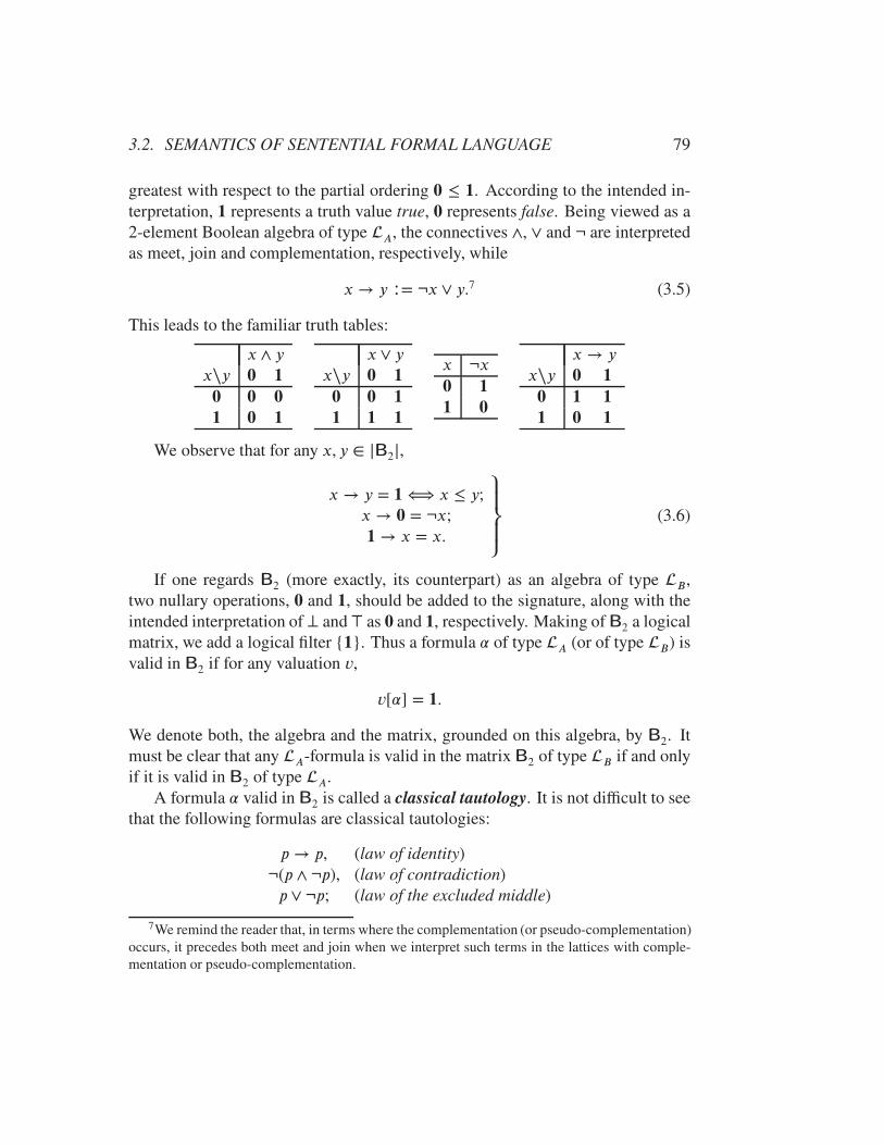
3.2. SEMANTICS OF SENTENTIAL FORMAL LANGUAGE 79
greatest with respect to the partial ordering 0 ≤ 1. According to the intended in-terpretation, 1 represents a truth value true, 0 represents false. Being viewed as a2-element Boolean algebra of type A, the connectives ∧, ∨ and ¬ are interpretedas meet, join and complementation, respectively, while
x→ y ∶= ¬x ∨ y.7 (3.5)
This leads to the familiar truth tables:
x ∧ yx∖y 0 1
0 0 0
1 0 1
x ∨ yx∖y 0 1
0 0 1
1 1 1
x ¬x0 1
1 0
x → yx∖y 0 1
0 1 1
1 0 1
We observe that for any x, y ∈ |B2|,
x → y = 1 ⟺ x ≤ y;x → 0 = ¬x;1 → x = x.
⎫⎪⎬⎪⎭
(3.6)
If one regards B2 (more exactly, its counterpart) as an algebra of type B,two nullary operations, 0 and 1, should be added to the signature, along with theintended interpretation of ⊥ and⊤ as 0 and 1, respectively. Making of B2 a logicalmatrix, we add a logical filter {1}. Thus a formula � of type A (or of type B) isvalid in B2 if for any valuation v,
v[�] = 1.
We denote both, the algebra and the matrix, grounded on this algebra, by B2. Itmust be clear that any A-formula is valid in the matrix B2 of type B if and onlyif it is valid in B2 of type A.
A formula � valid in B2 is called a classical tautology. It is not difficult to seethat the following formulas are classical tautologies:
p→ p, (law of identity)¬(p ∧ ¬p), (law of contradiction)p ∨ ¬p; (law of the excluded middle)
7We remind the reader that, in terms where the complementation (or pseudo-complementation)occurs, it precedes both meet and join when we interpret such terms in the lattices with comple-mentation or pseudo-complementation.

80 CHAPTER 3. SENTENTIAL FORMAL LANGUAGES
as well as the following:
p→ (q → p);
¬p→ (p→ q).
}(“paradoxes of material implication”)
The above tautologies had been known from ancient times. In modern times, suchtautologies as the following have been in focus:
((p → q) → p) → p; (Peirce’s law)¬¬p↔ p; (double negation law)
¬(p ∧ q) ↔ ¬p ∨ ¬q;
¬(p ∨ q) ↔ ¬p ∧ ¬q.
}(De Morgan’s laws)
By the two-valued logic, one usually means the set of all classical tautologies.
3.2.2 The Łukasiewicz logic of a three-valued matrix
Perhaps, the “Łukasiewicz 3-valued logic” is the best-known of all multiple-valuedsystems alternative to the set of classical tautologies. The matrix which definesthis “logic” has three values, 0 (false), � (indeterminate) and 1 (true), which arearranged by a linear ordering as follows: 0 ≤ � ≤ 1. On this carrier, an algebraof type A is defined in such a way that ∧ and ∨ are interpreted as meet and joinin the 3-element distributive lattice; then, ¬ and → are defined according to thefollowing tables:
x ¬x0 1
� �
1 0
x → yx∖y 0 � 1
0 1 1 1
� � 1 1
1 0 � 1
We denote this algebra by Ł3. Actually, when we have defined ¬ in Ł3 asabove, the operation → can be defined according to (3.6). Moreover, the followingidentities can be easily checked:
x ∨ y = (x → y) → y;
x ∧ y = ¬(¬x ∨ ¬y).
}(3.7)
(Exercise 3.2.6.) Also, we note that, as algebras of type A, B2 is a subalgebra Ł3.(See Exercise 3.2.7.)
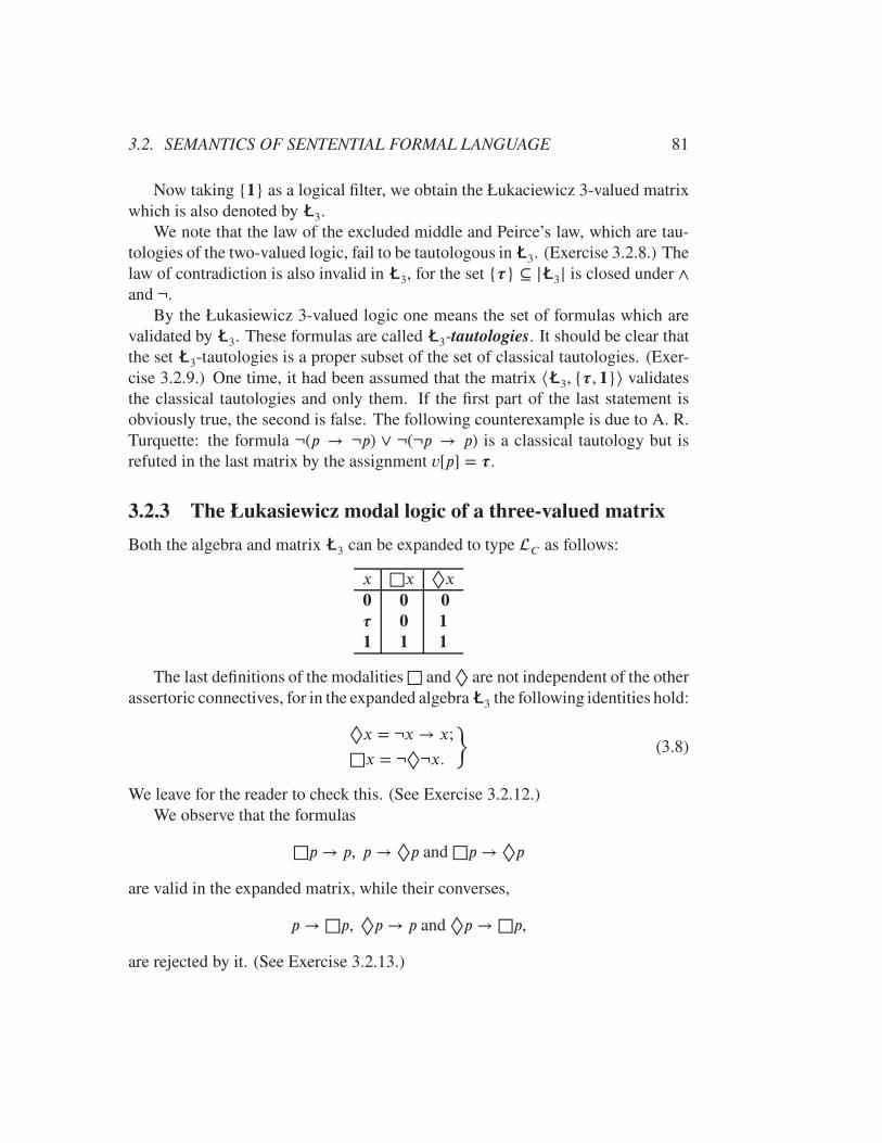
3.2. SEMANTICS OF SENTENTIAL FORMAL LANGUAGE 81
Now taking {1} as a logical filter, we obtain the Łukaciewicz 3-valued matrixwhich is also denoted by Ł3.
We note that the law of the excluded middle and Peirce’s law, which are tau-tologies of the two-valued logic, fail to be tautologous in Ł3. (Exercise 3.2.8.) Thelaw of contradiction is also invalid in Ł3, for the set {�} ⊆ |Ł3| is closed under ∧and ¬.
By the Łukasiewicz 3-valued logic one means the set of formulas which arevalidated by Ł3. These formulas are called Ł3-tautologies. It should be clear thatthe set Ł3-tautologies is a proper subset of the set of classical tautologies. (Exer-cise 3.2.9.) One time, it had been assumed that the matrix ⟨Ł3, {� , 1}⟩ validatesthe classical tautologies and only them. If the first part of the last statement isobviously true, the second is false. The following counterexample is due to A. R.Turquette: the formula ¬(p → ¬p) ∨ ¬(¬p → p) is a classical tautology but isrefuted in the last matrix by the assignment v[p] = �.
3.2.3 The Łukasiewicz modal logic of a three-valued matrix
Both the algebra and matrix Ł3 can be expanded to type C as follows:
x □x ◊x0 0 0
� 0 1
1 1 1
The last definitions of the modalities □ and ◊ are not independent of the otherassertoric connectives, for in the expanded algebra Ł3 the following identities hold:
◊x = ¬x→ x;
□x = ¬◊¬x.
}(3.8)
We leave for the reader to check this. (See Exercise 3.2.12.)We observe that the formulas
□p→ p, p → ◊p and □p→ ◊p
are valid in the expanded matrix, while their converses,
p→ □p, ◊p→ p and ◊p→ □p,
are rejected by it. (See Exercise 3.2.13.)
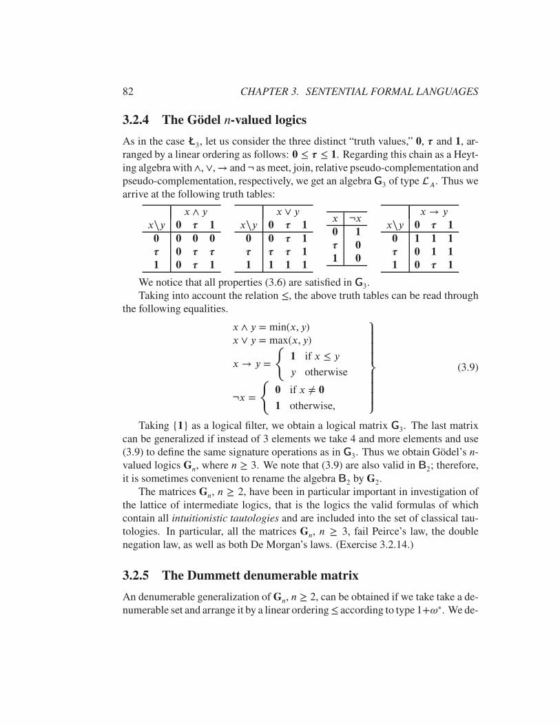
82 CHAPTER 3. SENTENTIAL FORMAL LANGUAGES
3.2.4 The Gödel n-valued logics
As in the case Ł3, let us consider the three distinct “truth values,” 0, � and 1, ar-ranged by a linear ordering as follows: 0 ≤ � ≤ 1. Regarding this chain as a Heyt-ing algebra with∧, ∨, → and ¬ as meet, join, relative pseudo-complementation andpseudo-complementation, respectively, we get an algebra G3 of type A. Thus wearrive at the following truth tables:
x ∧ yx∖y 0 � 1
0 0 0 0
� 0 � �
1 0 � 1
x ∨ yx∖y 0 � 1
0 0 � 1
� � � 1
1 1 1 1
x ¬x0 1
� 0
1 0
x→ yx∖y 0 � 1
0 1 1 1
� 0 1 1
1 0 � 1
We notice that all properties (3.6) are satisfied in G3.Taking into account the relation ≤, the above truth tables can be read through
the following equalities.
x ∧ y = min(x, y)x ∨ y = max(x, y)
x → y =
{1 if x ≤ y
y otherwise
¬x =
{0 if x ≠ 0
1 otherwise,
⎫⎪⎪⎪⎬⎪⎪⎪⎭
(3.9)
Taking {1} as a logical filter, we obtain a logical matrix G3. The last matrixcan be generalized if instead of 3 elements we take 4 and more elements and use(3.9) to define the same signature operations as in G3. Thus we obtain Gödel’s n-valued logics Gn, where n ≥ 3. We note that (3.9) are also valid in B2; therefore,it is sometimes convenient to rename the algebra B2 by G2.
The matrices Gn, n ≥ 2, have been in particular important in investigation ofthe lattice of intermediate logics, that is the logics the valid formulas of whichcontain all intuitionistic tautologies and are included into the set of classical tau-tologies. In particular, all the matrices Gn, n ≥ 3, fail Peirce’s law, the doublenegation law, as well as both De Morgan’s laws. (Exercise 3.2.14.)
3.2.5 The Dummett denumerable matrix
An denumerable generalization of Gn, n ≥ 2, can be obtained if we take take a de-numerable set and arrange it by a linear ordering≤ according to type 1+!∗. We de-
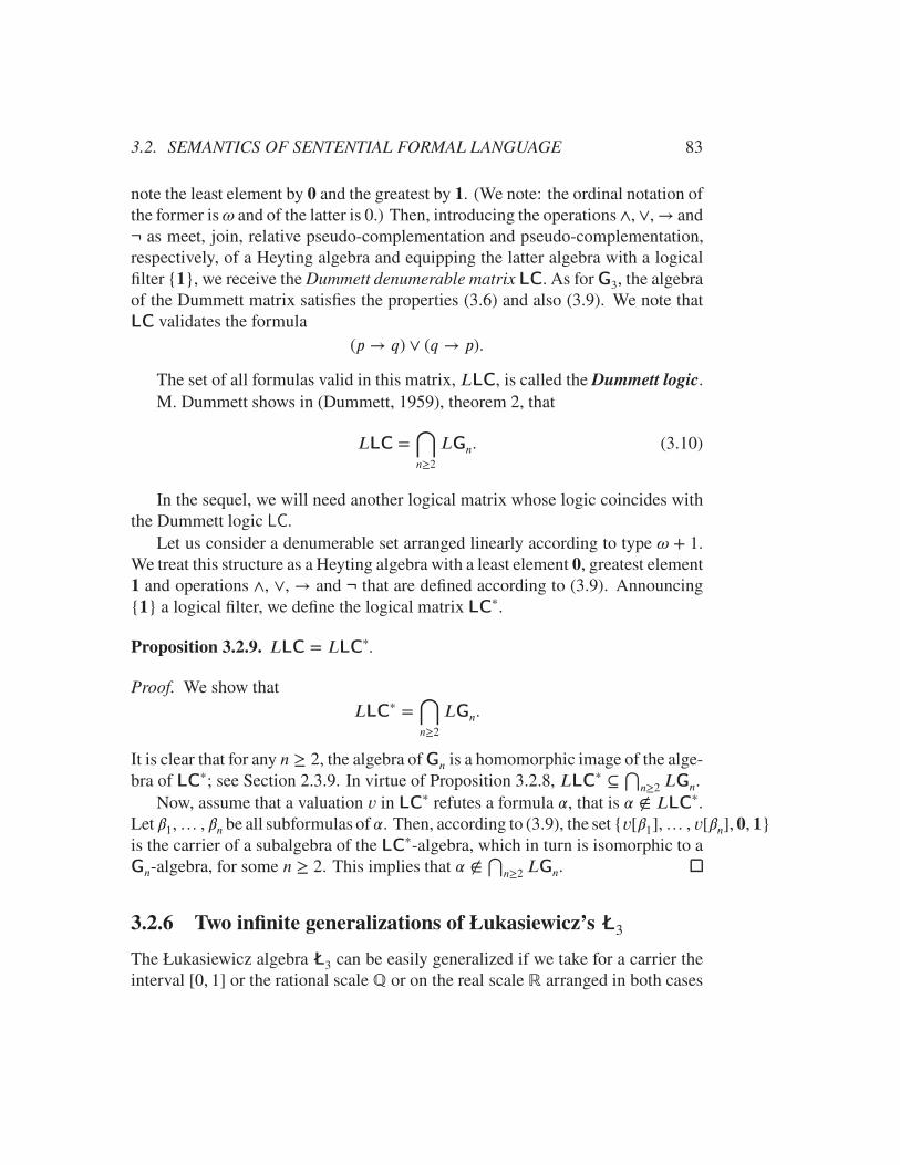
3.2. SEMANTICS OF SENTENTIAL FORMAL LANGUAGE 83
note the least element by 0 and the greatest by 1. (We note: the ordinal notation ofthe former is! and of the latter is 0.) Then, introducing the operations ∧, ∨, → and¬ as meet, join, relative pseudo-complementation and pseudo-complementation,respectively, of a Heyting algebra and equipping the latter algebra with a logicalfilter {1}, we receive the Dummett denumerable matrix LC. As for G3, the algebraof the Dummett matrix satisfies the properties (3.6) and also (3.9). We note thatLC validates the formula
(p → q) ∨ (q → p).
The set of all formulas valid in this matrix, LLC, is called the Dummett logic.M. Dummett shows in (Dummett, 1959), theorem 2, that
LLC =⋂n≥2
LGn. (3.10)
In the sequel, we will need another logical matrix whose logic coincides withthe Dummett logic LC.
Let us consider a denumerable set arranged linearly according to type ! + 1.We treat this structure as a Heyting algebra with a least element 0, greatest element1 and operations ∧, ∨, → and ¬ that are defined according to (3.9). Announcing{1} a logical filter, we define the logical matrix LC
∗.
Proposition 3.2.9. LLC = LLC∗.
Proof. We show thatLLC
∗ =⋂n≥2
LGn.
It is clear that for any n ≥ 2, the algebra of Gn is a homomorphic image of the alge-bra of LC
∗; see Section 2.3.9. In virtue of Proposition 3.2.8, LLC∗ ⊆
⋂n≥2LGn.
Now, assume that a valuation v in LC∗ refutes a formula �, that is � ∉ LLC
∗.Let �1,… , �n be all subformulas of �. Then, according to (3.9), the set {v[�1],… , v[�n], 0, 1}is the carrier of a subalgebra of the LC
∗-algebra, which in turn is isomorphic to aGn-algebra, for some n ≥ 2. This implies that � ∉
⋂n≥2LGn.
3.2.6 Two infinite generalizations of Łukasiewicz’s Ł3
The Łukasiewicz algebra Ł3 can be easily generalized if we take for a carrier theinterval [0, 1] or the rational scale ℚ or on the real scale ℝ arranged in both cases
84 CHAPTER 3. SENTENTIAL FORMAL LANGUAGES
by the ordinary less-than-or-equal relation ≤. The set of designated elements inboth cases is {1}. The operations ¬ and → are defined as follows:
¬x ∶= 1 − x,x→ y ∶= min(1, 1 − x + y);
then, the other operations are defined according to (3.7). This leads to the identities
x ∧ y = min(x, y) and x ∨ y = max(x, y),
which can be taken as definitions of ∧ and ∨ as well.The set of formulas valid in the first matrix, that is when [0, 1] is considered in
the rational scale, is denoted by Łℵ0and the formulas valid in the second matrix
by Łℵ1.
So far, we have discussed the semantic rules for the language . As we in-troduce other schematic languages later on (in Chapters 7), we will have to adjustthese rules for them. However, although semantic rules allow us to distinguishvalid formulas from refuted ones, they, taken alone, do not suffice to analyze rea-soning. This echoes the remark due to Aristotle that “it is absurd to discuss refu-tation (ἔλεγχος) without discussing reasoning (συλλογισμός).”8 We discuss therelation of formal deduction between -formulas in the form of consequence re-lation. This is a topic of the next chapter.
Exercises 3.2
1. Show that any endomorphism f ∶ F ⟶ F can be regarded as a substitu-tion; that is f is a unique extension of v ∶ ⟶ F such that v(p) = f (p),for any p ∈ .
2. Prove the second part of Proposition 3.2.1.
3. Prove that the laws of identity, of contradiction, of the excluded middle, aswell as Peirce’s and double negation laws are tautologies in B2.
4. Prove the properties (3.6).
5. Show that for any two A-formulas � and �, � ↔ � is a classical tautologyif and only if for any B2-valuation v, v[�] = v[�].
8Cf. (Kneale and Kneale, 1962), chapter I, section 4.
3.3. HISTORICAL NOTES 85
6. Prove the identities (3.7).
7. Prove that B2 is a subalgebra of Ł3.
8. Show that the law of the excluded middle and Peirce’s law are not tautolo-gous in Ł3.
9. Prove that the set of Ł3-tautologies is properly included in the set of classicaltautologies.
10. Prove that the “paradoxes of material implications” (p. 79) are Ł3-tautologous.
11. Show that the following formulas are Ł3-tautologies.
(a) p→ (q → p);(b) (p→ q) → ((q → r) → (p→ r));(c) (¬p→ ¬q) → (q → p);(d) ((p→ ¬p) → p) → p.
12. Prove that the identities (3.8) hold the algebra Ł3 expanded by the modalities□ and ◊.
13. Show that the logical matrix of type C of Section 3.2.3 validates the for-mulas □p → p, p → ◊p and □p → ◊p and rejects their conversesp→ □p, ◊p→ p and ◊p→ □p.
14. Show that Peirce’s law, the double negation law and both De Morgan’s lawscan be refuted in G3.
15. Let us designate on the algebra G3 the logical filter {� , 1}. We denote thenew matrix by G
′
3. Show that G
′
3validates a formula � if and only if � is a
classical tautology.
3.3 Historical notes
The idea that logic, as the science of reasoning, deals with the universal ratherthan the particular can be traced back to Plato and Aristotle. According to thePlatonic doctrine of Forms, a single Form is associated with each group of thingsto which a common name can be applied. Plato believed that each Form differsfrom the particulars it represents but, at the same time, is a particular of its own

86 CHAPTER 3. SENTENTIAL FORMAL LANGUAGES
kind. Applying this doctrine to reasoning, he believed that correct reasoning isbased on the connections of the involved Forms. This is how W. Kneale and M.Kneale summarize Plato’s view on reasoning.
“For Plato necessary connexions hold between Forms, and inference ispresumably valid when we follow in thought the connexions betweenForms as they are. How is this view related to the theory which assignstruth and falsity to sentences made up of nouns and verbs? Plato seemsto hold that a sentence is true if the arrangement of its parts reflects orcorresponds to connexion between Forms.” (Kneale and Kneale, 1962),section I.5.
However, what Plato wrote about correct thinking can be regarded as philos-ophy of logic rather than logic itself. The first construction of formal logic weencounter in Aristotle. Although Aristotle was influenced by Plato’s doctrine ofForms, he rejected it. Nevertheless, we dare to assert that Aristotle’s doctrine ofthe syllogism is formal in the Platonic sense. Namely Aristotle was the first tointroduce variables into logic. In his influential book on Aristotle’s syllogistic J.Łukasiewicz makes the following comment about this fact.
“It seems that Aristotle regarded his invention as entirely plain andrequiring no explanation, for there is nowhere in his logical works anymention of variables. It was Alexander who first said explicitly thatAristotle presents his doctrine in letters, στοιχεια, in order to showthat we get the conclusion not in consequence of the matter of the pre-misses, but in consequence of their form and combination; the lettersare marks of universality and show that such a conclusion will followalways and for any term we may choose.” (Łukasiewicz, 1951), § 4.
Although in the course of the development of logic, when after Aristotle thegeneralized nature of formal judgments was reflected in the use of letters, and thelatter were perceived, at least gradually, as sentential variables,9 and therefore itwould be natural to consider the uniform substitution, as defined above, as a legit-imate operation that would apply to all formal judgments, however, the uniformsubstitution was first proposed as an inference rule, that is, only in conjunction
9It is appropriate to quote J. Łukasiewicz, who wrote, “[. . . ] the Stoics prepared the way forformalism, and they cannot be credited highly enough for that. They held strictly to words andnot to their meanings, which is the principle requirement of formalization, and they even did so inconscious opposition to the Peripatetics.” (Łukasiewicz, 1934)
3.3. HISTORICAL NOTES 87
with (and for constructing) logical inferences. A brief history of how the rule ofuniform substitution has paved its way to existence will be discussed in more detailin Section 5.4.
Nonetheless, the realization, though implicit and at least for propositional lan-guages such as -languages above, of that the set of formulas is closed under sub-stitution and that the notion of validity should be defined in such a way to maintainthis closedness for the formulas identified as valid one can find in George Boole.As to the first part of this observation, Boole puts it as follows.
“Let us imagine any known or existing language freed from idioms anddivested of superfluity and let us express in that language any givenproposition in a manner the most simple and literal [. . . ] The transi-tion from such a language to the notation of analysis would consist ofno more than the substitution of one set of signs for another, withoutessential change either in form or character.” (Boole, 2003), chapter11, section 15.
As to the second, he writes:
“I shall in some instances modify the premises by [. . . ] substitutionof some new proposition, and shall determine how by such change theultimate conclusions are affected.” (Boole, 2003), chapter 13, section1.
It appears that this idea has become fully realized by the 1920s in the Lvov-Warsaw School, for without this, Lindenbaum’s Theorem (Proposition 4.3.12)would be impossible. Although we can only guess, but it seems plausible to sug-gest that the confusion between the concepts of predicate and propositional termwas an obstacle for such a long delay.
With merely some reservation, one can say that George Boole was the firstwho interpreted symbolic expressions representing “laws of thought” as algebraicterms. However, his algebraic treatment of logic was merely the beginning of along way. This is how T. Hailperin estimates Boole’s contribution.
“Boole wrote his Laws of Thought before the notion of an abstractformal system, expressed within a precise language, was fully devel-oped. And, at that time, still far in the future was the contemporaryview which makes a clear distinction between a formal system andits realization or models. Boole’s work contributed to bringing theseideas to fruition.” (Hailperin, 1986), chapter 1, § 1.0.

88 CHAPTER 3. SENTENTIAL FORMAL LANGUAGES
We find interpretation of formal judgments in an abstract logical matrix, namelyB2, in Tractatus; cf. (Wittgenstein, 2001), 4.441 and further. Also, Wittgensteinused the term tautology, applying it to any classical tautology. Later on, logicalmatrices turned to be a natural way to define numerous deductive systems. Weowe to Alfred Tarski a systematic approach to deductive systems through logicalmatrices. (See more about this in Section 5.4.)
At first matrices were employed in the search for an independent axiomatic sys-tem for the set of classical tautologies in (Bernays, 1926) and (Łukasiewicz, 1964),section 6; in particular, Bernays coined the term a “designated element.”10 Also,J. C. C. McKinsey used in (McKinsey, 1939) matrices to prove independence oflogical connectives in intuitionistic propositional logic.
The idea of the use of a 3-valued matrix was expressed by J. Łukasiewicz inhis inaugural address as Chancellor of the University of Warsaw in 1922. Lateron, a revised version of this speech was published as (Łukasiewicz, 1961), whereone can read:
“I maintain that there are propositions which are neither true nor falsebut indeterminate. All sentences about future facts which are not yetdecided belong to this category. Such sentences are neither true at thepresent moment, for they have no real correlate, nor are they false,for their denials too have no real correlate. If we make use of philo-sophical terminology which is not particularly clear, we could say thatontologically there corresponds to these sentences neither being nornon-being but possibility. Indeterminate sentences, which ontolog-ically have possibility as their correlate, take the third truth-value.”(Łukasiewicz, 1970), p. 126.
Technically, however, Łukasiewicz proposed Ł3 already in 1920; cf. (Łukasiewicz, 1920).In (Łukasiewicz, 1930) he expands Ł3 to include modalities and thus obtain thematrix of Section 3.2.3. In fact, he defines only ◊, but it is easy to check that thedefinition
□x ∶= ¬◊¬x
gives operation □ as introduced in Section 3.2.3 directly.It is worth noting that Lukasiewicz’s interest in "multivalued logic" (in the
sense of logical matrices having more than two values) was motivated by his in-terest in modal contexts, and not vice versa. Indeed, he wrote:
10Cf. (Bernays, 1926), p. 316.
3.3. HISTORICAL NOTES 89
“I can assume without contradiction that my presence in Warsaw ata certain moment of next year, e.g. at noon on 21 December, is atthe present time determined neither positively nor negatively, Henceit is possible, but not necessary, that I shall be present in Warsaw atthe given time. On this assumption the proposition ‘I shall be in War-saw at noon on 21 December of next year’, can at the present time beneither true nor false. For if it were true now, my future presence inWarsaw would have to be necessary, which is contradictory to the as-sumption. If it were false now, on the other hand, my future presencein Warsaw would have to be impossible, which is also contradictoryto the assumption. Therefore the proposition considered is at the mo-ment neither true nor false and must possess a third value, differentfrom ‘0’ or falsity and ‘1’ or truth. This value we can designate by‘12’. It represents ‘the possible’, and joins ‘the true’ and ‘the false’
as a third value.” (Łukasiewicz, 1930), § 6; cf. English translationin (McCall (editor), 1967), pp. 40–65.
The logical matrix Łℵ1and its logic for the first time were discussed by Łukasiewicz
in his address delivered at a meeting of the Polish Philosophical Society in Lvov onOctober 14, 1922. The report of this lecture was published in Ruch Filozoficzny,vol. 7 (1923), no. 6, pp. 92–93; see English translation in (Łukasiewicz, 1970),pp. 129–130. According to this report, Łukasiwicz’s motivation for this matrixwas as follows.
“The application of this interpretation is twofold: 1) It can be demon-strated that if those verbal rules, or directives, which are accepted bythe authors of Principia Mathematica (the rule of deduction and therule of substitution) are adopted, then no set of the logical laws thathave the numerical value 1 can yield any law that would have a lessernumerical value. 2) If 0 is interpreted as falsehood, 1 as truth, andother numbers in the interval 0–1 as the degrees of probability cor-responding to various possibilities, a many-valued logic is obtained,which is an expansion of three-valued logic and differs from the latterin certain details.” (Łukasiewicz, 1961), p. 130.
It is clear that Łℵ0is an obvious simplification of Łℵ1
.
Answering a question of Hahn, K. Gödel considered (Gödel, 1932) (see En-glish translation in (Gödel, 1986)) an infinite series of finite logical matrices and

90 CHAPTER 3. SENTENTIAL FORMAL LANGUAGES
their logics, where the matrix B2 was the second and G3 the third in the series. Allthese matrices were partially ordered chains with the maximal element designated.Gödel’s goal was twofold: to show that 1) the intuitionistic propositional calculuscannot be determined by a single matrix; and that 2) there are at least countablymany logics between the intuitionistic and classical logics. (These logics will bedescussed in more detail in Chapter 4.)
The aforementioned series of Gödel’s matrices produces a descending chainof logics all containing the intuitionistic propositional logic. Michael Dummettshowed (Dummett, 1959) that LC equals the intersection of all Gödel’s logics. Healso gave an axiomatization of LC, which will be discussed in Chapter 4.
Chapter 4
Logical Consequence
The conception of logical consequence which we discuss in this chapter can betraced to Aristotle’s distinction between demonstrative and dialectical argument.The essence of their difference lies in the status of the premises of the argument inquestion. In a demonstrative argument, its premises are regarded as true. Aristotlecalled the argument with such premises “didactic” and compared them with what ateacher lays down as a starting point of the development of his subject. We wouldcall such premises the axioms of a theory. In a dialectical argument, according toAristotle, any assumptions can be employed for premises. More than that, in thereductio ad absurdum argument one starts with a premise which is aimed to beproven false.
Thus, the focus in the dialectical reasoning is transferred on the argument itself.This involves considering such an argumentation as a binary relation between a setof premises and what can be obtained from them in the course of this argumenta-tion. And the first question raised by this point of view is this: What characteristicsof the dialectical argument could qualify it as sound?
4.1 Consequence relations
From the outset, we are faced with a choice between two paths each addressingone of the questions: Should consequence relation state determination between aset of premises (which can be empty) and a set of conclusions (which can alsobe empty), or should it do it between a set of premises (possibly the empty one)and a single formula? The first type is known as a multiple-conclusion, or poly-conclusion, consequence, the second — as a single-conclusion consequence, or
91
92 CHAPTER 4. LOGICAL CONSEQUENCE
simply a logical consequence. In this book, we discuss only the second option. Asto the first, we refer the reader to (Shoesmith and Smiley, 2008).
Talking about consequence relation in general, we denote it by “⊢” and equipthis sign with subscript when referring to a specific consequence relation.
In the context of consequence relation, we use the following notation:
X, Y ,… , Z ∶= X ∪ Y ∪… ∪Z;
X, �,… , � ∶= X ∪ {�,… , �},
}(4.1)
for any sets X, Y ,… , Z of -formulas and any -formulas �,… , �.
Definition 4.1.1 (single-conclusion consequence relation). A relation⊢⊆ (Fm)×
Fm is an-single-conclusion consequence relation (or simply an-consequence
relation or just a consequence relation when consideration occurs in a fixed,though unspecified, formal language) if the following conditions are satisfied:
(a) � ∈ X implies X ⊢ �; (reflexivity)(b) X ⊢ � and X ⊆ Y imply Y ⊢ �; (monotonicity)(c) if X ⊢ �, for all � ∈ Y , and Y ,Z ⊢ �, then X,Z ⊢ �, (transitivity)
for any sets X, Y and Z of -formulas.
In case Y = {�}, the property (c) reads:
(c∗) X ⊢ � and Z, � ⊢ � imply X,Z ⊢ �. (cut)
A consequence relation ⊢ is called nontrivial if
⊢ ⊂ (Fm) × Fm;
otherwise it is trivial.A consequence relation ⊢ is called finitary if
X ⊢ � implies that there is Y ⋐ X such that Y ⊢ �. (finitariness)
The last notion can be generalized as follows. Let � be an infinite cardinal. Aconsequence relation ⊢ is called �-compact if
X ⊢ � implies that there is Y ⊆ X such that Y ⊢ � and card(Y ) < �.(�-compactness)

4.1. CONSEQUENCE RELATIONS 93
Thus finitariness is simply ℵ0-compactness.A consequence relation ⊢ is structural if
X ⊢ � ⟹ �(X) ⊢ �(�), (structurality)
for any set X ∪ {�} ⊆ Fm and any -substitution �. ⊢ is structural in a weak
sense if the previous implication holds for all nonempty sets X.1
We will be using the term sequent for a statement ‘X ⊢ �’.
Remark 4.1.1 (Note on monotonicity of ⊢). . The property (b) of Definition 4.1.1characterizes the category of monotone consequence relations as opposed to thatof non-monotone consequence relations when the property (b) does not hold. Inthis book we consider only the first category of consequence relations.
Other, specific, properties in addition to (a)–(c) have been considered in liter-ature. For instance, for the language B and its expansions the following propertyis typical for many consequence relations:
X, � ⊢ ⊥ ⟹ X ⊢ ¬�. (reductio ad absurdum)
We will be using indices to distinguish in the same formal language either twodifferent consequence relations or two equal consequence relation that are defineddifferently. The following three propositions will be used in the sequel.
Proposition 4.1.1. Let {⊢i}i∈I be a family of consequence relations in a language. Then the relation⊢ defined by
⋂i∈I{⊢i} is also a consequence relation. More-
over, if each ⊢i is structural, so is ⊢. In addition, if I is finite and each ⊢i isfinitary, then ⊢ is also finitary.
Proof is left to the reader. (See Exercise 4.1.2.)
Given a consequence relation ⊢ and a set X0 of -formulas. We define a rela-tion as follows:
X ⊢X0�
df⟺ X,X0 ⊢ �. (4.2)
Proposition 4.1.2. For any consequence relation ⊢ and arbitrary fixed set X0,⊢X0
is a consequence relation such that
∅ ⊢X0� ⟺ X0 ⊢ �.
1The concept of structurality in a weak sense will be used when we want to show that abstractlogics obtained in a certain way have a very weak connection with structurality.
94 CHAPTER 4. LOGICAL CONSEQUENCE
Proof is left to the reader. (Exercise 4.1.3)
For any consequence relation ⊢, we define:
X ⊢◦ �df
⟺ X ⊢ � and X ≠ ∅. (4.3)
Proposition 4.1.3. Let ⊢ be a consequence relation. Then ⊢◦ is also a conse-quence relation. In addition, if ⊢ is structural, ⊢◦ is also structural; further, if ⊢is �-compact, so is ⊢◦.
Proof is left to the reader. (Exercise 4.1.4)
Now for any consequence relation ⊢, we define:
X ⊢∙ �df
⟺ there is a set X0 ⋐ X such that X0 ⊢ �. (4.4)
Proposition 4.1.4. Given a consequence relation ⊢, the relation ⊢∙ is the largestfinitary consequence relations among those finitary consequence relations that areincluded in ⊢. Hence, if ⊢ is finitary then ⊢=⊢∙. In addition, if ⊢ is structural,then ⊢∙ is also structural.
Proof is left to the reader. (Exercise 4.1.5)
As is seen from the Proposition 4.1.1, Definition 4.1.1 is essentially exten-sional, because it does not show how the transition from premises to conclusioncan be carried out. However, before addressing this issue, we will discuss howthe concept of single-conclusion consequence relation can be represented purelyin terms of sets of -formulas.
Exercises 4.1
1. Consider the properties (a), (b) and (c) of Definition 4.1.1. Show that (a)and (c) imply (b).
2. Prove Proposition 4.1.1.
3. Prove Proposition 4.1.2.
4. Prove Proposition 4.1.3.
5. Prove Proposition 4.1.4.
4.2. CONSEQUENCE OPERATORS 95
4.2 Consequence operators
Let ⊢ be a consequence relation for -formulas. Then, we define:
Cn(X) ∶= {� | X ⊢ �}, (4.5)
for any set X of -formulas. We observe the following connection:
X ⊢ � ⟺ � ∈ Cn(X). (4.6)
The last equivalence induces the following definition.
Definition 4.2.1. A map Cn ∶ (Fm) ⟶ (Fm) is called a consequence
operator if it satisfies the following three conditions:
(a†) X ⊆ Cn(X); (reflexivity)(b†) X ⊆ Y implies Cn(X) ⊆ Cn(Y ); (monotonicity)(c†) Cn(Cn(X)) ⊆ Cn(X), (closedness)
for any sets X and Y of -formulas.
A consequence operator Cn is called finitary (or compact) if
(d†) Cn(X) ⊆⋃{Cn(Y ) | Y ⋐ X}. (finitariness or compactness)
As in case of consequence relation, we generalize the last notion for any infinitecardinal �: an consequence operator Cn is �-compact if
Cn(X) ⊆⋃
{Cn(Y ) | Y ⊆ X and card(Y ) < �}. (�-compactness)
And a consequence operator Cn is called structural, if for any set X and anysubstitution �,
�(Cn(X)) ⊆ Cn(�(X)). (structurality)
We say that Cn is structural in a weak sense if the previous inclusion is true forall nonempty X.
Remark 4.2.1 (Note on monotonicity of Cn). A consequence operator as definedin Definition 4.2.1 is called monotone as opposed to non-monotone consequenceoperators.
96 CHAPTER 4. LOGICAL CONSEQUENCE
A set X of formulas is called closed, or is a theory, (with respect to Cn) ifX = Cn(X). This, in view of (a†) and (c†), any set Cn(X) is a theory; we call itthe theory generated by X (with respect to Cn).
A theory X (with respect to Cn) is called finitely axiomatizable if there is aset X0 ⋐ X such that X = Cn(X0).
For any consequence operator Cn, the theory Cn(∅) is finitely axiomatizable.Indeed, it is obvious when Cn(∅) = ∅. If ∅ ⊂ Cn(∅), then for any X with∅ ⊂ X ⋐ Cn(∅), we have: Cn(∅) ⊆ Cn(X) ⊆ Cn(∅).
On the other hand, even if every theory of a consequence operator is finitelyaxiomatizable, it does not guarantee that the consequence operator is finitary.
Indeed, let card() = ℵ0; thus
Fm = {�0, �1,…}.
We define:
Cn(X) ∶=
⎧⎪⎨⎪⎩
Fm if �0 ∈ X;
Fm if �0 ∉ X and card(X) = ℵ0;
X if �0 ∉ X and card(X) < ℵ0.
It must be clear that Cn(X) = X if, and only if, either X = Fm or both�0 ∉ X and card(X) < ℵ0. This implies that every theory with respect to Cn isfinitely axiomatizable. For if X = Fm, then X = Cn(�0). If X is a theory withcard(X) < ℵ0, then X is obviously finitely axiomatizable.
On the other hand, the operator Cn is not finitary. Indeed, letX be any infiniteset with �0 ∉ X. Then �0 ∈ Cn(X), but �0 ∉
⋃{Cn(Y ) | Y ⋐ X}.
There is a very simple and effective criterion for finitely axiomatizable theories.
Proposition 4.2.1 (Tarski’s criterion). Let X be a theory with respect to a con-sequence operator Cn in a language with card() = ℵ0. Then X is finitelyaxiomatizable if, and only if, there is no countable-infinite family {Xi}i<! of theo-ries (all with respect to Cn) such that
X0 ⊆ X1 ⊆… ⊂ X
and⋃
i<!Xi = X.
4.2. CONSEQUENCE OPERATORS 97
Proof. The ‘if’ part is true, even if we drop the restriction on the cardinality of .We leave for the reader to prove this part of the criterion. (Exercise 4.2.1)
To prove the ‘only-if’ part, we assume that a theory X is not finitely axiom-atizable. Since card(X) = ℵ0, we can arrange all formulas of X as an infinitesequence:
�0, �1,…
Then, we define:
X0 ∶= Cn({�0}), X1 ∶= Cn({�0, �1}) and so on.
It is clear that the so obtained theoriesXi satisfy the conditions of the proposition.
We observe the following.
Proposition 4.2.2. Given a consequence operator Cn, any set⋂
i∈I{Cn(Xi)} isclosed.
Proof is left to the reader. (See Exercise 4.2.2.) Compare this proposition withProposition 4.1.1.
The next proposition establishes connection between the notion of consequencerelation and that of consequence operator.
Proposition 4.2.3. Let ⊢ be a consequence relation. The operator Cn definedby (4.5) is a consequence operator. Conversely, for a given consequence operatorCn, the corresponding relation defined by (4.6) is a consequence relation. More-over, Cn is finitary (�-compact) if, and only if, so is⊢. In addition, Cn is structuralif, and only if, so is ⊢.
Proof can be obtained by routine check and is left to the reader. (See Exercise 4.2.3.)
Proposition 4.2.3 allows us to use the notion of consequence relationand that of consequence operator interchangeably.
The next observation confirms the last remark; it just mirrors Proposition 4.1.1
Proposition 4.2.4. Let {Cni}i∈I be a family of consequence operators in a lan-guage . Then the operator Cn defined by the equality
Cn(X) ∶=⋂i∈I
Cni(X)
is also a consequence operator. Moreover, if each Cni is structural, so is Cn. Inaddition, if I is finite and each Cni is finitary, then Cn is also finitary.

98 CHAPTER 4. LOGICAL CONSEQUENCE
Proof is left to the reader. (Exercise 4.2.6)
Besides the properties (a†)–(c†), finitariness and �-compactness, other prop-erties of a map Cn ∶ (Fm) ⟶ (Fm) related to logical consequence havebeen considered in literature. These are some of them.
(e†) X ⊆ Cn(Y ) implies Cn(X) ⊆ Cn(Y ); (cumulative transitivity)(f†) X ⊆ Cn(Y ) implies Cn(X ∪ Y ) ⊆ Cn(Y ); (strong cumulative transitivity)(g†) X ⊆ Y ⊆ Cn(X) implies Cn(Y ) ⊆ Cn(X); (weak cumulative transitivity)(h†)
⋃{Cn(Y ) | Y ⋐ X} ⊆ Cn(X); (finitary inclusion)
(i†) if X ≠ ∅, then Cn(X) ⊆⋃{Cn(Y ) | Y ≠ ∅ and Y ⋐ X}; (strong finitariness)
(j†) if � ∉ Cn(X), then there is a maximal X∗ such that X ⊆ X∗
and � ∉ Cn(X∗). (maximalizability)
Proposition 4.2.5. Let Cn be a map from (Fm) into (Fm), Then the follow-ing implications hold ∶
i) (a†) and (g†) imply (c†);ii) (b†) and (c†) imply (e†);iii) (e†) implies (g†);
iv) (f†) implies (g†);
v) (a†) and (g†) imply (f†);vi) (a†) and (f†) imply (c†);vii) (a†) and (b†) and (c†) imply (f†);viii) (i†) implies (d†);
ix) (b†) and (d†) imply (i†);x) (b†) implies (h†);
xi) (b†) and (d†) imply (j†);xii) (d†) and (h†) imply (b†).
Proof. We prove (vi), (xi) and (xii), in this order, and leave the rest to the reader.(See Exercise 4.2.7.)
Suppose X ⊆ Cn(Y ), Then, by virtue of (a†), X ∪ Y ⊆ Cn(Y ). According to(b†) and (c†), we have: Cn(X ∪ Y ) ⊆ Cn(Cn(Y )) ⊆ Cn(Y ).
To prove (xi), we assume that � ∉ Cn(X), for some set X.Let us denote
C� ∶= {Y | X ⊆ Y and � ∉ Cn(Y )}.
We aim to show that C� contains a maximal set.
4.2. CONSEQUENCE OPERATORS 99
First, we observe that C� is nonempty, forX ∈ C�. Regarding C� as a partiallyordered set with respect to ⊆, we consider a chain {Yi}i∈I in C�. That is, eitherYi ⊆ Yj or Yi ⊆ Yj , and � ∉ Yi, for any i ∈ I . Next we denote
Y0 ∶=⋃i∈I
{Yi}.
We aim to show that � ∉ Cn(Y0). For contradiction, assume that � ∈ Cn(Y0).Then, by (d†), there is a set Y ′ ⋐ Y0 such that � ∈ Cn(Y ′). We note that Y ′ ≠ ∅,for otherwise, by (b†), we would have that � ∈ Cn(X). Since Y ′ is finite, there isi0 ∈ I such that Y ′ ⊆ Yi0 . Then, by virtue of (b†), � ∈ Cn(Yi0). We have obtaineda contradiction. Thus C� satisfies the conditions of Zorn’s lemma, according towhich C� contains a maximal set.
Finally, to prove (xii), we assume that X ⊆ Y and � ∈ Cn(X). In virtue of(d†), there is a finite Y ′ ⊆ X such that � ∈ Cn(Y ′). We note that, by premise,Y ′ ⋐ Y . Then, by (h†), � ∈ Cn(Y ).
In the sequel, we employ a letter ‘’ to denote both ⊢ and Cn interrelatedin the sense of (4.6). More specifically, we call a consequence relation ⊢ andthe corresponding consequence operator Cn an abstract logic . Thus, given anabstract logic , for any sets X of -formulas and any -formula �, we have:
X ⊢ � ⟺ � ∈ Cn(X). (4.7)
Further, we denoteT ∶= Cn(∅)
and call the elements of the latter set theorems, or theses, of , or simply -theorems, or -theses. Any set Cn(X) is call the -theory generated by a set
X. Thus T is the least -theory with respect to ⊆.We note that definition (4.2) in conjunction with Proposition 4.1.2 shows a sim-
ple way to define an abstract logic without theorems. Indeed, let be any abstractlogic. Then the abstract logic corresponding to the consequence relation ⊢◦
has
no theorems.
A set X, as well as the theory Cn(X), is called inconsistent (relative to )if Cn(X) = Fm; otherwise both are consistent. An abstract logic is trivial
if ⊢ is trivial, and otherwise is nontrivial. We observe that any structural istrivial if, and only if, for any arbitrary variable p, p ∈ Cn(∅). (Exercise 4.3.1)We note that for any nontrivial abstract logic , T ⊂ Fm. (Exercise 4.3.2) ) We
100 CHAPTER 4. LOGICAL CONSEQUENCE
also note that a theory is not required to be closed under substitution. A bit morewe can say about substitution in the structural abstract logics: every theory of astructural abstract logic is closed under substitution if, and only if, this theory isgenerated by a set itself closed under substitution. (Exercise 4.3.3)
We denote
Σ ∶= {X | Cn(X) = X} (the set of -theories)
and
Σc∶= {X | Cn(X) = X ⊂ Fm} (the set of consistent -theories)
Let be an abstract logic and X0 ⊆ Fm. For future reference, we denote:
Cn[X0](X) ∶= Cn(X0 ∪X),
where X ⊆ Fm.It must be clear that Cn[X0]
is a consequence operator. The correspondingabstract logic we denote by [X0]. (See Exercise 4.2.8.)
Exercises 4.2
1. Prove that if X is a theory with respect to to Cn and there is a countable-infinite family {Xi}i<! of theories (all with respect to Cn) such that
X0 ⊆ X1 ⊆… ⊂ X
and⋃
i<! = Xi = X, then X is not finitely axiomatizable.
2. Prove Proposition 4.2.2.
3. Prove Proposition 4.2.3.
4. Prove that a consequence operator Cn is structural if, and only if, Cn(�(Cn(X))) =
Cn(�(X)), for any set X and any substitution �.
5. Let Cn be a structural operator. Prove that a set �(Cn(X)) is closed (or isa theory) if, and only if, �(Cn(X)) = Cn(�(X)), for any set X and anysubstitution �. (Cf. (Zygmunt, 2012), section 2.2.)
6. Prove Proposition 4.2.4.
7. Complete the proof of Proposition 4.2.5.
8. Given an abstract logic and X0 ⊆ Fm, show that [X0] is an abstractlogic.

4.3. REALIZATIONS OF ABSTRACT LOGIC 101
4.3 Realizations of abstract logic
Abstract logic, understood either as a consequence relation or as a consequenceoperator, as we will see below, can be implemented in different forms. The im-plementation of abstract logic by the closure system (see Section 4.3.2) is quitetechnical and does not reveal the meaning of the term ‘consequence’. Secondly,we note that perhaps historically arose first in the discourse of logic, namely, a log-ical consequence that can be determined by a deductive system, that is, throughthe concepts of a rule of inference and formal deduction. It is no coincidence thatA. Tarski (Tarski, 1936b) called this method of defining the logical consequence“the old concept of consequence” in the following passage:
“It is perhaps not superfluous to point out in advance that — in com-parison with the new — the old concept of consequence as commonlyused by mathematical logicians in no way loses its importance. Thisconcept will probably always have a decisive significance for the prac-tical construction of deductive theories, as an instrument which allowsus to prove or disprove particular sentences of these theories.” (quotedfrom (Tarski, 1956), p. 413)
We present this way of defining abstract logic in Section 4.3.5, and then use itthroughout. What Tarski called above the “new” concept of consequence is con-nected with semantics. This will be our main way of representing abstract logic.Therefore, we dwell on this in more detail. A general exposition of semantic ap-proach begins in Section 4.3.3, a detailed implementation of it continues in Sec-tion 4.3.4. This brings us to the conception of separating tools, which we willdiscuss in Section 5.3.
The presence of two forms of representation of abstract logic as a consequencerelation and as consequence operator, gives us a certain flexibility. Thus, we canchoose one form or another that is more convenient in the given circumstances.We start with a fairly general way of defining a new abstract logic from a givenone using the concept of substitution.
102 CHAPTER 4. LOGICAL CONSEQUENCE
4.3.1 Defining new abstract logics from given ones by substitu-
tion
Let be an abstract logic in a language . We define a binary relation ⊢subon
(Fm) × Fm as follows:
X ⊢sub�
df⟺ SbX ⊢ �. (4.8)
First, we notice the following.
Proposition 4.3.1. Let be a structural abstract logic. Then for any setX∪{�} ⊆Fm and any -substitution �,
X ⊢sub� ⟹ X ⊢sub
�(�).
Proof. Assume that X ⊢sub�, that is SbX ⊢ �. Since is structural, we
have that �(SbX) ⊢ �(�). And, in virtue of Proposition 3.1.3–e, we derive thatSbX ⊢ �(�), that is X ⊢sub
�(�).
Proposition 4.3.2. If is a structural abstract logic, then ⊢subis a consequence
relation.
Proof. To check the properties (a)–(c) of Definition 4.1.1 for ⊢sub, we will use
Proposition 3.1.3.To prove the condition (a), we notice that if � ∈ X, then � ∈ SbX (Proposi-
tion 3.1.3–a) and hence, be definition (4.8), X ⊢sub�.
Next, suppose that X ⊢sub� and X ⊆ Y . In virtue of Proposition 3.1.3–d,
SbX ⊆ SbY . Using (4.8) twice, we conclude that Y ⊢sub�. Using the first
premise and Proposition 4.3.1Now, assume that X ⊢sub
�, for all � ∈ Y , and Y ∪ Z ⊢sub�. Applying the
property Proposition 3.1.3–b to the second premise, we get: SbY ∪ SbZ ⊢sub�.
Using the first premise and Proposition 4.3.1, we obtain that SbX ⊢ , for all ∈ SbY . Therefore, SbX ∪ SbZ ⊢ �, that is X ∪Z ⊢sub
�.
We denote by sub the abstract logic corresponding to the relation ⊢sub, pro-
viding that is a structural abstract logic.
Proposition 4.3.3. Let be a structural abstract logic. Then
X ⊢ � ⟹ X ⊢sub�.
4.3. REALIZATIONS OF ABSTRACT LOGIC 103
Proof. Assume that X ⊢ �. Then, obviously, X ∪ SbX ⊢ �. According to theproperty Proposition 3.1.3–a, SbX ⊢ �, that is X ⊢sub
�.
The converse of the implication in Proposition 4.3.3 in general does not hold.See Exercise 4.3.9 below.
In order to define sub, we need a structural logic . However, sub itself isalmost never structural, although for any substitution �, �(Cnsub
(∅)) ⊆ Cnsub(∅).
More precisely, sub is structural in a weak sense if, and only if, X ⊢sub�, for any
nonempty set X and any formula �.Indeed, in view of Proposition 4.3.1, we have: p ⊢sub
q. Let X be a nonemptyset with � ∈ X and � be an arbitrary formula. Then, if sub is structural in a weaksense, we have: � ⊢sub
� and hence X ⊢sub�.
The converse is obvious.
Proposition 4.3.4. Let be a structural abstract logic. If is finitary, then sub
is also finitary.
Proof. Suppose X ⊢sub�, that is SbX ⊢ �. Since is finitary, there is a set
Y0 ⋐ SbX such that Y0 ⊢ �. The latter implies that SbY0 ⊢ �. Further, in virtueof Proposition 3.1.3–e, SbY0 ⊆ SbX.
Now, we define: X0 ∶= Y0∩X. Using the property (c) of Proposition 3.1.3 andthe above inclusion, we conclude that SbX0 = SbY0. This implies that X0 ⊢ �and, hence, X0 ⊢sub
�.
4.3.2 Consequence operator via a closure system
A set ⊆ (Fm) which contains Fm and is closed under any nonempty inter-sections in (Fm) is called a closure system over Fm. That is, for any closuresystem , Fm ∈ and for any I ≠ ∅,
{Xi}i∈I ⊆ ⟹
⋂i∈I
{Xi} ∈.
All operators in this subsection are considered over a fixed language .
Proposition 4.3.5. Let be a closure system. Then the operator
Cn(X) ∶=⋂
{Y | X ⊆ Y and Y ∈}
is a consequence operator and = {X | X = Cn(X)}. Conversely, if Cn is aconsequence operator and Cn is the family of its closed sets, then Cn = CnCn
.
104 CHAPTER 4. LOGICAL CONSEQUENCE
Proof. Assume that is a closure system. It is easy to check that the operatorCn satisfies the properties (a†) and (b†) of Definition 4.2.1. We prove that it alsosatisfies (c†). For this, given a set X, we denote
X0 ∶= Cn(X)
and suppose that � ∈ Cn(X0). Aiming to show that � ∈ X0, we note that
� ∈ X0 ⟺ ∀Y ∈. X ⊆ Y ⇒ � ∈ Y .
Thus, we assume that X ⊆ Y , for an arbitrary Y ∈ . In virtue of (b†), X0 ⊆Cn(Y ) and hence Cn(X0) ⊆ Y , for Y ∈ . This implies that � ∈ Y and, usingthe equivalence above, we obtain that � ∈ X0.
Finally, one can easily observe that
X ∈ ⟺ Cn(X) = X.
Conversely, suppose Cn is a consequence operator and
Cn ∶= {X | Cn(X) = X}.
Assume that {Xi}i∈I ⊆Cn and denote
X0 ∶=⋂i∈I
{Xi}. (4.9)
Since X0 ⊆ Xi, for each i ∈ I , Cn(X0) ⊆ Cn(Xi) = Xi, also for each i ∈ I .Hence Cn(X0) ⊆ X0, that is X0 ∈Cn.
Finally, we show that for any formula � and any set X of formulas,
� ∈ Cn(X) ⟺ � ∈ CnCn(X).
First, we notice that
� ∈ CnCn(X) ⟺ ∀Y . (X ⊆ Y and Cn(Y ) = Y ) ⇒ � ∈ Y . (∗)
Then, in virtue of (∗), we have:
� ∈ CnCn(X)⟹ [(X ⊆ Cn(X) and Cn(Cn(X)) = Cn(X)) ⇒ � ∈ Cn(X)]
⟹ � ∈ Cn(X).
Now we suppose that � ∈ Cn(X), X ⊆ Y and Cn(Y ) = Y . From the secondpremise, we derive that Cn(X) ⊆ Cn(Y ) and hence Cn(X) ⊆ Y . Thus � ∈ Y .Since Y is an arbitrary set satisfying the aforementioned conditions, using (∗), weconclude that � ∈ CnCn
(X).
4.3. REALIZATIONS OF ABSTRACT LOGIC 105
Given an abstract logic , we denote:
∶= {X | X = Cn(X)}.
We conclude with the following observation.
Proposition 4.3.6 (Brown-Suszko theorem). An abstract logic in a language is structural if, and only if, for any set X ⊆ Fm and any substitution �, thefollowing holds:
X ∈ ⟹ �−1(X) ∈ .
Proof. Suppose is structural. Let � be a substitution andX ∈ . Assume that�−1(X) ⊢ �. Since is structural, we have: �(�−1(X)) ⊢ �(�). In virtue of(3.2–i), X ⊢ �(�), that is �(�) ∈ X. This means that � ∈ �−1(X).
To prove the converse, we assume that the conditional above holds. Then we,with help of (3.2–ii), obtain thatX ⊆ �−1(�(X)) ⊆ �−1(Cn(�(X))). This impliesthat Cn(X) ⊆ Cn(�
−1(Cn(�(X)))). Applying the assumption, we get thatCn(X) ⊆ �−1(Cn(�(X))). Thus, if X ⊢ �, that is � ∈ Cn(X), then � ∈
�−1(Cn(�(X))), that is �(X) ⊢ �(�).
4.3.3 Defining abstract logic semantically: a general approach
Consider an abstract object M that does not belong to the language , which canverify -formulas. The term ‘verify’ will remain undefined during considerationuntil the end of this subsection, when we propose two explications for this term andfor the object M. We call M a model. If the model M, verifying an -formula�, accepts it, we write M ⊧ �, if it does not, we write M ⊧ � and say that Mrejects �. Thus a metalogic here is two-valued, which is useful to remember. Therelation of verification of an -formula in a model M is extended to any set X of-formulas in a usual way:
M ⊧ Xdf
⟺ (M ⊧ �, for any � ∈ X).
The relation of semantic consequence is defined as follows: Given a model M,for any set X ∪ {�} ⊆ Fm,
X ⊧M �df
⟺ (M ⊧ X ⟹ M ⊧ �). (4.10)

106 CHAPTER 4. LOGICAL CONSEQUENCE
As an auxiliary notation, we also define:
X ⊧M Ydf
⟺ (M ⊧ X ⟹ M ⊧ Y ),
where X ∪ Y ⊆ Fm.
Proposition 4.3.7. The semantic consequence (4.10) is a consequence relation.
Proof. Let M be a model that can verify or reject every -formula. We have toshow that the properties (a)–(c) of Definition 4.1.1 are valid for the relation ⊧M.In terms of this relation, these properties can be written as follows.
(a∗) X ⊧M �, whenever � ∈ X;
(b∗) (X ⊧M � and X ⊆ Y ) ⟹ Y ⊧M �;(c∗) (X ⊧M Y and Y ∪Z ⊧M �) ⟹ X ∪Z ⊧M �.
We prove (c∗) and leave the properties (a∗) and (b∗) to the reader. (Exer-cise 4.3.4)
Assume that X ⊧M Y , Y ∪Z ⊧M � and M ⊧ X ∪Z. Then the first and thirdpremises imply that M ⊧ Y and hence M ⊧ Y ∪Z. This, in conjunction with thesecond premise, implies that M ⊧ �.
Let TM be the set of all -formulas that are verified by a model M, that is,
TM ∶= {� ∈ Fm | M ⊧ �}.
It is obvious that, given a model M, the consequence relation ⊧M can be for-mulated in terms of TM as follows:
X ⊧M � ⟺ X ⊈ TM or � ∈ TM. (4.11)
The last observation gives rise to the following definitions:
T ∗M
∶= {(X, �) | X ∪ {�} ⊆ Fm and � ∈ TM}
andT ∗∗
M∶= {(X, �) | X ∪ {�} ⊆ Fm and X ⊈ TM}.
Using (4.11), one can easily conclude that
T ∗M∪ T ∗∗
M⊆⊧M .
On the other hand, if ⊢ is a consequence relation with T ∗
M∪T ∗∗
M⊆⊢, then ⊧M⊆⊢.
(See Exercise 4.3.5.)Thus, we have proved the following.
4.3. REALIZATIONS OF ABSTRACT LOGIC 107
Proposition 4.3.8. Given a model M, the consequence relation ⊧M is the leastconsequence relation ⊢ with T ∗
M∪ T ∗∗
M⊆⊢.
The discussion above can be easily extended to the case when instead of onemodel we have a class of models, each of which can verify or reject each -formula.
Let be such a class of models. Then we define:
X ⊧ �df
⟺ (X ⊧M �, for any M ∈ ). (4.12)
Proposition 4.3.9. Let be a class of models that can verify or reject-formulas.Then the relation ⊧ defined in (4.12) is a consequence relation.
Proof. In virtue of Proposition 4.3.7 and Proposition 4.1.1, the relation ⊧ is aconsequence relation.
We note that, in virtue of Proposition 4.3.8, we have:
⊧=⋂
M∈
{⊢ | ⊢ is a consequence relation with T ∗
M∪ T ∗∗
M⊆⊢}. (4.13)
(Exercise 4.3.6)
Now, let us fix a set X ∪ {�} ⊆ Fm and a class of models. We denote:
Mod(X, �) ∶= {M ∈ | X ⊧M �},
Mod(X) ∶= {M ∈ | M ⊧ X},
and as a particular case of the last definition
Mod(�) ∶= {M ∈ | M ⊧ �}.
Proposition 4.3.10. Given a set X ∪ {�} ⊆ Fm and a class of models,
Mod(X, �) = Mod(�) ∪ ( ⧵ Mod(X)).
Proof. Indeed, we have:
M ∈ Mod(X, �) ⟺ M ⊧ � or X ⊈ TM, and M ∈ [in virtue of (4.11)]⟺ M ∈ Mod(�) ∪ ( ⧵ Mod(X)).
108 CHAPTER 4. LOGICAL CONSEQUENCE
Now, if we do not limit ourselves to the class of models, but take intoaccount all models that have the ability to accept or reject -formulas, we canoffer similar definitions.
Mod(X, �) ∶= {M | X ⊧M �},
Mod(X) ∶= {M ∈ |M ⊧ X},
andMod(�) ∶= {M | M ⊧ �}.
Also, as in Proposition 4.3.10, we have the following equality:
Mod(X, �) = Mod(�) ∪ {M | M ∉ Mod(X)}. (4.14)
Let R ⊂ (Fm) × Fm. We define:
Mod(R) ∶=⋂
(X,�)∈R
Mod(X, �).
In particular, we have:
Mod(⊧) =⋂
{Mod(X, �) | X ⊧ �}.
For brevity, we denote:
∗ ∶= Mod(⊧).
The, we observe that ⊆∗. (4.15)
and⊧ = ⊧∗ (4.16)
(We leave for the reader to prove (4.15) and (4.16); see Exercise 4.3.7 and Exer-cise 4.3.8, respectively.)
This takes us to the conception of separating tools which will be discussed inSection 5.3. Indeed, if we aim to show that X ⊧ �, it may be easier to find amodel that separates X from � in ∗, not .
In this book, the term model will be refined in two different ways. These tworefinements will lead to two different types of consequence relation given seman-tically.

4.3. REALIZATIONS OF ABSTRACT LOGIC 109
Let M = ⟨A, D⟩ be a logical matrix of type and let ΦM be the set of allvaluations in the algebra A. We call a model of type (A) a pair ⟨M, v⟩, wherev ∈ ΦM. The model ⟨M, v⟩ accepts a formula � if v[�] ∈ D; otherwise it rejects�. The models of type (A) are used in the definition of matrix consequence forthe formulas of language (see Section 4.3.4), in the definition of -consequencefor -equalities (see Section 7.2), and in the definition of -consequence for -formulas (see Section 9.3).
A model of type (B) is a pair ⟨M,ΦM⟩. The model ⟨M,ΦM⟩ accepts a formula� if, and only if, v[�] ∈ D, for every v ∈ ΦM. This type is used in the definitionof L-consequence for -equalities (see Section 8.1).
4.3.4 Consequence relation via logical matrices
The importance of this section is that the consequence operator of any abstractlogic is determined by -theories.
Given a (logical) matrix M = ⟨A, D⟩, we define a relation ⊧M on (Fm) ×
Fm as follows:
X ⊧M �df
⟺ (v[X] ⊆ D ⇒ v[�] ∈ D, for any valuation v in A),
where
v[X] ∶= {v[�] | � ∈ X}.
Let be a nonempty class of matrices. We define the relation of matrix
consequence (with respect to a class ) as follows:
X ⊧ �df
⟺ (X ⊧M �, for all M ∈ ). (4.17)
Accordingly, the relation ⊧M is called a single-matrix consequence, or M-consequence
for short. If a class is known, we call a matrix consequence associated with aclass an -consequence. Given a nonempty set of matrices , we will bedenoting the -consequence by and will be saying that an abstract logic isdetermined by if = ; and we use the notation
Mif = {M}.
The justification for the terminology ‘-consequence’ and ‘M-consequence’is the following.
Proposition 4.3.11. Any matrix consequence is a structural consequence relation.
110 CHAPTER 4. LOGICAL CONSEQUENCE
Proof. Let = {Mi}i∈I be a nonempty set of matrices. We have to check that theconditions (a)–(c) of Definition 4.1.1 are satisfied for the relation ⊧. In addition,we have to show that this consequence relation is structural. We leave this routinecheck to the reader. (Exercise 4.3.11)
Single-matrix consequence gives us examples of both finitary and non-finitaryconsequence relations. The first type is exemplified by ⊧B2
, a single-matrix con-sequence with respect to the matrix B2 (Section 3.2.1). This will be explainedin Section 4.3.5. Now, we show that the single-matrix consequence ⊧
LC∗ (with
respect to the matrix LC∗ (Section 3.2.5)) is not finitary.
Indeed, let us denote:
X ∶= {(pi ↔ pj) → p0 | 0 < i < j < !}.Let v be a valuation in the LC
∗-algebra. Assume that v[X] ⊆ {1}. If forsome i and j with i < j, v[pi] = v[pj], then v[p0] = 1. If for any i and j withi < j, v[pi] ≠ v[pj], then each v[pi ↔ pj] = v[pi] ∧ v[pj]. Hence, there is anascending chain, all element of which are less than or equal to v[p0]. This impliesthat v[p0] = 1. From this we conclude that X ⊧
LC∗ p0.
On the other hand, let X0 be any finite subset of X. If X0 = ∅, then anyvaluation v′ with v′[p0] ≠ 1 “separates” X from p0. Suppose that X0 ≠ ∅. Let ustake a valuation v∗ with the property: v∗[pi] = ai, where
0 = a1 < a2 <… < 1
are the elements of the matrix LC∗. It must be clear that for any i, v[pi ↔ pj] =
ai. Thus v∗[X0] = {ai1 ,… , aik}. If we define v∗[p0] to satisfy the conditionsmax{ai1 ,… , aik} < v
∗[p0] < 1, then v∗[X0] ⊆ {1}, but v∗[p0] ≠ 1.
Let be an abstract logic and M = ⟨A, D⟩ be a matrix. Accordingly, we havethe consequence relation ⊢ and a single-matrix consequence ⊧M. If ⊢⊆⊧M, wecall the filter D an -filter, in which case the matrix M is called an -matrix (oran -model).
Definition 4.3.1 (Lindenbaum matrix). Let be a structural abstract logic andD be an -theory. The matrix ⟨F, D⟩ is called a Lindenbaum matrix (relativeto ). For an arbitrary X ⊆ Fm, we denote:
Lin[X] ∶= ⟨F,Cn(X)⟩and
Lin ∶= ⟨F,Cn(∅)⟩.
4.3. REALIZATIONS OF ABSTRACT LOGIC 111
We remind the reader that
any -substitution is a valuation in F and vice versa.
(Cf. Proposition 3.2.2.)
It is obvious that, given a set X ⊆ Fm, for any formula �,
X ⊢ � ⟺ Lin[X] ⊧� �,
where � is the identity substitution.This shows the prospect that we need to explore if we want to find a method
for determining whether X ⊢ � or X ⊢ �.We begin with the following.
Proposition 4.3.12 (Lindenbaum’s theorem). Let be a structural abstract logic.Then Lin is an -model. Also, if a set X ⊆ Fm is closed under arbitrary -substitution, then for any -formula �,
X ⊢ � ⟺ Lin[X] ⊧ �;
in particular,� ∈ T ⟺ Lin ⊧ �.
Proof. Let us take any set X ∪ {�} ⊆ Fm such that X ⊢ �. Then, for anarbitrary -substitution �, �(X) ⊢ �(�). Therefore, if �(X) ⊆ Cn(∅), then�(�) ∈ Cn(∅). Thus Lin is an -model.
Now, if, in addition, �(X) ⊆ X, then �(�) ∈ Cn(X). Since � is an arbitrary-substitution, we have that Lin[X] ⊧ �.
Conversely, if Lin[X] ⊧ �, then, in particular, �(�) ∈ Cn(X), that is X ⊢
�.The second equivalence is a specification of the first.
We say that a matrix is weakly adequate for an abstract logic if this matrixvalidates all -theorems and only them. Thus, by virtue of the last equivalence ofProposition 4.3.12, we obtain the following.
Corollary 4.3.12.1. Let be structural abstract logic. Then any Lindenbaummatrix relative to is an -model. Moreover, Lin is weakly adequate for .
112 CHAPTER 4. LOGICAL CONSEQUENCE
Proof is left to the reader. (Exercise 4.3.12)
Proposition 4.3.12 can be generalized as follows.
Proposition 4.3.13. Given a structural abstract logic , let be the set of allLindenbaum matrices relative to . Then ⊢ = ⊧
; that is for any set X of for-mulas and any formula �,
X ⊢ � ⟺ X ⊧�.
Proof. First we suppose that X ⊢ �. Let us take any ⟨F, T ⟩, where T ∈ Σ .Assume that for some substitution �, �(X) ⊆ T . Since is structural, �(X) ⊢
�(�). This implies that �(�) ∈ Cn(�(X)) and hence �(�) ∈ T .Conversely, assume thatX ⊬ �. This means (see (4.7)) that � ∉ Cn(X). Let
us denote M ∶= ⟨F,Cn(X)⟩ and take the identity substitution �. It is obviousthat �(X) ⊆ Cn(X) but �(�) ∉ Cn(X); that is X ⊧M �.
The last proposition inspires us for the following (complex) definition.
Definition 4.3.2. A (nonempty) family = {⟨Ai, Di⟩}i∈I of matrices of type iscalled a bundle if for any i, j ∈ I , the algebras Ai and Aj are isomorphic. A pair⟨A, {Di}i∈I⟩, where each Di is a logical filter in (or of) A, is called an atlas. Bydefinition, the matrix consequence relative to an atlas ⟨A, {Di}i∈I⟩ is the same asthe matrix consequence related the bundle {⟨A, Di⟩}i∈I , which in turn is definedaccording to (4.17). Given an abstract logic , the bundle {⟨F, T ⟩}T∈Σ
, whereΣ is the set of all -theories, is called a Lindenbaum bundle relative to andthe atlas Lin[Σ] ∶= ⟨F,Σ⟩, is called a Lindenbaum atlas relative to .
We say that a given matrix (bundle or atlas) is adequate for an abstract logic if ⊢ and the corresponding matrix relation coincide.
We define:
X ⊧Lin[Σ ]
�df
⟺ for any -substitution � and any T ∈ Σ ,�(X) ⊆ T implies �(�) ∈ T ,
for any X ∪ {�} ⊆ Fm.Thus we conclude with the following.
Corollary 4.3.13.1. The Lindenbaum atlas relative to a structural abstract logicis adequate for this logic. That is, for any X ∪ {�} ⊆ Fm,
X ⊢ � ⟺ X ⊧Lin[Σ ]
�.
4.3. REALIZATIONS OF ABSTRACT LOGIC 113
Proof is left to the reader. (Exercise 4.3.13)
Corollary 4.3.13.2. Let be a structural abstract logic and be the set of all-models. Then = .
Proof is left to the reader. (Exercise 4.3.14)
Any -atlas (or -bundle) defines a structural consequence relation. The con-verse is also true as the next proposition shows.
Proposition 4.3.14. Let = {⟨Ai, Di⟩}i∈I be a nonempty set of -matrices.There is an atlas ∗ such that for any set X ∪ {�} ⊆ Fm,
X ⊢ � ⟺ X ⊢∗ �.
Proof. We define an atlas ∗ = ⟨A, {D∗i }i∈I⟩ as follows.
A ∶=∏i∈I
Ai
and for every i ∈ I ,D∗i ∶=
∏j∈I
Hj ,
where, given i ∈ I ,
Hj ∶=
{Di if j = i
|Aj| if j ≠ i.
We aim to prove that
X ⊬ � ⟺ X ⊬∗ �.
Assume first thatX ⊬ �, that is, for some valuation v in Ai0, although v[X] ⊆
Di0, v[�] ∉ Di0
. Since each set |Ai| is not empty, we select elements ai ∈ |Ai|,foe each i ∈ I . Next, we define a valuation v∗ in A as follows:
v∗[p] = (ai(p))i∈I , for every p ∈ ,
where
ai(p) ∶=
{ai if i ≠ i0v[p] if i = i0.

114 CHAPTER 4. LOGICAL CONSEQUENCE
It must be clear that
v∗[X] ⊆ D∗i and v∗[�] ∉ D∗
i . (Pr 4.3.14–∗)
We leave for the reader to prove (Pr 4.3.14–∗). (See Exercise 4.3.15.)
Now, we suppose that at some valuation v◦ in A, v◦[X] ⊆ D∗j0
and v◦[�] ∉ D∗j0
,for some j0 ∈ I . This means that for any � ∈ X, the projection of v◦[�] on the j0thcomponent of A belongs to Dj0
but the projection of v◦[�] does not; in symbols
(v◦[�])j0 ∈ Dj0, for every � ∈ X, but (v◦[�])j0 ∉ Dj0
. (Pr 4.3.14–∗∗)
We leave for the reader to prove (Pr 4.3.14–∗∗). (See Exercise 4.3.15.)Thus we obtain that X ⊬ �.
4.3.5 Consequence relation via inference rules
Since we perceive the sentential formulas as forms of judgments (Section 2.1),our understanding of a rule of inference, at least in one important case, will be arelation in the class of forms of formulas. As in the first event, where substitutionplays a key role in seeing any sentential formula as an abstract representation ofinfinitely many judgments, it will play a similar role in the concept of inferencerule, at least in this important class of inference rules. It is a way, by which wecreate an abstraction of infinitely many instances of one element that falls underthe name of structural inference rule2.
Rules and hyperrules
An inference rule is a set R ⊆ (Fm) × Fm. An inference rule receives itssignificance, when it is a subset of some consequence relation, say ⊢. We say thata rule R is sound with respect to ⊢ if for any ⟨Γ, �⟩ ∈ R, Γ ⊢ �.
Let be a set of inference rules. Taking into account that (Fm) × Fm isthe trivial consequence relation (relative to a language ), we define
⊢[]∶=⋂
{⊢ | ∀R ∈ . R is sound with respect to }. (4.18)
(We note that the right-hand set is nonempty.)
2This notion (see definition below) should not be confused with the notion of a structural rulein structural proof theory; for the latter see, e.g., in (Negri and von Plato, 2001), section 1.3.
4.3. REALIZATIONS OF ABSTRACT LOGIC 115
It is not difficult to see that ⊢[] is a consequence relation. (Exercise 4.3.16)We say that an abstract logic is determined by a set of inference rules if⊢ =⊢[]. Given an abstract logic , one can treat the consequence relation ⊢
as an inference rule that determines .
Now we turn to structural rules.Let us consider a pair ⟨Γ, �⟩ ∈ (Mf) × Mf. We call the set
R⟨Γ,�⟩ ∶= {⟨�(Γ),�(�)⟩ | � is an instantiation of Mv}
a structural rule (in) with the premisesΓ and conclusion�. Each pair ⟨�(Γ),�(�)⟩is an instance of the rule R⟨Γ,�⟩ (with the premises �(Γ) and conclusion �(�)). Itis convenient (and we follow this practice) to identify the rule R⟨Γ,�⟩ with its label⟨Γ, �⟩, using them interchangeably. It is customary to write a structural rule ⟨Γ, �⟩in the forms Γ∕� or Γ
�. (It is customary to omit the set-builder notation “{…}”,
when a set of premises is finite, and leave the space blank if Γ = ∅.)Given an abstract logic , specifically, a structural rule ⟨Γ, �⟩ is sound with
respect to if for any instantiation �, �(Γ) ⊢ �(�).A structural rule is called finitary (or a modus or modus rule) if Γ ⋐ Mf. If
an abstract logic is determined by a finite set of modus rules, one says that setof modus rules is a calculus for . An abstract logic may be defined by more thanone calculus, if any. An example of a modus rule is modus ponens which is therule �,� → �∕�.
Not all useful inference rules are structural.Let � be a fixed -substitution. Then we define
R� ∶= {⟨{�}, �(�)⟩ | � ∈ Fm}.
Then the rule of substitution is the set
Rsub ∶=⋃
{R� | � is an -substitution}.
Each ⟨�, �(�)⟩ is called an application of the substitution � to �. A customaryutterance is: �(�) is obtained from � by substitution �.
Although substitution is an important component of any structural rule (seeProposition 3.1.4), the rule of substitution itself is not structural, providing that contains sentential connectives.
Indeed, for contradiction, we assume that
Rsub = R⟨Γ,�⟩,

116 CHAPTER 4. LOGICAL CONSEQUENCE
for some Γ ∪ {�} ⊆ Mf. Let us fix an arbitrary p ∈ . By definition, it isclear that for any � ∈ Fm, ⟨{p}, �⟩ ∈ Rsub. This implies that for any � ∈ Fm,there is an instantiation �� such that ��(Γ) = {p} and ��(�) = �. Thus, we con-clude that Γ ∪ {�} ⊆ Mv and Γ ∩ {�} = ∅; moreover, it must be clear that Γcannot have more than one metavariables, because if it were otherwise, the claim⟨{p}, �⟩ ∈ R⟨Γ,�⟩ would not be true. Thus, ⟨Γ, �⟩ = ⟨{ }, �⟩, for two distinctmetavariables and �. Then, providing that contains sentential connectives,there is an instantiation � such that the degree of �( ) is greater than the degree of�(�). A contradiction.
In the sequel (Chapter 8), we will discuss other non-structural rules of infer-ence.
Proposition 4.3.15. Let be a structural abstract logic in . Then there arestructural rules that determine .
Proof. Since card() ≤ card(Mv), there is a one-one map ⟶ Mv whichcan, obviously, be extended to f ∶ F ⟶ M. (We employ the same notationfor both maps.)
Next, we define:
∶= {⟨f (X), f (�)⟩ | X ⊢ �}.
It must be clear that any rule R ∈ is structural. And if R = ⟨f (X), f (�)⟩,then there is an instantiation �
0such that �
0(f (X)) = X and �
0(f (�)) = �. This
implies that any rule R ∈ is sound with respect to . Hence ⊢[]⊆⊢ .Now we assume that any ruleR ∈ is sound with respect to some ′. Suppose
X ⊢ �. Then ⟨f (X), f (�)⟩ ∈ . Therefore, for any instantiation �, �(f (X)) ⊢′
�(f (�)). In particular, �0(f (X)) ⊢′ �0(f (�)). Hence X ⊢′ �.
For defining consequence relations, especially structural consequence rela-tions, sometimes even more powerful machinery is convenient. We mean the useof hyperrules.
An (n+1)-tuple
Θ ∶= ⟨⟨Γ1, �1⟩,… , ⟨Γn, �n⟩, ⟨Δ, ⟩⟩,where Γ1∪…∪Γn∪Δ∪{�1,…�n, } ⊆ Mf, is called a (structural) hyperrule.
A hyperruleΘ is sound with respect to an abstract logic if for any-instantiation� and any set X ⊆ Fm,
[X ∪ �(Γ1) ⊢ �(�1),… , X ∪ �(Γn) ⊢ �(�n)] ⟹ X ∪ �(Δ) ⊢ �( ).
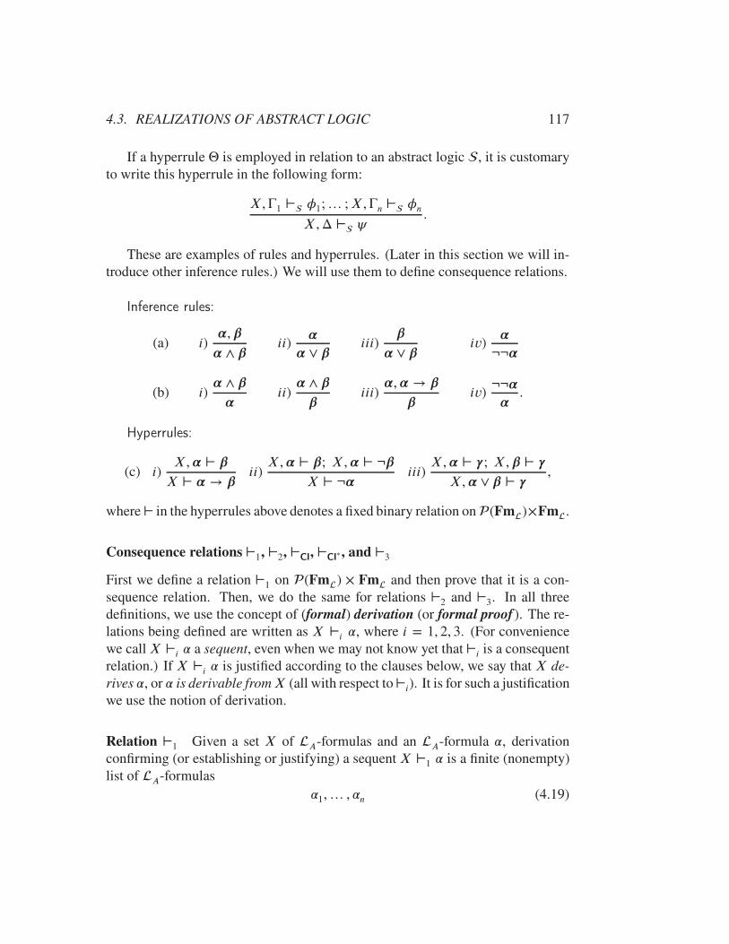
4.3. REALIZATIONS OF ABSTRACT LOGIC 117
If a hyperrule Θ is employed in relation to an abstract logic , it is customaryto write this hyperrule in the following form:
X,Γ1 ⊢ �1;… ;X,Γn ⊢ �nX,Δ ⊢
.
These are examples of rules and hyperrules. (Later in this section we will in-troduce other inference rules.) We will use them to define consequence relations.
Inference rules:
(a) i)�, �
� ∧ �ii)
�
� ∨ �iii)
�
� ∨ �iv)
�
¬¬�
(b) i)� ∧ �
�ii)
� ∧ �
�iii)
�,� → �
�iv)
¬¬�
�.
Hyperrules:
(c) i)X,� ⊢ �
X ⊢ � → �ii)X,� ⊢ �; X,� ⊢ ¬�
X ⊢ ¬�iii)
X,� ⊢ ; X, � ⊢
X,� ∨ � ⊢ ,
where⊢ in the hyperrules above denotes a fixed binary relation on(Fm)×Fm.
Consequence relations ⊢1, ⊢2, ⊢Cl, ⊢
Cl∗ , and ⊢3
First we define a relation ⊢1 on (Fm) × Fm and then prove that it is a con-sequence relation. Then, we do the same for relations ⊢2 and ⊢3. In all threedefinitions, we use the concept of (formal) derivation (or formal proof ). The re-lations being defined are written as X ⊢i �, where i = 1, 2, 3. (For conveniencewe callX ⊢i � a sequent, even when we may not know yet that ⊢i is a consequentrelation.) If X ⊢i � is justified according to the clauses below, we say that X de-rives �, or � is derivable fromX (all with respect to⊢i). It is for such a justificationwe use the notion of derivation.
Relation ⊢1 Given a set X of A-formulas and an A-formula �, derivationconfirming (or establishing or justifying) a sequent X ⊢1 � is a finite (nonempty)list of A-formulas
�1,… , �n (4.19)

118 CHAPTER 4. LOGICAL CONSEQUENCE
such that
(d1) �n = �; and(d2) each �i is either in X or obtained from one or more formulas
preceeding it on the list (4.19) by one of the rules (a)–(b).
It is easy to see that ⊢1 satisfies the properties (a)–(c) of Definition 4.1.1 andthus is a consequence relation. Moreover, this relation is obviously finitary andstructural. One peculiarity of it is that the set of the theses of this relation is empty.Another property of ⊢1 is that
X ⊢1 � ⟹ X ⊧B2�, (4.20)
where ⊧B2is a single-matrix consequence with respect to matrix B2 (Section 3.2.1).
To prove (4.20), one needs to show that each rule of (a)–(b) preserves validity inB2. We leave this task to the reader. (Exercise 4.3.18)
Clearly, the converse of (4.20) is not true, for if � is a classical tautology, then∅ ⊧B2
� but ∅ ⊬1 �.
Relation ⊢2 Our next example, relation ⊢2, is a modification of ⊢1. Namely wedefine:
X ⊢2 �df
⟺ X,LB2 ⊢1 �,
where LB2 is the logic of matrix B2 (Definition 3.2.5), that is the set of classicaltautologies. According to Proposition 4.1.2, ⊢2 is a consequence relation whoseset of theses is LB2.
In addition, we claim that
X ⊢2 � ⟹ X ⊧B2�. (4.21)
The proof of (4.21) follows from the proof of (4.20), where we have to add onemore (obvious) case — when �i in (4.19) is a classical tautology, that is �i ∈ LB2.
The converse of (4.21) is also true, that is
X ⊧B2� ⟹ X ⊢2 �. (4.22)
To prove (4.22), we first prove that the consequence relation ⊧B2is finitary.
Indeed, the premiseX ⊧B2� is equivalent to that the setX∪{¬�} is not satisfiable
in B2, that is for any valuation v in B2, v[X ∪{¬�}] ⊈ {1}. Then, by compactness

4.3. REALIZATIONS OF ABSTRACT LOGIC 119
theorem,3 X ∪ {¬�} is not finitely satisfiable in B2, that is, there is X0 ⋐ X suchthat X0 ∪ {¬�} is not satisfiable in B2. The latter is equivalent to X0 ⊧B2
.4
In the next step, having X0 ⊧B2� with X0 ⋐ X, we show that X0 ⊢2 �.
If X0 = ∅, then � is a classical tautology and the conclusion is obvious. As-sume that
X0 ∶= {�1,… , �n}.
We denote∧X0 ∶= (… (�1 ∧ �2) ∧ … ∧ �n)
and observe that ∧X0 → � is a classical tautology, that is ∧X0 → � ∈ LB2.Further, it is easy to see that X0 ⊢2 ∧X0. The two last observations imply thatX0 ⊢2 � and hence X ⊢2 �.
According to Proposition 4.3.11 and the consideration above, ⊧B2, as well as
⊢2, is a finitary structural consequence relation.
Relation ⊢Cl
We begin with the remark that ⊢2 is not a calculus, for the set LB2
of classical tautologies infinite. However, ⊢2 can be reformulated in such a waythat in a new formulation, we denote it by ⊢
Cl, the latter is a calculus. First of
all, we remove from the definition of ⊢2 all rules except �, � → �∕� (known asmodus ponens or detachment). The removed rules are actually replaced with ruleswithout premises, that is rules of type ∅∕', where ' is one of the following formsof formulas (which are called axiom schemata):
ax1 � → (� → �),ax2 (� → �) → ((� → (� → )) → (� → )),ax3 � → (� → (� ∧ �)),ax4 (� ∧ �) → �,ax5 (� ∧ �) → �,ax6 � → (� ∨ �),ax7 � → (� ∨ �),ax8 (� → ) → ((� → ) → ((� ∨ �) → )),ax9 (� → �) → ((� → ¬�) → ¬�),
ax10 ¬¬� → �.
The abstract logic Cl, corresponding to ⊢Cl is called classical propositional
logic. It is obvious that Cl is a calculus.
3Cf. (Barwise, 1977), theorem 4.2. See also (Chang and Keisler, 1990), corollary 1.2.12.4We will consider this argument in a more general setting in Section 5.2.
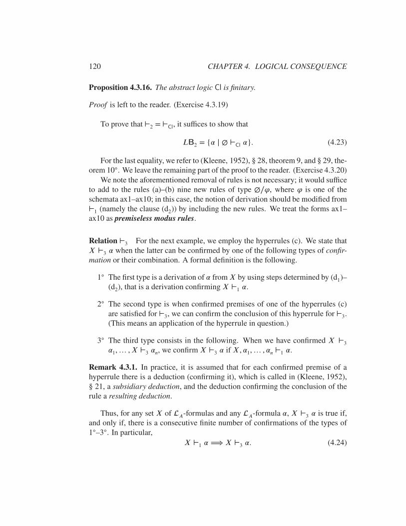
120 CHAPTER 4. LOGICAL CONSEQUENCE
Proposition 4.3.16. The abstract logic Cl is finitary.
Proof is left to the reader. (Exercise 4.3.19)
To prove that ⊢2 = ⊢Cl, it suffices to show that
LB2 = {� | ∅ ⊢Cl�}. (4.23)
For the last equality, we refer to (Kleene, 1952), § 28, theorem 9, and § 29, the-orem 10◦. We leave the remaining part of the proof to the reader. (Exercise 4.3.20)
We note the aforementioned removal of rules is not necessary; it would sufficeto add to the rules (a)–(b) nine new rules of type ∅∕', where ' is one of theschemata ax1–ax10; in this case, the notion of derivation should be modified from⊢1 (namely the clause (d2)) by including the new rules. We treat the forms ax1–ax10 as premiseless modus rules.
Relation ⊢3 For the next example, we employ the hyperrules (c). We state thatX ⊢3 � when the latter can be confirmed by one of the following types of confir-mation or their combination. A formal definition is the following.
1◦ The first type is a derivation of � fromX by using steps determined by (d1)–(d2), that is a derivation confirming X ⊢1 �.
2◦ The second type is when confirmed premises of one of the hyperrules (c)are satisfied for ⊢3, we can confirm the conclusion of this hyperrule for ⊢3.(This means an application of the hyperrule in question.)
3◦ The third type consists in the following. When we have confirmed X ⊢3
�1,… , X ⊢3 �n, we confirm X ⊢3 � if X, �1,… , �n ⊢1 �.
Remark 4.3.1. In practice, it is assumed that for each confirmed premise of ahyperrule there is a deduction (confirming it), which is called in (Kleene, 1952),§ 21, a subsidiary deduction, and the deduction confirming the conclusion of therule a resulting deduction.
Thus, for any set X of A-formulas and any A-formula �, X ⊢3 � is true if,and only if, there is a consecutive finite number of confirmations of the types of1◦–3◦. In particular,
X ⊢1 � ⟹ X ⊢3 �. (4.24)

4.3. REALIZATIONS OF ABSTRACT LOGIC 121
We illustrate the last definition on the following example. Using X = {�, �}(for concrete formulas � and �), we confirm X ⊢3 � ∧ � by the derivation
�, �, � ∧ �.
Then, we rewrite the last sequent as {�}, � ⊢3 � ∧ � and apply (c-i) to obtain{�} ⊢3 � → (� ∧ �) (confirmation of the second type). Now, we rewrite the lastsequent as ∅, � ⊢3 � → (� ∧ �) and apply this hyperrule one more time. Theresulting sequent is ∅ ⊢3 � → (� → (� ∧ �)), or simply ⊢3 � → (� → (� ∧ �)).
It should be clear that the relation ⊢3 is monotone; that is
(X ⊢3 � and X ⊆ Y ) ⟹ Y ⊢3 �. (4.25)
At the point, we do not know yet if⊢3 is a consequence relation. Our aim is to provethis. More than that, we shall show that ⊢3 and ⊢2 are equal as relations, thoughdefined differently. We discuss advantage and disadvantage of ⊢3 in relation to ⊢2
at the end of this subsection.Aiming to prove ⊢3 =⊢2, we notice that the relation ⊢3 enjoys the following
variant of cut (the property (c∗) from Definition 4.1.1).
(X, � ⊢3 � and ⊢3 �) ⟹ X ⊢3 �. (4.26)
Indeed, applying the hyperrule of (c-i), we confirm that X ⊢3 � → �. Us-ing (4.25), we obtain that X ⊢3 �. Finally, we use a confirmation of type 3◦ toconclude that X ⊢3 �.
On the next step, we prove that
X ⊢2 � ⟹ X ⊢3 �. (4.27)
Our proof of (4.27) is based on the following observation.
� ∈ LB2 ⟹ ⊢3 �. (4.28)
To prove (4.28), first, we show that for any A-formula �,
⊢3 � ∨ ¬�. (4.29)
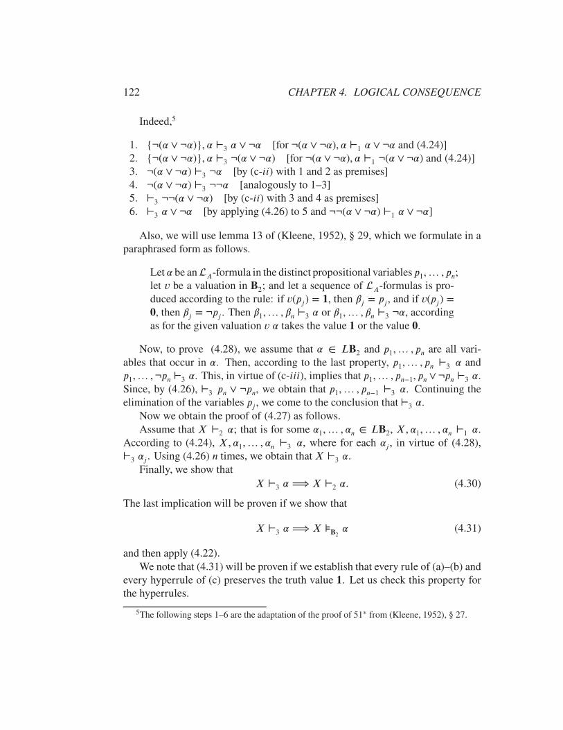
122 CHAPTER 4. LOGICAL CONSEQUENCE
Indeed,5
1. {¬(� ∨ ¬�)}, � ⊢3 � ∨ ¬� [for ¬(� ∨ ¬�), � ⊢1 � ∨ ¬� and (4.24)]2. {¬(� ∨ ¬�)}, � ⊢3 ¬(� ∨ ¬�) [for ¬(� ∨ ¬�), � ⊢1 ¬(� ∨ ¬�) and (4.24)]3. ¬(� ∨ ¬�) ⊢3 ¬� [by (c-ii) with 1 and 2 as premises]4. ¬(� ∨ ¬�) ⊢3 ¬¬� [analogously to 1–3]5. ⊢3 ¬¬(� ∨ ¬�) [by (c-ii) with 3 and 4 as premises]6. ⊢3 � ∨ ¬� [by applying (4.26) to 5 and ¬¬(� ∨ ¬�) ⊢1 � ∨ ¬�]
Also, we will use lemma 13 of (Kleene, 1952), § 29, which we formulate in aparaphrased form as follows.
Let � be anA-formula in the distinct propositional variables p1,… , pn;let v be a valuation in B2; and let a sequence of A-formulas is pro-duced according to the rule: if v(pj) = 1, then �j = pj, and if v(pj) =0, then �j = ¬pj . Then �1,… , �n ⊢3 � or �1,… , �n ⊢3 ¬�, accordingas for the given valuation v � takes the value 1 or the value 0.
Now, to prove (4.28), we assume that � ∈ LB2 and p1,… , pn are all vari-ables that occur in �. Then, according to the last property, p1,… , pn ⊢3 � andp1,… ,¬pn ⊢3 �. This, in virtue of (c-iii), implies that p1,… , pn−1, pn ∨ ¬pn ⊢3 �.Since, by (4.26), ⊢3 pn ∨ ¬pn, we obtain that p1,… , pn−1 ⊢3 �. Continuing theelimination of the variables pj , we come to the conclusion that ⊢3 �.
Now we obtain the proof of (4.27) as follows.Assume that X ⊢2 �; that is for some �1,… , �n ∈ LB2, X, �1,… , �n ⊢1 �.
According to (4.24), X, �1,… , �n ⊢3 �, where for each �j , in virtue of (4.28),⊢3 �j . Using (4.26) n times, we obtain that X ⊢3 �.
Finally, we show thatX ⊢3 � ⟹ X ⊢2 �. (4.30)
The last implication will be proven if we show that
X ⊢3 � ⟹ X ⊧B2� (4.31)
and then apply (4.22).We note that (4.31) will be proven if we establish that every rule of (a)–(b) and
every hyperrule of (c) preserves the truth value 1. Let us check this property forthe hyperrules.
5The following steps 1–6 are the adaptation of the proof of 51∗ from (Kleene, 1952), § 27.
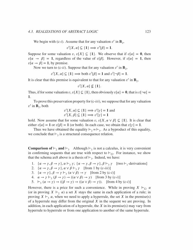
4.3. REALIZATIONS OF ABSTRACT LOGIC 123
We begin with (c-i). Assume that for any valuation v′ in B2,
v′[X, �] ⊆ {1} ⟹ v′[�] = 1.
Suppose for some valuation v, v[X] ⊆ {1}. We observe that if v[�] = 0, thenv[� → �] = 1, regardless of the value of v[�]. However, if v[�] = 1, thenv[� → �] = 1, by premise.
Now we turn to (c-ii). Suppose that for any valuation v′ in B2,
v′[X, �] ⊆ {1} ⟹ both v′[�] = 1 and v′[¬�] = 1.
It is clear that this premise is equivalent to that for any valuation v′ in B2,
v′[X, �] ⊈ {1}.
Thus, if for some valuation v, v[X] ⊆ {1}, then obviously v[�] = 0, that is v[¬�] =1.
To prove this preservation property for (c-iii), we suppose that for any valuationv′ in B2, both
v′[X, �] ⊆ {1} ⟹ v′[ ] = 1 andv′[X, �] ⊆ {1} ⟹ v′[ ] = 1
hold. Now assume that for some valuation v, v[X, � ∨ �] ⊆ {1}. It is clear thateither v[�] = 1 or v[�] = 1 (or both). In each case, we obtain that v[ ] = 1.
Thus we have obtained the equality ⊢2 =⊢3. As a byproduct of this equality,we conclude that ⊢3 is a structural consequence relation.
Comparison of ⊢2 and ⊢3 Although ⊢3 is not a calculus, it is very convenientin confirming sequents that are true with respect to ⊢
Cl. For instance, we show
that the schema ax8 above is a thesis of ⊢3. Indeed, we have:
1. {� → , � → }, � ⊢3 ; {� → , � → }, � ⊢3 [two ⊢1-derivations]2. {� → , � → }, � ∨ � ⊢3 [from 1 by (c-iii)]3. {� → }, � → ⊢3 (� ∨ �) → [from 2 by (c-i)]4. � → ⊢3 (� → ) → ((� ∨ �) → ) [from 3 by (c-i)]5. ⊢3 (� → ) → ((� → ) → ((� ∨ �) → )). [from 4 by (c-i)]
However, there is a price for such a convenience. While in proving X ⊢Cl �(or in proving X ⊢2 �) a set X stays the same in each application of a rule; inproving X ⊢3 �, when we need to apply a hyperrule, the set X in the premise(s)of a hyperrule may differ from the original X in the sequent we are proving. Inaddition, in each application of a hyperrule, theX in its premise(s) may vary fromhyperrule to hyperrule or from one application to another of the same hyperrule.
124 CHAPTER 4. LOGICAL CONSEQUENCE
The idea of semantic completeness The equalities like ⊢2 = ⊧B2or ⊢
Cl= ⊧B2
or⊢3 = ⊧B2
, but not ⊢2 =⊢Clor ⊢2 =⊢3, (see Section 4.3.5) are typical examples of
semantic completeness. That is, a completeness result is claimed when one and thesame consequence relation admits two different definitions — one purely syntacticand the other with the help of semantic concepts, such as, e.g., logical matrices.The former is regarded as a convenient way to define an abstract logic, say , thelatter as an effective way to show that for a particular set X and formula �, thesequent X ⊢ � does not hold. This issue will be further discussed in the nextchapter (Section 5.3).
To demonstrate, e.g., the validity of ⊢2 = ⊧B2, we proved the properties (4.21)
and (4.22). The former is known in literature as soundness, the latter as (properly)semantic completeness. Thus we can state that the abstract logic ⊢2 is completewith respect to the logical matrix B2, or that ⊢2 is determined by B2.
Although the main concept of this book is consequence relation, the equalitieslike
TLC
= LLC and TLC
= LLC∗
(compare with the LC completeness above) will attract our attention too. We callthem also completeness results but in a weaker sense of the term “completeness”.
Exercises 4.3
1. Prove that a structural logic is trivial if, and only if, for any arbitraryvariable p, p ∈ Cn(∅).
2. Prove that for any abstract logic , is trivial if, and only if, T is incon-sistent.
3. Let be a structural abstract logic. Prove that an -theory is closed undersubstitution if, and only if, this theory is generated by a set closed under sub-stitution. Prove that T is the least -theory closed under any substitution.
4. Prove the properties (a∗) and (b∗) of Proposition 4.3.7.
5. Prove that, given a model M and a consequence relation⊢, if T ∗
M∪T ∗∗
M⊆⊢,
then ⊧M⊆⊢. (Hint: use (4.11).)
6. Prove the equality (4.13). (Hint: use the equality
⊧M=⋂
{⊢ | ⊢ is a consequence relation with T ∗M∪ T ∗∗
M⊆⊢};
see Proposition 4.3.8.)

4.3. REALIZATIONS OF ABSTRACT LOGIC 125
7. Prove the inclusion (4.15).
8. Prove the equality (4.16).
9. Let be the logic given by the rule (b–iii). It is clear that p, p → q ⊢ qand p, p → q ⊢sub
r. Prove that p, p → q ⊬ r. This would demonstratethat the converse of the implication in Proposition 4.3.3 in general does nothold.
10. Let be the same as in the previous exercise. Show that sub is not trivial.
11. Prove Proposition 4.3.11.
12. Prove Corollary 4.3.12.1.
13. Prove Corollary 4.3.13.1
14. Prove Corollary 4.3.13.2
15. Complete the proof of Proposition 4.3.14 by proving (Pr 4.3.14–∗) and (Pr 4.3.14–∗∗).
16. Show that ⊢[] is a consequence relation.
17. Prove that for any abstract logic , the consequence relation ⊢ is deter-mined by {⊢}.
18. Prove (4.20).
19. Prove that the abstract logic Cl is finitary.
20. Using (4.23), prove the equality ⊢2 = ⊢Cl.
21. Show that the schemata ax1–ax7 and ax9–ax10 are theses of ⊢3.
22. Although for any consequence operator Cn, Cn(X ∩ Y ) ⊆ Cn(X) ∩ Cn(Y )for any sets X and Y , the converse inclusion is not necessarily true. Definesuch an abstract logic that Cn(X) ∩ Cn(Y ) ⊈ Cn(X ∩ Y ) for somesets X and Y .
126 CHAPTER 4. LOGICAL CONSEQUENCE
4.4 Abstract logics defined by modus rules
When we use or investigate calculi, we inevitably deal with modus rules. As wewill see below (Corollary 4.4.1.2), for a structural logic to be finitary and definedas calculus, are equivalent properties. On the other hand, the modus rules arenaturally modeled in first order logic.
4.4.1 General characterization
If is a set of modus rules, there is an effective way to determine the consequencerelation ⊢[] defined in (4.18) (Section 4.3.5). For this, we define a relation ⊢ on(Fm) × Fm, by generalizing (for -formulas) the notion of derivation whichearlier was defined for A-formulas via (d1)–(d2).
The relation X ⊢ � holds, by definition, if there is a list
�1,… , �n, � (4.32)
(the list �1,… , �n can be empty), where each formula on (4.32) is
(d∗1) either in X or
(d∗2) obtained from the formulas preceding it on (4.32) by one of the rules .
We note that so defined ⊢ is finitary. About (4.32), we say that it is an -derivation of � from X.
Proposition 4.4.1. Let be a set of modus rules. Then ⊢=⊢[]. Hence ⊢ isa consequence relation.
Proof. We shall prove successively the following three claims.
1◦ ⊢ is a structural consequence relation;2◦ for any R ∈ , R is sound with respect to ⊢;
3◦ if an abstract logic is such that if for any R ∈ ,R is sound with respect to , then ⊢⊆⊢ .
We notice that the properties (a)–(b) of Definition 4.1.1 are obviously true for⊢; and we leave for the reader to check the property (c) and structurality property.(Exercise 4.4.2)
Next, suppose that ⟨Γ, �⟩ ∈ . Let � be an arbitrary instantiation in . SinceΓ is finite, we denote
�(Γ) ∶= {�1,… , �n}.

4.4. ABSTRACT LOGICS DEFINED BY MODUS RULES 127
According to the clauses (d∗1)–(d∗
2), the list
�1,… , �n,�(�)
is an -derivation of �(�) from �(Γ). Hence �(Γ) ⊢ �(�).Finally, let be an abstract logic and for any R ∈ , R is sound with respect
to . We show that thenX ⊢ � ⟹ X ⊢ �.
Suppose (4.32) is a derivation with respect to . We prove that for each for-mula �i of (4.32), X ⊢ �i. We employ induction on the number of the formulaspreceding � in (4.32). Indeed, we see that, if � = �1, then X ⊢ �1, for either� ∈ X or � is a conclusion of a premiseless rule.
Now, suppose � is obtained by application of a rule R⟨Γ,�⟩. That is, for someformulas �i1 ,… , �ik preceding � and some instantiation �, �(Γ) = {�i1 ,… , �ik}and �(�) = �. Since, by induction, X ⊢ �ij , 1 ≤ j ≤ k, and, by soundness ofR⟨Γ,�⟩ with respect to , �(Γ) ⊢ �, we conclude that X ⊢ �.
Given a set of modus rules, we denote by the abstract logic correspondingto⊢[] (see the definition (4.18)) or, equivalently (due to Proposition 4.4.1), to⊢.
Corollary 4.4.1.1. If is a set of modus rules, then the abstract logic is struc-tural and finitary.
Proof is left to the reader. (Exercise 4.4.1)
Corollary 4.4.1.2. Let be a structural abstract logic. Then is finitary if, andonly if, there is a set of modus rules such that = .
Proof. The if-part follows from Corollary 4.4.1.1.To prove the ‘only-if’ part, we assume that is finitary. Next we define:
∶= {⟨Γ, �⟩ | Γ ∪ {�} ⋐ Mf and �(Γ) ⊢ �(�), for any instantiation �}.
We aim to prove that = .First, assume that X ⊢ �, for a particular set X ∪ {�} ⊆ Fm. Since is
finitary, there is a set Y ⋐ X such that Y ⊢ �. Now, replacing the variables(Y ∪ {�}) with metavariables according to arbitrary one-one correspondence,we obtain a finite set Γ ∪ {�} of metaformulas such that for any instantiation �,�(Γ) ⊢ �(�) and for a particular instantiation �0, �0(Γ) = Y and �0(�) = �. This

128 CHAPTER 4. LOGICAL CONSEQUENCE
implies that ⟨Γ, �⟩ ∈ . The latter in turn allows us to conclude that Y ⊢ � andhence X ⊢ �.
Now, we suppose that X ⊢ �. That is, there is an –derivation, determinedby (d∗
1)–(d∗
2):
�1,… , �n, �. (∗)
It is obvious that the list (∗) is not empty. We prove (by induction) that for eachformula of (∗), X ⊢ .
It is true for the first formula in (∗), in which case = �1 = �, for, then, ∈ X and hence X ⊢ .
Suppose we proved that for each �i, X ⊢ �i. If � ∈ X, we are done. If� ∉ X, then � is obtained from �i1 ,… , �ik by a rule ⟨Γ, �⟩ ∈ . By induction,this implies that {�i1 ,… , �ik} ⊢ �. By the transitivity property, we conclude thatX ⊢ �.
4.4.2 Abstract logics ⋆
Let an abstract logic be equal , for some set of modus rules. We define arelation⊢⋆ on the set (Fm)×Fm by adding to (d∗
1)–(d∗
2) one more clause: any
formula of‘(4.32) can be obtained from one of the preceding formulas by (uniform)substitution.
Proposition 4.4.2. ⊢⋆ = ⊢sub. Hence ⋆ is a finitary abstract logic.
Proof. Suppose for some set X ∪ {�} ⊆ Fm, X ⊢⋆ �. This means that there isa derivation
�1,… , �n,
where �n = � and each �i is either obtained by one of a given set of modus rules(which includes instantiations of axioms, if any) belong to X or obtained by sub-stitution from one of the preceding formulas in the derivation.
It is clear that only a finite set X0 of the formulas of X may occur in such aderivation. According to a technique developed by B. Sobociński (Sobociński, 1974)(see also (Lambros, 1979)), the above derivation can be reconstructed in such away that a new derivation will have the last formula identical with � and, in ad-dition, all substitution applications can only occur with the formulas of X0. Thisimplies that SbX0 ⊢ �, that is X0 ⊢sub
�; hence X ⊢sub�.
Conversely, assume that X ⊢sub�, that is SbX ⊢ �. Since is finitary
(Corollary 4.4.1.1), there is a set Y0 ⋐ SbX such that Y0 ⊢ �. This implies thatX ⊢⋆ �.

4.4. ABSTRACT LOGICS DEFINED BY MODUS RULES 129
The equality ⊢⋆ = ⊢subin turn implies that ⋆ is an abstract logic (because
sub is); and from the definition of ⋆ we derive that the latter is finitary.
Although a logic defined by modus rules is always structural (Corollary 4.4.1.1),⋆ is not necessarily so. We conclude this subsection with the following example.
Since the abstract logic Cl is defined by modus rules, we define an abstractlogic Cl
⋆. The latter logic is not structural. (See Exercise 4.4.3.) It is noteworthythat Cl
⋆ has only two theories. Namely the following proposition holds.
Proposition 4.4.3. For any set X ⊆ FmA,
CnCl⋆(X) =
{T
Clif X ⊆ T
Cl
FmAotherwise.
Proof is left to the reader. (Exercise 4.4.4)
4.4.3 The class of -models
The class of-models, when is given semantically, was discussed in Section 4.3.In this subsection we focus on the class of -models, when an abstract logic canbe determined by a set of modus rules. Given a structural abstract logic in alanguage , we employ for our characterization of -models a special language offirst order. This language depends on and we denote it by FO.
The denumerable set of the individual variables of FO consists of the sym-bols x�, for each metavariable �. The functional connectives coincide with theconnectives of . Also, there is one unary predicate symbol, D, two logical con-nectives, ∧∧∧ (conjunction) and →→→ (implication), universal quantifier ∀, as well theparentheses, ‘(’ and ‘)’. The rules of formula formation are usual, as well as isusual the notion of an FO-structure (including the notions of satisfactory and va-lidity). If Θ is an FO-formula containing only free variables, its universal closureis denoted by ∀…∀Θ. Main reference here is (Chang and Keisler, 1990).
It must be clear that if � is a metaformula relevant to , then, replacing eachmetavariable � in � with the individual variable x�, we obtain a term of FO. Wedenote this term (obtained from �) by �∗.
Further, any modus rule R ∶= 1,… , n
�is translated to the formula
R∗ ∶= ∀∀∀…∀∀∀((D( ∗1) ∧∧∧…∧∧∧D( ∗
n ))→→→ D(�∗)) (4.33)
130 CHAPTER 4. LOGICAL CONSEQUENCE
and any premiseless rule T ∶= ∅∕� to the formula
T ∗ ∶= ∀∀∀…∀∀∀D(�∗). (4.34)
The formulas of types (4.33) and (4.34) belong to the class of basic Horn sen-tences; cf. (Chang and Keisler, 1990), section 6.2.
It is clear that any matrix M = ⟨A, D⟩ of type can be regarded as a modelfor FO-formulas. We denote the validity of a closed formula Θ in M by M ⊩ Θ.
Let be a metaformula of Mf containing only metavariables �1,… , �n. Wenote that there is a strong correlation between the standard valuation of the term ∗ (containing only individual variables x�1 ,… , x�n) in a first order structure M
and a valuation of a formula �( ), obtained from by a simple instantiation �,in a logical matrix M. For instance, let us denote the value of ∗ on a sequencea1,… , an in M (as a first order structure) by ∗[a1,… , an]. Now let � be a simpleinstantiation with �(�i) = pi. Then, if v is a valuation in A with v[pi] = ai, then ∗[a1,… , an] = v[�( )]. This can be proven by induction on the degree of .
Grounding on the last conclusion, we obtain The first order formula D( ∗) issatisfied on the sequence �1,… , �n in the first order structure M if, and only if,v[�( )] ∈ D in the logical matrix M.
This argument leads to the following lemma.
Lemma 4.4.1. Let M = ⟨A, D⟩ be a matrix of type . For any modus rule R, Ris sound with respect to ⊧M if, and only if, M ⊩ R∗.
Proof is left to the reader. (Exercise 4.4.7)
Proposition 4.4.4. Let be a set of modus rules in . Then for any -matrix M,M is an -model if, and only if, M ⊩ R∗, for any R ∈ .
Proof. We fix an -matrix M = ⟨A, D⟩. In view of Proposition 4.4.1, we canassociate with the abstract logic the consequence relation ⊢.
We begin with the ‘only-if’ part. Thus we assume that the inclusion ⊢⊆⊧M
holds. This implies that anyR ∈ is sound with respect to ⊧M. By Lemma 4.4.1,this in turn implies that M ⊩ R∗, for any R ∈ .
To prove the ‘if’ part, we assume that the last conclusion holds. By Lemma 4.4.1,we derive that any R ∈ is sound with respect to ⊧M.
Now, suppose that X ⊢ �. That is, there is an -derivation (4.32). Byinduction on the length of (4.32), one can prove that for any valuation v in A, ifv[X] ⊆ D, then v[�] ∈ D. We leave this task to the reader. (Exercise 4.4.8)
4.4. ABSTRACT LOGICS DEFINED BY MODUS RULES 131
Corollary 4.4.4.1. Let be a set of modus rules in . Then the class of all -models is closed under reduced products, in particular under ultraproducts.
Proof. Let be the class of all -models. According to Proposition 4.4.4, an-matrix M ∈ if, and only if, for any R ∈ , R ∈ . This means that is determined by a set of Horn formulas. It is well known that every Hornsentence is preserved under reduced products, in particular under ultraproducts;cf. (Chang and Keisler, 1990), proposition 6.2.2.
4.4.4 Modus rules vs. non-finitary rules
Proposition 4.4.1 and Corollary 4.4.1.1 show limitation of modus rules in defin-ing consequent relations. It should not be surprising that there are consequencerelations that cannot be defined by any set of modus rules. Below we discuss anexample of the consequence relation of that kind; moreover, the theorems of thatabstract logic, as we will show, coincide with the theorems of a calculus, LC. (SeeLC completeness below.)
In the language A, we formulate two more premiseless structural rules:
ax11 � → (¬� → �),ax12 (� → �) ∨ (� → �).
A calculus LC is defined through derivations according to (d1)–(d2) where in(d2), however, we use only the rules ax1–ax9, ax11-ax12 and (b-iii) (modus po-nens).
We note two properties of LC. The first is that for any set X0 ∪ {�} ⋐ FmA,
X0 ⊢LC� ⟺ ∧X0 ⊢LC
�. (4.35)
(See Exercise 4.4.5.)The second property is known as the “deduction theorem” (for LC), which in
its ⇒-part, in essence, asserts that the hyperrule (c-i) is sound with respect to ⊢LC
.Namely, for any set X ∪ {�, �} ⊆ FmA
,
X, � ⊢LC� ⟺ X ⊢
LC� → �. (4.36)
(See Exercise 4.4.6.)In our consideration, we employ the single-matrix relation ⊧LC which is grounded
on the logical matrix LC; see Section 3.2.5.

132 CHAPTER 4. LOGICAL CONSEQUENCE
We will need the following property.For any A-formulas � and �,
⊢LC� ⟺ ⊧LC �. (LC completeness)
The last equivalence is due to M. Dummett (Dummett, 1959), theorem 1.
Next, we define a consequence relation,⊢LC
and, accordingly, an abstract logicLC), analogously to the relation ⊢
Cl(Section ??), but by using the rules ax1–ax9,
ax11–ax12 and modus ponens (the rule (b-iii)) for the notion of LC-derivationdefined by the clauses (d∗
1)–(d∗
2) above.
In addition, we consider the non-modus structural rule R∗ ∶= R⟨Γ∗,�0⟩ with
Γ∗ ∶= {(�i ↔ �j) → �0 | 0 < i < j < !},where �i, 0 ≤ i < !, are pairwise distinct metavariables. Also, we define aninfinite set of modus rules
∶= {Γ∕�0 | ∅ ⊂ Γ ⋐ Γ∗}.
Then, two consequence relations, ⊢∗ and ⊢⋆, are defined in (FmA) × FmA
similarly to the notion of LC-derivation but also for ⊢∗ with R∗ as an additionalinference rule and for ⊢⋆ with the rules of as additional inference rules.
We aim to show that, although for any set X0 ∪ {�} ⋐ FmA,
X0 ⊢⋆ � ⟺ X0 ⊢
∗ �, (4.37)
the consequence relation⊢∗ cannot be defined by any set of structural modus rules,for, as we will show, it is not finitary; see Corollary 4.4.1.1.
As concerns (4.37), it is obvious, for in any ⊢∗-derivation with a finite set X0
as a set of premises, the rule R∗ can be applied only under such an instantiation �,for which there is an instantiation � such that �(Γ∗)∕�(�
0) = �(Γ)∕� (�), for some
Γ ⋐ Γ∗; and vice versa.Finally, we demonstrate that the consequence relation ⊢∗ differs from ⊢
LC, for
the latter is finitary (Corollary 4.4.1.1), while the former cannot be defined by anyset of modus rules.
For contradiction, assume that ⊢∗ is finitary. Let � be an instantiation suchthat �(�i) = pi, 0 ≤ i < !. We note that �(Γ∗) ⊢∗ p0. By assumption, forsome finite X0 ⋐ �(Γ∗), X0 ⊢
∗ p0. In virtue of (4.37), X0 ⊢LCp0. This in turn,
according to (4.35) and (4.36), implies that ⊢LC
∧X0 → p0. By LC completeness,
4.5. EXTENSIONS OF ABSTRACT LOGICS 133
we obtain that ⊧LC ∧X0 → p0 and hence X0 ⊧LC p0. Thus, by monotonicity, wehave that �(Γ∗) ⊧LC p0. However, let v be such a valuation that v[p0] is a pre-lastelement a of LC with respect to ≤ and v[pi] ≠ v[pj], whenever i < j. Then, sincev[pi ↔ pj] ≤ a, we have: v[�(Γ∗)] ⊆ {1}, but v[p0] = a ≠ 1.
Exercises 4.4
1. Prove Corollary 4.4.1.1.
2. Show that if is a set of structural modus rules, then the relation ⊢[] sat-isfies the property (c) and structurality property of Definition 4.1.1.
3. The logic Cl⋆ is obtained from Cl as explained in Section 4.4.2. Show that
Cl⋆ is not structural.
4. Prove Proposition 4.4.3.
5. Prove the equivalence (4.35).
6. Prove the equivalence (4.36) (the deduction theorem for LC).
7. Prove Lemma 4.4.1.
8. Finish the proof of Proposition 4.4.4.
4.5 Extensions of abstract logics
In this section we consider interaction of abstract logics defined in different formallanguages. We begin with the following definition.
Definition 4.5.1 (extension, conservative extension). Let a language + be anextension of a language . Also, let + and be abstract logics in the languages+ and , respectively. The abstract logic + is an extension of (or over) if forany set X of -formulas,
Cn(X) ⊆ Cn+(X).
We call + a conservative extension of (or over) if for any setX of -formulas,
Cn+(X) ∩ Fm = Cn(X). (4.38)
The following two observation are almost obvious.
134 CHAPTER 4. LOGICAL CONSEQUENCE
Proposition 4.5.1. Let a language + be an extension of a language . Assumethat is a structural logic in and + is its structural extension in +. Then if is trivial, then so is +.
Proof. If is trivial, then p ∈ Cn(∅), for an arbitrary p ∈ . Since + is anextension of , p ∈ Cn+(∅). And since + is structural, the latter implies that+ is trivial.
Proposition 4.5.2. Let a language + be an extension of a language and let be an abstract logic in . The intersection of any nonempty set of conservativeextensions of in + is a conservative extensions of in +.
Proof is left to the reader. (Exercise 4.5.1)
In the sequel, we will need to keep in mind that, given a language and itsextension +, for any structural logic in , there is a conservative structuralextension +.
Indeed, assume that is a structural logic in and + is an extension of .According to Corollary 4.3.13.1, the atlas Lin[Σ] = ⟨F,Σ⟩ is adequate for .Let us select an arbitrary formula � ∈ Fm and expand the signature of F to+, denoting a new algebra by F[�]
+, as follows. We interpret in F[�]+ any
constant c ∈ + ⧵ as the element � ∈ |F|. Similarly, we interpret any termF (�1,… , �n), where F ∈ + ⧵ , as �. Then, we define an abstract logic + asthe one determined by the atlas ⟨F[�]
+,Σ⟩.According to Proposition 4.3.11, + is structural. Further, + is a conservative
extension of , because for any set X ∪ {�} ⊆ Fm,
X ⊢+ � ⟺ X ⊧Lin[Σ ]
�. (4.39)
We leave the reader to prove (4.39); see Exercise 4.5.2.In virtue of Proposition 4.5.1, + is trivial if is trivial.
We summarize as follows.
Proposition 4.5.3. Let be an structural abstract logic in and + be an exten-sion of . Then there is a conservative structural extension + of . Moreover, if is trivial, + is also trivial.
Corollary 4.5.3.1. Let a language + be an extension of a language . Any struc-tural abstract logic in has a least structural conservative extension in +.
4.5. EXTENSIONS OF ABSTRACT LOGICS 135
Proof. We use Proposition 4.5.3 and Proposition 4.5.2.
Our next definition will play a key part in the sequel.
Definition 4.5.2 (relation ⊢()+). Let a language + be an extension of a language. Also, let be an abstract logic in . We define a relation ⊢()+ in (Fm+) ×
Fm+ as follows:
X ⊢()+ �df
⟺ there is a set Y ∪ {�} ⊆ Fm and an +-substitution� such that �(Y ) ⊆ X, � = �(�) and Y ⊢ �.
We find a justification for the last definition in the following proposition.
Proposition 4.5.4. Let a language + be an extension of a language and be astructural abstract logic in . If the relation ⊢()+ is a consequence relation, then()+ is the least structural conservative extension of in +. In addition, ()+ isnontrivial if, and only if, is nontrivial.
Proof. Assume that ⊢()+ is a consequence relation. Then it is obvious that ()+
is a conservative extension of . (The structurality of should be used.)Next, we prove the structurality of ()+. For this, assume that X ⊢()+ �. By
definition, there are a set Y ∪ {�} ⊆ Fm+ and an +-substitution � such thatY ⊢ �, �(Y ) ⊆ X and �(�) = �. Let � be any +-substitution. We observe:�◦�(Y ) ⊆ �(X) and �◦�(�) = �(�). Then, by definition, �(X) ⊢()+ �(�).
Now, let + be an arbitrary structural conservative extension of in +. Sup-pose that X ⊢()+ �. Then there is a set Y ∪ {�} ⊆ Fm and an +-substitution� such that Y ⊢ �, �(Y ) ⊆ X and �(�) = �. By premise, Y ⊢+ �. Since + isstructural, we also have that �(Y ) ⊢+ �(�). This implies that X ⊢+ �.
Finally, the last claim of the proposition follows from the conservativeness of()+ over .
In the next proposition, we give a sufficient condition for ()+ to be a conse-quence relation.
Proposition 4.5.5. Let be a language with � = card() ≥ ℵ0 and + be aprimitive extension of . Assume that is a structural abstract logic in . Thenthe relation ⊢()+ is a consequence relation in +. Moreover, the abstract logic()+ is �-compact. Moreover, if is finitary, then ()+ is also finitary.
136 CHAPTER 4. LOGICAL CONSEQUENCE
Proof. First, we have to show that ⊢()+ satisfies the properties of (a)–(c) of Def-inition 4.1.1. Leaving the check of the properties (a)–(b) to the reader, we turn tothe property (c). (Exercise 4.5.3)
Assume that for a set X ∪ Y ∪Z ∪ {�} ⊆ Fm+ ,
(P1) X ⊢()+ , for all ∈ Y ;(P2) Y ,Z ⊢()+ �.
In virtue of (P2) and Definition 4.5.2 (further in this proof, simply definition),there are sets Y0 and Z0 with Y0 ∪ Z0 ∪ {�0} ⊆ Fm and an +-substitution �0such that �0(Y0) ⊆ Y , �0(Z0) ⊆ Z, �0(�0) = � and Y0, Z0 ⊢ �0.
We denote:{ i}i∈I ∶= �0(Y0).
In virtue of (P1) and definition, for each i ∈ I , there is a set Xi ∪ {�i} ⊆ Fm
and an +-substitution �i such that �i(Xi) ⊆ X, �i(�i) = i and Xi ⊢ �i.Now the assumptions (P1)–(P2) can be refined as follows.
(P1∗)⋃
i∈I �i(Xi) ⊢()+ i, for all i ∈ I ;(P2∗) { i}i∈I , �0(Z0) ⊢()+ �.
We denote:X∗ ∶=
⋃i∈I
�i(Xi) and Z∗ ∶= �0(Z0).
We aim to show that X∗, Z∗ ⊢()+ �. Since X∗ ⊆ X and Z∗ ⊆ Z, we willthus obtain that X,Z ⊢()+ �, for we have already proved that ⊢()+ is monotone.
Let us make notes about the cardinalities of the +-variables of some formulasets. (This is where we use that the extension + is primitive.)
• card(({ i}i∈I )) ≤ card();
• card((Z∗)) = card((�0(Z0))) ≤ card();
• card((X∗)) = card((⋃
i∈I �i(Xi))) ≤ card().
Thus we have: card(({ i}i∈I ∪X∗ ∪Z∗ ∪ {�})) ≤ card(). This allows us
to claim that there is a one-one map
f ∶ ({ i}i∈I ∪X∗ ∪Z∗ ∪ {�})
1–1⟶ .
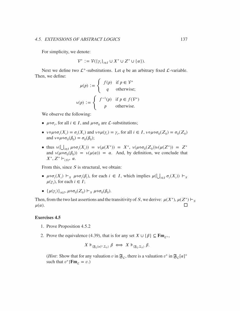
4.5. EXTENSIONS OF ABSTRACT LOGICS 137
For simplicity, we denote:
∗ ∶= ({ i}i∈I ∪X∗ ∪Z∗ ∪ {�}).
Next we define two +-substitutions. Let q be an arbitrary fixed -variable.Then, we define:
�(p) ∶=
{f (p) if p ∈ ∗
q otherwise;
�(p) ∶=
{f−1(p) if p ∈ f (∗)
p otherwise.
We observe the following:
• �◦�i, for all i ∈ I , and �◦�0 are -substitutions;
• �◦�◦�i(Xi) = �i(Xi) and �◦�( i) = i, for all i ∈ I , �◦�◦�0(Z0) = �0(Z0)
and �◦�◦�0(�0) = �0(�0);
• thus �(⋃
i∈I �◦�i(Xi)) = �(�(X∗)) = X∗, �(�◦�0(Z0))�(�(Z∗)) = Z∗
and �(�◦�0(�0)) = �(�(�)) = �. And, by definition, we conclude thatX∗, Z∗ ⊢()+ �.
From this, since is structural, we obtain:
• �◦�i(Xi) ⊢ �◦�i(�i), for each i ∈ I , which implies �(⋃
i∈I �i(Xi)) ⊢
�( i), for each i ∈ I ;
• {�( i)}i∈I , �◦�0(Z0) ⊢ �◦�0(�0).
Then, from the two last assertions and the transitivity of , we derive: �(X∗), �(Z∗) ⊢
�(�).
Exercises 4.5
1. Prove Proposition 4.5.2
2. Prove the equivalence (4.39), that is for any set X ∪ {�} ⊆ Fm+ ,
X ⊧⟨F[�]+,Σ ⟩ � ⟺ X ⊧⟨F,Σ ⟩ �.
(Hint: Show that for any valuation v in F, there is a valuation v∗ in F[�]+
such that v∗↾Fm = v.)

138 CHAPTER 4. LOGICAL CONSEQUENCE
3. Let + be a primitive extensions of a language and let be an abstractlogic in . Show that the relation⊢()+ of Definition 4.5.2 satisfies the prop-erties (a)–(b) of Definition 4.1.1.
4. Prove that ()+ in Proposition 4.5.5 is �-compact.
4.6 Historical notes
As was mentioned in Section 1.1 and in the beginning of this chapter, the dis-tinction in the argumentation of reasoning with predetermined premises from ar-guments with arbitrary premises goes back to Aristotle, who called the formera demonstrative argument, and the latter a dialectical one. It is very likely thatthe notion of demonstration has gradually developed in connection with geometryfrom “empirical study” to “a demonstrative a priory science;” (Kneale and Kneale, 1962),chapter I, section 2. Dialectical arguments, on the other hand, were characteristicof metaphysics. In the early twentieth century, this distinction was emphasized byC. I. Lewis:
“The consequences of this difference between the “implies” of the al-gebra and the “implies” of valid inference are most serious.” (Lewis, 1913a),p. 242. 6
The formalization of logical consequence (a dialectical argument in the senseof Aristotle) in the framework of modern logic was undertaken by A. Tarski in the1930s, by introducing the notion of consequence operator, not that of consequencerelation; see (Tarski, 1930b; Tarski, 1930a)7. It seems that an earlier attempt by P.Hertz (Hertz, 1922) was made from an essentially different perspective, since heinterpreted ‘(a1,… , an) → b’ (where a1, ,… , an, b are sentences) as
“If (a1,… , an) altogether holds, so does b,”(quoted from (Beziau (editor), 2012), p. 11)
while Tarski would interpret ‘� ∈ Cn(�1,… , �n)’ that � is obtained from �1,… , �nwith respect to Cn, regardless whether any �i (or they altogether) holds or not. Thefollowing passage shows that Hertz regarded ‘→’ as a relation of demonstration,and not as a dialectical argument when he wrote:
6It should be noted that Lewis did not distinguish between the “algebra of implication” and“calculus of propositions.” See, for example, the first line of (Lewis, 1913a) or of (Lewis, 1914).
7The English translations of these important papers were later on published in (Tarski, 1956;Tarski, 1983)

4.6. HISTORICAL NOTES 139
“Whenever a system of sentences is recognized to be valid, it is of-ten not necessary to convey each or every sentence to memory; itis sufficient to choose some of them from which the rest can follow.Such sentences, as it is generally known, are called axioms.” Quotedfrom (Beziau (editor), 2012), p. 11.
Also, it seems that D. Scott was the first to start using consequence as a relation;cf. (Scott, 1974a). He also stated explicitly therein that the two notions can be usedinterchangeably; cf. (Shoesmith and Smiley, 2008), Historical note, pp. 19–20.8
It is worthwhile to dwell on the works of Tarski in the 1930s in a little moredetail. As can be assumed from the title of (Tarski, 1930a), Tarski had in mind afar-reaching program. So he writes in (Tarski, 1930a), § 1,
“The two concepts — of sentence and of consequence — are the onlyprimitive concepts which appear in this discussion.”(italics highlighted by Tarski)
The first concept in Tarski’s passage is a nonempty set of cardinality less thanor equal to ℵ0, and the second is a map, defined on the power set of all sentencesand satisfying (a†)–(c†) of Definition 4.2.1. Interestingly, Tarski admits, at leastimplicitly, that the set of sentences may be finite, a condition that was changedto ‘greater than or equal to ℵ0’ in later expositions; cf., e.g., (Czelakowski, 2001;Font et al., 2009; Font, 2016).
It may seem surprising that there is no structure in Tarski’s “meaningful sen-tences” (from the first concept). Perhaps he wanted to propose a concept of logicalconsequence independent of the grammatical structure of the objective language.Indeed, criticizing Carnap’s definitions of logical consequence, he wrote,
“These definitions, in so far as they set up on the basis of ‘general syn-tax’, seem to me to be materially inadequate, just because the definedconcepts depend essentially, in their extension, on the richness of thelanguage investigated.” (Tarski, 1936b)
However, the deprivation of sentences from a grammatical structure immediatelyblocks the Lindenbaum method, not allowing to define the formula algebra.
In (Tarski, 1930b) and (Tarski, 1930a), the property (d†) (finitariness) is a manda-tory axiom, while the structurality property is not mentioned at all, even as an
8D. J. Shoesmith and T. J. Smiley also used consequence relation but did not relate it to Tarski’sconsequence operator; cf. (Shoesmith and Smiley, 1971).
140 CHAPTER 4. LOGICAL CONSEQUENCE
option. Structurality is defined through the notion of substitution. However, sub-stitution plays a dual role in logic.
Although Aristotle was familiar with the idea of a variable, but he “never ar-gued by means of substitutions, as we have been doing, except in proofs of inva-lidity,” that is, only using instantiation; “for example, no thought of substitutingvariables for variables” (Bocheński, 1970), § 13, sections B and C, respectively.Alexander of Aphrodisias, who lived at the turn of the fourth century AD, al-ready knew the operation of identification of sentential variables and Boethius (c.477–524 AD) knew substitution of sentential formulas for variables. He wouldprobably be the first philosopher to agree, if he had a chance, that any map � ∶
Fm ⟶ Fm satisfying the conditions of Definition 3.1.3 conveys the idea thatlogic deals with forms rather than with their instances.9 Boethius also showedhis “aspiration to the rule of substitution” but never used it as a rule of inference;cf. (Bocheński, 1970), § 24, section E.
G. Frege was perhaps the first to start using substitution as a rule of inference,though implicitly. This is what van Heijenoort wrote in his introductory note toFrege’s Begriffsschrift (1879),
“His axioms for the propositional calculus (they are not independent)are formulas [. . . ]. His rules of inference are the rule of detachmentand an unstated rule of substitution.” Quoted from (van Heijenoort, 2002),p. 2.
Although A. Church credits L. Couturat for being the first to explicitly formu-late the substitution rule “specifically for the propositional calculus,” this is hardlyjustified. Indeed in (Couturat, 1980), the first edition of which was published in1905, Couturat wrote,
“That is not all: to that principle one must add the substitution prin-ciple which is described thusly: “In a general formula, to a general orindeterminate term one may substitute a particular or individual term.”That is evident since a general formula has no value nor even meaningexcept in the way it can be applied to particular terms” (Couturat, 1980),chapter 1. 10
9I. M. Bocheński calls this “the clear distinction between propositional functions and proposi-tions themselves;” cf. (Bocheński, 1970), § 24, section I.
10We are indebted to Dr. L. Wolffe for translating this passage from the French.

4.6. HISTORICAL NOTES 141
Fair enough, right after his remark, Church adds,“but his [Couturat’s] statementis perhaps insufficient as failing to make clear that the expression substituted for a(propositional) variable may itself contain variables.”11
B. Russell did use the substitution rule in (Russell, 1906) in formal deriva-tions of sentential formulas, but there is still confusion for the author in using theterm “substitution” in the sense of Definition 3.1.3 and as universal instantiation inhigher-order logic. After Russell, Lewis illustrates in (Lewis, 1913b; Lewis, 1914)the use of the substitution rule in the sense of Section 4.3.5, but without such gener-ality; and after (Lewis, 1960) (the first publication appeared in 1918) substitutionas an operation and as a rule of inference became standard.
Yet, the structurality principle understood as implication
X ⊢ � ⟹ �(X) ⊢ �(�),
for any substitution �, does not come down to the rule of substitution since itis a characteristic of an entire deductive system with this property. The struc-turality as a important property of a consequence operator was introduced by J.Łoś and R. Suszko in (Łoś and Suszko, 1958), although was anticipated by Lewisin (Lewis, 1913b), when he wrote,
“Proof takes place through the collusion of two factors; first, postu-lates or propositions of the particular mathematical system in hand;secondly, postulates of the logical or mathematical type and the de-sired conclusion. A mathematical operation is ideally no more thanthis: the substitution of the variables or functions of variables of theparticular system — say, of cardinal number — for the logical vari-ables in some proposition about implication. This proposition is morethan a rule for inference; when the substitution is made, it states theimplication.”
We conclude the theme of substitution with the following passage by B. Russellin (Russell, 1993) (the second edition appeared in 1920), where he wrote,
“The primitive propositions, whatever they may be, are to be re-garded as asserted for all possible values of the variable propositionsp, q, r which occur in them. We may therefore substitute for (say) pany expression whose value is always a proposition, e.g. not-p, “s im-plies t,” and so on. By means of such substitutions we really obtain
11Cf. (Church, 1996), § 29.

142 CHAPTER 4. LOGICAL CONSEQUENCE
sets of special cases of our original proposition, but from a practicalpoint of view we obtain what are virtually new propositions. The le-gitimacy of substitutions of this kind has to be insured by means ofa non-formal principle of inference. [Footnote: No such principle isenunciated in Principia Mathematica [. . . ] But this would seem to bean omission.]” (ibid, chapter XIV)
From this passage, we learn that although the authors of Principia Mathemat-ica were unable to appreciate the importance of the concept of substitution, by1920 Russell already realized (or was close to this) that propositions themselvescan be used as (truth) values for propositions, which leads directly to Lindenbaummethod.
The properties (e†) and (j†) of Cn in Section 4.2 were considered earlier by D.Makinson in (Makinson, 2005), section 1.2.
Given a consequence operator Cn, the notion of a theory (under the name “de-ductive system”) with respect to Cn is due to (Tarski, 1930b), as well as Proposi-tion 4.2.1, ibid, theorem 20.12
A. Tarski introduced a matrix method for studying “deductive systems,” thatis, theories of abstract logics.13 In print form, the concept of a logical matrix wasdefined in (Łukasiewicz and Tarski, 1930), definition 3.
The theorem, which was originally known as the Lindenbaum theorem first ap-peared in print without proof in (Łukasiewicz and Tarski, 1930), theorem 3. Thistheorem reads that, given a consequence operator Cn, for any “deductive system”X0, there exists “a normal matrix,” say M, such that
� ∈ Cn(X0) ⟺ X0 ⊧M �. (4.40)
Since X0 in (4.40) was tacitly assumed to be fixed, defining an abstract logic bythe equivalence
X ⊢ �df
⟺ � ∈ Cn(X0 ∪X),
for any set X and formula �, we can reduce (4.40) to the second part of Proposi-tion 4.3.12.
12A revised text of this article appeared in English translation in (Tarski, 1983), pp. 30–37, underthe title ‘On some fundamental concepts of metamathematics’.
13We read in (Łukasiewicz and Tarski, 1930), footnote 2, “The view of matrix formation as ageneral method of constructing systems is due to Tarski.”

4.6. HISTORICAL NOTES 143
The condition that X0 is an -theory, that is X0 = Cn(∅), is not important,but it is important to add thatX0 is closed under substitution, which must have beentacitly assumed. This observation implies two conclusions. First, participants inthe seminar for mathematical logic at the University of Warsaw, where, accordingto (Łukasiewicz and Tarski, 1930), footnote ‡, the result was reported, perhapsfocused on the set of theorems of a deductive system, and not on the consequencerelation associated with this system; and secondly, the set of theorems was assumedto be closed under substitution.
Further, in (Łukasiewicz and Tarski, 1930), there was no indication of whatkind of matrix M is, in particular, whether M = Lin . Moreover, althoughthe nature of M was very likely known (to Lindenbaum at least), the statementof theorem 3 did not contribute to the take-off of the Lindenbaum method. Thebirth of the concept of a matrix consequence was also delayed until the publica-tion of (Łoś and Suszko, 1958); see definition (8.1) therein. The proof of Linden-baum’s theorem was published in (Łoś, 1949), proposition 10, and, independently,in (Hermes, 1951). (To prove (4.40), Łoś used Lin as M.) Further, since the au-thors of (Łukasiewicz and Tarski, 1930) did not require explicitly the closednessunder substitution for an -theory X (as Łoś did 14), they missed to notice thatany Lindenbaum matrix Lin[X] is an -model, which was noted in (Łoś, 1949),proposition 7.15
The last omission and the omission of structurality in the 1930s however de-layed the result, due to (Wójcicki, 1969), theorem 4, that any structural abstractlogic is determined by its Lindenbaum matrices (Corollary 4.3.13.1). After this,the role of substitution was clearly understood, since any valuation in the formulaalgebra is a substitution.
The Wójcicki’s observation opened up a way to define consequence relationsusing bundles or atlases of logical matrices. Instead of the term ‘atlas’ Wójcickiused the term ‘generalized matrix’. But even before him, T. Smiley (Smiley, 1962)used a similar concept, known as a ‘Smiley matrix’. The term ‘atlas’ was coined byM. J. Dunn and G. M. Hardegree in (Dunn and Hardegree, 2001). The concept andterm of the Lindenbaum bundle were used by G. Malinowski in (Malinowski, 2007).
Almost certainly, introducing the concept of a logical consequence, A. Tarskihad in mind the usual practice of obtaining new hypothetical truths in mathematics
14Cf. (Łoś, 1949), definition 3.15Actually,Lin [X] is an-model, even ifX is not closed under substitution, but is structural;
see Corollary 4.3.12.1.

144 CHAPTER 4. LOGICAL CONSEQUENCE
and other deductive sciences. So in his very first article (Tarski, 1930b) on logicalconsequence, he wrote,
“From the sentences of any set X cernain other sentences can be ob-tained by means of certain operations called rules of inference. Thesesentences are called the consequences of the set X. The set of all con-sequences is denoted by the symbol ‘Cn(X).” Quoted from (Tarski, 1983),p. 30.
In antiquity, according to Plato, in the framework of his Theory of Forms,“inference was [is] presumably valid when we follow in thought the connexionsbetween Forms as they are.”16 And in later antiquity, Galen and Boethius presentedAristotle’s view on inference “as a theory of inference schemata, i.e. as a theory inwhich rules of inference are thought by means of skeleton arguments.”17 And later,in the development of logic, “the Stoics generally concentrated attention on validinference schemata (συνακτικὰ σχήματα).”18 The modern name for “inferenceschemata” is structural (inference) rules. The last concept and term was introducedin (Łoś and Suszko, 1958), section 3.
However, any system of inference rules, structural (such as modus ponens) ornon-structural (such as substitution), does not suffice to define a consequence re-lation. Perhaps G. Leibniz was the first logician who understood the importanceof the notion of formal derivation, or formal proof, or formal deduction.19 Also,Bolzano is recognized as “a noteworthy precursor of modern proof-theory.”20 G.Boole used derivations in abstract manner to obtain consequences without refer-ring to interpretation. G. Frege was close to formalizing the concept of deductionwhen he wrote:
“Inference is conducted in my symbolic system (Begriffsschrift) ac-cording to a kind of calculation. I do not mean this in the narrowsense, as though an algorithm was in control, the same as or similar tothat of ordinary addition and multiplication, but in the sense that thewhole is algorithmic, with a complex of rules which so regulate the
16Cf. (Kneale and Kneale, 1962), chapter I, section 5.17Cf. (Kneale and Kneale, 1962), chapter II, section 6.18Cf. (Kneale and Kneale, 1962), chapter III, section 5.19See (Kneale and Kneale, 1962), chapter V, section 2, where we read: “The most fruitful idea
that Leibniz derived from his study of Aristotelian logic was the notion of formal proof.”20Cf. (Bocheński, 1970), § 38, section B1.
4.6. HISTORICAL NOTES 145
passage from one proposition or from two such to another, that noth-ing takes place but what is in accordance with these rules.” Quotedfrom (Bocheński, 1970), § 38, section B2.
But only D. Hilbert and P. Bernays (1934) gave an exact definition of formalderivation, or formal proof, as a sequence of formulas satisfying certain conditionsbased on the rules of detachment (modus ponens) and substitution. 21 Moreover,they formulated the first rule in terms of metavariables, that is, as a structural infer-ence rule. The importance of such a definition is that it makes it possible to studyformal derivations as words in a formal alphabet, using mathematical induction onthe length of the derivation in question.
The inference rules (a)–(b) were introduced by G. Gentzen; cf. (Gentzen, 1969b).The hyperrules (c) were used by S. C. Kleene in (Kleene, 1952), § 23, althoughas derived rules, not as postulated ones. 22 The inference rules (a)–(b) and thehyperrules (c) are similar to the proper rules and, respectively, to deduction rulesof (Prawitz, 1965), chapter 1, § 1.
Proposition 4.3.6 first appeared in (Brown and Suszko, 1973) as theorem 1 ofsection XII.
21Cf. (Hilbert and Bernays, 1968), chapter III, § 2.22Consult (Scott, 1974b) about the difference between (postulated) rules and derived rules; the
idea of a ‘derived rule of inference’ is also explained on the example of uniform substitutionin (Church, 1996), § 19. It seems that the idea of derived inference rules was familiar to the Stoics;cf. (Łukasiewicz, 1934).
146 CHAPTER 4. LOGICAL CONSEQUENCE
Chapter 5
Matrix Consequence
5.1 Single-matrix consequence
Two circumstances draw our attention to a single-matrix consequence. The firstone is Lindenbaum’s theorem (Proposition 4.3.12) which provides a universal wayof definition of a weakly adequate logical matrix, namely the Lindenbaum matrix,which being defined for a given consequence relation, validates all of the thesesof this consequence relation and only them. The other circumstance is related tothe consequence relation ⊢2 (Section 4.3.5) which turned out to be equal to thesingle-matrix relation ⊧B2
. These circumstances lead to the the following concept.We recall (Section 4.3.4) that a logical matrix M is called adequate for an
abstract logic if⊢ = ⊧M; that is, for any setX of -formulas and any -formula�,
X ⊢ � ⟺ X ⊧M �.
In connection with the notion of an adequate matrix, two questions arise. Is ittrue that any abstract logic has an adequate matrix? And if the answer to the firstquestion is negative, what are the properties of an abstract logic that make it havean adequate matrix?
The first question can be answered in the negative as follows. Suppose is anontrivial abstract logic inwith card() ≥ ℵ0, which has a nonempty consistentset, say X0, and such that T ≠ ∅. Now, let ⊢◦
be a relation obtained from ⊢
according to (4.3). In virtue of Proposition 4.1.3, ⊢◦
is a consequence relation.We claim that there is no adequate matrix for ⊢◦
. (Such a relation ⊢◦
can be
exemplified, e.g., by ⊧◦B2
withX0 = LB2, where ⊧B2is a single-matrix consequence
of Section 4.3.4.)
147
148 CHAPTER 5. MATRIX CONSEQUENCE
Indeed, for contradiction, assume that a matrix M = ⟨A, D⟩ is adequate for⊢◦
. Since X0 is consistent with respect to , it is also consistent with respect to
⊢◦
. This and the assumption thatX0 is nonempty imply thatD ≠ ∅. Assume thata ∈ D. By premise, there is a thesis � ∈ T . Let us take a variable p ∈ ⧵(�).By definition, ∅ ⊬◦
� and p ⊢◦
�. The former implies that there is a valuation v
in A such that v[�] ∉ D. Now we define a valuation:
v′[q] ∶=
{v[q] if q ≠ p
a if q = p.
It is clear that v′[�] = v[�] and hence p ⊧M �.
Trying to find a characteristic for abstract logic to have an adequate matrix, weconsider any logical matrix M ∶= ⟨A, D⟩ of type .
Now, let �, � and be -formulas with ((�)∪(�))∩( ) = ∅. Assume thatfor some valuation v0, v0( ) ∈ D. (This assumption is equivalent to the conditionthat the set { } is consistent with respect to the consequence relation ⊧M.) Weprove that
, � ⊧M � implies � ⊧M �.
Indeed, for contrapositive, suppose that � ⊧M �; that is, for some valuation v,v(�) ∈ D, but v(�) ∉ D.
Let us define a valuation
v1(p) =
{v0[p] if p ∈ ( )
v[p] otherwise.
We note that v1[ ] = v0[ ], v1[�] = v[�] and v1[�] = v[�]. This implies that , � ⊧M �.
The above consideration leads to the following definition.
Definition 5.1.1 (uniform abstract logic). An abstract logic is said to be uniform
if for any set X ∪ Y ∪ {�} of -formulas with (X ∪ {�}) ∩ (Y ) = ∅ andCn(Y ) ≠ Fm, if X, Y ⊢ �, then X ⊢ �.
We note that the consequence relation ⊧◦B2
mentioned above is finitary but notuniform. (Exercise 5.1.1) The importance of the last definition becomes clear fromProposition 5.1.1 below. We prove this proposition by means of two lemmas.
5.1. SINGLE-MATRIX CONSEQUENCE 149
Lemma 5.1.1. If an abstract logic has an adequate matrix, then is uniform.
Proof. Let a matrix M = ⟨A, D⟩ be adequate for . Suppose X, Y ⊢ �, where(X, �) ∩ (Y ) = ∅ and Cn(Y ) ≠ Fm. We will show that X ⊧M �, which, invirtue of the adequacy of M for , will in turn imply that X ⊢ �.
For contradiction, assume that for some valuation v in A, v[X] ⊆ D but v[�] ∉D. Since Y is consistent with respect to , there is a valuation v′ such that v′[Y ] ⊆D. Then, we define a valuation v′′ as follows:
v′′[p] ∶=
{v[p] if p ∈ (X, �)
v′[p] if p ∈ (Y ).
It must be clear that v′′[�] = v[�], whenever � ∈ X ∪ {�}, and v′′[�] = v′[�],if � ∈ Y . Therefore, X, Y ⊧M �; that is X, Y ⊬ �. A contradiction.
As preparation to the next proposition we observe the following.
Lemma 5.1.2. Let be a uniform structural abstract logic in a language withcard() ≥ ℵ0 and + be a primitive extension of . Then the abstract logic ()+
is also uniform.
Proof. Suppose for a set X ∪ Y ∪ {�} ⊆ Fm+ , X, Y ⊢()+ �, providing that(X ∪ {�}) ∩ (Y ) = ∅ and Y is consistent with respect to ()+. Then, bydefinition, there is X0 ∪ Y0 ∪ {�} ⊆ Fm and an +-substitution � such that�(X0) ⊆ X, �(Y0) ⊆ Y , �(�) = � and X0, Y0 ⊢ �. It is clear that (X0 ∪ {�}) ∩(Y0) = ∅. Also, Y0 is consistent with respect to , for if it were otherwise, invirtue of conservativity of ()+ over , we would have �(Y0) ⊢()+ , for anyarbitrary +-formula . This would imply the inconsistency of Y in ()+.
Since is uniform, X0 ⊢ � and hence X0 ⊢()+ �, for ()+ is a conservativeextension of . And since ()+ is structural (Proposition 4.5.4), �(X0) ⊢()+ �and hence X ⊢()+ �.
Proposition 5.1.1 (Łoś-Suszko-Wójcicki theorem). Let be a finitary structuralabstract logic in a language with card() ≥ ℵ0. Then has an adequatematrix if, and only if, is uniform.
Proof. The ‘only-if’ part follows from Lemma 5.1.1. So we continue with theproof of the ‘if’ part.
We distinguish two cases: is trivial and is nontrivial. If the former is thecase, then the matrix ⟨F,Fm⟩ is adequate for .
150 CHAPTER 5. MATRIX CONSEQUENCE
Now, we assume that is nontrivial; that is, the set Σc
of consistent sets withrespect to is nonempty.
We introduce for each X ∈ Σc
and each p ∈ , a new sentential variable pXso that for any p, q ∈ and any X, Y ∈ Σc
,
pX = qY ⟺ p = q and X = Y .
Accordingly, for an arbitrary X ∈ Σc
, we denote:
X = {pX | p ∈ }.
Thus for any X, Y ∈ Σc
,
X ≠ Y ⟹ X ∩ Y = ∅. (5.1)
A language + is defined as a primitive extension of , by adding the newsentential variables to . Then, we introduce ()+ according to Definition 4.5.2.
Next, for each X ∈ Σc
, we define two +-substitutions:
�X ∶ p↦ pX , for any p ∈ , and �X ∶ pY ↦ pY , for any pY ∈ + ⧵ ;
�X ∶ pX ↦ p, for any pX ∈ X and �X ∶ q ↦ q, for any q ∈ + ⧵ X .
We observe: for any X ∈ Σc
,
�X◦�X(�) = �, for all � ∈ Fm. (5.2)
Then, we make two observations. First, since for any X ∈ Σc
, (�X(X)) ⊆X , (8.3) yields that for any X, Y ∈ Σc
,
X ≠ Y ⟹ (�X(X)) ∩ (�Y (Y )) = ∅. (5.3)
Second,
for each X ∈ Σc
, the set �X(X) is consistent with respect to ()+. (5.4)
Indeed, for contradiction, assume that �X(X) is inconsistent. Let � be anyformula of Fm. By assumption, �X(X) ⊢()+ �X(�). Since ()+ is structural(Proposition 4.5.4), we have that �X(�X(X)) ⊢()+ �X(�X(�)) and hence, in virtueof (5.2), X ⊢()+ �. Since ()+ is conservative over , we obtain that X ⊢ �. Acontradiction.
5.1. SINGLE-MATRIX CONSEQUENCE 151
Now, we define:
M ∶= ⟨F+ ,Cn()+(⋃
{�X(X) | X ∈ Σc})⟩.
We aim to show that M is adequate for ; that is, for any set Y ∪ {�} ⊆ Fm,
Y ⊢ � ⟺ Y ⊧M �.
Suppose Y ⊢ �. Since ()+ is conservative over , this implies that Y ⊢()+
�. Now, let � be any+-substitution. Assume that �(Y ) ⊆ Cn()+(⋃{�X(X) |X ∈
Σc}). Since ()+ is structural, we have: �(�) ∈ Cn()+(�(Y )) and hence �(�) ∈
Cn()+(⋃{�X(X) | X ∈ Σc
}).
Conversely, suppose that Y ⊬ �. We denote:
X0 ∶= Cn(Y ).
Thus � ∉ X0 and henceX0 ∈ Σc
. The latter implies that �X0(X0) ⊆ Cn()+(
⋃{�X(X) |X ∈
Σc}).For contradiction, we assume that
�X0(�) ∈ Cn()+(
⋃{�X(X) | X ∈ Σc
}). (∗)
In virtue of finitariness of ()+ (Proposition 4.5.5), there is a finite number of setsX1,… , Xn ∈ Σc
such that
�X0(�) ∈ Cn()+(�X0
(X0) ∪ �X1(X1) ∪ … ∪ �Xn(Xn)).
Since, according to (5.4), �Xn(Xn) is consistent and
(�X0(X0) ∪ �X1
(X1) ∪ … ∪ �Xn−1(Xn−1)) ∩ (�Xn(Xn)) = ∅,
in virtue of the uniformity of ()+ (Lemma 5.1.2),
�X0(X0), �X1
(X1),… �Xn−1(Xn−1) ⊢()+ �X0(�)
Repeating this argument several times, we arrive at the conclusion that�X0(X0) ⊢()+
�X0(�). Then, applying the substitution �X0
, we get X0 ⊢()+ �. Finally, the con-servativity of ()+ over yields X0 ⊢ �. A contradiction.
The case of nonfinitary abstract logics needs an additional investigation.

152 CHAPTER 5. MATRIX CONSEQUENCE
Definition 5.1.2 (couniform abstract logic). An abstract logic in a language iscalled couniform if for any collection {Xi}i∈I of formula sets with(Xi)∩(Xj) =
∅, providing that i ≠ j, and (⋃
i∈I{Xi}) ≠ , there is at least one Xi which isinconsistent, whenever the union
⋃i∈I{Xi} is inconsistent.
The next lemma shows that couniformity is necessary for an abstract logic tohave an adequate matrix.
Lemma 5.1.3. If an abstract logic has an adequate matrix, then is couniform.
Proof. Let a matrix M = ⟨A, D⟩ be adequate for . We assume that a family{Xi}i∈I of formula sets satisfies all the premises of couniformity. Suppose eachXi is consistent with respect to . Then for each i ∈ I , there is a formula �i suchthat Xi ⊬ �i. This implies that there is a valuation vi in A such that vi[Xi] ⊆ Dbut vi[�i] ∉ D. Let us select either one of vi[�i] and denote
a ∶= vi[�i].
Then, we select any variable p ∈ ⧵ (⋃
i∈I{Xi}) and for each vi, define:
v∗i [q] ∶=
{vi[q] if q ∈ (
⋃i∈I{Xi})
a if q ∈ ⧵ (⋃
i∈I{Xi}).
It must be clear that for each i ∈ I , v∗i [Xi] ⊆ D. And since (Xi)∩(Xj) = ∅,providing i ≠ j, we also have that v∗i [
⋃i∈I{Xi}] ⊆ D. Thus
⋃i∈I{Xi} ⊬ p, that
is the set⋃
i∈I{Xi} is consistent.
The next lemma is rather technical and we will need it for the proof of Propo-sition 5.1.2 below.
Lemma 5.1.4. Let be a couniform structural abstract logic in a language withcard() ≥ ℵ0 and + be a primitive extension of . Then the abstract logic ()+
is also couniform.
Proof. Let {Xi}i∈I be a nonempty family of nonempty sets of +-formulas, aboutwhich we assume that the union
⋃i∈I{Xi} is inconsistent and (
⋃i∈I{Xi}) ≠
+ . Let us select any p ∈ + ⧵ (⋃
i∈I{Xi}). Since⋃
i∈I{Xi} is inconsistent,we have that
⋃i∈I{Xi} ⊢()+ p. By definition of ()+ (Definition 4.5.2), there are
a set Y of -formulas, an -variable q and an -substitution � such that �(Y ) ⊆⋃i∈I{Xi}, �(q) = p and Y ⊢ q.

5.1. SINGLE-MATRIX CONSEQUENCE 153
Next we define: for each i ∈ I ,
Yi ∶= { ∈ Y | �( ) ∈ Xi}.
Firstly, we notice that for each i ∈ I , �(Yi) ⊆ Xi, and⋃
i∈I{Yi} ⊢ q. (Thelatter is true because
⋃i∈I{Yi} = Y .) Secondly, q ∈ ⧵(
⋃i∈I{Yi}). Indeed, if
it were the case that q ∈ (⋃
i∈I{Yi}), then we would have that p ∈ (⋃
i∈I{Xi}).Thus we obtain that
⋃i∈I{Yi} is inconsistent with respect to . Since, by
definition, is couniform, there is i0 ∈ I such that Yi0 is inconsistent with respectto . This implies that Since ()+ is a conservative extension of , we receivethat Yi0 ⊢()+ q. And since ()+ is structural (Proposition 4.5.4), �(Yi0) ⊢()+ pand hence Xi0
⊢()+ p. We recall that p ∉ (Xi0). Therefore, the structurality of
()+ implies that Xi0is inconsistent.
Proposition 5.1.2 (Wójcicki theorem). Let be a structural abstract logic in alanguage with card() ≥ ℵ0. Then has an adequate matrix if, and only if, is both uniform and couniform.
Proof. The ‘only-if’ part follows from Lemmas 5.1.1 and 5.1.3.The proof of the ‘if’ part repeats the steps of the “if” part of the proof of the Loś-
Suszko theorem (Proposition 5.1.1) up to the assumption (∗). Then, we continueas follows.
First, we notice that, in virtue of (5.4) and of the couniformity of ()+ (Lemma 5.1.4),the set
⋃{�X(X) | X ∈ Σc
} is consistent. Thus, we have:
�X0(X0),
⋃{�X(X) | X ∈ Σc
and X ≠ X0} ⊢()+ �X0
(�),
where the set⋃{�X(X) |X ∈ Σc
andX ≠ X0} is consistent with respect to ()+.
Let us denote
Y0 ∶=⋃
{�X(X) | X ∈ Σc
and X ≠ X0}.
With the help of (8.3) and (5.3), we conclude that (�X0(X0) ∪ {�X0
(�)})(⨗) =
∅. Then, using the uniformity of ()+, we derive that �X0(�) ⊢()+ �X0
(�). This,in virtue of structurality of ()+ (Proposition 4.5.4), implies that �X0
(�X0(�)) ⊢()+
�X0(�X0
(�)) and hence, according to (5.2), X0 ⊢()+ �. Because of the conserva-tiveness of ()+ over , the latter leads to X0 ⊢ �. A contradiction.
Definition 5.1.3. An abstract logic has the cancellation property if for any sys-tem {Xi}i∈I of consistent sets with (Xi) ∩ (Xj) = ∅, whenever i ≠ j, and aset X ∪ {�} of -formulas such that for all i ∈ I , (Xi) ∩ (X ∪ {�}) = ∅, ifX ∪
⋃i∈I{Xi} ⊢ �, then X ⊢ �.
154 CHAPTER 5. MATRIX CONSEQUENCE
Lemma 5.1.5. Let an abstract logic be structural. Then has the cancellationproperty if, and only if, is uniform and couniform.
Proof. Assume first that has the cancellation property. Then, obviously, isalso uniform.
Next, let a system {Xi}i∈I of consistent sets satisfy all the premises of counifor-mity. If card(I) = 1, that is {Xi}i∈I = {X}, then, by premise Cn(
⋃i∈I{Xi}) =
Cn(X) ≠ Fm. Otherwise, let us fix any Xi0, where i0 ∈ I .
Now, let us take p ∈ ⧵⋃
i∈I{Xi}. By premise,Xi0is consistent. For contra-
diction, assume that⋃
i∈I{Xi} is inconsistent, that is, Cn(Xi0∪⋃
j∈I⧵{i0}{Xj}) =
Fm. By the cancellation property, Xi0⊢ p. Since is structural, we derive that
Xi0is inconsistent. A contradiction.Conversely, suppose is uniform and couniform. Let {Xi}i∈I and X ∪ {�}
be a system of consistent sets and, respectively, a set of formulas satisfying all thepremises of the cancellation property.
We denoteY ∶=
⋃i∈I
{Xi}.
Since is couniform, Y is consistent. Now assume that X, Y ⊢ �. Since
is uniform, X ⊢ �.
Proposition 5.1.3 (Shoesmith-Smiley theorem). Let be a structural abstractlogic in a language with card() ≥ ℵ0. Then has an adequate matrix if, andonly if, has the cancellation property.
Proof. We apply Lemma 5.1.5 to Proposition 5.1.2.
The following two criteria for single-matrix consequence are formulated interms of matrix consequence.
Suppose we have an -matrix M = ⟨A, D⟩. We define:
X ∈ S(M)df
⟺ there is a valuation v in A such that X = {� | v[�] ∈ D}.
Then, we define:
X ∈ ℜ(M)df
⟺ there is Y ∈ S(M) such that X ⊆ Y . (5.5)
According to (5.5), we have:
S(M) ⊆ ℜ(M).
5.1. SINGLE-MATRIX CONSEQUENCE 155
Next, given -matrices M and N, we observe:
S(M) ⊆ S(N) ⟹ ℜ(M) ⊆ ℜ(N).
Indeed, let X ∈ ℜ(M). In virtue of (5.5), X ⊆ Y , for some Y ∈ S(M). Bypremise, Y ∈ S(N) and hence, by (5.5), X ∈ ℜ(N).
The last implication obviously implies that
S(M) = S(N) ⟹ ℜ(M) = ℜ(N). (5.6)
First, we use the ℜ-operator to characterize single-matrix consequence.
Proposition 5.1.4. A structural consequence relation in a language is a single-matrix consequence if, and only if, it can be determined by a class = {Mi}i∈Iof -matrices such that for any i, j ∈ I , ℜ(Mi) = ℜ(Mj).
Proof. The ‘only-if’ implication is obvious.So, assume that the given consequence relation is determined by a class =
{Mi}i∈I with ℜ(Mi) = ℜ(Mj), for any i, j ∈ I .Using notation Mi = ⟨Ai, Di⟩, we define the matrix
M∗ ∶= ⟨∏
i∈I
Ai,∏i∈I
Di⟩,
where the first component is the direct product of the algebras Ai and the secondis the Cartesian product of the sets Di.
We intend to prove that the -consequence equals M∗-consequence.
SupposeX ⊢ � and let v be a valuation with v[X] ⊆∏
i∈I Di. We denote byvi the projection of v on Ai. Since each vi is a valuation, respectively, in Ai withvi[X] ⊆ Di, then, by premise, vi[�] ∈ Di, for any i ∈ I . Hence v[�] ∈
∏i∈I Di.
Next, assume that X ⊢M
∗ �. Let vi0 be a valuation in Mi0with vi0[X] ⊆ Di0
,for arbitrary i0 ∈ I . This means thatX ∈ ℜ(Mi0
). By premise, for all other j ∈ I ,X ∈ ℜ(Mj) with respect to corresponding valuations vj in Mj . This allows usto define the valuation v in M
∗ so that for each i ∈ I , the projection of v on Ai
equals vi. Then, by premise, we have that v[�] ∈∏
i∈I Di which in turn impliesthat vi[�] ∈ Di, for each i ∈ Di, in particular, vi0[�] ∈ Di0
.
An advantage of the S-operator over the ℜ-operator is that in terms of theformer, matrix consequence can be easily formulated.
Indeed, let ∶= {Mi}i∈I be a set of -matrices. It is obvious that
X ⊢ � ⟺ for every i ∈ I , for every Y ∈ S(Mi), if X ⊆ Y , then � ∈ Y .(5.7)
(Exercise 5.1.3)

156 CHAPTER 5. MATRIX CONSEQUENCE
Proposition 5.1.5. A structural consequence relation in a language is a single-matrix consequence if, and only if, it can be determined by a class = {Mi}i∈Iof -matrices such that for any i, j ∈ I , S(Mi) = S(Mj).
Proof. Indeed, the ‘only-if’ part is obvious.To prove the ‘if’ part, we notice that, in virtue of (5.6), for any i, j ∈ I ,
ℜ(Mi) = ℜ(Mj). It remains to apply Proposition 5.1.4.
We note that the restriction on the language ‘card() ≥ ℵ0’ imposed inProposition 5.1.1, Proposition 5.1.2 and Proposition 5.1.3 in Proposition 5.1.4 andProposition 5.1.5 can be dropped.
Exercises 5.1
1. Prove that the relation ⊧◦B2
obtained from ⊧B2according to (4.3) with X0 =
LB2 is finitary but not uniform.
2. Prove that a consequence relation defined by premiseless rules and modusponens is uniform.
3. Prove the equivalence (5.7).
5.2 Finitary matrix consequence
Given a (nonempty) class of -matrices, an abstract logic , according toProposition 4.3.11, is structural and, according to Corollary 4.3.13.2, is determinedby the class of all -models. The last class definitely contains . For the pur-pose of this section, it will not be an exaggeration to assume that coincides withthe class of all-models. Under this assumption, the question arises: What char-acteristics should have in order for to be finitary? Proposition 5.2.2 belowproposes an answer to this question.
However, first we discuss the property that the matrix consequence of any fi-nite matrix is finitary. To prove this, we use topological methods discussed inSection 2.2.
Let M = ⟨A, D⟩ be a finite logical matrix of type and let VA∶= A
(theset of all valuations in algebra A). We regard |A| as a finite topological space withdiscrete topology and V
Aas the cartesian power of the space |A| relative to the
product topology. According to Corollary 2.2.2.1, the space VA
is compact.
5.2. FINITARY MATRIX CONSEQUENCE 157
For any formula � ∈ Fm, we denote:
VA(�) ∶= {v ∈ V
A| v[�] ∈ D}.
We aim to show that each VA(�) is open and closed in V
A. The idea is that,
since an arbitrary formula � contains finitely many sentential variables and the set|A| is finite, there are only finitely many restricted assignments that validate � andthere are finitely many restricted assignments that refute it in M.
We show that each VA(�) is an open set in the product topology. The closedness
of it, that is the openness of its complement, is similar.Given an arbitrary formula �, we define a binary relation on V
A(�) as follows:
v ≡ wdf
⟺ v(p) = w(p), for any p ∈ (�).
It is clear that the relation ≡ is an equivalence. For any v ∈ VA(�), we denote:
|v| ∶= {w ∈ VA(�) | w ≡ v}. (the equivalence class generated by v)
It is well know that {|v| | v ∈ VA(�)} is a partition of V
A(�). If we show that
each |v| is open in the product topology, so will be VA(�).
We observe that|v| =∏
p∈
Zp,
where
Zp =
{{v(p)} if p ∈ VA(�)
|A| otherwise.
According to the description (2.1) of the product topology in Section 2.2, thisdemonstrates that each |v| is open. In a similar manner, we prove that each
VA⧵ V
A(�) = {v ∈ V
A| v[�] ∉ D}
is also open.
Now, assume that for a set X ∪ {�} ⊆ Fm, X ⊧M �. This implies (is evenequivalent to) that
⋂�∈X VA
(�) ⊆ VA(�). The last inclusion in turn is equivalent
to the following:V
A(�) ∪
⋃�∈X
(VA⧵ V
A(�)) = V
A. (5.8)
158 CHAPTER 5. MATRIX CONSEQUENCE
This means that {VA(�} ∪ {(V
A⧵ V
A(�))}�∈X is an open cover of V
A. Since
the space VA
is compact, it has a finite subcover {VA(�} ∪ {(V
A⧵ V
A(�))}�∈Y , for
some Y ⋐ X. The latter is equivalent to Y ⊧M �.Thus we have proved the following.
Proposition 5.2.1. A single-matrix consequence relative to a finite matrix is fini-tary.
Corollary 5.2.1.1. Let be a nonempty finite family of finite matrices of type .Then the -consequence is finitary.
Proof is left to the reader. (Exercise 5.1.1)
The next example shows that the converse of the statement of Proposition 5.2.1in general is not true.
Example 5.2.1. Let be a propositional language with any set (perhaps finite) ofpropositional variables and a single binary connective ⊛. An abstract logic ⊛ isdefined by the premiseless rule �⊛� and modus ponens, �, �⊛ �∕�. We claimthat ⊛ has no finite adequate matrix.
We will prove that ⊛ has no finite weakly adequate matrix; this will implythat it has no adequate matrix as well.
First of all, we note that the logic ⊛ is structural and finitary. Secondly, wenotice the set of ⊛-theses consists of the formulas of the form � ⊛ �, for any� ∈ Fm.
Now, for contradiction, assume that a matrix M ∶= ⟨A;⊛,D⟩ is weakly ad-equate for ⊛ and has n elements. The observations above (about ⊛-theses)implies that for any a ∈ A, a ⊛ a ∈ D.
Let us definite an infinite sequence of terms as follows:
t1(x) = x ⊛ xtn+1(x) = t(tn(x)).
It must be clear that for an arbitrary a ∈ A, there is a natural number k ≥ 1
such that tk(a) = a. Assume that a = v[�], for some formula � at some valuationv in A. We note that tk(�) is a formula unequal to � and hence tk(�)⊛ � is not an⊛-theorem, though v[tk(�)⊛ �] ∈ D. A contradiction.
Now we turn to a more general case.
5.2. FINITARY MATRIX CONSEQUENCE 159
Proposition 5.2.2 (Bloom-Zygmunt criterion). Let be the class of all modelsof an abstract logic in . Then is finitary if, and only if, the class is closedwith respect to ultraproducts.1
Proof. Suppose is finitary. Then, according to Corollary 4.4.1.2, there is a set of modus rules such that = . Thus, is the class of all -models. Then,in virtue of Corollary 4.4.4.1, is closed under ultraproducts.
Next, let the class be closed with respect to ultraproducts. For contradiction,assume that is not finitary. That is, for some set X ∪ {�} ⊆ Fm, � ∈ Cn(X)
but for any Y ⋐ X, � ∉ Y .We denote:
I ∶= {Y | Y ⋐ X}
and for any Y ∈ I ,⟨Y ⟩ ∶= {Z ∈ I | Y ⊆ Z}.
We observe that for any Y1,… , Yn ∈ I ,
⟨Y1⟩ ∩… ∩ ⟨Yn⟩ = ⟨Y1 ∩… ∩ Yn⟩.That is, the set {⟨Y ⟩ | Y ∈ I} has the finite intersection property. According tothe Ultrafilter Theorem ((Chang and Keisler, 1990), proposition 4.1.3), there is anultrafilter ∇ over I such that
{⟨Y ⟩ | Y ∈ I} ⊆ ∇. (5.9)
Given an -formula � ∈ X, we note that
⟨{�}⟩ = {Y ∈ I | � ∈ Y } ⊆ {Y ∈ I | � ∈ Cn(Y )}.
This, in view of (5.9), implies that for arbitrary formula � ∈ X,
{Y ∈ I | � ∈ Cn(Y )} ∈ ∇. (5.10)
Using the notation Lin[Y ] ∶= ⟨F,Cn(Y )⟩ (Section 4.3.4), we define:
M ∶=∏F
Lin[Y ].
ThusM = ⟨(F)
I∕∇, D⟩,1Ultraproducts are understood in the sense of (2.21).
160 CHAPTER 5. MATRIX CONSEQUENCE
where a set D ⊆ |(F)I∕∇| and such that for any � ∈ |(F)
I |,�∕∇ ∈ D ⟺ {Y ∈ I | �Y ∈ Cn(Y )} ∈ ∇. (5.11)
For any -formula �, we define:
� ∶ I ⟶ {�}
and then, for any � ∈ Fm,v ∶ � ↦ �∕∇.
It must be clear that v ∶ F ⟶ (F)I∕∇ is a homomorphism and, hence, can
be regarded as an assignment of the -formulas in (F)I∕∇.
We aim to show that v[X] ⊆ D but v[�] ∉ D. This will imply that M is notan -model and hence does not belong to . The latter in turn will implies that is not closed under ultraproducts, which is contrary to the assumption.
Indeed, it follows from (5.11) and (5.10) that for any � ∈ X,
v[�] = �∕∇ ∈ D.
On the other hand,{Y ∈ I | � ∈ Cn(Y )} = ∅.
Therefore, in view of (5.11), v[�] = �∕∇ ∉ D.
Exercises 5.2
1. Prove Corollary 5.2.1.1.
2. Show that the class of all models of Cl (Section 4.3.5) is closed with respectto ultraproducts.
3. Let be a set of modus rules. Prove that the abstract logic (Section 4.4.1)is finitary.
5.3 The conception of separating tools
Considering an abstract logic as a consequence relation ⊢ , there are two maintasks: to confirm X ⊢ � or to refute it. Given a finitary abstract logic , thesetwo tasks can be regarded as one twofold problem (of extreme importance): Is
5.3. THE CONCEPTION OF SEPARATING TOOLS 161
there an algorithm that for any set X ∪ {�} ⋐ Fm, decides whether X ⊢ � istrue or false.
The importance of the second part of this dual-task was emphasized by J.Łukasiewicz; namely, he wrote:
Of two intellectual acts, to assert a proposition and to reject it,2 onlythe first has been taken into account in modern formal logic. Gott-lob Frege introduced into logic the idea of assertion, and the sign ofassertion (⊢), accepted afterwards by the authors of Principia Math-ematica. The idea of rejection, however, so far as I know, has beenneglected up to the present day. (Łukasiewicz, 1957), § 27
Trying to confirm X ⊢ �, one can use rules of inference (sound with respectto ) or a suitable adequate matrix or a set of matrices which determine . Onthe other hand, to refute X ⊢ �, we need “means” that would separate X from�, for any X ∪ {�} ⊆ Fm or at least for any X ∪ {�} ⋐ Fm. According toCorollary 4.3.13.1, the Lindenbaum atlas for is a universal tool, for it works, atleast in principal, for both tasks. However, it is too complicated and can be usedmainly to prove very general theorems. For the refutation task, the Lindenbaumatlas is very inefficient. Nevertheless, in many cases, as we will see, it can besimplified to an extent to be useful.
A general view on the conception of separating tools was formulated by A.Kuznetsov (Kuznetsov, 1979). According to him, if all formulas of a set X standin a relation R to an object M, but a formula � does not stand in R to M, we saythat M separates X from � with respect to R. In this case, the character of therelationRmust be such that from the separation ofX from � it follows thatX ⊢ �does not hold.3 He also emphasized that the object M which was employed as aseparating tools in the above sense has often been of algebraic nature.4
While the Lindenbaum atlas relative to an abstract logic can play a role ofuniversal separating tools, but for a particular pair X and �, in case X ⊢ � doesnot hold, potentially any -matrix can be a separating tools. Sometimes a suitableseparating model may not be the Lindenbaum matrix itself, but another matrixwhose algebraic carrier is related to the algebraic carrier of the former. Here it is
2[Łukasiewicz’s footnote]: “I owe this distinction to Franz Brentano, who describes the act ofbelieving as anerkennen and verwerfen.”
3The conception of separating tools, proposed by Kuznetsov, was intended to be applied notonly to the issue of derivability, but also to that of expressibility understood within the frameworkof a given calculus.
4One important exception is Kleene’s notion of realizability; see (Kleene, 1952), § 82.

162 CHAPTER 5. MATRIX CONSEQUENCE
appropriate to recall the corelations (4.15) and (4.16) and the final remark aboutthem in Section 4.3. Therefore, it would be interesting to find an algebraic connec-tion between the Lindenbaum atlas or Lindenbaum matrix relative to and any-matrix. This will be the topic of the next chapter.
5.4 Historical notes
Although Proposition 5.1.1, Proposition 5.1.2 and Proposition 5.1.3 were provena bit longer than a half century ago, their history is somewhat complicated. There-fore, we break the statements of Proposition 5.1.1 and Proposition 5.1.2 into sev-eral part and add several new ones. This will allow us to see the logical structureof these statements, as well as a few more. Then, all statements will be analyzedfrom a historical point of view.
(A) an abstract logic has an adequate matrix;(B) an abstract logic is structural;(C) an abstract logic is finitary;(D) an abstract logic is uniform (Definition 5.1.1);(E) an abstract logic is couniform (Definition 5.1.2);(F) an abstract logic has the cancellation property (Definition 5.1.3);(G) an abstract logic is regular (see the definition of a regular logic
in (Wójcicki, 1969) or in (Wójcicki, 1970), section 1.(H) an abstract logic is absolutely separable (see the definition
of an absolutely separable logic in (Wójcicki, 1984), section 34.6).
The original theorem of Lindenbaum, as was stated in (Łukasiewicz and Tarski, 1930),theorem 3, concerned, using the formulation of (Zygmunt, 2012), the “(weak) ad-equacy problem.” That is, as the aforementioned theorem 3 was clarified andproved in (Łoś, 1949), theorem 10, given an abstract logic , any -theory Xis determined by a single logical matrix, namely Lin[X]. And, again, accordingto (Zygmunt, 2012), (Łoś and Suszko, 1958) turned this problem into the “(strong)adequacy problem;” namely, they raised the question of which abstract logic canbe determined using a single logical matrix.
Having introduced the notion of a uniform abstract logic, Łoś and Suszko thenattempted to prove that a structural abstract logic defines a single-matrix conse-quence if, and only if, it is uniform. The ‘only-if’ part of this criterion was statedin (Łoś and Suszko, 1958), section 8, p. 181, while the ‘if’ part was presented as
5.4. HISTORICAL NOTES 163
“the main theorem.” Thus, their combined statement was
(A) ⟺ (B)&(D) (5.12)
However, R. Wójcicki noticed in (Wójcicki, 1969) that, while
(A) ⟹ (B)&(D)
is true, the converse,(B)&(D) ⟹ (A),
in general is not. Since the implication
(A) ⟹ (B)
(Lemma 5.1.1) is true, the problem was with the implication
(D) ⟹ (A),
providing that the logic is structural. Thus, in the sequel, we always assume (B)as a premise.
Fixing a lacuna in Łoś and Suszko’s argumentation for (5.12), Wócicki an-nounced in (Wójcicki, 1969), theorem 2, and proved in (Wójcicki, 1970), theorem2.2, that
(B) ⟹ ((D)&(G) ⟹ (A)).
Also, he proved in (Wójcicki, 1970) that
(B) ⟹ ((C) ⟹ (G))
(assertion 1.3) and(B) ⟹ ((A) ⟹ (D)&(G)).
(assertion 2.1). Thus, it was proven therein that
(B) ⟹ ((A) ⟺ (D)&(G)).
Later on, in (Wójcicki, 1984), theorem 34.14, Wójcicki replaced regularitywith absolute separability, i.e.
(B) ⟹ ((A) ⟺ (D)&(H))

164 CHAPTER 5. MATRIX CONSEQUENCE
and in (Wójcicki, 1988), theorem 3.2.5, with finitariness, i.e.
(B)&(C) ⟹ ((A) ⟺ (D)).
(Proposition 5.1.1) which we call the Łoś-Suszko-Wójcicki theorem.In (Wójcicki, 1988), he introduced a couniform logic and proved (theorem
3.2.7) that(B) ⟹ ((A) ⟺ (D)&(E))
(Proposition 5.1.2) which we call the Wójcicki theorem.In (Shoesmith and Smiley, 1971), not referring to either (Łoś and Suszko, 1958)
or (Wójcicki, 1969; Wójcicki, 1970), D. J. Shoesmith and T. J. Smiley gave theirversion of the adequacy theorem: structural abstract logic has an adequate matrixif, and only if, it has the cancellation property, i.e.
(B) ⟹ ((A) ⟺ (F))
(Proposition 5.1.3) which we call the Shoesmith-Smiley theorem.Proposition 5.2.1 is due to (Łoś and Suszko, 1958), section 8, p.181.Example 5.2.1 is due to (McKinsey and Tarski, 1948), section 2, Remark on p.
6.The ‘only-if’ part of Proposition 5.2.2 was proved in (Zygmunt, 1974), corol-
lary; the full equivalence is due to (Bloom, 1975), theorem 2.6.

Chapter 6
Unital Abstract Logics
6.1 Unital algebraic expansions
From the discussion in Section 5.3, the following questions arise.
(1) Is there a regular method of simplifying the Lindenbaum atlas (Lindenbaummatrix) relative to an abstract logic to obtain an adequate atlas (or matrix),or at least weakly adequate matrix that would be a more working separatingtool than Lin[Σ] or Lin?
(2) Is there a regular method of simplifying the Lindenbaum atlas (Lindenbaummatrix) relative to an abstract logic to have a connection between thesesimplified forms of Lin[Σ] or Lin and other -atlases and -matrices,respectively?
As to the question (1), any finite matrix determines an abstract logic, the Lin-denbaum matrix of which is always infinite, for the cardinality of any Lindenbaummatrix equals the cardinality of the set of formulas. Take, for instance, the ma-trix B2 of Section 3.2.1. In Section 4.3.5 we have proved the equality ⊧B2
= ⊢Cl
.The latter corresponds to the abstract logic Cl (classical propositional logic). Evena rough comparison between Lin
Cland B2 demonstrates the difference between
their complexities.One thing is remarkable about the logical matrices discussed in Sections 3.2.1–
3.2.5. The logical filters of all of them consist of a single element. A logical matrixM = ⟨A, D⟩ is called unital if D is a one-element set. We denote the designatedelement of a unital matrix by 1 (perhaps with subscript). Thus, if M = ⟨A, {1}⟩,we can consider the algebra ⟨A, 1⟩ as a semantics for -formulas. We call ⟨A, 1⟩
165
166 CHAPTER 6. UNITAL ABSTRACT LOGICS
a unital expansion of A. Very often, such an expansion is not needed. Namely,whenD = {c}, where c is a constant from the signature of A, we count that 1 = c.In this event, we count ⟨A, 1⟩ the same as A.
Thus, in case M is unital, instead of saying that an -formula � is valid in M,we say that � is valid in ⟨A, 1⟩, meaning that for any valuation v in A, v[�] = 1.Further, given an algebra ⟨A, 1⟩, for any set X ∪ {�} ⊆ Fm, we define:
X ⊧⟨A,1⟩ �df
⟺ v[X] ⊆ {1} ⇒ v[�] = 1, for any valuation v in A.
The last definition allows us to adapt the definition of -model to algebras⟨A, 1⟩. Namely such an algebra is an algebraic -model if for any set X ∪ {�} ⊆Fm,
X ⊢ � ⟹ X ⊧⟨A,1⟩ �.
Further, we say that an algebra ⟨A, 1⟩ is adequate for an abstract logic if forany set X ∪ {�} ⊆ Fm,
X ⊢ � ⟺ X ⊧⟨A,1⟩ �;
and that A is weakly adequate for if for any � ∈ Fm,
� ∈ T ⟺ for any valuation v in A, v[�] = 1.
The definition of -consequence (Section 4.3.4) can be applied to the casewhen = {⟨Ai, 1i⟩}i∈I . Namely, for any (nonempty) such class , we define:
X ⊧ �df
⟺ X ⊧⟨Ai,1i⟩ �, for each ⟨Ai, 1i⟩.An abstract logic which can be defined as an -consequence of this type is calledassertional; cf (Font, 2016), definition 3.5. Thus the assertional abstract logics arethose which are determined by classes of their algebraic models.
It will be convenient to treat the validity of an -formula � in ⟨A, 1⟩ as thevalidity of a first-order formula in a first-order model.
Namely, given a sentential language , we define a first-order language FO∗
whose individual variables are the sentential variables of and the connectivesof and the constants of are the functional symbols. (The constant symbolsare treated as 0-ary functional symbols). In addition, FO∗
has a 0-ary functional
symbol 1 which is interpreted in the FO∗
-models by a constant 1. Also, FO∗

6.1. UNITAL ALGEBRAIC EXPANSIONS 167
has symbol ‘≈’ which is interpreted in the FO∗
-models as equality, the first-order
logical connectives & (conjunction), →→→ (implication) and universal quantifier ∀∀∀.The parentheses ‘(’ and ‘)’ are used in the usual way.
Thus each -formula becomes in FO∗
a term. In addition, FO∗
has terms like
�(p,… , 1,… , q) obtained from �(p,… , r,… , q) by replacement of a variable rwith the constant 1.
The atomic formulas of FO∗
, called also equalities, are the expressions of the
form:r ≈ t,
where r and t are FO∗
-terms.
Thus FO∗
as a logical system is a first-order logic with equality.
With each expansion ⟨A, 1⟩ we associate an FO∗
-model A = ⟨A, 1,≈⟩ so that,
talking about validity of identities and quasiidentities in A, we, referring to (2.20),will be writing
A ⊧ �(p, 1,…) ≈ �(q, 1,…) and A ⊧ (�1&…&�n)→→→ �
instead of, respectively, A ⊧ ∀∀∀…∀∀∀(�(p, 1,…) ≈ �(q, 1,…)) andA ⊧ ∀∀∀…∀∀∀((�1&…&�n) →→→ �). Thus, it must be clear that for any -formula �and any FO∗
-model A = ⟨A, 1,≈⟩,
⊧⟨A,1⟩ � ⟺ A ⊧ ∀∀∀…∀∀∀(� ≈ 1). (6.1)
Let X ∶= {�1,… , �n}. We denote:
X ≈ 1df
⟺ �1 ≈ 1&…&�n ≈ 1.
Thus, in this notation, for any set X ∪ {�} ⋐ Fm, we can observe that
X ⊧⟨A,1⟩ � ⟺ A ⊧ ∀∀∀…∀∀∀(X ≈ 1→→→ � ≈ 1). (6.2)
(If X = ∅, we understand the last equivalence as (6.1).)
Proposition 6.1.1. Let be a finitary assertional abstract logic. Then all alge-braic -models form a quasi-variety.
Proof. Indeed, let ⟨A, 1⟩ be a unital algebraic expansion. Then, since is finitary,⟨A, 1⟩ is an -model if, and only if, ⟨A, 1,≈⟩ ⊧ X ≈ 1→→→ � ≈ 1, for anyX∪{�} ⋐Fm such that X ⊢ �.

168 CHAPTER 6. UNITAL ABSTRACT LOGICS
Exercises 6.1
1. Prove that if an abstract logic has a finite unital adequate matrix, then theclass of all algebraic -models is a quasi-variety.
2. Show that the class of all algebraic Cl-models is a quasi-variety.
6.2 Unital abstract logics
Given a set X ⊆ Fm, we denote by �(X) the congruence on F, generated bythe set X ×X. We will be interested in congruences �(D), where D is a theory ofan abstract logic , in particular in congruences �(T ).
The following observation will be useful in the sequel.
Proposition 6.2.1. A structural abstract logic is nontrivial if, and only if, itsatisfies the following property: For any p, q ∈ ,
p ≠ q ⟹ p∕�(T ) ≠ q∕�(T ). (6.3)
Proof. To prove the ‘only-if’ part, we assume that is nontrivial. Then, since isstructural, T does not contain sentential variables. LetM be the congruence classwith respect to �(T ), which contains the variable p. Now, we define: M1 ∶= {p}and M2 ∶= M ⧵ {p}. The new partition of Fm induces the equivalence �. It isobvious that � ⊂ �(T ). We will show that � is a congruence on F.
Let F be an arbitrary n-ary connective with n ≥ 1. Assume that for formulas�1,… , �n, �1,… , �n, each pair (�i, �i) ∈ �. Then each pair (�i, �i) ∈ �(T ) andhence (F�1 … �n, F �1… �n) ∈ �(T ). This means that either both F�1 … �n andF�1 … �n belong toM2 or they belong to a class of �(T ) that is different fromMand hence is a class of �. This implies that {p} and {q} are two distinct congruenceclasses with respect to �(T ).
Conversely, suppose the implication (6.3) holds. Then, since one of the con-gruence classes with respect to �(T ) contains T and there are more than twoclasses, T ≠ Fm.
6.2.1 Definition and some properties
Definition 6.2.1 (unital abstract logic). A structural abstract logic is called uni-
tal if any -theory D is a congruence class with respect to the congruence �(D).

6.2. UNITAL ABSTRACT LOGICS 169
In the sequel (Chapter 9), we also use the following notation:
�(X)df
⟺ �(Cn(X)).
where is a given abstract logic.
We need the following property in the sequel.
Proposition 6.2.2. Given a unital logic and a set X ⊆ Fm, the abstract logic[X] (Section 4.2) is also unital.
Proof. We observe that any [X]-theory is also an -theory.
Since any congruence class cannot be empty, from Definition 6.2.1 and Propo-sition 6.2.1, we immediately obtain the following.
Proposition 6.2.3. For any unital abstract logic , T ≠ ∅; in addition, isnontrivial if, and only if, (6.3) holds.
As we will see below (Corollary 6.2.4.2), the unitality of an abstract logic isconnected to the following concept.
Definition 6.2.2. Let X ⊆ Fm and X ≠ ∅. A congruence � on F is said to becompatible with X if for any (�, �) ∈ �,
� ∈ X ⟺ � ∈ X;
in other words, X is the union of congruence classes with respect to �.
It is obvious that�0 ∶= {(�, �) | � ∈ F}
is a congruence on F, which is compatible with any nonempty set X ⊆ Fm.
Proposition 6.2.4. Let X ⊆ Fm and X ≠ ∅. For any congruence � on F, Xis a congruence class with respect to � if, and only if, the following conditions aresatisfied:
(a) �(X) ⊆ �;(b) � is compatible with X.
Proof. Suppose X is a congruence class with respect to �. Then (a) and (b) areobviously true.
Conversely, suppose both (a) and (b) are fulfilled. Then, according to (a), allformulas in X are �-congruent to one another. In addition, in virtue of (b), eachformula in X cannot be �-congruent to a formula beyond X.

170 CHAPTER 6. UNITAL ABSTRACT LOGICS
The next two corollaries follow immediately from Proposition 6.2.4.
Corollary 6.2.4.1. Let be an abstract logic with T ≠ ∅ and D be an -theory. Then D is a congruence class with respect to �(D) if, and only if, �(D) iscompatible with D.
Corollary 6.2.4.2. Let be a structural abstract logic with T ≠ ∅. Then thefollowing conditions are equivalent ∶
(a) is unital;(b) �(D) is compatible with D, for each -theory D;
(c) for any -theory D, there is a congruence � on F
such that �(D) ⊆ � and � is compatible with D.
6.2.2 Some subclasses of unital logics
In this subsection, we introduce several classes of abstract logics, which were con-sidered in the literature and which turned out to be included in the class of unitallogics.
Definition 6.2.3 (implicative logic). A structural logic in a language is calledimplicative if contains a binary connective → such that for any -theoryD, thefollowing conditions are satisfied:
(a) � → � ∈ D, for any formula �;(b) � → � ∈ D and � → ∈ D imply � → ∈ D, for any �, �, ∈ Fm;
(c) � ∈ D and � → � ∈ D imply � ∈ D, for any �, � ∈ Fm;
(d) � ∈ D implies � → � ∈ D, for any �, � ∈ Fm;
(e) if �i → �i ∈ D, �i → �i ∈ D, 1 ≤ i ≤ n, and F is any n-ary connective,then F�1 … �n → F�1 … �n ∈ D, for any formulas �1,… , �n, �1,… , �n.
We note that if a logic is implicative, then T ≠ ∅.Let be (at least) an implicative logic and D be an -theory. We define:
(�, �) ∈ �Ddf
⟺ � → � ∈ D and � → � ∈ D.
Proposition 6.2.5. Let D be a theory of an implicative logic . Then �D is acongruence on F and D is a congruence class with respect to �D.

6.2. UNITAL ABSTRACT LOGICS 171
Proof. That �D is a congruence follows straightforwardly from (a), (b) and (e) ofDefinition 6.2.3.
Next, we first note that, by premise, D ≠ ∅. Secondly, if both � and � belongto D, then, according to (d) of Definition 6.2.3, both � → � and � → � belong toD, that is (�, �) ∈ �D. And, thirdly, let (�, �) ∈ �D and � ∈ D. Then � ∈ D. Invirtue of Proposition 6.2.4, this implies that D is a congruence class with respectto �D.
Corollary 6.2.5.1. If an abstract logic is implicative, then is unital.
Proof. Let D be any -theory. If �, � ∈ D, then, in virtue of Proposition 6.2.5,(�, �) ∈ �D. Then means that �(D) ⊆ �D. Further, by premise, �D is compatiblewith D. In virtue of Corollary 6.2.4.2, is unital.
In Section 4.3.5, we defined the calculus Cl (classical propositional logic) in thelanguage A, which is defined by the inference rules ax1–ax10 and (b-iii) (modusponens) of Section 4.3.5. The calculus in A, which is defined by the rules ax1–ax9, ax11 (Section 4.4.4) and modus ponens, is called the intuitionistic proposi-
tional logic and denoted by Int. Also, it will be convenient to consider anothercalculus in the language A, P, which is defined by the inference rules ax1–ax8and (b-iii) (modus ponens) of Section 4.3.5. We call P positive logic.
It must be clear that for any set X ∪ {�} ⊆ FmA
X ⊢P � implies both X ⊢Int � and X ⊢Cl �. (6.4)
Further, it can be easily shown that P, Cl and Int are implicative. (See Exer-cise 6.2.2.)
Another class of abstract logics, the class of Fregean logics, stems from Frege’sprinciple of compositionality (FPC).
An abstract logic has the FPC if for for any set X ∪ { (p,…), �, �} ⊆ Fm,
X, � ⊢ � and X, � ⊢ � imply X, (�,…) ⊢ (�,…).
This leads to the following (equivalent) definition.
Definition 6.2.4 (Frege relation, Fregean logic). Given a structural logic andan -theory D, the relation on F defined by the equivalence
(�, �) ∈ ΛDdf
⟺ D, � ⊢ � and D, � ⊢ �
is called a Frege relation relative to D. A structural logic is Fregean if for every-theory D, ΛD is a congruence on F.

172 CHAPTER 6. UNITAL ABSTRACT LOGICS
We leave the reader to prove that for any structural logic , the properties ofsatisfying the FPC and being Fregean are equivalent. (See Exercise 6.3.4.)
Proposition 6.2.6. If is a Fregean logic with T ≠ ∅, then is unital.
Proof. Let D be an arbitrary -theory. We observe that �(D) ⊆ ΛD. Also, ΛD iscompatible with D. Applying Corollary 6.2.4.2, we obtain that is unital.
Exercises 6.2
1. Prove that the B2- consequence and Ł3-consequence are unital.
2. Prove that the abstract logics P, Cl and Int are implicative.
3. Prove that the abstract logics P, Cl and Int are Fregean.
4. Prove that a structural logic is Fregean if, and only if, it satisfies the FPC.
6.3 Lindenbaum-Tarski algebras
6.3.1 Definition and properties
The concept of unital abstract logic in turn induces the following important notion.
Definition 6.3.1 (Lindenbaum-Tarski algebras). Let be a unital logic and D bean -theory. The algebra LT[D] ∶= ⟨F∕�(D), 1D⟩, where 1D is D understoodas a congruence class with respect to �(D), (or very often only the first componentF∕�(D)) is called a Lindenbaum-Tarski algebra (of ) relative to D. The alge-bra LT ∶= ⟨F∕�(T ), 1T
⟩ (or the first component F∕�(T )) is called simplya Lindenbaum-Tarski algebra of .
Proposition 6.3.1. Let be a unital logic and and let D and D′ be -theories. IfD ⊆ D′, then the algebra LT[D
′] is a homomorphic image of LT[D]. Hence,for any -theory D, the algebra LT[D] is a homomorphic image of LT .
Proof. We observe that, given a unital logic and any -theories D and D′, ifD′ ⊆ D, then �(D) ⊆ �(D′); see (2.4). Further, in virtue of Proposition 2.3.5, thisimplies thatLT[D] is a homomorphic image of LT[D
′]. Thus, for any -theoryD, the algebra LT[D] is a homomorphic image of LT .

6.3. LINDENBAUM-TARSKI ALGEBRAS 173
Lemma 6.3.1. Let � be a congruence on F. Then for any valuation v in F∕�,there is an -substitution � such that for any formula �, v[�] = �(�)∕�.
Proof. Let v be any valuation in F∕�; that is, v is a homomorphism of F toF∕�. Suppose v[p] = �p∕�, where p ∈ . Then we define a substitution asfollows:
� ∶ p↦ �p,
for all p ∈ , with any selection of �p from the class �p∕�. Thus, we have:v[p] = �(p)∕�, for all p ∈ .
Now let us take any formula � and assume that p1,… , pn are all variables thatoccur in �. Then we have:
v[�] = �(v[p1],… , v[pn]) = �(�(p1)∕�,… , �(pn)∕�) = �(�)∕�.
Proposition 6.3.2. Let be a unital logic. Then each LT[D] is an algebraic-model.
Proof. Suppose that X ⊢ �. Let us take any LT[D] and consider a valuation vin it. In virtue of Lemma 6.3.1, there is a substitution � such that for any formula�, v[�] = �(�)∕�(D). Further, we note that, since is structural, �(X) ⊢ �(�).
Now, suppose that for any ∈ X, v[ ] = 1D. Then, since is unital, for any ∈ X, �( ) ∈ D. This implies that �(�) ∈ D, that is v[�] = 1D.
Corollary 6.3.2.1. Let be a unital logic. Then for any setX ∪ {�} ⋐ Fm, andfor any -theory D,
X ⊢ � ⟹ LT[D] ⊧ X ≈ 1D →→→ � ≈ 1D.
Proof. We apply successively Proposition 6.3.2 and (6.2).
Proposition 6.3.3. Let be a unital logic and let D ∶= Cn(X). Then for anyformula �,
⊧LT [D] � ⟺ ⊧
Lin [X] �.
Hence, LT is weakly adequate for .
Proof. First, assume that ⊧Lin [X] �; that is for any substitution �, �(�) ∈ D. Let
v be a valuation in LT[D]. By Lemma 6.3.1, there is a substitution �v such thatv[�] = �v(�)∕�(D). By premise, this implies that v[�] = 1D.
Conversely, suppose for some substitution �, �(�) ∉ D. We define a valuationin LT[D] as follows: v[p] ∶= �(p)∕�(D), for any p ∈ . Then v[�] = �(�)∕�(D) ≠ 1D.
174 CHAPTER 6. UNITAL ABSTRACT LOGICS
Corollary 6.3.3.1. LetD be an -theory of a unital logic . Then for any -thesis�, the algebra LT[D] validates �.
Proof. Having noticed that LT[D] is a homomorphic image of LT , we applythe last part of Proposition 6.3.3.
We recall that Σ denotes the set of all -theories.
Corollary 6.3.3.2. Any unital logic is determined by the class {LT[D] | D ∈ Σ}.Hence, any unital abstract logic is assertional.
Proof. Indeed, if X ⊢ �, then, in virtue of Proposition 6.3.2, X ⊧LT [D] �, for
each D ∈ Σ .On the other hand, if X ⊬ �, then ⊧
Lin [X] � and hence, according to Propo-sition 6.3.3, ⊧
LT [D] �, where D = Cn(X).
Corollary 6.3.3.3. Let be a unital logic. If a set X ⊆ Fm is closed underarbitrary substitutions, then for any formula �,
X ⊢ � ⟺ ⊧LT [D] �,
where D = Cn(X).
Proof. We have:
X ⊢ � ⟺ ⊧Lin [X] � [Lindenbaum’s theorem (Proposition 4.3.12)]
⟺ ⊧LT [D] �. [Proposition 6.3.3]
Now we define a special valuation in LT[D]:
vD ∶ p ↦ p∕�(D), (Lindenbaum valuation)
for any p ∈ .
Proposition 6.3.4. Let be a unital logic andD = Cn(X). Then for any formula�, the following conditions are equivalent ∶
(a) X ⊢ �;(b) X ⊧
LT [D] �;(c) vD[�] = 1D.
In particular, the following conditions are equivalent ∶
(a∗) � ∈ T ;
(b∗) v[�] = 1T , for any valuation v in LT ;
(c∗) vT [�] = 1T
.
6.3. LINDENBAUM-TARSKI ALGEBRAS 175
Proof. The implication (a)⇒(b) follows from Corollary 6.3.2.1.Assume (b). Let us take any � ∈ X. We have: vD[�] = �∕�(D) = 1D. Hence
(c).Now assume (c), that is vD[�] = 1D. This means that �∕�(D) = 1D, that is
� ∈ D. Hence (a).
We aim to show that the Lindenbaum-Tarski algebras are good as separatingtools (Section 5.3); or, better to say, they are useful for creating separating tools.With this in mind, given a unital, and thus assertional (Corollary 6.3.3.2), logic in a language , we define the following classes of unital expansions. Thesedefinitions are based on the conclusion of Corollary 6.3.3.2 that all unital logicsare assertional.
• ℙ is the class of all algebraic -models; according to Proposition 6.1.1, ℙ
is a quasi-variety.
• ℚ is the quasi-variety generated by the set {LT[D] |D ∈ Σ}. Accordingto Proposition 6.3.2,
ℚ ⊆ ℙ . (6.5)
Also, if is finitary, then, in virtue of Corollary 6.3.2.1, ℚ is determinedby the quasiidentities X ≈ 1 →→→ � ≈ 1, for any X ∪ {�} ⋐ Fm such thatX ⊢ �.
• T is the class of all unital expansions ⟨A, 1⟩ such that ⟨A, 1⟩ ⊧ � ≈ 1, forany � ∈ T . In view of (6.1), the class T is a variety. This, the second partof Proposition 6.3.4 and Proposition 6.3.1 imply that
{LT[D] | D ∈ Σ} ⊆ T , (6.6)
which in turn implies thatℚ ⊆ T . (6.7)
We conclude this subsection with the following.
Proposition 6.3.5. Let be a unital logic. Then the following conditions areequivalent ∶
(a) X ⊢ �;(b) X ⊧⟨A,1⟩ �, for any ⟨A, 1⟩ ∈ ℙ ;
(c) X ⊧⟨A,1⟩ �, for any ⟨A, 1⟩ ∈ ℚ ;
(d) X ⊧LT [D] �, for any D ∈ Σ .
176 CHAPTER 6. UNITAL ABSTRACT LOGICS
Proof. The implication (a)⇒(b) is due to definition of ℙ ; (b)⇒(c) is due to in-clusion ℚ ⊆ ℙ ; (c)⇒(d) is due to definition of ℚ ; and (d)⇒(a) is due to Corol-lary 6.3.3.2.
Thus, we see that if X ⊬ �, an algebra ⟨A, 1⟩ separating X from � can befound among the algebras of the classℚ = SP
r{LT[D]}D∈Σ
; cf. (Mal’cev, 1973),§ 11, theorem 4. As we will see in the next subsection, under a restriction on ,separating algebras (in the above sense) can be reached as homomorphic imagesof LT . In the proof of this below, the class T plays a key role.
Corollary 6.3.5.1. Let be a unital logic. Then has an adequate matrix.
Proof. First we assume that is nontrivial.Basing on the equivalence (a)⇔(c) of Proposition 6.3.5, for any pair (X, �)
with X ⊬ �, we define:
⟨A, 1⟩(X,�) is such an algebra ⟨A, 1⟩ ∈ ℚ that X ⊧⟨A,1⟩ �.
Further, we define:
∶= {⟨A, 1⟩(X,�) | (X, �) ∈ (Fm) × Fm and X ⊬ �}.1
We observe that ≠ ∅ and ⊆ ℚ . Next, we denote:
⟨A, 1⟩ ∶= ∏ .
It is obvious that ⟨A, 1⟩ ∈ ℚ . Further, ⟨A, 1⟩ is an adequate matrix for .Indeed, if X ⊢ �, then, since ⟨A, 1⟩ ∈ ℚ , in virtue of the equivalence (a)⇔(c)of Proposition 6.3.5, X ⊧⟨A,1⟩ �. On the other hand, if X ⊬ �, then for some⟨A, 1⟩ ∈ , X ⊧⟨A,1⟩ � and, hence, X ⊧⟨A,1⟩ �.
If is trivial, a degenerated algebra in ℚ is an adequate matrix.
Corollary 6.3.5.2. Both Cl and Int have an adequate matrix. Therefore, both areuniform, couniform and have cancellation property.
1Axiom of Choice is needed for this definition.

6.3. LINDENBAUM-TARSKI ALGEBRAS 177
6.3.2 Implicational unital logics
We aim to show that, under above restriction on , LT is a free algebra over T .
Definition 6.3.2 (implicational abstract logic). Let be a unital abstract logic in alanguage . Assume that there is an -formula of two sentential variables, �(p, q),such that for any -formulas � and �, any algebra ⟨A, 1⟩ ∈ T and any valuationv in A,
v[�] = v[�] ⟺ v[�(�, �)] = 1 and v[�(�, �)] = 1.
Then we call implicational with respect to �(p, q).
The abstract logics P, Cl and Int are examples of implicational logics w.r. p →q. (Exercise 6.3.1) This means that if is one of these abstract logics, then
(�, �) ∈ �(T ) ⟺ ⊢ � ↔ �.
The last observations leads to the following proposition.
Proposition 6.3.6 (replacement property). Let be one of the abstract logics P, Cl
or Int. Assume that a formula � is a subformula of a formula � so that a designatedoccurrence of � in � is denoted by �[… �…]. Then
⊢ � ↔ ⟹ ⊢ �[… �…] ↔ �[… …],
where �[… …] is the formula obtained from �[… �…] by replacement of thedesignated occurrence of � with .
Proof. To prove we notice that if, by premise, �∕�(T ) = ∕�(T ), then �[… �∕�(T )… ] = �[… ∕�(T )… ] and hence �[… �…]∕�(T ) = �[… …]∕�(T ).
Below we will be considering implicational logics which are also unital. Sincefor such a logic , T ≠ ∅ (Proposition 6.2.3), we select an arbitrary -formula★ ∈ T .
In virtue of Proposition 6.3.4, for any valuation v in LT ,
v(★) = 1T . (6.8)
(Exercise 6.3.2)We recall the signature of any unital expansion ⟨A, 1⟩ is of type expanded
by an additional constant symbol 1 which is interpreted by the 0-ary operation 1
in ⟨A, 1⟩ (denoted by 1T in LT). We denote this extended type by ⋆.

178 CHAPTER 6. UNITAL ABSTRACT LOGICS
Let t be a term of type ⋆. The conversion of t is the -formula (or term oftype ), denoted by t⋆, which is obtained from t by simultaneous replacement ofall occurrences of 1, if any, in t by ★.
Consequently, any valuation v in an algebra A of type is extended to thevaluation v⋆ in ⟨A, 1⟩ such that v⋆(p) = v(p), for any p ∈ , and v⋆(1) = 1,where the first occurrence of ‘1’ is a 0-ary constant of ⋆, and the second is the0-ary operation 1 of ⟨A, 1⟩. We refer to v⋆ as a ⋆-extension of v. We note thatthe valuation v can be restored from v⋆ in the sense that if w is any valuation in⟨A, 1⟩, there is a unique valuation v in A such that v⋆ = w. (Exercise 6.3.3)
Using (6.8), we observe that for any ⋆-terms t and r and any valuation v⋆ inLT ,
v⋆(t) = v⋆(r) ⟺ v(t⋆) = v(r⋆). (6.9)
(Exercise 6.3.4)
For any terms t and r of type ⋆, we denote:
T ⊧ t ≈ rdf
⟺ for any ⟨A, 1⟩ ∈ T , ⊧⟨A,1⟩ t ≈ r.
The equivalence (6.9) can be generalized as follows.
Lemma 6.3.2. Let ⟨A, 1⟩ ∈ T . Then for any term t of type ⋆ and any valuationv⋆ in ⟨A, 1⟩, v⋆(t) = v(t⋆).
Proof can be carried out by induction on the number of functional symbols of thelanguage ⋆. We leave it to the reader. (Exercise 6.3.5)
Proposition 6.3.7. Let be nontrivial unital logic which is implicational withrespect to �(p, q). Then for terms t and r of type ⋆,
T ⊧ t ≈ r ⟺ v⋆0(t) = v⋆
0(r),
where v⋆0
is the ⋆-extension of v0. Hence LT is a free algebra of rank card()over the variety T and also over the quasi-variety ℚ .
6.3. LINDENBAUM-TARSKI ALGEBRAS 179
Proof. We successively obtain:
T ⊧ t ≈ r ⟺ T ⊧ t⋆ ≈ r⋆ [Lemma 6.3.2]
⟺ T ⊧ �(t⋆, r⋆) ≈ 1T
and T ⊧ �(r⋆, t⋆) ≈ 1T
[for is implicational with respect to �(p, q)]⟺ �(t⋆, r⋆) ∈ T and �(r⋆, t⋆) ∈ T
[since LT ∈ T and Proposition 6.3.3, part 2]⟺ v0(�(t
⋆, r⋆)) = 1T and v0(im(r
⋆, t⋆)) = 1T
[Proposition 6.3.3, part 2]⟺ v0(t
⋆) = v0(r⋆) [for is implicational with respect to �(p, q)]
⟺ v⋆0(t⋆) = v⋆
0(r⋆) [in virtue of (6.9)].
According to (Mal’cev, 1973), § 12.2, theorem 1, this implies thatLT is a freealgebra over the class T . In virtue of Proposition 6.2.1, the rank of LT equalscard().
Since the quasi-varietyℚ contains all algebrasLT[D] and because of Corol-lary 6.3.3.2, is determined by the algebraic expansions of ℚ . It is obvious thatLT is a free algebra over ℚ .
6.3.3 Examples of Lindenbaum-Tarski algebras
Let be a nontrivial unital logic in a languagewith card() = �. Then, accord-ing to (6.3), card(|LT |) ≥ �. In particular, card(|LT
Cl|) = card(|LT
Int|) = ℵ0.
It must be clear that {p∕�(T ) | p ∈ } is the set of free generators of LT , if thelatter can be considered as a free algebra of T . For some questions like decisionproblem for the consequence relation or theoremhood of , it suffices to considerthe formulas built of a limited set of variables. Thus, if ⊆ with card() = �and our consideration of is limited to the formulas built from , we denote byLT(�) a subalgebra of LT , generated by the set {p∕�(T ) | p ∈ }. The nota-tion is justified by the fact if ′ ⊆ and card( ′) = card(), then the subalgebrasof LT , generated by {p∕�(T ) | p ∈ } and, respectively, by {p∕�(T ) | p ∈ ′}
are isomorphic; cf. (?), §24, corollary 2. Since each such LT(�) is a free algebrain ℚ (or even in T), it is called the free algebra of rank �. We note that, sinceLT is always has at least one 0-ary operation, 1, even it makes sense to talk abouta free algebra of rank 0.
We consider the free algebrasLTCl(0), LT
Int(0), LT
Cl(1)LT
Cl(2) andLT
Int(1),
in order. The first two algebras should be understood as subalgebras of LTCl
andLT
Int, generated by their unit, 1. The resulting algebras are isomorphic (see Sec-
tion 2.3.8 and Section 2.3.9) and can be depicted by the diagram:
180 CHAPTER 6. UNITAL ABSTRACT LOGICS
∙
∙1
Figure 6.1: Lindenbaum-Tarski algebra LTCl(0), or equivalently LT
Int(0)
Before discussing the structure of the other just mentioned Lindenbaum-Tarskialgebras, we first consider the varieties T
Cland T
Int. Namely, we aim to show
that these varieties coincide with the varieties of Boolean and Heyting algebras,respectively.
Since the classes TCl
and TInt
consist of the algebras validating the theses ofCl and Int, respectively, (defined in Section 6.2.2) we take a look at these calculimore closely.
Technically, it is convenient to have a collective name for the calculi P, Int andCl. Refereeing to any of these calculi, we sometimes use the latter C.
Lemma 6.3.3. In addition to modus ponens, the inference rules (a–i)–(a–iii) and(b–i)–(b–ii) of Section 4.3.5 are sound with respect to P, Int and Cl.
Proof. To prove the soundness of the rules (a–i)–(a–iii), we have to show that forany A-formulas � and �, the following hold:
�, � ⊢C� ∧ �, � ⊢
C� ∨ �, � ⊢
C� ∨ �, � ∧ � ⊢
C� and � ∧ � ⊢
C�;
and then, for the soundness of the rules (b–i)–(b–ii):
� ∧ � ⊢C� and � ∧ � ⊢
C�.
We leave this task to the reader. (Exercise 6.3.6)
The next lemma is known as the deduction theorem.
Lemma 6.3.4. The hyperrule (c–i) of Section 4.3.5 is sound with respect to P, Int
and Cl.
Proof. First of all, we notice that for any A-formulas � and �,
1. ⊢C� → (� → �) [an instance of ax1]
2. ⊢C� → ((� → �) → �) [an instance of ax1]
3. ⊢C(� → (� → �)) → ((� → ((� → �) → �)) → (� → �)) [an instance of ax2]
4. ⊢C(� → ((� → �) → �)) → (� → �) [from 1 and 3 by (b–iii)]
5. ⊢C� → �. [from 2 and 4 by (b–iii)]
6.3. LINDENBAUM-TARSKI ALGEBRAS 181
Thus for any formula �,
⊢C� → �. (∗)
Now assume that X, � ⊢C�. That is, there is a C-derivation of � from X, �:
�1,… , �. (∗∗)
Let us form a finite sequence:
� → �1,… , � → �
and denote: i ∶= � → �i, where 1 ≤ i ≤ n; so that n ∶= � → �. By inductionon the number n of the formulas of (∗∗), we prove that ⊢
C n.
If n = 1, then either � = � or � ∈ X. If the former is the case, then we apply(∗). If � ∈ X, then we successively obtain: ⊢
C� → (� → �) and X ⊢
C� → �.
Next, assume that � is obtained from �i and �j = �i → �. By inductionhypothesis, ⊢
C� → �i and ⊢
C� → (�i → �). Using ax2 and (b–iii) twice, we
receive that ⊢C� → �.
Lemma 6.3.5. The hyperrules (c–ii) and (c–iii) of Section 4.3.5 are sound withrespect to Int and Cl. Hence the rule (a–iv) is sound with respect to Int and Cl.
Proof. The proof of the first part is straightforward and is left to the reader. (Ex-ercise 6.3.7)
The proof of the second part is as follows. Let be either Int or Cl. Since�,¬� ⊢ � and �,¬� ⊢ ¬�, by (c-ii), we conclude that � ⊢ ¬¬�.
Corollary 6.3.7.1. The logic Cl is an extension of Int.
Proof. We show that ⊢Cl ax11, that is, for any A-formulas � and �,
⊢Cl� → (¬� → �). (6.10)
Indeed, since �,¬�,¬� ⊢Cl� and �,¬�,¬� ⊢
Cl¬�, by the hyperrrule (c–ii),
we derive that �,¬� ⊢Cl¬¬�. Also, since, in virtue of Lemma 6.3.5, ¬¬� ⊢
Cl�,
by cut, we obtain that �,¬ ⊢Cl�. Then, we apply twice the hyperrule (c–i).
182 CHAPTER 6. UNITAL ABSTRACT LOGICS
Lemma 6.3.6. For any A-formulas �, � and , the following formulas and theirconverses are theses of P:
(a) (� ∧ �) → (� ∧ �),(b) (� ∧ (� ∧ )) → ((� ∧ �) ∧ ),(c) ((� ∧ �) ∧ ) → (� ∧ (� ∧ )),(d) ((� ∧ �) ∨ �) → �,(e) (� ∨ �) → (� ∨ �),(f) (� ∨ (� ∨ )) → ((� ∨ �) ∨ ),(g) ((� ∧ �) ∨ �) → �,(h) � ∧ (� ∨ �) → �,(j) (� ∧ (� ∨ )) → ((� ∧ �) ∨ (� ∧ )),(i) (� ∨ (� ∧ )) → ((� ∨ �) ∧ (� ∨ )).
Proof. We show about one of these formulas, namely (j), that it and its converseare theses of P. First, we prove that
⊢P(� ∧ (� ∨ )) → ((� ∧ �) ∨ (� ∧ )).
We obtain:
1a. � ∧ (� ∨ ) ⊢P � [Lemma 6.3.3 and rule (b–i)]2a. � ∧ (� ∨ ) ⊢
P� ∨ [Lemma 6.3.3 and rule (b–ii)]
3a. �, � ⊢P� ∧ � [Lemma 6.3.3 and rule (a–i)]
4a. � ∧ (� ∨ ), � ⊢P� ∧ � [from 1a and 3a by cut (Section 4.1)]
5a. � ∧ � ⊢P(� ∧ �) ∨ (� ∧ ) [Lemma 6.3.3 and rule (a–ii)]
6a. � ∧ (� ∨ ), � ⊢P(� ∧ �) ∨ (� ∧ ) [from 4a and 5a by cut]
7a. �, ⊢P� ∧ [Lemma 6.3.3 and rule (a–i)]
8a. � ∧ (� ∨ ), ⊢P� ∧ [from 1a and 7a by cut]
9a. � ∧ ⊢P(� ∧ �) ∨ (� ∧ ) [Lemma 6.3.3 and rule (a–iii)]
10a. � ∧ (� ∨ ), ⊢P(� ∧ �) ∨ (� ∧ ) [from 8a and 9a by cut]
11a. � ∧ (� ∨ ), � ∨ ⊢P(� ∧ �) ∨ (� ∧ ) [from 6a and 10a by hyperrule (c–iii)]
12a. � ∧ (� ∨ ) ⊢P(� ∧ �) ∨ (� ∧ ) [from 2a and 11a by cut]
13a. ⊢P(� ∧ (� ∨ )) → ((� ∧ �) ∨ (� ∧ )). [from 12a by hyperrule (c–i)]
6.3. LINDENBAUM-TARSKI ALGEBRAS 183
Further, we have:
1b. � ∧ � ⊢P� [Lemma 6.3.3 and rule (b–i)]
2b. � ∧ � ⊢P� [Lemma 6.3.3 and rule (b–ii)]
3b. � ⊢P � ∨ [Lemma 6.3.3 and rule (a–ii)]4b. � ∧ � ⊢
P� ∨ [from 2b and 3b by cut]
5b. � ∧ ⊢P� [Lemma 6.3.3 and rule (b–i)]
6b. � ∧ ⊢P [Lemma 6.3.3 and rule (b–ii)]
7b. ⊢P� ∨ [Lemma 6.3.3 and rule (a–iii)]
8b. � ∧ ⊢P� ∨ [from 6b and 7b by cut]
9b. (� ∧ �) ∨ (� ∧ ) ⊢P� ∨ [Lemma 6.3.5 and hyperrule (c–iii)]
10b. (� ∧ �) ∨ (� ∧ ) ⊢P� [Lemma 6.3.5 and hyperrule (c–iii)]
11b. �, � ∨ ⊢P � ∧ (� ∨ ) [Lemma 6.3.3 and rule (a–i)]12b. (� ∧ �) ∨ (� ∧ ), � ⊢
P� ∧ (� ∨ ) [from 9b and 11b by cut]
13b. (� ∧ �) ∨ (� ∧ ) ⊢P� ∧ (� ∨ ) [from 10b and 12b by cut]
14b. ⊢P((� ∧ �) ∨ (� ∧ )) → (� ∧ (� ∨ )). from 13b by hyperrule (c–i)
We leave for the reader to complete the proof of this lemma. (Exercise 6.3.8)
Lemma 6.3.7. For any A-formulas � and �, the following formulas and theirconverses are theses of Cl:
(k) ((� ∧ ¬�) ∨ �) → �,(l) ((� ∨ ¬�) ∧ �) → �.
Proof. We prove that (k) and its converse are theses of Cl and leave the rest to thereader. (Exercise 6.3.9)
First, we prove that⊢
Cl((� ∧ ¬�) ∨ �) → �.
Indeed, we have:
1a. � ∧ ¬� ⊢Cl� [Lemma 6.3.3, rules (b-i), (b–ii), (6.10) and cut]
2a. � ⊢Cl�
3a. (� ∧ ¬�) ∨ � ⊢Cl� [Lemma 6.3.5 and hyperule (c–iii)]
4a. ⊢Cl((� ∧ ¬�) ∨ �) → �. [Lemma 6.3.5 and hyperule (c–i)]
For the converse, we have:
1b. ⊢Cl� → ((� ∧ ¬�) ∨ �). [rule ax7]
184 CHAPTER 6. UNITAL ABSTRACT LOGICS
Proposition 6.3.8. TCl
coincides with the class of all Boolean algebras.
Proof. Let B = ⟨B; ∧,∨,¬, 1⟩ be a Boolean algebra. Expanding this algebra withan operation
x → y ∶= ¬x ∨ y, (∗)
according to Proposition 2.3.23, we obtain a Heyting algebra H = ⟨B; ∧,∨,→,¬, 1⟩.In virtue of Proposition 2.3.24, the rules ax1–ax9 are valid in H and hence in B.In view of Corollary 2.3.23.1, the rule ax10 is also valid in B. And, because ofthe property (h2) (Section 2.3.9), modus ponens preserves this validity over anyCl-derivation.
Now, assume that an algebra A = ⟨A; ∧,∨,¬, 1⟩ ∈ TCl
. That is, for any A-formula � ∈ T
Cl, A ⊧ � ≈ 1. This means that for any � ∈ T
Cland any A-
valuation v in A, v(�) = 1. Therefore, in virtue of Lemma 6.3.6 and the factthat P is implicational w.r.t →, the properties (l1)–(l4) are valid in A. Namely, wehave: (a) and its converse prove the validity of (l1–i); (b) and its converse provethe validity of (l1–ii); (c) and its converse prove the validity of (l2–i); (f) and itsconverse prove the validity of (l2–ii); (g) and its converse prove the validity of (l3–i); (h) and its converse prove the validity of (l3–ii); (j) and its converse prove thevalidity of (l4–i); (i) and its converse prove the validity of (l4–ii). Thus ⟨A; ∧,∨⟩is a distributive lattice.
Further, if ★ is an arbitrary Cl-thesis and p is an arbitrary variable, then
⊢Clp→ ★. (6.11)
This implies that for any element x ∈ A, x ≤ 1, that is the equalities (b1) hold in⟨A; ∧,∨, 1⟩, where 1 turns to be a greatest element in the sense of≤ (Section 2.3.8).
Finally, we use Lemma 6.3.7 and the fact that Cl is and implicational abstractlogic with respect to → to conclude that A is a Boolean algebra.
Corollary 6.3.8.1. LTCl
is a free Boolean algebra of rank card(A). Hence,
LTCl(�), where � ≤ card(A
), is a free Boolean algebras of rank �.
According to Corollary 6.3.8.1 and Proposition 2.3.21, any LTCl(�) of a finite
rank � is finite. Let us take � = 1, assuming that = {p}. For simplicity, wedenote
[p] ∶= p∕�(TCl).
It is not difficult to show that the subalgebra of LTCl
generated by [p] consistsof the four pairwise distinct elements: [p], [¬p], [p ∨ ¬p] and [p ∧ ¬p]. (Exer-cise 6.3.3.10)This subalgebra is LT
Cl(1). The relation ≤ between [�] and [�] of

6.3. LINDENBAUM-TARSKI ALGEBRAS 185
this algebra is defined, according to (2.8), as follows:
[�] ≤ [�]df
⟺ [�] ∧ [�] = [�].
Thus, we arrive at the following diagram:
∙
∙[p]∙[¬p]
∙1 = [p ∨ ¬p]
0 = [p ∧ ¬p]
Figure 6.2: Lindenbaum-Tarski algebra LTCl(1)
If = {p, q}, we obtain LTCl(2) as a subalgebra of LT
Clgenerated by the
classes [p] and [q]. If we identify any congruence class of this subalgebra with itsrepresentative, we can depict LT
Cl(2) by the following diagram:
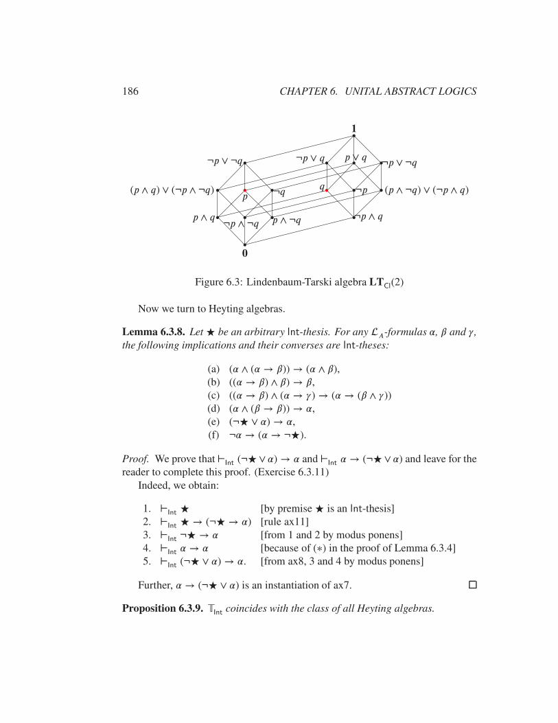
186 CHAPTER 6. UNITAL ABSTRACT LOGICS
∙
∙∙
∙p
∙p ∧ q
∙∙(p ∧ q) ∨ (¬p ∧ ¬q)
∙¬p ∨ ¬q
∙¬p ∧ q
∙ (p ∧ ¬q) ∨ (¬p ∧ q)∙
∙
∙¬p
∙¬p ∨ ¬q∙
∙
p ∧ ¬q¬p ∧ ¬q
¬p ∨ q p ∨ q
¬q q
1
0
Figure 6.3: Lindenbaum-Tarski algebra LTCl(2)
Now we turn to Heyting algebras.
Lemma 6.3.8. Let ★ be an arbitrary Int-thesis. For any A-formulas �, � and ,the following implications and their converses are Int-theses:
(a) (� ∧ (� → �)) → (� ∧ �),(b) ((� → �) ∧ �) → �,(c) ((� → �) ∧ (� → ) → (� → (� ∧ ))(d) (� ∧ (� → �)) → �,(e) (¬★ ∨ �) → �,(f) ¬� → (� → ¬★).
Proof. We prove that ⊢Int
(¬★∨ �) → � and ⊢Int� → (¬★∨ �) and leave for the
reader to complete this proof. (Exercise 6.3.11)Indeed, we obtain:
1. ⊢Int
★ [by premise ★ is an Int-thesis]2. ⊢
Int★ → (¬★ → �) [rule ax11]
3. ⊢Int
¬★ → � [from 1 and 2 by modus ponens]4. ⊢
Int� → � [because of (∗) in the proof of Lemma 6.3.4]
5. ⊢Int
(¬★ ∨ �) → �. [from ax8, 3 and 4 by modus ponens]
Further, � → (¬★ ∨ �) is an instantiation of ax7.
Proposition 6.3.9. TInt
coincides with the class of all Heyting algebras.
6.3. LINDENBAUM-TARSKI ALGEBRAS 187
Proof. Let H = ⟨H; ∧,∨,→,¬, 1⟩ be a Heyting algebra. In virtue of Proposi-tion 2.3.24, the rules ax1–ax9 are valid in H. In virtue of the properties (2.16),(2.17) and (2.18), we receive that ax11 is also valid in H. Noticing, that modusponens preserves validity in any Heyting algebra, we conclude that if � ∈ T
Int,
then H ⊧ � ≈ 1.Next, assume that an algebra H = ⟨H; ∧,∨,→,¬, 1⟩ ∈ T
Int. That is, for any
� ∈ T Int and any valuation v in H, v(�) = 1. We show that the properties (l1)–(l4),(b1), and (h1)–(h6) are valid in H.
In virtue of Lemma 6.3.6 and the fact that P is implicational w.r.t →, the prop-erties (l1)–(l4) are valid in H. Thus ⟨H; ∧,∨⟩ is a distributive lattice.
Further, similarly to (6.11), we derive that
⊢Intp→ ★,
for any variable p and Int-thesis ★. This implies that the equalities (b1) are true inH.
To prove the properties (h1)–(h6), we apply Lemma 6.3.8.
Corollary 6.3.9.1. LTInt is a free Heyting algebra of rank card(A). Hence,
LTInt(�), where � ≤ card(A
), is a free Heyting algebras of rank �.
Below we give a description of LTInt(1). For this, we consider the following
formulas of an arbitrary variable p.First, we define:
p0 ∶= p ∧ ¬p, p1 ∶= ¬p, p2 ∶= p, p! ∶= p→ p.
Then for any n ≥ 0, we define:
i) p2n+3 ∶= p2n+1 → p2n ii) p2n+4 ∶= p2n+1 ∨ p2n+2. (6.12)
Thus ‘m’ in ‘pm’ can take the value of any ordinal less than or equal to the firstinfinite ordinal, symbolically m ≤ !.
We conclude with the following observation, due to I. Nishimura (Nishimura, 1960);see also (Rieger, 1957).
A description of LTInt(1) can be outlined in terms of the following relations
on the set of FmA-formulas.
∙ � ≼ �df
⟺ ⊢Int� → �;
∙ � ∼ �df
⟺ ⊢Int� → � and ⊢
Int� → �;
∙ � ≺ �df
⟺ � ≼ � and not � ∼ �;
(6.13)
188 CHAPTER 6. UNITAL ABSTRACT LOGICS
It should be clear that
� ∼ � ⟺ �∕�(TInt) = �∕�(T
Int);
and, since
� ∼ � ⟺ � ≼ � and � ≼ �,
�∕�(TInt) ≤ �∕�(T
Int) ⟺ � ≼ �,
where≤ is the (ordinary) partial order in the Heyting algebraLTInt
(Corollary 6.3.9.1).Below we treat ∼ as a congruence on FmA
.
The above equivalences will be used without reference. In particular, in thedescription of LT
Int(1) as a diagram below, we depict each congruence class by
its representative. Thus if a formula � can be connected by an upward path witha formula �, which means that �∕�(T
Int) ≤ �∕�(T
Int), then � ≼ �. Also, �∕
�(TInt) < �∕�(T
Int) if, and only if, � ≺ �.
In accordance with this agreement, we have:
0 ∶= p0 and 1 ∶= p!.
It should be clear that for any FmA-formula �,
0 ≼ � and � ≼ 1.
Thus the elements 0 and 1 are a least and greatest elements, respectively, ofany Lindenbaum-Tarski algebra of Int and hence are those of LT
Int(1).
Proposition 6.3.10. Every A-formula of one variable p is equivalent in Int to oneand only one formula pi, which are not equivalent to each other (in the sense of ∼)and related to each other (in the sense of≼) as shown in the diagram of Figure 6.4.
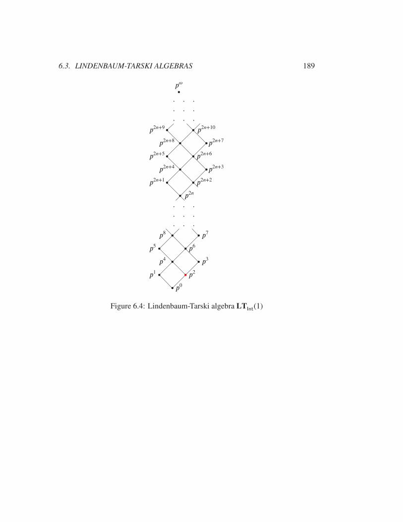
6.3. LINDENBAUM-TARSKI ALGEBRAS 189
∙p!
. . .
. . .
. . .
∙ p2n∙ p2n+2∙p2n+1
∙p2n+4 ∙p2n+3∙ p2n+6∙p2n+5
∙p2n+8 ∙p2n+7∙ p2n+10∙p2n+9
. . .
. . .
. . .
∙ p0∙ p2∙p1
∙p4 ∙ p3∙ p6∙p5
∙p8 ∙ p7
Figure 6.4: Lindenbaum-Tarski algebra LTInt(1)
190 CHAPTER 6. UNITAL ABSTRACT LOGICS
We call the above diagram Rieger-Nishimura algebra; other names in the lit-erature are Rieger-Nishimura ladder and Rieger-Nishimura lattice. The rest of thissection is devoted to the proof of Proposition 6.3.10.
6.3.4 Rieger-Nishimura algebra
In the proofs of propositions and lemmas below in this subsection we use Propo-sition 6.3.6 and transitivity of ∼ without reference. Also, we use rules of (a) and(b) and the hyperrules of (c) (Section 4.3.5), as needed. The applications of thoserules are guaranteed by Lemma 6.3.3, Lemma 6.3.4 and Lemma 6.3.5.
At one point or another, we will need to use the Int-theses that we have collectedin the following lemma.
Lemma 6.3.9. For arbitrary A-formulas �, � and , the following propertieshold:
(a) (� → ¬�) ∼ ¬(� ∧ �),(b) (¬� → �) ≼ ¬¬(� ∨ �),(c) (� → (� → )) ∼ ((� ∧ �) → ),(d) ((� ∨ �) → ) ∼ ((� → ) ∧ (� → )),(e) (� → (� ∧ )) ∼ ((� → �) ∧ (� → )),(f) (� → ¬�) ∼ ¬�,(g) (¬� → �) ∼ ¬¬�,(h) (¬� → ¬¬�) ∼ ¬¬�,(i) (¬¬� → ¬�) ∼ ¬�,(j) ¬� ∼ � → (p ∧ ¬p),(k) ¬¬¬� ∼ ¬�;(l) (¬� ∧ �) ∼ p0;(m) ((� → �) ∧ (� → )) → (� → );(n) � ∧ (� → �) ∼ � ∧ �.
Proof. We prove (a) and leave the rest to the reader as an exercise. (Exercise 6.3.12)With the help of rules (b–i) (b–iii) and the definition of Int, we obtain:
� → ¬�, � ∧ � ⊢Int�; � → ¬�, � ∧ � ⊢
Int�; and � → ¬�, � ∧ �, � ⊢
Int¬�.
Hence we have:
� → ¬�, � ∧ � ⊢Int� and � → ¬�, � ∧ � ⊢
Int¬�.

6.3. LINDENBAUM-TARSKI ALGEBRAS 191
By hyperrules (c–ii) and (c–i), we successively derive:
� → ¬� ⊢Int
¬(� ∧ �) and ⊢Int
(� → ¬�) → ¬(� ∧ �).
Conversely, applying rule (a–i), we derive:
¬(� ∧ �), �, � ⊢Int� ∧ �.
Hence, by hyperrule (c–ii),
¬(� ∧ �), � ⊢Int
¬�.
Applying hyperrule (c–i) twice, we conclude that ¬(� ∧ �) → (� → ¬�) is anInt-thesis.
Then, it remains to apply rule (a–i).
Further, we add to the relations (6.13) one more, namely we define:
� ≪ �df
⟺ ⊢Int
(� → �) → �.
It should be clear that Proposition 6.3.10 will be proven when we prove Corol-lary 6.3.11.1 and Corollary 6.3.13.1 below. These corollaries follow from Propo-sition 6.3.11 and, respectively, Proposition 6.3.13. Thus, our argument consistsof two almost separate paths. Both paths, however, pass through Lemma 6.3.11which is about properties of the relations ≼, ∼ and≪ for concrete formulas, or sayit better, for concrete elements of LT
Int(1). But we start with general properties of
these relations.
Lemma 6.3.10. For arbitrary A-formulas �, � and , the following conditionalsand equivalences hold:
(a) (� ≼ � and � ≼ ) ⟹ � ≼ ;(b) � ≪ � ⟺ ⊢
Int(� → �) ∧ ((� → �) → �);
(c) (� → �) ∼ � ⟺ ⊢Int
(� → �) → �;(d) � ≪ � ⟺ � ≼ � and � → � ∼ �;(e) ((� → �) ∼ � and � ≼ ) ⟹ � → ∼ ;(f) (� ≪ � and � ≼ ) ⟹ � ≪ ;(g) (� ≼ � and � ≪ ) ⟹ � ≪ ;(h) (� ∼ � and � ∼ ) ⟹ � ∼ ;(i) � ≼ � ⟺ � ∧ � ∼ �;(j) � ≼ � ⟺ � ∨ � ∼ �;(k) � ∨ � ≼ ⟺ � ≼ and � ≼ ;(l) � ∧ � ≼ ⟺ � ≼ � → .
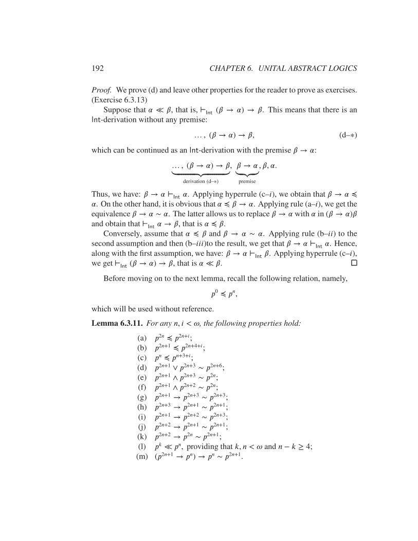
192 CHAPTER 6. UNITAL ABSTRACT LOGICS
Proof. We prove (d) and leave other properties for the reader to prove as exercises.(Exercise 6.3.13)
Suppose that � ≪ �, that is, ⊢Int
(� → �) → �. This means that there is anInt-derivation without any premise:
… , (� → �) → �, (d–∗)
which can be continued as an Int-derivation with the premise � → �:
… , (� → �) → �⏟⏞⏞⏞⏞⏞⏞⏞⏞⏞⏟⏞⏞⏞⏞⏞⏞⏞⏞⏞⏟
derivation (d–∗)
, � → �⏟⏟⏟
premise
, �, �.
Thus, we have: � → � ⊢Int �. Applying hyperrule (c–i), we obtain that � → � ≼�. On the other hand, it is obvious that � ≼ � → �. Applying rule (a–i), we get theequivalence � → � ∼ �. The latter allows us to replace � → � with � in (� → �)�and obtain that ⊢
Int� → �, that is � ≼ �.
Conversely, assume that � ≼ � and � → � ∼ �. Applying rule (b–ii) to thesecond assumption and then (b–iii)to the result, we get that � → � ⊢
Int�. Hence,
along with the first assumption, we have: � → � ⊢Int�. Applying hyperrule (c–i),
we get ⊢Int
(� → �) → �, that is � ≪ �.
Before moving on to the next lemma, recall the following relation, namely,
p0 ≼ pn,
which will be used without reference.
Lemma 6.3.11. For any n, i < !, the following properties hold:
(a) p2n ≼ p2n+i;(b) p2n+1 ≼ p2n+4+i;(c) pn ≼ pn+3+i;(d) p2n+1 ∨ p2n+3 ∼ p2n+6;(e) p2n+1 ∧ p2n+3 ∼ p2n;(f) p2n+1 ∧ p2n+2 ∼ p2n;(g) p2n+1 → p2n+3 ∼ p2n+3;(h) p2n+3 → p2n+1 ∼ p2n+1;(i) p2n+1 → p2n+2 ∼ p2n+3;(j) p2n+2 → p2n+1 ∼ p2n+1;(k) p2n+2 → p2n ∼ p2n+1;(l) pk ≪ pn, providing that k, n < ! and n − k ≥ 4;
(m) (p2n+1 → pn) → pn ∼ p2n+1.

6.3. LINDENBAUM-TARSKI ALGEBRAS 193
Proof. We prove successively each statement of (a)–(m).Proof of (a). We observe that for any n ≥ 0,
p2n ≼ p2n+2 (a–∗)
Indeed, it is obvious if n = 0. Now, assuming that n = l+1, we have p2(l+1)+2 =p2l+1 ∨ p2l+2.
Now we observe that for any n ≥ 0,
p2n+1 ≼ p2n+5 (a–∗∗)
Indeed, we successively obtain the following:
(a) p2n+1, p2n+1 → p2n ⊢Intp2n [by rule (b-iii)]
(b) p2n+1, p2n+1 → p2n ⊢Intp2n+2 [using (e–∗)]
(c) p2n+1, p2n+3 ⊢Intp2n+2 [by definition (6.12–i)]
(d) p2n+1 ⊢Intp2n+3 → p2n+2 [by hyperrule (c–i)]
(e) p2n+1 ⊢Intp2n+5 [by definition (6.12–i)]
(f) ⊢Intp2n+1 → p2n+5 [by hyperrule (c–i)].
Next we observe that for any n ≥ 0,
p2n ≼ p2n+1. (a-∗∗∗)
Omitting the obvious case when n = 0, we notice that, when n = 1, ⊢Intp → p3,
since p3 ∼ ¬¬p. Now, assuming that n = l + 2, we, on the one hand, have:p2n = p2l+1 ∨ p2l+2 and, on the other hand, p2n+1 = p2(l+1)+1 → p2l+2. It must beobvious that p2l+2 ≼ p2l+3 → p2(l+1). On the other hand, in the light of the rule(b–iii), p2l+1, p2l+1 → p2l ⊢
Intp2l and hence, in virtue of (a–∗∗∗), p2l+1, p2l+1 →
p2l ⊢Intp2l+2. Applying the hyperrule (c–i), we obtain that p2l+1 ≼ p2l+3 → p2l+2.
Then, we apply Lemma 6.3.10–k.Now, we begin the proof of (a) by induction on i. The case when i = 0 is
obvious. The case when i = 1 follows from (a–∗∗∗) and the case when i = 2
follows from (a–∗∗).By induction hypothesis, assume that
p2n ≼ p2n+k,
for any k with 0 ≤ k < i, where i ≥ 2. Thus 0 ≤ k ≤ i − 2.We consider two cases: 2n + (i − 1) is even and 2n + (i − 1) is odd.

194 CHAPTER 6. UNITAL ABSTRACT LOGICS
If 2n + (i − 1) is even, then, in virtue of (a–∗∗∗), p2n+(i−1) ≼ p2n+i and hence,according Lemma 6.3.10–k, p2n ≼ p2n+i.
Now let 2n+(i−1) = 2l+1. This implies that 2n+i = 2l+2. By induction hy-pothesis, p2n ≼ p2n+(i−2) = p2l. Applying (a–∗), we receive that p2l ≼ p2l+2 = p2n+i.Then, we apply Lemma 6.3.10–k.
Proof of (b). Since LTInt(1) is a Heyting algebra (Corollary 6.3.9.1) and by def-inition (6.12–ii), p2n+1 ≼ p2n+1 ∨ p2n+2 = p2n+4. Further, in virtue of (a), p2n+4 =
22(n+2) ≼ 22(n+2)+i. Then, we apply Lemma 6.3.10–a.
Proof of (c). Considering two cases, whether n is even or odd, we get: p2l ≼ p2l+3+i,by (a), and p2l+1 ≼ p2l+1+3+i, by (b).
Proof of (d). We successively obtain:
p2n+6 = p2(n+1)+4 = p2(n+1)+1 ∨ p22(n+1)+2
[definition (6.12–ii)]= p2n+3 ∨ p2n+4 = p2n+3 ∨ (p2n+1 ∨ p2n+2) [definition (6.12–ii)]
∼ p2n+1 ∨ (p2n+2 ∨ p2n+3) [associative law for ∨ in LTInt(1)]
∼ p2n+1 ∨ p2n+3 [by (a)].
Proof of (e). Since LTInt(1) is a Heyting algebra (Corollary 6.3.9.1) and by defi-
nition, we have: p2n+1 ∧ p2n+3 ∼ p2n+1 ∧ p2n. Then, we apply (a–∗∗∗).
Proof of (f). First, we notice that, in view of (a),
p2n ≼ p2n+1 ∧ p2n+2.
Then, in virtue of Lemma 6.3.9–c,
(p2n+1 ∧ p2n+2) → p2n ∼ p2n+2 → (p2n+1 → p2n) ∼ p2n+2 → p2n+3.
Applying (a), we conclude that p2n+1 ∧ p2n+2 ≼ p2n.
Proof of (g). Using definition (6.12–i) and Lemma 6.3.9–c, we have:
p2n+1 → p2n+3 = p2n+1 → (p2n+1 → p2n) ∼ (p2n+1∧p2n+1) → p2n ∼ (p2n+1) → p2n = p2n+3.
Proof of (h). If n = 0, according to Lemma 6.3.9–i, we have:
p3 → p1 ∼ ¬¬p→ ¬p ∼ ¬p = p1.

6.3. LINDENBAUM-TARSKI ALGEBRAS 195
And for any n = l+1, applying Lemma 6.3.9–c, (a–∗∗) and definition (6.12–i),we have:
p2(l+1)+3 → p2(l+1)+1 ∼ p2l+5 → (p2l+1 → p2l) ∼ (p2l+5 ∧ p2l+1) → p2l
∼ p2l+1 → p2l ∼ p2l+3.
Proof of (i). On the one hand, in virtue of (6.12–i), (a–∗) and Lemma 6.3.9–m,we have
p2n+3 ∼ (p2n+1 → p2n) ∧ (p2n → p2n+2) ≼ p2n+1 → p2n+2.
On the other hand, in virtue of Lemma 6.3.9–n and (f), we obtain:
p2n+1 ∧ (p2n+1 → p2n+2) ∼ p2n+1 ∧ p2n+2 ∼ p2n.
In particular,(p2n+1 → p2n+2) ∧ p2n+1 ≼ p2n,
which, according to Lemma 6.3.10–l, is equivalent to
p2n+1 → p2n+2 ≼ p2n+1 → p2n⏟⏞⏞⏞⏟⏞⏞⏞⏟
p2n+3
.
Proof of (j). If n = 0, then, using Lemma 6.3.9–f, we have:
p2 → p1 ∼ ¬p = p1.
Now let n = l + 1. Then we obtain:
p2l+4 → p2l+3 = (p2l+1 ∨ p2l+2) → p2l+3 [by definition (6.12–ii)]∼ (p2l+1 → p2l+3) ∧ (p2l+2 → p2l+3) [Lemma 6.3.9–d]
∼ p2l+1 → p2l+3 [by (a–∗∗∗)]∼ p2l+1 → (p2l+1 → p2l) [by definition (6.12–i)]
∼ p2l+1 → p2l [Lemma 6.3.9–c]∼ p2l+3 = p2n+1 [definition (6.12–i)].
Proof of (k). If n = 0, according to Lemma 6.3.9–j, we have:
p2 → p0 ∼ ¬p = p1.
Now assume that n = l + 1. Then we obtain:
p2l+4 → p2l+2 ∼ (p2l+2 ∨ p2l+1) → p2l+2 [definition (6.12–ii)]∼ (p2l+2 → p2l+2) ∧ (p2l+1 → p2l+2) [Lemma 6.3.9–d]
∼ p2l+1 → p2l+2 [(∗) in the proof of Lemma 6.3.4]∼ p2l+3 [by (i)].

196 CHAPTER 6. UNITAL ABSTRACT LOGICS
Proof of (l). We distinguish two cases: k is even and k is odd.Suppose k = 2l; then n = 2l+4+i. We notice that, on the one hand, according
to (a), p2l ≼ p2l+2. On the other hand, we obtain:
p2l+4 → p2l = (p2l+1 ∨ p2l+2) → p2l [by definition (6.12–ii)]∼ (p2l+1 → p2l) ∧ (p2l+2 → p2l) [Lemma 6.3.9–d]
= p2l+3 ∧ (p2l+2 → p2l) [by definition (6.12–ii)]∼ p2l+3 ∧ p2l+1 [by (k)]
∼ p2l [by (e)].
Applying Lemma 6.3.10–d, we receive that p2l ≪ p2l+4. And since, in virtueof (a), p2l+4 ≼ p2l+4+i, we, applying Lemma 6.3.10–f, derive that p2l ≪ p2l+4+i.
Now assume that k = 2l + 1; then n = 2l + 5 + i. First, we prove thatp2l+1 ≪ p2l+4.
Indeed, on the one hand, in virtue of definition (6.12–ii), p2l+1 ≼ p2l+1∨p2l+2 =p2l+4. On the other hand, we have:
p2l+4 → p2l+1 = (p2l+1 ∨ p2l+2) → p2l+1 [by definition (6.12–ii)]∼ (p2l+1 → p2l+1) ∧ (p2l+2 → p2l+1) [Lemma 6.3.9–d]
∼ p2l+2 → p2l+1 ∼ p2l+1 [by (j)].
Then, applying Lemma 6.3.10–d, we get that p2l+1 ≪ p2l+4.Now, since, in virtue of (a), p2l+4 ≼ p2l+4+i, according to Lemma 6.3.10–f, we
conclude that p2l+1 ≪ p2l+4+i, in particular, p2l+1 ≪ p2l+5+i.
Proof of (m). If n = 0, then we have:
(p1 → p0) → p0 ∼ ¬¬¬p ∼ ¬p
(Lemma 6.3.9, (g) twice and (h)).Next we take n = 1. Then we have:
(p3 → p2) → p2 ∼ (¬¬p→ p) → p.
First, we prove that
(¬¬p→ p) → p ⊢Int
¬¬p (m–∗)
and, then, it will remain to apply the hyperrule (c–i) (Lemma 6.3.4).
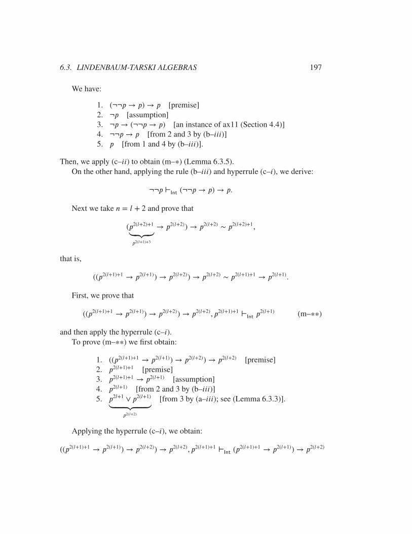
6.3. LINDENBAUM-TARSKI ALGEBRAS 197
We have:
1. (¬¬p→ p) → p [premise]2. ¬p [assumption]3. ¬p→ (¬¬p→ p) [an instance of ax11 (Section 4.4)]4. ¬¬p→ p [from 2 and 3 by (b–iii)]5. p [from 1 and 4 by (b–iii)].
Then, we apply (c–ii) to obtain (m–∗) (Lemma 6.3.5).On the other hand, applying the rule (b–iii) and hyperrule (c–i), we derive:
¬¬p ⊢Int
(¬¬p→ p) → p.
Next we take n = l + 2 and prove that
(p2(l+2)+1⏟⏟⏟p2(l+1)+3
→ p2(l+2)) → p2(l+2) ∼ p2(l+2)+1,
that is,
((p2(l+1)+1 → p2(l+1)) → p2(l+2)) → p2(l+2) ∼ p2(l+1)+1 → p2(l+1).
First, we prove that
((p2(l+1)+1 → p2(l+1)) → p2(l+2)) → p2(l+2), p2(l+1)+1 ⊢Intp2(l+1) (m–∗∗)
and then apply the hyperrule (c–i).To prove (m–∗∗) we first obtain:
1. ((p2(l+1)+1 → p2(l+1)) → p2(l+2)) → p2(l+2) [premise]2. p2(l+1)+1 [premise]3. p2(l+1)+1 → p2(l+1) [assumption]4. p2(l+1) [from 2 and 3 by (b–iii)]5. p2l+1 ∨ p2(l+1)
⏟⏞⏞⏞⏞⏞⏟⏞⏞⏞⏞⏞⏟p2(l+2)
[from 3 by (a–iii); see (Lemma 6.3.3)].
Applying the hyperrule (c–i), we obtain:
((p2(l+1)+1 → p2(l+1)) → p2(l+2)) → p2(l+2), p2(l+1)+1 ⊢Int
(p2(l+1)+1 → p2(l+1)) → p2(l+2)
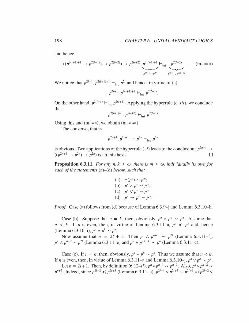
198 CHAPTER 6. UNITAL ABSTRACT LOGICS
and hence
((p2(l+1)+1 → p2(l+1)) → p2(l+2)) → p2(l+2), p2(l+1)+1⏟⏟⏟p2l+1→p2l
⊢Int
p2(l+2)⏟⏟⏟p2l+1∨p2(l+1)
. (m–∗∗∗)
We notice that p2l+1, p2(l+1)+1 ⊢Intp2l and hence, in virtue of (a),
p2l+1, p2(l+1)+1 ⊢Int p2(l+1).
On the other hand, p2(l+1) ⊢Intp2(l+1). Applying the hyperrule (c–iii), we conclude
thatp2(l+1)+1, p2(l+2) ⊢
Intp2(l+1).
Using this and (m–∗∗), we obtain (m–∗∗∗).The converse, that is
p2n+1, p2n+1 → p2n ⊢Intp2n,
is obvious. Two applications of the hyperrule (–i) leads to the conclusion: p2n+1 →((p2n+1 → p2n) → p2n) is an Int-thesis.
Proposition 6.3.11. For any n, k ≤ !, there is m ≤ !, individually its own foreach of the statements (a)–(d) below, such that
(a) ¬(pn) ∼ pm;(b) pn ∧ pk ∼ pm;(c) pn ∨ pk ∼ pm
(d) pn → pk ∼ pm.
Proof. Case (a) follows from (d) because of Lemma 6.3.9–j and Lemma 6.3.10–h.
Case (b). Suppose that n = k, then, obviously, pn ∧ pk ∼ pn. Assume thatn < k. If n is even, then, in virtue of Lemma 6.3.11–a, pn ≼ pk and, hence(Lemma 6.3.10–i), pn ∧ pk ∼ pn.
Now assume that n = 2l + 1. Then pn ∧ pn+1 ∼ p2l (Lemma 6.3.11–f),pn ∧ pn+2 ∼ p2l (Lemma 6.3.11–e) and pn ∧ pn+3+i ∼ pn (Lemma 6.3.11–c).
Case (c). If n = k, then, obviously, pn ∨ pk ∼ pn. Thus we assume that n < k.If n is even, then, in virtue of Lemma 6.3.11–a and Lemma 6.3.10–j, pn ∨ pk ∼ pk.
Let n = 2l+1. Then, by definition (6.12–ii), pn∨pn+1 ∼ pn+3. Also, pn∨pn+2 ∼pn+5. Indeed, since p2l+2 ≼ p2l+3 (Lemma 6.3.11–a), p2l+1 ∨ p2l+3 ∼ p2l+1 ∨ (p2l+2 ∨
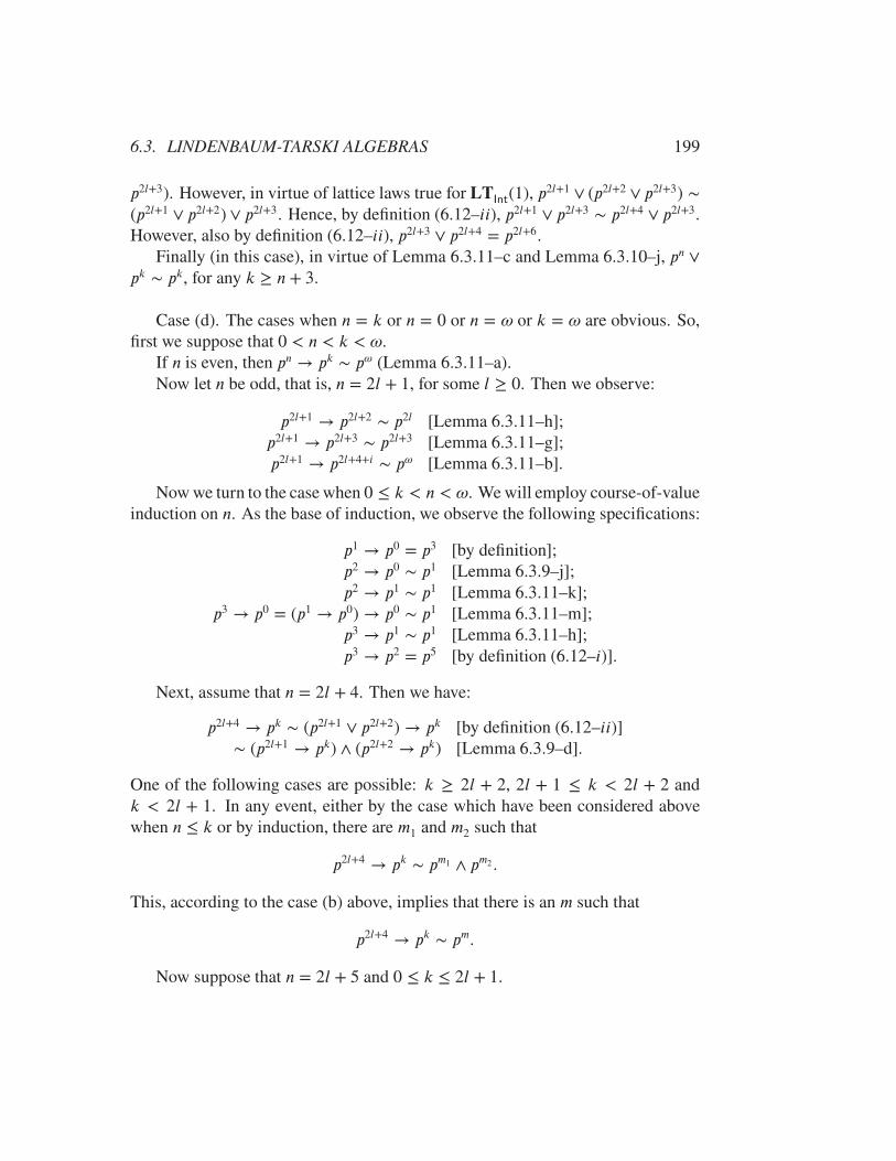
6.3. LINDENBAUM-TARSKI ALGEBRAS 199
p2l+3). However, in virtue of lattice laws true for LTInt(1), p2l+1 ∨ (p2l+2 ∨ p2l+3) ∼
(p2l+1 ∨ p2l+2) ∨ p2l+3. Hence, by definition (6.12–ii), p2l+1 ∨ p2l+3 ∼ p2l+4 ∨ p2l+3.However, also by definition (6.12–ii), p2l+3 ∨ p2l+4 = p2l+6.
Finally (in this case), in virtue of Lemma 6.3.11–c and Lemma 6.3.10–j, pn ∨pk ∼ pk, for any k ≥ n + 3.
Case (d). The cases when n = k or n = 0 or n = ! or k = ! are obvious. So,first we suppose that 0 < n < k < !.
If n is even, then pn → pk ∼ p! (Lemma 6.3.11–a).Now let n be odd, that is, n = 2l + 1, for some l ≥ 0. Then we observe:
p2l+1 → p2l+2 ∼ p2l [Lemma 6.3.11–h];p2l+1 → p2l+3 ∼ p2l+3 [Lemma 6.3.11–g];p2l+1 → p2l+4+i ∼ p! [Lemma 6.3.11–b].
Now we turn to the case when 0 ≤ k < n < !. We will employ course-of-valueinduction on n. As the base of induction, we observe the following specifications:
p1 → p0 = p3 [by definition];p2 → p0 ∼ p1 [Lemma 6.3.9–j];p2 → p1 ∼ p1 [Lemma 6.3.11–k];
p3 → p0 = (p1 → p0) → p0 ∼ p1 [Lemma 6.3.11–m];
p3 → p1 ∼ p1 [Lemma 6.3.11–h];p3 → p2 = p5 [by definition (6.12–i)].
Next, assume that n = 2l + 4. Then we have:
p2l+4 → pk ∼ (p2l+1 ∨ p2l+2) → pk [by definition (6.12–ii)]∼ (p2l+1 → pk) ∧ (p2l+2 → pk) [Lemma 6.3.9–d].
One of the following cases are possible: k ≥ 2l + 2, 2l + 1 ≤ k < 2l + 2 andk < 2l + 1. In any event, either by the case which have been considered abovewhen n ≤ k or by induction, there are m1 and m2 such that
p2l+4 → pk ∼ pm1 ∧ pm2 .
This, according to the case (b) above, implies that there is an m such that
p2l+4 → pk ∼ pm.
Now suppose that n = 2l + 5 and 0 ≤ k ≤ 2l + 1.
200 CHAPTER 6. UNITAL ABSTRACT LOGICS
If k = 2l + 4, then, by definition, pn → pk ∼ p2(l+2)+3. If k = 2l + 3, thenpn → pk = p2(l+1)+3 → p2(l+1)+1 ∼ p2(l+1)+1 (Lemma 6.3.11–h). And if k = 2l + 2,then pn → pk = p2(l+1)+3 → p2(l+1) = (p2(l+1)+1 → p2(l+1)) → p2(l+1) ∼ p2(l+1)+1
(Lemma 6.3.11–m).
Thus it remains to consider the case when n = 2l + 5 and k ≤ 2l + 1. Butthen n− k ≥ 4 and, in virtue Lemma 6.3.11–l, we conclude that pk ≪ pn. This, invirtue of Lemma 6.3.10–d, implies that pn → pk ∼ pk.
Corollary 6.3.11.1. For any formula �(p) with a single variable p, there is n ≤ !such that �(p) ∼ pn.
Proof. Using Proposition 6.3.11, the proof can be carried out by induction on thenumber of logical connectives occurring in �(p). We leave this to the reader as anexercise. (Exercise 6.3.14)
Now we turn to the other path of our argument. Since to prove Proposition 6.3.13,we have to separate the set of Int-theses from the formulas pn, for any n < !. Ifsome initial powers of p can be refuted in relatively simple Heyting algebras, inorder to carry out proof by induction, we will need a o more transparent presenta-tion of Int-theses. ⤇
For our purposes, we borrow a sequential calculus G3 from (Kleene, 1952),chapter XV. The main formal objects are sequents which are pairs of finite setsof A-formulas, say Γ and Θ, divided by the symbol ⤇ — Γ ⤇ Θ, where Θ isallowed to consist of not more than one formula. The system G3 is formulatedin terms of metavariables for A-formulas and variables Γ and Θ for finite sets offormulas (with the aforementioned restriction on Θ) as follows.
Axiom schema: Γ,� ⤇ �.
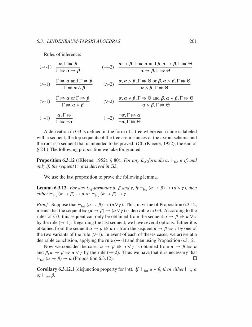
6.3. LINDENBAUM-TARSKI ALGEBRAS 201
Rules of inference:
(→-1)�,Γ ⤇ �
Γ ⤇ � → �(→-2)
� → � ,Γ ⤇ � and �,� → �,Γ ⤇ Θ
� → �,Γ ⤇ Θ
(∧-1)Γ ⤇ � and Γ ⤇ �
Γ ⤇ � ∧ �(∧-2)
�,� ∧ � ,Γ ⤇ Θ or �,� ∧ �,Γ ⤇ Θ
� ∧ �,Γ ⤇ Θ
(∨-1)Γ ⤇ � or Γ ⤇ �
Γ ⤇ � ∨ �(∨-2)
�,� ∨ � ,Γ ⤇ Θ and �,� ∨ �,Γ ⤇ Θ
� ∨ � ,Γ ⤇ Θ
(¬-1)�,Γ ⤇
Γ ⤇ ¬�(¬-2)
¬�,Γ ⤇ �
¬�,Γ ⤇ Θ
A derivation in G3 is defined in the form of a tree where each node is labeledwith a sequent; the top sequents of the tree are instances of the axiom schema andthe root is a sequent that is intended to be proved. (Cf. (Kleene, 1952), the end of§ 24.) The following proposition we take for granted.
Proposition 6.3.12 ((Kleene, 1952), § 80). For any A-formula �, ⊢Int� if, and
only if, the sequent ⤇ � is derived in G3.
We use the last proposition to prove the following lemma.
Lemma 6.3.12. For any A-formulas �, � and , if ⊢Int
(� → �) → (� ∨ ), theneither ⊢
Int(� → �) → � or ⊢
Int(� → �) → .
Proof. Suppose that ⊢Int
(� → �) → (�∨ ). This, in virtue of Proposition 6.3.12,means that the sequent ⤇ (� → �) → (� ∨ ) is derivable in G3. According to therules of G3, this sequent can only be obtained from the sequent � → � ⤇ � ∨ by the rule (→-1). Regarding the last sequent, we have several options. Either it isobtained from the sequent � → � ⤇ � or from the sequent � → � ⤇ by one ofthe two variants of the rule (∨-1). In event of each of theses cases, we arrive at adesirable conclusion, applying the rule (→-1) and then using Proposition 6.3.12.
Now we consider the case: � → � ⤇ � ∨ is obtained from � → � ⤇ �and �, � → � ⤇ � ∨ by the rule (→-2). Thus we have that it is necessary that⊢
Int(� → �) → � (Proposition 6.3.12).
Corollary 6.3.12.1 (disjunction property for Int). If ⊢Int� ∨ �, then either ⊢
Int�
or ⊢Int�.
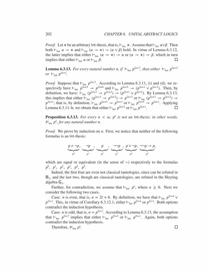
202 CHAPTER 6. UNITAL ABSTRACT LOGICS
Proof. Let⋆ be an arbitrary Int-thesis, that is,⊢Int⋆. Assume that⊢
Int�∨�. Then
both ⊢Int� → ⋆ and ⊢
Int(� → ⋆) → (� ∨ �) hold. In virtue of Lemma 6.3.12,
the latter implies that either ⊢Int
(� → ⋆) → � or (� → ⋆) → �, which in turnimplies that either ⊢
Int� or ⊢
Int�.
Lemma 6.3.13. For every natural number n, if ⊢Intp2n+7, then either ⊢
Intp2n+3
or ⊢Intp2n+1.
Proof. Suppose that ⊢Int p2n+7. According to Lemma 6.3.11, (i) and (d), we re-
spectively have ⊢Intp2n+5 → p2n+6 and ⊢
Intp2n+5 → (p2n+1 ∨ p2n+3). Then, by
definition, we have: ⊢Int
(p2n+3 → p2n+2) → (p2n+1 ∨ p2n+3). By Lemma 6.3.13,this implies that either ⊢
Int(p2n+3 → p2n+2) → p2n+3 or ⊢
Int(p2n+3 → p2n+2) →
p2n+1; that is, by definition, ⊢Intp2n+5 → p2n+3 or ⊢
Intp2n+5 → p2n+1. Applying
Lemma 6.3.11–h, we obtain that either ⊢Intp2n+3 or ⊢
Intp2n+1.
Proposition 6.3.13. For every n < !, pn is not an Int-thesis; in other words,⊬
Intpn, for any natural number n.
Proof. We prove by induction on n. First, we notice that neither of the followingformulas is an Int-thesis:
p ∧ ¬p⏟⏟⏟
p0
, ¬p⏟⏟⏟
p1
, p⏟⏟⏟
p2
, ¬¬p⏟⏟⏟
p3
, p ∨ ¬p⏟⏟⏟
p4
, ¬¬p→ p⏟⏞⏟⏞⏟
p5
,
which are equal or equivalent (in the sense of ∼) respectively to the formulasp0, p1, p2, p3, p4, p5.
Indeed, the first four are even not classical tautologies, since can be refuted inB2, and the last two, though are classical tautologies, are refuted in the Heytingalgebra G3.
Further, for contradiction, we assume that ⊢Int pn, where n ≥ 6. Next we
consider the following two cases.Case: n is even, that is, n = 2l + 6. By definition, we have that ⊢
Intp2l+4 ∨
p2l+1. This, in virtue of Corollary 6.3.12.1, either ⊢Intp2l+4 or p2l+1. Both options
contradict the induction hypothesis.Case: n is odd, that is, n = p2l+7. According to Lemma 6.3.13, the assumption
that ⊢Int
p2l+7 implies that either ⊢Int
p2l+3 or ⊢Int
p2l+1. Again, both optionscontradict the induction hypothesis.
Therefore, ⊬Intpn.

6.3. LINDENBAUM-TARSKI ALGEBRAS 203
Remark 6.3.1. In the light of Proposition 6.3.13, the conditional in Lemma 6.3.13should be understood as counterfactual rather than implication. That is, it wouldbe more appropriate to formulas it as follows: If it were the case that ⊢
Intp2n+7,
then it would be that either ⊢Intp2n+3 or ⊢
Intp2n+1.
Corollary 6.3.13.1. For any n, k ≤ !,
pn ∼ pk ⟺ n = k.
Proof. The ⇐-implication is obvious. Now, for definiteness, suppose that n < k.If it were that pn ∼ pk, then it would imply that ⊢
Intpk → pn. This in turn would
imply that there is a natural number m such that ⊢Int pm. (Proposition 6.3.11–d).
A contradiction.
Exercises 6.3
1. Show that the abstract logics P, Cl and Int are implicational with respect top→ q.
2. Prove (6.8).
3. Prove that for any valuation w in ⟨A, 1⟩, there is a unique valuation v in A
such that v⋆ = w.
4. Prove (6.9).
5. Prove Lemma 6.3.2.
6. Complete the proof of Lemma 6.3.3.
7. Show that the hyperrules (c–ii) and (c–iii) are sound with respect to Cl andInt.
8. Complete the proof of Lemma 6.3.6.
9. Complete the proof of Lemma 6.3.7.
10. Show that the elements [p], [¬p], [p∨¬p] and [p ∧¬p] are pairwise distinctin LT
Cl. (Hint: prove that the matrix B2 is a Cl-model.)
11. Complete the proof of Lemma 6.3.8.

204 CHAPTER 6. UNITAL ABSTRACT LOGICS
12. Complete the proof of Lemma 6.3.9. (Hint: consult (Kleene, 1952), § 26and § 27 if necessary.)
13. Complete the proof of Lemma 6.3.10.
14. Prove Corollary 6.3.11.1.
6.4 Examples of application of Lindenbaum-Tarski
algebras
In this section, we discuss several examples where the notion of Lindenbaum-Tarski algebra plays a key role.
6.4.1 Glivenko’s theorem
The following theorem was established by Glivenko (Glivenko, 1929): For anyA-formula �,
� ∈ TCl
⟺ ¬¬� ∈ TInt. (Glivenko’s theorem)
Sketch of proof. Let us fix an A-formula �.First, we notice that ¬¬� → � ∈ T
Cland T
Int⊆ T
Cl. Taking into account that
TCl
is closed under detachment rule, we obtain the implication:
¬¬� ∈ TInt
⟹ � ∈ TCl.
Conversely, assume that � ∈ TCl
. According to the second part of Propo-sition 6.3.4, � is valid in LT
Cland hence (Corollary 6.3.8.1) � is valid in any
Boolean algebra.Now, assume that ¬¬� ∉ T
Int. This implies that v[¬¬�] is invalid in LT
Int
at v, where v is the Lindenbaum valuation. This in turn implies that the ele-ment v[�] is not dense in the Heyting algebra LTInt. Thus, � will be invalidin the homomorphic image with respect to the homomorphism determined bythe filter of all dense elements of LT
Int, which, according Rasiowa and Siko-
rski (Rasiowa and Sikorski, 1970), chapter IV, theorem 5.8, is a Boolean algebra.Then, in virtue of Corollary 6.3.8.1, � is invalid in LT
Cland hence (Proposi-
tion 6.3.4) � ∉ TCl
.
6.4. EXAMPLES OF APPLICATION OF LINDENBAUM-TARSKI ALGEBRAS205
6.4.2 Completeness
In this subsection by ‘completeness’ we understand the following. A unital logic is complete with respect to that class T (in this narrow sense) if the equivalence
� ∈ T ⟺ � is valid in all algebras of T ,
holds for all formulas �.The above equivalence, in particular, is true if the conditions of Proposition 6.3.7
are fulfilled. This allowed Rasiowa and Sikorski to prove in (Rasiowa and Sikorski, 1970)that for any A-formula �,
� ∈ TInt
⟺ � is valid in all Heyting algebras.
However, the first result of this kind was obtained in (McKinsey, 1941) in re-lation to the Lewis systems S2 and S4. But it was A. Tarski who opened the doortowards this direction, proving in (Tarski, 1935), theorem 4, thatLT
Clis a Boolean
algebra.
6.4.3 Admissible and derivable structural inference rules
Let be a unital logic. Since the logic is structural, any modus rule sound withrespect to ⊢ can be written in terms of a pair ⟨X, �⟩, where X = {�1,… , �n}is a finite (perhaps empty) set of formulas, not metaformulas as we formulatedin Section 4.3.5 in general. According to this definition, for any -substitution�, �(X) ⊢ �(�); and, according to Proposition 6.3.3 and Proposition 6.3.4,X ⊧
LT [X] �, which, in virtue of (6.2), implies that
⟨LT[X],≈⟩ ⊧ ∀∀∀…∀∀∀ (�1 ≈ 1D&…&�n ≈ 1D →→→ � ≈ 1D),
where D = Cn(X). The latter is especially interesting when we investigate ad-
missible rules of a unital calculus, that is, those rules that, being added as postu-lated rules, do not change the set of theses of the calculus. Then, a modus rule⟨X, �⟩ is admissible in a unital calculus if, and only if,
⟨LT ,≈⟩ ⊧ ∀∀∀…∀∀∀ (�1 ≈ 1T &…&�n ≈ 1T
→→→ � ≈ 1T ),
The first to pay attention to this equivalence with respect to Int was A. Citkin;cf. (Citkin, 1977). This idea was later picked up by other researches, which led to acorrespondence between finitary structural abstract logics and quasi-varieties; for
206 CHAPTER 6. UNITAL ABSTRACT LOGICS
more information see (Rybakov, 1997), section 1.4, and (Gorbunov, 1998), section1.5.2.
Given a consequence relation ⊢ and a set of rules , one can construct a new,stronger, consequence relation ⊢: for any set of formulas Γ and a formula �,Γ ⊢ � if, and only if, there is a sequence of formulas �0,… , �n such that �n =� and for each i < n, �i ∈ Γ, or �0,… , �i−1 ⊢ �i, or �i can be derived from thepreceding formulas by application of an instance of one of the rules from R. Sucha sequence is called an ⊢-inference.
It is clear that if each rule of is admissible in a consequence relation ⊢, thenconsequence relations ⊢ and ⊢ have the same sets of theorems.
Example. According to Lemma 6.3.13, for any n ≥ 0, if ⊢Int
p2n+7, either⊢
Intp2n
3or ⊢
Intp2n+1. Hence, for each n ≥ 0, the rule
Rn ∶= p2n+7∕p2n3
∨ p2n1
(6.14)
is admissible for ⊢Int
and therefore, for any set N of natural numbers, if =
{Rn | n ∈ N}, the set of the theorems of the consequence relation ⊢ coincideswith T
Int.
A rule R = Γ∕� is said to be derivable from a set of rules relative to aconsequence relation ⊢ (in symbols ⊢ R) if
Γ ⊢ �. (6.15)
Sets of rules 0 and 1 are said to be equivalent relative to a consequence relation⊢ (in symbols 0 ≈⊢ 1) if 0 ⊢ R for each R ∈ 1 and 1 ⊢ R for eachR ∈ 0.
Proposition 6.4.1. Let ⊢ be a consequence relation and let 0 and 1 be equiv-alent sets of rules relative to ⊢. Then for each rule R, 0 ⊢ R entails 1 ⊢ R,and conversely.
Proof. Suppose that 0 ⊢ R, where R = Γ∕�. Then, Γ ⊢0�, that is, there
is a ⊢0-inference of � from Γ. The proof can be carried out by induction by
induction on the minimal number of the applications of the rules from R0 in the⊢0
-inferences of � from Γ. The basis is obvious, and the proof of the inductionstep fis based on the observation that in the ⊢0
-inference of � from Γ the lastapplication of rule from 0, let say Δ∕�, can be replaced by an ⊢1
-inference of �from Δ. A more detailed sketch of the proof of the induction step is the following.

6.4. EXAMPLES OF APPLICATION OF LINDENBAUM-TARSKI ALGEBRAS207
Suppose that in a ⊢0-inference �0,… , �n = � of � from Γ, formula �i is
obtained by application of an instance �(Δ)∕�(�) of the rule Δ∕� ∈ 0. Byassumption, 1 ⊢ Δ∕�, that is, by the definition, Δ ⊢1
�. Hence, there is a ⊢1-
inference �0,… , �m = � of � from Δ. Thus, �(�0),… , �(�m) is a ⊢1-inference of
�(�) from �(Δ). Now we observe that we can replace the application of �(Δ)∕�(�)with �(�0),… , �(�m), and use the induction assumption to obtain a ⊢1
-inferenceof � from Γ.
Corollary 6.4.1.1. Let ⊢ be a consequence relation and let 0 and 1 be sets ofrules. Then
⊢0= ⊢1
⟺ 0 ≈⊢ 1. (6.16)
Proof. Suppose that ⊢0=⊢1
. Let r = Γ∕� and R ∈ 0. It is clear that Γ ⊢0�.
Hence, by the assumption, Γ ⊢1�, which means that 1 ⊢ R. Thus, for each
R ∈ 0, R1 ⊢ R. By the same argument, 0 ⊢ R for each R ∈ 1, that is,0 ≈⊢ 1.
Conversely, suppose that 0 ≈⊢ 1. Let Γ be a set of formulas and � be aformula. Let us consider the rule R ∶= Γ∕�. If Γ ⊢0
�, then by (6.15), 0 ⊢ Rand by Proposition 6.4.1, 1 ⊢ R, which means that Γ ⊢1
�. Thus, ⊢0⊆ ⊢1
.By the same argument, ⊢1
⊆ ⊢0.
Let = {Rn | n ≥ 0}, where Rn are the rules defined in (6.14), and n ∶=
⧵ {Rn | n ≥ 0}. It was observed in (Citkin, 1977) that n ⊬IntRn. Hence,
by Corollary 6.4.1.1, for any 0,1 ⊆ , if 0 ≉⊢Int1, then, ⊢R0
≠ ⊢R1.
Consequently, the set of consequence relations each having the set of its theoremsequal to T
Int, is not countable.
6.4.4 Classes of algebras corresponding and fully correspond-
ing to a calculus
Definition 6.4.1. Let be a unital calculus. A unital logic ′ is said to be anormal extension of if Cn(∅) ⊆ Cn′(∅) and Cn′(∅) is closed under allrules of inference that are postulated in the calculus .
For example, both Cl and LC are normal extension of Int.
Definition 6.4.2. Let be a unital logic and be a class of unital expansions.We say that corresponds to if for any formula �,
� ∈ Cn(∅) ⟺ (A ⊧ �, for any A ∈ );
208 CHAPTER 6. UNITAL ABSTRACT LOGICS
and fully corresponds to if for any X ∪ {�} ⊆ Fm
X ⊢ � ⟺ (A ⊧ X ⟹ A ⊧ �, for any A ∈ );
Proposition 6.4.2. Given a unital logic , the class T corresponds to . More-over, T is the largest such a class.
Proof. In virtue of (6.6), LT ∈ T . Then, we apply the second part of Proposi-tion 6.3.4.
The second part is obvious.
It must be clear that
If a class fully corresponds to , also corresponds to . (6.17)
The converse is not always true.2
Next we define: For any unital calculus ,
ℙ◦∶= {A ∈ ℙ | [LA] is a normal extension of }.
Lemma 6.4.1. Let be a unital logic and Σ be the sett of all -theories. Then{LT[D] | D ∈ Σ} ⊆ ℙ◦
.
Proof. It suffices to show that for any instance �1,… , �n∕� of an inference rule ofthe calculus ,
LT[D] ⊧ {�1,… , �n} ⟹ LT[D] ⊧ �,
for any D ∈ Σ . So, suppose LT[D] ⊧ {�1,… , �n}. Since {�1,… , �n} ⊢ �, invirtue of the first part of Proposition 6.3.4, LT[D] ⊧ �.
Proposition 6.4.3. Given a unital calculus , the class ℙ◦
fully corresponds to .And if a class ⊆ ℙ fully corresponds to , then ⊆ ℙ◦
.
Proof. Let X ⊢ � and suppose that A ⊧ X, where A ∈ ℙ◦
. Since A is analgebraic -model, A ⊧ �.
Next, assume that X ⊬ �. We note that, in virtue of Proposition 6.3.4,LT[D] ⊧ X and LT[D] ⊧ �, where D = Cn(X). However, according toProposition 6.3.5, LT[D] ∈ ℙ . It remains to show that LLT[D] is closedunder any inference rule postulated in .
2See examples in (Muravitsky, 2014b), section 7.3.
6.5. AN ALTERNATIVE APPROACH TO THE CONCEPT OF LINDENBAUM-TARSKI ALGEBRA209
Let �1,… , �n∕� be an instance of such a rule and LT[D] ⊧ {�1,… , �n}.In virtue of Proposition 6.3.4, {�1,… , �n} ⊆ T . By premise, this implies that� ∈ T and hence (Proposition 6.3.4) LT[D] ⊧ �, that is, LLT[D] is closedunder the given rule of inference. Thus LT[D] ∈ ℙ◦
.
This completes the proof that ℙ◦
fully corresponds to .Now, suppose that a class ⊆ ℙ fully corresponds to and A ∈ . We need
to showLA is closed under any inference rule postulated in , since Cn[LA](∅) =
LA.Indeed, let �1,… , �n∕� be an instance of such a rule. This implies that {�1,… , �n} ⊢
�. Thus, if A ⊧ {�1,… , �n}, then, by premise, A ⊧ �.
Corollary 6.4.3.1. Given a unital calculus , ℙ◦⊆ T .
Proof. We prove the inclusion in question, by using Proposition 6.4.3, (6.17) andProposition 6.4.2.
Proposition 6.4.4. Let ⊆ ℙ be an equational class defined by identities of theform ≈ 1. If fully corresponds to a unital calculus , then = ℙ◦
= T .
Proof. In virtue of Proposition 6.4.3 and Corollary 6.4.3.1, we have: ⊆ ℙ◦⊆
T . For contradiction, we assume that ⊂ T . This implies that there is an iden-tity � ≈ 1 that belongs the equational theory of but � ∉ T . Since, accordingto (6.17), corresponds to , there is an algebra A ∈ such that A ⊧ �; that is,� ≈ 1 does not belong to the equational theory of . A contradiction.
6.5 An alternative approach to the concept of Lindenbaum-
Tarski algebra
The approach to the concept of Lindenbaum-Tarski algebra, which we present con-cisely below, is not supposed to be used in the search of convenient separating toolsin the sense of Section 5.3.
Let M = ⟨A, D⟩ be a logical matrix. It is not difficult to see that a congruence� on A is compatible with D if, and only if
D =⋃
{x∕� | x ∈ D}.
The set of all congruences compatible with D has a least element, the equality,and, as was proved in (Blok and Pigozzi, 1989), has also a largest congruence with
210 CHAPTER 6. UNITAL ABSTRACT LOGICS
respect to ⊆. This congruence is called the Leibniz congruence of M; it is denotedby Ω
AD and can be defined as follows:
ΩAD = {(a, b) | ∀�(p, p0,… , pn) ∈ Fm∀c0,… , cn ∈ |A|.
�(a, c0,… , cn) ∈ D ⇔ �(b, c0,… , cn) ∈ D}.
If the matrix in question is a Lindenbaum matrix ⟨F, D⟩, where D is an -theory, then an example of a compatible equivalence on this matrix is the Fregerelation relative to D (Definition 6.2.4).
Another example of a compatible relation on ⟨A, D⟩ is the largest congruenceof A contained in ΛD , which is referred to as a Suszko congruence:
(�, �) ∈ ΩD ⟺ for every (p), D , (�∕p) ⊢ (�∕p)and D , (�∕p) ⊢ (�∕p).
(Suszko congruence relative to D)Obviously, a system is Fregean if, and only if, ΛD = ΩD , for all D .The Leibniz congruence of a matrix ⟨F, D⟩ is referred to as Leinbniz con-
gruence relative to D . It turns out that
ΩD =⋂
{ΩD′| D ⊆ D
′}
and, therefore, each Suszko congruence ΩD is compatible with D . Also, givenan abstract logic , one defines
Ω =⋂
{ΩD | D is an -theory}. (Tarski congruence)
Thus we have:Ω ⊆ ΩD ⊆ ΛD ∩ ΩD .
Suszko, Leibniz and Tarski congruences give rise to the-matrices ⟨F∕ΩD , D∕ΩD⟩,⟨F∕ΩD , D∕ΩD⟩, and the atlas ⟨F∕Ω , {D∕Ω | D is an -theory}⟩,whose first components, F∕ΩD , F∕ΩD and F∕Ω , in Algebraic abstractlogic are referred to as Lindenbaum-Tarski algebras. (See (Font et al., 2003) and (Font and Jansana, 2009)with update in (Font et al., 2009) for comprehensive surveys.)
6.6 Historical notes
The notion of a unital matrix is a natural bridge from (ordinary) logical matricesto algebras. Such a transition makes it possible to employ more methods of uni-versal algebra than methods of model theory. This notion was formally introduced

6.6. HISTORICAL NOTES 211
in (Czelakowski, 2001) and extensively used therein, although many of the firslogical matrices in the history of many-valued logic were unital. Thus, by 2010,when Czelakowski’s book was published, the concept, not the term, had been wellknown.
The class of unital logics was defined in (Muravitsky, 2014a), although thename for this class of logics was suggested by an anonymous referee of this pa-per. In fact, this notion is rooted in Definition 4 of (Muravitsky, 2014b), where“a calculus C [that] admits the Lindenbaum-Tarski algebra” was defined, which issomewhat weaker than the notion of a unital logic.
It was established in (Muravitsky, 2014a) that the class of implicative logics(studied in (Rasiowa, 1974)) and that of Freagean logics (studied in (Czelakowski and Pigozzi, 2004))are properly included in the class of unital logics.
In Algebraic Abstract Logic, a different approach to the notion of a Lindenbaum-Tarski algebra has been developed. See (Font, 2016) and references therein for de-tail; a brief outline of this approach can be found in (Citkin and Muravitsky (originators), 2013).Unlike ours, this approach does not focus on the Lindenbaum-Tarski algebra as asource for constructing separating tools.
The second part of Corollary 6.3.5.2 was proved in (Shoesmith and Smiley, 1971),theorem 5.
Corollary 6.3.9.1 was established in (Rieger, 1949), theorem 4.4.The diagram in Figure 6.4 was discovered by L. Rieger in (Rieger, 1957) and
I. Nishimura in (Nishimura, 1960). However, earlier in (Rieger, 1949), theorem4.6, Rieger, as well as Nishimura in (Nishimura, 1960), § 3, gave the definitionof the elements of LTInt(1) similar to definition (6.12). Both researchers merelysketched their proofs. Referring to theorem 4.6, Rieger wrote:
“The proof is essentially not difficult but somewhat labourious.”(Rieger, 1949),p. 33
For his part, referring to the diagram, Nishimura wrote:
“We can investigate inclusion, noninclusion and equivalence relation-ships between these logics [. . . ]” (Nishimura, 1960), § 3
Both researchers only sketched the proof of Proposition 6.3.11 in order to ob-tain with its help Corollary 6.3.11.1. However, they failed to notice that Corol-lary 6.3.13.1 is also important.
212 CHAPTER 6. UNITAL ABSTRACT LOGICS
For the treatment of Int-theses (and, in fact, for a broader framework), G.Gentzen introduced in (Gentzen, 1969b) a sequential calculus LJ.3 Kleene callsin (Kleene, 1952), § 77, this calculus G1 for the intuitionistic system.4 Kleene’ssequential calculus G3 (see (Kleene, 1952), § 80) was proved equivalent to G1 (inthe sense of (Kleene, 1952), § 80, Theorem 56). The treatment of Int-theses in theframework of G3 is carried out through Proposition 6.3.12.
3An English translation of (Gentzen, 1969b) can be found in (Gentzen, 1969a), pp. 68–131.4The difference between the classical and intuitionistic systems G1 consists in one restriction
for two postulates of G1. See (Kleene, 1952), § 77 for detail.
Chapter 7
Equational Consequence
The type of consequence we are going to discuss in this chapter is perhaps one ofthe earliest kinds of reasoning found in mathematical practice. Indeed, suppose wewant to solve an equation x+a = b. Assuming that c is a solution to this equation,we, then, proceed as follows.
c + a = b ⟹ c = b − a. (7.1)
Thus we obtain a solution under the assumption that a solution exists. To seethat a solution does exist, we observe that the step indicated by (7.1), in fact, isinvertible, that is, actually, the equivalence
c + a = b ⟺ c = b − a (7.2)
holds. As we will see below, (7.2) is the exception rather than the rule. Therefore,we focus on the type of consequence exemplified by (7.1).
Also, we would like to note that in the antecedent ‘c + a = b’ of (7.1) weonly assume that it is true. In other words, we will be treating equalities ratheras formal messages which can be true or false. This viewpoint requires a specialformal language which we introduce in the next section.
7.1 Language for equalities and its semantics
Our language for equalities has the same schematic character as the language
of Chapter 3. Actually, the new language is based on but is not its extension(in the sense of Section 3.1). What is called -formulas in Definition 3.1.1, in
213
214 CHAPTER 7. EQUATIONAL CONSEQUENCE
this chapter we call -terms; accordingly, sentential (or propositional) variableswe call term variables and subformulas now will be called subterms. The set ofall (term) variables is denoted by (or simply by ), and the set of variablesoccurring in the formulas of a set X by (X); in particular, given an equality �,(�) denotes the set of all variables occurring in �. If language is specified as alanguage ′, ′′,…, accordingly, we have ′-terms, ′′-terms and so on.
For formulas, the language is extended by one predicate symbol, ≈, whichwill be used in the infix notation; that is for any -terms � and �, � ≈ � is aformula. The formulas are only those words that can be obtained in this way.The formulas are also called -equalities (or simply equalities). The set of allequalities of -terms is denoted by Eq. Slightly abusing notation, we denote thenew formal language also by Eq.
In accordance with this change of terminology, in this chapter we call the setFm of Section 3.1 the set of -terms and the algebra F the algebra of -terms.
The notion of substitution defined for -formulas in Definition 3.1.3 now isrenamed as substitution of -terms for term variables. (We continue calling it-substitution.) And the latter is extended to the equalities, so that if � = � ≈ �and � is an -substitution, then
�(�) ∶= �(�) ≈ �(�).
As before, the unit substitution is denoted by �; that is
�(� ≈ �) ∶= � ≈ �.
Similar to what we defined for -formulas in Section 3.1, the last definition isextended to any set X of equalities as follows:
�(X) ∶= {�(�) | � ∈ X}.
In parallel, we treat-metaformulas of Definition 3.1.2 as-metaterms. Then,given -metaterms � and , we call a metaequality the following expression:
� ≈ .
If � is metaequality, say� ∶= � ≈ ,
in which some occurrences of a metavariable� are designated, symbolically�[�] ∶=�[�] ≈ [�], (� may occur in � or in or in both), then we denote by
�[�] ∶= �[�] ≈ [�]
7.2. EQUATIONAL CONSEQUENCE 215
the result of replacement of the designated occurrences of � with a metavariable�. We will need metaequalities, when we discuss rules of inference for equationalconsequence.
Let A = ⟨A, , ⟩ be a (nontrivial) algebra of type and D(x, y) be a binarypredicate on |A|. We call the structure ⟨A, D(a, y)⟩ a binary logical matrix. In-stead of predicate D(x, y), we will also be using a binary relation D ⊆ A × A,in which case a binary logical matrix will be denoted in the form ⟨A, D⟩. Wecontinue to call D a logical filter.
A binary logical matrix ⟨A, D⟩ is called an equational matrix (or an E-matrix
for short) if D = �, where � is the diagonal of A × A.We recall that, working with � as a binary predicate, we have:
(x, y) ∈ � ⟺ x = y,
for any x, y ∈ |A|. We note that, given equational matrices M = ⟨A, �⟩ andN = ⟨B, �⟩, the first occurrence of � is the diagonal of |A|×|A| and the second on|B|×|B|. It should not cause any confusion, since we will be using � always as thediagonal of the Cartesian square of the carrier of an indicated algebra. However,sometimes, when an algebra A is introduced and we need to refer to the diagonalof |A| × |A|, we will use � with a subscript — �
A.
Given E- matrices M = ⟨A, �⟩ and N = ⟨B, �⟩, any homomorphism of A toB we treat as a homomorphism of M to N; and we say M and N are isomorphic
if so are A and B.Given an equality � = � ≈ � and a valuation v in algebra A, by a value of an
equality � in A under v we understand the pair v[�] = (v[�], v[�]), where v[�]and v[�] are the corresponding values of � and �; see Definition 3.2.3.
7.2 Equational consequence
We begin with the following definition.
Definition 7.2.1 (E-matrix semantics). Let M = ⟨A, D⟩ be a binary matrix. Wesay that an equality � ≈ � is satisfiable in M if there is a valuation v in A such that(v[�], v[�]) ∈ D, in which case we say that � ≈ � is satisfied at v, or v satisfies
� ≈ � in M. A set X of equalities is satisfiable in M if there is a valuation v suchthat all equalities of X are satisfied at v. An equality � ≈ � is valid in M if it is
216 CHAPTER 7. EQUATIONAL CONSEQUENCE
satisfied at any valuation v in A. Accordingly, a set X of equalities is valid in M
if each equality of X is valid. We denote the satisfiability of X in M at v by
M ⊧v X
and validity byM ⊧ X.
This suggests to extend the definition (4.17) of matrix consequence to comprisethe new notion of formula (equality) and new notion of logical matrix (binarylogical matrix).
Thus for a (nonempty) class of binary matrices, we define a relation ⊧⊆(Eq) × Eq as follows:
X ⊧ � ≈ �df
⟺ for any matrix M ∈ and any valuationv in A, M ⊧v X implies M ⊧v � ≈ �.
(7.3)
We write simplyX ⊧
M� ≈ �
if = {M}.
Proposition 7.2.1. The relation ⊧ as defined in (7.3) is a structural consequencerelation.
Proof. That ⊧ is a consequence relation we obtain with the help of Proposi-tion 4.3.8. We leave to the reader to show that this consequence is structural. (SeeExercise 7.2.1)
The definition (7.3) and Proposition 7.2.1 give rise to the following concept.Let be a nonempty class of E-matrices. The matrices of are called -
matrices.We define a relation ⊢⊆ (Eq) × Eq as follows:
X ⊢ � ≈ �df
⟺ for any -matrix M = ⟨A, �⟩ and anyvaluation v in A, M ⊧v X implies M ⊧v � ≈ �.
(7.4)
We call any such a relation ⊢ an equational consequence. If a set of E-matrices is specified, we call the corresponding equational consequence-consequence
or equational (abstract) logic . Thus will be using the notation as a class ofE-matrices and as the equational abstract logic this class generates.
Applying Proposition 7.2.1 to ⊢ , we obtain straightforwardly the following.
7.2. EQUATIONAL CONSEQUENCE 217
Corollary 7.2.1.1. Any -consequence is a structural consequence relation.
Remark 7.2.1. To the question of whether any equational consequence can begiven by a single E-matrix, we can answer as follows. Since any equational con-sequence is structural, although in a new sense that differs from the old one in thatinstead of substitution instances of terms we use substitution instances of equali-ties, many, if not all, of the properties of structural abstract logic can be extendedto equational consequence. In particular, this is true about Łoś-Suszko-Wójcickiand Wójcicki theorems (Proposition 5.1.1 and Proposition 5.1.2, respectively) un-derstood in the context of equational consequence.
We leave the task mentioned in Remark 7.2.1 to the reader. (Exercise 7.2.2)
The following property is rather technical; it will be needed in the sequel.
Proposition 7.2.2. Let a language′ be a primitive extension of. Also, let f be afunction from ′ ⧵ into F Assume thatX is a set of -equalities and a set Y isobtained by adding toX some or all equalities of the set {q ≈ f (q) | q ∈ ′⧵}.Then for any equality � with (�) ⊆ , if Y ⊢ �, then X ⊢ �.
Proof. Let ⟨A, �⟩ be a matrix of . Assume that v[X] ⊆ �, where v is a valuationof -terms in A. Now we define:
v′[q] ∶=
{v[q] if q ∈
v[f (q)] if q ∈ ′ ⧵ .
It must be clear that for any -term �,
v′[�] = v[�]. (7.2.2–∗)
This implies that v′[Y ] ⊆ � and hence, by premise, v′[�] ∈ �. Applying (7.2.2–∗)again, we obtain that v[�] ∈ �.
Definition 7.2.2 (abstract logics and ). The abstract logic and consequenceoperator corresponding to ⊢ we denote also by and by Cn , respectively. If is the class of all E-matrices of type , we denote the corresponding abstract logicby .
We immediately observe that Cn (∅) ≠ ∅, for ∅ ⊢ � ≈ �, that is � ≈ � ∈
Cn (∅), for any -term �. In fact, Cn (∅) does not contain any other formu-las. Indeed, let � and � be two distinct -terms. Consider the equational matrix

218 CHAPTER 7. EQUATIONAL CONSEQUENCE
⟨F, �⟩. We note that all valuations in this matrix are substitutions. Let us take theidentity substitution �. Since �(�) ≠ �(�) in F, according to (7.4), ∅ ⊢ � ≈ �,that is � ≈ � ∉ Cn(∅).
Thus we have proved the following.
Proposition 7.2.3. Cn (∅) = {� ≈ � | � ∈ Fm}.
In the sequel, we will find the following remark useful.
Corollary 7.2.3.1. The class Cn (∅) is closed under any -substitution.
Proof is left to the reader. (Exercise 7.2.3)
To prove the next proposition we introduce a quantifier-free firs-order lan-guage, FO[], in which the terms are built from individual variables, the indi-vidual constants are taken from the set ∪ , and is a set of functional con-stants. (Thus the set of individual constants of FO[] is never empty.) The onlyelementary formulas are equalities of FO[]-terms. Thus, the closed elementaryFO[]-formulas are -equalities and only them.
Let M = ⟨A, �⟩ be an E-matrix. We extend the signature of A by the set of 0-ary operations and denote so obtained algebra by A[]. The structureM[] ∶= ⟨A[], �⟩ is a FO[]-structure.
Thus, given an -matrix M = ⟨A, �⟩ of type and a valuation v in A, wecan extend the interpreting function associated with M over the FO[]-constantsof by means of the valuation v. This leads to the understanding of an FO[]-structure M[] as a pair (M, v), where M ∶= ⟨A, �⟩ is an -matrix and v is avaluation in A. Employing the usual definition of satisfiability in first-order models(see Section 2.4), we observe that, given FO[]-model (M, v), for any -equality�, � is true in (M, v) if, and only if, M ⊧v �, in symbols
(M, v) ⊧ � ⟺ M ⊧v �. (7.5)
A direct consequence of (7.5) is the following observation.
Proposition 7.2.4. Let be a nonempty class of E-matrices such that the class[] is closed under ultraproducts. Then the abstract logic is finitary.
Proof. Let X ∪ {�} ⊆ Eq. Regarding each E-matrices of as a FO[]-model,

7.2. EQUATIONAL CONSEQUENCE 219
we obtain:
X ⊢ � ⟺ for any E-matrix M and any valuation v, M ⊧v X implies M ⊧v �;⟺ the set X ∪ {¬¬¬�} is not satisfiable in ;
⟺ for some X0 ⋐ X, the set X0 ∪ {¬¬¬�} is not satisfiablein [by Proposition 2.4.5];
⟺ there is X0 ⋐ X such that for any M ∈ and any valuation v,M ⊧v X implies M ⊧v �;
⟺ there is X0 ⋐ X such that X0 ⊢ �.
The next corollary is straightforwardly derived from the last propostion.
Corollary 7.2.4.1. The abstract logic is finitary.
In the sequel (Section 7.6), we will see that Proposition 7.2.3 is not true forsome abstract logics . Now we show that Proposition 7.2.4 also is not true forsome abstract logics .
Indeed, let M ∶= ⟨A, �⟩ be an E-matrix, where A is the algebra of the matrixLC
∗ of Section 3.2.5, extended with an additional 0-ary operation 1 (the greatestelement of |A|). And be the abstract logic determined by this matrix.
We remind that A is an algebra of typeA extended with an additional constant⊤ which is interpreted in A by 1. Now we define:
X ∶= {(pi ↔ pj) → p0 ≈ ⊤ | 0 < i < j < !}.We aim to show that
X ⊢ p0 ≈ ⊤.
Let v be an arbitrary valuation in A. By premise, for any i and j with 0 < i <j < !,
v[pi] ↔ v[pj] ≤ v[p0].
If for at least one pair i and j, v[pi] = v[pj], then obviously v[p0] = 1, that isM ⊧v p0 ≈ ⊤.
Now assume that for pairs i and j with 0 < i < j < !, v[pi] ≠ v[pj]. Then theset {v[pi] | 0 < i < !} is infinite and can be arranged as an increasing chain withrespect to <. We observe that v[p0] is an upper bound of this set. Since there onlyone upper bound of any infinite set in |A|, namely 1, v[p0] = 1.

220 CHAPTER 7. EQUATIONAL CONSEQUENCE
On the other hand, it is obvious that
∅ ⊢ p0 ≈ ⊤.
Further, let X0 be any nonempty finite subset of X; that is, X0 is included inthe set
X1 ∶= {(pi ↔ pj) → p0 ≈ ⊤ | 0 < i < j < n},for some positive integer n. We prove that
X1 ⊢ p0 ≈ ⊤,
which, by monotonicity, implies that
X0 ⊢ p0 ≈ ⊤
either.Let us take any valuation v in A such that for any i with 0 < i < n, v[pi] equals
the ith element with respect to the linear order ≤ in A and v[p0] equals the nthelement. It is obvious that M ⊧v X1 and M ⊧v p0 ≈ ⊤.
Given a nonempty class of E-matrices, we denote by T the set of -theorems;that is
T = Cn (∅).
Since, by definition, the logical filter of a binary matrix is a binary relation, weneed the following adjuster:
t(� ≈ �) ∶= (�, �);
and for any X ⊆ Eq,Xt ∶= {t(�) | � ∈ X}.
Sometimes it will be convenient to write [X]t instead of Xt.
Using this notation, we may seem somewhat pedantic when we note:
t(�) ∈ Xt⟺ � ∈ X.
By means of the above adjuster, we define Lindenbaum matrices as follows:
Lin [X] ∶= ⟨F, [Cn (X)]t⟩, (7.6)
7.2. EQUATIONAL CONSEQUENCE 221
for any X ⊆ Eq; respectively, we denote:
Lin ∶= ⟨F, [Cn (∅)]t⟩.We note that, in virtue of Proposition 7.2.3, the matrix Lin is equational. On
the other hand, the matrix Lin [X] is equational if, and only if, X ⊆ Cn (∅);thus, for , the only Lindenbaum matrix which is equational (up to isomorphism)is Lin .
Further, we observe that any valuation in Lin [X] is an -substitution. Thisobservation leads to an analogue of Lindenbaum’s theorem (Proposition 4.3.12).
Proposition 7.2.5. For any setX∪{�} ⊆ Eq, the following conditions are equiv-alent.
(a) X ⊢ �;(b) X ⊧
Lin [X] �;(c) Lin [X] ⊧� �.
Consequently,� ∈ T ⟺ Lin ⊧ �.
Proof. We will prove the following implications: (a)⇒(b)⇒(c)⇒(a).Case: (a)⇒(b). Assume thatX ⊢ � and let � be any -substitution. If �(X) ⊆
Cn (X), then, first, Cn (�(X)) ⊆ Cn (X) and, second, since ⊢ is structural(Corollary 7.2.1.1), �(�) ∈ Cn (�(X)) and hence �(�) ∈ Cn (X).
Case: (b)⇒(c) is obvious, for �(X) = X ⊆ Cn (X).Case: (c)⇒(a). Assume that �(�) ∈ Cn (X), that is � ∈ Cn (X), which in turn
means that X ⊢ �.
A set X ⊆ Eq is called an -theory if Cn (X) = X. We denote:
Σ ∶= {X | X is an -theory}
and[Σ ]
t ∶= {Xt | X is an -theory}
The last notion initiates the following definition.
Definition 7.2.3 (Lindenbaum -bundle/-atlas). The bundle {⟨F, Dt⟩}D∈Σ
iscalled a Lindenbaum -bundle and the atlas Lin[Σ ] ∶= ⟨F, [Σ]
t⟩ is a Lin-
denbaum -atlas.
222 CHAPTER 7. EQUATIONAL CONSEQUENCE
As earlier, we define for any set X ∪ {�} ⊆ Eq:
X ⊧Lin[Σ ]
�df
⟺ for any -substitution � and any D ∈ Σ ,�(X) ⊆ D implies �(�) ∈ D.
(7.7)
Proposition 7.2.6. For any set X ∪ {�} ⊆ Eq,
X ⊢ � ⟺ X ⊧Lin[Σ ]
�.
Proof. Suppose X ⊢ �. Let D be an -theory. Now assume that, given a substi-tution �, �(X) ⊆ D. This implies that Cn (�(X)) ⊆ D as well. Also, since isstructural, �(X) ⊢ �(�). Hence, �(�) ∈ D.
Conversely, suppose thatX ⊧Lin[Σ ]
�. This implies that for the unit substitution� and the theory D = Cn (X), if �(X) ⊆ D, then �(�) ∈ D. Hence X ⊢ �.
Exercises 7.2
1. Complete the proof of Proposition 7.2.1.
2. Prove Proposition 5.1.1 and Proposition 5.1.2 in the context of equationalconsequence.
3. Prove Corollary 7.2.3.1.
7.3 as a deductive system
In this section we will show, how the abstract logic can be defined via inferencerules. Below we define three deductive systems. It turns out that each of them de-fines a consequence relation equal to . In our exposition we employ the procedureof replacement that was defined in Section 3.1.
System E1:
Axiom: � ≈ �.
Rules of inference: a)� ≈ �
� ≈ �b)
� ≈ � , � ≈
� ≈ c)
�1 ≈ �1,… , �n ≈ �n
F�1 …�n ≈ F�1 … �n,
for any F ∈ of arity n > 0.

7.3. AS A DEDUCTIVE SYSTEM 223
System E2:
Axiom: � ≈ �.
Rules of inference: a)� ≈ �
� ≈ �b)
�[�1,… ,�n], �1 ≈ �1,… , �n ≈ �n
�[�1,… , �n],
for any metaequality �[�1,… ,�n].
System E3:
Axiom: � ≈ �.
Rules of inference: a)� ≈ �
� ≈ �b)
�[�], � ≈ �
�[�],
for any metaequality �[�].
The notion of formal derivation is similar for all three E1–E3. Namely, let E∗
stand for any of E1–E3. A finite list of equalities
�1,… , �n (7.8)
is a formal derivation (or simply a derivation) in E∗ from a set X of equalitiesif each �i is either an instantiation of the axiom of E∗ or belongs to X or can beobtained from any suitable group of the preceding equalities �1,… , �i−1, by one ofthe inference rules of E∗. We say that an equality � is (formally) derivable from
X, in symbols X ⊢E∗ �, if there is a derivation (7.8), where � = �n. Given aderivation, the number of the formulas in it is called the length of this derivation.
Remark 7.3.1. Prior to Proposition 7.3.5, we do not claim that the relations ‘⊢E1’,‘⊢E2’ and‘⊢E3’ are examples of equational consequence, although Proposition 7.3.5claims that they are.
Proposition 7.3.1 (variables preservation property). Let X ⊢E∗ �. Then (�) ⊆(X) if, and only if, there is a derivation of � from X in which any instantiationof the axiom, � ≈ �, satisfies the condition (�) ⊆ (X).
Proof is left to the reader. (Exercise 7.3.1)
224 CHAPTER 7. EQUATIONAL CONSEQUENCE
Proposition 7.3.2. For any setX∪{�} ⊆ Eq, the following conditions are equiv-alent.
(a) X ⊢E1 �;(b) X ⊢E2 �;(c) X ⊢E3 �.
Proof. We prove in the following order: (a)⇒(b)⇒(c)⇒(a).Case: (a)⇒(b). Suppose that the sequence (7.8) is a derivation E1. Assume that
one of the equalities of this sequence, � ≈ , is obtained from equalities � ≈ � and� ≈ , preceding it in (7.8), by the rule (b). Then we treat � ≈ � as �[�] and obtain� ≈ by replacement �[�], � ≈ ∕�[ ], which is an instance of the rule (E2–b).
Now suppose (7.8) has an application of the rule (E1–c). And assume that
�1 ≈ �1,… , �n ≈ �nF�1 … �n ≈ F�1 … �n
is the first such application. Then we insert the equality F�1 … �n ≈ F�1 … �n,which is an instance of the axiom, right before the equalityF�1 … �n ≈ F�1 … �n.Now we treat the former equality as �[�1,… , �n], where the designated occur-rences of terms appear after the equality sign ≈. Next we apply the rule (E2–c) toobtain F�1 … �n ≈ F�1 … �n. Since we may only insert new equalities in (7.8),the resulting sequence will be a derivation of �n from X in E2.
Case: (b)⇒(c) is obvious, for (E2–b) is a generalization of (E3–b).Case: (c)⇒(a). Now we assume that (7.8) is a derivation in E3. And suppose
�[�], � ≈ �
�[�]
is the first application of this rule in (7.8). Now, by induction on the degree of thecomplexity of �, we prove that this step can be replaced with the axiom and rulesof E1. Indeed, assume that �[�] ∶= � ≈ . Then, using (E1–a) and (E1–b), weobtain:
�1,… , � ≈ ,… , � ≈ �, � ≈ �, � ≈ ,
which is a derivation in E1. The case, when �[�] ∶= ≈ �, is considered analo-gously.
Next, we assume that
�[�] ∶= F�1[�]… �m[�] ≈ G�1[�]… �k[�].
Then, before the first application of (E3-b) in (7.8), we insert the sequence:
�1[�] ≈ �1[�], �1[�] ≈ �1[�],… , �m[�] ≈ �m[�], �m[�] ≈ �m[�]
7.3. AS A DEDUCTIVE SYSTEM 225
and�1[�] ≈ �1[�], �1[�] ≈ �1[�],… , �k[�] ≈ �k[�], �k[�] ≈ �k[�].
Let us focus on the sequence:
�1,… , � ≈ �,… , �i[�] ≈ �i[�], �i[�] ≈ �i[�],
which is an initial subsequence of the sequence obtained from (7.8) by such aninsertion. We see that it is an E3-derivation, where the last equality is obtainedfrom � ≈ � and �i[�] ≈ �i[�] by (E3–b). By induction hypothesis, this applicationof (E3–b) can be transformed to an E1-derivation. Applying this argument to allequalities �i[�] ≈ �i[�] and all equalities �i[�] ≈ �i[�], we, then, apply (E1-c) toobtain that
X ⊢E1 F�1[�]… �m[�] ≈ F�1[�]… �m[�]
andX ⊢E1 G�1[�]… �k[�] ≈ G�1[�]… �k[�].
Finally, by means of application of (E1–a) and (E1–b), we obtain:
X ⊢E1 F�1[�]… �m[�] ≈ G�1[�]… �k[�].
Proposition 7.3.3. Let be any nonempty class of E-matrices. Suppose�1,… , �n
�,
where n ≥ 1, is one of the inference rules of any of E1–E3. ThenX ⊢ �, wheneverX ⊢ �1,… , X ⊢ �n. Consequently,
X ⊢E∗ � ⟹ X ⊢ �.
Proof is left to the reader. (Exercise 7.3.2)
Given a set X ∪ {� ≈ �} ⊆ Eq, we define:
(�, �) ∈ � (X)df
⟺ X ⊢E∗ � ≈ �. (7.9)
Proposition 7.3.4. Given a set X ⊆ Eq, the relation � (X) is a congruence onFm.
Proof. To prove this proposition we apply Proposition 7.3.2 and the definition ofE1.

226 CHAPTER 7. EQUATIONAL CONSEQUENCE
We aim to prove the following.
Proposition 7.3.5 (soundness and completeness). For any set X ∪ {�} ⊆ Eq,
X ⊢E∗ � ⟺ X ⊢ �.
Proof. The ⇒-implication (soundness) is the second part of Proposition 7.3.3.Now we prove the ⇐-implication (completeness). Let
� ∶= � ≈ �
and X ⊬E∗ � ≈ �. Then (�, �) ∉ � (X) and, in virtue of Proposition 7.3.4, �∕� (X) ≠ �∕� (X) in the algebra F∕� (X).
For convenience, we denote
A0 ∶= F∕� (X).
Let us consider a valuation
v ∶ F ⟶ F∕� (X) ∶ p ↦ p∕� (X),
for any p ∈ .It must be clear that for any �′ ∈ X, v(�′) ∈ �
A0, but (�∕� (X), �∕� (X)) ∉
�A0. Hence X ⊢ �.
Corollary 7.3.5.1. Given a set X ⊆ Eq, for any equality � ≈ �,
(�, �) ∈ � (X) ⟺ � ≈ � ∈ Cn (X).
Proof follows immediately from Proposition 7.3.5.
We note that Corollary 7.2.4.1 also follows from Proposition 7.3.5.
Exercises 7.3
1. Prove Proposition 7.3.1 by induction on the length of derivation in E∗.
2. Prove Proposition 7.3.3.

7.4. LINDENBAUM-TARSKI MATRICES FOR LOGIC 227
7.4 Lindenbaum-Tarski matrices for logic
We draw the reader’s attention to the fact that Lindenbaum matrices of the defini-tion (7.6) are not necessarily E-matrices. On the other hand, we remind the readerthat the concept of Lindenbaum-Tarski algebra, which was introduced for the uni-tal abstract logics in Section 6.3, turned out to be a convenient tool for constructingseparating tools. (The latter conception was discussed in Section 5.3.) In this sec-tion we implement the same idea in relation to equational consequence.
For an arbitrary equational logic , we define:
(�, �) ∈ � (X)df
⟺ X ⊢ � ≈ �, (7.10)
for any set X ⊆ Eq; in case X = ∅, we denote
� ∶= � (∅).
We note that for any X ∪ Y ⊆ Eq,
X ⊆ Y ⟹ � (X) ⊆ � (Y ); (7.11)
in particular, it is obvious that
(�, �) ∈ � ⟹ (�, �) ∈ � (X). (7.12)
According to Proposition 7.3.3, each � (X) is a congruence on F.
Definition 7.4.1 (Lindenbaum-Tarski matrices for ). Let be an equational logic.For an arbitrary set X ⊆ Eq, the E-matrix LT [X] ∶= ⟨F∕� (X), �⟩ is calleda Lindenbaum-Tarski matrix for relative to X. We denote LT ∶= LT [∅]
and call the latter simply a Lindenbaum-Tarski matrix for .
We note that, in virtue of Proposition 7.2.3, the map � ↦ {�} is an isomor-phism of F onto LT -algebra. (See Exercise 7.4.1.)
Proposition 7.4.1. Let be an equational logic and X ⊆ Eq. Then the mapp∕� ↦ p∕� (X), where p ∈ , can be uniquely extended to an epimorphism ofLT onto LT [X].
Proof. We use (7.12) and Proposition 2.3.5. (See Exercise 7.4.2.)
228 CHAPTER 7. EQUATIONAL CONSEQUENCE
The following lemma is an adaptation of Proposition 3.2.5.
Lemma 7.4.1. Let be an equational logic and X ⊆ Eq. For any valuation vin F∕� (X), there is an -substitution � such that for any term �, v[�] = �(�)∕� (X). Conversely, for any -substitution �, there is a unique valuation v� in F∕
� (X) such that for any term �, v�[�] = �(�)∕� (X).
Now we define a valuation in F∕� (X):
vX[p] ∶= p∕� (X), for any p ∈ .
Extending vX on all F, we get:
vX[�] = �∕� (X), for any � ∈ F.
Proposition 7.4.2. Let be an equational logic. For any set X ∪ {�} ⊆ Eq, thefollowing conditions are equivalent.
(a) X ⊢ �;(b) X ⊧
LT [X] �;(c) LT [X] ⊧vX �.
Proof. We prove the desired equivalence in the following order: (a)⇒(b)⇒(c)⇒(a).Suppose that � = � ≈ �.Case: (a)⇒(b). Assume that X ⊢ � ≈ �. Let us take any valuation v in
F∕� (X). Now we take any valuation v in F such that for any �′ ≈ �′ ∈
X, v[�′] = v[�′]. In virtue of Lemma 7.4.1, there is a substitution � such that�v(�
′)∕� (X) = �(�′)∕� (X), that is �(�′ ≈ �′) ∈ Cn(X). This implies thatCn (�(X)) ⊆ Cn (X). Since is structural (Corollary 7.2.1.1), X ⊢ �(�) ≈
�(�). This in turn implies that v[�] = v[�].Case: (b)⇒(c). It must be clear that for any term �′′, vX[�
′′] = �′′∕� (X).Since for any �′ ≈ �′ ∈ X, in virtue of Proposition 7.3.5 and (7.9), vX[�
′] =
vX[�′], by means of (b), we conclude that vX[�] = vX[�].
Case: (c)⇒(a). Suppose that vX[�] = vX[�], that is �∕� (X) = �∕� (X).According to (7.10), this implies that X ⊢ � ≈ �.
Proposition 7.4.3. Let be an equational logic; also, let X be a set of equalitiesand M = ⟨A, �⟩ be an E-matrix. Given a valuation v in A, M ⊧v X if, andonly if, the map f ∶ p∕� (X) ↦ v[p], for any p ∈ , can be extended to ahomomorphism from F∕� (X) to A.

7.4. LINDENBAUM-TARSKI MATRICES FOR LOGIC 229
Proof. Suppose M ⊧v X. Let us define an extension of f to all elements of F∕
� (X) as follows:
f ∗(�∕� (X)) ∶= v[�], for any term �. (7.13)
This map is a homomorphism if the above definition is correct. To show cor-rectness, we assume that �∕� (X) = �∕� (X). According to (7.10), X ⊢ � ≈ �.This, by premise, implies that v[�] = v[�].
Conversely, assume that f ∶ p∕� (X) ↦ v[p] can be extended to a homomor-phism. This means that (7.13) holds. Now let us take any equality � ≈ � ∈ X.Since X ⊢ � ≈ �, applying again the definition (7.10), we derive �∕� (X) = �∕� (X). Then, by means of (7.13), we conclude that v[�] = v[�].
So far, we have dealt with individual matrix algebras. Now we want to considerthem as a class.
Let be a nonempty class of E-matrices of type . We denote:
[] is the class of all matrix algebras of the class .
Given a nonempty class of E-matrices , for every X ⊆ Eq, we define:
Φ (X) ∶= {� ∈ ConF | Xt ⊆ � and F∕� ∈ S[]}.
Lemma 7.4.2. Let be an equational logic andX ⊆ Eq. If contains a matrixthat satisfies all equalities of X, then Φ (X) ≠ ∅.
Proof. Let be an equational logic and a matrix M = ⟨A, �⟩ of satisfies allequalities of X. According to Proposition 7.4.3, there is a homomorphism of F∕
� (X) onto a subalgebra B of A (Proposition 2.3.3). In virtue of Proposition 2.3.7,there is a congruence � ∈ ConF such that � (X) ⊆ � and F∕� is isomorphicto B; that is � ∈ Φ (X).
Next we define:�[](X) ∶=
⋂Φ (X).
Lemma 7.4.3. If is an equational logic and contains a matrix that satisfiesall equalities of X, then �[](X) = � (X).
Proof. We need the condition of the lemma to make sure that Φ is not empty.First we assume that (�, �) ∈ � (X). Let us take any � ∈ Φ (X) and define a
valuation v in F∕� as follows:
v[p] ∶= p∕�, for any p ∈ .

230 CHAPTER 7. EQUATIONAL CONSEQUENCE
Now we take any equality ≈ ′ ∈ X. Since ( , ′) ∈ �, we conclude that ⟨F∕
�, �⟩ ⊧v X. By definition, there is an algebra A ∈ [] such that F∕� is asubalgebra of A (Proposition 2.3.3). It must be clear that ⟨A, �⟩ ⊧v X and hence,by premise, ⟨A, �⟩ ⊧v � ≈ �. Since v[�] and v[�] belong to |F∕�|, (�, �) ∈ �.This allows us to conclude that � (X) ⊆ �[](X).
Conversely, suppose that (�, �) ∉ � (X). This means that for some matrixM = ⟨A, �⟩ of and a valuation v in A, M ⊧v X and M ⊧v � ≈ �, that isv[�] ≠ v[�] in A. By Proposition 7.4.3, there is a homomorphism f ∗ of F∕
� (X) onto a subalgebra B of A such that f ∗( ∕� (X)) = v[ ], for any -term . This implies that there is a congruence � such that � (X) ⊆ � and F∕� isisomorphic B (Proposition 2.3.7). It is obvious that �∕� ≠ �∕�. That is, � ∈ Φ
and (�, �) ∉ �. This implies that (�, �) ∉ �[].
Proposition 7.4.4 (Birkhoff’s theorem generalized). Let X ⊆ Eq and a class contain a matrix which satisfies all equalities ofX. Then LT[X]-algebra belongsto SP[]. Thus if contains a trivial matrix and I[] ⊆ [], S[] ⊆[], and P[] ⊆ [], in particular if [] is a quasi-variety, then LT [X]-algebra belongs to [].
Proof. Taking into account Lemma 7.4.3, we then employ Proposition 2.3.19 di-rectly.
Exercises 7.4
1. Prove that the map � ↦ {�} is an isomorphism of F onto LT -algebra.
2. Give a detailed proof of Proposition 7.4.1.
7.5 Mal’cev matrices
According to Proposition 7.4.2, given a set X ∪ {�} of equalities, the matrixLT [X] is an adequate tool to determine whether X ⊢ � or not. In case (�) ⊆(X), there is a more effective tool, especially when the set (X) is finite. Thistool is a refinement of LT [X] in the form of Mal’cev matrix, Mal [X] (see Def-inition 7.5.1 below). Moreover, as Proposition 7.4.4 and Proposition 7.5.9 show,given a class of E-matrices, if [] satisfies certain closure conditions, bothLT [X] and Mal [X] belong to .
7.5. MAL’CEV MATRICES 231
Given a set X ⊆ Eq, we denote by F[(X)]∕� (X) the subalgebra of F∕
�[](X) which is generated by the elements of the set {p∕�(X) | p ∈ (X)}.
Definition 7.5.1 (Mal’cev matrices). Let be a nonempty class of E-matrices.For any set X ⊆ Eq, we define Mal [X] ∶= ⟨F[(X)]∕� (X), �⟩, and callthis matrix a Mal’cev matrix relative to X. We denote Mal ∶= Mal [∅].
We note that Mal = LT . Hence, Mal is is isomorphic to F; see Exer-cise 7.4.1.
Taking into account Proposition 7.4.2, we derive the following.
Proposition 7.5.1. For any set X ∪ {�} ⊆ Eq with (�) ⊆ (X), the followingconditions are equivalent.
(a) X ⊢ �;(b) X ⊧
Mal [X] �;(c) Mal [X] ⊧v′ �, providing that v′[p] = vX(p), for any p ∈ (X).
Proof is left to the reader. (Exercise 7.5.1)
Definition 7.5.2. A set X ⊆ Eq is called a defining set for a matrix M = ⟨A, �⟩(or X defines M) relative to if there is a valuation v in A such that
(a) A is generated by the elements of the set {v[p] | p ∈ (X)};
(b) M ⊧v X;
(c) for any equality � with (�) ⊆ (X), if M ⊧v �, then X ⊢ �.
We also say that X is a defining set for M (or X defines M) with respect to v.
Proposition 7.5.2. For any set X ⊆ Eq, X defines Mal [X] relative to .
Proof. Let v′ be any valuation in F[(X)]∕� (X) with
v′[p] = vX[p], for any p ∈ (X).
Then, according to Proposition 7.5.1,X is a defining set for Mal [X] with respectto v′.

232 CHAPTER 7. EQUATIONAL CONSEQUENCE
Proposition 7.5.3. LetX be a defining set for M = ⟨A, �⟩ relative to with respectto a valuation v. Then the maps f ∶ �∕� (X) ↦ v[�] and g ∶ v[�] ↦∶ �∕� (X),where(�) ⊆ (X), are mutually invertible isomorphisms fromF[(X)]∕� (X)
onto A and from A onto F[(X)]∕� (X), respectively. Hence, M and Mal [X]
are isomorphic.
Proof. According to Proposition 7.4.3, the map defined in (7.13), being restrictedto the terms built from (X), is an epimorphism of F[(X)]∕�(X) onto A andis coincident with f .
On the other hand, if v[�] = v[�], then M ⊧v � ≈ �. This, by premise, impliesthat X ⊢ � ≈ �. Hence, by the definition (7.10), �∕� (X) = �∕� (X). Thisshows that g is defined correctly. It is a routine check that g is an epimorphism. Itis also obvious that f and g are inverses of one another.
Corollary 7.5.3.1. All the E-matrices, for which X is a defining set relative to ,are isomorphic.
Proposition 7.5.4 (Mal’cev’s first theorem). Let X ⊆ Eq and M = ⟨A, �⟩ bean E-matrix satisfying the conditions (a) and (b) of Definition 7.5.2 with respectto a valuation v in A. Then X is a defining set for M relative to with respectto v if, and only if, for any E-matrix N = ⟨B, �⟩, if N ⊧w X, for some valuationw in B, then the map ℎ ∶ v[p] ↦ w[p], for any p ∈ (X), can be extended to ahomomorphism of A to B.
Proof. First, we suppose that X is a defining set for M with respect to v. Becauseof Proposition 7.5.3, without loss of generality, we can identify M with Mal [X]
and v with any valuation v′X that is coincident with vX for any p ∈ (X). Accord-ingly, we will have that ℎ ∶ p∕� (X) ↦ w[p]. Now, we extend ℎ according to therule
ℎ∗(�) = w[�], for any � with (�) ⊆ (X).
The correctness of ℎ∗ is proved as follows. Suppose �∕� (X) = �∕� (X).This means that X ⊢ � ≈ �. Then, by premise, w[�] = w[�].
That ℎ∗ is a homomorphism is obvious. Since the conditions (a) and (b) ofDefinition 7.5.2 are fulfilled, we have to show that the condition (c) is also true.
Now we prove the ‘if’-part. For contradiction, assume that M ⊧v � ≈ �, butX ⊢ � ≈ �. The latter means that there is an E-matrix N = ⟨B, �⟩ and a valuationw in B such that N ⊧w X and w[�] ≠ w[�]. Using the homomorphism ℎ whichexists by premise, we obtain: ℎ(v[�]) = w[�] and ℎ(v[�]) = w[�]. This impliesthat v[�] ≠ v[�]. A contradiction.
7.5. MAL’CEV MATRICES 233
Proposition 7.5.5. Given an E-matrix M = ⟨A, �⟩ and an epimorphism g ∶
F[(X)]∕� (X) ⟶ A, there is a valuation v in A such that the conditions(a) and (b) of Definition 7.5.2 are satisfied.
Proof. Let a be an element of |A|. Then, we define:
v[p] ∶=
{g(p∕� (X)) if p ∈ (X)
a if otherwise,
for any p ∈ .It must be clear that the condition (a) is fulfilled. According to Proposition 7.5.1,
Mal [X] ⊧v′XX, where v′X[p] = vX[p], for any p ∈ (X). Since A is a ho-
momorphic image of F[(X)]∕� (X) with respect to g, M ⊧v X. (See Exer-cise 7.5.2.)
Proposition 7.5.6 (Dyck’s theorem). Let X ∪ Y ⊆ Eq with (X) ⊆ (Y ). If forevery � ∈ X, Y ⊢ �, then the map f ∶ p∕� (X) ↦ p∕� (Y ) can be extended toan epimorphism ofMal [X]-algebra ontoMal [Y ]-algebra. Moreover, if(X) =
(Y ) and for any � with (�) ⊆ (X), the equivalence
X ⊢ � ⟺ Y ⊢ �
holds, then the above epimorphism is an isomorphism.
Proof. We extend the map f according to the rule:
f ∗(�∕� (X)) ∶= �∕� (Y ),
for any term � with (�) ⊆ (X). The proof of the correctness of this definitionis standard. Namely, assume that for terms � and �, where (�) ∪ (�) ⊆ (X),�∕� (X) = �∕� (X). This means that X ⊢ � ≈ �. By transitivity of ⊢ ,Y ⊢ � ≈ �; that is �∕� (Y ) = �∕� (Y ).
It is easy to see that f ∗ is a homomorphism. (Exercise 7.5.3)The proof of the second part of the proposition is also left to the reader. (See
Exercise 7.5.4.)
Proposition 7.5.7 (Tietze’s theorem). Let be a nonempty class of E-matrices.Also, let a language ′ of terms be a primitive extension of a language and letX be a set of equalities with (X) ⊆ . Now we obtain a set Y by adding to Xthe set of equalities in the language ′ that are formed in the following way: forany term variable p ∈ ′ ⧵ , we select at random an -term �p and form anequality p ≈ �p. Then Mal [X] and Mal [Y ] are isomorphic.
234 CHAPTER 7. EQUATIONAL CONSEQUENCE
Proof. We note that the signatures of the languages and ′ are the same.We define a map f ∗ from Mal [Y ]-algebra to Mal [X]-algebra as follows.
First, we define:
f (p∕� (Y )) ∶=
{p∕� (X) if p ∈
�p∕� (X) if p ∈ ′ ⧵ .
Then, we extend f in the following way:
f ∗(�(p1,… , pn)∕� (Y )) ∶= �(f (p1),… , f (pn)),
where �(p1,… , pn) is any ′-term and {p1,… , pn} = (�).First, we show that f ∗ is defined correctly. For this, we take any two ′-terms
�(p1,… , pk, q1,… , ql) and �(p1,… , pk, q1,… , ql), where {p1,… , pk} ⊆ (X),{q1,… , ql} ⊆ ′ ⧵ and {p1,… , pk, q1,… , ql} = (�) ∪ (�).
Now assume that �∕� (Y ) = �∕� (Y ), that is Y ⊢ � ≈ �. Since, by defini-tion,
Y ⊢ q1 ≈ �q1 ,… , Y ⊢ ql ≈ �ql ,
in virtue of (the first part of) Proposition 7.3.3, we obtain that
Y ⊢ �(p1,… , pk, �q1 ,… , �ql) ≈ �(p1,… , pk, �q1 ,… , �ql).
This, in virtue of Proposition 7.2.2, implies that
X ⊢ �(p1,… , pk, �q1 ,… , �ql) ≈ �(p1,… , pk, �q1 ,… , �ql).
Hence,
�(p1,… , pk, �q1 ,… , �ql)∕� (X) = �(p1,… , pk, �q1 ,… , �ql)∕� (X).
This completes the proof of the correctness of the definition of f ∗.It is easily seen that f ∗ is a homomorphism of Mal [Y ] onto Mal [X]. We
leave for the reader to show that f ∗, in fact, is an isomorphism. (Exercise 7.5.5)
The following proposition is useful, if one wants to move from one set of equal-ities to another one that is expressed in terms of different term variables so that bothsets would define the same E-matrix relative to a class .
7.5. MAL’CEV MATRICES 235
Proposition 7.5.8. Let X ⊆ Eq and ′ ⊆ with ′ ∩ (X) = ∅. Also, let Xdefine an E-matrix M = ⟨A, �⟩ with respect to a valuation v. Assume that thereis a valuation w in A such that the set {w(q) | q ∈ ′} generates A, that is, thereis a map f ∶ (X) ⟶ Fm′
with ′ =⋃{(f (p)) | p ∈ (X)} such that
for any p ∈ (X), v[p] = w[f (p)]. Now let a set Y be obtained from X by thesimultaneous replacement of every occurrence of p ∈ (X) in each equality of Xby the term f (p). Then Y defines M with respect to w.
Proof. We define:
Y ′ ∶= Y ∪ {p ≈ f (p) | p ∈ (X)}.
In virtue of Tietze’s theorem (Proposition 7.5.7), the matrices Mal [Y ] andMal [Y
′] are isomorphic.Now we define a valuation in A:
v∗ ∶=
{v[q] if q ∈ (X)
w[q] if q ∉ (X).
We note that for any equality � with (�) ⊆ (X),
M ⊧v∗ � ⟺ M ⊧v �.
This implies that X defines M with respect to v∗. In particular, for any equality �with (�) ⊆ (X),
M ⊧v∗ � ⟹ X ⊢ �. (7.5.8–∗)
Next we define:
X′ ∶= X ∪ {p ≈ f (p) | p ∈ (X)}.
We notice that (X′) = (Y ′) = (X) ∪ ′. Also, it should be clear that,using Proposition 7.2.2, for any � with (�) ⊆ (X) ∪ ′,
Y ′ ⊢ � ⟺ X′ ⊢ �. (7.5.8–∗∗)
(See Exercise 7.5.6.) In virtue of Dyck’s theorem (Proposition 7.5.6), the matricesMal [Y
′] and Mal[X′] are isomorphic and, hence, the matrices Mal [Y ] and
Mal [X′] are also isomorphic. It remains to show that the matrices Mal [X
′] andMal [X] are isomorphic.
236 CHAPTER 7. EQUATIONAL CONSEQUENCE
First, we note that (X) ⊆ (X′). Second, we observe that for any term �with (�) ⊆ (X), X ⊢ � implies X′ ⊢ �. According to the proof of Dyck’stheorem (Proposition 7.5.6), this means that the map
g ∶ �∕� (X) ↦ �∕� (X′), for any term � with (�) ⊆ (X),
is an epimorphism of Mal [X]-algebra ontoMal [X′]-algebra. We will show that
g is, in fact, an isomorphism.Indeed, assume that for arbitrary terms � and � with (�) ∪ (�) ⊆ (X),
�∕� (X′) = �∕� (X
′), that is X′ ⊢ � ≈ �. We observe that M ⊧v∗ X′ and
hence M ⊧v∗ � ≈ �. Since X defines M with respect to v∗, X ⊢ � ≈ �,that is �∕� (X) = �∕� (X). Thus, we conclude that Mal [x] and Mal [X
′] areisomorphic. Hence Mal [X], Mal [Y ] and M are also isomorphic; that is Y is adefining set for M.
What remains to finish the proof is to show that Y defines M with respect tow. We leave for the reader to complete the proof. (See Exercise 7.5.7.)
Remark 7.5.1. We note that Proposition 7.5.8 is true, even when⋃{(f (p)) | p ∈
(X)} ⊂ ′. In this case, we, having selected a term variable p0 ∈ (X), add toY the set {p0 ≈ q | q ∈ ′ ⧵
⋃{(f (p)) | p ∈ (X)}}. (Exercise 7.5.8)
Proposition 7.5.9 (Mal’cev’s second theorem). Let be a class of E-matriceswhich contains a trivial matrix. Then if I[] ⊆ [], S[] ⊆ [], andP[] ⊆ [], in particular if [] is a quasi-variety, then each Mal [X] be-longs to [].
Proof. We recall that Mal [X]-algebra is a subalgebra of LT [X]-algebra. Then,we apply Proposition 7.4.4.
Exercises 7.5
1. Prove Proposition 7.5.1.
2. Give details of the concluding step of the proof of Proposition 7.5.5.
3. Prove that f ∗ in the proof of Proposition 7.5.6 is a homomorphism.
4. Prove that, given X ∪ Y ⊆ Eq, if (X) = (Y ) and for any � with (�) ⊆(X), the equivalence
X ⊢ � ⟺ Y ⊢ �
holds, then f ∶ p∕� (X) ↦ p∕� (Y ) can be extended to an isomorphism ofMal [X]-algebra onto Mal [Y ]-algebra.
7.6. EQUATIONAL CONSEQUENCE BASED ONIMPLICATIONAL LOGIC237
5. Complete the proof of Proposition 7.5.7, by showing that the homomor-phism f ∗ is an isomorphism.
6. Prove a step in the proof of Proposition 7.5.8: for any � ∈ X, Y ⊢E2 �.
7. Complete the proof of Proposition 7.5.8, by showing that the set Y , as de-fined in the proof, defines M with respect to the valuation w. Hint: Proofcan go as follows.
(a) Similarly to (7.5.8–∗), prove that for any equality � with (�) ⊆ (Y ),
M ⊧v∗ � ⟺ M ⊧w �.
(b) Show thatX′ defines M with respect to v∗. (This is a generalization ofthe statement in the proof that X defines M with respect to v∗.)
(c) Use (7.5.8–∗∗) to prove that Y ′ defines M with respect to v∗.
(d) Prove that for any � with (�) ⊆ (Y ),
Y ′ ⊢ � ⟹ Y ⊢ �.
(This implication is analogous to the one regarding X′ and X in theproof.)
(e) Use the last implication to derive that Y defines M with respect to w.
8. Prove Proposition 7.5.8 when⋃{(f (p)) | p ∈ (X)} ⊂ ′. See Re-
mark 7.5.1.
7.6 Equational consequence based on
implicational logic
Let be an implicational logic with respect to �(p, q) in a language .In this section, we discuss equational consequence based on implicational as-
sertional consequence. For any equation � ≈ � in , we define the followingtransforming function:
i(� ≈ �) ∶= {�(�, �), �(�, �)};
and for any X ⊆ Eq,X i ∶=
⋃{i(�) | � ∈ X}.
238 CHAPTER 7. EQUATIONAL CONSEQUENCE
To discuss equational consequence based on abstract logics that are both im-plicative and implicational with respect to p → q, we define a transforming func-tion:
s(� ≈ �) ∶ � ↔ �,
where� ↔ � ∶= (� → �) ∧ (� → �).
The function s is extended to an arbitrary set X ⊆ Eq as follows:
Xs ∶= {s(�) | � ∈ X}.
We aim to prove the following proposition.
Proposition 7.6.1. Let be an implicational logic with respect to �(p, q) in .Also, let be an equational logic with [] such that {⟨A, 1⟩ |A ∈ []} = ℚ .Then for any X ∪ {�} ⊆ Eq,
X ⊢ � ⟺ i(�) ⊆ Cn(Xi).
Further, if is implicative and implicational with respect to p → q, and, in addi-tion, if is sound with respect to the inferences rules (a–i) and (b–i) (Section 4.3.5), then for any X ∪ {�} ⊆ Eq,
X ⊢ � ⟺ Xs ⊢ s(�). (7.14)
Proof. Let � ∶= � ≈ �. Also, we denote by A∗ ∶= ⟨A, 1⟩, an algebraic expansions
of algebra A of type . We use this notation to refer to algebras of ℙ .1
By premise, the logic is assertional. We note that, according to Proposi-tion 6.3.5, is determined by ℚ .
Assume that X ⊢ �. Let v be a valuation in A such that A∗ ∈ ℚ . Suppose
that v[X i] ⊆ {1}. This implies that for each equality�′ ≈ �′ ∈ X, {v[�(�′, �′)], v[�(�′, �′)]} ⊆{1}. Taking into account (6.7), by Definition 6.3.2, v[�′] = v[�′]. This means thatv[X] ⊆ �. By premise, we obtain that v[�] = v[�]. Using Definition 6.3.2 again,we derive that v[i(�)] ⊆ {1}.
Conversely, suppose that i(�) ⊆ Cn(Xi) that v[X] ⊆ {1}, for any valuation
v in A with A∗ ∈ ℚ . According to Definition 6.3.2, v[X i] ⊆ {1}. Since
is assertional, v[�(�, �)], v[�(�′, �′)]} ⊆ {1}. Applying Definition 6.3.2 one moretime, we get that v[�] = v[�]. This completes the proof of the first part.
We leave for the reader to prove the second claim of the proposition. (Exer-cise 7.6.1)
1We remind the reader that, if the constant 1 is already present in the signature of A, we count⟨A, 1⟩ the same as A; see Section 6.1.
7.6. EQUATIONAL CONSEQUENCE BASED ONIMPLICATIONAL LOGIC239
The next proposition is a refinement of the last one.
Proposition 7.6.2. Let be a finitary logic whose language contains binary con-nectives∧ and→ such that is implicative and implicational with respect to p→ qand sound with respect to the hyperrule (c–i) and the inferences rules (a–i) and (b–i) (Section 4.3.5). Also, we assume that the restriction of any algebraic -model tothe signature ⟨∧,→, 1⟩ is a Brouwerian semilattice, or at least satisfies the prop-erties (d4), (2.6) and (2.10) (Section 2.3). Further, let be an equational logic de-termined by a class [] such that {⟨A, 1⟩ |A ∈ []} = ℚ and ′ be an equa-tional logic determined by a class [ ′] with ℚ ⊆ {⟨A, 1⟩ | A ∈ [ ′]} ⊆ T .Then for any set X ∪ {�} ⊆ Eq, the following conditions are equivalent ∶
(a) X ⊢ ′ �;(b) X ⊢ �;(c) Xs ⊢ s(�).
Proof. The implication (a)⇒(b) is supported by the inclusion (6.7). The implica-tion (b)⇒(c) is the ⇒-part of the equivalence (8.14). Thus, it remains to prove theimplication (c)⇒(a).
Assume that (c) holds. Since is finitary, for some set X0 ⋐ X, Xs0⊢ s(�).
For the logic is sound with respect to the rules (a–i) and (b–i) and the hyperrule(c–i), we derive that ⊢
⋀Xs
0→ s(�), that is, Xs
0→ s(�) ∈ T . Since the logic
is unital, in virtue of the second part of Proposition 6.3.4, at the valuation vT in
the algebra LT , vT [⋀Xs
0→ s(�)] = 1T
, that is,
vT [⋀
Xs0] → vT
[s(�)] = 1T . (7.6.2–∗)
Now let A ∈ [ ′] and v be a valuation in A such that v[X] ⊆ �. Thelatter implies that v[X0] ⊆ �. Using successively (d4) and (2.10), this implies thatv[⋀Xs
0] = 1.
Next, we define a map f ∶ vT [�] ↦ v[�], for any -term �. Since LT is a
free algebra of rank over T (Proposition 6.3.7), the map f is a homomorphismof LT into A. Using (7.6.2–∗), we derive that
v[⋀
Xs
0] → v[s(�)] = 1.
Then, with the help of (2.6), we conclude that v[s(�)] = 1, that is, in virtue of (2.10)and (d4), v[�] ∈ �.

240 CHAPTER 7. EQUATIONAL CONSEQUENCE
Remark 7.6.1. Besides applications of Proposition 7.6.2 which are demonstratedbelow, the usefulness of this proposition is seen in the following. In order to proveXs ⊢ s(�) we have to examine the class ℚ , but for refuting the deducibilityassertion, namely forXs ⊬ s(�), we have at our disposal a larger class of algebraicseparating tools.
Below we consider two applications of Proposition 7.6.2.
7.6.1 Abstract logic B
Let B be the class of all E-matrices whose algebras are Boolean algebras. Sincethe class [B] is a variety and, therefore, is closed under ultraproducts, in virtueof Proposition 7.2.4, the abstract logic B is finitary. A more complete character-ization of it is obtained below. For this characterization, we employ the matrixconsequence ⊧B2
, that is the matrix consequence with respect to the logical matrixB2 (Section 3.2.1), and the classical propositional logic Cl (Section 4.3.5).
Proposition 7.6.3. For any setX∪{�} ⊆ Eq, the following conditions are equiv-alent:
(a) X ⊢B�;
(b) Xs ⊧B2s(�);
(c) Xs ⊢Cl
s(�).
Proof. The implication (a)⇒(b) follows from (8.14) and the fact that B2-algebrais a simplest nontrivial Boolean algebra.
To prove the implication (b)⇒(c) we recall that, in virtue of Proposition 5.2.1,the consequence ⊧B2
is finitary. Then, we apply the equality (4.23).To prove the implication (c)⇒(a) we apply Proposition 7.6.2.
Corollary 7.6.3.1. {� ≈ � | � ∈ Fm} ⊂ CnB(∅).
Proof. Indeed, we notice that ∅ ⊢Clp∧(q∨ r) ↔ (p∧ q)∨ (p∧ r). Then, we apply
Proposition 7.6.3.
7.6.2 Abstract logic H
Let H be the class of all E-matrices whose algebras are Heyting algebras. Sincethe class of all Heyting algebras is a variety, the abstract logic H is finitary. (SeeExercise 7.6.2.) We learn more about it in the following proposition.
7.7. PHILOSOPHICAL AND HISTORICAL NOTES 241
Proposition 7.6.4. For any setX∪{�} ⊆ Eq, the following conditions are equiv-alent:
(a) X ⊢H�;
(b) Xs ⊢Int
s(�).
Proof. Using Proposition 6.3.9 and Proposition 7.6.2, we obtain the equivalencein question.
Similarly to Corollary 7.6.3.1, we obtain:
Corollary 7.6.4.1. {� ≈ � | � ∈ Fm} ⊂ CnH(∅).
Exercises 7.6
1. Prove that if is implicative and implicational with respect to p → q, and,in addition, is sound with respect to the inferences rules (a–i) and (b–i)(Section 4.3.5), then for any X ∪ {�} ⊆ Eq,
X ⊢ � ⟺ Xs ⊢ s(�).
2. Show that the equational logic H is finitary.
7.7 Philosophical and historical notes
The question about the nature of equality had been challenging in philosophy oflogic, at least until the beginning of the twentieth century. To illustrate the core ofthe problem, we quote A. N. Whitehead.
“Identity may be conceived as a special limiting case of equivalence.For instance in arithmetic we write, 2 + 3 = 3 + 2. This means that,in so far as the total number of objects mentioned, 2 + 3 and 3 + 2
come to the same number, namely 5. But 2 + 3 and 3 + 2 are notidentical: the order of the symbols is different in the two combinations,and this difference of order directs different processes of thought. Theimportance of the equation arises from its assertion that these differentprocesses of thought are identical as far as the total number of thingsthought of is concerned.” (Whitehead, 2009), section I.3
242 CHAPTER 7. EQUATIONAL CONSEQUENCE
In the above excerpt, it is clear that Whitehead, on the one hand, points at thedifference between the terms ‘2 + 3’ and ‘3 + 2’ and on the other hand, indicatesthe sameness of what the two thought processes associated with these terms, lead,namely, the number 5. Thus, Whitehead makes it clear, though there may be con-fusion in the way he uses the terminology, that there is the equality between theterms ‘2+3’ and ‘3+2’ (he uses the term equivalence), at the same time pointingat their non-identity.
The distinction between the concepts of equality and identity, as we will seebelow, was fully realized (e.g., by Frege) only by the end of the nineteenth century.The inability to see this distinction was, as Quine put it, a “confusion between thesign and the object.” No wonder that Wittgenstein mockingly, in our opinion,stated:
“[… ] to say of two things that they are identical is nonsense, and tosay of one thing that it is identical with itself is to say nothing at all.”(Wittgenstein, 2001), 5.5303
For Aristotle, the distinction indicated in the last paragraph has not yet beenrecognized. He determines rather than defines things that should be consideredone and the same, if they are indistinguishable by all the attributes that can beapplied to them:
“Only to things that are indistinguishable and one in being it gener-ally agreed that all the same attributes belong.” Topics, vii.I (152a30);quoted from (Kneale and Kneale, 1962), section II.3
As regards logic, in full accordance with Aristotle’s view, signs, and not things,are a working tool of argumentation. Then, applying Aristotle’s observation, notto things, but to their names and replacing identity with equality, we could expressAristotle’s observation in symbolic form as follows:
∀F (F (�) ⇔ F (�)) ⇒ � ≈ �). (7.15)
In philosophical literature (7.15) is known as Leibniz’s principle of identity ofindiscernibles; cf., e.g., (Ishiguru, 1990), section II.1. And again in accordancewith Aristotle’s view, the quantification in (7.15) is supposed to run over all appli-cable attributes, or, better to say (in accordance with a new linguistic tune), overall applicable contexts.
However, there is a problem with attributing (7.15) to Leibniz, since, as H.Ishiguro points out, “many discussions on extensionality and intensionality or ref-erential transparency and referential opacity are made by using the salva veritate
7.7. PHILOSOPHICAL AND HISTORICAL NOTES 243
principle in the sense of ‘indiscernibility of identicals’, and calling it Leibniz’slaw. But this indiscernibility principle is not one that Leibniz himself expressed;”cf. (Ishiguru, 1990), section II.1. Leibniz formulated his “salva veritate” principleas follows:
“Those terms of which one can be substituted for the other without af-fecting truth are identical. (Eadem sunt, quorum unum alteri substituipotest salva veritate)” Quoted from (Ishiguru, 1990), section II.1; seealso (Kneale and Kneale, 1962), section V.3
Quoting Leibniz’s salva veritate principle, Ishiguro adds the comment:
“The salva veritate principle is . . . an attempt to determine the iden-tity of concepts expressed by words, not by reference to mental imagesinvoked, or any consideration that we can apply the words taken in iso-lation, but by the role they play in determining the truth of the propo-sition in which they occur. Intersubstitutivity discovers the identity ofthe role.” (Ishiguru, 1990), section II.1
And a bit further, she continues:
“The Leibnizian salva veritate principle which occurs mainly in hislogical works and in his treatises on conceptual analysis, is not, I sug-gest, a general definition of identity. It is simply a principle to deter-mine the identity of concepts.” (Ishiguru, 1990), section II.1
Note that, although Aristotle and Leibniz do not make a clear distinction be-tween the equal and the identical, they employ the substitution operation, that isour replacement in the sense of Section 3.1, which we use in the formulations ofthe deductive systems E1–E3.
We believe that G. Frege was the first who not only made it clear that there isa distinction between the equal and the identical, but also pointed at two featuresof the former: 1) equality is a relation between terms of a formal language, and 2)the determination of equal terms is of semantic character.
He starts his famous paper Über Sinn und Bedeutung with the following dis-cussion.
“Equality∗ [Frege’s footnote: ∗I use this word in the sense of identityand understand ‘a = b’ to have the sense of ‘a is the same as b’ or‘a and b coincide.’] gives rise to challenging questions which are not

244 CHAPTER 7. EQUATIONAL CONSEQUENCE
altogether easy to answer. Is it a relation? A relation between objects,or between names or signs of objects? In my Begriffsschrift I assumethe latter. The reasons which seem to favour this are the following: a =a and a = b are obviously statements of differing cognitive value; a =a holds a priori and, according to Kant, is to be labeled analytic, whilestatements of the form a = b often contain very valuable extensionsof our knowledge and cannot always be established a priori.” Quotedfrom (van Heijenoort, 2002), p. 56
Frege further adds:
“Now if we were to regard equality as a relation between that whichthe names ‘a’ and ‘b’ designate, it would deem that a = b could notdiffer from a = a (i.e. provided a = b is true). A relation wouldthereby be expressed of a thing itself, and indeed one in which eachthing stands to itself but to no other thing. What is intended to be saidby a = b seems to be that signs or names ‘a’ and ‘b’ designate the samething, so that those signs themselves would be under discussion; arelation between them would be asserted. But this relation would holdbetween the names or signs only in so far as they named or designatedsomething.” Quoted from ibid., p. 56
Following Frege’s approach, we use the sign ‘≈’ to denote a relation betweenequal terms and the sign ‘=’ for denoting the fact of identity. The necessity forthe employment of the two different signs comes from a “delay” when, in orderto assert an equality � ≈ �, we have to leave the linguistic framework of a formallanguage and enter the semantic framework of an algebra with a valuation v in itand, then, check whether v(�) and v(�) are identical. The delay occurs when thetwo evaluations, � ↦ v[�] and � ↦ v[�], (“different processes of thought,” asWhitehead calls them) are running to arrive at one element of algebra, which factis stated by writing ‘v[�] = v[�]’.
On the other hand, if we stay in the framework of a formal language and defineequality axiomatically, we have to use inference rules that define ≈ as an equiva-lence relation (as was noted by Whitehead; see above), which are exemplified bythe axiom and rules E1–a and E1–b, while the rules E1–c, E2–b and E3–b, whichtogether represent the converse of (7.15) in a weakened form, exemplify the prin-ciple of substitutivity, or that of indiscernibility of identicals. This is how W. V.Quine explains this principle.
7.7. PHILOSOPHICAL AND HISTORICAL NOTES 245
“It provides that, given a true statement of identity, one of its two termsmay be substituted for the other in any true statement and the resultwill be true.” (Quine, 1994), VIII Reference and Modality 2
The definition of the relation ⊢ is a natural implementation of Ferege’s viewon equality in the framework of matrix consequence. We also encounter in (Mal’cev, 1973),section 11.2, a similar definition of what it means that a first-order formula is a“consequence in the class ℜ of the collection of formulas S.” This similarityprompted us to adapt Mal’cev’s approach, having implemented it within the frame-work of equational consequence. The equational consequence in a language with-out logical connectives and quantifiers has been studied in (Blok and Pigozzi, 1989),chapter 2, however, for a different purpose.
The conception a defining set of equalities and generating symbols was in-troduced by W. von Dyck in (Dyck, 1882), introduction and part 1, § 4 and § 5,where [] was the class of all groups. This idea was picked up by other au-thors, including H. Tietze (Tietze, 1908), part 4, § 11. A. I. Mal’cev extended thisapproach to abstract algebras in (Mal’cev, 1956) and to models of first-order lan-guage in (Mal’cev, 1958) and especially in (Mal’cev, 1973). (The latter book is aposthumous publication of Mal’cev’s unfinished manuscript.)
The conception of a defining set (of equalities) for an E-matrix (Definition 7.5.2)is our adaptation of an analogous definition for first-order logic in (Mal’cev, 1973),section 11.2; see also (Henkin et al., 1985), remark 0.4.65. Furthermore, Proposi-tion 7.5.4 and Proposition 7.5.9 correspond to theorem 1 and theorem 4 of (Mal’cev, 1973),section 11.2, respectively; and Proposition 7.5.6 and Proposition 7.5.7 correspond,respectively, to theorem 5 and theorem 6 there. The two last theorems originallyappeared in (Dyck, 1882) and (Tietze, 1908), respectively, where they were provedfor groups.
Taken by themselves, Proposition 7.6.3 and Proposition 7.6.4 are part of folk-lore.
2Although Quine points out that this principle may fail if “the occurrence to be supplanted isnot purely referential,” (see ibid.) this remark is not related to our usage of the aforementionedrules.

246 CHAPTER 7. EQUATIONAL CONSEQUENCE
Chapter 8
Equational L-Consequence
Substitution does not play a significant role in equational consequence, at least notmore than it plays in ordinary matrix consequence. But we get to a different worldwhen we let substitution play a key role. Because of this, the type of consequencewhich we will discuss in this chapter, as it can be seen after examination, falls intothe category of Carnap’s L-concepts; see (Carnap, 1942), § 14. Roughly speaking,while in equational consequence the equality � ≈ � is interpreted as an equation,in equational L-consequence it is interpreted as an identity.
8.1 Equational L-consequence
Definition 8.1.1. Given a non-empty class of E-matrices, we define: For any setX ∪ {�} ⊆ Eq,
X ⊢L�
df⟺ M ⊧ X implies M ⊧ �, for any M ∈ .
It is clear thatX ⊢ � ⟹ X ⊢L
�, (8.1)
but not vice versa. The first part we leave to the reader. (See Exercise 8.1.1.)To show that the converse of (8.1) in general does not hold, we take the class
consisting only of the E-matrixM = ⟨B2, �⟩. Let us consider the twoB-equalities— p ≈ ⊤ and p ≈ ¬⊤. It is obvious that M ⊭ p ≈ ⊤ and M ⊭ p ≈ ¬⊤. Hencep ≈ ⊤ ⊢L
p ≈ ¬⊤. On the other hand, for any valuation v in B2 with v[p] = 1,we obtain that v satisfies p ≈ ⊤ and refutes p ≈ ¬⊤; that is p ≈ ⊤ ⊬ p ≈ ¬⊤.
247
248 CHAPTER 8. EQUATIONAL L-CONSEQUENCE
The equivalence in (8.1) however occurs when X = ∅, namely
∅ ⊢ � ⟺ ∅ ⊢L�. (8.2)
Proposition 8.1.1. For any nonempty class of E-matrices, the relation ⊢Lis a
consequence relation.
Proof. It suffices to apply Proposition 4.3.8 for -equalities and the concept ofmodel of type (B); see Section 4.3.
Given a nonempty class of E-matrices, we denote by L the abstract logic cor-responding to the consequence relation⊢L
and call it the equational L-consequence
relative to , or L-equational logic (relative to ) for short. In particular, we em-ploy the class of all E-matrices of type , we have the abstract logic L.
We note that structurality is a very rare property of equational L-consequence.
Proposition 8.1.2. Suppose the set of term variables contains at least threevariables. Then, given a class of E-matrices, the consequence relation ⊢L
isstructural if, and only if, contains only a trivial E-matrix.
Proof. Let an E-matrix M be trivial. Then M ⊧ �, for any equality �.Conversely, assume that M is an arbitrary nontrivial E-matrix from and p, q
and r are three distinct term variables. It is obvious that M ⊧ p ≈ q and M ⊧p ≈ r. Hence p ≈ q ⊢L
p ≈ r. Now let � be the substitution that maps q top and is identical on the other variables. Thus, we have: M ⊧ �(p) ≈ �(q) andM ⊧ �(p) ≈ �(r). That is, �(p) ≈ �(q) ⊢L
�(p) ≈ �(r).
Even if only the trivial equational L-consequence is structural, every abstractlogic L always has the following property:
X ⊢L� ⟹ X ⊢L
�(�), (8.3)
for any -substitution �.Indeed, supposeX ⊢L
� and � is an arbitrary -substitution. Let M = ⟨A, �⟩be any matrix of . Assume that M ⊨ X and consider any valuation v in A. Invirtue of Proposition 3.2.3, there is a valuation v� in A such that for any equality�,
v[�(�)] ∈ �⟺ v�[�] ∈ �.
Since, by premise, M ⊧ �, then, in particular, M ⊧v� �, that is v�[�] ∈ �. Thelatter, through the equivalence above, implies that v[�(�)] ∈ �.
Thus we have proved the following proposition.
8.1. EQUATIONAL L-CONSEQUENCE 249
Proposition 8.1.3. Every L-theory is closed under substitution.
As it is the case with equational consequence, there is a correlation betweenequational L-consequence and validity in model theory.
We relate an instantiation of term language expanded with a binary predicatesymbol ≈ to form a first-order language FO, where the term variables play a roleof individual variables and elementary formulas like � ≈ � are interpreted bythe equality of term functions �A and �A in the corresponding first-order modelM = ⟨A,, , �⟩. For any elementary formula �, we denote by ∀∀∀� the universalclosure of this formula; accordingly for a set X of equalities, we denote:
∀∀∀X ∶= {∀∀∀� | � ∈ X}.
The following equivalence must be obvious:
M ⊧ ∀∀∀� ⟺ (M ⊧v �, for any valuation v in A)
⟺ M ⊧ �,(8.4)
where the first occurrence of ‘⊧’ denotes the validity in the first-order model M
(Section 2.4), and the last one the validity in the sense of Definition 7.2.1.Naturally, (8.4) implies that
M ⊧ ∀∀∀X ⟺ M ⊧ X,
with the same distinction of the usage of ⊧ in the two last occurrences.Using (8.4), we observe: For any nonempty class of E-matrices,
X ⊢L� ⟺ (M ⊧ ∀∀∀X ⇒ M ⊧ ∀∀∀�, for any M ∈ ). (8.5)
Now we obtain the following.
Proposition 8.1.4. Let be a nonempty class of E-matrices such that the class[] is closed under ultraproducts. Then the abstract logic L is finitary.
Proof. Indeed, we begin, using (8.5):
X ⊢L� ⟺ the set ∀∀∀X ∪ {¬¬¬∀∀∀�} is not satisfiable in ;
⟺ for some X0 ⋐ X, the set ∀∀∀X0 ∪ {¬¬¬∀∀∀�} is not satisfiablein [by Proposition 2.4.5];
⟺ for some X0 ⋐ X, X0 ⊢L� [again in virtue of (8.5)].
The next corollary directly follows from the last proposition.
Corollary 8.1.4.1. The abstract logic L is finitary.
250 CHAPTER 8. EQUATIONAL L-CONSEQUENCE
Exercises 8.1
1. Prove the implication (8.1).
2. Complete the proof of Proposition 8.1.1.
8.2 L as a deductive system
In this section we describe L deductively, that is, by means of axioms and infer-ence rules. Our treatment of L will similar to that of in Section 7.3.
Indeed, first, we define systems E1s–E3s which obtained, respectively, fromthe systems E1–E3 the rule of (uniform) substitution as an additional inferencerule. We use notation E∗s to refer to any of the systems E1s–E3s.
Substitution:� ≈ �
�(�) ≈ �(�),
where � is an -substitution, and � and � are -terms.Each relation ⊢E∗s is defined through the notion of formal derivation similar to
the one defined in Section 7.3 with the only difference — the substitution rule isallowed in E∗s-derivations.
Next we prove a proposition analogous to Proposition 7.3.2.
Proposition 8.2.1. For any setX∪{�} ⊆ Eq, the following conditions are equiv-alent.
(a) X ⊢E1s �;(b) X ⊢E2s �;(c) X ⊢E3s �.
Proof. Argumentation is literally the same as in the proof of Proposition 7.3.2,with one additional step. We demonstrate it, proving the case (a)⇒(b). Suppose wehave that ⊢E1s � and want to show thatX ⊢E2s �. Considering any E1s-derivation,we show, by induction on the length of this E1s-derivation, all moves along thisderivation can be carried out in E2s. Sine the substitution rule is common in bothsystems, we have to be concerned about other rules of inference. But this was donein the case ‘(a)⇒(b)’ of the proof of Proposition 7.3.2.
The other cases are considered analogously.

8.2. L AS A DEDUCTIVE SYSTEM 251
Proposition 8.2.2. Let be any nonempty class of E-matrices. Suppose�1,… , �n
�,
where n ≥ 1, is one of the inference rules of any of E1s–E3s. Then for any matrixM ∈ , if all M ⊧ �1,… ,M ⊧ �n hold, then M ⊧ � also holds. Consequently, ifall X ⊢L
�1,… , X ⊢L�n hold, then X ⊢L
� also holds. Hence,
X ⊢E∗s � ⟹ X ⊢L�.
Proof. We prove the first part only for the substitution rule and leave the rest ofthe proof to the reader. (Exercise 8.2.1)
Assume that the term variables of an equality� ≈ � constitute a set {p1,… , pn}.Let � be an -substitution according to which �[pi] = i. Let M ∈ , for whichwe assume that M ⊧ � ≈ �. Now let v be any valuation in M. Next, we define avaluation v′ in M such that v′[pi] = v[ i]. It must be cleat that v′[�] = v[�(�)]and v′[�] = v[�(�)]. By premise, we obtain that v[�(�)] = v[�(�)].
Given a set X ∪ {� ≈ �} ⊆ Eq, we define:
(�, �) ∈ �L(X)
df⟺ X ⊢E∗s � ≈ �. (8.6)
Proposition 8.2.3. Given a set X ⊆ Eq, the relation �L(X) is a congruence on
Fm.
Proof. To prove this proposition we apply Proposition 8.2.1 and the definition ofE1s.
Our next aim is to prove soundness and completeness. Our proof will almostliterally repeat the proof of Proposition 7.3.5, though with L instead of and with⊢E∗s instead of ⊢E∗ .
Proposition 8.2.4 (soundness and completeness). For any set X ∪ {�} ⊆ Eq,
X ⊢E∗s � ⟺ X ⊢L�.
Proof. The ⇒-implication (soundness) is the third part of Proposition 8.2.2.Now we prove the ⇐-implication (completeness). Let
� ∶= � ≈ �
and X ⊬E∗s � ≈ �. Then (�, �) ∉ �L(X) and, in virtue of Proposition 8.2.3,
�∕�L(X) ≠ �∕�L
(X) in the algebra F∕�L(X).
252 CHAPTER 8. EQUATIONAL L-CONSEQUENCE
For convenience, we denote
A1 ∶= F∕�L(X).
Now, let ≈ � ∈ X and � be any -substitution. By definition,X ⊢E∗s �( ) ≈�(�); therefore, in virtue of (8.6), (�( ), �(�)) ∈ �L
(X), that is, �( )∕�L= �(�)∕
�L.Since any valuation in A1 is a composition an -substitution and the canonical
map � ↦ �∕�L, this explains that ⟨A1,Δ⟩ ⊧ X.
Let us consider a valuation
v ∶ F ⟶ F∕�L(X) ∶ p ↦ p∕�L
(X),
for any p ∈ .It must be clear that that v[(� ≈ �)] = (�∕�L
, �∕�L). Therefore, ⟨A1,Δ⟩ ⊧
� ≈ �.
Remark 8.2.1. A congruence � on an algebra A is called fully invariant (or com-pletely invariant) if for any substitution �,
(a, b) ∈ � ⟹ (�(a), �(b) ∈ �.
Thus, we see that the fact that �Lis fully invariant was essential in the proof
of the ⇐-implication (completeness) of Proposition 8.2.4.
The following two corollaries follow immediately from Proposition 8.2.4.
Corollary 8.2.4.1. Given a set X ⊆ Eq, for any equality � ≈ �,
(�, �) ∈ �L(X) ⟺ � ≈ � ∈ CnL
(X).
We have earlier proved that the logic L is finitary; see Corollary 8.1.4.1. An-other way to obtain this result is by Proposition 8.2.4.
Exercises 8.2
1. Complete the proof of Proposition 8.2.2.
2. Prove Corollary 8.2.4.1.
8.3. LINDENBAUM-TARSKI MATRICES FOR LOGIC L 253
8.3 Lindenbaum-Tarski matrices for logic L
Given a nonempty class of E-matrices, we define:
(�, �) ∈ �L(X)
df⟺ X ⊢Ł
� ≈ �; (8.7)
and we denote�L
∶= �L(∅).
It is clear that
(�, �) ∈ �L⟺ for every M ∈ , M ⊧ � ≈ �.
In virtue of Proposition 8.2.2, each �L(X) is a congruence on F.
We note thatX ⫅ Y ⟹ �L
(X) ⊆ �L(Y ); (8.8)
in particular,(�, �) ∈ �L
⟹ (�, �) ∈ �L(X). (8.9)
Definition 8.3.1 (Lindenbaum-Tarski matrices for L). Let L be an L-equationallogic. For an arbitrary set X ⊆ Eq, the E-matrix LTL
[X] ∶= ⟨F∕�L(X), �⟩
is called a Lindenbaum-Tarski matrix for L relative to X. We denote LTL∶=
LTL[∅] and call the latter simply a Lindenbaum-Tarski matrix for L.
The following lemma is similar to Lemma 7.4.1 and also is an adaptation ofProposition 3.2.5.
Lemma 8.3.1. Let L be an L-equational logic and X ⊆ Eq. For any valuationv in LTL
[X], there is an -substitution � such that for any term �, v[�] = �(�)∕�L
(X). Conversely, for any -substitution �, there is a unique valuation v� inF∕�L
(X) such that for any term �, v�[�] = �(�)∕�L(X).
Proof is left to the reader. (Exercise 8.3.1)
Analogous to what we did in Section 7.4, we define a special valuation in F∕
�L(X):
vX[p] ∶= p∕�L(X), for any p ∈ .
Extending vX on all F, we get:
vX[�] = �∕�L(X), for any � ∈ F.
254 CHAPTER 8. EQUATIONAL L-CONSEQUENCE
Proposition 8.3.1. Let L be an L-equational logic. For any set X ∪ {�} ⊆ Eq,the following conditions are equivalent.
(a) X ⊢Ł�;
(b) LTL[X] ⊧ �;
(c) LTL[X] ⊧vX �.
Hence, LTL[X] ⊧ X and, certainly, LTL
[X] ⊧vX X.
Proof. Let us denote: � ∶= � ≈ �. We will consecutively prove (a)⇒(b)⇒(c)⇒(a).Case: (a)⇒(b). Let X ⊢L
� ≈ � and v be any valuation in LTL[X]. In
virtue of Lemma 8.3.1, there is a substitution � such that v[�] = �(�)∕�L(X)
and v[�] = �(�)∕�L(X). On the other hand, according to (8.3) and (8.7), �(�)∕
�L(X) = �(�)∕�L
(X), that is v[�] = v[�].Case: (b)⇒(c). It is obvious.Case: (c)⇒(a). If LTL
[X] ⊧vX � ≈ �, then, by definition, �∕�L(X) = �∕
�L(X), that is, according to (8.7), X ⊢Ł
� ≈ �.
Remark 8.3.1. Comparing Proposition 8.3.1 with Proposition 7.4.2, we noticethe difference in the conditions (b) in both propositions. This difference becomesclear when we recall that LTL
[X] ⊧ X and thus LTL[X] ⊧ � is equivalent to the
implication ‘LTL[X] ⊧ X ⇒ LTL
[X] ⊧ �’.
Let be a nonempty class of E-matrices and X ⊆ Eq. We denote:
[X] ∶= {M ∈ | M ⊧ X}.
It is obvious that [X] ⊆ , and, in virtue of Proposition 8.3.1,
X ⊢L� ⟺ ∅ ⊢[X]L
�.
Now we denote:∗[X] ∶= ModEQ
([X]).
According to Proposition 2.4.1, the classes [X] and ∗[X] have the same equa-tional theory; in our case, it implies that for any � ∈ Eq,
X ⊢L� ⟺ ∅ ⊢∗[X]L
�. (8.10)
(Exercise 8.3.2)The importance of the last equivalence is that LTL
[X] ∈ ∗[X], though itis not necessary that LTL
[X] ∈ . Thus, to prove that X ⊢L�, one can

8.3. LINDENBAUM-TARSKI MATRICES FOR LOGIC L 255
use LTL[X] as a separating matrix (in the sense of Section 5.3) to show that
LTL[X] ⊧ � or even LTL
[X] ⊧vX �. Since the class [∗[X]] is a variety (Sec-tion 2.4), one of the last two rejections (and hence both) can be achieved if wenotice the following.
Proposition 8.3.2. Let, given a set X ⊆ Eq, ∗[X] be a class of E-matrices asdefined above. Then the algebra of LTL
[X], that if F∕�L(X), is a free algebra
with generators {p∕�L(X) | p ∈ } in the variety [∗[X]].
Proof. First, it is obvious that F∕�L(X) is generated by the set {p∕�L
(X) | p ∈}.
Now let A be an arbitrary algebra from [∗[X]], that is the matrix M ∶=
⟨A,Δ⟩ belongs to ∗[X]. Let us consider a map
f ∶ {p∕�L(X) | p ∈ } ⟶ |A|.
We define a valuation v in A as follows:
v ∶ p ↦ f (p∕�L(X)),
for each p ∈ .According to Proposition 3.2.1, v can be extended to a homomorphism (de-
noted also by v) of F into A. It must be obvious that
v[�] = f (�∕�L(X)),
for any � ∈ |F|.We notice that
�L(X) ⊆ ker(v).
Indeed, suppose (�, �) ∈ �L(X). Then �∕�L
(X) = �∕�L(X) and, hence,
v[�] = v[�].Adapting the definition (2.5) to our situation, we obtain:
ker(v)∕�L(X) = {(�∕�L
(X), �∕�L(X)) | �, � ∈ Fm and v[�] = v[�]}.
From Section 2.3, we know that ker(v)∕�L(X) is a congruence on F∕�L
(X).Next, we define the following maps:
g ∶ �∕�L(X) ↦ (�∕�L
(X))∕(ker(v)∕�L(X));
ℎ ∶ (�∕�L(X))∕(ker(v)∕�L
(X)) ↦ �∕ker(v);
j ∶ �∕ker(v) ↦ v[�].
256 CHAPTER 8. EQUATIONAL L-CONSEQUENCE
The map g is obviously a homomorphism; in virtue of Proposition 2.3.6, ℎ isan isomorphism; according to Proposition 2.3.4, j is a homomorphism. Then, wedefine:
f ∶= j◦ℎ◦g.
It is obvious that f is a homomorphism of F∕�L(X) into A.
Finally, we observe:
f (p∕�L(X)) = j(ℎ(g(p∕�L
(X))))
= j(ℎ((p∕�L(X))∕(ker(v)∕�L
(X))))
= j(p∕ker(v))= v[p] = f (p∕�L
(X)).
Thus f is an extension of f .
Exercises 8.3
1. Prove Lemma 8.3.1.
2. Prove the equivalence (8.10).
8.4 Interconnection between and L
In this section we show that there is an interconnection between abstract logics and L, where substitution play a key role.
We begin with expanding the operator Sb (Section 3.1) from the set Fm toEq. Namely, for any X ⊆ Eq, we define:
SbX ∶= {�(�) ≈ �(�) | � ∈ Sbs and � ≈ � ∈ X}.
Proposition 8.4.1. Let be a nonempty class of E-matrices with S([]) ⊆ [].Then for any set X ∪ {�} ⊆ Eq,
X ⊢L� ⟺ SbX ⊢ �.
Proof. Suppose that X ⊢L�. That is, for any M ∈ ,
M ⊧ X ⟹ M ⊧ �. (8.4.1–∗)

8.5. L-MODELS 257
Now let us take an arbitrary M ∈ and valuation v0 in A, the algebra of M.Assume that M ⊧v0 SbX. Next we denote:
A0 ∶= [{v0[p] | p ∈ }]A and M0 ∶= ⟨A0,Δ⟩.Since A0 is a subalgebra of A, by premise, A0 ∈ [] and, hence, M0 ∈ .
Also, it is clear that M0 ⊧v0 SbX.Now, we aim to show that M0 ⊧ X. Let v be any valuation in A0. According
to Proposition 3.2.4, there is a substitution � such that v = v0◦�. This implies thatfor any � ∈ X, v[�] = v0[�(�)]. Since �(�) ∈ SbX, then, by premise, v[�] ∈ Δ.
Using (8.4.1–∗), we derive that M0 ⊧ �; in particular, M0 ⊧v0 �. The latterimplies that M ⊧v0 �.
Conversely, assume that SbX ⊢ �. Let us take an arbitrary M ∈ andsuppose (as a premise) that M ⊧ X. Then, let us take any valuation v1 in M andany equality � ∈ SbX. By definition, there is a substitution � such that � = �(�),for some � ∈ X. Now we define: v2 ∶= v1◦�. Since v2 is a valuation in M and,by premise, v2[�] ∈ Δ, v1[�] ∈ Δ. The latter means that M ⊧v1 SbX. By premise,we obtain that M ⊧v1 �.
8.5 L-models
Let be a class of E-matrices of type and let L be an abstract logic of equationalL-consequence which is determined by . An E-matrix M of type is an L-model
if for any set X ∪ {�} ⊆ Eq, X ⊢Ł� implies
M ⊧ X ⟹ M ⊧ �.
It is important to note that the class of all L-models can be larger than theclass . And it is the class of all L-models should be taken into account if, in thelight of the conception of separating tools (Section 5.3), we aim to refuteX ⊢Ł
�.For if M is an E-matrix such that M ⊧ X and M ⊧ �, then X ⊢Ł
�.
With this in mind, we define:
Mod (X, �) ∶= {M ∈ | M ⊧ X ⇒ M ⊧ �},
where, we remind, is the class of all E-matrices of type ;
Mod (X) ∶= {M ∈ | M ⊧ X};
258 CHAPTER 8. EQUATIONAL L-CONSEQUENCE
and as a particular case of the last definition
Mod (�) ∶= {M ∈ | M ⊧ �}.
(These definitions imitate definitions in Section 4.3.)
Applying Proposition 4.3.10 to the new definitions above, we obtain the equal-ity:
Mod (X, �) = Mod (�) ∪ ( ⧵ Mod (X)). (8.11)
The equality (8.11) is especially useful if we intend to separated X from � byan E-matrix. With this in mind, we have:
M ∉ Mod (X, �) ⟺ M ∈ Mod (X) ⧵ Mod (�)⟺ M ⊧ X and M ⊧ �;applying Proposition 2.4.2, we obtain:⟺ Hsi{M} ⊧ X and Hsi{M} ⊧ �.
Thus an E-matrix M separates X from � if, and only if, every equality of Xis valid in each matrix of Hsi{M} and there is a matrix in Hsi{M} which rejects�. We remind the the class Hsi{M} consists of those E-matrices whose carriersare subdirectly irreducible homomorphic images of the carrier of M. (Proposi-tion 2.3.12)
8.6 Examples of logics L
We consider two examples — the L-equational consequence determined by theclass B and by the class H of Sections 7.6.1 and 7.6.2, respectively. We denotethe corresponding L-equational logics by BL and HL, respectively.
Let X ⊆ Eq. It is clear that [BL[X]] is a variety of Boolean algebras.According to Proposition 2.4.3, either all algebras of [BL[X]] are degenerate or[BL[X]] = [B]. Thus, in the second case, X ⊢BL
� if, and only if, B ⊧ �.And the latter is equivalent to that a 2-element Boolean E-matrix validates �. Theproblem is that if X is infinite, we may not know what our case is. Of course, ifX is finite, then it is easy to check whether LTL
[X] is degenerate or not, sinceLTL
[X] is not degenerate if, and only, if it contains a 2-element Boolean algebraas its subalgebra, and the last condition is equivalent to whether all equalities of

8.7. L-EQUATIONAL CONSEQUENCE BASED ONIMPLICATIONAL LOGIC259
X are validated by the 2-element Boolean algebra.
Our next example is the abstract logic HL. Given a set X ⊆ Eq, we obtain avariety [HL[X]] of Heyting algebras. First of all, we note that there is a contin-uum of such varieties.1 Even if we restrict to the finite setsX, the problem whetherX ⊢HL
� is algorithmically undecidable; cf. (Shehtman, 1978), (Chagrov and Zakharyaschev, 1997),section 16.5, with reference to the previous footnote. And here it is appropriateto recall Proposition 8.3.2 and Proposition 2.4.6. For in the hope to prove thatX ⊬HL
�, in the light of Proposition 8.3.2, we can try to find such an algebraA ∈ [HL[X]] that the matrix M = ⟨A,Δ⟩ refutes �. Such an algebra A mustbe a homomorphic image of LTL
(Proposition 8.3.2), so all equalities of X arevalidated by M (Proposition 2.4.6).
8.7 L-Equational consequence based on
implicational logic
In this section we use some notions and their notation of Section 7.6. As in thatsection, let be an implicational logic with respect to �(p, q) in a language .
Let � be an arbitrary -substitution. Then the following equalities are obvious:
�(�(�, �)) = �(�(�), �(�)),i(�(� ≈ �)) = i(�(�) ≈ �(�)) = {�(�(�), �(�)), �(�(�), �(�))},
= �(i(� ≈ �)).
This implies that for any set X ⊆ Eq,
(�(X))i = (�(X i))
and hence(SbX)i = SbX i. (8.12)
Similarly, for the function s, we have:
s(�(� ≈ �)) = s(�(�) ≈ �(�)) = �(�) ↔ �(�).
This in turn implies that for any set X ⊆ Eq,
(�(X))s = (�(Xs))
1Cf. (Blok, 1977) and references therein.
260 CHAPTER 8. EQUATIONAL L-CONSEQUENCE
and hence(SbX)s = SbXs. (8.13)
Proposition 8.7.1. Let be an implicational logic with respect to �(p, q) in .Also, let L be an L-equational logic with [] such that {⟨A, 1⟩ | A ∈ []} =
ℚ . Then for any X ∪ {�} ⊆ Eq,
X ⊢Ł� ⟺ i(�) ⊆ Cnsub
(X i).
Further, if is implicative and implicational with respect to p → q, and, in addi-tion, if is sound with respect to the inferences rules (a–i) and (b–i) (Section 4.3.5),then for any X ∪ {�} ⊆ Eq,
X ⊢Ł� ⟺ Xs ⊢sub
s(�). (8.14)
Proof. The first part is proved as follows:
X ⊢Ł� ⟺ SbX ⊢ � [by Proposition 8.4.1]
⟺ i(�) ⊆ Cn((SbX)i) [by Proposition 7.6.1]
⟺ i(�) ⊆ Cn(SbX i) [by (8.12)]
⟺ i(�) ⊆ Cnsub(X i) [by definition (4.8)].
Next, we turn to the second part. Indeed, we obtain:
X ⊢Ł� ⟺ SbX ⊢ � [by Proposition 8.4.1]
⟺ (SbX)s ⊢ s(�) [by Proposition 7.6.1]
⟺ SbXs ⊢ s(�) [by (8.13)]
⟺ Xs ⊢subs(�) [by definition (4.8)].
Below we consider two examples.
First, let us consider the two abstract logics — Cl and Cl⋆ (Section 4.3.5). The
former logic, being formulated in the languageA, is implicative and implicational
8.7. L-EQUATIONAL CONSEQUENCE BASED ONIMPLICATIONAL LOGIC261
with respect to p→ q. (See Exercise6.2.2 and Exercise 6.3.1.) On the other hand,the abstract logic Cl
⋆ is not even structural (Exercise 4.4.3) However, in view of thesecond part of Proposition 8.7.1 and Proposition 4.4.2, we obtain the following.
Proposition 8.7.2. For any setX∪{�} ⊆ Eq, the following conditions are equiv-alent:
(a) X ⊢BL�;
(b) Xs ⊢Clsub
s(�);(c) Xs ⊢
Cl⋆ s(�).
In view if Proposition 4.4.3 and the equivalence of (a) and (c) of Proposi-tion 8.7.2, we conclude that there are only two BL-theories — the set of equalities� such that s(�) is a classical tautology and the set Eq. Therefore, for finite setsX, the problem whetherX ⊢BL
� can be easily decided; this problem even is algo-rithmically decidable. (See Chapter 10 for other applications of the last concept.)
Next, we define an abstract logic Int⋆ that is based on the abstract logic Int (Sec-tion 6.2.2). The Int⋆-theories are known as superintuitionistic logics. Using thesame argumentation as in the proof of Proposition 8.7.2, we get the correspondingproposition in this case.
Proposition 8.7.3. For any setX∪{�} ⊆ Eq, the following conditions are equiv-alent:
(a) X ⊢HL�;
(b) Xs ⊢Intsub
s(�);(c) Xs ⊢
Int⋆ s(�).
The last proposition shows that the abstract logic BL appears to be compli-cated. One of the reasons of its analysis is that, similarly to the logic Int⋆, inview of the equivalence of (a) and (c) of Proposition 8.7.3, the cardinality of HL-theories equals 2card(FmA
), providing that card(A) ≥ ℵ0.
2 On the other hand, theproblem of characterizing some of the HL-theories seem to be quite difficult. Oneof the examples of such a theory is the HL-theory associated with Medvedev’slogic which is a finitely approximable but not finitely axiomatizable Int⋆-theory.3
2See the footnote on p. 259.3About Medvedev’s logic, see (Chagrov and Zakharyaschev, 1997), section 2.9.

262 CHAPTER 8. EQUATIONAL L-CONSEQUENCE
8.8 Historical notes
An L-equational consequence first appeared in (Birkhoff, 1935). However, Birkhoff’sapproach is not as direct as ours, as well as the ones shown in (Pigozzi, 1975), sec-tion 1.3, in (?), chapter II, §14, and in (Burris, 1998), chapter 3. Therefore, itwould be interesting to look at the Birkhoff approach from our point of view onthe equational L-consequence.
First of all, Birkhoff does not distinguish E-matrices and their algebras. Tofacilitate our analysis, in this section, we do not do it too. This allows as to usethe phrases such as ‘a homomorphic image of an E-matrix’, ‘a subalgebra of an E-matrix’, and ‘the direct product of a family of E-matrices’. Also, the classes []
and will not be distinguished.One of the difficulties of reading (Birkhoff, 1935) is that he does not make
a clear distinction between substitution as an operation on terms and a valuationin algebra. In this regard, we must remember that any valuation in the formulaalgebra F is a substitution.
The third remark, before we begin our analysis, is that Birkhoff deals mainlywith L, that is, when the class of algebras (of E-matrices) contains all algebrasof type ; and he uses ⊆ only to form the variety EQ[] or even the latticeof all such varieties. It was this trend that influenced the further development ofBirkhoff’s “equational logic”; cf. (Tarski, 1968; Pigozzi, 1975; Taylor, 1979).
The equivalence between formally inferred equalities from a given set X andthose which follow from X in the logic L is established by Birkhoff in the firststatement of Theorem 9. As a formal system, Birkhoff uses E1s. For convenience,we denote:
CnE1s(X) ∶= {� ∈ Eq | X ⊢E1s �},
where X ⊆ Eq. We note that we do not claim at this moment that CnE1s is aconsequence operator, although afterwards it is; see Remark 7.3.1. Thus, the firststatement of Theorem 9 reads:
� ∈ CnE1s(X) ⟺ [X] ⊧ �. (8.15)
The⇒-implication of (8.15) is essentially the⇒-implication of Proposition 8.2.4,that is the soundness of ⊢E1s.
Turning to the ⇐-implication of (8.15), we first recall that for any substitution�,
� ∈ CnE1s(X) ⟹ �(�) ∈ CnE1s(X). (8.16)

8.8. HISTORICAL NOTES 263
Further, since [X] is an equational class (or a variety), it contains the alge-bra LTL
[X] (see (8.6) and Definition 8.3.1) which is a free algebra in this vari-ety (Proposition 8.3.2).4 This implies that if � ∉ CnE1s(X), then, by definition,LTL
[X] refutes �.
The proof of completeness theorem in the aforementioned works (Pigozzi, 1975),(Burris and Sankappanavar, 1981), and (Burris, 1998) is similar to ours, where,E2s is used as a formal system. In all these cases, it is demonstrated that the ruleE1–c is derivable in E2.
Perhaps, under the influence of Tarski for many years, studies of equationalL-consequence were limited to considering equational classes, or varieties, of al-gebras of the same similarity type. Tarski wrote in (Tarski, 1968), section 1:
“Two system of equational logic differ only in operational symbols.”
The focus, then, was on equational theories, where
“[by] the equational theory of an algebra A, or a class K of al-gebras, we understand the set of all equations, in the system of logicdetermined by [a similarity type] �, which are identically satisfied inthe algebra A, or in all algebras of K.” Ibid
Thus, in our notation, given a nonempty class of E-matrices, the algebras ofwhich form a variety, all questions are about the set CnL
(∅); for instance: whetherit is decidable? whether it consists of the equalities derivable from its finite subset(finitely based theories)? and some others. The reader can find a detailed discus-sion of these issues in (Pigozzi, 1975) and (Taylor, 1979).
A. Selman in (Selman, 1972) goes even further from the L-equational con-sequence. He uses the format of Definition 8.3.1 to prove a Birkhoff-style com-pleteness result for any set X of quasi-equalities as premises and a quasi-equality�1 ∧… ∧ �n → � as a conclusion.
4Namely (8.16) is used to show that LTL[X] validates all equalities of X.

264 CHAPTER 8. EQUATIONAL L-CONSEQUENCE
Chapter 9
-Consequence
9.1 -Languages
-languages, as the reader will see below, admit logical constants of a new type.This, however, requires a restructuring of the whole grammar of the formation ofjudgment. Therefore, we will start with a new formal language and its grammar.As in Section 3.1, we deal most of the time with a schematic -language whichwe denote by . This language includes the (schematic) language of terms, T ,which is extended to the language of formulas, which is denoted by . In thislanguage, we designate a sublanguage, F , which includes only logical connec-tives and no quantifiers.
All grammatical categories are listed below as follows.
• a denumerable (or infinitely countable) set T of bound (individual) vari-
ables that are ordered by type of !:
x1, x2, …; (9.1)
unspecified bound variables are denoted by the letters x, y with or withoutsubscripts; sometimes, we will need to use finite lists of bound variables,they are denoted by over-lined letters like x,…;
• a denumerable (or infinitely countable) set T of free (individual) variables
(called also parameters) that are ordered by type of !:
u1, u2, …; (9.2)
265
266 CHAPTER 9. -CONSEQUENCE
unspecified free variables are denoted by u with or without superscript orwith an apostrophe or asterisk; finite (maybe void) lists of bound variablesare denoted by over-lined letters like u, u∗,…;
• a set (maybe empty) of function symbols is denoted by T and the elementsofT by letters f, g (with or without subscripts); a nonnegative integer num-ber is assigned to each element f ∈ T ; this number is called the arity off ; we denote the arity of f by #(f ); the function symbols of arity 0, if any,are called (individual) constants; the set of all constants is denoted by T(maybe empty); thus T ⊆ T ;
• a nonempty set F of predicate symbols which will be denoted by lettersp, q,… (with or without subscripts); each predicate symbol p also has anarity which is greater than or equal to 1 and is denoted by #(p); the equalitysymbol ‘≈’ may or may not be in F ; but if it is present, its arity equals 2;
• a set (maybe empty) F of logical connectives; unspecified logical connec-tives will be denoted by letters F ,G,H ; each logical connective has an aritywhose value is a nonnegative integer; a logical connective of arity 0 is calleda logical constant; the set of logical constants (maybe empty) is denoted byF ; thus F ⊆ F ;
• a nonempty set of (generalized) quantifiers; each quantifier Q ∈ hasan arity greater than 0.
• as usual, the parentheses, ‘(’ and ‘)’, are used as punctuation marks.
All these categories, except quantifiers, are the categories of language F .
The next definition addresses three concepts; the first one, the concept of aT -term expression, is an auxiliary one; it will, however, help us define two otherconcepts.
Definition 9.1.1 (T -prototerm and T -term). T -prototerms are defined induc-tively by the following clauses:
(a) each element of the set T ∪T ∪ T is an T -prototerm;
(b) if t1,… , tn are T -prototerms and f ∈ T has arity n ≥ 1, then ft1 … tn isan T -prototerm;

9.1. -LANGUAGES 267
(c) the T -prototerms are only those expressions that can be constructed by (a)and (b).
An T -term is an T -prototerm which does not contain bound variables.
The set of all terms is denoted by TmT.
Similar to the definition of the formula algebra of type of Section 3.2, wedefine a term algebra of type T , whose carrier is TmT
and the fundamentaloperations are the function symbols of T (including the constants of T ). Wedenote this algebra by TT
; that is,
TT∶= ⟨TmT
;F ⟩.It is allowed to substitute (in the sense of Section 3.1) only terms in those
prototerms that contain free variables and only for free variables. Thus, althoughan T -substitution can be regarded as a map � ∶ T ⟶ TmT
which can, inthe usual way, be extended to a homomorphism (denoted by the same symbol) � ∶
TT⟶ TT
, we also allow the situations when substitutions apply to prototerms,setting by definition for any T -substitution �,
�(t(xi1 ,… , xin, ui1 ,… , uim)) ∶= t(xi1 ,… , xin, �(ui1),… , �(uim)),
where xi1 ,… , xin are all bound variables and ui1 ,… , uim are all parameters thatoccur in a prototerm t.
The identity substitution is denoted by �; that is,
�(t) = t,
for any prototerm t.Given anT -substitution�, we will often use another substitution which differs
from � at finitely many elements of its domain.Let u = (ui1 ,… , uin) be a nonvoid list of pairwise distinct free variables, t =
(t1,… , tn) be a list of terms, not necessarily pairwise distinct, and � be an T -substitution. Then we define:
�(�,u∖t)(u′) ∶=
{tk if u′ = uik�(u′) otherwise.
Also, just for given u and t as above, we define an T -substitution:
�u∖t(u′) ∶=
{tk if u′ = uiku′ otherwise.
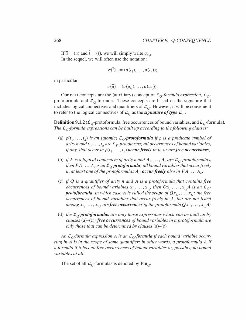
268 CHAPTER 9. -CONSEQUENCE
If u = (u) and t = (t), we will simply write �u∖t.In the sequel, we will often use the notation:
�(t) ∶= (�(t1),… , �(tn));
in particular,�(u) = (�(ui1),… , �(uin)).
Our next concepts are the (auxiliary) concept of -formula expression, -protoformula and -formula. These concepts are based on the signature thatincludes logical connectives and quantifiers of . However, it will be convenientto refer to the logical connectives of as the signature of type F .
Definition 9.1.2 (-protoformula, free occurrences of bound variables, and-formula).The -formula expressions can be built up according to the following clauses:
(a) p(t1,… , tn) is an (atomic) -protoformula if p is a predicate symbol ofarity n and t1,… , tn are T -prototerms; all occurrences of bound variables,if any, that occur in p(t1,… , tn) occur freely in it, or are free occurrences;
(b) if F is a logical connective of arity n and A1,… , An are -protoformulas,thenFA1 …An is an-protoformula; all bound variables that occur freelyin at least one of the protoformulasAi, occur freely also in FA1 …An;
(c) if Q is a quantifier of arity n and A is a protoformula that contains freeoccurrences of bound variables xi1,… , xin, then Qxi1,… , xinA is an -protoformula, in which case A is called the scope of Qxi1 ,… , xin; the freeoccurrences of bound variables that occur freely in A, but are not listedamong xi1 ,… , xin, are free occurrences of the protoformulaQxi1,… , xinA;
(d) the -protoformulas are only those expressions which can be built up byclauses (a)–(c); free occurrences of bound variables in a protoformula areonly those that can be determined by clauses (a)–(c).
An -formula expression A is an -formula if each bound variable occur-ring in A is in the scope of some quantifier; in other words, a protoformula A ifa formula if it has no free occurrences of bound variables or, possibly, no boundvariables at all.
The set of all -formulas is denoted by Fm.
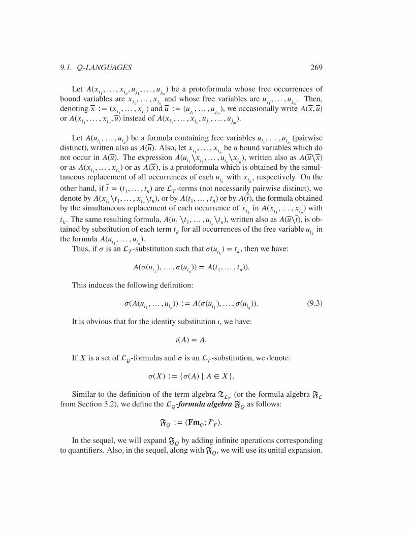
9.1. -LANGUAGES 269
Let A(xi1 ,… , xin, uj1 ,… , ujm) be a protoformula whose free occurrences ofbound variables are xi1,… , xin and whose free variables are uj1 ,… , ujm. Then,denoting x ∶= (xi1 ,… , xin) and u ∶= (uj1 ,… , ujm), we occasionally write A(x, u)or A(xi1 ,… , xin, u) instead of A(xi1 ,… , xin, uj1 ,… , ujm).
Let A(ui1 ,… , uin) be a formula containing free variables ui1 ,… , uin (pairwisedistinct), written also as A(u). Also, let xi1,… , xin be n bound variables which donot occur in A(u). The expression A(ui1∖xi1 ,… , uin∖xin), written also as A(u∖x)or as A(xi1 ,… , xin) or as A(x), is a protoformula which is obtained by the simul-taneous replacement of all occurrences of each uik with xik , respectively. On the
other hand, if t = (t1,… , tn) are T -terms (not necessarily pairwise distinct), wedenote by A(xi1∖t1,… , xin∖tn), or by A(t1,… , tn) or by A(t), the formula obtainedby the simultaneous replacement of each occurrence of xik in A(xi1 ,… , xin) with
tk. The same resulting formula, A(ui1∖t1,… , uin∖tn), written also as A(u∖t), is ob-tained by substitution of each term tk for all occurrences of the free variable uik inthe formula A(ui1 ,… , uin).
Thus, if � is an T -substitution such that �(uik) = tk, then we have:
A(�(ui1),… , �(uin)) = A(t1,… , tn)).
This induces the following definition:
�(A(ui1 ,… , uin)) ∶= A(�(ui1 ),… , �(uin)). (9.3)
It is obvious that for the identity substitution �, we have:
�(A) = A.
If X is a set of -formulas and � is an T -substitution, we denote:
�(X) ∶= {�(A) | A ∈ X}.
Similar to the definition of the term algebra TT(or the formula algebra F
from Section 3.2), we define the -formula algebra FQ as follows:
FQ ∶= ⟨Fm;F ⟩.In the sequel, we will expand FQ by adding infinite operations corresponding
to quantifiers. Also, in the sequel, along with FQ, we will use its unital expansion.
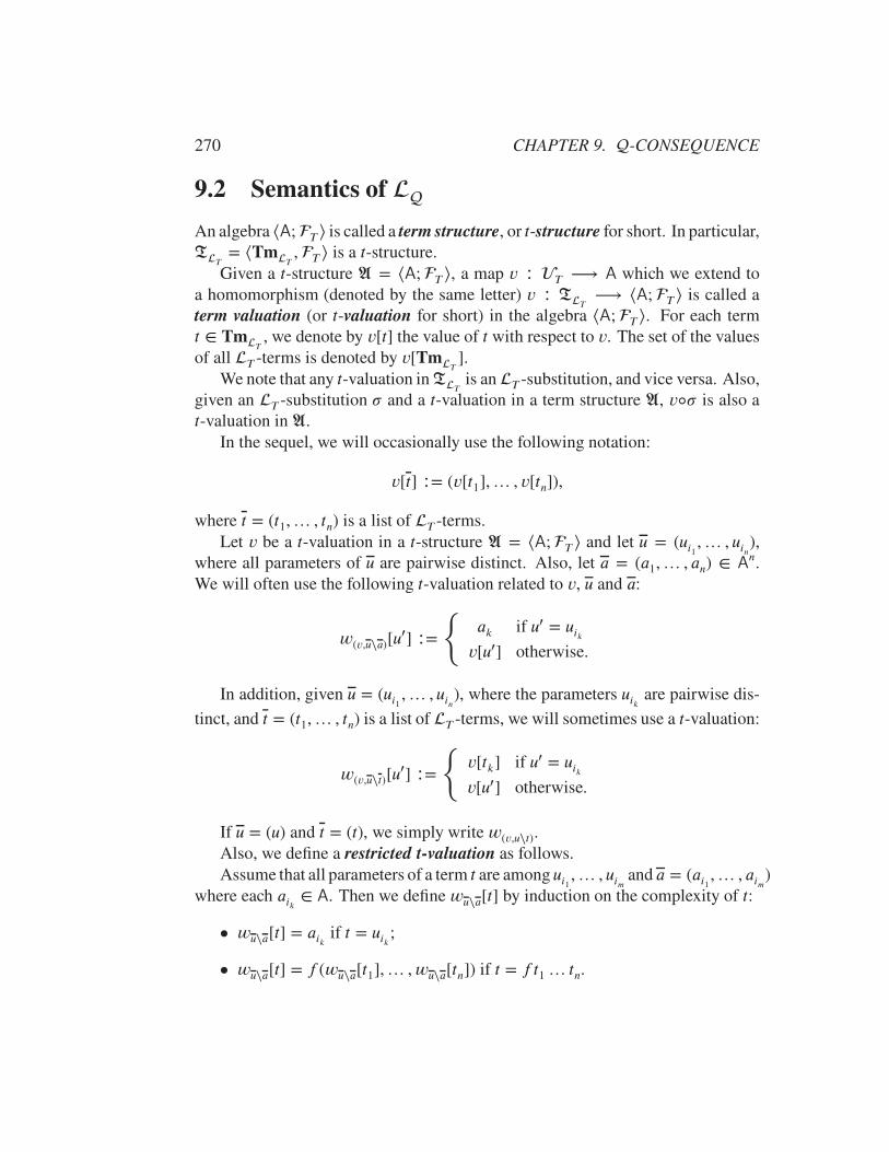
270 CHAPTER 9. -CONSEQUENCE
9.2 Semantics of
An algebra ⟨A;T ⟩ is called a term structure, or t-structure for short. In particular,TT
= ⟨TmT,T ⟩ is a t-structure.
Given a t-structure A = ⟨A;T ⟩, a map v ∶ T ⟶ A which we extend toa homomorphism (denoted by the same letter) v ∶ TT
⟶ ⟨A;T ⟩ is called aterm valuation (or t-valuation for short) in the algebra ⟨A;T ⟩. For each termt ∈ TmT
, we denote by v[t] the value of t with respect to v. The set of the valuesof all T -terms is denoted by v[TmT
].We note that any t-valuation in TT
is an T -substitution, and vice versa. Also,given an T -substitution � and a t-valuation in a term structure A, v◦� is also at-valuation in A.
In the sequel, we will occasionally use the following notation:
v[t] ∶= (v[t1],… , v[tn]),
where t = (t1,… , tn) is a list of T -terms.Let v be a t-valuation in a t-structure A = ⟨A;T ⟩ and let u = (ui1 ,… , uin),
where all parameters of u are pairwise distinct. Also, let a = (a1,… , an) ∈ An.We will often use the following t-valuation related to v, u and a:
w(v,u∖a)[u′] ∶=
{ak if u′ = uikv[u′] otherwise.
In addition, given u = (ui1 ,… , uin), where the parameters uik are pairwise dis-
tinct, and t = (t1,… , tn) is a list of T -terms, we will sometimes use a t-valuation:
w(v,u∖t)[u′] ∶=
{v[tk] if u′ = uikv[u′] otherwise.
If u = (u) and t = (t), we simply write w(v,u∖t).Also, we define a restricted t-valuation as follows.Assume that all parameters of a term t are among ui1 ,… , uim and a = (ai1 ,… , aim)
where each aik ∈ A. Then we define wu∖a[t] by induction on the complexity of t:
• wu∖a[t] = aik if t = uik;
• wu∖a[t] = f (wu∖a[t1],… , wu∖a[tn]) if t = ft1 … tn.
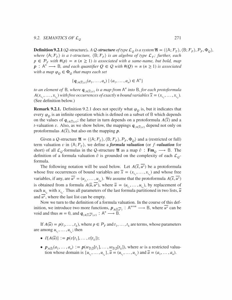
9.2. SEMANTICS OF 271
Definition 9.2.1 (-structure). A-structure of type is a systemA = ⟨⟨A;T ⟩, ⟨B;F ⟩,F ,Φ⟩,where ⟨A;T ⟩ is a t-structure, ⟨B;F ⟩ is an algebra of type F ; further, eachp ∈ F with #(p) = n (n ≥ 1) is associated with a same-name, but bold, mapp ∶ An
⟶ B, and each quantifier Q ∈ with #(Q) = n (n ≥ 1) is associatedwith a map 'Q ∈ Φ that maps each set
{q(A(x),v)(a1,… , an) | (a1,… , an) ∈ An}
to an element of B, where q(A(x),v) is a map from An into B, for each protoformulaA(xi1 ,… , xin) with free occurrences of exactly n bound variables x = (xi1 ,… , xin).(See definition below.)
Remark 9.2.1. Definition 9.2.1 does not specify what 'Q is, but it indicates thatevery 'Q is an infinite operation which is defined on a subset of B which dependson the values of q(A(x),v); the latter in turn depends on a protoformula A(x) and at-valuation v. Also, as we show below, the mappings q(A(x),v) depend not only onprotoformulas A(x), but also on the mapping p.
Given a -structure A = ⟨⟨A;T ⟩, ⟨B;F ⟩,F ,Φ⟩ and a (restricted or full)term valuation v in ⟨A;T ⟩, we define a formula valuation (or f -valuation forshort) of all -formulas in the -structure A as a map v ∶ Fm ⟶ B. Thedefinition of a formula valuation v is grounded on the complexity of each -formula.
The following notation will be used below. Let A(x, u∗) be a protoformulawhose free occurrences of bound variables are x = (xi1 ,… , xin) and whose free
variables, if any, are u∗ = (uj1 ,… , ujm). We assume that the protoformula A(x, u∗)
is obtained from a formula A(u, u∗), where u = (ui1 ,… , uin), by replacement ofeach uik with xik . Thus all parameters of the last formula partitioned in two lists, u
and u∗, where the last list can be empty.Now we turn to the definition of a formula valuation. In the course of this def-
inition, we introduce two more functions, pA(u,u∗) ∶ An+m⟶ B, where u∗ can be
void and thus m = 0, and q(A(x,u∗),v) ∶ An⟶ B.
IfA(u) = p(t1,… , tk), where p ∈ F and t1,… , tk are terms, whose parametersare among ui1 ,… , uin; then
• v[A(u)] ∶= p(v[t1],… , v[tk]);
• pA(u)(a1,… , an) ∶= p(wu∖a[t1],… , wu∖a[tk]), where w is a restricted valua-tion whose domain is {ui1,… , uin}, u = (ui1 ,… , uin) and a = (a1,… , an).
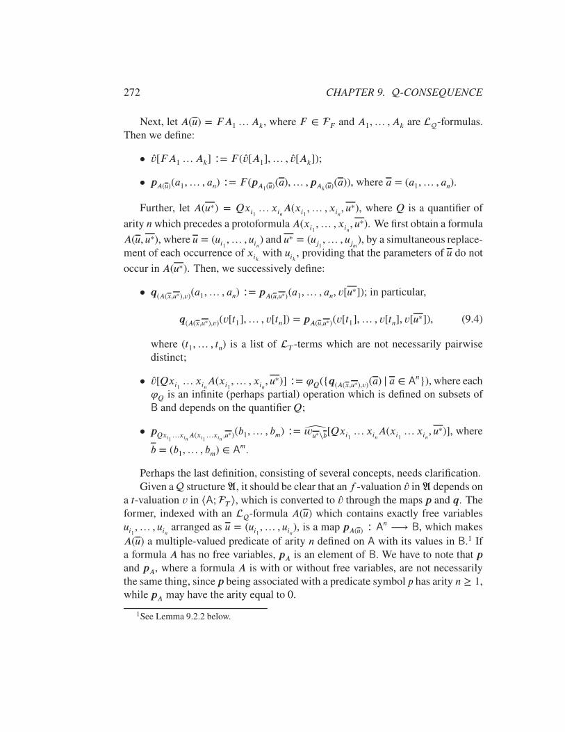
272 CHAPTER 9. -CONSEQUENCE
Next, let A(u) = FA1 …Ak, where F ∈ F and A1,… , Ak are -formulas.Then we define:
• v[FA1 …Ak] ∶= F (v[A1],… , v[Ak]);
• pA(u)(a1,… , an) ∶= F (pA1(u)(a),… , pAk(u)(a)), where a = (a1,… , an).
Further, let A(u∗) = Qxi1 … xinA(xi1 ,… , xin, u∗), where Q is a quantifier of
arity nwhich precedes a protoformulaA(xi1 ,… , xin, u∗). We first obtain a formula
A(u, u∗), where u = (ui1 ,… , uin) and u∗ = (uj1 ,… , ujm), by a simultaneous replace-ment of each occurrence of xik with uik , providing that the parameters of u do not
occur in A(u∗). Then, we successively define:
• q(A(x,u∗),v)(a1,… , an) ∶= pA(u,u∗)(a1,… , an, v[u∗]); in particular,
q(A(x,u∗),v)(v[t1],… , v[tn]) = pA(u,u∗)(v[t1],… , v[tn], v[u∗]), (9.4)
where (t1,… , tn) is a list of T -terms which are not necessarily pairwisedistinct;
• v[Qxi1 … xinA(xi1 ,… , xin, u∗)] ∶= 'Q({q(A(x,u∗),v)(a) | a ∈ An}), where each
'Q is an infinite (perhaps partial) operation which is defined on subsets ofB and depends on the quantifier Q;
• pQxi1…xinA(xi1…xin ,u∗)(b1,… , bm) ∶= wu∗∖b[Qxi1 … xinA(xi1 … xin, u
∗)], where
b = (b1,… , bm) ∈ Am.
Perhaps the last definition, consisting of several concepts, needs clarification.Given a structure A, it should be clear that an f -valuation v in A depends on
a t-valuation v in ⟨A;T ⟩, which is converted to v through the maps p and q. Theformer, indexed with an -formula A(u) which contains exactly free variablesui1 ,… , uin arranged as u = (ui1 ,… , uin), is a map pA(u) ∶ An
⟶ B, which makesA(u) a multiple-valued predicate of arity n defined on A with its values in B.1 Ifa formula A has no free variables, pA is an element of B. We have to note that pand pA, where a formula A is with or without free variables, are not necessarilythe same thing, since p being associated with a predicate symbol p has arity n ≥ 1,while pA may have the arity equal to 0.
1See Lemma 9.2.2 below.

9.2. SEMANTICS OF 273
A map q(A(x,u∗),v), where A(x, u∗) is a protoformula with free occurrences ofexactly one bound variable x and v is a t-valuation, is needed to generate the set{q(A(x,u∗),v)(a) | a ∈ A} ⊆ B, to which each of infinite unary operations, '∀ and '∃,
applies to obtain in B the values v[∀xA(x, u∗)] or v[∃xA(x, u∗)], respectively.
Remark 9.2.2. Although p in general depends on the carriers A and B, we usethe same notation, p, for the except of the cases when A = TmT
and B is Fm
or a quotient of the latter; in the first of the last cases, we use the notation pL
(defined in Example 9.2.1 below), and in the second pLT (defined in Section 9.5).Accordingly, we employ the notations: pL
A(u)and qL
(A(x,u∗),v)in the first case and
pLT
A(u), and qLT
(A(x,u∗),v)in the second case.
Now we consider some properties pertaining to formula valuations. The nextlemma is a refinement of a definition above.
Lemma 9.2.1. Let (A(u, u∗) be a formula whose parameters are partitioned in a listu = (ui1 ,… , uin) and a list (maybe empty) u∗ = (uj1 ,… , ujm). Let a = (a1,… , an)be an element of An. Then
pA(u,u∗)(a1,… , an, v[u∗]) = p(A(u,u∗)(w(v,u∖a)[u], w(v,u∖a)[u∗]).
Proof is left to the reader. (Exercise 9.2.2)
Lemma 9.2.2. Let A(u) be a formula, whose free variables are u = (ui1 ,… , uin).Then for any t-valuation v in an arbitrary -structure,
v[A(u)] = pA(u)(v[u]).
Proof. We use induction on the complexity of A(u). We will consider the basiscase, leaving the rest of the proof to the reader. (Exercise 9.2.3)
Assume that A(u) = p(t1(u),… , tk(u)), where t1,… , tk are T -terms whose(free) variables are included in u. By definition,
v[A(u)] = p(v[t1],… , v[tk]) = p(A(u),v)(v[t1],… , v[tk]).
Lemma 9.2.3. Let A(u) be a formula, whose free variables are u = (ui1 ,… , uin),and let � be an T -substitution. Then for any t-valuation v in any -structure,
v◦�[A(u)] = v[�(A(u))] = v[A(�(u)].
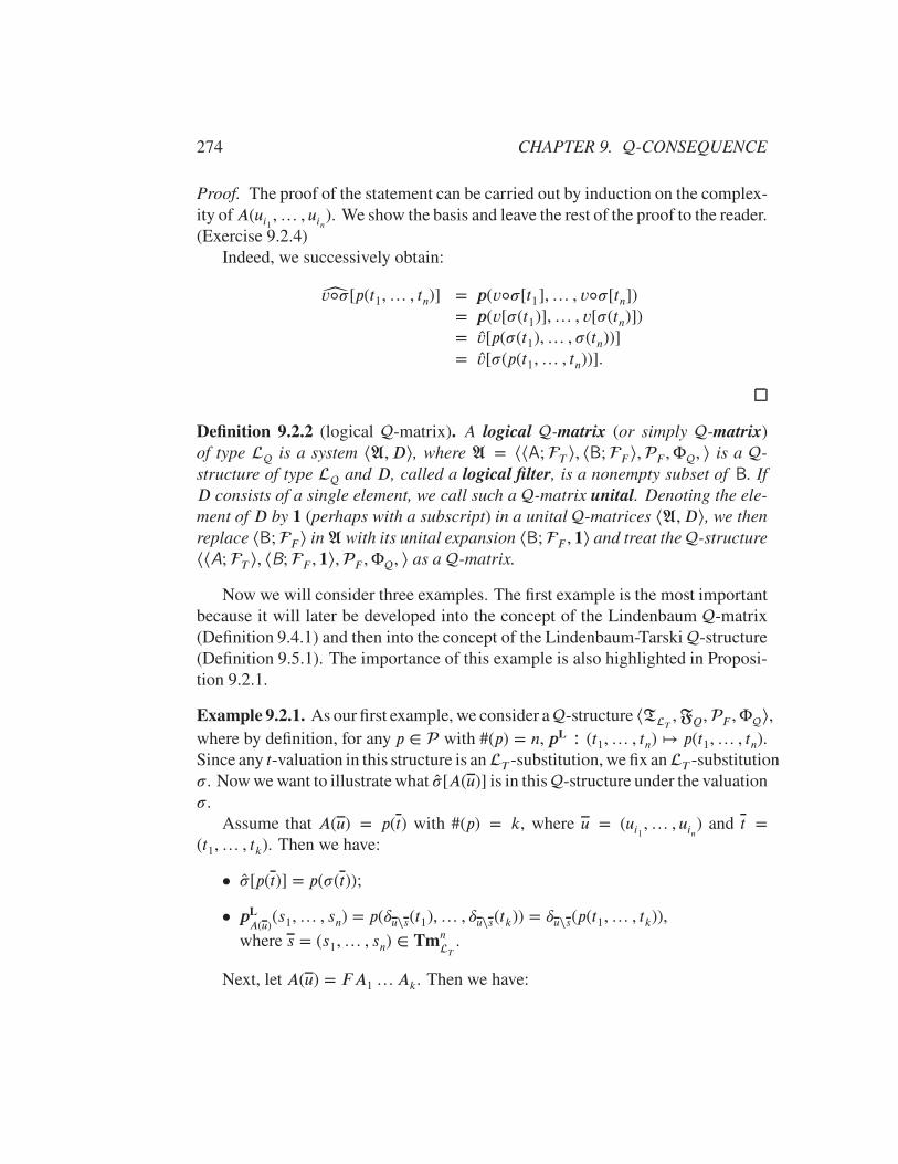
274 CHAPTER 9. -CONSEQUENCE
Proof. The proof of the statement can be carried out by induction on the complex-ity ofA(ui1 ,… , uin). We show the basis and leave the rest of the proof to the reader.(Exercise 9.2.4)
Indeed, we successively obtain:
v◦�[p(t1,… , tn)] = p(v◦�[t1],… , v◦�[tn])= p(v[�(t1)],… , v[�(tn)])= v[p(�(t1),… , �(tn))]= v[�(p(t1,… , tn))].
Definition 9.2.2 (logical -matrix). A logical -matrix (or simply -matrix)
of type is a system ⟨A, D⟩, where A = ⟨⟨A;T ⟩, ⟨B;F ⟩,F ,Φ, ⟩ is a -structure of type and D, called a logical filter, is a nonempty subset of B. IfD consists of a single element, we call such a -matrix unital. Denoting the ele-ment of D by 1 (perhaps with a subscript) in a unital -matrices ⟨A, D⟩, we thenreplace ⟨B;F ⟩ in A with its unital expansion ⟨B;F , 1⟩ and treat the -structure⟨⟨A;T ⟩, ⟨B;F , 1⟩,F ,Φ, ⟩ as a -matrix.
Now we will consider three examples. The first example is the most importantbecause it will later be developed into the concept of the Lindenbaum -matrix(Definition 9.4.1) and then into the concept of the Lindenbaum-Tarski -structure(Definition 9.5.1). The importance of this example is also highlighted in Proposi-tion 9.2.1.
Example 9.2.1. As our first example, we consider a-structure ⟨TT,FQ,F ,Φ⟩,
where by definition, for any p ∈ with #(p) = n, pL ∶ (t1,… , tn) ↦ p(t1,… , tn).Since any t-valuation in this structure is anT -substitution, we fix anT -substitution�. Now we want to illustrate what �[A(u)] is in this-structure under the valuation�.
Assume that A(u) = p(t) with #(p) = k, where u = (ui1 ,… , uin) and t =
(t1,… , tk). Then we have:
• �[p(t)] = p(�(t));
• pL
A(u)(s1,… , sn) = p(�u∖s(t1),… , �u∖s(tk)) = �u∖s(p(t1,… , tk)),
where s = (s1,… , sn) ∈ TmnT
.
Next, let A(u) = FA1 …Ak. Then we have:

9.2. SEMANTICS OF 275
• �[A(u)] = F (�[A1],… , �[Ak]);
• pL
A(u)(s1,… , sn) = F (pL
A1(u)(s),… , pL
Ak(u)(s));
Now, letA(u∗) = Qxi1 … xinA(xi1 ,… , xin, u∗) andA(u, u∗) be a formula, where
u = (ui1 ,… , uin) and u∗ = (uj1 ,… , ujm), such that neither of uik occurs in the
protoformula A(xi1 ,… , xin, u∗) and all uik are pairwise distinct. Then, defining
qL
(A(x,u∗),�)(s1,… , sn) ∶= pL
A(u,u∗)(s1,… , sn, �(u∗))
and
'Q({qL
(A(x,u∗),�)(s) | s ∈ Tm
nT}) ∶= �(Qxi1 … xinA(xi1 ,… , xin, u
∗)
= Qxi1 … xinA(xi1 ,… , xin, �(u∗)),
where 'Q ∈ Φ, we successively obtain:
• �[Qxi1 … xinA(xi1 ,… , xin, u∗)] = �(Qxi1 … xinA(xi1 ,… , xin, u
∗);
• pL
QxA(x,u∗)(t1,… , tm) ∶= �u∗∖t[QxA(x, u
∗)] = �u∗∖t(QxA(x, u∗)).
Summarizing the definitions and their simplifications of the last example, weobtain the following.
Proposition 9.2.1. Let � be anT -substitution,A(u) andB(u, u∗) be formulas suchthat u = (ui1 ,… , uin) is the list of all parameters of the former and the parameters of
the latter are partitioned in two lists — u and u∗ = (uj1 ,… , ujm) Then the followinghold in ⟨TT
,FQ,F ,Φ⟩:(a) �[A(u)] = �(A(u));(b) pL
B(u,u∗)(s1,… , sn, �(u∗)) = �(�,u∖s)(B(u, u∗));
(c) qL
(B(x,u∗),�)(s1,… , sn) = �(�,u∖s)(B(u, u∗)).
Proof. We leave for the reader to check the statement. (Exercise 9.2.6)
Example 9.2.2. Suppose an -language contains a nonempty set T of func-tion symbols, a nonempty set F of predicate symbols, the binary logical con-nectives: ∧,∨,→,¬, and two unary quantifiers, ∀ and ∃. Consider a -structure

276 CHAPTER 9. -CONSEQUENCE
A = ⟨⟨A;T ⟩, ⟨{0, 1}; ∧,∨,→,¬⟩,F , {'∀, '∃}⟩, where ⟨{0, 1}; ∧,∨,→⟩ is a 2-element Boolean algebra. Further, given a t-valuation v and a protoformulaA(x, u∗)containing free occurrences of only x, we define
'∀({q(A(x,u∗),v) | a ∈ A}) ∶=
{1 if {q(A(x,u∗),v) | a ∈ A} = A
0 otherwise,
and
'∃({q(A(x,u∗),v)(a) | a ∈ A}) ∶=
{1 if {q(A(x,u∗),v)(a) | a ∈ A} ≠ ∅
0 otherwise.
As a -matrix, we use the unital expansion ⟨{0, 1}; ∧,∨,→, 1⟩.It should be clear that the above maps '∀ and '∃ define the ordinary interpre-
tation of the universal and existential quantifier, respectively, in an -languageexemplifying that of firs-order logic.
The next example may seem artificial.2
Example 9.2.3. Suppose an -language, besides the mandatory categories, con-tains only one predicate symbol p of arity 3 and one binary quantifier Q. LetA = ⟨⟨ℤ+; ∅⟩, ⟨ℤ+; ∅⟩, {p}, {'Q}⟩, where ℤ+ is the set of positive integers, isa -structure for this language, where the predicate symbol p is interpreted asthe map p ∶ (a, b, c) ↦ gcd(a, b, c), where ‘gcd(a, b, c)’ stands for the greatestcommon divisor of a, b, c, and 'Q(X), if it is defined, is the maximal element ofX ⊆ ℤ+. It should be clear that the operation 'Q is partial. However, since the set
{q(p(x,y,u),v)(a, b) | (a, b) ∈ ℤ+ × ℤ+} = {p(a, b, v[u]) | (a, b) ∈ ℤ+ × ℤ+}
is always finite, for any t-valuation v,
v[Qxy p(x, y, u)] = 'Q({q(p(x,y,u),v)(a, b) | (a, b) ∈ ℤ+ × ℤ+}) = v[u].
More examples will be given in Section 9.6.
The vocabulary and contents of the next definition are similar to those of Def-inition 3.2.5.
2See a remark in (Rosser and Turquette, 1951), p. 51: “To the best of our knowledge, no onehas so far found need for quantifiers with either �i > 1 or i > 1. However, such quantifiers aredistinctly possible …”
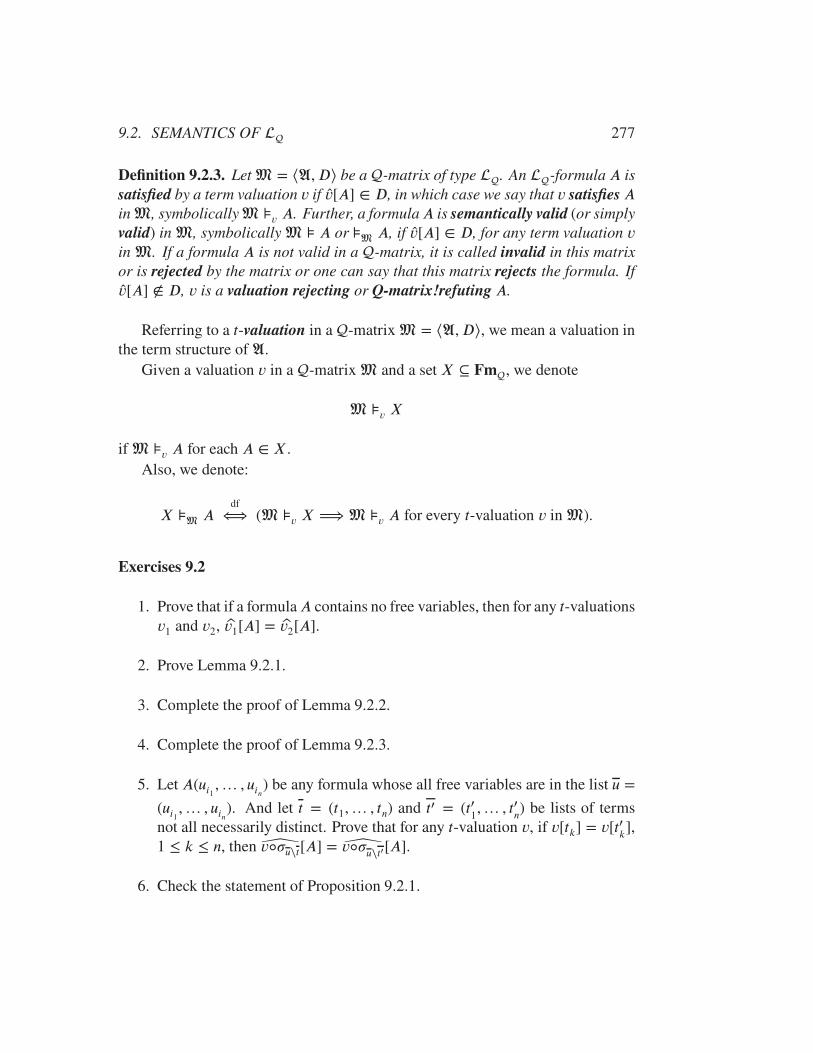
9.2. SEMANTICS OF 277
Definition 9.2.3. Let M = ⟨A, D⟩ be a -matrix of type . An -formula A issatisfied by a term valuation v if v[A] ∈ D, in which case we say that v satisfiesAin M, symbolicallyM ⊧v A. Further, a formulaA is semantically valid (or simplyvalid) in M, symbolically M ⊧ A or ⊧M A, if v[A] ∈ D, for any term valuation vin M. If a formula A is not valid in a -matrix, it is called invalid in this matrixor is rejected by the matrix or one can say that this matrix rejects the formula. Ifv[A] ∉ D, v is a valuation rejecting or Q-matrix!refuting A.
Referring to a t-valuation in a -matrix M = ⟨A, D⟩, we mean a valuation inthe term structure of A.
Given a valuation v in a -matrix M and a set X ⊆ Fm, we denote
M ⊧v X
if M ⊧v A for each A ∈ X.Also, we denote:
X ⊧M Adf
⟺ (M ⊧v X ⟹ M ⊧v A for every t-valuation v in M).
Exercises 9.2
1. Prove that if a formulaA contains no free variables, then for any t-valuationsv1 and v2, v1[A] = v2[A].
2. Prove Lemma 9.2.1.
3. Complete the proof of Lemma 9.2.2.
4. Complete the proof of Lemma 9.2.3.
5. Let A(ui1 ,… , uin) be any formula whose all free variables are in the list u =
(ui1 ,… , uin). And let t = (t1,… , tn) and t′ = (t′1,… , t′n) be lists of terms
not all necessarily distinct. Prove that for any t-valuation v, if v[tk] = v[t′k],1 ≤ k ≤ n, then v◦�u∖t[A] = v◦�u∖t′[A].
6. Check the statement of Proposition 9.2.1.
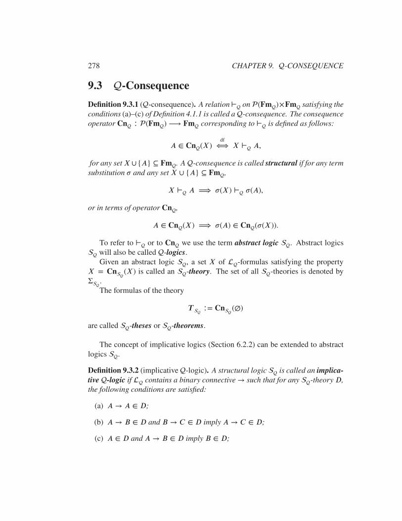
278 CHAPTER 9. -CONSEQUENCE
9.3 -Consequence
Definition 9.3.1 (-consequence). A relation⊢ on (Fm)×Fm satisfying theconditions (a)–(c) of Definition 4.1.1 is called a -consequence. The consequenceoperator Cn ∶ (Fm) ⟶ Fm corresponding to ⊢ is defined as follows:
A ∈ Cn(X)df
⟺ X ⊢ A,
for any setX ∪{A} ⊆ Fm. A -consequence is called structural if for any termsubstitution � and any set X ∪ {A} ⊆ Fm,
X ⊢ A ⟹ �(X) ⊢ �(A),
or in terms of operator Cn,
A ∈ Cn(X) ⟹ �(A) ∈ Cn(�(X)).
To refer to ⊢ or to Cn we use the term abstract logic . Abstract logics will also be called -logics.
Given an abstract logic , a set X of -formulas satisfying the propertyX = CnQ
(X) is called an -theory. The set of all -theories is denoted byΣ
.The formulas of the theory
T ∶= CnQ
(∅)
are called -theses or -theorems.
The concept of implicative logics (Section 6.2.2) can be extended to abstractlogics .
Definition 9.3.2 (implicative -logic). A structural logic is called an implica-
tive -logic if contains a binary connective → such that for any -theory D,the following conditions are satisfied:
(a) A→ A ∈ D;
(b) A→ B ∈ D and B → C ∈ D imply A→ C ∈ D;
(c) A ∈ D and A→ B ∈ D imply B ∈ D;

9.3. -CONSEQUENCE 279
(d) B ∈ D implies A → B ∈ D;
(e) if Ai → Bi ∈ D, Bi → Ai ∈ D, where 1 ≤ i ≤ n, and F is any n-aryconnective from F , then FA1 …An → FB1 …Bn ∈ D.
Given an abstract -logic , for any -theory D = CnQ(X), we define:
(A,B) ∈ �(X)
df⟺ A→ B and B → A ∈ D.
We denote:�
∶= �(∅).
Employing the argument used in the proof of Proposition 6.2.5, we obtain:
Proposition 9.3.1. Let D = CnQ(X) be a theory of an implicative -logic .
Then �(X) is a congruence on FQ and D is a congruence class with respect to
�(X).
Remark 9.3.1. From the point of view of Definition 6.2.1, the implicative-logicsare unital. We will not develop this concept for all structural -logics, but we willuse the property indicated in Proposition 9.3.1 for particular ones; see Section 9.6.
9.3.1 -consequence defined by -matrices
Let be a (nonempty) set of -matrices of type . For any set X ∪ {A} ⊆Fm, we define:
X ⊧ Adf
⟺ for any M ∈ and any valuation v in M,M ⊧v X implies M ⊧v A
(9.5)
Proposition 9.3.2. The relation ⊧ defined in (9.5) is a structural-consequence.
Proof. That the relation is a consequence relation can be obtained by applyingProposition 4.3.9 to -formulas and -matrices. Or this can be done directly;this last task is left to the reader. (Exercise 9.3.2) We prove below that ⊧Q isstructural.
Let A = ⟨⟨A;T ⟩, ⟨B;F ⟩,F ,, ⟩ be a -structure and ⟨A, D⟩ be an arbi-trary -matrix of . Also, assume that v is an arbitrary t-valuation and � is anarbitrary T -substitution. Since the former is a homomorphism v ∶ TT
⟶
⟨A,T ⟩ and the latter a homomorphism � ∶ TT⟶ TT
, the composition

280 CHAPTER 9. -CONSEQUENCE
v◦� ∶ TT⟶ ⟨A,T ⟩ is also a homomorphism; that is, the map v◦� is a term
valuation in ⟨A,T ⟩.Let us denote
v1 ∶= v◦�.
We recall that for any T -term t,
v1[t] = v[�(t)]. (∗)
(This can be proved by induction on the construction of term t; see Exercise 9.3.1.)In virtue of Lemma 9.2.3, the property (∗) further implies that for any -
formula A,v1[A] = v[�(A)] (∗∗)
Then the equality (∗∗) obviously implies that for any -formula A,
v1[A] ∈ D ⟺ v[�(A)] ∈ D.
The last equivalence in turn implies that the relation ⊧ is structural.
We call the consequence relation defined in (9.5)-consequence, for a givenclass of -matrices.
Given a -matrix M and an abstract logic , M is an -model if for any setX ∪ {A} ⊆ Fm,
X ⊢A ⟹ X ⊧M A.
9.3.2 -consequence defined via inference rules
In this subsection we limit ourselves with a formal language ∀∃ and its fragment(∀∃)+ ; the former has already been employed in Example 9.2.2. We recall that theset of the logical connectives of ∀∃ consists of binary connectives ∧,∨,→, and aunary connective¬; the language(∀∃)+ contains only the first three binary connec-tives. Also, both languages have only two unary quantifiers: ∀ and ∃. Thus, ∀∃ isan extension of (∀∃)+ . Since we will consider the formulas in these languages to-gether, it will be convenient to call the formulas of both languages ∀∃-formulas.With the last remark in mind, we denote by Fm∀∃ the set of all ∀∃-formulas. Un-specified∀∃-formulas will be denoted by lettersA,B, C (with indices or without).
We will consider three -consequence relations given by three different sets ofaxiom schemata. To do this, we reproduce the axiom schemata that first appearedin Section 4.3.5 and Section 4.4.4, provided that the metavariables are replaced
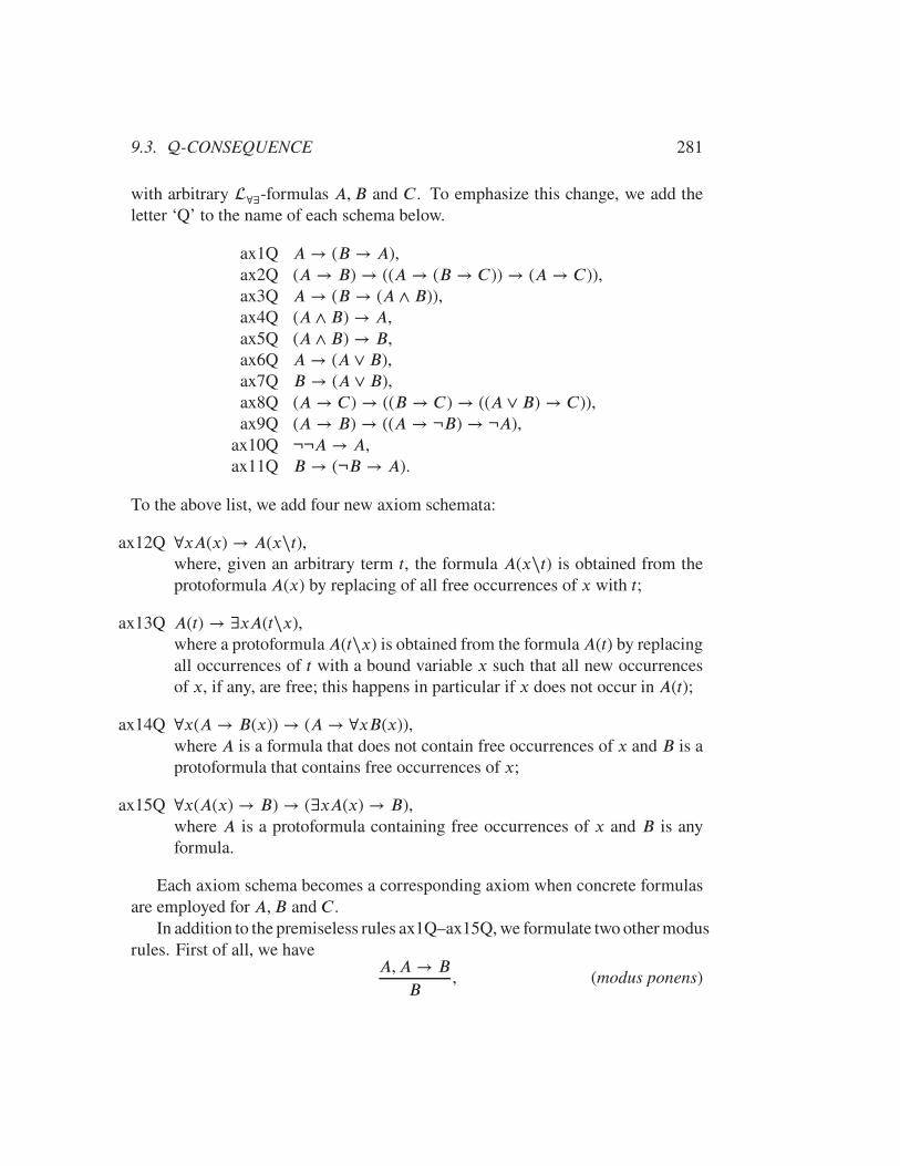
9.3. -CONSEQUENCE 281
with arbitrary ∀∃-formulas A,B and C . To emphasize this change, we add theletter ‘Q’ to the name of each schema below.
ax1Q A→ (B → A),ax2Q (A→ B) → ((A → (B → C)) → (A→ C)),ax3Q A→ (B → (A ∧ B)),ax4Q (A ∧ B) → A,ax5Q (A ∧ B) → B,ax6Q A→ (A ∨ B),ax7Q B → (A ∨ B),ax8Q (A→ C) → ((B → C) → ((A ∨ B) → C)),ax9Q (A→ B) → ((A → ¬B) → ¬A),
ax10Q ¬¬A→ A,ax11Q B → (¬B → A).
To the above list, we add four new axiom schemata:
ax12Q ∀xA(x) → A(x∖t),where, given an arbitrary term t, the formula A(x∖t) is obtained from theprotoformula A(x) by replacing of all free occurrences of x with t;
ax13Q A(t) → ∃xA(t∖x),where a protoformulaA(t∖x) is obtained from the formulaA(t) by replacingall occurrences of t with a bound variable x such that all new occurrencesof x, if any, are free; this happens in particular if x does not occur in A(t);
ax14Q ∀x(A→ B(x)) → (A→ ∀xB(x)),where A is a formula that does not contain free occurrences of x and B is aprotoformula that contains free occurrences of x;
ax15Q ∀x(A(x) → B) → (∃xA(x) → B),where A is a protoformula containing free occurrences of x and B is anyformula.
Each axiom schema becomes a corresponding axiom when concrete formulasare employed for A,B and C .
In addition to the premiseless rules ax1Q–ax15Q, we formulate two other modusrules. First of all, we have
A,A→ BB
, (modus ponens)

282 CHAPTER 9. -CONSEQUENCE
as well asA(u)
∀xA(u∖x), (9.6)
where a protoformula A(u∖x) is obtained from a formula A(u) by replacing all oc-currences of a free variable u with a bound variable x which does not occur freelyin A(u) and all new occurrences of x in A(u∖x) are free.
The concept of derivation in calculi based on the axiom schemata ax1Q–ax15Qand rules modus ponens and (9.6) is slightly different from what was discussed inSection 4.3.5. We will consider three types of derivation, all of which are basedon one and the same scheme. They differ only in what axiom schemata from theabove list can be employed. We use a notation ‘CQ’ to denote one of the threecalculi which we are going to deal with in this chapter:
• a calculus PQ is formulated in (∀∃)+ and is based on the use of the schemataax1Q–ax8Q and ax12Q–ax15Q;
• a calculus ClQ is in the language ∀∃ and is based on the use of the schemataax1Q–ax10Q and ax12Q–ax15Q;
• a calculus IntQ is also in ∀∃ and uses the schemata ax1–ax9Q, ax11Q andax12Q–ax15Q.
The fact of derivability, that is, the existence of a derivation of the correspond-ing type will be denoted by a binary relation ⊩CQ between a finite set (possiblyempty) of formulas and a formula. Thus, for any set X ∪ {A} ⋐ Fm∀∃, we defineX ⊩
CQ A to mean that there is a (nonempty) list of ∀∃-formulas
A1,… , An,
where the last formula,An, isA and each formula in the list is either fromX or oneof the axQ-axioms of CQ or can be obtained from two preceding formulas in thelist by modus ponens or, if A(u) is among preceding formulas and a free variableu does not occur in the formulas of X, by the rule (9.6). If X ⊩
CQ A, we say thatA is derivable from X in CQ. We call any such derivation a CQ-derivation.
Let X ⊩CQ A. Assume that there is a CQ-derivation whose free variables re-
lated to every application of (9.6) in this derivation constitute a finite list ui1 ,… , uinof pairwise distinct symbols of (9.2). We denote an arbitrary such derivation by
X ⊩CQ A ↾ {ui1 ,… , uin}.
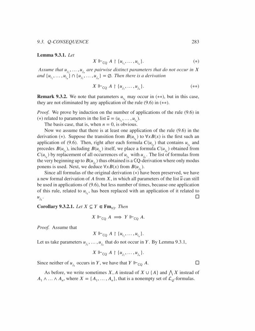
9.3. -CONSEQUENCE 283
Lemma 9.3.1. LetX ⊩
CQ A ↾ {ui1 ,… , uin}. (∗)
Assume that uj1 ,… , ujn are pairwise distinct parameters that do not occur in Xand {ui1,… , uin} ∩ {uj1 ,… , ujn} = ∅. Then there is a derivation
X ⊩CQ A ↾ {uj1 ,… , ujn}. (∗∗)
Remark 9.3.2. We note that parameters uik may occur in (∗∗), but in this case,they are not eliminated by any application of the rule (9.6) in (∗∗).
Proof. We prove by induction on the number of applications of the rule (9.6) in(∗) related to parameters in the list u = (ui1 ,… , uin).
The basis case, that is, when n = 0, is obvious.Now we assume that there is at least one application of the rule (9.6) in the
derivation (∗). Suppose the transition from B(uik) to ∀xB(x) is the first such anapplication of (9.6). Then, right after each formula C(uik) that contains uik andprecedes B(uik), including B(uik) itself, we place a formula C(ujk) obtained fromC(uik) by replacement of all occurrences of uik with ujk . The list of formulas fromthe very beginning up toB(ujk) thus obtained is a CQ-derivation where only modusponens is used. Next, we deduce ∀xB(x) from B(ujk).
Since all formulas of the original derivation (∗) have been preserved, we havea new formal derivation of A from X, in which all parameters of the list u can stillbe used in applications of (9.6), but less number of times, because one applicationof this rule, related to uik , has been replaced with an application of it related toujk .
Corollary 9.3.2.1. Let X ⊆ Y ⋐ Fm∀∃. Then
X ⊩CQ A ⟹ Y ⊩
CQ A.
Proof. Assume thatX ⊩
CQ A ↾ {ui1 ,… , uin}.
Let us take parameters uj1 ,… , ujn that do not occur in Y . By Lemma 9.3.1,
X ⊩CQ A ↾ {uj1 ,… , ujn}.
Since neither of ujk occurs in Y , we have that Y ⊩CQ A.
As before, we write sometimes X,A instead of X ∪ {A} and⋀X instead of
A1 ∧… ∧ An, where X = {A1,… , An}, that is a nonempty set of -formulas.

284 CHAPTER 9. -CONSEQUENCE
Lemma 9.3.2. For any finite set X ∪ {A,B} ⊆ Fm∀∃,
(X ⊩CQ A and X ⊩
CQ B) ⟹ X ⊩CQ A ∧ B.
Proof. Suppose we have:
X ⊩CQ A ↾ {ui1 ,… , uin} and X ⊩
CQ B ↾ {uj1 ,… , ujm}.
Applying Lemma 9.3.1 to each of the two last CQ-derivations, we obtain:
X ⊩CQ A ↾ {u′i1 ,… , u′in} and X ⊩
CQ B ↾ {u′j1 ,… , u′jm}.
Without loss of generality, we can count that {[ui′1,… , u′in} ∩ {u′j1 ,… , u′jm} = ∅.
Then, if we take the concatenation of the last formal proofs and add to the resultinglist the axiom ax3Q, B → (A∧B) and A∧B, we obtain a CQ-derivation of A∧Bfrom X in CQ.
Lemma 9.3.3. For any nonempty finite set X ⊆ Fm∀∃, X ⊩CQ
⋀X.
Proof. We prove by induction on the number of formulas in X. If X consists ofone formula, then the conclusion is obvious.
Suppose X = Y ∪ {A}, where Y ≠ ∅. By induction hypothesis, Y ⊩CQ
⋀Y
and hence Y , A ⊩CQ
⋀Y . On the other hand, it is obvious that Y , A ⊩
CQ A.Applying Lemma 9.3.2, we receive that X ⊩
CQ
⋀Y ∧A.
The next lemma is similar to Lemma 6.3.4.
Lemma 9.3.4 (deduction theorem). For any set X ∪ {A,B} ⊆ Fm∀∃,
X,A ⊩CQ B ⟹ X ⊩
CQ A→ B.
Proof. In the proof of this lemma, we use the argument given in the proof ofLemma 6.3.4. Indeed, the first steps of the both proofs are the same, until, inthis proof, we arrive at the consideration when in a given derivation a formula∀xAk(u∖x) is obtained from a preceding formula Ak(u), where a parameter u doesnot occur in X,A. Then, by induction hypothesis, X ⊩
CQ A → Ak(u). Apply-ing (9.6), we get that X ⊩
CQ ∀x(A → Ak(u∖x)). Applying modus ponens to thelast formula and ax14Q, we derive that X ⊩
CQ A→ ∀xAk(u∖x)).
Lemma 9.3.5. For any finite nonempty set X ⊆ Fm∀∃ and a formula A,
X ⊩CQ A ⟺⊩
CQ
⋀X → A.
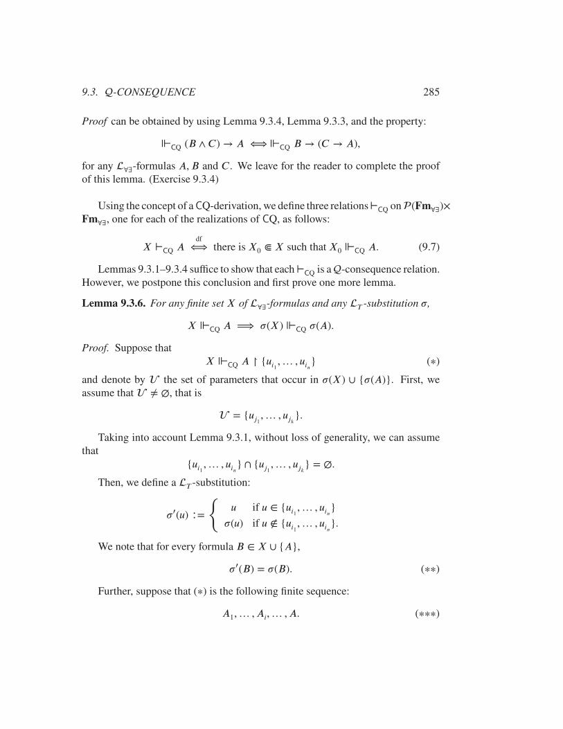
9.3. -CONSEQUENCE 285
Proof can be obtained by using Lemma 9.3.4, Lemma 9.3.3, and the property:
⊩CQ (B ∧ C) → A ⟺⊩
CQ B → (C → A),
for any ∀∃-formulas A,B and C . We leave for the reader to complete the proofof this lemma. (Exercise 9.3.4)
Using the concept of a CQ-derivation, we define three relations⊢CQ on(Fm∀∃)×
Fm∀∃, one for each of the realizations of CQ, as follows:
X ⊢CQ A
df⟺ there is X0 ⋐ X such that X0 ⊩CQ A. (9.7)
Lemmas 9.3.1–9.3.4 suffice to show that each⊢CQ is a-consequence relation.
However, we postpone this conclusion and first prove one more lemma.
Lemma 9.3.6. For any finite set X of ∀∃-formulas and any T -substitution �,
X ⊩CQ A ⟹ �(X) ⊩
CQ �(A).
Proof. Suppose thatX ⊩
CQ A ↾ {ui1 ,… , uin} (∗)
and denote by the set of parameters that occur in �(X) ∪ {�(A)}. First, weassume that ≠ ∅, that is
= {uj1 ,… , ujk}.
Taking into account Lemma 9.3.1, without loss of generality, we can assumethat
{ui1 ,… , uin} ∩ {uj1 ,… , ujk} = ∅.
Then, we define a T -substitution:
�′(u) ∶=
{u if u ∈ {ui1 ,… , uin}
�(u) if u ∉ {ui1 ,… , uin}.
We note that for every formula B ∈ X ∪ {A},
�′(B) = �(B). (∗∗)
Further, suppose that (∗) is the following finite sequence:
A1,… , Ai,… , A. (∗∗∗)

286 CHAPTER 9. -CONSEQUENCE
Let us consider the sequence:
�′(A1),… , �′(Ai),… , �′(A). (∗∗∗∗)
We aim to show that (∗∗∗∗) is a CQ-derivation of �(A) from �(X). In view of theremark (∗∗) above, it suffices to show that (∗∗∗∗) is a CQ-derivation.
Indeed, let �′(Ai) of (∗∗∗∗) is obtained from Ai of (∗∗∗). We consider herethe two main cases: when Ai is obtained from Ak and Ak → Ai by modus ponensand when Ai = ∀xB(u∖x) and B(u) precedes Ai in (∗∗∗) (in which case u ∈
{ui1 ,… , uin}).The first case is obvious and we turn to the second. We notice that the param-
eter u occurs in �′(B(u)) and does not occur in �′(X). Therefore,
∀x�′(B(u))(u∖x) = �′(∀xB(u∖x)).
Finally, we arrive at the main conclusion of this section.
Proposition 9.3.3. Each ⊢CQ is a finitary structural -consequence relation. In
addition, each CQ is an implicative -logic.
Proof. The main task is obviously to prove that the property (c) of Definition 4.1.1holds for ⊢
CQ.To do this, assume that for some sets X, Y and Z of -formulas, X ⊢CQ B,
for all formulas B ∈ Y , where Y ≠ ∅, and Y ,Z ⊢CQ A. By definition, we first
have thatY0, Z0 ⊩CQ A ↾ {ui1 ,… , uin}
for some Y0 ∪Z0 ⋐ Fm∀∃, where Y0 is assumed to be unequal to ∅.We denote
Y0 ∶= {B1,… , Bk}.
By premise, we have that
X1 ⊩CQ B1,… , Xn ⊩CQ Bk,
where X1 ∪… ∪Xk ⋐ X. Apply Lemma 9.3.1, we first obtain that
X1 ∪… ∪Xn ⊩CQ B1,… , X1 ∪… ∪Xk ⊩CQ Bk.
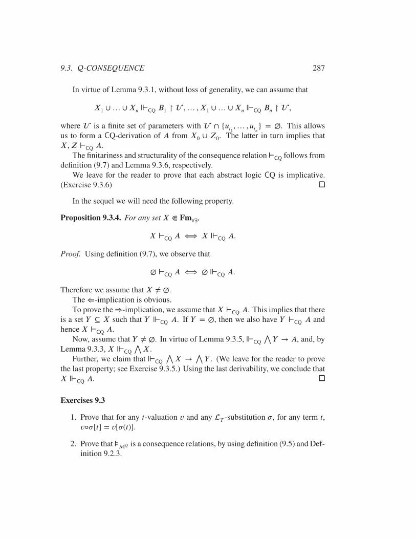
9.3. -CONSEQUENCE 287
In virtue of Lemma 9.3.1, without loss of generality, we can assume that
X1 ∪… ∪Xn ⊩CQ B1 ↾ ,… , X1 ∪… ∪Xn ⊩CQ Bn ↾ ,
where is a finite set of parameters with ∩ {ui1 ,… , uin} = ∅. This allowsus to form a CQ-derivation of A from X0 ∪ Z0. The latter in turn implies thatX,Z ⊢
CQ A.The finitariness and structurality of the consequence relation⊢CQ follows from
definition (9.7) and Lemma 9.3.6, respectively.We leave for the reader to prove that each abstract logic CQ is implicative.
(Exercise 9.3.6)
In the sequel we will need the following property.
Proposition 9.3.4. For any set X ⋐ Fm∀∃,
X ⊢CQ A ⟺ X ⊩
CQ A.
Proof. Using definition (9.7), we observe that
∅ ⊢CQ A ⟺ ∅ ⊩
CQ A.
Therefore we assume that X ≠ ∅.The ⇐-implication is obvious.To prove the ⇒-implication, we assume thatX ⊢
CQ A. This implies that thereis a set Y ⊆ X such that Y ⊩
CQ A. If Y = ∅, then we also have Y ⊢CQ A and
hence X ⊢CQ A.
Now, assume that Y ≠ ∅. In virtue of Lemma 9.3.5, ⊩CQ
⋀Y → A, and, by
Lemma 9.3.3, X ⊩CQ
⋀X.
Further, we claim that ⊩CQ
⋀X →
⋀Y . (We leave for the reader to prove
the last property; see Exercise 9.3.5.) Using the last derivability, we conclude thatX ⊩
CQ A.
Exercises 9.3
1. Prove that for any t-valuation v and any T -substitution �, for any term t,v◦�[t] = v[�(t)].
2. Prove that ⊧ is a consequence relations, by using definition (9.5) and Def-inition 9.2.3.
288 CHAPTER 9. -CONSEQUENCE
3. Complete the proof of Proposition 9.3.2, by proving that for any -formulaA, any t-valuation v and any T -substitution �, v◦�[A] = v[�(A)].
4. Complete the proof of Lemma 9.3.5
5. Suppose Y ⊆ X ⋐ Fm∀∃ and Y ≠ ∅. Then ⊩CQ
⋀X →
⋀Y ; moreover,
there is a derivation which does not use the axioms ax12Q–ax15Q and therule (9.6).
6. Prove that each logic CQ is implicative.
9.4 Lindenbaum -matrices
The -matrices we discuss in this section are based on the -structure of Exam-ple 9.2.1.
Definition 9.4.1 (Lindenbaum -matrix). Given an abstract logic Q, for any setX ⊆ Fm, we define a -matrix LinQ
[X] ∶= ⟨⟨TT,FQ,F ,Φ⟩,CnQ
(X)⟩,where for every p ∈ F with #(p) = n and any t1,… , tn ∈ TmT
, pL(t1,… , tn) =p(t1,… , tn); and the mappings pL
A(u), qL
(A(x,u∗))and 'Q are defined as in Exam-
ple 9.2.1. Each LinQ[X] is called a Lindenbaum -matrix for Q (relative to
X). We denote the Lindenbaum Q-matrix LinQ[∅] by LinQ
.
Reviewing Example 9.2.1, we conclude the following.
Proposition 9.4.1. Every LinQ[X] is a -matrix.
Proof is obvious and is left to the reader. (Exercise 9.4.1)
The next proposition is similar to Proposition 4.3.12.
Proposition 9.4.2. Let Q be a structural abstract -logic. Then LinQis an Q-
model. In addition, if X is closed under arbitrary term substitution, then for any-formula A,
X ⊢QA ⟺ LinQ
[X] ⊧ A;
in particular,A ∈ T Q
⟺ LinQ⊧ A.
9.4. LINDENBAUM -MATRICES 289
Proof. Suppose X ⊢QA and let � be any t-substitution. Since the logic Q
is structural, �(X) ⊢Q�(A), that is, �(A) ∈ CnQ
(�(X)). Thus, if �(X) ⊆CnQ
(∅), then, obviously, �(A) ∈ CnQ(∅). This shows that LinQ
is an Q-model.
Next, if X is closed under T -substitutions, then, in particular, �(X) ⊆ X.This implies that CnQ
(�(X)) ⊆ CnQ(X) and hence �(A) ∈ CnQ
(X).Conversely, assume that LinQ
[X] ⊧ A. Taking the identity T -substitution �,we have: A = �(A) ∈ CnQ
(X), that is, X ⊢QA.
The next definition is similar to Definition 4.3.2.
Definition 9.4.2. A (nonempty) family = {⟨A, Di⟩}i∈I of-matrices, which maydiffer by logical filters Di, is called a -bundle. A pair ⟨A, {Di}i∈I⟩, where eachDi is a logical filter in A, is called an -atlas. By definition, the -consequence
relative to an atlas ⟨A, {Di}i∈I⟩ is the same as the-consequence related the bun-dle {⟨A, Di⟩}i∈I , which in turn is defined according to (9.5). Given an abstractlogic , the bundle {⟨FQ, D⟩}D∈Σ
, where Σis the set of all -theories,
is called a Lindenbaum -bundle relative to and the atlas Lin[Σ
] ∶=
⟨FQ,Σ⟩, is called a Lindenbaum -atlas relative to .
According to the last definition and the main definition (9.5), for any set X ∪
{A} ⊆ Fm,
X ⊧Lin
[Σ] A ⟺ for any D ∈ Σ
and any T -substitution �,
if �(X) ⊆ D, then �(A) ∈ D.(9.8)
Proposition 9.4.3. Let be a structural -consequence. Then for any set X ∪
{A} ⊆ Fm,X ⊢Q
A ⟺ X ⊧Lin
[Σ] A.
Proof is similar to the proof of Proposition 4.3.13 and is left to the reader. (Exer-cise 9.4.2)
Exercises 9.4
1. Prove Proposition 9.4.1.
2. Prove Proposition 9.4.3.
290 CHAPTER 9. -CONSEQUENCE
9.5 Lindenbaum-Tarski -structures
Let be an arbitrary -logic. For any set X ⊆ Fm, we denote:
(A,B) ∈ �(X)
df⟺ (A,B) ∈ �(CnQ
(X)). (9.9)
Thus �(X) is a congruence on FQ. We employ the above definition when
is a unital -logic.
Definition 9.5.1 (Lindenbaum-Tarski -structure). Let be a unital-logic andX ⊆ Fm. A structure
LT[X] ∶= ⟨TT
, ⟨FQ∕�(X), 1D⟩,F ,⟩,
whereD = CnQ(X) and 1D isD understood as a congruence class with respect to
the congruence �(D) on FQ, is called Lindenbaum-Tarski -structure (of )
relative to D (or relative to X) if each p ∈ F with #(p) = n is associate with amap pLT ∶ (t1,… , tn) ↦ p(t1,… , tn)∕�
(X). Accordingly, for any t-substitution�, the value of a formula A(u) in LT
[X] under � is denoted by �X[A(u)] andis defined inductively on the complexity of this formula in the following way. IfA(u) = p(t) with #(p) = k, where u = (ui1 ,… , uin) and t = (t1,… , tk), then wehave:
• �X[p(t)] ∶= pL(�(t))∕�(X) = pLT(�(t));
• pLT
A(u)(s1,… , sn) ∶= pL(�u∖s(t))∕�
(X) = �u∖s(p(t))∕�(X),
where s = (s1,… , sn) ∈ TmnT
.
If A(u) = FA1 …Ak, then
• �X[A(u)] ∶= F (�[A1],… , �[Ak]) = �(A(u))∕�(X);
• pLT
A(u)(s) = F (pLT
A1(u)(s),… , pLT
Ak(u)(s));
and for any protoformula A(x, u∗), where x = (xi1 ,… , xin),
• qLT
(A(x,u∗),�)(s) ∶= pLT
A(u,u∗)(s, �(u∗));
and for any Q ∈ ,

9.5. LINDENBAUM-TARSKI -STRUCTURES 291
• 'Q({qLT
(A(x,u∗),�)(s) | s ∈ Tm
nT}) ∶= �(Qxi1 … xinA(xi1 ,… , xin, u
∗)∕�(X)
= Qxi1 … xinA(xi1 ,… , xin, �(u∗))∕�
(X).
• �X[Qxi1 … xinA(xi1 ,… , xin, u∗)] ∶= �[Qxi1 … xinA(x, u
∗)]∕�(X) = �(Qxi1 … xinA(x, u
∗))∕�(X);
• pLT
QxA(x,u∗)(t1,… , tm) ∶= �u∗∖t[QxA(x, u
∗)]∕�(X) = �u∗∖t(QxA(x, u
∗))∕�(X).
We will also use the notationsLT[D] for LT
[X] and 1[X] for 1D, where
D = CnQ(X), and LT
∶= LT[∅].
In the above definition, ⟨FQ∕�(X), 1D⟩ is a unital expansion of FQ∕�
(X).In the sequel, we treat LT
[X] as a -matrix
⟨⟨TT,FQ∕�
(D),F ,⟩, {1D}⟩.
Below, instead of �X , we occasionally write �D, whereD = CnQ(X). It is not
difficult to see that �X = �D. (Exercise 9.5.1)
Lemma 9.5.1. Let be a unital-logic andD be an-theory. Then �D satisfiesa formula A in LT
[D] if, and only if, A ∈ D.
Proof is left to the reader. (Exercise 9.5.2)
Similarly to Proposition 6.3.4, we prove the following.
Proposition 9.5.1. Let be a unital logic and D = CnQ(X). Then for any
-formula A, the following conditions are equivalent ∶
(a) X ⊢A;
(b) X ⊧LT
[D] A;
(c) �X[A] = 1D.
In particular, the following conditions are equivalent ∶
(a∗) A ∈ T ;
(b∗) �X[A] = 1T
, for any t-substitution �;
(c∗) �T
[A] = 1T
.

292 CHAPTER 9. -CONSEQUENCE
Proof. Suppose X ⊢A. Let � be an t-substitution. Assume that �X satisfies
in LT[D] every B ∈ X. This means that for every B ∈ X, �X[B] = 1D,
that is, �X[B] ∈ CnQ(X). In virtue of Proposition 9.2.1-a, for every B ∈ X,
�(B) ∈ CnQ(X), that is, �(X) ⊆ CnQ
(X). Since is structural (being unital),�(A) ∈ CnQ
(X). Hence �X satisfies A in LT[D].
To prove the implication (b)⇒(c), we use Lemma 9.5.1 to observe that �D sat-isfies every B ∈ X.
Now, assume that �D[A] = 1D, that is, �D[A]∕�(D) = 1D. In virtue of
Lemma 9.5.1, we conclude that A ∈ CnQ(X).
Exercises 9.5
1. Let D = CnQ(X). Show that �X = �D.
2. Let be a unital -logic and D be an -theory. Prove that �D valuates aformulaA in LT
[D] if, and only if, A ∈ D. (Hint: Use Proposition 9.2.1-a.)
9.6 Three -matrix consequences
In this section, we return to the languages ∀∃ and (∀∃)+ of Section 9.3.2. We usethese languages to further analyze the consequence relations ⊢
CQ, where C standsfor PQ, ClQ or IntQ. Therefore, it is convenient to denote the set of formulas,corresponding to a particular relation ⊢
CQ, by FmCQ and call the element of this
set CQ-formulas.Accordingly, we consider -structures of the following two forms:
i) ⟨⟨A;T ⟩, ⟨B; ∧,∨,→⟩,F , {'∀, '∃}⟩ii) ⟨⟨A;T ⟩, ⟨B; ∧,∨,→,¬⟩,F , {'∀, '∃}⟩. (9.10)
We call a structure of the first form a p-structure (or positive -structure),and that of the second form a a-structure (or assertoric -structure). Accord-ingly, we define the notions of p-matrix and a-matrix and, respectively, thenotions of unital p-matrix and unital a-matrix.
We denote byLinPQ[X], Lin
ClQ[X] andLinIntQ[X] the Lindenbaum-matrices
for PQ, ClQ, and IntQ, respectively; also, we employ the notation LinCQ[X] to re-
fer to one of these three types of Lindenbaum matrices. Accordingly, we denote
9.6. THREE -MATRIX CONSEQUENCES 293
the formula algebra associated with CQ by FCQ, that is,
FCQ ∶= ⟨Fm
CQ;CQ⟩,where
PQ ∶= {∧,∨,→} and ClQ =
IntQ ∶= {∧,∨,→,¬}. The set of terms isdenoted by Tm
CQ.
Proposition 9.6.1. Each abstract logic CQ is implicative and, therefore, is unital.
Proof. When the first statement is proved, we apply Proposition 6.2.5.To establish the first statement, it suffices to prove that: For any finite set Z,
• Z ⊩CQ A→ B and Z ⊩
CQ C → D imply Z ⊩CQ (A ∧ C) → (B ∧D)
and Z ⊩CQ (A ∨ C) → (B ∨D);
• Z ⊩CQ A→ B and Z ⊩
CQ B → C imply Z ⊩CQ A→ C; and
• if CQ = ClQ or CQ = IntQ, thenZ ⊩CQ A→ B impliesZ ⊩
CQ ¬B → ¬A.
We leave the task of proving these implications to the reader. (Exercise 9.6.2)
Using Proposition 9.3.3 and Corollary 6.2.5.1, we conclude that each CQ isunital.
Applying Proposition 9.6.1, Proposition 6.2.5 and Proposition 9.4.2, we obtainthe following.
Corollary 9.6.1.1. For the congruence �CQ(X) defined in (9.9), the following equiv-
alences hold:
(A,B) ∈ �CQ(X) ⟺ X ⊢
CQ A→ B and X ⊢CQ B → A,
⟺ LinCQ[X] ⊧ A→ B and Lin
CQ[X] ⊧ B → A.
We note thatX ⊆ Y ⟹ �
CQ(X) ⊆ �CQ(Y ). (9.11)
We denote:
LTCQ[X] ∶= ⟨TT
, ⟨FCQ∕�CQ(X), 1
CQ[X]⟩,F , {'∀, '∃}⟩.According to Definition 9.5.1, we have:
pLT ∶ (t1,… , tn) ↦ p(t1,… , tn)∕�CQ(X),
where (t1,… , tn) ∈ TmnT
and p ∈ F with #(p) = n. Also, specifically for ∀∃,according to this definition, for any t-substitution �, we have:First, if A(u) = p(t), where u = (ui1 ,… , uin) and all uik are pairwise distinct, then
294 CHAPTER 9. -CONSEQUENCE
• �X[p(t)] ∶= pLT(�(t)) = pL(�(t))∕�CQ(X) = p(�(t))∕�
CQ(X);
• pLT
A(u)(s1,… , sn) ∶= pL(�u∖s(t))∕�CQ(X) = �u∖s(p(t))∕�CQ(X),
where s = (s1,… , sn) ∈ TmnT
.
If A(u) = FA1 …Ak, then
• �X[A(u)] ∶= F (�X[A1],… , �X[Ak]) = �[A(u)]∕�CQ(X);
• pLT
A(u)(s) = F (pLT
A1(u)(s),… , pLT
Ak(u)(s));
and for any protoformula A(x, u∗) and s ∈ TmT,
• qLT
(A(x,u∗),�)(s) ∶= pLT
A(u,u∗)(s, �(u∗));
and for any Q ∈ {∀, ∃},
• 'Q({qLT
(A(x,u∗),�)(s) | s ∈ TmT
}) ∶= 'Q({qL
(A(x,u∗),�)(s) | s ∈ TmT
})∕�CQ(X) =
�(QxA(x, u∗))∕�CQ(X) = QxA(x, �(u∗))∕�
CQ(X);
• �X[QxA(x, u∗)] ∶= �[QxA(x, u∗)]∕�CQ(X) = �(QxA(x, u∗))∕�
CQ(X);
• pLT
QxA(x,u∗)(t1,… , tm) ∶= �u∗∖t[QxA(x, u
∗)]∕�CQ(X) = �u∗∖t(QxA(x, u
∗))∕�CQ(X).
Similarly to Proposition 9.2.1, we summarize the multiple definition above inthe following proposition
Proposition 9.6.2. Let � be an T - substitution, A(u) and B(u, u∗) be formulassuch that u = (ui1 ,… , uin) is the list of all parameters of the former and the pa-
rameters of the latter are partitioned in two lists — (u) and u∗ = (uj1 ,… , ujm) with
u ∉ u∗. Then the following hold in ⟨TT,F
CQ∕�CQ(X),F , {'∀, '∃}⟩:
(a) �X[A(u)] = �(A(u))∕�CQ(X);
(b) pLT
B(u,u∗)(s, �(u∗)) = �(�,u∖s)(B(u, u∗))∕�CQ(X);
(c) qLT
(B(x,u∗),�)(s) = �(�,u∖s)(B(u, u∗))∕�CQ(X).
9.6. THREE -MATRIX CONSEQUENCES 295
For the next proposition, we also need the following relation on FCQ∕�CQ(X).
A∕�CQ(X) ≤CQ B∕�CQ(X)df
⟺ X ⊢CQ A → B.
The soundness of ≤CQ can be easily shown. For this, one needs to prove that
if A∕�CQ(X) = C∕�
CQ(X) and B∕�CQ(X) = D∕�
CQ(X), then
X ⊢CQ A→ B ⟺ X ⊢
CQ C → D.
(Exercise 9.6.1)
Lemma 9.6.1. The relation ≤CQ is a partial order on ⟨F
CQ∕�CQ(X), 1CQ[X]⟩ so
that 1CQ[X] is a greatest element.
Proof. We prove that the relation ≤CQ is transitive and that 1
CQ[X] is a greatestelement.
Indeed, suppose A∕�CQ(X) ≤
CQ B∕�CQ(X) and B∕�
CQ(X) ≤CQ C∕�
CQ(X).By definition, it means that X ⊢CQ A → B and X ⊢CQ B → C , that is, for someX1, X2 ⋐ X,X1 ⊩CQ A→ B andX2 ⊩CQ B → C . In virtue of Corollary 9.3.2.1,X1 ∪X2 ⊩CQ A→ B and X1 ∪X2 ⊩CQ B → C . This implies that X1 ∪X2 ⊩CQ
A→ C . Hence X ⊢CQ A→ C .
Now, if A is an CQ-thesis, then for any formula B, ∅ ⊩ B → A. HenceB∕�
CQ(X) ≤CQ A∕�CQ(X). It remains to note that A∕�
CQ(X) = 1CQ[X].
Proposition 9.6.3. Let X ⊆ FmCQ. Then the following are true:
(a) A1 = ⟨FPQ∕�PQ(X), 1
PQ[X]⟩ is a relatively pseudo-complemented lattice;(b) A2 = ⟨F
ClQ∕�ClQ(X), 1ClQ[X]⟩ is a Boolean algebra, where x → y ∶= ¬x ∨ y;
(c) A3 = ⟨FIntQ∕�IntQ(X), 1
IntQ[X]⟩ is a Heyting algebra.
In addition, the relation ≤i defined in each Ai according to (2.7), or equivalentlyaccording to (2.8), coincides with the corresponding relation ≤
CQ. Moreover, ifthe set of parameters not occurring in the formulas of X is infinite, then for anyt-substitution � and any protoformulaA(x) with free occurrences of only x ∈ T ,both ⋀
{qLT
(A(x),�)(t) | t ∈ TmT} and
⋁{qLT
(A(x),�)(t) | t ∈ TmT}
exist, where⋀
and⋁
are the operations of a greatest lower bound and a least up-per bound, respectively, with respect to ≤
CQ in FCQ∕�CQ(X). Consequently, defin-
ing'∀ as⋀
and'∃ as⋁
in a-matrix ⟨TT, ⟨F
CQ∕�CQ(X), 1CQ[X]⟩,F , {'∀, '∃}⟩,
we have:�X[∀xA(x)] =
⋀{qLT
(A(x),�)(t) | t ∈ TmT} (9.12)

296 CHAPTER 9. -CONSEQUENCE
and�X[∃xA(x)] =
⋁{qLT
(A(x),�)(t) | t ∈ TmT}. (9.13)
Proof. Since the restriction of any Heyting algebra to the signature ⟨∧,∨,→⟩ isa relatively pseudo-complemented lattice and in view of that the sentential frag-ments of PQ,ClQ and IntQ are coincident, respectively, with P,Cl and Int, in virtueof Proposition 9.5.1, we observe that (a)–(c) above hold.
To show that the relation ≤CQ is coincident with the corresponding ≤i, weconsider the following equivalences:
A∕�CQ(X) ≤
CQ B∕�CQ(X) ⟺ X ⊢CQ A→ B
⟺ A→ B ∈ CnCQ(X)
⟺ A→ B∕�CQ(X) = 1CQ[X]
⟺ A∕�CQ(X) → B∕�
CQ(X) = 1CQ[X].
To prove (9.12) and (9.13), we fix a protoformula A(x, u∗) with free occur-rences of a single bound variable x and a finite list u∗ = (uj1 ,… , ujm) of all pa-
rameters that occur in this protoformula. Further, we consider a formula A(u, u∗)obtained from A(x, u∗) by replacing each free occurrence of x with a parameter u,providing that u does not occur in this protoformula.
In view of Proposition 9.6.2, we have:
qLT
(A(x,u∗),�)(t) = �(�,u∖t)[A(u, u∗)]∕�CQ(X) = A(t, �(u∗))∕�
CQ(X).
That is,
{qLT
(A(x,u∗),�)(t) | t ∈ TmT
} = {A(t, �(u∗))∕�CQ(X) | t ∈ TmT
}.
We recall that, in virtue of ax12Q,
⊩CQ ∀xA(x, �(u∗)) → A(t, �(u∗)),
for an arbitrary t ∈ TmT. Hence,
∀xA(x, �(u∗))∕�CQ(X) ≤
CQ A(t, �(u∗))∕�CQ(X).
On the other hand, assume that for some formula B,
X ⊢CQ B → A(t, �(u∗)),

9.6. THREE -MATRIX CONSEQUENCES 297
for any t ∈ TmT. In particular,
X ⊢CQ B → A(u′, �(u∗)),
where u is a parameter which occurs neither in X nor in B. This means that forsome set Y ⋐ X,
Y ⊩CQ B → A(u, �(u∗)).
We observe that u does not occur in the formulas of Y . Then, by the rule (9.6),
Y ⊩CQ ∀x(B → A(x, �(u∗)).
Applying modus ponens to the last formula and ax14Q, we derive that
Y ⊩CQ B → ∀xA(x, �(u∗)),
that is,X ⊢
CQ B → ∀xA(x, �(u∗)).
Hence,B∕�
CQ(X) ≤CQ ∀xA(x, �(u∗))∕�
CQ(X).
This completes the proof of (9.12). We leave for the reader to prove (9.13).(Exercise 9.6,3)
The last proposition induces the following definition.
Definition 9.6.1 (P-matrix,B-matrix, andH-matrix). A unitalp-matrix ⟨⟨A;T ⟩, ⟨B; ∧,∨,→, 1⟩,F , {'∀, '∃}⟩ is called a P-matrix if ⟨B; ∧,∨,→, 1⟩ is a relatively pseudo-complemented lattice, and for any t-valuation v in ⟨A;T ⟩ and any formulas∀xA(x, u)and ∃xA(x, u), both
⋀{q(A(x,u),v)(a, v[u]) | a ∈ A} and
⋁{q(A(x,u),v)(a, v[u]) | a ∈
A}, where⋀
is a greatest lower bound and⋁
is a least upper bound, exist so that'∀ and '∃ are defined as
⋀and
⋁, respectively.
A unital a-matrix ⟨⟨A;T ⟩, ⟨B; ∧,∨,→,¬, 1⟩,F , {'∀, '∃}⟩ is called a B-matrix if ⟨B; ∧,∨,→,¬, 1⟩, where x → y ∶= ¬x ∨ y, is a Boolean algebra; itis called a H-matrix if ⟨B; ∧,∨,→,¬, 1⟩ is a Heyting algebra, providing thatthe other conditions and definitions in the two last cases are the same as for P-matrices.
Referring collectively to each of these -matrices, we use the term C-matrix.

298 CHAPTER 9. -CONSEQUENCE
Thus, according to the definition of an f -valuation (Section 9.2), in all C-matrices, for any t-valuation v and protoformula A(x, u),
v[∀xA(x, u)] ∶=⋀
{q(A(x,u),v)(a, v[u]) | a ∈ A} (9.14)
andv[∃xA(x, u)] ∶=
⋁{q(A(x,u),v)(a, v[u]) | a ∈ A}. (9.15)
Corollary 9.6.3.1. Let X ⊆ Fm∀∃ such that the set of parameters not occurringin the formulas of X is infinite. Then each LT
CQ[X] is a C-matrix.
Definition 9.6.2 (logics P, B and H). Abstract logics P, B and H are de-fined as the consequence relations that are determined, respectively, by the classesof P-matrices, B-matrices, and H-matrices. The corresponding consequencerelations are denoted by ⊢P
, ⊢B, and ⊢H
. Referring to each of these conse-quence relations, we employ the notation ⊢C
.
We aim to show that every C-matrix is a CQ-model. We will do it by meansof the following lemma which exemplifies the simplest case of this property.
Lemma 9.6.2. Every CQ-thesis is valid in any C-matrix; in other words,
⊢CQ A ⟹ ⊢C
A.
Proof. In view of Proposition 9.3.4, it suffices to prove the implication:
⊩CQ A ⟹ ⊢C
A;
in other words, every formula A derivable in CQ is valid in any C-matrix.
We prove the last implication by induction on the length of a CQ-derivationof a formula A. The “sentential axiom schemata” ax1Q–ax11Q are easy and weleave the base case, concerning these schemata, to the reader (Exercise 9.6.4) andmove to the schemata ax12Q–ax15Q.
Let us fix a C-matrix:
M = ⟨⟨A;T ⟩, ⟨B; ∧,∨,→,¬, 1⟩,F , {'∀, '∃}⟩3
and a t-valuation v in M.3If CQ = PQ, instead of ⟨B; ∧,∨,→,¬, 1⟩, we have ⟨B; ∧,∨,→, 1⟩.
9.6. THREE -MATRIX CONSEQUENCES 299
We aim to show that v[∀xA(x) → A(u∖t)] = 1, that is, v[∀xA(x)] ≤ v[A(u∖t)],where ≤ is the partial order in ⟨B;F , 1⟩ which is determined by ∧ (or by ∨) fromF . The formula A(u) may have other free variables, different from u; we denotethem by u∗ = (uj1 ,… , ujm).
According to (9.14),
v[∀xA(x, u∗)] =⋀
{q(A(x,u∗),v)(a) | a ∈ A}, (∗)
and, in virtue of Lemma 9.2.3 and Lemma 9.2.2,
v[A(u∖t)] = pA(u,u∗)(v◦�u∖t[u], v◦�u∖t[u∗])
= pA(u,u∗)(v[t], v[u∗]),
In virtue of (9.4), the desired conclusion is obvious.
Sincev[∃xA(x, u∗)] =
⋁{q(A(x,u∗),v)(a) | a ∈ A},
in virtue of Lemma 9.2.2, v[A(u∖t)] ≤ v[∃xA(x)].
We leave for the reader to show that the axioms ax14Q and ax15Q are alsovalid in any C-matrix. (Exercise 9.6.5)
Now suppose a formula B is obtained by modus ponens from A and A → B.By induction hypothesis, for any t-valuation v is any C-structure v[A] = v[A] →v[B] = 1. This implies that v[B] = 1.
Finally, suppose, by induction hypothesis, w[A(u, u∗)] = 1, where u ∉ u∗, forany valuation w in M.
Assume, for contradiction, v[∀xA(x, u∗)] ≠ 1. Then, because of (∗), there isan element a ∈ A such that q(A(x,u∗),v)(a) ≠ 1. With the purpose of deriving acontradiction, we define:
w(v,u∖a)[u′] =
{a if u′ = u
v[u′] otherwise.
By definition,
w(v,u∖a)[A(u, u∗)] = pA(u,u∗)(a, v[u∗])
= q(A(x,u∗),v)(a) ≠ 1.
A contradiction.
300 CHAPTER 9. -CONSEQUENCE
Proposition 9.6.4 (soundness). Every C-matrix is a CQ-model; in other words,
X ⊢CQ A ⟹ X ⊢C
A.
Proof. Suppose X ⊢CQ A, that is, for some set Y ⋐ X, Y ⊩
CQ A. In virtueof Lemma 9.3.5, ⊩
CQ
⋀Y → A. By Lemma 9.6.2, ⊢C
⋀Y → A, which in
particular implies that Y ⊢CA. And by monotonicity, we conclude that X ⊢C
A.
Proposition 9.6.5 (limited completeness). Let X ⊆ Fm∀∃ such that the set ofparameters not occurring in the formulas of X is infinite. Then
X ⊢CA ⟹ X ⊢
CQ A.
Proof. Assume thatX ⊬CQ A. According to Proposition 9.5.1, the algebraLTCQ[X]
validates all formulas of X and refutes A. On the other hand, in virtue of Corol-lary 9.6.3.1, LT
CQ[X] is a C-matrix. Thus X ⊬CA.
Remark 9.6.1. The reader should remember that each abstract logic C is a -matrix consequence. Let be the abstract class of unital -matrices of the type⟨⟨A;T ⟩,B2,F , {'∀, '∃}⟩. Suppose that the semantics of language∀∃ is definedas in Example 9.2.2. Then the well-known completeness of first-order logic reads:
X ⊢ClQ A ⟺ X ⊧Q A.
Comparing the last equivalence with Proposition 9.6.5 when C = Cl, we notethat the completeness expressed by the last equivalence is reached at the cost ofnarrowing the class of determining -matrices. However, due to the fact that therelation ⊩
ClQ is known to be undecidable, to show that X ⊬ClQ A, it could be
easier if we have a class of ClQ-models as large as possible.
Exercises 9.6
1. Show that the definition of relation≤CQ is sound. (Hint: use Corollary 9.3.2.1.)
2. Complete the proof of Proposition 9.6.1 (Hint: use Corollary 9.3.2.1 andLemma 9.3.4).
3. Complete the proof of Proposition 9.6.3 by proving (9.13).
4. Prove that every CQ-axiom in the list ax1Q–ax11Q is valid in anyC-matrix.
5. Show that the axioms ax14Q and ax15Q are valid in any C-matrix.
9.7. HISTORICAL NOTES 301
9.7 Historical notes
Algebraic treatment of predicate language systems, which was discussed in thischapter,4 began with A. Mostowski, who demonstrated in (Mostowski, 1948) thatif ordinary quantifiers, ∀ and ∃, are interpreted as a greatest lower bound and aleast upper bound, respectively, in a complete lattice, then
⊩IntQ A ⟹ ⊧
1A (9.16)
holds, whereA is a sentence and
1is the class of-structures ⟨⟨A;T ⟩, ⟨B; ∧,∨,→
,¬⟩,F , {'∀, '∃}, ⟩, where ⟨B; ∧,∨,→,¬⟩ is a complete Heyting algebra.Mostowski states clearly the aim of his approach:
“… to outline a general method which permits us to establish the intu-itionistic non-deducibility of many formulas … ” (Mostowski, 1948),p. 204
As the reader can see, Mostowski’s approach is consistent with the conceptionof separating tools (Section 5.3) and, therefore, the spirit of this book.
Using his method, Mostowski shows that the formula¬¬(∀x¬¬p(x) → ¬¬∀x p(x))is not derivable in IntQ, the result which had earlier been established by S. C.Kleene and D. Nelson in a different way.
Regarding (9.16), we note that the difference between it and the ⇒-implicationof Lemma 9.6.2 is that, firstly, the formula A in Lemma 9.6.2 is not necessarily asentence, and secondly, a H-matrix is not necessarily a complete Heyting algebra,for greatest lower bounds and least upper bounds must exist but for some subsetsof B.
A decisive step towards strengthening Mostowski’s approach was made in (Henkin, 1950).At first glance, this does not look like a strengthening, because Henkin used the cal-culus ImQ, which is based on the schemata ax1Q–ax2Q and ax12Q–ax15Q and,therefore, is weaker than IntQ. Henkin showed however that the implication oftype (9.16) can be enhanced by equivalence:
⊩ImQ A ⟺ ⊧
2A, (9.17)
for any sentence A, where
2is the class of -matrices, where ⟨B;→, 1⟩ is a
complete positive implication algebra; see (Rasiowa, 1974), chapter II, section 2.
4The reader can find other algebraic approaches to first-order languages in the theory of polyadicalgebras and of cylindrical algebras; see (Halmos, 1962) and (Henkin et al., 1985), respectively.
302 CHAPTER 9. -CONSEQUENCE
Lemma 9.6.2 does not discuss the relationship between ⊩ImQ and a conse-
quence relation based on corresponding -matrices. However, such an equiva-lence could be easily proved. In this event, the difference between (9.17) and suchan enhancement of the equivalence in Lemma 9.6.2 would be that, firstly, in theenhanced lemma, A could be any formula, and secondly, the -matrices involvedwould be not necessarily complete implication algebras, but implication algebraswhere greatest lower bounds and least upper bounds but partially exist.
In the final section of (Henkin, 1950), it is shown how the main results can beextended to IntQ, ClQ and a modal predicate calculus S4Q (based on sententialmodal system S4). However, the remark concerning the comparison of the equiv-alence of Lemma 9.6.2 and the equivalences regarding these systems remains inforce.
Independently of Henkin, H. Rasiowa established in (Rasiowa, 1951) the fol-lowing equivalences:
⊩IntQ A ⟺ ⊧
1A, for any sentence A;
⊩S4Q A ⟺ ⊧
3A, for any sentence A.
Here
3is the class of complete topological Boolean algebras; see (Rasiowa, 1974),
supplement. Rasiowa makes an important remark:
“The assumption that the lattices under consideration are completewas made only in order to ensure that all the least upper bounds andgreatest lower bounds appearing in an interpretation of formulas ex-ist. However, it may happen that, by a certain interpretation of m-argument predicates as mappings from Jm into a suitable lattice A,all the least upper bounds and all the greatest lower bounds appear-ing in the interpretation of formulas exist in spite of the fact that A isincomplete.” (Rasiowa, 1974), supplement, introduction
There have been obtained numerous results, mostly by H. Rasiowa and R.Sikorski, according to which completeness theorems for the theses of the above-mentioned abstract logics, as well as for the predicate calculus of minimal logicand of constructive logic with strong negation, are proved for specific classes of-structures. (See references in (Rasiowa, 1974), supplement.) In this regard, wewould like, however, to quote D. Scott, who wrote:
“The ‘first-order disease’ is most plainly seen in the book by Rasiowaand Sikorski (1963). They had for a number of years considered Boolean-
9.7. HISTORICAL NOTES 303
valued models of first-order sentences (as had Tarski, Mostowski, Hal-mos, and many others working on algebraic logic). Unfortunately theyspent most of the time considering logical validity (truth in all models)rather than the construction of possibly interesting particular models.”(D. Scott, Foreword to (Bell, 2011))
The models mentioned by Scott are discussed, for example, in (Bell, 2011); seealso references there.
The concept of unary generalized quantifiers is rooted in the numerical quan-tifiers of A. Tarski; cf. (Tarski, 1994), section 20. A further explication of unarygeneralized quantifiers was given in (Mostowski, 1957). While the quantifiers ofboth Tarski and Mostowski operate with a set of two truth values, N. Rescher pro-posed the use of multivalued logic for a set of truth values; see (Rescher, 1969),chapter 2, section 29, and references therein.
Our definition of -consequence (definition (9.5)) is similar to a more re-stricted definition of consequence that was introduced in (Mal’cev, 1973), section11.2. Namely, in his definition of defining collection of first-order atomic formulas,Mal’cev employed the notion of -consequence, X ⊧ A, in the frameworkof Example 9.2.2 and for the case when X is a set of atomic formulas.
304 CHAPTER 9. -CONSEQUENCE
Chapter 10
Decidability
From a very general point of view, one can see the following two ways of definingabstract logic: (a) using a set of axioms or axiom schemata and a set of inferencerules, that is, by defining a deductive system, and (b) using a class of logical ma-trices. In each case, the following questions naturally arise.
(d.1) Is there an effective procedure (in the sense of Section 2.5) that, for a givenfinite deductive system, decides whether the abstract logic defined by thissystem is consistent, that is, whether T ≠ Fm?
(d.2) Is there an effective procedure that for two given finite deductive systemsdecides whether these deductive systems are weakly equivalent, that is, dothe abstract logics defined by these systems have the same set of theorems?
(d.3) Is there an effective procedure that, for two given finite deductive systems,decides whether these deductive systems are equivalent, that is, do they de-fine the same abstract logic?
Similarly, if abstract logics are defined by finite matrices, the following ques-tions arise.
(m.1) Is there an effective procedure, which, for a given finite matrix M, decideswhether the abstract logic
Mdefined by this matrix is nontrivial, that is,
whether LM ≠ Fm?
(m.2) Is there an effective procedure that for two given finite matrices decideswhether these matrices are weakly equivalent, that is, whether the abstractlogics defined by these matrices have the same set of theorems?
305

306 CHAPTER 10. DECIDABILITY
(m.3) Is there an effective procedure that given two finite sets of finite -matricesdecides whether these sets define the same abstract logic? In view of Propo-sition 4.3.14, this problem is equivalent to the following problem: Is therean effective procedure that, given two finite -atlases, decides whether theseatlases are equivalent, that is whether they define the same abstract logic?
We do not ask whether a finite deductive system has theorems because to havetheorems, it has to contain axioms or rules without premises. On the other hand,we do not ask whether an abstract logic defined by a finite matrix is nontrivial, forif the matrix contains at least one non-designated element, formula p, where p isa variable, is not a theorem. In addition, in questions m.1 and m.2 we take a finitematrix and not a finite set of finite matrices because any finite set of finite matriceshas the same set of theorems as their direct product.
Problems (m.1) and (m.2) can be formulated for finite atlases. Let us observethat if = ⟨A,⟩ is an atlas, then
T = T M
= LM,
where M = ⟨A,⋂⟩; that is, Cn(∅) = CnM
(∅), although the identity Cn(X)=
CnM(X), for all X ⊆ Fm, is not necessarily true. Thus, the problems (m.1) and
(m.2) for finite atlases can be reduced to finite matrices.
It was observed in (Kuznecov, 1963) that the problems (d.1)–(d.3) are undecid-able for a broad class of naturally defined deductive systems. On the other hand,the problems (m.1)–(m.3) have positive solutions for finite matrices: to the ques-tions (m.1) and (m.2) are due to J. Łoś (cf. (Łoś, 1949, Propositions 25 and 27*))and J. Kalicki (cf. (Kalicki, 1948; Kalicki, 1952)); the positive solutions to (m.3)were found in (Citkin, 1975), (Zygmunt, 1983) and (Devyatkin, 2013).
In this chapter we will look at solutions to the problems (m.1)–(m.3).
10.1 Abstract logics defined by finite atlases
In this chapter, we suppose that a language contains only a finite number of con-nectives and countably infinite set of variables. For each n > 0, we denote by Fm
(n)
the set of all -formulas containing variables only from the set {p1,… , pn} ⊆ .If X ⊆ Fm, we denote:
X(n) ∶= X ∩ Fm(n).
In what follows, for abstract logics defined by atlases and the notions of indis-tinguishably and restricted Lindenbaum algebra will play a key role.

10.1. ABSTRACT LOGICS DEFINED BY FINITE ATLASES 307
10.1.1 Indistinguishable formulas
Definition 10.1.1. Given an algebra A of type , formulas �, � ∈ Fm are A-indistinguishable, in symbols � ∼
A�, if
v[�] = v[�], for every valuation v in A. (10.1)
It is not hard to see that A-indistinguishability relation (10.1) is an equivalencerelation on Fm. (Exercise 10.1.1)
Proposition 10.1.1. Let = ⟨A,⟩ be an -atlas. Then, for any {�, �′, �, �′} ∪X ⊆ Fm, whenever � ∼
A�′ and � ∼
A�′,
X, � ⊧ � ⟺ X, �′ ⊧ �′.
Proof immediately follows from definition of∼A
and definition of the consequencerelation defined by an atlas. (Exercise 10.1.2)
Thus, if = ⟨A,⟩ is an -atlas, then, for each -theory D and any for-mulas �, � such that � ∼
A�,
� ∈ D ⟺ � ∈ D. (10.2)
That is, for each � ∈ Fm,
�∕∼A⊆ D or �∕∼
A∩ D = ∅,
i.e. the ∼A
-equivalence classes (aka ∼A
-cosets) do not cross the boundaries of D(cf. Fig. 10.4).
D
Fm
D∕∼A
Fm∕∼A
Figure 10.1: ∼A-Equivalence partitioning
The notion of a depth of formula is instrumental in describing the completesets of representatives of ∼
A.
308 CHAPTER 10. DECIDABILITY
Definition 10.1.2. Let � be an -formula. The depth of � (denoted by d(�)) is anumber defined inductively: d(p) = 0 for each variable p of , d(c) = 0 for eachconstant c of ; also, if F is an n-ary connective of and � = F�1,… , �n, then
d(�) = 1 + max(d(�1),… , d(�n)).
It is not hard to see that d(�) is a maximal nestedness of connectives in �, or thatd(�) is a length of the longest branch in the formula-tree of �. (See Section 3.1.)
Example 10.1.1. Let A be an arbitrary nontrivial Boolean algebra. Then, everyformula � is ∼
A-equivalent to its disjunctive normal form �. It is not hard to see
that d(�) ≤ 3: variables have depth equal to 0, the negations of variables havedepth equal to 1, the conjunctions of variables and negations of variables havedepth equal to at most 2, and the disjunctions of the conjunctions of the variablesand their negations have depth equal to at most 3. We note that, even though thedepth of disjunctive normal form does not exceed 3, the formula may be very long.
Lemma 10.1.1. Suppose that �, � ∈ Fm such that � ∼A�. Also, let [�] be a
formula having an occurrence of �, while [�] be a formula obtained from [�]by replacing this occurrence of � with �. Then [�] ∼
A [�].
Proof is left to the reader. (Exercise 10.1.3)
Proposition 10.1.2. Let A be an -algebra and X ⊆ Fm be a set of formulas ofdepth < n. If for each formula � ∈ Fm of depth ≤ n, there is formula �′ ∈ Xsuch that � ∼
A�′, then for any formula � ∈ Fm there is a formula �′ ∈ X such
that � ∼A�′.
Proof. Let � be a formula of depth m. If m ≤ n the statement is trivial. Letm = n + k and we prove the statement by induction on k.
Basis. The case k = 0 is trivial.Assumption. Assume that for each formula � of depth ≤ n + s, there is a
formula �′ ∈ X such that � ∼A�′.
Step. Let � be a formula of depth n + s + 1. Then for some m-ary connectiveF ∈ , � = F�1,… , �m. By the induction assumption, for each i ∈ {1,… , m},because d(�i) ≤ n + s, there is a formula �′i ∈ X such that �i ∼A
�′i , that is forevery valuation v in A, v[�i] = v[�′i ]. Then, in virtue of Lemma 10.1.1, for eachvaluation v in A,
v[F�1,… , �m] = F (v[�1],… , v[�m]) = F (v[�′1],… , v[�′m]) = v[F�′
1,… , �′n].
10.1. ABSTRACT LOGICS DEFINED BY FINITE ATLASES 309
and hence, F�1,… , �m ∼AF�′
1,… , �′m. Let us observe that because all �′i are
in X, we have d(�′i ) < n and hence, d(F�′1,… , �′m) ≤ n. By the assumption of
the theorem, there is a formula � ∈ X such that F�′1,… , �′m ∼
A� and, hence,
F�1,… , �m ∼A�.
Let A be an algebra. Any set Fm∼A⊆ Fm satisfying the properties
•⋃{�∕ ∼
A| � ∈ Fm∼A
} = Fm, and
• for all �, � ∈ Fm∼A, �∕ ∼A= �∕ ∼A if, and only if, � = �,
is called a complete set of representatives of Fm∕ ∼A
.
We observe the following.
Proposition 10.1.3. Let 1 = ⟨A,1⟩ and 2 = ⟨A,2⟩ be two -atlases. Andlet Fm∼A
be a complete set of representatives of Fm∕ ∼A
. Then the followingproperties hold:
(a) T 1= T 2
, if, and only if, T 1∩ Fm∼A
= T 2∩ Fm∼A
;
(b) ⊢1⊆⊢2
if, and only if, for each � ∪X ⊆ Fm∼A, X ⊧1
� entails X ⊧2�.
Proof is left to the reader. (Exercise 10.1.4)
10.1.2 Matrix equivalences.
We recall the definition of matrix equivalence introduced in (Zygmunt, 1983).
Definition 10.1.3. Suppose that M = ⟨A, D⟩ is an -matrix. An equivalencerelation ∼ on A is a matrix equivalence (on M) if for every a, b ∈ |A|, a ∈ D anda ∼ b entails b ∈ D. Respectively, a congruence � on A is a matrix congruence
if it is a matrix equivalence. Accordingly, given an -atlas = ⟨A,⟩, anequivalence relation ∼ on A is an atlas equivalence if for each D ∈ and everya, b ∈ |A|, if a ∈ D and a ∼ b, then b ∈ D, and a congruence � on A is an atlas
congruence if � is an atlas equivalence.
It should be clear that if = ⟨A,⟩ is an -atlas, a relation ∼ on A is anatlas equivalence (or matrix congruence) if, and only if, ∼ is a matrix equivalence(or matrix congruence) for each matrix ⟨A, D⟩, where D ∈ .
310 CHAPTER 10. DECIDABILITY
The identity relation is an example of matrix congruence.
If is an abstract logic, then an equivalence ∼ on Fm(n)
is a matrix equivalenceif the following holds: For any �, � ∈ Fm,
� ∼ � ⟹ � ⊢ � and � ⊢ �.
It is not hard to see that relation ∼ defined as
� ∼ �df
⟺ � ⊢S � and � ⊢S �
is a matrix equivalence on Lin , that is, on the Lindenbaum matrix of .
Suppose that M = ⟨A, D⟩ is an -matrix. Consider the partition {D, |A|⧵D}.This partition defines a matrix equivalence which obviously is the greatest matrixequivalence on M. If = ⟨A,⟩ is an -atlas and ∼D is a greatest matrixequivalence on ⟨A, D⟩, where D ∈ , then
⋂{∼D | D ∈ } is the greatest atlas
equivalence on . (See Exercise 10.1.5.)Thus, each -atlas (-matrix) has the greatest atlas equivalence (matrix equiv-
alence). Let us note that this equivalence needs not to be a congruence. Neverthe-less, the following holds.
Proposition 10.1.4 ((Brown and Suszko, 1973), theorem 8). Each -atlas has thegreatest atlas congruence (matrix congruence).
Proof. Suppose that = ⟨A,⟩. Recall that the class of all congruences on A
is a complete lattice in which the join⋁
i∈I �i of congruences is defined as follows(cf. (Burris and Sankappanavar, 1981), theorem 4.7):
(a, b) ∈⋁i∈I
�i ⟺ there are a0,… , an ∈ A such that
a = a0, an = b and (a0, a1) ∈ �i1 ,… , (an−1, an) ∈ �n.
It is not hard to see that if �i are atlas (or matrix) congruences, then their join is anatlas (or matrix) congruence. Thus, the join of all atlas (or matrix) congruences isthe greatest atlas (or matrix) equivalence.
Proposition 10.1.5. Let M = ⟨A, D⟩ be a logical matrix. Then relation ∼A
is amatrix congruence on the Lindenbaum matrix Lin
M= ⟨Fm,CnM
(∅)⟩.
10.1. ABSTRACT LOGICS DEFINED BY FINITE ATLASES 311
Proof. It should be clear that ∼A
is an equivalence relation. Moreover, if � ∈
T M= CnM
(∅), then v[�] ∈ D, for all valuations v. If � ∈ Fm and � ∼A�,
then, by definition of ∼A
, v[�] = v[�] and, hence, v[�] ∈ D, for all valuations v.Thus, � ∈ T M
and ∼A
is a matrix congruence.Suppose that F is an n-ary connective, �1, �1… , �n, �n,∈ Fm and �i ∼A
�ifor i ∈ {1,… , n}. Then, by definition of ∼A, for each valuation v, v[�i] = v[�i]for all i ∈ {1,… , n} and, hence,
v[F�1,… , �n] = F (v[�1],… , v[�n]) = F (v[�1],… , v[�n]) = v[F�1,… , �n].
and hence, F�1,… , �n ∼AF�1,… , �n.
Corollary 10.1.5.1. Let = ⟨A,⟩ be an -atlas. Then ∼A is an atlas congru-ence on the Lindenbaum atlas of the abstract logic defined by .
10.1.3 Restricted Lindenbaum matrices and atlases
Let Fm(n)
denote the subset of all formulas from Fm containing only the variablesp1,… , pn.
Suppose that is an abstract logic and Lin = ⟨Fm,Σ⟩ is its Lindenbaumatlas. Then, for any n > 0, one can define a restricted Lindenbaum atlas:
Lin(n)
∶= ⟨Fm(n),Σ(n)
⟩, where Σ
(n)
= {D ∩ Fm(n)
| T ∈ Σ}.
Let us observe that if T is an -theory, that is T ∈ Σ , then the set T (n) isclosed in Fm
(n)
relative to ⊢ in the following sense:
for any � ∪X ⊆ Fm(n), X ⊢S � and X ⊆ T (n)
⟹ � ∈ T (n).
Moreover, if is structural and � is a substitution mapping all variables into Fm(n)
,
then for any -theory T , �(T ) ⊆ Fm(n)
and is closed in Fm(n)
relative to ⊢ .
In this chapter, dealing chiefly with abstract logics determined by -atlasesand matrices, we use the following notation:
• Σ ∶= Σand Σ
M∶= ΣM
, where is an -atlas and, respectively, Mis an -matrix;
• Lin ∶= ⟨Fm,Σ⟩ and LinM∶= ⟨Fm,ΣM
⟩;
312 CHAPTER 10. DECIDABILITY
• Σ(n)
∶= {T ∩ Fm(n)
| T ∈ Σ} and Σ(n)M
∶= {T ∩ Fm(n)
| T ∈ ΣM}, where
is an -atlas and, respectively, M is an -matrix;
• Lin(n)
∶= ⟨Fm(n),Σ(n)
⟩ and Lin
(n)M
∶= ⟨Fm(n),Σ(n)
M⟩;
• T [M] ∶= CnM(∅) and T (n)[M] ∶= T [M] ∩ Fm
(n)
, where M is an -matrix;1
• given two -atlases 1 and 2,
[1] ≼ [2]df
⟺ ⊧1⊆⊧2
;
accordingly,
[1] = [2]df
⟺ [1] ≼ [2] and [2] ≼ [1];
• given two -matrices M1 and M2,
[M1] ≼ [M2]df
⟺ ⊧M1⊆⊧
M2;
accordingly,
[M1] = [M2]df
⟺ [M1] ≼ [M2] and [M2] ≼ [M1].
The notion of restricted Lindenbaum atlas is just an example of a more generalconcept.
Definition 10.1.4. Let 1 = ⟨A1,1⟩ and 2 = ⟨A2,2⟩ be -atlases. 1 iscalled a subatlas of2 if A1 is a subalgebra of A2 and1 = {D∩|A1| |D ∈ 2}.In particular, given -matrices M1 = ⟨A1, D1⟩ and M2 = ⟨A2, D2⟩, M1 is asubmatrix of M2 if A1 is a subalgebra of A2 and D1 = D2 ∩ |A1|.
Thus, in the terminology of Definition 10.1.4, Lin(n)
is a subatlas of Lin and
Lin(n)M
is a submatrix of LinM.
Proposition 10.1.6. Let 1 = ⟨A1,1⟩ be a subatlas of 2 = ⟨A2,2⟩. Then[2] ⊆ [1]. In particular, if an -matrix M1 is a submatrix of a matrixM2, then T [M2] ⊆ T [M1].
1Although T [M] = LM (the logic of M), however, it will be convenient to use the notationsT [M] and T (n)[M] in the same context.

10.1. ABSTRACT LOGICS DEFINED BY FINITE ATLASES 313
Proof. Suppose X ⊧2�. Let v be a valuation in A1 such that v[X] ⊆ D, where
D ∈ 1. By definition, there is a logical filter D′ ∈ 2 such that D = D′ ∩ A1.Thus, v[X] ⊆ D′. Hence, by premise, v[�] ∈ D′, which implies that v[�] ∈ D.
The second statement is obvious.
An obvious consequence of Proposition 10.1.6 is the following.
Corollary 10.1.6.1. Let be an -atlas. Then [] = [Lin] ≼ [Lin(n)].
In particular, T [LinM] ⊆ T [Lin
(n)M].
Proof. The first equality follows from Corollary 4.3.12.1, the first inclusion fromProposition 10.1.6.
We note that every atlas congruence on Lin (matrix congruence on LinM
)can be restricted to Lin
(n)
(respectively, to Lin(n)M
).Let us observe that for any -matrix M = ⟨A, D⟩, relation ∼
Adepends only
on A and does not depend on D and hence, Proposition 10.1.5 yields that for anyD ⊆ |A|, ∼
Ais a matrix congruence on Lindenbaum matrix ⟨Fm, T [M]⟩. Thus,
the following holds.
Corollary 10.1.6.2. Let M1 = ⟨A, D1⟩ and M1 = ⟨A, D2⟩ be -matrices. Then
D1 ⊆ D2 ⟹ T [M1]∕∼A⊆ T [M2]∕∼A
.
Proof. Indeed, if D1 ⊆ D2, then T [M1] ⊆ T [M2] and because ∼A
is a matrixequivalence and the ∼
A-cosets do not cross boundaries of T [M1] and T [M2] (cf.
Fig. 10.2), T [M1]∕∼A⊆ T [M2]∕∼A
.
T (n)[M2]
T (n)[M1]
Fm(n)
T (n)[M2]∕∼A
T (n)[M1]∕∼A
Fm(n)∕∼A
Figure 10.2: ∼A-Equivalence partitioning

314 CHAPTER 10. DECIDABILITY
In some cases, we the equality [Lin] = [Lin(n)] may hold.
Proposition 10.1.7. Let = ⟨A,⟩ be an -atlas and A be generated by ele-ments a1,… , an. Then [Lin] = [Lin
(n)].
Proof. In view of Corollary 10.1.6.1, it remains to prove that[Lin(n)] ≼ [Lin],
that is, for any set X ∪ {�} ⊆ Fm,
X ⊧Lin
(n)
� ⟹ X ⊧Lin
�;
and, in virtue of of the first equality of Corollary 10.1.6.1, it suffices to show that
X ⊧Lin
(n)
� ⟹ X ⊧ �.
For contradiction, assume that there is a valuation v in A such that
v[X] ⊆ D and v[�] ∉ D, for some D ∈ .
We aim to prove that there is a substitution � in Lin(n)
such that
�(X) ⊆ T (n) while �(�) ∉ T (n), for some theory T (n) ∈ Σ(n).
Indeed, valuations in Lin(n)
are substitutions mapping the variables of into
Fm(n)
. Assume that � contains variables only from a set {q1,… , qm}. Then, be-cause A is generated by elements a1,… , an, there are formulas �j in variablesp1,… , pn and such that for every j = 1,… , m,
v[qi] = �j[a1,… , an].
Let us consider a substitution �:
�(q) =
{�j if q = qj ,
�1 otherwise.
It should be clear that � is a valuation in Lin(n)
= ⟨Fm(n),Σ(n)
⟩.
LetT ∶= {� ∈ Fm | �[X] ⊢S[] �}.
Then, T (n) ∈ Σ(n)
and �(X) ⊆ T (n). We aim to show that �(�) ∉ T (n).
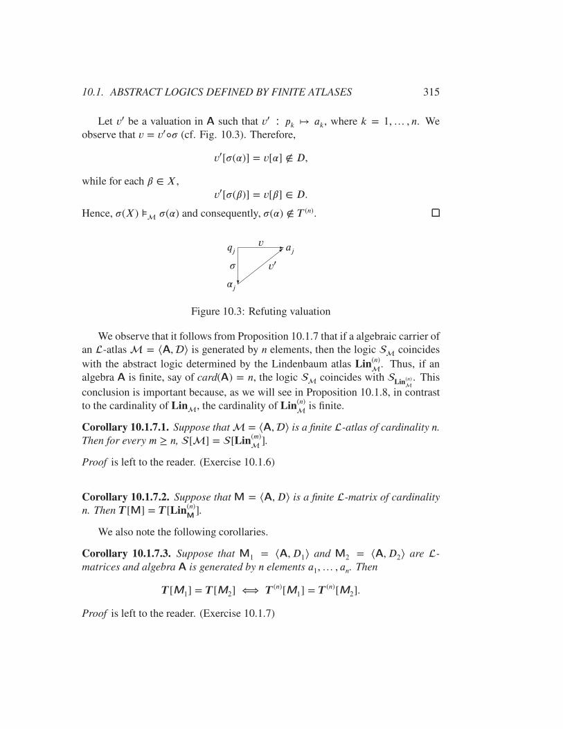
10.1. ABSTRACT LOGICS DEFINED BY FINITE ATLASES 315
Let v′ be a valuation in A such that v′ ∶ pk ↦ ak, where k = 1,… , n. Weobserve that v = v′◦� (cf. Fig. 10.3). Therefore,
v′[�(�)] = v[�] ∉ D,
while for each � ∈ X,v′[�(�)] = v[�] ∈ D.
Hence, �(X) ⊧ �(�) and consequently, �(�) ∉ T (n).
v
� v′
qj aj
�j
Figure 10.3: Refuting valuation
We observe that it follows from Proposition 10.1.7 that if a algebraic carrier ofan -atlas = ⟨A,⟩ is generated by n elements, then the logic coincideswith the abstract logic determined by the Lindenbaum atlas Lin
(n)
. Thus, if analgebra A is finite, say of card(A) = n, the logic coincides with
Lin(n)
. Thisconclusion is important because, as we will see in Proposition 10.1.8, in contrastto the cardinality of Lin, the cardinality of Lin(n)
is finite.
Corollary 10.1.7.1. Suppose that = ⟨A,⟩ is a finite -atlas of cardinality n.Then for every m ≥ n, [] = [Lin
(m)].
Proof is left to the reader. (Exercise 10.1.6)
Corollary 10.1.7.2. Suppose that M = ⟨A, D⟩ is a finite -matrix of cardinalityn. Then T [M] = T [Lin
(n)M].
We also note the following corollaries.
Corollary 10.1.7.3. Suppose that M1 = ⟨A, D1⟩ and M2 = ⟨A, D2⟩ are -matrices and algebra A is generated by n elements a1,… , an. Then
T [M1] = T [M2] ⟺ T (n)[M1] = T (n)[M2].
Proof is left to the reader. (Exercise 10.1.7)
316 CHAPTER 10. DECIDABILITY
Corollary 10.1.7.4. Suppose that M1 = ⟨A, D1⟩ and M2 = ⟨A, D2⟩ are finite-matrices of cardinality n. Then
T [M1] = T [M2] ⟺ T (n)[M1] = T (n)[M2].
Proof is left to the reader. (Exercise 10.1.8)
A very important property of equivalence∼A
, which will be used for construct-ing an effective procedure, is formulated in the following proposition.
Proposition 10.1.8. For any finite -atlas = ⟨A,⟩ and any natural numbern > 0, the set Fm
(n)∕∼
Ais finite.
Proof. We need to prove that ∼A
partitions set Fm(n)
in a finite number of equiva-
lence classes. The proof follows from the observation that each formula � ∈ Fm(n)
can be regarded as a function on A in n variables:
f�(a1,… , an) = v[�],
where v is a valuation with v ∶ pi ↦ ai. From the definition of ∼A
, it follows thatfor any �, � ∈ Fm
(n)
,� ∼
A� ⟺ f� = f� .
Hence, the cardinality of Fm(n)∕∼
Adoes not exceed the cardinality of the set of all
n-ary functions on A, that is card(Fm(n)∕∼A) ≤ kk
n, where k = card(A).
Suppose that ∼ is an equivalence relation on a set A. A subset of A containingexactly one element from each ∼-equivalence class is called a complete set of
representatives of A∕∼. Proposition 10.1.8 entails that if M = ⟨A, D⟩ is a finite-matrix, then a complete set of representatives of Fm
(n)∕∼
Ais finite. Moreover,
there is an effective procedure that, given a finite -matrix or -atlas, delivers acomplete set of representatives of Fm
(n)∕∼
A.
Indeed, let us observe that we can enumerate Fm(n)
; see Section 2.5.2 and Sec-tion 2.5.3. To that end, we enumerate the formulas in order of growing depth: wetake all formulas of depth 0, and then we construct all formulas of depth n basedon formulas of lesser depth.
Because algebra A is finite, for any two formulas � and �, we can easily de-termine whether � ∼
A� or not. Thus, after obtaining a new formula during enu-
meration of Fm(n)
, we decide whether this formula is ∼A
-equivalent to a precedingformula, and if it is, we omit this formula, otherwise we retain this formula as a

10.2. ENUMERATING PROCEDURE 317
representative of the respective ∼A
-coset. And we stop when we determine thatsuch a process does not produce any new representatives. Proposition 10.1.2 givesus a way to determine when to stop: if we did not retain any of formulas of depthn + 1, we have obtain representatives of all ∼
A-cosets.
Exercises 10.1
1. Prove that that the relation ∼A of A-indistinguishability is an equivalence onFm.
2. Prove Proposition 10.1.1.
3. Suppose that �, � ∈ Fm such that � ∼A�. Also, let [�] be a formula
having an occurrence of �, while [�] be a formula obtained from [�] byreplacing this occurrence of � with �. Then [�] ∼
A [�] (Lemma 10.1.1).
4. Prove Proposition 10.1.3.
5. Prove that if = ⟨A,⟩ is an -atlas and ∼D is a greatest matrix equiva-lence on ⟨A, D⟩, where D ∈ , then
⋂{∼D | D ∈ } is the greatest atlas
equivalence on .
6. Prove Corollary 10.1.7.1.
7. Prove Corollary 10.1.7.3.
8. Prove Corollary 10.1.7.4.
10.2 Enumerating procedure
We consider the formulas of Fm(n)
as words of a finite alphabet (Section 2.5.2).Actually, the set Fm
(n)
is an effectively decidable word set. (Exercises 10.2.1)Now we aim to show that, given a finite algebra A, a complete set of represen-
tatives of Fm(n)∕∼
Acan be effectively generated.
If A has one element, then all formulas of Fm(n)
are equivalent to each other
with respect to∼A
. Thus a set consisting of any formula of Fm(n)
is a complete setof representatives.
Now we assume that A has more than one element. We describe a generatingprocedure inductively.
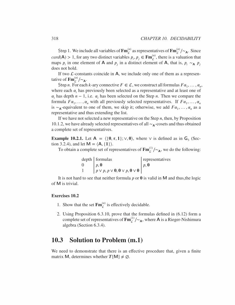
318 CHAPTER 10. DECIDABILITY
Step 1. We include all variables of Fm(n)
as representatives of Fm(n)∕∼
A. Since
card(A) > 1, for any two distinct variables pi, pj ∈ Fm(n)
, there is a valuation thatmaps pi in one element of A and pj in a distinct element of A, that is, pi ∼A pjdoes not hold.
If two -constants coincide in A, we include only one of them as a represen-tative of Fm
(n)∕∼
A.
Step n. For each k-ary connectiveF ∈ , we construct all formulasF�1,… , �n,where each �i has previously been selected as a representative and at least one of�i has depth n − 1, i.e. �i has been selected on the Step n. Then we compare theformula F�1,… , �n with all previously selected representatives. If F�1,… , �nis ∼A-equivalent to one of them, we skip it; otherwise, we add F�1,… , �n as arepresentative and thus extending the list.
If we have not selected a new representative on the Step n, then, by Proposition10.1.2, we have already selected representatives of all ∼
A-cosets and thus obtained
a complete set of representatives.
Example 10.2.1. Let A = ⟨{0, �, 1}; ∨, 0⟩, where ∨ is defined as in G3 (Sec-tion 3.2.4), and let M = ⟨A, {1}⟩.
To obtain a complete set of representatives of Fm(1)
∕∼
A, we do the following:
depth formulas representatives0 p, 0 p, 01 p ∨ p, p ∨ 0, 0 ∨ p, 0 ∨ 0
It is not hard to see that neither formula p or 0 is valid in M and thus,the logicof M is trivial.
Exercises 10.2
1. Show that the set Fm(n)
is effectively decidable.
2. Using Proposition 6.3.10, prove that the formulas defined in (6.12) form acomplete set of representatives of Fm
(1)
∕∼
A, where A is a Rieger-Nishimura
algebra (Section 6.3.4).
10.3 Solution to Problem (m.1)
We need to demonstrate that there is an effective procedure that, given a finitematrix M, determines whether T [M] ≠ ∅.

10.3. SOLUTION TO PROBLEM (M.1) 319
The idea behind such a procedure is this: given a finite -matrix M = ⟨A, D⟩,we enumerate the formulas of Fm, and for each formula, we test whether it be-longs to T [M], that is, we check whether the formula is valid in M. If we havefound a valid formula, T [M] ≠ ∅ and we stop. The problem arises if T [M] = ∅,because in this case, the procedure does not stop. To alleviate this problem, we dothe following.
(a) Firstly, we reduce the problem to formulas in one variable: because set T [M]
is closed relative to substitutions, if � ∈ T [M], then �(p) ∈ T [M], where�(p) is a formula obtained from � by substituting p for each variable. Thatis, T [M] = ∅ if and only if T (1)[M] = ∅, and we need to list only formulasfrom Fm
(1)
, although, if contains connectives, Fm
(1)
is still an infinite set
and we need to make further reductions.
(b) Since the algebra A is finite, by Proposition 10.1.8, the set Fm(1)
∕ ∼
Ais fi-
nite. In addition, if one of the representatives of ∼A
-cosets is in T [M], thenall of them are in T [M]. Hence, it suffices to test just one of the representa-tives from each ∼
A-coset.
(c) All we need is to be able to enumerate the representatives of ∼A
-cosets: onefor each class, and we will construct a procedure that does precisely this.Then, for each representative � we can check whether � is valid in M; andif so, clearly T [M] ≠ ∅, or we will exhaust the list of representatives andconclude that T [M] = ∅.
T (1)[M]
Fm(1)
T (1)[M]∕∼A
Fm(1)
∕∼
A
Figure 10.4: ∼A-Equivalence partitioning
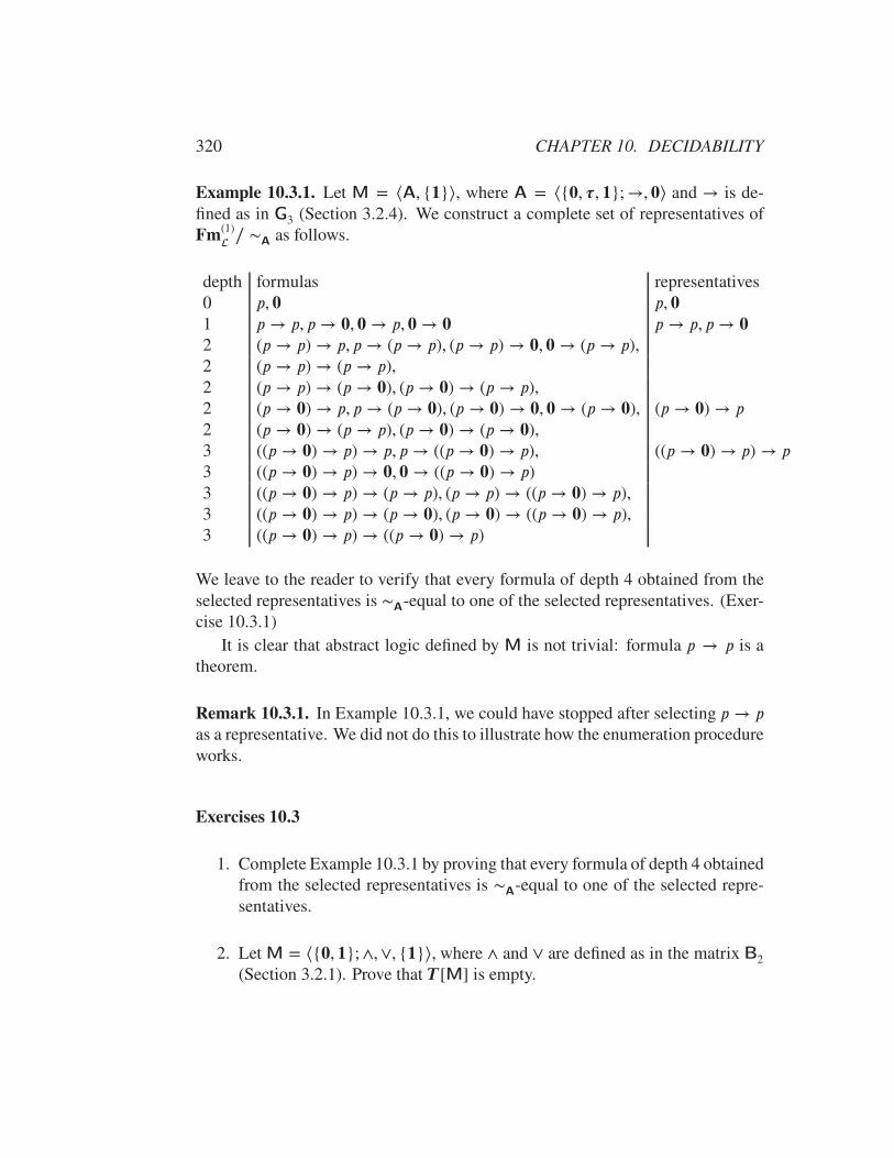
320 CHAPTER 10. DECIDABILITY
Example 10.3.1. Let M = ⟨A, {1}⟩, where A = ⟨{0, �, 1};→, 0⟩ and → is de-fined as in G3 (Section 3.2.4). We construct a complete set of representatives ofFm
(1)
∕ ∼
Aas follows.
depth formulas representatives0 p, 0 p, 01 p → p, p→ 0, 0 → p, 0 → 0 p → p, p→ 0
2 (p → p) → p, p→ (p→ p), (p→ p) → 0, 0 → (p → p),2 (p → p) → (p → p),2 (p → p) → (p → 0), (p→ 0) → (p → p),2 (p → 0) → p, p→ (p → 0), (p → 0) → 0, 0 → (p→ 0), (p → 0) → p2 (p → 0) → (p → p), (p→ 0) → (p → 0),3 ((p → 0) → p) → p, p→ ((p→ 0) → p), ((p → 0) → p) → p3 ((p → 0) → p) → 0, 0 → ((p → 0) → p)3 ((p → 0) → p) → (p → p), (p→ p) → ((p → 0) → p),3 ((p → 0) → p) → (p → 0), (p→ 0) → ((p → 0) → p),3 ((p → 0) → p) → ((p → 0) → p)
We leave to the reader to verify that every formula of depth 4 obtained from theselected representatives is ∼
A-equal to one of the selected representatives. (Exer-
cise 10.3.1)It is clear that abstract logic defined by M is not trivial: formula p → p is a
theorem.
Remark 10.3.1. In Example 10.3.1, we could have stopped after selecting p → pas a representative. We did not do this to illustrate how the enumeration procedureworks.
Exercises 10.3
1. Complete Example 10.3.1 by proving that every formula of depth 4 obtainedfrom the selected representatives is ∼
A-equal to one of the selected repre-
sentatives.
2. Let M = ⟨{0, 1}; ∧,∨, {1}⟩, where ∧ and ∨ are defined as in the matrix B2
(Section 3.2.1). Prove that T [M] is empty.
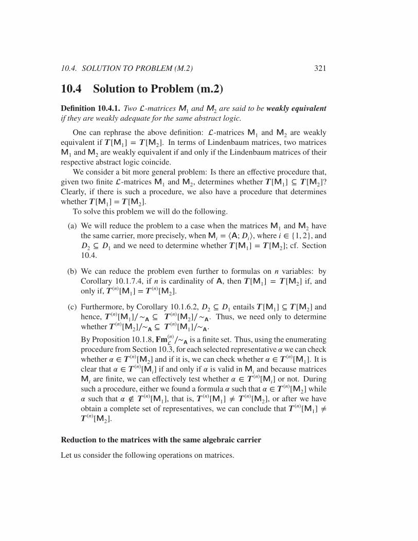
10.4. SOLUTION TO PROBLEM (M.2) 321
10.4 Solution to Problem (m.2)
Definition 10.4.1. Two -matrices M1 and M2 are said to be weakly equivalent
if they are weakly adequate for the same abstract logic.
One can rephrase the above definition: -matrices M1 and M2 are weaklyequivalent if T [M1] = T [M2]. In terms of Lindenbaum matrices, two matricesM1 and M2 are weakly equivalent if and only if the Lindenbaum matrices of theirrespective abstract logic coincide.
We consider a bit more general problem: Is there an effective procedure that,given two finite -matrices M1 and M2, determines whether T [M1] ⊆ T [M2]?Clearly, if there is such a procedure, we also have a procedure that determineswhether T [M1] = T [M2].
To solve this problem we will do the following.
(a) We will reduce the problem to a case when the matrices M1 and M2 havethe same carrier, more precisely, when Mi = ⟨A;Di⟩, where i ∈ {1, 2}, andD2 ⊆ D1 and we need to determine whether T [M1] = T [M2]; cf. Section10.4.
(b) We can reduce the problem even further to formulas on n variables: byCorollary 10.1.7.4, if n is cardinality of A, then T [M1] = T [M2] if, andonly if, T (n)[M1] = T (n)[M2].
(c) Furthermore, by Corollary 10.1.6.2, D2 ⊆ D1 entails T [M1] ⊆ T [M2] andhence, T (n)[M1]∕∼A
⊆ T (n)[M2]∕∼A. Thus, we need only to determine
whether T (n)[M2]∕∼A⊆ T (n)[M1]∕∼A
.
By Proposition 10.1.8, Fm(n)∕∼
Ais a finite set. Thus, using the enumerating
procedure from Section 10.3, for each selected representative �we can checkwhether � ∈ T (n)[M2] and if it is, we can check whether � ∈ T (n)[M1]. It isclear that � ∈ T (n)[Mi] if and only if � is valid in Mi and because matricesMi are finite, we can effectively test whether � ∈ T (n)[Mi] or not. Duringsuch a procedure, either we found a formula � such that � ∈ T (n)[M2] while� such that � ∉ T (n)[M1], that is, T (n)[M1] ≠ T (n)[M2], or after we haveobtain a complete set of representatives, we can conclude that T (n)[M1] ≠
T (n)[M2].
Reduction to the matrices with the same algebraic carrier
Let us consider the following operations on matrices.
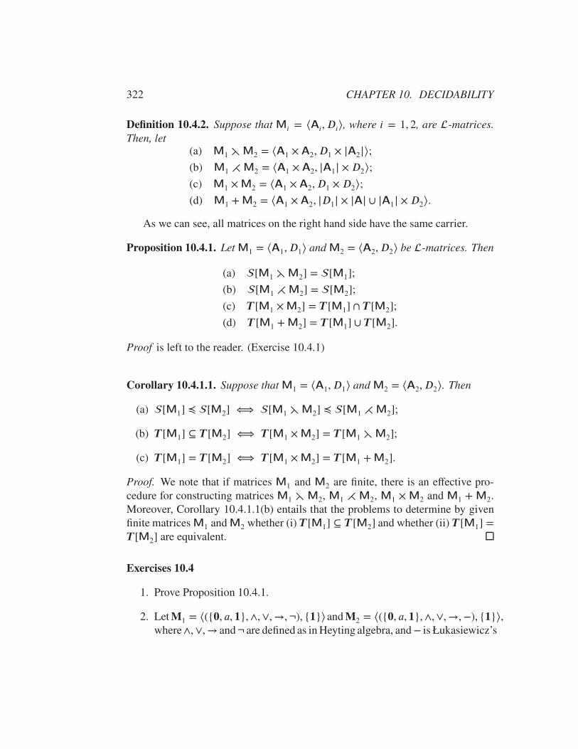
322 CHAPTER 10. DECIDABILITY
Definition 10.4.2. Suppose that Mi = ⟨Ai, Di⟩, where i = 1, 2, are -matrices.Then, let
(a) M1 ⋋ M2 = ⟨A1 × A2, D1 × |A2|⟩;(b) M1 ⋌ M2 = ⟨A1 × A2, |A1| ×D2⟩;(c) M1 × M2 = ⟨A1 × A2, D1 ×D2⟩;(d) M1 +M2 = ⟨A1 × A2, |D1| × |A| ∪ |A1| ×D2⟩.
As we can see, all matrices on the right hand side have the same carrier.
Proposition 10.4.1. Let M1 = ⟨A1, D1⟩ and M2 = ⟨A2, D2⟩ be -matrices. Then
(a) [M1 ⋋M2] = [M1];
(b) [M1 ⋌ M2] = [M2];
(c) T [M1 × M2] = T [M1] ∩ T [M2];
(d) T [M1 +M2] = T [M1] ∪ T [M2].
Proof is left to the reader. (Exercise 10.4.1)
Corollary 10.4.1.1. Suppose that M1 = ⟨A1, D1⟩ and M2 = ⟨A2, D2⟩. Then
(a) [M1] ≼ [M2] ⟺ [M1 ⋋ M2] ≼ [M1 ⋌ M2];
(b) T [M1] ⊆ T [M2] ⟺ T [M1 × M2] = T [M1 ⋋ M2];
(c) T [M1] = T [M2] ⟺ T [M1 × M2] = T [M1 +M2].
Proof. We note that if matrices M1 and M2 are finite, there is an effective pro-cedure for constructing matrices M1 ⋋ M2, M1 ⋌ M2, M1 × M2 and M1 + M2.Moreover, Corollary 10.4.1.1(b) entails that the problems to determine by givenfinite matrices M1 and M2 whether (i) T [M1] ⊆ T [M2] and whether (ii) T [M1] =
T [M2] are equivalent.
Exercises 10.4
1. Prove Proposition 10.4.1.
2. LetM1 = ⟨({0, a, 1},∧,∨,→,¬), {1}⟩andM2 = ⟨({0, a, 1},∧,∨,→,−), {1}⟩,where∧,∨,→ and¬ are defined as in Heyting algebra, and− is Łukasiewicz’s
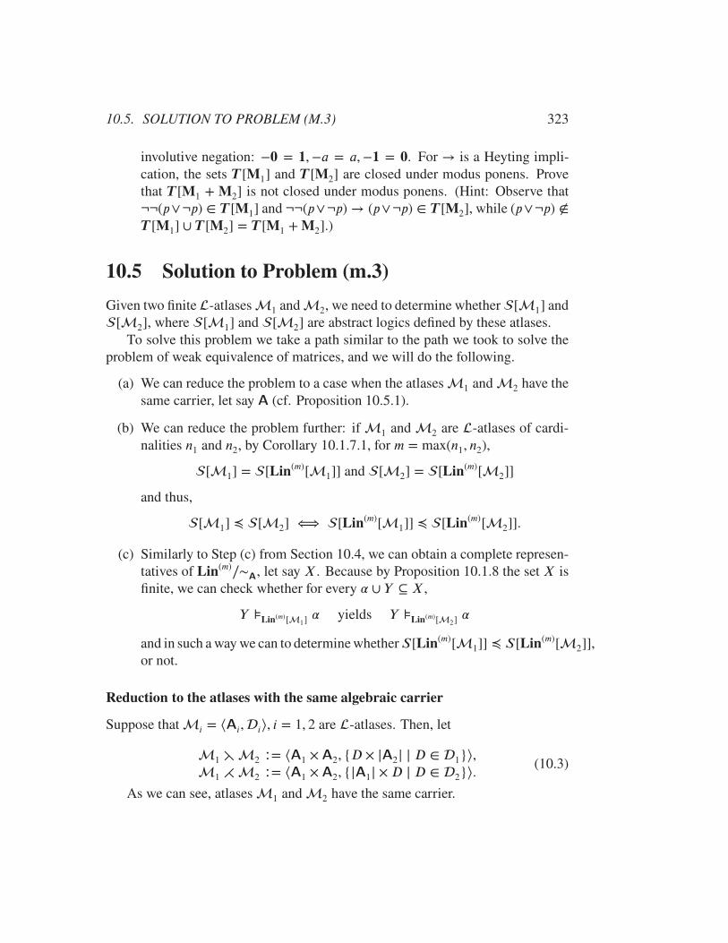
10.5. SOLUTION TO PROBLEM (M.3) 323
involutive negation: −0 = 1,−a = a,−1 = 0. For → is a Heyting impli-cation, the sets T [M1] and T [M2] are closed under modus ponens. Provethat T [M1 + M2] is not closed under modus ponens. (Hint: Observe that¬¬(p∨¬p) ∈ T [M1] and ¬¬(p∨¬p) → (p∨¬p) ∈ T [M2], while (p∨¬p) ∉T [M1] ∪ T [M2] = T [M1 +M2].)
10.5 Solution to Problem (m.3)
Given two finite -atlases 1 and 2, we need to determine whether [1] and[2], where [1] and [2] are abstract logics defined by these atlases.
To solve this problem we take a path similar to the path we took to solve theproblem of weak equivalence of matrices, and we will do the following.
(a) We can reduce the problem to a case when the atlases 1 and 2 have thesame carrier, let say A (cf. Proposition 10.5.1).
(b) We can reduce the problem further: if 1 and 2 are -atlases of cardi-nalities n1 and n2, by Corollary 10.1.7.1, for m = max(n1, n2),
[1] = [Lin(m)[1]] and [2] = [Lin(m)[2]]
and thus,
[1] ≼ [2] ⟺ [Lin(m)[1]] ≼ [Lin(m)[2]].
(c) Similarly to Step (c) from Section 10.4, we can obtain a complete represen-tatives of Lin(m)∕∼
A, let say X. Because by Proposition 10.1.8 the set X is
finite, we can check whether for every � ∪ Y ⊆ X,
Y ⊧Lin
(m)[1]� yields Y ⊧
Lin(m)[2]
�
and in such a way we can to determine whetherS[Lin(m)[1]] ≼ S[Lin(m)[2]],
or not.
Reduction to the atlases with the same algebraic carrier
Suppose that i = ⟨Ai,i⟩, i = 1, 2 are -atlases. Then, let
1 ⋋2 ∶= ⟨A1 × A2, {D × |A2| | D ∈ 1}⟩,1 ⋌2 ∶= ⟨A1 × A2, {|A1| ×D | D ∈ 2}⟩. (10.3)
As we can see, atlases 1 and 2 have the same carrier.

324 CHAPTER 10. DECIDABILITY
Proposition 10.5.1. Let 1 = ⟨A1,1⟩ and 2 = ⟨A2,2⟩ be -atlases. Then[1] = [1 ⋋2] and [2] = [1 ⋌2].
Proof is left to the reader. (Exercise 10.5.1)
Thus, there is an effective procedure to determine whether two finite -atlasesare equivalent. Because there is a procedure that
Remark 10.5.1. Let us observe that for any -atlases 1 and 2, by Proposition10.5.1, S[1 ⋋2] = S[1] and because S[1 ×2] = S[1] ∩ S[2],
S[1] ≼ S[2] ⟺ S[1 ⋋2] = S[1 ×2].
Thus, the problems to determine by two finite -atlases 1 and 2 whether1 ≼ [2] and whether [1] = [2] are equivalent.
By Proposition 4.4.10, for any finite set Mi, where i ∈ {1,… , m}, of finite -matrices, there is a finite -atlas defining the same abstract logic. The proof ofProposition 4.4.10 gives an effective procedure how to construct . Therefore,there is an effective procedure which, given two finite sets of finite -matrices,determines whether these sets define the same abstract logic.
We note that Corollary 10.1.7.1 holds for the abstract logics understood asmultiple conclusion consequence relations. Hence, the procedure that solves theproblem of equivalence of two finite sets of finite matrices can be easily modifiedfo the multiple conclusion consequence relations.
Exercises 10.5
1. Prove Proposition 10.5.1.
2. Derive the equalities [⋋] = [⋌] = [] from the defini-tion (10.3), without using Proposition 10.5.1.
10.6 Historical notes
In (Łoś, 1949) Łoś observed that if S is an abstract logic defined by a logical ma-trix M = ⟨A, D⟩, for any n > 0, one can consider a functional matrix: M
(n) ∶=
⟨A(n), D(n)⟩, where A(n) is a set of all functions f ∶ |A|n ⟶ |A|, D′ ⊆ A
(n) con-sisting of all functions from A
(n) taking values only from D, and connectives are
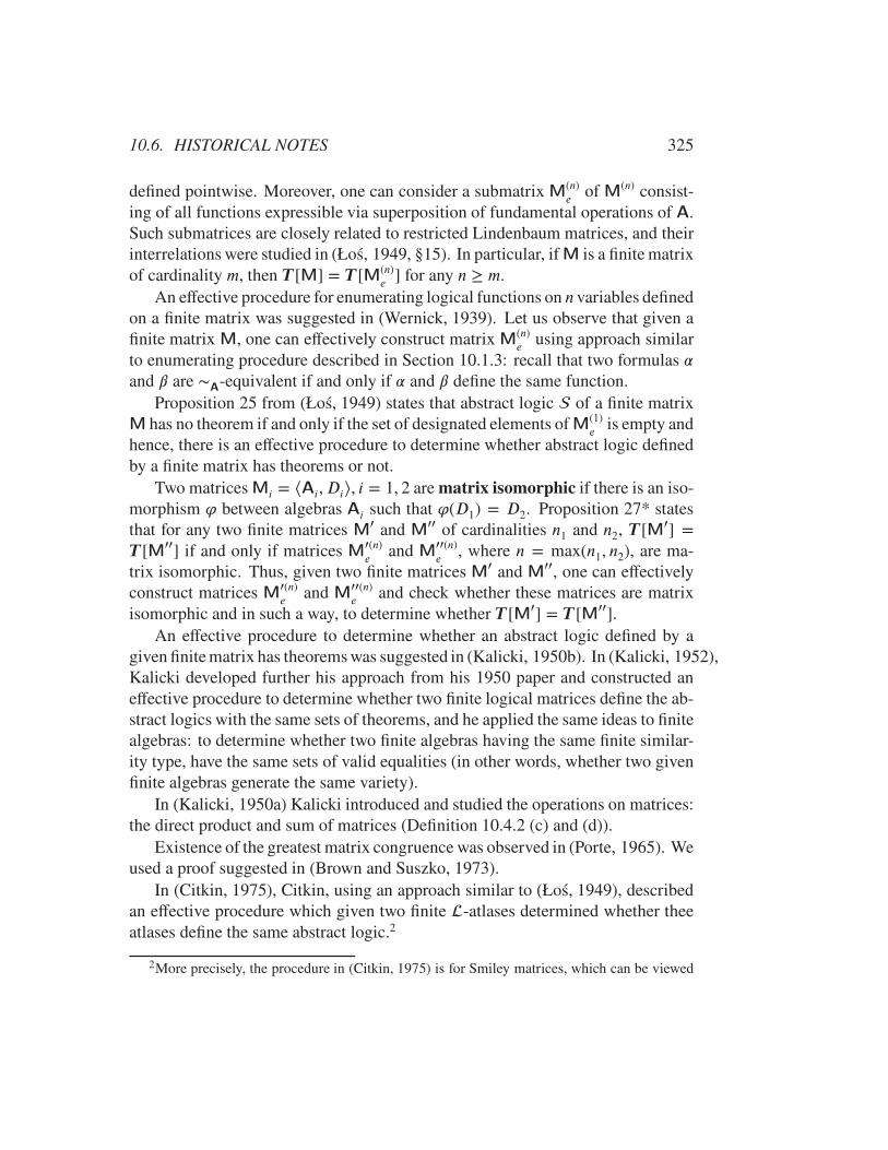
10.6. HISTORICAL NOTES 325
defined pointwise. Moreover, one can consider a submatrix M(n)e of M
(n) consist-ing of all functions expressible via superposition of fundamental operations of A.Such submatrices are closely related to restricted Lindenbaum matrices, and theirinterrelations were studied in (Łoś, 1949, §15). In particular, if M is a finite matrixof cardinality m, then T [M] = T [M(n)
e ] for any n ≥ m.An effective procedure for enumerating logical functions on n variables defined
on a finite matrix was suggested in (Wernick, 1939). Let us observe that given afinite matrix M, one can effectively construct matrix M
(n)e using approach similar
to enumerating procedure described in Section 10.1.3: recall that two formulas �and � are ∼
A-equivalent if and only if � and � define the same function.
Proposition 25 from (Łoś, 1949) states that abstract logic of a finite matrixM has no theorem if and only if the set of designated elements of M(1)
e is empty andhence, there is an effective procedure to determine whether abstract logic definedby a finite matrix has theorems or not.
Two matrices Mi = ⟨Ai, Di⟩, i = 1, 2 are matrix isomorphic if there is an iso-morphism ' between algebras Ai such that '(D1) = D2. Proposition 27* statesthat for any two finite matrices M
′ and M′′ of cardinalities n1 and n2, T [M
′] =
T [M′′] if and only if matrices M′(n)e and M
′′(n)e , where n = max(n1, n2), are ma-
trix isomorphic. Thus, given two finite matrices M′ and M
′′, one can effectivelyconstruct matrices M
′(n)e and M
′′(n)e and check whether these matrices are matrix
isomorphic and in such a way, to determine whether T [M′] = T [M′′].An effective procedure to determine whether an abstract logic defined by a
given finite matrix has theorems was suggested in (Kalicki, 1950b). In (Kalicki, 1952),Kalicki developed further his approach from his 1950 paper and constructed aneffective procedure to determine whether two finite logical matrices define the ab-stract logics with the same sets of theorems, and he applied the same ideas to finitealgebras: to determine whether two finite algebras having the same finite similar-ity type, have the same sets of valid equalities (in other words, whether two givenfinite algebras generate the same variety).
In (Kalicki, 1950a) Kalicki introduced and studied the operations on matrices:the direct product and sum of matrices (Definition 10.4.2 (c) and (d)).
Existence of the greatest matrix congruence was observed in (Porte, 1965). Weused a proof suggested in (Brown and Suszko, 1973).
In (Citkin, 1975), Citkin, using an approach similar to (Łoś, 1949), describedan effective procedure which given two finite -atlases determined whether theeatlases define the same abstract logic.2
2More precisely, the procedure in (Citkin, 1975) is for Smiley matrices, which can be viewed

326 CHAPTER 10. DECIDABILITY
Later, in (Zygmunt, 1983) suggested an effective procedure that given two fi-nite -atlases 1 and 2 (ramified matrices in Zygmunt’s terms), determineswhether [1] ≼ [2].
In (Devyatkin, 2013), the Kalicki’s approach from (Kalicki, 1950b) was usedto construct an effective procedure which by two finite -matrices determineswhether these matrices define the same abstract logic.
Even though there are effective procedures to determine equivalence of two fi-nite-atlases, these procedures have a high complexity: it follows from (Bergman and Slutzki, 2000)that even problem to determine by two finite algebras whether they generate thesame quasivariety, it is NP-complete. And for algebraziable logics, the latter prob-lem is equivalent to the problem of determining equivalence of two finite matrices.
as atlases.

Bibliography
Barwise, J. (1977). An introduction to first-order logic. In Handbook of math-ematical logic, volume 90 of Stud. Logic Found. Math., pages 5–46. North-Holland, Amsterdam. [119]
Bell, J. and Slomson, A. (1969). Models and ultraproducts: An introduction.North-Holland Publishing Co., Amsterdam-London. [40, 43, 44]
Bell, J. L. (2011). Set theory, volume 47 of Oxford Logic Guides. Oxford Univer-sity Press, Oxford. Boolean-valued models and independence proofs, With aforeword by Dana Scott, Paperback of the third (2005) edition. [303]
Bergman, C. and Slutzki, G. (2000). Complexity of some problems concerningvarieties and quasi-varieties of algebras. SIAM J. Comput., 30(2):359 – 382.[326]
Bernays, P. (1926). Axiomatische Untersuchung des Aussagen-Kalküls der “Prin-cipia Mathematica”. Math. Z., 25:305–320. [88]
Beth, E. (1962). Formal methods: an introduction to symbolic logic and to thestudy of effective operations in arithmetic and logic. Synthese library. D.Reidel Pub. Co. [46]
Beth, E. (1965). Mathematical thought. An introduction to the philosophy of math-ematics. D. Reidel Publishing Co., Dordrecht. Translated in part from theDutch by Horace S. Glover. [58]
Beziau (editor), J.-Y. (2012). Universal Logic: An Anthology, From Paul Hertz toDov Gabbay. Basel, Switzreland: Birkhäuser. [138, 139, 332]
Birkhoff, G. (1935). On the structure of abstract algebras. Proc. of the Camb. Phil.Soc., 29:433–454. [262]
327

328 BIBLIOGRAPHY
Blok, W. (1977). 2ℵ0 varieties of Heyting algebras not generated by their finitemembers. Algebra Universalis, 7(1):115–117. [259]
Blok, W. and Pigozzi, D. (1989). Algebraizable logics. Mem. Amer. Math. Soc.,77(396):vi+78. [209, 245]
Bloom, S. (1975). Some theorems on structural consequence operations. StudiaLogica, 34(1):1–9. [164]
Bocheński, I. (1970). A history of formal logic. Translated from the German andedited by Ivo Thomas. Second edition. Chelsea Publishing Co., New York.[140, 144, 145]
Boole, G. (2003). The laws of thought. Great Books in Philosophy. PrometheusBooks, Amherst, NY. Reprint of the 1854 original, With an introduction byJohn Corcoran. [87]
Bourbaki, N. (1998). General topology. Chapters 1–4. Elements of Mathematics(Berlin). Springer-Verlag, Berlin. Translated from the French, Reprint of the1989 English translation. [17]
Brown, D. and Suszko, R. (1973). Abstract logics. In Borsuk, K., editor, Disser-tationes Math. (Rozprawy Mat.), volume 102, pages 9–41. [145, 310, 325]
Burris, S. (1998). Logic for mathematics and computer science. Prentice Hall,Upper Saddle River, N.J. [262, 263]
Burris, S. and Sankappanavar, H. (1981). A course in universal algebra, volume 78of Graduate Texts in Mathematics. Springer-Verlag, New York. [19, 20, 21, 22, 23,
24, 27, 28, 29, 35, 40, 41, 42, 44, 263, 310]
Carnap, R. (1942). Introduction to Semantics. Harvard University Press, Cam-bridge, Mass. [247]
Chagrov, A. and Zakharyaschev, M. (1997). Modal logic, volume 35 of OxfordLogic Guides. The Clarendon Press, Oxford University Press, New York.Oxford Science Publications. [259, 261]
Chang, C. and Keisler, H. (1990). Model theory, volume 73 of Studies in Logic andthe Foundations of Mathematics. North-Holland Publishing Co., Amsterdam,third edition. [40, 43, 44, 119, 129, 130, 131, 159]

BIBLIOGRAPHY 329
Church, A. (1996). Introduction to mathematical logic. Princeton Landmarksin Mathematics. Princeton University Press, Princeton, NJ. Reprint of thesecond (1956) edition, Princeton Paperbacks. [141, 145]
Citkin, A. (1975). On an effective method concerning mutuall adequacy of twofinite truth tables (Russian). In Proceedingth of the Fourth Conference on theoccasion of 30tℎ Anniversary of the Liberation of Transcarpathia. UzhgorodState University. [306, 325]
Citkin, A. (1977). On admissible rules of intuitionistic propositional logic (Rus-sian). Mat. Sb. (N.S.), 102(144)(2):314–323, 328. English translation: MathUSSR Sbornik, 31 (2):279–288, 1977. [205, 207]
Citkin, A. and Muravitsky, A. (2016). Lindenbaum method (propositional lan-guage). http://arXiv.org/pdf/1609.07379. [6]
Citkin, A. and Muravitsky (originators), A. (2013). Lindenbaum method(propositional language). In Encyclopaedia of Mathematics. Springer.http://www.encyclopediaofmath.org/index.php?title=Lindenbaum_method&oldid=30469.[6, 211]
Cohn, P. (1981). Universal algebra, volume 6 of Mathematics and its Applications.D. Reidel Publishing Co., Dordrecht-Boston, Mass., second edition. [18, 19, 22]
Couturat, L. (1980). Les principes des mathématiques. Librairie Scientifique etTechnique Albert Blanchard, Paris. With an appendix “La philosophie desmathématiques de Kant”. [“Kant’s philosophy of mathematics”], Reprint. [140]
Curry, H. (1966). A theory of formal deducibility. Second edition, reprinting.Notre Dame Mathematical Lectures, No. 6. University of Notre Dame Press,South Bend, Ind. [73]
Cutland, N. (1980). Computability. Cambridge University Press, Cambridge-NewYork. An introduction to recursive function theory. [49, 53, 55, 56]
Czelakowski, J. (2001). Protoalgebraic logics, volume 10 of Trends in Logic—Studia Logica Library. Kluwer Academic Publishers, Dordrecht. [139, 211]
Czelakowski, J. and Pigozzi, D. (2004). Fregean logics. Ann. Pure Appl. Logic,127(1-3):17–76. Provinces of logic determined. [6, 211]
330 BIBLIOGRAPHY
Davis, M. (1958). Computability and unsolvability. McGraw-Hill Series in Infor-mation Processing and Computers. McGraw-Hill Book Co., Inc., New York-Toronto-London. [49, 53, 55, 56]
Davis, M., Sigal, R., and Weyuker, E. (1994). Computability, complexity, and lan-guages. Computer Science and Scientific Computing. Academic Press, Inc.,Boston, MA, second edition. Fundamentals of theoretical computer science.[49, 53, 55, 56]
Devyatkin, L. Y. (2013). Equality of consequence relations in finite-valued logicalmatrices. In Logical investigations. Vol. 19, volume 19 of Log. Issled., pages273–280. Ross. Akad. Nauk, Inst. Filos., Moscow. [306, 326]
Diego, A. (1962). On implicative algebras (Spanish). Rev. Un. Mat. Argentina,20:310–311. [29, 30]
Diego, A. (1966). Les algèbres de Hilbert. Gauthier-Villars, Paris. [29]
Dummett, M. (1959). A propositional calculus with denumerable matrix. J. Symb.Logic, 24:97–106. [83, 90, 132]
Dunn, J. and Hardegree, G. (2001). Algebraic methods in philosophical logic,volume 41 of Oxford Logic Guides. The Clarendon Press Oxford UniversityPress, New York. Oxford Science Publications. [143]
Dyck, W. v. (1882). Gruppentheoretische Studien. (German). MathematischeAnnalen, 20(1):1–44. [245]
Enderton, H. (2001). A mathematical introduction to logic. Harcourt/AcademicPress, Burlington, MA, second edition. [40, 44]
Font, J. (2016). Abstract algebraic logic, volume 60 of Studies in Logic (Lon-don). College Publications, London. An introductory textbook, MathematicalLogic and Foundations. [139, 166, 211]
Font, J. and Jansana, R. (2009). A general algebraic semantics for sentential logics,volume 7 of Lecture Notes in Logic. Second edition. [210]
Font, J. M., Jansana, R., and Pigozzi, D. (2003). A survey of abstract alge-braic logic. Studia Logica, 74(1-2):13–97. Abstract algebraic logic, PartII (Barcelona, 1997). [210]
BIBLIOGRAPHY 331
Font, J. M., Jansana, R., and Pigozzi, D. (2009). Update to “A survey of abstractalgebraic logic”. Studia Logica, 91(1):125–130. [139, 210]
Fraenkel, A., Bar-Hillel, Y., and Levy, A. (1973). Foundations of set theory.North-Holland Publishing Co., Amsterdam-London, revised edition. Withthe collaboration of D. van Dalen, Studies in Logic and the Foundations ofMathematics, Vol. 67. [15, 53]
Gentzen, G. (1969a). The collected papers of Gerhard Gentzen. Edited by M. E.Szabo. Studies in Logic and the Foundations of Mathematics. North-HollandPublishing Co., Amsterdam-London. [212]
Gentzen, G. (1969b). Untersuchungen über das logische Schließen. Wis-senschaftliche Buchgesellschaft, Darmstadt. “Libelli”, Band 275, Unverän-derter reprografischer Nachdruck aus Math. Z. 39 (1934), 176–210; ibid. 39(1934), 405–431. [145, 212]
Glivenko, V. (1929). Sur quelques points de la logique de M. Brouwer. Acad. Roy.Belgique, Bull. cl. sci., ser. 5, 15:183–188. [204]
Gödel, K. (1932). Zum intuitionistischen Aussagenkalkül (German). Anzeigerder Akademie der Wissenschaften in Wien, 69:65–66. Both German orig-inal and English translation “On the intuitionistic propositional calculus”in: (Gödel, 1986), pp. 223–225. [89]
Gödel, K. (1986). Collected works. Vol. I. The Clarendon Press, Oxford UniversityPress, New York. Publications 1929–1936, Edited and with a preface bySolomon Feferman. [89, 331]
Gorbunov, V. (1998). Algebraic theory of quasivarieties. Siberian School of Alge-bra and Logic. Consultants Bureau, New York. Translated from the Russian.[42, 44, 206]
Grätzer, G. (2008). Universal algebra. Springer, New York, second edition. Withappendices by Grätzer, Bjarni Jónsson, Walter Taylor, Robert W. Quacken-bush, Günter H. Wenzel, and Grätzer and W. A. Lampe. [18, 19, 22, 24, 40, 44]
Hailperin, T. (1986). Boole’s logic and probability, volume 85 of Studies in Logicand the Foundations of Mathematics. North-Holland Publishing Co., Ams-terdam, second edition. A critical exposition from the standpoint of contem-porary algebra, logic and probability theory. [87]

332 BIBLIOGRAPHY
Halmos, P. (1962). Algebraic logic. Chelsea Publishing Co., New York. [301]
Halmos, P. (1974). Naive set theory. Springer-Verlag, New York-Heidelberg.Reprint of the 1960 edition, Undergraduate Texts in Mathematics. [15]
Henkin, L. (1950). An algebraic characterization of quantifiers. Fund. Math.,37:63–74. [301, 302]
Henkin, L., Monk, J. D., and Tarski, A. (1985). Cylindric algebras. Part I, vol-ume 64 of Studies in Logic and the Foundations of Mathematics. North-Holland Publishing Co., Amsterdam. With an introductory chapter: Generaltheory of algebras, Reprint of the 1971 original. [245, 301]
Hermes, H. (1951). Zur Theorie der aussagenlogischen Matrizen. (German).Math. Z., 53:414–418. [143]
Hertz, P. (1922). Über Axiomensysteme für beliebige Ssatzsysteme, Teil 1: Sätheund Grades (German). Mathematische Annalen, 87 (3-4):246–269. En-glish translation: On axiomatic systems for arbitrary systems of sentences,in: (Beziau (editor), 2012), pp. 11–29. [138]
Hilbert, D. and Bernays, P. (1968). Grundlagen der Mathematik. I. ZweiteAuflage. Die Grundlehren der mathematischen Wissenschaften, Band 40.Springer-Verlag, Berlin-New York. (German, first edition 1934). [145]
Hodges, W. (1993). Model theory, volume 42 of Encyclopedia of Mathematicsand its Applications. Cambridge University Press, Cambridge. [40, 44]
Ishiguru, H. (1990). Leibniz’s philosophy of logic and language. Cambridge Uni-versity Press, Cambridge, second edition. [242, 243]
Johnstone, P. (1987). Notes on logic and set theory. Cambridge MathematicalTextbooks. Cambridge University Press, Cambridge. [15]
Kalicki, J. (1948). On Tarski’s matrix method. Soc. Sci. Lett. Varsovie. C. R. Cl.III. Sci. Math. Phys., 41:130–142 (1950). [306]
Kalicki, J. (1950a). Note on truth-tables. J. Symbolic Logic, 15:174–181. [325]
Kalicki, J. (1950b). A test for the existence of tautologies according to many-valued truth-tables. J. Symbolic Logic, 15:182–184. [325, 326]

BIBLIOGRAPHY 333
Kalicki, J. (1952). On comparison of finite algebras. Proc. Amer. Math. Soc.,3:36–40. [306, 325]
Kelley, J. (1975). General topology. Springer-Verlag, New York-Berlin. Reprintof the 1955 edition [Van Nostrand, Toronto, Ont.], Graduate Texts in Mathe-matics, No. 27. [17]
Kleene, S. (1952). Introduction to metamathematics. D. Van Nostrand Co., Inc.,New York, N. Y. [120, 122, 145, 161, 200, 201, 204, 212]
Kneale, W. and Kneale, M. (1962). The development of logic. Clarendon Press,Oxford. [1, 2, 76, 84, 86, 138, 144, 242, 243]
Köhler, P. (1981). Brouwerian semilattices. Trans. Amer. Math. Soc., 268(1):103–126. [32]
Kuratowski, K. and Mostowski, A. (1976). Set theory. North-Holland Publish-ing Co., Amsterdam-New York-Oxford; PWN—Polish Scientific Publishers,Warsaw, revised edition. With an introduction to descriptive set theory, Trans-lated from the 1966 Polish original, Studies in Logic and the Foundations ofMathematics, Vol. 86. [15]
Kuznecov, A. V. (1963). Undecidability of the general problems of complete-ness, solvability and equivalence for propositional calculi (Russian). Algebrai Logika Sem., 2(4):47–66. English edition: American Mathematical SocietyTranslations. Series 2, Vol. 59: Twelve papers on logic and algebra, Ameri-can Mathematical Society, Providence, R.I., 1966. [306]
Kuznetsov, A. (1979). Means for detection of nondeducibility and inexpressibil-ity (Russian). In Logical inference (Moscow, 1974), pages 5–33. “Nauka”,Moscow. [5, 161]
Lambros, C. (1979). A shortened proof of Sobociński’s theorem concerning arestricted rule of substitution in the field of propositional calculi. Notre DameJ. Formal Logic, 20(1):112–114. [128]
Lewis, C. (1913a). Interesting theorems in symbolic logic. The Journal of Philos-ophy, Psychology and Scientific Methods, 10(9):239–242. [138]
Lewis, C. (1913b). A new algebra of implications and some consequences. TheJournal of Philosophy, Psychology and Scientific Methods, 10(16):428–438.[141]
334 BIBLIOGRAPHY
Lewis, C. (1914). The matrix algebra for implications. The Journal of Philosophy,Psychology and Scientific Methods, 11(22):589–600. [138, 141]
Lewis, C. I. (1960). A Survey of Symbolic Logic. New York: Dover Publications.[141]
Łoś, J. (1949). On logical matrices. (Polish). Trav. Soc. Sci. Lett. Wrocław. Ser.B., (19):42. [143, 162, 306, 324, 325]
Łoś, J. and Suszko, R. (1958). Remarks on sentential logics. Nederl. Akad. Weten-sch. Proc. Ser. A 61 = Indag. Math., 20:177–183. Reprinted with a list ofcorrigenda as (Łoś and Suszko, 2012). [3, 4, 141, 143, 144, 162, 164, 334]
Łoś, J. and Suszko, R. (2012). Remarks on sentential logics [reprintof mr0098670]. In Universal logic: an anthology, Stud. Univers.Log., pages 177–184. Birkhäuser/Springer Basel AG, Basel. Reprintof (Łoś and Suszko, 1958) with a list of corregenda. [334]
Łukasiewicz, J. (1920). O logice trójwartościowej. Ruch Filozoficzny, 5:170–171.English translation: On three-valued logic, in: (Łukasiewicz, 1970), pp. 87–88. [88]
Łukasiewicz, J. (1930). Philosophische Bemerkungen zu mehrwertigen Systemendes Aussagenkalküls (German). Comptes rendus des séances de la Sociétédes sciences et des letters de Varsovie, Classe III, vol. xxiii:51–77. Englishtranslation: Philosophical remarks on many-valued systems of propositionallogic, in: (McCall (editor), 1967), pp. 40–65. [88, 89]
Łukasiewicz, J. (1934). Z historii logiki zdań (Polish). Przeglad Filozoficzny,37:417–437. English translation: On the history of the logic of propositions,in: (McCall (editor), 1967), pp. 66–87; also in: (Łukasiewicz, 1970), pp. 197–217. [2, 86, 145]
Łukasiewicz, J. (1951). Aristotle’s syllogistic from the standpoint of modern formallogic. Oxford, at the Clarendon Press. [86]
Łukasiewicz, J. (1957). Aristotle’s syllogistic from the standpoint of modern formallogic. The Clarendon Press, Oxford, 2 edition. [161]
Łukasiewicz, J. (1961). On determinizmie. In Słupecki, J., editor, Z zagadnieńlogiki i filozofii, pages 114–126. Państwowe Wydawnictwo Naukowe. Englishtranslation: On determinism, in: (Łukasiewicz, 1970), pp. 110–128. [88, 89]

BIBLIOGRAPHY 335
Łukasiewicz, J. (1964). Elements of mathematical logic. Translated from Polishby Olgierd Wojtasiewicz. International Series of Monographs on Pure andApplied Mathematics. Vol. 31. A Pergamon Press Book; The Macmillan Co.,New York. English translation of the second edition of the 1929 authorizedlecture notes. [88]
Łukasiewicz, J. (1970). Selected works. North-Holland Publishing Co.,Amsterdam-London; PWN-Polish Scientific Publishers, Warsaw. Edited byL. Borkowski, Studies in Logic and the Foundations of Mathematics. [88, 89,
334]
Łukasiewicz, J. and Tarski, A. (1930). Untersuchungen über den Aussagenkalkül(German). Comptes rendus des séances de la Société des Sciences et desLettres de Varsovie, CI III, 23:30–50. English translation: Investigations intothe sentential calculus, in: (Tarski, 1956), pp. 38–59; also in: (Tarski, 1983),pp. 38–59. [4, 142, 143, 162]
Makinson, D. (2005). Bridges from classical to nonmonotonic logic, volume 5 ofTexts in Computing. King’s College Publications, London. [142]
Mal’cev, A. (1956). Quasiprimitive classes of abstract algebras. (russian). Dokl.Akad. Nauk SSSR (N.S.), 108:187–189. [245]
Mal’cev, A. (1958). Defining relations in categories. (Russian). Dokl. Akad. NaukSSSR, 119:1095–1098. [245]
Mal’cev, A. (1970). Algorithms and recursive functions. Translated from the firstRussian edition by Leo F. Boron, with the collaboration of Luis E. Sanchis,John Stillwell and Kiyoshi Iséki. Wolters-Noordhoff Publishing, Groningen.[49, 56]
Mal’cev, A. (1973). Algebraic systems. Akademie-Verlag, Berlin. Posthumousedition, edited by D. Smirnov and M. Taıclin, Translated from the Russian byB. D. Seckler and A. P. Doohovskoy. [27, 28, 29, 43, 44, 176, 179, 245, 303]
Malinowski, G. (2007). Many-valued logic and its philosophy. In The many valuedand nonmonotonic turn in logic, volume 8 of Handb. Hist. Log., pages 13–94.Elsevier/North-Holland, Amsterdam. [143]
Markov, A. (1960). The theory of algorithms. Amer. Math. Soc. Transl. (2), 15:1–14. [48, 56]
336 BIBLIOGRAPHY
Markov, A. (1962). Theory of algorithms. Translated from Russian by JacquesJ. Schorr-Kon and PST staff. Israel Program for Scientific Translations,Jerusalem. [48, 54, 56]
McCall (editor), S. (1967). Polish Logic, 1920-1939. Oxford University Press. [89,
334]
McKenzie, R., McNulty, G., and Taylor, W. (2018). Algebras, lattices, varieties.Vol. 1. AMS Chelsea Publishing/American Mathematical Society, Provi-dence, RI. Reprint of [ MR0883644], ©1969. [40, 44]
McKinsey, J. (1939). Proof of the independence of the primitive symbols of Heyt-ing’s calculus of propositions. J. Symbolic Logic, 4:155–158. [88]
McKinsey, J. (1941). A solution of the decision problem for the Lewis systems S2and S4, with an application to topology. J. Symbolic Logic, 6:117–134. [205]
McKinsey, J. and Tarski, A. (1948). Some theorems about the sentential calculi ofLewis and Heyting. J. Symbolic Logic, 13:1–15. [164]
Mostowski, A. (1948). Proofs of non-deducibility in intuitionistic functional cal-culus. J. Symbolic Logic, 13:204–207. [301]
Mostowski, A. (1957). On a generalization of quantifiers. Fund. Math., 44:12–36.[303]
Muravitsky, A. (2014a). Beyond Rasiowan systems: Unital deductive systems.Log. Univers., 8(1):83–102. [5, 211]
Muravitsky, A. (2014b). Logic KM: a biography. In Bezhanishvili, G., editor,Leo Esakia on duality in modal and intuitionistic logics, volume 4 of Outst.Contrib. Log., pages 155–185. Springer, Dordrecht. [208, 211]
Negri, S. and von Plato, J. (2001). Structural proof theory. Cambridge UniversityPress, Cambridge. Appendix C by Aarne Ranta. [114]
Nemitz, W. (1965). Implicative semi-lattices. Trans. Amer. Math. Soc., 117:128–142. [32]
Nishimura, I. (1960). On formulas of one variable in intuitionistic propositionalcalculus. J. Symbolic Logic, 25:327–331 (1962). [187, 211]

BIBLIOGRAPHY 337
Pigozzi, D. (1975). Equational theory and equational theories of algebras. Tech-nical Report 71-135, Perdue Uuniversity. [262, 263]
Porte, J. (1965). Recherches sur la théorie générale des systèmes formels et surles systèmes connectifs. Collection de Logique Mathématique, Série A, No.18. Gauthier-Villars & Cie, Paris; E. Nauwelaerts, Louvain. [325]
Prawitz, D. (1965). Natural deduction. A proof-theoretical study. Acta Universi-tatis Stockholmiensis. Stockholm Studies in Philosophy, No. 3. Almqvist &Wiksell, Stockholm. [145]
Quine, W. (1994). From a logical point of view. Harvard University Press, Cam-bridge, MA, second edition. Nine logico-philosophical essays. [245]
Rasiowa, H. (1951). Algebraic treatment of the functional calculi of Heyting andLewis. Fund. Math., 38:99–126. [302]
Rasiowa, H. (1974). An algebraic approach to non-classical logics. North-HollandPublishing Co., Amsterdam. Studies in Logic and the Foundations of Math-ematics, Vol. 78. [5, 29, 30, 31, 32, 34, 35, 39, 211, 301, 302]
Rasiowa, H. and Sikorski, R. (1970). The mathematics of metamathematics.PWN—Polish Scientific Publishers, Warsaw, third edition. MonografieMatematyczne, Tom 41. [31, 32, 34, 35, 39, 204, 205]
Rautenberg, W. (2010). A concise introduction to mathematical logic. Universi-text. Springer, New York, third edition. With a foreword by Lev Beklemishev.[40, 44]
Rescher, N. (1969). Many-Valued Logic. New York: Mcgraw-Hill. [303]
Rieger, L. (1949). On the Lattice Theory of Brouwerian Propositional Logic. Spisyvyd. přírodověd. fak. univ. Karlovy. Řivnáč. [211]
Rieger, L. (1957). A remark on the so-called free closure algebras (Russian).Czechoslovak Math. J., 7(82):16–20. [187, 211]
Rosenbloom, P. (1950). The Elements of Mathematical Logic. Dover Publications,Inc., New York, N. Y. [61]

338 BIBLIOGRAPHY
Rosser, J. and Turquette, A. (1951). Many-valued logics. Studies in Logic andthe Foundations of Mathematics. North-Holland Publishing Co., Amsterdam.[276]
Russell, B. (1906). The Theory of Implication. Amer. J. Math., 28(2):159–202.[141]
Russell, B. (1993). Introduction to mathematical philosophy. Dover Publications,Inc., New York, second edition. [141]
Rybakov, V. (1997). Admissibility of logical inference rules, volume 136 of Studiesin Logic and the Foundations of Mathematics. North-Holland Publishing Co.,Amsterdam. [206]
Scott, D. (1971). On engendering an illusion of understanding. Journal of Philos-ophy, 68(21):787–807. [2]
Scott, D. (1974a). Completeness and axiomatizability in many-valued logic. InProceedings of the Tarski Symposium (Proc. Sympos. Pure Math., Vol. XXV,Univ. California, Berkeley, Calif., 1971), pages 411–435. [2, 139]
Scott, D. (1974b). Rules and derived rules. In Stenlund, S., Henschen-Dahlquist,A.-M., Lindahl, L., Nordenfelt, L., and Odelstad, J., editors, Logical Theoryand Semantic Analysis: Essays Dedicated to STIG KANGER on His FiftiethBirthday, pages 147–161. Springer Netherlands, Dordrecht. [145]
Selman, A. (1972). Completeness of calculi for axiomatically defined classes ofalgebras. Algebra Universalis, 2:20–32. [263]
Shehtman, V. (1978). An undecidable superintuitionistic propositional calculus.Dokl. Akad. Nauk SSSR, 240(3):549–552. [259]
Shoesmith, D. and Smiley, T. (1971). Deducibility and many-valuedness. J. Sym-bolic Logic, 36:610–622. [139, 164, 211]
Shoesmith, D. and Smiley, T. (2008). Multiple-conclusion logic. Cambridge Uni-versity Press, Cambridge. Reprint of the 1978 original [MR0500331]. [2, 92,
139]
Smiley, T. (1962). The independence of connectives. J. Symbolic Logic, 27:426–436. [143]
BIBLIOGRAPHY 339
Sobociński, B. (1974). A theorem concerning a restricted rule of substitution in thefield of propositional calculi. I, II. Notre Dame J. Formal Logic, 15:465–476;ibid. 15 (1974), 589–597. [128]
Tarski, A. (1930a). Fundamentale Begriffe der Methodologie der deduktiven Wis-senschaften. I (German). Monatshefte für Mathematik und Physik, 37:361–404. English translation: Fundamental concepts of the methodology of thedeductive sciences, in: (Tarski, 1956), pp. 60–109; also in: (Tarski, 1983), pp.60–109. [2, 3, 4, 138, 139]
Tarski, A. (1930b). Üder einige fundamentale Begriffe der Metamathematik(German). Comptes Rendus Séantes de la Société des Sciences et des Let-ters de Varsovie, Classe III, Sciences Mathéantiques et Physiques, 23:22–29. English translation: On some fundamental concepts of metamathematics,in: (Tarski, 1956), pp. 30–37; also in: (Tarski, 1983), pp. 30–37. [2, 138, 139, 142,
144]
Tarski, A. (1935). Grundzüge der systemenkalkül. erter teil. Fundamenta Math-ematicae, 25:503–526. English translation: Foundations of the calculus ofsystems, in: (Tarski, 1956), pp. 342–383; (Tarski, 1983), pp. 342–383. [205]
Tarski, A. (1936a). Grundzüge der Systemenkalkül. Zweiter Teil. FundamentaMathematicae, 26:283–301. [2]
Tarski, A. (1936b). Über den Begriff der logischen Folgerung (German). Actesdu Congrès International de Philosophie Scientifique, 7:1–11. English trans-lation: On the concept of logical consequence, in: (Tarski, 1956), pp. 409–420; (Tarski, 1983), pp. 409–420. [2, 101, 139]
Tarski, A. (1956). Logic, Semantics, Metamathematics. Papers from 1923 to 1938.Oxford at the Clarendon Press. Translated by J. H. Woodger. [101, 138, 335, 339]
Tarski, A. (1968). Equational logic and equational theories of algebras. In Con-tributions to Math. Logic (Colloquium, Hannover, 1966), pages 275–288.North-Holland, Amsterdam. [262, 263]
Tarski, A. (1983). Logic, Semantics, Metamathematics. Hackett Publishing Co.,Indianapolis, IN, second edition. Papers from 1923 to 1938, Translated by J.H. Woodger, Edited and with an introduction by John Corcoran. [2, 3, 138, 142,
144, 335, 339]
340 BIBLIOGRAPHY
Tarski, A. (1994). Introduction to logic and to the methodology of the deductivesciences, volume 24 of Oxford Logic Guides. The Clarendon Press, OxfordUniversity Press, New York, fourth edition. Translated from the Polish byOlaf Helmer, Edited and with a preface by Jan Tarski. [303]
Taylor, W. (1979). Equational logic. Houston J. Math., pages iii+83. Survey. [262,
263]
Tietze, H. (1908). Über die topologischen Invarianten mehrdimensionaler Man-nigfaltigkeiten. (German). Monatshefte für Mathematik und Physik, 19(1):1–118. [245]
Uspensky, V. and Semenov, A. (1993). Algorithms: main ideas and applications,volume 251 of Mathematics and its Applications. Kluwer Academic Pub-lishers Group, Dordrecht. Translated from the Russian by A. Shen’. [47, 49,
56]
van Heijenoort, J., editor (2002). From Frege to Gödel. Harvard University Press,Cambridge, MA. A source book in mathematical logic, 1879–1931, Reprintof the third printing of the 1967 original [ MR0209111 (35 #15)]. [140, 244]
Vernant, J.-P. (1982). The Origins of Greek Thought. Cornell University Press,Ithaca, N.Y. [1]
Wernick, W. (1939). An enumeration of logical functions. Bull. Amer. Math. Soc.,45:885–887. [325]
Whitehead, A. (2009). A Treatise on Universal Algebra: With Applications. Cam-bridge Library Collection - Mathematics. Cambridge University Press, Cam-bridge. [241]
Whitehead, A. and Russell, B. (1997). Principia mathematica to *56. CambridgeMathematical Library. Cambridge University Press, Cambridge. Reprint ofthe second (1927) edition. [57]
Wittgenstein, L. (2001). Tractatus Logico-Philosophicus. Routledge Classics.Routledge, New York, NY. Translated from the German by D. Pears and B.McGuinness, and with an introduction by Bertrand Russell. [73, 88, 242]
Wójcicki, R. (1969). Logical matrices strongly adequate for structural sententialcalculi. Bull. Acad. Polon. Sci. Sér. Sci. Math. Astronom. Phys., 17:333–335.[143, 162, 163, 164]
BIBLIOGRAPHY 341
Wójcicki, R. (1970). Some remarks on the consequence operation in sententiallogics. Fund. Math., 68:269–279. (loose errata). [4, 162, 163, 164]
Wójcicki, R. (1984). Lectures on propositional calculi. Ossolineum PublishingCo., Wrocław. [162, 163]
Wójcicki, R. (1988). Theory of logical calculi, volume 199 of Synthese Library.Kluwer Academic Publishers Group, Dordrecht. Basic theory of consequenceoperations. [4, 164]
Zygmunt, J. (1974). A note on direct products and ultraproducts of logical matri-ces. Studia Logica, 33:349–357. [164]
Zygmunt, J. (1983). An application of the Lindenbaum method in the domainof strongly finite sententional calculi. Acta Universitatis Wratislaviensis,(517):59 – 68. [306, 309, 326]
Zygmunt, J. (2012). Structural consequence operations and logical matrices ade-quate for them. In Universal logic: an anthology, Stud. Univers. Log., pages163–175. Birkhäuser/Springer Basel AG, Basel. [100, 162]

342 BIBLIOGRAPHY
Subject Index
SymbolsHo . . . . . . . . . . . . . . . . . . . . . . . . . 22Pu . . . . . . . . . . . . . . . . . . . . . . . . . . 22X ⊢E1s � . . . . . . . . . . . . . . . . . . . . . 250X ⊢E2s � . . . . . . . . . . . . . . . . . . . . . 250X ⊢E3s � . . . . . . . . . . . . . . . . . . . . . 250X ⊢E∗ � . . . . . . . . . . . . . . . . . . . . . . 223CQ . . . . . . . . . . . . . . . . . . . . . . . . . . 282CQ-derivation . . . . . . . . . . . . . . . . 282Cn() . . . . . . . . . . . . . . . . . . . . . . . . . . 95-tehory . . . . . . . . . . . . . . . . . . . . . 221L-model . . . . . . . . . . . . . . . . . . . . 257EQ[] . . . . . . . . . . . . . . . . . . . . . . 40FO . . . . . . . . . . . . . . . . . . . . . . . . . . 24FO[]-structure . . . . . . . . . . . . . . 218FQ . . . . . . . . . . . . . . . . . . . . . . . . . . 269F . . . . . . . . . . . . . . . . . . . . . . . . . . . 24IntQ . . . . . . . . . . . . . . . . . . . . . . . . . 282I . . . . . . . . . . . . . . . . . . . . . . . . . . . .22-formula . . . . . . . . . . . . . . . . . . . . . 59-metaformula . . . . . . . . . . . . . . . . 60-formula . . . . . . . . . . . . . . . . . . 268-protoformula . . . . . . . . . . . . . . 268T -prototerm . . . . . . . . . . . . . . . . . 266T -term . . . . . . . . . . . . . . . . . . . . . 267A . . . . . . . . . . . . . . . . . . . . . . . . . . . .69B . . . . . . . . . . . . . . . . . . . . . . . . . . . 70
C . . . . . . . . . . . . . . . . . . . . . . . . . . . 70Lin . . . . . . . . . . . . . . . . . . . . . . . . 110Pr . . . . . . . . . . . . . . . . . . . . . . . . . . 22
P . . . . . . . . . . . . . . . . . . . . . . . . . . . 22Ps . . . . . . . . . . . . . . . . . . . . . . . . . . 22
B-matrix . . . . . . . . . . . . . . . . . . . . 297H-matrix . . . . . . . . . . . . . . . . . . . .297P-matrix . . . . . . . . . . . . . . . . . . . . 297Sbs . . . . . . . . . . . . . . . . . . . . . . . . . . 65Hsi . . . . . . . . . . . . . . . . . . . . . . . . . .22S . . . . . . . . . . . . . . . . . . . . . . . . . . . 22Sub(�) . . . . . . . . . . . . . . . . . . . . . . . . 61TmT
. . . . . . . . . . . . . . . . . . . . . . . . 267TT
. . . . . . . . . . . . . . . . . . . . . . . . . 267⊩
CQ . . . . . . . . . . . . . . . . . . . . . . . . . 282 . . . . . . . . . . . . . . . . . . . . . . . . . . 278-model . . . . . . . . . . . . . . . . . . . . 280-tehorem . . . . . . . . . . . . . . . . . . 278-theory . . . . . . . . . . . . . . . . . . . . 278TM . . . . . . . . . . . . . . . . . . . . . . . . . . 106B2 . . . . . . . . . . . . . . . . . . . . . . . . . . . . 78G3 . . . . . . . . . . . . . . . . . . . . . . . . . . . . 82Ł3 . . . . . . . . . . . . . . . . . . . . . . . . . . . . 81M1 +M2 . . . . . . . . . . . . . . . . . . . . 322M1 ⋋ M2 . . . . . . . . . . . . . . . . . . . . 322M1 ⋌ M2 . . . . . . . . . . . . . . . . . . . . 322M1 × M2 . . . . . . . . . . . . . . . . . . . . .322
343

344 SUBJECT INDEX
Fm . . . . . . . . . . . . . . . . . . . . . . . . . . 59-matrix . . . . . . . . . . . . . . . . . . . . . 274-structure . . . . . . . . . . . . . . . . . . . 271F(X) . . . . . . . . . . . . . . . . . . . . . . . . 29F . . . . . . . . . . . . . . . . . . . . . . . . . . . 74∼
A. . . . . . . . . . . . . . . . . . . . . . . . . . 307
⊧ . . . . . . . . . . . . . . . . . . . . . . . . . . . . 105⊧M . . . . . . . . . . . . . . . . . . . . . . . . . . 106Cn . . . . . . . . . . . . . . . . . . . . . . . . . 104⋆-extension . . . . . . . . . . . . . . . . . . 178Cn(X) . . . . . . . . . . . . . . . . . . . . . 104Gn . . . . . . . . . . . . . . . . . . . . . . . . . . . . 82Mod . . . . . . . . . . . . . . . . . . . . . . . 107⊢()+ . . . . . . . . . . . . . . . . . . . . . . . . .135⊢B
. . . . . . . . . . . . . . . . . . . . . . . . . .298⊢H
. . . . . . . . . . . . . . . . . . . . . . . . . 298⊢P
. . . . . . . . . . . . . . . . . . . . . . . . . . 298f -valuation . . . . . . . . . . . . . . . . . . 271Mf . . . . . . . . . . . . . . . . . . . . . . . . . . 60
Aalgebra
Birkhoff Theorem . . . . . . . . . . .21Boolean . . . . . . . . . . . . . . . . . . . 33class operators . . . . . . . . . . . . . 22congruence . . . . . . . . . . . . . . . . 18congruence class . . . . . . . . . . . 18direct power . . . . . . . . . . . . . . . 21direct product . . . . . . . . . . . . . . 21formula . . . . . . . . . . . . . . . . . . 269free . . . . . . . . . . . . . . . . . . . . . . . 29fundamental operation . . . . . . 17generator . . . . . . . . . . . . . . . . . . 17Heyting . . . . . . . . . . . . . . . . . . . 35Hilbert . . . . . . . . . . . . . . . . . . . . 29Homomorhism Theorem . . . . 19homomorphism . . . . . . . . . . . . 18inessential expansion . . . . . . . 73
Lindenbaum-Tarski . . . . . . . . 172of type . . . . . . . . . . . . . . . . . . 73pseudo-Boolean . . . . . . . . . . . . 35quotient algebra . . . . . . . . . . . .18Rieger-Nishimura . . . . . . . . . 190Second Isomorphism Theorem
20subdirect product . . . . . . . . . . .21subdirectly irreducible . . . . . . 21term . . . . . . . . . . . . . . . . . . . . . 267term algebra . . . . . . . . . . . . . . . 24Third Isomorphism Theorem 19
atlasequivalence . . . . . . . . . . . . . . .309
axiomof choice . . . . . . . . . . . . . . . . . . 13of infinity . . . . . . . . . . . . . . . . . . 13
Bbinary relation . . . . . . . . . . . . . . . . .12bound variable . . . . . . . . . . . . . . . . 25
Ccalculus . . . . . . . . . . . . . . . . . . . . . .115Cartesian product . . . . . . . . . . . . . . 12characteristic function . . . . . . . . . . 45classical tautology . . . . . . . . . . . . . 79closed under substitution . . . . . . . 66closure system . . . . . . . . . . . . . . . . 103compatible congruence . . . . . . . . 169complementation . . . . . . . . . . . . . . . 33complete set of representatives . 309conjunctive normal decomposition
34consequence
determined by . . . . . . . . . . . . 109matrix . . . . . . . . . . . . . . . . . . . 109single matrix . . . . . . . . . . . . . 109

SUBJECT INDEX 345
consequence operator . . . . . . . . . . 95compact . . . . . . . . . . . . . . . . . . . 95finitary . . . . . . . . . . . . . . . . . . . . 95structural . . . . . . . . . . . . . . . . . .95structural in weak sense . . . . .95
consequence relationcompact . . . . . . . . . . . . . . . . . . . 92finitary . . . . . . . . . . . . . . . . . . . . 92nontrivial . . . . . . . . . . . . . . . . . .92single conclusion . . . . . . . . . . . 92structural . . . . . . . . . . . . . . . . . .93structural in weak sense . . . . .93trivial . . . . . . . . . . . . . . . . . . . . . 92
constant . . . . . . . . . . . . . . . . . . . . . 266coset . . . . . . . . . . . . . . . . . . . . . . . . .307
Ddecidable
set . . . . . . . . . . . . . . . . . . . . . . . . 45degree of formula . . . . . . . . . . . . . . 60degree of metaformula . . . . . . . . . . 60direct product . . . . . . . . . . . . . . . . . 12disjunctive normal decomposition 34
E
E-logicderivation . . . . . . . . . . . . . . . . 223
E-matrixFO[]-structure . . . . . . . . . . 218abstract logic . . . . . . . . . . . . . 217defining set . . . . . . . . . . . . . . . 231E-correspondence . . . . . . . . . 216equational correspondence .216Lindenbaum . . . . . . . . . . . . . . 220Lindenbaum -bundle . . . . . 221Lindenbaum-Tarski matrix . 227logic . . . . . . . . . . . . . . . . . . . . . 216Mal’cev . . . . . . . . . . . . . . . . . . 231
semantics . . . . . . . . . . . . . . . . 215stisfiable equality . . . . . . . . . 215valid equality . . . . . . . . . . . . . 216
effectively enumerable . . . . . . . . . . 54equational abstract logic . . . . . . 216equational class . . . . . . . . . . . . . . . 26equational logic
Lindenbaum-Tarski matrix . 253equational theory . . . . . . . . . . . . . . 40equational L-consequence . . . . . 248
Ffirst-order formula . . . . . . . . . . . . . 25formal derivation . . . . . . . . . . . . . 117formal proof . . . . . . . . . . . . . . . . . . 117formula
depth . . . . . . . . . . . . . . . . . . . . 308invalid . . . . . . . . . . . . . . . . . . . . 76valid . . . . . . . . . . . . . . . . . . . . . . 76valuation . . . . . . . . . . . . . . . . . . 74
formula algebra . . . . . . . . . . . . . . . .74formula tree . . . . . . . . . . . . . . . . 61, 71formula valuation . . . . . . . . . . . . . 271function . . . . . . . . . . . . . . . . . . . . . . . 12function symbol . . . . . . . . . . . . . . . 266
HHilbert algebra . . . . . . . . . . . . . . . . 29hyperrule
sound . . . . . . . . . . . . . . . . . . . . 116structural . . . . . . . . . . . . . . . . 116
Iidentity . . . . . . . . . . . . . . . . . . . . . . . 26implicative class . . . . . . . . . . . . . . . 28indistinguishable formulas . . . . . 307inference rule . . . . . . . . . . . . . . . . .114
finitary . . . . . . . . . . . . . . . . . . . 115instance . . . . . . . . . . . . . . . . . . 115

346 SUBJECT INDEX
modus . . . . . . . . . . . . . . . . . . . 115sound . . . . . . . . . . . . . . . . . . . . 114
instantiation . . . . . . . . . . . . . . . . . . . 69simple . . . . . . . . . . . . . . . . . . . . .69
Llanguage
cardinality . . . . . . . . . . . . . . . . . 61conservative extension . . . . . 133extension . . . . . . . . . . . . . . . . . . 59primitive . . . . . . . . . . . . . . . . . . 59restriction . . . . . . . . . . . . . . . . . 59sentential schematic . . . . . . . . 58
latticecomplete . . . . . . . . . . . . . . . . . . 31distributive . . . . . . . . . . . . . . . . 30relatively pseudo-complemented
lattice . . . . . . . . . . . . . . . . . 32Lindenbaum-Tarski Q-structure 290logic
B . . . . . . . . . . . . . . . . . . . . . . . 298H . . . . . . . . . . . . . . . . . . . . . . 298P . . . . . . . . . . . . . . . . . . . . . . . 298Łukasiewicz . . . . . . . . . . . . . . . 80abstract . . . . . . . . . . . . . . . . . . . 99cancellation property . . . . . . 153classical propositional . . . . . 119determined by . . . . . . . . . . . . 115Dummett . . . . . . . . . . . . . . . . . . 83equational . . . . . . . . . . . . . . . . 248Fregean . . . . . . . . . . . . . . . . . . 171implicational . . . . . . . . . . . . . 177implicative . . . . . . . . . . . . . . . 170intuitionistic propositional . 171positive . . . . . . . . . . . . . . . . . . 171two-valued . . . . . . . . . . . . . . . . 80uniform abstract . . . . . . . . . . 148unital . . . . . . . . . . . . . . . . . . . . 168
corresponds . . . . . . . . . . . . 207fully corresponds . . . . . . . . 208normal extension . . . . . . . . 207
logical connectives . . . . . . . . . . . . 266logical matrix . . . . . . . . . . . . . . . . . 76
Mmatrix
adequate . . . . . . . . . . . . . . . . . 112atlas . . . . . . . . . . . . . . . . . . . . . 112bundle . . . . . . . . . . . . . . . . . . . 112congrquence . . . . . . . . . . . . . . 309equivalence . . . . . . . . . . . . . . .309filter . . . . . . . . . . . . . . . . . . . . . 110Lindenbaum . . . . . . . . . . . . . . 110Lindenbaum atlas . . . . . . . . . 112
restricted . . . . . . . . . . . . . . . 311Lindenbaum bundle . . . . . . . 112logical . . . . . . . . . . . . . . . . . . . . 76Smiley . . . . . . . . . . . . . . . . . . . 143weak equivalence . . . . . . . . . 321weakly adequate . . . . . . 111, 321
metaformula . . . . . . . . . . . . . . . . . . . 60metaformula algebra . . . . . . . . . . . 74metavariable . . . . . . . . . . . . . . . . . . 59model . . . . . . . . . . . . . . . . . . . . . . . . . 39
Ppredicate symbol . . . . . . . . . . . . . . 266problem
decidable . . . . . . . . . . . . . . . . . . 44undecidable . . . . . . . . . . . . . . . 44
proper subformula . . . . . . . . . . . . . 61propositiona
formula . . . . . . . . . . . . . . . . . . . 59propositional
connective . . . . . . . . . . . . . . . . . 59constant . . . . . . . . . . . . . . . . . . . 59
SUBJECT INDEX 347
variable . . . . . . . . . . . . . . . . . . . 59protoformula
free occurence . . . . . . . . . . . . 268
QQ-consequence . . . . . . . . . . . . . . . 278Q-logic . . . . . . . . . . . . . . . . . . . . . . 278
implicative . . . . . . . . . . . . . . . 278Q-matrix
Lindenbaum . . . . . . . . . . . . . . 288Lindenbaum Q-atlas . . . . . . . 289Lindenbaum Q-bundle . . . . . 289Q-atlas . . . . . . . . . . . . . . . . . . .289Q-bundle . . . . . . . . . . . . . . . . . 289rejecting . . . . . . . . . . . . . . . . . 277valuation . . . . . . . . . . . . . . . . . 277
refuting . . . . . . . . . . . . . . . . 277quantifier . . . . . . . . . . . . . . . . . . . . 266quasi-identity . . . . . . . . . . . . . . . . . . 26quasi-variety . . . . . . . . . . . . . . . . . . 28
R
realization . . . . . . . . . . . . . . . . . . . . 69reduced product . . . . . . . . . . . . . . . 42replacement . . . . . . . . . . . . . . . . . . . 68restricted t-valuation . . . . . . . . . . 270Rieger-Nishimura ladder . . . . . . 190rul
of substitution . . . . . . . . . . . . 115rule
admissible . . . . . . . . . . . . . . . . 205generalization . . . . . . . . . . . . 282premissless modus . . . . . . . . 120
S
semilatticeBrouwerian . . . . . . . . . . . . . . . . 31implicative . . . . . . . . . . . . . . . . 31
relatively pseudo-complemented31
sentence . . . . . . . . . . . . . . . . . . . . . . 39sentential language . . . . . . . . . . . . .58sequent . . . . . . . . . . . . . . . . . . . . . . . 93Shoesmith-Smiley . . . . . . . . . . . . . 154subatlas . . . . . . . . . . . . . . . . . . . . . . 312subformula . . . . . . . . . . . . . . . . . . . . 61submatrix . . . . . . . . . . . . . . . . . . . . 312substitution . . . . . . . . . . . . . . . . . . . . 64
application . . . . . . . . . . . . . . . 115identity . . . . . . . . . . . . . . . . . . . . 66simultaneous . . . . . . . . . . . . . . 64unary . . . . . . . . . . . . . . . . . . . . . 64uniform . . . . . . . . . . . . . . . . . . . 64
substitution instance . . . . . . . . . . . .65
Tt-structure . . . . . . . . . . . . . . . . . . . . 270tautology . . . . . . . . . . . . . . . . . . . . . . 81term . . . . . . . . . . . . . . . . . . . . . . . . . . 73term structure . . . . . . . . . . . . . . . . 270term valuation . . . . . . . . . . . . . . . . 270Theorem
Łoś-Suszko-Wójcicki . . . . . . . 149Birkhoff Theorem . . . . . . . . . . .21Bloom-Zygmunt . . . . . . . . . . . 159Homomorphism Theorem . . . 19Lindebaum . . . . . . . . . . . . . . . 111Lindenbaum copleteness . . . 112Second Isomorphism Theorem
20Third Isomorphism Theorem 19Tychonoff Theorem . . . . . . . . . 17Wójcicki . . . . . . . . . . . . . . . . . . 153
theorem . . . . . . . . . . . . . . . . . . . . . . . 99theory . . . . . . . . . . . . . . . . . . . . . . . . 96
consistent . . . . . . . . . . . . . . . . . 99

348 SUBJECT INDEX
finitely axiomatizable . . . . . . . 96generated by . . . . . . . . . . . . . . . 96inconsistent . . . . . . . . . . . . . . . . 99nontrivial . . . . . . . . . . . . . . . . . .99trivial . . . . . . . . . . . . . . . . . . . . . 99
thesese . . . . . . . . . . . . . . . . . . . . . . . . 99topological space . . . . . . . . . . . . . . 15
closed sets . . . . . . . . . . . . . . . . . 15compact . . . . . . . . . . . . . . . . . . . 15open cover . . . . . . . . . . . . . . . . .15open sets . . . . . . . . . . . . . . . . . . 15
topological spacesCartesian product . . . . . . . . . . 16product topology . . . . . . . . . . . 16Tychonoff topology . . . . . . . . . 16
Uultraproduct . . . . . . . . . . . . . . . . . . . 42unital -logic . . . . . . . . . . . . . . . . 279
universal closure . . . . . . . . . . . . . . . 25universal mapping property . . . . . 24
Vvalid quasi-identity . . . . . . . . . . . . . 26valuation . . . . . . . . . . . . . . . . . . . . . . 74
refuting . . . . . . . . . . . . . . . . . . . 76rejecting . . . . . . . . . . . . . . . . . . 76
variableindividual . . . . . . . . . . . . . . . . . 73propositional . . . . . . . . . . . . . . 59sentential . . . . . . . . . . . . . . . . . . 59
variety . . . . . . . . . . . . . . . . . . . . . . . . 27
Wword . . . . . . . . . . . . . . . . . . . . . . . . . . 53
ZZFC . . . . . . . . . . . . . . . . . . . . . . . . . . 11