Ranking relations using analogies in biological and ... - arXiv

arX

iv:0

912.

5193

v3 [

stat

.ME

] 2

9 A

ug 2

013

The Annals of Applied Statistics

2010, Vol. 4, No. 2, 615–644DOI: 10.1214/09-AOAS321c© Institute of Mathematical Statistics, 2010

RANKING RELATIONS USING ANALOGIES IN BIOLOGICAL

AND INFORMATION NETWORKS1

By Ricardo Silva, Katherine Heller,

Zoubin Ghahramani and Edoardo M. Airoldi

University College London, University of Cambridge,

University of Cambridge and Harvard University

Analogical reasoning depends fundamentally on the ability tolearn and generalize about relations between objects. We develop an

approach to relational learning which, given a set of pairs of objectsS= {A(1) :B(1),A(2) :B(2), . . . ,A(N) :B(N)}, measures how well otherpairs A :B fit in with the set S. Our work addresses the followingquestion: is the relation between objects A and B analogous to thoserelations found in S? Such questions are particularly relevant in in-formation retrieval, where an investigator might want to search foranalogous pairs of objects that match the query set of interest. Thereare many ways in which objects can be related, making the task ofmeasuring analogies very challenging. Our approach combines a sim-ilarity measure on function spaces with Bayesian analysis to producea ranking. It requires data containing features of the objects of inter-est and a link matrix specifying which relationships exist; no furtherattributes of such relationships are necessary. We illustrate the po-tential of our method on text analysis and information networks. Anapplication on discovering functional interactions between pairs ofproteins is discussed in detail, where we show that our approach canwork in practice even if a small set of protein pairs is provided.

1. Contribution. Many university admission exams, such as the Ameri-can Scholastic Assessment Test (SAT) and Graduate Record Exam (GRE),have historically included a section on analogical reasoning. A prototypicalanalogical reasoning question is as follows:

doctor :hospital:(A) sports fan :stadium

Received May 2009; revised November 2009.1Supported in part by NSF Grant DMS-09-07009, by NIH Grant R01 GM096193, and

by the Gatsby Charitable Foundation.Key words and phrases. Network analysis, Bayesian inference, variational approxima-

tion, ranking, information retrieval, data integration, Saccharomyces cerevisiae.

This is an electronic reprint of the original article published by theInstitute of Mathematical Statistics in The Annals of Applied Statistics,2010, Vol. 4, No. 2, 615–644. This reprint differs from the original in paginationand typographic detail.

1

http://arxiv.org/abs/0912.5193v3

http://www.imstat.org/aoas/

http://dx.doi.org/10.1214/09-AOAS321

http://www.imstat.org

http://www.imstat.org

http://www.imstat.org/aoas/

http://dx.doi.org/10.1214/09-AOAS321

2 SILVA, HELLER, GHAHRAMANI AND AIROLDI

(B) cow :farm(C) professor :college(D) criminal :jail(E) food :grocery store

The examinee has to answer which of the five pairs best matches therelation implicit in doctor :hospital. Although all candidate pairs havesome type of relation, pair professor :college seems to best fit the notionof (profession, place of work), or the “works in” relation implicit betweendoctor and hospital.

This problem is nontrivial because measuring the similarity between ob-jects directly is not an appropriate way of discovering analogies, as exten-sively discussed in the cognitive science literature. For instance, the analogybetween an electron spinning around the nucleus of an atom and a planet or-biting around the Sun is not justified by isolated, nonrelational, comparisonsof an electron to a planet, and of an atomic nucleus to the Sun [Gentner(1983)]. Discovering the underlying relationship between the elements ofeach pair is key in determining analogies.

1.1. Applications. This paper concerns practical problems of data anal-ysis where analogies, implicitly or not, play a role. One of our motivationscomes from the bioPIXIE 2 project [Myers et al. (2005)]. bioPIXIE is a toolfor exploratory analysis of protein–protein interactions. Proteins have multi-

ple functional roles in the cell, for example, regulating metabolism and regu-lating cell cycle, among others. A protein often assumes different functionalroles while interacting with different proteins. When a molecular biologistexperimentally observes an interaction between two proteins, for example, abinding event of {Pi, Pj}, it might not be clear which function that particu-lar interaction is contributing to. The bioPIXIE system allows a molecularbiologist to input a set S of proteins that are believed to have a particu-lar functional role in common, and generates a list of other proteins thatare deduced to play the same role. Evidence for such predictions is pro-vided by a variety of sources, such as the expression levels for the genesthat encode the proteins of interest and their cellular localization. Anotherimportant source of information bioPIXIE takes advantage of is a matrixof relationships, indicating which proteins interact according to some bio-logical criterion. However, we do not necessarily know which interactionscorrespond to which functional roles.

The application to protein interaction networks that we develop in Sec-tion 5 shares some of the features and motivations of bioPIXIE. However,we aim at providing more detailed information. Our input set S is a small

2http://pixie.princeton.edu/pixie/.

http://pixie.princeton.edu/pixie/

RANKING RELATIONS USING ANALOGIES 3

set of pairs of proteins that are postulated to all play a common role, andwe want to rank other pairs Pi :Pj according to how similar they are withrespect to S. The goal is to automatically return pairs that correspond toanalogous interactions.

To use an analogy itself to explain our procedure, recall the SAT examplethat opened this section. The pair of words doctor :hospital presented inthe SAT question play the role of a protein–protein interaction and is thesmallest possible case of S, that is, a single pair. The five choices A–E inthe SAT question correspond to other observed protein–protein interactionswe want to match with S, that is, other possible pairs. Since multiple validanswers are possible, we rank them according to a similarity metric. In theapplication to protein interactions, in Section 5, we perform thousands ofqueries and we evaluate the goodness of the resulting rankings according tomultiple gold standards, widely accepted by molecular and cellular biologists[Ashburner et al. (2000); Kanehisa and Goto (2000); Mewes et al. (2004)].

The general problem of interest in this paper is a practical problem of in-formation retrieval [Manning, Raghavan and Schutze (2008)] for exploratorydata analysis: given a query set S of linked pairs, which other pairs of objectsin my relational database are linked in a similar way? We apply this analysisto cases where it is not known how to explicitly describe the different classesof relations, but good models to predict the existence of relationships areavailable. In Section 4 we consider an application to information retrieval intext documents for illustrative purposes. Given a set of pairs of web pageswhich are related by some hyperlink, we would like to find other pairs ofpages that are linked in a similar way. In information network settings, theproposed method could be useful, for instance, to answer queries for en-cyclopedia pages relating scientists and their major discoveries, to searchfor analogous concepts, or to identify the absence of analogous concepts,in Wikipedia. From an evaluation perspective, this application domain pro-vides an example where large scale evaluation is more straightforward thanin the biological setting.

In this paper we introduce a method for ranking relations based on theBayesian similarity criterion underlying Bayesian sets, a method originallyproposed by Ghahramani and Heller (2005) and reviewed in Section 2. Incontrast to Bayesian sets, however, our method is tailored to drawing analo-gies between pairs of objects. We also provide supplementary material witha Java implementation of our method, and instructions on how to rebuildthe experiments [Silva et al. (2010)].

1.2. Related work. To give an idea of the type of data which our methodis useful for analyzing, consider the methods of Turney and Littman (2005)for automatically solving SAT problems. Their analysis is based on a largecorpus of documents extracted from the World Wide Web. Relations be-


tween two words Wi and Wj are characterized by their joint co-ocurrencewith other relevant words (such as particular prepositions) within a smallwindow of text. This defines a set of features for each Wi :Wj relationship,which can then be compared to other pairs of words using some notion ofsimilarity. Unlike in this application, however, there are often no (or veryfew) explicit features for the relationships of interest. Instead we need amethod for defining similarities using features of the objects in each rela-tionship, while at the same time avoiding the mistake of directly comparingobjects instead of relations.

One of the earliest approaches for determining analogical similarity wasintroduced by Rumelhart and Abrahamson (1973). In their paper, one isinitially given a set of pairwise distances between objects (say, by the sub-jective judgement of a group of people). Such distances are used to embedthe given objects in a latent space via a multidimensional scaling approach.A related pair A :B is then represented as a vector connecting A and B inthe latent space. Its similarity with respect to another pair C :D is definedby comparing the direction and magnitude of the corresponding vectors.Our approach is probabilistic instead of geometrical, and operates directlyon the object features instead of pairwise distances.

We will focus solely on ranking pairwise relations. The idea can be ex-tended to more complex relations, but we will not pursue this here. Ourapproach is described in detail in Section 3.

Finally, the probabilistic, geometrical and logical approaches applied toanalogical reasoning problems can be seen as a type of relational data anal-ysis [Dzeroski and Lavrac (2001); Getoor and Taskar (2007)]. In particular,analogical reasoning is a part of the more general problem of generating la-tent relationships from relational data. Several approaches for this problemare discussed in Section 6. To the best of our knowledge, however, most ana-logical reasoning applications are interesting proofs of concept that tackleambitious problems such as planning [Veloso and Carbonell (1993)], or aremotivated as models of cognition [Gentner (1983)]. Our goal is to create anoff-the-shelf method for practical exploratory data analysis.

2. A review of probabilistic information retrieval and the Bayesian sets

method. The goal of information retrieval is to provide data points (e.g.,text documents, images, medical records) that are judged to be relevant to aparticular query. Queries can be defined in a variety of ways and, in general,they do not specify exactly which records should be presented. In practice,retrieval methods rank data points according to some measure of similaritywith respect to the query [Manning, Raghavan and Schutze (2008)]. Al-though queries can, in practice, consist of any piece of information, for thepurposes of this paper we will assume that queries are sets of objects of thesame type we want to retrieve.


Probabilities can be exploited as a measure of similarity. We will brieflyreview one standard probabilistic framework for information retrieval [Man-ning, Raghavan and Schutze (2008), Chapter 11]. Let R be a binary randomvariable representing whether an arbitrary data point X is “relevant” for agiven query set S (R= 1) or not (R= 0). Let P (·|·) be a generic probabilitymass function or density function, with its meaning given by the context.Points are ranked in decreasing order by the following criterion:

P (R= 1|X,S)

P (R= 0|X,S)=

P (R= 1|S)

P (R= 0|S)

P (X|R= 1,S)

P (X|R= 0,S),

which is equivalent to ranking points by the expression

logP (X|R= 1,S)− logP (X|R= 0,S).(2.1)

The challenge is to define what form P (X|R = r,S) should assume. Itis not practical to collect labeled data in advance which, for every possibleclass of queries, will give an estimate for P (R = 1|X,S): in general, onecannot anticipate which classes of queries will exist. Instead, a variety ofapproaches have been developed in the literature in order to define a suitableinstantiation of (2.1). These include a method that builds a classifier on-the-fly using S as elements of the positive class R= 1, and a random subset ofdata points as the negative class R= 0 [e.g., Turney (2008b)].

The Bayesian sets method of Ghahramani and Heller (2005) is a state-of-the-art probabilistic method for ranking objects, partially inspired byBayesian psychological models of generalization in human cognition [Tenen-baum and Griffiths (2001)]. In this setup the event “R= 1” is equated withthe event that X and the elements of S are i.i.d. points generated by thesame model. The event “R= 0” is the event by which X and S are generatedby two independent models: one for X and another for S. The parametersof all models are random variables that have been integrated out, with fixed(and common) hyperparameters. The result is the instantiation of (2.1) as

logP (X|S)− logP (X) = logP (X,S)

P (X)P (S),(2.2)

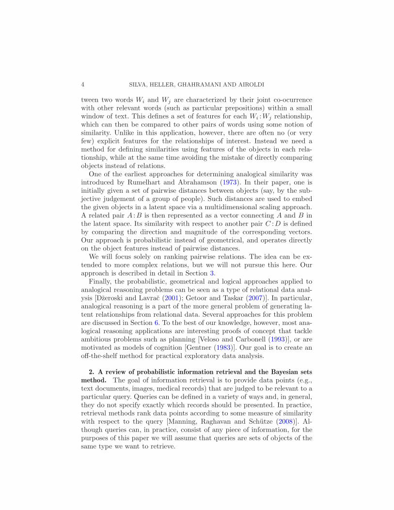
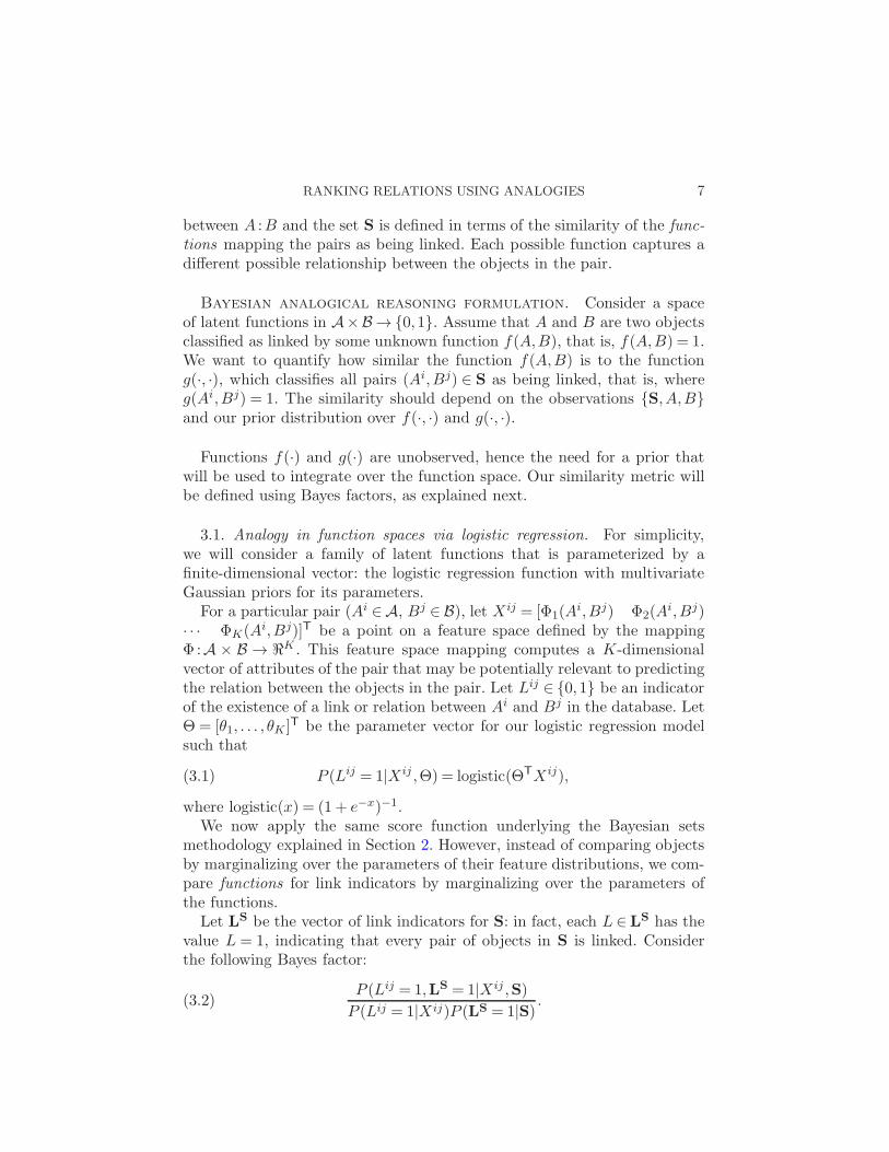
the Bayesian sets score function by which we rank points X given a queryS. The right-hand side was rearranged to provide a more intuitive graphicalmodel, shown in Figure 1. From this graphical model interpretation we cansee that the score function is a Bayes factor comparing two models [Kassand Raftery (1995)].

In the next section we describe how the Bayesian sets method can beadapted to define analogical similarity in the biological and informationnetworks settings we consider, and why such modifications are necessary.

3. A model of Bayesian analogical similarity for relations. To define ananalogy is to define a measure of similarity between structures of relatedobjects. In our setting, we need to measure the similarity between pairs of


Fig. 1. In order to score how well an arbitrary element X fits in with query setS = {X1,X2, . . . ,Xq}, the Bayesian sets methodology compares the marginal likelihoodof the model in (a), P (X,S), against the model in (b), P (X)P (S). In (a), the randomparameter vector Θ is given a prior defined by the (fixed) hyperparameter α. The same (la-tent) parameter vector is shared by the query set and the new point. In (b), the parametervector Θ that generates X is different from the one that generates the query set.

objects. The key aspect that distinguishes our approach from others is thatwe focus on the similarity between functions that map pairs to links, ratherthan focusing on the similarity between the features of objects in a candidatepair and the features of objects in the query pairs.

As an illustration, consider an analogical reasoning question from a SAT-like exam where for a given pair (say, water : river) we have to choose, outof 5 pairs, the one that best matches the type of relation implicit in such a“query.” In this case, it is reasonable to say car :highway would be a bettermatch than (the somewhat nonsensical) soda :ocean , since cars flow on ahighway, and so does water in a river. Notice that if we were to measure thesimilarity between objects instead of relations, soda :ocean would be a muchcloser pair, since soda is similar to water, and ocean is similar to river.

Nevertheless, it is legitimate to infer relational similarity from individualobject features, as summarized by Gentner and Medina (1998) in their “kindworld hypothesis.” What is needed is a mechanism by which object featuresshould be weighted in a particular relational similarity problem. We postu-late that, in analogical reasoning, similarity between features of objects isonly meaningful to the extent by which such features are useful to predictthe existence of the relationships.

Our approach can be described as follows. Let A and B represent ob-ject spaces. To say that an interaction A :B is analogous to S= {A(1) :B(1),

A(2) :B(2), . . . ,A(N) :B(N)} amounts to implicitly defining a measure of sim-ilarity between the pair A :B and the set of pairs S, where each query item

A(k) :B(k) corresponds to some pair Ai :Bj . However, this similarity is notdirectly derived from the similarity of the information contained in the dis-tribution of objects themselves, {Ai} ⊂A, {Bi} ⊂ B. Rather, the similarity


between A :B and the set S is defined in terms of the similarity of the func-tions mapping the pairs as being linked. Each possible function captures adifferent possible relationship between the objects in the pair.

Bayesian analogical reasoning formulation. Consider a spaceof latent functions in A×B→{0,1}. Assume that A and B are two objectsclassified as linked by some unknown function f(A,B), that is, f(A,B) = 1.We want to quantify how similar the function f(A,B) is to the functiong(·, ·), which classifies all pairs (Ai,Bj) ∈ S as being linked, that is, whereg(Ai,Bj) = 1. The similarity should depend on the observations {S,A,B}and our prior distribution over f(·, ·) and g(·, ·).

Functions f(·) and g(·) are unobserved, hence the need for a prior thatwill be used to integrate over the function space. Our similarity metric willbe defined using Bayes factors, as explained next.

3.1. Analogy in function spaces via logistic regression. For simplicity,we will consider a family of latent functions that is parameterized by afinite-dimensional vector: the logistic regression function with multivariateGaussian priors for its parameters.

For a particular pair (Ai ∈A, Bj ∈ B), let Xij = [Φ1(Ai,Bj) Φ2(A

i,Bj)· · · ΦK(Ai,Bj)]T be a point on a feature space defined by the mappingΦ :A × B → ℜK . This feature space mapping computes a K-dimensionalvector of attributes of the pair that may be potentially relevant to predictingthe relation between the objects in the pair. Let Lij ∈ {0,1} be an indicatorof the existence of a link or relation between Ai and Bj in the database. LetΘ = [θ1, . . . , θK ]T be the parameter vector for our logistic regression modelsuch that

P (Lij = 1|Xij ,Θ)= logistic(ΘTXij),(3.1)

where logistic(x) = (1 + e−x)−1.We now apply the same score function underlying the Bayesian sets

methodology explained in Section 2. However, instead of comparing objectsby marginalizing over the parameters of their feature distributions, we com-pare functions for link indicators by marginalizing over the parameters ofthe functions.

Let LS be the vector of link indicators for S: in fact, each L ∈LS has the

value L = 1, indicating that every pair of objects in S is linked. Considerthe following Bayes factor:

P (Lij = 1,LS = 1|Xij ,S)

P (Lij = 1|Xij)P (LS = 1|S).(3.2)


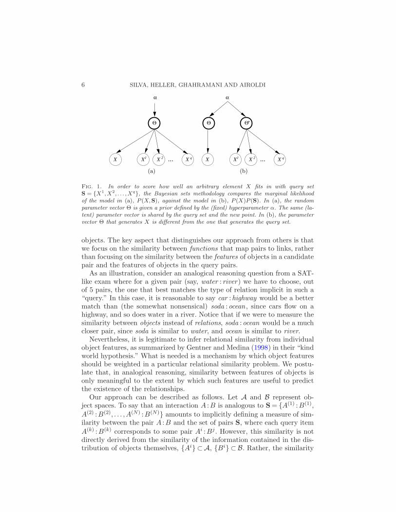
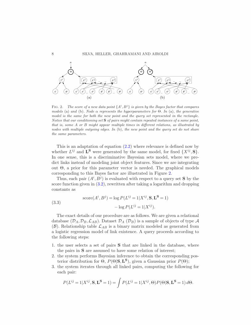
Fig. 2. The score of a new data point {Ai,Bj} is given by the Bayes factor that comparesmodels (a) and (b). Node α represents the hyperparameters for Θ. In (a), the generativemodel is the same for both the new point and the query set represented in the rectangle.Notice that our conditioning set S of pairs might contain repeated instances of a same point,that is, some A or B might appear multiple times in different relations, as illustrated bynodes with multiple outgoing edges. In (b), the new point and the query set do not sharethe same parameters.

This is an adaptation of equation (2.2) where relevance is defined now bywhether Lij and L

S were generated by the same model, for fixed {Xij ,S}.In one sense, this is a discriminative Bayesian sets model, where we pre-dict links instead of modeling joint object features. Since we are integratingout Θ, a prior for this parameter vector is needed. The graphical modelscorresponding to this Bayes factor are illustrated in Figure 2.

Thus, each pair (Ai,Bj) is evaluated with respect to a query set S by thescore function given in (3.2), rewritten after taking a logarithm and droppingconstants as

score(Ai,Bj) = logP (Lij = 1|Xij ,S,LS = 1)(3.3)

− logP (Lij = 1|Xij).

The exact details of our procedure are as follows. We are given a relationaldatabase (DA,DB,LAB). Dataset DA (DB) is a sample of objects of type A(B). Relationship table LAB is a binary matrix modeled as generated froma logistic regression model of link existence. A query proceeds according tothe following steps:

1. the user selects a set of pairs S that are linked in the database, wherethe pairs in S are assumed to have some relation of interest;

2. the system performs Bayesian inference to obtain the corresponding pos-terior distribution for Θ, P (Θ|S,LS), given a Gaussian prior P (Θ);

3. the system iterates through all linked pairs, computing the following foreach pair:

P (Lij = 1|Xij ,S,LS = 1) =

∫P (Lij = 1|Xij ,Θ)P (Θ|S,LS = 1)dΘ.


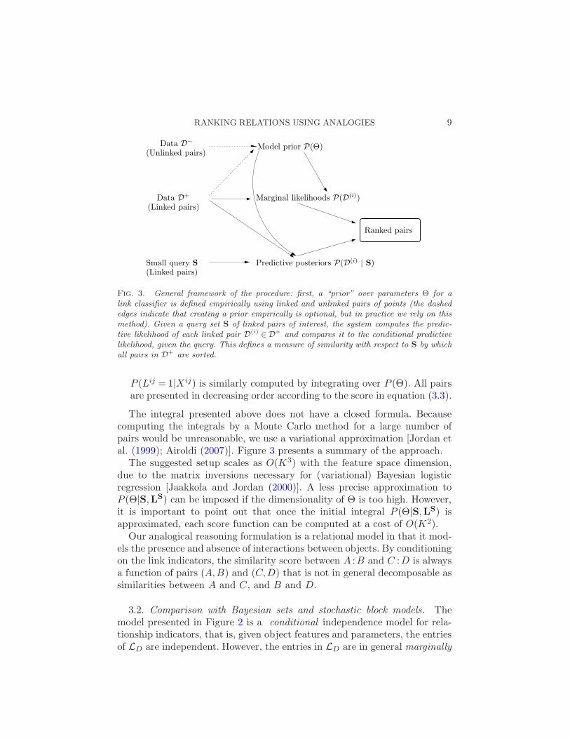
Fig. 3. General framework of the procedure: first, a “prior” over parameters Θ for alink classifier is defined empirically using linked and unlinked pairs of points (the dashededges indicate that creating a prior empirically is optional, but in practice we rely on thismethod). Given a query set S of linked pairs of interest, the system computes the predic-tive likelihood of each linked pair D(i) ∈ D+ and compares it to the conditional predictivelikelihood, given the query. This defines a measure of similarity with respect to S by whichall pairs in D+ are sorted.

P (Lij = 1|Xij) is similarly computed by integrating over P (Θ). All pairsare presented in decreasing order according to the score in equation (3.3).

The integral presented above does not have a closed formula. Becausecomputing the integrals by a Monte Carlo method for a large number ofpairs would be unreasonable, we use a variational approximation [Jordan etal. (1999); Airoldi (2007)]. Figure 3 presents a summary of the approach.

The suggested setup scales as O(K3) with the feature space dimension,due to the matrix inversions necessary for (variational) Bayesian logisticregression [Jaakkola and Jordan (2000)]. A less precise approximation toP (Θ|S,LS) can be imposed if the dimensionality of Θ is too high. However,it is important to point out that once the initial integral P (Θ|S,LS) isapproximated, each score function can be computed at a cost of O(K2).

Our analogical reasoning formulation is a relational model in that it mod-els the presence and absence of interactions between objects. By conditioningon the link indicators, the similarity score between A :B and C :D is alwaysa function of pairs (A,B) and (C,D) that is not in general decomposable assimilarities between A and C, and B and D.

3.2. Comparison with Bayesian sets and stochastic block models. Themodel presented in Figure 2 is a conditional independence model for rela-tionship indicators, that is, given object features and parameters, the entriesof LD are independent. However, the entries in LD are in general marginally


dependent. Since this is a model of relationships given object attributes, wecall the model introduced here the relational Bayesian sets model.

Our approach has some similarity to the so-called stochastic block models.These models were developed four decades ago in the network literature toquantify the notion of “structural equivalence” by means of blocks nodesthat instantiate similar connectivity patterns [Lorrain and White (1971);Holland and Leinhardt (1975)]. Modern stochastic block model approaches,in statistics and machine learning, build on these seminal works by intro-ducing the discovery of the block structure as part of the model search strat-egy [Fienberg, Meyer and Wasserman (1985); Nowicki and Snijders (2001);Kemp et al. (2006); Xu et al. (2006); Airoldi et al. (2005, 2008); Hoff (2008)].The observed features in our approach, Xij , effectively play the same roleas the latent indicators in stochastic block models.3 Since Xij is observed,there is no need to integrate over the feature space to obtain the posteriordistribution of Θ. This computational efficiency is particularly relevant ininformation retrieval and exploratory data analysis, where users expect arelatively short response time.

As an alternative to our relational Bayesian sets approach, consider thefollowing direct modification of the standard Bayesian sets formulation tothis problem: merge the data sets DA and DB into a single data set, cre-ating for each pair (Ai,Bj) a row in the database with an extra binaryindicator of relationship existence. Create a joint model for pairs by usingthe marginal models for A and B and treating different rows as being in-dependent. This ignores the fact that the resulting merged data points arenot really i.i.d. under such a model, because the same object might appearin multiple relations [Dzeroski and Lavrac (2001)]. The model also fails tocapture the dependency between Ai and Bj that arises from conditioningon Lij , even if Ai and Bj are marginally independent. Nevertheless, heuris-tically this approach can sometimes produce good results, and for severaltypes of probability families it is very computationally efficient. We evaluateit in Section 4.

3.3. Choice of features and relational discrimination. Our setup assumesthat the feature space Φ provides a reasonable classifier to predict the ex-istence of links. Useful predictive features can also be generated automati-cally with a variety of algorithms [e.g., the “structural logistic regression”of Popescul and Ungar (2003)]. See also Dzeroski and Lavrac (2001). Jensenand Neville (2002) discuss shortcomings of methods for automated featureselection in relational classification.

3In a stochastic block model, typically each object has a single feature η indicatingmembership to some latent class. For a pair Ai,Bj , the corresponding feature vector Xij

would be (ηA, ηB).


We also assume feature spaces are the same for all possible combinationsof objects. This allows for comparisons between, for example, cells from dif-ferent species, or web pages from different web domains, as long as featuresare generated by the same function Φ(·, ·). In general, we would like to relaxthis requirement, but for the problem to be well-defined, features from thedifferent spaces must be related somehow. A hierarchical Bayesian formu-lation for linking different feature spaces is one possibility which might betreated in a future work.

3.4. Priors. The choice of prior is based on the observed data, in a waythat is equivalent to the choice of priors used in the original formulation ofBayesian sets [Ghahramani and Heller (2005)]. Let Θ be the maximum likeli-hood estimator of Θ using the relational database (DA,DB,LAB). Since thenumber of possible pairs grows at a quadratic rate with the number of ob-jects, we do not use the whole database for maximum likelihood estimation.Instead, to get Θ, we use all linked pairs as members of the “positive” class(L= 1), and subsample unlinked pairs as members of the “negative” class(L= 0). We subsample by sampling each object uniformly at random fromthe respective data sets DA and DB to get a new pair. Since link matricesLAB are usually very sparse, in practice, this will almost always provide anunlinked pair. Sections 4 and 5 provide more details.

We use the prior P (Θ) = N (Θ, (cT)−1), where N (m,V) is a normal of

mean m and variance V. Matrix T is the empirical second moments matrixof the linked object features, although a different choice might be adequatefor different applications. Constant c is a smoothing parameter set by theuser. In all of our experiments we set c to be equal to the number of positivepairs. A good choice of c might be important to obtain maximum perfor-mance, but we leave this issue as future work. Wang et al. (2009) presentsome sensitivity analysis results for a particular application in text analysis.

Empirical priors are a sensible choice, since this is a retrieval, not a predic-tive, task. Basically, the entire data set is the population, from which priorinformation is obtained on possible query sets. A data-dependent prior basedon the population is important for an approach such as Bayesian sets, sincedeviances from the “average” behavior in the data are useful to discriminatebetween subpopulations.

3.5. On continuous and multivariate relations. Although we focus onmeasuring similarity of qualitative relationships, the same idea could be ex-tended to continuous (or ordinal) measures of relationship, or relationshipswhere each Lij is a vector. For instance, Turney and Littman (2005) mea-sure relations between words by their co-occurrences on the neighborhoodof specific keywords, such as the frequency of two words being connected by


a specific preposition in a large body of text documents. Several similaritymetrics can be defined on this vector of continuous relationships. However,given data on word features, one can easily modify our approach by sub-stituting the logistic regression component with some multiple regressionmodel.

4. Ranking hyperlinks on the web. In the following application we con-sider a collection of web pages from several universities: the WebKB col-lection, where relations are given by hyperlinks [Craven et al. (1998)]. Webpages are classified as being of type course, department, faculty, project,staff, student or other. Documents come from four universities (Cornell,Texas, Washington and Wisconsin). We are interested in recovering pairsof web pages {A,B} where web page A has a link to web page B. Noticethat the relationship is asymmetric. Different types of web pages imply dif-ferent types of links. For instance, a faculty web page linking to a project

web page constitutes a type of link. The analogical reasoning task here issimplified if we assume each web page object has a single role (i.e., exactlyone out of the pre-defined types {course, department, faculty, project, staff,student, other}), and therefore a pair of web pages implies a unique typeof relationship. The web page types are for evaluation purposes only, as weexplain later: we will not provide this information to the model.

Our main standard of comparison is a “flattened Bayesian sets” algo-rithm (which we will call “standard Bayesian sets,” SBSets, in constrast tothe relational model, RBSets). Using a multivariate independent Bernoullimodel as in the original paper [Ghahramani and Heller (2005)], we mergelinked web page pairs into single rows, and then apply the original algorithmdirectly to the merged data. It is clear that data points are not independentanymore, but the SBSets algorithm assumes this is the case. Evaluatingthis algorithm serves the purpose of both measuring the loss of not treatingrelational data as such, as well as the limitations of evaluating the similarityof pairs through models for the marginal probabilities of A and B insteadof models for the predictive function P (Lij |Xij).

Binary data was extracted from this database using the same methodol-ogy as in Ghahramani and Heller (2005). A total of 19,450 binary variablesper object are generated, where each variable indicates whether a word froma fixed dictionary appears in a given document more frequently than the av-erage. To avoid introducing extra approximations into RBSets, we reducedthe dimensionality of the original representation using singular value decom-position, obtaining 25 measures per object.

In this experiment objects are of the same type, and therefore, dimen-sionality. The feature vector Xij for each pair of objects {Ai,Bj} consistsof the V features for object Ai, the V features of object Bj , and mea-sures Z = {Z1, . . . ,ZV }, where Zv = (Ai

v × Bjv)/(|Ai| × ‖Bj‖), ‖Ai‖ being


the Euclidean norm of the V -dimensional representation of Ai. We also adda constant value (1) to the feature set as an intercept term for the logisticregression. Feature set Z is exactly the one used in the cosine distance mea-sure,4 a common and practical measure widely used in information retrieval[Manning, Raghavan and Schutze (2008)]. This feature space also has theimportant advantage of scaling well (linearly) with the number of variablesin the database. Moreover, adopting such features will make our compar-isons fairer, since we evaluate how well cosine distance itself performs inour task. Notice that our choice of Xij is suitable for asymmetric relation-ships, as naturally occurs in the domain of web page links. For symmetricrelationships, features such as |Ai

v −Bjv| could be used instead.

In order to set the empirical prior, we sample 10 “negative” pairs foreach “positive” one, and weight them to reflect the proportion of linked tounlinked pairs in the database. That is, in the WebKB study we use 10negatives for each positive, and we count each negative case as being 350cases replicated. We perform subsampling and reweighting in order to beable to fit the database in the memory of a desktop computer.

Evaluation of the significance of retrieved items often relies on subjectiveassessments [Ghahramani and Heller (2005)]. To simplify our study, we willfocus on particular setups where objective measures of success are defined.

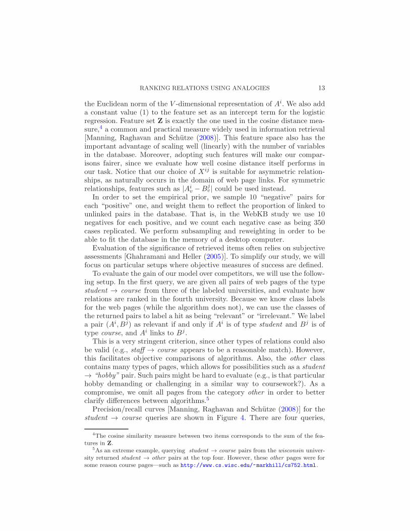
To evaluate the gain of our model over competitors, we will use the follow-ing setup. In the first query, we are given all pairs of web pages of the typestudent → course from three of the labeled universities, and evaluate howrelations are ranked in the fourth university. Because we know class labelsfor the web pages (while the algorithm does not), we can use the classes ofthe returned pairs to label a hit as being “relevant” or “irrelevant.” We labela pair (Ai,Bj) as relevant if and only if Ai is of type student and Bj is oftype course, and Ai links to Bj .

This is a very stringent criterion, since other types of relations could alsobe valid (e.g., staff → course appears to be a reasonable match). However,this facilitates objective comparisons of algorithms. Also, the other classcontains many types of pages, which allows for possibilities such as a student

→ “hobby” pair. Such pairs might be hard to evaluate (e.g., is that particularhobby demanding or challenging in a similar way to coursework?). As acompromise, we omit all pages from the category other in order to betterclarify differences between algorithms.5

Precision/recall curves [Manning, Raghavan and Schutze (2008)] for thestudent → course queries are shown in Figure 4. There are four queries,

4The cosine similarity measure between two items corresponds to the sum of the fea-tures in Z.

5As an extreme example, querying student → course pairs from the wisconsin univer-sity returned student → other pairs at the top four. However, these other pages were forsome reason course pages—such as http://www.cs.wisc.edu/~markhill/cs752.html.

http://www.cs.wisc.edu/~markhill/cs752.html


Fig. 4. Results for student → course relationships.

each corresponding to a search over a specific university given all valid stu-

dent → course pairs from the other three. There are four algorithms oneach evaluation: the standard Bayesian sets with the original 19,450 binaryvariables for each object, plus another 19,450 binary variables, each cor-responding to the product of the respective variables in the original pairof objects (SBSets1); the standard Bayesian sets with the original binaryvariables only (SBSets2); a standard cosine distance measure over the 25-dimensional representation (Cosine 1) for each page, with pairs being givenby the combined vector of 50 features; a cosine distance measure using theraw 19,450-dimensional binary for each document (Cosine 2); our approach,RBSets.

In Figure 4RBSets demonstrates consistently superior or equal precision-recall. Although SBSets performs well when asked to retrieve only student

items or only course items, it falls short of detecting what features of stu-

dent and course are relevant to predict a link. The discriminative modelwithin RBSets conveys this information through the link parameters.

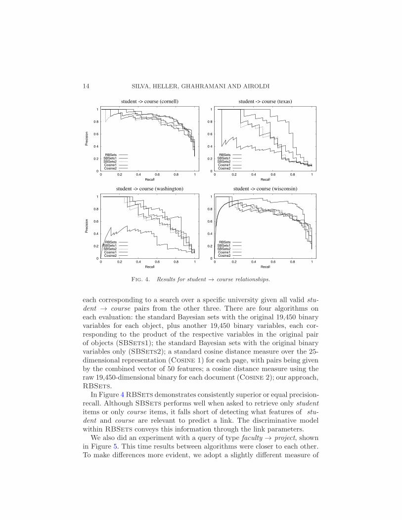
We also did an experiment with a query of type faculty → project, shownin Figure 5. This time results between algorithms were closer to each other.To make differences more evident, we adopt a slightly different measure of


Fig. 5. Results for faculty → project relationships.

success: we count as a 1 hit if the pair retrieved is a faculty → project pair,and count as a 0.5 hit for pairs of type student → project and staff → project.Notice this is a much harder query. For instance, the structure of the projectweb pages in the texas group was quite distinct from the other universities:they are mostly very short, basically containing links for members of theproject and other project web pages.

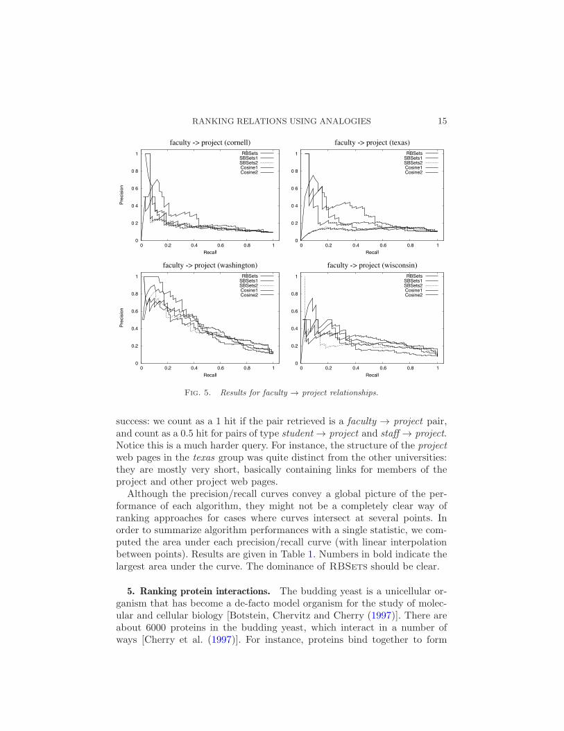
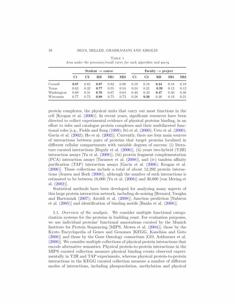
Although the precision/recall curves convey a global picture of the per-formance of each algorithm, they might not be a completely clear way ofranking approaches for cases where curves intersect at several points. Inorder to summarize algorithm performances with a single statistic, we com-puted the area under each precision/recall curve (with linear interpolationbetween points). Results are given in Table 1. Numbers in bold indicate thelargest area under the curve. The dominance of RBSets should be clear.

5. Ranking protein interactions. The budding yeast is a unicellular or-ganism that has become a de-facto model organism for the study of molec-ular and cellular biology [Botstein, Chervitz and Cherry (1997)]. There areabout 6000 proteins in the budding yeast, which interact in a number ofways [Cherry et al. (1997)]. For instance, proteins bind together to form


Table 1

Area under the precision/recall curve for each algorithm and query

Student → course Faculty → project

C1 C2 RB SB1 SB2 C1 C2 RB SB1 SB2

Cornell 0.87 0.82 0.87 0.82 0.80 0.19 0.18 0.24 0.18 0.18Texas 0.62 0.32 0.77 0.55 0.54 0.24 0.21 0.29 0.12 0.12Washington 0.69 0.31 0.76 0.67 0.64 0.40 0.42 0.47 0.40 0.40Wisconsin 0.77 0.72 0.88 0.75 0.73 0.28 0.30 0.26 0.19 0.21

protein complexes, the physical units that carry out most functions in thecell [Krogan et al. (2006)]. In recent years, significant resources have beendirected to collect experimental evidence of physical proteins binding, in aneffort to infer and catalogue protein complexes and their multifaceted func-tional roles [e.g., Fields and Song (1989); Ito et al. (2000); Uetz et al. (2000);Gavin et al. (2002); Ho et al. (2002)]. Currently, there are four main sourcesof interactions between pairs of proteins that target proteins localized indifferent cellular compartments with variable degrees of success: (i) litera-ture curated interactions [Reguly et al. (2006)], (ii) yeast two-hybrid (Y2H)interaction assays [Yu et al. (2008)], (iii) protein fragment complementation(PCA) interaction assays [Tarassov et al. (2008)], and (iv) tandem affinitypurification (TAP) interaction assays [Gavin et al. (2006); Krogan et al.(2006)]. These collections include a total of about 12,292 protein interac-tions [Jensen and Bork (2008)], although the number of such interactions isestimated to be between 18,000 [Yu et al. (2008)] and 30,000 [von Mering etal. (2002)].

Statistical methods have been developed for analyzing many aspects ofthis large protein interaction network, including de-noising [Bernard, Vaughnand Hartemink (2007); Airoldi et al. (2008)], function prediction [Nabievaet al. (2005)] and identification of binding motifs [Banks et al. (2008)].

5.1. Overview of the analysis. We consider multiple functional catego-rization systems for the proteins in budding yeast. For evaluation purposes,we use individual proteins’ functional annotations curated by the MunichInstitute for Protein Sequencing [MIPS, Mewes et al. (2004)], those by theKyoto Encyclopedia of Genes and Genomes [KEGG, Kanehisa and Goto(2000)] and those by the Gene Ontology consortium [GO, Ashburner et al.(2000)]. We consider multiple collections of physical protein interactions thatencode alternative semantics. Physical protein-to-protein interactions in theMIPS curated collection measure physical binding events observed experi-mentally in Y2H and TAP experiments, whereas physical protein-to-proteininteractions in the KEGG curated collection measure a number of differentmodes of interactions, including phosporelation, methylation and physical


Table 2

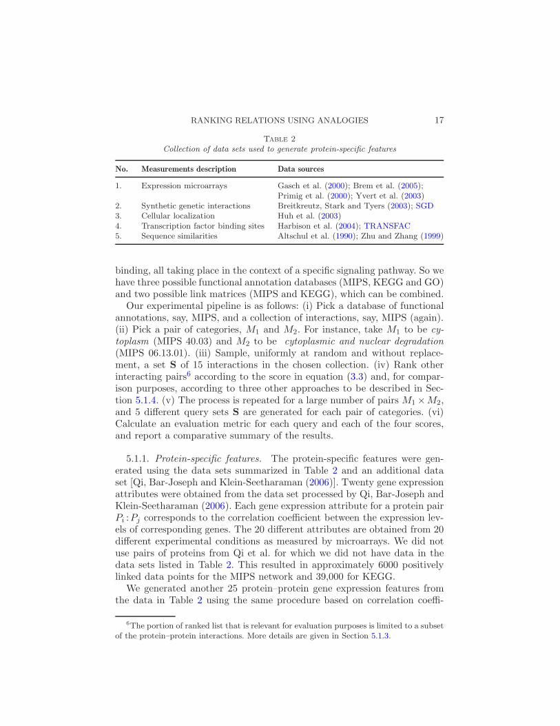
Collection of data sets used to generate protein-specific features

No. Measurements description Data sources

1. Expression microarrays Gasch et al. (2000); Brem et al. (2005);Primig et al. (2000); Yvert et al. (2003)

2. Synthetic genetic interactions Breitkreutz, Stark and Tyers (2003); SGD3. Cellular localization Huh et al. (2003)4. Transcription factor binding sites Harbison et al. (2004); TRANSFAC5. Sequence similarities Altschul et al. (1990); Zhu and Zhang (1999)

binding, all taking place in the context of a specific signaling pathway. So wehave three possible functional annotation databases (MIPS, KEGG and GO)and two possible link matrices (MIPS and KEGG), which can be combined.

Our experimental pipeline is as follows: (i) Pick a database of functionalannotations, say, MIPS, and a collection of interactions, say, MIPS (again).(ii) Pick a pair of categories, M1 and M2. For instance, take M1 to be cy-

toplasm (MIPS 40.03) and M2 to be cytoplasmic and nuclear degradation

(MIPS 06.13.01). (iii) Sample, uniformly at random and without replace-ment, a set S of 15 interactions in the chosen collection. (iv) Rank otherinteracting pairs6 according to the score in equation (3.3) and, for compar-ison purposes, according to three other approaches to be described in Sec-tion 5.1.4. (v) The process is repeated for a large number of pairs M1 ×M2,and 5 different query sets S are generated for each pair of categories. (vi)Calculate an evaluation metric for each query and each of the four scores,and report a comparative summary of the results.

5.1.1. Protein-specific features. The protein-specific features were gen-erated using the data sets summarized in Table 2 and an additional dataset [Qi, Bar-Joseph and Klein-Seetharaman (2006)]. Twenty gene expressionattributes were obtained from the data set processed by Qi, Bar-Joseph andKlein-Seetharaman (2006). Each gene expression attribute for a protein pairPi :Pj corresponds to the correlation coefficient between the expression lev-els of corresponding genes. The 20 different attributes are obtained from 20different experimental conditions as measured by microarrays. We did notuse pairs of proteins from Qi et al. for which we did not have data in thedata sets listed in Table 2. This resulted in approximately 6000 positivelylinked data points for the MIPS network and 39,000 for KEGG.

We generated another 25 protein–protein gene expression features fromthe data in Table 2 using the same procedure based on correlation coeffi-

6The portion of ranked list that is relevant for evaluation purposes is limited to a subsetof the protein–protein interactions. More details are given in Section 5.1.3.


cients. This gives a total of 45 attributes, corresponding to the main dataset used in our relational Bayesian sets runs.

Another data set was generated using the remaining (i.e., nonmicroarray)features of Table 2. Such features are binary and highly sparse, with mostentries being 0 for the majority of linked pairs. We removed attributes forwhich we had fewer than 20 linked pairs with positive values according tothe MIPS network. The total number of extra binary attributes was 16.

Several measurements were missing. We imputed missing values for eachvariable in a particular data point by using its empirical average among theobserved values.

Given the 45 or 61 attributes of a given pair {Pi, Pj}, we applied anonlinear transformation where we normalize the vector by its Euclideannorm in order to obtain our feature table X.

5.1.2. Calibrating the prior for Θ. We initially fit a logistic regressionclassifier using a maximum likelihood estimation (MLE) and our data, ob-

taining the estimate Θ. Our choice of covariance matrix Σ for Θ is definedto be a rescaling of a squared norm of the data:

(Σ)−1 =XT

POSXPOS,(5.1)

where XPOS is the matrix containing the protein–protein features only ofthe linked pairs used in the MLE computation.

5.1.3. Evaluation metrics. As in the WebKB experiment, we propose anobjective measure of evaluation that is used to compare different algorithms.Consider a query set S, and a ranked response list R= {R1,R2,R3, . . . ,RN}of protein–protein pairs. Every element of S is a pair of proteins Pi :Pj

such that Pi is of class Mi and Pj is of class Mj , where Mi and Mj areclasses from either MIPS, KEGG or Gene Ontology. In general, proteinsbelong to multiple classes. This is in contrast with the WebKB experiment,where, according to our web page categorization, there was only one possibletype of relationship for each pair of web pages. The retrieval algorithmthat generates R does not receive any information concerning the MIPS,KEGG or GO taxonomy. R starts with the linked protein pair that is judgedmost similar to S, followed by the other protein pairs in the population,in decreasing order of similarity. Each algorithm has its own measure ofsimilarity.

The evaluation criterion for each algorithm is as follows: as before, wegenerate a precision-recall curve and calculate the area under the curve(AUC). We also calculate the proportion (TOP10), among the top 10 ele-ments in each ranking, of pairs that match the original {M1,M2} selection(i.e., a “correct” Pi :Pj is one where Pi is of class M1 and Pj of class M2,or vice-versa. Notice that each protein belongs to multiple classes, so both


conditions might be satisfied.) Since a researcher is only likely to look at thetop ranked pairs, it makes sense to define a measure that uses only a subsetof the ranking. AUC and TOP10 are our two evaluation measures.

The original classes {M1,M2} are known to the experimenter but notknown to the algorithms. As in the WebKB experiment, our criterion israther stringent, in the sense that it requires a perfect match of each RI

with the MIPS, KEGG or GO categorization. There are several ways bywhich a pair RI might be analogous to the relation implicit in S, and theydo not need to agree with MIPS, GO or KEGG. Still, if we are willing tobelieve that these standard categorization systems capture functional or-ganization of proteins at some level, this must lead to association betweencategories given to S and relevant subpopulations of protein–protein inter-actions similar to S. Therefore, the corresponding AUC and TOP10 areuseful tools for comparing different algorithms even if the actual measuresare likely to be pessimistic for a fixed algorithm.

5.1.4. Competing algorithms. We compare our method against a variantof it and two similarity metrics widely used for information retrieval:

1. The cosine score [Manning, Raghavan and Schutze (2008)], denoted bycos.

2. The nearest neighbor score, denoted by nns.3. The relational maximum likelihood sets score, denoted by mls.

The nearest neighbor score measures the minimum Euclidean distance be-tween RI and any individual point in S, for a given query set S and a givencandidate point RI . The relational maximum likelihood sets is a variationof RBSets where we initially sample a subset of the unlinked pairs (10,000points in our setup) and, for each query S, we fit a logistic regression modelto obtain the parameter estimate ΘMLE

S. We also use a logistic regression

model fit to the whole data set (the same one used to generate the priorfor RBSets), giving the estimate ΘMLE. A new score, analogous to (3.3),is given by logP (Lij = 1|Xij ,ΘMLE

S)− logP (Lij = 1|Xij ,ΘMLE), that is, we

do not integrate out the parameters or use a prior, but instead the modelsare fixed at their respective estimates.

Neither cos or nns can be interpreted as measures of analogical simi-larity, in the sense that they do not take into account how the protein pairfeatures X contribute to their interaction.7 It is true that a direct measure ofanalogical similarity is not theoretically required to perform well accordingto our (nonanalogical) evaluation metric. However, we will see that thereare practical advantages in doing so.

7As a consequence, none uses negative data. Another consequence is the necessity ofmodeling the input space that generates X, a difficult task given the dimensionality andthe continuous nature of the features.


5.2. Results on the MIPS collection of physical interactions. For thisbatch of experiments, we use the MIPS network of protein–protein inter-actions to define the relationships. In the initial experiment, we selectedqueries from all combinations of MIPS classes for which there were at least50 linked pairs Pi :Pj in the network that satisfied the choice of classes. Eachquery set contained 15 pairs. After removing the MIPS-categorized proteinsfor which we had no feature data, we ended up with a total of 6125 pro-teins and 7788 positive interactions. We set the prior for RBSets using asample of 225,842 pairs labeled as having no interaction, as selected by Qi,Bar-Joseph and Klein-Seetharaman (2006).

For each tentative query set S of categories {M1,M2}, we scored andranked pairs P ′

i :P′

j such that both P ′

i and P ′

j were connected to some pro-tein appearing in S by a path of no more than two steps, according to theMIPS network. The reasons for the filtering are two-fold: to increase thecomputational performance of the ranking since fewer pairs are scored; andto minimize the chance that undesirable pairs would appear in the top 10ranked pairs. Tentative queries would not be performed if after filtering weobtained fewer than 50 possible correct matches. Trivial queries, where filter-ing resulted only in pairs in the same class as the query, were also discarded.The resulting number of unique pairs of categories {M1,M2} was 931 classesof interactions. For each pair of categories, we sampled our query set S 5times, generating a total of 4655 rankings per algorithm.

We run two types of experiments. In one version, we give to RBSets thedata containing only the 45 (continuous) microarray measurements. In thesecond variation, we provide to RBSets all 61 variables, including the 16sparse binary indicators. However, we noticed that the addition of the 16binary variables hurts RBSets considerably. We conjecture that one reasonmight be the degradation of the variational approximation. Including thebinary variables hardly changed the other three methods, so we choose touse the 61 variable data set for the other methods.8

Table 3 summarizes the results of this experiment. We show the numberof times each method wins according to both the AUC and TOP10 criteria.The number of wins is presented as divided by 5, the number of randomsets generated for each query type {M1,M2} (notice these numbers do notneed to add up to 931, since ties are possible). Moreover, we also presented“smoothed” versions of this statistic, where we count a method as the winnerfor any given {M1,M2} category if, for the group of 5 queries, the methodobtains the best result in at least 3 of the sets. The motivation is to smooth

8We also performed an experiment (not included) where only the continuous attributeswere used by the other methods. The advantage of RBSets still increased, slightly (bya 2% margin against the cosine distance method). For this reason, we analyze the mostpessimistic case.


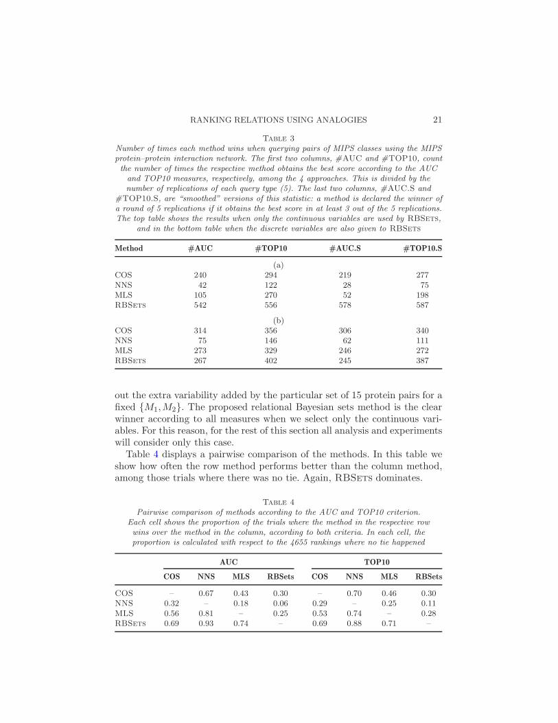
Table 3

Number of times each method wins when querying pairs of MIPS classes using the MIPSprotein–protein interaction network. The first two columns, #AUC and #TOP10, countthe number of times the respective method obtains the best score according to the AUCand TOP10 measures, respectively, among the 4 approaches. This is divided by thenumber of replications of each query type (5). The last two columns, #AUC.S and

#TOP10.S, are “smoothed” versions of this statistic: a method is declared the winner ofa round of 5 replications if it obtains the best score in at least 3 out of the 5 replications.The top table shows the results when only the continuous variables are used by RBSets,

and in the bottom table when the discrete variables are also given to RBSets

Method #AUC #TOP10 #AUC.S #TOP10.S

(a)COS 240 294 219 277NNS 42 122 28 75MLS 105 270 52 198RBSets 542 556 578 587

(b)COS 314 356 306 340NNS 75 146 62 111MLS 273 329 246 272RBSets 267 402 245 387

out the extra variability added by the particular set of 15 protein pairs for afixed {M1,M2}. The proposed relational Bayesian sets method is the clearwinner according to all measures when we select only the continuous vari-ables. For this reason, for the rest of this section all analysis and experimentswill consider only this case.

Table 4 displays a pairwise comparison of the methods. In this table weshow how often the row method performs better than the column method,among those trials where there was no tie. Again, RBSets dominates.

Table 4

Pairwise comparison of methods according to the AUC and TOP10 criterion.Each cell shows the proportion of the trials where the method in the respective rowwins over the method in the column, according to both criteria. In each cell, theproportion is calculated with respect to the 4655 rankings where no tie happened

AUC TOP10

COS NNS MLS RBSets COS NNS MLS RBSets

COS – 0.67 0.43 0.30 – 0.70 0.46 0.30NNS 0.32 – 0.18 0.06 0.29 – 0.25 0.11MLS 0.56 0.81 – 0.25 0.53 0.74 – 0.28RBSets 0.69 0.93 0.74 – 0.69 0.88 0.71 –


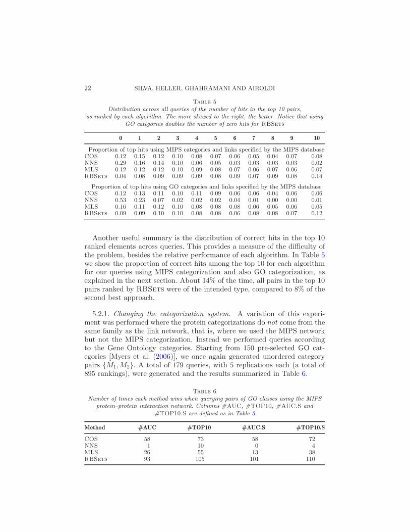
Table 5

Distribution across all queries of the number of hits in the top 10 pairs,as ranked by each algorithm. The more skewed to the right, the better. Notice that using

GO categories doubles the number of zero hits for RBSets

0 1 2 3 4 5 6 7 8 9 10

Proportion of top hits using MIPS categories and links specified by the MIPS databaseCOS 0.12 0.15 0.12 0.10 0.08 0.07 0.06 0.05 0.04 0.07 0.08NNS 0.29 0.16 0.14 0.10 0.06 0.05 0.03 0.03 0.03 0.03 0.02MLS 0.12 0.12 0.12 0.10 0.09 0.08 0.07 0.06 0.07 0.06 0.07RBSets 0.04 0.08 0.09 0.09 0.09 0.08 0.09 0.07 0.09 0.08 0.14

Proportion of top hits using GO categories and links specified by the MIPS databaseCOS 0.12 0.13 0.11 0.10 0.11 0.09 0.06 0.06 0.04 0.06 0.06NNS 0.53 0.23 0.07 0.02 0.02 0.02 0.04 0.01 0.00 0.00 0.01MLS 0.16 0.11 0.12 0.10 0.08 0.08 0.08 0.06 0.05 0.06 0.05RBSets 0.09 0.09 0.10 0.10 0.08 0.08 0.06 0.08 0.08 0.07 0.12

Another useful summary is the distribution of correct hits in the top 10ranked elements across queries. This provides a measure of the difficulty ofthe problem, besides the relative performance of each algorithm. In Table 5we show the proportion of correct hits among the top 10 for each algorithmfor our queries using MIPS categorization and also GO categorization, asexplained in the next section. About 14% of the time, all pairs in the top 10pairs ranked by RBSets were of the intended type, compared to 8% of thesecond best approach.

5.2.1. Changing the categorization system. A variation of this experi-ment was performed where the protein categorizations do not come from thesame family as the link network, that is, where we used the MIPS networkbut not the MIPS categorization. Instead we performed queries accordingto the Gene Ontology categories. Starting from 150 pre-selected GO cat-egories [Myers et al. (2006)], we once again generated unordered categorypairs {M1,M2}. A total of 179 queries, with 5 replications each (a total of895 rankings), were generated and the results summarized in Table 6.

Table 6

Number of times each method wins when querying pairs of GO classes using the MIPSprotein–protein interaction network. Columns #AUC, #TOP10, #AUC.S and

#TOP10.S are defined as in Table 3


COS 58 73 58 72NNS 1 10 0 4MLS 26 55 13 38RBSets 93 105 101 110


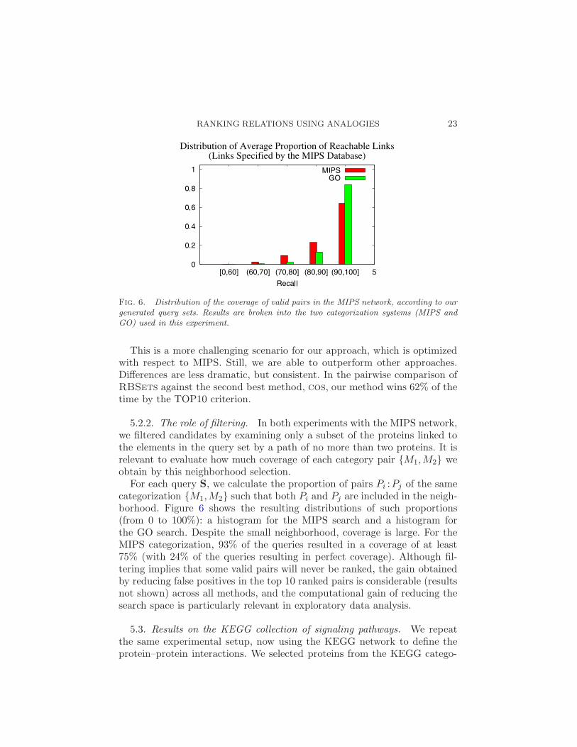
Fig. 6. Distribution of the coverage of valid pairs in the MIPS network, according to ourgenerated query sets. Results are broken into the two categorization systems (MIPS andGO) used in this experiment.

This is a more challenging scenario for our approach, which is optimizedwith respect to MIPS. Still, we are able to outperform other approaches.Differences are less dramatic, but consistent. In the pairwise comparison ofRBSets against the second best method, cos, our method wins 62% of thetime by the TOP10 criterion.

5.2.2. The role of filtering. In both experiments with the MIPS network,we filtered candidates by examining only a subset of the proteins linked tothe elements in the query set by a path of no more than two proteins. It isrelevant to evaluate how much coverage of each category pair {M1,M2} weobtain by this neighborhood selection.

For each query S, we calculate the proportion of pairs Pi :Pj of the samecategorization {M1,M2} such that both Pi and Pj are included in the neigh-borhood. Figure 6 shows the resulting distributions of such proportions(from 0 to 100%): a histogram for the MIPS search and a histogram forthe GO search. Despite the small neighborhood, coverage is large. For theMIPS categorization, 93% of the queries resulted in a coverage of at least75% (with 24% of the queries resulting in perfect coverage). Although fil-tering implies that some valid pairs will never be ranked, the gain obtainedby reducing false positives in the top 10 ranked pairs is considerable (resultsnot shown) across all methods, and the computational gain of reducing thesearch space is particularly relevant in exploratory data analysis.

5.3. Results on the KEGG collection of signaling pathways. We repeatthe same experimental setup, now using the KEGG network to define theprotein–protein interactions. We selected proteins from the KEGG catego-


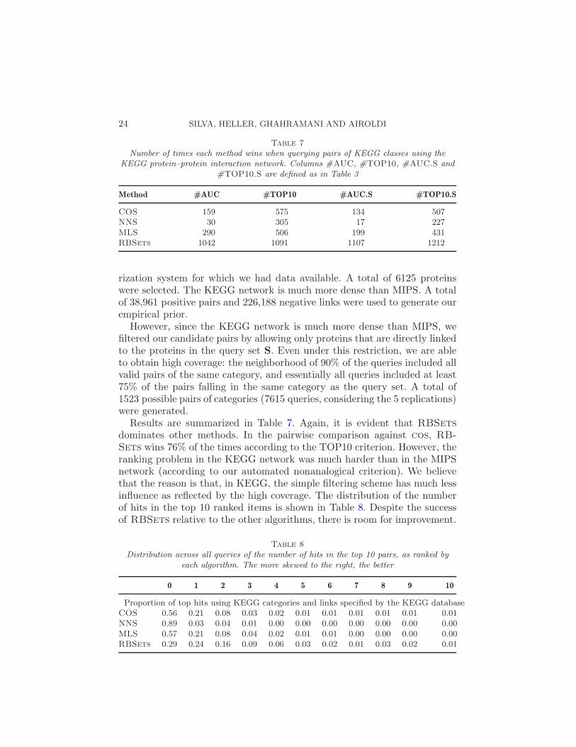
Table 7

Number of times each method wins when querying pairs of KEGG classes using theKEGG protein–protein interaction network. Columns #AUC, #TOP10, #AUC.S and

#TOP10.S are defined as in Table 3


COS 159 575 134 507NNS 30 305 17 227MLS 290 506 199 431RBSets 1042 1091 1107 1212

rization system for which we had data available. A total of 6125 proteinswere selected. The KEGG network is much more dense than MIPS. A totalof 38,961 positive pairs and 226,188 negative links were used to generate ourempirical prior.

However, since the KEGG network is much more dense than MIPS, wefiltered our candidate pairs by allowing only proteins that are directly linkedto the proteins in the query set S. Even under this restriction, we are ableto obtain high coverage: the neighborhood of 90% of the queries included allvalid pairs of the same category, and essentially all queries included at least75% of the pairs falling in the same category as the query set. A total of1523 possible pairs of categories (7615 queries, considering the 5 replications)were generated.

Results are summarized in Table 7. Again, it is evident that RBSets

dominates other methods. In the pairwise comparison against cos, RB-

Sets wins 76% of the times according to the TOP10 criterion. However, theranking problem in the KEGG network was much harder than in the MIPSnetwork (according to our automated nonanalogical criterion). We believethat the reason is that, in KEGG, the simple filtering scheme has much lessinfluence as reflected by the high coverage. The distribution of the numberof hits in the top 10 ranked items is shown in Table 8. Despite the successof RBSets relative to the other algorithms, there is room for improvement.

Table 8

Distribution across all queries of the number of hits in the top 10 pairs, as ranked byeach algorithm. The more skewed to the right, the better

0 1 2 3 4 5 6 7 8 9 10

Proportion of top hits using KEGG categories and links specified by the KEGG databaseCOS 0.56 0.21 0.08 0.03 0.02 0.01 0.01 0.01 0.01 0.01 0.01NNS 0.89 0.03 0.04 0.01 0.00 0.00 0.00 0.00 0.00 0.00 0.00MLS 0.57 0.21 0.08 0.04 0.02 0.01 0.01 0.00 0.00 0.00 0.00RBSets 0.29 0.24 0.16 0.09 0.06 0.03 0.02 0.01 0.03 0.02 0.01


6. More related work. There is a large literature on analogical reasoningin artificial intelligence and psychology. We refer to French (2002) for a sur-vey, and to more recent papers on clustering [Marx et al. (2002)], prediction[Turney and Littman (2005); Turney (2008a)] and dimensionality reduction[Memisevic and Hinton (2005)] as examples of other applications. Classicalapproaches for planning have also exploited analogical similarities [Velosoand Carbonell (1993)].

Nonprobabilistic similarity functions between relational structures havealso been developed for the purpose of deriving kernel matrices, such asthose required by support vector machines. Borgwardt (2007) provides acomprehensive survey and state-of-the-art methods. It would be interestingto adapt such methods to problems of analogical reasoning.

The graphical model formulation of Getoor et al. (2002) incorporatesmodels of link existence in relational databases, an idea used explicitly inSection 3 as the first step of our problem formulation. In the clusteringliterature, the probabilistic approach of Kemp et al. (2006) is motivated byprinciples similar to those in our formulation: the idea is that there is aninfinite mixture of subpopulations that generates the observed relations. Ourproblem, however, is to retrieve other elements of a subpopulation describedby elements of a query set, a goal that is closer to the classical paradigm ofanalogical reasoning.

As discussed in Section 3.2, our model can be interpreted as a type ofblock model [Kemp et al. (2006); Xu et al. (2006); Airoldi et al. (2008)] withobservable features. Link indicators are independent given the object fea-tures, which might not actually be the case for particular choices of featurespace. In theory, block models sidestep this issue by learning all the neces-sary latent features that account for link dependence. An important futureextension of our work would consist of tractably modeling the residual linkassociation that is not accounted for by our observed features.

Discovering analogies is a specific task within the general problem of gen-erating latent relationships from relational data. Some of the first formalmethods for discovering latent relationships from multiple data sets were in-troduced in the literature of inductive logic programming, such as the inverseresolution method [Muggleton (1981)]. A more recent probabilistic methodis discussed by Kok and Domingos (2007). Dzeroski and Lavrac (2001) andGetoor and Taskar (2007) provide an overview of relational learning methodsfrom a data mining and machine learning perspective.

A particularly active subfield on latent relationship generation lies withintext analysis research. For instance, Stephens et al. (2001) describe an ap-proach for discovering relations between genes given MEDLINE abstracts.In the context of information retrieval, Cafarella, Banko and Etzioni (2006)describe an application of recent unsupervised information extraction meth-ods: relations generated from unstructured text documents are used as a


preprocessing step to build an index of web pages. In analogical reasoningapplications, our method has been used by others for question-answeringanalysis [Wang et al. (2009)].

The idea of measuring the similarity of two data points based on a predic-tive function has appeared in the literature on matching for causal inference.Suppose we are given a model for predicting an outcome Y given a treatmentZ and a set of potential confounders X. For simplicity, assume Z ∈ {0,1}.The goal of matching is to find, for each data point (Xi, Yi,Zi), the closestmatch (Xj, Yj ,Zj) according to the confounding variables X. In principle,any clustering criterion could be used in this task [Gelman and Hill (2007)].The propensity score criterion [Rosenbaum (2002)] measures the similarityof two feature vectors Xi and Xj by comparing the predictions P (Zi = 1|Xi)and P (Zj = 1|Xj). If the conditional P (Z = 1|X) is given by a logistic re-gression model with parameter vector Θ, Gelman and Hill (2007) suggestmeasuring the difference between X

T

i Θ and XT

j Θ. While this is not the sameas comparing two predictive functions as in our framework, the core idea ofusing predictive functions to define similarity remains.

A preliminary version of this paper appeared in the proceedings of the11th International Conference on Artificial Intelligence and Statistics [Silva,Heller and Ghahramani (2007)].

7. Conclusion. We have presented a framework for performing analogi-cal reasoning within a Bayesian data analysis formulation. There is of coursemuch more to analogical reasoning than calculating the similarity of relatedpairs. As future work, we will consider hierarchical models that could inprinciple compare relational structures (such as protein complexes) of dif-ferent sizes. In particular, the literature on graph kernels [Borgwardt (2007)]could provide insights on developing efficient similarity metrics within ourprobabilitistic framework.

Also, we would like to combine the properties of the mixed-membershipstochastic block model of Airoldi et al. (2008), where objects are clusteredinto multiple roles according to the relationship matrix LAB , with our frame-work where relationship indicators are conditionally independent given ob-served features.

Finally, we would like to consider the case where multiple relationshipmatrices are available, allowing for the comparison of relational structureswith multiple types of objects.

Much remains to be done to create a complete analogical reasoning sys-tem, but the described approach has immediate applications to informationretrieval and exploratory data analysis.

Acknowledgments. We would like to thank the anonymous reviewers andthe editor for several suggestions that improved the presentation of thispaper, and for additional relevant references.


SUPPLEMENTARY MATERIAL

Supplement: Java implementation of the Relational Bayesian Sets method

(DOI: 10.1214/09-AOAS321SUPP; .zip). We provide complete source codefor our method, and instructions on how to rebuild our experiments. Withthe code it is also possible to test variations of our queries, analyzing thesensitivity of the results to different query sizes and initialization of thevariational optimizer.

REFERENCES

Airoldi, E. M. (2007). Getting started in probabilistic graphical models. PLoS Compu-tational Biology 3 e252.

Airoldi, E. M., Blei, D. M., Xing, E. P. and Fienberg, S. E. (2005). A latent mixed-membership model for relational data. In Workshop on Link Discovery: Issues, Ap-proaches and Applications, in Conjunction With the 11th International ACM SIGKDDConference. Chicago, IL.

Airoldi, E. M., Blei, D. M., Fienberg, S. E. and Xing, E. P. (2008). Mixed mem-bership stochastic blockmodels. J. Mach. Learn. Res. 9 1981–2014.

Altschul, S. F., Gish, W., Miller, W., Myers, E. W. and Lipman, D. J. (1990).Basic local alignment search tool. Journal of Molecular Biology 215 403–410.

Ashburner, M.,Ball, C. A.,Blake, J. A.,Botstein, D., Butler, H.,Cherry, J. M.,Davis, A. P.,Dolinski, K.,Dwight, S. S., Eppig, J. T.,Harris, M. A.,Hill, D. P.,Issel-Tarver, L., Kasarskis, A., Lewis, S., Matese, J. C., Richardson, J. E.,Ringwald, M., Rubinand, G. M. and Sherlock, G. (2000). Gene ontology: Tool forthe unification of biology. The gene ontology consortium. Nature Genetics 25 25–29.

Banks, E., Nabieva, E., Peterson, R. and Singh, M. (2008). NetGrep: Fast networkschema searches in interactomes. Genome Biology 24 1473–1480.

Bernard, A., Vaughn, D. S. and Hartemink, A. J. (2007). Reconstructing the topol-ogy of protein complexes. In Research in Computational Molecular Biology 2007 (RE-COMB07) (T. Speed and H. Huang, eds.). Lecture Notes in Bioinformatics 4453 32–46.Springer, Berlin.

Borgwardt, K. (2007). Graph kernels. Ph.D. thesis, Ludwig-Maximilians-Univ. Munich.Botstein, D., Chervitz, S. A. and Cherry, J. M. (1997). Yeast as a model organism.

Science 277 1259–1260.Breitkreutz, B. J., Stark, C. and Tyers, M. (2003). The GRID: The General Repos-

itory for Interaction Datasets. Genome Biology 4 R23.Brem, R. B., Storey, J. D., Whittle, J. and Kruglyak, L. (2005). Genetic interac-

tions between polymorphisms that affect gene expression in yeast. Nature 436 701–703.Cafarella, M., Banko, M. and Etzioni, O. (2006). Relational web search. Technical

report 2006-04-02, Univ. Washington, Dept. Computer Science and Engineering.Cherry, J. M., Ball, C., Weng, S., Juvik, G., Schmidt, R., Adler, C., Dunn, B.,

Dwight, S., Riles, L., Mortimer, R. K. and Botstein, D. (1997). Genetic andphysical maps of saccharomyces cerevisiae. Nature 387 67–73.

Craven, M., DiPasquo, D., Freitag, D., McCallum, A., Mitchell, T., Nigam, K.

and Slattery, S. (1998). Learning to extract symbolic knowledge from the WorldWide Web. In Proceedings of AAAI’98 509–516. MIT Press, Cambridge, MA.

Dzeroski, S. and Lavrac, N. (2001). Relational Data Mining. Springer, Berlin.Fields, S. and Song, O. (1989). A novel genetic system to detect protein–protein inter-

actions. Nature 340 245–246.

http://dx.doi.org/10.1214/09-AOAS321SUPP


Fienberg, S. E., Meyer, M. M. and Wasserman, S. (1985). Statistical analysis ofmultiple sociometric relations. J. Amer. Statist. Assoc. 80 51–67.

French, R. (2002). The computational modeling of analogy-making. Trends in CognitiveSciences 6 200–205.

Gasch, A. P., Spellman, P. T., Kao, C. M., Carmel-Harel, O., Eisen, M. B.,Storz, G., Botstein, D. and Brown, P. O. (2000). Genomic expression programs inthe response of yeast cells to environmental changes. Molecular Biology of the Cell 114241–4257.

Gavin, A.-C., Bosche, M., Krause, R., Grandi, P., Marzioch, M., Bauer, A.,Schultz, J., Rick, J. M., Michon, A.-M., Cruciat, C.-M., Remor, M.,Hofert, C., Schelder, M., Brajenovic, M., Ruffner, H., Merino, A., Klein, K.,Dickson, D., Hudak, M., Rudi, T., Gnau, V., Bauch, A., Bastuck, S., Huhse, B.,Leutwein, C., Heurtier, M.-A., Copley, R. R., Edelmann, A., Querfurth, E.,Rybin, V., Drewes, G., Raida, M., Bouwmeester, T., Bork, P., Seraphin, B.,Kuster, B., Neubauer, G. and Superti-Furga, G. (2002). Functional organizationof the yeast proteome by systematic analysis of protein complexes. Nature 415 141–147.

Gavin, A.-C., Aloy, P., Grandi, P., Krause, R., Boesche, M., Marzioch, M.,Rau, C., Jensen, L. J., Bastuck, S., Dumpelfeld, B., Edelmann, A.,Heurtier, M., Hoffman, V., Hoefert, C., Klein, K., Hudak, M., Michon, A.,Schelder, M., Schirle, M., Remor, M., Rudi, T., Hooper, S., Bauer, A.,Bouwmeester, T., Casari, G., Drewes, G., Neubauer, G., Rick, J. M.,Kuster, B., Bork, P., Russell, R. B. and Superti-Furga, G. (2006). Proteomesurvey reveals modularity of the yeast cell machinery. Nature 440 631–636.

Gelman, A. and Hill, J. (2007). Data Analysis Using Multilevel/Hierarchical Models.Cambridge Univ. Press.

Gentner, D. (1983). Structure-mapping: A theoretical framework for analogy. CognitiveScience 7 155–170.

Gentner, D. and Medina, J. (1998). Similarity and the development of rules. Cognition65 263–297.

Getoor, L. and Taskar, B. (2007). Introduction to Statistical Relational Learning. MITPress, Cambridge, MA. MR2391486

Getoor, L., Friedman, N., Koller, D. and Taskar, B. (2002). Learning probabilisticmodels of link structure. J. Mach. Learn. Res. 3 679–707. MR1983942

Ghahramani, Z. and Heller, K. A. (2005). Bayesian sets. Advances in Neural Infor-mation Processing Systems 18 435–442.

Harbison, C. T., Gordon, D. B., Lee, T. I., Rinaldi, N. J., Macisaac, K. D.,Danford, T. W., Hannett, N. M., Tagne, J. B., Reynolds, D. B., Yoo, J.,Jennings, E. G., Zeitlinger, J., Pokholok, D. K., Kellis, M., Rolfe, P. A.,Takusagawa, K. T., Lander, E. S., Gifford, D. K., Fraenkel, E. andYoung, R. A. (2004). Transcriptional regulatory code of a eukaryotic genome. Na-ture 431 99–104.

Ho, Y., Gruhler, A., Heilbut, A., Bader, G. D., Moore, L., Adams, S.-

L., Millar, A., Taylor, P., Bennett, K., Boutilier, K., Yang, L., Wolt-

ing, C., Donaldson, I., Schandorff, S., Shewnarane, J., Vo, M., Taggart, J.,Goudreault, M., Muskat, B., Alfarano, C., Dewar, D., Lin, Z., Michal-

ickova, K., Willems, A. R., Sassi, H., Nielsen, P. A., Rasmussen, K. J.,Andersen, J. R., Johansen, L. E., Hansen, L. H., Jespersen, H., Podtele-

jnikov, A., Nielsen, E., Crawford, J., Poulsen, V., Sørensen, B. D., Hen-

drickson, R. C., Matthiesen, J., Gleeson, F., Pawson, T., Moran, M. F.,Durocher, D., Mann, M., Hogue, C. W. V., Figeys, D. and Tyers, M. (2002).

http://www.ams.org/mathscinet-getitem?mr=2391486



Systematic identification of protein complexes in saccharomyces cerevisiae by massspectrometry. Nature 415 180–183.

Hoff, P. D. (2008). Modeling homophily and stochastic equivalence in symmetric rela-tional data. Advances in Neural Information Procesing Systems 20 657–664.

Holland, P. W. and Leinhardt, S. (1975). Local structure in social networks. In Soci-ological Methodology (D. Heise, ed.) 1–45. Jossey-Bass, New York.

Huh, W. K., Falvo, J. V., Gerke, L. C., Carroll, A. S., Howson, R. W., Weiss-

man, J. S. and O’Shea E. K. (2003). Global analysis of protein localization in buddingyeast. Nature 425 686–691.

Ito, T., Tashiro, K.,Muta, S.,Ozawa, R., Chiba, T.,Nishizawa, M.,Yamamoto, K.,Kuhara, S. and Sakaki, Y. (2000). Toward a protein–protein interaction map ofthe budding yeast: A comprehensive system to examine two-hybrid interactions in allpossible combinations between the yeast proteins. Proc. Natl. Acad. Sci. 97 1143–1147.

Jaakkola, T. and Jordan, M. (2000). Bayesian parameter estimation via variationalmethods. Stat. Comput. 10 25–37.

Jensen, D. and Neville, J. (2002). Linkage and autocorrelation cause feature selectionbias in relational learning. In Proc. 19th International Conference on Machine Learning.Morgan Kaufmann, San Francisco.

Jensen, L. J. and Bork, P. (2008). Biochemistry: Not comparable, but complementary.Science 322 56–57.

Jordan, M., Ghahramani, Z., Jaakkola, T. and Saul, L. (1999). Introduction tovariational methods for graphical models. Machine Learning 37 183–233.

Kanehisa, M. and Goto, S. (2000). KEGG: Kyoto encyclopedia of genes and genomes.Nucleic Acids Research 28 27–30.

Kass, R. and Raftery, A. (1995). Bayes factors. J. Amer. Statist. Assoc. 90 773–795.Kemp, C., Tenenbaum, J., Griffths, T., Yamada, T. and Ueda, N. (2006). Learning

systems of concepts with an infinite relational model. In Proceedings of AAAI’06. MITPress, Cambridge, MA.

Kok, S. and Domingos, P. (2007). Statistical predicate invention. In 24th InternationalConference on Machine Learning 12 93–104. Omnipress, Madison, WI.

Krogan, N. J., Cagney, G., Yu, H., Zhong, G., Guo, X., Ignatchenko, A.,Li, J., Pu, S., Datta, N., Tikuisis, A. P., Punna, T., Peregrin-Alvarez, J. M.,Shales, M., Zhang, X., Davey, M., Robinson, M. D., Paccanaro, A., Bray, J. E.,Sheung, A., Beattie, B., Richards, D. P., Canadien, V., Lalev, A., Mena, F.,Wong, P., Starostine, A., Canete, M. M., Vlasblom, J., Wu, S., Orsi, C.,Collins, S. R., Chandran, S., Haw, R., Rilstone, J. J., Gandi, K., Thomp-

son, N. J., Musso, G., St. Onge, P., Ghanny, S., M. Lam, H. Y., Butland, G.,Altaf-Ul, A. M., Kanaya, S., Shilatifard, A., O’Shea, E., Weissman, J. S., In-gles, C. J., Hughes, T. R., Parkinson, J., Gerstein, M., Wodak, S. J., Emili, A.

and Greenblatt, J. F. (2006). Global landscape of protein complexes in the yeastSaccharomyces Cerevisiae. Nature 440 637–643.

Lorrain, F. and White, H. C. (1971). Structural equivalence of individuals in socialnetworks. Journal of Mathematical Sociology 1 49–80.

Manning, C., Raghavan, P. and Schutze, H. (2008). Introduction to Information Re-trieval. Cambridge Univ. Press.

Marx, Z., Dagan, I., Buhmann, J. and Shamir, E. (2002). Coupled clustering:A method for detecting structural correspondence. J. Mach. Learn. Res. 3 747–780.MR1983945

Memisevic, R. and Hinton, G. (2005). Multiple relational embedding. In 18th NIPS.Vancouver, BC.



Mewes, H. et al. (2004). MIPS: Analysis and annotation of proteins from whole genome.Nucleic Acids Research 32 D41–D44.

Muggleton, S. (1981). Inverting the resolution principle. Machine Intelligence 12 93–104.

Myers, C., Robson, D., Wible, A., Hibbs, M., Chiriac, C., Theesfeld, C., Dolin-

ski, K. and Troyanskaya, O. (2005). Discovery of biological networks from diversefunctional genomic data. Genome Biology 6 R114.1–R114.16.

Myers, C. L., Barret, D. A., Hibbs, M. A., Huttenhower, C. and Troyan-

skaya, O. G. (2006). Finding function: An evaluation framework for functional ge-nomics. BMC Genomics 7 187.

Nabieva, E., Jim, K., Agarwal, A., Chazelle, B. and Singh. M. (2005). Whole-proteome prediction of protein function via graph-theoretic analysis of interaction maps.Bioinformatics 21 i302–i310.

Nowicki, K. and Snijders, T. A. B. (2001). Estimation and prediction for stochasticblockstructures. J. Amer. Statist. Assoc. 96 1077–1087. MR1947255

Popescul, A. and Ungar, L. H. (2003). Structural logistic regression for link analysis. InMulti-Relational Data Mining Workshop at KDD-2003 92–106. ACM Press, New York.

Primig, M., Williams, R. M., Winzeler, E. A., Tevzadze, G. G., Conway, A. R.,Hwang, S. Y., Davis, R. W. and Esposito, R. E. (2000). The core meiotic transcrip-tome in budding yeasts. Nature Genetics 26 415–423.

Qi, Y., Bar-Joseph, Z. and Klein-Seetharaman, J. (2006). Evaluation of differentbiological data and computational classification methods for use in protein interactionprediction. Proteins: Structure, Function, and Bioinformatics 63 490–500.

Reguly, T., Breitkreutz, A., Boucher, L., Breitkreutz, B.-J., Hon, G., My-

ers, C., Parsons, A., Friesen, H., Oughtred, R., Tong, A., Stark, C., Ho, Y.,

Botstein, D., Andrews, B., Boone, C., Troyanskya, O., Ideker, T., Dolin-

ski, K., Batada, N. and Tyers, M. (2006). Comprehensive curation and analysis ofglobal interaction networks in saccharomyces cerevisiae. Journal of Biology 5 11.

Rosenbaum, P. (2002). Observational Studies. Springer, Berlin. MR1899138Rumelhart, D. andAbrahamson, A. (1973). A model for analogical reasoning. Cognitive

Psychology 5 1–28.SGD. Saccharomyces genome database. Available at ftp://ftp.yeastgenome.org/yeast/.Silva, R., Heller, K. A. and Ghahramani, Z. (2007). Analogical reasoning with re-

lational Bayesian sets. In 11th International Conference on Artificial Intelligence andStatistics, AISTATS. San Juan.

Silva, R., Heller, K. A., Ghahramani, Z. and Airoldi, E. M. (2010). Supplementto: “Ranking relations using analogies in biological and information networks.” DOI:10.1214/09-AOAS321SUPP.

Stephens, M., Palakal, M., Mukhopadhyay, S., Raje, R. and Mostafa, J. (2001).Detecting gene relations from MEDLINE abstracts. In Proceedings of the Sixth AnnualPacific Symposium on Biocomputing 483–496. World Scientific, Singapore.

Tarassov, K., Messier, V., Landry, C. R., Radinovic, S., Molina, M. M. S.,

Shames, I., Malitskaya, Y., Vogel, J., Bussey, H. and Michnick, S. W. (2008).An in vivo map of the yeast protein interactome. Science 320 1465–1470.

Tenenbaum, J. and Griffiths, T. (2001). Generalization, similarity, and Bayesian in-ference. Behavioral and Brain Sciences 24 629–641.

TRANSFAC. Transcription factor database. Available at http://www.gene-regulation.com/.

Turney, P. (2008a). The latent relation mapping engine: Algorithm and experiments.J. Artificial Intelligence Res. 33 615–655.



ftp://ftp.yeastgenome.org/yeast/

http://dx.doi.org/10.1214/09-AOAS321supp

http://www.gene-regulation.com/

http://www.gene-regulation.com/


Turney, P. (2008b). A uniform approach to analogies, synonyms, antonyms, and associa-tions. In Proceedings of the 22nd International Conference on Computational Linguistics(COLING-08) 905–912. Association for Computational Linguistics, Stroudsburg, PA.

Turney, P. and Littman, M. (2005). Corpus-based learning of analogies and semanticrelations. Machine Learning 60 251–278.

Uetz, P., Giot, L., Cagney, G., Mansfield, T. A., Judson, R. S., Knight, J. R.,Lockshon, D., Narayan, V., Srinivasan, M., Pochart, P., Qureshi-Emili, A.,Li, Y., Godwin, B., Conover, D., Kalbfleisch, T., Vijayadamodar, G.,Yang, M., Johnston, M., Fields, S. and Rothberg, J. M. (2000). A comprehen-sive analysis of protein–protein interactions in saccharomyces cerevisiae. Nature 403

623–627.Veloso, M. and Carbonell, J. (1993). Derivational analogy in PRODIGY: Automating

case acquisition, storage and utilization. Machine Learning 10 249–278.von Mering, C., Krause, R., Snel, B., Cornell, M., Oliver, S. G., Fields, S. and

Bork, P. (2002). Comparative assessment of large-scale data sets of protein–proteininteractions. Nature 417 399–403.

Wang, X.-J., Tu, X., Feng, D. and Zhang, L. (2009). Ranking community answersby modeling question–answer relationships via analogical reasoning. In Proceedings ofthe 32nd Annual ACM SIGIR Conference on Research & Development on InformationRetrieval. Association for Computing Machinery, New York.

Xu, Z., Tresp, V., Yu, K. and Kriegel, H.-P. (2006). Infinite hidden relational models.In Proceedings of the 22nd Conference on Uncertainty in Artificial Intelligence. MorganKaufmann, San Francisco, CA.

Yu, H., Braun, P., Yildirim, M. A., Lemmens, I., Venkatesan, K., Sahalie, J.,

Hirozane-Kishikawa, T., Gebreab, F., Li, N., Simonis, N., Hao, T., Rual, J.-F.,

Dricot, A., Vazquez, A., Murray, R. R., Simon, C., Tardivo, L., Tam, S.,

Svrzikapa, N., Fan, C., de Smet, A.-S., Motyl, A., Hudson, M. E., Park, J.,

Xin, X., Cusick, M. E., Moore, T., Boone, C., Snyder, M., Roth, F. P.,

Barabasi, A.-L., Tavernier, J., Hill, D. E. and Vidal, M. (2008). High-qualitybinary protein interaction map of the yeast interactome network. Science 322 104–110.

Yvert, G., Brem, R. B., Whittle, J., Akey, J. M., Foss, E., Smith, E. N.,Mackelprang, R. and Kruglyak, L. (2003). Trans-acting regulatory variation insaccharomyces cerevisiae and the role of transcription factors. Nature Genetics 35 57–64.

Zhu, J. and Zhang, M. Q. (1999). SCPD: A promoter database of the yeast Saccha-romyces cerevisiae. Bioinformatics 15 607–611.

R. Silva

University College London

Gower Street

London, WC1E 6BT

United Kingdom

E-mail: [email protected]

K. Heller

Z. Ghahramani

University of Cambridge

Trumpington Street

Cambridge, CB2 1PZ

United Kingdom

E-mail: [email protected]@eng.cam.ac.uk

E. M. Airoldi

Harvard University

1 Oxford street

Cambridge, Massachusetts 02138

USA

E-mail: [email protected]

mailto:[email protected]




Ranking relations using analogies in biological and ... - arXiv

Documents

Transcript of Ranking relations using analogies in biological and ... - arXiv