Elaborating Analogies from Conceptual Models

George Spanoudakis

Department of Computer Science, The City University, U.KEmail: gespan@cs.city.ac.uk

Panos Constantopoulos

Department of Computer Science, University of Crete, Greece andInstitute of Computer Science, Foundation for Research and Technology-Hellas

Email: panos@ics.forth.gr

Abstract. This paper defines and analyses a computational model of similarity which detects analogies between objects

based on conceptual descriptions of them, constructed from classification, generalization relations and attributes. Analogies

are detected(elaborated) by functions which measure conceptual distances between objects with respect to these semantic

modelling abstractions. The model is domain independent and operational upon objects described in non uniform ways. It

doesn’t require any special forms of knowledge for identifying analogies and distinguishes the importance of distinct object

elements. Also, it has a polynomial complexity. Due to these characteristics, it may be used in complex tasks involving intra

or inter-domain analogical reasoning. So far the similarity model has been applied in the domain of software engineering.

First, to support the specification of software requirements by analogical reuse and second, to enable the integration of

requirements specifications, generated by the multiple agents involved in information system development. Details of these

applications can be found in sited references. Also, we have conducted an empirical evaluation of: (i) the consistency of the

estimates generated by the model against human intuition about similarity and (ii) its recall performance in tasks of analogi-

cal retrieval, the results of which are presented in this paper.

1. Introduction

The remarkable ability of humans to understand novel situations by analogy to familiar ones and to

solve new problems by remembering solutions to old analogous ones, has motivated the study of anal-

ogy as a non deductive paradigm of reasoning and its application in a variety of domains including

law[4], medicine[16], economics[3], mechanical[59]) and software engineering[44,53,54,64,75,76,77].

Analogy has been studied in cognitive science, psychology, philosophy and artificial intelligence, yet

from different perspectives. Cognitive scientists and psychologists are primarily concerned with how

humans recall analogs and reason by analogy[22,24,47,56]. Philosophers concentrate on prerequisite

conditions for drawing valid analogical inferences[38,46]. Finally, AI researchers focus on the

development of computational models and systems for reasoning by analogy[26,31].

Along the latter direction of research, most of the computational models of analogical reasoning were

developed as models of human cognition[20,28,47,65] without emphasizing efficiency and usability

aspects, during the eighties. As a result, these models were very sensitive to the representation, the

- 2 -

kinds and the domains of the analogs involved; highly dependent to the specific purpose of reasoning;

operational only when informed by extensive amounts of knowledge determining critical aspects for

the detection of analogies; and, computationaly expensive. As such, they could hardly support

efficient analogical reasoning, applicable to complex tasks in different application domains.

To address these pragmatic limitations, our research focused on the development of a computational

model for detecting analogies, which would:

(1) employ domain independent matching criteria;

(2) require no special, causal knowledge for determining analogies[51];

(3) be operational upon non uniformly represented analogs(i.e. analogs described via different sets of

features and/or relations);

(4) be relatively tolerant to incomplete descriptions of analogs; and,

(5) scale efficiently along with increments in analogs complexity.

The developed similarity model operates on objects described using three semantic modelling

abstractions, namely the classification, generalization and attribution [6,27,35,40,49]. The semantics

of these abstractions have been taken into account in defining criteria for (1) deciding whether or not

descriptional elements of two objects might be analogous to each other, and (2) discriminating the

importance of such elements to the existence of analogies.

Analogies are detected by metric functions, which measure partial conceptual distances between

objects with respect to their classification, generalization relations and attributes. These partial dis-

tances are aggregated in an overall object distance, which is transformed into a similarity measure

indicating the aptness of detected analogies. None of the employed metrics uses any a-priori defined

or user-supplied distance measures, which could limit the applicability of the model in tasks and

domains where such measures wouldn’t be readily available. The importance of the different

classification, generalization relations and the attributes of objects to the existence of analogies is

measured and taken into account while evaluating their partial distances. Importance measures are

obtained by two functions, namely the specialization depth in the case of classification and generaliza-

tion relations and the salience function in the case of attributes.

The selected representation framework is cognitively close to the human way of expressing

knowledge[18] and has been utilized for constructing conceptual models(i.e. human-oriented descrip-

tions) of artifacts in various application domains, including programming[15], software design[79]

and cultural information systems[10]. This is because it can accommodate definitions of meta-models

- 3 -

composed of types of concepts and relations meaningful in different domains and subsequently

descriptions of artifacts as instances of these meta-models.

Having defined the similarity model over this framework, in a way requiring no domain-specific infor-

mation for the detection of analogies, we can employ it for elaborating analogies between different

sorts of artifacts in various application domains. So far the model has been applied to software

engineering tasks. The first application concerns the modelling and elicitation of requirements

specifications for software systems by reusing analogous specifications of existing systems[53,54] and

the second the integration of specifications of software systems built in a distributed fashion[75,76].

These applications indicated an acceptable behaviour of the model regarding the pragmatic concerns

motivated our research. Yet, a detailed discussion of them is beyond the scope of this paper and can be

found in the sited references. Currently, we are investigating another application of the model, in par-

ticular the detection of analogies between traced enactments of software process models to intelli-

gently guide humans in performing relevant activities[78].

The rest of this paper focuses on the formal definition and analysis of the model and is organized as

follows. Section 2 describes the representation framework of the model, defines its distance and

importance measuring functions and discusses the basic properties of these functions. Section 3

describes the computation of the model’s functions and analyses its complexity. Section 4 presents an

empirical evaluation of the model and section 5 compares it with other models for analogical reason-

ing. Finally, section 6 summarizes the model and discusses its open research issues. The paper has

two appendices. The first gives an axiomatization of metrics and Dempster-Shafer belief functions,

which underlie the definitions of the distance and the importance measuring functions of the model.

The second includes proofs of theorems expressing basic properties of the model, which are presented

in the main body of the paper, built upon these axiomatizations.

2. Formal Definition and Analysis of the Similarity Model

2.1 The Conceptual Modelling Framework

i) General description

The similarity model assumes a representation framework, where analogs are described using attri-

butes, classification and generalization relations.

In this framework, entities and relationships are treated uniformly as objects with equal rights.

Objects may belong to one or more classes introducing different kinds of attributes, which are used for

building up object descriptions. Classification relations have a set-membership semantics. Classes

themselves are objects, which are classified under metaclasses, metaclasses are objects classified under

- 4 -

metametaclasses and so on. Furthermore, classes(but not individual objects) can be related through

multiple generalization relations(i.e. Isa relations), provided that they have the same classification

level (i.e. both are classes or metaclasses or metametaclasses and so on). Isa relations have a set-

inclusion semantics and enforce the strict inheritance of attributes from superclasses to subclasses.

The treatment of attributes as objects, which can be grouped into classes and may have their own attri-

butes, allows the definition of different kinds of relations, without the need of supplying specific

representation primitives for each of them. Furthermore, the ability to introduce multiple and meta

classification relations enables the definition of different models for describing objects.

In the following, we define - in a set theoretic manner - basic concepts of this framework, which are

necessary for the subsequent treatment of the similarity model.

ii) Basic Definitions

The objects in the prescribed conceptual modelling framework are formally defined as:

Definition 1: An object is a 7-tuple Oid = [id , l , FROM , In , Isa , A , TO ] where

id is the object identifier of Oid (id ε I )

l is an object logical name of Oid (l ε L )

FROM is an object identifier denoting the possessing object of Oid (FROM ε I )

In is a finite set of object identifiers denoting the classes of Oid (In ⊂I )

Isa is a finite set of object identifiers denoting the superclasses of Oid (Isa ⊂I )

A is a finite set of object identifiers denoting the direct attributes of Oid (A ⊂I )

TO is an object identifier denoting the value object of Oid (TO ε I )

I is a countably infinite set of symbols called object identifiers

L is a countably infinite set of symbols called object logical names

Objects are uniquely identified by identifiers, due to the existence of an isomorphism o, which is inter-

nally constructed by enumeration as a by-product of their creation and is defined as:

Definition 2: o is a total and onto isomorphism between the set of object identifiers I and the set of all

the objects of an object base T, o :I → T such that forall x 1 ε I and x 2 ε T :

o (x 1) = x 2 ⇐⇒ x 2.id = x 1

Also, objects are associated with logical names assigned to them directly by their creators. This asso-

ciation is implicitly defined, through the identifiers of objects, as:

- 5 -

Definition 3: n is an onto, M:1 mapping between object identifiers and object logical names is

n :I → L .

Objects are partitioned according to two criteria. The first of them concerns whether they represent

entities or relationships in the real world and the second whether they represent atomic concepts,

groups of atomic concepts, groups of groups of atomic concepts and so on. These criteria lead to the

following two partitions, respectively:

i) the partition of objects into the set of individuals IU and the set of attributes AU (IU ∩AU = ∅);

and,

ii) the partition of objects into the successive instantiation levels of tokens(i.e. the set C 0 ), simple

classes (i.e. the set C 1), meta classes(i.e. the set C 2), meta meta classes(i.e. the set C 3 ) and so on

(i

∩Ci = ∅ i = 0,1,2, . . . ).

The combination of the prescribed criteria results in another partition consisting of the sets

IUCi and AUCi , defined as:

IUCi = IU ∩Ci , AUCi = AU ∩Ci , i = 0,1,2, . . .

Class objects have an extension, including all their instances, defined as:

Definition 4: The extension of a class object with identifier #i is a set of object identifiers, defined as:

EXT [#i ] =

�� �x | (#i ε o (x ).In

� ��

Also, we define the shared extension of a class as the set of its instances, which are also instances of

at least one of its subclasses:

Definition 5: The shared extension of a class with identifier #i EXTs [#i ] is defined as:

EXTs [#i ] =

�� �x | (#i ε o (x ).In ) and ( |−−− y : (#i ε o (y ).Isa ) and (y ε o (x ).In ))

� ��

Objects have attributes, which are said to belong to their intensions. Intensions of classes comprise

their own attributes and the attributes inherited from their superclasses. Intensions are defined as fol-

lows:

Definition 6: The intension of an object with identifier #i, INT[#i], is a set of attribute object

identifiers, defined as:

INT [#i ] =

�� �o (#i ).A ∪INH [#i ] otherwiseo (#i ).A if (#i ε EXT [#C 0])

- 6 -

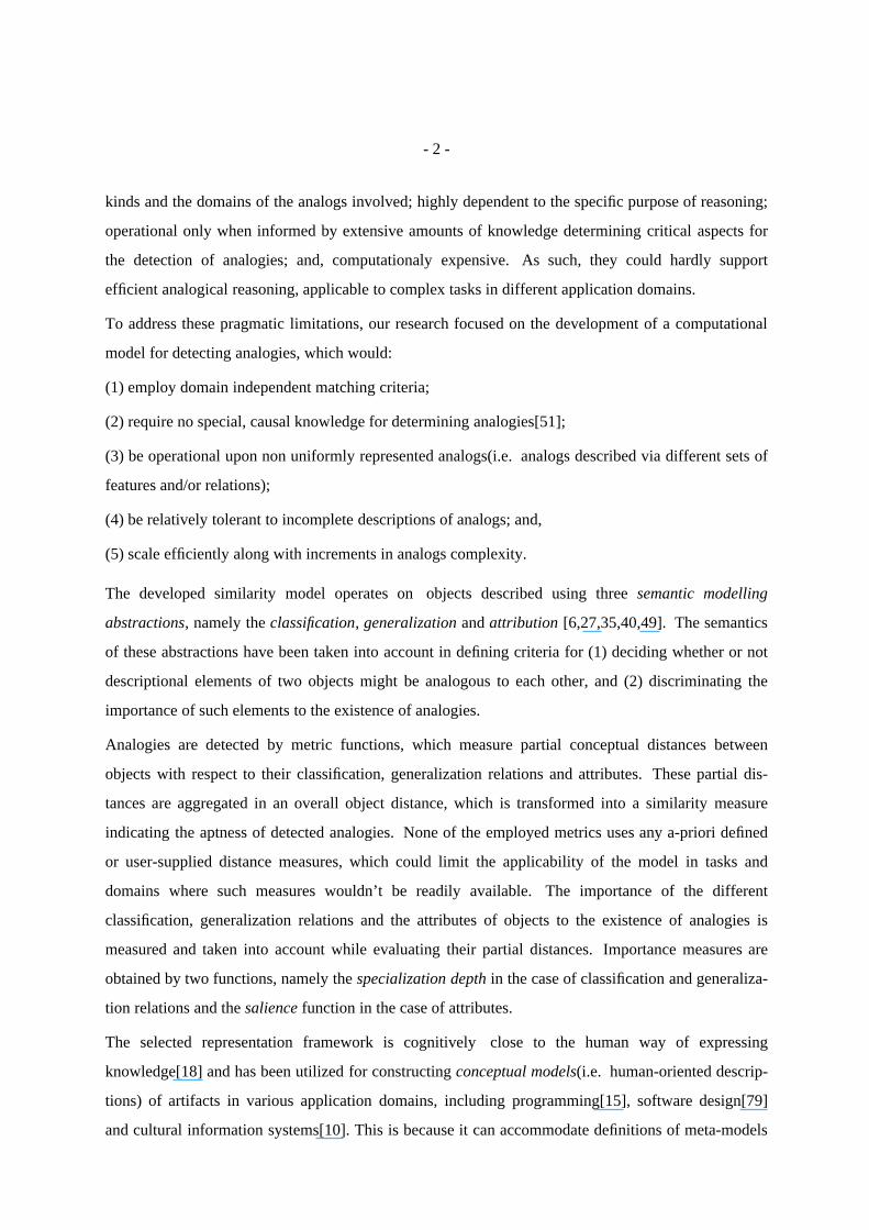
where INH[#i] is the set of the inherited attributes of #i, defined as:

INH [#i ] =

�� �x | ( |−−− x 1 : (x 1 ε I ) and (x 1 ε o (#i ).Isa ) and (x ε o (x 1).A ) and

(not ( |−−− x 2 : (x 2 ε I ) and (x 2 ε o (#i ).A ) and (x ε o (x 2).Isa ) and (n (x ) = n (x 2))) and

(not ( |−−− x 3 , x 4 : (x 3 ε I ) and (x 4 ε I ) and (x 3 ε o (#i ).Isa ) and (x 1 ε o (x 3).Isa ) and

(x 4 ε o (x 3).A ) and (x ε o (x 4).Isa ) and (n (x 4) = n (x ))))

� ��

In reference to the modelling of attribute classes, we also define:

i) their original class(i.e. their most general superclass which has an identical logical name with

them):

Definition 7: The original class of an attribute class with identifier #i OC#i is a class u satisfying the

following condition

(u ε o (#i ).Isa ) and((n (#i ) = n (u )) and (not ( |−−− x 1 : (x 1 ε o (#i ).Isa ) and (x 1 ε o (u ).Isa ) and (n (#i ) = n (x 1)))))

(ii) their original domain class(i.e. the class which first introduces attribute classes in a conceptual

schema):

Definition 8: The original domain class of an attribute class with identifier #i, ODC#i is the domain

class of its original class

ODC#i = o (OC#i ).FROM

(iii) their scope(i.e. the set of classes which an attribute class applies to):

Definition 9: The scope of an attribute class with identifier #i, S[#i], is defined as:

S [#i ] =

�� �x | ODC#i ε o (x ).Isa

� ��

(iv) their refining classes (these are the classes which either introduce or refine an attribute class):

Definition 10: The set of the refining classes of an attribute with identifier #i, R[#i], is defined as:

R [#i ] =

�� �c | (c ε S [#i ]) and ( |−−− x 1 : (x 1 ε o (c ).A ) and (n (#i ) = n (x 1)))

� ��

(v) their possible ranges(i.e. the distinct classes which are used as class-ranges for an attribute class in

a conceptual schema):

- 7 -

Definition 11: The set of the possible attribute ranges of an attribute #i, AR[#i], is defined as:

AR [#i ]=

�� �x | ( |−−− x 1,x 2 : (x 1 ε R [#i ]) and (x 2 ε o (x 1).A ) and (n (x 2) = n (#i )) and (o (x 2).TO = x ))

� ��

This conceptual modelling framework has been implemented as an object-oriented knowledge

representation language called Telos, which is described in detail in[35,40].

2.2 The Distance and Similarity Functions

To avoid the possibility of comparing objects having different levels of abstraction in the prescribed

conceptual modelling framework, similarity analysis obeys a basic ontological restriction, namely the

principle of Ontological Uniformity. According to it, only objects which have the same instantiation

level(i.e. they are both tokens or simple classes or meta classes or meta meta classes and so on) and

furthermore both denote individuals or attributes can be compared with each other.

�������������������������������������������������������������������������������������������������������������������������������������������������������������

Person

Company Address

company1

attribute

instanceOf

isa

Employee

Lawyer Engineer

employee1 employee2

SimpleClass

TaxableEntityIncome

annualIncome

address

fatherOf

(1)

(2)(2)

(3)(3)

(4) (4)

Figure 1: Ontologically Uniform and Not Uniform Objects

�������������������������������������������������������������������������������������������������������������������������������������������������������������

Thus, the similarity comparison between the attribute class annualIncome and the individual class

Person as well as between the simple class Person and the token company1 in figure 1 wouldn’t be

allowed. On the other hand, comparisons between objects classified under different classes of the

same instantiation level, such as the objects employee1 and company1 in figure 1 are permitted.

Hence, the ontological uniformity does not preclude the detection of analogies between objects with

classification differences, such as the analogy in paying taxes regarding the objects employee1 and

company1. However, it considers unlikely the modelling of analogous objects at different instantia-

tion levels and consequently precludes searching for analogies between such objects as meaningless.

- 8 -

Comparisons are based on distance functions. Distance functions, unlike other forms of matching

such as the ratio and the contrast models of similarity [52,58,67,72], have well-defined mathematical

properties (e.g. symmetry, triangularity) and intuitive geometric interpretations. In particular, onto-

logically uniform objects are compared by four partial distance functions, namely the identification

distance (d 1), the classification distance(d 2), the generalization distance (d 3) and the attribution dis-

tance (d 4). These functions compare objects at different levels of detail and complement each other in

preserving the ability of the model to detect analogies from descriptions of objects, which may be

incomplete with respect to any of the prescribed relations.

2.2.1 The Identification Distance

The identification distance is introduced to provide a coarse-grain distinction between different objects

with identical semantics(e.g. the two copies of the same book in figure 2) and is defined as follows:

Definition 12 : The identification distance d 1 between two objects with identifiers #i , #j is defined as a

function: d 1 : (i =0∪∞

(IUCi × IUCi ))∪(i =0∪∞

(AUCi × AUCi )) → [0,...,1]

such that d 1(#i ,#j ) =

�� �0 if #i = #j1 if #i ≠ #j

�������������������������������������������������������������������������������������������������������������������������������������������������������������

bookCopy1

bookCopy2

book1

BooKCopy Bookattribute

copyOf

copyOf

copyOf

link1

instanceOfattribute

link2

Figure 2: Non Identical Objects with Identical Semantics

�������������������������������������������������������������������������������������������������������������������������������������������������������������

- 9 -

2.2.2 The Classification Distance

The classification distance is introduced to give a rough estimate about the analogy over the substance

of two objects by measuring and aggregating the importance of their non common classes. Formally,

it is defined as follows:

Definition 13 : The normalized classification distance d 2 between two objects with identifiers #i , #j is

defined by the homographic transformation:

d 2(#i ,#j ) = β2D 2(#i ,#j ) + 1β2D 2(#i ,#j )

���������������������������

D 2 is their absolute classification distance defined as:

D 2 : (k =0∪∞

(IUCi × IUCi ))∪(k =0∪∞

(AUCi × AUCi )) → [0,...,∞) D 2(#i ,#j )=x ε SDC [#i ,#j ]

Σ SD (x )1

�����������

where SDC [#i ,#j ] =

�� �o (#i ).In −o (#j ).In

� �� ∪

�� �o (#j ).In −o (#i ).In

� �� and,

SD(x) is the maximum length of the paths connecting x with the most general class of its generaliza-

tion taxonomy, called the specialization depth of x

D 2 measures the importance of classes by the inverse of their specialization depths. Classes with high

specialization depths (i.e. classes placed at lower levels in generalization hierarchies) tend to express

fine grain distinctions between homogeneous populations of objects, while classes with low speciali-

zation depths (i.e. classes placed at higher levels in generalization hierarchies) tend to express basic

semantic distinctions between different types of objects. This weighting coincides with cognitive stu-

dies of classification in human mental models, which indicate that the more general a class the more

significant the classification it express in a taxonomy [80]. According to definition 13, the absolute

classification distances between the object employee1 and the objects employee2 and company1 in

figure 1 are 0.5(i.e. 1/4 + 1/4) and 1.41(i.e. 1/2 + 1/3 + 1/4 + 1/3), respectively.

The parameter β2 in definition 13 determines the rate of asymptotic convergence of d 2 measures to 1 as

D 2 goes to infinity. β2 may evaluated so that d 2 be equal to 0.5 when D 2 takes its average value given

a particular set of objects, thus making the estimation of the classification distance context-

sensitive[58].

Function d 2 is a pseudometric:

Theorem 1: The function d 2 is a pseudometric.

In other words, it takes positive values, is triangular and symmetric. Also, it might take zero values

even for non identical objects. Theorem 1, like all the theorems in sections 2 and 3, is proved in the

- 10 -

second appendix of the paper.

2.2.3 The Generalization Distance

The generalization distance gives a rough estimate over the semantic differences of two classes, as

evidenced by measuring and aggregating the importance of their non-common superclasses. Since

token objects can not participate generalization relations this distance function is defined only between

class objects:

Definition 14: The normalized generalization distance d 3 between two class objects with identifiers #i

, #j is defined as:

d 3(#i ,#j ) =

�����do (#i ,#j ) if #i , #j ε AUCi i = 1,2, . . .1 + β3D 3(#i ,#j )

β3D 3(#i ,#j )��������������������������� if #i , #j ε IUCi i = 1,2, . . .

do is the generalization distance between attribute classes defined as:

do (#i ,#j ) =

�� �0 if OC#i = OC#j

1 if OC#i ≠ OC#j

D 3 is their absolute generalization distance defined as:

D 3 : (i =1∪∞

(IUCi × IUCi )) → [0,...,∞) D 3(#i ,#j )=x ε SDSC [#i ,#j ]

Σ SD (x )1

�����������

where SDSC [#i ,#j ] =

�� �o (#i ).Isa ∪(

�� �#i

� �� )−o (#j ).Isa ∪

�� �#j

� ��

� �� ∪

�� �o (#j ).Isa ∪(

�� �#j

� �� )−o (#i ).Isa ∪

�� �#i

� ��

� ��

SD(x) is the specialization depth of class x.

The generalization distance between individual classes is defined in a way similar to their

classification distance except that their supeclasses are taken into account. Unlike it, the generaliza-

tion distance between attribute classes depends on the identity of their original attribute classes.

The criterion of the original class identity in definition 14 enables a differentiation between

refinements of inherited attribute classes (i.e. specialization of their range classes) representing the

same relations or properties and specializations of attribute classes with shared but non identical

semantics, both expressible by Isa relations in conceptual schemas. Consider for instance the speciali-

zation of the attribute class identifiedBy of Person by the attribute classes identifiedBy of Soldier and

hasSecurityNumber of Employee in figure 3. The attribute class identifiedBy of Soldier refines the

same identification relation modelled by the attribute class identifiedBy of Person for the particular

case of soldiers(the latter is the original class of the former according to definition 7). On the other

hand, the attribute class hasSecurityNumber of Employee, although a specialization of the class

- 11 -

�������������������������������������������������������������������������������������������������������������������������������������������������������������

attributeIsa

SimpleClass

hasSecurityNumberSecurityNumber

PersonidentifiedBy

Employee

IdentityCard

identifiedByMilitary

IdentityCardSoldier

ArmyOfficeridentifiedBy

(1)

(2)

(3) (3)

(4)

Figure 3: A Conceptual Schema of Classes of Persons

�������������������������������������������������������������������������������������������������������������������������������������������������������������

identifiedBy of Person, doesn’t express the same relation with it. In fact, an employee may have an

ordinal identification card in addition to his/her security number(notice that the attribute identifiedBy

of Person is inherited by the class Employee according to definition 6). This difference is reflected by

the generalization distances between the relevant pairs of attribute classes, which are 0 and 1 respec-

tively.

Parameter β3 has the same role and is estimated in the same way with parameter β2(cf. section 2.2.2).

Given its definition, the generalization distance is a metric:

Theorem 2: Function d 3 is a metric .

2.2.4 The Attribution Distance

The abstraction of attribution as defined in the modelling framework of similarity analysis is semanti-

cally overloaded[27]. In other words, attributes may be used for describing very different aspects of

objects, including structural decompositions, non structural relations with other objects or even simple

properties. This overloading may contribute to the expressive power of the framework but also intro-

duces the problem of deciding whether arbitrary pairs of attributes are analogous while comparing

their owning objects.

The similarity model deals with this problem by introducing the principle of the semantic homo-

geneity[61]. According to it, two attributes cannot be considered analogous unless they are semanti-

cally homogeneous. These by definition are attributes classified under exactly the same original attri-

bute classes:

- 12 -

Definition 15: Two attribute objects with identifiers #i , #j are semantically homogeneous sh (#i ,#j ), if

and only if:

OCL [#i ] = OCL [#j ] where OCL [x ] =

�� �x 1 | (x 1 = OCx 2

) and (x 2 ε o (x ).In )

� �� x =#i , #j

�������������������������������������������������������������������������������������������������������������������������������������������������������������

NumberTransportation

VehicleidentifiedBy

transportationNum

BookCopy LibraryCodeidentifiedBylibraryCode

EntityClass

attribute

identifiedBy

PersonClass

attributeattributeemploymentRelationfamilyRelation

Person

MarriedPerson

Spouce

identifiedBy

familyRelation

hasIdCard

hasSpouce

fatherOffamilyRelation

CompanyworksAtemploymentRelation

IdentityCard

attribute

instanceOf

Isa

Figure 4: Semantically Homogeneous & Heterogeneous Attributes

�������������������������������������������������������������������������������������������������������������������������������������������������������������

In reference to figure 4, the attribute classes libraryCode of BookCopy, transportationNum of Vehicle

and hasIdCard of Person are semantically homogeneous since they are all classified under the same

original attribute metaclass identifiedBy of EntityClass. In fact, they have the same descriptive role for

their owning objects, i.e. they uniquely identify them within the extensions of their classes. Conse-

quently, they could be compared while detecting analogies between vehicles and copies of books or

persons. Unlike them, the attribute class worksAt of Person is semantically heterogeneous with the

attribute hasSpouce of MarriedPerson, since the former has been classified as an employment while

the latter as a family relation.

As the following theorem states, semantic homogeneity is a reflexive, symmetric and transitive rela-

tion.

Theorem 3: The semantic homogeneity of attributes is an equivalence relation

The symmetry of semantic homogeneity ensures that attribute comparisons will be associative while

its transitivity enables the definition of a metric over the attribution of objects(cf. proof of lemma 3 in

- 13 -

appendix 2).

On the basis of semantic homogeneity, the set of semantically homogeneous pairs of attributes of two

objects is defined as follows:

Definition 16: The set of the semantically homogeneous of two objects with identifiers #i , #j

SH [#i ,#j ] is defined as:

SH [#i ,#j ] =

�� �(x 1,x 2) | (x 1 ε INT [#i ]) and (x 2 ε INT [#j ]) and sh (x 1,x 2)

� ��

The powerset of SH [#i ,#j ] can be thought of as the set of all the possible interpretations of the analogy

between #i and #j. Motivated by empirical evidence about the way humans interpret analogies[20],

the similarity model considers only isomorphic mappings between the semantically homogeneous

attributes of objects as valid interpretations of their analogy. The set of these valid mappings is for-

mally defined as:

Definition 17: The set of the valid isomorphisms between the semantically homogeneous attributes of

two objects with identifiers #i , #j is defined as:

C [#i ,#j ] =

�� �ck | (ck ⊆ SH [#i ,#j ]) and ( V− x 1 , x 2 :

((x 1,x 2) ε ck )⇒(not ( |−−− x 3 , x 4 :((x 3 , x 4 ) ε ck ) and (((x 1 = x 3) and (x 2 ≠ x 4)) or

((x 1 ≠ x 3) and (x 2 = x 3))))) and (not ( |−−− ck′ : (ck′ ε C [#i ,#j ]) and (ck′ ⊂ ck ))))

� ��

Notice that since they are isomorphic, all the mappings in set C[#i,#j] are invertible. Therefore, the

interpretation of the analogy between two objects using them can be grounded on exactly the same

object elements, regardless of the direction of their comparison.

Each interpretation ck determines the non analogous attributes of the involved objects(i.e. attributes

not mapped by it):

Definition 18: The set of the non analogous attributes of an object #i, with respect to an object #j,

given their isomorphism ck is defined as:

A#i [ck ] =

�� �x 1 | (x 1 ε INT [#i ]) and (not ( |−−− x 2 , x 3 : ((x 2,x 3) ε ck ) and (x 1 = x 2)))

� ��

Therefore, even semantically homogeneous attributes of objects may not be considered as being analo-

gous, under different interpretations of their analogy.

- 14 -

From all the valid interpretations C[#i,#j] of the analogy between two objects, the similarity model

selects the one with the minimum total distance. The total distance of each isomorphism ck in C[#i,#j]

is measured by the weighted sum of the distances between the pairs of attributes that constitute it and

the importance of the non analogous attributes according to it. Thus, the selection of an interpretation

for the analogy between two objects is based on an objective criterion of optimality, referred to as the

principle of the minimum distance isomorphism. The total distance of the selected isomorphism

between the attributes of two objects is defined as their attribution distance:

Definition 19: The absolute attribution distance D 4 between two objects with identifiers #i , #j is

defined as a function:

D 4 : (k =0∪∞

(IUCi X IUCi ))∪(k =0∪∞

(AUCi X AUCi )) X PowersetOf (IU ∪AU )) → [0, . . . , ∞)

D 4(#i ,#j ,V ) =

�����

ck ε C [#i ,#j ]min

�� �(x 1,x 2) ε ck

Σ s (x 1)s (x 2)d′ (x 1,x 2,V ) +x 3 ε A#i [ck ]

Σ s (x 3)2 +x 4 ε A#j [ck ]

Σ s (x 4)2

� �� otherwise

∞ if INT [#i ] = ∅ or INT [#j ] = ∅

d′ (#i ,#j ,V ) = βD ′(#i ,#j ,V ) + 1βD ′(#i ,#j ,V )

� ���������������������������

D′ (#i ,#j ,V ) =

�������D (#i ,#j ,V ) otherwise(PD����� et W��� 2PD����� et

T )1/2 if #i , #j ε AUC 0 and ((o (#i ).TO ε V ) or (o (#j ).TO ε V )

(PD����� ec W��� 1PD����� ecT )1/2 if (#i , #j ε

k =1∪∞

AUCi ) and ((o (#i ).TO ε V ) or (o (#j ).TO ε V )

where

W 1 =

����0001

1610

6660

1610� �

�� W 2 =

���001

610

660 � ��

PDec = [d 1(#i ,#j ) d 2(#i ,#j ) d 3(#i ,#j ) d 4(#i ,#j ) ]

PDet = [d 1(#i ,#j ) d 2(#i ,#j ) d 4(#i ,#j ,V ∪�� �#i ,#j

� �� ) ]

V is a set of identifiers of objects( V ⊆IU ∪AU ) and,

s (xi ) =xj ε OCL [xi ]

max

�� �SL (xj )

� �� SL (xj ) is the salience of xj (see def inition 32 below ),s (xi ) ε [0,...,1]

D 4 selects minimum distance isomorphic mappings between the attributes at all the successive levels

in the transitive closures of the attribution graphs of the involved objects, recursively (see figure 5).

Also, it assigns an infinum distance measure to pairs of objects, whose intensions are empty. In this

case, it essentially assumes that the yet unknown intensions of objects will more likely include

semantically heterogeneous attributes rather than homogeneous ones.

- 15 -

�������������������������������������������������������������������������������������������������������������������������������������������������������������

O#j

O#i

optimal isomorphism

attribute

O1

O2

O3

O4

O5

O6

O8

O9

O7

O10

O11

Figure 5: Synthesis of Successive Optimal Interpretations of Analogies

�������������������������������������������������������������������������������������������������������������������������������������������������������������

In cases of attributes having as values objects, whose distance to some other object is currently being

estimated (i.e. the members of set V in definition 19), recursion is controlled by estimating their dis-

tance only with respect to their identification, classification, generalization and attribution but not with

respect to these values.

The absolute distance measures D 4 are normalized into relative ones, according to the following

definition:

Definition 20: The normalized attribution distance d 4 between two objects with identifiers #i , #j is

defined as a function:

d 4(#i ,#j ) = β4D 4(#i ,#j ) + 1β4D 4(#i ,#j )

���������������������������

Theorem 4: Function d 4 is a metric.

An implication of the definitions of the attribution and generalization distances is that the pairs of the

semantically homogeneous attributes of two objects, which also have the same original class, will

always belong to their optimal isomorphism:

Theorem 5: All the pairs of attributes (x 1,x 2) of two objects #i, #j that belong to the set SH[#i,#j] and

have the same original class belong to the optimal isomorphism copt between the objects #i and #j.

- 16 -

This property is reasonable considering that attributes sharing of a common original class express the

same relation, as discussed in section 2.2.3.

2.2.5 The Overall Distance Function

The partial metrics d 1,d 2,d 3 and d 4 are aggregated into an overall distance D according to the following

quadric function:

Definition 21: The overall distance D between two objects, identified by #i,#j, is defined as a function:

D : (k =0∪∞

(IUCi X IUCi ))∪(k =0∪∞

(AUCi X AUCi )) x PowersetOf (IU ∪AU ) → [0,...,∞)

D (#i ,#j ,V ) =

����������� (PD��� � at W��� at PD��� � at

T )1/2 if #i , #j ε AUC 0

(PD��� � ac W��� ac PD����� acT )1/2 if #i , #j ε

k =1∪∞

AUCi

(PD��� � et W��� et PD����� etT )1/2 if #i , #j ε IUC 0

(PD��� � ec W��� ec PD����� ecT )1/2 if #i , #j ε

k =1∪∞

IUCi

where

PDec = [d 1(#i ,#j ) d 2(#i ,#j ) d 3(#i ,#j ) d 4(#i ,#j ) ]

PDet = [d 1(#i ,#j ) d 2(#i ,#j ) d 4(#i ,#j ,V ∪�� �#i ,#j

� �� ) ]

PDac = [d 1(#i ,#j ) d 2(#i ,#j ) d 3(#i ,#j ) d 4(#i ,#j ,V ∪�� �#i ,#j

� �� ) D (o (#i ).TO ,o (#j ).TO ,V ∪

�� �#i ,#j

� �� ) ]

PDat = [d 1(#i ,#j ) d 2(#i ,#j ) d 4(#i ,#j ,V ∪�

� �#i ,#j

� �� ) D (o (#i ).TO ,o (#j ).TO ,V ∪

�� �#i ,#j

� �� ) ]

W��� ec =

����0001

1110

1110

1110� �

�� W��� et =

���001

110

110 � �� W��� ac =

�����00001

01610

06660

01610

10000� �

��� W��� at =

����0001

0110

0110

1000 � �

��A series of experiments, whose results are summarized by table 1 indicated statistically significant

correlations between classification/generalization and attribution distances, thus prompting the use of

a quadric functional form for the overall distance D. These experiments were performed using con-

ceptual models of requirements specifications (cases 1,2,3,4), abstractions of domain knowledge for

information systems[44](case 5), static analysis data of CooL programs[70], C++ programming con-

structs [15](cases 7,8) and cultural artifacts[10](cases 9,10). In 4 out of the 6 cases where both d 2 and

d 3 were definable(i.e. the involved objects were not tokens) and not equal to 0, a statistically

significant(p <0.05) positive correlation between their resulting measures was found( cf. coefficients

marked with asterisks in table 1).

- 17 -

���������������������������������������������������������������������������������������������������Table 1: Correlation Coefficients Between Partial Distances���������������������������������������������������������������������������������������������������

Case Set Size d 2,d 3 d 2,d 4 d 3,d 4���������������������������������������������������������������������������������������������������1 231 - - .81*���������������������������������������������������������������������������������������������������2 28 .47* .59* .6*���������������������������������������������������������������������������������������������������3 6 0 .74 .08���������������������������������������������������������������������������������������������������4 861 .45* .12* .51*���������������������������������������������������������������������������������������������������5 10 - - .53���������������������������������������������������������������������������������������������������6 903 - .15* -���������������������������������������������������������������������������������������������������7 171 .24* .09 .64*���������������������������������������������������������������������������������������������������8 66 -0.05 .17 .21���������������������������������������������������������������������������������������������������9 741 - - .39*���������������������������������������������������������������������������������������������������

10 946 .55* .6* .4*��������������������������������������������������������������������������������������������������������������������

���������������

���������������

���������������

���������������

�����������������

As a quadric aggregate of distance metrics, the overall object distance D is a metric itself:

Theorem 6: Function D is a metric.

2.2.6 The Similarity Function

The overall distance measures between objects are transformed into similarity measures, according to

the following function:

Definition 22: The similarity S between two objects with identifiers #i,#j is defined as a function:

S : (k =0∪∞

(IUCi X IUCi ))∪(k =0∪∞

(AUCi X AUCi )) x powersetOf (IU ∪AU ) → [0,...,1]

S (#i ,#j ,V ) = e −N*D (#i ,#j ,V ) , N ε (0, . . . ,∞)

Similarity measures indicate the aptness of the analogy between two objects.

2.2.7 An Example of Similarity Analysis

In the following, we give an example of using the prescribed functions in estimating the conceptual

distances and thereby detecting the analogy between the classes LibraryBorrower and CarAgencyCus-

tomer, given the conceptual model of figure 6. The partial and the overall distances as well as the simi-

larity measures between the objects in this model are shown in table 2(these measures were obtained

by setting all the s (xi ) measures in definition 19 equal to 1).

Library borrowers and car agency customers do not have any non-common classes(they are both

instances of the meta-class EntityClass) and therefore they have a zero classification distance(cf.

column d 2 in table 2). Also, they are both specializations of the same superclass, i.e. ResourceBor-

rower, thus having a relatively low generalization distance, that is 0.56(cf. column d 3 in table 2).

The computation of their attribution distance results into an isomorphism between their attributes,

depicted by the thick dotted lines in figure 6. This isomorphism maps the attributes libraryCard and

- 18 -

�������������������������������������������������������������������������������������������������������������������������������������������������������������

ResourceBorrowerResource

borrowsResourceattribute

hasBorrowedattribute

EntityClass

instanceOfattributeIsa

LibraryBorrower CarAgencyCustomer

idCard

IdCard

libraryCard

CarAgencyAccount

LibraryCard IdentificationDocument

attributehasAccount

attributeidentifiedBy

attribute

analogical isomorphism

BookCopy VehicleborrowsBook

Figure 6: Analogy Between Library Borrowers and Car Agency Customers

�������������������������������������������������������������������������������������������������������������������������������������������������������������

borrowsBook of LibraryBorrower onto the attributes idCard and hasBorrowed of CarAgencyCusto-

mer, respectively. In fact, these pairs of attributes have analogous roles for their owning classes.

The attributes of the first pair enable the identification of library borrowers and car agency customers

as borrowers. Such an identification is possible through a card awarded by the library in the case of

library borrowers and through their ordinary identification cards in the case of car agency customers.

This dissimilarity does not devalidate the underlying analogy evidenced from the conceptual schema

through the classification of the relevant attributes under the attribute class identifiedBy of EntityClass.

On the contrary, the analogy becomes more evident by the fact that the object-values of these

attributes(i.e. the classes LibraryCard and IdCard) are specializations of a common superclass,

namely the class IdentificationDocument, which decreases their generalization distance (since it

increases their specialization depths). Notice that the mapping of the attribute libraryCard onto the

attribute idCard was the only valid one according to the criterion of the semantic homogeneity.

- 19 -

�������������������������������������������������������������������������������������������������������������������������������������������������������������������Table 2: Distance Measures Between Objects of Figure 6�������������������������������������������������������������������������������������������������������������������������������������������������������������������

Objects d 1 d 2 d 3 d 4 DTO D S�������������������������������������������������������������������������������������������������������������������������������������������������������������������β2 = 2 β3 = 2 β4 = .5 N =0.3�������������������������������������������������������������������������������������������������������������������������������������������������������������������

LibraryBorrower,CarAgencyCustomer 1 0 0.56 0.34 - 1.61 0.61�������������������������������������������������������������������������������������������������������������������������������������������������������������������BookCopy,Vehicle 1 0 0.56 1 - 1.36 0.66�������������������������������������������������������������������������������������������������������������������������������������������������������������������

LibraryCard,Vehicle 1 0 0.56 1 - 1.36 0.66�������������������������������������������������������������������������������������������������������������������������������������������������������������������BookCopy,CarAgencyAccount 1 0 0.72 1 - 1.79 0.58�������������������������������������������������������������������������������������������������������������������������������������������������������������������

LibraryCard,CarAgencyAccount 1 0 0.72 1 - 1.79 0.58�������������������������������������������������������������������������������������������������������������������������������������������������������������������borrowsBook,hasBorrowed 1 0 1 1 1.36 2.2 0.51�������������������������������������������������������������������������������������������������������������������������������������������������������������������

libraryCard,idCard 1 0 1 1 1.36 2.2 0.51�������������������������������������������������������������������������������������������������������������������������������������������������������������������borrowsBook,hasAccount 1 0.5 1 1 1.79 2.33 0.49�������������������������������������������������������������������������������������������������������������������������������������������������������������������

���������������

��������������

��������������

��������������

��������������

��������������

��������������

��������������

���������������

Unlike it, the mapping of the attribute borrowsBook onto the attribute hasBorrowed was not the only

valid one, according to the same criterion. In fact, since borrowsBook was also semantically homo-

geneous to the attribute hasAccount of CarAgencyCustomer(they were both instances of the attribute

meta-class attribute, whose extension corresponds to set AU in section 2.1) it could have been mapped

on it, alternatively. However, as it can be observed from table 2, the overall distance between the attri-

butes borrowsBook and hasBorrowed is less than the overall distance between borrowsBook and

hasAccount(2.2 vs. 2.33). This is due to the distances of their values: the overall distance D between

BookCopy and Vehicle equals 1.36 while the same distance between BookCopy and CarAgencySAc-

couny equals 1.79. Consequently, borrowsBook was mapped onto hasBorrowed due to the criterion of

the minimun distance isomorphism.

2.3 The Salience Functions

2.3.1 The Problem of Salience

Like classification and generalization relations, different attributes are expected to have varying

degrees of importance to the existence of analogies, depending on their role to the description of their

owning objects[47]. Usually, attributes expressing fundamental structural and behavioural characteris-

tics of objects are more important to the existence of analogies than attributes which express simple

properties.

Often, computational models of analogical reasoning make such distinctions of importance on the

basis of:

(1) syntactic differences regarding the representation of attributes(e.g. SME[17]);

(2) direct estimates provided by users(e.g. ARCS[65],MACKBETH[72]);

(3) assessments about the results of reasoning sessions provided by external observers(e.g.

CBL4[2],CBR+EBL[14]); and

- 20 -

(4) knowledge determining the attributes, which are related to the purpose of reasoning(expressed

either by causal relations between attributes and goals as in Protos[48] and PRODIGY[69] or by

indices to descriptions of analogs in memory as in MEDIATOR[37]).

Knowledge-based distinctions are usually bounded by the knowledge acquisition bottleneck. On the

other hand, user-based ones might be sensitive to subjective biases. As opposed to them, the similar-

ity model estimates the importance of attributes based on the concept of attribute dominance. Attri-

bute dominance is introduced as a compound property derived from three primitive properties of attri-

butes, namely their charactericity, abstractness and determinance. These are defined by logical con-

ditions on the representation of attributes in conceptual models. Salience is then introduced as belief

that an attribute is dominant and provides a graded alternative to the logical strictness of dominance.

2.3.2 The Properties Underlying Attribute Dominance

i) The Charactericity of Attributes

We distinguish as characteristic attributes which discriminate the different classes they apply to in a

conceptual schema. This discrimination can be evidenced from the refinement of attributes (i.e. the

specialization of their range-classes) by classes which inherit them in generalization taxonomies.

Such refinements express how subclasses differ from their superclasses. Attributes refined in many

classes of a generalization taxonomy become characteristic of it. Formally, the charactericity of an

attribute is defined as:

Definition 23: An attribute class with identifier #i is characteristic CH#i if and only if

| S [#i ] | = | AR [#i ] |

For instance, the attribute qualification in figure 7 is characteristic since it has distinct range classes in

all the classes of its scope thereby distinguishing the different subclasses of employees, according to

definition 23. Unlike it, the attribute worksFor, which represents the relation between a researcher and

the project he/she is involved in, is not characteristic since there exist employees not related with any

project(e.g. administrative staff). Furthermore, the special types of researchers are not differentiated

by the projects they work for.

ii) The Abstractness of Attributes

Attributes have different significance for the existence and behaviour of their objects, subject to the

class which introduces them in a conceptual schema(i.e. their original domain class). Classes may be

divided into abstract and concrete, according to whether or not they have instances of their own

[1,42,71]. Concrete classes introduce attributes enabling a detailed description of their instances,

- 21 -

�������������������������������������������������������������������������������������������������������������������������������������������������������������

ResearchInstituteEmployee

ResearchStaff

AdministrativeStaff Research

ProjectworksFor

qualificationQualification

manages

qualification DegreePostGraduate

qualificationAssociate

belongsTo

GroupResearch

MastersDegree

qualification

Attribute

Isa

UniversityDegreePhD Degree

ResearchersResearchersSenior

employmentAgreement

ResearchContractTemporary

Contract

Agreementemployment

qualification

ResearchContractPermanent

Agreementemployment

employmentAgreement

ContractPermanent

Figure 7: A Conceptual Schema of Employees of a Research Institute

�������������������������������������������������������������������������������������������������������������������������������������������������������������

while abstract ones introduce only attributes which are essential for the structure and the functional

behaviour of the instances of their concrete subclasses[80]. Consider for example the difference in the

significance of the attribute hasSteeringSystem of a vehicle and the attribute luggageCarryingCapacity

of a car. The former is essential for driving any sort of vehicle(e.g. airplanes, trains, cars). Unlike it,

the latter neither applies to all vehicles(e.g. fighting airplanes) nor relates to the functionality of the

special kind of vehicles, it applies to. Thus, we introduce the abstractness of attributes as a property

reflecting this behavioural and structural significance and define it on the basis of the abstractness of

their original domain classes.

In particular, we define abstract classes as:

Definition 24: A class with identifier #i is abstract AB#i , if and only if EXT [#i ]=EXTs [#i ]

and abstract attributes as:

Definition 25: An attribute class with identifier #i is abstract (i.e. ABS#i ) if and only if its original

domain class #u(i.e. #u = ODC#i ) is abstract (i.e. AB#u )

According to these definitions, the attributes qualification and employmentAgreement in figure 7 are

abstract since their common original domain class is the abstract class ResearchInstituteEmployee(we

assume that it has no instances of its own). Unlike them, the attribute manages, whose original

domain class is the concrete class SeniorResearchers, is not abstract.

- 22 -

iii) The Determinance of Attributes

We consider as determinant attributes whose values determine the values of other attributes. For

example, the model of a car could dictate the place where it has been produced if the relevant

manufacturer produces its different models in different countries. We restrict our interest in dependen-

cies between attributes that have the same domain and in a special case of them, namely the total

equivalences. Both these types of dependencies can be precluded for specific attributes, given their

modelling in a conceptual schema.

Suppose that two attributes x and y are defined as associations x :Dx → Ix , y :Dy → Iy where Ix and Iy

denote their images(i.e. the sets of their actual values). In our view, the attribute y might depend on

the attribute x(i.e. Mxy ) only if they have identical domains, Dx ≡ Dy (i.e. both of them apply to exactly

the same set of objects). Given that they have, their dependency is defined as a mapping M between

their values(i.e. M :Ix → Iy ). A total equivalence between x and y exists in cases where M is a total

and onto isomorphism.

�������������������������������������������������������������������������������������������������������������������������������������������������������������

EXT(C1)

C1

x y

C2

C3

C4

domain of y

domain of x

EXT(C3)

EXT(C2)

EXT(C4)

x1

R2

x1

C2 C1

R1

EXT(R1)

EXT(R2)

EXT(R3)

R3

x2

M

MEXT(C1)

EXT(C2)

hasExtensiondependency mapping

AttributeIsa

Case 1: Non Common Classes Case 2: Non Common Refinements

Figure 8: Non Common Classes and Refinements in Conceptual Schemas

�������������������������������������������������������������������������������������������������������������������������������������������������������������

The domain equality condition of dependencies is checked by the identity of the scopes of the

involved attributes(i.e. S [#i ] = S [#j ]). Non common classes in the scopes of two attributes indicate

that they have non identical domains. Consider for example the attributes x and y in case 1 of figure 8.

The classes C1 and C2 in their scopes are not common to both of them. In fact, there must be objects

- 23 -

belonging to the class C1 but not to C2 and vice versa(i.e. the sets EXT[C1]-EXT[C2] and EXT[C2]-

EXT[C1] will be non-empty in general) regardless of the current state of their extensions. If this was

not the case, there would be no need for maintaining both C1 and C2, two classes not related by a gen-

eralization relation, in the conceptual schema. Hence, we will consider dependencies between attri-

butes x and y as not definable(i.e. M� �

xy and M� �

yx ) whenever:

(cnd 1) : S [x ] ≠ S [y ]

Also, total equivalences might exist subject to a second definability condition. Given two attributes x

and y, it will be impossible to define a total equivalence mapping between their images whenever their

refining classes do not coincide:

(cnd 2) : ((S [x ]−R [x ]) ∩R [y ]))∪((S [y ]−R [y ])∩R [x ])≠∅

Case 2 in figure 8 exemplifies this condition. The attribute x1 is refined by class C2 unlike the attri-

bute x2, which is simply inherited by it. If an equivalence mapping(i.e. a total and onto isomorphism)

between these two attributes were definable their images with respect to C1 and C2, should have

equal numbers of elements(i.e. | EXT (R 1) | = | EXT (R 3) | and | EXT (R 2) | = | EXT (R 3) | ). However,

since attribute x1 is refined in C2 its image with respect to C2 will have fewer elements than its image

with respect to C1 (since R2 is a subset of R1 | EXT (R 2) | < | EXT (R 1) | ) which is a contradiction.

Notice that, according to conditions cnd1 and cnd2 no dependency mapping could be defined between

the attributes worksFor and qualification in figure 7. By contrast, a dependency between the attributes

worksFor and belongsTo (it express the research group of a researcher) in the same figure might exist.

These attributes have identical scopes and they are not refined separately. In fact, projects are nor-

mally allocated to research groups and thus the projects a researcher is involved with depend on

his(her) group.

It must be pointed out that, failing to preclude the definability of a dependency mapping indicates that

a dependency might exist but it doesn’t necessarily imply it.

On the basis of interattribute dependencies we define determinative attributes as:

Definition 26: An attribute class with identifier #i is determinative DET#i , if and only if

( |−−− x ,y :(x ε S [#i ]) and (y ε INT [x ]) and Miy )

According to this definition, it is sufficient to identify even one dependency between an attribute x and

another attribute y of a class in its scope for characterizing x as determinative.

- 24 -

iv) The Dominance of Attributes

We define the dominance of attributes on the basis of their charactericity, abstractness and determi-

nance, as follows:

Definition 27: An attribute class with identifier #i is dominant DOM#i , if and only if

(ABS#i and CH#i ) or DET#i

The conjunction of abstractness and charactericity excludes cases satisfying only one of those proper-

ties, as extreme ones. In fact, certain attribute classes may be introduced in abstract classes only

because of their broad applicability(e.g. the attribute class securityNumber of ResearchInstituteEm-

ployee in figure 9). Also, attribute classes, which are introduced in leaf classes of generalization taxo-

nomies, although satisfy the definition of charactericity do not have a general classification

significance for them(e.g. the attribute class responsibleFor of AdministrationManager in figure 9).

2.3.4 Attribute Salience: Belief on their Dominance

The logical conditions defining the charactericity, abstractness and determinance may prove too res-

trictive and be violated by attributes intuitively satisfying these properties(especially due to flaws in

conceptual models). To overcome this problem, we derive inferences about the properties underlying

attribute dominance(and consequently the dominance itself) in an approximate way, where their truth

values are associated with evidence measures.

In particular, we introduce attribute salience as a measure of evidence that an attribute is dominant or

not. Salience is estimated from evidence measures about the truth values for each of the underlying

properties of dominance. These measures are obtained by evidence functions, which measure the

extent to which the defining conditions of the relevant property are satisfied in a conceptual model and

are interpreted as belief functions in the context of the Dempster-Shafer theory of evidence[57](since

as we prove in appendix 2, they satisfy the axioms defining such beliefs).

i) A Frame of Discernment for Defining and Combining Evidence Functions

The definition and combination of evidence functions for the charactericity, abstractness and determi-

nance is based on the introduction of a frame of discernment Θi [57] for each attribute #i.

Θi consists of proposition vectors [vc ,va ,vm 1,vm 2,...,vmn ], whose elements are variables indicating the

truth value of the charactericity (i.e. variable vc ) and the abstractness(i.e. variable va ) of an attribute

#i as well as the definability of a dependency mapping between #i and the n other attributes defined for

the classes of its scope (variables vm j ). By convention, the value 1(0) for any of these variables means

the truth(falsity) of the relevant property. Each proposition vector represents the conjunction of its

- 25 -

elements by assumption. Θi includes all the proposition vectors which can be formed by taking all the

possible combinations of values for these variables.

Given Θi , the properties determining the dominance of #i are defined as the following subsets of it:

CHi ≡

�� �[vc ,va ,vm 1,vm 2,...,vmn ] | vc = 1

� ��

CH� � �

i ≡

�� �[vc ,va ,vm 1,vm 2,...,vmn ] | vc = 0

� ��

ABSi ≡

�� �[vc ,va ,vm 1,vm 2,...,vmn ] | va = 1

� ��

ABS� � � �

i ≡

�� �[vc ,va ,vm 1,vm 2,...,vmn ] | va = 0

� ��

DETi ≡j =1∪

nMj where Mj ≡

�� �[vc ,va ,vm 1,vm 2,...,vmn ] | vm j = 1

� ��

DET� � � �

i ≡j =1∩

nM

� �

j where M� �

j ≡

�� �[vc ,va ,vm 1,vm 2,...,vmn ] | vm j = 0

� ��

DOMi ≡ (CHi ∩ABSi )∪DETi

DOM� � � � �

i ≡ (CH� � �

i ∪ABS� � � �

i )∩DET� � � �

i

ii) The Evidence to Charactericity

Different specializations of classes in conceptual schemas are not always associated with refinements

of the same attribute classes. For instance, the attribute employementAgreement, which express the

contract of an employment, is not refined by the class ResearchStaff in figure 7. Nevertheless, it is

characteristic of the other classes of employees in the relevant taxonomy. Such cases motivated the

definition of an evidence measure about charactericity, as follows:

Definition 28: The evidence to the charactericity of an attribute class with identifier #i, mich is meas-

ured by the function:

mich(P )=

�����01−ci

ci

if P ⊆ Θ & P ≠ CHi & P ≠ CH� � �

i

if P = CH� � �

i

if P = CHi

where ci = | S [#i ] || AR [i ] |� �������������

mich(P ) relaxes the logical definition of charactericity giving an evidence measure equal to 1 whenever

this definition is satisfied ( | AR [#i ] | = | S [i ] | → ci = 1 ). It also satisfies the axiomatic definition of

the Dempster-Shafer basic probability assignments(cf. appendix 1):

- 26 -

Theorem 7: The evidence function mich(P ) is a basic probability assignment.

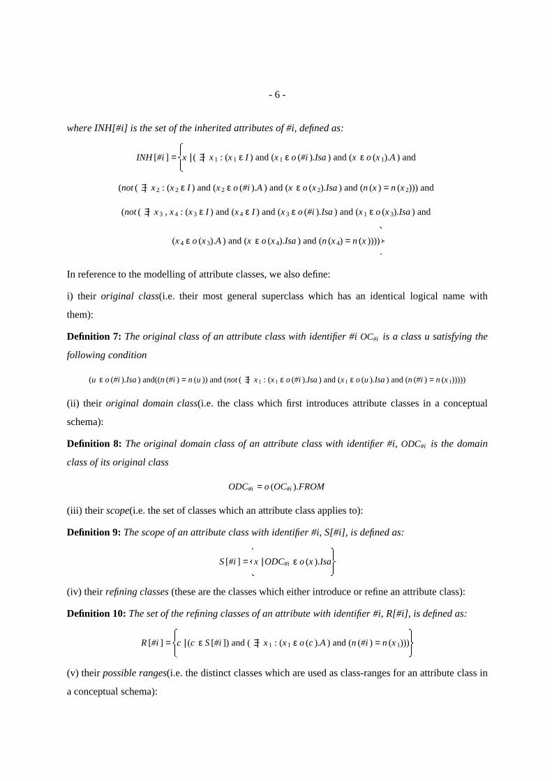
iii)The Evidence to Abstractness

Since an abstract attribute is defined by consequence of the abstractness of its original domain class,

the evidence about its own abstractness is also estimated from the evidence about the abstractness of

this class:

Definition 29: The evidence to the abstractness of an attribute class with identifier #i, mia is measured

by the function:

mia(P )=

�����01−ej

ej

if P ⊆ Θ & P ≠ABSi & P ≠ ABS� � � �

i

if P = ABS� � � �

i

if P = ABSi

where j = ODC#i , ej = g (EXT [#j ])| EXTs [#j ] |� ������������������� and , g (EXT [#j ]) =

�� �1| EXT [#j ] |

if EXT [#j ] = ∅if EXT [#j ] ≠ ∅

mia(P ) relaxes the logical definition of abstractness giving an evidence measure equal to 1, whenever

this definition is satisfied. In fact, provided that EXT [#j ] ≠ ∅, if | EXTs [#j ] | = | EXT [#j ] | then ej = 1.

mia(P ) satisfies the axiomatic definition of the Dempster-Shafer probability assignments:

Theorem 8: The function mia(P ) is a basic probability assignment.

iv) The Evidence to Undefinability of Dependencies

The evidence about the undefinability of a dependency mapping between two attributes #i and #j, due

to their non common classes is measured by the following function:

Definition 30: The evidence to the undefinability of a dependency mapping between an attribute class

with identifier #i and an attribute class with identifier #j, due to their non common scope, mi jncs , is

measured by the function:

mi jncs(P )=

�����01−di j

di j

if P ⊆ Θ & P ≠ M� �

j & P ≠ Θif P = Θif P = M

� �

j

where di j = ( | S [#i ]∪S [#j ] | )( | S [#i ]−S [#j ] | + | S [#j ]−S [#i ] | )�������������������������������������������������������

According to mi jncs(P ), the more the non common classes in the scopes of two attributes the more

unlikely to be able to define a dependency mapping between them. mi jncs(P ) satisfies the axiomatic

definition of the Dempster-Shafer probability assignments:

Theorem 9: The function mi jncs(P ) is a basic probability assignment.

- 27 -

v) The Evidence to Undefinability of Total Equivalences

The evidence to the undefinability of total equivalence mappings between two attributes #i and #j, due

to their non common refinements over a conceptual schema, is measured according to the following

definition:

Definition 31: The evidence to the undefinability of a total equivalence mapping between an attribute

class with identifier #i and an attribute class with identifier #j, due to their non common refinements

over a conceptual schema, mi jncr is measured by the function:

mi jncr(P )=

�����01−ri j

ri j

if (P ⊆ Θ & P ≠ M� �

j & (P ≠ Θ)if P = Θif P = M

� �

j

where ri j = | R [#i ]∪R [#j ] || (S [#i ]−R [#i ])∩R [#j ] | + | (S [#j ]−R [#j ])∩R [#i ] |� ���������������������������������������������������������������������������������������

According to mi jncr(P ), the more the non common refinements of two attributes over a schema, the more

evident the impossibility of defining a total equivalence mapping between them. mi jncr(P ) satisfies the

axiomatic definition of the Dempster-Shafer probability assignments:

Theorem 10: The function mi jncr(P ) is a basic probability assignment.

vi) Total Belief and Plausibility of Dominance

The total belief and the plausibility to the dominance of an attribute #i(i.e. Bel (DOMi ) and

P* (DOMi ) = 1−Bel (DOMi )) are estimated by combining the basic probability assignments mich and mi

a

with the assignment mi jncs, when every kind of interattribute dependency is taken into account:

Theorem 11: The combination of the basic probability assignments mia,mi

ch and m ncs results into the

following Dempster-Shafer combined beliefs:

Bel (DOMi )=ci eu

Bel (DOM� � � � �

i )=(1−ci eu )j =1Π

ndi j

P* (DOMi )=1−(1−ci eu )j =1Π

ndi j

where u = ODC#i .

On the other hand, these beliefs and plausibilities are estimated by combining the basic probability

assignments mich and mi

a with the assignments mi jncs and mi j

ncr, when only total equivalencies are taken

into account:

- 28 -

Theorem 12: The combination of the basic probability assignments mia,mi

ch with the basic probability

assignments mi jncs and mi j

ncr results into the following Dempster- Shafer combined beliefs:

Bel (DOMi )=ci eu

Bel (DOM� � � � �

i )=(1−ci eu )j =1Π

n(1−(1−ri j )(1−di j ))

P* (DOMi )=1−(1−ci eu )j =1Π

n(1−(1−ri j )(1−di j ))

where u = ODC#i .

vii) The Salience Measuring Function

The salience of an attribute class is measured from the belief and plausibility of its dominance by the

following function:

Definition 32: The salience of attribute classes is measured by the function SL :i =1∪∞

Ai → [0,...,1], which

is defined as

SL (j ) = 2Bel (DOM j ) + P* (DOM j )� ����������������������������������������� V− j ε

i =1∪∞

Ai

2.3.4 An Example of Salience Estimates

In the following, we give an example of salience estimates in reference to the conceptual schema of

figure 9, that is a generalization taxonomy of classes of employees in a research institute. The numbers

in the right lowers of thick boxes indicate the cardinalities of the extensions of the relevant classes.

Table 3 presents belief and plausibility measures to the charactericity, abstractness, determinance and

dominance of attributes as well as their salience measures(subscripts 1 and 2 distinguish between

measures obtained considering all kinds of dependencies or only total equivalencies, respectively).

As shown in this table, the attribute classes employmentAggreement and qualification are the more

salient ones. They are not only abstract(cf. column mia in table 3) but also they are specialized by most

of the subclasses of employees (thus becoming characteristic of the relevant generalization taxonomy).

Furthermore, a dependency mapping between them cannot be precluded(cf. columns Bel 1(DET� � � �

i ) and

Bel 2(DET� � � �

i ) in table 3) as a result of non common scope or significant numbers of non common

refinements. In fact, the qualifications of an employee determine the kind of the job he/she is eligible

for and thus the type of the contract he/she may have.

At the other end of the spectrum, the attribute class keepsAccountsOf is neither abstract nor deter-

minant (cf. columns mia, Bel 1(DET

� � � �

i ) and Bel 2(DET� � � �

i ) in table 3). Also, it is characteristic only for the

- 29 -

�������������������������������������������������������������������������������������������������������������������������������������������������������������

ResearchProject

AdministrationTask

ResearchGroup

ResearchInstEmployee

ResearchStaffResearch

ResearchGroup

AdministrationManagers

Leaders

AssociateResearchers

Researchers

ResearchInstScholars

StudentsResearch

Assistants

AdministrativeStaff

AgreementEmp

SecurityNumber Qualification

employmentAgreement

qualificationsecurityNumber

AccountancyDegreeIn

qualification

responsibleFor

qualification

qualification

directs

PhD DegreeMastersDegreequalification

belongTo

employmentAgreementContract

Research Scholarship

employmentAgreement

ScholarshipStudent

employmentAgreementqualification

employmentAgreement

ScholarshipResearch

enrolledAtUniversity

employmentAgreement

TemporalResContract

employmentAgreement

PermanentResContract

employmentAgreement

CertificateForeignLang

qualification

StaffemploymentAgreement

Contract

PermanentContract

employementAgreement

5

7

ResearchersSenior

2

4

10

20 50

80 20 10

30

11014

88

118

Accountants

Secretaries

worksFor

manages

keepsAccountsOf

JuniorResearchers

Figure 9: An Example for Estimating Salience of Attributes

�������������������������������������������������������������������������������������������������������������������������������������������������������������� �����������������������������������������������������������������������������������������������������������������������������������������������������������

Table 3: Evidence and Salience Measures for Attributes in Figure 9� �����������������������������������������������������������������������������������������������������������������������������������������������������������Attribute mi

ch Bel (DOMi) P*

1(DOM

i) SL (i )mi

a Bel1(DET� �����

i) Bel

2(DET� �����

i) P*

2(DOM

i)� �����������������������������������������������������������������������������������������������������������������������������������������������������������

employmentAggreement 0.53 1 0 0.17 0.53 1 0.92 0.765� �����������������������������������������������������������������������������������������������������������������������������������������������������������qualification 0.4 1 0 0.15 0.4 1.0 0.91 0.7� �����������������������������������������������������������������������������������������������������������������������������������������������������������enrolledAt 0.33 1 0.25 0.47 0.33 0.83 0.68 0.58� �����������������������������������������������������������������������������������������������������������������������������������������������������������manages 0.33 0.6 0.1 0.28 0.198 0.92 .77 0.55� �����������������������������������������������������������������������������������������������������������������������������������������������������������worksFor 0.1 1 0 0 0.1 1.0 1.0 0.55� �����������������������������������������������������������������������������������������������������������������������������������������������������������belongsTo 0.1 1 0 0 0.1 1.0 1.0 0.55� �����������������������������������������������������������������������������������������������������������������������������������������������������������securityNumber 0.06 1 0 0 0.06 1.0 1.0 0.503� �����������������������������������������������������������������������������������������������������������������������������������������������������������responsibleFor 1 0 0.44 0.64 0 0.56 0.36 0.28� �����������������������������������������������������������������������������������������������������������������������������������������������������������directs 1 0 0.44 0.64 0 0.56 0.36 0.28� �����������������������������������������������������������������������������������������������������������������������������������������������������������keepsAccountsOf 1 0 0.81 0.77 0 0.19 0.23 0.095� �����������������������������������������������������������������������������������������������������������������������������������������������������������

�����������������

���������������

���������������

���������������

���������������

���������������

���������������

���������������

���������������

�����������������

particular kind of employees it applies to(i.e. Accountants) but not for the entire taxonomy.

3. Computation of Distance and Salience Functions- Analysis of Complexity

i) The Computation of the Classification Distance

The computation of the classification distance between two objects retrieves their classes, identifies

the non-common of them and estimates their specialization depths. Its worst-case time complexity is

O (C 13 + C 2

3 ), where C 1 and C 2 are the numbers of the classes of the involved objects, since it might be

necessary to estimate the specialization depths for each of them if the involved objects have no classes

in common. This step requires the retrieval of the transitive closures of their own superclasses, which

- 30 -

has a complexity O (C 12 + C 2

2 ) (the complexity of spanning the transitive closure of a graph with N

nodes is N 2 [50]).

ii) The Computation of the Generalization Distance

The computation of the generalization distance between two individual classes retrieves their superc-

lasses, identifies the non-common of them and estimates their specialization depths. In the case of

attribute classes, it retrieves their original classes and checks their identity. Similarly to the computa-

tion of the classification distance, the computation of the generalization distance has a worse-case time

complexity of O (S 13 + S 2

3 ), where S 1 and S 2 are the numbers of the superclasses of the involved

objects.

iii) The Computation of the Attribution Distance

To compute the attribution distance between two objects, initially their semantically homogeneous

attributes are identified and then their saliences as well as the pairwise distances between them are

estimated. The complexity of testing the semantic homogeneity of two attributes x and y is

O (Nx2 + Nx logNx +

z εClasses (x )Σ Nz logNz + Ny

2 + Ny logNy +w εClasses (y )

Σ Nw logNw ) where Nx , Ny , Nz and Nw are

the numbers of the classes of the attributes x,y,z and w, as proved in [61].

Then, the selection of the minimum distance isomorphism between the semantically homogeneous

attributes of two objects is a weigthed bipartite graph matching problem[50]:

Theorem 13: The selection of the minimum distance isomorphism in computing function D 4 is a

weighted bipartite graph matching problem.

Thus, the minimum distance isomorphism between the attributes of two objects can be selected by an

algorithm solving this problem. A traditional such algorithm is the Hungarian Method[50], whose

complexity is O (n 3) for graphs with n nodes in total. Therefore, the time complexity of selecting the

minimum distance isomorphism between the attributes of two objects x and y is O (Ax3 + Ay

3), where Ax

and Ay are the numbers of their attributes[61].

iv) The Computation of Salience

The computation of an attribute’s salience is based on the estimation of the beliefs and plausibilities to

the determinance of the original classes of the attribute classes it has been an instance of (cf.

definitions 19 and 28). To obtain these measures, it is necessary to retrieve the scope, the refining

classes, the possible ranges and the original domain class (together with its extension) for each of

these original classes and use them in estimating the beliefs to the charactericity and the abstractness

of the involved attribute. Furthermore, to estimate the belief to its non-determinance, it is necessary to

- 31 -

retrieve the original classes of all the other attributes of the classes in its scope (together with their

own refining and possible range classes). As discussed in[61], the worse-case time complexity of this

computation is O (L (NM +M 2logM )), where L is the number of the attributes of the classes in the scope

of the attribute in hand, N is the number of the instances of its original domain class and M is the

number of the classes in its scope.

v) The Computation of the Overall Distance

The computation of the overall distance between objects aggregates their partial distances. Due to the

recursive computation of the attribution distance, the time complexity of the computation of the

overall distance is given by the following fomula(x denotes the level of recursion):

Tx = Kin + Kisa + (A 1 + A 2)Ksal + (A 1A 2)Kmap + (A 13 + A 2

3 ) + (iΣxi yi +1)Tx −1 (1)

where

� Kin is the cost of estimating the classification distance of two objects(see relevant complexity above)

� Kisa is the cost of estimating the generalization distance of two objects(see relevant complexity

above)

� Kmap is the cost of testing the semantic homogeneity of two attributes of the involved objects(see

relevant complexity above)

� Ksal is the cost of estimating the salience of an attribute(see relevant complexity above)

� xi , yi are the numbers of attributes of the involved objects in each category of semantic homogeneity

i (thus,iΣxi = A 1 ,

iΣyi = A 2).

Formula (1) can be rewritten as:

Tx = ATx −1 + B (2)

where A =iΣxi yi + 1 and B = Kin + Kisa + (A 1 + A 2)Ksal + (A 1A 2)Kmap + (A 1

3 + A 23 )

Assuming that, the factors A and B are constant at the different levels of recursion x, formula 2 is a

linear first-order difference equation and its general solution is Tx = B A −1A x −1� ��������� + CA x where C = T 0 [68].

T 0 is the cost of similarity analysis between objects having no attributes and equals to Kin + Kisa since

the computation of the similarity between such objects depends solely on their classification and gen-

eralization distances.

Thus, controlling recursion while computing the attribution distance makes the complexity of similar-

ity analysis polynomial. For instance, the termination of recursion after having examined the

- 32 -

attributes at the first two levels of the attribution graphs of two objects results in a complexity

B (A +1) + CA 2 . Under controlled recursion, the selected isomorphism between attributes will only

approximate the optimal one with a quality depending on the correlation between the classification,

generalization and the attribution distances between the relevant objects. However, to the extent that

our experiments have shown positive and statistically significant such correlations (cf. table 1 in sec-

tion 2.2.5), we can expect good such approximations.

4. Empirical Evaluation of the Model

The prescribed similarity model has been implemented in C++[62] and integrated with the Semantic

Index System(SIS) (see [11, 74] for details). The SIS is a tool for representing scientific knowledge

and engineering designs. The resulted prototype was used in preliminary experiments concerning: (1)

the consistency of estimates produced by our model with similarity assessments provided by

humans(consistency is a prerequisite for applying the model to tasks, where analogical reasoning has

to be carried out in cooperation with humans); and (2) the recall performance of similarity analysis in

retrieval.

4.1 Ordering Consistency

In the first experiment, we used a conceptual model of the C++ language[62] representing concepts of

C++(e.g classes, operators, member functions), the normal file structure of C++ programs(e.g depen-

dencies between source code files and header files) and dependencies between C++ program elements

(e.g. function calls, access of variables). The model was developed to support the static analysis of

C++ programs[15] and its accuracy regarding the representation of C++ concepts has been evidenced

through this application.

�������������������������������������������������������������������������������������������������������������������������������Table 4: Rank Correlations Between Model and Human Similarity Orderings�������������������������������������������������������������������������������������������������������������������������������Case Set Size Subject 1 Subject 2 Subject 3 Subject 4 Subject 5�������������������������������������������������������������������������������������������������������������������������������

1 17 0.37 0.5 * 0.47 * 0.37 0.46 *�������������������������������������������������������������������������������������������������������������������������������2 37 0.84 * 0.75 * 0.57 * 0.60 * -0.06�������������������������������������������������������������������������������������������������������������������������������3 18 -0.32 - 0.5 * -0.13 0.12�������������������������������������������������������������������������������������������������������������������������������4 18 -0.12 - 0.5 * -0.18 0.10�������������������������������������������������������������������������������������������������������������������������������5 4 0.55 0.55 0.55 0.55 0.55�������������������������������������������������������������������������������������������������������������������������������6 17 0.55 * 0.60 * 0.55 * 0.51 * 0.64 *�������������������������������������������������������������������������������������������������������������������������������7 4 0.55 0.85 0.65 0.55 0.4�������������������������������������������������������������������������������������������������������������������������������8 18 0.57 * 0.48 * 0.87 * 0.65 * 0.52 *�������������������������������������������������������������������������������������������������������������������������������9 17 0.42 * 0.71 * 0.39 0.50 * 0.5 *�������������������������������������������������������������������������������������������������������������������������������10 19 0.52 * 0.87 * 0.73 * 0.86 * 0.64 *�������������������������������������������������������������������������������������������������������������������������������

������������������

����������������

����������������

����������������

����������������

����������������

����������������

������������������

Ten cases of similarity analysis were carried out. In each case, the elements of a source set of C++

concepts were ranked in descending similarity order with respect to a target C++ concept. The

- 33 -

similarities between the compared concepts in each of these cases were measured from their concep-

tual descriptions in the employed model of C++. The same cases were given to five software

engineers, ignorant of the similarity analysis imposed ordering, who were asked to rank the source

concepts with respect to their similarities to the target(as they perceived them). The subjects had dif-

ferent degrees of expertise and knowledge of the C++ conceptual model(decreasing along with

increasing subject numbers in table 4).

The rank correlations of the two orderings were measured according to the Spearman

coefficient[25,33]. As shown in table 4, a positive rank correlation was found in all but 5 cases. Most

of the positive coefficients(28 out of 44) were found statistically significant(i.e. coefficients marked

by an asterisk) according to the D or t criteria[33] at the level p < 0.05, unlike the negative ones.

These preliminary findings indicate that the similarity model generates measures, which do not violate

human intuition about similarity.

4.2 Recall Evaluation

Recall measures, as indicators of completeness in retrieval[63], associate with the possibility of ignor-

ing relevant analogs in an analogical reasoning session after analogical retrieval (high recall indicates

a low such possibility and vice versa).

Using exactly the same C++ conceptual model and four of the subjects participated in the first experi-

ment we also measured the recall performance of the similarity model. The subjects were given the

same 10 cases of the previous experiment and were asked to indicate whether each of the source C++

concepts could be used instead of the target one in some programming task they could think of. Their

answers - interpreted as indicating the analogy between the relevant concepts in programming - were

used as judgements of relevance[63]. On the basis of these judgements, we measured the recall per-

formance of the model in reference to the source sets. Recall was measured according to the follow-

ing formula:

r = ac /R

where ac was the number of the relevant sources in the first c % positions of the sorted(in descending

similarity order) source set and R the total number of the relevant items in it[32].

Table 5 presents measured recalls for different subjects and cutoff levels. In our view, these measures

are encouraging since the first two of the selected cutoffs were fairly low and the proportion of the

items in any of the source sets, judged as relevant by any of the subjects did not exceed 25%. In fact,

only 10% of items in the source sets were assessed as being relevant on the average.

- 34 -

�����������������������������������������������������������������������������������������������������������Table 5: Average Recall for Different Cutoffs�����������������������������������������������������������������������������������������������������������

Cutoff Subject 1 Subject 2 Subject 3 Subject 5 General�����������������������������������������������������������������������������������������������������������10% 0.33 0.35 0.34 0.44 0.35�����������������������������������������������������������������������������������������������������������25% 0.54 0.40 0.74 1.00 0.60�����������������������������������������������������������������������������������������������������������50% 0.83 0.80 0.91 1.00 0.86�����������������������������������������������������������������������������������������������������������

��������

������

������

������

������

������

��������

5. Related Work

This section assesses the merits of the similarity and other computational models of analogical reason-

ing with respect to criteria related to pragmatic aspects of their application. These criteria include: (1)

the ability of a model to elaborate analogies between objects in different domains(i.e. domain

independence); (2) the need of causal knowledge and/or user-supplied information for the elaboration

of analogies and; (3) the computational complexity of a model. The former two criteria shape the

spectrum of the tasks a model might be applicable to, while the latter determines the efficiency of its

application.

Computational models of analogical reasoning can be distinguished into:

(1) general models which detect analogies without distinguishing the purpose of reasoning and the

types of the involved analogs(i.e. the Structure Mapping Engine(SME)[17], the Constraint Satisfac-

tion Theory(CST) implemented by ACME [28] and ARCS[65] and the Constrained Semantic

Transference(CST)[29]);

(2) models of analogical understanding which detect analogies to explain unfamiliar domains in terms

of familiar ones, (e.g. MACKBETH[72] and CARL[7]);

(3) models of analogical problem solving, which detect analogies to solve specific problems and

involve analogs from different domains(e.g. ANA[41], explicit planning[45], MEDIATOR[37],

ARCHES[5], purpose-directed analogy[30], transformational and derivational analogy[8, 9, 43],

NLANG[23], PRODIGY[69] and ANAGRAM[13]; and,

(4) models of case-based reasoning, a special kind of models of analogical problem solving, which

detect analogies between items in the same application domain(e.g. PARADYME/JULIA[36],

SURVER III[73], HYPO[4], CADET[59], CABOT[12], Protos[48], FGP[16], CBL4[2] and

CBR+EBL[14]).

In general, the models of the latter three types utilize causal knowledge determining the elements of

analogs, which are important for analogies sought for a particular purpose. This knowledge usually

enables a fast detection of analogies, by limiting the search space of the analog-elements that must be

taken into account. However, there might be domains which totally or partially lack such knowledge

or where it is very expensive to acquire it. Also, the substance[61], the granularity[39] and the

- 35 -

representation of causal knowledge might differ across domains [39,61]. Hence, the whole approach

and consequently the models adopting it may not be always usable.

However, even the general models of analogical reasoning might be weak in the light of the prescribed

criteria. In particular:

The SME is domain independent and does not rely on causal knowledge. In fact, the model matches

identical relations of analogs, which do not violate the relational structures of their objects according

to the systematicity principle[20] (i.e. when two relations are mapped their corresponding arguments

must be mapped as well). Also the importance of different relations is distinguished syntactically from

their arity and order. However, the SME has a combinatorial computational complexity, i.e. O (N !)

where N is the number of analog elements that must be considered for mapping.

The CST matches analogs obeying the systematicity principle but it considers only elements, which

are known to be important for analogies or related to goal attainment. Also, elements cannot be

matched unless they are associated with concepts in a lexicon related by specific types of semantic

similarity relations (e.g. synonymy, hyponymy, meronymy[65]). To the extent that these lexicon con-

cepts usually have context and domain dependent meanings[19] and the specific primitives used for

expressing causalities between analog elements and goals may not be adequate for all possible

domains[61], the model is not domain independent and is sensitive to causal knowledge. Its parallel

implementation using connectionist networks does not allow an analytical prediction of its worse-time

complexity, although the model is claimed to be efficient[65].

The Constrained Semantic Transference model is domain independent and does not need causal

knowledge or explicit user-information for detecting analogies. It maps elements of analogs, which are

of the same type. Mappings are constrained by demanding the consistency of the properties of the

image of an element with existing knowledge about it(i.e. coherent mappings). This formal notion of

coherency can only be approximately checked within limited computational time but is not comput-

able in the general case. Hence, the model is of limited practical utility.

In the light of our previous criticism, the similarity model ranks better than other general models when

all the prescribed criteria are taken into account. In fact, neither it employs any domain dependent

matching criteria, nor it relies on special types of causal knowledge or user-supplied information for

detecting analogies. Also, as discussed in section 3, it has a polynomial complexity.

6. Conclusions and Future Research

In this paper, we defined and analysed a computational model for elaborating analogies between con-

ceptual objects. The model consists of metric functions, which measure the conceptual distances

- 36 -

between objects with respect to their classifications, generalizations and attributes as well as functions

which measure the importance of these semantic modelling elements to the existence of analogies. Its

competence in detecting analogies depends on how precisely the semantics of objects are expressed by

their conceptual descriptions. Improper conceptual modelling deteriorates this competence and cannot

be identified by similarity analysis, itself.

Because of the formal definition of its distance and salience measuring functions the model is amen-

able to analytic assessment. Also, it is domain independent and operational upon non uniform

representations of objects. It does not need causal knowledge or explicit, user-supplied information

for detecting analogies and has a polynomial complexity. These characteristics give it a potential of

being applicable to complex tasks involving intra or inter-domain analogical reasoning, some of which

have been investigated elsewhere[52,53,54,75,76,77].

A further and extensive empirical evaluation of the model is necessary for validating the initial empiri-

cal findings presented in this paper and the positive evidence acquired from applying it to tasks of

software reuse[52,53,54,55]. Such an evaluation is being planned within real application environments

and tasks varying with respect to the goals they impose and the conceptual models they use for

describing potential analogs. The implementation of the model upon the Semantic Index System

platform(see [11,74] for details) makes this application feasible regarding information management

and usability requirements[11].

We are also designing a parallel implementation of the model. In fact, the classification, generaliza-

tion and attribution distances can be computed in parallel because they do not depend on each other.

Also, since the semantic homogeneity is an equivalence relation, it partitions the attributes of objects

into disjoint categories. This makes possible the parallel computation of partial optimal isomorphisms

for each such category followed by their merging into an overall optimal isomorphism, while comput-

ing the attribution distance between objects(cf. proof of theorem 13 in Appendix 2).

- 37 -

Appendix 1: Axiomatic Foundation of Metric Functions and Dempster-Shafer

Beliefs

i) Metrics

Following [21], a function d on a non empty set X is a metric for it, if it assigns to each pair of its ele-

ments of a real number(i.e. d : X ×X → R ), which satisfies the following axioms:

(α1) D (x ,y ) ≥ 0

(α2) D (x ,y ) ≡ D (y ,x )

(α3) D (x ,z ) ≤ D (x ,y ) + D (y ,z )

(α4) D (x ,y ) = 0⇐⇒x =y

A function d which satisfies only the first three of these axioms is called pseudometric[34].

ii) Elements of the Dempster-Shafer Theory of Evidence

Belief in the context of the Dempster-Shafer theory of evidence[57] is a function

Bel : PowersetOf (Θ) → [0,...1]

obeying the axioms:

(α5) Bel (P ) = 0, if P = ∅

(α6) Bel (Θ) = 1

(α7) Bel (i =1∪

nPi ) ≥

I ⊆ {1,2,...,n },I ≠∅Σ (−1) | I | +1Bel (i ε I∩Pi )

where Θ is a set of mutually exclusive propositions referred to as the frame of discernment,

n = | PowersetOf (Θ) | and P, Pi are subsets of Θ denoting the logical disjunction of their elements.

The total belief committed to a subset P, i.e. Bel (P ), results from accumulating basic probability

assignments to its subsets:

(f 1) Bel (P ) =A ⊆ PΣ m (A )

A basic probability assignment is a function m obeying the following axioms:

(α8) m : PowersetOf (Θ) → [0,...,1]

(α9) m (∅) = 0

(α10)P ⊆ ΘΣ m (P ) = 1

Different basic probability assignments arised from distinct bodies of evidence can be combined

according to the formula:

- 38 -

m 1 +�� � m 2(P ) = 1−k 0

X ∩ Y = PΣ m 1(X )m 2(Y )

����������������������������������� where k 0 =Z∩W = ∅ , Z ⊆Θ , W ⊆Θ

Σ m 1(Z )m 2(W )

which is known as the rule of the orthogonal sum [57].

- 39 -

Appendix 2: Proofs of Theorems in Sections 2 and 3

Lemma 1: For any three sets A,B,D it holds that

(A −B )∪(B −A )⊆((A −D )∪(D −A ))∪((D −B )∪(B −D )).

Proof: It can be proved by algebraic manipulation as in [61]. �

Lemma 2: The homographic transformation d (x 1,x 2) = aD (x 1,x 2) + 1aD (x 1,x 2)

����������������������� , a > 0 of a metric D is a metric

Proof: It can be proved by algebraic manipulation as in [61]. �

Theorem 1: Function d 2 is a pseudometric.

Proof: Function D 2 is pseudometric since:

(i) D 2(#i ,#j )=x ε (o (#i ).In −o (#j ).In )

Σ SD (x )1

����������� +x ε (o (#j ).In −o (#i ).In )

Σ SD (x )1

����������� ≥ 0 (i.e. axiom α1) )

(ii) D 2(#i ,#j ) =x 1 ε Sij

Σ SD (x 1)1

� ����������� +x 2 ε Sji

Σ SD (x 2)1

� ����������� =x 2 ε Sji

Σ SD (x 2)1

� ����������� +x 1 ε Sij

Σ SD (x 1)1

� ����������� = D 2(#j ,#i ) (if

Si j =

�� �o (#i ).In ∪−o (#j ).In

� �� and Sji =

�� �o (#j ).In −o (#i ).In

� �� ) (i.e. axiom α2) ) and

(iii)x ε S 1

Σ SD (x )1

����������� ≤x ε (S 2∪S 3)

Σ SD (x )1

����������� ≤x ε S 2

Σ SD (x )1

����������� +x ε S 3

Σ SD (x )1

����������� if S 1 = (Si −Sj )∪(Sj −Si )

S 2 = (Si −Sl )∪(Sl −Si ) S 3 = (Sl −Sj )∪(Sj −Sl ) (Si = o (#i ).In , Sj = o (#j ).In , Sl = o (#l ).In ) since by

lemma 1 S 1⊆S 2∪S 3 (i.e. axiom α3) ) . Then by lemma 2 d 2 is also a pseudometric. �

Theorem 2: Function d 3 is a metric .

Proof: It can be proved in a way similar to theorem 1 as in [61]. �

Theorem 3: The semantic homogeneity of attributes is an equivalence relation

Proof: The semantic homogeneity is a reflexive (i.e. sh (#i ,#i ) ) since OCL [#i ] ≡ OCL [#i ], symmetric

(i.e. sh (#i ,#j )⇐⇒sh (#j ,#i ) ) since OCL [#i ] = OCL [#j ]⇒OCL [#j ] = OCL [#i ] and transitive relation

(i.e. sh (#i ,#j ) and sh (#j ,#l )⇒sh (#i ,#l ) ) since (OCL [#i ] = OCL [#j ]) and

(OCL [#j ] = OCL [#l ])⇒(OCL [#i ] = OCL [#l ]) �

Lemma 3: Function D 4 is a metric.

Proof: a) D 4 satisfies axiom α1 when INT [#i ] = ∅ or INT [#j ] = ∅ since D 4(#i ,#j ) = ∞. Also, when both

#i and #j have attributes, let us assume that one attribute of each element (x 1,x 2) of their optimal iso-

morphism ck has no attributes of its own. This is a valid assumption since eventually some of the

INT [x 1] or INT [x 2] will be empty(even due to V = IU ∪AU ). In this case, D 4(x 1,x 2,V ) ≥ 0, as it was

just proved, and by lemmas 4 and 5 D′ (x 1,x 2,V ) ≥ 0 and d′ (x 1,x 2,V ) ≥ 0 , respectively. Therefore,

- 40 -

ck ε C [#i ,#j ]min

�� �(x 1,x 2) ε ck

Σ s (x 1)s (x 2)d′ (x 1,x 2,V ) +x 3 ε A#i [ck ]

Σ s (x 3)2 +x 4 ε A#j [ck ]

Σ s (x 4)2

� �� ≥ 0 or equivalently

D 4(#i ,#j ,V ) ≥ 0.

b) D 4 is symmetric by definition when INT [#i ] = ∅ or INT [#j ] = ∅. When, #i or #j have their own

attributes, each of the isomorphisms ck in C[#i,#j] will have an inverse isomorphism c′k (c′k = ck−1) in

C[#j,#i] and furthermore A#i [c′k ] = A#i [ck ] and A#j [c′k ] = A#j [ck ] . Assuming that at least one attribute

of each element (x 1,x 2) in combinations ck and c′k has no attributes of its own, D 4(x 1,x 2,V )=D 4(x 2,x 1,V )

(as already proved) and therefore d′ (x 1,x 2,V ) = d′ (x 2,x 1,V ) (by lemma 5). Thus, forall ck , c′k :

(x 1,x 2) ε ck

Σ s (x 1)s (x 2)d′ (x 1,x 2,V ) =(x 2,x 1) ε c′k

Σ s (x 2)s (x 1)d′ (x 2,x 1,V ) and

x 3 ε A#i [ck ]Σ s (x 3)2 =

x 3 ε A#i [c′k ]Σ s (x 3)2 and

x 4 ε A#j [ck ]Σ s (x 3)2 =

x 4 ε A#j [c′k ]Σ s (x 3)2

Therefore,

ck ε C [#i ,#j ]min

�� �(x 1,x 2) ε ck

Σ s (x 1)s (x 2)d′ (x 1,x 2,V ) +x 3 ε A#i [ck ]

Σ s (x 3)2 +x 4 ε A#j [ck ]

Σ s (x 4)2

� �� =

c′k ε C [#j ,#i ]min

�� �(x 2,x 1) ε c′k

Σ s (x 2)s (x 1)d′ (x 2,x 1,V ) +x 3 ε A#i [c′k ]

Σ s (x 3)2 +x 4 ε A#j [c′k ]

Σ s (x 4)2

� ��

or equivalently D 4(#i ,#j ,V ) = D 4(#j ,#i ,V ).

c) D 4 is triangular by definition when one, two or all of three objects #i,#j and #l have no attributes

When all #i , #j and #l have attributes, let Cilopt and Cl j

opt be the optimal isomorphisms between the attri-

butes of the objects #i, #l and #l, #j, respectively and, C′i j be an isomorphism between the attributes

of #i and #j defined as(see transitivity of semantic homogeneity):

C′i j =

�� �(x 1,x 3) | ( |−−− x 2 : ((x 1,x 2) ε Cil

opt) and ((x 2,x 3) ε Cl jopt))

� �� (I)

Given C′i j , it is sufficient to prove that

(x 1,x 2) ε C′ij

Σ s (x 1)s (x 2)d′ (x 1,x 2,V ) +x 3 ε A#i [C′ij ]

Σ s (x 3)2 +x 4 ε A#j [C′ij ]

Σ s (x 4)2 ≤

(x 5,x 6) ε Cilopt

Σ s (x 5)s (x 6)d′ (x 5,x 6,V ) +x 7 ε A#i [Cil

opt]Σ s (x 7)2 +

x 8 ε A#l [Cilopt]

Σ s (x 8)2 +

(x 9,x 10) ε Cljopt

Σ s (x 9)s (x 10)d′ (x 9,x 10,V ) +x 11 ε A#l [Clj

opt]Σ s (x 11)2 +

x 12 ε A#j [Cljopt]

Σ s (x 12)2 (II)

because even if C′i j is not the optimal isomorphism Ci jopt , between the objects #i , #j, Ci j

opt will result

into a less total distance according to definition 19. However, if:

C′il =

�� �(x 1,x 2) | ((x 1,x 2) ε Cil

opt) and ( |−−− x 3 : ((x 1,x 3) ε C′i j )

� �� (III)

- 41 -

and

C′l j =

�� �(x 1,x 2) | ((x 1,x 2) ε Cl j

opt) and ( |−−− x 3 : ((x 3,x 2) ε C′i j )

� �� (IV)

then,

(x 1,x 2) ε Cilopt

Σ s (x 1)s (x 2)d′ (x 1,x 2,V ) =

(x 3,x 4) ε C′il

Σ s (x 3)s (x 4)d′ (x 3,x 4,V ) +(x 5,x 6) ε (Cil

opt−C′il )Σ s (x 5)s (x 6)d′ (x 5,x 6,V )

and

(x 1,x 2) ε Cljopt

Σ s (x 1)s (x 2)d′ (x 1,x 2,V ) =

(x 3,x 4) ε C′lj

Σ s (x 3)s (x 4)d′ (x 3,x 4,V ) +(x 5,x 6) ε (Clj

opt−C′lj )Σ s (x 5)s (x 6)d′ (x 5,x 6,V )

Also, if we define:

A#i(1)[C′i j ] =

�� �x 1 | (not ( |−−− x 2 : (x 1,x 2) ε Cil

opt

� ��

A#i(2)[C′i j ] =

�� �x 1 | ( |−−− x 2 : ((x 1,x 2) ε Cil

opt)) and (not ( |−−− x 3 : ((x 2,x 3) ε Cl jopt)))

� �� and

A#j(1)[C′i j ] =

�� �x 2 | (not ( |−−− x 1 : (x 1,x 2) ε Cl j

opt

� ��

A#j(2)[C′i j ] =

�� �x 2 | ( |−−− x 1 : ((x 1,x 2) ε Cl j

opt)) and (not ( |−−− x 3 : ((x 3,x 1) ε Cilopt)))

� ��

then

A#i [C′i j ] = A#i(1)[C′i j ] ∪ A#i

(2)[C′i j ] and A#i(1)[C′i j ] = A#i [Cil

opt]

A#j [C′i j ] = A#j(1)[C′i j ] ∪ A#j

(2)[C′i j ] and A#j(1)[C′i j ] = A#j [Cl j

opt]

Thus, (II) becomes,

(x1,x

2) ε C′

ij

Σ s (x 1)s (x 2)d′ (x 1,x 2,V ) +x

3ε A

#i[Cil

opt]Σ s (x 3)2 +

x4ε A#i

(2)[C′ij]

Σ s (x 4)2 +x

5ε A

#j[Clj

opt]Σ s (x 5)2 +

x6ε A#j

(2)[C′ij]

Σ s (x 6)2 ≤

(x7,x

8) ε C′

il

Σ s (x 7)s (x 8)d′ (x 7,x 8,V ) +(x

9,x

10) ε (Cil

opt−C′il)

Σ s (x 9)s (x 10)d′ (x 9,x 10,V ) +x

11ε A

#i[Cil

opt]Σ s (x 11)2 +

x12

ε A#l

[Cilopt]

Σ s (x 12)2 +

(x13,x

14) ε C′

il

Σ s (x13)s (x14)d′ (x13,x14,V ) +(x

15,x

16) ε (Clj

opt−C′lj)

Σ s (x15)s (x16)d′ (x15,x16,V ) +x

17ε A

#j[Clj

opt]Σ s (x17)2 +

x18

ε A#l

[Cljopt]

Σ s (x18)2 (V)

and equivalently,

- 42 -

(x 1,x 2) ε C′ij

Σ s (x 1)s (x 2)d′ (x 1,x 2,V ) +x 4 ε A#i

(2)[C′ij ]Σ s (x 4)2 +

x 6 ε A#j(2)[C′ij ]Σ s (x 6)2 ≤

(x 7,x 8) ε C′il

Σ s (x 7)s (x 8)d′ (x 7,x 8,V ) +(x 9,x 10) ε (Cil

opt−C′il )Σ s (x 9)s (x 10)d′ (x 9,x 10,V ) +

x 12 ε A#l [Cilopt]

Σ s (x 12)2 +

(x13,x

14) ε C′

il

Σ s (x 13)s (x 14)d′ (x 13,x 14,V ) +(x

15,x

16) ε (Clj

opt−C′lj)

Σ s (x 15)s (x 16)d′ (x 15,x 16,V ) +x

18ε A

#l[Clj

opt]Σ s (x 18)2 (VI)

However, according to the definition of the isomorphisms C′i j , C′il , C′l j , we have that:

V− x 1 , x 3 : ((x 1,x 3) ε C′i j ) ⇒ ( |−−− x 2 : ((x 1,x 2) ε C′il ) and ((x 2,x 3) ε C′l j )) and

sh (x 1,x 3) and sh (x 1,x 2) and sh (x 2,x 3)

Thus, x 1 ,x 2 and x 3 must belong to the same original attribute classes and by definition 19:

s (x 1) = s (x 2) = s (x 3) (VII)

Let us also assume that at least one attribute x of each element in C′i j , C′il , Cilopt , C′l j , Cl j

opt has no attri-

butes of its own, as in parts (a) and (b). In this case, D 4 has been already shown to be triangular.

Therefore by lemma 4 D ′ is triangular and by lemma 5:

d′ (x 1 , x 3,V ) ≤ d′ (x 1 , x 2,V ) + d′ (x 2 , x 3,V ) (IIX)

From (VII),(IIX) we have that:

(x 1,x 2) ε C′ij

Σ s (x 1)s (x 2)d′ (x 1,x 2,V ) ≤(x 1,x 3) ε C′il

Σ s (x 1)s (x 3)d′ (x 1,x 3,V ) +(x 2,x 3) ε C′lj

Σ s (x 2)s (x 3)d′ (x 2,x 3,V )⇐⇒

(x 1,x 2) ε C′ij

Σ s (x 1)2d′ (x 1,x 2,V ) ≤(x 1,x 3) ε C′il

Σ s (x 1)2d′ (x 1,x 3,V ) +(x 2,x 3) ε C′lj

Σ s (x 1)2d′ (x 2,x 3,V )

Thus, for proving (VI) it is sufficient to prove that:

x 4 ε A#i(2)[C′ij ]Σ s (x 4)2 +

x 6 ε A#j(2)[C′ij ]Σ s (x 6)2 ≤

(x 9,x 10) ε (Cilopt−C′il )

Σ s (x 9)s (x 10)d′ (x 9,x 10,V ) +x 12 ε A#l [Cil

opt]Σ s (x 12)2 +

(x 15,x 16) ε (Cljopt−C′lj )

Σ s (x 15)s (x 16)d′ (x 15,x 16,V ) +x 18 ε A#l [Clj

opt]Σ s (x 18)2 (IX)

However, due to definitions of A#i(2)[C′i j ] , A#j

(2)[C′i j ] , A#l [Cilopt] and A#l [Cl j

opt] , we have that:

V− x 1 : (x 1 ε A#i(2)[C′i j ]) ⇒ ( |−−− x 2 : ((x 1,x 2) ε Cil

opt) and (not ( |−−− x 3 : ((x 2,x 3) ε Cl jopt)))

or, equivalently, V− x 1 : (x 1 ε A#i(2)[C′i j ]) ⇒ ( |−−− x 2 : (x 2 ε A#l [Cl j

opt]) and sh (x 1 , x 2))

- 43 -

Then according to the restriction of the s(i) factors, it will also be that s (x 1) = s (x 2) and therefore

x 4 ε A#i(2)[C′ij ]Σ s (x 4)2 ≤

x 18 ε A#l [Cljopt]

Σ s (x 18)2 (X)

Similarly, V− x 1 : (x 1 ε A#j(2)[C′i j ]) ⇒ ( |−−− x 2 : ((x 2,x 1) ε Cl j

opt) and (not ( |−−− x 3 : ((x 3,x 2) ε Cilopt)))

or equivalently, V− x 1 : (x 1 ε A#j(2)[C′i j ]) ⇒ ( |−−− x 2 : (x 2 ε A#l [Cil

opt]) and sh (x 2 , x 1))

Then according to the restriction of the s(i) factors, it will also be that s (x 1) = s (x 2) and therefore

x 4 ε A#j(2)[C′ij ]Σ s (x 4)2 ≤

x 18 ε A#l [Cilopt]

Σ s (x 18)2 (XI)

(X) and (XI) imply (IX) and equivalently (II). Therefore, D 4 is triangular even if objects have attri-

butes. Thus, (IIX) is true in general and consequently D 4 is triangular in general. �Theorem 4: Function d 4 is a metric.

Proof: This theorem is an implication of lemmas 3 and 2 . �Theorem 5: All the pairs of attribute objects (x 1,x 2) of two objects #i, #j that belong to the set

SH[#i,#j] and have the same original class belong to the optimal isomorphism copt between the objects

#i and #j.

Proof(Sketch): The axiomatic foundation of the representation framework of similarity analysis, res-

tricts the attributes of an object to have different original classes(see axiom A.3.19 in[61]). Let as also

assume that the optimal isomorphism copt between the attributes of two objects #i and #j does not map

the attribute x 1 of #i onto the only attribute x 2 of #j, which has the same original class with it but the

attribute xn . Then if isomorphism c ′ is defined as c ′ = copt −

�� �(x 1,xk ) , (xn ,x 2)

� �� ∪

�� �(x 1,x 2) , (xn , xk )

� �� it

can be proved that d′ (x 1,x 2,V ) + d′ (xn ,xk ,V ) < d′ (x 1,xk ,V ) + d′ (xn ,x 2,V ) or equivalently that

(x 1,x 2) ε c ′Σ s (x 1)s (x 2)d′ (x 1,x 2,V ) +x 3 ε A#i [c ′]Σ s (x 3)2 +

x 4 ε A#j [c′ ]Σ s (x 4)2 <

(x 1,x 2) ε copt

Σ s (x 1)s (x 2)d′ (x 1,x 2,V ) +x 3 ε A#i [copt ]

Σ s (x 3)2 +x 4 ε A#j [copt ]

Σ s (x 4)2

which contradicts the initial assumption of copt being the optimal isomorphism between #i and #j. The

proof, as presented in detail in [61], is constructed by algebraic manipulation of this inequality based

on d 3(x 1,x 2) = 0 and d 3(xn ,x 2) = d 3(x 1,xk ) = 1 �Theorem 6: Function D is a metric.

Proof: The metric axioms are proved for the quadric form defined by matric Wec (i.e.

D (x 1,x 2,V ) = (d 1(x 1,x 2)2 + (d 2(x 1,x 2) + d 3(x 1,x 2) + d 4(x 1,x 2,V ))2)1/2 ). Similar proofs can be constructed

for the other quadric forms, defined by matrices Wet , Wac and Wat . Axioms α1 and α2 are satisfied by

- 44 -

D since they are satisfied by each of the d 1,d 2,d 3 and d 4. Notice also that D (x 1,x 2) is the Euclidean

norm of the vector Vx 1x 2= [d 1(x 1,x 2) d 2(x 1,x 2) + d 3(x 1,x 2) + d 4(x 1,x 2,V ))]. Since, the Euclidean norm

obeys the triangular inequality(i.e. | | Vx 1x 2+ Vx 2x 3

| | 2 ≤ | | Vx 1x 2| | 2 + | | Vx 2x 3

| | 2 and

D (x 1,x 3)≤ | | Vx 1x 2+ Vx 2x 3

| | 2 (because d 1 and d 2 + d 3 + d 4 are triangular themeselves) D also obeys axiom

α3. Finally, axiom α4 is satisfied, since D(#i,#j) cannot be equal to 0 unless d 1(#i ,#j ) equals 0, which

is true if and only if #i and #j are equal by definition 12. �

Lemma 4: Function D’ is a metric.

Proof: It can be obtained exactly as the proof of theorem 6 replacing D by D’. �

Lemma 5: Function d’ is a metric .

Proof: This lemma is a consequence of lemmas 4, and 2. �

Theorem 7: The function mich(P ) is a basic probability assignment.

Proof: Axiom α8 : By its definition mich(P ) ≥0. Also by definition 11,

V− x :(x ε AR [#i ])→( |−−− y , z : (y ε R [#i ]) and(z ε o (y ).A )and(o (z ).TO = x )) implying that

AR [#i ]⊆R [#i ] and | AR [#i ] | ≤ | R [#i ] | . Furthermore, by definition 10, V− x : x ε R [#i ]→x ε S [#i ] and

thus R [#i ]⊆S [#i ] and | R [#i ] | ≤ | S [#i ] | . Therefore, ei = | AR [i ] | / | S [#i ] | ≤ 1 and 1−ei ≤ 1 or

equivalently, mich ≤ 1.

Axiom α9 : It is implied by the definition of the focals, CHi and CH����� i of mich as non empty sets in the

frame of discernment Θ.

Axiom α10 :P ⊆ ΘΣ mi

ch(P ) = mich(CHi ) + mi

ch(CH����� i ) +P ⊆ Θ & P ≠CHi & P ≠CH� ��� i

Σ mich(P ) = ci + (1 − ci ) + 0 = 1 �

Theorem 8: The function mia(P ) is a basic probability assignment.

Proof: Axiom α8 : By its definition mia(P ) ≥ 0. Also, by definition 5 V− x : x ε EXTs [#j ]→x ε EXT [#j ].

Therefore, EXTs [#j ]⊆EXT [#j ] and | EXTs [#j ] | ≤ | EXT [#j ] | or equivalently mia ≤ 1.

Axiom α9 : It is implied by the definition of the focals ABSi and ABS� ����� i of mia as non empty sets in the

frame of discernment Θ.

Axiom α10 :P ⊆ ΘΣ mi

a(P ) = mia(ABSi ) + mi

a(ABS� ����� i ) +P ⊆ Θ & P ≠ABSi & P ≠ABS� ����� i

Σ mia(P ) = ej + (1 − ej ) + 0 = 1 �

Theorem 9: The function mi jncs(P ) is a basic probability assignment.

Proof: Axiom α8 : By its definition, mi jncs(P ) ≥ 0. Also, since (S [#i ]−S [#j ])∩(S [#j ]−S [#i ]) = ∅ and

| S [#i ]−S [#j ] | + | S [#j ]−S [#i ] | = | (S [#i ]−S [#j ])∪(S [#j ]−S [#i ]) | ≤ | S [#i ]∪S [#j ] | or equivalently,

mi jncs(P ) ≤ 1.

- 45 -

Axiom α9: It is implied by the definition of the focals M� � j and Θ of mi jncs as non empty sets in the frame

of discernment Θ.

Axiom α10 :P ⊆ ΘΣ mi j

ncs(P ) = mi jncs(M� � j ) + mi j

ncs(Θ) +P ⊆ Θ & P ≠M

� �j & P ≠Θ

Σ mi jncs(P ) = di j + (1 − di j ) + 0 = 1

�

Theorem 10: The function mi jncr(P ) is a basic probability assignment.

Proof: Axiom α8: By its definition mi jncr(P ) ≥ 0. Also,

| (S [#i ]−R [#i ])∩R [#j ] | + | (S [#j ]−R [#j ])∩R [#i ] | ≤ | R [#j ]−R [#i ] | + | R [#i ]−R [#j ] | ≤ | R [#i ]∪R [#j ] | or

equivalently, mi jncr ≤ 1.

Axiom α9 : It is implied by the definition of the focals M� � j and Θ of mi jncr as non empty sets in the frame

of discernment Θ.

Axiom α10 :P ⊆ ΘΣ mi j

ncr(P ) = mi jncr(M� � j ) + mi j

ncr(Θ) +P ⊆ Θ & P ≠M

� �j & P ≠Θ

Σ mi jncr(P ) = ri j + (1 − ri j ) + 0 = 1

�

Lemma 6: The basic probability assignments mich,mi

a,mi jncs andmi j

ncr can be combined into total beliefs in

any possible order.

Proof: The focals of mich,mi

a,mi jncs and mi j

ncr are: Cr (mich) ≡ CHi ∪CH����� i = Θ Cr (mi

a) ≡ ABi ∪AB� ��� i = Θ

Cr (mi jncs) = Cr (mi j

ncr)i ≡ M� � i j ∪Θ = Θ, V− j =1,...,n . Therefore, their intersection is not empty and by

theorem 3.4 in ([57] page 63) mich,mi

a,mi jncs and mi j

ncr can be combined in any possible order.�

Lemma 7: It holds thatI ⊆

�� �1,2,...,n

�

Σj ε IΠxj

j ε I cΠ (1−xj ) = 1 if 0≤ xj ≤1 and

j =1Σn

xj = 1

Proof(by induction on n):

Base Case(n=2):I ⊆

�� �1,2

�

Σj ε IΠxj

j ε I cΠ (1−xj ) = (1−x 1)(1−x 2)+x 1(1−x 2)+(1−x 1)x 2+x 1x 2 = 1

Induction hypothesis(n = k):I ⊆

�� �1,2,...,k

�

Σj ε IΠxj

j ε I cΠ (1−xj ) = 1

Induction step(n = k + 1):

I ⊆

�� �1,2,...,k ,k +1

�

Σj ε IΠxj

j ε I cΠ (1−xj ) =

I ⊆

�� �1,2,...,k

�

Σj ε I∪

�� �k +1

�

Π xjj ε I cΠ (1−xj ) +

I ⊆

�� �1,2,...,k

�

Σj ε IΠxj

j ε I c ∪�� �k +1

�

Π (1−xj )) =

I ⊆

�� �1,2,...,k

�

Σ xk +1j ε IΠxj

j ε I cΠ (1−xj ) +

I ⊆

�� �1,2,...,k

�

Σ (1−xk +1)j ε IΠxj

j ε I cΠ (1−xj ) =

- 46 -

xk +1

I ⊆

�� �1,2,...,k

� ��Σ

j ε IΠxj

j ε I cΠ (1−xj ) + (1−xk +1)

I ⊆

�� �1,2,...,k

� ��Σ

j ε IΠxj

j ε I cΠ (1−xj ) = xk +1+1−xk +1=1 �

Lemma 8: The combination of the basic probability assignments mi jncs results into the following com-

bined basic probability assignment:

m ncs (j ε I , I ⊆

�� �1,2,...,n

� �� & I ≠∅

∩ M� � j ) =j ε IΠdi j

j ε I cΠ (1−di j ) and m ncs (Θ) =

j =1Π

n(1−di j )

Proof(by induction on n): Base Case(n=2): None of the pairwise intersections of the focals of func-

tions mi 1ncs ,mi 2

ncs is empty(i.e. M� � 1∩M� � 2≠∅ , M� � 1∩Θ=M� � 1≠∅ , Θ∩M� � 2=M� � 2≠∅ , Θ∩Θ=Θ≠∅). Thus, their

combination, according to the rule of the orthogonal sum(cf. appendix 1) (where k 0 = 0) gives:

m ncs (M� � 1∩M� � 2)=mi 1ncs (M� � 1)mi 2

ncs (M� � 2)=di 1di 2 m ncs (M� � 1∩Θ)=mi 1ncs (M� � 1)mi 2

ncs (Θ)=di 1(1−di 2)

m ncs (Θ∩M� � 2)=mi 1ncs (Θ)mi 2

ncs (M� � 2)=(1−di 1)di 2 and, m ncs (Θ∩Θ)=mi 1ncs (Θ)mi 2

ncs (Θ)=(1−di 1)(1−di 2)

Induction hypothesis(n = k):

m′ ncs (j ε I , I ⊆

�� �1,2,...,k

� �� & I ≠∅

∩ M� � j )=j ε IΠdi j

j ε I cΠ (1−di j ) and, m′ ncs (Θ) =

j =1Π

k(1−di j )

Induction step(n = k + 1): The pairwise intersections are:

j ε I , I ⊆

�� �1,2,...,k

� �� & I ≠∅

∩ M� � j ∩M� � k +1=j ε I , I ⊆

�� �1,2,...,k +1

� �� & I ≠∅

∩ M� � j ≠∅ Θ∩M� � k +1=M� � k +1≠∅

j ε I , I ⊆

�� �1,2,...,k

� �� & I ≠∅

∩ M� � j ∩Θ=j ε I , I ⊆

�� �1,2,...,k

� �� & I ≠∅

∩ M� � j ≠∅ Θ∩Θ=Θ≠∅

Thus, by applying the rule of the orthogonal sum(cf. appendix 1) we get:

m ncs (j ε I , I ⊆

�� �1,2,...,k +1

� �� & I ≠∅

∩ M� � j )=m′ ncs (j ε I′ , I′ ⊆

�� �1,2,...,k

� �� & I′ ≠∅

∩ M� � j )mi k +1ncs (M� � k +1)=

j ε I′Πdi jj ε I′ cΠ (1−di j )di k +1=

j ε I′∪�� �k +1

� ��Рdi j

j ε I′ cΠ (1−di j ) =

j ε IΠdi j

j ε I cΠ (1−di j )

m ncs (j ε I , I ⊆

�� �1,2,...,k

� �� & I ≠∅

∩ M� � j )=m′ ncs (j ε I′ , I′ ⊆

�� �1,2,...,k

� �� & I′ ≠∅

∩ M� � j )mi k +1ncs (Θ)=

j ε I′Πdi jj ε I′ cΠ (1−di j )(1−di k +1)=

j ε I′Πdi j

j ε I′ c ∪�� �k +1

� ��Π (1−di k +1) =

j ε IΠdi j

j ε I cΠ (1−di j )

m ncs (Θ∩M� � k +1)=m′ ncs (Θ)mi k +1ncs (M� � k +1)=

j =1Π

k(1−di j )di k +1=

j ε

�� �k +1

� ��Рdi j

j ε

�� �1,2,...,k

� ��Π (1−di j )

- 47 -

m ncs (Θ∩Θ)=m′ ncs (Θ)mi k +1ncs (Θ)=

j =1Π

k(1−di j )(1−di k +1)=

j =1Πk +1

(1−di j ) �Lemma 9: The combination of the two basic probability assignments mi j

ncs and mi jncr results into the

simple support function: mi jncsr(P )=

�� �(1−di j )(1−ri j )1−(1−di j )(1−ri j )

if P = Θif P = M� � j

Proof: The pairwise intersections of the focals M� � j and Θ of mi jncs with the focals M� � j and Θ of mi j

ncr,

M� � j ∩M� � j = M� � j , M� � j ∩Θ = M� � j , Θ∩M� � j = M� � j and Θ∩Θ = Θ are not empty. Thus, mi jncs and mi j

ncr can be

combined according to the rule of the orthogonal sum (k 0 = 0, cf. appendix 1) as:

mi jncsr(M� � j ) = mi j

ncr(M� � j )mi jncs(M� � j )+mi j

ncr(M� � j )mi jncs(Θ)+mi j

ncr(Θ)mi jncs(M� � j ) = 1−((1−ri j )(1−di j )) and

mi jncsr(Θ)=mi j

ncr(Θ)mi jncs(Θ)=(1−ri j )(1−di j ) �

Lemma 10: The combination of the basic probability assignments mi jncsr obtained in lemma 8 results

into the following basic probability assignment:

m ncsr (j ε I , I ⊆

�� �1,2,...,n

� ∩ M� � j )=

j ε IΠ(1−(1−di j )(1−ri j ))

j ε I cΠ (1−di j )(1−ri j ) and,

m ncsr (Θ)=j =1Π

n(1−di j )(1−ri j )

Proof: It can be obtained exactly as the proof of lemma 8 by substituting m ncs with m ncsr , mi jncs with

mi jncsr and di j with (1−(1−di j )(1−ri j )) �

Lemma 11: a) The combination of the basic probability assignments mi jncs , j =1,2, . . . ,n provides

total belief to the non determinance of an attribute i, DET����� � i estimated by: Bel 1(DET��� ��� i )=j =1Π

ndi j

b) The combination of the basic probability assignments mi jncs and mi j

ncr, j =1,2, . . . ,n provides total

belief to the non determinance of an attribute j, DET��� ��� i estimated by: Bel 2(DET��� � � i )=j =1Π

n(1−(1−ri j )(1−di j ))

Proof: a) Bel 1(DET��� � � i )=Bel 1(j =1∩

nM� � j )=

X ⊆j =1∩

nM� � j

Σ m ncs (X )=m ncs (j =1∩

nM� � j ) and by lemma 8 Bel 1(DET��� � � i )=

j =1Π

ndi j .

b) Bel 2(DET����� � i )=Bel 2(j =1∩

nM� � j )=

X ⊆j =1∩

nM� � j

Σ m ncsr (X )=m ncsr (j =1∩

nM� � j ) and by lemma 9,

Bel 2(DET����� � i )=j =1Π

n(1−(1−ri j )(1−di j )) �

Theorem 11: The combination of the basic probability assignments mia,mi

chandm ncs results into the fol-

lowing Dempster-Shafer combined beliefs:

- 48 -

Bel (DOMi )=ci eu Bel (DOM� ������� i )=(1−ci eu )j =1Π

ndi j P* (DOMi )=1−(1−ci eu )

j =1Π

ndi j

where u = ODC#i .

Proof: By lemma 6, mia,mi

ch and m ncs can be combined in any possible order.

Step 1(combination of mia,mi

ch): The pairwise intersections of the focals of mia and mi

ch are not empty.

Consequently, their combination by the rule of the orthogonal sum (k 0 = 0 , cf. appendix 1) gives:

m′ (ABSi ∩CHi )=mia(ABSi )mi

ch(CHi )=eu ci m′ (ABS� ����� i ∩CHi )=mia(ABS� ����� i )mi

ch(CHi )=(1−eu )ci

m′ (ABSi ∩CH����� i )=mia(ABSi )mi

ch(CH����� i )=eu (1−ci ) m′ (ABS� ����� i ∩CH����� i )=mia(ABS� ����� i )mi

ch(CH����� i )=(1−eu )(1−ci )

Step 2(combination of m′ , m ncs ): The focals of m ncs and m′ (obtained in the previous step) have non

empty intersections. Thus, by applying of the rule of the orthogonal sum ( k 0 = 0 , cf. appendix 1):

m′′ (ABSi ∩CHi

j ε I , I ⊆

�� �1,2,...,n

� � I ≠∅

∩ M� � j )=m′ (ABSi ∩CHi )m ncs (j ε I , I ⊆

�� �1,2,...,n

� � I ≠∅

∩ M� � j )= ci euj ε IΠdi j

j ε I cΠ (1−di j )

m′′ (ABS� ����� i ∩CHi

j ε I , I ⊆

�� �1,2,...,n

� � I ≠∅

∩ M� � j )= m′ (ABS� ����� i ∩CHi )m ncs (j ε I , I ⊆

�� �1,2,...,n

� � I ≠∅

∩ M� � j )=

ci (1−eu )j ε IΠdi j

j ε I cΠ (1−di j )

m′′ (ABSi ∩CH����� i

j ε I , I ⊆

�� �1,2,...,n

� � I ≠∅

∩ M� � j )= m′ (ABSi ∩CH����� i )m ncs (j ε I , I ⊆

�� �1,2,...,n

� � I ≠∅

∩ M� � j )=

(1−ci )euj ε IΠdi j

j ε I cΠ (1−di j )

m′′ (ABS� ����� i ∩CH����� i

j ε I , I ⊆

�� �1,2,...,n

� � I ≠∅

∩ M� � j )= m′ (ABS� ����� i ∩CH����� i )m ncs (j ε I , I ⊆

�� �1,2,...,n

� � I ≠∅

∩ M� � j )=

(1−ci )(1−eu )j ε IΠdi j

j ε I cΠ (1−di j )

m′′ (ABSi ∩CHi ∩Θ)=m′ (ABSi ∩CHi )m ncs (Θ)=ci euj =1Π

n(1−di j )

m′′ (ABS� ����� i ∩CHi ∩Θ)=m′ (ABS� ����� i ∩CHi )m ncs (Θ)=ci (1−eu )j =1Π

n(1−di j )

m′′ (ABSi ∩CH����� i ∩Θ)=m′ (ABSi ∩CH����� i )m ncs (Θ)=(1−ci )euj =1Π

n(1−di j )

m′′ (ABS� ����� i ∩CH����� i ∩Θ)=m′ (ABS� ����� i ∩CH����� i )m ncs (Θ)=(1−ci )(1−eu )j =1Π

n(1−di j )

By accumulating these basic probability assignments into beliefs according to formula (f1) (cf. appen-

dix 1) we get:

- 49 -

i. Bel (DOMi )=X ⊆ (ABSi ∩CHi )∪DETi

Σ m′′ (X )=

I ⊆

�� �1,2,...,n

� �� & I ≠∅

Σ m′′ (ABSi ∩CHij ε I∩ M� � j )+m′′ (ABSi ∩CHi ∩Θ)=

ci eu (I ⊆

�� �1,2,...,n

� �� & I ≠∅

Σ (j ε IΠdi j

j ε I cΠ (1−di j ))+

j =1Π

n(1−di j ))= ci eu (

I ⊆

�� �1,2,...,n

� ��Σ

j ε IΠdi j

j ε I cΠ (1−di j ))

Thus by lemma 6 Bel (DOMi )=ci eu .

ii. Bel (DOM� ������� i )=X ⊆(ABS i ∪CH i )∩DET i )

Σ m′′ (X )=

m′′ ((ABS� ����� i ∪CHi )j =1∩

nM� � j )+m′′ ((ABSi ∪CH����� i )

j =1∩

nM� � j )+m′′ ((ABS� ����� i ∪CH����� i )

j =1∩

nM� � j )=

(1−eu )cij =1Π

ndi j +eu (1−ci )

j =1Π

ndi j +(1−eu )(1−ci )

j =1Π

ndi j =(1−ci eu )

j =1Π

ndi j .

Therefore, P* (DOMi )=1−(1−ci eu )j =1Π

ndi j �

Theorem 12: The combination of the basic probability assignments mia,mi

ch with the basic probability

assignments mi jncs and mi j

ncr results into the following Dempster- Shafer combined beliefs:

Bel (DOMi )=ci eu Bel (DOM� ������� i )=(1−ci eu )j =1Π

n(1−(1−ri j )(1−di j ))

P* (DOMi )=1−(1−ci eu )j =1Π

n(1−(1−ri j )(1−di j )) where u = ODC#i .

Proof: As shown in theorem 11, the basic probability assignments mich and mi

a can be combined pro-

viding belief to the following focals: m′ (ABSi ∩CHi )=eu ci m′ (ABS� ����� i ∩CHi )=(1−eu )ci

m′ (ABSi ∩CH����� i )=eu (1−ci ) and m′ (ABS� ����� i ∩CH����� i )=(1−eu )(1−ci )

Notice that the intersections of these focals with the focals of m ncsr are not empty. Therefore, these

functions can be combined according to the rule of the orthogonal sum ( k 0 = 0 , cf. appendix 1) as fol-

lows:

m′′ (ABSi ∩CHi

j ε I , I ⊆

�� �1,2,...,n

� �� & I ≠∅

∩ M� � j )=m′ (ABSi ∩CHi )m ncsr (j ε I , I ⊆

�� �1,2,...,n

� �� & I ≠∅

∩ M� � j )=

ci euj ε IΠdi j

j ε I cΠ (1−di j )

m′′ (ABS� ����� i ∩CHi

j ε I , I ⊆

�� �1,2,...,n

� �� & I ≠∅

∩ M� � j )= m′ (ABS� ����� i ∩CHi )m ncsr (j ε I , I ⊆

�� �1,2,...,n

� �� & I ≠∅

∩ M� � j )=

ci (1−eu )j ε IΠdi j

j ε I cΠ (1−di j )

- 50 -

m′′ (ABSi ∩CH����� i

j ε I , I ⊆

�� �1,2,...,n

� �� & I ≠∅

∩ M� � j )= m′ (ABSi ∩CH���� i )m ncsr (j ε I , I ⊆

�� �1,2,...,n

� �� & I ≠∅

∩ M� � j )=

(1−ci )euj ε IΠdi j

j ε I cΠ (1−di j )

m′′ (ABS� ���� i ∩CH����� i

j ε I , I ⊆

�� �1,2,...,n

� �� & I ≠∅

∩ M� � j )= m′ (ABS� ����� i ∩CH���� i )m ncsr (j ε I , I ⊆

�� �1,2,...,n

� �� & I ≠∅

∩ M� � j )=

(1−ci )(1−eu )j ε IΠdi j

j ε I cΠ (1−di j )

m′′ (ABSi ∩CHi ∩Θ)=m′ (ABSi ∩CHi )m ncsr (Θ)=ci euj =1Π

n(1−di j )

m′′ (ABS� ���� i ∩CHi ∩Θ)=m′ (ABS� ���� i ∩CHi )m ncsr (Θ)=ci (1−eu )j =1Π

n(1−di j )

m′′ (ABSi ∩CH����� i ∩Θ)=m′ (ABSi ∩CH����� i )m ncsr (Θ)=(1−ci )euj =1Π

n(1−di j )

m′′ (ABS� ���� i ∩CH����� i ∩Θ)=m′ (ABS� ���� i ∩CH����� i )m ncsr (Θ)=(1−ci )(1−eu )j =1Π

n(1−di j )

By accumulating these basic probability assignments into beliefs according to formula (f1) (cf. appen-

dix 1) we get:

i. Bel (DOMi )=X ⊆ (ABSi ∩CHi )∪DETi

Σ m′′ (X )=

I ⊆

�� �1,2,...,n

� �� & I ≠∅

Σ m′′ (ABSi ∩CHij ε I∩ M� � j )+m′′ (ABSi ∩CHi ∩Θ)=

ci eu (I ⊆

�� �1,2,...,n

� �� & I ≠∅

Σ (j ε IΠ(1−(1−di j )(1−ri j )))

j ε I cΠ (1−di j )(1−ri j ))+

j =1Π

n(1−di j )(1−ri j ))=

ci eu (I ⊆

�� �1,2,...,n

� ��

Σ (j ε IΠ(1−(1−di j )(1−ri j ))

j ε I cΠ ((1−di j )(1−ri j ))))

Thus by lemma 7 Bel (DOMi )=ci eu .

ii. Bel (DOM� ������ i )=X ⊆(ABS �� i ∪CH � i )∩DET �� i )

Σ m (X )=

m′′ ((ABS� ���� i ∪CHi )j =1∩

nM� � j )+m′′ ((ABSi ∪CH����� i )

j =1∩

nM� � j )+m′′ ((ABS� ���� i ∪CH����� i )

j =1∩

nM� � j )=

(1−eu )cij =1Π

n(1−(1−di j )(1−ri j ))+ eu (1−ci )

j =1Π

n(1−(1−di j )(1−ri j ))+

(1−eu )(1−ci )j =1Π

n(1−(1−di j )(1−ri j ))= (1−ci eu )

j =1Π

n(1−(1−di j )(1−ri j ))

- 51 -

Therefore, P* (DOMi ) = 1−(1−ci eu )j =1Π

n(1−(1−di j )(1−ri j )) �

Theorem 13: The selection of the minimum distance isomorphism in computing function D 4 is a

weighted bipartite graph matching problem.

Proof: Since semantic homogeneity is an equivalence relation(see theorem 3), it decomposes each of

the sets of the attributes of two objects #i and #j, A#i and A#j , into the following two partitions:

A#i(1), . . . ,A#i

(n ) where A#i(p )∩A#i

(q ) = ∅ V− p ,q 1 ≤ p ,q ≤ n

A#j(1), . . . ,A#j

(m ) where A#j(p )∩A#j

(q ) = ∅ V− p ,q 1 ≤ p ,q ≤ m

Let E#i and E#j be two sets with elements all the sets A#i(p ) and A#j

(q ), respectively. Then, we can define

an isomorphism R between E#i and E#j as:

R =

�� �(X ,Y ) | (X ε E#i ) and (Y ε E#j ) and ( |−−− x ,y : (x ε X ) and (y ε Y ) and sh (x ,y )

� ��

R is an isomorphism since for any two pairs of elements (X,Y), (X,Z) and (W,Z), (V,Z) belonging to

it, Y =Z and W =Z . In fact, suppose that Y ≠Z and in particular that there exists an element y of Y that

does not also belong to Z. Notice that y is semantically homogeneous to every element x of X(i.e.

sh (y ,x ) V− x ε X ). However, since (X,Z) also belongs to R, each element x of X is semantically

homogeneous to all the elements of Z (i.e. sh (x ,z ) V− z ε Z ). Then, y is semantically homogeneous

to z and thus it must be member of Z. This contradicts our initial assumption that y does not belong to

Z and therefore, it must be Y ⊆Z . Similarly it can be proved that Z ⊆Y , thus Y =Z . The proof that W =V

is identical.

For each element e =(A#i(e ) , A#j

(e )) of R, we can define a complete bipartite graph G (e ), with even number

of nodes, as: G (e ) = (A′#i(e ) , A′#j

(e ), E (e )) where

A′#i(e )=

��� �� A#i

(e )∪D#i(e ) ,D#i

(e ) =

�� �#di 1

(e ) , . . . ,#din(e )

� �� n = | A#j

(e ) | − | A#i(e ) | otherwise

A#i(e ) if | A#i

(e ) | ≥ | A#j(e ) |

A′#j(e )=

��� �� A#j

(e )∪D#j(e ) ,D#j

(e ) =

�� �#dj 1

(e ) , . . . ,#djm(e )

� �� m = | A#i

(e ) | − | A#j(e ) | otherwise

A#j(e ) if | A#j

(e ) | ≥ | A#i(e ) |

and E (e ) = A′#j(e ) x A′#j

(e ).

D#i(e ) and D#j

(e ) are sets with special identifiers of dummy attributes. Also, | A′#i(e ) | = | A′#j

(e ) | and

A′#i(e ) ∩ A′#j

(e ) = ∅ since the sets A#i(e ) and A#j

(e ) include attributes from different objects.

- 52 -

The set of edges E (e ) is partitioned into the sets

Eho(e ) = A#i

(e ) x A#j(e ) , Edi

(e ) = A#i(e ) x D#j

(e ) and Edj(e ) = D#i

(e ) x A#j(e )

including the edges expressing all the possible mappings between the semantically homogeneous attri-

butes in A#i(e ) and A#j

(e ), connecting the attributes of #i with dummy attributes of #j(expressing mappings

of the former attributes to null attributes) and connecting the attributes of #j with dummy attributes of

#i (expressing mappings of the former attributes to null attributes), respectively.

Furthermore, each edge (#v,#u) in E (e ) is assigned a weight c#v#u defined as

c#v#u =

��� �

� s (#u )2 if (#v ,#u ) ε Edj

s (#v )2 if (#v ,#u ) ε Edi

d′ (#v ,#u )s (#v )s (#u ) if (#v ,#u ) ε Eho(e )

The factors d′ (#v ,#u ) , s (#v ) , s (#u ) are defined by definition 14. Then, the weighted bipartite graph

matching problem is to find a matching M (e ) (i.e. a susbset of E (e )) with the minimum possible sum of

weights.

In an algebraic formulation, let the variables x#v#u (#v εA′#i(e ) and #u ε A′#j

(e )) denote whether or not an

edge belongs to a matching of G (e ) by taking the values 1 and 0, respectively. The weighted bipartite

graph matching problem is to find an assignment to the variables x#v#u , minimizing the objective func-

tion

#v ε A′#i(e ) , #u ε A′#j

(e )Σ x#v#u c#v#u (F)

while satisfying the constraints

#u ε A′#j(e )

Σ x#v#u = 1 V− #v ε A′#i(e ) (c1)

#v ε A′#i(e )

Σ x#v#u = 1 V− #u ε A′#j(e ) (c2)

and

x#v#u = 0 or 1V− #v ,#u : #v ε A′#i(e ) and #u ε A′#j

(e ) (c3)

The constraint c1(c2) together with c3 guarantee that elements of A′#i(e ) ( A′#j

(e ) ) can be mapped onto

only one element of A′#j(e ) ( A′#i

(e ) ). Also the minimization of function (F) guarantees that the isomor-

phism between the elements of A′#i(e ) and A′#j

(e ) will have the lowest possible overall attribute distance,

due to the particular assignment of factors c#v#u . It is known that even if (c3) is relaxed to x#v#u ≥ 0, the

resulting linear programming problem is of a special form that guarantees the existence of

- 53 -

integer(therefore, 0 or 1) optimal solutions.

Notice that any attribute in A#i(e ) can only be mapped onto one attribute of A#j

(e )(and vice versa) or to the

null attribute. Also the weights of the edges in E (e ) are exactly the distance factors between semanti-

cally homogeneous attributes(for edges in Eho(e ) ) or unmapped attributes(for edges in Edi

(e )∪Edj(e ) )

defined by definition 19. Thus, the optimal matching of the bipartite graph G (e ) will also be the

optimal isomorphism between the attributes A#i(e ) and A#j

(e ).

Therefore, solving the bipartite weighted graph matching problem for all the graphs G (e ) defined by R

and taking the union of the obtained optimal matchings, we obtain the optimal isomorphism between

the attributes of the objects #i and #j. Attributes belonging to those sets of E#i and E#j which are not

included in R cannot be mapped to any attribute of the other object and their contribution to the attri-

bution distance is fixed(i.e. equal to the square of their saliences). These factors must be added to the

sum of the minimal distances obtained by solving the bipartite weighted graph matching problems for

the graphs G (e ) �

- 54 -

References

1. Abiteboul S., Hall R., IFO: A Formal Semantic Database Model, ACM Transactions on Database

Systems, 12(4), December 1987

2. Aha D., Case-Based Learning Algorithms, Proceedings of the DARPA Workshop on Case-Based

Reasoning, 1991

3. Allen B., Case-Based Reasoning: Business Applications, Communications of the ACM, 33(3),

1994

4. Ashley K., Modelling Legal Argument: Reasoning with Cases and Hypotheticals, A Bradford

Book, The MIT Press, 1990

5. Bourrelly L., Chouraqui E., A Formal Approach to Analogical Reasoning, Approximate Reasoning

in Expert Systems, Elsevier Science Publishers, 1985

6. Borgida A., et al., Generalization/Specialization as a Basis for Software Specification, On Concep-

tual Modelling: Perspectives from Artificial Intelligence, Databases and Programming Languages, (ed)

Mylopoulos J., Springer-Verlang, 1986

7. Burstein M., Concept Formation By Incremental Analogical Reasoning and Debugging, Machine

Learning: An Artificial Intelligence Approach, Vol. II, Morgan Kaufmann Publishers Inc., Los Altos,

California, 1986

8. Carbonell J.G., Learning by Analogy: Formulating and Generalizing Plans from Past Experience,

Machine Learning: An Artificial Intelligence Approach, Vol. I, Morgan Kaufmann Publishers Inc.,

Los Altos, California, 1983

9. Carbonell J.G., Derivational Analogy: A Theory of Reconstructive Problem Solving and Expertise

Acquisition, Machine Learning: An Artificial Intelligence Approach, Vol. II, Morgan Kaufmann Pub-

lishers Inc., Los Altos, California, 1986

10. Maria Christoforaki, Cultural documentation with system CLIO, FORTH-ICS / TR-088, Institute

of Computer Science, Foundation for Research and Technology-Hellas, Iraklion, Crete, Greece, 1994

11. Constantopoulos P., Doerr M., The Semantic Index System: A Brief Presentation, Institute of

Computer Science, Foundation for Research and Technology-Hellas, Iraklion, Crete, Greece, 1993

12. Callan J., Fawrett T., Rissland E., CABOT: An Adaptive Approach to Case Based Search,

Proceedings of the International Joint Conference on Artificial Intelligence, 1991

13. Cook D., The Base Selection Task in Analogical Planning, Proceedings of the DARPA Workshop

on Case-Based Reasoning, 1991

14. Cain T., et al., Using Domain Knowledge to Influence Similarity Judgements, Proceedings of the

DARPA Workshop on Case-Based Reasoning, 1991

- 55 -

15. Doerr M., Klimathianakis P., A TELOS Model for C++ Static Analysis Data, Technical Report,

Institute of Computer Science, Foundation for Research and Technology-Hellas, Iraklion, Crete,

Greece, September 1993

16. Fertig S., Gelernter D., FGP: A Virtual Machine for Acquiring Knowledge from Cases, Proceed-

ings of the International Joint Conference on Artificial Intelligence, 1991

17. Falkenhainer B., Forbus K., Gentner D., The Structure Mapping Engine: Algorithm and Exam-

ples, Artificial Intelligence, 41, 1990

18. Fikes R., Kehler T., The Role of Frame-Based Representation in Reasoning, Communications of

the ACM, 28(9),1985

19. Furnas G.W., et al., The Vocabulary Problem in Human-System Communication, Communica-

tions of the ACM, 30(11), 1987

20. Gentner D., Analogical Inference and Analogical Access, Analogica, (ed) Armand Prieditis, Mor-

gan Kaufmann Pub., 1988

21. Giles J.R., Introduction to the Analysis of Metric Spaces, Australian Mathematical Society, Cam-

bridge University Press, 1987

22. Gentner D., Landers R., Analogical Reminding: A Good Match is Hard to Find, Proceedings of

International Conference on Systems, Man and Cybernetics, Tucson, AZ, 1985

23. Greiner R., Learning and Understanding by Analogies, Artificial Intelligence, 35, 1988

24. Gentner D., Toupin C., Systematicity and Surface Similarity in the Development of Analogy, Cog-

nitive Science, 1986

25. Glasser G. J., Winter R.F., Critical Values of the Coefficient of Rank Correlation for Testing the

Hypothesis of Independence, Biometrika, 48, 1961

26. Hall R., Computational Approaches to Analogical Reasoning: A Comparative Analysis, Artificial

Intelligence, 39, 1989

27. Hull R., King R., Semantic Database Modelling: Survey, Applications and Research Issues, ACM

Computing Surveys, 19(3), 1987

28. Holyoak K., Thagard P., Analogical Mapping by Constraint Satisfaction, Cognitive Science, 13,

1989

29. Indurkhya B., Constrained Semantic Transference: A Formal Theory of Metaphors, Synthese,

68(3), Reidel Publishing Company, 1986

30. Kedar-Cabelli S., Purpose-Directed Analogy, Proceedings of the 7th Annual Conference of the

Cognitive Science Society, Irvine, CA, 1985

- 56 -

31. Kedar-Cabelli S., Analogy-From a Unified Perspective, Analogical Reasoning: Perspectives of

Artificial Intelligence, Cognitive Science and Philosophy, (ed) Helman D.H., Kluwer Academic Pub.,

Dordrecht, The Netherlands, 1988

32. Keen M., Presenting Results of Experimental Retrieval Comparisons, Information Processing &

Management, 28(4), 1992

33. Kevork K., Analysis of Regression and Correlation, Statistical Methods, Vol. III, Economical

University of Athens, Athens, 1984

34. Kowalski J., Topological Spaces, Academic Press, N.Y, 1965

35. Koubarakis M., et al., Telos: Features and Formalization, Technical Report, Technical Report

Series, FORTH/CSI/TR/1989/018, Institute of Computer Science, Foundation for Research and

Technology-Hellas, Iraklion, Crete, Greece, 1989

36. Kolonder J., Judging Which is the "Best" Case for a Case-Based Reasoner, Proceedings of the

DARPA Workshop on Case-Based Reasoning, 1988

37. Kolonder J.L., et al., A Process Model of Case-Based Reasoning in Problem Solving, Proceedings

of International Joint Conference on Artificial Intelligence(IJCAI-85), Los Angeles, CA, 19855

38. Kuiper T., Inductive Analogy By Similarity and Proximity, Analogical Reasoning: Perspectives of

Artificial Intelligence, Cognitive Science and Philosophy, (ed) Helman D.H., Kluwer Academic Pub.,

Dordrecht, The Netherlands, 1988

39. Maiden N., Analogical Specification Reuse During Requirements Analysis, Ph.D Thesis, Dept. of

Business Computing, City University, London , July 1992

40. Mylopoulos J., et. al., Telos: Representing Knowledge About Information Systems, ACM Tran-

sactions on Information Systems, 8(4), 1990

41. McDermott J., Learning to Use Analogies, Proceedings of the International Joint Conference on

Artificial Intelligence(IJCAI-79), Tokyo, 1979

42. Meyer B., Object Oriented Software Construction, C.A.R Hoare, Series Editor, 1989

43. Mostow J, Design By Derivational Analogy: Issues in the Automatic Replay of Design Plans,

Artificial Intelligence, 40, 1989

44. Maiden N., Sutcliffe A., Exploiting Reusable Specifications through Analogy, Communications of

the ACM, 35(4), 1992

45. Munyer C., Analogy as a Means of Discovery in Problem Solving and Learning, Ph.D Thesis,

University of California at Santa Cruz, CA, 1981

46. Niiniluoto I., Analogy and Similarity in Scientific Reasoning, Analogical Reasoning: Perspectives

of Artificial Intelligence, Cognitive Science and Philosophy, (ed) Helman D.H., Kluwer Academic

Pub., Dordrecht, The Netherlands, 1988

- 57 -

47. Novick L., Analogical Transfer: Processes and Individual Differences, Analogical Reasoning:

Perspectives of Artificial Intelligence, Cognitive Science and Philosophy, (ed) Helman D.H., Kluwer

Academic Pub., Dordrecht, The Netherlands, 1988

48. Porter W.B., et al., Concept Learning and Heuristic Classification in Weak-Theory Domains,

Artificial Intelligence, 45, 1990

49. Peckham J., Maryanski F., Semantic Data Models, ACM Computing Surveys, 20(3), 1988

50. Papadimitriou C., Steiglitz K., Combinatorial Optimization: Algorithms and Complexity,

Prentice-Hall, Inc., Englewood Cliffs, New Jersey, 1982

51. Russel S., Analogy By Similarity, Analogical Reasoning: Perspectives of Artificial Intelligence,

Cognitive Science and Philosophy, (ed) Helman D.H., Kluwer Academic Pub., Dordrecht, The Neth-

erlands, 1988

52. Spanoudakis G., Constantopoulos P., Similarity for Analogical Software Reuse: A Conceptual

Modelling Approach, Proceedings of the 5th International Conference on Advanced Information Sys-

tems Engineering, (CAiSE ’93), (eds) Rolland C., Cauvet C., LNCS 685, June 1993

53. Spanoudakis G., Constantopoulos P., Measuring Similarity Between Software Artifacts, Proceed-

ings of the 6th International Conference on Software Engineering and Knowledge Engineering, SEKE

’94, Printed by Knowledge Systems Institute, Skokie, 1994

54. Spanoudakis G., Constantopoulos P., Similarity for Analogical Software Reuse: A Computational

Model, Proceedings of the 11th European Conference on Artificial Intelligence(ECAI ’94), Amster-

dam, The Netherlands, August 1994

55. Spanoudakis G., Constantopoulos P., On Evidential Feature Salience, Proceedings of the 5th

International Conference on Database and Expert Systems Applications(DEXA’94), Athens, Sep-

tember 1994

56. Seifert C., Hammond C., Why There is No Analogical Transfer, Proceedings of the DARPA

Workshop on Case-Based Reasoning, 1988

57. Shafer G., A Mathematical Theory of Evidence, Princeton University Press, 1975

58. Sjoberg L., A Cognitive Theory of Similarity, Goteborg Psychological Reports, Number 10, Vol.

II, 1972

59. Sycara K., Navinhandria D., Influences: A Thematic Abstraction for Creative Use of Multiple

cases, Proceedings of the DARPA Workshop on Case-Based Reasoning, 1991

60. van Someren M.W., Using Attribute Dependencies for Rule Learning, European Workshop on

Knowledge Representation and Organization in Machine Learning, Springer- Verlang, 1988

61. Spanoudakis G., Analogical Similarity of Objects: A Conceptual Modelling Approach, Doctoral

Dissertation, Department of Computer Science, University of Crete, Heraklion, Crete, Greece,

- 58 -

September 1994 (also available from http://web.cs.city.ac.uk/homes/gespan/info.html)

62. Stroustrup B., The C++ Programming Language, Addison-Wesley, Reading, Mass. , 1987

63. Su L., Evaluation Measures for Interactive Information Retrieval, Information Processing and

Management, 28(4), 1992

64. Tausend B., Bell S., Analogical Reasoning for Logic Programming, Proceedings of European

Working Session on Learning, (ed) Kodratoff Y., Springer-Verlang, 1991

65. Thagard P. et al., Analog Retrieval by Constraint Satisfaction, Artificial Intelligence, 46, 1990

66. Turner M., Categories and Analogies, Analogical Reasoning: Perspectives of Artificial Intelli-

gence, Cognitive Science and Philosophy, (ed) Helman D.H., Kluwer Academic Pub., Dordrecht, The

Netherlands, 1988

67. Tversky A., Features of Similarity, Psychological Review, 44(4), July 1977

68. Yamane T., Kinti A., Mathematics for Economists, Vol. I and II, Gutenberg, Athens, 1980

69. Veloso M., Carbonell J., Learning by Analogical Replay in PRODIGY: First Results, Proceedings

of European Working Session on Machine Learning, (ed) Kodratoff Y., Springer-Verlang, 1991

70. Weber M., Implementation Models for the SIB, ITHACA.SNI.92.E2.#2, Siemens-Nixdorf, Sep-

tember, 1992

71. Wegner P., Dimensions of Object Based Language Design, Proceedings of the ACM Conference

on Object-Oriented Programming, Systems, Languages and Applications, (OOPSLA ’87), 1987

72. Winston P., Learning and Reasoning By Analogy, Communications of the ACM 23(12), 1980

73. Whitaker L., et al., Using Qualitative or Multi-Attribute Similarity to Retrieve Useful Cases from

a Case Base, Proceedings of the DARPA Workshop on Case-Based Reasoning, 1988

74. Spanoudakis G., Similarity Analyzer: An Implementation Overview, Working Paper No 11, Insti-

tute of Computer Science, Foundation of Research and Technology-Hellas, September 1994 (also

available from http://web.cs.city.ac.uk/homes/gespan/info.html)

75. Maiden N., et al., Computational Mechanisms for Distributed Requirements Engineering,

Proceedings of the 7th International Conference on Software Engineering & Knowledge Engineering

(SEKE ’95), Pitsburg, Maryland, USA, June 1995

76. Spanoudakis G., Constantopoulos P., Integrating Specifications: A Similarity Reasoning

Approach, submitted for publication to the Automated Software Engineering Journal

77. Constantopoulos P., Spanoudakis G., Integrating Specifications (a position paper), Proceedings of

the Dagstuhl Seminar on Systems Requirements Analysis - Management & Exploitation; Schloss

Dagstuhl, Germany, October 4th-7th 1994 (also available from

http://web.cs.city.ac.uk/homes/gespan/info.html)

- 59 -

78. Spanoudakis G., Constantopoulos P., Kyprioti M., Similarity Analysis for Process Modelling of

Requirements Engineering (a position paper), Proceedings of the Dagstuhl Seminar on Systems

Requirements Analysis - Management & Exploitation; Schloss Dagstuhl, Germany, October 4th-7th

1994 (also available from http://web.cs.city.ac.uk/homes/gespan/info.html)

79. Constantopoulos P. et al., The Software Information Base: A Server for Reuse, The VLDB

Journal(to appear)

80. Rosch E. et al., Basic Objects in Natural Categories, Cognitive Psychology, 8, 1976