arX

iv:c

ond-

mat

/971

0208

v2 [

cond

-mat

.mes

-hal

l] 1

1 Ja

n 19

98

Classification of Disordered Phases of Quantum Hall Edge States

Joel E. Moore and Xiao-Gang WenDepartment of Physics, Massachusetts Institute of Technology, Cambridge, MA 02139

(October 20, 1997)

The effects of impurity scattering on a general Abelian fractional quantum Hall (FQH) edge state areanalyzed within the chiral-Luttinger-liquid model of low-energy edge dynamics. We find that somedisordered edges can have several different phases characterized by different symmetries. The stableimpurity edge phases are in general more symmetric than the original clean system and demonstratethe phenomenon of dynamical symmetry restoration at low energies and long length scales. Thephase transitions between different disordered phases are characterized by broken symmetries andobey Landau’s symmetry breaking principle for continuous phase transitions. Phase diagrams forvarious edges are found using a new system of coordinates for the interactions between modes in aquantum Hall edge. The temperature dependence of tunneling through a point contact is calculatedand is found to be able to distinguish different impurity edge phases of the same FQH state.

PACS numbers: 72.10.-d 73.20.Dx

I. INTRODUCTION

It was realized soon after the discovery of the inte-ger quantum Hall effect (QHE) that interesting phenom-ena occur at the one-dimensional boundary of a two-dimensional electron gas.1 In a strong applied magneticfield, the bulk electron gas forms an incompressible quan-tum liquid2 at certain filling factors ν which are foundexperimentally to be either integers or simple fractions.The only gapless excitations at these filling factors arealong the edge of the liquid and as a result current flowis confined to the edge.3 The low-energy excitation spec-trum at the edge is accessible to tunneling4 and magne-toplasma5 experiments and in principle allows the struc-ture of complicated FQH liquids to be probed because ofthe connection between the internal topological orders ofthe bulk electron gas6,7 and the “chiral Luttinger liquid”theory of the edge.8

The properties of disordered quantum Hall edges areimportant for a number of reasons. The edge is de-scribed by a chiral Luttinger liquid (χLL) theory simi-lar to the ordinary Luttinger liquid,9 the generic stateof a one-dimensional interacting electron gas, which isknown to be sensitive to impurities. In fact, the dif-ficulty involved in fabricating sufficiently clean and con-ducting one-dimensional electron gases has led to interestin quantum Hall edges as an ideal one-dimensional sys-tem.10 The quantum Hall edge can be impervious to dis-order, as in the ν = 1 state, which has a single branch oflow-energy excitations propagating in one direction andhence remains conducting when random impurities areadded.

The effects of disorder on a nonchiral Hall edge (onewith excitations moving in both directions) are morecomplex. The χLL theory of a clean edge with n con-densates is characterized by two matrices K and V anda charge vector t: the K matrix describes the topologicalorders of the bulk state, such as the relative statistics ofquasiparticles, and the V matrix gives the edge Hamil-

tonian and related properties such as velocities. K istaken to be the same for all edges of the same quantumHall state, while the values in V are nonuniversal andexpected to vary for different experiments. The conduc-tance of a maximally chiral edge (all modes propagatingin the same direction) is independent of V and henceuniversal. For clean nonchiral edges, the conductancecalculated using the Kubo formula depends on V andthus appears to be nonuniversal, contradicting experi-ment. The conductance is bounded below by the quan-tized value νe2/h associated with the bulk filling factor νbut only has this value for a subset of the allowed V ma-trices. However, in real samples, the different modes atthe edge equilibrate and the conductance takes the quan-tized value. Kane, Fisher, and Polchinski (KFP) arguedthat for the ν = 2/3 edge this equilibration is caused byscattering from random impurities.11

Haldane has argued that an additional term must beincluded in the Kubo conductance formula to accountfor contributions from the bulk QHE liquid.12 With thisterm the conductance is always fixed at the quantizedvalue νe2/h, even for a nonchiral edge. This argumentinvolves some subtle questions which have been partlyexplored in later work;13 here we will just mention thatdisorder-driven instabilities can affect other measurableproperties besides the conductance, such as tunneling be-havior through a point contact. Thus such instabilitiesare relevant to experiments whether or not the originaluse of the Kubo formula is correct. One result of ourwork is that for some edges measurably different phasescan occur even when the conductance, calculated withor without the additional term, is fixed at the quantizedvalue.

The equilibration of different edge modes is also an im-portant process in the integer quantum Hall effect withν = n, since nonideal contacts will populate the n differ-ent edge channels at different chemical potentials. Inter-channel electron scattering can equilibrate the modes, aspredicted by Buttiker14 and demonstrated in several in-

1

novative experiments.15–17 Experiments show equilibra-tion in the IQHE on a length scale ℓe ∼ 40µm. NonchiralFQH edges differ in that even ideal contacts do not giverise to an equilibrated edge. Some interactions capable oftransferring charge between channels, such as backscat-tering by random impurities and/or electron-phonon in-teractions, are necessary for edge equilibration.13 In realsamples the different branches of FQH edges are alwaysclose to each other and the different branches are alwaysin equilibrium, which leads to a quantized Hall conduc-tance.

The ν = 2/3 edge contains one branch propagating ineach direction. KFP showed that when impurity scat-tering is relevant, it can drive the velocity matrix V toone of the subset of possible values which give conduc-tance quantization. This subset of “charge-unmixed” Vmatrices has a simple physical property: one eigenmodeof edge fluctuation is charged and the others are neu-tral, with no interaction between the charged and neu-tral eigenmodes. Impurity scattering is not relevant forevery velocity matrix, so conductance may not alwaysbe quantized. But for all velocity matrices sufficientlyclose to a charge-unmixed matrix, weak impurity scat-tering drives the edge state to the fixed point, where thevelocity matrix is charge-unmixed and the conductanceis quantized.

The V matrices for current experimental setups mayall fall within the basin of attraction of the KFP fixedpoint. A velocity matrix is close to a charge-unmixed ma-trix if the interaction between charged modes has muchhigher energy than the interaction between a chargedmode and a neutral mode. The Coulomb interaction be-tween charges in an experimental QHE setup is typicallyonly screened at a distance of many magnetic lengthsℓ =

√

hc/eB from the edge, so that the charge-chargeinteraction may indeed be much larger than the residualinteraction between a charged mode and a neutral one.18

The flow to the impurity fixed point is especially in-teresting from the point of view of symmetries of theχLL action. The K matrix of the state ν = n/(2n− 1)has a hidden SU(n) symmetry, as first pointed out byRead.19 A generic V matrix breaks the symmetry of theK matrix, but precisely at the impurity fixed point, thevelocity matrix does have all the symmetries of K.20 Theimpurity scattering thus acts to increase the symmetryof the edge. In this paper we find that in some quan-tum Hall edges the impurity fixed points have some butnot all of the symmetries of the K matrix. In this casedifferent fixed points are related by symmetry transfor-mations, in the same way as the spin-up and spin-downfixed points of the Ising ferromagnet in zero external fieldare different but are related by a symmetry of the start-ing Hamiltonian. This new type of broken symmetry isdiscussed in Section IV. Edge states differ from ferro-magnets in that symmetry is “spontaneously restored”rather than spontaneously broken: a starting Hamilto-nian of low symmetry is driven by impurity scattering toa more symmetric fixed point.

In this article we analyze the effects of impurity scat-tering on a general nonchiral quantum Hall edge. Notall edge states have a potentially relevant impurity scat-tering operator, which is required for impurity scatteringto cause edge equilibration. For example, it is shown inSection III that the only nonchiral level two states in theHaldane-Halperin hierarchy21,22 with a possibly relevantimpurity scattering operator are the principal hierarchystates with filling factor ν = 2/(2p+1), p an odd integer.The other level two states, such as ν = 4/5, have an equi-libration length from impurity scattering which divergesat low temperature.13 Edges with no relevant operatorsmay still equilibrate by another process such as inelasticscattering from phonons. In order to determine whethera given state flows to an impurity fixed point, it is nec-essary to consider all the potentially relevant scatteringoperators in the chiral Luttinger liquid theory.

Section II defines a function K(m) whose absolutevalue is twice the minimum scaling dimension of the ver-tex operator Om = exp(i

∑

j mjφj), where the mj are in-tegers and φj are the fields of the χLL theory. For impu-rity scattering Om has charge zero and K(m) is an eveninteger. Impurity scattering operators with |K(m)| ≥ 4are never relevant. Equilibration by impurity scatteringdepends on having scattering operators with |K(m)| = 2to drive the velocity matrix to a charge-unmixed matrix.Haldane has argued that a neutral operator Om withK(m) = 0 drives a topological instability which removesa pair of oppositely directed neutral modes from the low-energy theory.12 Edges with no neutral K(m) = 0 op-erators are “T -stable” and it is conjectured that onlyT -stable states are seen experimentally. All the exam-ples studied in this paper are T -stable, but the methodsintroduced do not depend on T -stability.T -stability is useful because there are only finitely

many classes of T -stable states with neutral modes inboth directions, as we now explain. In Section II we in-troduce a system of coordinates for the V matrix whichsimplifies the treatment of states with several conden-sates. The dimension of the coordinate space is less thanthe number of free parameters in V . For states withall neutral modes traveling opposite to the charge mode,the charge-unmixed subset is a single point in these co-ordinates and a small number of |K(m)| = 2 opera-tors are relevant in a region around this point, whichis the only impurity fixed point. This class includes theν = n/(2n − 1) states. For dim K = 3 there are alsostates in which the charge-unmixed matrices form a linein our coordinate space and there are infinitely many|K(m)| = 2 operators. These states have many impurityfixed points. With dim K = 4 the charge-unmixed statescan form a plane or a point. For dim K = 5 there are noprincipal hierarchy states and for dim K > 5 no states atall which are T -stable and have neutral modes moving inboth directions, as a consequence of a deep theorem onintegral quadratic forms.12,23

Section III studies T -stable hierarchical quantum Hallstates and finds that several classes of such states ex-

2

hibit “V stability”: every V matrix sufficiently close toa charge-unmixed matrix is driven to a charge-unmixedmatrix by weak impurity scattering. In particular, everyprincipal hierarchy state with two or three condensatesis shown to have this property. Some of the three-speciesstates have infinitely many possibly relevant operatorswhich lead to many impurity fixed points with differentcharge-unmixed V matrices. For V stable states, im-purity scattering can explain the edge equilibration androbust quantization seen experimentally.

The rest of this article is organized as follows. SectionII puts the model of a general Abelian quantum Hall edgewith impurities into a form which isolates the dependenceof scaling dimensions of various operators on the velocitymatrix. This is convenient for the calculation of phase di-agrams for particular edges in Section III. Section III ap-plies the formalism to states in the hierarchy containingseveral species of quasiparticles and finds new behaviorsassociated with the existence of a large number of pos-sibly relevant operators. Two classes of edges with highsymmetry are studied in some detail: the SU(n) × U(1)edge solved exactly by Kane and Fisher20 and the “Fi-bonacci” edge, in which the sequence an+1 = an + an−1

plays a special role. All principal hierarchy states withthree condensates are shown to belong to one of thesetwo classes. The Fibonacci edge has two types of fixedpoints which correspond to different phases with differ-ent tunneling conductance and other measurable prop-erties. Some four-condensate edges, such as ν = 12/17,are shown to have three different types of fixed points,representing three different broken symmetries of the Kmatrix.

Sections IV-VI contain results obtained using themethod developed in the earlier, more technical sectionsand require only a general understanding of the earliersections. Section IV explains how the many fixed pointsin some edges are related to broken symmetries of theK matrix. Section V examines the experimental conse-quences of the multiple phases in disordered edges. Thelow-temperature scaling behavior of the tunneling con-ductance through a point constriction is calculated forall phases of all T -stable principal hierarchy states withfilling fractions ν > 1/4. This experiment is capable ofdistinguishing different impurity phases of the same edgestate. In Section VI we summarize our results from thepoint of view of general principles of phase transitions.

II. GENERAL PROPERTIES OF THE

DISORDERED EDGE

Edges of quantum Hall systems are described by a chi-ral Luttinger liquid (χLL) theory related to the topolog-ical orders of the bulk quantum Hall state. We introducethe theory for a clean edge and diagonalize it to obtainscaling dimensions of impurity scattering operators. TheχLL action in imaginary time for a clean edge of a QH

state characterized by the matrix K contains n = dim Kbosonic fields φi and has the form8

S0 =1

4π

∫

dx dτ [Kij∂xφi∂τφj + Vij∂xφi∂xφj ] (2.1)

where, as in the rest of this paper, the sum over repeatedindices is assumed. K is a symmetric integer matrix andV a symmetric positive matrix. K gives the topologicalproperties of the edge: the types of quasiparticles andtheir relative statistics. V , the velocity matrix, is positivedefinite so that the Hamiltonian is bounded below. Thecharges of quasiparticles are specified by an integer vectort and the filling factor is ν = ti(K

−1)ijtj .Scattering by spatially random quenched impurities is

described by the action

S1 =

∫

dx dτ [ξ(x)eimjφj + ξ∗(x)e−imjφj ] (2.2)

Here ξ is a complex random variable and [ξ(x)ξ∗(x′)] =Dδ(x − x′), with D the (real) disorder strength. Theinteger vector m describes how many of each type ofquasiparticle are annihilated or created by the operatorOm = exp(imjφj). For a real system all charge-neutralscattering operatorsmj are expected to appear, but mostof these will be irrelevant in the RG sense as discussedin the following. The condition for charge-neutrality isti(K

−1)ijmj = 0. The random variables ξm for differentscattering operators Om may be uncorrelated or corre-lated depending on the nature of the physical impuritiescausing the scattering.

Now consider the correlation functions of these scat-tering operators with respect to the clean action S0.For integer vectors m, define the function K(m) ≡mi(K

−1)ijmj . K(m) governs the topological part of thecorrelation function of the scattering operator Om as fol-lows: the correlation function is, ignoring cutoffs,

G(x, τ) = 〈eimjφj(x,τ)e−imjφj(0,0)〉∝ (∏n+

k=1(x+ iv+k τ)

−αk )(∏n−

k=1(x − iv−k τ)−βk). (2.3)

Here n+ and n− are the numbers of positive and neg-ative eigenvalues of K, and v±k , αk, βk are nonnegativereal numbers which depend on V and K. However,∑n+

k=1 αk −∑n−

k=1 βk = K(m) independent of V . Setting

all velocities v±k = 1 and introducing z = x+ iτ ,

〈eimjφj(x,τ)e−imjφj(0,0)〉 ∝ 1

zK(m)

1

|z|2∆(m)−K(m)(2.4)

with K(m) assumed positive. ∆(m) = (∑n+

k=1 αk +∑n−

k=1 βk)/2 is the scaling dimension of the operatorexp(imjφj).

The scaling dimensions of the various operators in thetheory are functions of V , an n× n matrix. Much of thephysics of a disordered edge depends on V only through

3

the scaling dimensions of various operators. The conduc-tance in units of e2/h is given by twice the scaling dimen-sion ∆(t) of the charge operator as a consequence of theKubo formula.11 This is the conductance measured withideal contacts; a kinetic theory model for nonideal tunnel-junction contacts gives a different nonuniversal value.13

It remains true that edge equilibrium is required for theuniversal value of conductance νe2/h to be observed, anda necessary condition is 2∆(t) = ν.

The scaling dimension of an operator determineswhether that operator is relevant in the RG sense whenadded to the clean action S0. The operator is relevantwith a uniform coefficient when ∆(m) < 2, relevant witha spatially random coefficient when ∆(m) < 3/2, andrelevant at a point (with a δ-function coefficient) when∆(m) < 1. For the random case this follows from theleading-order RG flow equation for disorder strengthD,24

dD

dl= (3 − 2∆)D. (2.5)

It is thus useful to write V in a way which isolates theparts of V which affect ∆(m) so that scaling dimensionsdepend on as few parameters as possible.

Equation 2.3 is obtained by simultaneously diagonal-izing K and V by a basis change φi = Mij φj . SupposeM1 brings K to the pseudo-identity I(n+, n−), i.e.,

MT1 KM1 = In+,n− =

(

In+ 00 −In−

)

. (2.6)

Basis changes preserve the number of positive and neg-ative eigenvalues of a matrix (“Sylvester’s law of iner-tia”). Now consider another basis change M2 whichwill diagonalize V without affecting the pseudo-identity:M2 ∈ SO(n+, n−) ⇒ MT

2 I(n+, n−)M2 = I(n+, n−), in-

troducing the proper pseudo-orthogonal group SO(m,n).The real positive symmetric matrix V ′ ≡ MT

1 VM1 canbe written as (M−1

2 )TVDM−12 for some diagonal matrix

VD and some M2 ∈ SO(n+, n−). The entries in VD areall positive and are the v±k from (2.3), with (v+, v−) cor-responding to (positive, negative) eigenvalues of K.

Since VD and I(n+, n−) are diagonal, the correlation

functions in the basis φ = (M1M2)−1φ are trivial:

〈eiφj(x,τ)e−iφj(0,0)〉 = e〈φj(x,τ)φj(0,0)〉−〈φj(0,0)φj(0,0)〉

∝ 1

x± ivjτ(2.7)

where the sign depends on whether φj appears with −1or +1 in I(n+, n−). Going back to the original fields φ,we obtain

K−1 = M1M2In+,n−MT2 M

T1 = M1In+,n−MT

1 , (2.8)

VD = MT2 M

T1 VM1M2. (2.9)

Let us define a matrix ∆ through

I = MT2 M

T1 (2∆)−1M1M2

⇒ 2∆ = M1M2MT2 M

T1 . (2.10)

The positive definite matrix ∆ gives the scaling dimen-sion of the operator Om: ∆(m) = mi∆ijmj . Note

that under the basis change φi = Mij φj , the vector

m transforms to preserve miφi = miφi = miMij φj , som = MTm. Thus the functions K(m) and ∆(m) arebasis-invariant.

The scaling dimensions are independent of the n =n++n− velocities in VD, as expected on physical grounds.M1 depends only on K, not on V , so all possible matri-ces ∆ for a given edge are obtained as M2 ranges overSO(m,n) with M1 fixed. We now introduce a parame-terization of M2 in which only n+n− coordinates affect∆. The physical picture is that the scaling dimensionsare independent of the velocities of the eigenmodes andalso of the interactions between modes going in the samedirection; the scaling dimensions are only affected by in-teractions between counterpropagating modes. Thus ofthe n(n + 1)/2 free parameters in V , n correspond tovelocities of eigenmodes, (n+(n+ − 1) + n−(n− − 1))/2to same-direction interactions, and n+n− to opposite-direction interactions.

The study of a nonchiral edge with several branchesof excitations is thus feasible if one is willing to concen-trate on edge properties and renormalization-group flowsdetermined by the scaling dimensions of various opera-tors. There are interesting physical phenomena which arenot determined solely by scaling dimensions, such as theequilibration of velocities of modes moving in the samedirection by interchannel hopping (which does not af-fect the conductance). But the effects of disorder on thecommonly measured physical properties can be obtainedfrom studying only the n+n− parameters of V which af-fect scaling dimensions, rather than the n(n+1)/2 neededfor a complete description of the theory. This is apparentin the study of an n = 2 case (ν = 2/3)11: the velocitymatrix has the form

V =

(

v1 v12v12 3v2

)

(2.11)

with one branch in each direction, and the conductanceand the structure of the RG flow are found to dependonly on the combination c = 2v12(v1 + v2)

−1/√

3.The separation of V comes about because every ele-

ment M in SO(m,n) can be written as a product of asymmetric positive matrix B and an orthogonal matrixR, both of which are in SO(m,n). This is a general-ization of the familiar decomposition of a Lorentz trans-formation (an element of SO(3, 1)) into a boost (a sym-metric positive matrix) and a rotation (an orthogonalmatrix). For all examples in this paper m = 1 or n = 1and this decomposition follows easily from the parame-terization of boost matrices given below. More detailsare in Appendix A. Writing M2 = BR,

4

2∆ = M1M2MT2 M

T1 = M1BRR

TBTMT1 = M1B

2MT1 .

(2.12)

So ∆ is independent of R and depends only on the n+n−

parameters in B. B can be written

B = exp

(

0 bbT 0

)

(2.13)

for some n+ × n− matrix b.For a maximally chiral edge, the boost part B is just

the identity matrix, so the scaling dimension of everyoperator exp(imjφj) is independent of V , and in par-ticular the conductance σ = 2∆(t) = K(t) = ν. Fornonchiral edges, nonuniversal values of the conductanceare possible with 2∆(t) ≥ ν and equality if and only ifthe velocity matrix is charge-unmixed. This is a spe-cial case of the general property 2∆(m) ≥ |K(m)| forall integer vectors m (with equality if and only if theV1j vanish in the basis with e1 ‖ m and K−1 diagonal).Consequently the scattering term exp(imjφj) can onlybe relevant if |K(m)| ≤ 3. The scattering operator musthave bosonic commutation relations so the three possi-bilities are K(m) = 2, 0,−2. If a null vector exists withK(m) = 0, the edge is not T -stable. Operators with|K(m)| = ±2 are necessary if the impurities are to drivethe edge state to a fixed point. The next step is to cal-culate which velocity matrices make the scattering termsξ(x) exp(imjφj) + ξ∗(x) exp(−imjφj) relevant.

The possible matrices ∆ for a given edge can be stud-ied simply by calculating 2∆ = M1B

2MT1 for all boosts

B. For a two-component edge with one branch propagat-ing in each direction, there is just one boost parameter.For a three-component edge, there are two parameters,and the scaling dimensions of various operators can beplotted on the plane as functions of these two parame-ters. For SO(1,m) a useful parameterization of boostsas a function of momentum coordinates (p1, . . . , pm) is25

B11 = γ =√

1 + p2, B1i = Bi1 = pi−1,

Bij = δij + pi−1pj−1(γ − 1)/p2 (2.14)

where 2 ≤ i, j ≤ m + 1. It is convenient to work withdimensionless momentum p = γv because of the singu-larity at v = c = 1 in the velocity coordinates. However,in Section III we mention an advantage of the velocitycoordinates for certain edges. Permuting indices gives aversion appropriate for SO(m, 1).

For a given edge it is now possible to search for allpossibly relevant neutral operators (|K(m)| = 2) andthen calculate where in the space of boost parameterseach operator is relevant. The rest of this section de-scribes a few technical details needed to carry out thisprogram. The search for |K(m)| = 2 operators is doneon a computer: there is a finite p-adic test for whetheran integer quadratic form takes the value zero,23 but weknow of none to determine all vectors for which an integerquadratic form takes a particular nonzero value. When

finding phase diagrams in the next section, it will be use-ful to consider basis changes not in SL(n,Z) which bringK−1 to diagonal form, so that the locality condition is nolonger that m be an integer vector. The local operatorsin the new theory are the transforms of integer vectors inthe original theory. The advantage of such a basis change

K−1 → OK−1OT, m → OT−1m which makes K−1 di-

agonal and brings the charge vector t to the first basisvector e1 is that some of the boost parameters can beinterpreted as the strength of mixing of the charge modewith neutral modes. Then the charge-unmixed velocitymatrices will be exactly those with these boost parame-ters equal to zero. Table I summarizes the possible pa-rameter spaces for all nonchiral edges with four or fewercomponents.

For each operator with |K(m)| = 2, there is some ve-locity matrix which gives that operator scaling dimension2∆(m) = 2: this follows from the possibility of choosingM1 in (2.8-2.10) to make m one of the basis vectors andchoosing M2 so that all parameters rotating m into otherbasis vectors are zero. The operation of changing basesdistorts the phase diagram nonlinearly but preserves itstopology and produces the same set of possible scalingmatrices ∆. The sign of K(m) will turn out to affectthe dimension of the subset of matrices V which makeexp imjφj maximally relevant. The examples of differ-ent types of edges listed in Table I are the subject of thefollowing section.

III. STRUCTURE OF DISORDERED EDGES

The method described in the previous section greatlysimplifies the analysis of a nonchiral edge of several con-densates. In particular it allows us to determine in whichregions of the space of velocity matrices V a particularimpurity scattering operator exp(imjφj) is relevant, andhence determine the phase diagram of the edge state. Wefind that the edge of a single quantum Hall state can havedifferent phases, with transitions between phases causedby changes in V . We also find that only a special classof edge states (“principal hierarchy states”) have enough|K(m)| = 2 impurity scattering operators to ensure thatthe conductivity is driven to the quantized value. Thephase diagrams for this class of edge states show remark-able symmetries absent in the phase diagram of a generaledge. In Section IV these symmetries are shown to reflectbroken symmetries of the K matrix.

All the examples are in the hierarchy of quantumHall states.21,22 Hierarchical states have tridiagonal Kmatrices with all off-diagonal matrix elements equal to1 and K11 = l an odd integer, Kii = ni even fori = 2, . . . ,dim K. The matrix will often be given simplyby its diagonal elements (l, n2, . . .). The charge vector ist = (1, 0, . . . , 0). The number of modes moving oppositethe direction of the charge mode is equal to the numberof negative elements on the main diagonal. States with

5

all |ni| = 2 are called principal states and are the moststable states at each level of the hierarchy.

First we study the edges of all hierarchy states at sec-ond level (dim K = 2) and show that the principal hier-archy states are all similar to the ν = 2/3 state studiedby KFP. The states which are not principal have no rele-vant random operators and are thus unaffected by weakimpurity scattering. In particular, for these states elas-tic impurity scattering alone is insufficient to give edgeequilibration at low temperature.

A rich variety of behavior is possible for dim K = 3states, where the two neutral modes can move in thesame direction (opposite the charge mode) or in oppositedirections (cf. Table I). The principal hierarchy state ofdim K = n with all neutral modes in the same directionflows to an SU(n) × U(1) fixed point which is the onlypoint where conductance is quantized. The charge modesatisfies a U(1) Kac-Moody algebra, and the n−1 neutralmodes satisfy an SU(n) Kac-Moody algebra. The highlysymmetric phase diagram for the SU(3) case is shownnot to describe the simplest few non-principal states.

For the dim K = 3 case with neutral modes in bothdirections, conductance is quantized along a line in thephase diagram, and for the principal hierarchy states wefind an infinite number of fixed points along this linecorresponding to the infinite number of possibly rele-vant random operators. There are two different typesof fixed points which correspond to two measurably dif-ferent phases. A few results on the dim K = 4 casesare also presented. No principal hierarchy edges withdim K > 4 are topologically stable except those with allneutral modes in the same direction.12

A. Edges with dim K = 2

The K matrix in the hierarchy basis has the form

K =

(

l 11 n

)

, t = (1, 0) (3.1)

with l odd and n even. For the state to be nonchiral,n < 0. A quick calculation shows that if m = (m1,m2)is a charge-neutral K(m) = −2 operator (there are nocharge-neutralK(m) = 2 operators), m1

2 = −2/n whichhas the solutions m1 = ±1 if n = −2 and no integersolution otherwise. Hence for principal hierarchy states(n = −2) there is one complex-conjugate pair of possi-bly relevant operators labeled by m = ±(1,−2), whilefor other hierarchy states there are no relevant randomoperators.

For a dim K = 2 state there is a single boost param-eter p and a single value of this parameter that makesV charge-unmixed. It remains to show that this valueis exactly the value which gives the scattering operatorexp(imjφj) its minimum scaling dimension ∆ = 1. Inthe basis of t = (1, 0) and m = (1,−2), K−1 is diagonal

with elements (ν,−2) and the scaling dimension matrixis

2∆ =

(√ν 0

0√

2

)

B2

(√ν 0

0√

2

)

(3.2)

=

(√ν 0

0√

2

)(√

1 + p2 p

p√

1 + p2

)(√ν 0

0√

2

)

.

The conductance 2∆(t) is ν√

1 + p2 and the scaling di-

mension ∆(m) is√

1 + p2. So ∆(m) = 1 exactly at thecharge-unmixed point (p = 0), as required. The region ofattraction of this fixed point is determined by the equa-tion ∆(m) ≤ 3/2 giving −

√5/2 ≤ p ≤

√5/2 for ν = 2/3.

Now we briefly outline the exact solution at the fixedpoint found by KFP which also shows the stability of thefixed point under RG transformations. Let the elemen-tary fields in the basis defined above be the charge modeφρ and neutral mode φσ. At the fixed point,

K =

(

ν 00 −2

)

, V =

(

vρ 00 2vσ

)

. (3.3)

The three operators ∂xφσ, exp(iφσ), exp(−iφσ) all havescaling dimension 1 and satisfy an SU(2) algebra. Theaction at the fixed point is

S =

∫

x,τ

[ν∂xφρ

4π(i∂τ + vρ∂x)φρ

+2∂xφσ

4π(−i∂τ + vσ∂x)φσ + (ξ(x)eiφσ + h.c.)], (3.4)

obtained by substituting the fixed point K and V into(2.1,2.2). Now the fixed point action can be writtenin terms of a two-component Fermi field by introduc-ing an auxiliary bosonic field χ which does not affectphysical quantities: ψ1 = exp[i(χ + φσ)/

√2], ψ2 =

exp[i(χ−φσ)/√

2]. The clean part of the action is diago-nal in the components while the impurity term becomes ahermitian combination of raising and lowering operators,

ψ†1ψ2 and ψ†2ψ1, with random coefficients. The impurityterm is then eliminated by a local SU(2) gauge transfor-mation which preserves the clean part of the action. Theclean part of the action is just the action for free chiralfermions.

When the system is near but not at the fixed point,there is a weak coupling Vρσ∂xφρ∂xφσ between thecharged and neutral modes. The scaling dimension ofthis term in the original action is 2 so the operator ismarginal with a uniform coefficient. However, the SU(2)rotation of ∂xφσ gives this term a random coefficient andmakes it irrelevant. According to this picture, once Vfalls into the basin of attraction of the fixed point, i.e.,|p| <=

√5/2 in (3.2), it flows to the fixed point p = 0

with K and V given by (3.3). Since the boost part of Vis uniquely determined at the fixed point, many physi-cal properties are uniquely determined, such as the con-ductance σ = νe2/h. The same technique of fermion-ization followed by a gauge transformation solves theSU(n) × U(1) fixed point described below.

6

B. Three-branch edges with parallel neutral modes

Such edges have both neutral modes antiparallel to thecharge mode (line 3 of Table I). There is a single charge-unmixed point in the boost coordinates of Section II. Inthe hierarchy representation such edges have K matrix(l,−n1,−n2). The principal hierarchy edges of this typeare ν = 3/5 with K = (1,−2,−2), ν = 3/11 with K =(3,−2,−2), and so forth. The principal hierarchy edgeswith n condensates and all neutral modes antiparallel tothe charge mode have an SU(n) symmetry (n = dim K)in their K matrix (l,−2, . . . ,−2), as first pointed out byRead.19 The filling fraction is ν = n/(n(l+1)−1). Kaneand Fisher showed20 that each of these edges has a fixedpoint with a charge field φρ of dimension ν/2 and a set

of n−1 dimension 1 neutral fields φσi obeying an SU(n)

algebra. There are n−1 roots of SU(n) which correspond

to the n− 1 operators ∂xφσi. Now we obtain the phase

diagram for the n = 3 case, which is easily generalized ton > 3.

Any neutral operator Om for these edges has negativeK(m) because all neutral modes travel opposite the di-rection of charge. There must be (n2 − 1) − (n − 1) =n(n − 1) operators with K(m) = −2 in order to ob-tain the complete SU(n) algebra (here m and −m arecounted independently). For ν = 3/5 this requires 6such operators which in the hierarchy basis are labeledby m = ±(0, 1,−2),±(1,−2, 1),±(1,−1,−1). Now thetechnique of Section II can be used to find when theseoperators become relevant and thus the region of attrac-tion of the fixed point. For this case the procedure isdescribed in detail for the sake of clarity; for subsequentcases some intermediate steps will be skipped.

The basis {(1, 0, 0),(0, 1,−2),(2,−3, 0)} brings K−1

to diagonal form with elements (3/5,−2,−6). Theabove six operators with K(m) = −2 become ±(0, 1, 0),±(0, 1/2, 1/2), ±(0, 1/2,−1/2). At the fixed point point,V is also diagonal in the new basis {φρ, φ1, φ2}, andexp(iφρ) has scaling dimension ν/2 = 3/10, exp(iφ1)scaling dimension 1, and exp(iφ2) scaling dimension 3, sothat a neutral operator exp(im1φ1 + im2φ2) has scalingdimensionm1

2+3m22. LetD be the diagonal matrix with

diagonal elements (√

3/5,√

2,√

6), which are the squareroots of twice the scaling dimensions of the basis fieldsat the fixed point. Using the boost parameters (p1, p2),

γ =√

1 + p12 + p2

2, to parameterize non-diagonal V , wefind the scaling dimension matrix in the basis {φρ, φ1, φ2}is

2∆ = D

γ p1 p2

p1 1 + p12(γ−1)

p12+p2

2

p1p2(γ−1)p1

2+p22

p2p1p2(γ−1)p1

2+p22 1 + p2

2(γ−1)p1

2+p22

2

D (3.5)

From this equation it is apparent that for p1 = p2 = 0(a diagonal V in the new basis) all six operators havescaling dimension equal to 1, and this is the only charge-unmixed point since if pi is nonzero the charge mode is

partly mixed with the ith neutral mode. Fig. 1 showsthe scaling dimension of the possibly relevant operatorsas functions of (p1, p2). The scaling dimension of (0, 1, 0)is independent of p2 so its contours are exactly vertical.Note that such a plot can be drawn without any infor-mation about the fixed point.

The interpretation of RG flows from Fig. 1 is quitesimple. Each relevant scattering operator causes the ve-locity matrix to move to make the operator maximallyrelevant (∆ = 1). If the starting velocity matrix is nearthe origin, all three operators are relevant and drive thevelocity matrix to the origin, the only point at whichall three are maximally relevant. The high symmetryof the graph reflects the SU(3) symmetry of the fixedpoint. General three-species hierarchy states do not havethis symmetry in the phase diagram and do not haveenough |K(m)| = −2 operators to determine a uniquefixed point. For example, the ν = 7/11 state (1,−2,−4)and the ν = 7/9 state (1,−4,−2) both have just oneK(m) = −2 operator which is maximally relevant alonga line through the origin. The phase diagram is like Fig. 1with only one line instead of three. Now the charge-unmixed point has an SU(2) symmetry rather than anSU(3) symmetry because only one impurity operator isrelevant. It is not clear that the system flows to thispoint in the absence of long-range interactions, even ifit starts near the charge-unmixed point, because otherpoints along the maximally relevant line are also possi-ble fixed points.

The ν = 15/19 state (1,−4,−4) has no |K(m)| = 2operators at all so no stable fixed points result from theaddition of weak disorder. States with no |K(m)| = 2operators are predicted to have diverging equilibrationlengths from impurity scattering as temperature is low-ered since impurity scattering is never relevant. For theother type of third level hierarchical states, which haveone neutral mode parallel to the charge mode, the samebasic property is seen: only for principal hierarchy statesare there enough |K(m)| = 2 operators for impurity scat-tering to determine a discrete set of charge-unmixed fixedpoints.

C. Three-branch edges with antiparallel neutral

modes

These edges have a line in the phase diagram alongwhich the conductance is quantized, rather than a pointas in the previous cases. For the principal hierarchystates, there are infinitely many |K(m)| = 2 operators,and these can be enumerated by a simple linear recursionrelation. Examples are ν = 5/3 with K = (1, 2,−2), ν =5/7 with K = (1,−2, 2), ν = 5/13 with K = (3, 2,−2),and ν = 5/17 with K = (3,−2, 2). These four edges allhave the property that their |K(m)| = 2 operators Om

form a (vector) Fibonacci sequence: mn+1 = mn+mn−1.The reason why these four edges have the same Fibonacci

7

pattern is that their χLL theories have, up to a minussign, the same neutral sector. Thus properties which de-pend only on neutral operators are shared by all statesK = (l, 2,−2) and K = (l,−2, 2) independent of l. Thefamiliar scalar Fibonacci sequence (1, 1, 2, 3, 5, . . .) haspreviously appeared in physics in growth models of phyl-lotaxis. Note that the property mn+1 = mn + mn−1 islinear and hence independent of basis.

The ν = 5/3 edge is convenient to study because ofits SL(3, Z) equivalence to the diagonal K matrix withelements (1, 1,−3). The charge vector in this basis ist = (1, 1, 1). This gives the state a natural interpreta-tion as a ν = 1/3 gas of holes in two filled Landau lev-els. Also in this basis K(m1,m2,m3) = K(m2,m1,m3).The |K(m)| = 2 operators in this theory are labeledby m = ±(1,−1, 0), ±(1, 0, 3), ±(2,−1, 3), ±(3,−1, 6),±(5,−2, 9), . . . plus the same list with first and second el-ements exchanged. The sign of K(m) alternates betweenterms in this sequence: (1,−1, 0) has K(m) = 2 (asbefits hopping between two rightward-moving modes),(1, 0,−3) has K(m) = −2, and so forth. There is an im-portant difference between K(m) = 2 and K(m) = −2operators: K(m) = 2 operators are maximally relevantalong a line in the phase diagram, while K(m) = −2operators are maximally relevant at a single point. Thishappens for the same reason that the charge-unmixed re-gion was a single point for edges with all neutral modesopposite the charge mode. In a basis with m an eigenvec-tor, if there are no other eigenvectors with the same di-rection then every boost involves m and affects its scalingdimension. If there are other eigenvectors in the same di-rection, there is a nontrivial linear space of boosts whichdo not affect the scaling dimension of Om.

The scaling dimension of the first few |K(m)| = 2 op-erators for ν = 5/3 are plotted in Fig. 2 as functions ofboost parameters (pn, pc) according to

2∆ = D′

1 + pc2(γ−1)

pc2+pn

2 pcpcpn(γ−1)pc

2+pn2

pc γ pnpcpn(γ−1)pc

2+pn2 pn 1 + pn

2(γ−1)pc

2+pn2

D′. (3.6)

This expression for ∆ is in the basis t = (1, 1, 1) ,m1 = (1,−1, 0) and m2 = (1, 1, 6) in terms of the origi-nal basis. φρ, φ1, φ2 with φ1 = (1,−1, 0), φ2 = (1, 1, 6) interms of the original basis (where K = (1, 1,−3)). Letφρ, φ1, φ2 be the three boson fields in the new basis. The

diagonal matrix D′ has elements (√

5/3,√

2,√

10). Thisexpression for ∆ is similar to (3.5) for ν = 3/5 with twoimportant differences: the scaling dimension of eiφ2 is 5rather than 3 at the fixed point (pn = pc = 0), and thetimelike row and column of the boost matrix correspondto φ1 rather than φρ, because now it is one of the neutralmodes rather than the charge mode which has no othermodes parallel to it.

In the coordinate space (pn, pc) (Fig. 2), K(m) = −2operators are relevant on compact regions and K(m) = 2operators on noncompact regions of the plane. The fixed

points form lines and isolated points in Fig. 2, where oneoperator with |K(m)| = 2 is maximally relevant. Forfixed points on the charge-unmixed line pc = 0 (the x-axis in Fig. 2), there are two marginal operators withthe opposite sign of K(m). The x-coordinates of thesespecial points are found by taking alternately the ratio-nal part and the coefficient of

√5 in ((1 +

√5)/2)n. The

theory at each of these fixed points is similar: in a basisbringing the maximally relevant operator exp(imjφj) toexp(iφ1), φ2 can be chosen so that the marginal opera-tors at the fixed point are exp(i(φ1±φ2)/2), and exp(iφ2)has scaling dimension 5 rather than 3 in the ν = 3/5case. The scaling dimension of the marginal operators isthen (∆(φ1) + ∆(φ2))/4 = (1 + 5)/4 = 3/2 as required.The marginal operators cannot form an SU(3) multipletwith the maximally relevant operator because their scal-ing dimensions are different. We have not been able toobtain an exact solution of this fixed point. AppendixB describes the leading-order RG flows along the charge-unmixed line between points A and B and addresses thestability of the two types of fixed points. The reasons forthe periodicity of Fig. 2 are discussed in Section IV.

Several dim K = 3 non-principal edges of this type(antiparallel neutral modes) were studied, and all werefound to have too few |K(m)| = 2 operators for the sys-tem to flow to a quantized σ. The four hierarchical stateswithK matrices (1, 2,−4), (1,−2, 4), (1,−4, 2), (1, 4,−2),ν = (9/5, 9/13, 9/11, 9/7) are not T -stable and have onlyone |K(m)| = 2 operator. The two states with K ma-trices (1, 4,−4) and (1,−4, 4), ν = (17/13, 17/21) eachhave a Fibonacci sequence of |K(m)| = 4 operators aswell as one K(m) = 2 and one K(m) = −2 operator.The resulting phase diagram for ν = 17/13 is shown inFig. 3. Most velocity matrices near the charge-unmixedline are not affected by either |K(m)| = 2 operator. Ifthe starting V matrix makes the K(m) = −2 operatorrelevant, the system is driven by impurity scattering tothe (0, 0) point on the charge-unmixed line. For startingpoints with this operator irrelevant, impurity scatteringis insufficient to give edge equilibration at low tempera-tures.

Tuning the V matrix in the ν = 17/13 state in principleallows a transition like the KFP transition for ν = 2/3 tobe observed, even if the system is always on the charge-unmixed line. Recall that for ν = 2/3 the system has con-tinuous, nonuniversal scaling dimensions as long as V isnot too close to the charge-unmixed point. A Kosterlitz-Thouless type transition occurs when |p| =

√5/2 in (3.2),

and for |p| <=√

5/2 the system has a universal scalingdimension matrix. In the ν = 17/13 state, as V is tunedon the charge-unmixed line the scaling dimension matrixis continuously variable until one of the disorder oper-ators becomes relevant; then V is driven to one of thetwo fixed points, depending on which operator is rele-vant. Unfortunately the ν = 17/13 state is expected tobe quite difficult to observe, as it is a nonprincipal statewith three condensates.

8

D. Edges with dim K = 4

The edges with all neutral modes opposite the chargemode have a single charge-unmixed point in the three-dimensional space of boost parameters, while the othertwo types of edges (Table I) have a plane of charge-unmixed points. This section studies the charge-unmixedplane of four-condensate T -stable principal hierarchystates and finds a pattern with high symmetry and threedifferent types of fixed points, two of which are exactlysolvable. The states studied have K = (l, 2,−2, 2) orK = (l,−2, 2,−2), which were shown by Haldane to bethe only dim K = 4 T -stable principal hierarchy stateswith neutral modes traveling in both directions.12 Exam-ples are ν = 12/31 withK = (3,−2, 2,−2) and ν = 12/17with K = (1, 2,−2, 2).

These states behave differently away from the charge-unmixed plane but have identical structures on the plane,where each state has two neutral modes traveling in onedirection and one neutral mode traveling in the oppo-site direction as well as a decoupled charge mode. Fordefiniteness we study the ν = 12/17 state, although allfour states ν = 12/7, 12/17, 12/31, 12/41 have the sameneutral sector. Each of these states has an infinite num-ber of |K(m)| = 2 operators. For the ν = 12/17 state,K(m) = 2 operators are relevant on compact regionsand K(m) = −2 operators on noncompact regions of theplane. The maximally relevant points and contours areplotted in Fig. 4 as functions of boost parameters. Thepoints and the intersections of the contours mark theposition of fixed points. The points marked A, B, C areexamples of the three different types of fixed points. Plot-ting the marginal contours of the |K(m)| = 2 operatorsgives Fig. 5a-c. Fig. 5a was obtained by choosing a basisto bring a point (A) of sixfold symmetry to the origin.There are also points of fourfold symmetry (B) as at theorigin of Fig. 4, Fig. 5b, and Fig. 6, and points of twofoldsymmetry (C) as in Fig. 5c. There is no a priori reason tofavor one type over the others. In the same way, Fig. 2could have been drawn using a different basis to bringpoint B at the origin. The third type of fixed point hasone operator maximally relevant and four marginal op-erators: these points are visible in Fig. 5a-c as the cross-ings of four marginal lines at the center of a marginalcircle. These “double marginal” fixed points resemblethe fixed points of the Fibonacci ν = 5/3 state exceptthat there are four rather than two marginal operators.Fig. 6 shows a curious property of these four-condensateedges: the most relevant contours plotted as functionsof “velocity” coordinates rather than “momenta” pi in(2.14) turn out to be straight lines. Marginal contoursare not straight lines, even those which are straight linesin Fig. 5b. Mathematically the most relevant contoursare straight because the square-root terms cancel in theequation ∆(m) = 1 which determines the contour, leav-ing only linear terms.

The complicated patterns in Fig. 5a-c have physical

consequences. The sixfold symmetric points like A havethree maximally relevant operators and an SU(3) sym-metry identical to that of the ν = 3/5 fixed point pre-viously studied. The fourfold symmetric points like Bhave two independent |K(m)| = 2 operators and anSU(2) × SU(2) symmetry which is similar to the SU(2)symmetry of the ν = 2/3 fixed point. The doublemarginal points like C are shown in Section V to givea different tunneling exponent than the roughly simi-lar ν = 5/3 fixed point. These different phases withinthe charge-unmixed plane are important even if quantumHall systems necessarily have quantized conductance, ashas been suggested.12 PointsA andB are stable and solv-able but are shown in Section V to have different mea-surable properties, so a single FQH edge with impuritiescan have several physically different stable phases.

A complete understanding of these dim K = 4 stateswould require studying the three- or four-dimensionalplots of which Fig. 5a-c are sections. One difference be-tween the dim K = 4 states and the states studied up tothis point is that there are small regions of the charge-unmixed plane on which only one operator is relevant,making it less certain that points not on the plane butnear one of these regions would flow toward the planeas required for robust quantization. The dashed line be-tween A and B in Fig. 5a passes through one such region.Some experimental properties of the dim K = 4 statesare discussed in Section V.

IV. SYMMETRIES OF THE EDGE

This section discusses the effects of impurity scatteringon the symmetries in the χLL theories of various edges.The restoration of symmetry by impurity scattering willbe shown to explain the patterns in the phase diagramsfound in Section III. The χLL theory of a quantum Halledge contains two matrices K and V and a charge vec-tor t as described in Section II. The integer matrix Kmay admit discrete symmetries, which are described byinteger matrices M invertible over the integers with

MTKM = K, MTt = t. (4.1)

Most velocity matrices V do not have such symmetries.Thus a symmetry possessed by K is in general broken bythe V terms in the χLL action.

One result of KFP is that impurity scattering can drivethe velocity matrix to a fixed point where all the symme-tries of K are symmetries of the full theory. In this sec-tion we show that, for the edges with infinitely many fixedpoints found in section III, impurity scattering sometimesrestores some but not all of the symmetry of the K ma-trix. Because of this broken symmetry, the different fixedpoints are like spin-up and spin-down fixed points for anIsing ferromagnet below the transition temperature: theIsing fixed points are carried into each other by spin ro-tation, which is a symmetry of the starting Hamiltonian

9

but not of the fixed points. The infinitely many impurityfixed points are carried into each other by symmetries ofK which are not symmetries of V at the fixed points.The broken-symmetry structure can be very rich, as inthe case of the ν = 12/17 state, which has three differenttypes of fixed points, each breaking different symmetriesof K.

The matrix M in (4.1) gives a transformation φi =

Mij φj of the bosonic fields φi under which the action isform-invariant. The discrete symmetry transformationM can reflect an underlying continuous symmetry, as inthe theory of the ν = 2/3, 3/5, 4/7, . . . states, where thediscrete symmetries of the K matrix reflect an SU(n)symmetry of the field theory, n = dim K.19 It is eas-ily seen that the symmetries M of a given K matrixform a group with matrix multiplication as the groupproduct. The key difference between edges with a sin-gle impurity fixed point and edges with infinitely manyfixed points is that the the former have finite symmetrygroups, while the latter have infinite symmetry groups.As examples of the two types, we find the symmetries ofthe ν = 3/5 (finite) and ν = 5/3 (infinite) edges. Theresults presented for ν = 5/3 also apply to the otherFibonacci-type edges: ν = 5/7, ν = 5/13, ν = 5/17.Section V shows that the two different types of fixedpoints in the ν = 5/3 edge have different experimen-tally observable properties. The ν = 12/17 edge (likewiseν = 12/7, ν = 12/31, ν = 12/41) is shown to have threedifferent types of fixed points related by a complicatedsymmetry group.

The ν = 3/5 state in the hierarchy basis has

K =

(

1 1 01 −2 10 1 −2

)

, t = (1, 0, 0). (4.2)

One way to find the symmetries of K is to start withtransformations W bringing K to diagonal form and pre-serving t, as were used in Section III to obtain phasediagrams. Let D be the matrix with diagonal elements(1,−1, 1). If WTKW is diagonal, then M = WDW−1

is a symmetry of K with the property that M2 = I, theidentity. The effect ofM is to useW to go to independentfields φi, change the sign of one field, and then return tothe original fields. The problem is that M is only inte-gral for some choices of W . One hopes that by choosingdifferent matrices Wi, one can find enough integral Mi

to generate the entire group of symmetries. The Mi areimproper since det Mi = −1; the proper symmetry groupcontains only products of even numbers of Mi.

For ν = 3/5 two generators found using this trick are

x =

(

1 0 00 1 00 1 −1

)

, y =

(

1 0 01 −1 10 0 1

)

. (4.3)

The element xy is a proper symmetry which generates a120◦ rotation of Fig. 1, and as expected (xy)3 = I. Thesymmetry group has six elements: three proper elements

{I, xy, (xy)2 = y−1x−1} and three improper elements{x, y, xyx}. It is easy to check that these six elementsare the full symmetry group G. The velocity matrix atthe fixed point also has all of these symmetries. (For thesake of exactness, recall that the origin of Fig. 1 repre-sents the set of all velocity matrices with certain values ofthe boost parameters, as described in Section II. Thereis an additional RG flow of the other parameters in Vwhich makes the two neutral modes have the same veloc-ity. Without this additional flow, only the boost part ofthe velocity matrix would have the symmetry.)

One simple consequence of the symmetry at the ν =3/5 fixed point is that the V -dependent scaling dimen-sion matrix ∆, which determines the scaling dimen-sion of the operator Om = exp(imjφj) according to∆(m) = mi∆ijmj , has the same symmetries as K−1:x∆xT = y∆yT = ∆. Note that ∆ transforms like K−1

rather than K so its symmetries are transposed symme-tries of K. At the fixed point ∆ is invariant under allsymmetries of K−1 for any edge with all neutral modesmoving opposite the charge mode, as now shown. Theseedges have fixed points where K−1 and ∆ are both diag-onal in some integral basis with first basis vector e1 = t.K−1 has all diagonal entries negative except for the first,and 2∆ = |K−1| has all diagonal entries positive. Anyvector m with charge q = tK−1m can be written asm = at + n, where n has charge zero (tK−1n = 0) anda = tK−1m/tK−1t = qν−1. Now with K(x) = xK−1x,

2∆(m) = 2∆(at + n) = a2K(t) −K(n) =q2

ν−K(n).

(4.4)

Let m′ = Mm be the image of m under a symmetry ofK−1. Then 2∆(m′) = q2/ν − K(n′) = q2/ν − K(n) =2∆(m), since n′ = Mn. Thus ∆ has every symmetry ofK−1 for any charge-unmixed fixed point in a state withall neutral modes opposite the charge mode. Broken-symmetry fixed points therefore appear only in stateswith neutral modes in both directions. The same argu-ment gives that at any charge-unmixed fixed point whereK and ∆ are diagonal,

2∆(m) ≥ q2/ν (4.5)

where q is the charge of m. This inequality appears inthe discussion of quasiparticles in Section V.

The same technique can be used to find the symme-tries of K for the ν = 5/3 Fibonacci-type edge shown inFig. 2. Two elements of the symmetry group are foundfrom changing the sign of (1,−1, 0), which correspondsto reflecting x ↔ −x in Fig. 2, and from changing thesign of (0, 1, 3), which corresponds to reflecting the x-axisthrough the point B. The resulting matrices are

u =

(

0 1 01 0 00 0 1

)

, v =

(

1 0 00 2 30 −1 −2

)

. (4.6)

10

The difference between this case and the previous one ap-pears when u and v are multiplied to obtain other groupelements. The element w ≡ uv is a proper symmetryof infinite order: I, w,w2, . . . are all different matricesand all symmetries of K. Each application of w corre-sponds to translating Fig. 2 horizontally. The Fibonacciproperty mn+1 = mn +mn−1 mentioned earlier is a con-sequence of symmetry under w. The powers of w and itsinverse give the entire proper symmetry group, which isisomorphic to Z+, the group of integers under addition.The full symmetry group is isomorphic to the semidirectproduct of Z+ and the binary group {1,−1}.

At each fixed point ∆ has a much smaller symmetrygroup than K. The only symmetry of ∆ at a fixed pointother than I is the unique reflection which changes thesign of the operator maximally relevant at the fixed point.For example, u is a symmetry of point A (u∆Au

T = ∆A)but v is not. It is apparent from Fig. 2 that some sym-metry of K−1 is broken at each fixed point because neu-tral operators mi with the same minimum scaling dimen-sions K(mi) = 2 have different actual scaling dimensions∆(mi). The matrix w = uv is a symmetry of no fixedpoint, but its effect is to move the system from one fixedpoint to the next: w∆iw

T = ∆i+1, where i labels fixedpoints of the same type, i.e., w never takes maximallyrelevant points of K(m) = −2 operators to maximallyrelevant points of K(m) = 2 operators, since w preservesK. Thus in Fig. 2 there is no symmetry taking point Ato point B. In Section V it is shown that the two dif-ferent types of fixed points have different experimentallymeasurable properties.

By applying symmetries ofK, the boost part of any ve-locity matrix can be made to lie in the region bounded bythe maximally relevant lines of (1,−1, 0) and (−1, 2, 3) inFig. 2. This region is a “fundamental period” of the sym-metries of K. However, different fixed points of the sametype may correspond to experimentally different phases,even though they are related by a discrete symmetry andwill have the same scaling dimensions, etc. The reasonis that an experimental probe will couple nonuniversallyto some combination of the original fields φi, which afterapplying a symmetry of K will be some different combi-nation of the redefined fields φ′i. Experiments will mea-sure different prefactors for various quantities at differentfixed points of the same type. Hence even if only pointsof type A are found to be stable for ν = 5/3, for ex-ample, there would still be multiple edge phases withtrue transitions at phase boundaries. This is not true ifthere are continuous rather than discrete symmetries ofthe χLL system relating fixed points of the same type,since then all the fixed points are continuously connected.Such a situation occurs if the discrete symmetries of thebosonized (K,V ) theory arise from continuous symme-tries of the underlying fermionic Lagrangian. We discussthis point further for the ν = 3/5 state in Section VI.Stable fixed points of different types always give differ-ent phases.

Multiple-condensate edges have quite complicated

symmetry groups, and it is an interesting mathemati-cal exercise to classify these groups in terms of famil-iar finitely generated groups. The symmetry group ofν = 3/5 found above isD3, the triangular dihedral group,for example. Principal hierarchy states with all neutralmodes opposite the charge mode have finite symmetrygroups, and principal hierarchy states with neutral modesin both directions have infinite symmetry groups. Non-principal hierarchy states often have no nontrivial sym-metries. Here we will be content to mention some resultson the four-condensate principal hierarchy states dis-cussed previously. The four-condensate states ν = 12/7,12/17, 12/31, 12/41 have three distinct types of fixedpoints (A,B,C in Fig. 5a-c). The phase diagram has six-fold symmetry about point A, fourfold symmetry aboutpoint B, and twofold symmetry about point C. It seemslikely that these point symmetries are sufficient to gener-ate the full symmetry group, which at point A is brokento a six-element subgroup and similarly for B and C. Afundamental period of the symmetry group is drawn inFig. 5a. A set of generating matrices for ν = 12/17 inthe hierarchy basis is then

m1 =

1 0 0 00 1 0 00 0 1 00 0 1 −1

, m2 =

1 0 0 01 −1 1 00 0 1 00 0 0 1

,

m3 =

1 0 0 00 1 0 00 −1 −1 −10 0 0 1

. (4.7)

Thesemi were obtained with the sign-flip procedure usedabove: for each i det mi = −1 and mi

2 = I. The sym-metries of point B are generated by m1 and m2, whichcommute, and m3 gives a rotation by π around pointC. A sample element of order 3 is m1m3m2m3, and anelement of infinite order is m3m2.

V. IMPLICATIONS FOR EXPERIMENT

The conductance and other experimental properties ofa quantum Hall state are affected by disorder accord-ing to the RG flows described in the preceding sections.One important feature of the three- and four-condensateprincipal hierarchy states is that they can have multi-ple phases within the charge-unmixed subset of veloc-ity matrices. This is different from the situation intwo-condensate states and for any state with all neutralmodes moving in the same direction, where the quanti-zation of conductance occurs at a single point in boost-parameter space and no phase transitions are predictedwithin the charge-unmixed subset of velocity matrices.

In this section we first consider the ν = 5/3 state andargue that experimental setups are likely to be close topoint B in the phase diagram, Fig. 2. The ν = 5/7

11

state probably offers the best chance for an experimen-tally accessible phase transition. We calculate electronand quasiparticle tunneling exponents for the differenttypes of fixed points found in the preceding sections andshow that different phases at the same filling fractionhave different temperature dependences of electron tun-neling through a barrier.

The ν = 5/3 state seen experimentally is likely tocontain both up spins and down spins: it consists of aν = 1 state of spin-up electrons and a ν = 2/3 stateof spin-down electrons, or vice versa. The fully polar-ized state has higher energy than the mixed-spin statebecause some electrons lie in the second Landau levelrather than the first, costing energy proportional to hωc,ωc the cyclotron frequency. This dominates the savingsin the Zeeman and Coulomb energies from polarizing thespins, at least in GaAs, where the effective g-factor andZeeman energy are small. The fully polarized state mightappear in other materials with larger g, or in tilted-fieldconfigurations which allow the Zeeman energy to be in-creased with ωc constant.

In the mixed-spin ν = 5/3 state, scattering between upand down spins is expected to be very weak unless mag-netic impurities are added. Thus the spin-up and spin-down components are largely independent. Independentν = 1 and ν = 2/3 liquids are described by point B inFig. 2 because the velocity matrix which has no interac-tions between the two liquids gives the scaling dimensionmatrix

2∆ =

(

2∆1 0 000

2∆2/3

)

=

(

1 0 00 2/3 00 0 2

)

, t = (1, 1, 0)

(5.1)

which is brought by a change of basis to point B. It isshown below that point B has the same low-temperaturetunneling conductance exponent G ∼ T 0 as a combi-nation of a ν = 1 state (G ∼ T 0) and ν = 2/3 state(G ∼ T 2) would have. The fixed point A is not easilyinterpreted as a sum of two independent edges. At Athe operator (1,−1, 0) which hops charge between thetwo right-moving modes is maximally relevant, suggest-ing that in this phase the ν = 1/3 left-moving mode pairswith a bound, SU(2) symmetric combination of right-moving modes rather than with just one right-movingmode as at point B.

The ν = 5/7 ground state is spin-polarized and itstwo edge fixed points may be more easily found experi-mentally than those of the ν = 5/3 state. The ν = 5/7state is equivalent in K-matrix terms to a ν = 2/7 gas ofholes in a ν = 1 state: Kh = MTK ′M,MTt′ = t, witht′ = (1, 1, 0), t = (1, 0, 0),

Kh =

(

1 1 01 −2 10 1 2

)

,

K ′ =

(

K1 0 000

−K2/7

)

=

(

1 0 00 −3 −10 −1 2

)

,

M =

(

1 1 00 −1 00 0 1

)

. (5.2)

However, the V matrix V1−2/7 with no interactions be-tween the ν = 2/7 holes and ν = 1 electrons gives aconductance (in units of e2/h) σ = 9/7 = 1 + 2/7 ratherthan σ = 5/7 = 1 − 2/7. This happens for exactly thesame reason that a ν = 2/3 state with velocity matrixdescribing ν = 1/3 holes not interacting with ν = 1 elec-trons gives a conductance σ = 4/3: the quantized valueof conductance is only obtained if the edge equilibratesand all charged eigenmodes move in the same direction.

It is not difficult to find the point represented by V1−2/7

in the ν = 5/7 version of Fig. 2 (which looks similar butwith some stretching along the y-axis): it lies on the

y-axis with boost coordinates (0,√

2/5). This is not afixed point in the presence of disorder, and we expectthe system to flow to a fixed point of type A or typeB. Unlike in the ν = 5/3 case, where type B was eas-ily interpreted as a ν = 1 state plus a ν = 2/3 statewith no interactions between the two, for ν = 5/7 wehave no simple interpretation of either phase as two in-dependent subedges. The K matrix Kh is inequivalentto a combination of ν = 2/3 and ν = 1/21 because detKh 6= (det K2/3)(det K1/21), so no invertible integral ba-sis change can relate the two. Below we show that theA and B phases can be distinguished experimentally, sothat measurements of a ν = 5/7 sample edge would al-low its phase to be determined. Then changes in the Vmatrix (from changes in the gate voltages, e.g.) mightdrive a new type of impurity phase transition.

Before calculating tunneling properties for the variousfixed points, we would like to suggest briefly an exper-imental approach to edge impurity scattering based onthe existence of spin-polarized and spin-singlet states atν = 2/3. At ν = 2/3 there is an unpolarized spin-singletstate with the same K matrix and charge vector as thewell-known spin-polarized state. The polarized state isnaturally interpreted as the particle-hole conjugate of theLaughlin ν = 1/3 state2, while the unpolarized state isnot the double-layer state consisting of a spin-up ν = 1/3state and a spin-down ν = 1/3 state, which has an in-equivalent K matrix. The unpolarized state can be stud-ied in tilted-spin experiments such as those of Eisensteinet al.26 and appears because of the relatively low Zee-man energy in GaAs as suggested by Halperin.27 TheKFP treatment should be just as valid for the unpolar-ized edge as for the polarized edge because they havethe same K matrix. The unpolarized edge has an exactSU(2) symmetry if the Zeeman energy is ignored, how-ever, and this symmetry has physical consequences.

Numerical results on the unpolarized edge show thatat low energy there are two branches of excitations, onespin-singlet charge branch and one spin branch described

12

by the SU(2) Kac-Moody algebra.28 This is the struc-ture found at the KFP fixed point and different from thenumerical results on the clean polarized edge, which in-dicate two spatially separated subedges with no specialsymmetry.29,30 It seems logical that the physical require-ment of SU(2) spin symmetry of the unpolarized edgeforces the system to the KFP fixed point even in the ab-sence of disorder, assuming the “hidden” SU(2) symme-try is only found at the fixed point. The SU(2) structureof the unpolarized edge is found in a small system (hencewithout RG flows) for both Coulomb and short-rangeinteractions. The separation of the ν = 2/3 edge intocharge modes and neutral modes can thus be caused by(i) an exactly charge-unmixed velocity matrix, (ii) an un-broken SU(2) symmetry, or (iii) random impurities. Thepossibility that impurities affect the polarized edge butnot the unpolarized edge suggests that measurements ofthe edge equilibration length and tunneling conductanceacross the topological phase transition31 between the twomay be illuminating.

In FQH states the tunneling conductance through apoint constriction in a Hall bar decreases with decreas-ing temperature. In the integer effect this conductance istemperature-independent. The physical electron opera-tor is a superposition of all charge-e fermionic operators,and the low-temperature conductance is determined bythe scaling dimension ∆e of the most relevant such oper-ator according to32,33

G(T ) ≈ t2T 2(2∆e−1) (5.3)

where t is the amplitude for the dominant tunnelingprocess. Different fixed points in the same FQH statecan have different ∆e and different tunneling exponents.These exponents can be calculated for the marginal-typefixed points even though the electron dynamics at thesepoints is unclear. All fixed points of the same type havethe same scaling exponents but are expected to have mea-surably different prefactors as described in Section IV.

Charge-e operators m have tiK−1ij mj = 1 and scaling

dimension ∆e = mi∆ijmj where ∆ is the same symmet-ric matrix calculated in Section III. Since ∆ is known ateach fixed point, it is simple to search for the most rel-evant charge-e operator. The SU(n) fixed points foundby Kane and Fisher for the ν = n/(2n − 1) states have2∆e = 3 − 2n−1 and tunneling exponent

G(T ) ≈ t2Tα, α = 4 − 4n−1. (5.4)

In Table II we list the low-temperature conductance be-havior for each of the fixed points found in Section III.Note that corresponding fixed points in states with thesame neutral sector, such as ν = 5/3 and ν = 5/7, canhave different tunneling exponents because the chargesectors of the two edge theories are different. TheFibonacci-type states have two possible values of the low-temperature tunneling conductance exponent, so thatthere is a real physical difference between the A and Bphases.

The level four states studied (ν = 12/7, 12/17, 12/31,12/41) have three different tunneling exponents corre-sponding to the three different types of fixed points. Forexample, in the ν = 12/17 state the SU(3) fixed pointshave ∆e = 7/6 and α = 8/3 as appear in the SU(3) fixedpoint of the ν = 3/5 state. The SU(2) × SU(2) fixedpoint is the same as the SU(2) fixed point for ν = 2/3except that there are two charge-e operators of minimalscaling dimension rather than one. The double marginalfixed point has an operator with ∆e = 11/12 so α = 5/3.So the three different fixed points have three differentvalues of α: 5/3 for the double marginal points, 2 forthe SU(2) × SU(2) points, and 8/3 for the SU(3) fixedpoints.

Other tunneling experiments are sensitive to the mostrelevant quasiparticle operator at a fixed point, ratherthan the most relevant electron operator. One exper-iment sensitive to the quasiparticle scaling dimensionis tunneling through a slight constriction rather thanthrough a deep constriction as described above.20 Wehave calculated the scaling dimension of the most rele-vant quasiparticle operators for the various fixed points.No simple patterns are observed: often two or morequasiparticle operators have nearly the same minimumscaling dimension, and the charge of the most relevantquasiparticle operator varies among different fixed pointsof the same edge. As an example, in the 12/17 edgethe most relevant quasiparticles at the different fixedpoints are: 2∆ = 5/17, q = 3e/17 at the SU(3) points,2∆ = 6/17, q = 2e/17 at the SU(2) points, and 2∆ =43/102, q = e/17 at the double-marginal points. Typi-cally the most relevant quasiparticles have small charges,as expected from the inequality (4.5).

Time-domain experiments have so far not resolved theneutral modes in nonchiral edge states,5 but in principlea perturbation at one contact on a sample edge should ex-cite propagating charged and neutral modes observableat another contact. Such an experiment might revealwhether the neutral modes in the Fibonacci-type statesν = 5/3, 5/7, 5/13, 5/17 propagate or are localized. Themeasurement of edge equilibration lengths might alsogive interesting results: measurements on the edge of theν = 4/5 edge, which has no |K(m)| = 2 operators andhence no KFP-type instability, could show another typeof equilibration mechanism (such as inelastic scatteringfrom phonons) with a different temperature dependence.

VI. SUMMARY

We have developed a technique for studying impurityscattering in a general FQH edge and used it to find phasediagrams and experimentally measurable properties for abroad class of nonchiral edges. We find that some FQHedges can have several different phases (fixed points) inthe presence of randomness. These phases in general havehigher symmetry at low energies and long wavelengths

13

than the original system. Thus random edges demon-strate an interesting phenomenon of dynamical restora-tion of symmetries at low energies and long length scales.Different phases have different experimentally observableproperties. It would be very interesting to find thesephases and study transitions between them experimen-tally.

The transitions between phases are interesting fromthe point of view of Landau’s symmetry breaking princi-ple for continuous transitions: A continuous phase tran-sition (second-order in the Ehrenfest classification) canonly occur between two phases which differ in symme-try, and the symmetries of one phase are a subset of thesymmetries of the other phase. This principle appears tobe satisfied by all the transitions between definitely sta-ble fixed points in the edges we study. The principle issatisfied even though the RG flows for some transitions(such as the ν = 2/3 transition11) are similar to those inthe Kosterlitz-Thouless transition, which is not clearlyinterpreted in terms of a broken symmetry. The symme-try breaking principle also has some implications for apossible phase transition in the ν = 5/3 state, which hastwo types of possibly stable fixed points.

To summarize our results, two situations, with or with-out long-range interactions, need to be discussed sepa-rately. In the absence of long-range interactions, all theedge modes, in general, carry some amount of charge andthe edge is called charge-mixed. Several different situa-tions are illustrated by the following examples.

• The ν = 2/3 edge has two phases. In one phase theedge is charge-mixed and the two-terminal conduc-tance σ and the exponent α of electron tunnelingbetween two edges σtun ∝ Tα are not universal. Inthe other phase the edge has an SU(2) symmetryand is charge-unmixed (i.e. only one propagatingmode, the charge mode, carries charge and otherpropagating modes are neutral). In this case (σ, α)

take universal values (23

e2

h , 2).

• The ν = 3/5 edge has three phases, described bya fixed point (the point (0, 0) in Fig. 1), fixed lines(the solid lines outside the hexagon bounded by thedashed lines in Fig. 1) and fixed planes (the regionoutside the region bounded by the dashed lines).This is because a point on the fixed planes does notflow as the energy is lowered, while a point betweentwo paralell dashed lines flows to the fixed line be-tween them and a point inside the hexagon flows tothe fixed point. The fixed point has an SU(3) sym-

metry and is charge-unmixed. (σ, α) = (35

e2

h ,83 )

are universal. The fixed-line and fixed-plane phasesare charge-mixed and (σ, α) are not universal. Butin the fixed-line phase there is an SU(2) symme-try and (σ, α) and other exponents all depend on asingle parameter which parametrizes the fixed line.The fixed-plane phase has no particular symme-tries. We would like to point out that although the

fixed-line phase in Fig. 1 contains six disconnectedsegments, this does not guarantee that there aresix disconnected fixed-line phases. This is becausethe disconnected fixed lines may be connected in ahigher-dimensional space of Lagrangians of whichFig. 1 is just a two-dimensional cross section. If dif-ferent line segments are connected in the enlargedspace, it is possible to move continuously from onesegment to another without any transition. Forthe ν = 3/5 state the higher-dimensional space re-sults from applying the SU(3) transformation onthe the full Lagrangian. Note that the SU(3) trans-formation does not change the commutators be-tween fermions (which can be seen in the fermionicform of the Lagrangian but is not evident in the(Abelian) bosonized form), and hence leaves theHilbert space unchanged. Acting with the SU(3)generators creates off-diagonal interaction terms ofthe form f(x)(ψ1ψ2)(ψ2ψ2), after we make the lo-cal SU(3) transformation to remove the randomhopping term between different fermions. Thusthe precise form of the function f(x) depends onthe impurities which generate the random hoppingterms. If the off-diagonal terms have precisely thevariable coefficients f(x), then the different fixed-line phases can be continuously connected via in-clusion of such off-diagonal terms. However, in realexperiments it is impossible to control the preciseform of the variable coefficients f(x), and the La-grangians for experimental samples do not containthe above off-diagonal terms. Therefore for realsamples all different fixed-line phases are discon-nected. Similarly all fixed planes are disconnectedfor real samples. However, since fixed-line phases(or fixed-plane phases) all have the same symmetry,the symmetry breaking principle prohibits continu-ous phase transitions between two connected fixed-line phases or two connected fixed-plane phases.But there are still continuous phase transitions be-tween a fixed-line phase and a fixed-plane phase,and a fixed-line phase and a fixed-point phase.

We would like to stress that the sequence of thephase transition: fixed-point phase → fixed-linephase → fixed-plane phase represents a sequenceof symmetry breaking: SU(3) → SU(2) → SU(1).This is consistent with the symmetry breaking prin-ciple discussed above. It appears that the sym-metry breaking principle that governs the continu-ous transitions between clean phases in other con-densed matter systems also governs the continu-ous transitions between disordered phases of FQHedges. All the continuous phase transitions be-tween different disordered edge phases that we findin this paper are related to symmetry breaking.

• The ν = 5/3 edge also has three (types of) phasesdescribed by fixed points (such as B in Fig. 2, butnot A), fixed lines (the solid lines in Fig. 2) and

14

fixed planes (the region outside the region boundedby the dashed lines). Again the fixed-point phaseis charge-unmixed and has universal (σ, α). Thefixed-line and fixed-plane phases are charge-mixedand have non-universal (σ, α). However, here thefixed point contains two marginal operators. Itis not clear whether the fixed point is stable ornot (depending on whether the two marginal op-erators are marginally relevant or not). It is notclear if different fixed lines and fixed planes areconnected or not in a higher-dimensional space.There is a continuous phase transition between thefixed-line phase (with SU(2) symmetry) and fixed-plane phase (with no symmetry). We note thatboth the fixed-point phase and the fixed-line phasehave SU(2) symmetry. According to the symme-try breaking principle for continuous transition, ei-ther there is another phase separating the the fixed-point phase and the fixed-line phase, or the fixed-point phase is unstable, or the transition is first-order (discontinuous) and the first-order line doesnot terminate in a second-order point for any fi-nite disorder strength. The perturbative RG inAppendix B is consistent with the last possibility.

• The ν = 17/13 edge (K = (1, 4,−4)) again hasthree phases described by a fixed point, a fixed lineand a fixed plane. (Fig. 3) However, the phase di-agram is quite different from the above two. Therecan only be continuous phase transitions betweenthe following phases: the fixed-point phase (withSU(2) symmetry) ⇐⇒ the fixed-plane phase (withno symmetry) ⇐⇒ the fixed-line phase (with SU(2)symmetry).

• The K = (l, 2,−2, 2) and K = (l,−2, 2,−2) edgesare too complicated, and we will only discuss themfor the case of long-range interactions.

In the presence of long-range interactions the edge is al-ways (nearly) charge-unmixed and the two-terminal con-

ductance always takes the quantized value σ = ν e2

h . Wecan restrict our discussion to the charge-unmixed sub-space (the (0, 0) point in Fig. 1 and the x-axis in Fig. 2and 3). Table II gives the low-temperature tunnelingexponent for all the charge-unmixed phases of principalhierarchy states. The above examples with short-rangeinteractions can be easily modified to cover the case oflong-range interactions:

• The ν = 2/3 edge has only one phase which is de-scribed by a fixed point. (σ, α) take universal values

(23

e2

h , 2).

• The ν = 3/5 edge has only one phase, described bya fixed point (the point (0, 0) in Fig. 1). The fixed-point phase is the same as the fixed-point phase forshort-range interactions: it has an SU(3) symmetry

and universal (σ, α) = (35

e2

h ,83 ).

• The ν = 5/3 edge has two (types of) phases de-scribed by A-type and B-type fixed points in Fig. 2.The fixed-point phases have universal α given byα = 2/5 for A-type and α = 0 for B-type. Howeverboth A-type and B-type fixed points contain twomarginal operators, and it is not clear whether thefixed points are stable.

• The ν = 17/13 edge (K = (1, 4,−4)) has threephases described by two fixed points (A and B inFig. 3) and a fixed line (the x-axis outside the re-gion bounded by the dashed lines). All three phasesare stable. The two fixed-point phases have dif-ferent universal values for the temperature expo-nent: α = 2 for the A-type and α = 18/17 forthe B-type fixed-point phase. α is not universalfor the fixed-line phase. The only continuous phasetransitions are between one of the two fixed-pointphases (SU(2) symmetry) and the fixed-line phase(no symmetry).

• The K = (l, 2,−2, 2) and K = (l,−2, 2,−2) edgeswith ν = 12/7, 12/17, ... are very interesting. Thereare four different phases described by three typesof fixed points (A, B, C in Fig. 4 and 5) and afixed line (the middle segment of the dashed lineconnecting A and B in Fig. 5a). Certainly thereare infinitely many different disconnected A-, B-,C-type fixed points and fixed lines in Fig. 5a, andit is not clear if all fixed points (lines) of each typeare connected in a higher-dimensional space. TheA-type fixed point has an SU(3) symmetry, theB-type fixed point has an SU(2) × SU(2) sym-metry, the fixed line and the C-type fixed pointhave an SU(2) symmetry. The exponent α hasthe universal values (8/3, 2, 5/3) for the A-, B-,C-type fixed points respectively. The C-type fixedpoint has four marginal operators and it is not clearwhether it is a stable fixed point. Among the threedefinitely stable phases the only possible continu-ous transitions are: A-type phases (SU(3) symme-try) ⇐⇒ fixed-line phase (SU(2) symmetry) ⇐⇒B-type phases (SU(2) × SU(2) symmetry). Thesetransitions are consistent with the symmetry break-ing principle for continuous transitions. An A-type⇐⇒ B-type transition would violate the symmetrybreaking principle and is not found in the phasediagram.

This study just starts to reveal some general intrinsicstructures of disordered phases of FQH edges and tran-sitions between those phases. It is amazing to see thatdifferent disordered phases are characterized by symme-tries and that phase transitions are characterized by bro-ken symmetries. Certainly there are many open problemsand much needs to be done in order to have a completetheory of disordered edges. The possibilities of transi-tions between different disordered phases on the edge of

15

a single bulk quantum Hall liquid also open up new di-rections for experimental explorations.

J. E. M. wishes to thank W. R. Mann and C. Mudryfor helpful conversations. X.-G. W. is supported by NSFGrant No. DMR–97–14198 and NSF-MRSEC Grant No.DMR–94–00334. J. E. M. acknowledges a fellowship fromthe Fannie and John Hertz Foundation.

APPENDIX A: BOOSTS AND ROTATIONS

The decomposition of an element of SO(m,n) into aproduct of a boost and a rotation follows in a neigh-borhood of the origin simply by writing the productM = BR in terms of infinitesimal generators of the Liegroup. If bi are the boost generators and ri the rotationgenerators, then a boost (similarly, rotation) close to theidentity element contains only boost (rotation) genera-tors:

BR = (1 + ǫibi)(1 + δjr

j) ≈ 1 + ǫibi + δjr

j , (A1)

where ǫi and δj are arbitrary infinitesimal parameters.There are exactly enough free parameters to cover aneighborhood of the identity in SO(m,n). Thus if thedecomposition does not hold on the entire group, theremust be some boundary in SO(m,n) where it ceases tohold. In the next paragraph we outline a global proof ofthe decomposition. The details are given for SO(m, 1),which is the only case used in the body of this paper.

The boost part of a given matrixM can be constructedif every symmetric positive definite element of SO(m,n)has a square root within the group which is also symmet-ric. The square root is simple for m = 1 or n = 1, whereevery symmetric positive definite matrix is of the formintroduced in Section II and associated with a unique ve-locity vector v = p/γ. Then the square root is the boost

with velocity v′ = v(1 −√

1 − v2)/v2, which is chosenso that the special-relativistic velocity addition formula

holds: v = 2v′/(1 + v′2). For the general SO(m,n) case,

a square root can be defined by the Inverse FunctionTheorem within a neighborhood of the identity and ana-lytically continued. Such a square root exists globally ifevery boost matrix can be written as an exponential ofonly boost generators, since then

B′ = exp

(

0 bbT 0

)

,√B′ = exp

(

0 b2

bT

2 0

)

. (A2)

With a square root, the proof is simple. Given anarbitrary element M ∈ SO(m,n), MMT is symmetric

and positive definite, so let B ≡√MMT. It remains to

show that R ≡ B−1M is in SO(m,n) and is orthogonal:

RIm,nRT = B−1MIm,nM

TB−1T

= B−1Im,nB−1T

= Im,n, (A3)

RTR = (√MMT

−1M)T(

√MMT

−1M)

= MT(√MMT

2)−1M = I. (A4)

APPENDIX B: RENORMALIZATION GROUP

TREATMENT OF THE FIBONACCI EDGE

The exactly solvable SU(2) fixed point found by KFPis stable under RG transformations: near the fixed pointthe velocity matrix weakly couples the modes which aredecoupled at the fixed point, but this originally marginalterm in the action acquires a random coefficient from theSU(2) rotation and becomes irrelevant. The fixed pointis no longer necessarily stable if there is an additionalmarginal disorder operator, since this term has a randomcoefficient to begin with and does not have its scalingdimension decreased by the SU(2) rotation. Thereforesuch a term remains marginal and must be treated. Inthis section we obtain the first-order coupled RG equa-tions for the Fibonacci-type edge ν = 5/3, which hasadditional marginal operators present at each of its fixedpoints.

These first-order equations suggest that both types Aand B of fixed points are in fact stable and that whichfixed point the system flows to asymptotically dependson the initial velocity matrix and the disorder strengths.The picture from the first-order equations is incompleteat the fixed point because the higher-order effects of onedisordered operator upon another are ignored, althoughthese effects may well determine the properties of thefixed point. The main conclusion of the somewhat com-plicated discussion below is that the fixed points withmarginal operators are probably stable under RG trans-formations although the long-length-scale dynamics atthe fixed point are unclear. Note that even if only onetype of fixed point turns out to be stable, different fixedpoints of that type are distinguishable phases as dis-cussed in Section IV. Fixed points of the same type havethe same stability properties because they have the sameχLL theory up to a redefinition of fields.

For the calculation on the ν = 5/3 edge, we will assumethat the system is on the charge-unmixed line and usethe scaling dimension of one operator ∆1 as a coordinateon this line. This is reasonable since points close to theline are driven to the line under RG by the K(m) = −2operators. It is possible that the strengths of all K(m) =−2 operators may decrease sufficiently rapidly that thesystem is left on one of the K(m) = 2 marginal linesaway from the charge-mixed point. Then there is onlyone relevant operator and the fixed point is solvable withan SU(2) symmetry, exactly as for the ν = 2/3 fixedpoint studied by KFP. Only on the charge-unmixed linedoes a new type of fixed point appear.

At most three disorder operators can be relevant ata point on the charge-mixed line. One operator’s scal-ing dimension serves as an independent coordinate and

16

determines the other scaling dimensions: writing ∆1 forthe scaling dimension of the operator whose maximallyrelevant point will be studied, the scaling dimensions ofthe two neighboring operators (Fig. 2) are the two roots∆± of

∆2± − 3∆±∆1 + ∆2

1 +5

4= 0. (B1)

The disorder strength of each operator has leading-orderRG flow dDi/dℓ = (3 − 2∆i)Di. It remains to calculatehow the velocity matrix and scaling dimensions flow.

The decomposition of the velocity matrix in SectionIII into a boost part which determines the scaling dimen-sions, plus a remaining “rotational” part, is not compat-ible with the RG transformation. The rotational partaffects the flow of the boost part and vice versa. How-ever, the qualitative character of the boost part is insome sense not affected by the rotational part as nowexplained. (Note that the K matrix is invariant underthe RG transformation because it is purely topologicaland does not enter the Hamiltonian.) Consider the per-turbative RG flow equation for the scaling dimension ofthe one |K(m)| = 2 operator for the ν = 2/3 edge:11

d∆

dℓ= −8π

√

v+v−3−

v+ + v−(∆2 − 1)D. (B2)

The eigenmode velocities v+, v− are in the rotational partof the velocity matrix and flow according to

dv±dℓ

= −4πv2±

√

v+v5−

(∆ ∓ 1)D. (B3)

The eigenmode velocities affect how fast ∆ flows to 1, butthe basic idea that ∆ flows smoothly to 1 is independentof the precise values of v+ and v− and of the detailsof their flow. In order to make the coupled RG flowstractable we will replace velocity-dependent prefactorsby constants.

Suppose that the system is in between the maximallyrelevant points of two disorder operators with strengthsD1, D2. Then from (B1) the scaling dimensions flow as

d∆1

dℓ= −c1(∆2

1 − 1)D1

+c23∆1 − 2∆2

3∆2 − 2∆1(∆2

2 − 1)D2, (B4)

d∆2

dℓ= −c2(∆2

2 − 1)D2

+c13∆2 − 2∆1

3∆1 − 2∆2(∆2

1 − 1)D1, (B5)

with c1 and c2 some positive constants. These two equa-tions are not independent and each together with (B1)determines the other. A complete set of first-order equa-tions consists of one scaling-dimension equation plus the

flow of the disorder strengths, with the other scaling di-mension found by (B1). The two disorder operators com-pete to drive the system to one of the maximally relevantpoints. The disorder strength flow implies that the fixedpoint which must exist somewhere between the two max-imally relevant points is unstable, as expected, becauseon each side of this unstable point the disorder strengthpushing the system away is the more rapidly growing ofthe two disorder operators. What happens at one of themaximally relevant points is a little tricky, because atsuch a point one disorder strength D1 is growing rapidlybut does not push the system in either direction since∆2 − 1 = 0.

The main physical question to be settled is whetherthe disorder strength of one of the marginal operators be-comes infinite, remains finite, or decreases to zero as thesystem moves to the fixed point. Now we show that in theleading-order equations the marginal disorder strengthsremain finite as the system decays exponentially to thefixed point. This does not necessarily mean that the dis-order strength of a marginal operator actually remains fi-nite, since exactly at the fixed point this disorder strengthis a constant to leading order but may increase or de-crease at higher order. Linearizing the flow equationsabout ∆1 = 1,∆2 = 3/2, and keeping ∆2 as independentvariable and writing ǫ = 3/2 − ∆2 > 0, we have

dD1

dℓ= (1 − 4ǫ2/5)D1 ≈ D1, (B6)

dD2

dℓ= 2ǫD2, (B7)

dǫ

dℓ= −c2(9/4 + 3ǫ− 1)D2 + c1ǫD1

≈ −5c2D2/4 + c1ǫD1. (B8)

An asymptotic solution is found by taking D1 =D1(0) exp(ℓ), ǫ = A exp(−ℓ). The right side of (B8) willbalance if D2 → 4c1A/5c2 as ℓ → ∞ since the leftside is much smaller in magnitude. This limiting formis consistent since with this form of ǫ, (B7) yields a finiteD2 = exp(

∫

2ǫd ℓ). The linearized analysis suggests thateventually the system decays exponentially to the fixedpoint with D2 asymptotically finite. This prediction isconfirmed by numerical integration of the original differ-ential equations. Which fixed point the system reachesas ℓ → ∞ depends the initial scaling dimensions anddisorder strengths.

A more complete RG treatment would give a deeperunderstanding of the fixed points, but determining theRG equations to second order in the disorder becomesquite complicated. We discuss some features here andhope to treat this problem more fully in another publi-cation. A preliminary step is to assume that the systemis driven near the fixed point by the first-order termsin the equation and then to carry out an SU(2) rota-tion to eliminate the random term with the maximallyrelevant operator. If the impurity operators are uncor-related, the marginal operators will still have random

17

coefficients. However, it is physically likely that differentimpurity operators will be at least partially correlated,possibly giving a uniform coefficient for the marginal op-erator, which then becomes relevant. In the case of un-correlated impurities, the possibility of carrying out thisrotation shows that no terms involving D1 appear in theflow equation forD2 exactly at the fixed point, so there isstill hope for a perturbative treatment. Near but not atthe fixed point, the SU(2) rotation of the dominant im-purity operator may affect the marginal operator even ifthe impurities are uncorrelated. Even if the second-orderterms in this case have the proper sign to driveD2 to zero,dD2/dℓ ∝ −D2

2, the decrease of D2 is only as 1/ℓ ratherthan exp(−ℓ), and at finite temperature the marginal op-erators should have significant effects. Another approachto understanding the marginal fixed point is via an exactsolution, which we have not been able to find.

1 K. von Klitzing, G. Dorda, and M. Pepper, Phys. Rev.Lett. 45, 494 (1980).

2 R. B. Laughlin, Phys. Rev. Lett. 50, 1395 (1983).3 B. I. Halperin, Phys. Rev. B 25, 2185 (1982).4 F. Milliken, C. Umbach and R. Webb, Solid State Comm.,97, 309 (1995); A.M. Chang, L.N. Pfeiffer and K.W. West,Phys. Rev. Lett, 77, 2538 (1996).

5 R. C. Ashoori, H. Stormer, L. Pfeiffer, K. Baldwin and K.West, Phys. Rev. B 45, 3894 (1992).

6 For a review, X.-G. Wen, Adv. in Phys. 44, 405 (1995).7 S. M. Girvin and A. H. MacDonald, Phys. Rev. Lett. 58,1252 (1987); S. C. Zhang, T. H. Hansson and S. Kivelson,Phys. Rev. Lett. 62, 82 (1989); N. Read, Phys. Rev. Lett.62, 86 (1989); Phys. Rev. Lett. 65, 1502 (1990); X.-G. Wenand A. Zee, Nucl. Phys. B15, 135 (1990); B. Blok and X.-G. Wen, Phys. Rev. B42, 8133 (1990); Phys. Rev. B42,8145 (1990); J. Frohlich and A. Zee, Nucl. Phys. B364,517 (1991).

8 X.-G. Wen, Phys. Rev. B 43, 11025 (1991); Phys. Rev.Lett. 64, 2206 (1990).

9 F. D. M. Haldane, Phys. Rev. Lett. 47, 1840 (1981); J. M.Luttinger, J. Math. Phys. 4, 1154 (1963); S. Tomonaga,Prog. Theor. Phys. 5, 544 (1950).

10 C. W. J. Beenakker and H. van Houten, in Solid State

Physics, eds. H. Ehrenreich and D. Turnbull (Academic,New York, 1991), vol. 44.

11 C. L. Kane, M. P. A. Fisher, and J. Polchinski, Phys. Rev.Lett. 72, 4129 (1994).

12 F. D. M. Haldane, Phys. Rev. Lett. 74, 2090 (1995).13 C. L. Kane and M. P. A. Fisher, Phys. Rev. B 52, 17393

(1995).14 M. Buttiker, Phys. Rev. B 38, 9375 (1988).15 B. W. Alphenaar, P. L. McEuen, R. G. Wheeler, and R.

N. Sacks, Phys. Rev. Lett. 64, 677 (1990).16 L. P. Kouwenhoven et al., Phys Rev. Lett. 64, 685 (1990).17 Y. Takagaki et al., Phys. Rev. B 50, 4456 (1994).

18 KFP argue that long-range Coulomb interactions includedin the low-energy field theory give corrections of orderlog−2(L/ℓ) to the conductance, with L the screening lengthand ℓ the magnetic length, and that such corrections arenot observed experimentally. Another model is that de-scribed in the text: contact interactions but with thecharge-charge term larger than the charge-neutral term af-ter integrating the interaction up to the screening length.In any event it seems quite plausible that current experi-mental setups are almost charge-unmixed.

19 N. Read, Phys. Rev. Lett. 65, 1502 (1990).20 C. L. Kane and M. P. A. Fisher, Phys. Rev. B 51, 13449

(1994).21 F. D. M. Haldane, Phys. Rev. Lett. 51, 605 (1983).22 B. I. Halperin, Phys. Rev. Lett. 52, 1583 (1984).23 G. L. Watson, Integral Quadratic Forms (Cambridge Uni-

versity Press, Cambridge, 1960), chaps. 1-3.24 T. Giamarchi and H. J. Schultz, Phys. Rev. B 37, 325

(1988).25 C. W. Misner, K. S. Thorne and J. A. Wheeler, Gravitation

(W. H. Freeman and Co., New York, 1973), p. 69.26 J. P. Eisenstein, H. L. Stormer, L. N. Pfeiffer, and K. W.

West, Phys. Rev. Lett. 62, 1540 (1989); Phys. Rev. B 41,7910 (1990).

27 B. I. Halperin, Helv. Phys. Acta. 56, 75 (1983).28 J. E. Moore and F. D. M. Haldane, Phys. Rev. B 55, 7818

(1997).29 M. D. Johnson and A. H. MacDonald, Phys. Rev. Lett. 67,

2060 (1991).30 X.-G. Wen, Int. J. Mod. Phys. B 6, 1711 (1992).31 I. A. McDonald and F. D. M. Haldane, Phys. Rev. B 53,

15845 (1996).32 K. Moon et al., Phys. Rev. Lett. 71, 4381 (1993).33 C. L. Kane and M. P. A. Fisher, Phys. Rev. B 46, 15233

(1992).

18

-10 -5 0 5 10

-4

-2

0

2

4

(1,-2,1) (0,1,-2) (1,-1,-1)

FIG. 1. Plot of scaling dimension of the three |K(m)| = 2 operators for ν = 3/5 edge as functions of boost parameters(p1, p2). The charge-unmixed point is the origin. Dashed lines indicate when operators become marginal (∆(m) = 3/2) andsolid lines indicate when operators become maximally relevant (∆(m) = 1).

-7.5 -5 -2.5 0 2.5 5 7.5

-4

-2

0

2

4

(1,0,3)

(2,-1,3)

(3,-1,6)(5,-2,9)

(8,-3,15)

(1,-1,0) (-1,2,3)

(-2,5,9)(0,1,3) (-1,3,6)

(-3,8,15)

A B

FIG. 2. Plot of scaling dimension of the first 11 |K(m)| = 2 operators for ν = 5/3 edge as functions of boost parameters(pn, pc). Dashed and solid lines are as in Fig. 1. The charge-unmixed line is the x-axis. At each point on the x-axis where oneoperator is maximally relevant, two other operators are marginal. Points A and B are examples of the two different types offixed point.

19

-7.5 -5 -2.5 0 2.5 5 7.5 10

-4

-2

0

2

4

(1,3,5)

(1,5,-3)

A B

FIG. 3. Plot of scaling dimension of the two |K(m)| = 2 operators for ν = 17/13. Axes are as in Fig. 2. At most points onthe charge-unmixed line, there are no relevant disorder operators. Points A and B are the two charge-unmixed fixed points.

20

0.0

-5.0

5.0

-5.0 0.0 5.0

A

B

C

FIG. 4. The most relevant contours of |K(m)| = 2 operators on the charge-unmixed plane of the ν = 12/17 edge as functionsof boost parameters (p1, p2). Points A, B, C are examples of the three different types of fixed points: A is an SU(3) point, Ban SU(2) × SU(2) point, and C a “double marginal” point. Dots are most relevant points of K(m) = 2 operators, lines aremost relevant lines of K(m) = −2 operators.

21

0.0

-5.0

5.0

-5.0 0.0 5.0

B

A

C

22

0.0

-5.0

5.0

-5.0 0.0 5.0

A

B

C

23

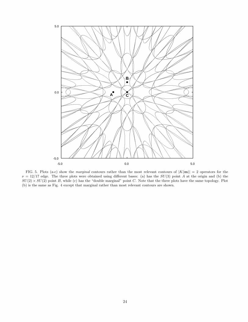
0.0

-5.0

5.0

-5.0 0.0 5.0

B

CA

FIG. 5. Plots (a-c) show the marginal contours rather than the most relevant contours of |K(m)| = 2 operators for theν = 12/17 edge. The three plots were obtained using different bases: (a) has the SU(3) point A at the origin and (b) theSU(2) × SU(2) point B, while (c) has the “double marginal” point C. Note that the three plots have the same topology. Plot(b) is the same as Fig. 4 except that marginal rather than most relevant contours are shown.

24

(-1.0,0.0)

(0.0,1.0)

(0.0,-1.0)

(1.0,0.0)

A

B

C

FIG. 6. The most relevant contours of |K(m)| = 2 operators on the charge-unmixed plane of the ν = 12/17 edge as functionsof “velocity” coordinates (v1, v2). Plot is the same as Fig. 4 except that contours are shown as functions of “velocities” ratherthan “momenta”. Only the 42 most relevant operators at the origin are shown because the full diagram becomes infinitelydense at the edge of the circle.

25

TABLE I. Possible nonchiral edge types for dim K ≤ 4. For dim K = 5 there are no principalhierarchy states and for dim K > 5 no states at all which are T -stable and have neutral modes inboth directions.

dim K Mode directions Example Boost parameters Boost parameters with(charge always →) charge mode unmixed

2 1→1← ν = 2/3 1 0

3 2→1← ν = 5/3 2 1

1→2← ν = 3/5 2 0

4 3→1← ν = 12/31 3 2

2→2← ν = 12/17 4 2

1→3→ ν = 4/7 3 0

26

TABLE II. Low-temperature tunneling conductance behavior G ∼ T α for hierarchical daughterstates of ν = 1 (top) and ν = 1/3. Only “charge-unmixed” phases (those with quantized conduc-tance, or alternately those which can occur with long-range interactions) are shown. The differentfixed points A and B for the Fibonacci-type states correspond to the labeling in Fig. 2. The phasesν = 12/7, 12/17, 12/31, 12/41 have fixed lines L and three types of fixed point with SU(2)×SU(2)symmetry (abbreviated SU(2) in the table), SU(3) symmetry, or two independent marginal opera-tors (DM). The tunneling exponent on the fixed lines L is nonuniversal. Note that each exponentin the lower table is given by α1/3 = 4+α1 where α1 is the exponent of the state in the upper tableat the same position in the hierarchy. The pattern continues to lower filling fractions: daughterstates of ν = 1/5 have filling fractions between 1/8 < ν < 1/4 and tunneling exponents 8 ≤ α ≤ 12,e.g.

· · · ν = n G ∼ T 0

ν = 3, G ∼ T 0 G ∼ T 0 DM

ν = 2, G ∼ T 0 ν = 12/7 G ∼ T 1/3 SU(2)

ν = 5/3, G ∼ T 0

T 2/5

BA G ∼ T 1 SU(3)

G ∼ Tα Lν = 1, G ∼ T 0

ν = 5/7, G ∼ T 8/5

T 2

BA G ∼ T 5/3 DM

ν = 2/3, G ∼ T 2 ν = 12/17 G ∼ T 2 SU(2)

ν = 3/5, G ∼ T 8/3 G ∼ T 8/3 SU(3)G ∼ Tα L

· · · ν = n2n−1 G ∼ T 4−4/n

· · · ν = n2n+1 G ∼ T 4

ν = 3/7, G ∼ T 4 G ∼ T 4 DM

ν = 2/5, G ∼ T 4 ν = 12/31 G ∼ T 13/3 SU(2)

ν = 5/13, G ∼ T 4

T 22/5

BA G ∼ T 5 SU(3)

G ∼ Tα Lν = 1/3, G ∼ T 4

ν = 5/17, G ∼ T 28/5

T 6

BA G ∼ T 17/3 DM

ν = 2/7, G ∼ T 6 ν = 12/41 G ∼ T 6 SU(2)

ν = 3/11, G ∼ T 20/3 G ∼ T 20/3 SU(3)G ∼ Tα L

· · · ν = n4n−1 G ∼ T 8−4/n

27