Quantum simulation of high-energy physics with ultracold atoms
199
Dissertation submitted to the Combined Faculty of Natural Sciences and Mathematics of Heidelberg University, Germany for the degree of Doctor of Natural Sciences Put forward by Torsten Victor Zache born in: Berlin Oral examination: June 17, 2020
-
Upload
khangminh22 -
Category
Documents
-
view
0 -
download
0
Transcript of Quantum simulation of high-energy physics with ultracold atoms

Dissertation
submitted to the
Combined Faculty of Natural Sciences and Mathematics
of Heidelberg University, Germany
for the degree of
Doctor of Natural Sciences
Put forward by
Torsten Victor Zache
born in: Berlin
Oral examination: June 17, 2020


Quantum simulation of high-energy physics with ultracold atoms
Referees: Prof. Dr. Jürgen BergesPriv.-Doz. Dr. Martin Gärttner

HEIDELBERG UNIVERSITY
DOCTORAL THESIS
Quantum simulation of high-energyphysics with ultracold atoms
Author: Torsten Victor Zache Supervisor: Prof. Dr. Jürgen Berges
Dissertation
submitted to the
Combined Faculty of Natural Sciences and Mathematics
of Heidelberg University, Germany
for the degree of
Doctor of Natural Sciences
April 4, 2020

ii
“And I’m not happy with all the analyses that go withjust the classical theory, because nature isn’t classical,dammit, and if you want to make a simulation of na-ture, you’d better make it quantum mechanical, and bygolly it’s a wonderful problem, because it doesn’t lookso easy.”
R. P. Feynman [1]
iii
Zusammenfassung
Quantensimulation der Hochenergiephysik mit ultrakalten Atomen
Die Vorhersage der Quantendynamik von geladener Materie, die mit dynamischenEichfeldern interagiert, ist eine außerordentliche Herausforderung in der theoreti-schen Physik. In Ermangelung einer allgemein anwendbaren Berechnungsmethodebieten Quantensimulatoren eine vielversprechende Alternative.Die vorliegende Arbeit leistet einen Beitrag zur Quantensimulation der Hochener-giephysik, wobei wir uns auf die Plattform ultrakalter Atome konzentrieren. MittelsWilson-Fermionen schlagen wir vor die Implementierung von Gittereichtheorienbasierend auf Gemischen kalter Atome in einem optischen Gitter zu verbessern.Numerische Simulationen zeigen, dass dies die Realisierung der Schwinger-Paar-Produktion mit aktueller Technologie möglich macht. Unsere vorgeschlagene Im-plementierung ist modular und ein elementarer Baustein wird experimentell de-monstriert. Darüber hinaus identifizieren wir dynamische topologische Übergänge,die wir im massiven Schwinger-Modell entdeckt haben, als geeignetes Ziel für dieAnwendung von Quantensimulatoren. Durch die Definition eines eichinvariantenOrdnungsparameter können wir zeigen, dass diese Übergänge jenseits schwacherWechselwirkungen bestehen bleiben.Im zweiten Teil dieser Arbeit entwickeln wir einen Formalismus für die Analysevon Quantensimulatoren mittels experimentell zugänglicher irreduzibler Korrelati-onsfunktionen zu gleichen Zeiten. Wir verifizieren diesen Ansatz numerisch für dasSine-Gordon-Modell im thermischen Gleichgewicht, das durch zwei tunnelgekop-pelte Superfluide quantensimuliert wird. Schließlich wenden wir unsere Analyseauf die Nichtgleichgewichtsdynamik eines Spinor-Bose-Gases an und finden eineunterdrückte effektive Wechselwirkung in einem stark korrelierten Infrarotbereich.


v
Abstract
Quantum simulation of high-energy physics with ultracold atoms
Predicting the quantum dynamics of charged matter interacting with dynamicalgauge fields poses an outstanding challenge in theoretical physics. Lacking a gen-erally applicable computational method, quantum simulators offer a promisingalternative.In this thesis, we contribute to the quantum simulation of high-energy physics,focusing on the platform of ultracold atoms. Using Wilson fermions, we propose toimprove implementations of lattice gauge theories based on mixtures of cold atomsin optical lattices. Numerical benchmarks indicate that this makes the realization ofSchwinger pair production feasible with current technology. Our proposal is modu-lar and an elementary building is demonstrated experimentally. We further identifydynamical topological transitions, which we discovered in the massive Schwingermodel, as a suitable target for quantum simulators. Defining a gauge-invariantorder parameter, these transitions are shown to persist beyond weak coupling.In the second part of this thesis, we develop a framework for analyzing quantumsimulators in terms of experimentally accessible irreducible correlation functionsat equal times. We verify this approach numerically for the sine-Gordon modelin thermal equilibrium, quantum simulated by two tunnel-coupled superfluids.Finally, we apply our analysis to the non-equilibrium dynamics of a spinor Bose gas,revealing suppressed effective interactions in a strongly-correlated infrared regime.


vii
AcknowledgmentsFirst of all, I want to express my gratitude towards my supervisor Jürgen Berges
for his guidance through my doctoral studies. Our discussions shaped my viewon physics in general and his support enabled the success of my projects. Second,I thank Philipp Hauke, whose time in Heidelberg luckily fell into the years of mydoctoral studies. I profited a lot from his open-mindedness in discussions, wheremany new ideas were generated. Further, I am indebted to Fred Jendrzejewski, JörgSchmiedmayer and Markus Oberthaler for exciting collaborations on their amazingexperiments, which were of paramount importance for my work. I also want to takethis opportunity to thank the administration at our institute, in particular Tina Kuka.The relevance of their work for the ITP can not be underestimated.
Thanks to all the past and present members of our research group: ValentinKasper for his mentoring during my time as a master student, Asier Piñeiro Oriolifor listening to crazy Friday’s ideas, Niklas Müller for not taking things too seriouslyand Aleksas Mazeliauskas for always bringing in new ideas. Oscar Garcia-Monterofor providing the most enjoyable coffee and the experience of sharing an office forwhat felt like a life-time, Robert Ott for endless discussions and coffee breaks, LindaShen for perfecting the construction of doctoral hats, Aleksandr Chatrchyan forbeing humorously himself and Alexander Lehmann for being honest. Also KirillBoguslavski, Alexander Schuckert, Roland Walz, Daniel Spitz, Malo Tarpin, MichaelHeinrich, Gregor Fauth, Ignacio Aliaga Sirvent, Jan Schneider, Erekle Arshilava,Lasse Gresista, Daniel Kirchhoff, Frederick del Pozo, Dustin Peschke and everyoneelse for making the time in Phil’weg 12 so enjoyable. I am also very thankful for mypart-time membership of SynQS, whose members treated me as one of their own. Asecond desk in the NaLi office was extremely valuable for our collaborations andI specifically thank Alexander Mil, also for the walrus. Thanks to Sebastian Erneand Thomas Schweigler for a great collaboration, and to the whole Vienna group fortheir hospitality. Special thanks to Maximilian Prüfer, for maintaining our friendshipthrough weekly physics lunches that turned into great research.
In the life beyond physics, there could not be better friends than Florian Andreas,Jens Puschhof and Micha Wijesingha and I am looking forward to extend ourtraditions forever. I further want to thank Raissa Meurer and Franz Liewald for everysingle board game evening and a fun festival, David Becker-Koch for the sharedattempt to learn the Russian language and Fabian Krajewski for Doppelkopflersbootcamp and the advice when my motorbike got lost.
Finally, I am grateful for my family, in particular my parents who supported mein every decision of my life leading to the person I am today, and Lars for being thebest brother I can imagine. And Isabella, for everything else.
Thanks again to Linda, Max, Robert, David, Jürgen and Isa for valuable com-ments and proof-reading parts of this thesis.


ix
Contents
Zusammenfassung iii
Abstract v
Acknowledgments vii
1 Introduction 11.1 Motivation . . . . . . . . . . . . . . . . . . . . . . . . . . . . . . . . . . 11.2 Key concepts . . . . . . . . . . . . . . . . . . . . . . . . . . . . . . . . . 21.3 Overview . . . . . . . . . . . . . . . . . . . . . . . . . . . . . . . . . . . 5
I Quantum simulation of gauge theories 9
2 Implementation of lattice gauge theories with Wilson fermions 112.1 Introduction . . . . . . . . . . . . . . . . . . . . . . . . . . . . . . . . . 112.2 Wilson fermions . . . . . . . . . . . . . . . . . . . . . . . . . . . . . . . 132.3 Cold-atom QED . . . . . . . . . . . . . . . . . . . . . . . . . . . . . . . 192.4 Details of the experimental implementation . . . . . . . . . . . . . . 252.5 Choice of experimental parameters . . . . . . . . . . . . . . . . . . . . 312.6 Benchmark: Onset of Schwinger pair production . . . . . . . . . . . . 342.7 Details of the numerical simulation . . . . . . . . . . . . . . . . . . . . 392.8 Summary . . . . . . . . . . . . . . . . . . . . . . . . . . . . . . . . . . . 45
2.A The Wannier-Stark system . . . . . . . . . . . . . . . . . . . . . . . . . 472.B Derivation of the Landau-Zener formula . . . . . . . . . . . . . . . . . 51
3 Realization of a scalable building block for U(1) gauge theories 553.1 Proposed implementation . . . . . . . . . . . . . . . . . . . . . . . . . 553.2 Experimental realization of the building block . . . . . . . . . . . . . 583.3 Effective description of the building block dynamics . . . . . . . . . . 613.4 Summary . . . . . . . . . . . . . . . . . . . . . . . . . . . . . . . . . . . 64
3.A Experimental details . . . . . . . . . . . . . . . . . . . . . . . . . . . . 653.B Details of the implementation . . . . . . . . . . . . . . . . . . . . . . . 663.C Numerical simulation of the trapped mixture . . . . . . . . . . . . . . 713.D Spin-changing collisions as an anharmonic oscillator . . . . . . . . . . 77

x
4 Dynamical topological transitions in the massive Schwinger model 814.1 Motivation and setup . . . . . . . . . . . . . . . . . . . . . . . . . . . . 814.2 Non-interacting limit . . . . . . . . . . . . . . . . . . . . . . . . . . . . 834.3 Towards strong coupling . . . . . . . . . . . . . . . . . . . . . . . . . . 864.4 Summary . . . . . . . . . . . . . . . . . . . . . . . . . . . . . . . . . . . 90
4.A Free fermion calculations . . . . . . . . . . . . . . . . . . . . . . . . . . 914.B Solving Gauss’ law on a ring . . . . . . . . . . . . . . . . . . . . . . . . 95
II Analyzing quantum simulators with quantum field theory 101
5 Extraction of the instantaneous effective action in equilibrium 1035.1 Introduction . . . . . . . . . . . . . . . . . . . . . . . . . . . . . . . . . 1035.2 Extracting the irreducible vertices from equal-time correlations . . . 1055.3 Example: Sine-Gordon model . . . . . . . . . . . . . . . . . . . . . . . 1145.4 Experimental results: Proof of principle . . . . . . . . . . . . . . . . . 1205.5 Summary . . . . . . . . . . . . . . . . . . . . . . . . . . . . . . . . . . . 124
5.A Technical details . . . . . . . . . . . . . . . . . . . . . . . . . . . . . . . 1265.B Quantum thermal equilibrium . . . . . . . . . . . . . . . . . . . . . . 135
6 Extraction of the instantaneous effective action out of equilibrium 1396.1 Introduction . . . . . . . . . . . . . . . . . . . . . . . . . . . . . . . . . 1396.2 Extraction of the effective action . . . . . . . . . . . . . . . . . . . . . 1406.3 Momentum and time dependence . . . . . . . . . . . . . . . . . . . . 1436.4 Summary . . . . . . . . . . . . . . . . . . . . . . . . . . . . . . . . . . . 145
6.A Experimental details . . . . . . . . . . . . . . . . . . . . . . . . . . . . 1476.B Data analysis of correlation functions . . . . . . . . . . . . . . . . . . 1486.C Quantum field dynamics with equal-time correlations . . . . . . . . . 149
7 Conclusion 1597.1 Discussion . . . . . . . . . . . . . . . . . . . . . . . . . . . . . . . . . . 1597.2 Outlook . . . . . . . . . . . . . . . . . . . . . . . . . . . . . . . . . . . . 160
Declaration of authorship and publications 163
Bibliography 165
xi
List of figures and tables
2.1 Sketch of the proposed implementation of lattice QED in one spatialdimension . . . . . . . . . . . . . . . . . . . . . . . . . . . . . . . . . . 12
2.2 Comparison of the continuum and lattice dispersion relations . . . . 142.3 Sketch of a cold-atom implementation of lattice fermions in one spa-
tial dimension . . . . . . . . . . . . . . . . . . . . . . . . . . . . . . . . 162.4 Sketch of the proposed implementation based on Wilson fermions . . 212.5 The limiting time-scales . . . . . . . . . . . . . . . . . . . . . . . . . . 332.6 Dimensionless parameters entering the lattice QED simulation . . . . 332.7 Benchmarking simulations . . . . . . . . . . . . . . . . . . . . . . . . . 372.8 Particle-production rate . . . . . . . . . . . . . . . . . . . . . . . . . . 382.9 Benchmarking simulations for the second parameter set . . . . . . . . 432.10 Fits of the particle production rate . . . . . . . . . . . . . . . . . . . . 432.11 Mass-quenched simulation . . . . . . . . . . . . . . . . . . . . . . . . 45
3.1 Engineering a gauge theory . . . . . . . . . . . . . . . . . . . . . . . . 563.2 Tunability of the initial conditions . . . . . . . . . . . . . . . . . . . . 593.3 Dynamics of particle production . . . . . . . . . . . . . . . . . . . . . 603.4 Resonant particle production . . . . . . . . . . . . . . . . . . . . . . . 623.5 Integrated two-dimensional density profiles of the two-species BEC . 733.6 Integrated one-dimensional density profiles of the two-species BEC . 743.7 Illustration of a single GPE simulation with experimental imperfections 753.8 Particle production dynamics from averaged GPE simulations . . . . 763.9 Resonance shape . . . . . . . . . . . . . . . . . . . . . . . . . . . . . . 783.10 Asymmetry of the resonance and the anharmonic potential . . . . . . 79
4.1 Phase of the time-ordered correlator . . . . . . . . . . . . . . . . . . . 834.2 Dynamical topological transitions at vanishing gauge coupling . . . 844.3 Dynamical topological transitions beyond weak coupling . . . . . . . 864.4 Finite-size dependence of the critical times . . . . . . . . . . . . . . . 89
5.1 Feynman diagrams relating full and connected correlation functions 1095.2 Feynman diagrams relating connected and 1PI correlation functions 1115.3 1PI vertices in the weak coupling regime . . . . . . . . . . . . . . . . 1165.4 Loop corrections to the 1PI two-point function . . . . . . . . . . . . . 1175.5 Loop corrections to the 1PI four-vertex . . . . . . . . . . . . . . . . . . 1185.6 1PI four-vertex as a function of Q . . . . . . . . . . . . . . . . . . . . . 119

xii
5.7 Schematics of the experimental setup . . . . . . . . . . . . . . . . . . . 1205.8 Cosine transformed second-order connected correlation function . . 1215.9 Experimental 1PI two-point function . . . . . . . . . . . . . . . . . . . 1225.10 Experimental four-vertex . . . . . . . . . . . . . . . . . . . . . . . . . . 1235.11 Running coupling . . . . . . . . . . . . . . . . . . . . . . . . . . . . . . 1255.12 The different generating functionals . . . . . . . . . . . . . . . . . . . 126
6.1 Experimental platform and extraction of correlation functions . . . . 1416.2 Statistical significance of the four-point 1PI correlator in momentum
space . . . . . . . . . . . . . . . . . . . . . . . . . . . . . . . . . . . . . 1426.3 Momentum conserving diagonals of the 1PI correlators . . . . . . . . 1446.4 Observation of scaling in time of the distribution function and the
four-vertex . . . . . . . . . . . . . . . . . . . . . . . . . . . . . . . . . . 1466.5 Number of experimental realizations . . . . . . . . . . . . . . . . . . . 148

xiii
List of abbreviations
BCH Baker-Campbell-HausdorffBEC Bose-Einstein CondensateCP Charge conjugation (and) ParityDQPT Dynamical Quantum Phase TransitionED Exact DiagonalizationGPE Gross-Pitaevskii EquationHEP High-Energy PhysicsIR InfraRedLGT Lattice Gauge TheoryLZ Landau Zener1PI One(1)-Particle Irreducible(P)BC (Periodic) Boundary CondtionsPDE Partial Differential EquationQCD Quantum ChromoDynamicsQED Quantum ElectroDynamicsQFT Quantum Field TheorySCC Spin-Changing CollisionsSG Sine-GordonTF Thomas-FermiUV UltraVioletWS Wannier-Stark

1
Chapter 1
Introduction
1.1 Motivation
Since quantum computers were first envisioned in the early 1980’s [1, 2] the mi-croscopic control of quantum systems has reached an unprecedented level. Thisprogress paved the way for the fast-growing field of quantum simulation [3, 4].By quantum simulation we understand the controlled manipulation of a physicalquantum system with the purpose of emulating another quantum system [4]. Whilequantum simulators found their first application in condensed matter physics [5, 6],the interest in quantum simulations of high-energy physics (HEP) started growingin the last decade [7–9]. Physical phenomena arising in this context include fermionpair production [10] or string breaking [11], both occurring in the real-time dynamicsof gauge theories such as quantum electrodynamics (QED) or quantum chromody-namics (QCD). Difficulties in simulating the quantum dynamics of these theoriesmotivate the use of quantum devices, which promise to overcome the limitations ofclassical computational resources [3, 12]. In recent years, several theoretical propos-als have been put forward, resulting in the first experimental realizations [13–16] ofquantum simulators for simple small-scale model systems motivated by HEP.
Along the way towards the long-time goal of quantum simulating QCD [17],a number of open problems need to be resolved. The first theoretical task in anyquantum simulation is the identification of an appropriate experimental platform,together with a mapping of the target model onto the experimental system. Inthis context, the improvement and extension of existing proposals to higher spatialdimensions and non-abelian gauge groups (see [7–10, 18–30] and references therein),while retaining experimental feasibility together with the possibility to reach largesystem sizes [31], is the key challenge. At the same time, it is necessary to identifyrelevant physical scenarios [32, 33] that can be addressed by a quantum simulator,taking into account experimental limitations and imperfections. Related questionsare how to verify a quantum simulation [34, 35], and in particular, to what extentdoes the simulator respect gauge invariance [36, 37]? These questions lead tothe read-out of quantum simulators in general. What observables are accessibleand how to sort the relevant information [38, 39]? This thesis presents our recentcontributions towards resolving these open questions. Specifically, we address the
2 Chapter 1. Introduction
quantum simulation of U(1) gauge theories and the analysis of quantum simulatorsfrom a quantum field theory perspective.
1.2 Key concepts
The quantum simulation of HEP is an interdisciplinary field of research, bringingtogether different disciplines within physics. In order to bridge this gap, we givea brief introduction into key concepts relevant for this thesis: quantum simulation,quantum field theory, and gauge theories.
1.2.1 Quantum simulation
In a digital quantum computation, described by the circuit model [40], one encodesinformation in the quantum state of a collection of quantum bits (qubits) as asuperposition of binary bit strings. An arbitrary unitary transformation of this statemay then be realized in terms of elementary operations (universal quantum gates)acting on a few qubits. While it is indeed possible to simulate any local quantumsystem in this way [41], digital quantum simulators are not the main topic of thiswork.
Instead, we focus on analog quantum simulators. The basic idea of an analogquantum simulation is to engineer a synthetic quantum system in a highly controlledfashion in order to emulate the physics of a target model. This approach is usuallyformulated in the Hamiltonian picture as follows [4]. The task is to control anexperimental system described by Hsim such that its Hamiltonian can be directlymapped to a desired model Htarget,
Htarget ↔ Hsim . (1.1)
Ideally, Eq. (1.1) should be understood as a one-to-one map1 that identifies suitabledegrees of freedom, Hilbert spaces, and the structure of the Hamiltonians on bothsides. In this way, the experimental system describes the same physical content as thetarget model. In practice, the mapping (1.1) between target model and simulator isof course not exact, but relies on approximations. Nevertheless, an analog quantumsimulation can provide important qualitative or even quantitative predictions [34].
The potential of quantum simulators is based on the structure of quantum many-body systems. In general, the Hilbert space dimension grows exponentially withthe number of degrees of freedom. This fact impedes solutions using an exact diago-nalization of the Hamiltonian for large systems, for instance in the thermodynamiclimit. Sometimes this curse of dimensionality can be circumvented by quantumMonte-Carlo methods [42, 43] that solve the quantum many-body problem by effi-cient sampling from a statistical ensemble. However, these statistical approaches
1Crucially, only relative (energy) scales matter for this mapping such that the huge difference inabsolute scales between, e.g., a high-energy collision and an ultracold atom experiment is unimportant.

1.2. Key concepts 3
can break down due to so-called sign problems [44, 45], which can occur for instancein the presence of fermions or in real-time dynamics. Quantum simulators, beingintrinsically of quantum nature, are a priori free of these complications and thusoffer a promising alternative [3].
The platforms employed for quantum simulations range from arrays of trappedions [46] over photons [47] and superconducting circuits [48] to ultracold atomicgases [49]. The choice of platform depends on the desired target model and thedetails of its implementation. In this thesis, we focus on quantum simulations basedon ultracold atoms.
1.2.2 Quantum field theory
Quantum field theory (QFT) describes quantum many-body systems in the limit ofinfinitely many degrees of freedom. The most profound difference between (few-body) quantum mechanics and QFT is the concept of renormalization. In a genericQFT, quantum fluctuations introduce a dependence of coupling parameters g on theenergy scale µ at which the system is observed. This scale-dependence is describedwithin the renormalization group by beta-functions [50],
β(g) =dg
d log µ. (1.2)
If β(g) > 0, the coupling increases with increasing energy scale. Conversely, itdecreases with decreasing energy scale and therefore does not affect the low-energyphysics. Consequently, the coupling is called irrelevant. The situation is reversedfor β(g) < 0 and the coupling is called relevant.
Due to this behavior, the renormalization group provides the modern interpreta-tion of QFT: A (renormalizable) QFT is determined by a finite number of relevantcouplings (and the corresponding terms in the action or Hamiltonian) whose valuesat a given energy scale have to be fixed by an experimental measurement. At thesame time, QFT can be seen as a low-energy effective theory which describes theuniversal long-distance behavior (determined by the relevant couplings) that isindependent of the microscopic details (the irrelevant couplings) [51].
The observables of QFT are correlation functions C(n)(x1, . . . , xn), i.e., quantumexpectation values of field operators at different points x1, . . . , xn in space-time. Theway in which these correlators change at large distances between points encodesthe scale-dependence of the QFT. Thus, by measuring correlation functions in aquantum simulator, it is in principle possible to access this information and toidentify the relevant couplings.
For numerical calculations2, a QFT can be formulated by specifying an action Swith coupling parameters g on a space-time lattice with finite spacing a. Formally, aprovides an ultraviolet (UV) regulator and sets the energy scale µ ∼ 1/a at which
2In fact, this is more than a practicality: The lattice approach provides a definition of QFTs beyondperturbation theory.
4 Chapter 1. Introduction
S with its parameters g is defined. One then calculates correlators according to afunctional integral with a weight determined by S. Finally, one has to reduce awhilekeeping certain values of (renormalized) correlators fixed, such as a physical massm [52]. The existence of a continuum limit with finite m means that it is possible toapproach the limit a→ 0 with fixed m by appropriately adjusting the parameters gaccording to β(g). In this limit, the correlation length ξ = (ma)−1, which controls theexponential decay of the correlator C(2)(x, 0) ∼ e−|x|/ξ at large distances, diverges.In practice, this allows to extract the physical behavior at small but finite a from asuitable scaling analysis [52].
Throughout this thesis, we employ a Hamiltonian formulation of QFT. Whilethis choice is less common in the HEP context, it is most convenient for quantumsimulations because we aim to identify an experimental setup with a target modelaccording to Eq. (1.1). Within this approach, it is also useful to employ a Hamiltonianlattice regularization where space is discretized but time is kept continuous.
1.2.3 Gauge theories
The concept of symmetries is ubiquitous in theoretical physics. It describes thatcertain aspects of a physical model are preserved under transformations described bya corresponding symmetry group. Most prominent examples include the invarianceof the laws of classical mechanics under spatial translations and rotations. Theseglobal symmetries imply, via Noether’s theorem [53], the conservation of linear andangular momentum.
A symmetry is called local if the corresponding transformation can act differentlyat every point in space-time. Loosely speaking, gauge theories are physical modelswith such local symmetries. More precisely, a gauge theory can be defined as afield theory whose action is gauge invariant, i.e., it remains unchanged under localtransformations specified the gauge group [50]. Among the simplest examplesare U(1) gauge theories, such as QED. Here, a global U(1) symmetry implies theconservation of an associated charge Q. Gauge invariance further ties local changesof this charge to the surrounding gauge fields. For example, in electrodynamics theelectric charge density ρ and the corresponding current j are coupled to electric E
and magnetic fields B according to Maxwell’s equations [54].The framework of lattice gauge theories (LGT) implements the lattice formulation
of QFT while retaining gauge invariance exactly [52, 55]. This formulation providesa non-perturbative definition of quantum gauge field theories and has proven tobe invaluable for numerical simulations. It is also perfectly suited for quantumsimulators as discussed in this thesis.
In the Hamiltonian formulation of LGTs [56], gauge invariance implies an exten-sive3 number of conserved quantities described by operators Gn that commute with
3Here we mean extensive in the thermodynamic sense: There exist constraints at every lattice pointn and thus the number of constraints increases linearly with the system size.
1.3. Overview 5
the Hamiltonian H ,
[Gn, H] = 0 . (1.3)
Additionally, the allowed states |phys〉 are restricted to be eigenstates of Gn. Theseconstraints make a prediction of the resulting dynamics extremely challenging.
1.3 Overview
In this work, we specifically address the quantum simulation of gauge theories andthe analysis of quantum simulators from a QFT perspective. Accordingly, this thesisis structured in two parts. In the remainder of this introduction, we give a briefoverview over our contributions to the quantum simulation of HEP.
1.3.1 Quantum simulation of gauge theories
The main target model of part I is QED in one spatial dimension, also known as themassive Schwinger model. This model is one of the simplest theories to describecharged matter interacting with gauge fields, here electrons and positrons interactingwith an electric field. Sharing certain features with QCD, the massive Schwingermodel has proven to be a valuable toy model for HEP [57].
Implementation of lattice gauge theories with Wilson fermions. In chapter 2, wedescribe a detailed proposal [29] to implement the massive Schwinger model with amixture of ultracold bosons and fermions trapped in an optical lattice potential. Here,two hyperfine states of the bosonic and fermionic species are used to implement thegauge and matter fields, respectively. Following earlier proposals [10, 18], we realizethe gauge-invariant interaction with hetero-nuclear collisions that exchange angularmomentum between the two species. Crucially, these spin-changing collisions (SCC)conserve the global magnetization, which – by careful engineering of the trappedmixture – is turned into a local symmetry that furnishes the required U(1) gaugeinvariance of QED.
In contrast to earlier proposals, we exploit the possibility to use different latticeformulations leading to the same continuum theory to improve our setup by usingWilson fermions. With numerical benchmark simulations, we show that an opti-mized set of experimental parameters allows to observe the process of Schwingerpair production, i.e., the creation of electron-positron pairs from the fermionic vac-uum due to a strong electric field. In particular, we show that the non-perturbativenature of this effect can be extracted quantitatively from a quantum simulation withcurrently available technology.
Realization of a scalable building bock for U(1) gauge theories. The followingchapter 3 extends our proposal by giving up the direct correspondence between

6 Chapter 1. Introduction
the lattice sites of the target model and the lattice wells of the simulator. In thisway, the gauge-invariant interaction is isolated in an elementary building block,which simplifies the experimental realization. An extended U(1) gauge theory canbe realized by connecting multiple building blocks via laser-assisted tunneling,demonstrating the potential scalability of our approach.
We further describe our recent experiment [16] that realizes a single buildingblock with bosonic instead of fermionic matter. The faithful representation of thisminimal U(1) gauge theory and its full tunability is demonstrated experimentally,which we verify by comparison to numerical simulations of the target model includ-ing experimental imperfections.
Dynamical topological transitions in the massive Schwinger model. The firstpart closes with chapter 4, which focuses on an extension of the massive Schwingermodel that includes a so-called topological θ-term. This term originates in thevacuum structure of the theory and analogous terms also appear for other gaugetheories, in particular QCD in three spatial dimensions. In both cases, the topolog-ical term breaks combined charge conjugation and parity (CP) symmetry, i.e., theinvariance of the model under a simultaneous reflection of space and the exchangeof positively and negatively charged excitations. Experimental observations indicatethat QCD conserves CP [58], which implies the absence of a θ-term. This puzzle hasbeen coined the strong CP problem. Its most common resolution [59] involves anadditional hypothetical field (the axion) that leads to a dynamical relaxation of theθ-term.
Motivated by this solution to the strong CP problem, we study the dynamicsof the massive Schwinger model after a quench of its θ-term [33]. We discoverdynamical topological transitions, which are signaled by an order parameter thatwe construct from gauge-invariant time-ordered two-point correlation functionsof the matter fields. These transitions are related to dynamical quantum phasetransitions (DQPT), which have been observed previously in condensed matterlattice models [60]. Our results show that DQPTs also exist in the continuum limit.Moreover, our numerical simulations indicate that the transitions persist in thepresence of interactions. Furthermore, these transition can robustly be identifiedon small lattices due to their topological origin. Together with their occurrence onshort time-scales, the dynamical topological transitions constitute an ideal target forquantum simulations of QED.
1.3.2 Analyzing quantum simulators with quantum field theory
The focus of part II lies on the read-out of quantum simulators. We address thequestion of how to sort the information that can be extracted by measuring higher-order correlation functions. To this end, we apply the concept of one-particleirreducible (1PI) correlators [50], which constitute the building blocks of every QFT.

1.3. Overview 7
Extraction of the instantaneous effective action in equilibrium. In chapter 5, wefirst give a detailed review of the different types of correlation functions and theassociated generating functionals which occur in the construction of QFTs. In con-trast to the standard approach, we employ a formulation [61] based on correlationfunctions at equal times, which have become accessible in recent quantum simula-tion experiments [38]. We show that the measurement of equal-time 1PI correlators,which are generated by the instantaneous effective action, allows to extract themomentum-dependence of effective interaction vertices, thereby providing impor-tant information about the scale-dependence of the underlying QFT.
In thermal equilibrium, we test our approach [39] for the example of the Sine-Gordon model, a paradigmatic QFT in one spatial dimension. Numerical sim-ulations exhibit excellent agreement with qualitative and quantitative analyticalexpectations, which verifies our method. Additionally, the model is quantum sim-ulated by two tunnel-coupled superfluids in a proof-of-principle experiment thatconfirms the possibility to extract the field theory description of a quantum many-body system from experimental data.
Extraction of the instantaneous effective action out of equilibrium. The chapter6 extends the approach developed in the previous chapter and contains a firstapplication out of equilibrium. Here, the experimental platform is a spin-1 Bose gasthat has recently been employed to quantum simulate the physics of non-thermalfixed points [62]. The latter are characterized by a self-similar evolution of anemergent (particle number) distribution function in momentum and time. Thetheoretical description of non-thermal fixed points remains challenging as it requiresnon-perturbative methods due to strong correlations (large occupations) in theinfrared (IR) regime. Approximate kinetic descriptions [63, 64] suggest that thedynamics is driven by an effective momentum-dependent interaction vertex.
Our analysis [65] of the non-equilibrium dynamics in terms of equal-time 1PIcorrelators indeed reveals a similar qualitative behavior We find a strong suppressionof the 1PI four-vertex in a strongly-correlated IR regime. Additionally, the structureof this vertex indicates momentum conservation, which signals spatial translationinvariance of the quantum simulation. These results demonstrate the capabilities ofquantum simulators to provide input for improving QFT descriptions of challengingnon-equilibrium situations.
Conclusion. We discuss our results and their relevance for the quantum simulationof HEP in the concluding chapter 7. In the final section, we give an outlook forfuture research directions.
1.3.3 Statement of contribution
The five main chapters of this thesis are based on research articles [16, 29, 33, 39,65] that are either published or being considered in peer-reviewed journals. Since
8 Chapter 1. Introduction
modern physics is a collaborative research effort, I am not the single author of any ofthese articles. While none of the discussed experiments were carried out by myself,I performed most of the theoretical calculations. My personal contributions to thearticles [16, 29, 33, 39, 65] are clearly indicated in the beginning of the correspondingchapters where I list the contributions of all authors and mark the inclusion ofadditional material.
9
Part I
Quantum simulation of gaugetheories

11
Chapter 2
Implementation of lattice gaugetheories with Wilson fermions
This chapter is based on the article [29] with the figures and large parts of thetext taken from it. The improved implementation based on Wilson fermions wasdeveloped in discussions among all authors (F. Hebenstreit, F. Jendrzejewski, M.Oberthaler, J. Berges, P. Hauke and myself). While all authors participated in thewriting of the manuscript [29], I made significant contributions to the wording andstructuring of the text. The explicit calculations, i.e., the parameter estimates andthe numerical simulation, were performed by me. In the appendices 2.A and 2.B, Iinclude additional related material that was not printed in [29].
2.1 Introduction
Even though many proposals to quantum simulate gauge theories exist, there isyet no experimental realization capable of simulating relevant physical processes,such as Schwinger pair production of fermions and anti-fermions in the presence ofstrong electric fields [66, 67] or string breaking due to confinement [68–70]. Furtherprogress hinges crucially on efficient implementations, such that present state-of-the-art experimental resources become sufficient to achieve this goal. In viewof finding optimal implementations, the Nielsen-Ninomiya no-go-theorem [71]becomes particularly important: it states that it is not possible to discretize relativisticfermions while retaining the relevant symmetries of the continuum theory. Beingforced to make a choice between discretizations with different symmetry properties,one should be guided by the requirements of the task at hand, e.g, by conceptualadvantages, numerical efficiency, or – as discussed here – ease of experimentalimplementation. So far, however, most proposals for the engineering of quantumsimulators for lattice gauge theories employ one specific discretization procedurevia the so-called staggered fermion formulation [72].
In this chapter, we propose the use of an alternative discretization based on Wil-son fermions [73]. As discussed below, Wilson fermions have conceptual advantagesover staggered fermions when going to higher dimensions. Moreover, we showthat Wilson fermions can provide a very efficient framework for the experimental

12 Chapter 2. Implementation of lattice gauge theories with Wilson fermions
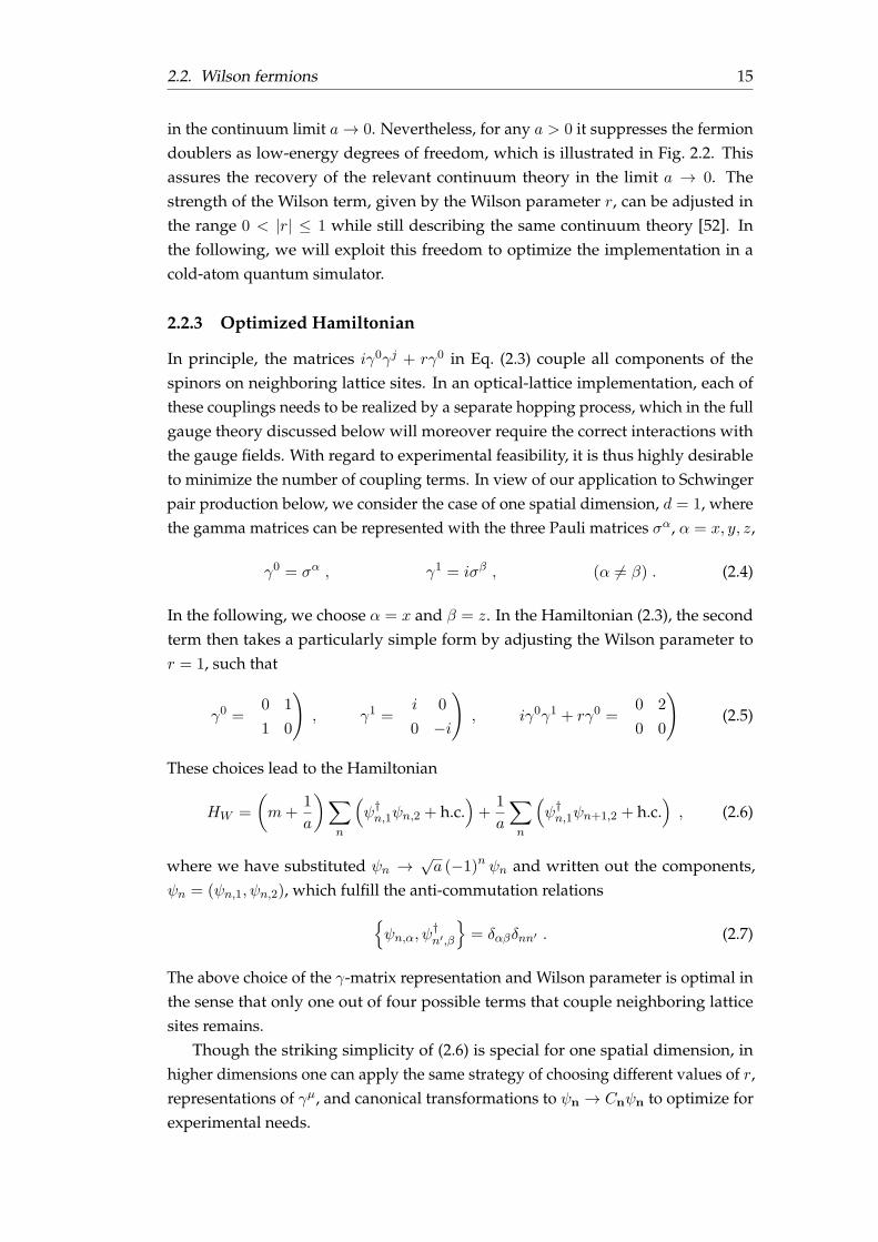
FIGURE 2.1: Sketch of the proposed implementation of lattice QED in onespatial dimension. Fermions trapped on the lattice sites (blue circles) arecoupled via a correlated interaction with the Bose condensates residing on thelinks (red ellipses). The zoom schematically shows how the gauge-invariantcoupling can be realized via spin-changing collisions between the fermions(blue) and bosons (orange) in a tilted optical lattice. This process involves twointernal states per species as indicated by the blue and red bars.
implementation of gauge theories using ultracold atoms in optical lattices. As anexample, we discuss QED in 1 + 1 space-time dimensions implemented with atwo-species mixture. Radiofrequency-dressed 6Li atoms act as the fermionic matter,while small condensates of bosonic 23Na atoms represent the dynamical gauge fields.Inter-species spin-changing collisions generate the dynamics of an interacting gaugetheory, where local gauge invariance is ensured by angular momentum and energyconservation, see Fig. 2.1. Strikingly, the use of Wilson fermions enables an imple-mentation through tilted optical lattices, instead of the more involved superlatticesemployed for staggered fermions [11]. We benchmark our proposal by a theoreticalanalysis, and show that the non-perturbative onset of Schwinger pair productionmay be observed in realistic experimental settings.
Wilson fermions have been considered previously in a cold-atom context for thequantum simulation of topological insulators [74–76]. In contrast, we are interestedhere in the full, interacting quantum theory with dynamical gauge fields.
This chapter is organized as follows. In Sec. 2.2, we present the lattice Hamilto-nian of Wilson fermions. We show that an optimal choice of parameters significantlysimplifies the resulting setup, and we compare it to the staggered-fermion formula-tion. In Sec. 2.3, we discuss how the theory is promoted to a gauge theory by theintroduction of dynamical gauge fields. Moreover, we reformulate the gauge theoryto match it with the degrees of freedom available in cold atomic gases and proposea possible implementation in a Bose-Fermi mixture in an optical lattice. We givean intuitive interpretation of various processes appearing in the proposed experi-mental setup, describe the envisioned experimental protocol, and discuss possible
2.2. Wilson fermions 13
limitations. Sections 2.4 and 2.5 give details on the experimental implementationand the choice of parameters, respectively. In Sec. 2.6, we benchmark the proposedexperiment with the example of the Schwinger mechanism. In particular, we showthat an experiment with realistic parameters may extract the rate of particle–anti-particle production. Details of the numerical simulation are discussed in Sec. 2.7.Section 2.8 presents our conclusions.
2.2 Wilson fermions
Before turning to dynamical gauge theories describing the Lorentz-invariant in-teraction of fermionic matter with gauge bosons, we momentarily drop the gaugedegrees of freedom for clarity. The non-interacting fermion part of the theory isdescribed in the continuum in d spatial dimensions by the Dirac Hamiltonian
HD =
ˆddxψ†(x)γ0
[iγj∂j +m
]ψ(x) , (2.1)
where ψ(x) is a fermionic Dirac spinor with 2d/2 components for d even and 2(d+1)/2
components for d odd. The γ0 and γj denote the gamma matrices in d+1 space-timedimensions [77] and ∂j is a partial derivative in the spatial direction j = 1, . . . , d.This Hamiltonian describes the kinetic energy and rest mass m of Dirac fermionsand leads to the dispersion relation of relativistic particles with energy
√m2 + p2.
2.2.1 The doubling problem
For simulations on classical computers as well as on quantum devices consisting ofsites in optical lattices or arrays of qubits, the continuum theory has to be discretizedon a lattice. In view of quantum simulation, we work here in the Hamiltonian latticeformalism, with spatial lattice spacing a and continuous real time t.
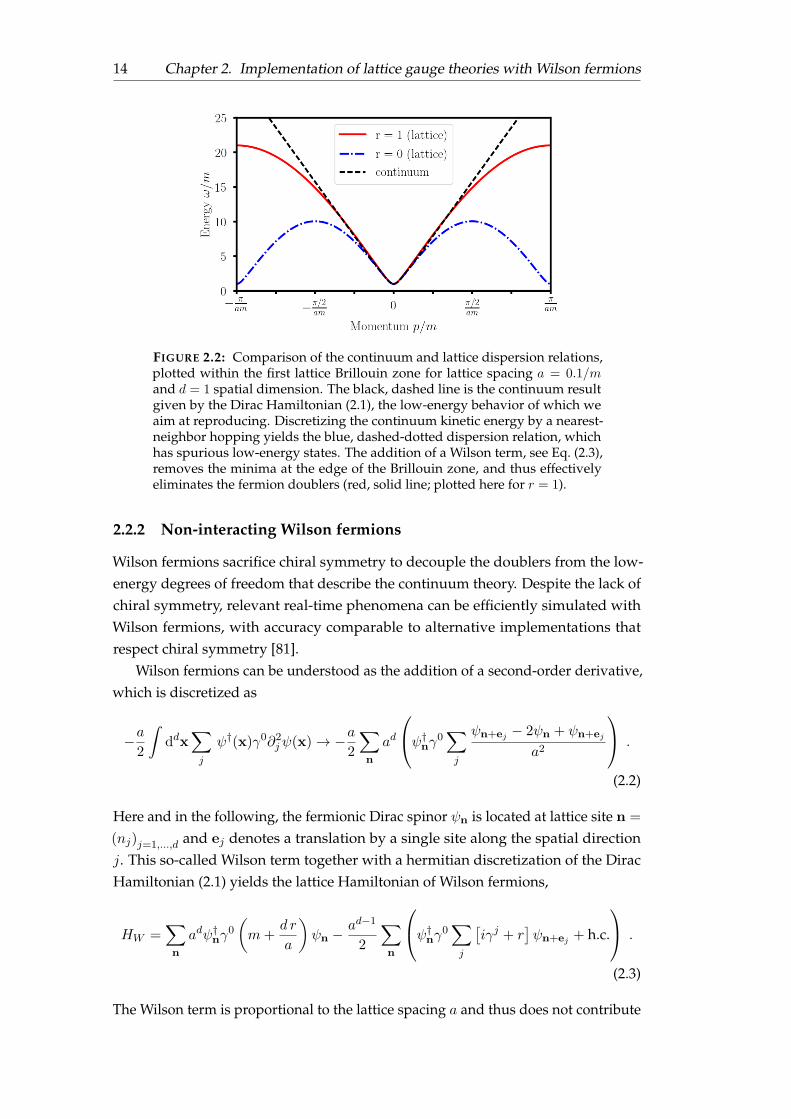
The simplest discretization of fermions replaces the kinetic energy in Eq. (2.1)with a nearest-neighbor hopping term. This naive procedure, however, leads to adiscretized model with an additional “doubling symmetry” [78]. Its physical conse-quence is the appearance of spurious states, where each fermion in the continuumtheory leads to 2d fermion species for d discretized dimensions, see Fig. 2.2. Theseadditional degrees of freedom affect the extrapolation to the continuum limit suchthat the correct continuum results are not recovered.
The Nielsen–Ninomiya no-go-theorem [71] implies that, in order to remove thesedoublers, one has to sacrifice at least one of several fundamental characteristics ofthe continuum derivative: hermiticity, locality, discrete translational symmetry orchiral symmetry. The choice which of these characteristics to sacrifice gives roomfor various strategies [79], with the staggered fermion [72] and Wilson fermion [80]prescriptions being among the ones most commonly known.
14 Chapter 2. Implementation of lattice gauge theories with Wilson fermions
FIGURE 2.2: Comparison of the continuum and lattice dispersion relations,plotted within the first lattice Brillouin zone for lattice spacing a = 0.1/mand d = 1 spatial dimension. The black, dashed line is the continuum resultgiven by the Dirac Hamiltonian (2.1), the low-energy behavior of which weaim at reproducing. Discretizing the continuum kinetic energy by a nearest-neighbor hopping yields the blue, dashed-dotted dispersion relation, whichhas spurious low-energy states. The addition of a Wilson term, see Eq. (2.3),removes the minima at the edge of the Brillouin zone, and thus effectivelyeliminates the fermion doublers (red, solid line; plotted here for r = 1).
2.2.2 Non-interacting Wilson fermions
Wilson fermions sacrifice chiral symmetry to decouple the doublers from the low-energy degrees of freedom that describe the continuum theory. Despite the lack ofchiral symmetry, relevant real-time phenomena can be efficiently simulated withWilson fermions, with accuracy comparable to alternative implementations thatrespect chiral symmetry [81].
Wilson fermions can be understood as the addition of a second-order derivative,which is discretized as
−a2
ˆddx
∑
j
ψ†(x)γ0∂2jψ(x)→ −a
2
∑
n
ad
ψ†nγ0
∑
j
ψn+ej − 2ψn + ψn+ej
a2
.
(2.2)
Here and in the following, the fermionic Dirac spinor ψn is located at lattice site n =
(nj)j=1,...,d and ej denotes a translation by a single site along the spatial directionj. This so-called Wilson term together with a hermitian discretization of the DiracHamiltonian (2.1) yields the lattice Hamiltonian of Wilson fermions,
HW =∑
n
adψ†nγ0
(m+
d r
a
)ψn −
ad−1
2
∑
n
ψ†nγ0
∑
j
[iγj + r
]ψn+ej + h.c.
.
(2.3)
The Wilson term is proportional to the lattice spacing a and thus does not contribute
2.2. Wilson fermions 15
in the continuum limit a→ 0. Nevertheless, for any a > 0 it suppresses the fermiondoublers as low-energy degrees of freedom, which is illustrated in Fig. 2.2. Thisassures the recovery of the relevant continuum theory in the limit a → 0. Thestrength of the Wilson term, given by the Wilson parameter r, can be adjusted inthe range 0 < |r| ≤ 1 while still describing the same continuum theory [52]. Inthe following, we will exploit this freedom to optimize the implementation in acold-atom quantum simulator.
2.2.3 Optimized Hamiltonian
In principle, the matrices iγ0γj + rγ0 in Eq. (2.3) couple all components of thespinors on neighboring lattice sites. In an optical-lattice implementation, each ofthese couplings needs to be realized by a separate hopping process, which in the fullgauge theory discussed below will moreover require the correct interactions withthe gauge fields. With regard to experimental feasibility, it is thus highly desirableto minimize the number of coupling terms. In view of our application to Schwingerpair production below, we consider the case of one spatial dimension, d = 1, wherethe gamma matrices can be represented with the three Pauli matrices σα, α = x, y, z,
γ0 = σα , γ1 = iσβ , (α 6= β) . (2.4)
In the following, we choose α = x and β = z. In the Hamiltonian (2.3), the secondterm then takes a particularly simple form by adjusting the Wilson parameter tor = 1, such that
γ0 =
(0 1
1 0
), γ1 =
(i 0
0 −i
), iγ0γ1 + rγ0 =
(0 2
0 0
)(2.5)
These choices lead to the Hamiltonian
HW =
(m+
1
a
)∑
n
(ψ†n,1ψn,2 + h.c.
)+
1
a
∑
n
(ψ†n,1ψn+1,2 + h.c.
), (2.6)
where we have substituted ψn →√a (−1)n ψn and written out the components,
ψn = (ψn,1, ψn,2), which fulfill the anti-commutation relations
ψn,α, ψ
†n′,β
= δαβδnn′ . (2.7)
The above choice of the γ-matrix representation and Wilson parameter is optimal inthe sense that only one out of four possible terms that couple neighboring latticesites remains.
Though the striking simplicity of (2.6) is special for one spatial dimension, inhigher dimensions one can apply the same strategy of choosing different values of r,representations of γµ, and canonical transformations to ψn → Cnψn to optimize forexperimental needs.
16 Chapter 2. Implementation of lattice gauge theories with Wilson fermions
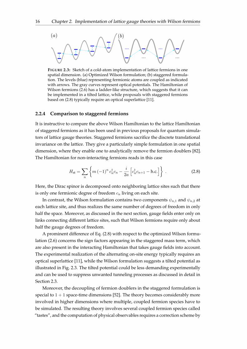
FIGURE 2.3: Sketch of a cold-atom implementation of lattice fermions in onespatial dimension. (a) Optimized Wilson formulation; (b) staggered formula-tion. The levels (blue) representing fermionic atoms are coupled as indicatedwith arrows. The gray curves represent optical potentials. The Hamiltonian ofWilson fermions (2.6) has a ladder-like structure, which suggests that it canbe implemented in a tilted lattice, while proposals with staggered fermionsbased on (2.8) typically require an optical superlattice [11].
2.2.4 Comparison to staggered fermions
It is instructive to compare the above Wilson Hamiltonian to the lattice Hamiltonianof staggered fermions as it has been used in previous proposals for quantum simula-tors of lattice gauge theories. Staggered fermions sacrifice the discrete translationalinvariance on the lattice. They give a particularly simple formulation in one spatialdimension, where they enable one to analytically remove the fermion doublers [82].The Hamiltonian for non-interacting fermions reads in this case
Hst =∑
n
m (−1)n c†ncn − i
2a
[c†ncn+1 − h.c.
]. (2.8)
Here, the Dirac spinor is decomposed onto neighboring lattice sites such that thereis only one fermionic degree of freedom cn living on each site.
In contrast, the Wilson formulation contains two components ψn,1 and ψn,2 ateach lattice site, and thus realizes the same number of degrees of freedom in onlyhalf the space. Moreover, as discussed in the next section, gauge fields enter only onlinks connecting different lattice sites, such that Wilson fermions require only abouthalf the gauge degrees of freedom.
A prominent difference of Eq. (2.8) with respect to the optimized Wilson formu-lation (2.6) concerns the sign factors appearing in the staggered mass term, whichare also present in the interacting Hamiltonian that takes gauge fields into account.The experimental realization of the alternating on-site energy typically requires anoptical superlattice [11], while the Wilson formulation suggests a tilted potential asillustrated in Fig. 2.3. The tilted potential could be less demanding experimentallyand can be used to suppress unwanted tunneling processes as discussed in detail inSection 2.3.
Moreover, the decoupling of fermion doublers in the staggered formulation isspecial to 1 + 1 space-time dimensions [52]. The theory becomes considerably moreinvolved in higher dimensions where multiple, coupled fermion species have tobe simulated. The resulting theory involves several coupled fermion species called“tastes”, and the computation of physical observables requires a correction scheme by
2.2. Wilson fermions 17
taking roots of the staggered fermion determinant. This “rooting procedure” is some-times discussed controversially, but in practice many complications come from themulti-parameter fitting procedures that are required because of (“taste”) symmetryviolations involving the spurious degrees of freedom in staggered formulations [52].
In comparison, the Wilson decoupling of spurious doublers proceeds alongthe same lines in one or more spatial dimensions. On the other hand, while thelow-energy sector of staggered fermions produces the correct dispersion relation upto order a2, the usual Wilson Hamiltonian is only accurate to first order in the latticespacing a. Nevertheless, as it has been recently shown, relatively simple (“tree-level”) improvements enable a remarkably good scaling towards the continuumlimit of relevant real-time processes of QED and QCD in three spatial dimensions [83–85]. These include not only Schwinger pair production but also, e.g., the importantphenomenon of anomalous currents due to the presence of quantum anomaliesin QED and QCD. The latter depend crucially on the chiral characteristics of thesystem, showing that the explicit breaking of chiral symmetry by Wilson fermions isno fundamental roadblock.
2.2.5 Coupling to gauge fields
The strong potential of Wilson fermions for atomic quantum simulations becomesfully apparent when considering interacting gauge theories, as we will discussnow. Prominent examples for interacting gauge theories include QED based on theAbelian U(1) gauge group, and QCD with underlying non-Abelian SU(3) gaugegroup [52].
To illustrate the use of Wilson fermions, we proceed by focusing on the rela-tively simple example of the gauge group G = U(1) as realized in QED, where thefermionic matter fields ψn represent single-flavor Dirac spinors. In this case, sincethe U(1) gauge group is local, gauge transformations amount to multiplication ofthe fermion fields with a potentially site-dependent phase αn,
ψn → ψ′n = eiαnψn . (2.9)
Hopping terms such as ψ†nψn+ej appearing in the non-interacting fermion Hamil-tonian (2.3) are not invariant under this local gauge transformation for arbitrarynon-constant αn 6= αn+ej .
In the interacting gauge theory, gauge invariance is obtained by coupling tooperators Un,j , which reside on the links between two neighboring lattice sites n
and n + ej , and which transform as
Un,j → U ′n,j = eiαnUn,je−iαn+ej . (2.10)
The transformations (2.9) and (2.10) can be realized as ψ′n = V †ψnV and U ′n,j =

18 Chapter 2. Implementation of lattice gauge theories with Wilson fermions
V †Un,jV via the unitary operator V = exp [−i/e∑n αnGn] with the hermitian gen-erator Gn =
∑j
(En,j − En−ej ,j
)− eψ†nψn
1. Here, En,j is the conjugate field to Un,j ,which fulfills the commutation relation
[En,j , Um,k] = eδjkδn,mUm,k . (2.11)
Gauge invariance corresponds to [Gn, H] = 0. Thus, the full Hilbert space can bedecomposed into sectors corresponding to different eigenvalues qn of Gn, and thephysical Hilbert space is defined by picking a suitable subspace. Physically, the qnare interpreted as the conserved charges of the group G = U(1), i.e., the electriccharge. The restriction of the accessible Hilbert space to a single eigensector of thegenerator Gn is the lattice analogue of the familiar Gauss’ law, which states that theelectric charge is locally conserved, i.e.,∇E = ρ. To fulfill the requirement of gaugeinvariance, in the interacting theory the hopping terms in the lattice Hamiltonian(2.3) are replaced by the combination ψ†nUn,jψn+ej , which couples the dynamics ofthe fermions to that of the gauge fields.
The presence of the gauge fields is associated to an energy cost, governed by theelectric Hamiltonian2
HE =a2−d
2
∑
n,j
E2n,j . (2.12)
This Hamiltonian is gauge invariant and implements the equations of motion forU that give rise to the correct continuum limit as a→ 0 [56]. In spatial dimensionshigher than d = 1, the gauge fields also have a magnetic contribution HB , for detailson which we refer to Refs. [56]. In total, we end up with the lattice Hamiltonian ofQED with Wilson fermions as
HQED = HE +HB +∑
n
ψ†nγ0(m+
r
a
)ψn (2.13)
− 1
2a
∑
n
ψ†nγ0
∑
j
[iγj + r
]Un,jψn+ej + h.c.
.
As far as the fermion sector is concerned, it is straightforward to generalizethe above construction also to non-Abelian gauge theories. In the fundamentalrepresentation of SU(N), the fermion spinors carry an additional group index andthe link variables require a different formulation, but the structure of the gauge-matter interactions as given by Eqs. (2.9) and (2.10) remains the same [52]. For
1The definition of Gn is not unique. The sign of e and a possible constant shift are conventionsdepending on the definition of the fermionic charge operator (see Eq.s (2.15) and (2.24)).
2The power of a arises from our choice of dimensions, where [E] = [e] = (3− d)/2 in units where[m] = 1, in contrast to [E] = (d+ 1)/2 in the continuum. While both choices agree for d = 1, in ourconvention the phase α is dimensionless for all d. Similarly, we rescaled ψ to be dimensionless incontrast to [ψ] = d/2 in the continuum.
2.3. Cold-atom QED 19
staggered fermions, implementations of non-Abelian gauge theories with coldatoms have been discussed in Refs. [19, 23, 24].
2.3 Cold-atom QED
The lattice gauge theory written in Eq. (2.13) consists of fermions interacting withgauge fields. We now reformulate the theory in a way that matches the degreesof freedom available in cold atomic gases, using the simplest case of QED in onespatial dimension, also known as the massive Schwinger model [86]. In this case,Eq. (2.13) simplifies due to the absence of the magnetic field term HB and we canadopt the compact form of Eq. (2.6).
2.3.1 Optimized cold-atom Wilson Hamiltonian
Using the same optimization choices as led to Eq. (2.6), Eq. (2.13) yields the quantummany-body Hamiltonian
HQED =∑
n
a
2E2n +
(m+
1
a
)ψ†n
(0 1
1 0
)ψn
(2.14)
+1
a
∑
n
ψ†n
(0 1
0 0
)Unψn+1 + h.c.
.
To alleviate notation, we label the gauge fields for d = 1 only with the site to the left,i.e., En = En,j=1 and analogously for U . Here, n = 1 . . . N is the number of latticesites. Thanks to the choices of the previous section, the number of links carryingthe gauge–matter interactions is only half that of staggered fermions for the samenumber of quantum simulated fermionic degrees of freedom.
The generators of the gauge transformations are now given by
Gn = En − En−1 + e
1−
∑
α=1,2
ψ†n,αψn,α
. (2.15)
We choose our physical states from the zero-charge sector Gn|phys〉 = 0.The remaining procedure is similar to previous implementations with stag-
gered fermions [10, 87]. The commutation relation (2.11), together with the re-quirements of E being hermitian and U being unitary, can only be fulfilled in aninfinite-dimensional Hilbert space. Since the quantum control of infinitely manydegrees of freedom is in practice impossible, we adopt the so-called quantum link[88] formalism as a regularization, which replaces the gauge operators on each linkby spin operators,
En → eLz,n , Un → [`(`+ 1)]−1/2 L+,n , (2.16)

20 Chapter 2. Implementation of lattice gauge theories with Wilson fermions
with [Ln,α, Lm,β ] = iδnmεαβγLm,γ , α, β, γ ∈ x, y, z and L±,n = Lx,n ± iLy,n. Thisregularization leaves gauge invariance and the commutation relation (2.11) intact,but sacrifices unitarity of the link operators, which now fulfill the commutationrelation
[Un, U
†m
]= 2δnmEm/ [e`(`+ 1)]. Already for small representations of the
quantum spin [89], quantum link models share salient features with QED, such asconfinement and string breaking [23]. Moreover, in the limit of large spins (`→∞),which we are focusing on, one recovers full QED [10]. Finally, we represent the spinoperators with two Schwinger bosons,
Lz,n =1
2
(b†nbn − d†ndn
), L+,n = b†ndn , (2.17)
which fulfill the constraint
2` = b†nbn + d†ndn . (2.18)
This yields the final Hamiltonian that may be realized with cold atoms in an opticallattice,
HCA =ae2
4
∑
n
(b†nb†nbnbn + d†nd
†ndndn
)+
(m+
1
a
)∑
n
(ψ†n,1ψn,2 + h.c.
)
+1
a√`(`+ 1)
∑
n
(ψ†n,1b
†ndnψn+1,2 + h.c.
), (2.19)
where we used thatL2z,n =
(b†nbn − `
)2/2+
(`− d†ndn
)2/2 and dropped an irrelevant
constant. As it becomes apparent in this formulation, gauge degrees of freedomonly enter in couplings between matter fields at different sites, but not in the on-siteterms ∼ ψ†n,1ψn,2.
2.3.2 Experimental implementation
We propose to realize the Hamiltonian (2.19) with a Bose-Fermi mixture in a tiltedoptical lattice as sketched in Fig. 2.4. Transverse motion is frozen out by a strongradial confinement, rendering the system effectively one-dimensional. The mixtureis additionally subjected to an optical lattice potential that is attractive (repulsive)for the fermions (bosons), such that the atomic species are allocated in an alternatingfashion. In the following, we will refer to the positions of the fermions (bosons) assites (links). For a sufficiently deep lattice, the atoms will occupy localized Wannierstates, such that tunneling beyond neighboring sites (links) can be neglected. Tiltingthe optical potential suppresses this direct tunneling and effectively localizes theatoms on single sites (links). Moreover, the species are prepared in two selected hy-perfine states each (denoted by annihilation operators ψ1,n, ψ2,n respectively bn, dn).The desired dynamics governed by Eq. (2.19) can now be realized by implementingthe following three interactions among these states (angular momentum and energyconservation ensure that the dynamics accesses no other states [18, 87]).
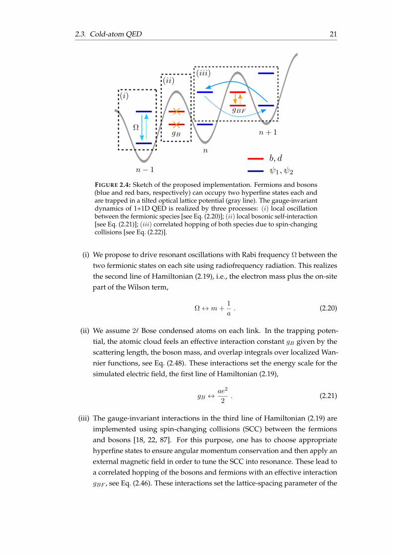
2.3. Cold-atom QED 21
FIGURE 2.4: Sketch of the proposed implementation. Fermions and bosons(blue and red bars, respectively) can occupy two hyperfine states each andare trapped in a tilted optical lattice potential (gray line). The gauge-invariantdynamics of 1+1D QED is realized by three processes: (i) local oscillationbetween the fermionic species [see Eq. (2.20)]; (ii) local bosonic self-interaction[see Eq. (2.21)]; (iii) correlated hopping of both species due to spin-changingcollisions [see Eq. (2.22)].
(i) We propose to drive resonant oscillations with Rabi frequency Ω between thetwo fermionic states on each site using radiofrequency radiation. This realizesthe second line of Hamiltonian (2.19), i.e., the electron mass plus the on-sitepart of the Wilson term,
Ω ↔ m+1
a. (2.20)
(ii) We assume 2 Bose condensed atoms on each link. In the trapping poten-tial, the atomic cloud feels an effective interaction constant gB given by thescattering length, the boson mass, and overlap integrals over localized Wan-nier functions, see Eq. (2.48). These interactions set the energy scale for thesimulated electric field, the first line of Hamiltonian (2.19),
gB ↔ ae2
2. (2.21)
(iii) The gauge-invariant interactions in the third line of Hamiltonian (2.19) areimplemented using spin-changing collisions (SCC) between the fermionsand bosons [18, 22, 87]. For this purpose, one has to choose appropriatehyperfine states to ensure angular momentum conservation and then apply anexternal magnetic field in order to tune the SCC into resonance. These lead toa correlated hopping of the bosons and fermions with an effective interactiongBF , see Eq. (2.46). These interactions set the lattice-spacing parameter of the
22 Chapter 2. Implementation of lattice gauge theories with Wilson fermions
quantum-simulated gauge theory,
gBF ↔1
a√`(`+ 1)
. (2.22)
Further details on a possible realization will be discussed in the following section2.4. Equations (2.20-2.22) define the two relevant dimensionless parameters of thesimulated theory, am and e/m. Note that the value of a is not equivalent to theoptical-lattice spacing alat imposed in the quantum simulator [see Eq. (2.27)].
2.3.3 Interpretation of the cold atom Hamiltonian
The individual processes contributing to Eq. (2.19) permit of physical interpretationsin simplified limits, which are useful to gain some intuition.
Free fermion Hamiltonian
The fermionic part of Hamiltonian (2.19) becomes particularly simple in the absenceof interactions with the gauge fields. Referring to the single-particle states of ψn,1 andψn,2 as |↑〉n and |↓〉n, respectively, we start by considering the local, purely fermionicpart in the second line of (2.19), which dominates in the heavy-mass limit m→∞.It is diagonal in the basis |←〉n = 1√
2(|↑〉n − |↓〉n) and |→〉n = 1√
2(|↑〉n + |↓〉n), with
eigenvalues −m and +m, respectively. In this basis the local fermionic Hilbert spaceis given by
Hn = |0←0→〉n, |1←0→〉n, |0←1→〉n, |1←1→〉n , (2.23)
where |j→k←〉n denotes a state with j fermions in the state |→〉n and k fermions in|←〉n. We can therefore identify the fermionic vacuum and electron/positron statesaccording to
vacuum (“Dirac sea”) : |Ω〉n ↔ |1←0→〉n , (2.24a)
electron : |e−〉n ↔ |1←1→〉n , (2.24b)
positron : |e+〉n ↔ |0←0→〉n , (2.24c)
electron + positron : |e−e+〉n ↔ |0←1→〉n . (2.24d)
Intuitively, an electron corresponds to the presence of a fermion in |→〉n, while apositron corresponds to the absence of a fermion in |←〉n.
For a finite fermion mass m, we have to take into account the fermionic hoppingterms in (2.19). The decomposition of the vacuum state into the local fermionicstates is then formally given by a Slater determinant involving all lattice sites.In this case, it is more convenient to describe the quantum system in terms ofcorrelation functions. In absence of interactions with the gauge field, the matterfields form a free theory. An initial vacuum of non-interacting fermions can thus
2.3. Cold-atom QED 23
be completely described in terms of the equal-time statistical propagators Fαβmn =12
⟨[ψm,α, ψ
†n,β
]⟩. In momentum space, this non-interacting vacuum is characterized
by the correlations (cf. section 2.7)
F 11kk = 0 , F 22
kk = 0 , F 21kk =
ωk2zk
(2.25)
and Fαβkk′ = 0 for k 6= k′. Here, zk = m + 1a
(1 + exp
(2πikN
))and the dispersion
ωk = |zk|, k = 0, 1, . . . , N − 1.
Gauge-field energy
In the experiment, the gauge part corresponds to an array of trapped spinor BECsin two hyperfine states. For the semi-classical limit of large occupation numbers,every local BEC can be pictured by a collective spin Bloch sphere. Accordingto the replacements (2.16) and (2.17) the simulated electric field corresponds toan occupation imbalance between the two states, i.e., En/e ↔ 1/2
(b†nbn − d†ndn
).
Consequently it can be associated with the azimuthal angle measuring the distancefrom the equator of the Bloch sphere. Thus, the electric energy, which arises from thebosonic self-interactions in Eq. (2.19) corresponds to the so-called one-axis twistingHamiltonian [90]. This clarifies the contribution from (2.21): It generates a rotation ofthe polar angle, whose frequency depends on the azimuthal angle. This correspondsto a phase rotation of Un ↔ [`(`+ 1)]−1/2 b†ndn in the gauge theory. However, thissimple dynamics that happens locally on every link is modified by the correlatedhopping of bosons and fermions.
Correlated hopping
In the heavy-mass limit underlying the identifications of equation (2.24), one canalso easily visualize the effect of the correlated hopping (2.22). For example, theelementary process for the local production of a single e+e− pair is composed of thehopping and simultaneous flipping of a single (fermionic) spin from one site to thenext, while decreasing the (bosonic) imbalance on the link joining the two sites.
As for the free-fermion part discussed above, the simplified interpretation interms of local single-particle states is convenient to gain a basic understanding ofthe cold-atom system, but in order to describe the full complexity of the many-particle quantum dynamics it becomes necessary to consider many-body correlationfunctions. Indeed, for a finite fermion mass, pair production happens non-locallyand can only be detected by measuring correlation functions. In fact, even theconcept of a particle is ill-defined in the generic interacting non-equilibrium situation[91]. As a measure for the total fermion particle number density n = 1
L
∑k nk, we
employ a typical definition following from the instantaneous diagonalization of thepurely fermionic contribution to the full Hamiltonian. Then, n can be expressed interms of the energy density εk, which is a function of the statistical propagator, and

24 Chapter 2. Implementation of lattice gauge theories with Wilson fermions
the dispersion ωk,
nk =εkωk
+ 1 , εk = −(zkF
21kk +
[zkF
21kk
]∗), (2.26)
where the tilde indicates that all quantities have to be calculated on the backgroundof the gauge fields.
2.3.4 Experimental limitations
There are a number of experimental limitations that set bounds on the implementa-tion of (2.19). In realistic conditions, the number of bosons on each link will fluctuatearound the target value 2` in a range in the order of
√2`/ (2`). One may interpret
this as disorder on the hopping terms between sites. In the weak-coupling regimesaccessible to our benchmarking calculations, one may estimate the resulting local-ization lengths by diagonalizing the free-fermion Hamiltonian. For the occupationnumbers that we aim at, the relative disorder strength will be on the percent level,resulting in localization lengths that are purely finite-size limited for realistic systemsizes of few tens of sites. Thus, while it is an interesting perspective to study theeffect of this disorder in large systems and strong coupling, for early experiments itis negligible compared to other error sources. Another error source derives fromnearest-neighbor elastic scattering between the species. As we argue below in sec-tion 2.4, for weak coupling its effect on the dynamics is negligible, though it mayhave a quantitative influence at strong coupling. Nevertheless, these terms aregauge invariant, so that the result will remain a valid U(1) gauge theory.
Stronger restrictions come from several experimental imperfections. The mostimportant ones limit the accessible time-scales in the experiment as summarized inthe following, and discussed in detail in the sections 2.4 and 2.5.
First of all, we have replaced the gauge fields by finite spin operators (2.16). Toquantitatively approach QED predictions, we would thus like to employ BECs withlarge atom numbers corresponding to `→∞. The large boson density will lead toconsiderable three-body losses [92], which depend on the precise lattice structure.These losses set a limiting time T3 for the validity of the quantum simulation.
A second restriction comes from the need to suppress direct hopping terms ofthe two species and to conserve the boson number locally on each link to ensure theconstraint (2.18). Wilson fermions naturally favor a tilted lattice, which convenientlysuppresses direct tunneling. On the downside, the tilt renders states localized onsingle lattice sites unstable [93]. After a time TLZ , they decay due to Landau-Zenertransitions, which is the second main limitation of our proposed setup.
Finally, experiments will implement a set of lattice QED parameters a,m, e witha resulting Brillouin zone of finite size ∼ 1/a. Since we are interested in Schwingerpair production in strong electric fields, the creation and subsequent acceleration ofparticles becomes unphysical when the energy of these particles reaches the cutoff∼ 1/a. This gives a third time-scale Tlat that limits the accessible dynamics.
2.4. Details of the experimental implementation 25
An experimental implementation will have to carefully balance between thesedifferent imperfections. Nevertheless, as we will show in the remainder of thischapter, the observation of relevant phenomena is achievable in state-of-the artexperiments. Moreover, T3 and Tlat can be mitigated if we do not require quantitativeagreement with continuum QED. For any finite a, the experiment will implementa valid lattice gauge theory. Similarly, by settling for finite representations l <∞,one implements quantum links models, which are valid gauge theories in their ownright. Already for extremely small representations, these share the most salientqualitative features with usual QED, such as string-breaking dynamics [11].
2.4 Details of the experimental implementation
As outlined above, we propose to implement (2.19) with a mixture of fermions andbosons trapped in an optical lattice. In the following, we discuss some details andsubtleties that arise in this implementation. Though we keep the discussion general,when giving numerical estimates we assume a mixture of fermionic 6Li and bosonic23Na. For the most part, we assume transverse degrees of freedom to be frozen outand consider the mixture to be effectively one-dimensional.
2.4.1 Single-particle Hamiltonian
In accordance with the structure of Wilson fermions (see Fig. 2.3), we propose toemploy a tilted optical lattice of the form
V (lat)χ (x) = Fχx+
Vχ cos2
(πxalat
), χ = B
Vχ sin2(πxalat
), χ = F
, (2.27)
where the species index χ = F,B refers to either fermions on the lattice sites orbosons on the links. The depth Vχ, the spacing alat, and the tilt strength Fχ ofthe optical lattice may be tuned independently. Additionally, we apply a constantmagnetic field B perpendicular to the x-direction, which we assume to give rise to alinear Zeeman shift,
V (Z)χ,s = −mχ,sg
(B)χ,sµBB . (2.28)
Here, s =↑, ↓ denotes the selected two hyperfine states for each species to which therelevant dynamics of the system is restricted; mχ,s is the corresponding magneticquantum number, µB denotes the Bohr magneton, and g
(B)χ,s is the Landé g-factor.
Neglecting interactions for a moment, the quadratic part of the full Hamiltonian is
26 Chapter 2. Implementation of lattice gauge theories with Wilson fermions
given by
H0 =∑
χ,s
ˆdx χ†s(x)H0(χ, s)χs(x) (2.29)
H0(χ, s) = −~2∂2x
2Mχ+ V (lat)
χ (x) + V (Z)χ,s , (2.30)
where Mχ is the atomic mass and we assumed the lattice potential to be species-dependent, but the same for different hyperfine states. The fields, which we denoteby χs, obey canonical commutation or anti-commutation relations according to theirstatistics, i.e.,
[χs(x), χ†r(y)
]ζ(χ)
= δ(x− y) , (2.31)
where we abbreviate [X,Y ]± = XY ± Y X with ζ(B) = − and ζ(F ) = +.
2.4.2 Suppression of direct tunneling in a tilted lattice
Additionally to its matching the natural structure of Wilson fermions, we employthe tilt to suppress direct tunneling of the fermions. This is crucial to ensure gaugeinvariance, because the fermions must only hop between different lattice sites dueto interactions with the bosons. In the untilted case (Fχ = 0), the one-particle Blochwaves for the potential in Eq. (2.30) without external magnetic field (B = 0) areMathieu functions. In this case, the ground band has the dispersion relation
εχ(k) =ωχ2− 2Jχ cos(kalat) , k ∈
[− π
alat,π
alat
), (2.32)
with the mean energy ωχ = 2√VχErec,χ. Here Erec,χ = ~2/
[2Mχ(alat/π)2
]is the
recoil energy and the ratio ξχ = 2√Vχ/Erec,χ controls the lattice depth. In the limit
of a deep lattice (ξχ 1) the hopping element is given by
Jχ =
√2
πErec,χ (ξχ)3/2 e−ξχ [1 +O(1/ξχ)] , (2.33)
which can be obtained exactly from analytic properties of the Mathieu functions.We can suppress direct tunneling for both species by choosing a sufficiently
strong tilt, i.e.,
alatFχ Jχ . (2.34)
In the presence of the tilt, the states in the ground band are modified into resonances
2.4. Details of the experimental implementation 27
of a Wannier-Stark ladder (for more details see the appendix 2.A). Including non-vanishing B 6= 0, the energy levels are
EF,s(l) =1
2ωF + lalatFF −mF,sg
(B)F,sµBB , (2.35)
EB,s(l) =1
2ωB +
(l +
1
2
)alatFB −mB,sg
(B)B,sµBB . (2.36)
The states of the Wannier-Stark ladder have a finite lifetime which can be esti-mated from the decay rate Γχ due to Landau-Zener transitions (for more details seethe appendices 2.A and 2.B).
Γχ =alatFχ2π~
exp
(−
π2∆2χ
8EχalatFχ
)≤ alatFχ
2π~, (2.37)
where ∆χ ≈ ωχ is the gap between the ground band and the first excited band. Thislifetime is one of the relevant experimental restrictions.
2.4.3 Choice of the magnetic field
Under the above condition (2.34), we may neglect direct tunneling. The quadraticpart (2.29) of the full Hamiltonian then amounts to a Wannier-Stark ladder of long-lived resonances. These are coupled by a correlated hopping of the fermions andbosons as in Ref. [87], which induces the gauge-invariant matter–gauge-field inter-action. For this purpose, the spin-changing collisions for the chosen hyperfine levelss =↑, ↓ need to be tuned into resonance, i.e., we demand
EF↑ (l)− EF↓ (l + 1)!
= EB↑ (l)− EB↓ (l) ∀l . (2.38)
If the two components ↑, ↓ are chosen from the same hyperfine manifold for eachspecies, the g-factors are spin-independent, g(B)
χ,s = g(B)χ . Then the resonance condi-
tions can be rewritten as
alatFFµBB
!= g
(B)B ∆
(B)B − g(B)
F ∆(B)F , (2.39)
where we introduced the abbreviation ∆(B)χ = mχ↑ −mχ↓.
For a mixture of bosonic 23Na and fermionic 6Li, respectively, we choose thefollowing levels from the ground hyperfine manifold:
mB↑ = 0 , mB↓ = −1 , mF↑ =1
2, mF↓ = −1
2. (2.40)
The corresponding Landé factors are g(B)F = −2
3 and g(B)B = −1
2 .
28 Chapter 2. Implementation of lattice gauge theories with Wilson fermions
2.4.4 Effective interaction constants from overlap integrals in the tiltedlattice
In order to match the coefficients of Hamiltonian (2.19) with experimental param-eters, we need to calculate overlap integrals involving Wannier-Stark functionsΨl,χ(x). In our case, they are built from the Wannier functions ψl,χ(x) located atlattice sites (respectively links) l = 1 . . . N of the untilted lattice. The Wannier-Starkfunctions can be written as superpositions (see the appendix 2.A)
Ψl,χ(x) =∑
m
Jm−l(
2JχalatFχ
)ψm,χ(x) , (2.41)
where Jm(. . . ) denote Bessel functions of the first kind. We only consider theground band here. For sufficiently deep lattices, to estimate the relevant overlapintegrals, we may approximate the Wannier functions appearing in the series (2.41)as harmonic oscillator eigenfunctions,
ψl,χ(x) =(πaHO
χ
)−1/4exp
[−1
2
(x− xl,χaHOχ
)2], (2.42)
where xl,χ denote the minima of the tilted potentials and the harmonic oscillatorlengths should be determined from a Taylor expansion of the tilted potentials aroundtheir minima. The minima are shifted from the untilted case to the positions
xl,B =
(l +
1
2
)alat − δB , xl,F = lalat − δF , (2.43)
δχ =alat
2πarcsin
(alatFχπVχ
)≈ alat
2π
alatFχπVχ
. (2.44)
The oscillator length, aHOχ =
√~/(mχωHO
χ
), is determined from the condition
mχ
(ωHOχ
)2 != 2Vχ
(π
alat
)2√
1−(alatFχπVχ
)2
. (2.45)
Using the approximation (2.42), we can calculate the effective interaction con-stants that enter the quantum simulation. For clarity, we first present estimates basedon single-particle wavefunctions. For the bosonic condensates, we subsequently usea more appropriate estimate to take their high occupation into account.
The effective boson-fermion inter-species interaction generating the matter-fieldhopping is given by the 3D overlap integral
gBF =g
(3D)BF
2
ˆdx dy dz |ΦB(y, z)|2 |ΦF (y, z)|2 (Ψl+1,F (x))∗ |Ψl,B(x)|2 Ψl,F (x) ,
(2.46)
2.4. Details of the experimental implementation 29
where g(3D)BF =
(√2/3)
2π~2aBF /Mred is the relevant three-dimensional interac-tion constant with scattering length aBF ≈ 0.9a0 and the reduced mass Mred =
MFMB/ (MF +MB). The Clebsch-Gordon coefficient√
2/3 is the same as for theprevious proposal [87]. For simplicity, we assume a symmetrically harmonic trans-verse confinement with the same trapping frequency ω⊥ for B and F , i.e.,
Φχ(y, z) =(πa2⊥,χ)−1/2
exp
(−y
2 + z2
2a2⊥,χ
)(2.47)
and a⊥,χ =√~/ (Mχω⊥) .
Furthermore, we need to calculate the effective bosonic intra-species interaction
gB =g
(3D)B
2
ˆdx dy dz |ΦB(y, z)|4 |Ψl,B(x)|4 , (2.48)
where g(3D)B = (1/6) 4π~2aB/MB is the relevant interaction strength with aB ≈ 5a0.
For the Clebsch-Gordon coefficient, we again refer to [87]. At the large bosonoccupation numbers that we are interested in, the effective interaction constantis modified due to deviations of the bosonic wave-function from the harmonic-oscillator shape. In a first approximation, we may treat this effect in a Thomas-Fermi(TF) limit, i.e., we consider the bosonic mean-field wavefunction as
ΦTF(x) =
õ
g
[1− x2
x2TF
]Θ (|x| − xTF) (2.49)
with the TF radius xTF =
√2µ/
[MB
(ωHOB
)2] and the effective chemical potential µ
is determined by the number of bosons on each link as NB = 4xTFµ/ (3g). Thus, interms of the experimental parameters,
xTF =
4VB3gNB
(πa
)2
√1−
(alatFBπVB
)2
−1/3
, (2.50)
where g is the effective 1D inter-bosonic coupling given by
g =g
(3D)B
2
ˆdy dz |ΦB(y, z)|4 . (2.51)
Due to the vastly different trapping frequencies (few Hz compared to several kHz,see below), it is justified to treat the bosons in the radial direction in the harmonicapproximation, while taking into account the TF profile in the longitudinal direction.The results of the following sections are obtained with the effective interactionconstants calculated within this approximation.

30 Chapter 2. Implementation of lattice gauge theories with Wilson fermions
2.4.5 Other scattering processes
So far, we have only related the effective interaction constants of the desired interac-tions to the microscopic properties of the Bose-Fermi mixture. In this subsection, webriefly discuss possible other scattering processes.
In general, all on-site or nearest-neighbor, both of density-density and spin-spintype, inter- and intra-species interactions could be as relevant as the desired spin-changing collision (2.22). Due to a judicious choice of the magnetic field togetherwith the tilted lattice as described above only the SCCs are resonant and all otherinelastic processes are presumably suppressed. We therefore restrict ourselves toelastic collisions. Since these do not change the local occupation numbers of eitherspecies, the corresponding contributions all commute with the Gauss’ law operatorand hence do not spoil gauge-invariance of the quantum simulator. The leadingpurely bosonic contribution comes from on-site interactions that have already beentaken into account and set the energy scale for the simulated electric field (2.21).
In addition, density-density interactions between the two species on neighboringsites give rise to a term like
∼∑
n
(b†nbn + d†ndn
) ∑
α=1,2
(ψ†n,αψn,α + ψ†n+1,αψn+1,α
) . (2.52)
For an appropriate initial state preparation that respects the constraint (2.18), theabove term reduces to the total fermion particle number (which is conserved) andthus does not affect the dynamics.
Nearest-neighbor spin-spin interactions on the other hand lead to the contribu-tion
∼∑
n
(d†n−1dn−1 + d†ndn
)(ψ†n,1ψn,1 − ψ†n,2ψn,2
)(2.53)
=∑
n
(2`− En−1 + En
e
)(ψ†n,1ψn,1 − ψ†n,2ψn,2
), (2.54)
where we used the definitions (2.16) & (2.17), as well as the constraint (2.18). Theterm proportional to ` only affects the resonance condition (2.39) and can be absorbedinto a redefinition of the energy levels (2.38). For the real-time dynamics consideredin this work, it is useful to further define En ≡ E
(0)n + δEn, where E(0)
n = 〈En(t =
0)〉 & m2
e is the initial value of the electric field. Absorbing also E(0)n into the
energy levels (2.38), we parametrically estimate that the above contribution doesnot alter the dynamics as long as 〈δEn〉 m2
e . This argument is most accurate in theweak-coupling limit, where
(me
)2 1. In fact, for our benchmarking simulationsthe condition is fulfilled for all times shown below in figures 2.9 & 2.7. We cantherefore neglect it for the proposed experiment that may extract the Schwingerpair production rate as shown in figure 2.8. For the case of strong coupling, whichwe are ultimately interested in, these elastic inter-species spin-spin interactions
2.5. Choice of experimental parameters 31
will however quantitatively change the behavior in general. We want to stress thatthe resulting theory will nevertheless be a fully interacting dynamical U(1) gaugetheory.
Finally, we note that for a general choice of fermion species, purely fermionicon-site interactions can yield unwanted effects. However, for the present choiceof Lithium, these are absent due to a zero of the relevant scattering length at lowmagnetic fields [94].
2.4.6 Three-body losses
One of the leading limitations of our proposal is the instability of the local BECsdue to three-body collisions. On a mean-field level, these three-body losses may bemodeled as
NB
NB= −K3
NB
ˆdx dy dz |ψB(x, y, z)|6 , (2.55)
with the total particle number per link NB =´
dx dy dz |ψB(x, y, z)|2 and thespecies-dependent constant K3, commonly referred to as the three-body loss ratecoefficient. We estimate the typical time-scale for three-body losses, T3, as the inverseof the right-hand side of equation (2.55). Demanding this time to be much largerthan any other time scale in the experiment sets a limit on the boson particle numberNB per link.
2.5 Choice of experimental parameters
In the implementation proposed above, several imperfections arise that limit accessi-ble time scales. In this section, we discuss the main limitations and an optimizationprocedure to maximize the time simulatable in the experiment.
2.5.1 Experimental limitations
A first limitation appears through the three-body loss time of the bosonic conden-sates, T3. Second, the localized Wannier-Stark states in the tilted periodic potentialhave a finite life-time. For the choice of a mixture between 6Li and 23Na, due to thesmaller mass of the fermionic atoms the limiting factor will be the fermion life time,which we denote by TLZ . Third, the proposed lattice QED implementation will havea finite lattice spacing a. Deviations from the continuum limit will appear at a timescale Tlat, which is defined below.
One can balance between these three effects by adapting the following experi-mental parameters:
1. The number of bosons per link NB ,
2. the number of lattice sites N ,

32 Chapter 2. Implementation of lattice gauge theories with Wilson fermions
3. the optical lattice spacing alat,
4. the lattice depth Vχ,
5. the radial confinement ω⊥,χ,
6. the tilt of the lattice alatFχ.
Allowing different parameters for the bosons and fermions, the three time-scalesdepend on 9 different experimental parameters. We are looking for a set of parame-ters for which the minimum of (T3, TLZ , Tlat) becomes maximal. This optimizationis constrained by experimental restrictions, for instance the achievable number oflattice sites.
In addition, each parameter set corresponds to two dimensionless parameters onthe lattice QED side, namely the lattice spacing am and the coupling constant e/min units of the fermion mass m. We wish to obtain relevant results for continuumQED and thus seek small values of am . 1. On the other hand, we want to performbenchmarking simulations employing an approximation which relies on e/m < 1.These different desiderata generate a rather complicated optimization problem.
2.5.2 Simplified optimization procedure
Relying on physical intuition, we simplify the problem by considering the limitingtime-scales as a function of alat in the range 5 − 10 µm. Since one of the maincomplications consists of realizing strong spin-changing collisions, we choose rathershallow lattices, VB = 2Erec,B and VF = Erec,F and fix the tilts alatFχ = 10Jχ suchthat direct tunneling in the shallow lattice is suppressed. We further fix a strongradial confinement ω⊥,χ = 2π × 10 kHz that renders the system effectively one-dimensional. Now we can tune NB , such that T3 and TLZ lie approximately in thesame range. We choose NB = 3000, i.e., ` = 1500, which is sufficiently large forthe quantum link regularization to approximate QED. Finally, the total number oflattice sites is irrelevant for the determination of three time-scales, but enters as theIR-cutoff after having determined the simulation parameter am. We will come backto this point later.
We can now calculate the effective bosonic interaction constant (gB) and the ef-fective interaction constant for correlated hopping between the fermions and bosons(gBF ) as functions of alat. Finally, we may adjust the local oscillation frequency be-tween the two fermionic states (Ω). Then, we can make the connection to lattice QEDaccording to Eqs. (2.20), (2.21), and (2.22). On the QED side, we choose to measureenergies and times in units of m, which in experimental parameters correspondsto m ↔ Ω − 2
√`(`+ 1)gB . As a bound for the validity of the lattice simulation,
we take Tlatm = 2π/ (am), which is the time when the momentum plat = eETlat ofparticles accelerated by a constant electric field E = m2/e reaches the cutoff ∼ 2π/a.Within this framework, we consider a two-step procedure choosing first alat and

2.5. Choice of experimental parameters 33
FIGURE 2.5: The limiting time-scales T3(alat) (blue, solid), TLZ(alat) (red,dashed), and Tlat(alat,Ω) (green, dotted; top to bottom for Ω = 2π × 4− 7Hzin steps of 0.5Hz). An optimal choice of experimental parameters maximizesthe minimum of these three time scales, conditioned on the desired set ofsimulation parameters, see 2.6. Note the logarithmic scale of the ordinate.
FIGURE 2.6: Dimensionless parameters entering the lattice QED simulation,am (Ω) (red diamonds, dashed), and e/m (Ω) (blue squares, dotted). Thehorizontal gray dashed-dotted line indicates the limiting unity. The inversebehavior favors strong coupling at small lattice spacing.
subsequently Ω in order to optimize the functions T3(alat), TLZ(alat) and Tlat(alat,Ω),am(alat,Ω), e/m(alat,Ω).
Figure 2.5 shows the limiting time-scales for different values of Ω in the rangeof 2π × (4 − 7)Hz. As this plot shows, large values of alat are favorable if weadjust Ω accordingly. Consequently, we choose a rather large alat = 10µm andplot the remaining Ω dependence of the lattice QED parameters in Fig. 2.6. Theobserved converse behavior of am and e/m restrains us from choosing an arbitrarilysmall lattice spacing a for the benchmarking simulations. Note that this shouldnot be seen as a problem of the implementation, but rather getting close to the
34 Chapter 2. Implementation of lattice gauge theories with Wilson fermions
continuum limit means studying the strong-coupling regime of QED3. This regimeis notoriously difficult for numerical simulations and thus a non-trivial target forquantum simulation. For benchmarking, however, we choose the following twopossibilities:
Ω = 2π × 4.5 Hz : am = 0.45 , e/m = 0.45 (2.56)
Ω = 2π × 6 Hz : am = 0.94 , e/m = 0.22 (2.57)
Finally, we choose the number of lattice sites to be N = 20, which corresponds toa reasonable size of the optical lattice. The corresponding IR-cutoff on the QEDside in units of the fermion mass is given by 1/ (N × am) ∼ O(0.1). Thus, weshould be able to resolve sufficiently many modes at small momenta to observe thephenomenon of Schwinger pair production.
2.6 Benchmark: Onset of Schwinger pair production
Having shown how to use Wilson fermions in order to realize a particularly compactformulation of 1+1D QED in optical lattices, we now turn to making quantitativepredictions for the proposed experimental realization. To this end, we performnumerical simulations of an important effect that occurs in 1+1D QED: pair produc-tion via the Schwinger mechanism [66, 67]. The mechanism describes how a strongexternal electric field transfers energy to vacuum fluctuations and turns them intopairs of real particles and anti-particles. In the present case of 1+1 dimensions, onecan analytically compute the particle-production rate in the continuum
n
m2=
E
πEcexp
(−πEc
E
), (2.58)
which is valid for a constant background field that was turned on in the infinite past[67] (see appendix 2.B for a heuristic derivation). Most importantly, the exponentialfactor induces a dramatic increase of particle production above a critical field Ec =
m2/e. In this regime, the particle production is non-perturbative and thus constitutesan excellent non-trivial target for quantum simulation. Moreover, there is no knownanalytic prediction for the fully interacting theory including the back-reaction of theproduced particles onto the gauge fields [91].
In the following, we show that the proposed implementation strategy, using amixture of fermionic 6Li and bosonic 23Na based on current technology, allows oneto simulate the Schwinger mechanism and the non-perturbative particle-productionrate. For benchmarking purposes, we consider the limit of weak gauge coupling,where powerful functional-integral methods provide quantitatively reliable results[95, 96]. Beyond this weak-coupling benchmark regime, the experiment should
3Here, we are referring to the bare parameters am and e/m. Approaching the correct continuumlimit is more subtle in general since it requires to adjust the bare coupling parameters as brieflydiscussed in the introduction.
2.6. Benchmark: Onset of Schwinger pair production 35
be able to proceed also into the regime of strong coupling, where these functional-integral methods are expected to fail. Details of the simulation procedure aresummarized in the following section 2.7.
2.6.1 Proposed experimental protocol
To quantum simulate the Schwinger mechanism, we propose the following experi-mental protocol. First, the bosonic and fermionic atoms are loaded into the tilted op-tical lattice structure. At sufficiently low temperatures, we will have single fermionsper lattice site in the state |↓〉n and single-component condensates with averageparticle number 〈d†ndn〉 on the links. Initially, the imbalance δNn = 〈b†nbn − d†ndn〉 ofthe two hyperfine states, which defines the electric field as discussed in section 2.3.3,is tuned to δNn = 0. This can be achieved with a linear coupling between the twostates, e.g., via radiofrequency radiation. This initial state, where the electric field isprepared in a product of coherent states, is only approximately restricted to a singlegauge sector. However, as it has been shown numerically [95], in the limit of largeboson number and for the present scenario the small fluctuations of the electric fieldare too insignificant to compromise the gauge-invariant dynamics.
As described in the previous section, in the heavy-mass limit, the fermionicvacuum is given by the local superpositions |←〉n = 1√
2(|↑〉n − |↓〉n). This state
can be easily generated from a polarized gas by a π/2 radiofrequency pulse (witha phase shift of π/2 with respect to the radiofrequency pulse ∝ Ω that drives thedynamics). Together with the gauge fields, this realizes the ground state at infinitefermion mass. Alternatively, one may adiabatically prepare the ground state at afinite value of the fermion rest mass, e.g., by adiabatically ramping down the opticallattice such that the correlated hopping is gradually turned on.
With either choice of the fermion initial state, the dynamics can be started byquenching the bosonic imbalance δNn from zero to a desired initial electric field. Forthe experimentally less demanding case of the infinite-mass ground state, this willrealize a combination of the targeted Schwinger mechanism with a mass quenchfrom infinity to a desired, finite value. Below, we demonstrate that both initializationprocedures yield comparable results for the particle production rate, at least for theparameter regimes studied in this work (i.e., weak coupling and relatively coarselattices).
After the initialization procedure, the system evolves for a desired time underHamiltonian (2.19), after which we extract the relevant observables. In particular,we are interested in the volume-averaged electric field and the total fermion particlenumber. The first is easily achieved by reading out the bosonic imbalance viastandard absorption imaging. Current experimental techniques allow for single-siteresolution, such that one can also access the local electric fields and their spatialcorrelations.
36 Chapter 2. Implementation of lattice gauge theories with Wilson fermions
The total fermion particle number can be measured in a number of ways. First,the definition of the particle number given in Eq. (2.26) can be measured by adia-batically transferring the system to the limit of infinite mass by increasing Ω, seeEq. (2.20). A subsequent π/2 radiofrequency pulse around the y axis on the fermionBloch sphere maps fermions in the upper (lower) band onto the pseudo-spin state|↑〉 (|↓〉). Through a Stern-Gerlach measurement, one can thus detect the producedparticle–anti-particle pairs. In addition, their momentum dependence can be re-solved by time-of-flight imaging. Since the increase of m amounts to an increase ofthe critical field Ec = m2/e, this scheme effectively turns the Schwinger mechanismoff smoothly, in a similar spirit as for the so-called Sauter pulses that are oftenused to model the Schwinger mechanism in time-dependent (classical) backgroundfields [91]. Second, one can map out the full band structure by adapting the to-mography scheme developed in Ref. [97] and first demonstrated experimentallyin Ref. [98]. The particle number is obtained by comparison to the tomographyfor the ground state at the mass parameter targeted in the dynamics. Third, thefull information about the fermionic part of the theory can be reconstructed bymeasuring spin-dependent and spatially resolved fermion correlation functions,either via quantum-gas microscopy [99–101] or, since we are interested in the spatialcontinuum limit, on coarse grained length scales larger than the lattice spacing.
2.6.2 Simulated real-time dynamics of fermion density and electric field
While lattice-QED has only two free parameters am and e/m, one can changevarious ingredients on the experimental side. Different choices can drastically affectthe various time scales governing the quantum simulator. Following the simpleoptimization procedure discussed in 2.5, we focus on two examples of realisticparameter sets, which translate to
(i): am = 0.45 , e/m = 0.45 , E0/Ec = 7 .
(ii): am = 0.94 , e/m = 0.22 , E0/Ec = 3 ,
As these values illustrate, if working at finer lattice spacing am, experimental re-strictions of the present proposal require an increase of the coupling e/m. Thiscombination limits the numerical technique employed here to coarse lattices, as it isquantitatively reliable only at small e/m. However, in the experiment it will allowone to reach exactly the most interesting regime, namely close to the continuumlimit and with strong coupling.
Since the results for these parameter sets are qualitatively very similar, wediscuss in the following only the set (i) (Fig. 2.7) and delegate the results of set (ii)to the next section (Fig. 2.9). For both choices, the initial electric field E0 exceedsthe critical value in Eq. (2.58), and thus we expect an enhanced production ofelectron-positron pairs. We simulate the real-time evolution of the particle number

2.6. Benchmark: Onset of Schwinger pair production 37
0.0 0.2 0.4 0.6 0.8 1.0Time tm
0.00
0.25
0.50
0.75
1.00
1.25
1.50
Ferm
iondensity
n/m
0 20 40 60 80 100 120Time t[ms]
6.80
6.85
6.90
6.95
7.00
ElectricField
E/E
c
ideal cold-atom QED
realistic (am = 0.45)
am = 0.3
am = 0.225
am = 0.1
FIGURE 2.7: Benchmarking simulations (e/m = 0.45, am = 0.45, N = 20, and = 1500; blue solid line) qualitatively recover the ideal continuum Schwingerrate (the limit of small am as well as large N and ; black dash-dotted). Asthe interpolating lines for different am at fixed volume L = aN = 9/m show,the benchmark simulations are converged with respect to and smoothlyapproach the continuum prediction (dashed lines from dark to light blueam = 0.3, 0.225, and 0.1).
as well as the decay of the initial electric field employing a semi-classical functional-integral method [10, 87, 95] summarized in the next section 2.7 and compare themto an idealized implementation with ,N → ∞ and a → 0. The latter is obtainednumerically by increasing and approaching the spatial continuum limit (a → 0
with aN = const) until convergence of the fermion density and the electric field isobserved. For the presented realistic parameter sets, though quantitative deviationsfrom the expected QED behavior occur, the observed particle production showsgood qualitative agreement. It is also possible to observe the onset of the decay ofthe electric field due to the backreaction of the fermions. Observed deviations aremainly due to the large lattice spacings and do not result from the finite < ∞,which we conclude from the interpolating curves that approach the continuumlimit with decreasing a, while keeping constant. The quantum simulator will thusbe capable of simulating a dynamical lattice gauge theory, though the realisticallyreachable lattice parameters a still lead to quantitative deviations from the spatialcontinuum limit, at least for the weak coupling regime.
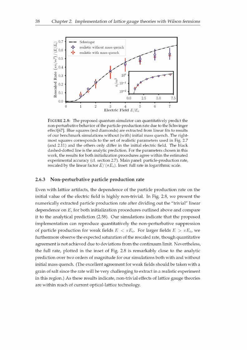
3 8 C h a pt e r 2. I m pl e m e nt ati o n of l atti c e g a u g e t h e o ri e s wit h Wil s o n f e r mi o n s
0 1 2 3 4 5 6 7El e c t ri c Fi el d E / E c
0 .0
0 .1
0 .2
0 .3
0 .4
0 .5
0 .6
0 .7
Res
cal
ed
Rat
eπn/
m2
/(E
/E
c) S c h wi n g er
r e alisti c wit h o ut m ass q u e n c h
r e alisti c wit h m ass q u e n c h
0 .0 2 .5 5 .0 7 .5
1 0 − 2
1 0 − 1
1 0 0
n/m
2
F I G U R E 2. 8: T h e p r o p o s e d q u a nt u m si m ul at o r c a n q u a ntit ati v el y p r e di ct t h en o n- p e rt u r b ati v e b e h a vi o r of t h e p a rti cl e- p r o d u cti o n r at e d u e t o t h e S c h wi n g e reff e ct[ 6 7 ]. Bl u e s q u a r e s ( r e d di a m o n d s) a r e e xt r a ct e d f r o m li n e a r fit s t o r e s ult sof o u r b e n c h m a r k si m ul ati o n s wit h o ut ( wit h) i niti al m a s s q u e n c h. T h e ri g ht-m o st s q u a r e s c o r r e s p o n d s t o t h e s et of r e ali sti c p a r a m et e r s u s e d i n Fi g. 2. 7( a n d 2. 1 1 ) a n d t h e ot h e r s o nl y diff e r i n t h e i niti al el e ct ri c fi el d. T h e bl a c kd a s h e d- d ott e d li n e i s t h e a n al yti c p r e di cti o n. F o r t h e p a r a m et e r s c h o s e n i n t hi sw o r k, t h e r e s ult s f o r b ot h i niti ali z ati o n p r o c e d u r e s a g r e e wit hi n t h e e sti m at e de x p e ri m e nt al a c c u r a c y ( cf. s e cti o n 2. 7 ). M ai n p a n el: p a rti cl e- p r o d u cti o n r at e,r e s c al e d b y t h e li n e a r f a ct o r E / (π E c ) . I n s et: f ull r at e i n l o g a rit h mi c s c al e.
2. 6. 3 N o n- p ert ur b ati v e p arti cl e pr o d u cti o n r at e
E v e n wit h l atti c e a rtif a ct s, t h e d e p e n d e n c e of t h e p a rti cl e p r o d u cti o n r at e o n t h e
i niti al v al u e of t h e el e ct ri c fi el d i s hi g hl y n o n-t ri vi al. I n Fi g. 2. 8 , w e p r e s e nt t h e
n u m e ri c all y e xt r a ct e d p a rti cl e p r o d u cti o n r at e aft e r di vi di n g o ut t h e “t ri vi al ” li n e a r
d e p e n d e n c e o n E , f o r b ot h i niti ali z ati o n p r o c e d u r e s o utli n e d a b o v e a n d c o m p a r e
it t o t h e a n al yti c al p r e di cti o n (2. 5 8 ). O u r si m ul ati o n s i n di c at e t h at t h e p r o p o s e d
i m pl e m e nt ati o n c a n r e p r o d u c e q u a ntit ati v el y t h e n o n- p e rt u r b ati v e s u p p r e s si o n
of p a rti cl e p r o d u cti o n f o r w e a k fi el d s E < π E c . F o r l a r g e r fi el d s E > π E c , w e
f u rt h e r m o r e o b s e r v e t h e e x p e ct e d s at u r ati o n of t h e r e s c al e d r at e, t h o u g h q u a ntit ati v e
a g r e e m e nt i s n ot a c hi e v e d d u e t o d e vi ati o n s f r o m t h e c o nti n u u m li mit. N e v e rt h el e s s,
t h e f ull r at e, pl ott e d i n t h e i n s et of Fi g. 2. 8 i s r e m a r k a bl y cl o s e t o t h e a n al yti c
p r e di cti o n o v e r t w o o r d e r s of m a g nit u d e f o r o u r si m ul ati o n s b ot h wit h a n d wit h o ut
i niti al m a s s q u e n c h. ( T h e e x c ell e nt a g r e e m e nt f o r w e a k fi el d s s h o ul d b e t a k e n wit h a
g r ai n of s alt si n c e t h e r at e will b e v e r y c h all e n gi n g t o e xt r a ct i n a r e ali sti c e x p e ri m e nt
i n t hi s r e gi o n.) A s t h e s e r e s ult s i n di c at e, n o n-t ri vi al eff e ct s of l atti c e g a u g e t h e o ri e s
a r e wit hi n r e a c h of c u r r e nt o pti c al-l atti c e t e c h n ol o g y.

2.7. Details of the numerical simulation 39
2.7 Details of the numerical simulation
For our numerical simulations, we employ a functional-integral approach that wasalso used to benchmark a previous implementation with staggered fermions [10,87]. The main idea of this method is to map the full quantum theory onto a classical-statistical ensemble, which is achieved by a semi-classical expansion around theinitial state. Observables are then obtained by solving classical equations of motionand sampling over fluctuating initial values. This results in a non-perturbativeapproximation of the quantum dynamics, which is valid for sufficiently large electricfields E and weak coupling e/m. In the context of cold atomic gases, the methodis related to the well-known truncated Wigner approximation and can be derivedby integrating out the fermionic degrees of freedom. The validity to benchmark theproposed quantum simulator relies on the fact that the dynamics is dominated bythe Bose condensates and that direct interactions between the fermions are absent.
2.7.1 Classical equations of motion
In order to calculate the equations of motions for the classical-statistical approach toBose-Fermi mixtures, we consider the Weyl symbol of the cold atom Hamiltonian(2.19), which is given by
H =ae2
4
∑
n
(|bn|4 + |dn|4
)+
(m+
1
a
)∑
n
(ψ†n,1ψn,2 + ψ†n,2ψn,1
)(2.59)
+1
a√` (`+ 1)
∑
n
(ψ†n−1,1b
∗n−1dn−1ψn,2 + h.c.
).
In this expression, bn, dn are c-numbers and ψn,α are fermionic operators at site nand hyperfine state α. Thus, we can decompose the Hamiltonian to H = HB +HF ,with the pure c-number part HB = ae2
4
∑n
(|bn|4 + |dn|4
)and the fermionic part
HF =∑
mn,αβ ψ†m,α (hF )αβmn ψn,β , where we abbreviated
(hF )αβmn =
(m+
1
a
)δmnσ
αβx
+1
a√` (`+ 1)
(b∗mdmδm,n−1σ
αβ+ + d∗m−1bm−1δm−1,nσ
αβ−)
(2.60)
with the Pauli matrices
σx =
(0 1
1 0
), σy =
(0 −ii 0
), σ± =
1
2(σx ± iσy) . (2.61)
In terms of the equal-time two-point function Dαβmn =
⟨ψ†m,αψn,β
⟩, where 〈. . . 〉
denotes a quantum expectation value, the explicit equations of motion for the
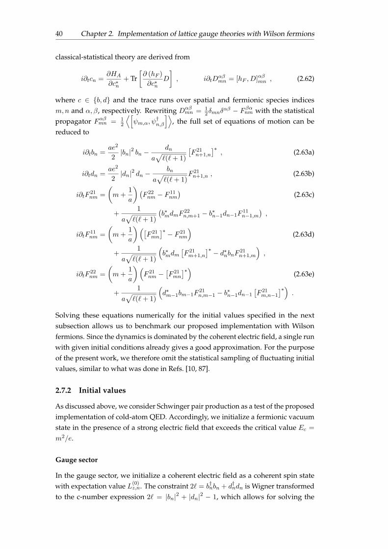
40 Chapter 2. Implementation of lattice gauge theories with Wilson fermions
classical-statistical theory are derived from
i∂tcn =∂HA
∂c∗n+ Tr
[∂ (hF )
∂c∗nD
], i∂tD
αβmn = [hF , D]αβmn , (2.62)
where c ∈ b, d and the trace runs over spatial and fermionic species indicesm,n and α, β, respectively. Rewriting Dαβ
mn = 12δmnδ
αβ − F βαnm with the statisticalpropagator Fαβmn = 1
2
⟨[ψm,α, ψ
†n,β
]⟩, the full set of equations of motion can be
reduced to
i∂tbn =ae2
2|bn|2 bn −
dn
a√`(`+ 1)
[F 21n+1,n
]∗, (2.63a)
i∂tdn =ae2
2|dn|2 dn −
bn
a√`(`+ 1)
F 21n+1,n , (2.63b)
i∂tF21nm =
(m+
1
a
)(F 22nm − F 11
nm
)(2.63c)
+1
a√`(`+ 1)
(b∗mdmF
22n,m+1 − b∗n−1dn−1F
11n−1,m
),
i∂tF11nm =
(m+
1
a
)([F 21mn
]∗ − F 21nm
)(2.63d)
+1
a√`(`+ 1)
(b∗mdm
[F 21m+1,n
]∗ − d∗nbnF 21n+1,m
),
i∂tF22nm =
(m+
1
a
)(F 21nm −
[F 21mn
]∗) (2.63e)
+1
a√`(`+ 1)
(d∗m−1bm−1F
21n,m−1 − b∗n−1dn−1
[F 21m,n−1
]∗).
Solving these equations numerically for the initial values specified in the nextsubsection allows us to benchmark our proposed implementation with Wilsonfermions. Since the dynamics is dominated by the coherent electric field, a single runwith given initial conditions already gives a good approximation. For the purposeof the present work, we therefore omit the statistical sampling of fluctuating initialvalues, similar to what was done in Refs. [10, 87].
2.7.2 Initial values
As discussed above, we consider Schwinger pair production as a test of the proposedimplementation of cold-atom QED. Accordingly, we initialize a fermionic vacuumstate in the presence of a strong electric field that exceeds the critical value Ec =
m2/e.
Gauge sector
In the gauge sector, we initialize a coherent electric field as a coherent spin statewith expectation value L(0)
z,n. The constraint 2` = b†nbn + d†ndn is Wigner transformedto the c-number expression 2` = |bn|2 + |dn|2 − 1, which allows for solving the
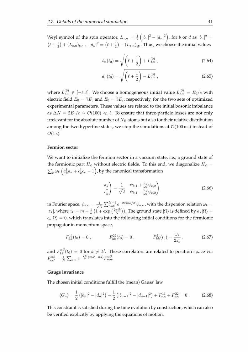
2.7. Details of the numerical simulation 41
Weyl symbol of the spin operator, Lz,n = 12
(|bn|2 − |dn|2
), for b or d as |bn|2 =
(`+ 1
2
)+ (Lz,n)W , |dn|2 =
(`+ 1
2
)− (Lz,n)W . Thus, we choose the initial values
bn(t0) =
√(`+
1
2
)+ L
(0)z,n , (2.64)
dn(t0) =
√(`+
1
2
)− L(0)
z,n , (2.65)
where L(0)z,n ∈ [−`, `]. We choose a homogeneous initial value L(0)
z,n = E0/e withelectric field E0 = 7Ec and E0 = 3Ec, respectively, for the two sets of optimizedexperimental parameters. These values are related to the initial bosonic imbalanceas ∆N = 2E0/e ∼ O(100) `. To ensure that three-particle losses are not onlyirrelevant for the absolute number ofNB atoms but also for their relative distributionamong the two hyperfine states, we stop the simulations at O(100 ms) instead ofO(1 s).
Fermion sector
We want to initialize the fermion sector in a vacuum state, i.e., a ground state ofthe fermionic part Hψ without electric fields. To this end, we diagonalize Hψ =∑
k ωk
(a†kak + c†kck − 1
), by the canonical transformation
(ak
c†k
)=
1√2
(ψk,1 + zk
ωkψk,2
ψk,1 − zkωkψk,2
)(2.66)
in Fourier space, ψk,α = 1√N
∑N−1n=0 e
−2πink/Nψn,α, with the dispersion relation ωk =
|zk|, where zk = m+ 1a
(1 + exp
(2πikN
)). The ground state |Ω〉 is defined by ak|Ω〉 =
ck|Ω〉 = 0, which translates into the following initial conditions for the fermionicpropagator in momentum space,
F 11kk (t0) = 0 , F 22
kk (t0) = 0 , F 21kk (t0) =
ωk2zk
, (2.67)
and Fαβkk′(t0) = 0 for k 6= k′. These correlators are related to position space viaFαβkk′ = 1
N
∑nm e
− 2πiN
(mk′−nk)Fαβmn.
Gauge invariance
The chosen initial conditions fulfill the (mean) Gauss’ law
〈Gn〉 =1
2
(|bn|2 − |dn|2
)− 1
2
(|bn−1|2 − |dn−1|2
)+ F 11
nn + F 22nn = 0 . (2.68)
This constraint is satisfied during the time evolution by construction, which can alsobe verified explicitly by applying the equations of motion.
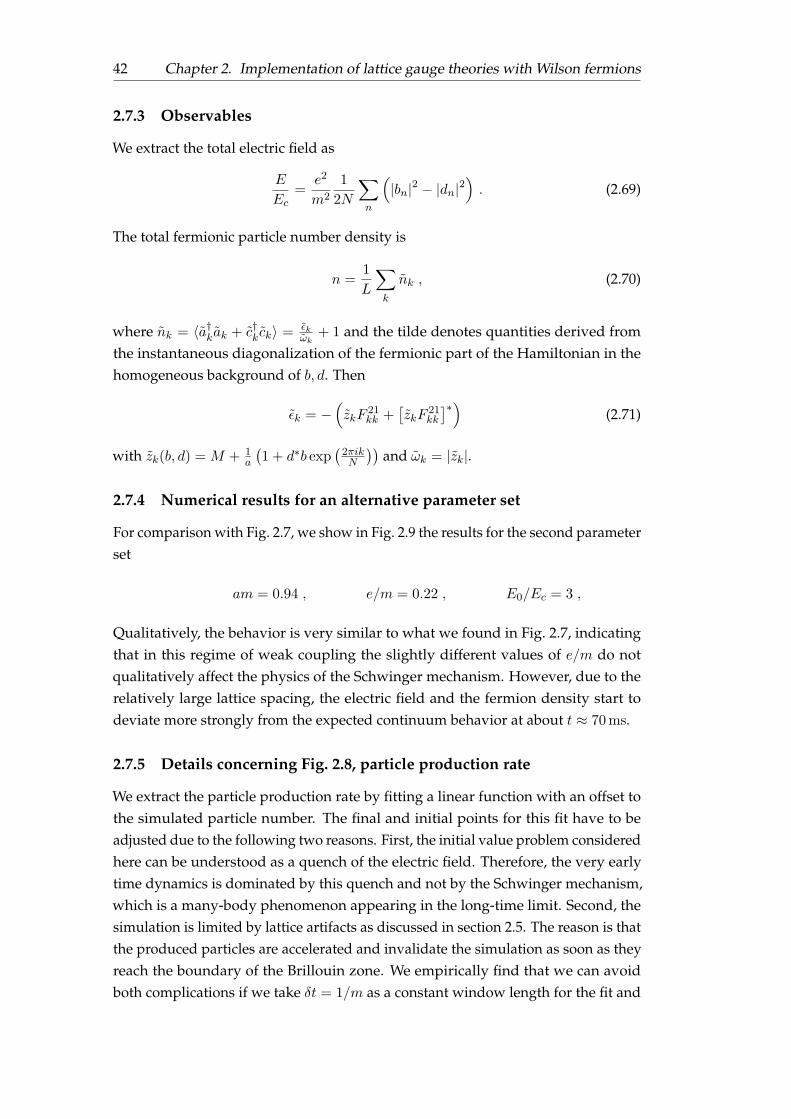
42 Chapter 2. Implementation of lattice gauge theories with Wilson fermions
2.7.3 Observables
We extract the total electric field as
E
Ec=
e2
m2
1
2N
∑
n
(|bn|2 − |dn|2
). (2.69)
The total fermionic particle number density is
n =1
L
∑
k
nk , (2.70)
where nk = 〈a†kak + c†k ck〉 = εkωk
+ 1 and the tilde denotes quantities derived fromthe instantaneous diagonalization of the fermionic part of the Hamiltonian in thehomogeneous background of b, d. Then
εk = −(zkF
21kk +
[zkF
21kk
]∗) (2.71)
with zk(b, d) = M + 1a
(1 + d∗b exp
(2πikN
))and ωk = |zk|.
2.7.4 Numerical results for an alternative parameter set
For comparison with Fig. 2.7, we show in Fig. 2.9 the results for the second parameterset
am = 0.94 , e/m = 0.22 , E0/Ec = 3 ,
Qualitatively, the behavior is very similar to what we found in Fig. 2.7, indicatingthat in this regime of weak coupling the slightly different values of e/m do notqualitatively affect the physics of the Schwinger mechanism. However, due to therelatively large lattice spacing, the electric field and the fermion density start todeviate more strongly from the expected continuum behavior at about t ≈ 70 ms.
2.7.5 Details concerning Fig. 2.8, particle production rate
We extract the particle production rate by fitting a linear function with an offset tothe simulated particle number. The final and initial points for this fit have to beadjusted due to the following two reasons. First, the initial value problem consideredhere can be understood as a quench of the electric field. Therefore, the very earlytime dynamics is dominated by this quench and not by the Schwinger mechanism,which is a many-body phenomenon appearing in the long-time limit. Second, thesimulation is limited by lattice artifacts as discussed in section 2.5. The reason is thatthe produced particles are accelerated and invalidate the simulation as soon as theyreach the boundary of the Brillouin zone. We empirically find that we can avoidboth complications if we take δt = 1/m as a constant window length for the fit and
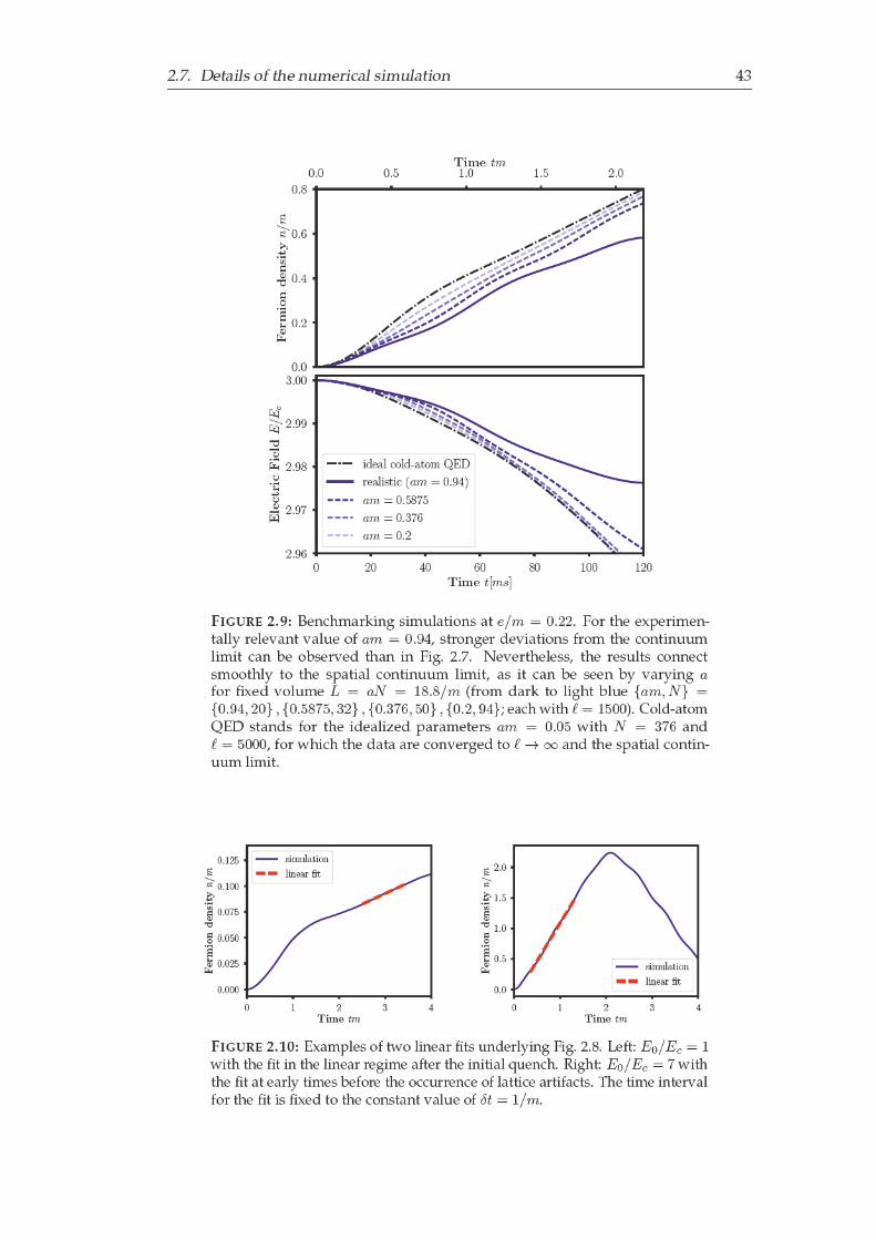
2. 7. D et ail s of t h e n u m e ri c al si m ul ati o n 4 3
0 .0 0 .5 1 .0 1 .5 2 .0Ti m e t m
0 .0
0 .2
0 .4
0 .6
0 .8
Fer
mio
n de
nsit
yn/
m
0 2 0 4 0 6 0 8 0 1 0 0 1 2 0Ti m e t[m s ]
2 .9 6
2 .9 7
2 .9 8
2 .9 9
3 .0 0
Elec
tric
Fi
eld
E/
Ec
i d e al c ol d- at o m Q E D
r e alisti c (a m = 0 .9 4)
a m = 0 .5 8 7 5
a m = 0 .3 7 6
a m = 0 .2
F I G U R E 2. 9: B e n c h m a r ki n g si m ul ati o n s at e / m = 0 .2 2 . F o r t h e e x p e ri m e n-t all y r el e v a nt v al u e of a m = 0 .9 4 , st r o n g e r d e vi ati o n s f r o m t h e c o nti n u u mli mit c a n b e o b s e r v e d t h a n i n Fi g. 2. 7 . N e v e rt h el e s s, t h e r e s ult s c o n n e cts m o ot hl y t o t h e s p ati al c o nti n u u m li mit, a s it c a n b e s e e n b y v a r yi n g af o r fi x e d v ol u m e L = a N = 1 8 .8 / m (f r o m d a r k t o li g ht bl u e a m, N = 0 .9 4 , 2 0 , 0 .5 8 7 5 , 3 2 , 0 .3 7 6 , 5 0 , 0 .2 , 9 4 ; e a c h wit h = 1 5 0 0 ). C ol d- at o mQ E D st a n d s f o r t h e i d e ali z e d p a r a m et e r s a m = 0 .0 5 wit h N = 3 7 6 a n d
= 5 0 0 0 , f o r w hi c h t h e d at a a r e c o n v e r g e d t o → ∞ a n d t h e s p ati al c o nti n-u u m li mit.
0 1 2 3 4Ti m e t m
0 .0 0 0
0 .0 2 5
0 .0 5 0
0 .0 7 5
0 .1 0 0
0 .1 2 5
Fer
mio
n de
nsit
yn/
m
si m ul ati o n
li n e ar fi t
0 1 2 3 4Ti m e t m
0 .0
0 .5
1 .0
1 .5
2 .0
Fer
mio
n de
nsit
yn/
m
si m ul ati o n
li n e ar fi t
F I G U R E 2. 1 0: E x a m pl e s of t w o li n e a r fit s u n d e rl yi n g Fi g. 2. 8 . L eft: E 0 / E c = 1wit h t h e fit i n t h e li n e a r r e gi m e aft e r t h e i niti al q u e n c h. Ri g ht: E 0 / E c = 7 wit ht h e fit at e a rl y ti m e s b ef o r e t h e o c c u r r e n c e of l atti c e a rtif a ct s. T h e ti m e i nt e r v alf o r t h e fit i s fi x e d t o t h e c o n st a nt v al u e of δ t = 1 / m .

44 Chapter 2. Implementation of lattice gauge theories with Wilson fermions
adjust the initial point accordingly. In Fig. 2.10, we show the fits for the largest andsmallest values of E0 that we considered.
In order to estimate the experimental error of the rescaled rate, we tentativelyassume that the bosonic particle number imbalance 〈b†nbn − d†ndn〉 can be measuredwith an absolute accuracy of 10 particles on each site. Then the electric field E/Echas an uncertainty of ∆ (E/Ec) ≈ 0.07, see Eq. (2.69). We have further included thestandard deviation of the fits in the calculation of the errors, although it is negligiblysmall compared to the uncertainty of the electric field. Though both errors arebarely visible in total rate (inset of Fig. 2.8), they lead to significant uncertaintiesof the rescaled rate for larger fields (main panel of Fig. 2.8). Nevertheless, the non-perturbative behavior of the Schwinger rate can be clearly seen, and the qualitativeagreement with the analytical predictions is satisfactory, in particular in light of thefact that the latter are derived for the limit of infinitely large times.
To close this section, let us comment on the experimental challenges to extract therate. The total particle number corresponding to the density n/m = 1 is n/m×L = 9,thus on average O(10) respectively O(0.1) particles are produced over the wholelattice for the initial value E = 7Ec respectively E = 1Ec. Consequently, while thelarge-field case seems reasonably accessible, in the weak-field case the precise detec-tion of the produced particles is very challenging with current technology. Moreover,the measurement of the rate requires an even higher accuracy as compared to thetotal particle number. This is more relevant for the weak-field regime, where theinitial quench dynamics dominates the total particle number production at the shorttimes accessible in the experiment. Concerning the time-scales, we finally notethat the fits for E < 7Ec require an observation time of up to ∼ 400 ms. This maylimit the observability of rates at small fields, since then three body losses becomeincreasingly important, see Sec. 2.5.1.
2.7.6 Results for the initial infinite-mass vacuum
In this subsection, we present results for the experimentally more feasible initial-ization of the free fermion vacuum for infinite mass m. Therefore we initialize thenumerical simulation according to the fermion correlators (2.67) with m→∞ andsolve the same equations of motions as before (with finite m). This corresponds toan additional quench of the fermion mass that is absent in the adiabatic preparationof the fermion vacuum. Figure 2.11 compares the extracted particle number densityand the electric field for this initial condition to the data already shown in the mainpart. Due to the additional mass quench, the initial state is not the true vacuum offree fermions and thus the system starts at non-vanishing fermion density. Eventhough the quantitative behavior of the particle-production is quite different, theproduction rate is very similar to the previously shown result. At the short timespresented here, the electric field also shows qualitatively the same behavior as for
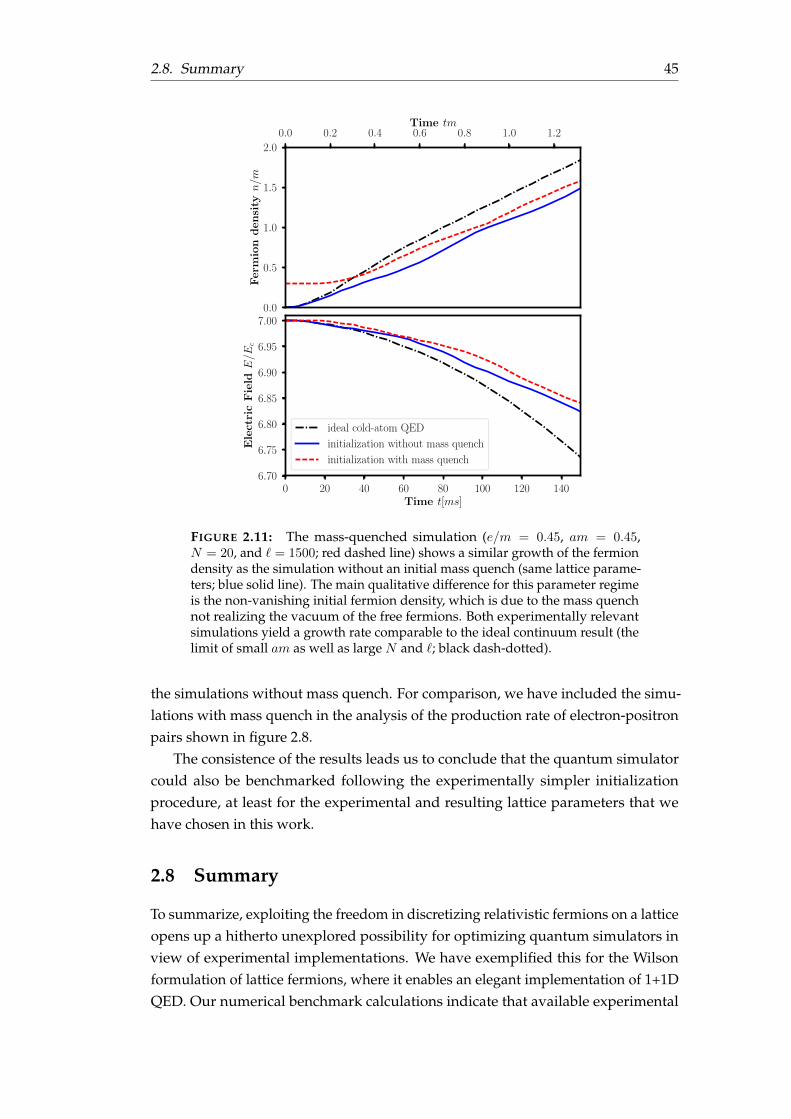
2.8. Summary 45
0.0 0.2 0.4 0.6 0.8 1.0 1.2Time tm
0.0
0.5
1.0
1.5
2.0
Ferm
ion
den
sity
n/m
0 20 40 60 80 100 120 140Time t[ms]
6.70
6.75
6.80
6.85
6.90
6.95
7.00
Ele
ctri
cF
ield
E/E
c
ideal cold-atom QED
initialization without mass quench
initialization with mass quench
FIGURE 2.11: The mass-quenched simulation (e/m = 0.45, am = 0.45,N = 20, and = 1500; red dashed line) shows a similar growth of the fermiondensity as the simulation without an initial mass quench (same lattice parame-ters; blue solid line). The main qualitative difference for this parameter regimeis the non-vanishing initial fermion density, which is due to the mass quenchnot realizing the vacuum of the free fermions. Both experimentally relevantsimulations yield a growth rate comparable to the ideal continuum result (thelimit of small am as well as large N and ; black dash-dotted).
the simulations without mass quench. For comparison, we have included the simu-lations with mass quench in the analysis of the production rate of electron-positronpairs shown in figure 2.8.
The consistence of the results leads us to conclude that the quantum simulatorcould also be benchmarked following the experimentally simpler initializationprocedure, at least for the experimental and resulting lattice parameters that wehave chosen in this work.
2.8 Summary
To summarize, exploiting the freedom in discretizing relativistic fermions on a latticeopens up a hitherto unexplored possibility for optimizing quantum simulators inview of experimental implementations. We have exemplified this for the Wilsonformulation of lattice fermions, where it enables an elegant implementation of 1+1DQED. Our numerical benchmark calculations indicate that available experimental
46 Chapter 2. Implementation of lattice gauge theories with Wilson fermions
resources may access the Schwinger mechanism of particle-anti-particle production,and in particular extract the non-perturbative onset of the production rate. Theperformance of the quantum simulator may even be further improved by resortingto mixtures with enhanced spin-changing collisions, such as sodium–potassium.
As a final aim of a cold-atom quantum simulator, it stands to advance into pa-rameter regimes that are not accessible to computer simulations. For the optimizedparameters in the experimental implementation proposed in this work, the dimen-sionless coupling e/m and the lattice spacing am cannot be tuned independently.Rather, as one is increased, the other one has to be decreased and vice versa, whichcan be exploited as follows. First, one can use the particle-production rate in theregime of small e/m (and thus large am) to benchmark the quantum simulator usingnumerical methods. The experiment may then proceed into the relevant regimeof strong coupling, which for the optimized parameters permits us also to reducethe lattice spacing. This regime of strong coupling is not accessible within currentnumerical simulations such as the functional integral method employed here. Theproposed experiment involves 20× 2 = 40 fermionic degrees of freedom interactingwith 20 BECs of O(1000) atoms each, resulting in a Hilbert space size that is alsobeyond the capability of exact diagonalization methods. While the specific caseof 1+1D gauge theories can also be treated efficiently using methods based on thedensity matrix renormalization group [96, 102–104], these approaches are typicallylimited to low dimensions and equilibrium properties or short time dynamics. Sincea quantum simulation of lattice gauge theories may in principle be free of suchlimitations, a generalization of our present work using Wilson fermions to, e.g.,higher dimensions will be extremely interesting.
Our work also opens an interesting pathway for future theoretical investigations.By casting Wilson fermions in the compact form of the Hamiltonian in Eq. (2.6),the free lattice theory becomes manifestly equivalent to the Su-Schrieffer-Heegermodel, one of the simplest models displaying non-trivial topological properties [105].Indeed, the topological properties of free Wilson fermions have been considered inRef. [74] and, very recently, in Ref. [76]. Such topological properties in the context ofinteracting gauge theories are the subject of the final chapter 4 of the first part of thisthesis.

2.A. The Wannier-Stark system 47
Appendix: Cold atoms in a tilted optical lattice and Landau-Zener tunneling
In this appendix, we give more details about the description of cold atoms a tiltedoptical lattice. In section 2.A, we discuss the energy levels of the Wannier-Stark lad-der, their wavefunctions and estimated lifetime. In section 2.B, we present a simplederivation of the Landau-Zener formula, from which we deduce the Schwinger pairproduction rate.
2.A The Wannier-Stark system
In this section, we summarize some important aspects of the Wannier-Stark problemfollowing the detailed review [93]. Consider a quantum-mechanical particle ofmass m moving in a one-dimensional periodic potential V (x + a) = V (x) withlattice spacing a, subject to a constant force F . For later purposes, we also assume areflection invariant potential V (−x) = V (x). The corresponding Hamiltonian reads
HW = H0 + Fx , H0 =p2
2m+ V (x) , (2.72)
where H0 denotes the unperturbed Hamiltonian (F = 0). Most importantly, thelinear term breaks the discrete symmetry x→ x+ a. Thus for an eigenstate HWΨ =
E0Ψ, we can generate a ladder of new eigenstates with different energies
El = E0 + laF , l ∈ Z , (2.73)
by translation over l periods. This is the so-called Wannier-Stark (WS) ladder. Weexpect any superposition of these states to show oscillations with the Bloch periodTB = 2π
aF . However, the tilt leaves the full Hamiltonian (F 6= 0) unbounded frombelow, such that HW has a continuous spectrum. In fact, the states of the WS ladderare merely resonances,
Eα,l = Eα + laF − i
2Γα , (2.74)
with a finite lifetime τ = 1Γα
and band index α. There exist powerful methods todetermine the precise value of Eα,l and the corresponding eigenfunctions, see [93].For our purposes, it suffices to treat the eigenfunctions and the real part of Eα,lwithin a tight-binding approximation and determine the imaginary part of Eα,l froma Landau-Zener tunneling estimate.

48 Chapter 2. Implementation of lattice gauge theories with Wilson fermions
2.A.1 Tight-binding model
It is well known that the eigenfunctions of the F = 0 case are Bloch waves,
H0φα,k = εα(k)φα,k , φα,k(x) = eikxuα,k(x) , uα,k(x+ a) = uα,k(x) , (2.75)
where the quasi-momentum k is restricted to the first Brillouin zone −πa ≤ k < π
a
because of the periodicity of the Bloch bands, εα(k) = εα(k + 2π
a
). We may choose
the phase of the complex Bloch functions φα,k(x) to make them periodic and analyticfunctions of k, such that we can expand them in a Fourier series with coefficients
ψα,l(x) =
ˆ π/a
−π/adk e−iklaφα,k(x) (2.76)
known as Wannier functions. They are exponentially localized in the l-th cellof the potential and form a complete set w.r.t. both indices, α and l. The tight-binding approximation is derived by calculating matrix elements in the Wannierbasis, keeping only the diagonal elements of Fx, as well as diagonal and secondarydiagonal elements of H0 w.r.t. l, i.e.,
HTB =∑
α,l
〈ψα,l|H0 + Fx|ψα,l〉|ψα,l〉〈ψα,l|
+∑
α,l
〈ψα,l|H0|ψα,l+1〉|ψα,l〉〈ψα,l+1|+ 〈ψα,l+1|H0|ψα,l〉|ψα,l+1〉〈ψα,l| .
(2.77)
In particular, H0 gives the energy contribution
〈ψα,l|H0|ψα,l〉 =
ˆdxψ∗α,l(x)H0ψα,l(x) =
ˆdx dk dq φα,q(x)eiqlaH0e
−iklaφα,k(x)
=a
2π
ˆdk dq ei(q−k)laδααδkqεα(k) =
a
2π
ˆdk εα(k) ≡ εα (2.78)
and similarly the hopping element
〈ψα,l|H0|ψα,l+1〉 =
ˆdxψ∗α,l+1(x)H0ψα,l(x) =
a
2π
ˆdk e−ikaεα(k) ≡ Jα , (2.79)
where every momentum integration is restricted to the first Brillouin zone. SinceBloch waves are eigenfunctions of the translation operator Tax = x+ a, the Wannierfunctions obey ψα,l+1(x) = ψα,l(x− a) from which we find
〈ψα,l+n|Fx|ψα,l+n〉 − 〈ψα,l|Fx|ψα,l〉 = naF , n ∈ N. (2.80)
Dropping an irrelevant constant, the tight-binding Hamiltonian becomes
HTB =∑
α,l
(εα + laF ) |ψα,l〉〈ψα,l|+ Jα [|ψα,l〉〈ψα,l+1|+ h.c.] , (2.81)
2.A. The Wannier-Stark system 49
where we have used Jα = J∗α due to the symmetry εα(−k) = εα(k). To diagonalizeHTB , we make the ansatz |Ψα,l〉 =
∑m cm (α, l) |ψα,l〉. The eigenvalue equation
HTB|ψα,l〉 = Eα,l|ψα,l〉 implies
cm+1(α, l) + cm−1(α, l) =Eα,l − (εα +maF )
Jαcm(α, l) , (2.82)
i.e., the expansion coefficients obey the same recurrence relation as solutions to theBessel equation
z2B′′ν (z) + zB′ν(z) +(z2 − ν2
)Bν(z) = 0 ,
2ν
zBν(z) = Bν+1(z) +Bν−1(z) .
(2.83)
Normalizability in the infinitely large system determines the coefficients to be Besselfunctions of the first kind4,
cm(α, l) = Jm−l
(2JαaF
), (2.84)
and determines the spectrum to be the WS ladder, Eα,l = εα + laF . The physicalinterpretation is the following:
• For F = 0, the energy levels of the Wannier states |ψα,l〉 coincide for everyl and the tunneling Jα couples them into Bloch states |φα,k〉 =
∑l eikl|ψα,l〉,
which produces the Bloch bands εα(k) = εα + 2Jα cos(ak).
• For F 6= 0, the degeneracy is lifted and tunneling is suppressed, such that wefind the Wannier-Stark functions |Ψα,l〉 =
∑m Jm−l
(2JαaF
)|ψα,l〉 as eigenfunc-
tions corresponding to the discrete WS ladder, which are effectively localizedon a few lattice sites.
2.A.2 Landau-Zener tunneling
Since the tight-binding approximation is unable to determine the lifetime of theWS resonances, we make a semi-classical estimate using the Landau-Zener (LZ)formula,
PLZ = exp
(− π∆2
4 |ε(∆ = 0)|
), (2.85)
which yields the asymptotic probability for a transition between two energy eigen-states at an avoided crossing. Here, ∆ denotes the energy gap between the twostates and |ε(∆ = 0)| is the “velocity” of the crossing at vanishing gap. We restrictourselves to the lowest band in the tight-binding model described above. ∆ is thenjust given by the band gap between the ground band and the first excited band andit remains to determine the “velocity” |ε(∆ = 0)|.
4There should be no danger of confusing the tunneling elements Jα with the Bessel functions Jm−l.

50 Chapter 2. Implementation of lattice gauge theories with Wilson fermions
The gauge transformation ψ(t, x)→ ψ(t, x)e−iFxt brings the Hamiltonian (2.72)into the form
H ′ =(p− Ft)2
2m+ V (x) . (2.86)
This observation demonstrates that any Bloch state (semi-classically) has a time-dependent momentum k(t) = k0 − Ft, which explores the first Brillouin zone andgets periodically reflected at its boundaries, |k| = π
a . For simplicity, we considera single LZ transition at the position of the avoided crossing between the groundband and the first excited band, i.e., at |kavoided| = π
a , for each Bloch period TB . Inthe limit of vanishing gap, the dispersion relation becomes the one of a free particle,ε(k) = k2
2m , such that we can calculate the “velocity”
|ε(∆ = 0)| =∣∣∣∣dε(k)
dk
dk(t)
dt
∣∣∣∣∆=0 , k=π
a
=π
maF =
2a
πErF , (2.87)
where we have introduced the recoil energy Er = π2
2ma2 . Thus we approximate thedecay rate of the ground band as
Γ ≈ 1
TBPLZ =
aF
2πexp
(− π2∆2
8EraF
). (2.88)
Note that we have implicitly assumed that the system is “off resonance”, in thesense that no two states of WS ladders from different bands are degenerate. Weshould keep in mind that such a degeneracy may drastically decrease the lifetimedue to resonant LZ tunneling.
2.A.3 Cold atoms in a tilted lattice
For the relevant case of cold quantum gases in an optical lattice, we consider thepotential
V (x) = V0 sin2(πxa
). (2.89)
The case of F = 0 is well-known [106] and the corresponding eigenvalue problemcan be brought into the form of a Mathieu equation,
[∂2y +
(E
V0− s)
+ s cos(2y)
]ψE(y) = 0 , (2.90)
where y = πxa and the parameter s = 2
√V0Er
controls the lattice depth. The dispersionrelation for the ground band is given by
ε(k) =ω0
2− 2J cos(ka) , (2.91)

2.B. Derivation of the Landau-Zener formula 51
where ω0 = sEr. The width J of the band can be expressed with the help of Mathieufunctions. In the limit of a deep lattice, s 1, one finds
J ≈ ω0
(8s
π2
)1/4
e−s + . . . . (2.92)
Consequently, the tilted lattice (F 6= 0) features the WS ladder
El =ω0
2+ laF , l ∈ Z (2.93)
and nearest-neighbor hopping is suppressed for
aF |J | = 2J . (2.94)
Additionally, experiments are limited by the lifetime
τ =1
Γ=
2π
aFexp
(π2∆2
8EraF
)≈ 2π
aFexp
(π2s2Er
8aF
), (2.95)
where the band gap can be calculated from Mathieu eigenvalues as ∆ ≈ ω0 in thelimit s 1. In this limit, we may further approximate the Wannier functions of theground band at site l as harmonic oscillator eigenfunctions
ψl(x) =(πa2
HO)−1/4
exp
(−(x− xl)2
2a2HO
), (2.96)
where xl denotes the l-th minimum of V (x) and the harmonic oscillator length aHO =
(mωHO)−1/2 is obtained by matching the trapping frequencies with the curvature ofthe potential around the minima, i.e., mω2
HO = V ′′(xl). For the calculation of overlapintegrals involving Wannier-Stark functions we use the next-to leading order in theirexpansion as
Ψl(x) =∑
m
Jm−l
(− 4J
aF
)ψm(x) ≈ ψl(x)− 2J
aF[ψl+1(x)− ψl−1(x)] , (2.97)
where we made use of the series expansion of Bessel’s functions as
Jn(z) =∞∑
j=0
(−1)j
j! Γ(n+ j + 1)
(z2
)2j+n. (2.98)
2.B Derivation of the Landau-Zener formula
Consider a two-level system described by the Hamiltonian
HLZ =1
2
(vt ∆
∆ −vt
). (2.99)
52 Chapter 2. Implementation of lattice gauge theories with Wilson fermions
It has the eigenvalues λ±(t) = ±12
√∆2 + (vt)2, i.e., for ∆ 6= 0 the system exhibits
an avoided crossing. Let us assume that we prepare the ground state in the infinitepast. What is the probability to find the system in the excited state in the infinitefuture? The answer is given by the Landau-Zener (LZ) as discussed below.
We give a convenient solution of the problem [107] that does not rely on theexplicit solution of the Schrödinger equation. Writing the general wavefunctionψ(t) = (α(t), β(t))T with the initial condition |ψ(t)|2 → (1, 0)T (t→ −∞), it is ourtask to calculate |α(t)|2 at t → ∞. Applying the Schrödinger equation i∂tψ(t) =
Hψ(t) twice, the components decouple and we find
−α(t) =
[iv
2+
(∆
2
)2
+
(vt
2
)2]α(t) . (2.100)
Instead of solving this equation explicitly, we use the fact that
ˆ ∞−∞
dtα(t)
α(t)= log
[α(∞)
α(−∞)
](2.101)
and evaluate the left-hand side as follows. If the problem has a convergent solution,then
α(t) ' |α|e−iϕα(t) (2.102)
as an asymptotic expansion at t → ±∞ with a time-dependent phase ϕα(t) and atime-independent amplitude |α|. Then the e.o.m. becomes
ϕ2α(t)−
[(∆
2
)2
+
(vt
2
)2]
+ i[ϕα(t)− v
2
]α(t) = 0 , (2.103)
which is solved by
ϕα(t) =v
2, ϕα(t) = ±v|t|
2
√1 +
(∆
vt
)2
=vt
2
1 +
1
2
(∆
vt
)2
+O[(
∆
vt
)4]
.
(2.104)
Consequently, we approximate
α(t)
α(t)' −iϕα(t) ≈ −i
(vt
2+
∆2
4vt
)+ . . . (2.105)
and solve the integral by extending it to the complex plane and applying Cauchy’stheorem,
ˆ ∞−∞
dtα(t)
α(t)= −
ˆC±
dzα(z)
α(z), (2.106)
2.B. Derivation of the Landau-Zener formula 53
where C± denotes an upper resp. lower infinite half-circle given by z = Re±iθ withθ ∈ [0, π] and R→∞. Therefore
log
[α(∞)
α(−∞)
]= ±
ˆ π
0dθ
(vR2
2e±2iθ +
∆2
4v
)= ±π∆2
4v. (2.107)
Normalizability requires the negative sign, such that
α(∞) = α(−∞) exp
(−π∆2
4v
). (2.108)
Using the initial value |α(−∞)|2 = 1, we arrive at the celebrated LZ formula for theprobability to find the system in the excited state,
P ≡ |α(∞)|2 = exp
(−π∆2
2v
). (2.109)
The final result depends on the energy gap ∆ between the two states. We want toemphasize that the second parameter v can be obtained as
v
2=
∣∣∣∣dλ±(t)
dt
∣∣∣∣∆=0
, (2.110)
i.e., it describes the “slope” of the energy levels at the avoided crossing in the limit∆→ 0.
2.B.1 Schwinger pair production from Landau-Zener tunneling
Using the Landau-Zener formula, we also provide a heuristic derivation of theSchwinger pair production, Eq. (2.58), in the following. The bare fermion vacuumof QED can be seen as an insulator with mass gap 2m. Applying a constant externalelectric field modifies the momentum as p→ p+ eEt. Focusing first on p = 0, theprobability of exciting a fermion-antifermion pair is equivalent to the Landau-Zenerproblem with v = eE and ∆ = 2m. This observation immediately implies that theelectric field results in an occupation of
n0 = exp
(−πm
2
eE
). (2.111)
Due to the dispersion ω(p) =√p2 +m2, the pair production is exponentially sup-
pressed for any p 6= 0. Neglecting any backreaction of the produced fermions onthe electric field, the former will simply shift through momentum space with p(t) =
p+ eEt. We thus expect the particle number distribution n(p, t) = n0Θ(p)Θ(eEt− p)for an external field turned on at t = 0. Then the total particle number density is
n(t) = 2
ˆ ∞−∞
dp
2πn(p, t) =
eEt
πexp
(−πm
2
eE
), (2.112)

54 Chapter 2. Implementation of lattice gauge theories with Wilson fermions
where we included a factor of 2 to account for fermions and anti-fermions. Taking atime derivative, we reproduce Eq. (2.58). This argument also gives another pointof view on the validity of the Schwinger rate. It neglects any switch-on effect ofthe electric field and can therefore only be valid at sufficiently late times when theLandau-Zener formula becomes accurate. At the same time, the backreaction of theproduced fermions on the electric field is neglected, which invalidates the rate infully dynamical QED at late times. Moreover, the whole argument is based on atunneling process across the mass gap. Hence, we can the expect the pair productionrate to be correct in an intermediate regime of not too early and not too late times,parametrically 1/m . t . 1/e, in a weak-coupling regime e m with strong fieldsE & m2/e.
55
Chapter 3
Realization of a scalable buildingblock for U(1) gauge theories
This chapter and its appendices 3.A and 3.B are based on the article [16] with thefigures and large parts of the text taken from it. The authors of [16] contributedas follows: A. Mil, A. Hegde, A. Xia and R. P. Bhatt set up the experiment andperformed the measurements; A. Mil and myself performed the data analysis;P. Hauke, J. Berges and myself developed the theory; P. Hauke, J. Berges, M. K.Oberthaler and F. Jendrzejewski supervised the project. All authors participatedin the writing of the manuscript [16] and I made significant contributions to thewording and structuring of the text. In the appendices 3.C and 3.D, I includeadditional related material that was not printed in [16]. The article [16] is alsocovered in the experimental doctoral thesis by A. Mil [108].
3.1 Proposed implementation
Our aim is the development of a scalable and highly tunable platform for a continu-ous U(1) gauge theory, such as realized in QED. Here we enforce the defining localU(1) symmetry through spin-changing collisions in atomic mixtures, as discussedin the previous chapter. This promising mechanism to protect gauge-invariancehas been put forward in various proposals [10, 18, 22, 29] but so far it was notdemonstrated experimentally. In this chapter we demonstrate the engineering ofan elementary building block in a mixture of bosonic atoms, demonstrate its hightunability, and verify its faithful representation of the desired model.
Building on the results of the previous chapter, we further propose an extendedimplementation scheme in an optical lattice, where each lattice well constitutes anelementary building block that contains both matter and gauge fields. Repetitionsof this elementary unit can be connected using laser-assisted tunneling. Importantly,gauge and matter fields are spatially arranged in such a way that the spin-changingcollisions occur within single lattice wells, in contrast to previous proposals [10,18, 22, 29] where the gauge and matter fields were spatially separated and spin-changing collisions had to be accompanied by hopping across different sites of theoptical lattice.
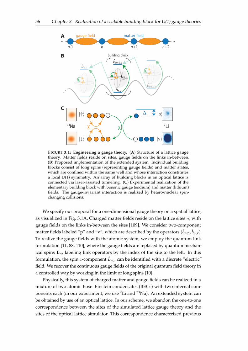
56 Chapter 3. Realization of a scalable building block for U(1) gauge theories
matter field
Cp
v
gauge field
7Li23Na χ λ
Δ
B
A
n+1 n+2nn-1
... ...
bn+1,pˆ
bn,vˆ
Lnˆ
building block
bn,pˆ
bn+1,vˆ
FIGURE 3.1: Engineering a gauge theory. (A) Structure of a lattice gaugetheory. Matter fields reside on sites, gauge fields on the links in-between.(B) Proposed implementation of the extended system. Individual buildingblocks consist of long spins (representing gauge fields) and matter states,which are confined within the same well and whose interaction constitutesa local U(1) symmetry. An array of building blocks in an optical lattice isconnected via laser-assisted tunneling. (C) Experimental realization of theelementary building block with bosonic gauge (sodium) and matter (lithium)fields. The gauge-invariant interaction is realized by hetero-nuclear spin-changing collisions.
We specify our proposal for a one-dimensional gauge theory on a spatial lattice,as visualized in Fig. 3.1A. Charged matter fields reside on the lattice sites n, withgauge fields on the links in-between the sites [109]. We consider two-componentmatter fields labeled “p” and “v”, which are described by the operators (bn,p, bn,v).To realize the gauge fields with the atomic system, we employ the quantum linkformulation [11, 88, 110], where the gauge fields are replaced by quantum mechan-ical spins Ln, labeling link operators by the index of the site to the left. In thisformulation, the spin z-component Ln,z can be identified with a discrete “electric”field. We recover the continuous gauge fields of the original quantum field theory ina controlled way by working in the limit of long spins [10].
Physically, this system of charged matter and gauge fields can be realized in amixture of two atomic Bose–Einstein condensates (BECs) with two internal com-ponents each (in our experiment, we use 7Li and 23Na). An extended system canbe obtained by use of an optical lattice. In our scheme, we abandon the one-to-onecorrespondence between the sites of the simulated lattice gauge theory and thesites of the optical-lattice simulator. This correspondence characterized previous
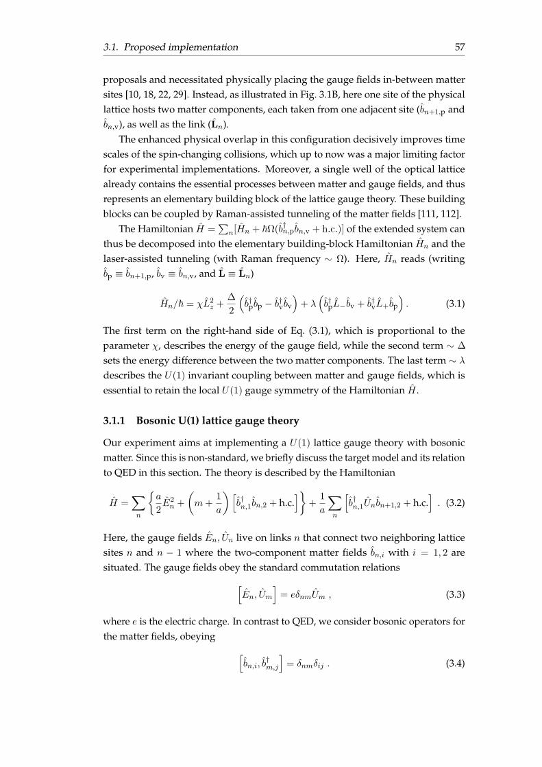
3.1. Proposed implementation 57
proposals and necessitated physically placing the gauge fields in-between mattersites [10, 18, 22, 29]. Instead, as illustrated in Fig. 3.1B, here one site of the physicallattice hosts two matter components, each taken from one adjacent site (bn+1,p andbn,v), as well as the link (Ln).
The enhanced physical overlap in this configuration decisively improves timescales of the spin-changing collisions, which up to now was a major limiting factorfor experimental implementations. Moreover, a single well of the optical latticealready contains the essential processes between matter and gauge fields, and thusrepresents an elementary building block of the lattice gauge theory. These buildingblocks can be coupled by Raman-assisted tunneling of the matter fields [111, 112].
The Hamiltonian H =∑
n[Hn + ~Ω(b†n,pbn,v + h.c.)] of the extended system canthus be decomposed into the elementary building-block Hamiltonian Hn and thelaser-assisted tunneling (with Raman frequency ∼ Ω). Here, Hn reads (writingbp ≡ bn+1,p, bv ≡ bn,v, and L ≡ Ln)
Hn/~ = χL2z +
∆
2
(b†pbp − b†vbv
)+ λ
(b†pL−bv + b†vL+bp
). (3.1)
The first term on the right-hand side of Eq. (3.1), which is proportional to theparameter χ, describes the energy of the gauge field, while the second term ∼ ∆
sets the energy difference between the two matter components. The last term ∼ λdescribes the U(1) invariant coupling between matter and gauge fields, which isessential to retain the local U(1) gauge symmetry of the Hamiltonian H .
3.1.1 Bosonic U(1) lattice gauge theory
Our experiment aims at implementing a U(1) lattice gauge theory with bosonicmatter. Since this is non-standard, we briefly discuss the target model and its relationto QED in this section. The theory is described by the Hamiltonian
H =∑
n
a
2E2n +
(m+
1
a
)[b†n,1bn,2 + h.c.
]+
1
a
∑
n
[b†n,1Unbn+1,2 + h.c.
]. (3.2)
Here, the gauge fields En, Un live on links n that connect two neighboring latticesites n and n − 1 where the two-component matter fields bn,i with i = 1, 2 aresituated. The gauge fields obey the standard commutation relations
[En, Um
]= eδnmUm , (3.3)
where e is the electric charge. In contrast to QED, we consider bosonic operators forthe matter fields, obeying
[bn,i, b
†m,j
]= δnmδij . (3.4)

58 Chapter 3. Realization of a scalable building block for U(1) gauge theories
Nevertheless, the Hamiltonian is gauge-invariant,[H, Gn
]= 0, with the Gauss’ law
operator
Gn = En − En−1 − e∑
i
b†n,ibn,i (3.5)
that generates U(1) gauge transformation. Consequently, the model is a proper U(1)
lattice gauge theory.The Hamiltonian in the form (3.2) is motivated by our previous proposal, dis-
cussed in chapter 2, to implement QED with Wilson fermions with mass m andlattice spacing a. With the identifications
χ↔ ae2
2, λ↔ 1
a√L(L+ 1)
, Ω↔ m+1
a, (3.6)
our proposed extended implementation realizes the target model in the limit oflarge spin length L of the “gauge” bosons when tuning ∆ → 0. When bosonicmatter is used instead of fermionic matter, for QED in three spatial dimensions it isknown that Lorentz invariance remains broken even in the continuum limit, whichprohibits an interpretation as a relativistic quantum field theory. Similarly, in onespatial dimension, we expect that the theory with bosonic matter will not lead to arelativistic continuum theory. Thus, to obtain a well-behaved continuum limit, weintend to replace the bosons by fermions in future experiments. Following Ref. [29],after replacing the bosons in the experiment by fermions, the above Hamiltonianwill describe a standard lattice discretization of QED. In particular, the fermionicversion of the model has a well-behaved continuum limit where Lorentz invariance,which is explicitly broken by the lattice discretization, is recovered.
3.2 Experimental realization of the building block
We implement the elementary building block Hamiltonian Hn with a mixture of300× 103 sodium and 50× 103 lithium atoms as sketched in Fig. 3.1C (see appen-dices 3.A and 3.B for details). Both species are kept in an optical dipole trap suchthat the external trapping potential is spin-insensitive for both species. An externalmagnetic bias field of B ≈ 2 G suppresses any spin change energetically, such thatonly the two Zeeman levels, mF = 0 and 1, of the F = 1 hyperfine ground statemanifolds are populated during the experiment. The 23Na states are labeled as|↑〉 = |mF = 0〉 and |↓〉 = |mF = 1〉, on which the spin operator L associated to thegauge field acts. The first term of (3.1) is then identified with the one-axis twistingHamiltonian [113, 114]. We label the 7Li states as “particle” |p〉 = |mF = 0〉 and“vacuum” |v〉 = |mF = 1〉, in accordance with the matter field operators bp andbv. With this identification, the second term arises from energy shifts due to theexternal magnetic field and density interactions. Finally, the term ∼ λ is physicallyimplemented by hetero-nuclear spin-changing interactions [115].

3.2. Experimental realization of the building block 59
μ
F = 2
FIGURE 3.2: Tunability of the initial conditions. The normalized spin z-component Lz/L of 23Na atoms as a function of the preparation pulse length,which shows that the gauge field can be tuned experimentally over the entirepossible range. Simultaneously, the particle number Np/N of 7Li is kept in thevacuum state. The inset shows a sketch of the experimental protocol used fortuning the initial conditions.
3.2.1 Initialization
The resulting setup is highly tunable, as we now demonstrate experimentally on thebuilding block. We achieve tunability of the gauge field through a two-pulse Rabicoupling of the Na atoms between |↓〉 and |↑〉 using an intermediate |F = 2〉 state,which yields a desired value of Lz/L = (N↑ −N↓)/(N↑ +N↓) (Fig. 3.2). At the sametime, we keep the 7Li atoms in |v〉, corresponding to the initial vacuum of the mattersector at ∆ → ∞, with 1% detected in |p〉 (see Fig. 3.2).
3.2.2 Dynamics of spin-changing collisions
If the gauge invariant coupling is turned off by removing the Na atoms from thetrap, we observe no dynamics in the matter sector beyond the detection noise. Onthe other hand, once the gauge field is present, the matter sector clearly undergoesa transfer from |v〉 to |p〉 for proper initial conditions, as illustrated in Fig. 3.3Afor an initialization to NG = −0.188 at a magnetic field of BA = 2.118(2)G 1. Thisobservation demonstrates the controlled operation of hetero-nuclear spin-changingcollisions implementing the gauge-invariant dynamics in the experiment.
To quantify our observations, we extract the ratio NP , with N = Np + Nv, asa function of time as presented in Fig. 3.3B. We observe non-zero NP , describing“particle production”, on a timescale of few tens of ms, with up to 6% of the totalN being transferred to |p〉. This value is consistent with our expectations fromconservation of the initial energy E0/ = χL2
z −∆Nv/2, from which we estimate amaximum amplitude on the order of a few percent (see appendix 3.D for a simpleexplanation of the maximum amplitude in terms of a particle oscillating in ananharmonic potential). Due to the much larger 23Na condensate, the expected
1All uncertainties given in this chapter correspond to a 68% confidence interval.

60 Chapter 3. Realization of a scalable building block for U(1) gauge theories
pA
B
FIGURE 3.3: Dynamics of particle production. (A) The number density dis-tribution in state |p〉 as a function of time for NG = −0.188. (B) The cor-responding particle number Np/N . The blue circles give the experimentalvalues with bars indicating the statistical error on the mean. The red curveis the theoretical mean-field prediction of Hamiltonian (3.1) with parametersdetermined from a fit of the data in Fig. 3.4A and phenomenological damping.The shaded area indicates the experimental noise floor. The dashed line marksthe time of 30ms as it is used for the experimental sequence generating thedata in Fig. 3.4.
corresponding change in NG is ∼ 2%, which is currently not detectable with ourimaging routine (see appendix 3.A). Coherent oscillations in NP are seen to persistfor about 100ms.
3.2.3 Tunability of the model parameters
We display NP /N over the entire range of initial Lz in Fig. 3.4, keeping a fixedtime of 30ms. The upper panel A corresponds to the same experimental setting asin Fig. 3.3. A clear resonance for particle production can be seen around Lz/L −0.5, approximately captured by the resonance condition 2χLz ∼ ∆ (see section3.3 below). The asymmetry of the resonance is a clear manifestation of the non-linearity of the dynamics (see appendix 3.D for a detailed discussion of the non-linearity). As we reduce the magnetic field B, presented in Fig. 3.4B-D, we observea shift of the resonant particle production together with a reduction in amplitude,which continues to be qualitatively captured by the resonance condition 2χLz ∼∆. The maximal amplitude of the particle production is necessarily reduced bythe conservation of total magnetization as the resonant peak is pushed closer toLz/L = −1. For fields that are smaller than Bmin ≈ 1.96G, the matter field andgauge field dynamics become too off-resonant and particle production can no longerbe observed.
We compare the experimental results to the mean-field predictions of Hamilto-nian (3.1) for chosen χ, λ and ∆(Lz, B) = ∆0 +∆LLz/L+∆B(B−BA)/BA (see 3.B
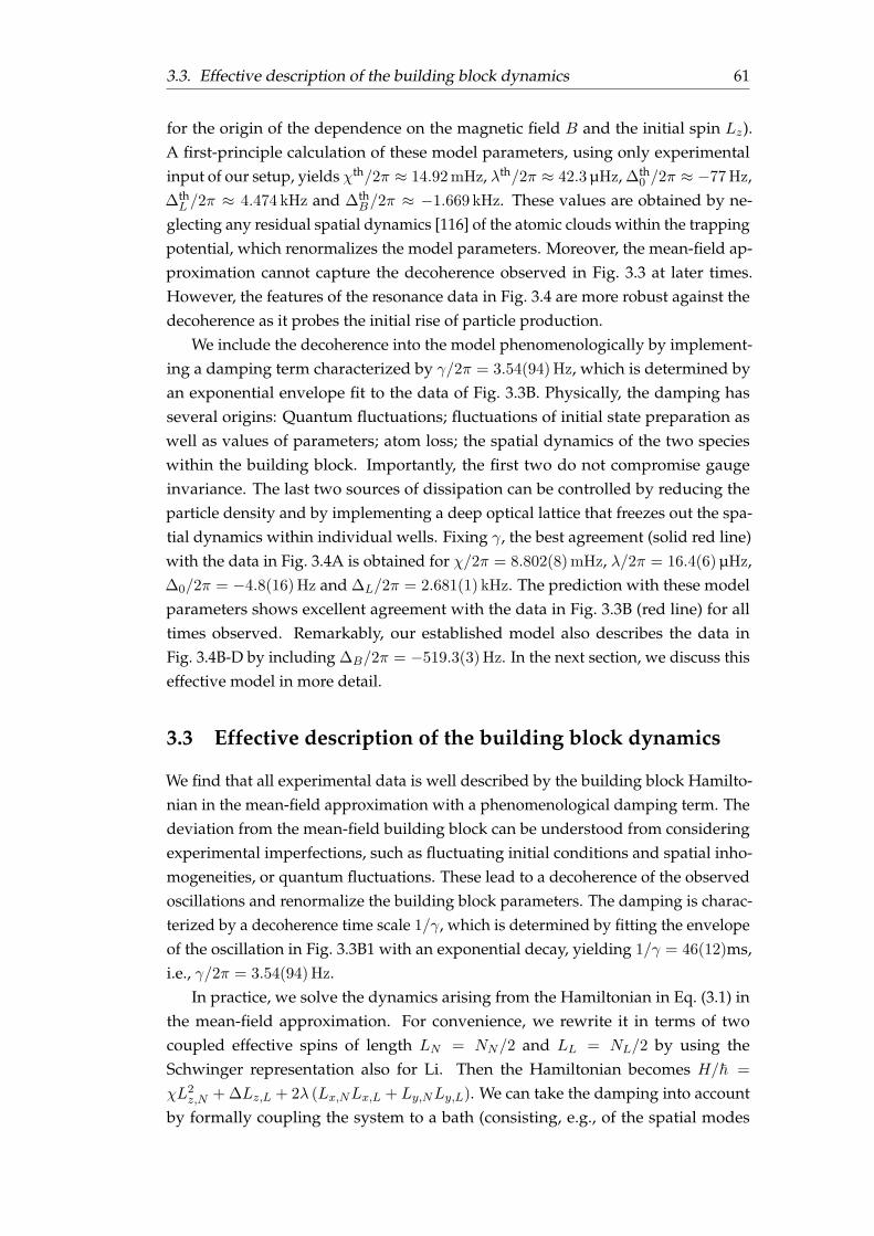
3.3. Effective description of the building block dynamics 61
for the origin of the dependence on the magnetic field B and the initial spin Lz).A first-principle calculation of these model parameters, using only experimentalinput of our setup, yields χth/2π ≈ 14.92 mHz, λth/2π ≈ 42.3 µHz, ∆th
0 /2π ≈ −77 Hz,∆thL /2π ≈ 4.474 kHz and ∆th
B/2π ≈ −1.669 kHz. These values are obtained by ne-glecting any residual spatial dynamics [116] of the atomic clouds within the trappingpotential, which renormalizes the model parameters. Moreover, the mean-field ap-proximation cannot capture the decoherence observed in Fig. 3.3 at later times.However, the features of the resonance data in Fig. 3.4 are more robust against thedecoherence as it probes the initial rise of particle production.
We include the decoherence into the model phenomenologically by implement-ing a damping term characterized by γ/2π = 3.54(94) Hz, which is determined byan exponential envelope fit to the data of Fig. 3.3B. Physically, the damping hasseveral origins: Quantum fluctuations; fluctuations of initial state preparation aswell as values of parameters; atom loss; the spatial dynamics of the two specieswithin the building block. Importantly, the first two do not compromise gaugeinvariance. The last two sources of dissipation can be controlled by reducing theparticle density and by implementing a deep optical lattice that freezes out the spa-tial dynamics within individual wells. Fixing γ, the best agreement (solid red line)with the data in Fig. 3.4A is obtained for χ/2π = 8.802(8) mHz, λ/2π = 16.4(6) µHz,∆0/2π = −4.8(16) Hz and ∆L/2π = 2.681(1) kHz. The prediction with these modelparameters shows excellent agreement with the data in Fig. 3.3B (red line) for alltimes observed. Remarkably, our established model also describes the data inFig. 3.4B-D by including ∆B/2π = −519.3(3) Hz. In the next section, we discuss thiseffective model in more detail.
3.3 Effective description of the building block dynamics
We find that all experimental data is well described by the building block Hamilto-nian in the mean-field approximation with a phenomenological damping term. Thedeviation from the mean-field building block can be understood from consideringexperimental imperfections, such as fluctuating initial conditions and spatial inho-mogeneities, or quantum fluctuations. These lead to a decoherence of the observedoscillations and renormalize the building block parameters. The damping is charac-terized by a decoherence time scale 1/γ, which is determined by fitting the envelopeof the oscillation in Fig. 3.3B1 with an exponential decay, yielding 1/γ = 46(12)ms,i.e., γ/2π = 3.54(94) Hz.
In practice, we solve the dynamics arising from the Hamiltonian in Eq. (3.1) inthe mean-field approximation. For convenience, we rewrite it in terms of twocoupled effective spins of length LN = NN/2 and LL = NL/2 by using theSchwinger representation also for Li. Then the Hamiltonian becomes H/~ =
χL2z,N + ∆Lz,L + 2λ (Lx,NLx,L + Ly,NLy,L). We can take the damping into account
by formally coupling the system to a bath (consisting, e.g., of the spatial modes
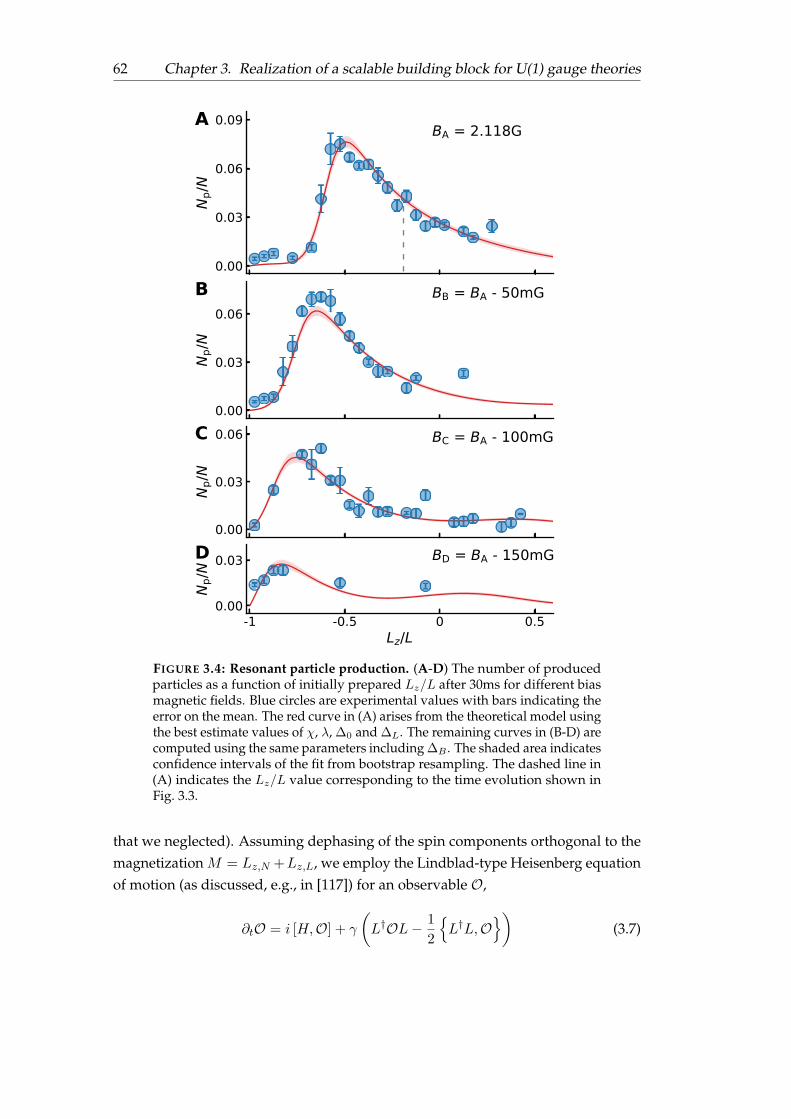
62 Chapter 3. Realization of a scalable building block for U(1) gauge theories
B
A
C
D
FIGURE 3.4: Resonant particle production. (A-D) The number of producedparticles as a function of initially prepared Lz/L after 30ms for different biasmagnetic fields. Blue circles are experimental values with bars indicating theerror on the mean. The red curve in (A) arises from the theoretical model usingthe best estimate values of χ, λ, ∆0 and ∆L. The remaining curves in (B-D) arecomputed using the same parameters including ∆B . The shaded area indicatesconfidence intervals of the fit from bootstrap resampling. The dashed line in(A) indicates the Lz/L value corresponding to the time evolution shown inFig. 3.3.
that we neglected). Assuming dephasing of the spin components orthogonal to themagnetization M = Lz,N +Lz,L, we employ the Lindblad-type Heisenberg equationof motion (as discussed, e.g., in [117]) for an observable O,
∂tO = i [H,O] + γ
(L†OL− 1
2
L†L,O
)(3.7)
3.3. Effective description of the building block dynamics 63
with a single jump operator L = M with the decay rate γ. The resulting (mean-field)equations of motion for the spin components are
∂tLx,N = −2χLz,NLy,N + 2λLz,NLy,L −γ
2Lx,N , (3.8a)
∂tLy,N = 2χLz,NLx,N − 2λLz,NLx,L −γ
2Ly,N , (3.8b)
∂tLz,N = 2λ(Ly,NLx,L − Lx,NLy,L) , (3.8c)
∂tLx,L = −∆Ly,L + 2λLz,LLy,N −γ
2Lx,L , (3.8d)
∂tLy,L = ∆Lx,L − 2λLz,LLx,N −γ
2Ly,L , (3.8e)
∂tLz,L = 2λ(Ly,LLx,N − Lx,LLy,N ) , (3.8f)
with initial conditions LL(0) = (0, 0,−1) × LL and LN (0) = (cos θ, 0, sin θ) × LN .Here, θ ∈ [−π, π] is chosen in accordance to the quench that initiates the dynamics.We fit the numerical solution to the resonance data via the observableNp = Lz,L+LL.To this end, we assume that ∆ = ∆0 + ∆LLz,N (0)/LN + ∆B(B − BA)/BA. Thisdependence of ∆ on the initial spin Lz,N (0) (for fixed LL(0)) and the magnetic fieldB is analogous to the functional form derived in appendix 3.B for an ideal buildingblock. We obtain the effective model parameters χ, λ,∆0 and ∆L from a single fit tothe data shown in Fig. 3.4A with given γ. Fixing these parameters, ∆B is determinedby a second fit to the data of Fig. 3.4B-D. Explicitly, the fits yield the following set ofmodel parameters describing all experimental data:
χ
2π= 8.802(8) mHz , (3.9a)
λ
2π= 16.4(6) µHz , (3.9b)
∆0
2π= −4.8(16) Hz , (3.9c)
∆L
2π= 2.681(1) kHz , (3.9d)
∆B
2π= −519.3(3) Hz . (3.9e)
Comparing to the microscopic ab-initio estimates (see appendices 3.B and 3.C)gives
χth/χ ≈ 1.7 , (3.10a)
λth/λ ≈ 2.6 , (3.10b)
∆th0 /∆0 ≈ 16 , (3.10c)
∆thL /∆L ≈ 1.7 , (3.10d)
∆thB/∆B ≈ 3.2 . (3.10e)
The estimates are typically larger than the measured values by factors of about 2 to 3,which hints at a systematic uncertainty in the microscopic parameters that enter the
64 Chapter 3. Realization of a scalable building block for U(1) gauge theories
ab-initio calculation. Nevertheless, most values lie in the right order of magnitude.Importantly, the signs agree, such that the qualitative nature of the shift due to Band Lz,N is predicted in agreement with the experiment. The precise value of ∆0 isless important to fit the experimental data (essentially because of the large value of∆L), which is also apparent from its larger uncertainty. This observation makes thelarger deviation between the fitted value ∆0 and the estimate ∆th
0 plausible.In terms of the two coupled spins, the resonance can also be understood more
intuitively as follows. In our case, LN ≈ 6LL and thus by angular momentumconservation the component Lz,N can not change much (at most ∼ 17%) in thecourse of the dynamics. Now, if the spins were not coupled, they would rotate inthe (x, y)-plane with frequencies given by 2χLz,N and ∆. If the two frequencieswere very different, the coupling ∝ λ would average out. Therefore 2χLz,N ∼ ∆
gives an approximate condition for the resonance (assuming approximately constantLz,N ). Solving this condition for Lz,N with the fitted experimental parameters givesthe following resonance estimates for the four magnetic fields employed in theexperiment:
Lz,NLN
∣∣∣∣resonance
=∆0 + ∆B (B −BA) /BA
χNN −∆L∈ 0.12(4),−0.18(4),−0.47(5),−0.78(6) ,
B ∈ BA, BB, BC, BD . (3.11)
The actual peak position is not accurately reproduced because the naive resonancecondition is not quantitative for the employed particle numbers, and non-linearitiesand damping of the equations of motion modify the resonance. Nevertheless, thequalitative shift of the resonance peak is well captured.
3.4 Summary
Our results demonstrate the controlled operation of an elementary building blockof a U(1) gauge theory, and thus open the door for large-scale implementationsof lattice gauge theories in atomic mixtures. The potential for scalability is animportant ingredient for realistic applications to gauge field theory problems. Digitalquantum simulations of gauge theories on universal quantum computers [13, 14]are challenging to scale up. This difficulty makes analog quantum simulators, astreated here, highly attractive, since they can be scaled up while still maintainingexcellent quantum coherence [3, 25, 31, 35, 118, 119]. Proceeding to the extendedsystem requires to combine the current experiment with the established tools ofan optical lattice and laser-assisted tunneling (see appendix 3.B). The resultingextended gauge theory will enable the observation of relevant phenomena such asplasma oscillations or resonant particle production in strong-field QED [95]. Alongthe path to the relativistic gauge theories realized in nature, we will replace bosonic7Li with fermionic 6Li, which will allow for the recovery of Lorentz-invariance inthe continuum limit.
3.A. Experimental details 65
Appendix: More details about the spinor Bose-Bose mixture
In this appendix, we give more details about the experiment (section 3.A) and aboutthe implementation of the U(1) gauge theory (section 3.B). In section 3.C, we discusshow to simulate the experiment in three spatial dimensions, which demonstrateshow spatial dynamics affects the evolution. Finally, we give another explanation forthe observed resonance by rewriting the dynamics of spin-changing collisions as ananharmonic oscillator in section 3.D.
3.A Experimental details
We prepare a mixture of bosonic 23Na and 7Li in a single crossed optical dipoletrap from a far red detuned laser with 1064 nm wavelength. The atoms experiencetrapping frequencies of (ωx, ωy, ωz)Na ≈ 2π × (243, 180, 410)Hz for sodium and(ωx, ωy, ωz)Li = 2.08× (ωx, ωy, ωz)Na for lithium. To maximize the spatial overlap ofthe two individual clouds, we align the direction of strongest confinement in gravitydirection whereby reducing the differential gravitational sag to approximately 1.1µm.The atomic clouds are evaporatively cooled to Bose Einstein condensation andcontain about 300 ×103 23Na atoms and 50 ×103 7Li atoms respectively.
For the spin-exchange dynamics we take into account the following sublevelsof the Hyperfine ground state: |↓〉 = |F = 1,mF = 1〉 , |↑〉 = |F = 1,mF = 0〉 forsodium, as well as |v〉 = |F = 1,mF = 1〉 , |p〉 = |F = 1,mF = 0〉 for lithium. Weapply an offset magnetic field of BA = 2.118(2)G, which lifts the degeneracy of themagnetically sensitive states. Moreover around B0 the level spacing of both speciesapproach each other at (E|↑〉 − E|↓〉)/~ ≈ (E|p〉 − E|v〉)/~ ∼ 1.45 MHz, energeticallyallowing hetero-nuclear spin transfer. Detailed information about the scatteringlengths in our system is given in section 3.B.
At the beginning of the experimental sequence the atoms are prepared in |↓〉and |v〉 respectively, suppressing any spin exchange due to conservation of mag-netization. We initiate the spin dynamics by quenching sodium into a desiredsuperposition of |↑〉 and |↓〉. To ensure that lithium stays spin polarized duringthe quench, instead of direct radiofrequency transfer we couple the sodium stateswith a two pulse microwave transition sequence using the sodium |F = 2,mF = 0〉state as an intermediate state. The first pulse is of variable length, driving pop-ulation from |↓〉 to the intermediate state with a Rabi frequency of 2π × 2.5 kHz.The second pulse is fixed to 100µs (corresponding to a π-pulse) and subsequentlydrives the population from the intermediate state to |↑〉. The total length of the pulsesequence is at most 300µs, which is at least one order of magnitude faster than thespin dynamics we observe in our experiment. The initial superposition quenchcauses undesired external dynamics of the sodium cloud due to the two states |↑〉and |↓〉 being immiscible [116]. This leads to relative motion of the two sodiumspin components within the trap after the superposition quench (see section 3.C for

66 Chapter 3. Realization of a scalable building block for U(1) gauge theories
more details). Our observation time is limited by losses in the |↑〉 state, leading to alifetime of the |↑〉 population of about 560 ms for the data shown in Fig. 3.4.
After an evolution time of up to 100 ms we switch off the trapping potential andperform a Stern-Gerlach sequence, where a magnetic field gradient is applied acrossthe atoms’ position for 1.5 ms that separates the magnetic substates spatially. After afree expansion time of 3 ms (sodium) and 2 ms (lithium) the two spin states of eachspecies are separated by approximately 130µm. Then we use absorption imaging todetect the spatial distribution of both species on two individual CCD cameras. Theinformation about the population of substates is then extracted from the images byintegrating the density distribution of the individual spin components.
The observable in the experiment is the relative lithium atom number populationNp/N . For lithium being initially spin polarized in |v〉, atoms transferred to |p〉 arethe signature of spin-changing collisions. The main source of detection noise for thisobservable are fringe patterns on the images which are resulting from diffractionand interference in the imaging path. To account for those we post-process thelithium absorption images by applying a fringe removal algorithm [120], whichreduces the experimental noise floor below 1% (see Fig. 3.3B).
Due to the 6 times higher sodium atom number the relative change between thepopulation of |↑〉 and |↓〉 resulting from spin-changing collisions is expected to be atmost 1%. This change can currently not be detected with our imaging routine. Mainlimitation are the external dynamics of the sodium spin components in the trapafter the initial quench. This results in strong variation of the density distribution ofthe individual sodium components which our imaging calibration is systematicallysensitive to [121].
The observable Np/N is obtained as an average from a statistical ensembleof multiple experimental realizations. Each data point shown in Figs. 3.3 and 3.4corresponds to at least three and ten measurements, respectively. The data displayedin Fig. 3.4 is binned in 5% intervals of Lz/L. As the curve in Fig. 3.4D becomescomparably featureless, we used our resources to more accurately resolve the othersets for Fig. 3.4A-C.
For more details about the experiment, we refer to the doctoral thesis of A.Mil [108].
3.B Details of the implementation
3.B.1 Microscopic Hamiltonian
In our experiments, we work with two internal spin states, mF = 0, 1, each fromthe spin Fs = 1 manifold of the two Bose gases, s = N,L (23Na and 7Li in ourcase). The total Hamiltonian, H = H0 +H1, of the combined system splits into free,H0 = HN +HL, and interaction, H1 = HNN +HLL +HNL, parts [122, 123]. The free

3.B. Details of the implementation 67
parts have the form
Hs =
ˆd3x
∑
α
ψ†s,α(x)Hs,α (x) ψs,α (x) , (3.12a)
Hs,α (x) =−∇2
x
2ms+ Vs(x) + Es,α(B) . (3.12b)
Here, ms denotes the atomic masses, Vs is the trapping potential and Es,α(B) isthe Zeeman shift in the presence of an external magnetic field B, given by theBreit-Rabi formula. The field operators ψs,α(x) fulfill bosonic commutation relations[ψs,α(x), ψ†s′,β(y)
]= δss′δαβδ (x− y), where α, β ∈ 0, 1 denote the mF states.
The intra-species and inter-species interactions which are spin-conserving aredescribed by
Hss =1
2
ˆd3x
∑
α,β
gsαβ ψ†s,α(x)ψ†s,β(x)ψs,β(x)ψs,α(x) , (3.13a)
HNL =
ˆd3x
∑
α,β
gMixαβ ψ†N,α(x)ψ†L,β(x)ψL,β(x)ψN,α(x) , (3.13b)
where the interaction constants gsαβ = 4π~2
msasαβ and gMix
αβ = 2π~2
µ aMixαβ are determined
by the following scattering lengths: aN11 = aN10 = aN01 = 55aB , aN00 = 53aB , aL11 =
aL10 = aL01 = 6.8aB , aL00 = 12.5aB [122] and aMix00 = aMix
10 = aMix01 = 19.65aB ,
aMix11 = 20aB [124]. The hetero-nuclear spin-changing collisions are described by
HSCC = gSCCˆ
d3xψ†N,0(x)ψ†L,1(x)ψN,1(x)ψL,0(x) + h.c. (3.14)
with the interaction strength gSCC = 2π~2
µ aSCC and the scattering length aSCC =
0.35aB [124].
3.B.2 Proposed extended implementation
We propose to implement the extended U(1) gauge theory described in section 3.1 asfollows. Starting from the microscopic Hamiltonian, a deep optical lattice localizesthe atomic clouds on individual lattice wells n. Expanding the field operators into lo-calized Wannier functions, ψs,α =
∑n bs,α,nΦs,α,n(x), we first perform the spatial in-
tegration to obtain a tight-binding Hamiltonian. For a sufficiently deep potential, alltunneling and interaction terms between neighboring wells are negligible, resultingin an array of elementary building blocks n, each containing both species. The Hamil-tonian has the form H =
∑n Hn with Hn =
∑s,n
(Hs,n + Hss,n
)+ HNL,n + HSCC,n
68 Chapter 3. Realization of a scalable building block for U(1) gauge theories
and
Hs,n =∑
α
Es,α(B)b†s,α,nbs,α,n , (3.15a)
Hss,n = Xs11b†s,1,nb
†s,1,nbs,1,nbs,1,n +Xs
00b†s,0,nb
†s,0,nbs,0,nbs,0,n
+ 2Xs10b†s,1,nb
†s,0,nbs,1,nbs,0,n , (3.15b)
HNL,n = XMix11 b†N,1,nbN,1,nb
†L,1,nbL,1,n +XMix
00 b†N,0,nbN,0,nb†L,0,nbL,0,n
+XMix10 b†N,1,nbN,1,nb
†L,0,nbL,0,n +XMix
10 b†N,0,nbN,0,nb†L,1,nbL,1,n , (3.15c)
HSCC,n = XSCC[b†N,0,nb
†L,1,nbN,1,nbL,0,n + b†N,1,nb
†L,0,nbN,0,nbL,1,n
]. (3.15d)
The precise values of the energy levels E and interaction constants X depend on thedetails of the optical lattice and the corresponding Wannier functions Φs,α,n(x).
We then identify the gauge fields on the building block via the Schwinger repre-sentation of angular momentum operators,
L+,n = b†N,0,nbN,1,n , L−,n = b†N,1,nbN,0,n , Lz,n =1
2
(b†N,0,nbN,0,n − b
†N,1,nbN,1,n
).
(3.16)
The matter fields on a building block, however, are partially associated with the twoneighboring internal degrees of freedom according to
bn =
(bn,p
bn,v
), bn,p = bL,n−1,0 , bn,v = bL,n,1 . (3.17)
The matter fields carry a U(1) charge Qn, which enters the Gauss’ law operators Gnas
Qn = bnbn = b†n,pbn,p + b†n,vbn,v , Gn = Lz,n − Lz,n−1 − Qn . (3.18)
This construction ensures Gauss’ law,[Gn, H
]=[Gn, HSCC,n + HSCC,n−1
]= 0, be-
cause[Lz,n, HSCC,n
]−[Lz,n−1, HSCC,n−1
]=[Qn, HSCC,n + HSCC,n−1
]. Physically,
a global U(1) symmetry due to the conservation of the total magnetization, whicharises from angular momentum conservation, is localized on each building block.This localization, which is achieved by associating a building block n with a link nand components of the matter fields on the neighboring lattice sites n and n+ 1, isthe key to the scalability of our proposal.
Finally, we connect the building blocks to an extended one-dimensional systemby the term
HΩ = ~Ω∑
n
(b†L,n,1bL,n−1,0 + h.c.
)= ~Ω
∑
n
(b†n,vbn,p + h.c.
), (3.19)
which can be realized with, e.g., laser-assisted tunneling. Crucially, this connection
3.B. Details of the implementation 69
respects Gauss’ law,[HΩ, Gn
]=[HΩ, Qn
]= 0. The resulting lattice model is similar
to our previous proposal [29] with Dirac fermions replaced by two-componentbosons,
H/~ =∑
n
χ L2
z,n + Ω b†nσxbn + λ[b†n,vL−,nbn+1,p + h.c.
](3.20)
+ (other gauge-invariant terms) ,
as discussed in section 3.1.
3.B.3 The building block
In the following, we focus on a single building block n of the extended proposal, asrealized in the present experiment. To this end, we consider only two matter fieldcomponents, bp = bL,n,0 and bv = bL,n,1, together with a single spin L = Ln. Themicroscopic Hamiltonian conserves the total magnetization M and the total particlenumbers NL, NN . To simplify the Hamiltonian of a single building block, we assumean initial state with fixed magnetization M and particle numbers NN , NL
2. Aftersome algebra, we obtain the building block Hamiltonian given in Eq. (3.1), up toconstants involving only the conserved numbers NN , NL and M . The Hamiltonianis gauge invariant because it commutes with the two reduced Gauss’ law operatorsassociated with neighboring lattice sites,
G′n = Lz + b†pbp , G′n+1 = −Lz + b†vbv . (3.21)
The parameters are given by
∆ = −[δLext − δNext + δLint − δNint +
χNL2
(NN −NL) + 2M−χL −
χNL2
], (3.22a)
χ = −χN − χL − χNL , (3.22b)
λ = XSCC , (3.22c)
where we abbreviated the effective interaction constants
χs = − [Xs00 +Xs
11 − 2Xs10] = [Xs
11 −Xs00] , (3.23)
the mean-field energy shifts
δsint = [Xs11 −Xs
00] (Ns − 1) = χs(Ns − 1) , (3.24)
2It is questionable whether this condition can be realized by preparing a corresponding eigenstatein the experiment. The fact that we can describe the experiment on the mean-field level shows that thissubtlety is not relevant at the moment. However, it can be crucial for investigating quantum effectsafter preparing a gauge-invariant state in future experiments.
70 Chapter 3. Realization of a scalable building block for U(1) gauge theories
and the single-particle energy level differences δsext = Es,1 − Es,0. The interactionconstants are calculated from the relevant overlap integrals by rescaling the mi-croscopic parameters as Xs
αβ = Isαβgsαβ
2 , XMisαβ = IMix
αβ gMixαβ and XSCC = IMix
10 gSCC
with
Isαβ =
ˆd3xΦ2
s,α,n(x)Φ2s,β,n(x) , IMix
αβ =
ˆd3xΦ2
N,α,n(x)Φ2L,β,n(x) , (3.25)
where we have chosen real basis functions Φ. From the known experimental parame-ters, we estimate the overlap integrals from the initial mean-field BEC wave-functionΦs,1,n with all atoms of both species in the mF = 1 state by setting Φs,1,n = Φs,0,n.We have calculated the necessary wave-functions by imaginary-time propagation ofthe Gross-Pitaevskii equation corresponding to full microscopic Hamiltonian (formore details see the section 3.C). In the experiment, we tune the magnetization Mthrough the initial value of the spin Lz(0) and the magnetic field B. To quantify thisdependence, we split ∆ = ∆0 + ∆LLz,N (0)/LN + ∆B(B − BA)/BA, which holdsfor (B − BA) BA and fixed initial condition for the Li atoms. With the givenexperimental and microscopic parameters, we obtain the following estimates:
χth
2π≈ 14.92 mHz , (3.26a)
λth
2π≈ 42.3 µHz , (3.26b)
∆th0
2π≈ −77 Hz , (3.26c)
∆thL
2π≈ 4.474 kHz , (3.26d)
∆thB
2π≈ −1.669 kHz . (3.26e)
3.B.4 Estimates for the extended system
For scaling up our system to an extended lattice gauge theory, we propose to use aone-dimensional optical lattice array created by a laser of 532nm wavelength, whichis blue detuned for both species. The connecting term, Eq. (3.19), can be realizedby laser-assisted tunneling between neighboring lattice sites. Former proposals re-quired a species selective lattice, where different species reside on alternating latticesites whereas in this implementation both atomic species reside on the same sites.This arrangement greatly improves the feasibility of an experimental realization.First, an alternating lattice is technically more demanding. Second, in an alternatinglattice tight confinement is necessary to avoid undesired direct tunneling betweenlattice sites. This confinement, however, diminishes also the spin-changing collisionsdynamics, which involve spatial hopping across lattice sites. In our implementation,each site already contains the gauge-invariant interaction via on-site spin-changingcollisions. Therefore, tight confinement on individual lattice wells that suppressesdirect tunneling at the same time increases the gauge-invariant coupling.
3.C. Numerical simulation of the trapped mixture 71
For the laser-assisted tunneling, we consider two laser beams, each having alarge detuning ∆ from the lithium D1 line. We describe the two beams by E1,2 =
E1,2u1,2 cos(k1,2x− ω1,2t), with k1,2 and ω1,2 being the wave vector and frequencyof each laser beam, respectively. The frequency difference of the lasers is tuned tomatch the transition frequency between the states ψp = ψL,0 and ψv = ψL,1. Asdiscussed, e.g., in [125] this leads to the following contribution to the Hamiltonian,
V =
ˆd3x Ωeψ
†p(x)ψv(x)eiqx + h.c. , (3.27)
where q = k1 − k2, and Ωe being the effective coupling strength. To estimate theeffective tunneling strength, we use similar parameters as in the previous proposal[29]. For the lattice this results in a lattice spacing of aL = 2 µm and a lattice depth of15ER for lithium, and 115ER for sodium, such that tunneling is even more stronglysuppressed for sodium. In this configuration, we obtain a direct tunneling elementon the order of a few Hz. We then estimate the tunneling strength in the presenceof Eq. (3.27). A lower limit for the estimate is given when considering the Wannierfunctions within the lattice sites to be harmonic oscillator ground states. Furtherassuming a detuning of ∆ = 1nm, we estimate a laser-assisted tunneling strengthon the order of a few kHz. Considering spin-changing collisions dynamics, whichmay also happen on the scale of hundreds of Hz, we expect the overall dynamics ofthe extended system to be at least ten times faster than in previous proposals [10,29].
3.C Numerical simulation of the trapped mixture
To get a better understanding of the experimental setup we need to go beyondan ideal setup and take into account experimental imperfections. Here, we focuson the spatial structure and residual dynamics of the atomic clouds within thetrapping potential. As a first approximation, we describe the BECs in a mean-fieldapproximation which means that we solve the Gross-Pitaevskii equation (GPE)derived from the microscopic Hamiltonian described in section 3.B.1 numerically.The numerical solution is based on a pseudo-spectral method, called “split-step”,where we refer to [126, 127] for more details. In the following we briefly summarizethe main idea and point out necessary modifications to simulate the present model.
Consider a partial differential equation (PDE) of the form
i∂tψ(t, x) = (T + V )ψ(t, x) , (3.28)
where T and V are (not necessarily linear) differential operators, for which thecorresponding PDE is exactly solvable, i.e., we have explicit expressions for theformal solutions ψ(t, x) = e−iDtψ(0, x) with D = T, V . Then the solution for a short
72 Chapter 3. Realization of a scalable building block for U(1) gauge theories
time ∆t may be written as
ψ(t, x) = e−i(T+V )∆tψ(0, x) ≈ e−iT∆te−iV∆tψ(0, x) , (3.29)
where the error goes to zero as ∆t → 0 according to the BCH formula. For theGPE of a one-component BEC, T = −∇2/(2m) is the kinetic energy term, which isdiagonal in Fourier space, and V = Vtrap + g|ψ|2 is the potential energy term, whichis diagonal in position space. By evolving ψ(t, x) in alternating steps accordingto T and V one obtains an approximation to the exact solution of the full PDE. Inpractice, space is discretized on a periodic lattice with spacing a and spatial extentL and one can efficiently switch between position and momentum space using thefast Fourier transform algorithm. The resulting numerical implementation scalesas ∼ NtNx logNx, where Nt is the number of time steps and Nx = (L/a)d is thetotal number of lattice sites for spatial dimension d. The parameters have to betuned such that convergence with respect to decreasing the time step ∆t, increasingthe system size L and decreasing the lattice spacing a (for fixed L) is achieved to adesired precision. Crucially, the split-step method is symplectic, which ensures thatcertain symmetries of the system are preserved [127, 128]. For the case of a GPE, thisincludes the conservation of total particle number and total energy.
In contrast to the standard GPE, the Bose-Bose mixture involves four hyperfinecomponents, described by ψN/L,1/0. As a consequence, the GPE includes not onlykinetic energy terms T and potential energy terms V , which are both diagonal in thehyperfine index. There is a third type of terms, due to the spin-changing collisions,that mix the different hyperfine components. This part of the evolution equation islocal in position space and takes the form
i∂tψN,1 = gψ∗L,1ψL,0ψN,0 , i∂tψN,0 = gψ∗L,0ψL,1ψN,1 , (3.30a)
i∂tψL,1 = gψ∗N,1ψN,0ψL,0 , i∂tψL,0 = gψ∗N,0ψN,1ψL,1 . (3.30b)
We have not found a simple analytic solution to these equations. To be able toinclude the spin-changing collision in the simulation, we instead consider
i∂ψ1 = gψ0 , i∂ψ0 = g∗ψ1 , (3.31)
which can be seen as “half” of the previous equations for, e.g., fixed g = gψ∗L,1ψL,0.With initial conditions ψ1(0) and ψ0(0), the solution is
ψ1(t) = ψ1(0) cos(ωt)− iψ0(0)ω
gsin(ωt) , (3.32a)
ψ0(t) = ψ0(0) cos(ωt)− iψ1(0)ω
g∗sin(ωt) , (3.32b)
with ω = |g|. We can thus approximate the solution to Eq. (3.30) by solving alternat-ingly for ψN,1/0 with g = gψ∗L,1ψL,0 and for ψL,1/0 with g = gψ∗N,1ψN,0. Specifically,we evolve ψN,1/0 for a short time ∆t/2, then ψL,1/0 for ∆t and again ψN,1/0 for ∆t/2.

3. C. N u m e ri c al si m ul ati o n of t h e t r a p p e d mi xt u r e 7 3
− 1 0 0 1 0y [µ m]
− 1 0
0
1 0
x[µ
m]
− 5 0 5z [µ m]
− 1 0
0
1 0
x[µ
m]
− 5 0 5z [µ m]
− 1 0
0
1 0
y[µ
m]
− 1 0 0 1 0y [µ m]
− 1 0
0
1 0
x[µ
m]
− 5 0 5z [µ m]
− 1 0
0
1 0
x[µ
m]
− 5 0 5z [µ m]
− 1 0
0
1 0
y[µ
m]
0
2
4
× 1 0 1 5
0
1
2
3
× 1 0 1 5
F I G U R E 3. 5: T h e pl ot s s h o w t h e i nt e g r at e d ( o v e r z, y, x f r o m l eft t o ri g ht) t w o-di m e n si o n al d e n sit y p r o fil e s i n u nit s of 1 / m 2 of s o di u m (i n m F = 1 , t o p r o w)a n d lit hi u m (i n m F = 1 , t o p r o w), o bt ai n e d f r o m i m a gi n a r y ti m e p r o p a g ati o nof t h e c o r r e s p o n di n g G P E. We o b s e r v e a cl e a r c h a n g e of t h e at o mi c cl o u d s d u et o t h ei r i nt e r a cti o n: t h e s m all e r a n d li g ht e r lit hi u m cl o u d “ sit s ” o n t o p of adi st o rt e d elli p s oi d al s o di u m cl o u d ( g r a vit y a ct s i n z - di r e cti o n). T h e si m ul ati o nw a s d o n e o n a t h r e e- di m e n si o n al l atti c e wit h N x = N y = 2 5 6 a n d N z = 1 2 8g ri d p oi nt s a n d l atti c e s p a ci n g a = 0 .1 5 µ m.
T hi s ( s o- c all e d St r a n g) s plitti n g i s a c c u r at e t o s e c o n d o r d e r [ 1 2 7 ]. I n t hi s w a y w e
i n cl u d e t h e s pi n- c h a n gi n g c olli si o n s i nt o t h e n u m e ri c al s plit- st e p i nt e g r ati o n of
t h e c o m bi n e d G P E. A s a r e s ult, t h e fi n al i nt e g r at o r i s a g ai n s y m pl e cti c a n d al s o
a p p r o xi m at el y c o n s e r v e s t h e t ot al m a g n eti z ati o n ( u p t o b o u n d e d o s cill ati o n s t h at
g o t o z e r o a s ∆ t → 0 ).
S ol vi n g t h e i m a gi n a r y ti m e v e r si o n f o r t h e G P E (t o g et h e r wit h a p p r o p ri at e n o r-
m ali z ati o n st e p s, s e e [ 1 2 9 ] f o r m o r e d et ail s) w e h a v e c al c ul at e d t h e i niti al m e a n- fi el d
w a v ef u n cti o n s ψ( 0 )N / L, 1 ( x, y, z ) of t h e B E C mi xt u r e i n t h e m F = 1 st at e s. T h e r e s ult-
i n g d e n sit y p r o fil e s n( 0 )N / L, 1 ( x, y, z ) = |ψ
( 0 )N / L, 1 ( x, y, z )|2 a r e s h o w n i n t h e fi g u r e s 3. 5
a n d 3. 6 . T h e o bt ai n e d s ol uti o n s a r e t h e n u s e d a s a n i niti al st at e f o r si m ul ati n g
t h e r e al-ti m e d y n a mi c s f oll o wi n g t h e q u e n c h of t h e e x p e ri m e nt, w hi c h w e r e al-
i z e b y i niti ali zi n g a d e si r e d i m b al a n c e b et w e e n t h e t w o s o di u m c o m p o n e nt s, i. e.,
ψ N, m F( x, y, z )( t = 0) = α m F ψ
( 0 )N, 1 ( x, y, z ) wit h |α 1 |2 + |α 0 |2 = 1 .
I n o r d e r t o d e s c ri b e t h e e x p e ri m e nt i n m o r e d et ail, w e t a k e i nt o a c c o u nt s e v e r al
i m p e rf e cti o n s t h at a r e n e gl e ct e d i n t h e i d e al G P E si m ul ati o n. I n p a rti c ul a r, w e
h a v e o b s e r v e d l o s s i n t h e m F = 0 d e n sit y of s o di u m. A n e x p o n e nti al fit of t h e
e x p e ri m e nt al d at a r e v e al e d a fi nit e lif e-ti m e τ , w hi c h w e t a k e i nt o a c c o u nt b y a d di n g
a t e r m, i /( 2 τ )ψ N, 0 , t o t h e c o r r e s p o n di n g c o m p o n e nt of t h e G P E. F u rt h e r m o r e, w e
h a v e o b s e r v e d a st r o n g d e p e n d e n c e of t h e si m ul ati o n r e s ult s o n t h e i niti al p a rti cl e
n u m b e r s N N a n d N L . C o n s e q u e ntl y, w e e xt r a ct e d t h e fl u ct u ati o n s f r o m e x p e ri m e nt

7 4 C h a pt e r 3. R e ali z ati o n of a s c al a bl e b uil di n g bl o c k f o r U( 1) g a u g e t h e o ri e s
− 2 0 0 2 0x [µ m]
0
1
2
3
Na:
nx[1
/m]
× 1 0 1 0
T F
I T
− 2 0 0 2 0y [µ m]
0
1
2
Na:
ny[1
/m]
× 1 0 1 0
− 1 0 0 1 0z [µ m]
0
2
4
Na:
nz[1
/m]
× 1 0 1 0
− 2 0 0 2 0x [µ m]
0 .0
0 .5
1 .0
Li:n
x[1
/m]
× 1 0 1 0
T F
I T
− 2 0 0 2 0y [µ m]
0 .0
0 .5
1 .0
Li:n
y[1
/m]
× 1 0 1 0
− 1 0 0 1 0z [µ m]
0
1
Li:n
z[1
/m]
× 1 0 1 0
F I G U R E 3. 6: T h e pl ot s s h o w t h e i nt e g r at e d ( o v e r z a n d y , z a n d x , y a n d xf r o m l eft t o ri g ht) o n e- di m e n si o n al d e n sit y p r o fil e s of s o di u m (i n m F = 1 , t o pr o w) a n d lit hi u m (i n m F = 1 , t o p r o w) f o r t h e p a r a m et e r s a s i n fi g u r e 3. 5 . Wec o m p a r e t h e r e s ult f r o m i m a gi n a r y ti m e p r o p a g ati o n ( s oli d li n e s, “I T ”) t o aT h o m a s- F e r mi p r e di cti o n t h at n e gl e ct s t h e i nt e r a cti o n b et w e e n s o di u m a n dlit hi u m ( d a s h e d li n e s, “ T F ”), w hi c h s h o w s t h at t h e d e n sit y- d e n sit y i nt e r a cti o n ssi g ni fi c a ntl y m o dif y t h e s h a p e of t h e t w o- s p e ci e s c o n d e n s at e.
a n d c al c ul at e d t h ei r m e a n v al u e s a n d e m pi ri c al st a n d a r d d e vi ati o n s,
¯N N ≈ 2 9 5 .8 × 1 0 3 , σ N N≈ 7 .2 × 1 0 3 , ( 3. 3 3 a)
¯N L ≈ 5 5 .6 × 1 0 3 , σ N L≈ 3 .9 × 1 0 3 , ( 3. 3 3 b)
τ ≈ 5 0 5 .7 m s , σ τ ≈ 2 4 .0 m s . ( 3. 3 3 c)
We i n cl u d e t h e s e fl u ct u ati o n s i nt o o u r si m ul ati o n b y s a m pli n g t h e c o r r e s p o n di n g
p a r a m et e r s f r o m i n d e p e n d e nt G a u s si a n di st ri b uti o n s wit h e x p e ct ati o n v al u e a n d
v a ri a n c e e sti m at e d f r o m t h e e x p e ri m e nt al d at a. T h e r e s ult s of a si n gl e si m ul ati o n
a r e ill u st r at e d i n fi g u r e 3. 7 .
T h e si m ul ati o n d e m o n st r at e s t h at t h e s o di u m cl o u d s c h a n g e t h ei r s p ati al s h a p e
i n t h e c o u r s e of t h e d y n a mi c s. I n p a rti c ul a r, t h e t w o c o m p o n e nt s m F = 1 , 0 t e n d
t o “ a v oi d e a c h ot h e r ”, i. e., r e gi o n s of l a r g e d e n sit y i n o n e c o m p o n e nt t y pi c all y
c o r r e s p o n d t o l o w d e n siti e s i n t h e ot h e r c o m p o n e nt. T hi s b e h a vi o r i s e x p e ct e d
b e c a u s e t h e h y p e r fi n e st at e s a r e i m mi s ci bl e [ 1 3 0 ]. A s a di r e ct c o n s e q u e n c e of t hi s
o b s e r v ati o n, w e d o n ot e x p e ct t o b e a bl e t o d e s c ri b e t h e e x p e ri m e nt i n a si n gl e- m o d e
a p p r o xi m ati o n wit h t h e n ai v e mi c r o s c o pi c p a r a m et e r s gi v e n i n E q. (3. 2 6 ). H o w e v e r,
t h e fit s h o w n i n fi g u r e s 3. 3 a n d 3. 4 d e m o n st r at e s t h at a si n gl e m o d e d e s c ri pti o n i s
s uf fi ci e nt t o d e s c ri b e t h e e x p e ri m e nt al o b s e r v ati o n s. T hi s f a ct f o rti fi e s o u r st at e m e nt
t h at t h e s p ati al d y n a mi c s e s s e nti all y “ r e n o r m ali z e s ” t h e m o d el p a r a m et e r s, w hi c h
i n t u r n e n a bl e s a si m pl e d e s c ri pti o n of t h e gl o b al o b s e r v a bl e N p / N .
B y a v e r a gi n g m ulti pl e G P E si m ul ati o n s, w e o bt ai n a p r e di cti o n f o r t h e e x p e ri-
m e nt al o b s e r v a bl e, s h o w n i n fi g u r e 3. 8 . E v e n t h o u g h t h e p r e di ct e d c u r v e d o e s n ot
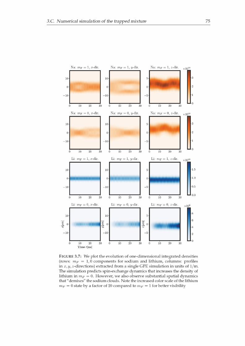
3. C. N u m e ri c al si m ul ati o n of t h e t r a p p e d mi xt u r e 7 5
0 1 0 2 0 3 0
− 1 0
0
1 0
N a: m F = 1, x - dir.
0 1 0 2 0 3 0
− 1 0
0
1 0
N a: m F = 1, y - dir.
0 1 0 2 0 3 0
− 5
0
5
N a: m F = 1, z - dir.
0 1 0 2 0 3 0
− 1 0
0
1 0
N a: m F = 0, x - dir.
0 1 0 2 0 3 0
− 1 0
0
1 0
N a: m F = 0, y - dir.
0 1 0 2 0 3 0
− 5
0
5
N a: m F = 0, z - dir.
0 1 0 2 0 3 0
− 1 0
0
1 0
Li: m F = 1, x - dir.
0 1 0 2 0 3 0
− 1 0
0
1 0
Li: m F = 1, y - dir.
0 1 0 2 0 3 0
− 5
0
5
Li: m F = 1, z - dir.
0 1 0 2 0 3 0
Ti m e t[ m s]
− 1 0
0
1 0
x[µ
m]
Li: m F = 0, x - dir.
0 1 0 2 0 3 0
− 1 0
0
1 0
y[µ
m]
Li: m F = 0, y - dir.
0 1 0 2 0 3 0
− 5
0
5
z[µ
m]
Li: m F = 0, z - dir.
0
1
2
3
× 1 0 1 0
0
1
2
3
× 1 0 1 0
0 .0
0 .5
1 .0
1 .5
× 1 0 1 0
0
2
4
6
8
× 1 0 8
F I G U R E 3. 7: We pl ot t h e e v ol uti o n of o n e- di m e n si o n al i nt e g r at e d d e n siti e s( r o w s: m F = 1 , 0 c o m p o n e nt s f o r s o di u m a n d lit hi u m, c ol u m n s: p r o fil e si n x, y, z - di r e cti o n s) e xt r a ct e d f r o m a si n gl e G P E si m ul ati o n i n u nit s of 1 / m .T h e si m ul ati o n p r e di ct s s pi n- e x c h a n g e d y n a mi c s t h at i n c r e a s e s t h e d e n sit y oflit hi u m i n m F = 0 . H o w e v e r, w e al s o o b s e r v e s u b st a nti al s p ati al d y n a mi c st h at “ d e mi x e s ” t h e s o di u m cl o u d s. N ot e t h e i n c r e a s e d c ol o r s c al e of t h e lit hi u mm F = 0 st at e b y a f a ct o r of 2 0 c o m p a r e d t o m F = 1 f o r b ett e r vi si bilit y

76 Chapter 3. Realization of a scalable building block for U(1) gauge theories
0 20 40 60 80 100Time t[ms]
0.00
0.01
0.02
0.03
0.04
0.05
0.06
0.07
Part
icle
nu
mb
erN
p/N
single run
averaged GPE
experiment
FIGURE 3.8: We show the average evolution of the particle number (blackdashed line) obtained from 100 GPE simulations with fluctuating experimentalparameters. The red band indicates the error on the mean and the graydashed-dotted line corresponds to the specific realization shown in figure 3.7.The initial rise is in reasonable agreement with the experimental data (bluesymbols).
quantitatively agree with the experimental data, the amplitude of the initial riseagrees well3. However, due to lattice artifacts at t 30ms (not shown) the presentlattice sizes prohibit long simulation times, which would be necessary to make aquantitative prediction of, e.g., an oscillation frequency. Additionally, the individualruns start to differ strongly after ∼ 20ms, such that also the required statistics in-creases with the evolution time. As a consequence, we have no quantitative ab-initioprediction of the experiment for the full observation time at the moment.
There is a number of possible reasons for the deviations between the simulationand the experiment. First, the GPE simulation is a mean-field approximation thatneglects quantum-statistical fluctuations. Second, the approximation also assumesperfect condensates and neglects any thermal fraction of the Bose gases. Third, anyexperimental input parameter is not perfectly fixed; moreover, their fluctuations areneither Gaussian nor independent. Finally, after the presented simulations werecompleted, the particle number measurements were re-calibrated, which revealedsubstantially lower particle numbers for lithium (see [108] for new parameter esti-mates). We expect that a repetition of the simulation, including for instance moreappropriate fluctuations and refined parameters, would lead to a better agreement.Nevertheless, the results presented in this section already provide a qualitativepicture of the real-space dynamics of spin-changing collisions and indicate that theexperiment indeed follows the expected dynamics.
3We have chosen to display a specific realization in figure 3.7 that is close to this mean evolution.

3.D. Spin-changing collisions as an anharmonic oscillator 77
3.D Spin-changing collisions as an anharmonic oscillator
Let us reconsider the mean-field single mode evolution equations of the two coupledspins, Eq. (3.8). Without the phenomenological damping, this set of equations canbe written as
i∂tLz,N = λ (L+,NL−,L − L−,NL+,L) , (3.34a)
i∂tL±,N = ∓2χLz,NL±,N ± 2λLz,NL±,L , (3.34b)
i∂tLz,L = λ (L+,LL−,N − L−,LL+,N ) , (3.34c)
i∂tL±,L = ∓∆L±,L ± 2λLz,LL±,N , (3.34d)
where L± = Lx ± iLy, which arise from the classical Hamiltonian
H = χL2z,N + ∆Lz,L + λ (L+,NL−,L + L−,NL+,L) . (3.35)
The evolution can be simplified by considering the conservation of the total energyE = H , the magnetization M = Lz,N + Lz,L, as well as the spin lengths `s =√L2z,s + L+,sL−,s = Ns
2 for both species s = N,L. With
Lz,N = M − Lz,L , (3.36a)
L+,LL−,L = `2L − L2z,L , (3.36b)
L+,NL−,N = `2L − (M − Lz,L)2 , (3.36c)
λ (L+,NL−,L + L−,NL+,L) = E − χ (M − Lz,L)2 −∆Lz,L , (3.36d)
we can exploit the conservation laws to derive a closed equation for Lz,N . Explicitly,we calculate
−∂2t Lz,L = λ [(−∆L+,L + 2λLz,LL+,N )L−,N − (∆L−,L − 2λLz,LL−,N )L+,N ]
+ λ [(2χLz,NL−,N − 2λLz,NL−,L)L+,L
− (−2χLz,NL+,N + 2λLz,NL+,L)L−,L] (3.37a)
= g (L+,NL−,L + L−,NL+,L) (−∆ + 2χLz,N )
+ 4λ2 [Lz,LL+,NL−,N − Lz,NL+,LL−,L] (3.37b)
= λ(E − χ (M − Lz,L)2 −∆Lz,L
)[−∆ + 2χ (M − Lz,L)]
+ 4λ2Lz,L
[`2N − (M − Lz,L)2
]− (M − Lz,L)
(`2L − L2
z,L
). (3.37c)
This equation has the form of a particle oscillating in an anharmonic potential, i.e.,
∂2t Lz,L = −V ′ (Lz,L) , V (Lz) = c1Lz +
c2
2L2z +
c3
3L3z +
c4
4L4z (3.38)

78 Chapter 3. Realization of a scalable building block for U(1) gauge theories
FIGURE 3.9: The plot shows the resonance of figure 3.4A with the same ex-perimental data (blue symbols), together with numerical simulations of theanharmonic oscillator, Eq. (3.38), with fit parameters given in Eq. (3.9). Whilethe damped simulation (red curve, evaluated at fixed time t = 30ms) fits theexperimental data, the pure anharmonic oscillator (black dashed curved, eval-uated is the oscillation amplitude) clearly shows the characteristic triangularshape (cf. figure 3.10.)
with the coefficients
c1 = −∆m+ 2χEM − 4λ2`2LM + χ ∆M − 2χ2M3 , (3.39a)
c2 = −2χE + 4λ2`2L + 4λ2`2N + ∆2 − 4χ∆M + 6χ2M2 − 4λ2M2 , (3.39b)
c3 = 3χ∆− 6χ2M + 12λ2M , (3.39c)
c4 = 2χ2 − 8λ2 . (3.39d)
For our usual initial conditions, Li is fully polarized. This implies the initial values
Lz,L(t0) = −`L , ∂tLz,L(t0) = 0 . (3.40)
The resulting oscillation of Lz,L can therefore be pictured by the potential V , whichis set by the initial condition of Na. In our case, the total energy is then fixed to be
E = χ (M − `L)2 + ∆`L (3.41)
and the behavior of the system is dictated by the initial Na imbalance, which setsthe magnetization in the range
−`L − `N ≤M ≤ −`L + `N . (3.42)
In figure 3.9, we show the resulting resonance obtained from a numerical solutionwith the parameters given in Eq. (3.9) that we used to fit the experiment at themagnetic field BA. The plot shows the amplitude of the oscillation of Lz,L (i.e., themaximum value) together with the value at fixed time t = 30ms for a simulationwhere we include a friction term 2γ∂tLz,L with the same damping constant as before.Although the dynamics of this damping is not identical with the one introduced inEq. (3.8), the obtained resonance again fits the experimental data. Both the damped

3.D. Spin-changing collisions as an anharmonic oscillator 79
- - - - - ---
- - - - - ------
-----
- - - - - ---
- - - - - ------
-----
- - - - - ---
- - - - - ------
-----
FIGURE 3.10: The three rows show simulation results for different values ofLz,N/N = −0.7,−0.68,−0.118 (top to bottom). The middle panel shows thepotential V with the initial condition Lz,L = −L indicated by the gray lines.The right panel shows the following dynamics of Lz,L for undamped (graydashed line) and damped (red solid line) oscillators. The left panel shows aphase space picture of the evolution. The change of the shape of the potentialis responsible for the shape of the resonance shown in figure 3.9. In particular,the (dis)appearance of a local minimum close to the initial state is responsiblefor the non-analytic change of the amplitude of Lz,L as a function of the initialLz,N .
and undamped results show a characteristic asymmetric shape with a very steepslope around Lz,N ≈ −0.7N .
The origin of this shape is a direct consequence of the anharmonic potentialV (Lz). This is illustrated in figure 3.10. Depending on the initial value of Lz,N ,the potential V (Lz,L) changes its shape and the spin Lz,L is either “trapped” in alocal minimum or can “escape” to the global minimum, resulting in much largeroscillation amplitudes.
The plot in the bottom right of figure 3.10, which includes the experimentaldata, shows that the phenomenological friction term describes the experiment lessaccurately than the damping introduced in Eq. (3.8). However, the resonance shownin figure 3.9 is not affected because it only probes the early-time dynamics wherethis difference is insignificant. In conclusion, the qualitative features of the spin-changing collisions observed in the experiment are well captured by a anharmonicoscillator. This observation may provide important physical intuition for futureexperiments on hetero-nuclear spin-changing collisions.

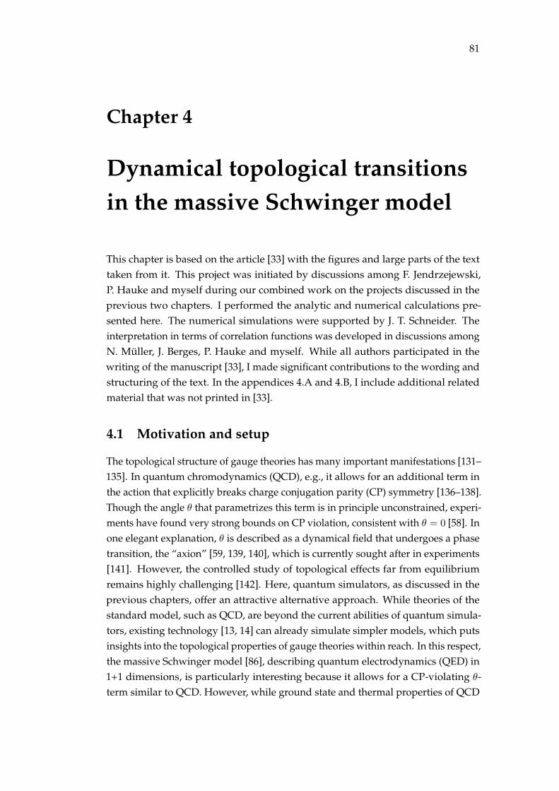
81
Chapter 4
Dynamical topological transitionsin the massive Schwinger model
This chapter is based on the article [33] with the figures and large parts of the texttaken from it. This project was initiated by discussions among F. Jendrzejewski,P. Hauke and myself during our combined work on the projects discussed in theprevious two chapters. I performed the analytic and numerical calculations pre-sented here. The numerical simulations were supported by J. T. Schneider. Theinterpretation in terms of correlation functions was developed in discussions amongN. Müller, J. Berges, P. Hauke and myself. While all authors participated in thewriting of the manuscript [33], I made significant contributions to the wording andstructuring of the text. In the appendices 4.A and 4.B, I include additional relatedmaterial that was not printed in [33].
4.1 Motivation and setup
The topological structure of gauge theories has many important manifestations [131–135]. In quantum chromodynamics (QCD), e.g., it allows for an additional term inthe action that explicitly breaks charge conjugation parity (CP) symmetry [136–138].Though the angle θ that parametrizes this term is in principle unconstrained, experi-ments have found very strong bounds on CP violation, consistent with θ = 0 [58]. Inone elegant explanation, θ is described as a dynamical field that undergoes a phasetransition, the “axion” [59, 139, 140], which is currently sought after in experiments[141]. However, the controlled study of topological effects far from equilibriumremains highly challenging [142]. Here, quantum simulators, as discussed in theprevious chapters, offer an attractive alternative approach. While theories of thestandard model, such as QCD, are beyond the current abilities of quantum simula-tors, existing technology [13, 14] can already simulate simpler models, which putsinsights into the topological properties of gauge theories within reach. In this respect,the massive Schwinger model [86], describing quantum electrodynamics (QED) in1+1 dimensions, is particularly interesting because it allows for a CP-violating θ-term similar to QCD. However, while ground state and thermal properties of QCD

82 Chapter 4. Dynamical topological transitions in the massive Schwinger model
and of the Schwinger model have been extensively studied [57, 143], much less isknown about their topological structure out of equilibrium.
In this chapter, we investigate the non-equilibrium real-time evolution of themassive Schwinger model after a quench of the topological θ angle. We find topolog-ical transitions in the fermion sector, which appear as vortices in the single-particlepropagator when θ changes by more than a critical value. In the limit of vanishinggauge coupling, we rigorously connect this phenomenon to dynamical quantumphase transitions (DQPTs), which in condensed-matter lattice models are currentlyreceiving considerable attention [60, 144–146]. A topological nature of DQPTs haspreviously been revealed in non-interacting theories [147–149]. Here, we demon-strate how to construct a general dynamical topological invariant that is valid in thecontinuum and, most importantly, also in interacting theories. Moreover, our topo-logical invariant provides a physical interpretation of DQPTs in terms of fermioniccorrelation functions. Enabled by this result, we use non-perturbative real-timelattice calculations at intermediate to strong coupling to show that the topologicaltransition persists up to e/m . 1. Already for lattices as small as 8 sites, we obtaingood infrared convergence. Moreover, the relevant phenomena occur on time scalesthat have already been accessed in proof-of-principle quantum simulations of gaugetheories [13, 14]. These features will enable near-future experiments based ontrapped ions [13], superconducting qubits [14], and cold neutral atoms [29] to probethis dynamical topological transition.
4.1.1 θ-quenches in the massive Schwinger model
The massive Schwinger model is a prototype model for 3+1D QCD since both shareimportant features such as a non-trivial topological vacuum structure and a chiralanomaly [57, 86]. CP violation can be studied by adding a so-called topologicalθ-term, (eθ/2π)Ex, to the Hamiltonian density, where E is the electric field and e
the dimensionful gauge coupling. In temporal axial gauge, and by making a chiraltransformation, the θ-term can be absorbed into the fermion mass term to give thefollowing Hamiltonian [86],
Hθ =
ˆdx
[1
2E2x + ψ†xγ
0(iγ1Dx +m eiθγ
5)ψx
]. (4.1)
Here, ψ are two-component fermion operators, γ0/1 constitute the Clifford algebrain two space-time dimensions, and γ5 ≡ γ0γ1. The Hamiltonian contains the energyof the electric field, the kinetic term of the fermions, which are coupled to thegauge sector via the covariant derivative Dx = ∂x + ieAx, where e is the electriccoupling, and the fermion rest mass m. While the addition of the θ-term is animaginary contribution to the action (see [150]), we emphasize that the Hamiltonian(4.1) remains hermitian. In particular, its spectrum is real and θ does not introduceany instability.
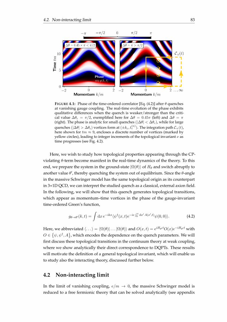
4.2. Non-interacting limit 83
FIGURE 4.1: Phase of the time-ordered correlator [Eq. (4.2)] after θ quenchesat vanishing gauge coupling. The real-time evolution of the phase exhibitsqualitative differences when the quench is weaker/stronger than the criti-cal value ∆θc = π/2, exemplified here for ∆θ = 0.45π (left) and ∆θ = π(right). The phase is analytic for small quenches (|∆θ| < ∆θc), while for largequenches (|∆θ| > ∆θc) vortices form at (±kc, t(n)c ). The integration path C+(t),here shown for tm ≈ 9, encloses a discrete number of vortices (marked byyellow circles), leading to integer increments of the topological invariant ν astime progresses (see Fig. 4.2).
Here, we wish to study how topological properties appearing through the CP-violating θ-term become manifest in the real-time dynamics of the theory. To thisend, we prepare the system in the ground-state |Ω(θ)〉 of Hθ and switch abruptly toanother value θ′, thereby quenching the system out of equilibrium. Since the θ-anglein the massive Schwinger model has the same topological origin as its counterpartin 3+1D QCD, we can interpret the studied quench as a classical, external axion field.In the following, we will show that this quench generates topological transitions,which appear as momentum–time vortices in the phase of the gauge-invarianttime-ordered Green’s function,
gθ→θ′(k, t) =
ˆdx e−ikx〈ψ†(x, t)e−ie
´ x0 dx′ A(x′,t)ψ(0, 0)〉. (4.2)
Here, we abbreviated 〈. . . 〉 = 〈Ω(θ)| . . . |Ω(θ)〉 and O(x, t) = eiHθ′ tO(x)e−iHθ′ t withO ∈
ψ,ψ†, A
, which encodes the dependence on the quench parameters. We will
first discuss these topological transitions in the continuum theory at weak coupling,where we show analytically their direct correspondence to DQPTs. These resultswill motivate the definition of a general topological invariant, which will enable usto study also the interacting theory, discussed further below.
4.2 Non-interacting limit
In the limit of vanishing coupling, e/m → 0, the massive Schwinger model isreduced to a free fermionic theory that can be solved analytically (see appendix

84 Chapter 4. Dynamical topological transitions in the massive Schwinger model
(a)
(b)
FIGURE 4.2: Dynamical topological transitions at vanishing gauge coupling.(a) The topological invariant exhibits jumps at critical times t(n)c = (2n −1)π/ [2ω(kc)] with n ∈ N, if |∆θ| > π/2, while the dynamics is topologicallytrivial for |∆θ| < π/2. (b) For |∆θ| > π/2, the rate function [Eq. (4.5)] showsnon-analytic kinks at times t(n)c .
4.A for detailed calculations) by diagonalizing Hθ =´
dkHθ(k), with Hθ(k) =
ψ†kγ0(kγ1 +m eiθγ
5)ψk. Figure 4.1 displays the phase of gθ→θ′ as a function of (k, t)
for two exemplary quenches with ∆θ = 0.45π, π (our results here depend only on∆θ = (θ − θ′) ∈ (−π, π]). Strong quenches in the range |∆θ| > π
2 are accompaniedby the formation of vortices at critical times t(n)
c = (2n− 1)tc, with tc = π/ [2ω(kc)],n ∈ N and ω(k) =
√k2 +m2. These appear in pairs of opposite winding at critical
modes ±kc = ±m√− cos (∆θ).
4.2.1 An order parameter for dynamical topological transitions
This observation suggests to define a dynamical topological order parameter thatcounts the difference of vortices contained in left (−) versus right (+) moving modes,ν ≡ n+ − n−, with
n±(t) ≡ 1
2π
˛C±(t)
dzg†(z)∇zg(z)
. (4.3)
Here, g(z) ≡ gθ→θ′(k, t′)/|gθ→θ′(k, t′)| and C±(t) is a rectangular path enclosing theleft/right half of the z = (k, t′)-plane up to the present time t, i.e., it runs (counter-clockwise) along (0, 0) ↔ (0, t) ↔ (±∞, t) ↔ (±∞, 0) ↔ (0, 0) as visualized in
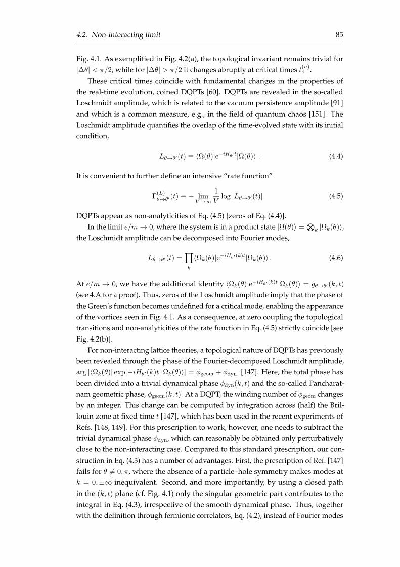
4.2. Non-interacting limit 85
Fig. 4.1. As exemplified in Fig. 4.2(a), the topological invariant remains trivial for|∆θ| < π/2, while for |∆θ| > π/2 it changes abruptly at critical times t(n)
c .These critical times coincide with fundamental changes in the properties of
the real-time evolution, coined DQPTs [60]. DQPTs are revealed in the so-calledLoschmidt amplitude, which is related to the vacuum persistence amplitude [91]and which is a common measure, e.g., in the field of quantum chaos [151]. TheLoschmidt amplitude quantifies the overlap of the time-evolved state with its initialcondition,
Lθ→θ′(t) ≡ 〈Ω(θ)|e−iHθ′ t|Ω(θ)〉 . (4.4)
It is convenient to further define an intensive “rate function”
Γ(L)θ→θ′(t) ≡ − lim
V→∞1
Vlog |Lθ→θ′(t)| . (4.5)
DQPTs appear as non-analyticities of Eq. (4.5) [zeros of Eq. (4.4)].In the limit e/m→ 0, where the system is in a product state |Ω(θ)〉 =
⊗k |Ωk(θ)〉,
the Loschmidt amplitude can be decomposed into Fourier modes,
Lθ→θ′(t) =∏
k
〈Ωk(θ)|e−iHθ′ (k)t|Ωk(θ)〉 . (4.6)
At e/m → 0, we have the additional identity 〈Ωk(θ)|e−iHθ′ (k)t|Ωk(θ)〉 = gθ→θ′(k, t)
(see 4.A for a proof). Thus, zeros of the Loschmidt amplitude imply that the phase ofthe Green’s function becomes undefined for a critical mode, enabling the appearanceof the vortices seen in Fig. 4.1. As a consequence, at zero coupling the topologicaltransitions and non-analyticities of the rate function in Eq. (4.5) strictly coincide [seeFig. 4.2(b)].
For non-interacting lattice theories, a topological nature of DQPTs has previouslybeen revealed through the phase of the Fourier-decomposed Loschmidt amplitude,arg [〈Ωk(θ)| exp[−iHθ′(k)t]|Ωk(θ)〉] = φgeom + φdyn [147]. Here, the total phase hasbeen divided into a trivial dynamical phase φdyn(k, t) and the so-called Pancharat-nam geometric phase, φgeom(k, t). At a DQPT, the winding number of φgeom changesby an integer. This change can be computed by integration across (half) the Bril-louin zone at fixed time t [147], which has been used in the recent experiments ofRefs. [148, 149]. For this prescription to work, however, one needs to subtract thetrivial dynamical phase φdyn, which can reasonably be obtained only perturbativelyclose to the non-interacting case. Compared to this standard prescription, our con-struction in Eq. (4.3) has a number of advantages. First, the prescription of Ref. [147]fails for θ 6= 0, π, where the absence of a particle–hole symmetry makes modes atk = 0,±∞ inequivalent. Second, and more importantly, by using a closed pathin the (k, t) plane (cf. Fig. 4.1) only the singular geometric part contributes to theintegral in Eq. (4.3), irrespective of the smooth dynamical phase. Thus, togetherwith the definition through fermionic correlators, Eq. (4.2), instead of Fourier modes
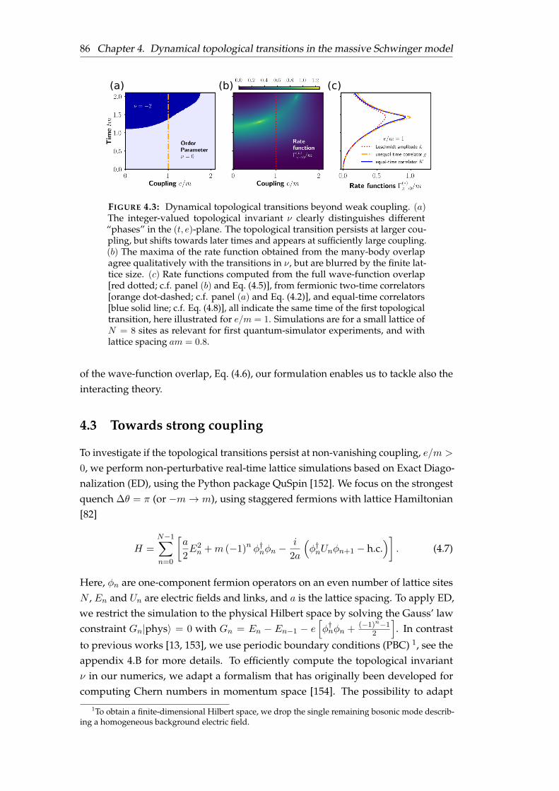
86 Chapter 4. Dynamical topological transitions in the massive Schwinger model
(a) (b) (c)
FIGURE 4.3: Dynamical topological transitions beyond weak coupling. (a)The integer-valued topological invariant ν clearly distinguishes different“phases” in the (t, e)-plane. The topological transition persists at larger cou-pling, but shifts towards later times and appears at sufficiently large coupling.(b) The maxima of the rate function obtained from the many-body overlapagree qualitatively with the transitions in ν, but are blurred by the finite lat-tice size. (c) Rate functions computed from the full wave-function overlap[red dotted; c.f. panel (b) and Eq. (4.5)], from fermionic two-time correlators[orange dot-dashed; c.f. panel (a) and Eq. (4.2)], and equal-time correlators[blue solid line; c.f. Eq. (4.8)], all indicate the same time of the first topologicaltransition, here illustrated for e/m = 1. Simulations are for a small lattice ofN = 8 sites as relevant for first quantum-simulator experiments, and withlattice spacing am = 0.8.
of the wave-function overlap, Eq. (4.6), our formulation enables us to tackle also theinteracting theory.
4.3 Towards strong coupling
To investigate if the topological transitions persist at non-vanishing coupling, e/m >
0, we perform non-perturbative real-time lattice simulations based on Exact Diago-nalization (ED), using the Python package QuSpin [152]. We focus on the strongestquench ∆θ = π (or −m→ m), using staggered fermions with lattice Hamiltonian[82]
H =N−1∑
n=0
[a
2E2n +m (−1)n φ†nφn −
i
2a
(φ†nUnφn+1 − h.c.
)]. (4.7)
Here, φn are one-component fermion operators on an even number of lattice sitesN , En and Un are electric fields and links, and a is the lattice spacing. To apply ED,we restrict the simulation to the physical Hilbert space by solving the Gauss’ lawconstraint Gn|phys〉 = 0 with Gn = En − En−1 − e
[φ†nφn + (−1)n−1
2
]. In contrast
to previous works [13, 153], we use periodic boundary conditions (PBC) 1, see theappendix 4.B for more details. To efficiently compute the topological invariantν in our numerics, we adapt a formalism that has originally been developed forcomputing Chern numbers in momentum space [154]. The possibility to adapt
1To obtain a finite-dimensional Hilbert space, we drop the single remaining bosonic mode describ-ing a homogeneous background electric field.
4.3. Towards strong coupling 87
this formalism to our case is another feature of our definition in Eq. (4.3) since itis enabled by the use of a closed integration path in the (k, t) plane. This adaptionforces ν to remain integer-valued even when evaluated on coarse grids, thus leadingto convergence already for small lattices 2.
As can be expected from the above discussions, at small e/m transitions inthe topological invariant coincide with maxima in the rate function, see Fig. 4.3.Further, both structures congruently persists at larger values of e/m. Importantly,however, while the system sizes accessible for ED do not allow one to discernclear kinks in the rate function, the non-equilibrium topological invariant ν sharplydistinguishes between topologically inequivalent phases, revealing a shift of thetransitions towards larger tc as e/m is increased. While the results for e/m . 1
are already reasonably finite-volume converged for the small system size plotted,at e/m & 1 finite-volume effects persist up to N = 20 (see section 4.3.2 below).Nevertheless, the topological transition must vanish at sufficiently large couplingec because θ becomes an irrelevant parameter in the limit m→ 0 [155]. Finite sizeeffects in our numerical results hinder a quantitative determination of ec. Motivatedby these limitations, we propose to quantum simulate of the present setup.
4.3.1 Quantum simulation
Importantly, the first topological transition happens on times of order tcm ∼ 1− 2,which lies within coherence times that are accessible with existing and proposedquantum simulators [13, 14, 29]. A straightforward realization of the scenariodiscussed in this chapter may be achieved with a quantum computer based ontrapped-ions or superconducting qubits, where quench dynamics has been studiedrecently [13, 14]. Though these experiments used only four lattice sites of staggeredfermions, larger lattices are within reach of current technology [156–159]. Veryrecently, it has been shown that variational algorithms can prepare the ground stateof the lattice Schwinger model with 8 to 20 sites with high fidelity [35, 160]. The rele-vant dynamics can be implemented by discretizing the unitary evolution operatorinto a sequence of quantum gates [13, 161]. For staggered fermions, the mass term isrealized by local rotations and can be quenched by inverting the direction of rota-tion. All observables studied in this chapter can then be accessed by an appropriatesequence of unitary operators intermitted by spin flips. Alternatively, various workshave proposed analog quantum simulators of the massive Schwinger model [7, 8,26, 162]. In the implementations proposed in the previous chapters, which are basedon mixtures of cold atoms in a tilted optical lattice, the fermion mass corresponds toRabi oscillations between two hyperfine states driven by radiofrequency radiationor is set by the laser-assisted tunneling. In these setups, a mass quench may be
2In the non-interacting limit the topological invariant is not affected by the choice of lattice regular-ization, which we have explicitly checked at the example of staggered and Wilson fermions. Here, werestrict the simulations in the interacting case to staggered fermions, which are closer to the continuumlimit given the limited resources.

88 Chapter 4. Dynamical topological transitions in the massive Schwinger model
simply implemented by abruptly adjusting the corresponding parameters, e.g., theRabi frequency.
These experiments may unveil the topological transitions through differentobservables: First, a digital quantum computer could in principle work with themany-body wavefunctions to directly calculate the order parameter ν [Eq. (4.3)]and the rate function Γθ→θ′(t) [Eq. (4.5)]. Second, one could measure the two-timecorrelator gθ→θ′(k, t) [Eq. (4.2)] [163, 164] and thereby avoid the study of many-body overlaps. Third, the discrete transition points of the order parameter areindicated also in experimentally more accessible equal-time correlation functions,[F (t)]αβxy ≡
⟨[ψα(t, x), ψβ(t, y)
]⟩. Namely, let us define
Kθ→θ′(t) ≡∏
k
[F(k, t) + F(k, 0)]2 , (4.8)
where F = (Fs, F1, F5) are Lorentz components3 of the correlator, F (t) = Fs(t)1 +
Fµ(t)γµ + iF5(t)γ5. One has Kθ→θ′(t) =∏k |gθ→θ′(k, t)|2 = |Lθ→θ′(t)|2 in the non-
interacting limit (for details, see the appendix 4.A). This motivates to define the ratefunctions Γ(g)(t) and Γ(K)(t) analogously to Γ(L)(t) by replacing |L(t)| in Eq. (4.5)with
∏k |g(k, t)| and
√K(t), respectively. We thus have three complementary defini-
tions that coincide for e/m→ 0, obtained from equal-time correlators, Eq. (4.8), two-time correlators, Eq. (4.2), and the full many-body Loschmidt amplitude, Eq. (4.4).Remarkably, as illustrated in Fig. 4.3(c) for e/m = 1, even at intermediate couplingsthe maxima of all three rate functions indicate the same critical times with relativedeviation less than about 8%. Below we show a quantitative comparison, whichdemonstrates that the three rate functions show comparable finite size deviations,which for the topological order parameter are significantly smaller.
Besides its experimental simplicity, Eq. (4.8) also gives an interesting interpreta-tion of the dynamical topological transition in terms of a dephasing effect. Namely,Eq. (4.8) has zeros if and only if the mode kc at time tc exhibits perfect anti-correlationwith the initial state, F(kc, tc) = −F(kc, 0). This anti-correlation is responsible forthe non-analytic behavior of the associated rate function.
4.3.2 Finite size dependence of the transition times
We have extracted the critical times of the first topological transition t(1)c as indicated
by the rate functions of the Loschmidt amplitude L, the equal-time correlator K, thetwo-time correlator g, and the dynamical topological order parameter ν. While νunambiguously determines a critical time by its discontinuous jump between twointeger values, we have chosen the maxima of the three different rate functionsas an indicator of t(1)
c for a quantitative comparison. This comparison is shown inFig. 4.4 for weak (e/m = 0.5) and intermediate (e/m = 1.0) coupling strength asa function of lattice sites N . Remarkably, all three rate functions indicate similar
3We exclude F0 in F because mode-wise charge conservation implies F0(k, t) = 0 at e/m = 0.
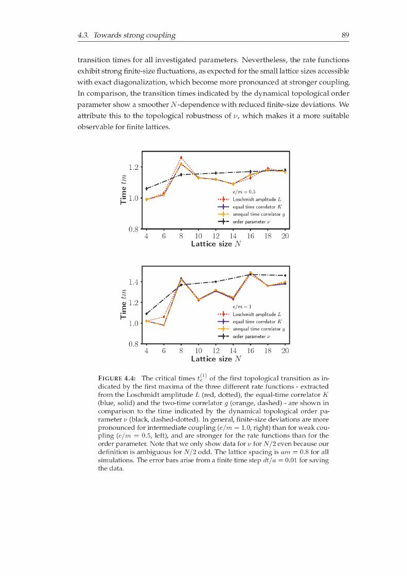
4. 3. T o w a r d s st r o n g c o u pli n g 8 9
t r a n siti o n ti m e s f o r all i n v e sti g at e d p a r a m et e r s. N e v e rt h el e s s, t h e r at e f u n cti o n s
e x hi bit st r o n g fi nit e- si z e fl u ct u ati o n s, a s e x p e ct e d f o r t h e s m all l atti c e si z e s a c c e s si bl e
wit h e x a ct di a g o n ali z ati o n, w hi c h b e c o m e m o r e p r o n o u n c e d at st r o n g e r c o u pli n g.
I n c o m p a ri s o n, t h e t r a n siti o n ti m e s i n di c at e d b y t h e d y n a mi c al t o p ol o gi c al o r d e r
p a r a m et e r s h o w a s m o ot h e r N - d e p e n d e n c e wit h r e d u c e d fi nit e- si z e d e vi ati o n s. We
att ri b ut e t hi s t o t h e t o p ol o gi c al r o b u st n e s s of ν , w hi c h m a k e s it a m o r e s uit a bl e
o b s e r v a bl e f o r fi nit e l atti c e s.
4 6 8 1 0 1 2 1 4 1 6 1 8 2 0L a t ti c e si z e N
0 .8
1 .0
1 .2
Time
tm
e / m = 0 .5
L os c h mi dt a m plit u d e L
e q u al ti m e c orr el at or K
u n e q u al ti m e c orr el at or g
or d er p ar a m et er ν
4 6 8 1 0 1 2 1 4 1 6 1 8 2 0L a t ti c e si z e N
0 .8
1 .0
1 .2
1 .4
Time
tm
e / m = 1
L os c h mi dt a m plit u d e L
e q u al ti m e c orr el at or K
u n e q u al ti m e c orr el at or g
or d er p ar a m et er ν
F I G U R E 4. 4: T h e c riti c al ti m e s t( 1 )c of t h e fi r st t o p ol o gi c al t r a n siti o n a s i n-
di c at e d b y t h e fi r st m a xi m a of t h e t h r e e diff e r e nt r at e f u n cti o n s - e xt r a ct e df r o m t h e L o s c h mi dt a m plit u d e L ( r e d, d ott e d), t h e e q u al-ti m e c o r r el at o r K( bl u e, s oli d) a n d t h e t w o-ti m e c o r r el at o r g ( o r a n g e, d a s h e d) - a r e s h o w n i nc o m p a ri s o n t o t h e ti m e i n di c at e d b y t h e d y n a mi c al t o p ol o gi c al o r d e r p a-r a m et e r ν ( bl a c k, d a s h e d- d ott e d). I n g e n e r al, fi nit e- si z e d e vi ati o n s a r e m o r ep r o n o u n c e d f o r i nt e r m e di at e c o u pli n g ( e / m = 1 .0 , ri g ht) t h a n f o r w e a k c o u-pli n g ( e / m = 0 .5 , l eft), a n d a r e st r o n g e r f o r t h e r at e f u n cti o n s t h a n f o r t h eo r d e r p a r a m et e r. N ot e t h at w e o nl y s h o w d at a f o r ν f o r N / 2 e v e n b e c a u s e o u rd e fi niti o n i s a m bi g u o u s f o r N / 2 o d d. T h e l atti c e s p a ci n g i s a m = 0 .8 f o r allsi m ul ati o n s. T h e e r r o r b a r s a ri s e f r o m a fi nit e ti m e st e p dt / a = 0 .0 1 f o r s a vi n gt h e d at a.
90 Chapter 4. Dynamical topological transitions in the massive Schwinger model
4.4 Summary
In this chapter, we have studied the real-time dynamics of massive 1+1D QEDwith a θ-term, as a prototype model for topological effects in gauge theories. Byestablishing a general dynamical topological order parameter, which can be obtainedfrom fermionic correlators and is valid in interacting theories, we have identifiedthe appearance of dynamical topological transitions after changes in the external“axion” field. A connection between the topological transitions to DQPTs, which isrigorous at zero coupling, persists in our numerics of the interacting theory, thusproviding a physical interpretation of DQPTs in terms of fermionic correlators.Finally, our topological order parameter can directly be applied also in the studyof condensed-matter models, where the construction of topological invariants forinteracting systems is a major outstanding challenge [165–167].
In this study, we have identified a relevant problem for state-of-the-art quantumsimulation. The described dynamical transitions constitute an ideal first step becausethe relevant dynamics appears at short time scales and small system sizes. We expectthe topological nature to provide robustness against experimental imperfections,which may provide a starting point to tackle the question of certifiability of quantumsimulation.
Despite the simplicity of the considered model, our study shows that quantumsimulators provide a unique perspective to the topological structure of QCD outof equilibrium. Phenomena closely related to the physics studied in this chapterare the conjectured Chiral Magnetic and similar effects [168–171], which remainchallenging in and out of equilibrium for theoretical studies [81, 84, 142, 172–178].Here, a simple next step for future quantum simulators is to model these effects byspatial domains of the θ-parameter [179].

4.A. Free fermion calculations 91
Appendix: Even more about the massive Schwinger model
In the first section 4.A of this appendix, we give a detailed summary of analyticpredictions for the quench dynamics, which are based on non-interacting fermions.In the second section 4.B, we prove a general solution of Gauss’ law on a periodicone-dimensional lattice for arbitrary fermion discretizations, which we used for thenumerical ED simulations.
4.A Free fermion calculations
4.A.1 Diagonalization
Consider the free fermion Hamiltonian H =´ L
0 dxψ†xγ0(iγ1∂x +meiθγ
5)ψx on a
circle of length L. The spatial structure of the Hamiltonian becomes diagonal inFourier space,
ψx =1√L
∑
p
ψpeipx , ψp =
1√L
ˆ L
0dxψxe
−ipx , (4.9)
where the sum runs over all p = 2πn/L with n ∈ Z. Choosing
γ0 =
(1 0
0 −1
), γ1 =
(0 1
−1 0
), γ5 =
(0 1
1 0
), (4.10)
as a specific representation of the Clifford algebra, the Hamiltonian reads
H =∑
p
ψ†pHpψp , Hp(θ,m) =
(m cos θ −p+ im sin θ
−p− im sin θ −m cos θ
), (4.11)
which leads to the eigenvalues and -vectors ±ωp = ±√p2 +m2 and u±p . Defining
quasi-particle operators by
(ap
b†−p
)= U †pψp , (4.12)
where Up = (u+p , u
−p ) is the unitary with U †pHpUp = diag(ωp,−ωp), this yields
H =∑
p
ωp
(a†pap + b†pbp − 1
). (4.13)

92 Chapter 4. Dynamical topological transitions in the massive Schwinger model
The explicit expressions for the eigenvectors are
u+p = [2ωp(ωp −m cos θ)]−1/2
(p− im sin θ
m cos θ − ωp
), (4.14a)
u−p = [2ωp(ωp −m cos θ)]−1/2
(−m cos θ + ωp
p+ im sin θ
), (4.14b)
such that the commutation relations are preserved,ap, a
†q
= δpq =
bp, b
†q
. The
vacuum |Ω〉 is the ground state of H and fulfills ap|Ω〉 = 0 = b−p|Ω〉.Two sets of quasi-particle operators corresponding to H(θ,m) and H(θ′,m′) are
directly related by
(ap(θ,m)
b†−p(θ,m)
)= U †p(θ,m)Up(θ
′,m′)
(ap(θ
′,m′)
b†−p(θ′,m′)
). (4.15)
The two corresponding vacuua can be related by
|Ω(θ,m)〉 =∏
p
N−1p
[Ap +Bpa
†p(θ′,m′)b†−p(θ
′,m′)]|Ω(θ′,m′)〉 (4.16)
with the coefficients
Ap(θ,m; θ′,m) =(u−p)†
(θ′,m′)u−p (θ,m) , (4.17a)
Bp(θ,m; θ′,m) =(u−p)†
(θ′,m′)u+p (θ,m) (4.17b)
and |Np|2 = |Ap|2 + |Bp|2 = 1 is fixed by the normalization 〈Ω|Ω〉 = 1 and theorthonormality of the eigenvectors u±p .
4.A.2 Quench dynamics and DQPT
The dynamics following a quench from H(θ,m) to H(θ′,m′) is described by
|ψθ,m→θ′,m′(t)〉 = e−iH(θ′,m′)t|Ω(θ,m)〉 (4.18)
=∏
p
N−1p
[Ape
iωp(m′)t +Bpa†p(θ′,m′)b†−p(θ
′,m′)e−iωp(m′)t]|Ω(θ′,m′)〉 .
Thus, the Loschmidt amplitude follows as
Lθ,m→θ′,m′(t) = 〈ψθ,m→θ′,m′(0)|ψθ,m→θ′,m′(t)〉 (4.19)
=∏
p
[cos(ωpt) + i
|Bp|2 − |Ap|2|Ap|2 + |Bp|2
sin(ωpt)
].

4.A. Free fermion calculations 93
Focusing on θ-quenches with m′ = m, we explicitly obtain after some algebra,
|Ap|2 =ω2p + p2 +m2 cos (θ − θ′)
2ω2p
, |Bp|2 =m2 sin2
(θ′−θ
2
)
ω2p
. (4.20)
Therefore the Loschmidt amplitude becomes
Lθ→θ′(t) =∏
p
`θ→θ′(t, p) , `θ→θ′(t, p) = cos (ωpt)− ip2 +m2 cos (θ′ − θ)
ω2p
sin (ωpt) ,
(4.21)
and from the condition `(p, t) = 0 we can read off the zeros to occur at
t(n)c =
π(2n+ 1)
ωpc, p2
c = −m2 cos(θ − θ′
). (4.22)
In the thermodynamic limit, these zeros cause non-analyticities in the rate functionassociated to the Loschmidt amplitude,
Γθ′→θ(t) = − limV→∞
1
Vlog |Lθ→θ′(t)| = −
ˆ −∞∞
dp
2πlog `θ→θ′(t, p). (4.23)
The final integral expression is evaluated numerically for the results plotted in figure4.1.
4.A.3 Two-time correlation functions and the order parameter
To get a better understanding of the physics underlying the DQPT, we observe thefollowing identity
`θ→θ′(t, p) = 〈Ω(θ)|a†p(θ′)ap(θ′)eiωpt + b−p(θ′)b†−p(θ
′)e−iωpt|Ω(θ)〉= 〈Ω(θ)|ψ†p(t)ψp(0)|Ω(θ)〉 = g(t, p) , (4.24)
where ψ(t) = eiH(θ′)tψe−iH(θ′)t denotes a Heisenberg field operator w.r.t. to the post-quench Hamiltonian. Consequently, the DQPTs occur at zeros of the time-orderedcorrelator g(t, p). As a consequence, the phase of g(t, p) = |g(t, p)|eiϕ(t,p) becomesill-defined at the critical points (t
(n)c , pc) and develops a winding. This observation
underlies the order parameter introduced in this chapter. Crucially, we changethe perspective from the Loschmidt amplitude to correlation functions, which inturn have a straightforward generalization and interpretation also in the interactingtheory.
94 Chapter 4. Dynamical topological transitions in the massive Schwinger model
4.A.4 Interpretation with equal-time correlators
We can give yet another interpretation by considering the Loschmidt echo,
|Lθ→θ′(t)|2 = Tr [ρθ→θ′(t)ρθ→θ′(0)] , (4.25)
where ρθ→θ′(t) = e−iH(θ′)t|Ω(θ)〉〈Ω(θ)|eiH(θ′)t is the pure-state density operator. Fortwo Gaussian states ρk, k = 1, 2, e.g., ground states of a non-interacting system andtheir time-evolution, the trace in (4.25) can be calculated (see [180]) as
Tr [ρ1ρ2] = det[G1G2 + G1G2
], (4.26)
with the correlators
(Gk)ij = Tr[ρkψ
†iψj
],
(Gk
)ij
= δij − (Gk)ij . (4.27)
In our case the indices i, j label both lattice sites and spinor components. Introducingthe statistical propagator
(Fk)ij =1
2Tr[ρk
(ψ†iψj − ψjψ
†i
)], (4.28)
and using the commutation relationsψ†i , ψj
= δij , we can rewrite the result (4.26)
as
Tr [ρ1ρ2] = det
[2F1F2 +
1
2
]. (4.29)
In the our case, this gives
|Lθ→θ′(t)|2 = det
[2F (t)F (0) +
1
2
]=∏
p
det′[F (p, t)F (p, 0) +
1
2
], (4.30)
where the prime indicates the remaining determinant in spinor space after perform-ing the spatial functional determinant in Fourier space where the correlators arediagonal,
Fxy(t) =
ˆdp
2πeip(x−y)F (p, t) . (4.31)
We further decompose the correlator in its Lorentz components4, F = Fγ0 =
Fs1 + F0γ0 + F1γ
1 + iF5γ5. For brevity, we only state the explicit expressions for
4The additional matrix γ0 corresponds to a change of variables from ψ† to ψ = ψ†γ0.

4.B. Solving Gauss’ law on a ring 95
the simplest quench −m→ m (or θ′ = π → θ = 0),
Fs(p, t) =1
2Tr[F (p, t)γ0
]=m
ω3p
[1
2(p2 −m2) + p2 cos (2ωpt)
](4.32a)
F0(p, t) =1
2Tr[γ0F (p, t)γ0
]= 0 (4.32b)
F1(p, t) =1
2Tr[γ1F (p, t)γ0
]=
p
ω3p
[1
2(m2 − p2) +m2 cos (2ωpt)
](4.32c)
F5(p, t) =1
2Tr[−iγ5F (p, t)γ0
]=mp
ω2p
sin (2ωpt) . (4.32d)
At the critical momenta, where p2c = m2, these equations further simplify
Fs(pc, t) = F1(pc, t) =1
2√
2cos(
2√
2mt), F5(pc, t) =
1
2sin(
2√
2mt). (4.33)
For a general θ-quench, the electric charge is conserved for each momentummode separately, i.e., F0(p, t) = 0, and the remaining components form a spin-1/2 vector F(p, t) = (Fs(p, t), F1(p, t), F5(p, t)) with F2(p, t) = 1/4. Then a directcomputation of the relevant determinant gives
det′[F (p, t)γ0F (p, 0)γ0 +
1
2
]=
1
2+ 2F(p, t) · F(p, t) (4.34)
and therefore the Loschmidt can be written as
|Lθ→θ′(t)|2 =∏
p
[F(p, t) + F(p, 0)]2 . (4.35)
Thus a DQPT, determined by |Lθ→θ′(t)|2 = 0, occurs if F(p, t) = −F(p, 0) (as alreadyvisible in Eq. (4.33)). This expression for the orthogonality of the time-evolvedstate and the initial state becomes particularly simple because the (non-interacting)system remains in a product state in momentum space, completely determined bythe spin-1/2 vectors F(p, t), and may be pictured as a collection of Bloch spheres.
4.B Solving Gauss’ law on a ring
In one spatial dimension, gauge invariance is very restrictive and prohibits propagat-ing gauge degrees of freedom. As a consequence, the restriction to gauge-invariantstates that fulfill Gauss’ law allows us to rephrase the theory in terms of fermionsonly. While this procedure is well known in the continuum and straightforwardlygeneralizes to a lattice with open boundary conditions, we are not aware of a solu-tion of Gauss’ law with periodic boundary conditions (PBC). In this section we givea detailed solution of this problem with PBC.

96 Chapter 4. Dynamical topological transitions in the massive Schwinger model
4.B.1 Separating the background
We consider a general coupling between gauge and matter fields described bysome fermion Hamiltonian Hψ and focus on the electric energy part HE . The fullHamiltonian reads
H = HE +Hψ , HE =a
2
N−1∑
n=0
E2n (4.36)
with a general Gauss’ law operator
Gn = En − En−1 −Qn , (4.37)
where Hψ and Qn depend on the fermion discretization. PBCs imply E0 = EN andQ0 = QN . We split
En = E + δEn (4.38)
with E =∑
nEn, such that we have the constraint
∑
n
δEn = 0 . (4.39)
We can thus rewrite
∑
n
1
2
[E2 + 2EδEn + (δEn)2
]=N
2E2 +
1
2
∑
n
(δEn)2 . (4.40)
In the following we focus on the background-independent part and change notationδEn → En and HE → HE − aNE2/2, i.e we restrict ourselves to
HE =a
2
N−1∑
n=0
E2n ,
N−1∑
n=0
En = 0 . (4.41)
4.B.2 Solving Gauss’ law
For simplicity, we assume N even. We will show that
HE ' aN−1∑
n=0
N/2∑
d=0
f(d)Qn (Qn+d +Qn−d) (4.42)
for a suitably chosen function f(d). Here, “'” denotes equality on the physicalsubspace where Gn = 0. This result depends crucially on the periodic boundaryconditions and the constraint (4.39) as will become clear in the following. Consider
4.B. Solving Gauss’ law on a ring 97
the contribution
Cd =∑
n
Qn (Qn+d +Qn−d) (4.43)
'∑
n
(En − En−1) (En+d − En+d−1 + En−d − En−d−1) (4.44)
=∑
n
En (2En+d + 2En−d − En+d+1 − En+d−1 − En−d+1 − En−d−1) , (4.45)
where we have first applied (4.37) for Gn = 0 and then shifted indices (which ispossible due to the PBCs). It is helpful to picture the different contributions by astring of numbers specifying their coefficients as follows
C0 ↔ · · · − 2,+ 4,−2 . . . (4.46a)
C1 ↔ · · · − 1,+2,− 2,+2,−1 . . . (4.46b)
C2 ↔ · · · − 1,+2,−1,+ 0,−1,+2,−1 . . . (4.46c)
C3 ↔ · · · − 1,+2,−1,+0,+ 0,+0,−1,+2,−1 . . . . (4.46d)
Now, we we want to choose f(d), weighting the coefficients in the above diagram,such that every column-wise sum is canceled and only the middle one is non-vanishing. Special care needs to be taken about the boundary conditions. To thisend, we replace the terms
EnEn+N/2 = −∑
j 6=N/2EnEn+j (4.47)
according to the constraint (4.39). In this way, we arrive at the following conditionson f(d) (the “obvious” conditions from the above diagram on the left-hand side, the“boundary” conditions on the right-hand side)
4f(0)− 2f(1) 6= 4f
(N
2
)− 2f
(N
2− 1
)(4.48a)
2f(1)− 2f(0)− f(2) = 4f
(N
2
)− 2f
(N
2− 1
)(4.48b)
2f(d)− f(d− 1)− f(d+ 1) = 4f
(N
2
)− 2f
(N
2− 1
)(4.48c)
2f
(N
2− 1
)− 2f
(N
2
)− f
(N
2− 2
)= 4f
(N
2
)− 2f
(N
2− 1
). (4.48d)
Here the first inequality insures that the coefficient in front of E2n is non-zero, while
the other coefficients (EnEn+d) are all vanishing. The d-dependent equation is onlyvalid for d 6= 0, 1, N/2−1, N/2. In principle we thus have 2+(N/2 + 1)−4 = N/2−1
equations and one inequality for N/2 + 1 unknown variables. The normalization(the overall factor) gives one more condition, such that we expect a one-dimensionalsolution space (without the inequality).
98 Chapter 4. Dynamical topological transitions in the massive Schwinger model
We will make the ansatz f(0) = 0 and f(1) = 1 and solve the system recursively.In the end, we will see that the solution satisfies the inequality
f
(N
2− 1
)− 2f
(N
2
)6= 1 (4.49)
and we adjust the overall factor. Note that there could be other solutions, but thefollowing one leads to consistent physical interpretation as discussed further below.Our recursive ansatz yields
f(2) = 2− 4f
(N
2
)+ 2f
(N
2− 1
)(4.50a)
f(d+ 1) = 2f(d)− f(d− 1)− 4f
(N
2
)+ 2f
(N
2− 1
), 3 ≤ d ≤ N
2− 1
(4.50b)
6f
(N
2
)= 4f
(N
2− 1
)− f
(N
2− 2
). (4.50c)
The first two lines are solved as
f(d) = d−
d−2∑
j=0
4j
f
(N
2
)+
d−2∑
j=0
2j
f
(N
2− 1
), 2 ≤ d ≤ N
2− 1 (4.51)
= d+(d2 − 3d+ 2
) [−2f
(N
2
)+ f
(N
2− 1
)], (4.52)
which can be used to obtain
f
(N
2− 1
)=−2N + 4 + 2f
(N2
) (N2 − 10N + 24
)
N2 − 10N + 20(4.53)
f
(N
2− 2
)=N2 − 8N + 8 + 2f
(N2
) (N2 − 14N + 48
)
N2 − 10N + 20, (4.54)
from which one finds from the remaining equation
6f
(N
2
)=−N2 + 8 + f
(N2
) (6N2 − 52N + 96
)
N2 − 10N + 20(4.55)
with the solution
f
(N
2
)=
N2 − 8
8(N − 3), (4.56)
such that
f(d) = d+d2 − 3d+ 2
3−N , 2 ≤ d ≤ N
2− 1 (4.57)
4.B. Solving Gauss’ law on a ring 99
and the constraint
f
(N
2− 1
)− 2f
(N
2
)=
1
3−N 6= 1 (4.58)
is indeed satisfied if N 6= 2. The difference of the two sides of the equality N−2N−3 sets
the prefactor of E2n.
In conclusion, we have found the identity
N−1∑
n=0
E2n ' −
N − 3
2(N − 2)
N−1∑
n=0
Qn (Qn+1 +Qn−1) +
N2 − 8
4(N − 3)QnQn+N/2
+
N/2−1∑
d=2
[(d+
d2 − 3d+ 2
N − 3
)Qn (Qn+d +Qn−d)
] ,
(4.59)
on the physical Hilbert space, assuming N 6= 2, periodic boundary conditions andthe separation of the background electric field.
4.B.3 Limits of the potential
In a more compact notation our result takes the form
HE =a
2
∑
n
E2n =
∑
nm
v (dnm)QnQm , (4.60)
where dnm is the distance
dnm = min (|n−m| , N − |n−m|) , (4.61)
and the potential v(d) is given by
v(d) = −a4
(N − 3
N − 2
)×
d , d = 0, 1
d+ d2−3d+23−N , 2 ≤ d ≤ N
2 − 1
N2−84(N−3) , d = N
2
. (4.62)
If we take first the infinite volume limit N →∞, then
v(d)→ −ad4, d <∞ . (4.63)
Taking first the continuum limit, we define x = ad and L = aN . Keeping L fixed theasymptotic behavior is
d+d2 − 3d+ 2
3−N =x2 − Lx+ 2a2
3a2 − La → 1
a
(x− x2
L
), (4.64)
100 Chapter 4. Dynamical topological transitions in the massive Schwinger model
such that
v(d)→ −1
4
(x− x2
L
). (4.65)
In any case, the continuum limit in infinite volume gives
HE → −e2
4
ˆdx dy |x− y|ρ(x)ρ(y) , (4.66)
which is precisely the result one can obtain directly in the continuum theory (see[86]). For a finite system size with periodic boundary conditions, we have
H(L)E = −e
2
4
ˆdx dy V (rxy) ρ(x)ρ(y) (4.67)
with the potential
V (r) = r − r2
L, rxy = min (|x− y|, L− |x− y|) =
1
2(L− |L− 2 |x− y||) . (4.68)
Note that this gives a correction to the (otherwise constant) force
F (r) = V ′(r) = 1− 2r
L, (4.69)
with minimum/maximum at r = 0, L/2.In summary, we have obtained an explicit expression for the electric energy in
terms of the fermionic charge. Our result agrees with the expectations from thecontinuum and provides a consistent correction for finite lattices.
101
Part II
Analyzing quantum simulatorswith quantum field theory


103
Chapter 5
Extraction of the instantaneouseffective action in equilibrium
This chapter is based on the article [39] with the figures and large parts of the texttaken from it. The contributions are the following. Foundational ideas for thisproject were defined in discussions among J. Schmiedmayer, J. Berges and S. Erne.I performed the analytical and numerical calculations for the theoretical part ofthis work. The code for extracting 1PI correlators was written by myself, whilethe code for generating thermal phase profiles was written by S. Erne. T. Schwei-gler performed the experiment and analyzed the experimental data, including thecomparison to theory. J. Schmiedmayer and J. Berges supervised and guided theproject. While all authors participated in the writing of the manuscript [39], I madesignificant contributions to the wording and structuring of the text. F. Cataldini, S.Ji, B. Rauer and M. Tajik helped conducting the experiment. In the appendix 5.B, Iinclude additional related material that was not printed in [39].
5.1 Introduction
Quantum Field Theory (QFT) has a wide range of very successful applications fromearly-universe cosmology and high-energy physics to condensed matter physics. Acentral aspect of QFT is that it describes the many-body limit of complex interactingquantum systems, which is also relevant for quantum technology if devices becomelarge. Present large-scale analog quantum simulators using ultra-cold atoms explorethe many-body limit described by QFT [38, 62, 65, 99, 118, 119, 181–192]. Therefore,they may also be used to solve outstanding theoretical problems of QFT that arebeyond classical computational techniques.
One of the big experimental challenges is probing the complex many-bodystates. One strategy is to detect every constituent (atom, superconducting qubit,quantum dot . . . ) and its state. Such detections constitute a projective measurementof the many-body wave function in the constituent basis. For large systems such ameasurement contains way too much information to be ever analyzed fully. This isreflected by the exponential complexity of “tomography” that prevents a completecharacterization of the many-body quantum states [193].

104 Chapter 5. Extraction of the instantaneous effective action in equilibrium
By contrast, there are important simplifications occurring in the many-body limitdescribed by QFT. In QFT, often only a small subset of the microscopic details of theunderlying theory is relevant for the computation of measurable physical properties.This effective loss of details has its mathematical foundation in the renormalizationprogram of QFT [50]. As a result, for a quantum simulation of such a theory, manyof the detailed properties of the microscopic quantum device have no effect on thesimulation outcome for quantities of interest [31].
This raises the important question of how to extract from experimental data therelevant information content of QFT. It is well known that an efficient descriptionof QFT can be based on one-particle irreducible (1PI) correlation functions, calledirreducible or proper vertices [50]. They represent the irreducible building blocksfrom which all physical observables may be constructed. This can be, e.g., theeffective Hamiltonian determining the macroscopic dynamics, a possible spectrumof quasi-particles and their effective interaction strength. In a general setting, thesevertices are functions of space and time or momentum and frequency, encodingthe “running” of couplings prominently discussed in high-energy physics in theframework of the Standard Model of particle physics.
In principle, the irreducible vertices can be extracted from higher-order correla-tion functions [50]. The standard procedure employs correlation functions involvinglarge time differences. While this is very suitable for high-energy collider experi-ments, where an analysis is based on the concept of asymptotic states in the infinitepast and future, this is not adequate for many realizations of strongly interactingmany-body systems where the notion of an initial state “long before” and a finalstate “long after” the collision is not physical. Moreover, often these systems arestudied at a given snapshot in time, without any direct reference to states in theasymptotic past or future. This is especially true for cold-atom experiments whereone takes pictures, for example measuring every atom either after time of flight [194]or in-situ [195, 196].
In this chapter, we develop a pathway to extract the irreducible vertices of aquantum many-body system from experimental measurements. Our approach em-ploys a formulation of QFT based on equal-time correlation functions only [61, 197].Equal-time correlation functions can be extracted from snapshot measurements [38,190, 198] and, therefore, match well with experimental capabilities. We lay out thetheoretical foundations of this approach, and illustrate the derivations using thesine-Gordon model. The irreducible vertices at equal times are estimated for thismodel both analytically and using numerical simulations. In particular, we showhow to recover from the vertices the effective Hamiltonian underlying the dynamics.These theoretical results provide the basis for the benchmark verification of theQFT description extracted from experimental measurement. In the experiment, thesine-Gordon model is quantum simulated with two tunnel-coupled superfluids inthermal equilibrium [38]. We show how to extract the irreducible vertices fromthe experimental setup and compare the measurements to the theoretical estimates.

5.2. Extracting the irreducible vertices from equal-time correlations 105
The agreement of the experimental results with the theoretical expectations withinerrors provides a proof-of-principle verification of the approach. This represents animportant step towards quantum simulator applications that are beyond reach ofclassical computational techniques. A first example of such an application is therecent experimental extraction of the irreducible two- and four-vertices for a stronglycorrelated spin-1 Bose condensate far from equilibrium [65], where no theoreticalsolution is available and which has been performed in parallel to this work.
This chapter is organized as follows. We start in section 5.2 with a self-containeddescription of an equal-time formulation of quantum field theory and equal-timecorrelation functions as they arise naturally in experiments. In particular, we showhow the instantaneous 1PI vertices, which constitute the fundamental buildingblocks of the QFT description of the many-body system, can be extracted fromthe measured equal-time correlation functions. In section 5.3, we illustrate thesetheoretical foundations for the sine-Gordon (SG) model [199–202] and calculate the1PI correlation functions and the instantaneous effective action in the classical fieldtheory limit in thermal equilibrium and compare it to numerical simulations. As aproof of principle, we show in section 5.4 an application to an experiment with twotunnel-coupled superfluids, which realizes the SG model [38, 203]. We concludeour work in section 5.5. The appendix 5.A contains detailed calculations.
5.2 Extracting the irreducible vertices from equal-time cor-relations
In a standard formulation of quantum field theory one starts from a typical scatteringexperiment which gives access to the transition amplitude between an initial state attimes long before the collision and its final state at much later times. These transitionamplitudes determine the S-matrix elements, which can be expressed in terms oftime-ordered correlation functions of the underlying quantum field theory [50].Knowledge of all time-ordered correlation functions is then equivalent to solvingthe quantum theory [204, 205].
However, time-ordered correlation functions and the description by an S-matrixformulation are conceptually less suitable in the analysis of strongly correlatedcomplex quantum systems, which are often studied at a given snapshot in time. Suchmeasurements at a given instant of time lead to the notion of equal-time correlationfunctions. In quantum field theory, these can be represented by expectation values ofWeyl ordered products of field operators [61, 206]. Knowledge of all instantaneous(equal-time) correlation functions at a given time t contains all information about themany-body system at this instant of time. For example, the factorization propertiesof higher-order correlation functions directly reveal if the system is free (factorizing)or interacting (non factorizing) [38]. To extract the interaction constants of theunderlying (effective) Hamiltonian one has to extract the so-called one-particle

106 Chapter 5. Extraction of the instantaneous effective action in equilibrium
irreducible (1PI) correlation functions [50] which represent the full non-perturbativeinteraction vertices of the quantum system.
While there are standard textbook concepts to extract the 1PI correlation func-tions from time-ordered correlation functions, the possibility to extract them fromequal-time correlation functions is much less explored. Here we illustrate how toextract them from the equal-time correlations and thereby show how to determinethe effective Hamiltonian from experiment at a snapshot in time.
We start in section 5.2.1 with an introduction to quantum field theory in anequal-time formalism. At the example of a scalar field theory, we show the relationto Wigner’s phase-space formalism commonly used, e.g., in quantum optics. Wefurther summarize how to extract connected correlation functions (5.2.2) and one-particle irreducible vertices (5.2.3) by introducing suitable generating functionals.Finally, we approximately calculate the instantaneous 1PI effective action in thermalequilibrium in section 5.2.4, which provides a direct connection to the parameters ofthe microscopic Hamiltonian, and give a recipe on how to proceed (5.2.5).
5.2.1 Equal-time formulation of quantum field theory
The use of equal-time correlations is motivated by the progress of cold atomic setupswhich nowadays allow to extract highly resolved images at a given instant in time.It has long been known that QFT can be set up by only employing such equal-time information, without relying on multi-time correlations [61, 197, 207]. Thisformulation has, however, never been widely used. Theoretical progress in solvingthe equal-time formalism is hampered by the lack of appropriate approximationschemes. Nevertheless, an equal-time formulation is perfectly suited to extract theirreducible vertices from experimental data representing a snapshot of the system ata fixed time.
Setting up an equal-time formulation relies on measurements of conjugate ele-mentary operators that are non-commuting. As a consequence, one has to choosean ordering prescription [206]. Since correlations in cold atom systems are straight-forwardly obtained by multiplying and averaging single shot results, the obtainedcorrelations correspond to a fully symmetrized (so-called Weyl) ordering of thequantum operators. Moreover, as we show below, this choice of ordering leads to adefinition of 1PI correlators that is directly related to Hamiltonian parameters. Forthe rest of this paper, we thus focus on Weyl-ordered correlation functions. A shortdiscussion of other ordering prescriptions is given in the appendix 5.A.2.
For simplicity, we start with a real scalar field theory with Schrödinger fieldoperators Φ(x) and Π(x) that fulfill the canonical commutation relation
[Φ(x), Π(y)
]= i~δ (x− y) . (5.1)
A general quantum state at time t is in the Schrödinger picture described by thedensity operator ρt. Equivalently, knowing all correlations characterizes the state ρt
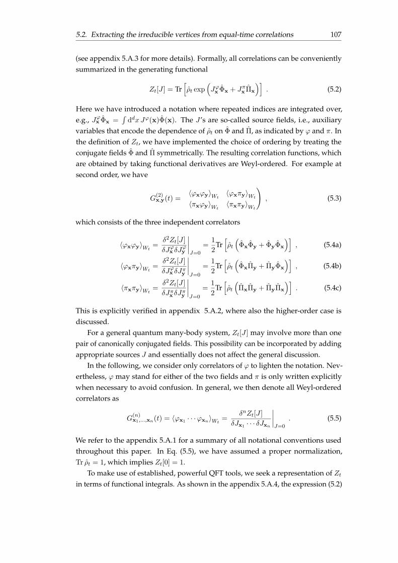
5.2. Extracting the irreducible vertices from equal-time correlations 107
(see appendix 5.A.3 for more details). Formally, all correlations can be convenientlysummarized in the generating functional
Zt[J ] = Tr[ρt exp
(Jϕx Φx + Jπx Πx
)]. (5.2)
Here we have introduced a notation where repeated indices are integrated over,e.g., Jϕx Φx =
´ddxJϕ(x)Φ(x). The J ’s are so-called source fields, i.e., auxiliary
variables that encode the dependence of ρt on Φ and Π, as indicated by ϕ and π. Inthe definition of Zt, we have implemented the choice of ordering by treating theconjugate fields Φ and Π symmetrically. The resulting correlation functions, whichare obtained by taking functional derivatives are Weyl-ordered. For example atsecond order, we have
G(2)x,y(t) =
(〈ϕxϕy〉Wt
〈ϕxπy〉Wt
〈πxϕy〉Wt〈πxπy〉Wt
), (5.3)
which consists of the three independent correlators
〈ϕxϕy〉Wt=
δ2Zt[J ]
δJϕx δJϕy
∣∣∣∣J=0
=1
2Tr[ρt
(ΦxΦy + ΦyΦx
)], (5.4a)
〈ϕxπy〉Wt=
δ2Zt[J ]
δJϕx δJπy
∣∣∣∣J=0
=1
2Tr[ρt
(ΦxΠy + ΠyΦx
)], (5.4b)
〈πxπy〉Wt=
δ2Zt[J ]
δJπx δJπy
∣∣∣∣J=0
=1
2Tr[ρt
(ΠxΠy + ΠyΠx
)]. (5.4c)
This is explicitly verified in appendix 5.A.2, where also the higher-order case isdiscussed.
For a general quantum many-body system, Zt[J ] may involve more than onepair of canonically conjugated fields. This possibility can be incorporated by addingappropriate sources J and essentially does not affect the general discussion.
In the following, we consider only correlators of ϕ to lighten the notation. Nev-ertheless, ϕ may stand for either of the two fields and π is only written explicitlywhen necessary to avoid confusion. In general, we then denote all Weyl-orderedcorrelators as
G(n)x1,...,xn(t) = 〈ϕx1 · · ·ϕxn〉Wt
=δnZt[J ]
δJx1 · · · δJxn
∣∣∣∣J=0
. (5.5)
We refer to the appendix 5.A.1 for a summary of all notational conventions usedthroughout this paper. In Eq. (5.5), we have assumed a proper normalization,Tr ρt = 1, which implies Zt[0] = 1.
To make use of established, powerful QFT tools, we seek a representation of Ztin terms of functional integrals. As shown in the appendix 5.A.4, the expression (5.2)

108 Chapter 5. Extraction of the instantaneous effective action in equilibrium
can be rewritten as a
Zt[J ] =
ˆDϕDπWt [ϕ, π] exp (Jϕxϕx + Jπxπx) . (5.6)
The integration kernel Wt can be interpreted as a quasi-probability distribution,
Wt[ϕ, π] =
ˆDϕ
⟨ϕ− ϕ
2
∣∣∣∣ ρt∣∣∣∣ϕ+
ϕ
2
⟩exp
(i
~ϕxπx
), (5.7)
the so-called Wigner functional. Here |ϕ〉 denotes an eigenstate of the field opera-tor Φ with eigenvalue ϕ. The Wigner function itself has previously been appliedsuccessfully in the context of quantum optics [208] and also plays a prominent rolein the semi-classical description of non-equilibrium quantum dynamics [209, 210].Eq. (5.6) is the basis of the equal-time formulation of QFT and allows us to applyestablished procedures in the following.
5.2.2 Connected correlation functions
In QFT (and analogously in classical probability theory) it is well known that the cor-relations encoded in Zt are largely redundant [50, 211]. The first step is the removalof additive redundancies, by the introduction of another generating functional,
Et[J ] = logZt[J ] . (5.8)
We denote the corresponding correlations, called connected correlators, as
G(n)c,x1,...,xn(t) =
δnEt[J ]
δJx1 · · · δJxn
∣∣∣∣J=0
. (5.9)
Explicitly, as shown in the appendix 5.A.5, up to fourth order they are given by
G(1)c,x1
= G(1)x1
, (5.10a)
G(2)c,x1,x2
= G(2)x1,x2
−G(1)c,x1
G(1)c,x2
, (5.10b)
G(3)c,x1,x2,x3
= G(3)x1,x2,x3
−(G(2)
c,x1,x2G(1)
c,x3+G(2)
c,x2,x3G(1)
c,x1+G(2)
c,x3,x1G(1)
c,x2
)
−G(1)c,x1
G(1)c,x2
G(1)c,x3
, (5.10c)
G(4)c,x1,x2,x3,x4
= G(4)x1,x2,x3,x4
−(G(2)
c,x1,x2G(2)
c,x3,x4+G(2)
c,x1,x3G(2)
c,x2,x4+G(2)
c,x1,x4G(2)
c,x2,x3+)
−(G(3)
c,x1,x2,x3G(1)
c,x4+G(3)
c,x2,x3,x4G(1)
c,x1+G(3)
c,x3,x4,x1G(1)
c,x2+G(3)
c,x4,x1,x2G(1)
c,x3
)
−(G(2)
c,x1,x2G(1)
c,x3G(1)
c,x4+G(2)
c,x1,x3G(1)
c,x2G(1)
c,x4+G(2)
c,x1,x4G(1)
c,x2G(1)
c,x3
+ G(2)c,x2,x3
G(1)c,x1
G(1)c,x4
+G(2)c,x2,x4
G(1)c,x1
G(1)c,x3
+G(2)c,x3,x4
G(1)c,x1
G(1)c,x2
)
−G(1)c,x1
G(1)c,x2
G(1)c,x3
G(1)c,x4
, (5.10d)
where we suppressed the overall time-dependence for brevity. For every order n,the connected part G(n)
c , is obtained by subtracting the information already given bylower-order functions G(m<n)
c .

5.2. Extracting the irreducible vertices from equal-time correlations 109
FIGURE 5.1: Feynman diagrams relating full and connected correlationfunctions. At first-order (a) the correlations are identical. At second-order(b) there is one disconnected diagram that contains redundant information.At higher orders an increasing number of disconnected diagrams need tobe considered. We explicitly show the third-order (c) and fourth-order (d)correlations. The dots indicate permutations of the diagrammatic structurewithin the brackets, similar to (c).
This can be visualized by a graphical representation in terms of Feynman dia-grams, which is very helpful to organize the underlying combinatorics. By carefulexamination of this reorganization, exemplified in Fig. 5.1, one learns that onlyconnected graphs contribute to the correlators generated by Et, hence the nameconnected correlations. In short, taking the logarithm of Zt in Eq. (5.8) removes alldisconnected diagrams.
Physically, this means that by inspecting the factorization of higher-order corre-lation functions, one can determine whether or not the quantum system is describedby a Gaussian density operator ρt. Since Gaussian distributions correspond to free(non-interacting) QFTs, this in principle allows to determine the basis of conjugatefields which diagonalizes the quantum many-body Hamiltonian that governs thesystem at hand.
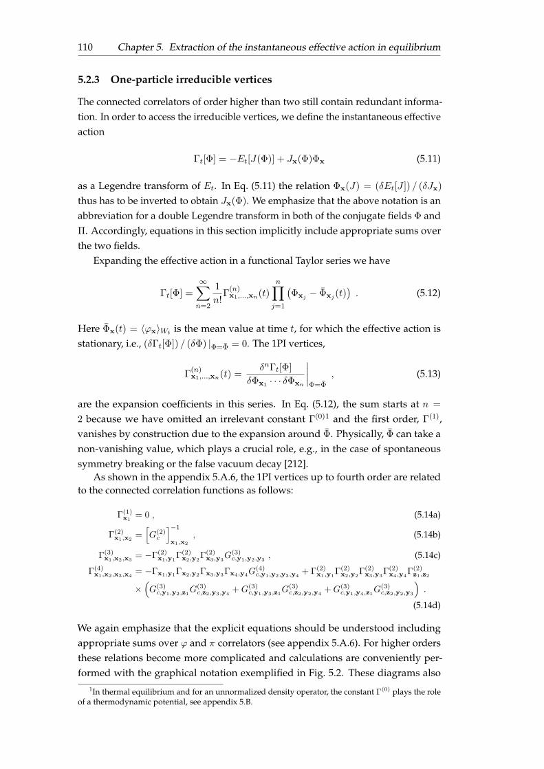
110 Chapter 5. Extraction of the instantaneous effective action in equilibrium
5.2.3 One-particle irreducible vertices
The connected correlators of order higher than two still contain redundant informa-tion. In order to access the irreducible vertices, we define the instantaneous effectiveaction
Γt[Φ] = −Et[J(Φ)] + Jx(Φ)Φx (5.11)
as a Legendre transform of Et. In Eq. (5.11) the relation Φx(J) = (δEt[J ]) / (δJx)
thus has to be inverted to obtain Jx(Φ). We emphasize that the above notation is anabbreviation for a double Legendre transform in both of the conjugate fields Φ andΠ. Accordingly, equations in this section implicitly include appropriate sums overthe two fields.
Expanding the effective action in a functional Taylor series we have
Γt[Φ] =∞∑
n=2
1
n!Γ
(n)x1,...,xn(t)
n∏
j=1
(Φxj − Φxj (t)
). (5.12)
Here Φx(t) = 〈ϕx〉Wt is the mean value at time t, for which the effective action isstationary, i.e., (δΓt[Φ]) / (δΦ) |Φ=Φ = 0. The 1PI vertices,
Γ(n)x1,...,xn(t) =
δnΓt[Φ]
δΦx1 · · · δΦxn
∣∣∣∣Φ=Φ
, (5.13)
are the expansion coefficients in this series. In Eq. (5.12), the sum starts at n =
2 because we have omitted an irrelevant constant Γ(0)1 and the first order, Γ(1),vanishes by construction due to the expansion around Φ. Physically, Φ can take anon-vanishing value, which plays a crucial role, e.g., in the case of spontaneoussymmetry breaking or the false vacuum decay [212].
As shown in the appendix 5.A.6, the 1PI vertices up to fourth order are relatedto the connected correlation functions as follows:
Γ(1)x1
= 0 , (5.14a)
Γ(2)x1,x2
=[G(2)
c
]−1x1,x2
, (5.14b)
Γ(3)x1,x2,x3
= −Γ(2)x1,y1
Γ(2)x2,y2
Γ(2)x3,y3
G(3)c,y1,y2,y3
, (5.14c)
Γ(4)x1,x2,x3,x4
= −Γx1,y1Γx2,y2Γx3,y3Γx4,y4G(4)c,y1,y2,y3,y4
+ Γ(2)x1,y1
Γ(2)x2,y2
Γ(2)x3,y3
Γ(2)x4,y4
Γ(2)z1,z2
×(G(3)
c,y1,y2,z1G(3)
c,z2,y3,y4+G(3)
c,y1,y3,z1G(3)
c,z2,y2,y4+G(3)
c,y1,y4,z1G(3)
c,z2,y2,y3
).
(5.14d)
We again emphasize that the explicit equations should be understood includingappropriate sums over ϕ and π correlators (see appendix 5.A.6). For higher ordersthese relations become more complicated and calculations are conveniently per-formed with the graphical notation exemplified in Fig. 5.2. These diagrams also
1In thermal equilibrium and for an unnormalized density operator, the constant Γ(0) plays the roleof a thermodynamic potential, see appendix 5.B.
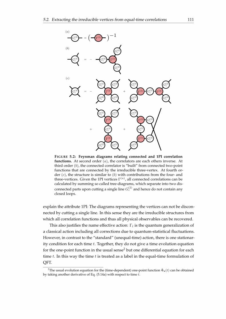
5.2. Extracting the irreducible vertices from equal-time correlations 111
FIGURE 5.2: Feynman diagrams relating connected and 1PI correlationfunctions. At second order (a), the correlators are each others inverse. Atthird order (b), the connected correlator is “built” from connected two-pointfunctions that are connected by the irreducible three-vertex. At fourth or-der (c), the structure is similar to (b) with contributions from the four- andthree-vertices. Given the 1PI vertices Γ(n), all connected correlations can becalculated by summing so called tree-diagrams, which separate into two dis-connected parts upon cutting a single line G
(2)c and hence do not contain any
closed loops.
explain the attribute 1PI: The diagrams representing the vertices can not be discon-nected by cutting a single line. In this sense they are the irreducible structures fromwhich all correlation functions and thus all physical observables can be recovered.
This also justifies the name effective action: Γt is the quantum generalization ofa classical action including all corrections due to quantum-statistical fluctuations.However, in contrast to the “standard” (unequal-time) action, there is one stationar-ity condition for each time t. Together, they do not give a time evolution equationfor the one-point function in the usual sense2 but one differential equation for eachtime t. In this way the time t is treated as a label in the equal-time formulation ofQFT.
2The usual evolution equation for the (time-dependent) one-point function Φx(t) can be obtainedby taking another derivative of Eq. (5.14a) with respect to time t.

112 Chapter 5. Extraction of the instantaneous effective action in equilibrium
5.2.4 Measuring the effective Hamiltonian
So far, we have equivalently rewritten the quantum-statistical information of asystem described by a density operator ρt in terms of generating functionals Zt,Et and Γt which encode full, connected and 1PI correlation functions, respectively.While the entries of the density matrix are typically inaccessible and less intuitive,the equal-time correlators can be measured in experiments and are directly relatedto relevant observables and structural information, such as occupation numbers andcouplings. Next, we employ the equal-time formalism to relate parameters of anHamiltonian to the 1PI correlators.
As a generic example we consider a relativistic scalar field theory with potentialV described by the Hamiltonian
H =
ˆx
[1
2Π2
x +1
2
(∇xΦx
)2+ V
(Φx
)]. (5.15)
Given the Hamiltonian H , it is possible to derive an evolution equation for Γt [61](see also the next chapter 6). For simplicity, we focus on the case of thermalequilibrium, which is a stationary solution Γβ , described by the density operatorρβ ∼ exp
(−βH
)with the prefactor fixed by normalization
In order to obtain the generating functional Eq. (5.6) we need to calculate theWigner functional Eq. (5.7). In the interacting case, the involved functional integra-tion can only be performed approximately. It is however possible to derive an exactequation for the thermal Wigner functional (see appendix 5.A.7). It takes the formof a functional flow equation, ∂βWβ = −(H0 + ~2H1 + . . . )Wβ , with
H0 =
ˆx
[1
2π2x +
1
2(∇xϕx)2 + Vx (ϕ)
]. (5.16)
It is straightforward to solve the equation for Wβ perturbatively by a semi-classicalexpansion in powers of ~. An exact solution for V = 0 is discussed in appendix 5.B.
The leading order is the classical field theory limit, where we obtain Wβ ∼exp (−βH0) with the classical Hamiltonian H0. Then the generating functionalEq. (5.6) becomes
Zβ [J ] ∼ˆDπDϕ e−βH0+Jϕx ϕx+Jπxπx . (5.17)
Thus βH0 plays the role of a classical action for the fluctuating fields ϕ and π. Thisallows us to calculate the effective action Γβ in the equal-time formalism usingestablished QFT methods, such as a the background field method employed below.
We note that the two conjugate fields ϕ and π decouple in the present limit,which implies that the effective action separates as
Γβ [Φ,Π] = Γβ [Φ] + Γβ [Π] (5.18)

5.2. Extracting the irreducible vertices from equal-time correlations 113
with Γβ [Π] = β2
´x Π2
x + const., as shown in appendix 5.A.8. The separation Eq. (5.18)is a property of the classical field approximation. In general, the quantum effectiveaction of the full quantum theory requires knowledge of all equal-time correlatorsof ϕ and π, including mixed terms. However, symmetries such as time translationinvariance simplify the discussion, see appendix 5.A.9.
By means of the background field method, we can calculate the effective actionin a loop expansion. In the present formalism, we split
Γβ [Φ] = βH[Φ] + Γ′β [Φ] , (5.19)
where H[Φ] = H0[ϕ = Φ, π = 0]. As shown in the appendix 5.A.10, the “rest” Γ′βobeys the following functional integro-differential equation,
e−Γ′β [Φ] =
ˆDϕ exp
(−βK[ϕ,Φ] +
δΓ′β [Φ]
δΦxϕx
), (5.20)
where we abbreviated
K[ϕ,Φ] = H[Φ + ϕ]−H[Φ]−ˆx
δH[Φ]
δΦxϕx . (5.21)
The solution of this equation is organized diagrammatically as an expansion inthe number of loops (see [213] for a proof to all orders). At leading order (tree-level) in this expansion Γ′β = 0 and thus the equal-time effective action is directlyrelated to the microscopic Hamiltonian. Consequently, the 1PI vertices correspondto the interaction constants of the underlying system. Beyond the leading-orderapproximation, the notion of the microscopic Hamiltonian becomes a less usefulconcept. The effective action then plays the role of an “effective Hamiltonian”, withall corrections from quantum-statistical fluctuations taken into account.
Returning to the leading order approximation, which gives rise to the tree-level1PI vertices, we explicitly have
Γ(2)x,y = ∇2
xδ(x− y) +
ˆz
δ2Vz(Φ)
δΦxδΦy
∣∣∣∣Φ=Φ
, (5.22a)
Γ(n)x1,...,xn =
ˆz
δnVz(Φ)
δΦx1 · · · δΦxn
∣∣∣∣Φ=Φ
, (5.22b)
where n ≥ 3. Eq. (5.19) or more explicitly Eq. (5.22) directly show the relationbetween the 1PI correlation functions and the parameters of the microscopic (ormore generally an effective) Hamiltonian. Together with the procedure to obtainthe 1PI correlators, outlined below, they provide an experimental prescription formeasuring a quantum many-body Hamiltonian.

114 Chapter 5. Extraction of the instantaneous effective action in equilibrium
5.2.5 Recipe to extract 1PI correlators
The extraction of 1PI correlators, which are the fundamental irreducible buildingblocks for the QFT description, from equal-time data proceeds in the following steps.
1. Identify the degrees of freedom of interest which constitute the elementaryfields ϕ of the QFT.
2. Obtain many realisations (i = 1, . . . , N ) of the desired field ϕi(x) at the times tof interest.
3. Estimate the full correlators up to order n by calculating the ensemble averageG
(n)x1,...,xn ≈ 1
N
∑i ϕi(x1) · · ·ϕi(xn).
4. Obtain the connected correlators G(n)c by subtracting the disconnected contri-
butions according to Eq. (5.10).
5. Calculate the 1PI correlators Γ(n) by reducing the connected correlators accord-ing to Eq. (5.14).
This procedure corresponds to a shift of representation from the density operatorρ to Γ, the generating functional for 1PI correlators. In the following two sectionswe will illustrate and verify the method in the case of the sine-Gordon model withnumerically simulated data (Section 5.3) and with experimental measurements(Section 5.4).
5.3 Example: Sine-Gordon model
As an explicit example, we consider the sine-Gordon model [199–202] in thermalequilibrium. It is an interacting relativistic scalar field theory described by
βHSG =
ˆx
βgΠ2
x +λT4
[1
2
(∂xΦx
)2− 1
`2Jcos(
Φx
)], (5.23)
where β = (kBT )−1 is the inverse temperature. The specific form of the HamiltonianHSG given above is motivated by the recent progress to quantum simulate the SGmodel by two tunnel coupled 1D superfluids [38, 203]. See section 5.4 for thephysical origin of the fields Φ and Π, the microscopic parameter g and the lengthscales λT and `J .
The semi-classical approximation Eq. (5.17) is valid for
√4γ min
[1,
4
Q
], (5.24)
where the dimensionless parameters are γ = 16gβ/λT and Q = λT /`J . In the semi-classical limit the loop expansion is controlled byQwith the tree-level approximation
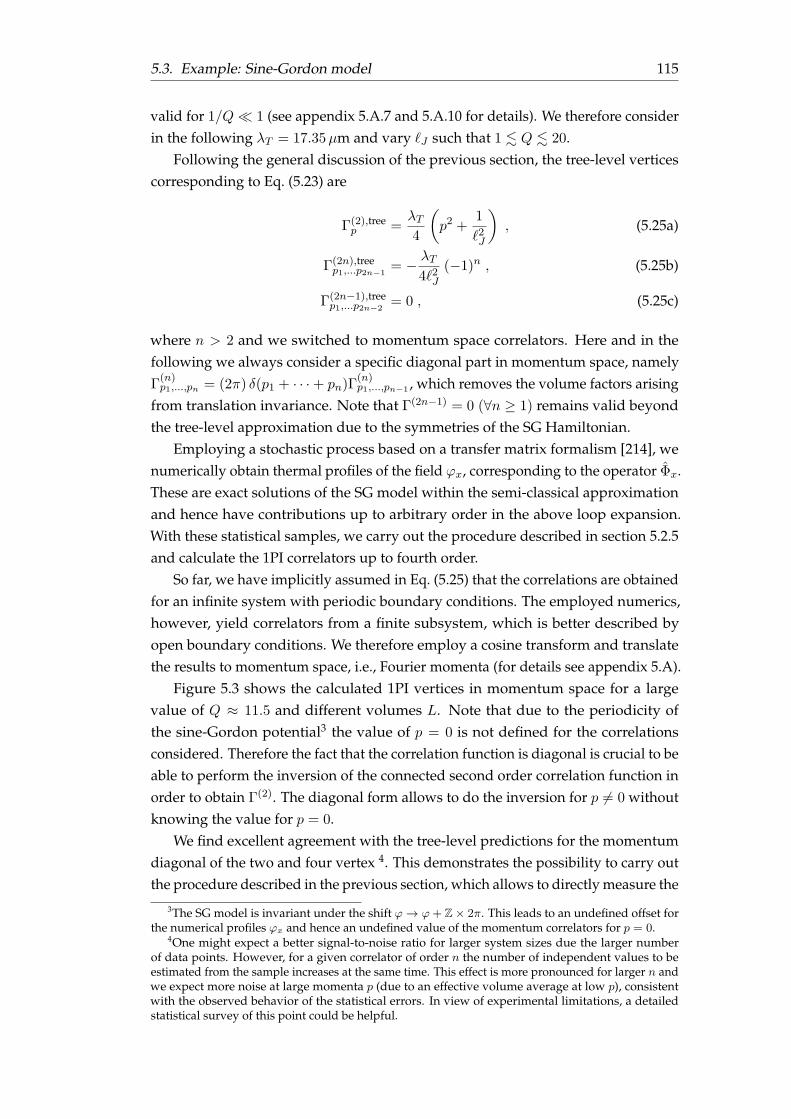
5.3. Example: Sine-Gordon model 115
valid for 1/Q 1 (see appendix 5.A.7 and 5.A.10 for details). We therefore considerin the following λT = 17.35µm and vary `J such that 1 . Q . 20.
Following the general discussion of the previous section, the tree-level verticescorresponding to Eq. (5.23) are
Γ(2),treep =
λT4
(p2 +
1
`2J
), (5.25a)
Γ(2n),treep1,...p2n−1
= − λT4`2J
(−1)n , (5.25b)
Γ(2n−1),treep1,...p2n−2
= 0 , (5.25c)
where n > 2 and we switched to momentum space correlators. Here and in thefollowing we always consider a specific diagonal part in momentum space, namelyΓ
(n)p1,...,pn = (2π) δ(p1 + · · ·+ pn)Γ
(n)p1,...,pn−1 , which removes the volume factors arising
from translation invariance. Note that Γ(2n−1) = 0 (∀n ≥ 1) remains valid beyondthe tree-level approximation due to the symmetries of the SG Hamiltonian.
Employing a stochastic process based on a transfer matrix formalism [214], wenumerically obtain thermal profiles of the field ϕx, corresponding to the operator Φx.These are exact solutions of the SG model within the semi-classical approximationand hence have contributions up to arbitrary order in the above loop expansion.With these statistical samples, we carry out the procedure described in section 5.2.5and calculate the 1PI correlators up to fourth order.
So far, we have implicitly assumed in Eq. (5.25) that the correlations are obtainedfor an infinite system with periodic boundary conditions. The employed numerics,however, yield correlators from a finite subsystem, which is better described byopen boundary conditions. We therefore employ a cosine transform and translatethe results to momentum space, i.e., Fourier momenta (for details see appendix 5.A).
Figure 5.3 shows the calculated 1PI vertices in momentum space for a largevalue of Q ≈ 11.5 and different volumes L. Note that due to the periodicity ofthe sine-Gordon potential3 the value of p = 0 is not defined for the correlationsconsidered. Therefore the fact that the correlation function is diagonal is crucial to beable to perform the inversion of the connected second order correlation function inorder to obtain Γ(2). The diagonal form allows to do the inversion for p 6= 0 withoutknowing the value for p = 0.
We find excellent agreement with the tree-level predictions for the momentumdiagonal of the two and four vertex 4. This demonstrates the possibility to carry outthe procedure described in the previous section, which allows to directly measure the
3The SG model is invariant under the shift ϕ→ ϕ+ Z× 2π. This leads to an undefined offset forthe numerical profiles ϕx and hence an undefined value of the momentum correlators for p = 0.
4One might expect a better signal-to-noise ratio for larger system sizes due the larger numberof data points. However, for a given correlator of order n the number of independent values to beestimated from the sample increases at the same time. This effect is more pronounced for larger n andwe expect more noise at large momenta p (due to an effective volume average at low p), consistentwith the observed behavior of the statistical errors. In view of experimental limitations, a detailedstatistical survey of this point could be helpful.
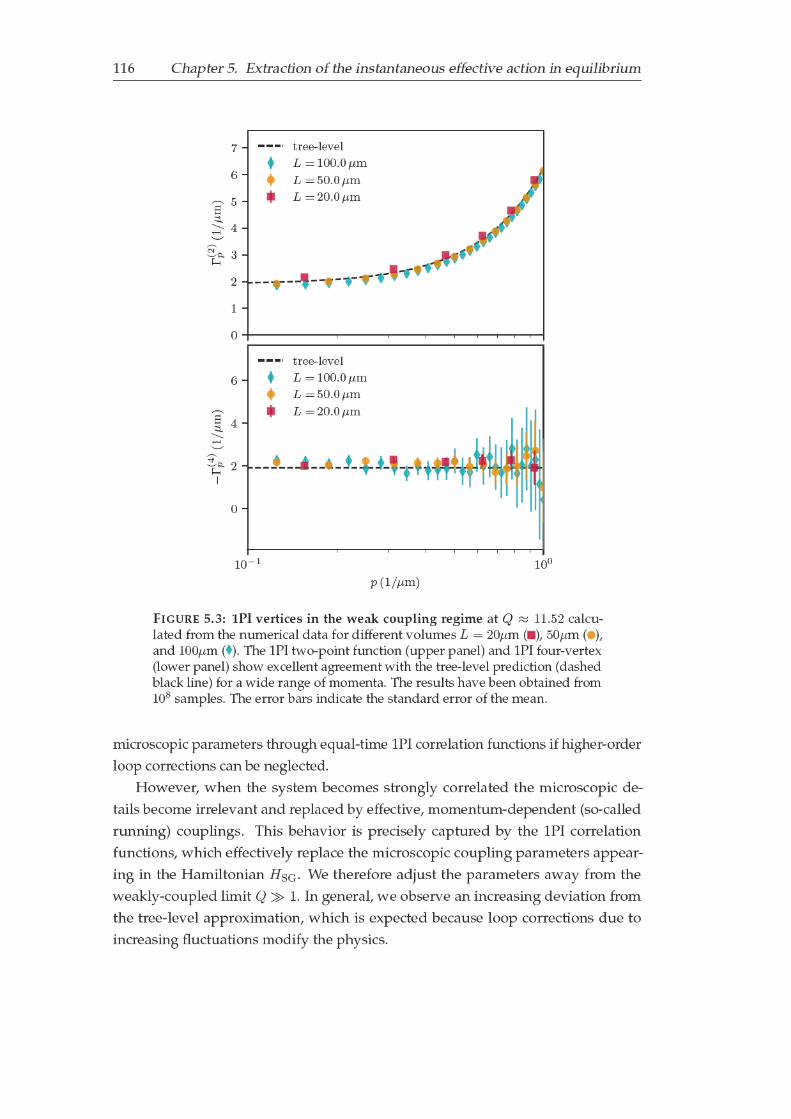
1 1 6 C h a pt e r 5. E xt r a cti o n of t h e i n st a nt a n e o u s eff e cti v e a cti o n i n e q uili b ri u m
0
1
2
3
4
5
6
7
Γ(
2)p
(1/µ
m)
t r e e-l e v el
L = 1 0 0. 0 µ m
L = 5 0. 0 µ m
L = 2 0. 0 µ m
1 0 − 1 1 0 0
p ( 1 /µ m )
0
2
4
6
−Γ
(4)
p(1/µ
m)
t r e e-l e v el
L = 1 0 0. 0 µ m
L = 5 0. 0 µ m
L = 2 0. 0 µ m
F I G U R E 5. 3: 1 PI v erti c e s i n t h e w e a k c o u pli n g r e gi m e at Q ≈ 1 1 .5 2 c al c u-l at e d f r o m t h e n u m e ri c al d at a f o r diff e r e nt v ol u m e s L = 2 0 µ m ( ), 5 0 µ m ( ),a n d 1 0 0 µ m ( ). T h e 1 PI t w o- p oi nt f u n cti o n ( u p p e r p a n el) a n d 1 PI f o u r- v e rt e x(l o w e r p a n el) s h o w e x c ell e nt a g r e e m e nt wit h t h e t r e e-l e v el p r e di cti o n ( d a s h e dbl a c k li n e) f o r a wi d e r a n g e of m o m e nt a. T h e r e s ult s h a v e b e e n o bt ai n e d f r o m1 0 8 s a m pl e s. T h e e r r o r b a r s i n di c at e t h e st a n d a r d e r r o r of t h e m e a n.
mi c r o s c o pi c p a r a m et e r s t h r o u g h e q u al-ti m e 1 PI c o r r el ati o n f u n cti o n s if hi g h e r- o r d e r
l o o p c o r r e cti o n s c a n b e n e gl e ct e d.
H o w e v e r, w h e n t h e s y st e m b e c o m e s st r o n gl y c o r r el at e d t h e mi c r o s c o pi c d e-
t ail s b e c o m e i r r el e v a nt a n d r e pl a c e d b y eff e cti v e, m o m e nt u m- d e p e n d e nt ( s o- c all e d
r u n ni n g) c o u pli n g s. T hi s b e h a vi o r i s p r e ci s el y c a pt u r e d b y t h e 1 PI c o r r el ati o n
f u n cti o n s, w hi c h eff e cti v el y r e pl a c e t h e mi c r o s c o pi c c o u pli n g p a r a m et e r s a p p e a r-
i n g i n t h e H a milt o ni a n H S G . We t h e r ef o r e a dj u st t h e p a r a m et e r s a w a y f r o m t h e
w e a kl y- c o u pl e d li mit Q 1 . I n g e n e r al, w e o b s e r v e a n i n c r e a si n g d e vi ati o n f r o m
t h e t r e e-l e v el a p p r o xi m ati o n, w hi c h i s e x p e ct e d b e c a u s e l o o p c o r r e cti o n s d u e t o
i n c r e a si n g fl u ct u ati o n s m o dif y t h e p h y si c s.

5. 3. E x a m pl e: Si n e- G o r d o n m o d el 1 1 7
p ( 1 /µ m )
1 0 − 2
1 0 − 1
1 0 0
1 0 1
Γ(
2)p
(1/µ
m)t r e e-l e v el
o n e-l o o p
Q = 8. 1 4
Q = 5. 7 6
Q = 4. 0 7
1 0 − 2 1 0 − 1 1 0 0
p ( 1 /µ m )
− 1 .0
− 0 .8
− 0 .6
− 0 .4
− 0 .2
0 .0
Σp/Γ
(2)
,tree
p
t r e e-l e v el
o n e-l o o p
Q = 8. 1 4
Q = 5. 7 6
Q = 4. 0 7
F I G U R E 5. 4: L o o p c orr e cti o n s t o t h e 1 PI t w o- p oi nt f u n cti o n f o r diff e r e nt Qi n t h e st r o n g c o u pli n g r e gi m e, Q = 8 .1 4 ( ), 5 .7 6 ( ), a n d 4 .0 7 ( ). T h e c al c u-l at e d t w o- p oi nt f u n cti o n ( u p p e r p a n el) al w a y s a p p r o a c h e s t h e c o r r e s p o n di n gt r e e-l e v el p r e di cti o n s ( bl a c k d a s h e d li n e s) at hi g h m o m e nt a, a s e x p e ct e d. I n t h ei nf r a r e d, w e o b s e r v e d e vi ati o n s d u e t o l o o p c o r r e cti o n s. T h e c o r r e s p o n di n gc ol o r e d d a s h e d- d ott e d li n e s i n cl u d e t h e o n e-l o o p c o r r e cti o n. T h e c o r r e s p o n d-i n g s elf- e n e r g y (l o w e r p a n el) q u a nti fi e s t h e d e vi ati o n s f r o m t h e t r e e-l e v elp r e di cti o n. T h e c o r r e cti o n s b e c o m e m o r e p r o n o u n c e d f o r s m all e r Q , a s e x-p e ct e d. N u m e ri c al r e s ult s a r e c al c ul at e d f o r L = 2 0 0 µ m a n d a s a m pl e si z e of1 0 8 .
Q u a ntit ati v el y, t h e c o r r e cti o n s t o t h e 1 PI t w o- p oi nt f u n cti o n a r e s u m m a ri z e d i n
t h e “ s elf- e n e r g y ” Σ , d e fi n e d vi a
Γ ( 2 )p = Γ ( 2 ) ,t r e e
p + Σ p . ( 5. 2 6)
I n t h e a p p e n di x 5. A. 1 3 , w e c al c ul at e t h e l e a di n g c o r r e cti o n,
Σo n e-l o o pp = − 1 / ( 4 J ) . ( 5. 2 7)
I n Fi g. 5. 4 , t h e 1 PI t w o- p oi nt f u n cti o n a n d t h e s elf- e n e r g y a r e pl ott e d a s a f u n cti o n
of p . G e n e ri c all y, t r e e-l e v el d o mi n at e s i n t h e U V (i. e., at hi g h m o m e nt a), w hi c h w e

1 1 8 C h a pt e r 5. E xt r a cti o n of t h e i n st a nt a n e o u s eff e cti v e a cti o n i n e q uili b ri u m
p ( 1 /µ m )
1 0 − 1
1 0 0
1 0 1
1 0 2
1 0 3
−Γ
(4)
p(1/µ
m)
t r e e-l e v el
Q = 8. 1 4
Q = 5. 7 6
Q = 4. 0 7
1 0 − 1 1 0 0
p ( 1 /µ m )
1 0 − 4
1 0 − 3
1 0 − 2
1 0 − 1
1 0 0
−Γ
(4)
p(1/µ
m)
t r e e-l e v el
Q = 2. 8 8
Q = 2. 0 4
Q = 1. 4 4
F I G U R E 5. 5: L o o p c orr e cti o n s t o t h e 1 PI f o ur- v ert e x f o r diff e r e nt v al u e s of Q .T h e ( n e g ati v e) f o u r- v e rt e x ( , , ), s h o w n f o r l a r g e r v al u e s of Q ( u p p e r p a n el,c o r r e s p o n di n g t o Fi g. 5. 4 ), cl e a rl y a p p r o a c h e s t h e c o r r e s p o n di n g t r e e-l e v elp r e di cti o n s ( c ol o r e d d a s h e d li n e s) at hi g h m o m e nt a. I n t h e i nf r a r e d, w e o b-s e r v e a st r o n g m o m e nt u m d e p e n d e n c e, i n c r e a si n g t h e eff e cti v e c o u pli n g. F o rd e c r e a si n g v al u e s of Q (l o w e r p a n el) t h e ( n e g ati v e) f o u r- v e rt e x i s i n c r e a si n gl ys u p p r e s s e d i n t h e i nf r a r e d. T h e r e s ult s a r e c o n si st e nt wit h t h e a p p r o a c h oft h e t r e e-l e v el p r e di cti o n ( c ol o r e d d a s h e d li n e s) f o r hi g h m o m e nt a. N u m e ri c alr e s ult s a r e c al c ul at e d f o r L = 1 0 0 µ m a n d a s a m pl e si z e of 1 0 8 . T h e e r r o r b a r si n di c at e t h e st a n d a r d e r r o r of t h e m e a n. N ot e t h at w e e x cl u d e d d at a p oi nt s athi g h m o m e nt a wit h e r r o r s l a r g e r t h a n t h e m e a n f r o m t hi s pl ot.
al s o o b s e r v e n u m e ri c all y. T h e 1 PI t w o- p oi nt f u n cti o n a p p r o a c h e s t h e p o w e r-l a w
∝ p 2 i n t hi s li mit a n d t h e ( n o r m ali z e d) s elf- e n e r g y v a ni s h e s.
I n t h e I R (l o w m o m e nt a), h o w e v e r, l o o p c o r r e cti o n s a r e i m p o rt a nt. It i s t hi s
r e gi m e w h e r e c oll e cti v e m a c r o s c o pi c p h e n o m e n a e m e r g e a n d t h e mi c r o s c o pi c d et ail s
a r e w a s h e d o ut. We o b s e r v e a n e g ati v e s elf- e n e r g y a n d h e n c e a r e d u cti o n of t h e
1 PI t w o- p oi nt f u n cti o n, w hi c h a g r e e s wit h t h e o n e-l o o p r e s ult o v e r a n i nt e r m e di at e
r a n g e of m o m e nt a ( a n d Q ). P h y si c all y, t hi s r e s ult i m pli e s st r o n g e r fl u ct u ati o n s a s
Q d e c r e a s e s, c o n si st e nt wit h t h e e x p e ct ati o n f o r a st r o n gl y c o r r el at e d r e gi m e of t h e
si n e- G o r d o n m o d el.
Si mil a rl y, t h e l o o p c o r r e cti o n s t o t h e 1 PI v e rti c e s l e a d t o t h e n oti o n of r u n ni n g
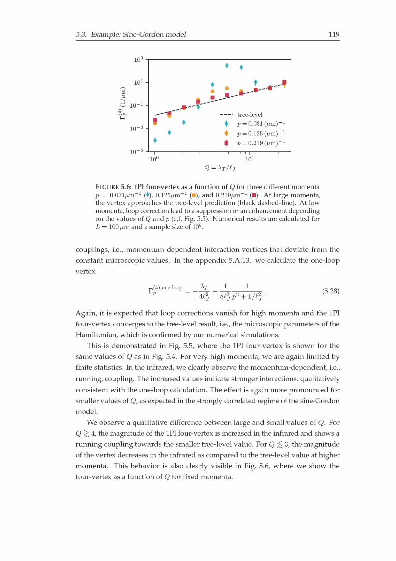
5. 3. E x a m pl e: Si n e- G o r d o n m o d el 1 1 9
1 0 0 1 0 1
Q = λ T / J
1 0 − 5
1 0 − 3
1 0 − 1
1 0 1
1 0 3
−Γ
(4)
p(1/µ
m)t r e e-l e v el
p = 0. 0 3 1 ( µ m ) − 1
p = 0. 1 2 5 ( µ m ) − 1
p = 0. 2 1 9 ( µ m ) − 1
F I G U R E 5. 6: 1 PI f o ur- v ert e x a s a f u n cti o n of Q f o r t h r e e diff e r e nt m o m e nt ap = 0 .0 3 1 µ m − 1 ( ), 0 .1 2 5 µ m − 1 ( ), a n d 0 .2 1 9 µ m − 1 ( ). At l a r g e m o m e nt a,t h e v e rt e x a p p r o a c h e s t h e t r e e-l e v el p r e di cti o n ( bl a c k d a s h e d-li n e). At l o wm o m e nt a, l o o p c o r r e cti o n l e a d t o a s u p p r e s si o n o r a n e n h a n c e m e nt d e p e n di n go n t h e v al u e s of Q a n d p ( c.f. Fi g. 5. 5 ). N u m e ri c al r e s ult s a r e c al c ul at e d f o rL = 1 0 0 µ m a n d a s a m pl e si z e of 1 0 8 .
c o u pli n g s, i. e., m o m e nt u m- d e p e n d e nt i nt e r a cti o n v e rti c e s t h at d e vi at e f r o m t h e
c o n st a nt mi c r o s c o pi c v al u e s. I n t h e a p p e n di x 5. A. 1 3 . w e c al c ul at e t h e o n e-l o o p
v e rt e x
Γ( 4 ) ,o n e-l o o pp = −
λ T
4 2J
−1
8 3J
1
p 2 + 1 / 2J
. ( 5. 2 8)
A g ai n, it i s e x p e ct e d t h at l o o p c o r r e cti o n s v a ni s h f o r hi g h m o m e nt a a n d t h e 1 PI
f o u r- v e rt e x c o n v e r g e s t o t h e t r e e-l e v el r e s ult, i. e., t h e mi c r o s c o pi c p a r a m et e r s of t h e
H a milt o ni a n, w hi c h i s c o n fi r m e d b y o u r n u m e ri c al si m ul ati o n s.
T hi s i s d e m o n st r at e d i n Fi g. 5. 5 , w h e r e t h e 1 PI f o u r- v e rt e x i s s h o w n f o r t h e
s a m e v al u e s of Q a s i n Fi g. 5. 4 . F o r v e r y hi g h m o m e nt a, w e a r e a g ai n li mit e d b y
fi nit e st ati sti c s. I n t h e i nf r a r e d, w e cl e a rl y o b s e r v e t h e m o m e nt u m- d e p e n d e nt, i. e.,
r u n ni n g, c o u pli n g. T h e i n c r e a s e d v al u e s i n di c at e st r o n g e r i nt e r a cti o n s, q u alit ati v el y
c o n si st e nt wit h t h e o n e-l o o p c al c ul ati o n. T h e eff e ct i s a g ai n m o r e p r o n o u n c e d f o r
s m all e r v al u e s of Q , a s e x p e ct e d i n t h e st r o n gl y c o r r el at e d r e gi m e of t h e si n e- G o r d o n
m o d el.
We o b s e r v e a q u alit ati v e diff e r e n c e b et w e e n l a r g e a n d s m all v al u e s of Q . F o r
Q 4 , t h e m a g nit u d e of t h e 1 PI f o u r- v e rt e x i s i n c r e a s e d i n t h e i nf r a r e d a n d s h o w s a
r u n ni n g c o u pli n g t o w a r d s t h e s m all e r t r e e-l e v el v al u e. F o r Q 3 , t h e m a g nit u d e
of t h e v e rt e x d e c r e a s e s i n t h e i nf r a r e d a s c o m p a r e d t o t h e t r e e-l e v el v al u e at hi g h e r
m o m e nt a. T hi s b e h a vi o r i s al s o cl e a rl y vi si bl e i n Fi g. 5. 6 , w h e r e w e s h o w t h e
f o u r- v e rt e x a s a f u n cti o n of Q f o r fi x e d m o m e nt a.
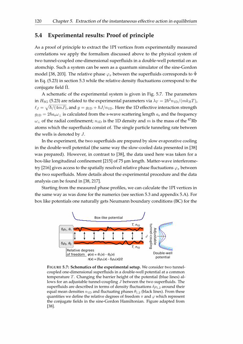
120 Chapter 5. Extraction of the instantaneous effective action in equilibrium
5.4 Experimental results: Proof of principle
As a proof of principle to extract the 1PI vertices from experimentally measuredcorrelations we apply the formalism discussed above to the physical system oftwo tunnel-coupled one-dimensional superfluids in a double-well potential on anatomchip. Such a system can be seen as a quantum simulator of the sine-Gordonmodel [38, 203]. The relative phase ϕx between the superfluids corresponds to Φ
in Eq. (5.23) in section 5.3 while the relative density fluctuations correspond to theconjugate field Π.
A schematic of the experimental system is given in Fig. 5.7. The parametersin HSG (5.23) are related to the experimental parameters via λT = 22n1D/(mkBT ),J =
√/(4mJ), and g = g1D + J/n1D. Here the 1D effective interaction strength
g1D = 2asω⊥ is calculated from the s-wave scattering length as and the frequencyω⊥ of the radial confinement; n1D is the 1D density and m is the mass of the 87Rbatoms which the superfluids consist of. The single particle tunneling rate betweenthe wells is denoted by J .
In the experiment, the two superfluids are prepared by slow evaporative coolingin the double-well potential (the same way the slow-cooled data presented in [38]was prepared). However, in contrast to [38], the data used here was taken for abox-like longitudinal confinement [215] of 75 µm length. Matter-wave interferome-try [216] gives access to the spatially resolved relative phase fluctuations ϕx betweenthe two superfluids. More details about the experimental procedure and the dataanalysis can be found in [38, 217].
Starting from the measured phase profiles, we can calculate the 1PI vertices inthe same way as was done for the numerics (see section 5.3 and appendix 5.A). Forbox like potentials one naturally gets Neumann boundary conditions (BC) for the
Adjustabletunnel-coupling
Relative degrees of freedom Double-well
potentialφ(x) = θ1(x) - θ2(x)π(x) = [δρ1(x) - δρ2(x)]/2
δρ1, θ1
δρ2, θ2
T, n1D
Box-like potential
T, n1D
J
FIGURE 5.7: Schematics of the experimental setup. We consider two tunnel-coupled one-dimensional superfluids in a double-well potential at a commontemperature T . Changing the barrier height of the potential (blue lines) al-lows for an adjustable tunnel-coupling J between the two superfluids. Thesuperfluids are described in terms of density fluctuations δρ1,2 around theirequal mean densities n1D and fluctuating phases θ1,2 (black lines). From thesequantities we define the relative degrees of freedom π and ϕ which representthe conjugate fields in the sine-Gordon Hamiltonian. Figure adapted from[38].

5.4. Experimental results: Proof of principle 121
-50 0 50 -40 -20 0 20 40
FIGURE 5.8: Cosine transformed second-order connected correlation func-tion. Results for different phase-locking strength as indicated by the valuesof Q stated above the respective subplots. The color represents the valuesfor cosine transformed second-order connected correlation function G(2)
c,p,p′ asdefined in (5.29). Note that the value (249.9 in the left subplot and 93.9 in theright subplot) for the lowest leftmost data point, lies outside the color-range.The color-range was chosen like this to get better visibility.
phase from the condition of vanishing particle current on the edges [215]. From thecosine transform (compatible with the Neumann BC) of the complete system wetherefore get the 1PI vertices of the Hamiltonian with this BC. Acknowledging thatour system is still too short to get results free from finite size effects, we neverthelessapply the conversion factors to Fourier momentum space given in (5.64) and (5.65)for consistency when presenting Γ(n).
Let us start the discussion of the experimental results with the cosine transformedsecond-order correlation function
G(2)c,p,p′ =
2
L
(〈ϕpϕp′〉 − 〈ϕp〉〈ϕp′〉
). (5.29)
Here ϕp represents the cosine transform (5.63b) over the finite interval with lengthL and we chose the prefactors for later convenience. The factor 2 comes from theidentity (5.64) and the factor 1/L from the delta function. We see from Fig. 5.8that the correlations are approximately diagonal. Further, note that density-phasetwo-point correlations, 〈πϕ〉Wt , vanish due to time-translation invariance of thethermal state, even beyond the semi-classical approximation Eq. (5.17). Together,this enables us to calculate the 1PI two-point correlator as
Γ(2)p =
1
G(2)c,p,p
, (5.30)
where we neglected the small off-diagonal elements of G(2)c,p,p′ . The results are
presented in Fig. 5.9.

122 Chapter 5. Extraction of the instantaneous effective action in equilibrium
FIGURE 5.9: Experimental 1PI two-point function. The four different mea-surements correspond to Q = 4.5 ( ), 3.1 ( ), 2.4 ( ), and 1.3 ( ). The errorbars represent the 80% confidence intervals obtained using bootstrapping. Wesee good agreement with the theory prediction from the sine-Gordon modelin thermal equilibrium calculated for 106 numerical realizations (black solidlines). The height of the green bars indicates the 80% confidence interval forthe numerical predictions considering the finite experimental sample size.Note that all uncertainty comes from the finite sample size, no uncertainty inthe parameters λT and Q was assumed. The width of the bars was chosenarbitrarily.
All experimental results presented in this chapter are corrected for the expectedinfluence of the finite imaging resolution. In our simple model, the imaging processleads to a convolution of the true phase profiles with a Gaussian function with σpsf =
3 µm [217]. In momentum space this leads to a multiplication with exp(−p2σ2
psf/2)
,which can be corrected by dividing the cosine transformed relative phase ϕ(p) bythis factor.
In order to connect the experimental results to the theoretical model (section 5.3)we estimate λT = 11 µm for all the different measurements. The values for Q =
λT /J are then self consistently fitted from 〈cos(ϕ)〉 [217]. We see good agreementbetween experiment and thermal sine-Gordon theory for the 1PI two-point functionin Fig. 5.9.
Having obtained the two-point function, and using that the third-order correla-tion functions vanish for symmetry reasons, we can calculated the diagonal part ofthe 4-vertex as
Γ(4)p = −8
3
1
L〈ϕ4
p〉c ×(Γ(2)p
)4. (5.31)
Here 〈ϕ4p〉c stands for the diagonal elements of the cosine transformed fourth-order
connected correlation function. The factor 8/3 comes from the identity (5.65), thefactor 1/L again comes from the delta function. The results for the three lowest lyingmomentum modes are presented in Fig. 5.10 as a function of Q. We find qualitativeagreement between experiment and theory as well as the expected approach towardsthe tree-level result for higher momenta. The momentum dependence for themeasurements with large experimental sample size (Fig. 5.11) reveal a running

5.4. Experimental results: Proof of principle 123
FIGURE 5.10: Experimental four-vertex. The red bullets represent the exper-imental results for the four-vertex as a function of Q = λT /J . The points inone particular subplot correspond to separate measurements with differenttunneling strength. The different subplots show the results for the lowest threevalues of p indicated in the upper left corner of the subplots. The error barsrepresent 80% confidence intervals obtained using bootstrapping. The numer-ical prediction from the sine-Gordon model in thermal equilibrium is given bythe green bars. The height of the bars indicates the 80% confidence interval forthe theory predictions considering the finite experimental sample size. Notethat all uncertainty comes from the finite sample size, no uncertainty in theparameters λT and Q was assumed. The width of the bars was chosen arbitrar-ily. The solid black line represents the theory prediction from 106 numericalrealizations and the dashed black line the tree-level prediction (5.25).

124 Chapter 5. Extraction of the instantaneous effective action in equilibrium
coupling with a qualitative agreement between the experiment and thermal sine-Gordon theory.
5.5 Summary
The presented method provides a general framework to extract and test the effectiveor emergent quantum field theoretical description of generic quantum many-bodysystems from experiments. For the example of the sine-Gordon model, which isquantum simulated with two tunnel-coupled superfluids, we have demonstratedhow to experimentally obtain the irreducible vertices in thermal equilibrium andcompared to theoretical expectations. This represents an essential step in the verifi-cation of the approach, which opens a new pathway to study fundamental questionsof QFT through large-scale (analog) quantum simulators.
This becomes especially interesting for strongly correlated systems and in non-equilibrium situations, where it is often not possible to solve the theory usingclassical computational techniques. Extracting the irreducible building blocks ofquantum many-body systems, and how they change with time, promises to providedetailed insights into the dynamics for these cases. The next chapter – where wediscuss a spin-1 Bose condensate far from equilibrium [65], which has been studiedin parallel to the work presented in this chapter and employed similar methods –presents an example where currently no theoretical solution is available. In turn, theinsight from experimental measurement can support theoretical developments indevising new approximation schemes and effective field theory descriptions.

5.5. Summary 125
FIGURE 5.11: Running coupling. Like Fig. 5.10, but showing Γ(4)p as a func-
tion of p for the four measurements with the biggest experimental samplesize. Depending on the value of Q indicated in the different subplots one cansee a clear momentum dependence, i.e., “running coupling”. Note that thevertical axis of the uppermost subplot is different from the rest. However, thelogarithmic range is the same as in the other subplots.
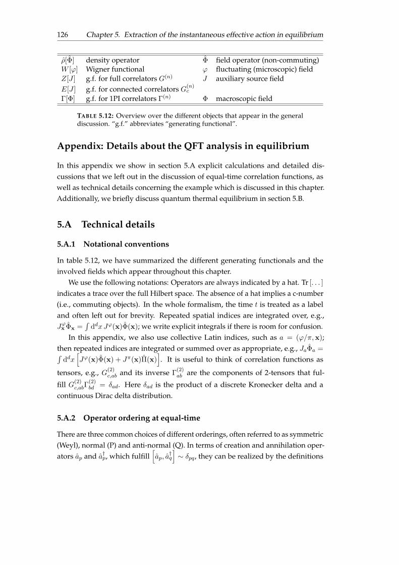
126 Chapter 5. Extraction of the instantaneous effective action in equilibrium
ρ[Φ] density operator Φ field operator (non-commuting)W [ϕ] Wigner functional ϕ fluctuating (microscopic) fieldZ[J ] g.f. for full correlators G(n) J auxiliary source fieldE[J ] g.f. for connected correlators G(n)
c
Γ[Φ] g.f. for 1PI correlators Γ(n) Φ macroscopic field
TABLE 5.12: Overview over the different objects that appear in the generaldiscussion. “g.f.” abbreviates “generating functional”.
Appendix: Details about the QFT analysis in equilibrium
In this appendix we show in section 5.A explicit calculations and detailed dis-cussions that we left out in the discussion of equal-time correlation functions, aswell as technical details concerning the example which is discussed in this chapter.Additionally, we briefly discuss quantum thermal equilibrium in section 5.B.
5.A Technical details
5.A.1 Notational conventions
In table 5.12, we have summarized the different generating functionals and theinvolved fields which appear throughout this chapter.
We use the following notations: Operators are always indicated by a hat. Tr [. . . ]
indicates a trace over the full Hilbert space. The absence of a hat implies a c-number(i.e., commuting objects). In the whole formalism, the time t is treated as a labeland often left out for brevity. Repeated spatial indices are integrated over, e.g.,Jϕx Φx =
´ddxJϕ(x)Φ(x); we write explicit integrals if there is room for confusion.
In this appendix, we also use collective Latin indices, such as a = (ϕ/π,x);then repeated indices are integrated or summed over as appropriate, e.g., JaΦa =´
ddx[Jϕ(x)Φ(x) + Jπ(x)Π(x)
]. It is useful to think of correlation functions as
tensors, e.g., G(2)c,ab and its inverse Γ
(2)ab are the components of 2-tensors that ful-
fill G(2)c,abΓ
(2)bd = δad. Here δad is the product of a discrete Kronecker delta and a
continuous Dirac delta distribution.
5.A.2 Operator ordering at equal-time
There are three common choices of different orderings, often referred to as symmetric(Weyl), normal (P) and anti-normal (Q). In terms of creation and annihilation oper-ators ap and a†p, which fulfill
[ap, a
†q
]∼ δpq, they can be realized by the definitions

5.A. Technical details 127
Z(W )t [J ] = Tr
[ρt exp
(Jpa†p − J∗p ap
)], (5.32a)
Z(P )t [J ] = Tr
[ρt exp
(Jpa†p
)exp
(−J∗p ap
)], (5.32b)
Z(Q)t [J ] = Tr
[ρt exp
(−J∗p ap
)exp
(Jpa†p
)]. (5.32c)
In general, there is a continuum of other choices that smoothly connect these threecases. However, all different choices are fully equivalent in the sense that theycontain all measurable information and the main difference lies in the associatedquasi-probability distributions. For more details we refer to [206].
Explicitly, for our choice, the ordering is resolved as
exp(Jϕx Φx + Jπx Πx
)= eJ
ϕx ΦxeJ
πx Πxe−
i2Jϕx J
πx = eJ
πx ΠxeJ
ϕx Φxe
i2Jϕx J
πx (5.33)
where we used the BCH formula in the form
eA+B = eAeBe−12 [A,B] , (5.34)
which is valid for[[A, B
], B]
=[[A, B
], A]
= 0. Thus, derivatives acting on
exp(Jϕx Φx + Jπx Πx
)from the left result in operators and additional sources accord-
ing to
δ
δJϕx→ Φx −
iJπx2
,δ
δJπx→ Πx +
iJϕx2
. (5.35)
Using this correspondence, it is straightforward to generate explicit expression forall correlators. For instance, at second order, we have
δ
δJϕx
δ
δJπy→ δ
δJϕx
(Πy +
iJϕy2
)→(
Πy +iJϕy2
)(Φx −
iJπx2
)+i
2δ (x− y) .
Setting the sources to zero proves that
〈ϕxπy〉Wt= Tr
[ρtΠyΦx
]+i
2δ (x− y) =
1
2Tr[ρt
(ΦxΠy + ΠyΦx
)], (5.36)
where we used the canonical commutation relations and the normalization of ρt. Inthe following we drop the label t for brevity.
5.A.3 Correlations and the density operator
The density operator ρ can formally be recovered from Z as [206]
ρ =
ˆDJϕDJπ Z[J ]
[exp
(Jϕx Φx + Jπx Πx
)]−1. (5.37)
128 Chapter 5. Extraction of the instantaneous effective action in equilibrium
Furthermore, the mappings between the different functionals are invertible (underappropriate mathematical assumptions): W and Z are related by Fourier transforms,Z and E by an exponential (or logarithmic) map, E and Γ by Legendre transforms.Thus, it is completely equivalent to work with the Wigner functional W or any ofthe generating functionals Z, E, Γ instead of the density operator ρ.
5.A.4 Functional integral representation, Eq. (5.6)
We seek a representation of Z in terms of classical (commuting) instead of operator-valued fields. To this end, we evaluate the trace as
Z[J, ρ(t)] =
ˆDϕ+Dϕ−
⟨ϕ+∣∣ρ(t)
∣∣ϕ−⟩ ⟨ϕ−∣∣eJϕx Φx+Jπx Πx
∣∣ϕ+⟩
(5.38a)
=
ˆDϕ+Dϕ−Dπ
⟨ϕ+∣∣ρ(t)
∣∣ϕ−⟩ ⟨ϕ−∣∣eJϕx Φx
∣∣π⟩ ⟨π∣∣eJπx Πx
∣∣ϕ+⟩e−
i2Jϕx J
πx
(5.38b)
=
ˆDϕDϕDπ
⟨ϕ+
ϕ
2
∣∣∣∣ρ(t)
∣∣∣∣ϕ−ϕ
2
⟩
× eJϕx (ϕx− ϕx2 )+i(ϕx− ϕx2 )πx+Jπx πx−i(ϕx+ ϕx
2 )πx− i2Jϕx J
πx (5.38c)
=
ˆDϕDϕDπDπWt [ϕ, π] eiπxϕx+Jϕx (ϕx− ϕx2 )+Jπx πx−iϕxπx− i
2Jϕx J
πx
(5.38d)
=
ˆDϕDπWt [ϕ, π] exp [Jϕxϕx + Jπxπx] . (5.38e)
In the above calculation, we have again used the BCH formula, performed a changeof variables ϕ± ≡ ϕ± ϕ/2, and employed the definition of the Wigner functional.
5.A.5 The connected correlators, Eq. (5.10)
To discuss the explicit form of the connected and 1PI correlators, we use the short-hand notation, where sources Ja have a single index indicating space x, as well asany of the two fields ϕ and π. Repeated indices are summed and integrated over.Similarly, we abbreviate the fields as ϕa.
At first order, the connected correlators are directly related to the full Weyl-ordered one-point function,
δE
δJa=δ logZ
δJa=
1
Z
δZ
δJa. (5.39)
Setting the sources to zero, we have Z[J = 0] = 1, which proves Eq. (5.10a).At second order, we calculate
δ2E
δJaδJb=
δ
δJa
(1
Z
δZ
δJb
)=
1
Z
δ2Z
δJaδJb− 1
Z2
δZ
δJa
δZ
δJb, (5.40)
which proves Eq. (5.10b).
5.A. Technical details 129
The higher orders follow analogously by the combinatorics of the derivatives.E.g., the third order, Eq. (5.10c), is obtained by
δ3E
δJaδJbδJc=
1
Z
δ3Z
δJaδJbδJc−(
1
Z2
δ2Z
δJaδJb
δZ
δJc+ 2 perm.
)+ 2
1
Z3
δZ
δJa
δZ
δJb
δZ
δJc
(5.41)
and using Eqs. (5.39) and (5.40).
5.A.6 The 1PI vertices, Eq. (5.14)
The expression for the 1PI two-point function is central for the construction of thehigher orders. It follows by considering a derivative of the stationarity condition,
δ2Γ
δΦaδΦb=δJbδΦa
. (5.42)
This is the matrix inverse of the derivative of the one-point function (in the presenceof sources), i.e.,
δΦa(J)
δJb=
δ
δJb
(1
Z
δZ
δJa
)=
δ2E
δJaδJb. (5.43)
Thus, we find Eq. (5.14b), or
δ2Γ
δΦaδΦb=
[(δ2E
δJδJ
)−1]
ab
, (5.44)
which also holds without setting the sources to zero.The higher orders follow by taking derivatives of this equation (with non-zero
sources). To this end, we replace a derivative by
δ
δΦc=δJc′
δΦc
δ
δJc′=
δ2Γ
δΦcδΦc′
δ
δJc′(5.45)
and calculate the derivative of the inverse of a matrix M(y) depending on a parame-ter y according to
d
dy
(M−1
)= −M−1 · dM
dy·M−1 . (5.46)
This results for the third order in
δ3Γ
δΦaδΦbδΦc= − δ2Γ
δΦaδΦa′
δ2Γ
δΦbδΦb′
δ2Γ
δΦcδΦc′
δ3E
δJa′δJb′δJc′, (5.47)
which proves Eq. (5.14c).
130 Chapter 5. Extraction of the instantaneous effective action in equilibrium
Similarly, the fourth order, Eq. (5.14d) , follows by the combinatorics of takingfurther derivatives,
δ4Γ
δΦaδΦbδΦcδΦd=− δ2Γ
δΦaδΦa′
δ2Γ
δΦbδΦb′
δ2Γ
δΦcδΦc′
δ2Γ
δΦdδΦd′
δ4E
δJa′δJb′δJc′δJd′
+δ2Γ
δΦaδΦa′
δ2Γ
δΦbδΦb′
δ2Γ
δΦcδΦc′
δ2Γ
δΦdδΦd′
×(
δ3E
δJa′δJb′δJe
δ2Γ
δΦeδΦf
δ3E
δJfδJc′δJd′+ 2 perm.
). (5.48)
5.A.7 The thermal case and the classical limit
In thermal equilibrium, the (unnormalized) canonical density operator ρβ = e−βH
fulfills the equation ∂β ρβ = −12
(Hρβ + ρβH
). Employing the quasi-probability
formalism [208], one can show that this equation translates to an equation for Wβ . Ittakes the form
∂βWβ = −1
2
[H+W +H−W
]Wβ , (5.49)
where H±W = HW
[ϕ± i~
2δδπ , π ∓ i~
2δδϕ
]is a functional differential operator obtained
from the Weyl-transform HW [ϕ, π] of the Hamiltonian H by replacing the argu-ments with the given operators [208]. With the initial condition Wβ→∞ = const.,which follows from the high-temperature limit, this functional flow equation can besolved perturbatively by expanding Wβ = exp
[∑∞n=0 ~nW
(n)β
]in powers of ~ and
comparing the coefficients5.The first order in this expansion is the classical field theory limit, where Wβ ∼
e−βH with the classical Hamiltonian H = HW . Parametrically, this is a valid ap-proximation when ~ is small. Since ~ is a dimensionful quantity, the precise power-counting of this expansion has to be determined for each theory separately. Ingeneral, any quantum system in thermal equilibrium will be governed by (at least)two dimensionless parameters εq and εth that control the strength of quantum andclassical fluctuations, respectively. A sufficient condition for the validity of theclassical approximation is
εq min[1, εth] . (5.50)
The parameters εq and εth are obtained by rescaling the Hamiltonian and thefundamental fields to dimensionless quantities. Explicitly, for the sine-Gordonmodel in the form of Eq. (5.23), we have
βH =1
εth
ˆx′
1
2
[(Π′)2
x′+(∂x′Φ
′x′
)2]− cos
(Φ′x′)
, (5.51)
5See, however, our comment on this point for the example of a non-interacting theory in section5.B.

5.A. Technical details 131
together with the rescaled commutation relations
[Φ′x′ , Π
′y′
]= iεqδ(x
′ − y′) , (5.52)
such that we find
εq =√
4γ , εth =4`JλT
=4
Q. (5.53)
Here
γ =mg
~2n1D= γLL +
1
n21D`
2J
, (5.54)
is dominated by the 1D Lieb-Liniger parameter γLL = mg1D/(~2n1D), such that thesemi-classical approximation is valid in the weakly interacting regime γLL 1, asexpected.
5.A.8 Derivation of Eq. (5.18) and the Π-dependence
From Eq. (5.17), the generating functional separates into a product, i.e., Zβ [J ] =
Zϕβ [Jϕ]Zπβ [Jπ], with
Zϕβ [Jϕ] ∼ˆDϕe−β
´x[ 1
2(∇xϕx)2+Vx(ϕ)]+
´x J
ϕx ϕx , (5.55a)
Zπβ [Jπ] ∼ˆDπ exp
[−β
2
ˆxπ2x +
ˆxJπxπx
]∼ exp
[1
2β
ˆx
(Jπx )2
]. (5.55b)
This directly implies that E[J ] = logZϕβ [Jϕ] + logZπβ [Jπ] + const. and thus theeffective action becomes Γ[Φ,Π] = Γϕ[Φ] + Γπ[Π] + const., which proves Eq. (5.18).
Carrying out the Legendre transform in Jπ, we solve
Πx(Jπ) =δZπ[Jπ]
δJπx
∣∣∣∣J=0
=Jπxβ⇒ Jπx (Π) = βΠx . (5.56)
and finally obtain
Γπ[Π] = − logZπ[Jπ(Π)] + Jπx (Π)Πx =β
2
ˆx
Π2x . (5.57)
5.A.9 Time translation invariance
For a stationary system, all observables are time-independent, ∂tTr [ρt . . . ] = 0. Ifadditionally the Hamiltonian is of the form H[Φ, Π] = H[Π] + H[Φ] with H[Π] =12
´x Π2
x, then it follows that 0 = Tr[ρt
(ΦxΠy + ΠxΦy
)]= 〈ϕxπy〉Wt . As a con-
sequence the two-point function becomes block diagonal, which simplifies the
132 Chapter 5. Extraction of the instantaneous effective action in equilibrium
inversion,
G(2)c =
(〈ϕϕ〉 0
0 〈ππ〉
)⇒ Γ(2) =
(〈ϕϕ〉−1 0
0 〈ππ〉−1
). (5.58)
5.A.10 Loop expansion of the effective action
Starting from Eq. (5.19), we calculate
e−Γ′β [Φ] = e−Γβ [Φ]+βH[Φ] = elogZ[J(Φ)]−Jx(Φ)Φx+βH[Φ] (5.59a)
=
ˆDϕe−βH[ϕ]+Jx(Φ)ϕx−Jx(Φ)Φx+βH[Φ] (5.59b)
=
ˆDϕe−β(H[ϕ+Φ]−H[Φ])+Jx(Φ)ϕx (5.59c)
=
ˆDϕe−β
(H[ϕ+Φ]−H[Φ]− δH[Φ]
δΦxϕx
)+δΓ′β [Φ]
δΦxϕx . (5.59d)
Here, we have used Eqs. (5.11) and (5.17), then performed a change of variablesϕ→ ϕ+ Φ and finally expressed the sources as Jx(Φ) = (δΓ[Φ]) / (δΦx) .
The first non-trivial correction (one-loop) is obtained by neglecting all termsbeyond quadratic order in the fluctuating fields ϕ. The remaining Gaussian integralcan then be performed analytically, which gives
e−Γ′,one-loopβ [Φ] =
ˆDϕe− 1
2ϕxG
−1x,y[Φ]ϕy =
(detG−1[Φ]
)−1/2. (5.60)
The name “one-loop” stems from the expansion in terms of the tree-level two-pointfunction G0. To see this, we rewrite
Γ′,one-loopβ [Φ] =
1
2log detG−1[Φ] =
1
2Tr logG−1[Φ] (5.61a)
=1
2Tr log
(G0G
−1[Φ])
+1
2Tr logG−1
0 (5.61b)
=1
2
∞∑
n=1
(−1)n+1
nTrG0
(G−1[Φ]−G−1
0
)n (5.61c)
where we have used the identity log detA = Tr logA, employed the series expansionof the logarithm and dropped the irrelevant constant. Graphically the result can bepictured as a sum of loops consisting of lines that stand for G0 connected by fieldinsertions coming from
(G−1[Φ]−G−1
0
). For more details about the loop expansion,
we refer to [50, 213].Note that in the standard (unequal-time) formalism, the loop expansion is used as
an expansion in weak quantum fluctuations. Here, in the context of the classical fieldtheory limit in thermal equilibrium, it is employed as an expansion in weak thermalfluctuations. In terms of the dimensionless parameters introduced in section 5.A.7,the loop expansion is applicable for εth 1. Thus, the tree-level approximation (i.e.,the leading order in the loop expansion), which we used to extract the microscopic

5.A. Technical details 133
Hamiltonian parameters, is applicable when the following separation of scales holds:
εq εth 1 . (5.62)
Colloquially speaking, this is the limit of weak thermal fluctuations and even weakerquantum fluctuations.
5.A.11 Cosine vs. Fourier transform and the boundary conditions
For an infinite system with translation invariance, the correlation functions in mo-mentum (Fourier) space are directly related to the correlators obtained by a cosinetransform. Explicitly, with the transforms
ϕp =
ˆdx e−ipxϕx , (5.63a)
ϕp =
ˆdx cos(px)ϕx =
1
2(ϕp + ϕ−p) , (5.63b)
the two-point functions are related as
〈ϕ2p〉 =
1
2〈ϕpϕ−p〉 , (5.64)
where we assumed translation invariance, thus 〈ϕ2p〉 = 0. Similarly, for the four-point
functions, we have
〈ϕ4p〉 =
3
8〈ϕpϕpϕ−pϕ−p〉 , (5.65)
where the prefactors arises from the 6 non-vanishing contributions out of 24 = 16
combinations.In practice, we deal with a finite system without periodic boundary conditions.
A discrete Fourier transform is then not appropriate as it yields numerical artifacts.Since the calculation of 1PI correlators simplifies tremendously in Fourier space, westill prefer to work in a Fourier basis. Therefore, we calculate the correlators with adiscrete cosine transform, which reduces the artifacts from the boundary conditions.Then we translate the correlators using the factors of 1/2 and 3/8 to Fourier-spacecorrelators and subsequently calculate the 1PI correlation functions. For sufficientlylarge system sizes, this procedure yields the desired results and reduces numericalartifacts in a controlled way.
5.A.12 The 1PI vertices from the numerical data
In practice, the numerical and experimental profiles live on a spatial lattice withlattice spacing ∆x and a finite number of lattice sites N , i.e., we have ϕx forx
∆x ∈ 0, 1, . . . , N − 1. We employ a discrete cosine transform of the individual real-izations to obtain profiles ϕplat and later translate the results to the Fourier transform.
134 Chapter 5. Extraction of the instantaneous effective action in equilibrium
The lattice momentum takes the values plat = j 2π∆xN with j ∈
−N
2 , . . . ,N2 − 1
. We
correct for some artifacts of the discrete transform at large momenta by consideringphysical momenta
pphys =2
∆xsin
(plat∆x
2
). (5.66)
The two- and four-vertex densities (normalized to have units of 1/L with L = N∆x)from the main part of this chapter are obtained by
Γ(2)p =
L⟨∣∣∣ϕpphys
∣∣∣2⟩
c
, Γ(4)p = −
L3
⟨∣∣∣ϕpphys
∣∣∣4⟩
c⟨∣∣∣ϕpphys
∣∣∣2⟩4
c
. (5.67)
Here, the expectation values are
⟨|ϕp|2
⟩c
= 〈ϕpϕ−p〉c = 2⟨ϕ2p
⟩c , (5.68a)
⟨|ϕp|4
⟩c
= 〈ϕpϕpϕ−pϕ−p〉c =8
3
⟨ϕ2p
⟩c , (5.68b)
where the index c indicates connected correlators according to Eq. (5.10).
5.A.13 One-loop corrections
To obtain the one-loop correction to the effective action, we approximate
βK[ϕ,Φ] = β
(H[ϕ+ Φ]−H[Φ]− δH[Φ]
δΦxϕx
)(5.69a)
=λT4
ˆx
1
2(∂xϕx)2 − 1
`2Jcos Φx [−1 + cosϕx]− 1
`2Jsin Φx [ϕx − sinϕx]
(5.69b)
=1
2ϕxG
−1x,y[Φ]ϕy +O
(ϕ3)
(5.69c)
with G−1xy [Φ] = λT
4
[−∂2
x + 1`2J
cos (Φx)]δ(x− y). From Eq. (5.61), we then have
Γ′,one-loopβ [Φ] = −1
2
∞∑
n=1
1
n
(λT4
2
`2J
)nTrG0 sin2
(Φ
2
)n, (5.70)
where
G0,xy =
ˆdp
2πeip(x−y)G0,p (5.71)
with G0,p = 4λT/(p2 + 1/`2J).
The one-loop corrections to the 1PI vertices are now obtained by taking deriva-tives of Eq. (5.70), evaluated at Φ = 0 in the symmetric case. Explicitly, we find at

5.B. Quantum thermal equilibrium 135
second order
∆Γ(2),one-loopxy = − 1
2`2JG0,xxδ(x− y) (5.72)
and at fourth order
∆Γ(4),one-loopxyzw =
1
2`2JG0,xxδ(x− y)δ(x− z)δ(x− w)
− 1
2`4J[G0,xyG0,zwδ(x− z)δ(y − w) + 2 perm.] . (5.73)
The involved loop integrals are given by
ˆ ∞−∞
dq
2π
1
q2 + 1/`2J=`J2, (5.74a)
ˆ ∞−∞
dq
2π
1
q2 + 1/`2J
1
(p− q)2 + 1/`2J=
`J(2/`J)2 + p2
, (5.74b)
which results in the expressions discussed in the main part of this chapter,
Γ(2),one-loopp =
λT4
(p2 +
1
`2J
)− 1
4`J, (5.75a)
Γ(4),one-loopp = − λT
4`2J− 1
8`3J
1
p2 + 1/`2J. (5.75b)
Note that the one-loop correction is indeed of order O (εth) = O (1/Q) = O (`J/λT )
compared to the tree-level approximation.
5.B Quantum thermal equilibrium
The main results of this chapter are obtained for a system in classical thermal equi-librium. We now briefly discuss how quantum fluctuations enter the presentedformalism, which differs from the usual approach (see [218]). For simplicity, we re-strict ourselves to a non-interacting real scalar field theory (in one spatial dimension),where the instantaneous effective action can be calculated analytically. Starting fromthe Hamiltonian
H =1
2
ˆx
Π2x +
(∂xΦx
)2+m2Φ2
x
, (5.76)
136 Chapter 5. Extraction of the instantaneous effective action in equilibrium
the β-flow equation for the Wigner functional Wβ of the unnormalized densityoperator ρβ = e−βH , Eq. (5.49), becomes
∂βWβ = −1
2
ˆx
π2x +
[(m2 − ∂2
x
)ϕ2x
]− ~2
4
(δ2
δϕ2x
+
[(m2 − ∂2
x
) δ2
δπ2x
])Wβ
(5.77a)
= −ˆp>0
π∗pπp + ω2
pϕ∗pϕp −
~2
4
[δ
δϕ∗p
δ
δϕp+ ω2
p
δ
δπ∗p
δ
δπp
], (5.77b)
where we switched to Fourier space6 in second the line, used ϕ−p = ϕ∗p and thesame for π and abbreviated ω2
p = p2 +m2. The flow equation can be solved by theansatz7
Wβ [ϕ, π] = exp
−ˆp>0
[∆β,p
(π∗pπp + ω2
pϕ∗pϕp)
+Nβ,p
]. (5.78)
Then the functions ∆ and N have to obey the equations
∂β∆β,p = 1−~2ω2
p
4∆2β,p , (5.79a)
∂βNβ,p =~2ω2
p
4∆β,pL , (5.79b)
and the volume factor arises from functional derivatives like (δϕp) / (δϕp) = L. Withthe initial condition ρβ=0 = 1, which translates to Wβ=0 = 1 and thus ∆β=0,p = 0
and Nβ=0,p = 0, we obtain the solutions
∆β,p =2
~ωptanh
(β~ωp
2
), (5.80a)
Nβ,p = L log
[cosh
(β~ωp
2
)]. (5.80b)
As a consistency check we note that ∆β,p → β and Nβ,p → 0 in the limit ~ → 0,such that we recover the classical limit Wβ → e−βHW . From this simple example wealso learn that a perturbative solution of the flow equation in powers of ~ has to beconsidered very carefully. Here, the dimensionless expansion parameter would beβ~ωp and thus the range of validity of the semi-classical expansion involves a certaintemperature and momentum regime. Including interactions, the power countingwill be more complicated in general.
Since the Wigner function (5.78) is Gaussian, we can directly read off the instan-taneous effective action as
Γβ [Φ, π] =
ˆp>0
∆β,p
(Π∗pΠp + ω2
pΦ∗pΦp
)+ Γβ [0, 0] , (5.81)
6We ignore the zero modes in the following.7Here, we follow [208]. We refer to [207] for an alternative derivation in the context of a scalar field
theory.

5.B. Quantum thermal equilibrium 137
where the constant Γβ [0, 0] would be zero if we had normalized the Wigner func-tional. If we keep the density operator unnormalized, the constant is determined bythe normalization and can be calculated by performing the Gaussian integration,
e−Γβ [0,0] =
ˆDϕDπWβ [ϕ, π] =
∏
p
[eNβ,p/L
~ωp∆β,p
]=∏
p
1
2 sinh(β~ωp
2
)
. (5.82)
In this way, we can recover the well-known result for the free energy density [218]
F
L= − 1
βLlog Tr
[e−βH
]=
Γβ [0, 0]
βL=
1
β
ˆp
log
[2 sinh
(β~ωp
2
)]
=
ˆp
~ωp2
+1
βlog[1− e−β~ωp
]. (5.83)
In the free theory, the only non-trivial equal-time correlation functions are
Γππp = ∆β,p , Γϕϕp = ω2p∆β,p . (5.84)
They determine the particle number distribution np as
(np +
1
2
)−1
= Γa∗ap =
~2ωp
Γϕϕp +~ωp2
Γππp = ~ωp∆β,p , (5.85)
which follows from a change of variables to the modes ap, a∗p,
Φp =
√~
2ωp
(ap + a∗−p
), Φp = −i
√~ωp2
(ap − a∗−p
), (5.86)
As expected, we find the Bose-Einstein distribution
np =1
2
1
tanh(β~ωp
2
) − 1
=
1
eβ~ωp − 1, (5.87)
which is characteristic for non-interacting bosons in thermal equilibrium.Finally, by identifying Γβ = βHeff with an effective “Hamiltonian”, we can also
identify an effective “mass” as
m2eff =
Γϕϕp=0
β=
2m
β~tanh
(β~m
2
). (5.88)
It reduces to the bare mass in the limit of weak fluctuations, i.e., m2eff → m2 as
β~m→ 0. For large fluctuations (for instance increasing the temperature), the massbecomes irrelevant, m2
eff → 0, as expected.In conclusion, the equal-time formulation provides an alternative approach to
study quantum field theory in thermal equilibrium. An extension to interactingtheories may give a new perspective on thermal phase transitions and critical

138 Chapter 5. Extraction of the instantaneous effective action in equilibrium
phenomena. We plan to study this possibility in a future work.

139
Chapter 6
Extraction of the instantaneouseffective action out of equilibrium
This chapter is based on the article [65] with the figures and large parts of the texttaken from it. The authors of [65] contributed as follows: The experimental andtheoretical concept was developed in discussions among all authors. M. Prüfer, P.Kunkel, S. Lannig, and A. Bonnin controlled the experimental apparatus. M. Prüferand myself analyzed the data. M. Prüfer, P. Kunkel, H. Strobel, J. Berges, M. K.Oberthaler and myself discussed the measurement results. J. Berges and myselfelaborated the equal-time formalism. All authors participated in the writing of themanuscript [65] and I made significant contributions to the wording and structuringof the text. In appendix 6.C, I include additional related material that was notprinted in [65]. The article [65] is also covered in the experimental doctoral thesis byM. Prüfer [219].
6.1 Introduction
Understanding how macroscopic phenomena emerge from a given microscopic de-scription is a formidable and often unsolvable theoretical task. On the fundamentallevel, quantum fluctuations or entanglement lead to novel forms of complex macro-scopic dynamical behavior in many-body systems [220] for which a description asemergent phenomena can be found within the framework of quantum field theory.A central quantity in these efforts, containing all information about the measurablephysical properties, is the quantum effective action [50]. Though the problem of non-equilibrium quantum dynamics can be exactly formulated in terms of the quantumeffective action, the solution is in general beyond capabilities of classical computerswhen real-time or non-equilibrium questions are addressed [221]. In this chapter,we extend the strategy introduced in the previous chapter to determine the non-equilibrium quantum effective action [61] using analog quantum simulators, anddemonstrate our method experimentally with a quasi one-dimensional spinor Bosegas out of equilibrium [122, 222]. Spatially resolved snapshots of the complex-valuedtransversal spin field [223] allow us to infer the quantum effective action up to fourthorder in an expansion in one-particle irreducible correlation functions at equal times.
140 Chapter 6. Extraction of the instantaneous effective action out of equilibrium
We uncover a strong suppression of the irreducible four-vertex emerging at lowmomenta, which solves the problem of dynamics in a highly occupied regime farfrom equilibrium where perturbative descriptions fail [224]. Similar behavior inthis non-perturbative regime has been proposed in the context of early-universecosmology [225]. Our results constitute a new realm of large-scale analog quantumcomputing [226], where the high level of control of synthetic quantum systems [227]provides the means for the solution of theoretical problems in high-energy andcondensed matter physics with an experimental approach [8, 44, 45, 228].
6.2 Extraction of the effective action
In the many-body limit the measurable physical properties of an interacting quan-tum system are determined by only a small subset of all microscopic parameters.As a consequence of this effective loss of details, efficient descriptions of quantummany-body systems can be found using a concept known as the renormalization pro-gram of quantum field theory [50, 229]. Renormalization implies a scale-dependentdescription that links the physics on small characteristic distances with phenomenaon macroscopic length scales. The scale dependence is encoded in “running” cou-plings, determined by momentum dependent expansion coefficients of the quantumeffective action. Matching the experimental capabilities, we choose a formulationof quantum field theory based on equal-time correlation functions only [61] whichhas been exemplified in thermal equilibrium [39] but remains challenging far fromequilibrium. Finding the time-dependent quantum effective action Γt, equivalent tosolving the non-equilibrium dynamics, involves experimentally observable expec-tation values of the underlying quantum fields. Therefore, the problem is mappedonto the ability of synthetic quantum systems giving higher-order correlation func-tions [38, 198, 230, 231].
Our quantum simulation builds on a spinor Bose-Einstein condensate [122] andthe spatially resolved detection of a complex-valued field F⊥(y) = Fx(y) + iFy(y) =
|F⊥(y)|eiϕ(y) [223] (see appendix 6.A). We employ ∼ 100, 000 87Rb atoms in a quasione-dimensional regime and quench the effective detuning of spin-mixing [62] byemploying microwave dressing [232]. This leads to spin dynamics in the F = 1
hyperfine manifold (see Fig. 6.1a), building up excitations in the Fx-Fy-plane [233].Here, Fx and Fy are the components of the hyperfine spin perpendicular to anapplied external magnetic field. With an optimized optical trap we achieve coherencetimes, i.e., we find well defined phase relations of the three magnetic sublevels, upto ∼ 50 s due to reduced heating and efficient evaporative cooling. We find thatthe dynamics leads to an approximately constant spin length |F⊥| and a fluctuatingphase degree of freedom ϕ (see Fig. 6.1c), resembling the structure of a single-component Bose gas. By averaging over many realizations, we infer an estimatorof the two- and four-point correlation functions (correlators) from the single-shotresults of F⊥(y) (see Fig. 6.1b).
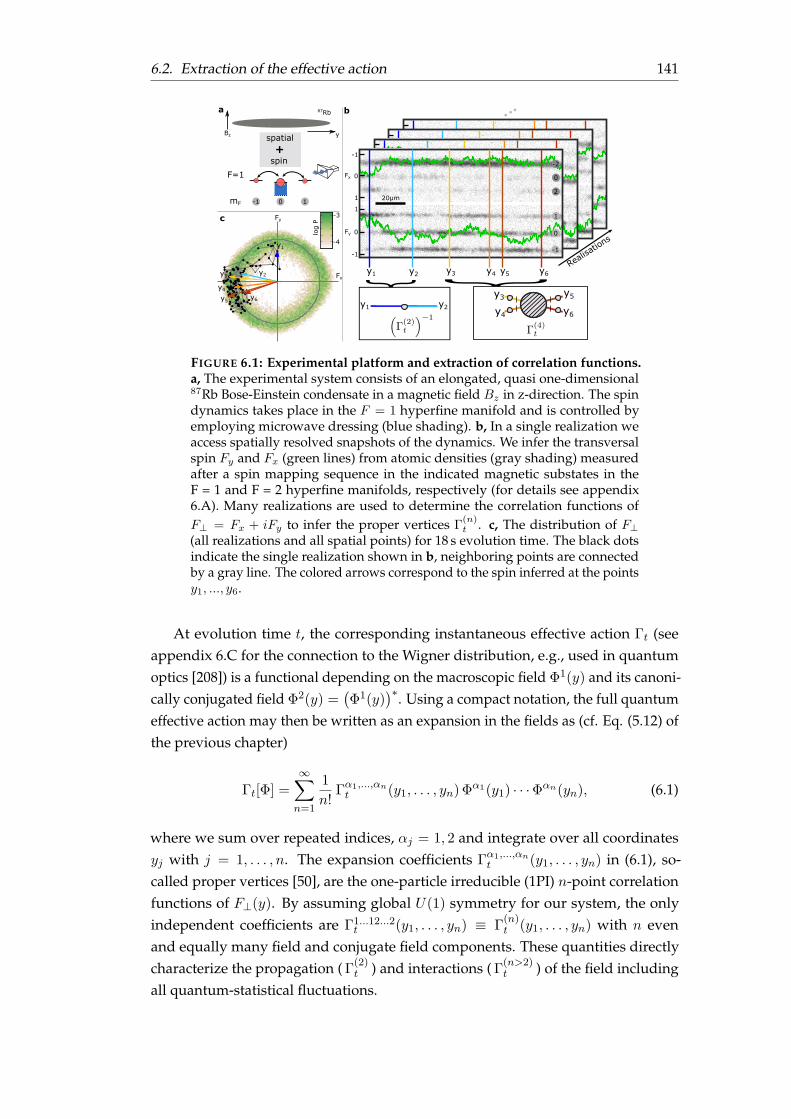
6.2. Extraction of the effective action 141
y1 y2 y4 y5 y6y3
y3 y5
y6y4
+
spatial
spin
y
a b87Rb
Realisa
tions
-1 0 1
Fy
Fx
1
0
-1
-1
0
12
0
-2
-1
0
1c
Fx
Fy
y1
y2
y4
y5 y6
y3
mF
F=1
y1 y2
-3
log
P
-4
20µm
Bz
FIGURE 6.1: Experimental platform and extraction of correlation functions.a, The experimental system consists of an elongated, quasi one-dimensional87Rb Bose-Einstein condensate in a magnetic field Bz in z-direction. The spindynamics takes place in the F = 1 hyperfine manifold and is controlled byemploying microwave dressing (blue shading). b, In a single realization weaccess spatially resolved snapshots of the dynamics. We infer the transversalspin Fy and Fx (green lines) from atomic densities (gray shading) measuredafter a spin mapping sequence in the indicated magnetic substates in theF = 1 and F = 2 hyperfine manifolds, respectively (for details see appendix6.A). Many realizations are used to determine the correlation functions ofF⊥ = Fx + iFy to infer the proper vertices Γ
(n)t . c, The distribution of F⊥
(all realizations and all spatial points) for 18 s evolution time. The black dotsindicate the single realization shown in b, neighboring points are connectedby a gray line. The colored arrows correspond to the spin inferred at the pointsy1, ..., y6.
At evolution time t, the corresponding instantaneous effective action Γt (seeappendix 6.C for the connection to the Wigner distribution, e.g., used in quantumoptics [208]) is a functional depending on the macroscopic field Φ1(y) and its canoni-cally conjugated field Φ2(y) =
(Φ1(y)
)∗. Using a compact notation, the full quantumeffective action may then be written as an expansion in the fields as (cf. Eq. (5.12) ofthe previous chapter)
Γt[Φ] =∞∑
n=1
1
n!Γα1,...,αnt (y1, . . . , yn) Φ
α1(y1) · · ·Φαn(yn), (6.1)
where we sum over repeated indices, αj = 1, 2 and integrate over all coordinatesyj with j = 1, . . . , n. The expansion coefficients Γα1,...,αn
t (y1, . . . , yn) in (6.1), so-called proper vertices [50], are the one-particle irreducible (1PI) n-point correlationfunctions of F⊥(y). By assuming global U(1) symmetry for our system, the onlyindependent coefficients are Γ1...12...2
t (y1, . . . , yn) ≡ Γ(n)t (y1, . . . , yn) with n even
and equally many field and conjugate field components. These quantities directlycharacterize the propagation (Γ(2)
t ) and interactions (Γ(n>2)t ) of the field including
all quantum-statistical fluctuations.

142 Chapter 6. Extraction of the instantaneous effective action out of equilibrium
FIGURE 6.2: Statistical significance of the four-point 1PI correlator in mo-mentum space. a, 1PI four-vertex Γ
(4)t=18s(0, 0, p3, p4) for experimental data
(left panel); for Gaussian model with same statistics (right panel). pL = 1/L isthe lowest momentum corresponding to the size L of the evaluation region. b,Ratio of experimental data and Gaussian model indicating the statistical sig-nificance of the inferred signal (see colorbar for scale). c, Γ
(4)t=18s(p1, p2, p3, p4)
for different p1 and p2 (fixed in each gray square), divided by the Gaussianbias, revealing an overall momentum conserving structure (see colorbar in bfor scale). We note that some values in b and c lie below the lower limit of thecolorbar of 2.4, which was chosen for better visibility.
As discussed in the previous chapter 5, the equal-time 1PI effective action con-tains the same information as the density matrix but expressed in terms of observ-ables (see also appendix 6.C for more details in the non-equilibrium case). Whilethe entries of the density matrix are often inaccessible, the equal-time correlatorscan be extracted in experiments and are directly related to relevant observables,such as occupation number distributions. The 1PI vertices such as Γ
(4)t quantify the
interactions between the excitations described by F⊥ in our system. These verticesare a generalization of the scattering amplitudes, which are often employed for thedescription of high-energy collider experiments. However, the scattering amplitudes
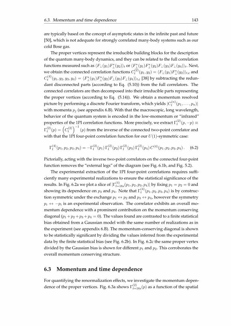
6.3. Momentum and time dependence 143
are typically based on the concept of asymptotic states in the infinite past and future[50], which is not adequate for strongly correlated many-body systems such as ourcold Bose gas.
The proper vertices represent the irreducible building blocks for the descriptionof the quantum many-body dynamics, and they can be related to the full correlationfunctions measured such as 〈F⊥(y1)F ∗⊥(y2)〉t or 〈F ∗⊥(y1)F ∗⊥(y2)F⊥(y3)F⊥(y4)〉t. Next,we obtain the connected correlation functions C(2)
t (y1, y2) = 〈F⊥(y1)F ∗⊥(y2)〉t,c andC
(4)t (y1, y2, y3, y4) = 〈F ∗⊥(y1)F ∗⊥(y2)F⊥(y3)F⊥(y4)〉t,c [38] by subtracting the redun-
dant disconnected parts (according to Eq. (5.10)) from the full correlators. Theconnected correlators are then decomposed into their irreducible parts representingthe proper vertices (according to Eq. (5.14)). We obtain a momentum resolvedpicture by performing a discrete Fourier transform, which yields |C(n)
t (p1, . . . , pn)|with momenta pj (see appendix 6.B). With that the macroscopic, long wavelength,behavior of the quantum system is encoded in the low-momentum or “infrared”properties of the 1PI correlation functions. More precisely, we extract Γ
(2)t (p,−p) ≡
Γ(2)t (p) =
(C
(2)t
)−1(p) from the inverse of the connected two-point correlator and
with that the 1PI four-point correlation function for our U(1)-symmetric case:
Γ(4)t (p1, p2, p3, p4) = −Γ
(2)t (p1) Γ
(2)t (p2) Γ
(2)t (p3) Γ
(2)t (p4)C(4)(p1, p2, p3, p4) . (6.2)
Pictorially, acting with the inverse two-point correlators on the connected four-pointfunction removes the “external legs” of the diagram (see Fig. 6.1b, and Fig. 5.2).
The experimental extraction of the 1PI four-point correlations requires suffi-ciently many experimental realizations to ensure the statistical significance of theresults. In Fig. 6.2a we plot a slice of |Γ(4)
t=18s(p1, p2, p3, p4)| by fixing p1 = p2 = 0 andshowing its dependence on p3 and p4. Note that Γ
(4)t (p1, p2, p3, p4) is by construc-
tion symmetric under the exchange p1 ↔ p2 and p3 ↔ p4, however the symmetrypi ↔ −pi is an experimental observation. The correlator exhibits an overall mo-mentum dependence with a prominent contribution on the momentum conservingdiagonal (p1 +p2 +p3 +p4 = 0). The values found are contrasted to a finite statisticalbias obtained from a Gaussian model with the same number of realizations as inthe experiment (see appendix 6.B). The momentum-conserving diagonal is shownto be statistically significant by dividing the values inferred from the experimentaldata by the finite statistical bias (see Fig. 6.2b). In Fig. 6.2c the same proper vertexdivided by the Gaussian bias is shown for different p1 and p2. This corroborates theoverall momentum conserving structure.
6.3 Momentum and time dependence
For quantifying the renormalization effects, we investigate the momentum depen-dence of the proper vertices. Fig. 6.3a shows Γ
(2)t=18s(p) as a function of the spatial

144 Chapter 6. Extraction of the instantaneous effective action out of equilibrium
a
c
b
d
1 2 3 4 5 6 7 8 9
0.002 0.005 0.01 0.02
100
10-1
10-2
1 2 3 4 5 6 7 8 9
0.002 0.005 0.01 0.02
1 2 3 4 5 6 7 8 9
0.002 0.005 0.01 0.02
1 2 3 4 5 6 7 8 9
0.002 0.005 0.01
10-3
10-4
10-3
10-4
10-3
10-4
Momentum p/pL Momentum p/pL
Momentum p/pL Momentum p/pL
Spatial momentum p (1/µm) Spatial momentum p (1/µm)
Spatial momentum p (1/µm) Spatial momentum p (1/µm)
( )-10
0
p
-p
-p
0 0
pL
p-pL
-p
1PI
two-
poin
t co
rrel
ator
1PI
four
-poi
nt c
orre
lato
r
1PI
four
-poi
nt c
orre
lato
r
1PI
four
-poi
nt c
orre
lato
r
0.02
p
0
FIGURE 6.3: Momentum conserving diagonals of the 1PI correlators. a, Mo-mentum conserving diagonal of Γ(2)
t=18s. b-d, We show three different momen-tum conserving diagonals of the four point 1PI correlations (blue diamonds)for t = 18 s. They are statistically significant as quantified by the comparisonto the finite statistics level for the Gaussian case (gray shaded region, seeappendix 6.B). The complex-valued field allows the distinction between caseb and c. The momentum dependence of these correlators over almost twoorders of magnitude indicates the dramatic renormalization of the couplings.All error bars shown are 1 s.d. calculated from bootstrap resampling.
momentum p. We observe a suppression in the infrared [62, 187] up to a characteris-tic momentum set by the inverse of the length scale ls ∼ 30µm. For the four-vertex|Γ(4)
t=18s(p1, p2, p3, p4)|, we focus on statistically significant momentum conservingdiagonals. As a representative example, the case of p1 = p2 = 0 and p = p3 = −p4
(Fig. 6.3b) shows strongly momentum-dependent values in the observed momen-tum regime; a similar behavior is also found for different diagonals as shown inFig. 6.3c and 6.3d. This demonstrates that the infrared regime exhibits a stronglysuppressed interaction vertex in this far-from-equilibrium situation [63, 64, 225, 234].While quantitative theoretical predictions for this vertex are so far not possible, theobserved qualitative behavior is expected from the large occupations in the infrared,as discussed below.
Motivated by the observed structure of the complex valued field, we derive anexact evolution equation for the two-point function C
(2)t (p) of a one-component
Bose gas with interaction strength g (assuming spatial translational invariance; see
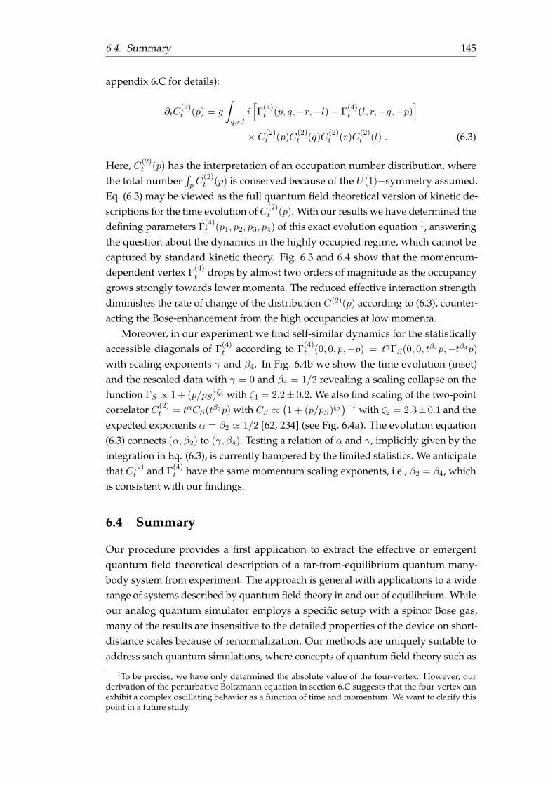
6.4. Summary 145
appendix 6.C for details):
∂tC(2)t (p) = g
ˆq,r,l
i[Γ
(4)t (p, q,−r,−l)− Γ
(4)t (l, r,−q,−p)
]
× C(2)t (p)C
(2)t (q)C
(2)t (r)C
(2)t (l) . (6.3)
Here, C(2)t (p) has the interpretation of an occupation number distribution, where
the total number´pC
(2)t (p) is conserved because of the U(1)−symmetry assumed.
Eq. (6.3) may be viewed as the full quantum field theoretical version of kinetic de-scriptions for the time evolution of C(2)
t (p). With our results we have determined thedefining parameters Γ
(4)t (p1, p2, p3, p4) of this exact evolution equation 1, answering
the question about the dynamics in the highly occupied regime, which cannot becaptured by standard kinetic theory. Fig. 6.3 and 6.4 show that the momentum-dependent vertex Γ
(4)t drops by almost two orders of magnitude as the occupancy
grows strongly towards lower momenta. The reduced effective interaction strengthdiminishes the rate of change of the distribution C(2)(p) according to (6.3), counter-acting the Bose-enhancement from the high occupancies at low momenta.
Moreover, in our experiment we find self-similar dynamics for the statisticallyaccessible diagonals of Γ
(4)t according to Γ
(4)t (0, 0, p,−p) = tγΓS(0, 0, tβ4p,−tβ4p)
with scaling exponents γ and β4. In Fig. 6.4b we show the time evolution (inset)and the rescaled data with γ = 0 and β4 = 1/2 revealing a scaling collapse on thefunction ΓS ∝ 1 + (p/pS)ζ4 with ζ4 = 2.2± 0.2. We also find scaling of the two-pointcorrelator C(2)
t = tαCS(tβ2p) with CS ∝(1 + (p/pS)ζ2
)−1 with ζ2 = 2.3±0.1 and theexpected exponents α = β2 ' 1/2 [62, 234] (see Fig. 6.4a). The evolution equation(6.3) connects (α, β2) to (γ, β4). Testing a relation of α and γ, implicitly given by theintegration in Eq. (6.3), is currently hampered by the limited statistics. We anticipatethat C(2)
t and Γ(4)t have the same momentum scaling exponents, i.e., β2 = β4, which
is consistent with our findings.
6.4 Summary
Our procedure provides a first application to extract the effective or emergentquantum field theoretical description of a far-from-equilibrium quantum many-body system from experiment. The approach is general with applications to a widerange of systems described by quantum field theory in and out of equilibrium. Whileour analog quantum simulator employs a specific setup with a spinor Bose gas,many of the results are insensitive to the detailed properties of the device on short-distance scales because of renormalization. Our methods are uniquely suitable toaddress such quantum simulations, where concepts of quantum field theory such as
1To be precise, we have only determined the absolute value of the four-vertex. However, ourderivation of the perturbative Boltzmann equation in section 6.C suggests that the four-vertex canexhibit a complex oscillating behavior as a function of time and momentum. We want to clarify thispoint in a future study.
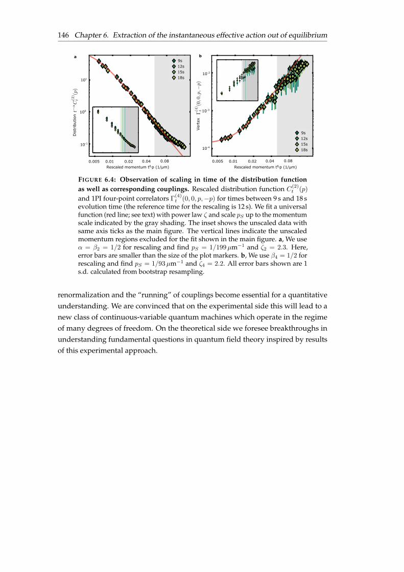
146 Chapter 6. Extraction of the instantaneous effective action out of equilibrium
0.005 0.01 0.02 0.04 0.080.005 0.01 0.02 0.04 0.08Rescaled momentum tβ p (1/µm)
100
101
10-2
10-3
10-4
a b
Rescaled momentum tβ p (1/µm)
10-1
Dis
trib
utio
n
Ver
tex
42
9s12s15s18s
9s12s15s18s
FIGURE 6.4: Observation of scaling in time of the distribution functionas well as corresponding couplings. Rescaled distribution function C
(2)t (p)
and 1PI four-point correlators Γ(4)t (0, 0, p,−p) for times between 9 s and 18 s
evolution time (the reference time for the rescaling is 12 s). We fit a universalfunction (red line; see text) with power law ζ and scale pS up to the momentumscale indicated by the gray shading. The inset shows the unscaled data withsame axis ticks as the main figure. The vertical lines indicate the unscaledmomentum regions excluded for the fit shown in the main figure. a, We useα = β2 = 1/2 for rescaling and find pS = 1/199µm−1 and ζ2 = 2.3. Here,error bars are smaller than the size of the plot markers. b, We use β4 = 1/2 forrescaling and find pS = 1/93µm−1 and ζ4 = 2.2. All error bars shown are 1s.d. calculated from bootstrap resampling.
renormalization and the “running” of couplings become essential for a quantitativeunderstanding. We are convinced that on the experimental side this will lead to anew class of continuous-variable quantum machines which operate in the regimeof many degrees of freedom. On the theoretical side we foresee breakthroughs inunderstanding fundamental questions in quantum field theory inspired by resultsof this experimental approach.

6.A. Experimental details 147
Appendix: Details about the QFT analysis out of equilibrium
In this appendix we give more details about the experiment (section 6.A) and thedata analysis (section 6.B). Additionally, we discuss in detail the real-time evolutionof the instantaneous effective action for the example of a non-relativistic Bose gasin section 6.C. Within this formalism, we also provide an alternative derivation ofBoltzmann’s kinetic equation in a perturbative limit.
6.A Experimental details
In the experiment, we prepare ∼ 105 atoms in the state |F,mF〉 = |1, 0〉 in a staticmagnetic field of 0.884 G in an optical dipole trap of 1030 nm light with trappingfrequencies (ω‖, ω⊥) ≈ 2π × (1.6, 167) Hz. We initiate dynamics by changing theexperimental control parameter q, the second order Zeeman shift, by applying off-resonant microwave dressing. For details on the experiment and the parameterregime employed see [62].
We use a readout scheme to detect multiple spin projections in a single realization[223]. After the desired evolution time t we apply a first π/2-rf rotation aroundthe y-axis to map the spin projection Fx on the detectable population imbalanceN+1 −N−1. We store this projection in the initially empty F = 2 hyperfine manifoldby splitting the populations of the three mF states with three mw π/2 pulses. Asecond, hyperfine selective, rf rotation in F = 1 around the x-axis allows us to mapthe spin projection Fy onto the population imbalance in F = 1. Together with asingle absorption image of the 8 hyperfine levels this procedure allows us to extractsingle shot snapshots of the complex valued order parameter F⊥(y) = Fx(y)+ iFy(y)
with
Fx(y) =(NF=2
+2 (y)−NF=2−2 (y)
)/NF=2
tot (y) (6.4)
Fy(y) =(NF=1
+1 (y)−NF=1−1 (y)
)/NF=1
tot (y), (6.5)
where NF=fmf (y) is is the atom number in the state |f,mf 〉 at position y and NF=f
tot (y)
is the total atom number in the hyperfine manifold f after the readout sequence.At evolution times of 18 s we observe no substantial loss of coherence of the
different mF states which would correspond to reductions of the transversal spinlength. Optimizing the transversal confinement leads to coherence times up to∼ 50 sdue to reduced heating and efficient evaporative cooling. Due to the harmonicconfinement the atomic density is inhomogeneous and so is the transversal spinlength profile. We choose to analyze the central 400 pixels corresponding to ∼168µm. The spatial resolution is ∼ 1.1µm corresponding to three pixels (pixel sizecorresponds to 420 nm). As we are interested in the long wavelength (infrared)excitations we sum over 9 adjacent pixels to reduce the number of points and
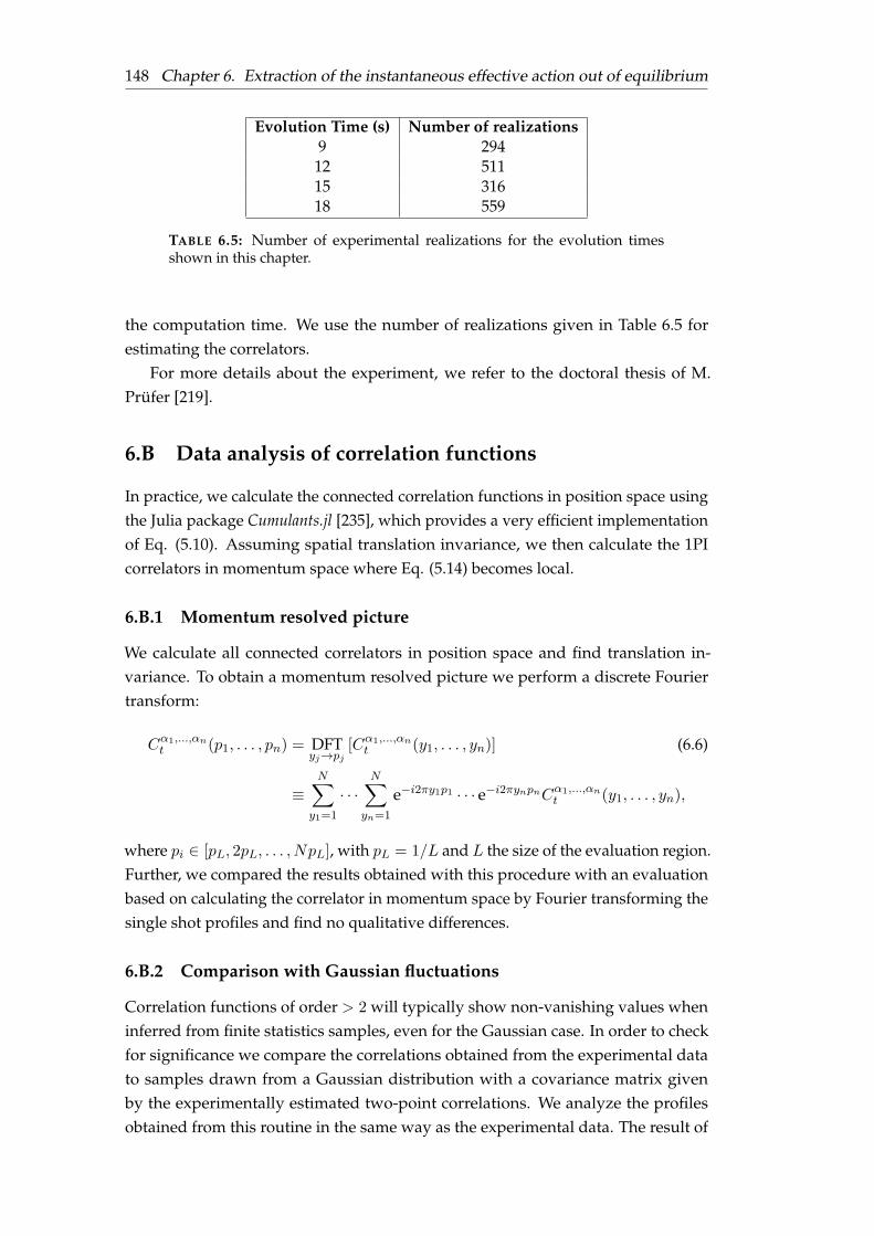
148 Chapter 6. Extraction of the instantaneous effective action out of equilibrium
Evolution Time (s) Number of realizations9 29412 51115 31618 559
TABLE 6.5: Number of experimental realizations for the evolution timesshown in this chapter.
the computation time. We use the number of realizations given in Table 6.5 forestimating the correlators.
For more details about the experiment, we refer to the doctoral thesis of M.Prüfer [219].
6.B Data analysis of correlation functions
In practice, we calculate the connected correlation functions in position space usingthe Julia package Cumulants.jl [235], which provides a very efficient implementationof Eq. (5.10). Assuming spatial translation invariance, we then calculate the 1PIcorrelators in momentum space where Eq. (5.14) becomes local.
6.B.1 Momentum resolved picture
We calculate all connected correlators in position space and find translation in-variance. To obtain a momentum resolved picture we perform a discrete Fouriertransform:
Cα1,...,αnt (p1, . . . , pn) = DFT
yj→pj[Cα1,...,αnt (y1, . . . , yn)] (6.6)
≡N∑
y1=1
· · ·N∑
yn=1
e−i2πy1p1 · · · e−i2πynpnCα1,...,αnt (y1, . . . , yn),
where pi ∈ [pL, 2pL, . . . , NpL], with pL = 1/L and L the size of the evaluation region.Further, we compared the results obtained with this procedure with an evaluationbased on calculating the correlator in momentum space by Fourier transforming thesingle shot profiles and find no qualitative differences.
6.B.2 Comparison with Gaussian fluctuations
Correlation functions of order > 2 will typically show non-vanishing values wheninferred from finite statistics samples, even for the Gaussian case. In order to checkfor significance we compare the correlations obtained from the experimental datato samples drawn from a Gaussian distribution with a covariance matrix givenby the experimentally estimated two-point correlations. We analyze the profilesobtained from this routine in the same way as the experimental data. The result of

6.C. Quantum field dynamics with equal-time correlations 149
this procedure is shown as the upper limit of the gray shaded areas in Fig. 6.3. Datapoints for which the 1 s.d. interval lies above this threshold are called significant.For non-significant points we cannot make a statement whether they are zero in theinfinite statistics limit or just too small to resolve their value with the amount ofexperimental realizations employed here.
6.C Quantum field dynamics with equal-time correlations
In this section, we discuss a formulation of quantum field dynamics in terms ofequal-time correlation functions. To be specific, we restrict ourselves to a single-component non-relativistic complex bosonic field, i.e., Schrödinger picture fieldoperators ψ, ψ† that fulfill
[ψx, ψ
†y
]= δx,y. A generalization to multiple components,
fermions, or relativistic fields is straightforward.
6.C.1 Instantaneous effective action
For completeness, we first repeat the constructions of chapter 5, but now withnon-relativistic fields. An arbitrary state is determined by a density operator ρt, orequivalently a generating functional Zt, constructed as
Zt[J, J∗] = Tr
[ρt e
´x
(Jxψ
†x+J∗x ψx
)]=
ˆDψDψ∗Wt[ψ,ψ
∗] e´x(Jxψ∗x+J∗xψx) . (6.7)
Zt generates symmetrically ordered equal-time correlation functions and it is givenby a functional integral with measure DψDψ∗ =
∏x
[1πdRe (ψx) dIm (ψx)
]over Wt,
the field theoretic version of the Wigner distribution which is extensively employedin quantum optics [208]. The Wigner functional Wt is given by the Wigner-Weyltransform of the density operator,
Wt[ψ,ψ∗] =
ˆDηDη∗
⟨ψ − η
2
∣∣∣ ρt∣∣∣ψ +
η
2
⟩e−´x[ψ∗xψx+ 1
4η∗xηx+ 1
2(ψ∗xηx−η∗xψx)] . (6.8)
The instantaneous (equal-time) effective action is defined by the Legendre transform
Γt[Ψ,Ψ∗] = − logZt[J(Ψ,Ψ∗), J∗(Ψ,Ψ∗)] +
ˆx
[J∗x(Ψ,Ψ∗)Ψx + Ψ∗xJx(Ψ,Ψ∗)] .
(6.9)
It generates the 1PI correlation functions as discussed in chapter 5.
6.C.2 Evolution equation
Given a Hamiltonian H , the von-Neumann equation,
i∂tρt =[H, ρt
], (6.10)
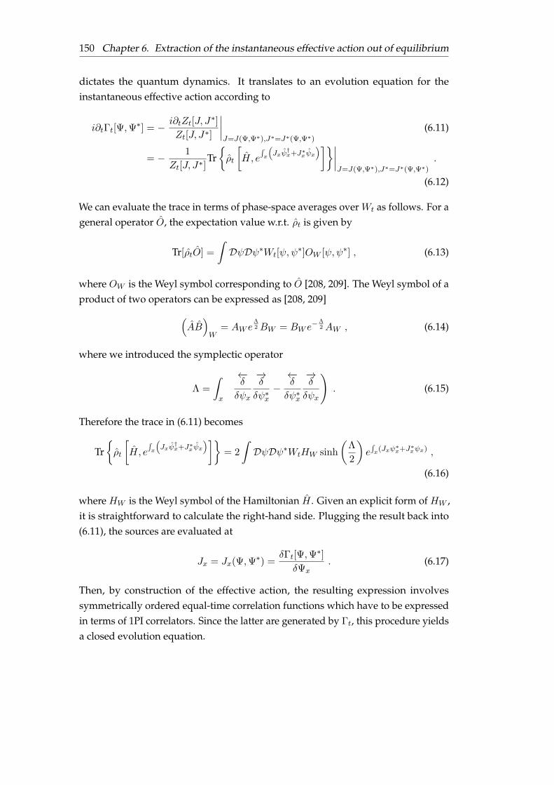
150 Chapter 6. Extraction of the instantaneous effective action out of equilibrium
dictates the quantum dynamics. It translates to an evolution equation for theinstantaneous effective action according to
i∂tΓt[Ψ,Ψ∗] = − i∂tZt[J, J
∗]Zt[J, J∗]
∣∣∣∣J=J(Ψ,Ψ∗),J∗=J∗(Ψ,Ψ∗)
(6.11)
= − 1
Zt[J, J∗]Trρt
[H, e
´x
(Jxψ
†x+J∗x ψx
)]∣∣∣∣J=J(Ψ,Ψ∗),J∗=J∗(Ψ,Ψ∗)
.
(6.12)
We can evaluate the trace in terms of phase-space averages over Wt as follows. For ageneral operator O, the expectation value w.r.t. ρt is given by
Tr[ρtO] =
ˆDψDψ∗Wt[ψ,ψ
∗]OW [ψ,ψ∗] , (6.13)
where OW is the Weyl symbol corresponding to O [208, 209]. The Weyl symbol of aproduct of two operators can be expressed as [208, 209]
(AB)W
= AW eΛ2 BW = BW e
−Λ2 AW , (6.14)
where we introduced the symplectic operator
Λ =
ˆx
( ←−δ
δψx
−→δ
δψ∗x−←−δ
δψ∗x
−→δ
δψx
). (6.15)
Therefore the trace in (6.11) becomes
Trρt
[H, e
´x
(Jxψ
†x+J∗x ψx
)]= 2
ˆDψDψ∗WtHW sinh
(Λ
2
)e´x(Jxψ∗x+J∗xψx) ,
(6.16)
where HW is the Weyl symbol of the Hamiltonian H . Given an explicit form of HW ,it is straightforward to calculate the right-hand side. Plugging the result back into(6.11), the sources are evaluated at
Jx = Jx(Ψ,Ψ∗) =δΓt[Ψ,Ψ
∗]δΨx
. (6.17)
Then, by construction of the effective action, the resulting expression involvessymmetrically ordered equal-time correlation functions which have to be expressedin terms of 1PI correlators. Since the latter are generated by Γt, this procedure yieldsa closed evolution equation.

6.C. Quantum field dynamics with equal-time correlations 151
6.C.3 Evolution of the Bose gas
As an explicit example, relevant for the experiment discussed in this chapter, weconsider a non-relativistic Bose gas described by the quantum many-body Hamilto-nian
H =
ˆx
[1
2m
(∇xψ†x
)(∇xψx
)+g
2ψ†xψ
†xψxψx − µψ†xψx
]. (6.18)
Here, m, g and µ denote the mass, interaction constant and chemical potential,respectively. Direct computation yields the Weyl symbol
HW =
ˆx
[ |∇xψx|22m
− (µ+ gδ(0)) |ψx|2 +g
2|ψx|4 +
g
4δ2(0)
], (6.19)
where δ(0) =[ψx, ψ
†x
]arises from the commutation relations. The last term is a
constant and does not affect the evolution. The remaining term involving δ(0) canbe removed by adding the constant2 term gδ(0)
´x ψ†xψx to the Hamiltonian, which
renormalizes the chemical potential.Since HW involves at most four powers of fields, only the first two terms of
2 sinh(Λ/2) = Λ + Λ3/4! + . . . contribute to (6.16). Explicitly, the quadratic termscontribute asˆxψ∗xψx 2 sinh
(Λ
2
)e´y(Jyψ
∗y+J∗yψy) =
ˆx
(ψ∗xJx − J∗xψx) e´y(Jyψ
∗y+J∗yψy) (6.20)
and the quartic term gives
ˆxψ∗xψ
∗xψxψx 2 sinh
(Λ
2
)e´y(Jyψ
∗y+J∗yψy)
=
ˆx
[ψ∗x
(2ψ∗xψx −
1
2J∗xJx
)Jx − J∗x
(2ψ∗xψx −
1
2J∗xJx
)ψx
]e´y(Jyψ
∗y+J∗yψy) .
(6.21)
Taking the phase space average w.r.t. Wt and replacing the sources by derivatives,we find
i∂tΓt[Ψ,Ψ∗] = LclΓt[Ψ,Ψ
∗] + Lq[Γt] , (6.22)
where the “classical” part Lcl resp. “quantum” part Lq are linear resp. nonlinear inderivatives,
Lcl =
ˆx
[(−∇
2x
2m− µ
)Ψx + gGψ
∗ψψxxx
]δ
δΨx−[(−∇
2x
2m− µ
)Ψ∗x + gGψ
∗ψ∗ψxxx
]δ
δΨ∗x
,
(6.23a)
Lq =g
4
ˆx
(Ψ∗x
δΓtδΨ∗x
δΓtδΨ∗x
δΓtδΨx
−ΨxδΓtδΨx
δΓtδΨx
δΓtδΨ∗x
). (6.23b)
2It is proportional to the total number of particles, which is conserved.
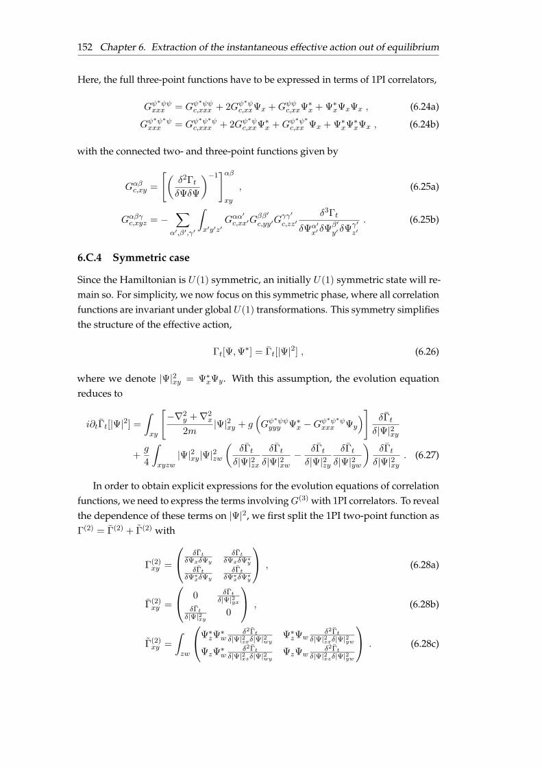
152 Chapter 6. Extraction of the instantaneous effective action out of equilibrium
Here, the full three-point functions have to be expressed in terms of 1PI correlators,
Gψ∗ψψ
xxx = Gψ∗ψψ
c,xxx + 2Gψ∗ψ
c,xxΨx +Gψψc,xxΨ∗x + Ψ∗xΨxΨx , (6.24a)
Gψ∗ψ∗ψ
xxx = Gψ∗ψ∗ψ
c,xxx + 2Gψ∗ψ
c,xxΨ∗x +Gψ∗ψ∗
c,xx Ψx + Ψ∗xΨ∗xΨx , (6.24b)
with the connected two- and three-point functions given by
Gαβc,xy =
[(δ2ΓtδΨδΨ
)−1]αβ
xy
, (6.25a)
Gαβγc,xyz = −∑
α′,β′,γ′
ˆx′y′z′
Gαα′
c,xx′Gββ′c,yy′G
γγ′c,zz′
δ3Γt
δΨα′x′ δΨ
β′y′ δΨ
γ′z′. (6.25b)
6.C.4 Symmetric case
Since the Hamiltonian is U(1) symmetric, an initially U(1) symmetric state will re-main so. For simplicity, we now focus on this symmetric phase, where all correlationfunctions are invariant under global U(1) transformations. This symmetry simplifiesthe structure of the effective action,
Γt[Ψ,Ψ∗] = Γt[|Ψ|2] , (6.26)
where we denote |Ψ|2xy = Ψ∗xΨy. With this assumption, the evolution equationreduces to
i∂tΓt[|Ψ|2] =
ˆxy
[−∇2
y +∇2x
2m|Ψ|2xy + g
(Gψ∗ψψ
yyy Ψ∗x −Gψ∗ψ∗ψ
xxx Ψy
)] δΓtδ|Ψ|2xy
+g
4
ˆxyzw
|Ψ|2xy|Ψ|2zw(
δΓtδ|Ψ|2zx
δΓtδ|Ψ|2xw
− δΓtδ|Ψ|2zy
δΓtδ|Ψ|2yw
)δΓtδ|Ψ|2xy
. (6.27)
In order to obtain explicit expressions for the evolution equations of correlationfunctions, we need to express the terms involvingG(3) with 1PI correlators. To revealthe dependence of these terms on |Ψ|2, we first split the 1PI two-point function asΓ(2) = Γ(2) + Γ(2) with
Γ(2)xy =
δΓtδΨxδΨy
δΓtδΨxδΨ∗y
δΓtδΨ∗xδΨy
δΓtδΨ∗xδΨ∗y
, (6.28a)
Γ(2)xy =
0 δΓt
δ|Ψ|2yxδΓt
δ|Ψ|2xy 0
, (6.28b)
Γ(2)xy =
ˆzw
Ψ∗zΨ
∗w
δ2Γtδ|Ψ|2zxδ|Ψ|2wy Ψ∗zΨw
δ2Γtδ|Ψ|2zxδ|Ψ|2yw
ΨzΨ∗w
δ2Γtδ|Ψ|2xzδ|Ψ|2wy ΨzΨw
δ2Γtδ|Ψ|2xzδ|Ψ|2yw
. (6.28c)

6.C. Quantum field dynamics with equal-time correlations 153
Analogously, we write the connected two-point function as G(2)c = G
(2)c + G
(2)c with
G(2)c =
(Γ(2)
)−1, which implies the geometric (Dyson-type) series
G(2)c = G(2)
c − G(2)c Γ(2)G(2)
c + G(2)c Γ(2)G(2)
c Γ(2)G(2)c ∓ . . . . (6.29)
In the following, we will further restrict our attention to the 1PI two- and four-pointfunctions,
Γxy =δΓtδ|Ψ|2xy
∣∣∣∣Ψ=Ψ∗=0
= Γ(2)xy
∣∣∣Ψ=Ψ∗=0
, (6.30a)
Γxy,zw =δ2Γt
δ|Ψ|2xyδ|Ψ|2zw
∣∣∣∣Ψ=Ψ∗=0
. (6.30b)
Since we need to take at most two |Ψ|2 derivatives of equation (6.27), only the firsttwo terms of the Dyson series contribute to the evolution of these correlators.
6.C.5 Evolution of the two-point and four-point functions
Explicitly, the two-point function evolves according to
i∂tΓxy =−∇2
y +∇2x
2mΓxy + g
ˆzw
δ(Gψ∗ψψ
www Ψ∗z −Gψ∗ψ∗ψ
zzz Ψw
)
δ|Ψ|2xy
∣∣∣∣∣∣Ψ=Ψ∗=0
Γzw . (6.31)
The evolution equation for the four-point function reads
i∂tΓxy,zw =−∇2
x +∇2y −∇2
z +∇2w
2mΓxy,zw
+ g
ˆab
δ(Gψ∗ψψ
bbb Ψ∗a −Gψ∗ψ∗ψ
aaa Ψb
)
δ|Ψ|2xy
∣∣∣∣∣∣Ψ=Ψ∗=0
Γab,zw + (xy ↔ zw)
+ g
ˆab
δ2(Gψ∗ψψ
bbb Ψ∗a −Gψ∗ψ∗ψ
aaa Ψb
)
δ|Ψ|2xyδ|Ψ|2zw
∣∣∣∣∣∣Ψ=Ψ∗=0
Γab
+g
4
[(ΓzwΓxw − ΓzyΓyw
)Γxy +
(ΓxzΓzy − ΓxwΓwy
)Γzw
], (6.32)
where (xy ↔ zw) denotes the permutation of the expression in the same line withthe indicated replacement. Evaluating the remaining derivatives is tedious, butstraightforward. For future reference, we sketch how to perform this calculation.Consider
δ(Gψ∗ψψ
www Ψ∗z)
δ|Ψ|2xy=δ(Gψ∗ψψ
c,wwwΨ∗z)
δ|Ψ|2xy+ |Ψ|2zw
δGψ∗ψ
c,ww
δ|Ψ|2xy+δ(Gψψc,wwΨ∗wΨ∗z
)
δ|Ψ|2xy+ 2δxzδywG
ψ∗ψc,ww + δxwδyw|Ψ|2zw + δxzδyw|Ψ|2ww . (6.33)

154 Chapter 6. Extraction of the instantaneous effective action out of equilibrium
Using the geometric series for the two-point functions, we obtain
δGψ∗ψ
c,ww
δ|Ψ|2xy=δGψ
∗ψc,ww
δ|Ψ|2xy−ˆw′w′′
δ(Gψ∗ψ
c,ww′Γψψ∗w′w′′G
ψ∗ψc,ww′
)
δ|Ψ|2xy± . . . (6.34)
The first term is given by
δGψ∗ψ
c,ww
δ|Ψ|2xy= −ˆw′w′′
δΓ
δ|Ψ|2ww′δ2Γ
δ|Ψ|2w′w′′δ|Ψ|2xyδΓ
δ|Ψ|2w′′w, (6.35)
and the second term does not contribute to the evolution of the two- and four-pointfunctions. Similarly, we have
δ(Gψψc,wwΨ∗wΨ∗z
)
δ|Ψ|2xy= −ˆw′w′′
δ(Gψψ
∗c,ww′Γ
ψ∗ψ∗w′w′′G
ψ∗ψc,w′′wΨ∗wΨ∗z
)
δ|Ψ|2xy± . . . (6.36)
and only the leading term contributes as
δ(Gψψ
∗c,ww′Γ
ψ∗ψ∗w′w′′G
ψ∗ψc,w′′wΨ∗wΨ∗z
)
δ|Ψ|2xy
=
ˆw′w′′
[(δΓ
δ|Ψ|2)−1
]
w′w
δ2Γ
δ|Ψ|2w′w′δ|Ψ|2w′′w′′
[(δΓ
δ|Ψ|2)−1
]
w′′w
×(δxzδyw′′ |Ψ|2ww′ + δxwδyw′ |Ψ|2zw′′
)+ . . . , (6.37)
where we have not written out terms involving higher powers of |Ψ|2. The connectedthree-point function contributes
δ(Gψ∗ψψ
c,wwwΨ∗z)
δ|Ψ|2xy= −
∑
α,β,γ
ˆw′w′′w′′′
δ
δ|Ψ|2xy
Gψ∗α
c,ww′Gψβc,ww′′G
ψγc,ww′′′
δ3Γt
δΨαw′δΨ
βw′′δΨ
γw′′′
Ψ∗z
.
(6.38)
Again, we do not need the full expression, but just the terms up to |Ψ|2. The leadingterm in the series of the “diagonal” two-point functions Gψψc and Gψ
∗ψ∗c involves
two powers of the fields Ψ or Ψ∗. The same is true for the third derivative of Γt
times one field Ψ. Thus only the following four (out of the total eight) terms of the

6.C. Quantum field dynamics with equal-time correlations 155
sum can contribute,
(1) = Gψ∗ψ
c,ww′Gψψ∗c,ww′′G
ψψ∗c,ww′′′
δ3ΓtδΨw′δΨ
∗w′′δΨ
∗w′′′
Ψ∗z , (6.39a)
(2) = Gψ∗ψ∗
c,ww′Gψψ∗c,ww′′G
ψψ∗c,ww′′′
δ3ΓtδΨ∗w′δΨ
∗w′′δΨ
∗w′′′
Ψ∗z , (6.39b)
(3) = Gψ∗ψ
c,ww′Gψψc,ww′′G
ψψ∗c,ww′′′
δ3ΓtδΨw′δΨw′′δΨ
∗w′′′
Ψ∗z , (6.39c)
(4) = Gψ∗ψ
c,ww′Gψψ∗c,ww′′G
ψψc,ww′′′
δ3ΓtδΨw′δΨ
∗w′′δΨw′′′
Ψ∗z . (6.39d)
For example, the term (1) involves the third-order derivative
δ3ΓtδΨw′δΨ
∗w′′δΨ
∗w′′′
Ψ∗z =
ˆw′′w′′′
[(|Ψ|2zw′′δw′w′ + |Ψ|2zw′′δw′′′w′
) δ2Γtδ|Ψ|2w′′′w′′′δ|Ψ|2w′′w′
+|Ψ|2zw′ |Ψ|2w′w′′δ3Γt
δ|Ψ|2w′′′w′′′δ|Ψ|2w′′w′′δ|Ψ|2w′w′
]. (6.40)
Collecting all relevant terms, the evolution equation of the 1PI two-point functionreads
i∂tΓxy =
[−∇2
y +∇2x
2m+ 2g
(Γ−1yy − Γ−1
xx
)]
Γxy
+ 2g
ˆzabc
Γ−1za Γ−1
bz
(Γ−1zc Γcy,abΓxz − Γ−1
cz Γxc,abΓzy), (6.41)
where we denote the inverse of Γxy as Γ−1xy . We emphasize that this equation holds
exactly (assuming only U(1) invariance). Given the 1PI four-point function Γxy,zw,it determines the real-time evolution of Γxy.
The evaluation of the terms for the evolution equation of the four-point functionproceeds analogously. For brevity, we just state a part of the full result,
i∂tΓxy,zw =
[−∇2
y +∇2x −∇2
z +∇2w
2m+ 2g
(Γ−1yy − Γ−1
xx + Γ−1ww − Γ−1
zz
)]
Γxy,zw
+ g[δxyδxwΓzx + δzyδzwΓxz − δyxδyzΓyw − δwxδwzΓwy
]
+g
4
[(ΓzwΓxw − ΓzyΓyw
)Γxy +
(ΓxzΓzy − ΓxwΓwy
)Γzw
]
+ . . . . (6.42)
The dots indicate several terms that we omitted. They are all proportional to thecoupling g and involve at least one power of Γxy,zw or they depend on the 1PI six-point function Γxy,zw,uv. Neglecting the six-point function closes the set of coupledevolution equations. If we further assume that the four-point function is of orderg, then the omitted terms above do not contribute to leading order in g. In theremainder of this section, we will demonstrate analytically that this perturbativetruncation can be reduced to a standard kinetic description. We plan to solve the full
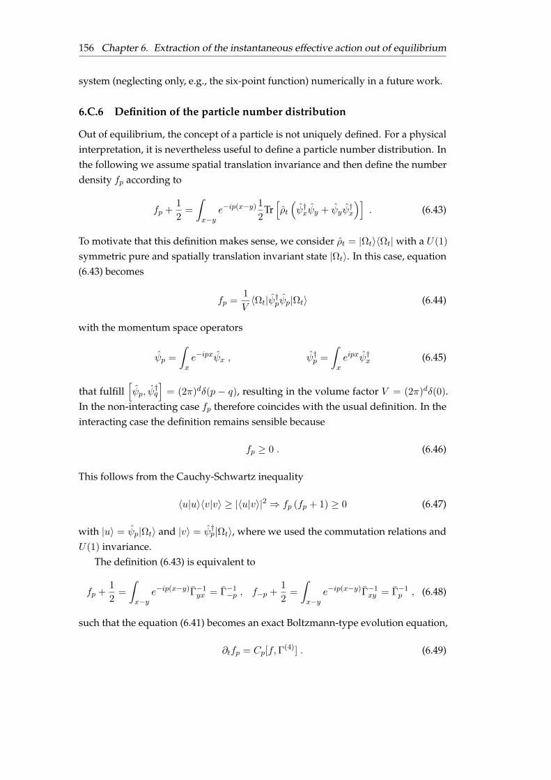
156 Chapter 6. Extraction of the instantaneous effective action out of equilibrium
system (neglecting only, e.g., the six-point function) numerically in a future work.
6.C.6 Definition of the particle number distribution
Out of equilibrium, the concept of a particle is not uniquely defined. For a physicalinterpretation, it is nevertheless useful to define a particle number distribution. Inthe following we assume spatial translation invariance and then define the numberdensity fp according to
fp +1
2=
ˆx−y
e−ip(x−y) 1
2Tr[ρt
(ψ†xψy + ψyψ
†x
)]. (6.43)
To motivate that this definition makes sense, we consider ρt = |Ωt〉〈Ωt|with a U(1)
symmetric pure and spatially translation invariant state |Ωt〉. In this case, equation(6.43) becomes
fp =1
V〈Ωt|ψ†pψp|Ωt〉 (6.44)
with the momentum space operators
ψp =
ˆxe−ipxψx , ψ†p =
ˆxeipxψ†x (6.45)
that fulfill[ψp, ψ
†q
]= (2π)dδ(p − q), resulting in the volume factor V = (2π)dδ(0).
In the non-interacting case fp therefore coincides with the usual definition. In theinteracting case the definition remains sensible because
fp ≥ 0 . (6.46)
This follows from the Cauchy-Schwartz inequality
〈u|u〉〈v|v〉 ≥ |〈u|v〉|2 ⇒ fp (fp + 1) ≥ 0 (6.47)
with |u〉 = ψp|Ωt〉 and |v〉 = ψ†p|Ωt〉, where we used the commutation relations andU(1) invariance.
The definition (6.43) is equivalent to
fp +1
2=
ˆx−y
e−ip(x−y)Γ−1yx = Γ−1
−p , f−p +1
2=
ˆx−y
e−ip(x−y)Γ−1xy = Γ−1
p , (6.48)
such that the equation (6.41) becomes an exact Boltzmann-type evolution equation,
∂tfp = Cp[f,Γ(4)] . (6.49)
6.C. Quantum field dynamics with equal-time correlations 157
Here the “collision integral”Cp[f,Γ(4)] explicitly depends on the two-point functions(or according to (6.48) equivalently on f ) and on the 1PI four-vertices as
Cp[f,Γ(4)] = −ig
ˆqrl
(fp +
1
2
)(fq +
1
2
)(fr +
1
2
)(fl +
1
2
)
×[Γψψψ
∗ψ∗l,r,−q,−p − Γψψψ
∗ψ∗p,q,−r,−l
], (6.50)
where we relabeled the 1PI four-vertex in accordance with the presentation in section6.3,
Γψψψ∗ψ∗
l,r,−q,−p =δ4Γt
δΨlδΨrδΨ∗−qδΨ∗−p
∣∣∣∣∣Ψ=Ψ∗=0
=
ˆxyzw
e−i(ly−rw−qx−pz)Γxy,zw
2. (6.51)
Of course the Boltzmann-type equation (6.49) can be obtained with much less effort,e.g., by directly calculating the Heisenberg equations of motion for the product oftwo field operators, taking the average w.r.t. the density operator and expressingthe appearing four-point functions in terms of 1PI correlators. The advantage of theapproach presented here is that it generates equations for the full hierarchy of 1PIcorrelators. We use this to discuss the evolution of the 1PI four-vertex next.
6.C.7 Perturbative four-vertex and Boltzmann equation
To leading order in g, the evolution of the four-vertex [Eq. (6.42)] can be written inmomentum space as
i∂tΓψψψ∗ψ∗pqrl = −∆ωpqrlΓ
ψψψ∗ψ∗pqrl − g
2δ (p+ q + r + l) gpqrl (6.52)
with ∆ωpqrl = (p2 + q2 − r2 − l2)/(2m) and the abbreviation
gpqrl[f ] = 4(Γp + Γq − Γ−r − Γ−l
)− ΓpΓq
(Γ−r + Γ−l
)+ Γ−rΓ−l
(Γp + Γq
).
(6.53)
The general solution of (6.52) with initial condition Γψψψ∗ψ∗
pqrl (t0) is given by
Γψψψ∗ψ∗
pqrl (t) = Γψψψ∗ψ∗
pqrl (t0) ei∆ωpqrl(t−t0)
+ig
2δ (p+ q + r + l)
ˆ t
t0
dτ e−i∆ωpqrl(τ−t) gpqrl[f ](τ) . (6.54)
158 Chapter 6. Extraction of the instantaneous effective action out of equilibrium
Without the initial condition (for, e.g., a Gaussian initial state) the contribution tothe collision integral (6.50) becomes
Γψψψ∗ψ∗
l,r,−q,−p − Γψψψ∗ψ∗
p,q,−r,−l = 2ig δ (p+ q − r − l)ˆ t
t0
dτ cos [∆ωpqrl(τ − t)] gp,q,−r,−l[f ](τ)
≈ 2ig δ (p+ q − r − l) gp,q,−r,−l[f ](t)
ˆ t
t0
dτ cos [∆ωpqrl(τ − t)] ,
= 2ig δ (p+ q − r − l) gp,q,−r,−l[f ](t)sin [∆ωpqrl(t− t0)]
∆ωpqrl(τ − t)→ 2igδ (p+ q − r − l)πδ(∆ωpqrl)gp,q,−r,−l[f ](t) , (6.55)
where the approximation of the second line holds for slowly varying f and we havetaken the limit of late times (t − t0 → ∞) in the last line. Inserting this result into(6.50) gives
Cp[f ] ≈ g2
2
ˆqrl
dΩpqrl
(fp +
1
2
)(fq +
1
2
)(fr +
1
2
)(fl +
1
2
)gp,q,−r,−l[f ] (6.56)
with the integration constrained by momentum and energy conservation,
ˆqrl
dΩpqrl =
ˆddq
(2π)dddr
(2π)dddl
(2π)d(2π)d δ(d) (p+ q − r − l) (2π) δ (∆ωpqrl) . (6.57)
Rewriting the integrand in terms of the distribution f ,
(fp +
1
2
)(fq +
1
2
)(fr +
1
2
)(fl +
1
2
)gp,q,−r,−l[f ]
= 4 [(fp + 1)(fq + 1)frfl − (fr + 1)(fl + 1)fpfq] , (6.58)
we finally arrive at the standard perturbative Boltzmann equation (see, e.g., [234])
∂tfp ≈ 2g2
ˆqrl
dΩpqrl [(fp + 1)(fq + 1)frfl − (fr + 1)(fl + 1)fpfq] . (6.59)
In the approach presented here, the Boltzmann equation relies on several assump-tions. It is valid in the spatially translation invariant and U(1) symmetric case.Additionally, we solved the evolution of the 1PI four-vertex by neglecting the effectall 1PI correlators of order six or higher, assuming Gaussian initial conditions anda perturbative expansion in the coupling. Finally, we approximated the resultingintegral for a slowly evolving two-point function at sufficiently late times.
159
Chapter 7
Conclusion
The work presented in this thesis includes several results relevant for the quantumsimulation of high-energy physics. In this chapter, we briefly discuss the relevanceof the different results before closing with an outlook on possible future researchdirections.
7.1 Discussion
Our proposal to implement a quantum simulation of QED in one spatial dimensionwith Wilson fermions (chapter 2) illustrates the importance of taking into accountequivalent formulations of the same physics for finding experimentally feasibleschemes. Here we exploited the possibility to choose different representations ofthe Clifford algebra together with the fundamental non-uniqueness of discretizingDirac fermions. From a more general point of view, it is sufficient to realize anexperimental system that has the right continuum limit. In principle this opens upthe possibility to consider a multitude of different Hamiltonians, only constrainedby relevant couplings (in the sense of the renormalization group), which share thesame universal properties.
In a similar spirit, it is only necessary to retain the mathematical equivalencebetween the target system of the quantum simulation and the experimental platform.By giving up the direct correspondence between the lattice sites of the simulatedgauge theory and the lattice wells of the trapped quantum gas, we have also ex-ploited this fact (chapter 3). Our improved proposal combines these advances andcan be scaled to large system sizes by connecting elementary gauge-invariant build-ing blocks. Together with the experimental demonstration of the building block, thismoved the quantum simulation of continuous U(1) gauge theories in one spatialdimension within immediate reach.
Motivated by the prospect of an experimental realization of QED, we identifieddynamical topological transitions (chapter 4) as an ideal target phenomenon for aquantum simulation. Here we take into account experimental imperfections sincethis physical phenomenon is robustly accessible within relatively short time-scalesand small lattice sizes. In this context, we also re-interpreted the physics of DQPTs interms of correlation functions, which allowed us to obtain a dynamical topologicalorder parameter that remains well-defined in the interacting theory.

160 Chapter 7. Conclusion
Since correlation functions completely determine any quantum field theory,a correlator-based description of quantum simulators is highly desirable for thesimulation of high-energy physics. We presented such a formulation based onequal-time correlation functions (chapter 5), which allows for the extraction ofirreducible vertices directly from experimental data. We verified this novel approachto analyze quantum simulators for the example of the sine-Gordon model in thermalequilibrium, both numerically and in a proof-of-principle experiment.
The application of this approach to the dynamics of a strongly correlated Bose gas(chapter 6) shed some new light on the interaction vertices in a far-from-equilibriumregime associated to a non-thermal fixed point. In this way, the analysis in terms ofthe instantaneous effective action can provide new input for developing effectivemodels for situations that have otherwise eluded an efficient description.
7.2 Outlook
While our results significantly advance the quantum simulation of high-energyphysics – specifically the simulation of U(1) LGTs and the analysis of quantumsimulators from a QFT perspective – many important questions remain to be tackledin the future.
One of the most pressing tasks is the extension of LGT implementations tospatial dimensions larger than one, where qualitatively different phenomena emerge.The drastic simplification of our approach based on Wilson fermions is unique toone spatial dimension. However, by relaxing the requirement to recover Lorentzcovariance in the continuum limit and by allowing, e.g., for bosonic matter, anextension of the matter-gauge coupling to higher dimensions appears to be feasible.
The implementation of non-abelian theories, which has not been addressedwithin this thesis, is of equal importance. Since the formulation of non-abeliangauge invariance differs significantly from the abelian case, we believe that thisstep requires a careful re-examination of the available mathematically equivalentdescriptions [56, 236, 237]. For the U(1) case, it was the combination [18] of a suitableformulation, together with the atomic symmetry underlying SCCs that allowed foran efficient scalable implementation. We expect a similar approach to be successfulin the case of non-abelian gauge groups, such as SU(N). Promising examples are thecombination of a quantum link formulation with the approximate SU(N) symmetrypresent in alkaline-earth atoms [23], and dual formulations of LGTs combined withatomic constraints arising in Rydberg systems [30].
For both higher dimensions and non-abelian theories, it is conceivable that thedynamical topological transitions discovered in this work persist. Moreover, it isstraightforward to apply the dynamical topological order parameter introducedhere to these situations and other models as well. It will be exciting to study thispossibility, for instance in QED in two spatial dimensions [32] and related condensedmatter models, arising in the context of topological insulators [238], in the future.
7.2. Outlook 161
The demonstrated equal-time formulation of QFT offers unique complementaryperspectives. It provides an equivalent, but yet unexplored description of thermalfield theory that requires further development. If successful, this approach mightprovide an alternative picture for thermal phase transitions and critical phenomena.With the directly experimentally accessible 1PI vertices, this possibility becomesparticularly appealing in the vicinity of a quantum critical point, which couldlead to new experimental signatures of the quantum critical region in terms ofrenormalization effects.
Out of equilibrium, extracting the instantaneous effective action can providepreviously unavailable information of the physics emerging in the real-time dynam-ics of quantum fields. To elevate this method from diagnostics to a theoretical toolwith predictive power, it is crucial to develop controlled approximation schemes.Although this has not been achieved yet [239], the fact that it is possible to recoverperturbative kinetic descriptions gives hope that this endeavor is not in vain. Astarting point can be non-thermal fixed points [234], which simplify the dynamicsdue to self-similarity. If possible, an approximate numerical solution of the evo-lution of the instantaneous effective action, which is local in time and scales onlypolynomially with increasing order of the employed correlation functions, couldeven shed new light on the late-time dynamics of quantum fields and the eventualthermalization [240].
Finally, we plan to apply the equal-time formulation also to LGTs. To this end, itis necessary to extend the formalism from scalars to fermions [241], spins and gaugefields [242]. Since the instantaneous effective action captures the same informationas the density matrix, it is in principle possible to study intriguing quantum effectssuch as entanglement in real-time dynamics in terms of 1PI correlation functions.Moreover, it is possible to translate unitary transformations, in particular thosecorresponding to symmetries, to the correlators. Concerning gauge invariance,this translation will yield a set of constraints among the correlators, similar toWard identities [50], which in turn may provide the means to test gauge invarianceexperimentally. In this way, analyzing quantum simulators of LGTs with QFTmethods may facilitate the controlled quantum simulation of the non-equilibriumdynamics of gauge theories.

163
Declaration of authorship and publicationsI, Torsten Victor ZACHE, declare that this thesis titled, “Quantum simulation of high-energy
physics with ultracold atoms” and the work presented in it are my own. I confirm that:
• Where any part of this thesis has previously been submitted for a degree or any otherqualification at this University or any other institution, this has been clearly stated.
• Where I have consulted the published work of others, this is always clearly attributed.
• Where I have quoted from the work of others, the source is always given. With theexception of such quotations, this thesis is entirely my own work.
• Parts of this dissertation have been published in the following articles:
1. Zache, T. V., Hebenstreit, F., Jendrzejewski, F., Oberthaler, M. K., Berges, J.,and Hauke, P., “Quantum simulation of lattice gauge theories using Wilsonfermions”, Quantum Science and Technology 3, 034010 (2018)
2. Mil, A., Zache, T. V., Hegde, A., Xia, A., Bhatt, R. P., Oberthaler, M. K., Hauke,P., Berges, J., and Jendrzejewski, F., “A scalable realization of local U(1) gaugeinvariance in cold atomic mixtures”, Science 367, 1128–1130 (2020)
3. Zache, T. V., Mueller, N., Schneider, J. T., Jendrzejewski, F., Berges, J., and Hauke,P., “Dynamical Topological Transitions in the Massive Schwinger Model with aθ Term”, Physical Review Letters 122, 50403 (2019)
4. Zache, T. V., Schweigler, T., Erne, S., Schmiedmayer, J., and Berges, J., “Ex-tracting the Field Theory Description of a Quantum Many-Body System fromExperimental Data”, Physical Review X 10, 11020 (2020)
5. Prüfer, M., Zache, T. V., Kunkel, P., Lannig, S., Bonnin, A., Strobel, H., Berges, J.,and Oberthaler, M. K., “Experimental extraction of the quantum effective actionfor a non-equilibrium many-body system”, arXiv:1909.05120 (2019)
• During my doctoral studies I was involved in the following publications that are notpart of this dissertation:
6. Zache, T. V., Kasper, V., and Berges, J., “Inflationary preheating dynamics withtwo-species condensates”, Physical Review A 95, 063629 (2017)
7. Ott, R., Zache, T. V., Mueller, N., and Berges, J., “Non-cancellation of the parityanomaly in the strong-field regime of QED2+1”, arXiv:1903.11109 (2019)
8. Yang, B., Sun, H., Ott, R., Wang, H.-Y., Zache, T. V., Halimeh, J. C., Yuan, Z.-S.,Hauke, P., and Pan, J.-W., “Observation of gauge invariance in a 71-site quantumsimulator”, arXiv:2003.08945 (2020)
Signed:
Date:

165
Bibliography
1Feynman, R. P., “Simulating physics with computers”, International Journal ofTheoretical Physics 21, 467–488 (1982).
2Manin, Y., “Computable and Uncomputable (in Russian)”, Sovetskoye RadioPress, Moscow 128 (1980).
3Cirac, J. I. and Zoller, P., “Goals and opportunities in quantum simulation”, NaturePhysics 8, 264–266 (2012).
4Georgescu, I. M., Ashhab, S., and Nori, F., “Quantum simulation”, Reviews ofModern Physics 86, 153–185 (2014).
5Jaksch, D., Bruder, C., Cirac, J. I., Gardiner, C. W., and Zoller, P., “Cold BosonicAtoms in Optical Lattices”, Physical Review Letters 81, 3108–3111 (1998).
6Greiner, M., Mandel, O., Esslinger, T., Hänsch, T. W., and Bloch, I., “Quantumphase transition from a superfluid to a Mott insulator in a gas of ultracold atoms”,Nature 415, 39–44 (2002).
7Wiese, U.-J.U. J., “Ultracold quantum gases and lattice systems: Quantum simula-tion of lattice gauge theories”, Annalen der Physik 525, 777–796 (2013).
8Zohar, E., Cirac, J. I., and Reznik, B., “Quantum simulations of lattice gaugetheories using ultracold atoms in optical lattices”, Reports on Progress in Physics79, 14401 (2015).
9Bañuls, M. C., Blatt, R., Catani, J., Celi, A., Cirac, J. I., Dalmonte, M., Fallani, L.,Jansen, K., Lewenstein, M., Montangero, S., Muschik, C. A., Reznik, B., Rico, E.,Tagliacozzo, L., Van Acoleyen, K., Verstraete, F., Wiese, U. J., Wingate, M., Za-krzewski, J., and Zoller, P., “Simulating Lattice Gauge Theories within QuantumTechnologies”, arXiv:1911.00003 (2019).
10Kasper, V., Hebenstreit, F., Oberthaler, M., and Berges, J., “Schwinger pair produc-tion with ultracold atoms”, Physics Letters B 760, 742–746 (2016).
11Banerjee, D., Dalmonte, M., Müller, M., Rico, E., Stebler, P., Wiese, U.-J. J., andZoller, P., “Atomic Quantum Simulation of Dynamical Gauge Fields Coupled toFermionic Matter: From String Breaking to Evolution after a Quench”, PhysicalReview Letters 109, 175302 (2012).
12Preskill, J., “Quantum Computing in the NISQ era and beyond”, Quantum 2, 79(2018).
166 Bibliography
13Martinez, E. A., Muschik, C. A., Schindler, P., Nigg, D., Erhard, A., Heyl, M.,Hauke, P., Dalmonte, M., Monz, T., Zoller, P., Blatt, R., and Others, “Real-timedynamics of lattice gauge theories with a few-qubit quantum computer”, Nature534, 516–519 (2016).
14Klco, N., Dumitrescu, E. F., McCaskey, A. J., Morris, T. D., Pooser, R. C., Sanz, M.,Solano, E., Lougovski, P., and Savage, M. J., “Quantum-classical computation ofSchwinger model dynamics using quantum computers”, Physical Review A 98,032331 (2018).
15Schweizer, C., Grusdt, F., Berngruber, M., Barbiero, L., Demler, E., Goldman, N.,Bloch, I., and Aidelsburger, M., “Floquet approach to Z2 lattice gauge theorieswith ultracold atoms in optical lattices”, Nature Physics 15, 1168–1173 (2019).
16Mil, A., Zache, T. V., Hegde, A., Xia, A., Bhatt, R. P., Oberthaler, M. K., Hauke,P., Berges, J., and Jendrzejewski, F., “A scalable realization of local U(1) gaugeinvariance in cold atomic mixtures”, Science 367, 1128–1130 (2020).
17Wiese, U. J., “Towards quantum simulating QCD”, Nuclear Physics A 931, 246–256 (2014).
18Zohar, E., Cirac, J. I., and Reznik, B., “Quantum simulations of gauge theories withultracold atoms: Local gauge invariance from angular-momentum conservation”,Physical Review A 88, 023617 (2013).
19Zohar, E., Cirac, J. I., and Reznik, B., “Cold-atom quantum simulator for SU(2)yang-mills lattice gauge theory”, Physical Review Letters 110, 125304 (2013).
20Zohar, E., Cirac, J. I., and Reznik, B., “Simulating (2+1)-dimensional lattice QEDwith dynamical matter using ultracold atoms”, Physical Review Letters 110, 55302(2013).
21Marcos, D., Rabl, P., Rico, E., and Zoller, P., “Superconducting circuits for quantumsimulation of dynamical gauge fields”, Physical Review Letters 111, 110504 (2013).
22Stannigel, K., Hauke, P., Marcos, D., Hafezi, M., Diehl, S., Dalmonte, M., andZoller, P., “Constrained dynamics via the zeno effect in quantum simulation:Implementing non-abelian lattice gauge theories with cold atoms”, PhysicalReview Letters 112, 120406 (2013).
23Banerjee, D., Bögli, M., Dalmonte, M., Rico, E., Stebler, P., Wiese, U. J., and Zoller,P., “Atomic quantum simulation of U(N) and SU(N) Non-abelian lattice gaugetheories”, Physical Review Letters 110, 125303 (2013).
24Rico, E., Dalmonte, M., Zoller, P., Banerjee, D., Bögli, M., Stebler, P., and Wiese,U. J., “SO(3) ’Nuclear Physics’ with ultracold Gases”, Annals of Physics 393, 466–483 (2018).
25Surace, F. M., Mazza, P. P., Giudici, G., Lerose, A., Gambassi, A., and Dalmonte,M., “Lattice gauge theories and string dynamics in Rydberg atom quantumsimulators”, arXiv:1902.09551 (2019).

Bibliography 167
26Dalmonte, M. and Montangero, S., “Lattice gauge theory simulations in thequantum information era”, Contemporary Physics 57, 388–412 (2016).
27Yang, D., Giri, G. S., Johanning, M., Wunderlich, C., Zoller, P., and Hauke, P.,“Analog quantum simulation of (1+1) -dimensional lattice QED with trappedions”, Physical Review A 94, 52321 (2016).
28González-Cuadra, D., Zohar, E., and Cirac, J. I., “Quantum simulation of theAbelian-Higgs lattice gauge theory with ultracold atoms”, New Journal of Physics19, 063038 (2017).
29Zache, T. V., Hebenstreit, F., Jendrzejewski, F., Oberthaler, M. K., Berges, J., andHauke, P., “Quantum simulation of lattice gauge theories using Wilson fermions”,Quantum Science and Technology 3, 034010 (2018).
30Celi, A., Vermersch, B., Viyuela, O., Pichler, H., Lukin, M. D., and Zoller, P.,“Emerging 2D Gauge theories in Rydberg configurable arrays”, arXiv:1907.03311(2019).
31Berges, J., “Scaling up quantum simulations”, Nature 569, 339–340 (2019).32Ott, R., Zache, T. V., Mueller, N., and Berges, J., “Non-cancellation of the parity
anomaly in the strong-field regime of QED2+1”, arXiv:1903.11109 (2019).33Zache, T. V., Mueller, N., Schneider, J. T., Jendrzejewski, F., Berges, J., and Hauke,
P., “Dynamical Topological Transitions in the Massive Schwinger Model with a θTerm”, Physical Review Letters 122, 50403 (2019).
34Hauke, P., Cucchietti, F. M., Tagliacozzo, L., Deutsch, I., and Lewenstein, M., “Canone trust quantum simulators?”, Reports on Progress in Physics 75, 82401 (2012).
35Kokail, C., Maier, C., Bijnen, R. van, Brydges, T., Joshi, M. K., Jurcevic, P., Muschik,C. A., Silvi, P., Blatt, R., Roos, C. F., and Zoller, P., “Self-verifying variationalquantum simulation of lattice models”, Nature 569, 355–360 (2019).
36Halimeh, J. C. and Hauke, P., “Reliability of lattice gauge theories”, arXiv:2001.00024(2019).
37Yang, B., Sun, H., Ott, R., Wang, H.-Y., Zache, T. V., Halimeh, J. C., Yuan, Z.-S.,Hauke, P., and Pan, J.-W., “Observation of gauge invariance in a 71-site quantumsimulator”, arXiv:2003.08945 (2020).
38Schweigler, T., Kasper, V., Erne, S., Mazets, I., Rauer, B., Cataldini, F., Langen, T.,Gasenzer, T., Berges, J., and Schmiedmayer, J., “Experimental characterization of aquantum many-body system via higher-order correlations”, Nature 545, 323–326(2017).
39Zache, T. V., Schweigler, T., Erne, S., Schmiedmayer, J., and Berges, J., “Extractingthe Field Theory Description of a Quantum Many-Body System from Experimen-tal Data”, Physical Review X 10, 11020 (2020).
40Nielsen, M. A. and Chuang, I. L., Quantum Computation and Quantum Information(2010).
168 Bibliography
41Lloyd, S., “Universal Quantum Simulators”, Science 273, 1073–1078 (1996).42Ceperley, D. and Alder, B., “Quantum Monte Carlo”, Science 231, 555–560 (1986).43Sokal, A., “Monte Carlo Methods in Statistical Mechanics: Foundations and New
Algorithms”, in Functional integration (Springer, 1997), pp. 131–192.44Loh, E. Y., Gubernatis, J. E., Scalettar, R. T., White, S. R., Scalapino, D. J., and Sugar,
R. L., “Sign problem in the numerical simulation of many-electron systems”,Physical Review B 41, 9301–9307 (1990).
45Troyer, M. and Wiese, U. J., “Computational complexity and fundamental limita-tions to fermionic quantum Monte Carlo simulations”, Physical Review Letters94, 170201 (2005).
46Blatt, R. and Roos, C. F., “Quantum simulations with trapped ions”, NaturePhysics 8, 277–284 (2012).
47Aspuru-Guzik, A. and Walther, P., “Photonic quantum simulators”, Nature Physics8, 285–291 (2012).
48Houck, A. A., Türeci, H. E., and Koch, J., “On-chip quantum simulation withsuperconducting circuits”, Nature Physics 8, 292–299 (2012).
49Gross, C. and Bloch, I., “Quantum simulations with ultracold atoms in opticallattices”, Science 357, 995–1001 (2017).
50Weinberg, S., The quantum theory of fields (Cambridge University Press, 1995).51Zinn-Justin, J., Quantum Field Theory and Critical Phenomena (2010).52Montvay, I. and Münster, G., Quantum Fields on a Lattice (1994).53Landau, L. D. and Lifshitz, E. M., “Course of Theoretical Physics Volume 1:
Mechanics”, in Course of theoretical physics (1982).54Jackson, J. D. and Fox, R. F., Classical Electrodynamics (1999).55Rothe, H. J., Lattice Gauge Theories: An Introduction (World Scientific Publishing
Company, 2005).56Kogut, J. and Susskind, L., “Hamiltonian formulation of Wilson’s lattice gauge
theories”, Physical Review D 11, 395–408 (1975).57Coleman, S., Jackiw, R., and Susskind, L., “Charge shielding and quark confine-
ment in the massive schwinger model”, Annals of Physics 93, 267–275 (1975).58Chupp, T. E., Fierlinger, P., Ramsey-Musolf, M. J., and Singh, J. T., “Electric dipole
moments of atoms, molecules, nuclei, and particles”, Reviews of Modern Physics91, 015001 (2019).
59Peccei, R. D. and Quinn, H. R., “CP conservation in the presence of pseudoparti-cles”, Physical Review Letters 38, 1440–1443 (1977).
60Heyl, M., Polkovnikov, A., and Kehrein, S., “Dynamical Quantum Phase Transi-tions in the Transverse-Field Ising Model”, Physical Review Letters 110, 135704(2013).
Bibliography 169
61Wetterich, C., “Nonequilibrium time evolution in quantum field theory”, PhysicalReview E 56, 2687–2690 (1997).
62Prüfer, M., Kunkel, P., Strobel, H., Lannig, S., Linnemann, D., Schmied, C. M.,Berges, J., Gasenzer, T., and Oberthaler, M. K., “Observation of universal dynamicsin a spinor Bose gas far from equilibrium”, Nature 563, 217–220 (2018).
63Walz, R., Boguslavski, K., and Berges, J., “Large- N kinetic theory for highlyoccupied systems”, Physical Review D 97, 116011 (2018).
64Chantesana, I., Orioli, A. P., and Gasenzer, T., “Kinetic theory of nonthermal fixedpoints in a Bose gas”, Physical Review A 99, 043620 (2019).
65Prüfer, M., Zache, T. V., Kunkel, P., Lannig, S., Bonnin, A., Strobel, H., Berges, J.,and Oberthaler, M. K., “Experimental extraction of the quantum effective actionfor a non-equilibrium many-body system”, arXiv:1909.05120 (2019).
66Sauter, F., “Über das Verhalten eines Elektrons im homogenen elektrischen Feldnach der relativistischen Theorie Diracs”, Zeitschrift für Physik 69, 742–764 (1931).
67Schwinger, J., “On gauge invariance and vacuum polarization”, Physical Review82, 664–679 (1951).
68Philipsen, O. and Wittig, H., “String breaking in non-abelian gauge theories withfundamental matter fields”, Physical Review Letters 81, 4056–4059 (1998).
69Prkacin, Z., Bali, G. S., Düssel, T., Lippert, T., Neff, H., and Schilling, K., “Anatomyof string breaking in QCD”, Proceedings of Science 20, 114513 (2005).
70Hebenstreit, F., Berges, J., and Gelfand, D., “Real-time dynamics of string break-ing”, Physical Review Letters 111, 201601 (2013).
71Nielsen, H. B. and Ninomiya, M., “Absence of neutrinos on a lattice. (I). Proof byhomotopy theory”, Nuclear Physics B 185, 20–40 (1981).
72Wilczek, F., “Lattice fermions”, Physical Review Letters 59, 2397–2400 (1987).
73Wilson, K. G., “Quarks and Strings on a Lattice”, in New phenomena in subnuclearphysics (Springer, 1977), pp. 69–142.
74Bermudez, A., Mazza, L., Rizzi, M., Goldman, N., Lewenstein, M., and Martin-Delgado, M. A., “Wilson fermions and axion electrodynamics in optical lattices”,Physical Review Letters 105, 190404 (2010).
75Mazza, L., Bermudez, A., Goldman, N., Rizzi, M., Martin-Delgado, M. A., andLewenstein, M., “An optical-lattice-based quantum simulator for relativistic fieldtheories and topological insulators”, New Journal of Physics 14, 015007 (2012).
76Kuno, Y., Ichinose, I., and Takahashi, Y., “Generalized lattice Wilson–Dirac fermionsin (1 + 1) dimensions for atomic quantum simulation and topological phases”,Scientific Reports 8, 10699 (2018).
77Sernelius, B. E., “Polaron in n dimensions”, Physical Review B 36, 9059–9067(1987).
170 Bibliography
78Karsten, L. H. and Smith, J., “Lattice fermions: Species doubling, chiral invarianceand the triangle anomaly”, Nuclear Physics B 183, 103–140 (1981).
79Irving, A. C. and Thomas, A., “Finite lattice fermions and gauge fields in 1+1dimensions”, Nuclear Physics B 215, 23–44 (1983).
80Wilson, K. G., “Confinement of quarks”, Physical Review D 10, 2445–2459 (1974).81Mace, M., Mueller, N., Schlichting, S., and Sharma, S., “Nonequilibrium study of
the chiral magnetic effect from real-time simulations with dynamical fermions”,Physical Review D 95, 36023 (2017).
82Banks, T., Susskind, L., and Kogut, J., “Strong-coupling calculations of latticegauge theories: (1 + 1)-dimensional exercises”, Physical Review D 13, 1043–1053(1976).
83Mueller, N., Hebenstreit, F., and Berges, J., “Anomaly-Induced Dynamical Refrin-gence in Strong-Field QED”, Physical Review Letters 117, 61601 (2016).
84Müller, N., Schlichting, S., and Sharma, S., “Chiral Magnetic Effect and AnomalousTransport from Real-Time Lattice Simulations”, Physical Review Letters 117,142301 (2016).
85Mace, M., Mueller, N., Schlichting, S., and Sharma, S., “Simulating chiral magneticeffect and anomalous transport phenomena in the pre-equilibrium stages ofheavy-ion collisions”, Nuclear Physics A 967, 752–755 (2017).
86Coleman, S., “More about the massive Schwinger model”, Annals of Physics 101,239–267 (1976).
87Kasper, V., Hebenstreit, F., Jendrzejewski, F., Oberthaler, M. K., and Berges, J.,“Implementing quantum electrodynamics with ultracold atomic systems”, NewJournal of Physics 19, 023030 (2017).
88Chandrasekharan, S. and Wiese, U. J. J., “Quantum link models: A discrete ap-proach to gauge theories”, Nuclear Physics B 492, 455–471 (1997).
89Kühn, S., Cirac, J. I., and Bañuls, M.-C., “Quantum simulation of the Schwingermodel: A study of feasibility”, Physical Review A 90, 042305 (2014).
90Macomber, J. D. and Lynch, R., “Squeezed spin states”, The Journal of ChemicalPhysics 83, 6514–6519 (1985).
91Gelis, F. and Tanji, N., “Schwinger mechanism revisited”, Progress in Particle andNuclear Physics 87, 1–49 (2016).
92Pethick, C. J. and Smith, H., Bose–Einstein condensation in dilute gases (Cambridgeuniversity press, 2008).
93Glück, M., Kolovsky, A. R., Korsch, H. J., and Zimmer, F., “Wannier-Stark reso-nances in semiconductor superlattices”, Physical Review B 65, 115302 (2002).
94Houbiers, M., Stoof, H. T., McAlexander, W. I., and Hulet, R. G., “Elastic andinelastic collisions of 6-Li atoms in magnetic and optical traps”, Physical ReviewA 57, R1497–R1500 (1998).

Bibliography 171
95Kasper, V., Hebenstreit, F., and Berges, J., “Fermion production from real-timelattice gauge theory in the classical-statistical regime”, Physical Review D 90,025016 (2014).
96Buyens, B., Haegeman, J., Hebenstreit, F., Verstraete, F., and Van Acoleyen, K.,“Real-time simulation of the Schwinger effect with matrix product states”, Physi-cal Review D 96, 114501 (2017).
97Hauke, P., Lewenstein, M., and Eckardt, A., “Tomography of band insulators fromquench dynamics”, Physical Review Letters 113, 45303 (2014).
98Fläschner, N., Rem, B. S., Tarnowski, M., Vogel, D., Lühmann, D. S., Sengstock, K.,and Weitenberg, C., “Experimental reconstruction of the Berry curvature in aFloquet Bloch band”, Science 352, 1091–1094 (2016).
99Parsons, M. F., Mazurenko, A., Chiu, C. S., Ji, G., Greif, D., and Greiner, M., “Site-resolved measurement of the spin-correlation function in the Fermi-Hubbardmodel”, Science 353, 1253–1256 (2016).
100Boll, M., Hilker, T. A., Salomon, G., Omran, A., Nespolo, J., Pollet, L., Bloch,I., and Gross, C., “Spin- and density-resolved microscopy of antiferromagneticcorrelations in Fermi-Hubbard chains”, Science 353, 1257–1260 (2016).
101Cheuk, L. W., Nichols, M. A., Lawrence, K. R., Okan, M., Zhang, H., Khatami, E.,Trivedi, N., Paiva, T., Rigol, M., and Zwierlein, M. W., “Observation of spatialcharge and spin correlations in the 2D Fermi-Hubbard model”, Science 353, 1260–1264 (2016).
102Bañuls, M., Cichy, K., Cirac, J., and Jansen, K., “The mass spectrum of theSchwinger model with matrix product states”, Journal of High Energy Physics2013, 158 (2013).
103Pichler, T., Dalmonte, M., Rico, E., Zoller, P., and Montangero, S., “Real-timedynamics in U(1) lattice gauge theories with tensor networks”, Physical ReviewX 6, 11023 (2016).
104Kühn, S., Zohar, E., Cirac, J. I., and Bañuls, M. C., “Non-Abelian string breakingphenomena with matrix product states”, Journal of High Energy Physics 2015,130 (2015).
105Su, W. P., Schrieffer, J. R., and Heeger, A. J., “Solitons in polyacetylene”, PhysicalReview Letters 42, 1698–1701 (1979).
106Zwerger, W., “Mott Hubbard transition of cold atoms in optical lattices”, Journalof Optics B: Quantum and Semiclassical Optics 5, S9–S16 (2003).
107Ho, L. T. A. and Chibotaru, L. F., “A simple derivation of the Landau-Zenerformula”, Physical Chemistry Chemical Physics 16, 6942–6945 (2014).
108Mil, A., “Experimental realization of U(1) gauge invariance in ultracold atomicmixtures”, PhD thesis (2020).
172 Bibliography
109Kogut, J. B., “An introduction to lattice gauge theory and spin systems”, Reviewsof Modern Physics 51, 659–713 (1979).
110Horn, D., “Finite matrix models with continuous local gauge invariance”, PhysicsLetters B 100, 149–151 (1981).
111Jaksch, D. and Zoller, P., “Creation of effective magnetic fields in optical lattices:the Hofstadter butterfly for cold neutral atoms”, New Journal of Physics 5, 56–56(2003).
112Aidelsburger, M., Atala, M., Nascimbène, S., Trotzky, S., Chen, Y. A., and Bloch, I.,“Experimental realization of strong effective magnetic fields in optical superlatticepotentials”, Applied Physics B 113, 1–11 (2013).
113Gross, C., Zibold, T., Nicklas, E., Estève, J., and Oberthaler, M. K., “Nonlinearatom interferometer surpasses classical precision limit”, Nature 464, 1165–1169(2010).
114Riedel, M. F., Böhi, P., Li, Y., Hänsch Signnsch, T. W., Sinatra, A., and Treutlein, P.,“Atom-chip-based generation of entanglement for quantum metrology”, Nature464, 1170–1173 (2010).
115Li, X., Zhu, B., He, X., Wang, F., Guo, M., Xu, Z. F., Zhang, S., and Wang, D., “Co-herent Heteronuclear Spin Dynamics in an Ultracold Spinor Mixture”, PhysicalReview Letters 114, 255301 (2015).
116Nicklas, E., Strobel, H., Zibold, T., Gross, C., Malomed, B. A., Kevrekidis, P. G., andOberthaler, M. K., “Rabi flopping induces spatial demixing dynamics”, PhysicalReview Letters 107, 193001 (2011).
117Preskill, J., “Lecture Notes for Physics 229: Quantum Information and Computa-tion”, California Institute of Technology 16 (1998).
118Bloch, I., Dalibard, J., and Zwerger, W., “Many-body physics with ultracold gases”,Reviews of Modern Physics 80, 885–964 (2008).
119Bernien, H., Schwartz, S., Keesling, A., Levine, H., Omran, A., Pichler, H., Choi, S.,Zibrov, A. S., Endres, M., Greiner, M., Vuletic, V., and Lukin, M. D., “Probingmany-body dynamics on a 51-atom quantum simulator”, Nature 551, 579–584(2017).
120Ockeloen, C. F., Tauschinsky, A. F., Spreeuw, R. J. C., and Whitlock, S., “Detectionof small atom numbers through image processing”, Physical Review A 82, 061606(2010).
121Reinaudi, G., Lahaye, T., Wang, Z., and Guéry-Odelin, D., “Strong saturationabsorption imaging of dense clouds of ultracold atoms”, Optics Letters 32, 3143(2007).
122Stamper-Kurn, D. M. and Ueda, M., “Spinor Bose gases: Symmetries, magnetism,and quantum dynamics”, Reviews of Modern Physics 85, 1191–1244 (2013).

Bibliography 173
123Luo, M., Li, Z., and Bao, C., “Bose-Einstein condensate of a mixture of two speciesof spin-1 atoms”, Physical Review A 75, 043609 (2007).
124Tiemann, E., Private communication.
125Dao, T.-L., Carusotto, I., and Georges, A., “Probing quasiparticle states in stronglyinteracting atomic gases by momentum-resolved Raman photoemission spec-troscopy”, Physical Review A 80, 023627 (2009).
126Weideman, J. A. and Herbst, B. M., “Split-Step Methods for the Solution of theNonlinear Schroedinger Equation.”, SIAM Journal on Numerical Analysis 23,485–507 (1986).
127Bao, W., Jaksch, D., and Markowich, P. A., “Numerical solution of the Gross-Pitaevskii equation for Bose-Einstein condensation”, Journal of ComputationalPhysics 187, 318–342 (2003).
128McLachlan, R. I. and Atela, P., “The accuracy of symplectic integrators”, Nonlin-earity 5, 541–562 (1992).
129Chiofalo, M. L., Succi, S., and Tosi, M. P., “Ground state of trapped interactingBose-Einstein condensates by an explicit imaginary-time algorithm”, PhysicalReview E 62, 7438–7444 (2000).
130Stenger, J., Inouye, S., Stamper-Kurn, D. M., Miesner, H. J., Chikkatur, A. P., andKetterle, W., “Spin domains in ground-state Bose-Einstein condensates”, Nature396, 345–348 (1998).
131Klinkhamer, F. R. and Manton, N. S., “A saddle-point solution in the Weinberg-Salam theory”, Physical Review D 30, 2212–2220 (1984).
132Dashen, R. F., Hasslacher, B., and Neveu, A., “Nonperturbative methods andextended-hadron models in field theory. III. Four-dimensional non-Abelian mod-els”, Physical Review D 10, 4138–4142 (1974).
133Soni, V., “Possible classical solutions in the Weinberg-Salam model”, PhysicsLetters B 93, 101–106 (1980).
134Boguta, J., “Can nuclear interactions be long ranged?”, Physical Review Letters50, 148–152 (1983).
135Forgács, P. and Horváth, Z., “Topology and saddle points in field theories”,Physics Letters B 138, 397–401 (1984).
136’t Hooft, G., “Computation of the quantum effects due to a four-dimensionalpseudoparticle”, Physical Review D 14, 3432–3450 (1976).
137Jackiw, R. and Rebbi, C., “Vacuum periodicity in a Yang-Mills quantum theory”,Physical Review Letters 37, 172–175 (1976).
138Callan, C. G., Dashen, R. F., and Gross, D. J., “Instantons as a bridge betweenweak and strong coupling in quantum chromodynamics”, Physical Review D 20,3279–3291 (1979).
174 Bibliography
139Weinberg, S., “A new light boson?”, Physical Review Letters 40, 223–226 (1978).
140Wilczek, F., “Problem of strong P and T invariance in the presence of instantons”,Physical Review Letters 40, 279–282 (1978).
141Graham, P. W., Irastorza, I. G., Lamoreaux, S. K., Lindner, A., and Bibber, K. A.van, “Experimental Searches for the Axion and Axion-Like Particles”, AnnualReview of Nuclear and Particle Science 65, 485–514 (2015).
142Mace, M., Schlichting, S., and Venugopalan, R., “Off-equilibrium sphaleron tran-sitions in the glasma”, Physical Review D 93, 74036 (2016).
143Petreczky, P., “Lattice QCD at non-zero temperature”, Journal of Physics G: Nu-clear and Particle Physics 39, 093002 (2012).
144Fläschner, N., Vogel, D., Tarnowski, M., Rem, B. S., Lühmann, D. S., Heyl, M.,Budich, J. C., Mathey, L., Sengstock, K., and Weitenberg, C., “Observation ofdynamical vortices after quenches in a system with topology”, Nature Physics 14,265–268 (2018).
145Jurcevic, P., Shen, H., Hauke, P., Maier, C., Brydges, T., Hempel, C., Lanyon, B. P.,Heyl, M., Blatt, R., and Roos, C. F., “Direct Observation of Dynamical QuantumPhase Transitions in an Interacting Many-Body System”, Physical Review Letters119, 80501 (2017).
146Heyl, M., “Dynamical quantum phase transitions: A review”, Reports on Progressin Physics 81, 54001 (2018).
147Budich, J. C. and Heyl, M., “Dynamical topological order parameters far fromequilibrium”, Physical Review B 93, 085416 (2016).
148Tian, T., Ke, Y., Zhang, L., Lin, S., Shi, Z., Huang, P., Lee, C., and Du, J., “Obser-vation of dynamical phase transitions in a topological nanomechanical system”,Physical Review B 100, 024310 (2019).
149Xu, X.-Y., Wang, Q.-Q., Heyl, M., Budich, J. C., Pan, W.-W., Chen, Z., Jan, M.,Sun, K., Xu, J.-S., Han, Y.-J., Li, C.-F., and Guo, G.-C., “Measuring a dynamicaltopological order parameter in quantum walks”, Light: Science & Applications 9,7 (2020).
150Shimizu, Y. and Kuramashi, Y., “Critical behavior of the lattice Schwinger modelwith a topological term at θ=π using the Grassmann tensor renormalizationgroup”, Physical Review D 90, 74503 (2014).
151Gorin, T., Prosen, T., Seligman, T. H., and Žnidaric, M., “Dynamics of Loschmidtechoes and fidelity decay”, Physics Reports 435, 33–156 (2006).
152Weinberg, P. and Bukov, M., “QuSpin: a Python package for dynamics and exactdiagonalisation of quantum many body systems. Part II: bosons, fermions andhigher spins”, SciPost Physics 7, 020 (2019).
Bibliography 175
153Hamer, C. J., Weihong, Z., and Oitmaa, J., “Series expansions for the massiveSchwinger model in Hamiltonian lattice theory”, Physical Review D 56, 55–67(1997).
154Fukui, T., Hatsugai, Y., and Suzuki, H., “Chern numbers in discretized Brillouinzone: Efficient method of computing (spin) Hall conductances”, Journal of thePhysical Society of Japan 74, 1674–1677 (2005).
155Abdalla, E., Abdalla, M. C. B., and Rothe, K. D., Non-perturbative methods in 2dimensional quantum field theory (World Scientific, 1991).
156Monz, T., Nigg, D., Martinez, E. A., Brandl, M. F., Schindler, P., Rines, R., Wang,S. X., Chuang, I. L., and Blatt, R., “Realization of a scalable Shor algorithm”,Science 351, 1068–1070 (2016).
157Barends, R., Shabani, A., Lamata, L., Kelly, J., Mezzacapo, A., Heras, U. L., Bab-bush, R., Fowler, A. G., Campbell, B., Chen, Y., Chen, Z., Chiaro, B., Dunsworth,A., Jeffrey, E., Lucero, E., Megrant, A., Mutus, J. Y., Neeley, M., Neill, C., O’Malley,P. J., Quintana, C., Roushan, P., Sank, D., Vainsencher, A., Wenner, J., White,T. C., Solano, E., Neven, H., and Martinis, J. M., “Digitized adiabatic quantumcomputing with a superconducting circuit”, Nature 534, 222–226 (2016).
158Kandala, A., Mezzacapo, A., Temme, K., Takita, M., Brink, M., Chow, J. M., andGambetta, J. M., “Hardware-efficient variational quantum eigensolver for smallmolecules and quantum magnets”, Nature 549, 242–246 (2017).
159Landsman, K. A., Figgatt, C., Schuster, T., Linke, N. M., Yoshida, B., Yao, N. Y.,and Monroe, C., “Verified quantum information scrambling”, Nature 567, 61–65(2019).
160Lu, H.-H., Klco, N., Lukens, J. M., Morris, T. D., Bansal, A., Ekström, A., Hagen,G., Papenbrock, T., Weiner, A. M., Savage, M. J., and Lougovski, P., “Simulationsof subatomic many-body physics on a quantum frequency processor”, PhysicalReview A 100, 012320 (2019).
161Muschik, C., Heyl, M., Martinez, E., Monz, T., Schindler, P., Vogell, B., Dalmonte,M., Hauke, P., Blatt, R., and Zoller, P., “U(1) Wilson lattice gauge theories in digitalquantum simulators”, New Journal of Physics 19, 103020 (2017).
162Magnifico, G., Vodola, D., Ercolessi, E., Kumar, S. P., Müller, M., and Bermudez,A., “Symmetry-protected topological phases in lattice gauge theories: TopologicalQED2”, Physical Review D 99, 014503 (2019).
163Knap, M., Kantian, A., Giamarchi, T., Bloch, I., Lukin, M. D., and Demler, E.,“Probing real-space and time-resolved correlation functions with many-bodyramsey interferometry”, Physical Review Letters 111, 147205 (2013).
164Uhrich, P., Gross, C., and Kastner, M., “Probing unitary two-time correlations in aneutral atom quantum simulator”, Quantum Science and Technology 4, 024005(2019).
176 Bibliography
165Gurarie, V., “Single-particle Green’s functions and interacting topological insula-tors”, Physical Review B 83, 085426 (2011).
166Goldman, N., Budich, J. C., and Zoller, P., “Topological quantum matter withultracold gases in optical lattices”, Nature Physics 12, 639–645 (2016).
167Rachel, S., “Interacting topological insulators: a review”, Reports on Progress inPhysics 81, 116501 (2018).
168Kharzeev, D. E., McLerran, L. D., and Warringa, H. J., “The effects of topologicalcharge change in heavy ion collisions: ’Event by event P and CP violation’”,Nuclear Physics A 803, 227–253 (2008).
169Fukushima, K., Kharzeev, D. E., and Warringa, H. J., “Chiral magnetic effect”,Physical Review D 78, 74033 (2008).
170Kharzeev, D., Liao, J., Voloshin, S., and Wang, G., “Chiral magnetic and vorticaleffects in high-energy nuclear collisions—A status report”, Progress in Particleand Nuclear Physics 88, 1–28 (2016).
171Koch, V., Schlichting, S., Skokov, V., Sorensen, P., Thomas, J., Voloshin, S., Wang,G., and Yee, H.-U., “Status of the chiral magnetic effect and collisions of isobars”,Chinese Physics C 41, 072001 (2017).
172Son, D. T. and Surówka, P., “Hydrodynamics with Triangle Anomalies”, PhysicalReview Letters 103, 191601 (2009).
173Yee, H.-U., “Holographic Chiral magnetic conductivity”, Journal of High EnergyPhysics 2009, 085–085 (2009).
174Son, D. T. and Yamamoto, N., “Berry curvature, triangle anomalies, and the chiralmagnetic effect in fermi liquids”, Physical Review Letters 109, 181602 (2012).
175Stephanov, M. A. and Yin, Y., “Chiral kinetic theory”, Physical Review Letters109, 162001 (2012).
176Chen, J. W., Pang, J. Y., Pu, S., and Wang, Q., “Kinetic equations for massiveDirac fermions in electromagnetic field with non-Abelian Berry phase”, PhysicalReview D 89, 94003 (2014).
177Mueller, N. and Venugopalan, R., “Chiral anomaly, Berry phase, and chiral kinetictheory from worldlines in quantum field theory”, Physical Review D 97, 051901(2018).
178Mueller, N. and Venugopalan, R., “Worldline construction of a covariant chiralkinetic theory”, Physical Review D D96, 16023 (2017).
179Tuchin, K., “Impact of domain walls on the chiral magnetic effect in hot QCDmatter”, Physical Review C 97, 064914 (2018).
180Rosales-Zárate, L. E. C. and Drummond, P. D., “Linear entropy in quantum phasespace”, Physical Review A 84, 042114 (2011).
Bibliography 177
181Haller, E., Hart, R., Mark, M. J., Danzl, J. G., Reichsöllner, L., Gustavsson, M.,Dalmonte, M., Pupillo, G., and Nägerl, H.-C., “Pinning quantum phase transitionfor a Luttinger liquid of strongly interacting bosons”, Nature 466, 597–600 (2010).
182Gring, M., Kuhnert, M., Langen, T., Kitagawa, T., Rauer, B., Schreitl, M., Mazets, I.,Smith, D. A., Demler, E., and Schmiedmayer, J., “Relaxation and Prethermalizationin an Isolated Quantum System”, Science 337, 1318–1322 (2012).
183Hung, C.-L., Gurarie, V., and Chin, C., “From Cosmology to Cold Atoms: Obser-vation of Sakharov Oscillations in a Quenched Atomic Superfluid”, Science 341,1213–1215 (2013).
184Langen, T., Erne, S., Geiger, R., Rauer, B., Schweigler, T., Kuhnert, M., Rohringer,W., Mazets, I. E., Gasenzer, T., and Schmiedmayer, J., “Experimental observationof a generalized Gibbs ensemble”, Science 348, 207–211 (2015).
185Navon, N., Gaunt, A. L., Smith, R. P., and Hadzibabic, Z., “Critical dynamicsof spontaneous symmetry breaking in a homogeneous Bose gas”, Science 347,167–170 (2015).
186Navon, N., Gaunt, A. L., Smith, R. P., and Hadzibabic, Z., “Emergence of aturbulent cascade in a quantum gas”, Nature 539, 72–75 (2016).
187Erne, S., Bücker, R., Gasenzer, T., Berges, J., and Schmiedmayer, J., “Universaldynamics in an isolated one-dimensional Bose gas far from equilibrium”, Nature563, 225–229 (2018).
188Eckel, S., Kumar, A., Jacobson, T., Spielman, I. B., and Campbell, G. K., “A RapidlyExpanding Bose-Einstein Condensate: An Expanding Universe in the Lab”, Phys-ical Review X 8, 021021 (2018).
189Hu, J., Feng, L., Zhang, Z., and Chin, C., “Quantum simulation of Unruh radia-tion”, Nature Physics 15, 785–789 (2019).
190Feng, L., Hu, J., Clark, L. W., and Chin, C., “Correlations in high-harmonic gener-ation of matter-wave jets revealed by pattern recognition”, Science 363, 521–524(2019).
191Murthy, P. A., Defenu, N., Bayha, L., Holten, M., Preiss, P. M., Enss, T., and Jochim,S., “Quantum scale anomaly and spatial coherence in a 2D Fermi superfluid”,Science 365, 268–272 (2019).
192Keesling, A., Omran, A., Levine, H., Bernien, H., Pichler, H., Choi, S., Samajdar, R.,Schwartz, S., Silvi, P., Sachdev, S., Zoller, P., Endres, M., Greiner, M., Vuletic, V.,and Lukin, M. D., “Quantum Kibble–Zurek mechanism and critical dynamics ona programmable Rydberg simulator”, Nature 568, 207–211 (2019).
193Flammia, S. T., Gross, D., Liu, Y.-K., and Eisert, J., “Quantum tomography viacompressed sensing: error bounds, sample complexity and efficient estimators”,New Journal of Physics 14, 095022 (2012).
178 Bibliography
194Bücker, R., Perrin, A., Manz, S., Betz, T., Koller, C., Plisson, T., Rottmann, J.,Schumm, T., and Schmiedmayer, J., “Single-particle-sensitive imaging of freelypropagating ultracold atoms”, New Journal of Physics 11, 103039 (2009).
195Bakr, W. S., Gillen, J. I., Peng, A., Fölling, S., and Greiner, M., “A quantum gas mi-croscope for detecting single atoms in a Hubbard-regime optical lattice”, Nature462, 74–77 (2009).
196Sherson, J. F., Weitenberg, C., Endres, M., Cheneau, M., Bloch, I., and Kuhr, S.,“Single-atom-resolved fluorescence imaging of an atomic Mott insulator”, Nature467, 68–72 (2010).
197Nachbagauer, H., “Wigner Functionals and their Dynamics in Quantum-Field-Theory”, arXiv:hep-th/9703105 (1997).
198Rispoli, M., Lukin, A., Schittko, R., Kim, S., Tai, M. E., Léonard, J., and Greiner, M.,“Quantum critical behaviour at the many-body localization transition”, Nature573, 385–389 (2019).
199Coleman, S., “Quantum sine-Gordon equation as the massive Thirring model”,Physical Review D 11, 2088–2097 (1975).
200Mandelstam, S., “Soliton operators for the quantized sine-Gordon equation”,Physical Review D 11, 3026–3030 (1975).
201Faddeev, L. and Korepin, V., “Quantum theory of solitons”, Physics Reports 42,1–87 (1978).
202Sklyanin, E. K., Takhtadzhyan, L. A., and Faddeev, L. D., “Quantum inverseproblem method. I”, Theoretical and Mathematical Physics 40, 688–706 (1979).
203Gritsev, V., Polkovnikov, A., and Demler, E., “Linear response theory for a pair ofcoupled one-dimensional condensates of interacting atoms”, Physical Review B75, 174511 (2007).
204Schwinger, J., “The Theory of Quantized Fields. I”, Physical Review 82, 914–927(1951).
205Schwinger, J., “On the Green’s functions of quantized fields. II”, Proceedings ofthe National Academy of Sciences 37, 455–459 (1951).
206Cahill, K. E. and Glauber, R. J., “Density Operators and Quasiprobability Distri-butions”, Physical Review 177, 1882–1902 (1969).
207Mrówczynski, S. and Müller, B., “Wigner functional approach to quantum fielddynamics”, Physical Review D 50, 7542–7552 (1994).
208Hillery, M., O’Connell, R. F., Scully, M. O., and Wigner, E. P., “Distribution func-tions in physics: Fundamentals”, Physics Reports 106, 121–167 (1984).
209Polkovnikov, A., “Phase space representation of quantum dynamics”, Annals ofPhysics 325, 1790–1852 (2010).

Bibliography 179
210Aarts, G. and Berges, J., “Classical aspects of quantum fields far from equilibrium”,Physical Review Letters 88, 416031–416034 (2002).
211Shiryaev, A. N., Probability - 1 (Springer, New York, 2016).
212Coleman, S., “Erratum: Fate of the false vacuum: semiclassical theory”, PhysicalReview D 16, 1248–1248 (1977).
213Kleinert, H., Particles and quantum fields (World Scientific Singapore, 2016).
214Beck, S., Mazets, I. E., and Schweigler, T., “Nonperturbative method to computethermal correlations in one-dimensional systems”, Physical Review A 98, 023613(2018).
215Rauer, B., Erne, S., Schweigler, T., Cataldini, F., Tajik, M., and Schmiedmayer, J.,“Recurrences in an isolated quantum many-body system”, Science 360, 307–310(2018).
216Schumm, T., Hofferberth, S., Andersson, L. M., Wildermuth, S., Groth, S., Bar-Joseph, I., Schmiedmayer, J., and Krüger, P., “Matter-wave interferometry in adouble well on an atom chip”, Nature Physics 1, 57–62 (2005).
217Schweigler, T., “Correlations and dynamics of tunnel - coupled one - dimensionalBose gases”, PhD thesis (TU Wien, 2019).
218Laine, M., “Basics of Thermal Field Theory 1”, Lecture Notes in Physics 925 (2008).
219Prüfer, M., “Experimentally testing quantum field theory concepts with spinorBose gases far from equilibrium”, PhD thesis (2020).
220Polkovnikov, A., Sengupta, K., Silva, A., and Vengalattore, M., “Colloquium:Nonequilibrium dynamics of closed interacting quantum systems”, Reviews ofModern Physics 83, 863–883 (2011).
221Jordan, S. P., Lee, K. S., and Preskill, J., “Quantum algorithms for quantum fieldtheories”, Science 336, 1130–1133 (2012).
222Sadler, L. E., Higbie, J. M., Leslie, S. R., Vengalattore, M., and Stamper-Kurn, D. M.,“Coherence-Enhanced Imaging of a Degenerate Bose-Einstein Gas”, PhysicalReview Letters 98, 110401 (2007).
223Kunkel, P., Prüfer, M., Lannig, S., Rosa-Medina, R., Bonnin, A., Gärttner, M.,Strobel, H., and Oberthaler, M. K., “Simultaneous Readout of NoncommutingCollective Spin Observables beyond the Standard Quantum Limit”, PhysicalReview Letters 123, 63603 (2019).
224Lifshitz, E. M. and Pitaevskii, L. P., Physical kinetics (Butterworth-Heinemann,1981).
225Berges, J., Rothkopf, A., and Schmidt, J., “Nonthermal fixed points: Effective weakcoupling for strongly correlated systems far from equilibrium”, Physical ReviewLetters 101, 41603 (2008).
180 Bibliography
226Horsman, C., Stepney, S., Wagner, R. C., and Kendon, V., “When does a physicalsystem compute?”, Proceedings of the Royal Society A 470, 20140182 (2014).
227Bloch, I., Dalibard, J., and Nascimbène, S., “Quantum simulations with ultracoldquantum gases”, Nature Physics 8, 267–276 (2012).
228Lewenstein, M., Sanpera, A., Ahufinger, V., Damski, B., Sen(De), A., and Sen, U.,“Ultracold atomic gases in optical lattices: mimicking condensed matter physicsand beyond”, Advances in Physics 56, 243–379 (2007).
229Wilson, K. G., “The renormalization group: Critical phenomena and the Kondoproblem”, Reviews of Modern Physics 47, 773–840 (1975).
230Hodgman, S. S., Khakimov, R. I., Lewis-Swan, R. J., Truscott, A. G., and Kheruntsyan,K. V., “Solving the Quantum Many-Body Problem via Correlations Measuredwith a Momentum Microscope”, Physical Review Letters 118, 240402 (2017).
231Preiss, P. M., Becher, J. H., Klemt, R., Klinkhamer, V., Bergschneider, A., Jochim, S.,Defenu, N., and Jochim, S., “High-Contrast Interference of Ultracold Fermions”,Physical Review Letters 122, 143602 (2019).
232Gerbier, F., Widera, A., Fölling, S., Mandel, O., and Bloch, I., “Resonant controlof spin dynamics in ultracold quantum gases by microwave dressing”, PhysicalReview A 73, 041602 (2006).
233Kawaguchia, Y. and Uedaa, M., “Spinor Bose-Einstein condensates”, PhysicsReports 520, 253–381 (2012).
234Piñeiro Orioli, A., Boguslavski, K., and Berges, J., “Universal self-similar dynamicsof relativistic and nonrelativistic field theories near nonthermal fixed points”,Physical Review D 92, 25041 (2015).
235Domino, K., Gawron, P., and Pawela, Ł., “Efficient Computation of Higher-OrderCumulant Tensors”, SIAM Journal on Scientific Computing 40, A1590–A1610(2018).
236Zohar, E. and Burrello, M., “Formulation of lattice gauge theories for quantumsimulations”, Physical Review D 054506, 1–15 (2015).
237Anishetty, R., Mathur, M., and Raychowdhury, I., “Prepotential formulation ofSU (3) lattice gauge theory”, Journal of Physics A: Mathematical and Theoretical43, 035403 (2010).
238Asboth, J. K., Oroszlany, L., and Palyi, A., A Short Course on Topological Insulators(2016).
239Bettencourt, L. M. and Wetterich, C., “Time evolution of correlation functions innon-equilibrium field theories”, Physics Letters B 430, 140–150 (1998).
240Berges, J. and Cox, J., “Thermalization of quantum fields from time-reversalinvariant evolution equations”, Physics Letters B 517, 369–374 (2001).
241Mrówczynski, S., “Wigner functional of fermionic fields”, Physical Review D 87,065026 (2013).

Bibliography 181
242Bialynicki-Birula, I., “The Wigner functional of the electromagnetic field”, OpticsCommunications 179, 237–246 (2000).
243Zache, T. V., Kasper, V., and Berges, J., “Inflationary preheating dynamics withtwo-species condensates”, Physical Review A 95, 063629 (2017).