HAL Id: tel-01301505https://tel.archives-ouvertes.fr/tel-01301505

Submitted on 12 Apr 2016

HAL is a multi-disciplinary open accessarchive for the deposit and dissemination of sci-entific research documents, whether they are pub-lished or not. The documents may come fromteaching and research institutions in France orabroad, or from public or private research centers.

L’archive ouverte pluridisciplinaire HAL, estdestinée au dépôt et à la diffusion de documentsscientifiques de niveau recherche, publiés ou non,émanant des établissements d’enseignement et derecherche français ou étrangers, des laboratoirespublics ou privés.

Quantum Interferences in the Dynamics of Atoms andMolecules in Electromagnetic Fields

Raijumon Puthumpally Joseph

To cite this version:Raijumon Puthumpally Joseph. Quantum Interferences in the Dynamics of Atoms and Moleculesin Electromagnetic Fields. Quantum Physics [quant-ph]. Université Paris Saclay (COmUE), 2016.English. NNT : 2016SACLS035. tel-01301505

NNT: 2016SACLS035

Thèse de doctoratde

l’université paris-saclaypréparée à

l’université paris-sud

Institut des Sciences Moléculaires d’Orsay

Ecole Doctorale no 572Ondes et Matière

Physique Quantique

par

Raijumon PUTHUMPALLY JOSEPH

Quantum Interferences in the Dynamics ofAtoms and Molecules in Electromagnetic Fields

Thèse présentée et soutenue à Orsay, le 29 février 2016.

Composition du jury :

Dr Desouter-Lecomte Michèle Professeur, Université Paris Sud, France PrésidenteDr Kaiser Robin Directeur de Recherche, CNRS, France RapporteurDr Taïeb Richard Directeur de Recherche, CNRS, France RapporteurDr Kirrander Adam Professeur, University of Edinburgh, UK ExaminateurDr Nguyen-Dang Thanh-Tung Professeur, Université Laval, Canada ExaminateurDr Sukharev Maxim Professeur, Arizona State University, USA ExaminateurDr Charron Eric Professeur, Université Paris Sud, France Directeur de thèseDr Atabek Osman Directeur de Recherche, CNRS, France Membre invité

QUANTUM INTERFERENCES IN THEDYNAMICS OF ATOMS AND MOLECULES IN

ELECTROMAGNETIC FIELDS

Raijumon Puthumpally Joseph

SCOPE OF THIS THESIS

Quantum interferences refer to the superposition of matter waves. Theymodify the physical response of a system to an incident light. In thisthesis, two specific cases of laser-matter interaction where quantuminterference plays a key role are discussed. Quantum interferences canbe used to image quantum world. One of many ways to image moleculesusing quantum interference is discussed in the first part of the thesis.The method is demonstrated for symmetric linear CO2. The secondpart deals with collective effects in dense atomic vapors, overlappingresonances and associated quantum interferences. Once two or moretransitions are broadened enough by the collective effects, they overlapand this leads to destructive interference. Effect of such interferences inthe optical response of the system is discussed in detail.

Keywords:Strong Field Physics, Recollision, Attosecond Dynamics, Laser InducedElectron Diffraction (LIED), Orbital Tomography, Dense Vapors, StrongDipole-Dipole Interactions, Transparency, Dipole Induced Electromag-netic Transparency (DIET), Slow Light

Preface

This thesis was submitted to the Faculty of Science, Université Paris Sud, UniversitéParis Saclay, Orsay, as a partial fulfillment of the requirements to obtain the Doctoraldegree in Quantum Physics. The work presented was carried out during the period2012-2015 in the group of Prof. Eric Charron, Institut des Sciences Moléculairesd’Orsay, France. A part of the thesis was done in collaboration with the ComputationalOptics Group of Dr. Maxim Sukharev at Arizona State University, U.S.A

The work was supported by the Marie Curie project CORINF (Correlated MultielectronDynamics in the Intense Laser Field: Project ITN-2010-264951). The aim of thiswork was to study quantum interferences in the laser-matter interaction in the non-Relativistic regime. Quantum interferences refer to the superposition of matter waves.They modify the physical response of a system to the interacting outer world.

Among many quantum interference problems, two specific cases are chosen. One ofthem is to make use of these interferences to image the quantum world. The secondproject was to investigate collective response and associated overlapping resonances indense atomic vapors.

These two problem in the two different landscapes of atomic and molecular physicsprovide a unique opportunity to explore many conceptual, theoretical and technicalaspects. I thank my supervisor Eric Charron for offering this challenge.

Raiju Puthumpally-Joseph

List of Papers

PublishedDipole-Induced Electromagnetic TransparencyR. Puthumpally-Joseph, M. Sukharev, O. Atabek, and E. CharronPhysical Review Letters. 113, 163603 (2014)Theoretical Analysis of Dipole-Induced Electromagnetic TransparencyR. Puthumpally-Joseph, O. Atabek, M. Sukharev, and E. CharronPhysical Review A. 91, 043835 (2015)

In PressNon-Hermitian wavepacket propagation in Intense Laser FieldsR. Puthumpally-Joseph, M. Sukharev, and E. CharronJournal of Chemical Physics (2016)(arXiv)

SubmittedImaging molecular orbitals using laser induced electron diffractionR. Puthumpally-Joseph, M. Peters, J. Viau-Trudel, T. T. Nguyen-Dang, O. Atabek,E. CharronSubmitted to Physical Review A (arXiv)

In PreparationImaging orbitals of aligned Linear MoleculesR. Puthumpally-Joseph, O. Atabek, and E. Charron

Declaration of Authorship

I, Raijumon Puthumpally Joseph, declare that this thesis titled, Quantum Interferencesin the Dynamics of Atoms and Molecules in Electromagnetic Fields and the workpresented in it are my own. I confirm that:

This work was done wholly or mainly while in candidature for the doctoral degreeat Université Paris Sud.

Where I have consulted the published work of others, this is always clearlyattributed.

Where I have quoted from the work of others, the source is always given. Withthe exception of such quotations, this thesis is entirely my own work.

I have acknowledged all main sources of help.

Where the thesis is based on work done by myself jointly with others, I havemade clear exactly what was done by others and what I have contributed myself.

RPJ29-02-2016

Dedicated to all who have lighted my way.

Acknowledgment

I feel extremely fortunate to be one of the PhD students of an excellent scientist,outstanding professor and an exceptional human being. I express my sincere gratitudeto my advisor Prof: Eric Charron for the continuous supports of my research work,for his patience, motivation and wide and deep knowledge. I could not have imaginedhaving a better advisor for my research and better mentor for last four years.

Besides my advisor, I thank my collaborators. Dr: Osman Atabek taught me manyaspects of research career from his own career including research ethics and considerationtowards young researchers. Our discussions outside science were very interesting andinformative. Dr: Maxim Sukharev partially supervised the project on collective effectsin dense media and hosted my exchange visitor program in Arizona State University.He gave me a different kind of training on the field of nano-optics. I express my sinceregratitude towards them.

Discussions among us were the prime source that helped me to understand differentroles of a researcher as an author and reviewer of papers and projects, as a critiqueof an idea or concept, as a speaker and organizer of conferences and seminars and asa trainer and collaborator in research community. I enjoyed all those open-mindeddiscussions.

I thank the two referees of my thesis Dr. Richard Taieb and Dr. Robin Kaiser for theircritical view into the work I did. And I convey my heartfelt thanks to all members ofthe jury.

Being away from homeland and adapting to a community with different culture andlanguage was difficult in the beginning. But the presence of a wonderful group of peoplewas a real relief from many tensions and helped for keeping a healthy environment,especially Nitin chetan, Ibrahim Saideh, Andrea Le-Marec.

Last but not least, I thank my family for the immense support they have giventhroughout these periods. I thank especially my parents Joseph and Mary for lettingand supporting me to choose a carrier that I love. I also thank my best friend and wifeFency for the special care she gave throughout my life to achieve things I have dreamedof. She kept my hope, motivation and momentum. She never let me to be depressedin failures. And her courageous mind while carrying our little angel Christelle was agreat relief for concentrating on the preparation of the thesis manuscript.

Raiju Puthumpally-Joseph

Résumé succinct en Français

Les interférences quantiques apparaissant lors de la superposition cohérente d’étatsquantiques de la matière sont à l’origine de la compréhension et du contrôle de nombreuxprocessus élémentaires au niveau microscopique.

Dans cette thèse, deux problèmes distincts, qui ont pour origine de tels effets, sontdiscutés avec leurs applications potentielles :

1. La diffraction électronique induite par Laser (LIED) et l’imagerie des orbitalesmoléculaires que l’on peut réaliser grâce à ce processus,

2. Les effets collectifs dans des vapeurs atomiques ou moléculaires denses et un effetde transparence électromagnétique induite par interaction dipôle-dipôle (DIET) quiapparaît dans ces systèmes denses.

Le manuscrit est donc constitué de deux parties distinctes qui peuvent lues indépen-damment l’une de l’autre. La première partie de cette thèse traite du mécanisme derecollision dans des molécules linéaires simples lorsque le système est exposé à un champlaser infrarouge de forte intensité. Cette interaction provoque une ionisation tunnel dusystème moléculaire, conduisant à la création d’un paquet d’ondes électronique dans lecontinuum. Ce paquet d’ondes suit une trajectoire oscillante, dirigée par le champ laser.Cela provoque une collision avec l’ion parent qui lui a donné naissance. Ce processusde diffraction peut être de nature inélastique, engendrant la génération d’harmoniquesd’ordre élevé (HHG) ou l’ionisation double non-séquentielle, ou de nature élastique,processus que l’on appelle généralement “ diffraction électronique induite par laser”.La LIED porte des informations sur la molécule et sur l’état initial à partir duquelles électrons sont arrachés sous forme de motifs de diffraction formés en raison del’interférence entre différentes voies de diffraction. Dans ce projet, une méthode estdéveloppée pour l’imagerie des orbitales moléculaires, reposant sur des spectres dephotoélectrons obtenus par LIED. Cette méthode est basée sur le fait que la fonctiond’ondes du continuum conserve la mémoire de l’objet à partir duquel elle a été diffractée.Un modèle analytique basé sur l’approximation de champ fort (SFA) est développépour des molécules simples linéaires et appliqué aux orbitales moléculaires HOMOet HOMO-1 du dioxyde de carbone. L’interprétation et l’extraction des informationsorbitalaires imprimées dans les spectres de photoélectrons sont présentées en détail.Par ailleurs, nous estimons que ce type d’approche pourrait être étendu à l’imageriede la dynamique électronucléaire de tels systèmes.

La deuxième partie de cette thèse traite des effets collectifs dans des vapeurs atomiquesou moléculaires denses. L’action de la lumière sur ces gaz crée des dipôles induits

xvi

localisés qui oscillent temporellement et produisent des ondes électromagnétiquessecondaires. Lorsque les particules constitutives de ce gaz sont assez proches, ces ondessecondaires peuvent coupler les dipôles induits entre-eux, et lorsque cette corrélationdevient prépondérante la réponse du gaz devient une réponse collective : les atomesou molécules sont alors fortement couplées. Ceci conduit à des effets uniques pour detels systèmes, comme l’effet Dicke, la super-radiance, ou les décalages spectraux deLorentz-Lorenz ou de Lamb. A cette liste d’effets collectifs, nous avons ajouté un effetde transparence induite dans l’échantillon. Cet effet collectif a été appelé “transparenceélectromagnétique induite par interaction dipôle-dipôle”, ou DIET. La nature collectivede l’excitation du gaz dense réduit la vitesse de groupe de la lumière transmise àquelques dizaines de mètre par seconde, créant ainsi une lumière dite “lente”. Ces effets,qui ont été prédits théoriquement dans le cas d’un système modèle, sont démontrésensuite pour les transitions de type D1 du Rubidium-85, et d’autres applicationspotentielles sont également discutées, en particulier un effet de façonnage spectrald’impulsions laser ainsi que les applications liées au ralentissement très important dela vitesse de propagation de la lumière dans le milieu.

Abstract

Quantum interferences, the superposition of quantum mechanical quantities, are widelyused for the understanding and engineering of the quantum world. In this thesis, twodistinct problems that are rooted in quantum interferences are discussed with theirpotential applications:

1. Laser induced electron diffraction (LIED) and molecular orbital imaging,

2. Collective effects in dense vapors and dipole induced electromagnetic transparency(DIET).

The first part deals with the recollision mechanism in molecules when the system isexposed to high intensity infrared laser fields. The interaction with the intense fieldwill tunnel ionize the system, creating an electron wave packet in the continuum. Thiswave packet follows an oscillatory trajectory directed by the laser field. This results ina collision with the parent ion from which the wave packet was formed. This scatteringprocess can end up in different channels including either inelastic scattering resultingin high harmonic generation (HHG) and non-sequential double ionization, or elasticscattering often called laser induced electron diffraction. LIED carries informationabout the molecule and about the initial state from which the electron was bornas diffraction patterns formed due to the interference between different diffractionpathways. In this project, a method is developed for imaging molecular orbitalsrelying on scattered photoelectron spectra obtained via LIED. It is based on thefact that the scattering wave function keeps the memory of the object from whichit has been scattered. An analytical model based on the strong field approximation(SFA) was developed for linear molecules and applied to the HOMO and HOMO-1molecular orbitals of carbon dioxide. Extraction of orbital information imprinted in thephotoelectron spectra is presented in detail. It is anticipated that it could be extendedto image the electro-nuclear dynamics of such systems.

The second part of the thesis deals with collective effects in dense atomic or molecularvapors. The action of light on the vapor samples creates dipoles which oscillate andproduce secondary electro-magnetic waves. When the constituent particles are closeenough and exposed to a common exciting field, the induced dipoles can affect oneanother, setting up a correlation which forbids them from responding independentlytowards the external field. The result is a cooperative response leading to effectsunique to such systems which include Dicke narrowing, superradiance, Lorentz-Lorenzand Lamb shifts. To this list of collective effects, one more candidate has beenadded, which was revealed during this study: an induced transparency in the sample.This transparency, induced by dipole-dipole interactions, is named “dipole-induced

xviii

electromagnetic transparency”. The collective nature of the dense vapor excitationreduces the group velocity of the transmitted light to a few tens of meter per secondresulting in ’slow’ light. These effects are demonstrated for the D1 transitions of 85Rband other potential applications are also discussed.

Contents

1 General Introduction . . . . . . . . . . . . . . . . . . . . . . . . . . . . . . . . . . . . . . . 1

1.1 A Brief History of Light 31.1.1 From Corpuscles to Wave . . . . . . . . . . . . . . . . . . . . . . . . . . . . . . . . . . . . . . . 31.1.2 The Electromagnetic Character of Light . . . . . . . . . . . . . . . . . . . . . . . . . 41.1.3 The dual nature of Light . . . . . . . . . . . . . . . . . . . . . . . . . . . . . . . . . . . . . . . . 41.2 Maxwell’s Equations 51.3 Structure of the Thesis 61.4 References 7

I

Atoms and Moleculesin Intense Laser Fields

1 Introduction to Part I . . . . . . . . . . . . . . . . . . . . . . . . . . . . . . . . . . . . 11

1.1 Introduction 131.2 Basics of Strong Field Physics 131.2.1 Electron in intense laser field . . . . . . . . . . . . . . . . . . . . . . . . . . . . . . . . . 141.2.2 Strong field ionization . . . . . . . . . . . . . . . . . . . . . . . . . . . . . . . . . . . . . . . . 151.2.3 The three-step model of recollision physics . . . . . . . . . . . . . . . . . . . . 161.3 Orbital Imaging 211.4 References 22

2 System & Numerical Implementation . . . . . . . . . . . . . . . . . . 29

2.1 Introduction 312.2 System and interaction potential 312.2.1 Single active electron approximation . . . . . . . . . . . . . . . . . . . . . . . . . . 312.2.2 Soft-Coulomb potential . . . . . . . . . . . . . . . . . . . . . . . . . . . . . . . . . . . . . . . 332.2.3 Interaction potential . . . . . . . . . . . . . . . . . . . . . . . . . . . . . . . . . . . . . . . . . . 352.3 Numerical Method 352.3.1 Spatial grid . . . . . . . . . . . . . . . . . . . . . . . . . . . . . . . . . . . . . . . . . . . . . . . . . . . 36

xx Contents

2.3.2 Split operator method . . . . . . . . . . . . . . . . . . . . . . . . . . . . . . . . . . . . . . . . 372.3.3 Absorbing boundaries . . . . . . . . . . . . . . . . . . . . . . . . . . . . . . . . . . . . . . . . . 392.3.4 Asymptotic analysis of the wave function . . . . . . . . . . . . . . . . . . . . . . 412.4 Preliminary Results 422.4.1 Imaginary time propagation: Calculation of the initial state . . . 422.4.2 Ionization of the HOMO and HOMO-1 of CO2 . . . . . . . . . . . . . . . . 442.5 Conclusion and Outlook 472.6 References 48

3 LIED of the HOMO and HOMO-1 . . . . . . . . . . . . . . . . . . . . . 53

3.1 Introduction 553.2 Interference Patterns of the LIED Spectrum 553.3 Dependence of the LIED on various Laser Parameters 593.3.1 Dependence of the LIED Spectrum on the Wavelength . . . . . . . . 603.3.2 Dependence of the LIED Spectrum on the Pulse Duration . . . . . 613.3.3 Dependence of the LIED Spectrum on the CEP . . . . . . . . . . . . . . . 633.4 LIED Spectra of the HOMO and HOMO-1 653.5 References 68

4 SFA Model & Orbital Imaging . . . . . . . . . . . . . . . . . . . . . . . . . . 71

4.1 Introduction 734.2 Building Blocks for the SFA Model 734.3 Formal Exact Solution of the TDSE 754.4 Exact Transition Amplitude 774.5 Approximate Transition Amplitude 784.6 Application of the SFA model on CO2 824.6.1 A choice of initial state . . . . . . . . . . . . . . . . . . . . . . . . . . . . . . . . . . . . . . . 824.6.2 Ionization Amplitude . . . . . . . . . . . . . . . . . . . . . . . . . . . . . . . . . . . . . . . . . 844.7 Reconstruction of the Molecular Orbitals 894.7.1 The HOMO of an elongated molecule . . . . . . . . . . . . . . . . . . . . . . . . . 914.7.2 Imaging the dissociation dynamics of CO2 . . . . . . . . . . . . . . . . . . . . . 934.8 Conclusion 1014.9 References 101

5 Conclusion & Outlook- Part I . . . . . . . . . . . . . . . . . . . . . . . . . . 103

Contents xxi

5.1 Conclusion 1055.2 Outlook 106

II

Collective Effects in the Interactionof Light with Atoms and Molecules

1 Introduction to Part II . . . . . . . . . . . . . . . . . . . . . . . . . . . . . . . . . . 109

1.1 Introduction 1111.2 Collective Effects 1111.2.1 Lorentz-Lorenz (or LL) Shift . . . . . . . . . . . . . . . . . . . . . . . . . . . . . . . . . 1121.2.2 Cooperative Lamb Shift . . . . . . . . . . . . . . . . . . . . . . . . . . . . . . . . . . . . . . 1121.2.3 Dicke Narrowing . . . . . . . . . . . . . . . . . . . . . . . . . . . . . . . . . . . . . . . . . . . . . 1131.2.4 Superradiance . . . . . . . . . . . . . . . . . . . . . . . . . . . . . . . . . . . . . . . . . . . . . . . 1141.3 Towards New Directions 1141.4 References 115

2 Atom-Field Interactions in Dense Media . . . . . . . . . . . . . . 123

2.1 Introduction 1252.2 Maxwell’s Equations in Source Free Isotropic Medium 1252.2.1 Correction to the Electric Field . . . . . . . . . . . . . . . . . . . . . . . . . . . . . . 1272.2.2 Energy flow and reflection or transmission spectra . . . . . . . . . . . . 1282.3 Maxwell-Bloch Equations 1292.3.1 The two-level system . . . . . . . . . . . . . . . . . . . . . . . . . . . . . . . . . . . . . . . . 1292.3.2 Multi-level system . . . . . . . . . . . . . . . . . . . . . . . . . . . . . . . . . . . . . . . . . . . 1332.3.3 Connection with the electromagnetic field . . . . . . . . . . . . . . . . . . . . 1352.4 Non-Hermitian Wave Packet Propagation Technique 1352.5 System 1392.6 Numerical implementation 1402.6.1 Comparison of the two quantum models . . . . . . . . . . . . . . . . . . . . . . 1442.7 Conclusion 1472.8 References 148

3 Collective Response of Two Level Systems . . . . . . . . . . . 151

xxii Contents

3.1 Introduction 1533.2 Spectral Broadening, Lineshapes and Shifts 1533.2.1 Lorentz Model for Two Level Systems . . . . . . . . . . . . . . . . . . . . . . . . 1573.2.2 Detuning and Scaling . . . . . . . . . . . . . . . . . . . . . . . . . . . . . . . . . . . . . . . . 1613.3 Optical Response of a Two-Level System 1613.3.1 Lorentz-Lorenz shift and reflection window . . . . . . . . . . . . . . . . . . . 1643.3.2 Fabry-Pérot Modes . . . . . . . . . . . . . . . . . . . . . . . . . . . . . . . . . . . . . . . . . . 1683.4 Conclusion and Outlook 1703.5 References 172

4 Dipole Induced Electromagnetic Transparency . . . . . . . 175

4.1 Introduction 1774.2 Multilevel Systems 1774.3 Dipole Induced Electromagnetic Transparency (DIET) 1794.4 Rubidium Atoms 1844.5 Conclusion 1894.6 References 189

5 Potential Applications of DIET . . . . . . . . . . . . . . . . . . . . . . . . 191

5.1 Introduction 1935.2 Pulse Shaping 1935.3 Slow Light 1965.4 Conclusion 1995.5 References 200

6 Conclusion & Outlook- Part II . . . . . . . . . . . . . . . . . . . . . . . . . 203

6.1 Conclusion 2056.2 Non-Hermitian Model Revisited 2066.2.1 Improved Non-Hermitian Model for a Two-Level System . . . . . 2076.2.2 Comparison of the Different Non-Hermitian Models . . . . . . . . . . 2086.3 Outlook 2126.4 References 212

III

Contents xxiii

Appendices

A Atomic Unit System . . . . . . . . . . . . . . . . . . . . . . . . . . . . . . . . . . . . . 215

A.1 Concept of Atomic Units 215A.2 Other Units 216

B Runge-Kutta Method . . . . . . . . . . . . . . . . . . . . . . . . . . . . . . . . . . . . 219

1General Introduction

This chapter is the General Introduction of the topics in this thesis.

Keywords:

Electromagnetic waves, Quantization, Maxwell’s Equations

Contents1.1 A Brief History of Light 3

1.2 Maxwell’s Equations 5

1.3 Structure of the Thesis 6

1.4 References 7

1.1 A Brief History of Light 3

1.1 A Brief History of Light

The interaction of matter with light is one of the fundamental topic of research since thebeginning of scientific culture. Understanding the fundamentals of the dynamics of physicalsystems such as atoms and molecules due to the interaction with light provides a pathtowards engineering and manipulating the systems. Their electromagnetic response led tomany breakthroughs in science and technology and extended the area of our knowledge byproviding new methods and tools to explore more in all science fields including chemistry,cosmology, biology etc...

Nowadays, light and related technologies became an integral part of our daily life. The UNGeneral Assembly on the 20th of December 2013 proclaimed 2015 as the ”InternationalYear of Light and Light-based Technologies” by ”... recognizing the importance of lightand light-based technologies in the lives of the citizens of the world and for the futuredevelopment of global society on many levels .... This year, in fact, ... coincides withthe anniversaries of a series of important milestones in the history of the science of light,including the works on optics by Ibn Al-Haytham in 1015, the notion of light as a waveproposed by Fresnel in 1815, the electromagnetic theory of light propagation proposed byMaxwell in 1865, Einstein’s theory of the photoelectric effect in 1905 and of the embeddingof light in cosmology through general relativity in 1915, the discovery of the cosmicmicrowave background by Penzias and Wilson and Kao’s achievements concerning thetransmission of light in fibres for optical communication, both in 1965, ...”(a)

The most important conceptual milestones that changed our ’vision about light’ are recalledhere.

1.1.1 From Corpuscles to Wave

Light propagation has always been an interesting topic of scientific studies. Sir IssacNewton (1642-1726) developed the corpuscular theory of light in his book Opticks (1704)to understand the classical behavior of light, including the straight line propagation oflight through a medium by assuming it as a collection of perfectly elastic particles. In

(a) Quoted from the Resolution adopted by the UN General Assembly on 20 December 2013:A/68/440/Add.2; Globalization and interdependence: science and technology for development -Report of the Second Committee

4 Chapter 1. General Introduction

1678 Christian Huygens (1629-1695) communicated to the Académie des sciences hisalternative longitudinal wave model of light and published it in 1690 in his Traité de lalumière which did not get a lot of attention at that time. As explained by Huygens, lightwas then considered as a disturbance in a luminiferous aether. Almost a century afterNewton’s Opticks, in 1801, the experiments on interference of light by Thomas Young(1773-1829) were explained by the concepts of wave theory. Later in 1818, Augustin-JeanFresnel (1788-1827) used the idea of a wave character of light to explain the phenomenonof diffraction. He also showed mathematically that the polarization of light can be explainedonly if light is a transverse wave. Those studies confirmed the wave character of light andthe corpuscular theory was rejected completely.

1.1.2 The Electromagnetic Character of Light

In 1845, Michael Faraday (1791-1867) demonstrated in the presence of a dielectric, thatlinearly polarized light can be rotated by the application of a magnetic field. This was anindication of the relation of light with electricity and magnetism. James Clark Maxwell(1831-1879) unified the electric and magnetic fields via his famous four equations firstappeared in 1865 in [1] describing the self-propagating electromagnetic field. The theorysuggested that electromagnetic (EM) waves travel with the speed of light though vacuumand Maxwell himself proposed that light is a disturbance of the same hypothetical medium,aether. In 1887 Albert A. Michelson (1852-1931) and Edward W. Morley (1838-1923)disproved in their famous experiment the existence of this unrealistic hypothetical aether.The existence of electromagnetic waves was then confirmed by Heinrich Rudolf Hertz(1857-1894) in 1888 [2].

1.1.3 The dual nature of Light

In 1900 the theoretical model of light was again revised by Max Planck (1858-1947)while explaining the black body spectrum. He proposed that light waves could loose orgain energy only as an integral multiple of a fundamental unit of energy, called quantum,which is proportional to the frequency of the light wave. This quantization of energyexchange explained the black body spectrum. This theoretical proposal of the dual natureof light was used by Albert Einstein (1879-1955) for giving a convincing explanation for

1.2 Maxwell’s Equations 5

the photo-electric effect in 1905, which in turn proved the existence of photons. Later, in1927, the wave-particle duality of matter, as suggested by Louis de Broglie (1892-1987) inhis PhD thesis (1924), was confirmed experimentally by Clinton Davisson (1881-1958) andLester Germer (1896-1971) and independently by Sir George Paget Thomson (1892-1975).These discoveries triggered the development of the quantum mechanical description ofmatter.

The complete and exact description of Light-Matter interactions requires quantized theoriesof light and matter, an exercise which is often extremely difficult in practice. But in manycases, and for example for the propagation of weak EM fields through a medium, thequantum model of light can be neglected. In those problems light will be described bysimple oscillatory functions which obey Maxwell’s equations. This semi-classical treatmentof the light-matter interaction is used in this thesis.

1.2 Maxwell’s Equations

Maxwell’s Equations are very influential because of their wide applicability in differentdomains of physics. The most interesting and important remark we obtained from Maxwell’sequations is the insight regarding the electromagnetic character of light: ”Changing electricfields produce magnetic fields, and changing magnetic fields produce electric fields. Thusthe fields can animate one another in turn, giving birth to self-reproducing disturbancesthat travel at the speed of light. Ever since Maxwell, we understand that these disturbancesare what light is” - Frank Wilczek. Those equations are used in this thesis because of theclassical behavior of light considered throughout the investigation.

Maxwell’s equations in the presence of a dielectric medium can be written as [3]

O× E = −∂B∂t

(1.1a)

O×H = J + ∂D∂t

(1.1b)O·D = ρ (1.1c)O·B = 0 (1.1d)

where E is the electric field, ρ is the free charge density, J is the free charge current density,H is the magnetic field, D is the displacement current and B is the magnetic flux.

6 Chapter 1. General Introduction

In a linear dielectric, those electrodynamic quantities are related via

D = εE (1.2a)

H = Bµ

(1.2b)

where ε = ε0(1 + χe) is the electric permittivity and µ = µ0(1 + χm) is the magneticpermeability of the medium. ε0 is the absolute permittivity and µ0 is the absolutepermeability of free space. χe and χm are the electric and magnetic susceptibilitiesthat tell us how the system responds to an applied electromagnetic field.

The electric field E and magnetic field B are related to the scalar and vector potentials as

E = −OV − ∂A∂t

(1.3a)B = O×A (1.3b)

where A is the vector potential and V is the scalar (electrostatic) potential.

The electromagnetic force acting on a charge q moving under the influence of an electro-magnetic field with a velocity v is given by the Lorentz force

F = q(E + v×B) . (1.4)

Maxwell’s equations together with the Lorentz force explain classical electrodynamicscompletely, provided that the boundary conditions related to the electromagnetic fields aregiven at the interfaces. The interaction of a system with the electromagnetic fields can bestudied using these equations (under the semiclassical approximations) by modeling thesystem under consideration properly so that the quantum behavior of the observables ofthe system are taken into account.

1.3 Structure of the Thesis

In this thesis, a non-relativistic semiclassical approach is used to study the interaction oflight with dilute and dense samples of simple quantum emitters, such as atoms or molecules.

My thesis is divided into two major parts: 1) Interaction of strong electromagnetic fieldwith single atoms and molecules, and 2) Interaction of weak electromagnetic field with

1.4 References 7

dense layer of atoms and molecules.

The first part is devoted to the electron dynamics in atoms and molecules induced by theaction of intense infrared (IR) laser fields. Due to the high energy applied to the system,the electrons are ionized and are driven back and forth by the oscillating external electricfield. This leads to multiple collisions of ionized electrons with the residual ion system, aphenomenon also known as ”recollision”. The action of strong laser pulses and the inducedprocess of recollision lead to many phenomena, including Above Threshold Ionization (ATI),High Harmonic Generations (HHG), and Laser Induced Electron Diffraction (LIED).

Laser induced electron diffraction can be used to analyse the initial electron density of thesystem. In the first part of the thesis, the possibility for extracting informations regardingthe initial orbital (or electron density) from the LIED signal is studied. This tomographytechnique is applied to simple linear molecules in two dimensions. Simple approximateexpressions are derived to calculate the ionization signal, and are compared with ”exact”numerical calculations, so that the essential information for the reconstruction of the initialwave function can be extracted.

In the second part of the thesis, the response of a dilute or dense collection of quantumemitters (atoms or molecules) towards an applied laser field is studied. The influence of theinter-particle interactions on the collective response of the system to the applied field isinvestigated in detail. A numerical approach based on the Liouville-von Neumann equationis developed for the calculation of the response of the system, and a simple analytical modelis derived to analyse the results obtained from the numerical simulations.

1.4 References

[1] J. C. Maxwell. “A Dynamical Theory of the Electromagnetic Field”. In: Philo-sophical Transactions of the Royal Society of London 155 (1865), page 459. doi:10.1098/rstl.1865.0008 (cited on page 4).

[2] A. A. Huurdeman. The Worldwide History of Telecommunications. Wiley, 2003,page 201 (cited on page 4).

[3] D. J. Griffiths. Introduction to Electrodynamics (3rd Edition). Benjamin Cum-mings, 1998 (cited on page 5).

I

Atoms and Moleculesin Intense Laser Fields

1Introduction to Strong Field

Physics

This chapter is a short introduction towards strong field physics. Prior tothe realization of laser systems producing high intensity beams, theobservation of the dynamics of atoms and molecules was limited to linear ora few orders of non-linear effects. In the weak interaction regime, thedynamics is turned on via single photon excitations. All higher orderexcitations are then negligible compared to the dominant single photonprocesses. The action of intense electromagnetic fields on an atom ormolecule will turn on these higher order processes and the response of thesystem will become more interesting due to the presence of many non-linearphenomena that drastically change the outcomes of light-matterinteractions. Such effects are introduced in this chapter.

Keywords:Recollision, Three-Step Model, Strong-Field Ionization, Tunnel Ionization,Long and Short Trajectories, laser Induced Electron Diffraction, HighHarmonic Generation, Double Ionization.

Contents1.1 Introduction 13

1.2 Basics of Strong Field Physics 13

1.3 Orbital Imaging 21

1.4 References 22

1.1 Introduction 13

1.1 Introduction

The dynamics of atomic and molecular systems was studied widely using relatively weak andlong laser pulses since the 1960s. Until the end of the 1980s, many interesting phenomenawere out of the scope due to the short time scales of the nuclear and electronic motions.The nuclear dynamics is occurring in the tens of femtosecond (fs) time scale while theelectronic dynamics is taking place at shorter time scale, of a few hundred attoseconds(as). The introduction of Q-switching in 1961 [1] and mode-locking in 1965 [2] were twogreat tools that helped for decreasing the pulse duration of such laser systems. To achievemuch shorter pulses, say in sub-femtosecond or attosecond regime, one has to go for acombination of high harmonics which can be achieved only via electron dynamics. Toturn on nonlinear electron dynamics in atoms and molecules that can eventually produceharmonic generation demand intense laser fields.

The electric field experienced by the ground state electron of the hydrogen atom can beestimated as about 5.1× 1011 V/m. Depending on the size of the orbitals in which theelectrons are located, the Coulomb attraction experienced by each electron will be differentfrom one another. The field intensity corresponding to the electric field experienced by theground state electron of the Hydrogen atom is about 3.5× 1016 W/cm2. Thus having anintense laser field is essential in order to excite an atomic system to such high energiesthat lead finally to the production of high harmonics. Getting a higher intensity, say 1013

W/cm2 at least, became an issue because of the saturation of the system. Amplifyingelectromagnetic fields to values comparable with the field at atomic sites will ionize anddamage laser systems permanently. Chirped Pulse Amplification (CPA) [3] revolutionizedthe race for high intensity by reducing the cost and the size of laser systems. With thehelp of the CPA technique, the field can be amplified up to the ultra-relativistic regime.

1.2 Basics of Strong Field Physics

Increasing the intensity and reducing the pulse duration triggered the development of Strongfield physics and attosecond science [4]. In 1979, Agostini et. al published their results onthe multiphoton ionization in xenon atoms at a pressure of 5× 10−5 Torr using a linearlypolarized 15 ns pulse with an intensity of the order of 1013 W/cm2 [5]. For the secondharmonic of the laser applied on the system, they observed a signature of above threshold

14 Chapter 1. Introduction to Part I

ionization for the first time as an additional peak appeared exactly at the separation of aphoton energy from the six-photon ionization peak. Since then, the studies on quantumsystems in the presence of strong electromagnetic fields became a hot topic of research.Later, Paul Corkum introduced a semi-classical description for the understanding of theelectron dynamics in the presence of strong electromagnetic fields [6].

1.2.1 Electron in intense laser field

The states |Φvk〉 of electrons in a linearly polarized plane-wave electric field were analyzed

within the framework of quantum mechanics by D. M. Volkov as early as 1935 [7]. Theyare solutions of the time-dependent Schrödinger equation

i~ ∂t|Φvk〉 = Hv |Φv

k〉 , (1.1)

where |Φvk〉 are the Volkov states and Hv is the Volkov Hamiltonian given in Eq. (4.11a).

Volkov states, the quantum states of charged particles in the presence of an oscillatingelectric field, are widely used in studies including Compton scattering, photoionization orbremsstrahlung effects. Here, the atomic or molecular system is subjected to intense laserfields and ionized. For a general view, it is easier to consider the ionized electron as aclassical point charge in the laser field with certain initial velocity and direction, determinedby the phase and strength of the field at the time of ionization.

Now, let us consider a free electron in the presence of a linearly polarized sinusoidal electricfield of amplitude E0 and frequency ωL. The force acting on the electron within the frameof classical mechanics can be written as

F (t) = −eE0 sin(ωL t). (1.2)

The classical trajectory followed by the electron under the action of the applied field isgiven by

r(t) = eE0

mω2L

sin(ωL t) + Vd t+ r0 , (1.3)

where m denotes the mass of the electron, r0 its initial position and Vd the drift velocity.

Fig. 1.1 shows as red dots the graphical solutions for the equation |r(t) − r0| = 0.Depending on the ionization time, the number of solutions will vary. They give the timesat which the electron in the laser field returns to its initial position. The return of electronto its initial position is referred as a recollision [6]. If the electron is ionized from an atom

1.2 Basics of Strong Field Physics 15

referred as the core located at r = r0, the field will drive back the electron to the core(parent atom or ion) that results in this recollision process. In such a recollision event, thefield contributed by the core will be important compared to the case discussed here.

tr(t)

Vdt

Figure 1.1.: Typical classical trajectory of an electron in the presenceof an oscillating field.

In such an oscillating field, the average electron energy is given by the ponderomotivepotential

Up = e2 E20

4mω2L

. (1.4)

In the presence of strong fields, an electron wave packet can therefore be formed in thecontinuum, where the motion of the wave packet is mainly determined by the electric field.

1.2.2 Strong field ionization

In the presence of intense fields, nonlinear effects will show up in the laser-matter interaction.They were initially treated using perturbation theory [8, 9]. But the experimental results of[5] where not fitting with the well established lowest order perturbation theory, indicatingthe breakdown of the approximation and the need for introducing higher order terms whichbecame equally important as the lower order terms. It was because of the dynamic shift –known as AC-Stark shift – in the atomic energy levels.

The problem became more complex as the laser intensity increased to values at which thefirst ionization peak starts to diminish in favor of higher order ionization events, disagreeingwith the power laws of perturbation theory [8, 10, 11]. This disappearance or suppression of

16 Chapter 1. Introduction to Part I

first order peak is due to the AC-Stark shift in the continuum. If the intensity is large enough,the shift in the ionization potential can almost be equal to the ponderomotive energy Up.That means, in addition to the number of photons required to overcome the ionizationenergy nI ≈ Ip/(~ωL), the system has to absorb additional photons nS ≈ Up/(~ωL) toovercome the AC-Stark shift. As a result, the first appearance of ATI peaks will be at theenergy (nS + nP )~ωL − (Ip + Up).

In the infrared regime, strong field ionization can take place due to the formation of apotential barrier in the quasi-static picture of the system potential coupled to the intenselaser field. If the field is varying slowly, i.e. if ωL Ip/~, as the field gets stronger thetotal potential will be distorted forming a barrier through which the bound electrons cantunnel out. It was first proposed by Keldysh in 1965 [12, 13] and later on, it was realizedthat it was the key process behind strong field ionization in low frequency fields. Fig. 1.2(a) shows the quasi-static picture of an atomic potential coupled to such an intense field.

(a) Tunnel ionization (b) Above the barrier ionization

Figure 1.2.: Quasi-static picture of an atomic potential coupled toan intense infrared laser field. Panel (a): Tunneling regime. Panel (b):Above the barrier ionization.

Since the barrier formation is an intensity dependent phenomenon, above a certain intensity,the barrier formed can be smaller and lower resulting in the exposure of the bound stateto the continuum, which eventually will end in the ionization of the system. This type ofstrong field ionization is known as above the barrier ionization [14]. It is illustrated in Fig.1.2 (b). A review of the Keldysh theory of strong field ionization can be found in [15].

1.2.3 The three-step model of recollision physics

The three-step model introduced by Paul Corkum [6] is based on three major events in thedynamics of the system while it is exposed to an intense infrared laser field. The action of

1.2 Basics of Strong Field Physics 17

the electromagnetic field alters the tails of the Coulomb potential and when the oscillatingfield becomes high enough, a barrier appears, depending on the intensity of the appliedfield. Fig. 1.3 at t = π/(2ωL) shows such a situation for the peak value of the oscillatingelectric field. Depending on the height of the barrier formed, the bound state electron wavefunction can be ionized either through tunnel ionization or via above the barrier ionization.The ionized wave packet will be accelerated in the applied field until the field cancels outat t = π/ωL. As the driving field changes sign, the wave packet starts to return to theparent ion from which it has been ionized initially.

0 π/2ωL π/ωL 3π/2ωL 2π/ωL

t

Figure 1.3.: Three step model. At t = 0: The bound state electron.At t = π/(2ωL): Formation of the potential barrier and ionization ofan electron. At t = π/ωL: Excursion of the ionized electron in thelaser field. At t = 3π/(2ωL): The ionized electron is driven back tothe parent ion. At t = 2π/ωL: Recollision with the parent ion.

Since the barrier formation is a slow process compared to the time scales of the electronicdynamics, the bound electrons will be tunneling out when the barrier is thin enough and theionization rate will increase as the barrier gets thinner over a half cycle and will progressivelybe stopped when the field changes sign. This behavior of tunnel ionization will give birthto electron wave packets in the continuum at different times ti. During tunnel ionization,the electron wave packets are formed in the continuum, outside of the Coulomb dominantpotential well, so that the effect of the Coulomb core can be neglected in the presence ofthe applied field. This is the main assumption of the Strong Field Approximation (SFA).

Fig. 1.4 shows the classical trajectories followed by electrons born at different momentsof an optical cycle. Electrons born early are shown in blue and the ones born later are inred. Curves with colors in between are the trajectories of electrons born in between. Eachelectron born at time ti will follow the electric field and at certain time tr it will return toits initial position. Early born electrons are traveling very far from the core and hence willreturn to the core very late. These trajectories, which go very far and return late to thecore, are called long trajectories. On the other hand, those born late during the first halfcycle can not go far from the core. Relatively, a short interval of time after the birth ofthese electrons the field will change its sign and will direct the electron back to the core.

18 Chapter 1. Introduction to Part I

These trajectories are called short trajectories.

0 0.1 0.2 0.3 0.4 0.5 0.6 0.7 0.8 0.9 1−400

−200

0

200

400

600

800

No. of cycles

electroncoordinate

(a.u)

Short Trajectories

Long Trajectories

Figure 1.4.: Classical trajectories of electrons ionized at differentintervals of time. Electron born at earlier time is shown in blue andthat born late in the cycle is shown in red. Other electrons born inbetween are shown in order with colors from blue to red

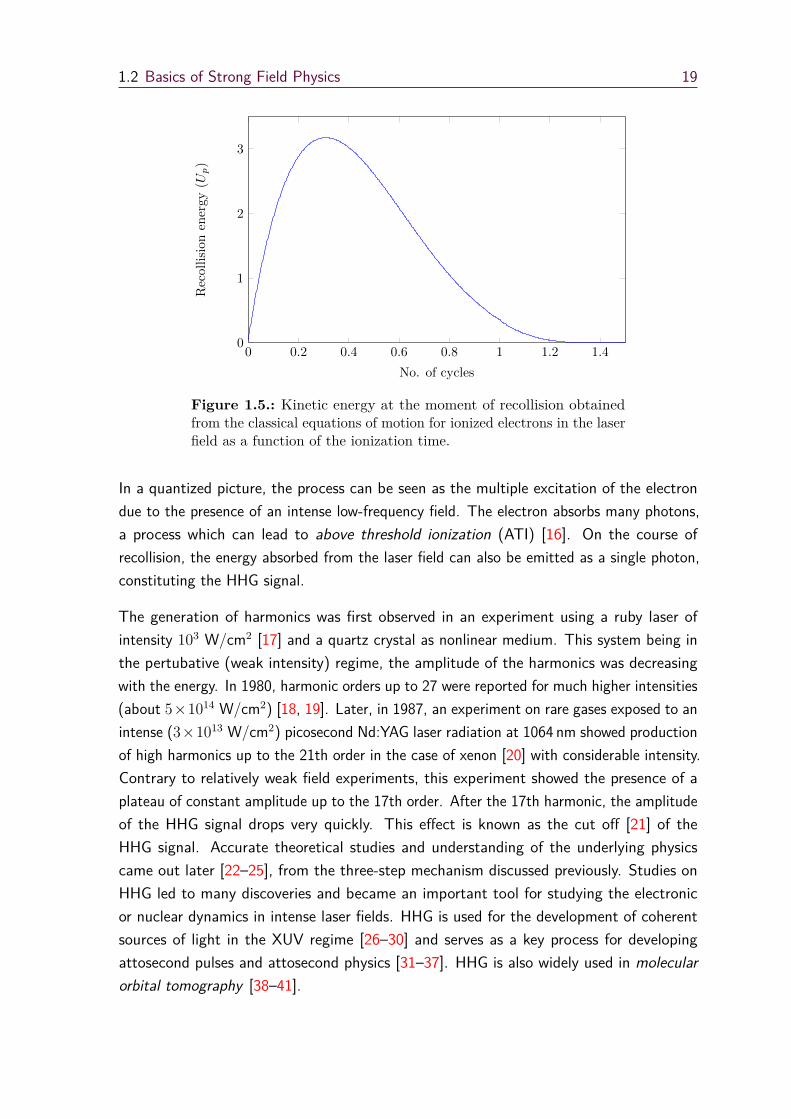
The kinetic energy distribution of these different electron trajectories upon recollision canbe estimated from the classical equations of motion. Being transcendental equations, exactanalytical solutions for the kinetic energy of electrons at the moment of recollision are notpossible. Fig. 1.5 shows a typical recollision energy distribution obtained from numericalanalysis of long and short trajectories. The recolliding electrons are distributed over anenergy range between zero and a maximum of 3.17Up. This peak value of the recollidingenergy is possessed by those electrons born at about ti ' 0.3 (2π/ωL). This value of energyis the upper limit for the energy accumulated in recolliding process. Thus, as Up increases,electrons will acquire more energy from the field and will posses higher energy at the timeof recollision with the core. This rescattering process leads to different outcomes describedhereafter: High harmonic generation, non-sequential double ionization and laser inducedelectron diffraction.

1.2.3.1 High Harmonic Generation (HHG)

The kinetic energy accumulated during the excursion in the continuum can be emitted ina recombination process. This emitted energy will be of frequencies of an odd multipleof the frequency of the driving field. This process is known as high harmonic generation.

1.2 Basics of Strong Field Physics 19

0 0.2 0.4 0.6 0.8 1 1.2 1.40

1

2

3

No. of cycles

Recollisionenergy

(Up)

Figure 1.5.: Kinetic energy at the moment of recollision obtainedfrom the classical equations of motion for ionized electrons in the laserfield as a function of the ionization time.

In a quantized picture, the process can be seen as the multiple excitation of the electrondue to the presence of an intense low-frequency field. The electron absorbs many photons,a process which can lead to above threshold ionization (ATI) [16]. On the course ofrecollision, the energy absorbed from the laser field can also be emitted as a single photon,constituting the HHG signal.

The generation of harmonics was first observed in an experiment using a ruby laser ofintensity 103 W/cm2 [17] and a quartz crystal as nonlinear medium. This system being inthe pertubative (weak intensity) regime, the amplitude of the harmonics was decreasingwith the energy. In 1980, harmonic orders up to 27 were reported for much higher intensities(about 5×1014 W/cm2) [18, 19]. Later, in 1987, an experiment on rare gases exposed to anintense (3×1013 W/cm2) picosecond Nd:YAG laser radiation at 1064 nm showed productionof high harmonics up to the 21th order in the case of xenon [20] with considerable intensity.Contrary to relatively weak field experiments, this experiment showed the presence of aplateau of constant amplitude up to the 17th order. After the 17th harmonic, the amplitudeof the HHG signal drops very quickly. This effect is known as the cut off [21] of theHHG signal. Accurate theoretical studies and understanding of the underlying physicscame out later [22–25], from the three-step mechanism discussed previously. Studies onHHG led to many discoveries and became an important tool for studying the electronicor nuclear dynamics in intense laser fields. HHG is used for the development of coherentsources of light in the XUV regime [26–30] and serves as a key process for developingattosecond pulses and attosecond physics [31–37]. HHG is also widely used in molecularorbital tomography [38–41].

20 Chapter 1. Introduction to Part I

1.2.3.2 Non-Sequential Double Ionization (NSDI)

Double ionization is a process in which two electrons leave the system simultaneously asthe liberation of the second electron is assisted by the first one via electron correlations.It was first observed in alkaline earth elements in 1975 [42] and then observed in noblegases in the presence of low frequency fields of high intensity [43, 44]. In such a field, theenergy of the recolliding electron can be shared with another bound electron of the system,leading to non-sequential double ionization. Multiple ionization was also observed in raregas atoms in strong low frequency laser fields [45, 46]. Studying double ionization yieldsgives insights to the electron correlations in the system, which can be used for probing theinner atomic electron dynamics that is occurring in the attosecond time scale.

Some studies showed that NSDI can occur through two different channels. Either thereturning electron has acquired enough energy so that both electrons end up in thecontinuum after the recollision. In this case NSDI occurs instantaneously and the twoelectrons leave the system in the same direction. If the energy acquired by the recollidingelectron is not sufficient for the ionization of the second electron, the former can still excitethe ion so that the second electron can be ionized by the field. This process is delayed andthe two electrons leave in opposite directions due to the electron-electron repulsion [47].

1.2.3.3 Laser Induced Electron Diffraction (LIED)

In conventional electron diffraction, a few kV electron beam from an external source isdiffracted by a molecular system via elastic scattering. Likewise, the coherent electronwave packet recolliding with the core can be scattered elastically. This leads to electrondiffraction known as laser induced electron diffraction. As in the case of conventionalelectron diffraction, LIED can be used for the estimation of the structural details of themolecules and imaging the molecular dynamics [48, 49]. It can also be used for thereconstruction of molecular orbitals. This is the subject of this part of the thesis.

1.3 Orbital Imaging 21

1.3 Orbital Imaging

Understanding the dynamics of molecular systems is an important problem. Properties ofatoms and molecules are depending on how the electrons are distributed around nuclei.Hence, understanding changes in the electron densities are of importance especially to studythe reaction dynamics of the molecular systems. Due to the ultrashort time scales of theelectron dynamics, it is extremely hard to investigate changes in the electron density duringa reaction dynamics. A way to image the molecular orbitals is via orbital tomography.

Tomography is a general technique for reconstructing an object from a set of sectionalimages. The idea of the orbital tomography technique also lies in the same principle ofextracting informations about the electron density. It was shown experimentally that suchreconstructions of molecular orbitals are possible in the case of aligned molecules in the gasphase using the HHG spectrum obtained from selective ionization [38]. The spectrum ofthe emitted harmonics is recorded from spatially aligned molecules excited with strong nearinfrared laser fields. The characteristics of the oriented molecular orbital will be imprintedin this HHG spectrum since the spectrum is a projection of the recolliding electron wavepacket on the ground state wave function. Hence, by repeating the procedure at differentrelative orientations (molecule with respect to the applied field), one can get more detailsabout the orbitals in space. These spectra provide sectional images and then, following thetomographic technique [50], the molecular orbitals can be reconstructed.

The experimental realization of orbital tomography enhanced research in the related fieldsand there were many modifications done on improving the reconstruction procedure [41,51–55]. The molecular orbital imaging technique shows a possibility for imaging thechemical reactions and reaction dynamics occurring at the molecular level in femtosecondtimescales [48, 49, 56, 57].

In this part of the thesis, molecular orbital imaging using LIED is discussed with the help ofa theoretical model based on the strong field approximation (SFA). The model is applied forreconstructing of the highest occupied molecular orbitals HOMO and HOMO-1 of carbondioxide. The effect of the degree of alignment is also discussed.

The system, numerical method and relevant details for the calculation of photoelectronspectra are discussed in the forthcoming chapter. An analytical model based on SFA isthen developed and the model is applied for extracting the information from the calculatedphotoelectron signals that are relevant for the reconstruction of molecular orbitals.

22 Chapter 1. Introduction to Part I

1.4 References

[1] F. J. McClung and R. W. Hellwarth. “Giant Optical Pulsations from Ruby”.In: Journal of Applied Physics 33 (1962). doi: 10.1063/1.1777174 (cited onpage 13).

[2] H. W. Mocker and R. J. Collins. “Mode Competition and Self-Locking Effects ina Q-Switched Ruby Laser”. In: Applied Physics Letters 7 (1965), page 270. doi:10.1063/1.1754253 (cited on page 13).

[3] D. Strickland and G. Mourou. “Compression of amplified chirped optical pulses”.In: Optics Communications 56 (1985), page 219. doi: 10.1016/0030-4018(85)90120-8 (cited on page 13).

[4] F. Krausz and M. Ivanov. “Attosecond physics”. In: Rev. Mod. Phys. 81 (1 Feb.2009), page 163. doi: 10.1103/RevModPhys.81.163 (cited on page 13).

[5] P. Agostini, F. Fabre, G. Mainfray, G. Petite, and N. K. Rahman. “Free-FreeTransitions Following Six-Photon Ionization of Xenon Atoms”. In: Phys. Rev.Lett. 42 (17 Apr. 1979), page 1127. doi: 10.1103/PhysRevLett.42.1127 (citedon pages 13, 15).

[6] P. B. Corkum. “Plasma perspective on strong field multiphoton ionization”. In:Phys. Rev. Lett. 71 (13 Sept. 1993), page 1994. doi: 10.1103/PhysRevLett.71.1994 (cited on pages 14, 16).

[7] D. Wolkow. “Über eine Klasse von Lösungen der Diracschen Gleichung”. In:Zeitschrift für Physik 94 (1935), page 250. doi: 10.1007/BF01331022 (cited onpage 14).

[8] F. Fabre, G. Petite, P. Agostini, and M. Clement. “Multiphoton above-thresholdionisation of xenon at 0.53 and 1.06m”. In: Journal of Physics B: Atomic andMolecular Physics 15 (1982), page 1353. url: http://stacks.iop.org/0022-3700/15/i=9/a=012 (cited on page 15).

[9] G. Petite, F. Fabre, P. Agostini, M. Crance, and M. Aymar. “Nonresonantmultiphoton ionization of cesium in strong fields: Angular distributions andabove-threshold ionization”. In: Phys. Rev. A 29 (5 1984), page 2677. doi:10.1103/PhysRevA.29.2677 (cited on page 15).

[10] F. Yergeau, G. Petite, and P. Agostini. “Above-threshold ionisation withoutspace charge”. In: Journal of Physics B: Atomic and Molecular Physics 19 (1986),page L663. url: http://stacks.iop.org/0022-3700/19/i=19/a=005 (citedon page 15).

1.4 References 23

[11] G. Petite, P. Agostini, and H. G. Muller. “Intensity dependence of non-pertur-bative above-threshold ionisation spectra: experimental study”. In: Journal ofPhysics B: Atomic, Molecular and Optical Physics 21 (1988), page 4097. url:http://stacks.iop.org/0953-4075/21/i=24/a=010 (cited on page 15).

[12] L. V. Keldysh. In: Zh. Eksp. Teor. Fiz. 47 (1965), page 1945. url: http ://www.jetp.ac.ru/cgi-bin/dn/e_020_05_1307.pdf (cited on page 16).

[13] L. V. Keldysh. “Ionization in the Field of a Strong Electromagnetic Wave”. In:Journal of Experimental and Theoretical Physics 47 (1965), page 1945. url:http://www.jetp.ac.ru/cgi-bin/dn/e_020_05_1307.pdf (cited on page 16).

[14] M. Protopapas, C. H. Keitel, and P. L. Knight. “Atomic physics with super-highintensity lasers”. In: Reports on Progress in Physics 60 (1997), page 389. url:http://stacks.iop.org/0034-4885/60/i=4/a=001 (cited on page 16).

[15] S. V. Popruzhenko. “Keldysh theory of strong field ionization: history, applica-tions, difficulties and perspectives”. In: Journal of Physics B: Atomic, Molecularand Optical Physics 47 (2014), page 204001. url: http://stacks.iop.org/0953-4075/47/i=20/a=204001 (cited on page 16).

[16] D. B. Milošević, G. G. Paulus, D. Bauer, and W. Becker. “Above-thresholdionization by few-cycle pulses”. In: Journal of Physics B: Atomic, Molecularand Optical Physics 39 (2006), R203. url: http://stacks.iop.org/0953-4075/39/i=14/a=R01 (cited on page 19).

[17] P. A. Franken, A. E. Hill, C. W. Peters, and G. Weinreich. “Generation ofOptical Harmonics”. In: Phys. Rev. Lett. 7 (4 Aug. 1961), page 118. doi: 10.1103/PhysRevLett.7.118 (cited on page 19).

[18] R. L. Carman, D. W. Forslund, and J. M. Kindel. “Visible Harmonic Emissionas a Way of Measuring Profile Steepening”. In: Phys. Rev. Lett. 46 (1 Jan. 1981),page 29. doi: 10.1103/PhysRevLett.46.29 (cited on page 19).

[19] R. L. Carman, C. K. Rhodes, and R. F. Benjamin. “Observation of harmonicsin the visible and ultraviolet created in CO2-laser-produced plasmas”. In: Phys.Rev. A 24 (5 Nov. 1981), page 2649. doi: 10.1103/PhysRevA.24.2649 (cited onpage 19).

[20] M. Ferray, A. L’Huillier, X. F. Li, L. A. Lompre, G. Mainfray, and C. Manus.“Multiple-harmonic conversion of 1064 nm radiation in rare gases”. In: Journalof Physics B: Atomic, Molecular and Optical Physics 21 (1988), page L31. url:http://stacks.iop.org/0953-4075/21/i=3/a=001 (cited on page 19).

[21] A. L’Huillier, M. Lewenstein, P. Salières, P. Balcou, M. Y. Ivanov, J. Larsson,and C. G. Wahlström. “High-order Harmonic-generation cutoff”. In: Phys. Rev. A48 (5 Nov. 1993), R3433. doi: 10.1103/PhysRevA.48.R3433 (cited on page 19).

24 Chapter 1. Introduction to Part I

[22] K. C. Kulander and B. W. Shore. “Calculations of Multiple-Harmonic Conversionof 1064-nm Radiation in Xe”. In: Phys. Rev. Lett. 62 (5 Jan. 1989), page 524.doi: 10.1103/PhysRevLett.62.524 (cited on page 19).

[23] M. Lewenstein, P. Balcou, M. Y. Ivanov, A. L’Huillier, and P. B. Corkum. “Theoryof high-harmonic generation by low-frequency laser fields”. In: Phys. Rev. A 49(3 Mar. 1994), page 2117. doi: 10.1103/PhysRevA.49.2117 (cited on page 19).

[24] J. L. Krause, K. J. Schafer, and K. C. Kulander. “High-order harmonic generationfrom atoms and ions in the high intensity regime”. In: Phys. Rev. Lett. 68 (24June 1992), page 3535. doi: 10.1103/PhysRevLett.68.3535 (cited on page 19).

[25] W. Becker, A. Lohr, M. Kleber, and M. Lewenstein. “A unified theory of high-harmonic generation: Application to polarization properties of the harmonics”.In: Phys. Rev. A 56 (1 July 1997), page 645. doi: 10.1103/PhysRevA.56.645(cited on page 19).

[26] C. Spielmann, N. H. Burnett, S. Sartania, R. Koppitsch, M. Schnürer, C. Kan,M. Lenzner, P. Wobrauschek, and F. Krausz. “Generation of Coherent X-rays inthe Water Window Using 5-Femtosecond Laser Pulses”. In: Science 278 (1997),page 661. doi: 10.1126/science.278.5338.661 (cited on page 19).

[27] A. Rundquist, C. G. Durfee, Z. Chang, C. Herne, S. Backus, M. M. Murnane,and H. C. Kapteyn. “Phase-Matched Generation of Coherent Soft X-rays”. In:Science 280 (1998), page 1412. doi: 10.1126/science.280.5368.1412 (citedon page 19).

[28] Z. Chang, A. Rundquist, H. Wang, M. M. Murnane, and H. C. Kapteyn.“Generation of Coherent Soft X Rays at 2.7 nm Using High Harmonics”. In: Phys.Rev. Lett. 79 (16 Oct. 1997), page 2967. doi: 10.1103/PhysRevLett.79.2967(cited on page 19).

[29] Y. Tamaki, Y. Nagata, M. Obara, and K. Midorikawa. “Phase-matched high-order-harmonic generation in a gas-filled hollow fiber”. In: Phys. Rev. A 59 (5May 1999), page 4041. doi: 10.1103/PhysRevA.59.4041 (cited on page 19).

[30] J. J. Macklin, J. D. Kmetec, and C. L. Gordon. “High-order harmonic generationusing intense femtosecond pulses”. In: Phys. Rev. Lett. 70 (6 Feb. 1993), page 766.doi: 10.1103/PhysRevLett.70.766 (cited on page 19).

[31] L.-Y. Peng, W.-C. Jiang, J.-W. Geng, W.-H. Xiong, and Q. Gong. “Tracing andcontrolling electronic dynamics in atoms and molecules by attosecond pulses”.In: Physics Reports 575 (2015). Tracing and controlling electronic dynamics inatoms and molecules by attosecond pulses, page 1. doi: 10.1016/j.physrep.2015.02.002 (cited on page 19).

1.4 References 25

[32] P. Antoine, D. B. Milo ševi ć, A. L’Huillier, M. B. Gaarde, P. Salières, and M.Lewenstein. “Generation of attosecond pulses in macroscopic media”. In: Phys.Rev. A 56 (6 Dec. 1997), page 4960. doi: 10.1103/PhysRevA.56.4960 (cited onpage 19).

[33] P. M. Paul, E. S. Toma, P. Breger, G. Mullot, F. Augé, P. Balcou, H. G.Muller, and P. Agostini. “Observation of a Train of Attosecond Pulses fromHigh Harmonic Generation”. In: Science 292 (2001), page 1689. doi: 10.1126/science.1059413 (cited on page 19).

[34] M. Hentschel, R. Kienberger, C. Spielmann, G. A. Reider, N. Milosevic, T.Brabec, P. Corkum, U. Heinzmann, M. Drescher, and F. Krausz. “Attosecondmetrology”. In: Nature 414 (Nov. 29, 2001), page 509. doi: 10.1038/35107000(cited on page 19).

[35] R. Kienberger, E. Goulielmakis, M. Uiberacker, A. Baltuska, V. Yakovlev, F.Bammer, A. Scrinzi, T. Westerwalbesloh, U. Kleineberg, U. Heinzmann, M.Drescher, and F. Krausz. “Atomic transient recorder”. In: Nature 427 (Feb. 26,2004), page 817. doi: 10.1038/nature02277 (cited on page 19).

[36] P. B. Corkum and F. Krausz. “Attosecond science”. In: Nat Phys 3 (June 2007),page 381. doi: 10.1038/nphys620 (cited on page 19).

[37] E. Goulielmakis, M. Schultze, M. Hofstetter, V. S. Yakovlev, J. Gagnon, M.Uiberacker, A. L. Aquila, E. M. Gullikson, D. T. Attwood, R. Kienberger, F.Krausz, and U. Kleineberg. “Single-Cycle Nonlinear Optics”. In: Science 320(2008), page 1614. doi: 10.1126/science.1157846 (cited on page 19).

[38] J. Itatani, J. Levesque, D. Zeidler, H. Niikura, H. Pepin, J. C. Kieffer, P. B.Corkum, and D. M. Villeneuve. “Tomographic imaging of molecular orbitals”.In: Nature 432 (Dec. 16, 2004), page 867. doi: 10.1038/nature03183 (cited onpages 19, 21).

[39] N. L. Wagner, A. Wüest, I. P. Christov, T. Popmintchev, X. Zhou, M. M. Murnane,and H. C. Kapteyn. “Monitoring molecular dynamics using coherent electronsfrom high harmonic generation”. In: Proceedings of the National Academy ofSciences 103 (2006), page 13279. doi: 10.1073/pnas.0605178103 (cited onpage 19).

[40] P. Hockett, C. Z. Bisgaard, O. J. Clarkin, and A. Stolow. “Time-resolved imagingof purely valence-electron dynamics during a chemical reaction”. In: Nat Phys 7(Aug. 2011), page 612. doi: 10.1038/nphys1980 (cited on page 19).

[41] C. Vozzi, M. Negro, F. Calegari, G. Sansone, M. Nisoli, S. De Silvestri, andS. Stagira. “Generalized molecular orbital tomography”. In: Nat Phys 7 (Oct.2011), page 822. doi: 10.1038/nphys2029 (cited on pages 19, 21).

26 Chapter 1. Introduction to Part I

[42] V. V. Suran and I. P. Zapesnochnii. “Observation of Sr2+ in multiple-photonionization of strontium”. In: Soviet Technical Physics Letters 1 (1975), page 420(cited on page 20).

[43] A. L’Huillier, L. A. Lompre, G. Mainfray, and C. Manus. “Multiply ChargedIons Formed by Multiphoton Absorption Processes in the Continuum”. In: Phys.Rev. Lett. 48 (26 June 1982), page 1814. doi: 10.1103/PhysRevLett.48.1814(cited on page 20).

[44] A. l’Huillier, L. A. Lompre, G. Mainfray, and C. Manus. “Multiply charged ionsinduced by multiphoton absorption in rare gases at 0.53 µm”. In: Phys. Rev. A 27(5 May 1983), page 2503. doi: 10.1103/PhysRevA.27.2503 (cited on page 20).

[45] A. Rudenko, K. Zrost, B. Feuerstein, V. L. B. de Jesus, C. D. Schröter, R.Moshammer, and J. Ullrich. “Correlated Multielectron Dynamics in UltrafastLaser Pulse Interactions with Atoms”. In: Phys. Rev. Lett. 93 (25 Dec. 2004),page 253001. doi: 10.1103/PhysRevLett.93.253001 (cited on page 20).

[46] K. Zrost, A. Rudenko, T. Ergler, B. Feuerstein, V. L. B. de Jesus, C. D. Schröter,R. Moshammer, and J. Ullrich. “Multiple ionization of Ne and Ar by intense 25fs laser pulses: few-electron dynamics studied with ion momentum spectroscopy”.In: Journal of Physics B: Atomic, Molecular and Optical Physics 39 (2006), S371.url: http://stacks.iop.org/0953-4075/39/i=13/a=S10 (cited on page 20).

[47] B. Feuerstein, R. Moshammer, D. Fischer, A. Dorn, C. D. Schröter, J. Deipen-wisch, J. R. Crespo Lopez-Urrutia, C. Höhr, P. Neumayer, J. Ullrich, H. Rottke,C. Trump, M. Wittmann, G. Korn, and W. Sandner. “Separation of RecollisionMechanisms in Nonsequential Strong Field Double Ionization of Ar: The Role ofExcitation Tunneling”. In: Phys. Rev. Lett. 87 (4 July 2001), page 043003. doi:10.1103/PhysRevLett.87.043003 (cited on page 20).

[48] C. I. Blaga, J. Xu, A. D. DiChiara, E. Sistrunk, K. Zhang, P. Agostini, T. A.Miller, L. F. DiMauro, and C. D. Lin. “Imaging ultrafast molecular dynamicswith laser-induced electron diffraction”. In: Nature 483 (Mar. 8, 2012), page 194.doi: 10.1038/nature10820 (cited on pages 20, 21).

[49] M. Peters, T. T. Nguyen-Dang, E. Charron, A. Keller, and O. Atabek. “Laser-induced electron diffraction: A tool for molecular orbital imaging”. In: Phys. Rev.A 85 (5 May 2012), page 053417. doi: 10.1103/PhysRevA.85.053417 (cited onpages 20, 21).

[50] A. Kak and M. Slaney. Principles of Computerized Tomographic Imaging. Societyfor Industrial and Applied Mathematics, 2001. doi: 10.1137/1.9780898719277(cited on page 21).

1.4 References 27

[51] S. Patchkovskii, Z. Zhao, T. Brabec, and D. M. Villeneuve. “High HarmonicGeneration and Molecular Orbital Tomography in Multielectron Systems: Beyondthe Single Active Electron Approximation”. In: Phys. Rev. Lett. 97 (12 Sept.2006), page 123003. doi: 10.1103/PhysRevLett.97.123003 (cited on page 21).

[52] E. V. van der Zwan, C. C. Chiril ă, and M. Lein. “Molecular orbital tomographyusing short laser pulses”. In: Phys. Rev. A 78 (3 Sept. 2008), page 033410. doi:10.1103/PhysRevA.78.033410 (cited on page 21).

[53] Z. Diveki, R. Guichard, J. Caillat, A. Camper, S. Haessler, T. Auguste, T. Ruchon,B. Carré, A. Maquet, R. Taïeb, and P. Salières. “Molecular orbital tomographyfrom multi-channel harmonic emission in N2”. In: Chemical Physics 414 (2013).Attosecond spectroscopy, page 121. doi: 10.1016/j.chemphys.2012.03.021(cited on page 21).

[54] E. V. van der Zwan and M. Lein. “Molecular Imaging Using High-Order HarmonicGeneration and Above-Threshold Ionization”. In: Phys. Rev. Lett. 108 (4 Jan.2012), page 043004. doi: 10.1103/PhysRevLett.108.043004 (cited on page 21).

[55] S. Haessler, J. Caillat, W. Boutu, C. Giovanetti-Teixeira, T. Ruchon, T. Auguste,Z. Diveki, P. Breger, A. Maquet, B. Carre, R. Taieb, and P. Salieres. “Attosecondimaging of molecular electronic wavepackets”. In: Nature Physics 6 (Mar. 2010),page 200. doi: 10.1038/nphys1511 (cited on page 21).

[56] S. Haessler, J. Caillat, and P. Salières. “Self-probing of molecules with highharmonic generation”. In: Journal of Physics B: Atomic, Molecular and OpticalPhysics 44 (2011), page 203001. url: http://stacks.iop.org/0953-4075/44/i=20/a=203001 (cited on page 21).

[57] M. Peters, T. T. Nguyen-Dang, C. Cornaggia, S. Saugout, E. Charron, A. Keller,and O. Atabek. “Ultrafast molecular imaging by laser-induced electron diffraction”.In: Phys. Rev. A 83 (5 May 2011), page 051403. doi: 10.1103/PhysRevA.83.051403 (cited on page 21).

2System and Numerical

Implementation

This chapter discusses the numerical modeling of the molecular systemdynamics in intense laser fields. All approximations and the details ofnumerical method used are explained. Convergence conditions are alsodemonstrated. Preliminary results are finally given. For simplicity, startingfrom this chapter and for the rest of Part I, we are using atomic units.

Keywords:

Soft-Coulomb Potential, Single Active Electron Model, Split Operator Me-thod, Photoelectron Spectra, Volkov States.

Contents2.1 Introduction 31

2.2 System and interaction potential 31

2.3 Numerical Method 35

2.4 Preliminary Results 42

2.5 Conclusion and Outlook 47

2.6 References 48

2.1 Introduction 31

2.1 Introduction

During the interaction of strong fields with dilute samples of atoms and/or molecules inwhich the applied field can no more be treated as a simple perturbation to the system, theionized electron wave packet on the course of recollision with its parent ion will end up indifferent output channels as explained in the previous chapter. The process considered hereis the elastic scattering of the returning wave packet from the ionic core. On scattering, thewave packet will be diffracted from the core that gives rise to the diffraction pattern. Thisspectrum contains many information about the system and the ionization processes. Thegoal of this project is to extract those informations that are relevant for the reconstructionof the initial orbital from which the electron was ionized.

In this chapter, the numerical model is discussed by which the system is treated in order toget the relevant quantities.

2.2 System and interaction potential

In general the systems considered are multi-particle systems like atoms or molecules.Treating exactly such systems in intense laser field is not practical because of the complexityin the potentials and dynamics. But there are some approximations that can be usedfor transforming the problem tractable both numerically and experimentally. The mainingredients chosen for modeling the problem of laser-matter interaction in the intense near-infrared are the following: Single active electron approximation, soft-Coulomb potentials,frozen nuclei, dipole approximation.

2.2.1 Single active electron approximation

An atom (molecule) is a multi-particle system composed of a heavy nucleus (nuclei)surrounded by lighter electrons. Depending on the complexity of the system, the numberof particles involved in the electronic dynamics can vary from one to a few tens. For such

32 Chapter 2. System & Numerical Implementation

an atom the potential of the system can be written as

Vc =N∑

ı=1

(− 1|rı|

+N∑

=ı+1

1|rı|

), (2.1)

where rı is the position of the ıth electron and rı = rı − r are the relative positions ofthe electrons in the system. An exact quantum treatment of such a system beyond thesimplest cases of hydrogen or helium by considering all interaction terms between particlesmakes it intractable.

In a single-active electron approximation (SAE), we will assume that the laser field willinteract only with the most weakly-bound electron in the system. One can then reducethe multi-particle problem to a two body problem, provided the central bound potential ismodified such that it accounts for the influence of other interactions empirically. In thisapproach all other electrons are considered as a frozen [1–3].

By choosing the SAE model, the actual system is approximated to a single electron atomsimilar to the hydrogen atom but with a modified core potential. The potential can thusbe reduced to

Vc(r′) = −Vr′ , (2.2)

where r′ is a function of the spatial coordinate of the active electron and the coefficient Vis chosen empirically such that the potential behaves well (see below).

The model assumes that the response of the system is entirely due to the active electron inthis effective potential given by Eq. (2.2). Similar to atoms, SAE models are widely usedfor understanding the dynamics of simple molecules in intense fields [4–7].

It is counter-intuitive when one considers the real physical picture in which there are manyequivalent electrons that can interact with the electromagnetic field in a similar way. But inpractice there are many cases where all interaction terms in the system are not importantin determining the results of the laser-matter interaction and in explaining experimentalresults. The reason for the wide applicability of SAE-models for explaining experimentalresults lies in the fact that multiply excited states are usually well separated from singlyexcited states [6, 8–10]. In the case of closely spaced levels, the approximation collapses[11]. In the case of processes like non-sequential double ionization, the correlation betweenthe electrons is important and has to be discussed for a real physical picture [12–14]. In thisspecific case the SAE-model is obviously inappropriate. There are other studies showingevidences of the breakdown of the SAE approximation [5, 15–18] and many attempts forincluding multi-electron effects were proposed [19–22].

2.2 System and interaction potential 33

2.2.2 Soft-Coulomb potential

There is yet another major problem to be fixed in order to be ready with the model systemfor numerical calculations: The form of the Coulomb potential causes numerical difficultiesdue to the divergence at the origin. A simple and elegant way to skip this numericalchallenge is the choice of a soft-core potential that can mimics the main features of thereal potential [23]. In general, soft-core potentials are defined by choosing the followingform for r′ in Eq. (2.2)

r′ =(|r|l + al

)1/l

, (2.3)

where r is the coordinate of the active electron and a is a parameter chosen specificallyto remove the singularity of the Coulomb potential at the origin. It can also be seen as aparameter that empirically represents the screening effects of the other electrons in thesystem. l is a power that can be chosen depending on the problem. Here we have chosenthe usual value of l = 2 [24, 25](a) .

The exact value of a is chosen such that the energy of the lowest eigenvalue of the potentialmatches the ground state energy of the system. In addition, the non-zero value chosen fora converts the infinite Coulomb well to a finite well which falls like −1/|r| asymptoticallyin order to represent the long range part of the potential accurately. Thus the effectivesoft-Coulomb potential for an atom under the SAE approximation can be written as

Vc(r) = −V√|r|2 + a2

. (2.4)

In general, for molecules composed of N atoms, the soft-Coulomb potential is given by

Vc(r) =N∑

=1

−V√|r −R|2 + a2

, (2.5)

where R is the position vector of th nucleus. The functions V and the parameters a arechosen depending on the system.

In this part of the thesis, the strong field ionization and the associated electron scatteringfrom a symmetric CO2 molecule are discussed in detail. The system is prepared by aligningit along the so-called y-axis. The C-O bond length is denoted by R and a linearly polarizedlaser pulse is applied perpendicular to the alignment direction.

(a) Reference [25] gives a nice account on soft-Coulomb potentials

34 Chapter 2. System & Numerical Implementation

The choice of molecule fixes the potential and is chosen from [26], in which the samesystem was studied. The potential is given by

Vc(r) =3∑

=1

−V(r)√|r −R|2 + a2

, (2.6)

where

V(r) = V∞ +

(V0

− V∞

)exp

[− |r −R|2

σ2

], (2.7)

where V∞ is the he effective nuclear charge of th nucleus as seen by the electron at infinite

distance, V0 is the bare charge of the th nucleus and the decrease of the effective charge of

the nucleus with distance due to the distance-dependent electron-electron screening effectsis taken into account via the parameter σ.

y

xE

R

R

Figure 2.1.: CO2 molecule aligned along the y axis. A linearlypolarized (in the x direction) electric field is applied to the molecule.

The pulse is chosen such that its duration is smaller than the time scale of the nucleardynamics of the molecule. We therefore further simplify the problem by freezing the nuclearcoordinates. If the polarization of the applied field is taken as the x-axis, as shown in Fig.2.1, the three dimensional problem is reduced to two dimensions with all relevant dynamicsof the system limited in the xy-plane.

2.3 Numerical Method 35

2.2.3 Interaction potential

Being in the long wavelength regime (IR domain), the interaction of the system with theapplied field is taken into account under the dipole approximation. Thus the total potentialenergy of the system can be written as

V (r, t) =3∑

=1

−V(r)√|r −R|2 + a2

− µ.E(t) , (2.8)

where µ denotes the electric dipole. The Hamiltonian of the system can then be written a

H(t) = −∇2/2 + V (r, t). (2.9)

It is important to note that the interaction potential and the Hamiltonian are written herein the length gauge [27]. Being gauge invariant, the results of exact quantum mechanicalcalculations obtained in different gauges should be the same. But the calculations basedon approximate theoretical models may be gauge-dependent [28–30]. It is chosen that thelength gauge will be employed for all calculations in the present thesis.

2.3 Numerical Method

As introduced previously, the system considered here is the symmetric CO2 molecule. TheHOMO is of 1πg symmetry and the HOMO-1 is 1πu. Fig. 2.2 shows these two orbitals forthe equilibrium geometry. For the HOMO, which has an ionization energy of 13.8 eV atequilibrium separation, the electron density is concentrated around the two oxygen atomsand is characterized by two nodal planes. For the HOMO-1 of ionization energy 17.6 eV,the electron density is distributed in all atoms [31].

Being a polyatomic molecule, CO2 possesses additional degrees of freedoms includingvibrational degrees. Since the molecule in the following studies is assumed to have frozennuclei, one has to be careful with the choice of pulse duration. The CO2 molecule hasthree vibrational modes. Out of them, asymmetric bending has a time scale of about 15fs. Thus the constraint on the nuclear degrees of freedom restricts us from choosing apulse that lasts for more than this time. It is also important to keep in mind that choosing

36 Chapter 2. System & Numerical Implementation

HOMOHOMO-1E0 −13.8 eV−17.6 eV

Figure 2.2.: HOMO & HOMO-1 of the CO2 molecule.

a pulse longer than the time scale of asymmetric vibration will essentially invalidate theassumption of a symmetric molecule. The following numerical model is prepared for treatingthis particular problem which can be adapted to other systems very easily.

Solving the time-dependent Schrödinger equation (TDSE) using numerical techniques isthe key for studying the dynamics of such a quantum system in the presence of the timedependent potential V (r, t). In general, solving the TDSE numerically is based on threesteps:

1. The representation of the initial wave function and operators related to the problemon a finite spatial grid.

2. The propagation of the wave function in time.

3. The analysis of the wave function at a specific time as required by the problem forcalculating the desired quantities.

These steps are discussed in the following subsections.

2.3.1 Spatial grid

The implementation of the numerical simulation relies on the definition of the grid whichwill be used for describing the system and the operators. The grid, in general, needs not bean equidistant grid. There are many methods using non-uniform spatial grids for solvingthe TDSE like [32] for instance. The advantage of having non-uniform grids is that itgives a freedom to choose a very fine mesh in regions where the wave function is of more

2.3 Numerical Method 37

interest or where it varies quickly, and to choose a relatively wide mesh in regions of leastinterest or where the wave function varies smoothly. But the efficiency of the FFT algorithmassociated with uniform grids is a strong argument, in terms of computation times, in favorof uniform grids without compromising on the accuracy of the computation.

The spatial grid is defined as follows:

xı = xmin + (ı− 1) ∆x, ı = 1, 2, · · · , Nx, (2.10)

where ı is the index associated with a grid point and Nx is the total number of grid pointsin the x direction. The grid step is given by

∆x = (xmax − xmin) /(Nx − 1), (2.11)

where xmax and xmin are the upper and lower limits of the grid in x. A similar grid is usedin the y direction, giving finally a two dimensional spatial grid. In principle, the space in xthat one has to take into account for the exact solution of the TDSE is continuous andinfinite.

Discretization in space converts all continuous integrals into finite sums. Indeed, any xintegral of a function g(x) can be expressed approximately as∫ ∞

−∞g(x)dx '

∑ı

g(xı) ∆x . (2.12)

The methods also requires to discretize all operators and wave functions on the definedgrid for the calculations. Out of many ways to solve the TDSE, the system under the SAEis simulated here using the split operator method.

The code is prepared as described in [33, 34], and detailed below.

2.3.2 Split operator method

The split operator method was used first in the context of the paraxial wave equation inoptics which is quite similar to the TDSE in the mathematical point of view [35]. Themethod was then adapted for solving the TDSE to make use of its easiness in applyingfast Fourier transforms (FFT). As the name indicates this method relies on the effectivesplitting of the operator used for propagating the wave function.

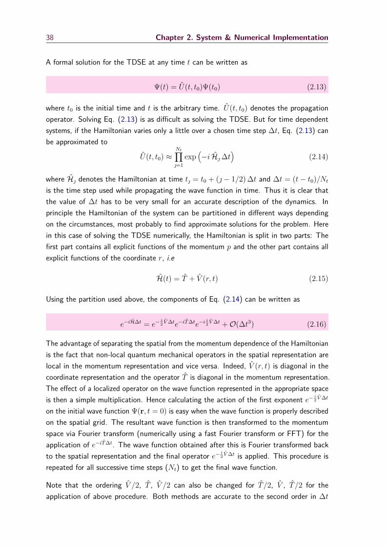
38 Chapter 2. System & Numerical Implementation

A formal solution for the TDSE at any time t can be written as

Ψ(t) = U(t, t0)Ψ(t0) (2.13)

where t0 is the initial time and t is the arbitrary time. U(t, t0) denotes the propagationoperator. Solving Eq. (2.13) is as difficult as solving the TDSE. But for time dependentsystems, if the Hamiltonian varies only a little over a chosen time step ∆t, Eq. (2.13) canbe approximated to

U(t, t0) ≈Nt∏=1

exp(−i H ∆t

)(2.14)

where H denotes the Hamiltonian at time t = t0 + (− 1/2) ∆t and ∆t = (t− t0)/Nt

is the time step used while propagating the wave function in time. Thus it is clear thatthe value of ∆t has to be very small for an accurate description of the dynamics. Inprinciple the Hamiltonian of the system can be partitioned in different ways dependingon the circumstances, most probably to find approximate solutions for the problem. Herein this case of solving the TDSE numerically, the Hamiltonian is split in two parts: Thefirst part contains all explicit functions of the momentum p and the other part contains allexplicit functions of the coordinate r, i.e

H(t) = T + V (r, t) (2.15)

Using the partition used above, the components of Eq. (2.14) can be written as

e−iH∆t = e− i2 V ∆te−iT ∆te−i i

2 V ∆t +O(∆t3) (2.16)

The advantage of separating the spatial from the momentum dependence of the Hamiltonianis the fact that non-local quantum mechanical operators in the spatial representation arelocal in the momentum representation and vice versa. Indeed, V (r, t) is diagonal in thecoordinate representation and the operator T is diagonal in the momentum representation.The effect of a localized operator on the wave function represented in the appropriate spaceis then a simple multiplication. Hence calculating the action of the first exponent e− i

2 V ∆t

on the initial wave function Ψ(r, t = 0) is easy when the wave function is properly describedon the spatial grid. The resultant wave function is then transformed to the momentumspace via Fourier transform (numerically using a fast Fourier transform or FFT) for theapplication of e−iT ∆t. The wave function obtained after this is Fourier transformed backto the spatial representation and the final operator e− i

2 V ∆t is applied. This procedure isrepeated for all successive time steps (Nt) to get the final wave function.

Note that the ordering V /2, T , V /2 can also be changed for T /2, V , T /2 for theapplication of above procedure. Both methods are accurate to the second order in ∆t

2.3 Numerical Method 39

and the error is proportional to [[T , V ], H]∆t3. The choice between these two approachesis merely a question of the implementation of the problem, the two approaches being asefficient and accurate.

2.3.3 Absorbing boundaries

A common difficulty with propagating wave functions in a finite grid is the unwantedreflection of outgoing wave functions at the boundary of the simulation region (end ofthe grid). Here, the FFT algorithm used for Fourier transforms will give rise to unphysicalreflections which have to be avoided for the proper description of the dynamics. This canbe done by patching the boundaries of the grid with an absorbing term C2D(r), or maskfunction, which will absorb the outgoing wave function.

The procedure for including such boundaries is rather complicated because of the factthat any kind of action on the wave function will add additional momentum componentsto the wave packet that ultimately affect the accuracy of the calculation. This error onthe calculation cannot be completely avoided but can be reduced by optimizing variousparameters of the mask function. C2D(r) can be any normalized piece-wise function whichhas value 1 in the regions where the dynamics is taking place (simulation region) and goesto zero smoothly in the regions close to the boundaries. Multiplying such a function withthe wave function on the course of the evolution at each time step will solve the problemof unwanted reflections.

The mask function C2D(r) chosen in the following calculations is

C2D(r) = C(x)× C(y) (2.17)

where r =√x2 + y2. The one dimensional components of the mask function are given by

C(x) =

0 |x| > 2xs[1 + cos

(π x−xs

xs

)]/2 xs < |x| < 2xs

1 |x| 6 xs

(2.18)

where xs is a pre-fixed position in space defining the range of the simulation region. Itshould be adjusted with the specific problem under consideration. This value depends onthe laser parameters used and on the type of dynamics considered. xs also defines the

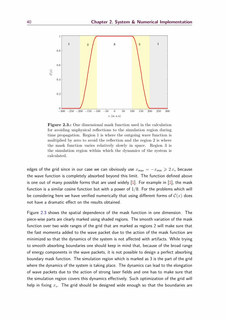
40 Chapter 2. System & Numerical Implementation

3 221 1

−300 −250 −200 −150 −100 −50 0 50 100 150 200 250 3000

0.2

0.4

0.6

0.8

1

x (in a.u)

C(x)

Figure 2.3.: One dimensional mask function used in the calculationfor avoiding unphysical reflections to the simulation region duringtime propagation. Region 1 is where the outgoing wave function ismultiplied by zero to avoid the reflection and the region 2 is wherethe mask function varies relatively slowly in space. Region 3 isthe simulation region within which the dynamics of the system iscalculated.

edges of the grid since in our case we can obviously use xmax = −xmin > 2xs becausethe wave function is completely absorbed beyond this limit. The function defined aboveis one out of many possible forms that are used widely [1]. For example in [1], the maskfunction is a similar cosine function but with a power of 1/8. For the problems which willbe considering here we have verified numerically that using different forms of C(x) doesnot have a dramatic effect on the results obtained.

Figure 2.3 shows the spatial dependence of the mask function in one dimension. Thepiece-wise parts are clearly marked using shaded regions. The smooth variation of the maskfunction over two wide ranges of the grid that are marked as regions 2 will make sure thatthe fast momenta added to the wave packet due to the action of the mask function areminimized so that the dynamics of the system is not affected with artifacts. While tryingto smooth absorbing boundaries one should keep in mind that, because of the broad rangeof energy components in the wave packets, it is not possible to design a perfect absorbingboundary mask function. The simulation region which is marked as 3 is the part of the gridwhere the dynamics of the system is taking place. The dynamics can lead to the elongationof wave packets due to the action of strong laser fields and one has to make sure thatthe simulation region covers this dynamics effectively. Such optimization of the grid willhelp in fixing xs. The grid should be designed wide enough so that the boundaries are

2.3 Numerical Method 41

beyond the slowly varying part of the mask function. An alternative way to implementan absorbing boundary condition is by adding an artificial purely imaginary component tothe potential part of the Hamiltonian, similar to an imaginary optical potential in optics.In split operator methods this technique helps to dampen the wave function where theimaginary terms are defined. It has been shown that both methods, adding an imaginarypart to the Hamiltonian or using a well defined mask function, give similar results.

2.3.4 Asymptotic analysis of the wave function

The wave packet is propagated as described above and the procedure for extracting thephoto-electron spectrum is based on analyzing the wave function near the grid boundaries,where the Coulomb potential is negligible.At each time step, the total wave function is splitin two parts: The inner part ΨI(r, t) and the asymptotic part ΨA(r, t). It can be done bymultiplying the wave function Ψ(r, t) with C2D(r). The inner part of the wave function,which is the part of wave packet that interacts with the attractive Coulomb potential, canbe separated out as follows

ΨI(r, t) = C2D(r)Ψ(r, t). (2.19)

The asymptotic part is then

ΨA(r, t) = [1− C2D(r)] Ψ(r, t). (2.20)

This asymptotic part of the wave function can be considered as evolving under a simplifiedHamiltonian where the Coulomb potential is neglected. Hence it can be seen as a freeelectron wave packet propagating in an electric field.

The asymptotic part of the wave function can thus be expanded in Volkov states in orderto propagate it analytically. For this purpose, the numerical procedure we are following isdescribed in details in Refs. [33, 34]. It allows to calculate accurately and efficiently theaccumulated ionized wave packet at any time t after the end of the pulse in the momentumrepresentation. The photo-electron spectrum is directly obtained from the square modulusof this propagated momentum wave function.

In this approach, the calculated ionization amplitude is approximate. It is in part becauseof the fact that there are very slow electrons which will take infinite time to reach the

42 Chapter 2. System & Numerical Implementation

asymptotic boundary. The wave function is therefore propagated for a long period of timeafter the end of the pulse to collect all electrons, whatever their energy. This is testednumerically until convergence is achieved.

2.4 Preliminary Results

The CO2 molecule is assumed to be aligned along the y axis. The applied field is actingperpendicular to the molecular axis. This scheme sets a natural orthonormal coordinatesystem for the problem. The linearly polarized applied field ionizes the system both in thepositive and negative directions of this axis and drives back and forth the ionized electronvia the interaction potential. Hence the electron motion is taking place in the xy-plane.

The numerical code was prepared with a spatial grid in x and y such that −250 a.u 6

x 6 250 a.u and −250 a.u 6 y 6 250 a.u with a time step ∆t ' 0.45 a.u. The potentialparameters for CO2 are taken from [26].

2.4.1 Imaginary time propagation: Calculation of the initial state

The initial state Ψ(r, 0) of the system can be any of the eigenstates Ψn(r) of the systemHamiltonian. These states are calculated using the split operator method in imaginary timet = −iτ . The time evolution of an arbitrary wave packet in imaginary time can be writtenas

Ψ(r, τ) =∑

n

an e−Enτ Ψn(r) . (2.21)

It is clear from the above equation that as the propagation goes on, the wave packet willconcentrate to the lowest energy eigenstate. This method is very efficient in calculatingthe ground state of the system. But here it is also aimed at getting orbitals other than theground state. It can be obtained by recognizing the possible solutions with their symmetry.The solutions should be correctly symmetrized and orthonormalized at each time step sothat the right solutions are picked from different numerical solutions. This can be donevia the Gram-Schmidt orthogonalization procedure. More details of the imaginary timepropagation (ITP) technique are given in [36]. While calculating the initial state, it is

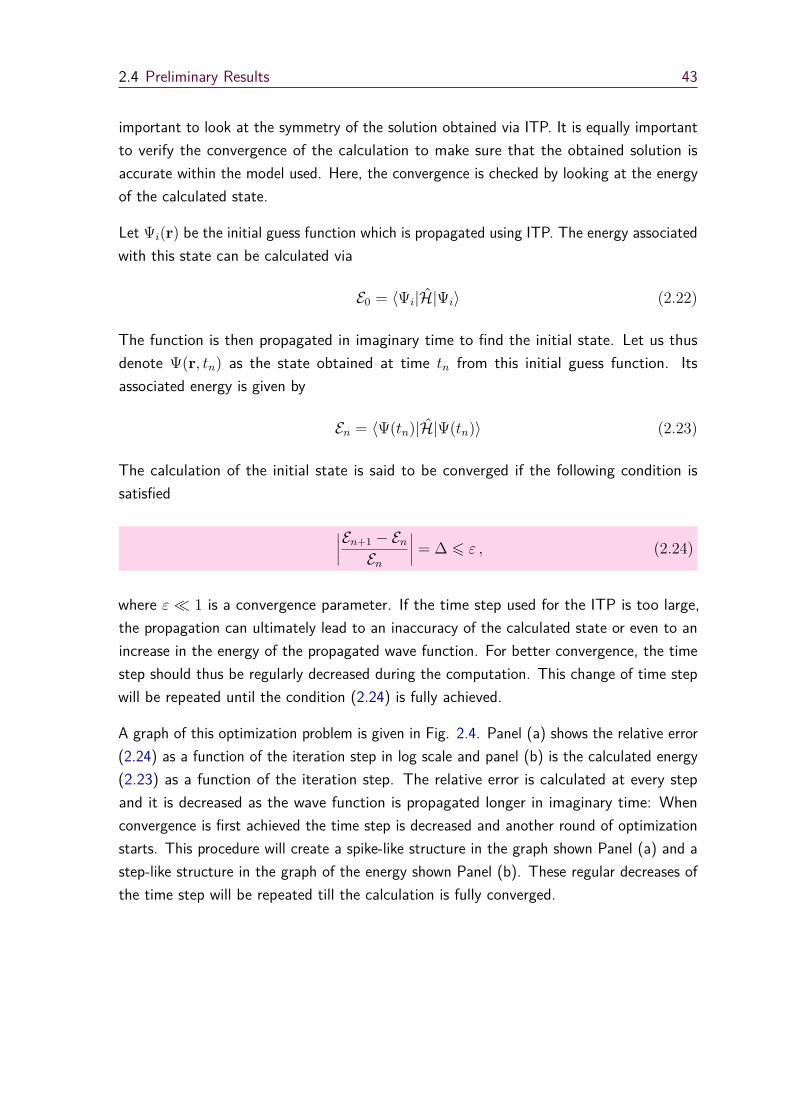
2.4 Preliminary Results 43

important to look at the symmetry of the solution obtained via ITP. It is equally importantto verify the convergence of the calculation to make sure that the obtained solution isaccurate within the model used. Here, the convergence is checked by looking at the energyof the calculated state.

Let Ψi(r) be the initial guess function which is propagated using ITP. The energy associatedwith this state can be calculated via

E0 = 〈Ψi|H|Ψi〉 (2.22)

The function is then propagated in imaginary time to find the initial state. Let us thusdenote Ψ(r, tn) as the state obtained at time tn from this initial guess function. Itsassociated energy is given by

En = 〈Ψ(tn)|H|Ψ(tn)〉 (2.23)

The calculation of the initial state is said to be converged if the following condition issatisfied

∣∣∣∣En+1 − En

En

∣∣∣∣ = ∆ 6 ε , (2.24)

where ε 1 is a convergence parameter. If the time step used for the ITP is too large,the propagation can ultimately lead to an inaccuracy of the calculated state or even to anincrease in the energy of the propagated wave function. For better convergence, the timestep should thus be regularly decreased during the computation. This change of time stepwill be repeated until the condition (2.24) is fully achieved.

A graph of this optimization problem is given in Fig. 2.4. Panel (a) shows the relative error(2.24) as a function of the iteration step in log scale and panel (b) is the calculated energy(2.23) as a function of the iteration step. The relative error is calculated at every stepand it is decreased as the wave function is propagated longer in imaginary time: Whenconvergence is first achieved the time step is decreased and another round of optimizationstarts. This procedure will create a spike-like structure in the graph shown Panel (a) and astep-like structure in the graph of the energy shown Panel (b). These regular decreases ofthe time step will be repeated till the calculation is fully converged.

44 Chapter 2. System & Numerical Implementation

1,000 1,200 1,40010−15

10−8

10−1

(a)

(b)

0 5 10 15 20 25 30−0.35

−0.3

−0.25

−0.2

−0.15

Number of iterations (103)

Energy

ofinitialstate

0 20 40 60 80

−0.3

−0.2

−0.1

10−13

10−11

10−9

10−7

10−5

10−3

10−1

∆

Figure 2.4.: Convergence scheme chosen in the ITP. Panel (a):Optimization of the relative error (2.24). A zoom of a portion ofthe graph is given in the inset. Panel (b): Convergence of the stateenergy (2.23). A zoom of a portion of the graph is given in the inset.

2.4.2 Ionization of the HOMO and HOMO-1 of CO2

The HOMO and HOMO-1 of CO2 are calculated using ITP. Electron density plotscorresponding to these states are given in Fig. 2.5. The equilibrium bond length forthe molecule is 1.2 Å, but for the sake of clarify in the present figure an elongated moleculeis considered with C-O bonds of length 2.5 Å. These orbitals and their dynamics will bediscussed in detail in the forthcoming chapters.

The system is excited with a strong laser pulse E(t) = −∂tAx(t), where Ax(t) is thepotential vector given by

Ax(t) = E0

ωL

sin2(πt

T

)cos(ωLt+ φ) (2.25)

and hence the associated electric field is given by

2.4 Preliminary Results 45

−3 −2 −1 0 1 2−4

−2

0

2

4

x

y

(a) HOMO

−3 −2 −1 0 1 2−4

−2

0

2

4

x

y

(b) HOMO-1

Figure 2.5.: Square modulus of the HOMO and HOMO-1 of asymmetric CO2 molecule with R = 2.5 Å calculated by imaginarytime propagation.

E(t) = E0

[sin2

(πt

T

)sin(ωLt+ φ)− π

ωLTsin

(2πtT

)cos(ωLt+ φ)

], (2.26)

where E0 ∝√I0 is the field amplitude, T is the pulse duration, ωL = 2πc/λL is the laser

frequency and φ is the career envelope phase. In the present study we will choose the IRwavelength λL = 2.1 µm and intensities around I0 = 1× 1014 W/cm2. A typical electricpulse obtained from Eq.(2.26) is shown Fig. 2.6.

0 5 10 15 20−1

−0.5

0

0.5

t (fs)

E(t)/E

0

Figure 2.6.: Typical normalized electric field E(t)/E0 from Eq.(2.26)used for inducing the dynamics in the system.

The choice made on the form of the electric field given by Eq. (2.26) ensures that thevector potential goes to zero when the field vanishes at time t = T , in agreement withMaxwell’s equations. This is important since the asymptotic analysis is build upon the

46 Chapter 2. System & Numerical Implementation

value of the vector potential Ax(T ) at the end of the pulse [33, 34]. Non-zero values of thevector potential at t = T give rise to unphysical DC components, which can be unphysicallypresent in the LIED spectrum as a global shift.

The pre-aligned target molecule is exposed to an intense laser pulse lasing at a wavelengthof 2.1 µm with an intensity of the order of 1014 W/cm2. A schematic representation ofthe ionization process in strong IR fields is given in Fig. 2.7.

z

y

x

Source

Pulse

e−

e−

CO2

Figure 2.7.: Schematic drawing of LIED from a CO2 molecule.

Fig. 2.8 shows typical ionization probabilities obtained for the HOMO and HOMO-1,calculated from the norm of the electronic wave function, together with the associatedelectric field. Both the HOMO and HOMO-1 ionization probabilities show a quite similartime dependence. There are here two jumps in the ionization signal followed by a plateau.This is because ionization of the system in intense infrared laser fields is occurring only overtime windows during which the intensity reaches values large enough to tunnel ionize thesystem. The ionization bursts do not show up when the field is maximum, this is becauseit takes some time for the ionized electrons to reach the grid boundary where they will becounted as ionized.

The two main peaks of the exciting pulse trigger two ionization events which are imprintedin the ionization signal as a function of time. At the end of the pulse, the remainingcontinuum wave packet is left with a distribution of kinetic energies. This wave packetwill take a certain time to reach the detector. Thus, the asymptotic analysis should bedone for certain time even after the pulse. Once all high energy components reach thedetector, the signal starts to form the second plateau which will keep increasing with asmall slope due to the arrival of low kinetic energy electrons. Due to the presence of verysmall kinetic energy components in the wave packet, a negligible increment in the signal

2.5 Conclusion and Outlook 47

0

1

2

3

4

5

6

·10−2

IonizationProbab

ility

0 2 4 6 8 10 12 14 16 18−1

−0.5

0

0.5

1

t (fs)

E(t)/E

0

HOMOHOMO-1

Figure 2.8.: Time dependence of the HOMO and HOMO-1 ionizationsignals for a pulse of carrier wavelength 2.1 µm and intensity 1014

W/cm2. The electric field is given as a blue solid line and thecorresponding ionization probabilities are shown as a red dotted linefor the HOMO and as a red solid line for the HOMO-1.

will sustain forever. The convergence of the calculation can, hence, be checked by lookingat the ionization probability versus time. Once the increment in the signal is small enough,i.e, smaller than a fixed threshold, the propagation and the asymptotic analysis can bestopped and the LIED (photo-electron) spectrum can be computed.

2.5 Conclusion and Outlook

In this chapter, the system and the numerical model that will be used for studying thedynamics of CO2 in strong IR laser pulses are discussed in detail. The system consideredhere is an aligned carbon dioxide molecule. The strong field ionization and the associatedelastic scattering of the ionized wave packet will be studied using a numerical solution ofthe time-dependent Schrödinger equation obtained from the split operator method. Thestates from which electrons are ionized are the HOMO and HOMO-1. These initial statesare calculated using the imaginary time propagation technique. The code is optimized forthe system and tested in terms of convergence.

The numerical results are discussed in the next chapter.

48 Chapter 2. System & Numerical Implementation

2.6 References

[1] J. L. Krause, K. J. Schafer, and K. C. Kulander. “Calculation of photoemissionfrom atoms subject to intense laser fields”. In: Phys. Rev. A 45 (7 Apr. 1992),pages 4998–5010. doi: 10.1103/PhysRevA.45.4998 (cited on pages 32, 40).

[2] J. L. Krause, K. J. Schafer, and K. C. Kulander. “High-order harmonic generationfrom atoms and ions in the high intensity regime”. In: Phys. Rev. Lett. 68 (24June 1992), page 3535. doi: 10.1103/PhysRevLett.68.3535 (cited on page 32).

[3] H. Xu, X. Tang, and P. Lambropoulos. “Nonperturbative theory of harmonicgeneration in helium under a high-intensity laser field: The role of intermediateresonance and of the ion”. In: Phys. Rev. A 46 (5 Sept. 1992), R2225. doi:10.1103/PhysRevA.46.R2225 (cited on page 32).

[4] M. Awasthi, Y. V. Vanne, A. Saenz, A. Castro, and P. Decleva. “Single-active-electron approximation for describing molecules in ultrashort laser pulses andits application to molecular hydrogen”. In: Phys. Rev. A 77 (6 June 2008),page 063403. doi: 10.1103/PhysRevA.77.063403 (cited on page 32).

[5] D. Pavi či ć, K. F. Lee, D. M. Rayner, P. B. Corkum, and D. M. Villeneuve.“Direct Measurement of the Angular Dependence of Ionization for N2, O2, andCO2 in Intense Laser Fields”. In: Phys. Rev. Lett. 98 (24 June 2007), page 243001.doi: 10.1103/PhysRevLett.98.243001 (cited on page 32).

[6] J. Itatani, J. Levesque, D. Zeidler, H. Niikura, H. Pepin, J. C. Kieffer, P. B.Corkum, and D. M. Villeneuve. “Tomographic imaging of molecular orbitals”.In: Nature 432 (Dec. 16, 2004), page 867. doi: 10.1038/nature03183 (cited onpage 32).

[7] F. Krausz and M. Ivanov. “Attosecond physics”. In: Rev. Mod. Phys. 81 (1 Feb.2009), page 163. doi: 10.1103/RevModPhys.81.163 (cited on page 32).

[8] S. G. Preston, A. Sanpera, M. Zepf, W. J. Blyth, C. G. Smith, J. S. Wark,M. H. Key, K. Burnett, M. Nakai, D. Neely, and A. A. Offenberger. “High-orderharmonics of 248.6-nm KrF laser from helium and neon ions”. In: Phys. Rev. A53 (1 Jan. 1996), R31. doi: 10.1103/PhysRevA.53.R31 (cited on page 32).

[9] M. Lewenstein, P. Balcou, M. Y. Ivanov, A. L’Huillier, and P. B. Corkum. “Theoryof high-harmonic generation by low-frequency laser fields”. In: Phys. Rev. A 49(3 Mar. 1994), page 2117. doi: 10.1103/PhysRevA.49.2117 (cited on page 32).

2.6 References 49

[10] R. Moshammer, J. Ullrich, B. Feuerstein, D. Fischer, A. Dorn, C. D. Schröter,J. R. Crespo Lopez-Urrutia, C. Hoehr, H. Rottke, C. Trump, M. Wittmann,G. Korn, and W. Sandner. “Rescattering of Ultralow-Energy Electrons for SingleIonization of Ne in the Tunneling Regime”. In: Phys. Rev. Lett. 91 (11 Sept.2003), page 113002. doi: 10.1103/PhysRevLett.91.113002 (cited on page 32).

[11] M. Smits, C. A. de Lange, A. Stolow, and D. M. Rayner. “Absolute IonizationRates of Multielectron Transition Metal Atoms in Strong Infrared Laser Fields”.In: Phys. Rev. Lett. 93 (21 Nov. 2004), page 213003. doi: 10.1103/PhysRevLett.93.213003 (cited on page 32).

[12] V. V. Suran and I. P. Zapesnochnii. “Observation of Sr2+ in multiple-photonionization of strontium”. In: Soviet Technical Physics Letters 1 (1975), page 420(cited on page 32).

[13] K. Zrost, A. Rudenko, T. Ergler, B. Feuerstein, V. L. B. de Jesus, C. D. Schröter,R. Moshammer, and J. Ullrich. “Multiple ionization of Ne and Ar by intense 25fs laser pulses: few-electron dynamics studied with ion momentum spectroscopy”.In: Journal of Physics B: Atomic, Molecular and Optical Physics 39 (2006), S371.url: http://stacks.iop.org/0953-4075/39/i=13/a=S10 (cited on page 32).

[14] B. Feuerstein, R. Moshammer, D. Fischer, A. Dorn, C. D. Schröter, J. Deipen-wisch, J. R. Crespo Lopez-Urrutia, C. Höhr, P. Neumayer, J. Ullrich, H. Rottke,C. Trump, M. Wittmann, G. Korn, and W. Sandner. “Separation of RecollisionMechanisms in Nonsequential Strong Field Double Ionization of Ar: The Role ofExcitation Tunneling”. In: Phys. Rev. Lett. 87 (4 July 2001), page 043003. doi:10.1103/PhysRevLett.87.043003 (cited on page 32).

[15] A. E. Boguslavskiy, J. Mikosch, A. Gijsbertsen, M. Spanner, S. Patchkovskii,N. Gador, M. J. J. Vrakking, and A. Stolow. “The Multielectron IonizationDynamics Underlying Attosecond Strong-Field Spectroscopies”. In: Science 335(2012), page 1336. doi: 10.1126/science.1212896 (cited on page 32).

[16] H. Akagi, T. Otobe, A. Staudte, A. Shiner, F. Turner, R. Dörner, D. M. Villeneuve,and P. B. Corkum. “Laser Tunnel Ionization from Multiple Orbitals in HCl”.In: Science 325 (2009), page 1364. doi: 10.1126/science.1175253 (cited onpage 32).

[17] X. Zhou, R. Lock, N. Wagner, W. Li, H. C. Kapteyn, and M. M. Murnane.“Elliptically Polarized High-Order Harmonic Emission from Molecules in LinearlyPolarized Laser Fields”. In: Phys. Rev. Lett. 102 (7 Feb. 2009), page 073902. doi:10.1103/PhysRevLett.102.073902 (cited on page 32).

50 Chapter 2. System & Numerical Implementation

[18] O. Smirnova, Y. Mairesse, S. Patchkovskii, N. Dudovich, D. Villeneuve, P.Corkum, and M. Y. Ivanov. “High harmonic interferometry of multi-electrondynamics in molecules”. In: Nature 460 (Aug. 20, 2009), page 972. doi: 10.1038/nature08253 (cited on page 32).

[19] S. Patchkovskii, Z. Zhao, T. Brabec, and D. M. Villeneuve. “High HarmonicGeneration and Molecular Orbital Tomography in Multielectron Systems: Beyondthe Single Active Electron Approximation”. In: Phys. Rev. Lett. 97 (12 Sept.2006), page 123003. doi: 10.1103/PhysRevLett.97.123003 (cited on page 32).

[20] J. Prager, S. X. Hu, and C. H. Keitel. “High-order regime of harmonic generationwith two active electrons”. In: Phys. Rev. A 64 (4 Sept. 2001), page 045402. doi:10.1103/PhysRevA.64.045402 (cited on page 32).

[21] C. Guo. “Multielectron Effects on Single-Electron Strong Field Ionization”. In:Phys. Rev. Lett. 85 (11 Sept. 2000), page 2276. doi: 10.1103/PhysRevLett.85.2276 (cited on page 32).

[22] G. Lagmago Kamta and A. F. Starace. “Multielectron system in an ultrashort,intense laser field: A nonperturbative, time-dependent two-active-electron ap-proach”. In: Phys. Rev. A 65 (5 May 2002), page 053418. doi: 10.1103/PhysRevA.65.053418 (cited on page 32).

[23] R. L. Hall, N. Saad, K. D. Sen, and H. Ciftci. “Energies and wave functions fora soft-core Coulomb potential”. In: Phys. Rev. A 80 (3 Sept. 2009), page 032507.doi: 10.1103/PhysRevA.80.032507 (cited on page 33).

[24] J. Javanainen, J. H. Eberly, and Q. Su. “Numerical simulations of multiphotonionization and above-threshold electron spectra”. In: Phys. Rev. A 38 (7 Oct.1988), page 3430. doi: 10.1103/PhysRevA.38.3430 (cited on page 33).

[25] Q. Su and J. H. Eberly. “Model atom for multiphoton physics”. In: Phys. Rev.A 44 (9 Nov. 1991), page 5997. doi: 10.1103/PhysRevA.44.5997 (cited onpage 33).

[26] M. Peters, T. T. Nguyen-Dang, E. Charron, A. Keller, and O. Atabek. “Laser-induced electron diffraction: A tool for molecular orbital imaging”. In: Phys. Rev.A 85 (5 May 2012), page 053417. doi: 10.1103/PhysRevA.85.053417 (cited onpages 34, 42).

[27] A. D. Bandrauk, F. Fillion-Gourdeau, and E. Lorin. “Atoms and moleculesin intense laser fields: gauge invariance of theory and models”. In: Journal ofPhysics B: Atomic, Molecular and Optical Physics 46 (2013), page 153001. url:http://stacks.iop.org/0953-4075/46/i=15/a=153001 (cited on page 35).

2.6 References 51

[28] C. Leone, S. Bivona, R. Burlon, F. Morales, and G. Ferrante. “Gauge aspectsin multichannel multiphoton ionization”. In: Phys. Rev. A 40 (4 Aug. 1989),page 1828. doi: 10.1103/PhysRevA.40.1828 (cited on page 35).

[29] T. K. Kjeldsen and L. B. Madsen. “Strong-field ionization of N 2 : length andvelocity gauge strong-field approximation and tunnelling theory”. In: Journal ofPhysics B: Atomic, Molecular and Optical Physics 37 (2004), page 2033. url:http://stacks.iop.org/0953-4075/37/i=10/a=003 (cited on page 35).

[30] Y. J. Chen and B. Hu. “Strong-field approximation for diatomic molecules:Comparison between the length gauge and the velocity gauge”. In: Phys. Rev. A80 (3 Sept. 2009), page 033408. doi: 10.1103/PhysRevA.80.033408 (cited onpage 35).

[31] D. W. Turner and M. I. Al-Joboury. “Molecular Photoelectron Spectroscopy”.In: Bulletin des Sociétés Chimiques Belges 73 (1964), page 428. doi: 10.1002/bscb.19640730511 (cited on page 35).

[32] J. L. Krause and K. J. Schafer. “Control of THz Emission from Stark WavePackets”. In: The Journal of Physical Chemistry A 103 (1999), page 10118. doi:10.1021/jp992144+ (cited on page 36).

[33] S. Chelkowski and A. D. Bandrauk. “Wave-function splitting technique forcalculating above-threshold ionization electron spectra”. In: International Journalof Quantum Chemistry 60 (1996), page 1685. doi: 10 . 1002 / (SICI ) 1097 -461X(1996)60:7<1685::AID-QUA51>3.0.CO;2-X (cited on pages 37, 41, 46).

[34] A. Keller. “Asymptotic analysis in time-dependent calculations with divergentcoupling”. In: Phys. Rev. A 52 (2 Aug. 1995), page 1450. doi: 10.1103/PhysRevA.52.1450 (cited on pages 37, 41, 46).

[35] J. Fleck J.A., J. Morris, and M. Feit. “Time-dependent propagation of highenergy laser beams through the atmosphere”. English. In: Applied physics 10(1976), page 129. doi: 10.1007/BF00896333 (cited on page 37).

[36] L. Lehtovaara, J. Toivanen, and J. Eloranta. “Solution of time-independentSchrödinger equation by the imaginary time propagation method”. In: Journal ofComputational Physics 221 (2007), page 148. url: http://www.sciencedirect.com/science/article/pii/S0021999106002798 (cited on page 42).

3Laser induced Electron Diffraction

in CO2

In this chapter we study the structure of the photoelectron spectra obtainedfrom laser induced electron diffraction from the HOMO and HOMO-1 orbitalsof carbon dioxide molecules. Different pathways for electron wave packetsto interfere in photoelectron spectra are discussed in detail.

The different diffraction patterns that appear in the spectra are discussed.

Keywords:

Electron Diffraction, Interference, Recollision, Direct ionization, LIED spec-trum.

Contents3.1 Introduction 55

3.2 Interference Patterns of the LIED Spectrum 55

3.3 Dependence of the LIED on various Laser Parameters 59

3.4 LIED Spectra of the HOMO and HOMO-1 65

3.5 References 68

3.1 Introduction 55

3.1 Introduction

In the previous chapter, all essential details were given for calculating the SAE dynamics ofof a model CO2 molecule. In the current chapter, the elastic scattering of the ionized wavepacket is discussed.

In brief, the photoionization of CO2 is calculated by propagating the initial wave functionusing the split operator method. The asymptotic part of the wave function is analyzedand the photoelectron spectrum is calculated. Photoelectrons obtained via strong infraredfield excitation can be classified in two main categories: Directly ionized and rescatteredelectrons. These photoelectrons are carrying essential information about the system.

High energy electrons and high frequency electromagnetic waves are used widely for studyingthe structure of matter [1, 2]. After a scattering event, the diffraction patterns drawn bythe electrons or photons can be analyzed, and some structural information on the systemcan be extracted. Laser induced electron diffraction can be seen in the same perspective [3,4]. Unlike traditional scattering processes, in LIED the scattering beam of electrons is takenfrom the molecule itself. After ionization, the resulting outgoing waves carry informationabout the scattering centers. Just like in the case of photons, the electrons which arescattered from the ionic core can be considered as an image of the system in the reciprocalspace. If it is possible to transfer this information back to the spatial coordinate space, oneshould gain an image of the system taken by the rescattering electrons.

In the case of a single polyatomic molecule, the recolliding process can simply be relatedto the well-known multiple-slit experiment. Here, the slits are replaced by the attractiondue to the different nuclei in the molecule. In the case of CO2, there are a maximum ofthree potential slits corresponding to the three atoms. But the spectra obtained via LIEDis complicated due to many physical processes involved throughout the formation of thespectra. These are discussed in the following sections.

3.2 Interference Patterns of the LIED Spectrum

LIED spectra will be also referred as photoelectron spectra. They give a picture of themomentum distribution of the ionized electron. A typical photoelectron spectrum obtainedfrom the solution of the TDSE for the HOMO of CO2 is given in Fig. 3.1 for a square

56 Chapter 3. LIED of the HOMO and HOMO-1

pulse consisting of a single optical cycle. Panel (a) shows the spectrum in a linear scalewhile panel (b) shows the same spectrum using a logarithmic scale.

The spectrum is elongated in the kx direction along which the electric field is acting.Two successive ionization events create a continuum wave packet which is driven veryfar from the molecule. These two events happen along the direction of the field, givingphotoelectrons distributed with momenta as shown in the figure.

−6 −4 −2 0 2 4 6

−6

−4

−2

0

2

4

6

kx (a.u.)

ky(a.u.)

(a) Linear scale

−6 −4 −2 0 2 4 6

−6

−4

−2

0

2

4

6

kx (a.u.)

ky(a.u.)

(b) Log scale

Figure 3.1.: Typical Photoelectron spectrum S(kx, ky) in linear (a)and log (b) scale for a square pulse consisting of a single optical cyclewith a wavelength of 2.1 µm and an intensity of 1014 W/cm2.

Two ionization events and a single recollision event occur over a single optical cycle and giverise to interferences between the photoelectrons in momentum space via two major typesof ionization pathways: Directly ionized electron, and electrons ionized after a recollisionevent. The spectrum will be more complicated as the number of cycles increases. This isdue to the repeated ionization and recollision events which can be seen as an overlay ofmany single optical cycle spectra. Thus it is interesting to understand the basic structuresthat can be found in the simplest LIED spectrum that we obtain with a single optical cycle.

Fig.3.1 (b) contains bright and dark regions, which are due to the interference between theionized wave packets. The horizontal diffraction patterns seen in the spectra are due tothe interference between the different components of the electron wave packet that arescattered from different atoms in the molecule.

It is well-known from optical physics that the diffracted waves from an object will carry theimage of the scattering centers in the reciprocal space. These images, when transformed

3.2 Interference Patterns of the LIED Spectrum 57

back to the real space, give an image of the scattering object. This property of diffractionis transposable to matter waves and has been used in a wide variety of experiments andstudies proving the correspondence of matter waves with optical waves. It has also beenused for practical purposes [2, 5, 6]. These interference patterns carry information aboutthe structure of the molecule [7–9].

Fig. 3.2 gives an emphasized zoom of the LIED spectrum shown in Fig. 3.1 (b). Theblack parallel dashed lines show the multiple slit-like interference due to the superpositionof scattered wave packets from different atomic centers.

−3 −2 −1 0

−2

0

2

kx (a.u.)

ky(a.u.)

Figure 3.2.: Zoom of the photoelectron spectrum S(kx, ky) given inFig. 3.1 (b) showing interferences between electron wave packets inmomentum space. The dashed horizontal lines mark some multiple-slitlike interference patterns due to the interference between wave packetsrescattered by different atomic centers. The faint circular dottedcurves mark interferences between long and short trajectories.

Apart from multiple-slit like diffraction patterns, there are other interference patternsappearing in the spectra. Indeed, additional ring-like structures can be seen, which alsocome from the interference between the rescattered electron wave packets. These ring-likestructures appearing in the photoelectron spectra (marked with faint dotted lines in Fig. 3.2)are due to the interference between the long and short trajectories of the recolliding electrons.As shown in Fig. 1.4 and Fig. 1.5, for a specific energy we can find two trajectories: Along and a short trajectory which will necessarily interfere in the photoelectron spectrum.This results in the ring-like structures seen in the LIED spectrum [10].

Another interesting interference in the LIED spectrum is due to the superposition of the

58 Chapter 3. LIED of the HOMO and HOMO-1

direct and recollision pathways of the strong field process. This holographic interferenceof the electron wave occurs only over a small window of ky, due to the limited spread ofdirectly ionized electrons in the transverse direction [11–13]. To see distinct structuresdue to this particular type of interference, it is worth to use, in the numerical simulation,a hypothetical electric field which consists of a half-cycle pulse with very high intensityand an associated counter part with very low amplitude, sustaining for a longer time [14].Such a pulse does not lead to recollision. Mathematically, it can be designed by taking anappropriate time-dependent envelop. The long half-cycle with very small amplitude willimpose a zero potential vector at the end of the pulse. The strong field ionization will betriggered only when the intense half-cycle interacts with the system. Being very weak, thesecond half of the optical cycle will be unable to brings back the ionized electron to thecore. The spectrum obtained will be a spectrum build up of directly ionized electrons only.

−2 0 2 4 6

−2

0

2

kx (a.u.)

ky(a.u.)

(a) Direct Ionization

−4 −2 0 2 4 6

kx (a.u.)

(b) Recollision & Direct Ionization

Figure 3.3.: Holographic structure in the LIED spectrum S(kx, ky).Recolliding wave packets interfere with the directly ionized wavepacket creating rich interference patterns around the region where thedirectly ionized electrons are distributed.

Fig. 3.3 (a) shows the log scale LIED spectrum obtained for such a half-cycle calculation.In the case of a full cycle excitation, holographic interferences take place in this energyrange. They can be easily identified by comparing the photoelectron spectra of Panel(a) and Panel (b), which shows the log scale photoelectron spectrum with a full cyclewhere the holographic interference is taking place. The branchings appearing in the LIEDspectrum given in Fig. 3.3 (b) are the holographic structures. It should be possible to getinformation about the molecules from these structures but they are very hard to measurebecause they are shifted for molecules seeing different field intensities because located atdifferent positions within the focal volume of the laser beam.

These interference patterns are widely used for extracting information about molecules.LIED was suggested as a tool for extracting the structural information by T. Zuo, A. D.Bandrauk and P. B. Corkum in [3]. Later on, it was demonstrated both theoretically and

3.3 Dependence of the LIED on various Laser Parameters 59

experimentally that LIED is a reliable tool for retrieving structural information [4, 8, 9,11–13, 15, 16].

An important comment on the LIED spectrum is that the final energies are not equal to therecollision energy. The laser field keeps accelerating the electron after the recollision. Thisadditional velocity gained by the photoelectrons is playing a role in the interference betweendifferent electron waves recolliding at different times with different energies. For the problemconsidered here which is aimed at retrieving the information about the molecule fromthe LIED spectrum, out of different interferences in this spectrum, the multiple-slit typeinterference is a rather good candidate, because it is at the origin of the robust interferencestructure seen in the ky momentum distribution which is mainly due to the rescatteringwith the ionic core. The most interesting information about the system, including theposition of the nuclei and the orbital of origin of the photoelectron, is imprinted in the ky

momentum distribution, along the molecular axis.

Thus, to get a simpler spectrum for analyzing these details, the least interesting part ofthe spectrum, that is also affected by many different interference processes and distortionsinduced by the laser field itself, is averaged out so that a simplified 1D photoelectronspectrum S(ky) is obtained. Averaging out the kx component of the 2D spectrum S(kx, ky)yields the averaged 1D spectrum

S(ky) =∫ ∞

−∞S(kx, ky) dkx . (3.1)

One has to keep in mind that there are some cases where the spectrum is not resolvedenough for extracting information. This is the case when Up is too small, leading to smallrecolliding energies. Low energy electrons are characterized by large de Broglie wavelengthswhich are inappropriate for resolving the short distances in the diffraction process. Thisproblem can be avoided to a certain extend by using low frequency fields and high intensitiesso that the recolliding energy increases. The dependence of the LIED spectrum on differentlaser parameters is analyzed in the next section.

3.3 Dependence of the LIED on various Laser Parameters

LIED, as its name is indicating, has a strong dependence on the laser parameters includingintensity, wavelength, carrier envelop phase (CEP), pulse duration and state of polarization(ellipticity). For instance, there are many works discussing strong field ionization in

60 Chapter 3. LIED of the HOMO and HOMO-1

elliptically or circularly polarized fields [17, 18]. For our study, linearly polarized fields ofintensities around 1014 W/cm−2 are used. In the following subsections we explore thedependence of the LIED spectrum on the wavelength, pulse duration and CEP.

3.3.1 Dependence of the LIED Spectrum on the Wavelength

The quasi-static picture of laser induced ionization holds well for infrared frequencies. Butthe dependence of the recollision energy on the wavelength of the applied field has astrong influence on the outcome of the process. Being proportional to the square of thewavelength, the recollision energy increases quickly with longer wavelengths. In the caseof LIED, gaining more energy while in the continuum will increase the resolution of thephotoelectron spectrum because the recolliding electron is then characterized by a smallerde Broglie wavelength. Interference patterns will be more pronounced and will be extendedto higher kinetic energies.

Fig. 3.4 shows for instance the 2D LIED spectrum S(kx, ky) (in log scale) obtained for asingle optical cycle pulse of λ = 800 nm, 1300 nm and 2100 nm in panels (a), (b) and (c)respectively. All spectra are plotted with the same color map, i.e., between 10−8 and 1.

−4 −2 0 2 4

−4

−2

0

2

4

kx (a.u.)

ky(a.u.)

(a)

−4 −2 0 2 4

kx (a.u.)

(b)

−4 −2 0 2 4

−4

−2

0

2

4

kx (a.u.)

ky(a.u.)

(c)

Figure 3.4.: LIED spectrum S(kx, ky) obtained for a single opticalcycle pulse and an internuclear distance R = 3 Å. The field intensity is1014 W/cm−2. Panel (a) is for 800 nm, (b) is for 1300 nm and panel(c) is for 2100 nm.

The interference structures are well pronounced at 1.3µm and 2.1µm. At 800 nm, theinterference patterns are more difficult to read. Averaged 1D spectra S(ky) obtained fromEq. (3.1) are plotted in Fig. 3.5. Being primarily due to the recollision, the distribution ofthe photoelectrons in ky shows a dependence on the wavelength. The blue solid line is the

3.3 Dependence of the LIED on various Laser Parameters 61

averaged spectrum at 800 nm. The red and green solid curves show the same for 1.3 and2.1 µm respectively.

−2 −1 0 1 2−4

−3

−2

−1

0

ky (a.u.)

S(ky)(log.scale)

Figure 3.5.: Normalized average photoelectron spectrum S(ky) forthe same laser parameters as in Fig. 3.4. The blue, red and greensolid curves are the spectra for 800 nm, 1.3 µm and 2.1 µm.

Here, λ = 2.1µm will be chosen in order to have a better resolution and in order to providea broader range of energies where the LIED spectrum can be analyzed. This is of courseimportant for a reliable analysis.

3.3.2 Dependence of the LIED Spectrum on the Pulse Duration

For few optical cycle pulses, the LIED spectrum has a strong dependence on the pulseduration. An important and evident change in the LIED spectrum is the shape of thespectrum itself. With a single optical cycle pulse, the spectrum has a shape which indicatesthe directionality of the process of ionization and associated recollision. Fig. 3.6 shows theLIED spectrum S(kx, ky) obtained with a single optical cycle pulse of λ = 2.1µm from theHOMO at the internuclear distance R = 3 Å.

In a single optical cycle pulse, there are two ionization events and a recollision event.Ionized electrons from the first half cycle will be recolliding with the core on the phasechange of the field. While the recollision is occurring, a second ionization event is alsolaunched. This creates an asymmetry in the spectrum. In addition, the maximum kineticenergy that recolliding electrons can achieve is 3.17Up. Thus in the momentum space, thephotoelectron spectrum will drop quickly to zero beyond this energy limit. The momentumdistribution should therefore be mainly contained inside a circle of radius

√3.17Up, as seen

62 Chapter 3. LIED of the HOMO and HOMO-1

in Fig. 3.6. This circular shape associated with the asymmetry discussed above are themain reasons behind the peculiar brain-shape of this photoelectron spectrum.

−4 −2 0 2 4

−2

0

2

kx (a.u.)

ky(a.u.)

Figure 3.6.: LIED spectrum obtained for a single optical cycle pulse.The blue circle represents the maximum recolliding energy of 3.17Up.

This shape will of course be modified by the action of a multi-cycle field. Fig. 3.7 depictsthe LIED spectra S(kx, ky) for multi-cycle pulses. The laser parameters used are the sameas in Fig. 3.6 except for the pulse duration. Panel (a) is the LIED spectrum for a 2-opticalcycle pulse while (b) and (c) are for 3- and 4-optical cycle pulses.

−4 −2 0 2 4

−2

0

2

kx (a.u.)

ky(a.u.)

(a)

−4 −2 0 2 4

kx (a.u.)

(b)

−4 −2 0 2 4

kx (a.u.)

(c)

Figure 3.7.: LIED spectra S(kx, ky) obtained for (a) 2 optical cycles(b) 3 optical cycles and (c) 4 optical cycles.

The asymmetry in the spectrum, due to unbalanced ionization and recollision events,gradually disappears in the case of multi-cycle pulses. The ionization process thus becomesmore and symmetric with large pulse durations.

An important assumption made on modeling the system was on the nuclear degrees offreedom of the molecule. Nuclear coordinates participate in both rotational and vibrational

3.3 Dependence of the LIED on various Laser Parameters 63

motions of the molecule. Rotational degrees of freedom will be out of the time scalesconsidered in the present case and they are neglected. The vibrational degrees of freedomof an isolated CO2 molecule are characterized by three vibrational modes: A symmetric,an anti-symmetric and a bending mode. Out of these, the anti-symmetric stretch has theshortest period, around 15 fs. For the pulses used in this calculation, the 4-optical cyclepulse, which lasts for 10 fs (FWHM), is already a bit long but one can also note that theanti-symmetric stretch can only be excited if the symmetry of the system is broken, butthis is not the case here.

3.3.3 Dependence of the LIED Spectrum on the CEP

In general, the phase of any oscillating function can be written as

θ(t) = ωL t+ φ , (3.2)

where ωL is the frequency of the oscillation and φ is a constant phase. In the case ofpulsed oscillations of long durations, i.e. oscillations with a slowly varying envelop, thisadditional constant φ does not affect the oscillatory characteristics, but shifts the positionsof the maxima and minima in the pulse. This phase φ is known as the carrier envelop phase(CEP). In other words, in the case of a sinus pulse, φ is translating the oscillation smoothlyfrom a sine to a cosine wave.

0 2 4 6−1

−0.5

0

0.5

1

t (fs)

E(t)/E

0

Figure 3.8.: Normalized electric fields E(t)/E0 with CEP φ = 0(blue curve) and CEP φ = π/2 (red curve) in the case of a singleoptical cycle laser pulse.

In addition, since strong field processes are highly nonlinear, the CEP becomes an importantparameter while using ultra-short pulses. Fig. 3.8 shows typical single optical cycle pulses

64 Chapter 3. LIED of the HOMO and HOMO-1

for the CEPs φ = 0 and φ = π/2. We clearly see that the blue curve corresponding to theCEP φ = 0 shows two identical maxima pointing in opposite directions. On the other hand,the red curve corresponding to the CEP φ = π/2 shows the presence of a main negativepeak. One can thus expect that the associated LIED spectra will be very different.

Fig. 3.9 depicts these LIED spectra. The spectrum obtained for φ = 0 with two identicalmaxima pointing in opposite directions has more high kinetic energy electrons than whatis obtained when the recolliding mechanism is absent as for φ = π/2 which shows thepresence of a main negative peak in the associated electric field.

−4 −2 0 2 4

−4

−2

0

2

4

kx (a.u.)

ky(a.u.)

(a)

−4 −2 0 2 4

kx (a.u.)

(b)

−2 −1 0 1 2−4

−3

−2

−1

0

ky (a.u.)

S(ky)(log

scale)

(c)

Figure 3.9.: LIED spectra S(kx, ky) obtained for a single opticalcycle for the CEPs φ = 0 (a) and φ = π/2 (b). Panel (c) shows theaveraged 1D spectra S(ky): The blue curve is for φ = 0 and the redcurve is for φ = π/2.

Panel (c) of Fig. 3.9 shows the corresponding 1D spectra for these two cases. The bluesolid curve corresponds panel (a) and the red solid curve to panel (b). The ky distributionof the photoelectrons dies of very quickly for the cosine pulse. Again, this is due to theweak recollision probability. In the case of a sine wave, the recollision process enhances thesignal for large values of ky.

The dependence of the LIED spectrum with the CEP is much less dramatic with moreoptical cycles because in this case a larger number of ionization-followed-by-recollisionevents takes place. To illustrate this effect, Fig. 3.10 shows the average 1D spectra S(ky)for the CEPs φ = 0 and φ = π/2 with a 4-optical cycle pulse. As it can be seen, the twospectra coincide rather well when compared with Fig. 3.9 (c).

In the forthcoming discussions, for such longer pulses, we will chose a CEP fixed at φ = 0.

3.4 LIED Spectra of the HOMO and HOMO-1 65

−2 0 2−4

−2

0

2

ky (a.u.)

S(ky)(log

scale)

Figure 3.10.: 1D spectra S(ky) obtained for a 4-optical cycle pulsewith CEP φ = 0 (blue curve) and CEP φ = π/2 (red curve).

3.4 LIED Spectra of the HOMO and HOMO-1

All the discussions done in the previous sections are for the HOMO of the molecule. Itis interesting to see the modifications in the LIED spectra due to the initial state of thephotoelectrons. Indeed, the key ideas for an attempt to extract the orbital informationfrom the LIED spectra must rely in this modification.

In the LCAO approximation, the HOMO of CO2, an antisymmetric orbital, is mainly formedby mixing the 2px orbitals of the oxygen atoms. The zero contribution of the carbon atomorbitals arises from the presence of a nodal plane perpendicular to the molecular axis (seeFigs. 2.2 and 2.5 of Chapter 2). In the case of an aligned molecule as considered here, thisnodal plane is parallel to the polarization direction of the field. This anti-symmetry impliesthat the electron necessarily leaves the molecule with a non-zero ky component of itsmomentum. Thus it indicates the presence of a nodal plane parallel to the field polarizationin the reciprocal space of (kx, ky). A signature of this symmetry information can be seenin the 2D spectra S(kx, ky) and in the 1D spectra S(ky) of the HOMO (see Fig. 3.9 forinstance). The antisymmetric nature of the initial state also gives a vanishing recollisionprobability at the origin, where the carbon atom is located. The mono-periodic interferencestructure seen for the HOMO along ky with a continuously decreasing amplitude (seeFig. 3.10 for instance) is therefore an indication of a double-slit type interference effectreminiscent of a standard Young’s type experiment.

A different interference pattern will be obtained for the HOMO-1. This is because thisorbital is a symmetric mixture of the 2px orbitals of both oxygens and carbon. As explained

66 Chapter 3. LIED of the HOMO and HOMO-1

in details in the next chapter, this symmetry leads to a doubly-periodic structure in the ky

dependence of the LIED spectrum, as shown in Fig. 3.11. This doubly-periodic structure isreminiscent of a triple-slit Young’s type experiment.

−5 0 5

−5

0

5

kx (a.u.)

ky(a.u.)

(a)

−5 0 5

kx (a.u.)

(b)

−2 0 2−4

−2

0

2

ky (a.u.)

S(ky)(log

scale)

(c)

Figure 3.11.: LIED spectra from the HOMO-1 of CO2. Panel (a) isthe 2D spectrum S(kx, ky) obtained for a single optical cycle pulseand panel (b) shows the same for a 4-optical cycle pulse. Panel (c)shows the corresponding averaged 1D LIED spectra S(ky). The bluecurve is for one optical cycle and the red curve is for 4 optical cycles.The wavelength is 2.1 µm and the intensity 1014 W/cm2.

The doubly-periodic structure is clearly seen in the successive periodic appearance of peaksof higher and lower amplitudes in the red curve of panel (c), associated with a 4-opticalcycle pulsed ionization. The period between the higher peaks is the double of that betweenthe higher and lower peaks. The later coincides with the fringe separation between the peaksobtained for the HOMO, indicating that this smaller inter-fringe separation corresponds tothe distance between the two oxygen atoms. The larger separation is doubled compared tothe previous one, and it therefore corresponds to the C-O bond length.

A noticeable difference is therefore seen in both the 2D and 1D photoelectron spectra of theHOMO-1 in comparison with the ones of the HOMO. This is due to the different symmetriesof these orbitals and therefore to the additional contribution of the 2px orbital of the carbonatom in the HOMO-1. With this qualitative understanding of the photoelectron LIEDspectra, it is clear that these spectra should now be analyzed in more details, quantitatively,using an analytical model, hoping that the structural information about the molecularorbitals could be retrieved with a reasonable accuracy using such an analytical approach.

This will be done in the next chapter.

3.4 LIED Spectra of the HOMO and HOMO-1 67

−6 −4 −2 0 2 4 6

−6

−4

−2

0

2

4

6

kx (a.u.)

ky

(a.u

.)2.0 A

−6 −4 −2 0 2 4 6

−6

−4

−2

0

2

4

6

ky

(a.u

.)

3.0 A

−6 −4 −2 0 2 4 6

−6

−4

−2

0

2

4

6

ky

(a.u

.)

4.0 A

−6 −4 −2 0 2 4 6

−6

−4

−2

0

2

4

6

kx (a.u.)

ky

(a.u

.)

5.0 A

−6 −4 −2 0 2 4 6

−6

−4

−2

0

2

4

6

kx (a.u.)

ky

(a.u

.)

2.0 A

−6 −4 −2 0 2 4 6

−6

−4

−2

0

2

4

6

ky

(a.u

.)

3.0 A

−6 −4 −2 0 2 4 6

−6

−4

−2

0

2

4

6

ky

(a.u

.)

4.0 A

−6 −4 −2 0 2 4 6

−6

−4

−2

0

2

4

6

kx (a.u.)

ky

(a.u

.)

5.0 A

Figure 3.12.: Photoelectron spectra for different internuclear dis-tances: The left column is for the HOMO and the right column isfor the HOMO-1 of CO2. The wavelength is 2.1 µm, the intensity is1014 W/cm2 with a 4 optical cycle pulse.

68 Chapter 3. LIED of the HOMO and HOMO-1

A choice of pulse duration much smaller than the vibrational timescale will help to analyzethe system within the frozen nuclei approximation. Such an approximate analysis of thedependence of the LIED spectrum on the C-O bond length can be done with independentcalculations at different internuclear distances. Because of the change in the position ofthe scattering centers, the spectrum will necessarily be affected.

Fig. 3.12 shows the 2D LIED spectra obtained for internuclear distances of 2, 3, 4 and5 Å. The left column shows the photoelectron spectra of the HOMO and the right columnshows the same for the HOMO-1. For both the HOMO and HOMO-1, the LIED spectrashow a modification in the periodicity along ky which is connected to the arrangementof the nuclei in the molecule. As the bond length increases, the fringes become thinnerand are getting closer. One should note that it has already been shown that for the caseconsidered here, the bond length can directly be extracted from the interference patterns [7,19].

3.5 References

[1] M. P. Minitti, J. M. Budarz, A. Kirrander, J. S. Robinson, D. Ratner, T. J.Lane, D. Zhu, J. M. Glownia, M. Kozina, H. T. Lemke, M. Sikorski, Y. Feng,S. Nelson, K. Saita, B. Stankus, T. Northey, J. B. Hastings, and P. M. Weber.“Imaging Molecular Motion: Femtosecond X-Ray Scattering of an ElectrocyclicChemical Reaction”. In: Phys. Rev. Lett. 114 (25 2015), page 255501. doi:10.1103/PhysRevLett.114.255501 (cited on page 55).

[2] S. P. Weathersby, G. Brown, M. Centurion, T. F. Chase, R. Coffee, J. Corbett,J. P. Eichner, J. C. Frisch, A. R. Fry, M. Gühr, N. Hartmann, C. Hast, R. Hettel,R. K. Jobe, E. N. Jongewaard, J. R. Lewandowski, R. K. Li, A. M. Lindenberg,I. Makasyuk, J. E. May, D. McCormick, M. N. Nguyen, A. H. Reid, X. Shen, K.Sokolowski-Tinten, T. Vecchione, S. L. Vetter, J. Wu, J. Yang, H. A. Dürr, andX. J. Wang. “Mega-electron-volt ultrafast electron diffraction at SLAC NationalAccelerator Laboratory”. In: Review of Scientific Instruments 86 (2015). doi:10.1063/1.4926994 (cited on pages 55, 57).

[3] T. Zuo, A. Bandrauk, and P. Corkum. “Laser-induced electron diffraction: a newtool for probing ultrafast molecular dynamics”. In: Chemical Physics Letters 259(1996), page 313. url: http://www.sciencedirect.com/science/article/pii/0009261496007865 (cited on pages 55, 58).

3.5 References 69

[4] M. Meckel, D. Comtois, D. Zeidler, A. Staudte, D. Pavicic, H. C. Bandulet,H. Pepin, J. C. Kieffer, R. Dorner, D. M. Villeneuve, and P. B. Corkum. “Laser-Induced Electron Tunneling and Diffraction”. In: Science 320 (2008), page 1478.url: http://www.sciencemag.org/content/320/5882/1478.abstract (citedon pages 55, 59).

[5] I.-R. Lee, A. Gahlmann, and A. H. Zewail. “Structural Dynamics of Free AminoAcids in Diffraction”. In: Angewandte Chemie International Edition 51 (2012),page 99. doi: 10.1002/anie.201105803 (cited on page 57).

[6] A. H. Zewail. “4D Ultrafast Electron Diffraction, Crystallography, and Mi-croscopy”. In: Annual Review of Physical Chemistry 57 (2006), page 65. doi:10.1146/annurev.physchem.57.032905.104748 (cited on page 57).

[7] M. Peters, T. T. Nguyen-Dang, E. Charron, A. Keller, and O. Atabek. “Laser-induced electron diffraction: A tool for molecular orbital imaging”. In: Phys. Rev.A 85 (5 May 2012), page 053417. doi: 10.1103/PhysRevA.85.053417 (cited onpages 57, 68).

[8] C. I. Blaga, J. Xu, A. D. DiChiara, E. Sistrunk, K. Zhang, P. Agostini, T. A.Miller, L. F. DiMauro, and C. D. Lin. “Imaging ultrafast molecular dynamicswith laser-induced electron diffraction”. In: Nature 483 (Mar. 8, 2012), page 194.doi: 10.1038/nature10820 (cited on pages 57, 59).

[9] M. G. Pullen, B. Wolter, A.-T. Le, M. Baudisch, M. Hemmer, A. Senftleben,C. D. Schroter, J. Ullrich, R. Moshammer, C. D. Lin, and J. Biegert. “Imagingan aligned polyatomic molecule with laser-induced electron diffraction”. In: NatCommun 6 (June 24, 2015). doi: 10.1038/ncomms8262 (cited on pages 57, 59).

[10] M. Spanner, O. Smirnova, P. Corkum, and M. Ivanov. “Reading diffractionimages in strong field ionization of diatomic molecules”. In: J. Phys. B - At. Mol.Opt. Phys 37 (2004), page L243. doi: 10.1088/0953-4075/37/12/L02 (cited onpage 57).

[11] M. Meckel, A. Staudte, S. Patchkovskii, D. M. Villeneuve, P. B. Corkum, R.Dorner, and M. Spanner. “Signatures of the continuum electron phase in molecularstrong-field photoelectron holography”. In: Nat Phys 10 (2014), page 594. doi:10.1038/nphys3010 (cited on pages 58, 59).

[12] L. Chen, C. Huang, X. Zhu, P. Lan, and P. Lu. “Molecular photoelectronholography by an attosecond XUV pulse in a strong infrared laser field”. In:Opt. Express 22 (2014), page 20421. url: http://www.opticsexpress.org/abstract.cfm?URI=oe-22-17-20421 (cited on pages 58, 59).

70 Chapter 3. LIED of the HOMO and HOMO-1

[13] Y. Huismans, A. Rouzée, A. Gijsbertsen, J. H. Jungmann, A. S. Smolkowska,P. S. W. M. Logman, F. Lépine, C. Cauchy, S. Zamith, T. Marchenko, J. M.Bakker, G. Berden, B. Redlich, A. F. G. van der Meer, H. G. Muller, W.Vermin, K. J. Schafer, M. Spanner, M. Y. Ivanov, O. Smirnova, D. Bauer,S. V. Popruzhenko, and M. J. J. Vrakking. “Time-Resolved Holography withPhotoelectrons”. In: Science 331 (2011), page 61. url: http://www.sciencemag.org/content/331/6013/61.abstract (cited on pages 58, 59).

[14] Y. Gao, T. Drake, Z. Chen, and M. F. DeCamp. “Half-cycle-pulse terahertzemission from an ultrafast laser plasma in a solid target”. In: Opt. Lett. 33 (Dec.2008), page 2776. doi: 10.1364/OL.33.002776 (cited on page 58).

[15] R. Murray, M. Spanner, S. Patchkovskii, and M. Y. Ivanov. “Tunnel Ionization ofMolecules and Orbital Imaging”. In: Phys. Rev. Lett. 106 (17 2011), page 173001.doi: 10.1103/PhysRevLett.106.173001 (cited on page 59).

[16] M. Lein. “Molecular imaging using recolliding electrons”. In: Journal of PhysicsB: Atomic, Molecular and Optical Physics 40 (2007), R135. url: http://stacks.iop.org/0953-4075/40/i=16/a=R01 (cited on page 59).

[17] K.-J. Yuan, H. Lu, and A. D. Bandrauk. “Electron Interference in MolecularPhotoionization by Attosecond Laser Pulses”. In: ChemPhysChem 14 (2013),page 1496. doi: 10.1002/cphc.201300168 (cited on page 60).

[18] K.-J. Yuan, S. Chelkowski, and A. D. Bandrauk. “Rotations of molecularphotoelectron angular distributions in above threshold ionization of H 2 + byintense circularly polarized attosecond UV laser pulses”. In: Journal of PhysicsB: Atomic, Molecular and Optical Physics 47 (2014), page 204009. url: http://stacks.iop.org/0953-4075/47/i=20/a=204009 (cited on page 60).

[19] M. Peters, T. T. Nguyen-Dang, C. Cornaggia, S. Saugout, E. Charron, A. Keller,and O. Atabek. “Ultrafast molecular imaging by laser-induced electron diffraction”.In: Phys. Rev. A 83 (5 May 2011), page 051403. doi: 10.1103/PhysRevA.83.051403 (cited on page 68).

4SFA Model and Orbital Imaging

In this chapter an approximate analytical model is developed using the strongfield approximation (SFA). The model is then used for extracting informationfrom the LIED spectrum of the HOMO and HOMO-1 orbitals of the CO2

molecule. The extracted information is then used for the reconstruction ofthe molecular orbitals at different internuclear distances.

Keywords:

Strong Field Approximation, Laser Induced Electron Diffraction, VolkovStates, Transition Amplitudes, Direct Ionization Probability, RecollisionAmplitude, LCAO, Orbital Imaging, Gaussian-type Orbital, Slater-typeOrbital.

Contents4.1 Introduction 73

4.2 Building Blocks for the SFA Model 73

4.3 Formal Exact Solution of the TDSE 75

4.4 Exact Transition Amplitude 77

4.5 Approximate Transition Amplitude 78

4.6 Application of the SFA model on CO2 82

4.7 Reconstruction of the Molecular Orbitals 89

4.8 Conclusion 101

4.9 References 101

4.1 Introduction 73

4.1 Introduction

The numerical calculations and some preliminary results obtained for the HOMO andHOMO-1 of aligned CO2 molecules were discussed in Chapters 2 and 3.

The 2D LIED spectrum S(kx, ky) calculated by solving the time-dependent Schrödingerequation contains some information about the molecule and therefore about the initialelectronic wave function.

We will try to extract this information from the momentum distribution in the directiony parallel to the molecular axis since the momentum distribution along the direction x

parallel to the field is dominated by the interaction with the strong linearly polarized field.It is therefore of a lower interest for the imaging purpose we intend to develop.

Averaging S(kx, ky) along the field direction provides a 1D spectrum S(ky) from whichthe information will be extracted. But to extract this information, we need to derive ananalytical model that will be compared, at some stage, with the calculated 1D spectra.

The model we develop is a very simplified approximate analytical model for LIED based onthe strong field approximation (SFA). It is first developed in the general case of a linearmolecule aligned in a direction normal to the polarization vector. It is then applied to theHOMO and HOMO-1 of the CO2 molecule.

This model will finally be used to image the molecular orbitals at different internucleardistances to estimate if it is of interest for imaging a dynamical process such as thesymmetric dissociation of the CO2 molecule.

4.2 Building Blocks for the SFA Model

The CO2 molecule is aligned perpendicular to the field. Ionization and the associateddynamics take predominantly place in the plane defined by the orthogonal system ofcoordinates consisting of the molecular axis and the polarization of the applied field. Thefield direction is taken as the x-axis and the molecular axis as the y-axis. The system isexposed to an intense IR electric field of the form

E = f(t) sin(ωL t+ φ) x , (4.1)

74 Chapter 4. SFA Model & Orbital Imaging

where f(t) is the envelop of the pulse. As a first simplification, during the derivation of theSFA model we will consider that f(t) = E0 is constant over an optical cycle. The vectorpotential associated to a single optical cycle is then given by

A(t) = E0

ωL

[cos(ωL t)− 1

]x . (4.2)

The system evolves according to the TDSE and the state of the system |Ψt〉 at time t canbe written formally as

|Ψt〉 = U(t← ti) |Ψti〉 , (4.3)

where |Ψti〉 is the initial state and U(t← ti) is the evolution operator obeying the TDSE

i ∂t U(t← ti) = H(t) U(t← ti) , (4.4)

where H(t) is the system Hamiltonian given in Eq. (2.9). It contains a kinetic energypart and a time dependent potential part. Depending on the situation, one of them couldbe more influential than the other and could decide for the outcome of the dynamicalprocess [1]. To take such an idea into account, we partition the Hamiltonian H(t) in twoparts as

H(t) = H1(t) + H2(t) , (4.5)

without specifying, at the moment, which parts of the Hamiltonian are included in H1(t)and which parts are included in H2(t). It is important to note that neither H1 nor H2(t)stand necessarily for the field free Hamiltonian H0(t). They can stand for any part of thetotal Hamiltonian H(t). In practice, one of these two Hamiltonians, say H2(t) for instance,is usually chosen as the part of H(t) which is responsible for the particular physical processunder study.

With such an arbitrary partition of the Hamiltonian, the total evolution operator U(t← ti)can be related to the evolution operator U1(t← ti) associated with H1(t) and to H2(t)via the Dyson equation [2]

U(t← ti) = U1(t← ti)− i∫ t

ti

U(t← t′) H2(t′) U1(t′ ← ti) dt′ . (4.6)

4.3 Formal Exact Solution of the TDSE 75

It is easy to prove that this equation is exact simply by verifying that this formal expressionis a solution Eq. (4.4). Here, U1(t← ti) is the evolution operator obeying

i ∂t U1(t← ti) = H1(t) U1(t← ti) . (4.7)

4.3 Formal Exact Solution of the TDSE

Eq. (4.6) gives a formal exact solution of the TDSE. Following Eq. (2.9), the systemHamiltonian can be written as

H(t) = −∇2/2 + Vc(r)− µ.E(t) , (4.8)

where ∇ = i k is the gradient operator and Vc(r) is the Coulomb or soft-Coulomb SAEpotential of the molecule given in Eq. (2.5). The last term denotes the length gaugecoupling with the field written within the dipole approximation.

The simplest realistic picture of strong field ionization including the essential ingredients oftunnel ionization followed by recollision, requires to consider at least a complete opticalcycle. For the derivation of the model we limit ourself to a single optical cycle.

We now specify the partition we use to describe the tunnel ionization process as [3, 4]

H1 ≡ H0 = k2

2 + Vc(r) (4.9a)

H2(t) ≡ −µ.E(t) (4.9b)

Under such a partition the Dyson equation (4.6) can be written as

U(t← ti) = U0(t← ti)− i∫ t

ti

U(t← t′)[− µ.E(t′)

]U0(t′ ← ti) dt′ . (4.10)

The physical interpretation of this equation is simple: Starting from the right, the systemevolves field free and accumulates a phase from the initial time ti until the excitation by thefield at time t′. The resulting ionization process forms an electron wave packet propagatingin the field under the total Hamiltonian until an arbitrary final time t. The integral over t′

simply means that the ionization process can take place at any time between ti and t.

The Dyson equation (4.10) involves the total evolution operator (also called propagator

76 Chapter 4. SFA Model & Orbital Imaging

in the present study) U(t ← t′) between the time of ionization t′ and the final time t.During this time interval a recollision event may take place. In order to emphasize thisrecollision event in the expression of U(t ← t′), we now adopt another partition of thetotal Hamiltonian as

H1(t) ≡ Hv(t) = k2

2 − µ.E(t) (4.11a)

H2 ≡ Vc(r) (4.11b)

In this case H1(t) ≡ Hv(t) is the Volkov Hamiltonian that we have already introduced inEq. (1.1). Using this new partition, the evolution operator U(t← t′) can be written as

U(t← t′) = Uv(t← t′)− i∫ t

t′U(t← t′′) Vc(r) Uv(t′′ ← t′) dt′′ , (4.12)

where Uv(t← t′) is the propagator associated with Hv(t). It verifies

i ∂t Uv(t← t′) = Hv(t) Uv(t← t′) . (4.13)

Substituting Eq.(4.12) in Eq.(4.10) we get

U(t← ti) = U0(t← ti) + Ud(t← ti) + Ur(t← ti) (4.14)

where

U0(t← ti) = exp[− i H0 (t− ti)

](4.15a)

Ud(t← ti) = −i∫ t

ti

dt′ Uv(t← t′)[− µ.E(t′)

]U0(t′ ← ti) (4.15b)

Ur(t← ti) = −∫ t

ti

dt′∫ t

t′dt′′ U(t← t′′) Vc(r) Uv(t′′ ← t′)

[− µ.E(t′)

]U0(t′ ← ti)(4.15c)

In this expression U0(t← ti) is the field free evolution of the system, Ud(t← ti) correspondsa direct ionization process and Ur(t← ti) includes the recollision. It is worth noting thatEq. (4.14) with the definitions given in Eq. (4.15) is still exact. This type of Dysonexpansion can be iterated as much as necessary. In our simplified model we stop at secondorder and we make use of Eq. (4.14). The total wave function can be split in accordancesuch that

|Ψt〉 = |Ψ0t 〉+ |Ψd

t 〉+ |Ψrt 〉 (4.16)

4.4 Exact Transition Amplitude 77

where

|Ψ0t 〉 = U0(t← ti) |Ψti

〉 (4.17a)

|Ψdt 〉 = Ud(t← ti) |Ψti

〉 (4.17b)

|Ψrt 〉 = Ur(t← ti) |Ψti

〉 (4.17c)

4.4 Exact Transition Amplitude

Once the formal solution of the problem is established, the transition amplitude between thestate at the end of the pulse and the continuum can be calculated by projecting the formalsolution given by Eqs. (4.16) and (4.17) at the end of the pulse (t = tf ) on the field-freeionized states. Let |Ψ+

k 〉 be the elastically scattered outgoing waves in the direction ofthe electron wave vector k = (k, θk) for a prescribed asymptotic kinetic energy k2/2. Thetransition amplitude can be calculated as

a(k) = 〈Ψ+k |Ψtf

〉 (4.18a)

= 〈Ψ+k |Ψ0

t 〉+ 〈Ψ+k |Ψd

t 〉+ 〈Ψ+k |Ψr

t 〉 (4.18b)

The dynamics is starting at the initial time ti from an eigenstate |Φ0〉 of the field-freeHamiltonian H0, of energy −Ip where Ip is the ionization potential. Therefore

|Ψ0tf〉 = exp

[i Ip (tf − ti)

]|Φ0〉 . (4.19)

Since the ionized states |Ψ+k 〉 are orthogonal to |Φ0〉, the transition amplitude reduces to a

sum of two terms

a(k) = ad(k) + ar(k) (4.20)

where

ad(k) = 〈Ψ+k |Ψd

tf〉 (4.21a)

ar(k) = 〈Ψ+k |Ψr

tf〉 (4.21b)

78 Chapter 4. SFA Model & Orbital Imaging

ad(k) is the transition amplitude associated to direct ionization and ar(k) includes therecollision process. Hence, the energy-resolved and angle-resolved ionization probability, orin other words the 2D LIED spectrum, can be written as

S(kx, ky) =∣∣∣ad(k)

∣∣∣2 + 2 Re[a∗

d(k)ar(k)]

+∣∣∣ar(k)

∣∣∣2 (4.22)

where

ad(k) = −i∫ tf

ti

〈Ψ+k | Uv(tf ← t′)

[− µ.E(t′)

]U0(t′ ← ti) |Φ0〉 dt′ , (4.23)

and

ar(k) = −∫ tf

ti

dt′∫ tf

t′dt′′ 〈Ψ+

k | U(tf ← t′′) Vc Uv(t′′ ← t′)

×[− µ.E(t′)

]U0(t′ ← ti) |Φ0〉 . (4.24)

These formal expressions where the total evolution operator U(tf ← t′′) is still involved,are exact for the calculation of the 2D LIED spectrum S(kx, ky).

4.5 Approximate Transition Amplitude

To take into account recollision processes one needs to evaluate the amplitude ar(k) givenin Eq. (4.24). However, because of the appearance of U(tf ← t′′) in this expression, itappears that evaluating ar(k) is as difficult as solving the TDSE. To render this evaluationsimpler, an approximation should be made. For this purpose, we use the Strong FieldApproximation (SFA) [4, 5]. At this point, the evolution operator U(t← t′′) in Eq. (4.24)is replaced by the Volkov evolution operator Uv(t← t′′). Thus

ar(k) ' −∫ tf

ti

dt′∫ tf

t′dt′′ 〈Ψ+

k | Uv(tf ← t′′) Vc Uv(t′′ ← t′)

×[− µ.E(t′)

]U0(t′ ← ti) |Φ0〉 . (4.25)

Replacing U(t ← t′′) by Uv(t ← t′′) in Eq. (4.24) means that after the first recollisionevent we neglect the Coulomb interaction compared to the interacting with the strong IRfield. It means that we are not taking into account any recollision process beyond the first

4.5 Approximate Transition Amplitude 79

one. If a second recollision takes place the approximation should break down. These eventsare however relatively rare and the approximation seems relatively reasonable. In addition,the wave packets are analyzed in the asymptotic region where SFA should hold within areasonable accuracy in comparison with the exact treatment of the problem.

The second important approximation we are going to make is that the outgoing waves|Ψ+

k 〉 are approximated by simple plane waves |Φpwk 〉, whose coordinate representation is

Φpwk (r) = 〈r|Φpw

k 〉 = eik.r

2π . (4.26)

This approximation is obviously valid at large distances where the Coulomb interaction isweak compared to the kinetic energy of the wave packet but it is not very accurate in thevicinity of the ionic core. The reason behind this approximation is that the action of theVolkov evolution operator Uv(t← t′′) on a plane wave can be evaluated analytically usingan expansion in a basis of Volkov states |Φv

k(t)〉 (see Eq. (1.1)). Within an arbitrarytime interval [t1, t2], the Volkov propagator can be written as

Uv(t2 ← t1) =∫dk |Φv

k(t2)〉 〈Φvk(t1)| (4.27)

where〈r|Φv

k(t)〉 = Φvk(r, t) = e−i S(k,t) ei [k+ A(t)].r

2π , (4.28)

andS(k, t) = 1

2

∫ t

ti

[k + A(τ)]2 dτ . (4.29)

is the classical action. The effect of the Volkov propagator Uv(t← t′′) on a plane wave〈Φpw

k | gives rise to a different form for the action as

〈Φpwk | Uv(t2 ← t1) = e−i S(k,t1,t2) 〈Φpw

k′ | (4.30)

wherek′ = k −A(t2) + A(t1) (4.31)

andS(k, t1, t2) = 1

2

∫ t2

t1[k − A(t2) + A(τ)]2 dτ . (4.32)

The substitution of the exact outgoing waves |Ψ+k 〉 with the plane waves |Φpw

k 〉 and theinsertion of Eqs. (4.19) and (4.30) in Eqs. (4.23) and (4.25) lead to

ad(k) ' −i∫ tf

ti

e−i[S(k,t′,tf )−Ip(t′−ti)

]〈Φpw

k′ | − µ.E(t′)|Φ0〉 dt′ (4.33)

80 Chapter 4. SFA Model & Orbital Imaging

wherek′ = k −A(tf ) + A(t′) (4.34)

and to

ar(k) ' −∫ tf

ti

dt′∫ tf

t′dt′′ e−i

[S(k,t′′,tf )−Ip(t′−ti)

]× 〈Φpw

k′′ |Vc Uv(t′′ ← t′) [−µ.E(t′)] |Φ0〉 (4.35)

wherek′′ = k −A(tf ) + A(t′′) (4.36)

In a realistic case, the potential vector A(tf) will be zero at the end of the pulse, thussimplifying Eqs. (4.34) and (4.36). In addition, the electrons with a large recollision energyare ionized around t′ ' 0.3 (2π/ωL), near the maximum of the field, as explained in section1.2.3. Thus the value of the potential vector A(t′) at the time t′ of ionization will berelatively small for these high kinetic energy electrons and we are going to neglect thisquantity in Eq. (4.34). The same high kinetic energy electron recollides with the ionic coreat a time t′′ close to a minimum of the field, corresponding to a maximum of the vectorpotential A(t′′) ' ±E0/ωL x [6, 7]. We thus finally end up with

k′ ' k (4.37a)

k′′ ' k ± E0/ωL x (4.37b)

The potential vector A(t′′) therefore induces a strong shift on the parallel component kx

of the electron momentum. Since our aim is to derive an approximate expression for the1D spectrum along ky we will safely assume that this shift is of no real importance sinceit will be averaged out in the calculation of S(ky) and we will therefore not take it intoaccount in the following.

To avoid large discrepancies between the approximate SFA spectrum and the spectrumobtained from the solution of the TDSE we should keep in mind that we should restrictthe analysis to the highest electron momentum components. Moreover, it is clear fromthe numerical calculations that the multiple-slit interference patterns are not well resolvedin the LIED spectra for slow electrons. These approximations allow us to separate thetemporal from the spatial integral in Eq. (4.33) as

ad(k) ' Ad 〈Φpwk |x |Φ0〉 (4.38)

whereAd = −i

∫ tf

ti

E(t′) e−i[S(k,t′,tf )−Ip(t′−ti)

]dt′ (4.39)

4.5 Approximate Transition Amplitude 81

Similarly, the recollision amplitude becomes

ar(k) ' −∫ tf

ti

dt′∫ tf

t′dt′′ E(t′) e−i

[S(k,t′′,tf )−Ip(t′−ti)

]〈Φpw

k | Vc Uv(t′′ ← t′)x |Φ0〉 (4.40)

The completion of the general approximate formula for the calculation of ar(k) relies onthe evaluation of the integrals shown in (4.40). This calculation requires the knowledge ofthe wave function at the time of recollision

|Φrec(t′′)〉 = Uv(t′′ ← t′)x |Φ0〉 (4.41)

This wave function can be evaluated by making use of the closure relation of the completebasis set of plane waves |Φpw

k 〉

|Φrec(t′′)〉 =∫dk′ 〈Φpw

k′ | Uv(t′′ ← t′)x |Φ0〉 |Φpwk′ 〉 (4.42a)

'∫dk′ e−i k′2(t′′−t′)/2 〈Φpw

k′ |x |Φ0〉 |Φpwk′ 〉 (a) (4.42b)

where we have again dropped the momentum shift along the parallel component kx sinceit will be averaged out in the calculation of S(ky). Finally, as seen previously, high kineticenergy electrons have an excursion time in the continuum between ionization and recollisionwhich lasts for about t′′− t′ = ∆t ' 0.7 (2π/ωL) [6, 7]. We will therefore approximate therecolliding wave function as

|Φrec〉 '∫dk′ e−i k′2∆t/2 〈Φpw

k′ |x |Φ0〉 |Φpwk′ 〉 (b) (4.43)

an expression which does not depend anymore on t′′.

The temporal and spatial integrals can then be separated in the expression (4.40) of therecollision amplitude as

ar(k) ' Ar 〈Φpwk | Vc |Φrec〉 (4.44)

where

(a) This integral can also be evaluated in the coordinate representation, yielding the convolution

Φrec(r, t′′) ∝∫

dr′ ei(r−r′)2

2(t′′−t′) x′ Φ0(r′) .

(b) Note that this evolution is reminiscent from a free wave packet evolution during the time interval∆t. This is because the momentum shift in the kx direction was dropped.

82 Chapter 4. SFA Model & Orbital Imaging

Ar = −∫ tf

ti

dt′∫ tf

t′dt′′ E(t′) e−i

[S(k,t′′,tf )−Ip(t′−ti)

](4.45)

Thus the approximate, but still general expression for total transition amplitude is given by

a(k) = Ad 〈Φpwk |x |Φ0〉+ Ar 〈Φpw

k | Vc |Φrec〉 (4.46)

and the approximate 2D photoelectron spectrum can be calculated as

S(kx, ky) =∣∣∣Ad 〈Φpw

k |x |Φ0〉+ Ar 〈Φpwk | Vc |Φrec〉

∣∣∣2 (4.47)

It is possible to calculate the coefficients Ad and Ar via the saddle point method. Wewill not perform this calculation because we would rather prefer to use the coefficients astwo adjustable parameters that we will be able to tune in order to match the approximateformula (4.47) with the spectrum calculated from the TDSE.

4.6 Application of the SFA model on CO2

The general expression obtained for the transition amplitude should now be applied to thespecific case of CO2 discussed so far. With the adapted expression of the LIED spectra forCO2 we will be able to compare the approximate spectra with the ones obtained from thenumerical solution of the TDSE in order to verify the validity of the model.

4.6.1 A choice of initial state

We now need to specify more precisely the initial state |Φ0〉 of the system. In quantumchemistry, there are many basis set ansatz for representing localized wave functions likeGaussian- or Slater -type orbitals, which can facilitate the calculation of bound states. Herewe will choose a similar but simplified approach. The HOMO and HOMO-1 of CO2 werepresented in Chapter 2. Here, appropriate functional forms will be chosen that can representthese wave functions with a reasonable precision.

In order to obtain a simple analytical form of the 1D ionization probability S(ky) in thecase of CO2, the initial state can be assumed, in a crude approximation, to be a simple

4.6 Application of the SFA model on CO2 83

combination of 2px Slater type orbitals (STO), whose coordinate representation is

Φs2px

(r) = 〈r|Φs2px〉 = Ns r cos(θr) e−ζ r (4.48)

in two dimensions, with the normalization factor

Ns =√

83π ζ

2 , (4.49)

ζ being the so-called Slater orbital exponent. This analytical form, which constitutes areasonable candidate for representing the orbitals, will be used for the present imaging andreconstruction purpose.

In quantum chemistry, STOs are sometimes used as basis set functions for developingmolecular orbitals due to their similarity with the eigenfunctions of the hydrogen atom.A linear combination of these atomic orbitals with the right symmetry, following theLCAO theory, can therefore provide a realistic approximate molecular orbital. One ofthe disadvantage of STOs lies however in the difficulty of the evaluation of multi-centerintegrals with such analytical forms. This was an important reason, historically, for theintroduction of Gaussian-type orbitals (GTO). If we express CO2 molecular orbitals as linearcombinations of atomic orbitals centered on different nuclei, such integrals will show up inthe evaluation of Eq. (4.44). We will therefore also use 2px Gaussian type orbitals, whosecoordinate representation is

Φg2px

(r) = 〈r|Φg2px〉 = Ng r cos(θr) e−α r2 (4.50)

in two dimensions, with the normalization factor

Ng =√

8πα , (4.51)

α being the so-called Gaussian orbital exponent.

The overlap between these STO and GTO orbitals can be easily calculated. It depends onthe adimensional parameter ζ/

√α. This overlap is shown Fig. 4.1.

It is clear from this picture that for a particular choice of the ratio ζ/√α the STO and

GTO orbitals are very similar. It can be shown numerically that this ratio corresponds toζ ' 2.165

√α (see Fig. 4.1) or, equivalently, to α ' 0.2134 ζ2. For this particular choice,

the overlap between the STO and GTO, 〈Φs2px|Φg

2px〉, approaches 0.98. In this case, even

though the STO and GTO show a different asymptotic behavior, they are quite similar

84 Chapter 4. SFA Model & Orbital Imaging

0 5 10 15 20 250

0.2

0.4

0.6

0.8

1

ζ/√α

〈Φs 2px|Φ

g 2px〉

Figure 4.1.: Overlap between a 2px STO and a 2px GTO orbital, asa function of the adimensional parameter ζ/

√α.

at short range, as show Fig. 4.2. We will use these two types of basis functions in thefollowing in order to derive a simple analytical formula for S(ky).

(a) STO (b) GTO

Figure 4.2.: Panel (a): 2px Slater type orbital (STO). Panel (b):2px Gaussian orbital (GTO) for α ' 0.2134 ζ2.

4.6.2 Ionization Amplitude

Here there are three atoms and two of them are identical. Thus, in general, the HOMOand HOMO-1 molecular orbitals can be represented using STOs or GTOs as the followinglinear combination

|Φ0〉 = ξo1 |Φ−2px〉+ ξc |Φ2px

〉+ ξo2 |Φ+2px〉 , (4.52)

4.6 Application of the SFA model on CO2 85

where ξo1 and ξo2 are distinct weighting factors applied on the two oxygen atoms and ξc isthe weighting factor of carbon. These parameters are assumed to be real. They can beeither positive or negative. |Φ2px

〉 denotes the 2px orbital centered on carbon. |Φ−2px〉 is

the 2px orbital centered on the first oxygen atom at r = −R and |Φ+2px〉 is the 2px orbital

centered on the second oxygen atom at r = +R. We thus have

|Φ±2px〉 = T±R |Φ2px

〉 (4.53)

where T±R denotes the translation operator by the displacement vector ±R.

The expression for the transition amplitude a(k) given in Eq. (4.46) can be expanded onthis initial guess.

a(k) = Ad

[ξo1 〈Φ

pwk |x |Φ−

2px〉+ ξc 〈Φpw

k |x |Φ2px〉+ ξo2 〈Φ

pwk |x |Φ+

2px〉]

+ Ar

[ξo1 〈Φ

pwk | Vc |Φ−

rec〉+ ξc 〈Φpwk | Vc |Φ0

rec〉+ ξo2 〈Φpwk | Vc |Φ+

rec〉]

(4.54)

where, following Eq. (4.43), |Φ0rec〉 and |Φ±

rec〉 are given by

|Φ0rec〉 =

∫dk′ e−i k′2∆t/2 〈Φpw

k′ |x |Φ2px〉 |Φpw

k′ 〉 (4.55a)

|Φ±rec〉 =

∫dk′ e−i k′2∆t/2 〈Φpw

k′ |x |Φ±2px〉 |Φpw

k′ 〉 (4.55b)

The above general expression for a(k), Eq. (4.54), can be further simplified for the alignedCO2 molecule. Looking at the properties of the integrals in Eq. (4.54), the first threeintegrals represent direct ionization from displaced orbitals and the last three are theionization amplitudes after a recollision event. From this expression, it appears that thethree direct ionization amplitudes are nothing but Fourier transforms of products of thedipole with displaced 2px orbitals. In momentum space, this spatial translation becomes asimple phase shift of the form e±ikyR. Taking this simplification into account, Eq. (4.54)can be reduced to

a(k) = Ad

[ξo1 ei kyR + ξc + ξo2 e−i kyR

]〈Φpw

k |x |Φ2px〉

+ Ar

[ξo1 〈Φ

pwk | Vc |Φ−

rec〉+ ξc 〈Φpwk | Vc |Φ0

rec〉+ ξo2 〈Φpwk | Vc |Φ+

rec〉]

(4.56)

Compared to Eq. (4.54), the number of integrals that we have to evaluate is reduced tofour. Out of them, the last three are very similar. The evaluation of the first integral usinga GTO orbital yields

〈Φpwk |x |Φ

g2px〉 ∝ (k2

x − 2α) exp[−k2

x + k2y

4α

], (4.57)

86 Chapter 4. SFA Model & Orbital Imaging

and the direct ionization amplitude using a GTO becomes

agd(k) = Ad

[ξo1 ei kyR + ξc + ξo2 e−i kyR

](k2

x − 2α) exp[−k2

x + k2y

4α

], (4.58)

where the proportionality factor of Eq. (4.57) has been included in Ad.

The calculation of the recollision amplitude ar(k) is more involved since it needs theknowledge of the functional form of the recolliding wave functions |Φ−

rec〉, |Φ0rec〉 and |Φ+

rec〉.Using a GTO initial state we obtain

Φ0rec(r) = 〈r|Φ0

rec〉 ∝(α− iβ − 2β2x2

(α− iβ)3

)exp

[i

αβ

α− iβr2], (4.59)

where β−1 = 2∆t in atomic units. From Eq. (4.55a) we see that the initial 2px orbital usedfor the calculation of the wave function Φ0

rec(r) is centered at the origin where the carbonatom is located. Eq. (4.59) therefore gives the recolliding wave function for electronsemitted from the 2px orbital of the carbon atom. The two other wave functions Φ±

rec(r)are the recolliding wave functions for electrons emitted from the 2px orbitals of the twooxygen atoms. In a similar maner as what we have obtained for the direct ionizationamplitude, these two additional wave functions are identical to the one of carbon apartfrom an additional phase shift. The total recolliding wave function is therefore

Φrec(r) = Φ−rec(r) + Φ0

rec(r) + Φ+rec(r)

=[ξo1 ei αβ

α−iβ(R2+2yR) + ξc + ξo2 ei αβ

α−iβ(R2−2yR)

]Φ0

rec(r) , (4.60)

Φ0rec(r) being given by Eq. (4.59). It is also interesting to note that in the near IR (800 nm

to 2.5µm) the parameter β is in the range 10−2 to 10−3 a.u. In comparison, the Gaussianorbital exponent α is usually of the order of 1 a.u. These orders of magnitudes will be usedin following in order to simplify the expression of the ionization amplitude.

To evaluate precisely the amplitude ar(k) we have 9 integrals to calculate since ionizationmay originate from any of the three atoms and recollision may take place on any of thethree atoms. Fortunately, these 9 integrals are similar. To understand the origin of these 9terms, we can consider a simple picture, as shown in Fig. 4.3.

In general, all three atoms are contributing to the ionization signal. On recollision, thecontribution from the first oxygen atom O1 will scatter from the parent atom O1 itself(shown as O1 - O1 in Fig. 4.3) as well as from the two neighboring atoms: from the carbonatom C (shown as O1 - C) and from the second oxygen atom O2 (shown as O1 - O2). This

4.6 Application of the SFA model on CO2 87

O1 - O1

O1 - C

O1 - O2

y

x

O2

C

O1

Figure 4.3.: Schematic of the recollision process in CO2.

part of the rescattering amplitude shown in the figure can be written as

aO1r (k) = 〈Φpw

k | Vc |Φ−rec〉 . (4.61)

where the potential operator Vc, supposed to be of a Coulomb form, is given in thecoordinate representation by

Vc(r) = − 1|r + R|

− 1|r|− 1|r −R|

(4.62)

On the course of recollision one is interested by the scattering taking place in the vicinityof the three Coulombic cores. At first order near the singularities of the potential wells, i.e.for x → 0 and y → −R, 0, R , and taking into account Eqs. (4.59) and (4.60), theabove integral can be reduced to

aO1r (k) ∝ − ξo1

|ky|

[eikyR + eiβR2 + e−ikyR eiβ4R2

]. (4.63)

Similarly, we obtain for the second oxygen atom

aO2r (k) = 〈Φpw

k | Vc |Φ+rec〉 ∝ −

ξo2

|ky|

[e−ikyR + eiβR2 + eikyR eiβ4R2

], (4.64)

and for the carbon atom

aCr (k) = 〈Φpw

k | Vc |Φ0rec〉 ∝ −

ξc

|ky|

[2 eiβR2 cos(kyR) + 1

]. (4.65)

Finally, the total recollision amplitude is

88 Chapter 4. SFA Model & Orbital Imaging

ar(k) = Ar

[aO1

r (k) + aCr (k) + aO2

r (k)], (4.66)

where the proportionality factors have been included in Ar. Note that within thisapproximation the recolliding amplitude ar(k) depends only on ky and not on kx. Inthis simplified case there is no need for integrating the recolliding amplitude over kx toobtain S(ky). It significantly simplifies our quest for a 1D LIED spectrum. We will nowapply this model to the specific cases of the HOMO and HOMO-1 of CO2.

4.6.2.1 Approximate LIED Spectrum of the HOMO

The HOMO of CO2 can be seen as a combination of two 2px orbitals of opposite signlocalized on the oxygen atoms of the molecule. This structure of the HOMO can beimitated by choosing the weighting parameters of the model as follows: ξc = 0, ξo1 = 1and ξo2 = −1. This choice will reduce the general expressions obtained for the direct andrescattering amplitudes significantly. The direct ionization amplitude becomes

aHOMOd (k) = Ad (k2

x − 2α) e−k2

x+k2y

4α sin(kyR) . (4.67)

The recollision amplitude is reduced to

aHOMOr (k) = Ar

(1− ei4βR2

|ky|

)sin(kyR) , (4.68)

and the 1D spectrum can finally be written as

SHOMO(ky) =(|Ad|2 e−

k2y

2α + |Ar|2

k2y

)sin2(kyR) . (4.69)

4.6.2.2 Approximate LIED Spectrum of the HOMO-1

The HOMO-1 of CO2 has contributions from all atoms of the molecule. It can be seenas a combination of three 2px orbitals of same sign localized on the oxygens and on thecarbon. Hence the weighting parameters of the model are chosen as follows: ξc = 1 andξo1 = ξo2 = ξo 6= 0. With this choice, the direct ionization probability is given by

4.7 Reconstruction of the Molecular Orbitals 89

aHOMO-1d (k) = Ad (k2

x − 2α) e−k2

x+k2y

4α

[2ξo cos(kyR) + 1

]. (4.70)

The recolliding amplitude can be written as

aHOMO-1r (k) = Ar

|ky|

[cos(kyR)

(eiβR2 + ξo ei4βR2 + ξo

)+ 1

2 + ξo eiβR2], (4.71)

and the 1D spectrum can finally be written as

SHOMO-1(ky) = A2d e−

k2y

2α

[2ξo cos(kyR) + 1

]2+ A2

r

k2y

∣∣∣∣ cos(kyR)(eiβR2 + ξo ei4βR2 + ξo

)+ 1

2 + ξo eiβR2∣∣∣∣2 . (4.72)

4.6.2.3 Presentation of the Approximate 1D LIED Spectra

Fig 4.4 shows the 1D spectra for the HOMO and for the HOMO-1, SHOMO(ky) andSHOMO-1(ky), as a function of ky, for an arbitrary set of parameters. The HOMO spectrum,shown in blue, has a regular periodicity similar to that of the TDSE results (see for instanceFig. 3.10 for the HOMO). This periodicity is related to the sin2(kyR) function in theapproximate model of Eq. (4.69). The HOMO-1 spectrum, shown in red, has a doubleperiodicity consisting of relatively high peaks separated by small peaks. These are thecharacteristic features of the LIED spectra from the HOMO-1, as observed in the TDSEcalculations (see for instance Fig. 3.11 for the HOMO-1).

As expected, both spectra are dropping to zero as they go to higher kinetic energies.Globally, since they show the right behavior, the functions SHOMO(ky) and SHOMO-1(ky)are promising candidates in terms of possibilities to find a set of parameters that couldadequately reproduce the LIED spectra calculated from the TDSE.

4.7 Reconstruction of the Molecular Orbitals

Within the ansatz we have chosen for the initial state of the HOMO, there are two keyparameters that are essential if we want to reconstruct the orbital from the 1D spectra:

90 Chapter 4. SFA Model & Orbital Imaging

1.6 1.8 2 2.2 2.4 2.6 2.8 3 3.2 3.4 3.6 3.8 40

2

4

6

8

10

12

ky (a.u.)

SHOMO(ky)SHOMO-1(ky)

Figure 4.4.: 1D Approximate spectra for the HOMO and HOMO-1of CO2. Both signals are estimated for an arbitrary set of parameters.

first the Gaussian orbital exponent α, and second the internuclear separation R. A thirdimportant parameters appears for the HOMO-1: the weighting parameter ξo.

As we can figure out from the sin2(kyR) function of the approximate model for the HOMO,the internuclear distance can be extracted directly from the LIED spectrum by measuringthe position of the fringes. The minima of the spectrum correspond to a destructiveinterference and they can hence can be equated to the momenta

kn = nπ

R, (4.73)

where n is the order of diffraction. Once the bond length R is obtained from the minima ofthe spectrum, it can be set in the model as a known parameter and we can then perform afitting procedure in order to search for other parameters such as α or ξo.

One should remember that the fringes will be profoundly imprinted in the LIED spectraonly if the de Broglie wavelength of the ionized electrons is small enough to resolve thedifferent scattering centers. One of the problems we will be facing is that the criterionset by the de Broglie wavelength of the electrons will become an important issue if thebond length is small. For example, in the case of CO2, the equilibrium value for R is about1.16 Å. For this distance the fringe separation is ∆k = π/R ' 2.7 a.u. One has thereforeto have recolliding electrons with momenta larger than 5.4 a.u. in order to see a minimumof two diffraction peaks. This corresponds to a recolliding kinetic energy of 14.6 a.u. If thetunnel ionization process is induced by a 2µm radiation, such energies are obtained for laser

4.7 Reconstruction of the Molecular Orbitals 91

intensities larger than 2.5× 1014 W/cm2. This is therefore relatively demanding in terms oflaser performance if we take into account the fact that the reconstruction procedure alsorequires ultra-short pulses. In such cases of small internuclear separations, the extractionof R from the LIED spectrum is difficult, as we will see in the following sections.

In a first step, the reconstruction procedure will be shown considering an elongated CO2

molecule. We will then check wether the method could be used as an imaging process forthe dissociation of CO2.

4.7.1 The HOMO of an elongated molecule

Let us first consider an elongated CO2 molecule, with R = 5 Å. This large value of R helpsto obtain a well contrasted LIED spectrum.

Fig. 4.5 shows the 1D spectrum SHOMO(ky) and the fitted model for obtaining R and α.The result of the TDSE is given in blue and the fit obtained with our approximate formula(4.69) is shown in red. The value of R that we have extracted from the fitting procedure is5.12 Å. The error obtained in the extraction of R is therefore of 2.4 % only.

We have also obtained the value α = 0.92 a.u for the Gaussian orbital exponent. Theassociated Slater exponent ζ can be estimated using the relation ζ ' 2.165

√α ' 2.08 a.u.

The accuracy of α and ζ can be estimated from the reconstruction of the initial state.Panel (a) of Fig. 4.6 shows the initial state used in the TDSE for calculating the bluespectrum given in Fig. 4.5. Panel (b) of the same figure is the reconstructed Slater HOMOorbital and Panel (c) shows the reconstructed Gaussian HOMO orbital.

In order to quantify the quality of the reconstruction, we also compute the overlaps of thereconstructed HOMO orbitals with the initial state used in the TDSE calculation. They aredefined as

OG = 〈Φg0|ΦT DSE

0 〉 (4.74a)OS = 〈Φs

0|ΦT DSE0 〉 (4.74b)

The values we have obtained here are OG ' 91.1 % and OS ' 94.7 %. Obviously, theSlater HOMO orbital has a better overlap with the TDSE initial state. This is not toosurprising since this state shows a correct asymptotic behavior while the Gaussian HOMOorbital does not.

92 Chapter 4. SFA Model & Orbital Imaging

1.6 1.8 2 2.2 2.4 2.6 2.80

5 · 10−2

0.1

0.15

0.2

0.25

0.3

0.35

ky (a.u.)

SHOM

O(k

y)

TDSEModel

Figure 4.5.: Fit obtained for the HOMO in the case of R = 5 Å.The blue solid line is the TDSE result and the red dashed line isthe model fitted to the calculated spectrum. The wavelength used is2.1 µm for a total pulse duration of 4 optical cycles and an intensityof 1014 W/cm2.

The absolute differences between the TDSE wave function and the reconstructed states areshown in Fig. 4.7. The difference with the Gaussian HOMO orbital (ΦTDSE

0 −Φg0) is shown

in panel (a) and the difference with the Slater HOMO orbital (ΦTDSE0 − Φs

0) is shown inpanel (b).

As expected from the overlaps, the Gaussian orbital has more discrepancy compared tothe Slater orbital. One can also note that, apart from the inaccuracy in the value of α,the small mismatch in the bond length R will shift the peaks of the reconstructed orbitalsfrom the expected position by 0.12 Å. This creates a small distortion that one can see inpanels (a) and (b) of Fig. 4.7. This can be verified by calculating the same differencesfor the fitted values α = 0.92 a.u and ζ ' 2.08 a.u and for the exact internuclear distanceR = 5 Å. Panels (c) and (d) of Fig. 4.7 show the result of this additional estimation.

Compared to panels (a) and (b) of Fig. 4.7 where both errors in R and ζ or α are considered,panels (c) and (d) of the same figure explicitly show the discrepancy in the reconstructedorbital due to the error in the estimated value of ζ or α. The distortion induced due to theerror in R can be seen by comparing both figures.

With the satisfactory results obtained here for an elongated CO2 molecule, the model willnow be applied to more complicated situations. Here, in this demonstration of orbitalreconstruction, the spectrum is well resolved with many maxima and minima that helped

4.7 Reconstruction of the Molecular Orbitals 93

−10 0 10

−10

0

10

x (a.u.)

y(a.u.)

(a) TDSE

−0.4

−0.2

0

0.2

0.4

Color map

−10 0 10

−10

0

10

x (a.u.)

y(a.u.)

(b) Slater

−10 0 10

−10

0

10

x (a.u.)

y(a.u.)

(c) Gaussian

Figure 4.6.: Reconstructed HOMO for R = 5 Å. Panel (a) is theinitial state used in the TDSE calculation of the LIED spectrum shownin Fig. 4.5. Panel (b) is the reconstructed Slater HOMO orbital andpanel (c) is the reconstructed Gaussian HOMO orbital.

to extract information with a very good accuracy (see the TDSE spectrum shown in bluein Fig. 4.5). The position of the maxima and minima are the key for fitting accurately theanalytical model with the numerical result. Once several maxima and minima are clearlyseen, fitting all parameters is relatively easy.

4.7.2 Imaging the dissociation dynamics of CO2

In the present section, the molecule is assumed to be following a dissociation dynamics.We suppose that the experiment is realized with ultrashort pulses such that the frozennuclei approximation can still be used to obtain snapshots of the dynamics at differenttimes, and therefore at different internuclear distances.

94 Chapter 4. SFA Model & Orbital Imaging

−10 0 10

−10

0

10

x (a.u.)

y(a

.u.)

(a) ΦTDSE0 − Φg

0

−10 0 10

−10

0

10

x (a.u.)

y(a

.u.)

(b) ΦTDSE0 − Φs

0

−10 0 10

−10

0

10

x (a.u.)

y(a

.u.)

(c) ΦTDSE0 − Φg

0

−10 0 10

−10

0

10

x (a.u.)y

(a.u

.)

(d) ΦTDSE0 − Φs

0

Figure 4.7.: Difference between the TDSE initial state and thereconstructed orbitals: Panel (a) shows (ΦTDSE

0 − Φg0) and panel (b)

shows (ΦTDSE0 − Φs

0). Panels (c) and (d) show the same quantity butfor the exact internuclear distance R = 5 Å.

The HOMO and HOMO-1 are leaving different signatures in the LIED spectrum and themodel developed will be fitted to the spectrum, as demonstrated in Section 4.7.1. Thefitting procedure will be performed for both the HOMO and HOMO-1 at internucleardistances R equal to 2.0, 3.0, 4.0 and 5.0 Å.

4.7.2.1 Imaging the HOMO orbital dynamics

Fig. 4.8 shows the 1D LIED spectra for the HOMO at different internuclear distances. Theblue solid curves are the numerical TDSE results and the red dashed lines are the fit ofour analytical model. Panel (a) shows the results for R = 2 Å, (b) for R = 3 Å, (c) forR = 4 Å and (d) for R = 5 Å.

Table 4.1 summarizes the retrieved values of the parameters obtained by the fit, especially

4.7 Reconstruction of the Molecular Orbitals 95

α and ζ, for different internuclear distances. It also shows the corresponding overlapsbetween the TDSE wave function and the GTO and STO reconstructed initial states.

R α ζ R′ |R−R′|R

(%) OG (%) OS (%)

2.0 1.06 2.23 2.13 6.4% 89.1% 92.7%3.0 0.98 2.15 3.11 3.6% 90.5% 94.2%4.0 0.94 2.10 4.12 2.9% 90.8% 94.4%5.0 0.92 2.08 5.12 2.3% 91.7% 94.7%

Table 4.1.: Retrieved parameters for the HOMO orbital at differentinternuclear distances.

In table 4.1, the internuclear distance obtained by the fitting procedure is denoted by R′,while R is the exact value of the internuclear distance used in the TDSE calculation. Therelative error achieved in the retrieval of the internuclear distance is also given.

Fig. 4.9 finally shows the reconstructed GTO and STO orbitals along with the exact initialstate. The color map used for these plots is the same as the one given in Fig. 4.6. Theorbitals in the left column are the initial states used in the TDSE. Those in the middlecolumn are the reconstructed orbitals using the Gaussian approximated initial states, andthe right column contains the approximate Slater HOMO orbitals.

The internuclear distances R′ are retrieved with very good accuracy, even from spectrawith relatively small internuclear distances. The accuracy of R′ increases as the spectrumgets more and more resolved. The overlaps of the reconstructed orbitals are good and theSlater type orbitals, as expected, show better overlap with the TDSE initial states.

96 Chapter 4. SFA Model & Orbital Imaging

1.6 1.8 2 2.2 2.4 2.60

0.5

1

1.5

2·10−2

ky (a.u.)

SHOM

O(k

y)

(a)

1.6 1.8 2 2.2 2.4 2.60

2

4

·10−2

ky (a.u.)

SHOM

O(k

y)

(b)

1.4 1.6 1.8 2 2.2 2.4 2.60

0.1

0.2

0.3

ky (a.u.)

SHOM

O(k

y)

(c)

1.6 1.8 2 2.2 2.4 2.60

0.1

0.2

0.3

ky (a.u.)

SHOM

O(k

y)

(d)

Figure 4.8.: Calculated and fitted 1D LIED spectra for the HOMOorbital at different internuclear distances. Panel (a) is for R = 2.0 Å,(b) shows R = 3.0 Å, (c) shows R = 4.0 Å, and (d) is at R = 5.0 Å.The blue solid lines are the numerical results of the TDSE and the reddashed lines are the results of the analytical model. The wavelengthused is 2.1 µm for a total pulse duration of 4 optical cycles and anintensity of 1014 W/cm2.

4.7 Reconstruction of the Molecular Orbitals 97

−20 −10 0 10 20−20

−10

0

10

20

y(a

.u.)

TDSE

2.0 A

−20 −10 0 10 20−20

−10

0

10

20

y(a

.u.)

3.0 A

−20 −10 0 10 20−20

−10

0

10

20

y(a

.u.)

4.0 A

−20 −10 0 10 20−20

−10

0

10

20

x (a.u.)

y(a

.u.)

5.0 A

−20 −10 0 10 20−20

−10

0

10

20

Gaussian

2.0 A

−20 −10 0 10 20−20

−10

0

10

20

3.0 A

−20 −10 0 10 20−20

−10

0

10

20

4.0 A

−20 −10 0 10 20−20

−10

0

10

20

x (a.u.)

5.0 A

−20 −10 0 10 20−20

−10

0

10

20

Slater

2.0 A

−20 −10 0 10 20−20

−10

0

10

20

3.0 A

−20 −10 0 10 20−20

−10

0

10

20

4.0 A

−20 −10 0 10 20−20

−10

0

10

20

x (a.u.)

5.0 A

Figure 4.9.: Reconstructed HOMO orbitals at different internucleardistances. The left column contains the initial states used in the TDSE.The middle column contains the reconstructed Gaussian orbitals andthe right column is for the reconstructed Slater type orbitals.

98 Chapter 4. SFA Model & Orbital Imaging

4.7.2.2 Imaging the HOMO-1 orbital dynamics

The HOMO-1 of CO2 is an interesting case since, unlike the HOMO, it has contributionsfrom all atoms of the molecule. The symmetry of this molecular orbital with the contributionfrom the carbon atom create a double period structure in the 1D LIED spectra (see Fig.3.11). The photoelectron spectrum obtained from the model also possesses this doubleperiod structure (see the red curve in Fig. 4.4). This analytical model will be fitted to thenumerical spectra at different internuclear distances for retrieving the set of parameters R′,α and ξo.

The additional parameter ξo is a crucial quantity that determines how much is thecontribution from the 2px of the oxygen atoms compared to the 2px of the carbonatom in the HOMO-1. Since it is a non-bonding orbital, the structure of the HOMOremains unchanged when the internuclear distance is varied, as shown in Fig. 4.9. This isno more the case for the HOMO-1, which is a bonding orbital whose dependence on theinternuclear distance is strong.

Fig. 4.10 shows the different fits obtained. The parameters obtained from the plots areused for the reconstruction of the HOMO-1 and for the calculation of the overlaps. Theretrieved values of bond lengths are in very good agreement with the values used in theTDSE calculations. The orbitals reconstructed are also of good quality, as shown by thevalues of the overlaps in table 4.2. This table gives the numerical values of all relevantquantities obtained from the fitting procedure.

R α ζ ξo R′ |R−R′|R

(%) OG (%) OS (%)

2.0 0.98 2.15 0.35 2.11 5.4% 88.5% 92.9%3.0 0.94 2.09 0.08 3.08 2.7% 90.4% 94.1%4.0 0.93 2.09 0.00 4.10 2.5% 90.7% 94.4%5.0 0.88 2.03 0.00 5.11 2.1% 91.5% 95.1%

Table 4.2.: Retrieved parameters for the HOMO-1 orbital at differentinternuclear distances. Compared to Table 4.1, a column has beenadded with the value of ξo.

4.7 Reconstruction of the Molecular Orbitals 99

The reconstructed orbitals are finally given in Fig. 4.11. The color map used for these plotsis the same as the one given in Fig. 4.6. The orbitals in the left column are the initialstates used in the TDSE. Those in the middle column are the reconstructed orbitals usingthe Gaussian approximated initial states, and the right column contains the approximateSlater HOMO orbitals.

1.6 1.8 2 2.2 2.4 2.6 2.80

0.2

0.4

0.6

0.8

1

ky (a.u.)

SHOM

O-1(k

y)

(a)

1.5 2 2.50

0.2

0.4

0.6

0.8

1

ky (a.u.)SH

OM

O-1(k

y)

(b)

1.5 2 2.5 30

0.2

0.4

0.6

0.8

1

ky (a.u.)

SHOM

O-1(k

y)

(c)

1.5 2 2.5 30

0.5

1

ky (a.u.)

SHOM

O-1(k

y)

(d)

Figure 4.10.: Calculated and fitted LIED spectra for the HOMO-1at different internuclear distances. Panel (a) is for R = 2.0 Å, (b)shows R = 3.0 Å, (c) shows R = 4.0 Å, and (d) is at R = 5.0 Å. Theblue solid lines are the TDSE results and the red dashed lines are theanalytical model.

As expected, the HOMO-1 is mainly made up of the atomic orbital of carbon and thecontributions from the oxygens are relatively small. This contribution drops quickly asthe bond length increases. Beyond 3 Å, the HOMO-1 is simply the 2px orbital located oncarbon. But the potential wells of the oxygens still play an important role during recollision,and leave their signature in the LIED spectra. If there was not such contributions from theoxygens, the 1D LIED spectra would not posses any periodicity. The analytical model wehave derived is able to extract the correct information from the LIED spectrum, as shownin the reconstructed images of Fig. 4.11.

100 Chapter 4. SFA Model & Orbital Imaging

−20 −10 0 10 20−20

−10

0

10

20

y(a

.u.)

TDSE

2.0 A

−20 −10 0 10 20−20

−10

0

10

20

y(a

.u.)

3.0 A

−20 −10 0 10 20−20

−10

0

10

20

y(a

.u.)

4.0 A

−20 −10 0 10 20−20

−10

0

10

20

x (a.u.)

y(a

.u.)

5.0 A

−20 −10 0 10 20−20

−10

0

10

20

Gaussian

2.0 A

−20 −10 0 10 20−20

−10

0

10

20

3.0 A

−20 −10 0 10 20−20

−10

0

10

20

4.0 A

−20 −10 0 10 20−20

−10

0

10

20

x (a.u.)

5.0 A

−20 −10 0 10 20−20

−10

0

10

20

Slater

2.0 A

−20 −10 0 10 20−20

−10

0

10

20

3.0 A

−20 −10 0 10 20−20

−10

0

10

20

4.0 A

−20 −10 0 10 20−20

−10

0

10

20

x (a.u.)

5.0 A

Figure 4.11.: Reconstructed HOMO-1 orbitals at different internu-clear distances. The left column contains the initial states used inthe TDSE. The middle column contains the reconstructed Gaussianorbitals and the right column is for the reconstructed Slater typeorbitals.

4.8 Conclusion 101

4.8 Conclusion

In this chapter, a simple analytical model for extracting the molecular information forimaging the orbitals was developed. The model deployed is based on the strong fieldapproximation. It separates the direct and recolliding parts of the wave function in theevaluation of the ionization spectrum. The general model is applied to the HOMO andHOMO-1 orbitals of CO2. The orbitals of CO2 are assumed as linear combinations ofGaussian-type orbitals for the evaluation of the integrals associated with the model. TheGaussian-type orbitals are then fitted with more realistic Slater-type orbitals to obtain anapproximate form that can mimic the HOMO and HOMO-1 with a good accuracy.

The model is used to fit the results obtained from the TDSE calculations. The Gaussian andthe Slater orbital exponents are extracted along with the bond length and other parameters.The overlaps between the initial states used in the TDSE and the reconstructed orbitalsare in the range 90 - 95%, depending on the value of the internuclear distance. The bondlengths are extracted with a maximum error of 6%.

A slow dissociation of the CO2 molecule can therefore be imaged using this model, whichshowed its ability to extract the orbital information over a wide range of internucleardistances (2 Å and beyond).

4.9 References

[1] D. B. Milošević, G. G. Paulus, D. Bauer, and W. Becker. “Above-thresholdionization by few-cycle pulses”. In: Journal of Physics B: Atomic, Molecularand Optical Physics 39 (2006), R203. url: http://stacks.iop.org/0953-4075/39/i=14/a=R01 (cited on page 74).

[2] M. Frasca. “A strongly perturbed quantum system is a semiclassical system”.In: Proceedings of the Royal Society of London A: Mathematical, Physical andEngineering Sciences 463 (2007), page 2195 (cited on page 74).

[3] H. R. Reiss. “Foundations of the Strong-Field Approximation”. In: Progress inUltrafast Intense Laser Science III. Volume 89. Springer Series in Chemical Physics.Springer Berlin Heidelberg, 2008, page 1. doi: 10.1007/978-3-540-73794-0_1(cited on page 75).

102 Chapter 4. SFA Model & Orbital Imaging

[4] D. B. Milosevic. “Strong-field approximation for ionization of a diatomic moleculeby a strong laser field”. In: Phys. Rev. A 74 (6 2006), page 063404. doi: 10.1103/PhysRevA.74.063404 (cited on pages 75, 78).

[5] M. Busuladzic, A. Gazibegovic-Busuladzic, D. B. Milosevic, and W. Becker.“Strong-field approximation for ionization of a diatomic molecule by a stronglaser field. II. The role of electron rescattering off the molecular centers”. In:Phys. Rev. A 78 (3 2008), page 033412. doi: 10.1103/PhysRevA.78.033412(cited on page 78).

[6] P. B. Corkum. “Plasma perspective on strong field multiphoton ionization”. In:Phys. Rev. Lett. 71 (13 Sept. 1993), page 1994. doi: 10.1103/PhysRevLett.71.1994 (cited on pages 80, 81).

[7] M. Y. Ivanov, T. Brabec, and N. Burnett. “Coulomb corrections and polarizationeffects in high-intensity high-harmonic emission”. In: Phys. Rev. A 54 (1 1996),page 742. doi: 10.1103/PhysRevA.54.742 (cited on pages 80, 81).

5Conclusion and Outlook- Part I

This chapter concludes the Part I of this thesis.

Contents5.1 Conclusion 105

5.2 Outlook 106

5.1 Conclusion 105

5.1 Conclusion

In this part of the thesis, Laser Induced Electron Diffraction (LIED) from a CO2 moleculeinitiated by an intense ultra-short linearly polarized infrared laser field was studied in detail.

The molecule was assumed to be initially pre-aligned in a direction perpendicular to thefield polarization. Spectra of rescattered photoionized electrons were calculated by solvinga 2D time dependent Schrödinger equation (TDSE) using the split operator method.

The diffraction patterns obtained via LIED imprint information about the molecular structureand orbitals which are of interest for imaging the molecular dynamics in real time.

The calculations were performed for different bond lengths and orientations of the system.Extraction of the bond length seems relatively accessible with current laser facilities fordistances larger than 2 Å, from clear diffraction patterns observed in the LIED spectra.

In order to extract the information about the orbital, an analytical model was developedbased on the Strong Field Approximation (SFA) using a Linear Combination of AtomicOrbitals (LCAO) as a guess initial molecular wave function.

The 2D LIED spectra obtained by solving the TDSE were averaged along the polarizationdirection of the applied field to obtain 1D photoelectron spectra.

The SFA model we have developed includes a limited number of adjusting parameters.These parameters were adjusted to match the TDSE 1D spectra in order to retrieve thegeometrical and orbital parameters characterizing the initial molecular orbital.

The parameters obtained in this fitting procedure are in good agreement with the exactinitial molecular orbital, proving that the approximation we have derived has the potentialto be used for imaging purposes based on LIED.

This analytical model allowed us to extract R, the bond length, α, the Gaussian orbitalexponent, and ξo the relative contribution of the 2px atomic orbitals of the oxygen atomsin comparison with the contribution from the 2px atomic orbital of the carbon atom in themolecular orbitals we have analyzed: the HOMO and HOMO-1.

R could be extracted with an error that never exceeds 6%. The Gaussian orbital exponentsthat we obtained can be used to design Slater-type orbitals in order to obtain an accuratereconstructed molecular orbital. The reconstructed molecular orbitals are in good agreementwith the exact initial states, with overlaps in the range of 90 to 95%.

106 Chapter 5. Conclusion & Outlook- Part I

5.2 Outlook

Imaging the dissociation dynamics of a molecular system is of wide interest in the community.The main difficulty that is faced on this matter is the short time scale of typical molecularfragmentation processes.

The recollision process that occurs within a very few femtoseconds, hence, has the potentialto reveal these dynamics which is hidden from traditional imaging techniques. Aside of thepopular HHG based imaging techniques, LIED can also be an alternative candidate in therace for imaging fast reaction dynamics.

LIED spectra have a strong dependence on the geometry of the scattering centers andhence the nuclear motions can be related to modifications seen in the LIED spectra. Thusthe mapping of time resolved LIED spectra to the nuclear dynamics will give the possibilityfor imaging the reaction dynamics with very good spatial and temporal resolutions.

However, the LIED reconstructing method still suffers from important limitations.

For a reliable reconstruction of the molecular orbitals, high energy photoelectrons arerequired. With high kinetic energy electrons, the diffraction patterns show clear signaturesof the internuclear distance which are the key information to analyze the reaction dynamics.In contrast to this inevitable need, typical LIED spectra are mainly built with directly ionizedslow electrons and this reduces the quality of the spectrum significantly.

Another disadvantage of LIED based imaging techniques is the need for pre-aligned molecules.We are currently working on this topic, and we hope that in the near future the LIEDreconstructing method could be extended to molecular systems which are not perfectlyaligned.

II

Collective Effects in theInteractionof Light with Atoms andMolecules

1Introduction to Collective Effects

in Dense Systems

This chapter is the introduction to the second part of this Thesis. It brieflyintroduces the domain and current research interests.

Keywords:

Collective Effects, Lorentz-Lorenz Shift, Cooperative Lamb Shift, DickeNarrowing, Superradiance, Superradiant Laser

Contents1.1 Introduction 111

1.2 Collective Effects 111

1.3 Towards New Directions 114

1.4 References 115

1.1 Introduction 111

1.1 Introduction

In a clear contrast with the first part of this thesis, in which interactions of isolated atomsand molecules with intense laser fields and following dynamics were discussed, this secondpart deals with dense samples of atoms or molecules, that we will denote as quantumemitters, in the weak field regime.

The aim of this part is to understand the effect of dipole-dipole interactions in dense samplesof quantum emitters coupled to a weak electromagnetic field. The action of the laser fieldwill induce dipoles which will in turn act as local sources of electromagnetic fields oscillatingat a frequency determined by the applied field and the collective nature of the medium.Dipole fields produced by the excited particles in the system will keep them coupled to eachother. If the couplings are strong enough, the entire system will response cooperatively suchthat the field will not see the system as a collection of independent particles. The responseof such systems towards the light will be modified dramatically via cooperative effects,which opens a broad regime with a lot of interesting practical applications, including slowlight, storage of light, elements for light based memory devices and quantum informationtechnologies, radiation transport in light-harvesting systems, sources of coherent radiationand even cooperative effect based lasers [1–10]. Investigations for designing attosecondsources based on high harmonic generations are nowadays extended to dense atomic andmolecular systems and even to solids [11–14]. These diversities in interest of research andconcomitant technical developments demand an intensive study on how quantum emittersinteract with each other as they transit from weakly dense systems, where they behavealmost independently, to dense systems, where they behave cooperatively. Research onthe cooperative behavior of dense systems is hence a hot area owing to the fact that itscomplexity leads to the observation of new dynamics and better engineering of materialsfor future technologies. Before proceeding further, a brief account of collective effects isgiven below.

1.2 Collective Effects

The interaction of a laser field with an ensemble of collectively responding quantum emittersis a complex physical problem. These complexities are arising from dipole-dipole interactionsin the system which lead to many well-known collective effects. These effects are profound

112 Chapter 1. Introduction to Part II

when the average inter-particle separation is smaller than the transition wavelengths of theconstituent particles. At this condition, the cooperativeness between quantum emitters willinduce shifts in the resonance frequencies and other associated effects.

1.2.1 Lorentz-Lorenz (or LL) Shift

A detailed analysis of how a dense system respond to an electric field in the weak fieldregime dates back to 1888. In the phenomenal works of H. A. Lorentz and L. Lorenz, theyintroduced a simple and elegant way to correct the driving field of an arbitrary quantumemitter in a dense system which is now known as the Lorentz-Lorenz correction. It isa mean field correction used to account for electric fields from the induced sources inthe system. It will induce, as it is known for coupled oscillators, a shift in the resonancefrequency which is known as the Lorentz-Lorenz (or LL) shift

∆LL = Nµ2

3~ε0, (1.1)

where N is the number density of the system and µ is the electric dipole. This shift in theresonance frequency of the system is clearly a signature that the quantum emitters in thesystem are well coupled via dipole-dipole interactions.

This predicted LL shift was observed experimentally by different research teams of thedomain, validating the applicability of this mean field approach while determining theoptical properties of such systems in normal conditions [15, 16]. But in the case of coldatomic samples, the shift in the resonance frequency is still a matter of debate since thereare some experimental results defying the models based on the mean field approach. Theinteresting fact here is that the expected mean field behavior is retrieved in such systemswhen some incoherence broadenings are added [17, 18].

1.2.2 Cooperative Lamb Shift

An additional shift of resonance frequency in dense systems is the cooperative Lamb shift.The standard Lamb shift is the shift introduced to the resonance frequency of an atomdue to its interaction with the vacuum, through which the atom absorbs and emits virtual

1.2 Collective Effects 113

photons [19].

Similar to the interaction of an atom with the vacuum, quantum emitters in a dense samplecan absorb and emit virtual photons among themselves, keeping the constituent emitterscoupled, and resulting in a shift of the resonance frequency known as the collective orcooperative Lamb shift (CLS). Because of the exchange of virtual photons among theatoms or molecules in the system, the CLS is a geometry dependent shift which can begiven as a function of the LL shift. To give an example, for a system of atoms confined ina rectangular slab the CLS is given by [20]

∆CLS = 34∆LL

[1− sin(2k`)

2k`

]. (1.2)

The existence of the CLS in dense systems was observed in various systems [21–23].

1.2.3 Dicke Narrowing

Robert H. Dicke predicted in 1952 that, if a system is prepared with a large number ofquantum emitters, frequent coherence-preserving collisions could decrease the Dopplerwidth of a spectral line of the system [24]. This narrowing of the spectral width, whichis now known as the Dicke narrowing, occurs when the mean free path of an atom getssmaller than the resonance wavelength of the system. In a system that preserves coherenceduring collision processes, it leads to an averaging over different Doppler states whichresults in a narrower line width than the Doppler width. The spectrum SD of the systemcan then be written as

SD = Γ + ηΓD

∆2 + (Γ + ηΓD)2 , (1.3)

where ΓD is the Doppler width of the spectrum, ∆ is the detuning and η = 2πΛ/λ is theDicke parameter, where Λ is the mean free path and λ is the wavelength. The understandingof Dicke narrowing is very important in spectroscopy and for analyzing the optical responseof a many particle systems for processes like electromagnetically induced transparency-EIT[25–29] for instance.

114 Chapter 1. Introduction to Part II

1.2.4 Superradiance

In a dense sample of atoms where the average separation between the constituent particlesis smaller than the radiative transition wavelength of the system, spontaneous emission canbe enhanced via cooperative effects.

If an electric field excites a system prepared in the cooperative regime, the excited emitterswill be coupled via dipole-dipole interactions. This interaction between particles will forcethem to emit photons collectively via spontaneous emission which will scale as the squareof the number of total excited atoms in the system. This enhancement in spontaneousemission is know as superradiance [30–32]. Superradiance was observed in many differentsystems, see [33–36] for instance, and it continues to be a topic of investigation.

1.3 Towards New Directions

There are many works on these topics of collective effects giving insight to the laser-matterinteraction in the cooperative regime [37, 38]. Collective effects start to be used fordeveloping new technologies which can revolutionize current technology. Cooperativeeffects in coherent and incoherent systems are studied extensively by many research teams[39–41]. Out of them, one of the recent developments was based on superradiance fordesigning a new laser system as suggested in [42]. In traditional laser systems using aresonance cavity to create a standing wave, the coherence is maintained by the photonstrapped in this cavity. Because of the vibrations of the cavity mirrors, the monochromaticityof emitted photons is affected and will give a spread in the frequency around the resonance.But if one uses the superradiance in which the coherence is stored in the coupled excitedatoms, the problem related to the vibrating mirrors is solved. In 2012, a group of scientistsfrom the University of Colorado designed a laser based on superradiance [6, 42] andthere are many propositions and studies on this topic, hoping that superradiance can beefficiently used for lasing purposes [43, 44]. The superradiant laser offers a highly stableand monochromatic source of light that could influence all fields of science, from definingtime to detecting gravitational waves.

Other interesting developments in the field deal with the use of cooperative effects fordesigning essential elements for light storage, for light based memory devices or for makinguse of the ability of photons to transfer quantum information effectively [1, 45–48]. These

1.4 References 115

are based on the slowing down of light inside a medium [49]. Slow light, which wasdemonstrated both in cold and thermal systems, is caused by a dramatic increase in thegroup index of refraction of a dispersive system [50, 51] due to the nonlinearity. Besidesslow light, there are experimental realizations on stopping and storing of light up toone minute and then retrieving the information stored, thus indicating the possibility fordeveloping photon-based memory devices [52–57]. These developments, which are based onelectromagnetic induced transparency, have however small fidelity due to the distortion ofthe photon [58–60]. On this ground, the interest is now turned on improving the mechanismfor storing photons for useful purposes [61, 62].

Nonlinearity can thus be achieved by preparing the system in the cooperative regime. Thepurpose of this part of the PhD work was to investigate collective scattering of light from adense sample of quantum emitters for understanding the response of such system towardsthe electromagnetic field in different interaction regimes. The collective response canbe observed in any dense medium composed of homogeneous as well as heterogeneousquantum emitters. But the mixing of different types of quantum emitters with differentphysical properties and energy level structures can make the system extremely complicated.Thus, in this part, the system is first assumed to be composed of only one type of quantumemitters. These studies can be extended in a straightforward way to a mixture of morethan one type of quantum emitters.

We have shown during this study that the cooperativeness of systems with at leasttwo excited states coupled to a ground state via a laser field can posses an interestingphenomenon which is named as dipole-induced electromagnetic transparency. In the comingchapters of the thesis, this topic will be discussed in detail with a theoretical demonstrationby using a realistic system of rubidium atoms.

1.4 References

[1] H. J. Kimble. “The quantum internet”. In: Nature 453 (June 2008), page 1023.doi: 10.1038/nature07127 (cited on pages 111, 114).

[2] R. Puthumpally-Joseph, O. Atabek, M. Sukharev, and E. Charron. “Theoreticalanalysis of dipole-induced electromagnetic transparency”. In: Phys. Rev. A 91(4 Apr. 2015), page 043835. doi: 10.1103/PhysRevA.91.043835 (cited onpage 111).

116 Chapter 1. Introduction to Part II

[3] M. Sarovar, A. Ishizaki, G. R. Fleming, and K. B. Whaley. “Quantum entan-glement in photosynthetic light-harvesting complexes”. In: Nat. Phys. 6 (June2010), page 462. doi: 10.1038/nphys1652 (cited on page 111).

[4] O. Firstenberg, P. London, M. Shuker, A. Ron, and N. Davidson. “Elimination,reversal and directional bias of optical diffraction”. In: Nat Phys 5 (Sept. 2009),page 665. doi: 10.1038/nphys1358 (cited on page 111).

[5] A. Ü. C. Hardal and Ö. E. Müstecaplıoğlu. “Superradiant Quantum Heat Engine”.In: Scientific Reports 5 (Aug. 2015), page 12953. doi: 10.1038/srep12953 (citedon page 111).

[6] J. G. Bohnet, Z. Chen, J. M. Weiner, D. Meiser, M. J. Holland, and J. K.Thompson. “A steady-state superradiant laser with less than one intracavityphoton”. In: Nature 484 (Apr. 2012), page 78. doi: 10.1038/nature10920 (citedon pages 111, 114).

[7] M. Gross, P. Goy, C. Fabre, S. Haroche, and J. M. Raimond. “Maser Oscillationand Microwave Superradiance in Small Systems of Rydberg Atoms”. In: Phys.Rev. Lett. 43 (5 July 1979), page 343. doi: 10.1103/PhysRevLett.43.343 (citedon page 111).

[8] D. Plankensteiner, L. Ostermann, H. Ritsch, and C. Genes. “Selective protectedstate preparation of coupled dissipative quantum emitters”. In: Scientific Reports5 (Nov. 2015), page 16231. doi: 10.1038/srep16231 (cited on page 111).

[9] H. Keßler, J. Klinder, M. Wolke, and A. Hemmerich. “Steering Matter WaveSuperradiance with an Ultranarrow-Band Optical Cavity”. In: Phys. Rev. Lett.113 (7 Aug. 2014), page 070404. doi: 10.1103/PhysRevLett.113.070404 (citedon page 111).

[10] C. Hamner, C. Qu, Y. Zhang, J. Chang, M. Gong, C. Zhang, and P. Engels.“Dicke-type phase transition in a spin-orbit-coupled Bose–Einstein condensate”.In: Nat Commun 5 (June 2014), page 4023. doi: 10.1038/ncomms5023 (citedon page 111).

[11] V. V. Strelkov, V. T. Platonenko, and A. Becker. “High-harmonic generationin a dense medium”. In: Phys. Rev. A 71 (5 May 2005), page 053808. doi:10.1103/PhysRevA.71.053808 (cited on page 111).

[12] K. Y. Kim and Y. S. You. “Terahertz optics: Terahertz-driven harmonics”. In:Nat. Photon. 8 (Feb. 2014), page 92. doi: 10.1038/nphoton.2014.6 (cited onpage 111).

1.4 References 117

[13] O. Schubert, M. Hohenleutner, F. Langer, B. Urbanek, C. Lange, U. Huttner,D. Golde, T. Meier, M. Kira, S. W. Koch, and R. Huber. “Sub-cycle control ofterahertz high-harmonic generation by dynamical Bloch oscillations”. In: Nat.Photon. 8 (Feb. 2014), page 119. doi: 10.1038/nphoton.2013.349 (cited onpage 111).

[14] C. R. McDonald, G. Vampa, G. Orlando, P. B. Corkum, and T. Brabec. “Theoryof high-harmonic generation in solids”. In: Journal of Physics: Conference Series594 (2015), page 012021. url: http://stacks.iop.org/1742-6596/594/i=1/a=012021 (cited on page 111).

[15] J. J. Maki, M. S. Malcuit, J. E. Sipe, and R. W. Boyd. “Linear and nonlinearoptical measurements of the Lorentz local field”. In: Phys. Rev. Lett. 67 (8 Aug.1991), page 972. doi: 10.1103/PhysRevLett.67.972 (cited on page 112).

[16] S. Cundiff, J. Shacklette, and E. Gibson. “Observation of the Lorentz LocalField in a Dense Atomic Vapor Using Transient Spectroscopy”. In: UltrafastPhenomena XII. Volume 66. Springer Series in Chemical Physics. Springer BerlinHeidelberg, 2001, page 344. doi: 10.1007/978-3-642-56546-5_100 (cited onpage 112).

[17] J. Javanainen, J. Ruostekoski, Y. Li, and S.-M. Yoo. “Shifts of a Resonance Linein a Dense Atomic Sample”. In: Phys. Rev. Lett. 112 (11 Mar. 2014), page 113603.doi: 10.1103/PhysRevLett.112.113603 (cited on page 112).

[18] S. Jennewein, M. Besbes, N. Schilder, S. Jenkins, C. Sauvan, J. Ruostekoski, J.-J.Greffet, Y. Sortais, and A. Browaeys. “Observation of the Failure of Lorentz Localfield Theory in the Optical Response of Dense and Cold Atomic Systems”. In:ArXiv (2015). url: http://arxiv.org/abs/1510.08041 (cited on page 112).

[19] W. E. Lamb and R. C. Retherford. “Fine Structure of the Hydrogen Atomby a Microwave Method”. In: Phys. Rev. 72 (3 Aug. 1947), page 241. doi:10.1103/PhysRev.72.241 (cited on page 113).

[20] R. Friedberg, S. R. Hartmann, and J. T. Manassah. “Frequency shifts in emissionand absorption by resonant systems ot two-level atoms”. In: Physics Reports 7(1973), page 101. doi: 10.1016/0370-1573(73)90001-X (cited on page 113).

[21] R. Röhlsberger, K. Schlage, B. Sahoo, S. Couet, and R. Rüffer. “Collective LambShift in Single-Photon Superradiance”. In: Science 328 (2010), page 1248. doi:10.1126/science.1187770 (cited on page 113).

[22] J. Keaveney, A. Sargsyan, U. Krohn, I. G. Hughes, D. Sarkisyan, and C. S. Adams.“Cooperative Lamb Shift in an Atomic Vapor Layer of Nanometer Thickness”. In:Phys. Rev. Lett. 108 (17 Apr. 2012), page 173601. doi: 10.1103/PhysRevLett.108.173601 (cited on page 113).

118 Chapter 1. Introduction to Part II

[23] Z. Meir, O. Schwartz, E. Shahmoon, D. Oron, and R. Ozeri. “Cooperative LambShift in a Mesoscopic Atomic Array”. In: Phys. Rev. Lett. 113 (19 Nov. 2014),page 193002. doi: 10.1103/PhysRevLett.113.193002 (cited on page 113).

[24] R. H. Dicke. “The Effect of Collisions upon the Doppler Width of Spectral Lines”.In: Phys. Rev. 89 (2 Jan. 1953), page 472. doi: 10.1103/PhysRev.89.472 (citedon page 113).

[25] T. Q. Bui, D. A. Long, A. Cygan, V. T. Sironneau, D. W. Hogan, P. M.Rupasinghe, R. Ciuryło, D. Lisak, and M. Okumura. “Observations of Dickenarrowing and speed dependence in air-broadened CO2 lineshapes near 2.06 m”.In: The Journal of Chemical Physics 141, 174301 (2014). doi: 10.1063/1.4900502 (cited on page 113).

[26] Y. Xiao. “Spectral line narrowing in electromagnetically induced transparency”.In: Mod. Phys. Lett. B 23 (2009), page 661. doi: 10.1142/S0217984909019028(cited on page 113).

[27] D. Shwa, E. Shtranvasser, Y. Shalibo, and N. Katz. “Controllable motion ofoptical vortex arrays using electromagnetically induced transparency”. In: Opt.Express 20 (Oct. 2012), page 24835. doi: 10.1364/OE.20.024835 (cited onpage 113).

[28] M. Shuker, O. Firstenberg, R. Pugatch, A. Ben-Kish, A. Ron, and N. Davidson.“Angular dependence of Dicke-narrowed electromagnetically induced transparencyresonances”. In: Phys. Rev. A 76 (2 Aug. 2007), page 023813. doi: 10.1103/PhysRevA.76.023813 (cited on page 113).

[29] O. Firstenberg, M. Shuker, R. Pugatch, D. R. Fredkin, N. Davidson, and A. Ron.“Theory of thermal motion in electromagnetically induced transparency: Effectsof diffusion, Doppler broadening, and Dicke and Ramsey narrowing”. In: Phys.Rev. A 77 (4 Apr. 2008), page 043830. doi: 10.1103/PhysRevA.77.043830(cited on page 113).

[30] R. H. Dicke. “Coherence in Spontaneous Radiation Processes”. In: Phys. Rev. 93(1 Jan. 1954), page 99. doi: 10.1103/PhysRev.93.99 (cited on page 114).

[31] A. V. Andreev, V. I. Emel’yanov, and Y. A. Il’inskiĭ. “Collective spontaneousemission (Dicke superradiance)”. In: Soviet Physics Uspekhi 23 (1980), page 493.url: http://stacks.iop.org/0038-5670/23/i=8/a=R04 (cited on page 114).

[32] M. O. Scully and A. A. Svidzinsky. “The Super of Superradiance”. In: Science325 (2009), page 1510. doi: 10.1126/science.1176695 (cited on page 114).

[33] N. Skribanowitz, I. P. Herman, J. C. MacGillivray, and M. S. Feld. “Observationof Dicke Superradiance in Optically Pumped HF Gas”. In: Phys. Rev. Lett. 30 (8Feb. 1973), page 309. doi: 10.1103/PhysRevLett.30.309 (cited on page 114).

1.4 References 119

[34] M. Scheibner, T. Schmidt, L. Worschech, A. Forchel, G. Bacher, T. Passow,and D. Hommel. “Superradiance of quantum dots”. In: Nat Phys 3 (Feb. 2007),page 106. doi: 10.1038/nphys494 (cited on page 114).

[35] M. Gross, C. Fabre, P. Pillet, and S. Haroche. “Observation of Near-InfraredDicke Superradiance on Cascading Transitions in Atomic Sodium”. In: Phys. Rev.Lett. 36 (17 Apr. 1976), page 1035. doi: 10.1103/PhysRevLett.36.1035 (citedon page 114).

[36] T. Laurent, Y. Todorov, A. Vasanelli, A. Delteil, C. Sirtori, I. Sagnes, and G.Beaudoin. “Superradiant Emission from a Collective Excitation in a Semicon-ductor”. In: Phys. Rev. Lett. 115 (18 Oct. 2015), page 187402. doi: 10.1103/PhysRevLett.115.187402 (cited on page 114).

[37] E. Akkermans, A. Gero, and R. Kaiser. “Photon Localization and Dicke Superra-diance in Atomic Gases”. In: Phys. Rev. Lett. 101 (10 Sept. 2008), page 103602.doi: 10.1103/PhysRevLett.101.103602 (cited on page 114).

[38] K. Baumann, C. Guerlin, F. Brennecke, and T. Esslinger. “Dicke quantum phasetransition with a superfluid gas in an optical cavity”. In: Nature 464 (Apr. 2010),page 1301. doi: 10.1038/nature09009 (cited on page 114).

[39] T. Bienaimé, S. Bux, E. Lucioni, P. W. Courteille, N. Piovella, and R. Kaiser.“Observation of a Cooperative Radiation Force in the Presence of Disorder”. In:Phys. Rev. Lett. 104 (18 May 2010), page 183602. doi: 10.1103/PhysRevLett.104.183602 (cited on page 114).

[40] T. Bienaimé, N. Piovella, and R. Kaiser. “Controlled Dicke Subradiance froma Large Cloud of Two-Level Systems”. In: Phys. Rev. Lett. 108 (12 Mar. 2012),page 123602. doi: 10.1103/PhysRevLett.108.123602 (cited on page 114).

[41] J. Pellegrino, R. Bourgain, S. Jennewein, Y. R. P. Sortais, A. Browaeys, S. D.Jenkins, and J. Ruostekoski. “Observation of Suppression of Light ScatteringInduced by Dipole-Dipole Interactions in a Cold-Atom Ensemble”. In: Phys. Rev.Lett. 113 (17 Sept. 2014), page 133602. doi: 10.1103/PhysRevLett.113.133602(cited on page 114).

[42] J. G. Bohnet, Z. Chen, J. M. Weiner, K. C. Cox, and J. K. Thompson. “Linear-response theory for superradiant lasers”. In: Phys. Rev. A 89 (1 Jan. 2014),page 013806. doi: 10.1103/PhysRevA.89.013806 (cited on page 114).

[43] E. Mascarenhas, D. Gerace, M. F. ç. Santos, and A. Auffèves. “Cooperativity ofa few quantum emitters in a single-mode cavity”. In: Phys. Rev. A 88 (6 Dec.2013), page 063825. doi: 10.1103/PhysRevA.88.063825 (cited on page 114).

120 Chapter 1. Introduction to Part II

[44] H. A. M. Leymann, A. Foerster, F. Jahnke, J. Wiersig, and C. Gies. “Sub- andSuperradiance in Nanolasers”. In: Phys. Rev. Applied 4 (4 Oct. 2015), page 044018.doi: 10.1103/PhysRevApplied.4.044018 (cited on page 114).

[45] M. Lukin, M. Fleischhauer, R. Cote, L. Duan, D. Jaksch, J. Cirac, and P.Zoller. “Dipole Blockade and Quantum Information Processing in MesoscopicAtomic Ensembles”. In: Phys. Rev. Lett. 87 (3 June 2001), page 037901. doi:10.1103/PhysRevLett.87.037901 (cited on page 114).

[46] K. L. Tsakmakidis, T. W. Pickering, J. M. Hamm, A. F. Page, and O. Hess.“Completely Stopped and Dispersionless Light in Plasmonic Waveguides”. In:Phys. Rev. Lett. 112 (16 Apr. 2014), page 167401. doi: 10.1103/PhysRevLett.112.167401 (cited on page 114).

[47] R. Zhang, S. Garner, and L. Hau. “Creation of Long-Term Coherent OpticalMemory via Controlled Nonlinear Interactions in Bose-Einstein Condensates”. In:Phys. Rev. Lett. 103 (23 Dec. 2009), page 233602. doi: 10.1103/PhysRevLett.103.233602 (cited on page 114).

[48] Y.-H. Chen, M.-J. Lee, W. Hung, Y.-C. Chen, Y.-F. Chen, and I. A. Yu.“Demonstration of the Interaction between Two Stopped Light Pulses”. In: Phys.Rev. Lett. 108 (17 Apr. 2012), page 173603. doi: 10.1103/PhysRevLett.108.173603 (cited on page 114).

[49] A. H. Safavi-Naeini, T. P. M. Alegre, J. Chan, M. Eichenfield, M. Winger, Q.Lin, J. T. Hill, D. E. Chang, and O. Painter. “Electromagnetically inducedtransparency and slow light with optomechanics”. In: Nature 472 (Apr. 2011),page 69. doi: 10.1038/nature09933 (cited on page 115).

[50] L. V. Hau, S. E. Harris, Z. Dutton, and C. H. Behroozi. “Light speed reductionto 17 metres per second in an ultracold atomic gas”. In: Nature 397 (Feb. 1999),page 594. doi: 10.1038/17561 (cited on page 115).

[51] D. Budker, D. F. Kimball, S. M. Rochester, and V. V. Yashchuk. “NonlinearMagneto-optics and Reduced Group Velocity of Light in Atomic Vapor withSlow Ground State Relaxation”. In: Phys. Rev. Lett. 83 (9 Aug. 1999), page 1767.doi: 10.1103/PhysRevLett.83.1767 (cited on page 115).

[52] C. Liu, Z. Dutton, C. H. Behroozi, and L. V. Hau. “Observation of coherentoptical information storage in an atomic medium using halted light pulses”. In:Nature 409 (Jan. 2001), page 490. doi: 10.1038/35054017 (cited on page 115).

[53] D. F. Phillips, A. Fleischhauer, A. Mair, R. L. Walsworth, and M. D. Lukin.“Storage of Light in Atomic Vapor”. In: Phys. Rev. Lett. 86 (5 Jan. 2001), page 783.doi: 10.1103/PhysRevLett.86.783 (cited on page 115).

1.4 References 121

[54] G. Heinze, C. Hubrich, and T. Halfmann. “Stopped Light and Image Storage byElectromagnetically Induced Transparency up to the Regime of One Minute”. In:Phys. Rev. Lett. 111 (3 July 2013), page 033601. doi: 10.1103/PhysRevLett.111.033601 (cited on page 115).

[55] H.-N. Dai, H. Zhang, S.-J. Yang, T.-M. Zhao, J. Rui, Y.-J. Deng, L. Li, N.-L. Liu,S. Chen, X.-H. Bao, X.-M. Jin, B. Zhao, and J.-W. Pan. “Holographic Storage ofBiphoton Entanglement”. In: Phys. Rev. Lett. 108 (21 May 2012), page 210501.doi: 10.1103/PhysRevLett.108.210501 (cited on page 115).

[56] M. Gündo ğan, P. M. Ledingham, K. Kutluer, M. Mazzera, and H. de Riedmatten.“Solid State Spin-Wave Quantum Memory for Time-Bin Qubits”. In: Phys. Rev.Lett. 114 (23 June 2015), page 230501. doi: 10.1103/PhysRevLett.114.230501(cited on page 115).

[57] Simon, C., Afzelius, M., Appel, J., Boyer de la Giroday, A., Dewhurst, S. J.,Gisin, N., Hu, C. Y., Jelezko, F., Kröll, S., Müller, J. H., Nunn, J., Polzik,E. S., Rarity, J. G., De Riedmatten, H., Rosenfeld, W., Shields, A. J., Sköld, N.,Stevenson, R. M., Thew, R., Walmsley, I. A., Weber, M. C., Weinfurter, H.,Wrachtrup, J., and Young, R. J. “Quantum memories”. In: Eur. Phys. J. D 58(2010), page 1. doi: 10.1140/epjd/e2010-00103-y (cited on page 115).

[58] J. H. Shapiro. “Single-photon Kerr nonlinearities do not help quantum computa-tion”. In: Phys. Rev. A 73 (6 June 2006), page 062305. doi: 10.1103/PhysRevA.73.062305 (cited on page 115).

[59] J. Gea-Banacloche. “Impossibility of large phase shifts via the giant Kerr effectwith single-photon wave packets”. In: Phys. Rev. A 81 (4 Apr. 2010), page 043823.doi: 10.1103/PhysRevA.81.043823 (cited on page 115).

[60] B. Viswanathan and J. Gea-Banacloche. “Multimode analysis of a conditionalphase gate based on second-order nonlinearity”. In: Phys. Rev. A 92 (4 Oct.2015), page 042330. doi: 10.1103/PhysRevA.92.042330 (cited on page 115).

[61] H. Zheng, D. J. Gauthier, and H. U. Baranger. “Waveguide-QED-Based PhotonicQuantum Computation”. In: Phys. Rev. Lett. 111 (9 Aug. 2013), page 090502.doi: 10.1103/PhysRevLett.111.090502 (cited on page 115).

[62] D. Paredes-Barato and C. S. Adams. “All-Optical Quantum Information Process-ing Using Rydberg Gates”. In: Phys. Rev. Lett. 112 (4 Jan. 2014), page 040501.doi: 10.1103/PhysRevLett.112.040501 (cited on page 115).

2Atom-Field Interactions in Dense

Media

The purpose of this chapter is to introduce the basic theory and theapproximations used for studying the interaction of weak electromagneticfields with a dilute or dense sample of atoms and/or molecules. The modelused, based on Maxwell-Bloch equations, is first explained for the simplecase of two-level systems in order to introduce all essential physics of themodel. It is then generalized to multilevel systems. An alternative approachbased on non-Hermitian wave packet propagation for treating the atom-fieldinteraction is also discussed in detail for multilevel systems. Numericalimplementations are also described in this chapter.Keywords:Maxwell’s Equations, Optical Bloch Equations, Non-Hermitian Wave pack-ets, Two and Multilevel Systems, Nano-Layer, Susceptibility, Resonances,Finite-Difference Time Domain, Perfectly Matched Layers

Contents2.1 Introduction 125

2.2 Maxwell’s Equations in Source Free Isotropic Medium 125

2.3 Maxwell-Bloch Equations 129

2.4 Non-Hermitian Wave Packet Propagation Technique 135

2.5 System 139

2.6 Numerical implementation 140

2.7 Conclusion 147

2.8 References 148

2.1 Introduction 125

2.1 Introduction

This part of the thesis deals with a collection of millions of quantum emitters confined in acell of nanometric size exposed to weak electromagnetic fields. In principle, a full descriptionof such a system needs a complete quantum approach based on quantum electrodynamics.In this quantum picture, the electromagnetic field is a collection of discretized wave modespropagating through space: the photons. Even if the system we consider contains only afew number of atoms or molecules and a small number of photons, it is already difficult totreat the system by preserving the quantum description of light.

In practice, for a laser power of 1 mW and a photon energy of 1.5 eV, the approximatenumber of photons encountering the surface of the nano-layer per second can be estimatedas about 1011. Treating this large number of photons individually becomes a herculeantask. At this point, it is important to make an approximation in order to exclude thedifficulty for treating the system exactly. Therefore, as we discussed in chapter 1, we use asemi-classical approach in which the material system is described quantum mechanically(in order to include the quantized behavior of the observables of interest), while explainingthe light-mater interaction by keeping the electromagnetic field under the classical picturegoverned by Maxwell’s equations.

There is another complementary approximation to the system by treating it as a statisticalensemble: quantities like position, velocity, or electric dipole are averaged to produce somecontinuous distribution functions of those quantities. This approach is justified when theparticle density is not too weak. It is the case in our theoretical study since the dynamicswe are interested in concerns the collective response of the quantum system which showsup for relatively large densities.

2.2 Maxwell’s Equations in Source Free Isotropic Medium

The system under consideration is assumed to be non-magnetic and to have no free electriccharges, so that χm = 0, and ρ = 0 (see Chapter 1).

In that caseJ = ∂P

∂t(2.1)

126 Chapter 2. Atom-Field Interactions in Dense Media

where P is the macroscopic polarization of the system induced by the field. In weak fieldsthe polarization varies linearly with E

P = ε0χeE . (2.2)

Maxwell’s equations become

OOO× E = −µ0∂H∂t

(2.3a)

OOO×H = ∂P∂t

+ ε0∂E∂t

(2.3b)

OOO·E = 0 (2.3c)

OOO·H = 0 (2.3d)

Since the system is approximated as a continuous medium, the field obtained by solvingMaxwell’s equations is a macroscopic field. The wave equation for the macroscopic electricfield can be written as (

O2 − ε0µ0∂2

∂t2

)E = µ0

∂2P∂t2

. (2.4)

Substituting for the polarization P and taking into account Eq.(2.4), in the frequencydomain we obtain

O2E− ε0µ0ω2[1 + χe(ω)

]E = 0 (2.5)

where E(ω) denotes the Fourier transform of E(t). The factor ε0µ0[1 + χe(ω)] can beequated to 1/v 2, where v is the velocity of light through the medium. It can also be shownthat in the time domain the complex functions

E±(r, t) = E0 e∓i(k·r−ωt) e , (2.6)

where ω2/v2 = |k|2 = k2 and e is a unit vector, are solutions of the wave equation whoseFourier transform is given in Eq.(2.5), k being the wave vector. The magnetic field canfinaly be calculated from the electric field using Eq.(2.3a) as

H±(r, t) = H0 e∓i(k·r−ωt) h (2.7)

where h = (k/k)× e and H0 = k E0/(µ0ω). The positive and negative signs on the fieldsrepresent the positive and negative frequency solutions respectively.

Note that the vectors e, h and k form an orthonormal system. The modes of the

2.2 Maxwell’s Equations in Source Free Isotropic Medium 127

electromagnetic field described here, which contain the transverse electric and magneticfields (TEM modes), will be used for studying the dense system of quantum emitters. Notethat the electric field corresponding to the wave equation can also be written as a linearcombination of the positive and negative parts

E(r, t) = 12[E+(r, t) + E−(r, t)

], (2.8a)

H(r, t) = 12[H+(r, t) + H−(r, t)

]. (2.8b)

Note finaly that a general temporal shape of the propagating wave can be obtained bysuperimposing different spectral components together, i.e,

E+(r, t) = 12π

∫ ∞

0E+(r, ω) ei(ωt−k·r) dω , (2.9a)

H+(r, t) = 12π

∫ ∞

0H+(r, ω) ei(ωt−k·r) dω . (2.9b)

2.2.1 Correction to the Electric Field

The equations detailed here are sufficient to treat the propagation of the macroscopicelectromagnetic fields. While doing the assumption of classical propagation of light throughthe medium, the system is considered as a continuous ensemble of quantum emitters.This smoothing of a system comprised of discretized constituent particles (atoms and/ormolecules), approximates the system to a continuous medium as in the ”Polarium” modelof R. J. Glauber [1]. The averaging on the position of the particles also suggests that inthe presence of an applied electromagnetic field, the polarization of the system can bewritten as a smooth (continuous) function that depends on the position vector r.

While solving the dynamical equations at any point inside the system, one has to accountfor the electric fields at the position of calculation due to the neighboring polarizationelements. Since the averaging process removes the structural information of the system,the solutions of Maxwell’s equations give only the macroscopic field, which is differentfrom the microscopic field experienced by individual particles. The separation between theparticles at the microscopic level modifies the field depending on the inter-particle distanceand therefore on the number of particles per unit volume [2]. This mutual influence of theconstituent particles can be included by doing a correction to the electric field locally. An

128 Chapter 2. Atom-Field Interactions in Dense Media

elegant way to include this correction is via the Lorentz-Lorenz correction term that can beeasily derived for a dense system as a function of the macroscopic polarization.

The electric field experienced by a constituent particle, the so-called local field Elocal(r, t),can be written as the sum of the macroscopic field E(r, t) and the internal field producedby the constituent dipoles in the system Eint(r, t). It can be shown that [3, 4]

Eint(r, t) = P(r, t)3ε0

. (2.10)

Thus, inside the system

Elocal(r, t) = E(r, t) + P(r, t)3ε0

. (2.11)

This correction to the macroscopic field is essential for explaining the collective macroscopicresponse of a dense system, including light scattering, reflection, absorption and transmissionof incident electromagnetic waves. This correction and related formula were discovered byH. A. Lorentz [5] and independently by L. Lorenz [6] at the end of the 19th century. Thus,the correction made on the local field is known as the Lorentz-Lorenz correction, or LLcorrection.

2.2.2 Energy flow and reflection or transmission spectra

Our ultimate aim is to study the response of a system of interest towards an appliedelectromagnetic field. From a fundamental point of view, the action of the electromagneticfield will turn on the energy flow into and out of the system. A part of this energy willbe dissipated in the system due to decay effects and incoherent processes which can beestimated classically from the well-known Beer-Lambert’s law [7]. In addition, energytransfer in the system directly relates to the excitation dynamics and hence by analyzingthe energy flow, the dynamics of the system can be studied.

The electromagnetic energy flow can be represented by the Poynting vector, first proposedby J. H. Poynting [8], which gives the rate of energy flux per unit area of an electromagneticfield. The law of energy conservation is written

∂u

∂t= −OOO·S (2.12)

where u(r, t) is the energy density of the electromagnetic field and S(r, t) is the Poynting

2.3 Maxwell-Bloch Equations 129

vector, given byS(r, t) = E(r, t)×H(r, t) . (2.13)

Being a vector, S(r, t) gives the energy flux at a particular point and in a particulardirection. Thus, knowing the electric and magnetic fields, the reflection and transmissionspectra characterizing the response of the system can be defined as the ratio

F(ω) = |S(r, ω)||S0(r, ω)| (2.14)

where |S(r, ω)| is the magnitude of energy flux measured at a particular position and ina particular direction, and |S0(ω)| is the incident energy flux at the same position anddirection.

2.3 Maxwell-Bloch Equations

The electromagnetic field equations given in section 2.2 are used to describe the fieldpropagation through the system. Describing the system itself by retaining its quantumbehavior alongside the classically described fields including the particle-field interactionforms the basic platform for performing the calculations to study the dynamics and responseof the system. Quantum mechanically, the dynamics of a system under the influence ofany potential is described by the time dependent Schrödinger equation (TDSE) or by theLiouville-von Neumann equation. From the fundamental point of view, a weak field actingon a quantum emitter can excite the system to a higher energy state which is resonantwith the frequency of the field. First, it is better to understand the dynamics by consideringthe simplest case of a two-level system that can encapsulate the basic physics that we willexplore later on with more complicated systems.

2.3.1 The two-level system

In a real physical world, there are many and sometimes infinite energy levels in a quantumemitter. In some cases a multilevel system can be approximated by a two level systemthat provides a simplified physical insight to its basics quantum behavior. An ideal

130 Chapter 2. Atom-Field Interactions in Dense Media

E(t)

hω1

hω12

hω2

|1〉

|2〉

Figure 2.1.: Two-level system of transition frequency ω12 = ω2 − ω1coupled to a monochromatic electromagnetic field E(t) at frequencyω = ω12. The ground state |1〉 is associated to the energy ~ω1 andthe excited state |2〉 to ~ω2.

monochromatic field acting on a system having an energy level resonant with the fieldcan usually be treated as a two level system (see Fig. 2.1). A system that contains alarge number of such atoms is of interest to explain the basic physics of dense samples ofideal two-level systems. Relatively large number of photons are also necessary to keep theelectromagnetic field classical in practice. Since the system is assumed to have a very largenumber of interacting quantum emitters, it is advisable to approach the system via thedensity matrix formalism in order to include decay and decoherence processes associated,for instance, with atomic or molecular collisions.

Let ω2 − ω1 = ω12 be the transition frequency of the two level system under consideration,where the frequency ω1 corresponds to state |1〉 and ω2 to state |2〉 (see Fig. 2.1). Thefield free Hamiltonian of the system can de written as

H0 = ~ω1|1〉〈1|+ ~ω2|2〉〈2| (2.15)

Assuming for simplicity that the applied electric field is monochromatic and linearly polarizedalong y(a) , the interaction of the system with the applied field can be written using theelectric dipole approximation as

HI = −µ·E = −[|1〉〈2|+ |2〉〈1|

]〈2|µy|1〉E0 cos(ωt) (2.16)

where µ is the electric dipole and E0 cos(ωt) is the y component of the electric field givenby Eq.(2.8a). µy is the y component of the electric dipole and 〈2|µy|1〉 is the associateddipole matrix element. Note that we have assumed here that, for symmetry reasons,〈1|µy|1〉 = 〈2|µy|2〉 = 0.

(a) i.e. e = y in Eq.(2.6).

2.3 Maxwell-Bloch Equations 131

The Rabi frequency, which can be used to define the frequency of the oscillations of thepopulations of states |1〉 and |2〉 due to the coupling with the field, can be written as

Ω12 = −〈2|µy|1〉E0

~(2.17)

and substituting it in Eq. (2.16) we obtain

HI = ~Ω12 cos(ωt)[|1〉〈2|+ |2〉〈1|

]. (2.18)

Note that this expression simplifies within the rotating wave approximation (RWA) [9],where we only keep the slowly varying components in the interaction Hamiltonian

HRW AI = ~Ω12

2

[|1〉〈2| eiωt + |2〉〈1| e−iωt

]. (2.19)

In order to introduce the density matrix formulation of the same two-state problem, let usnow assume that the system is initially in a pure state

|Ψ〉 = C1|1〉+ C2|2〉 , (2.20)

so that the associated density matrix is

ρ = |Ψ〉〈Ψ| =ρ11 ρ12

ρ21 ρ22

(2.21)

with

ρ11 = C∗1C1 (2.22a)

ρ12 = C∗1C2 = ρ∗

21 (2.22b)ρ21 = C∗

2C1 = ρ∗12 (2.22c)

ρ22 = C∗2C2 (2.22d)

The evolution of the system can be evaluated using the von-Neumann equation, written inatomic units as

˙ρ = −i[H, ρ

](2.23)

where the dot symbol denotes the first order time derivative and where

H = H0 +HI . (2.24)

132 Chapter 2. Atom-Field Interactions in Dense Media

Writing explicitly the evolution equations for each element in the density matrix we get

ρ11 = iΩ12 cos(ωt) (ρ12 − ρ21) (2.25a)ρ12 = iΩ12 cos(ωt) (ρ11 − ρ22) + i ω12 ρ12 (2.25b)ρ21 = iΩ12 cos(ωt) (ρ22 − ρ11)− i ω12 ρ21 (2.25c)ρ22 = iΩ12 cos(ωt) (ρ21 − ρ12) (2.25d)

The equations (2.25a) and (2.25d) describe the evolution of the populations and theequations (2.25b) and (2.25c) show the evolution of the coherences. The two-level systemdescribed by these equations was assumed to have no decay. But in practice it is almostimpossible to find such a system without any interaction with its surroundings (or reservoir).In the cases where the coupling of the system with the reservoir is weak, so that any changein the reservoir due to the interaction with the system is negligible, the master equationwhich governs the evolution of the system can be written in the interaction picture as

˙ρ = −i[H, ρ

]+ Λ ρ (2.26)

where ρ now denotes the quantum emitter reduced density matrix which is calculatedby taking the partial trace over the reservoir degrees of freedom of the density matrixassociated with the total system quantum emitter + reservoir . The approximationperformed here is known as the Born approximation.

The operator Λ contains the self correlations in the reservoir which carry the informationregarding the interaction of the reservoir with the system, i.e, the memory regarding theinteraction with the system. If the characteristic time scales over which the reservoircorrelation function decays are much smaller than the characteristic time scales of thesystem, memory effects in the dynamics of reduced density matrix can be neglected. Thisapproximation is known as the Markov approximation [10, 11]. Now, the positivity of thereduced density matrix ensures the Lindblad form of the master equation, first introducedby V. Gorini, A. Kossakowski, E. Sudarshan [12, 13] and independently by G. Lindblad [14].

Finally, the operator Λ contains all decay effects in the system due to the interactionwith the reservoir. The non-diagonal elements of Λ include a pure dephasing rate γ andthe diagonal elements account for the radiationless decay rate Γ of the excited state |2〉.This leads to the following set of evolution equations of the system, including decay anddephasing [15, 16]

2.3 Maxwell-Bloch Equations 133

ρ11 = iΩ12 cos(ωt) (ρ12 − ρ21) + Γ ρ22 (2.27a)

ρ12 = iΩ12 cos(ωt) (ρ11 − ρ22) + [iω12 − (γ + Γ/2)] ρ12 (2.27b)

ρ21 = iΩ12 cos(ωt) (ρ22 − ρ11)− [iω12 + (γ + Γ/2)] ρ21 (2.27c)

ρ22 = iΩ12 cos(ωt) (ρ21 − ρ12)− Γ ρ22 (2.27d)

The set of equations given in (2.27) is known as the Optical Bloch Equations [17].

2.3.2 Multi-level system

In reality, the incident electromagnetic field consists in a laser pulse which is characterizedby a certain spread in frequency and the physical system may have many energy levelsclose enough so that the action of such a laser pulse can drive the system to a coherentsuperposition of all those states (see Fig. 2.2). Thus, the model should be extended tomultilevel systems. However, the physical insight gained from two-level system simulationscan still be used to analyse multi-level results.

hω1

hω2

hω3

hω

hωN

|1〉

|2〉|3〉|〉

|N〉

hω12 hω13 hω1 hω1N

E(ω

)

Figure 2.2.: N -level system of transition frequencies ω1 coupledto an electromagnetic field of limited duration. The action of theelectromagnetic pulse can populate more than one excited state.

The evolution of a multi-level system can be calculated using Eq.(2.26), provided that thetotal Hamiltonian H is given by

H = H0 +HI (2.28)

134 Chapter 2. Atom-Field Interactions in Dense Media

whereH0 =

∑

~ω|〉〈| (2.29)

andHI (r, t) =

∑,ı

~Ωı(r, t) |〉〈ı| . (2.30)

Note that, compared to Eq.(2.17), we have used here a generalized definition of aninstantaneous Rabi frequency associated with the value of the electric field at position rand time t

Ωı(r, t) = −〈|µ |ı〉·E(r, t)~

(2.31)

The density matrix ρ for multilevel systems can be defined from its elements

ρı = 〈|ρ|ı〉 . (2.32)

It is important to note that for this study, the electromagnetic field that will be used toturn on the dynamics of the system will be weak enough so that stimulated emission andmultiple excitations can be neglected, such that

ρ00 ∑

ρ (2.33)

Following the same weak field assumption, we will also neglect coherences between twoexcited states. This assumption reduces the number of equations to be solved for analyzingthe dynamics of the system. Following now the same development as the one detailed fortwo-level systems, one can easily show that the N -level density matrix elements obey thefollowing optical Bloch equations

ρ11 =∑>1

iΩ1(r, t) [ρ1 − ρ1] + Γ ρ (2.34a)

ρ1 = iΩ1(r, t) [ρ11 − ρ] + [iω1 − (γ + Γ/2)] ρ1 (2.34b)

ρ1 = iΩ1(r, t) [ρ − ρ11]− [iω1 + (γ + Γ/2)] ρ1 (2.34c)

ρ = iΩ1(r, t) [ρ1 − ρ1]− Γ ρ (2.34d)

A detailed report on the density-matrix approach to the dynamics of multilevel atoms inelectromagnetic fields can be found for instance in [18]. These equations describe theevolution of the system. They allow the evaluation of the density matrix elements providedthe decay rates of the system and the field acting on the system are known. This system

2.4 Non-Hermitian Wave Packet Propagation Technique 135

of equations is necessarily coupled to Maxwell’s equation, describing the propagation of theelectromagnetic field in the medium.

2.3.3 Connection with the electromagnetic field

The action of the electromagnetic field produces a macroscopic polarization in the mediumwhich can be calculated, in the linear regime, via

P(r, t) = N〈 µ 〉, (2.35)

where N is the number of quantum emitters per unit volume and 〈 µ 〉 is the expectationvalue of the transition dipole calculated from the density matrix at position r and time tusing the following definition

〈 µ 〉 = Tr[ρ(r, t) µ] . (2.36)

Solving Eqs.(2.34) requires to know the electromagnetic field since the Rabi frequenciesdemand the knowledge of the electric field as a function of t and r. In turn, solvingMaxwell’s equations (2.3) at any position and time requires to know the density matrix atthe same position and time in order to calculate the macroscopic polarization. Thus, theequations (2.34) and (2.3) have to be solved self-consistently. These set of equations arecalled Maxwell-Bloch equations.

Once the electromagnetic field is calculated, the energy flow into and out of the system canbe estimated by calculating the Poynting vector from which the reflection and transmissionspectra are obtained. The difference between the incident and the transmitted plus reflectedenergy flows gives finally access to the energy loss in the medium. This procedure cantherefore be used to calculate the extinction spectrum associated with the system.

2.4 Non-Hermitian Wave Packet Propagation Technique

An alternative approach based on non-Hermitian Hamiltonians was suggested recently [19]for describing the dynamics of the system under the influence a of weak field.

136 Chapter 2. Atom-Field Interactions in Dense Media

The time-dependent Schrödinger equation (TDSE) for a two-level system described by thestate vector |Ψ(t)〉 given in Eq. (2.20) with time-dependent coefficients C1(t) and C2(t)can be written as

i~∂

∂t|Ψ(t)〉 = H|Ψ(t)〉. (2.37)

In principle, the energies of the ground state |1〉 and of the excited state |2〉 are real,and correspond to the frequencies ω1 and ω2. The idea presented in [19] is to introducesome arbitrary imaginary parts to these energies so that by fixing them in comparison withthe optical Bloch equations describing the two-level system given by Eq. (2.27), one canevaluate the dissipative dynamics in a simpler way.

Let us therefore assume that the ground state energy includes an imaginary part (+~γ1/2)and that the excited state energy includes (−~γ2/2) in its imaginary part. Writing downthe TDSE including the new terms yields in atomic units

i C1 = (ω1 + iγ1/2)C1(t) + Ω12(t)C2(t) (2.38a)i C2 = Ω12(t)C1(t) + (ω2 − iγ2/2)C2(t) (2.38b)

It is also possible to derive a density matrix form of evolution from Eq.(2.38) whereC∗

ı C = ρNHı . The superscript NH stands for the non-Hermitian form of the Hamiltonian.

For the populations, the evolution of the density matrix elements takes the form

ρNH11 = iΩ12(t) (ρNH

12 − ρNH21 ) + γ1 ρ

NH11 (2.39a)

ρNH22 = iΩ12(t) (ρNH

21 − ρNH12 )− γ2 ρ

NH22 (2.39b)

where ρNH11 + ρNH

22 = 0 due to the conservation of the norm. It therefore comes that,necessarily,

γ1 ρNH11 (t) = γ2 ρ

NH22 (t) (2.40)

and it appears that the ratio (γ1/γ2) has therefore to be time-dependent.

We now write the complete set of evolution equations for the density matrix elements ofthe system:

ρNH11 = iΩ12(t) (ρNH

12 − ρNH21 ) + γ2 ρ

NH22 (2.41a)

ρNH12 = iΩ12(t) (ρNH

11 − ρNH22 ) + [i ω12 − (γ2 − γ1)/2] ρNH

12 (2.41b)ρNH

21 = iΩ12(t) (ρNH22 − ρNH

11 )− [i ω12 + (γ2 − γ1)/2] ρNH21 (2.41c)

ρNH22 = iΩ12(t) (ρNH

21 − ρNH12 )− γ2 ρ

NH22 (2.41d)

An immediate comparison with the optical Bloch equations (2.34) gives two options for

2.4 Non-Hermitian Wave Packet Propagation Technique 137

choosing the additional imaginary parts γ1 and γ2 introduced in the energies:

– Choosing γ2 = Γ allows to describe correctly the population dynamics at the cost ofa bad description of the coherences ρ12(t) and ρ21(t).

– Choosing γ2− γ1 = 2γ+ Γ allows to describe correctly the coherence dynamics whileloosing the accuracy in the description of the populations ρ11(t) and ρ22(t).

At this point it is interesting to note that, unlike in the optical Bloch equations, the decayterms which appear in Eq.(2.41) are due to the imaginary terms introduced in the stateenergies. This is in contrast with the optical Bloch equations where they are defined by thesuper-operator Λ (2.26) which contains all decay effects in the system.

Note also that the two options mentioned previously are not compatible if one wants tomaintain the conservation of the norm, as defined in Eq.(2.40). A choice has thereforeto be made between these two options. Now assuming that the system is initially in itsground state, and looking at Eq.(2.41) we can see that the evolution of the populations[Eqs.(2.41a) and (2.41d)] involves terms of second order in Ω12 while the evolution of thecoherences [Eqs.(2.41b) and (2.41c)] involves terms of first order in Ω12. We hence adoptthe second option

γ2 − γ1 = 2γ + Γ. (2.42)

In the linear regime, this choice should be able to describe the dynamics of the systemadequately.

From Eqs.(2.40) and (2.42), we obtain

γ1(t) = (2γ + Γ) |C2(t)|2|C1(t)|2 − |C2(t)|2

(2.43a)

γ2(t) = (2γ + Γ) |C1(t)|2|C1(t)|2 − |C2(t)|2

(2.43b)

Another difference between the decay terms in the optical Bloch equations and in thenon-Hermitian model is that in the later they are time dependent. The time dependence iscoming into the picture described by Eq.(2.43) via the populations |C1(t)|2 and |C2(t)|2.As mentioned before, the reason for the intrinsic wrong description of the populations in thechosen model is due to the fact that they are formulated as quantities that help to adaptthe equations for describing correctly the coherences, which are essential for analyzing the

138 Chapter 2. Atom-Field Interactions in Dense Media

dynamics of the system. This non-Hermitian model is supposed to hold if

|C1(t)|2 |C2(t)|2 (2.44)

at any time t.

With this choice of γ1(t) and γ2(t), the evolution of the coefficients C1(t) and C2(t) canfinally be written in atomic units as

i C1 =[ω1 + i

(γ + Γ/2) |C2(t)|2|C1(t)|2 − |C2(t)|2

]C1(t) + Ω12(t)C2(t) (2.45a)

i C2 = Ω12(t)C1(t) +[ω2 − i

(γ + Γ/2) |C1(t)|2|C1(t)|2 − |C2(t)|2

]C2(t) (2.45b)

It is possible to generalize the non-Hermitian model to multi-level systems by following thesame path, i.e, by adding imaginary parts: (+~γ1/2) to the ground state and (−~γ/2) tothe th excited state, where = 2, 3, ..., N , and solving the equations in comparison withthe optical Bloch equations given in Eq.(2.34). One arrives at the following expressions forthe time-dependent decay rates

γ1(t) = (2γ + Γ)∑

k>2 |Ck(t)|2

|C1(t)|2 −∑

k>2 |Ck(t)|2 (2.46)

γ(t) = (2γ + Γ) |C1(t)|2|C1(t)|2 −

∑k>2 |Ck(t)|2 (2.47)

and the evolution of the coherences can then be written in atomic units as

i C1 =[ω1 + iγ1(t)/2

]C1(t) +

∑>2

Ω1(t)C(t) (2.48a)

i C = Ω1(t)C1(t) +[ω − iγ(t)/2

]C(t) (2.48b)

The advantage of this model is clear while implementing the numerical scheme. OpticalBloch equations demand the evaluation of a full density matrix which is in practice a set of

2.5 System 139

x

y

z

Incident Field

Reflected Field

Nano-Layer

`

Transmitted Field

Figure 2.3.: Schematic view of the system: a nano-layer of thickness `is exposed to a normal incident y-polarized electric field represented inblue in this figure. The excitation dynamics of the quantum emittersis solved and the calculated reflected (in red) and transmitted (indark green) fields are used to extract the reflection and transmissionspectra associated to this system.

first order differential equations. The density matrix elements have to be calculated foreach couple of states, i.e, three equations for each transition, which is time consuming ifthe quantum emitter has many levels. On the contrary, the non-Hermitian model requiresonly two equations (corresponding to the coefficients C1(t) and C(t)) to be solved foreach transition. There is therefore a clear practical advantage for the non-Hermitian wavepacket propagation if there are many allowed transitions in the system. It is however limitedto weak fields in order to fulfill the condition (2.44).

2.5 System

Before going into the details of the numerical evaluation of the coupled Maxwell-Blochequations described above, I will describe here the type of system and its geometry.

The system is a nanometric thick infinite layer of quantum emitters having two flat surfaces(see Fig. 2.3). The quantum emitter density N and the thickness ` of the layer are fixedso that the effects arisen in the system can only be due to the fundamental dynamics ofthe quantum emitters themselves. These quantum emitters could be atoms, molecules ornano-particles. The potential transitions involved are, for example, transitions betweenelectronic, vibrational or rotational levels in a molecule. Another candidate could be

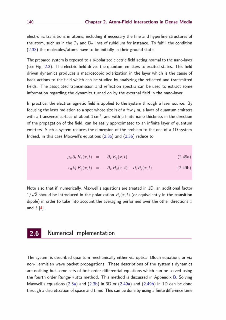
140 Chapter 2. Atom-Field Interactions in Dense Media

electronic transitions in atoms, including if necessary the fine and hyperfine structures ofthe atom, such as in the D1 and D2 lines of rubidium for instance. To fulfill the condition(2.33) the molecules/atoms have to be initially in their ground state.

The prepared system is exposed to a y-polarized electric field acting normal to the nano-layer(see Fig. 2.3). The electric field drives the quantum emitters to excited states. This fielddriven dynamics produces a macroscopic polarization in the layer which is the cause ofback-actions to the field which can be studied by analyzing the reflected and transmittedfields. The associated transmission and reflection spectra can be used to extract someinformation regarding the dynamics turned on by the external field in the nano-layer.

In practice, the electromagnetic field is applied to the system through a laser source. Byfocusing the laser radiation to a spot whose size is of a few µm, a layer of quantum emitterswith a transverse surface of about 1 cm2, and with a finite nano-thickness in the directionof the propagation of the field, can be easily approximated to an infinite layer of quantumemitters. Such a system reduces the dimension of the problem to the one of a 1D system.Indeed, in this case Maxwell’s equations (2.3a) and (2.3b) reduce to

µ0 ∂t Hz(x, t) = − ∂x Ey(x, t) (2.49a)

ε0 ∂t Ey(x, t) = − ∂x Hz(x, t)− ∂t Py(x, t) (2.49b)

Note also that if, numerically, Maxwell’s equations are treated in 1D, an additional factor1/√

3 should be introduced in the polarization Py(x, t) (or equivalently in the transitiondipole) in order to take into account the averaging performed over the other directions xand z [4].

2.6 Numerical implementation

The system is described quantum mechanically either via optical Bloch equations or vianon-Hermitian wave packet propagations. These descriptions of the system’s dynamicsare nothing but some sets of first order differential equations which can be solved usingthe fourth order Runge-Kutta method. This method is discussed in Appendix B. SolvingMaxwell’s equations (2.3a) and (2.3b) in 3D or (2.49a) and (2.49b) in 1D can be donethrough a discretization of space and time. This can be done by using a finite difference time

2.6 Numerical implementation 141

domain (FDTD) method [20] within which both the electric and magnetic fields, E andH , are propagated in time and space on a spatial and temporal grid. This method ensuresthe explicit description of the electromagnetic field and it is numerically very stable. Theboundary conditions are automatically taken into account through a staggered grid whichwas developed initially by K. S. Yee [21, 22] and later named as the Yee cell. Maxwell’sequations are discretized on the Yee cell using the central finite difference scheme.

nx − 3/2 nx − 1 nx − 1/2 nx nx + 1/2 nx + 1

Spatial Grid ( in units of ∆x)

nt−

1/2

nt

nt

+1/2

Tem

por

alG

rid

(in

un

its

of

∆t)

Ey

Hz

Ey

Figure 2.4.: Yee cell used in the simulations of the 1D electromagneticfield equations (2.49). The grid in red is for the electric field andthe one in black is for the magnetic field. The grids for the electricand magnetic fields are shifted by ∆x/2 in space and ∆t/2 in time.The electric field is calculated at spatial points (nx − 1)∆x, nx∆x,(nx+1)∆x, etc... for the times (nt−3/2)∆t, (nt−1/2)∆t, (nt+1/2)∆t,etc... The magnetic field is calculated at spatial points (nx − 3/2)∆x,(nx − 1/2)∆x, (nx + 1/2)∆x, etc... for the times (nt − 1)∆t, nt∆t,(nt + 1)∆t, etc...

Since this discretization necessarily induces some error in the evaluation of the derivatives,the spatial and temporal grid steps have to be chosen carefully. Let ∆t′ be the time takenby the electromagnetic wave to travel by ∆x in the vacuum, then ∆t′ = ∆x/c where c isthe speed of light in vacuum. If ∆x is the spatial grid step then the temporal grid step ∆tshould be less than ∆t′, i.e,

∆t ≤ ∆xc. (2.50)

Eq.(2.50) is known as the Courant-Friedrichs-Lewy condition (CFL), which appeared in 1928in the seminal paper of R. Courant, K. Friedrichs and H. Lewy explaining the conditionalstability of explicit time-dependent finite difference schemes [23, 20]. In our simulations,we use the temporal step ∆t = ∆t′/2, i.e. for a spatial grid step ∆x = 1 nm the temporal

142 Chapter 2. Atom-Field Interactions in Dense Media

grid step is ∆t = 1.67 as.

Yee’s scheme consists in considering the electric and magnetic components shifted spatiallyby half the cell step (∆x/2) and by half the temporal step (∆t/2) when considering acentral difference approximation of the derivatives. Figure 2.4 shows the Yee cell in onedimension used for discretizing the electromagnetic field equations in space and time.

The algorithm can be summarized in three steps:

1. Replace all the derivatives in Eq.(2.49) with finite differences. Discretize space and timeso that the electric and magnetic fields are staggered in both dimensions, i.e(b) ,

Ent+1/2,nx+1y − Ent+1/2,nx

y

∆x = −µ0Hnt+1,nx+1/2

z −Hnt,nx+1/2z

∆t (2.51a)

Hnt,nx+1/2z −Hnt,nx−1/2

z

∆x = −ε0Ent+1/2,nx

y − Ent−1/2,nxy

∆t − ∂t Pnt−1/2,nxy (2.51b)

2. Solve (2.51) to obtain ”updated” electromagnetic fields from past (known) fields using

Ent+1/2,nxy = Ent−1/2,nx

y + ∆tε0

(Hnt,nx−1/2

z −Hnt,nx+1/2z

∆x − ∂tPnt−1/2,nxy

)(2.52a)

Hnt+1,nx+1/2z = Hnt,nx+1/2

z + ∆tµ0∆x

(Ent+1/2,nx

y − Ent+1/2,nx+1y

)(2.52b)

3. Update the electric and magnetic field for each time step by using Eq. (2.52) until thefields have been obtained over the desired duration.

Figure 2.5 shows a schematic view of the simulation region for better understanding. Thenano-layer of length ` is placed at the center of the spatial grid (in x), within whichMaxwell’s equations are discretized along with a temporal grid.

In order to avoid unphysical numerical reflections of outgoing electromagnetic fields backto the simulation region, the boundaries are covered with artificial non-physical absorbinglayers which can efficiently absorb any incident electromagnetic field. It can be done byusing the most powerful perfectly matched layers (PML) [24, 25]. The numerical approachused for this purpose is the most economical variant of this method known as convolutionalperfectly matched layers (CPML) [26].

(b) Note that ∂t Py can be calculated directly from the quantum evolution equations of the system.

2.6 Numerical implementation 143

CP

ML

x

y

z

Incident Field

Reflected Field

Nan

o-L

ayer

`

TransmittedField

CP

ML

x

Figure 2.5.: Schematic view of the numerical implementation: anano-layer of thickness `, exposed normal to a y-polarized electricfield, is placed in a spatio-temporal grid. The incident, reflectedand transmitted fields are calculated by solving Maxwell’s equationsusing the finite-difference time domain method. Polarization insidethe system is calculated using one of the models described in theprevious sections. Perfectly matched layers are used at the boundariesof the simulation region in order to avoid unphysical reflections of theelectromagnetic fields back to the simulation region.

144 Chapter 2. Atom-Field Interactions in Dense Media

The y-polarized electromagnetic field is acting normal to the nano-layer. A part of theincident field is reflected from the interface of the nano-layer. The rest of the field istransmitted through the layer. A part of the field is however lost in the layer due to thedissipative forces in the system. The calculation scheme of the cross-coupled equations,either Maxwell-Bloch equations or Maxwell-non-Hermitian wave packet equations, is givenbelow [27] (see Fig. 2.6).

Ampere’s &Faraday’s law

(FDTD)

E and HQuantumdynamics

(Runge-Kutta 4)

ρı

Calculation of the Macro-scopic Polarization

P

Figure 2.6.: Scheme used for the numerical implementation of thenano-layer and electromagnetic field dynamics.

The magnetic field H is calculated in accordance with Eq.(2.49a) and then by usingEq.(2.49b), the electric field E is updated. The knowledge of the macroscopic polarizationP calculated via the density matrix elements ρı (or via the wave packet coefficients C)from the previous time step is utilized in this step of the calculation. The density matrixelements (or the wave packet coefficients) are then updated at all spatial grid pointsusing the electric field calculated previously. Finally, from the calculated electromagneticfield components and the density matrix elements (or the wave packet coefficients), themacroscopic polarization P is updated at each grid point.

2.6.1 Comparison of the two quantum models

The self consistent model described above was implemented for both Maxwell-Blochequations and Maxwell-non-Hermitian wave packet equations as described in [19].

2.6 Numerical implementation 145

As a preliminary step we compare the two models by calculating coherences and populationsas a function of time. The calculation is performed for a number densities N = 2.5 ×1021 cm−3 in a nano-layer of thickness ` = 400 nm consisting of two level atoms having aradiationless decay rate Γ = 0.5 THz and a pure dephasing rate γ = 10 THz for a transitionenergy of 2 eV with a transition dipole of 2 D. The system is excited with a weak deltakick (in practice a 180 as Gaussian pulse of central frequency tuned near the transitionfrequency). Fig. 2.7 shows the results obtained with these two models.

0

1.0

2.0

3.0

Excited

State

Pop

ulation

(10−

23)

0 10 20 30 40 50 60 70 80 90 1000

1.0

2.0

3.0

4.0

t (fs)

Coh

erence

(10−

23)

Non Hermitian wave packets Optical Bloch equations

(a)

(b)

Figure 2.7.: Panel (a) shows the populations and panel (b) showsthe coherence as a function of time for a 400 nm thick layer of twolevel atoms of density N = 2.5 × 1021 cm−3. The solid blue linesare obtained from non-Hermitian wave packet propagations and thedashed red line are from optical Bloch equations (see text for details).

The evolution of the population of the excited state is shown in panel (a). The solid blue lineshows the excited state population calculated via a non-Hermitian wave packet propagationand the red dashed line shows the same calculated by using optical Bloch equations. Asexpected, for the non-Hermitian model, the population shows a clear mismatch with the

146 Chapter 2. Atom-Field Interactions in Dense Media

optical Bloch equations, which are, by definition, describing them correctly. This is becauseof the arbitrary choice made on γ(t) for = 1, 2 [Eq.(2.42)]. The evolution of the groundstate gain factor γ1(t) for this system is shown in Fig. 2.8.

0 10 20 30 40 50 60 70 80 90 1000

1.0

2.0

3.0

4.0

t (fs)

γ1(t)(10−

10Hz)

Figure 2.8.: Dependence of the ground state gain factor γ1(t) of thetwo-level system described in the non-Hermitian wave packet model.All parameters are the same as in Fig. 2.7.

One can easily notice the similar time-dependence of γ1(t) [Fig. 2.8] and of the excitedstate population |C2(t)|2 [Fig. 2.7, panel (a), blue line]. This is not surprising in view ofthe equation (2.43a). For a system prepared according to Eq.(2.44) and probed by a weakfield, the ground state gain factor in the non-Hermitian wave packet model γ1(t) is nothingbut the excited state population scaled by (2γ + Γ). Meanwhile, the wrong descriptionof the populations ensures the accuracy in the description of the coherences as it can benoticed from Fig.2.7, panel (b). Thus, for the analysis of coherence dynamics, especiallyfor the calculation of the macroscopic polarization Py(x, t) that we feed into Eq.(2.52),one can choose any of these two models in weak fields.

For a multilevel system there is however a clear advantage for choosing the non-Hermitianwave packet model in terms of computation time. Fig. 2.9 shows a comparison of theCPU time used by a non-Hermitian wave packet simulation compared to solving the opticalBloch equations, as a function of the number of quantum states involved.

The graph shows the CPU time taken by both models for a 1D spatial grid of total size2.56µm with a spatial step ∆x = 1 nm. The coupled equations were propagated for anano-layer of width ` = 400 nm for a total propagation time of 1.67 ps with a time stepof 1.67 as. The excitation pulse is a delta kick similar to the one used for Figs. 2.7 and2.8. These estimations were done on a Intel Xeon E5-1650 processor. The blue line showsthe time taken by the non-Hermitian wave packet propagation and the red line is the time

2.7 Conclusion 147

2 3 4 5 6 7 8 9 100

100

200

300

400

500

600

Number of States

CP

U−

tim

e (s

)

Non−Hermitian wave packets Optical Bloch equations

Figure 2.9.: Comparison between the CPU times taken by the non-Hermitian wave packet model and by optical Bloch equations as afunction of the number of states involved. The blue line shows thetime taken by the non-Hermitian wave packet propagation and thered line is the time taken by optical Bloch equations.

taken to solve the optical Bloch equations.

There are some situations in which the multilevel system is characterized by low dampingrates. In this case, the equations have to be propagated for longer times, and it is advisableto choose the non-Hermitian wave packet propagation scheme instead of the ”exact” opticalBloch equation scheme.

2.7 Conclusion

The basic theory describing the dynamics of quantum emitters in the presence of weakelectromagnetic fields was discussed in this chapter in order to introduce the basic conceptsand the fundamental assumptions made for the present research.

The coupled equations known as Maxwell-Bloch equations were introduced along with thenumerical implementation of these dynamical equations in a spatial and temporal grid.

The system studied was introduced. It is a nano-layer composed of quantum emitters(atoms, molecules, nano particles, ...) driven by an electromagnetic field acting normal tothe layer surface. The finite difference time domain (FDTD) method was described withrelevant details for such geometry.

148 Chapter 2. Atom-Field Interactions in Dense Media

An alternative model for the description of the coherences in the system, the non-Hermitianwave packet model, was also discussed. This approximate model can reduce the computationtime when dealing with multilevel systems. Preliminary calculations comparing opticalBloch equations with the non-Hermitian approach were done.

The theory discussed here will be used in the forthcoming chapters for analyzing bothtwo-state model systems and more complicated realistic quantum multilevel systems.

2.8 References

[1] S. Prasad and R. J. Glauber. “Polarium model: Coherent radiation by a resonantmedium”. In: Phys. Rev. A 61 (6 May 2000), page 063814. doi: 10.1103/PhysRevA.61.063814 (cited on page 127).

[2] M. Born, E. Wolf, and A. Bhatia. Principles of Optics: Electromagnetic Theory ofPropagation, Interference and Diffraction of Light. Cambridge University Press,1999 (cited on page 127).

[3] H. A. Lorentz. The theory of electrons and its applications to the phenomenaof light and radiant heat. 2nd edition. BG Teubner, 1916, page 138 (cited onpage 128).

[4] J. D. Jackson. Classical electrodynamics. 3rd edition. Wiley New York etc., 1998,page 160 (cited on pages 128, 140).

[5] H. A. Lorentz. In: Wiedemann Ann. 9 (1880), page 641 (cited on page 128).

[6] L. Lorenz. In: Wiedemann Ann. 11 (1881), page 70 (cited on page 128).

[7] F. Miller, A. Vandome, and J. McBrewster. Beer-Lambert Law. VDM Publishing,2009 (cited on page 128).

[8] J. H. Poynting. “On the Transfer of Energy in the Electromagnetic Field”. In:Philosophical Transactions of the Royal Society of London 175 (1884), page 343.doi: 10.1098/rstl.1884.0016 (cited on page 128).

[9] B. Shore. Manipulating Quantum Structures Using Laser Pulses. CambridgeUniversity Press, 2011 (cited on page 131).

[10] M. Schlosshauer. Decoherence: and the Quantum-To-Classical Transition. TheFrontiers Collection. Springer Berlin Heidelberg, 2007 (cited on page 132).

[11] F. Petruccione and H.-P. Breuer. The theory of open quantum systems. OxfordUniv. Press, 2002 (cited on page 132).

2.8 References 149

[12] V. Gorini, A. Kossakowski, and E. C. G. Sudarshan. “Completely PositiveDynamical Semigroups of N Level Systems”. In: J.Math.Phys. 17 (1976), page 821.doi: 10.1063/1.522979 (cited on page 132).

[13] A. Kossakowski. “On quantum statistical mechanics of non-Hamiltonian systems”.In: Reports on Mathematical Physics 3 (1972), page 247. doi: 10.1016/0034-4877(72)90010-9 (cited on page 132).

[14] G. Lindblad. “On the generators of quantum dynamical semigroups”. In: Com-munications in Mathematical Physics 48 (1976), page 119. doi: 10 . 1007 /BF01608499 (cited on page 132).

[15] C. Fleming, N. I. Cummings, C. Anastopoulos, and B. L. Hu. “The rotating-waveapproximation: consistency and applicability from an open quantum systemanalysis”. In: Journal of Physics A: Mathematical and Theoretical 43 (2010),page 405304. url: http://stacks.iop.org/1751-8121/43/i=40/a=405304(cited on page 132).

[16] T. Albash, S. Boixo, D. A. Lidar, and P. Zanardi. “Quantum adiabatic Markovianmaster equations”. In: New Journal of Physics 14 (2012), page 123016. url:http://stacks.iop.org/1367-2630/14/i=12/a=123016 (cited on page 132).

[17] L. Allen and J. H. Eberly. Optical resonance and two-level atoms. Courier DoverPublications, 2012 (cited on page 133).

[18] S. Chang and V. Minogin. “Density-matrix approach to dynamics of multilevelatoms in laser fields”. In: Physics Reports 365 (2002), page 65. doi: 10.1016/S0370-1573(02)00016-9 (cited on page 134).

[19] E. Charron and M. Sukharev. “Non-Hermitian wave packet approximation ofBloch optical equations”. In: The Journal of Chemical Physics 138, 024108 (2013).doi: 10.1063/1.4774056 (cited on pages 135, 136, 144).

[20] A. Taflove. Computational Electrodynamics: The Finite-difference Time-domainMethod. Artech House, 1995 (cited on page 141).

[21] K. Yee. “Numerical solution of initial boundary value problems involving Max-well’s equations in isotropic media”. In: IEEE Transactions on Antennas andPropagation 14 (May 1966), page 302. doi: 10.1109/TAP.1966.1138693 (citedon page 141).

[22] J. Homola. “Present and future of surface plasmon resonance biosensors”. In:Analytical and Bioanalytical Chemistry 377 (2003), page 528. doi: 10.1007/s00216-003-2101-0 (cited on page 141).

[23] R. Courant, K. Friedrichs, and H. Lewy. “Über die partiellen Differenzengle-ichungen der mathematischen Physik”. In: Mathematische Annalen 100 (1928),page 32. doi: 10.1007/BF01448839 (cited on page 141).

150 Chapter 2. Atom-Field Interactions in Dense Media

[24] J.-P. Bérenger. “A perfectly matched layer for the absorption of electromagneticwaves”. In: Journal of Computational Physics 114 (1994), page 185. doi: 10.1006/jcph.1994.1159 (cited on page 142).

[25] J.-P. Bérenger. “Perfectly Matched Layer (PML) for Computational Electro-magnetics”. In: Synthesis Lectures on Computational Electromagnetics 2 (2007),page 1. doi: 10.2200/S00030ED1V01Y200605CEM008 (cited on page 142).

[26] J. A. Roden and S. D. Gedney. “Convolution PML (CPML): An efficient FDTDimplementation of the CFS–PML for arbitrary media”. In: Microwave and OpticalTechnology Letters 27 (2000), page 334. doi: 10.1002/1098-2760(20001205)27:5<334::AID-MOP14>3.0.CO;2-A (cited on page 142).

[27] M. Sukharev and A. Nitzan. “Numerical studies of the interaction of an atomicsample with the electromagnetic field in two dimensions”. In: Phys. Rev. A 84(4 Oct. 2011), page 043802. doi: 10.1103/PhysRevA.84.043802 (cited onpage 144).

3Collective Response of Two Level

Systems

This chapter discusses the optical response of a two level system exposed toweak electromagnetic fields. Collective effects in the nano-layer are studiedvia the calculation of the electromagnetic fields reflected, transmitted andabsorbed by the medium using the FDTD method. We also calculate thesusceptibility of the medium from the numerical integration of the opticalBloch equations. We finally interpret our results using a simple analyticalsemi-classical description based on an extension of the Lorentz oscillatormodel for dense media.

Keywords:

Two Level Systems, Resonances, Lorentz-Lorenz Shift, Collective Effects,Reflection, Transmission, Extinction, Susceptibility.

Contents3.1 Introduction 153

3.2 Spectral Broadening, Lineshapes and Shifts 153

3.3 Optical Response of a Two-Level System 161

3.4 Conclusion and Outlook 170

3.5 References 172

3.1 Introduction 153

3.1 Introduction

The simplest case for studying the interaction of light with matter as described in theprevious chapter is a two-level system where only one of the many allowed transitions (offrequency ω12) of a quantum emitter is in resonance with the applied field. The dynamicsof such system can be studied using Eq.(2.34). Reflected and transmitted electromagneticenergies are calculated from Maxwell’s equations and by normalizing them with respect tothe incident energy, the reflection and transmission probabilities can be calculated.

Since the system under consideration is a collection of two-level emitters, there are manyother effects that should be considered for understanding the spectra calculated from thenumerical simulations which includes broadening mechanisms and other density effects.Temperature dependent broadening mechanisms like Doppler and pressure (collisional)broadening can be reduced to a certain extend in a dense system.

3.2 Spectral Broadening, Lineshapes and Shifts

Let us assume that there are N particles (two-level quantum emitters) per unit volume. Inweak fields, the response of the system can be described in terms of the electric susceptibilityχe(ω) which is a complex quantity that does not depend on the geometry of the system.

For the present discussion, we are only concerned with the time-dependence of a realmonochromatic optical wave of linear polarization that we write as

E(t) = E0 cos(ωt) y = E0

2

[eiωt + e−iωt

]y (3.1)

Being in the linear regime, the polarization can be obtained from Eq.(2.2) as

P = 12ε0E0

[χe(ω) eiωt + χe(−ω) e−iωt

]y (3.2)

since the field contains two conjugate frequencies ±ω.

The polarization can also be expressed using Eq.(2.35) as written below

P = N〈 µ 〉 . (3.3)

154 Chapter 3. Collective Response of Two Level Systems

Knowing from Eq.(2.16) that

µ =[|1〉〈2|+ |2〉〈1|

]µ12 y (3.4)

where µ12 denotes the dipole matrix element 〈2|µy |1〉, we finally obtain

P = N[ρ12 + ρ21

]µ12 y . (3.5)

Let us now introduce the slowly-varying density matrix elements

ρ12 = ρ12(t) eiωt (3.6a)ρ21 = ρ21(t) e−iωt (3.6b)

in Eq.(3.5) to obtainP = N

[ρ21 e

iωt + ρ12 e−iωt

]µ12 y . (3.7)

The comparison of Eqs.(3.2) and (3.7) yields

χe(ω) = 2µ12

ε0E0N ρ21 = 2µ12

ε0E0N ρ21(t) e−iωt . (3.8)

It is now possible to solve Eq.(2.34c) (with = 2) analytically if we assume that ρ21 variesslowly with time (i.e. ˙ρ21 ≈ 0) and that we are in the linear regime (i.e. ρ11 − ρ22 ≈ 1 ifwe start initially from the ground state). In this case, within the RWA [see Eq.(2.19)] weobtain

ρ21 = ρ21(t) e−iωt ≈ −iΩ12/2i(ω12 − ω) + (γ + Γ/2) . (3.9)

From these equations and from the definition (2.17) of the Rabi frequency it comes that

χe(ω) ≈ Nµ212

~ε0

1(ω12 − ω)− i (γ + Γ/2) . (3.10)

The expression (3.10) gives the RWA approximation of the susceptibility, thus neglecting the(very small) counter-rotating contribution. Note also that in this expression, as mentionedat the end of Section 2.5, the factor 1/3 that one may find in the literature (due to anaverage over the orientation of the dipole) is here already included in µ2

12.

Separating the real from the imaginary part, we have

3.2 Spectral Broadening, Lineshapes and Shifts 155

χe(ω) ≈ Nµ212

~ε0

[ω12 − ω

(ω12 − ω)2 + (γ + Γ/2)2 + iγ + Γ/2

(ω12 − ω)2 + (γ + Γ/2)2

]. (3.11)

Typical variations of the real and imaginary parts of χe(ω) are shown figure 3.1.

−10 −8 −6 −4 −2 0 2 4 6 8 10−1

−0.5

0

0.5

1

ω12 − ω

γ − +Γ/2

χ(ω

)/χmax

e(ω

)

Re[χ(ω)]

Im[χ(ω)]

Figure 3.1.: Real and imaginary parts of the susceptibility in atwo-state system as a function of the adimensional detuning.

Since in weak fields the transition probability between states |1〉 and |2〉 is proportional to|χe(ω)|2, it appears from Eq.(3.10) that this transition is characterized by a Lorentzian shape.It can be (and in practice will be) modified by other physical effects like inhomogeneousbroadening [1] (which assumes that different atoms see different electromagnetic fields),homogeneous broadening [2], or local field effects [3] for instance.

In general the particles are distributed within the nano-layer with different velocities.Assuming a Maxwell-Boltzmann distribution of the particles of mass m [4], the numberdensity N‖(v‖) associated with the speed v‖ along the direction k of the propagation ofthe electromagnetic field can be written as

N‖(v‖) = N(

m

2πkBT

)1/2exp

(−

v 2‖

v 2p

), (3.12)

156 Chapter 3. Collective Response of Two Level Systems

where N is the total number density for the uniform distribution of particles and

vp =√

2kBT

m(3.13)

is the most probable velocity at temperature T . This velocity distribution which is due tothe distribution of kinetic energies possessed by the particles has to be considered whendealing with a realistic sample. At room temperature, say for noble gases around 25 C,the most probable velocity varies between 250 to 1500 m/s depending on the mass of theatom. This thermal motion induces a shift in the resonance frequency which is nothing butthe Doppler shift which can be written as

∆Doppler = − k v‖ (3.14)

where k is the propagation constant of the applied field. Eq.(3.12) being the particlevelocity distribution in the direction of the propagation of the applied field, this thermaldistribution will induce an inhomogeneous broadening in the transition spectrum that should,in principle, be taken into account. The spectral shape induced by the Gaussian distributionof particles will also be Gaussian.

Combining the natural broadening with the inhomogeneous Doppler broadening, thesusceptibility will become a function of velocity and will have a temperature dependence

χe(ω, v‖) = Nµ212

~ε0

1(ω12 − ω − k v‖)− i (γ + Γ/2)

(m

2πkBT

)1/2exp

(−

v 2‖

v 2p

)(3.15)

to be compared with Eq.(3.10).

Averaging over all velocities in the nano-layer

χe(ω) =∫ +∞

−∞χe(ω, v‖) dv‖ (3.16)

is equivalent to the calculation of the convolution of a Lorentzian shape with a Gaussianshape. It is well known that the lineshape offered by Eq.(3.16) is a Voigt profile [5]. TheGaussian lineshape associated with the thermal (Doppler) broadening contributes morearound the resonance frequency and dies of quickly in the wings in comparison with theLorentzian shape due to the natural decay. Thus the Voigt profile has a Gaussian core anda Lorentzian tail.

There are many other broadening mechanisms like pressure broadening or collisionalbroadening in the system which can be important when one deals with systems with large

3.2 Spectral Broadening, Lineshapes and Shifts 157

number of particles. The source of the collisional broadening is the close encounters betweenthe quantum emitters carrying an electric dipole due to the polarization. Calculation ofprecise expressions for these type of broadening mechanisms is complicated since it involvesmany particles in different quantum states. But the collisional broadening is often treatedas a Lorentzian-type broadening [2, 6] which makes the calculation of the susceptibilitynot so hard in comparison with the inhomogeneous effects. Even though the timescales ofcollisional broadening and natural broadening are different it is proven that they usuallyhave comparable values [2, 6].

The dependence of the pressure broadening can be estimated from classical considerations.Let τ be the relaxation time for a mean free path l = 1/(Nσ) where σ is the collisioncross section, then

τ = l

vp

,∝ 1N√T. (3.17)

Thus the shift in the frequency is proportional to the number density N and to the squareroot of the temperature. A detailed review on the broadening mechanisms and associatedfrequency shifts in two level systems can be found in [7].

From this point we will assume that we deal with relatively cold atoms or molecules(temperatures typically below 1 K) and the constituent particles are assumed to be frozen.The Doppler broadening will therefore be neglected in order to investigate the collectiveeffects due to the local fields. This also helps for keeping the profile simple and easilytractable. On the contrary, the contributions from the collisional broadening are includedin our model using the Lindblad formalism of the operator Λ (see chapter 2, Eqs.(2.26)and (2.27)) [8, 9].

3.2.1 Lorentz Model for Two Level Systems

An alternative classical way of deriving an expression for the susceptibility is by modelingthe system as a collection of a large number of oscillating dipoles driven by an external field.This is the Lorentz oscillator model, and it takes all relevant physical processes into accountclassically. This approach is usually valid in the linear regime where the susceptibility doesnot dependent on the applied field.

The basic assumption of the Lorentz model is that an incident light wave propagatingthrough the medium of quantum emitters excites the system. The quantum emittersare considered as identical damped harmonic oscillators. The evolution of the inducedoscillating dipoles is due to a displacement of the positive and negative charge densities in

158 Chapter 3. Collective Response of Two Level Systems

the particle, compared to their equilibrium positions. This results in a polarization of thesystem, which in turn modifies the external electric field.

The differential equation for the displacement y(t) of the charged particles from theirequilibrium positions due to the action of the local electric field Elocal(t) can be written as

m y = −mω212 y −mγm y + q Elocal(t) (3.18)

where m and q are the mass and electric charge, respectively, of the particles considered.ω12 is the frequency of the harmonic oscillations and γm is the damping constant of theseoscillations. In this expression −mω2

12 y(t) denotes the binding force, −mγm y(t) is thefriction force and q Elocal(t) is Coulomb’s force.

Let us now remember that the polarization is modeled according to Eq.(2.35) as

P = N〈 µ 〉 (3.19)

and that one can relate the dipole operator µ with the displacement operator y

〈 µ 〉 = q 〈 y 〉 . (3.20)

Assuming now that the expectation value of the displacement operator can be assimilatedwith its classical counterpart y(t) we obtain a classical equation of motion for the polarizationcomponent Py(t) [3]

mPy = −mω212 Py −mγm Py +N q2 Elocal(t) (3.21)

The local field Elocal(t) is given by Eq.(2.11) and γm is the classical damping factor thatis necessarily related to the quantum decoherence and decay rates γ and Γ introduced inEq.(2.27) to explain the damping effects.

Substituting Eq.(2.11) for the local field and collecting the polarization terms we get

Py = −(ω2

12 −$2

123

)Py − γm Py + ε0$

212 Ey(t) (3.22)

where

$12 =√N q2

mε0(3.23)

3.2 Spectral Broadening, Lineshapes and Shifts 159

denotes the plasma frequency.

The solution of equation (3.22) can be obtained by the standard method of introducing theFourier decomposition of the time-dependent quantities Py(t) and Ey(t) into this equation.The result expressed in terms of the susceptibility is

χe(ω) = Py

ε0Ey

= $212

(ω′ 212 − ω2) + i ωγm

(3.24)

where

ω′ 212 = ω2

12 −$2

123 = ω2

12 −N q2

3mε0. (3.25)

We see here that the resonance frequency is shifted by a term which depends on the densityN and on the ratio q2/m. Reminding the argument for introducing the local field correctionin Section 2.2.1, one can safely interpret that this shift is induced by the dipole-dipolecoupling between the constituent quantum emitters in the system.

The difficulty for estimating the coupling frequency $12 in the system is because of thepresence of the parameter q2/m which can be estimated by quantizing the dipole oscillations.For this purpose let us consider an oscillating transition dipole µ12(t) characterized bythe charge q, the amplitude of oscillation x0 and the frequency ω12. We assume for themoment that there is no damping. The length of the dipole is then x(t) = x0 cos(ω12t)and µ12(t) = q x(t) = q x0 cos(ω12t). The RMS value of the dipole is therefore given by

µ12 =√⟨

µ212(t)

⟩=√⟨

q2 x2(t)⟩

= q x0√2. (3.26)

If the oscillation energy is quantized to the zero-point energy ~ω12/2 of the harmonicoscillator, it is easy to show that the amplitude of oscillation x0 is nothing else than thecharacteristic length of the harmonic oscillator

x0 =√

~mω12

. (3.27)

Introducing Eq.(3.27) in Eq.(3.26) yields

µ12 = q

√~

2mω12, (3.28)

and thereforeq2

m= 2ω12µ

212

~. (3.29)

160 Chapter 3. Collective Response of Two Level Systems

Thus the plasma frequency given by Eq.(3.23), which is due to the interaction with theneighboring quantum emitters, can be written as [3]

$12 =√

2Nω12

~ε0µ12 , (3.30)

and Eq.(3.25) becomes

ω′ 212 = ω2

12 −2Nω12µ

212

3~ε0. (3.31)

Let us now define ∆12 as the dipole shift induced in the resonance frequency as

ω′12 = ω12 −∆12 , (3.32)

it appears from Eq.(3.31) that

∆12 = ω12

1−√

1− 2Nµ212

3~ω12ε0

(3.33)

If ∆12 ω12, the first order approximation on Eq.(3.33) will reduce ∆12 to

∆12 ≈Nµ2

123~ε0

, (3.34)

which is nothing but the well-known Lorentz-Lorenz (LL) shift [10, 11] introduced inEq.(1.1). This LL shift and its contribution towards collective effects will be discussed laterin this chapter and the forthcoming chapter.

In the Lorentz model, the frequency $12 is known as the plasma frequency that explainsthe oscillation of charge centers in conducting media such as metals and plasmas. In thepresent case, it represents the natural collective oscillation frequency of the ”sea” of dipolesin the system, not of individual dipoles. This collective oscillation of the coupled dipolesmatters for the response of the system when the dipole-dipole interaction is not negligible.Indeed, these collective or cooperative behavior of the dipoles (which arise from the factthat the electromagnetic field experienced by an arbitrary quantum emitter in the system ismodified by its neighboring dipoles) can modify the response of the system towards theelectromagnetic field drastically [12–14].

3.3 Optical Response of a Two-Level System 161

3.2.2 Detuning and Scaling

There are some quantities that help to generalize the equations and variables to anadimensional form. The collective effects are represented by the plasma (or dipole coupling)frequency $12. Eq.(3.30) can be rewritten in terms of the LL shift,

$212 ≈ 6∆12ω12 . (3.35)

The Lorentz-Lorenz shift contains the essential part in the coupling frequency that describeshow strongly the system is interacting. It will be shown in the forthcoming section that thequantity Nµ2

12 is the key parameter for seeing the collective effects in the nano-layer of thetwo-level systems under consideration. Hence a dimensionless quantity called interactionstrength S12 is defined as

S12 = ∆12

γ + Γ/2 (3.36)

that helps to quantify the interaction regime. Note that the relation between the classicaldamping rate γm and the decay and decoherence rates is γ+ Γ/2 = γm/2. For large valuesof S12 the dipole coupling frequency dominates over the damping rate, and the constituentparticles interact strongly.

In the forthcoming section a reduced detuning is also used to analyze the optical responseof the dense two-level system. This reduced detuning is defined as

δ = ω − ω12

γ + Γ/2 . (3.37)

3.3 Optical Response of a Two-Level System

When the dipoles are close enough, the radiation from a dipole couples it with its neighbors.This effect can be explored by calculating probabilities for reflection and transmission atdifferent interaction regimes characterized by the value of S12 [15].

The reflection probability R can be calculated from Eq.(2.14) by measuring the reflectedenergy, i.e,

R(ω) = |S(ω)|R|S0(ω)| (3.38)

162 Chapter 3. Collective Response of Two Level Systems

where |S(ω)|R is the reflected energy.

The transmission probability T can be calculated in the same manner,

T (ω) = |S(ω)|T|S0(ω)| . (3.39)

where |S(ω)|T is the transmitted energy. Here the indexes R and T denote calculationsof the energy flux performed in front of (x = xR < 0) and beyond (x = xT > `) thenano-layer.

A part of the energy given to the system will be lost (extinction) while propagating throughthe layer. It is not recovered in the reflection or in the transmission. The probability ofextinction E can thus be calculated from the conservation of energy as

E(ω) = 1−[R(ω) + T (ω)

]. (3.40)

This loss of energy is related to the imaginary part of the propagation constant k insidethe nano-layer.

−100 −500

50100 0

0.010.1

110

0

0.5

1

×104×103

×50×2

×13∆12

Reduced Detuning δ ∆12/γm

(log scale)

R(ω

)

Figure 3.2.: Reflection spectra from a layer of identical two-levelquantum emitters of thickness ` = 600 nm as a function of the reduceddetuning δ and interaction strength S12. γ is 10 THz and Γ = 1 THz.Reflection from a layer of weakly interacting identical dipoles is feeble.Those are therefore multiplied by some constant factors given alongsidewith the same color codes for a better comparison.

Fig. 3.2 shows some reflection spectra from a 600 nm thick layer composed of identicaltwo-level emitters for different values of S12 [15]. The system is assumed to have a transitionenergy of 2 eV with a damping rate γ + Γ/2 = γm/2 = 10.5 THz due to the decay anddecoherence processes.

3.3 Optical Response of a Two-Level System 163

The incident electromagnetic fields are reflected selectively from the layer around thetransition frequency [16, 17]. The reflection increases with the increase in the interactionstrength. For S12 6 0.01, the system shows very weak reflection around the transitionfrequency and almost all energy given to the sample is transmitted or extinct. The responseof the system towards the electromagnetic field is very close to the independent particleresponse characterized by a Lorentzian profile in the frequency domain. It is because inweak densities, the effect of the polarization of the medium barely modifies the local electricfield experienced by the constituent dipoles. Hence they respond to the field as if they wereindependent.

(a)

(b)

0

0.33

0.66

0.99

−100 −80 −60 −40 −20 0 20 40 60 80 1000.97

0.98

0.99

1

Reduced Detuning δ

T(ω

)(arb.)

0

0.3

0.6

0.9

0

1

2

3·10−2

E(ω)(arb.)

Figure 3.3.: Extinction (panel a) and transmission (panel b)probabilities for the weak (blue solid line) and strong (brown solidline) interaction regime specified in Fig. 3.2. The y-scale on the left isfor weakly (S12 = 10−3) interacting dipoles and the one on the rightis for strongly (S12 = 12) interacting dipoles (see text for details).

The reflection gets stronger as the interaction between the induced dipoles increases. Itstarts to show some additional features that will be explained later as S12 approaches 1.

For S12 > 10, the constituent particles feel very strongly the presence of neighboring dipolesthat modify the system response. As the interaction strength increases, the layer becomesopaque, reflects most of the incident energy and absorbs the remaining. The energyabsorbed by the system can be dissipated due to many physical phenomena represented bythe decay constants γ and Γ. In the strong interaction regime (S12 > 1), the presence ofother dipoles becomes really significant. The system loses its transparency and behaves

164 Chapter 3. Collective Response of Two Level Systems

like a mirror around the transition frequency.

The transmission through the layer then falls to zero. Fig. 3.3 shows the extinction[panel (a)] and transmission [panel (b)] corresponding to weakly (S12 = 10−3) and strongly(S12 = 12) interacting dipoles.

For S12 = 12, the system behaves like a mirror by reflecting the major portion (≈ 80%)of the incident energy, the remaining portion being absorbed and dissipated. We notethat the window of reflection within which the incident field is mainly reflected measures3∆12 (see Fig. 3.2). This measure will be explained in the next section. The interactionbetween the induced dipoles enhances the reflection probability so that in this regime, thesystem (nano-layer of two-level quantum emitters) behaves like a metal. Note that a similarproblem was studied analytically by R. J. Glauber and S. Prasad in 2000 [13, 18] as aneigenvalue problem for a dense layer of quantum emitters.

3.3.1 Lorentz-Lorenz shift and reflection window

As demonstrated in Section 3.2.1, the LL correction on the local field experienced by anarbitrary quantum emitter induces a shift in the resonance frequency. We have shownusing the Lorentz model that the frequency shift is ∆12 and that it originates from thepresence of neighboring interacting dipoles. Indeed, as shown schematically Fig. 3.4, twoneighboring oscillating dipoles interact through the electric field they create.

The induced LL-shift has been known for a long time and the initial theoretical prediction ofLorentz and Lorenz has been confirmed by several experiments [19–22]. It was for instancemeasured while studying the optical response of dense atomic vapors (for N of the orderof 1017 cm−3) in the vicinity of the fundamental atomic resonance frequency [19, 23]. Thedependence of the shift on the degree of excitation was also predicted [7] and experimentalevidences showed the presence of such a dependence [24, 25]. The validity of the LL shifthas thus been shown by many different experimental groups. These measurement thereforevalidate the theories based on the LL correction introduced in the local field experienced bythe quantum emitters [14, 26].

In the calculation executed here for studying the linear optical response of dense two-levelsystems, the LL red-shift is obtained in the associated susceptibility χe(ω), as shown inEqs.(3.24), (3.32) and (3.34).

Eq.(3.24) is able to reproduce exactly the susceptibility extracted from the full quantum

3.3 Optical Response of a Two-Level System 165

calculation [3]. Fig. 3.5 shows a comparison between the susceptibilities obtained fromthe quantum calculation and the semi-classical analytical model developed in this chapter[Eq.(3.24)] for the parameters used to obtain S12 = 12 in Fig. 3.3, as a function of thereduced detuning δ. The blue solid line is the susceptibility obtained from the semi-classicalmodel and the red dashed line shows the susceptibility obtained from the numericalintegration of the optical Bloch equations. They mach in great accuracy, showing thefollowing essential feature: the resonance frequency is red-shifted by the LL shift ∆12.

p1 p2

Figure 3.4.: Dipole fields produced by two arbitrary oscillatingdipoles p1 and p2. The presence of the two oscillating fields keep themcoupled.

Analyzing the susceptibility, one can also estimate the width of the reflection windowobtained for large densities (see Fig. 3.2). Apart from the energy dissipated in the layer,this system reflects a large part of the incident radiation from the surface which receives it,where the reflectivity

R =∣∣∣∣∣n(ω)− 1n(ω) + 1

∣∣∣∣∣2

(3.41)

is close to unity.

In this expression, n(ω) = Re[√

1 + χe(ω)] is the real part of the refractive index of themedium. At maximum reflection R(ω) = 1, and the real part of the electric susceptibilitygoes to −1. Equating the real part of Eq.(3.24) with -1 gives the range of frequencies atwhich the reflection is maximum:

Re[χe(ω)

]= −1 ⇐⇒ ω12 −∆12 < ω < ω12 + 2∆12 . (3.42)

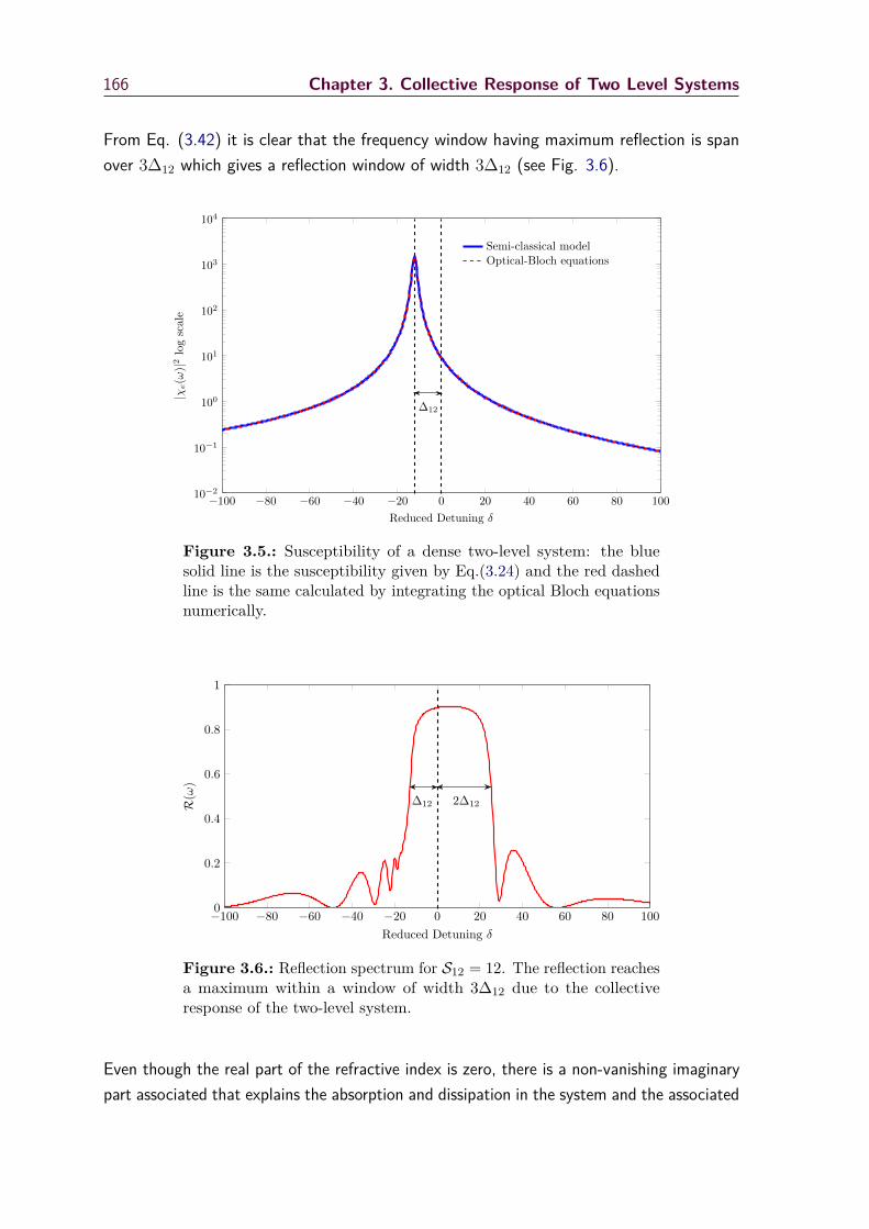
166 Chapter 3. Collective Response of Two Level Systems

From Eq. (3.42) it is clear that the frequency window having maximum reflection is spanover 3∆12 which gives a reflection window of width 3∆12 (see Fig. 3.6).

∆12

−100 −80 −60 −40 −20 0 20 40 60 80 10010−2

10−1

100

101

102

103

104

Reduced Detuning δ

|χe(ω

)|2lo

gsc

ale

Semi-classical modelOptical-Bloch equations

Figure 3.5.: Susceptibility of a dense two-level system: the bluesolid line is the susceptibility given by Eq.(3.24) and the red dashedline is the same calculated by integrating the optical Bloch equationsnumerically.

∆12 2∆12

−100 −80 −60 −40 −20 0 20 40 60 80 1000

0.2

0.4

0.6

0.8

1

Reduced Detuning δ

R(ω

)

Figure 3.6.: Reflection spectrum for S12 = 12. The reflection reachesa maximum within a window of width 3∆12 due to the collectiveresponse of the two-level system.

Even though the real part of the refractive index is zero, there is a non-vanishing imaginarypart associated that explains the absorption and dissipation in the system and the associated

3.3 Optical Response of a Two-Level System 167

zero transmission through the system. At R = 1, the nano-layer therefore behaves likea dissipative mirror. Zero transmission through the layer within the window of reflectionmeans that the electromagnetic field cannot penetrate through the entire layer of thickness` = 600 nm. The field can however propagate though the layer to a certain extend whichis determined by the system parameters. The field inside the nano-layer is exponentiallydecaying and the distance from the interface to the point inside the layer at which theexponentially decaying evanescent field falls to 1/e is known as the skin depth, ζ(ω). Bydefinition this skin depth is given by

ζ(ω) = 1κ

= c

ω

1Im

[√1 + χe(ω)

] (3.43)

where κ is the imaginary part of the propagation constant.

−14 −13 −12 −11 −10 −9 −8 −7 −6 −510

20

30

40

50

Reduced Detuning δ

ζ(ω

)(nm)

Figure 3.7.: Skin depth ζ(ω) as a function of the reduced detuningδ for S12 = 12. ζ(ω) is minimum at the shifted resonance frequencyω = ω′

12 of Eq.(3.32). The skin depth at ω′12 is very small (≈ 15 nm)

due to the collective response of the two-level system.

Fig. 3.7 shows the skin depth for the strongly interacting system (S12 = 12) as a function ofthe reduced detuning δ around the shifted resonance frequency ω′

12. The skin depth reachesa minimum of about 15 nm at the shifted resonance frequency ω = ω′

12 (correspondingto δ ≈ −12.4 in Fig. 3.7) i.e, the electromagnetic field of this frequency enters the layerand dies off very quickly, within a distance of 15 nm. In this situation the calculation ofpolarization, electromagnetic fields, populations and coherences should be done within thisskin depth limit where the field is not yet zero.

168 Chapter 3. Collective Response of Two Level Systems

3.3.2 Fabry-Pérot Modes

The sidebands seen in Fig. 3.6 in the tails of the reflection spectrum arise from theinterference between multiply reflected and transmitted electromagnetic fields and can beinterpreted as Fabry-Pérot modes [26, 27]. Indeed, systems with more than one interfacecan produce interferences between multiply reflected and transmitted fields. The systemstudied here can be seen as a Fabry-Pérot étalon consisting of two parallel partially reflectingplanes. Fig. 3.8 illustrates these multiple reflections and transmissions in the layer.

Nano-Layer

Incident Field1st

I II III

2nd

3rd

4th

xR

Ord

erof

Refl

ecti

on

3rd

2nd

1st

xT

Ord

erof

Tran

smission

`

x

Figure 3.8.: Schematic view of multiple reflections and transmissionsin the system: Reflection is measured at a point xR in region I andtransmission is measured at a point xT in region III. Region II coversthe nano-layer of thickness `. Linearly polarized light is incident onthe interface between I and II that results in primary reflection andtransmission. A part of the field is reflected back and forth inside thelayer in region II and contributes to the reflection and transmissionmeasurements.

The reflected electromagnetic fields are calculated at a point xR in region I (xR < 0) andthe transmitted fields are calculated at xT in region III (xT > `). Inside the layer (regionII), a part of the incident electromagnetic field is reflected back and forth, and is thereforeassociated with partial transmissions. These partially transmitted electromagnetic fieldscontribute to the reflected and transmitted fields at positions xR and xT . Due to the pathdifferences between different contributions induced by the additional geometrical pathstraveled inside the layer, the interference between them gives maxima and minima. Theseinterference fringes appear as sidebands in the reflection spectrum (see Fig. 3.6) and in

3.3 Optical Response of a Two-Level System 169

the transmission spectrum (see Fig. 3.3, panel b).

Approaching the problem formally, the (complex) geometrical path difference between anysuccessive fields can be written as

D = 2k′` (3.44)

where k′ = k′r + iκ is the wave vector of the electromagnetic field inside the layer. Let t1

be the transmissivity of the interface I→ II and t2 be the same for the interface II→ III,then the primary field noted 1st in Fig. 3.8 in the transmission region can be written as

E1st = t1t2e−κ`eikx (3.45)

where k is the wave vector in the vacuum. Similarly, the nth order electromagnetic fieldtransmitted to region III due to the everlasting multiple reflections inside the layer can bewritten as

Enth =(r2

2e−2κ`eiD

)n−1E1st (3.46)

where r22 = 1− t22.

Eq.(3.46) suggests that the transmitted field contributions behave like a geometricprogression. Thus the total transmitted field can be calculated by summing up all thecontributions. Taking the ratio between the incident amplitude and the transmittedamplitude of the electric field, the collective transmissivity can then be extracted as

t(ω) = 4ne−κ`

(n+ 1)2 − (n− 1)2e−i2nk`(3.47)

since we know the classical relations between the refractive index n and t1, t2 and r2

t1(ω) = 21 + n(ω) (3.48a)

t2(ω) = 2n(ω)1 + n(ω) (3.48b)

r2(ω) = n(ω)− 11 + n(ω) . (3.48c)

Following the same path, the global coefficient of collective reflection can be derived as

r(ω) = −2i(n2 − 1)e−ink`sin(nk`)(n+ 1)2 − (n− 1)2e−i2nk`

(3.49)

and the reflection and transmission probabilities can be finally written as

170 Chapter 3. Collective Response of Two Level Systems

R = |r(ω)|2 (3.50a)

T = |t(ω)|2 . (3.50b)

−100 −80 −60 −40 −20 0 20 40 60 80 1000

0.2

0.4

0.6

0.8

1

Reduced Detuning δ

R(ω

)

Numerical SimulationSemi-classical model

Figure 3.9.: Comparison between the calculated reflection spectrumobtained from the numerical solution of the optical Bloch equationsand the reflection probability obtained from Fabry-Pérot interferencescheme (Eq. 3.50) as a function of the reduced detuning δ for S12 = 12.

Fig. 3.9 shows a comparison between the calculated reflection spectrum obtained from thenumerical solution of the optical Bloch equations and the analytical form of the reflectionspectrum obtained via the semi-classical Lorentz model including the Fabry-Pérot formulatreatment. The blue dotted line is the calculated spectrum and the red solid line is theanalytical form of the reflection spectrum given by Eq. (3.50). The reflection windowand the sidebands are represented quite accurately by the analytical model, giving a veryaccurate analytical tool for analyzing the calculated dynamics in more complex systems.

3.4 Conclusion and Outlook

The collective response of a nanometric layer composed of two-level quantum emitters wascalculated by integrating the coupled Maxwell-Bloch equations. It was also analyzed usinga semi-classical model based on the Lorentz oscillator which can describe the linear opticalresponse of dielectrics.

3.4 Conclusion and Outlook 171

A clear collective behavior of the system is obtained for large densities in which thepredominant selective reflection associated with zero transmission is described by thecollective oscillation frequency of the induced dipoles in the system.

The analytical model developed in this thesis is accurate enough to explain the collectiveeffects observed in a dense layer of quantum emitters exposed to weak electromagneticfields. Fig. 3.10 shows for instance the relative error in the susceptibility given by Eq.(3.24)in comparison with the electric susceptibility calculated with the optical Bloch equations.The blue solid curve is the relative error for weakly coupled dipoles and the red solid lineis the same for strongly interacting dipoles. The error is maximum around the transitionfrequency, where the absorption of electromagnetic energy is more important and hencewhere the susceptibility varies abruptly. The shift in the curve for strongly interactingdipoles is due to the LL shift [15]. The relative errors in both cases are very small (of theorder of a few 10−4). Thus the analytical model developed here is accurate enough toexplain the physics of both dilute and dense systems.

−100 −80 −60 −40 −20 0 20 40 60 80 100−8

−6

−4

−2

0

2

4

6

8

Reduced Detuning δ

Rel.Error

in|χ

e(ω

)|(10−

4)

S12 = 10−3

S12 = 12

Figure 3.10.: Relative error in the electric susceptibilities |χe(ω)|obtained from the analytical model when compared to the numericalintegration of the optical Bloch equations as a function of the reduceddetuning δ. The blue curve is for S12 = 10−3 and the red curve forS12 = 12.

All features including the broad reflection window for strongly interacting dipoles and theFrabry-Pérot sidebands were explained from classical optics considerations and with thehelp of the mean-field Lorentz-Lorenz correction. The model is therefore convincing fortreating more complicated systems and this will be subject of the forthcoming chapters.

172 Chapter 3. Collective Response of Two Level Systems

3.5 References

[1] J. M. Hollas. Modern spectroscopy. J. Wiley, 1996 (cited on page 155).

[2] G. Peach. “Theory of the pressure broadening and shift of spectral lines”. In:Advances in Physics 30 (1981), page 367. doi: 10.1080/00018738100101467(cited on pages 155, 157).

[3] R. Puthumpally-Joseph, M. Sukharev, O. Atabek, and E. Charron. “Dipole-Induced Electromagnetic Transparency”. In: Phys. Rev. Lett. 113 (16 Oct. 2014),page 163603. doi: 10.1103/PhysRevLett.113.163603 (cited on pages 155, 158,160, 165).

[4] R. K. Pathria and P. D. Beale. Statistical Mechanics. Elsevier Science, 1996(cited on page 155).

[5] J. Olivero and R. Longbothum. “Empirical fits to the Voigt line width: A briefreview”. In: Journal of Quantitative Spectroscopy and Radiative Transfer 17(1977), page 233. doi: 10.1016/0022-4073(77)90161-3 (cited on page 156).

[6] S. Mukamel. “Collisional broadening of spectral line shapes in two-photon andmultiphoton processes”. In: Physics Reports 93 (1982), page 1. doi: 10.1016/0370-1573(82)90064-3 (cited on page 157).

[7] R. Friedberg, S. R. Hartmann, and J. T. Manassah. “Frequency shifts in emissionand absorption by resonant systems ot two-level atoms”. In: Physics Reports 7(1973), page 101. doi: 10.1016/0370-1573(73)90001-X (cited on pages 157,164).

[8] G. Lindblad. “On the generators of quantum dynamical semigroups”. In: Com-munications in Mathematical Physics 48 (1976), page 119. doi: 10 . 1007 /BF01608499 (cited on page 157).

[9] F. Petruccione and H.-P. Breuer. The theory of open quantum systems. OxfordUniv. Press, 2002 (cited on page 157).

[10] H. A. Lorentz. The theory of electrons and its applications to the phenomenaof light and radiant heat. 2nd edition. BG Teubner, 1916, page 138 (cited onpage 160).

[11] J. D. Jackson. Classical electrodynamics. 3rd edition. Wiley New York etc., 1998,page 160 (cited on page 160).

[12] R. H. Dicke. “Coherence in Spontaneous Radiation Processes”. In: Phys. Rev. 93(1 Jan. 1954), page 99. doi: 10.1103/PhysRev.93.99 (cited on page 160).

3.5 References 173

[13] S. Prasad and R. J. Glauber. “Polarium model: Coherent radiation by a resonantmedium”. In: Phys. Rev. A 61 (6 May 2000), page 063814. doi: 10.1103/PhysRevA.61.063814 (cited on pages 160, 164).

[14] J. Keaveney, I. Hughes, A. Sargsyan, D. Sarkisyan, and C. Adams. “MaximalRefraction and Superluminal Propagation in a Gaseous Nanolayer”. In: Phys. Rev.Lett. 109 (23 Dec. 2012), page 233001. doi: 10.1103/PhysRevLett.109.233001(cited on pages 160, 164).

[15] R. Puthumpally-Joseph, O. Atabek, M. Sukharev, and E. Charron. “Theoreticalanalysis of dipole-induced electromagnetic transparency”. In: Phys. Rev. A 91(4 Apr. 2015), page 043835. doi: 10.1103/PhysRevA.91.043835 (cited onpages 161, 162, 171).

[16] J. M. Hansen and H. W. Webb. “Specular Reflection from Mercury Vapor”. In:Phys. Rev. 72 (4 Aug. 1947), page 332. doi: 10.1103/PhysRev.72.332 (citedon page 163).

[17] V. Sautenkov, T. Varzhapetyan, H. Li, D. Sarkisyan, and M. Scully. “Selectivereflection of a laser beam from a dilute rubidium vapor”. In: Journal of RussianLaser Research 31 (2010), page 270. doi: 10.1007/s10946-010-9143-5 (citedon page 163).

[18] R. J. Glauber and S. Prasad. “Polarium model: Reflection and transmissionof coherent radiation”. In: Phys. Rev. A 61 (6 May 2000), page 063815. doi:10.1103/PhysRevA.61.063815 (cited on page 164).

[19] J. J. Maki, M. S. Malcuit, J. E. Sipe, and R. W. Boyd. “Linear and nonlinearoptical measurements of the Lorentz local field”. In: Phys. Rev. Lett. 67 (8 Aug.1991), page 972. doi: 10.1103/PhysRevLett.67.972 (cited on page 164).

[20] S. Cundiff, J. Shacklette, and E. Gibson. “Observation of the Lorentz LocalField in a Dense Atomic Vapor Using Transient Spectroscopy”. In: UltrafastPhenomena XII. Volume 66. Springer Series in Chemical Physics. Springer BerlinHeidelberg, 2001, page 344. doi: 10.1007/978-3-642-56546-5_100 (cited onpage 164).

[21] J. Javanainen, J. Ruostekoski, Y. Li, and S.-M. Yoo. “Shifts of a Resonance Linein a Dense Atomic Sample”. In: Phys. Rev. Lett. 112 (11 Mar. 2014), page 113603.doi: 10.1103/PhysRevLett.112.113603 (cited on page 164).

[22] S. Jennewein, M. Besbes, N. Schilder, S. Jenkins, C. Sauvan, J. Ruostekoski, J.-J.Greffet, Y. Sortais, and A. Browaeys. “Observation of the Failure of Lorentz Localfield Theory in the Optical Response of Dense and Cold Atomic Systems”. In:ArXiv (2015). url: http://arxiv.org/abs/1510.08041 (cited on page 164).

174 Chapter 3. Collective Response of Two Level Systems

[23] J. J. Maki, W. V. Davis, R. W. Boyd, and J. E. Sipe. “Phase conjugation usingthe surface nonlinearity of a dense potassium vapor”. In: Phys. Rev. A 46 (11Dec. 1992), page 7155. doi: 10.1103/PhysRevA.46.7155 (cited on page 164).

[24] V. A. Sautenkov, H. van Kampen, E. R. Eliel, and J. P. Woerdman. “Dipole-DipoleBroadened Line Shape in a Partially Excited Dense Atomic Gas”. In: Phys. Rev.Lett. 77 (16 Oct. 1996), page 3327. doi: 10.1103/PhysRevLett.77.3327 (citedon page 164).

[25] H. v. Kampen, V. A. Sautenkov, C. J. C. Smeets, E. R. Eliel, and J. P. Woerdman.“Measurement of the excitation dependence of the Lorentz local-field shift”. In:Phys. Rev. A 59 (1 Jan. 1999), page 271. doi: 10.1103/PhysRevA.59.271 (citedon page 164).

[26] J. Keaveney, A. Sargsyan, U. Krohn, I. G. Hughes, D. Sarkisyan, and C. S. Adams.“Cooperative Lamb Shift in an Atomic Vapor Layer of Nanometer Thickness”. In:Phys. Rev. Lett. 108 (17 Apr. 2012), page 173601. doi: 10.1103/PhysRevLett.108.173601 (cited on pages 164, 168).

[27] G. R. Fowles. Introduction to modern optics. Courier Dover Publications, 2012(cited on page 168).

4Dipole Induced Electromagnetic

Transparency

This chapter introduces the concept of Dipole Induced ElectromagneticTransparency (DIET) in three level systems. The manipulation of thereflection spectrum is also discussed. The concept is then further extendedto a realistic multilevel system: the D1 transition of rubidium atoms.

Keywords:

Three Level Systems, Overlapping Resonances, Dipole Induced Electromag-netic Transparency, Rubidium Atoms, Strong and Weak Interaction Regime,Lorentz-Lorenz Shift, Collective Effects, Reflection, Transmission, Extinction,Susceptibility

Contents4.1 Introduction 177

4.2 Multilevel Systems 177

4.3 Dipole Induced Electromagnetic Transparency (DIET) 179

4.4 Rubidium Atoms 184

4.5 Conclusion 189

4.6 References 189

4.1 Introduction 177

4.1 Introduction

The collective response of a nano-layer of two level quantum emitters was discussed inthe previous chapter. It was shown that, for a dense layer of identical coupled dipoles,reflection becomes dominant within a window around the transition frequency along with aredshift [1–3].

For a nano-layer comprised of three-level quantum emitters one can expect a similar behaviorwith two predominant reflection windows associated with the two transitions with theirown LL shifts whose amplitude will depend on the corresponding transition dipoles.

Depending on the energy splitting between the excited states, the system could behavedifferently. In this chapter, the optical response of such systems is discussed.

4.2 Multilevel Systems

The light sources and their associated bandwidths usually allow energetically more thanone transition in a quantum emitter. Limiting our study to two-level systems only wouldtherefore be very restrictive.

In a more realistic and general picture, one has to treat more than one excited states whendealing with light-matter interactions. In the previous chapter, a simple analytical modelwas developed for two level systems in order to analyze their optical response. This modelwill now be extended to the case of multilevel transitions within the same framework.

In a multilevel system, we consider (N − 1) transition dipoles between the ground state|1〉 and the excited states |〉, with = 2, ..., N . When the system is subjected to anexternal electromagnetic field, these dipoles will get excited, thus creating a macroscopicpolarization in the system. Here the system is a bit complicated due to the presence ofdifferent types of macroscopic polarizations that we note P1(t) due to the transition dipolesµ1, where = 2, ..., N .

As shown in the previous chapter, within the limits of linear optics, and thus for weakexcitation where ρ11

∑>2

ρ, the equation of evolution of the macroscopic polarization

178 Chapter 4. Dipole Induced Electromagnetic Transparency

associated with the |1〉 → |〉 transition in the system can be written as

P1 + γm P1 + ω21 P1 = ε0$

21 Elocal(t), (4.1)

where $1 is the coupling (or plasma) frequency associated with the th transition, defined asin Eqs.(3.23) and (3.30). Note that we are still considering here an incident electromagneticfield of linear polarization.

The driving field Elocal(t) includes the fields radiated by all dipoles. Thus the constituentparticles with many levels can be imagined as a collection of dipoles of different kindsimmersed in a collective field of these dipoles along with the applied field.

Thus in a system with more than one type of dipoles, additional couplings arise betweendipoles of different kinds which will be taken into account via the total polarization includedin the local field

Elocal(t) = E(t) + 13ε0

N∑=2

P1(t) . (4.2)

By taking into account the modification in the local field given by Eq.(4.2) and subsequentlylooking for the steady state solution, one can take the Fourier decomposition of Eq.(4.1)

W1(ω) P1(ω) = ε0$21 E(ω) +

$21

3

N∑k=2

P1k(ω) , (4.3)

whereW1(ω) = ω2

1 − ω2 + iγmω (4.4)

and$1 =

√2Nω1

~ε0µ1. (4.5)

In Eq.(4.3) we recognize the total polarization

P (ω) =N∑

k=2P1k(ω) (4.6)

and thereforeW1(ω) P1(ω) = ε0$

21 E(ω) +

$21

3 P (ω) . (4.7)

If we divide this equation by W1(ω)ε0E(ω) we can finally extract the partial susceptibility

4.3 Dipole Induced Electromagnetic Transparency (DIET) 179

χ1(ω) associated with the |1〉 → |〉 transition

χ1(ω) =$2

1

W1(ω) +$2

1

3W1(ω) χ(ω) , (4.8)

where χ(ω) is the total susceptibility of the system. Summing over all excited states wefinally obtain the total susceptibility of the system as

χ(ω) = 3X(ω)3−X(ω) , (4.9)

where

X(ω) =N∑

k=2

$21k

W1k(ω) (4.10)

Eq.(4.9) gives the total susceptibility associated with a system having N levels in which all(N − 1) excited states are coupled to the ground state only. There exists some systemswhich can potentially be candidates for such studies, like vibrational states of molecules [4]or electronic states of atomic species [2] for instance. The later will be discussed in detailin this chapter.

4.3 Dipole Induced Electromagnetic Transparency (DIET)

Eq.(4.9) is a general expression for an N -level system. Now looking at the specific case ofa three-level system, this equation can be further simplified to get a clear picture. Indeed,the susceptibility for a three-level system can be simplified to

χ(ω) = $213W12 +$2

12W13

W12W13 − 13 ($2

13W12 +$212W13)

. (4.11)

The resonance frequencies of the three-level system are shifted due to the coupling betweendipoles of same kind as well as between dipoles of different kinds, i.e, due to the transitions|1〉 → |2〉 and |1〉 → |3〉. Thus the resonance frequencies are expected to be shifted in acomplex way. These resonance frequencies, the eigenfrequencies of the coupled oscillatorsat which the collective dipoles absorb the incident radiation, can be found when the real

180 Chapter 4. Dipole Induced Electromagnetic Transparency

part of the denominator of Eq. (4.11) is zero. This is a simple second order equation in ωthat one can easily solve for a specific system. It therefore appears that the contributionsfrom different dipoles to the dynamics are not independent. The system responds to thefield collectively with two eigenfrequencies, that we will denote by ω− and ω+.

When the splitting between the two excited states is large enough, the two dipoles willrespond to the applied field independently, which means they produce their own reflectionwindows with certain width determined by the coupling terms. But the response is morecomplex for closely spaced transitions. Indeed, when the two dipoles are oscillating atsimilar resonance frequencies, the widths associated the large density could lead to anoverlapping of these two transitions that potentially enables quantum interference effectsbetween these two transitions. One such case is discussed below.

−100 −50 0 50 1000

0.2

0.4

0.6

0.8

1

Reduced Detuning δ

R(ω

)

UncoupledCoupled

ω− ω+

Figure 4.1.: Reflection spectrum for S12 = S13 ≈ 12 as a function ofthe reduced detuning defined with respect to the first excited state.The second excited state is shifted by ω13−ω12 = 48 THz. The red lineshows the expected reflection probability in the case of independentdipoles and the blue line shows the same for coupled dipoles. The blackdashed vertical lines show the positions of the shifted eigen-frequenciesω− and ω+.

The calculated reflection from a three-level system of transition frequencies ω12 = 484 THzand ω13 = 532 THz having transition dipoles µ12 = µ13 = 2 D is given in Fig. 4.1 as afunction of the reduced detuning. The reduced detuning is defined with respect to the firstexcited state. These two transitions broaden due to dipole-dipole interactions and result inthe overlapping of the two reflection windows.

Approximating the system to a collection of two types of dipoles, it is possible to calculatethe expected reflection probability in the absence of coupling between dipoles of differentkinds. For this we perform two separate calculations with a single dipole and we multiplythe calculated reflection probabilities. The result, shown as a red solid line in Fig. 4.1, peaks

4.3 Dipole Induced Electromagnetic Transparency (DIET) 181

around the resonance frequency ω+ where both dipoles contribute towards the collectivereflection. But in reality, these dipoles are coupled via dipole fields that change the responseof the system dramatically with two well separated windows of reflection.

The blue curve shows the reflection probability from a system of coupled dipoles. Dueto the couplings the reflection windows are broadened and overlap. In the region wherethey overlap, the reflection probability is maximum for an uncoupled system. The couplingbetween the dipoles leads however to an interference effect that produces a spectral hole, asseen Fig. 4.1. Thus, instead of a maximum in the reflection, the dipole coupling producesa minimum.

It can be seen as the cancellation of the induced dipoles in the medium [1]. When thedipoles in the system are aligned and out of phase, the resulting macroscopic polarizationhas a minimum value. Depending on the coupling, this minimum value could be zero whenthe system has no effective total dipole.

Lorentzian

Fano

−100 −50 0 50 100−2

0

2

4

Reduced Detuning δ

|χ(ω

)|(L

ogscale)

Figure 4.2.: Susceptibility of the three-level system forS12 = S13 ≈ 12 as a function of the reduced detuning defined withrespect to the first excited state. The two peaks correspond to thepositions of the shifted eigenfrequencies ω− and ω+. The first one hasa Lorentzian shape and the second one is a Fano profile which is dueto the presence of overlapping transitions.

The susceptibility associated with each dipole possesses independently a Lorentzian shapesimilar to the case discussed in the previous chapter. But here, in the presence ofdipole-dipole couplings, the line shape is modified. Fig. 4.2 shows the susceptibility in thecase of the three-level system discussed here.

The susceptibility shows a double peak structure that corresponds to the two transitions inthe system. The first transition corresponds to the shifted resonance frequency ω−. It hasa Lorentzian profile and the second peak shows a Fano profile characterizing the quantuminterference between the two indistinguishable excitation pathways [5]. The minimum in

182 Chapter 4. Dipole Induced Electromagnetic Transparency

the Fano profile corresponds to the cancellation of the two dipoles resulting in the minimumof the reflection window.

The frequency ωh at which the reflection has a minimum is

ωh =

√√√√ω212$

213 + ω2

13$212

$212 +$2

13. (4.12)

It corresponds to the frequency at which the real part of the numerator of Eq. (4.11) iszero. If the second dipole is stronger than the first one (µ12 < µ13), ωh shifts towards thetransition frequency ω12 of the first excited state. In the opposite case (µ12 > µ13), ωh

shifts towards ω13. Thus the position of the minimum reflection in the case of a three-levelsystem is somewhere in between the transition frequencies of the system [1], depending onthe coupling strengths.

ωh

−100 −50 0 50 1000

0.2

0.4

0.6

0.8

1

Reduced Detuning δ

T(ω

)

600 nm300 nm

Figure 4.3.: Transmission spectrum for S12 = S13 ≈ 12 as a functionof the reduced detuning. The blue line is for a layer of thickness` = 600 nm and the red line is for ` = 300 nm. The total decay rateis γm = 10.5 THz. The black dashed vertical line shows ωh calculatedfrom Eq. (4.12). The peaks in the middle correspond to DIET.

The most interesting information from the analysis done here is that a field of frequencyωh incident on such a system, will pass and will propagate though the layer withoutany collective reflective effects. The medium is lossy because of the propagation lossesassociated with the imaginary part of the refractive index.Thus the layer behaves like a lossyand transparent medium. Transparent in the sense that the real part of the refractive indexis one. Thus for a layer of low decay effects, the field corresponding to the spectral holeωh in the reflection spectrum can be observed in the transmitted signal. This transparencyis induced in the system due to the destructive interference of the overlapping excitationpathways and hence named as Dipole Induced Electromagnetic Transparency [1, 2]. Similar

4.3 Dipole Induced Electromagnetic Transparency (DIET) 183

situation has previously predicted in the case of overlapping transitions in isolated atom ormolecule [6, 7].

Fig. 4.3 shows the transmission spectrum of the three-level system considered here. Thepeak corresponding to DIET is exactly at the position predicted by Eq. (4.12). Thisfigure shows the transmission spectra for two different thicknesses. The blue curve isthe transmission spectrum for a layer of thickness ` = 600 nm. Even though the fieldcorresponding to the DIET frequency enters the system, feeling no reflection at the interface,a part of it is lost in the medium while propagating from one interface to the other via thedecay mechanisms of the system characterized by γm = 10.5 THz.

This propagation loss depends on the thickness of the medium via the Beer-Lambert’slaw [8]. Thus a reduction in the layer thickness can increase the transmitted signal. Thered curve in Fig. 4.3 is the transmission from a ` = 300 nm layer of the same three-levelquantum emitters.

−150 −100 −50 0 50 100 1500

0.2

0.4

0.6

0.8

1

Reduced Detuning δ

T(ω

)

Figure 4.4.: Transmission spectrum for γm = 5.5 THz as a functionof the reduced detuning for a layer of thickness ` = 300 nm.

Apart from the thickness, choosing a system with low damping rates, like with colder atomsfor instance, can improve the signal remarkably. This is shown in Fig. 4.4 for a layer ofthickness ` = 300 nm. The decay rate γm is reduced to 5.5 THz in comparison with theprevious calculation. The peak corresponding to DIET is increased compared to that ofγm = 10.5 THz shown in Fig. 4.3. The modification in the scale of reduced detuning isdue to the difference in γm.

Since the transmittance depends on the decay effects and hence on the imaginary part ofthe susceptibility of the system, the DIET signal could be absent in the transmitted signalof a system with high damping effects or large thicknesses even though the destructiveinterference effect is present. The presence of this destructive interference can be identifiedby looking at the reflected signal. The presence of a spectral hole in the reflection spectrum

184 Chapter 4. Dipole Induced Electromagnetic Transparency

is a clear signature of the destructive interference between the radiation emitted by thecoupled dipoles and hence it constitutes a signature of DIET [1].

4.4 Rubidium Atoms

These studies can be further extended to a realistic multilevel system having more thantwo excited states. In the strong dipole interaction (i.e. dense) regime, the Lorentz-Lorenzcorrection to the local field felt by the quantum emitters leads to redshifts in all transitions,as shown in the previous section. The most interesting case, discussed above, is when twonearby transitions are significantly overlapping. This leads to interferences between thesetwo transitions which modify the optical response of the system. It leads to DIET, which isdue to the interference between two indistinguishable excitation pathways [1]. A series ofsuch narrow windows can thus surely be obtained in the case of a multilevel system.

The DIET effect in a realistic multilevel system can be studied in a nano-layer of denserubidium atoms for instance. Rb is widely used both in thermal gases experiments [9] and incold atomic gases experiments [10]. In addition, the Rb D line transitions are characterizedby large S to P transition dipoles [11]. Having large transition dipoles is of special interestsince the dipole-dipole interaction depends on the square of the transition dipoles. Thesame scales linearly with the number density. Thus Rb allows to have relatively low densitywith strong interactions. Among most common isotopes of Rb, 85Rb is considered here. Itis possible to choose either the D1 or D2 transitions in 85Rb. Here the D1 transitions areconsidered, i.e, the system under consideration is a nano-layer of dense 85Rb atoms exposedto an electromagnetic field tuned near the 52S1/2 to 52P1/2 transitions (see Fig. 4.5) [11].

52S1/2 is the ground state of the system and 52P1/2 is the excited state. These levels aresplit into two sub-levels, as shown in Fig. 4.5, due to the hyperfine coupling [12] thateffectively turn the system into a multilevel system with four dipole-allowed transitions.Transitions between the hyperfine levels of same electronic state are obviously forbidden.Thus the D1 transitions of the 85Rb isotope can be considered as a mixture of two three-levelsystems having same excited states but different ground states. From Eqs. (4.9) and(4.10), the susceptibility of such a system can be written as

χ(ω) =∑

$21/W1 +∑

′ $21′′/W1′′

1− 13

(∑ $

21/W1 +∑

′ $21′′/W1′′

) , (4.13)

where the indices 1 correspond to the transitions from the sub-level F = 2 of 52S1/2 and

4.4 Rubidium Atoms 185

1′′ is for the transitions from F = 3.

52S1/2

52P1/2

377.10738569 THz

F = 3150.659 MHz

F = 2210.923 MHz

F = 31.26488851 GHz

1.77084392 GHzF = 2

Figure 4.5.: 85Rb- D1 Transitions

Now the possible overlapping that can be achieved in such a system for observing the DIETeffect are of two different kinds [2].

When the dipole interactions are strong enough the excited states can broaden, leading tooverlapping resonances that will induce DIET. There are two such possible DIET signals inthe system since transitions are possible to two different excited states from two differentground states. If the interaction between the dipoles extends further, it may exceed theground state splitting, giving rise to a new DIET effect due to the overlap of the twodifferent ground states.

The LL shifts for the D1 transitions of Rb can be written as

∆F F ′ = ∆0 S2

F F ′ (4.14)

where ∆0 = Nµ2SP/(3~ε0) is the LL shift defined in the absence of hyperfine splitting and

SF F ′ is a measure of the relative strength of the transitions [11] that should be multipliedwith the transition dipole µSP in the absence of hyperfine splitting in order to obtain thetransition dipoles to the hyperfine-splitted excited states. The interaction strength for theD1 transitions is defined as

SSP = ∆0

γm

(4.15)

The electric susceptibility and the associated reflection spectrum from a ` = 600 nm thick85Rb atomic layer for SSP = 3.8 × 10−3 are shown in Fig. 4.6. The sample is assumedto have negligible Doppler and collisional shifts. The reduced detuning δ is defined with

186 Chapter 4. Dipole Induced Electromagnetic Transparency

respect to the D1 transition frequency in the absence of hyperfine splitting [11].

−100 −50 0 50 1000.2

0.4

0.6

Reduced Detuning δ

R(ω

)(10−5)

(b)

10−6

10−5

10−4

10−3

10−2

|X(ω

)|

(a)

(3,2)

(3,3)

(2,2)

(2,3)

Figure 4.6.: Panel (a): Absolute value of the susceptibility in logscale. Panel (b): Reflection spectrum from a 600 nm thick layer of85Rb atoms with negligible Doppler and collisional broadening withSSP = 3.8×10−3. The transitions are marked with red dashed verticallines and with the corresponding (F, F ′) values

Panel (a) in Fig. 4.6 shows the magnitude of the susceptibility of the sample in log scale.The two double peaks are characterized by a Lorentzian shape in the negative detuningside corresponding to the transitions F = 3 → F ′ = 2 and F = 2 → F ′ = 2 and byanother Lorentzian shape in the positive detuning side corresponding to the transitionsF = 3→ F ′ = 3 and F = 2→ F ′ = 3. These transitions are marked in the figure withthe corresponding (F, F ′) values. The separation of the two double peaks is due to thehyperfine splitting of the ground state which is of the order of 3 GHz. The reflectionspectrum associated with these transitions is shown in Fig. 4.6(b). It shows a series ofLorentzian profiles corresponding to the different transitions. This was expected for aweakly interacting sample of dipoles (see Fig. 3.2).

The transition dipoles are large for the D1 transitions, of the order of 10 D and the excitedstates are separated by 350 MHz only. A relatively small increment in the density N cantherefore lead to the DIET regime. The calculated reflection and transmission spectra andthe susceptibility for such a system with SSP = 21 are given in Fig. 4.7.

The absolute value of the susceptibility of the system is shown in panel (a). Panel (b)

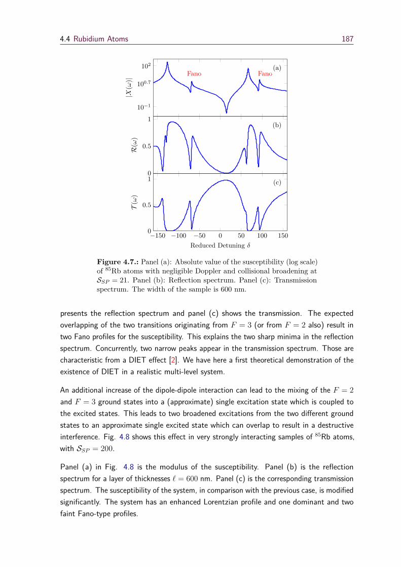
4.4 Rubidium Atoms 187

Fano Fano

−150 −100 −50 0 50 100 1500

0.5

1

Reduced Detuning δ

T(ω

)

(c)

0

0.5

1

R(ω

)(b)

10−1

100.7

102

|X(ω

)|

(a)

Figure 4.7.: Panel (a): Absolute value of the susceptibility (log scale)of 85Rb atoms with negligible Doppler and collisional broadening atSSP = 21. Panel (b): Reflection spectrum. Panel (c): Transmissionspectrum. The width of the sample is 600 nm.

presents the reflection spectrum and panel (c) shows the transmission. The expectedoverlapping of the two transitions originating from F = 3 (or from F = 2 also) result intwo Fano profiles for the susceptibility. This explains the two sharp minima in the reflectionspectrum. Concurrently, two narrow peaks appear in the transmission spectrum. Those arecharacteristic from a DIET effect [2]. We have here a first theoretical demonstration of theexistence of DIET in a realistic multi-level system.

An additional increase of the dipole-dipole interaction can lead to the mixing of the F = 2and F = 3 ground states into a (approximate) single excitation state which is coupled tothe excited states. This leads to two broadened excitations from the two different groundstates to an approximate single excited state which can overlap to result in a destructiveinterference. Fig. 4.8 shows this effect in very strongly interacting samples of 85Rb atoms,with SSP = 200.

Panel (a) in Fig. 4.8 is the modulus of the susceptibility. Panel (b) is the reflectionspectrum for a layer of thicknesses ` = 600 nm. Panel (c) is the corresponding transmissionspectrum. The susceptibility of the system, in comparison with the previous case, is modifiedsignificantly. The system has an enhanced Lorentzian profile and one dominant and twofaint Fano-type profiles.

188 Chapter 4. Dipole Induced Electromagnetic Transparency

1

50

1000

|χ(ω

)|

(a)

−1,500 −1,000 −500 0 500 1,000 1,500

0

0.5

1

Reduced Detuning δ

T(ω

)

(c)

0

0.5

1R(ω

)(b)

Figure 4.8.: Panel (a): Absolute value of the susceptibility (log scale)of 85Rb atoms at SSP = 200. Panel (b): Reflection spectrum. Panel(c): Transmission spectrum. The width of the sample is 600 nm.

The dominant Fano profile located near the zero of the reduced detuning arises from theoverlapping of two coupled dipoles F = 3 → F ′ = 2, 3 and F = 2 → F ′ = 2, 3. Thissuperposition of transition dipoles from two distinct ground states to an approximate singleexcited state leads to DIET, as seen in the reflection (Fig. 4.8(b)) and transmission (Fig.4.8(c)) signals of the layer. The other two faint Fano lineshapes are due to the splitting inthe excited states that also result in DIET, going along with two small transmission peakson the left and right of the dominant DIET transmission signal. These two DIET effect aremore clearly imprinted in the reflection spectrum via associated spectral holes (Fig. 4.8(c)).

The reflection and transmission spectra of the system have a background where DIET isobserved. This is because of the Fabry-Pérot etalon effect discussed previously. Due tothe mismatching between the layer thickness ` = 600 nm and the transition wavelengthλ0 ' 795 nm, long tails are created near the reflection window. This can be improved byusing a thicker slab.

4.5 Conclusion 189

4.5 Conclusion

In this chapter, the semi-classical model of the Lorentz oscillator was extended to a multilevelsystem. This extended model can explain the calculated response of a realistic multi-levelsystem towards weak electromagnetic fields.

A new collective effect named dipole induced electromagnetic transparency (DIET) wasdiscussed. It is an induced electromagnetic transparency in a system of strongly interactingquantum emitters with two (or more) closely spaced excitations. The mechanism lies onthe destructive interference between two overlapping resonances. The frequency ωh of theinduced transmission window can be calculated using Eq. (4.12). An electromagnetic fieldof this frequency, incident on the system, will be transmitted through the layer with anassociated extinction obeying Beer-Lambert’s law.

DIET was discussed in the case of the D1 transitions of a gas of 85Rb atoms at lowtemperature. Different DIET effects were calculated due to the mixing of the differentenergy levels of the considered transition.

The signature of DIET is imprinted very clearly in the reflection spectrum, which showsa spectral hole at the transmission frequency ωh. Several applications can be suggestedin which DIET could play an important role. Some of those will be discussed in the nextchapter.

4.6 References

[1] R. Puthumpally-Joseph, M. Sukharev, O. Atabek, and E. Charron. “Dipole-Induced Electromagnetic Transparency”. In: Phys. Rev. Lett. 113 (16 Oct. 2014),page 163603. doi: 10.1103/PhysRevLett.113.163603 (cited on pages 177, 181,182, 184).

[2] R. Puthumpally-Joseph, O. Atabek, M. Sukharev, and E. Charron. “Theoreticalanalysis of dipole-induced electromagnetic transparency”. In: Phys. Rev. A 91(4 Apr. 2015), page 043835. doi: 10.1103/PhysRevA.91.043835 (cited onpages 177, 179, 182, 185, 187).

190 Chapter 4. Dipole Induced Electromagnetic Transparency

[3] R. J. Glauber and S. Prasad. “Polarium model: Reflection and transmissionof coherent radiation”. In: Phys. Rev. A 61 (6 May 2000), page 063815. doi:10.1103/PhysRevA.61.063815 (cited on page 177).

[4] E. Charron and M. Sukharev. “Non-Hermitian wave packet approximation ofBloch optical equations”. In: The Journal of Chemical Physics 138, 024108 (2013).doi: 10.1063/1.4774056 (cited on page 179).

[5] U. Fano. “Effects of Configuration Interaction on Intensities and Phase Shifts”.In: Phys. Rev. 124 (6 Dec. 1961), page 1866. doi: 10.1103/PhysRev.124.1866(cited on page 181).

[6] D. A. Cardimona, M. G. Raymer, and C. R. S. Jr. “Steady-state quantuminterference in resonance fluorescence”. In: Journal of Physics B: Atomic andMolecular Physics 15 (1982), page 55. url: http://stacks.iop.org/0022-3700/15/i=1/a=012 (cited on page 183).

[7] P. Zhou and S. Swain. “Quantum Interference in Probe Absorption: NarrowResonances, Transparency, and Gain without Population Inversion”. In: Phys.Rev. Lett. 78 (5 Feb. 1997), pages 832–835. doi: 10.1103/PhysRevLett.78.832.url: http://link.aps.org/doi/10.1103/PhysRevLett.78.832 (cited onpage 183).

[8] F. Miller, A. Vandome, and J. McBrewster. Beer-Lambert Law. VDM Publishing,2009 (cited on page 183).

[9] J. Keaveney, A. Sargsyan, U. Krohn, I. G. Hughes, D. Sarkisyan, and C. S. Adams.“Cooperative Lamb Shift in an Atomic Vapor Layer of Nanometer Thickness”. In:Phys. Rev. Lett. 108 (17 Apr. 2012), page 173601. doi: 10.1103/PhysRevLett.108.173601 (cited on page 184).

[10] J. Pellegrino, R. Bourgain, S. Jennewein, Y. R. P. Sortais, A. Browaeys, S. D.Jenkins, and J. Ruostekoski. “Observation of Suppression of Light ScatteringInduced by Dipole-Dipole Interactions in a Cold-Atom Ensemble”. In: Phys. Rev.Lett. 113 (17 Sept. 2014), page 133602. doi: 10.1103/PhysRevLett.113.133602(cited on page 184).

[11] D. A. Steck. Alkali Data. Steck, 2013. url: http://steck.us/alkalidata(cited on pages 184–186).

[12] H. White. Introduction to Atomic Spectra. International series in physics. McGraw-Hill, 1934 (cited on page 184).

5Potential Applications of DIET

This chapter describes two potential applications of dipole induced electro-magnetic transparency (DIET): pulse shaping and slow light. These effectsare discussed for model systems and for the D1 transitions of 85Rb. A simplecontrol knob for manipulating the DIET frequency is also given.

Keywords:

DIET, Slow Light, Refractive Index, Group Velocity, Group Index, PulseShaping, Transmitted Pulse, Reflected Pulse

Contents5.1 Introduction 193

5.2 Pulse Shaping 193

5.3 Slow Light 196

5.4 Conclusion 199

5.5 References 200

5.1 Introduction 193

5.1 Introduction

An interference between two indistinguishable pathways leads to an induced electromagnetictransparency called dipole-induced electromagnetic transparency in a dense sample ofmultilevel particules. This effect was discussed in detail in the previous chapter. It providessome interesting applications. Two of the potential applications of DIET are pulse shapingand slow light. These applications are discussed in this chapter.

5.2 Pulse Shaping

Shaping a laser pulse in a desired way is an interesting application [1–3]. Pulse shapingor waveform synthesis is the process of changing the pulse shape (envelope) to a formthat is optimized for a desired application. There are many ways for achieving this goal.In some of the techniques the pulse is modified by using a beam shaper [2], spatial lightmodulators [4], deformable mirrors [5], etc...

Input Output

Pulse Shaper

Figure 5.1.: Schematic view: Pulse shaping.

Pulse shaping techniques showed their strong impact as an essential experimental controltool in ultrafast spectroscopy, nonlinear fiber optics, and strong-field physics. There aremany research fields where pulse shaping pulse shaping is used, like superconductingqubits [6], laser filament experiments [7], holographic and nonlinear pulse processing [4],chemical reactions, etc... The goal can be, for instance, to find an optimal pulse shapein order to minimize unwanted effects, for example to minimize the space-charge inducedemittance growth in RF photoinjector cathodes [8], or to maximize the desired processes inexperiments.

The cancellation of the dipoles due to the destructive interference of the overlappingresonances seen in DIET can also be used for pulse shaping. If the layer of interacting

194 Chapter 5. Potential Applications of DIET

three-level quantum emitters is characterized by a reflection window which is wider than theFWHM of the incident pulse ∆ω, the collective response of the quantum emitters resultsin a selective reflection and transmission of the incident pulse. Fig. 5.2 shows the reflectedpulse from a layer of width ` = 3.5µm of three-level systems with the same parameters asthe one used in section 4.3, for an incident pulse of ∆ω = 40π THz.

−150 −100 −50 0 50 100 150 200 250 3000

0.2

0.4

0.6

0.8

1

Reduced Detuning δ

Norm

ali

zed

Pu

lse

Sh

ape

Incident PulseReflected Pulse

60 80 1000

2

4

6

8·10−3

Figure 5.2.: The green line is the incident pulse shape normalizedwith respect to the peak intensity and the red line is the normalizedreflected pulse envelope. The corresponding transmission through thelayer is shown in the inset.

The blue curve is the reflected pulse shape from the layer which is compared with theincident pulse envelope shown by the green curve. The spectral hole is present at theposition where DIET occurs. The associated transmission is shown in the inset of the figure.The transmission is very small due to the high damping factor used in the calculations. Allthese plots are normalized with the peak intensity of the pulse. The reflected pulse has animportant modification compared to the incident field. The pulse shape now looks like thesuperposition of two distinct pulses. If the position of the spectral hole that separates thesetwo pulses can be controlled to a certain extend, it can be of great interest to eliminate apart of the frequencies from the pulse that could be of interest for many purposes.

Rewriting the equation for the frequency of the spectral hole

ωh =

√√√√ω212$

213 + ω2

13$212

$212 +$2

13, (5.1)

it is clear that the position of the spectral hole depends on the coupling between thedipoles and on the energies of the excited states. Thus once the excited states and otherparameters of the system are chosen, the control of the position of the hole over thereflection spectrum is limited. Since the number density N can be controlled by modifying

5.2 Pulse Shaping 195

the pressure of the gas [9], it opens a possibility to control the coupling between the dipoles.For example, if the system is prepared by mixing two different types of atoms having closelyspaced energy levels, the coupling between the dipoles can be modified by changing thenumber density of each type of emitters. The ratio of these couplings is

$212

$213

= ω12 N µ212

ω13 N ′ µ213, (5.2)

where N and N ′ are the number densities of the first and the second types of atoms.Controlling the dipole-dipole interaction in a dense medium by adjusting material parametersoffers an additional way that helps to engineer the collective effects in such systems. Fig. 5.3shows the result for a mixture of two two-level quantum emitters of very close transitionenergies. A simple change of the relative densities of the two types of quantum emitterschanges the position of the spectral hole as expected.

ω12 ω13

−100 −50 0 50 100 150 200 2500

0.2

0.4

0.6

0.8

1

Reduced Detuning δ

Norm

alizedPulseShap

e

$12 = $13/10$12 = $13

$12 = 10$13

Figure 5.3.: Reflected pulse shapes from a mixture of two two-levelsystems. The blue line is the reflection for $2

12 > $213, the red line is

for $212 = $2

13 and the green line is for $212 < $2

13. Two vertical linesshow the transition frequencies ω12 and ω13.

The blue solid curve shows the reflected pulse envelope for $213 = 10$2

12. For this case thespectral hole appears near the transition frequency of the first quantum emitter. The redline is for $2

12 = $213 and the spectral hole appears exactly in the middle. For $2

12 = 10$213

which is represented with the green line, the reflected pulse is imprinted with the hole nearthe second quantum emitter transition. Thus by changing the dipole-dipole coupling, thefrequency of DIET and hence the spectral hole in the reflected signal can be controlledbetween the two transitions. The upper and lower limits of this window within which DIETcan be controlled are fixed by the choice of quantum emitters.

196 Chapter 5. Potential Applications of DIET

−100 −50 0 50 100 1500

0.2

0.4

0.6

0.8

1

Reduced Detuning δ

Norm

ali

zed

Pu

lse

Sh

ape

Incident PulseReflected Pulse

Figure 5.4.: The blue line is the incident pulse shape normalizedwith respect to the peak intensity and the red line is the normalizedreflected pulse envelope.

In the case of a multilevel system, DIET will leave a succession of spectral holes in thereflected pulse. Fig. 5.4 shows the reflected pulse shape from such a system with tentransitions regularly spaced by 0.01 eV. The detuning is defined with respect to the firsttransition energy of the system, which is at 2 eV.

5.3 Slow Light

The speed of light is a fascinating quantity. For an electromagnetic field, the dependence ofthe field propagation on the material parameters is a consequence of Maxwell’s equations[10]. The refractive index of a system, which gives access to the speed of the light in amedium, depends on the resonances in the system under consideration. In addition, nearthe resonances a strong dispersion is observed. Precisely, the refractive index is defined asa ratio of phase velocities. For a pulse propagating in a dense gas, the group velocity vg

can be written as

vg(ω) = c

ng(ω) , (5.3)

where ng is called the group index of the medium and is defined as

ng(ω) = n(ω) + ωdn

dω. (5.4)

In general, the dispersion in a medium dn/dω is small. Large values of the dispersionare usually associated with resonances and hence with absorption in the medium. The

5.3 Slow Light 197

interesting phenomenon of slow light, that is associated with large values of the groupindex, is hence not easy to achieve in practice. The slow light effect in physical systems [11,12] was observed in weak pulse propagation through amplifying media in the late 1960’s[13, 14] and early 1970’s [15]. Later, researchers managed to decrease the speed of lightto a few tens of m/s and then stopped it [16–18]. There are many applications for theseeffects in different fields including communications, quantum information [19, 20], opticalmemories [21, 22], etc...

0

0.1

0.2

0.3

0.4

Transm

ittedPulse

65 70 75 80 85 90 950

0.5

1

1.5·106

Reduced Detuning δ

v g(ω

)

Figure 5.5.: The blue line is the transmitted pulse shape normalizedwith respect to the peak intensity and the red line is the group velocityas a function of the reduced detuning.

The physics behind slow light is based on electromagnetic induced transparency (EIT).Similar to EIT, DIET can also induce the slowing down of light at frequencies near theoverlapping resonances [23, 24]. To see this effect using DIET, we consider a 600 nm layerof strongly interacting three-level systems. Keeping all other parameters as in the previoussection, the group velocity of light can be estimated. Fig. 5.5 shows the group velocityand the transmitted field for the system considered. The group velocity of the transmittedpulse is here reduced by a factor of 210, i.e, the group index of the model system is 210.

The blue solid curve is the transmitted pulse due to the induced transparency using DIET.The transmission is not very efficient due to the inevitable losses in a dense medium. Thered curve shows the group velocity as a function of the reduced detuning. It is clearthat in the vicinity of DIET the group velocity is small compared to the speed of lightin the vacuum. Even though the model used here is not so efficient as already achievedexperiments using EIT, for example [18], it shows that the transmitted part of the incidentfield at DIET frequency will be traveling with a reduced speed.

It is also interesting to examine the effect in a realistic sample. For that, we consider the D1

transitions of 85Rb atoms. We suppose that the pressure is such that the system is in the

198 Chapter 5. Potential Applications of DIET

0

4

8

12

16

ng(106)

(c)

0

1

2

3

RefractiveIndex

Re[n(ω)]

Im[n(ω)]

(b)

0

0.2

0.4

Transm

ittedPulse

(a)

0 5 10 15 200

2

4

6

Reduced Detuning δ

v g(103

m/s)

Figure 5.6.: Panel (a): Group index ng(ω). Panel (b): Real andimaginary parts of the refractive index n(ω) of the system in thevicinity of DIET. Panel (c): Group velocity (left y-axis) and normalizedtransmitted pulse (right y-axis) for a layer of 2µm of 85Rb atoms.

strong interaction regime, with SSF = 200, so that the interaction between all dipoles inthe layer are strong enough to induce associated transparencies via destructive interferences.A similar kind of reduction in the velocity of the transmitted pulse is obtained. Fig. 5.6shows the relevant results for a layer of thickness 2µm.

Panel (a) shows the group index of the system. The group index is very high, a few 106,similar to recent experimental studies on slow light in plasmonic waveguides [12]. The localminimum in the group index, corresponding to ng ≈ 4.106 around δ = 15, corresponds tothe DIET transmission window. Within this window, the imaginary part of the refractiveindex n(ω), shown with the red curve in the panel (b), shows a window of minimum,making the layer less dissipative. The real part of the refractive index, represented by theblue solid curve in panel (b), shows a point of inflation at the frequency of DIET.

The red curve in panel (c) is the transmitted pulse through the layer. It lies exactly in thewindow of minimum dissipation. Even though the imaginary part of the refractive indexand hence the absorption coefficient is small, due to the relatively long distance (` = 2µm)traveled in the layer, the transmittance is reduced to 45%. The group velocity, representedby the blue curve in panel (c), is very small, a few tens of m/s. A zoom of the plot showing

5.4 Conclusion 199

this very small group velocity is given in Fig. 5.7. At the maximum of the group index, thegroup velocity drops below 20 m/s. At the peak of the transmission, the group velocityreaches 80 m/s.

The transit time for the pulse through the layer which is defined in general as T = `/vg

is also an interesting quantity to look at. Being the reciprocal of the group velocity, thetransit time behaves in the similar way as the group index as a function of the reduceddetuning and the value of the transit time for a particular value of the reduced detuning isgiven by the group index multiplied by the factor `/c. For the pulse considered here, thetransit time in the DIET regime lies around 30 ns, to be compared with a transit time ofabout 6 fs in the vacuum.

12 14 16 18 20 2220

40

60

80

100

Reduced Detuning δ

v g(m

/s)

Figure 5.7.: Group velocity as a function of the reduced detuning δfor the D1 transitions of 85Rb atoms.

5.4 Conclusion

In this chapter, two potential applications of DIET were discussed.

Pulse shaping was discussed in the case of a three-level system and of a multilevel systemin the strong interaction regime corresponding to a dense gas. A simple way for controllingthe position of the spectral hole in the reflected pulse was also discussed by varying therelative pressure of two different atomic gases. By changing the position of the spectralhole that corresponds to DIET, it is possible to exclude the desired frequency from thedeformed reflected pulse. This may be of interest for different purposes.

The slowing down of the speed of light inside the layer can be seen in systems showingDIET. Essentially, the pulse transmitted due to DIET is experiencing a large dispersion andhence a large group index that can slow down the pulse down to a few tens of m/s. Even

200 Chapter 5. Potential Applications of DIET

though there are some experiments showing better performance using EIT and/or evenstopped light, it is interesting to see that slow light can be observed also in DIET.

5.5 References

[1] Y. Fu, H. Xiong, H. Xu, J. Yao, B. Zeng, W. Chu, Y. Cheng, Z. Xu, W. Liu, andS. L. Chin. “Generation of extended filaments of femtosecond pulses in air byuse of a single-step phase plate”. In: Opt. Lett. 34 (Dec. 2009), page 3752. doi:10.1364/OL.34.003752 (cited on page 193).

[2] F. Dickey, T. Lizotte, S. Holswade, and D. Shealy. Laser Beam Shaping Applica-tions. Optical Science and Engineering. CRC Press, 2005 (cited on page 193).

[3] B. R. Frieden. “Lossless Conversion of a Plane Laser Wave to a Plane Wave ofUniform Irradiance”. In: Appl. Opt. 4 (Nov. 1965), page 1400. doi: 10.1364/AO.4.001400 (cited on page 193).

[4] J. W. Wilson, P. Schlup, and R. A. Bartels. “Ultrafast phase and amplitudepulse shaping with a single, one-dimensional, high-resolution phase mask.” In:Opt. Express 15 (July 2007), page 8979. doi: 10.1364/OE.15.008979 (cited onpage 193).

[5] H. Tomizawa, H. Dewa, H. Hanaki, and F. Matsui. “Development of a yearlongmaintenance-free terawatt Ti:Sapphire laser system with a 3D UV-pulse shapingsystem for THG”. In: Quantum Electronics 37 (2007), page 697. url: http://stacks.iop.org/1063-7818/37/i=8/a=A02 (cited on page 193).

[6] A. W. Cross and J. M. Gambetta. “Optimized pulse shapes for a resonator-induced phase gate”. In: Phys. Rev. A 91 (3 Mar. 2015), page 032325. doi:10.1103/PhysRevA.91.032325 (cited on page 193).

[7] Z. F. Feng, W. Li, C. X. Yu, X. Liu, J. Liu, and L. B. Fu. “Extended laserfilamentation in air generated by femtosecond annular Gaussian beams”. In: Phys.Rev. A 91 (3 Mar. 2015), page 033839. doi: 10.1103/PhysRevA.91.033839(cited on page 193).

[8] P. Musumeci, J. T. Moody, R. J. England, J. B. Rosenzweig, and T. Tran. “Exper-imental Generation and Characterization of Uniformly Filled Ellipsoidal Electron-Beam Distributions”. In: Phys. Rev. Lett. 100 (24 June 2008), page 244801. doi:10.1103/PhysRevLett.100.244801 (cited on page 193).

5.5 References 201

[9] D. A. Steck. Alkali Data. Steck, 2013. url: http://steck.us/alkalidata(cited on page 195).

[10] J. D. Jackson. Classical electrodynamics. 3rd edition. Wiley New York etc., 1998,page 160 (cited on page 196).

[11] A. H. Safavi-Naeini, T. P. M. Alegre, J. Chan, M. Eichenfield, M. Winger, Q.Lin, J. T. Hill, D. E. Chang, and O. Painter. “Electromagnetically inducedtransparency and slow light with optomechanics”. In: Nature 472 (Apr. 2011),page 69. doi: 10.1038/nature09933 (cited on page 197).

[12] K. L. Tsakmakidis, T. W. Pickering, J. M. Hamm, A. F. Page, and O. Hess.“Completely Stopped and Dispersionless Light in Plasmonic Waveguides”. In:Phys. Rev. Lett. 112 (16 Apr. 2014), page 167401. doi: 10.1103/PhysRevLett.112.167401 (cited on pages 197, 198).

[13] J. A. Carruthers and T. Bieber. “Pulse Velocity in a Self‐Locked He–Ne Laser”.In: Journal of Applied Physics 40 (1969), page 426. doi: http://dx.doi.org/10.1063/1.1657079 (cited on page 197).

[14] A. Frova, M. A. Duguay, C. G. B. Garrett, and S. L. McCall. “Pulse Delay Effectsin the He–Ne Laser Mode‐Locked by a Ne Absorption Cell”. In: Journal of AppliedPhysics 40 (1969), page 3969. doi: http://dx.doi.org/10.1063/1.1657127(cited on page 197).

[15] L. Casperson and A. Yariv. “Pulse Propagation in a High-Gain Medium”. In:Phys. Rev. Lett. 26 (6 Feb. 1971), page 293. doi: 10.1103/PhysRevLett.26.293(cited on page 197).

[16] N. S. Ginsberg, S. R. Garner, and L. V. Hau. “Coherent control of opticalinformation with matter wave dynamics”. In: Nature 445 (Feb. 8, 2007), page 623.doi: 10.1038/nature05493 (cited on page 197).

[17] D. F. Phillips, A. Fleischhauer, A. Mair, R. L. Walsworth, and M. D. Lukin.“Storage of Light in Atomic Vapor”. In: Phys. Rev. Lett. 86 (5 Jan. 2001), page 783.doi: 10.1103/PhysRevLett.86.783 (cited on page 197).

[18] G. Heinze, C. Hubrich, and T. Halfmann. “Stopped Light and Image Storage byElectromagnetically Induced Transparency up to the Regime of One Minute”. In:Phys. Rev. Lett. 111 (3 July 2013), page 033601. doi: 10.1103/PhysRevLett.111.033601 (cited on page 197).

[19] H. J. Kimble. “The quantum internet”. In: Nature 453 (June 2008), page 1023.doi: 10.1038/nature07127 (cited on page 197).

202 Chapter 5. Potential Applications of DIET

[20] M. Lukin, M. Fleischhauer, R. Cote, L. Duan, D. Jaksch, J. Cirac, and P.Zoller. “Dipole Blockade and Quantum Information Processing in MesoscopicAtomic Ensembles”. In: Phys. Rev. Lett. 87 (3 June 2001), page 037901. doi:10.1103/PhysRevLett.87.037901 (cited on page 197).

[21] R. Zhang, S. Garner, and L. Hau. “Creation of Long-Term Coherent OpticalMemory via Controlled Nonlinear Interactions in Bose-Einstein Condensates”. In:Phys. Rev. Lett. 103 (23 Dec. 2009), page 233602. doi: 10.1103/PhysRevLett.103.233602 (cited on page 197).

[22] H. de Riedmatten. “A Long-Term Memory for Light”. In: Physics 6 (July 2013),page 80. doi: 10.1103/Physics.6.80 (cited on page 197).

[23] R. Puthumpally-Joseph, M. Sukharev, O. Atabek, and E. Charron. “Dipole-Induced Electromagnetic Transparency”. In: Phys. Rev. Lett. 113 (16 Oct. 2014),page 163603. doi: 10.1103/PhysRevLett.113.163603 (cited on page 197).

[24] R. Puthumpally-Joseph, O. Atabek, M. Sukharev, and E. Charron. “Theoreticalanalysis of dipole-induced electromagnetic transparency”. In: Phys. Rev. A 91(4 Apr. 2015), page 043835. doi: 10.1103/PhysRevA.91.043835 (cited onpage 197).

6Conclusion and Outlook- Part II

This chapter concludes the work described in the second part of the thesis.It also describes some recent results obtained with stronger incident pulses.

Keywords:

Populations and Coherences, Non-Hermitian Wave Packets

Contents6.1 Conclusion 205

6.2 Non-Hermitian Model Revisited 206

6.3 Outlook 212

6.4 References 212

6.1 Conclusion 205

6.1 Conclusion

In this part of the thesis, the optical properties of multilevel systems confined in a nanometriccell (layer) was investigated in detail within the weak field limit.

The optical response of a dense sample of two-level systems was calculated in both the weak(dilute) and strong (dense) interaction regimes of the constituent particles. In the weakinteraction regime, the system is characterized by a weak Lorentzian lineshape that confirmsthe absence of collective behavior of the constituent particles. A simple Lorentz modeldescribing the system is used for interpreting the physics. Many interesting collective effectsare observed in the strong interaction regime, including the enhancement and broadeningof selective reflection due to the coupling between the dipoles.

In the presence of additional closely spaced quantum states, the response of the systemchanges dramatically. Broadened interactions due to dipole-dipole couplings induce anoverlap of different resonances, leading to the cancellation of the dipoles in the systemat a specific wavelength. The field then propagates through the medium, with minimumrefractive effects. This transparency induced due to the dipole coupling in the system wasnamed ”dipole-induced electromagnetic transparency” (DIET).

These effects were explained using model systems and realistic calculations were alsodesigned on the basis of the D1 transitions of 85Rb atoms at low temperature. Ananticipated transparency is obtained in the case of Rb atoms, giving a possibility forverifying the existence of DIET experimentally. Since there are many groups working onthe field using Rb samples, this may be achieved in the near future.

DIET resembles the well-known electromagnetically induced transparency process (EIT).Cancellation of the dipoles happens at a frequency between the two nearest transitions inthe system. The frequency at which the transparency occurs can be controlled by changingthe relative number density of different types of atoms. Just like in EIT, the light passingthrough the system is delayed due to a high dispersion effect. This slow light effect wascalculated in the case of Rb atoms.

DIET modifies the reflected spectrum, which shows one or several spectral holes. Thiseffect can be used for excluding desired frequencies from a laser pulse. This type of pulseshaping can be of experimental interests and it was discussed in the case of multilevelmodel systems.

All these effects were discussed exclusively within the limits of a weak probe. Moving out ofthis limit will affect the system significantly by populating excited states with a significant

206 Chapter 6. Conclusion & Outlook- Part II

probability and by turning on different kinds of responses to the applied fields. These effectsare briefly introduced in this last chapter of the thesis.

6.2 Non-Hermitian Model Revisited

For treating the system quantum mechanically, either Bloch equations or non-Hermitianwave packet equations [1] can be used. The later was of great interest while dealing withmultilevel systems since the method used speeds up the calculations. But the equations forthe non-Hermitian wave packet propagation will be diverging in strong fields due to thelarge number of excitations in the system. The equations describing the coherences of amultilevel system in the non-Hermitian wave packet model were given in Eq. (2.48). Werewrite them here:

i∂C1

∂t=

[ω1 + i

γ1(t)2

]C1 +

∑>2

Ω1(t)C (6.1a)

i∂C

∂t= Ω1(t)C1 +

[ω − i

γ(t)2

]C (6.1b)

where

γ1(t) =(2γ + Γ)∑k>2 |Ck(t)|2

|C1(t)|2 −∑

k>2 |Ck(t)|2 , (6.2a)

γ(t) = (2γ + Γ)|C1(t)|2|C1(t)|2 −

∑k>2 |Ck(t)|2 . (6.2b)

These equations were derived from the time dependent Schrödinger equation for a non-Hermitian Hamiltonian satisfied by a normalized wave function, with coefficients Cı whereı = 1, 2, 3..N .

The problem for extending this model beyond the weak probe limit is clear from Eq. (6.2).In the presence of strong fields, the excitation probabilities are not negligible. Since thedefinition of γı(t) depends on the population difference, these quantities will diverge as thepopulation of the excited states grows beyond 50%. This divergence is inevitable in thismodel. It can however be avoided if one relaxes the constraint of having a normalized wavefunction. In this case, both the ground and excited state populations can vary accordingly sothat the pole is eliminated from the calculation. Relaxing the condition on the conservation

6.2 Non-Hermitian Model Revisited 207

of the norm leads to another non-Hermitian model that, as we will see later, is valid in thestrong field limit.

6.2.1 Improved Non-Hermitian Model for a Two-Level System

From Eq. (2.27) it is clear that the coherences depend on the difference in populationsbetween the ground and excited states. Thus it is important to describe the quantity|C1(t)|2 − |C2(t)|2 accurately in a two-level system. The aim is therefore to find a set ofdynamical equations for C1(t) and C2(t) that describes this population difference correctly,and not necessarily the norm |C1(t)|2 + |C2(t)|2.

As seen from the previous approach, the condition on the empirical gain and decay factorsγ1(t) and γ2(t) should be

γ2(t)− γ1(t) = 2γ + Γ. (6.3)

In addition, an accurate description of the evolution of the population difference requires

2Γ |C2(t)|2 = γ1(t) |C1(t)|2 + γ2(t) |C2(t)|2 (6.4)

From Eqs. (6.3) and (6.4), we obtain

γ1(t) = (Γ− 2γ) |C2(t)|2|C1(t)|2 + |C2(t)|2

(6.5a)

γ2(t) = (2γ + Γ) γ1(t) + 2Γ |C2(t)|2|C1(t)|2 + |C2(t)|2

(6.5b)

With this approach, and in contrast with Eq. (6.2), it is clear that the rates γ1(t) and γ2(t)should not diverge anymore.

208 Chapter 6. Conclusion & Outlook- Part II

6.2.2 Comparison of the Different Non-Hermitian Models

We now compare the different models for different field strengths. A comparison betweenthe optical Bloch equations and the non-Hermitian model obtained for norm-conservedwave packets was already detailed in Chapter 2. Here the calculations are performed for a600 nm nano-layer composed of two levels systems with a transition energy of 2 eV andwith S12 = 1.26. Fig 6.1 shows the response of the system towards a Gaussian pulse withFWHM of 2π × 98.23 THz (10 fs pulse) within the weak probe limit.

−50−40−30−20−10 0 10 20 30 40 500

0.2

0.4

0.6

0.8

Reduced Detuning δ

A(ω

)

(c)

0

0.2

0.4

0.6

T(ω

)

(b)

0

0.1

0.2

0.3

0.4

R(ω

)

(a)

Figure 6.1.: Response of a 600 nm layer of two-level systemscalculated using optical Bloch equations (thick blue curve), thenon-Hermitian wavepacket model-1 (thin red curve) and the non-Hermitian wavepacket mode-2 (dashed green curve) as a function ofthe reduced detuning for S12 = 1.26. Panel (a): Reflection. Panel (b):Transmission. Panel (c): Extinction, with a weak 10 fs pulse.

The results obtained from the numerical integration of the optical Bloch equations areplotted with the thick blue curves. The red thin curves are calculated from the non-Hermitianmodel-1 (conservation of the norm) and the green dashed curves are the non-Hermitianmodel-2 (revised model). Panel (a) shows the reflection spectra, panel (b) shows thetransmission and the panel (c) is the extinction. As it is clear from the figure, the optical

6.2 Non-Hermitian Model Revisited 209

response calculated using the three models match very well in the weak probe regime.The choice made on the description of the quantity |C1(t)|2 − |C2(t)|2 for excluding thenumerical difficulty as the system approaches the population inversion does not bring anynoticeable discrepancy. Thus the non-Hermitian wave packet model-2 can be used forstudying dense two-level systems within the weak field limit.

0 50 100 150 200-2

-1

0

1

2

Time (fs)

Re[ρ12](arb.units)

(c)

0

0.5

1

1.5

|ρ12|(arb.units) (b)

0

1

2

3

4ρ22(arb.units) Non-Hermitian Model-1

Non-Hermitian Model-2(a)

Figure 6.2.: Density matrix elements calculated from the non-Hermitian wave packet models for a 600 nm layer of two-level systemsat S12 = 1.26 excited by a weak 10 fs gaussian pulse. Panel (a):Population of the excited state. Panel (b): Modulus of the coherence.Panel (c): Real part of the coherence. The blue solid line is the resultobtained from model-1 and the red dashed curve is for model-2.

Fig 6.2 shows the coherences and excited state population calculated using the twonon-Hermitian wave packet models. The comparison between the wave packet models withthe optical Bloch equations are excluded since a similar case for the non-Hermitian model-1is already discussed in Chapter 2. Panel (a) in Fig. 6.2 shows the population of the excitedstate. Panel (b) shows the absolute value of the coherence ρ12(t) and panel (c) shows thereal part of the coherence. The blue solid lines are the results obtained from model-1 andthe red dashed lines are from model-2. They are in excellent agreement. It is interesting tosee that the population of the excited state, which is not optimized with model-2, is stillvery accurate.

210 Chapter 6. Conclusion & Outlook- Part II

0 100 200 300 400

−0.4−0.2

0

0.2

0.4

Time (fs)

Re[ρ12](arb.unit)

(c)

0

0.2

0.4

|ρ12|(arb.unit) (b)

0

0.2

0.4

0.6

|ρ22|(arb.unit) (a)

Figure 6.3.: Density matrix elements calculated for a 600 nm layerof two-level systems at S12 = 1.26 excited by a strong 10 fs gaussianpulse. Panel (a): Population of the excited state. Panel (b): Modulusof the coherence. Panel (c): Real part of the coherence. The bluethick line is obtained from the optical Bloch equations, the greenthin line is from the non-Hermitian wave packet model-1 and the reddashed curve is for model-2.

But the case will be different as the incident field intensity increases so that the systemis disturbed significantly. In this case the condition |C1(t)|2 |C2(t)|2 is no more valid.Fig. 6.3 shows the population and the coherence and Fig. 6.4 shows the optical responsecalculated from the three models describing the dynamics of the two-level system exposedto a strong field. A 10 fs Gaussian pulse of amplitude E0 = 5× 109 V/m ≈ 0.01 au is used.In the presence of such a strong field, the optical Bloch equations are used as a referencefor comparing the results obtained from the non-Hermitian wave packet models.

The thick blue curves in Figs. 6.3 and 6.4 are the results obtained from the optical Blochequations. The green thin curves are those obtained from the non-Hermitian model-1 (withconservation of the norm) and the red dashed curves are those from the non-Hermitianmodel-2 (revised model). The panel (a) in Fig. 6.3 shows the population of the excitedstate calculated from the three models. None of the two wave packet methods are able todescribe accurately the evolution of this population even if the second method is doinga slightly better job. An interesting feature for the population calculated from model-2is that its variation is similar to the one of the coherence of the system which is given

6.2 Non-Hermitian Model Revisited 211

−100 −50 0 50 1000

0.5

1

Reduced Detuning δ

A(ω

)

(c)

0

0.2

0.4

0.6T(ω

)(b)

0

0.2

0.4

R(ω

)

(c)

Figure 6.4.: Optical response calculated for a 600 nm layer of two-level systems at S12 = 1.26 excited by a strong 10 fs gaussian pulse.Panel (a): Reflection. Panel (b): Transmission. Panel (c): Extinction.The blue thick lines are from the optical Bloch equations, the greenthin lines are from model-1 and the red dashed curves are frommodel-2.

in panel (b). The coherence calculated from model-1 disagrees clearly with the opticalBloch equations while the coherence calculated from model-2 is very accurate. A similarconclusion can be reached from the real part of the coherence.

The well-behaved coherence obtained from model-2 in strong fields ensures a better accuracyfor the calculation of the response of the system compared to model-1. Fig 6.4 shows thecomparison between the responses obtained from the different models. Panel (a) shows thereflection, panel (b) shows transmission and panel (c) shows the extinction. The color codesused in this plot are the same as in Fig. 6.3. The non-Hermitian model-1 shows a cleardisagreement with the optical Bloch equations while the model-2 reproduces accurately the”exact” results. This method could therefore be used to predict the response of the systemin strong fields.

212 Chapter 6. Conclusion & Outlook- Part II

6.3 Outlook

DIET is of experimental interest. It can be used in many ways for practical purposes. Thesystem considered in this thesis is a uniform distribution of quantum emitters. The pulsetransmitted through DIET systems constitutes slow light. In the case of 85Rb, we haveshown that the transmitted pulse can travel with velocities of a few tens of m/s. Thus theaddition (or the presence) of a mechanical wave (oscillation), like a sound wave for instance,could affect the quality of DIET. For example, the action of a longitudinal wave will setthe constituent particles in oscillation in the direction of propagation. If the acoustic waveand the applied electromagnetic fields are propagating in the same direction, the emissionof dipolar fields will happen while the dipoles are oscillating. Since the group velocity ofthe electromagnetic field is very small, there may be an important influence on DIET eitherin terms of frequency or in terms of efficiency. It is a problem that could be of interest forthe future.

The development of the non-Hermitian code for a multilevel system in the strong fieldregime is also interesting. Currently the model, named non-Hermitian model-2, workswell for two-level systems. The problem lies with the choice of the empirical decay anddecoherence rates introduced in the model. An appropriate definition of these empiricalquantities could lead to an accurate multilevel model. It could then be used for studyingstrong field phenomena in dense gases. Some groups reported high harmonic generationin dense systems. It may be of interest to look at similar systems to explore more aboutthe strong field effects in a high density sample of quantum emitters. The advantage ofhaving a wave packet model is that it is computationally much more efficient than a timedependent density matrix approach when many quantum states are populated.

6.4 References

[1] E. Charron and M. Sukharev. “Non-Hermitian wave packet approximation ofBloch optical equations”. In: The Journal of Chemical Physics 138, 024108 (2013).doi: 10.1063/1.4774056 (cited on page 206).

III

Appendices

AAtomic Unit System

It is important to use an appropriate unit system that ease the calculations we want todo. The most commonly used unit system, the Système International (SI) is not alwayspractical. For example, to describe physical quantities in relativistic calculations, stringtheory, etc.. the Lorentz-Heaviside system of units is more useful. When we deal withquantum gravity, the most practical unit system is based on Planck units. Atomic units(a.u.) is a system of units based on universal atomic physical constants related to theground state of the hydrogen atom. They simplify the equations and calculations of physicalquantities in atomic, molecular and optical (AMO) physics.

The standards of atomic units are described below.

A.1 Concept of Atomic Units

From the fundamental concept of charge in the low energy regime, the charge that canbe carried by any particle is an integer multiple of the electron charge e which is about1.60217657× 10−19 C. Or in other words, in atomic and molecular physics, charges can bespecified as units of the fundamental charge e. Thus it is convenient to set e as the unit ofcharge when dealing with atoms and molecules. Therefore,

e = 1.60217657× 10−19 C = 1 a.u. of charge. (A.1)

In the SI system, the time-dependent Schrödinger equation (TDSE) for a one electronatom with infinite nuclear mass can be written as

i~ ∂tψ = − ~2

2me

∆ψ + V ψ (A.2)

where me is the electron mass. If we rescale the coordinates associated with the equation

Appendix A. Atomic Unit System Chapter A. Atomic Unit System

(A.2) using the Bohr radius a0, we get ∆′ ≡ a20 ∆ and the TDSE becomes

imea

20

~∂tψ = −1

2 ∆′ψ + me a20

~2 V ψ. (A.3)

The LHS of equation (A.3) reveals the appearance of a characteristic time scale t0 = mea20/~

while the RHS of the same equation reveals the appearance of a characteristic energy scaleE0 = ~2/(mea

20). If we define t′ = t/t0 and V ′ = V/E0 Eq.(A.3) can be reorganized as the

following dimensionless equation

i ∂t′ψ = −12 ∆′ψ + V ′ ψ . (A.4)

We have the intrinsic scales of length, energy and time, a0, E0 and t0 that simplify theTDSE. In the atomic system of units, the Bohr radius is defined as 1 a.u. of length and thequantities E0 and t0 define the atomic units of energy and time. Note that the ionizationenergy of the hydrogen atom is 0.5 a.u. of energy and that the Bohr orbital period is2π a.u. of time.

A.2 Other Units

Comparing equations (A.2) and (A.4), we can see that the definition of atomic units arecompatible with the choices ~ = 1 a.u. for the unit of angular momentum and me = 1 a.u.for the unit of mass.

Defining now the atomic unit of electric field F0 as the field strength due to the hydrogennucleus (a proton) at a distance a0, we get

F0 = e

4πε0a20

= 1 a.u. of electric field. (A.5)

The intensity of a linearly polarized electric field of amplitude F0 can now be written as

I0 = 12

√ε0

µ0F 2

0 = 1 a.u. of intensity. (A.6)

One can finaly note that since dimensionless physical constants keep their value unchangedin any unit system, the fine structure constant α = e2

4πε0~c≈ 1

137 is preserved in the atomicunit system. The reciprocal of the fine structure constant therefore gives the speed of light

Appendix A. Atomic Unit System 217

in atomic units: c ≈ 137 a.u. of speed.

The table below summarizes the atomic unit system.

Table A.1.: Conversion Factors for Atomic Units

Physical Quantity Expression in the SI system Conversion Factor

Mass me (electron rest mass) 9.10938291.10−31 kgElectric Charge e (electron charge) 1.60217657.10−19 C

Angular Momentum ~ 1.05457173.10−34 J.sCoulomb Constant 1/4πε0 8.98755178.109 m/F

Length 4πε0~2/mee2 5.29177210.10−11 m

Time (4πε0)2~3/mee4 2.41888432.10−17 s

Energy mee4/(4πε0~)2 4.35974417.10−18 J

Electric Field m2ee

5/(4πε0)3~4 5.14220652.1011 V/mIntensity cε0m

4ee

10/(4πε0)6~8 3.50944758.1016 W.cm−2

Fine Structure Constant e2/4πε0~c ≈ 1/137Electric Dipole Moment 4πε0~2/mee 8.47835326.10−30 C.m

Magnetic Dipole Moment e~/2me 9.27400968.10−24 J.T−1

For More Details

– A short history of the SI units in electricity by Ludwik Kowalskiin The Physics Teacher 24, 97 (1986).

– Scaling Mount Planck I: A view from the bottom by Frank Wilczekin Physics Today 54, 6 (2001).

BRunge-Kutta Method

The optical Bloch equations and the non-Hermitian wave packet approach used for describingthe system quantum mechanically are a set of first-order differential equations of the formdy/dx = f(x, y). First order differential equations of this form can be solved numericallyby the well-known fourth-order Runge-Kutta method (the RK-4 method) provided the initialconditions are known (i.e, y(x0) = y0). This method was developed by the mathematicianC. Runge and extended by another mathematician, M. W. Kutta.

The differential equation that should be solved is

dy

dx= f(x, y(x)) (B.1)

The value of y at a point x+ h can be written as

y(x+ h) = y(x) +∫ x+h

xf(x′, y(x′))dx′ (B.2)

In those cases where the integration in Eq.(B.2) cannot be done analytically, the only wayto do it is by looking at possible ways to calculate them numerically. For this numericalpurpose, the integration can be replaced by the quadrature of order N

y(x+ h) ≈ y(x) + hN∑

i=1Ci f(x+ αih, y(x+ αih)) (B.3)

where Ci and αi are some numbers that will be determined later. In principle, the summationis an infinite sum that is truncated at a certain finite value N for numerical reasons. Theaccuracy on y(x+ h) strictly depends on the order of this quadrature.

Solving the quadrature is again difficult since it depends on the values of y at other positions(x+ αih). The unknown quantities αi and Ci can be estimated using a Taylor expansionof Eq.(B.3). For the first term we get

hC1 f(x+ α1h, y(x+ α1h)) = C1 K1 (B.4)

Appendix B. Runge-Kutta Method Chapter B. Runge-Kutta Method

where K1 = h f(x, y(x)). The second term can be written as follows

hC2 f(x+ α2h, y(x+ α2h)) = C2 K2 (B.5)

where K2 = h f(x+ α2, y(x) + α2K1). This procedure can be extended to any order i upto i = N . If one uses only two terms from this quadrature, we obtain the second orderRK-2 method. Here, for reasons related to a balance between accuracy and numericalefficiency, we use the RK-4 method, and four terms are included in the quadrature. In thecase of RK-4, the four expressions of the Ki’s are given by

K1 = h f(x, y(x)) (B.6a)K2 = h f(x+ h/2, y(x) +K1/2) (B.6b)K3 = h f(x+ h/2, y(x) +K2/2) (B.6c)K4 = h f(x+ h, y(x) +K3) (B.6d)

Eq.(B.3) can therefore be written as

y(x+ h) ≈ y(x) + 16 (K1 + 2K2 + 2K3 +K4) (B.7)

Starting from the initial values to the final values of the domain, the solution of Eq. (B.1)will be obtained from Eq. (B.7).

For More Details

– Handbook of Mathematical Functions: With Formulas, Graphs, and MathematicalTables by M. Abramowitz and I. A. Stegun, Dover Publications (1964).

– Numerical Methods for Ordinary Differential Systems: The Initial Value Problem byJ. D. Lambert, Wiley (1991).

– The Art of Scientific Computing by W. H. Press, Cambridge University Press (1992).

Interférences quantiques dans la dynamique d’atomes et molécules dans unchamp électromagnétiqueMots-clés: Recollision et Champs Intenses, Effets collectifs, Imagerie orbitalaire,Diffraction Electronique Induite par Laser, Transparence Electromagnétique Induite parInteraction Dipôle-Dipôle, Lumière Lente

Dans cette thèse, nous discutons deuxcas spécifiques d’interaction laser-matièreoù des effets d’interférences quantiquesjouent un rôle clé. Dans la première par-tie nous montrons qu’on peut obtenir uneimage d’une molécule par photo-ionisationpar champ laser intense infrarouge. Oncrée ainsi un paquet d’ondes électroniqueoscillant dans le continuum. Ces élec-trons subissent une collision élastique avecl’ion moléculaire parent, qui peut être util-isée pour imager la molécule et ses or-bitales. Le processus est démontré dansle cas de la HOMO et de la HOMO-1 de

CO2. La deuxième partie traîte des ef-fets collectifs dans des vapeurs atomiquesdenses confinées dans des cellules de taillenanométrique. Les atomes répondent alorscollectivement à un champ laser incident,ce qui conduit à un décalage et à un élar-gissement des transitions. Lorsque deuxrésonances se recouvrent, une interférencequantique destructive se produit à unefréquence caractéristique. Ceci induit unphénomène de transmission électromagné-tique induite par interaction dipolaire, ouDIET.

Quantum Interferences in the Dynamics of Atoms and Molecules inElectromagnetic FieldsKeywords: Recollision and Strong Fields, Collective Effects, Orbital Imaging,Laser Induced Electron Diffraction, Dipole Induced Electromagnetic Transparency, SlowLight

In this thesis, two specific cases of laser-matter interaction where quantum interfer-ence plays a key role are discussed. Thefirst part deals with imaging a molecule us-ing its own electrons. An intense infraredlaser field acting on the molecule can createlaser-driven electron wave packets in thecontinuum. These electrons undergo elas-tic collision with the parent molecule thatcan be used for imaging the molecule andits orbitals. The process is demonstrated inthe case of both the HOMO and HOMO-1 of symmetric CO2. The second part

discusses collective effects and overlappingresonances in dense atomic vapors confinedin nano-cells. Closely spaced atoms re-spond collectively to a common excitingfield that leads to shifts and broadening ofresonances. Once two or more transitionsare broad enough to overlap, quantum in-terference will take place and it leads todestructive interference corresponding to acharacteristic frequency determined by thesystem parameters. It will lead to a trans-mission peak called “Dipole-Induced Elec-tromagnetic Transparency" or DIET.

Université Paris-SaclayEspace Technologique / Immeuble DiscoveryRoute de l’Orme aux Merisiers RD 128 / 91190 Saint-Aubin, France