The University of QueenslandDepartment of Physics

2004

Lecture notes of the undergraduate

course

PHYS2041

QUANTUM PHYSICS

Lecturer: Dr. Zbigniew Ficek

Physics Annexe(6): Rm. 436Ph: 3365 2331

email: ficek@physics.uq.edu.au

Contact Hours:

1 . T u e s d a y : 1 1 a m , R m . 7 - 3 0 2 ( L e c t u r e s )

2 . F r i d a y : 1 1 a m , R m . 7 - 3 0 2 ( T u t o r i a l s )

Consultation Hours: Wednesday , 2pm -

4pm

ContentsGeneral

Bibliography

Assumed

Background

5

6

91 Radiation (Light) is a Wave 101.1 Wave equation...................................... 101.2 Energy of the EM wave............................. 12

2 Difficulties of the Wave Theory of Radiation 172.1 Discovery of the electron ....................... 172.2 Discovery of X-rays ............................. 182.3 Photoelectric effect ............................. 202.4 Compton scattering ............................... 222.5 Discrete atomic spectra ......................... 23

3 Black-Body Radiation 253.1 Number of radiation modes ....................... 253.2 Equipartition theorem ........................... 28

4 Planck’s Quantum Hypothesis 314.1 Boltzmann distribution function ............... 314.2 Planck’s formula for I(A) ....................... 324.3 Photoelectric effect ............................. 374.4 Compton scattering ............................... 37

5 The Bohr Model 415.1 The hydrogen atom ................................. 415.2 X-rays characteristic spectra .................. 445.3 Difficulties of the Bohr model ................. 45

6 Duality of Light and Matter 476.1 Matter waves ...................................... 476.2 Matter wave interpretation of the Bohr’s model 506.3 Wave function ..................................... 52

3

6.4 Physical meaning of the wave function ........ 536.5 Phase and group velocities ..................... 556.6 The Heisenberg uncertainty principle ......... 596.7 The superposition principle ................... 616.8 Wave packets ..................................... 62

7 Schrödinger Equation 667.1 Schrödinger equation of a free particle ...... 667.2 Operators ........................................ 687.3 Schrödinger equation of a particle in an externalpotential . ........................................... 707.4 Equation of continuity ........................ 73

8 Applications of the Schrödinger Equation: Potential (Quantum) Wells 798.1 Infinite potential quantum well .............. 818.2 Finite square-well potential .................. 888.3 Quantum tunneling .............................. 99

9 Multi-Dimensional Quantum Wells:Quantum Wires and Quantum Dots 1049.1 General solution of the three-dimensional

Schrödinger equation ........................... 1059.2 Quantum wire and quantum dot ................. 107

10 Linear Operators and Their Algebra 11010.1 Algebra of operators .......................... 11010.2 Hermitian operators ........................... 113

10.2.1 Properties of Hermitian operators ..... 11310.2.2 Examples of Hermitian operators ....... 114

10.3 Scalar product and orthogonality of two eigenfunctions . . . ............................... 11710.4 Expectation value of an operator ............ 119

3

10.5 The Heisenberg uncertainty principle revisited 12410.6 Expansion of wave functions in the basis of orthonormal func-

tions ............................................ 127

11 Dirac Notation 13011.1 Projection operator ........................... 132

11.2 Representations of linear operators ......... 133

12 Matrix Representation of Linear Operators 13512.1 Matrix representation of operators .......... 13512.2 Matrix representation of eigenvalue equations . 137

13 First-Order Time-Independent Perturbation Theory142

14 Quantum Harmonic Oscillator 14614.1 Algebraic operator technique .................. 14714.2 Special functions method ..................... 155

15 Angular Momentum and Hydrogen Atom 16015.1 Angular part of the wave function: Angular momentum . . . . 16215.2 Radial part of the wave function ............. 168

16 Systems of Identical Particles 17416.1 Symmetrical and antisymmetrical functions .. 17516.2 Pauli principle ................................ 179

Final Remark 181

Appendix A: Deriva t i o n o f t h e B o l t z m a n n distribution fun c tion P n 183

Appendix B: Useful mathematical formulae 185

Appendix C: Physical Constants and Conversion Factors 187

6

General Bibliography

· E. Merzbacher, Quantum Mechanics, (Wiley, New York, 1998). This is an excellent book on quantum physics, and the course is aimed at this level of treatment.

· R.A. Serway, C.J. Moses, and C.A. Moyer, Modern Physics, (Saunders, New York, 1989).This is an excellent introductory text on quantum physics.

· K. Krane, Modern Physics, (Wiley, New York, 1996). Agood introductory text on quantum physics.

· R. Eisberg and R. Resnick, Quantum Physics of Atoms. Molecules, Solids, Nuclei, and Particles, (Wiley, New York, 1985).A good introductory text on quantum physics with applications to atomic, molecular, solid state, and nuclear physics.

There are many excellent books on quantum physics, a few ofwhich are:

· L. Schiff, Quantum Mechanics, (McGraw-Hill, New York, 1968).

· A. Messiah, Quantum Mechanics, (North-Holland, Amsterdam, 1962).

· A.S. Davydov, Quantum Mechanics, (Pergamon Press, New York, 1965).

· C. Cohen-Tannoudji, B. Diu, and F. Laloe, Quantum

7

Mechanics, (Wiley, New York, 1977), Vols. I and II.

· J.J. Sakurai, Modern Quantum Mechanics, (Addison-Wesley, 1994).

8

Assumed Background

Necessary prerequisites for undertaking this course include:

· Any standard introductory calculus-based course coveringmechanics, electromagnetism, thermal physics and optics.In particular, PHYS1002 course on special relativityand modern physics.

· Mathematical Level: Recommended background is MATH2000.An alternative recommended background is MATH2400.Calculus are used extensively, and students should havesome familiarity with vector algebra, vector calculus,series and limits, complex numbers, partial differ-entiation, multiple integrals, first- and second-orderdifferential equations, Fourier series, matrix algebra,diagonalization of matrices, eigenvectors andeigenvalues, coordinate transformations, specialfunctions (Hermite and Legendre polynomials).

9

”Quantum mechanics is very puzzling.A particle can be delocalized,it can be simultaneously in several energy statesand it can even have several different identities at once.” S. Haroche

10

IntroductionQuantum Physics, also known as quantum mechanics or

quantum wave mechanics − born in the late 1800’s − is astudy of the submicroscopic world of atoms, the particlesthat compose them, and the particles that compose thoseparticles. In 1800’s physicists believed that radiationis a wave phenomenon, the matter is continuous, theybelieved in the existence of ether and they had no ideasof what charge was.

A series of experiments performed in late 1800’s has led to the formulation of Quantum Physics:

· Discovery of the electron

· Discovery of X-rays

· Photoelectric effect

· Observation of discrete atomic spectra

The PHYS2041 lectures cover the background theory ofvarious effects discussed from first principles, and asclearly as possible, to introduce students to the mainideas of quantum physics and to teach the basic math-ematical methods and techniques used in the fields ofadvanced quantum physics, atomic physics, quantumchemistry, and theoretical mathematics. Some of the keyproblems of quantum physics are also described, concentrat-ing on the background derivation, techniques, results andinterpretations. Due to the limited number of the contacthours, no attempt has been made at a complete explorationof all the predictions of quantum physics, but it ishoped that the predictions and problems explored here willprovide a useful starting point for those interested in

12

learning more. The intention is to explore problems whichhave been the most influential on the development ofquantum physics and formulation of what we now call modernquantum physics. Many of the predictions of quantumphysics appear to be contrary to our intuitive perceptions,and the goal to which this lecture notes aspires is compactlogical exposition and interpretation of these fundamentaland unusual predictions of quantum physics. Moreover, thislecture notes contains numerous detailed derivations,proofs, worked examples and a wide range of exercises fromsimple confidence-builders to fairly challenging problems,hard to find in textbooks on quantum physics.

1 Radiation (Light) is a WaveWe know from classical optics that light (opticalradiation) can exhibit polarization, interference anddiffraction phenomena, which are characteristic of waves,and some sort of wave theory is required for theirexplanation.

We begin our journey through quantum physics with adiscussion of classical description of the radiative field.We first briefly outline the electromagnetic theory ofradiation, and describe how the electromagnetic (EM)radiation may be understood as a wave which can berepresented by a set of harmonic oscillators. This isfollowed by an description of the Hamiltonian of the EMfield, which determines the energy of the EM wave. Inparticular, we will be interested in how the energy of theEM wave depends on the parameters characteristic of thewave: amplitude and frequency.

1.1 Wave equationWe start the lectures by considering the time-varying electric (E) and magnetic ( B) fields that satisfy the Maxwell’s equations

V · E = / E 0 , ( 1 )V · B = 0, (2)

V x E = − aatB , (3)

where the parameters E0 and µ0 are constants that determinethe property of the vacuum and are called the electric

Vx B =µ 0

J +1

aatE , (4)

14

permittivity and magnetic permeability, respectively. Theparameter c is equal to the speed of light in vacuum, c =3 x 108 [ms−1].

The symbol V is called ”nabla” or ”del”. It is a vectorand in the Cartesian coordinates has the form

wherei, j and k are the unit vectors in the x, y and z directions, respectively.

k az a , (5)V = ia+ ax

ja + ay

15

It would be more correctly to say that nabla behaves insome ways like a vector. Nabla is incomplete as it stands,it needs something to operate on. The result of theoperation is a vector. The dot (·) and the cross (x) symbolsappearing in the Maxwell’s equations are the standardscalar and vector products between two vectors.

In the absence of currents and charges, Jti = 0, p = 0, and then the above Maxwell’s equations describe a free EM field, i.e. an EM field in vacuum.

We can reduce the Maxwell’s equations for the EM fieldin vacuum into twodifferentialequationsforE t ior B t i alone.To show this, we apply Vx to both sides of Eq. (3), andthen using Eq. (4), we find

0 1 0 2 t iV x (V x g) = - a t ( V x : 4 ) = c 2

a t 2 E . ( 6 )

Since

V x (V x t iE) = −V2E t i + V(V · t iE) , (7)

tiand V · E = 0 in the vacuum, we obtain

where the operator V 2 = V · V is called Laplacian and is a scalar.

Equation (8) is a very familiar differential equation inphysics, called the Helmholtz wave equation for theelectric field. It is in the standard form of a three-dimensional vector wave equation.

Similarly, we can derive a wave equation for the

V2 Eti − 1c2

2t2

Eti= 0 , (8)

16

magnetic field as

General solution of the wave equations (8) and (9) is given in a form of plane waves

U t i = E t i U k e - i ( w k t - k . r ) , ( 1 0 )k

where U t i (tiE, t iB), wk is the frequency of the kth wave, and tiUk is the amplitude of the E t i or B t iwave propagating inthe k t i direction.

V2Bti − 1c2

2at2Bti = 0 . (9)

17

The vectork is called the wave vector and describesthe direction of propagation of the wave with respect toan observation point r. From the requirement that Eq.(10) is a solution of the wave equation (8), we find that|k| = wk/c = 27r/Ak, where Ak is the wavelength of the kthwave.

The solution (10) shows that the electric and magneticfields propagate in vacuum as plane (electromagnetic)waves. Properties of these waves are determined from theMaxwell’s equations.

The divergence Maxwell’s equations (1) and (2) demand that for all k:

k · Ek=0 and k · Bk=0. (11)

This means that E andB are both perpendicular to the direction of propagation k. Such a wave is called a transverse wave.The Maxwell’s equations (3) and (4) provide a further restriction on the fields that

Bk = 1c ×

Ek , (12)

where = k/| k| is the unit vector in thek direction.Equation (12) shows that the electric E and magneticB

fields of an EM wave propagating in vacuum are mutually orthogonal.

In summary: The electromagnetic field propagates in vacuum in a form of electromagnetic transverse plane waves.

1.2 Energy of the EM waveConsider an EM wave of the wave vectork confined in a

18

space of volume V. We will find the energy carried by theEM wave and will determine how the energy depends on theparameters characteristic of the wave (amplitude andfrequency). For simplicity, we will limit the calculationsof the energy of the EM wave to one dimension only, i.e. wewill assume that the wave is confined in a length L and k

·r= kz.Take a plane wave propagating in the z direction and

linearly polarized in the x direction. The wave is determined by the electric field

E (z, t) =iEx(z, t) = iq (t) sin(kz) ,(13)

19

where q (t) is the amplitude of the electric field.The energy of the EM field is given by the Hamiltonian{ }

f L

1 0| E|2 + 1H = 0 dz µ0 | B|2 , (14)2

where 0| E2|/2 is the energy density of the electric field, and | B|2/(2µ0) is the energy density of the magnetic field.

In order to determine the energy of the EM field, weneed the magnetic field B. Since we know the electricfield, we can find the magnetic field from the Maxwell’sequation (4). For the EM wave, the magnetic vector B is perpendicular to E and oriented along the y-axis.Hence, the magnitude of the magnetic field can be foundfrom the following equation

Since Bx = Bz = 0 and By =0, and obtain

The coefficients on both sides of Eq. (16) at the same unitvectors should be equal. Hence, we find that

Then, integrating 8By/8z over z, we find

f1 dz sin(kz) =    1

By (z, t) = − c2 q˙ (t) kc2 q˙ (t) cos(kz). (18)Thus, the energy of the EM field, given by the

Hamiltonian (14), is of the form

20

V × B q˙ (t)sin(kz) . (15)1c

i B y +

k B y

=i

1c2q˙ (t) sin(kz) . (16)

B y x =0 and B y

z = 1c2

q˙ (t) sin(kz) . (17)

{ }f L

1 0q2 (t) sin2(kz) + 1H = 0 dz k2c4µ0 ( q˙ (t))2 cos2(kz) .(19)2

Since

f0

f LL dz sin2(kz) = 0dzcos2(kz) = 1 2L,

21

This is the familiar Hamiltonian of a harmonic oscillator.We know from the classical mechanics that the energy of aharmonic oscillator is given by a sum of the kinetic andpotential energies as

H o s c = E K + E p = 2m ( ˙x) 2 + 11 2mw 2x2

1 ( p 2 + m 2w 2x 2)

= , (22)2m

where p = mx˙ is the momentum of the oscillating mass m.

Thus, the variables q(t) and ˙q(t) can be related to the position and momentum of the harmonic oscillator.

An important conclusion we can make from Eq. (21) that the energy of the EM wave is proportional to the square ofits amplitude, q (t).

In summary of this lecture: We have learnt that

1. The EM field propagates in vacuum as transverse planewaves, which can be represented by a set of harmonicoscillators. Thus, according to the Maxwell’s EMtheory, the radiation (light) is a wave.

2. The energy (intensity) of the EM field is proportionalto the square of the amplitude of the oscillation.

22

Exercise:

Show that the single mode electric field

E = E0 sin (kxx) sin (kyy) sin (kzz) sin (wt + ) (23)

( )

is a solution of the wave equation (8) if k = w/c, where k = k2 x + k2 y + k2 z is the magnitude of the wave vector.

12

Solution:

Using Eq. (23), we find

= —w2E, (24)

82 Ey E , 82 E8x2 = —k2 x E , 82 E8y2 = —k2 8z2 = —k2 z E . (25)

Hence, substituting Eqs. (24) and (25) into the wave equation

( 8 2 )

8x2 + 828y2 + 82 E-. — 1 82 E8t2 = 0 , (26)8z2 c2we obtain

E + w2— k2 x + k2 y + k2 c2 E = 0 , (27)z

or

— w2k2 x + k2 y + k2 E = 0 . (28)z c2

Since E = 0 and k2 x + k2 y + k2 z = k2, we find that the lhs of Eq. (28) is equal to zero when

k2 = w2 wc2 , i.e. when k = . (29)

23

82E

8t2

and

c

24

Hence, the single mode electric field (23) is a solution of the wave equation if k =w/c.

Exercise at home:

Using Eq. (12), show that

Ek = −ck x Bk,

which is the same relation one could obtain from the Maxwellequation (4). (Hint: Use the vector identity A x (B xÔ) = B(A· Ô) − C( A · B). )

25

2 Difficulties of the Wave Theory of Radiation

We have already learnt that light is an electromagneticwave. The typical signatures of the wave character oflight are the polarization, interference and diffractionphenomena. However, a series of experiments performed inlate nineteenth centenary showed that the wave modelpredicted from the Maxwell’s equations is not the correctdescription of the properties of light. In this lecture, wewill discuss some of the experiments which provided evidencethat light, which we have treated as a wave phenomenon,has properties that we normally associate with particles.In particular, these experiments indicated that the energyof light is not proportional to the amplitude of theoscillation, it is rather proportional to the frequency ofthe oscillation.

2.1 Discovery of the electronThomson in his famous e/m experiment, performed in 1896, found that the ratio e/m

1.Didn’t depend on the cathode material.

2.Didn’t depend on the residual gas in the tube.

3.Didn’t depend on anything else about the experiment.

This independence showed that the particles in the cathode beam are a common element of all materials.

Millikan in the oil-drop experiment measured electric

26

charge of individual oil drops. He made an importantobservation that every drop had a charge equal to somesmall integer multiple of a basic charge e (q = ne),where e = 1.602177 × 10_ 1 9 [C].

Thus, they concluded that matter is not continuous, is composed of discrete particles (corpuscular theory of matter).

27

2.2 Discovery of X-raysRöntgen, in 1895, was interested in the study of thepassage of a cathode beam through an aluminium-foilwindow. He noticed that a light sensitive screen glowedbrightly for no apparent reason. He called it X-rays.

In 1906, Barkla observed a partial polarization of X-rays, which indicated that they are transverse waves.

The X-rays are invisible, and then an obvious question arises: What are the wavelengths of X-rays?

To answer this question let us think how we could measurethe wavelength of the X-rays. One possibility, inprinciple at least, would be to perform Young’s doubleslit experiment.

However, any attempt to measure the wavelength using the Young double- slit experiment was unsuccessful with no interference pattern observed.

In 1912, Laue explained that no interference pattern isobserved because the wavelengths of X-rays are too small.To explore his argument, consider the condition forobservation of an interference pattern

2d sin e = mA , (30)

from which we have

mAsine = 2d . (31)

For A << d, we have sin e 0 even for large m. Hence, in order to makesin e1 to see the interference fringes separated from eachother, theseparation d between the slits should be very small.

Laue proposed to use a crystal for the interference

28

experiment. In crystals the average separation between theatoms, acting as slits, is about d 0.1 nm. From theexperiment, he found that the wavelength of the measuredX- rays was A 0.6 nm. Typical X-ray wavelengths are inthe range: 0.001 - 1 nm. These are very short wavelengthswell outside the ultraviolet wavelengths. For acomparison, visible light wavelengths are between: A 410nm (violet) and A 656 nm (red).

How the radiation of such small wavelengths is generated?

29

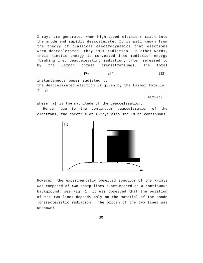
X-rays are generated when high-speed electrons crash intothe anode and rapidly deaccelerate. It is well known fromthe theory of classical electrodynamics that electronswhen deaccelerated, they emit radiation. In other words,their kinetic energy is converted into radiation energy(braking i.e. deaccelerating radiation, often referred toby the German phrase bremsstrahlung). The total

instantaneous power radiated bythe deaccelerated electron is given by the Larmor formula2 e2

3 4ir0c3 |where |a| is the magnitude of the deacceleration.

Hence, due to the continuous deacceleration of theelectrons, the spectrum of X-rays also should be continuous.

However, the experimentally observed spectrum of the X-rayswas composed of two sharp lines superimposed on a continuousbackground, see Fig. 1. It was observed that the positionof the two lines depends only on the material of the anode(characteristic radiation). The origin of the two lines wasunknown!

30

P= a|2 , (32)

I( )

Figure 1: Experimentally observed spectrum of X-rays.

Moreover, the minimum wavelength A min was observed todepend only on the potential in the tube ( A min V) and was thesame for all target (anode) material. The reason wasunknown!

31

2.3 Photoelectric effectIn 1887, Hertz discovered the photoelectric effect -emission of electrons from a surface (cathode) when lightstrikes on it. If a positive charged electrode is placednear the photoemissive cathode to attract thephotoelectrons, an electric current can be made to flow inresponse to the incident light.

The following properties of the photoelectric effect were observed:

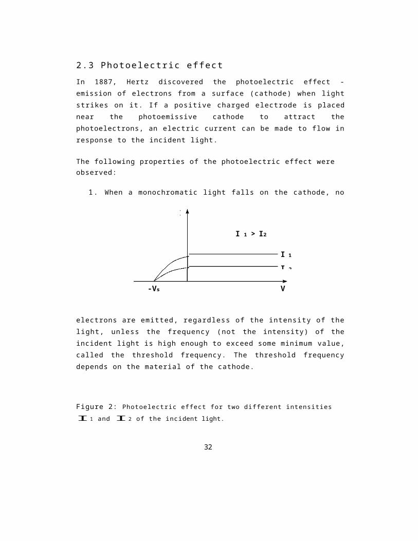
1. When a monochromatic light falls on the cathode, no

electrons are emitted, regardless of the intensity of thelight, unless the frequency (not the intensity) of theincident light is high enough to exceed some minimum value,called the threshold frequency. The threshold frequencydepends on the material of the cathode.

Figure 2: Photoelectric effect for two different intensities I1 and I2 of the incident light.

32

I

I 1 > I2

I 1I 2

-Vs V

2. Once the frequency of the incident light is greaterthan the threshold value, some electrons are emitted fromthe cathode with a non-zero speed. The reversed potentialis required to stop the electrons (stopping potential:eV5 = 1 2mv2).

3.When the intensity of light is increases, while itsfrequency is kept the same, more electrons are emitted,but the stopping potential is the same, see Fig. 2.

33

Conclusion: Velocity of the electrons, which is proportional to the energy, is unaffected by changes in the intensity of the incident light.

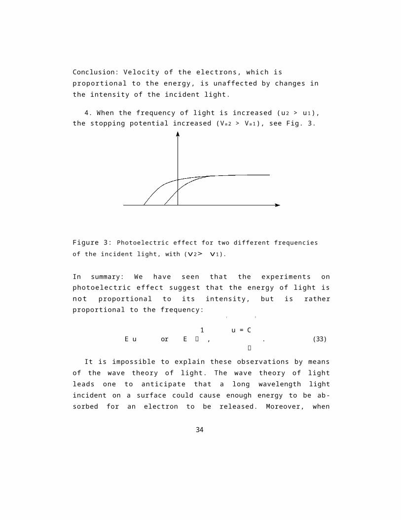
4. When the frequency of light is increased (u2 > u1), the stopping potential increased (V82 > V81), see Fig. 3.

Figure 3: Photoelectric effect for two different frequencies of the incident light, with (v2> v1).

In summary: We have seen that the experiments onphotoelectric effect suggest that the energy of light isnot proportional to its intensity, but is ratherproportional to the frequency:

(

1 u = CE u or E , . (33)

It is impossible to explain these observations by meansof the wave theory of light. The wave theory of lightleads one to anticipate that a long wavelength lightincident on a surface could cause enough energy to be ab-sorbed for an electron to be released. Moreover, when

34

I

-Vs2 - V

electrons are emitted, an increase in the incident lightintensity should cause an emitted electron to have morekinetic energy rather than more electrons of the sameaverage energy to be emitted.

35

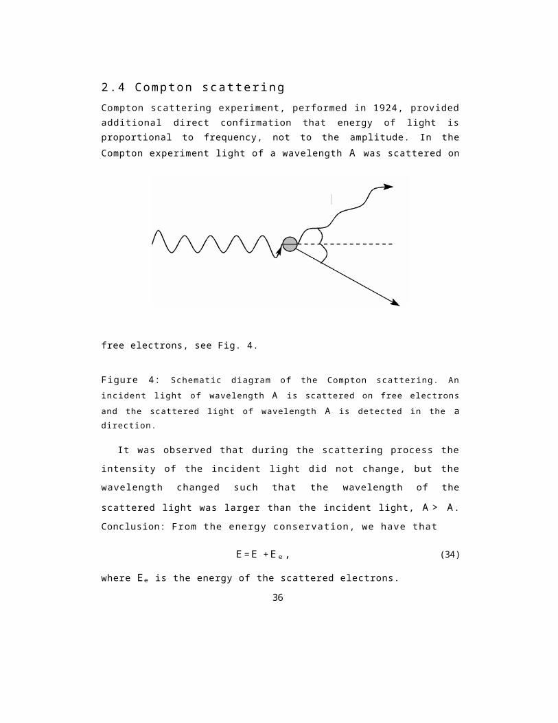
2.4 Compton scatteringCompton scattering experiment, performed in 1924, providedadditional direct confirmation that energy of light isproportional to frequency, not to the amplitude. In theCompton experiment light of a wavelength A was scattered on

free electrons, see Fig. 4.

Figure 4: Schematic diagram of the Compton scattering. Anincident light of wavelength A is scattered on free electronsand the scattered light of wavelength A ' is detected in the adirection.

It was observed that during the scattering process the

intensity of the incident light did not change, but the

wavelength changed such that the wavelength of the

scattered light was larger than the incident light, A '> A.Conclusion: From the energy conservation, we have that

E =E ' +E e , (34)

where Ee is the energy of the scattered electrons.

36

λ/Eλ > λλ e− α

ΘE

E

Since Ee > 0, then E ' < E, indicating that the energy ofthe incident light is

proportional to the frequency, or equivalently, to theinverse of the wavelength

1E u or E A . (35)

37

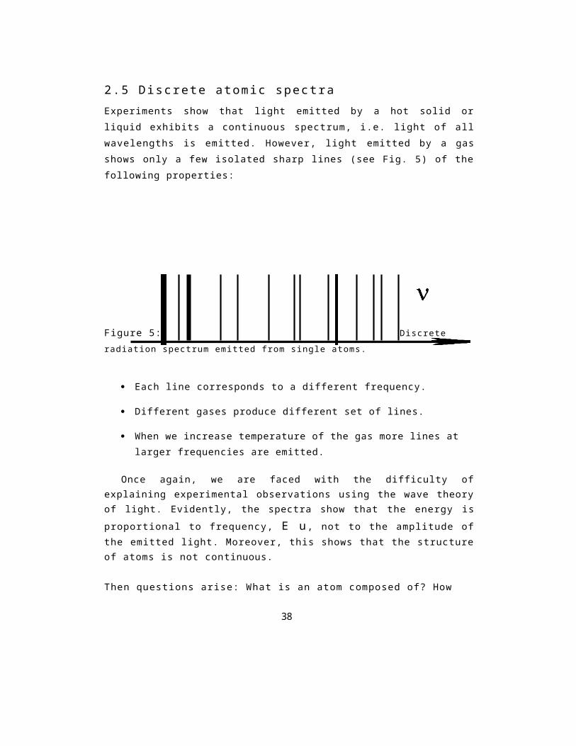
2.5 Discrete atomic spectraExperiments show that light emitted by a hot solid orliquid exhibits a continuous spectrum, i.e. light of allwavelengths is emitted. However, light emitted by a gasshows only a few isolated sharp lines (see Fig. 5) of thefollowing properties:

Figure 5: Discrete radiation spectrum emitted from single atoms.

· Each line corresponds to a different frequency.

· Different gases produce different set of lines.

· When we increase temperature of the gas more lines at larger frequencies are emitted.

Once again, we are faced with the difficulty ofexplaining experimental observations using the wave theoryof light. Evidently, the spectra show that the energy isproportional to frequency, E u, not to the amplitude ofthe emitted light. Moreover, this shows that the structureof atoms is not continuous.

Then questions arise: What is an atom composed of? How

38

does the discrete spectrum relate to the internal structure of the atom?

These questions were left without answers at that time.

39

In summary of this lecture:

We have seen that a series of experiments on

1. Properties of X-rays,

2.Properties of photoelectric effect,

3. Compton scattering,

4. Atomic spectra,

suggests that energy of the radiation field (light) isnot proportional to its amplitude, as one could expectfrom the wave theory of light, but rather to thefrequency of the radiation field, E r' u.

40

3 Black-Body RadiationThe radiation emitted by a body as a result of itstemperature is called thermal radiation. All bodies emitand absorb such radiation. Hot gases or individual atomsemit radiation with characteristic discrete lines. Hotmatter in a condensate state (solid or liquid) emitsradiation with a continuous distribution of wavelengthsrather than a line spectrum.

Consider spectral distribution of the radiation emitted by a black body. First, we will define what we mean by a blackbody.

Black-body - an object which absorbs completely all radiation falling on it, independent of its frequency, wavelength and intensity.

Examples: a box with perfectly reflecting sides and with asmall hole. The small hole can be treated as a black-body.

3.1 Number of radiation modesIn 1900, Rayleigh and Jeans calculated the energy densitydistribution I(A) of the radiation emitted by the black-body box at absolute temperature T. The energy densitydistribution is given by

I(A) = N(E) , (36)

where N is the number of modes (per unit volume and unitwavelength) inside the box

8irN = A4 , (37)

41

and (E) is the average energy of each mode.

Proof of Eq. (37): Number of modes inside the box

Consider an EM wave confined in the volume V. We take aplane wave propagating in r direction, which in terms ofx, y, z components can be written as

E = E0sin (kxx) sin (k yy) sin (kzz) sin (wt + ). (38)

42

The wave propagating in the box interfere with wavesreflected from the walls. The interference will destroy thewave unless it forms a standing wave inside the box. Thewave forms a standing wave when the amplitude of the wavevanishes at the walls. This happens when

sin (k xx) = 0 , sin (k yy) = 0 , sin (k zz) = 0 ,(39)

i.e. when k x = nir/x, k y = mir/y, k z = lir/z, where n,m, l are integer numbers (n, m, l = 1,2,3, . . .).

The condition (39) are called the boundary condition,i.e. condition imposed on the wave at the walls to formstanding waves inside the box. The standing wavecondition is common to all confined waves. In vibratingviolin strings or organ pipes, for example, it also happensthat only those frequencies which satisfy the boundarycondition are permitted.

Since k = 2ir/A, we have the following the condition fora standing wave inside the box

We see that each set of the numbers (n, m, l) corresponds to a particular wave, which we call mode.

In the k space of the components kx, ky, kz, a single mode, say (n, m, l) = (1, 1, 1) occupies a volume

where V = xyz is the volume of the box.Since kx, ky, kz are positive numbers, the modes

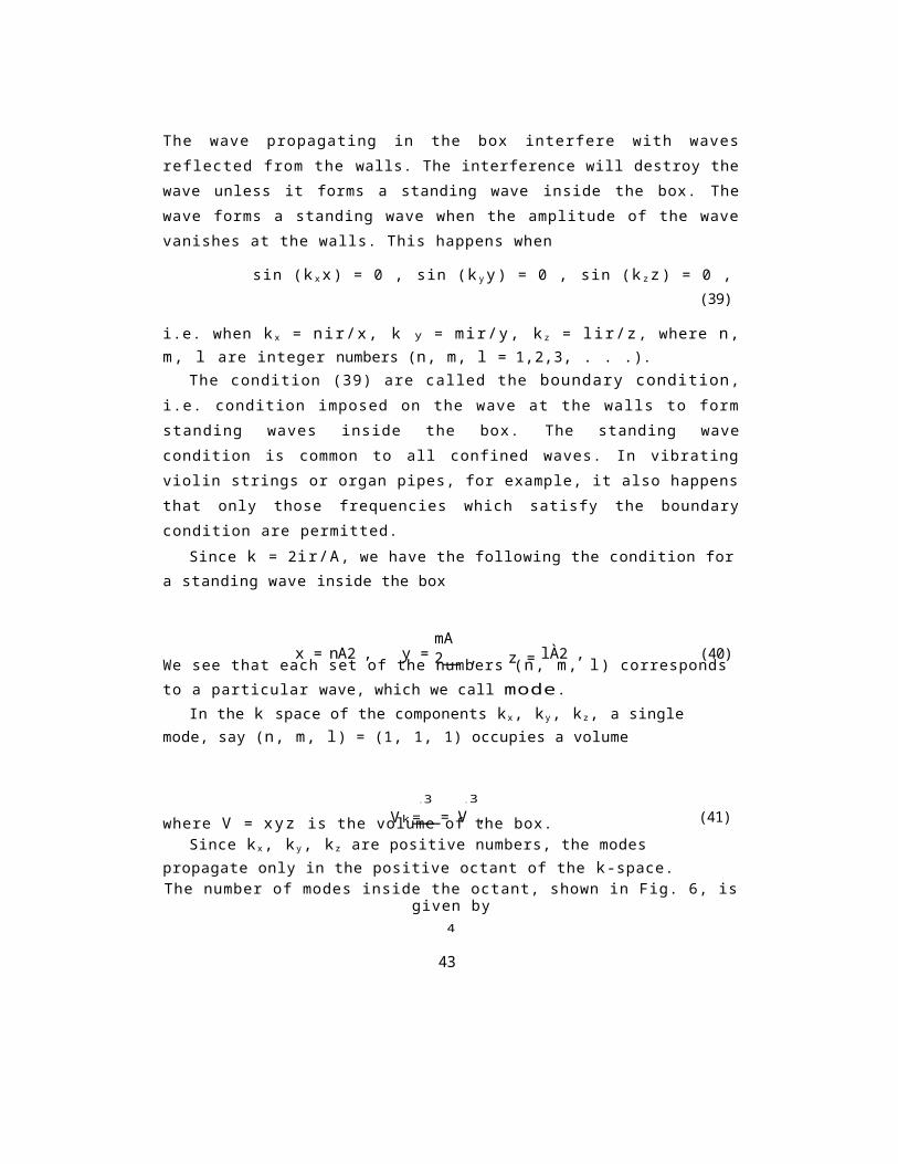
propagate only in the positive octant of the k-space.The number of modes inside the octant, shown in Fig. 6, is

given by4

43

x = nA2 , y =mA2__ , z = lÀ2 , (40)

3V k=

xyz

3____= V , (41)

1 3 k 3 N (k ) = _____ , (42)

8 Vki.e. is equal to the volume of the octant divided by the volume occupied by a single mode.

Since k = 2iru/c, we get8713

N(k) =    3c3 V , (43)

44

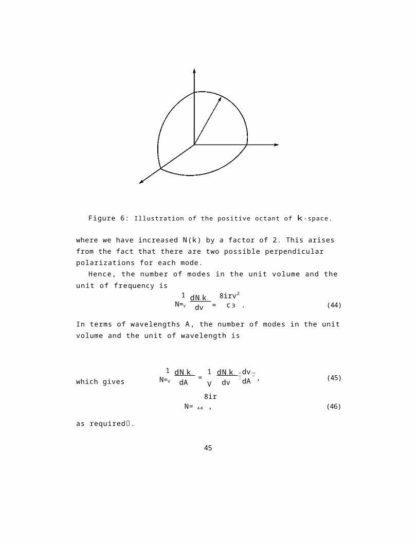
Figure 6: Illustration of the positive octant of k-space.

where we have increased N(k) by a factor of 2. This arises from the fact that there are two possible perpendicular polarizations for each mode.

Hence, the number of modes in the unit volume and the unit of frequency is

1N=V

dN ( k ) dv

8irv2= c3 . (44)

In terms of wavelengths A, the number of modes in the unit volume and the unit of wavelength is

which gives

8irN= A4 , (46)

as required.

45

k

k

k

k

1N=V

dN ( k ) dA =

1V

dN ( k ) dv

dvdA

, (45)

3.2 Equipartition theoremThe average energy can be found from so-calledEquipartition Theorem. This is a rigorous theorem ofclassical statistical mechanics which states that, inthermodynamical equilibrium at temperature T, the averageenergy associated with each degree of freedom of an atom(mode) is1

2k B T , where kB is the Boltzmann’s constant.The number of degrees of freedom is defined to be the

number of squared terms appearing in the expression for thetotal energy of the atom (mode). For example, consider anatom moving in three dimensions. The energy of the atom isgiven by

1 1 1E = 2mv2 x + 2mv2 y + 2mv2 z . (47)

There are three quadratic terms in the energy, and therefore the atom has three degrees of freedom, and a thermal energy3 2kBT.

46

ITHEORY

TT > T >T

T

T

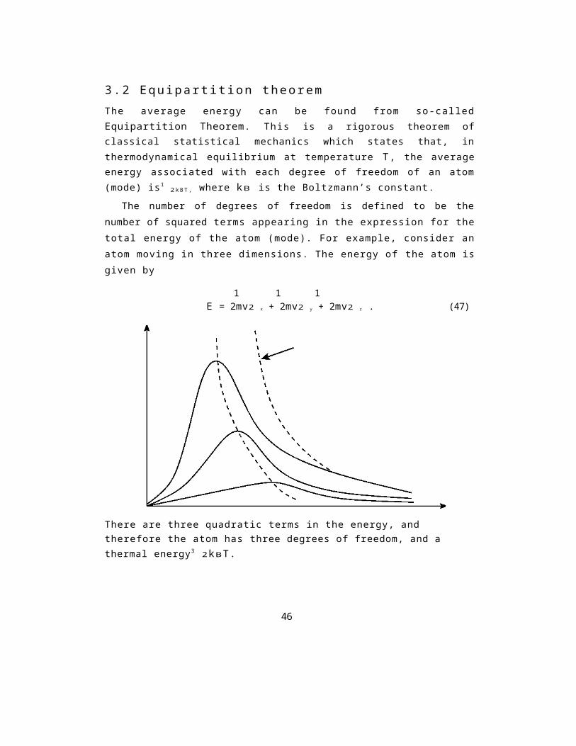
Figure 7: Energy density distribution (energy spectrum) of theblack-body radiation.

47

The energy of a single radiation mode is the energy of an electromagnetic wave

{ }

1 0| E|2 + 1H = V dV µ0 | B|2 . (48)

2

Because this expression contains two squared terms, Rayleighand Jeans argued that each mode has two degrees of freedomand therefore (E) = kBT. Hence

8I(A) = A4 kBT. (49)

The Rayleigh−Jeans formula agreed quite well with theexperiment in the long wavelength region, but disagreedviolently at short wavelengths, as it is seen from Fig. 7.The experimentally observed behavior shows that for a somereason the short wavelength modes do not contribute, i.e.,they are frozen out. As A tends to zero, I(A) tends tozero. The theoretical formula goes to infinity as A tendsto zero, leading to an absurd result that is known as theultraviolet (uv) catastrophe. Moreover, the theoreticalprediction does not even pass through a maximum.

We can summarize the presented experimental predictions as follows:

Spectrum of X-rays, properties of photoelectric effect,Compton scattering, atomic spectra, and the spectrum of theblack-body radiation indicate that something is seriouslywrong with the wave theory of light.

Exercise:

48

Show that the number of modes per unit wavelength and per unit length for a string of length L is given by

1L

dNdA

= A2

2 .

49

Solution:

Volume occupied by a single mode is

V k= L. (50)

Number of modes in the volume Vk is

Then, the number of modes per unit wavelength and per unit length is

Exercise at home:

We have shown in the lecture that the number of modes inthe unit volume and the unit of frequency is

1N = N = V

dN ( k ) dv

8irv2= c3 . (53)

In terms of the wavelength A, we have shown that the number of modes in the unit volume and the unit of wavelength is

8N=N A= A 4 . (54)

Explain, why it is not possible to obtain NA from N

simply by using the relation v = c/A.

==dA

2LA2

1L

1N= L A2 . (52)

k 2, r L 2LN(k) = V A A= = . (51)k

2dN

50

4 Planck’s Quantum HypothesisShortly after the derivation of the Rayleigh-Jeans formula,Planck found a simple way to explain the experimentalbehavior, but in doing so he contradicted the wave theoryof light, which had been so carefully developed over theprevious hundred years. Planck realized that the uvcatastrophe could be eliminated by assuming that a mode offrequency u could only take up energy in well defineddiscrete portions (small packets or quanta) each having theenergy

E = hu = ¯hw, (h¯= )h 2ir , =

2lru , (55)

where the constant h is adjusted to fit the experimentallyobserved I(A).

In a paper published, Planck states: ”We consider,however - this is the most essential point of the wholecalculations - E to be composed of a very definite numberof equal parts and and use thereto the constant of natureh”. If there are n quanta in the radiation mode, theenergy of the mode is E = nhu.

Contrast between the wave and Planck’s hypothesis is thatin the classical case the mode energy can lie at anyposition between 0 and oc of the energy line, whereas in thequantum case the mode energy can only take on discrete(point) values.

The assumption of the discrete energy distributionrequired a modification of the equipartition theorem.Planck introduced ”discrete portions” so that he might

51

apply Boltzmann’s statistical ideas to calculate the energydensity distribution of the black-body radiation.

4.1 Boltzmann distribution functionThe solution to the black-body problem may be developedfrom a calculation of the average energy of a harmonicoscillator of frequency u in thermal equilibrium attemperature T.

The probability that at temperature T an arbitrarysystem, such as a

52

radiation mode, has an energy En is given by the Boltzmanndistribution

ePn =

n

−En/kBT

e−E n/k BT . (56)

See Appendix A for the rigorous derivation of Eq. (56). For quantized energy En = m¯hw, we have

ePn =

e − n xn=0

where x = ¯hw/kBT.Since the sum I n = 0e− n x is a

particular example of a geometric series, and exp(_mx) < 1, the sum tends to the limit

1= ____________________________________ . (58)1 _ e−x

Hence, we can write the Boltzmann distribution function (56) in a simple form

( 1 _ e−x)Pn = e−nx. (59)

This is a very simple formula, which we will use in ourcalculations of the average energy (E), average number ofphotons (m), and higher statistical moments, (m2).

4.2 Planck’s formula for I ( A )

Assuming that m is a discrete variable, Planck showed that the average energy of the radiation mode is

53

−nx, (57)

e − n x

n=0

((E) = 1 _e−x)EnPn = ¯hwn

n=0

me−nx . (60)

Then, evaluating the sum in the above equation, he found

(E)=¯hw

ex_1 , (61)

54

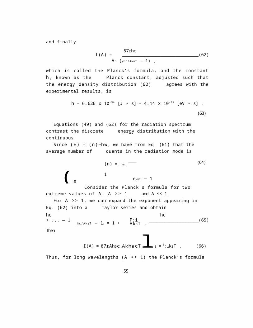
and finally

87rhcI(A) =    ______________________________(62)

A5 (ehc/AkBT — 1) ,

which is called the Planck’s formula, and the constanth, known as the Planck constant, adjusted such thatthe energy density distribution (62) agrees with theexperimental results, is

h = 6.626 x 10-34 [J • s] = 4.14 x 10-15 [eV • s] .

(63)

Equations (49) and (62) for the radiation spectrum contrast the discrete energy distribution with the continuous.

Since (E) = (n)~hw, we have from Eq. (61) that the average number of quanta in the radiation mode is

(n) = _̄hu,

1ek B T — 1

Consider the Planck’s formula for two extreme values of A: A >> 1 and A << 1.

For A >> 1, we can expand the exponent appearing in Eq. (62) into a Taylor series and obtainhc hc+ ... — 1 P:i    ___________________(65)AkBT .Then

I(A) = 87rAh5c ( Akh B c Tl1 = 8:4kBT . (66)

Thus, for long wavelengths (A >> 1) the Planck’s formula

55

(64).

(e

hc/Ak BT — 1) = 1 +

agrees perfectly with the Rayleigh—Jean’s formula.Outside this region, discreteness brings about Planck’s

quantum corrections. For A << 1, we can ignore 1 in thedenominator of Eq. (62) as it is much smaller thanthe exponent. Then

87rhcI ( A ) = ( 6 7 )A5ehc/Ak BT .

56

When A —* 0, ehc/kBT —* oc, and A5 —* 0. However, ea/A

function goes to infinity faster than A5 goes to zero.Therefore, I(A) —* 0 as A —* 0, which agrees perfectlywith the observed energy density spectrum, see Fig. 7.

In addition the Planck’s formula correctly predicts theWien displacement law

hcAmaxT =_________= constant, (68)

4.9651kBwhere A max is the value of A at which I(A) is maximal. Thefactor 4.9651 is a solution of the equation

1e_x +

5x—1=0. (69)

The Wien law says that with increasing temperature of theradiating body, the maximum of the intensity shifts towards shorter wavelengths.

Moreover, the Planck’s formula correctly predicts the Stefan—Boltzmann law

c

I = 0 I(A)dA = aT 4 , (70)4

where I is the total intensity of the emitted radiationand a is a constant, called the Stefan—Boltzmannconstant. The factor c/4, where c is the speed of light,arises from the relation between the intensity spectrum(radiance) and the energy density distribution. Therelation follows from classical electromagnetic theory.

Proof:

In the Planck’s formula8irhc

57

I(A) = A5 (ehc/kBT — 1), (71)

we substitute

x =h c ( 7 2 )

AkBT

58

and change the variable from A to x:

Hence, substituting for I(A) and dA in Eq. (70), we obtain

c x5

0 dx 8hc hcI =0 I ( A ) d A = c ( h c ) 5 _____4 4 ex − 1 kBT x2

kBT

k B T 4 0 dx 2irhc2 x3 0 dx    x3= ( h c     ) 4 ex − 1 = 2irhc2 ex − 1 . (74)hc

kBT

Since ° ° x3dx

15 , (75)e x − 1 = 40

we obtain( k B T 4 4E = 2 h c 2 _____ 15 = aT 4 , (76)hc

where

The constant a determined from experimental results agrees perfectly with the above value derived from the Planck’s formula.

In order to explore the importance of the discretedistribution of the radiation energy, it is useful tocompare the Planck’s formula for a discrete m with thatfor a continuous m.

Thus, assume for a moment that m is a continuous rather

59

hcA = kBT

1x

hcsothat dA=−k B T x2 1 dx . (73)

a = 2ir5k4 B = 5.67 x 10−8 [W/m2 · K4] . (77)15h3c

than a discrete variable. Then the Boltzmann distributiontakes the form

Pn = e −nx , (78)

f dm e−nx0

60

and hence the average energy is given by

(E)=¯hw dm me−nx

0 dm e− n x 0

= —¯hw(1 /x ) '

1/x

¯hw=

x= kBT, (79)

where ' denotes first derivative of 1/x with respect to x.This result is the one expected from the classical

equipartition theorem.

Looking backwards with the knowledge of the quantumhypothesis, we see that the essence of the black-bodycalculation is remarkably simple and provides a dramaticillustration of the profound difference that can arise fromsumming things discretely instead of continuously, i.e.making an integration.

61

4.3 Photoelectric effectIn 1905, Einstein extended Planck’s hypothesis bypostulating that these discrete quanta of energy ¯hw, thatcan be absorbed by a mode, can be considered like particlesof electromagnetic radiation (particles of light) which hetermed photons.

The energy of a single photon is E = ¯hw, and then the photoelectric effect is given by

where W is the work function required to remove an electronfrom the plate, and vma x is the maximal velocity of the removed electrons.

Photons with frequencies less than a threshold frequencyUT (a cutoff frequency) do not have enough energy to removean electron from a particular plate. The minimum energyrequired to remove an electron from the plate is

¯hw=W. (81)

The stopping potential - the potential at which the photoelectric current does drop to zero - is found from

1eVs= 2 mv2 max , (82)

which gives

We may conclude that the Einstein’s photoelectric formula (80) correctly explains the properties of the photoelectric effect discovered by Hertz.

4.4 Compton scattering

62

¯hw = W+ 2

mv2 max , (80)1

V shU -W

. (83)=2mv2 1max

Another support of the Planck’s hypothesis is Compton scattering.

Assume that in the Compton scattering the incidentphoton has momentum p and energy E = pc. The scatteredphoton has momentum p ' and energy E ' = p 'c. The electron isinitially at rest, so its energy is Ee = m 0c 2, and theinitial momentum is zero.

63

From the energy conservation, we have

E +E e = E ' +m c 2 , (84)

where m is the relativistic massm

0 (

8 5 )

and v is the velocity of the scattered electron. Hence,

(pc — p'c + m0c2) = mc2 . (86)

Taking square of both sides of Eq. (86), we obtain

(pc — p 'c + m0c2)2 = (mc2)2 = (m0c2)2 + (pec)2 , (87)

where pe is the momentum of the scattered electron.Thus

(p — p') 2 + 2m0c (p — p') = p2 e . (88)

Since the momentum of the scattered electrons is difficult to measure in experiments, we can eliminate pe using the momentum conservation law

pe = p — p' , (89)

from which we get

p2 e =p 2+p ' 2—2pp 'cosa, (90)

where a is the angle between directions of the incident andscattered photons.

Substituting Eq. (90) into Eq. (88), we get

64

m = V11 — (v/c)2 ,

2m 0 c (p — p ' )=2p p ' (1— cosa ) , (91)

from which, we find that

p — p ' = pp'(1—cosa) . (92)m0c

From the quantization of energy, we have

andfinally h

A' — A =________m0 c (1—cosa) . (94)

This is the Compton formula.The quantity h/(m0c) is called the Compton wavelength

A c = h = 2.426 x 10_ 1 2 [m] . (95)

m0 c

The quantum theory predicts correctly that the scatteredlight has different wavelength than the incident light. Theclassical (wave) theory predicts that A' = A.

We see from the Compton formula (94) that the transition from quantum (photon) to classical (wave) picture is to puth -* 0.

A significant feature of the derivation of the Comptonformula is that it relied essentially on specialrelativity. Thus, the Compton effect not only confirms theexistence of photons, it also provides a convincing proof of

65

Ep= c = hu

ch

= A , (93)

the validity of special relativity.

Exercise:

(a) A photon collides with a stationary electron.Show that in the collision the photon cannot transfer all its energy to the electron.

(b) Show that a photon cannot produce a positron-electron pair.

66

Solution:

(a) Assume that the photon can transfer all its energy to the electron. Then, from the conservation of energy

/Ef + m0c2 = mc2 =m2 0c4 + p2 ec2 , (96)

where Ef = hu is the energy of the photon, and pe is the momentum of the electron.

From the conservation of momentum, we have

= pe , (97)

and substituting (97) into (96), we obtain

/hu + m0c2 =m2 0c4 + (hu)2 , (98)

which is not true, as the rhs is larger than lhs.

(b) From the conservation of momentum, we have

/ /___pf = m2 0c2 + p2 e + m2 0c2 +p2 p , (99)

where pp is the momentum of the positron.We see from the above equation that

pf> p e + p p ~ p e + p p . (100)

Hence

pf> pe+ pp. (101)

Exercise at home:

67

hupf = c

Explain, why is it much more difficult to observe the Compton effect in the scattering of visible light than inthe scattering of X-rays?

68

”Anyone who is not shocked by quantum theory has not understood it”Niels Bohr

5 The Bohr ModelIn 1913, the Danish scientist Niels Bohr used the Planck’sconcept to propose a model of the hydrogen atom that had aspectacular success in explanation of the discrete atomicspectra. The model also correctly predicted the wavelengthsof the spectral lines. We have seen that the atomic spectraexhibit discrete lines unique to each atom. From thisobservation, Bohr concluded that atomic electrons can haveonly certain discrete energies. That is, the kinetic andpotential energies of electrons are limited to only discreteparticular values, as the energies of photons in a blackbody radiation.

5.1 The hydrogen atomIn the formulation of his model, Bohr assumed that theelectron in the hydrogen atom moves under the influence ofthe Coulomb attraction between it and the positively chargednucleus, as assumed in classical mechanics. However, hepostulated that the electron could only move in certainnon-radiating orbits, which he called stationary orbits(stationary states). Next, he postulated that the atomradiates only when the electron makes a transition betweenstates.

Let us illustrate the Bohr model in some details. Westart from the classical equation of motion for theelectron in a circular orbit, and find that the attractiveCoulomb force provides the centripetal acceleration v2/r,such that

e2

69

= m v2

r. (102)

4ir0r2

This relation allows us to calculate kinetic energy of the electron

2 mv 2 = e2

8ir0r , (103)

70

1K=

which together with the potential energy

e2U = − _______________________________(104)

4ir0r

gives the total energy of the electron as

From the kinetic energy, we can find the velocity of the electron and its linear momentum, and the angular momentum

me 2 r L = m v r = 4i r 0 . (106)

In order to find the radius of the orbit, Bohr furtherpostulated that the angular momentum is quantized. Thisidea came from the following observation:

It is seen from the Planck’s formula E = hu that hhas the units of energy multiplied by time (J.s), orequivalently of momentum multiplied by distance. Theelectron in the atom travels a distance 2irr per one turn.Since the momentum is p = mv, we obtain

(mv)(2irr) = nh , (107)

from which we find that the angular momentum is quantized

L=n¯h, n = 1 , 2 , 3 , . . . . ( 1 0 8 )

Comparing this quantum relation for the angular momentum with Eq. (106), we can find the radius of the orbits

me2r = n2 h2

71

E = K + U = .8ir0re2

42 , (109)

from which we

4ir0

r = n 2 0 h 2 irme2 . (110)

72

Substituting Eq. (110) into Eq. (105), we find the energy of the electron

From this equation, we see that the energy of theelectron varies inversely as n2 . Note also that the energyis negative and becomes less negative as n increases. At n-* oc, E n -* 0 and there is no binding energy of theelectron to the nucleus. We say the atom is ionized.

How the electron makes transitions between the states?

Bohr introduced the hypothesis of quantum jumps, that the electron jumps from one state to another emitting orabsorbing radiation of a frequency

or of wavelength

1A

) )me 4 ( 1 ( 1= = R , (113)

n2 − __ 1 n2 − 18c2 0h3 m2 m2

73

1E n = −

(4ir0)2n2 . (111)

me42̄ h2

1

U =Em − En

h( 1 )

me4 =    _______________,_____________________(112)

where R is the Rydberg constant.

En n

6-0.54 5-0.85 4

-1.51 3

-3.4 2

-13.6 1

LYMAN SERIES (UV)

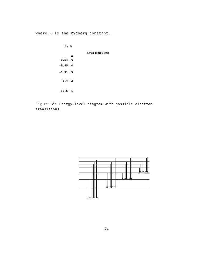
Figure 8: Energy-level diagram with possible electron transitions.

BALMER SERIES(VISIBLE

PASCHEN SERIES(INFRARED)

BRACKETT SERIES

74

It is convenient to represent the energies in anenergy-level diagram, shown in Fig. 8. The lowest levelis called the ground state, and in the hydrogen atom hasthe energy

me4E1 = — 82 0h2 = —13.6 [eV] . (114)

Note that the energy levels get closer together (converge)as the n value increases. Moreover, there is an infinitenumber of possible transitions between the energy levels.It is interesting that the transitions between the energylevels group into series.

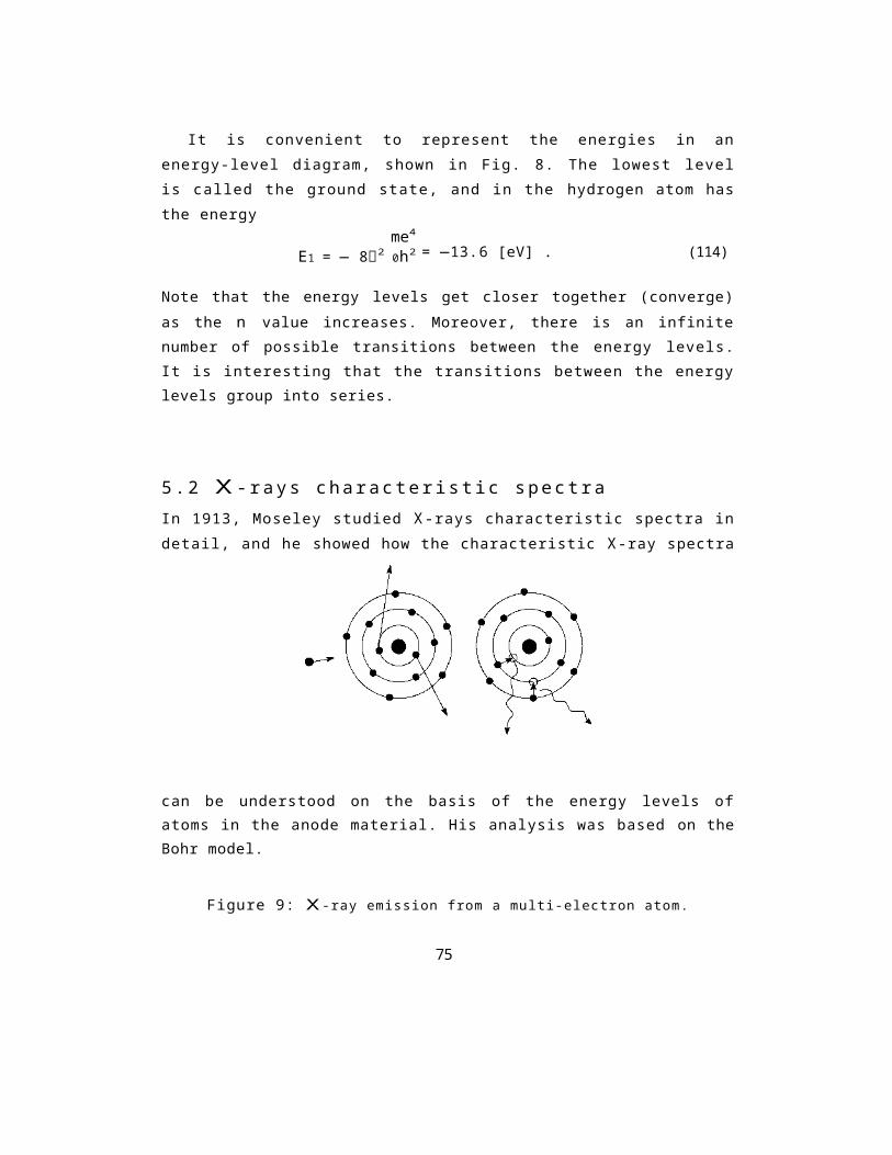
5.2 X -rays characteristic spectraIn 1913, Moseley studied X-rays characteristic spectra indetail, and he showed how the characteristic X-ray spectra

can be understood on the basis of the energy levels ofatoms in the anode material. His analysis was based on theBohr model.

Figure 9: X-ray emission from a multi-electron atom.

75

e

eX-

e

In a multi-electron atom, the fast electrons from thecathode knock electrons out of the inner orbits of theanode atoms, see Fig. 9. The outer electrons jump to theseempty places emitting X-ray (short-wavelength) photons.

76

In summary:

The Planck’s hypothesis of discrete energy quanta was verysuccessful in

explaining experimental results of the black-bodyradiation, photoelectric ef-

fect, Compton scattering, atomic spectra, and X-rayscharacteristic spectra.

5.3 Difficulties of the Bohr modelThe Bohr model was very successful in explaining the discrete atomic spectra of one-electron atoms.

However, there were many objections to the Bohr theory, and to complete our discussion of this theory, we indicate some of its undesirable aspects:

· The model contains both the classical (orbital) and quantum (jumps) concepts of motion.

· The model was applied with a mixed success to the structure of atoms more complex than hydrogen.

· Classical physics does not predicts the circular Bohrorbits to be stable. An electron in a circular orbitis accelerating towards the center and according toclassical electrodynamic theory should gradually loseenergy by radiation and spiral into the nucleus.

· The model does not tell us how to calculate the intensities of the spectral lines.

· If the electron can have only particular energies, whathappens to the energy when the electron jumps from oneorbit to another.

77

· How the electron knows that can jump only if the energy supplied is equal to Em − En.

· The model does not explain how atoms can form different molecules.

· Experiments showed that the angular momentum cannot be n¯h, but \/rather l(l + 1)¯h, wherel= 0,1,2,...,n−1: (Zeeman effect).

78

We see that some of these objections are really of a veryfundamental nature, and much effort was expended in attemptsto develop a quantum theory which would be free of theseobjections. As we will see later, the effort was wellrewarded and led to what we now know as quantum wavemechanics. Nevertheless, the Bohr theory is still frequentlyemployed as the first approximation to the more accuratedescription of quantum effects. In addition, the Bohrtheory is often helpful in visualizing processes which aredifficult to visualize in terms of the rather abstractlanguage of the quantum wave mechanics, which will beanalyzed in details in next few lectures.

Exercise at home:

We usually visualize electrons and protons as spinning balls. Is it a true model? To answer this question, consider the following example.Suppose that the electron is represented by a spinning ball.Using the Bohr’s quantization postulate, find the linearvelocity of the electron’s sphere. Assume that the radiusof the electron is order of the radius of a nucleus, r10_ 1 5 m (1 fm). What would you say about the validity ofthe spinning ball model of the electron?

Challenging problem: Collapse of the classical atom

The classical atom has a stability problem. Let’s model thehydrogen atom as a non-relativistic electron in aclassical circular orbit about a proton. From theelectromagnetic theory we know that a deaccelerating chargeradiates energy. The power radiated during the

79

deacceleration is given by the Larmor formula (32).

(a) Show that the energy lost per cycle is small comparedto the electron’s kinetic energy. Hence, it is an excellentapproximation to regard the orbit as circular at anyinstant, even though the electron eventually spirals intothe proton.

(a) How long does it take for the initial radius of r0 = 1A ˚ to be reduced to zero? Insert appropriate numericalvalues for all quantities and estimate the (classical)lifetime of the hydrogen atom.

80

6 Duality of Light and Matter

We have already encountered several aspects of quantumphysics, but in all the discussions so far, we have alwaysassumed that a particle is a small solid object. However,quantum physics as it developed in the three decades afterPlanck’s discovery, found a need for an uncomfortablefusion of the discrete and the continuous. This appliesnot only to light but also to particles. Arguments aboutparticles or waves gave way to a recognized need for bothparticles and waves in the description of radiation.Thus, we will see that our modern view of the nature ofradiation and matter is that they have a dual character,behaving like a wave under some circumstances and like aparticle under other.

In last few lectures, we discussed the wave and particleproperties of light, and with our current knowledge of theradiation theory, we can recognize the following wave andparticle aspects of radiation:

Wave character Particle character1. PolarizationPhotoelectric effect2. Interference Compton scattering3. Diffraction Blackbody radiation

How can light be a wave and a particle at the same moment? Is a photon a particle or a wave?

An obvious question arises: Is this dual character a property of light or of material particles as well?Then, one may ask: Is an electron really a particle or is it a wave?

81

There is no answer to these questions!

6.1 Matter waves

An important step in the development of a satisfactory quantum theory occurred when Louis de Broglie postulated that:

. Nature is strikingly symmetrical.

82

• Our universe is composed entirely of light and matter.

• If light has a dual wave-particle nature, perhaps matter also has this nature.

The dual nature of light shows up in equations

Each equation contains within its structure both a wave concept (A, u), and a particle (p, E).

The photon also has an energy given by the relationship from the relativity theory

E = mc2 . (116)

Since E = hu = hc/A, we find the wavelength

hA = mc

where p is the momentum of the photon.This does not mean that light has mass, but because

mass and energy can be interconverted, it has an energy that is equivalent to some mass.

De Broglie postulated that a particle can have a wavecharacter, and predicted that the wavelength of a matterwave would also be given by the same equation that heldfor light, where now p would be the momentum of theparticle

hA = mv

where v is the velocity of the particle.

83

hA = p , E=hu. (115)

= hp , (117)

= hp , (118)

Remember this formula! It is the fundamental matter-wave postulate and will appear very often in our journeythrough the developments of quantum physics.

84

If particles may behave as waves, could we ever observe the matter waves?

The idea was to perform a diffraction experiment withelectrons. But an obvious question was: How to performsuch an experiment? What wavelengths can we expect? Toanswer these questions, consider first a simple example.

Example: What is the de Broglie wavelength of an electron whose kinetic energy is K = 100 eV?

Calculate the velocity of the electron from which we than find the de Broglie wavelength corresponding to that velocity.

The velocity of the electron of energy 100 eV is

2 K v = m = 5. 9 × 10 [km/ s] .

Hence, the de Broglie wavelength corresponding to this velocity is

The wavelength is very small, it is about the size of atypical atom. Such small wavelengths can be tested in thesame way that the wave nature of X-rays was first tested:diffraction of particles on crystals.

In 1926, Davisson and Germer, and independently Thompson,performed electron scattering experiments and they foundthat the wavelength calculated from the diffractionrelation

mA=2dsinem, m=0,1,2,... (119)

85

hA = p = h

mv=1. 2[ ˚ A].

is in excellent agreement with the wavelength calculated from the de Broglie relation A = h/p.

They repeated the experiment not only with electrons, butalso with many other particles, charged or uncharged, whichalso showed wave-like character. Thus, for matter as well asfor light, we must face up to the existence of a dualcharacter: Matter behaves is some circumstances like aparticle and in others like a wave.

86

Exercise at home:

If, as de Broglie says, a wavelength can be associatedwith every moving particle, then why are we not forciblymade aware of this property in our everyday experience? Inanswering, calculate the de Broglie wavelength of each ofthe following ”particles”:

1.A car of mass 2000 kg traveling at a speed of 120 km/h.

2.A marble of mass 10 g moving with a speed of 10 cm/s.

3. A smoke particle of diameter 10-5 cm (and a density of,say, 2 g/cm3) being jostled about by air molecules atroom temperature (27oC = 300 K). Assume that theparticle has the same translational kinetic energy asthe thermal average of the air molecules

p2 =2m

32kBT.

6.2 Matter wave interpretation of the Bohr’s model

De Broglie’s wave-particle theory offered anotherinterpretation of the Bohr atom: The Bohr’s condition forangular momentum of the electron in a hydrogen atom isequivalent to a standing wave condition. The quantizationof angular momentum L = n~h means that

mvr = n~hor

nh

87

mv = _____ . (120)2irr

However, if we employ the de Broglie’s postulate that

p = mv = hA , (121)

then, we obtain

nA=2irr , n=1,2,3,... (122)

88

2ð r2r1 2ð

n=1 n=2

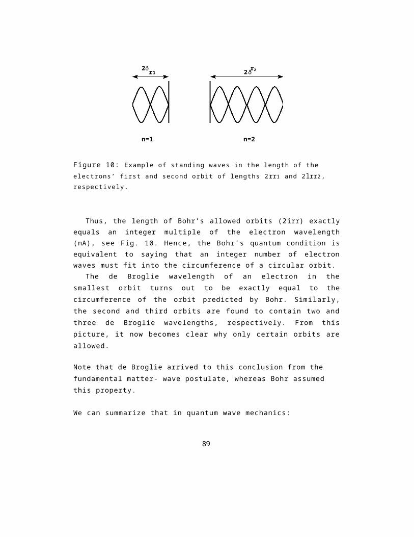
Figure 10: Example of standing waves in the length of the electrons’ first and second orbit of lengths 2rr1 and 2lrr2, respectively.

Thus, the length of Bohr’s allowed orbits (2irr) exactlyequals an integer multiple of the electron wavelength(nA), see Fig. 10. Hence, the Bohr’s quantum condition isequivalent to saying that an integer number of electronwaves must fit into the circumference of a circular orbit.

The de Broglie wavelength of an electron in thesmallest orbit turns out to be exactly equal to thecircumference of the orbit predicted by Bohr. Similarly,the second and third orbits are found to contain two andthree de Broglie wavelengths, respectively. From thispicture, it now becomes clear why only certain orbits areallowed.

Note that de Broglie arrived to this conclusion from the fundamental matter- wave postulate, whereas Bohr assumed this property.

We can summarize that in quantum wave mechanics:

89

1. The electron motion is represented by standing waves.

2. Since only certain wavelengths can now exist, the electron’s energy can take on only certain discrete values.

90

6.3 Wave functionThe idea that the electron’s orbits in atoms correspond tostanding matter waves was taken by Schrödinger in 1926 to formulate wave mechanics.

The basic quantity in wave mechanics is the wave function W(r, t), which measures the wave disturbance of matter waves at time t and at a point (r, t).

Before we explain the physical meaning of the wavefunction, consider an example in which we will describe thewave function in terms of a standing wave.

Consider a free particle of mass m confined between twowalls separated by a distance a. The motion of the particlealong the x axis may be represented by a standing wavewhose equation is

W(x, t) = Wmax sin(kx) sin(wt + ) , (123)where w = 2iru and k = 2ir/A.

The condition required for a standing wave is

from which we find that2ir

k = Aand then

( n )W(x, t) = Wm a x sin a x sin(wt + ). (126)The wave equation carries the information that the amplitude of the motion of the particle is quantized. Also, the linear momentum is quantized. Since

2aA = n

we can replace A by h/p, and obtainh

p = n . (128)2a

The momentum is related to the energy E, which gives

91

A n = 1 , 2 , 3 , . . . (124)a = n 2,

= nira , (125)

, (127)

This indicates that the energy of the particle isalso quantized. Thus, the particle cannot have any energy.

92

p2=n2_____h28ma 2 E , . (129)

1E=2m

6.4 Physical meaning of the wave functionWe can summarize what we have already learnt, that aparticle can behave like a wave, but a particle has massand some of them have electric charge. Does this mean thatthe mass and charge of an electron, for example, arespread out over the extent of the wave? This would becrazy. It would mean that if we isolate just a part of thewave, we would obtain a fraction of an electron charge.

How then should we interpret an electron wave?

The answer is that the wave itself does not have anysubstance. It is a probability wave. When we talk abouta particle wave, the amplitude of the wave at aparticular point tells us the probability of finding theparticle at that point.

The wave function of a particle describes theprobability distribution of a particle in space, just asthe wave function of an electromagnetic field describesthe distribution of the EM field in space.

From the interference and diffraction theorem, we knowthat the intensity of the interference pattern isproportional to the square of the field amplitude, oralternatively to the probability that the waves interferepositively or negatively at some points.

In analogy to this, Born suggested that the quantityW(r) 2 at any point r is a measure of the probabilitydensity that the particle will be found near that point.More precisely, the quantity W(r) 2dV is theprobability that the particle will be found within avolume dV around the point at which W(r) 2 is evaluated.

Since W (r) 2dV is interpreted as the probability, it is

93

normalized to one asV W(r) 2dV = 1 . (130)

Example:

Consider the wave function at time t = 0 of a freeparticle confined between two walls, Eq. (126). In thiscase, the probability density of finding the particle ata point x is given by

nir

( x , 0 ) 2 = m a x 2 s i n 2 a x . (131)

94

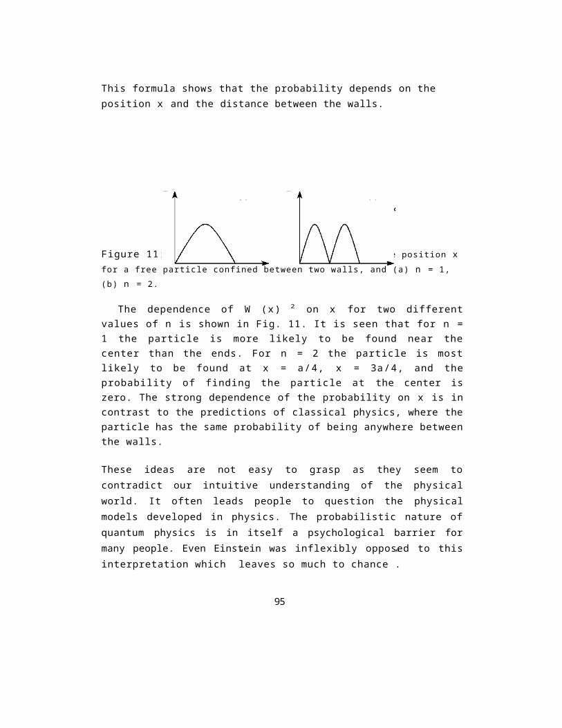
This formula shows that the probability depends on the position x and the distance between the walls.

0 xa x a/2 a

0

Figure 11: Probability density as a function of the position xfor a free particle confined between two walls, and (a) n = 1, (b) n = 2.

The dependence of W (x) 2 on x for two differentvalues of n is shown in Fig. 11. It is seen that for n =1 the particle is more likely to be found near thecenter than the ends. For n = 2 the particle is mostlikely to be found at x = a/4, x = 3a/4, and theprobability of finding the particle at the center iszero. The strong dependence of the probability on x is incontrast to the predictions of classical physics, where theparticle has the same probability of being anywhere betweenthe walls.

These ideas are not easy to grasp as they seem tocontradict our intuitive understanding of the physicalworld. It often leads people to question the physicalmodels developed in physics. The probabilistic nature ofquantum physics is in itself a psychological barrier formany people. Even Einstein was inflexibly opposed to thisinterpretation which ”leaves so much to chance”.

PP(b(a

95

”I cannot believe thatGod plays dice with the cosmos”Albert Einstein

Remember:Wave function W(r, t) of a particle is mathematical construct only.Only W(r, t) 2 has physical meaning - probability density, and W(r, t) 2dV is the probability of finding the particle in the volume dV.

96

6.5 Phase and group velocitiesIs there an analogy between the matter waves and

radiation? Matter waves

hA = p

where v is the velocity of a particle of the mass in.

ParticlesE =i n c 2 =h u . (133)

Hence, the wave-radiation relation leads to the velocity ofthe matter waves

The velocity u is called a phase velocity of the matterwaves. Thus, the velocity of the matter waves is largerthan speed of light in vacuum, u > c, unless v > c.

This result seems disturbing because it appears that thematter waves would propagate faster than the speed of lightand would not be able to keep up with particles whosemotion they govern.

However, the phase velocity of a wave is the velocity ofthe wave front, not its amplitude. The maximum of theamplitude of a given wave can propagate at differentvelocity, called group velocity. At this velocity theenergy (information) is transmitted. Usually, vg = u, butin the case of dispersion, u(u), the group velocity vg <u.Thus, the matter wave should be dispersive to match therequirement of vg <u when u> c.

Are the matter waves dispersive?

97

= hinv , (132)

hu = Au =

inc2inv h

= c2

v . (134)

Let us answer this by first defining the phase and group velocities.

Consider two waves of slightly different k and w, and propagating in the same direction. Let

k 1 = k 0 + /k , w1 = w0 + /w ,k 2 = k 0 - / k , w2 = w0 - /w , (135)

98

Take a linear superposition of the two wavesW(r, t) = 2ei(k 1·r−w 1t) + 1

1 2ei(k2·r−w2t) . (136)

Then, using Eq. (135) and the Euler’s formula (e ±ix = cos x± i sin x), we obtain

2ei[( k 0+ k) · r −( w 0+ w) t] + 1

1W (r, t) = 2ei[(k 0−Jk)i·r− (w 0 −w)t]

= ei( k 0 · r − w 0 t) cos (/k · r − /wt) , (137)

where · r is the distance the wave propagated, and is the unit vector in the k direction.

We see from Eq. (137) that in time t the fast varying function propagates a distance

w0 · r = t = ut ,

(138)k0

whereas the envelope propagates a distance

Hence, the envelope propagates at velocity vg = dw/dk, which is called the group velocity.

The envelope forms so called wave packets. we have already seen that the amplitude of the wave packet propagates with velocity vg.

Consider energy of a particle

99

/wi-. · r-. = /kt =

dwdk t = vgt. (139)

If the energy of the particle is quantized, E = ¯hw, and

then

100

1E = 2 m p 2 =

¯h2___k2 . (140)2 m

¯hdw= ¯h22m 2kdk , (141)

from which we find that

=0. (142)

Hence, if E = ¯hw then the matter waves are dispersive.

Exercise 1:

What is the group velocity of the wave packet of a particle moving with velocity v?

Solution:

From the definition of the group velocity, we have

where p = ¯hk. HoweverE2=m2 0c4+p2c2 . (144)

Thus

2EdE = 2pc2dp. (145)

from which we find that

Hence, vg = v, the group velocity is equal to the velocityof the particle. In other words, the velocity of theparticle is equal to the group velocity of the correspondingwave packet.

Exercise 2:

The dispersion relation for free relativistic electron waves is

dE=

dppc2

E

mvc2=______

mc2=v. (146)

101

dw ¯hk=d k m

dv2 dk

d ( hv ) 2

d(hk)

dE= dp , (143)vg =

dwdk

,/ w k = c2k2 + (mc2/¯h)2 .

102

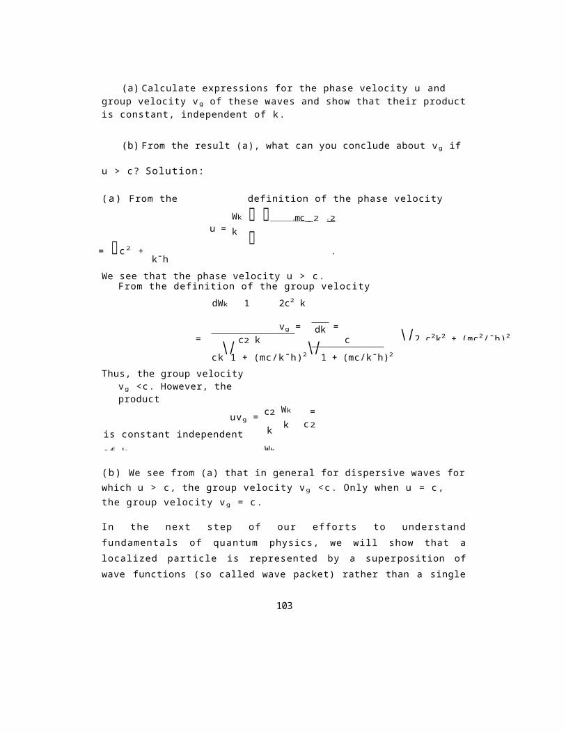
(a) Calculate expressions for the phase velocity u and group velocity vg of these waves and show that their productis constant, independent of k.

(b) From the result (a), what can you conclude about vg if

u > c? Solution:

(a) From the definition of the phase velocity

mc __2 2

= c 2 + .

k¯hWe see that the phase velocity u > c.

From the definition of the group velocitydWk 1 2c2 k

c2 k c\/ \/ck 1 + (mc/k¯h)2 1 + (mc/k¯h)2

Thus, the group velocity vg <c. However, the product

uvg =is constant independent of k.

c2

k

Wk

Wkk

=c2

(b) We see from (a) that in general for dispersive waves forwhich u > c, the group velocity vg <c. Only when u = c, the group velocity vg = c.

In the next step of our efforts to understandfundamentals of quantum physics, we will show that alocalized particle is represented by a superposition ofwave functions (so called wave packet) rather than a single

103

u =Wkk

vg = =dk \/2 c2k2 + (mc2/¯h)2=

wave function. Important steps on the way to understandthe concept of wave packets are the uncertainty principlebetween the position and momentum of the particle, and thesuperposition principle.

104

”What the electron is doing during its journey in the interferometer? During this time the electron is a great smoky dragon,which is only sharp at its tail (at the source) and at its mouth, where it bites the detector”J.A. Wheeler

6.6 The Heisenberg uncertainty principle

In quantum physics, we usually work with the wave functionW, whose W 2 describes a probability that a given object,e.g. a particle, is moving with a velocity v0. A non-zeroprobability means that we are not precisely sure that thevelocity of the particle is v0. We may say that thevelocity is v0 with some error, Lv0, which is calleduncertainty.

Consider a typical diffraction experiment shown in Fig. 12.

105

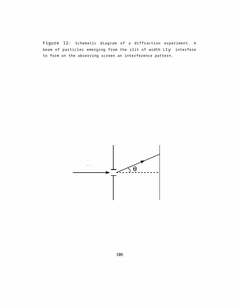
Figure 12: Schematic diagram of a diffraction experiment. Abeam of particles emerging from the slit of width LIy interfereto form on the observing screen an interference pattern.

106

A

vΔ

The position of the first minimum in the diffraction pattern is given by s i n = y

A . (147)In order to reach the point A, the particle has to gaina velocity in the y-direction,such that

v ys i n = v 0

Comparing Eqs. (147) and (148),we find

v y =v0

orvyy = v0A.

(149)However, from the deBroglie postulate

h = p

and therefore

p yy = h, (151)where /py = m/vy.

The relation (151) is called the Heisenberguncertainty principle and states that it is impossible tomeasure the momentum py and position y of a particlesimultaneously with the same precision. If the particle iscompletely unlocalized, Ly * oc, the momentum is certain,1py * 0.

The Heisenberg uncertainty principle is not a statementabout the inaccuracy of measurement instruments, nor areflection on the quality of experimental methods. It arisesfrom the wave properties inherent in the quantum mechanicaldescription of nature. Even with perfect instruments andtechniques, the uncertainty is inherent in the nature ofthings.

107

. (148)

ALy

= hmv0 , (150)

Exercise:

Last year after the lecture on uncertainty principle, a student asked a question: ”If I do not move, does it mean that I am everywhere”?How would you answer to this question?

108

6.7 The superposition principleIn quantum physics, a particle is represented by a wave function

W(r, t) = Aei(k·r−7t) . (152)

Since, W(r, t) 2 = A 2 = const., we see that the particleis completely unlocalized in space, that can be foundanywhere in space with the same probability. However, weknow that in practice particles are localized in space andtheir position can be given with some approximation. Inother words, particles are partly localized. Therefore, awave function such as (152) cannot represent a real physicalsystem.

According to the uncertainty principle, a particle partly localized (Lir) has an uncertainty in the momentum (Lip). Hence, if

W1(r, t) = A1ei(p 1·r/¯h−1t) (153)

is a wave function of the particle located atr, then

W2(r, t) = A2ei(p2·r/¯h−2t) , (154)

where, p1 − p2 <Lip , is also a wave function of the particle.

Moreover, any linear combination of the two wave-functions is also a wave-function of the particle, i.e.

W(r, t) = aW1(r, t) + bW2(r, t) , (155)

where a and b are complex numbers.Thus, a single wave function cannot represent a particle

of a given momentum.Equation (155) is an example of the superposition

principle which, in general, holds for an arbitrary numberof the wave functions.

109

It follows from the superposition principle that thewave function of a particle is represented by the sum of aset of sinusoidal waves exp [i( k·r−kt)]. The sum is ofcourse an integral

W(r, t) = k A(k)ei(k·r−kt)d3k , (156)

where d3k is the element of volume in k-space (momentumspace). In other words, the set contains an infinite numberof waves with continuously varying wave-number k.

110

One can see from Eq. (156) that the mathematics used incarrying out the procedure of obtaining a superposition wavefunction involves the Fourier transformation (Fourierintegral). If the superposition function is known, theamplitude A(k) can be found employing the inverse Fouriertransformation

A(k) =    1 V W(r, t(157)

/ 2 ir

In summary:

The superposition principle is in the complete contrastwith classical mechanics. In classical mechanics asuperposition of two states would be a complete nonsenseas it would imply that a particle could simultaneouslyoccupy two or more points in space. According to quantumphysics, a particle can exist in two or more states at thesame time. If more particles are involved, a superpositionof these particles is called entanglement. The su-perposition principle and entanglement have been exploitedin recent years in three important applications. Thefirst is quantum cryptography, where a communicationsignal between two people can be made completely secure fromeavesdroppers. The second is quantum communication, wherecapacities of transmission lines can be increased in comparewith that of classical transmission systems. The third isproposed device called a quantum computer, where allpossible calculations could be carried out simultaneously.

6.8 Wave packets

111

In the superposition state (156), the particle no longerhas a well defined momentum. Such a superposition isnamed a free particle wave packet. The relation (156) alsoshows that the momentum and then also the positiondistribution are roughly pictured by the behavior of A(k) 2

We now consider the motion of a free particle wave packet. For simplicity, we consider the motion in one-dimension (1D). In this case

0 0

(r, t) -* (x, t) = _ 0 0 A (k) e i ( k x _ k t ) d k ,(158)

where k = kx.

Let us suppose that A(k) has a maximum at k = k0 andrapidly goes to

zero for k = k0, and Lk is the region where A(k) = 0.Firstly, we will find the shape of the wave-function at t = 0.

At t = 0: 00W(x, 0) = −00 A (k) eikxdk . (159)

At x = 0, exp(ikx) = 1, indicating that all waves havethe same phase. For x = 0, the waves with different khave different phases. If Lx is the displacement of x fromx = 0, the maximal and minimal phases of the packet are( )

k0 - 1ix 2/k, minimal

( )k0 + 1

ix 2Lk, maximal.Since the phases are different, the waves will interferewith each other. The maximum of interference appears for the

112

difference between the phases equal to 2ir. Thus,

LxLk = 2ir. (160)

Hence, the particle can be found at points for which Lx =2ir/Lk, i.e. determined by the uncertainty relation.

Now, we will check how the packet moves in time.In order to do it, we expand wk into a Taylor series about k = k0. Taking k = k0 + 3, and wk0 = w0, we get1 ( d 2 w

32 +2 d32 k 0

If we take only first two terms of the series and substitute to W(x, t), we obtain 00

W(r, t) = ei(k0x−0t) −00 d3A (k0 + 3) ei(x−vgt) ,(162)

/ dw \where vg = k0 is the group velocity of the packet.d

113

(dw )wk = wk0+ = w0 + 3 +

d3 k0

. . . (161)

If we increase x by Lx, i.e. x —* x + Lx, then

ei(x _v gt) = ei/3xei/3(1x _v gt) . (163)

Then, for Lx = vgt we obtain the same packet as for t = 0, but shifted by vgt. Hence, the group velocity is the velocity of the packet moves as a whole. If we include thethird term of the Taylor expansion (161), we get

0 0

( r , t ) = e i ( k 0 x _ 0 t ) _ 0 0 d 3 A (k 0 + 3 )[ ( ]

( dv g ) )x exp i3 x − vg +    3 t .________________________(164)d3 k0

(dv g )The term vg + k0 3 plays the role of the velocity of the wave packet, d which now depends on 3. Thus, different parts of the wavepacket will move with different velocities, leading to aspreading of the wave packet. This spreading is due todispersion, that vg depends on 3.

We now can explain the connection between the group velocity and the phase velocity, and the role of dispersion.

Phase velocity u = k ,

dwGroup velocityvg = dk .

Hence

dk(ku) = u + k dud dk . (165)Thus, vg depends on k when du

dk = 0, i.e. when the phase velocity depends on k. The dependence of u on k is called dispersion.

Thus, we can say that the spread of the wave packet is due to the dependence of the phase velocity on k, [vg= u

114

vg =dwdk =

whendu

dk = 0].

115

In summary of this lecture: We have learnt that

1. In quantum physics, localized particles are representedby a superposition of wave functions (so called wavepacket) rather than a single wave function.

2.The maximum of a wave packet moves with the groupvelocity.

3. Since the matter waves are dispersive, a wave packet spreads out in time.

116

7 Schrödinger Equation

The Schrödinger equation is the basic relationship for determining wave functions and energy levels of a given physical system.

Consider a wave function of a particle moving along the x-axis

W = Wmaxe i(kx —wt). (166)

We will try to find a differential equation representingthe energy of the particle, whose the solution is the wavefunction (166), with the following conditions

· The equation must be linear.

· Coefficients appearing in this equation should only depend on the parameters characteristic of the particle.

We will limit our considerations the the non-relativistic case only.

7.1 Schrödinger equation of a free particleFirst, we will consider the case of a free particle. In this case the energy and momentum of the particle are related by

E = 2m |p|2 .1 (167)

Since E = ¯hw and p = ¯hk, we get

h¯w = ____k2. (168)

2m

117

Note that:

1. Taking the first derivative of Eq. (166) over x is equivalent to multiply W(x,t) by ik.

2. Taking the first derivative of Eq. (166) over t is equivalent to multiply W(x,t) by −iw.

118

Thus, from Eq. (168), we can conclude that thedifferential equation should be the first order in t andthe second order in x. The simplest equation of this formis

aW(x,t)at

= F2 a2W(x,t)

where F is a parameter, which we have to find.Substituting Eq. (166) into (169), we find

—iw = —F2k2 , (170)

and then from Eq. (168), we find that

F2 = i¯h . (171)2m

Thus, the wave function (166) satisfies the following differential equation

orequivalentl

aW(x,t)at

i¯h a2W(x,t)= ____ ax 2___ , (172)

2m

Equation (173) is the one-dimensional Schrödinger equationfor a free particle.

It is easy to extend the equation to three dimensions

where

i ¯haW(r,t) +at

¯h2 V2W(r, t) = 0,

___(174)

2mW(r, t) = Wmaxei( k·r—wt) . (175)

i ¯haW(x,t)+

¯h2a2W(x,t =0. (173)2m ax2

119

7.2 Operators

We can write the Schrödinger equation as( ¯ h ) ( ¯ h )

a 1 (r, t) = i V

i V w(r, t) ,______________(176)a t 2 mwhich shows that the Schrödinger equation can be obtainedfrom the energy (Hamiltonian) of the free particle (E = |p|2/2m) simply replacing E and p, respectively, by

E—* −¯hi

aat,

h¯p —* i V . (177)

Hence, in quantum physics the physical quantities are represented by mathematical operations, which are called operators.

V and a/at define operations to be carried out on thewave function W. The particular operation stated in Eq.(176), aw/at consists of taking a partial derivative ofW in terms of t, and V2W consists of taking partialderivatives of W in terms of Cartesian coordinates.

Example:

Calculate (a) t and (b) V2W, where W = Wm a xei ( k x _ t ).

Solution:

(a) The partial derivative of W in terms of t isa a = m a xei(kx_ wt) = −iwWm a xei(kx_ )t) = −iwW . (178)

a t a tThus, the operation of the operator a/at on the wave

120

¯h−i

function W results in a constant −iw times the originalwave function. We will see later, that such a wavefunction is called in quantum physics an eigenfunction ofthe a/at operator.Solution of the part (b) is left to the students.

121

Important property of operators:

In classical physics the multiplication of two quantities,say x and p X, is immaterial. However, in quantum physics,where physical quantities are represented by operators,the order of multiplication is important and, for example,xpX = pXx, where pX = —i¯h8/8x. We say that the twoquantities, x and pX, do not commute.1

A measure of the extent to which xp X = p Xx is given by the commutator bracket

[ˆx, ˆpX] = ˆxˆpX — ˆpXˆx , (179)

where the symbol ”ˆ” over the functions x and p X indicates that these functions are operators.

Note that the coordinates of r are the same in operator and classical forms. For example, the coordinate x is simply used in operator form as x.

How to calculate the commutator [ˆx, ˆpX]?

Since operators are ”action” operations on functions, we consider the action of this commutator on a trial function W(x):

f —i¯h8w + i¯h 8

[ˆx, ˆp X] (x) = x 8 x (xW)8x8 W 8W

= —i¯hx_____+ i ¯hW + i¯hx_= i¯hW . (180)8x 8x

Hence

[ˆx, ˆpX] = i¯h . (181)

It is easily to show that, in general, the components of the position rˆ and momentum p ˆ' operators satisfy the commutation relations

[ˆrm, ˆpn] = i¯h8mn , m,n=1,2,3, (182)

122

' Commutation consists in reversing the order of two quantities in an algebraic operation.

123

ˆr 1 = xˆ , ˆr 2=y ˆ , ˆr 3=zˆ ,ˆp1 = ˆp x, ˆp2= ˆp y, ˆp3 = ˆp z, (183)

and 8mn is called Kronecker 8 function, defined as

1 i f m = n

0 i f m = n .

Using the operator representation, the Schrödinger equation is often written as

i¯haw(r, t)at

= ˆHw(r, t) , (185)

where Hˆ = − ¯h22mV2 is the Hamiltonian (energy operator) of the free

particle.

7.3 Schrödinger equation of a particle in an external potential

In physics, we often deal with problems in whichparticles are free within some kind of boundary, but haveboundary conditions set by some external potentials. Theparticle in a box problem, discussed before, is thesimplest example.

In the presence of an external potential V(r, t), theHamiltonian of the particle takes the form

¯h2H ˆ =− V 2 +V ˆ ( r , t ). (186)

2mThe wave function of the particle moving in the externalpotential can be different from that of the freeparticle. The wave function is found solving the

124

8mn =(184)

where

Schrödinger equation the with following conditions

1. The wave function must be determined and continuous inany point of the space(r, t).

2. The wave function vanishes at ±oc.

125

We will try to solve the Schrödinger equation assumingthat the Hamiltonian H ˆ does not explicitly depend ontime, i.e. Vˆ (r, t) = Vˆ (r). In this case, theSchrödinger equation (SE) contains two terms: onedependent on time t, and the other dependent onr, i.e.

(

i¯h t - H ˆ = 0, (187)

where H ˆ depends solely on r.Since the time and r dependent parts are separated,

the solution of the SE will be in the form of a product of two functions q(r) and f(t):

W(r, t) = q(r)f(t). (188)

Substituting this equation into the SE, we get

i ̄ hq ( r ) d f ( t ) dt = f(t)ˆHq(r)

where f f(t), and q q(r).The left-hand side of Eq.

(189) is a function of onlyone variable t, whereas theright-hand side is a

function of only the positionr, i.e. each side isindependent of any changes in the other. Thus, both sidesmust be equal to a constant, say E:

= E, (190)1q

ˆHq = E. (191)

We can easily solve Eq. (190), and the solution can be written directly as f(t) = Ce− h¯ Et

=dfd

i¯h 1f

dfdt

i¯h 1f

126

ˆHq , (189)1q

i , (192)where C is a constant.

Equation (191) can be written asˆHq = Eq, (193)

127

which is called the stationary (time-independent) Schrödinger equation, or the eigenvalue equation for the Hamiltonian ˆH.

Hence, the solution of the SE is of the formW(r, t) = Cq(r)e− h¯ Et

i , (194)

where q(r) satisfies the eigenvalue equation (193).

Note, that the probability density

|W(r, t)|2 = |Cq(r)|2 , (195)

is independent of time.Thus, when the Hamiltonian of a particle is independent

of time, the probability of finding the particle in anarbitrary point r is independent of time. Such a state(wave function) is called a stationary state of theparticle.

The existence of stationary states has two very usefulpractical consequences. Physically, such states have apermanence in time, which allows their long timeexperimental investigations. Mathematically, they reducethe Schrödinger equation to the eigenvalue equation forthe Hamiltonian. Thus, in order to obtain specific valuesof energy and corresponding wave functions, we operate onthe wave function with the Hamiltonian and solve theresulting differential equation. However, not allmathematically possible solutions are accepted. Physicsimposes some limits on the solutions of the Schrödingerequation.

The solution of the Schrödinger equation should satisfy the following conditions:

128

1.The wave function q must be finite in all points of the space.

2. The wave function q must be continuous, and should have continuous first derivatives.

3.The wave function q must be a single-value function at any point r.

4.The wave function must be normalized.

129

When an operation on a wave function gives a constanttimes the original wave function, that constant is calledan eigenvalue and the wave function is called aneigenfunction or eigenstate. Thus, the wave functionwhich satisfies the stationary Schrödinger equation is the

eigenfunction of the Hamiltonian ˆH, and E is theeigenvalue of the Hamiltonian in the state çb.

The complete set of eigenvalues of the Hamiltonian H ˆ istermed energy spectrum. The energy spectrum can benondegenerated (different eigenfunctions have differenteigenvalues), or degenerated (all or few eigenfunctionshave the same eigenvalues), but it is not allowed that oneeigenfunction could have few different eigenvalues.

In summary of the lecture on the Schrödinger equation: We have learnt that

1.In quantum physics, physical quantities are represented by operators.

2. The operator representing the energy of a system is the Hamiltonian ˆH.

3.The eigenvalues of H ˆ are energies E.

4.If the potential V ˆ is independent of time, then separation of variables is possible, and we can write the wave function as W(r, t) = (r)f(t).

5.The wave function (r) is the eigenfunction of thetime-independent Hamiltonian H ˆ and can be found bysolving the stationary Schrödinger equation ˆH(r) =E(r).

130

7.4 Equation of continuity

We know that the probability is normalized to one, i.e.

|W(r)|2dV = 1 . (196)

The normalization must be valid for any wave functionevaluated at any

point r and at any time t. We will show that theSchrödinger equation

guarantees the conservation of normalization of the wave function. In other words, if W was normalized at t = 0, it will remain normalized at all times.

In addition, there is a flow of the probability densityor particle current density associated with a movingparticle. Therefore, we will also define what theparticle probability current density is in terms of theparticle wave function.

Suppose we have a particle described by a wave function W in a volume V enclosed by a surface S.

Consider the time evolution of the particle wave function, that is given by the time-dependent Schrödinger equation

i¯haW

at¯h2

= −____V2W+ Vˆ W. (197)2m

Take complex conjugate of the above equationi¯haW*

at¯h2

= −____V2W + Vˆ W . (198)2m

Multiplying Eq. (197) by W and Eq. (198) by W, and subtracting the resulting equations, we get

( ) (W* a W at + WaW = −_ ¯h2 W*V2W − WV2W*)i¯h . (199)

131

at 2mHowever

W* aW + WaW* a______= at |W|2 , (200)at at

and using the relation( )

V . u A = Vu . A + uV . A , (201)we find that

V. (W*VW − WVW*)

=V W * . V W+W * V . (V W)− V W. V W * − WV . (V W * )

= WV2W − WV2W . (202)

132

Thus h ̄

t | | 2 + · 2 i m ( * − * ) = 0 .(203)

Introducing a notation

|| 2 = p ,2im (W*VW − WVW*) =h¯ J , (204)

we get the continuityequation

p + J= 0 . (205)

This equation is well known from hydrodynamics andelectrodynamics and shows the conservation of matter orthe conservation of charge. In our case, the continuity

equation shows the conservation of the probabilitydensity p, and J is the probability current density.

Figure 13: Probability current density J crossing a surface S, with n ˆ- the unit vector normal to the surface.

To interpret the continuity equation, it is convenient

133

AdS = n J

dS

S

to integrate Eq. (205) over the volume V closed by a surface S, see Fig. 13:

V || 2dV = − V · JdV . (206) t

134

From the Gauss’s divergence theoremIV V . JdV = J . dS , (207) S

we getI a V || 2dV = − J . d S . (208)at S

The lhs of this equation is the time rate of increase ofprobability of finding the particle inside the volume V.The integral on the rhs is the probability per unit timeof the particle leaving the volume V through the surfaceS.

The scalar product J . dS is the probability that theparticle will cross an area dS on the surface. When theparticle remains inside the volume for all times, i.e. doesnot cross the surface S, then J . d S = 0, and we getthat

Ia V |W|2dV = 0 , (209)atwhich shows that the Schrödinger equation guarantees theconservation of normalization of the wave function. Inother words, if W was normalized at t = 0, it will remainnormalized at all times.

Suppose that particles inside the surface are representedby plane waves i n(r) = Aei k 1 · r + Be− i k 1 · r , (210)and outside the surface

Wout(r) = Cei k2 ·r , (211)

where k1 and k2 are the wave vectors of the particle

135

Jin=h¯2im (W inVWin − WinVW

i n) =

¯h

k1( |A|2 − |B|2) , (212)

and

J o u t

= 2 i m ( o u t o u t − ¯h k2 |C|2 . (213)m

h¯

inside and outside the surface, respectively.To interpret the wave functions, we calculate the

probability current densities inside and outside the surface, and find

Inside the surface, the current density can be written as

Jin = Ji + Jr (214)

where

Ji= ¯h k1 |A|2 (215)m

is interpreted as the incident particle current, and

Jr = ̄ h k1 |B|2 (216)

m

is interpreted as the reflected particle current. The current density outside the surface

Jt= ¯h k2 |C|2 (217)m

is interpreted as the transmitted

particle current. We can define the

reflection coefficient of the surface

136

R= | Jr| | Ji| , (218)

which is given by the probability current density reflected from the surface divided by the probability current density incident on the surface.

We can also define the transmission coefficient of the surface

T= | J t | | Ji| , (219)

which is given by the probability current density transmitted through the surface divided by the probability current density incident on the surface.

137

Using Eqs. (215)−(217), we can write the reflection and transmission coefficients as

R = B 2 k2_C 2A 2 , T = k1 A 2 , (220)

where k 1 = k 1 and k 2 = k 2 .

Thus, if B 2 = A 2 then R = 1, i.e. all the particlesthat are incident on the surface are reflected.

Exercise at home:

It is easy to show from the definition of theprobability current density, Eq. (204), that in generalwhen the wave function W of a particle in a given region isreal, the current density J = 0 in this region.How would you interpret this result?

138

8 Applications of the Schrödinger Equation: Potential (Quantum) Wells

We have seen that the wave nature of particles plays animportant role in their physical properties that, forexample, particles confined into a small bounded area canhave only particular discrete energies. However, thequestion we are most interested in is: can we create anartificial structure which exploits discrete energy levels?We can produce such structures, they involve potentialbarriers. One dimensional structures such constructed arecalled quantum wells, two dimensional are called quantumwires, and three dimensional are called quantum dots.

To illustrate that particles really exhibit unusualquantum effects when are located in such structures, we willsolve the time-independent Schrödinger equation

ˆH(r) = E(r), (221)

to find the eigenvalues E and the eigenfunctions (r) of a particle of a mass m moving in a potential V ˆ (r) that varies with the position r.

In this and the following lecture, we will limit our calculations to the one-dimensional case, in which the Hamiltonian of the particle is given by

With this Hamiltonian we get, from the SE, a second-order differential equation for the wave function of the particle

139

Hˆ =¯h2d22m dx2

+

Vˆ (x) . (222)

d 2 ( x ) dx2

which can be

2m= -____¯h2 (E - V(x)) (x) , (223)

where

d 2 ( x ) dx2

= -k2(x)(x) , (224)

(

2m E - V ˆ (x)k2(x) = ¯h2 . (225)

140

WhenV ˆ (x) is independent of x, i.e. the particle ismoving along the x axis under the influence of no forcebecause the potential is constant, the parameter k2(x) =k2, and then Eq. (224) reduces to a simple harmonicoscillator equation

d 2 (x)dx2

= —k2 (x) . (226)

This is a linear differential equation with a constantcoefficient. The solution of Eq. (226) depends on whether k2> 0 or k2 < 0. For k2 > 0, the general solution of Eq.(226) is in the form of an oscillating wave

(x) = Aeikx + Be−ikx , (E> V) . (227)

where A and B are amplitudes of the particle wave moving to the right and to the left, respectively.

For k2 < 0, the general solution of Eq. (226) is in the form

(x) = Ce−kx + Dekx , (E < V) , (228)

that the exponents are real and no longer represent an oscillating wave function. They represent a wave function with damped amplitudes.

Important note: The general solution (227) with bothconstants A and

B different from zero is physically acceptable. However,the general solution (228) with both constants C and Ddifferent from zero cannot be accepted. We have learntthat the wave function must vanish for x -* ±oc. Thus,if the particle moves in the direction of positive x, thenonly the wave function with C = 0 and D = 0 willsatisfy this condition, and vice versa, if the particlemoves in the direction of negative x, only the wavefunction withC = 0 and D = 0 will satisfy the condition of (x) -* 0

141

as x -* —oc.

Another important observation: The solutions (227) and(228) are single value solutions for the wave function(x). Thus, for the particle moving in an unbounded areawhere the potential V ˆ is constant, there are no restric-tions on k which, according to Eq. (225), means that thereare no restrictions on the energy E of the particle. Hence,the energy E of the particle can have any value rangingfrom zero to +oc (continuous spectrum). It is also validfor x-dependent potentials, where V(x) slowly changes withx.

For potentials rapidly changing with x the particle canbe trapped in potential holes, and then E can be different.

142

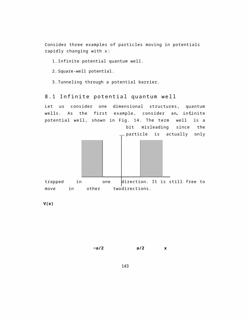
Consider three examples of particles moving in potentials rapidly changing with x:

1. Infinite potential quantum well.

2. Square-well potential.

3. Tunneling through a potential barrier.

8.1 Infinite potential quantum wellLet us consider one dimensional structures, quantumwells. As the first example, consider an infinitepotential well, shown in Fig. 14. The term ”well” is a

bit misleading since theparticle is actually only

trapped in one direction. It is still free tomove in other twodirections.

V(x)

a/2 x−a/2

143

Figure 14: An infinite

potential well. For the infinite

potential well

aV (x ) = 0 for − 2 x a 2 ,

a aV (x ) = o c for x < − 2 and x > 2 . (229)

According to classical physics, the particle trappedbetween the walls will

bounce back and forth indefinitely, its energy will beconstant E = mv 2/ 2.

144

Moreover, the probability of finding the particle at anypoint between the walls is constant, and anywhere outsidethe walls is zero. In fact, if we know the initial momentumand position of the particle, we can specify the locationof the particle at any time in the future. The classicalcase seems trivial. But, what quantum physics tells usabout the behave of the particle?

According to quantum physics, the particle is describedby a wave function (x), which satisfies the Schrödingerequation and some boundary conditions. One of the boundaryconditions says that the wave function (x) must befinite everywhere. Thus, in the regions x < —a/2 and x >a/2, the wave function (x) must be zero to satisfy thiscondition that V(x) (x) must be finite everywhere.

In the region — a 2 < x< a 2, the potential V(x) = 0,

and then the Schrödinger equation for the wave function isd 2 ( x ) dx2 = —k2 (x) , (230)

where now k2 = 2mE/¯h2.Since k2 is positive, the Schrödinger equation (230) has a

simple solution(x) = Aeikx + Be−ikx , —a 2 <x < a 2 , (231)

where A and B are constants, that in general are complex numbers.

In order to determine the unknown constants A and B, wewill use the boundary condition that the wave function mustbe continuous at x = —a/2 and x = a/2.

Usually, we find the constant B in terms of A, and thenwe find the remaining constant A from the normalizationcondition that the wave function is normalized to one,i.e.

− dx | (x)|2 =1. (232)

145

Since in the regions x < —a/2 and x > a/2, the wavefunction is equal to zero, and the wave function must becontinuous at x = —a/2 and x = a/2, we have that (x) = 0at these points. In other words, the wave functions mustjoin smoothly at these points.

Thus, at x = —a/2, the wave function (x) = 0 whenika

Ae− ika+ Be = 0 . (233)

146

At x = a/2, the wave function (x) = 0 whenika ika

A e 2 +B e _ 2 = 0. (234)

From Eq. (233), we find that

B = _ A e _ u l , (235)

whereas from Eq. (234), we find that

B = _Aeul . (236)

We have obtained two different solutions for thecoefficient B. Accepting these two different solutions,we would accept two different solutions for the wavefunction. However, we cannot accept it, as one of theconditions imposed on the wave function says that the wavefunction must be a single value function. Therefore, wehave to find a condition under which the two solutions(235) and (236) are equal. It is easily to see from Eqs.(235) and (236) that the two solutions for B will beequal if

e_ul = eul , (237)

which will be satisfied when

e2ul = cos(2ka) + i sin(2ka) = 1, (238)

or when

cos(2ka) = 1, (239)

i.e. when

Thus, for a particle confined in the infinite well there is a restriction for k, that k can only take discrete

147

k=na , with n = 0 , 1 , 2 , . . . . ( 2 4 0 )

values.Since k2 = 2mE/¯h2, we see that the energy of the

particle cannot be arbitrary, it can only takes on certaindiscrete values!

¯h2_k2 = n2 2¯h2E n = 2 m a 2 . (241)

2m

148

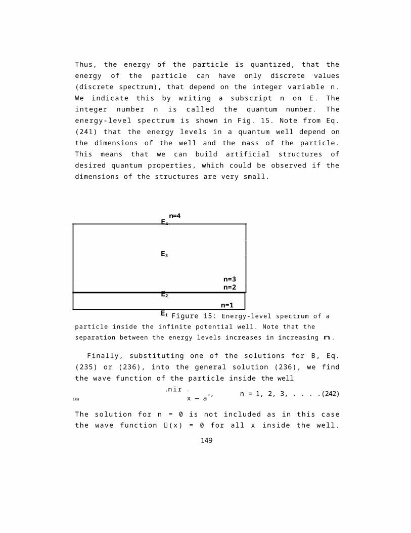
Thus, the energy of the particle is quantized, that theenergy of the particle can have only discrete values(discrete spectrum), that depend on the integer variable n.We indicate this by writing a subscript n on E. Theinteger number n is called the quantum number. Theenergy-level spectrum is shown in Fig. 15. Note from Eq.(241) that the energy levels in a quantum well depend onthe dimensions of the well and the mass of the particle.This means that we can build artificial structures ofdesired quantum properties, which could be observed if thedimensions of the structures are very small.

n=4

n=3n=2

n=1Figure 15: Energy-level spectrum of a

particle inside the infinite potential well. Note that the separation between the energy levels increases in increasing n.

Finally, substituting one of the solutions for B, Eq.(235) or (236), into the general solution (236), we findthe wave function of the particle inside the well

[nir

ika x — a , n = 1, 2, 3, . . . .(242)

The solution for n = 0 is not included as in this casethe wave function (x) = 0 for all x inside the well.

149

E4

E3

E2

E1

This would mean that the particle is not in the box.Thus, the minimum energy state in which the particle canbe inside the well is that with the energy E1 =ir2¯h2/2ma2. Since E1 > 0, the particle can never have zeroenergy.

150

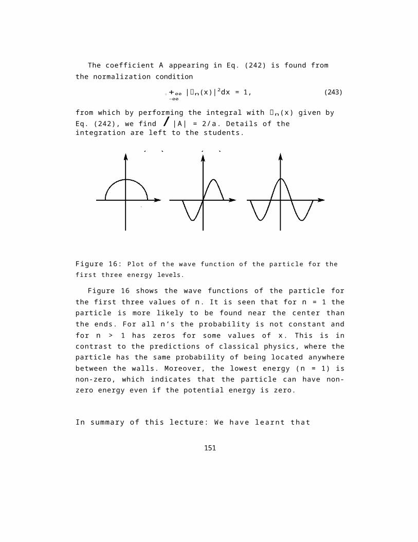
The coefficient A appearing in Eq. (242) is found from the normalization condition

+00−00

|n(x)|2dx = 1, (243)

from which by performing the integral with n(x) given by Eq. (242), we find /|A| = 2/a. Details of the integration are left to the students.

Figure 16: Plot of the wave function of the particle for the first three energy levels.

Figure 16 shows the wave functions of the particle forthe first three values of n. It is seen that for n = 1 theparticle is more likely to be found near the center thanthe ends. For all n’s the probability is not constant andfor n > 1 has zeros for some values of x. This is incontrast to the predictions of classical physics, where theparticle has the same probability of being located anywherebetween the walls. Moreover, the lowest energy (n = 1) isnon-zero, which indicates that the particle can have non-zero energy even if the potential energy is zero.

In summary of this lecture: We have learnt that

151

a/ x

n=

φ ( ) φ ( ) φ ()

a/

n=x

n=

−a/ a/x−a/

−a/

1. The energy of a particle in a quantum well can onlytake on certain discrete values. All other values ofthe energy are forbidden. We say that the energy ofthe particle is quantized.

152

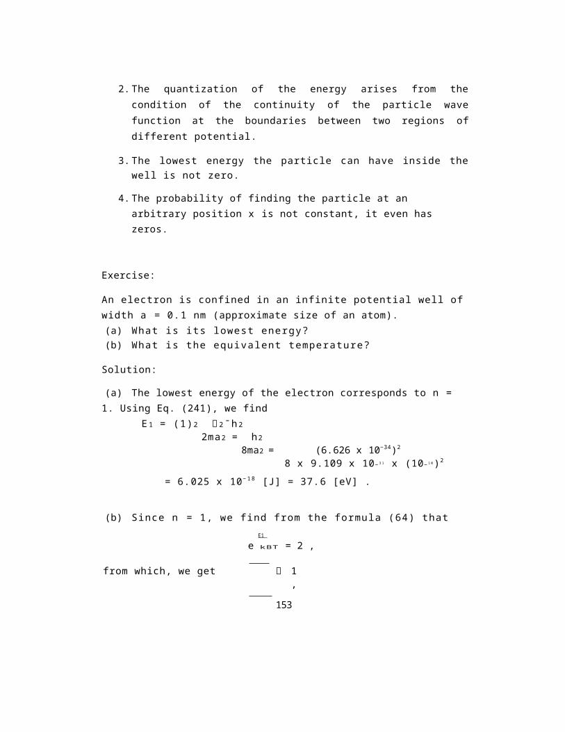
2.The quantization of the energy arises from thecondition of the continuity of the particle wavefunction at the boundaries between two regions ofdifferent potential.

3.The lowest energy the particle can have inside thewell is not zero.

4.The probability of finding the particle at an arbitrary position x is not constant, it even has zeros.

Exercise:

An electron is confined in an infinite potential well ofwidth a = 0.1 nm (approximate size of an atom).(a) What is its lowest energy?(b) What is the equivalent temperature?

Solution:

(a) The lowest energy of the electron corresponds to n = 1. Using Eq. (241), we find

E 1 = (1)2 2¯h 22ma2 = h2

8ma2 = (6.626 x 10−34)2

8 x 9.109 x 10− 3 1 x (10− 1 0)2

= 6.025 x 10− 18 [J] = 37.6 [eV] .

(b) Since n = 1, we find from the formula (64) thatE1

e kBT = 2 ,

from which, we get 1,

153

i.e.kBT

(

T E1/kB = 6.025 x 10− 1 8/ 1.381 x 10−13 ) = 43.6 [µK] .

154

Exercises at home:

(1) One may notice from Fig. 16 that the wave function forn = 2 is zero at x = 0, i.e. at the center of the well.This means that the probability of finding the particle atthe center of the well is also zero. Then, a questionarises: how does the particle move from one side of thewell to the other if the probability of being at the centeris zero?

(2) Solve the Schrödinger equation with appropriate boundary conditions for an infinite square well with with a centered at a/2

V (x ) = 0 for0 x a ,V (x ) = o c for x < 0 a n d x > a .

Check the the allowed energies are consistent with thosederived in lecture for an infinite well of width acentered at the origin. Confirm that the wave functionn(x) can be obtained from those found in lecture if oneuses the substitution x -* x + a/2.

155

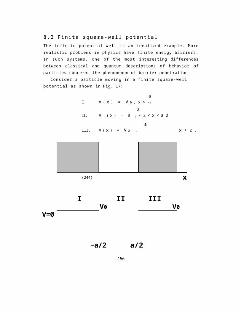
8.2 Finite square-well potentialThe infinite potential well is an idealized example. Morerealistic problems in physics have finite energy barriers.In such systems, one of the most interesting differencesbetween classical and quantum descriptions of behavior ofparticles concerns the phenomenon of barrier penetration.

Consider a particle moving in a finite square-well potential as shown in Fig. 17:

aI. V ( x ) = V 0 , x < -2

aII. V ( x ) = 0 , - 2 < x < a 2

aIII. V ( x ) = V 0 , x > 2 .

(244)

I II IIIV0 V0

V=0

−a/2 a/2156

x

Figure 17: Finite square-well potential.

In classical physics a particle is trapped in the well ifthe energy E of the particle is less than V0. In thiscase, the probability of finding the particle outside thewell is zero. When the energy E is larger than V0, theparticle can freely move in all three regions. Let’s lookat these situations from the point of view of quantumphysics.

Before going into the detailed calculations of theparticle wave function, we should point out that inbehavior of the particle in a finite square-well

157

potential, it must be recognized that the wave functionof the particle can exist in all space, that all regions inspace are accessible for the particle even if the energy Eis less than V0.

In the region II, —a/2 x a/2, the potential V(x) = 0, and then the Schrödinger equation reduces to

d22(x)dx2

= —k2 2cb2(x) , (245)

where k2 2 = 2mE/¯h2, and 2(x) is the wave function of the particle in the region II.

Since k2 2 is positive, the solution of Eq. (245) is of the form

2(x) = Aeik 2x + B e _ i k 2 x , (246)

that is the same as for the particle in the potentialwell. Thus, we expect that similar to the case of theinfinite potential barrier, the energy of the particlewill be quantized in the region II.

In the regions I and III, the potential is different from zero V(x) = V 0, andthen

2m 2mk2 1 = — ¯h2 (V0 — E) = ¯h2 (E — V0). (247)

In this case, the the Schrödinger equation is given by

d21(x)dx2

Solution of the above equation depends on the relation between V0 and E. For E> V0 the parameter k2 1 is positive,and then the solution of Eq. (248) is of the form

1(x) = Ceik 1x + D e _ i k 1 x , (249)

158

= —k2 1cb1(x) . (248)

indicating that the probability of finding the particlein the regions I and III is similar to that in the regionII. It is not difficult to show, (the details of thecalculations are left to the students), that in this casethe energy spectrum of the particle is continuous in allregions. Thus, one could conclude that there is nothingparticularly interesting about the solution when E > V0.However, we may obtain nonzero reflection coefficient atthe boundaries, which

is a quantum effect. Classically, one would expect that theparticle of energy E > V0 should travel from region I toregion III without any reflection at the boundaries.2

More interesting is the case of E < V 0. For E < V 0 theparameter k 2 1 is a negative real number, and then thesolution of Eq.(248) is in the form of exponentialfunctions

1(x) = Cek 1 x + D e _ k 1 x , x < −a2

1(x) = Fek 1 x + G e _ k 1 x , x > a 2 . (250)

In order to get 1(x) finite for each x > a/2, inparticular at x -* ±00, we have to choose D = F = 0.Otherwise, the wave function would be infinite at x =±00. Hence, the solution (250) reduces to

I. 1(x) = CekIx , for x < −a2

III. '1(x) = Ge_kIx , for x > a 2 . (251)

Assume for a moment that C, G = 0, then the probability(x) 2 has inter-

159

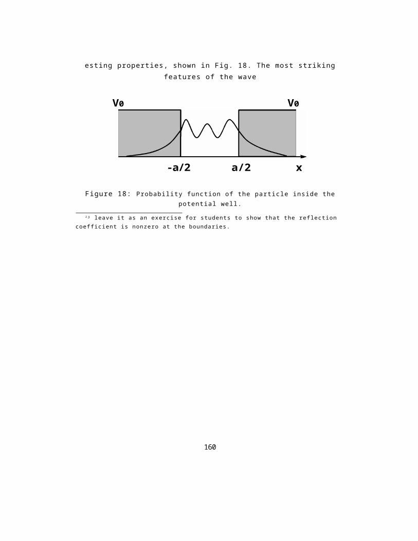
esting properties, shown in Fig. 18. The most strikingfeatures of the wave

V0 V0

-a/2 a/2 x

Figure 18: Probability function of the particle inside thepotential well.

2j leave it as an exercise for students to show that the reflection coefficient is nonzero at the boundaries.

160

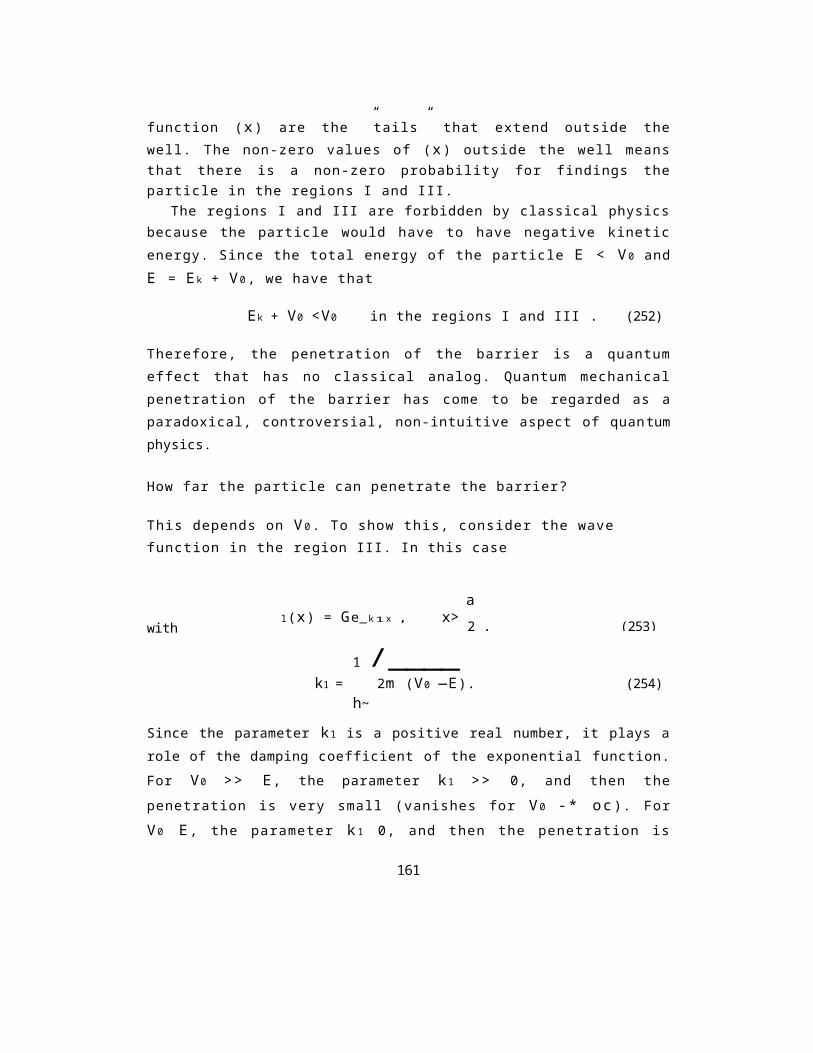
function (x) are the ”tails” that extend outside thewell. The non-zero values of (x) outside the well meansthat there is a non-zero probability for findings theparticle in the regions I and III.

The regions I and III are forbidden by classical physicsbecause the particle would have to have negative kineticenergy. Since the total energy of the particle E < V 0 andE = E k + V0, we have that

Ek + V0 <V0 in the regions I and III . (252)

Therefore, the penetration of the barrier is a quantumeffect that has no classical analog. Quantum mechanicalpenetration of the barrier has come to be regarded as aparadoxical, controversial, non-intuitive aspect of quantumphysics.

How far the particle can penetrate the barrier?

This depends on V 0. To show this, consider the wave function in the region III. In this case

with

1 /____k1 = 2m (V0 —E). (254)

h~Since the parameter k1 is a positive real number, it plays arole of the damping coefficient of the exponential function.For V0 >> E, the parameter k1 >> 0, and then thepenetration is very small (vanishes for V 0 -* oc). ForV0 E, the parameter k 1 0, and then the penetration is

161

a1(x) = Ge_k1x , x> 2 , (253)

very large. These two situations are shown in Fig. 19.

In order to prove that the penetration effect really exist,we have to demonstrate that the constants C and G are really non-zero.

To show this, we will turn to the details, and carry out the complete solution for the wave function of the particle.

162

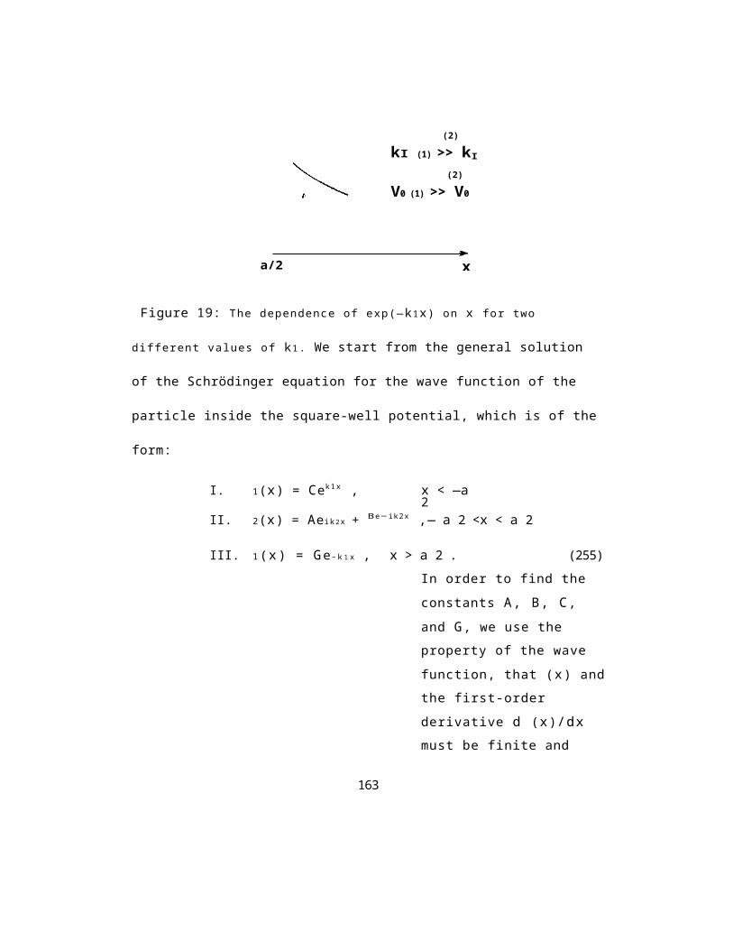
(2)

kI (1) >> kI(2)

V0 (1) >> V0

a/2 x

Figure 19: The dependence of exp(—k1x) on x for two

different values of k1. We start from the general solution

of the Schrödinger equation for the wave function of the

particle inside the square-well potential, which is of the

form:

I. 1(x) = Cek1x , x < —a2

II. 2(x) = Aeik2x + Be−ik2x ,— a 2 <x < a 2

III. 1(x) = Ge − k 1 x , x > a 2 . (255)In order to find the constants A, B, C, and G, we use the property of the wave function, that (x) andthe first-order derivative d (x)/dx must be finite and

163

(2Ik

1(k

continuous everywhere, in particular, at the boundaries x = —a/2 and x = a/2.

Hence, at x = —a/2 :

− 2 a k 1 = Ae − i 1 1 2 ak2 + Bei 1 2 ak2 .(256)

At x = a/2:Ge− 2 ak 1 = Aei 1

1 2 ak2 + Be−i 2 1 ak2 . (257)

We remember, that also d /dx must be continuous across thesame boundaries.

164

Ce

Sincedçb 1

I. dxdçb 2

I I . dxdçb 1

I I I . d

= Ck1ek1x ,

= iAk2eik2x − iBk2e−ik2x ,

= −Gk1e−k1x , (258)

we find that at x = −a/2:( 2 iak2 )

Ck1e− 2 ak1 = ik21 Ae− 2 1 iak2 −Be1

, (259)

( 2 iak2 )

−Gk1e− 2 ak1 = ik21 Ae1 2 iak2 − Be− 1

Dividing both sides of Eq. (259) byk1, we obtain

( 2 iak2 ) , (261)

where 3 = k2/k1.Comparing Eqs. (256) and (261), we get

(

Ae−i 1 2 ak2 + Bei 1 2 iak2 )

2 ak2 = i3 Ae− 1 2 iak2 − Be1

from which we find that

A = ( i3 + 1) (i3 − 1)Beiak2 . (263)

Hence, substituting Eq. (263) into Eq. (256), we find that2i3

C= (i3 − 1)Be2 ak1(i/3+1) . (264)1

Since B = 0, as the particle exists inside the well,we have that C = 0 indicating that there is a non-zeroprobability of finding the particle in the region I. Theprobability is given by |1(x)|2, that is

165

. (260)

, (262)

|1(x)|2 = |C|2e−2k1|x| , (265)

166

where x = —x for x < 0. Thus, 1(x) 2 = B 2 4 3 2

(32 + 1)e_2k1(|x|_ a 2). (266)

The probability is different from zero and decreases exponentially with the rate 2k1. The constant B is foundfrom the normalization of (x).

Exercise:

Show that the particle probability current density J iszero in region I, and deduce that R = 1, T = 0. This isthe case of total reflection, the particle coming towardsthe barrier will eventually be found moving back.”Eventually”, because the reversal of direction is notsudden. Quantum barriers are ”spongy” in the sense thequantum particle may penetrate them in a way thatclassical particles may not.

Consider now the continuity conditions at x = a/2.From the symmetry of the system, we expect that theconstant G, similar to C, will be different from zero,and may be found in a similar way as we have found theconstant C.

From Eqs. (257) and (260), and using Eq. (263), we find two solutions for the constant G in terms of B:

where

( 2 iak2 )

G e _ 2 ak 1 = B1 ue3 2 iak2 + e_ 1 ,

( 2 iak2 )

Ge_ 2 ak1 = —i3B

(267)

, (268)

( i3 + 1)u= (i3 — 1) . (269)

Here, we have two solutions for G. However, we cannotaccept both of the solutions as it would mean that there

167

are two different probabilities of finding the particle ata point x inside the region III. Therefore, we have to findunder which circumstances these two solutions are equal.

Dividing Eq. (268) by (267), we obtain( )i3 ue2iak2 —1 = —1, (270)(ue2iak2 + 1)

168

from which we find that the solutions (267) and (268) are equal when

2 k 1 k 2 tan(ak2) = _____ . (271)k2 2 - k2 1

To proceed further, we introduce dimensionless parameters

VI_2 - c2 = 1 2ak1 , (273)where (1 2a 2 mV 0 ) 22 = . (274)h¯

We see from the relation c = 1 2ak2 that determining cwe can get the energy E of the particle inside the well.In order to show this, we rewrite Eq. (271) in terms of cand , and find VIc tan c =2 - c2 . (275)This is a transcendental equation which, can be solved graphically as follows. Introducing the notation

p (c ) = c tanc ,VI___________q(c) = 2 - c2 , (276)

we find solutions of the equation p(c) = q(c) by plottingseparately p(c) and q(c). The functions p(c) and q(c) areshown in Fig. 20. The intersection points of the twocurves gives the solutions of the equation p(c) = q(c). Wesee from the figure that the equation p(c) = q(c) issatisfied only for discrete (finite) values of c. Sincethe energy E is proportional to c, see Eq. (272), we findthat the energy of the particle is quantized in the regionII, i.e. the energy spectrum is discrete.

The number of solutions, which will give us the number ofenergy levels, depends on , but always is finite. We see from Fig. 20 that there we have

one solution for < ,two solutions for < 2ir ,

169

c =1 12ak2 = 2 ( 2 mE ) 2

a , (272)

three solutions for < 3ir ,

170

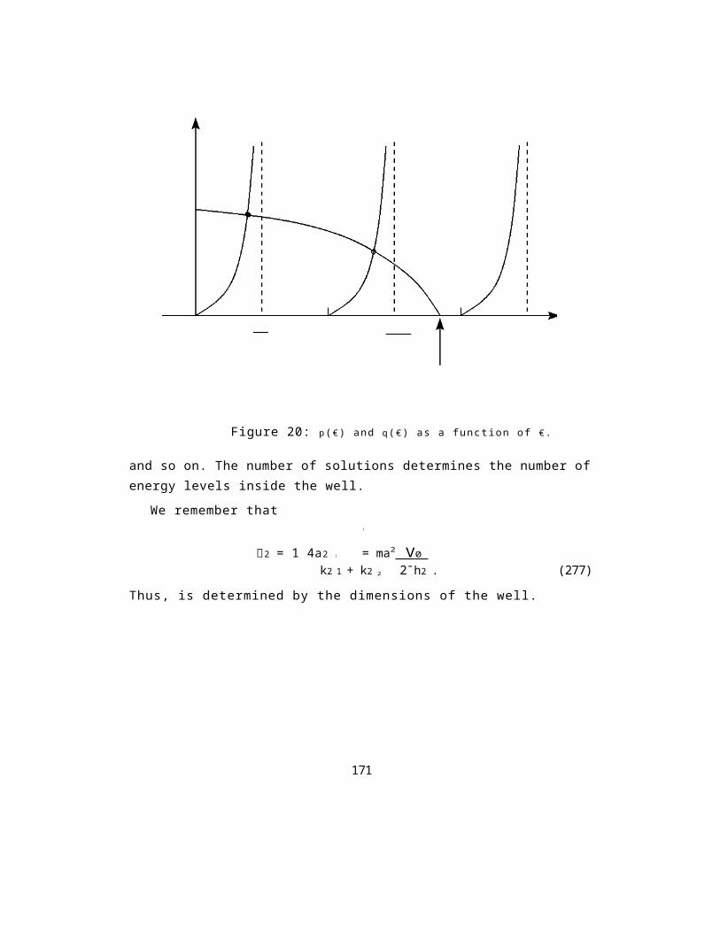
Figure 20: p(€) and q(€) as a function of €.

and so on. The number of solutions determines the number ofenergy levels inside the well.

We remember that)

2 = 1 4a2 ( = ma2 V 0 k2 1 + k2 2 2¯h2 . (277)

Thus, is determined by the dimensions of the well.

171

0 ð ð 3 ð 2 ð2 2 å

p(

q( )

p( ) p( )ε ε

ε

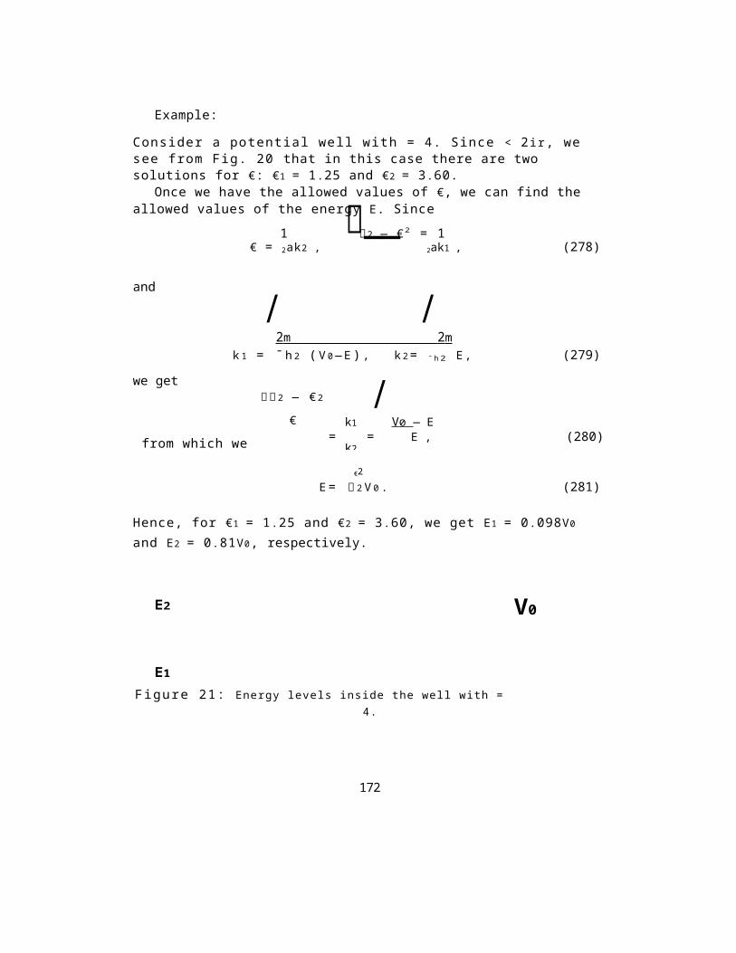
Example:

Consider a potential well with = 4. Since < 2ir, we see from Fig. 20 that in this case there are two solutions for €: €1 = 1.25 and €2 = 3.60.

Once we have the allowed values of €, we can find the allowed values of the energy E. Since__1 2 — €2 = 1

€ = 2ak2 , 2ak1 , (278)

and / /2 m 2 m

k 1 = ¯ h 2 (V 0—E), k 2= ¯ h 2 E, (279)

we get

from which we

2 — € 2

€/

k1 V 0 — E= = E , (280)

k2

€2E= 2 V 0 . (281)

Hence, for €1 = 1.25 and €2 = 3.60, we get E1 = 0.098V0 and E2 = 0.81V0, respectively.

E2

E1Figure 21: Energy levels inside the well with =

4.

172

V0

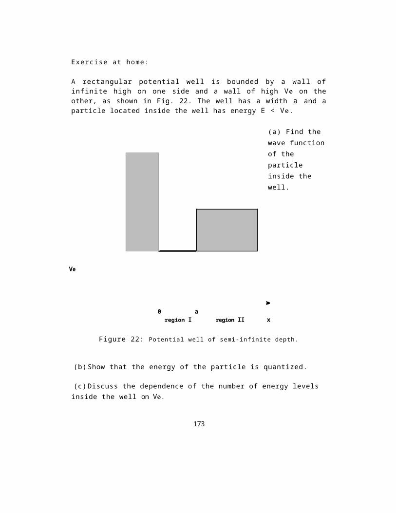
Exercise at home:

A rectangular potential well is bounded by a wall ofinfinite high on one side and a wall of high V0 on theother, as shown in Fig. 22. The well has a width a and aparticle located inside the well has energy E < V0.

(a) Find the wave functionof the particle inside the well.

V0

0 aregion I region II x

Figure 22: Potential well of semi-infinite depth.

(b)Show that the energy of the particle is quantized.

(c)Discuss the dependence of the number of energy levels inside the well on V0.

173

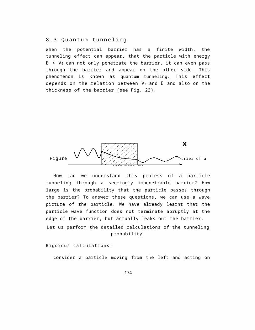
8.3 Quantum tunnelingWhen the potential barrier has a finite width, thetunneling effect can appear, that the particle with energyE < V0 can not only penetrate the barrier, it can even passthrough the barrier and appear on the other side. Thisphenomenon is known as quantum tunneling. This effectdepends on the relation between V0 and E and also on thethickness of the barrier (see Fig. 23).

x

Figure 23: Tunneling effect through a potential barrier of athickness a.

How can we understand this process of a particletunneling through a seemingly impenetrable barrier? Howlarge is the probability that the particle passes throughthe barrier? To answer these questions, we can use a wavepicture of the particle. We have already learnt that theparticle wave function does not terminate abruptly at theedge of the barrier, but actually leaks out the barrier.Let us perform the detailed calculations of the tunneling

probability.

Rigorous calculations:

Consider a particle moving from the left and acting on

I II IIIV0

174

the rectangular potential barrier, Fig. 23. Assume that E <V0. The solution of the Schrödinger equation for the threeregions is

I. 1(x) = Aei k 1 x + B e _ i k 1 x , x < -a2

II. 2(x) = Ce_ k 2 x + Dek 2 x ,- a 2 < x < a 2

III. 1 ( x ) = F e i k 1 x + G e _ i k 1 x , x > a 2 (282)

175

/ /where k1 = 2mE/¯h and k2 = 2m(V0 - E)/¯h.The continuity conditions for the wave function and the

first-order derivative at x = -a/2 areAe−jk 1 a 2+ Bejk 1 a 2= Cek 2 a 2+ De−k 2 a 2 ,( Ae− j k 1 a 2 - Bej k 1 a 2 = ik 2 Cek 2 a 2 - De− k 2 a 2.(283)

k1The continuity conditions at x = a/2are

Ce−k2 a 2+ Dek2 a 2= Fejk 1 a 2+ Ge−jk 1 a 2( )-Ce−k 2 a 2 + Dek 2 a 2 = ik 1 F ejk 1 a 2 - Ge−jk 1 a 2 .(284)k2

The continuity conditions (283) and (284) can be written in matrix forms as

( ( ( ( '\ 1 + jk 2 ek 2 a 2 +jk 1 a1 - j k 2 e− k 2 a 2 + j k 1 a2 2A = 1 C ( k 1 ( k 1 , (285)

B 21 - jk 2 ek 2 a 2 −jk 1 a1 + jk 2 e−k 2 a 2 −jk 1 a D2 2k1 k1

and( ( ( ( ) "\

1 - jk 1 ek 2 a 2 +jk 1 a1 + jk 1 ek 2 a 2 −jk 1 a2 2C = 1 F ( k2 ( k2 . (286)D 2 1 + jk 1 e−k 2 a 2 +jk 1 a 1 - jk 1 e−k 2 a 2 −jk 1 a G2 2

k2 k2

The relationship between the solution onthe left of the barrier and the solution onthe right can now be obtained by substituting

the matrix equation (286) into the right hand side of thematrix equation (285), and then we obtain

( A =B( cosh k2a + j 2 sinh k2a ejk1a j2 sinh k2a

176

,

F

( )- jT, 2 sinh k2a cosh k2a - j 2 sinh k2a e−jk1a

with c = k2 k1-and 'ij = k2k1 + k1k 2 . The solution with G = 0 is of particulark1 k2

interest as it represents the situation where no particles are incident on the barrier from the right. In this case

e−jk1a

cosh(k2a) +____________________1 2icsinh(k2a) . (288)

177

FA

Hence, the transmission coefficient of the particle currentis

[ (( ))2 I−1= 1 + + 1 sinh2(k 2a)

2[0 sinh 2 ( k 2 a ) I−11 + V 2

= 4E(V0 — E)

When E > V 0, the solution changes only in the region II,and the new solution can be obtained from the old solutionby replacing k2 by ik 2, where /k 2 = 2m(E — V0)/¯h. Sothat the expression for T changes to[ I−1

1 + V 0 2 sin2(k 2 a ) T = . (290)4E(E—V 0)

First, note that if there is no barrier, V0 = 0, and thenthere is 100% transmission. Thus, there is nothingparticularly remarkable about the solution when V0 = 0.Its physical interest lies in what happens when V0 = 0.

For V0 = 0, one could expect from the classicalmechanics that T = 0 for E < V 0, and T = 1 for E > V 0.However, Eq. (289) shows that T is not zero for E < V0

(non-zero transmission), and Eq. (290) shows that T < 1 forE > V0 (non-zero reflection).

Thus, tunneling effect for E < V 0 and partialreflection at the barrier for E > V0 are quantumphenomena. In the classical limit of h¯ -* 0, the parameterk2 -* oc, and then T -* 0. Hence, in the classical limit,there is no possibility of the particle of an energy E < V0

to pass the barrier. Moreover, since that k2 is proportional178

T = |F | 2 |A|2

[ ( )2= cosh2(k2a) +sinh2(k2a)2I−1

. (289)

to mass of the particle, the transmission coefficient (289)is large for light particles and decreases with theincreasing m. There is the further interesting phenomenonfor the case of E > V 0. One can see from Eq. (290) that ifk 2a = nir, n = 1, 2, 3,..., there is 100% transmissionfrom region I to III. This phenomenon is analogous to thebehavior of coated lenses in optics. Otherwise, quantumeffect (partial reflection) appears.

179

Quantum tunneling is important in the understanding ofnumber of physical phenomena such as thermonuclearreactions and conduction in metals and semiconductors. In1928, Gamov, Condon and Gurney used quantum tunneling toexplain the a-decay of unstable nuclei, in which an alphaparticle (a helium nucleus) is emitted from a radioactivenucleus. The alpha particle has energy which is less thanthe high of the potential barrier keeping the particleinside the nucleus. Nevertheless, alpha particles tunnelthrough the barrier and are detected outside the nucleus.

Tunneling has also been used in a number of electronicdevices. One is a tunnel diode in which the current ofelectrons is controlled by adjusting the energy E of theelectrons. This changes the value of k2 and thus the rate theelectrons tunnel through the device.

The most advanced application of quantum tunneling isthe scanning tunneling microscope. A probe needle is heldvery close (< 1 nm) above a conducting object and scannedacross it. The object is at a positive voltage V withrespect to the probe needle. However, for electrons to passfrom the needle to the object, they have to overcome thework function of the needle material. This creates apotential barrier through which electrons can tunnel. Asthey tunnel through the potential barrier they generate acurrent whose the variation tells us about the distancebetween the needle and the object.

Challenging problem: Quantum tunneling from and intoa semi-finite well

180

In the problem discussed in lecture, we have shown thereare no restrictions on the energy of a particle to tunnelthrough the barrier. The explanation of this effect issimple: The particle of an arbitrary energy can tunnelthrough the barrier because there are no restrictions onenergies which the particle can have in the region III.Lets us consider the exercise from page 98, a rectangularpotential well of width a bounded by a wall of infinitehigh on one side and a barrier of high V0 and infinitethickness on the other. We have learnt that inside thewell, region I, a particle can have only a limited numberof discrete energies.

181

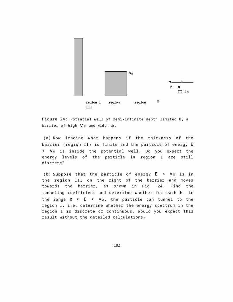
V0

E0 a

II 2a

region I region region III

Figure 24: Potential well of semi-infinite depth limited by a barrier of high V0 and width a.

(a) Now imagine what happens if the thickness of thebarrier (region II) is finite and the particle of energy E< V0 is inside the potential well. Do you expect theenergy levels of the particle in region I are stilldiscrete?

(b) Suppose that the particle of energy E < V0 is inthe region III on the right of the barrier and movestowards the barrier, as shown in Fig. 24. Find thetunneling coefficient and determine whether for each E, inthe range 0 < E < V0, the particle can tunnel to theregion I, i.e. determine whether the energy spectrum in theregion I is discrete or continuous. Would you expect thisresult without the detailed calculations?

182

x

9 Multi-Dimensional Quantum Wells: Quantum Wires and Quantum Dots

We have seen that in the one-dimensional case, particlesconfined into a small region can have quantized energies,can be be found in ”classically forbidden” region and evencan tunnel through this region. Although the one-dimensional case is very useful in the illustration andunderstanding of the quantum effects, we need a fullthree-dimensional treatment if we want to illustrateapplications of quantum mechanics to atoms, solid state,and nuclear physics. The application to atoms will bediscussed in a separate lecture on Angular Momentum andHydrogen Atom, Chapter 15. In this lecture, we extend theconcept of quantum wells from one to three dimensions.

183

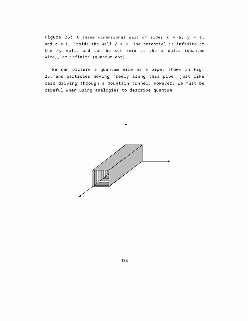
Figure 25: A three dimensional well of sides x = a, y = a,and z = L. Inside the well V = 0. The potential is infinite atthe xy walls and can be set zero at the z walls (quantumwire), or infinite (quantum dot).

We can picture a quantum wire as a pipe, shown in Fig.25, and particles moving freely along this pipe, just likecars driving through a mountain tunnel. However, we must becareful when using analogies to describe quantum

184

y

a

a

x

L

z

phenomena. We expect the cars to drive along the bottom ofthe tunnel, but we would be surprised to see the carsdriving through mid-air a few meters above the tunnelfloor. This is precisely how the particles appear tobehave in a quantum wire.

9.1 General solution of the three-dimensional Schrödinger equation

Let us find the wave function of a particle locatedinside the well and its energies. The wave function andthe energies are found from the three- dimensionalSchrödinger equation

¯h2-____V 2W+VW=E. (291)2m

We see that in cartesian coordinates 82/8x2 in the one-dimensional case is replaced in three dimensions by the Laplacian

V2 = 828x2 +

82 8y2

828z2 . (292)

Since x, y, z are independent (separable) variables, thewave function is also separable into three independentfunctions Wx, y, and iJJz . In this case, we can find thesolution of the Schrödinger equation in product form

W(x, y, z) = Wx(x)Wy(y)Wz(z) . (293)

Substituting this into the Schrödinger equation and dividing both sides by WxWyWz, we obtain

185

where, as before, we have put V = 0 inside the well, but outside the well we will set V = oc.

Since each term on the left-hand side of Eq. (294) is a function of only one variable, each will be independent of any change in the other two variables.

186

¯h2 d2Wx ¯h2 d2Wy ¯h2 d2Wz =E, (294)2mWx dx2 2mWy dy2 2mWz dz2

Thus, Eq. (294) can be separated into three independent equations. To illustrate this, we write this equation as

The lhs involves all of the x dependence. If we change x anyway we want, the rhs is not affected. Thus, it must be thatboth sides are equal to a constant, say Ex:

Equation (297), that depends only on y and z variables can be written as

Again, both sides depend on different variables, the lhsdepends only on y and the rhs depends only on z, thusboth sides are equal to a constant, say Ey:

Hence, after the separation of the variables, one differential equation in three variables has turned into three independent equations of one variable each

¯h2 d2x=

=

Ex ,

E y ,

(301)2mWx

¯h2dx2d2Wy

187

¯h2 d2Wx =E+¯h2 d 2 W y

dy2 +2mW y

¯h2 d2Wz

dz2 . (295)2mWx dx2 2mWz

¯h2 d2Wx = Ex , (296)2mWx dx2

¯h2 d2Wy ¯h2 d2Wz = E—E x . (297)2mWy dy2 2mWz dz2

¯h2 d2Wy =E—E x +¯h2 d2Wz

dz2 . (298)2mWy dy2 2mWz

¯h22mWy

d2Wy = E y , (299)dy2¯h2 d2Wz = E—E x —E y . (300)2mWz dz2

= Ez , (302)

(303)

2mWy

¯h2dy2d2Wz

2mWz dz2

188

where E z = E - E x - E y.The wave function of the particle inside the well and

its energies are found from these three independentequations. The parameters E x, E y and Ez are separationconstants, and represent energies of motion along the threeCartesian axis x, y and z. It is easily to see that thesethree constants satisfy the equation

E x +E y +E z =E. (304)

The solutions of the equations (301) and (302) are the same as that for the infinite square well in one dimension,and are given by

x = A sin a x , n1 = 1, 2, 3, . . . ,( n 1 (305)( n 2 7r

y = B sin a y , n2 = 1, 2, 3, . . . , (306)

with energies

2¯h2 ii2¯h2Ex = n2 1 2ma2 and Ey = n2 2 2ma2 . (307)

9.2 Quantum wire and quantum dotThe solution for the z component of the motion, Eq.(303), depends on whether the z sides of the well havezero or infinite potential. For zero potential, the zdirection is free for the motion of the particle(quantum wire), and is given by the wave function

z = Cei kz z , (308)

where k2 z = 2mEz/ ¯h2 , and Ez can have arbitrary values.If the potential at the z sides is infinite, we have an

example of quantum dot3. In this case, the solution of Eq.

189

(303) is the same as for the x and y components( n 3 i r

z = C sin L z,n3 = 1, 2, 3,... , (309)

3It would be more correct to call the quantum dot a quantum box, butin many calculations, quantum dots that have spherical symmetries are

approximated by rectangular boxes.

with the Ez energy taking only discrete values2¯h2

Ez = n2 _(310)

3 2mL2 .

Thus, we can summarize that for a quantum wire, the wavefunctions of the particle are of the form n2 1 + n2 + Ez , with n 1,n 2=1,2,3,... , (312)22ma2

where D = ABC is a constant which is found from the normalization condition of the wave function. It is easy to show that

. (313)

The proof is left to the students.

Interesting observation:Since the energy of the particle in the y direction cannever be zero, the particle will never move at the floor ofthe wire. Because the motion of the particle is restricted

190

n 1 I n 2 ir In1,n2 = D sin a x sin a y eikzz , (311)

and the corresponding energies are given by

2¯h2E=

D= /2 2a L

(quantized) in two dimensions, a quantum wire is sometimesreferred to as a one-dimensional system.

For a quantum dot with L = a, the wave functions of the particle inside the well are of the form

I 3f2 (n1r I ( n 2 7r I ( n 3 i r I2

n1,n2 ,n3 =s i n a x s i n a y s i n a zaand the corresponding energies are given by

2¯h 2 E=_________ n2 1 + n2 2 + n2 , with n1, n2, n3 = 1, 2,3, . . . . (315) 32ma2

Thus, energy of the particle in a quantum dot is quantizedin all three directions. Because the motion of theparticle is now restricted in all three dimensions(quantum confinement), a quantum dot is sometimes referredto as a zero-dimensional system. Quantum dots are alsoregarded as artificial atoms.

One can notice that the results obtained for the three-dimensional case are similar to that obtained for the one-dimensional case. However, there is a significantdifference between these two cases. For the three-dimensional case there might be few wave functionscorresponding to the same energy. We canillustrate this on a simple example of energiesand the corresponding wave functions of aquantum dot:The lowest energy state (the ground state), for which n1 = n2 = n3 = 1, has energy

191

, (314)

3 2¯h2E= 2ma2 , (316)

and there is only one wave function (singlet) correspondingto this energy. However, there are three wave functions corresponding to energy

6 2¯h2E= 2ma2 , (317)

as there are three combinations of n1, n2 and n3 whosesquares sum to 6. These combinations are n1 = 2, n2 = 1, n3= 1, or n1 = 1, n2 = 2, n3 = 1, or n1 = 1, n2 = 1, n3 = 2.The three wave functions corresponding to this energy areW2 ,1 ,1, W1 ,2 ,1, and W1,1,2. We say that the energy level isdegenerate.

It is easy to see from Eq. (315) that the degeneracy ofthe energy levels is characteristic of quantum wells whosethe sides are of equal lengths. The degeneracy can belifted, if the sides of the well were of unequal lengths.

Exercise at home:

Find the number of wave functions (energy states) of a particle in a quantum well of the sides of equal lengths corresponding to energy

9ir2¯h2

192

E = 2 m a 2 ,

i.e. for the combination of n1, n2 and n3 whose squares sum to 9.

10 Linear Operators and Their AlgebraWe have seen that in quantum physics energy and momentumappear as mathematical operations, which we calloperators. We now extend the idea of operators intoarbitrary quantities, and postulate that any quantity inquantum physics is specified by a linear operator.

An operator A ˆ is linear if for arbitrary functions fiand gi, and arbitrary complex numbers ci, such that

ˆAf1 = g1 and ˆAf2 = g2 ,

the linear superposition is

A ˆ(c1f1 +c2f2) = c1 ˆAf1 +c2 ˆAf2 = c1g1 +c2g2 .(318)

10.1 Algebra of operatorsThe sum of two operators Aˆ and B ˆ and their product are defined as

(Aˆ + B ˆ) f = ˆAf + ˆBf, (319)

)

( Aˆ Bˆ ) f = Aˆ ( ˆBf. (320)

The operators obey the following algebraic rules:1 . A ˆ + B ˆ = B ˆ + A ˆ , )

2. A ˆ + B ˆ + C ˆ = ( Aˆ + Bˆ ) + C ˆ = A ˆ + ( Bˆ + C ˆ ,

)

3. Aˆ Bˆ Cˆ = Aˆ ( Bˆ Cˆ ) Cˆ , = ( Aˆ Bˆ( Aˆ + Bˆ ) Cˆ = Aˆ Cˆ + Bˆ Cˆ .

4. (321)

193

The power of an operator and the sum of two operators is

defined as

1. ˆA2 = AˆAˆ, ˆA3 = AˆAˆAˆ, etc.) ( Aˆ + Bˆ )

( Aˆ + Bˆ )2 = ( Aˆ + Bˆ2. = ˆA2 + ˆB2 + AˆBˆ +Bˆ Aˆ . (322)

In general, AˆBˆ = BˆˆA. Thus, multiplication of operators is not necessarily commutative.

194

We can define a commutator:

[ˆA, Bˆ] = Aˆ Bˆ - BˆAˆ, (323)

and say, that two operators commute if

[ˆA, Bˆ] = 0. (324)We can also define anticommutator as]{ ˆA, B ̂} [ ˆA, B ̂+ = A ̂B ̂+ B ̂Aˆ

, (325)

and we say that two operators anticommute if

[ ˆA, B ̂] + = 0 . (326)

Inverse operator:

The inverse of an operator ˆA, if it exists, is defined by

AˆˆA−1 = ˆA−1Aˆ =1ˆ, (327)

where 1ˆ is the unit operator defined byˆ1f=f. (328)

Hermitian adjoint: (Hermitian conjugate)

Operator ˆA l is the Hermitian adjoint of an operator A ˆ if for two functions f and g that vanish at infinity

ff*ˆAgdV = f (ˆAlf)* gdV. (329)

Properties of Hermitian conjugate:( ˆAl)l = Aˆ .1. (330)

195

Proof:

ff* ̂ AgdV = f (ˆAT f)* gdV = f g (ˆAT f)*

dV = (f g* ̂ AT f dV)*= (f ((ˆAT)T g)* f dV)* = f ((ˆAT)T

g) f* dV

= f f* ((ˆAT)T g) dV , (331)

as required*.

2. (Aˆii)T = ̂ BT ̂ AT . (332)

Proof:

ff* (AˆBˆ)T gdV = f (Aˆ̂ Bf)* gdV = f [Aˆ (ˆBf)]* gdV . (333)

Introducing the notation ˆBf = u, we get

f(ˆAu) * gdV = f u* ̂AT gdV = f (ˆB

f) * ˆAT gdV

= f f*ˆBTˆATgdV . (334)

196

Thus, (AˆBˆ)T = ̂ BTˆAT, as

required*.

197

10.2 Hermitian operators

Operator A ˆ is called Hermitian if

ˆA† =Aˆ, (335)i.e. when

ff*ˆAgdV = f (ˆAf)* gdV. (336)

10.2.1 Properties of Hermitian operators

If Aˆ and B ˆ are Hermitian then:

1.A ˆ + B ˆ is Hermitian,

2. ˆA2,ˆA3, etc. are Hermitian,

3. c Aˆ is Hermitian if c is a real number. Proof of the property 3:ff* ( )f (

c Aˆ ) * gdV , (337)

gdV = c ˆAf ) * gdV = c* f ( ˆAf

as required.

4.AˆBˆ is Hermitian only if Aˆ and B ˆ commute. Proof:

(AˆBˆ)† = ˆB† ˆA† = BˆAˆ. (338))† = Aˆ Bˆ unless Aˆ

and Bˆ commute,

Hence, ( Aˆ Bˆas required.

198

5.From the property 4, we have that the commutator [ˆA, Bˆ] is not Hermitian, even if A ˆ

and B ˆ are Hermitian.

Proof: [ˆA, Bˆ] t = (AˆBˆ - BˆAˆ)t = (AˆBˆ)t - (BˆAˆ)t

ˆBtˆAt - ˆAtˆBt = BˆAˆ - AˆBˆ = - [ˆA, Bˆ], (339)

as required*.

6.However, i [ˆA, B] is Hermitian.Proof is left for the students.

7.For an arbitrary operatorˆA, the product A ˆ ˆAt is Hermitian. Proof: (Aˆ̂ At) t = (ˆAt)t ̂ At = Aˆ̂ At , (340)

as required*.

8.If A ˆ is non-Hermitian, A ˆ + ˆ A t and i (A ˆ - ˆ A t ) are Hermitian. Hence, Aˆ can be written as a linear combinationof two Hermitian operators

A ̂= 21 (A ̂+ ˆAt) + 21i (i (Aˆ - ˆAt)) .

(341)

10.2.2 Examples of Hermitian operators

1. Position operator r ˆ is Hermitian.Since |r| is a real number and ˆrg is just a

199

multiplication of the function g by r, we have

frkgdV = f 77'.f*gdV = f (kf) gdV .

(342)

200

2. Potential V^(r). .Since r is Hermitian, an arbitrary function of r' is also Hermitian.

3. Momentum operator is Hermitian. Proof:

fv (pfIv gdV = f (ni V f)*

gdV =

- . i f (V f*) gdV vh,i f ñ i

V ( f * g) dV + f* (V g) dV..lv i.lV

h hf V (f* g) dV + f f* (V) dV .(343)v vi

iUsing the Gauss’s divergence theorem, we get that Eq. (343) can be written as

= -~h is f* gdS + fv f* (pg) dV .

First integral in Eq. (344) vanishes as f and g vanish at infinity, and therefore we get

V(15'7)* gdV = f

f* (130 dV ,(345)

. iwhich means that p is Hermitian,

as required*.

We have defined before the eigenvalues and eigenfunctionsof the Hamiltonian of a particle, see Section 7.3. The ideaof eigenvalues and eigenfunctions can be extended toarbitrary operators. Thus, we can state:

201

= -

= -

If ^AIF = aIF, then IF is an eigenfunction of A ^ with eigenvalue a.

202

Example:

Determine if the function W = e2x is an eigenfunction of the operators (a) A ˆ = d/dx, (b) B ˆ = ()2, and (c) C ˆ = f dx.

(a) Operating on the wave function W with the operator ˆA,we obtain

ˆAW=ddx e2x = 2e2x = 2W , (346)

which is a constant times the original function. Therefore, W = e2x is an eigenfunction of the operator A ˆ = d/dx with an eigenvalue a = 2.

I leave the solution of the parts (b) and (c) to the students.

Hermitian operators play the important role in quantummechanics as they represent physical quantities. Thisimportance arises from the fact that eigenvalues of anHermitian operator are real.

Proof:

Assume that a is an eigenvalue of an Hermitian operator A ˆ

corresponding to the eigenfunction f (that vanishes at infinity). Then

a = a V f 2 dV = V f *afdV = V f*ˆAfdV

( ˆAf )* fdV = V a*f*fdV = a* V f 2dV = a* , (347)

V

as required.

203

10.3 Scalar product and orthogonality of two eigenfunctions

Two functions W1(r) and W2(r) are orthogonal iff +00−00 W 1(r)W2(r)dV =0. (348)

The orthogonality of two functions is related to theorthogonality of two vectors. The vectors are orthogonalwhen the scalar product of the vectors is zero. Inanalogy, we can write a scalar product of two functions as

f(Wi, W3) = W i (r)W3(r)dV = a38i3 , (349)

where a3 is a positive constant and 8i3 is the Kronecker

delta function. When a3 = 1, we say that the functions

are orthonormal.

The complex functions Wi form a complex linear vector space.The infinite- dimensional vector space of orthonormal functions is called Hilbert space.

The scalar product

f(wi, wi) = jjijj = jwij2 dV ,

(350)

where Wi is a square integrable function, is called thenorm of the state (vector) W. For a state function thatrepresents physical quantity the norm is finite. If thefunctions are orthonormal, the norm jjIJijj = 1.

Example of orthogonal functions:

Examples of orthogonal functions are sines and cosinesfunctions. Their product with any other function of the

204

same class gives zero when integrated over all ranges ofvariable, unless the two multiplied functions areidentical.

Jf 2 0 for m =6 n0 sin(m ) sin(n ) dçb = ir for m = n

(351)

205

f0

(2ir 0 for m

f0 2 ir sin(m) cos(n) dçb = 0 for all m and n .

From the orthogonality of the sines functions, we seethat the eigenfunctions of a particle in an infinite squarewell potential, Eq. (242), corresponding to differentenergies (n = m) are orthogonal.

Having available the definition of orthogonal functions, we can formulate an important property of eigenfunctions of a linear Hermitian operator.

Eigenfunctions of a linear Hermitian operator belonging to different eigenvalues are orthogonal.

Proof:

Consider a Hermitian operator ˆA. Let f and g are two eigenfunctions of A ˆ corresponding to two different eigenvalues af and ag, respectively,

ˆ A f = a f f ,ˆAg = agg , (354)

where af, a g are real numbers.) * = af f*, we can writeSince ( ˆAf

ff ( ˆAf )* gdV − f f* ( ˆAg ) dV = (af −

ag) f*gdV . (355)However )

f ( ˆAf ) * gdV = f f* ( ˆAg dV ,

(356)

and therefore the lhs of Eq. (355) vanishes. Since, af = 206

(352)

(353

ag, we have

f(f, g) = f*gdV = 0 , (357)

as required.

207

10.4 Expectation value of an operator

In classical physics, an expectation or average or meanvalue of an arbitrary quantity A is obtained by weightingeach measured value Ai by the associated probability Piand summing over all the measurements N. Thus,

(A) = PiAi i=1,2(358)

i

where Pi is a probability of measuring the value Ai.

How do we calculate expectation values in quantum physics?

Consider an operator Aˆ acting on a function Wi. Suppose that ˆAWi exists, then the scalar product( ) fWi, ˆAWi = W i ˆAWidV (359)

is called the expectation or average or mean value of the operator A ˆ in the state Wi.

Similarly as in classical physics, the expectation value can be calculated from the probability density as

f f f( ˆA) = ˆAp(r)dV = Aˆ |Wi|2 dV = W i ˆAWidV ,(360)

where the order of the factors under the integral is

not important. Properties of the expectation value

1. Expectation value of a Hermitian operator is real.

Proof:f

( ˆA) = WidVW i ˆAWidV = f ( ˆAWi

f )

208

= Wi ( ˆAWi ) dV = (f W i ˆAWidV= (ˆA), (361)

as required.

209

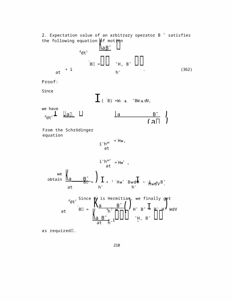
2. Expectation value of an arbitrary operator B ˆ satisfiesthe following equation of motionK a _ B ̂

ˆB = ˆH, Bˆ + i . (362)at h¯

Proof:

Since

I( ˆB) =W i ˆBWidV,we haveddtI a ( a B ̂ )

(a )From the Schrödinger equation

i¯haW

atand its complex conjugate

=ˆHw,

i¯haw*

at=ˆHw* ,

weobtain K a ____ B ̂ )I IˆB = + i ˆHw * ˆBwdV − i w* BˆˆHwdV .at h¯ h¯

Since Hˆ is Hermitian, we finally getKa B ̂ ) I )ˆB = + i w ( Hˆ Bˆ − Bˆ Hˆ WdVat h¯K a B ˆ ˆH, Bˆ + i ,at h¯as required.

210

ddt

ddt

Thus, expectation value of the operator Bˆ can depend on time even if the operator does not depend explicitly on time (0 ˆB/0t = 0).When [ˆH, ˆB] = 0, we have that d( ˆB)/dt = 0, and then theexpectation value is constant in time. In analogy toclassical physics, we call B ˆ a constant of motion.

We have already shown that expectation values of Hermitian operators are real. In term of the scalar product this is characterized by

(111i, ̂ A111i) =ˆA111i)* . (363)

From this property, we have in general, that for Hermitianoperators

ˆA1113) =, ̂ A111i)* . (364)

Proof:

(111i, /43) = f 111:ˆA1113dV = f 0111i)* 1113dV = f 1113 (ˆ

A111i)* dV f *= 111;ˆA111idV) = (1113, ̂ A111 i) ,

as required*.

The properties (363) and (364) is very often used to check whether operators are Hermitian.

Example:

Consider two operators Aˆ = d/ dx and B ˆ = d2 / dx2 actingon two orthonormal wave functions 1111 = a sin(nx) and 1112= a cos(nx), where n is a real number, a = 1/V7r and x E(-7r, 7r).

Are the operators A ˆ and B ˆ Hermitian?

Solution:

211

First, consider the operator A ˆ = d/ dx. Sinceˆ A 1111 = a d x sin(n x ) = a n cos(n x ) = a n 1112 , (365)

212

andd

ˆAW2 = adx cos(nx) = —an sin(nx) = —anW1 , (366)

we find the following values of the scalar products

(W1, ˆAW1 ) = —an (W1,W2) = 0 ,

(W1, ˆAW2 ) = —an (W1, W1) = —an ,

(W2, ˆAW2 ) = —an (W2, W1) = 0 ,

(W2, ˆAW1 ) = an (W2,W2) = an . (367)

Hence

(W1, ˆAW1 ) = (W2, ˆAW2 ) * , (368)

but

(W1, ˆAW2 ) = —an (W2, ˆAW1 ) * = an . (369)

Thus, the operator Aˆ= d/dx is not

Hermitian. Consider now the operator

Bˆ = d2/dx2. Since

d2BW1 = adx2 sin(nx) = —an2 sin(nx) = —an2W1 , (370)

and2

BW2 = adx2 cos(nx) = —an2 cos(nx) = —an2W2 , (371)

we find the following values of scalar products

(W1, ˆBW1 ) = —an2 (W1, W1) = —an2 ,213

(W1, BW2 ) = —an2 (W1,W2) = 0 ,

(W2, BW2 ) = —an2 (W2, W2) = —an2 ,

(W2, ˆBW1) = —an2 (W2, W1) = 0 . (372)

214

Hence( ) (

w1, ˆBw1 )* , (373)= —an2 = w2, ˆBw2

and( ) (

w1, ˆBw2 )* . (374)= 0 = w2, ˆBw1

Thus, the operator B ˆ = d2/dx2 is Hermitian.

Exercise at home:

Prove, using the condition (364) and the wave functions W1 and 1JJ 2 of the above example, that the momentum operator ˆpx = —i¯hô/ôx is Hermitian.

215

10.5 The Heisenberg uncertainty principle revisited

In Section 6.6, we have shown that the uncertainties in the position and momentum of a particle satisfy the relation

AyApy = h . (375)

This relation says the position and momentum of a particlecannot be measured simultaneously with the same precision.This is known as the Heisenberg uncertainty relation,or the Heisenberg uncertainty principle, and we will showthat the relation is a direct consequence of thenoncommutivity of the position and momentum operators

[̂ y,ˆpy] = i¯h . (376)

In fact, the Heisenberg uncertainty relation can beformulated for arbitrary two Hermitian operators that donot commute. In other words, if A ˆ and Bˆ are twoHermitian operators that do not commute, the physicalquantities represented by the operators cannot be measuredsimultaneously with the same precision.

Theorem:

The variances ((/ ˆA)2) = (ˆA2) — (ˆA)2 and ((L ˆB)2) =(ˆA2) — (ˆA)2 of two Hermitian operators satisfy the inequality

((AˆA)2)((ˆB)2) > —14([ˆA, ˆB])2 , (377)

which is called the Heisenberg inequality.

216

Proof:

First, we prove that for an arbitrary operator Aˆ the following inequality holds

(AˆˆA†) > 0 . (378)

217

It is easy to prove the above inequality using the definition of the expectation value

( AˆˆAt) = fll*AˆˆAtIlidV = f (ˆAtIlf)*ˆA4dV = fiii*2 dV > 0 . (379)

Now, we prove that for two Hermitian operators the following inequality is satisfied

(ˆA2)(ˆB2) > —41 ([ˆA, ̂ B])2 .

(380)

To prove it, we introduce an operator

Dˆ = Aˆ + izBˆ , (381)

where z is an arbitrary real number.Hence, from Eq. (378), we find

( DˆˆDt) = ((iii + izˆB)(Aˆ — izˆB))= (

ˆA2) — iz((AˆBˆ — BˆˆA)) + z2 (ˆB2) > 0 .(382)

This inequality is satisfied when

—(AˆBˆ — B ̂̂ A)2 — 4(ˆA2) (ˆB2) < 0 . (383)

Hence(ˆA2) (ˆB2) > 41 ([ˆA, ˆB])2 ,

(384)

as required.

Finally, since

218

[AˆA, AˆB] = [ˆA, ˆB] ,

(385)Uˆ = ˆA, ˆB), and replacing in Eq. (384), Aˆ —> AAˆ and

as required*.

219

whereAUˆ=Uˆ —ˆU

Example 1. The Heisenberg uncertainty relation for the position and momentum operators.

Since

[ˆx, ˆpx] = i¯h , (386)we obtain by substituting into Eq. (377), A ˆ =xˆ and Bˆ = ˆpx

1((ˆx)2)((ˆpx)2) ~ 4¯h2 , (387)

or in terms of the standard deviations (fluctuations)8x8px ~ 1 2¯h, (388)

__________________________________________________________________________________

where 8x = ((ˆx)2) and 8p x = ((ˆp x)2).Similarly, we can show that for the y and z components

of the position and momentum

8y8p y ~ 1 2¯hand 8z8pz ~ 1 2¯h. (389)

Note that the relation (375) satisfies the Heisenberg inequality as h > ¯h/2.

Example 2. The Heisenberg uncertainty relation forthe components of the electron spin.

Since

[ˆx, ˆy] = 2iˆz , (390)

(For a poof, see Tutorial Set 8), where ˆx, ˆy, ˆz are the operators corresponding to the three components of the electron spin, we obtain

((zˆx)2)((zˆy)2) ~ (ˆz)2 , (391)

220

or

8crx8cr y ~ |(ˆz)| . (392)

The uncertainty relation (392) shows that the components of the electron spin cannot be measured simultaneously with the same precision.

221

10.6 Expansion of wave functions in the basis of orthonormal functions

We now consider the most important property of orthonormal functions, which similar to the orthogonality, arises from the properties of vectors.

To illustrate this connection, consider a simple example:

In the Cartesian coordinates an arbitrary vector A can be written as a linear combination of the orthonormal unit vectors

A= (i . A)i + (j . A)1+ (k. A)k ,(393)

where i, j and k are unit vectors in the directions x,

y and z, respectively. Proof:

We know from the vector analysis that in the Cartesiancoordinates an arbitrary vector A may be presented interms of components Ax, Ay, Az, and three unit vectorsoriented in the directions of the coordinate axis

A = Axi + Ay

j + Azk . (394)

Since the components are the projections of the vector Aon the coordinate axis

Ax =i . A , Ay = j . A, Az =k.A, (395)

222

A = ë1 . A ë1 + ë2 . A ë2 +. . . + ën . A ën =

m

n=1

( )

ë n . Aën,(397)

we find that the vector (394) can be written in the form

A =(i. A)i + (j . A)1+ (k . A)k,(396)

as required.

We can extend this property to n dimensional space andstate that an arbitrary vector A can be written asa linear combination of the coordinate (basis) unitvectors ë' as

223

( )

where e n · A is the scalar product of e n and A, (nth component of A), and ei · ej = 8ij.

The norm (magnitude) of the vector A is|| A||2 = | A| = ( en · A

) 2.

(398)n

Thus, we see that an arbitrary vector can be expressed as alinear combination of the orthonormal vectors e n.

In analogy, an arbitrary wave function W can be expanded in terms of orthonormal wave functions W n as

= c n w n , (399)n

(discrete spectrum of Wn), or in the case of a continuous spectrum of Wn

f(r) = c n(r)Wn(r)dV n , (400)

where cn are arbitrary (unknown) expansion coefficients, and dV n is the volume element of the space the orthonormal functions Wn(r) are spanned.

We can find the coefficients cn(r) by multiplying Eq. (400) by W

m(r) and integrating over all space as follows

f f fW m(r)W(r)dV = c n(r) w

m(r)wn(r)dV dV n = c m(r), (401)

where we have used the orthonormality property of the 1JJ n functions

fw m(r)wn(r)dV n = 8nm. (402)

In general, the coefficients c m(r) are complex numbers and

224

are called the components of the function W in the basis ofthe orthonormal functions Wm. The components determine thefunction completely, and very often the coefficients c m(r)are called a representation of the wave function W in thebasis Wm.

The coefficients c m(r ) satisfy the following relation

fV |cm(r)|2 dV = 1 . (403)

225

Proof:

Multiplying Eq. (400) by W*(r) and integrating over V, weobtain

V W*(r)W(r)dV = V W(r) 2 dV

= Vm c* m(r)cn(r)WnWmdVndVmdVV V n

= Vn c* m(r)cn(r)8mndVndV = V cm(r) 2 dV .

(404)V

Since, fV W 2dV = 1, we get f V cm(r)2 dV = 1, as required.

From Eqs. (400) and (403), we see that cm(r) 2 can beinterpreted as the probability that a system, described bythe wave function W(r), is in the state described by thewave function Wm(r).

Example:

Let A ˆ is an operator andW(r) is an unknown wave function that is not aneigenfunction of ˆA. Suppose, that we cannot find theexplicit form of W(r) because we cannot solve theSchrödinger equation for W(r). However, we can find a formof the wave function in the basis of the eigenfunctions ofˆA. If Wm(r) is an eigenfunction of ˆ

fW(r) = cm(r)Wm(r)dVm . (405)

226

A, then

11 Dirac NotationDirac introduced a very useful (compact) notation of statevectors (wave functions) Wi in terms of ”bra” (i and ”ket” i) vectors.

For example, a wave function JJ i can be expressed by aket vector i), and W* i by a bra vector (Wi . Thisnotation can be further simplified to i) and (i ,respectively.

Let us illustrate what kind of simplifications we will get using the Dirac notation.

In the Dirac notation, a scalar product is written as

(Wi, Wj) = (Wi Wj) = (i j) , (406)

which is called a bracket.For orthonormal vectors we have used the notation (Wi,

Wj) = 8ij, which in the Dirac notation takes the form (i j) = 8 i j.Since (Wi, Wj) = (Wj, Wi)*, we have in the Dirac notation (ij) = (j i) *.In the bra-ket notation, the definition of the Hermitian

adjoint becomes

( )* ,( i ˆ A j ) = ( j ˆ A † i ) ( 4 0 7 )

or(j ˆA† i) = (i ˆA j)* . (408)

Thus, for a Hermitian operator

(i ˆA j) = (j ˆA i)* . (409)

Expectation value of an operator A ˆ in a state i) is given

by (i ˆ A i).

227

We write a linear superposition of ket states as

a) = >An n) , discrete states (410)n

or

fa) = A(x) x)dx . continuous states(411)

228

The bra-ket notation also extends to action of operators onstate vectors.

A linear operator A ˆ associates with every ket i) anotherket j):

ˆA i) = j) , (412)

such that

Aˆ( a) + b)) = ˆA a) +ˆA b),

and)

ˆAA a) = A ( ˆA a), (413)where A is a number.

Hermitian conjugate of ˆA i) is (i ˆA†.

An arbitrary ket state a) can be expanded in terms of orthonormal ket states as

a) = c n n ) . ( 4 1 4 )n

Since n) are orthonormal ((m n) = 8 i j), we get for c n:(m a) = cn(m n) = cn8nm = cm .n n

(415)

Thus

cn = (n a) ,

and then

a) = n) (n a) .n

(416)

(417)

Hence

n)(n = 1ˆ,n

where 1ˆ is the unit operator.

131

(418)

The product ket-bra ( m)(m ) is called a projection operator, and the relation (418) is called the completeness relation.

From Eq. (414) and (a a) = 1, we have

c n 2 = 1 . (419)n

11.1 Projection operatorIn general, we can define projection operator of two

different bra-ket states asˆPmn = m)(m . (420)

This operator projects an arbitrary state vector a) onto

the ket state m):

ˆPmn a) = m)(m a) . (421)

When m = m and (m m) = 1, the projection operator ˆPnn

satisfies the relation

Pˆ 2 nn = ˆPnn, (422)

which is easy to prove

Pˆ 2 nn = m)(m m)(m = ˆPnn. (423)

Thus, the square of ˆP n n equals itself.

Note that ˆP n n is a Hermitian operator, but ˆP m n, (m = m) is not Hermitian.

Proof:

231

Since(i ˆPmn j) = (i m)(m j) = 8im8nj , (424)

we have that, (m ˆPmn m) = 1, but (m ˆPmn m) = 0, and then(

(m ˆPmn m) = (m ˆPmn m) )* , (425)

as required.

11.2 Representations of linear operators

Consider an arbitrary operator ˆA. We can represent the operator A ˆ in terms of projection operators of the orthonormal states m).

To show this, we use the completeness relation for the states m) and multiply the operator A ˆ on both sides by unity in the form

1= m)(m , (426)m

and obtain

Aˆ = ( ) ( )

m)(m A ˆ m)(m = m)(m ˆA m)(mm n m,n

= (m ˆA m) m)(m = A m n ˆP m n , (427)m,n m,n

where A m n = (m ˆA m).

Thus, an arbitrary operator can be written (represented) as a linear combination of projection operators ˆP m n.

Since an arbitrary state a) can be expanded in terms of orthonormal states m), i.e.

a) = cn m) , (428)n

we can obtain the following expression for the expectation value ( ˆA) in the state a) as

(ˆA) = (a ˆA a) = (m ˆA m)c ncm . (429)m,n

If m) is an eigenfunction of ˆA, i.e. ˆA m) = A m m), then

( ˆA) = c ncmAm8mn = An cn 2 . (430)m,n n

Thus, the modulus square of the expansion coefficients is the probability that the quantity described by the operator

233

A ˆ is in the state m).As ( ˆA) is a weighted sum of the eigenvalues, this

suggests that the eigenvalues represent the possible resultsof measurement, while cn 2 is the probability that theeigenvalue An will be obtained as the result of anyindividual measurement.

234

This is in contrast to classical physics. In classicalphysics the measurement of a physical quantity at any timealways leads to a definite result. In quantum physics themeasurement of the physical quantity at any time leads to arange of possible results, each occurring with a certainprobability. In this sense quantum physics isprobabilistic.

Results of any measurement in physics are real numbers.Since eigenvalues of Hermitian operators are real, wepostulate that every physical quantity that is measurableis specified in quantum physics by a linear Hermitian op-erator A ˆ that is also called an observable.

In quantum physics the set of possible measured values fora physical quantity is the set of eigenvalues of a linearHermitian operator specifying the physical quantity.

Example:

Consider a particle specified by a wave function W a, orin the Dirac notation, by a). Let H ˆ is the Hamiltonian(energy) of the particles and m) are known eigenfunctionsof ˆH.

If a) is an eigenfunction of ˆH, then

ˆH a)=Ea a) , (431)

where E a is the eigenvalue (energy) of the particle. Thus, E a = (a ˆH a).

If a) is not an eigenfunction of ˆH, then we can expand a) in terms of the eigenfunctions m) as

a) = c7 m) , (432)7

235

and find that

a ˆH a) = E7 c7 2 . (433)7

Hence, the measurement of energy of the particle in thestate a) leads to a range of possible results, eachoccurring with probability c7 2. Thus, c7 2 is theprobability that the measurement of H ˆ will give thevalue E 7.

Since, a) = c 7 m), we say that the state of the particle is a superposition of the eigenfunctions of ˆH.

236

12 Matrix Representation of LinearOperators

Using an orthonormal basis, we can represent an arbitrarystate |a) as a linear superposition of the basis states

|a) = E cn |n) , (434)n

where, in general, the coefficients cn are complex numbers, andEn |cn|2 = 1.The set of the expansion coefficients c1, c2, ... defines

the state |a) and is called the representation of |a) in the basis of the orthonormal states |n).

We can write the set of the coefficients cn as a column (ket) vector

|a) =

[c1c2...cn

1. (435)

Then, the bra state (a| can be written as

(a| = (c*1, c2*, ... , c*n) . (436)

12.1 Matrix representation of operatorsUsing the representation (436), we will try to write in amatrix form the relationship between two ket states |a)and |b) related through a linear operator Aˆ as

|b) = ˆA|a) . (437)

Letm

237

|a) = E cn|n) ,n

|b) = Ebm|m) . (438)

bm = (m|b) = (m| ˆA|a) = Ecn(m|ˆA|n) =EAmncn ,

(439)n n

where Amn = (m|ˆA|n).The right-hand side of Eq. (439) is the result of

multiplication of a matrix composed of the elements A mn and the column vector c n:

Thus, the scalar product (111m, ˆA111n), or (m| ˆA|n) represents a matrix element of the operator A ˆ in the orthonormal basis |n).

Example:

Find the matrix representation of the operator A ˆ =d/dx in the basis of two orthonormal states 1111 = asin(nx) and 1112 = a cos(nx), where a = 1/V7r and x E (—7r,7r).

Sinced

A1111 = dx sin(nx) = n1112 ,d

ˆA1112 = dx cos(nx) = —n1111 , (441)

we find (1111, ̂ A1111) = —n(1111,1112) = 0 ,(1111, ̂ A1112) = —n (1111, 1111) = —n ,239

Then

[b1b2...bn1=[

A 1 1 A 1 2 . . . A 1 n

A 2 1 A 2 2 . . . A 2 n ...A n 1 A n 2 . . .

1c1c2...cn1. (440)

(1112, ̂ A1112) = —n (1112, 1111) = 0 ,(1112, ̂ A1111) = n(1112,1112) = n . (442)

240

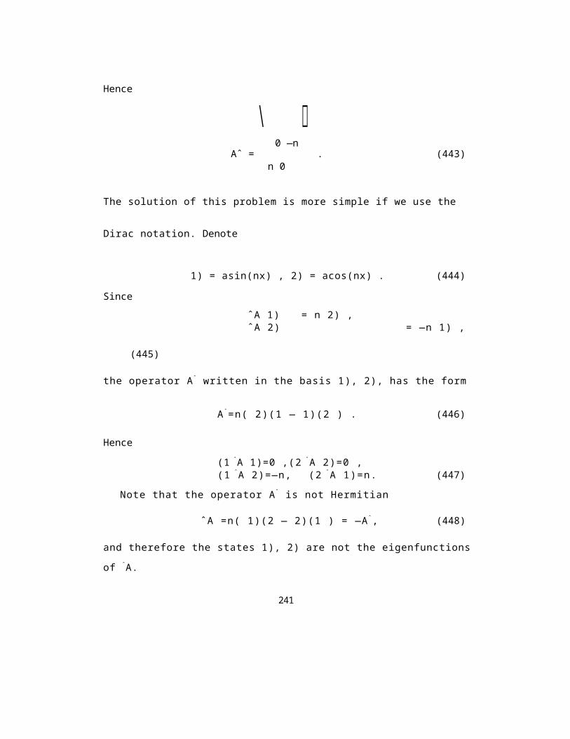
Hence

\ 0 —n

Aˆ = . (443)n 0

The solution of this problem is more simple if we use the

Dirac notation. Denote

1) = asin(nx) , 2) = acos(nx) . (444)

SinceˆA 1) = n 2) ,ˆA 2) = —n 1) ,

(445)

the operator Aˆ written in the basis 1), 2), has the form

A ˆ=n( 2)(1 — 1)(2 ) . (446)

Hence(1 ˆA 1)=0 ,(2 ˆA 2)=0 ,(1 ˆA 2)=—n, (2 ˆA 1)=n. (447)

Note that the operator Aˆ is not Hermitian

ˆA =n( 1)(2 — 2)(1 ) = —Aˆ, (448)

and therefore the states 1), 2) are not the eigenfunctions

of ˆA.

241

12.2 Matrix representation of eigenvalue equationsThe ket vector a) is an eigenvector of a linear operator Aˆ if the ket vector ˆA a) is a constant a times a), i.e.

ˆA a) = a a). (449)

242

The complex constant a is called the eigenvalue and a) is the eigenvector corresponding to the eigenvalue a.

Eigenvectors of an operator Aˆ can be found in terms of a linear superposition of orthonormal vectors m).

Since a) = c n m), we have

ˆA a) = cn ˆA m) = a cm m). (450)n m

Using the completeness relation to the lhs of Eq. (450), we get

c n m)(m ˆA m) =a c m m) , (451)n m m

which can be written as( )

c n(m ˆ A m) m) = (ac m) m). (452)m n m

Hence

cn(m ˆA m) = acm , (453)

cnAmn = acm. (454)n

The lhs of Eq. (454) is the product of a column vectorcomposed of the elements cn and a matrix composed of theelements Amn. Thus, we can write Eq. (454) in the matrix formas

243

n

or

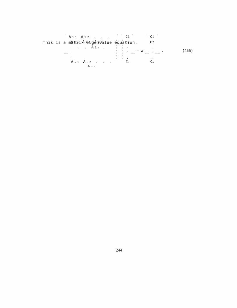
This is a matrix eigenvalue equation.

244

A 1 1 A 1 2 . . . A 1 n A 2 1 A 2 2. . . A 2 n ...A n 1 A n 2 . . .

A n n

c1c2...cn

= a

c1c2...cn

. (455)

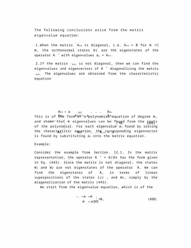
The following conclusions arise from the matrix eigenvalue equation:

1.When the matrix ¯A m n is diagonal, i.e. A m n = 0 for m =m, the orthonormal states m) are the eigenstates of theoperator A ˆ with eigenvalues an = Ann.

2.If the matrix ¯ A m n is not diagonal, then we can find theeigenvalues and eigenvectors of A ˆ diagonalizing the matrix¯Amn. The eigenvalues are obtained from the characteristicequation

This is of the form of a polynomial equation of degree m,and shows that m eigenvalues can be found from the rootsof the polynomial. For each eigenvalue ai found by solvingthe characteristic equation, the corresponding eigenvectoris found by substituting a i into the matrix equation.

Example:

Consider the example from Section. 12.1. In the matrixrepresentation, the operator A ˆ = d/dx has the form givenin Eq. (443). Since the matrix is not diagonal, the statesW1 and W2 are not eigenstates of the operator ˆA. We canfind the eigenstates of ˆA, in terms of linearsuperpositions of the states iJJ 1 and W2, simply by thediagonalization of the matrix (443).

We start from the eigenvalue equation, which is of the

245

A11 — a A12 . . . A1nA21 A22 — a . . . A2n

.

.

.An1 An2 . . . A n n — a

=0. (456)

—a —m m — a

=0, (458)

form( ) ( ) ( )

0 —m c1 c1= a . (457)

m 0 c2 c2First, we solve the characteristic equation

246

from which we find two eigenvalues a1 = +in and a2 = —in. For a1 = in the eigenvalue equation takes the form

( ) ( ) ( )

0 —n c1 c1= in , (459)

n 0 c 2 c2

from which, we find that

—nc2 = inc1or

c1 = ic2 . (460)

Hence, the eigenfunction corresponding to the eigenvalue a1 is of the form

( ) ( )

ic2 iW 1 = = c2 . (461)

c2 1

From the normalization of W 1, we get

( )

i1 = (Wa1, Wa1) = |c2|2 (—i, 1) = 2 |c2|2 . (462)

1

Thus, the normalized eigenfunction corresponding to the eigenvalue a1 is given by

( )1 iW 1 = 2 , (463)1

or1

W 1 = 2 [i sin(nx) + cos(nx)] . (464)

Similarly, we can easily show that the normalized eigenfunction corresponding to the eigenvalue a2 is of the

247

form

1Wa 2 = 2 [—i sin(nx) + cos(nx)] . (465)

248

In the Dirac notation, the normalized eigenvectors can be written in a compact form as

a1)

a2)

=

=

1(i 1) + 2)) ,

(466) 21 1) + 2)). 2 (−i

The physical interpretation of the superposition states(466) is as follows: The eigenfunctions a1) and a2) inthe form of the linear superpositions tell us that e.g.with the probability 1/2 the system described by theoperator A ˆ is in the state 1) or in the state 2).

In summary of this lecture: We have learnt that

1. In quantum physics, an arbitrary wave function may berepresented by a normalized column vector of expansioncoefficients in the basis of orthonormal states.

2. In an orthonormal basis, an arbitrary operator A ˆ maybe represented by a matrix, whose the elements A m n aregiven by scalar products (Wm, ˆAwn).

3. Using an orthonormal basis, an eigenvalue equation ofan arbitrary operator may be written in a matrix form.In this case, the problem of finding eigenvalues andeigenvectors of the operator reduces to a simple problemof diagonalization of the matrix.

249

13 First-Order Time-Independent Pert urbation Theory

In many situations in physics, the Hamiltonian H ˆ of agiven system is so complicated that the solution of thestationary Schrödinger equation is practically impossibleor very difficult.In some situations, however, the Hamiltonian can be split

into two partsH ˆ = ˆ H 0 + V ˆ ,

( 4 6 7 ) such that we can solve the eigenvalue equationfor ˆH0, i.e. we can findeigenvaluesE(0)

n and eigenvectors q(0)n of the Hamiltonian ˆH0, and

we can treat the part V ˆ as a small perturber to ˆH0.Thus, the problem of solvingthe eigenvalue equation

)

ˆHq = ( ˆH0 + Vˆ

q = Eq (468)reduces to find E and q when we know the eigenvalues E(0)

n and the eigen-vectorsq(0)n of ˆH0.

Since V ˆ appears as a small perturber to in the form of a series

q =q ( 0 )n + q(1)

n + . . . ,E = E ( 0 )n + E ( 1 )n+... , (469)

whereq(1)n is the first order correction to the unperturbedeigenstate q(0)

n ,and E(1)nis the first order correction to the unperturbedeigenvalue E ( 0 )

n .The subscript n indicates that the Hamiltonian ˆH0 can havemore than one eigenvalue and eigenvector.

Substituting the series expansion (469) into the eigenvalue equation (468), we get

) (( ˆH0 + Vˆ ) ( ) ( )

q(0)n + q ( 1 ) = E ( 0 )n + E ( 1 ) q ( 0 )n + q(1) . (470)250

ˆH0, we will try to find E and q

n n n

Expanding both sides of Eq. (470) and equating terms of the same order in Vˆ , we obtainˆH0q(0)

n = E ( 0 )

n q(0)n zeroth order in V ˆ , (471)ˆH0q(1)

n +Vˆ q(0)n = E ( 0 )n q(1)n + E ( 1 )

n q(0)n first order in Vˆ .

(472)

251

We know the solution of Eq. (471). In order to solve Eq. (472), we write this equation in the form

(ˆH0 − E(0)) (1)n = E ( 1 )

n ( 0 )n − Vˆ (0)n . (473)n

Assume that the eigenvalues E(0)n are non-degenerated, i.e. for a given E( 0)nthere is only one eigenfunction (0)

n .Multiplying Eq. (473) from the left by ( 0)*n , and integrating over dV, we

obtain ) ) ( ) ) ( 0 )n , ˆH 0 ( 1 ) − ( 0 )

n , E(0)n ( 1 ) = E ( 1 ) ( 0 )

n , ( 0 ) − ( 0 )n , Vˆ ( 0 ) . (474)n n n n n

Since ) ) ) ( 0 )n , ˆH0(1) = ( ˆH0(0)

n , ( 1 ) = E ( 0 ) ( 0 )n , (1) , (475)n n n n

the lhs of Eq. (474) vanishes, giving()

E(1) ( 0 )n = n , V ˆ ( 0 ) = ( ( 0 )

n | Vˆ |(0)n ) = (m| Vˆ |m). (476)n

Thus, the first order correction to the eigenvalue E(0)n is equal to the expec-tation value of V ˆ in the state (0)

n .In order to find the first-order correction to the eigenstate |(0)n ), we ex-pand |(1)

n ) state in terms of |(0)n ), using the completeness relation, as

|(1)n ) = i |(0)

m ) (' (0)

m |' (1)n ) = i cmn|(0)

m ) , (477)m mwhere cmn = (th(0)

252

m |th(1)n ).

We find the coefficients cmn from Eq. (473) by multiplying this equation from the left by ((0)

m |(in = m), and find((0)

m | ˆH0| th(1)

n ) − E(0)

n (th(0)

m | (1)n ) = E(1)n (th(0)

m | th(0)

n ) − ((0)m | Vˆ |(0)

n ) . (478)Since

(th(0)m |th(0)

n ) = 0and

((0)m | ˆH0|(1)

n ) = E(0)m ( ( 0 )m |(1)n ), (479)

253

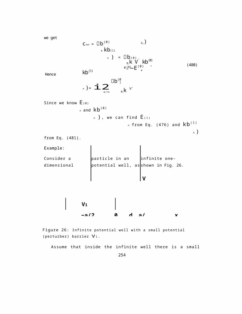
we getn )cmn = b(0)

m kb(1)

n ) = b(0)m k Vˆ kb(0)

. (480)E(0)n —E(0)

mHence kb(1)

n )= i2m =n

b(0)

m k Vˆ

Since we know E(0)

n and kb(0)

n ), we can find E ( 1 )

n from Eq. (476) and kb(1)

n )from Eq. (481).

Example:

Consider a particle in an infinite one-dimensional potential well, as shown in Fig. 26.

V

V1

−a/2 0 d a/ x

Figure 26: Infinite potential well with a small potential (perturber) barrier V 1.

Assume that inside the infinite well there is a small

254

potential barrier of high V1 and thickness d. Treating thebarrier V 1 as a small perturber, find the eigenvalues andeigenstates of the particle valid to the first order in V1.

255

Solution:

We know from Section 8.1 that the eigenstates of the particle in the infinite well, without V 1, are\/ /

2 nirx ( 0 )n = a sin , (482)a

and the corresponding eigenvaluesE(0)n = n 2 2¯h 2

2mga2 , (483)

where mg is the mass of the particle.Thus, the first order correction to the eigenvalue E( 0)n is

E(1)n

( d / nirx = ( 0 )

In order to find the first order correction to the eigenstate ( 0 )

n , we have tocalculate the matrix element (scalar product)( / mirx / nirx

V m n = ( 0 )m , ˆV 1 ( 0 ) = 2 V 1 d

0 dx sin ____ s i n _____ , (485)n a a a

where m = n.Performing the integrations in Eqs. (484) and (485), we get[ ]

d - 1 2a sin (2da) , (486) 1 }V1V m n = , (487)a - 3 sin [( - 3) d] - 1a + 3 sin [( + 3) d]a

where a = nir/a and 3 = mir/a.Hence, the first order correction to the eigenstate (0)

n i s'I(1)

n = 2 mg a2

n 2 - m 2

( 0 )

256

=E(1)n

V1a

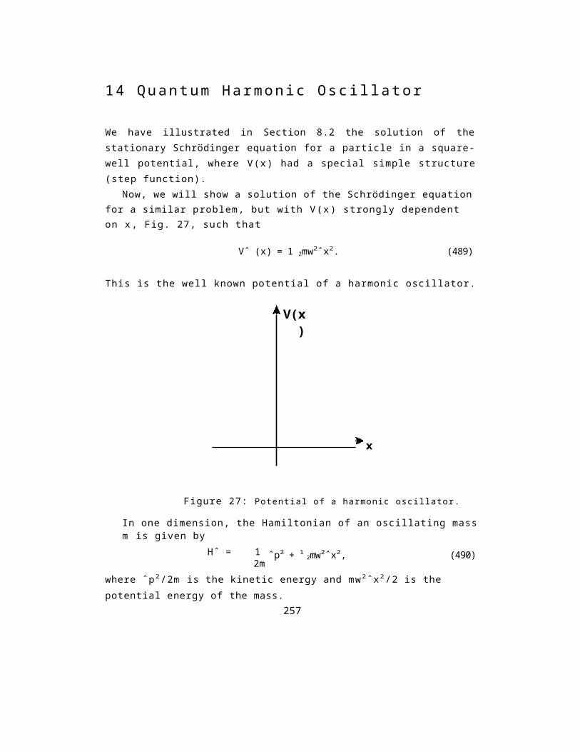
14 Quantum Harmonic Oscillator

We have illustrated in Section 8.2 the solution of thestationary Schrödinger equation for a particle in a square-well potential, where V(x) had a special simple structure(step function).

Now, we will show a solution of the Schrödinger equationfor a similar problem, but with V(x) strongly dependent on x, Fig. 27, such that

Vˆ (x) = 1 2mw2ˆx2. (489)

This is the well known potential of a harmonic oscillator.

V(x)

x

Figure 27: Potential of a harmonic oscillator.

In one dimension, the Hamiltonian of an oscillating massm is given by

Hˆ =    12m

ˆp2 + 1 2mw2ˆx2, (490)

where ˆp2/2m is the kinetic energy and mw2ˆx2/2 is the potential energy of the mass.

257

We will find energies (eigenvalues) and eigenfunctions ofthe harmonic oscillator by solving the stationarySchrödinger equation (eigenvalue equation) for the harmonicoscillator using two different approaches.

258

In the first, we will solve the equation using algebraicoperator technique which is based on the Dirac notation.This approach has several definite advantages and exploitsthe commutation relations among the operators involved andtheir properties.

In the second approach, we will transform thestationary Schrödinger equation into a second-orderdifferential equation, and will find the solution of theequation in terms of special functions.

14.1 Algebraic operator technique

The algebraic operator technique is based on thecommutation relation of two Hermitian operators involvedin the evolution of the harmonic oscillator: position xˆand momentum pˆ = ˆpx:

[ˆx,ˆp] = i¯h . (491)

We will introduce a non-Hermitian operator defined as m aˆ = 2¯h____________________xˆ + i1-s/ 2m¯hwpˆ, (492)

and the adjoint of this operatorV mˆat = 2¯h xˆ − i 1 2m¯h pˆ . (493)

Using the commutation relation (491), we find that the operators ˆa, ˆat satisfy the commutation relation

[ˆa, ˆat] = 1ˆ . (494)

This allows us to write the Hamiltonian Hˆ in a compact form ( (

Hˆ = 1 ˆat ̂ a + ̂ aˆat)ˆat ˆa + 1259

2¯hw = ¯hw . (495)2Hence, the eigenvalue equation

ˆH|) = E|), (496)can be written as

( ˆatˆa + 1¯hw ) = E ) . (497)2Multiplying Eq. (497) from the left by ( , and usingthe normalization ( ) = 1, we get

( ( ˆatˆa ) + 1¯hw = E . (498)2Since

( ˆa tˆa ) = (ˆa ),ˆa )) ~ 0, (499)

we have that

Thus, the energy of the quantum harmonic oscillator can never be zero.

From Eq. (497), we can generate a new eigenvalue equation multiplying this equation from the left by ˆat:

(

ˆatˆatˆa + 1¯hw 2ˆa t )= Eˆa t ). (501)

Using the commutation relation (494), we can write Eq. (501) as

(

ˆatˆa − 1¯hw ˆat ) = Eˆat ). (502)2Adding to both sides ¯hwˆat ), we obtain

( )

ˆatˆa + 1¯hw ˆat ) = (E + ¯hw) ˆat ) . (503)260

¯hw . (500)E > 2

2Introducing a notation W) = ˆat ), we see that W) is an eigenfunction of Hˆ with eigenvalue E + ¯hw.

Thus, the operator ˆat acting on the state ) of energyE transforms this state to the state W) of energy E + ¯hw.Therefore, the operator ˆat is called the raisingoperator or creation operator.

261

Now, multiplying Eq. (503) from the left by ˆat, we obtain

( )

ˆatˆatˆa + 1¯hw 2ˆat W) = (E + ¯hw) ˆat W). (504)

Proceeding similar as above, we get( )

ˆatˆa + 1¯hw ˆat W) = (E + 2¯hw) ˆat W). (505)2Thus, the state ˆat W) = ˆatˆat ) is an eigenfunction of Hˆ with an eigenvalue E+2¯hw.

Similarly, we can show that the state çbn) = (ˆat)n ) is an eigenfunction of H ˆ with an eigenvalue E + m¯hw.

Now, consider the action of the operator aˆ on the eigenfunctions and eigenvalues.

Consider the eigenvalue equation for n):( )ˆatˆa + 1¯hw n) = (E + m¯hw) n) = En n) . (506)

2Multiplying Eq. (506) from the left by ˆa, we get

( )ˆaˆatˆa + 1¯hw 2ˆa n)= (E + m¯hw) ˆa n), (507)

and using the commutation relation (494), we obtain( )ˆatˆaˆa + 3

¯hw 2ˆa n) = (E + m¯hw) ˆa n). (508)Hence

( )ˆatˆa + 1¯hw ˆa n) = [E + (m − 1) ¯hw] ˆa n) . (509)2Thus, the state n−1) = ˆa cbn) is an eigenfunction of H ˆwith an eigenvalue En − ¯hw. Therefore, the operator aˆis called the lowering operator or annihilation operator.

Suppose that the state 0) of energy E is the lowest(ground) state of the harmonic oscillator. Thus, the

262

energy spectrum (eigenvalues), shown

263

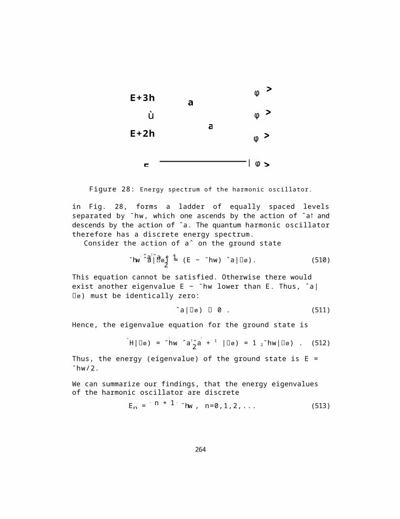
E | φ >Figure 28: Energy spectrum of the harmonic oscillator.

in Fig. 28, forms a ladder of equally spaced levelsseparated by ¯hw, which one ascends by the action of ˆa† anddescends by the action of ˆa. The quantum harmonic oscillatortherefore has a discrete energy spectrum.

Consider the action of aˆ on the ground state( ˆa†ˆa + 1¯hw ˆa|0) = (E − ¯hw) ˆa|0). (510)2

This equation cannot be satisfied. Otherwise there would exist another eigenvalue E − ¯hw lower than E. Thus, ˆa|0) must be identically zero:

ˆa|0) 0 . (511)

Hence, the eigenvalue equation for the ground state is( ˆH|0) = ¯hw ˆa†ˆa + 1 |0) = 1 2¯hw|0) . (512)2

Thus, the energy (eigenvalue) of the ground state is E = ¯hw/2.

We can summarize our findings, that the energy eigenvalues of the harmonic oscillator are discrete

( )n + 1En = ¯hw , n=0,1,2,... (513)

264

>|φ

>|φ

| >φ

E+3hù

E+2hù

a

a

with corresponding eigenfunctions

|00) , |01) = ˆat|00) ,|02) = (ˆat) 2|00) ,...,|0n) = (ˆat )n

|00) . (514)

From the above equation, it follows that starting with |00) , we may obtain the complete set of eigenvectors ofthe harmonic oscillator by repeatedly applying theoperator ˆat on the eigenstate |00).

However, the eigenstates found in this way are not normalized. The normalization of 0n(x) = cn (ˆat ) n00(x) gives

1 = (0n|0n) = |cn|2(00| (atn) t (ˆat

) n|00)= |cn|2(00|ˆanˆatn|00)=|cn| 2(0 0|ˆan- 1ˆaˆa t n|0 0) .

(515) Using the commutation relation

[ˆa, ( ˆ at ) n ] ( ˆ at)n- 1 = n ,

(516)

(Proof: by induction, leave for the students as a tutorial problem), we can continue Eq. (515) as

- |cn|2 (00 ̂ an-1 (nˆatn-1 + ̂ atnˆa) |00) =|cn|

2n(00|ˆan-1ˆatn-1|00)- |cn|2n(00|ˆan-2

((n — yttn-2ˆatn-1ˆa) |00)W0o| an-2atn-2|00)= cn|2n(n — (517)

Proceeding further, we find that Eq. (515) reduces to

1 = |cn|2n! . (518)

Thus, the normalized eigenfunctions of the harmonic oscillator are 1|0n) = (ˆat

)n|00).(519)

265

n!

Equation (519) shows that an nth eigenfunction can begenerated from the

ground state eigenfunction by the n-times repeated actionof the creation

266

operator on |0). Thus, it is enough to know the ground state eigenfunction to find all the eigenfunctions of the harmonic oscillator.

This is the complete solution to the problem. It isremarkable that the commutation relation (494) was all whatwe needed to deal with the harmonic oscillator completely.In a very effective way, we extracted the essential structureof the problem and have founded the eigenvalues andeigenvectors of the harmonic oscillator.

Using the definition of the ground state (511), we mayfind the explicit form of the ground state eigenfunction.Substituting for aˆ from Eq. (492) and using the explicitform of pˆ = _i¯hd/dx, we get

( j

_________ mw

2¯h x0 + i 1 _i ¯hd 0 = 0 , (520)

2¯hmw dxthat

simplifies to

where ' 0

dçb 0 + dx

mwxçb0=0, (521)h¯

mw=______xdx. (522)

0 h¯Integrating Eq. (522), we obtain

ln 0 ( x )

0(0)

mw= _2¯h___x 2, (523)

267

mw )

0 (x ) = )

4 _mw

1

dçb0

( )

_mw 0(x) = 0(0) exp 2¯h x2. (524)

We find 0(0) from the normalization, which finally gives

268

Thus, the wave function of the ground state is a Gaussian.The wave functions tm(x) of the other states can be found

from the relation( ˆa ) t m 0(x) .

tm(x) = (526)

Using the definition of ˆa (Eq. (493)), we can find tm(x) in terms of the position x:

1 ( x ) = ˆ a 0 ( x ) m w (

= 0(x) . (527)2¯h x − j 1v' −j¯h d2m¯hw dx

From Eq. (521), we have thatmw

= − x 0 .________(528)

dx h¯Hence

( v ' V/ m w )

1(x) = 2 h ¯ x 0(x). (529)Similarly, we can find that

[ ( m w ) ]

12(x) = v ' 2 2 ____ x 2 − 1 0(x). (530)h¯

We can introduce a new parameter1 mw = h¯ x , (531)

and write the wave functions as1

1 ( ) = v ' 2 H 1 ( ) 0 ( ) ,1

2 ( ) = 2 v ' 2 H 2 ( a ) 0 ( a ) , (532)

where Htm(a) are Hermite polynomials of degree n.

269

d 0

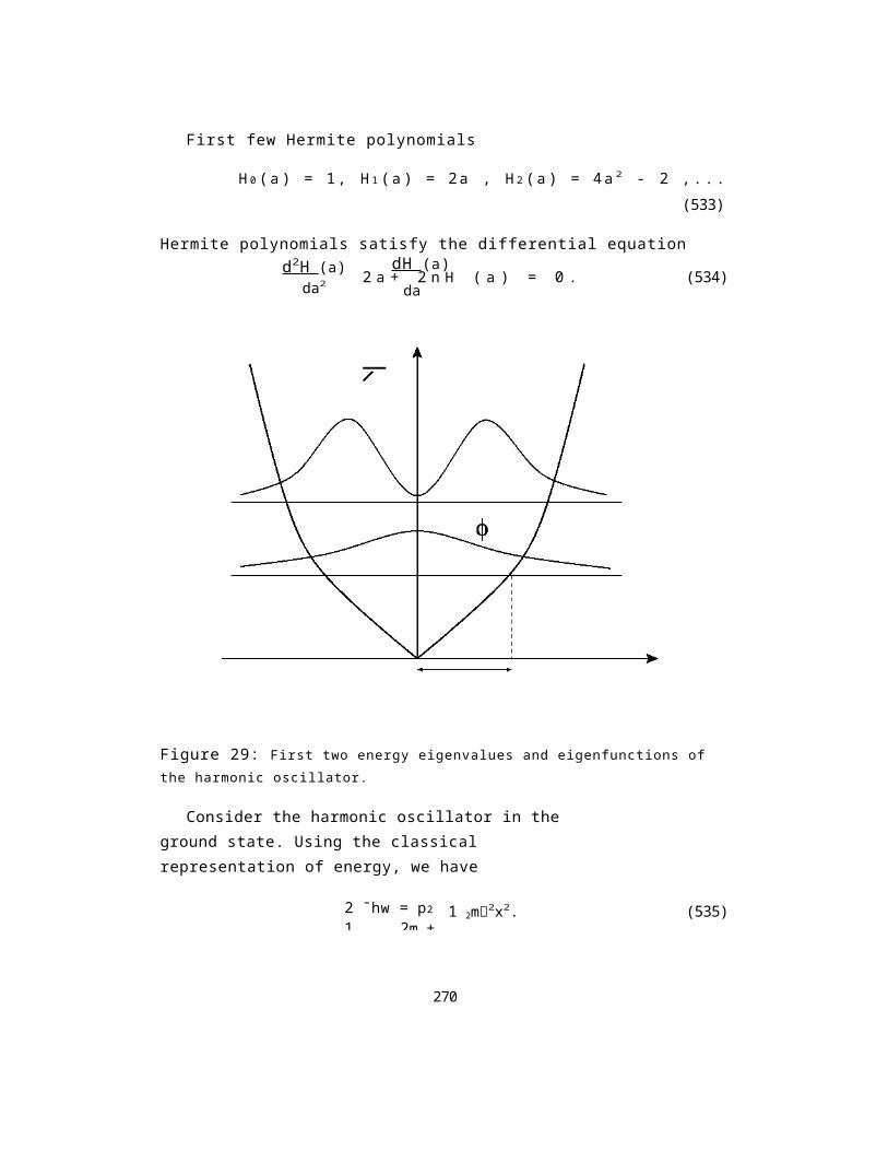
First few Hermite polynomials

H 0 (a ) = 1, H 1 (a ) = 2a , H 2 (a ) = 4a 2 - 2 , . . .(533)

Hermite polynomials satisfy the differential equationd 2 H (a)

da2dH (a)

2 a + 2 n H ( a ) = 0 . (534)da

Figure 29: First two energy eigenvalues and eigenfunctions of the harmonic oscillator.

Consider the harmonic oscillator in the ground state. Using the classical representation of energy, we have

2 ¯hw = p21 2m +

1 2m2x2. (535)

270

xx

EhV

|φ 2

E=3/| 0|2

E=

Since, p2 ~ 0, the particle must be restricted to positions x, such that

1 12m2x2 < 2¯hw, (536)

i.e.

The maximum of |x| x 0 = ¯h/mis called the

classical turning point.

Since the wave function 0(x) is not restricted to xx0, see Fig. 29, quantum mechanics predicts that theharmonic oscillator can be in the classically forbiddenregion.

14.2 Special functions method

We will carry out the solution of the eigenvalue equationof the harmonic oscillator again, this time using thestationary Schrödinger equation in a form of a second-order differential equation.

The starting point is the stationary Schrödinger equationfor the harmonic oscillator whose the Hamiltonian is of the form

Hˆ =    12m

ˆp2 + 1 2mw2ˆx2. (538)

Since in one dimension, pˆ = —i¯hd/dx, the Schrödinger (eigenvalue) equation takes the form/ )

— ¯h2 d2 = E , (539)dx2 + 1 2mw2x22m

271

|x| V h ̄ mw

. (537)

or multiplying by —2m and dividing by ¯h2, we obtain a second-order differential equation

d 2 çb dx2 +

(2 m E — m 2 ¯h2 2 )x2 cb = 0 . (540)

272

This is not a linear differential equation, and it is not easy to obtain a solution.

We can proceed in the following way. Introducing new variables

2m ¯h2 E ,32 = m2(, ,2

we can write Eq. (540) in asimpler form

d 2 ( A - 32x2)dx2 + = 0 . (542)

Despite of the difficulty, we will try to solve thedifferential equation (542). First, we will find thesolution of Eq. (542) in the asymptotic limit of large x(x >> 1). In this limit, we can ignore the A term asbeing small compared to 32x2, and obtain

d2dx2 32x2çb = 0 . (543)

Solution of Eq. (543) is of the form()- 1

cb(x) = C exp 23x2 , (544)where C is a constant.

Hence, we will try to find the solution of Eq. (542) in the form ()

- 1(x) = f(x) exp 23x2

(545)

i.e. in the form satisfying the asymptotic

solution (544). Substituting Eq. (545) into

Eq. (542), we get

273

A = ___¯h2 ,____(541)

d2fdx2

df23x + (A - 3)f =0. (546)dxIntroducing a new variable a = /3x, and a new function f(x) -* H(a), for which

3 d2Hdadx = 3 d2H= da2 , (547)da2

274

dfdx = dH da

da dx,i 3 dH

=d2f

the differential equation (546) transforms to(

d 2 H dHd 2 - 2 + - 1 H = 0 . (548)

d

This equation is identical to the differential equation for Hermite polynomials, with

- 1 = 2n , (549)

where n is integer.

Thus, the wave functions of the harmonic oscillator are ofthe form

( )

- 1n(x) = NHn(a) exp22 , (550)

where N is a normalization constant.Since n is integer, we find from Eqs. (549) and (541)

that the energy eigenvalue E is( )

n + 1E = ¯hw . (551)

2

In summary, the solution of the Schrödinger equationgiven in the differential form agrees perfectly with theresults obtained by the algebraic operator technique.

In summary of this lecture: We have learnt that

1. The energy of a harmonic oscillator is quantized, with

275

/3

the sequence of values( )

n + 1En = ¯hw , n =0, 1, 2, . . .

276

2. The energy levels are equally spaced. This is animportant point to remember. The difference in energybetween adjacent energy levels is equal to the energy ofa single photon, ¯hw.

3. The lowest energy the oscillator can have is E0 = 1 2¯hw, which is nonzero. Thus, the oscillator can never be made stationary.

4. The oscillator can be found in the classicallyforbidden region. This is an another example ofpenetration of a potential barrier or quantumtunneling.

Exercise:

Assume that the Harmonic oscillator is in the ground staten = 0. Calculate the probability that the oscillator willbe found in the classically forbidden region, where thekinetic energy is negative.

Solution:

We have shown in lecture that the wave function of the

ground state is

0(x) = Ae_ x 2 ,

where mw ) 1A = _________ 4 a n d =71¯h

mw 2¯h

277

= 2A 2 x 0 e _ 2 x 2dx = 2A 2

2 1

e_2x2

dx .

Classically forbidden regions are x −x 0 and x ~ x 0, where x 0 = ¯h/mw is the classical turning point, see Fig. 29.

Probability of finding the Harmonic Oscillator in the classically forbidden region is

_x 0

P = _ | 0 (x )| 2 d x + x 0 | 0 (x )| 2 d xSubstituting

y2 = 23x2 ,

we change the variable

x =1 1

2 y and (Ix = 2

(Iy .Hence2 A 2

1 e-y2 (Iy =    2P = 2 1 e - y

2 ( I y =

1 − Erf(1) =0.16 ,

x

2Erf(x ) = v 7 r 0 e - y 2 ( I y .

Thus, there is about a 16% chance that the oscillator will be found in the classically forbidden region.

Exercise at home:

Use the operator approach developed in lecture to provethat the nth har-

monic oscillator energy eigenfunction obeys the following

278

uncertainty relation

h¯8x8p= 2 (2n+1) ,

where 8x = (ˆx2) − (ˆx)2 and 8px = (ˆp2 x) − (ˆpx)2 are fluctuations of the position and momentum operators, respectively.

279

15 Angular Momentum and HydrogenAtom

In order to explain the observed discrete atomic spectra,Bohr postulated

that angular momentum of the electron in a hydrogen atom isquantized, i.e.

L=n¯h, n = 1 , 2 , 3 , . . . . ( 5 5 2 )

However, a careful analysis of the observed spectra showed that the angular momentum cannot be n¯h, but rather l(l + 1), where l = 0, 1, 2, . . . , n 1.

It follows from the Bohr postulate that energy and alsoelectron’s orbits are quantized, that the electron can beonly at some particular distances from the nucleus. Aquestion arrises, where really is the electron when itmakes a transition from one orbit to another?

Here, we will give the answer to this questionanalyzing the motion of the electron in the hydrogen atomfrom the point of view of quantum wave mechanics. In thisapproach, rather than worrying about the position andmotion of the electron, we will classify the electron interms of the amount of energy that the electron has. Inthis description, the electron is represented by a wavefunction W(r), which satisfies the stationary Schrödingerequation

ˆHW(r) = EW(r), (553)

where the Hamiltonian is¯h2

Hˆ = ____V2 + Vˆ (r), (554)2m

280

with

. (555)4 0 rThus, the potential depends only on the distance r of the moving electron from the nucleus (central force).

Since the potential V(r) has a spherical symmetry, we will work in the spherical coordinates, shown in Fig. 30, in which

1V2=

r2( ) ( )

8 r 2 8 +     1 8 + 1 82sin 8 82 . (556)

281

Vˆ (r) =e2 1

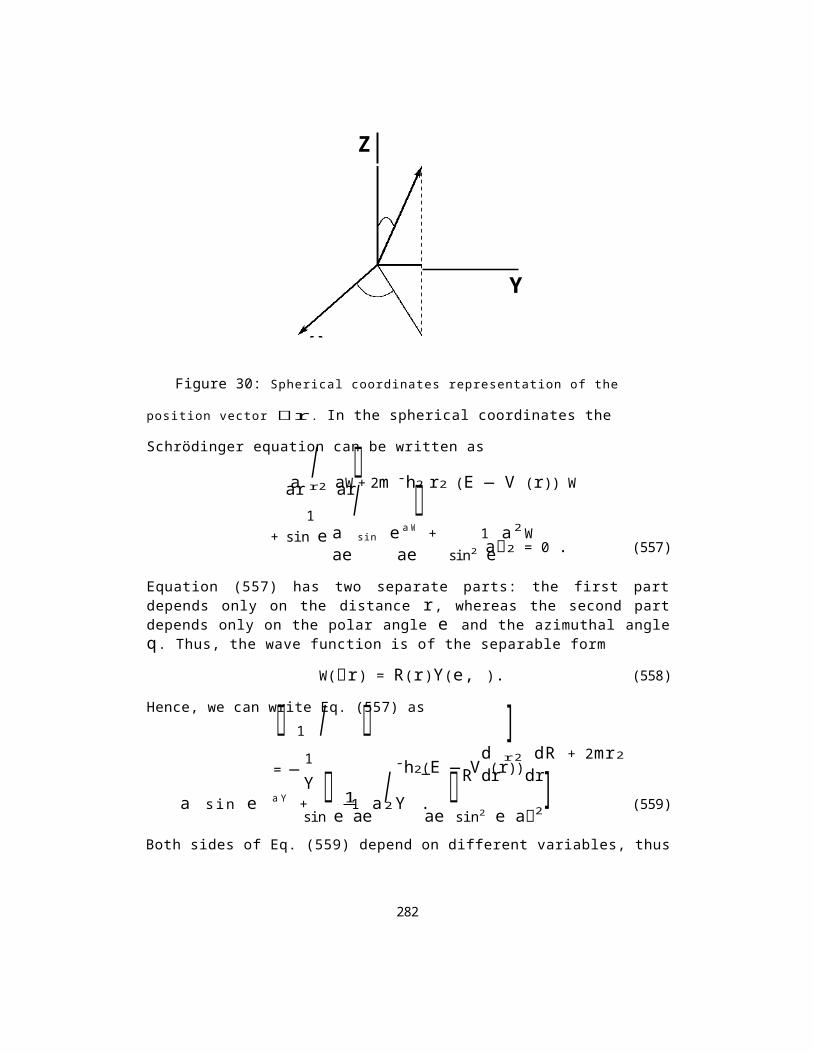
Z

θr

φ Y

X

Figure 30: Spherical coordinates representation of the

position vector r. In the spherical coordinates the

Schrödinger equation can be written as/ a r2 aW + 2m ¯h2 r2 (E — V (r)) War ar/ a sin e a W +    1 a 2 W

a2 = 0 . (557)ae ae sin2 eEquation (557) has two separate parts: the first partdepends only on the distance r, whereas the second partdepends only on the polar angle e and the azimuthal angleq. Thus, the wave function is of the separable form

W(r) = R(r)Y(e, ). (558)

Hence, we can write Eq. (557) as 1 / ]d r2 dR + 2mr2

¯h2_(E — V (r))R dr dr 1 / ]a sin e a Y +    1 a 2Y . (559)sin e ae ae sin2 e a2

Both sides of Eq. (559) depend on different variables, thus

282

1+ sin e

1= —Y

must be equal to

283

the same constant, say —a:( \1 d r2 dR +    ¯h2 2m (E — V (r)) R + r2 a R = 0 , (560)r2 dr dr

1sin9

( \8 sin 9 8 Y +     1 8 2 Y82 — aY = 0 . (561)

First, we consider Eq. (561) that depends on 9, q.

15.1 Angular part of the wave function: Angular momentum

In fact, Eq. (561) is the eigenvalue equation for the square of the angular momentum operator

that in the spherical coordinates ˆL2 is of the form 1 ( \ )8 8 2 Y

ˆL 2 = —¯h2    ____sin 9 8 Y +    1 . (563)sin 9 89 89 sin2 9 82

Since the eigenvalue equation for ˆL2 can be written asˆ

L2Y(9, ) = AY(9, ) , (564)

we have that a = —A/¯h2, where A is the eigenvalue of ˆL2.ˆL2 as ( \

sin 9 8 sin 98Y — a sin2 9Y + 82Y

82 = 0 . (565)89 89This equation contains two separate parts, one dependentonly on 9 and the other dependent only on çb. Therefore,the solution of Eq. (565) will be of the form

284

Lˆ = rˆx

pˆ = —i¯h

ˆr xV, (562)

Thus, we can write the eigenvalueequation for

Y (9, ) = X (9 )( ). (566)

285

Hence, substituting Eq. (566) into (565), and dividing both sides by X(e)(q), we obtain

( )

X sin e d1 sin e dX − a sin2 e = − 1 d2

dq2 , (567)de de

where X X(e) and cI (q).As before, both sides must be equal to a constant, say m2. Thus( )

X sin e d1 sin e dX − a sin2 e = m2 , (568)

de de

=−m2 . (569)

First, we will solve Eq. (569) for the azimuthal part of the wave function, which we can write as

=−m2 , (570)

and the solution of Eq. (570) is

(q) = Aexp(imq) , (571)

where A is a constant.Since in rotation, q and q + 2ir correspond to the same

position in space: (q) = II(q + 2ii-), which is satisfied when

exp(imq) = exp[im(q + 2ir)] . (572)

From this we find that

exp(i2irm) = 1 . (573)

However, this is satisfied only when m is an integer, m =0, ±1, ±2, . . .. Hence, the constant m2 is not an

286

1 d2

d2dq2

arbitrary number, is an integer. Normalization of (q) gives

2

1 = 0 |(q)|2 dq = 2|A|2 , (574)

287

which leads to the final form of () as1

( ) = / 2 ir exp(i m ) . (575)

The next step in the solution is to find X(e), the polarcomponent of the wave function.

From Eq. (568), if we multiply both sides of the equation by X and divide by sin2 e, and rearrange, we obtain

sin e1

de de sin2 ed sin e dX +_ m2

( ) ( ______ _ X = 0 . (576)Introducing a new variable z = cos e, and noting that

ded = _ dz , (577) 1 _ z2 d

we find(

( 1 _ z2 d2Xdz2 _ 2z dX +__ m2dz _ X = 0 ,1 _ z2or

Equation (578) is known in mathematics as the generalizedLegendre differential equation, and its solutions arethe associated Legendre polynomials. For m = 0, theequation is called the ordinary Legendre differentialequation whose solution is given by the Legendrepolynomials.

Solution of Eq. (578), that is regular at z = 1, is assumed to be represented by a power series of the form

288

ddz

[ (1 _ z2 )

dX +___ m2_ X = 0 .

X (z )=(1_ z ) 2 |m|1

3=0

a3z3 .

(579)

Substituting Eq. (579) into Eq. (578), we obtain the recursion relation for the coefficients a3:

( j + |m| )( j + |m| + 1) + a3+2 = (j + 1)(j +2) a3 . (580)

289

Since aj+2 > aj, the series diverges (logarithmically)for z = ±1. Therefore, in order to get the wave functionfinite everywhere in the space, we have to terminate theseries at some j = j0. In other words, we assume thataj0+1 = aj0+2 = . . . = 0.

The series terminating at j = j0 indicates that

(j 0 + m )(j 0 + m +1)+a =0. (581)

Introducingl=j 0+ m , (582)

we see that l ~ m , and

= −l(l + 1) , l=0,1(583)

Hence, we see that the eigenvalues of the angular momentum

are quantized

ˆL2 A=¯h2l(l+1),

,/_____Lˆ A = h¯ l(l + 1) . (584)

The integer number l is called the angular momentum

quantum number. Since l ~ m , the number m is limited to

absolute values not larger than l. Physical

interpretation of the quantum number m

We have already shown that the azimuthal part of the wave function is given by

1 ( ) = 2 ex p ( i m ) , m = 0, ±

(585)

290

Consider the z-component, ˆLz, of the angular momentum.We will try to find the eigenvalues and eigenfunctions of ˆLz:

ˆLz = Ii . (586)

In the spherical coordinates

ˆLz = −i¯h , (587)

291

and then we get from Eq. (586) a simple differential equation

—i¯h

9 q = µ , (588)

whose solution is( i )

(q) = A exp ¯hµq, (589)

where A is a constant.Using the same argument as before, that in rotation, q

and q + 2ir correspond to the same position in space, we find that

µ=m¯h, m=0,±1,±2,... (590)

Thus, the azimuthal part of the wave function is the wavefunction of the z- component of the angular momentum, andthe number m is the z-component angular momentum quantumnumber.

Example:

Consider angular momentum with l = 1. In this case, theeigenvalue of

L ˆ is /2¯h, and ˆLz can have three values +¯h, 0, —¯h.Thus, the orientation

ˆ ˆof L along the z-axis is quantized. The vector L

processes around z axis,

292

Xl m(z) = (1 — z)2 |m|1

l−|m|

j=0ajzj . (591)

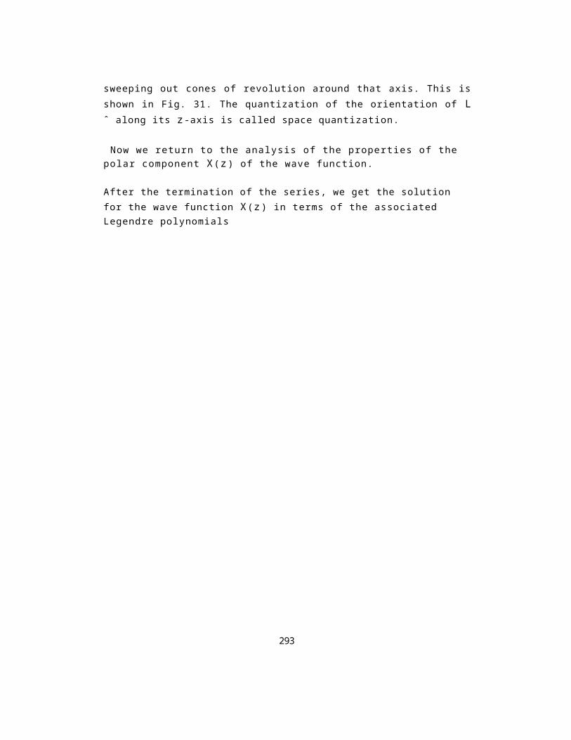
sweeping out cones of revolution around that axis. This isshown in Fig. 31. The quantization of the orientation of Lˆ along its z-axis is called space quantization.

Now we return to the analysis of the properties of the polar component X(z) of the wave function.

After the termination of the series, we get the solution for the wave function X(z) in terms of the associated Legendre polynomials

293

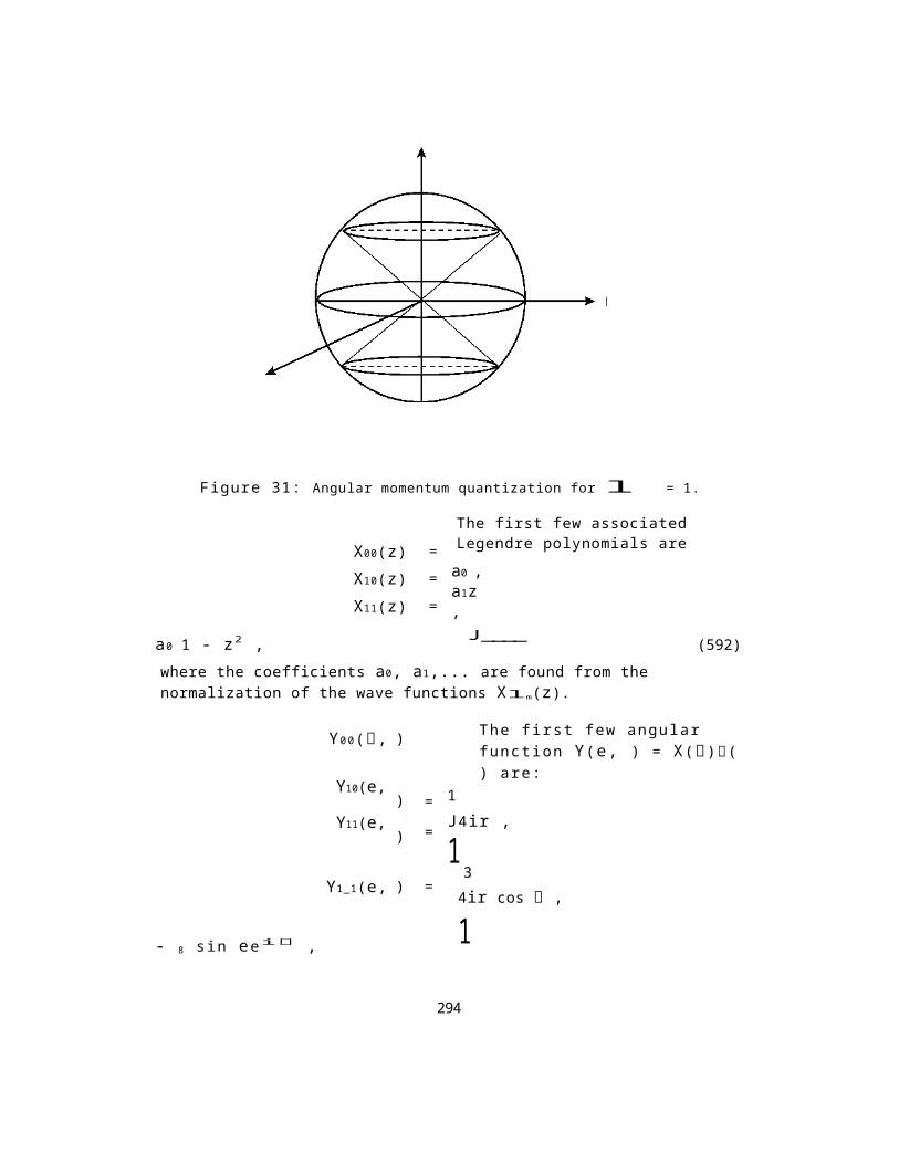
Figure 31: Angular momentum quantization for l = 1.

The first few associated Legendre polynomials area0 ,a1z ,J____a0 1 - z2 , (592)

where the coefficients a0, a1,... are found from the normalization of the wave functions Xlm(z).

The first few angular function Y(e, ) = X()() are:

1J4ir ,

134ir cos ,

1- 8 sin eei ,

294

L

m=+1

m=0L y

m=-1L

X00(z) =X10(z) =X11(z) =

Y00(, )

Y10(e,

Y11(e,)

)

=

=

Y1_1(e, ) =

3

18ir sin ee_i . (593)3

295

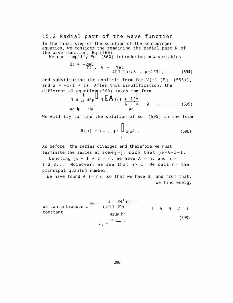
15.2 Radial part of the wave functionIn the final step of the solution of the Schrödinger equation, we consider the remaining the radial part R of the wave function, Eq.(560).

We can simplify Eq. (560) introducing new variables 2 = —2mE¯h2_ , A = me 2

4U¯h2/3 , p=2/3r, (594)

and substituting the explicit form for V(r) (Eq. (555)),and a = —l(l + 1). After this simplification, the differential equation (560) takes the form/ A 1 d p2 dRp — 1 4 — l(l + 1)

_ +     R = 0 . ________(595)p2 dp dp p2

We will try to find the solution of Eq. (595) in the form

R(p) = e− 2 p l 1

j

bjpj . (596)

As before, the series diverges and therefore we must terminate the series at somej =j U such that j U =A — l — 1.

Denoting jU + l + 1 = n, we have A = n, and n = 1,2,3,....Moreover, we see that n> l. We call n- the principal quantum number.We have found A (= n), so that we have 3, and from that,

we find energy

We can introduce a constant

ao =

4rU¯h2me2___ , (598)

296

1(4 U

)2

n2 .1 ( 5 9 7 )

E= me42̄ h2

Thus, the energy of the electron in the hydrogen atom isquantized. Note

that Eq. (599) agrees perfectly with the prediction of theBohr theory of the

297

1E= —

4lrEU

e2(599)

2aon2 .

hydrogen atom (see Eq.(111)).

Since p = 23r, and 3 = 1/(aom), the radial part of the wave function can be written as

Rnl(r) = e-r (23r)l Ll n(r) , (600)

where

are the associated Laquerre polynomials of order (m - l - 1).

The coefficients bj are found fromthe normalization of the radial

function

drr2|Rnl(r)|2 = 1 . (602)

Once the radial part of the wave function is known, thesolution for the problem of the hydrogen atom is completedby writing down the normalized wave function of theelectron

T'n l m(r, , q) = R n l(r)Y l m(e, ) . (603)

In summary of this lecture:

The eigenvalues of the energy of the electron in the hydrogen atom are quantized

and the corresponding eigenfunctions are

hmnlm(r, , q) = Rnl(r)Ylm(e, ) , (605)

298

0

E n = 4i r 0 2aom2 , (604)1 e2

Ll n(r)= n - l - 1

j=0

bj (23r)j (601)

where the discrete (quantum) numbers are

m = 1,2,3,...,oc,l = 0, 1, 2,...,m- 1 ,m = 0,±1,±2,...,±l . (606)

299

Few normalized eigenfunctions of the electron

1 1 0 0 = ./ e

7ra3 o

_r/ao,

( )

1

e_r/(2ao)1 −    r 2 0 0 = 8 a 3 2aoo

Note that eigenfunctions with l = 0 have spherical symmetry, i.e. are independent of and q.

The absolute square of the wave function |'T'nl m(r, , q)|2 is the probability density

of finding the electron at the point r(r, , q), and

Pnlm = |Wnlm(r, , q)|2dV = 4irr2|Wnl m(r, , q)|2drd dq (608)

is the probability of finding the electron in a small volume dV = drd dq around the point r.

P100

1 2 r/ao

300

,

1 2 1 0 = / _________________________________________________________________

32ira3 o

rao

e_r/(2ao) cos . (607)

Figure 32: Probability function of theelectron in the state (nlm) = (100).

The maximum value of Pnlm, which is themost probable distance of the electron fromthe nucleus, differs from the expectation(average) distance (r), given by

f(r) = n l mrJ'n l mdV .(609)

301

Examples of the probability function Pnlm are shown in Figs.32 and 33.

P 200

Figure 33: Probability function of the electron in the

state (nlm) = (200). Interesting properties of the

probability function P n l m:

1. For n = 1, the probability has one maximum at r = a o.

2. For (n = 2, l = 0, m = 0), the probability shows twomaxima located at r = n2ao.

3. Only for states such that n = l + 1, the probability shows one maximum located at r = n2ao.

Exercise:

The normalized wave function for the ground state of a hydrogen atom has the form

W (r) = Ae_r/ao ,

302

r/ao3+

where A = 1/ira3 o is a constant, a o = 4ir o¯h2/me2 is the Bohr radius, and r is the distance between the electron and the nucleus. Show the following:

303

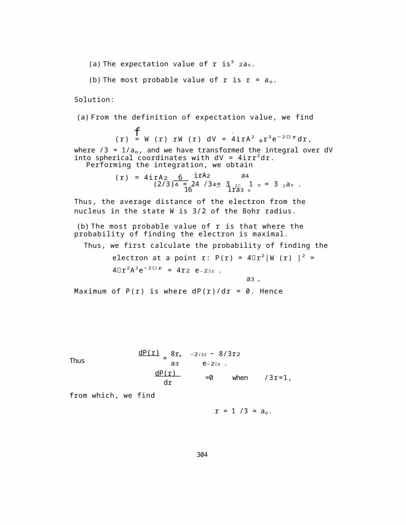
(a) The expectation value of r is3 2ao.

(b) The most probable value of r is r = ao.

Solution:

(a) From the definition of expectation value, we find

f

(r) = W (r) rW (r) dV = 4irA2 0r3e−2rdr,

where /3 = 1/ao, and we have transformed the integral over dVinto spherical coordinates with dV = 4irr2dr.

Performing the integration, we obtainirA2 a4(r) = 4irA2 6

(2/3)4 = 24 /34_= 3 2 1 o = 3 2ao .16 lra3 oThus, the average distance of the electron from the nucleus in the state W is 3/2 of the Bohr radius.

(b) The most probable value of r is that where the probability of finding the electron is maximal.

Thus, we first calculate the probability of finding the electron at a point r: P(r) = 4r2|W (r) |2 = 4r2A2e−2r = 4r2 e−2r .

a3 o

Maximum of P(r) is where dP(r)/dr = 0. Hence

ThusdP ( r )

drfrom which, we find

=0 when /3r=1,

r = 1 /3 = ao.

304

dP ( r )

dr= 8re

a3 o

−2/3r − 8/3r2e−2r .a3 o

Note that this result agrees with the prediction of the Bohr model, that the radius of the n = 1 orbit is equal toa o.

In summary of the solution: The expectation and mostprobable values of r are not the same. This is because theprobability curve P100( r) is not symmetric about the maximumat a o, see Fig. 32. Thus, values of r greater than a o areweighted more heavily in the equation for the expectationvalue than values smaller than ao. This results in theexpectation value (r) exceeding a o for this probabilitydistribution.

Challenging problem : Eigenfunctions of the angular momentum

The eigenfunctions of the angular momentum L ˆ of the electron in a Hydrogen atom for l = 1 are

3Y 1 0 ( , ) = 4 cos , Y 1 ± 1 ( , ) = 8 sin e ±i .

3

(a) Show that the eigenfunctions are also eigenfunctions of the ˆLz component of the angular momentum.

(b) Show that the eigenfunctions are not eigenfunctions of the ˆLx component of the angular momentum.

(c) Find the matrix representation of ˆL x in the basis of the eigenfunctions of ˆL.

(d) Find the eigenvalues and eigenfunctions of ˆLx in the basisof the eigenfunctions of ˆL.

305

16 Systems of Identical Particles

Consider a system composed of N parts (subsystems), e.g. a system of N identical and independent particles, whose theHamiltonian is given by

Hˆ = N ˆHi , (610)

i=1

and the wave function is

W(r) = 1(r 1) 2(r 2) . . . N (rN ) , (611)

where i (r i ) is the wave function of the ith particlelocated at the point r j, or equivalently we can say thati (rj) is the wave function of the jth particle being in theith state.

However, the wave function W(r) is not the only eigenfunction of the system. For example, a wave function

W(r) = 1(r 2) 2(r 1) . . . N (rN ) , (612)

is also an eigenfunction of the system with the

same eigenvalue. Proof:

Consider the eigenvalue equation with the eigenfunction (611):

ˆHW(r) = N ˆH iW(r)

i=1

= N ˆ H i 1 (r 1 ) 2 (r 2 ) . . . N (r N ) = N

E i W(r ) .

306

i i=1

Consider now the eigenvalue equation with the eigenfunction (612)

ˆHW(r) = N ˆH iW(r) = N

ˆH i 1(r 2) 2(r 1) . . . N ( r N )

.i=1 i

307

Since^H 1 1(r 2) = E 1 1(r 2) , andwe get that ^HW(r) = N

i=1EiW(r). Even if

^H11(r2) = E2çb1(r2), and we get that

^H 2 2(r 1) = E 2 2(r 1) ,

^H 2 2(r 1) = E 1 2(r 1) ,

^HW(r) = N EiW(r) , (613)

i=1

as required.

In fact there are a total N! permutations of çbi(rj) which are eigenfunctions of the system.

Moreover, an arbitrary linear combination of the wave functions i(rj) is also an eigenfunction of the system.We will illustrate this for N = 2.

16.1 Symmetrical and antisymmetrical functionsConsider an arbitrary linear combination of two wave functions

1W(r) = a 2 +

_________(614)

where W(r12 = 1(r1)2(r2) and W(r21 = 1(r2)2(r1).

Then)

^HW(r) = ( ^H1 + ^H2 W(r)1

308

=

__a 2 + b 2 [a (E1 + E2) W(r12) + b (E1 + E2) W(r21)]

=(E 1+E 2)W(r) . (615)

We know that in the linear combination a 2/( a 2 + b 2) isthe probability

that the particle ”1” is at the position r1 and theparticle ”2” is at r2.

309

Equivalently, for r1 = r2, we can say that this is the probability that the particle ”1” is in a state 1), andthe particle ”2” is in a state 2).

Similarly, b 2/( a 2 + b 2) is the probability that the particle ”1” is at the position r2, and the particle ”2” is at r1.

Note, that in general, the probabilities aredifferent. However, for two identical particles, theprobabilities should be the same as we cannot distinguishbetween two identical particles.

Thus, for two identical particles a = b . Hence, the parameters a and b can only differ by a phase factor: b =a exp(iq), where q is a real number:

1 [ ]

W(r) = 2 W(r 1 2) + eiW(r 2 1). (616)

If we exchange the positions of the particles (r1 —* r2) or energy states ( 1) —* 2)), then we obtain

1 [ ]

W '(r) = 2 eiW(r 1 2) + W(r 2 1). (617)

Thus, the exchange of r1 r2 or 1) —* 2) is equivalent to multiplying W(r)by ei and taking e2i = 1. Hence

ei = ±1, (618)

and therefore the wave functions of identical particles are either symmetrical or antisymmetrical

1W s (r ) = 2 [W(r 1 2 )+W(r 2 1 )] ,

310

1h1 a(r) = 2 [W(r 1 2) − W(r 2 1)] . (619)

Note that

1J1s(r12) = 1J1s(r21) ,Wa(r 1 2) = −Wa(r 2 1) . (620)

311

Properties of symmetrical and antisymmetrical functions:

1.If H ˆ = ˆH1 2 = ˆH2 1, i.e. the Hamiltonian is symmetrical, then ˆHW(r) has the same symmetry as W(r).

Proof:

Take W(r) = Ws(r). Denote f12 = ˆH12Ws(r12), then

f21 = ˆH21 Ws(r21) = ˆH12Ws(r12)

= f12 . Take now W(r) = Wa(r). Then

f21 = ˆH21 Wa(r21) = ˆH12 (—Ws(r12)) = —f12 ,

as required.

2. Symmetry of the wave function does not change in time, i.e.wave function initially symmetrical (antisymmetrical)remains symmetrical (antisymmetrical) for all times.

Proof:

Consider an evolution of a wave function W(t) in a time dt:

a W W(t + dt) = W(t) + _dt .

atThus, symmetry of the wave function depends on the symmetry of aW/at. From the time-dependent Schrödinger equation

i¯haW

at =ˆHW,

we see that aW/at has the same symmetry as ˆHW. From theproperty 1, we know that ˆHW has the same symmetry as W.Therefore, W(t + dt) has the same symmetry as W(t),

312

as required.

313

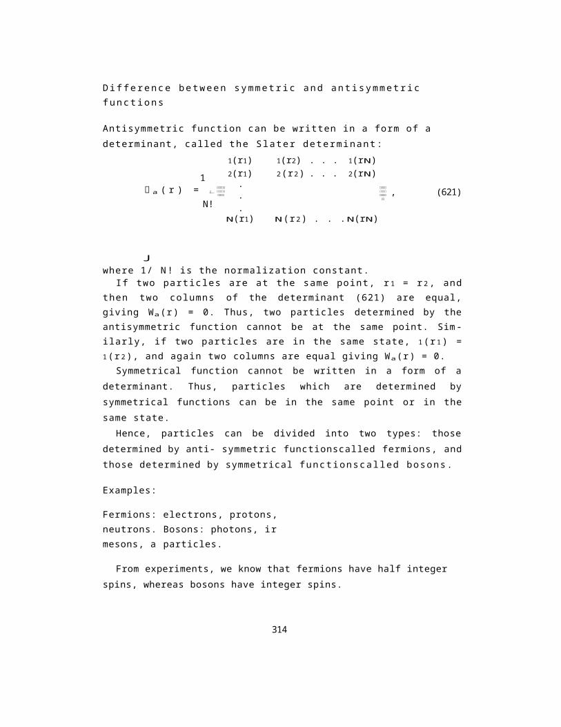
Difference between symmetric and antisymmetric functions

Antisymmetric function can be written in a form of a determinant, called the Slater determinant:

1 a ( r ) =

N!

1(r1) 1(r2) . . . 1(rN)2(r1) 2(r2) . . . 2(rN)...

N(r1) N(r2) . . .N(rN)

, (621)

Jwhere 1/ N! is the normalization constant.

If two particles are at the same point, r 1 = r 2, andthen two columns of the determinant (621) are equal,giving Wa(r) = 0. Thus, two particles determined by theantisymmetric function cannot be at the same point. Sim-ilarly, if two particles are in the same state, 1(r 1) =1(r 2), and again two columns are equal giving Wa(r) = 0.

Symmetrical function cannot be written in a form of adeterminant. Thus, particles which are determined bysymmetrical functions can be in the same point or in thesame state.

Hence, particles can be divided into two types: thosedetermined by anti- symmetric functionscalled fermions, andthose determined by symmetrical functionscalled bosons.

Examples:

Fermions: electrons, protons, neutrons. Bosons: photons, ir mesons, a particles.

From experiments, we know that fermions have half integer spins, whereas bosons have integer spins.

314

Since, an arbitrary number of bosons can be in thesame state, they can be condensated to a single state. Wecall this process Bose-Einstein condensation.

315

16.2 Pauli principle

In atoms, a limited number of electrons (fermions) canoccupy the same energy level. How many electrons does ittake to fill an energy level? The answer to this questionis given by the Pauli principle.

Pauli principle:

No two electrons can have the same quantum numbers (n ,l , in , s ) in a multi-electron atom.

It is also known as the exclusion principle, for the simplereason that if an electron has the quantum numbers (nlins)than at least one of the quantum numbers of any furtherelectrons must be different.

In an atom, for a given n, there are 2(2l + 1) degeneratestates corresponding to l = 0, 1,2,..., in = -l, . . . ,l, and s = - 1 2, +1

2. Thus, for a given n the total numberof electrons in the energy state J?n is

l= m 2(2l + 1) = 2n 2 . (622)l = - m

Following the Pauli principle, we can find numbers of electrons in the energy states

1 s , 2 s , 2 p , 3 s , 3 p , 4 s , 3 d , 4 p , 5 s , 4 d , 5 p2 2 6 2 6 2 10 6 2 10 6

The Pauli principle prevents the energy states being occupiedby an arbitrary number of electrons. The state 1s can beoccupied by two electrons. Hence, as more electrons areadded, the energy of the atom grows along with its size.

316

Thus, the Pauli principle prevents all atoms having thesame size and the same energy. This is the quantum physicsexplanation of atomic sizes and energies.

Since the number of electrons on given energy levels islimited, we get different ground state configurations fordifferent atoms. The ground state of a many electron atomis that in which the electrons occupy the lowest energylevels that they can occupy.

317

If the number of electrons for a given ml is 2(2l + 1), we say that there is a closed shell. Examples: Helium, Beryllium, Neon.

Since the chemical properties of atoms depend on thenumber of electrons outside the closed shells, the atoms withsimilar outer configurations will have similar chemicalproperties. Examples: The Alkali metals: Lithium (1s)22s,Sodium (1s)2(2s)2(2p)63s, and Potassium(1s)2(2s)2(2p)6(3s)2(3p)64s.This is the explanation from quantum physics of the periodic structure of the elements.

318

Final Remark

It is appropriate to close our lectures on quantum physicsby emphasizing the importance of quantum phenomena in thedevelopment of new areas in science and technology. Thepredictions of quantum physics have turned research andtechnology into new directions and have led to numerous tech-nological innovations and the development of a newtechnology on the scale of single atoms and electrons,called quantum technology or nanotechnology. The ability tomanufacture and control of the dimensions of tinystructures, such as quantum dots, allows us to engineer theunique properties of these structures and predict newdevices such as quantum computers. The technology forcreating a quantum computer is still in its infancy, butis developing very rapidly with little sign of theprogress slowing.

We have seen in our journey through the backgrounds ofquantum physics that despite its long history, quantumphysics still challenges our understanding, and continuesto excite our imagination. Feynman in his lectures onquantum physics referred in the following way to ourunderstanding of quantum physics:

”I think I can safely saythat nobody understands quantum mechanics.”

In summary of the subject, I think I can safely say:

319

”If you think you now know quantum physics, it means you do not know anything.”

Continue study of Quantum Physics with PHYS3040.

320

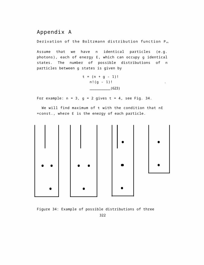
Appendix ADerivation of the Boltzmann distribution function Pn

Assume that we have n identical particles (e.g.photons), each of energy E, which can occupy g identicalstates. The number of possible distributions of nparticles between g states is given by

t = (n + g - 1)!n!(g - 1)! .___________(623)

For example: n = 3, g = 2 gives t = 4, see Fig. 34.

We will find maximum of t with the condition that nE =const., where E is the energy of each particle.

...

...

.

..

.

.

.

Figure 34: Example of possible distributions of three 322

particles between two states.

Taking ln of both sides of Eq. (623), we get

l n t = l n ( n + g - 1 ) ! - l n n ! - l n ( g - 1 ) ! . (624)

Using the Sterling’s formula

lnn! = nlnn - n, (625)

and assuming that g>> 1, i.e. g - 1 g, we obtainn+g

ln t = g ln__________________gn+g

+ n ln____n

. (626)

323

We find maximum of ln t using the method of Lagrange undetermined multipliers. In this method, we construct a function

K = ln t - AnE,

(627)where A is called a Lagrange

undetermined multiplier, and find the extremum

=0. (628)Thus, we get

from which, we

nl nn+g +AE=0 , (629)

e E - 1 .g ( 6 3 0 ) This is the Bose-

Einstein distribution function. Since n is dimensionless,A should be inverse of energy. We choose A = 1/(kBT),where kBT is the energy of free, non-interactingparticles.

When g/n>> 1, we can approximate Eq. (630) byE

n = ge kBT , (631)which is known in statistical physics as the Boltzmann distribution. This gives the number of particles n of energy E.

If there are particles, among N particles, which can havedifferent energies Eu, then

g= N e

324

8Kôn

n =

nuN

E

kB T (632)

is the probability that nu particles of the total N particles have energy Eu. Thus, we can write

E

P n = ae kBT , (633)where a is a constant.Since the probability is normalized to one( n P n = 1), we finally get

ePn =____

n eE

The sum n e kBT is called the partition function.

325

EkBT

. (634)

EkBT

Appendix B: Useful mathematical formulae

Useful properties of trigonometrical functions:

s i n ( a ± 8 ) =

s i n a c o s 8 ± s i n d c o s a

cos(a±8) =

cosacos/3fsinasin8 sin2a =

1 2(1−cos2a)1

c os 2a = 2 (1 +c os 2a )

0 s i n 3 e d e = 43

{

2ir 0 for m = nsin(m) sin(n) dçb = i r f o r m = n

{

2ir 0 for m = ncos(m) cos(n) dçb = ir for m = n

0 2 i r sin(m) cos(n) dçb = 0 for all m

and n

Useful integral expressions 0 0 e x − 1 dx = 4

x30 15

326

0

0

00 −00 e − x2dx =

0 0

−00 xe−x2dx = 0 −00 00 x2e−x2dx = 1

2aa

327

00 n!rne−rdr = an+1 ,

from which, we find

I 00

r2e−rdr = 2 0 r3e−rdr = 6a3 , a4

Taylor series

Kronecker 8 function{1 if m= n

8 m n = 0 i f m = n .

The Dirac delta function

328

5

( d 2 )1    ____2 + .. .2 d 2 k 0

(dw )W k = k 0 + = 0 + +

x5x3x − 3!

x77!+ .−

I0

I 001 , 0 re−rdr =I0 00 e−rdr =a2 1 ,

I0 00

e±x =

sinx =

cosx =

df3 k01 ± x + x22! ± x3

3! + . . .

x21 − 2!

x66!+ .

x4 −4

{0 if x

= 08(x) = oc i f x = 0 ,

I 00

such that−00

f( x) 8( x) d x= f(0) ,

329

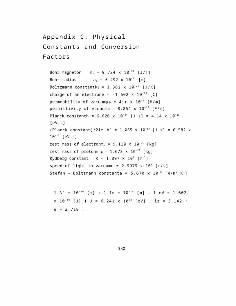
Appendix C: Physical Constants and Conversion Factors

Bohr magneton mB = 9.724 x 10−24 [J/T]Bohr radius ao = 5.292 x 10−11 [m]Boltzmann constantkB = 1.381 x 10−23 [J/K]charge of an electrone = -1.602 x 10−19 [C]permeability of vacuumµ0 = 4ir x 10−7 [H/m]permittivity of vacuum0 = 8.854 x 10−12 [F/m]Planck constanth = 6.626 x 10−34 [J.s] = 4.14 x 10−15 [eV.s](Planck constant)/2ir h¯ = 1.055 x 10−34 [J.s] = 6.582 x 10−16 [eV.s]rest mass of electronme = 9.110 x 10−31 [kg]rest mass of protonm p = 1.673 x 10−27 [kg]Rydberg constant R = 1.097 x 107 [m−1]speed of light in vacuumc = 2.9979 x 108 [m/s]Stefan - Boltzmann constanta = 5.670 x 10−8 [W/m2 K4]

1 A˚ = 10−10 [m] ; 1 fm = 10−15 [m] ; 1 eV = 1.602

x 10−19 [J] 1 J = 6.241 x 1018 [eV] ; ir = 3.142 ;

e = 2.718 .

330