arX

iv:q

uant

-ph/

0105

029v

2 1

4 D

ec 2

001

Decoherence of quantum registers

John H. Reina1,∗, Luis Quiroga2,† and Neil F. Johnson1,‡

1Physics Department, Clarendon Laboratory, Oxford University, Oxford, OX1 3PU, UK2Departamento de Fısica, Universidad de los Andes, A.A. 4976, Bogota, Colombia

The dynamical evolution of a quantum register of arbitrary length coupled to an environment ofarbitrary coherence length is predicted within a relevant model of decoherence. The results arereported for quantum bits (qubits) coupling individually to different environments (‘independentdecoherence’) and qubits interacting collectively with the same reservoir (‘collective decoherence’).In both cases, explicit decoherence functions are derived for any number of qubits. The decay ofthe coherences of the register is shown to strongly depend on the input states: we show that thissensitivity is a characteristic of both types of coupling (collective and independent) and not only ofthe collective coupling, as has been reported previously. A non-trivial behaviour (“recoherence”) isfound in the decay of the off-diagonal elements of the reduced density matrix in the specific situationof independent decoherence. Our results lead to the identification of decoherence-free states in thecollective decoherence limit. These states belong to subspaces of the system’s Hilbert space thatdo not get entangled with the environment, making them ideal elements for the engineering of“noiseless” quantum codes. We also discuss the relations between decoherence of the quantumregister and computational complexity based on the new dynamical results obtained for the registerdensity matrix.

PACS numbers: 03.65.Yz, 42.50.Lc, 03.67.-a, 03.67.Lx

I. INTRODUCTION

When any open quantum system, for example a quan-tum computer, interacts with an arbitrary surroundingenvironment, there are two main effects that have tobe considered when examining the temporal evolution.First, there is an expected loss of energy of the initialsystem due to its relaxation, which happens at the rateτ−1rel where τrel is the relaxation time-scale of the system.

Second, there is a process that spoils the unitarity of theevolution, the so-called decoherence [1], where the con-tinuous interaction between the quantum computer andthe environment leads to unwanted correlations betweenthem in such a way that the computer loses its abilityto interfere, giving rise to wrong outcomes when execut-ing conditional quantum dynamics. This phenomenon ischaracterized by a time that defines the loss of unitarity(i.e. the departure of coherence from unity), the deco-herence time τdec. Usually, the time-scale for this effectto take place is much smaller than the one for relaxation,hence quantum computers are more sensitive to decoher-ence processes than to relaxation ones. For practical ap-plications in quantum computing there are several differ-ent systems that might provide a long enough τrel; how-ever, what really matters for useful quantum informationprocessing tasks (e.g. quantum algorithms) to be per-formed reliably is the ratio τgating/τdec. τgating , the timerequired to execute an elementary quantum logic gate,must be much smaller than τdec. As a rough estimate,fault-tolerant quantum computation has been shown tobe possible if the ratio τgating to τdec of a single qubit is ofthe order of 10−4 [2] (a qubit is a two-state quantum sys-tem, the basic memory cell of any quantum information

processor).Decoherence and quantum theory are unavoidably con-

nected. Indeed, the ubiquitous decoherence phenomenonhas been ultimately associated with the “frontiers” be-tween the quantum behaviour of microscopic systemsand the emergence of the classical behaviour observed inmacroscopic objects [1]: roughly speaking, the decoher-ence time τdec determines the energy and length scalesat which quantum behaviour is observed. It generallydepends non-trivially on several different factors such astemperature, dimensionality, quantum vacuum fluctua-tions, disorder, and others whose origin is less well known(hardware characteristics). The time-scale for decoher-ence depends on the kind of coupling between the systemunder consideration and the environment, in a range thatcan go from pico−seconds in excitonic systems [3] up tominutes in nuclear spin systems [4].

The discovery of algorithms for which a computerbased on the principles of quantum mechanics [5] canbeat any traditional computer, has triggered intenseresearch into realistic controllable quantum systems.Among the main areas involved in this active researchfield are ion traps [6], nuclear magnetic resonance (NMR)[7], quantum electrodynamics cavities [8], Josephsonjunctions [9], and semiconductor quantum dots [10]. Themain challenge that we face is to identify a physical sys-tem with appropriate internal dynamics and correspond-ing external driving forces which enables one to selec-tively manipulate quantum superpositions and entangle-ments. For this to be done, the candidate system shouldhave a sufficiently high level of isolation from the en-vironment: quantum information processing will be areality when optimal control of quantum coherence innoisy environments can be achieved. The various com-

1

munities typically rely on different hardware method-ologies, and so it is important to clarify the underlyingphysics and limits for each type of physical realization ofquantum information processing systems. As mentionedabove, these limits are mainly imposed by the decoher-ence time of each particular system. However theoreticalwork has shown that, in addition to quantum error cor-recting codes [11,12], there are two additional ways thatmay potentially lead to decoherence-free or decoherence-controlled quantum information processing: one of themis the so-called “error avoiding” approach where, for agiven decoherence mechanism (e.g. collective decoher-ence discussed below), the existence of “decoherence-free” subspaces within the system’s Hilbert space can beexploited in order to obtain a quantum dynamics wherethe system is effectively decoupled from the environment[13,15]. This approach requires the system-environmentcoupling to possess certain symmetry properties. Theother approach is based on “noise suppression” schemes,where the effects of unwanted system-bath interactionsare dynamically controlled using a sequence of ‘tailoredexternal pulses’ [16,17]. These strategies have motivatedmuch theoretical and experimental work. In particu-lar, there are some recent experimental results regardingthe engineering of decoherence-free quantum memories[18,19].

We devote this paper to the study of decoherence ofan arbitrary quantum register (QR) of L qubits. In ad-dition to providing a general theoretical framework forstudying decoherence, we examine in detail the two lim-its where the qubits are assumed to couple (i) indepen-dently and (ii) collectively to an external (bosonic) reser-voir. The reservoir is modelled by a continuum of har-monic modes. In Section II we show that the decoher-ence process is very sensitive to the input states of theregister and give explicit expressions for the coherencedecay functions. We have found that these functionspossess a novel behaviour which we label “recoherence”(or coherence revivals) in the specific case of indepen-dent decoherence. This behaviour depends strongly onthe temperature and the strength of the qubit-bath cou-pling. By contrast, for a certain choice of the QR input,the calculation of the reduced density matrix leads to theidentification of decoherence-free quantum states [13,15]when the qubits are coupled “collectively” to the envi-ronment, i.e. when the distance between qubits is muchsmaller than the bath coherence length and hence theenvironment couples in a permutation-invariant way toall qubits. The calculations in this paper were motivatedby the results of Ref. [20,21]. The present paper showsthat some subtle but important details of these earlierresults are incomplete. Particularly, the calculation ofthe L−QR density matrix reported here leads both tonew qualitative results, when analyzing the behaviour ofcoherence decay, and new quantitative results, when es-timating typical decoherence times: these novel results

emerge for L > 1, as discussed in Section III. Conclud-ing remarks are given in Section IV. We emphasize thatthe results of this paper are not restricted to a particularphysical system; they are valid for any choice of the qubitsystem (e.g. photons, atoms, nuclei with spin 1/2, etc.)and any bosonic reservoir.

II. INDEPENDENT VERSUS COLLECTIVE

DECOHERENCE

Let us consider the general case of a L−QR coupled toa quantized environment modelled as a continuum of fieldmodes with corresponding creation (annihilation) bathoperator b† (b). Throughout this work we will analyzepure dephasing mechanisms only. We will not considerrelaxation mechanisms where the QR exchanges energywith the environment leading to bit-flip errors. Hence,the nth qubit operator Jn ≡ Jn

z (Jnx = Jn

y = 0) [23].As mentioned earlier, this is a reasonable approach sincedecoherence typically occurs on a much faster time scalethan relaxation. The dynamics of the qubits and theenvironment can be described by a simplified version ofthe widely studied spin-boson Hamiltonian [22]:

H =

L∑

n=1

ǫnJnz +

∑

k

ǫkb†kbk +

∑

n,k

Jnz (gn

kb†

k+ gn∗

kbk), (1)

where the first two terms describe the free evolution ofthe qubits and the environment, and the third term ac-counts for the interaction between them. Here gn

kde-

notes the coupling between the nth qubit and field modes,which in general depends on the physical system underconsideration. The initial state of the whole system isassumed to be ρS(0) = ρQ(0) ⊗ ρB(0) (the superscriptsstand for system, qubits, and bath), i.e. the QR andthe bath are initially decoupled [24]. We also assumethat the environment is initially in thermal equilibrium,a condition that can be expressed as

ρB(0) =∏

k

ρk(T ) =

∏

k

exp(−βhωkb†kbk)

1 +⟨

Nωk

⟩ , (2)

where⟨

Nωk

⟩

=[

exp(−βhωk)−1

]−1is the Bose-Einstein

mean occupation number, kB is the Boltzmann constantand β ≡ 1/kBT . For the model of decoherence presentedhere it is clear that we are in a situation where the qubitoperator Jn

z commutes with the total Hamiltonian H andtherefore there is no exchange of energy between qubitsand environment, as expected. We will not attempt toperform a group-theoretic description for the study ofquantum noise control [25]. Instead, we study the specificreal-time dynamics of the decay in the QR-density matrixcoherences within the model given by the HamiltonianEq. (1) (i.e. Abelian noise processes, in the language ofRefs. [26,27]).

2

In the interaction picture, the quantum state of thecombined (qubits + bath) system at time t is givenby |Ψ(t)〉

I= U

I(t)|Ψ(0)〉, where |Ψ(0)〉 is the initial

state of the system, UI(t) is the time evolution oper-

ator, UI(t) = T exp

[

− i/h∫ t

oH

I(t′)dt′

]

, and T is thetime ordering operator. For the Hamiltonian (1) weintroduce the notation H = H0 + V , where H0 =∑L

n=1 ǫnJnz +

∑

kǫkb

†kbk denotes the free evolution term

and V =∑

n,k Jnz (gn

kb†k + gn∗

kbk) is the interaction term.

Hence, the interaction picture Hamiltonian is given byH

I(t) = U †

0 (t)V U0(t), with U0 = exp(− ihH0t). A simple

calculation gives the result

HI(t) =

∑

n,k

Jnz

(

gnkeiω

ktb†

k+ g∗n

ke−iω

ktbk

)

, (3)

which allows us to calculate the time evolution operatorU

I(t). The result is (see appendix B.1 for details)

UI(t) = exp

[

iΦωk(t)

]

exp

[

∑

n,k

Jnz

{

ξnk(t)b†

k− ξ∗n

k(t)bk

}

]

(4)

with

Φωk(t) =

∑

n,k

∣

∣Jnz gn

k

∣

∣

2 ωkt − sin(ω

kt)

(hωk)2

,

ξnk(t) = gn

kϕω

k(t) ≡ gn

k

1 − eiωk

t

hωk

. (5)

This result differs from the one reported in Ref. [20]where the time ordering operation for U

I(t) was not per-

formed. As will become clear later, this correction altersthe resulting calculation of Ref. [20], and hence changesthe results for the reduced density matrix of an arbitraryL−QR. Based on the time evolution operator of Eq. (4),we report here a different result for this density matrixand discuss its implications with respect to those of Ref.[20].

Unless we specify the contrary, we will assume thatthe coupling coefficients gn

k(n = 1, ..., L) are position-

dependent, i.e. that each qubit couples individually toa different heat bath, hence the QR decoheres ‘indepen-

dently’. Implications for the ‘collective’ decoherence casewill be discussed later. Let us assume that the nth qubitexperiences a coupling to the reservoir characterized by

gnk

= gk

exp(−ik·rn) , (6)

where rn denotes the position of the nth qubit. It iseasy to see that the unitary evolution operator given byEq. (4) produces entanglement between register statesand environment states [20]. The degree of the entan-glement produced will strongly depend on the qubit in-put states and also on the separation ||rm−rn|| betweenqubits because of the position dependent coupling. As

we will show later, for some kind of input states no de-coherence occurs at all despite the fact that all of thequbits are interacting with the environment. We willalso identify states with dynamics decoupled from ther-mal fluctuations; this fact may be relevant when design-ing experiments where the involved quantum states havedephasing times (mainly due to temperature dependenteffects) on a very short time scale, as in the solid statefor example. We will also see that the above featuresare key issues when proposing schemes for maintainingcoherence in quantum computers [13].

Due to the pure dephasing (i.e. Abelian) characteristicof the noise model considered here, we can calculate an-alytically the functional dependence of the decay of thecoherences of the QR by taking into account all the fieldmodes of the quantized environment. We shall follow thenotation of Ref. [20]. Let us consider the reduced densitymatrix of the L−QR: the matrix elements of this reducedoperator can be expressed as

ρQ{in,jn}

(t) = 〈iL, i

L−1, ..., i1 |Tr

B{ρS(t)}|j

L, j

L−1, ..., j1〉 ,

(7)

where {in, jn} ≡ {i1, j1; i2, j2; ...; iL, j

L} refers to the

qubit states of the QR and

ρS(t) = UI(t)ρQ(0) ⊗ ρB(0)U †

I(t) . (8)

From this expression it becomes clear that the dynamicsof the register is completely determined by the evolutionoperator U

I(t). In Eq. (8), the initial density matrix

of the register can be expressed as ρQ(0) = ρQi1,j

1(0) ⊗

ρQi2 ,j2

(0)⊗ ...⊗ ρQiL

,jL(0), where ρQ

in ,jn= |i

n〉〈j

n|. In this

expansion, |in〉 = | ± 1

2 〉 are the possible eigenstates ofJn

z and will be associated with the two level qubit states|1〉 and |0〉, respectively. The eigenvalues i

n= ± 1

2 andj

n= ± 1

2 . In what follows, the subscripts of Eq. (7) willbe renamed with the values 1 and 0 to indicate the actualvalues 1

2 and − 12 , respectively. Hence we can rewrite Eq.

(7) as

ρQ{in,jn}

(t) = TrB

[

ρB(0)U †{jn}I

(t)U{in}I

(t)]

ρQ{in,jn}

(0) ,

(9)

U{in}I

(t) ≡ exp[

i∑

k

∣

∣gk

∣

∣

2s(ω

k, t)

∑

m,n

eik·rmn imin

]

×

exp[

∑

n,k

{

gkϕω

k(t)ine−ik·rnb†

k− g∗

kϕ∗

ωk(t)ineik·rnbk

}]

,

(10)

and calculate explicitly the decay of the coherences forthe L−QR. The result is (see appendix B.2)

ρQ{in,jn}

(t) = exp[

−∑

k;m,n

∣

∣gk

∣

∣

2c(ω

k, t) × (11)

3

coth( hω

k

2kBT

)

(im − jm)(in − jn) cosk · rmn

]

×

exp[

i∑

k;m,n

∣

∣gk

∣

∣

2s(ω

k, t)(imin − jmjn) cosk · rmn

]

×

exp[

− 2i∑

k;m,n

∣

∣gk

∣

∣

2c(ω

k, t)imjn sin k · rmn

]

ρQ{in,jn}

(0),

where rmn ≡ rm−rn is the relative distance between themth and nth qubits, s(ω

k, t) = [ω

kt − sin(ω

kt)]/(hω

k)2,

and c(ωk, t) = [1 − cos(ω

kt)]/(hω

k)2. In the continuum

limit, Eq. (11) reads

ρQ{in,jn}

(t) = exp[

i{

Θd(t, ts) − Λd(t, ts)}

]

×

exp[

− Γd(t, ts; T )]

ρQ{in,jn}

(0) , (12)

where

Θd(t, ts) =

∫

dωId(ω)s(ω, t) ×

2L

∑

m=1,n=2m 6=n

(imin − jmjn) cos(ωts) , (13)

Λd(t, ts) = 2

∫

dωId(ω)c(ω, t)

L∑

m=1n=2

imjn sin(ωts) , (14)

and

Γd(t, ts; T ) =

∫

dωId(ω)c(ω, t) coth( ω

2ωT

)

× (15)

{

L∑

m=1

(im − jm)2 + 2

L∑

m=1,n=2m 6=n

(im − jm)(in − jn) cos(ωts)}

.

Here ωT≡ k

BT/h is the thermal frequency (see discus-

sion below), ωts ≡ k · rmn sets the “transit time” ts,and Id(ω) ≡

∑

kδ(ω − ω

k)|g

k|2 ≡ dk

dωG(ω)|g(ω)|2 is thespectral density of the bath. This function is charac-terized by a cut-off frequency ωc that depends on theparticular physical system under consideration and setsId(ω) 7→ 0 for ω >> ωc [22]. We see that an explicitcalculation for the decay of the coherences requires theknowledge of the spectral density Id(ω). Here we assumethat Id(ω) = αdω

de−ω/ωc [22], where d is the dimension-ality of the field and αd > 0 is a proportionality constantthat characterizes the strength of the system-bath cou-pling. Hence, the functional dependence of the spectraldensity relies on the dimensionality of the frequency de-pendence of the density of states G(ω) and of the couplingg(ω). In Eq. (12) the “transit time” ts has been intro-duced in order to express the QR-bath coupling in thefrequency domain. This transit time is of particular im-portance when describing the specific “independent” de-coherence mechanism, because of the position-dependentcoupling between qubits and bath modes. However, ina scenario where the qubits are coupled “collectivelly”

to the same environment, ts does not play any role (seebelow).

The result of Eq. (12) differs in several respectsfrom the one reported in [20]: the decoherence func-tion Γd(t, ts; T ) contains additional information aboutthe characteristics of the independent decoherence andthe way in which the individual qubits couple to the en-vironment through the position-dependent terms whichare proportional to cos(k · rmn). In essence this meansthat the entanglement of the register with the noisefield depends on the qubit separation. Also the ex-pression for ρQ

{in,jn}(t) reveals the new dynamical factor

ℵd(t, ts) ≡ Θd(t, ts) − Λd(t, ts) which must be taken intoaccount when determining typical decoherence times forthe L−QR.

It is interesting that the decoherence effects aris-ing from thermal noise can be separated from theones due purely to vacuum fluctuations. Thisis simply because the average number of field ex-citations at temperature T can be rewritten as⟨

Nω

⟩

T= 1

2 exp(−hω/2kBT )cosech(hω/2k

BT ), and

hence coth(hω/2kBT ) = 1 + 2

⟨

Nω

⟩

Tin Eq. (15). The

other term contributing to the decay of the coherencesin Eq. (12), ℵd(t, ts), is due purely to quantum vacuumfluctuations. The separation made above allows us toexamine the different time-scales present in the (QR +bath) system’s dynamics. The fastest time scale of theenvironment is determined by the cut-off: τc ∼ ω−1

c , i.e.τc sets the “memory” time of the environment. Hence,the vacuum fluctuations will contribute to the dephasingprocess only for times t > τc. Also note that the charac-teristic thermal frequency ω

T≡ kBT/h sets another fun-

damental time scale τT∼ ω−1

T: thermal effects will affect

the qubit dynamics only for t > τT. Hence we see that

quantum vacuum fluctuations contribute to the dephas-ing process only in the regime τc < t < τ

T. From this

identification it becomes clear that the qubit dynamicsand hence the decoherence process of our open quantumsystem will depend on the ratio of the temperature-to-cut-off parameter ω

T/ωc and the spectral function Id(ω).

Later we will analyze how different qualitative behavioursare obtained for the decoherence depending on the rela-tionship between the cut-off and the thermal frequency.It is worth noticing that the analytical separation be-tween the thermal and vacuum contributions to the over-all decoherence process is a convenient property of thepure dephasing (Abelian) model considered here. Fur-ther generalizations of this model, e.g. by including re-laxation mechanisms, should make this separation non-trivial because the problem becomes no longer exactlysolvable.

Next, we analyze the case of “collective decoherence”.This situation can be thought of as a bath of “long” co-herence length (mean effective wave length λ) if com-pared with the separation rmn between qubits, in such a

4

way that λ >> rmn and hence the product of Eq. (6)has exp(−ik ·rn) ≈ 1. Roughly speaking, we are in a sit-uation where all the qubits “feel” the same environment,i.e. gn

k≡ g

k. A similar calculation to the one followed

in Appendix B gives the following result for the decay ofthe coherences for the case of collective coupling to thereservoir:

ρQin,jn

(t) = exp

{

iΘd(t)

[( L∑

m=1

im

)2

−( L

∑

m=1

jm

)2]}

×

exp

{

− Γd(t; T )

[ L∑

m=1

(

im − jm

)

]2}

ρQin,jn

(0)

(16)

where

Θd(t) =

∫

dωId(ω)s(ω, t) , (17)

and

Γd(t; T ) =

∫

dωId(ω)c(ω, t) coth( ω

2ωT

)

. (18)

Expressions (12) and (16) are to be compared with thosereported in Refs. [20] and [21]. Clearly, the new resultfor the evolution operator UI(t) of Eq. (4) induces aQR-environment dynamics different to the one reportedin [20]. This fact has been pointed out in Ref. [21] forthe situation of collective decoherence; in this particu-lar case, our results coincide with theirs. However, weobtain different results when considering the situationof independent decoherence: the new dynamical factorℵd(t, ts) includes additional information about individualqubit dynamics that cannot be neglected. Indeed, fromthe results derived in Ref. [21], the authors argue thatthe damping of the independent decoherence is insensi-tive to the type of initial states and hence the sensitivityto the input states is only a property of the collectivedecoherence. As can be deduced from Eqs. (12) and(16), we find that this statement is not generally trueand that the sensitivity to the initial states is a propertyof both collective and independent decoherence. This re-sult is particularly illustrated for the case of a 2−QR inthe next section. From the expressions (17) and (18) wesee that for hω << kBT , the high-temperature environ-ment (high-TE), the phase damping factor Γd(t; T ) is themain agent responsible for the qubits’ decoherence whilethe other dynamical damping factor Θd(t) plays a minorrole. In this case ωc is actually the only characteristicfrequency accessible to the system (ωc << ω

T) and ther-

mal fluctuations always dominate over the vacuum ones.However, when we consider the situation ωc >> ω

T, the

low-temperature environment (low-TE), these dampingfactors compete with each other over the same time scale,and Θd(t) now plays a major role in eroding the qubits’coherence. Here there is a much more interesting dynam-ics between thermal and vacuum contributions (see next

section). This shows the difference and the importanceof the additional terms of the reduced density matrix re-ported here when compared with those of Refs. [20,21].The above statements will be illustrated in the next sec-tion.

So far, the dynamics of the qubits and their couplingto the environment has been discussed in the interactionrepresentation. To go back to the Schrodinger represen-tation, recall ρ

Sch(t) = U

0(t)ρ

I(t)U †

0(t), with ρ

I(t) as cal-

culated before for the qubits decoherence (Eqs. (12) and(16)). Also note that in the Schrodinger representation(here denoted with subindex Sch) U

0(t) introduces mix-

ing but not decoherence. Next, we consider some par-ticular cases which allow us to evaluate the expressions(12) and (16) and hence give a qualitative picture of therespective decoherence rates for both collective and inde-pendent decoherence situations.

III. DIMENSIONALITY OF THE FIELD AND

DECOHERENCE RATES FOR FEW QUBIT

SYSTEMS

In this section we analyze the qualitative behaviour ofthe decay of the coherences given by Eqs. (12) and (16)for single and two qubit systems.

A. Single qubit case

Here we consider the case of only one qubit in thepresence of a thermal reservoir, as defined in Eq. (2).Hence, for both types of coupling (Eqs. (12) and (16))we get

ρQin,jn

(t) = exp[−Γd(t, T )]ρQin,jn

(0) . (19)

By using Eq. (4), with d = 1, it is easy to show that thepopulations remain unaffected: ρQ

ii(t) = ρQ

ii(0), i = 0, 1.

In general (i 6= j), the decay of coherences is determinedby Eq. (19). Here we can identify the main time regimesof decoherence for different dimensionalities of the field.In what follows, we consider the case of reservoirs withboth one-dimensional density of states (“Ohmic”) andthree-dimensional density of states (“super-Ohmic”), i.e.G(ω) = constant and G(ω) = ω2, respectively, where thefrequency dependent coupling g(ω) ∝ √

ω, as consideredin [20]. From Eq. (19) we see that a general solutionfor the case d = 1 requires numerical integration (seeAppendix A). However, for the case where the interplaybetween thermal and vacuum effects is more complex,i.e. the low-TE (ω

T<< ωc), we can solve it analytically.

Here we get

Γ1(t, T ) ≈ c1

[

2ωTt arctan(2ω

Tt) +

1

2ln

(

1 + ω2c t

2

1 + 4ω2Tt2

)]

,

(20)

5

where c1 ≡ α1/h2. On the other hand, an exact solutionfor the super-Ohmic case d = 3 (Eq. (19)) can be foundfor any temperature T . The result is:

Γ3(t, T ) = c3

{

θ2[

ζ(2, θ) + ζ(2, 1 + θ) − ζ(2, θ + iωTt) −

ζ(2, θ − iωTt)

]

+1 − ω2

c t2

[1 + ω2c t2]2

}

, (21)

where ζ(z, q) = [1/Γ(z)]∫ ∞

odt [tz−1e−qt/(1− e−t)] is the

generalized Riemann zeta function, Γ(z) =∫ ∞

o dt tz−1e−t

is the Gamma function, and c3 = α3ω2c/h2.

For the purpose of this paper, we concentrate on thecase L > 1 for which we have several novel results. Weleave the analysis of the L = 1 case to Appendix A, wherewe discuss the process of identifying typical decoherencetimes for a single qubit, and the interplay between thedifferent decoherence regimes as a function of the tem-perature.

B. L = 2 qubit register

Let us analyze the case of two qubits in the presenceof the bosonic reservoir discussed in the present paper.Using the same expressions for the density of states G(ω)and for the frequency dependent coupling g(ω) as above,we will analyze the coherence decay for several differentinput states. We set the qubits at positions ra and rb withcoupling factors given by gn

k= g

ke−ik·rn , and n = a, b. It

is easy to see that the unitary evolution operator inducesentanglement between qubit states and field states: UI(t)acts as a conditional displacement operator for the fieldwith a displacement amplitude depending on both qubitsof the QR, as discussed in more detail in [20]. As we havepointed out previously, it is this entanglement that is re-sponsible for the decoherence processes described in thepresent paper. In particular, the case of two qubits hasρQ

iaja,ibjb(t) = 〈i

a, i

b|Tr

B{ρS(t)}|j

a, j

b〉. Next we analyze

the register dynamics for the limiting decoherence situ-ations described above. First, let us study the case ofindependent decoherence:

(i) ia = ja, ib 6= jb:ρQ

iaia,ibjb(t) = exp

[

iΘd(t)fiaia,ibjb− Γd(t; T )

]

×ρQ

iaia,ibjb(0), where fiaia,ibjb

= 2ia(ib−jb) cosk ·rab.

Hence f00,01 = f11,10 = cosk · rab, and f00,10 =f11,01 = − cosk · rab: ρQ

iaia,ibjb(t) shows collective

decay. This result is contrary to the one reportedin Ref. [20].

(ii) ia = ja, ib = jb:ρQ

iaia,ibib(t) = ρQ

iaia,ibib(0); as expected, the popula-

tions remain unaffected.

(iii) ia 6= ja, ib 6= jb:ρQ

iaja,ibjb(t) = exp

[

− Γd(t; T )hiaja,ibjb

]

ρQiaja,ibjb

(0),

where hiaja,ibjb= 2[1+ (ia − ja)(ib − jb) cosk ·rab].

Clearly, h10,10 = h01,01 = 2[1 + cosk · rab], andh10,01 = h01,10 = 2[1−cosk·rab]. Hence ρQ

iaja,ibjb(t)

also shows collective decay.

In the above cases, analytic expressions for the corre-sponding decoherence functions can be found. As in Sec-tion III (a), we shall consider two different surroundingenvironments. In the low-TE regime, the ‘Ohmic envi-ronment’ (d = 1) induces the following coherence decay(the high-TE requires numerical integration):

ρ±d=1

(t) ≈ exp

[

− Γ1(t, T ) ± ic1

(

1

2arctan(ωct−) −

1

2arctan(ωct+) +

ωct

1 + ω2c t2s

)]

ρ±d=1

(0) (22)

for ia = ja, and ib 6= jb. For brevity, we have droppedthe subindices of the reduced density matrix, and sett+

= ts + t, and t− = ts − t. For ia 6= ja, and ib 6= jb weobtain the result

ρ±d=1

(t) ≈ exp

[

− 2Γ1(t, T ) ∓

2c1

(

1

4

{

2 ln

(

1 + 4ω2Tt2s

1 + ω2c t2s

)

+

ln

(

1 + ω2c t2−

1 + 4ω2Tt2−

)

+ ln

(

1 + ω2c t2+

1 + 4ω2Tt2+

)}

−

ωT

{

2ts arctan(2ωTts) − t− arctan(2ω

Tt−) −

t+

arctan(2ωTt+)}

)]

ρ±d=1

(0) . (23)

In Figs. 1 and 2 we have plotted the decay of twoqubit coherence due to the coupling to an environmentof the Ohmic type (Eqs. (23)). Here, Γ±

1 (t, T ) are definedfrom Eqs. (23) as ρ±

d=1(t) = exp[−Γ±

1 (t, T )]ρ+d=1

(0). Fromthese figures we can see the variations of the onset of de-cay when increasing the temperature. Figure (1) showshow the departure of coherence from unity changes withts (plot 1 (i)) whilst for high temperature (plot 1 (iii))there is no variation with ts at all. In the limit of large ts(see Table 1), we recover the onset of decay of Fig. 6 (Ap-pendix A). Note the difference between the time scales ofplots 1 (i) and (iii), and how an estimation of typical de-coherence times strongly relies on the temperature of theenvironment. Figure (2) shows how the coherence decayshown in Fig. 1 disappears for small ts values, i.e. for agiven temperature, it is possible to find a ts from whichthere is no decoherence of the two qubit system. Thisinteresting behaviour occurs only for the density matrixelements 〈10|Tr

B{ρS(t)}|01〉 = 〈01|Tr

B{ρS(t)}|10〉.

In Table 1 we give some typical two qubit decoherencetimes τdec for an Ohmic environment in terms of the tem-

6

perature, coupling constants c1, and ts. In all of the ta-bles in this paper, we have taken the beginning of the de-coherence process to occur when the reduced density ma-trix of the whole system exhibits a 2% deviation from theinitial condition, i.e. when exp[−Γi(t ≡ τdec, T )] = 0.98.The tables have been generated from the correspondingdecoherence functions reported in this paper. Here, tf isdefined from exp[−Γi(t = tf , T )] = 0.01, i.e. the differ-ence between tf and τdec gives an estimate for the dura-tion of the decoherence process, say tdecay; and τ±

dec, andt±f are evaluated from the respective decoherence func-

tions Γ±i (t, T ), with i = 1, 3. In order to gain insight into

some characteristic time-scales, consider for example thecase of the solid state, where in many situations the noisefield can be identified with the phonon field. Here thecut-off ωc can be immediately associated with the Debyefrequency ω

D. A typical Debye temperature ΘD = 100 K

has ωD≡ ωc ≈ 1013 s−1, so θ ≡ ω

T/ωc ≈ 10−2 T . Hence

we can see from Table 1 (Figs. 1 and 2) that for c1 = 0.25,ωcts = 0.5, and T = 0.1 K, the decoherence processstarts at τ+

dec ≈ 23.5 fs and τ−dec ≈ 43.7 fs, and it lasts for

t+decay ≈ 10.3 ps (for t−decay, exp[−Γ−1 (t 7→ ∞, 0.1 K)] sat-

urates above 0.01). If the strength of the coupling goesdown to c1 = 0.01 then τ+

dec ≈ 0.2 ps, and t+decay ≈ 3.5

ns. In this latter case, τ−dec, and t−decay are not reported

since the coherence saturates to a value above 0.98. Fromthe data reported in Table 1 is clear that the weaker thecoupling between the qubits and the environment, thelonger the decoherence times and the slower the decoher-ence process. In addition the higher the temperature, thefaster the qubits decohere, as expected intuitively.

The effect of the transit time becomes more evidentfrom Table 1: for large ts values there is no differencebetween τ+

dec and τ−dec (also t+decay ≈ t−decay). This is be-

cause for large ts, the contribution due to terms involvingts in Eq. (23) is negligible, hence the reduced density ma-trix ρ±

d=1(t) ≡ ρ

d=1(t) ≈ exp[−2Γ1(t, T )] and hence has

a similar behaviour to the single qubit case (Eq. (19)).Hence for large ts (e.g. ts = 104), Figs. 1 and 2 resem-ble the onset of decay of the single qubit case (see laterFig. 6) where there is no dependence on ts. We notethat exp[−Γ+

1 (t, T ] (exp[−Γ−1 (t, T ]) is the corresponding

decay of the coherences ρ10,10

= ρ01,01

(ρ10,01

= ρ01,10

),hence ρQ

10,10(t) = ρQ

10,01(t) for large ts.

By contrast, the super-Ohmic d = 3 field leads to thefollowing coherence decay

ρ±d=3

(t) = exp

[

− Γ3(t, T ) ±

ic3

(

sin(2 arctan(ωct−))

2(1 + ω2c t2−)

− sin(2 arctan(ωct+))

2(1 + ω2c t2+)

+

2ωct cos(3 arctan(ωcts))

(1 + ω2c t2s)

3/2

)]

ρ±d=3

(0) (24)

for ia = ja, and ib 6= jb, and

c1 kBT/hωc ωcts ωcτ−dec ωct

−f ωcτ

+dec ωct

+f

0.25 10−3 0.5 0.436919 saturates 0.235446 103.5070.25 100 0.5 0.183755 saturates 0.104119 2.059580.25 10−3 104 0.290113 1279.63 0.290113 1279.640.25 100 104 0.127778 3.45901 0.127778 3.459010.1 10−3 0.5 0.913573 saturates 0.37654 2025.750.1 100 0.5 0.303135 saturates 0.16504 4.283340.1 10−3 104 0.47316 5669.66 0.473159 5670.150.1 100 104 0.203549 7.86596 0.203549 7.865960.01 10−3 0.5 saturates saturates 1.45274 35004.70.01 100 0.5 saturates saturates 0.538502 37.27320.01 10−3 104 2.55738 saturates 2.55738 40816.80.01 100 104 0.709492 73.8325 0.709492 73.8325

Table 1. Characteristic times for two-qubit independent decoher-

ence τ±dec

for d = 1 dimensional density of states of the field. Dif-

ferent temperature, transit time, and coupling strength values are

considered. ia 6= ja, ib 6= jb (see text).

ρ±d=3

(t) = exp

[

− 2Γ3(t, T ) ∓ 2c3

(

− 1 − ω2c t2s

[1 + ω2c t2s]

2+

1 − ω2c t2+

2[1 + ω2c t2+]2

+1 − ω2

c t2−2[1 + ω2

c t2−]2

+

θ2

2

{

2ζ(2, θ − iωTts) + 2ζ(2, θ + iω

Tts) −

ζ(2, θ + iωTt+) − ζ(2, θ − iω

Tt+) −

ζ(2, θ + iωTt−) − ζ(2, θ − iω

Tt−)

})]

ρ±d=3

(0)

(25)

for ia 6= ja, and ib 6= jb. The results of Eqs. (24) and (25)are exact: no approximations have been made in obtain-ing them. Therefore, they are valid for any temperatureof the environment.

In Figs. 3 and 4 we have plotted the decay of twoqubit coherence due to the coupling to a reservoir withthree-dimensional density of states (Eqs. (25)). Someestimates for τc and tdecay have been given in Table2. The decoherence functions Γ±

3 (t, T ) are defined asρ±

d=3(t) = exp[−Γ±

3 (t, T )]ρ±d=1

(0).As we can see, there is a non-monotonic behaviour forthe decay of coherence for low temperature values, ascan be seen from Figs. 3 (i), and (ii). The decay givenby the functions Γ+

3 (t, T ) (Fig. 3) and Γ−3 (t, T ) (Fig.

4) saturates to a particular value, which is fixed by thestrength of the coupling and the temperature of the reser-voir: the lower the temperature, the slower the decay,and the higher the residual coherence. Some estimates

for these saturation values e−Γ±3 (t±

f,T ) are shown in Table

2. From Fig. 4 it is possible to find small ts values forwhich the onset of decay does not change in time and co-herence remains unaffected. This result is very differentfrom the case of Fig. 3, where coherence either vanishes(at high temperatures) or saturates to a residual coher-ence value (at low temperatures). Also note that whilstnothing happens to the onset of decay of Fig. 4, the

7

coherence decay is amplified in the case of Fig. 3, forsmall ts values. From Figs. 3 and 4 (Figs. (i), and(ii)) we see that there is saturation of the decay in thepresence of a non-trivial coherence process. However, forhigh temperatures (Figs. 3 (iii) and 4 (iii)) there is amonotonic behaviour where no saturation occurs at alland the residual coherence vanishes.We note that the non-monotonic behaviour reported herefor the low temperature regime is not just a characteristicof high dimensionality fields: it also occurs for the d = 1field, as can be seen from Figs. 1 (i) and 2 (i). We believethat this purely quantum-mechanical phenomenon is as-sociated with an interplay between the quantum vacuumand thermal fluctuations of the system and the quantumcharacter of the field. The system undergoes a dynam-ics where the environment manages to ‘hit back’ at thequbits in such a way that the coherences then exhibit aneffective revival before vanishing (at high temperatures)or saturating to a residual value (at low temperatures).An essential feature of the model studied here is the factthat the QR and bath are assumed to be initially uncor-related. In future work we will analyze the behaviour ofthese ‘recoherences’ with more general initial conditions,where the initial state of the combined system is allowedto contain some correlations between the bath and theQR (see also Ref. [28]). Such studies will help to clar-ify the origins of this ‘recoherence effect’ and also theeffectiveness of decoherence as a function of the initialconditions. We note that there is a previous work by Huet al. [30] where the study of quantum brownian motionin a general environment gives rise to a similar behaviour(although in a different context) to the one reported herefor the ‘recoherences’. A more detailed analysis of thephysical implications of this interesting behaviour of thecoherence decay is intended to be addressed elsewhere[31].

It is interesting that the dynamics of coherences de-pends so strongly on the strength of the coupling. It canbe seen from Table 2 and Fig. 5 that i) the coherencessaturate (sat.) to a very high ‘residual value’ and showless than a 2% decay for weak coupling (e.g. c3 = 0.01)and low temperatures (T = 0.1 K). This result is to becompared with the d = 1 case where the coherences al-ways vanish for long ts; ii) even at high temperatures(T = 104 K) where the coherences vanish, and weak cou-pling, we find the appearence of the ‘recoherence effect’discussed above. This makes more evident the role of theQR-bath coupling: recoherences should appear only un-der certain conditions imposed by the strength c3 (henceby the spectral density) and the temperature. These con-ditions can be directly obtained from the decoherencefunctions reported in this paper. Typical τ±

dec times forthis d = 3 dimensional environment are given in Table 2.From these we can conclude that the two QR decoher-ence time scales are shorter, and the decoherence processoccurs faster, than in the single qubit case.

c3 ωT /ωc ωcts ωcτ+dec

ωct+f

e−Γ+

3(t+

f)

ωcτ−dec

ωct−f

e−Γ−

3(t−

f)

0.25 10−3 0.5 0.1292 sat. 0.477 0.10818 sat. 0.7710.25 102 0.5 0.01338 0.20 0.01 0.01522 0.24 0.010.25 10−3 102 0.11738 sat. 0.6065 0.11738 sat. 0.60650.25 102 102 0.01421 0.22 0.01 0.01421 0.22 0.010.01 10−3 0.5 0.79957 sat. 0.971 sat. sat. 0.9890.01 102 0.5 0.066994 1.51 0.01 0.07645 sat. 0.4490.01 10−3 102 9.7767 sat. 0.9802 9.7767 sat. 0.98020.01 102 102 0.07124 sat. 0.01831 0.07124 sat. 0.01832

Table 2. Characteristic times for two qubit independent decoher-

ence τ±dec

for d = 3 dimensional density of states of field. ia 6= ja,

ib 6= jb.

We now analyze how the above results are af-fected when we consider the situation of collec-

tive decoherence, as given by Eq. (16). Thereduced density matrix for the two qubit system

now reads: ρQiaja,ibjb

(t) = exp{

iΘd(t)[(

∑bm=a im

)2 −(∑b

m=a jm

)2]}exp

{

− Γd(t; T )[∑b

m=a(im − jm)]2} ×

ρQiaja,ibjb

(0). In particular, we find:

(i) ia = ja, ib 6= jb:ρQ

iaia,ibjb(t) = exp

[

iΘd(t)f′

iaia,ibjb− Γd(t; T )

]

ρQiaia,ibjb

(0),

where f′

iaia,ibjb= 2ia(ib − jb). Hence f

′

00,01 = f′

11,10 = 1,

and f′

00,10 = f′

11,01 = −1. The corresponding decoher-ence rates are

ρ±d=1

(t) ≈ exp[

− Γ1(t, T ) ± ic1

(

ωct + arctan(ωct))]

ρ±d=1

(0)

ρ±d=3

(t) = exp

[

− Γ3(t, T ) ±

ic3

(

2ωct −sin(2 arctan(ωct))

1 + ω2c t2

)]

ρ±d=3

(0) (26)

for the Ohmic environment and the d = 3−dimensionaldensity of states, respectively.

(ii) ia = ja, ib = jb:ρQ

iaia,ibib(t) = ρQ

iaia,ibib(0): as expected, the populations

remain unaffected.

(iii) ia 6= ja, ib 6= jb:ρQ

iaja,ibjb(t) = exp

[

−Γd(t; T )h′

iaja,ibjb

]

ρQiaja,ibjb

(0), where

h′

iaja,ibjb= (ia + ib− ja − jb)

2. Then, h′

10,10 = h′

01,01 = 4,

and h′

10,01 = h′

01,10 = 0. Obviously, the correspondingdecoherence rates are:

ρ−d=1

(t) = ρ−d=1

(0) ,

ρ+d=1

(t) ≈ exp[

− 4Γ1(t, T )]

ρ+d=1

(0) (27)

for the d = 1 dimensional field, and

ρ−d=3

(t) = ρ−d=3

(0) ,

ρ+d=3

(t) ≈ exp[

− 4Γ3(t, T )]

ρ+d=3

(0) (28)

for the d = 3 dimensional field. Hence, regarding theinput states, the case of collective decoherence shows two

8

very well defined situations:

(a) A set of input states that shows no decoherence at all,despite the fact that the qubits are interacting with theenvironment. This is because under the specific situationof collective coupling there is a set of initial qubit statesthat does not entangle with the bosonic field and hencethe states preserve their coherence. These states are theso-called “coherence-preserving” states and, for the caseof a 2−QR, the corresponding reduced density matrix el-ements are 〈10|Tr

B{ρS(t)}|01〉, and 〈01|Tr

B{ρS(t)}|10〉.

As studied in more detail in Ref. [13] (where relaxationeffects are also included), this result can be used as anencoding strategy, where an arbitrary L−QR can be de-coupled from its environment provided that every sin-gle qubit of the register can be encoded using 2 qubits:e.g. using the simple encoding (though not the most ef-ficient one) |0〉 7→ |01〉, and |1〉 7→ |10〉. It turns out thatthis procedure is ensured even if relaxation effects are in-cluded in the Hamiltonian (1) [13]. Hence in the specificsituation of collective decoherence one can find, for arbi-trary L, a decoherence-free subspace (DFS) C

L∈ H⊗L

(the Hilbert space H = HQR⊗HB) that does not get en-tangled with the environment, and hence the QR shouldevolve without decoherence. Besides quantum error cor-rection codes, this is currently one of the most outstand-ing results in the battle against decoherence [13], partic-ularly because of its relevance to maintaining a coherentqubit memory in quantum information processing.

(b) The other two input states have the decay of coher-ences 〈11|Tr

B{ρS(t)}|00〉 and 〈00|Tr

B{ρS(t)}|11〉: these

give a situation of ‘superdecoherence’ [20], where thequbits are collectively entangled and hence these matrixelements give the fastest decay for the coherences. Thismeans that whilst there is a subspace which is robustagainst decoherence as discussed above, the remainingpart of the Hilbert space gets strongly entangled withthe environment. This superdecoherence situation is il-lustrated in Fig. 6 for the case of reservoirs with one andthree dimensional-density of states.The above process of calculating explicit results for thedecay of any coherence associated with the coupling of aL−QR to a bosonic reservoir, for both types of coupling(independent and collective), can be carried out for anyL > 2 using the general formulas Eqs. (12) and (16). Inso doing, we can obtain an estimate of typical decoher-ence times for a QR with an arbitrary number of qubits.We should point out that if no schemes for controlling theerrors induced by the decoherence phenomenon are used[11–17], τdec establishes an upper bound to the durationof any reliable quantum computing process.

IV. DISCUSSIONS AND CONCLUDING

REMARKS

We have revisited a model of decoherence based uponthe one previously studied by Leggett et al. [22] in con-nection with the tunneling problem in the presence ofdissipation, and used later by Unruh and Palma et al.

[32,20] for describing the decoherence process of a quan-tum register. We have presented here a more completedescription of this latter problem, which provides the fol-lowing new results. The decoherence rates of the den-sity matrix elements are correctly derived, leading to newquantitative results for both independent and collectivedecoherence situations. As discussed here, if no errorcorrecting/preventing strategies are used, this has impli-cations for an estimation of decoherence time-scales forwhich the quantum memory of a QR can be maintainedin any reliable computation (we note, however, there hasbeen a recent proposal by Beige et al. regarding the useof dissipation to remain and manipulate states within aDFS [14]). Our results agree with those reported in [21]for the case of collective decoherence but they are differ-ent to the ones reported there for the case of independentdecoherence: in Ref. [21] it is argued that independentdecoherence, as opposed to collective decoherence, is in-sensitive to the qubit input states. Here we have showninstead that both cases are very sensitive to the inputstates and that both of them show collective decay.

In the specific situation of independent decoherence wehave found a non-trivial behaviour in the decay of the off-diagonal elements of the reduced density matrix. Herethe coherences experience an effective revival before theyeither vanish or saturate to a residual value. This be-haviour depends on the temperature of the environmentand depends strongly on the strength of the coupling: thecoherence dynamics are different in the weak and strongcoupling regime. Also, there are important qualitativedifferences between the Ohmic d = 1 and the super-Ohmic environment d = 3, which is ultimately linked tothe spectral density of the bath. In the former case thecoherence is always lost, whilst in the latter the coherencegenerally saturates to a residual value which is fixed bythe temperature and strength of the coupling and onlyvanishes in the high-TE. By contrast, in the case of collec-tive decoherence we have identified QR input states thatallow the system to evolve in a decoherence-free fashion,the so-called coherence-preserving states. We note thatDFS’s do not exist in the specific situation of indepen-dent qubit decoherence. We also note that our attentionhas been drawn to a dynamical-algebraic description thatunifies the currently known quantum errors stabilizationprocedures [27] (see also Refs. [16](a), [26]). Within theframework of a system formed by a collection of L uncor-related clusters of subsystems where each cluster fulfillsthe requirements of collective decoherence, Zanardi has

9

shown that noiseless subsystems can be built [27].From the point of view of complexity analysis (and

without including any strategy for the stabilizing of quan-tum information), we should ask how the results reportedin the present paper affect those of Ref. [20]. We mustidentify the coherences that are destroyed more rapidly:from Eqs. (12) and (16) it is easy to see that the coher-ences with the fastest decay are given by the matrix ele-ments ρ

{0n,1n}and ρ

{1n,0n}. These off-diagonal elements

decay as exp[−Γd(t; T )f(L)], with

f(L) = L + 2L

∑

m=1,n=2m 6=n

(im − jm)(in − jn) cos(ωts) , (29)

for the limit of independent qubit decoherence, andas exp[−L2Γd(t; T )] for the collective decoherence case.Hence, it is clear that for both cases, the longer the QRcoherence length, the faster the coherence decay. Despitethe fact that the results of Palma et al. [20] are not thesame as ours, it turns out that both sets of results leadto the same unwelcome exponential increase of the errorrate. We note that the result of Eq. (29) is in generaldifferent to the one reported in [20]. We also note thatthe coherence decay for the case of collective decoherencecoincides with that of [20] only for the fastest off-diagonalelement decay: if we consider different density matrix el-ements, the results of Ref. [20] no longer coincide withours. If the information reported in our work is used foran estimation of the actual decoherence time associatedwith any given off-diagonal density matrix element (co-herence), the results are in general quite different fromthe ones reported in [20].

We have shown how a bosonic environment destroysthe coherences of an arbitrary quantum register. In do-ing so, we have identified DFS states that are invariantunder the coupling to such an environment. This re-sult could be of crucial importance for improving theefficiency of quantum algorithms, for example. We be-lieve that the engineering of DFS’s will become intrinsicto the designs of future quantum computation architec-tures. There was a recent experimental demonstrationof decoherence-free quantum memories [18,19]. This hasbeen achieved for one qubit, by encoding it into the DFSof a pair of trapped 9Be+ ions: in this way, Kielpinskiet al. have demonstrated the immunity of a DFS of twoatoms to collective dephasing [18]. Prior to this experi-ment with trapped ions, Kwiat et al. demonstrated therobustness of a DFS for two photons to collective noise[19]. Robust quantum memories seem therefore to bewell on their way, both theoretically and experimentally,to overcoming the main obstacle to quantum informationprocessing - namely, decoherence.

Acknowledgements. We are grateful to L. Viola fora critical reading of the manuscript. J.H.R. acknowl-

edges H. Steers for continuous encouragement and G.Hechenblaikner for stimulating discussions. J.H.R. isgrateful for financial suppport from the Colombian gov-ernment agency for science and technology (COLCIEN-CIAS). L.Q. was partially supported by COLCIENCIASunder contract 1204-05-10326. N.F.J. thanks EPSRC forsupport.

APPENDIX A: SINGLE QUBIT DECOHERENCE

The decoherence rates for a single qubit coupled to areservoir with d = 1, and d = 3 density of states are (Eq.(19))

Γ1(t, T ) =α1

h2

∫

dωe−ω/ωc1 − cos(ωt)

ωcoth

( ω

2ωT

)

(A1)

Γ3(t, T ) =α3

h2

∫

dω ωe−ω/ωc [1 − cos(ωt)] coth( ω

2ωT

)

.

(A2)

In Section III A we gave the analytic solutions to theseintegrals. However, we did not perform a full analysisof those results. We start here by recalling that the so-lution found for the integral (A1) was an approximateone, valid only for the low-TE (ω

T<< ωc): a general

solution to this integral requires numerical integration.The second integral was solved analytically for any tem-perature value T (without making any approximation).In these calculations note that the constant coupling αd

changes its units with the dimensionality of the field:[α1] =[(eV)2s2], [α3] =[(eV)2s4], etc.

We first analyze the case d = 1. In the low-TE, Eq.(20) leads to the identification of three main regimes forthe decay of the coherences: (a) a “quiet” regime, forwhich t < τc, and Γ1(t, T ) ≈ c1ω

2c t2/2; (b) a “quantum”

regime, where τc < t < τT, and Γ1(t, T ) ≈ c1 ln(ωct);

and (c) a “thermal” regime, for which t >> τT, and

Γ1(t, T ) ≈ 2c1ωTt. These regimes have also been dis-

cussed in Refs. [20,32] and can be easily identified in Fig.7 for several different temperatures. In Fig. 7 (i) we haveplotted Eq. (19) as a function of ωct for several differ-ent temperatures and for d = 1. Since the decoherenceeffects arising from thermal noise can be separated fromthe ones due to quantum vacuum fluctuations, we havealso plotted these partial contributions in order to seetheir effects over the time-scales involved in the decoher-ence of the single qubit (Eq. (A1)). It can be seen thatfor a given value of the temperature parameter θ, a char-acteristic time for which we start observing deviation ofcoherence from unity is determined by the shortest of thetwo time-scales τc and τ

T, and that this value is increased

when decreasing the temperature T , as expected.

10

From Fig. 7 (i.c) it can clearly be seen that at low tem-peratures the quantum vacuum fluctuations play the ma-jor role in eroding the qubit coherence whilst the contri-bution due to thermal fluctuations plays a minor role.From this plot we can see the three main regimes indi-cated above: a quiet (t < τc), a quantum (τc < t < τ

T)

and a thermal (t > τT) regime. In this limit of low-TE,

τc is the characteristic time that signals the departure ofcoherence from unity. Here the qubit dynamics shows acompetition between contributions arising from vacuumand thermal fluctuations: even at thermal time scales,the contribution to the decoherence due to vacuum fluc-tuations remains important.

In the case of the high-TE, the decay due to thermalnoise (see dashed line in Fig. 7 (i.a)) becomes more im-portant than the vacuum fluctuation contribution [33]and the start of the decoherence process is ruled by τ

T.

Similar conclusions can be obtained from Fig. 7 (ii),where the decay of coherence has been plotted as a func-tion of time but in units of the thermal frequency ω

Tfor

several different temperatures.We can see from Table 3 and Fig. 7 that tdecay is

comparable to τc for the high-TE, and to τT

for the low-TE. Indeed, if we assume ωc to be the Debye cut-off (ωc ∼1013 s−1), we obtain from Table 3 that for c1 = 0.25, andT = 1 mK, the decoherence process starts at τdec ≈ 41.9fs and lasts for tdecay ≈ 27.4 ns (for d = 1). Here ω

T=

1.3 × 1011 T ≈ 1.3 × 108 s−1, hence τT∼ 8 ns is of the

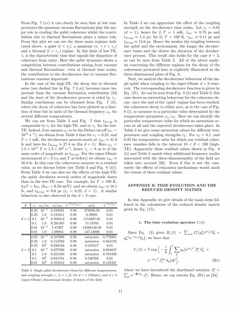
same order of magnitude as tdecay. For the super-Ohmicenvironment d = 3 (c3 and T as before) we obtain τdec ≈16.8 fs. In this case the coherences saturate to a residualvalue, as we discuss below (see Table 3 and Fig. 8 (ii)).From Table 3 we can also see the effects of the high-TE:the qubit decoheres several orders of magnitude fasterthan in the low-TE case. For example, for T = 100 K,kBT > hωc (hωc = 6.58 meV), and we obtain τdec ≈ 18.1fs, and tdecay ≈ 0.6 ps (c1 = 0.25, d = 1). A similarbehaviour is also observed in the d = 3 case.

d ci ωT/ωc ωcτdec e−Γi(τdec) ωctf e−Γi(tf )

0.25 10−5 0.418831 0.98 273950.34 0.010.25 1.0 0.181611 0.98 6.39891 0.01

d = 1 0.1 10−5 0.705612 0.98 1153307.91 0.010.1 1.0 0.291365 0.98 15.19703 0.010.01 10−5 7.47367 0.98 14346140.39 0.010.01 1.0 1.09604 0.98 147.12606 0.01

0.25 10−5 0.167969 0.98 saturates 0.7788010.25 1.0 0.154762 0.98 saturates 0.5641320.25 102 0.020104 0.98 0.318417 0.01

d = 3 0.1 10−5 0.275766 0.98 saturates 0.9048370.1 1.0 0.251550 0.98 saturates 0.7953390.1 102 0.031791 0.98 0.546769 0.010.01 102 0.101012 0.98 saturates 0.135331

Table 3. Single qubit decoherence times for different temperatures,

and coupling strength ci (i = 1, 3); for d = 1 (Ohmic), and d = 3

(super-Ohmic) dimensional density of states of the field.

In Table 3 we can appreciate the effect of the couplingstrength on the decoherence time scales. Let c1 = 0.01(d = 1), hence for i) T = 1 mK, τdec ≈ 0.75 ps andtdecay ≈ 1.4 µs; for ii) T = 100 K, τdec ≈ 0.11 ps andtdecay ≈ 14.6 ps. Hence the weaker the coupling betweenthe qubit and the environment, the longer the decoher-ence times and the slower the duration of the decoher-ence process. This result also holds for the case d = 3,as can be seen from Table 3. All of the above analy-sis concerning the different regimes for the decay of thecoherences presented here is explicitly illustrated in thethree-dimensional plots of Fig. 8.

Next, we analyze the decoherence behaviour of the sin-gle qubit when coupling to the super-Ohmic d = 3 reser-voir. The corresponding decoherence function is given byEq. (21). As can be seen from Fig. 8 (ii) and Table 3, thiscase shows an interesting behaviour for the coherence de-cay: once the end of the ‘quiet’ regime has been reached,the coherences decay to either zero, as in the case of Fig.8 (i), or saturate to a particular value determined by thetemperature parameter ω

T/ωc. Here we can identify the

particular temperature value for which no saturation oc-curs at all and the expected decoherence takes place. InTable 3 we give some saturation values for different tem-peratures and coupling strengths c3. For c3 = 0.1, and0.25 the temperature value for which any residual coher-ence vanishes falls in the interval 10 < θ < 100 (high-TE). Apparently these residual values shown in Fig. 8(ii) and Table 3 vanish when additional frequency modesassociated with the three-dimensionality of the field aretaken into account [20]. Even if this is not the case,surely the effects of relaxation mechanisms would markthe extent of these residual values.

APPENDIX B: TIME EVOLUTION AND THE

REDUCED DENSITY MATRIX

In this Appendix we give details of the main steps fol-lowed in the calculation of the reduced density matrixgiven by Eq. (15).

1. The time evolution operator UI(t)

Since Eq. (3) gives HI(t) =

∑

n,k Jnz

(

gnkeiω

ktb†k +

g∗nk

e−iωk

tbk

)

, we have that

UI(t) = T exp

[

− i

h

∫ t

o

∑

k

gk

(

eiωk

t′Jk

z b†k

+

e−iωk

t′J†k

z bk

)

dt′]

, (B1)

where we have introduced the shorthand notation Jk

z =∑

n e−ik·rnJnz . Hence, we can rewrite Eq. (B1) as [34]:

11

UI(t) = exp

[

∑

k

gkϕω

k(t)Jk

z b†k

]

×

T exp[

− i

h

∫ t′

o

dt′∑

k

e−iωk

t′ ×

exp(

−∑

k′

gk

′ϕωk′ (t

′)Jk′

z b†k

′

)

gkJ†k

z bk ×

exp(

∑

k′

gk

′ϕωk′ (t

′)Jk′

z b†k

′

)]

. (B2)

It is easy to show that the calculation of the productgiven by the last two lines Eq. (B2) gives the result

gkJ†k

z

[

bk + gkϕω

k(t)Jk

z

]

. (B3)

Hence, the following expression for UI(t) arises

UI(t) = e

∑

kg

kϕω

k(t)Jk

z b†k

e

−∑

kg

kϕ∗

ωk

(t)J†k

z bk ×

exp{

− i

h

∑

k

|gkJk

z |2∫ t

o

dt′ϕωk(t′)e−iω

kt′}

=

exp{

∑

k

gk

[

ϕωk(t)Jk

z b†k− ϕ∗

ωk(t)J†k

z bk

]

}

×

exp

{

∑

k

∣

∣gkJk

z

∣

∣

2[

it

h2ωk

−ϕ∗

ωk(t)

hωk

+|ϕω

k(t)|22

]}

(B4)

where we have used the result eA+B = eAeBe−[A,B]/2,which holds for any pair of operators A, B that satisfy[A, [A, B]] = 0 = [B, [A, B]] (as in the case of Eq. (B4)).It is straightforward to see that Eq. (B4) gives the finalresult

UI(t) = exp

[

i∑

k

∣

∣gk

∣

∣

2 ωkt − sin(ω

kt)

(hωk)2

J†k

z Jk

z

]

×

exp[

∑

k

{

A†k(t) − Ak(t)

}

]

, (B5)

where Ak(t) = g∗kϕ∗

ωk(t)J†k

z bk.

2. The reduced density matrix of a L−qubit register

We start by using the result for UI(t) in or-der to calculate the decay of the coherences, i.e.

TrB

[

ρB(0)U †{jn}I

(t)U{in}I

(t)]

, with U{in}I (t) as defined

in Eq. (10). In so doing, we first compute the operatoralgebra for the product U †{jn}

I(t)U{in}

I(t) by taking into

account the expression (B5). The result gives

U †{jn}I

(t)U{in}I

(t) = exp[

i∑

k

∣

∣gk

∣

∣

2 ωkt − sin(ω

kt)

(hωk)2

×

∑

m,n

(imin − jmjn) cosk · rmn

]

exp[

i∑

k

∣

∣gkϕω

k(t)

∣

∣

2 ×∑

m,n

imjn sin k · rmn

]

exp[

∑

k

(

σkb†k− σ∗

kbk

)]

, (B6)

where we have set σk ≡ gkϕω

k(t)

∑

m(im − jm)e−ik·rm .From the above equation note that the first two expo-nential terms commute, hence we only have to take thetrace over the third term. By doing this (see e.g. Ref.[29]), we obtain the result

TrB

[

ρB(0) exp{

∑

k

(

σkb†k− σ∗

kbk

)}]

=

∏

k

exp[

−∣

∣gk

∣

∣

2 1 − cos(ωkt)

(hωk)2

coth

(

hωk

2kBT

)

×∑

m,n

(im − jm)(in − jn) cosk · rmn

]

, (B7)

from where Eq. (11) arises immediately.

∗ Electronic address: j.reina-estupinan@physics.ox.ac.uk† Electronic address: lquiroga@uniandes.edu.co‡ Electronic address: n.johnson@physics.ox.ac.uk[1] W.H. Zurek, Physics Today 44(10), 36 (1991).[2] J. Preskill, Proc. Roy. Soc. London, Ser. A 452, 567

(1998).[3] N.H. Bonadeo et al., Science 282, 1473 (1998).[4] C. P. Slichter, Principles of Magnetic Resonance,

Springer Verlag, Berlin (1996).[5] P.W. Shor, in Proceedings of the 35th Annual Sympo-

sium on the Foundations of Computer Science, editedby S. Goldwasser (IEEE Computer Society Press, LosAlamitos, CA), pp. 124 (1994).

[6] J.I. Cirac and P. Zoller, Nature 404, 579 (2000), Phys.Rev. Lett. 74, 4091 (1995); C. Monroe et al., ibid. 75,4714 (1995); K. Molmer and A. Sorensen, ibid. 82, 1835(1999); C.A. Sackett et al., Nature 393, 133 (2000).

[7] N.A. Gershenfeld and I.L. Chuang, Science 275, 350(1997); D.G. Cory et al., Proc. Natn. Acad. Sci. USA94, 1634 (1997); E. Knill et al., Phys. Rev. A 57, 3348(1998); J.A. Jones et al., Nature 393, 344 (1998); B.E.Kane, Nature 393, 133 (1998).

[8] Q.A. Turchette et al., Phys. Rev. Lett. 75, 4710 (1995);A. Imamoglu et al., ibid. 83, 4204 (1999); A. Rauschen-beutel et al., ibid. 83, 5166 (1999).

[9] A. Shnirman et al., Phys. Rev. Lett. 79, 2371 (1997);D.V. Averin, Solid State Commun. 105, 659 (1998); Y.Makhlin et al., Nature 398, 305 (1999); Y. Nakamuraet al., Nature 398, 786 (1999); C.H. van der Wal et al.,Science 290, 773 (2000).

[10] A. Barenco et al., Phys. Rev. Lett. 74, 4083 (1995); D.Loss, and D.P. DiVincenzo, Phys. Rev. A 57 120 (1998);G. Burkard et al., Phys. Rev. B 59, 2070 (1999); L.Quiroga and N.F. Johnson, Phys. Rev. Lett. 83, 2270(1999); J.H. Reina et al., Phys. Rev. A 62, 12305 (2000);J.H. Reina et al., Phys. Rev. B 62, R2267 (2000), F.Troiani et al., Phys. Rev. B 62, R2263 (2000); E. Bio-latti et al., Phys. Rev. Lett. 85, 5647 (2000).

12

[11] P.W. Shor Phys. Rev. A 52, R2493 (1995); A.M. Steane,Phys. Rev. Lett. 77, 793 (1996).

[12] E. Knill and R. Laflamme, Phys. Rev. A 55, 900 (1997).[13] P. Zanardi and M. Rasetti, Phys. Rev. Lett. 79, 3306

(1997); L.-M. Duan and G.-C. Guo, ibid. 79, 1953 (1997);D.A. Lidar et al., ibid. 81, 2594 (1998).

[14] A. Beige et al., Phys. Rev. Lett. 85, 1762 (2000).[15] J. Kempe et al., Phys. Rev. A 63, 042307 (2001), and

references therein.[16] L. Viola, E. Knill and S. Lloyd, Phys. Rev. Lett. 85, 3520

(2000); ibid. 82, 2417 (1999); L. Viola and S. Lloyd, Phys.Rev. A 58, 2733 (1998).

[17] G. S. Agarwal et al., Phys. Rev. Lett. 86, 4271 (2001),and references therein; G. S. Agarwal, Phys. Rev. A 61,013809 (2000); C. Search and P.R. Berman, Phys. Rev.Lett. 85, 2272 (2000).

[18] D. Kielpinski et al., Science 291, 1013 (2001).[19] P.G. Kwiat et al., Science 290, 498 (2000).[20] G.M. Palma, K.-A. Suominen, and A.K. Ekert, Proc.

Roy. Soc. London, Ser. A 452, 567 (1996).[21] L.-M. Duan and G.-C. Guo, Phys. Rev. A 57, 737 (1998).[22] A. J. Leggett et al., Rev. Mod. Phys. 59, 1 (1987).[23] If relaxation mechanisms are also considered, in general

Jnx , Jn

y 6= 0. The presence of distinct error generatorsalong x, y, and z make the noise processes non-Abelianand the Hamiltonian can no longer be solved analytically.

[24] This factorizable condition is the one that has been ex-tensively studied so far. However, more general situationshave been analyzed in connection with the influence func-tional path-integral method of Feynman and Vernon. See,e.g., Ref. [28].

[25] Formally, noise processes can be characterized in terms ofthe interaction algebra that they generate, see e.g. Refs.[26,27].

[26] E. Knill, R. Laflamme, and L. Viola, Phys. Rev. Lett.84, 2525 (2000).

[27] P. Zanardi, Phys. Rev. A 63, 012301 (2001), and refer-ences therein.

[28] C. Morais Smith and A.O. Caldeira, Phys. Rev. A 41,3103 (1990) and references therein; ibid. 36, 3509 (1987);V. Hakim and V. Ambegaokar, ibid. 32, 423 (1985).

[29] C.W. Gardiner and P. Zoller, Quantum Noise, SpringerVerlag, Berlin (2000).

[30] B.L. Hu, J.P. Paz, and Y. Zhang, Phys. Rev. D 45, 2843(1992).

[31] J.H. Reina, L. Quiroga, and N.F. Johnson, in prepara-tion.

[32] W.G. Unruh, Phys. Rev. A 51, 992 (1995).[33] Over the time-scale considered for curve (a) in Fig. 7

(i), the vacuum fluctuation plot overlaps with curve (b),obscuring it from view. The same happens with the vac-uum fluctuation contribution associated with curve (b):this gets superposed with curve (c) and neither can bedirectly observed in Fig. 7 (i).

[34] G.D. Mahan, Many-Particle Physics, pp. 314 (2nd edi-tion), Plenum press, New York (1990).

Figure Captions

Figure 1. Two qubit “independent decoherence” due tothe coupling to a reservoir of the Ohmic type (d = 1) as afunction of time t and the transit time ts, for the input statesassociated with Γ+

1 (t, T ) (ia 6= ja, ib 6= jb) . Here c1 = 0.25,and (i) θ = 10−3, (ii) 100, and (iii) 102. Γ±

i (t, T ), with i = 1, 3are defined in the text.

Figure 2. Two qubit “independent decoherence” causedby the coupling to an ‘Ohmic environment’ as a function oftimes t and ts, for the input states associated with Γ−

1 (t, T )(ia 6= ja, ib 6= jb). c1 = 0.25, and (i) θ = 10−3, (ii) 100, and(iii) 102.

Figure 3. Two qubit “independent decoherence” due to thesuper-Ohmic environment d = 3 (Eq. (25)) as a function oftimes t and ts, for the input states associated with Γ+

3 (t, T ).c3 = 0.25, and (i) θ = 10−3, (ii) 100, and (iii) 102.

Figure 4. Two qubit “independent decoherence” due to thesuper-Ohmic environment d = 3 as a function of times t andts for the input states associated with Γ−

3 (t, T ). c3 = 0.25,and (i) θ = 10−3, (ii) 100, and (iii) 102.

Figure 5. Two qubit “independent decoherence”. d = 3,coupling strength c3 = 0.01, and (i), (iii) θ = 10−3, and (ii),(iv) θ = 102.

Figure 6. Two qubit “collective decoherence” for (i) d =1 ‘Ohmic environment’ (Eq. (27)), and (ii) d = 3 ‘super-Ohmic environment’ (Eq. (28)), as a function of time and thetemperature θ ≡ ω

T/ωc. c1 = c3 = 0.25, and ia 6= ja, and

ib 6= jb. Γ+d(t, T ) (d = 1, 3) is defined using Eqs. (27) and

(28).Figure 7. (i) Decoherence of a single qubit for an ‘Ohmic

environment’ as a function of t (in units of ωc). The con-tributions arising from the separate integration of thermal(exp[−ΓT (t)]) and vacuum (exp[−ΓV (t)]) fluctuations areshown as dotted curves. c1 = 0.25, (a) θ ≡ ω

T/ωc = 1,

(b) 10−2, (c) 10−5. If ωc is the Debye cutoff, θ ≈ 10−2 T(see text): the decoherence shown corresponds to T = 100 K,T = 1 K, and T = 1 mK, respectively. (ii) Coherence decayfor (a) θ = 10−5, (b) 10−2, (c) 102. c1 = 0.25. Here time isgiven in units of the thermal frequency ωT ≡ kB T/h.

Figure 8. Decoherence of a single qubit for (i) d = 1, and

(ii) d = 3, as a function of time (in units of the cut-off ωc)

and3 the temperature parameter θ ≡ ωT /ωc. c1 = c3 = 0.25.

If ωc is the Debye cut-off, the range of coherence decay goes

from a few mK up to (a) 104 K (plot (i)) and (b) 1.5× 103 K

(plot (ii)).

13

This figure "fig1.jpg" is available in "jpg" format from:

http://arXiv.org/ps/quant-ph/0105029v2

This figure "fig2.jpg" is available in "jpg" format from:

http://arXiv.org/ps/quant-ph/0105029v2

This figure "fig3.jpg" is available in "jpg" format from:

http://arXiv.org/ps/quant-ph/0105029v2

This figure "fig4.jpg" is available in "jpg" format from:

http://arXiv.org/ps/quant-ph/0105029v2

This figure "fig5.jpg" is available in "jpg" format from:

http://arXiv.org/ps/quant-ph/0105029v2

This figure "fig6.jpg" is available in "jpg" format from:

http://arXiv.org/ps/quant-ph/0105029v2

This figure "fig7.jpg" is available in "jpg" format from:

http://arXiv.org/ps/quant-ph/0105029v2

This figure "fig8.jpg" is available in "jpg" format from:

http://arXiv.org/ps/quant-ph/0105029v2