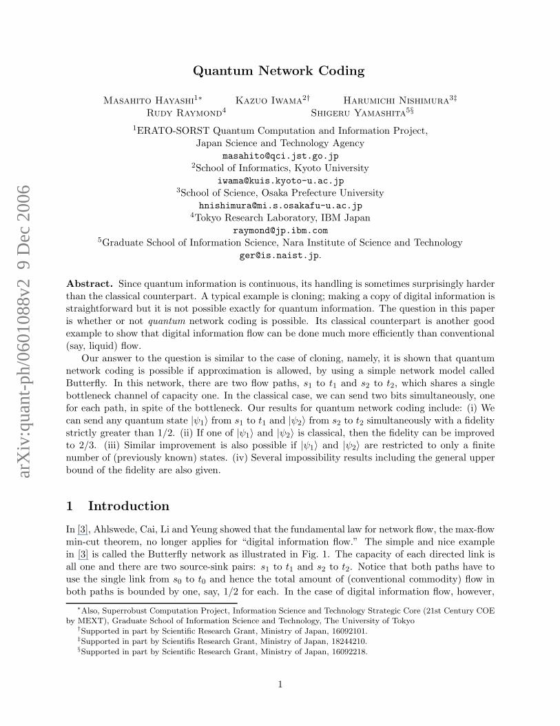
arX

iv:q

uant

-ph/

0601

088v

2 9

Dec

200

6

Quantum Network Coding

Masahito Hayashi1∗ Kazuo Iwama2† Harumichi Nishimura3‡

Rudy Raymond4 Shigeru Yamashita5§

1ERATO-SORST Quantum Computation and Information Project,Japan Science and Technology Agency

masahito@qci.jst.go.jp2School of Informatics, Kyoto University

iwama@kuis.kyoto-u.ac.jp3School of Science, Osaka Prefecture University

hnishimura@mi.s.osakafu-u.ac.jp4Tokyo Research Laboratory, IBM Japan

raymond@jp.ibm.com5Graduate School of Information Science, Nara Institute of Science and Technology

ger@is.naist.jp.

Abstract. Since quantum information is continuous, its handling is sometimes surprisingly harderthan the classical counterpart. A typical example is cloning; making a copy of digital information isstraightforward but it is not possible exactly for quantum information. The question in this paperis whether or not quantum network coding is possible. Its classical counterpart is another goodexample to show that digital information flow can be done much more efficiently than conventional(say, liquid) flow.

Our answer to the question is similar to the case of cloning, namely, it is shown that quantumnetwork coding is possible if approximation is allowed, by using a simple network model calledButterfly. In this network, there are two flow paths, s1 to t1 and s2 to t2, which shares a singlebottleneck channel of capacity one. In the classical case, we can send two bits simultaneously, onefor each path, in spite of the bottleneck. Our results for quantum network coding include: (i) Wecan send any quantum state |ψ1〉 from s1 to t1 and |ψ2〉 from s2 to t2 simultaneously with a fidelitystrictly greater than 1/2. (ii) If one of |ψ1〉 and |ψ2〉 is classical, then the fidelity can be improvedto 2/3. (iii) Similar improvement is also possible if |ψ1〉 and |ψ2〉 are restricted to only a finitenumber of (previously known) states. (iv) Several impossibility results including the general upperbound of the fidelity are also given.

1 Introduction

In [3], Ahlswede, Cai, Li and Yeung showed that the fundamental law for network flow, the max-flowmin-cut theorem, no longer applies for “digital information flow.” The simple and nice examplein [3] is called the Butterfly network as illustrated in Fig. 1. The capacity of each directed link isall one and there are two source-sink pairs: s1 to t1 and s2 to t2. Notice that both paths have touse the single link from s0 to t0 and hence the total amount of (conventional commodity) flow inboth paths is bounded by one, say, 1/2 for each. In the case of digital information flow, however,

∗Also, Superrobust Computation Project, Information Science and Technology Strategic Core (21st Century COEby MEXT), Graduate School of Information Science and Technology, The University of Tokyo

†Supported in part by Scientific Research Grant, Ministry of Japan, 16092101.‡Supported in part by Scientifis Research Grant, Ministry of Japan, 18244210.§Supported in part by Scientific Research Grant, Ministry of Japan, 16092218.

1

s1 s2s0

t1t2t0

Figure 1: Butterfly network.

x

yx

y

x⊕y

x⊕y x⊕y

y= x⊕(x⊕y) x= (x⊕y)⊕y

x y

Figure 2: Coding scheme

U

1ψ2ψ

1ρ2ρ

Figure 3: Network using acontrolled unitary operation

the protocol shown in Fig. 2 allows us to transmit two bits, x and y, simultaneously. Thus, we caneffectively achieve larger channel capacity than what can be achieved by simple routing. This isknown as network coding since [3] and has been quite popular (see e.g., Network coding home page[20] or [1, 15, 19, 21, 22] for recent developments).

Network coding obviously exploits the two side links, s1 to t2 and s2 to t1, which are completelyuseless graph-topologically. Now the primary question in this paper is whether this is also possiblefor quantum information: Our model is the same butterfly network with (unit-capacity) quantumchannels and our goal is to send two qubits from s1 to t1 and s2 to t2 simultaneously. To thisend, one should notice that the protocol in Fig. 2 uses (at least) two tricks. One is the EX-OR(Exclusive-OR) operation at node s0; one can see that the bit y is encoded by using x as a key whichis sent directly from s1 to t2, and vise versa. The other is the exact copy of one-bit information atnode t0. Are there any quantum counterparts for these key operations?

Neither seems easy in the quantum case: For the copy operation, there is the famous no-cloningtheorem. Also, there is no obvious way of encoding a quantum state by a quantum state at s0.Consider, for example, a simple extension of the classical operation at node s0,i.e., a controlledunitary transform U as illustrated in Fig. 3. (Note that classical EX-OR is realized by settingU = X “bit-flip.”) Then, for any U , there is a quantum state |φ〉 (actually an eigenvector ofU) such that |φ〉 and U |φ〉 are identical (up to a global phase). Namely, if |ψ1〉 = |φ〉, then thequantum state at the output of U is exactly the same for |ψ2〉 = |0〉 and |ψ2〉 = |1〉. This meanstheir difference is completely lost at that position and hence is completely lost at t1 also.

Thus it is highly unlikely that we can achieve an exact transmission of two quantum states,which forces us to consider an approximate transmission. As an approximation factor, we use a(worst-case) fidelity between the input state |ψ1〉 at s1 (|ψ2〉 at s2, resp.) and the output state ρρρ1

at t1 (ρρρ2 at t2, resp.) Recall that the fidelity is at most 1.0 by definition and 0.5 is automaticallyachieved by outputting a completely mixed state. Thus our question is whether we can achieve afidelity of strictly greater than 0.5.

Our Contribution. This paper gives a positive answer to this question. We first show thatwe do need the (topologically useless) side channels for our goal exactly as in the classical case(Theorem 2.1). Namely, without them, we can prove that for any protocol, there exists a quantumstate |ψi〉 (i = 1 or 2) and its output state ρρρi such that F (|ψi〉,ρρρi) ≤ 1/2. We then give ourprotocol which achieves a fidelity of strictly greater than 1/2 for the butterfly network (Theorem3.1). The idea is discretization of (continuous) quantum states. Namely, the quantum state froms2 is changed into classical two bits by using what we call “tetra measurement.” Those two bits arethen used as a key to encode the state from s1 at node s0 (“group operation”) and also to decodeit at node t1. Our protocol also depends upon the approximate cloning by Buzek and Hillery [9].This obviously distorts quantum states, but interestingly, it also has a merit (creating entanglementbetween cloned states) by which we can handle the second problem on the state distinguishabilitypreviously mentioned.

2

Note that the present general lower bound for the fidelity is only slightly better than 1/2 (some0.52). However, if we impose restriction, the value becomes much better. For example, if |ψ1〉is a classical state (i.e. either |0〉 or |1〉), then the fidelity becomes 2/3 (Theorem 4.1). Similarimprovement is also possible if |ψ1〉 and |ψ2〉 are restricted to only a finite number of (previouslyknown) states, especially if they are the so-called quantum random access coding states [4]. Byusing those states, we can design an interesting protocol which can send two classical bits from s1to t1 (similarly two bits from s2 to t2) but only one of them, determined by adversary, should berecovered. It is shown that the success probability for this protocol is 1/2 +

√2/16 (Theorem 5.1),

but classically the success probability for any protocol is at most 1/2.On the negative side, several upper bounds for the fidelity are given. Again, the most general one

(Theorem 3.10) may not seem very impressive (some 0.983), but it is improved under restrictions.In particular, if we impose the BC (bit-copy) assumption, we can prove an upper bound of 11/12(Theorem 4.2). (BC means that whenever we need to copy a classical bit, we use the classical (exact)copy, which seems quite reasonable.) We also give a limit of transmitting random access codingstates. Note that Theorem 5.1 can be extended to the three-bit case (with success probability some0.525) but that is the limit; no protocol exists for the four-bit transmission with success probabilitystrictly greater than 1/2 (Theorem 5.3).

Related Work. We usually allow approximation and/or errors in quantum computation, whichseems to be an essence of its power in some occasions. One example is observed in communicationcomplexity: The quantum communication complexity to compute the equality function EQn ex-actly is n [18]. However, even one qubit communication enables us to compute EQn with successprobability larger than 1/2. Another example can be seen in locally decodable codes and privateinformation retrievals: Any 2n-bit Boolean function F can be computed with success probability> 1/2 from an (n+ 1)-qubit information [31]. Namely, n+ 1 qubits can encode 2n classical bits forcomputing any Boolean function approximately.

Thus “1/2 + ǫ for very small ǫ” seems very powerful. Interestingly, this is not the case in someother occasions. the Nayak bound [24] says that there is no way to send two bits by one qubitwith success probability > 1/2. Moreover, [17] shows that one-qubit random access coding for fourbits can only be done with success probability at most 1/2, although we can enjoy a good successprobability up to three bits. In this context, our model in this paper also shows a clear differencedepending on whether or not the two side links exist.

The study of coding methods on quantum information and computation has been deeply ex-plored for error correction of quantum computation (since [30]) and data compression of quantumsources (since [28]). Recall that their techniques are duplication of data (error correction) andaverage-case analysis (data compression). Those standard approaches do not seem to help in thecore of our problem. More tricky applications of quantum mechanism are quantum teleportation[6], superdense coding [7], and a variety of quantum cryptosystems including the BB84 key distri-bution [5]. The random access coding by Ambainis, Nayak, Ta-shma, and Vazirani [4] is probablymost related one to this paper, which allows us to encode two or more classical bits into one qubitand decode it to recover any one of the source bits. Our third protocol is a realization of thisscheme on the Butterfly network.

The introduction of quantum network coding [16] triggered several new studies: Leung, Oppen-heim, and Winter [23] examined the asymptotic relation between the amount of quantum informa-tion and channel capacities on the Butterfly network (and more). Shi and Soljanin [29] consideredmulticasting networks from the viewpoint of lossless compression and decompression of copies ofquantum states.

3

U(s1)

U(s2)

U(s0) U(t0)

U(t2)

U(t1)

1ψ

2ψ

0

0

0

00

0

1ρ

2ρ

Figure 4: Quantum circuit for coding on the But-terfly network

s1 s2s0

t1t2t0

1ψ 2ψ

1Q

2Q 3Q

4Q5Q

6Q 7Q

1outρ2

outρ

Figure 5: Protocol XQQ.

2 The Model

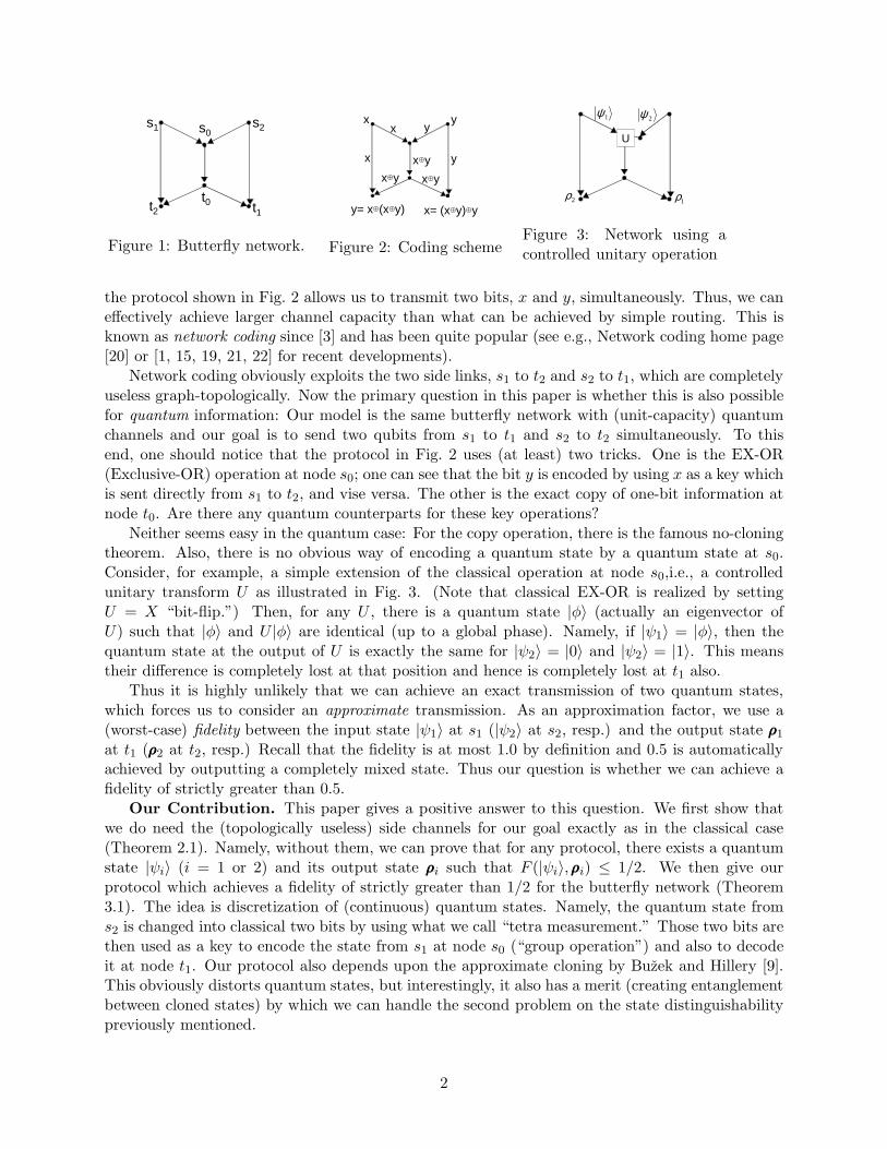
Our model as a quantum circuit is shown in Fig. 4. The information sources at nodes s1 and s2are pure one-qubit states |ψ1〉 and |ψ2〉. (It turns out, however, that the result does not changefor mixed states because of the joint concavity of the fidelity [25].) Any node does not haveprior entanglement with other nodes. At every node, a physically allowable operation, i.e., trace-preserving completely positive map (TP-CP map), is done, and each edge can send only one qubit.They are implemented by unitary operations with additional ancillae and by discarding all qubitsexcept for the output qubits [2, 25].

Our goal is to send |ψ1〉 to node t1 and |ψ2〉 to node t2 as well as possible. The quality of dataat node tj is measured by the fidelity between the original state |ψj〉 and the state ρρρj output atnode tj by the protocol. Here, the fidelity between two quantum states ρρρ and σσσ are defined as

F (σσσ,ρρρ) =(

Tr√

ρρρ1/2σσσρρρ1/2)2

as in [10, 8, 11]. (The other common definition is Tr√

ρρρ1/2σσσρρρ1/2.) In

particular, the fidelity between a pure state |ψ〉 and a mixed state ρρρ is F (|ψ〉,ρρρ) = 〈ψ|ρρρ|ψ〉. (Tosimplify the description, for a pure state |ψ〉〈ψ| we often use the vector representation |ψ〉 and wealso use bold fonts for a 2 × 2 or 4 × 4 density matrix for exposition.) We call the minimum ofF (|ψ1〉,ρρρ1) over all one-qubit states |ψ1〉 and |ψ2〉 the fidelity at node t1 and similarly for fidelity atnode t2.

Before presenting our protocols achieving a fidelity of strictly greater than 1/2, we show thatthe two side links, which are useless graph-topologically, are indispensable. One might think this istrivial from the Nayak bound [24]. Namely, if the two inputs are classical 0/1 bits, then they cannotbe sent using a single quantum channel (s0 to t0) with success probability (= fidelity) greater than1/2. This is not true since our definition only requires a fidelity at each sink. In fact, we can achievea fidelity of at least 0.75 in our definition, by simply using the one-qubit random access coding fortwo bits [4] and the phase-covariant cloning (a kind of approximated cloning) [8, 11]. (Note that0.752 > 0.5 but this does not violate the Nayak bound since the success probabilities at the twosides are not independent.) The proof of the following theorem needs a careful consideration ofphysical operations on the Bloch ball (see, e.g., [12, 27]) and the trace distance. Notice that inthis paper, the trace distance between two quantum states ρρρ and ρ′ρ′ρ′ is defined to be ||ρρρ − ρ′ρ′ρ′||trwithout the normalization factor 2 as in [25]. (If two states are qubits, this distance is equal to thegeometrical distance of the corresponding points in the Bloch ball.)

Theorem 2.1 No quantum protocol can achieve fidelity larger than 1/2 if both side links areremoved from the Butterfly.

Proof. We show that, for any proper protocol, if the fidelity at t2 is larger than 1/2 (say, 1/2+ ǫ

4

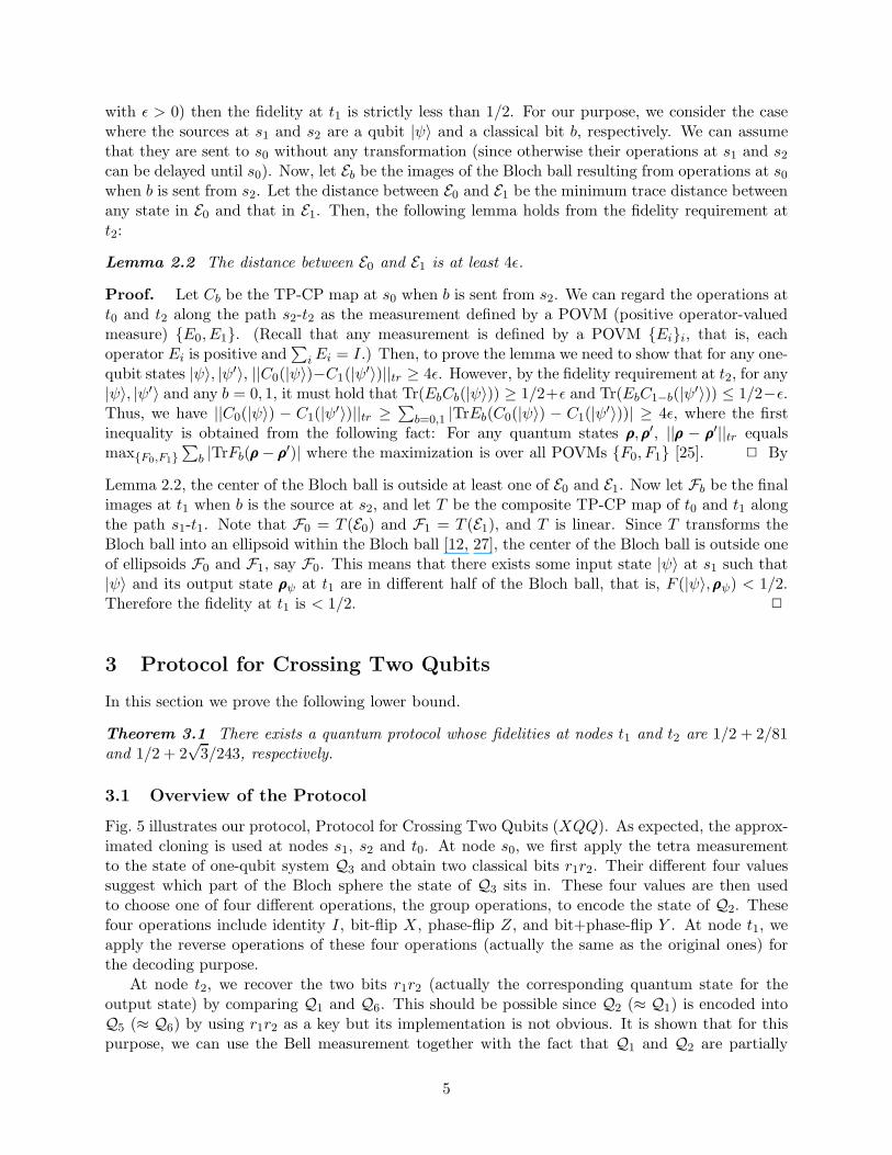
with ǫ > 0) then the fidelity at t1 is strictly less than 1/2. For our purpose, we consider the casewhere the sources at s1 and s2 are a qubit |ψ〉 and a classical bit b, respectively. We can assumethat they are sent to s0 without any transformation (since otherwise their operations at s1 and s2can be delayed until s0). Now, let Eb be the images of the Bloch ball resulting from operations at s0when b is sent from s2. Let the distance between E0 and E1 be the minimum trace distance betweenany state in E0 and that in E1. Then, the following lemma holds from the fidelity requirement att2:

Lemma 2.2 The distance between E0 and E1 is at least 4ǫ.

Proof. Let Cb be the TP-CP map at s0 when b is sent from s2. We can regard the operations att0 and t2 along the path s2-t2 as the measurement defined by a POVM (positive operator-valuedmeasure) {E0, E1}. (Recall that any measurement is defined by a POVM {Ei}i, that is, eachoperator Ei is positive and

∑

iEi = I.) Then, to prove the lemma we need to show that for any one-qubit states |ψ〉, |ψ′〉, ||C0(|ψ〉)−C1(|ψ′〉)||tr ≥ 4ǫ. However, by the fidelity requirement at t2, for any|ψ〉, |ψ′〉 and any b = 0, 1, it must hold that Tr(EbCb(|ψ〉)) ≥ 1/2+ǫ and Tr(EbC1−b(|ψ′〉)) ≤ 1/2−ǫ.Thus, we have ||C0(|ψ〉) − C1(|ψ′〉)||tr ≥

∑

b=0,1 |TrEb(C0(|ψ〉) − C1(|ψ′〉))| ≥ 4ǫ, where the firstinequality is obtained from the following fact: For any quantum states ρρρ,ρρρ′, ||ρρρ − ρρρ′||tr equalsmax{F0,F1}

∑

b |TrFb(ρρρ− ρρρ′)| where the maximization is over all POVMs {F0, F1} [25]. 2 By

Lemma 2.2, the center of the Bloch ball is outside at least one of E0 and E1. Now let Fb be the finalimages at t1 when b is the source at s2, and let T be the composite TP-CP map of t0 and t1 alongthe path s1-t1. Note that F0 = T (E0) and F1 = T (E1), and T is linear. Since T transforms theBloch ball into an ellipsoid within the Bloch ball [12, 27], the center of the Bloch ball is outside oneof ellipsoids F0 and F1, say F0. This means that there exists some input state |ψ〉 at s1 such that|ψ〉 and its output state ρρρψ at t1 are in different half of the Bloch ball, that is, F (|ψ〉,ρρρψ) < 1/2.Therefore the fidelity at t1 is < 1/2. 2

3 Protocol for Crossing Two Qubits

In this section we prove the following lower bound.

Theorem 3.1 There exists a quantum protocol whose fidelities at nodes t1 and t2 are 1/2 + 2/81and 1/2 + 2

√3/243, respectively.

3.1 Overview of the Protocol

Fig. 5 illustrates our protocol, Protocol for Crossing Two Qubits (XQQ). As expected, the approx-imated cloning is used at nodes s1, s2 and t0. At node s0, we first apply the tetra measurementto the state of one-qubit system Q3 and obtain two classical bits r1r2. Their different four valuessuggest which part of the Bloch sphere the state of Q3 sits in. These four values are then usedto choose one of four different operations, the group operations, to encode the state of Q2. Thesefour operations include identity I, bit-flip X, phase-flip Z, and bit+phase-flip Y . At node t1, weapply the reverse operations of these four operations (actually the same as the original ones) forthe decoding purpose.

At node t2, we recover the two bits r1r2 (actually the corresponding quantum state for theoutput state) by comparing Q1 and Q6. This should be possible since Q2 (≈ Q1) is encoded intoQ5 (≈ Q6) by using r1r2 as a key but its implementation is not obvious. It is shown that for thispurpose, we can use the Bell measurement together with the fact that Q1 and Q2 are partially

5

entangled as a result of cloning at node s1.Remark. It is not hard to average the fidelities at t1 and t2 by mixing the encoding state at

t1 with the Bell state (|00〉 + |11〉)/√

2, implying 1/2 + 2(2 −√

3)/27 ≈ 0.52 at both sinks.

3.2 Building Blocks

Universal Cloning (UC). As the first tool of our protocol, we recall the notion of the approxi-mated cloning by Buzek and Hillery [9], called the universal cloning. Let |Ψ+〉 = 1√

2(|01〉 + |10〉).

Then, it is given by the TP-CP map UC defined by

UC(|0〉〈0|) =2

3|00〉〈00| + 1

3|Ψ+〉〈Ψ+|, UC(|0〉〈1|) =

√2

3|Ψ+〉〈11| +

√2

3|00〉〈Ψ+|,

UC(|1〉〈0|) =

√2

3|11〉〈Ψ+| +

√2

3|Ψ+〉〈00|, UC(|1〉〈1|) =

2

3|11〉〈11| + 1

3|Ψ+〉〈Ψ+|. (1)

This map is intended to clone not only classical states |0〉 and |1〉 but also any superposition equallywell by mixing the symmetric state |Ψ+〉 with |00〉 and |11〉 as the output. Let ρρρ1 = Tr2UC(|ψ〉)and ρρρ2 = Tr1UC(|ψ〉), where Tri is the partial trace over the i-th qubit. Then, easy calculationimplies that ρρρ1 = ρρρ2 = 2

3 |ψ〉〈ψ| + 13 · III2 , which means F (|ψ〉,ρρρ1) = F (|ψ〉,ρρρ2) = 5/6. We call its

induced map |ψ〉 7→ ρρρ1 (or |ψ〉 7→ ρρρ2) the universal copy.Tetra Measurement (TTR). Next, we introduce the tetra measurement. We need the fol-

lowing four states |χ(00)〉 = cos θ|0〉 + eıπ/4 sin θ|1〉, |χ(01)〉 = cos θ|0〉 + e−3ıπ/4 sin θ|1〉, |χ(10)〉 =sin θ|0〉 + e−ıπ/4 cos θ|1〉, and |χ(11)〉 = sin θ|0〉 + e3ıπ/4 cos θ|1〉 with cos2 θ = 1/2 +

√3/6, which

form a tetrahedron in the Bloch sphere representation. The tetra measurement, denoted by TTR,is the POVM defined by {1

2 |χ(00)〉〈χ(00)|, 12 |χ(01)〉〈χ(01)|, 1

2 |χ(10)〉〈χ(10)|, 12 |χ(11)〉〈χ(11)|}.

Group Operation (GR). In what follows, let X =

(

0 11 0

)

be the bit-flip operation, Z =(

1 00 −1

)

be the phase-flip operation, and Y = XZ. Notice that the set of unitary maps on

one-qubit states ρρρ 7→ WρρρW † (W = I, Z,X, Y ) is the Klein four group. The group operationunder a two-bit string r1r2, denoted by GR(ρρρ, r1r2), is a transformation defined by GR(ρρρ, 00) = ρρρ,GR(ρρρ, 01) = Zρρρ, GR(ρρρ, 10) = Xρρρ, and GR(ρρρ, 11) = Y ρρρ. Note that we frequently use simplifiedexpressions like Xρρρ instead of XρρρX†.

3D Bell Measurement (BM). Moreover, for recovering |ψ2〉 at node t2 we introduce anothernew operation based on the Bell measurement, BM(Q,Q′) (or BM(σσσ)), which applies the followingthree operations (a), (b), and (c) with probability 1/3 for each, to the state σσσ (a 4×4 density matrix)of the two-qubit system Q⊗Q′.

(a) Measure σσσ in the Bell basis{

|Φ+〉 = |00〉+|11〉√2

, |Φ−〉 = |00〉−|11〉√2

, |Ψ+〉 = |01〉+|10〉√2

, |Ψ−〉 = |01〉−|10〉√2

}

,

and output |0〉 if the measurement result for |Φ+〉 or |Φ−〉 is obtained, and |1〉 otherwise.(b) Measure σσσ similarly, and output |+〉 if the measurement result for |Φ+〉 or |Ψ+〉 is obtained,

and |−〉 otherwise.(c) Measure σσσ similarly, and output |+′〉 = 1√

2(|0〉+ ı|1〉) if the measurement result for |Φ+〉 or

|Ψ−〉 is obtained, and |−′〉 = 1√2(|0〉 − ı|1〉) otherwise.

3.3 Protocol XQQ and Its Performance Analysis

Now here is the formal description of our protocol.

6

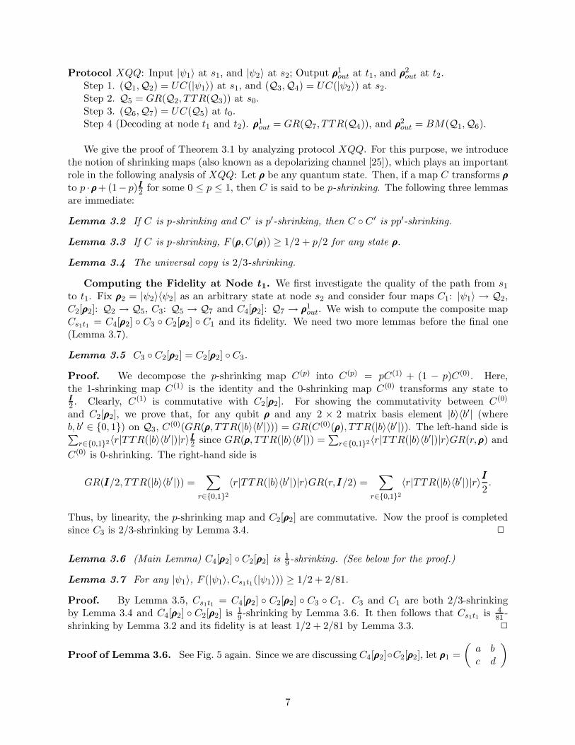
Protocol XQQ: Input |ψ1〉 at s1, and |ψ2〉 at s2; Output ρρρ1out at t1, and ρρρ2

out at t2.Step 1. (Q1,Q2) = UC(|ψ1〉) at s1, and (Q3,Q4) = UC(|ψ2〉) at s2.Step 2. Q5 = GR(Q2, TTR(Q3)) at s0.Step 3. (Q6,Q7) = UC(Q5) at t0.Step 4 (Decoding at node t1 and t2). ρρρ

1out = GR(Q7, TTR(Q4)), and ρρρ2

out = BM(Q1,Q6).

We give the proof of Theorem 3.1 by analyzing protocol XQQ. For this purpose, we introducethe notion of shrinking maps (also known as a depolarizing channel [25]), which plays an importantrole in the following analysis of XQQ: Let ρρρ be any quantum state. Then, if a map C transforms ρρρto p ·ρρρ+ (1− p)III2 for some 0 ≤ p ≤ 1, then C is said to be p-shrinking. The following three lemmasare immediate:

Lemma 3.2 If C is p-shrinking and C ′ is p′-shrinking, then C ◦ C ′ is pp′-shrinking.

Lemma 3.3 If C is p-shrinking, F (ρρρ,C(ρρρ)) ≥ 1/2 + p/2 for any state ρρρ.

Lemma 3.4 The universal copy is 2/3-shrinking.

Computing the Fidelity at Node t1. We first investigate the quality of the path from s1to t1. Fix ρρρ2 = |ψ2〉〈ψ2| as an arbitrary state at node s2 and consider four maps C1: |ψ1〉 → Q2,C2[ρρρ2]: Q2 → Q5, C3: Q5 → Q7 and C4[ρρρ2]: Q7 → ρρρ1

out. We wish to compute the composite mapCs1t1 = C4[ρρρ2] ◦ C3 ◦ C2[ρρρ2] ◦ C1 and its fidelity. We need two more lemmas before the final one(Lemma 3.7).

Lemma 3.5 C3 ◦ C2[ρρρ2] = C2[ρρρ2] ◦ C3.

Proof. We decompose the p-shrinking map C(p) into C(p) = pC(1) + (1 − p)C(0). Here,the 1-shrinking map C(1) is the identity and the 0-shrinking map C(0) transforms any state toIII2 . Clearly, C(1) is commutative with C2[ρρρ2]. For showing the commutativity between C(0)

and C2[ρρρ2], we prove that, for any qubit ρρρ and any 2 × 2 matrix basis element |b〉〈b′| (whereb, b′ ∈ {0, 1}) on Q3, C

(0)(GR(ρρρ, TTR(|b〉〈b′|))) = GR(C(0)(ρρρ), TTR(|b〉〈b′|)). The left-hand side is∑

r∈{0,1}2〈r|TTR(|b〉〈b′|)|r〉III2 since GR(ρρρ, TTR(|b〉〈b′|)) =∑

r∈{0,1}2〈r|TTR(|b〉〈b′|)|r〉GR(r,ρρρ) and

C(0) is 0-shrinking. The right-hand side is

GR(III/2, TTR(|b〉〈b′|)) =∑

r∈{0,1}2

〈r|TTR(|b〉〈b′|)|r〉GR(r,III/2) =∑

r∈{0,1}2

〈r|TTR(|b〉〈b′|)|r〉III2.

Thus, by linearity, the p-shrinking map and C2[ρρρ2] are commutative. Now the proof is completedsince C3 is 2/3-shrinking by Lemma 3.4. 2

Lemma 3.6 (Main Lemma) C4[ρρρ2] ◦ C2[ρρρ2] is 19-shrinking. (See below for the proof.)

Lemma 3.7 For any |ψ1〉, F (|ψ1〉, Cs1t1(|ψ1〉)) ≥ 1/2 + 2/81.

Proof. By Lemma 3.5, Cs1t1 = C4[ρρρ2] ◦ C2[ρρρ2] ◦ C3 ◦ C1. C3 and C1 are both 2/3-shrinkingby Lemma 3.4 and C4[ρρρ2] ◦ C2[ρρρ2] is 1

9 -shrinking by Lemma 3.6. It then follows that Cs1t1 is 481 -

shrinking by Lemma 3.2 and its fidelity is at least 1/2 + 2/81 by Lemma 3.3. 2

Proof of Lemma 3.6. See Fig. 5 again. Since we are discussing C4[ρρρ2]◦C2[ρρρ2], let ρρρ1 =

(

a bc d

)

7

be the state on Q2, ρρρ2 = |ψ2〉〈ψ2| =

(

e fg h

)

be the state at s2 and assume that Q5 = Q7. We

calculate the state on Q2 ⊗Q3 ⊗Q4, the state on Q5 ⊗Q4 (= Q7 ⊗Q4) and ρρρ1out in this order. For

Q2 ⊗Q3 ⊗Q4, recall that ρρρ2 is cloned into Q3 and Q4 and so, by Eq.(1) in Sec. 3.2, the state onQ2 ⊗Q3 ⊗Q4 is written as

ρρρ1 ⊗[

2e

3|00〉〈00| + e

6(|01〉 + |10〉)(〈01| + 〈10|) +

f

3((|01〉 + |10〉)〈11| + |00〉(〈01| + 〈10|))

+g

3(|11〉(〈01| + 〈10|) + (|01〉 + |10〉)〈00|) +

2h

3|11〉〈11| + h

6(|01〉 + |10〉)(〈01| + 〈10|)

]

= ρρρ1 ⊗ |0〉〈0| ⊗(

2e

3|0〉〈0| + f

3|0〉〈1| + g

3|1〉〈0| + 1

6|1〉〈1|

)

+ ρρρ1 ⊗ |0〉〈1| ⊗(

1

6|1〉〈0| + f

3III

)

+ ρρρ1 ⊗ |1〉〈0| ⊗(

1

6|0〉〈1| + g

3III

)

+ ρρρ1 ⊗ |1〉〈1| ⊗(

1

6|0〉〈0| + f

3|0〉〈1| + g

3|1〉〈0| + 2h

3|1〉〈1|

)

. (2)

Then, we apply the group operation to the first two bits of Q2⊗Q3⊗Q4. In general, for Q⊗Q′,GR(Q, TTR(Q′)) is given as follows (see Appendix for the proof).

Lemma 3.8 Let ρρρ be the state on Q. Then, GR(Q, TTR(Q′)) is the following TP-CP map:

ρρρ⊗ |0〉〈0| 7→ 1√3V (I, Z)ρρρ+

(

1 − 1√3

)

· III2, ρρρ⊗ |1〉〈1| 7→ 1√

3V (X,Y )ρρρ+

(

1 − 1√3

)

· III2,

ρρρ⊗ |0〉〈1| 7→ 1

2√

3(V (I,X)ρρρ − V (Y,Z)ρρρ+ ı(V (I, Y )ρρρ− V (Z,X)ρρρ)),

ρρρ⊗ |1〉〈0| 7→ 1

2√

3(V (I,X)ρρρ − V (Y,Z)ρρρ− ı(V (I, Y )ρρρ− V (Z,X)ρρρ)).

Here, V (I, Z)ρρρ = 12(Iρρρ + Zρρρ), and V (X,Y )ρρρ, V (I,X)ρρρ, V (Y,Z)ρρρ, V (I, Y )ρρρ, and V (Z,X)ρρρ are

similarly defined. Those six operations are III-invariant (meaning it maps III to itself) TP-CP maps.

Now the state on Q5⊗Q4 is obtained by applying Lemma 3.8 to Eq.(2). From now on, we omitthe term for III

2 . Namely, if the one-qubit state is ρρρ + αIII2 , we only describe ρρρ. This is not harmful

since any operation in this section is III-invariant and hence the III2 term can be recovered at the end

by using the trace property. Thus, the state on Q5 ⊗Q4 looks like

1√3V (I, Z)ρρρ1 ⊗

(

2e

3|0〉〈0| + 1

6|1〉〈1|

)

+1√3V (I, Z)ρρρ1 ⊗

(

f

3|0〉〈1| + g

3|1〉〈0|

)

+1

2√

3V (I,X; I, Y ; +)ρρρ1 ⊗

1

6|1〉〈0| + 1

2√

3V (I,X; I, Y ; +) ⊗ f

3III

+1

2√

3V (I,X; I, Y ;−)ρρρ1 ⊗

1

6|0〉〈1| + 1

2√

3V (I,X; I, Y ;−) ⊗ g

3III

+1√3V (X,Y )ρρρ1 ⊗

(

1

6|0〉〈0| + 2h

3|1〉〈1|

)

+1√3V (X,Y )ρρρ1 ⊗

(

f

3|0〉〈1| + g

3|1〉〈0|

)

, (3)

where V (I,X; I, Y ;±)ρρρ = V (I,X)ρρρ−V (Y,Z)ρρρ± ı(V (I, Y )ρρρ−V (Z,X)ρρρ), and the terms such thatthe state of Q5 is III

2 are omitted.We next transform the state of Q5 ⊗ Q4 to ρρρ1

out by using Lemma 3.8 again. For example,V (I, Z)ρρρ1 ⊗ |0〉〈0| is transformed to 1√

3V (I, Z)V (I, Z)ρρρ1. To simplify the resulting formula, the

following lemma is used (see Appendix for its proof).

8

Lemma 3.9 1) V (I, Z)V (I, Z)ρρρ1 = V (X,Y )V (X,Y )ρρρ1 =

(

a 00 d

)

.

2) V (I, Z)V (X,Y )ρρρ1 = V (X,Y )V (I, Z)ρρρ1 =

(

d 00 a

)

.

3) V (I,X)V (I,X)ρρρ1 = V (Y,Z)V (Y,Z)ρρρ1 =

(

12

b+c2

b+c2

12

)

.

4) V (I,X)V (Y,Z)ρρρ1 = V (Y,Z)V (I,X)ρρρ1 =

(

12 − b+c

2

− b+c2

12

)

.

5) V (I, Y )V (I, Y )ρρρ1 = V (Z,X)V (Z,X)ρρρ1 =

(

12

b−c2

c−b2

12

)

.

6) V (I, Y )V (Z,X)ρρρ1 = V (Z,X)V (I, Y )ρρρ1 =

(

12

c−b2

b−c2

12

)

.

7) For any two operators V, V ′ taken from any different two sets of {V (I, Z), V (X,Y )},{V (I,X), V (Y,Z)}, and {V (I, Y ), V (Z,X)}, V V ′ρρρ1 = III

2 .

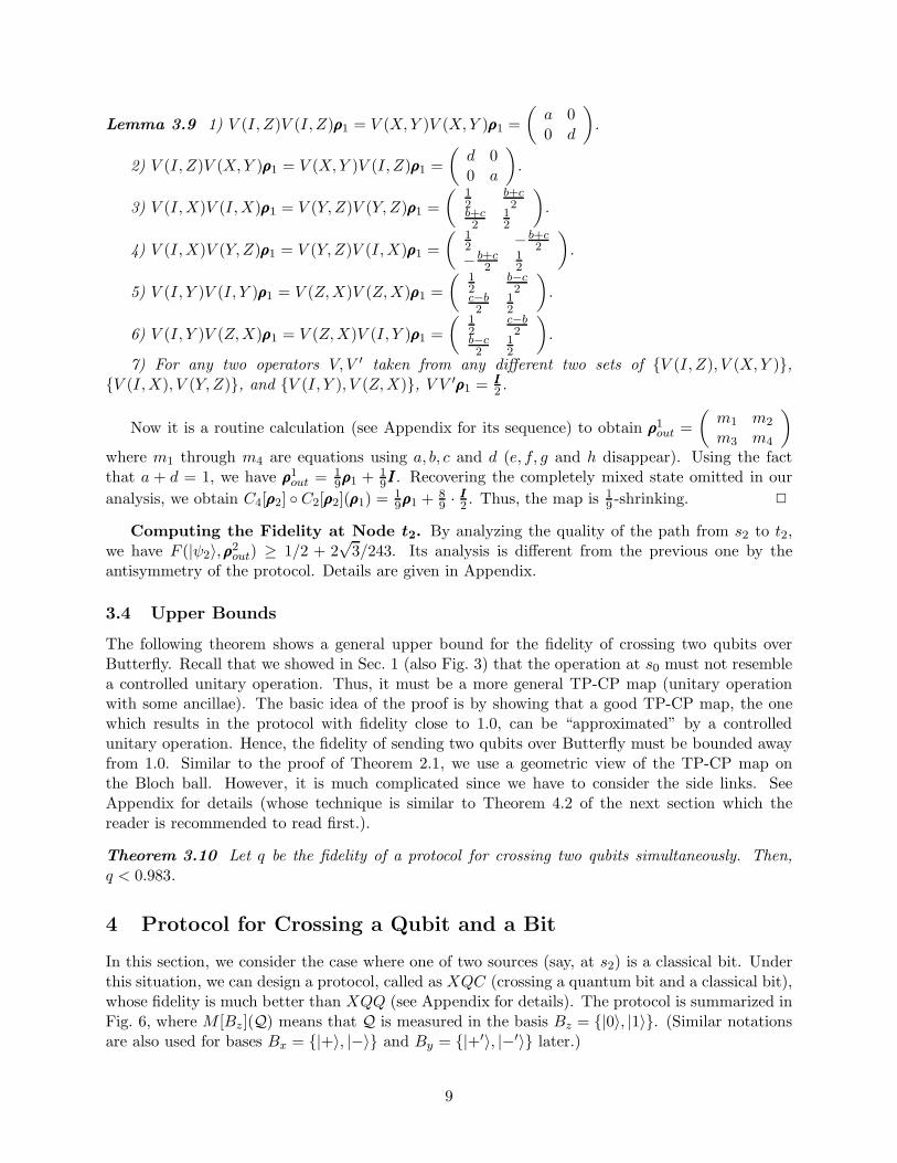
Now it is a routine calculation (see Appendix for its sequence) to obtain ρρρ1out =

(

m1 m2

m3 m4

)

where m1 through m4 are equations using a, b, c and d (e, f, g and h disappear). Using the factthat a + d = 1, we have ρρρ1

out = 19ρρρ1 + 1

9III. Recovering the completely mixed state omitted in our

analysis, we obtain C4[ρρρ2] ◦ C2[ρρρ2](ρρρ1) = 19ρρρ1 + 8

9 · III2 . Thus, the map is 19 -shrinking. 2

Computing the Fidelity at Node t2. By analyzing the quality of the path from s2 to t2,we have F (|ψ2〉,ρρρ2

out) ≥ 1/2 + 2√

3/243. Its analysis is different from the previous one by theantisymmetry of the protocol. Details are given in Appendix.

3.4 Upper Bounds

The following theorem shows a general upper bound for the fidelity of crossing two qubits overButterfly. Recall that we showed in Sec. 1 (also Fig. 3) that the operation at s0 must not resemblea controlled unitary operation. Thus, it must be a more general TP-CP map (unitary operationwith some ancillae). The basic idea of the proof is by showing that a good TP-CP map, the onewhich results in the protocol with fidelity close to 1.0, can be “approximated” by a controlledunitary operation. Hence, the fidelity of sending two qubits over Butterfly must be bounded awayfrom 1.0. Similar to the proof of Theorem 2.1, we use a geometric view of the TP-CP map onthe Bloch ball. However, it is much complicated since we have to consider the side links. SeeAppendix for details (whose technique is similar to Theorem 4.2 of the next section which thereader is recommended to read first.).

Theorem 3.10 Let q be the fidelity of a protocol for crossing two qubits simultaneously. Then,q < 0.983.

4 Protocol for Crossing a Qubit and a Bit

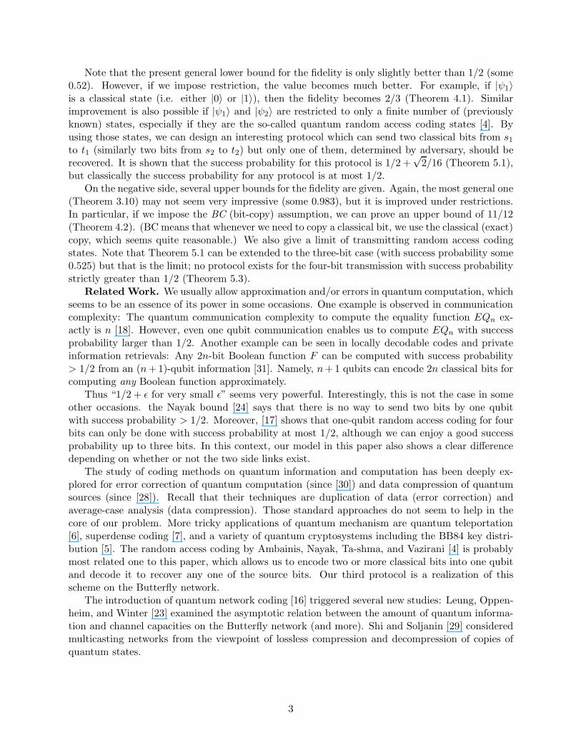
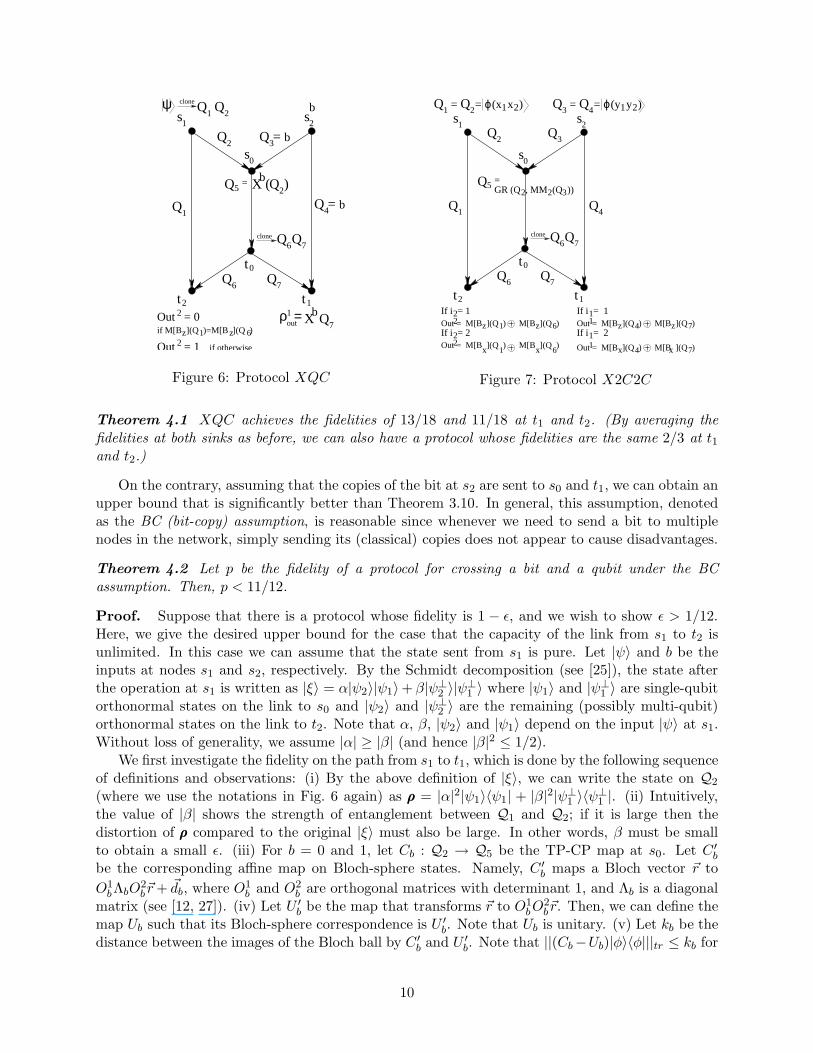
In this section, we consider the case where one of two sources (say, at s2) is a classical bit. Underthis situation, we can design a protocol, called as XQC (crossing a quantum bit and a classical bit),whose fidelity is much better than XQQ (see Appendix for details). The protocol is summarized inFig. 6, where M [Bz](Q) means that Q is measured in the basis Bz = {|0〉, |1〉}. (Similar notationsare also used for bases Bx = {|+〉, |−〉} and By = {|+′〉, |−′〉} later.)

9

ψ

2

Q2 Q = b3

Xb

zif M[B ](Q )=M[B ](Q )1 z 6

s

t

t t

0

1

0

2

2ss1

Q Q

Q

Q Q

1 2

1

clone

clone Q Q

b

1out

=Q bX ( )

2Out = 0

2 if otherwiseOut = 1

ρ =

bQ =4

5

6 7

6 7

Q7

Q

Figure 6: Protocol XQC

3

1

Q1 Q2= = ϕ(x x )1 2

s

t

t t

0

1

0

2

2ss1

Q Q

clone Q Q

1= = ϕQ Q3 4 (y y )2

Q2

Q4

Q3

6 7

6 7

z 6z

6x Out = M[B ](Q ) M[B ](Q )

z z1

1

Out = M[B ](Q ) M[B ](Q )4 7

4 7

=Q5

Out = M[B ](Q ) M[B ](Q )2

Out = M[B ](Q ) M[B ](Q )2 1x xx

If i = 2

If i = 1If i = 12

2

11

If i = 21

GR (Q , MM (Q ))2 2

Q

Figure 7: Protocol X2C2C

Theorem 4.1 XQC achieves the fidelities of 13/18 and 11/18 at t1 and t2. (By averaging thefidelities at both sinks as before, we can also have a protocol whose fidelities are the same 2/3 at t1and t2.)

On the contrary, assuming that the copies of the bit at s2 are sent to s0 and t1, we can obtain anupper bound that is significantly better than Theorem 3.10. In general, this assumption, denotedas the BC (bit-copy) assumption, is reasonable since whenever we need to send a bit to multiplenodes in the network, simply sending its (classical) copies does not appear to cause disadvantages.

Theorem 4.2 Let p be the fidelity of a protocol for crossing a bit and a qubit under the BCassumption. Then, p < 11/12.

Proof. Suppose that there is a protocol whose fidelity is 1 − ǫ, and we wish to show ǫ > 1/12.Here, we give the desired upper bound for the case that the capacity of the link from s1 to t2 isunlimited. In this case we can assume that the state sent from s1 is pure. Let |ψ〉 and b be theinputs at nodes s1 and s2, respectively. By the Schmidt decomposition (see [25]), the state afterthe operation at s1 is written as |ξ〉 = α|ψ2〉|ψ1〉+ β|ψ⊥

2 〉|ψ⊥1 〉 where |ψ1〉 and |ψ⊥

1 〉 are single-qubitorthonormal states on the link to s0 and |ψ2〉 and |ψ⊥

2 〉 are the remaining (possibly multi-qubit)orthonormal states on the link to t2. Note that α, β, |ψ2〉 and |ψ1〉 depend on the input |ψ〉 at s1.Without loss of generality, we assume |α| ≥ |β| (and hence |β|2 ≤ 1/2).

We first investigate the fidelity on the path from s1 to t1, which is done by the following sequenceof definitions and observations: (i) By the above definition of |ξ〉, we can write the state on Q2

(where we use the notations in Fig. 6 again) as ρρρ = |α|2|ψ1〉〈ψ1| + |β|2|ψ⊥1 〉〈ψ⊥

1 |. (ii) Intuitively,the value of |β| shows the strength of entanglement between Q1 and Q2; if it is large then thedistortion of ρρρ compared to the original |ξ〉 must also be large. In other words, β must be smallto obtain a small ǫ. (iii) For b = 0 and 1, let Cb : Q2 → Q5 be the TP-CP map at s0. Let C ′

b

be the corresponding affine map on Bloch-sphere states. Namely, C ′b maps a Bloch vector ~r to

O1bΛbO

2b~r+ ~db, where O1

b and O2b are orthogonal matrices with determinant 1, and Λb is a diagonal

matrix (see [12, 27]). (iv) Let U ′b be the map that transforms ~r to O1

bO2b~r. Then, we can define the

map Ub such that its Bloch-sphere correspondence is U ′b. Note that Ub is unitary. (v) Let kb be the

distance between the images of the Bloch ball by C ′b and U ′

b. Note that ||(Cb−Ub)|φ〉〈φ|||tr ≤ kb for

10

an arbitrary pure state |φ〉 (where the trace norm || · ||tr is defined by ||A||tr =√AA†). By a similar

reason as (ii) kb must be small for a small ǫ. (vi) Now we select the state ρρρ which is undesirableto achieve a high fidelity, i.e., the one such that U0ρρρ = U1ρρρ (such ρρρ exists, which is parallel tothe eigenvector of U−1

0 U1). Let ρ′ρ′ρ′ = |α|2|ψ1〉〈ψ1|, which is an approximation of ρρρ represented as aproduct state. (vii) The operation at t0 is considered to be the two TP-CP maps on the one qubits:One map CP1 is for t1 and the other CP2 is for t2. Their Bloch-sphere correspondence CP ′

1 andCP ′

2 have a trade-off on the size of their images. So, the image of CP ′1 must be large for a small ǫ,

and then we have a shrinking factor for CP ′2.

Now we are ready to bound both above and below ||(C0−C1)ρ′ρ′ρ′||tr, which produces an inequality

on ǫ as will be seen soon. For this purpose, we first evaluate the values of β and kb using geometricproperties of the Bloch sphere representation of the TP-CP map on the one qubits: it maps theBloch ball to an ellipsoid within the Bloch ball. The proof of this technical lemma is given inAppendix.

Lemma 4.3 |β|2 ≤ 12f(ǫ) and kb ≤ f(ǫ) where f(ǫ) = 3

2 + ǫ−√

94 + ǫ2 − 5ǫ.

Second, we decompose ||(C0 −C1)ρ′ρ′ρ′||tr as follows by the triangle inequality, and then bound it

from above:

||(C0 − C1)ρ′ρ′ρ′||tr ≤ ||(C0 − U0)ρ

′ρ′ρ′||tr + ||U0ρ′ρ′ρ′ − U0ρρρ||tr + ||U1ρρρ− U1ρ

′ρ′ρ′||tr + ||(U1 − C1)ρ′ρ′ρ′||tr

≤ |α|2 · k0 + ||ρρρ− ρ′ρ′ρ′||tr × 2 + |α|2 · k1

≤ (k0 + k1)|α|2 + 2|β|2. (4)

Third, for the shrinking factor by the operation at t0 the following lemma from [26] is used.

Lemma 4.4 (Niu-Griffiths) Let CP ′i be the Bloch sphere representation of CPi. Let l1 be the

shortest semiaxis length of the image of CP ′1, and l2 be the longest semiaxis length of the image of

CP ′2. Then, l1 ≤

√

1 − l22.

Since l1 ≥ 1 − 2ǫ by the fidelity requirement at t1, Lemma 4.4 gives us the condition for l2:

l2 ≤ 2√

ǫ− ǫ2. (5)

Finally, we bound ||(C0 − C1)ρ′ρ′ρ′||tr from below by focusing on the path s2-t2. Let M be the

TP-CP map done at t2, and D = M(I ⊗CP2)(I ⊗C0 − I ⊗C1). By the fidelity requirement at t2,||D|ξ〉〈ξ|||tr ≥ 2 − 4ǫ [2]. On the contrary, using the unnormalized product state |χ〉 = α|ψ2〉|ψ1〉we bound ||D|ξ〉〈ξ|||tr by

||D|ξ〉〈ξ|||tr ≤ ||D(|ξ〉〈ξ| − |χ〉〈χ|)||tr + ||D|χ〉〈χ|||tr .

The first term is bounded by 2|||ξ〉〈ξ| − |χ〉〈χ|||tr since D is the difference between two TP-CPmaps, each of which has the operator norm at most 1 [2]. Using the monotone decreasing propertyof the trace distance between two states by TP-CP maps, the second term is bounded by

||D|χ〉〈χ|||tr ≤ ||(I ⊗ (CP2 · (C0 − C1)))|ψ2〉〈ψ2| ⊗ ρ′ρ′ρ′||tr = ||(CP2 · (C0 − C1))ρ′ρ′ρ′||tr,

which is at most l2||(C0 −C1)ρ′ρ′ρ′||tr since CP ′

2 maps the Bloch ball to an ellipsoid within a ball withradius at most l2. By a simple calculation of the trace norm, we have the following bound.

Lemma 4.5 |||ξ〉〈ξ| − |χ〉〈χ|||tr ≤ 2|β|√

1 − |β|2/2.

11

A

F

E

B

C

D

O

P’

2

max2 βP

2ε

vr

θ

Figure 8: Image by the operation at s1

A

B

O

P’

Pvr

θ x

y

22 1

1

xy

l + = −

1 l−θ

0 0( , )x y

Figure 9: Image by operations at s0, t0 and t1

By Lemma 4.5 we have

2 − 4ǫ ≤ 2|||ξ〉〈ξ| − |χ〉〈χ|||tr + l2||(C0 − C1)ρ′ρ′ρ′||tr ≤ 2|β|

√

1 − |β|2/2 + l2||(C0 − C1)ρ′ρ′ρ′||tr. (6)

By Lemma 4.3, Ineqs.(4), (5) and (6), we produce an inequality on ǫ and |β|:

1 − 2ǫ ≤ 2|β|√

1 − |β|2/2 + 2√

ǫ− ǫ2(

(1 − |β|2)f(ǫ) + |β|2)

. (7)

(Recall that |α|2 = 1 − |β|2.) Note that the right-hand side of Ineq. (7) is monotone increasing onǫ and |β| while its left-hand side is monotone decreasing on ǫ. Therefore, by checking ǫ such thatIneq. (7) holds under the bound of |β| from Lemma 4.3, we obtain ǫ > 1/12.

It still remains to prove Lemma 4.3.

Proof of Lemma 4.3. We only prove the bound of |β| since the bound of kb is similarly shown.Let βmax be the maximum of all β’s when |ψ〉 varies on the pure qubits. Considering the Bloch

sphere representation, the point A corresponding to ρρρ is on the circle of radius 1 − 2|βmax|2 sinceρρρ = (1 − 2|βmax|2)|ψ1〉〈ψ1| + 2|βmax|2 · III2 . Note that the image of the Bloch ball by the operationat s1 is an ellipsoid whose cut CD parallel to segment AO has length ≤ 2 − 2|βmax|2 (see Fig. 8),where O is the center of the Bloch ball. Then, by geometric properties of the ellipsoid we can showthe following lemma.

Claim 1 After the operation at t1, this cut is shrunk by a factor at least 1 − 2|βmax|2 + 2ǫ.

Proof. See Fig. 8 again. Let P be the point on the line AB such that the length of segment PO is1−2ǫ. To satisfy the fidelity at t1, some point P ′ in the image at s0 must reach P in the final image

at t1. Letting l be the length of−−→P ′P , this means that the composite map by operations at s0, t0

and t1 shrinks the Bloch ball by a factor of 1− l to the direction of−−→P ′P since any TP-CP map must

transform the Bloch ball to an ellipsoid inside the ball. Let ~v be the component of−−→P ′P parallel to

the line AB. Note that the length of ~v is at least (1− 2ǫ)− (1− 2|βmax |2) = 2|βmax|2 − 2ǫ. Now weanalyze the maximum of the shrinking factor of the Bloch ball to the direction of AB since it is theworst case for our analysis. Since we want to know the maximum, we can assume that the length

of ~v is exactly 2|βmax|2 − 2ǫ. Then, the angle θ between−−→P ′P and ~v satisfies cos θ = 2|βmax|2−2ǫ

l .Notice that the ellipse ( x

1−l )2 + y2 = 1 (Fig. 9) is obtained by the projection of the final image to

12

the plane including all the vectors we are considering. (Here, we assume that the plane has x-y

coordinates. Note that the x-axis is the direction parallel to−−→P ′P .) Let (x0, y0) be the intersection

of the ellipse and the line y = (tan θ)x. We can see that√

x20 + y2

0 is the shrinking factor we want.By a simple calculation, this value is

√

x20 + y2

0 =

√

(1 + tan2 θ)1

( 11−l )

2 + tan2 θ=

√

l(1 − l)2

2|βmax|2 − 2ǫ+ (1 − l)2(l − 2|βmax|2 + 2ǫ),

which is monotone decreasing as the function of l (when l ≤ 1). Since l ≥ 2|βmax|2 − 2ǫ, themaximum value is obtained when l = 2|βmax|2 − 2ǫ and it is 1 − 2|βmax|2 + 2ǫ. 2

After the operation at t1, the distance between the Bloch sphere and its image by the oper-ations along the s1-t1 line must be at most 2ǫ to satisfy the fidelity requirement at t1. Thus,the shortest semiaxis length of the final image of all transformations on the s1-t1 line must beat least 1 − 2ǫ. On the contrary, Lemma 1 implies that the shortest semiaxis length is at most(1 − |βmax|2)(1 − 2|βmax|2 + 2ǫ). Hence, 1 − 2ǫ ≤ (1 − |βmax|2)(1 − 2|βmax|2 + 2ǫ), and we obtain

|βmax|2 ≤ 12

(

32 + ǫ−

√

94 + ǫ2 − 5ǫ

)

. By the definition of βmax we also have the same bound on

|β|2 for any β corresponding to an input at s1. 2

Now the proof of Theorem 4.2 is completed. 2

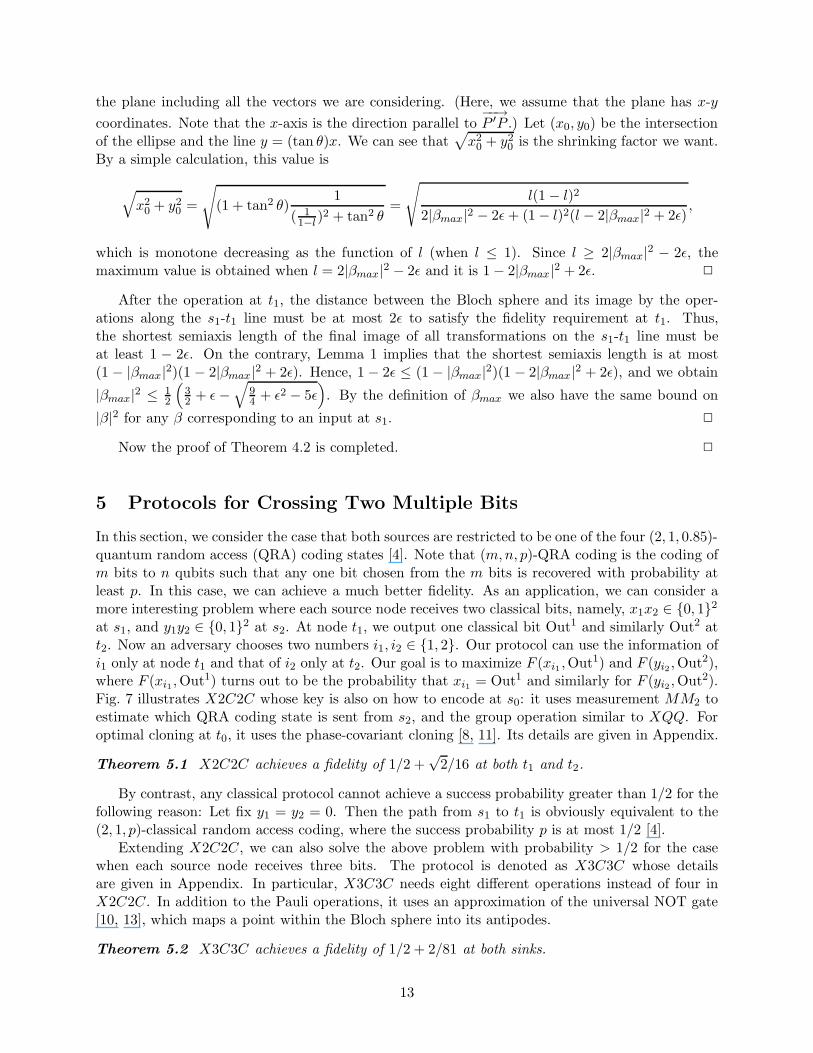
5 Protocols for Crossing Two Multiple Bits

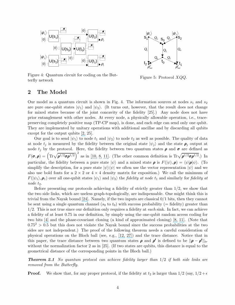
In this section, we consider the case that both sources are restricted to be one of the four (2, 1, 0.85)-quantum random access (QRA) coding states [4]. Note that (m,n, p)-QRA coding is the coding ofm bits to n qubits such that any one bit chosen from the m bits is recovered with probability atleast p. In this case, we can achieve a much better fidelity. As an application, we can consider amore interesting problem where each source node receives two classical bits, namely, x1x2 ∈ {0, 1}2

at s1, and y1y2 ∈ {0, 1}2 at s2. At node t1, we output one classical bit Out1 and similarly Out2 att2. Now an adversary chooses two numbers i1, i2 ∈ {1, 2}. Our protocol can use the information ofi1 only at node t1 and that of i2 only at t2. Our goal is to maximize F (xi1 ,Out1) and F (yi2 ,Out2),where F (xi1 ,Out1) turns out to be the probability that xi1 = Out1 and similarly for F (yi2 ,Out2).Fig. 7 illustrates X2C2C whose key is also on how to encode at s0: it uses measurement MM2 toestimate which QRA coding state is sent from s2, and the group operation similar to XQQ. Foroptimal cloning at t0, it uses the phase-covariant cloning [8, 11]. Its details are given in Appendix.

Theorem 5.1 X2C2C achieves a fidelity of 1/2 +√

2/16 at both t1 and t2.

By contrast, any classical protocol cannot achieve a success probability greater than 1/2 for thefollowing reason: Let fix y1 = y2 = 0. Then the path from s1 to t1 is obviously equivalent to the(2, 1, p)-classical random access coding, where the success probability p is at most 1/2 [4].

Extending X2C2C, we can also solve the above problem with probability > 1/2 for the casewhen each source node receives three bits. The protocol is denoted as X3C3C whose detailsare given in Appendix. In particular, X3C3C needs eight different operations instead of four inX2C2C. In addition to the Pauli operations, it uses an approximation of the universal NOT gate[10, 13], which maps a point within the Bloch sphere into its antipodes.

Theorem 5.2 X3C3C achieves a fidelity of 1/2 + 2/81 at both sinks.

13

s1 s2 s3

t1 t2 t3

sources

sinks

s0

t0

kt

ks

Figure 10: Network Gk

Interestingly, there is no X4C4C, which is an immediate corollary of the nonexistence of(4, 1, p > 1/2)-QRA coding [17].

Theorem 5.3 If an X4C4C protocol achieves fidelity q, then q ≤ 1/2.

6 Beyond the Butterfly Network – Concluding Remarks –

Obviously a lot of future work remains. First of all, there is a large gap between the current upperand lower bounds for the achievable fidelity, which should be narrowed. Equally important is toconsider more general networks. To this direction, it might be interesting to study the network Gkas shown in Fig. 10, introduced in [14]. Note that there are k source-sink pairs (si, ti) all of whichshare a single link from s0 to t0. For this network Gk, we can design the protocol XQk by a simpleextension of XQQ. The idea is to decompose the node s0 (similarly for t0) into a sequence of nodesof indegree two. At each of those nodes, we do exactly the same thing as before, i.e., encodingone state by the classical two bits obtained from the other state. It is not hard to see that such aprotocol achieves a fidelity strictly better than 1/2.

References

[1] M. Adler, N. J. Harvey, K. Jain, R. D. Kleinberg, and A. R. Lehman. On the capacity ofinformation networks. Proc. 17th ACM-SIAM SODA, pp.241–250, 2006.

[2] D. Aharonov, A. Kitaev, and N. Nisan. Quantum circuits with mixed states. Proc. 30thACM STOC, pp. 20–30, 1998.

[3] R. Ahlswede, N. Cai, S.-Y. R. Li, and R. W. Yeung. Network information flow. IEEETransactions on Information Theory 46 (2000) 1204–1216.

[4] A. Ambainis, A. Nayak, A. Ta-shma, and U. Vazirani. Dense quantum coding and quan-tum finite automata. J. ACM 49 (2002) 496–511.

[5] C. H. Bennett and G. Brassard. Quantum cryptography: public key distribution andcoin tossing. Proc. IEEE International Conference on Computers, Systems and SignalProcessing, pp. 175–179, 1984.

[6] C. H. Bennett, G. Brassard, C. Crepeau, R. Jozsa, A. Peres, and W. K. Wootters. Tele-porting an unknown quantum states via dual classical and Einstein-Podolsky-Rosen chan-nels. Phys. Rev. Lett. 70 (1993) 1895–1899.

[7] C. H. Bennett and S. J. Wiesner. Communication via one- and two-particle operators onEinstein-Podolsky-Rosen states. Phys. Rev. Lett. 69 (1992) 2881–2884.

14

[8] D. Bruß, M. Cinchetti, G. M. D’Ariano, and C. Macchiavello. Phase-covariant quantumcloning. Phys. Rev. A 62 (2000) 012302.

[9] V. Buzek and M. Hillery. Quantum copying: Beyond the no-cloning theorem. Phys. Rev.A 54 (1996) 1844–1852.

[10] V. Buzek, M. Hillery, and R. F. Werner. Optimal manipulation with qubits: universalNOT gate. Phys. Rev. A 60 (1999) 2626–2629.

[11] H. Fan, K. Matsumoto, X.-B. Wang, and H. Imai. Phase-covariant quantum cloning. J.Phys. A: Math. Gen. 35 (2002) 7415–7423.

[12] A. Fujiwara and P. Algoet. One-to-one parametrization of quantum channels. Phys. Rev.A 59 (1999) 3290–3294.

[13] N. Gisin and S. Popescu. Spin flips and quantum information for antiparallel spins. Phys.Rev. Lett. 83 (1999) 432–435.

[14] N. J. Harvey, R. D. Kleinberg, and A. R. Lehman. Comparing network coding withmulticommodity flow for the k-pairs communication problem. MIT LCS Technical Report964, September 2004.

[15] N. J. Harvey, D. R. Karger, and K. Murota. Deterministic network coding by matrixcompletion. Proc. 16th ACM-SIAM SODA, pp. 489–498, 2005.

[16] M. Hayashi, K. Iwama, H. Nishimura, R. Raymond, and S. Yamashita. Quantum net-work coding. Talk at 9th Workshop on Quantum Information Processing, 2006. Preprintavailable at quant-ph/0601088, January 2006.

[17] M. Hayashi, K. Iwama, H. Nishimura, R. Raymond, and S. Yamashita. (4, 1)-quantumrandom access coding does not exist. New J. Phys. 8 (2006) 129.

[18] P. Høyer and R. de Wolf. Improved quantum communication complexity bounds for dis-jointness and equality. Proc. 19th STACS, Lecture Notes in Comput. Sci. 2285 (2002)299–310.

[19] S. Jaggi, P. Sanders, P. A. Chou, M. Effros, S. Egner, K. Jain, and L. M. G. M. Tolhuizen.Polynomial time algorithms for multicast network code construction. IEEE Transactionson Information Theory 51 (2005) 1973–1982.

[20] R. Koetter. Network coding home page. http://tesla.csl.uiuc.edu/˜koetter/NWC/[21] A. R. Lehman and E. Lehman. Complexity classification of network information flow

problems. Proc. 15th ACM-SIAM SODA, pp. 142–150, 2004.[22] A. R. Lehman and E. Lehman. Network coding: does the model need tuning? Proc. 16th

ACM-SIAM SODA, pp. 499–504, 2005.[23] D. Leung, J. Oppenheim, and A. Winter. Quantum network communication –the butterfly

and beyond. Preprint available at quant-ph/0608233, August 2006.[24] A. Nayak. Optimal lower bounds for quantum automata and random access codes. Proc.

40th IEEE FOCS, pp. 369–376, 1999.[25] M. A. Nielsen and I. L. Chuang. Quantum Computation and Quantum Information, Cam-

bridge, 2000.[26] C.-S. Niu and R. B. Griffiths. Optimal copying of one quantum bit. Phys. Rev. A 58

(1998) 4377–4393.[27] M. B. Ruskai, S. Szarek, and E. Werner. An analysis of complete-positive trace-preserving

maps on 2 × 2 matrices. Lin. Alg. Appl. 347 (2002) 159–187.[28] B. Schumacher. Quantum coding. Phys. Rev. A 51 (1995) 2738–2747.[29] Y. Shi and E. Soljanin. On multicast in quantum network. Proc. 40th Annual Conference

on Information Sciences and Systems, 2006.[30] P. Shor. Scheme for reducing decoherence in quantum computer memory. Phys. Rev. A

52 (1995) 2493–2496.

15

[31] S. Wehner and R. de Wolf. Improved lower bounds for locally decodable codes and privateinformation retrieval. Proc. 32nd ICALP, Lecture Notes in Comput. Sci. 3580 (2005)1424–1436.

A Appendix

A.1 Proofs of Lemmas in Sec. 3.3

Proof of Lemma 3.8. Consider the tetra measurement as a TP-CP map. For any mixed stateρρρ, its TP-CP map, also denoted by TTR, transforms ρρρ to

Tr

[

1

2|χ(00)〉〈χ(00)|ρρρ

]

|00〉〈00| + Tr

[

1

2|χ(01)〉〈χ(01)|ρρρ

]

|01〉〈01|

+ Tr

[

1

2|χ(10)〉〈χ(10)|ρρρ

]

|10〉〈10| + Tr

[

1

2|χ(11)〉〈χ(11)|ρρρ

]

|11〉〈11|. (8)

By linearity, TTR is defined by the map that transforms each basis matrix |b〉〈b′| (b, b′ = 0, 1)to the matrix obtained by replacing ρρρ in Eq.(8) by |b〉〈b′|. Using the definition of the states|χ(00)〉, . . . , |χ(11)〉 we obtain

TTR(|0〉〈0|) =1

2(cos2 θ(|00〉〈00| + |01〉〈01|) + sin2 θ(|10〉〈10| + |11〉〈11|))

= 2 sin2 θ

(

III

2⊗ III

2

)

+ (cos2 θ − sin2 θ)

(

|0〉〈0| ⊗ III

2

)

=1√3

(

|0〉〈0| ⊗ III

2

)

+

(

1 − 1√3

)(

III

2⊗ III

2

)

. (9)

Similarly, we can check that

TTR(|1〉〈1|) =1√3

(

|1〉〈1| ⊗ III

2

)

+

(

1 − 1√3

)(

III

2⊗ III

2

)

, (10)

TTR(|0〉〈1|) =1

4√

3((|00〉〈00| + |10〉〈10| − |11〉〈11| − |01〉〈01|)

+ı(|00〉〈00| + |11〉〈11| − |01〉〈01| − |10〉〈10|)) (11)

TTR(|1〉〈0|) = TTR(|0〉〈1|)†. (12)

Now we consider the TP-CP map of GR(Q, TTR(Q′)). Assume that the state of Q is ρρρ. Recallthat GR(ρρρ, |00〉〈00|) = ρρρ, GR(ρρρ, |01〉〈01|) = Zρρρ, GR(ρρρ, |10〉〈10|) = Xρρρ, and GR(ρρρ, |11〉〈11|) = Y ρρρ.If the GR operation under the two bits being selected uniformly at random, which means thatthe state of TTR(Q′) is the state III

2 ⊗ III2 , is applied to ρρρ, then ρρρ is mapped to III

2 since the fourGR operations are evenly applied to ρρρ. Thus, Eqs.(9) and (10) imply that GR(·, TTR(·)) mapsρρρ⊗|0〉〈0| and ρρρ⊗|1〉〈1| to 1√

3

Iρρρ+Zρρρ2 +(1− 1√

3)III2 and 1√

3

Xρρρ+Y ρρρ2 +(1− 1√

3)III2 , respectively. Moreover,

by Eq.(11) ρρρ⊗ |0〉〈1| is mapped to

1

4√

3((Iρρρ+Xρρρ) − (Y ρρρ+ Zρρρ) + ı((Iρρρ + Y ρρρ) − (Zρρρ+Xρρρ))),

which is 12√

3(V (I,X)ρρρ− V (Y,Z)ρρρ+ ı(V (I, Y )ρρρ− V (Z,X)ρρρ)). By Eq.(12) it is clear that ρρρ⊗ |1〉〈0|

is mapped to 12√

3(V (I,X)ρρρ − V (Y,Z)ρρρ− ı(V (I, Y )ρρρ− V (Z,X)ρρρ)).

16

Next, we show that V (I, Z), which maps ρρρ to 12(Iρρρ+Zρρρ), is an III-invariant TP-CP map (similarly

shown for the other five operations). In fact, V (I, Z) is a TP-CP map since it is implementableby the following operation: Choose a bit r uniformly at random, and apply Z to ρρρ if r = 1. ItsIII-invariance comes from the fact that the Pauli operations are III-invariant. 2

Proof of Lemma 3.9. Let ρρρ =

(

a bc d

)

. Then, we can check that

Zρρρ =

(

a −b−c d

)

, Xρρρ =

(

d cb a

)

, Y ρρρ =

(

d −c−b a

)

.

Thus, V (I, Z) is the TP-CP map that maps ρρρ to V (I, Z)ρρρ =

(

a 00 d

)

. Similarly, we can see that

V (X,Y ), V (I,X), V (Y,Z), V (I, Y ), and V (Z,X) are TP-CP maps that map ρρρ to V (X,Y )ρρρ =(

d 00 a

)

, V (I,X)ρρρ =

(

12

b+c2

b+c2

12

)

, V (Y,Z)ρρρ =

(

12 − b+c

2

− b+c2

12

)

, V (I, Y )ρρρ =

(

12

b−c2

c−b2

12

)

,

and V (Z,X)ρρρ =

(

12

c−b2

b−c2

12

)

, respectively. Using these TP-CP maps, we can check that 1)-7)

hold. 2

Calculation of ρρρ1out. Here, we give the calculation to obtain ρρρ1

out in Sec. 3.3. Recall the state onQ5 ⊗Q4 (Eq. (3)). Using Lemma 3.9(7) and Lemma 3.8, the state ρρρ1

out is represented as

(

1√3

)2(2e

3V (I, Z)V (I, Z)ρρρ1 +

1

6V (X,Y )V (I, Z)ρρρ1

)

+

(

1

2√

3

)2 1

6V (I,X; I, Y ;−)V (I,X; I, Y ; +)ρρρ1 +

(

1

2√

3

)2 1

6V (I,X; I, Y ; +)V (I,X; I, Y ;−)ρρρ1

+

(

1√3

)2(2h

3V (X,Y )V (X,Y )ρρρ1 +

1

6V (I, Z)V (X,Y )ρρρ1

)

, (13)

where the terms III2 produced from the second, fourth, sixth, and eighth terms of Eq.(3) by Lemma

3.8(7) are omitted. Moreover, Eq.(13) is rewritten as follows using Lemma 3.8(1-2) for the firstand last terms of Eq.(13) and Lemma 3.8(3-7) for the second and third terms of Eq.(13):

1

3

[

2e+ 2h

3

(

a 00 d

)

+1

3

(

d 00 a

)]

+1

12

[

1

6

(

12

b+c2

b+c2

12

)

× 4 − 1

6

(

12 − b+c

2

− b+c2

12

)

× 4

]

+1

12

[

1

6

(

12

b−c2

c−b2

12

)

× 4 − 1

6

(

12

c−b2

b−c2

12

)

× 4

]

,

where the terms III2 produced by Lemma 3.8 are omitted. Using e+h = a+d = 1, the above formula

is finally rewritten as 19ρρρ1 + 1

9III.

A.2 Computing F (|ψ2〉, ρρρ2out)

We investigate the quality of the path from s2 to t2. Fix ρρρ1 = |ψ1〉〈ψ1| as an arbitrary state atnode s1, and consider four maps D1: |ψ2〉 → Q3, D2[ρρρ1]: Q3 → Q5, D3: Q5 → Q6 and D4[ρρρ1]:Q6 → ρρρ2

out. We wish to compute the fidelity of the composite map Ds2t2 = D4[ρρρ1]◦D3 ◦D2[ρρρ1]◦D1.

17

Lemma A.1 D3 ◦D2[ρρρ1] = D2[ρρρ1] ◦D3.

Proof. As with Lemma 3.5, it suffices to show that C(0) is commutative with D2[ρρρ1]. For thispurpose, we prove that, for any qubit ρρρ and any matrix basis element |b〉〈b′| (where b, b′ ∈ {0, 1}) onQ2, C

(0)(GR(|b〉〈b′|, TTR(ρρρ))) = GR(|b〉〈b′|, TTR(C(0)(ρρρ))). We first evaluate the left-hand side.Let T00 (resp. T01, T10, T11) be the map that transforms ρρρ to IρρρI† (resp. ZρρρZ†, XρρρX†, Y ρρρY †).Since C(0) is 0-shrinking,

C(0)(GR(|b〉〈b′|, TTR(ρρρ))) = C(0)

∑

r∈{0,1}2

〈r|TTR(ρρρ)|r〉Tr(|b〉〈b′|)

=∑

r∈{0,1}2

〈r|TTR(ρρρ)|r〉Tr ◦ C(0)(|b〉〈b′|) =

{

OOO (if b 6= b′)III2 (if b = b′).

Here, we used the commutativity between C(0) and the group operations for the second equality.Next, we evaluate the right-hand side:

GR(|b〉〈b′|, TTR(C(0)(ρρρ))) =∑

r∈{0,1}2

〈r|III2⊗ III

2|r〉Tr(|b〉〈b′|)

=1

4

∑

r∈{0,1}2

Tr(|b〉〈b′|) =

{

OOO (if b 6= b′)III2 (if b = b′).

Here, the first equality is obtained since the tetra measurement for III2 gives two bits uniformly at

random, and the third equality is obtained since I|b〉〈b′|I† + Z|b〉〈b′|Z† +X|b〉〈b′|X† + Y |b〉〈b′|Y †

is 2III if b = b′, and OOO otherwise. 2

Lemma A.2 (Main Lemma) D4[ρρρ1] ◦ D2[ρρρ1] is III-invariant and for any pure state |ψ2〉,F (|ψ2〉,D4[ρρρ1] ◦D2[ρρρ1](|ψ2〉)) = 1/2 +

√3/54.

Lemma A.3 For any pure state |ψ2〉, F (|ψ2〉,Ds2t2(|ψ2〉)) = 1/2 + 2√

3/243.

Proof. By Lemma A.1, Ds2t2 = D4[ρρρ1]◦D2[ρρρ1]◦D3◦D1. By Lemmas 3.2 and 3.4, D3◦D1(|ψ1〉) =49 |ψ2〉〈ψ2|+ 5

9 · III2 . By Lemma A.2, we have Ds2t2(|ψ2〉) = D4[ρρρ1]◦D2[ρρρ1](

49 |ψ2〉〈ψ2|+ 5

9 · III2 ) = 4

9ρρρ+ 59 · I

II2

for some ρρρ such that F (|ψ2〉,ρρρ) = 12 +

√3

54 . Thus, F (|ψ2〉,Ds2t2(|ψ2〉)) = 49(1

2 +√

354 )+ 5

9 · 12 = 1

2 + 2√

3243 .

2

Proof of Lemma A.2. It is not hard to see that D4[ρρρ1] ◦D2[ρρρ1] is III-invariant from the followingdescription. To compute D4[ρρρ1] ◦D2[ρρρ1](|ψ2〉), let |ψ2〉 = cos θ1|0〉 + eıθ2 sin θ1|1〉 be the state on

Q3, ρρρ1 =

(

a bc d

)

, and Q5 = Q6. Let p[r1r2] be the probability that r1r2 is obtained by the tetra

measurement of Q3. Then, we have the following values.

18

Lemma A.4

p[00] =1

4+

√3

12(cos 2θ1 + sin 2θ1(cos θ2 + sin θ2)) ,

p[01] =1

4+

√3

12(cos 2θ1 + sin 2θ1(− cos θ2 − sin θ2)) ,

p[10] =1

4+

√3

12(− cos 2θ1 + sin 2θ1(cos θ2 − sin θ2)) ,

p[11] =1

4+

√3

12(− cos 2θ1 + sin 2θ1(− cos θ2 + sin θ2)) .

Proof. Let ρ2 =

(

e ff∗ h

)

. Then,

p[00] = Tr

[

1

2|χ(00)〉〈χ(00)|

(

e ff∗ h

)]

=1

2(e cos2 θ + h sin2 θ + f sin θ cos θeıπ/4 + f∗ sin θ cos θe−ıπ/4).

Similarly, we obtain

p[01] =1

2(e cos2 θ + h sin2 θ + f sin θ cos θe−3ıπ/4 + f∗ sin θ cos θe3ıπ/4),

p[10] =1

2(e sin2 θ + h cos2 θ + f sin θ cos θe−ıπ/4 + f∗ sin θ cos θeıπ/4),

p[11] =1

2(e sin2 θ + h cos2 θ + f sin θ cos θe3ıπ/4 + f∗ sin θ cos θe−3ıπ/4).

Because e = cos2 θ1, h = sin2 θ1, f = e−ıθ2 sin θ1 cos θ1, and cos2 θ = 1/2 +√

3/6 (and hencesin θ cos θ = 1/

√6), p[00] is rewritten as

p[00] =1

2

(

1

2+

√3

6(cos2 θ1 − sin2 θ1) +

1√6

sin θ1 cos θ1

(

e−ıθ21 + ı√

2+ eıθ2

1 − ı√2

)

)

=1

4+

√3

12(cos 2θ1 + sin 2θ1(cos θ2 + sin θ2)),

which is the desired value. Similarly, we can calculate the desired values of p[01], p[10], p[11]. 2

Then, after the group operation, the state on Q1 ⊗Q5 = Q1 ⊗Q6 can be written as

σσσ = p[00]ρρρ(I) + p[01]ρρρ(Z) + p[10]ρρρ(X) + p[11]ρρρ(Y ),

where ρρρ(I), . . . can be given by the following lemma:

Lemma A.5 For W ∈ {I,X, Y, Z},

ρρρ(W ) =

(

2a

3|0〉〈0| + 1

6|1〉〈1| + b

3|0〉〈1| + c

3|1〉〈0|

)

⊗W (|0〉〈0|)

+

(

1

6|1〉〈0| + b

3I

)

⊗W (|0〉〈1|) +

(

1

6|0〉〈1| + c

3I

)

⊗W (|1〉〈0|)

+

(

1

6|0〉〈0| + 2d

3|1〉〈1| + b

3|0〉〈1| + c

3|1〉〈0|

)

⊗W (|1〉〈1|) .

19

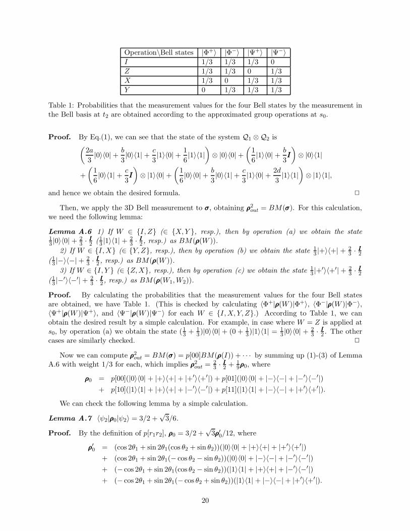
Operation\Bell states |Φ+〉 |Φ−〉 |Ψ+〉 |Ψ−〉I 1/3 1/3 1/3 0

Z 1/3 1/3 0 1/3

X 1/3 0 1/3 1/3

Y 0 1/3 1/3 1/3

Table 1: Probabilities that the measurement values for the four Bell states by the measurement inthe Bell basis at t2 are obtained according to the approximated group operations at s0.

Proof. By Eq.(1), we can see that the state of the system Q1 ⊗Q2 is(

2a

3|0〉〈0| + b

3|0〉〈1| + c

3|1〉〈0| + 1

6|1〉〈1|

)

⊗ |0〉〈0| +(

1

6|1〉〈0| + b

3III

)

⊗ |0〉〈1|

+

(

1

6|0〉〈1| + c

3III

)

⊗ |1〉〈0| +(

1

6|0〉〈0| + b

3|0〉〈1| + c

3|1〉〈0| + 2d

3|1〉〈1|

)

⊗ |1〉〈1|,

and hence we obtain the desired formula. 2

Then, we apply the 3D Bell measurement to σσσ, obtaining ρρρ2out = BM(σσσ). For this calculation,

we need the following lemma:

Lemma A.6 1) If W ∈ {I, Z} (∈ {X,Y }, resp.), then by operation (a) we obtain the state13 |0〉〈0| + 2

3 · III2 (13 |1〉〈1| + 2

3 · III2 , resp.) as BM(ρρρ(W )).

2) If W ∈ {I,X} (∈ {Y,Z}, resp.), then by operation (b) we obtain the state 13 |+〉〈+| + 2

3 · III2(13 |−〉〈−| + 2

3 · III2 , resp.) as BM(ρρρ(W )).

3) If W ∈ {I, Y } (∈ {Z,X}, resp.), then by operation (c) we obtain the state 13 |+′〉〈+′| + 2

3 · III2(13 |−′〉〈−′| + 2

3 · III2 , resp.) as BM(ρρρ(W1,W2)).

Proof. By calculating the probabilities that the measurement values for the four Bell statesare obtained, we have Table 1. (This is checked by calculating 〈Φ+|ρρρ(W )|Φ+〉, 〈Φ−|ρρρ(W )|Φ−〉,〈Ψ+|ρρρ(W )|Ψ+〉, and 〈Ψ−|ρρρ(W )|Ψ−〉 for each W ∈ {I,X, Y, Z}.) According to Table 1, we canobtain the desired result by a simple calculation. For example, in case where W = Z is applied ats0, by operation (a) we obtain the state (1

3 + 13 )|0〉〈0| + (0 + 1

3)|1〉〈1| = 13 |0〉〈0| + 2

3 · III2 . The othercases are similarly checked. 2

Now we can compute ρρρ2out = BM(σσσ) = p[00]BM(ρρρ(I)) + · · · by summing up (1)-(3) of Lemma

A.6 with weight 1/3 for each, which implies ρρρ2out = 2

3 · III2 + 19ρρρ0, where

ρρρ0 = p[00](|0〉〈0| + |+〉〈+| + |+′〉〈+′|) + p[01](|0〉〈0| + |−〉〈−| + |−′〉〈−′|)+ p[10](|1〉〈1| + |+〉〈+| + |−′〉〈−′|) + p[11](|1〉〈1| + |−〉〈−| + |+′〉〈+′|).

We can check the following lemma by a simple calculation.

Lemma A.7 〈ψ2|ρρρ0|ψ2〉 = 3/2 +√

3/6.

Proof. By the definition of p[r1r2], ρρρ0 = 3/2 +√

3ρρρ′0/12, where

ρρρ′0 = (cos 2θ1 + sin 2θ1(cos θ2 + sin θ2))(|0〉〈0| + |+〉〈+| + |+′〉〈+′|)+ (cos 2θ1 + sin 2θ1(− cos θ2 − sin θ2))(|0〉〈0| + |−〉〈−| + |−′〉〈−′|)+ (− cos 2θ1 + sin 2θ1(cos θ2 − sin θ2))(|1〉〈1| + |+〉〈+| + |−′〉〈−′|)+ (− cos 2θ1 + sin 2θ1(− cos θ2 + sin θ2))(|1〉〈1| + |−〉〈−| + |+′〉〈+′|).

20

Thus, it suffices to show that 〈ψ2|ρρρ′0|ψ2〉 = 2. We can rewrite ρρρ′0 as

ρρρ′0 = 2cos 2θ1(|0〉〈0| − |1〉〈1|) + 2 sin 2θ1 cos θ2(|+〉〈+| − |−〉〈−|)+ 2 sin 2θ1 sin θ2(|+′〉〈+′| − |−′〉〈−′|).

Recalling that |ψ2〉 = cos θ1|0〉 + eıθ2 sin θ|1〉, we can check that 〈ψ2||0〉〈0| − |1〉〈1||ψ2〉 = cos 2θ1,〈ψ2||+〉〈+| − |−〉〈−||ψ2〉 = sin 2θ1 cos θ2, and 〈ψ2||+′〉〈+′| − |−′〉〈−′||ψ2〉 = sin 2θ1 sin θ2. Thus, weobtain 〈ψ2|ρρρ′0|ψ2〉 = 2cos2 2θ1 + 2 sin2 2θ1 cos2 θ2 + 2 sin2 2θ1 sin2 θ2 = 2. 2

By Lemma A.7, we finally obtain 〈ψ2|ρρρ2out|ψ2〉 = 1

3 + 19

(

32 +

√3

6

)

= 12 +

√3

54 . This completes the

proof of Lemma A.2. 2

A.3 Proof of Theorem 3.10

Our bound is given under the case where the sources at s1 and s2 are a qubit |ψ〉 and a classicalbit b. Also, we assume that two side links have unlimited capacity, and then we can assume thatthe encoded states from sources are pure states. Suppose that there is a protocol with fidelity1 − ǫ. Then, we show ǫ > 0.017. Let |ξψ〉t2s0 be the encoded state sent from s1, and |φ(b)〉s0t1be the encoded state sent from s2, where the subscript of the ket vector presents where they arein. By the Schmidt decomposition, they are written as: |ξψ〉t2s0 = α|ψ2〉t2 |ψ1〉s0 + β|ψ⊥

2 〉t2 |ψ⊥1 〉s0 ,

and |φ(b)〉s0t1 = γb|φ(b)1〉s0|φ(b)2〉t1 + δb|φ(b)⊥1 〉s0 |φ(b)⊥2 〉t1 . Without loss of generality, |β| ≤ |α|and |δb| ≤ |γb|. Note that ρρρψ = |α|2|ψ1〉〈ψ1| + |β|2|ψ⊥

1 〉〈ψ⊥1 | (and ρρρ(b) = |γ|2|φ(b)1〉〈φ(b)1| +

|δ|2|φ(b)⊥1 〉〈φ(b)⊥1 |, resp.) are the states after the operations at s1 (and s2, resp.) when we focuson the path from s1 to t1 (the path from s2 to t2, resp.). Then, we have the following bounds onβ and δb.

Lemma A.8 |β|2 and |δb|2 are at most 12

(

32 + ǫ−

√

94 + ǫ2 − 5ǫ

)

, and |δ0| + |δ1| ≤ 2√ǫ.

Proof. The bounds on |β| and |δb| are obtained by the same proof as Lemma 4.3. So, we considerthe bound of |δ0| + |δ1|. The fidelity requirement at t2 gives us ||ρρρ(0) − ρρρ(1)||tr ≥ 2 − 4ǫ. Regardρρρ(0) and ρρρ(1) as the points in the Bloch ball. By the triangle inequality, their distance is at most(1− 2|δ0|2) + (1− 2|δ1|2). Thus, |δ0|2 + |δ1|2 ≤ 2ǫ. Then, it is easy to see that |δ0|+ |δ1| ≤ 2

√ǫ. 2

Similar to the proof of Theorem 4.2, we lead to two bounds on ǫ from the two paths. We firstconsider the path s1-t1. Let C be the TP-CP map at s0, and M1 be the composite TP-CP mapby the operations at t0 and t1. Take an arbitrary |ψ〉 and its orthogonal state |ψ⊥〉. The fidelityrequirement at t1 gives us the condition

||M1(C ⊗ I)(ρρρψ − ρρρψ⊥)|φ(b)〉〈φ(b)|||tr ≥ 2 − 4ǫ.

Note that, letting |φ(b)〉 = |φ(b)1〉|φ(b)2〉,

|||φ(b)〉〈φ(b)| − |φ(b)〉〈φ(b)|||tr = 2

√

1 − |〈φ(b)|φ(b)〉|2 = 2|δb|.Thus, by using the triangle inequality

||C(ρρρψ − ρρρψ⊥)|φ(b)1〉〈φ(b)1|||tr = ||(C ⊗ I)(ρρρψ − ρρρψ⊥)|φ(b)〉〈φ(b)|||tr≥ ||M1(C ⊗ I)(ρρρψ − ρρρψ⊥)|φ(b)〉〈φ(b)|||tr≥ ||M1(C ⊗ I)(ρρρψ − ρρρψ⊥)|φ(b)〉〈φ(b)|||tr − ||M1(C ⊗ I)(ρρρψ − ρρρψ⊥)(|φ(b)〉〈φ(b)| − |φ(b)〉〈φ(b)|)||tr≥ 2 − 4ǫ− ||ρρρψ − ρρρψ⊥ ||tr · 2|δb| ≥ 2 − 4ǫ− 4|δb|.

21

Let C(b) be the TP-CP map that transforms ρρρ to C(ρρρ⊗ |φ(b)1〉〈φ(b)1|). Then, we have

||C(b)(|ψ〉〈ψ| − |ψ⊥〉〈ψ⊥|)||tr ≥ ||C(b)(ρρρψ − ρρρψ⊥)||tr ≥ 2 − 4ǫ− 4|δb|.

This leads to the condition||C(b)|ψ〉〈ψ|||tr ≥ 1 − 4ǫ− 4|δb| (14)

since ||C(b)|ψ⊥〉〈ψ⊥|||tr ≤ 1. Recall that the Bloch sphere representation of C(b) is written as themap: ~r 7→ O1(b)Λ(b)O2(b)~r+ ~d(b) where O1(b), O2(b) are orthogonal matrices with determinant 1,and Λ(b) is a diagonal matrix. Let U(b) be the unitary operator whose Bloch sphere representationmaps a Bloch vector ~r to O1(b)O2(b)~r. Now we take |ψ〉 such that U(0)ρρρψ = U(1)ρρρψ. Then, weevaluate ||(C(0) − C(1))ρ′ρ′ρ′ψ||tr with ρ′ρ′ρ′ψ = |α|2|ψ1〉〈ψ1| as follows:

||(C(0) − C(1))ρ′ρ′ρ′ψ||tr≤ ||(C(0) − U(0))ρ′ρ′ρ′ψ||tr + ||U(0)(ρ′ρ′ρ′ψ − ρρρψ)||tr + ||U(1)(ρρρψ − ρ′ρ′ρ′ψ)||tr + ||(U(1) − C(1))ρ′ρ′ρ′ψ||tr= |α|2(||(C(0) − U(0))|ψ1〉〈ψ1|||tr + ||(C(1) − U(1))|ψ1〉〈ψ1|||tr) + 2||ρρρψ − ρ′ρ′ρ′ψ||tr.

Noting Ineq.(14), ||U(b)|ψ1〉〈ψ1|||tr = 1 and ||ρρρψ − ρ′ρ′ρ′ψ||tr = |β|2, we obtain

||(C(0) − C(1))ρ′ρ′ρ′ψ||tr ≤ |α|2(8ǫ+ 4|δ0| + 4|δ1|) + 2|β|2. (15)

Second, we consider the path s2-t2. Let M2 be the composite map by the operations at t0 andt2. By the fidelity requirement at t2, ||M2(I ⊗ C)|ξψ〉〈ξψ |(ρρρ(0) − ρρρ(1))||tr ≥ 2 − 4ǫ. The left-handside is at most

||(I ⊗ C)(|ψ2〉〈ψ2| ⊗ ρ′ρ′ρ′)(ρρρ(0) − ρρρ(1))||tr + ||(I ⊗ C)(|ξψ〉〈ξψ| − |ψ2〉〈ψ2| ⊗ ρ′ρ′ρ′)(ρρρ(0) − ρρρ(1))||tr≤ ||C(ρ′ρ′ρ′(ρρρ(0) − ρρρ(1)))||tr + |||ξψ〉〈ξψ| − |ψ2〉〈ψ2| ⊗ ρ′ρ′ρ′||tr||ρρρ(0) − ρρρ(1)||tr≤ ||(C ′(0) − C ′(1))ρ′ρ′ρ′||tr + 2|β|

√

1 − |β|2/2 × 2,

where C ′(b) is the TP-CP map: σσσ 7→ C(σσσ⊗ρρρ(b)) and the last term of the right-hand side is obtainedby the same calculation as Lemma 4.5. Since ρρρ(b) = (1 − 2|δb|2)|φ(b)1〉〈φ(b)1| + 2|δb|2 · III2 , C ′(b) isdecomposed into C ′(b) = (1 − 2|δb|2)C(b) + 2|δb|2CI with some TP-CP map CI . Now we assumethat |δ0|2 ≥ |δ1|2, which does not loss of generality. By the triangle inequality,

||(C ′(0) − C ′(1))ρ′ρ′ρ′||tr≤ ||(1 − 2|δ0|2)(C(0) − C(1))ρ′ρ′ρ′||tr + ||(2|δ0|2 − 2|δ1|2)C(1)ρ′ρ′ρ′||tr + ||(2|δ0|2 − 2|δ1|2)CIρ′ρ′ρ′||tr≤ (1 − 2|δ0|2)||(C(0) − C(1))ρ′ρ′ρ′||tr + 4|α|2(|δ0|2 − |δ1|2).

Thus, we have

2 − 4ǫ ≤ 4|β|√

1 − |β|2/2 + (1 − 2|δ0|2)||(C(0) − C(1))ρ′ρ′ρ′||tr + 4|α|2(|δ0|2 − |δ1|2). (16)

By Ineqs.(15) and (16) from the two paths and Lemma A.8, we obtain

2 − 4ǫ ≤ 4|β|√

1 − |β|2/2 + (1 − 2|δ0|2)(|α|2(8ǫ+ 4|δ0| + 4|δ1|) + 2|β|2) + 4|α|2(|δ0|2 − |δ1|2)≤ 4|β| + 2|β|2 + 4|δ0|2 + 8ǫ+ 4(|δ0| + |δ1|)≤ 4√

f(ǫ) + 6f(ǫ) + 8ǫ+ 8√ǫ,

where f(ǫ) = 12

(

32 + ǫ−

√

94 + ǫ2 − 5ǫ

)

. Therefore, we have 1 − 4√ǫ− 6ǫ ≤ 2

√

f(ǫ) + 3f(ǫ). The

left-hand side is monotone decreasing on ǫ while the right-hand side is monotone increasing on ǫ.By checking ǫ satisfying the inequality, we obtain ǫ > 0.017.

22

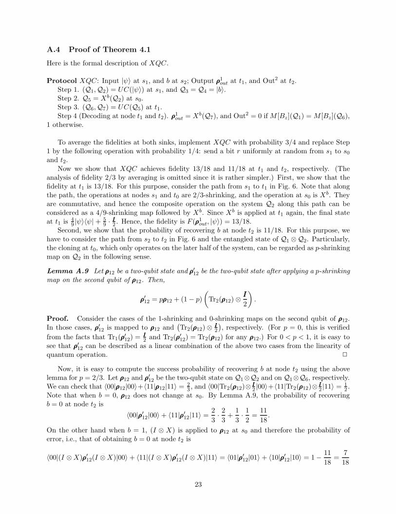
A.4 Proof of Theorem 4.1

Here is the formal description of XQC.

Protocol XQC: Input |ψ〉 at s1, and b at s2; Output ρρρ1out at t1, and Out2 at t2.

Step 1. (Q1,Q2) = UC(|ψ〉) at s1, and Q3 = Q4 = |b〉.Step 2. Q5 = Xb(Q2) at s0.Step 3. (Q6,Q7) = UC(Q5) at t1.Step 4 (Decoding at node t1 and t2). ρρρ

1out = Xb(Q7), and Out2 = 0 if M [Bz](Q1) = M [Bz](Q6),

1 otherwise.

To average the fidelities at both sinks, implement XQC with probability 3/4 and replace Step1 by the following operation with probability 1/4: send a bit r uniformly at random from s1 to s0and t2.

Now we show that XQC achieves fidelity 13/18 and 11/18 at t1 and t2, respectively. (Theanalysis of fidelity 2/3 by averaging is omitted since it is rather simpler.) First, we show that thefidelity at t1 is 13/18. For this purpose, consider the path from s1 to t1 in Fig. 6. Note that alongthe path, the operations at nodes s1 and t0 are 2/3-shrinking, and the operation at s0 is Xb. Theyare commutative, and hence the composite operation on the system Q2 along this path can beconsidered as a 4/9-shrinking map followed by Xb. Since Xb is applied at t1 again, the final stateat t1 is 4

9 |ψ〉〈ψ| + 59 · III2 . Hence, the fidelity is F (ρρρ1

out, |ψ〉) = 13/18.Second, we show that the probability of recovering b at node t2 is 11/18. For this purpose, we

have to consider the path from s2 to t2 in Fig. 6 and the entangled state of Q1 ⊗Q2. Particularly,the cloning at t0, which only operates on the later half of the system, can be regarded as p-shrinkingmap on Q2 in the following sense.

Lemma A.9 Let ρρρ12 be a two-qubit state and ρρρ′12 be the two-qubit state after applying a p-shrinkingmap on the second qubit of ρρρ12. Then,

ρρρ′12 = pρρρ12 + (1 − p)

(

Tr2(ρρρ12) ⊗III

2

)

.

Proof. Consider the cases of the 1-shrinking and 0-shrinking maps on the second qubit of ρρρ12.In those cases, ρρρ′12 is mapped to ρρρ12 and

(

Tr2(ρρρ12) ⊗ III2

)

, respectively. (For p = 0, this is verified

from the facts that Tr1(ρρρ′12) = III

2 and Tr2(ρρρ′12) = Tr2(ρρρ12) for any ρρρ12.) For 0 < p < 1, it is easy to

see that ρρρ′12 can be described as a linear combination of the above two cases from the linearity ofquantum operation. 2

Now, it is easy to compute the success probability of recovering b at node t2 using the abovelemma for p = 2/3. Let ρρρ12 and ρρρ′12 be the two-qubit state on Q1⊗Q2 and on Q1⊗Q6, respectively.We can check that 〈00|ρρρ12|00〉+〈11|ρρρ12|11〉 = 2

3 , and 〈00|Tr2(ρρρ12)⊗ III2 |00〉+〈11|Tr2(ρρρ12)⊗ III

2 |11〉 = 12 .

Note that when b = 0, ρρρ12 does not change at s0. By Lemma A.9, the probability of recoveringb = 0 at node t2 is

〈00|ρρρ′12|00〉 + 〈11|ρρρ′12|11〉 =2

3· 2

3+

1

3· 1

2=

11

18.

On the other hand when b = 1, (I ⊗ X) is applied to ρρρ12 at s0 and therefore the probability oferror, i.e., that of obtaining b = 0 at node t2 is

〈00|(I ⊗X)ρρρ′12(I ⊗X)|00〉 + 〈11|(I ⊗X)ρρρ′12(I ⊗X)|11〉 = 〈01|ρρρ′12|01〉 + 〈10|ρρρ′12|10〉 = 1 − 11

18=

7

18

23

since I ⊗ X is commutative with the p-shrinking map on the second qubit. Thus we obtain thefidelity 11/18 at t2.

A.5 Proof of Theorem 5.1

First, we recall the quantum random access (QRA) coding by Ambainis et al. [4]. An (n,m, p)-QRA coding is a function that maps n-bit strings x ∈ {0, 1}n to m-qubit states ρρρx satisfying thefollowing: For every i ∈ {1, 2, . . . , n} there exists a POVM Ei = {Ei0, Ei1} such that Tr(Eixi

ρρρx) ≥ pfor all x ∈ {0, 1}n, where xi is the i-th bit of x. If the m-qubit states are classical, the coding iscalled an (n,m, p)-classical random access coding. In [4], an (2, 1, 0.85)-QRA coding is given by thefollowing protocol.

Let |ϕ(00)〉 = cos(π/8)|0〉+sin(π/8)|1〉, |ϕ(10)〉 = cos(3π/8)|0〉+sin(3π/8)|1〉, |ϕ(11)〉 =cos(5π/8)|0〉+sin(5π/8)|1〉, and |ϕ(01)〉 = cos(7π/8)|0〉+sin(7π/8)|1〉 be the one-qubitstate used when the source x ∈ {0, 1}2 is respectively 00, 10, 11, and 01. The first bitof x is obtained by measuring in the basis Bz, while the second one by measuring inthe basis Bx.

In fact, the success probability of the above protocol is cos2(π/8) ≈ 0.85. On the contrary, it wasalso shown that any (2, 1, p)-classical random access coding should satisfy p ≤ 1/2.

A map that transforms an arbitrary equatorial state (i.e., the one-qubit state whose amplitudesare real) |ψ〉〈ψ| to p|ψ〉〈ψ|+(1−p)III2 is called a p-shrinking map on equatorial qubits. The followinglemma is verified from the transformation of the phase-covariant cloning machine [8, 11]. (The term“the phase-covariant copy” is defined similarly as the universal copy.) Fortunately, for our purposethe detail of the cloning machine except the fact that it is a 1/

√2-shrinking map is not needed.

Lemma A.10 The phase-covariant copy is 1/√

2-shrinking map on equatorial qubits.

Finally we introduce the 2D measurement. This measurement is defined by the POVM{1

2 |ϕ(z1z2)〉 | z1z2 ∈ {0, 1}2}, denoted by MM2. Its intuition is to do the two projective measure-ments in the bases {|ϕ(00)〉, |ϕ(11)〉} and {|ϕ(01)〉, |ϕ(10)〉} with probability 1/2 for each. Noticethat we estimate the QRA coding state from s2 correctly if we choose the right one of the twobases.

The detailed description of X2C2C is as follows. The term (Q,Q′) = PC(Q′′) means that Qand Q′ are the two copies output by the phase-covariant quantum cloning machine when Q′′ isgiven as the input.

Protocol X2C2C: Input x1x2 at s1, y1y2 at s2; Output Out1 at t1, Out2 at t2.Step 1. Q1 = |ϕ(x1x2)〉, Q2 = |ϕ(x1x2)〉, Q3 = |ϕ(y1y2)〉, and Q4 = |ϕ(y1y2)〉.Step 2. Q5 = GR(Q2,MM2(Q3)) at s0.Step 3. (Q6,Q7) = PC(Q5) at t0.Step 4 (Decoding the j-th bit at t1 and t2). Out1 = M [Bz ](Q4) ⊕M [Bz](Q7) if j = 1, and

M [Bx](Q4) ⊕M [Bx](Q7) if j = 2. Out2 = M [Bz](Q1) ⊕M [Bz](Q6) if j = 1, and M [Bx](Q1) ⊕M [Bx](Q6) if j = 2.

Here, we analyze the success probability of X2C2C. By the definition of MM2 the followinglemma is immediate.

Lemma A.11 Given a QRA coding state |ϕ(y1y2)〉, the probability that z1z2 is obtained by MM2

is 1/2 if z1z2 = y1y2, 1/4 if z1z2 = y1y2 or y1y2, and 0 if z1z2 = y1y2. Here, b denotes the negationof a bit b.

24

110

000

100

111

011

x

y

z

001

010

101

Figure 11: (3, 1, 0.79)-QRA coding in the Bloch sphere representation

For simplicity, let us assume that y1y2 = 00 (the analysis of the other cases are similar). By LemmaA.11, the state of Q2 ⊗Q3 after MM2 is

|ϕ(x1x2)〉〈ϕ(x1x2)| ⊗(

1

2|00〉〈00| + 1

4(|10〉〈10| + |01〉〈01|)

)

.

Note that if y1y2 is obtained by MM2, the state |ϕ(x1x2)〉 from s1 is transformed into |ϕ(x1 ⊕y1, x2 ⊕ y2)〉 by GR. Thus, the state of Q5 is

1

2|ϕ(x1x2)〉〈ϕ(x1x2)| +

1

4(|ϕ(x1x2)〉〈ϕ(x1x2)| + |ϕ(x1x2)〉〈ϕ(x1x2)|)

By Lemma A.10, the state of Q6 (or Q7) is

1

2√

2|ϕ(x1x2)〉〈ϕ(x1x2)| +

1

4√

2(|ϕ(x1x2)〉〈ϕ(x1x2)| + |ϕ(x1x2)〉〈ϕ(x1x2)|) +

(

1 − 1√2

)

III

2.

Now we check the success probability of decoding the first bit of y1y2 = 00, i.e., 0 at t2 (the othercases are similarly checked). As seen from the state of Q6, the success probability of decoding thefirst bit of x1x2 ⊕ y1y2, i.e., x1 is

1

2√

2· cos2 π

8+

1

4√

2(cos2 π

8+ sin2 π

8) +

1

2

(

1 − 1√2

)

,

which is 5/8. On the contrary, the success probability of decoding the first bit x1 from the state of Q1

is cos2 π8 . Thus, the success probability of decoding the first bit of y1y2 at t2 is cos2 π

8 · 58 +sin2 π

8 · 38 =

1/2 +√

2/16 as claimed.

A.6 Proof of Theorem 5.2

For the proof of Theorem 5.2, we need the following two primitives.3D Measurement (MM3). The 3D measurement, denoted by MM3, is defined by the POVM

described by {14 |ϕ(z1z2z3)〉〈ϕ(z1z2z3)| | z1z2z3 ∈ {0, 1}3}, where |ϕ(z1z2z3)〉 is the (3, 1, 0.79)-QRA

coding state of z1z2z3 (Fig. 11).Approximated Group Operation (AG). Before its definition, we introduce the operation

Inv, which maps a pure state |ψ〉 = a|0〉+b|1〉 to its “opposite” state b∗|0〉−a∗|1〉 in the Bloch sphere

25

(see e.g., [10, 13]). Formally, it is defined as follows: For any mixed state ρρρ =

(

u vw x

)

, Invρρρ =(

x −v−w u

)

. Note that the set of maps ρρρ 7→WρρρW † (W ∈ {I,X, Y, Z, Inv, InvX, InvY, InvZ}) is

an abelian group. Because Inv is not a TP-CP map, we introduce its approximation Inv′, whichmaps ρρρ to Inv′ρρρ = 1

3Invρρρ + 23 · III2 . We can check that Inv′ is a TP-CP map. The approximated

group operation under a three-bit string r1r2r3, denoted by AG(ρρρ, r1r2r3), is a transformationdefined by AG(ρρρ, 000) = ρρρ, AG(ρρρ, 011) = Zρρρ, AG(ρρρ, 101) = Xρρρ, AG(ρρρ, 110) = Y ρρρ and, for anyr1r2r3 ∈ {001, 010, 100, 111}, AG(ρρρ, r1r2r3) = Inv′AG(ρρρ, r1r2r3).

The description of the protocol X3C3C is as follows.

Protocol X3C3C: Input x1x2x3 at s1, y1y2y3 at s2; Output Out1 at t1, Out2 at t2.Step 1. Q1 = |ϕ(x1x2x3)〉, Q2 = |ϕ(x1x2x3)〉, Q3 = |ϕ(y1y2y3)〉, and Q4 = |ϕ(y1y2y3)〉.Step 2. Q5 = AG(Q2,MM3(Q3)) at s0.Step 3. (Q6,Q7) = UC(Q5) at t0.Step 4 (Decoding the j-th bit at t1 and t2). Out1 = M [Bz](Q4) ⊕ M [Bz](Q7) if j = 1,

M [Bx](Q4) ⊕M [Bx](Q7) if j = 2, and M [By](Q4) ⊕M [By](Q7) if j = 3. Out2 = M [Bz](Q1) ⊕M [Bz](Q6) if j = 1, M [Bx](Q1) ⊕M [Bx](Q6) if j = 2, and M [By](Q1) ⊕M [By](Q6) if j = 3.

Now, we analyze X3C3C, which is similar to X2C2C. By definition of POVM MM3, we caneasily check the following lemma.

Lemma A.12 Given a QRA coding state |ϕ(y1y2y3)〉, the probability that z1z2z3 is obtained byMM3 is

1/4 if z1z2z3 = y1y2y3,1/6 if z1z2z3 = y1y2y3, y1y2y3, y1y2y3,1/12 if z1z2z3 = y1y2y3, y1y2y3, y1y2y3,0 if z1z2z3 = y1y2y3

Henceforth, for simplicity of descriptions we only consider the case y1y2y3 = 000. By Lemma A.12,the state of Q2 ⊗Q3 after MM3 is

|ϕ(x1x2x3)〉〈ϕ(x1x2x3)| ⊗(

1

4|000〉〈000| + 1

6(|100〉〈100| + |010〉〈010|

+|001〉〈001|) +1

12(|110〉〈110| + |101〉〈101| + |011〉〈011|)

)

.

Noting that Inv′(|ϕ(z1z2z3)〉〈ϕ(z1z2z3)|) = 13 |ϕ(z1z2z3)〉〈ϕ(z1 z2z3)| + 2

3 · III2 , the state of Q5 is

1

4|ϕ(x1x2x3)〉〈ϕ(x1x2x3)|

+1

18(|ϕ(x1x2x3)〉〈ϕ(x1x2x3)| + |ϕ(x1x2x3)〉〈ϕ(x1x2x3)| + |ϕ(x1x2x3)〉〈ϕ(x1x2x3)|)

+1

12(|ϕ(x1x2x3)〉〈ϕ(x1x2x3)| + |ϕ(x1x2x3)〉〈ϕ(x1x2x3)| + |ϕ(x1x2x3)〉〈ϕ(x1x2x3)|) +

2

3· 1

6· 3 · III

2.

26

By Lemma 3.4, the state of Q6 (or Q7)) is

1

6|ϕ(x1x2x3)〉〈ϕ(x1x2x3)|

+1

27(|ϕ(x1x2x3)〉〈ϕ(x1x2x3)| + |ϕ(x1x2x3)〉〈ϕ(x1x2x3)| + |ϕ(x1x2x3)〉〈ϕ(x1x2x3)|)

+1

18(|ϕ(x1x2x3)〉〈ϕ(x1x2x3)| + |ϕ(x1x2x3)〉〈ϕ(x1x2x3)| + |ϕ(x1x2x3)〉〈ϕ(x1x2x3)|) +

5

9· III2,

where the last term is obtained by adding 13 · 1

4 · III2 , 13 · 1

18 · 3 · III2 , 13 · 1

12 · 3 · III2 , and 23 · 1

6 · 3 · III2 . Nowwe check the success probability of decoding the first bit of y1y2y3 = 000, i.e., 0. (The other casesare similarly checked.) As seen from the state of Q6, the success probability of decoding the firstbit of x1x2x3 ⊕ y1y2y3, i.e., x1 is

1

6

(

1

2+

√3

6

)

+1

27

(

2 ·(

1

2+

√3

6

)

+

(

1

2−

√3

6

))

+1

18

(

2 ·(

1

2−

√3

6

)

+

(

1

2+

√3

6

))

+5

9· 1

2=

1

2+

2√

3

81.

On the contrary, the success probability of decoding the first bit x1 from the state of Q1 is 1/2 +√3/6. Thus, the success probability of decoding the first bit of y1y2y3 at sink t2 is (1/2+

√3/6)(1/2+

2√

3/81) + (1/2 −√

3/6)(1/2 − 2√

3/81) = 1/2 + 2/81 as desired.

27