On the Role of Feedback in Network Codingby

Jay Kumar SundararajanS.M., Electrical Engineering and Computer Science, Massachusetts Institute of Technology (2005)

B.Tech., Electrical Engineering, Indian Institute of Technology Madras (2003)

Submitted to theDepartment of Electrical Engineering and Computer Science

in partial fulfillment of the requirements for the degree of

Doctor of Philosophy in Electrical Engineering and Computer Science

at the

MASSACHUSETTS INSTITUTE OF TECHNOLOGY

September 2009

c© Massachusetts Institute of Technology 2009. All rights reserved.

Author . . . . . . . . . . . . . . . . . . . . . . . . . . . . . . . . . . . . . . . . . . . . . . . .. . . . . . . . . . . . .Department of Electrical Engineering and Computer Science

August 14, 2009

Certified by . . . . . . . . . . . . . . . . . . . . . . . . . . . . . . . . . . . . . . . . . .. . . . . . . . . . . . . . .Muriel Medard

Professor of Electrical Engineering and Computer ScienceThesis Supervisor

Certified by . . . . . . . . . . . . . . . . . . . . . . . . . . . . . . . . . . . . . . . . . .. . . . . . . . . . . . . . .Devavrat Shah

Assistant Professor of Electrical Engineering and Computer ScienceThesis Supervisor

Accepted by. . . . . . . . . . . . . . . . . . . . . . . . . . . . . . . . . . . . . . . . . . .. . . . . . . . . . . . . .Terry P. Orlando

Chairman, Department Committee on Graduate Students

brought to you by COREView metadata, citation and similar papers at core.ac.uk

provided by DSpace@MIT

2

On the Role of Feedback in Network Coding

by

Jay Kumar Sundararajan

Submitted to the Department of Electrical Engineering and Computer Scienceon August 14, 2009, in partial fulfillment of the

requirements for the degree ofDoctor of Philosophy in Electrical Engineering and ComputerScience

Abstract

Network coding has emerged as a new approach to operating communication networks,with a promise of improved efficiency in the form of higher throughput, especially in lossyconditions. In order to realize this promise in practice, the interfacing of network codingwith existing network protocols must be understood well. Most current protocols makeuse of feedback in the form of acknowledgments (ACKs) for reliability, rate control and/ordelay control. In this work, we propose a way to incorporate network coding within such afeedback-based framework, and study the various benefits ofusing feedback in a network-coded system.

More specifically, we propose a mechanism that provides a clean interface betweennetwork coding and TCP with only minor changes to the protocolstack, thereby allowingincremental deployment. In our scheme, the source transmits random linear combinationsof packets currently in the TCP congestion window. At the heart of our scheme is a newinterpretation of ACKs – the receiver acknowledges every degree of freedom (i.e., a linearcombination that reveals one unit of new information) even if it does not reveal an originalpacket immediately. Such ACKs enable a TCP-compatible sliding-window implementationof network coding. Thus, with feedback, network coding can be performed in a completelyonline manner, without the need for batches or generations.

Our scheme has the nice feature that packet losses on the linkcan be essentially maskedfrom the congestion control algorithm by adding enough redundancy in the encoding pro-cess. This results in a novel and effective approach for congestion control over networksinvolving lossy links such as wireless links. Our scheme also allows intermediate nodes toperform re-encoding of the data packets. This in turn leads to a natural way of running TCPflows over networks that use multipath opportunistic routing along with network coding.

We use the new type of ACKs to develop queue management algorithms for codednetworks, which allow the queue size at nodes to track the true backlog in information withrespect to the destination. We also propose feedback-basedadaptive coding techniques thatare aimed at reducing the decoding delay at the receivers. Different notions of decodingdelay are considered, including an order-sensitive notionwhich assumes that packets areuseful only when delivered in order. We study the asymptoticbehavior of the expectedqueue size and delay, in the limit of heavy traffic.

Thesis Supervisor: Muriel MedardTitle: Professor of Electrical Engineering and Computer Science

Thesis Supervisor: Devavrat ShahTitle: Assistant Professor of Electrical Engineering and Computer Science

To my mother

Ms. Vasantha Sundararajan

Acknowledgments

I am very fortunate to have interacted with and learnt from many wonderful people through-

out my life – people whose support and good wishes have playeda very important role in

the completion of this thesis.

I am deeply indebted to my advisor Prof. Muriel Medard for her kind support and

guidance throughout the course of my graduate studies. Muriel takes a lot of care to ensure

that her students have the right environment to grow as researchers. Her advice and constant

encouragement helped me believe in myself and stay focused on my work. She helped

me to place my work in the big picture, and taught me to pay attention to the practical

implications of my work, which I believe, are very valuable lessons.

My co-advisor Prof. Devavrat Shah has been a great mentor andhas taught me a great

deal about how to go about tackling a research problem. His insights as well as his patience

and attention have played a big role in the progress of my research work. I am very grateful

to him for his care and support.

I would like to thank Prof. Michel Goemans for being on my thesis committee. In

addition, I really enjoyed his course on combinatorial optimization.

I have had the great fortune of interacting with several other professors during my grad-

uate studies. (Late) Prof. Ralf Koetter was a true inspiration and his thoughtful pointers on

my work proved extremely useful in its eventual completion.Prof. Michael Mitzenmacher

and Prof. Joao Barros provided several useful ideas and comments regarding the work itself

as well as its presentation. I would like to specially thank Prof. Dina Katabi and her group

for very valuable feedback on the work and also for providingthe resources and support

for the experimental portion of the work. I would also like tothank Prof. John Wyatt for

the opportunity to be his teaching assistant in Fall 2006. Many thanks to all the professors

who have taught me during my graduate studies.

My interaction with other graduate students, postdoctoralfellows and visitors in LIDS,

RLE and CSAIL was very rewarding. I am very thankful to all my seniors for mentor-

ing me through the graduate school process. Thanks also to mygroupmates and other

colleagues for many useful discussions and collaboration.In particular, I would like to

thank Shashibhushan Borade, Siddharth Ray, Niranjan Ratnakar, Ashish Khisti, Desmond

Lun, Murtaza Zafer, Krishna Jagannathan, Mythili Vutukuru, Szymon Jakubczak, Hari-

haran Rahul, Arvind Thiagarajan, Marie-Jose Montpetit, Fang Zhao, Ali ParandehGheibi,

MinJi Kim, Shirley Shi, Minkyu Kim, Daniel Lucani, Venkat Chandar, Ying-zong Huang,

Guy Weichenberg, Atilla Eryilmaz, Danail Traskov, Sujay Sanghavi, and Sidharth Jaggi.

A very special thanks to Michael Lewy, Doris Inslee, Rosangela Dos Santos, Sue Pat-

terson, Brian Jones, and all the other administrative staff,who have been a tremendous help

all these years.

Ashdown House proved to be a great community to live in. A special thanks is due to the

housemasters Ann and Terry Orlando. I made several good friends there during the course

of my PhD. The ‘cooking group’ that I was a part of, provided excellent food and also

entertainment in the form of many an interesting dinner-table debate and several foosball

and ping-pong sessions. This made a big difference in my MIT experience, and helped

offset the pressures of work. In addition, my friends were always there for me to share

my joys and also my concerns. Thanks to all of you, especiallyto Lakshman Pernenkil,

Vinod Vaikuntanathan, Ashish Gupta, Vivek Jaiswal, Krishna Jagannathan, Himani Jain,

Lavanya Marla, Mythili Vutukuru, Arvind Thiagarajan, Sreeja Gopal, Pavithra Harsha,

Hemant Sahoo, Vikram Sivakumar, Raghavendran Sivaraman, Pranava Goundan, Chintan

Vaishnav and Vijay Shilpiekandula. Thanks to my friends outside MIT, in particular, to

Sumanth and Hemanth Jagannathan for their advice and support on numerous occasions.

Thanks also to all my relatives and well-wishers whom I have not named here, but who

have been very encouraging and supportive all along.

I would like to express my heartfelt gratitude to my teachersat my high school Bhavan’s

Rajaji Vidyashram, and all the professors in my college, the Indian Institute of Technology

Madras for their tireless efforts in teaching me the basic skills as well as the values that

proved crucial in my graduate studies.

Last, but not the least, I am very deeply indebted to my motherMs. Vasantha Sun-

dararajan. Her sacrifice, patience and strength are the mainreasons for my success. Her

constant love, encouragement, and selfless support have helped me overcome many hurdles

and remain on track towards my goal. This thesis is dedicatedto her.

I would like to thank all the funding sources for their support. This thesis work was

supported by the following grants:

• Subcontract # 18870740-37362-C issued by Stanford University and supported by

the Defense Advanced Research Projects Agency (DARPA),

• National Science Foundation Grant No. CNS-0627021,

• Office of Naval Research Grant No. N00014-05-1-0197,

• Subcontract # 060786 issued by BAE Systems National Security Solutions, Inc.

and supported by the DARPA and the Space and Naval Warfare System Center

(SPAWARSYSCEN), San Diego under Contract No. N66001-06-C-2020,

• Subcontract # S0176938 issued by UC Santa Cruz, supported by the United States

Army under Award No. W911NF-05-1-0246, and

• DARPA Grant No. HR0011-08-1-0008.

10

Contents

1 Introduction 19

1.1 The role of feedback in communication protocols. . . . . . . . . . . . . . 21

1.2 Coding across packets. . . . . . . . . . . . . . . . . . . . . . . . . . . . . 22

1.3 Problems addressed. . . . . . . . . . . . . . . . . . . . . . . . . . . . . . 27

1.4 Main contributions . . . . . . . . . . . . . . . . . . . . . . . . . . . . . . 30

1.5 Outline of the thesis. . . . . . . . . . . . . . . . . . . . . . . . . . . . . . 31

2 Queue management in coded networks 33

2.1 ‘Seeing’ a packet – a novel acknowledgment mechanism. . . . . . . . . . 35

2.2 Background and our contribution. . . . . . . . . . . . . . . . . . . . . . . 37

2.2.1 Related earlier work. . . . . . . . . . . . . . . . . . . . . . . . . 37

2.2.2 Implications of our new scheme. . . . . . . . . . . . . . . . . . . 39

2.3 The setup . . . . . . . . . . . . . . . . . . . . . . . . . . . . . . . . . . . 40

2.4 Algorithm 1: Drop when decoded (baseline). . . . . . . . . . . . . . . . . 44

2.4.1 The virtual queue size in steady state. . . . . . . . . . . . . . . . 45

2.4.2 The physical queue size in steady state. . . . . . . . . . . . . . . . 46

2.5 Algorithm 2 (a): Drop common knowledge. . . . . . . . . . . . . . . . . 48

2.5.1 An intuitive description. . . . . . . . . . . . . . . . . . . . . . . . 49

2.5.2 Formal description of the algorithm. . . . . . . . . . . . . . . . . 50

2.5.3 Connecting the physical and virtual queue sizes. . . . . . . . . . . 53

2.6 Algorithm 2 (b): Drop when seen. . . . . . . . . . . . . . . . . . . . . . . 62

2.6.1 Some preliminaries. . . . . . . . . . . . . . . . . . . . . . . . . . 63

2.6.2 The main idea. . . . . . . . . . . . . . . . . . . . . . . . . . . . . 65

11

2.6.3 The queuing module. . . . . . . . . . . . . . . . . . . . . . . . . 67

2.6.4 Connecting the physical and virtual queue sizes. . . . . . . . . . . 68

2.6.5 The coding module. . . . . . . . . . . . . . . . . . . . . . . . . . 71

2.7 Overhead . . . . . . . . . . . . . . . . . . . . . . . . . . . . . . . . . . . 73

2.7.1 Amount of feedback. . . . . . . . . . . . . . . . . . . . . . . . . 73

2.7.2 Identifying the linear combination. . . . . . . . . . . . . . . . . . 73

2.7.3 Overhead at sender. . . . . . . . . . . . . . . . . . . . . . . . . . 75

2.7.4 Overhead at receiver. . . . . . . . . . . . . . . . . . . . . . . . . 75

2.8 Conclusions. . . . . . . . . . . . . . . . . . . . . . . . . . . . . . . . . . 76

3 Adaptive online coding to reduce delay 77

3.1 The system model. . . . . . . . . . . . . . . . . . . . . . . . . . . . . . . 79

3.2 Motivation and related earlier work. . . . . . . . . . . . . . . . . . . . . . 80

3.3 Bounds on the delay. . . . . . . . . . . . . . . . . . . . . . . . . . . . . . 82

3.3.1 An upper bound on delivery delay. . . . . . . . . . . . . . . . . . 82

3.3.2 A lower bound on decoding delay. . . . . . . . . . . . . . . . . . 84

3.4 The coding algorithm. . . . . . . . . . . . . . . . . . . . . . . . . . . . . 85

3.4.1 Intuitive description . . . . . . . . . . . . . . . . . . . . . . . . . 85

3.4.2 Representing knowledge. . . . . . . . . . . . . . . . . . . . . . . 86

3.4.3 Algorithm specification. . . . . . . . . . . . . . . . . . . . . . . . 88

3.5 Properties of the algorithm. . . . . . . . . . . . . . . . . . . . . . . . . . 89

3.5.1 Throughput. . . . . . . . . . . . . . . . . . . . . . . . . . . . . . 89

3.5.2 Decoding and delivery delay. . . . . . . . . . . . . . . . . . . . . 90

3.5.3 Queue management. . . . . . . . . . . . . . . . . . . . . . . . . . 91

3.6 Simulation results. . . . . . . . . . . . . . . . . . . . . . . . . . . . . . . 92

3.7 Conclusions. . . . . . . . . . . . . . . . . . . . . . . . . . . . . . . . . . 92

4 Interfacing network coding with TCP/IP 95

4.1 Implications for wireless networking. . . . . . . . . . . . . . . . . . . . . 97

4.2 The new protocol. . . . . . . . . . . . . . . . . . . . . . . . . . . . . . . 100

4.2.1 Logical description. . . . . . . . . . . . . . . . . . . . . . . . . . 101

12

4.2.2 Implementation. . . . . . . . . . . . . . . . . . . . . . . . . . . . 103

4.3 Soundness of the protocol. . . . . . . . . . . . . . . . . . . . . . . . . . . 106

4.4 Fairness of the protocol. . . . . . . . . . . . . . . . . . . . . . . . . . . . 107

4.4.1 Simulation setup. . . . . . . . . . . . . . . . . . . . . . . . . . . 107

4.4.2 Fairness and compatibility – simulation results. . . . . . . . . . . 107

4.5 Effectiveness of the protocol. . . . . . . . . . . . . . . . . . . . . . . . . 109

4.5.1 Throughput of the new protocol – simulation results. . . . . . . . 109

4.5.2 The ideal case. . . . . . . . . . . . . . . . . . . . . . . . . . . . . 112

4.6 Conclusions. . . . . . . . . . . . . . . . . . . . . . . . . . . . . . . . . . 118

5 Experimental evaluation 121

5.1 Sender side module. . . . . . . . . . . . . . . . . . . . . . . . . . . . . . 122

5.1.1 Forming the coding buffer. . . . . . . . . . . . . . . . . . . . . . 122

5.1.2 The coding header. . . . . . . . . . . . . . . . . . . . . . . . . . 125

5.1.3 The coding window. . . . . . . . . . . . . . . . . . . . . . . . . . 126

5.1.4 Buffer management. . . . . . . . . . . . . . . . . . . . . . . . . . 127

5.2 Receiver side module. . . . . . . . . . . . . . . . . . . . . . . . . . . . . 127

5.2.1 Acknowledgment. . . . . . . . . . . . . . . . . . . . . . . . . . . 127

5.2.2 Decoding and delivery. . . . . . . . . . . . . . . . . . . . . . . . 128

5.2.3 Buffer management. . . . . . . . . . . . . . . . . . . . . . . . . . 128

5.2.4 Modifying the receive window. . . . . . . . . . . . . . . . . . . . 128

5.3 Discussion of the practicalities. . . . . . . . . . . . . . . . . . . . . . . . 129

5.3.1 Redundancy factor. . . . . . . . . . . . . . . . . . . . . . . . . . 129

5.3.2 Coding Window Size. . . . . . . . . . . . . . . . . . . . . . . . . 130

5.3.3 Working with TCP Reno. . . . . . . . . . . . . . . . . . . . . . . 131

5.3.4 Computational overhead. . . . . . . . . . . . . . . . . . . . . . . 132

5.3.5 Interface with TCP. . . . . . . . . . . . . . . . . . . . . . . . . . 133

5.4 Results. . . . . . . . . . . . . . . . . . . . . . . . . . . . . . . . . . . . . 134

6 Conclusions and future work 139

13

14

List of Figures

1-1 The butterfly network of [1] . . . . . . . . . . . . . . . . . . . . . . . . . . 24

2-1 Relative timing of arrival, service and departure pointswithin a slot . . . . 43

2-2 Markov chain representing the size of a virtual queue. Here λ := (1 − λ)

andµ := (1 − µ). . . . . . . . . . . . . . . . . . . . . . . . . . . . . . . 45

2-3 The main steps of the algorithm, along with the times at which the various

U(t)’s are defined. . . . . . . . . . . . . . . . . . . . . . . . . . . . . . . 55

2-4 Seen packets and witnesses in terms of the basis matrix. . . . . . . . . . . 65

3-1 Delay to decoding event and upper bound for 2 receiver case, as a function

of 1(1−ρ)

. The corresponding values ofρ are shown on the top of the figure.. 85

3-2 Linear plot of the decoding and delivery delay. . . . . . . . . . . . . . . . 93

3-3 Log plot of the decoding and delivery delay. . . . . . . . . . . . . . . . . 94

4-1 Example of coding and ACKs. . . . . . . . . . . . . . . . . . . . . . . . 102

4-2 New network coding layer in the protocol stack. . . . . . . . . . . . . . . 103

4-3 Simulation topology. . . . . . . . . . . . . . . . . . . . . . . . . . . . . . 107

4-4 Fairness and compatibility - one TCP/NC and one TCP flow. . . . . . . . 108

4-5 Throughput vs redundancy for TCP/NC. . . . . . . . . . . . . . . . . . . 110

4-6 Throughput vs loss rate for TCP and TCP/NC. . . . . . . . . . . . . . . . 111

4-7 Throughput with and without intermediate node re-encoding . . . . . . . . 111

4-8 Topology: Daisy chain with perfect end-to-end feedback. . . . . . . . . . 113

5-1 The coding buffer. . . . . . . . . . . . . . . . . . . . . . . . . . . . . . . 124

5-2 The network coding header. . . . . . . . . . . . . . . . . . . . . . . . . . 125

15

5-3 Receiver side window management. . . . . . . . . . . . . . . . . . . . . . 129

5-4 Goodput versus loss rate. . . . . . . . . . . . . . . . . . . . . . . . . . . 136

5-5 Goodput versus redundancy factor for a 10% loss rate and W=3 . . . . . . 137

5-6 Goodput versus coding window size for a 5% loss rate and R=1.06 . . . . . 138

16

List of Tables

2.1 An example of the drop-when-seen algorithm. . . . . . . . . . . . . . . . 37

2.2 The uncoded vs. coded case. . . . . . . . . . . . . . . . . . . . . . . . . 50

17

18

Chapter 1

Introduction

Advances in communication technology impact the lives of human beings in many signif-

icant ways. In return, people’s lifestyle and needs play a key role in defining the direction

in which the technology should evolve, in terms of the types of applications and services it

is expected to support. This interplay generates a wide variety of fascinating challenges for

the communication engineer.

The main goal of communication system design is to guaranteethe fair and efficient

use of the available resources. Different kinds of engineering questions arise from this

goal, depending on the type of application as well as the environment in which it has to

be implemented. For example, while a large file transfer is mostly concerned with long-

term average throughput, a video-conferencing application requires strict delay guarantees.

Similarly, data networks over the wireless medium have to berobust to channel variability

and packet losses, which are usually not an issue in a wired network.

In addressing these challenges, it is useful to keep in mind that the problem of commu-

nicating information is quite different from the seeminglyrelated problem of transporting

physical commodities because information can be transformed in ways that commodities

cannot. For instance, it is easy to imagine a node replicating incoming data onto multiple

outgoing links. More generally, a node can code the data in different ways. By coding, we

mean that the node can view the incoming data as realizationsof some variables, and can

transmit the output of a function applied to these variables, evaluated at the incoming data.

Finding the “most useful” functions (codes) and establishing the fundamental limits on the

19

benefit that coding can provide over simple uncoded transmission have been the focus of

the field of information theory [2].

The concept of coding data has been put to good use in today’s communication systems

at the link level. For instance, practical coding schemes are known that achieve data rates

very close to the fundamental limit (capacity) of the additive white Gaussian noise channel

[3]. However, extending this idea to the network setting in a practical way has been a

challenging task. On the theoretical front, although the fundamental limits for many multi-

user information theory problems are yet to be established,it is well known that there are

significant benefits to coding beyond the link level (for instance from the results in the

field of network coding). Yet, today’s networks seldom applycoding ideas beyond the link

level. Even replication is seldom used – the most common way to implement a multicast

connection is to initiate multiple unicast connections, one for each receiver.

A possible explanation is the fact that once we go to the network setting, the control

aspect of the communication problem becomes more significant. Several new control prob-

lems show up just to ensure that the network is up and running and that all users get fair

access to the resources. These are arguably more critical goals than the problem of im-

proving the overall speed of communication. While the main question in the point-to-point

setting is one of how best to encode the data to combat channelerrors and variability (the

coding question), the network setting leads to new questions like who should send when

(scheduling), how fast to send (congestion control), and how to find the best path to the

destination (routing). To ensure simple and robust coordination and management of the

network, the conventional approach has been to group data into packets that are then pro-

cessed like commodities, without much coding inside the network.

In such a framework, the most popular approach to addressingthese control questions

has been the use of feedback. Most network protocols today are built around some form

of an acknowledgment mechanism. Therefore, in order to realize the theoretically proven

benefits of coding in the network setting, we have to find a way to incorporate coding into

the existing network protocols, without disrupting the feedback-based control operations.

In other words, we have to deal with the deployment problem – asolution that requires

significant changes to the existing communication protocols will be very difficult to deploy

20

in a large scale, for practical reasons. Also, the modification must besimple, as otherwise,

its interaction with the existing dynamics would be very hard to understand and control.

To summarize, coding is generally associated with improving the efficiency of the com-

munication process, and its robustness to errors. Feedback, on the other hand, is critical for

controlling various aspects of the communication system such as delay or congestion. We

would definitely like to make use of the flexibility of coding in order to make the commu-

nication process more efficient. At the same time, we also have to conform with existing

feedback-based protocols.

This thesis explores the option of integrating these two fundamental concepts, namely

feedbackandcoding, in the context of a packetized data network. We investigatethe prob-

lems associated with implementing this approach within theframework of existing systems

and propose a practical solution. We also demonstrate the potential benefits of combining

these two concepts.

1.1 The role of feedback in communication protocols

Feedback plays a crucial role in communication networks [4]. It is well known that feed-

back can significantly reduce communication delay (error exponents) and the computa-

tional complexity of the encoding and decoding process. It can even be used to predict and

correct noise if the noise is correlated across time, resulting in an improvement in capacity

[5]. In addition, feedback can be used to determine the channelat the transmitter side, and

accordingly adapt the coding strategy. In addition to theseapplications, feedback plays a

key role in managing the communication network, by enablingsimple protocols for con-

gestion control and coordination among the users. In this work, we do not study the use of

feedback for noise prediction or channel learning. Instead, we focus on acknowledgment-

based schemes and their use for reliability, congestion control and delay control.

The most common type of feedback signal used in practice is anacknowledgment

packet that indicates successful reception of some part of the transmitted data. The sim-

plest protocol that makes use of acknowledgments (ACKs) is the Automatic Repeat re-

Quest (ARQ) protocol. Reliable point-to-point communication over a lossy packet link or

21

network with perfect feedback can be achieved using the ARQ scheme. It uses the idea that

the sender can interpret the absence of an ACK to indicate the erasure of the corresponding

packet within the network, and in this case, the sender simply retransmits the lost packet.

Thus, we can ensure the reliability of the protocol.

In the ARQ scheme, if the feedback link is perfect and delay-free, then every success-

ful reception conveys a new packet, implying throughput optimality. Moreover, this new

packet is always the next unknown packet, which implies the lowest possible packet delay.

Since there is feedback, the sender never stores anything the receiver already knows, im-

plying optimal queue size. Thus, this simple scheme simultaneously achieves the optimal

throughput along with minimal delay and queue size. Moreover, the scheme is completely

online and not block-based. The ARQ scheme can be generalizedto situations that have

imperfections in the feedback link, in the form of either losses or delay in the ACKs. Ref-

erence [6] contains a summary of various protocols based on ARQ.

In addition to reliability and delay benefits, feedback plays another critical role in the

communication system, namely, it enables congestion control. In today’s internet, the

Transmission Control Protocol (TCP) makes use of an acknowledgment mechanism to

throttle the transmission rate of the sender in order to prevent congestion inside the net-

work [7, 8]. The main idea is to use ACKs to infer losses, and to use lossesas a congestion

indicator, which in turn triggers a reduction in the packet transmission rate.

Thus, acknowledgment mechanisms are very important for at least the following two

reasons:

1. Providing reliability guarantees in spite of losses and errors in the network

2. Controlling various aspects of the communication system,such as delay, queue sizes

and congestion

1.2 Coding across packets

However, acknowledgment schemes cannot solve all problems. First of all, the feedback

may itself be expensive, unreliable or very delayed. This happens, for instance, in satellite

22

links. In such situations, one has to rely on coding across packets to ensure reliability.

Even if the system has the capability to deliver ACKs reliablyand quickly, simple link-

by-link ARQ is not sufficient in general, especially if we go beyond a single point-to-point

link. The scenario and the requirements of the application may require something more

than simple retransmission. A case in point is multicast over a network of broadcast-mode

links, for instance, in wireless systems. If a packet it transmitted, it is likely to be received

by several nearby nodes. If one of the nodes experienced a badchannel state and thereby

lost the packet, then a retransmission strategy is not the best option, since the retransmission

is useless from the viewpoint of the other receivers that have already received the packet.

Instead, if we allowed coding across packets, then it is possible to convey simultaneously

new information to all connected receivers. Reference [9] highlights the need for coding

for the case of multicast traffic, even if feedback is present.

Another scenario where coding across packets can make a difference is in certain net-

work topologies where multiple flows have to traverse a bottleneck link. A good example

is the butterfly network from [1], which is shown in Figure1-1. Here, simple ARQ applied

to each link can ensure there are no losses on the links. However, even if the links are

error-free, the node D has to code (bitwise XOR) across packets in order to achieve the

highest possible multicast throughput of 2 packets per time-slot. In the absence of coding,

the highest achievable rate is 1.5 packets per time-slot.

Through this example, [1] introduced the field of network coding. The key idea is that

nodes inside the network are allowed to perform coding operations on incoming packets,

and send out coded versions of packets instead of simply routing the incoming packets onto

outgoing links. An algebraic framework for network coding was proposed by Koetter and

Medard in [10]. Network coding has been shown to achieve the multicast capacity of any

network. In fact, [11] showed that linear coding suffices if all the multicast sessions have the

same destination set. Reference [12] presented a random linear network coding approach

for this problem. This approach is easy to implement, and yet, does not compromise on

throughput. The problem of network coding based multicast with a cost criterion has also

been studied, and distributed algorithms have been proposed to solve this problem [13],

[14]. Network coding also readily extends to networks with broadcast-mode links or lossy

23

A

B C

D

F G

E

Figure 1-1: The butterfly network of [1]

links [15], [16], [17]. Thus, there are situations where coding is indispensablefrom a

throughput perspective.

Besides improving throughput, network coding can also be used to simplify network

management. The work by Bhadra and Shakkottai [18] proposed an interesting scheme for

large multi-hop networks, where intermediate nodes in the network have no queues. Only

the source and destination nodes maintain buffers to store packets. The packet losses that

occur due to the absence of buffers inside the network, are compensated for by random

linear coding across packets at the source.

In short, the benefits of network coding can be viewed to arisefrom two basic and

distinct reasons:

1. Resilience to losses and errors

2. Managing how flows share bottleneck links

Several solutions have been proposed that make use of codingacross packets. Each

solution has its own merits and demerits, and the optimal choice depends on the needs of

the application. We compare below, three such approaches – digital fountain codes, random

linear network coding and priority encoding transmission.

24

1. Digital fountain codes: The digital fountain codes ([19, 20, 21]) constitute a well-

known approach to this problem. From a block ofk transmit packets, the sender generates

random linear combinations in such a way that the receiver can, with high probability,

decode the block once it receivesany set of slightly more thank linear combinations.

This approach has low complexity and requires no feedback, except to signal successful

decoding of the block. However, fountain codes are designedfor a point-to-point erasure

channel and in their original form, do not extend readily to anetwork setting. Consider

a two-link tandem network. An end-to-end fountain code withsimple forwarding at the

middle node will result in throughput loss. If the middle node chooses to decode and re-

encode an entire block, the scheme will be sub-optimal in terms of delay, as pointed out

by [22]. In this sense, the fountain code approach is not composable across links. For

the special case of tree networks, there has been some recentwork on composing fountain

codes across links by enabling the middle node to re-encode even before decoding the entire

block [23].

2. Random linear network coding: Network coding was originally introduced for the

case of error-free networks with specified link capacities ([1, 10]), and was extended to the

case of erasure networks [15], [16], [17]. In contrast to fountain codes, the random linear

network coding solution of [12] and [16] does not require decoding at intermediate nodes

and can be applied in any network. Each node transmits a random linear combination of all

coded packets it has received so far. This solution ensures that with high probability, the

transmitted packet will have what we call theinnovation guarantee property, i.e., it will

be innovative1 to every receiver that receives it successfully, except if the receiver already

knows as much as the sender. Thus, every successful reception will bring a unit of new

information. In [16], this scheme is shown to achieve capacity for the case of a multicast

session.

The work of Danaet al. [15] also studied a wireless erasure network with broadcast but

no interference, and established the capacity region. Unlike [15] however, the scheme of

[16] does not require the destination to be provided the location of all the erasures through-

1An innovative packet is a linear combination of packets which is linearly independent of previouslyreceived linear combinations, and thus conveys new information. See Section2.3for a formal definition.

25

out the network.

An important problem with both fountain codes and random linear network coding is

that although they are rateless, the encoding operation is performed on a block (or gener-

ation) of packets. This means that in general, there is no guarantee that the receiver will

be able to extract and pass on to higher layers, any of the original packets from the coded

packets till the entire block has been received. This leads to a decoding delay.

Such a decoding delay is not a problem if the higher layers will anyway use a block

only as a whole (e.g., file download). This corresponds to traditional approaches in infor-

mation theory where the message is assumed to be useful only as a whole. No incentive is

placed on decoding “a part of the message” using a part of the codeword. However, many

applications today involve broadcasting a continuous stream of packets in real-time (e.g.,

video streaming). Sources generate a stream of messages which have an intrinsic temporal

ordering. In such cases, playback is possible only till the point up to which all packets have

been recovered, which we callthe front of contiguous knowledge. Thus, there is incentive

to decode the older messages earlier, as this will reduce theplayback latency. The above

schemes would segment the stream into blocks and process oneblock at a time. Block sizes

will have to be large to ensure high throughput. However, if playback can begin only after

receiving a full block, then large blocks will imply a large delay.

This raises an interesting question: can we code in such a waythat playback can begin

even before the full block is received? In other words, we aremore interested in packet

delay than block delay. These issues have been studied usingvarious approaches by [24],

[25] and [26] in a point-to-point setting. However, in a network setting, the problem is not

well understood. Moreover, these works do not consider the queue management aspects

of the problem. In related work, [27] and [28] address the question of how many original

packets are revealed before the whole block is decoded in a fountain code setting. However,

performance may depend on not onlyhow much datareaches the receiver in a given time,

but alsowhich part of the data. For instance, playback delay depends on not just the number

of original packets that are recovered, but also the order inwhich they are recovered. One

option is to precode the packets using some form of multiple description code []. In that

case, only the number of received coded packets would matter, and the order in which they

26

are received. However, in real-time streaming applications, this approach is likely to have

high computational complexity. Therefore, it is better to design the network so that it is

aware of the ordering of the data, and tries to deliver the earlier packets first.

3. Priority encoding transmission: The scheme proposed in [29], known as priority

encoding transmission (PET), addresses this problem by proposing a code for the erasure

channel that ensures that a receiver will receive the first (or highest priority)i messages

using the firstki coded packets, whereki increases with decreasing priority. In [30], [31],

this is extended to systems that perform network coding. A concatenated network coding

scheme is proposed in [31], with a delay-mitigating pre-coding stage. This scheme guar-

antees that thekth innovative reception will enable the receiver to decode thekth message.

In such schemes however, the ability to decode messages in order requires a reduction in

throughput because of the pre-coding stage.

Even in the presence of coding, we still need feedback to implement various control

mechanisms in the network. Especially, congestion controlrequires some mechanism to

infer the build-up of congestion. The problem of decoding delay or queue management

could also become simpler if we make use of feedback well. In short, both feedback and

coding have their benefits and issues. A good communication system design will have to

employ both concepts in a synergistic manner.

1.3 Problems addressed

This leads to the question – how to combine the benefits of ARQ and network coding? The

goal is to extend ARQ’s desirable properties in the point-to-point context, to systems that

require coding across packets.

Throughout this thesis, we focus on linear codes. The exact mechanism for coding

across packets in a practical system is described in Chapter4. For now, we can visualize

the coding operation as follows. Imagine the original data packets are unknown variables.

The coded packets generated by the encoder can be viewed as linear equations in these

unknown variables.

A variety of interesting problems arise when we try to incorporate a coding-based ap-

27

proach into an acknowledgment-based mechanism. The thesisfocuses on the following

problems:

1. The problem of decoding delay:One of the problems with applying ARQ to a coded

system is that a new reception may not always reveal the next unknown packet to

the receiver. Instead, it may bring in a linear equation involving the packets. In

conventional ARQ, upon receiving an ACK, the sender drops the ACKed packet and

transmits the next one. But in a coded system, upon receiving an ACK for a linear

equation, it is not clear which linear combination the sender should pick for its next

transmission to obtain the best system performance. This isimportant because, if the

receiver has to collect many equations before it can decode the unknowns involved,

this could lead to a large decoding delay.

2. How does coding affect queue management?A related question is: upon receiving

the ACK for a linear equation, which packet can be excluded from future coding,i.e.,

which packet can be dropped from the sender’s queue? More generally, if the nodes

perform coding across packets, what should be the policy forupdating the queues at

various nodes in the network?

In the absence of coding, the conventional approach to queuemanagement at the

sender node is that once a packet has been delivered at the destination, the sender

finds this out using the acknowledgments, and then drops the packet. As far as the

intermediate nodes in the network are concerned, they usually store and forward the

packets, and drop a packet once it has been forwarded.

With coding however, this simple policy may not be the best. As pointed out in the

example in the introduction to Chapter2, the conventional approach of retaining in

the sender’s queue any packet that has not been delivered to the destination is not

optimal. In fact, we will show in Chapter2 that this policy leads to a much larger

queue than necessary, especially as the traffic load on the network increases.

Also, if the intermediate nodes want to perform coding for erasure correction as in

the work of [16], they cannot drop a packet immediately after forwarding it. They

will need to retain it and involve it in the coding for a while,in order to make sure

28

the receiver has sufficiently many redundant (coded) packets to ensure reliable data

transfer. In such a case, we need to define an effective queue management policy for

the intermediate nodes as well.

3. Practical deployment of network coding:In order to bring the ideas of network cod-

ing into practice, we need a protocol that brings out the benefits of network coding

while requiring very little change in the protocol stack. Flow control and congestion

control in today’s internet are predominantly handled by the Transmission Control

Protocol (TCP), which works using the idea of a sliding transmission window of

packets, whose size is controlled based on feedback. On the theoretical side, Chen

et al. [32] proposed distributed rate control algorithms for networkcoding, in a

utility maximization framework, and pointed out its similarity to TCP. However, to

implement such algorithms in practice, we need to create a clean interface between

network coding and TCP.

The main idea behind TCP is to use acknowledgments of packets as they arrivein

correct sequence orderin order to guarantee reliable transport and also as a feedback

signal for the congestion control loop. Now, if we allow the network to perform

network coding however, the notion of an ordered sequence ofpackets as used by

TCP goes missing. What is received is a randomly chosen linear combination, which

might not immediately reveal an original packet, even if it conveys new information.

The current ACK mechanism in TCP does not allow the receiver to acknowledge a

packet before it has been decoded. This essentially means that the decoding delay

will enter the round-trip time measurement, thereby confusing the TCP source. For

network coding, we need a modification of the standard TCP mechanism that allows

the acknowledgment of every unit of information received, even if it does not cause

a packet to get decoded immediately.

In network coding, there have been several important advances in bridging the gap

between theory and practice. The distributed random linearcoding idea, introduced

by Ho et al. [33], is a significant step towards a robust practical implementation of

network coding. The work by Chouet al. [34] introduced the idea of embedding the

29

coefficients used in the linear combination in the packet header, and also the notion

of generations (coding blocks). In other work, Kattiet al. [35] used the idea of

local opportunistic coding to present a practical implementation of a network coded

system for unicast. The use of network coding in combinationwith opportunistic

routing was presented in [36]. However, these works rely on a batch-based coding

mechanism which is incompatible with TCP. Reference [37] proposed an on-the-fly

coding scheme, but the packets are acknowledged only upon decoding. Thus, none

of these works allows an ACK-based sliding-window network coding approach that

is compatible with TCP. This is the problem we address in our current work.

These issues motivate the following questions – if we have feedback in a system with

network coding, what is the best possible tradeoff between throughput, delay and queue

size? In particular, how close can we get to the performance of ARQ for the point-to-

point case? And finally, how to incorporate network coding inexisting congestion control

protocols such as TCP?

1.4 Main contributions

1. Theoretical contributions:The thesis introduces a new notion called the notion of

a node “seeing a packet” (The reader is referred to Section2.1 for the formal def-

inition.). This notion enables the study of delay and queue occupancy in systems

involving coding across packets, by mapping these problemsto well-known prob-

lems within the framework of traditional queuing theory. Using this notion, we com-

pute the expected queue size in a variety of scenarios with network coding. We also

develop models to analyze the decoding and delivery delay insuch systems. More

specifically, our contributions include the following:

(a) In a packet erasure broadcast scenario, we propose a novel queue management

algorithm called ‘drop-when-seen’, which ensures that thequeue size tracks the

true information backlog between the sender and the receivers, without compro-

mising on reliability or throughput. Our algorithm achieves the optimal heavy-

30

traffic asymptotic behavior ofthe expected queue size at the senderas a function

of 1/(1 − ρ), as the load factorρ approaches its limiting value of 1.

(b) In the same scenario, we propose a new coding algorithm which is throughput-

optimal and is conjectured to achieve the optimal heavy-traffic asymptotic growth

of the expected delay per packet, as the system load approaches capacity. This

algorithm is compatible with an appropriately modified drop-when-seen queue

management policy as well, implying that the algorithm willalso achieve the

optimal asymptotic behavior of the queue size.

2. Practical contributions: Using the notion of seen packets, we develop practically

useful queue management algorithms as well as a new congestion control protocol for

coded networks. In particular, we present a new interpretation of acknowledgments

(ACKs) where the nodes acknowledge a packet upon seeing it, without having to wait

till it is decoded. This new type of ACK is expected to prove very useful in realizing

the benefits of network coding in practice.

In particular, it enables the incorporation of network coding into the current TCP/IP

protocol stack. We propose the introduction of a new networkcoding layer between

the TCP and IP layers. The network coding layer accepts packets from the sender

TCP and transmits random linear combinations of these packets into the network.

Nodes inside the network may further transform these coded packets by re-encoding

them using random linear coding. We present a real-life implementation of our new

protocol on a testbed and demonstrate its benefits. Our work is a step towards the

implementation of TCP over lossy networks in conjunction with new approaches

such as multipath and opportunistic routing, and potentially even multicast.

1.5 Outline of the thesis

The thesis is organized as follows. Chapter2 studies the problem of queuing in coded

networks and presents a generic approach to queue management in the presence of coding

across packets. We also introduce a new type of acknowledgment in order to implement

31

this approach. Chapter3 addresses the important problem of coding for delay-sensitive

applications. In particular, it introduces a new algorithmfor adaptive coding based on

feedback, that ensures that the receiver does not experience much delay waiting to decode

the original packets. Chapter4 makes use of the new type of acknowledgment introduced

in Chapter2 in order to fit network coding into the TCP protocol. We proposethe insertion

of a new layer inside the protocol stack between TCP and IP thatprovides a clean interface

between TCP and network coding. As a result, the error correction and multipath capa-

bilities of coding are now made available to any applicationthat expects a TCP interface.

After laying the theoretical foundations of the new protocol in Chapter4, we then present

an experimental evaluation of the performance of this protocol in a real testbed. This is

described in Chapter5. Finally, Chapter6 presents a summary of the thesis with pointers

for potential extensions in the future.

32

Chapter 2

Queue management in coded networks

This chapter explores the option of using acknowledgments to manage effectively the

queues at the nodes in a network that performs network coding. If packets arrive at the

sender according to some stochastic process, (as in [38, 39]) and links are lossy (as in

[16, 17]), then the queue management aspect of the problem becomes important. The main

questions that we address in this chapter are – in a network that employs network coding,

when can the sender drop packets from its queue? Also, which packets should intermediate

nodes store, if any?

In the absence of coding, the conventional approach to queuemanagement at the sender

node is that once a packet has been delivered at the destination, the sender finds this out

using the acknowledgments, and then drops the packet. As faras the intermediate nodes

inside the network are concerned, they usually store and forward the packets, and drop a

packet once it has been forwarded to the next hop.

With coding however, this simple policy may not be the best. As pointed out in the

example below, the conventional approach of retaining in the sender’s queue any packet

that has not been delivered to the destination is not optimal. In fact, we shall show in this

chapter that this policy leads to a much larger queue than necessary, especially as the traffic

load on the network increases.

Also, if the intermediate nodes want to perform coding for erasure correction as in

the work of [16], they cannot drop a packet immediately after forwarding it. They will

need to retain it and involve it in the coded transmissions for a while, in order to make

33

sure the receiver has sufficiently many redundant (coded) packets to be able to decode the

transmitted data. In such a case, we need to define an effective queue management policy

for the intermediate nodes as well.

An example:Consider a packet erasure broadcast channel with one sender and many

receivers. Assume that in each slot the sender transmits a linear combination of packets

that have arrived thus far, and is immediately informed by each receiver whether the trans-

mission succeeded or got erased. With such feedback, one option for the sender is to drop

packets that every receiver has decoded, as this would not affect the reliability. However,

storing all undecoded packets may be suboptimal. Consider a situation where the sender

hasn packetsp1,p2 . . . ,pn, and every receiver has received the following set of (n − 1)

linear combinations: (p1+p2), (p2+p3), . . . , (pn−1+pn). A drop-when-decoded scheme

will not allow the sender to drop any packet, since no packet can be decoded by any re-

ceiver yet. However, the true backlog in terms of the amount of information to be conveyed

has a size of just 1 packet. We ideally want queue size to correspond to the information

backlog. Indeed, in this example, it would be sufficient if the sender stores any onepi in

order to ensure reliable delivery.

This example indicates that the ideal queuing policy will make sure that the physical

queue occupancy tracks the backlog in degrees of freedom, which is also called thevirtual

queue([38, 39]).

In this chapter, we propose a new queue management policy forcoded networks. This

policy allows a node to drop one packet for every degree of freedom that is delivered to

the receiver. As a result, our policy allows the physical queue occupancy to track the

virtual queue size. The chapter is organized as follows. Section 2.1 introduces the central

idea of the thesis, namely, the notion of a node ‘seeing’ a packet. Section2.2 explains

our contribution in the light of the related earlier work. The problem setup is specified in

Section2.3. Section2.4 presents and analyzes a baseline queue update algorithm called

the drop-when-decoded algorithm. Section2.5 presents our new queue update algorithm

in a generic form. This is followed by Section2.6 which proposes an easy-to-implement

variant of the generic algorithm, called the drop-when-seen algorithm. Section2.7studies

the overhead associated with implementing these algorithms. Finally, Section2.8presents

34

the conclusions.

2.1 ‘Seeing’ a packet – a novel acknowledgment mecha-

nism

In this work, we treat packets as vectors over a finite field. Werestrict our attention to

linear network coding. Therefore, the state of knowledge ofa node can be viewed as a

vector space over the field (see Section2.3for further details).

We propose a new acknowledgment mechanism that uses feedback to acknowledge

degrees of freedom1 instead of original decoded packets. Based on this new form of ACKs,

we propose an online coding module that naturally generalizes ARQ to coded systems.

The code implies a queue update algorithm that ensures thatthe physical queue size at the

sender will track the backlog in degrees of freedom.

It is clear that packets that have been decoded by all receivers need not be retained at

the sender. But, our proposal is more general than that. The key intuition is that we can

ensure reliable transmission even if we restrict the sender’s transmit packet to be chosen

from a subspace that is independent2 of the subspace representing the common knowledge

available at all the receivers.

In other words,the sender need not use for coding (and hence need not store) any

information that has already been received by all the receivers. Therefore, at any point in

time, the queue simply needs to store a basis for a coset spacewith respect to the subspace

of knowledge common to all the receivers. We define a specific way of computing this

basis using the new notion of a node “seeing” a message packet, which is defined below.

Definition 1 (Index of a packet). For any positive integerk, thekth packet that arrives at

the sender is said to have anindexk.

1Here, degree of freedomrefers to a new dimension in the appropriate vector space representing thesender’s knowledge.

2A subspaceS1 is said to beindependentof another subspaceS2 if S1 ∩ S2 = 0. See [40] for moredetails.

35

Definition 2 (Seeing a packet). A node is said to haveseena message packetp if it has

received enough information to compute a linear combination of the form(p + q), where

q is itself a linear combination involving only packets with anindex greater than that ofp.

(Decoding implies seeing, as we can pickq = 0.)

In our scheme, the feedback is utilized as follows. In conventional ARQ, a receiver

ACKs a packet upon decoding it successfully. However, in our schemea receiver ACKs a

packet when it sees the packet. Our new scheme is called thedrop-when-seenalgorithm

because the senderdrops a packet if all receivers have seen (ACKed) it.

Since decoding implies seeing, the sender’s queue is expected to be shorter under our

scheme compared to the drop-when-decoded scheme. However,we will need to show

that in spite of dropping seen packets even before they are decoded, we can still ensure

reliable delivery. To prove this, we present a deterministic coding scheme that uses only

unseen packets and still guarantees that the coded packet will simultaneously cause each

receiver that receives it successfully, to see its next unseen packet. We shall prove later

that seeing a new packet translates to receiving a new degreeof freedom. This means, the

innovation guarantee property (Definition7) is satisfied and therefore, reliability and 100%

throughput can be achieved (see Algorithm 2 (b) and corresponding Theorems6 and8 in

Section2.6).

The intuition is that, if all receivers have seenp, then their uncertainty can be resolved

using only packets with index more than that ofp because after decoding these packets,

the receivers can computeq and hence obtainp as well. Therefore, even if the receivers

have not decodedp, no information is lost by dropping it, provided it has been seen by all

receivers.

Next, we present an example that explains our algorithm for asimple two-receiver case.

Section2.6.3extends this scheme to more receivers.

Example: Table2.1shows a sample of how the proposed idea works in a packet erasure

broadcast channel with two receivers A and B. The sender’s queue is shown after the arrival

point and before the transmission point of a slot (see Section 2.3 for details on the setup).

In each slot, based on the ACKs, the sender identifies the next unseen packet for A and

36

Time Sender’s queue Transmittedpacket

Channelstate

A B

Decoded Seenbut notdecoded

Decoded Seenbut notdecoded

1 p1 p1 → A, 9 B p1 - - -2 p1, p2 p1 ⊕ p2 → A, → B p1, p2 - - p1

3 p2, p3 p2 ⊕ p3 9 A, → B p1, p2 - - p1,p2

4 p3 p3 9 A, → B p1, p2 - p1,p2, p3 -5 p3, p4 p3 ⊕ p4 → A, 9 B p1,p2 p3 p1,p2,p3 -6 p4 p4 → A, → B p1,p2,p3,p4 - p1,p2,p3,p4 -

Table 2.1: An example of the drop-when-seen algorithm

B. If they are the same packet, then that packet is sent. If not,their XOR is sent. It can

be verified that, with this rule, every reception causes eachreceiver to see its next unseen

packet.

In slot 1,p1 reaches A but not B. In slot 2,(p1 ⊕ p2) reaches A and B. Since A knows

p1, it can also decodep2. As for B, it has now seen (but not decoded)p1. At this point,

since A and B have seenp1, the sender drops it. This is acceptable even though B has not

yet decodedp1, because B will eventually decodep2 (in slot 4), at which time it can obtain

p1. Similarly,p2, p3 andp4 will be dropped in slots 3, 5 and 6 respectively. However, the

drop-when-decoded policy will dropp1 andp2 in slot 4, andp3 andp4 in slot 6. Thus,

our new strategy clearly keeps the queue shorter. This is formally proved in Theorem1 and

Theorem6. The example also shows that it is fine to drop packets before they are decoded.

Eventually, the future packets will arrive, thereby allowing the decoding of all the packets.

2.2 Background and our contribution

2.2.1 Related earlier work

In [41], Shrader and Ephremides study the queue stability and delay of block-based random

linear coding versus uncoded ARQ for stochastic arrivals in abroadcast setting. However,

this work does not consider the combination of coding and feedback in one scheme. In

related work, [42] studies the case of load-dependent variable sized coding blocks with

37

ACKs at the end of a block, using a bulk-service queue model. The main difference in our

work is that receivers ACK packets even before decoding them,and this enables the sender

to perform online coding.

Sagduyu and Ephremides [43] consider online feedback-based adaptation of the code,

and propose a coding scheme for the case of two receivers. This work focuses on the

maximum possible stable throughput, and does not consider the use feedback to minimize

queue size or decoding delay. In [44], the authors study the throughput of a block-based

coding scheme, where receivers acknowledge the successfuldecoding of an entire block,

allowing the sender to move to the next block. Next, they consider the option of adapting

the code based on feedback for the multiple receiver case. They build on the two-receiver

case of [43] and propose a greedy deterministic coding scheme that may not be throughput

optimal, but picks a linear combination such that the numberof receivers that immediately

decode a packet is maximized. In contrast, in our work we consider throughput-optimal

policies that aim to minimize queue size and delay.

In [37], Lacan and Lochin proposes an erasure coding algorithm called Tetrys to ensure

reliability in spite of losses on the acknowledgment path. While this scheme also employs

coding in the presence of feedback, their approach is to makeminimal use of the feedback,

in order to be robust to feedback losses. As opposed to such anapproach, we investigate

how best to use the available feedback to improve the coding scheme and other performance

metrics. For instance, in the scheme in [37], packets are acknowledged (if at all) only when

they are decoded, and these are then dropped from the coding window. However, we show

in this work that, by dropping packets when they are seen, we can maintain a smaller

coding window without compromising on reliability and throughput. A smaller coding

window translates to lower encoding complexity and smallerqueue size at the sender in the

case of stochastic arrivals.

The use of ACKs and coded retransmissions in a packet erasure broadcast channel

has been considered for multiple unicasts [45] and multicast ([46], [47], [48], [49]). The

main goal of these works however, is to optimize the throughput. Other metrics such as

queue management and decoding delay are not considered. In our work, we focus on using

feedback to optimize these metrics as well, in addition to achieving 100% throughput in

38

a multicast setting. Our coding module (in Section2.6.5) is closely related to the one

proposed by Larsson in an independent work [48]. However, our algorithm is specified

using the more general framework of seen packets, which allows us to derive the drop-

when-seen queue management algorithm and bring out the connection between the physical

queue and virtual queue sizes. Reference [48] does not consider the queue management

problem. Moreover, using the notion of seen packets allows our algorithm to be compatible

even with random coding. This in turn enables a simple ACK format and makes it suitable

for practical implementation. (See Remark2 for further discussion.)

2.2.2 Implications of our new scheme

The newly proposed scheme has many useful implications:

• Queue size:The physical queue size is upper-bounded by the sum of the backlogs in

degrees of freedom between the sender and all the receivers.This fact implies that as

the traffic load approaches capacity (as load factorρ → 1), the expected size of the

physical queue at the sender isO(

11−ρ

)

. This is the same order as for single-receiver

ARQ, and hence, is order-optimal.

• Queuing analysis:Our scheme forms a natural bridge between the virtual and physi-

cal queue sizes. It can be used to extend results on the stability of virtual queues such

as [38], [39] and [50] to physical queues. Earlier work has studied the backlog in

degrees of freedom (virtual queue size) using traditional queuing theory techniques

such as the transform based analysis for the queue size of M/G/1 queues, or even a

Jackson network type approaches [16]. By connecting the degree-of-freedom occu-

pancy to the physical queue size, we allow these results obtained for virtual queues,

to be extended to the physical queue size of nodes in a networkcoded system.

• Simple queue management:Our approach based onseen packetsensures that the

sender does not have to store linear combinations of the packets in the queue to

represent the basis of the coset space. Instead, it can storethe basis using the original

uncoded packets themselves. Therefore, the queue follows asimple first-in-first-out

service discipline.

39

• Online encoding: All receivers see packets in the same order in which they arrived

at the sender. This gives a guarantee that the information deficit at the receiver is

restricted to a set of packets that advances in a streaming manner and has a stable size

(namely, the set of unseen packets). In this sense, the proposed encoding scheme is

truly online.

• Easy decoding:Every transmitted linear combination is sparse – at mostn packets

are coded together for then receiver case. This reduces the decoding complexity as

well as the overhead for embedding the coding coefficients inthe packet header.

• Extensions: We present our scheme for a single packet erasure broadcast channel.

However, our algorithm is composable across links and can beapplied to a tandem

network of broadcast links. With suitable modifications, itcan potentially be ap-

plied to a more general setup like the one in [17] provided we have feedback. Such

extensions are discussed further in Chapter6.

2.3 The setup

In this chapter, we consider a communication problem where asender wants to broadcast

a stream of data ton receivers. The data are organized intopackets, which are essentially

vectors of fixed size over a finite fieldFq. A packet erasure broadcast channel connects the

sender to the receivers. Time is slotted. The details of the queuing model and its dynamics

are described next.

The queuing model

Earlier work has studied the effect on throughput, of havinga finite-sized buffer at the

sender to store incoming packets [51], [52]. Fixing the queue size to a finite value makes

the analysis more complicated, since we need to consider buffer overflow and its effects

on the throughput. Instead, in this work, we take an approachwhere we assume that the

sender has an infinite buffer,i.e., a queue with no preset size constraints. We then study

the behavior of the expected queue size in steady state in thelimit of heavy traffic. This

40

analysis is more tractable, and will serve as a guideline fordeciding the actual buffer sizes

while designing the system in practice.

We assume that the sender is restricted to use linear codes. Thus, every transmission is a

linear combination of packets from the incoming stream thatare currently in the buffer. The

vector of coefficients used in the linear combination summarizes the relation between the

coded packet and the original stream. We assume that this coefficient vector is embedded

in the packet header. A node can compute any linear combination whose coefficient vector

is in the linear span of the coefficient vectors of previouslyreceived coded packets. In this

context, the state of knowledge of a node can be defined as follows.

Definition 3 (Knowledge of a node). Theknowledge of a nodeat some point in time is

the set of all linear combinations of the original packets that the node can compute, based

on the information it has received up to that point. The coefficient vectors of these linear

combinations form a vector space called theknowledge spaceof the node.

We use the notion of a virtual queue to represent the backlog between the sender and

receiver in terms of linear degrees of freedom. This notion was also used in [38], [39] and

[50]. There is one virtual queue for each receiver.

Definition 4 (Virtual queue). For j = 1, 2, . . . , n, the size of thejth virtual queue is defined

to be the difference between the dimension of the knowledge space of the sender and that

of thejth receiver.

We shall use the termphysical queueto refer to the sender’s actual buffer, in order to

distinguish it from the virtual queues. Note that the virtual queues do not correspond to

real storage.

Definition 5 (Degree of freedom). The termdegree of freedomrefers to one dimension in

the knowledge space of a node. It corresponds to one packet worth of data.

Definition 6 (Innovative packet). A coded packet with coefficient vectorc is said to be

innovativeto a receiver with knowledge spaceV if c /∈ V . Such a packet, if successfully

received, will increase the dimension of the receiver’s knowledge space by one unit.

41

Definition 7 (Innovation guarantee property). LetV denote the sender’s knowledge space,

andVj denote the knowledge space of receiverj for j = 1, 2, . . . , n. A coding scheme is

said to have theinnovation guarantee propertyif, in every slot, the coefficient vector of the

transmitted linear combination is inV \Vj for everyj such thatVj 6= V . In other words,

the transmission is innovative to every receiver except whenthe receiver already knows

everything that the sender knows.

Arrivals

Packets arrive into the sender’s physical queue according to a Bernoulli process3 of rateλ.

An arrival at the physical queue translates to an arrival at each virtual queue since the new

packet is a new degree of freedom that the sender knows, but none of the receivers knows.

Service

The channel accepts one packet per slot. Each receiver either receives this packet with no

errors (with probabilityµ) or an erasure occurs (with probability(1 − µ)). Erasures occur

independently across receivers and across slots. The receivers are assumed to be capable

of detecting an erasure.

We only consider coding schemes that satisfy the innovationguarantee property. This

property implies that if the virtual queue of a receiver is not empty, then a successful recep-

tion reveals a previously unknown degree of freedom to the receiver and the virtual queue

size decreases by one unit. We can thus map a successful reception by some receiver to one

unit of service of the corresponding virtual queue. This means, in every slot, each virtual

queue is served independently of the others with probability µ.

The relation between the service of the virtual queues and the service of the physical

queue depends on the queue update scheme used, and will be discussed separately under

each update policy.

3We have assumed Bernoulli arrivals for ease of exposition. However, we expect the results to hold formore general arrival processes as well.

42

Slot number t

Point of

arrival

Point of

departure for

physical queue

Point of

transmission

Time

Point where

state variables

are measured

Point of

feedback

Figure 2-1: Relative timing of arrival, service and departure points within a slot

Feedback

We assume perfect delay-free feedback. In Algorithm 1 below, feedback is used to indicate

successful decoding. For all the other algorithms, the feedback is needed in every slot to

indicate the occurrence of an erasure.

Timing

Figure2-1shows the relative timing of various events within a slot. All arrivals are assumed

to occurjust after the beginningof the slot. The point of transmission is after the arrival

point. For simplicity, we assume very small propagation time. Specifically, we assume

that the transmission, unless erased by the channel, reaches the receivers before they send

feedback for that slot and feedback from all receivers reaches the senderbefore the end of

the same slot. Thus, the feedback incorporates the current slot’s reception also. Based on

this feedback, packets are dropped from the physical queuejust before the end of the slot,

according to the queue update rule. Queue sizes are measuredat the end of the slot.

The load factor is denoted byρ , λ/µ. In what follows, we will study the asymptotic

behavior of the expected queue size and decoding delay undervarious policies, in the heavy

traffic limit, i.e., asρ → 1 from below. For the asymptotics, we assume that eitherλ or µ

is fixed, while the other varies causingρ to increase to 1.

In the next section, we first present a baseline algorithm – retain packets in the queue

until the feedback confirms that they have been decoded by allthe receivers. Then, we

43

present a new queue update policy and a coding algorithm thatis compatible with this rule.

The new policy allows the physical queue size to track the virtual queue sizes.

2.4 Algorithm 1: Drop when decoded (baseline)

We first present the baseline scheme which we will call Algorithm 1. It combines a random

coding strategy with a drop-when-decoded rule for queue update. The coding scheme is

an online version of [16] with no preset generation size – a coded packet is formed by

computing a random linear combination of all packets currently in the queue. With such

a scheme, the innovation guarantee property will hold with high probability, provided the

field size is large enough (We assume the field size is large enough to ignore the probability

that the coded packet is not innovative. It can be incorporated into the model by assuming

a slightly larger probability of erasure because a non-innovative packet is equivalent to an

erasure.).

For any receiver, the packets at the sender are unknowns, andeach received linear com-

bination is an equation in these unknowns. Decoding becomespossible whenever the num-

ber of linearly independent equations catches up with the number of unknowns involved.

The difference between the number of unknowns and number of equations is essentially

the backlog in degrees of freedom,i.e., the virtual queue size. Thus,a virtual queue be-

coming empty translates to successful decoding at the corresponding receiver. Whenever

a receiver is able to decode in this manner, it informs the sender. Based on this, the sender

tracks which receivers have decoded each packet, and drops apacket if it has been decoded

by all receivers. From a reliability perspective, this is acceptable because there is no need

to involve decoded packets in the linear combination.

Remark 1. In general, it may be possible to solve for some of the unknownseven before

the virtual queue becomes empty. For example, this could happen if a newly received linear

combination cancels everything except one unknown in a previously known linear combi-

nation. It could also happen if some packets were involved in asubset of equations that can

be solved among themselves locally. Then, even if the overall system has more unknowns

than equations, the packets involved in the local system canbe decoded. However, these

44

λµλ +µλ

0 1 2 3

λµµλ +

µλ

λµµλ + λµµλ +

µλ

µλ µλµλ

Figure 2-2: Markov chain representing the size of a virtual queue. Hereλ := (1 − λ) andµ := (1 − µ).

are secondary effects and we ignore them in this analysis. Equivalently, we assume that if

a packet is decoded before the virtual queue becomes empty, the sender ignores the occur-

rence of this event and waits for the next emptying of the virtual queue before dropping the

packet. We believe this assumption will not change the asymptotic behavior of the queue

size, since decoding before the virtual queue becoming empty is a rare event with random

linear coding over a large field.

2.4.1 The virtual queue size in steady state

We will now study the behavior of the virtual queues in steadystate. But first, we introduce

some notation:

Q(t) := Size of the sender’s physical queue at the end of slott,

Qj(t) := Size of thejth virtual queue at the end of slott.

Figure2-2 shows the Markov chain forQj(t). If λ < µ, then the chainQj(t) is

positive recurrent and has a steady state distribution given by [53]:

πk := limt→∞

P[Qj(t) = k] = (1 − α)αk, k ≥ 0, (2.1)

whereα = λ(1−µ)µ(1−λ)

.

Thus, the expected size of any virtual queue in steady state is given by:

limt→∞

E[Qj(t)] =∞

∑

j=0

jπj = (1 − µ) ·ρ

(1 − ρ). (2.2)

Next, we analyze the physical queue size under this scheme.

45

2.4.2 The physical queue size in steady state

The following theorem characterizes the asymptotic behavior of the queue size under Al-

gorithm 1 in the heavy traffic limit,i.e., as the load on the system approaches capacity

(ρ → 1). We assume thatλ andµ are themselves away from 1, but only their ratio ap-

proaches 1 from below. Comparing with Equation (2.2), this result makes it clear that the

physical queue size does not track the virtual queue size.

Theorem 1. The expected size of the physical queue in steady state for Algorithm 1 is

Ω(

1(1−ρ)2

)

.

Proof. Let T be the time an arbitrary arrival in steady state spends in thephysical queue

before departure, excluding the slot in which the arrival occurs (Thus, if a packet departs

immediately after it arrives, thenT is 0.). A packet in the physical queue will depart

when each virtual queue has become empty at least once since its arrival. LetDj be the

time starting from the new arrival, till the next emptying ofthe jth virtual queue. Then,

T = maxj Dj and so,E[T ] ≥ E[Dj]. Hence, we focus onE[Dj].

We condition on the event that the state seen by the new arrival just before it joins the

queue, is some statek. There are two possibilities for the queue state at the end ofthe slot

in which the packet arrives. If the channel is ON in that slot,then there is a departure and

the state at the end of the slot isk. If the channel is OFF, then there is no departure and the

state is(k + 1). Now, Dj is simply the first passage time from the state at the end of that

slot to state 0,i.e., the number of slots it takes for the system to reach state 0 for the first

time, starting from the state at the end of the arrival slot. LetΓu,v denote the expected first

passage time from stateu to statev. The expected first passage time from stateu to state 0,

for u > 0 is given by the following expression:

Γu,0 =u

µ − λ.

This can be derived as follows. Consider the Markov chainQj(t) for the virtual

queue size, shown in Figure2-2. Assume that the Markov chain has an initial distribu-

46

tion equal to the steady state distribution (Equivalently,assume that the Markov chain has

reached steady state.). We use the same notation as in Section 2.4.

DefineNm := inft ≥ 1 : Qj(t) = m. We are interested in deriving fork ≥ 1, an

expression forΓk,0, the expected first passage time from statek to 0, i.e.,

Γk,0 = E[N0|Qj(0) = k].

Define fori ≥ 1:

Xi , a(i) − d(i)

where,a(i) is the indicator function for an arrival in sloti, andd(i) is the indicator function

for the channel being on in sloti. Let St ,∑t

i=1 Xi. If Qj(t) > 0, then the channel being

on in slott implies that there is a departure in that slot. Thus the correspondence between

the channel being on and a departure holds for all0 ≤ t ≤ N0. This implies that:

for t ≤ N0, Qj(t) = Qj(0) + St.

Thus,N0 can be redefined as the smallestt ≥ 1 such thatSt reaches−Qj(0). Thus,N0 is a

valid stopping rule for theXi’s which are themselves IID, and have a meanE[X] = (λ−µ).

We can findE[N0] using Wald’s equality [54]:

E[SN0|Qj(0) = k] = E[N0|Qj(0) = k] · E[X]

i.e., − k = E[N0|Qj(0) = k] · (λ − µ),

which gives:

Γk,0 = E[N0|Qj(0) = k] =k

µ − λ.

Now, because of the property that Bernoulli arrivals see timeaverages (BASTA) [55],

an arbitrary arrival sees the same distribution for the sizeof the virtual queues, as the steady

state distribution given in Equation (2.1).

47

Using this fact, we can compute the expectation ofDj as follows:

E[Dj] =∞

∑

k=0

P(New arrival sees statek)E[Dj|Statek]

=∞

∑

k=0

πk[µΓk,0 + (1 − µ)Γk+1,0]

=∞

∑

k=0

πk ·µk + (1 − µ)(k + 1)

µ − λ

=1 − µ

µ·

ρ

(1 − ρ)2. (2.3)

Now, the expected time that an arbitrary arrival in steady state spends in the system is

given by:

E[T ] = E[maxj

Dj] ≥ E[Dj] = Ω

(

1

(1 − ρ)2

)

.

Since each virtual queue is positive recurrent (assumingλ < µ), the physical queue will

also become empty infinitely often. Then we can use Little’s law to find the expected

physical queue size.

The expected queue size of the physical queue in steady stateif we use algorithm 1 is

given by:

limt→∞

E[Q(t)] = λE[T ] = Ω

(

1

(1 − ρ)2

)

.

This completes the proof.

2.5 Algorithm 2 (a): Drop common knowledge

In this section, we first present a generic algorithm that operates at the level of knowledge

spaces and their bases, in order to ensure that the physical queue size tracks the virtual

queue size. Later, we shall describe a simple-to-implementvariant of this generic algo-

rithm.

48

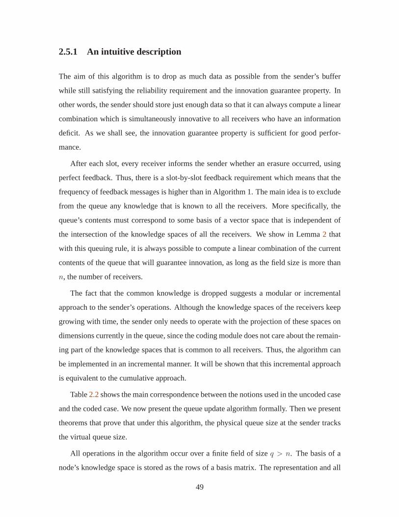
2.5.1 An intuitive description

The aim of this algorithm is to drop as much data as possible from the sender’s buffer

while still satisfying the reliability requirement and theinnovation guarantee property. In

other words, the sender should store just enough data so thatit can always compute a linear

combination which is simultaneously innovative to all receivers who have an information

deficit. As we shall see, the innovation guarantee property is sufficient for good perfor-

mance.

After each slot, every receiver informs the sender whether an erasure occurred, using

perfect feedback. Thus, there is a slot-by-slot feedback requirement which means that the

frequency of feedback messages is higher than in Algorithm 1. The main idea is to exclude

from the queue any knowledge that is known to all the receivers. More specifically, the

queue’s contents must correspond to some basis of a vector space that is independent of

the intersection of the knowledge spaces of all the receivers. We show in Lemma2 that

with this queuing rule, it is always possible to compute a linear combination of the current

contents of the queue that will guarantee innovation, as long as the field size is more than

n, the number of receivers.

The fact that the common knowledge is dropped suggests a modular or incremental

approach to the sender’s operations. Although the knowledge spaces of the receivers keep

growing with time, the sender only needs to operate with the projection of these spaces on

dimensions currently in the queue, since the coding module does not care about the remain-

ing part of the knowledge spaces that is common to all receivers. Thus, the algorithm can

be implemented in an incremental manner. It will be shown that this incremental approach

is equivalent to the cumulative approach.

Table2.2shows the main correspondence between the notions used in the uncoded case

and the coded case. We now present the queue update algorithmformally. Then we present

theorems that prove that under this algorithm, the physicalqueue size at the sender tracks

the virtual queue size.

All operations in the algorithm occur over a finite field of size q > n. The basis of a

node’s knowledge space is stored as the rows of a basis matrix. The representation and all

49

Uncoded Networks Coded NetworksKnowledgerepresentedby

Set of received packets Vector space spanned by the coeffi-cient vectors of the received linearcombinations

Amount ofknowledge

Number of packets received Number of linearly independent(innovative) linear combinations ofpackets received (i.e., dimension ofthe knowledge space)

Queue stores All undelivered packets Linear combination of packets whichform a basis for thecoset spaceof thecommon knowledge at all receivers

Update ruleafter eachtransmission

If a packet has been receivedby all receivers drop it.

Recompute the common knowledgespaceV∆; Store a new set of linearcombinations so that their span is in-dependent ofV∆

Table 2.2: The uncoded vs. coded case

operations are in terms of local coefficient vectors (i.e., with respect to the current contents

of the queue) and not global ones (i.e., with respect to the original packets).

2.5.2 Formal description of the algorithm

Algorithm 2 (a)

1. Initialize basis matricesB, B1, . . . , Bn to the empty matrix. These contain the bases

of the incremental knowledge spaces of the sender and receivers in that order.

2. Initialize the vectorg to the zero vector. This will hold the coefficients of the trans-

mitted packet in each slot.

In every time slot, do:

3. Incorporate new arrivals:

Let a be the number of new packets that arrived at the beginning of the slot. Place

these packets at the end of the queue. LetB haveb rows. SetB to Ia+b. (Im denotes

the identity matrix of sizem.) Note thatB will always be an identity matrix. To

make the number of columns of all matrices consistent (i.e., equal toa + b), append

a all-zero columns to eachBj.

50

4. Transmission:

If B is not empty, updateg to be any vector that is inspan(B), but not in∪j:Bj(Bspan(Bj).

(Note: span(B) denotes the row space ofB.)

Lemma2 shows that such ag exists. Lety1,y2, . . .yQ represent the current contents

of the queue, where the queue sizeQ = (a + b). Compute the linear combination∑Q

i=1 giyi and transmit it on the packet erasure broadcast channel. IfB is empty, set

g to 0 and transmit nothing.

5. Incorporate feedback:

Once the feedback arrives, for every receiverj = 1 to n, do:

If g 6= 0 and the transmission was successfully received by receiverj in this

slot, appendg as a new row toBj.

6. Separate out the knowledge that is common to all receivers:

Compute the following (the set notation used here considers the matrices as a set of

row vectors):

B∆ := Any basis of∩nj=1span(Bj).

B′ := Completion ofB∆ into a basis ofspan(B).

B′′ := B′\B∆.

B′j := Completion ofB∆ into a basis ofspan(Bj) in such a way that, if we

defineB′′j := B′

j\B∆, then the following holds:B′′j ⊆ span(B′′).

Lemma1 proves that this is possible.

7. Update the queue contents:

Replace the contents of the queue with packetsy′1,y

′2, . . .y

′Q′ of the form

∑Q

i=1 hiyi

for eachh ∈ B′′. The new queue sizeQ′ is thus equal to the number of rows inB′′.

8. Recompute local coefficient vectors with respect to the new queue contents:

Find a matrixCj such thatB′′j = XjB

′′ (this is possible becauseB′′j ⊆ span(B′′)).

Call Xj the newBj. Update the value ofB to IQ′.

51

9. Go back to step 3 for the next slot.

The above algorithm essentially removes, at the end of each slot, the common knowl-

edge (represented by the basisB∆) and retains only the remainder,B′′. The knowledge

spaces of the receivers are also represented in an incremental manner in the form ofB′′j ,

excluding the common knowledge. SinceB′′j ⊆ span(B′′), theB′′

j vectors can be com-

pletely described in terms of the vectors inB′′. It is as ifB∆ has been completely removed

from the entire setting, and the only goal remaining is to conveyspan(B′′) to the receivers.

Hence, it is sufficient to store linear combinations corresponding toB′′ in the queue.B′′

andB′′j get mapped to the newB andBj, and the process repeats in the next slot.

Lemma 1. In step 5 of the algorithm above, it is possible to completeB∆ into a basisB′j

of eachspan(Bj) such thatB′′j ⊆ span(B′′).

Proof. We show that any completion ofB∆ into a basis ofspan(Bj) can be changed to a

basis with the required property.

Let B∆ = b1,b2, . . . ,bm. Suppose we complete this into a basisCj of span(Bj)

such that:

Cj = B∆ ∪ c1, c2, . . . , c|Bj|−m.

Now, we claim that at the beginning of step 6,span(Bj) ⊆ span(B) for all j. This can

be proved by induction on the slot number, using the way the algorithm updatesB and the

Bj ’s. Intuitively, any receiver knows a subset of what the sender knows.

Therefore, for each vectorc ∈ Cj\B∆, c must also be inspan(B). Now, sinceB∆∪B′′

is a basis ofspan(B), we can writec as∑m

i=1 αibi+c′ with c′ ∈ span(B′′). In this manner,

eachci gives a distinctc′i. It is easily seen thatC ′j := B∆ ∪ c′1, c

′2, . . . , c

′|Bj|−m is also

a basis of the same space that is spanned byCj. Moreover, it satisfies the property that

C ′j\B∆ ⊆ span(B′′).

Lemma 2. Let V be a vector space with dimensionk over a field of sizeq, and let

V1,V2, . . .Vn, be subspaces ofV, of dimensionsk1, k2, . . . , kn respectively. Suppose that

k > ki for all i = 1, 2, . . . , n. Then, there exists a vector that is inV but is not in any of the

Vi’s, if q > n.

52

Proof. The total number of vectors inV is qn. The number of vectors inVi is qni. Hence,

the number of vectors in∪ki=1Vi is at most

∑k

i=1 qni. Now,

∑k

i=1 qni ≤ kqnmax ≤ kqn−1 < qn

where,nmax is maxi ni, which is at most(n − 1). Thus,V has more vectors than∪ki=1Vi.

This completes the proof.

This lemma is also closely related to the result in [48], which derives the smallest field

size needed to ensure innovation guarantee.

2.5.3 Connecting the physical and virtual queue sizes

In this subsection, we will prove the following result that relates the size of the physical

queue at the sender and the virtual queues, which themselvescorrespond to the backlog in

degrees of freedom.

Theorem 2. For Algorithm 2 (a), the physical queue size at the sender is upper bounded

by the sum of the backlog differences between the sender and each receiver in terms of the

number of degrees of freedom.

Let a(t) denote the number of arrivals in slott, and letA(t) be the total number of

arrivals up to and including slott, i.e., A(t) =∑t

t′=0 a(t′). Let B(t) (resp.Bj(t)) be the

matrixB (resp.Bj) after incorporating the slott arrivals,i.e., at the end of step 3 in slott.

Let H(t) be a matrix whose rows are theglobal coefficient vectors of the queue contents

at the end of step 3 in time slott, i.e., the coefficient vectors in terms of the original packet

stream. Note that each row ofH(t) is in FA(t)q .

Let g(t) denote the vectorg at the calculated in step 4 in time slott, i.e., the local

coefficient vector of the packet transmitted in slott. Also, letB∆(t) (resp. B′′(t), B′j(t)

andB′′j (t)) denote the matrixB∆ (resp.B′′, B′

j andB′′j ) at the end of step 6 in time slott.

Lemma 3. The rows ofH(t) are linearly independent for allt.

53

Proof. The proof is by induction ont.

Basis step:In the beginning of time slot 1,a(1) packets arrive. So,H(1) = Ia(1) and

hence the rows are linearly independent.

Induction hypothesis:AssumeH(t − 1) has linearly independent rows.

Induction step:The queue is updated such that the linear combinations corresponding

to local coefficient vectors inB′′ are stored, and subsequently, thea(t) new arrivals are

appended. Thus, the relation betweenH(t − 1) andH(t) is:

H(t) =

B′′(t − 1)H(t − 1) 0

0 Ia(t)

.

Now,B′′(t−1) has linearly independent rows, since the rows form a basis. The rows of

H(t−1) are also linearly independent by hypothesis. Hence, the rows ofB′′(t−1)H(t−1)

will also be linearly independent. Appendinga(t) zeros and then adding an identity matrix

block in the right bottom corner does not affect the linear independence. Hence,H(t) also

has linearly independent rows.

Define the following:

U(t) , Row span ofH(t)

Uj(t) , Row span ofBj(t)H(t)

U ′j(t) , Row span ofB′

j(t)H(t)

U ′∆(t) , ∩n

j=1U′j(t)

U ′′(t) , Row span ofB′′(t)H(t)

U ′′j (t) , Row span ofB′′

j (t)H(t).

All the vector spaces defined above are subspaces ofFA(t)q . Figure2-3shows the points

at which these subspaces are defined in the slot.

The fact thatH(t) has full row rank (proved above in Lemma3) implies that the op-

erations performed by the algorithm in the domain of the local coefficient vectors can be

mapped to the corresponding operations in the domain of the global coefficient vectors:

1. The intersection subspaceU ′∆(t) is indeed the row span ofB∆(t)H(t).

54

STEP 3

Incorporate arrivals

of slot t

STEP 5

Incorporate channel

state feedback

STEP 6

Separate out

common

knowledge

)(),( tVtU

)(),( tV tU

)(),( t'V t'U jj

)(),( t''U t''U j

)(),( t'V t'U∆∆

Slot tSlot (t-1)

)(),( tVtU j j)(),( t''U t''U j

Figure 2-3: The main steps of the algorithm, along with the times at which the variousU(t)’s are defined

2. LetRj(t) be an indicator (0-1) random variable which takes the value 1if and only

if the transmission in slott is successfully received without erasure by receiverj

and in addition, receiverj does not have all the information that the sender has. Let

gj(t) := Rj(t)g(t)H(t). Then,

U ′j(t) = Uj(t) ⊕ span(gj(t)) (2.4)

where⊕ denotes direct sum of vector spaces. The way the algorithm choosesg(t)

guarantees that ifRj(t) is non-zero, thengj(t) will be outside the corresponding

Uj(t), i.e., it will be innovative. This fact is emphasized by the directsum in this

equation.

3. Because of the way the algorithm performs the completion ofthe bases in the local

domain in step 6, the following properties hold in the globaldomain:

U(t) = U ′∆(t) ⊕ U ′′(t) (2.5)

U ′j(t) = U ′

∆(t) ⊕ U ′′j (t) and, (2.6)

U ′′j (t) ⊆ U ′′(t), ∀j = 1, 2, . . . , n. (2.7)

From the above properties, we can infer thatU ′′1 (t) + U ′′

2 (t) + . . . U ′′n(t) ⊆ U ′′(t). After

55

incorporating the arrivals in slott + 1, this givesU1(t + 1) + U2(t + 1) + . . . Un(t + 1) ⊆

U(t + 1). Since this is true for allt, we write it as:

U1(t) + U2(t) + . . . Un(t) ⊆ U(t). (2.8)

Now, in order to relate the queue size to the backlog in numberof degrees of freedom,

we define the following vector spaces which represent thecumulativeknowledge of the

sender and receivers (See Figure2-3 for the timing):

V (t) , Sender’s knowledge space after incorporating the arrivals(at the end of

step 3) in slott. This is simply equal toFA(t)q

Vj(t) , Receiverj’s knowledge space at the end of step 3 in slott

V ′j (t) , Receiverj’s knowledge space in slott, after incorporating the channel

state feedback intoVj(t), i.e., V ′j (t) = Vj(t) ⊕ span(gj(t)).

V∆(t) , ∩nj=1Vj(t)

V ′∆(t) , ∩n

j=1V′j (t).

For completeness, we now prove the following facts about direct sums of vector spaces

that we shall use.

Lemma 4. LetV be a vector space and letV∆, U1, U2, . . . Un be subspaces ofV such that,

V∆ is independent of the span of all theUj ’s, i.e., dim[V∆ ∩ (U1 + U2 + . . . + Un)] = 0.

Then,

V∆ ⊕ [∩ni=1Ui] = ∩n

i=1 [V∆ ⊕ Ui] .

Proof. For anyz ∈ V∆ ⊕ ∩ni=1Ui, there is ax ∈ V∆ andy ∈ ∩n

i=1Ui such thatz = x + y.

Now, for eachi, y ∈ Ui. Thus,z = x + y implies thatz ∈ ∩ni=1[V∆ ⊕ Ui]. Therefore,

V∆ ⊕ ∩ni=1Ui ⊆ ∩n

i=1[V∆ ⊕ Ui].

Now, letw ∈ ∩ni=1V∆ ⊕ Ui. Then for eachi, there is axi ∈ V∆ andyi ∈ Ui such that

w = xi +yi. But,w = xi +yi = xj +yj means thatxi−xj = yi−yj. Now, (xi−xj) ∈ V∆

and(yi − yj) ∈ (U1 + U2 + . . . + Un). By hypothesis, these two vector spaces have only

0 in common. Thus,xi − xj = yi − yj = 0. All the xi’s are equal to a commonx ∈ V∆

and all theyi’s are equal to a commony which belongs to all theUi’s. This means,w

56

can be written as the sum of a vector inV∆ and a vector in∩ni=1Ui, thereby proving that

∩ni=1[V∆ ⊕ Ui] ⊆ V∆ ⊕ ∩n

i=1Ui.

Lemma 5. LetA,B, andC be three vector spaces such thatB is independent ofC andA

is independent ofB ⊕ C. Then the following hold:

1. A is independent ofB.

2. A ⊕ B is independent ofC.

3. A ⊕ (B ⊕ C) = (A ⊕ B) ⊕ C.

Proof. Statement1 follows from the fact thatB is a subset ofB⊕C. Hence, ifA∩(B⊕C)

is empty, so isA ∩ B.

For statement2, we need to show that(A ⊕ B) ∩ C = 0. Consider any element

x ∈ (A ⊕ B) ∩ C. Since it is inA ⊕ B, there exist uniquea ∈ A andb ∈ B such that

x = a + b. Now, sinceb ∈ B andx ∈ C, it follows thata = x − c is in B ⊕ C. It is

also inA. SinceA is independent ofB ⊕ C, a must be0. Hence,x = b. But this means

x ∈ B. Since it is also inC, it must be0, asB andC are independent. This shows that the

only element in(A ⊕ B) ⊕ C is 0.

Statement3 can be proved as follows.

x ∈ A ⊕ (B ⊕ C)

⇔∃ uniquea ∈ A,d ∈ B ⊕ C s.t.x = a + d

⇔∃ uniquea ∈ A,b ∈ B, c ∈ C s.t.x = a + b + c

⇔∃ uniquee ∈ A ⊕ B, c ∈ C s.t.x = e + c

⇔x ∈ (A ⊕ B) ⊕ C

57

Theorem 3. For all t ≥ 0,

V (t) = V∆(t) ⊕ U(t)

Vj(t) = V∆(t) ⊕ Uj(t) ∀j = 1, 2, . . . n

V ′∆(t) = V∆(t) ⊕ U ′

∆(t).

Proof. The proof is by induction ont.

Basis step:

At t = 0, V (0), U(0) as well as all theVj(0)’s andUj(0)’s are initialized to0. Con-

sequently,V∆(0) is also0. It is easily seen that these initial values satisfy the equations

in the theorem statement.

Induction Hypothesis:

We assume the equations hold att, i.e.,

V (t) = V∆(t) ⊕ U(t) (2.9)

Vj(t) = V∆(t) ⊕ Uj(t),∀j = 1, 2, . . . n (2.10)

V ′∆(t) = V∆(t) ⊕ U ′

∆(t) (2.11)

Induction Step:We now prove that they hold in slot(t + 1). We have:

V (t) = V∆(t) ⊕ U(t) (from (2.9))

= V∆(t) ⊕ [U ′∆(t) ⊕ U ′′(t)] (from (2.5))

= [V∆(t) ⊕ U ′∆(t)] ⊕ U ′′(t) (Lemma5)

= V ′∆(t) ⊕ U ′′(t) (from (2.11)).

Thus, we have proved:

V (t) = V ′∆(t) ⊕ U ′′(t). (2.12)

Now, we incorporate the arrivals in slot(t+1). This convertsV ′∆(t) to V∆(t+1), U ′′(t)

58

to U(t + 1), andV (t) to V (t + 1), owing to the following operations:

Basis ofV∆(t + 1) =[

Basis ofV ′∆(t) 0

]

Basis ofU(t + 1) =

Basis ofU ′′(t) 0

0 Ia(t+1)

Basis ofV (t + 1) =

Basis ofV (t) 0

0 Ia(t+1)

.

Incorporating these modifications into (2.12), we obtain:

V (t + 1) = V∆(t + 1) ⊕ U(t + 1).

Now, consider each receiverj = 1, 2, . . . n.

V ′j (t)

= Vj(t) ⊕ span(gj(t))

= [V∆(t) ⊕ Uj(t)] ⊕ span(gj(t)) (from (2.10))

= V∆(t) ⊕ [Uj(t) ⊕ span(gj(t))] (Lemma5)

= V∆(t) ⊕ U ′j(t) (from (2.4))

= V∆(t) ⊕ [U ′∆(t) ⊕ U ′′

j (t)] (from (2.6))

= [V∆(t) ⊕ U ′∆(t)] ⊕ U ′′

j (t) (Lemma5)

= V ′∆(t) ⊕ U ′′

j (t) (from (2.11)).

Incorporating the new arrivals into the subspaces involvesaddinga(t + 1) all-zero

columns to the bases ofV ′j (t), V ′

∆(t), andU ′′j (t), thereby converting them into bases of

Vj(t + 1), V∆(t + 1), andUj(t + 1) respectively. These changes do not affect the above

relation, and we get:

Vj(t + 1) = V∆(t + 1) ⊕ Uj(t + 1), ∀j = 1, 2, . . . n.

59

Finally,

V ′∆(t + 1)

= ∩nj=1V

′j (t + 1)

= ∩nj=1[Vj(t + 1) ⊕ span(gj(t + 1))]

= ∩nj=1[V∆(t + 1) ⊕ Uj(t + 1) ⊕ span(gj(t + 1))]

(a)= V∆(t + 1) ⊕ ∩n

j=1[Uj(t + 1) ⊕ span(gj(t + 1))]

= V∆(t + 1) ⊕ U ′∆(t + 1).

Step(a) is justified as follows. Using equation (2.8) and the fact thatgj(t + 1) was chosen

to be insideU(t+1), we can show that the span of all the[Uj(t+1)⊕ span(gj(t+1))]’s is

insideU(t+1). Now, from the induction step above,V∆(t+1) is independent ofU(t+1).

Therefore,V∆(t + 1) is independent of the span of all the[Uj(t + 1) ⊕ span(gj(t + 1))]’s.

We can therefore apply Lemma4.

Theorem 4. Let Q(t) denote the size of the queue after the arrivals in slott have been

appended to the queue.

Q(t) = dim V (t) − dim V∆(t).

Proof. Q(t) = dim U(t) = dim U ′′(t − 1) + a(t)

= dim U(t − 1) − dim U ′∆(t − 1) + a(t)

(using (2.5))

= dim V (t − 1) − dim V∆(t − 1) − dim U ′∆(t) + a(t)

(from Theorem3)

= dim V (t − 1) − dim V ′∆(t) + a(t)

(from Theorem3)

= dim V (t) − dim V∆(t).

60

Lemma 6. LetV1, V2, . . . , Vk be subspaces of a vector spaceV . Then, fork ≥ 1,

dim(V1 ∩ V2 ∩ . . . ∩ Vk) ≥k

∑

i=1

dim(Vi) − (k − 1)dim(V ).

Proof. For any two subspacesX andY of V ,

dim(X ∩ Y ) + dim(X + Y ) = dim(X) + dim(Y )

whereX + Y denotes the span of subspacesX andY .

Hence,

dim(X ∩ Y ) = dim(X) + dim(Y ) − dim(X + Y )

≥ dim(X) + dim(Y ) − dim(V ) (2.13)

(sinceX + Y is also a subspace ofV ).

Now, we prove the lemma by induction onk.

Basis step:

k = 1 : LHS = dim(V1), RHS =dim(V1)

k = 2 : LHS = dim(V1 ∩ V2), RHS =dim(V1) + dim(V2) − dim(V ).

The claim follows from inequality (2.13).

Induction Hypothesis:

For some arbitraryk,

dim(∩k−1i=1 Vi) ≥

k−1∑

i=1

dim(Vi) − (k − 2)dim(V ).

Induction Step:

61

dim(∩ki=1Vi) = dim(Vk ∩ ∩k−1

i=1 Vi)

≥ dim(Vk) + dim(∩k−1i=1 Vi) − dim(V ) (using (2.13))

≥ dim(Vk) +

[

k−1∑

i=1

dim(Vi) − (k − 2)dim(V )

]

−dim(V )

=k

∑

i=1

dim(Vi) − (k − 1)dim(V ).

The above result can be rewritten as:

dim(V ) − dim(V1 ∩ V2 ∩ . . . Vk) ≤k

∑

i=1

[dim(V ) − dim(Vi)]. (2.14)

Using this result, we can now prove Theorem2.

Proof of Theorem2: If we apply Lemma6 to the vector spacesVj(t), j = 1, 2, . . . , n

andV (t), then the left hand side of inequality (2.14) becomes the sender queue size (using

Theorem4), while the right hand side becomes the sum of the differences in backlog be-

tween the sender and the receivers, in terms of the number of degrees of freedom. Thus,

we have proved Theorem2.

2.6 Algorithm 2 (b): Drop when seen

The drop-when-seen algorithm can be viewed as a specializedvariant of the generic Al-

gorithm 2 (a) given above. It uses the notion of seen packets (defined in Section2.1) to

represent the bases of the knowledge spaces. This leads to a simple and easy-to-implement

version of the algorithm which, besides ensuring that physical queue size tracks virtual

queue size, also provides some practical benefits. For instance, the sender need not store

linear combinations of packets in the queue like in Algorithm 2 (a). Instead only origi-

nal packets need to be stored, and the queue can be operated ina simple first-in-first-out

manner. We now present some mathematical preliminaries before describing the algorithm.

62

2.6.1 Some preliminaries

The newly proposed algorithm uses the notion of reduced row echelon form (RREF) of a

matrix to represent the knowledge of a receiver. Hence, we first recapitulate the definition

and some properties of the RREF from [40], and present the connection between the RREF

and the notion of seeing packets.

Definition 8 (Reduced row echelon form (RREF)). A matrix is said to be in reduced row

echelon form if it satisfies the following conditions:

1. The first nonzero entry of every row is 1.

2. The first nonzero entry of any row is to the right of the first nonzero entry of the

previous row.

3. The entries above the first nonzero row of any row are all zero.

The RREF leads to a standard way to represent a vector space. Given a vector space,

consider the following operation – arrange the basis vectors in any basis of the space as

the rows of a matrix, and perform Gaussian elimination. Thisprocess essentially involves

a sequence of elementary row transformations and it produces a unique matrix in RREF

such that its row space is the given vector space. We call thisthe RREF basis matrix of the

space. We will use this representation for the knowledge space of the receivers.

Let V be the knowledge space of some receiver. Supposem packets have arrived at

the sender so far. Then the receiver’s knowledge consists oflinear combinations of some

collection of thesem packets,i.e., V is a subspace ofFmq . Using the procedure outlined

above, we can compute thedim(V ) × m RREF basis matrix ofV overFq.

In the RREF basis, the first nonzero entry of any row is called apivot. Any column

with a pivot is called apivot column. By definition, each pivot occurs in a different column.

Hence, the number of pivot columns equals the number of nonzero rows, which isdim[V ].

Let pk denote the packet with indexk. The columns are ordered so that columnk maps

to packetpk. The following theorem connects the notion of seeing packets to the RREF

basis.

63

Theorem 5. A node has seen a packet with indexk if and only if thekth column of the

RREF basisB of the knowledge spaceV of the node is a pivot column.

Proof. The ‘if’ part is clear. If columnk of B is a pivot column, then the corresponding

pivot row corresponds to a linear combination known to the node, of the formpk+q, where

q involves only packets with index more thank. Thus, the node has seenpk.

For the ‘only if’ part, suppose columnk of B does not contain a pivot. Then, in any

linear combination of the rows, rows with pivot after columnk cannot contribute anything

to columnk. Rows with pivot before columnk will result in a non-zero term in some

column to the left ofk. Since every vector inV is a linear combination of the rows ofB,

the first non-zero term of any vector inV cannot be in columnk. Thus,pk could not have

been seen.

Since the number of pivot columns is equal to the dimension ofthe vector space, we

obtain the following corollary.

Corollary 1. The number of packets seen by a receiver is equal to the dimension of its

knowledge space.

The next corollary introduces a useful concept.

Corollary 2. If receiverj has seen packetpk, then it knows exactly one linear combination

of the formpk + q such thatq involves onlyunseenpackets with index more thank.

Proof. We use the same notation as above. The receiver has seenpk. Hence, columnk in

B is a pivot column. By definition of RREF, in the row containing thepivot in columnk,

the pivot value is 1 and subsequent nonzero terms occur only in non-pivot columns. Thus,

the corresponding linear combination has the given formpk + q, whereq involves only

unseenpackets with index more thank.

We now prove uniqueness by contradiction. Suppose the receiver knows another such

linear combinationpk + q′ whereq′ also involves only unseen packets. Then, the receiver

must also know(q − q′). But this means the receiver has seen some packet involved in

eitherq or q′ – a contradiction.

64

1 0

1 0

1 - - - - - - -

1 - - - - - - -

1 - - - - - - -

p1 p2 p3 p4 p5 p6 p7 p8

Decoded

Seen Unseen

Basis of knowledge

space in RREF

Witness for p4

Number of seen packets = Rank of matrix = Dim of knowledge space

Figure 2-4: Seen packets and witnesses in terms of the basis matrix

Definition 9 (Witness). We denote the unique linear combination guaranteed by Corollary

2 asWj(pk), thewitness for receiverj seeingpk.

Figure2-4 explains the notion of a seen packet and the notion of a witness in terms of

the basis matrix.

Example:Suppose a node knows the following linear combinations:x = (p1 + p2)

andy = (p1 + p3). Since these are linearly independent, the knowledge spacehas a

dimension of 2. Hence, the number of seen packets must be 2. Itis clear that packetp1 has

been seen, sincex satisfies the requirement of Definition2. Now, the node can compute

z , x − y = (p2 − p3). Thus, it has also seenp2. That meansp3 is unseen. Hence,y is

the witness forp1, andz is the witness forp2.

2.6.2 The main idea

The central idea of the algorithm is to keep track of seen packets instead of decoded packets.

The two main parts of the algorithm are the coding and queue update modules.

In Section2.6.5, we present the formal description of our coding module. Thecoding

module computes a linear combinationg that will cause any receiver that receives it, to

see its next unseen packet. First, for each receiver, the sender computes its knowledge

space using the feedback and picks out its next unseen packet. Only these packets will be

involved ing, and hence we call them thetransmit set. Now, we need to select coefficients

for each packet in this set. Clearly, the receiver(s) waitingto see the oldest packet in the

65

transmit set (sayp1) will be able to see it as long as its coefficient is not zero. Consider a

receiver that is waiting to see the second oldest packet in the transmit set (sayp2). Since

the receiver has already seenp1, it can subtract the witness forp1, thereby canceling it

from g. The coefficient ofp2 must be picked such that after subtracting the witness for

p1, the remaining coefficient ofp2 in g is non-zero. The same idea extends to the other

coefficients. The receiver can cancel packets involved ing that it has already seen by

subtracting suitable multiples of the corresponding witnesses. Therefore, the coefficients

for g should be picked such that for each receiver, after canceling the seen packets, the

remaining coefficient of the next unseen packet is non-zero.Then, the receiver will be

able to see its next unseen packet. Theorem8 proves that this is possible if the field size

is at leastn, the number of receivers. With two receivers, the coding module is a simple

XOR based scheme (see Table2.1). Our coding scheme meets the innovation guarantee

requirement because Theorem5 implies that a linear combination that would cause a new

packet to be seen brings in a previously unknown degree of freedom.

The fact that the coding module uses only the next unseen packet of all receivers readily

implies the following queue update rule.Drop a packet if all receivers have seen it.This

simple rule ensures that the physical queue size tracks the virtual queue size.

Remark 2. In independent work, [48] proposes a coding algorithm which uses the idea of

selecting those packets for coding, whose indices are one more than each receiver’s rank.

This corresponds to choosing the next unseen packets in the special case where packets are

seen in order. Moreover, this algorithm picks coding coefficients in a deterministic manner,

just like our coding module. Therefore, our module is closely related to the algorithm of

[48].

However, our algorithm is based on the framework of seen packets. This allows several

benefits. First, it immediately leads to the drop-when-seen queue management algorithm,

as described above. In contrast, [48] does not consider queuing aspects of the problem.

Second, in this form, our algorithm readily generalizes to the case where the coding coeffi-

cients are picked randomly. The issue with random coding is that packets may be seen out

of order. Our algorithm will guarantee innovation even in this case (provided the field is

large), by selecting a random linear combination of the nextunseen packets of the receivers

66

(the reasoning is similar to the arguments in [12]). However, the algorithm of [48] may

not work well here, as it may pick packets that have already beenseen, which could cause

non-innovative transmissions.

The compatibility of our algorithm with random coding makes it particularly useful

from an implementation perspective. With random coding, each receiver only needs to

inform the sender the set of packets it has seen. There is no need to convey the exact

knowledge space. This can be done simply by generating a TCP-like cumulative ACK upon

seeing a packet. Thus, the ACK format is the same as in traditional ARQ-based schemes.

Only its interpretation is different.

We next present the formal description and analysis of the queue update algorithm.

2.6.3 The queuing module

The algorithm works with the RREF bases of the receivers’ knowledge spaces. The co-

efficient vectors are with respect to the current queue contents and not the original packet

stream.

Algorithm 2 (b)

1. Initialize matricesB1, B2, . . . , Bn to the empty matrix. These matrices will hold the

bases of the incremental knowledge spaces of the receivers.

2. Incorporate new arrivals:Suppose there area new arrivals. Add the new packets to

the end of the queue. Appenda all-zero columns on the right to eachBj for the new

packets.

3. Transmission: If the queue is empty, do nothing; else computeg using the coding

module and transmit it.

4. Incorporate channel state feedback:

For every receiverj = 1 to n, do:

If receiverj received the transmission, include the coefficient vector of g in terms of

the current queue contents, as a new row inBj. Perform Gaussian elimination.

67

5. Separate out packets that all receivers have seen:

Update the following sets and bases:

S ′j := Set of packets corresponding to the pivot columns ofBj

S ′∆ := ∩n

j=1S′j

New Bj := Sub-matrix of currentBj obtained by excluding columns inS ′∆ and cor-

responding pivot rows.

6. Update the queue:Drop the packets inS ′∆.

7. Go back to step 2 for the next slot.

2.6.4 Connecting the physical and virtual queue sizes

The following theorem describes the heavy traffic asymptotic behavior of the expected

physical queue size under our new queuing rule.

Theorem 6. For Algorithm 2 (b), the physical queue size at the sender is upper-bounded by

the sum of the virtual queue sizes,i.e., the sum of the degrees-of-freedom backlog between

the sender and the receivers. Hence, the expected size of thephysical queue in steady state

for Algorithm 2 (b) isO(

11−ρ

)

.

In the rest of this section, we shall prove the above result. Now, in order to relate the

queue size to the backlog in number of degrees of freedom, we shall need the following

notation:

S(t) , Set of packets arrived at sender till the end of slott

V (t) , Sender’s knowledge space after incorporating the arrivalsin slot t. This is simply

equal toF|S(t)|q

Vj(t) , Receiverj’s knowledge space at the end of slott. It is a subspace ofV (t).

Sj(t) , Set of packets receiverj has seen till end of slott.

68

We shall now formally argue that Algorithm 2 (b) indeed implements the drop-when-

seen rule in spite of the incremental implementation. In anyslot, the columns ofBj are

updated as follows. When new packets are appended to the queue, new columns are added

to Bj on the right. When packets are dropped from the queue, corresponding columns

are dropped fromBj. There is no rearrangement of columns at any point. This implies

that a one-to-one correspondence is always maintained between the columns ofBj and

the packets currently in the queue. LetUj(t) be the row space ofBj at time t. Thus,

if (u1, u2, . . . , uQ(t)) is any vector inUj(t), it corresponds to a linear combination of the

form∑Q(t)

i=1 uipi, wherepi is theith packet in the queue at timet. The following theorem

connects the incremental knowledge spaceUj(t) to the cumulative knowledge spaceVj(t).

Theorem 7. In Algorithm 2 (b), for each receiverj, at the end of slott, for anyu ∈ Uj(t),

the linear combination∑Q(t)

i=1 uipi is known to the receiverj, wherepi denotes theith

packet in the queue at timet.

Proof. We shall use induction ont. For t = 0, the system is completely empty and the

statement is vacuously true. Let us now assume that the statement is true at time(t − 1).

Consider the operations in slott. A new row is added toBj only if the corresponding

linear combination has been successfully received by receiver j. Hence, the statement is

still true. Row operations involved in Gaussian eliminationdo not alter the row space.

Finally, when some of the pivot columns are dropped along with the corresponding pivot

rows in step 5, this does not affect the linear combinations to which the remaining rows

correspond because the pivot columns have a 0 in all rows except the pivot row. Hence, the

three operations that are performed between slot(t−1) and slott do not affect the property

that the vectors in the row space ofBj correspond to linear combinations that are known at

receiverj. This proves the theorem.

If a packet corresponds to a pivot column inBj, the corresponding pivot row is a linear

combination of the packet in question with packets that arrived after it. From the above

theorem, receiverj knows this linear combination which means it has seen the packet.

This leads to the following corollary.

69

Corollary 3. If a packet corresponds to a pivot column inBj, then it has been seen by

receiverj.

Thus, in step 5,S ′∆(t) consists of those packets in the queue that all receivers have seen

by the end of slott. In other words, the algorithm retains only those packets that have

not yet been seen by all receivers. Even though the algorithmworks with an incremental

version of the knowledge spaces, namelyUj(t), it maintains the queue in the same way

as if it was working with the cumulative versionVj(t). Thus, the incremental approach is

equivalent to the cumulative approach.

We require the following lemma to prove the main theorem.

Lemma 7. LetA1, A2, . . . , Ak be subsets of a setA. Then, fork ≥ 1,

|A| − | ∩ki=1 Ai| ≤

k∑

i=1

(|A| − |Ai|). (2.15)

Proof.

|A| − | ∩ki=1 Ai|

= |A ∩ (∩ki=1Ai)

c| (since theAi’s are subsets ofA)

= |A ∩ (∪ki=1A

ci)| (by De Morgan’s law)

= | ∪ki=1 (A ∩ Ac

i)| (distributivity)

≤k

∑

i=1

|A ∩ Aci | (union bound)

=k

∑

i=1

(|A| − |Ai|).

Now, we are ready to prove Theorem6.

Proof of Theorem6: Since the only packets in the queue at any point are those thatnot

all receivers have seen, we obtain the following expressionfor the physical queue size at

70

the sender at the end of slott:

Q(t) = |S(t)| − | ∩nj=1 Sj(t)|.

If we apply Lemma7 to the setsS(t) andSj(t), j = 1, 2, . . . , n then the left hand

side of inequality (2.15) becomes the sender queue sizeQ(t) given above. Now,|Sj(t)| =

dim[Vj(t)], using Corollary1. Hence the right hand side of inequality (2.15) can be rewrit-

ten as∑n

j=1

[

dim[V (t)] − dim[Vj(t)]]

, which is the sum of the virtual queue sizes.

Finally, we can find the asymptotic behavior of the physical queue size in steady state

under Algorithm 2 (b). Since the expected virtual queue sizes themselves are allO(

11−ρ

)

from Equation (2.2), we obtain the stated result.

2.6.5 The coding module

We now present a coding module that is compatible with the drop-when-seen queuing

algorithm in the sense that it always forms a linear combination using packets that are

currently in the queue maintained by the queuing module. In addition, we show that the

coding module satisfies the innovation guarantee property.

Let u1, u2, . . . , um be the set of indices of the next unseen packets of the receivers,

sorted in ascending order (in general,m ≤ n, since the next unseen packet may be the same

for some receivers). Exclude receivers whose next unseen packets have not yet arrived at

the sender. LetR(ui) be the set of receivers whose next unseen packet ispui. We now

present the coding module to select the linear combination for transmission.

1. Loop over next unseen packets

For j = 1 to m, do:

All receivers inR(uj) have seen packetspuifor i < j. Now, ∀r ∈ R(uj), find

yr :=∑j−1

i=1 αiWr(pui), whereWr(pui

) is the witness for receiverr’s seeingpui.

Pick αj ∈ Fq such thatαj is different from the coefficient ofpujin yr for each

r ∈ R(uj).

2. Compute the transmit packet:g :=∑m

i=1 αipui.

71

It is easily seen that this coding module is compatible with the drop-when-seen algo-

rithm. Indeed, it does not use any packet that has been seen byall receivers in the linear

combination. It only uses packets that at least one receiverhas not yet seen. The queue

update module retains precisely such packets in the queue. The next theorem presents a

useful property of the coding module.

Theorem 8. If the field size is at leastn, then the coding module picks a linear combination

that will cause any receiver to see its next unseen packet uponsuccessful reception.

Proof. First we show that a suitable choice always exists forαj that satisfies the require-

ment in step 1. Forr ∈ R(u1), yr = 0. Hence, as long asα1 6= 0, the condition is

satisfied. So, pickα1 = 1. Since at least one receiver is inR(u1), we have that, forj > 1,

|R(uj)| ≤ (n − 1). Even if eachyr for r ∈ R(uj) has a different coefficient forpuj, that

covers only(n − 1) different field elements. Ifq ≥ n, then there is a choice left inFq for

αj.

Now, we have to show that the condition given in step 1 impliesthat the receivers

will be able to see their next unseen packet. Indeed, for allj from 1 to m, and for all

r ∈ R(uj), receiverr knowsyr, since it is a linear combination of witnesses ofr. Hence, if

r successfully receivesg, it can compute(g−yr). Now,g andyr have the same coefficient

for all packets with index less thanuj, and a different coefficient forpuj. Hence,(g − yr)

will involve pujand only packets with index beyonduj. This meansr can seepuj

and this

completes the proof.

Theorem5 implies that seeing an unseen packet corresponds to receiving an unknown

degree of freedom. Thus, Theorem8 essentially says that the innovation guarantee property

is satisfied and hence the scheme is throughput optimal.

This theorem is closely related to the result derived in [48] that computes the mini-

mum field size needed to guarantee innovation. The difference is that our result uses the

framework of seen packets to make a more general statement byspecifying not only that

innovation is guaranteed, but also that packets will be seenin order with this deterministic

coding scheme. This means packets will be dropped in order atthe sender.

72

2.7 Overhead

In this section, we comment on the overhead required for Algorithms 1 and 2 (b). There

are several types of overhead.

2.7.1 Amount of feedback

Our scheme assumes that every receiver feeds back one bit after every slot, indicating

whether an erasure occurred or not. In comparison, the drop-when-decoded scheme re-

quires feedback only when packets get decoded. However, in that case, the feedback may

be more than one bit – the receiver will have to specify the list of all packets that were

decoded, since packets may get decoded in groups. In a practical implementation of the

drop-when-seen algorithm, TCP-like cumulative acknowledgments can be used to inform

the sender which packets have been seen.

2.7.2 Identifying the linear combination

Besides transmitting a linear combination of packets, the sender must also embed infor-

mation that allows the receiver to identify what linear combination has been sent. This

involves specifying which packets have been involved in thecombination, and what coeffi-

cients were used for these packets.

Set of packets involved

The baseline algorithm uses all packets in the queue for the linear combination. The queue

is updated in a first-in-first-out (FIFO) manner,i.e., no packet departs before all earlier

packets have departed. This is a consequence of the fact thatthe receiver signals success-

ful decoding only when the virtual queue becomes empty4. The FIFO rule implies that

specifying the current contents of the queue in terms of the original stream boils down to

specifying the sequence number of the head-of-line packet and the last packet in the queue

in every transmission.

4As mentioned earlier in Remark1, we assume that the sender checks whether any packets have beennewly decoded, only when the virtual queue becomes empty.

73

The drop-when-seen algorithm does not use all packets from the queue, but only at

mostn packets from the queue (the next unseen packet of each receiver). This set can be

specified by listing the sequence number of thesen packets.

Now, in both cases, the sequence number of the original stream cannot be used as it is,

since it grows unboundedly with time. However, we can avoid this problem using the fact

that the queue contents are updated in a FIFO manner (This is also true of our drop-when-

seen scheme – the coding module guarantees that packets willbe seen in order, thereby

implying a FIFO rule for the sender’s queue.). The solution is to express the sequence

number relative to an origin that also advances with time, asfollows. If the sender is

certain that the receiver’s estimate of the sender’s queue starts at a particular point, then

both the sender and receiver can reset their origin to that point, and then count from there.

For the baseline case, the origin can be reset to the current HOL packet, whenever the

receiver sends feedback indicating successful decoding. The idea is that if the receiver

decoded in a particular slot, that means it had a successful reception in that slot. Therefore,

the sender can be certain that the receiver must have received the latest update about the

queue contents and is therefore in sync with the sender. Thus, the sender and receiver can

reset their origin. Note that since the decoding epochs of different receivers may not be

synchronized, the sender will have to maintain a different origin for each receiver and send

a different sequence number to each receiver, relative to that receiver’s origin. This can be

done simply by concatenating the sequence number for each receiver in the header.

To determine how many bits are needed to represent the sequence number, we need

to find out what range of values it can take. In the baseline scheme, the sequence number

range will be proportional to the busy period of the virtual queue, since this determines how

often the origin is reset. Thus, the overhead in bits for eachreceiver will be proportional to

the logarithm of the expected busy period,i.e., O(

log21

1−ρ

)

.

For the drop-when-seen scheme, the origin can be reset whenever the receiver sends

feedback indicating successful reception. Thus, the origin advances a lot more frequently

than in the baseline scheme.

74

Coefficients used

The baseline algorithm uses a random linear coding scheme. Here, potentially all packets

in the queue get combined in a linear combination. So, in the worst case, the sender would

have to send one coefficient for every packet in the queue. If the queue hasm packets,

this would requirem log2 q bits, whereq is the field size. In expectation, this would be

O(

log2 q

(1−ρ)2

)

bits. If the receiver knows the pseudorandom number generator used by the

sender, then it would be sufficient for the sender to send the current state of the generator

and the size of the queue. Using this, the receiver can generate the coefficients used by the

sender in the coding process. The new drop-when-seen algorithm uses a coding module

which combines the next unseen packet of each receiver. Thus, the overhead for the coef-

ficients is at mostn log2 q bits, wheren is the number of receivers. It does not depend on

the load factorρ at all.

2.7.3 Overhead at sender

While Algorithm 2 (b) saves in buffer space, it requires the sender to store the basis matrix

of each receiver, and update them in every slot based on feedback. However, storing a row

of the basis matrix requires much less memory than storing a packet, especially for long

packets. Thus, there is an overall saving in memory. The update of the basis matrix simply

involves one step of the Gaussian elimination algorithm.

2.7.4 Overhead at receiver

The receiver will have to store the coded packets till they are decoded. It will also have

to decode the packets. For this, the receiver can perform a Gaussian elimination after

every successful reception. Thus, the computation for the matrix inversion associated with

decoding can be spread over time.

75

2.8 Conclusions

Comparing Theorem1 and Theorem6, we see that the queue size for the new Algorithm

2 is significantly lower than Algorithm 1, especially at heavy traffic. If the memory at the

sender is shared among many flows, then this reduction in queue size will prove useful in

getting statistical multiplexing benefits. Algorithm 2 allows the physical queue size to track

the virtual queue size. This extends stability and other queuing-theoretic results on virtual

queues to physical queues. We believe the proposed scheme will be robust to delayed

or lossy feedback, just like conventional ARQ. The scheme readily extends to a tree of

broadcast links with no mergers, if intermediate nodes use witness packets in place of

original packets. With suitable changes, we expect it to extend to other topologies as well.

In summary, we propose in this chapter, a natural extension of ARQ for coded networks,

and analyze it from a queue management perspective. This is the first step towards the

goal of using feedback on degrees of freedom to control the network performance, by

dynamically adjusting the extent to which packets are mixedin the network. In the next

chapter, we focus on a different metric, the decoding delay.We study how the encoding

process can be adapted dynamically based on the feedback, soas to ensure low delay.

76

Chapter 3

Adaptive online coding to reduce delay

In today’s communication systems, the demand for supporting real-time applications is

growing rapidly. In popular applications such as live videostreaming and video confer-

encing, the user’s experience is very sensitive to the per-packet delay. In pre-recorded

video streaming (i.e., not live), a low delay is still preferable because that would reduce the

amount of buffering required for playback at the receiver.

Note that this notion of per-packet delay is very different from download delay [56].

While downloading a file, usually the main performance criterion is the time it takes to

complete the download. From the system point of view, this goal essentially translates to a

high throughput requirement. The implicit assumption in such a scenario is that the file is

useful only as a whole.

From a throughput perspective, there are situations where coding across packets is very

useful. One reason is that coding can help correct errors anderasures in the network.

Another reason is, in certain network topologies such as thebutterfly network from the

network coding literature [1], coding is necessary to share bottleneck links across flows, in

order to achieve the system capacity. Similarly, in broadcast-mode links, especially with

erasures, coding across packets is critical for achieving ahigh throughput [16].

Now, any form of coding comes with an associated decoding delay. The receiver has to

wait to collect sufficiently many coded packets before it candecode the original packets.

Therefore, in delay-sensitive applications, it may be necessary to carefully design the cod-

ing scheme so that it not only satisfies the criteria needed toensure high throughput, but

77

also achieves a low decoding delay.

Motivated by this goal, we explore in our work, the possibility of making use of feed-

back in order to adapt the coding scheme in an online manner. We focus on the single hop

packet erasure broadcast channel with perfect immediate feedback. We propose and study a

new coding module for any number of receivers. We show that itis throughput optimal and

that it allows efficient queue management. We also study two different notions of delay.

The first one is the decoding delay per packet. This is simply the average over all pack-

ets of the time between arrival and decoding at an arbitrary receiver. The second notion,

known as delivery delay, is a much stronger notion of delay. It assumes that packets may be

delivered to the receiver’s application only in the order oftheir arrival at the sender. These

notions were also studied in earlier work [26]. We conjecture that our scheme achieves the

asymptotically optimal expected decoding delay and delivery delay in the limit of heavy

traffic.

Note that with the coding module of Section2.6.5in Chapter2, although a receiver can

see the next unseen packet in every successful reception, this does not mean the packet will

be decoded immediately. In general, the receiver will have to collect enough equations in

the unknown packets before being able to decode them, resulting in a delay.

The rest of the chapter is organized as follows. In Section3.1, we present the system

model and the problem statement. Section3.2 then motivates the problem in the context

of related earlier work. We then study in Section3.3.1, the delivery delay behavior of

Algorithms 1 and 2(b) of Chapter2, and provide an upper bound on the asymptotic ex-

pected delivery delay for any policy that satisfies the innovation guarantee property. This

is followed by a generic lower bound on the expected decodingdelay in Section3.3.2.

Section3.4presents the new generalized coding module for any number ofreceivers. The

performance of this algorithm is described in Section3.5. In Section3.6, we present our

simulation results. Finally, the conclusions and directions for future work are presented in

Section3.7.

78

3.1 The system model

The system model is identical to that in Chapter2. The load factorρ is defined to be

ρ := λ/µ as before, whereλ is the rate of the arrival process andµ is the probability of

successful delivery with respect to a particular receiver.In this chapter, we again assume

that the sender can only use linear codes. In other words, every transmission is a linear

combination of the current contents of the buffer. The coefficient vector corresponding to

a linear combination is conveyed to the receiver through thepacket header.

Unlike Chapter2 however, in this chapter we are interested not in the queue occupancy,

but in the delay performance. We will use two notions of delay.

Definition 10 (Decoding Delay). Thedecoding delayof a packet with respect to a receiver

is the time between the arrival of the packet at the sender and the decoding of the packet

by the receiver under consideration.

As discussed earlier, some applications can make use of a packet only if all prior packets

have been decoded. In other words, the application will accept packets only up tothe front

of contiguous knowledge, defined as follows.

Definition 11 (Front of contiguous knowledge). In an application where the sender gen-

erates a stream of packets, thefront of contiguous knowledgeof a receiver is defined to

be the largest packet indexk such that the receiver has decoded all packets with index less

than or equal tok.

This motivates the following stronger notion of delay.

Definition 12 (Delivery Delay). Thedelivery delayof a packet with respect to a receiver

is the time between the arrival of the packet at the sender and the delivery of the packet by

the receiver to the application, with the constraint that packets may be deliveredonly in

order.

It is easily seen from these definitions thatthe delivery delay is, in general, longer than

the decoding delay. Upon decoding the packets, the receiver will place them in areordering

buffer until they are delivered to the application.

79

It is well known that in this model, the queue can be stabilized as long asρ < 1, by

using linear network coding [16]. In this work, we are interested in the rate of growth of

the decoding and delivery delay, in the heavy traffic regime of ρ approaching 1. We focus

on the expectation of these delays for an arbitrary packet. It can be shown using ergodic

theory that the long term average of the delay experienced bythe packets in steady state

converges to this expectation with high probability.

The problem we study in this chapter is the following: Is there an adaptive coding

scheme that is throughput optimal and at the same time achieves the best possible rate of

growth of the decoding and delivery delay, as a function of1/(1 − ρ)?

3.2 Motivation and related earlier work

Coding for per-packet delay has been studied in earlier work by Martinian et al. [24].

However, that work considered a point-to-point setting unlike our broadcast scenario. The

problem of the delay for recovering packets from a file has been studied in the rateless code

framework with or without feedback, by [27] and [28]. Reference [25] also considered the

problem of coding for delay using feedback. The setting there is in terms of a fixed delay

model for point-to-point communication, where each packethas a deadline by which it

needs to be delivered. A packet which does not meet its deadline is considered to be in

error, and the corresponding error exponents are characterized.

In contrast, we consider the expected per-packet delay in a queuing theoretic frame-

work, with no strict deadlines. Besides, our setting is a point-to-multipoint (broadcast)

packet erasure channel.

For the case of packet erasure broadcast channel with two receivers, Durvyet al. [57]

have proposed a feedback-based throughput-optimal codingscheme that ensures that every

successful innovative reception at any receiver will causeit to decode an original packet.

This property is calledinstantaneous decodability. However, the authors provided an exam-

ple to show that for the three receiver case, instantaneous decodability cannot be achieved

without losing throughput. In related work, Sadeghiet al. [58] formulated the instan-

taneous decodability problem as an integer linear program and proposed algorithms for

80

different scenarios.

Keller et al. [59] also studied this problem and proposed and compared several al-

gorithms to reduce the decoding delay. This work did not consider the in-order delivery

problem. Both [57] and [59] consider the transmission of a given finite set of packets. In

contrast, [43] assumes that packets arrive at the source according to a stochastic process in

a streaming manner and proposes a coding scheme for two receivers. The focus however,

is to ensure stable throughput and not low delay. In [44], the authors propose a greedy

coding scheme for the case of more than 2 receivers, which aims to maximize the number

of receivers that can decode a packet instantaneously, at the expense of losing throughput.

Our current work considers stochastic packet arrivals. Whereas the earlier works did

not consider the in-order delivery constraint, we study thedelivery delay as well. We focus

on throughput optimal schemes. Since instantaneously decodability cannot be guaranteed

for more than 2 receivers, we consider the relaxed requirement of asymptotically optimal

decoding and delivery delay, where the asymptotics are in the heavy traffic limit of the load

factorρ → 1.

In Section3.3.2, we present a lower bound on the asymptotic growth of the expected

decoding delay ofO(

11−ρ

)

by arguing that even the single receiver case has this linearrate

of growth in terms of 11−ρ

. For the two receiver case, it can be proved that the algorithm

of [57] indeed achieves this lower bound for decoding delay, and seems to achieve it for

delivery delay as well, based on simulations.

In Chapter2 (also in [60]), we presented a feedback-based coding scheme for any

number of receivers. The main focus there, however, was to ensure efficient queue man-

agement. The queue size growth was shown to beO(

11−ρ

)

. However, the decoding delay

of the schemes proposed there, are seen to have aquadraticgrowth in1/(1 − ρ) based on

simulations, as explained in Section3.3.1below. The section also shows that the delay of

any policy that satisfies the innovation guarantee propertyis upper-bounded by a quadratic

function of1/(1 − ρ).

Reference [61] proposed a coding scheme for the case of three receivers that was con-

jectured to achieve the asymptotic lower bound. However, itwas not generalizable to multi-

ple receivers. Reference [62] considers the case of heterogeneous channels to the receivers,

81

and proposes a systematic online encoding scheme that sendsuncoded packets to enable

frequent decoding at the receivers. However, no characterization of the asymptotic behav-

ior of the decoding or delivery delay is provided. For more related work, the reader is

referred to [62].

The contribution of our current work is to provide a new coding module for any num-

ber of receivers, that is at the same time throughput-optimal, allows asymptotically opti-

mal queue sizes and is conjectured to achieve an asymptotically optimal O(

11−ρ

)

growth

for both decoding and delivery delay in the heavy traffic limit. It can be shown that the

two-receiver algorithm of [57] is a special case of our algorithm. The delay performance

conjecture is verified through simulations.

Adaptive coding allows the sender’s code to incorporate receivers’ states of knowledge

and thereby enables the sender to control the evolution of the front of contiguous knowl-

edge. Our scheme may thus be viewed as a step towards feedback-based control of the

tradeoff between throughput and decoding delay, along the lines suggested in [63].

3.3 Bounds on the delay

3.3.1 An upper bound on delivery delay

We now present the upper bound on delay for policies that satisfy the innovation guarantee

property. The arguments leading to this bound are presentedbelow.

Theorem 9. The expected delivery delay of a packet for any coding modulethat satisfies

the innovation guarantee property isO(

1(1−ρ)2

)

.

Proof. For any policy that satisfies the innovation guarantee property, the virtual queue

size evolves according to the Markov chain in Figure2-2. The analysis of Algorithm 1 in

Section2.4therefore applies to any coding algorithm that guarantees innovation.

As explained in that section, the event of a virtual queue becoming empty translates

to successful decoding at the corresponding receiver, since the number of equations now

82

matches the number of unknowns involved. Thus, an arbitrarypacket that arrives at the

sender will get decoded by receiverj at or before the next emptying of thejth virtual

queue. In fact, it will get delivered to the application at orbefore the next emptying of the

virtual queue. This is because, when the virtual queue is empty, every packet that arrived

at the sender gets decoded. Thus, the front of contiguous knowledge advances to the last

packet that the sender knows.

The above discussion implies that Equation (2.3) gives an upper bound on the expected

delivery delay of an arbitrary packet. We thus obtain the result stated above.

We next study the decoding delay of Algorithm 2 (b). We definethe decoding eventto

be the event that all seen packets get decoded. Since packetsare always seen in order, the

decoding event guarantees that the front of contiguous knowledge will advance to the front

of seen packets.

We use the termleader to refer to the receiver which has seen the maximum number

of packets at the given point in time. Note that there can be more than one leader at the

same time. The following lemma characterizes sufficient conditions for the decoding event

to occur.

Lemma 8. The decoding event occurs in a slot at a particular receiver if in that slot:

(a) The receiver has a successful reception which results in an empty virtual queue at

the sender; OR

(b) The receiver has a successful reception and the receiverwas a leader at the beginning

of the slot.

Proof. Condition (a) implies that the receiver has seen all packets that have arrived at the

sender up to that slot. Each packet at the sender is an unknownand each seen packet

corresponds to a linearly independent equation. Thus, the receiver has received as many

equations as the number of unknowns, and can decode all packets it has seen.

Suppose condition (b) holds. Letpk be the next unseen packet of the receiver in ques-

tion. The sender’s transmitted linear combination will involve only the next unseen packets

of all the receivers. Since the receiver was a leader at the beginning of the slot, the sender’s

83

transmission will not involve any packet beyondpk, since the next unseen packet of all

other receivers is eitherpk or some earlier packet. After subtracting the suitably scaled

witnesses of already seen packets from such a linear combination, the leading receiver will

end up with a linear combination that involves onlypk. Thus the leader not only seespk,

but also decodes it. In fact, none of the sender’s transmissions so far would have involved

any packet beyondpk. Hence, oncepk has been decoded,pk−1 can also be decoded. This

procedure can be extended to all unseen packets, and by induction, we can show that all

unseen packets will be decoded.

The upper bound proved in Theorem9 is based on the emptying of the virtual queues.

This corresponds only to case (a) in Lemma8. The existence of case (b) shows that in

general, the decoding delay will be strictly smaller than the upper bound. A natural question

is whether this difference is large enough to cause a different asymptotic behavior,i.e., does

Algorithm 2 (b) achieve a delay that asymptotically has a smaller exponent of growth than

the upper bound asρ → 1? We conjecture that this is not the case,i.e., that the decoding

delay for Algorithm 2 (b) is alsoΩ(

1(1−ρ)2

)

, although the constant of proportionality will

be smaller. For the two receiver case, based on our simulations, this conjecture seems to

hold. Figure3-1 shows the growth of the decoding delay averaged over a large number of

packets, as a function of 1(1−ρ)

. The resulting curve seems to be close to the curve0.37(1−ρ)2

,

implying a quadratic growth. The value ofρ ranges from 0.95 to 0.98, whileµ is fixed to

be 0.5. The figure also shows the upper bound based on busy period measurements. This

curve agrees with the formula in Equation (2.3) as expected.

3.3.2 A lower bound on decoding delay

Lemma 9. The expected per-packet decoding delay isΩ(

11−ρ

)

Proof. The expected per-packet delay for the single receiver case is clearly a lower bound

for the corresponding quantity at one of the receivers in a multiple-receiver system. We

will compute this lower bound in this section. Figure2-2 shows the Markov chain for the

queue size in the single receiver case. Ifρ = λµ

< 1, then the chain is positive recurrent

and the steady state expected queue size can be computed to beρ(1−µ)(1−ρ)

= Θ(

11−ρ

)

(see

84

15 20 25 30 35 40 45 500

500

1000

1500

2000

2500

3000

1/(1−ρ)

Num

ber

of ti

me

slot

s

Time till next decoding event (Simulation)Busy period upper bound (Simulation)

[(1−µ)ρ]/[µ(1−ρ)2] (from Eqn. (3))

0.37/(1−ρ)2

.94 .945 .95 .955 .96 .965 .97 .975 .98

Load factor (ρ)

Figure 3-1: Delay to decoding event and upper bound for 2 receiver case, as a function of1

(1−ρ). The corresponding values ofρ are shown on the top of the figure.

Equation (2.1)). Now, if ρ < 1, then the system is stable and Little’s law can be applied to

show that the expected per-packet delay in the single receiver system is alsoΘ(

11−ρ

)

.

3.4 The coding algorithm

We now present the new coding module for the general case of any number of receivers.

First, we describe the main ideas behind the algorithm. Then, we present the detailed

specification.

3.4.1 Intuitive description

The intuition behind the algorithm is first to identify for each receiver, the oldest packet

that it has not yet decoded, which we will call therequestof that receiver. The algorithm

then transmits a linear combination that involves packets from only within this set.

The linear combination is constructed incrementally. The receivers are grouped accord-

85

ing to their request, and the groups are processed in descending order of their requested

packet’s index. First, the newest request (i.e., the one with the largest index) is included in

the linear combination, as otherwise, the corresponding receivers, having decoded every-

thing older, will find the transmission non-innovative. Then, the algorithm checks whether

the linear combination formed thus far is innovative to every receiver in the next group.

If it is not innovative, then the coefficient of the next group’s request is adjusted till it is

simultaneously innovative to the whole group. The key idea is that, since the groups are

processed in descending order of their requests, the choices made for the coefficient of sub-

sequent groups’ requests will not affect the innovation of earlier groups. This is because,

the earlier groups have already decoded the subsequent groups’ requests.

After processing all the groups in this order, the transmitted linear combination is thus

chosen so that it satisfies the innovation guarantee property.

3.4.2 Representing knowledge

Before specifying the algorithm, we first propose a way to represent systematically the state

of knowledge of the receivers. This is based on the representation used in Chapter2, with

a key difference described below.

Thekth packet to have arrived at the sender is said to have anindexk and is denoted

by pk. Suppose the total number of packets that have arrived at anytime t is denoted by

A(t). Since we have a restriction that the coding must be linear, we can represent the state

of knowledge of a node by a vector space consisting of all the linear combinations that a

node can compute using what it has received thus far. We represent the state of knowledge

using a basis of this vector space. The basis is represented as the rows of a matrix which

is in the row-reduced echelon form (RREF). The matrix hasA(t) columns, one for each

packet that has arrived thus far. While all this is identical to the representation in Chapter

2, the main difference is in the ordering of the columns of the basis matrix. We use the

same framework, except that in our current work, the columnsare ordered so that packet

pk maps to columnA(t) − k. In other words, the columns are arranged in reverse order

with respect to the order of arrival at the sender.

86

Throughout this chapter, we shall use the RREF representationof the basis matrix, with

this reverse ordering of the packets. We also make use of the notion of seen packets that

was introduced in Chapter2. Note however that the definition becomes quite different from

that in the previous chapter, if we use the reverse ordering on the packets.

Definition 13 (Seeing a packet). A node is said to haveseena packet with indexk if and

only if thekth column from the right, of the RREF basisB of the knowledge spaceV of

the node, is a pivot column. Alternatively, a node has seen a packetpk if it has received

enough information to compute a linear combination of the form (pk +q), whereq is itself

a linear combination involving only packets with an indexless than that ofp. (Decoding

implies seeing, as we can pickq = 0.)

In contrast, the definition used in Chapter2 had replaced the word “less” with the

word “greater” in the above statement. We believe the reverse ordering is better suited to

analyzing the delivery delay. We now make some observationsabout the new definition.

Observation 1:As with the forward ordering, the notion of seen with the reverse or-

dering also has connections to the dimension of the knowledge space. In particular, we can

show that every innovative reception causes a new packet to be seen. In other words, the

number of seen packets is equal to the dimension of the knowledge space.

Observation 2:Owing to the reverse ordering of the packets, we have an interesting

property. For anyk > 0, if all packetsp1 to pk have been seen, then they have also been

decoded, and hence can be delivered to the application.

A more general definition that accommodates both the forwardand reverse ordering is

as follows. A packet is considered seen when the receiving node receives a linear combina-

tion including the packet and only subsequent packets, withrespect to some fixed ordering

on the original packet stream. Thus, a notion of seen exists for every order that is defined on

the packet stream. For the remaining part of this chapter, weshall use the reverse ordering

with respect to the order of arrival.

87

3.4.3 Algorithm specification

Now, we present the formal coding algorithm. Let us first define u1, u2, . . . , um to be

the set of indices of the oldest undecoded packets of then receivers, sorted in descending

order (m ≤ n, since the oldest undecoded packet may be the same for some receivers).

Exclude receivers whose oldest undecoded packet has not yetarrived at the sender. We call

this resulting set of packets thetransmit set, since the coding module will use only these

packets in computing the linear combination to be transmitted.

Let R(ui) be the group of receivers whose request ispui. We now present the coding

module to select the linear combination for transmission.

Initialize the transmit coefficient vectora to an all zero vector of lengthQ, the current

sender queue size.

for j = 1 to m do (Loop over the transmit set)

Initialize the veto list1 to the empty set.

for all r ∈ R(uj) do

Zero out the coefficient of all packets seen by receiverr from the current trans-

mission vectora by subtracting froma, suitably scaled versions of the rows of the

current RREF basis matrix, to get the vectora′. (This is essentially the first step

of Gaussian elimination.) Hence, find out which packet will be newly seen if the

linear combination corresponding toa is transmitted. This is simply the index of

the packet corresponding to the first non-zero entry ina′.

if no packet is newly seenthen

Append 0 to the veto list

else ifthe newly seen packet’s index isuj then

Append the additive inverse of the leading non-zero entry ofa′ to the veto list

else ifthe newly seen packet is anything elsethen

Do not add anything to the veto list

end if

end for

1This will hold the list of unacceptable coefficients ofpuj.

88

Arrange the elements of the finite field in any order, startingwith 0. Chooseaujto be

the first element in this order that is not in the veto list.

end for

Compute the transmit packet:g :=∑Q

k=1 akpk

3.5 Properties of the algorithm

3.5.1 Throughput

To ensure correctness, the algorithm uses a finite field of size at least as large as the number

of receivers. Theorem10shows that this is a sufficient condition to guarantee innovation.

Theorem 10. If the field is at least as large as the number of receivers, then the above

algorithm will always find values for theak’s such that the resulting transmission satisfies

the innovation guarantee property.

Proof. We first show that the choices made by the algorithm guaranteeinnovation. For any

j > 0, consider thejth request group. Leta(j − 1) be the value of the coefficient vector

just before processing groupj (Note,a(0) = 0.).

Any receiver in groupj has not decodedpujyet. Hence, it cannot know a linear com-

bination of the forma(j − 1) + βeujfor more than one value ofβ, whereeuj

is the unit

vector with a 1 in theuthj coordinate and 0 elsewhere. (If it knew two such combinations,

it could subtract one from the other to findpuj, a contradiction.)

Suppose the receiver knows exactly one such linear combination. Then, after the row

reduction step, the vectora(j−1) will get transformed intoa′ = −βeuj. Hence, the leading

non-zero coefficient ofa′ is−β, and its additive inverse givesβ. (Note: the resulting value

of β could be 0. This corresponds to the non-innovative case.) Ifthe receiver does not

know any linear combination of this form, then packetuj is not seen, and nothing is added

to the veto list.

In short, the values that are vetoed are those values ofβ for which some receiver knows

a linear combination of the forma(j − 1) + βeuj. Hence, by picking a value ofauj

from

89

outside this list, we ensure innovation. Thus, the algorithm essentially checks for inno-

vation by considering different coefficientsβ for includingpujinto the transmission and

eliminating the ones that do not work. Finally, processing subsequent groups will not affect

the innovation of the previous groups because the subsequent groups will only change the

coefficient of their requests, which have already been decoded by the previous groups.

We now show that the algorithm always has enough choices to pick such anaujeven

after excluding the veto list. As argued above, at any point in the algorithm, each receiver

adds at most one field element to the veto list. Hence, the vetolist can never be longer than

the number of receivers in the corresponding request group.Now, we consider two cases.

Case 1:If the group requesting the highest requestu1 does not include all the receivers,

then none of the groups containn receivers. Hence, the veto list for any group will always

be strictly shorter thann, and hence if the field size is at leastn, there is always a choice

left for auj.

Case 2:If all n receivers request the highest packetu1, then it has to be the case that

they have all decoded every packet beforeu1. Hence, the only coefficient that any receiver

would veto forpu1is 0, thus leaving other choices forau1

.

This completes the proof.

3.5.2 Decoding and delivery delay

We conjecture that the coding module described above has good delay performance.

Conjecture 1. For the coding module in Section3.4.3, the expected decoding delay per

packet, as well as the expected delivery delay per packet with respect to a particular re-

ceiver, grow asO(

11−ρ

)

asρ → 1, which is asymptotically optimal.

The exact analysis of the delay and the proof of this conjecture are open problems.

We believe that the notion of seen packets will be useful in this analysis. In particular, to

analyze the delivery delay, we can make use of Observation 2 from Section3.4.2. A packet

is delivered if and only if this packet and all packets with a lower index have been seen. This

condition is the same as what arises in problems involving a resequencing buffer. Thus, we

can formulate our delivery delay problem in terms of traditional queuing problems.

90

In our formulation, we break down the delivery delay of a packet for a particular re-

ceiver into two parts, as though the packet has to traverse two queues in tandem. The first

part is simply the time till the packet is seen. Once it is seen, the packet moves into a second

queue which is essentially a resequencing buffer. The second part is the time spent in this

buffer waiting for all older packets to be seen.

The expectation of the first part is easy to calculate, since every innovative reception

causes a new packet to be seen. By Little’s theorem, the delay is directly proportional to

the size of the queue of unseen packets. This queue’s behavior was studied in Chapter

2. Although that work used the older notion of seeing a packet,it can be shown that the

analysis still holds even if we use the new notion of seen packets based on reverse ordering.

Hence, we get aO(

11−ρ

)

bound on the first part of the delay. The analysis of the second

part of the delay however, seems more complicated.

3.5.3 Queue management

The coding module described above makes use of only the oldest undecoded packet of each

receiver in any given time-slot. Since our definition of seenpackets uses reverse ordering of

the packets (see Section3.4.2), the oldest undecoded packet is always an unseen packet. In

other words, the algorithm never uses packets that have beenseen by all the receivers. This

implies thatthe algorithm is compatible with the drop-when-seen queuing algorithm

that was proposed and analyzed in Chapter2, provided we use the new definition of

seen. As pointed out in Observation 1 in Section3.4.2, the new definition of seeing a

packet has the same relation to the dimension of the knowledge space as the old definition of

Chapter2. Thus, we can recycle all the queue size guarantees that wereobtained in Chapter

2. In other words, we can get a provableO(

11−ρ

)

growth of the expected queue size at the

sender, in addition to the provable innovation guarantee property and the conjectured delay

guarantees.

91

3.6 Simulation results

We now evaluate the performance of the newly proposed codingmodule through simula-

tions. In particular, we study the behavior of the decoding delay and the delivery delay as

a function of the load factorρ, in the limit asρ approaches 1,i.e., as the loading on the

system approaches capacity.

The probability of reception in any slot isµ = 0.5. The packets arrive according to a

Bernoulli process, whose arrival rate is calculated according to the load factorρ. The load

factor is varied through the following values: 0.8, 0.9, 0.92, 0.94, 0.96, 0.97, 0.98 and 0.99.

The decoding delay and delivery delay are averaged across the packets over a large number

of slots. The number of slots is set to106 for the first four data points,2 × 106 for the next

two points, and at5 × 106 for the last two points.

We consider two different cases. In the first case, there are three receivers. The entire

operation is therefore performed over aGF (3) (i.e., integer operations modulo 3). In the

second case, we consider the situation where there are five receivers. In this case, the

operations are performed over a field of size 5.

Figure3-2 shows the plot of the decoding and delivery delay as a function of 11−ρ

for

both the three and the five receiver cases. Figure3-3 shows the same plot in a logarithmic

scale. From both these figures, it is clearly seen that the algorithm achieves a linear growth

of the delay in terms of 11−ρ

. We have thus verified Conjecture1 for the case of 3 and 5

receivers, using simulations.

3.7 Conclusions

In this chapter, we have thus proposed a new coding module which not only achieves

optimal throughput, but is conjectured to achieve asymptotically optimal decoding and

in-order delivery delay as well in the heavy traffic limit. Inaddition, it also allows efficient

queue management, leading to asymptotically optimal expected queue size. The algorithm

applies to the case of any number of receivers. The conjecture on low delay is verified

through simulations.

92

0 10 20 30 40 50 60 70 80 90 1000

50

100

150

200

250

300

1/(1−ρ)

Del

ay (

in ti

me

slot

s)

Decoding delay (5 receivers)Delivery delay (5 receivers)Decoding delay (3 receivers)Delivery delay (3 receivers)

Figure 3-2: Linear plot of the decoding and delivery delay

Our work introduces a new way of adapting the encoding process based on feedback so

as to ensure low delay in combination with high throughput. In the future, several exten-

sions are possible. Of particular interest is the study of the effect of delayed or imperfect

feedback on the code design. We believe that the main ideas ofthe coding algorithm will

extend to the case where we have imperfections in the feedback link.

Also of interest for the future is the proof of Conjecture1. The delivery delay is closely

related to the problems concerning resequencing buffers, which have been studied in a

different context in the literature [64], [65] (see also [66] and the references therein). The

techniques used in those works might be useful in studying this problem as well.

93

0.8 1 1.2 1.4 1.6 1.8 2 2.2 2.4 2.6

0.8

1

1.2

1.4

1.6

1.8

2

2.2

2.4

2.6

log10

[1/(1−ρ)]

log 10

(Del

ay)

log(Decoding delay): 3 receiverslog(Delivery delay): 3 receiverslog(Decoding delay): 5 receiverslog(Delivery delay): 5 receivers

Figure 3-3: Log plot of the decoding and delivery delay

94

Chapter 4

Interfacing network coding with TCP/IP

Network coding has emerged as an important potential approach to the operation of com-

munication networks, especially wireless networks. The major benefit of network coding

stems from its ability tomix data, across time and across flows. This makes data transmis-

sion over lossy wireless networks robust and effective. Despite this potential of network

coding, we still seem far from seeing widespread implementation of network coding across

networks. We believe a major reason for this is that it is not clear how to naturally add net-

work coding to current network systems (the incremental deployment problem) and how

network coding will behave in a real network in the midst of the various other protocols

and network dynamics.

In order to bring the ideas of network coding into practice, we need a protocol that

brings out its benefits while requiring very little change inthe protocol stack. Flow control

and congestion control in today’s internet are predominantly based on the Transmission

Control Protocol (TCP), which works using the idea of a slidingtransmission window of

packets, whose size is controlled based on feedback. The TCP paradigm has clearly proven

successful. We therefore see a need to find a sliding-window approach as similar as possible

to TCP for network coding that makes use of acknowledgments for flow and congestion

control. (This problem was initially proposed in [63].) Such an approach would necessarily

differ from the generation-based approach more commonly considered for network coding

[34], [36]. In this chapter, we show how to incorporate network codinginto TCP, allowing

its use with minimal changes to the protocol stack, and in such a way that incremental

95

deployment is possible.

The main idea behind TCP is to use acknowledgments of newly received packets as

they arrivein correct sequence orderin order to guarantee reliable transport and also as a

feedback signal for the congestion control loop [7]. This mechanism requires some mod-

ification for systems using network coding. The key difference to be dealt with is that,

under network coding, the receiver does not obtain originalpackets of the message, but

linear combinations of the packets that are then decoded to obtain the original message

once enough such combinations have arrived. Hence, the notion of an ordered sequence

of packets as used by TCP is missing, and further, a linear combination may bring in new

information to a receiver even though it may not reveal an original packet immediately.

The current ACK mechanism does not allow the receiver to acknowledge a packet before it

has been decoded. For network coding, we need a modification of the standard TCP mech-

anism that acknowledges every unit of information received. A new unit of information

corresponds mathematically to adegree of freedom; essentially, oncen degrees of freedom

have been obtained, a message that would have requiredn uncoded packets can be decoded.

We present a mechanism that performs the functions of TCP, namely reliable transport and

congestion control, based on acknowledging every degree offreedom received, whether or

not it reveals a new packet. In fact, whereas TCP is an end-to-end protocol, the proposed

interface with network coding allows us to go beyond this andre-encode data inside the

network for better erasure-correction, while still presenting the same TCP interface to the

application layer above.

Our solution introduces a new network coding layer between the transport layer and

the network layer of the protocol stack. Thus, we recycle thecongestion control principle

of TCP, namely that the number of packets involved in transmissions cannot exceed the

number of acknowledgments received by more than the congestion window size. However,

we introduce two main changes. First, whenever the source isallowed to transmit, it sends

a random linear combination of all packets in the congestionwindow. Second, the receiver

acknowledges degrees of freedom and not original packets. (This idea was previously in-

troduced in Chapter2 in the context of a single hop erasure broadcast link.) An appropriate

interpretation of the degree of freedom allows us to order the receiver degrees of freedom

96

in a manner consistent with the packet order of the source. This allows us to use the stan-

dard TCP protocol with minimal change. We use the TCP-Vegas protocol [67] in the initial

description, as it is more compatible with our modifications. However, in the next chapter,

we shall demonstrate that our protocol is also compatible with the more commonly used

TCP-Reno.

4.1 Implications for wireless networking

In considering the potential benefits of our TCP-compatible network coding solution, we

focus on the area of wireless links. We now explain the implications of this new protocol

for improving throughput in wireless networks.

TCP was originally developed for wired networks and was designed to interpret each

packet loss as a congestion signal. Since wired networks have very little packet loss on

the links and the predominant source of loss is buffer overflow due to congestion, TCP’s

approach works well. In contrast, wireless networks are characterized by packet loss on

the link and intermittent connectivity due to fading. It is well known that TCP is not well

suited for such lossy links. The primary reason is that it wrongly assumes the cause of

link losses to be congestion, and reduces its transmission rate unnecessarily, leading to low

throughput.

Adapting TCP for wireless scenarios is a very well-studied problem (see [68] and refer-

ences therein for a survey). The general approach has been tomask losses from TCP using

link layer retransmission [69]. However, it has been noted in the literature ([70], [71]) that

the interaction between link layer retransmission and TCP’sretransmission can be com-

plicated and that performance may suffer due to independentretransmission protocols at

different layers.

More importantly, if we want to exploit the broadcast natureof the wireless medium,

conventional link layer retransmission may not be the best approach. For example, suppose

a node with two neighbors transmits two packets A and B and suppose A is heard by only

the first neighbor and B only by the second neighbor. Then, even though each neighbor has

lost one packet, no retransmission may be necessary if they both opportunistically forward

97

the packets that they received, towards the final destination. Even if, for some reason, we

want both neighbors to receive both packets, a coded transmission, namely A XOR B is

more efficient than repeating either A or B, as it would simultaneously convey the missing

packet to both neighbors.

There has been a growing interest in approaches that make active use of the intrinsic

broadcast nature of the wireless medium. In the technique known as opportunistic rout-

ing [72], a node broadcasts its packet, and if any of its neighbors receives the packet, that

node will forward the packet downstream, thereby obtaininga diversity benefit. In [73],

the authors study the case of unicast traffic in a wireless erasure network with feedback,

and present a capacity achieving flooding-based policy withno coding. Their algorithm

requires each node to transmit a packet chosen randomly fromits buffer. A node would

drop a packet from its buffer upon hearing an ACK from the receiver. The feedback is thus

not link-by-link, but of the form that every node throughoutthe network is immediately

informed of a successful reception at the receiver. Moreover, this scheme could generate

multiple copies of each packet. An alternate approach is that if more than one of the neigh-

bors receive the packet, they would coordinate and decide who will forward the packet. A

backpressure-based solution to this problem was proposed in [74]. However, in general,

such coordination could require a lot of overhead.

The MORE protocol [36] proposed the use of intra-flow network coding in combination

with opportunistic routing. The random linear mixing (coding) of incoming packets at a

node before forwarding them downstream was shown to reduce the coordination overhead

associated with opportunistic routing. Another advantageis that the coding operation can

be easily tuned to add redundancy to the packet stream to combat erasures, even with lim-

ited feedback. Besides, such schemes can potentially achieve capacity, even for a multicast

connection [12].

One issue with these approaches however, is that typical implementations use batches

of packets instead of sliding windows, and are generally therefore not compatible with

TCP. ExOR uses batching to reduce the coordination overhead,but as mentioned in [72],

this interacts badly with TCP’s window mechanism. MORE uses batching to perform the

coding operation. In this case, the receiver cannot acknowledge the packets until an entire

98

batch has arrived and has been successfully decoded. Since TCP performance heavily relies

on the timely return of ACKs, such a delay in the ACKs would affect the round-trip time

calculation and thereby reduce the throughput.

Another issue with opportunistic routing is that it could lead to reordering of packets.

Schemes such as [73], [72] or [74] that are based on forwarding of packets opportunis-

tically, may not be able to deliver the packets in their original order at the sender. Such

reordering is known to interact badly with TCP, as it can causeduplicate ACKs, and TCP

interprets duplicate ACKs as a sign of congestion.

Our work addresses both these issues – batching and reordering. It proposes a TCP-

compatible sliding window network coding scheme in combination with a new acknowl-

edgment mechanism for running TCP over a network coded system. The sender would

transmit a random linear combination of packets in the TCP congestion window. The new

type of ACK allows the receiver to acknowledge every linear combination (degree of free-

dom) that is linearly independent from the previously received linear combinations. The

receiver does not have to wait to decode a packet, but can senda TCP ACK for every degree

of freedom received, thus eliminating the problems of usingbatchwise ACKs.

It is shown later (Lemma10) that if the linear combination happens over a large enough

finite field, then every incoming random linear combination will, with high probability,

generate a TCP ACK for the very next unacknowledged packet in order, among the ones

involved in the linear combination. This is because the random combinations do not have

any inherent ordering. The argument holds true even when multiple paths deliver the ran-

dom linear combinations. Hence the use of random linear coding with the acknowledgment

of degrees of freedom can potentiallyaddress the TCP reordering problem for multipath

opportunistic routing schemes.

Our scheme does not rely on the link layer for recovering losses. Instead, we use an

erasure correction scheme based on random linear codes across packets. Coding across

packets is a natural way to handle losses. A coding based approach is better suited for

broadcast-mode opportunistic routing scenarios, as randomly chosen linear combinations

of packets are more likely to convey new information, compared to retransmissions. Refer-

ence [18] proposed a scheme where intermediate nodes in the network have no buffers and

99

the resulting packet drops are compensated for by random linear coding at the sender. In

contrast, our work uses random linear coding only to correctlosses that occur on the link

due to channel errors. We do not aim to mask buffer overflow losses, since these losses

may be needed for TCP to measure the level of congestion.

The tradeoff between using coding and using retransmissions to correct errors has been

studied at the physical layer from a theoretical point of view by [75]. A similar question

arises at the TCP layer as well. In fact, the question is further complicated by the fact that

error recovery using retransmission is directly linked with the congestion control mecha-

nism of TCP. We need sufficient coding to mask network layer losses from TCP, but at the

same time, we need to allow the buffer overflow losses to be recovered by the retransmis-

sion mechanism so that congestion may be correctly detectedwhen it happens.

In summary, by providing an interface between TCP and a network coded system, we

present a new approach to implementing TCP over wireless networks, and it is here where

the benefits of our solution are most dramatic.

It is important to note that our scheme respects the end-to-end philosophy of TCP – it

would work even if coding operations are performed only at the end hosts. Having said

that, if some nodes inside the network also perform network coding, our solution naturally

generalizes to such scenarios as well. The queuing analysisin Section4.5.2considers such

a situation.

The rest of the chapter explains the details of our new protocol along with its theoretical

basis, and analyzes its performance using simulations as well as an idealized theoretical

analysis.

4.2 The new protocol

In this section, we present the logical description of our new protocol, followed by a way to

implement these ideas with as little disturbance as possible to the existing protocol stack.

100

4.2.1 Logical description

The main aim of our algorithm is to mask losses from TCP using random linear coding.

We make some important modifications in order to incorporatecoding. First, instead of

the original packets, we transmit random linear combinations of packets in the congestion

window. While such coding helps with erasure correction, it also leads to a problem in ac-

knowledging data. TCP operates with units of packets, which have a well-defined ordering.

Thus, the packet sequence number can be used for acknowledging the received data. The

unit in our protocol is a degree of freedom. However, when packets are coded together,

there is no clear ordering of the degrees of freedom that can be used for ACKs. Our main

contribution is the solution to this problem. The notion of seen packets defines an ordering

of the degrees of freedom that is consistent with the packet sequence numbers, and can

therefore be used to acknowledge degrees of freedom.

Upon receiving a linear combination, the sink finds out whichpacket, if any, has been

newly seen because of the new arrival and acknowledges that packet. The sink thus pretends

to have received the packet even if it cannot be decoded yet. We will show in Section4.3

that in the end this is not a problem because if all the packetsin a file have been seen, then

they can all be decoded as well.

The idea of transmitting random linear combinations and acknowledging seen packets

achieves our goal of masking losses from TCP as follows. With alarge field size, every

random linear combination is very likely to cause the next unseen packet to be seen (see

Lemma10). So, even if a transmitted linear combination is lost, the next successful recep-

tion will cause the next unseen packet to be seen. From TCP’s perspective, this appears

as though the degree of freedom waits in a fictitious queue until the channel stops erasing

packets and allows it through. Thus, there will never be any duplicate ACKs. Every ACK

will cause the congestion window to advance. In short,the lossiness of the link is presented

to TCP as an additional queuing delay that leads to a larger effective round-trip time. The

term round-trip time thus has a new interpretation. It is theeffective time the network takes

to deliver reliably a degree of freedom (including the delay for the coded redundancy, if

necessary), followed by the return of the ACK. This is larger than the true network delay

101

4321 pppp +++

4321 pppp +++ 22

4321 pppp 43 +++

4321 pppp 624 +++

Lost

Lost

seen 1p

seen 2p

RTT1

RTT

t=0

RTT2

Figure 4-1: Example of coding and ACKs

needed for a lossless transmission and the return of the ACK. The more lossy the link is,

the larger will be the effective RTT. Presenting TCP with a larger value for RTT may seem

counterintuitive as TCP’s rate is inversely related to RTT. However, if done correctly, it

improves the rate by preventing loss-induced window closing, as it gives the network more

time to deliver the data in spite of losses, before TCP times out. Therefore, losses are

effectively masked.

Consider the example shown in Figure4-1. Suppose the congestion window’s length is

4. Assume TCP sends 4 packets to the network coding layer att = 0. All 4 transmissions

are linear combinations of these 4 packets. The1st transmission causes the1st packet to be

seen. The2nd and3rd transmissions are lost, and the4th transmission causes the2nd packet

to be seen (the discrepancy is because of losses). As far as the RTT estimation is concerned,

transmissions 2, 3 and 4 are treated as attempts to convey the2nd degree of freedom. The

RTT for the2nd packet must include the final attempt that successfully delivers the2nd

degree of freedom, namely the4th transmission. In other words, the RTT is the time from

t = 0 until the time of reception of ACK=3.

102

Application

TCP

Network Coding Layer

Internet Protocol

Application

TCP

Network Coding Layer

Internet Protocol

SOURCE SIDE RECEIVER SIDE

Data

ACK

Internet Protocol Internet Protocol

Lower layers

Figure 4-2: New network coding layer in the protocol stack

4.2.2 Implementation

The implementation of all these ideas in the existing protocol stack needs to be done in

as non-intrusive a manner as possible. We present a solutionwhich embeds the network

coding operations in a separate layer below TCP and above IP onthe source and receiver

side, as shown in Figure4-2. The exact operation of these modules is described next.

The sender module accepts packets from the TCP source and buffers them into an en-

coding buffer which represents the coding window1, until they are ACKed by the receiver.

The sender then generates and sends random linear combinations of the packets in the

coding window. The coefficients used in the linear combination are also conveyed in the

header.

For every packet that arrives from TCP,R linear combinations are sent to the IP layer

on average, whereR is the redundancy parameter. The average rate at which linear combi-

nations are sent into the network is thus a constant factor more than the rate at which TCP’s

congestion window progresses. This is necessary in order tocompensate for the loss rate

1Whenever a new packet enters the TCP congestion window, TCP transmits it to the network codingmodule, which then adds it to the coding window. Thus, the coding window is related to the TCP layer’scongestion window but generally not identical to it. For example, the coding window will still hold packetsthat were transmitted earlier by TCP, but are no longer in thecongestion window because of a reductionof the window size by TCP. However, this is not a problem because involving more packets in the linearcombination will only increase its chances of being innovative.

103

of the channel and to match TCP’s sending rate to the rate at which data is actually sent to

the receiver. If there is too little redundancy, then the data rate reaching the receiver will

not match the sending rate because of the losses. This leads to a situation where the losses

are not effectively masked from the TCP layer. Hence, there are frequent timeouts leading

to a low throughput. On the other extreme, too much redundancy is also bad, since then

the transmission rate becomes limited by the rate of the codeitself. Besides, sending too

many linear combinations can congest the network. The ideallevel of redundancy is to

keepR equal to the reciprocal of the probability of successful reception. Thus, in practice

the value ofR should be dynamically adjusted by estimating the loss rate,possibly using

the RTT estimates.

Upon receiving a linear combination, the receiver module first retrieves the coding coef-

ficients from the header and appends it to the basis matrix of its knowledge space. Then, it

performs a Gaussian elimination to find out which packet is newly seen so that this packet

can be ACKed. The receiver module also maintains a buffer of linear combinations of

packets that have not been decoded yet. Upon decoding the packets, the receiver module

delivers them to the TCP sink.

The algorithm is specified below using pseudo-code. This specification assumes a one-

way TCP flow.

Source side

The source side algorithm has to respond to two types of events – the arrival of a packet

from the source TCP, and the arrival of an ACK from the receiver via IP.

1. SetNUM to 0.

2. Wait state:If any of the following events occurs, respond as follows; else, wait.

3. Packet arrives from TCP sender:

(a) If the packet is a control packet used for connection management, deliver it to

the IP layer and return to wait state.

(b) If packet is not already in the coding window, add it to thecoding window.

104

(c) SetNUM = NUM+R. (R=redundancy factor)

(d) Repeat the following⌊NUM⌋ times:

i) Generate a random linear combination of the packets in thecoding window.

ii) Add the network coding header specifying the set of packets in the coding

window and the coefficients used for the random linear combination.

iii) Deliver the packet to the IP layer.

(e) SetNUM := fractional part ofNUM .

(f) Return to the wait state.

4. ACK arrives from receiver:Remove the ACKed packet from the coding buffer and

hand over the ACK to the TCP sender.

Receiver side

On the receiver side, the algorithm again has to respond to two types of events: the arrival

of a packet from the source, and the arrival of ACKs from the TCP sink.

1. Wait state: If any of the following events occurs, respond as follows; else, wait.

2. ACK arrives from TCP sink:If the ACK is a control packet for connection manage-

ment, deliver it to the IP layer and return to the wait state; else, ignore the ACK.

3. Packet arrives from source side:

(a) Remove the network coding header and retrieve the coding vector.

(b) Add the coding vector as a new row to the existing coding coefficient matrix,

and perform Gaussian elimination to update the set of seen packets.

(c) Add the payload to the decoding buffer. Perform the operations corresponding

to the Gaussian elimination, on the buffer contents. If any packet gets decoded

in the process, deliver it to the TCP sink and remove it from thebuffer.

(d) Generate a new TCP ACK with sequence number equal to that of the oldest

unseen packet.

105

4.3 Soundness of the protocol

We argue that our protocol guarantees reliable transfer of information. In other words, ev-

ery packet in the packet stream generated by the applicationat the source will be delivered

eventually to the application at the sink. We observe that the acknowledgment mechanism

ensures that the coding module at the sender does not remove apacket from the coding

window unless it has been ACKed,i.e., unless it has been seen by the sink. Thus, we only

need to argue that if all packets in a file have been seen, then the file can be decoded at the

sink.

Theorem 11.From a file ofn packets, if every packet has been seen, then every packet can

also be decoded.

Proof. If the sender knows a file ofn packets, then the sender’s knowledge space is of

dimensionn. Every seen packet corresponds to a new dimension. Hence, ifall n packets

have been seen, then the receiver’s knowledge space is also of dimensionn, in which case

it must be the same as the sender’s and all packets can be decoded.

In other words, seeingn different packets corresponds to havingn linearly independent

equations inn unknowns. Hence, the unknowns can be found by solving the system of

equations. At this point, the file can be delivered to the TCP sink. In practice, one does

not have to necessarily wait until the end of the file to decodeall packets. Some of the un-

knowns can be found even along the way. In particular, whenever the number of equations

received catches up with the number of unknowns involved, the unknowns can be found.

Now, for every new equation received, the receiver sends an ACK. The congestion control

algorithm uses the ACKs to control the injection of new unknowns into the coding window.

Thus, the discrepancy between the number of equations and number of unknowns does not

tend to grow with time, and therefore will hit zero often based on the channel conditions.

As a consequence, the decoding buffer will tend to be stable.

An interesting observation is that the arguments used to show the soundness of our

approach are quite general and can be extended to more general scenarios such as random

linear coding based multicast over arbitrary topologies.

106

1 2 53 4

1 Mbps ,

100 ms

SINK

2

SRC

1

SRC

2

SINK

1

22

Figure 4-3: Simulation topology

4.4 Fairness of the protocol

Here, we study the fairness property of our algorithm through simulations.

4.4.1 Simulation setup

The protocol described above is simulated using the NetworkSimulator (ns-2) [76]. The

topology for the simulations is a tandem network consistingof 4 hops (hence 5 nodes),

shown in Figure4-3. The source and sink nodes are at opposite ends of the chain. Two

FTP applications want to communicate from the source to the sink. There is no limit on

the file size. They emit packets continuously till the end of the simulation. They either use

TCP without coding or TCP with network coding (denoted TCP/NC). In this simulation,

intermediate nodes do not re-encode packets. All the links have a bandwidth of 1 Mbps,

and a propagation delay of 100ms. The buffer size on the links is set at 200. The TCP

receive window size is set at 100 packets, and the packet sizeis 1000 bytes. The Vegas

parameters are chosen to beα = 28, β = 30, γ = 2 (see [67] for details of Vegas).

4.4.2 Fairness and compatibility – simulation results

By fairness, we mean that if two similar flows compete for the same link, they must receive

an approximately equal share of the link bandwidth. In addition, this must not depend on

the order in which the flows join the network. The fairness of TCP-Vegas is a well-studied

problem. It is known that depending on the values chosen for the α andβ parameters,

TCP-Vegas could be unfair to an existing connection when a newconnection enters the

bottleneck link ([77], [78]). Several solutions have been presented to this problem inthe

literature (for example, see [79] and references therein). In our simulations, we first pick

107

0 200 400 600 800 1000 1200 1400 1600 1800 2000

0

0.2

0.4

0.6

0.8

1

Time (in seconds)

Thr

ough

put (

Mbp

s)

TCP/NC vs TCP

TCPTCP/NC

Figure 4-4: Fairness and compatibility - one TCP/NC and one TCPflow

values ofα andβ that allow fair sharing of bandwidth when two TCP flows withoutour

modification compete with each other, in order to evaluate the effect of our modification on

fairness. With the sameα andβ, we consider two cases:

Case 1:The situation where a network coded TCP flow competes with another flow

running TCP without coding.

Case 2:The situation where two coded TCP flows compete with each other.

In both cases, the loss rate is set to 0% and the redundancy parameter is set to 1 for a

fair comparison. In the first case, the TCP flow starts first att = 0.5s and the TCP/NC flow

starts at1000s. The system is simulated for 2000s. The current throughput is calculated

at intervals of2.5s. The evolution of the throughput over time is shown in Figure4-4. The

figure shows that the effect of introducing the coding layer does not affect fairness. We see

that, after the second flow starts, the bandwidth gets redistributed fairly.

For case 2, the experiment is repeated with the same startingtimes, but this time both

flows are TCP/NC flows. The plot for this case is essentially identical to Figure4-4 (and

hence is not shown here) because in the absence of losses, TCP/NC behaves identically to

TCP if we ignore the effects of field size. Thus, coding can coexist with TCP in the absence

of losses, without affecting fairness.

108

4.5 Effectiveness of the protocol

We now show that the new protocol indeed achieves a high throughput, especially in the

presence of losses. We first describe simulation results comparing the protocol’s perfor-

mance with that of TCP in Section4.5.1. Next, in Section4.5.2, we study the effectiveness

of the random linear coding ideas in a theoretical model withidealized assumptions such

as infinite buffer space, and known channel capacity. We showthat, in such a scenario, our

scheme stabilizes the queues for all rates below capacity.

4.5.1 Throughput of the new protocol – simulation results

The simulation setup is identical to that used in the fairness simulations (see Section4.4.1).

We first study the effect of the redundancy parameter on the throughput of TCP/NC for

a fixed loss rate of 5%. By loss rate, we mean the probability of apacket getting lost on

each link. Both packets in the forward direction as well as ACKsin the reverse direction

are subject to these losses. No re-encoding is allowed at theintermediate nodes. Hence, the

overall probability of packet loss across 4 hops is given by1− (1−0.05)4 which is roughly

19%. Hence the capacity is roughly 0.81 Mbps, which when split fairly gives 0.405 Mbps

per flow. The simulation time is10000s.

We allow two TCP/NC flows to compete on this network, both starting at0.5s. Their

redundancy parameter is varied between 1 and 1.5. The theoretically optimum value is

approximately1/(1 − 0.19) ≃ 1.23. Figure4-5 shows the plot of the throughput for the

two flows, as a function of the redundancy parameterR. It is clear from the plot thatR

plays an important role in TCP/NC. We can see that the throughput peaks aroundR = 1.25.

The peak throughput achieved is 0.397 Mbps, which is indeed close to the capacity that we

calculated above. In the same situation, when two TCP flows compete for the network, the

two flows see a throughput of 0.0062 and 0.0072 Mbps respectively. Thus, with the correct

choice ofR, the throughput for the flows in the TCP/NC case is very high compared to the

TCP case. In fact, even withR = 1, TCP/NC achieves about 0.011 Mbps for each flow

improving on TCP by almost a factor of 2.

Next, we study the variation of throughput with loss rate forboth TCP and TCP/NC.

109

1 1.05 1.1 1.15 1.2 1.25 1.3 1.35 1.4 1.45 1.5

0

0.05

0.1

0.15

0.2

0.25

0.3

0.35

0.4

0.45

0.5

Redundancy Factor (R)

Thr

ough

put (

Mbp

s)

Session 1Session 2

Figure 4-5: Throughput vs redundancy for TCP/NC

The simulation parameters are all the same as above. The lossrate of all links is kept at

the same value, and this is varied from 0 to 20%. We compare twoscenarios – two TCP

flows competing with each other, and two TCP/NC flows competingwith each other. For

the TCP/NC case, we set the redundancy parameter at the optimum value corresponding

to each loss rate. Figure4-6 shows that TCP’s throughput falls rapidly as losses increase.

However, TCP/NC is very robust to losses and reaches a throughput that is close to capacity.

(If p is the loss rate on each link, then capacity is(1−p)4, which must then be split equally.)

Figure4-7 shows the instantaneous throughput in a 642 second long simulation of a

tandem network with 3 hops (i.e., 4 nodes), where erasure probabilities vary with time in

some specified manner. The third hop is, on average, the most erasure-prone link. The plots

are shown for traditional TCP, TCP/NC with coding only at the source, and TCP/NC with

re-encoding at node 3 (just before the worst link). The operation of the re-encoding node

is very similar to that of the source – it collects incoming linear combinations in a buffer,

and transmits, on average,Rint random linear combinations of the buffer contents for every

incoming packet. TheR of the sender is set at 1.8, and theRint of node 3 is set at 1.5 for

the case when it re-encodes. The average throughput is shownin the table. A considerable

improvement is seen due to the coding, that is further enhanced by allowing intermediate

node re-encoding. This plot thus shows that our scheme is also suited to systems with

coding inside the network.

110

0 2 4 6 8 10 12 14 16 18 200

0.05

0.1

0.15

0.2

0.25

0.3

0.35

0.4

0.45

0.5

Loss rate on each link (%)

Thr

ough

put (

Mbp

s)

Throughput vs Loss Rate

TCP/NC − Session 1TCP/NC − Session 2TCP − Session 1TCP − Session 2Link capacity (split equally)

Figure 4-6: Throughput vs loss rate for TCP and TCP/NC

0 100 200 300 400 500 600 7000

0.1

0.2

0.3

0.4

0.5

0.6

0.7

Time (in seconds)

Thr

ough

put (

as a

frac

tion

of li

nk b

andw

idth

)

The effect of re−encoding

TCPEnd−to−end codingIntermediate re−encoding

TCP End-to-end coding Re-encoding at node 3 only

0.0042 Mbps 0.1420 Mbps 0.2448 Mbps

Figure 4-7: Throughput with and without intermediate node re-encoding

111

Remark 3. These simulations are meant to be a preliminary study of our algorithm’s per-

formance. Specifically, the following points must be noted:

– Link layer retransmission is not considered for either TCP or TCP/NC. If allowed, this

could improve the performance of TCP. However, as mentioned earlier, the retransmission

approach does not extend to more general multipath routing solutions, whereas coding is

better suited to such scenarios.

– The throughput values do not account for the overhead associated with the network cod-

ing headers. The main overhead is in conveying the coding coefficients and the contents of

the coding window. If the source and sink share a pseudorandomnumber generator, then

the coding coefficients can be conveyed succinctly by sending the current state of the gen-

erator. Similarly, the coding window contents can be conveyed in an incremental manner

to reduce the overhead.

– The loss in throughput due to the finiteness of the field has not been modeled in the

simulations. A small field might cause received linear combinations to be non-innovative,

or might cause packets to be seen out of order, resulting in duplicate ACKs. However,

the probability that such problems persist for a long time falls rapidly with the field size.

We believe that for practical choices of field size, these issues will only cause transient

effects that will not have a significant impact on performance. These effects remain to be

quantified exactly.

– Finally, the decoding delay associated with the network coding operation has not been

studied. We intend to focus on this aspect in experiments in the future. A thorough experi-

mental evaluation of all these aspects of the algorithm, on amore general topology, is part

of ongoing work.

4.5.2 The ideal case

In this section, we focus on an idealized scenario in order toprovide a first order analysis

of our new protocol. We aim to explain the key ideas of our protocol with emphasis on the

interaction between the coding operation and the feedback.The model used in this section

will also serve as a platform which we can build on to incorporate more practical situations.

112

11 22 NN

Figure 4-8: Topology: Daisy chain with perfect end-to-end feedback

We abstract out the congestion control aspect of the problemby assuming that the

capacity of the system is fixed in time and known at the source,and hence the arrival rate

is always maintained below the capacity. We also assume thatnodes have infinite capacity

buffers to store packets. We focus on a topology that consists of a chain of erasure-prone

links in tandem, with perfect end-to-end feedback from the sink directly to the source. In

such a system, we investigate the behavior of the queue sizesat various nodes.

System model

The network we study in this section is a daisy chain ofN nodes, each node being con-

nected to the next one by a packet erasure channel. We assume aslotted time system. The

source generates packets according to a Bernoulli process ofrateλ packets per slot. The

point of transmission is at the very beginning of a slot. Justafter this point, every node

transmits one random linear combination of the packets in its queue. The relation between

the transmitted linear combination and the original packetstream is conveyed in the packet

header. We ignore this overhead for the analysis in this section. We ignore propagation

delay. Thus, the transmission, if not erased by the channel,reaches the next node in the

chain almost immediately. However, the node may use the newly received packet only in

the next slot’s transmission. We assume perfect, delay-free feedback from the sink to the

source. In every slot, the sink generates the feedback signal after the instant of reception

of the previous node’s transmission. The erasure event happens with a probability(1− µi)

on the channel connecting nodei and (i + 1), and is assumed to be independent across

different channels and over time. Thus, the system has a capacity mini µi packets per slot.

We assume thatλ < mini µi, and define the load factorρi = λ/µi.

113

Queue update mechanism

Each node transmits a random linear combination of the current contents of its queue and

hence, it is important to specify how the queue contents are updated at the different nodes.

Queue updates at the source are relatively simple because inevery slot, the sink is assumed

to send an ACK directly to the source, containing the index of the oldest packet not yet seen

by the sink. Upon receiving the ACK, the source simply drops all packets from its queue

with an index lower than the sink’s request.

Whenever an intermediate node receives an innovative packet, this causes the node to

see a previously unseen packet. The node performs a Gaussianelimination to compute the

witness of the newly seen packet, and adds this to the queue. Thus, intermediate nodes

store the witnesses of the packets that they have seen. The idea behind the packet drop rule

is similar to that at the source – an intermediate node may drop the witnesses of packets up

to but excluding what it believes to be the sink’s first unseenpacket, based on its knowledge

of the sink’s status at that point of time.

However, the intermediate nodes, in general, may only know an outdated version of the

sink’s status because we assume that the intermediate nodesdo not have direct feedback

from the sink (see Figure4-8). Instead, the source has to inform them about the sink’s

ACK through the same erasure channel used for the regular forward transmission. This

feed-forward of the sink’s status is modeled as follows. Whenever the channel entering an

intermediate node is in the ON state (i.e., no erasure), the node’s version of the sink’s status

is updated to that of the previous node. In practice, the source need not transmit the sink’s

status explicitly. The intermediate nodes can infer it fromthe set of packets that have been

involved in the linear combination – if a packet is no longer involved, that means the source

must have dropped it, implying that the sink must have ACKed italready.

Remark 4. This model and the following analysis also works for the case when not all

intermediate nodes are involved in the network coding. If some node simply forwards the

incoming packets, then we can incorporate this in the following way. An erasure event on

either the link entering this node or the link leaving this node will cause a packet erasure.

Hence, these two links can be replaced by a single link whose probability of being ON is

114

simply the product of the ON probabilities of the two links being replaced. Thus, all non-

coding nodes can be removed from the model, which brings us back to the same situation

as in the above model.

Queuing analysis

We now analyze the size of the queues at the nodes under the queuing policy described

above. The following theorem shows that if we allow coding atintermediate nodes, then

it is possible to achieve the capacity of the network, namelymink µk. In addition, it also

shows that the expected queue size in the heavy-traffic limit(λ → mink µk) has an asymp-

totically optimal linear scaling in1/(1 − ρk).

Note that, if we only allow forwarding at some of the intermediate nodes, then we

can still achieve the capacity of a new network derived by collapsing the links across the

non-coding nodes, as described in Remark4.

Theorem 12. As long asλ < µk for all 0 ≤ k < N , the queues at all the nodes will be

stable. The expected queue size in steady state at nodek (0 ≤ k < N ) is given by:

E[Qk] =N−1∑

i=k

ρi(1 − µi)

(1 − ρi)+

k−1∑

i=1

ρi

An implication:Consider a case where all theρi’s are equal to someρ. Then, the above

relation implies that in the limit of heavy traffic,i.e., ρ → 1, the queues are expected to be

longer at nodes near the source than near the sink.

A useful lemma:The above theorem will be proved after the following lemma. The

lemma shows that the random linear coding scheme has the property that every time there is

a successful reception at a node, the node sees the next unseen packet with high probability,

provided the field is large enough. This fact will prove useful while analyzing the evolution

of the queues.

Lemma 10. LetSA andSB be the set of packets seen by two nodes A and B respectively. As-

sumeSA\SB is non-empty. Suppose A sends a random linear combination ofits witnesses

of packets inSA and B receives it successfully. The probability that this transmission causes

115

B to see the oldest packet inSA\SB is(

1 − 1q

)

, whereq is the field size.

Proof. Let MA be the RREF basis matrix for A. Then, the coefficient vector of the linear

combination sent by A ist = uMA, whereu is a vector of length|SA| whose entries are

independent and uniformly distributed over the finite fieldFq. Let d∗ denote the index of

the oldest packet inSA\SB.

Let MB be the RREF basis matrix for B before the new reception. Supposet is suc-

cessfully received by B. Then, B will appendt as a new row toMB and perform Gaussian

elimination. The first step involves subtracting fromt, suitably scaled versions of the pivot

rows such that all entries oft corresponding to pivot columns ofMB become 0. We need

to find the probability that after this step, the leading non-zero entry occurs in columnd∗,

which corresponds to the event that B sees packetd∗. Subsequent steps in the Gaussian

elimination will not affect this event. Hence, we focus on the first step.

Let PB denote the set of indices of pivot columns ofMB. In the first step, the entry in

columnd∗ of t becomes

t′(d∗) = t(d∗) −∑

i∈PB ,i<d∗

t(i) · MB(rB(i), d∗)

whererB(i) is the index of the pivot row corresponding to pivot columni in MB. Now,

due to the way RREF is defined,t(d∗) = u(rA(d∗)), whererA(i) denotes the index of the

pivot row corresponding to pivot columni in MA. Thus,t(d∗) is uniformly distributed.

Also, for i < d∗, t(i) is a function of only thoseu(j)’s such thatj < rA(d∗). Hence,t(d∗)

is independent oft(i) for i < d∗. From these observations and the above expression for

t′(d∗), it follows that for any givenMA andMB, t′(d∗) has a uniform distribution overFq,

and the probability that it is not zero is therefore(

1 − 1q

)

.

Computing the expected queue size:For the queuing analysis, we assume that a

successful reception always causes the receiver to see its next unseen packet, as long as

the transmitter has already seen it. The above lemma argues that this assumption becomes

increasingly valid as the field size increases. In reality, some packets may be seen out of

order, resulting in larger queue sizes. However, we believethat this effect is minor and can

116

be neglected for a first order analysis.

With this assumption in place, the queue update policy described earlier implies that

the size of the physical queue at each node is simply the difference between the number of

packets the node has seen and the number of packets it believes the sink has seen.

To study the queue size, we define a virtual queue at each node that keeps track of the

degrees of freedom backlog between that node and the next onein the chain. The arrival

and departure of the virtual queues are defined as follows. A packet is said to arrive at a

node’s virtual queue when the node sees the packet for the first time. A packet is said to

depart from the virtual queue when the next node in the chain sees the packet for the first

time. A consequence of the assumption stated above is that the set of packets seen by a

node is always a contiguous set. This allows us to view the virtual queue maintained by

a node as though it were a first-in-first-out (FIFO) queue. Thesize of the virtual queue is

simply the difference between the number of packets seen by the node and the number of

packets seen by the next node downstream

We are now ready to prove Theorem12. For each intermediate node, we study the

expected time spent by an arbitrary packet in the physical queue at that node, as this is

related to the expected physical queue size at the node, by Little’s law.

Proof of Theorem12: Consider thekth node, for1 ≤ k < N . The time a packet spends

in this node’s queue has two parts:

1) Time until the packet is seen by the sink:

The virtual queue at a node essentially behaves like a FIFOGeom/Geom/1 queue. The

Markov chain governing its evolution is identical to that ofthe virtual queues studied in [60]

and in Chapter2 of this thesis (see Figure2-2). Given that nodek has just seen the packet

in question, the additional time it takes for the next node tosee that packet corresponds

to the waiting time in the virtual queue at nodek. For a load factor ofρ and a channel

ON probability ofµ, the expected waiting time can be derived using Little’s theorem and

Equation2.2 to be (1−µ)µ(1−ρ)

. Now, the expected time until the sink sees the packet is the sum

117

of (N − k) such terms, which gives

N−1∑

i=k

(1 − µi)

µi(1 − ρi).

2) Time until sink’s ACK reaches intermediate node:

The ACK informs the source that the sink has seen the packet. This information needs

to reach nodek by the feed-forward mechanism. The expected time for this information to

move from nodei to nodei + 1 is the expected time until the next slot when the channel

is ON, which is just 1µi

(since theith channel is ON with probabilityµi). Thus, the time it

takes for the sink’s ACK to reach nodek is given by

k−1∑

i=1

1

µi

.

The total expected timeTk a packet spends in the queue at thekth node (1 ≤ k < N )

can thus be computed by adding the above two terms. Now, assuming the system is stable

(i.e., λ < mini µi), we can use Little’s law to derive the expected queue size atthekth node,

by multiplyingTk by λ:

E[Qk] =N−1∑

i=k

ρi(1 − µi)

(1 − ρi)+

k−1∑

i=1

ρi

4.6 Conclusions

In this chapter, we have proposed a new approach to congestion control on lossy links based

on the idea of random linear network coding. We have introduced a new acknowledgment

mechanism that plays a key role in incorporating coding intothe control algorithm. From

an implementation perspective, we have introduced a new network coding layer between

the transport and network layers on both the source and receiver sides. Thus, our changes

can be easily deployed in an existing system.

A salient feature of our proposal is that it is simultaneously compatible with the case

where only end hosts perform coding (thereby preserving theend-to-end philosophy of

118

TCP), as well as the case where intermediate nodes perform network coding. Theory sug-

gests that a lot can be gained by allowing intermediate nodesto code as well. Our scheme

naturally generalizes to such situations. Our simulationsshow that the proposed changes

lead to large throughput gains over TCP in lossy links, even with coding only at the source.

For instance, in a 4-hop tandem network with a 5% loss rate on each link, the through-

put goes up from about 0.007 Mbps to about 0.39 Mbps for the correct redundancy factor.

Intermediate node coding further increases the gains.

This chapter presents a new framework for combining coding with feedback-based rate-

control mechanisms in a practical way. It is of interest to extend this approach to more

general settings such as network coding based multicast over a general network. Even in

the point-to-point case, these ideas can be used to implement a multipath-TCP based on

network coding.

In the next chapter, we shall discuss some of the practical issues that arise in designing

an implementation of the TCP/NC protocol compatible with real TCP/IP stacks. These

issues were not considered in the idealized setting discussed up to this point. We shall

explain how to implement a network-coding layer that provides a clean interface with TCP.

119

120

Chapter 5

Experimental evaluation

We now present a real-life network coding implementation based on the theoretical foun-

dation presented in Chapter4. The main contributions of this chapter are as follows:

1. We explain how to address the practical problems that arise in making the network

coding and decoding operations compatible with TCP’s windowmanagement sys-

tem, such as variable packet length, buffer management, andnetwork coding over-

head.

2. We demonstrate the compatibility of our protocol with thewidely used TCP Reno;

the proposal of Chapter4 considered only TCP Vegas.

3. We present experimental results on the throughput benefits of the new protocol for

a TCP connection over a single-hop wireless link. Although currently our experi-

ments only study behavior over a single hop, this restriction is not mandatory and the

evaluation of the protocol over arbitrary topologies will be addressed elsewhere.

The rest of this chapter is organized as follows. Sections5.1 and 5.2 describe the

sender side and receiver side modules, respectively, in detail. In section5.3, we discuss

the parameters defined in the algorithm and how they affect the performance. Section5.3.5

discusses the interface presented by the coding layer to TCP,on the sender as well as the

receiver side. Section5.4presents the results obtained from the experiment.

In summary, we discuss the various measures needed in the actual system in order to

ensure that the theoretical ideas of Chapter4 can be implemented without violating the

121

primary requirement, which is, the correctness of the protocol. We show that it is possible

to implement a TCP-aware network-coding layer that has the property of a clean interface

with TCP.

5.1 Sender side module

The operation of the coding element at the sender is more involved than the sender side

operations described in Chapter4. Several complications arise, that need to be addressed

before ensuring that the theoretical ideas carry over to thereal system. We shall now

describe these issues and the corresponding fixes.

5.1.1 Forming the coding buffer

The description of the protocol in Chapter4 assumes a fixed packet length, which allows

all coding and decoding operations to be performed symbol-wise on the whole packet.

That is, in Chapter4 an entire packet serves as the basic unit of data (i.e., as a single

unknown), with the implicit understanding that the exact same operation is being performed

on every symbol within the packet. The main advantage of thisview is that the decoding

matrix operations (i.e., Gaussian elimination) can be performed at the granularityof packets

instead of individual symbols. Also, the ACKs are then able tobe represented in terms of

packet numbers. Finally, the coding vectors then have one coefficient for every packet, not

every symbol. Note that the same protocol and analysis of Chapter 4 holds even if we fix

the basic unit of data as a symbol instead of a packet. The problem is that the complexity

will be very high as the size of the coding matrix will be related to the number of symbols

in the coding buffer, which is much more than the number of packets (typically, a symbol

is one byte long).

In actual practice, TCP is a byte-stream oriented protocol inwhich ACKs are in terms

of byte sequence numbers. If all packets are of fixed length, we can still apply the packet-

level approach, since we have a clear and consistent map between packet sequence numbers

and byte sequence numbers. In reality, however, TCP might generate segments of different

sizes. The choice of how many bytes to group into a segment is usually made based on

122

the Maximum Transmission Unit (MTU) of the network, which could vary with time. A

more common occurrence is that applications may use the PUSHflag option asking TCP to

packetize the currently outstanding bytes into a segment, even if it does not form a segment

of the maximum allowed size. In short, it is important to ensure that our protocol works

correctly in spite of variable packet sizes.

A closely related problem is that of repacketization. Repacketization, as described in

Chapter 21 of [7], refers to the situation where a set of bytes that were assigned to two

different segments earlier by TCP may later be reassigned to the same segment during

retransmission. As a result, the grouping of bytes into packets under TCP may not be fixed

over time.

Both variable packet lengths and repacketization need to be addressed when implement-

ing the coding protocol. To solve the first problem, if we havepackets of different lengths,

we could elongate the shorter packets by appending sufficiently many dummy zero sym-

bols until all packets have the same length. This will work correctly as long as the receiver

is somehow informed how many zeros were appended to each packet. While transmitting

these extra dummy symbols will decrease the throughput, generally this loss will not be

significant, as packet lengths are usually consistent.

However, if we have repacketization, then we have another problem, namely it is no

longer possible to view a packet as a single unknown. This is because we would not have

a one-to-one mapping between packets sequence numbers and byte sequence numbers; the

same bytes may now occur in more than one packet. Repacketization appears to destroy

the convenience of performing coding and decoding at the packet level.

To counter these problems, we propose the following solution. The coding operation

described in Chapter4 involves the sender storing the packets generated by the TCP source

in a coding buffer. We pre-process any incoming TCP segment before adding it to the

coding buffer as follows:

1. First, any part of the incoming segment that is already in the buffer is removed from

the segment.

2. Next, a separate TCP packet is created out of each remainingcontiguous part of the

123

TCP SubHeader Data

TCP SubHeader Data

TCP SubHeader

TCP SubHeader Data

TCP SubHeader Data

p1

p2

p3

p4

p5

Data

Figure 5-1: The coding buffer

segment.

3. The source and destination port information is removed. It will be added later in the

network coding header.

4. The packets are appended with sufficiently many dummy zerobytes, to make them

as long as the longest packet currently in the buffer.

Every resulting packet is then added to the buffer. This processing ensures that the packets

in the buffer will correspond to disjoint and contiguous sets of bytes from the byte stream,

thereby restoring the one-to-one correspondence between the packet numbers and the byte

sequence numbers. The reason the port information is excluded from the coding is because

port information is necessary for the receiver to identify which TCP connection a coded

packet corresponds to. Hence, the port information should not be involved in the coding.

We refer to the remaining part of the header as the TCP subheader.

Upon decoding the packet, the receiver can find out how many bytes are real and how

many are dummy using theStarti andEndi header fields in the network coding header

(described below). With these fixes in place, we are ready to use the packet-level algorithm

of Chapter4. All operations are performed on the packets in the coding buffer. Figure

5.1.1shows a typical state of the buffer after this pre-processing. The gaps at the end of

the packets correspond to the appended zeros. It is important to note that, as suggested in

Chapter4, the TCP control packets such as SYN packet and reset packet are allowed to

bypass the coding buffer and are directly delivered to the receiver without any coding.

124

Base n End α Start End α …

14 2 1 2 2 1

Source Dest

22

TCP SubHeader Data

TCP SubHeader

TCP SubHeader Data

p1

pk

pn

Data

Base = first un-ACKed byte

Startk

Endk

RLC = α1p1+α2p2+α3p3+α4p4+α5p5

4

StartBase n End1 α1 Start2 End2 α2 …

n times

Source

Port

Dest

Port

Obtained from TCP

header Coding coefficient

Start1

Figure 5-2: The network coding header

5.1.2 The coding header

A coded packet is created by forming a random linear combination of a subset of the pack-

ets in the coding buffer. The coding operations are done overa Galois field of size 256 in

our implementation. Thus, one symbol corresponds to one byte, which is a natural choice

for breaking up a packet into symbols. The header of a coded packet should contain infor-

mation that the receiver can use to identify what is the linear combination corresponding to

the packet. We now discuss the header structure in more detail.

We assume that the network coding header has the structure shown in Figure5-2. The

typical sizes (in bytes) of the various fields are written above them. The meaning of the

various fields are described next:

• Source and destination port:The port information is needed for the receiver to iden-

tify the coded packet’s session. It must not be included in the coding operation. It is

taken out of the TCP header and included in the network coding header.

• Base: The TCP byte sequence number of the first byte that has not been ACKed.

The field is used by intermediate nodes or the decoder to decide which packets can

be safely dropped from their buffers without affecting reliability.

125

• n: The number of packets involved in the linear combination.

• Starti: The starting byte of theith packet involved in the linear combination.

• Endi: The last byte of theith packet involved in the linear combination.

• αi: The coefficient used for theith packet involved in the linear combination.

The Starti (exceptStart1) andEndi are expressed relative to the previous packet’s

End andStart respectively, to save header space. As shown in the figure, this header

format will add5n + 7 bytes of overhead for the network coding header in addition to the

TCP header, wheren is the number of packets involved in a linear combination. (Note that

the port information is not counted in this overhead, since it has been removed from the

TCP header.) We believe it is possible to reduce this overheadby further optimizing the

header structure.

5.1.3 The coding window

In the theoretical version of the algorithm, the sender transmits a random linear combina-

tion of all packets in the coding buffer. However, as noted above, the size of the header

scales with the number of packets involved in the linear combination. Therefore, mixing

all packets currently in the buffer will lead to a very large coding header.

To solve this problem, we propose mixing only a constant-sized subset of the packets

chosen from within the coding buffer. We call this subset thecoding window. The coding

window evolves as follows. The algorithm uses a fixed parameter for the maximum coding

window sizeW . The coding window contains the packet that arrived most recently from

TCP (which could be a retransmission), and the(W − 1) packets before it in sequence

number, if possible. However, if some of the(W − 1) preceding packets have already been

dropped, then the window is allowed to extend beyond the mostrecently arrived packet

until it includesW packets.

Note that this limit on the coding window implies that the code is now restricted in its

power to correct erasures and to combat reordering-relatedissues. The choice ofW will

thus play an important role in the performance of the scheme.The correct value forW will

126

depend on the length of burst errors that the channel is expected to produce. Other factors

to be considered while choosingW are discussed in Section5.3. In our experiment, we

fixedW based on trial and error.

5.1.4 Buffer management

A packet is removed from the coding buffer if a TCP ACK has arrived requesting a byte

beyond the last byte of that packet. If a new TCP segment arrives when the coding buffer is

full, then the segment with the newest set of bytes must be dropped. This may not always be

the newly arrived segment, for instance, in the case of a TCP retransmission of a previously

dropped segment.

5.2 Receiver side module

The decoder module’s operations are outlined below. The main data structure involved

is the decoding matrix, which stores the coefficient vectorscorresponding to the linear

combinations currently in the decoding buffer.

5.2.1 Acknowledgment

The receiver side module stores the incoming linear combination in the decoding buffer.

Then it unwraps the coding header and appends the new coefficient vector to the decoding

matrix. Gaussian elimination is performed and the packet isdropped if it is not innovative

(i.e. if it is not linearly independent of previously received linear combinations). After

Gaussian elimination, the oldest unseen packet is identified. Instead of acknowledging the

packet number as in Chapter4, the decoder acknowledges the last seen packet byrequesting

the byte sequence number of the first byte of the first unseen packet, using a regular TCP

ACK. Note that this could happen before the packet is decoded and delivered to the receiver

TCP. The port and IP address information for sending this ACK may be obtained from the

SYN packet at the beginning of the connection. Any ACKs generated by the receiver TCP

are not sent to the sender. They are instead used to update thereceive window field that

127

is used in the TCP ACKs generated by the decoder (see subsectionbelow). They are also

used to keep track of which bytes have been delivered, for buffer management.

5.2.2 Decoding and delivery

The Gaussian elimination operations are performed not onlyon the decoding coefficient

matrix, but correspondingly also on the coded packets themselves. When a new packet is

decoded, any dummy zero symbols that were added by the encoder are pruned using the

coding header information. A new TCP packet is created with the newly decoded data and

the appropriate TCP header fields and this is then delivered tothe receiver TCP.

5.2.3 Buffer management

The decoding buffer needs to store packets that have not yet been decoded and delivered to

the TCP receiver. Delivery can be confirmed using the receiverTCP’s ACKs. In addition,

the buffer also needs to store those packets that have been delivered but have not yet been

dropped by the encoder from the coding buffer. This is because, such packets may still be

involved in incoming linear combinations. TheBase field in the coding header addresses

this issue.Base is the oldest byte in the coding buffer. Therefore, the decoder can drop

a packet if its last byte is smaller thanBase, and in addition, has been delivered to and

ACKed by the receiver TCP. Whenever a new linear combination arrives, the value ofBase

is updated from the header, and any packets that can be dropped are dropped.

The buffer management can be understood using Fig.5-3. It shows the receiver side

windows in a typical situation. In this case,Base is less than the last delivered byte. Hence,

some delivered packets have not yet been dropped. There could also be a case whereBase

is beyond the last delivered byte, possibly because nothinghas been decoded in a while.

5.2.4 Modifying the receive window

The TCP receive window header field is used by the receiver to inform the sender how

many bytes it can accept. Since the receiver TCP’s ACKs are suppressed, the decoder

must copy this information in the ACKs that it sends to the sender. However, to ensure

128

Base

Dropped

Receive window

ACKed

(First unseen byte)

Seen

ACKed by

Receiver TCP

Delivered

Seen

Figure 5-3: Receiver side window management

correctness, we may have to modify the value of the TCP receivewindow based on the

decoding buffer size. The last acceptable byte should thus be the minimum of the receiver

TCP’s last acceptable byte and the last byte that the decodingbuffer can accommodate.

Note that while calculating the space left in the decoding buffer, we can include the space

occupied by data that has already been delivered to the receiver because such data will get

dropped whenBase is updated. If window scaling option is used by TCP, this needsto

be noted from the SYN packet, so that the modified value of the receive window can be

correctly reported. Ideally, we would like to choose a largeenough decoding buffer size so

that the decoding buffer would not be the bottleneck and thismodification would never be

needed.

5.3 Discussion of the practicalities

5.3.1 Redundancy factor

The choice of redundancy factor is based on the effective loss probability on the links. For

a loss rate ofpe, with an infinite window W and using TCP Vegas, the theoretically optimal

value ofR is 1/(1− pe), as shown in Chapter4. The basic idea is that of the coded packets

that are sent into the network, only a fraction(1 − pe) of them are delivered on average.

Hence, the value ofR must be chosen so that in spite of these losses, the receiver is able

to collect linear equations at the same rate as the rate at which the unknown packets are

129

mixed in them by the encoder. As discussed below, in practice, the value ofR may depend

on the coding window sizeW . As W decreases, the erasure correction capability of the

code goes down. Hence, we may need a largerR to compensate and ensure that the losses

are still masked from TCP. Another factor that affects the choice of R is the use of TCP

Reno. The TCP Reno mechanism causes the transmission rate to fluctuate around the link

capacity, and this leads to some additional losses over and above the link losses. Therefore,

the optimal choice ofR may be higher than1/(1 − pe).

5.3.2 Coding Window Size

There are several considerations to keep in mind while choosing W , the coding window

size The main idea behind coding is to mask the losses on the channel from TCP. In other

words, we wish to correct losses without relying on the ACKs. Consider a case where

W is just 1. Then, this is a simple repetition code. Every packet is repeatedR times on

average. Now, such a repetition would be useful only for recovering one packet, if it was

lost. Instead, ifW was say 3, then every linear combination would be useful to recover

any of the three packets involved. Ideally, the linear combinations generated should be able

to correct the loss of any of the packets that have not yet beenACKed. For this, we need

W to be large. This may be difficult, since a largeW would lead to a large coding header.

Another penalty of choosing a large value ofW is related to the interaction with TCP Reno.

This is discussed in the next subsection.

The penalty of keepingW small on the other hand, is that it reduces the error correction

capability of the code. For a loss probability of 10%, the theoretical value ofR is around

1.1. However, this assumes that all linear combinations areuseful to correct any packet’s

loss. The restriction onW means that a coded packet can be used only for recovering

thoseW packets that have been mixed to form that coded packet. In particular, if there

is a contiguous burst of losses that result in a situation where the receiver has received no

linear combination involving a particular original packet, then that packet will show up as a

loss to TCP. This could happen even if the value ofR is chosen according to the theoretical

value. To compensate, we may have to choose a largerR.

130

The connection betweenW , R and the losses that are visible to TCP can be visualized

as follows. Imagine a process in which whenever the receiverreceives an innovative linear

combination, one imaginary token is generated, and whenever the sender slides the coding

window forward by one packet, one token is used up. If the sender slides the coding window

forward when there are no tokens left, then this leads to a packet loss that will be visible

to TCP. The reason is, when this happens, the decoder will not be able to see the very next

unseen packet in order. Instead, it will skip one packet in the sequence. This will make the

decoder generate duplicate ACKs requesting that lost (i.e.,unseen) packet, thereby causing

the sender to notice the loss.

In this process,W corresponds to the initial number of tokens available at thesender.

Thus, when the difference between the number of redundant packets (linear equations)

received and the number of original packets (unknowns) involved in the coding up to that

point is less thanW , the losses will be masked from TCP. However, if this difference

exceedsW , the losses will no longer be masked. A theoretically optimal value ofW is not

known. However, we expect that the value should be a functionof the loss probability of

the link. For the experiment, we chose values ofW based on trial and error.

5.3.3 Working with TCP Reno

By adding enough redundancy, the coding operation essentially converts the lossiness of

the channel into an extension of the round-trip time (RTT). This is why Chapter4 proposed

the use of the idea with TCP Vegas, since TCP Vegas controls the congestion window in

a smoother manner using RTT, compared to the more abrupt loss-based variations of TCP

Reno. However, the coding mechanism is also compatible with TCP Reno. The choice

of W plays an important role in ensuring this compatibility. Thechoice ofW controls

the power of the underlying code, and hence determines when losses are visible to TCP.

As explained above, losses will be masked from TCP as long as the number of received

equations is no more thanW short of the number of unknowns involved in them. For

compatibility with Reno, we need to make sure that whenever the sending rate exceeds the

link capacity, the resulting queue drops are visible to TCP aslosses. A very large value of

131

W is likely to mask even these congestion losses, thereby temporarily giving TCP a false

estimate of capacity. This will eventually lead to a timeout, and will affect throughput. The

value ofW should therefore be large enough to mask the link losses and small enough to

allow TCP to see the queue drops due to congestion.

5.3.4 Computational overhead

It is important to implement the encoding and decoding operations efficiently, since any

time spent in these operations will affect the round-trip time perceived by TCP. The finite

field operations overGF (256) have been optimized using the approach of [80], which

proposes the use of logarithms to multiply elements. OverGF (256), each symbol is one

byte long. Addition inGF (256) can be implemented easily as a bitwise XOR of the two

bytes.

The main computational overhead on the encoder side is the formation of the random

linear combinations of the buffered packets. The management of the buffer also requires

some computation, but this is small compared to the random linear coding, since the coding

has to be done on every byte of the packets. Typically, packets have a lengthL of around

1500 bytes. For every linear combination that is created, the coding operation involvesLW

multiplications andL(W−1) additions overGF (256), whereW is the coding window size.

Note that this has to be doneR times on average for every packet generated by TCP. Since

the coded packets are newly created, allocating memory for them could also take time.

On the decoder side, the main operation is the Gaussian elimination. Note that, to

identify whether an incoming linear combination is innovative or not, we need to perform

Gaussian elimination only on the decoding matrix, and not onthe coded packet. If it is

innovative, then we perform the row transformation operations of Gaussian elimination on

the coded packet as well. This requiresO(LW ) multiplications and additions to zero out

the pivot columns in the newly added row. The complexity of the next step of zeroing out

the newly formed pivot column in the existing rows of the decoding matrix varies depending

on the current size and structure of the matrix. Upon decoding a new packet, it needs to

be packaged as a TCP packet and delivered to the receiver. Since this requires allocating

132

space for a new packet, this could also be expensive in terms of time.

As we will see in the next section, the benefits brought by the erasure correction begin

to outweigh the overhead of the computation and coding header for loss rates of about

3%. This could be improved further by more efficient implementation of the encoding and

decoding operations.

5.3.5 Interface with TCP

An important point to note is that the introduction of the newnetwork coding layer does not

require any change in the basic features of TCP. As described above, the network coding

layer accepts TCP packets from the sender TCP and in return delivers regular TCP ACKs

back to the sender TCP. On the receiver side, the decoder delivers regular TCP packets to

the receiver TCP and accepts regular TCP ACKs. Therefore, neither the TCP sender nor

the TCP receiver sees any difference looking downwards in theprotocol stack. The main

change introduced by the protocol is that the TCP packets fromthe sender are transformed

by the encoder by the network coding process. This transformation is removed by the de-

coder, making it invisible to the TCP receiver. On the return path, the TCP receiver’s ACKs

are suppressed, and instead the decoder generates regular TCP ACKs that are delivered to

the sender. This interface allows the possibility that regular TCP sender and receiver end

hosts can communicate through a wireless network even if they are located beyond the

wireless hosts.

While the basic features of the TCP protocol see no change, other special features of

TCP that make use of the ACKs in ways other than to report the nextrequired byte sequence

number, will need to be handled carefully. For instance, implementing the timestamp op-

tion in the presence of network coding across packets may require some thought. With

TCP/NC, the receiver may send an ACK for a packet even before it isdecoded. Thus, the

receiver may not have access to the timestamp of the packet when it sends the ACK. Simi-

larly, the TCP checksum field has to be dealt with carefully. Since a TCP packet is ACKed

even before it is decoded, its checksum cannot be tested before ACKing. One solution is

to implement a separate checksum at the network coding layerto detect errors. In the same

133

way, the various other TCP options that are available have to be implemented with care to

ensure that they are not affected by the premature ACKs.

5.4 Results

We test the protocol on a TCP flow running over a single-hop wireless link. The transmit-

ter and receiver are Linux machines equipped with a wirelessantenna. The experiment is

performed over 802.11a with a bit-rate of 6 Mbps and a maximumof 5 link layer retrans-

mission attempts. RTS-CTS is disabled.

Our implementation uses the Click modular router [81]. The Click code extracts the

IP packets transmitted by the source TCP module using theKernelTun element. These

packets are then processed by an element that encapsulates the network coding layer at the

sender. In order to control the parameters of the setup, we use the predefined elements of

Click. Since the two machines are physically close to each other, there are very few losses

on the wireless link. Instead, we artificially induce packetlosses using theRandomSample

element. Note that these packet losses are introduced before the wireless link. Hence, they

will not be recovered by the link layer retransmissions, andhave to be corrected by the

layer above IP. The round-trip delay is empirically observed to be in the range of a few tens

of milliseconds. The encoder and decoder queue sizes are setto 100 packets, and the size

of the bottleneck queue just in front of the wireless link is set to 5 packets. In our setup, the

loss inducing element is placed before the bottleneck queue.

The quantity measured during the experiment is the goodput over a 20 second long TCP

session. The goodput is measured usingiperf [82]. Each point in the plots shown is aver-

aged over 4 or more iterations of such sessions, depending onthe variability. Occasionally,

when the iteration does not terminate and the connection times out, the corresponding iter-

ation is neglected in the average, for both TCP and TCP/NC. This happens around 2 % of

the time, and is observed to be because of an unusually long burst of losses in the forward

or return path. In the comparison, neither TCP nor TCP/NC uses selective ACKs. TCP

uses delayed ACKs. However, we have not implemented delayed ACKs in TCP/NC at this

point.

134

Fig. 5-5 shows the variation of the goodput with the redundancy factor R for a loss

rate of 10%, with a fixed coding window size ofW = 3. The theoretically optimal value

of R for this loss rate is 1.11 (=1/0.9) (see Chapter4). However, from the experiment, we

find that the best goodput is achieved for anR of around 1.25. The discrepancy is possibly

because of the type of coding scheme employed. Our coding scheme transmits a linear

combination of only theW most recent arrivals, in order to save packet header space. This

restriction reduces the strength of the code for the same value ofR. In general, the value

of R andW must be carefully chosen to get the best benefit of the coding operation. As

mentioned earlier, nother reason for the discrepancy couldbe the use of TCP Reno.

Fig. 5-6 plots the variation of goodput with the size of the coding window sizeW .

The loss rate for this plot is 5%, with the redundancy factor fixed at 1.06. We see that the

best coding window size is 2. Note that a coding window size ofW = 1 corresponds to a

repetition code that simply transmits every packet 1.06 times on average. In comparison,

a simple sliding window code withW = 2 brings a big gain in throughput by making the

added redundancy more useful. However, going beyond 2 reduces the goodput because a

large value ofW can mislead TCP into believing that the capacity is larger than it really is,

which leads to timeouts. We find that the best value ofW for our setup is usually 2 for a

loss rate up to around 5 %, and is 3 for higher loss rates up to 25%. Besides the loss rate,

the value ofW could also depend on other factors such as the round-trip time of the path.

Fig. 5-4 shows the goodput as a function of the packet loss rate. For each loss rate, the

values ofR andW have been chosen by trial and error, to be the one that maximizes the

goodput. We see that in the lossless case, TCP performs betterthan TCP/NC. This could

be because of the computational overhead that is introducedby the coding and decoding

operations, and also the coding header overhead. However, as the loss rate increases, the

benefits of coding begin to outweigh the overhead. The goodput of TCP/NC is therefore

higher than TCP. Coding allows losses to be masked from TCP, and hence the fall in good-

put is more gradual with coding than without. The performance can be improved further

by improving the efficiency of the computation.

135

0 5 10 15 20 250

100

200

300

400

500

600

Packet Loss Rate (%)

Goo

dput

(in

kilo

byte

s/s)

TCPTCP/NC

Figure 5-4: Goodput versus loss rate

136

1.1 1.15 1.2 1.25 1.3 1.35 1.4 1.45200

250

300

350

400

450

Redundancy factor (R)

Goo

dput

(in

kilo

byte

s/s)

Loss rate = 10%, Coding window size (W) = 3

Figure 5-5: Goodput versus redundancy factor for a 10% loss rate and W=3

137

1 2 3 4 50

50

100

150

200

250

300

350

400

450

Coding window size (W)

Goo

dput

(in

kilo

byte

s/s)

Loss rate = 5%, Redundancy factor (R) = 1.06

Figure 5-6: Goodput versus coding window size for a 5% loss rate and R=1.06

138

Chapter 6

Conclusions and future work

In today’s world, wireless communication networks are becoming increasingly important.

Their relative ease of deployment and convenience for the end-user have been primarily

responsible for the rapid growth of wireless communications that we have seen and con-

tinue to see today. Hence, understanding the fundamental limits of communication over

the wireless medium, and designing effective protocols that approach these limits, are the

main goals of many communication engineers today.

In the applications side, the end-users are increasingly demanding multimedia data,

usually with the added requirement of low delay, due to the real-time nature of the com-

munication. Moreover, the demand for multicast traffic is also on the rise. These demands

place some difficult requirements on the network infrastructure, and we need some new

approaches to meet these demands.

Network coding provides a fundamentally new way to operate networks, by generaliz-

ing the routing operation at nodes to one involving coding across packets. The literature

in the field of network coding has shown that the traditional way of operating networks,

namely using store-and-forward (routing) strategies, is not best-suited for meeting such re-

quirements over lossy environments such as wireless. Instead, the option of intermediate

nodes in the network being able to code across packets adds a new dimension to the solution

space, and more often than not, brings with it a benefit in terms of either an improvement

in the efficiency, or a reduction in the complexity of the implementation, or both.

In order to realize these theoretical promises in practice however, it is important to

139

address the interfacing problem – when incorporating a new technological idea into an

existing infrastructure, it is crucial to ensure that the idea is compatible with current proto-

cols. In this thesis, we have addressed this question from the point of view of interfacing

acknowledgment-based protocols and the network coding operations.

The thesis is an effort to understand how to make use of feedback in the form of ac-

knowledgments, in the context of a network that employs network coding. We have studied

three different uses of feedback – efficient queue management, coding for low decoding

delay, and finally the congestion control problem. In each ofthese three cases, we have

provided a theoretical framework to analyze the problem, aswell as designed algorithms

that, we believe, are simple enough to be easily deployed in practice to improve the network

performance.

The notion ofseeing a packet, introduced in Chapter2, is the central idea of the thesis,

and it leads to a completely online feedback-based network coding scheme, which is readily

compatible with the widely used sliding-window congestioncontrol protocol, namely TCP.

Based on this idea, we propose new queue management strategies that can be used in any

scenario with coding across packets. The notion of seen packets is generalized in Chapter

3, where we study feedback-based adaptation of the code itself, in order to optimize the

performance from a delay perspective.

We believe that there are several extensions to the problemsstudied in this thesis. The

notion of seen packets also plays a crucial role in mapping the delay and queue manage-

ment problems in network coded systems, to traditional problems from queuing theory.

Moreover, it gives rise to several new and interesting queuing problems that are well mo-

tivated from the network coding framework. A striking example is the decoding delay

problem, discussed in Chapter3, and its relation to the resequencing buffer problem from

the queuing literature. We believe the techniques developed to study resequencing buffers

will prove useful in studying the delay performance of various schemes in the network

coding framework.

Another extension that is possible using the framework developed in this thesis is

the development of a TCP-like protocol for multicast sessions, even if we have multiple

senders. From the network coding theory, it is known that thepresence of multiple re-

140

ceivers does not significantly complicate the problem, as long as all of them have identical

demands. We believe that this understanding can be combinedwith a suitably defined no-

tion of seen packets, to develop an acknowledgment-based protocol for multiple-sender

multicast sessions with intra-session coding.

To summarize, we believe that the work done in this thesis is astep towards realizing

the benefits of network coding in a practical setting, by enabling a simple implementation

that is compatible with the existing infrastructure.

141

142

Bibliography

[1] R. Ahlswede, N. Cai, S.-Y. R. Li, and R. W. Yeung, “Network information flow,”IEEETrans. on Information Theory, vol. 46, pp. 1204–1216, 2000. (Cited on pages15, 23,24, 25, and77.)

[2] T. M. Cover and J. A. Thomas,Elements of information theory. John Wiley & SonsInc., 1991. (Cited on page20.)

[3] S.-Y. Chung, G. D. Forney, T. Richardson, and R. Urbanke, “Onthe design of low-density parity-check codes within 0.0045 dB of the Shannon limit,” IEEE Communi-cation Letters, vol. 5, no. 2, pp. 58–60, February 2001. (Cited on page20.)

[4] T. M. Cover, “The role of feedback in communication,”Chapter in Performance Lim-its in Communication Theory and Practice. Series E: Applied Sciences, pp. 225–235,1988. (Cited on page21.)

[5] T. M. Cover and S. Pombra, “Gaussian feedback capacity,”IEEE Transactions onInformation Theory, vol. 35, no. 1, pp. 37–43, Jan 1989. (Cited on page21.)

[6] D. Bertsekas and R. G. Gallager,Data Networks, 2nd ed. Prentice Hall, 1991. (Citedon page22.)

[7] W. R. Stevens,TCP/IP Illustrated, Volume 1: The Protocols. Addison-Wesley, 1994.(Cited on pages22, 96, and123.)

[8] G. R. Wright and W. R. Stevens,TCP/IP Illustrated, Volume 2: The Implementation.Addison-Wesley, 1994. (Cited on page22.)

[9] C. Jiang, B. Smith, B. Hassibi, and S. Vishwanath, “Multicast in wireless erasurenetworks with feedback,” inIEEE Symposium on Computers and Communications,2008 (ISCC 2008), July 2008, pp. 562–565. (Cited on page23.)

[10] R. Koetter and M. Medard, “An algebraic approach to network coding,”IEEE/ACMTrans. Netw., vol. 11, no. 5, pp. 782–795, 2003. (Cited on pages23and25.)

[11] S.-Y. Li, R. Yeung, and N. Cai, “Linear network coding,”IEEE Transactions on In-formation Theory, vol. 49, no. 2, pp. 371–381, February 2003. (Cited on page23.)

[12] T. Ho, M. Medard, R. Koetter, D. Karger, M. Effros, J. Shi, and B. Leong, “Arandomlinear network coding approach to multicast,”IEEE Trans. on Information Theory,vol. 52, no. 10, pp. 4413–4430, October 2006. (Cited on pages23, 25, 67, and98.)

143

[13] Y. Xi and E. M. Yeh, “Distributed algorithms for minimumcost multicast with net-work coding,” inAllerton Annual Conference on Communication, Control and Com-puting, 2005. (Cited on page23.)

[14] D. Lun, N. Ratnakar, R. Koetter, M. Medard, E. Ahmed, and H. Lee, “Achievingminimum-cost multicast: a decentralized approach based onnetwork coding,” inProceedings of IEEE INFOCOM, vol. 3, March 2005, pp. 1607–1617. (Cited onpage23.)

[15] A. F. Dana, R. Gowaikar, R. Palanki, B. Hassibi, and M. Effros, “Capacity of wirelesserasure networks,”IEEE Transactions on Information Theory, vol. 52, no. 3, pp. 789–804, March 2006. (Cited on pages24and25.)

[16] D. S. Lun, M. Medard, R. Koetter, and M. Effros, “On coding for reliable commu-nication over packet networks,”Physical Communication, vol. 1, no. 1, pp. 3 – 20,2008. (Cited on pages24, 25, 28, 33, 39, 44, 77, and80.)

[17] D. S. Lun, “Efficient operation of coded packet networks,” PhD Thesis, MassachusettsInstitute of Technology, Dept. of EECS, June 2006. (Cited on pages24, 25, 33,and40.)

[18] S. Bhadra and S. Shakkottai, “Looking at large networks:Coding vs. queueing,” inProceedings of IEEE INFOCOM, April 2006. (Cited on pages24and99.)

[19] M. Luby, “LT codes,” inProceedings of IEEE Symposium on Foundations of Com-puter Science (FOCS), November 2002, pp. 271–282. (Cited on page25.)

[20] A. Shokrollahi, “Raptor codes,” inProceedings of IEEE International Symposium onInformation Theory (ISIT), July 2004. (Cited on page25.)

[21] J. W. Byers, M. Luby, and M. Mitzenmacher, “A digital fountain approach to asyn-chronous reliable multicast,”IEEE Journal on Selected Areas in Communications,vol. 20, no. 8, pp. 1528–1540, October 2002. (Cited on page25.)

[22] P. Pakzad, C. Fragouli, and A. Shokrollahi, “Coding schemes for line networks,” inProceedings of IEEE International Symposium on Information Theory (ISIT), 2005.(Cited on page25.)

[23] R. Gummadi and R. S. Sreenivas, “Relaying a fountain code across multiple nodes,”in Proceedings of IEEE Information Theory Workshop, 2008. (Cited on page25.)

[24] E. Martinian, “Dynamic information and constraints insource and channel cod-ing,” PhD Thesis, Massachusetts Institute of Technology, Dept. of EECS, Sep. 2004.(Cited on pages26and80.)

[25] A. Sahai, “Why delay and block length are not the same thing for channel coding withfeedback,” inProc. of UCSD Workshop on Information Theory and its Applications.Invited Paper, Feb. 2006. (Cited on pages26and80.)

144

[26] C. T. K. Ng, M. Medard, and A. Ozdaglar, “Cross-layer optimization in wirelessnetworks under different packet delay metrics,” inProceedings of IEEE INFOCOM,2009. (Cited on pages26and78.)

[27] S. Sanghavi, “Intermediate performance of rateless codes,” inProceedings of IEEEInformation Theory Workshop (ITW), September 2007. (Cited on pages26and80.)

[28] A. Beimel, S. Dolev, and N. Singer, “RT oblivious erasurecorrecting,” inProceedingsof IEEE Information Theory Workshop (ITW), October 2004. (Cited on pages26and80.)

[29] A. Albanese, J. Blomer, J. Edmonds, M. Luby, and M. Sudan, “Priority encodingtransmission,”IEEE Trans. on Information Theory, vol. 42, pp. 1737–1744, Novem-ber 1996. (Cited on page27.)

[30] D. Silva and F. R. Kschischang, “Rank-metric codes for priority encoding transmis-sion with network coding,” inCanadian Workshop on Information Theory, June 2007,p. 8184. (Cited on page27.)

[31] J. M. Walsh and S. Weber, “A concatenated network codingscheme for multimediatransmission,” inProc. of NetCod, 2008. (Cited on page27.)

[32] L. Clien, T. Ho, S. Low, M. Chiang, and J. Doyle, “Optimization based rate controlfor multicast with network coding,” inProceedings of IEEE INFOCOM, May 2007,pp. 1163–1171. (Cited on page29.)

[33] T. Ho, “Networking from a network coding perspective,”PhD Thesis, MassachusettsInstitute of Technology, Dept. of EECS, May 2004. (Cited on page29.)

[34] P. A. Chou, Y. Wu, and K. Jain, “Practical network coding,” in Proc. of AllertonConference on Communication, Control, and Computing, 2003. (Cited on pages29and95.)

[35] S. Katti, H. Rahul, W. Hu, D. Katabi, M. Medard, and J. Crowcroft, “XORs in theAir: Practical Wireless Network Coding,”IEEE/ACM Transactions on Networking,vol. 16, no. 3, pp. 497–510, June 2008. (Cited on page30.)

[36] S. Chachulski, M. Jennings, S. Katti, and D. Katabi, “Trading structure for random-ness in wireless opportunistic routing,” inProc. of ACM SIGCOMM 2007, August2007. (Cited on pages30, 95, and98.)

[37] J. Lacan and E. Lochin, “On-the-fly coding to enable fullreliability withoutretransmission,” ISAE, LAAS-CNRS, France, Tech. Rep., 2008. [Online]. Available:http://arxiv.org/pdf/0809.4576(Cited on pages30and38.)

[38] T. Ho and H. Viswanathan, “Dynamic algorithms for multicast with intra-session net-work coding,” in43rd Allerton Annual Conference on Communication, Control andComputing, 2005. (Cited on pages33, 34, 39, and41.)

145

[39] A. Eryilmaz and D. S. Lun, “Control for inter-session network coding,” inProc. ofNetCod, 2007. (Cited on pages33, 34, 39, and41.)

[40] M. Artin, Algebra. Englewood Cliffs, NJ: Prentice-Hall, 1991. (Cited on pages35and63.)

[41] B. Shrader and A. Ephremides, “On the queueing delay of a multicast erasure chan-nel,” in IEEE Information Theory Workshop (ITW), October 2006. (Cited on page37.)

[42] ——, “A queueing model for random linear coding,” inIEEE Military Communica-tions Conference (MILCOM), October 2007. (Cited on page37.)

[43] Y. E. Sagduyu and A. Ephremides, “On broadcast stability region in random accessthrough network coding,” in44th Allerton Annual Conference on Communication,Control and Computing, 2006. (Cited on pages38and81.)

[44] ——, “On network coding for stable multicast communication,” in IEEE MilitaryCommunications Conference (MILCOM), October 2007. (Cited on pages38and81.)

[45] P. Larsson and N. Johansson, “Multi-user ARQ,” inProceedings of IEEE Vehicu-lar Technology Conference (VTC) - Spring, May 2006, pp. 2052–2057. (Cited onpage38.)

[46] M. Jolfaei, S. Martin, and J. Mattfeldt, “A new efficientselective repeat protocol forpoint-to-multipoint communication,” inProceedings of IEEE International Confer-ence on Communications (ICC), May 1993, pp. 1113–1117 vol.2. (Cited on page38.)

[47] S. Yong and L. B. Sung, “XOR retransmission in multicast error recovery,” inPro-ceedings of IEEE International Conference on Networks (ICON), 2000, pp. 336–340.(Cited on page38.)

[48] P. Larsson, “Multicast multiuser ARQ,” inProceedings of IEEE Wireless Commu-nications and Networking Conference (WCNC), 2008, pp. 1985–1990. (Cited onpages38, 39, 53, 66, 67, and72.)

[49] D. Nguyen, T. Tran, T. Nguyen, and B. Bose, “Wireless broadcast using networkcoding,” IEEE Transactions on Vehicular Technology, vol. 58, no. 2, pp. 914–925,February 2009. (Cited on page38.)

[50] J. K. Sundararajan, M. Medard, M. Kim, A. Eryilmaz, D. Shah, and R. Koetter, “Net-work coding in a multicast switch,” inProceedings of IEEE INFOCOM, 2007. (Citedon pages39and41.)

[51] D. Lun, P. Pakzad, C. Fragouli, M. Medard, and R. Koetter, “An analysis of finite-memory random linear coding on packet streams,” in4th International Symposium onModeling and Optimization in Mobile, Ad Hoc and Wireless Networks, April 2006.(Cited on page40.)

146

[52] B. Vellambi, N. Rahnavard, and F. Fekri, “The effect of finite memory on throughputof wireline packet networks,” inIEEE Information Theory Workshop (ITW 2007),September 2007. (Cited on page40.)

[53] J. J. Hunter,Mathematical Techniques of Applied Probability, Vol. 2, Discrete TimeModels: Techniques and Applications. NY: Academic Press, 1983. (Cited onpage45.)

[54] R. G. Gallager,Discrete Stochastic Processes. Kluwer Academic Publishers, 1996.(Cited on page47.)

[55] H. Takagi,Queueing Analysis, Vol. 3: Discrete-Time Systems. Amsterdam: ElseviserScience B. V., 1993. (Cited on page47.)

[56] A. Eryilmaz, A. Ozdaglar, and M. Medard, “On delay performance gains from net-work coding,” in40th Annual Conference on Information Sciences and Systems, 2006.(Cited on page77.)

[57] M. Durvy, C. Fragouli, and P. Thiran, “Towards reliable broadcasting using ACKs,”in Proceedings of IEEE ISIT, 2007. (Cited on pages80, 81, and82.)

[58] P. Sadeghi, D. Traskov, and R. Koetter, “Adaptive network coding for broadcast chan-nels,” in Workshop on Network Coding, Theory, and Applications (NetCod), June2009, pp. 80–85. (Cited on page80.)

[59] L. Keller, E. Drinea, and C. Fragouli, “Online broadcasting with network coding,” inNetCod, 2008. (Cited on page81.)

[60] J. K. Sundararajan, D. Shah, and M. Medard, “ARQ for network coding,” inProceed-ings of IEEE ISIT, July 2008. (Cited on pages81and117.)

[61] ——, “Online network coding for optimal throughput and delay - the three-receivercase,” inInternational Symposium on Information Theory and its Applications, De-cember 2008. (Cited on page81.)

[62] J. Barros, R. A. Costa, D. Munaretto, and J. Widmer, “Effective delay control in onlinenetwork coding,” inProceedings of IEEE INFOCOM, 2009. (Cited on pages81and82.)

[63] C. Fragouli, D. S. Lun, M. Medard, and P. Pakzad, “On feedback for network cod-ing,” in Proc. of 2007 Conference on Information Sciences and Systems(CISS 2007),March 2007. (Cited on pages82and95.)

[64] Z. Rosberg and N. Shacham, “Resequencing delay and bufferoccupancy under theselective-repeat ARQ,”IEEE Transactions on Information Theory, vol. 35, no. 1, pp.166–173, Jan 1989. (Cited on page93.)

[65] Z. Rosberg and M. Sidi, “Selective-repeat ARQ: the joint distribution of the transmit-ter and the receiver resequencing buffer occupancies,”IEEE Transactions on Com-munications, vol. 38, no. 9, pp. 1430–1438, Sep 1990. (Cited on page93.)

147

[66] Y. Xia and D. Tse, “Analysis on packet resequencing for reliable network protocols,”Performance Evaluation, vol. 61, no. 4, pp. 299–328, 2005. (Cited on page93.)

[67] L. S. Bramko, S. W. O’Malley, and L. L. Peterson, “TCP Vegas: New techniques forcongestion detection and avoidance,” inProceedings of the SIGCOMM ’94 Sympo-sium, August 1994. (Cited on pages97and107.)

[68] S. Rangwala, A. Jindal, K.-Y. Jang, K. Psounis, and R. Govindan, “Understandingcongestion control in multi-hop wireless mesh networks,” in Proc. of ACM/IEEEInternational Conference on Mobile Computing and Networking (MobiCom), 2008.(Cited on page97.)

[69] S. Paul, E. Ayanoglu, T. F. L. Porta, K.-W. H. Chen, K. E. Sabnani, and R. D.Gitlin, “An asymmetric protocol for digital cellular communications,” inProceedingsof IEEE INFOCOM, 1995. (Cited on page97.)

[70] A. DeSimone, M. C. Chuah, and O.-C. Yue, “Throughput performance of transport-layer protocols over wireless LANs,”IEEE Global Telecommunications Conference(GLOBECOM ’93), pp. 542–549 Vol. 1, 1993. (Cited on page97.)

[71] H. Balakrishnan, S. Seshan, and R. H. Katz, “Improving reliable transport and handoffperformance in cellular wireless networks,”ACM Wireless Networks, vol. 1, no. 4, pp.469–481, December 1995. (Cited on page97.)

[72] S. Biswas and R. Morris, “ExOR: opportunistic multi-hop routing for wireless net-works,” inProceedings of ACM SIGCOMM 2005. ACM, 2005, pp. 133–144. (Citedon pages98and99.)

[73] B. Smith and B. Hassibi, “Wireless erasure networks with feedback,” inIEEE In-ternational Symposium on Information Theory, July 2008, pp. 339–343. (Cited onpages98and99.)

[74] M. J. Neely and R. Urgaonkar, “Optimal backpressure routing for wireless networkswith multi-receiver diversity,”Ad Hoc Networks, vol. 7, no. 5, pp. 862–881, 2009.(Cited on pages98and99.)

[75] P. Wu and N. Jindal, “Coding versus ARQ in fading channels:How reliable shouldthe phy be?”CoRR, vol. abs/0904.0226, 2009. (Cited on page100.)

[76] “Network Simulator (ns-2),” in http://www.isi.edu/nsnam/ns/. (Cited on page107.)

[77] U. Hengartner, J. Bolliger, and T. Gross, “TCP Vegas revisited,” in Proceedings ofIEEE INFOCOM, 2000. (Cited on page107.)

[78] C. Boutremans and J.-Y. Le Boudec, “A note on fairness of TCP Vegas,” inProceed-ings of Broadband Communications, 2000. (Cited on page107.)

[79] J. Mo, R. La, V. Anantharam, and J. Walrand, “Analysis andcomparison of TCP Renoand Vegas,” inProceedings of IEEE INFOCOM, 1999. (Cited on page107.)

148

[80] N. R. Wagner,The Laws of Cryptography with Java Code. [Online]. Available:http://www.cs.utsa.edu/∼wagner/lawsbookcolor/laws.pdf(Cited on page132.)

[81] E. Kohler, R. Morris, B. Chen, J. Jannotti, and M. F. Kaashoek, “The Click modularrouter,” inACM Transactions on Computer Systems, vol. 18, no. 3, August 2000, pp.263–297. (Cited on page134.)

[82] NLANR Distributed Applications Support Team, “Iperf -the tcp/udp bandwidthmeasurement tool.” [Online]. Available:http://dast.nlanr.net/Projects/Iperf/(Citedon page134.)

149