arX

iv:0

805.

3824

v4 [

cs.IT

] 28

Aug

200

9

On Metrics for Error Correction in Network

CodingDanilo Silva and Frank R. Kschischang

Abstract

The problem of error correction in both coherent and noncoherent network coding is considered

under an adversarial model. For coherent network coding, where knowledge of the network topology

and network code is assumed at the source and destination nodes, the error correction capability of an

(outer) code is succinctly described by the rank metric; as aconsequence, it is shown that universal

network error correcting codes achieving the Singleton bound can be easily constructed and efficiently

decoded. For noncoherent network coding, where knowledge of the network topology and network code

is not assumed, the error correction capability of a (subspace) code is given exactly by a new metric,

called theinjection metric, which is closely related to, but different than, the subspace metric of Kotter

and Kschischang. In particular, in the case of a non-constant-dimension code, the decoder associated

with the injection metric is shown to correct more errors then a minimum-subspace-distance decoder. All

of these results are based on a general approach to adversarial error correction, which could be useful

for other adversarial channels beyond network coding.

Index Terms

Adversarial channels, error correction, injection distance, network coding, rank distance, subspace

codes.

I. INTRODUCTION

The problem of error correction for a network implementing linear network coding has been an active

research area since 2002 [1]–[12]. The crucial motivation for the problem is the phenomenon of error

This work was supported by CAPES Foundation, Brazil, and by the Natural Sciences and Engineering Research Council of

Canada. Portions of this paper were presented at the IEEE Information Theory Workshop, Bergen, Norway, July 2007, and at

the 46th Annual Allerton Conference on Communications, Control, and Computing, Monticello, IL, September 2008.

The authors are with The Edward S. Rogers Sr. Department of Electrical and Computer Engineering, University of Toronto,

Toronto, ON M5S 3G4, Canada (e-mail: danilo@comm.utoronto.ca, frank@comm.utoronto.ca).

2

propagation, which arises due to the recombination characteristic at the heart of network coding. A single

corrupt packet occurring in the application layer (e.g., introduced by a malicious user) may proceed

undetected and contaminate other packets, causing potentially drastic consequences and essentially ruling

out classical error correction approaches.

In the basic multicast model for linear network coding, a source node transmitsn packets, each

consisting ofm symbols from a finite fieldFq. Each link in the network transports a packet free of

errors, and each node creates outgoing packets asFq-linear combinations of incoming packets. There are

one or more destination nodes that wish to obtain the original source packets. At a specific destination

node, the received packets may be represented as the rows of an N × m matrix Y = AX, whereX is

the matrix whose rows are the source packets andA is the transfer matrix of the network. Errors are

incorporated in the model by allowing up tot error packets to be added (in the vector spaceFmq ) to the

packets sent over one or more links. The received matrixY at a specific destination node may then be

written as

Y = AX + DZ (1)

whereZ is a t × m matrix whose rows are the error packets, andD is the transfer matrix from these

packets to the destination. Under this model, a coding-theoretic problem is how to design an outer code

and the underlying network code such that reliable communication (to all destinations) is possible.

This coding problem can be posed in a number of ways dependingon the set of assumptions made.

For example, we may assume that the network topology and the network code are known at the source

and at the destination nodes, in which case we call the systemcoherent network coding. Alternatively,

we may assume that such information is unavailable, in whichcase we call the systemnoncoherent

network coding. The error matrixZ may be random or chosen by an adversary, and there may be further

assumptions on the knowledge or other capabilities of the adversary. The essential assumption, in order

to pose a meaningful coding problem, is that the number of injected error packets,t, is bounded.

Error correction for coherent network coding was originally studied by Cai and Yeung [1]–[3]. Aiming

to establish fundamental limits, they focused on the fundamental casem = 1. In [2], [3] (see also [9],

[10]), the authors derive a Singleton bound in this context and construct codes that achieve this bound.

A drawback of their approach is that the field size required can be very large (on the order of(|E|

2t

)

,

where |E| is the number of edges in the network), and no efficient decoding method is given. Similar

constructions, analyses and bounds appear also in [4], [5],[11], [12].

In Section IV, we approach this problem (for generalm) under a different framework. We assume

3

the pessimistic situation in which the adversary can not only inject up tot packets but can also freely

choose the matrixD. In this scenario, it is essential to exploit the structure of the problem whenm > 1.

The proposed approach allows us to find a metric—the rank metric—that succinctly describes the error

correction capability of a code. We quite easily obtain bounds and constructions analogous to those of

[2], [3], [9]–[11], and show that many of the results in [4], [12] can be reinterpreted and simplified in this

framework. Moreover, we find that our pessimistic assumption actually incurs no penalty since the codes

we propose achieve the Singleton bound of [2]. An advantage of this approach is that it isuniversal, in

the sense that the outer code and the network code may be designed independently of each other. More

precisely, the outer code may be chosen as any rank-metric code with a good error-correction capability,

while the network code can be designed as if the network were error-free (and, in particular, the field

size can be chosen as the minimum required for multicast). Anadditional advantage is that encoding and

decoding of properly chosen rank-metric codes can be performed very efficiently [8].

For noncoherent network coding, a combinatorial frameworkfor error control was introduced by Kotter

and Kschischang in [7]. There, the problem is formulated as the transmission of subspaces through an

operator channel, where the transmitted and received subspaces are the row spaces of the matricesX and

Y in (1), respectively. They proposed a metric that is suitable for this channel, the so-called subspace

distance [7]. They also presented a Singleton-like bound for their metric and subspace codes achieving

this bound. The main justification for their metric is the fact that a minimum subspace distance decoder

seems to be the necessary and sufficient tool for optimally decoding the disturbances imposed by the

operator channel. However, when these disturbances are translated to more concrete terms such as the

number of error packets injected, only decoding guaranteescan be obtained for the minimum distance

decoder of [7], but no converse. More precisely, assume thatt error packets are injected and a general

(not necessarily constant-dimension) subspace code with minimum subspace distanced is used. In this

case, while it is possible to guarantee successful decodingif t < d/4, and we know of specific examples

where decoding fails if this condition is not met, a general converse is not known.

In Section V, we prove such a converse for a new metric—calledthe injection distance—under a

slightly different transmission model. We assume that the adversary is allowed to arbitrarily select the

matricesA and D, provided that a lower bound on the rank ofA is respected. Under this pessimistic

scenario, we show that the injection distance is the fundamental parameter behind the error correction

capability of a code; that is, we can guarantee correction oft packet errorsif and only if t is less than half

the minimum injection distance of the code. While this approach may seem too pessimistic, we provide

a class of examples where a minimum-injection-distance decoder is able to correct more errors than a

4

minimum-subspace-distance decoder. Moreover, the two approaches coincide when a constant-dimension

code is used.

In order to give a unified treatment of both coherent and noncoherent network coding, we first develop

a general approach to error correction over (certain) adversarial channels. Our treatment generalizes the

more abstract portions of classical coding theory and has the main feature of mathematical simplicity. The

essence of our approach is to use a single function—called adiscrepancy function—to fully describe an

adversarial channel. We then propose a distance-like function that is easy to handle analytically and (in

many cases, including all the channels considered in this paper) precisely describes the error correction

capability of a code. The motivation for this approach is that, once such a distance function is found,

one can virtually forget about the channel model and fully concentrate on the combinatorial problem

of finding the largest code with a specified minimum distance (just like in classical coding theory).

Interestingly, our approach is also useful to characterizethe error detection capability of a code.

The remainder of the paper is organized as follows. Section II establishes our notation and review

some basic facts about matrices and rank-metric codes. Section III-A presents our general approach

to adversarial error correction, which is subsequently specialized to coherent and noncoherent network

coding models. Section IV describes our main results for coherent network coding and discusses their

relationship with the work of Yeung et al. [2]–[4]. Section Vdescribes our main results for noncoherent

network coding and discusses their relationship with the work of Kotter and Kschischang [7]. Section VI

presents our conclusions.

II. PRELIMINARIES

A. Basic Notation

DefineN = 0, 1, 2, . . . and[x]+ = maxx, 0. The following notation is used many times throughout

the paper. LetX be a set, and letC ⊆ X . Whenever a functiond : X × X → N is defined, denote

d(C) , minx,x′∈C: x 6=x′

d(x, x′).

If d(x, x′) is called a “distance” betweenx andx′, thend(C) is called theminimum“distance” ofC.

B. Matrices and Subspaces

Let Fq denote the finite field withq elements. We useFn×mq to denote the set of alln × m matrices

over Fq and usePq(m) to denote the set of all subspaces of the vector spaceFmq .

5

Let dim V denote the dimension of a vector spaceV, let 〈X〉 denote the row space of a matrixX,

and letwt(X) denote the number of nonzero rows ofX. Recall thatdim 〈X〉 = rank X ≤ wt(X).

Let U and V be subspaces of some fixed vector space. Recall that the sumU + V = u + v : u ∈

U , v ∈ V is the smallest vector space that contains bothU andV, while the intersectionU ∩ V is the

largest vector space that is contained in bothU andV. Recall also that

dim(U + V) = dim U + dim V − dim(U ∩ V). (2)

The rank of a matrixX ∈ Fn×mq is the smallestr for which there exist matricesP ∈ F

n×rq and

Q ∈ Fr×mq such thatX = PQ. Note that both matrices obtained in the decomposition are full-rank;

accordingly, such a decomposition is called a full-rank decomposition [13]. In this case, note that, by

partitioningP andQ, the matrixX can be further expanded as

X = PQ =[

P ′ P ′′]

Q′

Q′′

= P ′Q′ + P ′′Q′′

whererank(P ′Q′) + rank(P ′′Q′′) = r.

Another useful property of the rank function is that, forX ∈ Fn×mq andA ∈ F

N×nq , we have [13]

rank A + rank X − n ≤ rank AX ≤ minrank A, rank X. (3)

C. Rank-Metric Codes

Let X,Y ∈ Fn×mq be matrices. Therank distancebetweenX andY is defined as

dR(X,Y ) , rank(Y − X).

It is well known that the rank distance is indeed a metric; in particular, it satisfies the triangle inequality

[13], [14].

A rank-metric codeis a matrix codeC ⊆ Fn×mq used in the context of the rank metric. The Singleton

bound for the rank metric [14] (see also [8]) states that every rank-metric codeC ⊆ Fn×mq with minimum

rank distancedR(C) = d must satisfy

|C| ≤ qmaxn,m(minn,m−d+1). (4)

Codes that achieve this bound are calledmaximum-rank-distance(MRD) codes and they are known to

exist for all choices of parametersq, n, m andd ≤ minn,m [14].

6

III. A G ENERAL APPROACH TOADVERSARIAL ERROR CORRECTION

This section presents a general approach to error correction over adversarial channels. This approach

is specialized to coherent and noncoherent network coding in sections IV and V, respectively.

A. Adversarial Channels

An adversarial channelis specified by a finite input alphabetX , a finite output alphabetY and a

collection offan-out setsYx ⊆ Y for all x ∈ X . For each inputx, the outputy is constrained to be inYx

but is otherwise arbitrarily chosen by an adversary. The constraint on the output is important: otherwise,

the adversary could prevent communication simply by mapping all inputs to the same output. No further

restrictions are imposed on the adversary; in particular, the adversary is potentially omniscient and has

unlimited computational power.

A code for an adversarial channel is a subset1 C ⊆ X . We say that a code isunambiguousfor a channel

if the input codeword can always be uniquely determined fromthe channel output. More precisely, a

codeC is unambiguous if the setsYx, x ∈ C, are pairwise disjoint. The importance of this concept liesin

the fact that, if the code isnot unambiguous, then there exist codewordsx, x′ that areindistinguishable

at the decoder: ifYx ∩ Yx′ 6= ∅, then the adversary can (and will) exploit this ambiguity bymapping

both x andx′ to the same output.

A decoder for a codeC is any functionx : Y → C ∪ f, wheref 6∈ C denotes a decoding failure

(detected error). Whenx ∈ C is transmitted andy ∈ Yx is received, a decoder is said to besuccessful

if x(y) = x. We say that a decoder isinfallible if it is successful for ally ∈ Yx and all x ∈ C. Note

that the existence of an infallible decoder forC implies thatC is unambiguous. Conversely, given any

unambiguous codeC, one can always find (by definition) a decoder that is infallible. One example is the

exhaustive decoder

x(y) =

x if y ∈ Yx andy 6∈ Yx′ for all x′ ∈ C, x′ = x

f otherwise.

In other words, an exhaustive decoder returnsx if x is the unique codeword that could possibly have

been transmitted wheny is received, and returns a failure otherwise.

Ideally, one would like to find a large (or largest) code that is unambiguous for a given adversarial

channel, together with a decoder that is infallible (and computationally-efficient to implement).

1There is no loss of generality in considering a single channel use, since the channel may be taken to correspond to multiple

uses of a simpler channel.

7

B. Discrepancy

It is useful to consider adversarial channels parameterized by anadversarial effortt ∈ N. Assume that

the fan-out sets are of the form

Yx = y ∈ Y : ∆(x, y) ≤ t (5)

for some∆: X ×Y → N. The value∆(x, y), which we call thediscrepancybetweenx andy, represents

the minimum effort needed for an adversary to transform an input x into an outputy. The value oft

represents the maximum adversarial effort (maximum discrepancy) allowed in the channel.

In principle, there is no loss of generality in assuming (5) since, by properly defining∆(x, y), one can

always express anyYx in this form. For instance, one could set∆(x, y) = 0 if y ∈ Yx, and∆(x, y) = ∞

otherwise. However, such a definition would be of no practical value since∆(x, y) would be merely an

indicator function. Thus, an effective limitation of our model is that it requires channels that arenaturally

characterized by some discrepancy function. In particular, one should be able to interpret the maximum

discrepancyt as the level of “degradedness” of the channel.

On the other hand, the assumption∆(x, y) ∈ N imposes effectively no constraint. Since|X × Y| is

finite, given any “naturally defined”∆′ : X × Y → R, one can always shift, scale and round the image

of ∆′ in order to produce some∆: X × Y → N that induces the same fan-out sets as∆′ for all t.

Example 1:Let us use the above notation to define at-error channel, i.e., a vector channel that

introduces at mostt symbol errors (arbitrarily chosen by an adversary). Assumethat the channel input

and output alphabets are given byX = Y = Fnq . It is easy to see that the channel can be characterized

by a discrepancy function that counts the number of components in which an input vectorx and an

output vectory differ. More precisely, we have∆(x, y) = dH(x, y), wheredH(·, ·) denotes theHamming

distancefunction.

A main feature of our proposed discrepancy characterization is to allow us to study a whole family

of channels (with various levels of degradedness) under thesame framework. For instance, we can use

a single decoder for all channels in the same family. Define the minimum-discrepancy decodergiven by

x = argminx∈C

∆(x, y) (6)

where any ties in (6) are assumed to be broken arbitrarily. Itis easy to see that a minimum-discrepancy

decoder is infallible provided that the code is unambiguous. Thus, we can safely restrict attention to a

minimum-discrepancy decoder, regardless of the maximum discrepancyt in the channel.

8

C. Correction Capability

Given a fixed family of channels—specified byX , Y and∆(·, ·), and parameterized by a maximum

discrepancyt—we wish to identify the largest (worst) channel parameter for which we can guarantee

successful decoding. We say that a code ist-discrepancy-correctingif it is unambiguous for a channel

with maximum discrepancyt. Thediscrepancy-correction capabilityof a codeC is the largestt for which

C is t-discrepancy-correcting.

We start by giving a general characterization of the discrepancy-correction capability. Let the function

τ : X × X → N be given by

τ(x, x′) = miny∈Y

max∆(x, y), ∆(x′, y) − 1. (7)

We have the following result.

Proposition 1: The discrepancy-correction capability of a codeC is given exactly byτ(C). In other

words,C is t-discrepancy-correcting if and only ift ≤ τ(C).

Proof: Suppose that the code is nott-discrepancy-correcting, i.e., that there exist some distinct

x, x′ ∈ C and somey ∈ Y such that∆(x, y) ≤ t and ∆(x′, y) ≤ t. Then τ(C) ≤ τ(x, x′) ≤

max∆(x, y), ∆(x′, y)−1 ≤ t−1 < t. In other words,τ(C) ≥ t implies that the code ist-discrepancy-

correcting.

Conversely, suppose thatτ(C) < t, i.e.,τ(C) ≤ t−1. Then there exist some distinctx, x′ ∈ C such that

τ(x, x′) ≤ t−1. This in turn implies that there exists somey ∈ Y such thatmax∆(x, y), ∆(x′, y) ≤ t.

Since this implies that both∆(x, y) ≤ t and∆(x′, y) ≤ t, it follows that the code is nott-discrepancy-

correcting.

At this point, it is tempting to define a “distance-like” function given by2(τ(x, x′) + 1), since this

would enable us to immediately obtain results analogous to those of classical coding theory (such as

the error correction capability being half the minimum distance of the code). This approach has indeed

been taken in previous works, such as [12]. Note, however, that the terminology “distance” suggests a

geometrical interpretation, which is not immediately clear from (7). Moreover, the function (7) is not

necessarily mathematically tractable. It is the objectiveof this section to propose a “distance” function

δ : X ×X → N that is motivated by geometrical considerations and is easier to handle analytically, yet is

useful to characterize the correction capability of a code.In particular, we shall be able to obtain the same

results as [12] with much greater mathematical simplicity—which will later turn out to be instrumental

for code design.

9

For x, x′ ∈ X , define the∆-distancebetweenx andx′ as

δ(x, x′) , miny∈Y

∆(x, y) + ∆(x′, y)

. (8)

The following interpretation holds. Consider the completebipartite graph with vertex setsX andY, and

assume that each edge(x, y) ∈ X × Y is labeled by a “length”∆(x, y). Thenδ(x, x′) is the length of

the shortest path between verticesx, x′ ∈ X . Roughly speaking,δ(x, x′) gives the minimum total effort

that an adversary would have to spend (in independent channel realizations) in order to makex andx′

both plausible explanations for some received output.

Example 2:Let us compute the∆-distance for the channel of Example 1. We haveδ(x, x′) =

miny dH(x, y) + dH(x′, y) ≥ dH(x, x′), since the Hamming distance satisfies the triangle inequality.

This bound is achievable by taking, for instance,y = x′. Thus,δ(x, x′) = dH(x, x′), i.e., the∆-distance

for this channel is given precisely by the Hamming distance.

The following result justifies our definition of the∆-distance.

Proposition 2: For any codeC, τ(C) ≥ ⌊(δ(C) − 1)/2⌋.

Proof: This follows from the fact that⌊(a + b + 1)/2⌋ ≤ maxa, b for all a, b ∈ Z.

Proposition 2 shows thatδ(C) gives a lower bound on the correction capability of a code—therefore

providing a correction guarantee. The converse result, however, is not necessarily true in general. Thus,

up to this point, the proposed function is only partially useful: it is conceivable that the∆-distance

might be too conservative and give a guaranteed correction capability that is lower than the actual one.

Nevertheless, it is easier to deal with addition, as in (8), rather than maximization, as in (7).

A special case where the converse is true is for a family of channels whose discrepancy function

satisfies the following condition:

Definition 1: A discrepancy function∆: X × X → N is said to benormal if, for all x, x′ ∈ X and

all 0 ≤ i ≤ δ(x, x′), there exists somey ∈ Y such that∆(x, y) = i and∆(x′, y) = δ(x, x′) − i.

Theorem 3:Suppose that∆(·, ·) is normal. For every codeC ⊆ X , we haveτ(C) = ⌊(δ(C) − 1)/2⌋.

Proof: We just need to show that⌊(δ(C) − 1)/2⌋ ≥ τ(C). Take anyx, x′ ∈ X . Since∆(·, ·) is

normal, there exists somey ∈ Y such that∆(x, y)+∆(x′, y) = δ(x, x′) and either∆(x, y) = ∆(x′, y) or

∆(x, y) = ∆(x′, y)−1. Thus,δ(x, x′) ≥ 2max∆(x, y),∆(x′, y)−1 and therefore⌊(δ(x, x′)−1)/2⌋ ≥

τ(x, x′).

Theorem 3 shows that, for certain families of channels, our proposed∆-distance achieves the goal

of this section: it is a (seemingly) tractable function thatprecisely describes the correction capability of

a code. In particular, the basic result of classical coding theory—that the Hamming distance precisely

10

describes the error correction capability of a code—follows from the fact that the Hamming distance (as

a discrepancy function) is normal. As we shall see, much of our effort in the next sections reduces to

showing that a specified discrepancy function is normal.

Note that, for normal discrepancy functions, we actually have τ(x, x′) = ⌊(δ(x, x′) − 1)/2⌋, so

Theorem 3 may also be regarded as providing an alternative (and more tractable) expression forτ(x, x′).

Example 3:To give a nontrivial example, let us consider a binary vectorchannel that introduces at

most ρ erasures (arbitrarily chosen by an adversary). The input alphabet is given byX = 0, 1n,

while the output alphabet is given byX = 0, 1, ǫn, where ǫ denotes an erasure. We may define

∆(x, y) =∑n

i=1 ∆(xi, yi), where

∆(xi, yi) =

0 if yi = xi

1 if yi = ǫ

∞ otherwise

.

The fan-out sets are then given byYx = y ∈ Y : ∆(x, y) ≤ ρ. In order to computeδ(x, x′), observe

the minimization in (8). It is easy to see that we should choose yi = xi whenxi = x′i, andyi = ǫ when

xi 6= x′i. It follows that δ(x, x′) = 2dH(x, x′). Note that∆(x, y) is normal. It follows from Theorem 3

that a codeC can correct all theρ erasures introduced by the channel if and only if2dH(C) > 2ρ. This

result precisely matches the well-known result of classical coding theory.

It is worth clarifying that, while we callδ(·, ·) a “distance,” this function may not necessarily be a

metric. While symmetry and non-negativity follow from the definition, a ∆-distance may not always

satisfy “δ(x, y) = 0 ⇐⇒ x = y” or the triangle inequality. Nevertheless, we keep the terminology for

convenience.

Although this is not our main interest in this paper, it is worth pointing out that the framework of

this section is also useful for obtaining results on errordetection. Namely, the∆-distance gives, in

general, a lower bound on the discrepancy detection capability of a code under a bounded discrepancy-

correcting decoder; when the discrepancy function is normal, then the∆-distance precisely characterizes

this detection capability (similarly as in classical coding theory). For more details on this topic, see

Appendix A.

11

IV. COHERENT NETWORK CODING

A. A Worst-Case Model and the Rank Metric

The basic channel model for coherent network coding with adversarial errors is a matrix channel with

input X ∈ Fn×mq , output Y ∈ F

N×mq , and channel law given by (1), whereA ∈ F

N×nq is fixed and

known to the receiver, andZ ∈ Ft×mq is arbitrarily chosen by an adversary. Here, we make the following

additional assumptions:

• The adversary has unlimited computational power and is omniscient; in particular, the adversary

knows bothA andX;

• The matrixD ∈ FN×tq is arbitrarily chosen by the adversary.

We also assume thatt < n (more precisely, we should assumet < rank A); otherwise, the adversary

may always chooseDZ = −AX, leading to a trivial communications scenario.

The first assumption above allows us to use the approach of Section III. The second assumption may

seem somewhat “pessimistic,” but it has the analytical advantage of eliminating from the problem any

further dependence on the network code. (Recall that, in principle,D would be determined by the network

code and the choice of links in error.)

The power of the approach of Section III lies in the fact that the channel model defined above can be

completelydescribed by the following discrepancy function

∆A(X,Y ) , minr∈N, D∈FN×r

q , Z∈Fr×mq :

Y =AX+DZ

r. (9)

The discrepancy∆A(X,Y ) represents the minimum number of error packets that the adversary needs

to inject in order to transform an inputX into an outputY , given that the transfer matrix isA. The

subscript in∆A(X,Y ) is to emphasize the dependence onA. For this discrepancy function, the minimum-

discrepancy decoder becomes

X = argminX∈C

∆A(X,Y ). (10)

Similarly, the∆-distance induced by∆A(X,Y ) is given by

δA(X,X ′) , minY ∈F

N×mq

∆A(X,Y ) + ∆A(X ′, Y )

(11)

for X,X ′ ∈ Fn×mq .

We now wish to find a simpler expression for∆A(X,Y ) andδA(X,X ′), and show that∆A(X,Y ) is

normal.

12

Lemma 4:

∆A(X,Y ) = rank(Y − AX). (12)

Proof: Consider∆A(X,Y ) as given by (9). For any feasible triple(r,D,Z), we haver ≥ rank Z ≥

rank DZ = rank(Y −AX). This bound is achievable by settingr = rank(Y −AX) and lettingDZ be

a full-rank decomposition ofY − AX.

Lemma 5:

δA(X,X ′) = dR(AX,AX ′) = rank A(X ′ − X).

Proof: From (11) and Lemma 4, we haveδA(X,X ′) = minY dR(Y,AX) + dR(Y,AX ′). Since

the rank metric satisfies the triangle inequality, we havedR(AX,Y ) + dR(AX ′, Y ) ≥ dR(AX,AX ′).

This lower bound can be achieved by choosing, e.g.,Y = AX.

Note thatδA(·, ·) is a metric if and only ifA has full column rank—in which case it is precisely the

rank metric. (If rank A < n, then there existX 6= X ′ such thatδA(X,X ′) = 0.)

Theorem 6:The discrepancy function∆A(·, ·) is normal.

Proof: Let X,X ′ ∈ Fn×mq and let 0 ≤ i ≤ d = δA(X,X ′). Then rank A(X ′ − X) = d. By

performing a full-rank decomposition ofA(X ′ −X), we can always find two matricesW andW ′ such

that W + W ′ = A(X ′ −X), rank W = i andrank W ′ = d− i. TakingY = AX + W = AX ′ −W ′, we

have that∆A(X,Y ) = i and∆A(X ′, Y ) = d − i.

Note that, under the discrepancy∆A(X,Y ), a t-discrepancy-correcting code is a code that can correct

any t packet errors injected by the adversary. Using Theorem 6 andTheorem 3, we have the following

result.

Theorem 7:A codeC is guaranteed to correct anyt packet errors if and only ifδA(C) > 2t.

Theorem 7 shows thatδA(C) is indeed a fundamental parameter characterizing the errorcorrection

capability of a code in our model. Note that, if the conditionof Theorem 7 is violated, then there exists

at least one codeword for which the adversary can certainly induce a decoding failure.

Note that the error correction capability of a codeC is dependent on the network code through the

matrix A. Let ρ = n− rank A be the column-rank deficiency ofA. SinceδA(X,X ′) = rank A(X ′−X),

it follows from (3) that

dR(X,X ′) − ρ ≤ δA(X,X ′) ≤ dR(X,X ′)

and

dR(C) − ρ ≤ δA(C) ≤ dR(C). (13)

13

Thus, the error correction capability of a code is strongly tied to its minimum rank distance; in particular,

δA(C) = dR(C) if ρ = 0. While the lower boundδA(C) ≥ dR(C)−ρ may not be tight in general, we should

expect it to be tight whenC is sufficiently large. This is indeed the case for MRD codes, as discussed

in Section IV-C. Thus, a rank deficiency ofA will typically reduce the error correction capability of a

code.

Taking into account the worst case, we can use Theorem 7 to give a correction guarantee in terms of

the minimum rank distance of the code.

Proposition 8: A codeC is guaranteed to correctt packet errors, under rank deficiencyρ, if dR(C) >

2t + ρ.

Note that the guarantee of Proposition 8 depends only onρ and t; in particular, it is independent of

the network code or the specific transfer matrixA.

B. Reinterpreting the Model of Yeung et al.

In this subsection, we investigate the model for coherent network coding studied by Yeung et al. in

[1]–[4], which is similar to the one considered in the previous subsection. The model is that of a matrix

channel with inputX ∈ Fn×mq , outputY ∈ F

N×mq , and channel law given by

Y = AX + FE (14)

whereA ∈ FN×nq andF ∈ F

N×|E|q are fixed and known to the receiver, andE ∈ F

|E|×mq is arbitrarily

chosen by an adversary providedwt(E) ≤ t. (Recall that|E| is the number of edges in the network.) In

addition, the adversary has unlimited computational powerand is omniscient, knowing, in particular,A,

F andX.

We now show that some of the concepts defined in [4], such as “network Hamming distance,” can be

reinterpreted in the framework of Section III. As a consequence, we can easily recover the results of [4]

on error correction and detection guarantees.

First, note that the current model can be completely described by the following discrepancy function

∆A,F (X,Y ) , minE∈F

|E|×mq :

Y =AX+FE

wt(E). (15)

14

The ∆-distance induced by this discrepancy function is given by

δA,F (X1,X2) , minY

∆A,F (X1, Y ) + ∆A,F (X2, Y )

= minY,E1,E2:

Y =AX1+FE1

Y =AX2+FE2

wt(E1) + wt(E2)

= minE1,E2 :

A(X2−X1)=F (E1−E2)

wt(E1) + wt(E2)

= minE :

A(X2−X1)=FE

wt(E)

where the last equality follows from the fact thatwt(E1−E2) ≤ wt(E1)+wt(E2), achievable ifE1 = 0.

Let us now examine some of the concepts defined in [4]. For a specific sink node, the decoder proposed

in [4, Eq. (2)] has the form

X = argminX∈C

ΨA,F (X,Y ).

The definition of the objective functionΨA,F (X,Y ) requires several other definitions presented in

[4]. Specifically, ΨA,F (X,Y ) , Drec(AX,Y ), where Drec(Y1, Y2) , W rec(Y2 − Y1), W rec(Y ) ,

minE∈Υ(Y ) wt(E), and Υ(Y ) , E : Y = FE. Substituting all these values intoΨA,F (X,Y ), we

obtain

ΨA,F (X,Y ) = Drec(AX,Y )

= W rec(Y − AX)

= minE∈Υ(Y −AX)

wt(E)

= minE : Y −AX=FE

wt(E)

= ∆A,F (X,Y ).

Thus, the decoder in [4] is precisely a minimum-discrepancydecoder.

In [4], the “network Hamming distance” between two messagesX1 andX2 is defined asDmsg(X1,X2) ,

W msg(X2 − X1), whereW msg(X) , W rec(AX). Again, simply substituting the corresponding defini-

tions yields

Dmsg(X1,X2) = W msg(X2 − X1)

= W rec(A(X2 − X1))

= minE∈Υ(A(X2−X1))

wt(E)

15

= minE : A(X2−X1)=FE

wt(E)

= δA,F (X1,X2).

Thus, the “network Hamming distance” is precisely the∆-distance induced by the discrepancy function

∆A,F (X,Y ). Finally, the “unicast minimum distance” of a network code with message setC [4] is

preciselyδA,F (C).

Let us return to the problem of characterizing the correction capability of a code.

Proposition 9: The discrepancy function∆A,F (·, ·) is normal.

Proof: Let X1,X2 ∈ Fn×mq and let 0 ≤ i ≤ d = δA,F (X1,X2). Let E ∈ F

|E|×mq be a solution

to the minimization in (15). ThenA(X2 − X1) = FE and wt(E) = d. By partitioning E, we can

always find two matricesE1 andE′2 such thatE1 + E′

2 = E, rank E1 = i and rank E′2 = d − i. Taking

Y = AX1 + FE1 = AX2 − FE2, we have that∆A,F (X1, Y ) ≤ i and ∆A,F (X2, Y ) ≤ d − i. Since

d ≤ ∆A,F (X1, Y ) + ∆A,F (X2, Y ), it follows that∆A,F (X1, Y ) = i and∆A,F (X2, Y ) = d − i.

It follows that a codeC is guaranteed to correct anyt packet errors if and only ifδA,F (C) > 2t. Thus,

we recover theorems 2 and 3 in [4] (for error detection, see Appendix A). The analogous results for the

multicast case can be obtained in a straightforward manner.

We now wish to compare the parameters devised in this subsection with those of Section IV-A. From

the descriptions of (1) and (14), it is intuitive that the model of this subsection should be equivalent to

that of the previous subsection if the matrixF , rather than fixed and known to the receiver, is arbitrarily

and secretly chosen by the adversary. A formal proof of this fact is given in the following proposition.

Proposition 10:

∆A(X,Y ) = minF∈F

N×|E|q

∆A,F (X,Y )

δA(X,X ′) = minF∈F

N×|E|q

δA,F (X,X ′)

δA(C) = minF∈F

N×|E|q

δA,F (C).

Proof: Consider the minimization

minF∈F

N×|E|q

∆A,F (X,Y ) = minF∈F

N×|E|q , E∈F

|E|×mq :

Y =AX+FE

wt(E).

For any feasible(F,E), we havewt(E) ≥ rank E ≥ rank FE = rank(Y −AX). This lower bound can

be achieved by taking

F =[

F ′ 0]

and E =

E′

0

16

whereF ′E′ is a full-rank decomposition ofY −AX. This proves the first statement. The second statement

follows from the first by noticing thatδA(X,X ′) = ∆A(X,AX ′) and δA,F (X,X ′) = ∆A,F (X,AX ′).

The third statement is immediate.

Proposition 10 shows that the model of Section IV-A is indeedmore pessimistic, as the adversary has

additional power to choose the worst possibleF . It follows that any code that ist-error-correcting for

that model must also bet-error-correcting for the model of Yeung et al.

C. Optimality of MRD Codes

Let us now evaluate the performance of an MRD code under the models of the two previous subsections.

The Singleton bound of [2] (see also [9]) states that

|C| ≤ Qn−ρ−δA,F (C)+1 (16)

whereQ is the size of the alphabet2 from which packets are drawn. Note thatQ = qm in our setting,

since each packet consists ofm symbols fromFq. Using Proposition 10, we can also obtain

|C| ≤ Qn−ρ−δA(C)+1 = qm(n−ρ−δA(C)+1). (17)

On the other hand, the size of an MRD code, form ≥ n, is given by

|C| = qm(n−dR(C)+1) (18)

≥ qm(n−ρ−δA(C)+1) (19)

≥ qm(n−ρ−δA,F (C)+1)

where (19) follows from (13). SinceQ = qm, both (16) and (17) are achieved in this case. Thus, we

have the following result.

Theorem 11:Whenm ≥ n, an MRD codeC ⊆ Fn×mq achieves maximum cardinality with respect to

both δA andδA,F .

Theorem 11 shows that, if an alphabet of sizeQ = qm ≥ qn is allowed (i.e., a packet size of at least

n log2 q bits), then MRD codes turn out to be optimal under both modelsof sections IV-A and IV-B.

Remark: It is straightforward to extend the results of Section IV-A for the case of multiple heteroge-

neous receivers, where each receiveru experiences a rank deficiencyρ(u). In this case, it can be shown

that an MRD code withm ≥ n achieves the refined Singleton bound of [9].

2This alphabet is usually assumed a finite field, but, for the Singleton bound of [2], it is sufficient to assume an abelian group,

e.g., a vector space overFq.

17

Note that, due to (17), (18) and (19), it follows thatδA(C) = dR(C)−ρ for an MRD code withm ≥ n.

Thus, in this case, we can restate Theorem 7 in terms of the minimum rank distance of the code.

Theorem 12:An MRD codeC ⊆ Fn×mq with m ≥ n is guaranteed to correctt packet errors, under

rank deficiencyρ, if and only if dR(C) > 2t + ρ.

Observe that Theorem 12 holds regardless of the specific transfer matrixA, depending only on its

column-rank deficiencyρ.

The results of this section imply that, when designing a linear network code, we may focus solely

on the objective of making the network code feasible, i.e., maximizing rank A. If an error correction

guarantee is desired, then an outer code can be applied end-to-end without requiring any modifications on

(or even knowledge of) the underlying network code. The design of the outer code is essentially trivial,

as any MRD code can be used, with the only requirement that thenumber ofFq-symbols per packet,m,

is at leastn.

Remark: Consider the decoding rule (10). The fact that (10) togetherwith (12) is equivalent to [8,

Eq. (20)] implies that the decoding problem can be solved by exactly the same rank-metric techniques

proposed in [8]. In particular, for certain MRD codes withm ≥ n and minimum rank distanced, there

exist efficient encoding and decoding algorithms both requiring O(dn2m) operations inFq per codeword.

For more details, see [15].

V. NONCOHERENTNETWORK CODING

A. A Worst-Case Model and the Injection Metric

Our model for noncoherent network coding with adversarial errors differs from its coherent counterpart

of Section IV-A only with respect to the transfer matrixA. Namely, the matrixA is unknown to the

receiver and is freely chosen by the adversary while respecting the constraintrank A ≥ n − ρ. The

parameterρ, the maximum column rank deficiency ofA, is a parameter of the system that is known to

all. Note that, as discussed above for the matrixD, the assumption thatA is chosen by the adversary

is what provides the conservative (worst-case) nature of the model. The constraint on the rank ofA is

required for a meaningful coding problem; otherwise, the adversary could prevent communication by

simply choosingA = 0.

As before, we assume a minimum-discrepancy decoder

X = argminX∈C

∆ρ(X,Y ) (20)

18

with discrepancy function given by

∆ρ(X,Y ) , minA∈F

N×nq ,r∈N,D∈F

N×rq ,Z∈F

r×mq :

Y =AX+DZrank A≥n−ρ

r (21)

= minA∈F

N×nq :

rank A≥n−ρ

∆A(X,Y ).

Again,∆ρ(X,Y ) represents the minimum number of error packets needed to produce an outputY given

an inputX under the current adversarial model. The subscript is to emphasize that∆ρ(X,Y ) is still a

function of ρ.

The ∆-distance induced by∆ρ(X,Y ) is defined below. ForX,X ′ ∈ Fn×mq , let

δρ(X,X ′) , minY ∈F

N×mq

∆ρ(X,Y ) + ∆ρ(X′, Y )

. (22)

We now prove that∆ρ(X,Y ) is normal and thereforeδρ(C) characterizes the correction capability of

a code.

First, observe that, using Lemma 4, we may rewrite∆ρ(X,Y ) as

∆ρ(X,Y ) = minA∈FN×n

q :rank A≥n−ρ

rank(Y − AX). (23)

Also, note that

δρ(X,X ′) = minY

∆ρ(X,Y ) + ∆ρ(X′, Y )

= minA,A′∈FN×n

q :rank A≥n−ρrank A′≥n−ρ

minY

rank(Y − AX)

+ rank(Y − A′X ′)

= minA,A′∈FN×n

q :rank A≥n−ρrank A′≥n−ρ

rank(A′X ′ − AX) (24)

where the last equality follows from the fact thatdR(AX,Y )+dR(A′X ′, Y ) ≥ dR(AX,A′X ′), achievable

by choosing, e.g.,Y = AX.

Theorem 13:The discrepancy function∆ρ(·, ·) is normal.

Proof: Let X,X ′ ∈ Fn×mq and let 0 ≤ i ≤ d = δρ(X,X ′). Let A,A′ ∈ F

N×nq be a solution

to the minimization in (24). Thenrank(A′X ′ − AX) = d. By performing a full-rank decomposition of

A′X ′−AX, we can always find two matricesW andW ′ such thatW+W ′ = A′X ′−AX, rank W = i and

rank W ′ = d−i. TakingY = AX+W = AX ′−W ′, we have that∆ρ(X,Y ) ≤ i and∆ρ(X′, Y ) ≤ d−i.

Sinced ≤ ∆ρ(X,Y ) + ∆ρ(X′, Y ), it follows that∆ρ(X,Y ) = i and∆ρ(X

′, Y ) = d − i.

19

As a consequence of Theorem 13, we have the following result.

Theorem 14:A codeC is guaranteed to correct anyt packet errors if and only ifδρ(C) > 2t.

Similarly as in Section IV-A, Theorem 14 shows thatδρ(C) is a fundamental parameter characterizing

the error correction capability of a code in the current model. In contrast to Section IV-A, however, the

expression for∆ρ(X,Y ) (and, consequently,δρ(X,X ′)) does not seem mathematically appealing since

it involves a minimization. We now proceed to finding simplerexpressions for∆ρ(X,Y ) andδρ(X,X ′).

The minimization in (23) is a special case of a more general expression, which we give as follows.

For X ∈ Fn×mq , Y ∈ F

N×mq andL ≥ maxn − ρ, N − σ, let

∆ρ,σ,L(X,Y ) , minA∈FL×n

q ,B∈FL×Nq :

rank A≥n−ρrank B≥N−σ

rank(BY − AX).

The quantity defined above is computed in the following lemma.

Lemma 15:

∆ρ,σ,L(X,Y ) =[

maxrank X − ρ, rank Y − σ − dim(〈X〉 ∩ 〈Y 〉)]+

.

Proof: See Appendix B.

Note that∆ρ,σ,L(X,Y ) is independent ofL, for all valid L. Thus, we may drop the subscript and

write simply ∆ρ,σ(X,Y ) , ∆ρ,σ,L(X,Y ).

We can now provide a simpler expression for∆ρ(X,Y ).

Theorem 16:

∆ρ(X,Y ) = maxrank X − ρ, rank Y − dim(〈X〉 ∩ 〈Y 〉).

Proof: This follows immediately from Lemma 15 by noticing that∆ρ(X,Y ) = ∆ρ,0(X,Y ).

From Theorem 16, we observe that∆ρ(X,Y ) depends on the matricesX andY only through their row

spaces, i.e., only the transmitted and received row spaces have a role in the decoding. Put another way,

we may say that the channel really accepts an input subspace〈X〉 and delivers an output subspace〈Y 〉.

Thus, all the communication is made via subspace selection.This observation provides a fundamental

justification for the approach of [7].

At this point, it is useful to introduce the following definition.

Definition 2: The injection distancebetween subspacesU andV in Pq(m) is defined as

dI(U ,V) , maxdim U , dim V − dim(U ∩ V) (25)

= dim(U + V) − mindim U , dim V.

20

The injection distance can be interpreted as measuring the number of error packets that an adversary

needs to inject in order to transform an input subspace〈X〉 into an output subspace〈Y 〉. This can be

clearly seen from the fact thatdI(〈X〉 , 〈Y 〉) = ∆0(X,Y ). Thus, the injection distance is essentially

equal to the discrepancy∆ρ(X,Y ) when the channel is influenced only by the adversary, i.e., when the

non-adversarial aspect of the channel (the column-rank deficiency ofA) is removed from the problem.

Note that, in this case, the decoder (20) becomes precisely aminimum-injection-distance decoder.

Proposition 17: The injection distance is a metric.

We delay the proof of Proposition 17 until Section V-B.

We can now use the definition of the injection distance to simplify the expression for the∆-distance.

Proposition 18:

δρ(X,X ′) = [dI(〈X〉 ,⟨

X ′⟩

) − ρ]+.

Proof: This follows immediately after realizing thatδρ(X,X ′) = ∆ρ,ρ(X,X ′).

From Proposition 18, it is clear thatδρ(·, ·) is a metric if and only ifρ = 0 (in which case it is precisely

the injection metric). Ifρ > 0, thenδρ(·, ·) does not satisfy the triangle inequality.

It is worth noticing thatδρ(X,X ′) = 0 for any two matricesX andX ′ that share the same row space.

Thus, any reasonable codeC should avoid this situation.

For C ⊆ Fn×mq , let

〈C〉 = 〈X〉 : X ∈ C

be the subspace code (i.e., a collection of subspaces) consisting of the row spaces of all matrices inC.

The following corollary of Proposition 18 is immediate.

Corollary 19: SupposeC is such that|C| = | 〈C〉 |, i.e., no two codewords ofC have the same row

space. Then

δρ(C) = [dI(〈C〉) − ρ]+.

Using Corollary 19, we can restate Theorem 14 more simply in terms of the injection distance.

Theorem 20:A codeC is guaranteed to correctt packet errors, under rank deficiencyρ, if and only

if dI(〈C〉) > 2t + ρ.

Note that, due to equality in Corollary 19, a converse is indeed possible in Theorem 20 (contrast with

Proposition 8 for the coherent case).

Theorem 20 shows thatdI(〈C〉) is a fundamental parameter characterizing thecompletecorrection

capability (i.e., error correction capability and “rank-deficiency correction” capability) of a code in our

21

noncoherent model. Put another way, we may say that a codeC is good for the model of this subsection

if and only if its subspace version〈C〉 is a good code in the injection metric.

B. Comparison with the Metric of Kotter and Kschischang

Let Ω ⊆ Pq(m) be a subspace code whose elements have maximum dimensionn. In [7], the network

is modeled as an operator channel that takes in a subspaceV ∈ Pq(m) and puts out a possibly different

subspaceU ∈ Pq(m). The kind of disturbance that the channel applies toV is captured by the notions of

“insertions” and “deletions” of dimensions (represented mathematically using operators), and the degree

of such a dissimilarity is captured by the subspace distance

dS(V,U) , dim(V + U) − dim(V ∩ U)

= dim V + dim U − 2 dim(V ∩ U) (26)

= dim(V + U) − dim V − dim U .

The transmitter selects someV ∈ Ω and transmitsV over the channel. The receiver receives some

subspaceU and, using aminimum subspace distance decoder, decides that the subspaceV ⊆ Ω was sent,

where

V = argminV∈Ω

dS(V,U). (27)

This decoder is guaranteed to correct all disturbances applied by the channel ifdS(V,U) < dS(Ω)/2,

wheredS(Ω) is the minimum subspace distance between all pairs of distinct codewords ofΩ.

First, let us point out that this setup is indeed the same as that of Section V-A if we setV = 〈X〉,

U = 〈Y 〉 andΩ = 〈C〉, whereC is such that|C| = | 〈C〉 |. Also, any disturbance applied by an operator

channel can be realized by a matrix model, and vice-versa. Thus, the difference between the approach

of this section and that of [7] lies in the choice of the decoder.

Indeed, by using Theorem 16 and the definition of subspace distance, we get the following relationship:

Proposition 21:

∆ρ(X,Y ) =1

2dS(〈X〉 , 〈Y 〉) −

1

2ρ +

1

2| rank X − rank Y − ρ|.

Thus, we can see that when the matrices inC do not all have the same rank (i.e.,Ω is a non-constant-

dimension code), then the decoding rules (20) and (27) may produce different decisions.

Usingρ = 0 in the above proposition (or simply using (25) and (26)) gives us another formula for the

injection distance:

dI(V,U) =1

2dS(V,U) +

1

2| dim V − dim U|. (28)

22

V2

V1

V1 ∩ V2

V1 + V2

U

ǫ

γ

ǫincre

asi

ng

dim

ensi

on

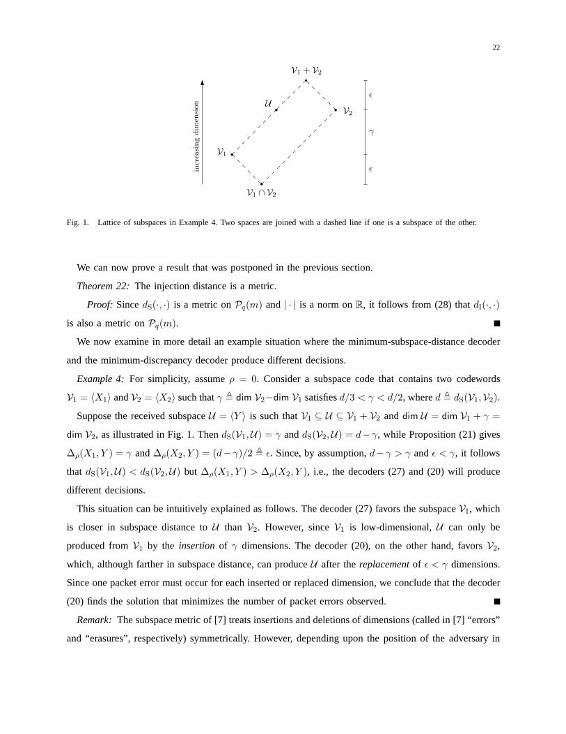
Fig. 1. Lattice of subspaces in Example 4. Two spaces are joined with a dashed line if one is a subspace of the other.

We can now prove a result that was postponed in the previous section.

Theorem 22:The injection distance is a metric.

Proof: SincedS(·, ·) is a metric onPq(m) and | · | is a norm onR, it follows from (28) thatdI(·, ·)

is also a metric onPq(m).

We now examine in more detail an example situation where the minimum-subspace-distance decoder

and the minimum-discrepancy decoder produce different decisions.

Example 4:For simplicity, assumeρ = 0. Consider a subspace code that contains two codewords

V1 = 〈X1〉 andV2 = 〈X2〉 such thatγ , dim V2−dim V1 satisfiesd/3 < γ < d/2, whered , dS(V1,V2).

Suppose the received subspaceU = 〈Y 〉 is such thatV1 ⊆ U ⊆ V1 + V2 anddim U = dim V1 + γ =

dim V2, as illustrated in Fig. 1. ThendS(V1,U) = γ anddS(V2,U) = d−γ, while Proposition (21) gives

∆ρ(X1, Y ) = γ and∆ρ(X2, Y ) = (d− γ)/2 , ǫ. Since, by assumption,d− γ > γ andǫ < γ, it follows

that dS(V1,U) < dS(V2,U) but ∆ρ(X1, Y ) > ∆ρ(X2, Y ), i.e., the decoders (27) and (20) will produce

different decisions.

This situation can be intuitively explained as follows. Thedecoder (27) favors the subspaceV1, which

is closer in subspace distance toU than V2. However, sinceV1 is low-dimensional,U can only be

produced fromV1 by the insertion of γ dimensions. The decoder (20), on the other hand, favorsV2,

which, although farther in subspace distance, can produceU after thereplacementof ǫ < γ dimensions.

Since one packet error must occur for each inserted or replaced dimension, we conclude that the decoder

(20) finds the solution that minimizes the number of packet errors observed.

Remark: The subspace metric of [7] treats insertions and deletions of dimensions (called in [7] “errors”

and “erasures”, respectively) symmetrically. However, depending upon the position of the adversary in

23

the network (namely, if there is a source-destination min-cut between the adversary and the destination)

then a single error packet may cause the replacement of a dimension (i.e., a simultaneous “error” and

“erasure” in the terminology of [7]). The injection distance, which is designed to “explain” a received

subspace with as few error-packet injections as possible, properly accounts for this phenomenon, and

hence the corresponding decoder produces a different result than a minimum subspace distance decoder.

If it were possible to restrict the adversary so that each error-packet injection would only cause either

an insertionor a deletionof a dimension (but not both), then the subspace distance of [7] would indeed

be appropriate. However, this is not the model considered here.

Let us now discuss an important fact about the subspace distance for general subspace codes (assuming

for simplicity thatρ = 0). The packet error correction capability of a minimum-subspace-distance decoder,

tS , is not necessarily equal to⌊(dS(C) − 1)/2⌋ or ⌊(dS(C) − 2)/4⌋, but lies somewhere in between. For

instance, in the case of a constant-dimension codeΩ, we have

dI(V,V ′) =1

2dS(V,V ′), ∀V,V ′ ∈ Ω,

dI(Ω) =1

2dS(Ω).

Thus, Theorem 20 implies thattS = ⌊(dS(C) − 2)/4⌋ exactly. In other words, in this special case, the

approach in [7] coincides with that of this paper, and Theorem 20 provides a converse that was missing

in [7]. On the other hand, supposeΩ is a subspace code consisting of just two codewords, one of which

is a subspace of the other. Then we have preciselytS = ⌊(dS(C)− 1)/2⌋, sincetS + 1 packet-injections

are needed to get past halfway between the codewords.

Since no single quantity is known that perfectly describes the packet error correction capability of

the minimum-subspace-distance decoder (27) for general subspace codes, we cannot provide a definitive

comparison between decoders (27) and (20). However, we can still compute bounds for codes that fit

into Example 4.

Example 5:Let us continue with Example 4. Now, we adjoin another codeword V3 = 〈X3〉 such

that dS(V1,V3) = d and whereγ′ , dim V3 − dim V1 satisfiesd/3 < γ′ < d/2. Also we assume that

dS(V2,V3) is sufficiently large so as not to interfere with the problem (e.g.,dS(V2,V3) > 3d/2).

Let tS andtM denote the packet error correction capabilities of the decoders (27) and (20), respectively.

From the argument of Example 4, we gettM ≥ maxǫ, ǫ′, while tS < minǫ, ǫ′, whereǫ′ = (d−γ′)/2.

By choosingγ ≈ d/3 andγ′ ≈ d/2, we getǫ ≈ d/3 andǫ′ ≈ d/4. Thus,tM ≥ (4/3)tS, i.e., we obtain a

1/3 increase in error correction capability by using the decoder (20).

24

VI. CONCLUSION

We have addressed the problem of error correction in networkcoding under a worst-case adversarial

model. We show that certain metrics naturally arise as the fundamental parameter describing the error

correction capability of a code; namely, the rank metric forcoherent network coding, and the injection

metric for noncoherent network coding. For coherent network coding, the framework based on the rank

metric essentially subsumes previous analyses and constructions, with the advantage of providing a clear

separation between the problems of designing a feasible network code and an error-correcting outer

code. For noncoherent network coding, the injection metricprovides a measure of code performance that

is more precise, when a non-constant-dimension code is used, than the so-called subspace metric. The

design of general subspace codes for the injection metric, as well as the derivation of bounds, is left as

an open problem for future research.

APPENDIX A

DETECTION CAPABILITY

When dealing with communication over an adversarial channel, there is little justification to consider

the possibility of error detection. In principle, a code should be designed to be unambiguous (in which

case error detection is not needed); otherwise, if there is any possibility for ambiguity at the receiver,

then the adversary will certainly exploit this possibility, leading to a high probability of decoding failure

(detected error). Still, if a system is such that (a) sequential transmissions are made over the same channel,

(b) there exists a feedback link from the receiver to the transmitter, and (c) the adversary is not able

to fully exploit the channel at all times, then it might be worth using a code with a lower correction

capability (but higher rate) that has some ability to detecterrors.

Following classical coding theory, we consider error detection in the presence of a bounded error-

correcting decoder. More precisely, define abounded-discrepancy decoder with correction radiust, or

simply a t-discrepancy-correcting decoder, by

x(y) =

x if ∆(x, y) ≤ t and∆(x′, y) > t for all x′ 6= x, x′ ∈ C

f otherwise.

Of course, when using at-discrepancy-correcting decoder, we implicitly assume that the code ist-

discrepancy-correcting. Thediscrepancy detection capabilityof a code (under at-discrepancy-correcting

decoder) is the maximum value of discrepancy for which the decoder is guaranteed not to make an

undetected error, i.e., it must return either the correct codeword or the failure symbolf .

25

For t ∈ N, let the functionσt : X × X → N be given by

σt(x, x′) , miny∈Y : ∆(x′,y)

∆(x, y) − 1. (29)

Proposition 23: The discrepancy-detection capability of a codeC is given exactly byσt(C). That is,

under at-discrepancy-correction decoder, any discrepancy of magnitude s can be detected if and only if

s ≤ σt(C).

Proof: Let t < s ≤ σt(C). Suppose thatx ∈ X is transmitted andy ∈ Y is received, where

t < ∆(x, y) ≤ s. We will show that∆(x′, y) > t, for all x′ ∈ C. Suppose, by way of contradiction, that

∆(x′, y) ≤ t, for somex′ ∈ C, x′ 6= x. Thenσt(C) ≤ ∆(x, y) − 1 ≤ s − 1 < s ≤ σt(C), which is a

contradiction.

Conversely, assume thatσt(C) < s, i.e., σt(C) ≤ s − 1. We will show that an undetected error may

occur. Sinceσt(C) ≤ s−1, there existx, x′ ∈ C such thatσt(x, x′) ≤ s−1. This implies that there exists

somey ∈ Y such that∆(x′, y) ≤ t and∆(x, y)−1 ≤ s−1. By assumption,C is t-discrepancy-correcting,

so x(y) = x′. Thus, if x is transmitted andy is received, an undetected error will occur, even though

∆(x, y) ≤ s.

The result above has also been obtained in [12], although with a different notation (in particular,

treatingσ0(x, x′)+1 as a “distance” function). Below, we characterize the detection capability of a code

in terms of the∆-distance.

Proposition 24: For any codeC, we haveσt(C) ≥ δ(C) − t − 1.

Proof: For anyx, x′ ∈ X , let y ∈ Y be a solution to the minimization in (29), i.e.,y is such that

∆(x′, y) ≤ t and∆(x, y) = 1+ σt(x, x′). Thenδ(x, x′) ≤ ∆(x, y)+ ∆(x′, y) ≤ 1+ σt(x, x′)+ t, which

implies thatσt(x, x′) ≤ δ(x, x′) − t − 1.

Theorem 25:Suppose that∆(·, ·) is normal. For every codeC ⊆ X , we haveσt(C) = δ(C) − t − 1.

Proof: We just need to show thatσt(C) ≤ δ(C) − t − 1. Take anyx, x′ ∈ X . Since ∆(·, ·) is

normal, there exists somey ∈ Y such that∆(x′, y) = t and∆(x, y) = δ(x, x′) − t. Thus,σt(x, x′) ≤

∆(x, y) − 1 = δ(x, x′) − t − 1.

APPENDIX B

PROOF OFLEMMA 15

First, we recall the following useful result shown in [8, Proposition 2]. LetX,Y ∈ FN×Mq . Then

rank(X − Y ) ≥ maxrank X, rank Y − dim(〈X〉 ∩ 〈Y 〉). (30)

26

Proof of Lemma 15:Using (30) and (3), we have

rank(AX − BY ) ≥ maxrank AX, rank BY − dim(〈AX〉 ∩ 〈BY 〉)

≥ maxrank X − ρ, rank Y − σ − dim(〈X〉 ∩ 〈Y 〉).

We will now show that this lower bound is achievable. Our approach will be to constructA as

A = A1A2, whereA1 ∈ FL×(L+ρ)q andA2 ∈ F

(L+ρ)×nq are both full-rank matrices. Then (3) guarantees

that rank A ≥ n − ρ. The matrixB will be constructed similarly:B = B1B2, whereB1 ∈ FL×(L+σ)q

andB2 ∈ F(L+σ)×Nq are both full-rank.

Let k = rank X, s = rank Y , andw = dim(〈X〉∩〈Y 〉). LetW ∈ Fw×mq be such that〈W 〉 = 〈X〉∩〈Y 〉,

let X ∈ F(k−w)×mq be such that〈W 〉+〈X〉 = 〈X〉 and letY ∈ F

(s−w)×mq be such that〈W 〉+〈Y 〉 = 〈Y 〉.

Then, letA2 andB2 be such that

A2X =

W

X

0

and B2Y =

W

Y

0

.

Now, choose anyA ∈ Fi×(k−w)q and B ∈ F

j×(s−w)q that have full row rank, wherei = [k − w − ρ]+

andj = [s − w − σ]+. For instance, we may pickA =[

I 0]

and B =[

I 0]

. Finally, let

A1 =

I 0 0 0

0 A 0 0

0 0 I 0

and B1 =

I 0 0 0

0 B 0 0

0 0 I 0

where, in both cases, the upper identity matrix isw × w.

We have

rank(AX − BY ) = rank(A1A2X − B1B2Y )

= rank(

W

AX

0

−

W

BY

0

)

= maxi, j

= maxk − w − ρ, s − w − σ, 0

= [maxk − ρ, s − σ − w]+ .

27

ACKNOWLEDGEMENT

The authors would like to thank the anonymous reviewers for their helpful comments.

REFERENCES

[1] N. Cai and R. W. Yeung, “Network coding and error correction,” in Proc. 2002 IEEE Inform. Theory Workshop, Bangalore,

India, Oct. 20–25, 2002, pp. 119–122.

[2] R. W. Yeung and N. Cai, “Network error correction, part I:Basic concepts and upper bounds,”Commun. Inform. Syst.,

vol. 6, no. 1, pp. 19–36, 2006.

[3] N. Cai and R. W. Yeung, “Network error correction, part II: Lower bounds,”Commun. Inform. Syst., vol. 6, no. 1, pp.

37–54, 2006.

[4] S. Yang and R. W. Yeung, “Characterizations of network error correction/detection and erasure correction,” inProc. NetCod

2007, San Diego, CA, Jan. 2007.

[5] Z. Zhang, “Linear network error correction codes in packet networks,”IEEE Trans. Inf. Theory, vol. 54, no. 1, pp. 209–218,

2008.

[6] S. Jaggi, M. Langberg, S. Katti, T. Ho, D. Katabi, M. Medard, and M. Effros, “Resilient network coding in the presence

of Byzantine adversaries,”IEEE Trans. Inf. Theory, vol. 54, no. 6, pp. 2596–2603, Jun. 2008.

[7] R. Kotter and F. R. Kschischang, “Coding for errors and erasures in random network coding,”IEEE Trans. Inf. Theory,

vol. 54, no. 8, pp. 3579–3591, Aug. 2008.

[8] D. Silva, F. R. Kschischang, and R. Kotter, “A rank-metric approach to error control in random network coding,”IEEE

Trans. Inf. Theory, vol. 54, no. 9, pp. 3951–3967, 2008.

[9] S. Yang and R. W. Yeung, “Refined coding bounds for networkerror correction,” inProc. 2007 IEEE Information Theory

Workshop, Bergen, Norway, Jul. 1–6, 2007, pp. 1–5.

[10] S. Yang, C. K. Ngai, and R. W. Yeung, “Construction of linear network codes that achieve a refined Singleton bound,” in

Proc. IEEE Int. Symp. Information Theory, Nice, France, Jun. 24–29, 2007, pp. 1576–1580.

[11] R. Matsumoto, “Construction algorithm for network error-correcting codes attaining the Singleton bound,”IEICE

Transactions on Fundamentals, vol. E90-A, no. 9, pp. 1729–1735, Sep. 2007.

[12] S. Yang, R. W. Yeung, and Z. Zhang, “Weight properties ofnetwork codes,”European Transactions on Telecommunications,

vol. 19, no. 4, pp. 371–383, 2008.

[13] A. R. Rao and P. Bhimasankaram,Linear Algebra, 2nd ed. New Delhi, India: Hindustan Book Agency, 2000.

[14] E. M. Gabidulin, “Theory of codes with maximum rank distance,”Probl. Inform. Transm., vol. 21, no. 1, pp. 1–12, 1985.

[15] D. Silva, “Error control for network coding,” Ph.D. dissertation, University of Toronto, Toronto, Canada, 2009.

28

Danilo Silva (S’06) received the B.Sc. degree from the Federal University of Pernambuco, Recife, Brazil, in 2002, the M.Sc.

degree from the Pontifical Catholic University of Rio de Janeiro (PUC-Rio), Rio de Janeiro, Brazil, in 2005, and the Ph.D.

degree from the University of Toronto, Toronto, Canada, in 2009, all in electrical engineering.

He is currently a Postdoctoral Fellow at the University of Toronto. His research interests include channel coding, information

theory, and network coding.

Frank R. Kschischang (S’83–M’91–SM’00–F’06) received the B.A.Sc. degree (withhonors) from the University of British

Columbia, Vancouver, BC, Canada, in 1985 and the M.A.Sc. andPh.D. degrees from the University of Toronto, Toronto, ON,

Canada, in 1988 and 1991, respectively, all in electrical engineering.

He is a Professor of Electrical and Computer Engineering andCanada Research Chair in Communication Algorithms at the

University of Toronto, where he has been a faculty member since 1991. During 1997–1998, he was a Visiting Scientist at the

Massachusetts Institute of Technology, Cambridge, and in 2005 he was a Visiting Professor at the ETH, Zurich, Switzerland.

His research interests are focused on the area of channel coding techniques.

Prof. Kschischang was the recipient of the Ontario Premier’s Research Excellence Award. From 1997 to 2000, he served as

an Associate Editor for Coding Theory for the IEEE TRANSACTIONS ONINFORMATION THEORY. He also served as Technical

Program Co-Chair for the 2004 IEEE International Symposiumon Information Theory (ISIT), Chicago, IL, and as General

Co-Chair for ISIT 2008, Toronto.