
A Naive Bayes classifier for automatic correction of preposition and determiner errors in ESL text
Upload
khangminh22Category
view
0download
0
PDF hosted at the Radboud Repository of the Radboud University
Nijmegen
The following full text is a publisher's version.
For additional information about this publication click this link.
http://hdl.handle.net/2066/168708
Please be advised that this information was generated on 2022-05-29 and may be subject to
change.


Memory-Based Text Correction
Proefschrift
ter verkrijging van de graad van doctor
aan de Radboud Universiteit Nijmegen,
op gezag van de rector magnificus prof. dr. J.H. J.M van Krieken,
volgens besluit van het college van decanen
in het openbaar te verdedigen op woensdag 12 april 2017
om 12.30 uur precies
door
Petrus Johannes Berck
geboren op 5 maart 1966
te Eindhoven
Promotoren: Prof. dr. A. P. J. van den Bosch
Prof. dr. E.O. Postma (Tilburg University)
Manuscriptcommissie:
Prof. dr. R.W.N.M. van Hout (Voorzitter)
Prof. dr. W.M. P. Daelemans (Universiteit Antwerpen, België)
Prof. dr. T.M. Heskes
The research reported in this thesis has been funded by NWO, the NetherlandsOrganisation for Scientific Research in the framework of the project ImplicitLinguistics, grant number 277-70-004, and by the Tilburg School of Humanities,Tilburg Centre for Cognition and Communication.
SIKS Dissertation Series No. 2017-15The research reported in this thesis has been carried out under the auspices ofSIKS, the Dutch Research School for Information and Knowledge Systems.
© 2017 Peter BerckCover artwork & design by IT MasalaTypeset in LATEX, printed by Tryckaren EngelholmISBN 978-94-92380-31-9


Acknowledgements
The thesis in front of you has an interesting history. A part has been written inThe Netherlands, first at Tilburg University, then at Radboud University, and itwas finished in Sweden.
First and foremost, I thank my supervisors, prof. dr. Antal van den Boschand prof. dr. Eric Postma, for their invaluable support and guidance, enthusiasmand optimism.
Antal, we have known each other for a long time; you were already mymentor when I started in Tilburg in 1989. We hadn’t seen each other for a coupleof years when we ran into each other again at a conference in Rotterdam. Youmentioned that Bertjan was changing jobs, and asked if I would be interested intaking over part of the work. As the work could be rolled into a PhD thesis, thiswas an offer I could not refuse, and I started working on the thesis in Tilburg.You moved to the Radboud University in Nijmegen in 2011, and I followed,working on the thesis as an external PhD candidate. Shortly after, I decided tomove to Sweden, and I finished the thesis at home in Margretetorp.
Eric, you may not have been part of this PhD thesis from the beginning, butyour efforts and guidance were crucial in bringing it to a successful conclusion. Iam grateful for the necessary fresh perspective you provided which gave me thefinal push and energy to complete the thesis. With me living in Sweden it washard to keep personal contact, but our bi-weekly Skype meetings were almost asgood.
I would also like to thank the members of the doctoral thesis committee,prof. dr. Roeland van Hout, prof. dr. Walter Daelemans, prof. dr. Tom Heskes,prof. dr. Fons Maes, and prof. dr. ir. Peter Desain.
I started working on the thesis in Tilburg, and I would like to take thisopportunity to thank my roommates in Tilburg, Herman Stehouwer (who wasfinishing his dissertation at the time and introduced me to the humppa musicof Eläkeläiset), and Ko van der Sloot, who not only provided me with the help
i

Acknowledgements
necessary to get all the software I used written and compiled, but also for keepingmy plants alive during the times I was in Sweden. Ko is also responsible forthe timbl toolkit which was the basis of the word predictor I wrote and usedfor the machine learning experiments in this thesis. I would also like to thankPaai, Menno, Sander, Maarten, Matje, Martin, Toine and the other people onthe third floor of the Dante building, who gave character and colour to Tilburg,and made it the place it was.
From the cold slopes of Hallandsåsen, the #ticc and #lst irc channelsprovided an opportunity to keep in contact with colleagues and friends fromNijmegen and Tilburg, and I thank all its participants for their conversationsand comments. A special mention goes to f0/0/f, the automated irc bot, whowas always ready to provide another cynical comment on life, the universe andeverything; !dank f0/0/f.
This thesis would not have happened without the support of Elisabet, mysambo, who never complained about me spending another Saturday behind mycomputer trying to finish another text correction run on yet another data set,and provided the necessary motivation to finish it.
I have moved around and lived in different countries over the last twodecades, and it has not always been easy to keep in touch with my friends. Frankand Jakub, you have always been there, and even if we don’t meet in person veryoften, I cherish the memories we share from noisy concerts in the Netherlandsand midsummer, crayfish parties and camping trips in Sweden. Thanks for beingmy paranymphs!
Last, but not least, the support of family and friends has been invaluable.
Peter BerckMargretetorp, Februari 2017
ii
Contents
Acknowledgements i
1 Introduction 11.1 Language modelling . . . . . . . . . . . . . . . . . . . . . . . . 21.2 A memory-based approach to text correction . . . . . . . . . . 3
1.2.1 Training the memory-based classifiers . . . . . . . . . . 51.2.2 Specific properties of the memory-based systems . . . . 6
1.3 Overall research question . . . . . . . . . . . . . . . . . . . . . 91.3.1 The advantage of skipping . . . . . . . . . . . . . . . . 91.3.2 The advantage of ensemble systems . . . . . . . . . . . 10
1.4 Research methodology . . . . . . . . . . . . . . . . . . . . . . 101.5 The structure of this thesis . . . . . . . . . . . . . . . . . . . . 11
I Language Modelling 13
2 Word Prediction and Language Modelling 152.1 Introduction . . . . . . . . . . . . . . . . . . . . . . . . . . . . 152.2 WOPR, word prediction and language modelling . . . . . . . . 152.3 The decision tree explained . . . . . . . . . . . . . . . . . . . . 192.4 Probabilities and perplexities . . . . . . . . . . . . . . . . . . . 22
2.4.1 Perplexity calculations . . . . . . . . . . . . . . . . . . 232.4.2 Probabilities in WOPR . . . . . . . . . . . . . . . . . . 252.4.3 Perplexity learning curve . . . . . . . . . . . . . . . . . 25
2.5 Word prediction and the distribution . . . . . . . . . . . . . . 272.6 Comparison of the algorithms . . . . . . . . . . . . . . . . . . 28
2.6.1 Baseline experiment . . . . . . . . . . . . . . . . . . . 282.6.2 Processing time . . . . . . . . . . . . . . . . . . . . . . 30
iii
Contents
2.6.3 Size of the distribution . . . . . . . . . . . . . . . . . . 312.6.4 Size of the context . . . . . . . . . . . . . . . . . . . . 33
2.7 Summary . . . . . . . . . . . . . . . . . . . . . . . . . . . . . 36
II Text Correction 39
3 Correction of Confusibles 413.1 Introduction . . . . . . . . . . . . . . . . . . . . . . . . . . . . 413.2 Confusibles . . . . . . . . . . . . . . . . . . . . . . . . . . . . 413.3 Evaluation of confusible correction systems . . . . . . . . . . . 423.4 Memory-based confusible disambiguation . . . . . . . . . . . . 45
3.4.1 System parameters . . . . . . . . . . . . . . . . . . . . 473.4.2 Data . . . . . . . . . . . . . . . . . . . . . . . . . . . . 50
3.5 Baseline experiment . . . . . . . . . . . . . . . . . . . . . . . . 523.6 Selective monolithic system . . . . . . . . . . . . . . . . . . . 543.7 Ensemble system . . . . . . . . . . . . . . . . . . . . . . . . . 563.8 Error-infusion systems . . . . . . . . . . . . . . . . . . . . . . 613.9 Monolithic error system . . . . . . . . . . . . . . . . . . . . . 633.10 Ensemble error system . . . . . . . . . . . . . . . . . . . . . . 683.11 Discussion of the results . . . . . . . . . . . . . . . . . . . . . 70
3.11.1 Comparison to other systems . . . . . . . . . . . . . . 723.12 Conclusion . . . . . . . . . . . . . . . . . . . . . . . . . . . . 72
4 Substitution Errors in Determiners and Prepositions 774.1 Introduction . . . . . . . . . . . . . . . . . . . . . . . . . . . . 774.2 Related work . . . . . . . . . . . . . . . . . . . . . . . . . . . 794.3 The determiner and preposition correction task . . . . . . . . . 85
4.3.1 Data . . . . . . . . . . . . . . . . . . . . . . . . . . . . 864.3.2 Evaluation of the correction system . . . . . . . . . . . 884.3.3 Introduction to the experiments . . . . . . . . . . . . . 90
4.4 Learning curve experiment . . . . . . . . . . . . . . . . . . . . 914.5 Experiments on the CoNLL-2013 shared task data . . . . . . . 934.6 Experiment on subsets of determiners and prepositions . . . . 954.7 Discussion of the results . . . . . . . . . . . . . . . . . . . . . 98
iv

Contents
5 Omission and Insertion Errors in Determiners and Prepositions 1015.1 Introduction . . . . . . . . . . . . . . . . . . . . . . . . . . . . 1015.2 The HOO determiner and preposition error corrector . . . . . 102
5.2.1 Binary classifiers . . . . . . . . . . . . . . . . . . . . . 1035.2.2 System parameters . . . . . . . . . . . . . . . . . . . . 1045.2.3 Data . . . . . . . . . . . . . . . . . . . . . . . . . . . . 106
5.3 Results on the HOO-2012 test set . . . . . . . . . . . . . . . . 1095.4 Discussion of the HOO-2012 results . . . . . . . . . . . . . . . 1105.5 Improving the HOO system . . . . . . . . . . . . . . . . . . . 114
5.5.1 Data . . . . . . . . . . . . . . . . . . . . . . . . . . . . 1155.5.2 Results on the CoNLL test set . . . . . . . . . . . . . . 1155.5.3 Results on artificial data . . . . . . . . . . . . . . . . . 117
5.6 Conclusion . . . . . . . . . . . . . . . . . . . . . . . . . . . . 119
6 Conclusion 1236.1 Answers to the research questions . . . . . . . . . . . . . . . . 124
6.1.1 Compared to other systems . . . . . . . . . . . . . . . 1266.1.2 Real world applications . . . . . . . . . . . . . . . . . 128
6.2 Future work . . . . . . . . . . . . . . . . . . . . . . . . . . . . 128
Appendix
A Determiner and Preposition Sets 133
Summary 145
Samenvatting 149
Sammanfattning 153
Curriculum Vitae 157
SIKS Dissertation Series 159
v

1Introduction
It is generally accepted that spelling correctly is important for both readers andwriters of texts [Moats, 2005]. It is also important in other areas; misspellingsare also a problem for search engines, as it has been estimated that about ten totwenty percent of queries are misspelled [Cucerzan and Brill, 2004,Broder et al.,2009].
Computer programs that help with spelling, grammar or writing texts arenothing new. Spell checkers, for example, have been around since the 1960s, andeveryone is to some degree familiar with the spelling and grammar checkers inword processors and other (home) computer software.
In this thesis we concentrate on developing and testing computational meth-ods for the detection and correction of a subset of spelling and grammar errors,namely confusible errors, and determiner and preposition errors. To the casualcomputer user these may seem like simple tasks which computers have been ableto do correctly for at least the last decade or more, but this is far from the truth;rather, they are subject to continuous research and improvement [Choudhuryet al., 2007].
The first versions of spelling and grammar checkers were often constructedaround rules and patterns which specified whether certain constructions werewell-formed or not. Examples of early work in this area are described in [Dam-erau, 1964] and [Alberga, 1967]. Due to the advent of better computer hardwareand the availability of large amounts of textual data, tied in with the rise of theinternet, the last decade has seen a shift towards empirical systems which learnfrom examples, often gathered from the internet [Carlson et al., 2001, Chenet al., 2007]. From these examples, we can learn which words are likely to appear
1
1. Introduction
in which context, and how likely certain sequences of words are compared toother sequences. The field that deals with these probabilities is called statisticallanguage modelling, or language modelling for short.
Language modelling is the basis of the ideas explored in this thesis, whichdeals primarily with text correction. A statistical language model is a probabilitydistribution over sequences of words (language models will be discussed in moredepth in section 1.1). The text-correction systems we describe are built around alanguage model implemented as a word predictor. The basis of each languagemodel is a classifier which predicts a list of words given a certain context. Thecontext refers to a number of words preceding and/or following the position ofthe word to be predicted. The likelihood of the predictions can be calculatedfrom the statistics contained in these lists. These predictions and probabilitiesare used in the text-correction systems to detect errors and provide potentialcorrections. We chose this technique because it provides a simple approach totext correction; the language model clues provide evidence that we are dealingwith an error, and the set of predicted words provides potential corrections.
In order to be able to explain the concepts which will be discussed, we willopen with a short introduction and overview of the field of language modelling.We then discuss the research questions and structure of the rest of the thesis.
1.1 Language modelling
In [Manning and Schütze, 1999], a language model is defined as the distributionof sequences of ‘words’ in the language, and language modelling as the problem topredict the next words given the previous words. In a statistical language model, thedistribution of words is expressed in probabilities, which are calculated from thenumber of times the words and the sequences occur. The term statistical is oftendropped, and statistical language models are commonly referred to as languagemodels.
Language models are used as a tool in many different fields of natural lan-guage processing, for example automatic speech recognition, machine translationand information retrieval, see for example [Federico et al., 2008]. They have asmall but important task; provide a measure of how likely a sequence of words isin a given language. In speech recognition, this helps to re-create the most likelyutterance from vocal data, and in machine translation it helps for example to puttranslated fragments in the right order. Language models have their basis in a
2
1.2. A memory-based approach to text correction
branch of mathematics and computer science called information theory.Information theory describes how information should be represented, stored
and transmitted. The foundations of information theory were laid in the late1940s with the publication of [Shannon, 1948]. It defines several key conceptswhich later became the foundation for statistical language modelling, such asusing a logarithmic base for measuring information, entropy as a measure forchoice or uncertainty, and the noisy channel model for information processing.The first practical application of language models came with automatic speechrecognition in the 1980s. The growth of computer capabilities over the lastdecades have made it possible to induce language models from vast amounts ofnatural language data. While the first statistics and probabilities were calculatedon the Brown Corpus containing around 1 million words [Kučera and Francis,1967], today the Google GigaWord corpus and other web data1 provide accessto a trillion (1012) words [Sethy et al., 2005, Brants and Franz, 2006, Bucket al., 2014]. The re-emergence of machine translation, this time in the form ofstatistical machine translation (see for example, Moses [Koehn et al., 2007]) hasfurther increased the interest and research in language models, and nowadaysmost language models are capable of handling large amounts of data (for examplesof large scale language models see [Federico et al., 2008,Tan et al., 2011]).
To illustrate the differences between statistical language models and our ownimplementation we make use of srilm [Stolcke, 2002]. Srilm2 is a frequentlyused collection of different programs and libraries to create and test statistical(n-gram-based) language model implementations. It is available under an opensource software licence, and is still being maintained and developed.
1.2 A memory-based approach to text correction
Memory-based learning describes a class of supervised learning algorithms. Ingeneral, supervised learning algorithms learn to solve classification tasks byinduction. Induction is the process of inferring a general rule from a set ofexamples. The algorithms are called supervised because they learn from labelledexamples consisting of a number of feature values and a class label. In memory-based learning, new instances are classified by searching for similar instances inmemory according to a certain distance measure, and the class label is extrapo-
1http://corporafromtheweb.org2http://www.speech.sri.com/projects/srilm/
3
1. Introduction
lated from the labels of the nearest neighbours. Memory-based learning is alsoa form of lazy learning, which is the collective word for learning techniqueswhich store information without permanently abstracting a model from theexamples. Instead, inferring a class from a set of nearest neighbours of a newinstance and assigning this class to this instance is postponed until the timethe information is needed [Stanfill and Waltz, 1986,Aha et al., 1991,Cost andSalzberg, 1993,Daelemans and Van den Bosch, 2005].
In Chapter 2 of this thesis we present two algorithms, called igtree andtribl2. Both are memory-based algorithms in the sense that they keep examplesin memory and postpone processing of the stored information until a newexample needs to be classified. At the same time, both algorithms abstract awayfrom the data by building a decision tree. Nevertheless, we consider the firstalgorithm, igtree, to be an approximation of a memory-based algorithm as itprunes the decision tree. The tree is pruned in such a way that only exceptionsto answers that are stored higher up in the tree are kept.
The second algorithm, tribl2, also builds a decision tree, but in contrastto igtree, this tree is not pruned. In the tribl2 tree, all information on allpreviously seen instances is stored and used when classifying instances. The onlyconcession made to storing every instance is that similar nodes in the tree aremerged to provide faster access and a smaller memory footprint.
In Chapters 3, 4 and 5 of this thesis we describe two text correction tasks.One task deals with the correction of confusibles errors, and the other withthe correction of determiner and preposition errors. We implement differentsystems based on the memory-based classifiers to perform the correction tasks.The systems build on the idea of implementing a memory-based language modelin the form of a word predictor. The list of predicted words is used by thecorrection system to detect errors and suggest potential corrections. We describea number of different implementations of each text-correction system, withclassifiers based on igtree or tribl2, and some implementations containingmore than one classifier.
The systems containing one classifier are referred to as monolithic systems,and those containing more than one are called ensemble systems. In a monolithicsystem, one classifier is trained on all the data in the corpus. This means that inthe monolithic type system, the classifier can return any word from the trainingdata, and is therefore also referred to as an all-word predictor. In the case ofthe confusible correction task, this is likely to generate predictions which areirrelevant. We define a subvariant of the monolithic system which filters the
4
1.2. A memory-based approach to text correction
output on the words relevant to the correction task. This is called a selectivemonolithic system. The ensemble systems consist of multiple classifiers, eachtrained on a specific error to be detected and corrected. The ensemble system hasthe advantage that the predictions come from a much smaller set of possibilities,namely only those relevant to the error under examination.
1.2.1 Training the memory-based classifiers
The classifiers are trained on plain text, and the training material consists ofsmall sequences of text called instances. These instances consist of a word, calledthe target word, with a few words before, after, or around it. Those words arecalled the context. The individual positions in the context are called features,and the words in the context are referred to as feature values. The position ofthe target value is referred to as the focus position.
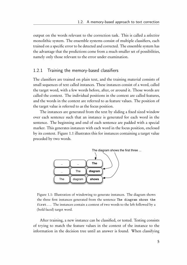
The instances are generated from the text by sliding a fixed sized windowover each sentence such that an instance is generated for each word in thesentence. The beginning and end of each sentence are padded with a specialmarker. This generates instances with each word in the focus position, enclosedby its context. Figure 1.1 illustrates this for instances containing a target valuepreceded by two words.
_ The_
_ diagramThe
The showsdiagram
The diagram shows the first three ...
Figure 1.1: Illustration of windowing to generate instances. The diagram showsthe three first instances generated from the sentence The diagram shows thefirst... The instances contain a context of two words to the left followed by a(bold faced) target word.
After training, a new instance can be classified, or tested. Testing consistsof trying to match the feature values in the context of the instance to theinformation in the decision tree until an answer is found. When classifying
5
1. Introduction
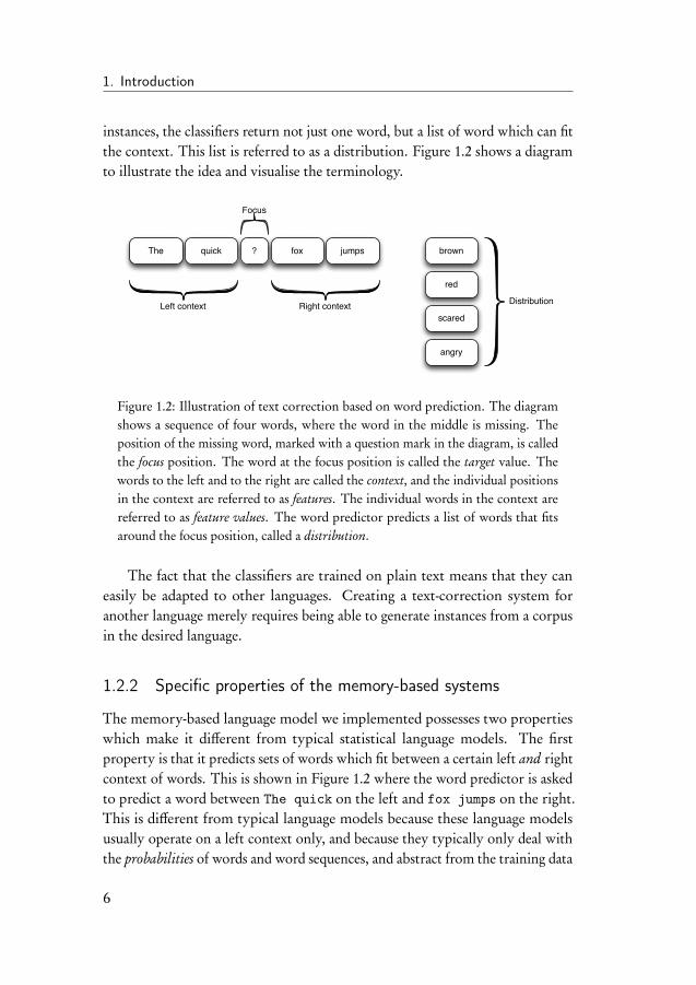
instances, the classifiers return not just one word, but a list of word which can fitthe context. This list is referred to as a distribution. Figure 1.2 shows a diagramto illustrate the idea and visualise the terminology.
The ? foxquick jumps
Left context Right context
Focus
brown
red
scared
angry
Distribution
Figure 1.2: Illustration of text correction based on word prediction. The diagramshows a sequence of four words, where the word in the middle is missing. Theposition of the missing word, marked with a question mark in the diagram, is calledthe focus position. The word at the focus position is called the target value. Thewords to the left and to the right are called the context, and the individual positionsin the context are referred to as features. The individual words in the context arereferred to as feature values. The word predictor predicts a list of words that fitsaround the focus position, called a distribution.
The fact that the classifiers are trained on plain text means that they caneasily be adapted to other languages. Creating a text-correction system foranother language merely requires being able to generate instances from a corpusin the desired language.
1.2.2 Specific properties of the memory-based systems
The memory-based language model we implemented possesses two propertieswhich make it different from typical statistical language models. The firstproperty is that it predicts sets of words which fit between a certain left and rightcontext of words. This is shown in Figure 1.2 where the word predictor is askedto predict a word between The quick on the left and fox jumps on the right.This is different from typical language models because these language modelsusually operate on a left context only, and because they typically only deal withthe probabilities of words and word sequences, and abstract from the training data
6
1.2. A memory-based approach to text correction
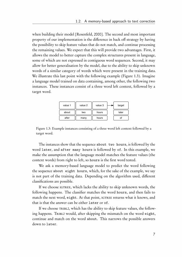
when building their model [Rosenfeld, 2000]. The second and most importantproperty of our implementation is the difference in back off strategy by havingthe possibility to skip feature values that do not match, and continue processingthe remaining values. We expect that this will provide two advantages. First, itallows the model to better capture the complex structures present in language,some of which are not expressed in contiguous word sequences. Second, it mayallow for better generalisation by the model, due to the ability to skip unknownwords of a similar category of words which were present in the training data.We illustrate this last point with the following example (Figure 1.3). Imaginea language model trained on data containing, among other, the following twoinstances. These instances consist of a three word left context, followed by atarget word.
about two later
after many of
value 1 value 2 target
hours
hours
value 3
Figure 1.3: Example instances consisting of a three word left context followed by atarget word.
The instances show that the sequence about two hours, is followed by theword later, and after many hours is followed by of. In this example, wemake the assumption that the language model matches the feature values (thecontext words) from right to left, so hours is the first word tested.
We ask a memory-based language model to predict the word followingthe sequence about eight hours, which, for the sake of the example, we sayis not part of the training data. Depending on the algorithm used, differentclassifications are possible.
If we choose igtree, which lacks the ability to skip unknown words, thefollowing happens. The classifier matches the word hours, and then fails tomatch the next word, eight. At that point, igtree returns what it knows, andthat is that the answer can be either later or of.
If we choose tribl2, which has the ability to skip feature values, the follow-ing happens. Tribl2 would, after skipping the mismatch on the word eight,continue and match on the word about. This narrows the possible answersdown to later.
7
1. Introduction
The ability to skip feature values make the tribl2 algorithm equivalent toskipgram modelling [Guthrie et al., 2006], and allows the classifier to returnanswers that tend to be both more precise and more relevant than the equivalentnon-skipping classifier would have done. For a (text correction) system whichdepends on a list of predicted words, this answer would likely be more usefulthan a list containing many possible words which depended on just one featurevalue match.
The combined left and right-hand side context and the specific back offstrategy (skipping non-matching feature values) turn out to be particularlyuseful for text correction, a task that requires precision; the correction systemhas to detect and correct the errors without generating too many unwantedcorrections. The idea is relatively straightforward; for each word in a text, wecan let the language model predict a list of alternative words that are likely tooccur in the same position in the text. This list can be examined and comparedto the word in the text. If certain conditions are met, such as that one alternativeword is suggested with a likelihood that exceeds a certain confidence threshold,this alternative word can be chosen as a replacement (i.e. correction) for theword in the text.
The strategy outlined above is a simple way of correcting errors, and thequestion springs to mind whether text correction can indeed be performedwithout language-specific knowledge such as grammars and rules for spelling,word morphology and word order. We take the approach that meaningful naturallanguage processing can be done without explicitly adding linguistic knowledgesuch as grammatical rules or other information, and that the surface structureof the text contains enough information for the system to perform the textcorrection task. The systems described in this thesis all learn from unmodifiedexamples extracted from plain English text, without added language-specificinformation. The idea behind this strategy is that the local context around thewords carries enough information for the text-correction systems to work.
This error correction approach will be tested on two linguistic tasks; thecorrection of confusible errors and the correction of determiner and prepositionerrors. Confusibles are words which are easily mistaken for other words, forexample two, too and to. Disambiguating them means choosing the correct onein the given context. Prepositions and determiners are two classes of wordswhich occur in most sentences, but are hard to master, especially when learninga foreign language [De Felice and Pulman, 2008, Bitchener et al., 2005, Leeand Seneff, 2008]. Disambiguating between sets of confusibles and among
8
1.3. Overall research question
prepositions and determiners were chosen as these tasks have been identified asbenchmark tasks in the literature.
1.3 Overall research question
We explore the possibilities of memory-based text correction, focusing on con-fusible correction and determiner and preposition correction. We determineto what extent it can provide a viable method to perform text correction, andexplore how far we can take the text correction capabilities of memory-basedtext correction. We will determine the answer to this latter question by stepwiseincreasing the difficulty of the correction task. The overall research question wetry to answer in this thesis is the following.
Given the simple nature of the memory-based language model, whatare the limits of its text correction abilities?
This question can be divided into two subquestions. First, we would like toknow if the ability to skip words offers a real advantage when applying the systemto text correction. In addition, we would like to investigate if the possibilityto include right-hand side context offers an advantage. Second, we would liketo know if the systems based on ensemble classifiers provide an advantage overthe monolithic classifiers. This leads to two subquestions which we will discussbelow.
1.3.1 The advantage of skipping
As we showed in the beginning of this chapter, one of the differences of memory-based language models compared to typical statistical language models, is theability to skip feature values. Where a typical statistical language model wouldback off to a shorter sequence on a feature value mismatch, the memory-basedlanguage model continues to try to match the remaining feature values.
We will explore the differences in output between the skipping and non-skipping algorithm, and investigate if the differences will provide an advantagein the text correction tasks. Thus, the second research question we will answeris the following.
To what extent does the ability to skip words offer an advantage in textcorrection?
9
1. Introduction
1.3.2 The advantage of ensemble systems
The third research question deals with the contrast between monolithic andensemble systems. The monolithic system is based on a classifier which has beentrained on all the data. In the case of the selective variant, the output is filteredon the words (confusibles in the case of the confusible correction task) relevantto the task. In contrast, the ensemble system consists of multiple classifiers, onefor each confusible set. That means that the ensemble system matches featurevalues on data pertaining only to the confusible set in question, and will onlysuggest relevant alternatives to the (potential) error. This should make it easierfor the system to detect and correct the error, and the expectation is that this willprove to be an advantage. The third research question is therefore the following.
To what extent does the ensemble system offer an advantage in textcorrection?
1.4 Research methodology
We will answer the research questions by implementing a number of memory-based text-correction systems (monolithic and ensemble) built around the igtreeand tribl2 classifiers. The systems will be tested on the confusible and preposi-tion and determiner tasks using real-world and artificial data. In other words,we will gather empirical evidence to answer our research questions. During thecourse of this thesis, we make use of different implementations of the same basicword predictor.
The chapters dealing with memory-based language model implementationin relation to a statistical language model implementation (Chapter 2), and thesystems correcting the confusibles (Chapter 3) use a language model implemen-tation written in C++ called wopr. Wopr uses the timbl library [Daelemanset al., 1997] to implement the memory-based learning and classification part ofthe systems. Its functionality includes word prediction with user-determinablecontext: neighbouring words, a frequency-filtered context word memory withdecay, and document-global features. In addition to all words prediction, woprcan be set to zoom in on specific prediction subsets (such as confusibles), orspecific contexts. It can test language models on new text, reporting perplexities,prediction distributions, and word-level entropy, and can export arpa-formattedlanguage model files. It can filter its output to produce spelling correction
10
1.5. The structure of this thesis
candidates. Wopr was developed during the writing of this thesis, and is madeavailable to the research community. It has been released under the gpl v.3 andis available at https://github.com/LanguageMachines/wopr.
The text-correction systems will be trained on plain text, without addedlinguistic information. Different data sets have been used in the different chapters,but all of them were in the English language. Our machine learning algorithmsare language agnostic, however. We could have used other languages3, but wecontained ourselves to English because it is available in large quantities, it makesit easier to understand and judge the output generated by the systems, and finally,the data sets provided in the shared tasks in which the systems competed [Daleet al., 2012,Ng et al., 2013b] were in English. In Chapter 2 where we comparewopr to srilm, the Reuters Newspaper corpus [Lewis et al., 2004] has beenused. In the other chapters, the umbc [Han et al., 2013a] corpus has been used,supplemented by the Cambridge Learners Corpus [Nicholls, 2003] which wasprovided to us when competing in the hoo-2012 and CoNLL-2013 shared tasks.
1.5 The structure of this thesis
In Chapter 2 we provide a formal description of the memory-based languagemodel, and present a comparison of the memory-based model with a statisticallanguage model, specifically srilm. The two different memory-based algorithms,igtree and tribl2, will be compared to each other, and we decide which is mostsuitable for text correction.
From there, we will move on to Chapter 3 that deals with the first text cor-rection task, the detection and correction of confusible errors. This is followedby Chapters 4 and 5 where the correction of prepositions and determiners willbe explored. Chapter 4 focuses on substitution errors only, and in Chapter 5insertion and deletion errors are added to the task. We wrap up with Chapter 6containing conclusions and further research, and try to answer to what extentwe have been able to answer our research questions.
Part of the work presented in this thesis is based on [Van den Bosch andBerck, 2009], [Van den Bosch and Berck, 2012] and [Van den Bosch and Berck,2013], but has been reworked from scratch.
3Languages similar in structure to English, like Dutch or Swedish, where determinersand prepositions are identifiable words.
11

Part I
Language Modelling
13


2Word Prediction and Language
Modelling
2.1 Introduction
This chapter provides an entry point into memory-based algorithms, word pre-diction, and some of the mathematics behind them. We examine the particularmemory-based algorithms on which much of this thesis hinges, the tribl2 algo-rithm and (to a lesser extent) the igtree algorithm, which are the foundation ofthe text-correction systems described in Chapters 3, 4 and 5. This chapter beginswith a short explanation of the memory-based language model implementationused in the systems described in this thesis, followed by an annotated example toshow the inner workings of the algorithms. Where appropriate, the differencesbetween our memory-based language model implementation and a statisticallanguage model implementation will be explained.
After the comparison, we move on to the word prediction capabilities of thememory-based system, and show how the precision and recall of the predictionscan be influenced.
2.2 WOPR, word prediction and language modelling
In this chapter, we make use of a memory-based language model implemented as aword predictor called wopr (word predictor). Wopr is based on the k-nn classifierTimbl [Daelemans et al., 2010], and implements a number of tools geared towards
15
2. Word Prediction and Language Modelling
the creation and evaluation of language models. Wopr has been developed bythe author during the past years, and the source code is freely available athttps://github.com/LanguageMachines/wopr. The timbl source code canbe downloaded from https://github.com/LanguageMachines/timbl.
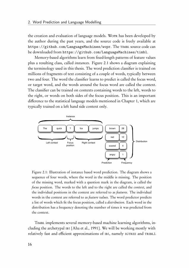
Memory-based algorithms learn from fixed-length patterns of feature valuesplus a resulting class, called instances. Figure 2.1 shows a diagram explainingthe terminology used in this thesis. The word prediction classifier is trained onmillions of fragments of text consisting of a couple of words, typically betweentwo and four. The word the classifier learns to predict is called the focus word,or target word, and the words around the focus word are called the context.The classifier can be trained on contexts containing words to the left, words tothe right, or words on both sides of the focus position. This is an importantdifference to the statistical language models mentioned in Chapter 1, which aretypically trained on a left hand side context only.
The ? foxquick jumps
Left context Right contextFocusposition
brown
red
scared
angry
Distribution
28
12
4
1
Prediction Frequency
Instance
Figure 2.1: Illustration of instance based word prediction. The diagram shows asequence of four words, where the word in the middle is missing. The positionof the missing word, marked with a question mark in the diagram, is called thefocus position. The words to the left and to the right are called the context, andthe individual positions in the context are referred to as features. The individualwords in the context are referred to as feature values. The word predictor predictsa list of words which fit the focus position, called a distribution. Each word in thedistribution has a frequency denoting the number of times it was predicted fromthe context.
Timbl implements several memory-based machine learning algorithms, in-cluding the archetypal ib1 [Aha et al., 1991]. We will be working mostly withrelatively fast and efficient approximations of ib1, namely igtree and tribl2.
16
2.2. WOPR, word prediction and language modelling
The latter two are approximations because they do not store all the instances,but rather compress the data in a decision tree structure. In the case of theigtree algorithm, this tree is heavily pruned. To distinguish the language modelsimplemented by wopr from other statistical language models, we refer to themcollectively as memory-based language models.
Ib1 is the simplest learning algorithm of the three. It implements the k-nearest neighbour classifier [Cover and Hart, 1967]. It compares vectors offeature values by calculating similarity using a similarity function. One of thedisadvantages of ib1 is that it is rather slow for very large data sets, mainly due tothe required search for the exact k-nearest neighbours, one of the reasons whyigtree was developed.
The k in k-nn represents the number of nearest neighbours of the instancebeing classified. The default value is k = 1, that is, it returns the instances (one ormore) that are equidistant and closest to the instance. There are often instancesin the training data which occur multiple times, but giving different answers.The number of times an instance predicts a certain answer is referred to as thefrequency of occurrence of the particular answer. The nearest neighbours canbe seen as lying in rings around a centre, the exact match at distance zero, andmoving outwards like ripples in water with increasing k’s. Each ring contains thenearest neighbours at a specific distance. The closest ring at which the algorithmfinds nearest neighbours is the k = 1 ring, the next one is k = 2 et cetera. In caseof two or more instances at exactly the same distance, the winner can not bedetermined. In that case, all of them are returned by the classifier. The instancewith the highest frequency is in that case the designated ‘winner’.
Where ib1 keeps all the instances as a list in its memory, the instance bases inour implementations are stored in a decision tree. In the decision tree, instancesare represented as paths through nodes labelled with class distributions. Theconnections between the nodes are labelled with the feature values. The wholestructure is anchored in a root node containing a default class distribution,representing unsmoothed word unigram probabilities. This default distributionis returned in the case that none of the feature values match.
The igtree algorithm produces a compressed pruned decision tree. Wordprediction performance is often close to or equal to ib1, but its classificationspeed is considerably faster [Daelemans et al., 1997]. While classifying newinstances, the igtree algorithm stops matching feature values when the firstmismatch is encountered. The algorithm returns the distribution on the node atthat point as the result.
17

2. Word Prediction and Language Modelling
Tribl2 is a mix between igtree and ib1; it starts its classification accordingto the decision-tree strategy of the igtree algorithm, but after a mismatch it con-tinues classification with ib1’s strategy of determining the k nearest neighbours.At this point, ib1’s strategy becomes useful again because it does not assume anordering of features and the number of instances remaining is small enough tobe computationally feasible [Daelemans et al., 2010].
It is important to note that possibly more than one answer is returned inwhat will be referred to as a distribution. It is this distribution which we areultimately interested in. It should also be noted that the algorithms will alwaysreturn an answer, even in the case of no matching feature values. In that case, thedistribution contains all the possible class labels stored in the tree, representingthe word unigram likelihood in the entire training corpus.
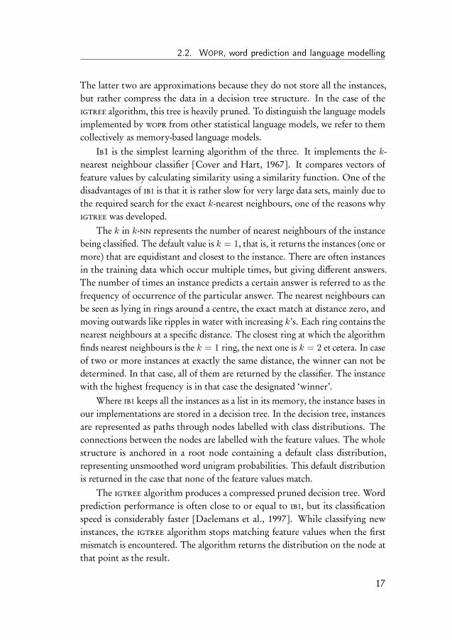
The features in the decision tree are ordered by gain ratio [Quinlan, 1993],with the most important feature being highest in the tree. The test instances arematched against the tree in the same order until no more feature values match.Gain ratio is a normalised version of information gain, which is a measurethat estimates how much information each individual feature contributes to theclassification. Normalisation is necessary because the information gain tendsto put an emphasis on features with a large number of values, even if theycontribute little to the classifiers generalisation abilities. It should be noted thatthis has not as much impact in the case of our word features, where the numberof feature values are similar for all the features. These values are automaticallycalculated when the classifier is trained. The typical ordering of the featuresis that the positions closest to the focus position have the highest gain ratio,that is, are considered to be the most important by the classifier. However,it depends on the data, and different data sets can lead to different orderings.Nevertheless, all the large data sets we have used in the experiments have shownthe aforementioned ordering of the closest features having the highest gain ratio.Figure 2.2 shows the order of importance of the features in a context of fourwords before and three words after the target word, i.e. the word to be predicted.The values were calculated on a one hundred thousand line English text takenfrom the Reuters newspaper corpus. The features nearest to the target (markedwith a T) are deemed to be the important ones, and in the example the firstfeature to the right is the one which is most important. This feature is followedby the one directly to the left of the target (marked l1). This pattern repeatsitself, with the next feature on the right being next in line (marked r2), followedby the next one on the left (l2), et cetera.
18
2.3. The decision tree explained
l4 l3 l2 l1 T r1 r2 r3
Figure 2.2: Relative feature importance in an instance containing a context offour words to the left and three words to the right of the target word. The wordimmediately to the right of the target is the most important feature, followed by theone immediately to the left, et cetera.
2.3 The decision tree explained
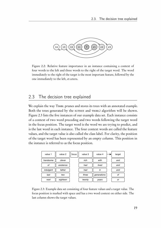
We explain the way Timbl prunes and stores its trees with an annotated example.Both the trees generated by the igtree and tribl2 algorithm will be shown.Figure 2.3 lists the five instances of our example data set. Each instance consistsof a context of two word preceding and two words following the target wordin the focus position. The target word is the word we are trying to predict, andis the last word in each instance. The four context words are called the featurevalues, and the target value is also called the class label. For clarity, the positionof the target word has been represented by an empty column. This position inthe instance is referred to as the focus position.
handsome rich withclever and
of had livedexistence and
indulgent had infather and
last three generationstwo of
next twenty yearseighteen or
value 1 value 3 value 4value 2 targetfocus
Figure 2.3: Example data set consisting of four feature values and a target value. Thefocus position is marked with space and has a two word context on either side. Thelast column shows the target values.
19

2. Word Prediction and Language Modelling
In the first line of the example, we are telling the machine learning algorithmthat the word and was found in the training data to occur between the wordshandsome clever to the left and rich with on the right. Training the instance baseswith the tribl2 and igtree algorithms on the example data gives the followingtwo tree structures (Figure 2.4).
root
twentythreehadrich
of indulgent
handsome last next
clever existence father two eighte
en
with lived in generations years
{ and:1 }
{ and:1 }
{ and:1 }
{ and:1 }
{ and:1 }
{ and:1 }
{ and:1 }
{ and:1 }
{ and:1 }
{ of:1 }
{ of:1 }
{ of:1 }
{ or:1 }
{ or:1 }
{ or:1 }
{ and:1 } { and:2 } { of:1 } { or:1 }
{ and:3 of:1 or:1 }
root
twentythree
{ of:1 } { or:1 }
{ and:3 of:1 or:1 }
Figure 2.4: Tribl2 tree (left) and igtree tree (right) trained on the instances shownin Figure 2.3. The top circle labelled ‘default distribution’ is the root node of the treecontaining the complete unigram distribution. The default distribution is returnedwhen none of the feature values match, and contains all the possible class labelssorted by their frequency. For each node, the distribution is drawn underneath in abox.
Classification is the process of taking a new instance, and determining theresulting class. Given the example, the following will happen when a new testinstance is classified. The top node labelled default distribution is returned whennone of the features in the test instance match. In that case, the answer could beany of the words in the distribution; and, of or or.
The igtree decision tree is the smaller of the two, and only contains twonodes under the root node. The root node carries the default distribution, con-
20

2.3. The decision tree explained
taining the three different target words with their associated frequency. The twonodes under the root node contain exceptions to this default. When classifyingnew instances, the features are matched according to gain-ratio order, and ac-cording to this order, the feature after the focus position is the most importantone and is matched first. When the word after the target word is three, thealgorithm decides the answer is of. Likewise for twenty; when that is the wordafter the target word, the answer is designated to be or. In all other cases, theigtree algorithm returns the default distribution (the complete word unigramdistribution according to the training set), consisting of and, of and or.
Due to this strategy, the igtree based approach has an inherent back offmechanism. The algorithm tries to match a longer sequence and reduce thenumber of possible predictions by moving further down the decision tree,returning the distribution stored at that point in the tree when an unknownword is encountered.
The tribl2 algorithm is more robust in that sense; it continues to try tomatch the remaining feature values, skipping the non-matching value(s). Thetribl2 algorithm is therefore equivalent to a skipgram model (for a closer look atskipgram modelling see for example [Guthrie et al., 2006,Onrust et al., 2016]).
If we look at the tribl2 tree in Figure 2.4 again, we see that all feature valuesare present. The only compression is achieved by the merging of two nodes withthe word had, which predicts and.
The two trees also show that igtree and tribl2 return different answers forthe same input. If we look at the node last just underneath three, we see oneexample of this. If the tribl2 algorithm was to encounter the word last, it wouldreturn of, whereas the igtree algorithm would return the default distribution.Even though of is part of this distribution, the word with the highest frequencyis and. The word last is not in the igtree decision tree, and the algorithmwould answer with the default distribution immediately, making it faster thanthe tribl2 algorithm.
The distributions returned by the word predictor consist of a list with wordsand their associated frequencies. In the example discussed in this section, thedefault distribution was defined as [and:3,of:1,or:1]. In the next section, we showhow these distributions can be related to the calculations performed by statisticallanguage models, and to what extent or our word predictor is equivalent to astatistical language model.
21
2. Word Prediction and Language Modelling
2.4 Probabilities and perplexities
This section explains how statistical language models calculate probabilities, andfrom these probabilities, perplexity. The calculations for statistical languagemodels and wopr are compared.
The first step of the calculations consists of calculating the probability of asingle word. The probability of a single word by itself is not a very meaningfulmeasure, but lies at the basis of language model calculations. The probabilityof a word occurring in a corpus, written here as P (w), is calculated by dividingthe number of times it occurs in the text (its frequency) by the number of allthe words in the corpus. The term C(w) is the count of how many times wordw occurs in the corpus, and CW is the total number of words in the corpus.Instead of CW , the symbol N is sometimes used. So in mathematical notation,we have the following equation (2.1).
P (w) =C(w)
CW(2.1)
This is quite a simplification. To begin with, it depends on the length ofthe text, and the probabilities will be generally overestimations, certainly thosebased on low counts. It also depends on the domain of the text; weather forecastswill give a different model than the sports pages in a newspaper. This can be anadvantage as well, for example if one wants to build a domain-specific system,but there is a more fundamental problem with single word probabilities. Notevery word can occur freely in any position in a sentence and therefore a singleprobability for a word does not really tell us much. For example, the probabilityof the word ‘Union’ might be low, but it will be markedly higher after theword ‘European.’ It would be better to calculate the probability of a wordfollowing another word (or words). This is sometimes referred to as transitionalprobability, but more generally we refer to it as conditional probability; theprobability of a word depends on the word or words preceding (or surrounding)it. The conditional probability of a word (wn ) following another word (wn−1 )is written as P (wn|wn−1). This is calculated as shown in the following equation(2.2).
P (wn|wn−1) =C(wn−1, wn)
C(wn−1)(2.2)
The two-word sequence wn−1wn is called a bigram. Aside from bigrams, se-
22

2.4. Probabilities and perplexities
quences containing three words, called trigrams, are commonly used in languagemodelling.
The conditional probability for bigrams can be generalised for sequencesof arbitrary length N , n-grams, as shown in Equation 2.3, where wn−1n−N+1 is asequence of N − 1 words preceding word wn.
P (wn|wn−1n−N+1) =C(wn−1n−N+1, wn)
C(wn−1n−N+1)(2.3)
Sequences larger than trigrams have become more common the last yearsbecause of the availability of larger data sets and better computers, but thereare good reasons to keep the sequences short. The longer the sequence, the lessoften, if at all, it occurs in the corpus. It is estimated that in an English corpuscontaining one and a half billion words, 30% of trigram tokens (individualoccurrences of trigrams, as opposed to trigram types) remain unseen [Allisonet al., 2006]. To show what kind of numbers we are dealing with in our data, wecalculated the percentages of unique n-grams created from one million lines ofEnglish text, taken from the GigaWord web corpus [Han et al., 2013a]. Of allthe bigram types, 63.4% are unique. This figure goes up to 78.3% for trigramstypes and 83.7% for 4-gram types. This means that most sequences only appearonce in the training data. The longer they get, word sequences which are used fortraining are often not present in the testing data, and the counts of the n-gramsto calculate the probabilities on are therefore not available.
The equations we have explained in this section are the basis on whichstatistical language models calculate the probabilities for their models. Theresulting language model can then be used to calculate probabilities on a newtext, and compare them to the original text the model was created on. Anothermeasure that is often calculated, and which is used to compare the performanceof language models is called perplexity. How perplexity is calculated is explainedthe next subsection.
2.4.1 Perplexity calculations
One of the measures that can be calculated from a distribution of predictedword probabilities is called perplexity [Jelinek et al., 1977]. Perplexity can beconsidered a measure of surprise; in this case surprise over how well a (new)text fits into the language model. Less surprise means more certainty from thelanguage model’s point of view, that is, the text fits better in the model of the
23
2. Word Prediction and Language Modelling
language. The mathematical definition of perplexity is as follows:
perplexity = 2H(p) (2.4)
The factor H(p) is called the entropy of the probability distribution p (inthis case the probabilities calculated by the language model), and is a measure ofthe unpredictability of information content [Shannon, 1948]. Its mathematicaldefinition is shown in Equation 2.5.
H(p) = −∑x
p(x) log2 p(x) (2.5)
The term p(x) is the probability of encountering event x, in this case theprobability of encountering a certain word x. To compute the entropy of acomplete text, we sum the term −p(x) log2 p(x) over all the words in the text.Using base two for the logarithm states the entropy in bits. Base ten is also oftenused; the resulting unit of entropy is then called ban [Good, 1966]. To be able tocompare perplexity values, the entropy is normalised for sentence or text length,that is, divided by the number of words in the text, giving an average perplexityper word. The exact perplexity for a single word can be calculated in a similarmanner. If we define the word level probability as shown in Equation 2.6, theword level perplexity can be calculated according to Equation 2.7 [Jelinek, 1998].
word level probability = − log2 p(x) (2.6)
word level perplexity = 2− log2 p(x) (2.7)
Out-of-vocabulary words are words which did not occur in the trainingdata, and we have no way of knowing how often they occurred. We cannotsimply set the probability of unknown words to zero in Equations 2.5, 2.6 and2.7 because we are, in fact, looking at evidence to the contrary. What we can todo is provide an estimate. This can be done in different ways. An easy way isto simply assign a very small fixed probability to new, unseen words. Anothermore advanced method is to estimate how many unseen words are expected tobe encountered, and to adjust the counts or probabilities of the known wordswith a certain amount. The ‘left over’ probability mass, as it is called, is assignedto the unseen words. This process is called discounting or smoothing. For anoverview of different smoothing techniques we refer to [Chen and Goodman,
24
2.4. Probabilities and perplexities
1998].
2.4.2 Probabilities in WOPR
Probabilities in wopr are calculated in a similar way as in the classical languagemodels, explained in the first part of this section, but with one importantdifference. Instead of on the whole corpus, the word probabilities are calculatedon the fly from the counts of the items in the distribution returned by wopr,according to Equation 2.8. The calculations only depend on the contents ofdistribution, and are independent from the algorithm, igtree or tribl2, used.
P (w|D) =C(w)∑
w′∈D C(w′)(2.8)
In Equation 2.8, w is the target word, and D is the distribution returned bywopr. The counts used are the local counts from the distribution. We back offto the lexical frequency (Equation 2.1) if the correct prediction is not found inthe distribution.
As we mentioned before, the contents of the distribution returned by wopr
are more important than the probabilities. The text-correction systems discussedin chapters 3, 4 and 5 of this thesis are built on the words in the distribution.
In the next section, the perplexity values calculated by a standard languagemodel and our memory-based language models will be compared by letting themcalculate perplexity on the same text.
2.4.3 Perplexity learning curve
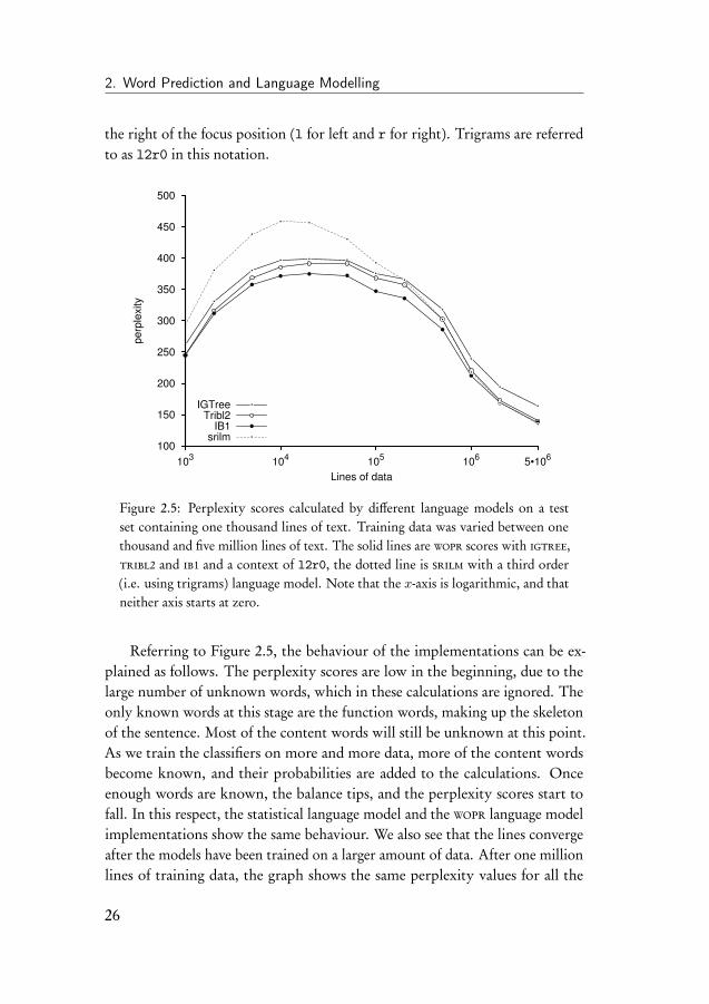
Perplexity is often used to compare language models, and lower perplexity scoresare considered to be better. Lower perplexity signifies a better fit of the testdata by the model. Wopr and srilm can both calculate perplexity on a text, andwe use this to compare the two language model implementations. The srilmtoolkit and wopr produce the perplexity graphs on the English data as shown inFigure 2.5. The graph has been created by training the classifier on increasinglylarger amounts of data and calculating perplexity on the same test set after eachiteration. The training material consisted of trigrams, that is, two context wordsfollowed by the target word. In this thesis the context format is abbreviated withan l_r_ shorthand notation, specifying the number of words to the left and to
25
2. Word Prediction and Language Modelling
the right of the focus position (l for left and r for right). Trigrams are referredto as l2r0 in this notation.
100
150
200
250
300
350
400
450
500
103
104
105
106
5•106
perp
lexity
Lines of data
IGTreeTribl2
IB1srilm
Figure 2.5: Perplexity scores calculated by different language models on a testset containing one thousand lines of text. Training data was varied between onethousand and five million lines of text. The solid lines are wopr scores with igtree,tribl2 and ib1 and a context of l2r0, the dotted line is srilm with a third order(i.e. using trigrams) language model. Note that the x-axis is logarithmic, and thatneither axis starts at zero.
Referring to Figure 2.5, the behaviour of the implementations can be ex-plained as follows. The perplexity scores are low in the beginning, due to thelarge number of unknown words, which in these calculations are ignored. Theonly known words at this stage are the function words, making up the skeletonof the sentence. Most of the content words will still be unknown at this point.As we train the classifiers on more and more data, more of the content wordsbecome known, and their probabilities are added to the calculations. Onceenough words are known, the balance tips, and the perplexity scores start tofall. In this respect, the statistical language model and the wopr language modelimplementations show the same behaviour. We also see that the lines convergeafter the models have been trained on a larger amount of data. After one millionlines of training data, the graph shows the same perplexity values for all the
26
2.5. Word prediction and the distribution
algorithms except for igtree. The reason it trails behind is, as explained before,the fact that its decision tree is pruned, and that only exceptions are stored. Thisleads to lower probabilities because a lot of exact matches are not present in thetree and the values are increasingly often calculated from large, default distribu-tions. In this respect, the better feature value matches and smaller distributionsof the tribl2 algorithm help to keep the probabilities higher and the perplexitylower.
This learning curve shows us that with respect to perplexity, the statisti-cal language model and memory-based language model implementations showsimilar behaviour, and given enough training data, they produce roughly thesame perplexity score. There are some differences in scores; the srilm scores arehigher in the beginning of the curve. This can be explained by the smoothingalgorithm implemented by srilm. Our memory-based language model does notimplement smoothing, and this leads to higher probabilities when trained onsmall amounts of data. The effect of smoothing diminishes after enough trainingdata has been processed.
The differences between the memory-based algorithms can be explained bythe different back off-strategies they implement, and by the fact that the igtreedecision tree is pruned. The curve also shows that we need a substantial amountof data, at least a million lines, to reach similar perplexity scores.
2.5 Word prediction and the distribution
The remainder of this chapter will focus on the distributions returned by theword predictor, with an emphasis on aspects of the distribution which can easilybe measured, such as its size and distribution of the sizes. The contents of thedistributions will be put to the test in the second part of this thesis dealing withthe text-correction systems. There we will determine if the predictions are goodenough to detect and correct textual errors.
There are a number of parameters which can be changed to control thedistribution returned by wopr. These are the choice of the algorithm, the sizeof the context and the amount of training data. If we want the contents of thedistribution to contain the correct answer to different kind of textual errors, itneeds to be precise, preferably containing only the right answer. We also need tofind the right trade-off between speed and size of the system. Speed and size areimportant when implementing text-correction systems that are to be used in the
27
2. Word Prediction and Language Modelling
real world. With the growing use of mobile systems (telephones, tablets) it isimportant that the system fits in the device’s memory, and does not cause extrawaiting time.
We have two ways to determine the best combination of algorithm andcontext. The first one is to look at the accuracy of the predictions. This canbe calculated in a straightforward manner, but it only measures the success ofpredicting the correct word. Our implementations return a distribution ofwords. The second way is to look at this distribution. Several characteristics ofthe distribution can easily be measured, and we mention three of them. Thefirst two are the size of the distribution, and how often certain distribution sizesoccur. If the correct prediction is not the first item in the distribution, but iscontained further down the list, the third characteristic, the mean reciprocal rankof the prediction can be calculated. Of course, proof of the pudding is in theeating, and in Chapters 3, 4 and 5 of this thesis we will examine the usefulness ofthe distribution in the text correction tasks.
First, in the next section, we will compare the three algorithms, ib1, igtreeand tribl2, to each other.
2.6 Comparison of the algorithms
As mentioned in the beginning of this chapter, we have three memory-basedlearning algorithms at our disposal in the timbl toolkit; ib1, igtree and tribl2.In this section, these algorithms are tried on different tasks to compare theoutput, processing time and perplexity scores. The sections opens with a baselineexperiment to determine and compare the word prediction capabilities of thedifferent algorithms to a simple word predictor.
2.6.1 Baseline experiment
We run three word prediction experiments, one for each algorithm, and comparethem to a baseline system. The baseline system is a simple system, whichconsists of a word predictor which always returns the full training set, sorted bylexical frequency. In other words, it returns a large distribution which alwayspredicts the majority class from the training data. The score of this classifierwas compared to the score obtained by the ib1, igtree and tribl2 algorithms.The classifiers were trained on trigrams (an l2r0 context) extracted from one
28
2.6. Comparison of the algorithms
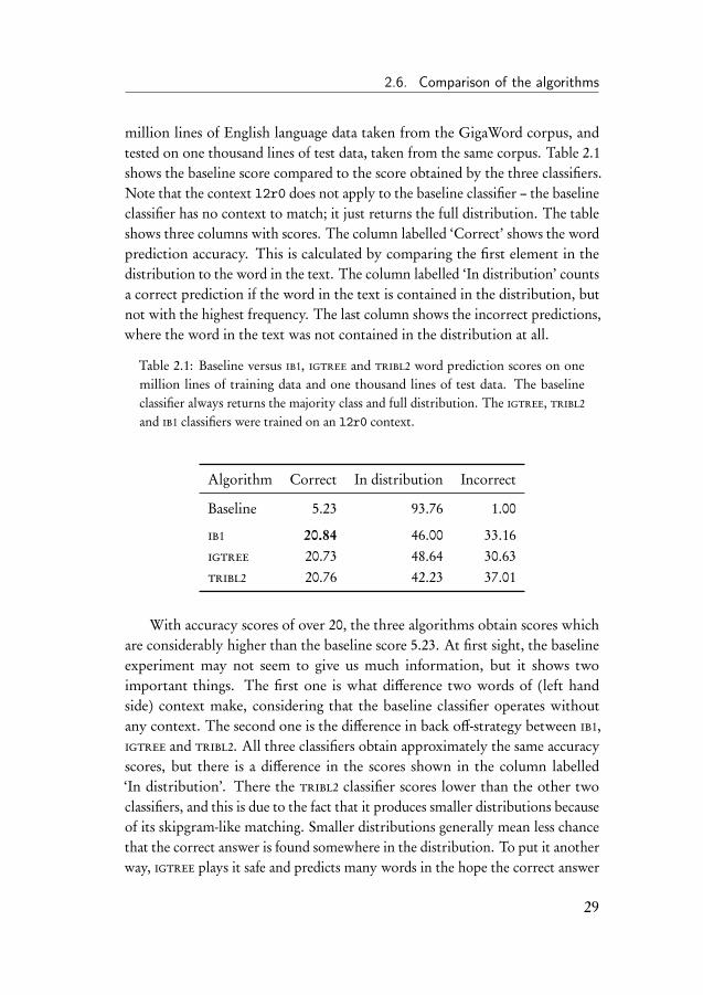
million lines of English language data taken from the GigaWord corpus, andtested on one thousand lines of test data, taken from the same corpus. Table 2.1shows the baseline score compared to the score obtained by the three classifiers.Note that the context l2r0 does not apply to the baseline classifier – the baselineclassifier has no context to match; it just returns the full distribution. The tableshows three columns with scores. The column labelled ‘Correct’ shows the wordprediction accuracy. This is calculated by comparing the first element in thedistribution to the word in the text. The column labelled ‘In distribution’ countsa correct prediction if the word in the text is contained in the distribution, butnot with the highest frequency. The last column shows the incorrect predictions,where the word in the text was not contained in the distribution at all.
Table 2.1: Baseline versus ib1, igtree and tribl2 word prediction scores on onemillion lines of training data and one thousand lines of test data. The baselineclassifier always returns the majority class and full distribution. The igtree, tribl2and ib1 classifiers were trained on an l2r0 context.
Algorithm Correct In distribution Incorrect
Baseline 5.23 93.76 1.00
ib1 20.84 46.00 33.16igtree 20.73 48.64 30.63tribl2 20.76 42.23 37.01
With accuracy scores of over 20, the three algorithms obtain scores whichare considerably higher than the baseline score 5.23. At first sight, the baselineexperiment may not seem to give us much information, but it shows twoimportant things. The first one is what difference two words of (left handside) context make, considering that the baseline classifier operates withoutany context. The second one is the difference in back off-strategy between ib1,igtree and tribl2. All three classifiers obtain approximately the same accuracyscores, but there is a difference in the scores shown in the column labelled‘In distribution’. There the tribl2 classifier scores lower than the other twoclassifiers, and this is due to the fact that it produces smaller distributions becauseof its skipgram-like matching. Smaller distributions generally mean less chancethat the correct answer is found somewhere in the distribution. To put it anotherway, igtree plays it safe and predicts many words in the hope the correct answer
29
2. Word Prediction and Language Modelling
is among them. Tribl2 takes a risk and predicts a smaller list of words, with thepossibility that the correct answer is not predicted at all.
In the next three subsections we look closely at three aspects of wordprediction using these algorithms. We show the differences in processing time,take a look at the sizes of the distributions returned by each algorithm, andexamine the influence of the context format on the distributions. We also take alook at the amount of training material in relation to word prediction accuracy.
The processing time measurements are of course very much dependent onhardware, and given the evolvement of computer technology will be out ofdate by the time this thesis is finished, but the relative differences between thealgorithms will still be relevant.
2.6.2 Processing time
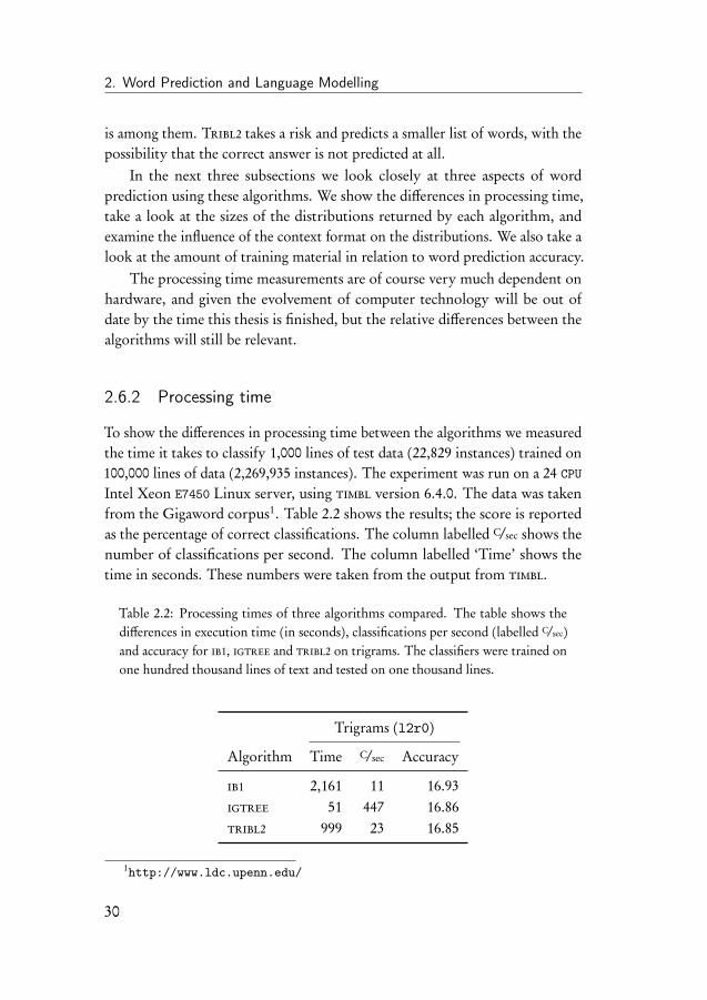
To show the differences in processing time between the algorithms we measuredthe time it takes to classify 1,000 lines of test data (22,829 instances) trained on100,000 lines of data (2,269,935 instances). The experiment was run on a 24 CPU
Intel Xeon E7450 Linux server, using timbl version 6.4.0. The data was takenfrom the Gigaword corpus1. Table 2.2 shows the results; the score is reportedas the percentage of correct classifications. The column labelled C/sec shows thenumber of classifications per second. The column labelled ‘Time’ shows thetime in seconds. These numbers were taken from the output from timbl.
Table 2.2: Processing times of three algorithms compared. The table shows thedifferences in execution time (in seconds), classifications per second (labelled C/sec)and accuracy for ib1, igtree and tribl2 on trigrams. The classifiers were trained onone hundred thousand lines of text and tested on one thousand lines.
Trigrams (l2r0)
Algorithm Time C/sec Accuracy
ib1 2,161 11 16.93igtree 51 447 16.86tribl2 999 23 16.85
1http://www.ldc.upenn.edu/
30
2.6. Comparison of the algorithms
The differences in accuracy between the three algorithms are small. Thedifferences in processing time however, are much larger. Although the ib1
algorithm scores marginally better than the other two on a l2r0 context, it ismore than 40 times slower than igtree. We are only showing the result of onerun here, but all the experiments we ran during the course of writing this thesisshowed ib1 being marginally better and markedly slower than igtree. Regardingprocessing time, tribl2 lies between the other two algorithms. It is about 20times slower than igtree on the l2r0 context. Tribl2 performance on thisparticular data set is slightly worse than the other two on the l2r0 context.
On the basis that ib1 is computationally too demanding, the decision wasmade to dispense with ib1 and build the text-correction systems described in thesecond part of this thesis around the igtree and tribl2 classifiers. Ib1 results arestill included in the results in the remainder of this chapter.
2.6.3 Size of the distribution
The difference in back off strategy between igtree and tribl2 is that igtreereturns a distribution upon the first feature mismatch, whereas tribl2 willcontinue to try to match the remaining features. The ib1 algorithm always triesto match every feature. We therefore expect the igtree algorithm to returndistributions containing more items than tribl2. For tribl2 to fully reach itspotential, it needs more than a two or three features to be able to continuematching feature values after a mismatch. For igtree, this is the other wayaround; training on more than a two or three features does not make sensebecause the algorithm stops on the first mismatch. A full match on all the featurevalues will almost never be found due to data sparseness, but the expectation isthat tribl2 distributions give better predictions because of the extra matches;better in the sense that they are smaller and more specifically suited to thecontext.
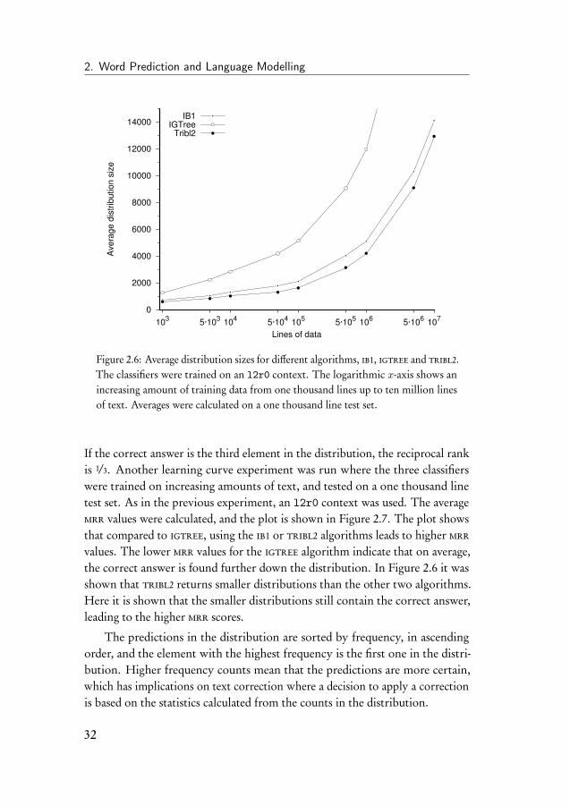
Figure 2.6 shows the differences in the sizes of the distributions returnedby ib1, igtree and tribl2, calculated on one thousand lines of test data. Thetraining data was increased in several steps from one thousand lines of data up toten million lines of data. The graph shows that with an l2r0 context the averagedistribution size for tribl2 (and ib1) is smaller than for igtree.
From the position of the correct prediction in the distribution, the meanreciprocal rank, mrr, of the classification can be calculated. The reciprocal rankof a classification is the multiplicative inverse of its position in the distribution.
31
2. Word Prediction and Language Modelling
0
2000
4000
6000
8000
10000
12000
14000
103
5·103
104
5·104
105
5·105
106
5·106
107
Avera
ge d
istr
ibution s
ize
Lines of data
IB1IGTree
Tribl2
Figure 2.6: Average distribution sizes for different algorithms, ib1, igtree and tribl2.The classifiers were trained on an l2r0 context. The logarithmic x-axis shows anincreasing amount of training data from one thousand lines up to ten million linesof text. Averages were calculated on a one thousand line test set.
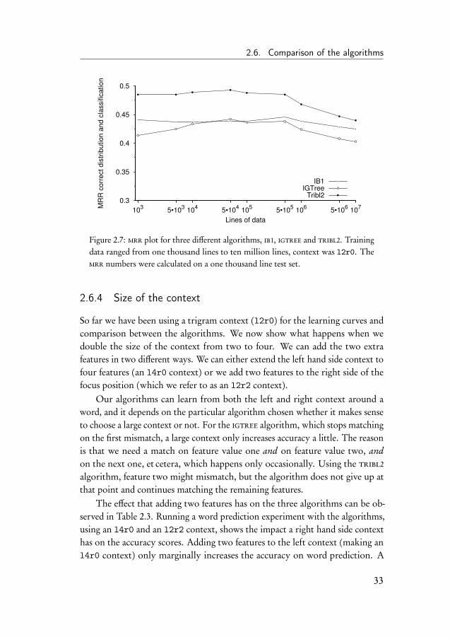
If the correct answer is the third element in the distribution, the reciprocal rankis 1/3. Another learning curve experiment was run where the three classifierswere trained on increasing amounts of text, and tested on a one thousand linetest set. As in the previous experiment, an l2r0 context was used. The averagemrr values were calculated, and the plot is shown in Figure 2.7. The plot showsthat compared to igtree, using the ib1 or tribl2 algorithms leads to higher mrrvalues. The lower mrr values for the igtree algorithm indicate that on average,the correct answer is found further down the distribution. In Figure 2.6 it wasshown that tribl2 returns smaller distributions than the other two algorithms.Here it is shown that the smaller distributions still contain the correct answer,leading to the higher mrr scores.
The predictions in the distribution are sorted by frequency, in ascendingorder, and the element with the highest frequency is the first one in the distri-bution. Higher frequency counts mean that the predictions are more certain,which has implications on text correction where a decision to apply a correctionis based on the statistics calculated from the counts in the distribution.
32
2.6. Comparison of the algorithms
0.3
0.35
0.4
0.45
0.5
103
5•103
104
5•104
105
5•105
106
5•106
107M
RR
co
rre
ct
dis
trib
utio
n a
nd
cla
ssific
atio
n
Lines of data
IB1
IGTree
Tribl2
Figure 2.7: mrr plot for three different algorithms, ib1, igtree and tribl2. Trainingdata ranged from one thousand lines to ten million lines, context was l2r0. Themrr numbers were calculated on a one thousand line test set.
2.6.4 Size of the context
So far we have been using a trigram context (l2r0) for the learning curves andcomparison between the algorithms. We now show what happens when wedouble the size of the context from two to four. We can add the two extrafeatures in two different ways. We can either extend the left hand side context tofour features (an l4r0 context) or we add two features to the right side of thefocus position (which we refer to as an l2r2 context).
Our algorithms can learn from both the left and right context around aword, and it depends on the particular algorithm chosen whether it makes senseto choose a large context or not. For the igtree algorithm, which stops matchingon the first mismatch, a large context only increases accuracy a little. The reasonis that we need a match on feature value one and on feature value two, andon the next one, et cetera, which happens only occasionally. Using the tribl2algorithm, feature two might mismatch, but the algorithm does not give up atthat point and continues matching the remaining features.
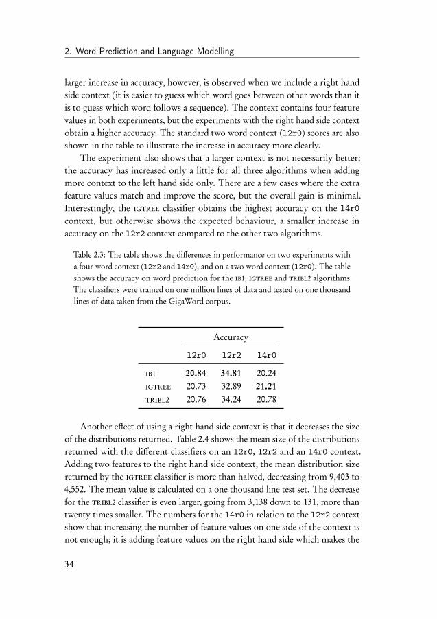
The effect that adding two features has on the three algorithms can be ob-served in Table 2.3. Running a word prediction experiment with the algorithms,using an l4r0 and an l2r2 context, shows the impact a right hand side contexthas on the accuracy scores. Adding two features to the left context (making anl4r0 context) only marginally increases the accuracy on word prediction. A
33
2. Word Prediction and Language Modelling
larger increase in accuracy, however, is observed when we include a right handside context (it is easier to guess which word goes between other words than itis to guess which word follows a sequence). The context contains four featurevalues in both experiments, but the experiments with the right hand side contextobtain a higher accuracy. The standard two word context (l2r0) scores are alsoshown in the table to illustrate the increase in accuracy more clearly.
The experiment also shows that a larger context is not necessarily better;the accuracy has increased only a little for all three algorithms when addingmore context to the left hand side only. There are a few cases where the extrafeature values match and improve the score, but the overall gain is minimal.Interestingly, the igtree classifier obtains the highest accuracy on the l4r0context, but otherwise shows the expected behaviour, a smaller increase inaccuracy on the l2r2 context compared to the other two algorithms.
Table 2.3: The table shows the differences in performance on two experiments witha four word context (l2r2 and l4r0), and on a two word context (l2r0). The tableshows the accuracy on word prediction for the ib1, igtree and tribl2 algorithms.The classifiers were trained on one million lines of data and tested on one thousandlines of data taken from the GigaWord corpus.
Accuracy
l2r0 l2r2 l4r0
ib1 20.84 34.81 20.24igtree 20.73 32.89 21.21tribl2 20.76 34.24 20.78
Another effect of using a right hand side context is that it decreases the sizeof the distributions returned. Table 2.4 shows the mean size of the distributionsreturned with the different classifiers on an l2r0, l2r2 and an l4r0 context.Adding two features to the right hand side context, the mean distribution sizereturned by the igtree classifier is more than halved, decreasing from 9,403 to4,552. The mean value is calculated on a one thousand line test set. The decreasefor the tribl2 classifier is even larger, going from 3,138 down to 131, more thantwenty times smaller. The numbers for the l4r0 in relation to the l2r2 contextshow that increasing the number of feature values on one side of the context isnot enough; it is adding feature values on the right hand side which makes the
34
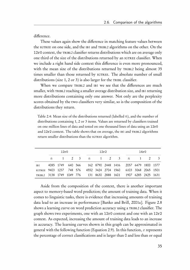
2.6. Comparison of the algorithms
difference.These values again show the difference in matching feature values between
the igtree on one side, and the ib1 and tribl2 algorithms on the other. On thel2r0 context, the tribl2 classifier returns distributions which are on average onlyone third of the size of the distributions returned by an igtree classifier. Whenwe include a right hand side context this difference is even more pronounced,with the mean size of the distributions returned by tribl2 being almost 35times smaller than those returned by igtree. The absolute number of smalldistributions (size 1, 2 or 3) is also larger for the tribl classifier.
When we compare tribl2 and ib1 we see that the differences are muchsmaller, with tribl2 reaching a smaller average distribution size, and ib1 returningmore distributions containing only one answer. Not only are the perplexityscores obtained by the two classifiers very similar, so is the composition of thedistributions they return.
Table 2.4: Mean size of the distributions returned (labelled n̄), and the number ofdistributions containing 1, 2 or 3 items. Values are returned by classifiers trainedon one million lines of data and tested on one thousand lines of data using an l2r0and l2r2 context. The table shows that on average, the ib1 and tribl2 algorithmsreturn smaller distributions than the igtree algorithm.
l2r0 l2r2 l4r0
n̄ 1 2 3 n̄ 1 2 3 n̄ 1 2 3
ib1 4085 1749 640 566 162 8790 2448 1416 2057 6479 1800 1377igtree 9403 1237 748 576 4552 3424 2704 1560 6103 3068 2065 1501tribl2 3138 1749 1049 776 131 8630 2888 1601 1907 6285 2425 1631
Aside from the composition of the context, there is another importantaspect to memory-based word prediction; the amount of training data. When itcomes to linguistic tasks, there is evidence that increasing amounts of trainingdata lead to an increase in performance [Banko and Brill, 2001a]. Figure 2.8shows a learning curve on word prediction accuracy using a tribl2 classifier. Thegraph shows two experiments, one with an l2r0 context and one with an l2r2context. As expected, increasing the amount of training data leads to an increasein accuracy. The learning curves shown in this graph can be approximated ingeneral with the following function (Equation 2.9). In this function, x representsthe percentage of correct classifications and is larger than 0 and less than or equal
35

2. Word Prediction and Language Modelling
to 100. The functions have been calculated with the curve fitting capability ofthe gnuplot program2.
f(x) = a · log10(x) + b (2.9)
Figure 2.8 shows two learning curves and their approximation. Inversely, wecan calculate the number of instances needed to reach a x% score (number ofcorrect classifications, or accuracy) with the following equation (Equation 2.10).The variable NIx represents the number of instances required to get the desiredaccuracy x.
NIx = 10x−ba (2.10)
We make two observations. First, when it comes to word prediction, moredata leads to better performance. Second, to get a linear increase in performance,the increase in data needs to be exponential, leading to longer processing timesand larger memory requirements.
This is only an approximation which only works for the corpus the functionwas calculated on. It also assumes unique training data without repeating largerchunks of texts to give a continuously rising score.
2.7 Summary
In this chapter we have shown how a memory-based word predictor can be usedto implement language modelling. We have provided an introduction of themathematics involved in language modelling, both in statistical language modelsand in our implementation of a memory-based language model.
We have explored three different memory-based learning algorithms availableto us in the timbl toolkit; ib1, igtree and tribl2. Ib1 is what we consider to bea pure memory-based learning algorithm. The instances that form the modelare stored in one large flat list which is traversed on processing. The algorithmattempts to match all feature values, skipping those that do not match. It istherefore also the slowest of the three algorithms.
Igtree and tribl2 are two approximations of the ib1 algorithm. Igtree isthe fastest implementation because it takes two shortcuts. First, the instancesare stored in a decision tree that is heavily pruned. The algorithm prefers to
2http://www.gnuplot.info/
36
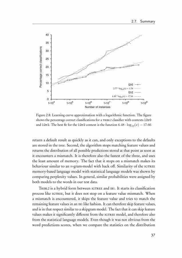
2.7. Summary
0
5
10
15
20
25
30
35
40
1•104
1•105
1•106
1•107
1•108
1•109
Perc
enta
ge c
orr
ect cla
ssific
ations
Number of instances
l2r0
2.77 * log10(x) + -1.58
l2r2
6.48 * log10(x) + -17.66
Figure 2.8: Learning curve approximation with a logarithmic function. The figureshows the percentage correct classifications for a tribl2 classifier with contexts l2r0and l2r2. The best fit for the l2r2 context is the function 6.48 · log10(x) − 17.66
return a default result as quickly as it can, and only exceptions to the defaultsare stored in the tree. Second, the algorithm stops matching feature values andreturns the distribution of all possible predictions stored at that point as soon asit encounters a mismatch. It is therefore also the fastest of the three, and usesthe least amount of memory. The fact that it stops on a mismatch makes itsbehaviour similar to an n-gram-model with back off. Similarity of the igtreememory-based language model with statistical language models was shown bycomparing perplexity values. In general, similar probabilities were assigned byboth models to the words in our test data.
Tribl2 is a hybrid form between igtree and ib1. It starts its classificationprocess like igtree, but it does not stop on a feature value mismatch. Whena mismatch is encountered, it skips the feature value and tries to match theremaining feature values in an ib1 like fashion. It can therefore skip feature values,and is in that respect similar to a skipgram model. The fact that it can skip featurevalues makes it significantly different from the igtree model, and therefore alsofrom the statistical language models. Even though it was not obvious from theword predictions scores, when we compare the statistics on the distribution
37
2. Word Prediction and Language Modelling
sizes returned by igtree and tribl2, we see the real practical difference betweenthe two algorithms. Tribl2 always returns smaller distributions, as shown inTable 2.4 and the mrr plot shown in Figure 2.7. In fact, the tribl2 distributionsizes are almost equal to those of the ib1 algorithm, but with higher mrr numbers.We expect that this feature of the tribl2 algorithm will be an advantage in thetext correction tasks; more values are matched, which means that instead ofworking with a large default distribution, the correction system works with asmaller distribution of only a few words. This will be explored in Chapters 3, 4and 5 of this thesis.
Another noticeable difference to standard statistical language models is thatigtree and tribl2 can easily make use of a right hand side context. In some real-world contexts (e.g. real-time speech recognition or word processing) right-handside context is not available, but in others (e.g. full-text spelling correction) right-hand side context is readily available. The performance on the word predictiontask showed that inclusion of a right hand side context raised accuracy by morethan 10%. This is an important improvement on the statistical language modelswe have looked at in this chapter, and is one of the strengths of the memory-basedmethods described here.
In the next part of this thesis, we will describe the text-correction systemsbuilt on the basis of the memory-based language models. The first task isconfusible error detection and correction, described in Chapter 3. Chapter 4describes a similar application to determiner and preposition substitution errordetection and correction. The third and last chapter on text correction, Chap-ter 5, describes a system that detects and corrects three types of determiner andpreposition errors; substitution, omission and insertion errors. All systemsuse the information in the distribution returned by the classifiers to detect andcorrect the errors.
38

Part II
Text Correction
39


3Correction of Confusibles
3.1 Introduction
In this chapter we describe the first of the two text-correction systems builtaround the output from the memory-based word predictor. The first task wedescribe is confusible correction, and this chapter opens with a description ofwhat we consider to be confusibles and which confusibles will be selected tobe handled by the correction system. This is followed by a description on howa memory-based corrector is constructed. The remainder of the chapter willreport on the text correction experiments and the results obtained. The systemswe describe are trained on plain English texts gathered from the web, and theywill be tested on data containing artificial errors. The results obtained by thememory-based systems are compared to results obtained by other systems.
3.2 Confusibles
Confusibles are words that bear some similarity to other words such that theyare easily mistaken for each other. For example, to, too and two, allusion andillusion, or flare and flair. Confusibles are a type of spelling error. Spelling errorscan result in words that are not in a dictionary (so called non-word errors) orwords which are in a dictionary (real-word errors). Confusible errors fall solelyin the latter category. Other than spelling errors which arise from sloppy writingor missing or inserting keys on the keyboard and often do not need more than adictionary to be corrected, confusibles need context to be corrected. Instead of
41
3. Correction of Confusibles
confusible correction, the term confusible disambiguation is sometimes used; itis known what the correct word sounds like, but a choice has to be made withregards to its spelling.
Confusible errors have several underlying causes. We mention three of them.First, they arise when words sound similar, for example their versus there, orprinciple versus principal. Second, there are words which are similar in meaning,but may not be used in place of each other. This type of error is called a semanticerror. Examples of semantic errors are number versus amount, and fewer versusless. The third and last cause we mention are typographical errors, for exampleform versus from or nuclear versus unclear which stem from incorrectly hittingor failing to hit keys on the keyboard.
3.3 Evaluation of confusible correction systems
Confusibles and the area of context-sensitive spelling checking have been thesubject of research for many years. [Golding and Roth, 1996] discuss a Winnow-based system to disambiguate confusibles. Their work is the origin of the listwith confusibles we use to test our text-correction system on. This list willbe introduced and explained later in this chapter. Another approach is de-scribed in [Mangu and Brill, 1997] who induce correction rules with a variant oftransformation-based learning. Other confusible disambiguation techniques usedinclude trigrams [Mays et al., 1991], decision lists [Yarowsky, 1994], Bayesianstatistics [Golding, 1995], memory-based learning [Van den Bosch, 2006], andsuffix-tree-based language models [Stehouwer and Van Zaanen, 2009]. For morerecent work we refer the reader to [Bergsma et al., 2009] who uses the recentavailability of large web corpora to train a number supervised and unsupervisedsystems on, amongst others, the task of context-sensitive spelling correction onconfusible sets. Similarly, [Carlson et al., 2008] and [Lapata and Keller, 2005]compare systems trained on very large amounts of web data on several naturallanguage processing tasks, such as spelling correction. In the last section of thischapter, we compare the results of our memory-based system to several of thesesystems.
A commonality between some of the approaches from before 2005 is thatthey measure the accuracy of disambiguating confusibles, that is, the accuracy oncorrectly choosing the right word in the given context from different confusiblesets [Golding and Roth, 1999,Gamon et al., 2008,Bergsma et al., 2009]. This is
42
3.3. Evaluation of confusible correction systems
akin to running the system on a test set without any errors. The accuracy num-bers reported are usually fairly high, but they lack one important aspect; theydo not measure whether these systems can actually detect (and after detection,correct) confusible errors, and to what extent. A high accuracy in disambiguatinga confusible set may correspond to a good detection of errors, but confusibleerrors are typically only a small and hard-to-detect subset of all occurrences ofthe words in a confusible set. Confusible error detection, like other spellingdetection tasks, is a needle-in-a-haystack problem. Most of the confusibles in atext will be correct, and errors occur only occasionally.
The following example illustrates the fallacy in reporting only the accuracynumbers and assuming these reflect the performance on confusible error de-tection. Imagine we have a system which disambiguates confusibles with anaccuracy of 98%. This means the system makes a mistake in producing theright confusible in two out of one hundred confusibles. That sounds good, butnow imagine we are trying to correct errors in data containing one error in twohundred confusibles. In those two hundred words, our system can be expectedto be wrong four times. That means we might find the error, but we are likelyto introduce a number of new errors as well. A system correcting one error intwo hundred words would need an accuracy of at least 99.5% if we do not wantto introduce more errors. To provide a better estimate of the performance, weneed to measure the precision and recall of the detection and correction of errorsas well. Precision measures the number of (correct) corrections in relation tothe number of corrections the system suggested. Recall measures the number of(correct) corrections in relation to the number of errors in the text.
Fortunately, measuring the precision and recall of the detection and cor-rection of errors has become standard practice when evaluating spelling andgrammatical correction systems [Reynaert, 2005,Ng et al., 2013b]. It is impor-tant that a correction system detects all errors, which is shown by the recallscore; the higher the better. At the same time, generating too many false alarms(suggesting a correction where none is needed) will lower the precision score.The harmonic mean of the precision and recall is called the F -score. In thischapter, we therefore report the precision, recall and F -score numbers whendescribing the results obtained by the systems. Accuracy numbers are reportedwhen comparing the results to other systems. The precision, recall and F -scoreare calculated as follows.
When we examine the output from the correction systems, we count theerrors that have been corrected, missed, or corrected wrongly. There are two
43

3. Correction of Confusibles
related but complementary ways of specifying these numbers. The first oneis using the following four statistics. A true positive (tp) is counted when wecorrectly correct a confusible error. A false negative occurs when the systemdoes not try to correct a confusible error, or when the system gives the wrongcorrection. A false positive (fp) is counted when the system tries to correct aconfusible that was correct. Finally, the remaining words are the true negatives(tn).
The second way to specify them is to count the following; proposed edits,correct edits and gold edits. The proposed edits are the number all the correctionsput forward by the correction system. The correct edits are the number ofproposed edits that were correct. The gold edits are the number of edits necessaryto correct the full text, that is, the number of errors in the text. These relate tothe true and false positives and negatives explained above in the following way.
Correct Edits = TP (3.1)
Proposed Edits = TP + FP (3.2)
Gold Edits = TP + FN (3.3)
From these statistics, we can calculate precision (abbreviated in this thesis aspre), recall (abbreviated here as rec), and accuracy (abbreviated here as acc).Precision counts the number of correctly identified errors compared to the totalnumber of errors identified. Recall counts the number of correctly identifiederrors compared to the total number of errors. Accuracy gives a measure of howgood the classifiers are by putting the number of correctly classified instancesin relation to the total number of instances in the test data. Expressed in termsof true and false positives and negatives, these are calculated according to thefollowing equations.
Precision =TP
TP + FP(3.4)
44
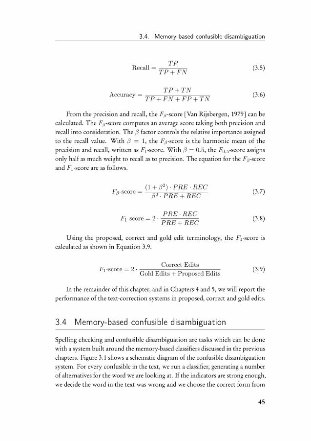
3.4. Memory-based confusible disambiguation
Recall =TP
TP + FN(3.5)
Accuracy =TP + TN
TP + FN + FP + TN(3.6)
From the precision and recall, the Fβ -score [Van Rijsbergen, 1979] can becalculated. The Fβ -score computes an average score taking both precision andrecall into consideration. The β factor controls the relative importance assignedto the recall value. With β = 1, the Fβ -score is the harmonic mean of theprecision and recall, written as F1-score. With β = 0.5, the F0.5-score assignsonly half as much weight to recall as to precision. The equation for the Fβ -scoreand F1-score are as follows.
Fβ-score =(1 + β2) · PRE ·RECβ2 · PRE +REC
(3.7)
F1-score = 2 · PRE ·RECPRE +REC
(3.8)
Using the proposed, correct and gold edit terminology, the F1-score iscalculated as shown in Equation 3.9.
F1-score = 2 · Correct Edits
Gold Edits + Proposed Edits(3.9)
In the remainder of this chapter, and in Chapters 4 and 5, we will report theperformance of the text-correction systems in proposed, correct and gold edits.
3.4 Memory-based confusible disambiguation
Spelling checking and confusible disambiguation are tasks which can be donewith a system built around the memory-based classifiers discussed in the previouschapters. Figure 3.1 shows a schematic diagram of the confusible disambiguationsystem. For every confusible in the text, we run a classifier, generating a numberof alternatives for the word we are looking at. If the indicators are strong enough,we decide the word in the text was wrong and we choose the correct form from
45
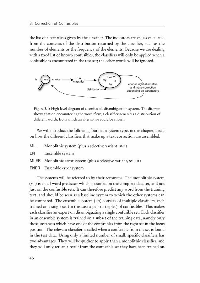
3. Correction of Confusibles
the list of alternatives given by the classifier. The indicators are values calculatedfrom the contents of the distribution returned by the classifier, such as thenumber of elements or the frequency of the elements. Because we are dealingwith a fixed list of known confusibles, the classifiers will only be applied when aconfusible is encountered in the test set; the other words will be ignored.
is there choice runclassifier
their
by choose right alternativeand make correction
depending on parameters
my a
distribution
Figure 3.1: High level diagram of a confusible disambiguation system. The diagramshows that on encountering the word there, a classifier generates a distribution ofdifferent words, from which an alternative could be chosen.
Wewill introduce the following four main system types in this chapter, basedon how the different classifiers that make up a text correction are assembled.
ML Monolithic system (plus a selective variant, sml)
EN Ensemble system
MLER Monolithic error system (plus a selective variant, smler)
ENER Ensemble error system
The systems will be referred to by their acronyms. The monolithic system(ml) is an all-word predictor which is trained on the complete data set, and notjust on the confusible sets. It can therefore predict any word from the trainingtext, and should be seen as a baseline system to which the other systems canbe compared. The ensemble system (en) consists of multiple classifiers, eachtrained on a single set (in this case a pair or triplet) of confusibles. This makeseach classifier an expert on disambiguating a single confusible set. Each classifierin an ensemble system is trained on a subset of the training data, namely onlythose instances which have one of the confusibles from the right set in the focusposition. The relevant classifier is called when a confusible from the set is foundin the test data. Using only a limited number of small, specific classifiers hastwo advantages. They will be quicker to apply than a monolithic classifier, andthey will only return a result from the confusible set they have been trained on.
46

3.4. Memory-based confusible disambiguation
The latter advantage will hopefully make it easier to choose the right alternativefrom the set, and as a consequence introduce fewer new errors into the text.
The monolithic systems suffer from the problem that the classifier alwaysreturns a large number of words which are not relevant for the confusibleset being checked. To alleviate this problem, we introduce a subtype called aselective monolithic system (sml). This variant filters the distributions returnedon the confusibles from the relevant set, and discards the other words in thedistribution.
Spelling and grammatical correction systems can benefit from training datain which errors have been artificially introduced [Brockett et al., 2006,Ehsanand Faili, 2013, Yuan and Felice, 2013]. The monolithic and ensemble errorsystems mler and ener are based on this idea. Instead of training the classifieron the context around the focus word, with the focus word masked, the focusword is included in the training material. Then, a random subset of confusiblesin the training data is substituted by another confusible from the same set. Thisresults in training data which contains examples of artificial errors in context,as well as examples of the (assumedly) correct form in context. We hypothesisethat having both types of examples in the training set will have the followingtwo effects on the error detection capabilities of the system. First, the errors incontext will be models for future errors in similar contexts. Second, the correctforms in context will lead the classifier to be confident about the correction ofan error in a similar context. This confidence stems from the ratio betweenexamples found with and without an error. If the number of examples of correctusage is much larger than the number of error examples, the system is likelydealing with a real error. The number of errors in the training data will need tobe determined as it is unclear a priori where the optimum ratio between artificialerrors in the training data and errors in the testing data lies. The error systemswill be explained in more depth in section 3.8.
3.4.1 System parameters
There are two positions in the system (Figure 3.1) where we can influencethe performance. The first possibility for adjustment is by modifying theclassifier; how to train it, on which data, and which context size and algorithmto use. The second way is to change the tuning parameters which govern thedecision if the distribution returned by the classifier contains a correction. Theparameters determine whether the distribution will be kept or discarded. When
47
3. Correction of Confusibles
the distribution is kept, the parameters decide if one of the answers could be acorrection of the word under examination. The parameters control what wecall abstention; the system abstains from using the suggested correction if it fallsoutside the limits of the parameters. We showed in Chapter 2 that the classifiersreturn a distribution of a certain size and with a certain entropy. Knowing this,we distinguish the following two measures.
entropy The entropy of the classification, i.e. the distribution of predictedwords. A measure of how certain the classifier is of the result.An entropy threshold value can be used as a cut off point whendeciding to use a classification or not.
confidence Confidence is defined as the ratio between the count of the firstanswer in the distribution, and the sum of the counts of thecomplete (including the first) distribution.
The entropy and confidence measures are calculated on the count valuesin the distribution. They both try to quantify the certainty of the classification.Experimental results show the first measure, entropy, ranges from zero to about12 when running an all-word classifier (see Chapter 2). Simply put, a lowerentropy means more certainty. The confidence values lie in the interval fromzero to one (but not including zero, in formal notation the interval would bewritten as ]0,1]). A high confidence value either means that there are only a fewanswers, or that the frequency of the top-answer is high compared to the otheranswers in the distribution. The maximum value of 1 means there is only oneanswer in the distribution. Previous experiments suggest that this parameter isideally set to a high value, somewhere in the range 0.95 – 1.00. This, however,may cause problems in the case of low frequency answers, which can occur inthe case of instances which match most, or all, feature values. A perfect matchon a context of two words to the left and two words to the right will not happenvery often, but tends to result in low frequency counts in the distribution. Forexample, a distribution where the top answer has a frequency of four, and thereare two other answers with a frequency of one will only result in a confidenceof 0.67 (4/6). This will probably fall under any practical threshold set by the user,but it is still potentially a good classification. A confidence threshold value ofexactly one will only allow distributions with one item.
The entropy and confidence parameters lose some of their usefulness whenused in the ensemble systems. The classifiers in an ensemble system are trainedon subsets of the data containing only words from a certain confusible set.
48
3.4. Memory-based confusible disambiguation
Having zoomed in on the data like this causes more feature value matches, anddistributions which never contain more than the number of elements in theconfusible set. That means the entropy of the classification is much lower thanin the case of the single all-word classifier. Experimental results suggests thatwhen dealing with ensemble classifiers, the entropy lies mostly below two. Thiseffect also affects the confidence parameter, where small distributions with lowfrequency elements cause the confidence to change a lot when the frequency ofone of the elements changes by as little as one.
A similar effect is observed when dealing with the error systems. Errorsystems contain an example of an error in context. The relevant instances in theinstance base will always match this feature value; this means the entropy of theclassifications will be much lower than that of its non-error counterpart, and theentropy values are too small to be used as a discriminating threshold.
A number of different experiments were run in the early stages of this thesiscomparing the results with different parameter settings to each other. Only theconfidence parameter turned out to be useful. As we will see later, we needto filter the distribution on elements from the relevant confusible set. Thisinvalidates entropy which is calculated on the unfiltered distribution returnedby the classifier. Add to this the limited range of the entropy values whenusing the ensemble or error classifier, and the decision was made to discardthis parameter. We limited ourselves therefore to the confidence parameter;it is easily recalculated on filtered distributions, and it gives a fair indicationof the relevance of the element with the highest frequency (the classification)compared to the other elements in the distribution. When reporting on theresults of the text-correction systems, scores with different confidence thresholdswill be shown, and the following values have been chosen because they representthe interesting boundaries of the decision making process: 0.0, 0.5, and 0.9(sometimes 0.95 or 0.99 as well). A confidence threshold of 0.0 always assumesthe answer given by the classifier is the correct word to fit the context. Thismeans that every prediction that is different from the word in the text will leadto a correction. After all, the classifier will always suggest something whenit is called, and it is this parameter which decides whether this suggestion isconsidered a correction or not. Ignoring the confidence, which is what a valueof 0.0 implies, therefore provides an upper bound on the number of correctionsthe system will suggest. No matter how we change the confidence threshold,the system will never generate more corrections. In this case, recall will bemaximal. A confidence value of 0.5 is more conservative – the system only takes
49
3. Correction of Confusibles
classifications where the given answer has a majority in the distribution. Fora confidence values of 0.9 and larger, the system is more sure of itself and theexpectation is that it will correct less errors, but at the same time generate lessfalse positives. For the confidence to reach 0.9 the frequency of the first elementmust be at least nine times larger than the sum of the frequencies of all the otherelements in the distribution. This translates into low recall and high precisionnumbers. Setting the confidence threshold higher than 0.9 tends to cause thediscarding of too many potential corrections, leading to a drop in performance.
3.4.2 Data
The English language data used for the experiments in this chapter was takenfrom the umbc corpus [Han et al., 2013b]. This corpus consists of three billionwords taken from the Stanford WebBase [WebBase, 2007] projects web crawlfrom February 2007. It contains texts from one hundred million web pageswhich have been post-processed to remove undesired sections, foreign languagetexts, repetitions and other noise. The resulting English language text has beenrearranged into paragraph form. There are two versions of the corpus; onetokenised with pos-tags, and one plain text version. We have taken the plaintext version, and applied the ucto tokeniser [Gompel et al., 2012] to tokenisethe text ourselves. This way, the tokenisation can be kept consistent with othercorpora which have also been tokenised by ucto. To get everything the way wewanted, we had to apply two post-processing steps.
The first step was to turn the separation by the tokeniser of, for example,‘you’re’ into the three separate tokens ‘you ’ re’, back into one token. Thisadmittedly arbitrary step was performed to keep the variations in context sizeswithin a small, manageable range, and to keep the patterns of words fed into thesystem more like they would appear in unprocessed text. Without the tokenisingstep, the above mentioned ‘you ’ re’ would need three context positions and noteven fit in a two word left or right context.
The second post-processing step was capitalisation. It appears that this pointis often left unmentioned in literature, but we feel it should not be ignored. Inthis thesis a practical approach has been taken, necessitated by the fact that wetrain the systems on plain English texts. For each confusible set, a duplicate setis created containing capitalised versions of the words, so we have one set forat the start of a sentence, and one for the other positions. The set I – me is theodd one out, and has not been duplicated. In this particular task, the capitalised
50
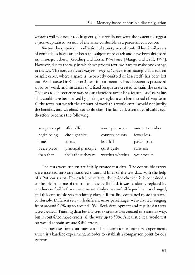
3.4. Memory-based confusible disambiguation
versions will not occur too frequently, but we do not want the system to suggesta (non-)capitalised version of the same confusible as a potential correction.
We test the system on a collection of twenty sets of confusibles. Similar setsof confusibles have earlier been the subject of research and have been discussedin, amongst others, [Golding and Roth, 1996] and [Mangu and Brill, 1997].However, due to the way in which we process text, we have to make one changein the set. The confusible set maybe – may be (which is an example of a run-onor split error, where a space is incorrectly omitted or inserted)) has been leftout. As discussed in Chapter 2, text in our memory-based system is processedword by word, and instances of a fixed length are created to train the system.The two token sequence may be can therefore never be a feature or class value.This could have been solved by placing a single, new token instead of may be inall the texts, but we felt the amount of work this would entail would not justifythe benefits, and we chose not to do this. The full collection of confusible setstherefore becomes the following.
accept except affect effect among between amount number
begin being cite sight site country county fewer less
I me its it’s lead led passed past
peace piece principal principle quiet quite raise rise
than then their there they’re weather whether your you’re
The tests were run on artificially created test data. The confusible errorswere inserted into one hundred thousand lines of the test data with the helpof a Python script. For each line of text, the script checked if it contained aconfusible from one of the confusible sets. If it did, it was randomly replaced byanother confusible from the same set. Only one confusible per line was changed,and this confusible was randomly chosen if the line contained more than oneconfusible. Different sets with different error percentages were created, rangingfrom around 0.6% up to around 10%. Both development and regular data setswere created. Training data for the error variants was created in a similar way,but it contained more errors, all the way up to 30%. A realistic, real world testset would contain around 0.5% errors.
The next section continues with the description of our first experiment,which is a baseline experiment, in order to establish a comparison point for oursystems.
51
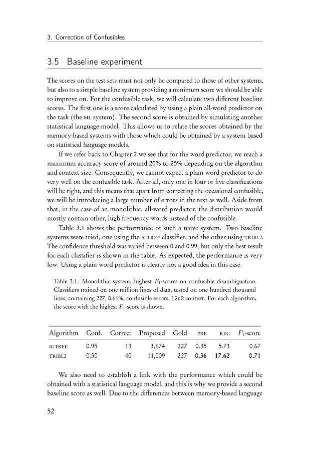
3. Correction of Confusibles
3.5 Baseline experiment
The scores on the test sets must not only be compared to those of other systems,but also to a simple baseline system providing a minimum score we should be ableto improve on. For the confusible task, we will calculate two different baselinescores. The first one is a score calculated by using a plain all-word predictor onthe task (the ml system). The second score is obtained by simulating anotherstatistical language model. This allows us to relate the scores obtained by thememory-based systems with those which could be obtained by a system basedon statistical language models.
If we refer back to Chapter 2 we see that for the word predictor, we reach amaximum accuracy score of around 20% to 25% depending on the algorithmand context size. Consequently, we cannot expect a plain word predictor to dovery well on the confusible task. After all, only one in four or five classificationswill be right, and this means that apart from correcting the occasional confusible,we will be introducing a large number of errors in the text as well. Aside fromthat, in the case of an monolithic, all-word predictor, the distribution wouldmostly contain other, high frequency words instead of the confusible.
Table 3.1 shows the performance of such a naïve system. Two baselinesystems were tried, one using the igtree classifier, and the other using tribl2.The confidence threshold was varied between 0 and 0.99, but only the best resultfor each classifier is shown in the table. As expected, the performance is verylow. Using a plain word predictor is clearly not a good idea in this case.
Table 3.1: Monolithic system, highest F1-scores on confusible disambiguation.Classifiers trained on one million lines of data, tested on one hundred thousandlines, containing 227, 0.61%, confusible errors, l2r2 context. For each algorithm,the score with the highest F1-score is shown.
Algorithm Conf. Correct Proposed Gold pre rec F1-score
igtree 0.95 13 3,674 227 0.35 5.73 0.67tribl2 0.50 40 11,009 227 0.36 17.62 0.71
We also need to establish a link with the performance which could beobtained with a statistical language model, and this is why we provide a secondbaseline score as well. Due to the differences between memory-based language
52
3.5. Baseline experiment
models and statistical language models, and the difficulty of implementing sucha word prediction system in a statistical language model, we have constructed asimulated baseline system. A statistical language model does not readily providea distribution of answers with different frequencies, but could conceivably beused to disambiguate confusibles in the following way. When encountering aconfusible, the probability for the confusible can be estimated from the trigramprobability at that point. The system knows the confusible sets, and can lookup or calculate the probability for the other members in the relevant confusibleset at that point. The confusible which provides the highest probability at thatpoint can be taken to be the correct one.
This was simulated as follows. A classifier was trained using trigrams, oran l2r0 context, and using igtree. This is the classifier which has a back offstrategy comparable to that of a statistical language model. When a confusiblewas encountered, a prediction was made, and the distribution returned wasfiltered on the confusibles in the relevant set. The highest frequency confusiblewas considered to be a possible correction at that point. To provide a bettercomparison with the results in the rest of this chapter, we examine the effect ofthe confidence threshold parameter on the performance.
Running this experiment on the same one hundred thousand line test setcontaining 227 errors yielded the scores listed in Table 3.2. The highest F1-score,34.24, reached is with a confidence of 0.95. This is a reasonable F1-score, witha precision of almost 25 and a recall over 55. The score with a confidencethreshold of 0.50 is equivalent to a system that takes the confusible with thehighest frequency (or probability). With higher confidence levels, the frequencyof the chosen confusible has to be a number of times larger than the others,if present. The confidence value can only go below 0.5 in case there are threeor more elements in the distribution (with two elements, the minimum valueis 0.5). The small difference in the scores between a confidence level of 0 and0.5 is due to a few of the three member confusible sets where the sum of thefrequencies of the two last elements is only slightly lower than the frequency ofthe first element.
In the next section, we turn to the first of the memory-based correctionsystems, the selective monolithic system.
53
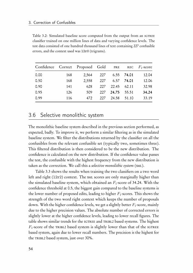
3. Correction of Confusibles
Table 3.2: Simulated baseline score computed from the output from an igtree
classifier trained on one million lines of data and varying confidence levels. Thetest data consisted of one hundred thousand lines of text containing 227 confusibleerrors, and the context used was l2r0 (trigrams).
Confidence Correct Proposed Gold pre rec F1-score
0.00 168 2,564 227 6.55 74.01 12.040.50 168 2,558 227 6.57 74.01 12.060.90 141 628 227 22.45 62.11 32.980.95 126 509 227 24.75 55.51 34.240.99 116 472 227 24.58 51.10 33.19
3.6 Selective monolithic system
The monolithic baseline system described in the previous section performed, asexpected, badly. To improve it, we perform a similar filtering as in the simulatedbaseline system. We filter the distributions returned by the classifier on all theconfusibles from the relevant confusible set (typically two, sometimes three).This filtered distribution is then considered to be the new distribution. Theconfidence is calculated on the new distribution. If the confidence value passesthe test, the confusible with the highest frequency from the new distribution istaken as the correction. We call this a selective monolithic system (sml).
Table 3.3 shows the results when training the two classifiers on a two wordleft and right (l2r2) context. The sml scores are only marginally higher thanthe simulated baseline system, which obtained an F1-score of 34.24. With theconfidence threshold at 0.5, the biggest gain compared to the baseline systems isthe lower number of proposed edits, leading to higher F1-scores. This shows thestrength of the two word right context which keeps the number of proposalsdown. With the higher confidence levels, we get a slightly better F1-score, mainlydue to the higher precision values. The absolute number of corrected errors isslightly lower at the higher confidence levels, leading to lower recall figures. Thetable shows similar trends for the igtree and tribl2 based systems. The highestF1-score of the tribl2 based system is slightly lower than that of the igtreebased system, again due to lower recall numbers. The precision is the highest forthe tribl2 based system, just over 30%.
54
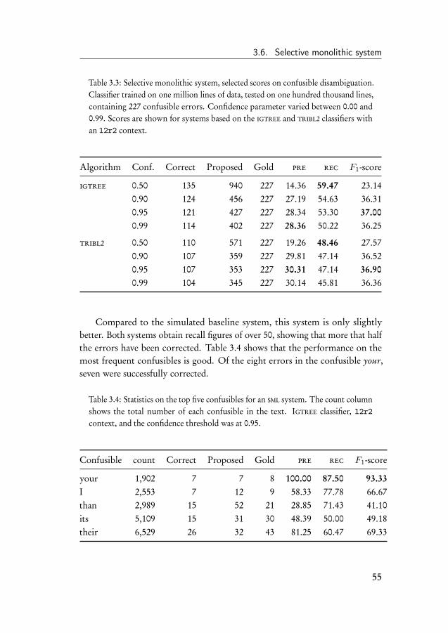
3.6. Selective monolithic system
Table 3.3: Selective monolithic system, selected scores on confusible disambiguation.Classifier trained on one million lines of data, tested on one hundred thousand lines,containing 227 confusible errors. Confidence parameter varied between 0.00 and0.99. Scores are shown for systems based on the igtree and tribl2 classifiers withan l2r2 context.
Algorithm Conf. Correct Proposed Gold pre rec F1-score
igtree 0.50 135 940 227 14.36 59.47 23.140.90 124 456 227 27.19 54.63 36.310.95 121 427 227 28.34 53.30 37.000.99 114 402 227 28.36 50.22 36.25
tribl2 0.50 110 571 227 19.26 48.46 27.570.90 107 359 227 29.81 47.14 36.520.95 107 353 227 30.31 47.14 36.900.99 104 345 227 30.14 45.81 36.36
Compared to the simulated baseline system, this system is only slightlybetter. Both systems obtain recall figures of over 50, showing that more that halfthe errors have been corrected. Table 3.4 shows that the performance on themost frequent confusibles is good. Of the eight errors in the confusible your,seven were successfully corrected.
Table 3.4: Statistics on the top five confusibles for an sml system. The count columnshows the total number of each confusible in the text. Igtree classifier, l2r2context, and the confidence threshold was at 0.95.
Confusible count Correct Proposed Gold pre rec F1-score
your 1,902 7 7 8 100.00 87.50 93.33I 2,553 7 12 9 58.33 77.78 66.67than 2,989 15 52 21 28.85 71.43 41.10its 5,109 15 31 30 48.39 50.00 49.18their 6,529 26 32 43 81.25 60.47 69.33
55
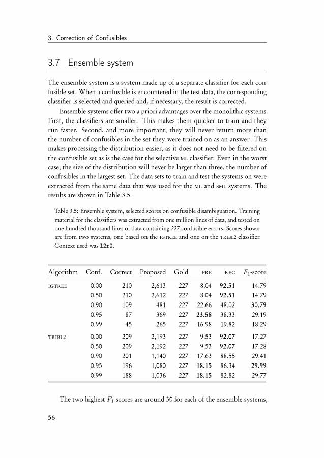
3. Correction of Confusibles
3.7 Ensemble system
The ensemble system is a system made up of a separate classifier for each con-fusible set. When a confusible is encountered in the test data, the correspondingclassifier is selected and queried and, if necessary, the result is corrected.
Ensemble systems offer two a priori advantages over the monolithic systems.First, the classifiers are smaller. This makes them quicker to train and theyrun faster. Second, and more important, they will never return more thanthe number of confusibles in the set they were trained on as an answer. Thismakes processing the distribution easier, as it does not need to be filtered onthe confusible set as is the case for the selective ml classifier. Even in the worstcase, the size of the distribution will never be larger than three, the number ofconfusibles in the largest set. The data sets to train and test the systems on wereextracted from the same data that was used for the ml and sml systems. Theresults are shown in Table 3.5.
Table 3.5: Ensemble system, selected scores on confusible disambiguation. Trainingmaterial for the classifiers was extracted from one million lines of data, and tested onone hundred thousand lines of data containing 227 confusible errors. Scores shownare from two systems, one based on the igtree and one on the tribl2 classifier.Context used was l2r2.
Algorithm Conf. Correct Proposed Gold pre rec F1-score
igtree 0.00 210 2,613 227 8.04 92.51 14.790.50 210 2,612 227 8.04 92.51 14.790.90 109 481 227 22.66 48.02 30.790.95 87 369 227 23.58 38.33 29.190.99 45 265 227 16.98 19.82 18.29
tribl2 0.00 209 2,193 227 9.53 92.07 17.270.50 209 2,192 227 9.53 92.07 17.280.90 201 1,140 227 17.63 88.55 29.410.95 196 1,080 227 18.15 86.34 29.990.99 188 1,036 227 18.15 82.82 29.77
The two highest F1-scores are around 30 for each of the ensemble systems,
56
3.7. Ensemble system
but there is a difference in the absolute numbers. The igtree based systemcorrects 109 confusibles (confidence threshold at 0.90), but the tribl2 basedsystem corrects 196 (at confidence threshold 0.95). This leads to a higher recall,but unfortunately, it proposes more than twice the amount of corrections leadingto a lower precision. Both systems reach the highest scores when the confidencethreshold is above 0.90, but the igtree based system breaks down at the 0.99level. The reason for this is the back off strategy employed by the igtree
algorithm. The classifier stops at the first feature value mismatch. This resultsin distributions which contain more elements with higher frequencies, leadingto a lower confidence. A confidence threshold of 0.99 means that the frequencyof the first element needs to be about a hundred times larger than that of thesecond element for it to be considered a correction. The elements in the igtreedistributions tend to be more evenly distributed than that, and the confidencethreshold is never crossed.
Figure 3.2 illustrates this by showing the distributions returned by igtree
and tribl2. In this example, the confusible there is corrected to their; inboth distributions it is the classification with the highest frequency. The firstline in the diagram shows the relevant instance processed by the systems. Thedistribution returned by the igtree classifier contains three elements, and hasa confidence of 0.77. The tribl2 classifier only returns one element, resultingin a confidence of 1. This particular igtree correction would be ignored at theconfidence levels 0.90 and higher, but the tribl2 correction would not. Note thatthe reverse is also true; the tribl2 classifier can be very confident, but wrong.
Table 3.6 shows the five most frequent confusibles in the test set. Thenumbers are much lower than the corresponding values for the sml system,except for the than and their confusibles, which score much better. In general,the precision values are lower, while the recall values are higher. The table showsthe results from an ensemble system (en) based on a tribl2 classifier.
The ensemble classifiers are trained on individual confusible sets. Table 3.7lists some of the sizes of the training material used to train them. The individualdata sets have all been extracted from one million lines of training data. Thetraining material for a classifier consists of all the instances which have a memberfrom the relevant confusible set in the focus position. That is, if an instancepredicts a member of a set, this instance is added to the training material forthe classifier for that set. To give an idea of the numbers involved, we countedhow often each instance occurred in the individual sets extracted from the data.The instance with the highest frequency is in which is a there in the their –
57
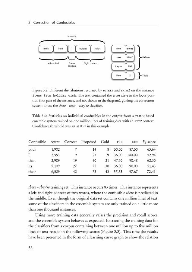
3. Correction of Confusibles
items ? holidayfrom wish
Left context Right contextFocusposition
their
there
they're
IGTree
64688
18910
790
Instance
their Tribl22
Figure 3.2: Different distributions returned by igtree and tribl2 on the instanceitems from holiday wish. The text contained the error there in the focus posi-tion (not part of the instance, and not shown in the diagram), guiding the correctionsystem to use the there – their – they’re classifier.
Table 3.6: Statistics on individual confusibles in the output from a tribl2 basedensemble system trained on one million lines of training data with an l2r2 context.Confidence threshold was set at 0.95 in this example.
Confusible count Correct Proposed Gold pre rec F1-score
your 1,902 7 14 8 50.00 87.50 63.64I 2,553 9 25 9 36.00 100.00 52.94than 2,989 19 40 21 47.50 90.48 62.30its 5,109 27 75 30 36.00 90.00 51.43their 6,529 42 73 43 57.53 97.67 72.41
there – they’re training set. This instance occurs 83 times. This instance representsa left and right context of two words, where the confusible there is predicted inthe middle. Even though the original data set contains one million lines of text,some of the classifiers in the ensemble system are only trained on a little morethan one thousand instances.
Using more training data generally raises the precision and recall scores,and the ensemble system behaves as expected. Extracting the training data forthe classifiers from a corpus containing between one million up to five millionlines of text results in the following scores (Figure 3.3). This time the resultshave been presented in the form of a learning curve graph to show the relation
58
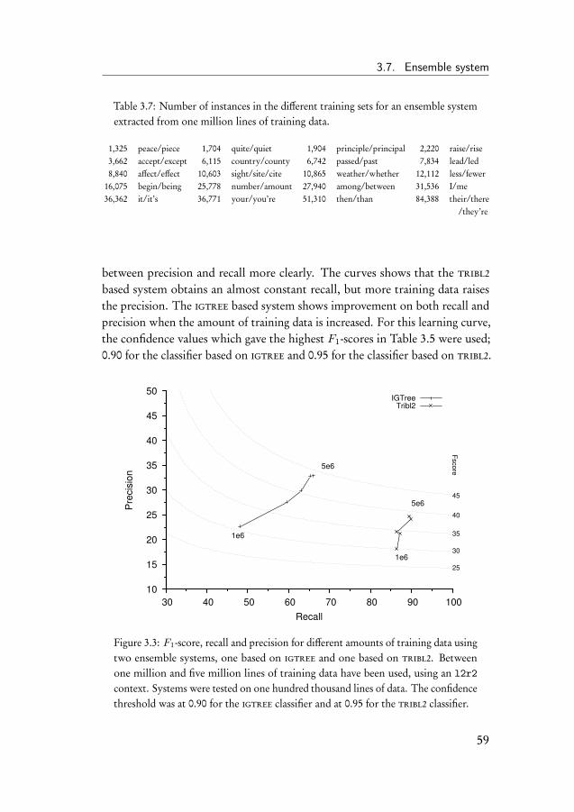
3.7. Ensemble system
Table 3.7: Number of instances in the different training sets for an ensemble systemextracted from one million lines of training data.
1,325 peace/piece 1,704 quite/quiet 1,904 principle/principal 2,220 raise/rise3,662 accept/except 6,115 country/county 6,742 passed/past 7,834 lead/led8,840 affect/effect 10,603 sight/site/cite 10,865 weather/whether 12,112 less/fewer16,075 begin/being 25,778 number/amount 27,940 among/between 31,536 I/me36,362 it/it’s 36,771 your/you’re 51,310 then/than 84,388 their/there
/they’re
between precision and recall more clearly. The curves shows that the tribl2based system obtains an almost constant recall, but more training data raisesthe precision. The igtree based system shows improvement on both recall andprecision when the amount of training data is increased. For this learning curve,the confidence values which gave the highest F1-scores in Table 3.5 were used;0.90 for the classifier based on igtree and 0.95 for the classifier based on tribl2.
10
15
20
25
30
35
40
45
50
30 40 50 60 70 80 90 100
1e6
1e6
5e6
5e6
Fsco
re
25
30
35
40
45
Pre
cis
ion
Recall
IGTree
Tribl2
Figure 3.3: F1-score, recall and precision for different amounts of training data usingtwo ensemble systems, one based on igtree and one based on tribl2. Betweenone million and five million lines of training data have been used, using an l2r2context. Systems were tested on one hundred thousand lines of data. The confidencethreshold was at 0.90 for the igtree classifier and at 0.95 for the tribl2 classifier.
59
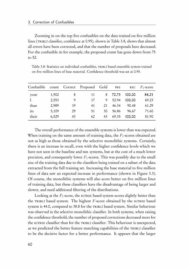
3. Correction of Confusibles
Zooming in on the top five confusibles on the data trained on five millionlines (tribl2 classifier, confidence at 0.95), shown in Table 3.8, shows that almostall errors have been corrected, and that the number of proposals have decreased.For the confusible its for example, the proposed count has gone down from 75to 52.
Table 3.8: Statistics on individual confusibles, tribl2 based ensemble system trainedon five million lines of base material. Confidence threshold was set at 0.95.
Confusible count Correct Proposed Gold pre rec F1-score
your 1,902 8 11 8 72.73 100.00 84.21I 2,553 9 17 9 52.94 100.00 69.23than 2,989 19 41 21 46.34 90.48 61.29its 5,109 29 51 30 56.86 96.67 71.60their 6,529 43 62 43 69.35 100.00 81.90
The overall performance of the ensemble systems is lower than was expected.When training on the same amount of training data, the F1-scores obtained arenot as high as those obtained by the selective monolithic systems. Certainly,there is an increase in recall, even with the higher confidence levels which wehave not seen in the baseline and sml systems, but at the cost of a much lowerprecision, and consequently lower F1-scores. This was possibly due to the smallsize of the training data due to the classifiers being trained on a subset of the dataextracted from the full training set. Increasing the base material to five millionlines of data saw an expected increase in performance (shown in Figure 3.3).Of course, the monolithic systems will also score better on five million linesof training data, but these classifiers have the disadvantage of being larger andslower, and need additional filtering of the distributions.
Looking at the F1-score, the igtree based system scores slightly better thanthe tribl2 based system. The highest F -score obtained by the igtree basedsystem is 44.0, compared to 38.8 for the tribl2 based system. Similar behaviourwas observed in the selective monolithic classifier. In both systems, when raisingthe confidence threshold, the number of proposed corrections decreased more forthe igtree classifier than for the tribl2 classifier. This behaviour is unexpected,as we predicted the better feature matching capabilities of the tribl2 classifierto be the decisive factor for a better performance. It appears that the larger
60
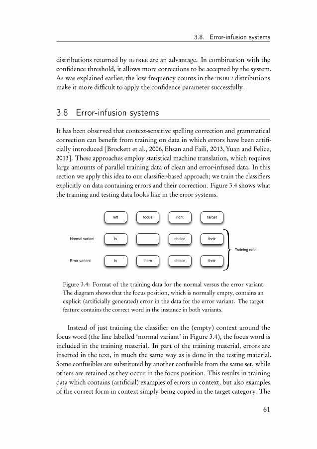
3.8. Error-infusion systems
distributions returned by igtree are an advantage. In combination with theconfidence threshold, it allows more corrections to be accepted by the system.As was explained earlier, the low frequency counts in the tribl2 distributionsmake it more difficult to apply the confidence parameter successfully.
3.8 Error-infusion systems
It has been observed that context-sensitive spelling correction and grammaticalcorrection can benefit from training on data in which errors have been artifi-cially introduced [Brockett et al., 2006,Ehsan and Faili, 2013,Yuan and Felice,2013]. These approaches employ statistical machine translation, which requireslarge amounts of parallel training data of clean and error-infused data. In thissection we apply this idea to our classifier-based approach; we train the classifiersexplicitly on data containing errors and their correction. Figure 3.4 shows whatthe training and testing data looks like in the error systems.
left focus right target
is choice their
is there choice their
Normal variant
Error variant
Training data
Figure 3.4: Format of the training data for the normal versus the error variant.The diagram shows that the focus position, which is normally empty, contains anexplicit (artificially generated) error in the data for the error variant. The targetfeature contains the correct word in the instance in both variants.
Instead of just training the classifier on the (empty) context around thefocus word (the line labelled ‘normal variant’ in Figure 3.4), the focus word isincluded in the training material. In part of the training material, errors areinserted in the text, in much the same way as is done in the testing material.Some confusibles are substituted by another confusible from the same set, whileothers are retained as they occur in the focus position. This results in trainingdata which contains (artificial) examples of errors in context, but also examplesof the correct form in context simply being copied in the target category. The
61

3. Correction of Confusibles
item labelled error variant in Figure 3.4 show an example of the confusible pairthere – their, where their is used instead of there. The idea behind this is that thefocus word feature will guide the classifier towards the right answer. When asimilar error in a similar context is encountered in the text, a match on the errorfeature value and other context feature values should hopefully lead directlyto the right answer. The fact that we use artificially generated errors probablymeans that we lose information which is present in text containing real-worlderrors. It is likely that in reality the distribution of the errors is neither randomnor balanced, and that the level of confusion between the individual confusiblesis skewed. That is, peace might be written as piece in 30% of the error cases, andpiece as peace in the remaining 70%. Due to lack of relevant statistics, the errorswere distributed evenly in the artificial error data. In this data peace would bewritten as piece as often as the reverse.
We introduce a new notation to specify the error context. The string t1will be specified between the normal l (left) and r (right) values. A context oftwo words to the left, two to the right and one error feature will be specified asl2t1r2, and contains five feature values. This is one more than the four featurevalues contained in the l2r2 context used previously.
Figure 3.5 shows several instances from the training data where an errorbetween a two word context to the left and right is shown together with itscorrect form. The error in this example is the word their used instead of there.The first line of the example shows an instance teaching the system that if thetext ‘issued when their is substantial’ is encountered, with the focus word their andthe target word there, their should be corrected into there. On a perfect matchof all the five feature values, this works similar to a look-up function. However,the strength of the tribl2 algorithm means that on a partial match, for exampleon only three of the five features (‘to [mismatch] their is [mismatch]’), the systemwill still suggest there. In this example, the feature value directly to the left ofthe error feature, and the last feature value, do not match. The tribl2 algorithmwould stll match on the second feature value to the left (to), where as igtreewould not. This is shown in the last line of the diagram.
The next two sections show the results of the monolithic and ensembleclassifiers combined with the error data. The parameters and learning algorithmsused will be similar to those described before. The only difference is that theerror data has been added to the training material of the classifiers.
62
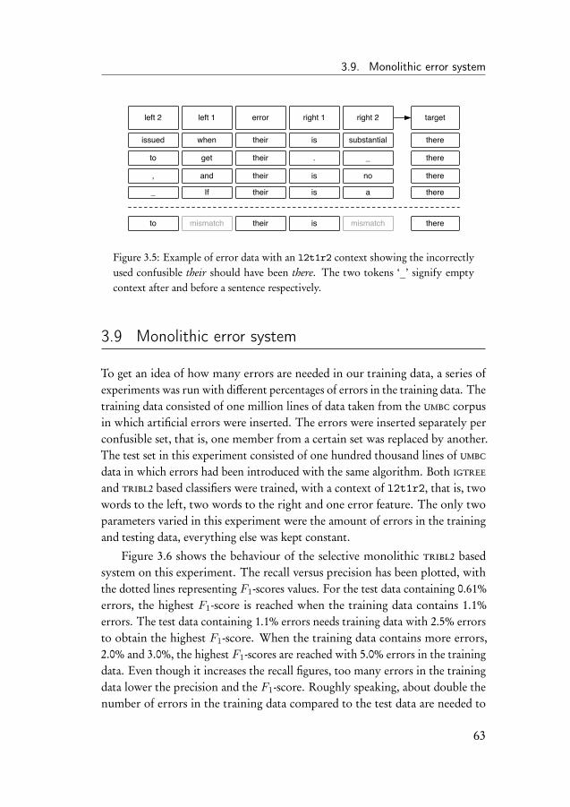
3.9. Monolithic error system
issued is substantialwhen there
to . _get there
, is noand there
_ is aIf there
left 2 right 1 right 2left 1 target
their
their
their
their
error
mismatch is mismatchto theretheir
Figure 3.5: Example of error data with an l2t1r2 context showing the incorrectlyused confusible their should have been there. The two tokens ‘_’ signify emptycontext after and before a sentence respectively.
3.9 Monolithic error system
To get an idea of how many errors are needed in our training data, a series ofexperiments was run with different percentages of errors in the training data. Thetraining data consisted of one million lines of data taken from the umbc corpusin which artificial errors were inserted. The errors were inserted separately perconfusible set, that is, one member from a certain set was replaced by another.The test set in this experiment consisted of one hundred thousand lines of umbcdata in which errors had been introduced with the same algorithm. Both igtree
and tribl2 based classifiers were trained, with a context of l2t1r2, that is, twowords to the left, two words to the right and one error feature. The only twoparameters varied in this experiment were the amount of errors in the trainingand testing data, everything else was kept constant.
Figure 3.6 shows the behaviour of the selective monolithic tribl2 basedsystem on this experiment. The recall versus precision has been plotted, withthe dotted lines representing F1-scores values. For the test data containing 0.61%errors, the highest F1-score is reached when the training data contains 1.1%errors. The test data containing 1.1% errors needs training data with 2.5% errorsto obtain the highest F1-score. When the training data contains more errors,2.0% and 3.0%, the highest F1-scores are reached with 5.0% errors in the trainingdata. Even though it increases the recall figures, too many errors in the trainingdata lower the precision and the F1-score. Roughly speaking, about double thenumber of errors in the training data compared to the test data are needed to
63
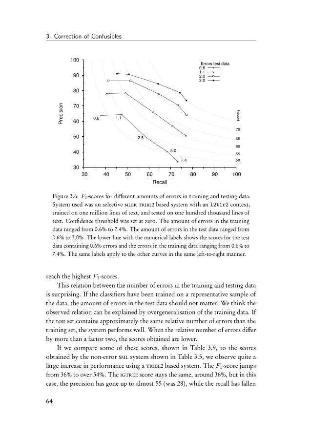
3. Correction of Confusibles
30
40
50
60
70
80
90
100
30 40 50 60 70 80 90 100
Fsco
re
50
55
60
65
70
Pre
cis
ion
Recall
Errors test data
0.6
0.6 1.1
2.5
5.0
7.4
1.1
2.0
3.0
Figure 3.6: F1-scores for different amounts of errors in training and testing data.System used was an selective mler tribl2 based system with an l2t1r2 context,trained on one million lines of text, and tested on one hundred thousand lines oftext. Confidence threshold was set at zero. The amount of errors in the trainingdata ranged from 0.6% to 7.4%. The amount of errors in the test data ranged from0.6% to 3.0%. The lower line with the numerical labels shows the scores for the testdata containing 0.6% errors and the errors in the training data ranging from 0.6% to7.4%. The same labels apply to the other curves in the same left-to-right manner.
reach the highest F1-scores.This relation between the number of errors in the training and testing data
is surprising. If the classifiers have been trained on a representative sample ofthe data, the amount of errors in the test data should not matter. We think theobserved relation can be explained by overgeneralisation of the training data. Ifthe test set contains approximately the same relative number of errors than thetraining set, the system performs well. When the relative number of errors differby more than a factor two, the scores obtained are lower.
If we compare some of these scores, shown in Table 3.9, to the scoresobtained by the non-error sml system shown in Table 3.5, we observe quite alarge increase in performance using a tribl2 based system. The F1-score jumpsfrom 36% to over 54%. The igtree score stays the same, around 36%, but in thiscase, the precision has gone up to almost 55 (was 28), while the recall has fallen
64
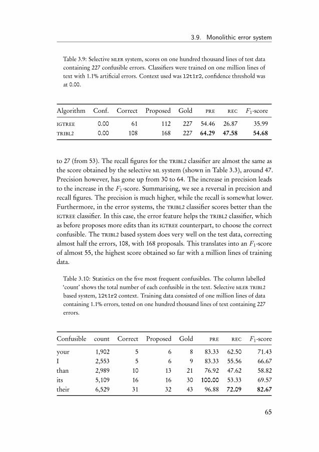
3.9. Monolithic error system
Table 3.9: Selective mler system, scores on one hundred thousand lines of test datacontaining 227 confusible errors. Classifiers were trained on one million lines oftext with 1.1% artificial errors. Context used was l2t1r2, confidence threshold wasat 0.00.
Algorithm Conf. Correct Proposed Gold pre rec F1-score
igtree 0.00 61 112 227 54.46 26.87 35.99tribl2 0.00 108 168 227 64.29 47.58 54.68
to 27 (from 53). The recall figures for the tribl2 classifier are almost the same asthe score obtained by the selective ml system (shown in Table 3.3), around 47.Precision however, has gone up from 30 to 64. The increase in precision leadsto the increase in the F1-score. Summarising, we see a reversal in precision andrecall figures. The precision is much higher, while the recall is somewhat lower.Furthermore, in the error systems, the tribl2 classifier scores better than theigtree classifier. In this case, the error feature helps the tribl2 classifier, whichas before proposes more edits than its igtree counterpart, to choose the correctconfusible. The tribl2 based system does very well on the test data, correctingalmost half the errors, 108, with 168 proposals. This translates into an F1-scoreof almost 55, the highest score obtained so far with a million lines of trainingdata.
Table 3.10: Statistics on the five most frequent confusibles. The column labelled‘count’ shows the total number of each confusible in the text. Selective mler tribl2
based system, l2t1r2 context. Training data consisted of one million lines of datacontaining 1.1% errors, tested on one hundred thousand lines of text containing 227errors.
Confusible count Correct Proposed Gold pre rec F1-score
your 1,902 5 6 8 83.33 62.50 71.43I 2,553 5 6 9 83.33 55.56 66.67than 2,989 10 13 21 76.92 47.62 58.82its 5,109 16 16 30 100.00 53.33 69.57their 6,529 31 32 43 96.88 72.09 82.67
65
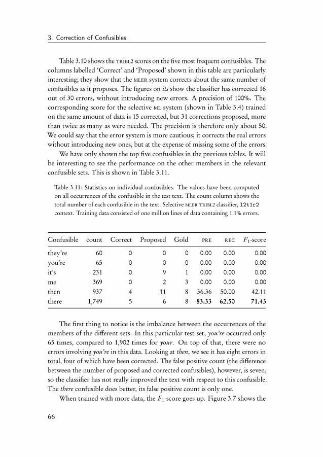
3. Correction of Confusibles
Table 3.10 shows the tribl2 scores on the five most frequent confusibles. Thecolumns labelled ‘Correct’ and ‘Proposed’ shown in this table are particularlyinteresting; they show that the mler system corrects about the same number ofconfusibles as it proposes. The figures on its show the classifier has corrected 16out of 30 errors, without introducing new errors. A precision of 100%. Thecorresponding score for the selective ml system (shown in Table 3.4) trainedon the same amount of data is 15 corrected, but 31 corrections proposed, morethan twice as many as were needed. The precision is therefore only about 50.We could say that the error system is more cautious; it corrects the real errorswithout introducing new ones, but at the expense of missing some of the errors.
We have only shown the top five confusibles in the previous tables. It willbe interesting to see the performance on the other members in the relevantconfusible sets. This is shown in Table 3.11.
Table 3.11: Statistics on individual confusibles. The values have been computedon all occurrences of the confusible in the test text. The count column shows thetotal number of each confusible in the text. Selective mler tribl2 classifier, l2t1r2context. Training data consisted of one million lines of data containing 1.1% errors.
Confusible count Correct Proposed Gold pre rec F1-score
they’re 60 0 0 0 0.00 0.00 0.00you’re 65 0 0 0 0.00 0.00 0.00it’s 231 0 9 1 0.00 0.00 0.00me 369 0 2 3 0.00 0.00 0.00then 937 4 11 8 36.36 50.00 42.11there 1,749 5 6 8 83.33 62.50 71.43
The first thing to notice is the imbalance between the occurrences of themembers of the different sets. In this particular test set, you’re occurred only65 times, compared to 1,902 times for your. On top of that, there were noerrors involving you’re in this data. Looking at then, we see it has eight errors intotal, four of which have been corrected. The false positive count (the differencebetween the number of proposed and corrected confusibles), however, is seven,so the classifier has not really improved the text with respect to this confusible.The there confusible does better, its false positive count is only one.
When trained with more data, the F1-score goes up. Figure 3.7 shows the
66
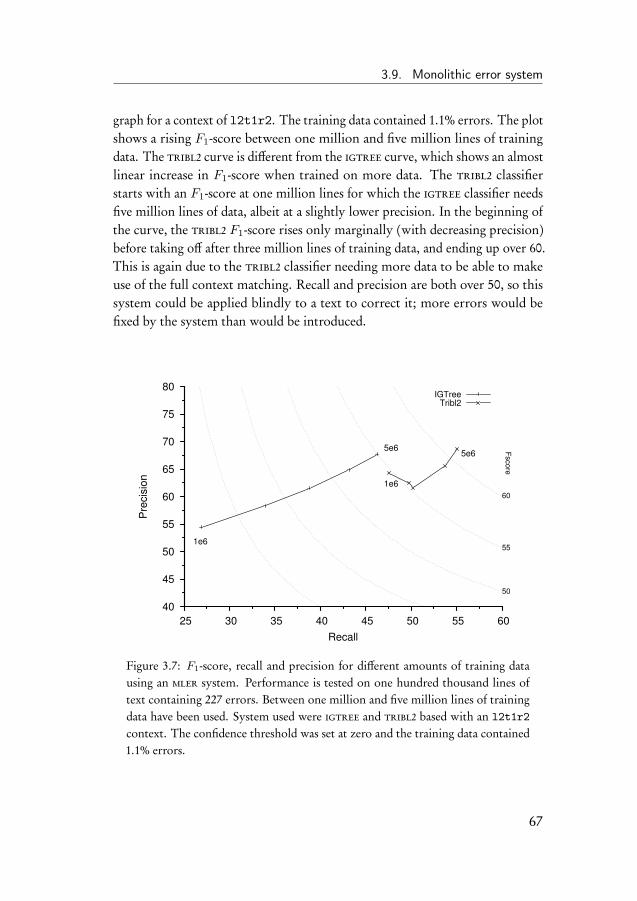
3.9. Monolithic error system
graph for a context of l2t1r2. The training data contained 1.1% errors. The plotshows a rising F1-score between one million and five million lines of trainingdata. The tribl2 curve is different from the igtree curve, which shows an almostlinear increase in F1-score when trained on more data. The tribl2 classifierstarts with an F1-score at one million lines for which the igtree classifier needsfive million lines of data, albeit at a slightly lower precision. In the beginning ofthe curve, the tribl2 F1-score rises only marginally (with decreasing precision)before taking off after three million lines of training data, and ending up over 60.This is again due to the tribl2 classifier needing more data to be able to makeuse of the full context matching. Recall and precision are both over 50, so thissystem could be applied blindly to a text to correct it; more errors would befixed by the system than would be introduced.
40
45
50
55
60
65
70
75
80
25 30 35 40 45 50 55 60
1e6
1e6
5e65e6
Fsco
re
50
55
60
Pre
cis
ion
Recall
IGTree
Tribl2
Figure 3.7: F1-score, recall and precision for different amounts of training datausing an mler system. Performance is tested on one hundred thousand lines oftext containing 227 errors. Between one million and five million lines of trainingdata have been used. System used were igtree and tribl2 based with an l2t1r2context. The confidence threshold was set at zero and the training data contained1.1% errors.
67
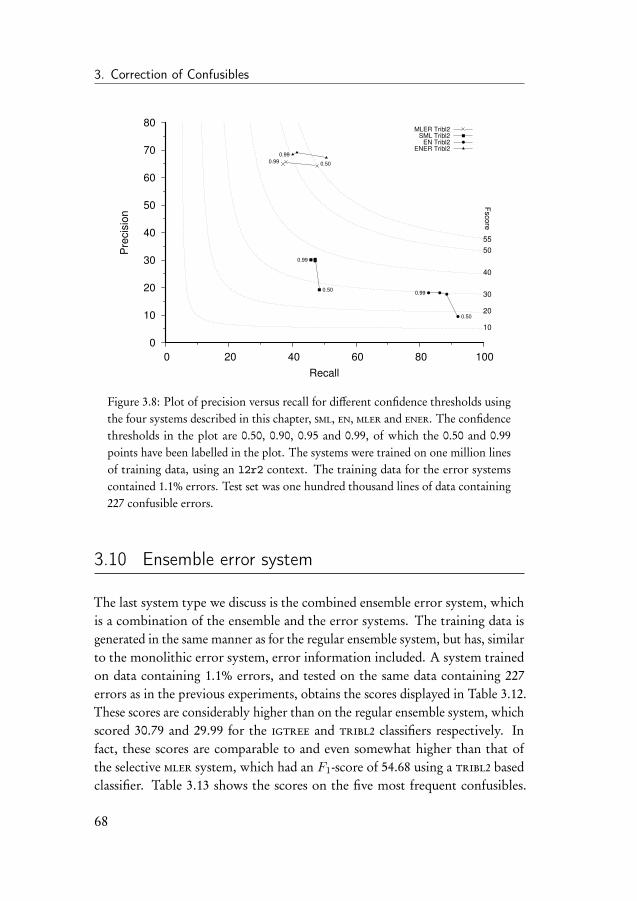
3. Correction of Confusibles
0
10
20
30
40
50
60
70
80
0 20 40 60 80 100
Fsco
re
55
50
40
30
20
10
Pre
cis
ion
Recall
MLER Tribl2
0.500.99
SML Tribl2
0.50
0.99
0.50
0.99
EN Tribl2
ENER Tribl20.99
Figure 3.8: Plot of precision versus recall for different confidence thresholds usingthe four systems described in this chapter, sml, en, mler and ener. The confidencethresholds in the plot are 0.50, 0.90, 0.95 and 0.99, of which the 0.50 and 0.99points have been labelled in the plot. The systems were trained on one million linesof training data, using an l2r2 context. The training data for the error systemscontained 1.1% errors. Test set was one hundred thousand lines of data containing227 confusible errors.
3.10 Ensemble error system
The last system type we discuss is the combined ensemble error system, whichis a combination of the ensemble and the error systems. The training data isgenerated in the same manner as for the regular ensemble system, but has, similarto the monolithic error system, error information included. A system trainedon data containing 1.1% errors, and tested on the same data containing 227errors as in the previous experiments, obtains the scores displayed in Table 3.12.These scores are considerably higher than on the regular ensemble system, whichscored 30.79 and 29.99 for the igtree and tribl2 classifiers respectively. Infact, these scores are comparable to and even somewhat higher than that ofthe selective mler system, which had an F1-score of 54.68 using a tribl2 basedclassifier. Table 3.13 shows the scores on the five most frequent confusibles.
68
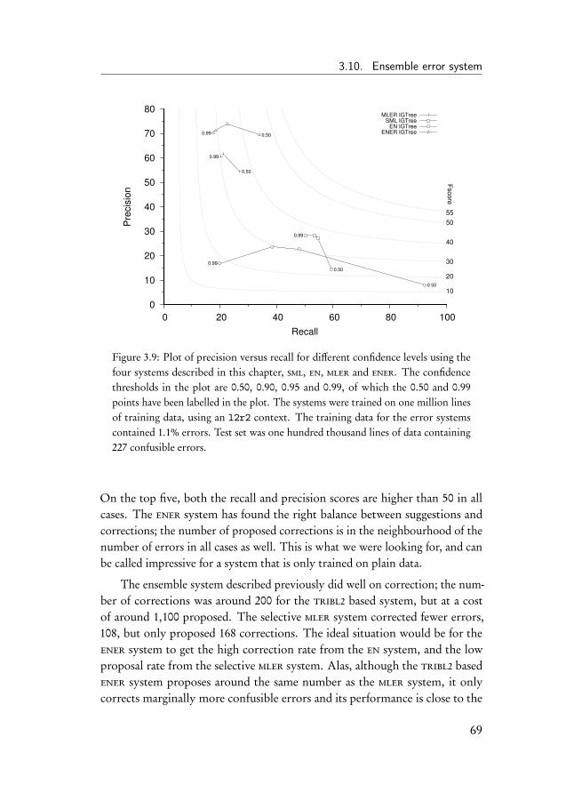
3.10. Ensemble error system
0
10
20
30
40
50
60
70
80
0 20 40 60 80 100
Fsco
re
55
50
40
30
20
10
Pre
cis
ion
Recall
MLER IGTree
0.50
0.99
SML IGTree
0.50
0.99
EN IGTree
0.50
0.99
ENER IGTree0.50
0.99
Figure 3.9: Plot of precision versus recall for different confidence levels using thefour systems described in this chapter, sml, en, mler and ener. The confidencethresholds in the plot are 0.50, 0.90, 0.95 and 0.99, of which the 0.50 and 0.99points have been labelled in the plot. The systems were trained on one million linesof training data, using an l2r2 context. The training data for the error systemscontained 1.1% errors. Test set was one hundred thousand lines of data containing227 confusible errors.
On the top five, both the recall and precision scores are higher than 50 in allcases. The ener system has found the right balance between suggestions andcorrections; the number of proposed corrections is in the neighbourhood of thenumber of errors in all cases as well. This is what we were looking for, and canbe called impressive for a system that is only trained on plain data.
The ensemble system described previously did well on correction; the num-ber of corrections was around 200 for the tribl2 based system, but at a costof around 1,100 proposed. The selective mler system corrected fewer errors,108, but only proposed 168 corrections. The ideal situation would be for theener system to get the high correction rate from the en system, and the lowproposal rate from the selective mler system. Alas, although the tribl2 basedener system proposes around the same number as the mler system, it onlycorrects marginally more confusible errors and its performance is close to the
69
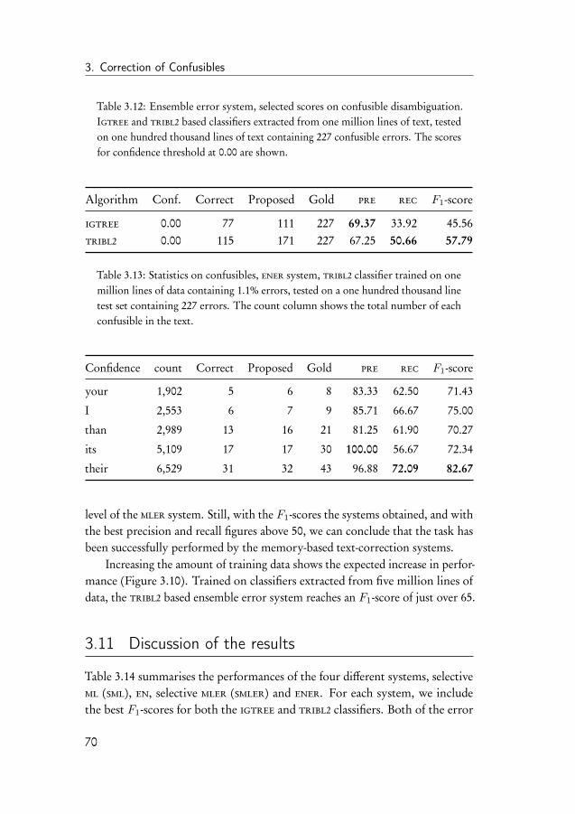
3. Correction of Confusibles
Table 3.12: Ensemble error system, selected scores on confusible disambiguation.Igtree and tribl2 based classifiers extracted from one million lines of text, testedon one hundred thousand lines of text containing 227 confusible errors. The scoresfor confidence threshold at 0.00 are shown.
Algorithm Conf. Correct Proposed Gold pre rec F1-score
igtree 0.00 77 111 227 69.37 33.92 45.56tribl2 0.00 115 171 227 67.25 50.66 57.79
Table 3.13: Statistics on confusibles, ener system, tribl2 classifier trained on onemillion lines of data containing 1.1% errors, tested on a one hundred thousand linetest set containing 227 errors. The count column shows the total number of eachconfusible in the text.
Confidence count Correct Proposed Gold pre rec F1-score
your 1,902 5 6 8 83.33 62.50 71.43
I 2,553 6 7 9 85.71 66.67 75.00
than 2,989 13 16 21 81.25 61.90 70.27
its 5,109 17 17 30 100.00 56.67 72.34
their 6,529 31 32 43 96.88 72.09 82.67
level of the mler system. Still, with the F1-scores the systems obtained, and withthe best precision and recall figures above 50, we can conclude that the task hasbeen successfully performed by the memory-based text-correction systems.
Increasing the amount of training data shows the expected increase in perfor-mance (Figure 3.10). Trained on classifiers extracted from five million lines ofdata, the tribl2 based ensemble error system reaches an F1-score of just over 65.
3.11 Discussion of the results
Table 3.14 summarises the performances of the four different systems, selectiveml (sml), en, selective mler (smler) and ener. For each system, we includethe best F1-scores for both the igtree and tribl2 classifiers. Both of the error
70

3.11. Discussion of the results
50
55
60
65
70
75
80
30 35 40 45 50 55 60 65 70
1e61e6
5e6
5e6 Fsco
re
60
65
Pre
cis
ion
Recall
IGTree
Tribl2
Figure 3.10: F1-score, recall and precision for different amounts of training datausing an ener classifier. Data is tested on one hundred thousand lines of data.Between one million and five million lines of training data have been used. Classifiersused were igtree and tribl2 with an l2t1r2 context. The confidence thresholdwas set at zero and the training data contained 1.1% errors.
systems perform best, with F1-scores over 50 and precision over 60. The enersystem managed to produce a recall over 50 as well, albeit just. All of the resultsare obtained with classifiers trained on one million lines of base material, whichwe considered to be the right amount of material to allow training and testing ina short time whilst at the same time giving an acceptable performance. Increasingthe amount of training material yielded increasing performance, with F1-scoresup to 65 and precision and recall over 60 at a training set size of five millionlines.
Igtree and tribl2 perform differently. The summary results in Table 3.14and Figure 3.8 and Figure 3.9 show the differences in precision and recall of thetwo system types. The graphs also clearly show the superiority of the systemsbased on tribl2 when precision and recall are also taken into consideration.
71
3. Correction of Confusibles
3.11.1 Comparison to other systems
It is difficult to compare these results to other systems due to the differencesin training and test sets, confusible sets, algorithms and evaluation method,et cetera. Many system descriptions in the explored literature report theirperformance in accuracy numbers only, and leave out precision, recall, andF1-score. We collected a number of these accuracy figures from literature onconfusible disambiguation, and show them in Table 3.15. In Table 3.16 weshow the accuracy figures from the four systems described in this chapter. Foreach system, the accuracy for the result giving the best F1-score result has beenreported.
Comparing the accuracy figures in Tables 3.15 and 3.16, we see that theaccuracy scores of the non error systems sml and en are higher on all sets butthen–than. When we compare the accuracy figures relating to the error systemssmler and ener, shown in Table 3.16, to the figures in Table 3.17, we see that thememory-based systems obtain the highest accuracy numbers on every confusibleset.
It should be stressed again that even though the memory-based systems showhigher accuracy figures, it is hard to draw any firm conclusions on the relativeperformance of the different systems. For that we would need similar statisticson the number of proposed corrections and corrected errors for all the systems,information which was not available to us.
3.12 Conclusion
We have compared several confusible disambiguation systems based around asimple memory-based classifier. We have shown that introducing artificial errorsin the training data leads to an substantial increase in performance. Four differentsystem types were tried: a selective monolithic, all-word predictor (sml), and anerror variant of the sml system (smler), an ensemble system (en), and finally,the ensemble error system (ener).
The performance of the selective monolithic, all-word predictor, confusibledisambiguation system went from good to better in the system trained on errorinfused data. The F1-scores went from 37 to almost 55 for the system based onthe tribl2 classifier. The ensemble variant obtained an F1-score of around 30 onthe same task. The ensemble error system reached the highest F1-scores, up toalmost 58. All these figures are on systems trained on one million lines of plain
72
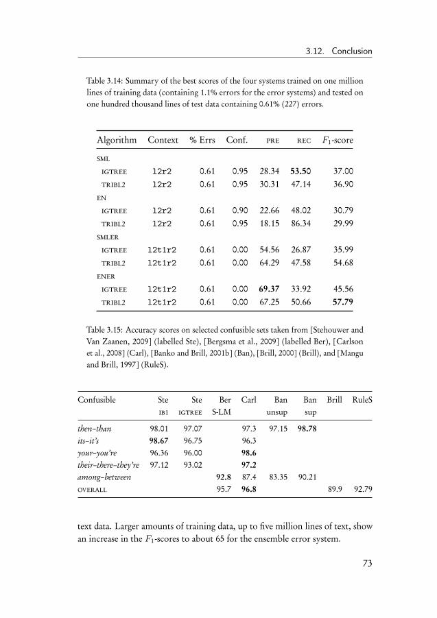
3.12. Conclusion
Table 3.14: Summary of the best scores of the four systems trained on one millionlines of training data (containing 1.1% errors for the error systems) and tested onone hundred thousand lines of test data containing 0.61% (227) errors.
Algorithm Context % Errs Conf. pre rec F1-score
sml
igtree l2r2 0.61 0.95 28.34 53.50 37.00tribl2 l2r2 0.61 0.95 30.31 47.14 36.90
en
igtree l2r2 0.61 0.90 22.66 48.02 30.79tribl2 l2r2 0.61 0.95 18.15 86.34 29.99
smler
igtree l2t1r2 0.61 0.00 54.56 26.87 35.99tribl2 l2t1r2 0.61 0.00 64.29 47.58 54.68
ener
igtree l2t1r2 0.61 0.00 69.37 33.92 45.56tribl2 l2t1r2 0.61 0.00 67.25 50.66 57.79
Table 3.15: Accuracy scores on selected confusible sets taken from [Stehouwer andVan Zaanen, 2009] (labelled Ste), [Bergsma et al., 2009] (labelled Ber), [Carlsonet al., 2008] (Carl), [Banko and Brill, 2001b] (Ban), [Brill, 2000] (Brill), and [Manguand Brill, 1997] (RuleS).
Confusible Ste Ste Ber Carl Ban Ban Brill RuleSib1 igtree S-LM unsup sup
then–than 98.01 97.07 97.3 97.15 98.78its–it’s 98.67 96.75 96.3your–you’re 96.36 96.00 98.6their–there–they’re 97.12 93.02 97.2among–between 92.8 87.4 83.35 90.21overall 95.7 96.8 89.9 92.79
text data. Larger amounts of training data, up to five million lines of text, showan increase in the F1-scores to about 65 for the ensemble error system.
73
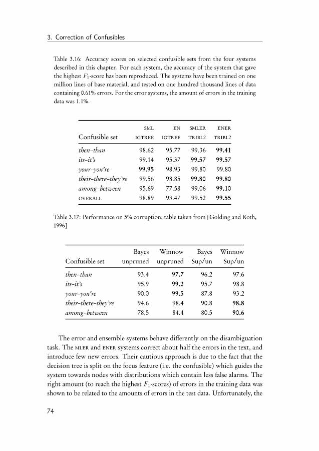
3. Correction of Confusibles
Table 3.16: Accuracy scores on selected confusible sets from the four systemsdescribed in this chapter. For each system, the accuracy of the system that gavethe highest F1-score has been reproduced. The systems have been trained on onemillion lines of base material, and tested on one hundred thousand lines of datacontaining 0.61% errors. For the error systems, the amount of errors in the trainingdata was 1.1%.
sml en smler ener
Confusible set igtree igtree tribl2 tribl2
then–than 98.62 95.77 99.36 99.41its–it’s 99.14 95.37 99.57 99.57your–you’re 99.95 98.93 99.80 99.80their–there–they’re 99.56 98.85 99.80 99.80among–between 95.69 77.58 99.06 99.10overall 98.89 93.47 99.52 99.55
Table 3.17: Performance on 5% corruption, table taken from [Golding and Roth,1996]
Bayes Winnow Bayes WinnowConfusible set unpruned unpruned Sup/un Sup/un
then–than 93.4 97.7 96.2 97.6its–it’s 95.9 99.2 95.7 98.8your–you’re 90.0 99.5 87.8 93.2their–there–they’re 94.6 98.4 90.8 98.8among–between 78.5 84.4 80.5 90.6
The error and ensemble systems behave differently on the disambiguationtask. The mler and ener systems correct about half the errors in the text, andintroduce few new errors. Their cautious approach is due to the fact that thedecision tree is split on the focus feature (i.e. the confusible) which guides thesystem towards nodes with distributions which contain less false alarms. Theright amount (to reach the highest F1-scores) of errors in the training data wasshown to be related to the amounts of errors in the test data. Unfortunately, the
74
3.12. Conclusion
amount of errors in the test data is not known in advance, but about doublethat amount of errors in the training data seemed to give the best performance.Our test data contained 0.6% errors, and the best performance was reached bysystems trained on data containing 1.1% errors.
The fact that the ener system obtains slightly higher precision and recallfigures than the mler system is most likely due to the fact the each of theindividual decision trees can have its own set of feature weights and feature orderspecifically tailored for the confusible in question.
The plain ensemble system on the other hand, is a rather eager system. Itcorrects almost all errors, but introduces a number of extra errors in the text aswell. Precision scores attained by the system are the lowest of the four systemtypes tested. The selective monolithic system did better than the ensemblesystem, but it too was overly eager, and also generated too many correctionscompared to what was needed.
In the end, the ener system trained on five million lines of data reachedprecision, recall and F1-scores which were all over 50. This means that thissystem could be applied blindly to a text without intervention from the user,and the text would contain fewer confusible errors. This is an encouraging result,and it shows that memory-based confusible disambiguation works.
75

4Substitution Errors in Determiners
and Prepositions
4.1 Introduction
In this chapter we show how the ideas introduced in the previous chapter can beextended from a confusible set of several pairs and triplets to two larger classes ofwords. The two classes treated in this chapter are determiners and prepositions.
Determiners are words that precede nouns and noun phrases, and determinethe sort of reference they have in relation to their context. Common Englishdeterminers are the, a or this. Prepositions are words which tell when, where orhow something occurred as well as specify position in place and time. Commonprepositions are in, with or by. The full list of determiners and prepositionstreated in this chapter will be detailed later.
Confusible errors with determiners and prepositions constitute interestingclasses of problems, especially for students whose mother tongue is not English.Prepositions are especially notorious in this respect, and their unpredictablebehaviour poses problems for most foreign speakers [De Felice and Pulman,2008, Bitchener et al., 2005]. These difficulties are caused by a number of fac-tors, of which we mention three. First, most prepositions have several differentfunctions. The preposition at, for example, can be use in the following ways,denoting time, place, or situation.
They stopped at a small station.The wind is cooler at night.
77
4. Substitution Errors in Determiners and Prepositions
Driving a at 30 kmph.He looked at him.
Second, there is no logical way to choose the right proposition, for example:after the adjective available, a number of different prepositions are possible:
Tickets are available from the box office.Not enough information was available to us.No figures are available for the number of items produced.There are hardly any jobs available in the area.
Third, different prepositions change the meaning of an otherwise similarsentence:
He looked at him.He looked for him.He looked after him.He looked through him.
Determiners and articles are considered to be slightly easier to use dependingon the mother tongue of the speaker [Lee and Seneff, 2008], but for foreignspeakers, it can be difficult to know when to use for example many, every, orfew, and some native speakers of for example Russian are known to leave outdeterminers all together when speaking English.
The determiner, article and preposition classes are closed, that is, theycontain a fixed number of members. They also occur frequently, meaning theyoften make up a large part of all the errors made, which in its turn means that agood correction system should be able fix a substantial number of errors in atext.
One of the goals of this thesis is to determine the limits of memory-basedtext correction. The determiner and preposition task is more complex than theconfusible task of the previous chapter in two ways. The first is that it makes useof larger classes, containing dozens of elements instead of only two or three. Thesecond is that there are three error types instead of only one. In the previoustask, a confusible could only be replaced by another one. In the case of thedeterminers and prepositions, words can also be omitted (called an omissionerror) or unnecessarily inserted (called a insertion error).
78
4.2. Related work
To be able to correctly determine the limits of memory-based text correction,we have chosen to introduce the new classes in this chapter, but only apply themto substitution errors. The other two error types, omission and insertion, willbe added in Chapter 5. The determiner class is a combination of determinersand articles, but will be referred to as the determiner class.
This chapter grew out of the work done for the hoo-2012 shared task [Daleet al., 2012]. A description of that system and a summary of the results will begiven in the next chapter.
4.2 Related work
There is a considerable amount of related research on the subject of correctingdeterminer and preposition errors. Even though the full correction task will notbe discussed until the next chapter, we already present an overview discussingthe most notable work and results now, and we take a special interest in the errorstatistics contained in the research. The reason for this is we use training andtesting data which have been infused with artificially created errors, as introducedin the previous chapter. The statistics on the errors are necessary to determinehow many errors of each kind, and in which proportions, are typically presentin English language texts.
We start by reviewing the oldest work, which was carried out already in theeighties and nineties of the previous century. Dalgish [Dalgish, 1985] presents astudy of about 3,000 sentences written by non-native English speakers, mostlyChinese, Spanish, Russian and Korean esl
1 students. The study analyses thekinds of errors made in the texts, focusing on prepositions, subject-verb agree-ment, part-of-speech confusibles, articles, verb tenses, et cetera. For prepositions,error counts are presented in Table 4.1.
These counts, and statistics on other errors, are used to create software totrain esl students to write correctly. The software presents sentences with errorsto students for them to correct and measures their performance. The errorspresented are typical for those made by people with the student’s mother tongue.An evaluation of the system is not given.
In [Atwell, 1987], a system named claws (Constituent Likelihood AutomaticWord-tagging System) is described which is built around a first order Markovmodel language model. This system is modified to detect grammatical errors by
1English as Second Language
79
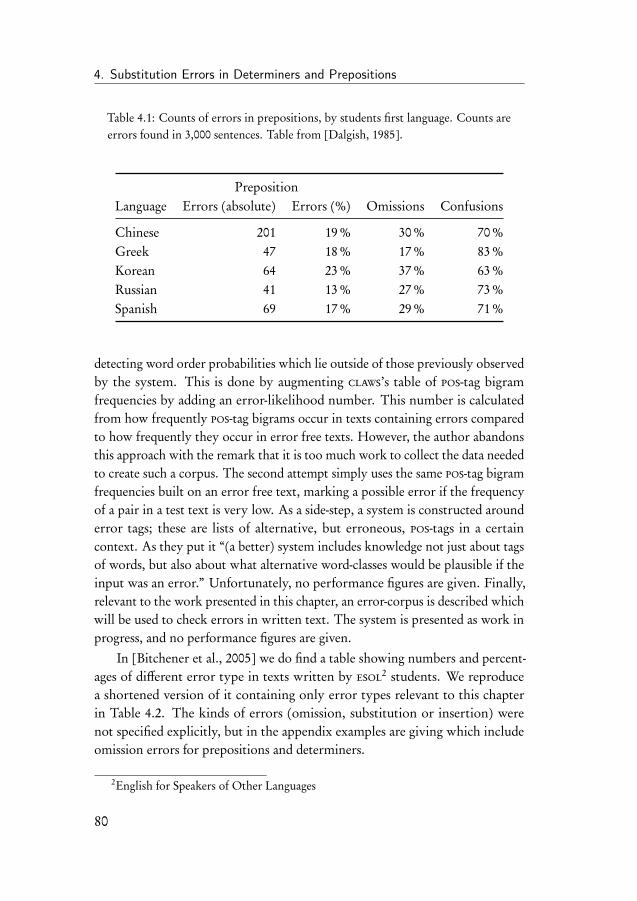
4. Substitution Errors in Determiners and Prepositions
Table 4.1: Counts of errors in prepositions, by students first language. Counts areerrors found in 3,000 sentences. Table from [Dalgish, 1985].
PrepositionLanguage Errors (absolute) Errors (%) Omissions Confusions
Chinese 201 19% 30% 70%Greek 47 18% 17% 83%Korean 64 23% 37% 63%Russian 41 13% 27% 73%Spanish 69 17% 29% 71%
detecting word order probabilities which lie outside of those previously observedby the system. This is done by augmenting claws’s table of pos-tag bigramfrequencies by adding an error-likelihood number. This number is calculatedfrom how frequently pos-tag bigrams occur in texts containing errors comparedto how frequently they occur in error free texts. However, the author abandonsthis approach with the remark that it is too much work to collect the data neededto create such a corpus. The second attempt simply uses the same pos-tag bigramfrequencies built on an error free text, marking a possible error if the frequencyof a pair in a test text is very low. As a side-step, a system is constructed arounderror tags; these are lists of alternative, but erroneous, pos-tags in a certaincontext. As they put it “(a better) system includes knowledge not just about tagsof words, but also about what alternative word-classes would be plausible if theinput was an error.” Unfortunately, no performance figures are given. Finally,relevant to the work presented in this chapter, an error-corpus is described whichwill be used to check errors in written text. The system is presented as work inprogress, and no performance figures are given.
In [Bitchener et al., 2005] we do find a table showing numbers and percent-ages of different error type in texts written by esol
2 students. We reproducea shortened version of it containing only error types relevant to this chapterin Table 4.2. The kinds of errors (omission, substitution or insertion) werenot specified explicitly, but in the appendix examples are giving which includeomission errors for prepositions and determiners.
2English for Speakers of Other Languages
80
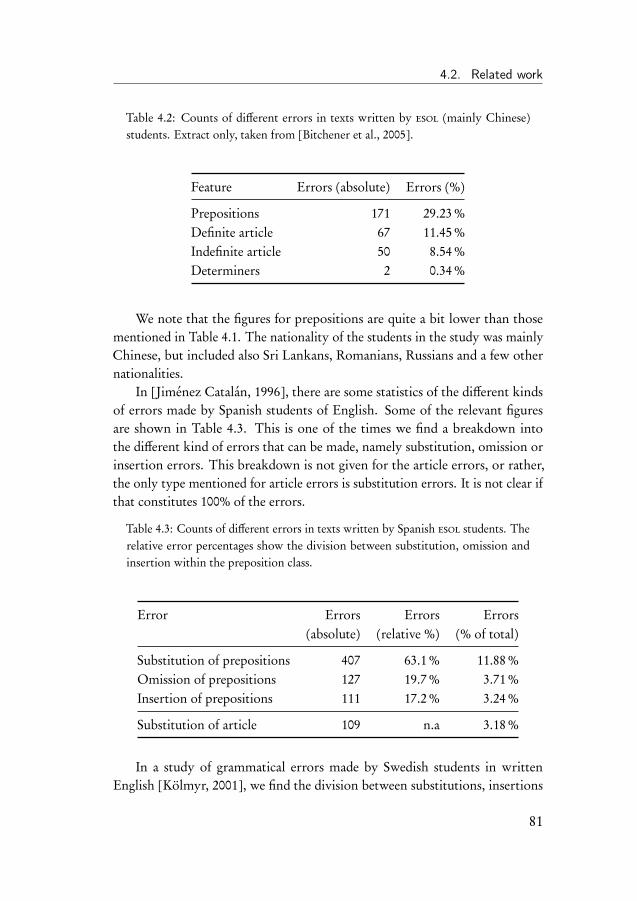
4.2. Related work
Table 4.2: Counts of different errors in texts written by esol (mainly Chinese)students. Extract only, taken from [Bitchener et al., 2005].
Feature Errors (absolute) Errors (%)
Prepositions 171 29.23%Definite article 67 11.45%Indefinite article 50 8.54%Determiners 2 0.34%
We note that the figures for prepositions are quite a bit lower than thosementioned in Table 4.1. The nationality of the students in the study was mainlyChinese, but included also Sri Lankans, Romanians, Russians and a few othernationalities.
In [Jiménez Catalán, 1996], there are some statistics of the different kindsof errors made by Spanish students of English. Some of the relevant figuresare shown in Table 4.3. This is one of the times we find a breakdown intothe different kind of errors that can be made, namely substitution, omission orinsertion errors. This breakdown is not given for the article errors, or rather,the only type mentioned for article errors is substitution errors. It is not clear ifthat constitutes 100% of the errors.
Table 4.3: Counts of different errors in texts written by Spanish esol students. Therelative error percentages show the division between substitution, omission andinsertion within the preposition class.
Error Errors Errors Errors(absolute) (relative %) (% of total)
Substitution of prepositions 407 63.1% 11.88%Omission of prepositions 127 19.7% 3.71%Insertion of prepositions 111 17.2% 3.24%
Substitution of article 109 n.a 3.18%
In a study of grammatical errors made by Swedish students in writtenEnglish [Kölmyr, 2001], we find the division between substitutions, insertions
81
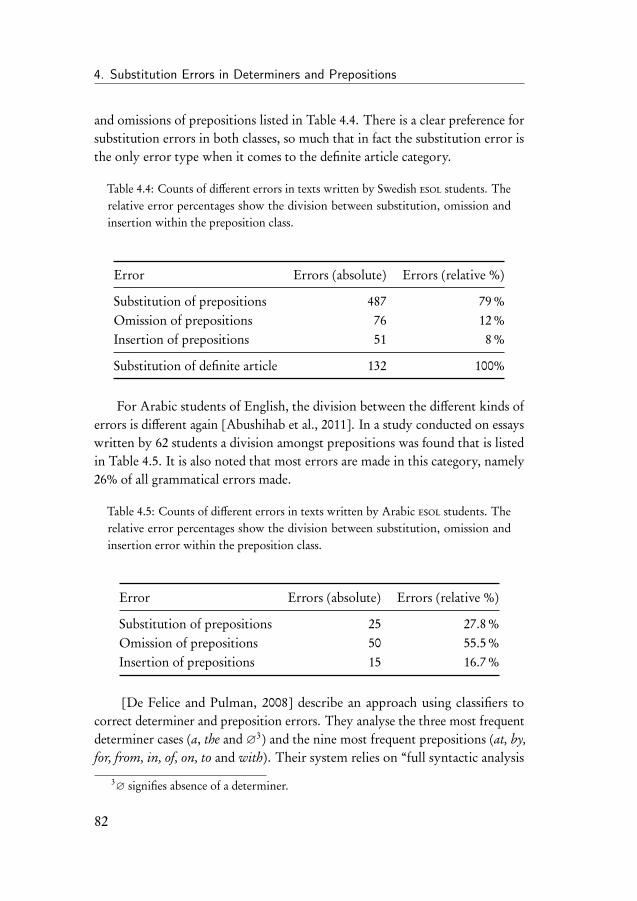
4. Substitution Errors in Determiners and Prepositions
and omissions of prepositions listed in Table 4.4. There is a clear preference forsubstitution errors in both classes, so much that in fact the substitution error isthe only error type when it comes to the definite article category.
Table 4.4: Counts of different errors in texts written by Swedish esol students. Therelative error percentages show the division between substitution, omission andinsertion within the preposition class.
Error Errors (absolute) Errors (relative %)
Substitution of prepositions 487 79%Omission of prepositions 76 12%Insertion of prepositions 51 8%
Substitution of definite article 132 100%
For Arabic students of English, the division between the different kinds oferrors is different again [Abushihab et al., 2011]. In a study conducted on essayswritten by 62 students a division amongst prepositions was found that is listedin Table 4.5. It is also noted that most errors are made in this category, namely26% of all grammatical errors made.
Table 4.5: Counts of different errors in texts written by Arabic esol students. Therelative error percentages show the division between substitution, omission andinsertion error within the preposition class.
Error Errors (absolute) Errors (relative %)
Substitution of prepositions 25 27.8%Omission of prepositions 50 55.5%Insertion of prepositions 15 16.7%
[De Felice and Pulman, 2008] describe an approach using classifiers tocorrect determiner and preposition errors. They analyse the three most frequentdeterminer cases (a, the and ∅3 ) and the nine most frequent prepositions (at, by,for, from, in, of, on, to and with). Their system relies on “full syntactic analysis
3∅ signifies absence of a determiner.
82
4.2. Related work
of data”, where data in this case refers to the bnc corpus. Their system scores70.06% accuracy on predicting prepositions when tested on a held-out part ofthe bnc training corpus. Note that this is data which is presumed to be error free.For the determiners, this score is 92.15%. They note a strong correlation betweenthe size of the training data and the performance on determiners. This definitecorrelation was absent in the case of the prepositions (although it was present forsome of the prepositions, like of and to). Their system was also evaluated on theCambridge Learner Corpus (clc). Here it scored 68% accuracy on recognisingincorrect prepositions, but they point out that a correct preposition was onlysuggested in 51.5% of these cases. The performance for the determiners onthe clc data is comparable to that on the bnc, 92.2%, and they observe thereare markedly fewer false alarms compared to the prepositions. However, ondetecting incorrect determiners, the recall is below ten percent. Finally, it ismentioned that the most frequent error type for determiners is omission of adeterminer where one is required, but that their model does not do well on thattask.
[Gamon, 2010] describes an error correction system combining a languagemodel and an error specific classifier. This meta-classifier is trained on datacontaining error annotations and optimises the output from the language modeland the classifier. The error correction is restricted to articles and prepositions,but only the top twelve most frequent prepositions (at, on, for, since, with, to, by,about, from, of and as) and three determiners; the, a and an. Gamon also useswhat he calls a presence-classifier (what we will call a positive –negative classifierin the next chapter) to determine the presence of a word of a certain category.Similar to our system, a choice-classifier is used to choose the right confusiblewhen the presence classifier gives a positive signal. The choice-classifier is ourword predictor. As we will show later in this and the next chapters, using apresence and a choice classifier gives rise to six possible operations (three for eachof the two classes); insertion (a word not present in the text), deletion (presentin the text, but unwanted) and substitution (present in the text, but wrong). Theclassifiers in this particular system are only trained on the three highest-scoringoperations of these six. The language model and error specific classifiers aretrained on data that is considered to be error free. The meta-classifier is trainedon suggestions from these classifiers on texts from the clc, containing errors andcorrections. Results are presented for a manual evaluation of the output. Theevaluation has been done manually to be able to sort them into seven categories.These range from a correct suggestion via several forms of alternative suggestions,
83
4. Substitution Errors in Determiners and Prepositions
to several grades of bad suggestions, with ‘the introduction of a new error’ atthe bottom. On prepositions, the system achieves a precision of 32.87% if onlycorrect suggestions are counted. For articles, this figure is 33.34%.
[Yi et al., 2008] describe a system that queries the web to get frequencycounts to identify and suggest corrections for writing errors made by esol
students. Their system obtains a 41% recall figure on determiner usage errors,and of the suggested corrections, 62% are correct.
In [Foster and Andersen, 2009], automatically generated error data is usedin detecting grammatical errors. Their system is trained to determine whethera sentence is grammatical or not, and to detect specific errors, like determinerand preposition errors. Their view on using error data in training is that, ingeneral, including negative evidence leads to more accurate classifiers. As theyput it, positive examples are necessary to detect correct usage, negative examplesare needed to detect errors. They also note the lack of error data that is freelyavailable and suggest generating artificial error data. This data, they argue, hasto have a similar statistical nature to real error data, an argument which is alsovoiced by [Wagner et al., 2009]. Artificially generating errors has the addedadvantage that the types of errors generated will occur in multiple contexts, evencontexts that have hitherto been unobserved (although care should be taken togenerate naturally occurring errors). They present a computer program called‘generrate’ which implements these ideas.
In [Han et al., 2010] a preposition correction system is described that istrained and tested on English essays written by Korean students of the Chung-dahm Institute. The system is optimised for precision as opposed to recall, andon a preposition substitution error detection task scores a precision of 93.3% anda recall of 14.8%. For insertion errors, the error detection scores are a precisionof 100% and a recall of 4.9%. The precision on the detection of omission errorsis 83.3%. The error correction scores for substitution errors are 81.7% precisionand 13.2% recall. For insertion correction the precision and recall numbers are81.7% and 13.2% respectively. No figures are given for correction of omissions.
The hoo-2012 shared task focused on the detection and correction of deter-miner and preposition errors [Dale et al., 2012]. It provided the opportunityto train and test a correction system on real-world data, and compare the re-sults with other systems on the same task. It provided training material withannotated errors, some of the statistics are shown in Table 4.6.
84
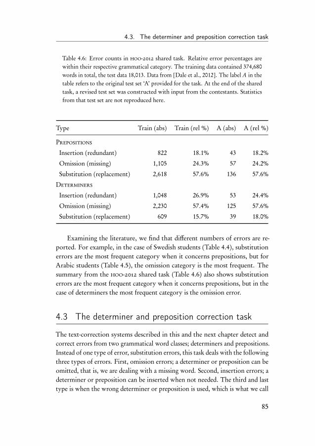
4.3. The determiner and preposition correction task
Table 4.6: Error counts in hoo-2012 shared task. Relative error percentages arewithin their respective grammatical category. The training data contained 374,680words in total, the test data 18,013. Data from [Dale et al., 2012]. The label A in thetable refers to the original test set ‘A’ provided for the task. At the end of the sharedtask, a revised test set was constructed with input from the contestants. Statisticsfrom that test set are not reproduced here.
Type Train (abs) Train (rel %) A (abs) A (rel %)
Prepositions
Insertion (redundant) 822 18.1% 43 18.2%
Omission (missing) 1,105 24.3% 57 24.2%
Substitution (replacement) 2,618 57.6% 136 57.6%
Determiners
Insertion (redundant) 1,048 26.9% 53 24.4%
Omission (missing) 2,230 57.4% 125 57.6%
Substitution (replacement) 609 15.7% 39 18.0%
Examining the literature, we find that different numbers of errors are re-ported. For example, in the case of Swedish students (Table 4.4), substitutionerrors are the most frequent category when it concerns prepositions, but forArabic students (Table 4.5), the omission category is the most frequent. Thesummary from the hoo-2012 shared task (Table 4.6) also shows substitutionerrors are the most frequent category when it concerns prepositions, but in thecase of determiners the most frequent category is the omission error.
4.3 The determiner and preposition correction task
The text-correction systems described in this and the next chapter detect andcorrect errors from two grammatical word classes; determiners and prepositions.Instead of one type of error, substitution errors, this task deals with the followingthree types of errors. First, omission errors; a determiner or preposition can beomitted, that is, we are dealing with a missing word. Second, insertion errors; adeterminer or preposition can be inserted when not needed. The third and lasttype is when the wrong determiner or preposition is used, which is what we call
85
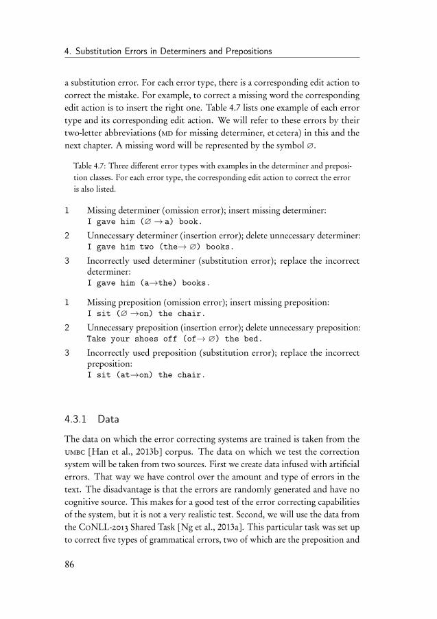
4. Substitution Errors in Determiners and Prepositions
a substitution error. For each error type, there is a corresponding edit action tocorrect the mistake. For example, to correct a missing word the correspondingedit action is to insert the right one. Table 4.7 lists one example of each errortype and its corresponding edit action. We will refer to these errors by theirtwo-letter abbreviations (md for missing determiner, et cetera) in this and thenext chapter. A missing word will be represented by the symbol ∅.
Table 4.7: Three different error types with examples in the determiner and preposi-tion classes. For each error type, the corresponding edit action to correct the erroris also listed.
1 Missing determiner (omission error); insert missing determiner:I gave him (∅→ a) book.
2 Unnecessary determiner (insertion error); delete unnecessary determiner:I gave him two (the→ ∅) books.
3 Incorrectly used determiner (substitution error); replace the incorrectdeterminer:I gave him (a→the) books.
1 Missing preposition (omission error); insert missing preposition:I sit (∅→on) the chair.
2 Unnecessary preposition (insertion error); delete unnecessary preposition:Take your shoes off (of→ ∅) the bed.
3 Incorrectly used preposition (substitution error); replace the incorrectpreposition:I sit (at→on) the chair.
4.3.1 Data
The data on which the error correcting systems are trained is taken from theumbc [Han et al., 2013b] corpus. The data on which we test the correctionsystem will be taken from two sources. First we create data infused with artificialerrors. That way we have control over the amount and type of errors in thetext. The disadvantage is that the errors are randomly generated and have nocognitive source. This makes for a good test of the error correcting capabilitiesof the system, but it is not a very realistic test. Second, we will use the data fromthe CoNLL-2013 Shared Task [Ng et al., 2013a]. This particular task was set upto correct five types of grammatical errors, two of which are the preposition and
86
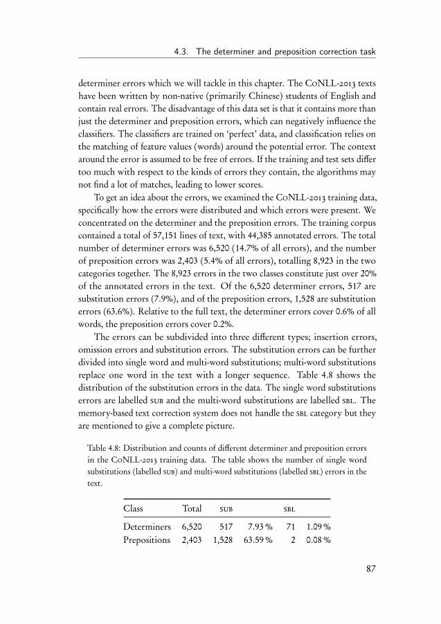
4.3. The determiner and preposition correction task
determiner errors which we will tackle in this chapter. The CoNLL-2013 textshave been written by non-native (primarily Chinese) students of English andcontain real errors. The disadvantage of this data set is that it contains more thanjust the determiner and preposition errors, which can negatively influence theclassifiers. The classifiers are trained on ‘perfect’ data, and classification relies onthe matching of feature values (words) around the potential error. The contextaround the error is assumed to be free of errors. If the training and test sets differtoo much with respect to the kinds of errors they contain, the algorithms maynot find a lot of matches, leading to lower scores.
To get an idea about the errors, we examined the CoNLL-2013 training data,specifically how the errors were distributed and which errors were present. Weconcentrated on the determiner and the preposition errors. The training corpuscontained a total of 57,151 lines of text, with 44,385 annotated errors. The totalnumber of determiner errors was 6,520 (14.7% of all errors), and the numberof preposition errors was 2,403 (5.4% of all errors), totalling 8,923 in the twocategories together. The 8,923 errors in the two classes constitute just over 20%of the annotated errors in the text. Of the 6,520 determiner errors, 517 aresubstitution errors (7.9%), and of the preposition errors, 1,528 are substitutionerrors (63.6%). Relative to the full text, the determiner errors cover 0.6% of allwords, the preposition errors cover 0.2%.
The errors can be subdivided into three different types; insertion errors,omission errors and substitution errors. The substitution errors can be furtherdivided into single word and multi-word substitutions; multi-word substitutionsreplace one word in the text with a longer sequence. Table 4.8 shows thedistribution of the substitution errors in the data. The single word substitutionserrors are labelled sub and the multi-word substitutions are labelled sbl. Thememory-based text correction system does not handle the sbl category but theyare mentioned to give a complete picture.
Table 4.8: Distribution and counts of different determiner and preposition errorsin the CoNLL-2013 training data. The table shows the number of single wordsubstitutions (labelled sub) and multi-word substitutions (labelled sbl) errors in thetext.
Class Total sub sbl
Determiners 6,520 517 7.93% 71 1.09%Prepositions 2,403 1,528 63.59% 2 0.08%
87
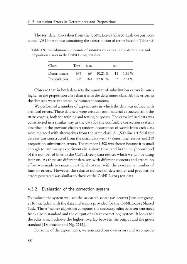
4. Substitution Errors in Determiners and Prepositions
The test data, also taken from the CoNLL-2013 Shared Task corpus, con-tained 1,381 lines of text containing the a distribution of errors listed in Table 4.9.
Table 4.9: Distribution and counts of substitution errors in the determiner andpreposition classes in the CoNLL-2013 test data.
Class Total sub sbl
Determiners 676 69 10.21% 11 1.63%Prepositions 303 160 52.81% 7 2.31%
Observe that in both data sets the amount of substitution errors is muchhigher in the preposition class than it is in the determiner class. All the errors inthe data sets were annotated by human annotators.
We performed a number of experiments in which the data was infused withartificial errors. These data sets were created from material extracted from theumbc corpus, both for training and testing purposes. The error infused data wasconstructed in a similar way as the data for the confusible correction systemsdescribed in the previous chapter; random occurrences of words from each classwere replaced with alternatives from the same class. A 1,500 line artificial testdata set was constructed from the umbc data with 77 determiner errors and 210preposition substitution errors. The number 1,500 was chosen because it is smallenough to run many experiments in a short time, and in the neighbourhoodof the number of lines in the CoNLL-2013 data test set which we will be usinglater on. As these are different data sets with different contents and errors, noeffort was made to create an artificial data set with the exact same number oflines or errors. However, the relative number of determiner and prepositionerrors generated was similar to those of the CoNLL-2013 test data.
4.3.2 Evaluation of the correction system
To evaluate the system we used the maxmatch-scorer (m2–scorer) [nus nlp group,2016] included with the data and scripts provided for the CoNLL-2013 SharedTask. The m2–scorer algorithm computes the necessary edits between sentencesfrom a gold standard and the output of a (text correction) system. It looks forthe edits which achieve the highest overlap between the output and the givenstandard [Dahlmeier and Ng, 2012].
For some of the experiments, we generated our own errors and accompany-
88
4.3. The determiner and preposition correction task
ing annotations for the m2–scorer. An example showing the annotation syntax isshown in Listing 4.1. It shows an edit annotation which in words says: replacethe preposition apart with the preposition up. The scorer requires that each line isprefixed with the letter S, and that the accompanying annotations are prefixedwith the letter A. One sentence can have multiple annotations.
Listing 4.1: Example m2–scorer file
S It was just too important to give apart on .A 7 8||| Prep |||up||| REQUIRED |||-NONE -|||0
The plain text output of the correction system is fed into the m2–scorer
together with the relevant scorer file containing the edit annotations. From this,the recall, precision and F -scores are calculated. The scorer also produces outputfor each line of data processed, showing the gold edits and the edits made (ormissed) by the correction system. Listing 4.2 shows an excerpt from the outputwhere a correct edit sequence (deletion of the redundant determiner the on wordposition three) by the system is identified by the scorer. To save space, the lineshave been truncated and the running totals of the different statistics have beenleft out in this example. The output includes the original sentences (source),the corrected version (labelled hypothesis), followed by the edits made by thecorrector (edit seq), the gold edits, and the edits which were correct.
Listing 4.2: Example m2–scorer output
SOURCE : ACE offers the tutoring and workshops on ...HYPOTHESIS : ACE offers tutoring and workshops on topics ...EDIT SEQ : [(2, 3, u’the ’, ’’)]GOLD EDITS : [(2, 3, u’the ’, [u’’])]CORRECT EDITS : [(2, 3, u’the ’, ’’)]
At the end of the run, the scorer outputs the precision, recall and F1-score based on the number of correct, proposed and gold edits, as explained inEquation 3.7 on page 45.
Listing 4.3: Precision, recall and F1-score output
CORRECT EDITS : 416 Precision : 0.2748PROPOSED EDITS : 1514 Recall : 0.1523GOLD EDITS : 2731 F1 : 0.1960
89
4. Substitution Errors in Determiners and Prepositions
Finally, to get a better understanding of the performance of the correctionsystem, the above output can be processed together with the annotation file toprovide statistics per category.
4.3.3 Introduction to the experiments
The experiments described in this section provide an estimate the performanceof our confusion correction system on two classes, determiners and prepositions.We constrain ourselves in these experiments on the detection and correction ofsubstitution errors, i.e. confusible errors, within these two classes; insertionand deletion errors are investigated in the next chapter. The elements of bothsets have been taken from the annotations supplied together with the data. Theannotations were examined for the right tags (in this case Prep and Det) andthe relevant words were put in their respective sets. The resulting determinerand article class contained 23 elements, and the preposition class contained64. The two sets are listed in Appendix A. We duplicated both classes in alowercase and capitalised (the initial letter) version. This is to prevent the systemfrom suggesting lowercase words in the beginning of sentences (for example, theinstead of The). This means we are working with two sets of words for eachclass.
In the previous chapter we used two variants of two different systems, a(selective) monolithic system (ml and sml) and an ensemble system (en), andtheir corresponding error variants (smler and ener). Due to their performance,the two non-error systems will not be explored further in this chapter. Of thetwo error systems smler and ener, the tribl2 based ener system performedbest in the previous chapter and it is this system we use for the experimentsin this chapter. An ener correction system consists of a number of classifiersonly dealing with the relevant words from each class. Table 4.10 shows theamount of instances for each class when they are extracted from five millionlines of material, containing around 132 million words. Note that the instancebases have different amounts of instances; the number of instances containingdeterminers in the focus position is not the same as the number of instancescontaining prepositions, but the statistics reflect what is present in the trainingdata. Also note the distinction between the lower case and capitalised variants asexplained earlier.
The first experiment we run is a learning curve experiment, designed todetermine the optimum number of errors in the training data for the error
90
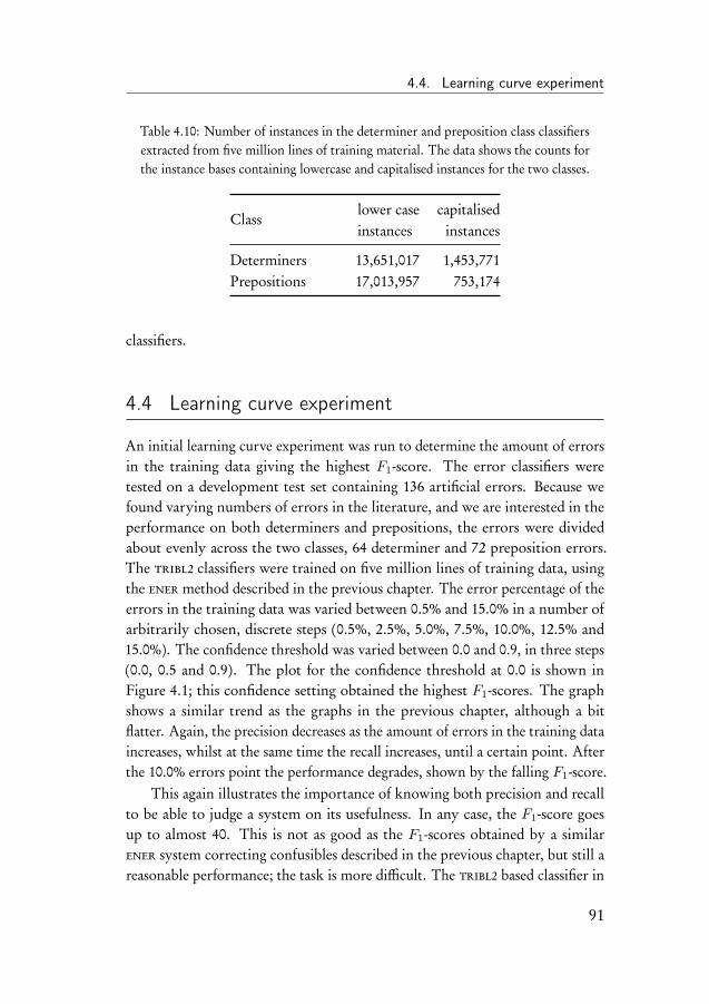
4.4. Learning curve experiment
Table 4.10: Number of instances in the determiner and preposition class classifiersextracted from five million lines of training material. The data shows the counts forthe instance bases containing lowercase and capitalised instances for the two classes.
Classlower case capitalisedinstances instances
Determiners 13,651,017 1,453,771Prepositions 17,013,957 753,174
classifiers.
4.4 Learning curve experiment
An initial learning curve experiment was run to determine the amount of errorsin the training data giving the highest F1-score. The error classifiers weretested on a development test set containing 136 artificial errors. Because wefound varying numbers of errors in the literature, and we are interested in theperformance on both determiners and prepositions, the errors were dividedabout evenly across the two classes, 64 determiner and 72 preposition errors.The tribl2 classifiers were trained on five million lines of training data, usingthe ener method described in the previous chapter. The error percentage of theerrors in the training data was varied between 0.5% and 15.0% in a number ofarbitrarily chosen, discrete steps (0.5%, 2.5%, 5.0%, 7.5%, 10.0%, 12.5% and15.0%). The confidence threshold was varied between 0.0 and 0.9, in three steps(0.0, 0.5 and 0.9). The plot for the confidence threshold at 0.0 is shown inFigure 4.1; this confidence setting obtained the highest F1-scores. The graphshows a similar trend as the graphs in the previous chapter, although a bitflatter. Again, the precision decreases as the amount of errors in the training dataincreases, whilst at the same time the recall increases, until a certain point. Afterthe 10.0% errors point the performance degrades, shown by the falling F1-score.
This again illustrates the importance of knowing both precision and recallto be able to judge a system on its usefulness. In any case, the F1-score goesup to almost 40. This is not as good as the F1-scores obtained by a similarener system correcting confusibles described in the previous chapter, but still areasonable performance; the task is more difficult. The tribl2 based classifier in
91
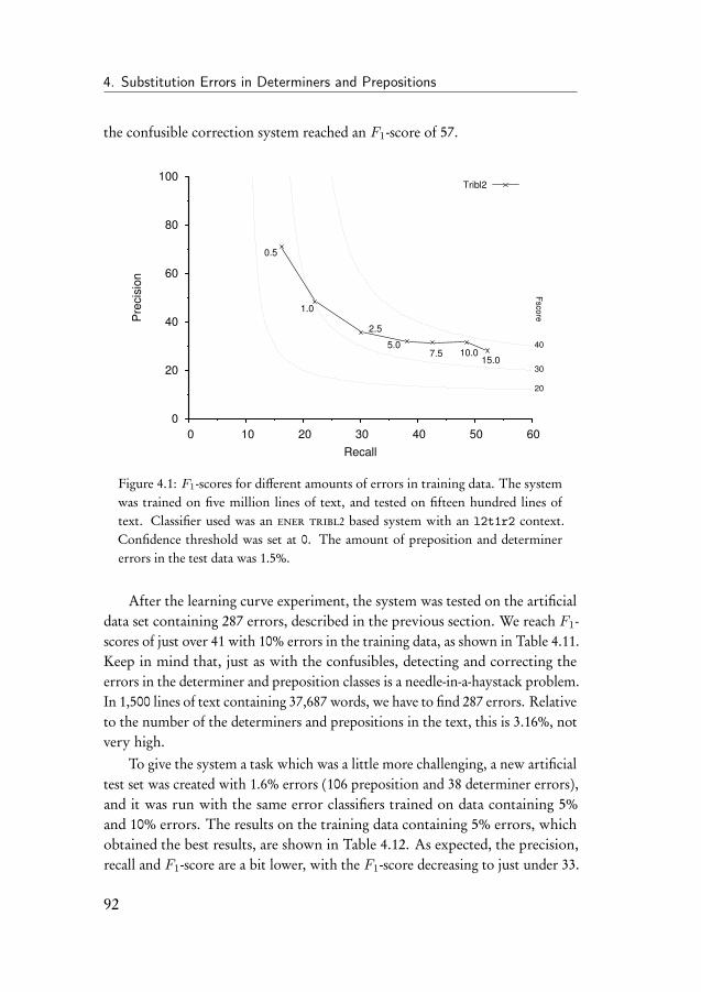
4. Substitution Errors in Determiners and Prepositions
the confusible correction system reached an F1-score of 57.
0
20
40
60
80
100
0 10 20 30 40 50 60
Fsco
re
20
30
40
Pre
cis
ion
Recall
Tribl2
0.5
1.0
2.5
5.07.5 10.0
15.0
Figure 4.1: F1-scores for different amounts of errors in training data. The systemwas trained on five million lines of text, and tested on fifteen hundred lines oftext. Classifier used was an ener tribl2 based system with an l2t1r2 context.Confidence threshold was set at 0. The amount of preposition and determinererrors in the test data was 1.5%.
After the learning curve experiment, the system was tested on the artificialdata set containing 287 errors, described in the previous section. We reach F1-scores of just over 41 with 10% errors in the training data, as shown in Table 4.11.Keep in mind that, just as with the confusibles, detecting and correcting theerrors in the determiner and preposition classes is a needle-in-a-haystack problem.In 1,500 lines of text containing 37,687 words, we have to find 287 errors. Relativeto the number of the determiners and prepositions in the text, this is 3.16%, notvery high.
To give the system a task which was a little more challenging, a new artificialtest set was created with 1.6% errors (106 preposition and 38 determiner errors),and it was run with the same error classifiers trained on data containing 5%and 10% errors. The results on the training data containing 5% errors, whichobtained the best results, are shown in Table 4.12. As expected, the precision,recall and F1-score are a bit lower, with the F1-score decreasing to just under 33.
92
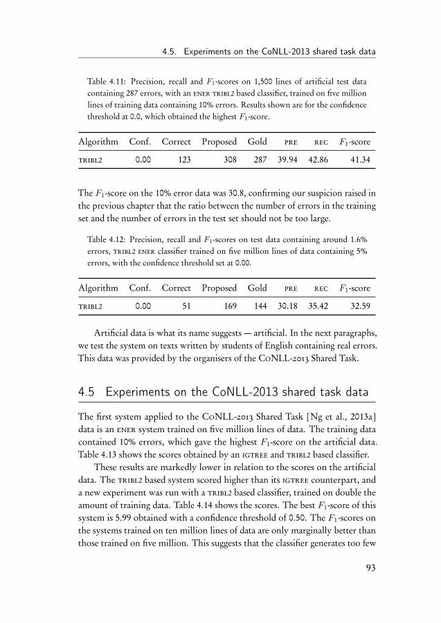
4.5. Experiments on the CoNLL-2013 shared task data
Table 4.11: Precision, recall and F1-scores on 1,500 lines of artificial test datacontaining 287 errors, with an ener tribl2 based classifier, trained on five millionlines of training data containing 10% errors. Results shown are for the confidencethreshold at 0.0, which obtained the highest F1-score.
Algorithm Conf. Correct Proposed Gold pre rec F1-score
tribl2 0.00 123 308 287 39.94 42.86 41.34
The F1-score on the 10% error data was 30.8, confirming our suspicion raised inthe previous chapter that the ratio between the number of errors in the trainingset and the number of errors in the test set should not be too large.
Table 4.12: Precision, recall and F1-scores on test data containing around 1.6%errors, tribl2 ener classifier trained on five million lines of data containing 5%errors, with the confidence threshold set at 0.00.
Algorithm Conf. Correct Proposed Gold pre rec F1-score
tribl2 0.00 51 169 144 30.18 35.42 32.59
Artificial data is what its name suggests — artificial. In the next paragraphs,we test the system on texts written by students of English containing real errors.This data was provided by the organisers of the CoNLL-2013 Shared Task.
4.5 Experiments on the CoNLL-2013 shared task data
The first system applied to the CoNLL-2013 Shared Task [Ng et al., 2013a]data is an ener system trained on five million lines of data. The training datacontained 10% errors, which gave the highest F1-score on the artificial data.Table 4.13 shows the scores obtained by an igtree and tribl2 based classifier.
These results are markedly lower in relation to the scores on the artificialdata. The tribl2 based system scored higher than its igtree counterpart, anda new experiment was run with a tribl2 based classifier, trained on double theamount of training data. Table 4.14 shows the scores. The best F1-score of thissystem is 5.99 obtained with a confidence threshold of 0.50. The F1-scores onthe systems trained on ten million lines of data are only marginally better thanthose trained on five million. This suggests that the classifier generates too few
93
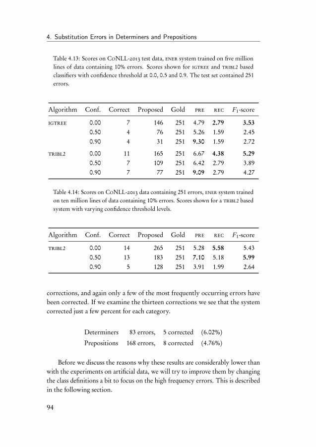
4. Substitution Errors in Determiners and Prepositions
Table 4.13: Scores on CoNLL-2013 test data, ener system trained on five millionlines of data containing 10% errors. Scores shown for igtree and tribl2 basedclassifiers with confidence threshold at 0.0, 0.5 and 0.9. The test set contained 251errors.
Algorithm Conf. Correct Proposed Gold pre rec F1-score
igtree 0.00 7 146 251 4.79 2.79 3.530.50 4 76 251 5.26 1.59 2.450.90 4 31 251 9.30 1.59 2.72
tribl2 0.00 11 165 251 6.67 4.38 5.290.50 7 109 251 6.42 2.79 3.890.90 7 77 251 9.09 2.79 4.27
Table 4.14: Scores on CoNLL-2013 data containing 251 errors, ener system trainedon ten million lines of data containing 10% errors. Scores shown for a tribl2 basedsystem with varying confidence threshold levels.
Algorithm Conf. Correct Proposed Gold pre rec F1-score
tribl2 0.00 14 265 251 5.28 5.58 5.430.50 13 183 251 7.10 5.18 5.990.90 5 128 251 3.91 1.99 2.64
corrections, and again only a few of the most frequently occurring errors havebeen corrected. If we examine the thirteen corrections we see that the systemcorrected just a few percent for each category.
Determiners 83 errors, 5 corrected (6.02%)
Prepositions 168 errors, 8 corrected (4.76%)
Before we discuss the reasons why these results are considerably lower thanwith the experiments on artificial data, we will try to improve them by changingthe class definitions a bit to focus on the high frequency errors. This is describedin the following section.
94
4.6. Experiment on subsets of determiners and prepositions
4.6 Experiment on subsets of determiners and preposi-tions
Until now we have been correcting the classes as they are, without any parti-tioning or ordering of the elements. In the literature we examined (especiallywork in connection with the hoo-2012 shared task, for example [Dahlmeieret al., 2012,Rozovskaya et al., 2012]), we found several suggestions on how toimprove determiner and preposition correction. One of these is to concentrateon the most frequent class members which have errors. This is tried in the nextexperiment.
The training data was examined to determine the extent of the substitutionerrors in our classes. Table 4.15 shows the five most frequent errors for eachclass. The table shows a determiner or preposition with the number of times ithad to be corrected by replacing it by another member from the class. We tookthe lists to be bidirectional; that is, we made the assumption that if in shouldhave been (replaced by) on, the reverse was also possible. This is a simplification,but given the limited amount of data these lists were extracted from, we did notwant to model the errors and corrections too precisely, and instead aimed for ageneral corrector. However, four observations have to be made. First, note thatfor some of the determiner errors there are fewer than five entries in the top–5.Second, there is overlap between the sets (in appears in all five preposition sets).Third, the sets are not clean, for example, to does not belong in the determinerset. The annotation is correct, the word to should have been the in this case, butthe error and correction are from different sets. This makes it impossible forthe system to correct this particular error because to is considered a member ofthe preposition class, and the will not be part of the answers suggested by theclassifier. Fourth, and last, the third row in the determiner class contains fourelements, but they are of low frequency. They were included anyway becausethey are the variants with the capital letter, that is, the first words in the sentence.It seemed logical to include them even when the frequencies were low, otherwisethe capitalised versions would be ignored completely. This resulted in ten setswith between four and six confusibles. Sentences starting with prepositionsare not very common, which is why there are no capitalised versions in thepreposition sets.
Table 4.16 shows the results of several tribl2 based ener systems trained onthese subsets instead of the full classes. The systems are trained on one, five and
95
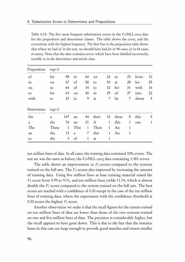
4. Substitution Errors in Determiners and Prepositions
Table 4.15: The five most frequent substitution errors in the CoNLL-2013 datafor the preposition and determiner classes. The table shows the error, and thecorrections with the highest frequency. The first line in the preposition table showsthat where we had of in the text, we should have had for in 98 cases, in in 64 cases,et cetera. Note that the data contains errors which have been labelled incorrectly,notably to in the determiner and article class.
Preposition top–5
of for 98 in 64 on 24 to 23 from 10in on 67 of 58 to 30 at 28 for 25on in 64 of 34 to 32 for 31 with 16to for 63 on 40 in 29 of 27 into 22with to 23 in 9 at 7 by 7 about 5
Determiner top–5
the a 147 an 44 their 10 these 8 this 5a the 76 an 21 A 1 this 1 one 1The These 1 This 1 Their 1 An 1an the 13 a 7 this 1 An 1to the 3 of 1 at 1
ten million lines of data. In all cases, the training data contained 10% errors. Thetest set was the same as before, the CoNLL-2013 data containing 1,381 errors.
The table shows an improvement in F1-scores compared to the systemstrained on the full sets. The F1-scores also improved by increasing the amountof training data. Using five million lines as base training material raised theF1-score from 5.99 to 9.31, and ten million lines yields 11.74, which is almostdouble the F1-score compared to the system trained on the full sets. The bestscores are reached with a confidence of 0.00 except in the case of the ten millionlines of training data, where the experiment with the confidence threshold at0.50 scores the highest F1-score.
Another observation we make is that the recall figures for the system trainedon ten million lines of data are lower than those of the two systems trainedon one and five million lines of data. The precision is considerably higher, butthe recall appears to have gone down. This is due to the fact that the instancebases in this case are large enough to provide good matches and return smaller
96
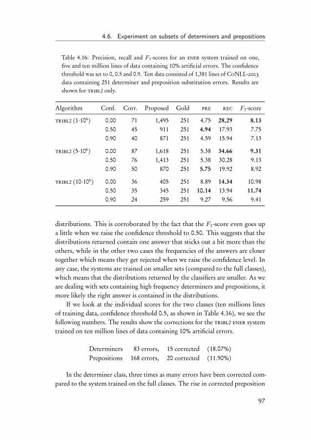
4.6. Experiment on subsets of determiners and prepositions
Table 4.16: Precision, recall and F1-scores for an ener system trained on one,five and ten million lines of data containing 10% artificial errors. The confidencethreshold was set to 0, 0.5 and 0.9. Test data consisted of 1,381 lines of CoNLL-2013
data containing 251 determiner and preposition substitution errors. Results areshown for tribl2 only.
Algorithm Conf. Corr. Proposed Gold pre rec F1-score
tribl2 (1·106 ) 0.00 71 1,495 251 4.75 28.29 8.130.50 45 911 251 4.94 17.93 7.750.90 40 871 251 4.59 15.94 7.13
tribl2 (5·106 ) 0.00 87 1,618 251 5.38 34.66 9.310.50 76 1,413 251 5.38 30.28 9.130.90 50 870 251 5.75 19.92 8.92
tribl2 (10·106 ) 0.00 36 405 251 8.89 14.34 10.980.50 35 345 251 10.14 13.94 11.740.90 24 259 251 9.27 9.56 9.41
distributions. This is corroborated by the fact that the F1-score even goes upa little when we raise the confidence threshold to 0.50. This suggests that thedistributions returned contain one answer that sticks out a bit more than theothers, while in the other two cases the frequencies of the answers are closertogether which means they get rejected when we raise the confidence level. Inany case, the systems are trained on smaller sets (compared to the full classes),which means that the distributions returned by the classifiers are smaller. As weare dealing with sets containing high frequency determiners and prepositions, itmore likely the right answer is contained in the distributions.
If we look at the individual scores for the two classes (ten millions linesof training data, confidence threshold 0.5, as shown in Table 4.16), we see thefollowing numbers. The results show the corrections for the tribl2 ener systemtrained on ten million lines of data containing 10% artificial errors.
Determiners 83 errors, 15 corrected (18.07%)Prepositions 168 errors, 20 corrected (11.90%)
In the determiner class, three times as many errors have been corrected com-pared to the system trained on the full classes. The rise in corrected preposition
97
4. Substitution Errors in Determiners and Prepositions
errors is slightly smaller, about two and a half times as many errors have beencorrected compared to the system trained on the full classes.
In the next section, we discuss the results obtained by the memory-based sys-tems. The next chapter, Chapter 5, discusses a correction system that corrects allthree error types, substitution, omission and insertion errors, in the determinerand preposition classes.
4.7 Discussion of the results
In this chapter we applied the correction system developed in the previouschapter to a new correction task. The task in this chapter was substitution errorsin two word classes; articles and determiners, and prepositions. Following fromthe results from the previous chapter, we decided to use the tribl2 ensembleerror system for the experiments.
The initial experiment was a learning curve over training data with differentamounts of errors to determine the optimum amount for the ener classifier. Thetest data contained 1,500 lines of data with artificial errors. The system trainedon error data containing 10% errors obtained the highest F1-score of just under40. The learning curve showed a similar, albeit flatter, shape as the learningcurves shown in the previous chapter. In both cases, the systems showed a fallingprecision versus a rising recall and rising F1-score when the amount of errors inthe training data was increased. The systems also started to degrade when theamount of errors in the training data increased from 10 to 15%.
After having determined the amount of errors needed, the experiment wasrepeated on artificial data containing errors which were distributed similarly tothose in the data supplied for the CoNLL-2013 Shared Task. The ensemble errorsystem obtained the highest score F1-score of just over 41 on this test set.
The same system was then applied to the test data supplied for the CoNLL-
2013 Shared Task. This data contained five different kind of errors, two of whichwere of interest, namely the determiner and preposition errors. Together withthe data, the organisers of the shared task supplied an annotation file and aprogram to process output from a correction system to calculate statistics on thecorrections made. We filtered the annotation file on the two kinds of errors ofinterest, and used that to calculate the performance of our systems.
Running the ener tribl2 based system on the CoNLL-2013 data, gave amaximum F1-score of 5.99. This system had been trained on ten million lines of
98
4.7. Discussion of the results
error data containing 10% errors. This was not as high as we expected from theresults on the data containing artificial errors.
We tried to raise the scores by dividing each of the two classes into fivesmaller subsets. Each subset contained one of the five most frequent classmembers together with its five most frequent substitution errors. This created asystem with ten classifiers in total. The ener tribl2 based system constructedin this manner obtained an F1-score of 9.31. One more system was trained ondouble the amount of data, ten million lines of text, and obtained the highestF1-score, namely 11.74.
The scores obtained on the determiner and preposition task are not as goodas those obtained on the confusible task in the previous chapter. The mainreason for this is that after the system has correctly detected an error, the correctreplacement needs to be found. In the case of the pairs and triplets in the previouschapter, this was much easier than for the larger determiner and prepositionclasses. When dealing with pairs, the correction is the other element of the pair,and even in the case of triplets we have a good chance (even if we pick randomly)of picking the right answer. When the classifiers were trained on the five mostfrequent errors only, the F1-score almost doubled, showing that training data onall class members instead of the most frequently confused ones, makes it harderto pick the correct answer.
On the other hand, the scores on the artificial data were considerably bet-ter than the scores on the CoNLL-2013 data, and were more in line of ourexpectations after having done the confusible task in the previous chapter. TheCoNLL-2013 data appears to suffer from three problems. First, it contains moreerrors than those in the two classes we were trying to correct. The total numberof errors in the test data was 1,643, of this we tried to correct 251 substitutionerrors. Even though we only counted the performance on the relevant errors,there were enough errors left of the other types to influence the classifiers, whichwere of course trained on ‘perfect’ data and only contained errors of the rightkind in the right place. Second, the test set with the artificial data had beenextracted form the same corpus as the training data, whereas the CoNLL-2013
data is from another corpus altogether. Third, several of the confusible setscontain members that are in other grammatical classes, for example to – too –two where we have a particle, a quantifier and a numeral. This means the contextaround the words is sufficiently different to be able to pick out the right one.After all, the confusion in this case stems from similarity in pronunciation, andthe context in which two is used is different from the context in which too is
99

4. Substitution Errors in Determiners and Prepositions
used. In the case of the determiner and preposition sets, the contexts will be verysimilar because we are dealing with words in the same grammatical class. In thecase of prepositions, it is not uncommon that several different prepositions arepossible in the same four or five word context on which the system is trained, allleading to grammatically correct sentences which only differ in meaning. Pickingthe intended one in this case is not possible without understanding what theauthor is trying to say.
On a final note we must add that we can not really compare these resultswith other correction systems yet as we have only investigated substitution errors.In the next chapter, we will expand the correction task to include omission andinsertion errors as well, and we will be able to compare our results to those ofothers.
100

5Omission and Insertion Errors in
Determiners and Prepositions
5.1 Introduction
In the previous chapter we discussed a text-correction system that correctedsubstitution errors in determiners and prepositions. In this chapter we extendthe task by adding two more error types to the corrector; omission and insertionerrors. To be able to handle these two new error types, we introduce a newkind of classifier which we call a positive –negative classifier. This type ofclassifier returns a binary yes – no, or a positive – negative answer in response tothe question if a certain word can, should, or should not be present in a certaincontext.
This is different from the classifiers previously used where the presence ofa certain class member (a confusible, preposition, or a determiner) was notdisputed, but the actual form used was possibly wrong. The positive –negativeclassifiers we introduce can be used to query the presence or absence of a classmember. As we will show, this has implications on the way the instances to trainthe classifiers are generated.
This chapter grew out of the work done for the hoo-2012 shared task [Daleet al., 2012]. The hoo-2012 (Helping Our Own) task focused on building atext-correction system to, ‘. . . “help our own” by developing tools which can helpnon-native speakers of English (and maybe some native ones) write academicEnglish prose of the kind that helps a paper get accepted’ ( [Dale and Kilgarriff,2010]). The 2012 task involved the correction of determiner and preposition
101
5. Omission and Insertion Errors in Determiners and Prepositions
errors. In this task, the errors were not limited to substitution errors only, butalso included insertion and omission errors.
The chronology of the text-correction systems in this thesis needs someexplanation. The hoo-2012 task was one of the first grammatical error problemstackled with the memory-based language model based correctors. The workwas done simultaneously with the development of the confusible corrector inChapter 3, but growing insights led to differences in parameters and data sets,most notably the use of the classifiers trained on error data, and the use of asingle confidence parameter instead of the five parameters used in the hoo-2012system. From a task-oriented point of view, it made more sense to start this thesisby describing the confusible corrector with substitution errors first, which weconsidered the easier task. This is described in Chapter 3. Chapter 4 introducedthe larger determiner and preposition classes on the same substitution task, andfinally, this chapter adds the insertion and omission errors.
Therefore the chapter begins with a description of the system built forthis task, and a discussion of the results obtained by it. A shorter version ofthis appeared in [Van den Bosch and Berck, 2012]. After this description, wediscuss a new system which adds the error classifiers which were developed afterthe hoo-2012 task, and were already introduced and discussed in the chapterdescribing the confusible correction task.
5.2 The HOO determiner and preposition error corrector
The Helping Our Own (hoo) linguistic tasks were created to encourage thedevelopment of natural language processing tools to help people writing texts[Dale and Kilgarriff, 2010,Dale and Kilgarriff, 2011]. The hoo-2012 task dealtwith the detection and correction of determiner and preposition errors [Daleet al., 2012]. A total of fourteen teams competed in this task, including ourhoo-2012 system which we describe in this chapter.
The hoo-2012 system is similar to the systems we have described in Chap-ters 3 and 4, but there are two important differences. The first difference is theuse of positive –negative classifiers which are used to determine missing andredundant words. The second difference is the use of the number of parametersto control the corrections. These differences will be explained in the next twosubsections.
102

5.2. The HOO determiner and preposition error corrector
5.2.1 Binary classifiers
To detect and correct insertion and omission errors, a different strategy is neededcompared to the substitution errors. The substitution errors can be detectedand corrected in one step. The classifier suggests a word that fits the contextwith a certain confidence. Is the confidence high enough, the word in the textis replaced by the suggested word. However, this strategy will not work forthe insertion and omission errors, as the normal classifiers do not provide theright kind of information. These classifiers will always respond with an answer,and that does not tell us if there is a missing or redundant word. For that, weintroduce the binary classifiers, which provide a yes – no answer to the question ifwe are dealing with insertion or omission. The binary classifier can only returna distribution of maximum two class labels, yes or no, which makes it easier forthe correction heuristics to process and work with.
Depending on whether we are checking for redundant or missing words, ananswer from a binary classifier can be interpreted in four different ways, shownin Table 5.1.
Table 5.1: Possible interpretations of the positive – negative classifiers depending onthe task.
Task Positive answer Negative answermeans means
Checking for insertion no, nothing inserted yes, insertionChecking for omission yes, missing no, nothing is missing
This can be explained as follows. The classifiers for the substitution errorswere trained on instances where the focus position is a position on a word, butin the case of omission or insertion errors, the focus position is between twowords. A positive – negative classifier predicts whether a position between wordsshould contain something or not. Therefore this type of classifier can be usedfor both insertions and omissions.
Figure 5.1 shows a diagram explaining this. To check if a word should bedeleted, an instance is created without the word, pretending it is missing. Thesystem then calls the binary classifier on this instance. If this classifier returnsa ‘negative’ answer, it means the classifier does not think a word is missing inthis context. This means the word was redundant. In the same vein, a positive
103

5. Omission and Insertion Errors in Determiners and Prepositions
sky above the port
Focus is on a word, in thiscase the word "above"
The
sky above theThe
Focus is between words. Should there bea word between "sky" and "above"?
Figure 5.1: Illustration of the focus position; on a word or between words. In bothexamples, the context is two words to the left and two words to the right (l2r2).The top example shows the instance for a substitution error, asking if above is thecorrect word in the context. In the bottom example, an instance for the insertion oromission errors is shown. For these kinds of errors, the classifier returns a yes –noanswer specifying whether a word should be present or not. The example showsthe instance for the question if there should be a word between sky and above.
answer from the classifier in this case signals that there should be a word in thisparticular context. If this is the case, a new instance is created with the wordthat was removed earlier in the focus position, that is, a normal instance suchas explained in the previous chapters. A new word that fits the context is thengenerated by the normal predicting classifier that is also used for the substitutionerrors. This means that in order to correct missing words, two different instancesare generated and classified.
5.2.2 System parameters
The systems described in Chapters 3 and 4 used one adjustable parameter settingand measurement, confidence, to control whether a prediction was a valid cor-rection or not. The hoo-2012 system, makes use of five adjustable parameters tocontrol the corrections. These five parameters can be assigned different thresholdvalues for the different classes. Analogous to the confidence, the measurementsare calculated from the different quantities relating to the distribution, such assize and frequency of the elements. Two of the parameters are for the positive –negative classifiers, and three for the word predictor. The following list shows theparameters for the preposition class. They are shown here with an abbreviationto which we refer when we discuss them. The corresponding parameters for thedeterminer class, not shown in this list, are similar. Separate sets of parameters
104

5.2. The HOO determiner and preposition error corrector
were used for each class in order to be able to fine-tune the behaviour of thecorrector.
UP_PNR The ratio between the frequencies of the positive and negative classi-fications must be larger than the value of this parameter. Calculatedfor a possibly redundant preposition (or determiner in the case of thedeterminer class). For example, if the classifier returns a distributioncontaining a positive answer with a count of 12,028, and a negative clas-sification with a count of 640, the ratio is 18.8. This value is comparedto the specific UD_PNR threshold.
MP_PNR The ratio between the frequencies of the positive and negative classifi-cations must be larger than the value of this parameter.
MP_DS The size of the distribution returned when predicting a prepositionmay not be larger than this.
MP_R The ratio between the frequencies of the classification and the original(the word which might need correcting) must be larger than this. If theoriginal word is not part of the predicted distribution, the threshold isconsidered passed.
MP_F The count of the first classification in the distribution must be largerthan this value.
The rationale behind the use of the parameters is to increase the certaintyof the predictions. They decide whether the classifier output is used or not; inother words, the parameters control abstention. They give the corrector a way toabstain from changing (correcting) the text. As was shown in Chapter 2, a largedistribution tends to point to a bad match on the feature values, resulting in adefault distribution being returned by the classifier. This is not the case for thepositive – negative classifiers, which only return a distribution of two elements.In this case we calculate the ratio between the frequencies of the two distributionitems.
An optimisation procedure was run on the gold training data provided bythe organisers of the hoo-2012 task. The aim was to optimise the parametersfor precision, recall, and F1-score respectively. Table 5.2 shows the optimalsettings found by the search. The results given in Section 5.3 refer to the systemoptimised on F1-score, listed in the rightmost column in Table 5.2.
The table shows that most of the ratio thresholds found to optimise F1-scoreare quite high. The positive –negative preposition classifier for example needs
105
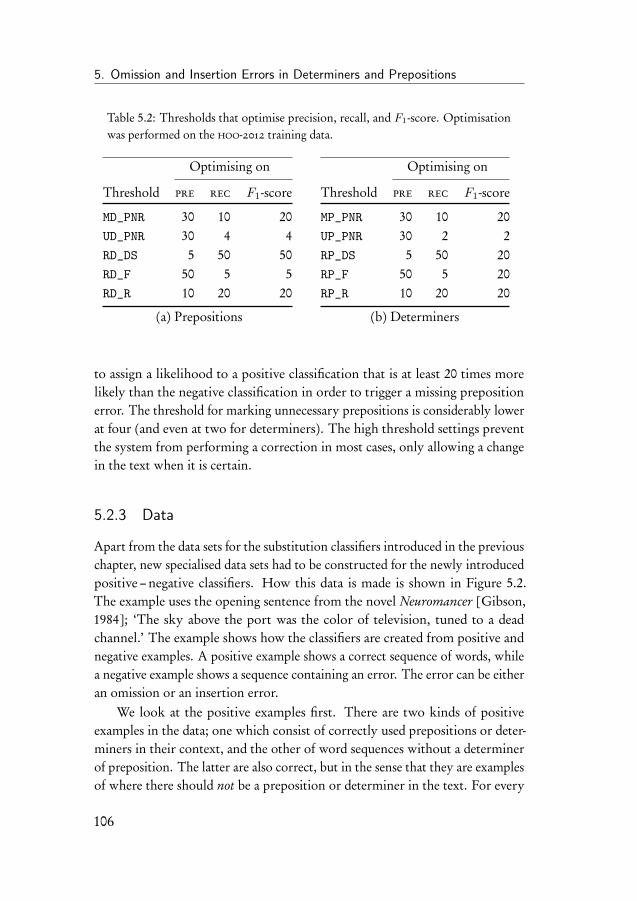
5. Omission and Insertion Errors in Determiners and Prepositions
Table 5.2: Thresholds that optimise precision, recall, and F1-score. Optimisationwas performed on the hoo-2012 training data.
Optimising on
Threshold pre rec F1-score
MD_PNR 30 10 20UD_PNR 30 4 4RD_DS 5 50 50RD_F 50 5 5RD_R 10 20 20
(a) Prepositions
Optimising on
Threshold pre rec F1-score
MP_PNR 30 10 20UP_PNR 30 2 2RP_DS 5 50 20RP_F 50 5 20RP_R 10 20 20
(b) Determiners
to assign a likelihood to a positive classification that is at least 20 times morelikely than the negative classification in order to trigger a missing prepositionerror. The threshold for marking unnecessary prepositions is considerably lowerat four (and even at two for determiners). The high threshold settings preventthe system from performing a correction in most cases, only allowing a changein the text when it is certain.
5.2.3 Data
Apart from the data sets for the substitution classifiers introduced in the previouschapter, new specialised data sets had to be constructed for the newly introducedpositive –negative classifiers. How this data is made is shown in Figure 5.2.The example uses the opening sentence from the novel Neuromancer [Gibson,1984]; ‘The sky above the port was the color of television, tuned to a deadchannel.’ The example shows how the classifiers are created from positive andnegative examples. A positive example shows a correct sequence of words, whilea negative example shows a sequence containing an error. The error can be eitheran omission or an insertion error.
We look at the positive examples first. There are two kinds of positiveexamples in the data; one which consist of correctly used prepositions or deter-miners in their context, and the other of word sequences without a determinerof preposition. The latter are also correct, but in the sense that they are examplesof where there should not be a preposition or determiner in the text. For every
106
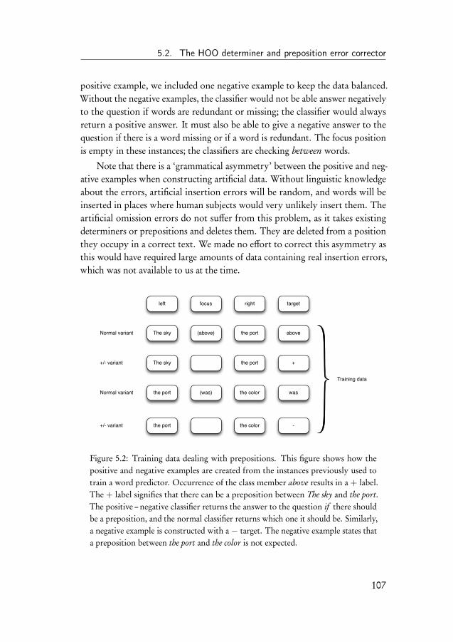
5.2. The HOO determiner and preposition error corrector
positive example, we included one negative example to keep the data balanced.Without the negative examples, the classifier would not be able answer negativelyto the question if words are redundant or missing; the classifier would alwaysreturn a positive answer. It must also be able to give a negative answer to thequestion if there is a word missing or if a word is redundant. The focus positionis empty in these instances; the classifiers are checking between words.
Note that there is a ‘grammatical asymmetry’ between the positive and neg-ative examples when constructing artificial data. Without linguistic knowledgeabout the errors, artificial insertion errors will be random, and words will beinserted in places where human subjects would very unlikely insert them. Theartificial omission errors do not suffer from this problem, as it takes existingdeterminers or prepositions and deletes them. They are deleted from a positionthey occupy in a correct text. We made no effort to correct this asymmetry asthis would have required large amounts of data containing real insertion errors,which was not available to us at the time.
left focus right target
The sky (above) the port above
The sky the port +
Normal variant
+/- variant
Training data
the port the color -+/- variant
the port (was) the color wasNormal variant
Figure 5.2: Training data dealing with prepositions. This figure shows how thepositive and negative examples are created from the instances previously used totrain a word predictor. Occurrence of the class member above results in a + label.The + label signifies that there can be a preposition between The sky and the port.The positive – negative classifier returns the answer to the question if there shouldbe a preposition, and the normal classifier returns which one it should be. Similarly,a negative example is constructed with a − target. The negative example states thata preposition between the port and the color is not expected.
107

5. Omission and Insertion Errors in Determiners and Prepositions
television, tuned (TO) a dead channel
left focus right target
, tuned a dead ?Missing variant
color of (THE) television , ?Redundant
Testing
the color of THE television,
Figure 5.3: Instances used in the correction task. Different instances are createddepending on whether we want to check for a missing or for a redundant classitem (but the same classifier is used). To check for a missing word, the instance forthe classifier is constructed without the normal skipping of the focus word. Theexample shows the instance created to check for the missing preposition to. Toprepare an instance to check for a redundant word, the word needs to be included.The example shows an instance for the redundant determiner the (labelled ‘(the)’)in the instance.
The training data for the system was constructed from the Google 1 tb
5-gram corpus [Brants and Franz, 2006]. The format of the corpus is nicelysuited to the l2r2 format used by the classifiers, the middle word in the 5-grambeing the focus word with the four context words to the left and the right.Table 5.3 shows the amount of training data used to train the classifiers.
Table 5.3: Counts of normal (labelled ‘Substitution’) and positive-negative instancesin training data for the preposition and determiner classes extracted from the Google1 tb 5-gram corpus.
Determiners PrepositionsCorpus Substitution +/− Substitution +/−
Google 132,483,802 252,634,322 118,105,582 235,730,253
The organisers of the shared task also supplied training data, containing374,680 words. We chose not to use this training data, except to extract the listcontaining the prepositions and determiners to be corrected by the system.
108
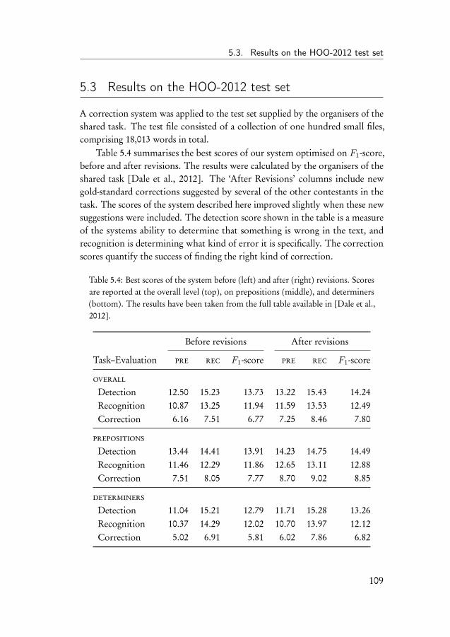
5.3. Results on the HOO-2012 test set
5.3 Results on the HOO-2012 test set
A correction system was applied to the test set supplied by the organisers of theshared task. The test file consisted of a collection of one hundred small files,comprising 18,013 words in total.
Table 5.4 summarises the best scores of our system optimised on F1-score,before and after revisions. The results were calculated by the organisers of theshared task [Dale et al., 2012]. The ‘After Revisions’ columns include newgold-standard corrections suggested by several of the other contestants in thetask. The scores of the system described here improved slightly when these newsuggestions were included. The detection score shown in the table is a measureof the systems ability to determine that something is wrong in the text, andrecognition is determining what kind of error it is specifically. The correctionscores quantify the success of finding the right kind of correction.
Table 5.4: Best scores of the system before (left) and after (right) revisions. Scoresare reported at the overall level (top), on prepositions (middle), and determiners(bottom). The results have been taken from the full table available in [Dale et al.,2012].
Before revisions After revisions
Task–Evaluation pre rec F1-score pre rec F1-score
overall
Detection 12.50 15.23 13.73 13.22 15.43 14.24Recognition 10.87 13.25 11.94 11.59 13.53 12.49Correction 6.16 7.51 6.77 7.25 8.46 7.80
prepositions
Detection 13.44 14.41 13.91 14.23 14.75 14.49Recognition 11.46 12.29 11.86 12.65 13.11 12.88Correction 7.51 8.05 7.77 8.70 9.02 8.85
determiners
Detection 11.04 15.21 12.79 11.71 15.28 13.26Recognition 10.37 14.29 12.02 10.70 13.97 12.12Correction 5.02 6.91 5.81 6.02 7.86 6.82
109
5. Omission and Insertion Errors in Determiners and Prepositions
The best score obtained by the memory-based system is an overall F1-score of14.24 on error detection, after revisions. The system performs slightly better onprepositions than on determiners, but the differences are small. Optimising onF1-score implies that a reasonable balance is found between recall and precision,but overall our results are not impressive, especially not in terms of correction.Compared to the other systems competing in the task, it ended on place nine outof fourteen, with an overall F1-score of 7.80 on correction. The highest F1-scoreon correction obtained in the task was 37.83, the lowest was 2.05.
5.4 Discussion of the HOO-2012 results
The best score was obtained by the system from the University of Singapore(nus) [Dahlmeier et al., 2012], which obtained an F1-score of 37.83 on correction,followed by the system of the University of Indiana with a score of 32.99[Rozovskaya et al., 2012].
These two systems obtain much better scores than we do, which we willtry to explain. There are four important differences between those two systemsand our system. First, both systems make use of the supplied training corpus,and even preprocess the text; spelling correction is done by both universities,and the nus goes as far as to even correct the casing of the text. We on the otherhand, have taken a more general approach and built a system without knowledgeabout the texts to be corrected. We have only used the training data to compile alist of determiners and prepositions the system needed to correct. We feel thatcorrecting the training text beforehand is debatable. On one hand, extra errorsin the text do interfere with the classifiers, but on the other hand, no text isperfect. It is unlikely that the corpora used for training the classifiers were errorfree, and even if both training and testing data are (spelling) corrected beforeprocessing, a lot depends on the quality of the spell checker which possiblyperforms differently on different bodies of texts. This can lead to unwanteddifferences between training and testing data.
The second difference is that both best-performing systems use grammaticalknowledge. The Singapore system depends on part-of-speech tags, and syntacticparser and chunker output to identify the phrases where errors occur. TheUniversity of Indiana uses the output from a shallow parser and pos-tagger toextract features for their learning algorithms. The only linguistic knowledge usedin our system are the two lists with the determiners and preposition members.
110
5.4. Discussion of the HOO-2012 results
These are used to detect a determiner or preposition in the text, and call therelevant classifiers.
Third, after analysing the training data, both universities decided to correctonly a subset (the most frequent) of all the errors, while we tried to handle allerrors.
Fourth, the University of Indiana uses an ‘adapted’ model, plus a techniquecalled ‘error inflation’ which introduces artificial errors in the training data[Rozovskaya and Roth, 2010]. An adapted model is a model which includesthe source word (in this case the preposition chosen by the author of the text)amongst the features. In the systems described in Chapters 3 and 4, this is calledthe error feature. Since non-native speakers mistakes are often systematic, thesource word carries a lot of information [Lee and Seneff, 2008,Rozovskaya andRoth, 2011]. Models that use this word in training learn which errors are typicalfor the author and outperform systems that only look at context. Error inflationis used to correct for the fact that the errors in the training data are few and farapart. Most of the prepositions or determiners used in the text will be correct –the actual error rates are in the neighbourhood of 2.5% in case of the trainingdata supplied with the task. To improve the training data, the error inflationmethod reduces the number of correct examples in the text, and replaces theseby artificially generated errors similar to those that already occur in the text. Itbalances the ratio between correct and incorrect examples in the text. We haveshown in the previous chapter that the percentage of errors in the training dataplays an important role in the performance of the system, and that it should beneither too low nor too high; our results suggested an optimal factor two moreerrors in the training set than in the test set. One difference with our method isthat [Rozovskaya et al., 2012] uses training data with errors, and tries to capturethe systematic errors made by the author(s) of the data when applying the errorinflation step. This has the advantage that it creates a better classifier, but it alsohas a disadvantage; the classifier will be tuned to the errors of the author(s) ofthe training data. We, on the other hand, introduce our errors randomly in thetext, which means that the classifier is probably partly trained on errors whichnever occur in real life, but is likely to be more general than a classifier trainedon specific errors.
Summarising, we can say that the systems made by the Singapore and Indianateams are more complex, both in preprocessing and processing of the training andtesting data, requiring language-specific spell checkers, pos-taggers and parsers.
We also compare our system to some contesting systems that scored lower
111

5. Omission and Insertion Errors in Determiners and Prepositions
than ours. A system that scores slightly below ours is the system from TrinityCollege in Dublin, obtaining an F1-score of 4.94 [Lynch et al., 2012]. Theirsystem uses a naïve Bayes classifier using 39 features in the error detection step,and 42 features in the error correction step. Like in the previous two systemsdiscussed above, the features in this system include pos-tags and spell-correctedversions of the context words, four to the right and four to the left. Informationon speaker age and native language is also included in the features. The systemgoes through three steps; (1) identifying errors, (2) classifying the edits into oneof the six error types, and (3) suggesting corrections. After the correction step,the corrections are re-evaluated based on a few simple heuristics which makesuse of pos-tags and head word information. This heuristic determines whethersuggested corrections are allowed or discarded, much like our five parameterscontrolling abstention. In their conclusion they recognise the difficulty ofthe task, and suggest several areas of improvement. One of the improvementsthey suggest is a better spell-checker to be used in the pre-processing stages –something we did not make use of either, but the best performing systems did.
Another system that obtained a slightly lower score than ours is the vtexsystem [Daudaravičius, 2012]. This system uses rules based on word length andword endings to do match patterns in the sentences where an error might becorrected. A language model is used to decide if a potential correction is goodor not. It does not make use of taggers or even other corpora; the rules andlanguage model are extracted from the training data supplied with the task. Thissystem also uses, like we do, a context of two words before and after the positionof interest.
The last system we mention is that submitted by the University of Cam-bridge [Kochmar et al., 2012]. Their F1-score after submission is 9.06, whichis higher than ours. The system uses naïve Bayes classifiers, but in this casethey are not using word context features, but rather a number of grammaticalfeatures. These feature include pos-tags, lemmas, and grammatical relations suchas head noun (in the case of the determiner errors) and dependent lemmas (inthe case of prepositions). The main motivation for this is, they write, that thesefeatures have been shown in previous work to be effective for error detectionand correction. Furthermore, they had access to the full clc corpus, of whichthe hoo-2012 data was a subset, so they had access to more training material con-taining real-world errors. They also limited the sets to the three most frequentdeterminers and the ten most frequent prepositions.
If we look at their missing preposition classifier, we see that they model
112
5.4. Discussion of the HOO-2012 results
the relations between the head lemma of the grammatical relation of which thetarget preposition is or is not present and the dependent lemma in which thepreposition is the head. If we take the following sentence as an example:
I am looking forward to your reply
we have to as the preposition, look is the head lemma and reply is the dependentlemma of the relation where the preposition is the head. This technique allowslong distance relations to be modelled as well, something which is lacking in oursystem. To overcome this limitation, we could try to train our system on datawith a very large context, but as it is commonly observed that n-gram modelsdo not improve with n-grams larger than five [Huang et al., 1992], it can beexpected that the long-distance dependencies are not easily captured using surfacestructure only.
Summarising the above we can conclude that we have one of the simplersystems. We train classifiers from general data (Google), and do not use spell-checkers, pos-taggers or other linguistic knowledge or (pre-)processing, nor dowe limit the number of class members we try to correct. We train our classifierson data which consist of a simple four word context around the focus word weare interested in.
The question remains why some of the system score so much better thanothers. Including extra linguistic information like pos-tags, speaker information,or applying spell-checking on the data does not seem to help in every case;compare for example the scores from Dublin and Singapore. The two top-scoring systems are both considerably optimised for this specific task. Thesystem we have built is not really optimised for this correction task; we aretrying to fit the task into the general correction system rather than to create afinely tuned bespoke system for the correction of prepositions and articles anddeterminers.
On the other hand, systems that do use all of this, do not necessarily obtainmuch higher scores. The Cambridge system is one example illustrating this. Thecreators of the Cambridge system hint at the fact that being too specific is notalways a good thing. They tried training specific versions of the classifiers basedon the speakers mother tongue, and selecting the relevant classifier in the testphase, but these specialised systems obtained lower results than the more generalsystems.
113
5. Omission and Insertion Errors in Determiners and Prepositions
5.5 Improving the HOO system
As explained in the beginning of this chapter, the hoo-2012 system was the firstmemory-based text correction we built. A major difference with the systemsdescribed in Chapters 3 and 4 is the use of error classifiers. In Chapter 4 weapplied the error classifiers to the preposition and determiner task, but only tothe substitution errors. The question is if it can be used to improve the scores inthe original system. The problem with the error classifier is that it can only beapplied to the substitution errors, and not to the omission and insertion errors.For the missing word classifier that corrects the omission errors, the informationis not available to begin with (it is impossible to have examples of specific missingwords), and for the redundant word classifier correcting the insertion errors,there are too many possibilities. To create examples of redundant words, everysequence with, for example, a preposition in it could be expanded to a similarsequence with one of the other class members in its place. The combinationof possible words in all possible positions would lead to an explosion of data.For example, a sentence with ten words has nine places between the wordswhere there could have been, for example, a redundant preposition. This onesentence would be expanded to 423 different possible versions in the case of 47prepositions. If we add the positions before the first and the last word, therewould another 94.
Of course, in real world data, the errors would not appear in all positions,but would be governed by the grammatical knowledge of the author of the text.This information could be extracted from a sufficiently large corpus of errorannotated data, but this was not done because of two reasons. First, no suchcorpus was readily available at the time this thesis was written, and second, inthis thesis we are exploring the possibilities to do text correction with a general(word predicting) system, and we try to rely as little as possible on specificheuristics or data.
The improved hoo-2012 system will therefore be a system that correctsthree types of preposition and determiner errors, using an error classifier for thesubstitution errors.
The original hoo-2012 shared task data was in a format that was not com-patible with the format used in the succeeding incarnations of the shared tasks.The error annotations in the original data set were in a different format fromthe format used in the experiments in Chapter 4, and software to evaluate theoutput was not provided. The implementation of the correction logic in the
114

5.5. Improving the HOO system
hoo-2012 system was, albeit similar to the systems described earlier in this thesis,sufficiently tied to the old data format so as to be unusable for the new (error)classifiers. The original system was therefore re-implemented to be able to handlethe more modern data format and incorporate the error classifiers.
First we will report on the data sets used in the remaining experiments.
5.5.1 Data
For the hoo-2012 system, the Google 1 tb corpus was used to train all theclassifiers. In Chapter 4, the umbc was used for the error classifiers, and thesetwo data sets will be used to train the system in the remainder of this chapter.
Due to the differences in data, the improved hoo-2012 system was tested onthe test set provided for the CoNLL-2013 Shared Task. The revised version ofthe data set is used, in which a number of erroneous annotations were corrected.This means the number of determiner and preposition errors is slightly differentfrom the similar CoNLL-2013 data set used in the previous chapter, but as this isa different system correcting different types of errors, we felt that this did notmatter.
The CoNLL-2013 task dealt with correcting five types of errors, but ourfocus was on the determiner and preposition errors. To prepare the data forthe experiments, we filtered out the other three categories from the scorer file,and used the filtered version instead. The resulting scorer file contained 1,001annotations, of which 690 were determiners errors and 311 were prepositionerrors.
The total number of instances in the different data sets is shown in Table 5.5,together with the counts for the Google data used previously.
5.5.2 Results on the CoNLL test set
The first system we built is similar to the system built for the hoo-2012 task;the same parameters, and the same logic was used to correct the test data. Thedifference is that this system can read the CoNLL-2013 test data, and that anerror classifier is used to correct the substitution errors. The classifiers for theomission and insertion errors are the same Google-data-based classifiers usedearlier. The word predictor for the substitution errors was an ensemble igtreeclassifier trained on the ten million line umbc corpus. The size of the corpus waswhat lead to the choice of igtree over tribl2. The tribl2 algorithm is slower
115
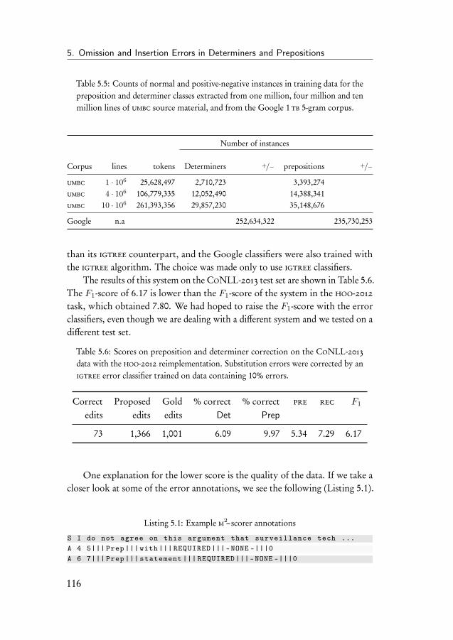
5. Omission and Insertion Errors in Determiners and Prepositions
Table 5.5: Counts of normal and positive-negative instances in training data for thepreposition and determiner classes extracted from one million, four million and tenmillion lines of umbc source material, and from the Google 1 tb 5-gram corpus.
Number of instances
Corpus lines tokens Determiners +/− prepositions +/−
umbc 1 · 106 25,628,497 2,710,723 3,393,274umbc 4 · 106 106,779,335 12,052,490 14,388,341umbc 10 · 106 261,393,356 29,857,230 35,148,676
Google n.a 252,634,322 235,730,253
than its igtree counterpart, and the Google classifiers were also trained withthe igtree algorithm. The choice was made only to use igtree classifiers.
The results of this system on theCoNLL-2013 test set are shown in Table 5.6.The F1-score of 6.17 is lower than the F1-score of the system in the hoo-2012task, which obtained 7.80. We had hoped to raise the F1-score with the errorclassifiers, even though we are dealing with a different system and we tested on adifferent test set.
Table 5.6: Scores on preposition and determiner correction on the CoNLL-2013
data with the hoo-2012 reimplementation. Substitution errors were corrected by anigtree error classifier trained on data containing 10% errors.
Correct Proposed Gold % correct % correct pre rec F1
edits edits edits Det Prep
73 1,366 1,001 6.09 9.97 5.34 7.29 6.17
One explanation for the lower score is the quality of the data. If we take acloser look at some of the error annotations, we see the following (Listing 5.1).
Listing 5.1: Example m2–scorer annotations
S I do not agree on this argument that surveillance tech ...A 4 5||| Prep ||| with ||| REQUIRED |||-NONE -|||0A 6 7||| Prep ||| statement ||| REQUIRED |||-NONE -|||0
116
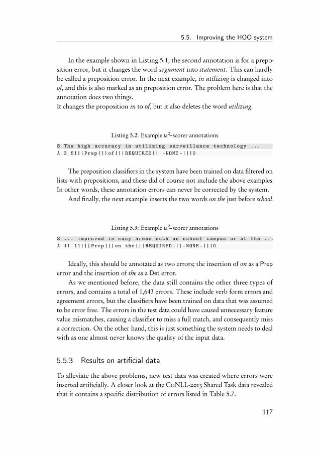
5.5. Improving the HOO system
In the example shown in Listing 5.1, the second annotation is for a prepo-sition error, but it changes the word argument into statement. This can hardlybe called a preposition error. In the next example, in utilizing is changed intoof, and this is also marked as an preposition error. The problem here is that theannotation does two things.It changes the proposition in to of, but it also deletes the word utilizing.
Listing 5.2: Example m2–scorer annotations
S The high accuracy in utilizing surveillance technology ...A 3 5||| Prep |||of||| REQUIRED |||-NONE -|||0
The preposition classifiers in the system have been trained on data filtered onlists with prepositions, and these did of course not include the above examples.In other words, these annotation errors can never be corrected by the system.
And finally, the next example inserts the two words on the just before school.
Listing 5.3: Example m2–scorer annotations
S ... improved in many areas such as school campus or at the ...A 11 11||| Prep |||on the ||| REQUIRED |||-NONE -|||0
Ideally, this should be annotated as two errors; the insertion of on as a Preperror and the insertion of the as a Det error.
As we mentioned before, the data still contains the other three types oferrors, and contains a total of 1,643 errors. These include verb form errors andagreement errors, but the classifiers have been trained on data that was assumedto be error free. The errors in the test data could have caused unnecessary featurevalue mismatches, causing a classifier to miss a full match, and consequently missa correction. On the other hand, this is just something the system needs to dealwith as one almost never knows the quality of the input data.
5.5.3 Results on artificial data
To alleviate the above problems, new test data was created where errors wereinserted artificially. A closer look at the CoNLL-2013 Shared Task data revealedthat it contains a specific distribution of errors listed in Table 5.7.
117
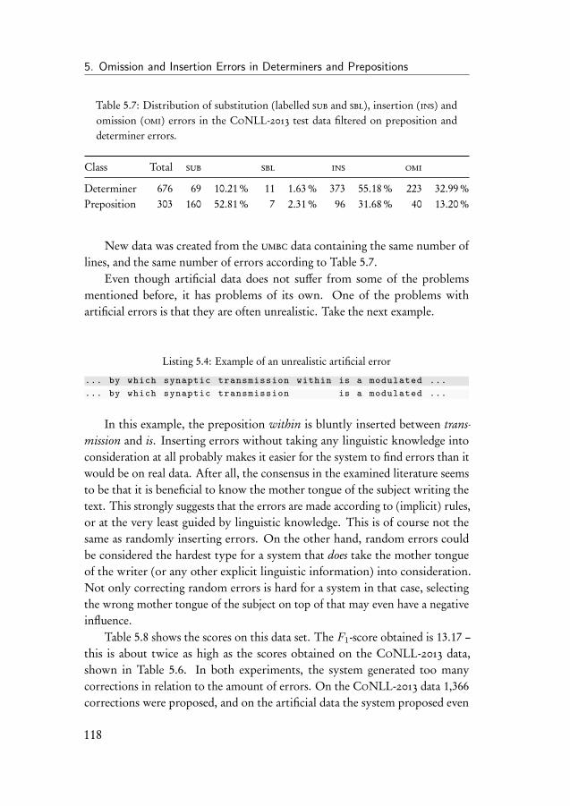
5. Omission and Insertion Errors in Determiners and Prepositions
Table 5.7: Distribution of substitution (labelled sub and sbl), insertion (ins) andomission (omi) errors in the CoNLL-2013 test data filtered on preposition anddeterminer errors.
Class Total sub sbl ins omi
Determiner 676 69 10.21% 11 1.63% 373 55.18% 223 32.99%Preposition 303 160 52.81% 7 2.31% 96 31.68% 40 13.20%
New data was created from the umbc data containing the same number oflines, and the same number of errors according to Table 5.7.
Even though artificial data does not suffer from some of the problemsmentioned before, it has problems of its own. One of the problems withartificial errors is that they are often unrealistic. Take the next example.
Listing 5.4: Example of an unrealistic artificial error
... by which synaptic transmission within is a modulated ...
... by which synaptic transmission is a modulated ...
In this example, the preposition within is bluntly inserted between trans-mission and is. Inserting errors without taking any linguistic knowledge intoconsideration at all probably makes it easier for the system to find errors than itwould be on real data. After all, the consensus in the examined literature seemsto be that it is beneficial to know the mother tongue of the subject writing thetext. This strongly suggests that the errors are made according to (implicit) rules,or at the very least guided by linguistic knowledge. This is of course not thesame as randomly inserting errors. On the other hand, random errors couldbe considered the hardest type for a system that does take the mother tongueof the writer (or any other explicit linguistic information) into consideration.Not only correcting random errors is hard for a system in that case, selectingthe wrong mother tongue of the subject on top of that may even have a negativeinfluence.
Table 5.8 shows the scores on this data set. The F1-score obtained is 13.17 –this is about twice as high as the scores obtained on the CoNLL-2013 data,shown in Table 5.6. In both experiments, the system generated too manycorrections in relation to the amount of errors. On the CoNLL-2013 data 1,366corrections were proposed, and on the artificial data the system proposed even
118
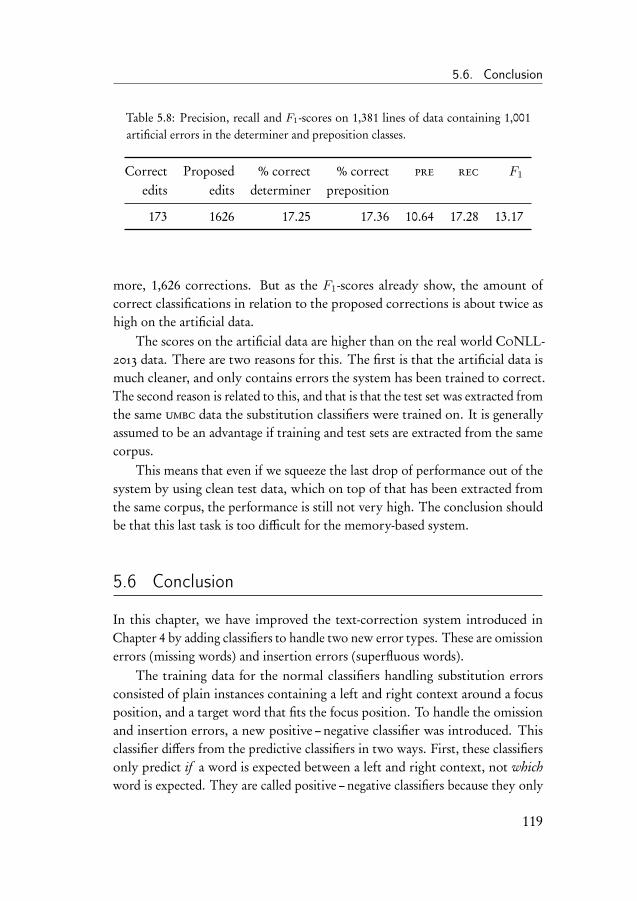
5.6. Conclusion
Table 5.8: Precision, recall and F1-scores on 1,381 lines of data containing 1,001artificial errors in the determiner and preposition classes.
Correct Proposed % correct % correct pre rec F1
edits edits determiner preposition
173 1626 17.25 17.36 10.64 17.28 13.17
more, 1,626 corrections. But as the F1-scores already show, the amount ofcorrect classifications in relation to the proposed corrections is about twice ashigh on the artificial data.
The scores on the artificial data are higher than on the real world CoNLL-
2013 data. There are two reasons for this. The first is that the artificial data ismuch cleaner, and only contains errors the system has been trained to correct.The second reason is related to this, and that is that the test set was extracted fromthe same umbc data the substitution classifiers were trained on. It is generallyassumed to be an advantage if training and test sets are extracted from the samecorpus.
This means that even if we squeeze the last drop of performance out of thesystem by using clean test data, which on top of that has been extracted fromthe same corpus, the performance is still not very high. The conclusion shouldbe that this last task is too difficult for the memory-based system.
5.6 Conclusion
In this chapter, we have improved the text-correction system introduced inChapter 4 by adding classifiers to handle two new error types. These are omissionerrors (missing words) and insertion errors (superfluous words).
The training data for the normal classifiers handling substitution errorsconsisted of plain instances containing a left and right context around a focusposition, and a target word that fits the focus position. To handle the omissionand insertion errors, a new positive –negative classifier was introduced. Thisclassifier differs from the predictive classifiers in two ways. First, these classifiersonly predict if a word is expected between a left and right context, not whichword is expected. They are called positive – negative classifiers because they only
119

5. Omission and Insertion Errors in Determiners and Prepositions
return a binary answer, signalling the desired presence or absence of a word byreturning a yes or no answer. The second difference is that a positive –negativeclassifier is trained on data which contains an empty focus position; that is whatthe text looks like when a word is missing.
In the first part of this chapter, we reported on the performance of thesystem in the hoo-2012 shared task. The memory-based text-correction systemranked ninth out of fourteen with an F1-score of 7.80. Comparing the systemto the other systems in the task revealed that ours was one of the simplestcorrectors entered in the competition. The top performing systems made useof preprocessing the data (spell checking, cleaning it up), used language-specificsyntactic features such as part-of-speech tags and relations between words, andfocused only on the most frequent errors in the data.
There is no denying that these systems were more successful than we were,but we were interested in more than just getting the highest score. The wholepoint of the exercise was to put a text-correction system based on a memory-based language model to the test. That also meant we trained the classifierson plain text without adding specialised knowledge for each particular task wetried, and assumed that the local context around the errors would give sufficientinformation to the systems to be able to correct them. This is not the case forlong-distance dependencies which stretch beyond the two positions around thefocus position.
The original hoo-2012-system did not make use of later improvements suchas error classifiers, which we described in Chapters 3 and 4. In the second part ofthe chapter, we implemented classifiers trained on error data for the substitutionerror handling. For the other two error categories, omissions and insertions,error classifiers are conceptually impossible to implement, and were not tried.Half the errors in the preposition class are substitution errors, and the systemwas expected to perform better even if only these errors were handled by errorclassifiers.
The updated system with the error classifiers was first tried on real worlddata, on the test set supplied with the CoNLL-2013 Shared Task. The obtainedF1-score was lower than that of the original system. We hypothesised that thiswas mainly due to the composition of the data, containing both more error typesthan the two we were correcting, plus a number of incorrectly annotated errors.A new experiment was run on artificial data containing the same number oferrors as the CoNLL-2013 test set. This obtained a higher F1-score, 13.17, butstill low enough to reach the conclusion that not the data was at fault. All things
120

5.6. Conclusion
considered, this task appeared too difficult for the memory-based classifierstrained on nothing more than plain data. Compared to the other systemscompeting in the hoo-2012 task, we ended up somewhere in the middle. Thesystems that performed best in the shared task were hand-crafted and optimisedfor the task, and even their best scores were under 40.
121

6Conclusion
In this chapter we summarise our findings, and discuss the results obtained bythe memory-based language model and text-correction systems. We also addressto what extent this thesis has answered the research questions raised in theintroductory chapter. As a reminder, the following questions were put forward.The overall research question we raised was as follows.
Given the simple nature of the memory-based language model, whatare the limits of its text correction abilities?
The overall research question was divided into two subquestions. The first oneconcentrated on the skipgram ability of the memory-based language model andread as follows.
To what extent does the ability to skip words offer an advantage in textcorrection?
The second one dealt with the advantage the ensemble systems could bring totext correction and was formulated like this.
To what extent does the ensemble system offer an advantage in textcorrection?
We now take a closer look at the answers to the research questions, andprovide a more detailed explanation. We then look at the system from anotherpoint of view, namely that of the usability and the use in real-world applications.We address the specific research questions first, before coming to a conclusionabout our general research question.
123
6. Conclusion
6.1 Answers to the research questions
We started this thesis by putting our memory-based language model in a languagemodelling perspective in Chapter 2. In that chapter, we compared igtree, afast decision-tree approximation of k-nn classification with a similar back offstrategy to those of standard statistical language models, together with ib1 andtribl2, to srilm, a standard statistical language model. We showed that the threealgorithms obtained perplexity scores which were similar to those obtained bysrilm, but finding similarities was not the main goal. The main goal was to assessif the predictions produced by the algorithms are suitable for text-correctionsystems.
The tribl2 algorithm possesses several unique features which sets it asidefrom conventional language models. First, both the tribl2 and igtree algorithmsdo not implement any explicit back off techniques. The algorithm which isconsidered to be equivalent to an n-gram model with back off, igtree, backsoff to a default distribution when feature values do not match, whereas thetribl2 algorithm skips the mismatching value and tries to match the remainingfeature values. The latter is equivalent to a skipgram model, and goes beyond thecapabilities of a normal n-gram language model. It was shown in the confusiblecorrection task that the ability to skip feature values gave tribl2 a significantadvantage over the igtree algorithm; the distributions returned by tribl2 weresmaller than those returned by igtree. The distributions returned by the igtreealgorithm would often contain many irrelevant words which made it moredifficult for the correction system to determine if it was dealing with an error,and if it was, to find the right correction. The distributions returned by thetribl2 algorithm were smaller, and contained more relevant predictions. Thismade it easier for the correction system to detect and correct errors.
In the second part of this thesis, we shifted focus from language modellingto text correction. The first text correction task we focused on was the detectionand correction of confusibles, which was explored in Chapter 3. The resultswere promising. The error detection seemed to work well for small confusiblesets, containing no more than three words. One thing that stood out was thestrength of the tribl2 algorithm. The idea behind tribl2 is simple; the algorithmskips over feature values that do not match, and continues to try to match theremaining values. This is a relatively simple change from the igtree algorithmwhich stops on the first mismatch, but turned out to give a large boost in F -scores. Looking closer at the results revealed that using the tribl2 algorithm
124
6.1. Answers to the research questions
caused a rise in both recall and precision. The largest gains were observed inthe recall figures. This confirmed the idea that skipgram capabilities allowedthe system to extract the relevant information to make a difference compared toigtree, in other words, it allowed the system to zoom in on specific instances inthe tree that carried the information needed for a successful correction.
To reiterate, the research question we are trying to answer at this point isif the skipgram approach of the memory-based model has advantages for textcorrection. In the case of confusible error detection and correction, we cananswer this question with a resounding yes.
The excellent results on the confusible detection and correction task can not,however, be solely attributed to the tribl2 algorithm. The ensemble system,which trains distinct classifiers for each confusible set, in combination withthe error-infused data, provided the extra bit of performance needed. On theerror-infused data, the ensemble system increased F -scores from 36 to over 45using the igtree classifier, and from 55 to almost 58 using the tribl2 classifier. Itturned out that on the non error-infused data, the ensemble system obtained ahigher number of corrections, but at the cost of more false positives. On theerror-infused data, the number of false positives was greatly reduced, resulting inhigher F -scores.
The ensemble system had a larger influence on the scores obtained by theigtree classifier than those obtained by tribl2. Due to the larger instance base,the monolithic igtree system generates larger distributions than its ensemblecounterpart, which made it more difficult for the corrector to find the rightanswer. The distributions from the ensemble system based on igtree weresmaller, turning the process of finding the correct answer in a choice betweentwo or three alternatives. The influence on the tribl2 algorithm was smaller,because this classifier already returned smaller distributions and the distributionsfrom the ensemble and monolithic system are more similar to begin with. Allin all, we can say that, with regard to the third research question, using theensemble system showed some improvement, but not as much as the use of thetribl2 classifier did.
In Chapters 4 and 5 the correction of two larger classes was explored, namelydeterminers and prepositions. In Chapter 4 a system was created that was similarto the confusible detection and correction system described in the precedingchapter. It focused on the correction of substitution errors in the determinerand preposition classes. The full task, described in Chapter 5, involved thecorrection of three kinds of errors; substitution, omission and insertion errors.
125

6. Conclusion
The promising results of the confusible correction system gave rise to highexpectations of the new system, but these expectations were not quite met.Whereas the results on artificially created test data were good, yielding F1-scoresof just over 40, they dropped to just under 12 on real world data. Investigatingthe cause of the differences pointed to the real world data used to test the system.It contained not only the errors from the training data, but a number of errorsfrom other grammatical categories as well. The artificial training and test datawere much more similar to each other than the real world training and test data.
In Chapter 5 the system was extended to handle the omission and insertionerrors as well. It was here we ran into the limits of what is possible with asimple memory-based text-correction system; the F1-scores obtained were in the5 – 10 range. Examining the output revealed that only a few of the errors in highfrequency determiners or prepositions were corrected. Previously, the same taskhad already been tried with a simpler corrector, and we had expected the newinsights gained in the two preceding chapters, classifiers trained on error-infuseddata in combination with the tribl2 algorithm, to make a difference in this taskas well. Both incarnations of the system, the original one and the augmentedone are described in Chapter 5. Even though the updated version of the systemreached an F1-score of almost 20 on data infused with artificial errors, neithersystem reached F1-scores of over eight on real world data.
6.1.1 Compared to other systems
The determiner and preposition detection and correction task was part of theCoNLL-2013 Shared Task, and this gave us the possibility to compare thememory-based systems with other systems. Comparing them to other systemsthat performed well on the same task revealed several significant differences. First,those systems made use of language-specific syntactic features. Second, they wereheavily tuned for the task they had to perform (including only correcting themost frequent mistakes and using training data with error statistics), and finally,they pre-processed the training data (by spellchecking it). We choose not to doany tuning or pre-processing, and our performance suffered because of it. We mayventure to conclude that the simple distribution based approach with minimalpre- and post-processing works for confusible detection and correction, but notfor anything beyond making the contextually appropriate choice between two orthree words. Considering the determiner and preposition task, it needs flexibleand long-distance dependency information to be done correctly, and these are
126
6.1. Answers to the research questions
not provided by the local contexts used by our system.We also had difficulties with the insertion and omission errors. This is
another area where the features used by the systems, or even the way they arehandled, could be improved. One of the disadvantages of using fixed sizedinstances is the difficulty of modelling missing and redundant information; weare training the system on text which is correct. Missing information is the mostcomputationally intensive of the two, for the following reason. For each positionin a sentence where there could be a word missing, and that is between eachpair of words, the system has to try to predict a possible missing word. Thatmeans that even in a five word sentence there are a total of six positions (alsocounting before the first and after the last word) where a word can be inserted,but most of these will be irrelevant. As is the nature of our memory-basedpredictor, a list of possible missing words will always be generated, leaving it upto the filtering algorithms and the parameters to decide if a prediction shouldbe inserted. This is further complicated by the fact that it is hard to determinewhich class the missing word belongs to, as all the classifiers will return ananswer. This led to many false positives being generated by our system. Theinsertion error check was slightly easier; the system only needs to apply theclassifier when encountering a class member, involving only the appropriateclassifier. The filtering algorithm decides if the probability of the word occurringat that position is low enough to signal a redundant word.
Finally, for the normal word predicting classifier, it proved to be profitablefor confusible error correction to use error-infused data to train the system. Thismeans that the instances contained the incorrect word in context, forcing theclassifier towards the right answer. The results on the confusible detection andcorrection task showed an improvement in F -scores when using this technique.In the determiner and preposition task, however, no such improvement wasobserved.
Even though the two text correction tasks described in this thesis seemed sim-ilar, they helped to locate where the strengths and weaknesses of memory-basedtext correction lie. The confusible detection and correction task was handledwith relative success by our methods because there were a number of smallclasses containing two or three elements which are used in contextually differentpositions. The determiner and preposition task centred around two larger classeswith elements which are used in similar contexts. The text-correction systemswe described only use the surface structure of the text in order to find errors anddetermine suitable corrections, which worked in the former but not in the latter
127
6. Conclusion
case. Examining the literature on similar text-correction systems supported thisconclusion. With this we have answered our research questions, and establishedthe limits of what is possible with a simple memory-based text corrector.
6.1.2 Real world applications
When it comes to practical applications, the language modelling and wordpredicting capabilities have been used in real world tasks. We mention twoof them. First, wopr provides the language model in t-scan1, which is a toolused for readability prediction of Dutch language texts [Pander Maat et al.,2014]. Second, a plain word predictor based on the igtree algorithm is usedin valkuil.net and fowlt.net. Valkuil.net is a Dutch language grammarand spelling checker using a number of different modules to check for errors,and fowlt.net is its English language counterpart.2 Both versions use wopras a general purpose corrector, which tries to catch the errors for which nospecialised module is available. In these systems, the distribution of a generalword predictor is used to find errors (as discussed in the second chapter), asopposed to the specialised predictors discussed in the later chapters. In boththese systems, the memory-based language model looks only for substitutionerrors, not for omission and insertion errors.
The fact that the memory-based systems are used in real-world applicationsonce more affirms the viability of the method. What remains is to turn our eyeto the future and see if there are areas where the system can be improved.
6.2 Future work
With regards to the future possibilities of memory-based text-correction systems,there are several ways of solving some of the performance issues that we faced inour studies.
The first one is centred around the task of text correction, for example thecorrection of determiner and preposition errors. The system discussed in thisthesis could be extended by adding grammatical features, (statistical) knowledgeabout the errors in the training data, tweaking of parameters per classifier,et cetera, but if we do this we change the nature of the system; it will not be this
1http://languagelink.let.uu.nl/tscan2See http://valkuil.net and http://fowlt.net
128

6.2. Future work
simple memory-based system anymore, the one which could easily and quicklybe trained on a large text corpus. The grammatical knowledge has to be providedfrom other sources such as treebanks and parsers; these are language specific,and not always readily available for any language. Incorporating grammaticalknowledge will lose one of the big advantages of the system, and that is that itcan be trained on plain text.
Another way to solve some of the performance problems could be to adaptparts of the system. Would better training data make a difference? It seemsunlikely – the scores obtained increased with clean artificial data, but that didstill not create a useful system. We have been using a ‘two words to the left andtwo to the right’ context throughout this thesis, hoping it would capture enoughinformation for the text correction tasks. What is left unexplored are larger, oreven flexible contexts. A flexible context would span a larger number of words,but with ‘gaps’ where the seemingly unimportant words would have been. Thisis different from the tribl2 skipgram approach used at this moment which istrained on the full context and only skips features when they do not match. Thiswould allow the instances to be both much longer, and at the same time keepthe memory requirements low. It is possible that these larger, flexible contextswould be able to capture some of the longer dependencies needed for our task.
The classifiers could also be incorporated in a real text-correction system.This can be done interactively, where the user of the system is given a choiceof possible corrections if an error is detected, or fully automatic, without userintervention. The performance of the confusible detection and correctionsystem was good enough to be used without user interaction. The determinerand preposition correction system could not be used without user input, butthis was the case for all the systems that competed in the CoNLL-2013 SharedTask. The question is how many false positives a user is willing to deal with,and if she is able to pick the right answer from a number of alternatives. Thelatter is not obvious if the text-correction system is aimed at language learners ornon-native speakers of a language.
Concluding, we have shown that the memory-based text-correction systemworked well on the confusible correction task, and it could be used in a text cor-rection system. The determiner and preposition correction system could alreadybe used interactively, and we feel confident that with the right improvements ittoo could deserve its place in a text-correction system.
129


Appendix
131

ADeterminer and Preposition Sets
The 23 determiners and articles
a, all, an, another, any, both, each, either, every, many, neither, no, some, that,the, these, this, those, what, whatever, which, whichever, who
The 64 prepositions
about, above, across, after, against, along, alongside, amid, among, amongst,apart, around, as, aside, at, atop, before, behind, below, beneath, beside, besides,between, beyond, by, down, due, for, from, in, inside, into, near, next, of, off,on, onto, out, outside, over, past, per, since, though, through, throughout, till,to, toward, towards, under, unlike, until, up, upon, versus, via, vs., whether,while, with, within, without
133

Bibliography
[Abushihab et al., 2011] Abushihab, I., El-Omari, A. H., and Tobat, M. (2011).An analysis of written grammatical errors of Arab learners of English asa foreign language at Alzaytoonah private university of Jordan. EuropeanJournal of Social Sciences, 20(4):543–552.
[Aha et al., 1991] Aha, D. W., Kibler, D., and Albert, M. (1991). Instance-basedlearning algorithms. Machine Learning, 6:37–66.
[Alberga, 1967] Alberga, C. N. (1967). String similarity and misspellings. Com-mun. ACM, 10(5):302–313.
[Allison et al., 2006] Allison, B., Guthrie, D., and Guthrie, L. (2006). Anotherlook at the data sparsity problem. In Text, Speech and Dialogue, pages 327–334.Springer.
[Atwell, 1987] Atwell, E. S. (1987). How to detect grammatical errors in atext without parsing it. In Proceedings of the third conference on Europeanchapter of the Association for Computational Linguistics, EACL ’87, pages38–45, Stroudsburg, PA, USA. Association for Computational Linguistics.
[Banko and Brill, 2001a] Banko, M. and Brill, E. (2001a). Mitigating thepaucity-of-data problem: Exploring the effect of training corpus size onclassifier performance for natural language processing. In Proceedings ofthe First International Conference on Human Language Technology Research,HLT ’01, pages 1–5, Stroudsburg, PA, USA. Association for ComputationalLinguistics.
[Banko and Brill, 2001b] Banko, M. and Brill, E. (2001b). Scaling to very verylarge corpora for natural language disambiguation. In Proceedings of the 39thAnnual Meeting of the Association for Computational Linguistics, pages 26–33.Association for Computational Linguistics.
135
Bibliography
[Bergsma et al., 2009] Bergsma, S., Lin, D., and Goebel, R. (2009). Web-scale n-grammodels for lexical disambiguation. In Proceedings of the 21st InternationalJoint Conference on Artificial Intelligence, IJCAI’09, pages 1507–1512, SanFrancisco, CA, USA. Morgan Kaufmann Publishers Inc.
[Bitchener et al., 2005] Bitchener, J., Young, S., and Cameron, D. (2005). Theeffect of different types of corrective feedback on {ESL} student writing.Journal of Second Language Writing, 14(3):191 – 205.
[Brants and Franz, 2006] Brants, T. and Franz, A. (2006). LDC2006T13: Web1T 5-gram Version 1.
[Brill, 2000] Brill, E. (2000). Pattern-based disambiguation for natural languageprocessing. In Proceedings of the 2000 Joint SIGDAT Conference on EmpiricalMethods in Natural Language Processing and Very Large Corpora: Held inConjunction with the 38th Annual Meeting of the Association for ComputationalLinguistics - Volume 13, EMNLP ’00, pages 1–8, Stroudsburg, PA, USA.Association for Computational Linguistics.
[Brockett et al., 2006] Brockett, C., Dolan, W. B., and Gamon, M. (2006). Cor-recting esl errors using phrasal smt techniques. In Proceedings of the 21stInternational Conference on Computational Linguistics and the 44th annualmeeting of the Association for Computational Linguistics, pages 249–256. Asso-ciation for Computational Linguistics.
[Broder et al., 2009] Broder, A., Ciccolo, P., Gabrilovich, E., Josifovski, V.,Metzler, D., Riedel, L., and Yuan, J. (2009). Online expansion of rare queriesfor sponsored search. In Proceedings of the 18th international conference onWorld wide web, page 511–520.
[Buck et al., 2014] Buck, C., Heafield, K., and van Ooyen, B. (2014). N-gramcounts and language models from the common crawl. In Proceedings of theLanguage Resources and Evaluation Conference, Reykjavík, Iceland.
[Carlson et al., 2008] Carlson, A., Mitchell, T. M., and Fette, I. (2008). Dataanalysis project: Leveraging massive textual corpora using n-gram statistics.Technical Report CMU-ML-08-107, CMU.
[Carlson et al., 2001] Carlson, A. J., Rosen, J., and Roth, D. (2001). Scaling upcontext-sensitive text correction. Urbana, 51:61801.
136

Bibliography
[Chen et al., 2007] Chen, Q., Li, M., and Zhou, M. (2007). Improving queryspelling correction using web search results. In EMNLP-CoNLL, volume 7,pages 181–189. Citeseer.
[Chen and Goodman, 1998] Chen, S. and Goodman, J. (1998). An empiricalstudy of smoothing techniques for language modeling. Technical ReportTR-10-98, Harvard University.
[Choudhury et al., 2007] Choudhury, M., Thomas, M., Mukherjee, A., Basu,A., and Ganguly, N. (2007). How difficult is it to develop a perfect spell-checker? a cross-linguistic analysis through complex network approach. InProceedings of the Second Workshop on TextGraphs: Graph-Based Algorithms forNatural Language Processing, pages 81–88, Rochester, NY, USA. Associationfor Computational Linguistics.
[Cost and Salzberg, 1993] Cost, S. and Salzberg, S. (1993). A weighted nearestneighbour algorithm for learning with symbolic features. Machine Learning,10:57–78.
[Cover and Hart, 1967] Cover, T. M. and Hart, P. E. (1967). Nearest neigh-bor pattern classification. Institute of Electrical and Electronics EngineersTransactions on Information Theory, 13:21–27.
[Cucerzan and Brill, 2004] Cucerzan, S. and Brill, E. (2004). Spelling correctionas an iterative process that exploits the collective knowledge of web users.In Lin, D. and Wu, D., editors, Proceedings of EMNLP 2004, pages 293–300,Barcelona, Spain. Association for Computational Linguistics.
[Daelemans and Van den Bosch, 2005] Daelemans, W. and Van den Bosch, A.(2005). Memory-based language processing. Cambridge University Press, Cam-bridge, UK.
[Daelemans et al., 1997] Daelemans, W., Van den Bosch, A., and Weijters, A.(1997). IGTree: using trees for compression and classification in lazy learningalgorithms. Artificial Intelligence Review, 11:407–423.
[Daelemans et al., 2010] Daelemans, W., Zavrel, J., Van der Sloot, K., and Vanden Bosch, A. (2010). TiMBL: Tilburg memory based learner, version 6.3,reference guide. Technical Report ILK 10-01, ILK Research Group, TilburgUniversity.
137
Bibliography
[Dahlmeier and Ng, 2012] Dahlmeier, D. and Ng, H. T. (2012). Better evalua-tion for grammatical error correction. In Proceedings of the 2012 Conference ofthe North American Chapter of the Association for Computational Linguistics:Human Language Technologies, NAACL HLT ’12, pages 568–572, Strouds-burg, PA, USA. Association for Computational Linguistics.
[Dahlmeier et al., 2012] Dahlmeier, D., Ng, H. T., and Ng, E. J. F. (2012). Nusat the hoo 2012 shared task. In Proceedings of the SeventhWorkshop on BuildingEducational Applications Using NLP, pages 216–224, Stroudsburg, PA, USA.Association for Computational Linguistics.
[Dale et al., 2012] Dale, R., Anisimoff, I., and Narroway, G. (2012). HOO2012: A report on the preposition and determiner error correction sharedtask. In Proceedings of the Seventh Workshop on Innovative Use of NLP forBuilding Educational Applications, Montreal, Canada.
[Dale and Kilgarriff, 2010] Dale, R. and Kilgarriff, A. (2010). Helping our own:Text massaging for computational linguistics as a new shared task. In INLG.
[Dale and Kilgarriff, 2011] Dale, R. and Kilgarriff, A. (2011). Helping ourown: The hoo 2011 pilot shared task. In Proceedings of the 13th EuropeanWorkshop on Natural Language Generation, pages 242–249. Association forComputational Linguistics.
[Dalgish, 1985] Dalgish (1985). Computer-Assisted ESL Research and Course-ware Development. http://computersandcomposition.candcblog.org/archives/v2/2_4_html/2_4_05_Dalgish.html. [Online resource;accessed 2016-02-22].
[Damerau, 1964] Damerau, F. J. (1964). A technique for computer detectionand correction of spelling errors. Commun. ACM, 7(3):171–176.
[Daudaravičius, 2012] Daudaravičius, V. (2012). Vtex determiner and preposi-tion correction system for the hoo 2012 shared task. In Proceedings of theSeventh Workshop on Building Educational Applications Using NLP, pages225–232, Stroudsburg, PA, USA. Association for Computational Linguistics.
[De Felice and Pulman, 2008] De Felice, R. and Pulman, S. G. (2008). Aclassifier-based approach to preposition and determiner error correction in L2English. In Proceedings of the 22nd International Conference on ComputationalLinguistics - Volume 1, COLING ’08, pages 169–176, Stroudsburg, PA, USA.Association for Computational Linguistics.
138
Bibliography
[Ehsan and Faili, 2013] Ehsan, N. and Faili, H. (2013). Grammatical andcontext-sensitive error correction using a statistical machine translation frame-work. Software: Practice and Experience, 43(2):187–206.
[Federico et al., 2008] Federico, M., Bertoldi, N., and Cettolo, M. (2008).Irstlm: an open source toolkit for handling large scale language models.In Interspeech, pages 1618–1621.
[Foster and Andersen, 2009] Foster, J. and Andersen, O. E. (2009). Generrate:generating errors for use in grammatical error detection. In Proceedings of theFourth Workshop on Innovative Use of NLP for Building Educational Applica-tions, EdAppsNLP ’09, pages 82–90, Stroudsburg, PA, USA. Association forComputational Linguistics.
[Gamon, 2010] Gamon, M. (2010). Using mostly native data to correct er-rors in learners’ writing: A meta-classifier approach. In Human LanguageTechnologies: The 2010 Annual Conference of the North American Chapterof the Association for Computational Linguistics, HLT ’10, pages 163–171,Stroudsburg, PA, USA. Association for Computational Linguistics.
[Gamon et al., 2008] Gamon, M., Gao, J., Chris Brockett and, A. K., Dolan,W. B., and Dmitriy Belenko, L. V. (2008). Using contextual speller techniquesand language modeling for esl error correction. IJCNLP.
[Gibson, 1984] Gibson, W. (1984). Neuromancer. Sprawl trilogy. Ace Books.
[Golding and Roth, 1999] Golding, A. and Roth, D. (1999). A Winnow-BasedApproach to Context-Sensitive Spelling Correction. Machine Learning, 34(1–3):107–130.
[Golding, 1995] Golding, A. R. (1995). A Bayesian hybrid method for context-sensitive spelling correction. In Proceedings of the 3rd workshop on very largecorpora, ACL-95, pages 39–53.
[Golding and Roth, 1996] Golding, A. R. and Roth, D. (1996). Applying Win-now to context-sensitive spelling correction. In Machine Learning, pages182–190.
[Gompel et al., 2012] Gompel, M. v., Sloot, K. v. d., and van den Bosch, A.(2012). Ucto: Unicode tokenizer. ILK Research Group Technical ReportSeries 12-05, Tilburg University.
139
Bibliography
[Good, 1966] Good, I. J. (1966). Studies in the history of probability andstatistics. xxxvii a. m. turing’s statistical work in world war ii. Biometrika,66(2):393–396.
[Guthrie et al., 2006] Guthrie, D., Allison, B., Liu, W., Guthrie, L., and Wilks,Y. (2006). A closer look at skip-gram modelling. In Proceedings of the 5thinternational Conference on Language Resources and Evaluation (LREC-2006),pages 1–4.
[Han et al., 2013a] Han, L., Kashyap, A. L., Finin, T., Mayfield, J., and Weese,J. (2013a). UMBC_EBIQUITY-CORE: Semantic Textual Similarity Systems.In Proceedings of the Second Joint Conference on Lexical and ComputationalSemantics. Association for Computational Linguistics.
[Han et al., 2013b] Han, L., Kashyap, A. L., Finin, T., Mayfield, J., and Weese,J. (2013b). UMBC_EBIQUITY-CORE: Semantic Textual Similarity Systems.In Proceedings of the Second Joint Conference on Lexical and ComputationalSemantics. Association for Computational Linguistics.
[Han et al., 2010] Han, N.-R., Tetreault, J. R., Lee, S.-H., and Ha, J.-Y. (2010).Using an error-annotated learner corpus to develop an esl/efl error correctionsystem. In LREC.
[Huang et al., 1992] Huang, X., Alleva, F., Hon, H.-W., Hwang, M.-Y., andRosenfeld, R. (1992). The SPHINX-II speech recognition system : an overview.Pittsburgh, Pa. : School of Computer Science, Carnegie Mellon University.
[Jelinek, 1998] Jelinek, F. (1998). Statistical Methods for Speech Recognition. TheMIT Press, Cambridge, MA.
[Jelinek et al., 1977] Jelinek, F., Mercer, R. L., Bahl, L. R., and Baker, J. K.(1977). Perplexity—a measure of the difficulty of speech recognition tasks.The Journal of the Acoustical Society of America, 62(S1):S63–S63.
[Jiménez Catalán, 1996] Jiménez Catalán, R. M. (1996). Frequency and vari-ability in errors in the use of English prepositions. A Journal of English andAmerican Studies, pages 171–187.
[Kochmar et al., 2012] Kochmar, E., Andersen, O., and Briscoe, T. (2012). Hoo2012 error recognition and correction shared task: Cambridge universitysubmission report. In Proceedings of the Seventh Workshop on Building Ed-ucational Applications Using NLP, pages 242–250, Stroudsburg, PA, USA.Association for Computational Linguistics.
140
Bibliography
[Koehn et al., 2007] Koehn, P., Hoang, H., Birch, A., Callison-Burch, C., Fed-erico, M., Bertoldi, N., Cowan, B., Shen, W., Moran, C., Zens, R., Dyer,C., Bojar, O., Constantin, A., and Herbst, E. (2007). Moses: Open sourcetoolkit for statistical machine translation. In Proceedings of the 45th AnnualMeeting of the Association for Computational Linguistics Companion VolumeProceedings of the Demo and Poster Sessions, pages 177–180, Prague, CzechRepublic. Association for Computational Linguistics.
[Kölmyr, 2001] Kölmyr, P. (2001). To err is human . . . An investigation ofgrammatical errors in Swedish 16-year-old learners’ written production in English.PhD thesis, Göteborg University.
[Kučera and Francis, 1967] Kučera, H. and Francis, W. N. (1967). Computa-tional Analysis of Present-Day American English. Brown University Press,Providence, RI.
[Lapata and Keller, 2005] Lapata, M. and Keller, F. (2005). Web-based modelsfor natural language processing. ACM Trans. Speech Lang. Process., 2(1).
[Lee and Seneff, 2008] Lee, J. and Seneff, S. (2008). An analysis of grammati-cal errors in non-native speech in english. In Spoken Language TechnologyWorkshop, 2008. SLT 2008. IEEE, pages 89–92.
[Lewis et al., 2004] Lewis, D., Yang, Y., Rose, T., and Li, F. (2004). RCV1: Anew benchmark collection for text categorization research. Journal of MachineLearning Research, 5:361–397.
[Lynch et al., 2012] Lynch, G., Moreau, E., and Vogel, C. (2012). A naivebayes classifier for automatic correction of preposition and determiner errorsin esl text. In Proceedings of the Seventh Workshop on Building EducationalApplications Using NLP, pages 257–262, Stroudsburg, PA, USA. Associationfor Computational Linguistics.
[Mangu and Brill, 1997] Mangu, L. and Brill, E. (1997). Automatic rule acquisi-tion for spelling correction. In Proceedings of the International Conference onMachine Learning, pages 187–194.
[Manning and Schütze, 1999] Manning, C. and Schütze, H. (1999). Foundationsof Statistical Natural Language Processing. The MIT Press, Cambridge, MA.
[Mays et al., 1991] Mays, E., Damerau, F. J., and Mercer, R. L. (1991). Contextbased spelling correction. Information Processing and Management, 27(5):517–522.
141
Bibliography
[Moats, 2005] Moats, L. C. (2005). How spelling supports reading and whyit is more regular and predictable than you may think. American Educator,pages 12–22, 42–43.
[Ng et al., 2013a] Ng, H. T., Tetreault, J., Wu, S. M., Wu, Y., and Hadiwinoto,C., editors (2013a). Proceedings of the Seventeenth Conference on Computa-tional Natural Language Learning: Shared Task. Association for Computa-tional Linguistics, Sofia, Bulgaria.
[Ng et al., 2013b] Ng, H. T., Wu, S. M., Wu, Y., Hadiwinoto, C., and Tetreault,J. (2013b). The CoNLL-2013 shared task on grammatical error correction.In Proceedings of the Seventeenth Conference on Computational Natural Lan-guage Learning: Shared Task, pages 1–12, Sofia, Bulgaria. Association forComputational Linguistics.
[Nicholls, 2003] Nicholls, D. (2003). The cambridge learner corpus: Error cod-ing and analysis for lexicography and elt. Proceedings of the Corpus Linguistics2003 conference, 16:572–581.
[nus nlp group, 2016] nus nlp group (2016). MaxMatch Evaluator. http://www.comp.nus.edu.sg/~nlp/software.html. [Online resource; accessed2016-02-23].
[Onrust et al., 2016] Onrust, L., van den Bosch, A., and Van hamme, H. (2016).Improving cross-domain n-gram language modelling with skipgrams. In Pro-ceedings of the 54th Annual Meeting of the Association for Computational Lin-guistics (Volume 2: Short Papers), pages 137–142, Berlin, Germany. Associationfor Computational Linguistics.
[Pander Maat et al., 2014] Pander Maat, H., Kraf, R., van den Bosch, A.,Dekker, N., van Gompel, M., Kleijn, S., Sanders, T., and van der Sloot,K. (2014). T-scan: a new tool for analyzing dutch text. ComputationalLinguistics in the Netherlands Journal, 4:53–74.
[Quinlan, 1993] Quinlan, J. (1993). C4.5: Programs for Machine Learning. Mor-gan Kaufmann, San Mateo, CA.
[Reynaert, 2005] Reynaert, M. (2005). Text-induced spelling correction. PhDthesis, Tilburg University.
[Rosenfeld, 2000] Rosenfeld, R. (2000). Two decades of statistical languagemodeling: Where do we go from here? Proceedings of the IEEE, 88(8):1270–1278.
142
Bibliography
[Rozovskaya and Roth, 2010] Rozovskaya, A. and Roth, D. (2010). Trainingparadigms for correcting errors in grammar and usage. In Human LanguageTechnologies: The 2010 Annual Conference of the North American Chapterof the Association for Computational Linguistics, HLT ’10, pages 154–162,Stroudsburg, PA, USA. Association for Computational Linguistics.
[Rozovskaya and Roth, 2011] Rozovskaya, A. and Roth, D. (2011). Algorithmselection and model adaptation for esl correction tasks. In ACL, Portland,Oregon. Association for Computational Linguistics.
[Rozovskaya et al., 2012] Rozovskaya, A., Sammons, M., and Roth, D. (2012).The ui system in the hoo 2012 shared task on error correction. In Proceedingsof the SeventhWorkshop on Building Educational Applications Using NLP, pages272–280, Stroudsburg, PA, USA. Association for Computational Linguistics.
[Sethy et al., 2005] Sethy, A., Georgiou, P. G., and Narayanan, S. (2005). Build-ing topic specific language models from webdata using competitive models.In INTERSPEECH, pages 1293–1296.
[Shannon, 1948] Shannon, C. E. (1948). A mathematical theory of communi-cation. Bell Systems Technical Journal, 27:623–656.
[Stanfill and Waltz, 1986] Stanfill, C. and Waltz, D. (1986). Toward memory-based reasoning. Communications of the ACM, 29(12):1213–1228.
[Stehouwer and Van Zaanen, 2009] Stehouwer, H. and Van Zaanen, M. (2009).Language models for contextual error detection and correction. In Pro-ceedings of the EACL 2009 Workshop on Computational Linguistic Aspects ofGrammatical Inference, pages 41–48, Athens, Greece.
[Stolcke, 2002] Stolcke, A. (2002). SRILM – An extensible language modelingtoolkit. In Proceedings of the International Conference on Spoken LanguageProcessing, pages 901–904, Denver, Colorado.
[Tan et al., 2011] Tan, M., Zhou, W., Zheng, L., and Wang, S. (2011). A largescale distributed syntactic, semantic and lexical language model for machinetranslation. In Proceedings of the 49th Annual Meeting of the Association forComputational Linguistics: Human Language Technologies, pages 201–210,Portland, Oregon, USA. Association for Computational Linguistics.
143
Bibliography
[Van den Bosch, 2006] Van den Bosch, A. (2006). All-word prediction as theultimate confusible disambiguation. In Proceedings of the HLT-NAACL Work-shop on Computationally hard problems and joint inference in speech and lan-guage processing, New York, NY.
[Van den Bosch and Berck, 2009] Van den Bosch, A. and Berck, P. (2009).Memory-based machine translation and language modeling. The PragueBulletin of Mathematical Linguistics, 91:17–26.
[Van den Bosch and Berck, 2012] Van den Bosch, A. and Berck, P. (2012).Memory-based text correction for preposition and determiner errors. InProceedings of the 7th Workshop on the Innovative Use of NLP for BuildingEducational Applications, pages 289–294, New Brunswick, NJ. ACL.
[Van den Bosch and Berck, 2013] Van den Bosch, A. and Berck, P. (2013).Memory-based grammatical error correction. In Proceedings of the Seven-teenth Conference on Computational Natural Language Learning: Shared Task,pages 102–108, Sofia, Bulgaria. Association for Computational Linguistics.
[Van Rijsbergen, 1979] Van Rijsbergen, C. (1979). Information Retrieval. But-tersworth, London.
[Wagner et al., 2009] Wagner, J., Foster, J., and Van Genabith, J. (2009). Judginggrammaticality: Experiments in sentence classification. CALICO Journal,26(3):474–490.
[WebBase, 2007] WebBase (2007). Stanford WebBase Project. http://bit.ly/WebBase. [Online resource; accessed 2016-02-18].
[Yarowsky, 1994] Yarowsky, D. (1994). Decision lists for lexical ambiguityresolution: application to accent restoration in spanish and french. In Proceed-ings of the 32nd annual meeting on Association for Computational Linguistics,ACL ’94, pages 88–95, Stroudsburg, PA, USA. Association for ComputationalLinguistics.
[Yi et al., 2008] Yi, X., Gao, J., and Dolan, W. B. (2008). A web-based englishproofing system for english as a second language users. In IJCNLP, pages619–624.
[Yuan and Felice, 2013] Yuan, Z. and Felice, M. (2013). Constrained grammati-cal error correction using statistical machine translation. In Proceedings of theSeventeenth Conference on Computational Natural Language Learning: SharedTask, pages 52–61, Sofia, Bulgaria. Association for Computational Linguistics.
144
Summary
The field of computational linguistics is already more than half a century old,but progress in the field of machine learning, availability of larger and largeramounts of data and the proliferation of capable computing devices (e.g. mobilephones) still provides a strong incentive for continuous development.
One of the areas which are subject to ongoing research is text correction.Text correction is a broad term, and includes techniques ranging from grammati-cal correction to spelling correction. While the first text-correction systems wereoften built around small sets of grammatical rules translated into a computerreadable format, the availability of large quantities of data has raised the questionif it is possible to build a well performing text-correction system using machinelearning, i.e. trained on large amounts of plain text.
One field of machine learning is memory-based learning, which is charac-terised by the following properties; learning consists of storing examples inmemory, and processing of data is done by comparing new examples with storedexamples in memory. This leads to systems which are easily trained and adapt-able, but would these systems be able to process natural language in a meaningfulway?
In this thesis, we introduce several text-correction systems which are builtaround a memory-based language model. Our goal is to determine to whatextent the memory-based models are suitable for text correction; when has thetask become too difficult for the system to handle? The main research questionwe pose is the following.
Given the simple nature of the memory-based language model, whatare the limits of its text correction abilities?
The language models, described in Chapter 2, have been implemented as aword predictor. They store information in a decision tree, and are capable ofpredicting a list of words fitting a context around it. The list not only contains

Summary
words, but also information about how often each predicted word occurs in thegiven context. This list will be referred to as a distribution. The words in thedistribution are used by the correction system to detect and correct errors in atext. If a word in a text is not part of the predicted words, we may be dealingwith an error.
In order to answer the research question, the systems are applied to twospecific tasks, confusible correction, and the correction of determiners andprepositions.
The confusible correction system is described in Chapter 3. The determinerand preposition correction task is divided into two subtasks. The first subtaskdeals only with substitution errors in the determiner and preposition class. Thissystem is similar to the system correcting the confusible errors. The secondsubtask correct three kinds of errors in these two classes; substitution, omissionand insertion errors. The two subtasks are assigned a chapter each, Chapter 4deals with substitution errors, and Chapter 5 with the omission and insertionerrors.
The memory-based language model implementation we use in this thesishas two interesting properties. First, it does not just use a left context butcan make use of both the left and right context. This means it does not justpredict a word following sequence, but can predict words which fit best inside acertain sequence. The second, more important property is related to the backoff strategy employed by the tribl2 algorithm in the text-correction systems.The tribl2 algorithm has the ability to skip mismatching feature values whenclassifying instances, which makes it equivalent to a skipgram model. Thisproperty is important enough to warrant its own research question. The secondresearch question we pose is this.
To what extent does the ability to skip words offer an advantage in textcorrection?
Beside training classifiers to correct all the errors in one class, we createsystems containing a number of classifiers which have been trained to correctjust one specific error each. We call these systems ensemble systems. In thisthesis, we also ask the question if this provides an advantage when performingtext correction. We pose the following research question.
To what extent does the ensemble system offer an advantage in textcorrection?
146

Summary
The answers to the research questions can be found in the final chapter,Chapter 6. As for the second research question, we conclude that the skipping-ability of tribl2 does provide an advantage. The third question can also beanswered positively – the ensemble systems give the extra push necessary tomake a very good text-correction system.
The overall research question has also been answered. The correction systemperforms well on the confusible correction task, especially when trained ondata infused with artificial errors. Applying the system to the determiners andpreposition correction task shows a marked decrease in performance, and wesee that the limit of its performance is reached when we extend it to deal withinsertion and deletion errors as well.
147


Samenvatting
Computersystemen die natuurlijke taal verwerken bestaan al een aantal decennia,maar ontwikkelingen op het gebied van machinaal leren, de beschikbaarheid vansteeds grotere hoeveelheden data en de toename van steeds kleinere en krachtigerecomputers (zoals mobiele telefoons) maakt dat onderzoek en ontwikkeling nogin volle gang zijn.
Een van de gebieden waarvoor dit geldt is dat van tekstcorrectie. Tekstcor-rectie is een tamelijk brede term. Aan de ene kant van het spectrum vindenwe systemen die fouten in grammatica en zinsbouw kunnen verbeteren, en aande andere kant systemen die spelfouten kunnen corrigeren. Waren de eerstetekstcorrectiesystemen nog gebaseerd op handgeschreven regels die omgezetwerden naar een voor de computer begrijpelijk formaat, heeft de toegenomen be-schikbaarheid van grote hoeveelheden data de vraag opgeworpen of het mogelijkis om een goed werkend tekstcorrectiesysteem te bouwen gebruikmakend vanzelflerende systemen, en getraind op grote hoeveelheden tekst.
Een deelgebied binnen kunstmatige intelligentie houdt zich bezig metgeheugen-gebaseerde systemen. Kenmerkend voor deze systemen is dat hetleren bestaat uit het opslaan van voorbeelden, en het verwerken van nieuwe databestaat uit het vergelijken van nieuwe gevallen met al opgeslagen voorbeelden.Deze systemen zijn eenvoudig te trainen en makkelijk aan te passen aan nieuwedata, maar de vraag is of ze een systeem opleveren dat goed genoeg is om eenbruikbaar tekstcorrectiesysteem van te bouwen.
In dit proefschrift beschrijven we verschillende tekstcorrectiesystemen diegebaseerd zijn op een geheugen-gebaseerd taalmodel dat op grote hoeveelhedentekst is getraind. Het hoofddoel van het hier beschreven onderzoek is omte bepalen of geheugen-gebaseerde modellen geschikt zijn om als basis voortekstcorrectiesystemen te dienen. De overkoepelende hoofdvraag die we onsstellen luidt als volgt.
Gegeven de eenvoud van het geheugen-gebaseerde taalmodel, waar
149

Samenvatting
liggen de grenzen wat betreft tekstcorrectie?
De geheugen-gebaseerde taalmodellen worden beschreven in Hoofdstuk 2.Ze zijn geïmplementeerd als een woordvoorspeller, en slaan hun informatie opin een beslissingsboom. Deze woordvoorspeller kan een lijstje met woorden ineen bepaalde context van andere woorden voorspellen. Behalve woorden bevatdeze lijst ook informatie over hoe vaak de woorden voorkomen. Dit lijstje metvoorspellingen noemen we in dit proefschrift een ‘distributie’. De voorspeldewoorden worden door het tekstcorrectiesysteem gebruikt om correcties voor testellen en toe te passen. Als het gebruikte woord in een tekst niet voorkomt inhet lijstje met voorspelde woorden, hebben we mogelijk met een fout in de tekstte maken.
Om de onderzoeksvraag te beantwoorden passen we verschillende tekstcor-rectiesysteem toe op twee specifieke taken; het verbeteren van verwisselwoorden,en het verbeteren van fouten in lidwoorden en voorzetsels.
Het systeem om de verwisselwoorden te verbeteren beschrijven we in Hoofd-stuk 3. Het systeem dat de lidwoorden en voorzetsels verbetert wordt in tweehoofdstukken behandeld. In Hoofdstuk 4 worden alleen de vervangingsfoutenbehandeld (dat wil zeggen, een bepaald woord wordt door een ander, fout woord,vervangen). In Hoofdstuk 5 wordt het systeem uitgebreid om ook weggelatenen redundante woorden te detecteren en corrigeren.
Het geheugen-gebaseerde taalmodel dat we implementeren heeft twee spe-ciale eigenschappen. De eerste eigenschap is dat het niet alleen een lijst metwoorden voorspelt die na een sequentie van andere woorden komt, maar ookwoorden in een bepaalde context kan voorspellen. De tweede eigenschap, diebelangrijker is dan de eerste, heeft te maken met de back-off strategie die door hettribl2 algoritme geimplementeerd wordt. Het tribl2 algoritme beschikt overde mogelijkheid om bepaalde woorden in een sequentie over te slaan, en tochde overblijvende woorden te gebruiken om een voorspelling te doen. Dit maakthet algoritme gelijk aan een skipgram algoritme. Deze eigenschap is belangrijkgenoeg om een eigen onderzoeksvraag te krijgen, en die luidt als volgt.
In hoeverre is de mogelijkheid om woorden over te slaan een voordeelvoor tekstcorrectie?
We trainen niet alleen klassificeerders die alle fouten in een klasse behandelen(deze noemen we monolithische systemen), maar onderzoeken ook systemen dieuit een aantal kleine, op slechts één fout getrainde klassificeerders bestaan. Deze
150

Samenvatting
systemen noemen we ensemblesystemen. De derde onderzoeksvraag heeft op dezeensemblesystemen betrekking, en luidt als volgt.
Biedt het voordelen een ensemblesysteem te gebruiken in plaats vaneen monolitisch systeem?
De antwoorden op de onderzoeksvragen worden in het laatste hoofdstuk,Hoofdstuk 6, gegeven. De tweede onderzoeksvraag wordt positief beantwoord;de mogelijkheid om woorden over te slaan biedt significante voordelen in detaken die we onderzocht hebben. Ook de derde onderzoeksvraag kan positiefbeantwoord worden. The ensemblesystemen verhogen de prestatie van decorrectiesystemen.
De eerste, overkoepelende onderzoeksvraag krijgt ook een antwoord. Detekstcorrectiesystemen doen het goed op fouten die in de verwisselwoordengemaakt worden, vooral als we trainingsdata gebruiken waarin kunstmatigefouten zijn geïntroduceerd. Als we dezelfde systemen toepassen op de vervan-gingsfouten in lidwoorden en voorzetsels is de prestatie iets lager. We zien datwe de limiet van de mogelijkheden bereikt hebben wanneer we ook de foutendie te maken hebben met redundantie en vergeten woorden toevoegen.
151

Sammanfattning
Språkteknologi har funnits sedan mitten av nittonhundratalet, men tekniskutveckling, nya behov och ökad kunskap driver utvecklingen vidare. Ett områdemed mycket aktiv forskning är textkorrigering. Textkorrigering är ett vitt be-grepp som omfattar olika tekniker för såväl stavningskontroll som korrigering avgrammatiska fel. Textkorrigeringssystem har traditionellt byggt på ett stort antalgrammatiska språkregler som omvandlats till programspråk. De stora mängderav textdata som idag finns tillgängliga har gett upphov till frågan om det går attuppnå bra resultat inom textkorrigering med hjälp av maskininlärning, dvs ge-nom att låta systemet lära sig själv av stora textmängder, utan förprogrammeraderegler.
Ett delområde inom maskininlärning är minnesbaserad inlärning som ka-rakteriseras av att inlärningen består av att en stor mängd exempel läses in ochlagras i minnet. Bearbetning av data sker därefter genom att ny data jämförs medde exempel som tidigare sparats. Fördelen med detta är att ett sådant system blirlättanpassat och enkelt att träna upp - men skulle det klara av att hantera ochbearbeta naturligt språk på ett ändamålsenligt sätt?
I denna avhandling presenteras olika textkorrigeringssystem som är upp-byggda kring en minnesbaserad språkmodell. Målsättningen är att avgöra i vilkenutsträckning en minnesbaserad modell är användbar för textkorrigering. Denövergripande forskningsfrågan är följande:
Med hänsyn till den minnesbaserade språkmodellens enkla karaktär,vad har den för begränsningar när det gäller användning inom text-korrigering?
Språkmodellen, beskriven i kapitel 2, har implementerats i form av enordprediktor som sparar informationen i ett beslutsträd och som kan analyserakringliggande text. Utifrån texten skapar den en lista av passande ord mednyckeltal som visar dess beräknade sannolikhet att uppträda i den aktuella
153

Sammanfattning
kontexten. Denna lista av utvalda ord och dess nyckeltal är mycket central i dennaavhandling och benämns här distribution. Listan används av korrigeringssystemetför att hitta och korrigera fel i texter. Om ett påträffat ord i en text inte ingår ilistan kan det tyda på att ett fel upptäckts.
För att besvara forskningsfrågan används systemet för korrigering två spe-cifika typer av fel i texter. Den första uppgiften är att korrigera förväxlingsord,den andra gäller korrigering av artiklar och prepositioner.
Systemet för korrigering av förväxlingsord beskrivs i kapitel 3. Korrigeringav artiklar och prepositioner är uppdelat i två delmoment. I ett första steg,beskrivet i kapitel 4, behandlas enbart utbytesord, dvs när ett ord i texten skaersättas av ett annat. Detta system liknar det tidigare beskrivna systemet förförväxlingsord. I steg två tillkommer korrigering av fel som gäller utelämnadeoch infogade ord. Detta beskrivs i kapitel 5.
Den minnesbaserade språkmodell vi implementerat har två intressanta egen-skaper. Den ger för det första möjlighet att inte bara förutsäga vilket ord somföljer på en viss ordsekvens utan kan utnyttja texten på båda sidor om det aktuel-la ordet och säga vilket ord som passar bäst inne i en viss text. Än viktigare är attden backoff-strategi som implementeringen av tribl2-algoritmen medför ger ossmöjlighet att hoppa över vissa ord i en sekvens och använda kvarvarande ord föratt förutsäga ett ord, vilket motsvarar en skipgram-algoritm. Denna egenskap ärviktig nog att motivera en separat forskningsfråga som lyder:
I vilken utsträckning är förmågan att bortse från vissa ord en fördelinom textkorrigering?
Utöver att träna upp klassificerare till att korrigera alla fel inom en vissklass skapar vi också system som kombinerar ett antal klassificerare där varoch en tränats upp att korrigera ett specifikt fel. Dessa system kallas här förensemblesystem. I denna avhandling undersöker vi om detta ger ett förbättratresultat avseende textkorrigering och ställer alltså också följande forskningsfråga:
I vilken utsträckning är användning av sammansatta klassificerare enfördel inom textkorrigering?
Avhandlingen avslutas med kapitel 6 där samtliga forskningsfrågor besvaras.Resultaten kan sammanfattas som följer. Slutsatsen avseende forskningsfråga tvåär att möjligheten att hoppa över ord ger en signifikant förbättring av resultatet igenomförda undersökningar. Även fråga tre kan besvaras positivt - sammansattaklassificerare förbättrar resultatet av korrigeringarna.
154

Sammanfattning
Den övergripande forskningsfrågan har också besvarats. Systemet ger ettbra resultat avseende korrigering av förväxlingsord, särskilt när det tränats uppmed hjälp av texter som innehåller konstruerade fel. När systemet används föratt korrigera artiklar och prepositioner uppnås inte inte lika bra resultat ochnär vi utökar funktionaliteten till korrigering av utelämnade och infogade ordkonstaterar att vi har nått gränsen för vad systemet klarar av.
155

Curriculum Vitae
Petrus Johannes Berck was born on the 5th of March 1966, in Eindhoven, TheNetherlands. From 1980 to 1983 he attended the �
éJËðYË@�
HA®Kñ
��Ë@
�é�PYÓ (Inter-
national School of Choueifat), in á�ªË@ (Al-Ain), �èYj
�JÖÏ @
�éJK. QªË@
�H@PAÓB
@ (U.A.E).
He finished his international baccalaureate at the Van Der Puttlyceum in Eind-hoven. From 1989 to 1994 he studied ‘Taal en Informatica’ at the University ofTilburg.
After a period as a researcher at the Universitaire Instelling Antwerpen, hespent 1998 in Singapore, working as a programmer for Volvo. After that hemoved to Ängelholm, Sweden, and worked for stil in 1999. The year 2000he found himself in Göteborg, also in Sweden, working as a system designerand programmer for Carmen Systems AB. In 2005 he moved to Nijmegen, TheNetherlands, taking a job as a programmer at the Max Planck Institute forPsycholinguistics.
From 2007 until the end of 2013 he was employed at the Tilburg Universityas a scientific programmer, where he started working on his PhD thesis. It wasfinished at the Radboud University, Nijmegen.
157

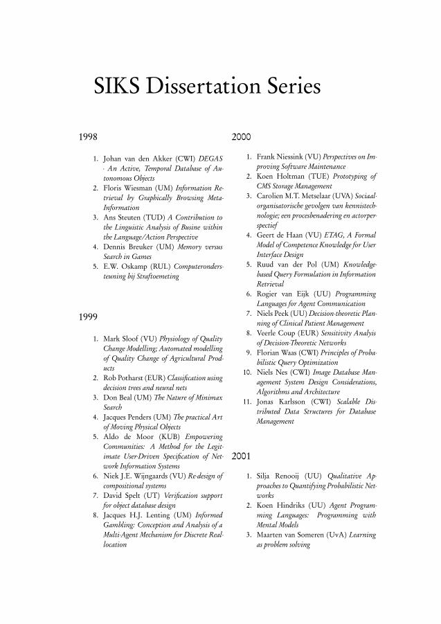
SIKS Dissertation Series
1998
1. Johan van den Akker (CWI) DEGAS- An Active, Temporal Database of Au-tonomous Objects
2. Floris Wiesman (UM) Information Re-trieval by Graphically Browsing Meta-Information
3. Ans Steuten (TUD) A Contribution tothe Linguistic Analysis of Busine withinthe Language/Action Perspective
4. Dennis Breuker (UM) Memory versusSearch in Games
5. E.W. Oskamp (RUL) Computeronders-teuning bij Straftoemeting
1999
1. Mark Sloof (VU) Physiology of QualityChange Modelling; Automated modellingof Quality Change of Agricultural Prod-ucts
2. Rob Potharst (EUR) Classification usingdecision trees and neural nets
3. Don Beal (UM) The Nature of MinimaxSearch
4. Jacques Penders (UM) The practical Artof Moving Physical Objects
5. Aldo de Moor (KUB) EmpoweringCommunities: A Method for the Legit-imate User-Driven Specification of Net-work Information Systems
6. Niek J.E. Wijngaards (VU) Re-design ofcompositional systems
7. David Spelt (UT) Verification supportfor object database design
8. Jacques H.J. Lenting (UM) InformedGambling: Conception and Analysis of aMulti-Agent Mechanism for Discrete Real-location
2000
1. Frank Niessink (VU) Perspectives on Im-proving Software Maintenance
2. Koen Holtman (TUE) Prototyping ofCMS Storage Management
3. Carolien M.T. Metselaar (UVA) Sociaal-organisatorische gevolgen van kennistech-nologie; een procesbenadering en actorper-spectief
4. Geert de Haan (VU) ETAG, A FormalModel of Competence Knowledge for UserInterface Design
5. Ruud van der Pol (UM) Knowledge-based Query Formulation in InformationRetrieval
6. Rogier van Eijk (UU) ProgrammingLanguages for Agent Communication
7. Niels Peek (UU) Decision-theoretic Plan-ning of Clinical Patient Management
8. Veerle Coup (EUR) Sensitivity Analyisof Decision-Theoretic Networks
9. Florian Waas (CWI) Principles of Proba-bilistic Query Optimization
10. Niels Nes (CWI) Image Database Man-agement System Design Considerations,Algorithms and Architecture
11. Jonas Karlsson (CWI) Scalable Dis-tributed Data Structures for DatabaseManagement
2001
1. Silja Renooij (UU) Qualitative Ap-proaches to Quantifying Probabilistic Net-works
2. Koen Hindriks (UU) Agent Program-ming Languages: Programming withMental Models
3. Maarten van Someren (UvA) Learningas problem solving
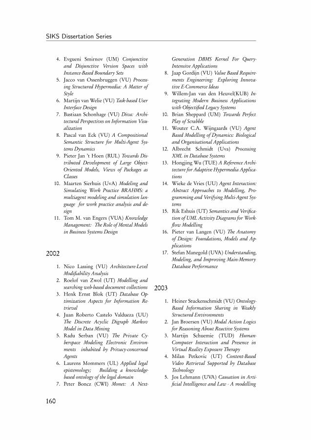
SIKS Dissertation Series
4. Evgueni Smirnov (UM) Conjunctiveand Disjunctive Version Spaces withInstance-Based Boundary Sets
5. Jacco van Ossenbruggen (VU) Process-ing Structured Hypermedia: A Matter ofStyle
6. Martijn van Welie (VU) Task-based UserInterface Design
7. Bastiaan Schonhage (VU) Diva: Archi-tectural Perspectives on Information Visu-alization
8. Pascal van Eck (VU) A CompositionalSemantic Structure for Multi-Agent Sys-tems Dynamics
9. Pieter Jan ’t Hoen (RUL) Towards Dis-tributed Development of Large Object-Oriented Models, Views of Packages asClasses
10. Maarten Sierhuis (UvA) Modeling andSimulating Work Practice BRAHMS: amultiagent modeling and simulation lan-guage for work practice analysis and de-sign
11. Tom M. van Engers (VUA) KnowledgeManagement: The Role of Mental Modelsin Business Systems Design
2002
1. Nico Lassing (VU) Architecture-LevelModifiability Analysis
2. Roelof van Zwol (UT) Modelling andsearching web-based document collections
3. Henk Ernst Blok (UT) Database Op-timization Aspects for Information Re-trieval
4. Juan Roberto Castelo Valdueza (UU)The Discrete Acyclic Digraph MarkovModel in Data Mining
5. Radu Serban (VU) The Private Cy-berspace Modeling Electronic Environ-ments inhabited by Privacy-concernedAgents
6. Laurens Mommers (UL) Applied legalepistemology; Building a knowledge-based ontology of the legal domain
7. Peter Boncz (CWI) Monet: A Next-
Generation DBMS Kernel For Query-Intensive Applications
8. Jaap Gordijn (VU) Value Based Require-ments Engineering: Exploring Innova-tive E-Commerce Ideas
9. Willem-Jan van den Heuvel(KUB) In-tegrating Modern Business Applicationswith Objectified Legacy Systems
10. Brian Sheppard (UM) Towards PerfectPlay of Scrabble
11. Wouter C.A. Wijngaards (VU) AgentBased Modelling of Dynamics: Biologicaland Organisational Applications
12. Albrecht Schmidt (Uva) ProcessingXML in Database Systems
13. Hongjing Wu (TUE) A Reference Archi-tecture for Adaptive Hypermedia Applica-tions
14. Wieke de Vries (UU) Agent Interaction:Abstract Approaches to Modelling, Pro-gramming and Verifying Multi-Agent Sys-tems
15. Rik Eshuis (UT) Semantics and Verifica-tion of UML Activity Diagrams for Work-flow Modelling
16. Pieter van Langen (VU) The Anatomyof Design: Foundations, Models and Ap-plications
17. Stefan Manegold (UVA) Understanding,Modeling, and Improving Main-MemoryDatabase Performance
2003
1. Heiner Stuckenschmidt (VU) Ontology-Based Information Sharing in WeaklyStructured Environments
2. Jan Broersen (VU) Modal Action Logicsfor Reasoning About Reactive Systems
3. Martijn Schuemie (TUD) Human-Computer Interaction and Presence inVirtual Reality Exposure Therapy
4. Milan Petkovic (UT) Content-BasedVideo Retrieval Supported by DatabaseTechnology
5. Jos Lehmann (UVA) Causation in Arti-ficial Intelligence and Law - A modelling
160
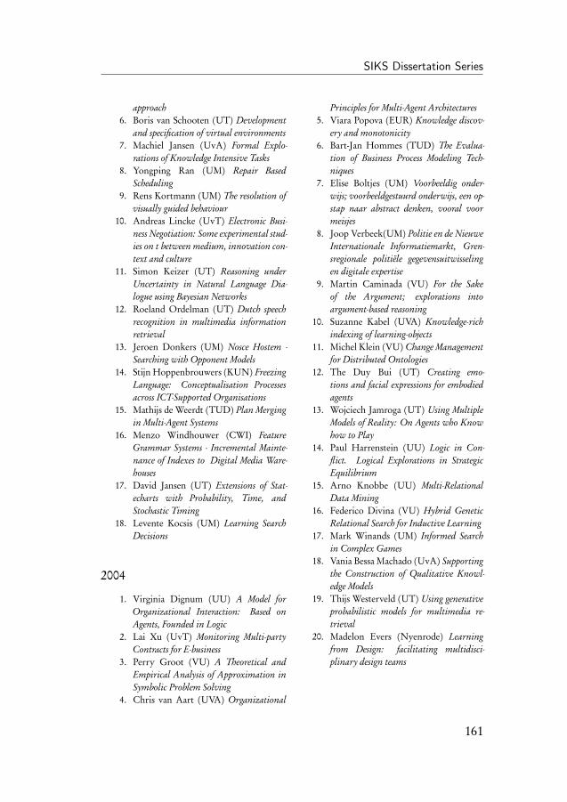
SIKS Dissertation Series
approach6. Boris van Schooten (UT) Development
and specification of virtual environments7. Machiel Jansen (UvA) Formal Explo-
rations of Knowledge Intensive Tasks8. Yongping Ran (UM) Repair Based
Scheduling9. Rens Kortmann (UM) The resolution of
visually guided behaviour10. Andreas Lincke (UvT) Electronic Busi-
ness Negotiation: Some experimental stud-ies on t between medium, innovation con-text and culture
11. Simon Keizer (UT) Reasoning underUncertainty in Natural Language Dia-logue using Bayesian Networks
12. Roeland Ordelman (UT) Dutch speechrecognition in multimedia informationretrieval
13. Jeroen Donkers (UM) Nosce Hostem -Searching with Opponent Models
14. Stijn Hoppenbrouwers (KUN) FreezingLanguage: Conceptualisation Processesacross ICT-Supported Organisations
15. Mathijs de Weerdt (TUD) Plan Mergingin Multi-Agent Systems
16. Menzo Windhouwer (CWI) FeatureGrammar Systems - Incremental Mainte-nance of Indexes to Digital Media Ware-houses
17. David Jansen (UT) Extensions of Stat-echarts with Probability, Time, andStochastic Timing
18. Levente Kocsis (UM) Learning SearchDecisions
2004
1. Virginia Dignum (UU) A Model forOrganizational Interaction: Based onAgents, Founded in Logic
2. Lai Xu (UvT) Monitoring Multi-partyContracts for E-business
3. Perry Groot (VU) A Theoretical andEmpirical Analysis of Approximation inSymbolic Problem Solving
4. Chris van Aart (UVA) Organizational
Principles for Multi-Agent Architectures5. Viara Popova (EUR) Knowledge discov-
ery and monotonicity6. Bart-Jan Hommes (TUD) The Evalua-
tion of Business Process Modeling Tech-niques
7. Elise Boltjes (UM) Voorbeeldig onder-wijs; voorbeeldgestuurd onderwijs, een op-stap naar abstract denken, vooral voormeisjes
8. Joop Verbeek(UM) Politie en de NieuweInternationale Informatiemarkt, Gren-sregionale politiële gegevensuitwisselingen digitale expertise
9. Martin Caminada (VU) For the Sakeof the Argument; explorations intoargument-based reasoning
10. Suzanne Kabel (UVA) Knowledge-richindexing of learning-objects
11. Michel Klein (VU) Change Managementfor Distributed Ontologies
12. The Duy Bui (UT) Creating emo-tions and facial expressions for embodiedagents
13. Wojciech Jamroga (UT) Using MultipleModels of Reality: On Agents who Knowhow to Play
14. Paul Harrenstein (UU) Logic in Con-flict. Logical Explorations in StrategicEquilibrium
15. Arno Knobbe (UU) Multi-RelationalData Mining
16. Federico Divina (VU) Hybrid GeneticRelational Search for Inductive Learning
17. Mark Winands (UM) Informed Searchin Complex Games
18. Vania Bessa Machado (UvA) Supportingthe Construction of Qualitative Knowl-edge Models
19. Thijs Westerveld (UT) Using generativeprobabilistic models for multimedia re-trieval
20. Madelon Evers (Nyenrode) Learningfrom Design: facilitating multidisci-plinary design teams
161
SIKS Dissertation Series
2005
1. Floor Verdenius (UVA) MethodologicalAspects of Designing Induction-Based Ap-plications
2. Erik van der Werf (UM)) AI techniquesfor the game of Go
3. Franc Grootjen (RUN) A Pragmatic Ap-proach to the Conceptualisation of Lan-guage
4. Nirvana Meratnia (UT) TowardsDatabase Support for Moving Objectdata
5. Gabriel Infante-Lopez (UVA) Two-Level Probabilistic Grammars for Natu-ral Language Parsing
6. Pieter Spronck (UM) Adaptive GameAI
7. Flavius Frasincar (TUE) HypermediaPresentation Generation for SemanticWeb Information Systems
8. Richard Vdovjak (TUE) A Model-driven Approach for Building DistributedOntology-based Web Applications
9. Jeen Broekstra (VU) Storage, Queryingand Inferencing for Semantic Web Lan-guages
10. Anders Bouwer (UVA) Explaining Be-haviour: Using Qualitative Simulationin Interactive Learning Environments
11. Elth Ogston (VU) Agent Based Match-making and Clustering - A DecentralizedApproach to Search
12. Csaba Boer (EUR) Distributed Simula-tion in Industry
13. Fred Hamburg (UL) Een Computer-model voor het Ondersteunen van Eu-thanasiebeslissingen
14. Borys Omelayenko (VU) Web-Serviceconfiguration on the Semantic Web; Ex-ploring how semantics meets pragmatics
15. Tibor Bosse (VU) Analysis of the Dy-namics of Cognitive Processes
16. Joris Graaumans (UU) Usability ofXML Query Languages
17. Boris Shishkov (TUD) Software Specifi-cation Based on Re-usable Business Com-ponents
18. Danielle Sent (UU) Test-selection strate-gies for probabilistic networks
19. Michel van Dartel (UM) Situated Repre-sentation
20. Cristina Coteanu (UL) Cyber Con-sumer Law, State of the Art and Perspec-tives
21. Wijnand Derks (UT) Improving Con-currency and Recovery in Database Sys-tems by Exploiting Application Seman-tics
2006
1. Samuil Angelov (TUE) Foundations ofB2B Electronic Contracting
2. Cristina Chisalita (VU) Contextual is-sues in the design and use of informationtechnology in organizations
3. Noor Christoph (UVA) The role ofmetacognitive skills in learning to solveproblems
4. Marta Sabou (VU) BuildingWeb ServiceOntologies
5. Cees Pierik (UU) Validation Techniquesfor Object-Oriented Proof Outlines
6. Ziv Baida (VU) Software-aided ServiceBundling - Intelligent Methods & Toolsfor Graphical Service Modeling
7. Marko Smiljanic (UT) XML schemamatching – balancing efficiency and effec-tiveness by means of clustering
8. Eelco Herder (UT) Forward, Back andHome Again - Analyzing User Behavioron the Web
9. Mohamed Wahdan (UM) AutomaticFormulation of the Auditor’s Opinion
10. Ronny Siebes (VU) Semantic Routing inPeer-to-Peer Systems
11. Joeri van Ruth (UT) Flattening Queriesover Nested Data Types
12. Bert Bongers (VU) Interactivation - To-wards an e-cology of people, our technolog-ical environment, and the arts
13. Henk-Jan Lebbink (UU) Dialogue andDecision Games for Information Ex-changing Agents
162
SIKS Dissertation Series
14. Johan Hoorn (VU) Software Require-ments: Update, Upgrade, Redesign - to-wards a Theory of Requirements Change
15. Rainer Malik (UU) CONAN: Text Min-ing in the Biomedical Domain
16. Carsten Riggelsen (UU) Approxima-tion Methods for Efficient Learning ofBayesian Networks
17. Stacey Nagata (UU) User Assistance forMultitasking with Interruptions on a Mo-bile Device
18. Valentin Zhizhkun (UVA) Graph trans-formation for Natural Language Process-ing
19. Birna van Riemsdijk (UU) CognitiveAgent Programming: A Semantic Ap-proach
20. Marina Velikova (UvT) Monotone mod-els for prediction in data mining
21. Bas van Gils (RUN) Aptness on the Web22. Paul de Vrieze (RUN) Fundaments of
Adaptive Personalisation23. Ion Juvina (UU) Development of Cogni-
tive Model for Navigating on the Web24. Laura Hollink (VU) Semantic Annota-
tion for Retrieval of Visual Resources25. Madalina Drugan (UU) Conditional
log-likelihood MDL and EvolutionaryMCMC
26. Vojkan Mihajlović (UT) Score RegionAlgebra: A Flexible Framework for Struc-tured Information Retrieval
27. Stefano Bocconi (CWI) Vox Populi: gen-erating video documentaries from seman-tically annotated media repositories
28. Borkur Sigurbjornsson (UVA) FocusedInformation Access using XML ElementRetrieval
2007
1. Kees Leune (UvT) Access Control andService-Oriented Architectures
2. Wouter Teepe (RUG) Reconciling Infor-mation Exchange and Confidentiality: AFormal Approach
3. Peter Mika (VU) Social Networks and
the Semantic Web4. Jurriaan van Diggelen (UU) Achieving
Semantic Interoperability in Multi-agentSystems: a dialogue-based approach
5. Bart Schermer (UL) Software Agents,Surveillance, and the Right to Privacy: aLegislative Framework for Agent-enabledSurveillance
6. Gilad Mishne (UVA) Applied Text Ana-lytics for Blogs
7. Natasa Jovanovic’ (UT) To Whom ItMay Concern - Addressee Identification inFace-to-Face Meetings
8. Mark Hoogendoorn (VU) Modeling ofChange in Multi-Agent Organizations
9. David Mobach (VU) Agent-Based Medi-ated Service Negotiation
10. Huib Aldewereld (UU) Autonomy vs.Conformity: an Institutional Perspectiveon Norms and Protocols
11. Natalia Stash (TUE) Incorporating Cog-nitive/Learning Styles in a General-Purpose Adaptive Hypermedia System
12. Marcel van Gerven (RUN) BayesianNetworks for Clinical Decision Sup-port: A Rational Approach to DynamicDecision-Making under Uncertainty
13. Rutger Rienks (UT) Meetings in SmartEnvironments; Implications of Progress-ing Technology
14. Niek Bergboer (UM) Context-Based Im-age Analysis
15. Joyca Lacroix (UM) NIM: a SituatedComputational Memory Model
16. Davide Grossi (UU) Designing Invisi-ble Handcuffs. Formal investigations inInstitutions and Organizations for Multi-agent Systems
17. Theodore Charitos (UU) Reasoningwith Dynamic Networks in Practice
18. Bart Orriens (UvT)On the developmentan management of adaptive business col-laborations
19. David Levy (UM) Intimate relationshipswith artificial partners
20. Slinger Jansen (UU) Customer Configu-ration Updating in a Software Supply Net-work
163
SIKS Dissertation Series
21. Karianne Vermaas (UU) Fast diffusionand broadening use: A research on resi-dential adoption and usage of broadbandinternet in the Netherlands between 2001and 2005
22. Zlatko Zlatev (UT) Goal-oriented de-sign of value and process models from pat-terns
23. Peter Barna (TUE) Specification of Appli-cation Logic in Web Information Systems
24. Georgina RamÃrez Camps (CWI)Structural Features in XML Retrieval
25. Joost Schalken (VU) Empirical Investi-gations in Software Process Improvement
2008
1. Katalin Boer-Sorbán (EUR) Agent-Based Simulation of Financial Markets:A modular, continuous-time approach
2. Alexei Sharpanskykh (VU) OnComputer-Aided Methods for Modelingand Analysis of Organizations
3. Vera Hollink (UVA) Optimizing hierar-chical menus: a usage-based approach
4. Ander de Keijzer (UT) Management ofUncertain Data - towards unattended in-tegration
5. Bela Mutschler (UT) Modeling and sim-ulating causal dependencies on process-aware information systems from a cost per-spective
6. Arjen Hommersom (RUN) On the Ap-plication of Formal Methods to ClinicalGuidelines, an Artificial Intelligence Per-spective
7. Peter van Rosmalen (OU) Supportingthe tutor in the design and support of adap-tive e-learning
8. Janneke Bolt (UU) Bayesian Networks:Aspects of Approximate Inference
9. Christof van Nimwegen (UU) The para-dox of the guided user: assistance can becounter-effective
10. Wauter Bosma (UT) Discourse orientedsummarization
11. Vera Kartseva (VU) Designing Controls
for Network Organizations: A Value-Based Approach
12. Jozsef Farkas (RUN) A Semiotically Ori-ented Cognitive Model of Knowledge Rep-resentation
13. Caterina Carraciolo (UVA) TopicDriven Access to Scientific Handbooks
14. Arthur van Bunningen (UT) Context-Aware Querying; Better Answers withLess Effort
15. Martijn van Otterlo (UT) The Logic ofAdaptive Behavior: Knowledge Represen-tation and Algorithms for the Markov De-cision Process Framework in First-OrderDomains
16. Henriette van Vugt (VU) Embodiedagents from a user’s perspective
17. Martin Op ’t Land (TUD) Applying Ar-chitecture and Ontology to the Splittingand Allying of Enterprises
18. Guido de Croon (UM) Adaptive ActiveVision
19. Henning Rode (UT) From Documentto Entity Retrieval: Improving Precisionand Performance of Focused Text Search
20. Rex Arendsen (UVA) Geen bericht, goedbericht. Een onderzoek naar de ef-fecten van de introductie van elektronischberichtenverkeer met de overheid op de ad-ministratieve lasten van bedrijven
21. Krisztian Balog (UVA) People Search inthe Enterprise
22. Henk Koning (UU) Communication ofIT-Architecture
23. Stefan Visscher (UU) Bayesian networkmodels for the management of ventilator-associated pneumonia
24. Zharko Aleksovski (VU) Using back-ground knowledge in ontology matching
25. Geert Jonker (UU) Efficient and Eq-uitable Exchange in Air Traffic Manage-ment Plan Repair using Spender-signedCurrency
26. Marijn Huijbregts (UT) Segmentation,Diarization and Speech Transcription:Surprise Data Unraveled
27. Hubert Vogten (OU) Design and Imple-mentation Strategies for IMS Learning De-
164
SIKS Dissertation Series
sign28. Ildiko Flesch (RUN) On the Use of Inde-
pendence Relations in Bayesian Networks29. Dennis Reidsma (UT) Annotations and
Subjective Machines - Of Annotators, Em-bodied Agents, Users, and Other Humans
30. Wouter van Atteveldt (VU) SemanticNetwork Analysis: Techniques for Extract-ing, Representing and Querying MediaContent
31. Loes Braun (UM) Pro-Active Medical In-formation Retrieval
32. Trung H. Bui (UT) Toward AffectiveDialogue Management using Partially Ob-servable Markov Decision Processes
33. Frank Terpstra (UVA) Scientific Work-flow Design; theoretical and practical is-sues
34. Jeroen de Knijf (UU) Studies in Fre-quent Tree Mining
35. Ben Torben Nielsen (UvT) Dendriticmorphologies: function shapes structure
2009
1. Rasa Jurgelenaite (RUN) SymmetricCausal Independence Models
2. Willem Robert van Hage (VU) Evaluat-ing Ontology-Alignment Techniques
3. Hans Stol (UvT) A Framework forEvidence-based Policy Making Using IT
4. Josephine Nabukenya (RUN) Improv-ing the Quality of Organisational PolicyMaking using Collaboration Engineering
5. Sietse Overbeek (RUN) Bridging Sup-ply and Demand for Knowledge IntensiveTasks - Based on Knowledge, Cognition,and Quality
6. Muhammad Subianto (UU) Under-standing Classification
7. Ronald Poppe (UT) DiscriminativeVision-Based Recovery and Recognitionof Human Motion
8. Volker Nannen (VU) EvolutionaryAgent-Based Policy Analysis in DynamicEnvironments
9. Benjamin Kanagwa (RUN) Design, Dis-
covery and Construction of Service-oriented Systems
10. Jan Wielemaker (UVA) Logic program-ming for knowledge-intensive interactiveapplications
11. Alexander Boer (UVA) Legal Theory,Sources of Law & the Semantic Web
12. Peter Massuthe (TUE, Humboldt-Universitaet zu Berlin) perating Guide-lines for Services
13. Steven de Jong (UM) Fairness in Multi-Agent Systems
14. Maksym Korotkiy (VU) From ontology-enabled services to service-enabled ontolo-gies (making ontologies work in e-sciencewith ONTO-SOA)
15. Rinke Hoekstra (UVA) Ontology Repre-sentation - Design Patterns and Ontolo-gies that Make Sense
16. Fritz Reul (UvT) New Architectures inComputer Chess
17. Laurens van der Maaten (UvT) FeatureExtraction from Visual Data
18. Fabian Groffen (CWI) Armada, AnEvolving Database System
19. Valentin Robu (CWI) Modeling Prefer-ences, Strategic Reasoning and Collabo-ration in Agent-Mediated Electronic Mar-kets
20. Bob van der Vecht (UU) Adjustable Au-tonomy: Controling Influences on Deci-sion Making
21. Stijn Vanderlooy (UM) Ranking and Re-liable Classification
22. Pavel Serdyukov (UT) Search For Exper-tise: Going beyond direct evidence
23. Peter Hofgesang (VU) Modelling WebUsage in a Changing Environment
24. Annerieke Heuvelink (VUA) CognitiveModels for Training Simulations
25. Alex van Ballegooij (CWI) "RAM: Ar-ray Database Management through Rela-tional Mapping"
26. Fernando Koch (UU) An Agent-BasedModel for the Development of IntelligentMobile Services
27. Christian Glahn (OU) Contextual Sup-port of social Engagement and Reflection
165
SIKS Dissertation Series
on the Web28. Sander Evers (UT) Sensor Data Manage-
ment with Probabilistic Models29. Stanislav Pokraev (UT) Model-Driven
Semantic Integration of Service-OrientedApplications
30. Marcin Zukowski (CWI) Balancing vec-torized query execution with bandwidth-optimized storage
31. Sofiya Katrenko (UVA) A Closer Lookat Learning Relations from Text
32. Rik Farenhorst (VU) and Remco deBoer (VU) Architectural KnowledgeManagement: Supporting Architects andAuditors
33. Khiet Truong (UT) How Does Real Af-fect Affect Affect Recognition In Speech?
34. Inge van de Weerd (UU) Advancing inSoftware Product Management: An Incre-mental Method Engineering Approach
35. Wouter Koelewijn (UL) Privacy en Poli-tiegegevens; Over geautomatiseerde nor-matieve informatie-uitwisseling
36. Marco Kalz (OUN) Placement Supportfor Learners in Learning Networks
37. Hendrik Drachsler (OUN) NavigationSupport for Learners in Informal Learn-ing Networks
38. Riina Vuorikari (OU) Tags and self-organisation: a metadata ecology forlearning resources in a multilingual con-text
39. Christian Stahl (TUE, Humboldt-Universitaet zu Berlin) Service Substi-tution – A Behavioral Approach Based onPetri Nets
40. Stephan Raaijmakers (UvT) Multino-mial Language Learning: Investigationsinto the Geometry of Language
41. Igor Berezhnyy (UvT) Digital Analysisof Paintings
42. Toine Bogers Recommender Systems forSocial Bookmarking
43. Virginia Nunes Leal Franqueira (UT)Finding Multi-step Attacks in ComputerNetworks using Heuristic Search and Mo-bile Ambients
44. Roberto Santana Tapia (UT) Assessing
Business-IT Alignment in Networked Or-ganizations
45. Jilles Vreeken (UU) Making PatternMining Useful
46. Loredana Afanasiev (UvA) QueryingXML: Benchmarks and Recursion
2010
1. Matthijs van Leeuwen (UU) Patternsthat Matter
2. Ingo Wassink (UT) Work flows in LifeScience
3. Joost Geurts (CWI) A Document Engi-neering Model and Processing Frameworkfor Multimedia documents
4. Olga Kulyk (UT) Do You Know WhatI Know? Situational Awareness of Co-located Teams in Multidisplay Environ-ments
5. Claudia Hauff (UT) Predicting the Effec-tiveness of Queries and Retrieval Systems
6. Sander Bakkes (UvT) Rapid Adaptationof Video Game AI
7. Wim Fikkert (UT) Gesture interactionat a Distance
8. Krzysztof Siewicz (UL) Towards an Im-proved Regulatory Framework of FreeSoftware. Protecting user freedoms in aworld of software communities and eGov-ernments
9. Hugo Kielman (UL) A Politielegegevensverwerking en Privacy, Naar eeneffectieve waarborging
10. Rebecca Ong (UL) Mobile Communica-tion and Protection of Childr
11. Adriaan Ter Mors (TUD) The worldaccording to MARP: Multi-Agent RoutePlanning
12. Susan van den Braak (UU) Sensemakingsoftware for crime analysis
13. Gianluigi Folino (RUN) High Perfor-mance Data Mining using Bio-inspiredtechniques
14. Sander van Splunter (VU) AutomatedWeb Service Reconfiguration
15. Lianne Bodenstaff (UT) Manag-
166
SIKS Dissertation Series
ing Dependency Relations in Inter-Organizational Models
16. Sicco Verwer (TUD) Efficient Identifica-tion of Timed Automata, theory and prac-tice
17. Spyros Kotoulas (VU) Scalable Discov-ery of Networked Resources: Algorithms,Infrastructure, Applications
18. Charlotte Gerritsen (VU) Caught in theAct: Investigating Crime by Agent-BasedSimulation
19. Henriette Cramer (UvA) People’s Re-sponses to Autonomous and Adaptive Sys-tems
20. Ivo Swartjes (UT) Whose Story Is It Any-way? How Improv Informs Agency andAuthorship of Emergent Narrative
21. Harold van Heerde (UT) Privacy-awaredata management by means of data degra-dation
22. Michiel Hildebrand (CWI) End-userSupport for Access to HeterogeneousLinked Data
23. Bas Steunebrink (UU) The Logical Struc-ture of Emotions
24. Designing Generic and Efficient Negotia-tion Strategies
25. Zulfiqar Ali Memon (VU) ModellingHuman-Awareness for Ambient Agents:A Human Mindreading Perspective
26. Ying Zhang (CWI) XRPC: Efficient Dis-tributed Query Processing on Heteroge-neous XQuery Engines
27. Marten Voulon (UL) Automatisch con-tracteren
28. Arne Koopman (UU) Characteristic Re-lational Patterns
29. Stratos Idreos(CWI) Database Cracking:Towards Auto-tuning Database Kernels
30. Marieke van Erp (UvT) Accessing Natu-ral History - Discoveries in data cleaning,structuring, and retrieval
31. Victor de Boer (UVA) Ontology Enrich-ment from Heterogeneous Sources on theWeb
32. Marcel Hiel (UvT) An Adaptive Ser-vice Oriented Architecture: Automati-cally solving Interoperability Problems
33. Robin Aly (UT) Modeling Representa-tion Uncertainty in Concept-Based Multi-media Retrieval
34. Teduh Dirgahayu (UT) Interaction De-sign in Service Compositions
35. Dolf Trieschnigg (UT) Proof of Con-cept: Concept-based Biomedical Informa-tion Retrieval
36. Jose Janssen (OU) Paving the Way forLifelong Learning; Facilitating compe-tence development through a learningpath specification
37. Niels Lohmann (TUE) Correctness ofservices and their composition
38. Dirk Fahland (TUE) From Scenarios tocomponents
39. Ghazanfar Farooq Siddiqui (VU) Inte-grative modeling of emotions in virtualagents
40. Mark van Assem (VU) Converting andIntegrating Vocabularies for the SemanticWeb
41. Guillaume Chaslot (UM) Monte-CarloTree Search
42. Sybren de Kinderen (VU) Needs-drivenservice bundling in a multi-supplier set-ting - the computational e3-service ap-proach
43. Peter van Kranenburg (UU) A Compu-tational Approach to Content-Based Re-trieval of Folk Song Melodies
44. Pieter Bellekens (TUE) An Approach to-wards Context-sensitive and User-adaptedAccess to Heterogeneous Data Sources, Il-lustrated in the Television Domain
45. Vasilios Andrikopoulos (UvT) A theoryand model for the evolution of softwareservices
46. Vincent Pijpers (VU) e3alignment: Ex-ploring Inter-Organizational Business-ICT Alignment
47. Chen Li (UT) Mining Process ModelVariants: Challenges, Techniques, Exam-ples
48. Milan Lovric (EUR) Behavioral Financeand Agent-Based Artificial Markets
49. Jahn-Takeshi Saito (UM) Solving diffi-cult game positions
167
SIKS Dissertation Series
50. Bouke Huurnink (UVA) Search in Au-diovisual Broadcast Archives
51. Alia Khairia Amin (CWI) Understand-ing and supporting information seekingtasks in multiple sources
52. Peter-Paul van Maanen (VU) AdaptiveSupport for Human-Computer Teams: Ex-ploring the Use of Cognitive Models ofTrust and Attention
53. Edgar Meij (UVA) Combining Conceptsand Language Models for Information Ac-cess
2011
1. Botond Cseke (RUN) Variational Algo-rithms for Bayesian Inference in LatentGaussian Models
2. Nick Tinnemeier(UU) OrganizingAgent Organizations. Syntax and Op-erational Semantics of an Organization-Oriented Programming Language
3. Jan Martijn van der Werf (TUE) Com-positional Design and Verification ofComponent-Based Information Systems
4. Hado van Hasselt (UU) Insights inReinforcement Learning; Formal analy-sis and empirical evaluation of temporal-difference learning algorithms
5. Base van der Raadt (VU) Enterprise Ar-chitecture Coming of Age - Increasing thePerformance of an Emerging Discipline
6. Yiwen Wang (TUE) Semantically-Enhanced Recommendations in CulturalHeritage
7. Yujia Cao (UT) Multimodal Informa-tion Presentation for High Load HumanComputer Interaction
8. Nieske Vergunst (UU) BDI-based Gener-ation of Robust Task-Oriented Dialogues
9. Tim de Jong (OU) Contextualised Mo-bile Media for Learning
10. Bart Bogaert (UvT) Cloud Content Con-tention
11. Dhaval Vyas (UT) Designing for Aware-ness: An Experience-focused HCI Perspec-tive
12. Carmen Bratosin (TUE) Grid Architec-ture for Distributed Process Mining
13. Xiaoyu Mao (UvT) Airport under Con-trol. Multiagent Scheduling for AirportGround Handling
14. Milan Lovric (EUR) Behavioral Financeand Agent-Based Artificial Markets
15. Marijn Koolen (UvA) The Meaning ofStructure: the Value of Link Evidence forInformation Retrieval
16. Maarten Schadd (UM) Selective Searchin Games of Different Complexity
17. Jiyin He (UVA) Exploring Topic Struc-ture: Coherence, Diversity and Related-ness
18. Mark Ponsen (UM) Strategic Decision-Making in complex games
19. Ellen Rusman (OU) The Mind ’ s Eye onPersonal Profiles
20. Qing Gu (VU) Guiding service-orientedsoftware engineering - A view-based ap-proach
21. Linda Terlouw (TUD) Modularizationand Specification of Service-Oriented Sys-tems
22. Junte Zhang (UVA) System Evaluationof Archival Description and Access
23. Wouter Weerkamp (UVA) Finding Peo-ple and their Utterances in Social Media
24. Herwin van Welbergen (UT) Behav-ior Generation for Interpersonal Coordi-nation with Virtual Humans On Spec-ifying, Scheduling and Realizing Multi-modal Virtual Human Behavior
25. Syed Waqar ul Qounain Jaffry (VU)Analysis and Validation of Models forTrust Dynamics
26. Matthijs Aart Pontier (VU) VirtualAgents for Human Communication -Emotion Regulation and Involvement-Distance Trade-Offs in Embodied Conver-sational Agents and Robots
27. Aniel Bhulai (VU) Dynamic website op-timization through autonomous manage-ment of design patterns
28. Rianne Kaptein(UVA) Effective FocusedRetrieval by Exploiting Query Contextand Document Structure
168
SIKS Dissertation Series
29. Faisal Kamiran (TUE) Discrimination-aware Classification
30. Egon van den Broek (UT) Affective Sig-nal Processing (ASP): Unraveling the mys-tery of emotions
31. Ludo Waltman (EUR) Computationaland Game-Theoretic Approaches for Mod-eling Bounded Rationality
32. Nees-Jan van Eck (EUR) Methodologi-cal Advances in Bibliometric Mapping ofScience
33. Tom van der Weide (UU) Arguing toMotivate Decisions
34. Paolo Turrini (UU) Strategic Reasoningin Interdependence: Logical and Game-theoretical Investigations
35. Maaike Harbers (UU) Explaining AgentBehavior in Virtual Training
36. Erik van der Spek (UU) Experiments inserious game design: a cognitive approach
37. Adriana Burlutiu (RUN) MachineLearning for Pairwise Data, Applicationsfor Preference Learning and SupervisedNetwork Inference
38. Nyree Lemmens (UM) Bee-inspired Dis-tributed Optimization
39. Joost Westra (UU) Organizing Adapta-tion using Agents in Serious Games
40. Viktor Clerc (VU) Architectural Knowl-edge Management in Global Software De-velopment
41. Luan Ibraimi (UT) CryptographicallyEnforced Distributed Data Access Con-trol
42. Michal Sindlar (UU) Explaining Behav-ior through Mental State Attribution
43. Henk van der Schuur (UU) Process Im-provement through Software OperationKnowledge
44. Boris Reuderink (UT) Robust Brain-Computer Interfaces
45. Herman Stehouwer (UvT) StatisticalLanguage Models for Alternative Se-quence Selection
46. Beibei Hu (TUD) Towards Contextual-ized Information Delivery: A Rule-basedArchitecture for the Domain of Mobile Po-lice Work
47. Azizi Bin Ab Aziz(VU) Exploring Com-putational Models for Intelligent Supportof Persons with Depression
48. Mark Ter Maat (UT) Response Selectionand Turn-taking for a Sensitive ArtificialListening Agent
49. Andreea Niculescu (UT) Conversa-tional interfaces for task-oriented spokendialogues: design aspects influencing inter-action quality
2012
1. Terry Kakeeto (UvT) Relationship Mar-keting for SMEs in Uganda
2. Muhammad Umair(VU) Adaptivity,emotion, and Rationality in Human andAmbient Agent Models
3. Adam Vanya (VU) Supporting Architec-ture Evolution by Mining Software Repos-itories
4. Jurriaan Souer (UU) Development ofContent Management System-based WebApplications
5. Marijn Plomp (UU) Maturing Interor-ganisational Information Systems
6. Wolfgang Reinhardt (OU) AwarenessSupport for Knowledge Workers in Re-search Networks
7. Rianne van Lambalgen (VU) Whenthe Going Gets Tough: Exploring Agent-based Models of Human Performance un-der Demanding Conditions
8. Gerben de Vries (UVA) Kernel Methodsfor Vessel Trajectories
9. Ricardo Neisse (UT) Trust and PrivacyManagement Support for Context-AwareService Platforms
10. David Smits (TUE) Towards a GenericDistributed Adaptive Hypermedia Envi-ronment
11. J.C.B. Rantham Prabhakara (TUE) Pro-cess Mining in the Large: Preprocessing,Discovery, and Diagnostics
12. Kees van der Sluijs (TUE) Model DrivenDesign and Data Integration in SemanticWeb Information Systems
169
SIKS Dissertation Series
13. Suleman Shahid (UvT) Fun and Face:Exploring non-verbal expressions of emo-tion during playful interactions
14. Evgeny Knutov(TUE) Generic Adapta-tion Framework for Unifying AdaptiveWeb-based Systems
15. Natalie van der Wal (VU) Social Agents.Agent-Based Modelling of Integrated In-ternal and Social Dynamics of Cognitiveand Affective Processes
16. Fiemke Both (VU) Helping people byunderstanding them - Ambient Agentssupporting task execution and depressiontreatment
17. Amal Elgammal (UvT) Towards a Com-prehensive Framework for Business Pro-cess Compliance
18. Eltjo Poort (VU) Improving SolutionArchitecting Practices
19. Helen Schonenberg (TUE) What’sNext? Operational Support for BusinessProcess Execution
20. Ali Bahramisharif (RUN) CovertVisual Spatial Attention, a RobustParadigm for Brain-Computer Interfac-ing
21. Roberto Cornacchia (TUD) QueryingSparse Matrices for Information Retrieval
22. Thijs Vis (UvT) Intelligence, politieen veiligheidsdienst: verenigbare groothe-den?
23. Christian Muehl (UT) Toward AffectiveBrain-Computer Interfaces: Exploring theNeurophysiology of Affect during HumanMedia Interaction
24. Laurens van der Werff (UT) Evalua-tion of Noisy Transcripts for Spoken Doc-ument Retrieval
25. Silja Eckartz (UT) Managing theBusiness Case Development in Inter-Organizational IT Projects: A Method-ology and its Application
26. Emile de Maat (UVA) Making Sense ofLegal Text
27. Hayrettin Gurkok (UT)Mind the Sheep!User Experience Evaluation & Brain-Computer Interface Games
28. Nancy Pascall (UvT) Engendering Tech-
nology Empowering Women29. Almer Tigelaar (UT) Peer-to-Peer Infor-
mation Retrieval30. Alina Pommeranz (TUD) Designing
Human-Centered Systems for ReflectiveDecision Making
31. Emily Bagarukayo (RUN) A Learningby Construction Approach for Higher Or-der Cognitive Skills Improvement, Build-ing Capacity and Infrastructure
32. Wietske Visser (TUD) Qualitativemulti-criteria preference representationand reasoning
33. Rory Sie (OUN) Coalitions in Coopera-tion Networks (COCOON)
34. Pavol Jancura (RUN) Evolutionaryanalysis in PPI networks and applications
35. Evert Haasdijk (VU) Never Too Old ToLearn –On-line Evolution of Controllersin Swarm- and Modular Robotics
36. Denis Ssebugwawo (RUN) Analysis andEvaluation of Collaborative ModelingProcesses
37. Agnes Nakakawa (RUN) A Collabora-tion Process for Enterprise ArchitectureCreation
38. Selmar Smit (VU) Parameter Tuningand Scientific Testing in Evolutionary Al-gorithms
39. Hassan Fatemi (UT) Risk-aware designof value and coordination networks
40. Agus Gunawan (UvT) Information Ac-cess for SMEs in Indonesia
41. Sebastian Kelle (OU) Game Design Pat-terns for Learning
42. Dominique Verpoorten (OU) Reflec-tion Amplifiers in self-regulated Learning
43. Anna Tordai (VU) On CombiningAlignment Techniques
44. Benedikt Kratz (UvT) AModel and Lan-guage for Business-aware Transactions
45. Simon Carter (UVA) Exploration andExploitation of Multilingual Data for Sta-tistical Machine Translation
46. Manos Tsagkias (UVA) Mining SocialMedia: Tracking Content and PredictingBehavior
47. Jorn Bakker (TUE) Handling Abrupt
170
SIKS Dissertation Series
Changes in Evolving Time-series Data48. Michael Kaisers (UM) Learning against
Learning - Evolutionary dynamics of rein-forcement learning algorithms in strategicinteractions
49. Steven van Kervel (TUD) Ontologogydriven Enterprise Information SystemsEngineering
50. Jeroen de Jong (TUD) Heuristics in Dy-namic Sceduling; a practical frameworkwith a case study in elevator dispatching
2013
1. Viorel Milea (EUR) News Analytics forFinancial Decision Support
2. Erietta Liarou (CWI) MonetDB/Dat-aCell: Leveraging the Column-storeDatabase Technology for Efficient andScalable Stream Processing
3. Szymon Klarman (VU) Reasoning withContexts in Description Logics
4. Chetan Yadati(TUD) Coordinating au-tonomous planning and scheduling
5. Dulce Pumareja (UT) Groupware Re-quirements Evolutions Patterns
6. Romulo Goncalves(CWI) The Data Cy-clotron: Juggling Data and Queries for aData Warehouse Audience
7. Giel van Lankveld (UvT) QuantifyingIndividual Player Differences
8. Robbert-Jan Merk(VU) Making ene-mies: cognitive modeling for opponentagents in fighter pilot simulators
9. Fabio Gori (RUN) Metagenomic DataAnalysis: Computational Methods andApplications
10. Jeewanie Jayasinghe Arachchige(UvT)A Unified Modeling Framework for Ser-vice Design
11. Evangelos Pournaras(TUD) Multi-levelReconfigurable Self-organization in Over-lay Services
12. Marian Razavian(VU) Knowledge-driven Migration to Services
13. Mohammad Safiri(UT) Service Tailor-ing: User-centric creation of integrated IT-
based homecare services to support inde-pendent living of elderly
14. Jafar Tanha (UVA) Ensemble Ap-proaches to Semi-Supervised LearningLearning
15. Daniel Hennes (UM) Multiagent Learn-ing - Dynamic Games and Applications
16. Eric Kok (UU) Exploring the practicalbenefits of argumentation in multi-agentdeliberation
17. Koen Kok (VU) The PowerMatcher:Smart Coordination for the Smart Elec-tricity Grid
18. Jeroen Janssens (UvT) Outlier Selectionand One-Class Classification
19. Renze Steenhuizen (TUD) CoordinatedMulti-Agent Planning and Scheduling
20. Katja Hofmann (UvA) Fast and ReliableOnline Learning to Rank for Informa-tion Retrieval
21. Sander Wubben (UvT) Text-to-text gen-eration by monolingual machine transla-tion
22. Tom Claassen (RUN) Causal Discoveryand Logic
23. Patricio de Alencar Silva(UvT) ValueActivity Monitoring
24. Haitham Bou Ammar (UM) AutomatedTransfer in Reinforcement Learning
25. Agnieszka Anna Latoszek-Berendsen(UM) Intention-based Decision Support.A new way of representing and imple-menting clinical guidelines in a DecisionSupport System
26. Alireza Zarghami (UT) ArchitecturalSupport for Dynamic Homecare ServiceProvisioning
27. Mohammad Huq (UT) Inference-basedFramework Managing Data Provenance
28. Frans van der Sluis (UT) When Com-plexity becomes Interesting: An Inquiryinto the Information eXperience
29. Iwan de Kok (UT) Listening Heads30. Joyce Nakatumba (TUE) Resource-
Aware Business Process Management:Analysis and Support
31. Dinh Khoa Nguyen (UvT) BlueprintModel and Language for Engineering
171
SIKS Dissertation Series
Cloud Applications32. Kamakshi Rajagopal (OUN) Network-
ing For Learning; The role of Networkingin a Lifelong Learner’s Professional Devel-opment
33. Qi Gao (TUD) User Modeling and Per-sonalization in the Microblogging Sphere
34. Kien Tjin-Kam-Jet (UT) DistributedDeep Web Search
35. Abdallah El Ali (UvA) Minimal MobileHuman Computer Interaction
36. Than Lam Hoang (TUe) Pattern Min-ing in Data Streams
37. Dirk Bürner (OUN) Ambient LearningDisplays
38. Eelco den Heijer (VU) AutonomousEvolutionary Art
39. Joop de Jong (TUD) AMethod for Enter-prise Ontology based Design of EnterpriseInformation Systems
40. Pim Nijssen (UM) Monte-Carlo TreeSearch for Multi-Player Games
41. Jochem Liem (UVA) Supporting theConceptual Modelling of Dynamic Sys-tems: A Knowledge Engineering Perspec-tive on Qualitative Reasoning
42. Léon Planken (TUD) Algorithms forSimple Temporal Reasoning
43. Marc Bron (UVA) Exploration and Con-textualization through Interaction andConcepts
2014
1. Nicola Barile (UU) Studies in LearningMonotone Models from Data
2. Fiona Tuliyano (RUN) Combining Sys-tem Dynamics with a Domain ModelingMethod
3. Sergio Raul Duarte Torres (UT) Infor-mation Retrieval for Children: Search Be-havior and Solutions
4. Hanna Jochmann-Mannak (UT) Web-sites for children: search strategies and in-terface design - Three studies on children’ssearch performance and evaluation
5. Jurriaan van Reijsen (UU) Knowledge
Perspectives on Advancing Dynamic Ca-pability
6. Damian Tamburri (VU) Supporting Net-worked Software Development
7. Arya Adriansyah (TUE) Aligning Ob-served and Modeled Behavior
8. Samur Araujo (TUD) Data Integrationover Distributed andHeterogeneous DataEndpoints
9. Philip Jackson (UvT) Toward Human-Level Artificial Intelligence: Representa-tion and Computation of Meaning in Nat-ural Language
10. Ivan Salvador Razo Zapata (VU) ServiceValue Networks
11. Janneke van der Zwaan (TUD) An Em-pathic Virtual Buddy for Social Support
12. Willem vanWilligen (VU) Look Ma, NoHands: Aspects of Autonomous VehicleControl
13. Arlette van Wissen (VU) Agent-BasedSupport for Behavior Change: Models andApplications in Health and Safety Do-mains
14. Yangyang Shi (TUD) Language ModelsWith Meta-information
15. Natalya Mogles (VU) Agent-Based Anal-ysis and Support of Human Functioningin Complex Socio-Technical Systems: Ap-plications in Safety and Healthcare
16. Krystyna Milian (VU) Supporting trialrecruitment and design by automaticallyinterpreting eligibility criteria
17. Kathrin Dentler (VU) Computinghealthcare quality indicators automati-cally: Secondary Use of Patient Data andSemantic Interoperability
18. Mattijs Ghijsen (UVA) Methods andModels for the Design and Study of Dy-namic Agent Organizations
19. Vinicius Ramos (TUE) Adaptive Hyper-media Courses: Qualitative and Quanti-tative Evaluation and Tool Support
20. Mena Habib (UT) Named Entity Extrac-tion and Disambiguation for InformalText: The Missing Link
21. Kassidy Clark (TUD) Negotiation andMonitoring in Open Environments
172
SIKS Dissertation Series
22. Marieke Peeters (UU) Personalized Ed-ucational Games - Developing agent-supported scenario-based training
23. Eleftherios Sidirourgos (UvA/CWI)Space Efficient Indexes for the Big DataEra
24. Davide Ceolin (VU) Trusting Semi-structured Web Data
25. Martijn Lappenschaar (RUN) New net-work models for the analysis of disease in-teraction
26. Tim Baarslag (TUD) What to Bid andWhen to Stop
27. Rui Jorge Almeida (EUR) ConditionalDensity Models Integrating Fuzzy andProbabilistic Representations of Uncer-tainty
28. Anna Chmielowiec (VU) Decentralizedk-Clique Matching
29. Jaap Kabbedijk (UU) Variability inMulti-Tenant Enterprise Software
30. Peter de Cock (UvT) AnticipatingCriminal Behaviour
31. Leo van Moergestel (UU) Agent Tech-nology in Agile Multiparallel Manufactur-ing and Product Support
32. Naser Ayat (UvA)On Entity Resolutionin Probabilistic Data
33. Tesfa Tegegne (RUN) Service Discoveryin eHealth
34. Christina Manteli(VU) The Effect ofGovernance in Global Software Devel-opment: Analyzing Transactive MemorySystems
35. Joost van Ooijen (UU) CognitiveAgents in Virtual Worlds: A MiddlewareDesign Approach
36. Joos Buijs (TUE) Flexible EvolutionaryAlgorithms for Mining Structured ProcessModels
37. Maral Dadvar (UT) Experts and Ma-chines United Against Cyberbullying
38. Danny Plass-Oude Bos (UT) Makingbrain-computer interfaces better: improv-ing usability through post-processing.
39. Jasmina Maric (UvT) Web Communi-ties, Immigration, and Social Capital
40. Walter Omona (RUN) A Framework
for Knowledge Management Using ICTin Higher Education
41. Frederic Hogenboom (EUR) Auto-mated Detection of Financial Events inNews Text
42. Carsten Eijckhof (CWI/TUD) Contex-tual Multidimensional Relevance Models
43. Kevin Vlaanderen (UU) Supporting Pro-cess Improvement using Method Incre-ments
44. Paulien Meesters (UvT) IntelligentBlauw. Met als ondertitel: Intelligence-gestuurde politiezorg in gebiedsgebondeneenheden
45. Birgit Schmitz (OUN) Mobile Gamesfor Learning: A Pattern-Based Approach
46. Ke Tao (TUD) Social Web Data Analyt-ics: Relevance, Redundancy, Diversity
47. Shangsong Liang (UVA) Fusion and Di-versification in Information Retrieval
2015
1. Niels Netten (UvA) Machine Learningfor Relevance of Information in Crisis Re-sponse
2. Faiza Bukhsh (UvT) Smart auditing: In-novative Compliance Checking in Cus-toms Controls
3. Twan van Laarhoven (RUN) Machinelearning for network data
4. Howard Spoelstra (OUN) Collabora-tions in Open Learning Environments
5. Christoph B�sch(UT) Cryptographi-cally Enforced Search Pattern Hiding
6. Farideh Heidari (TUD) Business Pro-cess Quality Computation - Comput-ing Non-Functional Requirements to Im-prove Business Processes
7. Maria-Hendrike Peetz(UvA) Time-Aware Online Reputation Analysis
8. Jie Jiang (TUD) Organizational Compli-ance: An agent-based model for design-ing and evaluating organizational inter-actions
9. Randy Klaassen(UT) HCI Perspectiveson Behavior Change Support Systems
173
SIKS Dissertation Series
10. Henry Hermans (OUN)OpenU: designof an integrated system to support lifelonglearning
11. Yongming Luo(TUE) Designing algo-rithms for big graph datasets: A study ofcomputing bisimulation and joins
12. Julie M. Birkholz (VU) Modi Operandiof Social Network Dynamics: The Effectof Context on Scientific CollaborationNetworks
13. Giuseppe Procaccianti(VU) Energy-Efficient Software
14. Bart van Straalen (UT) A cognitive ap-proach to modeling bad news conversa-tions
15. Klaas Andries de Graaf (VU) Ontology-based Software Architecture Documenta-tion
16. Changyun Wei (UT) Cognitive Co-ordination for Cooperative Multi-RobotTeamwork
17. André van Cleeff (UT) Physical andDigital Security Mechanisms: Properties,Combinations and Trade-offs
18. Holger Pirk (CWI) Waste Not, WantNot! - Managing Relational Data inAsymmetric Memories
19. Bernardo Tabuenca (OUN) UbiquitousTechnology for Lifelong Learners
20. Loïs Vanhée (UU) Using Culture andValues to Support Flexible Coordination
21. Sibren Fetter (OUN) Using Peer-Support to Expand and Stabilize OnlineLearning
22. Zhemin Zhu(UT) Co-occurrence RateNetworks
23. Luit Gazendam (VU) Cataloguer Sup-port in Cultural Heritage
24. Richard Berendsen (UVA) Finding Peo-ple, Papers, and Posts: Vertical Search Al-gorithms and Evaluation
25. Steven Woudenberg (UU) BayesianTools for Early Disease Detection
26. Alexander Hogenboom (EUR) Senti-ment Analysis of Text Guided by Seman-tics and Structure
27. Sándor Héman (CWI) Updating com-pressed colomn stores
28. Janet Bagorogoza(TiU) KNOWLEDGEMANAGEMENT ANDHIGH PERFOR-MANCE; The Uganda Financial Institu-tions Model for HPO
29. Hendrik Baier (UM) Monte-Carlo TreeSearch Enhancements for One-Player andTwo-Player Domains
30. Kiavash Bahreini(OU) Real-time Mul-timodal Emotion Recognition in E-Learning
31. Yakup Koç (TUD) On the robustness ofPower Grids
32. Jerome Gard(UL) Corporate VentureManagement in SMEs
33. Frederik Schadd (TUD) Ontology Map-ping with Auxiliary Resources
34. Victor de Graaf(UT) Gesocial Recom-mender Systems
35. Jungxao Xu (TUD) Affective Body Lan-guage of Humanoid Robots: Perceptionand Effects in Human Robot Interaction
2016
1. Syed Saiden Abbas (RUN) Recognitionof Shapes by Humans and Machines
2. Michiel Christiaan Meulendijk (UU)Optimizing medication reviews throughdecision support: prescribing a better pillto swallow
3. Maya Sappelli (RUN) Knowledge Workin Context: User Centered KnowledgeWorker Support
4. Laurens Rietveld (VU) Publishing andConsuming Linked Data
5. Evgeny Sherkhonov (UVA) ExpandedAcyclic Queries: Containment and an Ap-plication in Explaining Missing Answers
6. Michel Wilson (TUD) Robust schedul-ing in an uncertain environment
7. Jeroen de Man (VU) Measuring andmodeling negative emotions for virtualtraining
8. Matje van de Camp (TiU) A Link to thePast: Constructing Historical Social Net-works from Unstructured Data
9. Archana Nottamkandath (VU) Trust-
174
SIKS Dissertation Series
ing Crowdsourced Information on Cul-tural Artefacts
10. George Karafotias (VUA) ParameterControl for Evolutionary Algorithms
11. Anne Schuth (UVA) Search Engines thatLearn from Their Users
12. Max Knobbout (UU) Logics for Mod-elling and Verifying Normative Multi-Agent Systems
13. Nana Baah Gyan (VU) The Web, SpeechTechnologies and Rural Development inWest Africa - An ICT4D Approach
14. Ravi Khadka (UU) Revisiting LegacySoftware System Modernization
15. Steffen Michels (RUN) Hybrid Proba-bilistic Logics - Theoretical Aspects, Algo-rithms and Experiments
16. Guangliang Li (UVA) Socially Intelli-gent Autonomous Agents that Learn fromHuman Reward
17. Berend Weel (VU) Towards EmbodiedEvolution of Robot Organisms
18. Albert Meroño Peñuela (VU) RefiningStatistical Data on the Web
19. Julia Efremova (Tu/e) Mining SocialStructures from Genealogical Data
20. DaanOdijk (UVA) Context & Semanticsin News & Web Search
21. Alejandro Moreno C�lleri (UT)From Traditional to InteractivePlayspaces: Automatic Analysis of PlayerBehavior in the Interactive Tag Play-ground
22. Grace Lewis (VU) Software ArchitectureStrategies for Cyber-Foraging Systems
23. Fei Cai (UVA) Query Auto Completionin Information Retrieval
24. Brend Wanders (UT) Repurposing andProbabilistic Integration of Data; An It-erative and data model independent ap-proach
25. Julia Kiseleva (TU/e) Using Contex-tual Information to Understand Search-ing and Browsing Behavior
26. Dilhan Thilakarathne (VU) In or Out ofControl: Exploring Computational Mod-els to Study the Role of Human Aware-ness and Control in Behavioural Choices,
with Applications in Aviation and En-ergy Management Domains
27. Wen Li (TUD) Understanding Geo-spatial Information on Social Media
28. Mingxin Zhang (TUD) Large-scaleAgent-based Social Simulation - A studyon epidemic prediction and control
29. Nicolas Höning (TUD) Peak reduc-tion in decentralised electricity systems -Markets and prices for flexible planning
30. Ruud Mattheij (UvT) The Eyes Have It31. Mohammad Khelghati (UT) Deep web
content monitoring32. Eelco Vriezekolk (UT) Assessing
Telecommunication Service AvailabilityRisks for Crisis Organisations
33. Peter Bloem (UVA) Single Sample Statis-tics, exercises in learning from just one ex-ample
34. Dennis Schunselaar (TUE) Config-urable Process Trees: Elicitation, Analysis,and Enactment
35. Zhaochun Ren (UVA) Monitoring So-cial Media: Summarization, Classifica-tion and Recommendation
36. Daphne Karreman (UT) Beyond R2D2:The design of nonverbal interaction be-havior optimized for robot-specific mor-phologies
37. Giovanni Sileno (UvA) Aligning Lawand Action - a conceptual and computa-tional inquiry
38. Andrea Minuto (UT) MATERIALSTHAT MATTER - Smart Materials meetArt & Interaction Design
39. Merijn Bruijnes (UT) Believable SuspectAgents; Response and Interpersonal StyleSelection for an Artificial Suspect
40. Christian Detweiler (TUD) Accountingfor Values in Design
41. Thomas King (TUD) Governing Gov-ernance: A Formal Framework forAnalysing Institutional Design and En-actment Governance
42. Spyros Martzoukos (UVA) Combinato-rial and Compositional Aspects of Bilin-gual Aligned Corpora
43. Saskia Koldijk (RUN) Context-Aware
175

SIKS Dissertation Series
Support for Stress Self-Management: FromTheory to Practice
44. Thibault Sellam (UVA) Automatic Assis-tants for Database Exploration
45. Bram van de Laar (UT) ExperiencingBrain-Computer Interface Control
46. Jorge Gallego Perez (UT) Robots toMake you Happy
47. Christina Weber (UL) Real-time fore-sight - Preparedness for dynamic innova-tion networks
48. Tanja Buttler (TUD) Collecting LessonsLearned
49. Gleb Polevoy (TUD) Participation andInteraction in Projects. A Game-TheoreticAnalysis
50. Yan Wang (UVT) The Bridge of Dreams:Towards a Method for Operational Perfor-mance Alignment in IT-enabled ServiceSupply Chains
2017
1. Jan-Jaap Oerlemans (UL) InvestigatingCybercrime
2. Sjoerd Timmer (UU) Designing and Un-derstanding Forensic Bayesian Networksusing Argumentation
3. Daniël Harold Telgen (UU) Grid Man-ufacturing; A Cyber-Physical Approachwith Autonomous Products and Reconfig-
urable Manufacturing Machines4. Mrunal Gawade (CWI) MULTI-CORE
PARALLELISM IN A COLUMN-STORE
5. Mahdieh Shadi (UVA) Collaboration Be-havior
6. Damir Vandic (EUR) Intelligent Infor-mation Systems for Web Product Search
7. Roel Bertens (UU) Insight in Informa-tion: from Abstract to Anomaly
8. Rob Konijn (VU) Detecting InterestingDifferences:Data Mining in Health Insur-ance Data using Outlier Detection andSubgroup Discovery
9. Dong Nguyen (UT) Text as Social andCultural Data: A Computational Perspec-tive on Variation in Text
10. Robby van Delden (UT) (Steering) Inter-active Play Behavior
11. Florian Kunneman (RUN) Modellingpatterns of time and emotion in Twitter#anticipointment
12. Sander Leemans (UT) Robust ProcessMining with Guarantees
13. Gijs Huisman (UT) Social Touch Tech-nology - Extending the reach of socialtouch through haptic technology
14. Shoshannah Tekofsky (UvT) You AreWho You Play You Are: Modelling PlayerTraits from Video Game Behavior
15. Peter Berck (RUN) Memory-Based TextCorrection
176
Copyright © 2022 FDOKUMEN