arX

iv:1

108.

1695

v1 [

cs.IT

] 8

Aug

201

11

An Algebraic Approach toPhysical-Layer Network Coding

Chen Feng, Danilo Silva, and Frank R. Kschischang

Abstract—The problem of designing physical-layer networkcoding (PNC) schemes via lattice partitions is considered.Build-ing on the compute-and-forward (C&F) relaying strategy ofNazer and Gastpar, who demonstrated its asymptotic gain usinginformation-theoretic tools, an algebraic approach is taken toshow its potential in practical, non-asymptotic, settings. A gen-eral framework is developed for studying lattice-partition-basedPNC schemes—called lattice network coding (LNC) schemesfor short—by making a direct connection between C&F andmodule theory. In particular, a generic LNC scheme is presentedthat makes no assumptions on the underlying lattice partition.C&F is re-interpreted in this framework, and several generalizedconstructions of LNC schemes are given based on the genericLNC scheme. Next, the error performance of LNC schemes isanalyzed, with a particular focus on hypercube-shaped LNCschemes. The error probability of this class of LNC schemesis related to certain geometric parameters of the underlyinglattice partitions, resulting in design criteria both for choosingreceiver parameters and for optimizing lattice partitions. Thesedesign criteria lead to explicit algorithms for choosing receiverparameters that are closely related to sphere-decoding andlattice-reduction algorithms. These design criteria alsolead toseveral specific methods for optimizing lattice partitions, andexamples are provided showing that3 to 5 dB performanceimprovement over some baseline LNC schemes is easily obtainedwith reasonable decoding complexity.

I. I NTRODUCTION

A. Physical-layer Network Coding

I NTERFERENCE has traditionally been considered harm-ful in wireless networks. Simultaneous transmissions are

usually carefully avoided in order to prevent interference.Interference is, however, nothing but a sum of delayed andattenuated signals, and so may contain useful information.This point of view suggests the use of decoding techniques toprocess—rather than avoid or discard—interference in wirelessnetworks.

So-calledphysical-layer network coding(PNC) is one suchtechnique. PNC is inspired by the principle of network coding[1] in which intermediate nodes in the network forwardfunctions (typically linear combinations [2], [3]) of their(already decoded) incoming packets, rather than the packetsthemselves. As the terminology suggests, PNC moves thisphilosophy closer to the channel: rather than attempting to

C. Feng and F. R. Kschischang are with the Edward S. Rogers Sr.Depart-ment of Electrical and Computer Engineering, University ofToronto, Toronto,Ontario M5S 3G4, Canada, Emails:cfeng@eecg.utoronto.ca,frank@comm.utoronto.ca; D. Silva is with the Department of ElectricalEngineering, Federal University of Santa Catarina, Florianopolis, SC, Brazil,Email: danilo.silva@ieee.org.

Submitted toIEEE Trans. on Information Theory, July 21, 2011.

decode simultaneously received packets individually, interme-diate nodes inferlinear combinationsof these packets from thereceived signal, which are then forwarded. With a sufficientnumber of such linear combinations, any destination node inthe network is able to recover the original message packets.

The basic idea of PNC appears to have been independentlyproposed by several research groups in 2006: Zhang, Liew,and Lam [4], Popovski and Yomo [5], and Nazer and Gastpar[6]. The scheme of [4] assumes a very simple channel modelfor intermediate nodes, in which the received signaly is givenasy = x1 + x2 + z, wherex1 andx2 are binary-modulatedsignals,z is Gaussian noise, and intermediate nodes attemptto decode the modulo-two sum (XOR) of the transmittedmessages. It is shown that this simple strategy significantlyimproves the throughput of a two-way relay channel. The workof [5] assumes a more general channel model for intermediatenodes, in whichy = h1x1 + h2x2 + z, whereh1 and h2

are (known) complex-valued channel gains, and intermediatenodes again attempt to decode theXOR of the transmittedmessages. This channel model captures the effects of fadingand imperfect phase alignment. It is shown that, in a largerange of signal-to-noise ratios (SNR), the strategy in [5]outperforms conventional relaying strategies (such as amplify-and-forward and decode-and-forward) for a two-way relaychannel.

Due to its simplicity and potential to improve networkthroughput, PNC has received much research attention since2006. A large number of strategies for PNC have beenproposed, with a particular focus on two-way relay channels.For example, the strategies described in [7], [8] are able tomitigate phase misalignment for the two-way relay channels.This is achieved by generalizing theXOR combination toany binary operation that satisfies the so-calledexclusive lawof network coding. The strategies presented in [9]–[11] areable to approach the capacity of two-way relay channels athigh SNRS. This is proved by comparing their achievablerate regions with the cut-set bound. The amplify-and-forwardstrategy for two-way relay channels has been implemented ina test-bed using software radios [12]. A survey of PNC fortwo-way relay channels can be found in [13].

B. Compute-and-Forward Relaying

The framework of Nazer and Gastpar [14] moves beyondtwo-way relay channels. It assumes a Gaussian multiple-access channel (MAC) model for intermediate nodes, in whichy =

∑Lℓ=1 hℓxℓ + z, wherehℓ are (known) complex-valued

channel gains, andxℓ are points in a multidimensional lattice.

2

Intermediate nodes exploit the property that any integer com-bination of lattice points is again a lattice point. In the simplestcase, an intermediate node selects integersaℓ and a complex-valued scalarα, and then attempts to decode the lattice point∑L

ℓ=1 aℓxℓ from

αy =

L∑

ℓ=1

aℓxℓ +

L∑

ℓ=1

(αhℓ − aℓ)xℓ + αz

︸ ︷︷ ︸

effective noise

.

Here aℓ and α are carefully chosen so that the “effectivenoise,”

∑Lℓ=1(αhℓ − aℓ)xℓ + αz, is made (in some sense)

small. The intermediate node then maps the decoded latticepoint into a linear combination (over some finite field) of thecorresponding messages. This procedure is referred to as thecompute-and-forward (C&F) relaying strategy.

The C&F relaying strategy makes no assumption aboutthe network topologies, since the channel model for eachintermediate node is quite general. The C&F relaying strategytolerates phase misalignment well, since intermediate nodeshave the freedom to chooseaℓ andα according to the phasedifferences among channel gainshℓ. To further demonstratethe advantages of C&F strategy, Nazer and Gastpar [14] haveestablished the so-called “computation rate” for a class ofone-hop networks and have shown that this strategy outperformsthe outage rate of conventional relaying strategies for suchsimple network topologies.

The computation rate established in [14] is based on theexistence of an (infinite) sequence of “good” lattice parti-tions described in [15]. This sequence of lattice partitions—originally constructed by Erez and Zamir to approach thecapacity of AWGN channels— has also been suggested bysome other research groups for use in two-way relay channels.For instance, Narayanan, Wilson, and Sprintson [9] proposeda lattice-partition-based scheme for the case of equal channelgains. Subsequently, this scheme was extended to the case ofunequal channel gains by Nam, Chung, and Lee [10], andthen extended to the case of block-fading by Wilson andNarayanan [16]. All of these schemes are able to approachthe corresponding cut-set bounds for two-way relay channels.

The C&F strategy can be enhanced by assuming thattransmitters have access to additional side information. Forexample, it is shown in [17] that a modified version of theC&F strategy achieves allK degrees of freedom for aK×KMIMO channel; however, this scheme requires global channel-gain information at all transmitters. The C&F strategy can beextended to multi-antenna systems where each node in thenetwork is equipped with multiple antennas [18], [19]. It isshown in [18] that significant gains in the computation ratecan be achieved by using multiple antennas at the receiver tosteer the channel coefficients towards integer values. A recentsurvey of the C&F strategy can be found in [20].

In addition to the C&F strategy, we also note that, insome scenarios, it is advantageous to use the Quantize-Map-and-Forward and noisy network coding schemes [21]–[23].However, all of these schemes require global channel-gaininformation at all destinations, whereas the (original) C&Fstrategy only requires local channel-gain information.

C. System Model

Motivated by the advantages of C&F relaying strategy,in this paper we study lattice-partition-based PNC schemes(called lattice network coding schemes for short) in practical,non-asymptotic, settings. In particular, we attempt to constructLNC schemes using practical finite-dimensional lattice parti-tions rather than the sequence of asymptotically-good latticepartitions; we attempt to construct LNC schemes under a“non-coherent” network model (where destinations have noknowledge of the operations of intermediate nodes) ratherthan the coherent network model described in [14]. No sideinformation is assumed at the transmitters.

Although our main focus in this paper will be on physical-layer techniques, we will now provide a general networkmodel that provides a context for our approach. We considerwireless networks consisting of any number of nodes. A nodeis designated as asourceif it produces one or more originalmessages and as adestination if it demands one or moreof these messages. A node may be both a source and adestination, or neither (in which case it is called arelay).

We assume that time is slotted and that all transmissions areapproximately synchronized (at the symbol and block level,but not at the phase level). We also assume that nodes followa half-duplex constraint; i.e., at any time slot, a node mayeither transmit or receive, but not both. Thus, at each timeslot, a node may be scheduled as either a transmitter or areceiver (or remain idle).

Nodes communicate through a multiple-access channel sub-ject to block fading and additive white Gaussian noise. At eachtime slot, the signal observed by a specific receiver is givenby

y =

L∑

ℓ=1

hℓxℓ + z (1)

wherex1, . . . ,xL ∈ Cn are the signals transmitted by thecurrent transmitters,h1, . . . , hL ∈ C are the correspondingchannel fading coefficients, andz ∼ CN (0, N0In) is acircularly-symmetric jointly-Gaussian complex random vector.We assume that the channel coefficients are perfectly knownat the receivers but areunknownat the transmitters.

Transmitterℓ is subject to a power constraint given by1

nE[‖xℓ‖

2]≤ Pℓ.

For simplicity (and without loss of generality), we assumethat the power constraint is symmetric (P1 = · · · = PL)and that any asymmetric power constraints are incorporatedby appropriately scaling the coefficientshℓ.

Each communication instance consists of some specifiednumber of time slots, in which a number (say,M ) of fixed-size messages are produced by the sources and are required tobe successfully delivered to their destinations. In this paper,we are interested in a multi-source multicast problem whereeach destination node demandsall of the messages producedby all of the source nodes. This comprises a single use of thesystem. If desired, the system may be used again with a newset of messages.

We now present a high-level overview of the proposed three-layer system architecture.

3

Layer 3 (top): This layer is responsible for scheduling,at each time slot, nodes as transmitters or receivers, as well asdeciding on the power allocation. Note that although any nodelabeled a receiver is potentially listening to all current trans-mitters, only nodes within transmission range will effectivelybe able to communicate.

Layer 2 (middle):This layer implements standard (multi-source) random linear network coding over a finite-field or,more generally, over a finite ring (see, Sec. IV). Each node isassumed to have a buffer holding fixed-size packets which arelinear combinations of theM original messages. At each timeslot, a transmitter node computes a random linear combinationof the packets in its buffer and forwards this new packet to thelower layer. At each time slot, a receiver node receives fromthe upper layer one or more packets which are (supposedly)linear combinations of theM original messages and includesthese packets in its buffer. It then performs (some form of)Gaussian elimination in order to discard redundant (linearlydependent) packets and reduce the size of the buffer. Initially,only the source nodes have nonempty buffers, holding theoriginal messages produced at these nodes. When the commu-nication ends, each destination node attempts to recover all theoriginal messages based on the contents of its own buffer. Notethat the system is inherentlynoncoherentin the sense of [24],so messages are assumed to be already properly encoded inanticipation of this fact. For instance, eachith original messagemay include a header that is a length-P unit vector with a1in position i; this ensures that original messages are indeedlinearly independent.

Layer 1 (bottom): This layer implements (linear)physical-layer network coding. At each time slot, a transmitternode takes a packet from the upper layer and maps it to acomplex vector for transmission over the channel. At each timeslot, a receiver node takes a complex received vector from thechannel output and decodes it into one or more packets thatare forwarded to the upper layer. These packets are requiredto be linear combinations of the packets transmitted by all thetransmitter nodes within range. (By linearity, they will alsobe linear combinations of theM original messages.) Note,however, that onlylinearly independentlinear combinationsare useful. A receiver node will try to decode as many linearlyindependent packets as possible, but obviously the number ofpackets it is able to decode will depend on channel conditions.

D. Outline of the Paper

In the remainder of the paper, we mainly focus on thecommunication problem at Layer 1, as it fundamentally sets upthe problems to be solved at the higher layers. In Section III,we present a mathematical formulation of linear PNC atLayer 1. We then introduce Nazer-Gastpar’s C&F strategy bysummarizing some of their main results in the context of ourformulation. Nazer-Gastpar’s results are based on the existenceof a sequence of lattice partitions of increasing dimension.Criteria to construct LNC schemes using practical, finite-dimensional, lattice partitions are not immediately obvious.The purpose of this paper is to study practical LNC schemesunder a non-coherent network model. We note that lattice

partitions possess both algebraic properties and geometricproperties; both of these aspects will play important rolesinthis paper.

We begin with the algebraic properties in Section IV,presenting a general framework for studying LNC schemesby making a direct connection between the C&F strategyand module theory. In particular, we present a generic LNCscheme in Section IV-B that makes no assumption on theunderlying lattice partition, which allows us to study a varietyof LNC schemes. The generic LNC scheme is based on anatural projection, which can be viewed as a linear labellingthat gives rise to a beneficial compatibility between theC-linear arithmetic operations performed by the channel and thelinear operations in the message space that are required forlinear network coding. The construction of the linear labellingis described in Section IV-C. A key observation from theconstruction is that the message space of an LNC scheme isdetermined by the module-theoretic structure of the underlyinglattice partition, which can be computed by applying the Smithnormal form theorem.

Applying the algebraic framework, we provide a convenientcharacterization of the message space of the Nazer-Gastparscheme. More importantly, we show how standard construc-tions of lattice partitions can be used to design LNC schemes.In particular, we present three such examples in Section IV-D,all of which can be viewed as generalizations of the con-struction behind the Nazer-Gastpar scheme. Although someof these examples lead to message spaces more complicatedthan vector spaces, in Section IV-E, we show that only slightmodifications are needed in order to implement header-basedrandom linear network coding.

In Section V, we turn to the geometric properties of latticepartitions. Geometrically, a lattice partition is endowedwiththe properties of the space in which it is embedded, such asthe minimum Euclidean distance and the inter-coset distance.These geometric properties of lattice partitions determinethe error performance of an LNC scheme, as explained inSection V-A. In particular, we show that the error probabilityfor hypercube-shaped LNC schemes is largely determined bythe ratio of the squared minimum inter-coset distance and thevariance of the effective noise in the high-SNR regime. Thisresult leads to several design criteria for LNC schemes: 1) thereceiver parameters (e.g.,aℓ and α) should be chosen suchthat the variance of the effective noise is minimized, and 2)the lattice partition should be designed such that the minimuminter-coset distance is maximized.

Applying these criteria, we provide explicit algorithmsfor choosing receiver parameters in Section V-B and giveseveral specific methods for optimizing lattice partitionsinSection V-C. In particular, we show that the problem ofchoosing a single coefficient vector(a1, . . . , aL) is a shortestvector problem and that the problem of choosing multiplecoefficient vectors is closely related to some lattice reductionproblem. We introduce the nominal coding gain for latticepartitions — an important figure of merit for comparingvarious LNC schemes. We then illustrate how to design latticepartitions with large nominal coding gains.

Section VI contains several concrete design examples of

4

practical LNC schemes. It is shown through both analysisand simulation that a nominal coding gain of3 to 5 dBis easily obtained under practical constraints, such as shortpacket lengths and reasonable decoding complexity. (A moreelaborate scheme, based on signal codes [25], is described in[26]). Section VII concludes this paper.

The following section presents some well-known mathemat-ical preliminaries that will be useful in setting up our algebraicframework.

II. A LGEBRAIC PRELIMINARIES

In this section we recall some essential facts about principalideal domains, modules, and the Smith normal form, all ofwhich will be useful for our study of the algebraic propertiesof complex lattice partitions. All of this material is standard;see, e.g., [27]–[29].

A. Principal Ideal Domains and Gaussian Integers

Recall that a commutative ringR with identity 1 6= 0 iscalled anintegral domainif it has no zero divisors, i.e., if,like the integersZ, it contains no two nonzero elements whoseproduct is zero. An elementa is adivisor of an elementb in R,written a | b, if b = ac for some elementc ∈ R. An elementu ∈ R is called aunit of R if u | 1. A non-unit elementp ∈ Ris called aprime of R if wheneverp | ab for some elementsa and b in R, then eitherp | a or p | b. An ideal of R is anonempty subsetI of R that is closed under subtraction andinside-outside multiplication, i.e., for alla, b ∈ I, a − b ∈ Iand for alla ∈ I and allr ∈ R, ar ∈ I. If A is any nonemptysubset ofR, let (A) be the smallest ideal ofR containingA, called the ideal generated byA. An ideal generated by asingle element is called aprincipal ideal. An integral domainin which every ideal is principal is called aprincipal idealdomain(PID).

Let R be a ring and letI be an ideal ofR. Two elementsaandb are said to becongruentmoduloI if a−b ∈ I. Congru-ence moduloI is an equivalence relation whose equivalenceclasses are (additive) cosetsa + I of I in R. The quotientring of R by I, denotedR/I, is the ring obtained by definingaddition and multiplication operations on the cosets ofI in Rin the usual way, as

(a+I)+(b+I) = (a+b)+I and (a+I)×(b+I) = (ab)+I.

The so-called natural projection mapϕ : R → R/I is definedby ϕ(r) = r + I, for all r ∈ R.

The integersZ form a PID. In the context of complexlattices, the set of Gaussian integersZ[i] is an example ofa PID. Formally, Gaussian integers are the setZ[i] , {a+ bi :a, b ∈ Z}, which is a discrete subring of the complex numbers.

A Gaussian integer is called aGaussian primeif it is aprime in Z[i]. A Gaussian primea + bi satisfies exactly oneof the following:

1) |a| = |b| = 1;2) one of |a|, |b| is zero and the other is a prime number

in Z of the form4n+3 (with n a nonnegative integer);3) both of|a|, |b| are nonzero anda2+b2 is a prime number

in Z of the form4n+ 1.

Note that these properties are symmetric with respect to|a|and |b|. Thus, ifa+ bi is a Gaussian prime, so are{±a± bi}and{±b± ai}.

B. Modules

Modules are to rings as vector spaces are to fields. Formally,let R be a commutative ring with identity1 6= 0. An R-moduleis a setM together with 1) a binary operation+ on M underwhich M is an abelian group, and 2) an action ofR on Mwhich satisfies the same axioms as those for vector spaces.

An R-submodule ofM is a subset ofM which itself formsan R-module. LetN be a submodule ofM . The quotientgroupM/N can be made into anR-module by defining anaction ofR satisfying, for allr ∈ R, and allx+N ∈ M/N ,r(x + N) = (rx) + N . Again, there is a natural projectionmap,ϕ : M → M/N , defined byϕ(x) = x + N , for allx ∈ M .

Let M andN beR-modules. A mapϕ : M → N is calledanR-module homomorphismif the mapϕ satisfies

1) ϕ(x+ y) = ϕ(x) + ϕ(y), for all x, y ∈ M and2) ϕ(rx) = rϕ(x), for all r ∈ R, x ∈ M .

The setkerϕ , {m ∈ M : ϕ(m) = 0} is called thekernel ofϕ and the setϕ(M) , {n ∈ N : n = ϕ(m) for somem ∈M} is called theimage ofϕ. Clearly, kerϕ is a submoduleof M , andϕ(M) is a submodule ofN .

An R-module homomorphismϕ : M → N is called anR-module isomorphismif it is both injective and surjective.In this case, the modulesM andN are said to beisomorphic,denoted byM ∼= N . An R-moduleM is called a free moduleof rank k if M ∼= Rk for some nonnegative integerk.

There are several isomorphism theorems for modules. Theso-called “first isomorphism theorem” is useful for this paper.

Theorem 1:(First Isomorphism Theorem for Modules[28,p. 349]) LetM,N beR-modules and letϕ : M → N be anR-module homomorphism. Thenkerϕ is a submodule ofMandM/ kerϕ ∼= ϕ(M).

Let M be anR-module. An elementr ∈ R is said toannihilateM if rm = 0 for all m ∈ M . The set of all elementsof R that annihilateM is called theannihilatorof M , denotedby Ann(M). The annihilatorAnn(M) of M has some usefulproperties:

1) Ann(M) is an ideal ofR.2) M can be made into anR/Ann(M)-module by defining

an action of the quotient ringR/Ann(M) onM as(r+Ann(M))m = rm, ∀r ∈ R,m ∈ M .

3) More generally,M can be made into anR/I-module inthis way, for any idealI contained inAnn(M).

C. Modules over a PID

Finitely-generated modules over PIDs play an important rolein this paper, and are defined as follows.

Definition 1 (Finitely-Generated Modules):Let R be acommutative ring with identity1 6= 0 and letM be anR-module. For any subsetA of M , let 〈A〉 be the smallest sub-module ofM containingA, called the submodule generated

5

by A. If M = 〈A〉 for some finite subsetA, thenM is saidto befinitely generated.

A finite module (i.e., a module that contains finitely manyelements) is always finitely generated, but a finitely-generatedmodule is not necessarily finite. For example, the even integers2Z form aZ-module generated by{2}.

Let R be a PID and letM be a finitely-generatedR-module.If {m1,m2, . . . ,mt} is a generating set forM , then we have asurjectiveR-module homomorphismϕ : Rt → M that sends(r1, . . . , rt) ∈ Rt to

∑ti=1 rimi ∈ M . Let K be the kernel

of ϕ. If (r1, . . . , rt) ∈ K, then∑t

i=1 rimi = 0. Thus, eachelement ofK induces arelation among{m1, . . . ,mt}. Forthis reason,K is referred to as therelation submoduleof Rt

relative to the generating set{m1, . . . ,mt}. It is known [28,p. 460] thatK is finitely generated. Let{k1, . . . , ks} ⊆ Rt

be a generating set forK. Supposeki = (ai1, ai2, . . . , ait),for i = 1, . . . , s. Then thes × t matrix A = [aij ] is calleda relations matrix for M relative to the two generating sets{m1, . . . ,mt} and{k1, . . . , ks}.

The following structure theorem says that a finitely-generatedR-module is isomorphic to a direct sum of modulesof the formR or R/(r).

Theorem 2:(Structure Theorem for Finitely-GeneratedModules over a PID — Invariant Factor Form[28, p. 462])Let R be a PID and letM be a finitely generatedR-module. Then for some integerm ≥ 0 and nonzero non-unitelementsr1, . . . , rk of R satisfying the divisibility relationsr1 | r2 | · · · | rk,

M ∼= Rm ⊕R/(r1)⊕R/(r2)⊕ · · · ⊕R/(rk).

The elementsr1, . . . , rk, called theinvariant factorsof M ,are unique up to multiplication by units inR.

A consequence of Theorem 2 is the so-called Smith normalform theorem.

Theorem 3 (Smith Normal Form [29]):LetR be a PID andlet A be ans × t matrix overR (s ≤ t). Then, for someinvertible matricesP and Q over R, we havePAQ = D,whereD is a rectangular diagonal matrix

D = diag(r1, . . . , rk︸ ︷︷ ︸

k

, 1, . . . , 1︸ ︷︷ ︸

l

, 0, . . . , 0︸ ︷︷ ︸

m

)

with nonnegative integersk, l,m satisfyingk+ l+m = s andnonzero non-unit elementsr1, . . . , rk of R satisfyingr1 | r2 |· · · | rk. The elementsr1, . . . , rk, called theinvariant factorsof A, are unique up to multiplication by units inR.

Theorems 2 and 3 are connected as follows. If the matrixA is a relations matrix forM , then the invariant factors ofAare the invariant factors ofM .

III. PHYSICAL-LAYER NETWORK CODING

In this section, we describe in more detail the physical-layer network coding problem at Layer 1. We first consider a“basic setup,” where the receiver is interested in computing alinear combination whose coefficient vector ispredetermined.We then consider an “extended setup” where the receiver isinterested in computing multiple linear combinations whosecoefficient vectors are chosen “on-the-fly” by the receiver.

Gaussian

MAC

E

E

E

D

w1

w2

wLxL

x2

x1

y

u

u =

L∑

ℓ=1

aℓwℓ

h

a

.

.

.

.

.

.

y =

L∑

ℓ=1

hℓxℓ + z

Fig. 1. Computing a linear function over a Gaussian multiple-access channel.

Finally, we briefly describe the C&F strategy of Nazer andGastpar [14] by summarizing some of their main results.

A. Basic Setup

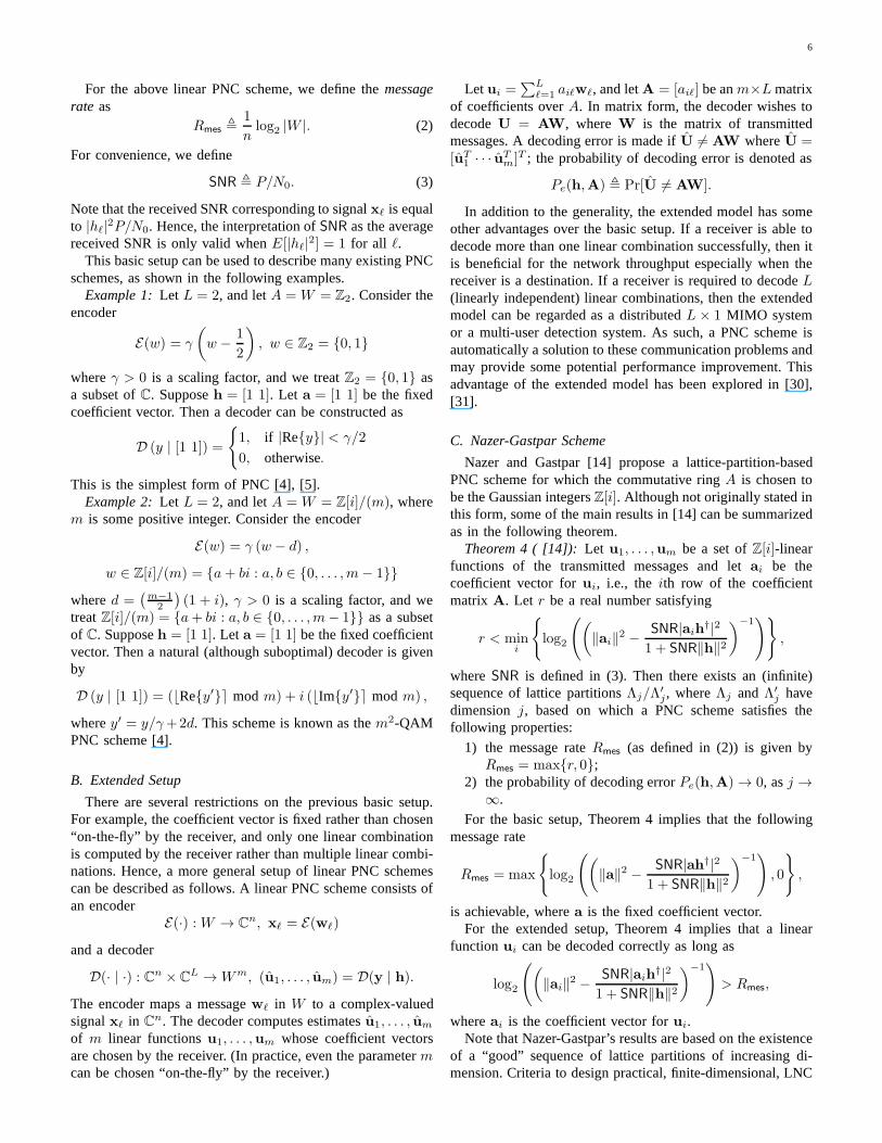
As shown in [14], the essence of a (linear) PNC scheme canbe abstracted as the problem of computing a linear functionover a Gaussian multiple-access channel as depicted in Fig.1.

Let the message spaceW be a finite module over somecommutative ringA. Let w1, . . . ,wL ∈ W be the messagesto be transmitted byL transmitters. We regard the messages asrow vectors and stack them into a matrixW = [wT

1 · · ·wTL ]

T .Transmitterℓ applies the encoder

E(·) : W → Cn, xℓ = E(wℓ)

that maps a message inW to a complex-valued signal inCn

satisfying an average power constraint

1

nE[‖E(wℓ)‖

2]≤ P,

where the expectation is taken with respect to a uniformdistribution overW .

As defined in (1), the receiver observes a channel output

y =

L∑

ℓ=1

hℓxℓ + z

where the complex-valued channel gainsh1, . . . , hL areknown perfectly at the receiver, but areunknown at thetransmitters.

The objective of the receiver (in this basic setup) is todecode the linear combination

u =

L∑

ℓ=1

aℓwℓ

of the transmitted messages, for a fixed coefficient vectora ,

(a1, . . . , aL). In matrix form, the objective of the receiver isto computeu = aW. This is achieved by applying a decoder

D(· | ·) : Cn × CL → W, u = D(y | h)

that computes an estimateu of the linear functionu. Adecoding error is made ifu 6= u; the probability of decodingerror is denoted as

Pe(h, a) , Pr[u 6= u].

6

For the above linear PNC scheme, we define themessagerate as

Rmes ,1

nlog2 |W |. (2)

For convenience, we define

SNR , P/N0. (3)

Note that the received SNR corresponding to signalxℓ is equalto |hℓ|2P/N0. Hence, the interpretation ofSNR as the averagereceived SNR is only valid whenE[|hℓ|2] = 1 for all ℓ.

This basic setup can be used to describe many existing PNCschemes, as shown in the following examples.

Example 1:Let L = 2, and letA = W = Z2. Consider theencoder

E(w) = γ

(

w −1

2

)

, w ∈ Z2 = {0, 1}

whereγ > 0 is a scaling factor, and we treatZ2 = {0, 1} asa subset ofC. Supposeh = [1 1]. Let a = [1 1] be the fixedcoefficient vector. Then a decoder can be constructed as

D (y | [1 1]) =

{

1, if |Re{y}| < γ/2

0, otherwise.

This is the simplest form of PNC [4], [5].Example 2:Let L = 2, and letA = W = Z[i]/(m), where

m is some positive integer. Consider the encoder

E(w) = γ (w − d) ,

w ∈ Z[i]/(m) = {a+ bi : a, b ∈ {0, . . . ,m− 1}}

whered =(m−12

)(1 + i), γ > 0 is a scaling factor, and we

treatZ[i]/(m) = {a+ bi : a, b ∈ {0, . . . ,m− 1}} as a subsetof C. Supposeh = [1 1]. Let a = [1 1] be the fixed coefficientvector. Then a natural (although suboptimal) decoder is givenby

D (y | [1 1]) = (⌊Re{y′}⌉ modm) + i (⌊Im{y′}⌉ modm) ,

wherey′ = y/γ+2d. This scheme is known as them2-QAMPNC scheme [4].

B. Extended Setup

There are several restrictions on the previous basic setup.For example, the coefficient vector is fixed rather than chosen“on-the-fly” by the receiver, and only one linear combinationis computed by the receiver rather than multiple linear combi-nations. Hence, a more general setup of linear PNC schemescan be described as follows. A linear PNC scheme consists ofan encoder

E(·) : W → Cn, xℓ = E(wℓ)

and a decoder

D(· | ·) : Cn × CL → Wm, (u1, . . . , um) = D(y | h).

The encoder maps a messagewℓ in W to a complex-valuedsignalxℓ in Cn. The decoder computes estimatesu1, . . . , um

of m linear functionsu1, . . . ,um whose coefficient vectorsare chosen by the receiver. (In practice, even the parametermcan be chosen “on-the-fly” by the receiver.)

Letui =∑L

ℓ=1 aiℓwℓ, and letA = [aiℓ] be anm×L matrixof coefficients overA. In matrix form, the decoder wishes todecodeU = AW, whereW is the matrix of transmittedmessages. A decoding error is made ifU 6= AW whereU =[uT

1 · · · uTm]T ; the probability of decoding error is denoted as

Pe(h,A) , Pr[U 6= AW].

In addition to the generality, the extended model has someother advantages over the basic setup. If a receiver is able todecode more than one linear combination successfully, thenitis beneficial for the network throughput especially when thereceiver is a destination. If a receiver is required to decode L(linearly independent) linear combinations, then the extendedmodel can be regarded as a distributedL × 1 MIMO systemor a multi-user detection system. As such, a PNC scheme isautomatically a solution to these communication problems andmay provide some potential performance improvement. Thisadvantage of the extended model has been explored in [30],[31].

C. Nazer-Gastpar Scheme

Nazer and Gastpar [14] propose a lattice-partition-basedPNC scheme for which the commutative ringA is chosen tobe the Gaussian integersZ[i]. Although not originally stated inthis form, some of the main results in [14] can be summarizedas in the following theorem.

Theorem 4 ( [14]): Let u1, . . . ,um be a set ofZ[i]-linearfunctions of the transmitted messages and letai be thecoefficient vector forui, i.e., the ith row of the coefficientmatrix A. Let r be a real number satisfying

r < mini

{

log2

((

‖ai‖2 −

SNR|aih†|2

1 + SNR‖h‖2

)−1)}

,

whereSNR is defined in (3). Then there exists an (infinite)sequence of lattice partitionsΛj/Λ

′j, whereΛj andΛ′

j havedimensionj, based on which a PNC scheme satisfies thefollowing properties:

1) the message rateRmes (as defined in (2)) is given byRmes = max{r, 0};

2) the probability of decoding errorPe(h,A) → 0, asj →∞.

For the basic setup, Theorem 4 implies that the followingmessage rate

Rmes = max

{

log2

((

‖a‖2 −SNR|ah†|2

1 + SNR‖h‖2

)−1)

, 0

}

,

is achievable, wherea is the fixed coefficient vector.For the extended setup, Theorem 4 implies that a linear

functionui can be decoded correctly as long as

log2

((

‖ai‖2 −

SNR|aih†|2

1 + SNR‖h‖2

)−1)

> Rmes,

whereai is the coefficient vector forui.Note that Nazer-Gastpar’s results are based on the existence

of a “good” sequence of lattice partitions of increasing di-mension. Criteria to design practical, finite-dimensional, LNC

7

schemes are not immediately obvious from these results. Inthe remainder of this paper, we will develop an algebraicframework for studying LNC schemes, which facilitates theconstruction of practical LNC schemes as well as the analysisof their performance.

IV. A LGEBRAIC FRAMEWORK OF LATTICE NETWORK

CODING

Inspired by Nazer-Gastpar’s C&F scheme, in this section,we present a general framework for studying a variety ofLNC schemes. Our framework is algebraic and makes a directconnection between the Nazer-Gastpar scheme and moduletheory. This connection not only sheds some new light on theNazer-Gastpar scheme, but also leads to several generalizedconstructions of LNC schemes.

A. Definitions

Our algebraic framework is based on a class of complexlattices calledR-lattices, which are defined as follows. LetRbe a discrete subring ofC forming a principal ideal domain(PID). Typical examples include the integer numbersZ and theGaussian integersZ[i]. Let N ≤ n. An R-lattice of dimensionN in Cn is defined as the set of allR-linear combinations ofN linearly independent vectors inCn, i.e.,

Λ = {rGΛ : r ∈ RN},

where GΛ ∈ CN×n is full-rank over C and is called agenerator matrixfor Λ. (In most cases considered in this paper,N = n.) Algebraically, anR-lattice is anR-module.

An R-sublatticeΛ′ of Λ is a subset ofΛ which is itselfan R-lattice, i.e., it is anR-submodule ofΛ. The set of allthe cosets ofΛ′ in Λ, denoted byΛ/Λ′, forms a partitionof Λ, hereafter called anR-lattice partition. Throughout thispaper, we only consider the case of finite lattice partitions, i.e.,|Λ/Λ′| is finite, which is equivalent to saying thatΛ′ andΛhave the same dimension.

A nearest-lattice-point (NLP) decoder is a mapDΛ : Cn →Λ that sends a pointx ∈ C

n to a nearest lattice point inEuclidean distance, i.e.,

DΛ(x) , argminλ∈Λ

‖x− λ‖. (4)

The setV(Λ) , {x : DΛ(x) = 0} of all points in Cn thatare closest to the origin is called theVoronoi regionaroundthe origin of the latticeΛ. The NLP decoder satisfies, for alllattice pointsλ ∈ Λ and all vectorsx ∈ Cn,

DΛ(λ+ x) = λ+DΛ(x). (5)

B. Encoding and Decoding

We present a generic LNC scheme that makes no assump-tions on the underlying lattice partition. As such, our genericLNC scheme can be applied to study a variety of LNCschemes.

We let the message spaceW = Λ/Λ′. Clearly, W isa finitely-generatedR-module. The encoding and decodingmethods of the generic scheme are based on the natural

Gaussian

MAC

w1

w2

wL

xL ∈ Cn

x2 ∈ Cn

x1 ∈ Cn

y

u

u =

L∑

ℓ=1

aℓwℓ

.

.

.

.

.

.

y =

L∑

ℓ=1

hℓxℓ + z

Scaling DΛ

αy

λ =

L∑

ℓ=1

aℓxℓ

Mappingλ

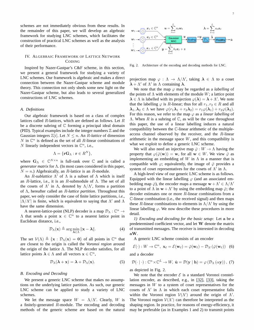
Fig. 2. Architecture of the encoding and decoding methods for LNC.

projection mapϕ : Λ → Λ/Λ′, taking λ ∈ Λ to a cosetλ+ Λ′ of Λ′ in Λ containingλ.

We note that the mapϕ may be regarded as alabelling ofthe points ofΛ with elements of the moduleW ; a lattice pointλ ∈ Λ is labelled with its projectionϕ(λ) = λ+Λ′. We notethat the labellingϕ is R-linear; thus for allr1, r2 ∈ R and allλ1,λ2 ∈ Λ we haveϕ(r1λ1 + r2λ2) = r1ϕ(λ1) + r2ϕ(λ2).For this reason, we refer to the mapϕ as alinear labellingofΛ. WhenR is a subring ofC, as will be the case throughoutthis paper, the use of a linear labelling induces a naturalcompatibility between theC-linear arithmetic of the multiple-access channel observed by the receiver, and theR-lineararithmetic in the message spaceW , and this compatibility iswhat we exploit to define a generic LNC scheme.

We will also need an injective mapϕ : W → Λ having theproperty thatϕ(ϕ(w)) = w, for all w ∈ W . We view ϕ asimplementing an embedding ofW in Λ in a manner that iscompatible withϕ; equivalently, the image ofϕ provides asystem of coset representatives for the cosets ofΛ′ in Λ.

A high-level view of our generic LNC scheme is as follows.Equipped with the linear labellingϕ (and an associated em-bedding mapϕ), the encoder maps a messagew+Λ′ ∈ Λ/Λ′

to a point ofΛ in w+Λ′ by using the embedding mapϕ; thedecoder estimates one or moreR-linear combinations from aC-linear combination (i.e., the received signal) and then mapstheseR-linear combinations to elements inΛ/Λ′ by using thelinear labellingϕ. We now describe these procedures in moredetail.

1) Encoding and decoding for the basic setup:Let a be apredetermined coefficient vector, and letW denote the matrixof transmitted messages. The receiver is interested in decodingaW.

A generic LNC scheme consists of an encoder

E(·) : W → Cn, xℓ = E(wℓ) = ϕ(wℓ)−DΛ′(ϕ(wℓ)) (6)

and a decoder

D(· | ·) : Cn×CL → W, u = D(y | h) = ϕ (DΛ (αy)) , (7)

as depicted in Fig. 2.We note that the encoderE is a standard Voronoi constel-

lation encoder, as described, e.g., in [32], [33], taking themessages inW to a system of coset representatives for thecosets ofΛ′ in Λ in which each coset representative fallswithin the Voronoi regionV(Λ′) around the origin ofΛ′.The Voronoi regionV(Λ′) can therefore be interpreted as theshaping region. In practice, for reasons of energy-efficiency, itmay be preferable (as in Examples 1 and 2) to transmit points

8

from a translate ofΛ rather than fromΛ. Such translation iseasily implemented at the transmitters and accommodated (bysubtraction) at the receiver. A pseudorandom additive dithercan be implemented similarly.

We note that the decoderD first detects anR-linear com-bination

∑

ℓ aℓxℓ from theC-linear combination∑

ℓ hℓxℓ+z

(i.e., the received signal) by using a scaling operatorα andan NLP decoderDΛ. The decoder then maps

∑

ℓ aℓxℓ (anelement in Λ) to

∑

ℓ aℓwℓ (an element inW ) by usingthe linear labellingϕ. The rationale behind this decodingarchitecture is explained by the following proposition.

Define

n ,

L∑

ℓ=1

(αhℓ − aℓ)xℓ + αz, (8)

which is referred to as theeffective noisefor the reason asseen shortly.

Proposition 1: The linear functionu =∑

ℓ aℓwℓ is de-coded correctly if and only ifDΛ(n) ∈ Λ′.

Proof: Note that

αy =

L∑

ℓ=1

αhℓxℓ + αz

=

L∑

ℓ=1

aℓxℓ +

L∑

ℓ=1

(αhℓ − aℓ)xℓ + αz

︸ ︷︷ ︸

n

=

L∑

ℓ=1

aℓxℓ + n

=L∑

ℓ=1

aℓ(ϕ(wℓ)−DΛ′(ϕ(wℓ))) + n

Thus, we have

u = ϕ (DΛ (αy))

= ϕ

(

DΛ

(L∑

ℓ=1

aℓ(ϕ(wℓ)−DΛ′(ϕ(wℓ))) + n

))

= ϕ

(L∑

ℓ=1

aℓ(ϕ(wℓ)− DΛ′(ϕ(wℓ))) +DΛ (n)

)

(9)

=L∑

ℓ=1

aℓwℓ + ϕ (DΛ (n)) (10)

where (9) follows from the property of an NLP decoderDΛ and (10) follows from the fact thatϕ is an R-modulehomomorphism with kernelΛ′. Therefore,u = u if and onlyif ϕ (DΛ (n)) = 0, or equivalently,DΛ (n) ∈ Λ′.

Proposition 1 suggests that the effective noisen should bemade “small” so thatDΛ (n) returns, in particular, the point0. This can be achieved by choosing an appropriate scalarα,which will be discussed fully in Sec. V-B. Here, we point outthat the decoder architecture induces an equivalent point-to-point channel with input

∑

ℓ aℓxℓ and additive channel noisen. Hence, the decoding complexity of our generic scheme isnot essentially different from that for a point-to-point channelusing the same lattice partition.

We also note that a generalized lattice quantizer that satisfiesthe property (5) (e.g., see [34]) can also be applied to theencoding and decoding operations. This may provide somepractical advantages (at the expense of error performance).

2) Encoding and decoding for the extended setup:Theencoding architecture for the extended setup is precisely thesame as that for the basic setup. The decoding architectureis similar to that for the basic setup, except the receiver hasthe freedom to choose coefficient vectors for multiple linearcombinations. Once these coefficient vectors are chosen, thereceiver applies exactly the same decoder as that for the basicsetup. Hence, the decoding architecture for the extended setuponly contains an additional component of choosing multiplecoefficient vectors, which will be discussed fully in Sec. V-B.

C. Algebraic Structure of Lattice Partitions

As shown in the previous section, the linear labellingϕ(and the associated embeddingϕ) play important roles in theencoding and decoding methods of our generic scheme. Inthis section, we construct the mapsϕ and ϕ explicitly andshow that the message space of the generic LNC schemeis determined by the module-theoretic structure of the latticepartition Λ/Λ′. Our main theoretical tool is the fundamentaltheorem of finitely generated modules over a PID.

Theorem 5 (Structural Theorem forR-Lattice Partitions):Let Λ/Λ′ be a finite R-lattice partition. Then for somenonzero, non-unit elementsπ1, . . . , πk ∈ R satisfying thedivisibility relationsπ1 | π2 | · · · | πk,

Λ/Λ′ ∼= R/(π1)⊕R/(π2)⊕ · · · ⊕R/(πk).

Proof: By Theorem 2, we have

Λ/Λ′ ∼= Rm ⊕R/(r1)⊕R/(r2)⊕ · · · ⊕R/(rk),

for some integerm and some invariant factorsr1, . . . , rk ofΛ/Λ′. Note that, since|Λ/Λ′| is assumed to be finite, theintegerm must be zero.

Theorem 5 characterizes the module-theoretic structure ofΛ/Λ′. By Theorem 5, the message spaceW , which we havetaken to be equal toΛ/Λ′, is isomorphic toR/(r1) ⊕ · · · ⊕R/(rk). Without loss of generality, we may identifyW withthis direct sum in the rest of the paper.

To construct the linear labellingϕ from Λ to W , we applythe Smith normal form, as shown in the following theorem.

Theorem 6:Let Λ/Λ′ be a finiteR-lattice partition. Thenthere exist generator matricesGΛ and GΛ′ for Λ and Λ′,respectively, satisfying

GΛ′ =

[diag(π1, . . . , πk) 0

0 IN−k

]

GΛ (11)

whereπ1, . . . , πk are the invariant factors ofΛ/Λ′. Moreover,the map

ϕ : Λ → R/(π1)⊕ · · · ⊕R/(πk)

given by

ϕ(rGΛ) = (r1 + (π1), . . . , rk + (πk)) (12)

is a surjectiveR-module homomorphism with kernelΛ′.

9

Proof: Let GΛ andGΛ′ be any generator matrices forΛandΛ′, respectively. ThenGΛ′ = JGΛ, for some nonsingularmatrix J ∈ RN×N . SinceR is a PID, by Theorem 3, thematrix J has a Smith normal form

D =

π1

. . .πk

IN−k

= PJQ

whereP,Q ∈ RN×N are invertible overR, andπ1 | π2 | · · · |πk. Thus, we can take

GΛ = Q−1GΛ

GΛ′ = PGΛ′ = DGΛ

as new generator matrices forΛ and Λ′. Here our notationsuggests thatπ1, . . . , πk are the invariant factors ofΛ/Λ′; thisfact will be clear after the second statement is proved.

Since GΛ has rankN , it follows that each lattice pointλ ∈ Λ has a unique representation asλ = rGΛ, and thus themapϕ in (12) is well defined. It is easy to see that the mapϕis a surjectiveR-module homomorphism. Next, we will showthat the kernel ofϕ is Λ′. Note that

ϕ(rGΛ) = 0 ⇐⇒ ri ∈ (πi), ∀i = 1, . . . , k.

Note also that

Λ′ = {rGΛ : ri ∈ (πi), ∀i = 1, . . . , k},

becauseGΛ′ = DGΛ. Hence, the kernel ofϕ is Λ′. Then bythe first isomorphism theorem (Theorem 1), we have

Λ/Λ′ ∼= R/(π1)⊕ · · · ⊕R/(πk).

Finally, by the uniqueness in Theorem 2,π1, . . . , πk mustbe the invariant factors ofΛ/Λ′. This also follows from theobservation thatJ is a relations matrix forΛ/Λ′ relative tothe rows ofGΛ andGΛ′ .

Theorem 6 constructs a surjectiveR-module homomor-phismϕ : Λ → W , i.e., anR-linear labelling ofΛ, explicitly.The next step is to construct the mapϕ. Consider the naturalprojection mapσ : Rk → W defined byσ(r) = (r1 +(π1), . . . , rk + (πk)). Let σ : W → Rk be some injectivemap such thatσ(σ(w)) = w, for all w ∈ W . Then the mapϕ can be constructed as

ϕ(w) = σ(w)[Ik 0

]GΛ. (13)

To sum up, the mapsϕ andϕ can be constructed explicitlyby using (12) and (13) whenever there exist generator matricesGΛ andGΛ′ satisfying the relation (11).

D. Constructions of Lattice Partitions

In the previous sections, we presented an algebraic frame-work for studying a variety of LNC schemes. In this sec-tion, we first apply the algebraic framework to study Nazer-Gastpar’s C&F scheme, showing that the message space of theNazer-Gastpar scheme is isomorphic to a vector space overFp2

or a direct sum of two vector spaces overFp, depending onthe prime parameterp. We then apply the algebraic framework

to construct three classes of lattice partitions, all of which canbe viewed as generalizations of Nazer-Gastpar’s constructionof lattice partitions.

The following example describes a variant of the class oflattice partitions constructed by Nazer and Gastpar.

Example 3 (Lifted Construction A):Let p be a prime inZ.Let C be a linear code of lengthn over Z/(p). Without lossof generality, we may assume the linear codeC is systematic.Define a “Construction A lattice” [35]ΛC as

ΛC , {λ ∈ Zn : σ(λ) ∈ C},

where σ : Zn → (Z/(p))n is the natural projection map.Define

Λ′C , {pr : r ∈ Z

n}.

It is easy to see thatΛ′C is a sublattice ofΛC . Hence, we obtain

a Z-lattice partitionΛC/Λ′C from the linear codeC.

Now we “lift” this Z-lattice partitionΛC/Λ′C to aZ[i]-lattice

partition. LetΛC = ΛC + iΛC , i.e.,

ΛC = {λ ∈ Z[i]n : Re{λ}, Im{λ} ∈ ΛC}.

Similarly, let Λ′C = Λ′

C + iΛ′C . In this way, we obtain aZ[i]-

lattice partitionΛC/Λ′C.

To study the structure of the partitionΛC/Λ′C, we specify

two generator matrices satisfying the relation (11). We notethat the latticeΛC has a generator matrixGΛC

given by

GΛC=

[Ik Bk×(n−k)

0(n−k)×k pIn−k

]

,

whereσ[I B] is a generator matrix forC. The lifted latticeΛC

has a generator matrixGΛCof the same form (but overZ[i]).

Similarly, we note that the latticeΛ′C has a generator matrix

GΛ′

C

given by

GΛ′

C

=

[pIk pBk×(n−k)

0(n−k)×k pIn−k

]

.

These two generator matricesGΛCandGΛ′

Csatisfy

GΛ′

C=

[pIk 0

0 In−k

]

GΛC.

It follows from Theorem 6 thatΛ/Λ′ ∼= (Z[i]/(p))k.If the primep in Example 3 is of the form4n+3, thenp is a

Gaussian prime andΛ/Λ′ is isomorphic to a vector space overthe fieldZ[i]/(p). If the primep is of the form4n+1 or if p =2, thenp is not a Gaussian prime andΛ/Λ′ is isomorphic to afree module over the ringZ[i]/(p). In this case, sincep can befactored into two Gaussian primes, i.e.,p = ππ∗, whereπ∗ isa conjugate ofπ, it can be shown from the Chinese remaindertheorem [28, p. 265] thatΛ/Λ′ is isomorphic to a direct sumof two vector spaces, i.e.,Λ/Λ′ ∼= Z[i]/(π)k ⊕Z[i]/(π∗)k. Tosum up, the message spaceW is isomorphic to either a vectorspace overFp2 or a direct sum of two vector spaces overFp,depending on the choice of the primep.

Nazer-Gastpar’s construction of lattice partitions is basedon Construction A. As is well known, Construction A mayproduce “asymptotically-good” lattices and/or lattice partitionsin the sense of [15], [36]. However, this generally requiresboth the primep and the dimensionn to go to infinity. From

10

a practical point of view, Construction A may not be thebest method of constructing lattices and/or lattice partitions.There are several alternative methods in the literature, such ascomplex Construction A, Construction D [35], low-density-parity-check lattices [37], signal codes [25], and low-densitylattice codes [38], to name a few. Our algebraic frameworksuggests that all of these methods may be used to constructlattice partitions for LNC schemes. In the sequel, we presentthree constructions of lattice partitions, all of which canbeviewed as generalizations of Nazer-Gastpar’s construction.

The first example is based on complex Construction A.Example 4 (Complex Construction A):Let π be a prime in

R. Let C be a linear code of lengthn overR/(π). Without lossof generality, we may assume the linear codeC is systematic.

Define a “complex Construction A lattice” [35]ΛC as

ΛC , {λ ∈ Rn : σ(λ) ∈ C},

where σ : Rn → (R/(π))n is the natural projection map.Define

Λ′C , {πr : r ∈ Rn}.

It is easy to seeΛ′C is a sublattice ofΛC. Hence, we obtain a

lattice partitionΛC/Λ′C from the linear codeC.

To study the structure ofΛC/Λ′C , we specify two generator

matrices satisfying the relation (11). It is well-known that ΛC

has a generator matrixGΛCgiven by

GΛC=

[Ik Bk×(n−k)

0(n−k)×k πIn−k

]

,

and thatΛ′C has a generator matrixGΛ′

Cgiven by

GΛ′

C=

[πIk πBk×(n−k)

0(n−k)×k πIn−k

]

.

These two generator matrices satisfy

GΛ′

C=

[πIk 0

0 In−k

]

GΛC.

Hence, we haveΛ/Λ′ ∼= (R/(π))k. We note that complexConstruction A reduces to lifted Construction A whenR =Z[i], π is a prime inZ of the form 4n + 3, and the matrixBk×(n−k) in GΛ′

Ccontains only elements ofZ.

Our next example replaces Construction A with Construc-tion D.

Example 5 (Lifted Construction D):Let p be a prime inZ.Let C0 ⊇ C1 ⊇ · · · ⊇ Ca be nested linear codes of lengthnoverZ/(p), whereCi has parameters[n, ki] for i = 0, . . . , a,and k0 = n. Without loss of generality, there exists a basis{g1, . . . ,gn} for (Z/(p))n such that 1)g1, . . . ,gki

spanCifor i = 0, . . . , a, and 2) if G denotes the matrix with rowsg1, . . . ,gn, some permutation of the rows ofG forms an uppertriangular matrix with diagonal elements equal to1.

Using the nested linear codes{Ci, 0 ≤ i ≤ a}, we define a“Construction D lattice” [35]Λ as

Λ ,⋃

paZn +

a∑

i=1

ki∑

j=1

pa−iβij σ(gj) : βij ∈ Z/(p)

whereβij ∈ {0, . . . , p − 1}, “+” denotes ordinary additionin Cn, and σ is a natural embedding map from(Z/(p))n to

{0, . . . , p − 1}n. It is easy to see that the lattice defined byΛ′ , {par : r ∈ Zn} is a sublattice ofΛ. Hence, we obtain aZ-lattice partitionΛ/Λ′ from the nested linear codes{Ci, 0 ≤i ≤ a}.

Next we lift this Z-lattice partitionΛ/Λ′ to a Z[i]-latticepartition Λ/Λ′ using the procedure in Example 3. That is, weset Λ = Λ + iΛ and Λ′ = Λ′ + iΛ′. In this way, we obtain aZ[i]-lattice partitionΛ/Λ′.

In Appendix A, we show that there exist two generatormatricesGΛ andGΛ′ satisfying

GΛ′ = diag(p, . . . , p︸ ︷︷ ︸

k1−k2

, p2, . . . , p2︸ ︷︷ ︸

k2−k3

, . . . , pa, . . . , pa︸ ︷︷ ︸

ka

)GΛ. (14)

It follows from Theorem 6 that

Λ/Λ′ ∼= (Z[i]/(p))k1−k2⊕(Z[i]/(p2))k2−k3⊕· · ·⊕(Z[i]/(pa))ka .

Whena = 1, lifted Construction D reduces to lifted Construc-tion A.

Our final example combines the ideas behind complexConstruction A and lifted Construction D.

Example 6 (Complex Construction D):Let π be a prime inR. Let C0 ⊇ C1 ⊇ · · · ⊇ Ca be nested linear codes of lengthnoverR/(π), whereCi has parameters[n, ki] for i = 0, . . . , a,and k0 = n. Without loss of generality, there exists a basis{g1, . . . ,gn} for (R/(π))n such that 1)g1, . . . ,gki

spanCifor i = 0, . . . , a, and 2) if G denotes the matrix with rowsg1, . . . ,gn, some permutation of the rows ofG forms an uppertriangular matrix with diagonal elements equal to1.

Using the nested linear codes{Ci, 0 ≤ i ≤ a}, we defineanR-latticeΛ as

Λ ,⋃

πaRn +

a∑

i=1

ki∑

j=1

πa−iβij σ(gj) : βij ∈ Aπ

whereAπ is a system of coset representatives forR/(π), “+”denotes ordinary addition inCn, andσ is an embedding mapfrom (R/(π))n to An

π . It is easy to verify that the latticedefined byΛ′ , {πar : r ∈ Rn} is a sublattice ofΛ. Hence,we obtain anR-lattice partitionΛ/Λ′ from the nested linearcodes{Ci, 0 ≤ i ≤ a}.

Similar to Example 5, we haveΛ/Λ′ ∼= (R/(π))k1−k2 ⊕(R/(π2))k2−k3 ⊕ · · · ⊕ (R/(πa))ka . When a = 1, complexConstruction D reduces to complex Construction A.

Note that when a lattice partition is isomorphic to a vectorspace or a direct sum of two vector spaces (e.g., those inExample 3 and Example 4), it is convenient to implementrandom linear network coding at Layer 2, since many of theuseful techniques (e.g., the use of headers for non-coherentnetwork coding) from the network coding literature can beapplied in a straightforward way. When a lattice partition hasa more complicated structure (e.g., those in Example 5 andExample 6), the implementation of random linear networkcoding requires some modification, as discussed in the nextsection.

E. Non-Coherent LNC

Recall that “headers” are usually used to implement randomlinear network coding at Layer 2 in non-coherent settings. In

11

this section, we discuss how to design “headers” for a messagespace which is more complicated than a vector space.

Consider a general message spaceW = R/(π1)⊕R/(π2)⊕· · · ⊕R/(πk), whereπ1 | π2 | . . . | πk. We propose to use thefirst k− P summands to store payloads and to use the lastPsummands to store headers, whereP denotes the number ofpackets in a generation. In other words, the “payload space”Wpayload is given by

Wpayload = R/(π1)⊕ · · · ⊕R/(πk−P )

and the “header space”Wheader is given by

Wheader = R/(πk−P+1)⊕ · · · ⊕R/(πk).

It is easy to see the annihilatorAnn(Wpayload) of the payloadspace is given byAnn(Wpayload) = (πk−P ). Hence, thepayload spaceWpayload can be regarded as anR/(πj)-module,for everyj ≥ k−P , since(πj) ⊆ Ann(Wpayload). This impliesthat there is no loss of information when a network-codingcoefficient is stored overR/(πj) rather than overR.

The use of headers incurs some overhead. If headers are notused, then the lastP summands can be used to store payloads,leading to additional

∑kj=k−P+1 log2 |R/(πj)| bits for storing

payloads. Hence, the normalized redundancy of headers canbe defined as

∑kj=k−P+1 log2 |R/(πj)|∑k

j=1 log2 |R/(πj)|.

This quantity is minimized for lattice partitions with(π1) =· · · = (πk), which we calluniform lattice partitions. Uniformlattice partitions are good candidates for applications inwhichthe normalized redundancy of headers is a major concern. Wenote that the lattice partitions in Example 3 and Example 4are uniform lattice partitions, while the lattice partitions inExample 5 and Example 6 are not uniform lattice partitionsin general.

V. PERFORMANCEANALYSIS FOR LATTICE NETWORK

CODING

In this section, we turn from algebra to geometry, presentingan error-probability analysis as well as its implications.

A. Error Probability for LNC

According to Proposition 1, the linear functionu is decodedcorrectly if and only ifDΛ(n) ∈ Λ′; thus, the error probabilityfor the basic setup is given by

Pe(h, a) = Pr[DΛ(n) /∈ Λ′],

wheren =∑L

ℓ=1(αhℓ − aℓ)xℓ + αz is the effective noise.Note that the effective noisen is not necessarily Gaussian,making the analysis nontrivial. To alleviate this difficulty, wefocus on a special case in which the shaping region (Voronoiregion)V(Λ′) is a (rotated) hypercube inCn, i.e.,

V(Λ′) = γUHn

where γ > 0 is a scalar factor,U is any n × n unitarymatrix, andHn is a unit hypercube inCn defined byHn =

([−1/2, 1/2)+ i[−1/2, 1/2))n. This corresponds to so-calledhypercube shapingin [39]. We note that all of our previousexamples of lattice partitions admit hypercube shaping. Theassumption of hypercube shaping not only simplifies the analy-sis of error probability, but also has some practical advantages,for example, the complexity of the shaping operation is low(however, there is no shaping gain [33], [39]). In the sequel,we will provide an approximate upper bound for the errorprobability for LNC schemes that admit hypercube shaping.This upper bound is closely related to certain geometricalparameters of a lattice partition as defined below.

The inter-coset distanced(λ1 + Λ′,λ2 + Λ′) between twocosetsλ1 + Λ′,λ2 + Λ′ of Λ/Λ′ is defined as

d(λ1+Λ′,λ2+Λ′) , min{‖x1−x2‖ : x1 ∈ λ1+Λ′, x2 ∈ λ2+Λ′}.

Clearly, d(λ1 + Λ′,λ2 + Λ′) = 0 if and only if λ1 + Λ′ =λ2 + Λ′.

Theminimum inter-coset distanced(Λ/Λ′) of Λ/Λ′ is thusdefined as

d(Λ/Λ′) , min{d(λ1 + Λ′,λ2 + Λ′) : λ1 + Λ′ 6= λ2 + Λ′}.

Let the set differenceΛ \ Λ′ = {λ ∈ Λ : λ /∈ Λ′}. Thend(Λ/Λ′) corresponds to the length of the shortest vectors inthe set differenceΛ \ Λ′. Denote byK(Λ/Λ′) the number ofthese shortest vectors.

An elementx in a cosetλ + Λ′ is called acoset leaderif‖x‖ ≤ ‖y‖ for all y ∈ λ+ Λ′.

1) Error analysis for the basic setup:We have the follow-ing union bound estimate (UBE) of the error probability.

Theorem 7 (Probability of Decoding Error):Assume hy-percube shaping is used forΛ/Λ′. Let u be a predeterminedlinear function. Then the union bound estimate of the proba-bility of decoding error is

Pe(h, a) ≈ K(Λ/Λ′) exp

(

−d2(Λ/Λ′)

4N0Q(α, a)

)

,

wherea ∈ RL (a 6= 0) is the coefficient vector foru, α ∈ C

is the scalar, and the parameterQ(α, a) is given by

Q(α, a) = |α|2 + SNR‖αh− a‖2. (15)

The proof is given in Appendix B.Theorem 7 has the following important implications.

1) The scalarα should be chosen such thatQ(α, a) isminimized;

2) The lattice partitionΛ/Λ′ should be designed such thatK(Λ/Λ′) is minimized andd(Λ/Λ′) is maximized.

These two implications will be discussed fully in Sec. V-Band Sec. V-C. Here, we point out that, under hypercubeshaping, the effective noisen is a random vector with i.i.d.components of varianceN0Q(α, a). Hence, the first implica-tion can be interpreted as aminimum variance criterion.

2) Error analysis for the extended setup:Once the coeffi-cient vectorsa1, . . . , am (for the linear functionsu1, . . . ,um)are chosen by the receiver, the following corollary followsimmediately from Theorem 7.

12

Corollary 1: Assume hypercube shaping is used forΛ/Λ′.Then for each linear functionui, the union bound estimate ofthe probability of decoding error is

Pe(h, ai) ≈ K(Λ/Λ′) exp

(

−d2(Λ/Λ′)

4N0Q(αi, ai)

)

,

where ai ∈ RL (ai 6= 0) is the coefficient vector forui,αi ∈ C is the scalar forui.

Recall that the linear combinationsu1, . . . ,um should belinearly independent. Thus, Corollary 1 suggests that eachcoefficient vectorai should be chosen such that eachQ(αi, ai)is as small as possible under the constraint thatu1, . . . ,um

are linearly independent. This can be regarded as aconstrainedminimum variance criterion, which will be explored next.

B. Choice of Receiver Parameters

In the previous section, we derive a minimum variancecriterion and a constrained minimum variance criterion forchoosing receiver parameters. In this section, we will applythese criteria to develop explicit algorithms for choosingre-ceiver parameters. In particular, we will show that 1) choosinga single coefficient vector is a shortest vector problem, and2) choosing multiple coefficient vectors is related to sphere-decoding algorithms and lattice-reduction algorithms.

1) Choice of the scalarα: We note that the minimumvariance criterion is equivalent to the maximum computation-rate criterion in [14]. Hence, the results in [14] can be carriedover here directly.

Proposition 2 ( [14]): For a predetermined coefficient vec-tor a ∈ RL (a 6= 0), the optimal scalarα, denoted byαopt, isgiven by

αopt =ahH

SNR

SNR‖h‖2 + 1. (16)

2) Choice of a single coefficient vector:Suppose the re-ceiver has the freedom to choose a single coefficient vector.ByProposition 2, for any coefficient vectora, the correspondingoptimal parameterQ(αopt, a) is equal toaMaH, where thematrix M is

M = SNRIL −SNR

2

SNR‖h‖2 + 1hHh.

Observe that the matrixM is Hermitian and positive-definite.Hence,M has a Cholesky decompositionM = LLH, whereL is a lower triangular matrix. It follows that

Q(αopt, a) = aMaH = ‖aL‖2.

Thus, finding an optimal coefficient vectora is equivalent tosolving the shortest vector problem

aopt = argmina 6=0

‖aL‖. (17)

3) Choice of multiple coefficient vectors:Suppose the re-ceiver has the freedom to choosem coefficient vectors. Thenthese coefficient vectorsa1, . . . , am should be chosen suchthat eachQ(αi, ai) = ‖aiL‖2 is as small as possible under theconstraint thatu1, . . . ,um are linearly independent. We willshow that, for lattice partitions constructed in Section IV-D,

there exists a feasible solution of{a1, . . . , am} that simulta-neously optimizes each‖aiL‖. We call such feasible solutionsdominated solutions, as defined below.

Definition 2 (Dominated Solutions):A feasible solutiona1, . . . , am (with ‖a1L‖ ≤ . . . ≤ ‖amL‖) is called adominated solutionif for any feasible solutiona′1, . . . , a

′m

(with ‖a′1L‖ ≤ . . . ≤ ‖a′mL‖), the following inequalities hold

‖aiL‖ ≤ ‖a′iL‖, i = 1, . . . ,m.

We will show the existence of dominated solutions for latticepartitions constructed in Section IV-D. For ease of presenta-tion, we mainly focus on lattice partitions obtained from com-plex Construction A here, since similar methods apply to otherconstructions as well. Note that for complex Construction A,the linear independence ofu1, . . . ,um ∈ (R/(π))k impliesthe linear independence ofa1, . . . , am ∈ (R/(π))L, whereai is the natural projection ofa. The existence of dominatedsolutions is proven in the following theorem.

Theorem 8:A feasible solution{a1, . . . , am} defined by

a1 = argmin {‖aL‖ | a is nonzero}

a2 = argmin {‖aL‖ | a, a1 are linearly independent}...

am = argmin {‖aL‖ | a, a1, . . . , am−1 are linearly independent}

always exists, and is a dominated solution.The proof is given in Appendix C.

4) Finding dominated solutions:We now propose a methodof finding a dominated solution, which consists of three steps.In the first step, we construct a ballB(ρ) = {x ∈ CL |‖x‖ ≤ ρ} that containsm lattice pointsv1L, . . . ,vmL suchthat v1, . . . , vm are linearly independent. In the second step,we order all lattice points withinB(ρ) based on their lengths,producing an ordered setSρ with ‖v1L‖ ≤ ‖v2L‖ ≤ · · · ≤‖v|Sρ|L‖. Finally, we find a dominated solution{a1, . . . , am}by using a greedy search algorithm given as Algorithm 1.

Algorithm 1 A greedy search algorithm

Input: An ordered setSρ = {v1L,v2L, . . . ,v|Sρ|L} with‖v1L‖ ≤ ‖v2L‖ ≤ · · · ≤ ‖v|Sρ|L‖.Output: An optimal solution{a1, . . . , am}.

1. Seta1 = v1. Seti = 1 andj = 1.2. while i < |Sb| andj < m do3. Set i = i+ 1.4. if vi, a1, . . . , aj are linearly independentthen5. Set j = j + 1. Setaj = vi.6. end if7. end while

The correctness of our proposed method follows immedi-ately from Theorem 8. Our proposed method is in the spirit ofsphere-decoding algorithms, since sphere-decoding algorithmsalso enumerate all lattice points within a ball centered at agiven vector. The selection of the radiusρ plays an importantrole here, just as it does for sphere-decoding algorithms. Ifρ is too large, then the second step may incur excessive

13

computations. Ifρ is too small, then the first step mayfail to construct a ball that containsm linearly independentv1, . . . , vm.

As shown in the following proposition, lattice-reductionalgorithms may be used to determine an appropriate radiusρ,like the Lenstra-Lenstra-Lovasz (LLL) algorithm that is usedin sphere decoding.

Proposition 3: Let {b1, . . . ,bL} be a reduced basis [40]for L. If ρ is set to be‖bm‖, then the setSρ contains atleastm lattice pointsv1L, . . . ,vmL such thatv1, . . . , vm arelinearly independent.

Proof: Let vi = biL−1 for i = 1, . . . , L. Let V be an

L × L matrix with vi as its ith row. Since{b1, . . . ,bL} isa reduced basis, it follows that the matrixV is invertible. Inparticular,v1, . . . , vm are linearly independent for all integersm ≤ L.

There are many existing lattice-reduction algorithms in theliterature. Among them, the LLL reduction algorithm is ofparticular importance. Recently, the LLL reduction algorithmhas been extended from real lattices (Z-lattices) toZ[i]-lattices[41]. Unfortunately, there exist no LLL reduction algorithmsfor generalR-lattices to the best of our knowledge; the designof such reduction algorithms is left as future work.

For the special case whenR = Z[i] andL = 2, a dominatedsolution can be computed very quickly and efficiently by usingthe lattice-reduction algorithm proposed in [42] in the contextof MIMO communication.

C. Design of Lattice Partitions

In Sec. V-A, we show that the lattice partitionΛ/Λ′ shouldbe designed such thatK(Λ/Λ′) is minimized andd(Λ/Λ′) ismaximized. These criteria apply to both the basic setup andthe extended setup under hypercube shaping. In this section,we first introduce a notion of nominal coding gain for an LNCscheme, which characterizes the performance improvementover the baseline LNC scheme. We then discuss how to designlattice partitions with large nominal coding gains.

1) Nominal coding gain for LNC: Recall that Nazer-Gastpar’s result for the basic setup can be rewritten asRmes = log(SNR/Q(α, a)) when SNR ≥ Q(α, a). Observethat SNR/Q(α, a) = P/(N0Q(α, a)), whereN0Q(α, a) isthe variance of the effective noisen under hypercube shaping.These facts suggest defining thesignal-to-effective-noise ratio

SENR =SNR

Q(α, a)

and thenormalized signal-to-effective-noise ratio

SENRnorm =SENR

2Rmes=

SNR

2RmesQ(α, a),

whereRmes is the actual message rate of an LNC scheme.For the Nazer-Gastpar scheme,SENRnorm = 1 (0 dB) when

SNR ≥ Q(α, a). Thus, the value ofSENRnorm for an LNCscheme signifies how far this LNC scheme is operating fromthe Nazer-Gastpar scheme in the high-SNR regime.

Recall that the UBE for an LNC scheme in the basic setupis given by

Pe(h, a) ≈ K(Λ/Λ′) exp

(

−d2(Λ/Λ′)

4N0Q(α, a)

)

,

for high signal-to-noise ratios. Note thatSENRnorm =P/(N0Q(α, a)2Rmes), 2nRmes = V (Λ′)/V (Λ), and V (Λ′) =γ2n = (6P )n (due to hypercube shaping). Combining theseresults, we obtain

Pe(h, a) ≈ K(Λ/Λ′) exp

(

−γc(Λ/Λ

′)3SENRnorm

2

)

,

whereγc(Λ/Λ′) , d2(Λ/Λ′)/V (Λ)1/n is thenominal codinggain of Λ/Λ′.

For a baseline lattice partition (i.e.,Λ/Λ′ = Z[i]n/πZ[i]n

for someπ ∈ Z[i]), the nominal coding gain equals to1.Thus, the nominal coding gain provides a first-order estimateof the performance improvement of an LNC scheme over thebaseline LNC scheme in terms ofSENRnorm.

2) Lattice partitions with large nominal coding gains:Inthis section, we illustrate how to design lattice partitions withlarge nominal coding gains. We use complex Construction A asa particular example, since similar methods can be applied toother constructions as well. Recall that complex ConstructionA produces a lattice partitionΛC/Λ

′C from a linear codeC.

To optimize the nominal coding gainγC(ΛC/Λ′C) for ΛC/Λ

′C,

we first relateγC(ΛC/Λ′C) to certain parameters of the linear

codeC.Let π be a prime inZ[i] with |π|2 > 2. To each codeword

c = (c1 + (π), . . . , cn + (π)) ∈ C, there corresponds a coset(c1, . . . , cn) + πZ[i]n, we denote by〈c〉 a coset leader. It iseasy to check that〈c〉 is uniquely given by

〈c〉 = (c1 − ⌊c1/π⌉ × π, . . . , cn − ⌊cn/π⌉ × π), (18)

where ⌊x⌉ is a rounding operation that sendsx ∈ C tothe closest Gaussian integer in the Euclidean distance. TheEuclidean weightwE(c) of c can then be defined as thesquared Euclidean norm of〈c〉, that is, wE(c) = ‖〈c〉‖2.Let wmin

E (C) be the minimum Euclidean weight of nonzerocodewords inC, i.e.,

wminE (C) = min{wE(c) : c 6= 0, c ∈ C}.

Then we have the following result.Proposition 4: Let C be a linear code overZ[i]/(π) and let

ΛC/Λ′C be a lattice partition constructed fromC using complex

construction A. Then

γc(ΛC/Λ′C) =

wminE (C)

|π|2(1−k/n).

The proof is in Appendix D.Proposition 4 suggests that optimizing the nominal cod-

ing gain γc(ΛC/Λ′C) of ΛC/Λ

′C amounts to maximizing the

minimum Euclidean weightwminE (C) of C. In the sequel, we

propose two simple methods for constructing linear codes withlargewmin

E (C).The first method applies to (terminated) convolutional

codes. Recall that convolutional codes with large free dis-tances can be found through simple computer searches. Thus,terminated convolutional codes with large minimum Euclideanweights can be found in an analogous way. A concrete exampleof this method will be given in Section VI-A. The secondmethod applies to linear codes over “small” fieldZ[i]/(π).Note that the minimum Euclidean weightwmin

E (C) of a linear

14

codeC is lower-bounded by its minimum Hamming weightwmin

H (C), i.e.,wminE (C) ≥ wmin

H (C). The smaller the field sizeis, the tighter the lower bound would be. Hence, codes withlarge wmin

H (C) implies codes with largewminE (C). This fact

can be used to construct good (not necessarily optimal) linearcodes over smallZ[i]/(π).

VI. D ESIGN EXAMPLES AND SIMULATION RESULTS

A. Design Examples

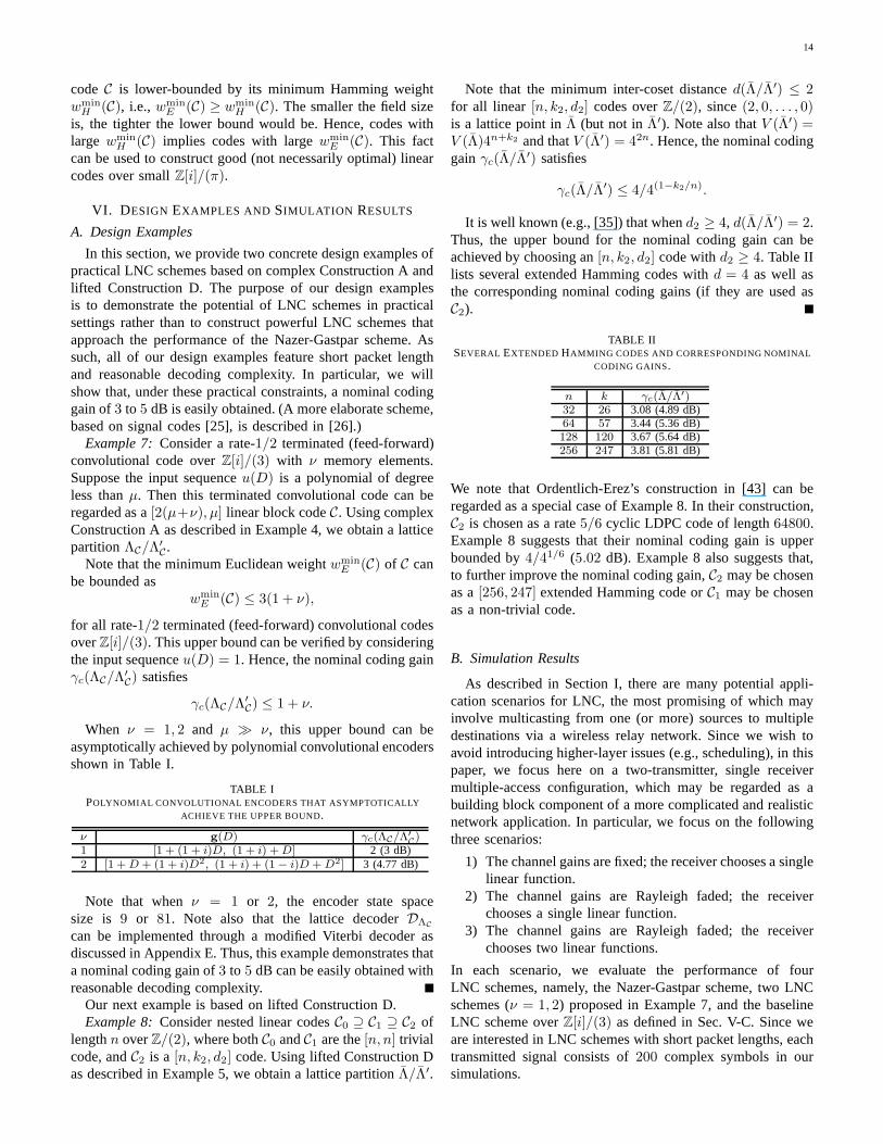
In this section, we provide two concrete design examples ofpractical LNC schemes based on complex Construction A andlifted Construction D. The purpose of our design examplesis to demonstrate the potential of LNC schemes in practicalsettings rather than to construct powerful LNC schemes thatapproach the performance of the Nazer-Gastpar scheme. Assuch, all of our design examples feature short packet lengthand reasonable decoding complexity. In particular, we willshow that, under these practical constraints, a nominal codinggain of3 to 5 dB is easily obtained. (A more elaborate scheme,based on signal codes [25], is described in [26].)

Example 7:Consider a rate-1/2 terminated (feed-forward)convolutional code overZ[i]/(3) with ν memory elements.Suppose the input sequenceu(D) is a polynomial of degreeless thanµ. Then this terminated convolutional code can beregarded as a[2(µ+ν), µ] linear block codeC. Using complexConstruction A as described in Example 4, we obtain a latticepartitionΛC/Λ

′C.

Note that the minimum Euclidean weightwminE (C) of C can

be bounded aswmin

E (C) ≤ 3(1 + ν),

for all rate-1/2 terminated (feed-forward) convolutional codesoverZ[i]/(3). This upper bound can be verified by consideringthe input sequenceu(D) = 1. Hence, the nominal coding gainγc(ΛC/Λ

′C) satisfies

γc(ΛC/Λ′C) ≤ 1 + ν.

When ν = 1, 2 and µ ≫ ν, this upper bound can beasymptotically achieved by polynomial convolutional encodersshown in Table I.

TABLE IPOLYNOMIAL CONVOLUTIONAL ENCODERS THAT ASYMPTOTICALLY

ACHIEVE THE UPPER BOUND.

ν g(D) γc(ΛC/Λ′

C)

1 [1 + (1 + i)D, (1 + i) +D] 2 (3 dB)2 [1 +D + (1 + i)D2, (1 + i) + (1− i)D +D2] 3 (4.77 dB)

Note that whenν = 1 or 2, the encoder state spacesize is 9 or 81. Note also that the lattice decoderDΛC

can be implemented through a modified Viterbi decoder asdiscussed in Appendix E. Thus, this example demonstrates thata nominal coding gain of3 to 5 dB can be easily obtained withreasonable decoding complexity.

Our next example is based on lifted Construction D.Example 8:Consider nested linear codesC0 ⊇ C1 ⊇ C2 of

lengthn overZ/(2), where bothC0 andC1 are the[n, n] trivialcode, andC2 is a [n, k2, d2] code. Using lifted Construction Das described in Example 5, we obtain a lattice partitionΛ/Λ′.

Note that the minimum inter-coset distanced(Λ/Λ′) ≤ 2for all linear [n, k2, d2] codes overZ/(2), since(2, 0, . . . , 0)is a lattice point inΛ (but not inΛ′). Note also thatV (Λ′) =V (Λ)4n+k2 and thatV (Λ′) = 42n. Hence, the nominal codinggain γc(Λ/Λ

′) satisfies

γc(Λ/Λ′) ≤ 4/4(1−k2/n).

It is well known (e.g., [35]) that whend2 ≥ 4, d(Λ/Λ′) = 2.Thus, the upper bound for the nominal coding gain can beachieved by choosing an[n, k2, d2] code withd2 ≥ 4. Table IIlists several extended Hamming codes withd = 4 as well asthe corresponding nominal coding gains (if they are used asC2).

TABLE IISEVERAL EXTENDED HAMMING CODES AND CORRESPONDING NOMINAL

CODING GAINS.

n k γc(Λ/Λ′)32 26 3.08 (4.89 dB)64 57 3.44 (5.36 dB)128 120 3.67 (5.64 dB)256 247 3.81 (5.81 dB)

We note that Ordentlich-Erez’s construction in [43] can beregarded as a special case of Example 8. In their construction,C2 is chosen as a rate5/6 cyclic LDPC code of length64800.Example 8 suggests that their nominal coding gain is upperbounded by4/41/6 (5.02 dB). Example 8 also suggests that,to further improve the nominal coding gain,C2 may be chosenas a[256, 247] extended Hamming code orC1 may be chosenas a non-trivial code.

B. Simulation Results

As described in Section I, there are many potential appli-cation scenarios for LNC, the most promising of which mayinvolve multicasting from one (or more) sources to multipledestinations via a wireless relay network. Since we wish toavoid introducing higher-layer issues (e.g., scheduling), in thispaper, we focus here on a two-transmitter, single receivermultiple-access configuration, which may be regarded as abuilding block component of a more complicated and realisticnetwork application. In particular, we focus on the followingthree scenarios:

1) The channel gains are fixed; the receiver chooses a singlelinear function.

2) The channel gains are Rayleigh faded; the receiverchooses a single linear function.

3) The channel gains are Rayleigh faded; the receiverchooses two linear functions.

In each scenario, we evaluate the performance of fourLNC schemes, namely, the Nazer-Gastpar scheme, two LNCschemes (ν = 1, 2) proposed in Example 7, and the baselineLNC scheme overZ[i]/(3) as defined in Sec. V-C. Since weare interested in LNC schemes with short packet lengths, eachtransmitted signal consists of200 complex symbols in oursimulations.

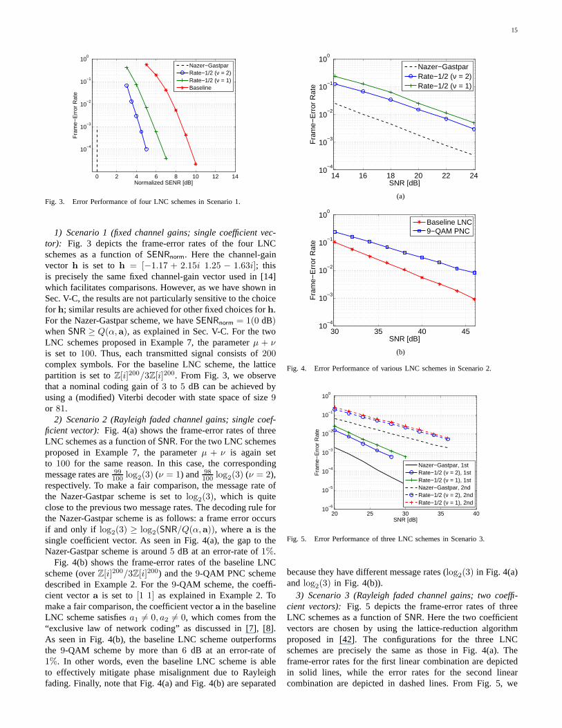
15

0 2 4 6 8 10 12 14

10−4

10−3

10−2

10−1

100

Normalized SENR [dB]

Fra

me−

Err

or R

ate

Nazer−GastparRate−1/2 (ν = 2)Rate−1/2 (ν = 1)Baseline

Fig. 3. Error Performance of four LNC schemes in Scenario 1.

1) Scenario 1 (fixed channel gains; single coefficient vec-tor): Fig. 3 depicts the frame-error rates of the four LNCschemes as a function ofSENRnorm. Here the channel-gainvector h is set toh = [−1.17 + 2.15i 1.25 − 1.63i]; thisis precisely the same fixed channel-gain vector used in [14]which facilitates comparisons. However, as we have shown inSec. V-C, the results are not particularly sensitive to the choicefor h; similar results are achieved for other fixed choices forh.For the Nazer-Gastpar scheme, we haveSENRnorm = 1(0 dB)whenSNR ≥ Q(α, a), as explained in Sec. V-C. For the twoLNC schemes proposed in Example 7, the parameterµ + νis set to100. Thus, each transmitted signal consists of200complex symbols. For the baseline LNC scheme, the latticepartition is set toZ[i]200/3Z[i]200. From Fig. 3, we observethat a nominal coding gain of3 to 5 dB can be achieved byusing a (modified) Viterbi decoder with state space of size9or 81.

2) Scenario 2 (Rayleigh faded channel gains; single coef-ficient vector): Fig. 4(a) shows the frame-error rates of threeLNC schemes as a function ofSNR. For the two LNC schemesproposed in Example 7, the parameterµ + ν is again setto 100 for the same reason. In this case, the correspondingmessage rates are99100 log2(3) (ν = 1) and 98

100 log2(3) (ν = 2),respectively. To make a fair comparison, the message rate ofthe Nazer-Gastpar scheme is set tolog2(3), which is quiteclose to the previous two message rates. The decoding rule forthe Nazer-Gastpar scheme is as follows: a frame error occursif and only if log2(3) ≥ log2(SNR/Q(α, a)), wherea is thesingle coefficient vector. As seen in Fig. 4(a), the gap to theNazer-Gastpar scheme is around5 dB at an error-rate of1%.

Fig. 4(b) shows the frame-error rates of the baseline LNCscheme (overZ[i]200/3Z[i]200) and the9-QAM PNC schemedescribed in Example 2. For the9-QAM scheme, the coeffi-cient vectora is set to[1 1] as explained in Example 2. Tomake a fair comparison, the coefficient vectora in the baselineLNC scheme satisfiesa1 6= 0, a2 6= 0, which comes from the“exclusive law of network coding” as discussed in [7], [8].As seen in Fig. 4(b), the baseline LNC scheme outperformsthe 9-QAM scheme by more than6 dB at an error-rate of1%. In other words, even the baseline LNC scheme is ableto effectively mitigate phase misalignment due to Rayleighfading. Finally, note that Fig. 4(a) and Fig. 4(b) are separated

14 16 18 20 22 2410

−4

10−3

10−2

10−1

100

SNR [dB]

Fra

me−

Err

or R

ate

Nazer−GastparRate−1/2 (ν = 2)Rate−1/2 (ν = 1)

(a)

30 35 40 4510

−4

10−3

10−2

10−1

100

SNR [dB]

Fra

me−

Err

or R

ate

Baseline LNC9−QAM PNC

(b)

Fig. 4. Error Performance of various LNC schemes in Scenario2.

20 25 30 35 4010

−6

10−5

10−4

10−3

10−2

10−1

100

SNR [dB]

Fra

me−

Err

or R

ate

Nazer−Gastpar, 1stRate−1/2 (ν = 2), 1stRate−1/2 (ν = 1), 1stNazer−Gastpar, 2ndRate−1/2 (ν = 2), 2ndRate−1/2 (ν = 1), 2nd

Fig. 5. Error Performance of three LNC schemes in Scenario 3.

because they have different message rates (log2(3) in Fig. 4(a)and log2(3) in Fig. 4(b)).

3) Scenario 3 (Rayleigh faded channel gains; two coeffi-cient vectors): Fig. 5 depicts the frame-error rates of threeLNC schemes as a function ofSNR. Here the two coefficientvectors are chosen by using the lattice-reduction algorithmproposed in [42]. The configurations for the three LNCschemes are precisely the same as those in Fig. 4(a). Theframe-error rates for the first linear combination are depictedin solid lines, while the error rates for the second linearcombination are depicted in dashed lines. From Fig. 5, we

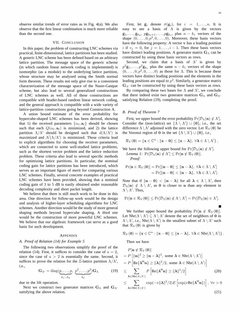
16

observe similar trends of error rates as in Fig. 4(a). We alsoobserve that the first linear combination is much more reliablethan the second one.

VII. C ONCLUSION

In this paper, the problem of constructing LNC schemes viapractical, finite-dimensional, lattice partitions has been studied.A generic LNC scheme has been defined based on an arbitrarylattice partition. The message space of the generic scheme(in which random linear network coding is implemented) isisomorphic (as a module) to the underlying lattice partition,whose structure may be analyzed using the Smith normalform theorem. These results not only give rise to a convenientcharacterization of the message space of the Nazer-Gastparscheme, but also lead to several generalized constructionsof LNC schemes as well. All of these constructions arecompatible with header-based random linear network coding,and the general approach is compatible with a wide variety oflattice-partition constructions going beyond Construction A.

A union bound estimate of the error probability forhypercube-shaped LNC schemes has been derived, showingthat 1) the received parameters{αℓ, aℓ} should be chosensuch that eachQ(αℓ, aℓ) is minimized, and 2) the latticepartition Λ/Λ′ should be designed such thatd(Λ/Λ′) ismaximized andN (Λ/Λ′) is minimized. These criteria leadto explicit algorithms for choosing the receiver parameters,which are connected to some well-studied lattice problems,such as the shortest vector problem and the lattice reductionproblem. These criteria also lead to several specific methodsfor optimizing lattice partitions. In particular, the nominalcoding gain for lattice partitions has been introduced, whichserves as an important figure of merit for comparing variousLNC schemes. Finally, several concrete examples of practicalLNC schemes have been provided, showing that a nominalcoding gain of3 to 5 dB is easily obtained under reasonabledecoding complexity and short packet length.

We believe that there is still much work to be done in thisarea. One direction for follow-up work would be the designand analysis of higher-layer scheduling algorithms for LNCschemes. Another direction would be the study of more generalshaping methods beyond hypercube shaping. A third onewould be the construction of more powerful LNC schemes.We believe that our algebraic framework can serve as a goodbasis for such development.

APPENDIX

A. Proof of Relation (14) for Example 5

The following two observations simplify the proof of therelation (14). First, it suffices to consider the case ofa = 2,since the case ofa > 2 is essentially the same. Second, itsuffices to prove the relation for theZ-lattice partitionΛ/Λ′,i.e.,

GΛ′ = diag(p, . . . , p︸ ︷︷ ︸

k1−k2

, p2, . . . , p2︸ ︷︷ ︸

k2

)GΛ (19)

due to the lift operation.Next we construct two generator matricesGΛ and GΛ′

satisfying the above relation.

First, let gi denote σ(gi), for i = 1, . . . , n. It iseasy to see a basis ofΛ is given by the vectorsg1, . . . , gk2

, pgk2+1, . . . , pgk1, plus n − k1 vectors of the

shape(0, . . . , 0, p2, 0, . . . , 0). Moreover, these basis vectorshave the following property: A vectorv has a leading positioni if vj = 0, for j = 1, . . . , i − 1. Then these basis vectorshave distinct leading positions. A generator matrixGΛ can beconstructed by using these basis vectors as rows.

Second, we claim that a basis ofΛ′ is given byp2g1, . . . , p

2gk1plus the samen − k1 vectors of the shape

(0, . . . , 0, p2, 0, . . . , 0) as those forΛ. This is because thesevectors have distinct leading positions and the elements intheleading positions are equal top2. Similarly, a generator matrixGΛ′ can be constructed by using these basis vectors as rows.

By comparing these two bases forΛ andΛ′, we concludethat there indeed exist two generator matricesGΛ andGΛ′

satisfying Relation (19), completing the proof.

B. Proof of Theorem 7

First, we upper bound the error probabilityPr[DΛ(n) /∈ Λ′].Consider the (non-lattice) set{Λ \ Λ′} ∪ {0}, i.e., the setdifferenceΛ\Λ′ adjoined with the zero vector. LetRV (0) bethe Voronoi region of0 in the set{Λ \ Λ′} ∪ {0}, i.e.,

RV (0) = {x ∈ Cn : ‖x− 0‖ ≤ ‖x− λ‖, ∀λ ∈ Λ \ Λ′} .

We have the following upper bound forPr[DΛ(n) /∈ Λ′].Lemma 1:Pr[DΛ(n) /∈ Λ′] ≤ Pr[n /∈ RV (0)].

Proof:

Pr[n ∈ RV (0)] = Pr[‖n− 0‖ ≤ ‖n− λ‖, ∀λ ∈ Λ \ Λ′]

= Pr[‖n− 0‖ < ‖n− λ‖, ∀λ ∈ Λ \ Λ′].

Note that if ‖n − 0‖ < ‖n − λ‖ for all λ ∈ Λ \ Λ′, thenDΛ(n) /∈ Λ \ Λ′, as 0 is closer ton than any element inΛ \ Λ′. Thus,

Pr[n ∈ RV (0)] ≤ Pr[DΛ(n) /∈ Λ \ Λ′] = Pr[DΛ(n) ∈ Λ′].

We further upper bound the probabilityPr[n /∈ RV (0)].Let Nbr(Λ \ Λ′) ⊆ Λ \ Λ′ denote the set of neighbors of0 inΛ \Λ′, i.e., Nbr(Λ \ Λ′) is the smallest subset ofΛ \Λ′ suchthatRV (0) is given by

RV (0) = {x ∈ Cn : ‖x− 0‖ ≤ ‖x− λ‖, ∀λ ∈ Nbr(Λ \ Λ′)} .

Then we have

P [n 6∈ RV (0)]

= P[‖n‖2 ≥ ‖n− λ‖2, someλ ∈ Nbr(Λ \ Λ′)

]

= P[

Re{λHn} ≥ ‖λ‖2/2, someλ ∈ Nbr(Λ \ Λ′)]

≤∑

λ∈Nbr(Λ\Λ′)

P[

Re{λHn} ≥ ‖λ‖2/2]

(20)

≤∑

λ∈Nbr(Λ\Λ′)

exp(−ν‖λ‖2/2)E[

exp(νRe{λHn})]

, ∀ν > 0

(21)

17

where (20) follows from the union bound and (21) followsfrom the Chernoff bound. From (8), we have

E[

exp(νRe{λHn}

)]

=E

[

exp(νRe{λH

(∑

ℓ

(αhℓ − aℓ)xℓ + αz

)

})

]

=E[

exp(νRe{λHαz})]

·∏

ℓ

E[

exp(νRe{λH(αhℓ − aℓ)xℓ})]

(22)

=exp(1

4ν2‖λ‖2|α|2N0)

·∏

ℓ

E[

exp(νRe{λH(αhℓ − aℓ)xℓ})]

(23)

where (22) follows from the independence ofx1, . . . ,xL, zand (23) follows from the moment-generating function of acircularly symmetric complex Gaussian random vector.

Lemma 2:Let x ∈ Cn be a complex random vectoruniformly distributed over a hypercubeγUHn for someγ > 0and somen× n unitary matrix. Then

E[exp(Re{vHx})

]≤ exp(‖v‖2γ2/24).

Proof: First, we consider a special case where the unitarymatrix U = In. In this case, we have

E[exp(Re{vHx})

]

=E[exp(Re{v}TRe{x}+ Im{v}T Im{x})

]

=E

[

exp(

n∑

i=1

(Re{vi}Re{xi}+ Im{vi}Im{xi}))

]

=

n∏

i=1

E [exp(Re{vi}Re{xi}]E [exp Im{vi}Im{xi})] (24)

=n∏

i=1

sinh(Re{vi}γ/2)

Re{vi}γ/2

sinh(Im{vi}γ/2)

Im{vi}γ/2(25)

≤n∏

i=1

exp

((Re{vi}γ)

2

24

)

exp

((Im{vi}γ)

2

24

)

(26)

=exp

(γ2

24‖v‖2

)

where (24) follows from the independence among eachreal/imaginary component, (25) follows from the moment-generating function of a uniform random variable (note thatboth Re{xi} and Im{xi} are uniformly distributed over[−γ/2, γ/2]), and (26) follows fromsinh(x)/x ≤ exp(x2/6)(which can be obtained by simple Taylor expansion).

Then we consider a general unitary matrixU. In thiscase, we havex = Ux′, where x′ ∈ γ[−1/2, 1/2]2n,i.e., both Re{x′

i} and Im{x′i} are uniformly distributed over

[−γ/2, γ/2]. Hence,

E[exp(Re{vHx})

]= E

[exp(Re{vHUx′})

]

= E[exp(Re{(UHv)Hx′})

]

≤ exp

(γ2

24‖UHv‖2

)

= exp

(γ2

24‖v‖2

)

Note thatP = 1nE[‖xℓ‖2] = γ2/6. Thus, we have

E[

exp(νRe{λHn})]

≤ exp(1

4ν2‖λ‖2|α|2N0)

∏

ℓ

exp(‖νλ(αhℓ − aℓ)‖2P/4)

= exp(1

4ν2‖λ‖2|α|2N0 + ‖νλ‖2‖αh− a‖2P/4)

= exp(1

4‖λ‖2ν2N0Q(α, a)),

where the quantityQ(α, a) is given by

Q(α, a) = |α|2 + SNR‖αh− a‖2

andSNR = P/N0.It follows that, for all ν > 0,

Pr[n 6∈RV (0)]

≤∑

λ∈Nbr(Λ\Λ′)

exp

(

−ν‖λ‖2/2 +1

4‖λ‖2ν2N0Q(α, a)

)

.

Choosingν = 1/(N0Q(α, a)), we have

Pr[n 6∈ RV (0)] ≤∑

λ∈Nbr(Λ\Λ′)

exp(−‖λ‖2

4N0Q(α, a)).

For high signal-to-noise ratios, we have∑

λ∈Nbr(Λ\Λ′)

exp(−‖λ‖2

4N0Q(α, a)) ≈ K(Λ/Λ′) exp

(

−d2(Λ/Λ′)

4N0Q(α, a)

)

.

Therefore, we have

Pr[DΛ(n) /∈ Λ′] ≤ Pr[n /∈ RV (0)]

≈ K(Λ/Λ′) exp

(

−d2(Λ/Λ′)

4N0Q(α, a)

)

,

completing the proof of Theorem 7.

C. Proof of Theorem 8

First, we show the existence of the solution{a1, . . . , am}by induction onm.

If m = 1, then the vectora1 can be chosen such thata1L isone of the shortest lattice points. Note thata1 is not divisibleby π; otherwise it will not be one of the shortest lattice points.In other words,a1 is indeed nonzero. Hence, the solutiona1always exists whenm = 1.

Now suppose the solution{a1, . . . , ak} exists whenk < m.We will show the existence of the vectorak+1.

Consider the following set

B = {b ∈ RL : b, a1, . . . , ak are linearly independent}.

18

Clearly, the setB is nonempty, sincek < m. Choose anelementb from the setB and construct a new setS as

S = {a ∈ RL : ‖aL‖ ≤ ‖bL‖,

a, a1, . . . , ak are linearly independent}.

Clearly,S is a nonempty set of finite elements. Then the vectorak+1 can be chosen as

ak+1 = argmina∈S

‖aL‖.

This proves the existence of the vectorak+1, which completesthe induction.

Second, we show that the solution{a1, . . . , am} is a dom-inated solution by induction onm.

If m = 1, then‖a1L‖ ≤ ‖b1L‖ for any feasible solutionb1, sincea1L is one of the shortest lattice points.

Now suppose that{a1, . . . , ak} is a dominated solutionwhenk < m. We will show that{a1, . . . , ak, ak+1} is also adominated solution.

Consider a feasible solution{b1, . . . ,bk,bk+1} with‖b1L‖ ≤ . . . ≤ ‖bk+1L‖. Since b1, . . . , bk are linearlyindependent, we have

‖aiL‖ ≤ ‖biL‖, i = 1, . . . , k.

It remains to show‖ak+1L‖ ≤ ‖bk+1L‖. We consider thefollowing two cases.

1) If there exists somebi (i = 1, . . . , k + 1) such thatbi, a1, . . . , ak are linearly independent, then by theconstruction ofak+1, we have

‖ak+1L‖ ≤ ‖biL‖ ≤ ‖bk+1L‖.

2) Otherwise, eachbi can be expressed as a linear combi-nation of a1, . . . , ak. That is,

bi ∈ Span{a1, . . . , ak}, ∀i = 1, . . . , k + 1.

This is contrary to the fact thatb1, . . . , bk+1 are linearlyindependent, since anyk + 1 vectors in a vector spaceof dimensionk are linearly dependent.

Therefore, we have‖ak+1L‖ ≤ ‖bk+1L‖, which completesthe induction.

D. Proof of Proposition 4

Note that the nominal coding gainγc(ΛC/Λ′C) is invariant

to scaling. Hence, we may assume, without loss of generality,that the lattice partitionΛC/Λ

′C is used instead of its scaled

version.First, we will show that

d2(ΛC/Λ′C) = wmin

E (C). (27)

Recall thatd(ΛC/Λ′C) is the length of the shortest vectors in

the set differenceΛC \ Λ′C . Hence, we have

d(ΛC/Λ′C) = min

c6=0

‖〈c〉‖.

It follows that d2(ΛC/Λ′C) = minc6=0 ‖〈c〉‖2 = wmin

E (C).Second, we will show that

V (Λ) = |π|2(n−k). (28)

Note thatV (Λ′) = |π|2n and V (Λ′)/V (Λ) = |π|2k. Hence,we haveV (Λ) = |π|2(n−k).

Combining (27) and (28), we haveγc(ΛC/Λ′C) =

wminE (C)/|π|2(1−k/n), which completes the proof.

E. Modified Viterbi Decoder for Example 7

We will show that the NLP decoderDΛCcan be imple-

mented through a modified Viterbi decoder.First, note that the NLP decoderDΛC

solves the followingoptimization problem

minimize ‖λ− αy‖ (29)

subject to λ ∈ ΛC

Second, note that the problem (29) is equivalent to

minimize ‖〈c〉+ λ′ − αy‖ (30)

subject to c ∈ C

λ′ ∈ Λ′

C

This is because each lattice pointλ ∈ ΛC can be decomposedasλ = 〈c〉 + λ

′, wherec = σ(λ) andλ′ ∈ Λ′C .

Third, note that Problem (30) is equivalent to

minimize ‖[〈c〉 − αy] modΛ′C‖ (31)

subject to c ∈ C

where[x] modΛ′C is defined as[x] modΛ′

C , x− DΛ′

C(x).

This is becauseλ′ = −DΛ′

C(〈c〉 − αy) solves Problem (30)

for any c ∈ C.Now it is easy to see the problem (31) can be solved

through a modified Viterbi decoder with the metric given by‖[·] modΛ′

C‖ instead of‖·‖. Therefore, the NLP decoderDΛC

can be implemented through a modified Viterbi decoder.

REFERENCES

[1] R. Ahlswede, N. Cai, S.-Y. R. Li, and R. W. Yeung, “Networkinforma-tion flow,” IEEE Trans. Inf. Theory, vol. 46, no. 4, pp. 1204–1216, Jul.2000.

[2] S.-Y. R. Li, R. W. Yeung, and N. Cai, “Linear network coding,” IEEETrans. Inf. Theory, vol. 49, no. 2, pp. 371–381, Feb. 2003.

[3] R. Koetter and M. Medard, “An algebraic approach to network coding,”IEEE/ACM Trans. Netw., vol. 11, no. 5, pp. 782–795, Oct. 2003.

[4] S. Zhang, S.-C. Liew, and P. P. Lam, “Hot topic: Physical layer networkcoding,” in Proc. of ACM Int. Conf. on Mobile Compu. and Netw., LosAngeles, CA, USA, Sep. 24–29, 2006, pp. 358–365.

[5] P. Popovski and H. Yomo, “The anti-packets can increase the achievablethroughput of a wireless multi-hop network,” inProc. of IEEE Int. Conf.on Commun., Istanbul, Turkey, Jun. 11–15, 2006, pp. 3885–3890.

[6] B. Nazer and M. Gastpar, “Computing over multiple-access channelswith connections to wireless network coding,” inProc. of IEEE Int.Symp. on Inf. Theory, Seattle, USA, Jul. 9–14, 2006, pp. 1354–1358.

[7] P. Popovski and H. Yomo, “Physical network coding in two-way wirelessrelay channels,” inProc. of IEEE Int. Conf. on Commun., Glasgow,Scotland, Jun. 24–28, 2007, pp. 707–712.

[8] T. Koike-Akino, P. Popovski, and V. Tarokh, “Optimized constellationsfor two-way wireless relaying with physical network coding,” IEEE J.Sel. Areas Commun., vol. 27, no. 5, pp. 773–787, Jun. 2009.

[9] M. P. Wilson, K. Narayanan, H. D. Pfister, and A. Sprintson, “Jointphysical layer coding and network coding for bidirectionalrelaying,”IEEE Trans. Inf. Theory, vol. 56, no. 11, pp. 5641–5654, Nov. 2010.

[10] W. Nam, S.-Y. Chung, and Y. H. Lee, “Capacity bounds for two-wayrelay channels,” inProc. of Int. Zurich Seminar on commun., Zurich,Switzerland, Mar. 12–14, 2008.

19

[11] A. S. Avestimehr, A. Sezgin, and D. N. C. Tse, “Capacity of the two-wayrelay channel within a constant gap,”Eur. Trans. Telecomms., vol. 21,no. 4, pp. 363–374, Jun. 2010.

[12] S. Katti, S. Gollakota, and D. Katabi, “Embracing wireless interference:Analog network coding,” inProc. of ACM Special Interest Group onData Commun., Kyoto, Japan, Aug. 27–31, 2007.

[13] P. Popovski and T. Koike-Akino, “Coded bidirectional relaying inwireless networks,” inNew Directions in Wireless CommunicationsResearch, V. Tarokh, Ed. Springer, 2009, pp. 291–316.

[14] B. Nazer and M. Gastpar, “Compute-and-forward: Harnessing interfer-ence through structured codes,”submitted to IEEE Trans. Inf. Theory,Aug. 2009.

[15] U. Erez and R. Zamir, “Achieving12log(1+SNR) on the awgn channel

with lattice encoding and decoding,”IEEE Trans. Inf. Theory, vol. 50,no. 10, pp. 2293–2314, Oct. 2004.

[16] M. P. Wilson and K. R. Narayanan, “Power allocation strategies andlattice based coding schemes for bi-directional relaying,” in Proc. ofIEEE Int. Symp. on Inf. Theory, Coex, Seoul, Korea, Jun. 28 – Jul. 3,2009, pp. 344–348.

[17] U. Niesen and P. Whiting, “The degrees of freedom of compute-and-forward,” submitted to IEEE Trans. Inf. Theory, Jan. 2011.

[18] J. Zhan, B. Nazer, M. Gastpar, and U. Erez, “MIMO compute-and-forward,” in Proc. of IEEE Int. Symp. on Inf. Theory, Seoul, SouthKorea, Jun. 28– Jul. 3, 2009, pp. 2848–2852.

[19] J.-C. Belfiore and M. A. V. Castro, “Managing interference throughspace-time codes, lattice reduction and network coding,” in IEEE Inf.Workshop, Cairo, Egypt, Jan. 6–8, 2010, pp. 1–5.

[20] B. Nazer and M. Gastpar, “Reliable physical layer network coding,”Proc. IEEE, vol. 99, no. 3, pp. 438–460, Mar. 2011.

[21] A. S. Avestimehr, S. N. Diggavi, and D. N. C. Tse, “Wireless networkinformation flow: A deterministic approach,”IEEE Trans. Inf. Theory,vol. 57, no. 4, pp. 1872–1905, Apr. 2011.

[22] S. H. Lim, Y.-H. Kim, A. E. Gamal, and S.-Y. Chung, “Noisynetworkcoding,” 2010, http://arxiv.org/abs/1002.3188.

[23] A. Ozgur and S. N. Diggavi, “Approximately achieving Gaussian relaynetwork capacity with lattice codes,” inProc. of IEEE Int. Symp. on Inf.Theory, Austin, Texas, USA, Jun. 13–18, 2010, pp. 669–673.

[24] R. Kotter and F. R. Kschischang, “Coding for errors anderasures inrandom network coding,”IEEE Trans. Inf. Theory, vol. 54, no. 8, pp.3579–3591, Aug. 2008.

[25] O. Shalvi, N. Sommer, and M. Feder, “Signal codes: Convolutionallattice codes,”IEEE Trans. Inf. Theory, to appear, 2011.

[26] C. Feng, D. Silva, and F. R. Kschischang, “Lattice network codingvia signal codes,” inProc. of IEEE Int. Symp. on Inf. Theory, SaintPetersburg, Russia, Jul. 31– Aug. 5, 2011.

[27] B. R. McDonald,Linear Algebra over Commutative Rings. New York:Marcel Dekker, 1984.

[28] D. S. Dummit and R. M. Foote,Abstract Algebra, 3rd ed. John Wiley& Sons, Inc., 2004.

[29] W. C. Brown, Matrices over Commutative Rings. New York: MarcelDekker, 1986.

[30] J. Zhan, B. Nazer, U. Erez, and M. Gastpar, “Integer-forcing linearreceivers,” inProc. of IEEE Int. Symp. on Inf. Theory, Austin, Texas,USA, Jun. 13–18, 2010, pp. 1022–1026.

[31] J. Zhan, B. Nazer, O. Ordentlich, U. Erez, and M. Gastpar, “Integer-forcing architectures for MIMO: Distributed implementation and SIC,”in Proc. of the 44th Ann. Asilomar Conf. on Signals, Syst., and Compu.,Monterey, CA, USA, Oct. 2010, pp. 322–326.

[32] J. H. Conway and N. Sloane, “A fast encoding method for lattice codesand quantizers,”IEEE Trans. Inf. Theory, vol. 29, no. 6, pp. 820–824,Nov. 1983.

[33] G. D. Forney, Jr., “Multidimensional constellations—part II: Voronoiconstellations,”IEEE J. Sel. Areas Commun., vol. 7, no. 6, pp. 941–958, Aug. 1989.

[34] R. Zamir and M. Feder, “On lattice quantization noise,”IEEE Trans.Inf. Theory, vol. 42, no. 4, pp. 1152–1159, Jul. 1996.

[35] J. H. Conway and N. J. A. Sloane,Sphere Packings, Lattices and Groups,3rd ed. New York: Springer-Verlag, 1999.

[36] U. Erez, S. Litsyn, and R. Zamir, “Lattices which are good for (almost)everything,” IEEE Trans. Inf. Theory, vol. 51, no. 10, pp. 3401–3416,Oct. 2005.

[37] M.-R. Sadeghi, A. H. Banihashemi, and D. Panario, “Low-density parity-check lattices: Construction and decoding analysis,”IEEE Trans. Inf.Theory, vol. 52, no. 10, pp. 4481–4495, Oct. 2006.

[38] N. Sommer, M. Feder, and O. Shalvi, “Low density latticecodes,”IEEETrans. Inf. Theory, vol. 54, no. 4, pp. 1561–1585, Apr. 2008.

[39] ——, “Shaping methods for low-density lattice codes,” in IEEE Inf.Workshop, Taormina, Sicily, Italy, Oct. 11-16, 2009, pp. 238–242.

[40] J. W. S. Cassels,An Introduction to the Geometry of Numbers. Springer-Verlag, 1971.

[41] Y. H. Gan, C. Ling, and W. H. Mow, “Complex lattice reductionalgorithm for low-complexity full-diversity MIMO detection,” IEEETrans. Signal Process., vol. 57, no. 7, pp. 2701 – 2710, Jul. 2009.

[42] H. Yao and G. W. Wornell, “Lattice-reduction-aided detectors for MIMOcommunication systems,” inProc. of IEEE Global Commun. Conf.,Taipei, Taiwan, R.O.C., Nov. 17–21, 2002, pp. 424–428.

[43] O. Ordentlich and U. Erez, “Achieving the gains promised by integer-forcing equalization with binary codes,” inProc. of 26th Convention ofElectr. and Electron. Eng. in Israel, Eilat, Israel, Nov. 2010, pp. 703–707.