HAL Id: tel-01238850https://tel.archives-ouvertes.fr/tel-01238850

Submitted on 7 Dec 2015

HAL is a multi-disciplinary open accessarchive for the deposit and dissemination of sci-entific research documents, whether they are pub-lished or not. The documents may come fromteaching and research institutions in France orabroad, or from public or private research centers.

L’archive ouverte pluridisciplinaire HAL, estdestinée au dépôt et à la diffusion de documentsscientifiques de niveau recherche, publiés ou non,émanant des établissements d’enseignement et derecherche français ou étrangers, des laboratoirespublics ou privés.

Adsorption on interstellar analog surfaces : from atomsto organic molecules

Mikhail Doronin

To cite this version:Mikhail Doronin. Adsorption on interstellar analog surfaces : from atoms to organic molecules. Chem-ical Physics [physics.chem-ph]. Université Pierre et Marie Curie - Paris VI, 2015. English. NNT :2015PA066254. tel-01238850

THÈSE DE DOCTORATDE L’UNIVERSITÉ PIERRE ET MARIE CURIE

Spécialité : PhysiqueÉcole doctorale : “Physique en Île-de-France”

réalisée

au Laboratoire d’Études du Rayonnement et de la Matière enAstrophysique et Atmosphères

et Laboratoire de Chimie Théorique

présentée par

Mikhail V. DORONIN

pour obtenir le grade de :

DOCTEUR DE L’UNIVERSITÉ PIERRE ET MARIE CURIE

Sujet de la thèse :

Adsorption on Interstellar Analog Surfaces: from Atoms toOrganic Molecules

soutenue le 28 Septembre 2015

devant le jury composé de :

M. Josep-Manel Ricart Pla RapporteurM. Patrice Theulé RapporteurM. Christophe Petit ExaminateurM. Lionel Amiaud ExaminateurMme Valentine Wakelam ExaminateurM. Jean-Hugues Fillion Directeur de thèseM. Alexis Markovits Directeur de thèse

Contents

1 Introduction 11.1 Astrophysical Context . . . . . . . . . . . . . . . . . . . . . . . . . . . . 11.2 Physisorption versus Chemisorption . . . . . . . . . . . . . . . . . . . . 2

1.2.1 Physisorption . . . . . . . . . . . . . . . . . . . . . . . . . . . . . 31.2.2 Chemisorption . . . . . . . . . . . . . . . . . . . . . . . . . . . . 4

1.3 Strategies for a reliable database . . . . . . . . . . . . . . . . . . . . . . 51.4 Case Studies . . . . . . . . . . . . . . . . . . . . . . . . . . . . . . . . . 6

I Employed Methods 13

2 Experimental approach 152.1 Experimental setup . . . . . . . . . . . . . . . . . . . . . . . . . . . . . . 15

2.1.1 General description and characteristics . . . . . . . . . . . . . . . 152.1.2 Cryogenics and temperature control . . . . . . . . . . . . . . . . 172.1.3 Gas phase species detection - quadrupole mass spectrometer

(QMS) . . . . . . . . . . . . . . . . . . . . . . . . . . . . . . . . . 212.1.4 Ultra-High Vacuum . . . . . . . . . . . . . . . . . . . . . . . . . 252.1.5 Sample species vapour preparation module . . . . . . . . . . . . 262.1.6 Adsorbate film thickness . . . . . . . . . . . . . . . . . . . . . . . 272.1.7 Other experimental issues . . . . . . . . . . . . . . . . . . . . . . 30

2.2 Temperature Programmed Desorption . . . . . . . . . . . . . . . . . . . 322.2.1 Desorption kinetics order . . . . . . . . . . . . . . . . . . . . . . 332.2.2 Surface coverage calibration . . . . . . . . . . . . . . . . . . . . . 342.2.3 Desorption data modeling and analysis . . . . . . . . . . . . . . . 35

2.3 Desorption data analysis: case study of CH3OH . . . . . . . . . . . . . 372.3.1 Coverage calibration . . . . . . . . . . . . . . . . . . . . . . . . . 372.3.2 Adsorption energy in multilayer regime . . . . . . . . . . . . . . 382.3.3 Adsorption energy in sub-monolayer regime . . . . . . . . . . . . 392.3.4 Summary . . . . . . . . . . . . . . . . . . . . . . . . . . . . . . . 45

3 Theoretical approach 493.1 First principles approach . . . . . . . . . . . . . . . . . . . . . . . . . . . 49

3.1.1 General introduction on DFT . . . . . . . . . . . . . . . . . . . . 493.1.2 Exchange-correlation functionals . . . . . . . . . . . . . . . . . . 51

i

ii CONTENTS

3.1.3 Van der Waals interactions . . . . . . . . . . . . . . . . . . . . . 513.2 Cluster versus periodic approaches . . . . . . . . . . . . . . . . . . . . . 523.3 Determining adsorption energetics . . . . . . . . . . . . . . . . . . . . . 52

3.3.1 Periodic system . . . . . . . . . . . . . . . . . . . . . . . . . . . . 533.3.2 Bulk geometry optimization . . . . . . . . . . . . . . . . . . . . . 533.3.3 Surface modelling . . . . . . . . . . . . . . . . . . . . . . . . . . 533.3.4 Adsorption sites . . . . . . . . . . . . . . . . . . . . . . . . . . . 553.3.5 Example:CH3OH adsorption on graphite . . . . . . . . . . . . . 55

3.4 Topological analysis . . . . . . . . . . . . . . . . . . . . . . . . . . . . . 633.4.1 Electronic Localization Function (ELF) . . . . . . . . . . . . . . 633.4.2 Integrated properties . . . . . . . . . . . . . . . . . . . . . . . . . 643.4.3 Example of ELF topology: methanol . . . . . . . . . . . . . . . . 64

II Systems studied 69

4 Adsorption and Trapping of Noble Gases by Water Ices 714.1 Study context . . . . . . . . . . . . . . . . . . . . . . . . . . . . . . . . . 71

4.1.1 Planetology issue . . . . . . . . . . . . . . . . . . . . . . . . . . . 714.1.2 Update review . . . . . . . . . . . . . . . . . . . . . . . . . . . . 724.1.3 Trapping by ices . . . . . . . . . . . . . . . . . . . . . . . . . . . 72

4.2 Experimental approach . . . . . . . . . . . . . . . . . . . . . . . . . . . . 744.2.1 Laboratory ice samples . . . . . . . . . . . . . . . . . . . . . . . 744.2.2 Adsorption on water ices . . . . . . . . . . . . . . . . . . . . . . . 764.2.3 Inclusion in water ices . . . . . . . . . . . . . . . . . . . . . . . . 83

4.3 Theoretical approach . . . . . . . . . . . . . . . . . . . . . . . . . . . . . 854.3.1 Modeling the ice surface . . . . . . . . . . . . . . . . . . . . . . . 854.3.2 Adsorption sites . . . . . . . . . . . . . . . . . . . . . . . . . . . 874.3.3 Convergence against cell dimensions . . . . . . . . . . . . . . . . 894.3.4 Adsorption . . . . . . . . . . . . . . . . . . . . . . . . . . . . . . 914.3.5 Substitution . . . . . . . . . . . . . . . . . . . . . . . . . . . . . . 924.3.6 Inclusion . . . . . . . . . . . . . . . . . . . . . . . . . . . . . . . 94

4.4 Comparisons and conclusions . . . . . . . . . . . . . . . . . . . . . . . . 94

5 Adsorption of CH3CN vs CH3NC at interstellar grain surfaces 995.1 Study context . . . . . . . . . . . . . . . . . . . . . . . . . . . . . . . . . 995.2 Experimental approach . . . . . . . . . . . . . . . . . . . . . . . . . . . . 100

5.2.1 Pure thick ices of CH3CN and CH3NC . . . . . . . . . . . . . . . 1005.2.2 Submonolayer of CH3CN and CH3NC on model surfaces . . . . . 104

5.3 Theoretical approach to adsorption energies . . . . . . . . . . . . . . . . 1105.3.1 Adsorption energies on highly oriented pyrolytic graphite . . . . 1105.3.2 Adsorption energies on silica . . . . . . . . . . . . . . . . . . . . 1125.3.3 Adsorption energies on crystalline water ice . . . . . . . . . . . . 113

5.4 Discussion and final remarks . . . . . . . . . . . . . . . . . . . . . . . . 114

CONTENTS iii

6 Ionization and trapping of sodium in cometary ices 1216.1 Study context . . . . . . . . . . . . . . . . . . . . . . . . . . . . . . . . . 1216.2 Paper . . . . . . . . . . . . . . . . . . . . . . . . . . . . . . . . . . . . . 1226.3 Conclusion . . . . . . . . . . . . . . . . . . . . . . . . . . . . . . . . . . 128

7 Conclusion and Perspectives 131

Appendices 137Appendix A

PID zones table . . . . . . . . . . . . . . . . . . . . . . . . . . . . . . . . 139Appendix B

TPD model function . . . . . . . . . . . . . . . . . . . . . . . . . . . . . 140Appendix C

VASP parameters . . . . . . . . . . . . . . . . . . . . . . . . . . . . . . . 142

iv CONTENTS

Chapter 1

Introduction

1.1 Astrophysical Context

To date, almost 200 different molecular species have been detected in various regionsof the interstellar space [1] and in various objects of the solar system. These moleculesrange from elementary species (H2, CO, N2, CO2, H2CO) to larger organic species ofup to 13 atoms including carbon chains, organic and even organometallic compoundsthat could eventually provide initial molecular stones for the formation of “pre-biotic”molecules. With the advent of new ground-based and space telescopes of high sensi-tivity in the visible, infrared and submillimiter wavelengths, the richness and diversityof molecular compounds discovered in various regions of the interstellar medium isincreasing dramatically. Especially, the observations with the ALMA and, in the nearfuture, the NOEMA radio-telescopes are beginning to revolutionize the field by provid-ing ultra-high spatial resolution, in particular within star-forming regions, promisinga tremendous forthcoming insight into this fascinating but still largely unknown inter-stellar chemical world. The rich organic inventory of space reflects the multitude ofchemical processes involved, that on the one hand, build up complex organic molecules(COMs) from simpler entities, and on the other hand, break down large molecules, in-jected by stars, into smaller fragments [2].

Over the last 30 years, significant progress in the understanding of formation,evolution and destruction of molecules in molecular clouds has revealed the crucialrole of dust grains which act as catalytic sites for molecule formation and explain thepresence of species that pure gas phase chemical networks failed to predict [3]. Gas-surface interactions are now considered as playing a major role in the monitoring ofmolecular diversity in space. In the interstellar medium and in planetary bodies aswell, the condensation and desorption of molecules from the surfaces play an essentialrole in the physics and chemistry of these objects, driving the different stages of theirevolution [2].

Interstellar dust grains are submicron-sized particles made of silicates and/or car-bonaceous cores. In cold regions, such as dense molecular clouds, pre-stellar coresand inner part of proto-planetary disks, grains are covered by an icy mantle, mainlycomposed of water, but also containing many other compounds. The main ice com-ponents (CO2, CO, CH3OH, CH4) are detected in the solid phase by infrared spec-

1

2 CHAPTER 1. INTRODUCTION

troscopy [4, 5]. These ices can be continuously processed by the impact of cosmic rays,UV-X photochemistry and thermal diffusion, providing a rich molecular reservoir anda source of larger species which, after being released into the gas phase, are more fa-vorably detected by sub-millimeter rotational transitions of molecules. It should benoted here that this observation technique is blind to the molecules that remain onthe grain.

From a chemical point of view, interstellar grains provide a surface on which atomsand molecules can accrete, meet and react. They also play the role of a third bodyin the reactions which efficiently dissipates the excess energy energy released in thereactions. It is the case for the formation of molecular hydrogen, the most abundantmolecule in space, which can only be thermalized by interaction with the surface ofdust grains. As initially suggested by Tielens and Hagen [6], it is now establishedthan many other species (such as H2O, CO2 or CH3OH) have efficient grain-surfacechemical formation routes.

The mobility and the surface residence time of an adsorbate bound to a surfaceare related to a fundamental parameter: the binding energy or “adsorption energy”.In case of exothermic reactions, the newly formed molecules on the surface can beeventually ejected promptly into the gas phase after formation. The efficiency ofthis process is partly determined by the ratio between the energy released by thereaction and the adsorption energy of the molecule just formed. Other non-thermalprocesses as the sputtering by fast particles in shocks or the desorption induced bycosmic rays and/or by UV-X rays (the so called “photo-desorption” phenomenon), arealso critically dependent of the adsorption energy. In other environments such as inhot cores or cometary nuclei, ices are heated and the molecular reservoir is releasedinto the gas-phase by thermal desorption. Again, the adsorption energy is a centralparameter to describe the phenomenon.

In summary, the adsorption energies appear to be highly crucial, because theirvalues govern the temperature at which the molecules are condensed on the solid statesurface or released into the gas phase, and also (for the smaller species) because theydrive the surface mobility and impact the subsequent chemistry. Adsorption energiesstrongly influence the gas-phase and grain-surface reactions simultaneously. Dependingon the physical conditions of the various sources (temperature and densities), thedesorption energies are key parameters that can explain (or predict) both the gasphase and condensed phase compositions. In such a context, complex astrochemicalnetworks including the coupling between gas-phase and grain-surface synthesis areunder fast development [7–10]. As a consequence, the need for quantitative physical-chemical data becomes more and more important. Today, everyone has to be awarethat the transition from elementary molecules towards more complex organic systemscould only be solved by developing accurate chemical models supported by relevantlaboratory data.

1.2 Physisorption versus ChemisorptionAdsorption energy is governed by the interaction potential between the atoms/moleculesadsorbates and the solid surface to which they are bound [11–13]. In the present con-text, the solid, or substrate, is either the bare grain surface, valid for “warm“ (> 100 K)

1.2. PHYSISORPTION VERSUS CHEMISORPTION 3

environments, or the water-rich icy mantles, valid for colder regions (10-100 K).

1.2.1 Physisorption

The weakest form of adsorption to a solid surface is called physical adsorption, orphysisorption. It is characterized by the lack of a strong chemical bond (covalent orionic) between adsorbate and substrate. The adsorbed molecule is bound to the surfacevia weak Van der Waals interactions. The attractive forces are due to a combinationof dispersion and dipolar forces. Dispersion forces originate from instantaneous fluc-tuations in electron density, which cause transient dipoles in the molecules. Theseinstantaneous dipole moments interact with the polarizable nearest neighbors on thesurface, presenting or not a permanent dipole moment [12]. Forces due to moleculesthat have permanent dipole moments are usually stronger. In some systems, an hy-drogen atom, bound to an electronegative atom, (NH or OH bonds), is close enoughto interact with the lone pairs of another electronegative atom (N/O), leading to theformation of what is called an ”hydrogen bond“. This type of bond is stronger thanpure Van der Waals interaction, although weaker than covalent or ionic bonds (see”chemisorption“ 1.2.2 below). Generally, adsorption on very low temperature surfaces,such as the ones encountered in the interstellar medium, is largely due to physisorption.

Figure 1.1 – Potential energy of an atom or molecule physisorbed on a planar surface.

As illustrated on Figure 1.1, an incoming atom/molecule, with kinetic energy Ek,that losses enough energy when impinging the surface and exciting phonons in thesubstrate, can equilibrate in a state in the potential well with the binding or adsorptionenergy Ea. The atom/molecule is said to be accommodated to the surface. Conversely,in order to leave the surface, the atom/molecule must acquire enough energy to escape

4 CHAPTER 1. INTRODUCTION

from the depth of the potential well, i.e. Ea. The desorption energy is thus equalto the adsorption energy. In the case of pure Van der Walls-type of interactions, theadsorption energies for physisorbed molecules are typically ranging between 0.01-0.4eV. In the case of hydrogen-bonds, the adsorption energies are higher and usuallyfound in the 0.4-0.5 eV range. This will generally correspond to adsorption of organicmolecular species playing an important role in astrochemistry.

1.2.2 Chemisorption

In some cases, electron sharing occurs between the adsorbed species and the surface. Arather strong bond is thus created with the surface and the atom/molecule is said to bechemisorbed. The bond formed may be ionic or covalent, or a mixture of both. A simpleexample of the potential energy diagram for chemisorption is shown in Fig. 1.2. Someof the impinging molecules are accommodated by the surface and become weakly boundin a physisorbed state. Then electronic or vibrational processes can occur, which allowsthe physisorbed molecules to surmount the barrier Ec and be equilibrated in a muchdeeper well. Chemisorption resulting in the formation of a chemical bond betweenthe adsorbing molecule and the surface is at least one order of magnitude stronger(extending from 0.5 to several eV in extreme cases) than physisorption. This processgenerally results in a profound modification of the local structure like an insertion inthe bonds of the surface. It is termed non-dissociative chemisorption. Adsorption can,alternatively, result into the dissociation of the molecule [13], and is then referred toas dissociative chemisorption.

Figure 1.2 – Chemisorption on a planar surface. Adapted from ref [11]

In this work we are concerned only with van der Waals and hydrogen bonding.However, even in this case, we will see that the study of the desorption of atoms andmolecules from a grain surface is not as ”simple“ as it may appear.

1.3. STRATEGIES FOR A RELIABLE DATABASE 5

1.3 Strategies for a reliable database

The lack of basic laboratory data concerning the interaction of many of these moleculeson astrophysical relevant surfaces strongly limits the possibilities of the modeling. Theadsorption (desorption) energies on surfaces are eventually known for some of thesmaller species but mainly assumed (or derived from non-relevant astrophysical stud-ies) for the larger ones. Fundamental laboratory data (experimental and/or theoret-ical) are thus urgently needed to help improving our current understanding of thiscomplex coupled gas-surface chemistry.

This thesis is the first step of a larger project whose main objective is to constructa coherent database that will provide fundamental parameters that can be confidentlyused to quantify a number of gas-surface interaction processes such as desorption, diffu-sion or trapping of molecules on a dust grain or more generally any kind of interstellarsolid. The program is then supposed to be developed around oxygen bearing molecules,nitrogen bearing molecules, large hydrocarbons (PAHs) and finally molecules directlylinked to pre-biotic compounds. Aiming at the highest reliability possible, a partic-ular effort had to be been done on the experimental side to optimize a methodologyfor performing and analyzing experiments based on thermal desorption. Altogetherand whenever feasible, the theoretical results produced were confronted with the lab-oratory experiments in conditions as close as possible to the interstellar environment,using well-defined surfaces as prototypes.

Dust grains are thought to be composed of silicates or oxides, surrounded by car-bonaceous materials and/or an icy mantle in some circumstances [5]. The precisecomposition and morphology of interstellar grains, as well as the identification of theconstituents of their icy mantles is of course not fully determined and subject to de-bate. This study deals with different surfaces of various nature and morphology, whichcould be considered as reasonable interstellar surface analogs: water ice (compactand crystalline) to simulate conditions in cold regions, a graphite surface and a sil-ica monocrystal (chiral quartz) to simulate conditions of warmer carbon/silicate richregions. The presence and influence of some kind of defects on the surface has alsobeen considered to mimic corrugated carbonaceous solids. Such investigations allowexploring the specificities of these potentially interstellar surfaces, by comparing thebehavior of closely related molecules on different surfaces.

The main experimental technique used to study the adsorption/desorption pro-cesses were thermal desorption techniques in the 10-200 K temperature range. Thesetechniques were coupled to Infrared spectroscopy in absorption-reflection mode, wellsuited to probe surface composition. Such diagnostics have been optimized on the re-cently developed new surface science set-up “Surface Processes and Ices” (SPICES) atLPMAA/LERMA [14, 15]. In particular the recent incorporation of a rotating surfacesample holder in the ultra-high vacuum experimental main chamber is well-suited toinvestigate and compare multiple surfaces under strictly identical conditions. A com-plete description of the experimental set-up is given in part 2.1 and the principle ofthe data treatment is explained in parts 2.2 and 2.3 on the example of methanol.

When confronting with laboratory experiments, studying the adsorption/desorptionprocesses can be more complex than expected. Practically, two specific situations arise.At first, one can distinguish the so-called “CO-like” species, related to species with ad-

6 CHAPTER 1. INTRODUCTION

sorption energies below 0.1 eV. In this case, a single desorption peak appearing at lowtemperature is observed (typically below 50 K in ultrahigh vacuum conditions) uponthermal heating. That would make the characterization of the desorption energy rel-atively straightforward. However, because the adsorption energy and, by correlation,the diffusion energies, are very low, these extremely weakly bound species are very mo-bile, even at very low temperatures (10 K). This is the case, for example, for CO, H2,O2 and N2 or atoms physisorbed on water ice. Those species easily diffuse within thewater ice network, being temporally trapped upon heating and giving rise to multipledesorption peaks associated to water ice crystallization and desorption. Another kindof complex situation may occur when the adsorbate-adsorbate interaction energy be-comes significant, that is of the same order of magnitude as mutual interactions withinthe solid substrate. This is typically the case for organic molecules adsorbed on solidwater ice, for which molecule-water, molecule-molecule and water-water interactionscan be very similar. It leads to thermal desorption signatures that can be difficult toassign, because it becomes difficult to distinguish between the desorption of the adsor-bate and the water desorption itself. These situations are encountered and discussedin this thesis. For completeness, one should mention that other classifications can befound depending on the desorption behavior of the molecules in ref. [16, 17].

On the theoretical side, the adsorption energy is usually seen as a local propertyarising from the electronic interaction between a solid support and the molecules de-posited on its surface. The determination of the interaction energy requires the calcu-lation of the energies of the adsorbate molecule, of the pristine surface of the substrateand of the adsorbate-substrate complex, all entities being optimized in isolation.

Two different ways of describing the solid surface can be considered, i.e. the clus-ter model and the periodic model. Representing a grain as a cluster seems to be anatural approach, but in such a model the surface is that of a molecular aggregate oflimited dimension, constrained by the number of molecules participating to the struc-ture. This representation presents several drawbacks. For example, the H2O clusters,when optimized, present very different surfaces [18] so that there is a complete loss ofgenerality. For larger clusters (over two hundreds molecules), the structure tends tocrystalline ice and the calculations becomes rapidly intractable.

Here the theoretical approach has been performed using “state of the art” methodsderived from Density Functional Theory (DFT) relying on a periodic description ofthe solid supports using plane-waves expansions. These methods often referred to asfirst principle simulations have proved very efficient for both water-ice and carbona-ceous materials [15, 19]. The calculations in the frame of the computational chemistryapproach were performed with the Vienna Ab initio Simulation Package (VASP) [20,21]. The theoretical background of all the methods is presented in the chapter 3.

1.4 Case StudiesThe research PhD program has been initiated by an important work on optimizing themethod for adsorption energies determination, both experimentally and theoretically.Significant experimental hardware and protocol improvements have been realized, anda method has been proposed for extracting dependable quantitative data from thermaldesorption experiments. This latter method has been benchmarked using the study of

1.4. CASE STUDIES 7

the methanol adsorption on graphite, a case for which some experimental and theoret-ical values were available. A complete and critical analysis of the desorption data fordifferent regimes is presented for this precise case in chapter 2.3. In order to ensure thecoupling of the experimental/theoretical approaches, a few specific computational testshave also been performed on this example, though another set of basic tests related totheoretical modeling was carried out on atoms (noble gases) for practical reasons.

The other cases presented here can be referred to as systems of interest for theTitan, the MIS and comets, respectively.

The first issue addressed in this thesis, in which adsorption may play a crucial role,is that of the depletion of argon, krypton and xenon observed in Titan atmosphere.The biggest satellite of Saturn is the only moon of the solar system with a really signif-icant atmosphere. A surprising characteristic of its atmosphere is that no other heavynoble gas than argon has been detected by the Gas Chromatograph Mass Spectrometer(GCMS) on board of the Huygens probe when descending towards the surface of Titanin 2005. Moreover the argon which is detected is essentially 40Ar, which is producedby the radiogenic disintegration of potassium 40K, and some primordial 36Ar, veryunder-abundant compared to the solar value (about 6 orders of magnitude) [22]. Theother primordial noble gases, i.e. 38Ar, krypton and xenon, have not been detectedby the instrument GCMS, which implies that their molar fractions are less than 10−8

(detection limit of Huygens GCMS) in Titan atmosphere. This noble gases deficiencyhas been extensively studied and multiple scenarios proposed but none of them givesa satisfactory global explanation. These scenarios are related either to the internalproperties of Titan and the specific structure of its atmosphere or to the formationconditions of Titan in the primitive nebula [23–30]. Among them, Osegovic and Maxsuggested that the noble gases could have been stocked in ices under clathrates allo-morphs supposed to be present in Titan, and performed some successful exploratorystudies with xenon [23]. The hypothesis was then reactivated by Mousis and collabo-rators for Xe, Kr and Ar [24, 25]. This kind of trapping seems to be possible thoughits efficiency is still to be proved, but in fine it has to be reminded that the existence ofsuch mechanism relies on the mere relevance of forming clathrates in interstellar con-ditions, which is still highly controversial. This is why we turn towards the adsorptiontrapping by other more conventional forms of ices. The mechanism considered hereis the adsorption/inclusion by the dominant solid surfaces available in the primitivenebula, i.e. the compact or crystalline icy grain mantles; those grains being the origi-nal constituents of Titan, this process should have had an impact on the noble gasesabundances, which has yet to be investigated.

The second issue addressed, in which adsorption may also be a determining fac-tor, is that of the relative abundances of isomers observed in the gas phase of theinterstellar medium (ISM). Here we focus on the CH3CN and CH3NC isomers. Thesecompounds are representatives of the nitrogen bearing molecules. They belong to thefamily of nitriles R-CN and iso-nitriles R-NC which, together, represent about 20% ofthe observed species. Not only these molecules are key molecules in the evolution chaintowards complexity and emergence of species of astrobiological interest, but the abun-dance ratios of their isomers have also been widely used to constrain the astrochemicalmodels. The couple HCN/HNC is well known to present gas phase abundances verysensitive to localization [31, 32], contrary to CH3CN/CH3NC whose abundance ratio

8 CHAPTER 1. INTRODUCTION

is very steady [33, 34]. Considering that radio astronomy technique cannot detect themolecules depleted on surfaces, that is molecules whose rotation is inhibited, it seemscompulsory to take into account the adsorption factor in the determination of abun-dances. As the environment obviously plays a decisive role, we chose to study threedifferent surfaces likely to figure reasonable analogs of interstellar surfaces, with thepurpose of covering the panel of surfaces supposedly available in the ISM: water ices,graphite and silica.

The third issue addressed, in which the interaction between an adsorbate and asolid may be critical, is that of the presence of a neutral sodium tail in some cometsthat are notably composed of water ice accreted onto a refractory nucleus.

Comets are thought to be among the most pristine material in the solar system.Their compositions represent the end point of processing that began in the parentmolecular cloud core and continued through the collapse of that core to form theproto-sun and the solar nebula, with the final stages during the evolution of the solarnebula itself as the cometary bodies were accreting. Disentangling the effects of thevarious epochs on the final composition of a comet is complicated. But learning aboutthe physical and chemical conditions under which comets formed can teach us a lotabout the types of dynamical processing that shaped the solar system we see today.This is the objective of the Rosetta mission, which actually boosts all studies aboutcomets.

The observation of comet C/199501 Hale-Bopp in spring 1997 led to the discoveryof a new tail connected with the sodium D line emission [35, 36]. Later on, severalobservations of this phenomenon were recorded in other comets [37, 38]. It meansthat we are in presence of a neutral sodium gas tail totally different from the usualion and dust tails, and whose associated source is unclear. Several suggestions havebeen advanced to rationalize the phenomenon, all physical reasons and unsatisfactory.The shaping of a third type of tail by radiation pressure due to resonance scattering ofsodium atoms [35, 38], the photo-sputtering and/or ion sputtering of nonvolatile dustgrains [37], or the collisions between the cometary dust and very small grains [39] wereconsidered.

In this thesis, the scenario presented is completely different since it is entirely basedupon chemical grounds. It is shown that the Na+ ions washed out of the refractorymaterial at the epoch of the hydration phase of the comet nucleus, are progressivelylosing their positive charge to evolve into neutral species during the re-formation of thecometary ices. The chemical path of sodium ends with a neutral atom adsorbed at thesurface and finally released from the sublimating cometary ice, largely contributing toa pure neutral sodium tail.

REFERENCES 9

References[1] Holger S.P. Müller et al.Molecules in Space. www.astro.uni-koeln.de/cdms/molecules,

2015.[2] A. G. G. M. Tielens. “The molecular universe”. In: Reviews of Modern Physics

85.3 (2013), pp. 1021–1081.[3] Daren J. Burke and Wendy A. Brown. “Ice in space: surface science investigations

of the thermal desorption of model interstellar ices on dust grain analogue sur-faces”. en. In: Physical Chemistry Chemical Physics 12.23 (June 2010), pp. 5947–5969.

[4] Emmanuel Dartois. “The Ice Survey Opportunity of ISO”. en. In: Space ScienceReviews 119.1-4 (Aug. 2005), pp. 293–310.

[5] A.C. Adwin Boogert, Perry A. Gerakines, and Douglas C.B. Whittet. “Obser-vations of the Icy Universe”. In: Annual Review of Astronomy and Astrophysics53.1 (2015), null.

[6] A. G. G. M. Tielens and W. Hagen. “Model calculations of the molecular compo-sition of interstellar grain mantles”. In: Astronomy and Astrophysics 114 (1982),pp. 245–260.

[7] R. T. Garrod and E. Herbst. “Formation of methyl formate and other organicspecies in the warm-up phase of hot molecular cores”. In: Astronomy & Astro-physics 457.3 (2006), p. 10.

[8] H. M. Cuppen and Eric Herbst. “Simulation of the Formation and Morphologyof Ice Mantles on Interstellar Grains”. en. In: The Astrophysical Journal 668.1(Oct. 2007), p. 294.

[9] George E. Hassel, Eric Herbst, and Robin T. Garrod. “Modeling the LukewarmCorino Phase: Is L1527 Unique?” en. In: The Astrophysical Journal 681.2 (July2008), p. 1385.

[10] R. T. Garrod, V. Wakelam, and E. Herbst. “Non-thermal desorption from in-terstellar dust grains via exothermic surface reactions”. In: Astronomy & Astro-physics 467.3 (2007), p. 13.

[11] M. Prutton. Introduction to Surface Physics. Oxford science publications. Claren-don Press, 1994.

[12] A. Zangwill. Physics at Surfaces. Cambridge University Press, 1988.[13] E.M. McCash. Surface Chemistry. Oxford University Press, 2001.[14] M. Bertin et al. “Adsorption of Organic Isomers on Water Ice Surfaces: A Study

of Acetic Acid and Methyl Formate”. In: The Journal of Physical Chemistry C115.26 (2011), pp. 12920–12928.

[15] M. Lattelais et al. “Differential adsorption of complex organic molecules isomersat interstellar ice surfaces”. In: Astronomy & Astrophysics 532 (Aug. 2011), A12.

[16] Mark P. Collings et al. “A laboratory survey of the thermal desorption of astro-physically relevant molecules”. en. In: Monthly Notices of the Royal AstronomicalSociety 354.4 (Nov. 2004), pp. 1133–1140.

10 CHAPTER 1. INTRODUCTION

[17] Serena Viti et al. “Evaporation of ices near massive stars: models based on lab-oratory temperature programmed desorption data”. en. In: Monthly Notices ofthe Royal Astronomical Society 354.4 (2004), pp. 1141–1145.

[18] Victoria Buch * et al. “Solid water clusters in the size range of tens–thousands ofH2O: a combined computational/spectroscopic outlook”. In: International Re-views in Physical Chemistry 23.3 (2004), pp. 375–433.

[19] M. Lattelais et al. “Differential adsorption of CHON isomers at interstellar grainsurfaces”. In: Astronomy & Astrophysics 578 (June 2015), A62.

[20] G. Kresse and J. Hafner. “\textitAb initio molecular dynamics for open-shelltransition metals”. In: Physical Review B 48.17 (1993), pp. 13115–13118.

[21] G. Kresse and J. Hafner. “\textitAb initio molecular-dynamics simulation ofthe liquid-metal\char21amorphous-semiconductor transition in germanium”.In: Physical Review B 49.20 (1994), pp. 14251–14269.

[22] H. B. Niemann et al. “The abundances of constituents of Titan’s atmospherefrom the GCMS instrument on the Huygens probe”. en. In: Nature 438.7069(2005), pp. 779–784.

[23] John P. Osegovic and Michael D. Max. “Compound clathrate hydrate on Titan’ssurface”. en. In: Journal of Geophysical Research: Planets 110.E8 (2005), E08004.

[24] C. Thomas et al. “A theoretical investigation into the trapping of noble gases byclathrates on Titan”. In: Planetary and Space Science. Surfaces and Atmospheresof the Outer Planets, their Satellites and Ring Systems, Part IV Meetings heldin 2007: EGU: PS3.0 & PS3.1; IUGG/IAMAS:JMS12 & JMS13; AOGS: PS09 &PS11; EPSC2: AO4 or PM1 56.12 (2008), pp. 1607–1617.

[25] Olivier Mousis et al. “Removal of Titan’s Atmospheric Noble Gases by TheirSequestration in Surface Clathrates”. en. In: The Astrophysical Journal Letters740.1 (Oct. 2011), p. L9.

[26] D. Cordier et al. “About the Possible Role of Hydrocarbon Lakes in the Originof Titan’s Noble Gas Atmospheric Depletion”. en. In: The Astrophysical JournalLetters 721.2 (Oct. 2010), p. L117.

[27] Ronen Jacovi and Akiva Bar-Nun. “Removal of Titan’s noble gases by theirtrapping in its haze”. In: Icarus 196.1 (2008), pp. 302–304.

[28] Antti Lignell et al. “On theoretical predictions of noble-gas hydrides”. In: TheJournal of Chemical Physics 125.18 (Nov. 2006), p. 184514.

[29] O. Mousis et al. “Sequestration of Noble Gases by H+3 in Protoplanetary Disksand Outer Solar System Composition”. en. In: The Astrophysical Journal 673.1(Jan. 2008), p. 637.

[30] F. Pauzat et al. “Gas-phase Sequestration of Noble Gases in the Protosolar Neb-ula: Possible Consequences on the Outer Solar System Composition”. en. In: TheAstrophysical Journal 777.1 (Nov. 2013), p. 29.

[31] P. P. Tennekes et al. “HCN and HNCmapping of the protostellar core Chamaeleon-MMS1”. In: Astronomy & Astrophysics 456.3 (2006), p. 7.

REFERENCES 11

[32] A. Fuente et al. “Observational study of reactive ions and radicals in PDRs”. In:Astronomy & Astrophysics 406.3 (2003), p. 15.

[33] Anthony J. Remijan et al. “A Survey of Large Molecules toward the Proto-Planetary Nebula CRL 618”. en. In: The Astrophysical Journal 626.1 (June2005), p. 233.

[34] J. Cernicharo et al. “Tentative detection of CH3NC towards SGR B2”. In: As-tronomy and Astrophysics 189 (1988), p. L1.

[35] G. Cremonese et al. “Neutral Sodium from Comet Hale-Bopp: A Third Type ofTail”. en. In: The Astrophysical Journal Letters 490.2 (Dec. 1997), p. L199.

[36] G. Cremonese et al. “Neutral sodium tails in comets”. In: Advances in SpaceResearch 29.8 (2002), pp. 1187–1197.

[37] F. Leblanc et al. “Comet McNaught C/2006 P1: observation of the sodium emis-sion by the solar telescope THEMIS”. In: Astronomy & Astrophysics 482.1 (2008),p. 6.

[38] Anita L. Cochran et al. “Spatially Resolved Spectroscopic Observations of Naand K in the Tail of Comet C/2011 L4 (PanSTARRS)”. en. In: AAS/Divisionfor Planetary Sciences Meeting Abstracts. Vol. 45. Oct. 2013.

[39] W.-H. Ip and L. Jorda. “Can the Sodium Tail of Comet Hale-Bopp Have a Dust-Impact Origin?” en. In: The Astrophysical Journal Letters 496.1 (Mar. 1998),p. L47.

12 CHAPTER 1. INTRODUCTION

Part I

Employed Methods

13

Chapter 2Experimental approach

This chapter describes all the aspects of experimental study of adsorption of astro-physically relevant species on models of ISM grain surfaces.

First part presents the experimental setup and gives some insights on the prin-cipals of instruments operation. Various experimental issues are discussed, includingreproducibility and accuracy.

An introduction to the Temperature Programmed Desorption (TPD) technique isgiven in the second part.

In the last part the experimental method is described in detail. Data treatmentprocedure is demonstrated using the example of Methanol (CH3OH) adsorption ongraphite.

2.1 Experimental setupSPICES, acronym for Surface Processes and ICES, is an experimental setup developedsince 2010 in Laboratoire d’Études du Rayonnement et de la Matière en Astrophysiqueet Atmosphères (LERMA), Pierre and Marie Curie University, Paris, France. It isan ultrahigh vacuum (UHV) setup intended to study thermal and ultraviolet/VUVphotodesorption of species from astrophysically relevant surfaces. Designed as a mobileexperiment, it can be transported and coupled to a synchrotron radiation source tostudy photodesorption. When not coupled to a light source, it can be employed tostudy thermal desorption.

2.1.1 General description and characteristicsConditions in the cold regions of the ISM are characterized by extreme low tempera-tures (below 100K) and densities of some hundreds of molecules per cm3, c.f. Chap-ter 1.1 and e.g. [1].

To study the interaction of gases and models of interstellar grains, UHV (2.1.4) andcryogenic temperature (2.1.2) conditions are necessary. Need for ultra-high vacuumcomes from the fact that sample surfaces need to be kept clean. Low desorptiontemperatures of 10-15K for Hydrogen H2, 25-45K for diatomic molecules like CO andN2, and 100-150K for water and small organic like CH3OH justify the need of cryogenictemperatures at such low pressures.

15

16 CHAPTER 2. EXPERIMENTAL APPROACH

Rotatable3-faces sample10K<T<300K

UHV chamberP~10-10 Torr

ice

grow

th

syst

em

IR M

CT

dete

ctor

FTIR

spectrometer

--IR-- --IR--

--VUV--

VUV-UV lightcoupling

QMSdetector

Desorbed species

Figure 2.1 – SPICES UHV chamber instruments

A schematic diagram of SPICES UHV chamber is presented on a figure 2.1.

SPICES setup has three sample surfaces: polycrystalline gold, quartz (alpha-0001)and highly-oriented pyrolithic graphite (HOPG), mounted on a sample holder on a tipof the cryocooler cold finger (sect. 2.1.2 a). Temperature of the sample holder andsurfaces is controlled within the range of 10 to 300 Kelvin, with 0.01K precision andabsolute accuracy of 0.5K (sect. 2.1.2 b). Cryostat assembly is mounted on a rotatablestage, permitting to orient the surface of interest against the dosing line or facing theQMS.

Ices are grown on sample surfaces in situ using a retractable dosing line (see sec-tions 2.1.5, 2.1.6).

To probe the adsorbate in the condensed state a Fourier-Transform Infrared (FTIR)spectrometer is used (namely Bruker Vector 22 with Mercury Cadmium Telluride(MCT) detector), working in reflection-absorption mode.

Desorbed species are detected with a QMS, Pfeiffer Vacuum Prisma 80 with chan-neltron detector (see section 2.1.3 for details).

Pressure in the vacuum chamber is monitored using a Bayard-Alpert gauge, injunction with Varian Multi-Gauge controller. The chamber is pumped with a high-performance turbomolecular pump (Pfeiffer Vacuum HiPace 800), backed by a dryscroll pump (Pfeiffer Vacuum XDS-10). Base pressure stays in a range of 1.5 · 10−10

to 4 · 10−10 mbar, depending on the experiment history.

2.1. EXPERIMENTAL SETUP 17

2.1.2 Cryogenics and temperature control

To control the substrate temperature in a range of cryogenic temperatures, three ele-ments are necessary: a heat sink (cryocooler, see 2.1.2 a), heat source (electric resistiveheater) and a temperature sensor (silicone diode) located as close to the controlledpoint as possible.

SumitomoCH204 N UHV

cryocooler

UHV cablefeedthrough

CF mount flange

1st stagecold end

2nd stagecold end

Sampleholder

Thermalshield

Cold fingerextender

Compressed He feed

Sapphireplate

Figure 2.2 – SPICES cryostat assembly diagram.

A diagram of SPICES cryostat assembly is shown on the figure 2.2. Cryocooler is acommercial Gifford-McMahon type closed-cycle helium type, Sumitomo CH-204 model.A home-made sample holder is attached to the cryocooler cold finger through theoxygen-free high thermal conductivity (OFHC) copper extender. A sapphire (Al2O3)crystal plate is inserted between the cryocooler extender and the sample holder toreduce the heat transfer when operating at high temperatures (above 70-100K). Cryo-genic part is isolated by a gold-plated OFHC copper thermal shield kept at tempera-tures around 100K to avoid heating by the infrared radiation.

Temperature sensor and heater are located on the sample holder (see the fig. 2.4a,sect. 2.1.2 b). Cryocooler operates constantly at maximum cooling power, while heateroutput is varied according to PID algorithm (see sect. 2.1.2 b) as a function of tem-perature sensor readings and target temperature.

Cool-down time from 300K to 10K is of about 90 minutes for SPICES setup.

18 CHAPTER 2. EXPERIMENTAL APPROACH

2.1.2 a Helium closed cycle cryocooler

With considerably improved reliability and reduced dimensions and costs over lasttwenty years, cryocoolers became of widespread use for the applications where cryo-genic temperatures are necessary.

Advantage of closed cycle He cryocoolers over open circuit system is reduced opera-tion cost: cryocoolers operate for long periods without or with little maintenance. Forexample, a maintenance interval of cryocooler used in SPICES setup is 13000 hours,that is a year and a half of constant operation.

The only disadvantage of Gifford-McMahon cryocoolers is the vibration inducedby moving parts of the cryostat. Although not an issue for our experiment, it rendersimpossible the usage of GM cryocoolers in junction with vibration-sensitive surfacescience methods like STM and AFM microscopy, as well as techniques that need tohave the top surface layer in the focal plain (X-ray diffraction).

Vl

Vh

Compressor

water cooling

rotaryvalve

displacer/regenerator

cold

flan

ge

Ta

Cryocooler assembly

Figure 2.3 – Gifford-McMahon cryocooler schematic diagram

A schema of a Gifford-McMahon cryocooler [2] stage is shown on a figure 2.3. Ituses compressed helium at room temperature. A working volume may be connectedto the high or the low pressure lines of a compressor with help of a rotary valve.Displacer/regenerator piston is actuated synchronously to the valve. Refrigerationcycle consists of four steps:

• Displacer is in the extreme right position, cold volume is minimal. Workingvolume is connected to the high-pressure line and is filled up to the high pressure.

• Displacer moves to the extreme left position, helium is passing through the re-generator to the cold volume and is precooled to the temperature of cold space.

• The valve connects the working volume to the low-pressure line, helium is cooleddown during the expansion, taking a portion of heat from cold space heat ex-changer and regenerator.

• Displacer moves back to the extreme right position, reducing the volume of thecold part to a minimum. The cycle is closed, the system is back to the statewhere it was before the first step.

In ideal conditions an amount of heat taken from the cold space is equal (ph − pl)Vwhere ph is the helium feed pressure, pl the return pressure and V the expansionvolume in the cryostat cold head.

2.1. EXPERIMENTAL SETUP 19

Two or three stages may be stacked one after another to reach extreme cold tem-peratures down to 4K. Modern cryocoolers operate with temperatures around 30K onthe first stage, 10K on the second stage and down to 4K on the third stage. The lowestattainable temperature on the third stage is limited by helium gas-liquid transition.Use of proper pre-cooled thermal shield is necessary to isolate the cryogenic stage fromthe infrared radiation.

Physics of cryocoolers is described in a paper of Waele [3], and a general review ofcurrent state and progress in cryocoolers development is given by Radebaugh [4].

2.1.2 b Temperature measurement and control

Temperature of the sample is measured by a silicone diode (calibrated LakeShore DT-670) mounted on a sample holder (see fig. 2.4a). Diode needs to be placed as close to thesample as possible to provide accurate readings. To compensate for cable resistance,a four-wire connection schema is used (fig. 2.4b). Current is fed through one pair,voltage drop on diode junction is measured through another. This approach allows toachieve stable and accurate temperature readings, whatever the length of the cables.

Samplesurfaces

Temperaturesensor

Heater capsule

Cryostatextender

(a) Spices sample holder

I±

V±

HeaterOUT

TemperaturecontrollerD

T6

70

Heate

r R

=2

5Ω

Sensor IN

(b) Heater and temperature sensor connection

Figure 2.4 – Sample holder schema and connection diagram

For the cryogenic part, a twisted phosphor bronze wire is used to limit thermaltransfer over the diode leads. Shielded double twisted pair cable is used for connectionbetween the cryostat and the temperature controller.

A resistive cartridge is used as a source of heat. Variable power applied to the heaterto maintain the sample temperature is controlled by LakeShore 336 using Proportional-Integral-Derivative (PID) algorithm.

20 CHAPTER 2. EXPERIMENTAL APPROACH

2.1.2 c PID control

Initially developed in the beginning of 20th century for automatic guidance of transat-lantic ships, PID control principle is widely used nowadays to control parameters ofsystems for which a complete model of disturbing factors can not be developed.

Control parameter value U(t) is set as a function of feedback error signal e(t) andits evolution over time (2.1).

U(t) = P · e(t) + I

ˆ t

0e(t)dt+D

de(t)dt

(2.1)

Here P is a proportional, I an integral and D a derivative term. For the case oftemperature control e(t) is the difference between the setpoint temperature Ts and theactual temperature Ta: e(t) = Ta − Ts.

Various approaches and methods exists to determine control parameters.In our case,the temperature controller is equipped with auto-tune feature, allowing to determineoptimal control parameters for a certain temperature.

System properties and thus control parameters change considerably with the sampletemperature: for example OFHC copper thermal conductivity and specific heat changefrom [1000; 10000] WmK and 5 J

kgK at 18K to 500 WmK and 100 J

kgK respectively at 80K(NIST monograph 177 [5]).

Temperature zones are used to compensate for this: control parameters are cali-brated for different temperature ranges using the controller auto-tune feature. Param-eter values are given in the Appendix A.

0 200 400 600 800 1000 12000

50

100

150

200

250

Time, s

Tem

pera

ture

, K

(a) Typical temperatureramp, β = 10K/min

0 50 100 150 200-0.4

-0.2

0

0.2

0.4

T, K

T r

am

p fi

t err

or,

K

(b) Temperature fit er-ror, inappropriate PIDcoefficients, oscillation in[70,100]K range

0 50 100 150 200-0.4

-0.2

0

0.2

0.4

T, K

T r

am

p fi

t err

or,

K

(c) Temperature fit error, agood set of PID coefficients,no oscillations

Figure 2.5 – Temperature ramp and fit errors

For the experimental technique used in this work (c.f. sect 2.2) the sample temper-ature is varied linearly against time: T (t) = T0 + βt (temperature ramp), over a widerange from 10K to 200K with heating rates β = [1,15] K

min . A typical heating rampis presented on a fig. 2.5a. Thus, a criteria for a good set of PID parameters is thelinearity of the ramp and the absence of oscillations in the whole temperature range.If values of P or I coefficients become too high for a certain temperature range, oscilla-tions may occur (fig 2.5b). Reducing the coefficient values or rearranging temperaturezones may considerably improve the situation (fig 2.5c).

2.1. EXPERIMENTAL SETUP 21

2.1.3 Gas phase species detection - quadrupole mass spectrometer (QMS)

Quadrupole mass spectrometer (QMS) consists of three principal elements: ionizationchamber, quadrupole mass filter, ions detector, schematically shown on a figure 2.6

Figure 2.6 – Quadrupole mass spectrometer elements

Neutral species desorbed from the surface are first ionized by electron impact inthe QMS Ionization Chamber producing positively-charged ions and fragments. Ions,collected and accelerated by electrostatic lenses, are then injected into QuadrupoleMass Filter. Filtered ions that are corresponding to the selected mass/charge ratio arethen captured by an Ion Detector.

2.1.3 a Ionization Chamber

Ion source of the SPICES mass spectrometer is an open-type high sensitivity electronimpact ionization source. Electron energy is chosen as 90 eV, which is close to amaximum of the ionization cross-section for most of the atoms and molecules [6].

For the case of atoms, electron impact with atom A produces mostly positivelycharged atoms A+ and a small fraction of multiply-charged atoms A++. Isotope peaksmay be observed at neighbour mass values. As an example, mass spectra of Ar is shownon a fig. 2.7a. A peak of Ar+ is observed at m/z = 40, additional peak correspondingto Ar2+ is observed at m/z = 20

Mass spectrum of molecules is much more complex. Additionally to a single-chargedpositive ion ABC+, an electron impact on molecule ABC may produce a bunch offragments:

22 CHAPTER 2. EXPERIMENTAL APPROACH

Table 2.1 – CH3NC fragments mas spectrum attribution

m/z 1 2 6 12 13 14ion H+ a ; H2+

2d,e H+

2d C2+ e C+ a CH+ b CH+

2b ; N+ a

m/z 15 16 26,27,28 38,39,40 41 42,43ion CH+

3b 13CH+

3b,c CHxN

+ b,f CHxNC+ b,f CH3NC

+ d CH3NC+ d,c

a atomic ionb fragment ionc isotopologued intact ione multiple ionizedf x=0,1,2

ABC + e−

→ ABC+ + 2e−

→ ABC2+ + 3e−

→ AB+ + C · + 2e−

→ A+ +BC · + 2e−

→ AC+ + C · + 2e−

Each molecule has its own unique fragments spectra. Chemical databases of frag-ments spectra are available and may be used to identify the species [7].

For example, on a figure 2.7b a mass spectra of methyl izocyanide (CH3NC) ispresented. One may note that along with a principal peak of intact CH3NC

+ (m/z =41) multiple peaks corresponding to fragment ions may be identified. A summary andattribution of fragments to m/z ratio for the most intense peaks is given in a Table 2.1.

0 10 20 30 400

5

10

15

20

25

30

Scan mass, a.m.u.

QM

S ion c

urr

ent,

×1

0-1

0A

Ar RGA

(a) Ar mass spectrum

0 10 20 30 400

5

10

15

20

Scan mass, a.m.u.

QM

S ion c

urr

ent,

×1

0-1

0 A

CH3NC RGA

(b) CH3NC mass spectrum

Figure 2.7 – Mass spectra of Ar atom and CH3NC molecule and its fragments

2.1. EXPERIMENTAL SETUP 23

2.1.3 b Quadrupole Mass Filter

Quadrupole mass filter was first described by W. Paul, and H. Steinwedel in 1953.It revolutionized the mass spectrometry: contrary to previous designs it employs nomagnets; all the filter parameters are controlled by the applied electric field. Such adesign favours reproducibility and temporal stability of the mass filter characteristics.

Quadrupole mass filter is composed of four conductive rods, with a distance r0between them, interconnected pairwise. A sum of two potentials: a constant U andoscillating V · cos(ωt) is applied between pairs of electrodes.

Motion of ions having mass m and elementary charge e in the electric field of thefilter is described by equations (2.2) (2.3). Here x and y axes are orthogonal to rodsand mass filter transmission axe z.

d2x

dt2+ e

mr20

(U − V cosωt)x = 0 (2.2)

d2y

dt2− e

mr20

(U − V cosωt)y = 0 (2.3)

Those are Mathieu type of equations. They can be solved numerically, giving a setof periodic trajectories. Trajectories remain finite (stable) in x and y plains for valuesof parameters a = 8eU

mω2r20and q = 4eV

mω2r20laying within stability region (see fig. 2.8).

Stability of the trajectory depends only on parameters a and q and is not affected bythe initial conditions.

Figure 2.8 – Stability region for parameters a and q of x and y plains, ref.[8]

Practically spectrometers operate at a constant ratio of U and V (operating lineon the fig. 2.8), mass resolution is determined by intersection of operating line withthe borders of the stability region. Radio frequency ω is kept constant. For PrismaQMA-200 spectrometer used in SPICES setup the frequency is 2 MHz.

For more details on the quadrupole mass filter and mass spectrometry c.f. [8]

2.1.3 c Ion Detector

Ions that match stability conditions for the quadrupole filter pass it and arrive to theparticle detector, either a Faraday cup or a secondary electron multiplier (SEM).

24 CHAPTER 2. EXPERIMENTAL APPROACH

Faraday cup detector is a simple electrode. It is connected to a sensitive electrom-eter amplifier, converting the ion current to the output voltage.

Figure 2.9 – Secondary electron multiplier detector diagram

SEM, depicted on a fig. 2.9 is a physical preamplifier. It consists of a series ofelectrodes covered with materials having a low electron work-function. When an ionhits the first dynode, it kicks out few (1 to 5) electrons, they are then accelerated bya positive potential difference and hit the next stage of the amplifier. Subsequentlyrepeated, multiplication steps produce a bunch of electrons for every ion that hits thefirst electrode. Typical amplification factor of a secondary electron multiplier is of 107.

SEM detector has much higher sensitivity than Faraday cup detector: it providesa minimal detectable partial pressure of Pmin ≈ 10−14mbar.

Limitations for SEM detector uses are:

• it needs high vacuum to operate (below 10−6mbar)

• amplification factor is sensitive to electrodes contamination

Linearity of the QMS with SEM detector used in SPICES setup was tested with Arand proved itself to be extremely linear up to the detector limit pressure of 10−6mbar.

The minimal measurable partial pressure of the QMS with SEM is limited by thenoise levels of the amplifier, and is of about Pmin(N2) ≈ 10−13mbar for our case.

2.1. EXPERIMENTAL SETUP 25

2.1.4 Ultra-High Vacuum

In order to keep the sample surface clean during the time of the experiment, ultra-high vacuum conditions are necessary. For example, for the background pressure of10−9mbar it will take approximately 1000s or 17 minutes to grow a monolayer (1015

molecules/cm for H2O ice) of adsorbate on the surface. For a pressure of 10−10mbarit will become 104s or a bit less than 3 hours.

For a typical experiment time of 30 to 50 minutes, base pressures of 10−10mbarrange or better are needed to keep the sample surface clean before the adsorbatedeposition and during the measurement.

To reach ultra-high vacuum conditions, special measures need to be taken: All-metal vacuum system should be used, with oxygen-free copper gaskets (CF standard).A list of usable materials is very limited, most of plastics (except PTFE and polyimide),greases and micro-porous materials like Aluminium may not be used.

Vacuum system needs to be constantly pumped with high-performance turbomolec-ular pump.

10 20 30 400.001

0.01

0.1

1

10

100

1000

Scan mass, a.m.u.

QM

S ion c

urr

ent,

×1

0-1

0A

Background RGARGA after baking

Figure 2.10 – Background pressure mass signal

A residual gas analysis (RGA) spectrum of vacuum is presented on a figure 2.10.Main pollutants of the vacuum are:

• Hydrogen (H2), which is not effectively pumped by turbomolecular pump, andthe flow of hydrogen through metal walls of the vacuum system balances thepumping speed.

• Water (H2O, mass 18), which sticks to the walls of the vacuum chamber andtakes a long time to evacuate.

• Carbon monoxide (CO, mass 28), produced inside vacuum chamber by crackingorganic molecules on hot filaments.

Hydrogen contamination is not an issue for this study: working temperatures areabove 20K for desorption of the majority of studied adsorbates, and in those conditionshydrogen molecules stay in gas phase and do not interfere with adsorbates. For studies

26 CHAPTER 2. EXPERIMENTAL APPROACH

where hydrogen contamination becomes a problem, that is for those that need ultra-cold temperatures of around or below 10K, hydrogen may be removed from gas phasewith help of ionic pumps.

Another major contaminant, water (H2O) adsorbs at 130-150K and thus is a prin-cipal contaminant that needs to be evacuated. Turbomolecular pumps are efficient toevacuate water, however due to effective sticking of water molecules to vacuum systemwalls, it takes an extremely long time to evacuate the system to base pressures be-low 10−9mbar. Typical pumping time after the experiment exposure to atmosphericpressure is about a week or two.

Pumping time to reach ultrahigh vacuum (UHV) conditions may be considerablyreduced thanks to a procedure called baking: It consists of slowly heating up allthe elements of the vacuum system to temperatures of 100-180C while constantlypumping the system. After a day of heating, when the pressure inside hot vacuumsystem drops down to 10−9mbar it can be cooled back down to operating temperature.Care should be taken to perform all the heating and cooling procedures slowly, in orderto reduce mechanical stress and risk of leaks. In our case, baking-out at 100C duringa few days is sufficient to reach the base pressure of 10−10 mbar.

2.1.5 Sample species vapour preparation module

To grow ices an adsorbate in a gas phase is injected into the vacuum system througha doser line. Vapours and mixtures of different gases are prepared and maintained ina dedicated vacuum system module (see fig. 2.11).

Pumping groupMix module

Dosing line 1

Dosing line 2

To d

ose

r lin

e

VG1

VG2

VG3

BV1 BV2

MV1

Figure 2.11 – Sample species preparation module

Vapour preparation system includes two ballast volumes (dosing lines) directlyconnected to the doser via leak valves. Pressure inside lines is monitored by thermalconductivity gauges VG1 and VG2 respectively.

Dosing lines are evacuated through a pumping group containing a turbomolecular

2.1. EXPERIMENTAL SETUP 27

pump and a dry scroll pump. Turbomolecular pump may be isolated by valves BV1 andBV2 and bypassed by the valve MV1 to quickly evacuate near-atmospheric pressures.

Calibrated mixtures of gases are prepared in mixing volume, real partial pressuresare monitored using a capacitive gauge VG3.

Pure gas adsorbates are injected into dosing lines from gas cylinders through pres-sure regulators (not shown on the schema).

Liquid adsorbates like water, methanol (CH3OH) or acetonitrile (CH3CN) arecontained in glass flasks. It is the vapour pressure that is injected. As liquids arestored under atmospheric pressure before being put into flasks, they need to be purifiedfrom diluted gases before injection.

Freeze-pump-thaw cycles are used to purify liquids: a flask with liquid sample isconnected to the vacuum system. Contents of the flask is frozen by submerging it intothe liquid nitrogen. Flask volume is pumped while contents heats up and melts, untilthe moment when the flow of vaporizing molecules saturates the turbomolecular pump.Then the flask is isolated and once all the liquid is melted a freeze-pump-thaw cycle isrepeated. Normally it takes 3 to 4 cycles to completely evacuate diluted atmosphericnitrogen, oxygen and CO2 from the liquid.

Unstable liquids like methyl isonitrile are additionally kept at low temperatures bysubmerging the flask in the icy water bath.

2.1.6 Adsorbate film thicknessTo grow a monolayer (1ML ≈ 1015cm−2 for small molecules) of adsorbate moleculeson a cold sample surface it needs to be exposed to a gas pressure of 1 · 10−6mbar forone second. By definition it is a unit of exposure, Langmuir (L).

In practice pressures around 1 ·10−8mbar and exposure times of about 100 secondsare used.

The deposition technique that consists of introducing the gas in the whole chamberis called the background deposition. A disadvantage of background deposition is thatall the cold parts of the cryostat get polluted with adsorbate, therefore it becomesimpossible to distinguish species desorbing from the sample surface and those desorbingfrom other elements of the cryostat.

DSDSamplesurface

Reflectorplate

Dosertube

(a) Doser schematic diagram (b) Doser tube (left, retracted), sampleholder (middle) and the QMS(right)

Figure 2.12 – SPICES doser and sample surfaces

A dosing tube is intended to solve the issue of the vacuum contamination. Shownon the figure 2.12a, doser enables to contain a high ( 10−8mbar) pressure in the vicinityof the sample surface, while keeping the background pressure inside the main vacuumchamber below 5 · 10−10mbar.

28 CHAPTER 2. EXPERIMENTAL APPROACH

A fraction of adsorbate molecules escapes the doser volume through the doser-surface gap, permitting to detect the deposition flow by means of the QMS. Thicknessof an adsorbate film is controlled by regulating the gas flow, while monitoring thebackground signal over the deposition time (c.f. 2.1.6 c).

2.1.6 a Reproducibility

Reproducibility of the deposited quantity was a major concern for this study. Twomain uncertainty factors were identified:

• system geometry needs to be kept stable, fixing a distance between the doser andthe surface

• deposition signal needs to be properly integrated over the time

2.1.6 b Doser-surface distance

The influence of the doser-surface distance (DSD) on the ratio of desorption and dosesignal integrals IT P D

Idoswas evaluated with the adsorption of Kr atoms on the amorphous

H2O ice film. Several sets of desorption experiments were performed, with H2O icedeposited on gold and graphite substrates.

0 2 4 6 8 10 12 140

5

10

15

20

DSD, mm

I TPD/I

dose

, un

itle

ss

graphite, 10K/mingraphite, 3K/mingold, 10K/mingold, 3K/minfit y=2+18e-x/4

Fixe

d D

SD

Figure 2.13 – TPD and dose signal integral ratio as a function of the doser-surfacedistance. Kr adsorption on the amorphous H2O ice film.

Integral ratio is plotted on the figure 2.13. At high distances the ratio converges toa value of 2, which corresponds to a background deposition ratio for the SPICES setupgeometry. When the doser is placed closely to the surface, less adsorbate molecules

2.1. EXPERIMENTAL SETUP 29

escape the surface and the ratio increases. The higher is that ratio, the less is theparasite adsorption on the cryostat, but the dose uncertainty is also increasing.

Finally, the doser-surface distance was chosen as 2 mm as a compromise betweenthe good reproducibility and decreased contamination. DSD is fixed mechanically by astopper ring on the doser translator. Additionally that ring serves as a safety measure,prohibiting the doser to touch the surface.

2.1.6 c Signal integration and dose end detection

To precisely reproduce the adsorbate deposited quantity, it is necessary to know whento interrupt the gas flow through the doser. The moment to close the valve may bepredicted by calculating the deposition signal integral during the dose.

In any moment of time tc the total deposition signal integral may be decomposedin two parts: (2.4)

Idose =ˆ tc

0i(t)dt︸ ︷︷ ︸I(1)

+ˆ ∞tc

i(tc)e−α(t−tc)dt︸ ︷︷ ︸I(2)

(2.4)

The first part corresponds to a numerically integrated signal over time. Second partgives the prediction of the doser outgasing integral in the approximation of non-stickingadsorbate. A typical QMS signal during the dose is shown on the figure 2.14

0 100 200 300 4000

0.1

0.2

0.3

0.4

0.5

0.6

Time, s

QM

S c

urr

ent,

×1

0-1

0A

Leak valve opened

Leak valve closed

Outgasingintegral

(a) Linear scale

0 100 200 300 4000.001

0.01

0.1

1.0

Time (s)

QM

S c

urr

ent,

x1

0-1

0A

Background signali=2.2x10-13

i(tc)

α

(b) Log scale

Figure 2.14 – QMS signal during deposition of 5ML thick Xe film on top of amorphousH2O ice film.

Real-time deposition signal integration was implemented in the experiment controlsoftware. In practice first integral is calculated as a sum using trapezoid method.Analytic solution I(2) = αi(tc) of the second integral is added to predict the totalintegral. A final equation to predict the dose integral takes the form (2.5).

30 CHAPTER 2. EXPERIMENTAL APPROACH

Idose =∑n

φ(t) (ti − ti−1)︸ ︷︷ ︸I(1)

+αφ(tc)︸ ︷︷ ︸I(2)

(2.5)

Here φ(t) = i(t)−min(i) is the mass signal with background extracted. A slidingaverage over 5 points is used to reduce the effect of noise on the outgasing signal startvalue φ(tc). Predicted integral Idose is compared to the desired dose integral Iset. Useris notified when the dose integral reaches 95% and 99% of the desired value in orderto close the leak valve at the correct moment.

2.1.6 d Conclusion

0 2 4 6 8 100

20

40

60

80

Dose integrals, ×10-10 AS

TPD

inte

gra

ls, ×

10

-10 A

S

<7

<6

<5

<4

<3<2

<1

Figure 2.15 – Desorption integral as a function of deposition signal integral. Xe ad-sorption on 30ML crystal H2O ice.

Taken together, fixing doser-surface distance and terminating the dose accordingto the integral calculation enabled to reach the accuracy and reproducibility (instanta-neous and day-to-day) of the adsorbate deposition quantity of better than 5% both inmulti-layer and sub-monolayer regimes. Such a (high) accuracy is necessary to enablethe use of the desorption data analysis technique described later in the section 2.3.3.

Desorption signal integral is linear against deposition signal integral (fig. 2.15).That allows to calibrate the adsorbate thickness in terms of deposition signal integraland reproduce any sub-monolayer surface coverage or adsorbate film thickness.

It should be noted that even for a fixed doser-surface distance, deposition anddesorption integral ratio ITPD/Idose stays dependant on the deposition regime (notably,deposition temperature) and the adsorbate itself, indicating that the sticking coefficientis not always equal to one.

2.1.7 Other experimental issuesFew other issues were identified and measures were developed to compensate for them.

2.1. EXPERIMENTAL SETUP 31

2.1.7 a gauge-temperature interference

An interference between the Bayard-Alpert pressure gauge and the temperature read-ings is observed. The origin of that interference is in the fact that the gauge is usingthe high voltage of 2kV to measure the ion current, while the temperature controllerreads the values of microvolts. Turning on the gauge while the cryostat was at theroom temperature induced the error of 20K to the temperature readings.

To resolve the issue, careful connection of all the masses of the experimental setupis required. This allows to reduce the temperature reading error to less than 0.2K atroom temperature and enables to perform the experiment with gauge on.

Keeping the gauge on permits to implement an additional safety measure: QMSemission and SEM voltage are cut by the experiment control software once overpressureis detected.

2.1.7 b Background and parasite desorption signal

Although the use of doser allows to amend the problem of the cryostat contaminationby adsorbates, it can not be completely resolved. Light gases like Hydrogen, Argonand Carbon Monoxide are producing an important contamination of the cryostat andshow a significant background desorption signal.

20 30 40 50 600

0.05

0.1

0.15

0.2

0.25

0.3

0.35

Temperature (K)

Deso

rpti

on fl

ow

(M

L/K

)

TPD normal positionTPD dosing position

(a) Ar/crystal H2O

40 50 60 70 800

0.005

0.01

0.015

0.02

0.025

Temperature (K)

Deso

rpti

on fl

ow

(M

L/K

)

TPD normal positionTPD dosing position

(b) Xe/crystal H2O

110 120 130 140 150 1600

0.01

0.02

0.03

0.04

0.05

Temperature (K)

Deso

rpti

on fl

ow

(M

L/K

)

Corrected TPDTPD normal positionTPD dosing position

(c) CH3OH/HOPG

Figure 2.16 – Background and parasite desorption correction. Normal desorption(solid, sample facing the QMS) compared to desorption signal with surface in a dosingposition (dashed).

It is possible to amend the background signal problem by performing a controldesorption of the similar adsorbate film with sample surface facing the retracted doser.With this geometry, no desorbing molecule can directly get to the QMS ionizationchamber, thus the detected signal corresponds entirely to the background signal. Asseen on the figure 2.16, Argon (2.16a) shows a significant background desorption signal,thus it is necessary to systematically extract the background signal for Ar desorptionstudy.

Xenon (2.16b) and Methanol (2.16c) on the other hand show a minimal backgroundsignal that adds only a small multiplicative factor to the entire desorption signal. Thereis no need for a systematic background extraction.

32 CHAPTER 2. EXPERIMENTAL APPROACH

2.2 Temperature Programmed DesorptionOn a macroscopic scale thermal desorption, as many other thermally-activated pro-cesses, is described by the Arrhenius equation (2.6). Desorption flux Φ depends on thetemperature T as a function of a system-dependent prefactor A and activation energyEa (adsorption energy).

Φ(t) = Ae− Ea

kbT (2.6)

Equation (2.6) may be written as Polanyi-Wigner equation to make appear thesurface coverage:

Φ(t) = −dθdt

= νθne− Ea

kbT (2.7)

The desorption flux is proportional to a number of adsorbed molecules available onthe surface (θ) to the power n, number of occasions per second each molecule has thechance to desorb (ν), and a temperature-dependent probability that desorption willoccur for each occasion.

To determine the adsorption energy Ea a technique called Temperature ProgrammedDesorption (TPD) may be employed. It consists of heating up the sample with the ad-sorbate at a constant rate dT

dt = β while registering the desorption signal as a functionof the sample temperature. If we switch to a temperature as the independent variable,Polanyi-Wigner equation will take a form:

Φ(T ) = − dθdT

= ν

βθne− Ea

kbT (2.8)

Here θ is the surface coverage, defined as the number of adsorption site occupieddivided by the total amount of sites (θ is taken equal to 1 for a complete adsorbatelayer). ν is a preexponential factor, n the kinetics order, T the substrate temperature.

Flux Φ of desorbing species is detected by QMS. An integral of the desorptioncurve for monolayer coverage is used as a conversion factor from the QMS current tothe flux Φ.

Parameter of interest, adsorption energy Ea, is difficult to access since three pa-rameters are unknown: n, Ea and ν. Therefore, the determined value of adsorptionenergy is expected to depend on the choice of the two others parameters. Additionallyin many cases more than one single adsorption energy should be considered, because ofthe presence of different adsorption sites on the same surface. Finally, diffusion effectsduring the sample warming-up may add complexity to the desorption description [9].

Many methods to solve the Polanyi-Wigner equation were developed by differentresearchers. The three quantities can be simultaneously determined by fitting them asfree parameters of the model. Other methods are based on some approximations inorder to reproduce with accuracy the experimental data while adding constraints onthe parameters (e.g. [10–12]).

In this work a protocol similar to the one used by Koch et al. [13] is developedand implemented. This method allows to determine all the parameters of the Polanyi-Wigner equation (2.8) from a set of experiments at various initial coverages θ0 andheating rates β. The method is described in detail later in the section 2.3.3.

2.2. TEMPERATURE PROGRAMMED DESORPTION 33

2.2.1 Desorption kinetics order

Desorption order n depends on the surface morphology and coverage. Desorptionof thick multi-layer ices usually follows a zero-order kinetics, while sub-monolayercoverages desorb according to first or second order.

Only integer values of the desorption orders (0,1 and 2) have a straightforwardphysical meaning. It is possible to choose the desorption order based on the behaviorof desorption curves at different coverages.

On a figure 2.17 a model of desorption curves is presented. Here all the parametersbut desorption order n are fixed, desorption spectra for two initial coverages θ0 =0.5ML and θ0 = 1.0ML are plotted. Adsorption energy is Ea = 0.130eV , prefactorν = 1012s−1, heating rate β = 3K/min.

40 45 50 550

0.1

0.2

0.3

0.4

0.5

Temperature (K)

Deso

rpti

on fl

ow

(M

L/K

)

2

3

1

5

6

4

2: 1.00 ML, n=13: 1.00 ML, n=2

1: 1.00 ML, n=0

5: 0.50 ML, n=16: 0.50 ML, n=2

4: 0.50 ML, n=0

Figure 2.17 – Model of desorption curves, orders n = 0 (dashed), n = 1 (solid)and n = 2 (dash-dotted line) for initial coverages θ0 = [0.5; 1]ML. Ea = 0.130eV ,ν = 1012s−1, β = 3K/min

2.2.1 a Zero-order desorption

An indicator of the zero-th order desorption kinetics is the superposed onset of thedesorption curves.

The simplest to understand and treat, zero-th order of desorption, is character-istic for the desorption of thick multi-layer adsorbate film from the surface. Indeedin a system where subsequent layers are indistinguishable from the surface layer andunderlying species instantly become available to desorb, desorption flux becomes in-dependent of the total number of adsorbed species, and is sensitive only to the surfacearea and adsorbate density. Desorption flux increases exponentially as a function of thesurface temperature, up till the moment when there is only one layer of the adsorbateis left on the substrate. Desorption kinetics switches to higher order at this moment.

34 CHAPTER 2. EXPERIMENTAL APPROACH

2.2.1 b First order desorption

In the case of sub-monolayer regime and in the approximation of non-interacting ad-sorbate, desorption flux is directly proportional to the number of adsorbate speciesstill present on the substrate surface (n = 1).

First order kinetics is characterized by no overlap between desorption curves takenat different coverages. The temperature of the maximum of desorption flux staysconstant. Desorption curves are similar to the multiplicative factor.

2.2.1 c Second and fractional desorption orders

Interaction between adsorbate species may lead to the second or fractional desorptionkinetics orders. Pure second order corresponds to a system where formation of a dimeris necessary to trigger desorption. A typical example is the recombination-induceddesorption of two radicals.

Overlapping trailing edges of desorption curves taken at different coverages serveas an indicator of the second order desorption. Another indicator is that the tempera-ture of the maximum of desorption flux decreases with increasing coverage. However,inter-sitial diffusion and adsorption energy variation with coverage for the first orderdesorption, as well as desorption from porous samples may result in a similar behaviour.

Fractional orders may occur in a system where desorption takes place from theedges of adsorbate islands (adsorbate-adsorbate interaction dominates over surface-adsorbate interaction)

In practice the use of higher desorption orders may improve the curve fit accuracy,but has no or minor effect on the determined values of adsorption energy Ea andprefactor ν.

2.2.2 Surface coverage calibration

Coverage variable θ of the Polanyi-Wigner equation (2.8) is a normalized coverageexpressed in monolayers (ML). Desorption flux Φ is expressed in monolayer per second(ML/s).

In case when the adsorption energy of the first layer (surface-adsorbate adsorptionenergy) is notably higher than the adsorbate-adsorbate multilayer adsorption energy, adistinct peak on the desorption curves may be observed. For instance, on a figure 2.18aa model of the desorption curves is presented, with multilayer adsorption energyEmultia = 0.120eV , sub-monolayer Esubmla = 0.130eV , prefactor ν = 1012s−1, heatingrate β = 3K/min different initial coverages θ0 = [0.1..3]ML. A monolayer calibrationcoefficient may be determined by integrating the curve for which the low-temperaturepeak starts to appear, that will give a monolayer desorption integral.

For weakly-bound adsorbate-substrate systems where the monolayer and multilayerpeaks are not separated on the energy scale, the only way to calibrate the monolayercoverage is to observe the transition between the sub-monolayer and multilayer regime.

A set of model TPD curves with various initial coverages and equal submono-layer and multilayer adsorption energies Emultia = Esubmla = 0.130eV is shown on afigure 2.18b. From the curve 1 to the curve 4 the initial coverage increases from 0.1 to1 ML, desorption follows the first order kinetics. Curves 5 to 7 correspond to initial

2.2. TEMPERATURE PROGRAMMED DESORPTION 35

40 42 44 46 48 50 52Temperature (K)

11

10

9

8

7

6

5

4

3

2

1

11: 3.00 ML10: 2.50 ML

9: 2.20 ML8: 2.00 ML7: 1.70 ML6: 1.40 ML5: 1.20 ML4: 1.00 ML3: 0.70 ML2: 0.40 ML1: 0.10 ML

0

0.2

0.4

0.6

0.8

Deso

rpti

on fl

ow

(M

L/K

)

(a) Different multilayer Emultia = 0.120eV

and sub-monolayer Esubmla = 0.130eV ,

ν = 1012s−1, β = 3K/min,θ0 = [0.1..3]ML

40 42 44 46 48 50 520

0.1

0.2

0.3

0.4

0.5

0.6

Temperature (K)

Deso

rpti

on fl

ow

(M

L/K

)

7

6

5

4

3

2

1

40 41 42 43 44 450

0.06

5,6,7 4

3

2

1

Desorption onset zoom

7: 2.00 ML6: 1.60 ML5: 1.30 ML4: 1.00 ML3: 0.70 ML2: 0.40 ML1: 0.10 ML

(b) Multilayer adsorption en-ergy same as sub-monolayerEmulti

a = Esubmla = 0.130eV , ν = 1012s−1,

β = 3K/min, θ0 = [0.1..2]ML

Figure 2.18 – Model TPD curves, transition from sub-monolayer to multilayer regimes

coverages from 1.3 to 2 ML, low-temperature parts are superposed and follow the zeroorder kinetics. From the moment when there is only a single layer of adsorbate left onthe surface, desorption switches to the first order kinetics.

A monolayer calibration coefficient may be determined by integrating the curvefor which the onset of desorption superposes with the curve taken at slightly highercoverage (curves 4 and 5). Although less accurate than the calibration for systemswith distinct monolayer peak, this calibration is sufficient to choose the ranges usedto determine the adsorption energy.

Such monolayer calibrations should be used with caution as they are sensitive tothe QMS parameters, the sample surface morphology, as well as the experimentalsetup geometry, and are thus not directly transferable. Nevertheless, ratios and ordersof magnitude of monolayer calibration coefficients may serve to give a hint for newcalibration attempts or calibrations for similar molecules.

Since desorption signal integral is directly proportional to deposition(dose) signalintegral (sect. 2.1.6 d), it is possible to identify the dose integral equivalent to a mono-layer surface coverage. A fraction or multiplicity of that integral is used than to depositany sub-monolayer or multilayer film of the adsorbate. Moreover, that calibration maybe reused to estimate to an order of magnitude the monolayer deposition integral ofsimilar molecules.

2.2.3 Desorption data modeling and analysis

GNU Octave software package is chosen to model and perform the analysis of thedesorption curves. Octave is a powerful Matlab-compatible, open-source package formanipulating the numerical data. It contains a comprehensive set of mathematicalfunctions and has advanced interactive plotting capabilities. Moreover, Octave packageis very mature with more than 20 years of history. That guarantees that once written,the code could be used and reused without the need to be adopted to new versions ofthe interpreter software[14].

36 CHAPTER 2. EXPERIMENTAL APPROACH

The implementation of LSODE [15] solver is used to solve the Polanyi-Wignerequation (2.8).

A function(see Appendix B) to model desorption spectra with constant parameterswas developed, inspired by the examples from the article by X.Zhao et al [16]. Thatmodel function comprises zero-order desorption for multi-layer desorption (n = 0 ifcoverage parameter θi > 1) and first-order desorption for sub-monolayer coveragevalues. It is suitable to model a distribution of adsorption energies with initial energyEa0 and step dE. In this case a vector of initial coverages θ0i is supplied instead of asingle initial coverage θ0.

A comprehensive TPD data analysis and modeling toolkit is developed implement-ing systematic data treatment procedure according to the method described later inthe section 2.3.

2.3. DESORPTION DATA ANALYSIS: CASE STUDY OF CH3OH 37

2.3 Desorption data analysis: case study of CH3OH

2.3.1 Coverage calibrationTo identify a monolayer coverage of methanol on graphite, a series of desorption ex-periments was performed with decreasing deposition integrals.

110 120 130 140 150 1600

0.1

0.2

0.3

0.4

0.5

Temperature (K)

Deso

rpti

on fl

ow

(M

L/K

)

10

9

8

7

6

543 2 1

10: 3.07 ML @ 12 K/min9: 2.21 ML @ 12 K/min8: 1.80 ML @ 12 K/min7: 1.33 ML @ 12 K/min6: 1.00 ML @ 12 K/min5: 0.70 ML @ 12 K/min4: 0.45 ML @ 12 K/min3: 0.19 ML @ 12 K/min2: 0.09 ML @ 12 K/min1: 0.03 ML @ 12 K/min

(a) sub-monolayer to multilayer transition

110 120 130 140 150 1600

0.02

0.04

0.06

0.08

Temperature (K)D

eso

rpti

on fl

ow

(M

L/K

)

6

5

4

3

2

1

6: 1.00 ML @ 12 K/min5: 0.70 ML @ 12 K/min4: 0.45 ML @ 12 K/min3: 0.19 ML @ 12 K/min2: 0.09 ML @ 12 K/min1: 0.03 ML @ 12 K/min

(b) sub-monolayer coverage

Figure 2.19 – CH3OH on HOPG surface, deposited at 90K, heating rate 12K/min

The Fig. 2.19 shows thermal desorption curves of CH3OH from HOPG surface,performed with a heating rate of 12K/min, for several initial methanol exposures at90K.

Two regimes may be identified from the set of curves: For higher exposures, TPDcurves are identical in the low temperature range (≈110-125K), while the maximumof the curves shifts to lower temperature with decreasing exposure. At high coverage(Fig. 2.19a), all the desorption curves share a common leading edge. This behaviouris the signature of a desorption following a zero order kinetics. For lower exposures(magnified on Fig. 2.19b), the behaviour is different: the maximum of curves is around130K and does not shift with coverage. Low temperature parts of the curves do notoverlap neither. Such behaviour is typical of higher order kinetics.

These two regimes correspond to two different kinetics of desorption, each beingassociated with the desorption of a multilayer of CH3OH (>1ML) and with the des-orption of (sub)monolayer of CH3OH (<1ML) respectively. This is in contrast withthe desorption kinetics of methanol on graphene consistent with zero-order desorp-tion [17], and to the fractional-order desorption kinetics reported for desorption onHOPG [18].

The transition between the zero and the higher order desorption gives the exposureassociated to a monolayer ML of CH3OH adsorbed on HOPG. Deposition and desorp-tion signal integrals of the monolayer are found to be 6,2 · 10−9A · s and 3.4 · 10−8A · srespectively. It should be noted that those calibration values are system-dependantand not directly transferable to any other experimental setup.

The precision of such monolayer coverage estimation, being hard to evaluate, isnevertheless sufficient for our purposes:

Multilayer adsorption energy is not influenced by the surface coverage for filmsthicker than ≈ 20ML

38 CHAPTER 2. EXPERIMENTAL APPROACH

For sub-monolayer regime and the case of the first-order desorption the exact initialcoverage is not important neither. Indeed, monolayer calibration coefficient wouldstand in both left and right terms of equation (2.8) and thus may be neglected incalculations.

2.3.2 Adsorption energy in multilayer regimeIn the multilayer regime, the interaction energy that drives the desorption kinetics isthe one associated to CH3OH adsorption on the subsequent layer of CH3OH.

From the multilayer desorption curves, this energy can be derived by solving thePolanyi-Wigner equation (2.8) at the zero order(n=0).

Φ(T ) = − dθdT

= ν

βθ(n=0)e

− EakbT

The adsorption energy Ea together with the pre-exponential factor ν are thenextracted from plotting ln(Φdes) against 1/T (2.9).

ln (Φ(T )) = ln

(ν

β

)− EakbT

(2.9)

Figure 2.20a presents the TPD curve obtained from a thick (65ML) multilayer filmof CH3OH deposited onto graphite at 90 K. The corresponding plot of ln(Φ(T )) as afunction of 1/T is shown on the figure 2.20b. The linear behaviour observed confirmsthat the zero order kinetics approximation fits well the obtained experimental data.

120 130 140 150 1600

2

4

6

8

Temperature (K)

Deso

rpti

on fl

ow

(M

L/K

)

1 1: 65.72 ML @ 12 K/min

(a) Linear scale. Round points indicatestarting and final points of ln(Φdes) fit.

7 7.2 7.4 7.6 7.8 8-4

-2

0

2

4

Inverse Temperature (1000/T, K)

ln(Φ

des)

exp. θ0=65.72 ML

lin. fit, Ea=0.43 eV

fit error x1000

(b) Logarithmic scale(black), linearfit(red) and fit error (x1000, blue)

Figure 2.20 – 65 ML of CH3OH on HOPG surface, deposited at 90K, heating rate12K/min. Adsorption energy fit.

However, it has to be noted that other studies [18] have considered a fractionalorder process (between 0 and 1) in order to better reproduce the experimental datafor multilayer methanol ices. At low multilayer coverage, the kinetics order has beenshown to vary with the initial coverage, and tends to zero at high coverage.

The justification given by the authors is that strong hydrogen bonding in betweenmethanol molecules impact the desorption probabilities. The reason why the order

2.3. DESORPTION DATA ANALYSIS: CASE STUDY OF CH3OH 39

evolves with the initial coverage may also be due to the increasing contribution of themonolayer desorption in the multilayer signal.

In our case, we did not find any strong evidence of a partial kinetics order, whichmay be due to the fact that we have studied thick CH3OH ice for the multilayeradsorption energy determination.

In addition, a similar zero order kinetics has also been recently reported[17] fordesorption of the multilayer film of methanol condensed on the Pt-supported graphene.

From a linear fit of the plot in fig. 2.20b, we find a value of 0.43eV for the adsorptionenergy and 5.0 · 1014s−1 for the pre-exponential factor. These values are in a goodagreement with previous results [17–19] which all gave adsorption energies for themultilayer, in the high coverage regime, between 0.38 and 0.44 eV.

Bolina et al. also reported the existence of a higher temperature desorption peak,attributed by them to the desorption of a crystalline phase of condensed methanol.Although we have performed our experiments in comparable conditions (ice thickness,heating rates), we do not see any evidence of this contribution in our case. Indeed,other studies performed by Smith et al. shows that for heating rate slower than 1 K/sthe whole methanol ice should already be totally crystalline at 120K, that is about 5Kbefore the onset of the observed desorption signal.

The multilayer desorption should therefore only be associated with the crystallinemethanol, and no second higher temperature peak should be observed. As this peakhas been observed only for thick CH3OH films, i.e. in conditions where the exposurewas important, it may be concluded that it originated from outgasing of another coldpart of the experiment during the warming up of the sample (see sect. 2.1.7 b).

2.3.3 Adsorption energy in sub-monolayer regimeDesorption in the submonolayer regime is a priori dominated by the interaction energybetween the CH3OH molecules and the graphite surface. However, determining thisenergy is much more complex than in the case of the multilayer ice desorption.

Indeed, a zero order kinetics cannot be used to reproduce the experimental data,since less than one layer is adsorbed on the substrate. The desorption flux becomesthen dependent on the amount of adsorbed molecules at a given temperature. ThePolanyi-Wigner equation becomes:

Φ(T ) = − dθdT

= ν

βθ(n)e

− EakbT

where n is the kinetic order of the desorption, and Ea the adsorption energy be-tween CH3OH and the graphite surface. Three unknown parameters have thus to bedetermined from one given equation.

In some cases, the experimental data are fitted with n, Ea and ν taken as freeparameters. Many other studies consider the first order desorption kinetics (n=1). Asa consequence lateral interactions or inhomogeneities effects are neglected, but at thesame time such an approach limits the number of free parameters of the model, makingit easier to perform the fit. In this case, the prefactor ν is usually arbitrary taken as1012 − 1013s−1 (e.g. [11, 20]), or estimated from an important set of TPD curves withdifferent initial coverages (e.g. [10]).

40 CHAPTER 2. EXPERIMENTAL APPROACH

Here, a method to determine both the prefactor and the adsorption energy isproposed. The first order kinetics and constant prefactor approximation are supposed.

The technique allows to determine the prefactor ν from a series of at least threedesorption curves of the same ice coverage, performed at different heating rates. How-ever, a very good reproducibility of the grown ice coverage is required to successfullyemploy this method. That is usually difficult to achieve with background depositionmethods, especially in the low coverage regime. That is why the deposition techniquedescribed in the section 2.1.6 plays an important role.

As an illustration this method is applied to determine the adsorption energy of a(sub)monolayer coverage of CH3OH on highly-oriented pyrolithic graphite (HOPG).

2.3.3 a Coarse estimation of Ea and ν

In the first order approximation, the Polanyi-Wigner equation (2.7) can be rewritten:

Φ(T ) = − dθdT

= ν

βθ(T )e−

EakbT (2.10)

Here, the coverage at a given temperature is accessed by subtracting the integratedflux between 0 and T from the total integrated flux.

The adsorption energy can then be estimated by fitting the experimental datapoints by the eq. (2.10). However, an infinite number of pairs (Ea, ν) may be attributedto the same desorption curve. That means that the desorption prefactor ν should bedetermined independently.

In this work, ν is determined by fitting a series of TPD curves performed with thesame initial coverage, but at different heating rates.

120 130 140 150Temperature (K)

Deso

rpti

on fl

ow

(arb

.u.)

1

2

3

1: 0.52 ML @ 2K/min2: 0.52 ML @ 3K/min3: 0.43 ML @ 12 K/minFit Ea=0.445eV, ν =1016

0

5x10-11

1x10-10

1.5x10-10

2x10-10

2.5x10-10

(a) Desorption curves fit with a single ad-sorption energy E0 = 0.445eV , prefactorν = 1016, heating rates β=(2,3,12) K/min

1010 1012 1014 1016 1018 10200

0.0005

0.001

0.0015

0.002

0.0025

0.003

0.0035

Prefactor ν, s-1

Fitt

ed E

a s

tddev, eV

(b) Standard deviation (2.11) of fitted ad-sorption energies Ea as a function of theprefactor value ν.

Figure 2.21 – 0.9 ML of CH3OH on HOPG sample, deposited at 90K, heating rates2, 3, 12K/min. Estimated prefactor ν = 1016s−1.

Figure 2.21a shows three TPD curves of a submonolayer coverage (0.9ML) ofCH3OH on graphite, realized using different heating rates (2, 3 and 12 K/min). Eachcurve is fitted by a first order law following eq. (2.10), with different values for νranging in [1010, 1020]s−1. Equation parameters are fitted using least-square methodemploying Nelder-Mead algorithm as implemented in fminsearch function of Octave.

2.3. DESORPTION DATA ANALYSIS: CASE STUDY OF CH3OH 41

Only the adsorption energy Ea is set as a free parameter for this fit. For each valueof ν, a set of adsorption energy values is obtained, each corresponding to a differentheating rate.

As the adsorption energy is not supposed to depend on the heating rate, the bestvalue for ν is the one for which adsorption energies are found equal or their divergenceis minimal. Numerically, a minimum of standard deviation σ(2.11) is determined.

σ =√

1(N − 1)

∑i

(Ea(i) − Ea)2 (2.11)

In our case, as shown on the figure 2.21b ,for low CH3OH coverage on HOPG wefind a prefactor νest = 1016, that gives the adsorption energy Ea = 0.445eV .

This pair (Ea, νest) provides a first good estimate of the adsorption energy. How-ever, as one can see from the fits presented in Fig. 2.21a a simple first order law stillonly roughly reproduces the experimental desorption curve shape. The above valuesare then partially correct, and need to be refined with a more accurate model. Thisrough estimate pair (Ea, νest) is used then as initial guess for the refined data treatmentprocedure, described in the following section.

2.3.3 b Fine prefactor and adsorption energies determination

The eq. (2.10) considers that all the adsorbed molecules interact with the surface withsame energy Ea. This is not realistic since different adsorption sites or geometriesof the adsorbed molecule are expected to result in different adsorption energies. TheTPD curves experimentally obtained should then be the result of the simultaneousdesorption from all the populated adsorption sites.

Introducing a distribution of the adsorption energies into the equation (2.10) allowsto take this effect into account. The aim is then to derive a distribution of adsorp-tion energies, estimate its average and width, together with an accurate value for theprefactor ν. Polanyi-Wigner equation will than take the form:

Φ(T ) =∑i

Φi(T ) =∑i

−dθidT

= 1β

∑i

νiθi(T )e−EaikbT (2.12)

where νi and Eai are the prefactor and the adsorption energy associated with theadsorption site i, and θi the fraction of the adsorbed molecule adsorbed in the site i atthe temperature T . We make here the approximation that the prefactor does not varysignificantly with the adsorption site, and use the prefactor obtained in the previousstep. This initial value for ν correspond to an average of the prefactors νi, and will befurther refined. Finally, we neglect the diffusion between adsorption sites with respectto the desorption during the warming up. This has for effect that the statistic weightfor the occupation of each site does only depend on the initial occupation statistic andon the desorption process. In these approximations, the eq. (2.12) can be rewritten as:

Φ(T ) =∑i

Φi(T ) =∑i

−dθidT

= ν

β

∑i

θi(T )e−EaikbT

42 CHAPTER 2. EXPERIMENTAL APPROACH

For this model the only free parameter is the array of initial coverages θi0. Fig. 2.22presents the fit of the experimental TPD of 1ML of CH3OH on HOPG with a dis-tribution of adsorption energies. One may see that the quality of the fit is improvedsignificantly, compared to a single adsorption energy fit (Fig. 2.21a).

110 120 130 140 150 1600

0.02

0.04

0.06

0.08

Temperature (K)

Deso

rpti

on fl

ow

(M

L/K

)

1 Experimental TPD

Model TPD with dE

dE components

(a) Experimental data in points. ModelTPD in dashed line. Distribution compo-nents are plotted independently in dottedlines.

0.45 0.5 0.550

0.05

0.1

0.15

0.2

0.25

EaSit

es

popula

tion

(b) Sites population θi0 for different Eaivalues

Figure 2.22 – TPD of 1ML of CH3OH adsorbed on HOPG surface. Deposited at 90K,heating rate 12K/min. Model fit with a distribution of adsorption energies.

Energy points Eai = E0 + i∆E are fixed such that the whole temperature rangeof desorption is covered. Interval ∆E between energy points is chosen such that onthe desorption plot the maximum of subsequent desorption component finds itself at0.75×max (Φi) of the amplitude of previous component. That provides a sufficientlydense array of energy points, keeping compromise between the calculations speed andthe fit quality.

Now we have all the components to refine the prefactor value determined in thesection 2.3.3 a. From the experimental desorption curve with a lowest available heatingrate three energy distributions are determined using prefactor values of 0.01× νest, νest,100× νest.

Figure 2.23a presents the same desorption curves as in Fig. 2.21a, fitted with adistribution of adsorption energies. Using a method similar to the rough prefactorestimation (sect. 2.3.3 a), initial energy point E0 of the energy distribution is fittedas a function of prefactor value νi for a dense set of prefactor points over a range[0.01νest, νest, 100νest]. Again, a minimum of standard deviations σE0(ν)(2.11) is de-termined, plotted on a figure 2.23b. One may note that all the minima coincide,irrespective to the energy distribution used to fit the desorption curves.

The value of the prefactor determined is νbest = 7.7(±3) × 1016s−1. The widthand shape of the minima on a figure 2.23b gives the indication on the accuracy of thedetermined prefactor value.

2.3.3 c Adsorption energies of CH3OH monolayer on graphite

Once the prefactor is determined, the adsorption energy distributions for sub-monolayercoverages may be accessed.

2.3. DESORPTION DATA ANALYSIS: CASE STUDY OF CH3OH 43

120 130 140 1500

5x10-11

1x10-10

1.5x10-10

2x10-10

2.5x10-10

Temperature (K)

Deso

rpti

on fl

ow

(arb

.u.)

3

1

2

1: 0.52 ML @ 2K/min2: 0.52 ML @ 3K/min3: 0.52 ML @ 12K/mindE model fit (scaled)

(a) Desorption curves fit with a single ad-sorption energy E0 = 0.445eV , prefactorν = 1016, heating rates β=(2,3,12) K/min

1014 1015 1016 1017 10182

4

6

8

10

12

14

16

Prefactor value, s-1

Energ

y fi

t st

ddev, eV

x1

0-4

νdE=1014

νdE=1016

νdE=1018

(b) Standard deviation (2.11) of fitted ad-sorption energies E0 as a function of theprefactor value ν.

Figure 2.23 – 0.9 ML of CH3OH on HOPG sample, deposited at 90K, heating rates2, 3, 12K/min. Estimated prefactor ν = 1016s−1.

110 120 130 140 150 1600

0.02

0.04

0.06

0.08

Temperature (K)

Deso

rpti

on fl

ow

(M

L/K

)

6

5

4

3

2

1

6: 0.99 ML @ 12 K/min5: 0.69 ML @ 12 K/min4: 0.44 ML @ 12 K/min3: 0.19 ML @ 12 K/min2: 0.09 ML @ 12 K/min1: 0.03 ML @ 12 K/min

(a) Desorption curves fit with a distribu-tion of adsorption energies

110 120 130 140 150 1600

0.002

0.004

0.006

0.008

0.01

0.012

Temperature (K)

Deso

rpti

on fl

ow

(M

L/K

)

3

2

1

3: 0.19 ML @ 12 K/min2: 0.09 ML @ 12 K/min1: 0.03 ML @ 12 K/min

(b) Zoom on coverages below 0.2 ML

Figure 2.24 – Various coverages of CH3OH on HOPG surface, deposited at 90K,heating rate 12K/min. Every fifth point of the experimental data is plotted in points,corresponding fitted models are plotted in dashed lines.

0.44 0.46 0.48 0.5 0.52 0.54 0.560

0.05

0.1

0.15

0.2

0.25

0.3

Ea

Sit

es

popula

tion

6: 0.99 ML @ 12 K/min5: 0.69 ML @ 12 K/min4: 0.44 ML @ 12 K/min3: 0.19 ML @ 12 K/min2: 0.09 ML @ 12 K/min1: 0.03 ML @ 12 K/min

6

5

4

3

2

1

(a) Coverages from 0.03 to 1ML

0.44 0.46 0.48 0.5 0.52 0.54 0.56 0.58

0

0.01

0.02

0.03

0.04

Ea

Sit

es

pop

ula

tion

3: 0.19 ML @ 12 K/min2: 0.09 ML @ 12 K/min1: 0.03 ML @ 12 K/min

3

2

1

(b) Zoom on coverages below 0.2 ML

Figure 2.25 – Fitted initial coverages θ0 for adsorption energy distribution.

44 CHAPTER 2. EXPERIMENTAL APPROACH

Fig. 2.24 shows the TPD curves of several submonolayer coverages, ranging from0.03 to 1 ML, of methanol deposited at 90 K on graphite. Fitted curves, obtainedfollowing our method, are superimposed. Corresponding adsorption energy distribu-tions are presented on the figure 2.25. It may be noted that fitting the experimentaldata with the energy distribution gives a very good match in a whole coverages andtemperatures range. That procedure may be considered as an analogue of Fouriertransform, allowing to switch from desorption signal against temperature to initialcoverage against adsorption energy scales. From the adsorption energy distributions,one can extract the most probable adsorption energy value Ea together with the vari-ation of adsorption energies ∆Ea taken as the width of the distribution.

θ0, ML Ea, eV ∆E(FWHM)a , eV

0.99 0.467 0.0290.69 0.467 0.0310.44 0.469 0.0350.19 0.473 0.0350.09 0.478 0.0460.03 0.498 0.116

Table 2.2 – Weighted average adsorption energies and energy distribution widths(FWHM) for CH3OH adsorption on graphite

The results are summarized in Table 2.2. Broadening of the energy distribution isobserved at low coverage, due to increasing contribution of high-energy defect sites.For initial coverages from 0.2 to 1 ML the adsorption energy is found to be weaklysensitive to the initial methanol coverage, with an average value of ≈ 0.47eV .

The uncertainty on adsorption energies caused by the limited prefactor accuracyis of ±0.02eV for prefactor variation of an order of magnitude, that is less than thewidth of the distribution found for low coverages and comparable to the distributionwidth at the near-ML coverage.

The determined value of the adsorption energy is in a good agreement with theone extracted by Smith et al. for the monolayer CH3OH adsorption on graphene(0.47eV), as well as by Bolina et al. for coverages close to the monolayer. In thelatter study, it was found that a monolayer adsorption energy varies from 0.34 eV toalmost 0.50 eV, increasing with the CH3OH coverage. Such an important variationof the adsorption energy was explained by the ability of CH3OH to perform stronghydrogen bonding with itself, thus increasing the adsorption energy with coverage dueto the lateral interactions. A similar finding is observed theoretically: Schröder[21] hasrecently studied methanol adsorption on graphene planes using DFT-based calculationsand found that the adsorption energy of methanol interacting with 4 neighbouringmolecules is already multiplied by 1.75 as compared to the isolated molecule. Inour case, we observe no evidence of such an increase of the adsorption energy withthe increasing coverage. The mean value that we measure at low coverage alreadycorresponds to the desorption of highly coordinated CH3OH molecules. Therefore,we suggest that at 90 K the first layer of methanol organizes as hydrogen-bondedislands on the HOPG surface, even at coverages as low as 0.1 ML. Similar hydrogen-

2.3. DESORPTION DATA ANALYSIS: CASE STUDY OF CH3OH 45

bonded structures at low coverage have already been observed in the case of H2Oadsorption, which form hydrogen-bonded chains along step-edges on Pt surfaces atvery low coverage[22, 23]. In our case, steps and defects on graphite surface maysimilarly explain the island-like organization of the CH3OH at very low coverage.

Discrepancies exist in literature concerning the kinetic order to be considered forthe methanol desorption from graphite. On the one hand, Smith et al. clearly showedthat a zero order kinetics dominates the monolayer desorption of CH3OH from aperfect surface of Pt-supported graphene. This is explained by the existence of a 2dimensional condensed island-gas equilibrium on the surface during the warming-upprocess, constraining the desorption flux as the non-evolving partial pressure of thegaseous phase. On the other hand, Bolina et al. have used a fractional 1.23 kineticsorder to extract the adsorption energies of methanol on graphite, presumably becauseof an aggregated structure of the methanol molecules. Such differences can be rea-sonably explained by the different morphology of the support surfaces, but also bydifferent homogeneities of the CH3OH layer on the substrate. Indeed, defects, butalso the deposition method (effusive beam, background deposition, etc.), can alter theresulting ice, and result in more or less structured or aggregated molecular film on thesample. In our case, as explained above, we believe our first layer to consist in CH3OHislands on the HOPG substrate. From the excellent agreement we obtain between theexperimental data set and the simulated curves we can conclude that a first-orderkinetics approximation remains valid for such strongly interacting molecular organiza-tion of the monolayer, with no need of using fractional kinetic order, whose physicalmeaning is less obvious. In our method, the inhomogeneities between edge and centralmolecules in the hydrogen-bounded islands are taken into account in the adsorptionenergy distribution, each configuration participating to the overall desorption signal.

2.3.4 SummaryAdsorption of the methanol (CH3OH) on HOPG was studied. Effective monolayer cal-ibrations for SPICES setup are found to be 6,2·10−9A·s and 3.4·10−8A·s for depositionand desorption signal integrals respectively (sect. 2.3.1) No separate monolayer peak isobserved, that means that sub-monolayer and multilayer adsorption energies are close.

Multilayer adsorption energy is found to be 0.43eV (sect. 2.3.2), sub-monolayeradsorption energy of ≈ 0.47eV for close to monolayer and 0.50eV for coverages below0.1ML are found (sect. 2.3.3 c). Adsorption energy values determined here are in agood agreement with previous studies [17, 18].

The prefactor value of ν = 7.7(±3) × 1016s−1 is found (sect. 2.3.3 b) for sub-monolayer coverages using a variable heating rate approach and a protocol similar tothe one used by Koch et al. [13]. The main difference between the method developedhere and the one proposed by Koch et al. is the minimized function.

A systematic experiment protocol is established. All data treatment proceduresare implemented in a software toolkit developed using Octave [14] language.

46 CHAPTER 2. EXPERIMENTAL APPROACH

References[1] A. G. G. M. Tielens. “The molecular universe”. In: Reviews of Modern Physics

85.3 (2013), pp. 1021–1081.[2] Howard O. McMahon and William E. Gifford. “Closed-cycle helium refrigera-

tion”. In: Solid-State Electronics 1.4 (1960), pp. 273–278.[3] A. T. A. M. de Waele. “Basic Operation of Cryocoolers and Related Thermal

Machines”. en. In: Journal of Low Temperature Physics 164.5-6 (June 2011),pp. 179–236.

[4] Ray Radebaugh. “Cryocoolers: the state of the art and recent developments”.en. In: Journal of Physics: Condensed Matter 21.16 (Apr. 2009), p. 164219.

[5] E.S. Drexler N.J. Simon and R.P. Reed. Properties of Copper and Copper Alloysat Cryogenic Temperatures. NIST Monograph no. 177. U.S. Dept. of Commerce,National Institute of Standards and Technology, 1992.

[6] W. Hwang, Y.-K. Kim, and M. E. Rudd. “New model for electron-impact ion-ization cross sections of molecules”. In: The Journal of Chemical Physics 104.8(Feb. 1996), pp. 2956–2966.

[7] P. J. Linstrom and W. G. Mallard, eds. NIST Chemistry WebBook, NIST Stan-dard Reference Database Number 69. Gaithersburg MD, 20899: National Instituteof Standards and Technology, June 2005.

[8] P.H. Dawson. Quadrupole Mass Spectrometry and Its Applications. Elsevier Sci-ence, 2013.

[9] Jiao He and Gianfranco Vidali. “Application of a diffusion–desorption rate equa-tion model in astrochemistry”. en. In: Faraday Discussions 168.0 (Aug. 2014),pp. 517–532.

[10] Z. Dohnálek et al. “Physisorption of CO on the MgO(100) Surface†”. In: TheJournal of Physical Chemistry B 105.18 (2001), pp. 3747–3751.

[11] A. M. de Jong and J. W. Niemantsverdriet. “Thermal desorption analysis: Com-parative test of ten commonly applied procedures”. In: Surface Science 233.3(1990), pp. 355–365.

[12] E. Habenschaden and J. Küppers. “Evaluation of flash desorption spectra”. In:Surface Science 138.1 (1984), pp. L147–L150.

[13] K. Koch et al. “A New Method of Analysing Temperature-Programmed Des-orption (TPD) Profiles Using an Extended Integral Equation”. In: Journal ofCatalysis 172.1 (1997), pp. 187–193.

[14] John W. Eaton. “GNU Octave and reproducible research”. In: Journal of ProcessControl. Ken Muske Special Issue 22.8 (2012), pp. 1433–1438.

[15] Krishnan Radhakrishnan and Alan C. Hindmarsh.Description and use of LSODE,the Livermore Solver for Ordinary Differential Equations. Tech. rep. Dec. 1993.

[16] X. Zhao et al. “Thermal desorption of hydrogen from carbon nanosheets”. In:The Journal of Chemical Physics 124.19 (May 2006), p. 194704.

REFERENCES 47

[17] R. Scott Smith, Jesper Matthiesen, and Bruce D. Kay. “Desorption Kineticsof Methanol, Ethanol, and Water from Graphene”. In: The Journal of PhysicalChemistry A 118.37 (2014), pp. 8242–8250.

[18] A. S. Bolina, A. J. Wolff, and W. A. Brown. “Reflection absorption infraredspectroscopy and temperature programmed desorption investigations of the in-teraction of methanol with a graphite surface”. In: The Journal of ChemicalPhysics 122.4 (Jan. 2005), p. 044713.

[19] R. Martín-Doménech et al. “Thermal desorption of circumstellar and cometaryice analogs”. In: Astronomy & Astrophysics 564 (Apr. 2014), A8.

[20] J. A. Noble et al. “Thermal desorption characteristics of CO, O2 and CO2 onnon-porous water, crystalline water and silicate surfaces at submonolayer andmultilayer coverages”. en. In: Monthly Notices of the Royal Astronomical Society421.1 (Mar. 2012), pp. 768–779.

[21] Elsebeth Schröder. “Methanol Adsorption on Graphene”. en. In: Journal ofNanomaterials 2013 (Sept. 2013), e871706.

[22] K Jacobi et al. “From monomers to ice – new vibrational characteristics of H2Oadsorbed on Pt(111)”. In: Surface Science 472.1–2 (2001), pp. 9–20.

[23] Mihail L. Grecea et al. “The Interaction of Water with the Pt(533) Surface”. In:The Journal of Physical Chemistry B 108.33 (2004), pp. 12575–12582.

48 CHAPTER 2. EXPERIMENTAL APPROACH

Chapter 3Theoretical approach

Another approach permits to study the adsorption in systems of astrophysical interest:the use of computational chemistry methods. Besides the possibility to determine theadsorption energies, it allows to get some insight into the behaviour of the astrochem-ically relevant surface-adsorbate systems at the atomic level.

First section (3.1) presents a brief introduction of the chosen method, DensityFunctional Theory (DFT), and its necessary basics. Only the main concepts and ideasbehind the DFT methodology are given (for more details please refer to books by Shollet al.[1] and Koch et al.[2] that give a practical description).

Different approaches to study adsorbate-surface interactions are presented in thesecond part (sect. 3.2).

Some practical issues as accuracy and performance are discussed in the third part(sect. 3.3) on the example of methanol adsorption on graphite.

Methods to analyze interactions, such as charge density analysis and electron lo-calization function analysis are shown in the last part (sect. 3.4).

3.1 First principles approachFirst-principles approaches start from the fundamental physics concepts to describethe model systems and deduce its properties.

In the context of quantum chemistry, solving the time-independent Schrödingerequation (3.1) allows to determine the physical properties of a quantum system.

EiΨi = HΨi (3.1)

Here, H is the Hamiltonian describing the system, Ψi wavefunctions (eigenfunctions)and Ei the corresponding state energies (eigenvalues).

3.1.1 General introduction on DFTDensity Functional Theory (DFT) is one of the methods of quantum chemistry, mod-elling the electrons of a quantum-mechanical system with a density ρ(~r). It is statedthat all the observable properties of the system in a ground state are determined bythat density ρ(~r), that depends on the potential v(~r).

DFT bases itself on a set of approximations and methods:

49

50 CHAPTER 3. THEORETICAL APPROACH

3.1.1 a Born-Oppenheimer approximation

Born-Oppenheimer approximation is currently used in most of quantum mechanic andquantum chemistry calculations. It states that the motion of electrons and nucleimay be considered independently and the wavefunction of the system decoupled intonuclear and electronic wavefunction.

Ψtotal = Ψnuclei ×Ψelectron

As a consequence the problem is reduced to the motion of electrons in a fixedpotential of the nuclei.

The Hamiltonian of the system becomes

H = T + V + VH + VXC

Where T is the kinetic energy of electrons, V is the interaction potential betweenelectron and nuclei, VH Hartree potential of the electron-electron coulomb repulsion,VXC electron-electron exchange and correlation potential.

3.1.1 b Hohenberg-Kohn theorems

The DFT is based on two theorems of Hohenberg and Kohn [3]:First theorem states that the properties of the system, including energy states,

potentials and wave-functions are uniquely determined by the electron density ρ(~r).Second theorem states that the electron density ρ0(~r) for which the energy E is

minimal is the true ground-state electron density.

3.1.1 c Kohn-Sham equations

A solution to determine the homogeneous electron density has been proposed by Kohnand Sham[4].

The physical system is replaced by a fictitious one consisting of the non-interactingelectrons moving in effective potentials. A set of one-electron equations is solved:[

− ~2

2m∇2 + V (r) + VH(r) + VXC(r)

]ψi(r) = ηiψi(r) (3.2)

here the first term is the kinetic energy of the electron, V the potential energy of inter-action with nuclei, VH(r) the electron-electron repulsion potential, VXC(r) exchange-correlation potential.

Electron density ρ(r) is determined as

ρ(r) =N∑i=1

ψ∗i (r)ψi(r) (3.3)

where N is the number of electrons and ψi are one-electron wavefunctions, solvingthe equation (3.2).

3.1. FIRST PRINCIPLES APPROACH 51

The potentials V (r), VH(r) are known functions of the electron density, while theexact equation for VXC(r) as a function of density is unknown. Finding a good ap-proximation of the exchange-correlation functional VXC(r) is one of the tasks currentlysolved by the developers of the DFT

To converge to a solution, an iterative approach is proposed by Kohn and Sham.Potentials are obtained from a trial electron density, then the equations (3.2) are solvedto obtain the wavefunctions. Finally, a new electron density is constructed accordingto the equation (3.3), and the calculations cycle is repeated.

3.1.2 Exchange-correlation functionalsAs mentioned in the previous section, one of the problems of the Density FunctionalTheory is the choice of the exchange-correlation functional Exc. Many classes of func-tionals Exc are available, among them

3.1.2 a Local density approximation (LDA)

For the cases where electron density ρ(~r) varies slowly, i.e. in bulk metals or metalliccompounds, Local Density Approximation (LDA) functionals are recommended andgive a good approximation of chemical properties. LDA functionals take into accountonly the density at the point ~r to determine Exc: Exc(~r) = Exc(ρ(r))

3.1.2 b Generalized Gradient Approximation (GGA)

For systems with important density gradients, LDA functionals often fail to predictproperties accurately. For example, geometries and ground-state energies of highly-polarized molecules are better determined using Generalized Gradient Approximation(GGA) functionals. In GGA the Exc is a function of both density ρ(~r) and densitygradient ∆ρ(~r). Exc(~r) = Exc(ρ(r),∆ρ(~r))

In this work, a GGA type functional developed by Perdew et al.[5] is used (PBE).It gives good results for geometries and atomization energies and reproduces well thehydrogen bonds

Other classes of functionals exist, but they are often tuned to solve particularproblems.

3.1.3 Van der Waals interactionsIn the systems studied in this thesis, adsorption energy is, to a big extent, due to theVan der Waals type of interaction, i.e. electrostatic interaction between dipoles, bothpermanent and induced ones.

Traditional DFT functionals fail to describe Van der Waals interactions correctly,in particular the ones between induced dipoles (London dispersion force). Different ap-proaches including specially crafted functionals [6–8] and semi-empirical [9] correctionswere proposed.

In this work a semi-empirical approach DFT-D2 proposed by Grimme[9] is em-ployed.

This is a computationally cheap and reasonably accurate [10] method to take theVan der Waals interactions into account. A dispersion term is added to the total DFT

52 CHAPTER 3. THEORETICAL APPROACH

energy:

Edisp = −s6

Nat∑i6=j

Cij6R6ij

fdmp(Rij)

Here, Nat is the number of atoms in the system, Cij6 =√Ci6C

j6 denotes the dispersion

coefficient for atom pair ij, s6 is a global scaling factor that only depends on the densityfunctional used, and Rij is an inter-atomic distance. In order to avoid near-singularitiesfor small R, a damping function fdmp is used. Coefficients Ci6 are determined as anempirical function of calculated atom ionization potentials and polarizabilities.

3.2 Cluster versus periodic approachesTwo main approaches are possible to study interactions of adsorbates and grain sur-faces. The first one is to represent the grain as a cluster of atoms, with adsorbateattached. The other approach is to study the adsorption on periodic slab surface.

Representing a grain as a cluster seems to be a natural approach, but it requiresrelatively big system size to avoid the effect of the edges on the adsorption energy.For example, for CH4 adsorption on Polycyclic Aromatic Hydrocarbons (PAH) andgraphene the experimental adsorption energy on graphene is reproduced only for Cir-cumcoronene (C54H18) molecule [11].

Modelling the grain surface with a periodic slab is another approach. It allowsto avoid the edge effects of the cluster while using a relatively small (10-100) numberof atoms. The use of plane wave basis sets to describe the electron density in pe-riodic systems allows to eliminate the main problem of cluster models, the basis setsuperposition error.

On the other hand the use of periodic approach has a limitation: modeling amor-phous systems becomes difficult, since the periodicity and thus a long-range order isimposed by the model.

In this work the periodic slab approach to model the surface is chosen. It will bedescribed in detail in the following chapter, along with practical details on adsorptionenergy calculation.

3.3 Determining adsorption energeticsIn this work all calculations are performed using Vienna Ab initio Simulation Package(VASP) code. VASP is a periodic DFT code, using a plane wave basis set to representelectron wavefunctions [12].

To reduce the number of plane waves, the atoms core electrons are replaced bypseudopotentials, calculated using projector augmented wave (PAW) method [13, 14].

As mentioned earlier, all calculations are performed using PBE Generalized Gra-dient Approximation (GGA) functional (sect. 3.1.2 b), [5]. Van der Waals interactionsare taken into account by employing the Grimme correction (sect. 3.1.3), [9].

Atoms are relaxed to the ground state using the conjugate-gradient algorithm.Minimum force per atom criteria is used to interrupt the geometry optimization, and

3.3. DETERMINING ADSORPTION ENERGETICS 53

not the minimum total energy of the system since the potential energy surface is flatfor the adsorption process.

To manipulate structures, Atomic Simulation Environment (ASE) [15, 16] Python-based software toolkit is used.

3.3.1 Periodic systemAdsorption on the surface is studied in the slab system (fig. 3.1). Since the calculationsare essentially periodic in three dimensions (x,y,z), it is necessary to add a large gapof vacuum in the z direction (orthogonal to the surface plane) to model the surface.

For the case of molecular adsorption, orthogonal primitive cells were routinely usedin this work. The surface is represented by 1 to 3 layers of bulk material, depending onthe system under study (see e.g. sect. 3.3.5 d for benchmark) To avoid the interaction ofan adsorbate with the periodic image of bottom layers in z direction, a large amount (atleast 10-15A, sect. 3.3.5 c, sect. 4.3.3) of vacuum is added. Convergence of adsorptionenergy against adsorbate-adsorbate distance (unit cell dimensions in x-y plane) shouldalso be verified if one seeks to model the adsorption of an isolated atom or molecule.As an example, convergence of methanol adsorbed on graphite is tested here in thechapter 3.3.5 c.

To determine the adsorption energy, total energies of three systems need to becalculated: slab with adsorbate Eslab+ads, slab alone Eslab and the adsorbate Eadsalone in the cell. The adsorption energy Ea is then determined as

Ea = Eslab+ads − (Eslab + Eads)

Within this convention, negative energies Ea stand for an exothermic process.

3.3.2 Bulk geometry optimizationWhen choosing and preparing a surface model, one first needs to determine the bulkgeometry.

For every bulk system a cohesion energy Ecoh may be determined as a differencebetween the bulk system total energy and n-times the total energy of bulk elementEelem (atom or molecule) in the vacuum:

Ecoh = Ebulk − nEelem (3.4)where n is the number of atoms or molecules constituting the bulk.Among many geometries possible, only stable ones (having energies in a (local)

minimum) will form the solid systems, and natural abundance of those structuresdepends on the cohesion energy (3.4) strength.

Even if the stable bulk geometry is known from the experiment or previous cal-culations, it needs to be re-optimized since the exact equilibrium geometry stronglydepends on the employed functional and calculation parameters.

3.3.3 Surface modellingWhen the slab is cut from the bulk, the outermost layer of material looses the at-tractive interaction with what used to be the continuation of the bulk. That leads

54 CHAPTER 3. THEORETICAL APPROACH

x

yz

Z v

acu

um

A-A distance

Figure 3.1 – Periodic unit cell: CH3OH adsorption on graphite example. Unit cell insolid color, x and z direction images are transparent.

3.3. DETERMINING ADSORPTION ENERGETICS 55

to a new equilibrium position of surface atoms, usually reducing the equilibrium in-terlayer distances for few topmost layers. Therefore the surface geometry needs to bere-optimized after the surface is cut from the bulk.

Essentially, for every bulk model there exists a number of ways to cut the surfaceaccording to Miller indices. But not all the possible surfaces are equivalent. Indeed,the more stable the surface is, the more it will be present in nature. On the otherhand, less stable surfaces may be more active for adsorption. A measurable quantityexists to characterize the surface stability, the surface energy Esurf . It may be derivedfrom calculations using the following equation:

Esurf = Eslab − nEbulk2A

Here, Eslab is the total energy of the relaxed slab system, n is the number of layersin slab, Ebulk is the bulk energy of a layer and A is the surface area of the slab unitcell in the surface plane. Coefficient two comes from the fact that the energy differencecomprises the energies of top and bottom slab surfaces.

Ebulk may be derived from the bulk calculations or taken as (3.5) in the limit of athick slab.

Ebulk = Eslab(n)− Eslab(n− 1) (3.5)

Eslab(n) here is the total energy of slab with n layers of material, and Eslab(n− 1)is a slab with one layer less. Both slab energies in this case are determined with thesame cell dimensions and calculation parameters. Such calculations converge quicklyagainst the number of slab layers. For example for the case of water ices convergenceat 5-6 bilayers is reported [17].

3.3.4 Adsorption sites

Quantum chemistry methods permit to identify different adsorption sites on the modelsurface, i.e. different local minima of adsorption energy. Various initial orientationsand positions of the adsorbate should be relaxed to local energy minima to determinedifferent classes of adsorption geometries, among them the one having lower adsorptionenergy is the most stable system. That means that in presence of diffusion on thesurface the adsorbate is likely to occupy it.

3.3.5 Example:CH3OH adsorption on graphite

As an example, methanol adsorption was studied on graphene and two graphite models:two-layer graphene and two-layer graphene with a defect in the topmost layer.

Apart from benchmarking the method against the known example, the interestof this study is to extend the existing study of [18] that investigates the adsorptionof single methanol molecule and two-dimensional molecular clusters on the graphenesurface. Hereafter, the effect of graphite substrate model and surface defects on themethanol adsorption energy is evaluated.

56 CHAPTER 3. THEORETICAL APPROACH

3.3.5 a Possible adsorption sites

For the graphene surface, three possible points of adsorption (figure 3.2a) may beconsidered:(1) on top of carbon atom(2) in the middle of the benzene ring(3) in the middle of C-C bond.

More degrees of freedom are added in case of the molecular adsorption: adsorbateorientation also plays a significant role.

(a) Graphene adsorption sites (b) Graphene 2x3x1 slab

Figure 3.2 – Graphene surface model

For the case of (almost) linear molecules with CH3 group like methanol and ace-tonitrile, four adsorbate orientations may be distinguished:

• vertical, CH3 umbrella close to the surface (L),(e.g. fig. 3.3a)

• vertical, reversed: CH3 umbrella away from the surface (i) (e.g. fig. 3.3e)

• parallel to the surface (p) (e.g. fig. 3.3k)

Additional degree of freedom is added due to the CH3OH rotation around the mainmolecular axis.

3.3. DETERMINING ADSORPTION ENERGETICS 57

(a) Side view, L orien-tation

(b) Site L1 (c) Site L2 (d) Site L3

(e) Side view, i orien-tation

(f) Site i1 (g) Site i2 (h) Site i3

(i) Side view, parallel (j) Site p2 (k) Side view, parallel,rotated

(l) Site p2r

Figure 3.3 – Probing methanol adsorption sites on graphene. 2x3x1 graphene sheet,10A vacuum

58 CHAPTER 3. THEORETICAL APPROACH

3.3.5 b Adsorption geometry search

For the optimum geometry search, a small cell with a single graphene plane of 24 carbonatoms and 10A of vacuum was used. Multiple initial adsorbate positions (fig. 3.3) weretested: vertical orientations with CH3 group pointing upwards or downwards againstthe surface plane, with C atom above carbon, above benzene ring or above c-c bond.Several orientations parallel to the surface were also tested.

Geometry optimization of the adsorbate atoms was performed, while the grapheneatoms were frozen. Adsorption energies were found to be orientation-dependent, thepreferred site (fig. 3.4, Ea=0.25 eV) corresponding to the parallel orientation, OHpointing in the direction of one of surface carbons. Vertical orientations (L, fig. 3.3a-3.3d) showed adsorption energies of 0.18..0.20 eV and vertical orientations (i, fig. 3.3e-3.3h) were found to be unstable, relaxing to the parallel orientation.

A summary of determined adsorption energies is given in Table 3.1.

Site Ea, eV d−C−O, A Final orient.L1 -0,195 4.70 verticalL1r -0,205 4.62 verticalp1 -0,241 3.16 parallelp1r -0,214 3.19 paralleli1 -0,249 3.22 parallelL2 -0,185 4.71 verticalL2r -0,185 4.73 verticali2 -0,235 3.18 paralleli2r -0,229 3.20 parallelL3 -0,196 4.66 verticalL3r -0,202 4.66 verticali3 -0,205 3.22 inclined

Table 3.1 – CH3OH adsorption sites and corresponding adsorption energies on grapheneplane (2x3x1 slab, 8.55x7.39x10A cell, 10A vacuum)

3.3. DETERMINING ADSORPTION ENERGETICS 59

2.17

3A

3.02

A

(a) Side view (b) Top view

Figure 3.4 – Methanol on graphene: strongest adsorption site geometry. 2x3x1graphene sheet, 8.55x7.39x15A cell.

3.3.5 c Convergence as a function of model parameters

To determine the required cell size and model parameters for the exact adsorptionenergy calculation, a series of tests was carried out on the strongest CH3OH adsorptionsite on graphene plane (fig. 3.4). Convergence against cell size in surface plane andvacuum size, as well as convergence against the number of slab layers was tested.

To test the convergence against the cell lateral size, a set of cells was used, eachof them with different dimensions in x-y plane and 15 angstroms on vacuum size(Table 3.2).

Size, A Slab index K points* No of carbon atoms4,27x4,93x15 121 5x5x1 88,55x4,93x15 221 3x5x1 168,55x7,39x15 231 3x3x1 248,55x9,86x15 241 3x3x1 3212,82x9,86x15 341 3x3x1 4812,82x12,32x15 351 3x3x1 64

Table 3.2 – Cell parameters for convergence verification against the unit cell X-Ydimensions.*enough K points is taken to ensure the convergence.

Convergence against vacuum size was tested on the 231 unit cell, with vacuumdimension varied from 10A to 35A.

Adsorption site and adsorbate geometry was re-optimized, and adsorbate energywas recalculated for every cell.

A summary of adsorption energies as a function of vacuum dimension, as well as

60 CHAPTER 3. THEORETICAL APPROACH

a function of minimal inter-adsorbate distance is given on a figure 3.5. One may seethat the adsorption energy converges to meV accuracy for vacuum size of more than15A, and for X-Y dimensions equal or larger than 7A (cell 231).

10 15 20 25 30 35

-0.26

-0.255

-0.25

z vacuum dimension, A

Ea,

eV

4 6 8 10 12-0.29-0.28-0.27-0.26-0.25-0.24-0.23-0.22

xy O-O minimum distance, A

Ea,

eV

ECH OH cellECH OH vac

3

3

Figure 3.5 – Methanol on graphene: strongest adsorption site geometry. 2x3x1graphene sheet. Bottom figure, blue trace (diamonds): adsorbate energy recalcu-lated in the same cell as slab+adsorbate system, red trace (stars): adsorbate energycalculated once in a big (10x10x10A) cell.

Finally, convergence against the slab thickness was studied: adsorption energy ongraphene, two and three-layered graphite was calculated. For graphite, the second layerwas shifted by intercarbon distance a. All calculations were performed in the same8.55x7.39x23A cell, underlying slab layers of three-layer graphite were removed oneafter another. Vacuum size was of 16.6A, 19.8A and 23A for three-, two- and single-layer slabs respectively. Calculation results are summarized in the Table 3.3. Passingfrom graphene to two-layer graphite increases the adsorption energy by 13 meV, thatis 5%, doubling the calculation time. Employing three-layer model quadruples thecalculation time, while increasing the calculated adsorption energy by 4 meV, or about1% of the total adsorption energy value.

To conclude, using graphene as a model for graphite is feasible if calculation timeis a concern and there is no need for a high accuracy. Otherwise, two-layer model issufficient.

3.3. DETERMINING ADSORPTION ENERGETICS 61

Slab layers Ea, eV dEa (+1L), eV dEa (+1L),% Time, s1 -0,247 602 -0,260 -0,013 0,051% 1453 -0,264 -0,004 0,016% 251

Table 3.3 – Convergence against number of slab layers, CH3OH on graphite.

3.3.5 d Surface defects influence

Interstellar graphitic surfaces are rarely perfect and a large amount of carbonaceousdust grains are of amorphous carbon. Dominance of hydrogen in the ISM and routinedetection of C-H dangling bonds suggest the presence of hydrogenated sites on thegraphitic surfaces. [19, 20]

In order to evaluate the role of surface defects, adsorption on two model defects:vacancy (fig. 3.6) and hydrogenated vacancy (fig. 3.7), was studied. An intact under-lying layer of graphene was added, shifted by intercarbon distance a, to stabilize thesurface. Positions of atoms of this underlying layer were frozen during all geometryoptimizations. The cell of 8.55x7.39x16.5A was used, with the vacuum size of 13.2A.

(a) Side view (b) Top view

Figure 3.6 – Methanol on graphite with two-carbon vacancy: strongest adsorption sitegeometry. 2x3x2 graphite sheet, 13.2A vacuum.

For both defects, the strongest site search was performed from scratch. Few initialadsorbate positions were tested, with adsorbate placed parallel to the surface, in thevicinity of the defect. Strongest adsorption geometries are presented on fig. 3.6 andfig. 3.7. The summary of adsorption energies is given in the Table 3.4. One may findthat the adsorption energy increases significantly with introduction of defect sites intothe surface model.

62 CHAPTER 3. THEORETICAL APPROACH

(a) Side view (b) Top view

Figure 3.7 – Methanol on graphite with hydrogenated vacancy: strongest adsorptionsite geometry. 2x3x2 graphite sheet, 13.2A vacuum.

Surface Ea, eV d−C−O, AGraphite -0.260 3.1042C Vacancy -0.315 2.702C vac.+4H -0.340 2.77

Table 3.4 – Strongest CH3OH adsorption sites on graphite, graphite with defects.8.55x7.39x16.5A cell, 13.5A vacuum size.

3.4. TOPOLOGICAL ANALYSIS 63

3.3.5 e Conclusion

It was found that methanol adsorbs preferentially in the orientation parallel to thesurface.

A model of graphite with two-layer graphene or single layer graphene planes givesinferiour adsorption energies, compared to the adsorption on the surface with defectsor experimental data obtained in this work using HOPG surface with uncontrolleddefects (2.3.3).

Energies of methanol adsorption on graphene determined here are consistent withthe values obtained by Schröder[18].

3.4 Topological analysis

Based on the theory of gradient dynamical systems, the topological analysis of scalarfunctions was proposed as a bridge between the traditional pictures of the chemicalbond derived from the Lewis theory [21, 22], and first principles quantum-mechanicalmethodologies. This analysis gives non-overlapping regions of the molecular space,providing an interesting alternative to overcome the complexity of molecular orbitalanalysis due to their delocalized character. These regions are termed basins (noted Ω)and are stable manifolds of the attractors (maxima) of a scalar function.

3.4.1 Electronic Localization Function (ELF)

While the topology of the electron density is only atomic (Atoms in Molecules The-ory) [21], the topological properties of the Electron Localization Function (ELF) pro-posed by Becke et al.[23] makes possible a partitioning of the physical space intonon-atomic basins. Since the last twenty years, the ELF topological analysis hasbeen intensively used for the study of bonding schemes in molecules and solids, orfor rationalizing chemical reactivity [24]. The function relies on the Laplacian of theconditional same spin pair probability scaled by the homogeneous electron gas kineticenergy density. Thus, ELF is generally interpreted as a signature of the electron-pairdistribution. This formulation has been generalized to the Density Functional theoryby Savin et al. [25], and rationalized in terms of the local excess kinetic energy due tothe Pauli repulsion. The ELF analysis is achieved by applying the theory of dynamicalsystems.

The basins are localized around attractors and are separated by zero-flux surfaces.Thus, in addition to core basins surrounding nuclei with atomic number Z > 2, non-atomic valence basins are found. These basins are characterized by the number of corebasins with which they share a common boundary (zero-flux surface). This number iscalled the synaptic order [26]. Each valence basin is presented with a chemical meaningin agreement with the Lewis theory (see Table 3.5).

Overall, the spatial distribution of the valence basins closely matches the non-bonding and bonding domains of the Valence shell electron pair repulsion (VSEPR)model [27].

64 CHAPTER 3. THEORETICAL APPROACH

Synaptic order Type Symbol bond1 monosynaptic V(X) lone pair2 disynaptic V(X,Y) bicentral bond

> 3 polycentric V(X,Y,Z,...) polycentric bond

Table 3.5 – ELF Valence basins

3.4.2 Integrated propertiesThe volumes and the populations of basins (Ω) are integrated properties. For example,the basin population is calculated by integration of the electron density over the basinvolume as follows:

pop(Ω) =ˆ

Ωρ(r)d3r

Most commonly, basin volumes and populations are used in order to rationalizethe bonding schemes in molecules or in solids. The atomic AIM charge q(Ω) of anytopological atom is calculated by subtracting the atomic population from the atomicnumber of each atom, Z. Overall, the integrated properties of basins have a chemicalmeaning inherited from the partition and thus, the integration of the density overan ELF V(A, B) or V(D) basin can be understood as the bond population of thetwo-centre A-B bond or of the one-centre D lone pair.

3.4.3 Example of ELF topology: methanolNine ELF basins may be distinguished for CH3OH molecule (fig. 3.8):

• two core basins associated with carbon and oxygen atoms (blue);

• two monosynaptic basins on oxygen, representing the oxygen lone pairs (red);

• four protonated disynaptic basins, V(O,H) and 3 V(C,H) corresponding to O-Hand C-H bonds respectively (purple);

• one disynaptic bicentral basin V(C,O) corresponding to C-O bond (violet).

It may be notified that positions of lone pairs and bonds conform to the VSEPRdomains. Carbon atom is situated in the centre of a tetrahedron corresponding to AX4configuration. Molecule is bent on the oxygen atom, forming a configuration AX2E2.

3.4. TOPOLOGICAL ANALYSIS 65

Figure 3.8 – Localization domains of CH3OH molecule (η = 0.84)

66 CHAPTER 3. THEORETICAL APPROACH

References[1] David Sholl and Janice A. Steckel. Density Functional Theory: A Practical In-

troduction. en. John Wiley & Sons, Sept. 2011.[2] Wolfram Koch, Max C Holthausen, and Max C Holthausen. A chemist’s guide

to density functional theory. Vol. 2. Wiley-Vch Weinheim, 2001.[3] P. Hohenberg and W. Kohn. “Inhomogeneous Electron Gas”. In: Physical Review

136.3B (1964), B864–B871.[4] W. Kohn and L. J. Sham. “Self-Consistent Equations Including Exchange and

Correlation Effects”. In: Physical Review 140.4A (1965), A1133–A1138.[5] John P. Perdew, Kieron Burke, and Matthias Ernzerhof. “Generalized Gradi-

ent Approximation Made Simple”. In: Physical Review Letters 77.18 (1996),pp. 3865–3868.

[6] Kyuho Lee et al. “Higher-accuracy van der Waals density functional”. In: PhysicalReview B 82.8 (2010), p. 081101.

[7] Oleg A. Vydrov and Troy Van Voorhis. “Nonlocal van der Waals density func-tional: The simpler the better”. In: The Journal of Chemical Physics 133.24 (Dec.2010), p. 244103.

[8] M. Dion et al. “Van der Waals Density Functional for General Geometries”. In:Physical Review Letters 92.24 (2004), p. 246401.

[9] Stefan Grimme. “Semiempirical GGA-type density functional constructed witha long-range dispersion correction”. en. In: Journal of Computational Chemistry27.15 (2006), pp. 1787–1799.

[10] T. Björkman et al. “Are we van der Waals ready?” In: Journal of Physics: Con-densed Matter 24.42 (Oct. 2012). arXiv:1206.3542 [cond-mat, physics:physics],p. 424218.

[11] Daniel G. A. Smith and Konrad Patkowski. “Interactions between Methane andPolycyclic Aromatic Hydrocarbons: A High Accuracy Benchmark Study”. In:Journal of Chemical Theory and Computation 9.1 (2013), pp. 370–389.

[12] G. Kresse and J. Furthmüller. “Efficient iterative schemes for \textitab initiototal-energy calculations using a plane-wave basis set”. In: Physical Review B54.16 (1996), pp. 11169–11186.

[13] P. E. Blöchl. “Projector augmented-wave method”. In: Physical Review B 50.24(1994), pp. 17953–17979.

[14] G. Kresse and D. Joubert. “From ultrasoft pseudopotentials to the projectoraugmented-wave method”. In: Physical Review B 59.3 (1999), pp. 1758–1775.

[15] Sune R. Bahn and KarstenW. Jacobsen. “An Object-Oriented Scripting Interfaceto a Legacy Electronic Structure Code”. In: Computing in Science & Engineering4.3 (May 2002), pp. 56–66.

[16] Atomic Simulation Environment. https://wiki.fysik.dtu.dk/ase/, 2015.

REFERENCES 67

[17] Ding Pan et al. “Surface energy and surface proton order of the ice Ih basal andprism surfaces”. en. In: Journal of Physics: Condensed Matter 22.7 (Feb. 2010),p. 074209.

[18] Elsebeth Schröder. “Methanol Adsorption on Graphene”. en. In: Journal ofNanomaterials 2013 (Sept. 2013), e871706.

[19] Th. Henning and F. Salama. “Carbon in the Universe”. In: Science. New Series282.5397 (1998), pp. 2204–2210.

[20] B. GRUN. Interplanetary Dust. Astronomy and Astrophysics Library. Springer,2001.

[21] Richard F. W. Bader. “A quantum theory of molecular structure and its appli-cations”. In: Chemical Reviews 91.5 (1991), pp. 893–928.

[22] B. Silvi and A. Savin. “Classification of chemical bonds based on topological anal-ysis of electron localization functions”. en. In: Nature 371.6499 (1994), pp. 683–686.

[23] A. D. Becke and K. E. Edgecombe. “A simple measure of electron localization inatomic and molecular systems”. In: The Journal of Chemical Physics 92.9 (May1990), pp. 5397–5403.

[24] B. Silvi, R. J. Gillespie, and C. Gatti. “9.07 - Electron Density Analysis”. In:Comprehensive Inorganic Chemistry II (Second Edition). Ed. by Jan Reedijk andKenneth Poeppelmeier. Amsterdam: Elsevier, 2013, pp. 187–226.

[25] Andreas Savin et al. “Electron Localization in Solid-State Structures of the Ele-ments: the Diamond Structure”. en. In: Angewandte Chemie International Edi-tion in English 31.2 (1992), pp. 187–188.

[26] Bernard Silvi. “The synaptic order: a key concept to understand multicenterbonding”. In: Journal of Molecular Structure 614.1–3 (2002), pp. 3–10.

[27] R. J. Gillespie. “Fifty years of the VSEPR model”. In: Coordination ChemistryReviews 252.12–14 (2008), pp. 1315–1327.

68 CHAPTER 3. THEORETICAL APPROACH

Part II

Systems studied

69

Chapter 4Adsorption and Trapping of NobleGases by Water Ices

4.1 Study context

4.1.1 Planetology issueTitan is the biggest satellite of Saturn and the only moon of the solar system with asignificant atmosphere. It is also one of the most studied, in particular because it isoften considered as a possible analog of the primitive Earth, hence its major importancein the quest for understanding our own origins and evolution. Titan has most probablybeen formed, 4.6 millions of years ago, at the same epoch as Saturn and Jupiter whichbelong to the giant planets family; in which case, it should be issued from the samebuilding blocks present in the feeding zone of Saturn during the accretion phase of theprimitive nebula [1].

Credit NASA/JPL-Caltech/SSITitan/Saturn by Cassini probe(2012)

In 2005 the Cassini-Huygens mission was ableto give precious information on the structure andcomposition of Titan. While descending towardsthe surface of Titan, the Huygens probe aimed atdetecting different chemical species with the GasChromatograph Mass Spectrometer (GCMS) onboard.

An unexpected result was that the Titan at-mosphere contains no other heavy noble gas thanargon and that the argon which is detected ismainly 40Ar, isotope which is produced by the ra-diogenic decay of potassium 40K. Some primordial36Ar is seen but very under-abundant compared tothe solar value (about 6 orders of magnitude) [2].The other primordial noble gases, i.e. 38Ar, krypton and xenon, have not been de-tected at all by the instrument GCMS, which implies that their molar fractions withrespect to hydrogen are under the detection limit of Huygens GCMS (10−8) in Titanatmosphere. By comparison, Jupiter presents an atmosphere enriched (by a factor of2 to 3) in noble gases with respect to the solar value [3].

71

72CHAPTER 4. ADSORPTION AND TRAPPING OF NOBLE GASES BY WATER ICES

4.1.2 Update reviewThis noble gases deficiency has been extensively studied and multiple scenarios havebeen proposed, based either on physical [4–8] or on chemical [9–15] trapping pro-cesses. None of them, however, gave a global satisfactory interpretation. Till now,among all these scenarios, the two most promising implied a chemical trapping by H+

3(sect. 4.1.2 a) and a physical trapping into clathrates structures (sect. 4.1.2 b).

4.1.2 a Chemical trapping

A chemical trapping process was proposed by Mousis et al.[12] based on an exhaustivetheoretical study of the interaction of molecular ion H+

3 with noble gases Ar, Kr andXe [13, 14]. This mechanism is assumed to occur during the formation of the satellite’sconstructive planetesimals and it depends mostly on the abundance of H+

3 moleculesin that medium. Therefore modeling the H+

3 abundance profile is crucial [15] and thevalues proposed for its abundance are still rather disputed.

4.1.2 b Clathrates trapping

Osegovic and Max [6] proposed that the noble gases could have been stocked in aspecific allomorphism of water ices, i.e. clathrates, supposed to be present on Titan’ssurface and they showed that xenon could be efficiently trapped in this way. Howeverthe code used was not adapted to the physical conditions of the primitive nebula andTitan and consequently their results even if promising were not reliable. Later on,Thomas et al. [7] demonstrated that krypton and xenon could be efficiently trappedby clathrates supposing their abundance to be large enough, and Mousis et al. [8]showed that argon could also be trapped by this mechanism. But in fine it has to bereminded that the existence of this mechanism relies on the presence of clathrates inTitan and the possibility of clathrates to be formed in interstellar conditions, which isstill highly controversial.

There are other possible trapping mechanisms at work in the nebula, among whichthe mechanism of adsorption on the solid surfaces available in the primitive nebula.The icy coating of the primitive grains can capture the noble gases without havingdisputed structures as clathrates intervening. The impact of this physical mechanismon the noble gases abundances has yet to be investigated.

4.1.3 Trapping by icesThe giant molecular clouds of molecular hydrogen are star-forming regions: once thegas clouds become dense enough, they start to collapse by the effect of gravity, resultingin the formation of a star and a gaseous proto-planetary disk around the young star.According to the current scenarios, most ices falling onto the proto-planetary diskvaporized when entering the solar nebula around 30 AU from the newly formed star(1AU is the mean distance between the Earth and the Sun, used as a unit of lengthin astronomy). As the temperature decreased with time, the water molecules startedto condense at about 150 K, in the form of microscopic crystalline ice [16]. It is thenconsidered that the volatiles present in the medium within 30 AU from the star couldbe trapped by those ices (eventually as clathrate hydrates if these structures can exist

4.1. STUDY CONTEXT 73

in such an environment), ices which subsequently accumulated with refractory dust toform planetesimals, former bodies of planets and comets [1].

Therefore, here is presented an exhaustive study of the behavior of noble gasesatoms, argon, krypton and xenon in the presence of water ice. A double approach,experimental and computational, is used to determine the energetic stability of struc-tures able to withdraw noble gases from the native atmosphere of Titan before it wasformed.

74CHAPTER 4. ADSORPTION AND TRAPPING OF NOBLE GASES BY WATER ICES

4.2 Experimental approach

4.2.1 Laboratory ice samples

In SPICES experimental setup, ices are grown in-situ from the water vapour accordingto the method described in the section 2.1.6. Water films are grown on either graphiteor gold surfaces. Gold surface should be preferred because of better wetting [17]and higher reflectivity in the infrared wavelength range, permitting the survey of thedeposited ice by means of Reflection-Absorption Infrared Spectroscopy (RAIRS).

Ice films thickness is controlled as a multiple of the monolayer water coverage(sect. 4.2.1 a). Amorphous (sect. 4.2.1 b) or (poly) crystalline (sect. 4.2.1 c) ice filmsare grown, depending on the substrate temperature. Ice sample morphology is verifiedby means of RAIRS spectroscopy by following H2O O-H stretching modes around3250 cm−1.

4.2.1 a Water ice monolayer calibration and ice thickness

Amonolayer (ML) calibration on HOPG surface was performed as described in (sect. 2.3.1,sect. 2.2.2). A series of TPD experiments at various initial coverages θ0 were conducted,with a heating rate of 15K/min. Intact water molecule mass 18 was tracked. Resultingdesorption curves are shown on a figure 4.1. Monolayer is identified as the coverage atwhich the TPD curve maximum starts to shift to higher temperatures with increasinginitial coverage. An additional indicator of a transition to multilayer regime is thesuperposition of low-temperature part of the curves (4-6).

130 140 150 1600

0.1

0.2

0.3

0.4

Temperature (K)

Deso

rpti

on fl

ow

(M

L/K

)

6

5

4

3

2

1

6: 3.34 ML @ 15 K/min5: 1.88 ML @ 15 K/min4: 1.15 ML @ 15 K/min3: 0.84 ML @ 15 K/min2: 0.69 ML @ 15 K/min1: 0.45 ML @ 15 K/min

Figure 4.1 – H2O on HOPG monolayer coverage search. Heating rate 15K/min. Des-orption integral of the monolayer ITPDML ≈ 2× 10−8A · s.

Desorption signal integral of a monolayer is found to be ITPDML ≈ 2 × 10−8A · s,corresponding deposition signal integral IdoseML ≈ 3.2× 10−9A · s (derived from thick icedesorption experiment).

In this work ≈ 100ML thick water ices were used, ice thickness was systematicallybeen verified by following the mass 18 signal during the desorption experiments.

4.2. EXPERIMENTAL APPROACH 75

4.2.1 b Amorphous ice

If deposited below ≈ 120K, water ice takes the amorphous form. A shoulder in thedesorption curve is observed at temperatures around 150K, corresponding to the icecrystallization (fig. 4.2a). The origin of this step is in the fact that the vapour pressureof amorphous ice is higher than that of crystalline ice.

50 100 1500

10

20

30

40

Temperature (K)

Deso

rpti

on fl

ow

(M

L/K

)

140 150 160 1700

10

20

30

40

Temperature (K)

Deso

rpti

on fl

ow

(M

L/K

)

(a) TPD spectra. Crystallization featureis observed at 153K.

0100020003000400050000

0.05

0.1

0.15

0.2

Wavenumber (cm-1)A

bso

rbance

173K18K37K62K88K123K149K153K

(b) Infrared spectra. Ice crystalliza-tion changes the shape of 3200cm−1 OHstretching band

Figure 4.2 – Desorption and infrared spectra of 400ML-thick amorphous ice depositedat 10K. Heating rate 5K/min, mass 18 signal is followed. Infrared spectra recorded at2cm−1 resolution, averaging over 50 scans.

Infrared spectra permits to verify the amorphous character of deposited ices in anon-destructive manner: OH stretching band around 3200cm−1 is unstructured foramorphous ice, while a typical crystalline ice structure emerges at temperatures above150K (fig. 4.2b). For thick and extremely porous ices, OH dangling band may alsobe observed around 3700 cm−1. It is is not distinguishable on the spectra presentedhere (fig. 4.2b).

Grade of porosity depends on the ice preparation technique [18]. In our setup,non-porous amorphous ice may be produced by deposition on a substrate having atemperature of 110K. Porosity increases considerably with lower substrate tempera-tures [19] during the deposition. If an extremely non-porous surface is needed, ice maybe annealed at ≈ 120K for several hours.

4.2.1 c Crystalline ice

Crystalline ice may be directly prepared by vapour deposition at relatively high sub-strate temperatures of ≈ 140K. Due to the lower sticking coefficient, the depositionsignal integral needs to be multiplied by a factor 1.3 to obtain the equivalent thick-ness of the ice, compared to the amorphous ice deposition at 110K. Once prepared,the crystalline structure is retained even if the ice sample is cooled down to cryogenictemperatures. Ice morphology may be verified by the presence of a typical form ofOH stretching band at 3200cm−1 (fig. 4.3b). The absence of crystallization step onthe desorption curve (fig. 4.3a) serves as an additional a posteriori indicator of thecrystalline ice structure.

76CHAPTER 4. ADSORPTION AND TRAPPING OF NOBLE GASES BY WATER ICES

80 100 120 140 160 1800

2

4

6

8

10

12

14

Temperature (K)

Deso

rpti

on fl

ow

(M

L/K

)

1: 134.15 ML @ 10 K/min

(a) TPD spectra. Absence of crystalliza-tion step.

2800300032003400360038000

0.02

0.04

0.06

0.08

0.1

Wavenumber (cm-1)

Ab

sorb

ance

182K

91K

152K

(b) Infrared spectra. The shape of3200cm−1 OH stretching band correspondsto crystalline ice even at 90K.

Figure 4.3 – Desorption and infrared spectra of 100ML-thick crystal ice deposited at140K. Heating rate 10K/min, mass 18 signal is followed. Infrared spectra recorded at2cm−1 resolution, averaging over 50 scans.

It is impossible to identify the exact crystalline form of ice that is deposited nei-ther by means of infrared spectroscopy nor by temperature programmed desorptiontechnique. Other studies suggest that the ice deposited in similar conditions takes theform of cubic ice Ic [20], and hexagonal ice may be produced by prolonged annealingof the amorphous ice at temperatures of ≈ 140K

4.2.2 Adsorption on water ices

Adsorption of noble gases: Ar, Kr, Xe on crystalline and amorphous water ices wasstudied using the approach described in the chapter 2.3. Ices of thickness of 100-500 ML were used, grown on the HOPG surface. Ices were deposited in-situ fromwater vapour as described in sect. 4.2.1. Crystalline ices are deposited at the sampletemperature of 140K. Amorphous ices were prepared using the substrate temperatureof 110K. Deposition at lower temperatures led to increased porosity and observablecompactification of the ice during the experiment time.

Ices then were cooled to cryogenic temperatures and one of the gases, Argon, Kryp-ton or Xenon was deposited on top. Deposition temperatures of 15K were used forArgon and Krypton, Xenon was deposited at 30K. Desorption curves were recordedby following the isotopes 40Ar, 84Kr and 129Xe. Heating rates of 3 to 5 K/min wereemployed for all the measurements except the multi-rate prefactor search. Upper tem-peratures of 80K were used for TPD records, which permitted to make a series ofmeasurements on the same ice sample without desorbing and redepositing the ice.

First, a monolayer coverage integral was identified (sect. 4.2.2 a). Then the needto correct for background signal due to parasite desorption and pumping inertia wasevaluated (sect. 4.2.2 b). Multilayer adsorption energy was determined to define thelower limit of the adsorption energies (sect. 4.2.2 c) Finally, the adsorption energiesand the corresponding desorption prefactor values in the sub-monolayer regime wereobtained (sect. 4.2.2 d).

4.2. EXPERIMENTAL APPROACH 77

4.2.2 a Monolayer coverage calibration

To identify the monolayer coverage of Argon on a crystalline ice, a series of desorptioncurves were obtained for the same ice substrate and different deposited initial coveragesof Argon (fig. 4.4).

20 25 30 35 40 45 500

0.2

0.4

0.6

0.8

1

Temperature (K)

Deso

rpti

on fl

ow

(M

L/K

)

7

6

5

4

32

1

7: 4.27 ML @ 3 K/min6: 3.44 ML @ 3 K/min5: 2.48 ML @ 3 K/min4: 1.53 ML @ 3 K/min3: 1.05 ML @ 3 K/min2: 0.72 ML @ 3 K/min1: 0.38 ML @ 3 K/min

Figure 4.4 – Ar / crystalline H2O / HOPG monolayer coverage search. Heating rates3K/min, desorption integral of the monolayer ITPDML ≈ 1× 10−7A · s.

One may observe that with increasing initial coverage a peak at low temperaturesstarts to emerge, with the temperature of the maximum lowering with increasing cover-age (curves 2-4). If the initial coverage is further increased, the low-temperature partsof curves start to superpose (curves 5-7), that is a clear indication of zero-th order des-orption and multilayer regime. However the exact monolayer coverage is impossibleto determine precisely since no saturation of the high-temperature monolayer part isobserved. This situation is acceptable since knowing the absolute surface coverage isnot required to determine adsorption energies. Here, the monolayer desorption inte-gral is taken to match the integral of the curve 3, the last one without an importantcontribution of the multilayer desorption peak at around 27K.

4.2.2 b Parasite desorption signal

The absence of the monolayer peak saturation (sect. 4.2.2 a) is due to the backgroundsignal: pumping inertia and desorption from other cold parts of the cryostat. It maybe compensated by performing a supplementary desorption experiment with the samesurface coverage and the sample surface facing off QMS (see the sect. 2.1.7 b for moredetails).

For example, on Figure 4.5 the background signal corresponding to Ar pumpingdeficiency is presented. One may see that at temperatures higher than 45K bothsignals superimpose, i.e. the desorption signal becomes independent of the samplesurface orientation. That indicates that the desorption signal detected above thattemperature is entirely due to the sources other than sample surface. Detected signalis due to the desorption from cryostat cold parts and to the pumping deficiency.

Although such an approach seems to work well to compensate for the backgroundsignal detection, it has some limitations.

78CHAPTER 4. ADSORPTION AND TRAPPING OF NOBLE GASES BY WATER ICES

20 30 40 50 600

0.1

0.2

0.3

Temperature (K)

Deso

rpti

on fl

ow

(M

L/K

) 2

1

2: 2.52 ML @ 3 K/min

1: Background contrib.

Figure 4.5 – Background signal correction: Ar / crystalline H2O / HOPG. Initialcoverage ≈ 2ML, Heating rates 3K/min. Blue curve: normal TPD; black curve: TPDreproduced with same initial coverage, surface facing off QMS.

First of all, a precise reproduction of the adsorbate deposited quantity is needed toemploy the method correctly. Such a requirement increases the experiment time by atleast factor of two, requiring a supplementary desorption experiment for every initialcoverage point.

Secondly, an additional error may be introduced since the background signal con-nected with desorption from the cryostat is dependent on the experiment history. Thatmay lead to overcompensated or under-compensated background signal, if a series ofTemperature Programmed Desorption (TPD) with decreasing or increasing initial cov-erage is performed.

30 40 50 600

0.02

0.04

0.06

0.08

Temperature (K)

Deso

rpti

on fl

ow

(M

L/K

)

2

1

1: background sign.2: 0.59 ML @ 3 K/min

(a) Kr background signal

45 50 55 60 65 70 750

0.01

0.02

0.03

0.04

0.05

Temperature (K)

Deso

rpti

on fl

ow

(M

L/K

)

2

1

2: 0.37 ML @ 12 K/min1: Background sign.

(b) Kr background signal

Figure 4.6 – Kr, Xe background signal contributions. Blue curves: TPD with samplesurface facing QMS, normal signal. Black curves: sample surface facing off QMS,background signal is detected.

For the cases of Kr and Xe adsorption the background signal problem is muchless pronounced. Background signal integral fraction for Kr and Xe is 0.16 and 0.097respectively, no significant tail is introduced by the background signal. To compare,for the case of Argon the background signal integral fraction reaches values of 0.40,i.e. 40% of detected argon atoms are not coming directly from the surface. We believe

4.2. EXPERIMENTAL APPROACH 79

that the low adsorption temperature of Ar and its important pumping inertia bothstand at the origin of that effect.

4.2.2 c Multilayer adsorption energy

To obtain the inferior limit on the adsorption energy, the multilayer adsorption energyis determined from the zero-th order desorption curves. The adsorption energy isderived from the slope of the desorption flow logarithm ln(Φdes) against the inversetemperature T−1 (refer to sect. 2.3.2 for the method). As an example, Figure 4.7presents the desorption of ≈ 500ML thick Argon layer deposited above the amorphouswater ice.

25 30 35 40 45 50

0

20

40

60

80

Temperature (K)

Deso

rpti

on fl

ow

(M

L/K

)

11: 471 ML @ 5 K/min

(a) Ar multilayer desorption curve.Circles limit the part used for the lin-ear regression (fig. 4.7b).

32 34 36 38

0

5

10

15

Inverse Temperature (1000/T)

ln(Φ

des)

exp. θ0=471 ML

lin. fit,Ea=0.06 eV

fit error x1000

(b) ln(Φdes) against the inverse tem-perature T−1

Figure 4.7 – Argon adsorption energy from the zero-th order desorption of a thick (≈500ML) Ar film adsorbed on the amorphous water ice sample. Heating rate 5K/min.

The multilayer adsorption energies obtained are presented in Table 4.1.

Atom Ea [21], K Ea[21], meV This work Ea, meVAr 873 75 60 ± 10Kr 1296 111 98 ± 10Xe 1824 157 135 ± 10

Table 4.1 – Multilayer adsorption energies for Ar,Kr and Xe, compared to the valuesobtained by Schlichting et al.[21]

The adsorption energies obtained in this work are systematically lower than thoseby Schlichting et al.[21]. In the case of Ar, as stated before, outgasing of other parts ofthe cryostat may add artefact on our desorption curves. This is especially true whendealing with high coverages of Ar on the surface, since a large quantity of the atommay have been adsorbed on other cold parts of the cryostat. This could participate tothe difference with the results of Schlichting et al. However, in the case of the two othernoble gas, this effect is negligible. In this case, the provenance of this difference is notidentified. One possible origin of such an error is the temperature control quality. Inthe current work the temperature is controlled to the precision of 0.5K, compared to

80CHAPTER 4. ADSORPTION AND TRAPPING OF NOBLE GASES BY WATER ICES

±0.7K uncertainty announced by Schlichting et al. The lower heating rates employedin current work also favour the precision, reducing possible temperature gradients.

4.2.2 d Sub-monolayer adsorption energy and desorption prefactor

Two parameters need to be determined to describe the desorption process in the sub-monolayer regime, desorption prefactor ν and adsorption energy Ea. Here, the methoddescribed in the chapter 2.3.3 is used. Prefactor is determined based on a set ofdesorption curves performed with the same initial surface coverage θ0 (around 0.5ML)and different heating rates β taken in range from 1K min−1 to 15 K min−1. Figure 4.8gives a summary of desorption curves employed and determined prefactor values.

(a) Ar fitted desorptioncurves, heating rates of1K/min and 10K/min.

(b) Kr fitted desorptioncurves; heating rates 3K/min,5K/min, 10K/min, 15K/min

(c) Xe fitted desorptioncurves; heating rates of2K/min and 15K/min.

(d) Ar prefactor search (e) Kr prefactor search (f) Xe prefactor search

Figure 4.8 – Desorption prefactor from multi-rate experiments. Ar: ν = 3 · 109±0.5s−1;Kr: ν = 2 · 1012±0.5s−1, Xe: ν = 8 · 1012±0.5s−1

In these cases, the experimental curves are well reproduced by the first order des-orption kinetic law, if the distribution of adsorption sites is considered (fig. 4.9a-4.9c).The clear minima of the Ea deviation curves (fig. 4.8d-4.8f) allows for an unambigu-ous determination of the prefactor for each gas. The obtained prefactor values are ofν = 3 · 109±0.5s−1 for Ar; ν = 2 · 1012±0.5s−1 for Kr; ν = 8 · 1012±0.5s−1 for Xe on thecrystalline ice.

4.2. EXPERIMENTAL APPROACH 81

Once the average prefactor values are determined, a model with a distribution ofadsorption energies Ei is fitted to match curves at different initial coverages. Thedetermined distributions of adsorption sites (fig. 4.9d-4.9f) give a clear view on thenoble gas adsorption on the ice surfaces. One may note that the adsorption energiesfound for highest coverages correspond well to the zero-order desorption energies foundin the chapter 4.2.2 c.

20 25 30 35 400

0.1

0.2

0.3

Temperature (K)

Deso

rpti

on fl

ow

(M

L/K

)

3

2

1

3: 1.54 ML @ 3 K/min2: 0.65 ML @ 3 K/min1: 0.28 ML @ 3 K/min

(a) Ar fitted desorption curves

30 35 40 45 50 55 600

0.05

0.1

0.15

Temperature (K)

Deso

rpti

on fl

ow

(M

L/K

)

7

6

5

4

3

21

7: 0.77 ML @ 3 K/min6: 0.65 ML @ 3 K/min5: 0.57 ML @ 3 K/min4: 0.38 ML @ 3 K/min3: 0.22 ML @ 3 K/min2: 0.13 ML @ 3 K/min1: 0.07 ML @ 3 K/min

(b) Kr fitted desorption curves

40 50 60 70 800

0.01

0.02

0.03

0.04

0.05

0.06

Temperature (K)

Deso

rpti

on fl

ow

(M

L/K

) 5

4

3

2

1

5: 0.38 ML @ 12 K/min4: 0.19 ML @ 12 K/min3: 0.10 ML @ 12 K/min2: 0.04 ML @ 12 K/min1: 0.02 ML @ 12 K/min

(c) Xe fitted desorption curves

0.05 0.06 0.07 0.08 0.090

0.05

0.1

0.15

0.2

0.25

0.3

Ea, eV

Sit

es

pop

ula

tion,

ML

1: 1.55 ML2: 0.65 ML3: 0.28 ML

(d) Ar Ea distribution

0.1 0.11 0.12 0.13 0.14 0.15 0.160

0.05

0.1

0.15

0.2

Ea, eV

Sit

es

pop

ula

tion,

ML

7: 0.78 ML6: 0.65 ML5: 0.57 ML4: 0.38 ML3: 0.22 ML2: 0.13 ML1: 0.07 ML

(e) Kr Ea distribution

0.13 0.14 0.15 0.16 0.17 0.18 0.190

0.02

0.04

0.06

0.08

Ea, eV

Sit

es

pop

ula

tion,

ML

5: 0.38 ML4: 0.19 ML3: 0.10 ML2: 0.04 ML1: 0.02 ML

(f) Xe Ea distribution

0.06 0.07 0.08 0.090

0.01

0.02

0.03

Ea, eV

Sit

es

popula

tion,

ML

1: 0.28 ML

(g) Ar Ea zoom lowest θ0

0.1 0.11 0.12 0.13 0.14 0.15 0.160

0.005

0.01

0.015

0.02

Ea, eV

Sit

es

popula

tion,

ML

1: 0.10 ML

(h) Kr Ea zoom lowest θ0

0.15 0.16 0.17 0.18 0.19 0.20

0.001

0.002

0.003

0.004

0.005

Ea, eV

Sit

es

pop

ula

tion,

ML

1: 0.02 ML

(i) Xe Ea zoom lowest θ0

Figure 4.9 – Adsorption energy distribution fit. Three topmost figures: (solid) ex-perimental Ar, Kr, Xe desorption curves, (dashed) first-order desorption model withthe average prefactor and a distribution of adsorption sites with fractional populationsθ0i. Middle row figures: Ar/Kr/Xe fractional population of adsorption sites distribu-tion, fitting the experimental curves. Bottom row figures: Zoom on the distributioncorresponding to the lowest coverage curve.

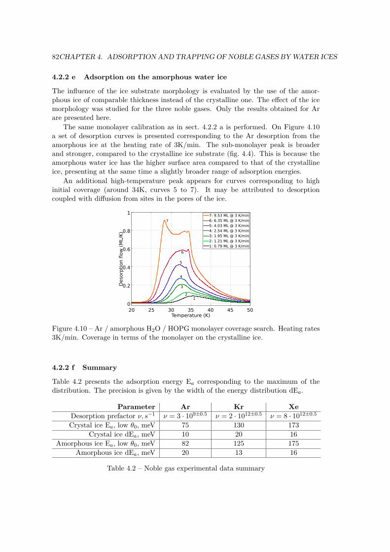
82CHAPTER 4. ADSORPTION AND TRAPPING OF NOBLE GASES BY WATER ICES

4.2.2 e Adsorption on the amorphous water ice

The influence of the ice substrate morphology is evaluated by the use of the amor-phous ice of comparable thickness instead of the crystalline one. The effect of the icemorphology was studied for the three noble gases. Only the results obtained for Arare presented here.

The same monolayer calibration as in sect. 4.2.2 a is performed. On Figure 4.10a set of desorption curves is presented corresponding to the Ar desorption from theamorphous ice at the heating rate of 3K/min. The sub-monolayer peak is broaderand stronger, compared to the crystalline ice substrate (fig. 4.4). This is because theamorphous water ice has the higher surface area compared to that of the crystallineice, presenting at the same time a slightly broader range of adsorption energies.

An additional high-temperature peak appears for curves corresponding to highinitial coverage (around 34K, curves 5 to 7). It may be attributed to desorptioncoupled with diffusion from sites in the pores of the ice.

20 25 30 35 40 45 500

0.2

0.4

0.6

0.8

1

Temperature (K)

Deso

rpti

on fl

ow

(M

L/K

)

7

6

5

4

3

21

7: 9.53 ML @ 3 K/min6: 6.35 ML @ 3 K/min5: 4.03 ML @ 3 K/min4: 2.54 ML @ 3 K/min3: 1.95 ML @ 3 K/min2: 1.21 ML @ 3 K/min1: 0.79 ML @ 3 K/min

Figure 4.10 – Ar / amorphous H2O / HOPG monolayer coverage search. Heating rates3K/min. Coverage in terms of the monolayer on the crystalline ice.

4.2.2 f Summary

Table 4.2 presents the adsorption energy Ea corresponding to the maximum of thedistribution. The precision is given by the width of the energy distribution dEa.

Parameter Ar Kr XeDesorption prefactor ν, s−1 ν = 3 · 109±0.5 ν = 2 · 1012±0.5 ν = 8 · 1012±0.5

Crystal ice Ea, low θ0, meV 75 130 173Crystal ice dEa, meV 10 20 16

Amorphous ice Ea, low θ0, meV 82 125 175Amorphous ice dEa, meV 20 13 16

Table 4.2 – Noble gas experimental data summary

4.2. EXPERIMENTAL APPROACH 83

4.2.3 Inclusion in water icesIn order to evaluate if the noble gas atoms may be trapped within the ice bulk, aspecial series of experiment were performed. The adsorbate atoms were deposited onthe previously prepared ice surface. Then, few equivalent layers of water moleculeswere deposited on top of the noble gas atoms, forming a sandwich with trapped noblegas atoms.

Since such experiments require a long time to perform (at least 3 hours per curve),requiring to prepare the ice for every new experiment, only a preliminary study wasperformed.

50 100 1500

0.2

0.4

0.6

0.8

1

Temperature (K)

Deso

rpti

on fl

ow

(arb

.u.)

129Xe H2O ice40Ar 84Kr

Xe, M=129. 43% trapped

Ar, M=40. 27% trappedKr, M=84. 16% trapped

H2O ice desorption

129Xe

84Kr

40Ar

Figure 4.11 – Trapping of noble gases in the amorphous water ice, covered with 1-2ML of ice. Heating rates 3K/min. Sub-monolayer noble gas initial coverage. Y axisnormalized to TPD maximum. No comparison should be made between gases sincethe deposition conditions: temperature, noble gas thickness, recovering ice thicknessare not the same.

As shown on Figure 4.11, all the noble gases may be trapped. The TPD curves ex-hibit three main desorption features for all the noble gas species. The low-temperature(below 100K) desorption peak is associated to the desorption of non-covered noble gasatoms. Smooth peak at 120-140K corresponds to the atoms diffusing through the icealong the warming-up and the onset of the ice sublimation. That is evidenced by thebroad shape of the peak. High-temperature (150K) peak corresponds to atoms ejectedfrom the ice during the ice crystallization.

The desorption signal for temperatures above 100K is associated with the desorp-tion of the water ice itself, and therefore these features correspond to noble gas atomstrapped inside the ice. A numerical quantity may be assigned to characterize the trap-ping process: Integrating the total noble gas desorption flow and the desorption flowat temperatures above 100K, and taking a ratio of integrals will reflect the ratio oftrapped atoms among the total deposited quantity.

The trapping data is summarized in Table 4.3. It may be seen that the trappingratio (the last column) is dependent on the ice-gas-ice sandwich preparation conditions:the deposition temperature, the noble gas coverage, the recovering ice layer thickness.For example, Argon and Krypton may only be trapped if deposited at around 15K,

84CHAPTER 4. ADSORPTION AND TRAPPING OF NOBLE GASES BY WATER ICES

System Tdep Ice top, ML I20−200KTPD ,ML I100−200K

TPD ,ML trapped fractionAr 10K 6 0,132 0,073 0,554Ar 10K 3 0,234 0,065 0,278Ar 10K 1,5 0,216 0,047 0,215Kr 13K 1,5 1,462 0,266 0,182Kr 30K 0,5 2,114 0,078 0,037Xe 50K 1,7 0,143 0,061 0,427Xe 50K 1,7 0,247 0,082 0,333

Table 4.3 – Noble gas inclusion between water ice layers. Ice substrate is 400ML thickamorphous ice prepared at 100K. Second column gives the noble gas and covering icelayers deposition temperatures. Third column specifies the approximate covering icethickness. Fourth column I20−200K

TPD gives the total desorbed quantity of a noble gas inthe units of the effective ML on the crystalline ice. Fifth column I100−200K

TPD containsthe desorption integral taken from 100 to 200K. Last column contains the ratio of thefifth and the fourth column, that is the fraction of a gas that is trapped inside the ice.

while Xenon may be deposited at 50K and still a big fraction is trapped.To conclude, this preliminary study indicates a big potential of amorphous ice

to trap noble gases. Further investigation must be performed to rigorously study theinfluence of the ice sandwich parameters: the ice thickness, the deposition temperature,a noble gas quantity on trapping. Diffusion through the ice bulk should also be verifiedusing the isothermal survey at temperatures below the ice sublimation temperature.

4.3. THEORETICAL APPROACH 85

4.3 Theoretical approach

4.3.1 Modeling the ice surface

Since many forms of ice exist and play role in the adsorption, modeling the ice struc-tures becomes a non-trivial task. Luckily, the major part of the adsorption energy isdetermined by the water molecules in the direct vicinity of the adsorbate. That makespossible to stick to a limited set of model surfaces, if they represent a broad range ofadsorption geometries.

An additional problem is posed by the fact that the proton order in ices is undefined,even if the oxygen grid positions are known. For crystal ice models, the only constraintis a Bernal-Fowler [22, 23] ice rule: exactly two hydrogens of neighbour water moleculesform hydrogen bonds with lone pairs of the water molecule oxygen atom.

In this work an apolar hexagonal ice model with surface protons ordered as pro-posed by Fletcher[24] is used. Studies [25, 26] show that it is the most stable surfaceconfiguration of the hexagonal ice basal (0001) plane. For slab systems, the bulk pro-ton ordering variation [27] has a small effect on the total energy, compared to thesurface ordering [25].

To prepare the surface model, the following steps were performed: First, bulk struc-ture was optimized to obtain the ground state geometry of ice (sect. 4.3.1 a). Then,the minimal slab was reoptimized with 15A of vacuum in Z direction (sect. 4.3.1 b).Finally, the minimal slab was multiplied in x-y directions to accomodate the adsor-bate (sect. 4.3.1 c) For further calculations, the positions of the bottom layer of watermolecules were constrained to maintain the surface geometry. The topmost surfacelayer is always kept free to relax to the local potential energy minimum.

4.3.1 a Bulk optimization

The resulting bulk structure is shown on the figures 4.12b(basal plane view) and 4.12a(sideview).

The bulk structure with protons ordered to give apolar surfaces for basal (0001)and prism (1010) cuts is used. The cell volume and atoms geometry are reoptimized forminimal orthogonal unit cell containing 8 water molecules (fig. 4.12). For this optimiza-tion, an energy cut-off of 800 eV for the basis set plane waves was used and a 9x9x9gamma-centered K-points mesh is employed. The minimum force per atom criteriais used to interrupt the geometry optimization loop, with the force threshold of 0.007eV/A. After the geometry optimization, the cell dimensions became (4.33x7.49x7.07)A.A bulk ice cohesive energy of -714 meV/H2O or -25 meV A−3 is found, which is slightlyhigher than the values obtained in [25]. The difference comes from the routine use fordispersion force corrections [28](sect. 3.1.3) in the current work.

4.3.1 b Slab surface

After the bulk geometry reoptimization, two minimal slabs (basal and prism) wereproduced. The basal slab was produced by adding 15A of vacuum in the Z directionof the bulk cell (cell dimensions 4.33 × 7.49 × 21.75A). The prism slab was produced

86CHAPTER 4. ADSORPTION AND TRAPPING OF NOBLE GASES BY WATER ICES

(a) Side view (b) Top view

Figure 4.12 – Hexagonal ice Ih minimal orthogonal unit cell (solid color), 3x2x1 image(transparent)

by rotating the bulk cell by 90around the x axis and adding 15A of vacuum (4.33 ×7.07× 22.49A cell).

The slab molecules were relaxed to the minimum of the potential energy. Thecalculation was performed with a standard energy cut-off of 400eV and 5x3x1 gamma-centered K-points mesh was used.

4.3.1 c Final slab geometries

Finally a 2x1x1 slab (fig. 4.13) containing two ice bilayers was used for probing ad-sorption geometries. The positions of the bottom layer molecules of the slab wereconstrained and the top layer was left free to relax to the potential energy minimumfor all calculations hereafter.

Inclusion and substitution calculations for rare gases (sect. 4.3.5, 4.3.6) were per-formed on a thick 2x1x2 slab (4 BL) with the two topmost layers unconstrained.

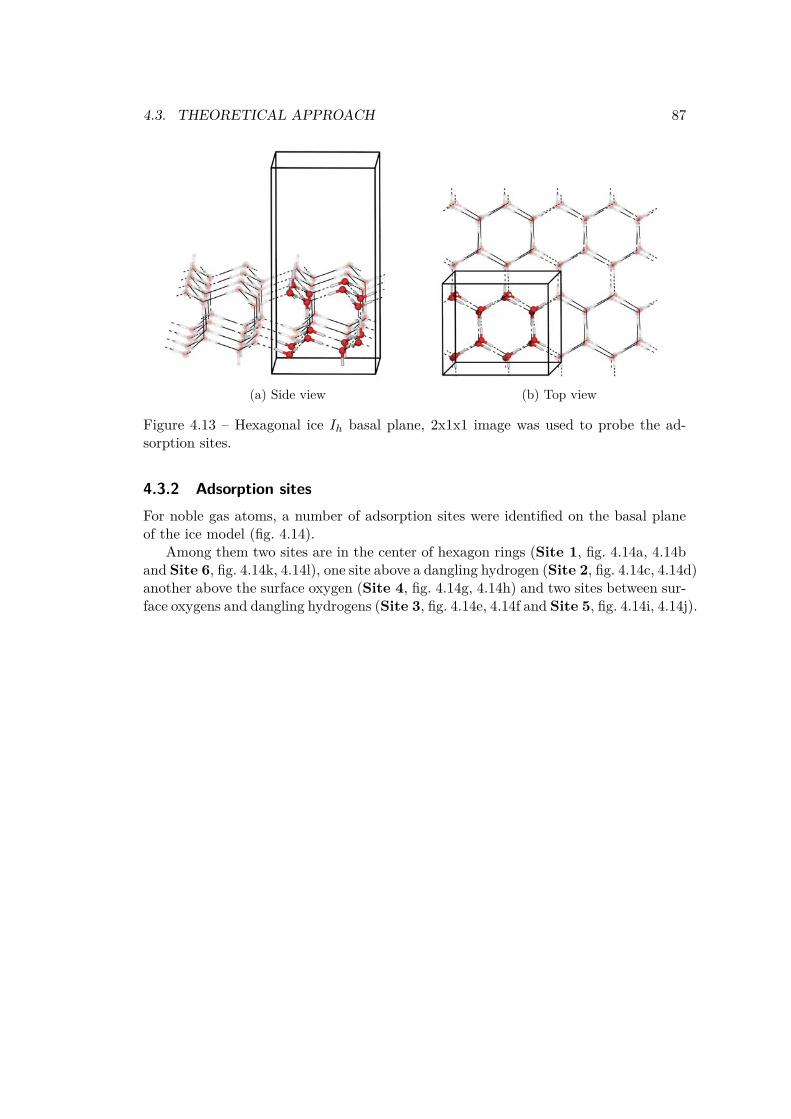
4.3. THEORETICAL APPROACH 87

(a) Side view (b) Top view

Figure 4.13 – Hexagonal ice Ih basal plane, 2x1x1 image was used to probe the ad-sorption sites.

4.3.2 Adsorption sitesFor noble gas atoms, a number of adsorption sites were identified on the basal planeof the ice model (fig. 4.14).

Among them two sites are in the center of hexagon rings (Site 1, fig. 4.14a, 4.14band Site 6, fig. 4.14k, 4.14l), one site above a dangling hydrogen (Site 2, fig. 4.14c, 4.14d)another above the surface oxygen (Site 4, fig. 4.14g, 4.14h) and two sites between sur-face oxygens and dangling hydrogens (Site 3, fig. 4.14e, 4.14f and Site 5, fig. 4.14i, 4.14j).

88CHAPTER 4. ADSORPTION AND TRAPPING OF NOBLE GASES BY WATER ICES

(a) Site 1, side (b) Site 1, top (c) Site 2, side (d) Site 2, top

(e) Site 3, side (f) Site 3, top (g) Site 4, side (h) Site 4, top

(i) Site 5, side (j) Site 5, top (k) Site 6, side (l) Site 6, top

Figure 4.14 – Noble gas adsorption sites on ice Ih basal plane. Solid line indicatesclosest hydrogen and oxygen atoms.

4.3. THEORETICAL APPROACH 89

4.3.3 Convergence against cell dimensions

To test the convergence of adsorption energy and identify the minimum required surfacemodel parameters. , A series of tests were performed on the cell dimensions and thenumber of ice bilayers with Kr adsorbed on sites 1, 3 and 5 (fig. 4.14b, 4.14f, 4.14j).

4.3.3 a Interadsorbate distance

Since the objective of this study is to derive the adsorption energies of isolated atomson the ice, it is necessary to identify the minimum interadsorbate distance at whichthe adsorbate-adsorbate interaction may be neglected. To determine this distance, aseries of calculations with noble gas dimers was performed. A big (10x10x20A) unitcell was set up, containing two identical noble gas atoms, placed at fixed distancesapart, with the center of mass in the middle of the cell. The interatomic distance inthe dimer was varied up to 10A, that is the maximum distance possible in the definedcell. The resulting interaction energy as a function of interatomic distance is presentedon Figure 4.15. The dimer interaction energy Edim(d) is calculated here as a differenceof interaction energies at a fixed interatomic distance d Etot(d) and Etot(dmax) (4.1)

Edim(d) = Etot(d)− Etot(dmax) (4.1)

where dmax is the maximum possible interatomic distance in the given cell.As one may see, the interaction energy becomes negligible at distances above 7A,

permitting to use the 2x1 ice slab with lateral dimensions of 8.66x7.50A, with theinteradsorbate distance of 7.50A.

To ensure that the cell size taken for this test was sufficient, a supplementary calcu-lation for the Xe dimer in a 15x15x30A cell was performed (black circles on fig. 4.15).No difference was identified neither in energies nor in the equilibrium position.

3 4 5 6 7 8 9-0.1

-0.05

0

0.05

0.1

Interatomic distance, A

Ed,

eV

Ar dimerKr dimerXe dimerXe, big cell

Figure 4.15 – Ar2, Kr2, Xe2 dimer energy as a function of interatomic distance. Unitcell: 10x10x20A; 3x3x3 K-points; plane wave energy cut-off 400 meV.

90CHAPTER 4. ADSORPTION AND TRAPPING OF NOBLE GASES BY WATER ICES

4.3.3 b Number of surface layers

As a next step, the required number of ice substrate bilayers was determined. Thecalculation was performed in a cell with a huge (40A) vacuum size (fig. 4.16a). For thatpurpose, the Krypton adsorption energies were calculated for sites 1 (fig. 4.14a, 4.14b)and 3 (fig. 4.14e, 4.14f) on different slabs (1 to 6 BL of ice).

For slabs thicker than 2BL, the topmost ice layer was set free to relax to the energyminimum, all underlying layers being kept frozen to simulate the ice bulk. No visibledifference in adsorption energy was observed for slabs from one to three layers thick.The calculated value of the adsorption energy diverges for thick slabs due to increasinguncertainty in the optimization procedure.

Hereafter, all calculations were performed on 2BL slab for adsorption (sect. 4.3.4)and 4BL slab for substitution/inclusion in the bulk (sect. 4.3.5, 4.3.6).

0 1 2 3 4 5 6 7-0.165

-0.16-0.155

-0.15-0.145

-0.14-0.135

Ice bilayers

Ea,

eV

Site 1Site 3

0 1 2 3 4 5 6 73

3.05

3.1

3.15

3.2

Ice bilayers

h (

ice-K

r),

A

(a) Convergence against number of layers.30A vacuum, cell 8.66x7.49x46 A

0 5 10 15 20 25 30 35-0.2

-0.19-0.18-0.17-0.16-0.15-0.14-0.13

Vacuum distance, A

Ea, eV

Site 1Site 3Site 5

0 5 10 15 20 25 30 352.9

3

3.1

3.2

3.3

3.4

Vacuum distance, A

h (

ice-K

r),

A

(b) Convergence against vacuum distance.2BL ice, cell 8.66x7.49x(7+zVac) A

Figure 4.16 – Kr on ice basal plane, convergence tests against slab thickness andvacuum size.

4.3.3 c Vacuum size

Finally the convergence against the vacuum size was tested. A set of cells was set up,with two bilayers of the hexagonal ice and a variable vacuum dimension.

Three different adsorption sites of Kr on ice basal plane were probed: Site 1,fig. 4.14a, 4.14b, Site 3, fig. 4.14e, 4.14f and Site 5, fig. 4.14i, 4.14j.

For each vacuum size three calculations, including slab, adsorbate and slab+adsorbatesystems energy were performed. The resulting adsorption energies as a function of vac-uum size are presented on Figure 4.16b. One may see that for atomic adsorbates even5 Angstroms of vacuum dimension is sufficient. Nevertheless, all further calculationswere performed using cells with vacuum size of at least 10A.

4.3. THEORETICAL APPROACH 91

4.3.4 AdsorptionAdsorption energies were calculated on the slab model of the basal plane of the hexag-onal ice surface, containing two bilayers of water molecules (16 water molecules percell, fig. 4.14).

The cell of 8.66x7.49x17A was used, with vacuum dimension of 10.5A. A gamma-centered mesh of 3x3x1 k-points was used. All calculations were performed with theplane wave energy cut-off of 400eV. Grimme correction [28] is routinely employed toimprove the description of Van der Waals interactions.

A summary of obtained adsorption energies is presented in the Table 4.4.

Site Ar Ea, eV Kr Ea, eV Xe Ea, eV1 -0,116 -0,146 -0,1762 -0,085 -0,101 -0,1353 -0,116 -0,149 -0,1814 -0,066 -0,097 -0,1015 -0,110 -0,139 -0,1686 -0,119 -0,153 -0,187

Table 4.4 – Noble gas adsorption energies on water ice.

All adsorption sites are found to be stable, giving a distribution of adsorptionenergies. Two classes of sites are observed: strongly bound, e.g. site 1, site 3 andsite 6, where adsorbate atom is adjacent to several surface water molecules, and weakly-bound, where the adsorbate atom is above a surface hydrogen (site 2) or oxygen (site 4)site. One may also note that the surface-adsorbate distance (Table 4.5) is smaller forstrongly-bound sites.

Site Ar h, A Kr h, A Xe h, A1 3,16 3,13 3,212 4,09 4,12 4,243 3,10 3,13 3,344 3,67 3,81 3,875 3,16 3,16 3,256 3,15 3,11 3,20

Table 4.5 – Adsorbate height above the surface (average z(O) coordinate)

A summary of the adsorption energies and the surface-adsorbate distances is alsoshown on Figure 4.17 for clarity.

To conclude, a distribution of adsorption energies is found. The difference betweenthe adsorption energies of the weakest and the strongest sites may serve as an estimateof the barrier height for noble gas diffusion on the surface.

92CHAPTER 4. ADSORPTION AND TRAPPING OF NOBLE GASES BY WATER ICES

0 1 2 3 4 5 6 7-0.2

-0.15

-0.1

-0.05

0

Site index

Ea,

eV

ArKrXe

0 1 2 3 4 5 6 73

3.23.43.63.8

44.24.4

Site index

d(s

urf

-ad

s),

A

Figure 4.17 – Ar, Kr, Xe adsorption on hexagonal ice basal plane: (top) adsorptionenergies; (bottom) surface-adsorbate distances.

4.3.5 SubstitutionAnother point of interest is whether substituting the ice water molecules by noble gasatoms would lead to a stable configuration. To investigate this, a thick (4BL) basalslab model of hexagonal ice was taken. The vacuum size of 10A was used, givingthe cell dimensions of 8.66x7.49x22A. Two bottom layers of ice were constrained andsuperior layers were left free to relax.

In that model one may identify four distinct surface water molecules positions(fig. 4.18), referred later Sub(1-4)

Those four water molecules were replaced one by one with noble gas atoms. Thesubstitution energy Es was calculated in a similar way to the adsorption energy:

Es = Etot − (Eslab−H2O + Eads)

where Etot is the total energy of the system with a water molecule replaced bya noble gas atom; Eslab−H2O is the total energy of the slab with one water moleculeextracted.

A summary of the substitution energies is given in the Table 4.6.The correspondingpositions relative to the superior layer of water molecules are presented in Table 4.7.

Two possible scenarios may be identified. a) the noble gas atom stays below thesurface, deforming the superior ice layer. Although this configuration is stable, it isenergetically unfavourable (positive values of Es). This is the case for sub2 site for allnoble gas atoms and sub4 site for Argon. b) the noble gas atom pops out from thesurface. The ice surface is reconstructed in some way. Such configurations are stableand energetically favorable, being the equivalent of adsorption on the ice defect sites.

Another point to investigate was to verify if we may stabilize a noble gas atom ifwe remove more (e.g. two) adjacent water molecules of the ice bulk. For the case ofArgon, for example, it was found that there exists at least one (Sub23) configurationwhere substitution (inclusion in the cavity) becomes energetically favorable. Refer to

4.3. THEORETICAL APPROACH 93

Site Ar Es, eV Kr Es, eV Xe Es, eVSub 1 -0,093 -0,134 -0,168Sub 2 0,538 0,245 0,196Sub 3 -0,105 -0,144 -0,182Sub 4 0,208 -0,094 -0,136Sub 12 0,243Sub 23 -0,060Sub 34 0,004

Table 4.6 – Noble gas substitution energies in water ice.

Site Ar h, A Kr h, A Xe h, ASub 1 2,12 2,42 2,57Sub 2 -0,89 -0,26 -0,46Sub 3 1,95 2,25 2,37Sub 4 -0,23 1,30 1,65

Table 4.7 – Noble gas atom height relative to the surface (average z(O) coordinate),substitution sites

(a) Site 1, side (b) Site 1, top (c) Site 2, side (d) Site 2, top

(e) Site 3, side (f) Site 3, top (g) Site 4, side (h) Site 4, top

Figure 4.18 – Noble gas substitution sites on ice Ih basal plane. Solid line indicatesclosest hydrogen and oxygen atoms.

94CHAPTER 4. ADSORPTION AND TRAPPING OF NOBLE GASES BY WATER ICES

the Table 4.6), sites Sub12, Sub23, Sub34.It may be concluded that noble gas atoms may be contained within the ice bulk,

but only if pores or crystalline structure defects are sufficiently big.

4.3.6 InclusionFinally, inclusion in the ice structure was studied (fig. 4.19). The ice model andcell dimensions were the same as for substitution calculations (sect. 4.3.5). Noble gasatoms were placed inside the non-modified slab structure between two hexagon centers,surrounded by 12 water molecules. A big energy penalty (see Table 4.8) was found forinclusion in the ice structure. Such energy penalty leads to the conclusion that noblegas atoms will not penetrate the ice structure, nor diffuse within. Diffusion will bepossible only through sufficiently large pores, and not through the ice bulk.

Site Ar Ei, eV Kr Ei, eV Xe Ei, eVInc12 0,284 0,543 1,115Inc23 0,360 0,711 1,353

Table 4.8 – Noble gas inclusion energies in water ice.

(a) Site 12, side (b) Site 12, top (c) Site 23, side (d) Site 23, top

Figure 4.19 – Noble gas inclusion sites in ice Ih basal slab. Solid line indicates closesthydrogen and oxygen atoms.

4.4 Comparisons and conclusions

In this chapter, the adsorption of noble gas atoms (Ar, Kr and Xe) onto water icesurfaces has been studied, both theoretically and experimentally. Theoretical calcula-tions have revealed the existence of 6 adsorption sites, identical for each species, oncrystalline ice surface. Each site is associated with an adsorption energy value, whichranges from 66 to 120 meV for Ar, from 100 to 150 meV for Kr and from 100 to 190meV for Xe. Experiments based on TPD could not access this exact site distribu-tion, mainly because the small energetic difference between the adsorption energies isblurred by the width of the desorption curves. However the experiments gave access toaverage adsorption energies, which have been evaluated to 75±10 meV for Ar, 130±20

4.4. COMPARISONS AND CONCLUSIONS 95

meV for Kr and 170±20 meV for Xe. These values compare well with the theoreticaldistributions. Note that, because of the TPD technique that is used, warming-up mayinduce an important diffusion of the noble gas atoms on the surface, that may fall intothe most tightly-bound sites prior to their desorption. Therefore the weight of themore bound sites will be enhanced in the mean values that are experimentally derived,which explains why the experimental mean values are found closer to the high energyside of the adsorption sites distribution predicted by the theory. Finally, experimentalvalues for the adsorption energy of Ar on crystalline ice are to be taken with caution,since important diffusion and outgasing from other cold parts of the cryostat duringthe warming-up have brought polluting signal on the TPD curves that were difficultto estimate and correct.

The theoretical study of the trapping of the noble gas atoms into the ice bulk hasrevealed that the inclusion of Ar, Kr or Xe in the water ice network is very unlikely.Nevertheless, should the water ice present cavity-like defects (missing molecules inthe water ice network), Ar is efficiently trapped and stabilized into these micro-pores.These “cavities” should anyway be at least bigger than a missing water molecule,otherwise the presence of the Ar atom induces a distortion of the ice network whichis energetically not favourable. This finding is very interesting since trapping of noblegases in cavities of the water ices may be an alternative candidate to the water iceclathrate organization. Preliminary experimental studies have been realized, in whichthe trapping of the noble gas has been observed by monitoring TPD curves of the atomsrecovered by an increasing thickness of amorphous water layer. Proportions of noblegas trapped into the ice have been estimated. However, the trapping being inverselydependent on the diffusion of the atoms through the ice layer, which is a dynamicaleffect, studies at fixed temperature (isothermal desorption), and as a function of time,is needed for a better quantification of the trapping. In addition, the presence of closedcavities when water ice is grown on top of rare gas atoms has still to be experimentallyevidenced.

To conclude, the study presented here offers an overview of the noble gas adsorptionand trapping by water ices. In an astrophysical context, the adsorption energies of Ar,Kr and Xe are found - not surprisingly - weaker than the adsorption energy of ice onice itself, which makes that the trapping by surface adsorption is not likely to be anefficient process except at very low temperature. But the adsorption energies can beused to estimate the amount and residence time of rare gas atoms on the water ice atany temperature, making possible to test the scenario during which additional watermolecules could accrete on top and result in noble gas enrichment within the ice bulk.Our study shows that, if the water which accretes on top presents cavity-like defects,the rare gas atom can get efficiently trapped into the water ice, up to temperaturecorresponding to the water sublimation. This trapping in the ice cavities is a veryinteresting effect, since, up to now, such trapping into ice bulks were only consideredif the water would organize as clathrates structures [8, 9]. Considering that the merepresence of this water allomorphism in the primitive nebula is still controversial, thetrapping in water ice cavities would be potentially a very promising alternative process.Therefore, this work opens the way to an in-depth study of this trapping effect intothe water ice, both experimentally and theoretically.

96CHAPTER 4. ADSORPTION AND TRAPPING OF NOBLE GASES BY WATER ICES

References[1] Olivier Mousis, Daniel Gautier, and Dominique Bockelée-Morvan. “An Evolu-

tionary Turbulent Model of Saturn’s Subnebula: Implications for the Origin ofthe Atmosphere of Titan”. In: Icarus 156.1 (2002), pp. 162–175.

[2] H. B. Niemann et al. “The abundances of constituents of Titan’s atmospherefrom the GCMS instrument on the Huygens probe”. en. In: Nature 438.7069(2005), pp. 779–784.

[3] Yann Alibert, Olivier Mousis, and Willy Benz. “On the Volatile Enrichments andComposition of Jupiter”. en. In: The Astrophysical Journal Letters 622.2 (Apr.2005), p. L145.

[4] Ronen Jacovi and Akiva Bar-Nun. “Removal of Titan’s noble gases by theirtrapping in its haze”. In: Icarus 196.1 (2008), pp. 302–304.

[5] D. Cordier et al. “About the Possible Role of Hydrocarbon Lakes in the Originof Titan’s Noble Gas Atmospheric Depletion”. en. In: The Astrophysical JournalLetters 721.2 (Oct. 2010), p. L117.

[6] John P. Osegovic and Michael D. Max. “Compound clathrate hydrate on Titan’ssurface”. en. In: Journal of Geophysical Research: Planets 110.E8 (2005), E08004.

[7] C. Thomas et al. “A theoretical investigation into the trapping of noble gases byclathrates on Titan”. In: Planetary and Space Science. Surfaces and Atmospheresof the Outer Planets, their Satellites and Ring Systems, Part IV Meetings heldin 2007: EGU: PS3.0 & PS3.1; IUGG/IAMAS:JMS12 & JMS13; AOGS: PS09 &PS11; EPSC2: AO4 or PM1 56.12 (2008), pp. 1607–1617.

[8] Olivier Mousis et al. “Removal of Titan’s Atmospheric Noble Gases by TheirSequestration in Surface Clathrates”. en. In: The Astrophysical Journal Letters740.1 (Oct. 2011), p. L9.

[9] Jan Lundell, Arik Cohen, and R. Benny Gerber. “Quantum Chemical Calcu-lations on Novel Molecules from Xenon Insertion into Hydrocarbons”. In: TheJournal of Physical Chemistry A 106.49 (2002), pp. 11950–11955.

[10] Antti Lignell et al. “On theoretical predictions of noble-gas hydrides”. In: TheJournal of Chemical Physics 125.18 (Nov. 2006), p. 184514.

[11] Jan Lundell et al. “Quantum chemical study of the hydrogen-bonded HXeOH–H2Ocomplex”. In: Journal of Molecular Structure. Horizons in Hydrogen Bond Re-search 2005A Collection of Papers from the XVIth International Conference"Horizons in Hydrogen Bond Research", Roskilde, Denmark, 30 August - 04September, 2005 790.1–3 (2006), pp. 31–39.

[12] O. Mousis et al. “Sequestration of Noble Gases by H+3 in Protoplanetary Disksand Outer Solar System Composition”. en. In: The Astrophysical Journal 673.1(Jan. 2008), p. 637.

[13] F. Pauzat and Y. Ellinger. “H3+ as a trap for noble gases - 2: structure and ener-getics of XH3+ complexes from X=neon to xenon”. In: The Journal of ChemicalPhysics 127.1 (July 2007), p. 014308.

REFERENCES 97

[14] F. Pauzat et al. “H3+ as a trap for noble gases-3: Multiple trapping of neon,argon, and krypton in XnH3+(n=1–3)”. In: The Journal of Chemical Physics130.17 (May 2009), p. 174313.

[15] F. Pauzat et al. “Gas-phase Sequestration of Noble Gases in the Protosolar Neb-ula: Possible Consequences on the Outer Solar System Composition”. en. In: TheAstrophysical Journal 777.1 (Nov. 2013), p. 29.

[16] A. Kouchi et al. “Conditions for condensation and preservation of amorphousice and crystallinity of astrophysical ices”. In: Astronomy and Astrophysics 290(1994), pp. 1009–1018.

[17] A. Gil et al. “Adsorption of Water on Solid Surfaces Studied by Scanning ForceMicroscopy”. In: Langmuir 16.11 (2000), pp. 5086–5092.

[18] A. Givan, A. Loewenschuss, and C. J. Nielsen. “Fourier transform infrared spec-trometry studies of surface and bulk porosity of water ice”. In: Vibrational Spec-troscopy 12.1 (1996), pp. 1–14.

[19] K. Isokoski et al. “Porosity and thermal collapse measurements of H2O, CH3OH,CO2, and H2O:CO2 ices”. en. In: Physical Chemistry Chemical Physics 16.8 (Jan.2014), pp. 3456–3465.

[20] P. Jenniskens and D. F. Blake. “Structural transitions in amorphous water iceand astrophysical implications”. en. In: Science 265.5173 (May 1994), pp. 753–756.

[21] H. Schlichting and D. Menzel. “Techniques for attainment, control, and calibra-tion of cryogenic temperatures at small single-crystal samples under ultrahighvacuum”. In: Review of Scientific Instruments 64.7 (July 1993), pp. 2013–2022.

[22] J. D. Bernal and R. H. Fowler. “A Theory of Water and Ionic Solution, with Par-ticular Reference to Hydrogen and Hydroxyl Ions”. In: The Journal of ChemicalPhysics 1.8 (Aug. 1933), pp. 515–548.

[23] Ernesto Cota and William G. Hoover. “Computer simulation of hexagonal ice”.In: The Journal of Chemical Physics 67.8 (Oct. 1977), pp. 3839–3840.

[24] N. H. Fletcher. “Reconstruction of ice crystal surfaces at low temperatures”. In:Philosophical Magazine Part B 66.1 (1992), pp. 109–115.

[25] Ding Pan et al. “Surface energy and surface proton order of the ice Ih basal andprism surfaces”. en. In: Journal of Physics: Condensed Matter 22.7 (Feb. 2010),p. 074209.

[26] V. Buch et al. “Proton order in the ice crystal surface”. en. In: Proceedings ofthe National Academy of Sciences 105.16 (Apr. 2008), pp. 5969–5974.

[27] Tomas K. Hirsch and Lars Ojamäe. “Quantum-Chemical and Force-Field Inves-tigations of Ice Ih: Computation of Proton-Ordered Structures and Prediction ofTheir Lattice Energies”. In: The Journal of Physical Chemistry B 108.40 (2004),pp. 15856–15864.

[28] Stefan Grimme. “Semiempirical GGA-type density functional constructed witha long-range dispersion correction”. en. In: Journal of Computational Chemistry27.15 (2006), pp. 1787–1799.

98CHAPTER 4. ADSORPTION AND TRAPPING OF NOBLE GASES BY WATER ICES

Chapter 5Adsorption of CH3CN vs CH3NC atinterstellar grain surfaces

5.1 Study context

Among the ∼ 200 molecules detected in the interstellar medium (ISM) gas phase [1],about one fifth consists in nitriles R-CN and isonitrile R-NC isomers. Consideringpurely organic species, two different families can be identified that cover the two classesof isomers: conjugated molecules in which R contains, or does not contain, a system ofbonds that can be delocalized onto the CN triple bond. The first one is known as thecyanopolyyne/isocyanopolyyne series derived, formally, by adding carbon atoms or C2fragments to HCN and HNC; the second one obtained, formally, by replacing the Hatom in HCN and HNC by saturated hydrocarbon fragments. The simplest commonancestor of both series is the CN radical, second species ever detected in the ISM [2–4].About the same time, HCN [5] and CH3CN [6] were also detected, together with thefirst cyanopolyyne HC3N [7]. The identification of HNC followed soon after [5, 8].Thecorresponding isonitrile CH3NC was detected 13 years later [9] towards Sgr B2 and ittook twenty five more years to confirm the presence of this species in the HorseheadPDR [10].

The abundance ratios between nitrile and iso nitrile isomers have been largely usedto constrain the chemical models proposed to account for their presence in the variousobjects in which they were observed. The HCN/HNC couple has been the most studiedsince, according to radioastronomy gas phase observations, its abundance ratio variesover a large range, namely, from values close to unity in cold molecular clouds [11–13] toseveral thousands in highly illuminated PDRs [14]. By contrast, the CH3CN/CH3NCabundance ratio of ∼50 appears remarkably even[9, 11, 15].

In a previous work, a systematic study was carried out devoted to determine theenergetics of 32 isomeric structures identified in various types of objects. The overallresult was rather unexpected in the sense that, on average, the most abundant isomerwas the most stable and that the abundances of the other isomers were decreasing withthe order up the energy scale. It is referred as the Minimum Energy Principle (MEP).For more details see [16] and references therein.

Although it is not clear yet why the MEP works in the interstellar medium (ISM),

99

100CHAPTER 5. ADSORPTION OF CH3CN VS CH3NC AT INTERSTELLAR GRAIN SURFACES

which makes it a debated concept due to a number of exceptions already pointed outin the original presentation [16], it has shown a notable predictive power [17]. Forexample, glycine, that is not the most stable isomer in its family [18] was said difficultto be detected. Based on the MEP, it was also predicted that acetamide and formamidebeing the most stable isomers in their respective families [17]should be more suited toradio detection. The latter prediction has been confirmed by the recent identificationof formamide in a dozen sources [19, 20].

In this context, where HCN is more stable than HNC by ∼15 kcal/mol and CH3CNmore stable than CH3NC by ∼24 kcal/mol the MEP would be verified for the lattercouple of isomers but only partially for the first one. However, it should not beforgotten that radio observations are blind to molecules depleted on the grains, andthat gas phase chemistry alone cannot account for the abundances of complex organicmolecules formed in the ISM. Solid-gas reactions, and even chemical processes involvingadsorbed partners, have to be considered, making adsorption energies a key factor forthe determination of real abundances and abundance ratios.

Among the various grain models originally proposed [21] such as ices and/or car-bonaceous coatings on refractory minerals we selected three components, identifiedaccording to the environment by means of Mid-IR spectroscopy, namely, polycyclicaromatic hydrocarbon (PAH) molecules that are present in the spectra of almost allobjects [23, 24], silicates [25] and water ices [26–29] that appear chemically relevant tothe distribution of the species between the gas phase and the grains.

In the next pages is presented a research focused on the determination of the adsorp-tion energies of the first members of the nitrile and isonitrile families on laboratoryanalogues of widespread grain surfaces, namely, water ice, highly oriented pyrolyticgraphite (HOPG) and silica. It should be noted that we are not concerned here by thepossible role of the grain surfaces in the formation of CH3CN and CH3NC.

5.2 Experimental approach

5.2.1 Pure thick ices of CH3CN and CH3NC

Before studying adsorption and desorption of CH3CN and CH3NC from different sur-faces, it is important to study these two species as pure ices. For both isomers, themass signal associated with the ionization of the intact molecule (C2H3N+, m = 41amu) has been chosen for both adsorbate deposition and TPD experiments. The twospecies present comparable mass spectra following electron-induced ionization at 90eV [30] making mass spectrometry unable to distinguish unambiguously the two iso-mers. This could potentially represent an important issue, in particular for CH3NC.This molecule, in its liquid form is much less stable than its isomer CH3CN. It wasspecifically prepared by J.-C. Guillemin for this study and had to be kept at lowtemperature (< 273K) and protected from light.

It is therefore important to verify whether the product we introduce in the vacuumchamber is solely CH3NC or if the molecule has been degraded or isomerized to CH3CN,CH2CNH or CH2NCH during the deposition or the warming-up. To this purpose,Fourier Transform Reflection-Absorption InfraRed Spectroscopy (FT-RAIRS) has beensystematically done on the CH3CN and CH3NC ices after their growth and during the

5.2. EXPERIMENTAL APPROACH 101

Figure 5.1 – Reflection-absorption infrared spectra of thick CH3CN ice (850 ML - upperpanel) and of thick CH3NC ice (890 ML - lower panel), condensed at 90 K on poly-crystalline gold. Indicated assignments are detailed in Figure 5.1. Peaks marked with(*) correspond to identified combination modes. Structures observed at ∼2350 cm−1

are associated with a modification of the reference spectra due to a change of gaseousCO2 concentration in the spectrometer during the experiment time.

102CHAPTER 5. ADSORPTION OF CH3CN VS CH3NC AT INTERSTELLAR GRAIN SURFACES

Table 5.1 – vibration wavenumbers (in cm−1) and mode assignments of gas phase andphysisorbed multilayers of CH3CN and CH3NC in the 800 - 3200 cm−1 range.

Acetonitrile CH3CN Methyl isocyanide CH3NCGasa Solidb This work Gasc Solidd This work Assignment3178 3161 3163 - - - ν(–C≡N) + ν(C–C)3009 3002 3000 3014 no 3008 νas(CH3)2954 2941 2939 2966 no 2953 νs(CH3)2417 2415 2411 - - - δs(CH3) + ρ(CH3)2305 2289 2293 - - - δs(CH3) + ν(C–C)2266 2250 2251 - - - ν(–C≡N)- - - 2166 2170 2172 ν(–N≡C)

1448 1455 1455 1467 1470 1459 δas(CH3)1410 1422 1419 - - - ρ(CH3) + δ(C–C≡N)1390 1378 1378 1429 no 1426 δs(CH3)1041 1038 1036 1129 no no ρ(CH3)- - - 945 no 918 ν(C–N)

920 no 917 - - - ν(C–C)

a, b, c and d are from Parker et al., Schaff et al., [30] and Murphy et al. respectively; νstands for stretching mode, δ for bending mode, ρ for rocking mode, as for asymmetricmode and s for symmetric mode; “no” indicates non-observed vibrations.

warming-up.IR spectra of thick ices (∼ 800 ML) of pure CH3CN (upper panel) and pure CH3NC

(lower panel), deposited on polycrystalline gold at 90 K are presented in Figure 5.1.Infrared spectra have been realized with a resolution of 2 cm−1. In the case of con-densed multilayer of acetonitrile, we obtain IR spectrum very similar to what has beenfound by Schaff and Roberts[32]. The more intense peaks are associated with normalvibration modes of the condensed molecules, while many less intense peaks are relatedto combination modes, marked in Figure 5.1. Less literature is available on infraredspectroscopy of condensed methyl isocyanide at low temperatures. Vibrational studyof condensed CH3NC in the 1000 - 2500 cm−1 range [33] and gas phase spectroscopyvalues have been used for the assignment of CH3NC IR peaks. The assignment wepropose for the observed vibrational peaks are summarized in Table 5.1.

In the case of condensed methylisocyanide ice, all the peaks are attributed to agiven CH3NC vibration, therefore confirming the purity of the deposited ice. Theclear difference in the stretching vibrations of the cyanide (2250 cm−1) and isocyanide(2170 cm−1) groups makes that the two isomers can be finely differentiated by infraredspectroscopy. The spectra in Figure 5.1 show no contribution of the other isomer ineach pure ice. This is still true during warming-up and desorption of the ices, demon-strating that the mass signal monitored from pure isomer ices will not be pollutedin-situ by any isomerization process during the TPD experiment.

Thermal desorption of the pure ices of each isomer has been realized in order to ex-tract the relevant adsorption energy and prefactor of the Polanyi-Wigner law. Thermal

5.2. EXPERIMENTAL APPROACH 103

Figure 5.2 – (a) TPD curve, with a heating rate of 2 K/min, of ∼ 800 ML of pureCH3CN deposited on polycrystalline gold at 90 K. (b) Plot of the logarithm of thedesorption flux as a function of the inverse temperature. Red line is a linear regressionof the plot.

Figure 5.3 – (a) TPD curve, with a heating rate of 2 K/min, of ∼ 800 ML of pureCH3NC deposited on polycrystalline gold at 90 K. The beginning of the desorption asbeen magnified by a factor of 10 (b) Infrared spectra in the region of the NC stretchingvibration, during the warming-up of the ice. (c) Plot of the logarithm of the desorptionflux as a function of the inverse temperature. Lines are linear regressions of the plot.

104CHAPTER 5. ADSORPTION OF CH3CN VS CH3NC AT INTERSTELLAR GRAIN SURFACES

desorption curves of multilayers of pure CH3NC and pure CH3CN on polycrystallinegold, using a heating rate of 2 K/min, are shown in Figures 5.3a and 5.2a respectively.The multilayer desorption of CH3NC presents a small shoulder at 121 K, which weattribute to a temperature-induced phase transition of the solid. This kind of phasetransition from a disordered to a more structured solid is observed in several pure ices,the most famous case being the water ice crystallization at ∼150 K. The shoulder inthe desorption curves is explained by different adsorption energies for each phase, witha higher value for the most ordered phase in which molecules are usually more coordi-nated. The desorption of the disordered phase competes with its crystallization duringthe warming-up, and the total desorption flux observed is then the superposition ofthe desorption of the disordered and the crystalline phases [34]. This hypothesis issupported by the infrared follow-up of the NC stretching mode during the warmup, asshown in Figure 5.3b. Between 115 and 125 K, the vibrational peak gets narrower andmore intense, whereas the amount of adsorbed molecules diminishes. This suggests achange of the local environment of the adsorbate, which modifies the dipole momentassociated with the NC stretching vibration together with its bond-strength. Suchchange is usually induced by a reorganization of the molecules in the solid, as it hasalready been highlighted in the case of the CO stretching modes in solid CH3COOHand HCOOCH3 [35, 36] or OH stretching modes in solid water [37]. Interestingly, nophase transition was observed in solid CH3CN, neither in the TPD curves nor in theinfrared spectra.

The adsorption energy of the multilayers of CH3CN and CH3NC can be derivedfrom the TPD curves by considering that the desorption of the thick ices follows azeroth order kinetic Polanyi-Wigner law. For this purpose the zero order kineticsPolanyi-Wigner equation (5.1) is used.

ln(Φdes) = −Eadsk

1T

+ ln(νβ

) (5.1)

Plotting the logarithm of the flux against the inverse temperature 1/T results ina linear behavior, in which the adsorption energy and prefactor can be derived fromthe slope and intercept respectively (see chapter 2.3.2 for details). This linear trendis observed for CH3NC and CH3CN (Figures 5.3c and 5.2b). In the case of CH3NC,the plot consists of two different linear regimes, each being associated with a differentadsorption energy for the solid CH3NC, which further confirms the hypothesis of aphase transition at 121 K. From linear fitting of the plots we find for CH3CN multilayerEads = 390 ± 10 meV and ν = 1013±0.5 s−1. For CH3NC we find Eads = 330 ± 10meV and ν = 5×1012±0.5 s−1 for the disordered phase and Eads = 420 ± 10 meV andν = 5×1016±0.5 s−1 for the crystalline phase.

5.2.2 Submonolayer of CH3CN and CH3NC on model surfaces

Desorption of monolayer and submonolayer coverages of CH3NC and CH3CN has beenstudied on Quartz-α(0001), HOPG and compact amorphous and crystalline water ices,in order to obtain the adsorption energy of these isomers on the different substrates.

The associated TPD curves, realized with a heating rate of 12 K/min for graphiteand quartz substrates and 10 K/min in the case of adsorption on water ices are shown

5.2. EXPERIMENTAL APPROACH 105

Figure 5.4 – : TPD curves of several initial coverages of CH3NC (left) and CH3CN(right) adsorbed on quartz-α (0001) surface, on HOPG surface, and on crystalline andcompact amorphous water ice surfaces. Applied heating rates are 12 K/min on graphiteand quartz, and 10 K/min on water surfaces. TPD curves of multilayers (∼100 ML)of crystalline and amorphous water ices are shown in dashed lines to indicate the icesublimation onset.

106CHAPTER 5. ADSORPTION OF CH3CN VS CH3NC AT INTERSTELLAR GRAIN SURFACES

in Figure 5.4. The coverages indicated in the figure have been calibrated for eachsurface. On the water ice surfaces, two desorption peaks can be observed. One atlower temperature is observed only for high exposures, and therefore is related to themultilayer desorption. The second peak at higher temperatures is associated with thedesorption of the first monolayer, for which the adsorption energy is very different fromthat of the multilayer. The area of this second peak, when saturated, gives the absolutecalibration for 1 ML. Finally, a weak desorption feature is seen at ∼155 K only in thecase of adsorbates on compact amorphous water. This temperature corresponds to thesupporting water ice crystallization, evidenced by a shoulder in the amorphous waterTPD curve (dashed line). This peak is attributed to the phenomenon known as volcanodesorption: some adsorbates remain trapped in corrugations of the amorphous waterice, and are suddenly released when crystallization of the water ice takes place [38,39]. However, this contribution remains weak as the signal is dominated by the surfacemonolayer desorption. In the case of desorption from graphite or quartz surfaces, onlyone desorption feature is observed, meaning that the adsorption energy of the firstlayer and of the multilayer are not different enough to result in a clear separation ofdesorption peaks. The transition between multilayer and monolayer adsorption cananyway be determined by observing a change in the desorption kinetics order from thezero to the first order with lower exposure. This transition allows for identifying thefull monolayer coverage with a relative precision of the order of 10% (see chapter 2.3.1).

In order to derive the adsorption energies of each isomer from these surfaces, weuse a method described in detail in chapter 2.3.3. The desorption of the submonolayercoverage of molecules from the substrate is modeled using a first order approximation ofthe Polanyi-Wigner law. In order to get a more accurate description of the desorption,a distribution of adsorption energies is considered instead of a single value. Such anapproach implicitly takes into account different adsorption geometries and sites, aswell as the surface defects.

The experimental desorption curves are then fitted using the following equation:

Φdes(T ) = ν

β

∑i

θi(T ) exp(− EikT

)

where Ei is the adsorption energy associated with site i and θi is the coverage ofthe molecules for site i. In this case, the approximation of a constant prefactor νis made, i.e. it does not depend on the adsorption site. The TPD curves obtainedexperimentally are fitted with this law using a simple sampling of the adsorption energyin the 350 - 550 meV range, with the only free parameter being the initial coverageθ0i of each site i. The result gives the fraction of initial molecules adsorbed with theadsorption energy Ei, which is the adsorption energy distribution on the surface for agiven total initial coverage θ0.

The search for the prefactor is illustrated in Figure 5.5 for the case of CH3CNdesorption from the HOPG surface. The algorithm for the prefactor search is describedin details in sections 2.3.3 a and 2.3.3 b.

Once the prefactor value is obtained, a distribution of adsorption energies may bederived from each of the desorption curves. Resulting adsorption energy distributionsare shown in Figure 5.6 for different initial coverages of each isomer adsorbed on thefour substrates.

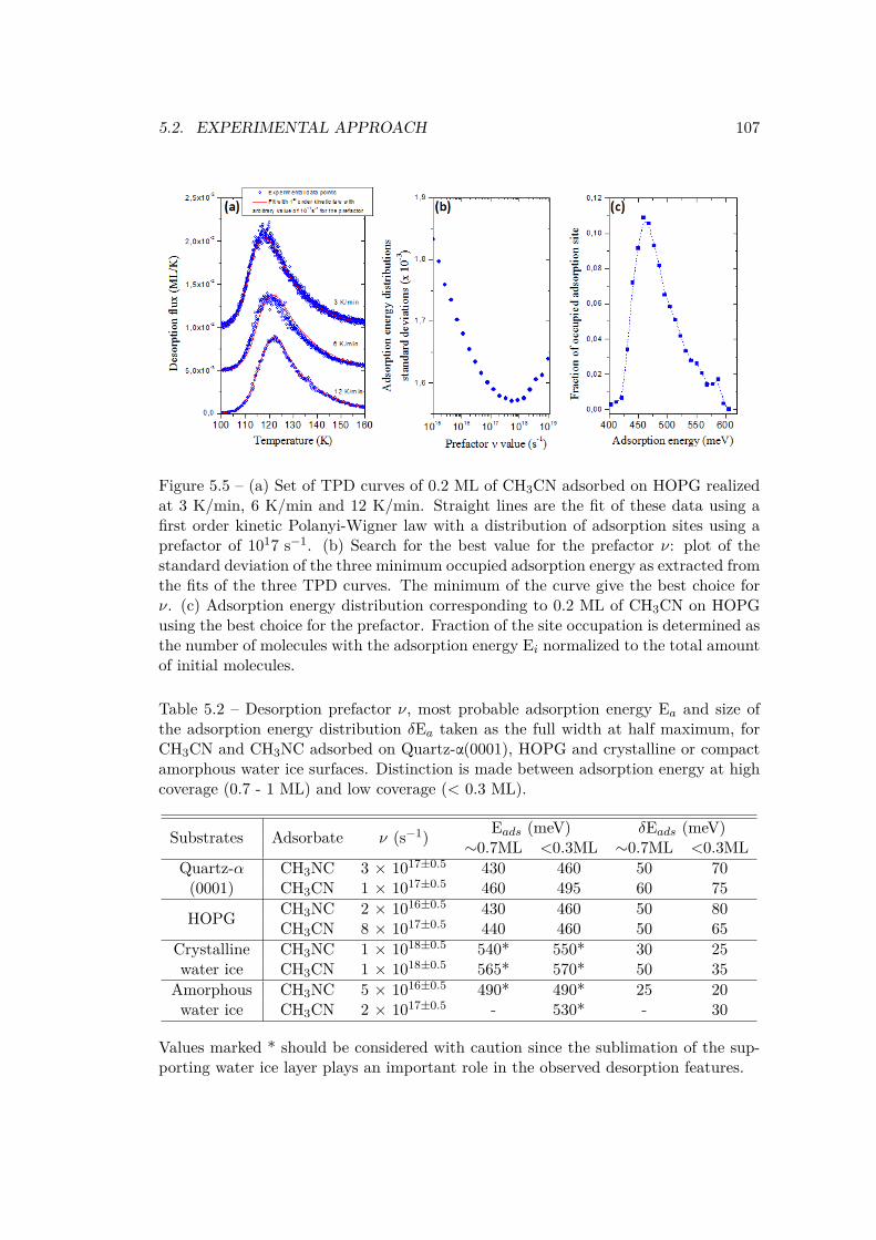
5.2. EXPERIMENTAL APPROACH 107

Figure 5.5 – (a) Set of TPD curves of 0.2 ML of CH3CN adsorbed on HOPG realizedat 3 K/min, 6 K/min and 12 K/min. Straight lines are the fit of these data using afirst order kinetic Polanyi-Wigner law with a distribution of adsorption sites using aprefactor of 1017 s−1. (b) Search for the best value for the prefactor ν: plot of thestandard deviation of the three minimum occupied adsorption energy as extracted fromthe fits of the three TPD curves. The minimum of the curve give the best choice forν. (c) Adsorption energy distribution corresponding to 0.2 ML of CH3CN on HOPGusing the best choice for the prefactor. Fraction of the site occupation is determined asthe number of molecules with the adsorption energy Ei normalized to the total amountof initial molecules.

Table 5.2 – Desorption prefactor ν, most probable adsorption energy Ea and size ofthe adsorption energy distribution δEa taken as the full width at half maximum, forCH3CN and CH3NC adsorbed on Quartz-α(0001), HOPG and crystalline or compactamorphous water ice surfaces. Distinction is made between adsorption energy at highcoverage (0.7 - 1 ML) and low coverage (< 0.3 ML).

Substrates Adsorbate ν (s−1) Eads (meV) δEads (meV)∼0.7ML <0.3ML ∼0.7ML <0.3ML

Quartz-α(0001)

CH3NC 3 × 1017±0.5 430 460 50 70CH3CN 1 × 1017±0.5 460 495 60 75

HOPG CH3NC 2 × 1016±0.5 430 460 50 80CH3CN 8 × 1017±0.5 440 460 50 65

Crystallinewater ice

CH3NC 1 × 1018±0.5 540* 550* 30 25CH3CN 1 × 1018±0.5 565* 570* 50 35

Amorphouswater ice

CH3NC 5 × 1016±0.5 490* 490* 25 20CH3CN 2 × 1017±0.5 - 530* - 30

Values marked * should be considered with caution since the sublimation of the sup-porting water ice layer plays an important role in the observed desorption features.

108CHAPTER 5. ADSORPTION OF CH3CN VS CH3NC AT INTERSTELLAR GRAIN SURFACES

Figure 5.6 – Adsorption energy distributions for several initial submonolayer coveragesof CH3NC (left) and CH3CN (right) adsorbed on quartz-α(0001), HOPG, crystallinewater and compact amorphous water surfaces.

5.2. EXPERIMENTAL APPROACH 109

In Table 5.2 are summarized for each adsorbate and each substrate the value ofthe prefactor, the most probable adsorption energy (taken as the maximum of thecorresponding distributions) and the size of the distributions defined as the width athalf maximum. From these values, a first conclusion is that, whatever the substrate,the adsorption energy of acetonitrile is found higher than that of methyl isocyanide.In the case of adsorption on graphite, though, the difference is small and close to ourexperimental error bars. Desorption from HOPG and quartz on the one hand, andfrom water surfaces on the other hand, show different behaviors, that will be discussedhereafter.

In any case, adsorption on the quartz substrates is found stronger than on graphite.However, the adsorption and thermal desorption of both isomers on Graphite andQuartz exhibit similar trends. Two regimes can be distinguished in these cases. Forinitial coverage above 0.5 ML, the adsorption energy distribution seems weakly depen-dent on the initial coverage. For initial coverage below 0.3 ML, the adsorption energydistribution significantly shifts toward higher energies with decreasing coverage. In-deed, at lower coverage, the molecules may diffuse during the warming-up and fall inthe tightly bounded adsorption sites. At higher coverage, all these sites being popu-lated, less bound sites will be probed by the excess molecules. Experiments performedat very low coverage therefore enhance the role of the most bounded sites (probably,defect sites) in the adsorption energy distribution. For being properly understood, thiseffect needs support from theoretical calculations, and will be further discussed in thesection 5.3.1.

In the case of adsorption on water ices, conclusions are not straightforward, andthe results obtained should be considered with caution. First, the adsorption energyon crystalline ice is, for both isomers, found higher than in the case of adsorption onamorphous ice. At first sight this is surprising since the amorphous water surface is ex-pected to present more different available adsorption sites than the crystalline surface.However, it can be understood as follows: the adsorption energies of CH3CN/CH3NCdetermined from the data treatment are very close to the adsorption energy of theunderneath water ice itself, whose desorption has already started when the monolayerdesorption of CH3CN/CH3NC is observed. The desorption energy of amorphous wateris of 490 meV and that of crystalline water is found within 500-520 meV [34, 40]. Thosevalues are very similar to the adsorption energy obtained in this study for CH3NC ad-sorption on water. Thus, the desorption observed for CH3CN and CH3NC is, at leastpartly, due to the desorption of the supporting water ice. Therefore the values that areobtained here for the adsorption energies do not reflect the real interaction strengthof the CH3CN/CH3NC molecules with the water ice surface, but suggest a lower limitfor it instead. However, a difference is still found between CH3CN and CH3NC ad-sorption energies, which would not be the case if their desorptions were only due tothe water sublimation. In particular, the adsorption energies for CH3CN on water isfound higher than that of water on water ice itself. Thus, the interaction of the methylcyanide and the acetonitrile with water also plays a role in the measured adsorptionenergies, and CH3CN is bound with a higher energy to the amorphous or crystallinewater surface than CH3NC.

110CHAPTER 5. ADSORPTION OF CH3CN VS CH3NC AT INTERSTELLAR GRAIN SURFACES

5.3 Theoretical approach to adsorption energiesTo determine the adsorption energies, periodic DFT calculations approach is employed,described in chapter 3.

5.3.1 Adsorption energies on highly oriented pyrolytic graphiteThe top layer of graphite on which the adsorption takes place can be identified asgraphene, i.e. an infinite planar sheet formed of hexagonal carbon rings that can beseen also as a polycyclic aromatic hydrocarbon (PAH) of infinite dimensions.

The geometry of the model system was optimized starting from the minimal or-thorhombic unit cell of graphite composed of 4 carbon atoms with the experimental [41]carbon-carbon distance a=1.42Å and an interlayer distance of 10Å. The optimizedbasal surface of the unit cell (4.275×2.46)Å2, practically identical to the initial system(4.26 × 2.46)Å2, gives an illustration of the quality of the method used for structuredeterminations.

A multiplied (2×3×1) orthorhombic cell (8.55×7.38×10)Å3 was constructed fromthe optimized geometry, large enough to accommodate the adsorbate molecule andavoid biased lateral interactions. The graphite model was built from the graphenestructure by adding a second carbon layer, shifted to intercarbon distance a, so thatcarbon atoms of the added layer found themselves below the center of an hexagon ofthe neighboring layer. The optimized interlayer distance c=3.2Å is found. The verticaldimension of the cell was increased to 25Å to accommodate the second carbon layerand the necessary vacuum between successive slab images.

In the case of atomic adsorption on graphite, three plausible sites may be consideredaccording to the surface topology, namely, on top of

• a carbon atom

• the center of a benzene ring

• the middle of a CC bond

What looks simple for atoms becomes more complicated for complex molecules likeCH3CN and CH3NC. Three different orientations can be distinguished for each ad-sorption site according to the orientations of the heavy atoms linear backbone and theposition of the CH3 groups whose rotation yields additional degrees of freedom. Allthese possibilities were systemically investigated. In particular it was verified that theCCN/CNC backbone stays linear in all situations (no deviation greater than 1 degreecould be detected).

For a vertical disposition of CH3CN and CH3NC with the methyl umbrella awayfrom the surface, the adsorption energy is 120 and 100 meV in average for CH3CNand CH3NC, respectively. The strongest adsorption occurs in both cases when theCCN/CNC backbones are on above the graphite carbon atom. However, when theverticality constrained is relaxed, the structure is no longer stable.

In the reverse position, with the methyl umbrella pointing to the surface, theadsorption energy is 160 meV in average for both CH3CN and CH3NC. Apart fromthe position above the middle of a CC bond that is less favorable for CH3NC. No

5.3. THEORETICAL APPROACH TO ADSORPTION ENERGIES 111

difference can be seen neither between CH3CN and CH3NC nor between the variousadsorption sites. The adsorption energy is stronger when the CH3 hydrogens are closeto the surface due to the polarization of the CH bonds by the CN and NC groups. Thisvertical orientation is energetically metastable, but in physical systems in presenceof defects, diffusion and thermal interactions with adjacent molecules these verticalarrangements will switch to orientations parallel to the surface.

Table 5.3 – Views of the most stable geometries of the adsorbed CH3CN and CH3NCisomers on graphite. Adsorption energies Ea are given in meV and kcal/mol

CH3CN CH3NCgraphite

Ea = 300 meV Ea = 290 meV6.99 kcal/mol 6.57 kcal/mol

graphite defect: 2 carbon hole

Ea = 330 meV Ea = 320 meV7.56kcal/mol 7.26 kcal/mol

graphite defect: 4H-hydrogenated 2 carbon hole

Ea = 410 meV Ea = 380 meV9.5 kcal/mol 8.6 kcal/mol

112CHAPTER 5. ADSORPTION OF CH3CN VS CH3NC AT INTERSTELLAR GRAIN SURFACES

To probe different orientations parallel to the graphite surface, a manifold of ∼24different geometries were probed (not counting rotations of the CH3 group). For bothCH3CN and CH3NC isomers, all adsorption energies are grouped within a range of∼50 meV giving the average values of 290 and 270 meV for CH3CN and CH3NC,respectively.

In both isomers we found a slight preference for geometries in which the CH3hydrogens are closer to the CC nuclear frame (Table 5.3 - top).

The preceding study focused on the graphite ideal surface, only. Though the dif-ference between the adsorption energies of the nitrile and isonitrile isomers is small,the same trend prevails for both isomers, namely, Eads(CH3CN) > Eads(CH3NC).

However, it is well understood that there is no perfect surface in space neitherin the laboratory and that the range of possible defects is too wide to be modeledexhaustively.

Nonetheless, to further approach the model surface to the experimental one, adefect in the topmost layer was a priori introduced, with the removal of two adjacentcarbon atoms, leaving a hole the size of pyrene (Table 5.3 - middle). The CH3CNand CH3NC isomers are no longer strictly parallel to the surface, the methyl groupsbeing slightly tilted towards the hole to favor the interaction oh the CH bonds with theelectrons released on the edge of the hole. The adsorption energies are then increasedby ∼ 10%.

Another type of possible defect was also considered by adding supplementary hy-drogen atoms to the 4 carbons on the edge of the hole (Table 5.3 - bottom) makingthe top layer locally resembling an hydrogenated amorphous carbon [42–44]. In thiscase, it is the CN/NC bonds that are over the edges of the hole, interacting with theadded hydrogens. The adsorption energies are then increased by ∼ 40% with respectto the pristine surface. In all cases, CH3CN is more tightly bound to the surface thanCH3NC.

5.3.2 Adsorption energies on silica

Silicates in different forms and silica itself, whose presence in the ISM has been a longtime disputed, are now clearly identified in protostellar envelopes [45] and protoplan-etary disks [46, 47] using mid- and far-infrared spectra obtained by the Spitzer SpaceTelescope. It is now well admitted that surfaces of that type may serve as catalystsfor a number of chemical syntheses such as methanol and water [48, 49]. In this work,we used quartz-α (0001) in both TPD experiments and theoretical modeling; it is themost stable crystal allotrope of silica and the most stable surface [50]. The active sur-face was hydroxylated by dissociative adsorption of water molecules (one per surfaceoxygen atom), which means that there are no free oxygen atoms left on the surface. Itis consistent with the calculations by Goumans et al. [48], which showed that, once hy-droxylated, the α-quartz (0001) surface was more stable than the raw surface obtainedby the simple cut of a single crystal.

The α-quartz (0001) surface model was constructed from a 3 layers slab, using theexperimental lattice parameters [50] and then re-optimized in the hydroxylated form.In the exploitation phase, a double minimal orthorhombic cell (2a ×

√3a × 3c, i.e.

(9.81× 8.49× 15,3)Å3 was used to probe the adsorption sites. The two bottom layers

5.3. THEORETICAL APPROACH TO ADSORPTION ENERGIES 113

Table 5.4 – Views of the most stable geometries of the adsorbed CH3CN and CH3NCisomers on α-quartz (0001). Adsorption energies Ea are given in meV and kcal/mol

CH3CN CH3NC

Ea = 0.5 eV Ea = 0.5 eV11.7 kcal/mol 11.7 kcal/mol

of Si and surrounding oxygen atoms were constrained to maintain the slab geometry.The most stable adsorption sites geometries were recalculated in a bigger cell

(14.59x16.85x21.18A, vacuum 15.7A) to verify the energy convergence. The differ-ence observed between huge and small cell calculations was about 20 meV, that is5% of the total adsorption energy value, suggesting the importance of the interadsor-bate interaction and requiring to use model cells large enough to accommodate theadsorbate molecule and avoid biased lateral interactions.

Similar to graphite case, the CH3CN and CH3NC isomers have close adsorptionenergies on silica. Both molecules are tilted over the hydroxylated surface with twoof the CH bonds pointing towards the oxygen lone pairs of the surface. The N and Cextremities of the CN, respectively NC, bonds interact with the dandling OH bondsof the surface, strongly enough to induce changes in the geometries of the hydroxylsurface arrangement (Table 5.4).

No signigicant difference is seen between the two isomers on the quartz surface forthe strongest adsorption sites.

5.3.3 Adsorption energies on crystalline water ice

Water ices constitute a major part of the condensed matter in cold and dense regionsof the ISM [51, 52]. Most of it is commonly believed to be in amorphous phase,alihough crystalline ice has also been detected in warmer regions such as the Kuiperbelt [53–55]. On the computational side, the structure of ice has been the center ofa number of studies [56–59]. Among the different structures possible, we focused onthe apolar variety of crystalline ice because only apolar structures can generate slabsthat are stable [60], reproduce the bulk properties, and have a balanced distributionof alternate hydrogen and oxygen sites at their surfaces (for a complete discussion,see Casassa et al.[59]).

The unit cell used to construct the slab is that of hexagonal ice Ih containing twobilayers, as described in chapter 4.3.1 b. After optimization, the cell volume became(4.33×7.49×7.07)Å3 and a vacuum of 15Å was introduced between neighboring slabs.

114CHAPTER 5. ADSORPTION OF CH3CN VS CH3NC AT INTERSTELLAR GRAIN SURFACES

Table 5.5 – Views of the most stable geometries of the adsorbed CH3CN and CH3NCisomers on apolar water ice. Adsorption energies Ea are given in meV and kcal/mol

CH3CN CH3NC

Ea = 0.620 eV Ea = 0.570 eV14.32 kcal/mol 13.14 kcal/mol

In the exploitation phase, the basal dimensions were doubled to avoid any lateralinteractions.

It can be seen in Table 5.5 that the CH3CN and CH3NC isomers adsorb on thesurface by two types of hydrogen bonds: one between an oxygen atom from the icesurface and the H atoms of the methyl group of the adsorbed isomer; the other betweenan H atom of an OH bond from the surface and the N or C atom at the other extremityof the adsorbate molecule. Both adsorption energies are practically identical, but oncemore the same trend is observed with Eads(CH3CN) > Eads(CH3NC).

5.4 Discussion and final remarksThe adsorption energies of the two isomers CH3NC and CH3CN on different astrophysically-relevant surfaces have been studied, both experimentally, using the TPD technique in astate-of-the-art ultrahigh vacuum system, and theoretically, by means of first principleperiodic DFT calculations. This unique approach allows for determining values of ad-sorption energies, obtained by two independent methods, whose reliabity is supportedby intercomparisons between experiments and numerical simulations.

In this work, the adsorption of the two nitrile and isonitrile isomers has been studiedon graphite and silica surface – as models for bare interstellar dust grain surfaces – andon water ice surface – water being the most abundant constituent of the icy mantlesrecovering the dust grains.

Experimentally, average adsorption energies of CH3CN and CH3NC onto graphiteare found relatively similar, and varying in the 430 - 460 meV range, depending on theinitial adsorbate coverage. Calculations performed on perfect graphene planes resultin much lower adsorption energy values, of 270 and 290 meV for CH3NC and CH3CN,respectively. This discrepancy may be explained by important role played by structuraldefects on the graphite surface. As shown by the numerical simulations, adsorptionenergies are very sensitive to imperfections of the graphite surface. Very simple modeldefects, such as 2-atoms holes, hydrogenated or not, lead to a strong increase in theadsorption energies of both isomers by more than 100 meV, resulting in energies close

5.4. DISCUSSION AND FINAL REMARKS 115

to what is observed experimentally. Because of the low Van der Waals interactionsbetween the adsorbates and the graphene planes, such increase is not negligible com-pared to the adsorption energy found on the perfect graphite surface. Therefore, therole played by defects as stabilizer of the adsorbates has to be considered to betterunderstand the experimental values. Earlier studies of methanol adsorption on thegraphite surface used in the experiment (chapters 3.3.5 and 2.3.3 c) also suggested atthat time the presence of an important amount of defects on our substrate. Thus weexpect these defects to be responsible for the observed high experimental adsorptionenergies of CH3CN and CH3NC on graphite as compared to what is calculated onperfect graphene and graphite planes.

Table 5.6 – Computed adsorption energies (meV) of CH3CN and CH3NC in the moststable configurations in presence of graphite, 4H hydrogenated graphite, α-quartz(0001) and 2 BL-H2O

CH3CN CH3NCSurface Ea, eV Ea, eV

graphite 0.30 0.292CC-hole graphite 0.33 0.324H-graphite 0.41 0.38α-quartz (0001) 0.50 0.50apolar ice Ih 0.62 0.57

Experiments and theoretical calculations for adsorptions on quartz and crystallinewater surfaces gave very similar results for both CH3CN and CH3NC. On these sub-strates, adsorption is mainly driven by hydrogen bonding between the adsorbates andthe surface O–H bonds. This kind of interaction is quite strong compared to the Vander Waals-type interaction on graphene planes, and therefore the role played by defectson adsorption energies is expected to be comparatively less important.

On the silica surface, the theoretical result shows no difference (0.50 eV both forstrongest sites of CH3NC and CH3CN) in the limit of a single molecule adsorptionon the surface. Since the calculations were performed for the most bounded sites,the theoretical values should match the highest values of the experimental energydistribution in the limit of the low surface coverage (460 and 495 meV respectively).This is the case here when considering the Ea distribution width of about 70meV.Some difference may originate from the differences in aggregation behavior of CH3NCand CH3CN, though. Further investigation on the effect of adsorbate aggregation,different quartz substrate models, as well as the topological analysis to investigatecharge distribution and bonds should be performed to clarify the case.

In the case of crystalline water ice surface, the values are also found to be veryclose between the experimental and theoretical approaches. Nevertheless, the fact thatthe underlying water ice desorbs simultaneously with CH3NC or CH3CN makes thatthe experimental values obtained represent a lower limit for the adsorption energy ofCH3CN/CH3NC on crystalline water. Only numerical simulations allow in this case forunambiguous determination of the adsorption energies of the nitrile/isonitrile isomers

116CHAPTER 5. ADSORPTION OF CH3CN VS CH3NC AT INTERSTELLAR GRAIN SURFACES

on the water ice. Interestingly, the calculated energies — 570 and 620 meV for CH3NCand CH3CN respectively — are found higher than the water adsorption energy oncrystalline water ice (497eV, [40]). This is what was expected from the experimentalresults: the difference that was experimentally observed between CH3NC and CH3CNcannot be explained by the desorption of the underlying crystalline ice only, but insteadby a contribution of the interactions between the isomers and the ice surface. If thoseinteractions had been much stronger than the adsorption of water on water ice, then allthe desorption would have been only due to the water sublimation, and no differencebetween isomers would have been detected.

The adsorption energies of CH3CN are found equal or slightly higher than the oneof CH3NC by 20 to 40 meV, both experimentally and theoretically. The reason forthat is not to be searched for in different values of the dipole moments since both areclose to ∼4 Debye (4.0 and 3.9 for CH3CN and CH3NC respectively), but in a slightlystronger ability of CH3CN to perform H-bonds because of a local excess of positivecharge on the hydrogens of the methyl group.

This comparable behavior of the two isomers might be a reason, also, why theirabundance ratio is relatively constant in many different ISM regions, from the colderones where the interaction of the species with the icy mantle — mainly composedof water — is more likely, to warmer regions where the adsorption/re-adsorption onthe naked carbonaceous or silicated grain surface may begin to play an importantrole. Since the difference in adsorption energies do not depend on the substrates,the differential desorption effect between isomers on the gas phase CH3CN/CH3NCabundance ratio should be the same whatever is the considered region (carbon rich orsilicate rich) of the ISM.

REFERENCES 117

References[1] Holger S.P. Müller et al.Molecules in Space. www.astro.uni-koeln.de/cdms/molecules,

2015.[2] A. McKellar. “Evidence for the Molecular Origin of Some Hitherto Unidentified

Interstellar Lines”. In: Publications of the Astronomical Society of the Pacific 52(1940), p. 187.

[3] Walter S. Adams. “Some Results with the COUDÉ Spectrograph of the MountWilson Observatory.” en. In: The Astrophysical Journal 93 (Jan. 1941), p. 11.

[4] K. B. Jefferts, A. A. Penzias, and R. W. Wilson. “Observation of the CN Radicalin the Orion Nebula and W51”. en. In: The Astrophysical Journal 161 (Aug.1970), p. L87.

[5] Lewis E. Snyder and David Buhl. “Interstellar Isocyanic Acid”. en. In: The As-trophysical Journal 177 (Nov. 1972), p. 619.

[6] P. M. Solomon et al. “Detection of Millimeter Emission Lines from InterstellarMethyl Cyanide”. en. In: The Astrophysical Journal 168 (Sept. 1971), p. L107.

[7] B. E. Turner. “Detection of Interstellar Cyanoacetylene”. en. In: The Astrophys-ical Journal 163 (Jan. 1971), p. L35.

[8] B. Zuckerman et al. “Observations of cs, HCN, U89.2, and U90.7 in NGC 2264”.en. In: The Astrophysical Journal 173 (May 1972), p. L125.

[9] J. Cernicharo et al. “Tentative detection of CH3NC towards SGR B2”. In: As-tronomy and Astrophysics 189 (1988), p. L1.

[10] P. Gratier et al. “The IRAM-30 m line survey of the Horsehead PDR: III. Highabundance of complex (iso-)nitrile molecules in UV-illuminated gas”. In: Astron-omy & Astrophysics 557 (Sept. 2013), A101.

[11] W. M. Irvine and F. P. Schloerb. “Cyanide and isocyanide abundances in thecold, dark cloud TMC-1”. en. In: The Astrophysical Journal 282 (July 1984),p. 516.

[12] P. Schilke et al. “A study of HCN, HNC and their isotopomers in OMC-1.I - Abundances and chemistry”. In: Astronomy and Astrophysics 256 (1992),pp. 595–612.

[13] P. P. Tennekes et al. “HCN and HNCmapping of the protostellar core Chamaeleon-MMS1”. In: Astronomy & Astrophysics 456.3 (2006), p. 7.

[14] A. Fuente et al. “Observational study of reactive ions and radicals in PDRs”. In:Astronomy & Astrophysics 406.3 (2003), p. 15.

[15] Anthony J. Remijan et al. “Interstellar Isomers: The Importance of BondingEnergy Differences”. en. In: The Astrophysical Journal 632.1 (Oct. 2005), p. 333.

[16] M. Lattelais et al. “Interstellar Complex Organic Molecules and the MinimumEnergy Principle”. en. In: The Astrophysical Journal Letters 696.2 (May 2009),p. L133.

118CHAPTER 5. ADSORPTION OF CH3CN VS CH3NC AT INTERSTELLAR GRAIN SURFACES

[17] M. Lattelais et al. “A new weapon for the interstellar complex organic moleculehunt: the minimum energy principle”. In: Astronomy and Astrophysics 519 (Sept.2010), A30.

[18] M. Lattelais et al. “About the detectability of glycine in the interstellar medium”.In: Astronomy & Astrophysics 532 (Aug. 2011), A39.

[19] Edgar Mendoza et al. “Molecules with a peptide link in protostellar shocks: acomprehensive study of L1157”. en. In: Monthly Notices of the Royal Astronom-ical Society 445.1 (Nov. 2014), pp. 151–161.

[20] A. López-Sepulcre et al. “Shedding light on the formation of the pre-bioticmolecule formamide with ASAI”. en. In: Monthly Notices of the Royal Astro-nomical Society 449.3 (May 2015), pp. 2438–2458.

[21] J. Mayo Greenberg. “Radical formation, chemical processing, and explosion ofinterstellar grains”. en. In: Astrophysics and Space Science 39.1 (Jan. 1976),pp. 9–18.

[22] Daniel S. Greenberg. “Dog Food, People Food and Other Matters”. In: NewEngland Journal of Medicine 295.26 (1976), pp. 1487–1488.

[23] A. Leger and J. L. Puget. “Identification of the ’unidentified’ IR emission featuresof interstellar dust?” In: Astronomy and Astrophysics 137 (1984), pp. L5–L8.

[24] L. J. Allamandola, A. G. G. M. Tielens, and J. R. Barker. “Polycyclic aromatichydrocarbons and the unidentified infrared emission bands - Auto exhaust alongthe Milky Way”. en. In: The Astrophysical Journal 290 (Mar. 1985), p. L25.

[25] F. J. Molster et al. “Low-temperature crystallization of silicate dust in circum-stellar disks”. en. In: Nature 401.6753 (1999), pp. 563–565.

[26] W. A. Schutte et al. “Weak ice absorption features at 7.24 and 7.41 MU M inthe spectrum of the obscured young stellar object W 33A”. In: Astronomy andAstrophysics 343 (1999), pp. 966–976.

[27] E. L. Gibb et al. “Interstellar Ice: The Infrared Space Observatory Legacy”. en.In: The Astrophysical Journal Supplement Series 151.1 (Mar. 2004), p. 35.

[28] Naoki Watanabe and Akira Kouchi. “Ice surface reactions: A key to chemicalevolution in space”. In: Progress in Surface Science 83.10–12 (2008), pp. 439–489.

[29] A.C. Adwin Boogert, Perry A. Gerakines, and Douglas C.B. Whittet. “Obser-vations of the Icy Universe”. In: Annual Review of Astronomy and Astrophysics53.1 (2015), null.

[30] P. J. Linstrom and W. G. Mallard, eds. NIST Chemistry WebBook, NIST Stan-dard Reference Database Number 69. Gaithersburg MD, 20899: National Instituteof Standards and Technology, June 2005.

[31] F. W. Parker, A. H. Nielsen, and W. H. Fletcher. “The infrared absorptionspectrum of methyl cyanide vapor”. In: Journal of Molecular Spectroscopy 1.1–4(1957), pp. 107–123.

REFERENCES 119

[32] Jason E. Schaff and Jeffrey T. Roberts. “Interaction of Acetonitrile with the Sur-faces of Amorphous and Crystalline Ice”. In: Langmuir 15.21 (1999), pp. 7232–7237.

[33] K. Murphy et al. “Adsorption, decomposition and isomerization of methyl iso-cyanide and acetonitrile on Pd(111)”. In: Surface Science 467.1–3 (2000), pp. 1–9.

[34] Robin J. Speedy et al. “The evaporation rate, free energy, and entropy of amor-phous water at 150 K”. In: The Journal of Chemical Physics 105.1 (July 1996),pp. 240–244.

[35] M. Bertin et al. “Adsorption of Organic Isomers on Water Ice Surfaces: A Studyof Acetic Acid and Methyl Formate”. In: The Journal of Physical Chemistry C115.26 (2011), pp. 12920–12928.

[36] P. Modica and M. E. Palumbo. “Formation of methyl formate after cosmic ionirradiation of icy grain mantles”. In: Astronomy and Astrophysics 519 (Sept.2010), A22.

[37] R. Alan May, R. Scott Smith, and Bruce D. Kay. “Probing the interaction ofamorphous solid water on a hydrophobic surface: dewetting and crystallizationkinetics of ASW on carbon tetrachloride”. en. In: Physical Chemistry ChemicalPhysics 13.44 (Nov. 2011), pp. 19848–19855.

[38] Patrick Ayotte et al. “Effect of porosity on the adsorption, desorption, trap-ping, and release of volatile gases by amorphous solid water”. en. In: Journal ofGeophysical Research: Planets 106.E12 (2001), pp. 33387–33392.

[39] R. Scott Smith et al. “The Molecular Volcano: Abrupt CC$\mathrml_4$Desorption Driven by the Crystallization of Amorphous Solid Water”. In: Phys-ical Review Letters 79.5 (1997), pp. 909–912.

[40] Helen J. Fraser et al. “Thermal desorption of water ice in the interstellar medium”.en. In: Monthly Notices of the Royal Astronomical Society 327.4 (Nov. 2001),pp. 1165–1172.

[41] B. E. Warren. “X-Ray Diffraction Study of Carbon Black”. In: The Journal ofChemical Physics 2.9 (Sept. 1934), pp. 551–555.

[42] R. Papoular et al. “On the nature of interstellar carbonaceous dust”. In: Plane-tary and Space Science. Dust, Molecules and Backgrounds: from Laboratory toSpace 43.10–11 (1995), pp. 1287–1291.

[43] L. Colangeli et al. “Extinction signatures of amorphous carbon grains from thevacuum UV to the far-IR”. In: Planetary and Space Science. Dust, Moleculesand Backgrounds: from Laboratory to Space 43.10–11 (1995), pp. 1263–1269.

[44] F. Pauzat and Y. Ellinger. “The 3.2–3.5 μm region revisited – II. A theoreticalstudy of the effects of hydrogenation on some model PAHs”. en. In: MonthlyNotices of the Royal Astronomical Society 324.2 (2001), pp. 355–366.

[45] Charles A. Poteet et al. “A Spitzer Infrared Spectrograph Detection of CrystallineSilicates in a Protostellar Envelope”. en. In: The Astrophysical Journal Letters733.2 (June 2011), p. L32.

120CHAPTER 5. ADSORPTION OF CH3CN VS CH3NC AT INTERSTELLAR GRAIN SURFACES

[46] A. Juhász et al. “Dust Evolution in Protoplanetary Disks Around Herbig Ae/BeStars—the Spitzer View”. en. In: The Astrophysical Journal 721.1 (Sept. 2010),p. 431.

[47] B. A. Sargent et al. “Silica in Protoplanetary Disks”. en. In: The AstrophysicalJournal 690.2 (Jan. 2009), p. 1193.

[48] T. P. M. Goumans et al. “Structure and stability of the (001) alpha-quartz sur-face”. eng. In: Physical chemistry chemical physics: PCCP 9.17 (May 2007),pp. 2146–2152.

[49] Jiao He and Gianfranco Vidali. “Experiments of Water Formation on WarmSilicates”. en. In: The Astrophysical Journal 788.1 (June 2014), p. 50.

[50] L. Levien, Ct Prewitt, and Dj Weidner. “Structure and Elastic Properties ofQuartz at Pressure”. English. In: American Mineralogist 65.9-10 (1980). WOS:A1980KR07600008,pp. 920–930.

[51] Karin I. Öberg et al. “The Spitzer Ice Legacy: Ice Evolution from Cores toProtostars”. en. In: The Astrophysical Journal 740.2 (Oct. 2011), p. 109.

[52] A. C. A. Boogert et al. “Ice and Dust in the Quiescent Medium of Isolated DenseCores”. en. In: The Astrophysical Journal 729.2 (Mar. 2011), p. 92.

[53] P. Jenniskens et al. “High-Density Amorphous Ice, the Frost on InterstellarGrains”. en. In: The Astrophysical Journal 455 (Jan. 1995), p. 389.

[54] David C. Jewitt and Jane Luu. “Crystalline water ice on the Kuiper belt object(50000) Quaoar”. en. In: Nature 432.7018 (2004), pp. 731–733.

[55] Sergio Molinari et al. “Detection of the 62 Micron Crystalline H2O Ice Featurein Emission toward HH 7 with the Infrared Space Observatory Long-WavelengthSpectrometer”. en. In: The Astrophysical Journal Letters 521.1 (Aug. 1999),p. L71.

[56] Silvia Casassa and Cesare Pisani. “Interaction of HOCl with a chlorinated icesurface to produce molecular chlorine: An ab-initio study”. In: The Journal ofChemical Physics 116.22 (June 2002), pp. 9856–9864.

[57] Jer-Lai Kuo and Sherwin J. Singer. “Graph invariants for periodic systems: To-wards predicting physical properties from the hydrogen bond topology of ice”.In: Physical Review E 67.1 (2003), p. 016114.

[58] Tomas K. Hirsch and Lars Ojamäe. “Quantum-Chemical and Force-Field Inves-tigations of Ice Ih: Computation of Proton-Ordered Structures and Prediction ofTheir Lattice Energies”. In: The Journal of Physical Chemistry B 108.40 (2004),pp. 15856–15864.

[59] S. Casassa et al. “Proton ordered cubic and hexagonal periodic models of ordinaryice”. In: Chemical Physics Letters 409.1–3 (2005), pp. 110–117.

[60] Giovanni Bussolin et al. “Ab initio study of HCl and HF interaction with crys-talline ice. I. Physical adsorption”. In: The Journal of Chemical Physics 108.22(June 1998), pp. 9516–9528.

Chapter 6Ionization and trapping of sodium incometary ices

Contrary to the other subjects presented in this thesis, this one is an all-theoreticalstudy. No experimental measurement has been performed for the adsorption energiesand the other observables necessary to interpret the process exposed here.

6.1 Study contextConditions in the proto-solar nebula have left their mark in the composition of cometaryvolatiles, thought to be some of the most pristine material in the solar system. Cometarycompositions represent the end point of processing that began in the parent molecu-lar cloud core and continued through the collapse of that core to form the proto-sunand the solar nebula, and finally during the evolution of the solar nebula itself as thecometary bodies were accreting. Disentangling the effects of the various epochs on thefinal composition of a comet is complicated.

Rosetta’s observations are eagerly awaited to provide new insights into the chemicalprocesses that resulted in the formation of cometary volatiles and consequently intothe conditions that were present in the solar nebula at their time of formation. Anystudy likely to prepare for the interpretation of the huge collection of data to come iswelcome. It is within this context that we propose an entirely theoretical study of amost peculiar component observed in the tail of some comets as Hale Bopp: neutralatomic sodium.

The presence of sodium D line emission has been confirmed in a large number ofcomets since it was first reported more than a century ago [1]. This neutral sodium gastail is totally different from the previously known ion and dust tails, and its associatedsource is still unclear.

To solve the enigma, we propose to follow the chemical journey of sodium, startingfrom the ion Na+ washed out of the refractory material of the core during the hydra-tion phase, until the final transformation into a neutral atom when released from thesublimating crystalline cometary ice. The environmental conditions and the evolutionof the atom and its charge, while progressing from the kernel to the surface into thesuccessive layers of ice, are presented in the following paper (6.2).

121

122CHAPTER 6. IONIZATION AND TRAPPING OF SODIUM IN COMETARY ICES

To perform the calculations needed, quantum chemistry methods have been usedas periodic DFT to determine the structures and energies of the systems (substrate-adsorbate) and ELF topological analysis to quantify the localization of the charge.

6.2 PaperY. Ellinger et al. “Neutral Na in Cometary Tails as a Remnant of Early AqueousAlteration”. en. In: The Astrophysical Journal Letters 801.2 (Mar. 2015), p. L30

NEUTRAL Na IN COMETARY TAILS AS A REMNANT OF EARLY AQUEOUS ALTERATION

Y. Ellinger1, F. Pauzat

1, O. Mousis

2, A. Guilbert-Lepoutre

3, F. Leblanc

4, M. Ali-Dib

3, M. Doronin

1,5, E. Zicler

1, and

A. Doressoundiram6

1 Laboratoire de Chimie Théorique, Sorbonne Universités, UPMC Univ. Paris 06, CNRS UMR 7616, F-75252 Paris CEDEX 05, France2 Laboratoire d’Astrophysique de Marseille (LAM), Aix Marseille Université, CNRS, UMR 7326, F-13388 Marseille, France

3 Observatoire des Sciences de l’Univers de Besançon, Université de Franche-Comté, Institut UTINAM, CNRS/INSU,UMR 6213, F-35030 Besançon CEDEX, France

4 LATMOS/IPSL, Sorbonne Universités, UPMC Univ. Paris 06, CNRS UMR 8190, F-75252 Paris CEDEX 05, France5 Laboratoire de Physique Moléculaire pour l’Atmosphère et l’Astrophysique (LERMA/LPMAA), Sorbonne Universités,

UPMC Univ. Paris 06, CNRS UMR 7092, F-75252 Paris CEDEX 05, France6 LESIA—Observatoire de Paris, Sorbonne Universités, UPMC Univ. Paris 06, Univ. Paris-Diderot, CNRS UMR 8109, F-92190 Meudon, France

Received 2014 November 6; accepted 2015 February 6; published 2015 March 12

ABSTRACT

Observations of comet C/1995O1 Hale-Bopp during the spring of 1997 led to the discovery of a neutral sodium tailwhose origin is still not clearly understood. Here, we propose an interpretation for the origin ofthis sodium tail,which is based upon chemical grounds. Starting from Na+ trapped chemically during the condensation of refractorymaterial in the protosolar nebula to its incorporation in the building blocks of comets and its transfer fromrefractory to volatile phases in the nucleus due to aqueous alteration, we follow the chemical path of sodium untilits transformation into a neutral atom when released from the sublimating cometary ice. We propose that two Nareservoirs should coexist in a comet: one coming from the refractory dust, the other one from the icy matrix. Theirrelative importance would depend on the extent of the zone where liquid water formed within the nucleus and thetime during which water remained liquid, thus favoring the Na+ exchange between rocks and ice. These two keyparameters would in turn strongly depend on the thermal history of the comet (amounts of radiogenic nuclides,orbital history, etc.). If our model is correct, the detection of Na originating from water ice would be a testimonialof the past aqueous alteration of the comet or its parent body.

Key words: astrochemistry – comets: general – Kuiper Belt: general – Oort Cloud – protoplanetary disks

1. INTRODUCTION

The presence of sodium D-line emission has been confirmedin a large number of comets close to perihelion for over morethan a century (Bredichin 1882; Lemon & Bobrovnikoff 1926;Levin 1964; Oppenheimer 1980; Leblanc et al. 2008; Cochranet al. 2013). Observations of comet C/1995O1 Hale-Boppduring the spring of 1997 led to the discovery of a new tailconnected with the sodium D-line emission. This neutralsodium gas tail is entirely different from the previously knownion and dust tails, and its associated source is unclear. It hasbeen proposed that the third type of tail is shaped by radiationpressure due to resonant scattering of sodium atoms (Cremo-nese et al. 1997). How the observed Na atoms are releasedfrom the nucleus and/or from the dust is debated. The evolutionof the Na release rate with respect to heliocentric distancesuggests a release dominated by thermal desorption (Watanabeet al. 2003; Furusho et al. 2005) rather than by energeticprocesses like photo-desorption, solar wind sputtering, orcometary ion sputtering (Leblanc et al. 2008).

Here, a completely different scenario built upon chemicalgrounds is proposed for discussion. Starting from Na+ trappedchemically during the condensation of refractory material in theprotosolar nebula to its incorporation in the building blocks ofcomets and its post-formation evolution in the cometary matrix,we follow the chemical path of sodium until its transformationinto a neutral atom when released from the sublimatingcometary ice. In this Letter, we address these critical points inchronological order in the subsequent sections. We first reportthe results of thermochemical equilibrium calculations thatshow that Na is mainly trapped in rocks in the protosolarnebula. Due to radiogenic heating, the parent bodies of comets,

initially made from a mixture of rocks and ices, haveundergone some melting in their interiors, implying that liquidwater interacted with rocks. This washing led to a transfer ofNa from the rocks to the aqueous phase in the form of Na+ ions.Once liquid water froze, Na was trapped in stable cages madefrom water molecules, as demonstrated by quantum calcula-tions. In the end, Na was released as a neutral atom when theice vaporized due to heating. In other words, having Na incometary tails could be a testimonial of the past presence ofliquid water during the thermal history of comets or the thermalhistory of their parent bodies.

2. FORMATION OF Na-RICH REFRACTORY MATERIALIN THE NEBULA

The solid/gaseous composition of the disk is obtained usingthe HSC Chemistry software developed by Outotec Research,7

which is based on the Gibbs energy minimization technique(White et al. 1958). This method takes as an input the initialcomposition of the system and then calculates the resultingmost stable species (having the minimal Gibbs energy) on apressure–temperature grid. This method necessitates a databaseof a large number of species for accuracy, hence ourcommercial package choice since the present version containsmore than 28,000 chemical compounds. As an input in ourcalculations, we have used a gaseous mixture of a protosolarcomposition (Asplund et al. 2009) with Na/H2 = 3.81 × 10−6 inthe initial gas phase. The software was run to get theabundances of the most abundant Na-bearing species in theprotosolar nebula at P = 10−4 bar, a typical disk’s pressure, and

The Astrophysical Journal Letters, 801:L30 (5pp), 2015 March 10 doi:10.1088/2041-8205/801/2/L30© 2015. The American Astronomical Society. All rights reserved.

7 http://outotec.com/en/Products-services/HSC-Chemistry

1

temperatures in the 10–1500 K range, which are valid for awide range of heliocentric distances (from ∼1 to 30 AU).Figure 1 shows that Na is in gaseous form at temperatureshigher than ∼900 K. Interestingly, it is unclear whether or notNa was ionized or neutral at high temperatures in the protosolarnebula. Indeed, if the ionization of the disk’s H2 from EUV andX-rays was efficient (Glassgold et al. 2000), then theprobability of Na+ meeting an electron would be high. Atlower temperatures, Na becomes essentially incorporated in thesolid refractory phase. Our calculations then support the ideathat the sodium observed in comets was originally acquired bytheir refractory material at its condensation epoch in theprotosolar nebula.

3. ICE MELTING IN COMETS

Comets and their parent bodies accreted from a mixture ofvolatile ices and rocky material. The refractory materialincludes radioactive isotopes, whose decay provides animportant source of heat in comet nuclei, possibly significantlyaltering their initial structure and composition. As of today, theeffects of early processing of comet material remain mostlyunknown. Comet nuclei appear very primitive in nature: forinstance, they contain volatiles like CO, which require that theysuffered from an extremely limited thermal processing aftertheir formation. Given their very short lifetime, the effective-ness of nuclides such as 26Al or 60Fe in heating a comet interiorstrongly depends on the nucleus formation timescale. Recentformation theories (Johansen et al. 2007; Johansen &Klahr 2011) arguing for very short formation timescales aretherefore compatible with a possible significant heating ofcomet material. This is supported by the detection of mineralsformed by aqueous alteration in meteorites and, moststrikingly, by the identification of brine inclusions in crystalslike those found in the Monahans chondrite, providing asample of the liquid presumably responsible for this aqueousalteration in planetesimals (Zolensky et al. 1999). Hints ofaqueous alteration were also found in the dust samples fromcomet 81P/Wild 2 brought by the Stardust mission(Brownlee 2014).

Despite the large uncertainty in our knowledge of cometearly thermal processing, we can investigate the possibleoutcome of radiogenic heating for a realistic range of initialparameters. Heating due to the radioactive decay of short-livednuclides such as 26Al or 60Fe can be described by

rt t

=æ

èçççç- ö

ø÷÷÷÷

X Ht1

exp , (1)drad rad radrad rad

with ρd, the dust bulk density; Xrad, the initial mass fraction ofthe nuclide in the dust; Hrad, the heat released by this nuclideper unit mass upon decay; τrad, its decay time; and t, the time.The decay product of short-lived radionuclide 26Al, 26Mg, canbe found in Ca–Al rich inclusions (CAIs), which are believedto be the first solids to condensate in the solar system. Acompilation of 26Mg abundance measurements for variousmeteorites shows that the majority of chondrites have acanonical ratio 26Al/27Al = 5 × 10−5 (MacPherson et al. 1995).The distribution of 26Al has been inferred to be uniform, atleast for the inner solar system (Jacobsen et al. 2008).However, CAIs with low ( ´ -5 10 6) ratios have beenreported (Kunihiro et al. 2004; Liu et al. 2009). The existenceof such inclusions with no excess of 26Mg is perceived as areason to invoke a non-uniform distribution of 26Al within thesolar system (Makide et al. 2011, 2013), but given the currentdebate, we consider that 26Al was uniformly distributed acrossthe solar system as a first approximation, with a canonical valueat the time of CAI formation.In order to assess the effect of radiogenic heating on the early

history of comet parent bodies, we need to solve the heatconduction equation:

r k¶¶

+æèççç-

¾ ¾ öø÷÷÷ = c

T

tTdiv grad , (2)rad

where T is the temperature distribution to be determined, ρ isthe nucleus bulk density, c is the material heat capacity, κ is itseffective thermal conductivity, and rad is the radiogenic heatsource described in Equation (1). Figure 2 presents theevolution of the internal temperature for a comet parent bodywith a radius of 30 km, computed with the thermal evolutionmodel of Guilbert-Lepoutre et al. (2011) and assuming that theicy matrix is initially made of amorphous ice and crystallineice, for formation times ranging from 0 to 3Myr after CAIformation. A typical mass fraction of 50% is assumed for theice (∼70% in volume fraction) in the nucleus (Huebneret al. 2006). For other thermophysical parameters, we assumedtypical values as found in the literature (Huebner et al. 2006),for example, a density of 700 kg m−3, a porosity of ∼80%, andan initial thermal inertia lower than 10 J K−1 m−2 s−1/2. Bothamorphous and crystalline cases lead to similar conclusions:the results show that liquid water is produced in manysituations, in particular, during the early evolution of comets.Whatever the initial state of the water-ice matrix, ourcalculations show that liquid water may be produced in thecore of comet parent bodies in many situations, especially ifcomets formed quickly after CAI formation (in typically lessthan 0.3 Myr). Although still debatable, the potential effect of26Al decay on the thermal history of comets has been knownfor decades. Interestingly, any intermediate case in which theicy matrix would be composed of a mixture of crystalline andamorphous water ice would have a temperature evolution

Figure 1. Equilibrium abundances relatives to H2 of Na-bearing compoundsforming over a wide range of temperatures at a constant total gas pressure of10−4 bar in the protosolar nebula. Sodium is in gaseous form at temperatureshigher than ∼900 K. At lower temperatures, Na is incorporated in the solidrefractory phase.

2

The Astrophysical Journal Letters, 801:L30 (5pp), 2015 March 10 Ellinger et al.

ranging between the two extreme cases and induce ice meltingat similar conditions.

The effects of 26Al decay on the thermal history of cometshas been known for decades. Irvine et al. (1980) and Wallis(1980) showed that the heat produced by 26Al decay could meltwater ice. Prialnik et al. (1987) studied the implications of thisintense heating with regard to the time formation of comets.They found that the heat released upon radioactive decay couldpotentially result in the melting of cores for objects larger than6 km. Characteristics such as porosity, thermal conductivity,composition, or size can strongly influence the outcome ofearly radiogenic heating. For example, a smaller amount of dustin the ice/dust mixture would result in lower internaltemperatures since fewer amounts of radionuclides would beavailable to heat the objects. This would decrease the chancesfor liquid water to be produced in the core of comet parentbodies. The influence of each of these unknown parameters hasalready been addressed in the literature. For instance,Haruyama et al. (1993) showed that thermal histories are alsovery sensitive to the material thermal conductivity. Indeed,Prialnik & Podolak (1995) demonstrated that depending on anobject’s size, thermal conductivity, porosity, and initialcomposition, the early thermal evolution under the influenceof 26Al decay could lead to distinct outcomes, ranging frompristine structure being thoroughly preserved to extensivemelting of ice in comet cores, sometimes extending all the wayup to the surface. We mention that, although debatable, theoccurrence of liquid water in comets or comet parent bodieswould be strengthened by accounting for some accretional

heating, processing comet material concurrently with radio-genic heating during the lifetime of short-lived nuclides.These two processes have been combined into a single

model (Merk & Prialnik 2006), showing that the earlyoccurrence of liquid water in 2–32 km radius bodies may bea very common phenomenon. For example, the authors find

Figure 2. Evolution of the central temperature of a 30 km radius comet parent body, as a function of time after CAI formation, under the influence of heating by thedecay of radioactive nuclides 26Al and 60Fe. The icy matrix is initially considered amorphous (left panel) or crystalline (right panel). The phase transition betweenamorphous and crystalline water ice considered here is exothermic (see Huebner et al. 2006 for a review). Each solid line shows the temperature evolution after aspecific formation time after CAI formation, ranging from 0 (top curve) to 3 Myr (bottom curve). The dashed line highlights the melting temperature of water ice.

Table 1Electronic Distribution within the Na–H2O Complex

Basins Population (e−)

Core (O) 2.12Core (Na) 10.02Val (OH) 1.68Val (OH) 1.68Val (lpO) 2.30Val (lpO) 2.37Val (Na) 0.77

Figure 3. Typical structures of Na–H2Oice arrangements. Column 3 gives thestability in eV and column 4 reports the net charge of Na according to position.Na, O, and H atoms are colored in yellow, red, and gray, respectively.

3

The Astrophysical Journal Letters, 801:L30 (5pp), 2015 March 10 Ellinger et al.

that for a given set of realistic initial parameters, all accretingobjects with a final radius above 4 km could produce liquidwater cores, extending from 10% to ∼90% of the overallinterior and lasting for up to 5Myr.

4. CHEMICAL MODEL

Neutral sodium cannot survive in liquid water and becomesionized Na+ with the formation of hydroxyl OH− and release ofmolecular hydrogen. This statement, which could be located inany college chemistry textbook for several decades now, hasonly really been explained in depth in the last 15 years. UsingCar–Parinello molecular dynamics (Mundy et al. 2000; Mer-curi et al. 2001), as well as static density functional theory in acluster approach (Ferro & Allouche 2003), it was shown that itis the Na2 dimer that is at the origin of this exothermic reaction,not atomic Na.

Taking the relative abundance ratio Na/H2O of ∼5.10−6 fromcomet Hale-Bopp (Cremonese et al. 2002), the probability offorming Na2 in the cometary environment is extremely weak.Hence, sodium can only be present in the form of isolatedatoms surrounded by layers of H2O molecules. A sampling ofthe representative structures of sodium in apolar solid water icehas been obtained using a strategy based on periodic densityfunctional theory that has proved appropriate for modeling bulkand surface ice structures (Casassa & Pisani 2002; Calatayudet al. 2003; Casassa et al. 2005).

Practically, we used the Vienna ab initio simulation package(Kresse & Hafner 1994a, 1994b). It is a code specificallydesigned for the study of solid state electronic structures in aperiodic formalism. It makes use of a plane-wave expansion ofthe basis set coupled to projector augmented wave ultrasoftpseudo-potentials for the atomic cores. The integration grid wasadapted to provide an equivalent treatment for all the unit cellsconsidered with an optimized 500 eV energy cutoff. As inprevious work on the adsorption of organic molecules(Lattelais et al. 2011), the generalized gradient approximationwas employed in the form of the Perdew and Wang exchange-correlation functional (PW 91; Perdew et al. 1992). Thecontribution of long-range interactions due to the spatialextension of the sodium 3 s orbital was considered byemploying the Grimme correction scheme (Grimme 2004, 2006;Grimme et al. 2010). The technical details concerning theoptimization schemes, the construction of the molecular slabs,and the definition of the unit cell can be found in theaforementioned specialized papers.

How the electronic charge of the sodium atom variesaccording to its position in the ice has been addressed by meansof a topological analysis (Silvi & Savin 1994) of the electronlocalization function. The physical space is partitioned intowell-defined volumes, each of which correspond to a clearchemical situation, as represented by the Lewis structuralformula in terms of core and valence (bonds and lone pair)electrons. The chemically significant electronic populations areobtained by numerical integration of the electronic density overthe corresponding volumes. In practice, the topological analysiswas performed by means of the TOPMOD package (Llusaret al. 1999) and its recent extension to periodic systems(Kozlowski & Pilmé 2011).

Using the same level of functionality as for crystalline ice,we first studied the elemental brick of the Na in ice puzzle, i.e.,Na-H2O. We found a stable pyramidal structure of Cssymmetry in which both the unpaired electron and the Na–O

linkage are situated in the bisector plane of the water molecule,meaning a 2A′ spectroscopic ground state with a bindingenergy of ∼0.3 eV. It should be pointed out that such energy isof the same order for the H2O–H2O dimer, which lets anticipatea possible replacement of H2O by Na in the crystal structure.The important finding shown by the topological analysis in

Table 1 is that Na retains 79% of its unpaired electron, whichamount to a net charge of qNa of +0.21 electron, far from a fullyionic structure. The path of Na from its inclusion in the bulk ofthe crystal to the surface where it desorbs is displayed top tobottom in Figure 3, together with the stability and ionicity ofeach typical situation.In the top structure, Na is encapsulated in a hole inside the

crystal (slightly distorted to accommodate the presence of Na).In this position, it is stabilized by ∼0.5 eV, i.e., by a little lessthan the cohesion energy of the ice, with qNa = +0.86 electron.In the substitution structures, Na is taking the place of an

H2O molecule. It interacts strongly with its three closestneighbors. In this structure, Na is stabilized by ∼1 eV whendeep in the crystal, a little less when reaching the top bilayer.At the same time, Na loses part of its ionic character (+0.82 to+0.56 electron).In the three bottom structures, Na is adsorbed on the surface

of the ice. When on top of the center of a surface hexagon, it isattached by ∼0.63 eV, i.e., by a bonding energy practicallyidentical to that of ∼0.61 eV with which a single H2O moleculeis retained on the ice. When on top of a surface oxygen, theadsorption energy decreases to ∼0.5 eV. The position on top ofan OH dandling bond, which is the last that can possibly beoccupied in the Na escape process, is stabilized by only∼0.1 eV. This evolution corresponds to an increase of thedistance of Na to the mean surface plane from 1.90 to 4.31 Å.The ionicity of Na falls to +0.11 electron, which means that thesodium atom has recovered ∼91% of its 11 electrons in the laststep before desorption as a neutral species.

5. DISCUSSION

The aforementioned developments allowed us to propose thefollowing scenario: Na has been essentially trapped in rocksduring their condensation in the protosolar nebula. Comets (ortheir parent bodies), which are made from a mixture of ices androcks, underwent some thermal heating due to radiogenic decayat early epochs after their formation. This enabled theformation of liquid water in the nuclei, washing the Na+ ionsout of the refractory material. The fraction of sodiumtransferred from rocks to liquid water has been investigatedin a few geophysical studies. Equilibrium calculationsperformed by Zhanshi (2001) at 120 °C, namely, the lowesttemperature we found in the literature so far, show that themole fraction of Na+ in liquid water increases from ∼10−3 to10−2 with the water-to-rock ratio decreasing from 106 to 10.Though studies performed in the 0 °C–100 °C range would bemore compatible with our nucleus model, extrapolating to anice-to-rock ratio of 1 as in our model (see Section 2), we findthat Na+/H2O mole fractions higher than 10−2 are plausible inthe liquid phase of the nucleus. Once transferred to liquidwater, the ionized sodium atoms acquired electrons from theforming ice. In this process, sodium atoms cannot remain in avacuum within the crystal cells that are not in a stable positionand migrate either to take the place of an H2O molecule ordiffuse to the surface. As the layers of ice vaporize, Na liescloser to the surface finally becoming an adsorbed atom and

4

The Astrophysical Journal Letters, 801:L30 (5pp), 2015 March 10 Ellinger et al.

acquiring a quasi-neutral structure in that position. Inconclusion, it is a neutral Na that is ejected from the surfacelayers with H2O.

Our scenario is consistent with the fact that Na can also bederived from refractory dust. In fact, two Na reservoirs shouldcoexist in a comet. The Rosetta spacecraft should have theability to verify our scenario. Two mass spectrometers, namely,Cometary Secondary Ion Mass Analyser (COSIMA; Le Royet al. 2012) and Rosetta Orbiter Spectrometer for Ion andNeutral Analysis (ROSINA; Balsiger et al. 2007), are on boardthe Rosetta spacecraft and should investigate the compositionof the material expelled from the nucleus of 67 P/Churyumov–Gerasimenko from 2014 August to the end of 2015. COSIMAand ROSINA are dedicated to the analysis of dust ejected fromthe nucleus and the determination of the comet’s atmosphere/ionosphere compositions, respectively. The COSIMA detectionof Na in dust would in principle support the likely existence ofits refractory reservoir, unless this atom has been adsorbed ongrains when volatiles were expelled throughout the crust. Onthe other hand, the ROSINA detection of Na in the coma andthe highlighting of a correlation between its production rate andthe one of H2O during the Rosetta flyby would validate (1) theexistence of a volatile reservoir and (2) the fact that 67 P/Churyumov–Gerasimenko or its parent body underwent someaqueous alteration in the past.

O.M. acknowledges support from CNES. This work hasbeen carried out thanks to the support of the A*MIDEX project(No. ANR-11-IDEX-0001-02) funded by “Investissementsd’Avenir” French Government programs, managed by theFrench National Research Agency (ANR). A.G.-L. acknowl-edges support from the European Space Agency Fellowshipprogram. This research was also supported by CNRS programPCMI (Physique et Chimie du Milieu Interstellaire) and a PhDgrant from MICHEM Labex to M.D.

REFERENCES

Asplund, M., Grevesse, N., Sauval, A. J., & Scott, P. 2009, ARA&A, 47, 481Balsiger, H., Altwegg, K., Bochsler, P., et al. 2007, SSRv, 128, 745Bredichin, T. 1882, AN, 102, 207Brownlee, D. 2014, AREPS, 42, 179Calatayud, M., Courmier, D., & Minot, C. 2003, CPL, 369, 287Casassa, S., Calatayud, M., Doll, K., Minot, C., & Pisani, C. 2005, CPL,

409, 110

Casassa, S., & Pisani, C. 2002, JChPh, 116, 9856Cochran, A. L., Wooden, D. H., McKay, A. J., et al. 2013, AAS/Division for

Planetary Sciences Meeting Abstracts, 45, #502.05Cremonese, G., Boehnhardt, H., Crovisier, J., et al. 1997, ApJL, 490, L199Cremonese, G., Huebner, W. F., Rauer, H. J., & Boice, D. C. 2002, AdSpR,

29, 1187Ferro, Y., & Allouche, A. 2003, JChPh, 118, 10461Furusho, R., Kawakita, H., Fujii, M., & Watanabe, J.-I. 2005, ApJ, 618, 543Glassgold, A. E., Feigelson, E. D., & Montmerle, T. 2000, in Protostars and

Planets IV, ed. V. Mannings, A. P. Boss, & S. S. Russell (Tuscon, AZ:Univ. of Arizona Press), 429

Grimme, S. 2004, JCoCh, 25, 1463Grimme, S. 2006, JCoCh, 27, 1787Grimme, S., Antony, J., Ehrlich, S., & Krieg, H. 2010, JChPh, 132, 154104Guilbert-Lepoutre, A., Lasue, J., Federico, C., et al. 2011, A&A, 529, A71Haruyama, J., Yamamoto, T., Mizutani, H., & Greenberg, J. M. 1993, JGR, 98,

15079Huebner, W. F., Benkhoff, J., Capria, M.-T., et al. 2006, in Heat and Gas

Diffusion in Comet Nuclei, ed. W. F. Huebner et al. (Noordwijk: ESAPublications Division), 31

Irvine, W. M., Leschine, S. B., & Schloerb, F. P. 1980, Natur, 283, 748Jacobsen, B., Yin, Q.-Z., Moynier, F., et al. 2008, E&PSL, 272, 353Johansen, A., & Klahr, H. 2011, EM&P, 108, 39Johansen, A., Oishi, J. S., Mac Low, M.-M., et al. 2007, Natur, 448, 1022Kozlowski, D., & Pilmé, J. 2011, JCoCh, 32, 3207Kresse, G., & Hafner, J. 1994a, PhRvB, 49, 14251Kresse, G., & Hafner, J. 1994b, JPCM, 6, 8245Kunihiro, T., Rubin, A. E., McKeegan, K. D., & Wasson, J. T. 2004, GeCoA,

68, 2947Le Roy, L., Briani, G., Briois, C., et al. 2012, P&SS, 65, 83Lattelais, M., Bertin, M., Mokrane, H., et al. 2011, A&A, 532, A12Leblanc, F., Fulle, M., López Ariste, A., et al. 2008, A&A, 482, 293Lemon, H. B., & Bobrovnikoff, N. T. 1926, Natur, 117, 623Levin, B. J. 1964, Icar, 3, 497Liu, M.-C., McKeegan, K. D., Goswami, J. N., et al. 2009, GeCoA, 73, 5051Llusar, R., Beltran, A., Andrès, J., & Silvi, B. 1999, JCoCh, 20, 1517MacPherson, G. J., Davis, A. M., & Zinner, E. K. 1995, Metic, 30, 365Makide, K., Nagashima, K., Krot, A. N., et al. 2011, ApJ, 733, L31Makide, K., Nagashima, K., Krot, A. N., et al. 2013, GeCoA, 110, 190Mercuri, F., Mundy, C. J., & Parrinello, M. 2001, JPCA, 105, 8423Merk, R., & Prialnik, D. 2006, Icar, 183, 283Mundy, C. J., Hutter, J., & Parrinello, M. 2000, JAChS, 122, 4837Oppenheimer, M. 1980, ApJ, 240, 923Perdew, J. P., Chevary, J. A., Vosko, S. H., et al. 1992, PhRvB, 46, 6671Prialnik, D., Bar-Nun, A., & Podolak, M. 1987, ApJ, 319, 993Prialnik, D., & Podolak, M. 1995, Icar, 117, 420Silvi, B., & Savin, A. 1994, Natur, 371, 683Wallis, M. K. 1980, Natur, 284, 431Watanabe, J.-I., Kawakita, H., Furusho, R., & Fujii, M. 2003, ApJL, 585, L159White, W. B., Johnson, S. M., & Dantzig, G. B. 1958, JChPh, 28, 751Zhanshi, Z. 2001, Geothermal Training in Iceland, Vol. 17 (Reykjavík:

Reykjavík University), 405Zolensky, M. E., Bodnar, R. J., Gibson, E. K., Jr., et al. 1999, Sci, 285, 1377

5

The Astrophysical Journal Letters, 801:L30 (5pp), 2015 March 10 Ellinger et al.

128CHAPTER 6. IONIZATION AND TRAPPING OF SODIUM IN COMETARY ICES

6.3 ConclusionThe all-chemical scenario proposed here has been discussed, opening the possibilityof a second reservoir for Na atoms, independently of the first one considered till now,i.e. the refractory dust assumed to be present in the ice. The existence of this secondreservoir depends strongly of the thermal history of the comet. Consequently, if ourscenario is valid and if Na originating from water ice is detected, then we face there atestimonial of the past aqueous alteration of the comet or its parent body. This pointis certainly the most important consequence of such a scenario for the understandingof the formation and evolution of the bodies of the primitive nebula.

A very close scenario could be eventually applied to other bodies of our solarsystem. For example, sodium and potassium have been detected in the exosphere ofEurope, satellite of Jupiter, which is assumed to hide an internal ocean under an icycrust of several tenths of kilometers [3]. Those two volatile elements could originatein the icy mantle of Europe and not, as previously proposed, in the strong volcanismof its neighbor Io [4–7]. Considering that, at an early stage of its history, Europehad a global ocean with direct contact on its rocky kernel, a situation which allowedthe transfer of sodium and potassium ions to water and then to ices when Europebegan to freeze. Later on, convection movements [8] could have brought to the surfacethe elements trapped in the ices and ejected them by some sputtering mechanism,explaining thereby their current observation in the atmosphere of Europe. Calculationsanalogous to those realized for the case of Na and comets, have to be performed inorder to assert such an hypothesis.

REFERENCES 129

References[1] Th. Bredichin. “Sur la queue du I. type de la comète de 1882 II.” en. In: As-

tronomische Nachrichten 106.12 (1884), pp. 177–180.[2] Y. Ellinger et al. “Neutral Na in Cometary Tails as a Remnant of Early Aqueous

Alteration”. en. In: The Astrophysical Journal Letters 801.2 (Mar. 2015), p. L30.[3] Kevin P. Hand et al. “Clathrate Hydrates of Oxidants in the Ice Shell of Europa”.

In: Astrobiology 6.3 (2006), pp. 463–482.[4] F. Cipriani et al. “Sodium recycling at Europa: what do we learn from the sodium

cloud variability?” en. In: Geophysical Research Letters 35.19 (2008), p. L19201.[5] F. Leblanc, R. E. Johnson, and M. E. Brown. “Europa’s Sodium Atmosphere:

An Ocean Source?” In: Icarus 159.1 (2002), pp. 132–144.[6] F. Leblanc et al. “Origins of Europa Na cloud and torus”. In: Icarus. Jovian

Magnetospheric Environment Science 178.2 (2005), pp. 367–385.[7] R. E. Johnson et al. “Energy Distributions for Desorption of Sodium and Potas-

sium from Ice: The Na/K Ratio at Europa”. In: Icarus 156.1 (2002), pp. 136–142.

[8] R. T. Pappalardo et al. “Geological evidence for solid-state convection in Eu-ropa’s ice shell”. en. In: Nature 391.6665 (1998), pp. 365–368.

130CHAPTER 6. IONIZATION AND TRAPPING OF SODIUM IN COMETARY ICES

Chapter 7Conclusion and Perspectives

One of the main aims of this thesis was to propose and use an original strategy to deter-mine the adsorption energies through a joint theoretical-experimental approach. Theadsorption energy is an intrinsic parameter that measures the strength of interactionsbetween an adsorbate and a surface. Because it represents the energy to overcome foran adsorbed species to be liberated into gas phase, it is at the cornerstone of the quan-tification of any solid-to-gas exchange process. In the astrophysical context it takes aspecial importance since constant exchange between the gas phase and interstellar dustgrain surfaces (bare or covered with water-rich ices) is expected to occur, impactingstrongly the gaseous molecules abundance ratios detected via radio-astronomy.

A better understanding of the origin of these molecules has motivated the develop-ment of astrochemical codes of increasing complexity, which take into account solid-state and gas phase chemical networks and the adsorption-desorption processes. Asa consequence, these codes require an increasing amount of quantitative and relevantdata, including the adsorption energies, for a collection of molecules and substrates.Determining such data reliably and quickly is a challenge this thesis takes up.

In this work, experimental determination of adsorption energies at low surface cov-erage (less than a monolayer) is performed by means of the Temperature ProgrammedDesorption (TPD) method. The technique itself is in principle relatively easy, but itimplies a very good control of the experimental conditions which are in practice difficultto achieve. Among them: the very low pressure (ultrahigh vacuum (UHV) conditions),the cryogenic temperature (T∼10-100 K), the absolute temperature measurement, itsstability and control with a linear heating rate, the quantification of the condensedmolecules in term of monolayers and the reproducibility of the deposition method, thelinearity of the detector and evaluation of the signal pollution by desorption from coldparts of the setup other than the sample surface. During this thesis, a large part ofthe experimental work was dedicated to a re-optimization of the already existing UHVsetup SPICES to fulfil all of these conditions. A special effort was made on:

• hardware development and optimization for the control and stability of the sam-ple temperature,

• development of the ice deposition protocol providing the deposited ice thickness(multilayer) or the surface coverage fraction (sub-monolayer) reproducibility ofthe order of a few percent,

131

132 CHAPTER 7. CONCLUSION AND PERSPECTIVES

• method of absolute surface coverage calibration by tracking the change of des-orption kinetics order,

• evaluation of the parasite desorption signal from cold parts of the cryostat by asystematic ’witness’ monitoring of the desorption with the sample surface facingthe opposite direction of the detector.

It has to be emphasized that a new acquisition software was developed duringthe thesis, which allows for controlling, at the same time, the mass spectrometer,temperature and pressure reading and the sample heating system. This new softwarerepresents a significant improvement for time gain, precision and reproducibility in theconduction of desorption experiments.

The extraction of adsorption energies from TPD experiments is also an issue thatwas addressed during this work. In particular, the desorption process depends on threeunknown parameters that are: adsorption energy, kinetic order and a pre-exponentialfactor. Many different methods can be found in the literature to evaluate these param-eters. Some researchers set them as free parameters in the desorption curve fitting,and some other use arbitrary values of the pre-factor, which in the end makes difficultthe inter-comparison of adsorption energies obtained by different groups. Since manycouples (adsorption energy / pre-factor) can result in appropriate experimental curvefitting, we have developed a method which allows quasi-independent determination ofthese two quantities. Our method, that relies on a first order kinetic approximationfor submonolayer desorption and on an adsorption energy distribution taking into ac-count different adsorption sites and geometries, has been used for all the presentedsystems. It has been benchmarked with the already known case of methanol adsorp-tion on graphite, and it has proven to be efficient in extracting dependable adsorptionenergy values from a limited set of desorption curves, together with bringing hints onadsorption parameters and quality of the substrates.

The computational chemistry strategy to determine the adsorption energies is basedon quantum chemistry calculations using periodic density functional theory (DFT)approach. The interactions between physisorbed atoms or molecules and the surface,though weak, can be computed with DFT by using a correction – namely the Grimmecorrection – to take into account the dispersion forces. The main challenge to overcomefor a proper evaluation of the adsorption comes from the size of the system to get anaccurate description of the surface. Using an approach where the solid is modelledas a cluster of finite number of atoms would require dealing with very big systems,for which both the computing time and the convergence of the calculation representimportant issues. Instead, the choice that has been made is to model the surface usinga periodic system, in which a finite unit cell, including the crystalline structure ofthe surface and bulk, the above-standing vacuum and the adsorbate, is periodicallytranslated along the three axis. Once the different parameters determining the unit cell(dimension of the plane cell, the slab thickness and the vacuum) have been optimized,it allows for easily modelling an infinite solid-vacuum interface. Geometries of theadsorbate positioned on the surface, together with the topmost layers of the surface,are optimized in order to reach the real minimum of the interaction potential well, andthus the adsorption energies. Using this powerful method, several adsorption sites, eachassociated with its own adsorption energy, can be distinguished on the surface models.

133

For each of them, not only the value of the adsorption energy, but the adsorptiongeometry can be accessed, which gives a valuable information on the parameters thatdrive the adsorption strength (role, number and nature of hydrogen bonds, involvedchemical functions of the molecule, involved surface sites and role of defects).

These two methods, experimental and theoretical, were used in parallel for all thesystems that are presented in this thesis. The strength of this dual approach comesfrom the systematic comparison between the experimental values and the calculationsoutputs. Indeed, the two methods are complementary on many aspects. The experi-ments bring adsorption energies together with another parameter, the pre-exponentialfactor, which is also of importance for quantifying desorption flux from a surface ata given temperature. In addition, the experimental approach enables to study des-orption from amorphous substrates, such as compact amorphous water ices, for whicha proper periodic theoretical description is difficult because of the lack of long-rangeordering in physical system. However, the experiments can only access the averagevalues over a large amount of different adsorption sites and geometries. It is impos-sible to probe them separately. Finally, lateral interactions between adsorbates andthe presence of defects on the substrates cannot be avoided in experiments, and be-gin to play an important role when low coverage of adsorbates is considered. In thecontrary, the computational approach brings a detailed description of the adsorption,separating different adsorption sites, providing geometries, and highlighting the weightof the chemical function in the adsorption energies. Lateral interactions between ad-sorbates can be evaluated by varying the size of the unit cell in the periodic description,and model defects can be generated in the surfaces to explain singular behaviour ob-served experimentally. Finally, theory can give the access to the adsorption energiesof molecules adsorbed on water surfaces, where adsorption energies are larger than thewater ice cohesive energy, and thus unreachable experimentally by desorption methods.

The first case that has been studied concerns the adsorption of noble gas atomson the water ice. This study has been realized in the context of the abnormal andstill unexplained under-abundance of noble gas in the gaseous giant planets and theirsatellites as compared to solar system abundances. Among the different hypothesesproposed, the question of the efficiency of trapping these atoms at the surface orinside the water-rich icy mantles of grains during the early stages of planets formationhas to be considered. For this purpose, argon, krypton and xenon adsorption andtrapping on water ices have been experimentally and theoretically addressed. TPDexperiments have been realized on crystalline and compact amorphous water ices. Forthe three atoms, no clear difference in adsorption energies were identified between thetwo allotropic forms of the ice, beside a very weak high temperature desorption featureassociated to a diffusion in the subsurface of amorphous water ice. Mean adsorptionenergies of 75±10 meV, 130±20 meV and 170±20 meV have been derived for Ar, Kr andXe adsorption on crystalline water ice respectively. DFT calculations have evidencedthe existence of various preferential adsorption sites of rare gas atoms on crystallinewater ice, which are identical for Ar, Kr and Xe despite their important size difference.The corresponding computed adsorption energies vary between 66 and 120 meV forAr, 100 and 150 meV for Kr and 100 and 190 meV for Xe, in general good agreementwith what has been experimentally found. The trapping of the noble gas atoms inthe ice matrix has also been evaluated experimentally and theoretically. Theoretically,

134 CHAPTER 7. CONCLUSION AND PERSPECTIVES

rare gas atoms were inserted in the water ice subsurface by both, substitution andintercalation. In both cases, after relaxation of the system, the insertion of the atomshas revealed to be energetically unfavourable by several hundreds of meV. However,if the defect in the water ice bulk is sufficiently big (several molecules missing), theAr can be stabilized and trapped into the water matrix. This opens the way to avery interesting possibilities of trapping rare gas atoms into icy bulk. To support this,experimental studies need to be performed in detail on the trapping efficiency of thewater ice. Very preliminary experiments have been realized during this thesis, thattend to show that amorphous water ice can retain efficiently rare gas atoms inside thebulk up to the ice desorption temperatures. If this is confirmed, then the trappingof Ar into “holes” defects of the water ice could be an alternative to the trapping ofrare gas by clathrate-like structures, whose presence in the interstellar medium is stillunder debate.

The second case presented in this work deals with the adsorption of two isomers,acetonitrile CH3CN and methyl izocyanide CH3NC, which has been investigated fordifferent astrophysically-relevant surfaces. Adsorption on graphite and quartz has beenstudied to mimic the adsorption of these species onto the surface of bare interstellardust grains, while water ice surfaces have been considered to represent the adsorptionon the icy mantles of the grains. The acetonitrile and isoacetonitrile are commonlydetected in many regions of the interstellar medium. On the contrary of the sim-plest nitrile and isonitrile HCN and HNC, the abundance ratio of CH3CN/CH3NC isobserved to be about about 50 independently of the detection region. If the adsorp-tion/desorption from grains plays an important role in their gas phase abundances,then differential desorption should be equivalent for the two isomers in these differentregions, and therefore the same behaviour is expected to be observed in the case ofdifferent grain surfaces, bare or recovered with ice. In this thesis, we have measured,using our experimental-theoretical approach, the adsorption energies of acetonitrileand isoacetonitrile on quartz-α(0001), graphite and water ice surfaces. The case ofadsorption on the graphite surface leads to different results: theoretical values on per-fect graphene planes were found systematically weaker than the experimental values.This can be understood by the preponderant role of the defects of the experimentalgraphite surface, whose stabilization power on the adsorbate has been evidenced theo-retically by model defects. For the adsorption on water ices and quartz surfaces, boththeoretical and experimental approaches lead to very similar values for the adsorptionenergies. The studies show a tighter bonding of the acetonitrile isomer as comparedto the isoacetonitrile, that we associate with a stronger ability of the CH3CN moleculeto be involved in hydrogen bonding with the surface OH groups. In general, for eachsurface (bare grain equivalent or ice mantle), CH3CN is more bonded to the substratethan CH3NC, which is consistent with a differential desorption process that we expectequivalent in different regions of the ISM.

The third case has been treated only within the computational approach. Con-cerning an unusual aspect of the composition of the coma of some comets (presenceof a only neutral sodium coma), this subject, motivated by the data abundance tocome with the Rosetta mission, required to study the behaviour of sodium atoms, inparticular from the point of view of the charge, all along their journey through thecometary ices to the surface. This implies to model not only adsorbed species on ices

135

but also inserted species into the ices. From the calculations giving the interactionNa-ice and the charge of Na as a function of the position into the ice (diminishingfrom 0.9 in the core to 0.1 at the surface), the presence of an additional (and may bemajor) reservoir of neutral sodium has been deduced. Two interesting consequencesare following: first, such an origin of the neutral Na tail observed in some comets couldbe seen as a proof for an early aqueous alteration phase of this kind of comets; second,this scenario and the computational treatment used here could be applied to othericy planets (or satellites) atmospheres, for example Europe, to elucidate some unusualcharacteristic observed but unexplained.

As we see all along this thesis and the examples quoted, the strategy which con-sists in combining two methods issued from totally different backgrounds, is efficientand general. Its application to systems of very different sizes with equivalent precisionproves its versatility. The coincidence of the values obtained through the two channelshelps to be confident of the reliability of the numbers and therefore of the interpre-tation of the phenomena considered. Many more astrophysical molecules (or atoms)should be studied in the months to come, in particular larger species of astrobiologicalinterest which are expected to form preferentially on the grains surfaces and for whichthe data constituted by the energy adsorptions are of utmost importance to modelformation and survival. All these data, crucial for astrochemical models, are to becollected in databases as KIDA (Kinetic Database for Astrochemistry), in order to beincorporated systematically in the astrochemical reactivity codes taking care of thegas-solid exchanges. It is obvious that the pressure for such data is currently verystrong and that too many couples molecule-surface have to be treated in a too shortamount of time; a wise and promising solution would be to use this dual strategy whoseexperimental versus computational confrontation asserts confidence in its reliability,to get quick predictive insight in the future. A systematic study of the main chemi-cal functions (ketone, nitrile, ester), and of the carbon-chain size, is currently underprogress.

136 CHAPTER 7. CONCLUSION AND PERSPECTIVES

Appendices

137

APPENDIX A. PID ZONES TABLE 139

Appendix APID zones table

PID parameter values as a function of sample holder temperature, calibrated forSPICES cryostat assembly:

T (K) P I D0..20 500 200 10020..30 450 175 10030..35 400 140 10035..40 200 120 10040..45 130 90 10045..50 110 75 10050..60 90 60 10060..80 70 45 10080..110 50 35 100110..400 45 30 100

140

Appendix BTPD model function

1 function [p,theta]=modelTPDmc(T,fitpar)2 %function [p,theta]=modelTPDmc(T,fitpar)3 %Model first order TPD curve as a sum of sites4 % with coverages fitpar.thetas,5 %fitpar should have following attributes:6 %energies Ei=E0+i*dE,7 %prefactor v,8 %heating rate rate9 %ml monolayer integral1011 % Returns:12 % p - desorption rates array13 % theta - coverages array1415 E0=fitpar.E0;16 dE=fitpar.dE;17 v=fitpar.v;18 rate=fitpar.rate;19 scale=fitpar.scale;20 monolay=fitpar.ml;21 thetas=fitpar.thetas;2223 k = 1.38e-23*6.24e18; % (J K^-1)*(eV/J) = eV K^-1 = 8.6e-5 eV K^-12425 numpts=length(thetas);26 E=linspace(E0,E0+dE*(numpts-1),numpts);27 #Pre-calculate parameters28 odepar.ek1=E/k; odepar.nuoa=v/rate;2930 if (rows(thetas)!=rows(T))31 thetas=thetas’;32 endif;3334 of=@(x,t) odemlde(x,t,odepar); #Solve the ODE35 theta=lsode(of,thetas,T);3637 #Derive desorption rates from coverage values38 numT=length(T);39 p=zeros(numT,1);40 for i=1:numT41 %For each temperature point find desorption flow42 % as a sum of flows defined by remaining coverages43 p(i)=(-sum(odemlde(theta(i,:)’,T(i),odepar)));

APPENDIX B. TPD MODEL FUNCTION 141

44 endfor4546 %Switch from 1/K to 1/sec.47 p=p*rate*monolay*scale;4849 endfunction;5051 %ODE for zero and first order desorption52 function dthetadT = odemlde(thetas,T,param)53 nuovera=param.nuoa;54 Eoverk=param.ek1;55 dthetadT = (thetas>eps)’.*(-nuovera).*min(thetas,1)’.*exp(-Eoverk./(T+eps));56 endfunction;

142

Appendix CVASP parameters

In the following table, VASP calculation parameters explicitly specified in the INCARfile are indicated.

Option Value DescriptionGGA PE Perdew-Burke-Ernzerhof GGA functional

LCHARG .FALSE. Omit saving the charge density to conserve disk space and reducememory consumption.

LELF .TRUE. Set to true to produce the ELF output file.NSW 1; 600 Maximum number of geometry optimization steps. Set to 1 to

disable the geometry optimization.ISIF 2 Calculate forces, stress tensor and relax ions. Use 3 or 6 for the cell

geometry optimization. Refer to VASP documentation for moredetails.

IBRION 2 Relax ions to the ground state using a conjugate-gradient algo-rithm.

VOSKOWN 1 Use the Vosko-Wilk-Nusair interpolation for the correlation partof the exchange correlation functional. Recommended for GGAfunctionals.

LDIPOL .FALSE. Do not use dipole correction.NPAR 4 The number of bands that are treated in parallel, determines the

parallelization efficiency. Set to approx. square of the number ofCPU cores used.

PREC Accurate Perform high-precision calculation to obtain correct energies.ENCUT 400 Explicitly set the maximum plane wave energy cut-off to 400 eV.LREAL A Use real-space projection for non-local part of the pseudopoten-

tials. Recommended for big systems with more than 20 atoms.LVDW .TRUE. Enable the DFT-D2 dispersion correction by Grimme.

EDIFFG -0.015 Minimum force per atom criteria to interrupt the geometry opti-mization loop. 0.015eV A−1 is a reasonable value.

Table .1 – VASP INCAR parameters used in this work to perform calculations.

Acronyms

ASE Atomic Simulation Environment. 53

DFT Density Functional Theory. 6, 49–51

DSD doser-surface distance. 28

ELF Electron Localization Function. 63

FTIR Fourier-Transform Infrared. 16

GGA Generalized Gradient Approximation. 51, 52

HOPG highly-oriented pyrolithic graphite. 16, 40, 45

ISM interstellar medium. 7, 8, 15, 99

LDA Local Density Approximation. 51

MCT Mercury Cadmium Telluride. 16

MEP Minimum Energy Principle. 99

OFHC oxygen-free high thermal conductivity. 17, 20

PAH Polycyclic Aromatic Hydrocarbons. 52

PID Proportional-Integral-Derivative. 19, 20

QMS quadrupole mass spectrometer. i, 16, 21, 24, 28, 31, 32, 35

RAIRS Reflection-Absorption Infrared Spectroscopy. 74

RGA residual gas analysis. 25

SEM secondary electron multiplier. 23, 24, 31

TPD Temperature Programmed Desorption. 15, 32, 78, 94, 131

143

144 Acronyms

UHV ultrahigh vacuum. 15, 26, 131

VASP Vienna Ab initio Simulation Package. 6, 52

VSEPR Valence shell electron pair repulsion. 63, 64

Acronyms 145

Mikhail V. DORONIN 28 Septembre 2015

Sujet : Adsorption on Interstellar Analog Surfaces: from Atoms toOrganic Molecules

Résumé : Les interactions gaz-grains jouent un rôle important dans la chimie des mi-lieux interstellaires et protoplanétaires. Le paramètre-clé qui gouverne les échanges en-tre la surface des grains et la phase gazeuse est l’énergie d’adsorption Ea. Ce travail apour but de développer une approche jointe expérimentale et théorique afin de déterminerles énergies d’adsorption pour des atomes et molécules d’intérêt astrophysique sur dessubstrats-modèles des surfaces des grains de poussière interstellaires.Expérimentalement, la méthode employée est la désorption programmée en température(TPD). Le travail a contribué en l’établissement d’une méthode de traitement des courbesde désorption, basée sur une distribution d’énergie d’adsorption et utilisant un set limitéde données à plusieurs rampes de chauffage, pour déterminer le couple de paramètres del’équation de Polanyi-Wigner que sont l’énergie d’adsorption et le préfacteur.D’un point de vue de la chimie théorique, les énergies d’adsorption sont déterminées enutilisant la théorie de la fonctionnelle de la densité (DFT) implémentée dans le module“Vienna Ab initio Simulation Package” (VASP). Cette méthode permet également d’accéderaux géométries d’adsorption, ainsi qu’aux différents sites sur la surface.La méthode expérimentale a été validée par une comparaison avec un système connu :l’adsorption du méthanol CH3OH sur le graphite. L’adsorption des gaz rares Ar/Kr/Xesur les glaces d’eau a été étudiée comme un cas d’intérêt pour la planétologie. L’adsorptionde l’acétonitrile (CH3CN) et de son isomère l’isoacétonitrile (CH3NC) sur les surfaces degraphite, de quartz et de glaces d’eau a également été étudiée, puisque ces deux moléculessont détectées dans le milieu interstellaire. Les energies d’adsorption trouvees dans le cadrede ce travail seront integrees dans la base des donnees KIDA.

Mots clés : Desorption Adsorption DFT

Subject : Adsorption on Interstellar Analog Surfaces: from Atomsto Organic Molecules

Résumé : Gas-grain interaction plays an important role in the chemistry of the coldinterstellar medium and protoplanetary disks. A key parameter for modeling the exchangebetween grain surfaces and gas phase is adsorption energy, Ea. This work aims to developa reliable and systematic experimental/theoretical approach to determine the adsorptionenergies of relevant atoms and molecules on models of interstellar grain surfaces.

Acronyms 147

Employed experimental technique is the Temperature Programmed Desorption. Developedexperimental protocol and data treatment technique based on distribution of adsorptionenergies and use of a set of heating rates enable to determine the coupled parameters ofPolanyi-Wigner equation: adsorption energy Ea and prefactor ν.Computational chemistry approach, Density Functional Theory (DFT) as implemented inVienna Ab initio Simulation Package (VASP) is used to get the insight on the behaviour ofthe surface-adsorbate systems at the atomic level. This approach allows as well to deter-mine adsorption energies. A presence of multiple adsorption sites with different adsorptionenergies is predicted.Methanol (CH3OH) adsorption on graphite is used as a known example to validate thetechnique. Ar/Kr/Xe adsorption on water ice is studied as a case relevant for planetology.Acetonitrile (CH3CN) and methyl isocyanide (CH3NC) adsorption on water ice, quartzand graphite is investigated since those two molecules are both detected in the interstellarmedium.Adsorption energies determined in this work will be included in KIDA database.

Keywords : TPD, DFT, Adsorption