241

Dynamic-error analysis of

digital and combined

analog-digital computersystems

by

ELMER G. GILBERT

The University of Michigan

FOREWORD

Except for very minor changes, the following paper is

identical with a chapter of the notes used in connectionwith the one-week intensive course on hybrid computa-tion, given July 1965 at the University of Michigan. Al-though the approach taken is in some respects novel, andthere are several previously unpublished results in Sec-tion 5, the intent of the presentation is tutorial. There arefour main areas of contribution: an introduction to theessentials of the z-transform; a review of basic integrationformulas for digital computer solution of differential equa-tions, and a z-transform analysis of their performance; thedevelopment of methods for the dynamic analysis ofmixed-data systems (i.e., systems wherein both discrete-and continuous-time signals are present); and the applica-tion of these methods to the analysis of some typical hy-brid computer loops. It is hoped that more extensive useof analytical methods such as those described will lead tobetter technical decisions in the selection of computingtechniques for the solution of dynamical problems.

1 INTRODUCTION

Until recent years the analog computer has been thealmost exclusive tool for the simulation of complex dy-namical systems. The greatly increased speed of digitalcomputers and demands for high accuracy in such fieldsas space technology have changed this situation; all-digitaland combined analog-digital simulations are today notuncommon. In comparing the technological and economicaspects of various methods for simulation or solution ofdifferential equations, there are two primary areas of con-sideration-speed and accuracy. With a given analog com-puter, the speed and accuracy of the parallel operatingcomponents are fixed. This means that it is possible tomake some trade-off between the speed and accuracy ofthe overall computation, but there is a definite upper limiton accuracy. With a digital computer a more varied trade-off between speed and accuracy is feasible (e.g., by theuse of multiple-precision arithmetic), but there is an upperlimit on speed having to do with the complexity of theproblem being solved and the size, flexibility, and speedof the computer. If the digital computer has an adequateword size, the primary source of errors is the approximaterepresentation of continuous-time functions by a sequenceof samples. Methods for studying this error source, whe-ther it occurs in a digital or combined analog-digital sys-tem, are the principal subject of this paper.

In all-digital systems, the dynamic errors are the resultof truncation errors due to the integration method used.There are a variety of methods for treating these errorswhich can be found in books on numerical analysis. 3’7

The approach taken here, which is quite different, is to

make use of the z-transform. This approach has two ad-vantages : it gives a systems theory interpretation of thedynamic errors, and it may be conveniently extended tothe analysis of combined analog-digital (hybrid) systems.Since the z-transform is effectively limited to linear sys-tems, nonlinear systems must be treated by considerationof &dquo;small motions&dquo; through the use of linearized equa-tions of motion; but this limitation is characteristic of mostmethods of error analysis. The goal of this paper is not toprovide an exhaustive treatment of digital and analog-digital systems, but rather to acquaint the reader with

general techniques for their analysis. It is hoped that theexamples which are used as a vehicle for developing thesetechniques will also provide insight into the limitations, aswell as the (better known) advantages, of the digital com-puter in dynamical computations.The plan of the paper is as follows. In Section 2 we

give a brief introduction to the theory of the z-transform.Section 3 applies the z-transform to the analysis of stand-ard methods for integrating differential equations. In com-bined analog-digital systems the presence of data expressedin both sequence and time-function form significantlycomplicates the analysis. Section 4 is a resume of theneeded theory, while Section 5 gives several examples ofits application to the analysis of hybrid computer loops.Much of the material in Sections 3 and 5 appeared in

an earlier report by R. M. Howe.4

242

2 INTRODUCTION TO THE z-TRANSFORMAs will be seen in subsequent sections, the z-transformis an effective mathematical tool for analyzing systemswhich involve sequences of data points. In this section abrief introduction to the theory and application of thez-transform is given. For a fuller and more precise presen-tation see reference 1, or standard texts on the subject.

Data sequences which will be considered are of theform fo, fl, ... , fn, .... The index n frequently denotesequally spaced points in time, nT, where T is the samplingperiod. The values fn may be sample values of a timefunction, or simply data points produced by a digital com-puter program. For compactness of notation the entire

sequence fo, fl,..., will be denoted by {f,,).The z-transform of the data sequence {fn} is defined

to be the following function of the complex variable z:

If reasonable conditions are imposed on the data sequence{fn} and I z is sufficiently large, the series converges andF*(z) is analytic. When the series does converge (the se-quence {fn} is z-transformable) knowledge of F*(z) impliesknowledge of {fn}. This fact is expressed in the inversionintegral

-1 I&dquo;&dquo;)

where C is a contour in the complex z-plane which mustcontain all the singularities of F*(z). Let us demonstratethe correspondence between F*(z) and {fn} by means ofsome examples.Example 2.1: f~ = a’~. This is the data sequence equiva-

lent of an exponential time function, i.e., {fn} may beobtained by sampling an exponential time function. From

, the definition (2.1)

where (1 - x) -1 = 1 + x + X2 + ... has been used toclose the series. Notice that F*(z) is analytic for I z > a.

Example 2.2 : fn = cos nb.Let cos nb = (1/2) ejnb + (1/2) e-jnb.Then

By extending the techniques illustrated in these ex-

amples it is possible to derive many other transform pairs.Table 2.1 displays a few of the more common pairs.

Table 2.1 - Table of z-transforms

Often it is necessary to determine {fn} from F*(z). Thiscan be done by evaluating the inversion integral (perhapsvia the method of residues), but it is generally preferableto use a power series expansion or a partial-fraction ex-pansion. Let us demonstrate these techniques by means ofan example:

Example 2.3: Obtain the data sequence correspondingto

The power series expansion method involves long divisionof F*(z) expressed as a rational function of z-i:

Thus

and

243

A partial-fraction expansion of z-1 F*(z) permits the useof table 2.1 in evaluating {fn}. First,

Thus

Since the z-transform has the property of linearitythe elements

of (fn) can be obtained by summing the elements of the

data sequences corresponding to

Therefore from line 5 of Table 2.1

The partial-fraction expansion method shows that theform of the data sequence corresponding to F*(z) is char-acterized by the location of the singularities of F*(z) inthe complex plane. To be more specific, suppose thatF*(z) is rational and that the singularities of F*(z) are sim-ple poles at z = zi, z2, ... zN. Then

where N(z) is a polynomial in z and ai, a2... aN are de-

pendent on N(z). Assuming that zi ~ 0, i =1, ..., N, it

follows that

Thus the zi determine the form, though not the amplitude,of the additive terms contributing to {fn~.To better appreciate the behavior of f zln~ let us visua-

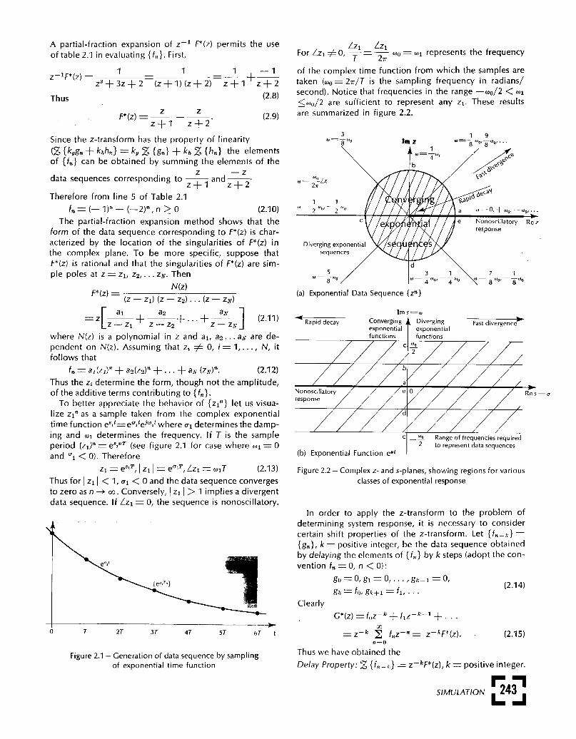
lize Zn as a sample taken from the complex exponentialtime function e81t = ealtejwlt where (11 determines the damp-ing and w, determines the frequency. If T is the sampleperiod (zi)l = e8inT (see figure 2.1 for case where ~1 = 0and ’l < 0). Therefore

Thus for I Z1 < 1, Ql < 0 and the data sequence convergesto zero as n - oo. Conversely, I Z1 > 1 implies a divergentdata sequence. if Zzi = 0, the sequence is nonoscillatory.

Figure 2.1 - Generation of data sequence by samplingof exponential time function

represents the frequency

of the complex time function from which the samples aretaken (wo = 2~/T is the sampling frequency in radians/second). Notice that frequencies in the range -~0/2 < wi

<wo/2 are sufficient to represent any zi These results

are summarized in figure 2.2.

Figure 2.2 - Complex z- and s-planes, showing regions for variousclasses of exponential response

In order to apply the z-transform to the problem ofdetermining system response, it is necessary to considercertain shift properties of the z-transform. Let {fn_~~} ={gn}, k = positive integer, be the data sequence obtainedby delaying the elements of {fn} by k steps (adopt the con-vention fn = 0, n < 0):

Clearly

Thus we have obtained the .

Delay Property: ~ (fn-d = z-kF*(z), k = positive integer.

244

Consider now the advanced data sequence {fn+k} =={gn}, k = positive integer, that is

We can write

This gives the

Advance property:

k = positive integer

Let us use this last property to obtain the solution of alinear difference equation.

Example 2.4: Solution of the forced, second-order,linear difference equation

co, cl = specified initial values. (2.18)

Since this equation holds for any n > 0, we have

Here {r,t} should be interpreted as the input or forcingsequence and {cn} as the output or response sequence.Taking the z-transform of (2.19) by utilizing the advanceproperty yields

11

This may be solved for C*(z),

The first two terms on the right side of (2.21) are initialcondition or transient terms; the last term represents theforced part of the response. By using a partial-fractionexpansion the reader may confirm that for a &dquo;step input,&dquo;rn = 1, n > 0, the response is

If in Example 2.4 the system is initially at rest (co = cl= 0) the z-transform of the response can be written

where H*(z) _ (z -+ 1/2)-1 (z ~- 1/3)-1 l can be inter-

preted as the transfer function of the system.Let us pursue this interpretation further. Consider a sys-

tem which processes an input data sequence {rn~ by theformula

to produce an output data sequence {cn}. This type ofsystem which occurs commonly, we will call a digital sys-tem. Following well-established terminology, we say thatfc,) is the convolution of the sequences fr.} and fh.).From

the substitution k = n - m, and rk = 0 for k < 0, it is

seen that

Letting

equation (2.26) can be written as equation (2.23). Thusfor co, cl = 0 the system described by the differenceequation (2.18) is a digital system whose output can beexpressed by the convolution formula (2.24). The sim-

plicity of (2.23) as compared with (2.24) is one of thereasons why the z-transform is an effective tool for an-

alyzing systems with sampled data.Many properties of digital-system response can be de-

termined from H*(z). For example, a digital system isstable if H*(z) is analytic for I z > 1. This seems reason-able in view of the results of figure 2.2. Also, by utilizing(2.24) it is easy to show that rn = ej(,)n7&dquo; - oo < n < + oo,gives cn = H*(ejwT)ejwnT. Thus the magnitude and angleof H*(e»T) represent the &dquo;gain&dquo; and &dquo;phase shift&dquo; of the

digital system for an input which is obtained by samplinga sinusoidal time function with frequency (ù.

245

3 APPLICATION OF THE z-TRANSFORM TO THEANALYSIS OF INTEGRATION METHODS

When differential equations are solved on the digital com-puter, they must first be &dquo;approximated&dquo; by differenceequations. The z-transform provides a method of investi-gating the dynamic errors introduced by this approxima-tion. The differential equations considered here are linear,and of first and second order. By laborious calculationsor the use of vector notation, results similar to those de-scribed may be obtained for linear systems of higherorder. In any case, most complex dynamical systems in-clude a number of linear first- and second-order loops.Thus the results of this section give considerable insightinto the nature of the dynamic errors. Computer round-off errors, which may be a serious problem with high-orderintegration formulas such as Runge-Kutta, are a nonlineareffect and are not investigated.

3.1 The Euler method, solution of a first-orderdifferential equation

The Euler method is the simplest and most naive approachfor constructing the approximating difference equation.In it the solution of the differential equation is extendedover an integration period by making the approximationthat the rate-of-change of the solution is constant. Thusif the differential equation to be solved is

its approximating difference equation is

where T is the (fixed) interval or step size and r~ = r(nT).Taking xo = x(0), successive application of equation (3.2)generates a sequence of points {xn}, which, if T is suffi-

ciently small, should approximate {x(nT)}, where x(t) is

the desired solution of (3.1). Let us now explore the natureof the approximation for the linear case where equations(3.1) and (3.2) become

.. , J’ ø_. &dquo;...........

Viewing (3.4) as the sequence relationship fx.+,) =(1 ~-- Ta){xn~ -f- Tb{rn}, we obtain from the advance prop-erty of the z-transform

Thus

First we examine the unforced solution of (3.4), R*(z)=0.Then reference to table 2.1 yields from (3.6)

If this equation is written as

o- represents the effective exponential constant obtainedin the solution of (3.4). Since the unforced solution of

(3.3) is x(t) = e~xo, (J’ should ideally be equal to a. From(3.7) and (3.8), eaT = 1 -~- aT. Thus

Using the power series In l

+ ... it follows that for aT <

Therefore the attained exponential constant is too small bya fractional error (1/2) aT.Now consider the response due to input forcing. A

variety of different test inputs can be used to evaluate thesolution error, but the sinusoidal input r(t) = ejúJt givesthe greatest insight. With xo = 0 equation (3.6) takes theform of equation (2.23) where the transfer function is

For (3.3) the transfer function for sinusoidal inputs is

R(jw) = b(jm - a)-’. Thus the magnitude and angle of

represent the gain and phase error introduced by (3.4).Equation (3.12) may be evaluated at any frequency w.

For example, R-1(j0)H*(ejO) = 1, and thus there is no errorfor the constant input r(t) = eil = 1. Another good testfrequency is ~ = a, where R(jm) gives a phase shift of-45° and the gain is down from H(j0) by 2’~. Usinga power series in a7 for e~, we obtain

Thus the error is the order of aT and (3.4) is a good rep-resentation of (3.3) only if aT < < 1. When a = 0 in (3.12),it is easy to show thatH-1(j~)H*(e’~’l’)=1-~-j(1/2)~T-(1/6)ro2T2 -i-- ~ ~ Thus when (3.3) corresponds to an integrator(a = 0), the error is small when roT < < 1.

3.2 The Euler method, solution of a second-orderdifferential equation

Second-order differential equations are introduced byconsidering the solution of the simultaneous first-orderdifferential equations

Following the pattern developed in Section 3.1, the Eulermethod yields

The special problem to be analyzed here is the second-order system x ~- 21k -f- x = r(t), whose undamped naturalfrequency is one radian/second and whose damping ratiois ~. By introducing x = y we obtain

which is in the format of (3.14). Thus the Euler integrationmethod gives

246

By using the z-transform on (3.17) we obtain

Solving these equations for X*(z) gives

To obtain the unforced solution we set R*(z) = 0 and

compare with lines 8 and 9 of table 2.1:

where

This equation can be written as

where Q and m determine the damping and frequency ofthe solution. By inspecting the solution x(t) of (3.16), it

can be shown that x(nT) = xn if Q = &horbar;~ and W = y1 _1;2.Actually, comparison of (3.20) and (3.21) shows

Thus the effective error in the damping ratio varies ap-proxi mately as the first power of T(T < < 1), being too low

for ,< 1/y2 and too high for ,> 1/y2. If ,== 0, theresponse diverges when it should remain bounded. Fornonzero ~, the attained frequency is fractionally high by~T(TGG1).

An analysis of the error for sinusoidal forcing can becarried out as in Section 3.1. For example i4-’(jO)H*(ejo)= 1, and again there is no error for a constant input. For0 < w < < 1/T, it is easy to show that the error is theorder of T.

3.3 The Heun method, solution of a first-orderdifferential equation

The Heun method achieves better accuracy than the Eulermethod by working with data at both ends of the integra-tion interval. It converts the differential equation (3.1) tothe difference equation

Thus for (3.3) we obtain

and hence from the z-transform

Consider now the solution of (3.24) for rn = 0, n > 0.

From table 2.1 and (3.25)

Comparing (3.26) and (3.8) as in Section 3.1 yields

Thus the attained exponential constant Q is too small bya fractional error (1/6) T2a2(Ta < < 1)/ a great improve-ment over the(1/2)Ta obtained with the Euler method.

Writing the last term in (3.25) as H*(z)R*(z), it is seen

that

Thus the error for sinusoidal forcing may be determinedfrom H*(ejwT). As before Fl-’(jO)H*(ejO) = 1. Using a powerseries expansion for e~~ it can be shown that

Comparing this with (3.13), it is seen that the error termis the order of (aT)2 rather than aT. Thus the error forsinusoidal forcing is much less than that obtained withthe Euler method. if in (3.3) a = 0, it is easy to show that

H-1(j~)H*(e’‘~T) = 1 - (1/12) w2T2 +... where the omit-ted terms are of order (T~)4 and higher. Thus when (3.3)is an integrator, a small sinusoidal response error willresult for (w T)2 < < 1.

247

3.4 The Heun method, solution of a second-orderdifferential equation

The application of the Heun method to (3.14) yields

After some manipulation, the application of (3.29) to

(3.16) gives

To simplify further developments it will be assumed that~ = 0. Then it follows from the z-transform, (3.30), andthe elimination of Y*(z) that

Again we examine the unforced case, R*(z) = 0. Bycomparing the first term in (3.31) with lines 8 and 9 ofTable 2.1, it is seen that

where

Ideally xn should be given by (3.21) (with C = 0), whereor = 0 and w == 1. Actually, comparison of (3.21) and (3.32)gives

Thus a very notable improvement over the Euler methodis noted (see equations (3.22)).

3.5 The Runge-Kutta method, solution of afirst-order differential equation

The Euler and Heun methods discussed in the previoussections lead to difference equations which are examplesof a family of formulas called Runge-Kutta formulas. 3’7

As these formulas become more complex, they tend toproduce more accurate results. In this section we examineone of the more commonly used methods which takesthe name of the family of formulas.With the Runge-Kutta method the difference equation

corresponding to (3.1) becomes

The function 0 (which is called the increment function)is sufficiently complex that it is best defined in terms ofthe following set of formulas:

If (3.34) and (3.35) are applied to (3.3), after some manip-ulation it follows that

Since the basic sampling period on the input is (1/2) T(half the sampling period for the response), it should bethe basic period if we wish to obtain the transfer function

by the z-transform. That is, we should replace n by 2m,Xn byzm, Xn+l by xm+2~ rn by 7:n =r(m (1/2) T), rn+1/2 byrm+ 1, and rn+1 by ~+2. Then -xm, evaluated for m = evenintegers, gives xn. In order to avoid this complication, wewill consider (3.36) only for the unforced case. Then z-transform may be applied to (3.36) in the customaryfashion to yield

The above result and reference to table 2.1 shows that

248

Following the approach taken in previous sections

which can be written

Thus the fractional error in the attained exponential con-stant is only (1/120) (Ta)4.The steps in evaluating formulas (3.35) may require

considerable computer time. It would be much quickerto solve directly the equation Xn+1 = axn + (3ofn +Pirn+1/2 + (32fn+lt where a, (30, ~31, and p2 are obtainedfrom (3.36). Of course, this simplification is feasible onlyif (3.1) is linear.

3.6 Multistep methodsThe methods of Euler, Heun, and Runge-Kutta are examplesof one-step methods, where the solution at index n + 1can be determined from the solution at index n. For multi-

step methods the solution at index n and still earlierindices is required. This section examines briefly multistepmethods of the linear type.

For the first-order differential equation (3.1), the linearmultistep method yields

where

Notice that for the first-order differential equation this

k-step formula is a kth order difference equation. GivenXo, Xl, - - - x~;_1 equation (3.41) can be solved for Xk, andthen successively for xk+1, ~ ~ ~ . If the formula is closed

(@o# 0) and f(x, r) is nonlinear, (3.41) may present somedifficulty in that xn+~; is contained in fn+1, and thereforeits determination from xn+~;_1, ... , xn involves the solu-tion of a nonlinear equation. Various predictor-correctorschemes are available for solving this problem. The k-stepformula also has a &dquo;start-up problem&dquo; in that one mustknow more than Xo to begin. Usually xl, ... Xk-l are sup-plied from Xo by k - 1 iterations of a one-step methodsuch as Runge-Kutta.

For the linear differential equation (3.3), the k-stepformula yields

In order to avoid the complexity of treating initial condi-tion terms, let us assume hereafter that xo, xl, ... I Xk-1

and ro, ri, ... r~;_1 are all zero. Then the z-transform of

(3.43) gives

which by introducing

can be written as

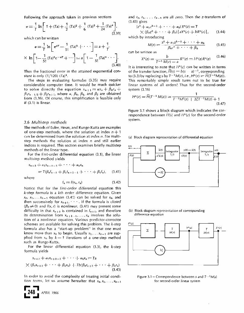
It is interesting to note that H*(z) can be written in termsof the transfer function, H(s) = b(s - a) -1, correspondingto (3.3) by replacing s by T-1M(z), i.e.,H*(z) = H(T-1M(z)).This remarkably simple result turns out to be true forlinear systems of all orders! Thus for the second-order

system (3.16)

Figure 3.1 shows a block diagram which indicates the cor-respondence between H(s) and H*(z) for the second-ordersystem.

(a) Block diagram representation of differential equation

(b) Block diagram representation of correspondingdifference equation

Figure 3.1 - Correspondence between s and T-1M(z)for second-order linear system

249

Let us now consider some specific realizations of (3.43).For k = 1, lY1 = -1, (30 = 0, pi -- 1, we have the Eulermethod. The reader may verify (3.11) and the last term of(3.19) by the substitution rule given in the preceding para-graph. It turns out that similar substitution rules do notexist for the more elaborate single-step methods such asthe Heun and Runge-Kutta methods.

have the two-step Nystrom method. Substituting

for s in H(s) = b(s - a)-’, we obtain H*(z) correspondingto the differential equation (3.3):

where

Recalling equations (2.11), (2.12), and (2.13) and lettingX*(z) = H*(z)R*(z), it is seen that one response term of

{xn} will have the form al(zl)l = al(e$1T)n. Since

it is seen that al(zl)n corresponds closely to samples takenfrom the expected transient response term in the solutionof (3.3), ce-ut. Thus the attained exponential constant Qlapproximates a within a fractional error of 1/6(Ta)2. Thisis the same result obtained by Heun’s method. The re-

sponse term a2(z2)n is undesired and appears because

(3.43) is a second-order difference equation acting as an&dquo;approximation&dquo; of a first-order system. If a < 0, that is

the transient response of (3.3) is damped, z2 - -1 -f- Tahas magnitude greater than one, and (Z2)n ~ oo as n ~ oo .In this case the method is said to be weakly unstable(weak because I z21 - 1 as T --> 0) and will for sufficientlylarge n give inaccurate results. If a2 is very small (as it

often is )this may not be a problem.The sinusoidal response errors for the Nystrom method

may be evaluated as in previous sections, with the follow-ing results:

Thus the error here is comparable with that obtained forHeun’s method, (3.28). -

Similar results are obtained when the Nystrom methodis applied to systems of higher order. If a linear differ-ential equation has a characteristic root 1, i.e., H(s) hasa pole at 5 = 1, the substitution rule implies H*(z) has

two poles at zl and 72 where (Zi2 - 1) ~2z~T~ -1 = À or

The pole at zi is the desired one in that

approximates .1. For example, the differential equationX -+- x = r(t) leads to H(s) = (s2 -f- 1)-1 which has poles at±j. Thus H*(z) has four poles, the desired two being at±j [1 + (1/6) T2 + (3/40) T4 + - - - 1. These values indi-cate that the approximate system has the desired dampingof zero, but that the natural frequency is 1 + (1/6) T2 2

+ (3/40) T4 + ..- rather than 1. Note that the undesiredpoles of H*(z) are at -1 ± jT -~ ~ ~ ~ and (for T < < 1)are outside the unit circle in the z-plane. Thus for thissystem the Nystrom method is weakly unstable.

Finally consider the two-step Simpson-Milne methodwhere k = 2, «1= 0, CX2 == -1, ~(30 =1 /3, ~31 = 4/3, p2=1 /3.Thus

and it is a simple exercise to derive the results correspond-ing to those obtained for the Nystrom method. In par-

ticular, corresponding to (3.50) and (3.51), we have

Thus the fractional error in the attained exponential con-stant is improved from (1/6)(Ta)l to (13/72) (Ta)4 (for Ta< < 1). Also for a < 0, ~ 1 Z21 > 1, and the method is

weakly unstable. For the second-order system, the attaineddamping is again zero, while the natural frequency is

1 &horbar; 13/72 7~+ - - - .

3.7 Derivation of difference equations byquadrature formulas

For any linear differential equation, it is possible to expressthe solution in closed form. By applying quadrature inte-gration formulas to such solution expressions, a family ofdifference equations may be derived which are differentfrom those discussed in previous sections. To keep thepresentation reasonably brief we will consider only (3.3),

250

although it is possible to derive similar results for time-varying linear differential equations of any order.

Equation (3.3) has the closed-form solution

Let us obtain an approximation to 7(T) by using a quadra-ture formula for the integral on the right side of (3.58).A simple quadrature integration formula can be obtainedby letting r(t) be approximated by

Then

which when integrated gives

This suggests the difference equation,

as a method for obtaining an approximate solution of (3.3).Let us examine (3.61) by methods of the previous sections.The z-transform of (3.61) gives

Thus

For the unforced case, R*(z) = 0, table 2.1 yields

Therefore xn =7(nT) and there is no solution error!Before becoming too elated about the desirability of

(3.61), let us consider the response with sinusoidal forc-

ing. Noting that H*(z) = a-I [eaT - 1 ~ ] b(z - eaT)-1 it is

easy to show that

Thus the error is comparable to that attained with theEuler method. From the manner in which (3.61) was de-rived, it is clear that there are inputs for which xn = X(nT).For instance, suppose r(t) is the unit step at t=0, i.e.,r(t) = 1 for t > 0, and r(t) = 0 for t < 0. Then the ap-proximation made for r(a) in (3.58) becomes exact. How-

ever, if the step occurs at some other time, such as

t=.1T, the error may be quite large.We can obtain an improvement over (3.61) by using

a better quadrature formula. For 0 < t < T, let r(Q) in (3.58)be approximated by ro ~- T-I(rl - ro)Q. Then

Once the indicated integrations are performed:

Thus we use the difference equation which is obtainedfrom (3.67) by augmenting the indices by n. For R*(z) = 0we again have (3.64), and there is no error for the un-forced case.

With sinusoidal forcing it can be shown that

Therefore the errors are comparable to those obtainedwith Heun’s method and the Nystrom method. For anyinput r(t) which is piecewise linear with jumps, and jumpsin slope only at t = nT, n = 0, 1, ... , there will be nosolution error. In practical applications, however, thereis no reason to believe that the input will have this form.

Higher-order difference equations of the above typecan be derived. For instance, by approximating r((T) by acubic, a difference equation which compares favorablywith the Runge-Kutta equation (3.38) may be derived.

However, in this case the fact that the unforced solutionhas no error is not of great importance because the Runge-Kutta method produces an unforced solution of very highaccuracy.

3.8 Summary and remarksMany of the results obtained in previous sections are

summarized along with a few more in table 3.1. The valuesshown are approximate in that additive terms of higherpowers in T are omitted.

Let us compare the integration methods with respectto their performance on the period of the undamped sec-ond-order differential equation. To keep the error in

period below 1 part in 104 with the Runge-Kutta method,it is necessary to have T4 < 120 X 10-4 or T < .33. This

corresponds to 2~/.33 - 19 points per cycle. For themethods of Heun, Nystrom, and Simpson-Milne the cor-responding numbers are, respectively: 256, 256, and 41.

It should be pointed out that there are many otherfactors besides those above which enter into the choiceof a method. For example, the complex operations re-

quired at each step in the Runge-Kutta method may leadto large solution errors because of computer round-offerrors. Thus from a practical point of view, the Simpson-Milne formula may be more satisfactory (provided theintegration period is sufficiently short so that the instabil-ity of the method is not a factor).

Another important factor which is freauently overlookedis the required &dquo;smoothness&dquo; of the differential equationsbeing solved. For example, the Runge-Kutta formula for&dquo;approximating&dquo; the first-order differential equation (3.1)is derived under the assumption that

are continuous in x and t. 3>7 in many practical problems,such as an on-off control system, f (x, r(t) ) may be discon-tinuous in t and even the Euler method is subject to doubt.

251

To explore this difficulty further, consider the solutionof (3.3) where b = -a and r(t) is the unit step functionat t = 0. The actual solution is

The corresponding solutions obtained from the differenceequation representations of (3.3) are:

Euler:

Heun:

Runge-Kutta: ;

Nystrom:

where for the coefficients of [ n additive terms of order(Ta)2 and higher have been omitted. Thus for small n theerrors produced by all methods are the same order of

magnitude. For large n the Nystrom method is par-

ticularly bad for a < 0 because the term 1/2 Ta[z2]n= 1/2 Ta ~-1 --~ aT ~- ~ ~ ~ ~n, which is initially large,grows rapidly. The above results may become even worseif the step is not applied at t = 0, since the sampling ofr(t) means that the position of the jump is uncertain with-in a timing error of up to T(T/2 in the case of Runge-Kutta).

Perhaps a less artificial method for evaluating the errors

present with rapidly varying inputs is to use sinusoidal

response. For the first-order system and w = a it has been

observed [see (3.13), (3.28), (3.52)] that errors are smaller

for the better integration methods. Table 3.1 shows someadditional results for the first-order system, where w =

(1/4)o)o, (1/2)~0, and wo = 2</T is the sampling frequencyassociated with the integration-formula step size. It has

been assumed that (aT) < < 1, and terms of higher orderin aT than those given have been omitted. In every case

the values H-1(j~)H*(e~~T) - 1 shown depart considerably .

from the desired value of zero. As might be suspectedfrom the stability result of the previous paragraph, theNystrom method gives particularly bad results.

Problems of the type described above can sometimes

be detected during the numerical integration by evaluat-ing residual terms generated by the integration formulas.In such cases the step size T may be adjusted automaticallyto bring the errors down to an acceptable level.

Table 3-1 -Approximate results for various integration methods

252

4 METHODS FOR THE ANALYSISOF MIXED-DATA SYSTEMS

The dynamic analysis of hybrid systems is inherently moredifficult than the analysis of digital systems, which havebeen the subject of the previous sections. This added

difficulty occurs because of the joint presence of datasequences and time functions (continuous-data signals).In this section we extend the z-transform to the treatment

of general systems with mixed data, and in the next sec-tion we apply the theory of this section to the dynamicanalysis of several hybrid systems. As in Section 2, thetreatment here is abbreviated, and for additional detailthe reader should see reference 1, which takes the pointof view developed below, or other texts on the theory ofsampled-data systems.

First of all let us review the methods for expressing theresponse of continuous-data systems. If the system is

linear, time-invariant, and initially at rest, it is possibleto write

where r(t) is the input, c(t) is the output, and h(t) is the

impulse response. Alternatively, by introducing the La-

place transform of the three time functions, e.g.,

the convolution integral (4.2) may be replaced by

Because of the inherent simplicity of the frequency do-main characterization, we will favor it in our subsequentwork.Now consider the simple mixed-data system shown in

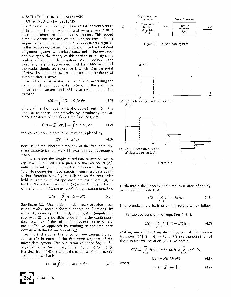
Figure 4.1. The input is a sequence of the data points fr.}with the point rn being generated at time nT. The digital-to analog converter &dquo;reconstructs&dquo; from these data pointsa time function rr(t). Figure 4.2b shows the zero-orderhold or zero-order extrapolation process where re(t) isheld at the value rn for nT < t < nT + T. Thus in terms

of the function h,(t), the extrapolation generating function,

See figure 4.2a. More elaborate data reconstruction proc-esses involve more elaborate generating functions. Byusing re(t) as an input to the dynamic system (impulse re-sponse hs(t)), it is possible to determine the continuous-data response of the mixed-data system. Let us seek a

more effective approach by working in the frequencydomain with the z-transform of (run).

As the first step in this direction, we express the re-

sponse c(t) in terms of the data-point response of themixed-data system. The data-point response h(t) is the

response c(t) to the unit input: ro = 1, rn = 0 for n > 0.It is clear from (4.4) that h(t) is the response of the dynamicsystem to he(t), that is

Figure 4.1 - Mixed-data system

Figure 4.2

Furthermore the linearity and time-invariance of the dy-namic system imply that

This formula is the basis of all the results which follow.

The Laplace transform of equation (4.6) is

Making use of the translation theorem of the Laplacetransform (2 [ f(t - T) ~ = F(s) e-ST) and the definition ofthe z-transform (equation (2.1)) we obtain

where

253

Note that H(s) = H,(s)H,(s) follows from (4.5) in the sameway that (4.3) follows from (4.1). Thus in the frequencydomain a very simple expression for system response holds(compare with (4.6)). For apparent reasons H(s) is calledthe data-point transfer function of the mixed-data system.Although we will find (4.8) most useful in setting up re-sponse equations for complex interconnections of systems,it is not very useful for actually evaluating c(t). This isbecause C(s) is generally a mixture of functions rational ins and rational in e8T, and tables of inverse Laplace trans-forms for such functions are not available.

While it is difficult to obtain c(t) for all t > 0, it is notdifficult to obtain c(t) for t = nT, n = 0, 1, .... Employingequation (4.6),

Defining hm = h(mT), (4.10) can be written as

Thus the results of Section 2 imply that

where

From C*(z), cn may be evaluated using the proceduresdescribed in Section 2, e.g., the inverse z-transform, thepower series expansion in z-1, and tables.

If the response c(t) is sufficiently &dquo;smooth&dquo; so that it is

&dquo;well represented&dquo; by f cn}, (4.12) serves as an adequatedescription for the dynamic response of the mixed-datasystem. By comparing (4.12) and (2.23), we see that wemay interpret the mixed-data system as a digital system.Thus, for example, if rn = ejúJnT, - oo < n < oo,

and H*(ei°T) determines the &dquo;gain&dquo; and &dquo;phase shift&dquo; at

frequency M. Our remaining problem is to obtain H*(z)when the sampled-data system has a more complex con-figuration than that shown in figure 4.1.The complex systems which we wish to consider con-

sist of the interconnection of the basic elements shownin figure 4.3. In addition to the response expressions shownin figure 4.3, we need the following notation,

Thus the z-transform of a time function is the z-transformof the data sequence generated by taking samples of thetime function at t = nT. Correspondingly, the z-transformof a Laplace transform F(s) is the z-transform of the timefunction f(t) corresponding to the Laplace transform F(s).If f(t) is piecewise continuous with a jump at t= nT forsome integer n, particular care must be taken in the defi-nition of ~ ~ [f(t)]. See reference 1. Using this notation,we will now derive the following important result:

Figure 4.3 - Basic elements of sampled-data systems

First note that by the definition of Y*(z) -

From the translation theorem of the Laplace transform, it

follows that the time function

we have by the convolution property

of the z-transform

In reference 1, Section 15, formula (4.16), and the re-sults of figure 4.3 are used to derive transfer function

expressions for a variety of complex systems. We limit ourderivations to the hybrid systems of the next section.

--

254

5. ANALYSIS OF HYBRID COMPUTER SYSTEMSIn this section we will illustrate, by means of several ex-amples the application of the methods of Section 4 to theanalysis of hybrid computer systems. As in Section 3 we

must assume that the systems treated can be representedsatisfactorily by a linear model.

Let us consider a hybrid system where differential equa-tions are integrated by means of analog elements, butwhere some of the required generation of nonlinear func-tions is implemented by table storage in a digital com-puter. To be more specific, let us direct our attention to

a typical computer loop, which might occur as part of anelaborate computer simulation. The differential equationbeing solved by this loop has the form

where x is an acceleration; F (x/ y(t), z(t)/ ...) is a non-

linear force term, dependent on x and other computervariables such as y(t) and z(t) ; and f(t) is an external forc-

ing function. Figure 5.1 shows the computer block dia-gram necessary for implementing (5.1) when F is generatedby a digital computer.The required computer operations proceed as follows.

At time t = nT the variables x(t), y(t), z(t) are sampled.Then they are given a digital representation by the con-version system and are stored in the computer memory.After a table look-up (which may involve interpolation),the digital computer places the value F(xn, yn, zn, ...) inthe output register. Let us suppose that all these stepsare carried out before t = nT + T. Then at t = nT -~- Tthe value F(x,,, Yll/ Z,1, ...) is transferred to the register of thedigital-to-analog converter, where it produces a constantanalog value F(xn, y,,, zn, ...) (within the quantizing error)during the period nT + T < t < nT + 2T. Different com-puter arrangements are possible (e.g., longer delay, moreelaborate data hold), but this is what will be used for the

subsequent analysis.In order to simplify things still further, let us make the

following assumptions: a) y(t), z(t),... are varying veryslowly so that they may be assumed constant with valuesy and z; b) for the range of x(t) considered F(x, y, t ...)- a2x. While these assumptions may not always hold, theywill at least allow us to get some feeling about the dy-namics of the process. Figure 5.2 shows the simplified sys-tem using the notation of figure 4.3.

Let us now apply the theory of Section 4 to the determi-nation of a response expression. Working in the frequencydomain, we see from figure 4.3b

The zero-order hold (D-to-A converter), having a data

sequence for an input and function of time for an output,is a mixed-data system. Since a unit data point (co = 1;c,, = 0, n > 0) at its input produces a response

(see figure 4.2), the data point transfer function is 2 [h(t) ]= H(s) _ (1 - e-ST)s-1. In any case figure 4.3d showsthat

Because D*(z) represents the function generation whichhas a computer lag of one sample period, the delay prop-erty of the z-transform gives D*(z) = a2z-1, i.e.,

Substituting (5.4) and (5.5) into (5.2)

We would like to solve (5.6) for either X or X*, but cannotbecause X and X* are both contained in the equation. Toget around this difficulty, we take the z-transform of (5.6),using (4.16) on the last term [X(s) - G(s)H(s), Y*(el’) -D* (e IT )X*(e IT) I, and obtain

Once we have determined (1 -~- D*(z)GH*(z) ~ -1=Y*(z) we can use (5.8) to determine X*(z) and hence {x(nT)}for a variety of inputs. For instance, if f(t) is the unit stepat time t = 0, F(s) = 1/s, and G(s)F(s) = 1/s3 correspondsto t2 /2, which is the double integral of the unit step. Thus

a result which follows from Table 2.1 or still more simplyfrom a table of z-transforms of Laplace transforms (refer-ence 1, table 13.1). Alternatively, if f(t) = eil&dquo;, we find

Thus the gain and phase shift of the hybrid system may beevaluated. Notice that in our development above we haveomitted all initial-condition terms, that is, we have as-

sumed the system to be initially at rest. To do otherwisewould introduce additional complexity. It is also possibleto obtain an expression for C(s), but it is too complex towork with conveniently.

_

Let us now determine GH*(z) and Y*(z). From the above-

-... -.. - - .

where we have observed from the translation property ofthe Laplace transform that the data sequence correspond-ing to s-3e-ST can be obtained by delaying the data se-quence corresponding to S-3 by one sample period. Wehave seen in the preceding paragraph that ~ (s-3~ = TZ/2X (z&horbar;1)-~z(z+1). Thus

Finally,

255

Figure 5.1 - Block diagram of hybrid system

Figure 5.2-Simplified representation of figure 5.1 showingmathematical operations and notation

Figure 5.3-Approximate representation of system in figure 5.2

It has been demonstrated in our analysis of integrationmethods that the poles of the system transfer function area good indication of system response because they de-termine the form of the response terms originating fromthe system properties. There are three poles of Y*(z) at zi,Z2, and z3. Let us determine zl, Z2, and Z3. For aT = 0 it isclear that the characteristic equation Z3 - 2z2 + [1 +(1/2)a2T2]z+(1/2)a2P==0 has a root z, 0. Thus foraT ~ 0 but 0 < aT < < 1, ZI - 0. By letting ZI = cl(aT)~- c2(aT)2 + ... and choosing ci, 02. ’ ’ ’ to make zi bea solution of the characteristic equation, it can be shownthat

By factoring the characteristic equation, we have

By using the quadratic formula on the quadratic in thebrackets and substituting for zl from (5.13), it follows that

Since zi, < < 1, the response term corresponding tozi decays very quickly and does not play a significant rolein system response. If the hybrid system is to give highsolution accuracy, the remaining roots, Z2 and Z3, shouldbe properly related to the solution properties of (5.1). In

particular, with F= a2x the system (5.1) is linear and hastransient response terms of the form e:!:jal, ;.e., the re-

sponse is purely oscillatory with frequency a. This meansthat if we write Z2, Z3 = eaT e:!:jù)T/ we should have « = 0and M==a. Actually, from

and

we see that

and

Thus we have errors in both the frequency and damping.The damping error corresponds to an attained dampingratio § - - (3/4) aT, and, being to the first power in aT,is the worse of the two. The values of a and (o are perhapsthe best single indicators of overall computational accu-racy for the system in figure 5.1. A complete analysis ofthe type undertaken in section 3 would include determi-nation of initial condition response and sinusoidal re-

sponse.Let us see if we can obtain a further understanding of

the source of the above errors. Consider the approximaterepresentation of the system shown in figure 5.3. Herewe have replaced the sampling, function-generation, anddata-hold operations with a transport lag (transfer func-tion e-11) and gain a 2. The delay time T should includethe delay T in the digital computer, and some measure of

256

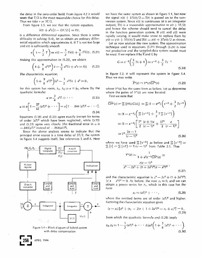
the delay in the zero-order hold. From figure 4.2 it wouldseem that T/2 is the most reasonable choice for this delay.Thus we take T = 3T/2.

From figure 5.3, we see that the system equation,

is a difference differential equation. Since there is some

difficulty in solving (5.4), let us obtain an ordinary differ-ential equation which approximates it. If T is not too largeand x(t) is sufficiently smooth

Making this approximation in (5.20), we obtain

The characteristic equation,

for this system has roots, ’B’1, k2 = « ± j~, where (by thequadratic formula)

Equations (5.18) and (5.23) agree exactly (except for termsof order (aT)3 which have been neglected), while (5.19)and (5.24) agree very closely (the fractional error in w is

-.844(aT)2 instead of -.864(aT)2).Since the above analysis seems to indicate that the

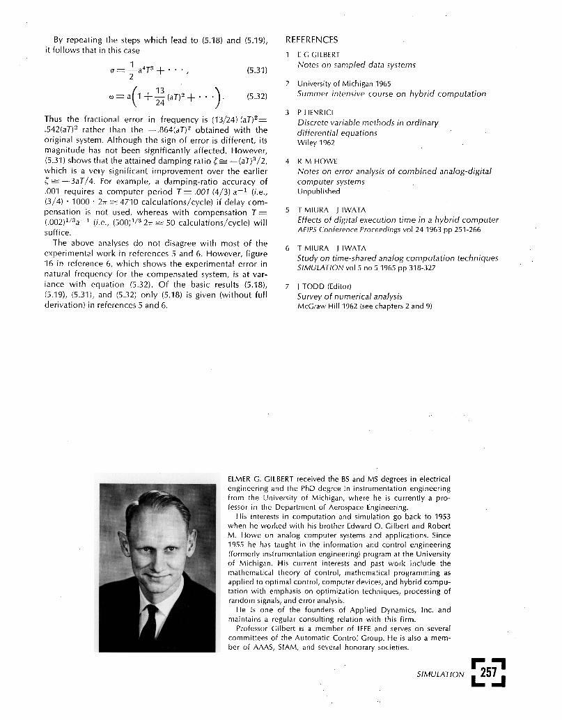
principal error source is a time delay of 3T/2, the systemin figure 5.4 suggests itself. See references 5 and 6. Here

Figure 5.4 - Block diagram of hybrid systemwith delay compensation

we have the same system as shown in figure 5.1, but nowthe signal x(t) + 3T~(t)/2 = X(t) is passed on to the con-version system. Since x(t) is continuous (it is an integratoroutput), 7(t) is a reasonable approximation to x(t + 3T/2)and hence the scheme should tend to cancel the delayin the function generation system. If y(t) and z(t) were

rapidly varying, it would make sense to replace them byy(t) = y(t) + 3T~(t)/2 and z(t) = z(t) + 3Tz(t)/2 as shown.

Let us now analyze this new system. The approximationtechnique used in equations (5.21) through (5.24) is nownot productive and the sampled-data system model mustbe used. If we replace X by X and G by

in figure 5.2, it will represent the system in figure 5.4.

Thus we may write

where Y*(z) has the same form as before. Let us determinewhere the poles of Y*(z) are now located.

First we note that

where we have used ji§ [s-3] as before and jg [s-2] _~[f]==~(r)7}=7z(z&horbar;1)~ from Table 2.1. Thus

and the characteristic equation is z3 - 2z2 + (1 -~- 2a2T2)X z - a2T2 = 0. As before, the root Zl - 0, and we canobtain a power series for zl, which in this case has theform

where the omitted terms are of order (aT)’ and higher.Factoring the characteristic equation gives

from which the quadratic formula and (5.28) imply

257

By repeating the steps which lead to (5.18) and (5.19),it follows that in this case

Thus the fractional error in frequency is (13/24) (aT)2=.542(aT)2 rather than the -.864(aT)2 obtained with theoriginal system. Although the sign of error is different, its

magnitude has not been significantly affected. However,(5.31) shows that the attained damping ratio ~~&horbar;(a7)~/2,which is a very significant improvement over the earlierI n -3aT/4. For example, a damping-ratio accuracy of.001 requires a computer period T=.001 (4/3) a-’ (i.e.,(3/4) ~ 1000 - 2< n 4710 calculations/cycle) if delay com-pensation is not used, whereas with compensation T =(.002)~a-i (i.e., (500) 1/3 2-,7 ~--- 50 calculations/cycle) willsuffice.The above analyses do not disagree with most of the

experimental work in references 5 and 6. However, figure16 in reference 6, which shows the experimental error innatural frequency for the compensated system, is at var-iance with equation (5.32). Of the basic results (5.18),(5.19), (5.31), and (5.32) only (5.18) is given (without fullderivation) in references 5 and 6.

REFERENCES

1 E G GILBERT

Notes on sampled-data systems

2 University of Michigan 1965Summer intensive course on hybrid computation

3 P HENRICI

Discrete variable methods in ordinarydifferential equations Wiley 1962

4 R M HOWE

Notes on error analysis of combined analog-digitalcomputer systemsUnpublished

5 T MIURA J IWATAEffects of digital execution time in a hybrid computerAFIPS Conference Proceedings vol 24 1963 pp 251-266

6 T MIURA J IWATA

Study on time-shared analog computation techniquesSIMULATION vol 5 no 5 1965 pp 318-327

7 TODD (Editor)Survey of numerical analysisMcGraw Hill 1962 (see chapters 2 and 9)

ELMER G. GILBERT received the BS and MS degrees in electricalengineering and the PhD degree in instrumentation engineeringfrom the University of Michigan, where he is currently a pro-fessor in the Department of Aerospace Engineering.

His interests in computation and simulation go back to 1953when he worked with his brother Edward O. Gilbert and RobertM. Howe on analog computer systems and applications. Since1955 he has taught in the information and control engineering(formerly instrumentation engineering) program at the Universityof Michigan. His current interests and past work include themathematical theory of control, mathematical programming asapplied to optimal control, computer devices, and hybrid compu-tation with emphasis on optimization techniques, processing ofrandom signals, and error analysis.He is one of the founders of Applied Dynamics, Inc. and

maintains a regular consulting relation with this firm.Professor Gilbert is a member of IEEE and serves on several

committees of the Automatic Control Group. He is also a mem-ber of AAAS, SIAM, and several honorary societies.