arX

iv:c

ond-

mat

/051

0711

v4 [

cond

-mat

.oth

er]

3 O

ct 2

006

Fractional-Period Excitations in Continuum Periodic Systems

H. E. Nistazakis1, Mason A. Porter2, P. G. Kevrekidis3, D. J. Frantzeskakis1, A. Nicolin4, and J. K. Chin5

1 Department of Physics, University of Athens, Panepistimiopolis, Zografos, Athens 15784, Greece2 Department of Physics and Center for the Physics of Information,

California Institute of Technology, Pasadena, CA 91125, USA3 Department of Mathematics and Statistics, University of Massachusetts, Amherst MA 01003-4515, USA

4Niels Bohr Institute, DK-2100, Blegdamsvej 17, Copenhagen, Denmark5 Department of Physics, MFIT-Harvard Center for Ultracold Atoms,

and Research Laboratory of Electronics, MIT, Cambridge, Massachusetts 02139, USA

We investigate the generation of fractional-period states in continuum periodic systems. As anexample, we consider a Bose-Einstein condensate confined in an optical-lattice potential. We showthat when the potential is turned on non-adiabatically, the system explores a number of transientstates whose periodicity is a fraction of that of the lattice. We illustrate the origin of fractional-period states analytically by treating them as resonant states of a parametrically forced Duffingoscillator and discuss their transient nature and potential observability.

PACS numbers: 05.45.Yv, 03.75.Lm, 05.45.-a

I. INTRODUCTION

In the past few years, there has been considerable inter-est in both genuinely discrete and continuum but periodicsystems [1]. These arise in diverse physical contexts [2],including coupled waveguide arrays and photorefractivecrystals in nonlinear optics [3], Bose-Einstein condensates(BECs) in optical lattices (OLs) in atomic physics [4],and DNA double-strand dynamics in biophysics [5]. Oneof the most interesting themes that emerges in this con-text is the concept of “effective discreteness” induced bycontinuum periodic dynamics. There have been manyefforts both to derive discrete systems that emulate thedynamics of continuum periodic ones [6] and to obtaincontinuum systems that mimic properties of discrete ones[7]. Additionally, the connection between discrete andcontinuum systems in various settings is one of the mainresearch thrusts that has emerged from studies of theFermi-Pasta-Ulam problem [2].

This paper examines a type of excitation, not previ-ously analyzed (to the best of our knowledge), with theintriguing characteristic that it can be observed in con-tinuum periodic systems but cannot be captured using agenuinely discrete description of the same problem. Thereason for this is that these states bear the unusual fea-ture that their length scale is a fraction of that of the con-tinuum periodic potential. Thus, the “fractional-period”states reported in this paper are not stationary states ofthe latter problem, but rather transient excitations thatpersist for finite, observable times.

To illustrate these fractional states, we consider theexample of a trapped BEC in which an OL potential isturned on (as a non-adiabatic perturbation) [4]. Our re-sults can also be applied in the context of optics by con-sidering, for example, the effect of abruptly turning onan ordinary polarization beam in a photorefractive crys-tal [3]. Our particular interest in BECs is motivated byrecent experiments [8], where after loading the conden-sate in an OL, the amplitude of the pertinent standing

wave was modulated and the resulting excitations wereprobed. These findings were subsequently analyzed inthe framework of the Gross-Pitaevskii equation in [9],where it was argued that a parametric resonance occursdue to the OL amplitude modulation. These results werefurther enforced by the analysis of [10], which included acomputation of the relevant stability diagram and growthrates of parametrically unstable modes. The results of [8]were also examined in [11] by treating the Bose gas as aTomonaga-Luttinger liquid.

A similar experiment, illustrating the controllability ofsuch OLs, was recently reported in [12], where instead ofmodulating the amplitude of the lattice, its location wastranslated (shaken) periodically. This resulted in mixingbetween vibrational levels and the observation of period-doubled states. Such states were predicted earlier [13, 14]in both lattice (discrete nonlinear Schrodinger) and con-tinuum (Gross-Pitaevskii) frameworks in connection toa modulational instability [15, 16] and were also exam-ined recently in [17]. Period-multiplied states may existas stationary (often unstable) solutions of such nonlin-ear problems and can usually be captured in the relevantlattice models.

To obtain fractional-period states, which cannot beconstructed using Bloch’s theorem [18], we will considera setting similar to that of [9], akin to the experimentsof [8]. However, contrary to the aforementioned earlierworks (but still within the realm of the experimentallyavailable possibilities of, e.g., Ref. [8]), we propose ap-plying a strong non-adiabatic perturbation to the sys-tem (which originally consists of a magnetically confinedBEC) by abruptly switching on an OL potential. Asa result, the BEC is far from its desired ground state.Because of these nonequilibrium conditions, the system“wanders” in configuration space while trying to achieveits energetically desired state. In this process, we monitorthe fractional-period states as observable transient exci-tations and report their signature in Fourier space. Afterpresenting the relevant setup, we give an analysis of half-

2

period and quarter-period states in a simplified setting.We illustrate how these states emerge, respectively, asharmonic and 1:2 superharmonic resonances of a para-metrically forced Duffing oscillator describing the spatialdynamics of BEC standing waves (see Appendices A andB for details). We subsequently monitor these states inappropriately crafted numerical experiments and exam-ine their dependence on system parameters. Finally, wealso suggest possible means for observing the relevantstates experimentally.

The rest of this paper is organized as follows. In Sec-tion II, we present the model and the analytical results.(The details of the derivation of these results are pre-sented in appendices; Appendix A discusses half-periodstates and Appendix B discusses quarter-period states.)We present our numerical results in Section III and sum-marize our findings and present our conclusions in Sec-tion IV.

II. MODEL AND ANALYSIS

A. Setup

A quasi-1D BEC is described by the dimensionlessGross-Pitaevskii (GP) equation [4, 19],

i∂ψ

∂t= −1

2

∂2ψ

∂x2+ g|ψ|2ψ + V (x, t)ψ , (1)

where ψ(x, t) is the mean-field wavefunction (with atomicdensity |ψ|2 rescaled by the peak density n0), x is mea-sured in units of the healing length ξ = ~/

√n0g1Dm

(where m is the atomic mass), t is measured in units

of ξ/c (where c =√

n0g1D/m is the Bogoliubov speedof sound), g1D = 2~ω⊥a is the effective 1D interactionstrength, ω⊥ is the transverse confinement frequency, ais the scattering length, and energy is measured in unitsof the chemical potential µ = g1Dn0. The nonlinearitystrength g (proportional to a) is taken to be positive inconnection to the 87Rb experiments of [8]. The potential,

V (x, t) =1

2Ω2x2 + V0H(t) [1 +A sin (ωt)] sin2(qx) , (2)

consists of a harmonic (magnetic) trap of strength Ω ≡~ωx/g1Dn0 (where ωx is the longitudinal confinement fre-quency) and an OL of wavenumber q, which is turned onabruptly at t = 0 [via the Heaviside function H(t)]. Thelattice depth, given by V0 [1 +A sin (ωt)], is periodicallymodulated with frequency ω.

Before the OL is turned on (i.e., for t < 0), the mag-netically trapped condensate is equilibrated in its groundstate, which can be approximated reasonably well by theThomas-Fermi (TF) cloud uTF =

√

max 0, µ0 − V (x),where µ0 is the normalized chemical potential [4]. TheOL is then abruptly turned on and can be modulatedweakly or strongly (by varying A) and slowly or rapidly(by varying ω).

To estimate the physical values of the parameters in-volved in this setting, we assume (for fixed values of thetrap strength and normalized chemical potential, givenby Ω = 0.01 and µ0 = 1, respectively) a magnetic trapwith ω⊥ = 2π × 1000 Hz. Then, for a 87Rb (23Na) con-densate with 1D peak density 5×107 m−1 and longitudi-nal confinement frequency ωx = 2π× 6 Hz (2π× 2.8 Hz),the space and time units are 0.4µm (1.25µm) and 0.27ms (0.57 ms), respectively, and the number of atoms (forg = 1) is N ≈ 4200 (12000).

B. Analytical Results

To provide an analytical description of fractional-period states, we initially consider the case of a homoge-neous, untrapped condensate in a time-independent lat-tice (i.e., Ω = A = 0). We then apply a standing waveansatz to Eq. (1) to obtain a parametrically forced Duff-ing oscillator (i.e., a cubic nonlinear Mathieu equation)describing the wavefunction’s spatial dynamics. As ex-amples, we analyze both half-period and quarter-periodstates. We discuss their construction briefly in thepresent section and provide further details in AppendicesA and B, respectively.

We insert the standing wave ansatz

ψ(x, t) = R(x) exp (−iµ0t) exp [−i(V0/2)t] (3)

into Eq. (1) to obtain

R′′ + δR+ αR3 + εV0R cos(κx) = 0 , (4)

where primes denote differentiation with respect to x,δ = 2µ0, α = −2g, εV0 = V0, and κ = 2q.

We construct fractional-period states using a multiple-scale perturbation expansion [20], defining η ≡ εx andξ ≡ bx = (1+εb1+ε2b2 + · · · )x for stretching parametersbj. We then expand the wavefunction amplitude R in apower series,

R = R0 + εR1 + ε2R2 + ε3R3 +O(ε4) . (5)

Note that although ξ and η both depend on the vari-able x, the prefactor ε in η indicates that it varies muchmore slowly than ξ so that the two variables describe phe-nomena on different spatial scales. In proceeding with aperturbative analysis, we treat ξ and η as if they wereindependent variables (as discussed in detail in Ref. [20])in order to isolate the dynamics arising at different scales[26]. We also incorporate a detuning into the proce-dure (in anticipation of our construction of resonant so-lutions) by also stretching the spatial dependence in the

OL, which gives W (ξ) = εV0 cos(κξ) for the last term inEq. (4) [22]. We insert Eq. (5) into Eq. (4), expand theresulting ordinary differential equation (ODE) in a powerseries in ε, and equate the coefficents of like powers of ε.

At each O(εj), this yields a linear ODE in ξ that Rj =Rj(ξ, η) must satisfy:

Lξ[Rj ] ≡∂2Rj

∂ξ2+ δRj = hj(ξ, Rk, D

lRk) , (6)

3

where hj depends explicitly on ξ and on Rk and itsderivatives (with respect to both ξ and η) for all k < j.We use the notation DlRk in the right hand side ofEq. (6) to indicate its functional dependence on deriva-tives of Rk. In particular, because of the second deriva-

tive term in Eq. (4), these terms are of the form ∂2Rk

∂ξ2 ,∂2Rk

∂η2 , and ∂2Rk

∂ξ∂η. [See, for example, Eq. (11) in Appendix

A.]

We scale α (see the discussion below) to include at leastone power of ε in the nonlinearity coefficient in orderto obtain an unforced harmonic oscillator when j = 0(so that h0 vanishes identically) [21]. At each order, weexpand hj in terms of its constituent harmonics, equatethe coefficients of the independent secular terms to zero,and solve the resulting equations to obtain expressionsfor each of the Rj in turn. (The forcing terms hj andthe solutions Rj are given in Appendix A for half-periodstates and Appendix B for quarter-period states.) EachRj depends on the variable η through the integrationconstants obtained by integrating Eq. (6) with respect toξ. The result of this analysis is an initial wavefunction,ψ(x, 0) = R(x), given by Eq. (5).

We obtain half-period states of Eq. (4) (and hence ofthe GP equation) by constructing solutions in harmonic

(1:1) resonance with the OL (i.e.,√δ = κ = 2q) [23].

To perform the (second-order) multiple-scale analysis forthis construction (see Appendix A), it is necessary toscale the nonlinearity to be of size O(ε) (i.e., α = εα),where ε is a formal small parameter. [The OL is also ofsizeO(ε).] We show below that full numerical simulationsof the GP equation with a stationary OL using initialconditions obtained from the multiple-scale analysis yieldstable half-period solutions even for large nonlinearities.The oscillations in time about this state are just largerbecause of the O(1) nonlinearity.

We also obtain quarter-period states of Eq. (4) (andhence of the GP equation) by constructing solutions in

1:2 superharmonic resonance with the OL (i.e.,√δ =

2κ = 4q). Because the 1:2 superharmonic resonant so-lutions of the linearization of (4) [that is, of the linearMathieu equation] are 4th-order Mathieu functions [24],we must use a fourth-order multiple-scale expansion (seeAppendix B) to obtain such solutions in the nonlinearproblem when starting from trigonometric functions atO(1). Accordingly, it is necessary to scale the nonlin-earity to be of size O(ε4) (i.e., α = ε4α). [The OLis still of size O(ε).] Nevertheless, as with half-periodstates, we show below that full numerical simulations ofthe GP equation with a stationary OL using initial con-ditions obtained from the multiple-scale analysis yieldstable quarter-period solutions even for large nonlinear-ities. The oscillations in time about this state are againlarger because of the O(1) nonlinearity.

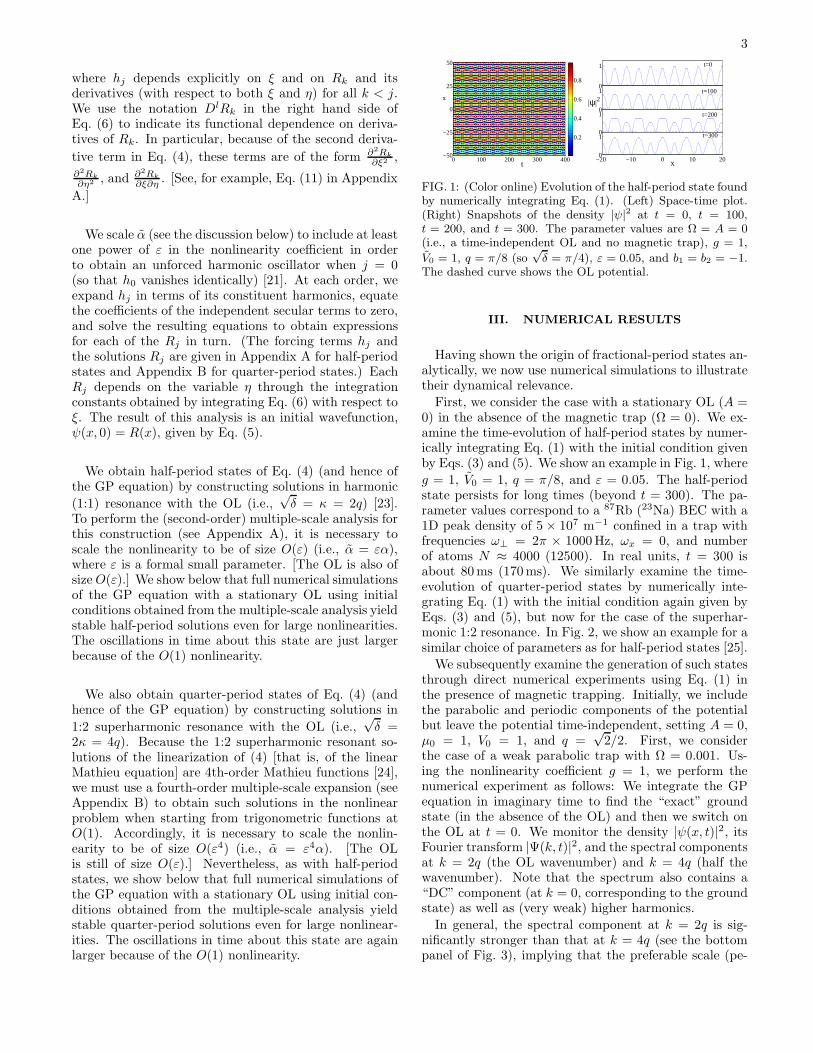
0 100 200 300 400−50

−25

0

25

50

0.2

0.4

0.6

0.8

x

t

0

1

0

1

0

1

−20 −10 0 10 200

1

|ψ|2

x

t=0

t=100

t=200

t=300

FIG. 1: (Color online) Evolution of the half-period state foundby numerically integrating Eq. (1). (Left) Space-time plot.(Right) Snapshots of the density |ψ|2 at t = 0, t = 100,t = 200, and t = 300. The parameter values are Ω = A = 0(i.e., a time-independent OL and no magnetic trap), g = 1,

V0 = 1, q = π/8 (so√δ = π/4), ε = 0.05, and b1 = b2 = −1.

The dashed curve shows the OL potential.

III. NUMERICAL RESULTS

Having shown the origin of fractional-period states an-alytically, we now use numerical simulations to illustratetheir dynamical relevance.

First, we consider the case with a stationary OL (A =0) in the absence of the magnetic trap (Ω = 0). We ex-amine the time-evolution of half-period states by numer-ically integrating Eq. (1) with the initial condition givenby Eqs. (3) and (5). We show an example in Fig. 1, where

g = 1, V0 = 1, q = π/8, and ε = 0.05. The half-periodstate persists for long times (beyond t = 300). The pa-rameter values correspond to a 87Rb (23Na) BEC with a1D peak density of 5 × 107 m−1 confined in a trap withfrequencies ω⊥ = 2π × 1000 Hz, ωx = 0, and numberof atoms N ≈ 4000 (12500). In real units, t = 300 isabout 80 ms (170 ms). We similarly examine the time-evolution of quarter-period states by numerically inte-grating Eq. (1) with the initial condition again given byEqs. (3) and (5), but now for the case of the superhar-monic 1:2 resonance. In Fig. 2, we show an example for asimilar choice of parameters as for half-period states [25].

We subsequently examine the generation of such statesthrough direct numerical experiments using Eq. (1) inthe presence of magnetic trapping. Initially, we includethe parabolic and periodic components of the potentialbut leave the potential time-independent, setting A = 0,µ0 = 1, V0 = 1, and q =

√2/2. First, we consider

the case of a weak parabolic trap with Ω = 0.001. Us-ing the nonlinearity coefficient g = 1, we perform thenumerical experiment as follows: We integrate the GPequation in imaginary time to find the “exact” groundstate (in the absence of the OL) and then we switch onthe OL at t = 0. We monitor the density |ψ(x, t)|2, itsFourier transform |Ψ(k, t)|2, and the spectral componentsat k = 2q (the OL wavenumber) and k = 4q (half thewavenumber). Note that the spectrum also contains a“DC” component (at k = 0, corresponding to the groundstate) as well as (very weak) higher harmonics.

In general, the spectral component at k = 2q is sig-nificantly stronger than that at k = 4q (see the bottompanel of Fig. 3), implying that the preferable scale (pe-

4

0

1

0

1

0

1

−20 −10 0 10 200

1

|ψ|2

x

t=0

t=100

t=200

t=300

FIG. 2: (Color online) Evolution of the quarter-period statefound by numerically integrating Eq. (1). (As in Fig. 1, thelattice is time-independent and the magnetic trap is not in-cluded.) We show snapshots of the density |ψ|2 at t = 0,t = 100, t = 200, and t = 300. The parameter values areΩ = A = 0, g = 1, V0 = 1, q = π/8 (so

√δ = π/2), ε = 0.05,

and b1 = b2 = b3 = b4 = −1. The dashed curve shows the OLpotential.

0

1

0

50

0

1

0

50

−15 0 150

1

−4 −2 0 2 40

50

0 5 10 150

100

|ψ|2 |Ψ|2

x k/q

t

|Ψ(2q)|2 |Ψ(4q)|2

t=1.2

t=7.3

t=7.7

FIG. 3: (Color online) Top panels: Snapshots of |ψ(x, t)|2(left) and its Fourier transform |Ψ(k, t)|2 (right) for the caseof a time-independent lattice and a magnetic trap at times t =1.2, t = 7.3, and t = 7.7. The parameter values are Ω = 0.001,µ0 = 1, V0 = 1, q =

√2/2, and A = 0. The dashed curves

(in the left panels) show the OL. Bottom panel: Evolution of|Ψ(4q)|2 (thin curve) and |Ψ(2q)|2 (bold curve). For t = 1.2,the density has the same period as the OL (i.e., k = 2q).For t = 7.3 (t = 7.7), we observe the formation of a quasi-harmonic (non-harmonic) half-period state with wavenumberk = 4q.

riod) of the system is set by the OL. This behavior is mostprominent at certain times (e.g., at t = 1.2), where thespectral component at k = 2q is much stronger than theother harmonics. Nevertheless, there are specific time in-tervals (of length denoted by τ) with |Ψ(4q)|2 > |Ψ(2q)|2,where we observe the formation of what we will hence-forth call a “quasi-harmonic” half-period state. For ex-ample, one can see such a state at t = 7.3. The purpose ofthe term “quasi-harmonic” is to characterize half-period

states whose second harmonic (at k = 4q, in this case)is stronger than their first harmonic (at k = 2q). Asmentioned above, such states have an almost sinusoidalshape, like the wavefunctions we constructed analytically.

One can use the time-evolution of the spectral com-ponents as a quantitative method to identify the for-mation of half-period states. This diagnostic tool alsoreveals a “revival” of the state, which disappears andthen reappears a number of times before vanishing com-pletely. Furthermore, we observe that other states thatcan also be characterized as half-period ones (which tendto have longer lifetimes than quasi-harmonic states) arealso formed during the time-evolution, as shown in Fig.3 at t = 7.7. These states, which we will hereafter call“non-harmonic” half-period states, have a shape whichis definititvely non-sinusoidal (in contrast to the quasi-harmonic states); they are nevertheless periodic struc-tures of period k = 4q. In fact, the primary Fourier peakof the non-harmonic half-period states is always greaterthan the secondary one. Such states can be observed fortimes t such that the empirically selected condition of|Ψ(2q, t)|2 ≤ 3|Ψ(4q, t)|2 is satisfied.

We next consider a stronger parabolic trap, settingΩ = 0.01. Because the system is generally less homo-geneous in this case, we expect that the analytical pre-diction (valid for Ω = 0) may no longer be valid and thathalf-period states may cease to exist. We confirmed thisnumerically for the quasi-harmonic half-period states.However, non-harmonic half-period states do still appear.The time-evolution of the spectral components at k = 2qand k = 4q is much more complicated and less efficient asa diagnostic tool, as |Ψ(4q, t)|2 < |Ψ(2q, t)|2 for all t. In-terestingly, the non-harmonic half-period states seem topersist as Ω is increased, even when the resonance condi-tion

√δ = κ = 2q is violated. For example, we found that

for time-independent lattices (i.e., A = 0), the lifetime of

a half-period state in the resonant case with q =√

2/2(recall that µ0 = 1) is τ ≈ 1.72, whereas for q = 1/2 it isτ ≈ 0.84. Moreover, the simulations show that the life-times become longer for periodically modulated OLs (us-ing, e.g., A = 1; also see the discussion below). In partic-ular, in the aforementioned resonant (non-resonant) case

with q =√

2/2 (q = 1/2), the lifetime of the half-periodstates has a maximum value, at ω = 1.59 (ω = 0.75),of τ ≈ 8.24, or 4.7 ms (τ ≈ 5.72, or 3.3 ms) for a 23Nacondensate. We show the formation of these states in thetop panels of Fig. 4.

We also considered other fractional states. For exam-ple, using the same parameter values as before except for√δ = 2κ (so that q =

√2/4), we observed quarter-period

transient states with lifetime τ ≈ 2.9. These states oc-curred even in the non-resonant case with q = 1/4 (yield-ing τ ≈ 1). We show these cases (for a temporally mod-ulated lattice with modulation amplitude A = 1) in thebottom panels of Fig. 4. In Fig. 5, we show the lifetimeτ for the half-period and quarter-period states as a func-tion of A. Observe that the lifetime becomes maximal(for values of A ≤ 1.5) around the value A = 1 considered

5

0

1

2

0

1

2

−15 0 150

1

2

3

−15 0 150

1

2

|ψ|2 |ψ|2

x x

ω=1.59 ω=0.75

ω=1.59 ω=0.75

A=1

A=1

A=1

A=1

FIG. 4: Half-period (top panels) and quarter-period (bottompanels) states for the case of a temporally modulated OL.The state in the top left panel has wavenumber q =

√2/2

(resonant), and that in the top right panel has wavenumberq = 1/2 (non-resonant). Similarly, the states in the bottompanels have wavenumbers q =

√2/4 (left, resonant) and q =

1/4 (right, non-resonant).

0.0 0.5 1.0 1.50

2

4

6

8

quarter-period state

Life

time

()

Modulation Amplitude (A)

half-period state

FIG. 5: The lifetime τ of the half-period (upper curve)and quarter-period (lower curve) states as a function of thelattice-modulation amplitude A. For the half-period (quarter-period) state, we show the case with wavenumber q =

√2/2

(q =√

2/4). In both examples, we used µ0 = 1 and lattice-modulation frequency ω = 1.59.

above. Understanding the shape of these curves and theoptimal lifetime dependence on A in greater detail mightbe an interesting topic for further study.

Finally, we also examined non-integer excitations, forwhich the system oscillates between the closest integerharmonics. For example, in Fig. 6, we show a state cor-responding to

√δ = (5/4)κ, so that q = 2

√2/5 (with

µ0 = 1). The system oscillates between the k = 4q(half-period) and k = 6q (third-period) states. Recallthat the case presented in the top right panel of Fig. 4(with q = 1/2) was identified as a “non-resonant half-

period state” (the resonant state satisfies q =√

2/2).Here it is worth remarking that this value, q = 1/2, is

0

1

2

−30 −15 0 15 300

1

2

t=3.9

t=5.5

x

|ψ|2

FIG. 6: (Color online) Density profiles for a fractional state

with√δ = (5/4)κ, so that q = 2

√2/5 (for µ0 = 1, lattice-

modulation amplitude A = 1, and lattice-modulation fre-quency ω = 1.59). The system oscillates in time between half-period (top panel) and third-period (bottom panel) states.

closer to q =√

2/3 (characterizing the third-period state)

than to√

2/2. Nevertheless, no matter which charac-terization one uses, the salient feature is that the valueq = 1/2 is nonresonant and lies between the third-periodand half-period wavenumbers. Accordingly, the respec-tive state oscillates between third-period and half-periodstates. Thus, in the case shown in the top right panel ofFig. 4, the third-period state also occurs (though we donot show it in the figure) and has a lifetime of τ = 4.2

(2.4 ms), while for q = 2√

2/5 its lifetime is τ = 2.92(1.67 ms). This indicates that states with wavenumberscloser to the value of the resonant third-period state havelarger lifetimes. This alternating oscillation between thenearest resonant period states is a typical feature that wehave observed for the non-resonant cases.

IV. CONCLUSIONS

In summary, we have investigated the formation andtime-evolution of fractional-period states in continuumperiodic systems. Although our analysis was based on aGross-Pitaevskii equation describing Bose-Einstein con-densates confined in optical lattices, it can also be ap-plied to several other systems (such as photonic crystalsin nonlinear optics). We have shown analytically anddemonstrated numerically the formation of fractional-period states and found that they may persist for suffi-ciently long times to be observed in experiments. Themost natural signature of the presence of such statesshould be available by monitoring the Fourier transformof the wavepacket through the existence of appropriateharmonics corresponding to the fractional-period states(e.g., k = 4q for half-period states, k = 8q for quarter-period states, etc.).

It would be interesting to expand the study of theparametric excitation of such states in order to betterunderstand how to optimally select the relevant drivingamplitude. Similarly, it would be valuable to examinemore quantitatively the features of the ensuing states asa function of the frequency of the parametric drive andthe parabolic potential.

6

Acknowledgements: We thank Richard Rand for use-ful discussions and an anonymous referee for insight-ful suggestions. We also gratefully acknowledge supportfrom the Gordon and Betty Moore Foundation (M.A.P.)and NSF-DMS-0204585, NSF-DMS-0505663 and NSF-CAREER (P.G.K.).

V. APPENDIX A: ANALYTICAL

CONSTRUCTION OF HALF-PERIOD STATES

To construct half-period states, we use the resonancerelation

√δ = κ and the scaling α = εα, so that Eq. (4)

is written

R′′ + κ2R+ εαR3 + εV0R cos(κx) = 0 (7)

and Eq. (6) is written

Lξ[Rj ] ≡∂2Rj

∂ξ2+ κ2Rj = hj(ξ, Rk, D

lRk) , (8)

where we recall that η = εx, ξ = bx = (1 + εb1 + ε2b2 +· · · )x, and DlRk signifies the presence of derivatives ofRk in the right hand side of the equation. Because of thescaling in Eq. (7), h0 ≡ 0, so that the O(1) term is anunforced harmonic oscillator. Its solution is

R0 = A0(η) cos(κξ) +B0(η) sin(κξ) , (9)

where A0 and B0 will be determined by the solvabilitycondition at O(ε).

The O(εj) (j ≥ 1) equations arising from (7) are forcedharmonic oscillators, with forcing terms depending on thepreviously obtained Rk(ξ, η) (k < j) and their deriva-tives. Their solutions take the form

Rj = Aj(η) cos(κξ) +Bj(η) sin(κξ) +Rjp , (10)

where each Rjp contains contributions from various har-monics. As sinusoidal terms giving a 1:1 resonance withthe OL arise at O(ε2), we can stop at that order.

At O(ε), there is a contribution from both the OL andthe nonlinearity, giving

h1 = −V0R0 cos(κξ) − αR3

0− 2

∂2R0

∂ξ∂η− 2b1

∂2R0

∂ξ2, (11)

where we recall that the OL depends on the stretchedspatial variable ξ because we are detuning from a reso-nant state [22]. With Eq. (9), we obtain

h1 =

[

2b1κ2A0 − 2κB′

0− 3

4αA0(A

2

0+B2

0)

]

cos(κξ)

+

[

2b1κ2B0 + 2κA′

0 −3

4αB0(A

2

0 +B2

0)

]

sin(κξ)

+αA0

4

(

−A2

0 + 3B2

0

)

cos(3κξ)

+αB0

4

(

−3A2

0 +B2

0

)

sin(3κξ) +V0A0

2

+V0A0

2cos(2κξ) +

V0B0

2sin(2κξ) . (12)

For R1(ξ, η) to be bounded, the coefficients of the sec-ular terms in Eq. (12) must vanish [20, 22]. The onlysecular harmonics are cos(κξ) and sin(κξ), and equatingtheir coefficients to zero yields the following equations ofmotion describing the slow dynamics:

A′

0 = −b1κB0 +3α

8κB0(A

2

0 +B2

0) ,

B′

0= b1κA0 −

3α

8κA0(A

2

0+B2

0) . (13)

We convert (13) to polar coordinates with A0(η) =C0 cos[ϕ0(η)] and B0(η) = C0 sin[ϕ0(η)] and see imme-diately that each circle of constant C0 is invariant. Thedynamics on each circle is given by

ϕ0(η) = ϕ0(0) +

(

b1κ− 3α

8κC2

0

)

η . (14)

We examine the special circle of equilibria, correspondingto periodic orbits of (7), which satisfies

C2

0 = A2

0 +B2

0 =8b1κ

2

3α. (15)

In choosing an initial configuration for numerical simula-tions of the GP equation (1), we set B0 = 0 without lossof generality.

Equating coefficients of (8) at O(ε2) yields

∂2R2

∂ξ2+ κ2R2 = h2 , (16)

where the forcing term again contains contributions fromboth the OL and the nonlinearity:

h2 = −(b21 + 2b2)∂2R0

∂ξ2− ∂2R0

∂η2− 2b1

∂2R0

∂ξ∂η

− 3αR2

0R1 − 2b1∂2R1

∂ξ2− 2

∂2R1

∂ξ∂η−R1V0 cos(κξ) .

(17)

Here, one inserts the expressions for R0, R1, and theirderivatives into the function h2.

To find the secular terms in Eq. (17), we compute

R1(ξ, η) = A1(η) cos(κξ) +B1(η) sin(κξ) +R1p(ξ, η) ,

R1p(ξ, η) = c1 cos(3κξ) + c2 sin(3κξ)

+ c3 + c4 cos(2κξ) + c5 sin(2κξ) , (18)

where

c1 =α

32κ2A0(A

2

0 − 3B2

0) , c2 =α

32κ2B0(3A

2

0 −B2

0) ,

c3 = − V0A0

2κ2, c4 =

V0A0

6κ2, c5 =

V0B0

6κ2. (19)

After it is expanded, the function h2 contains harmon-ics of the form cos(0ξ) = 1, cos(κξ) (the secular terms),cos(2κξ), cos(3κξ), cos(4κξ), and cos(5κξ) (as well as

7

sine functions with the same arguments). Equating thesecular cofficients to zeros gives the following equationsdescribing the slow dynamics:

A′

1=

1

3072κ5

[(

f1(α, κ)B2

0+ f2(α, κ)A

2

0+ f3(α, κ, b1)

)

B1

+f4(α, κ)A0B0A1 + f5(α, κ)B5

0

+f6(α, κ)A2

0B3

0 + f7(α, κ)A4

0B0 + f8s(α, κ, b2)B0

]

,

B′

1=

1

3072κ5

[(

f1(α, κ)A2

0+ f2(α, κ)B

2

0+ f3(α, κ, b1)

)

A1

+f4(α, κ)A0B0B1 + f5(α, κ)A5

0

+f6(α, κ)A3

0B2

0 + f7(α, κ)A0B4

0 + f8c(α, κ)A0

]

,

(20)

where

f1(α, κ) = 3f2(α, κ) ,

f2(α, κ) = −1152ακ4 ,

f3(α, κ, b1) = 3072κ6b1 ,

f4(α, κ) = 2f2(α, κ) ,

f5(α, κ) = 180α2κ2 ,

f6(α, κ) = 2f5(α, κ) ,

f7(α, κ) = f5(α, κ) ,

f8s(α, κ, b2) = fnon(α, κ) − 128V 2

0κ2 ,

f8c(α, κ) = fnon(α, κ) + 640V 2

0 κ2 ,

fnon(α, κ) = 3072κ6b2 . (21)

We use the notation fnon to indicate the portions of thequantities f8s and f8c that arise from non-resonant terms.The other terms in these quantities, which depend on thelattice amplitude V0, arise from resonant terms.

Equilibrium solutions of (20) satisfy

A1 =(f1B

2

0 + f2A2

0 + f3)(f5A5

0 + f6A3

0B2

0 + f7A0B4

0 + f8cA0) − (f4A0B0)(f5B5

0 + f6A2

0B3

0 + f7A4

0B0 + f8sB0)

f2

4A2

0B2

0− (f1B2

0+ f2A2

0+ f3)(f1A2

0+ f2B2

0+ f3)

,

B1 =(f1A

2

0 + f2B2

0 + f3)(f5B5

0 + f6A2

0B3

0 + f7A4

0B0 + f8sB0) − (f4A0B0)(f5A5

0 + f6A3

0B2

0 + f7A0B4

0 + f8cA0)

f2

4A2

0B2

0− (f1B2

0+ f2A2

0+ f3)(f1A2

0+ f2B2

0+ f3)

,

(22)

where one uses an equilibrium value of A0 and B0 fromEq. (15). Inserting equilibrium values of A0, B0, A1, andB1 into Eqs. (9) and (18), we obtain the spatial profileR = R0 + εR1 + O(ε2) used as the initial wavefunctionin the numerical simulations of the full GP equation (1)with a stationary OL.

VI. APPENDIX B: ANALYTICAL

CONSTRUCTION OF QUARTER-PERIOD

STATES

To construct quarter-period states, we use the reso-nance relation

√δ = 2κ and the scaling α = ε4α, so that

Eq. (4) is written

R′′ + 4κ2R+ ε4αR3 + εV0R cos(κx) = 0 (23)

and Eq. (6) is written

Lξ[Rj ] ≡∂2Rj

∂ξ2+ 4κ2Rj = hj(ξ, Rk, D

lRk) , (24)

where η = εx and ξ = bx = (1 + εb1 + ε2b2 + · · · )x, asbefore.

Because of the scaling in (23), h0 ≡ 0 (as in the case ofhalf-period states), so that the O(1) term is an unforcedharmonic oscillator. It has the solution

R0 = A0(η) cos(2κξ) +B0(η) sin(2κξ) , (25)

8

where A2

0+ B2

0= C2

0is an arbitrary constant (in the

numerical simulations, we take B0 = 0 without loss ofgenerality). With the different scaling of the nonlinearitycoefficient, the value C2

0is not constrained as it was in

the case of half-period states (see Appendix A).The O(εj) (j ≥ 1) equations arising from (24) are

forced harmonic oscillators, with forcing terms depend-ing on the previously obtained Rk(ξ, η) (k < j) and theirderivatives. Their solutions take the form

Rj = Aj(η) cos(2κξ) +Bj(η) sin(2κξ) +Rjp , (26)

where Rjp contain contributions from various harmonics.As sinusoidal terms giving a 1:2 resonance with the OLarise at O(ε4), we can stop at that order.

The equation at O(ε) has a solution of the form

R1 = A1(η) cos(2κξ) +B1(η) sin(2κξ) +R1p . (27)

The coefficients A1 and B1 are determined using a solv-ability condition obtained at O(ε2) by requiring that thesecular terms of h2 vanish. This yields

A1 =V0

16b1κ2(c11 + c12) −

b2b1A0 ,

B1 =V0

16b1κ2(c13 + c14) −

b2b1B0 . (28)

The particular solution is

R1p = c11 cos(κξ)+c12 cos(3κξ)+c13 sin(3κξ)+c14 sin(κξ) ,(29)

where

c11 = − V0A0

6κ2, c12 =

V0A0

10κ2,

c13 =V0B0

10κ2, c14 = − V0B0

6κ2. (30)

The solution at O(ε2) has the form

R2 = A2(η) cos(2κξ) +B2(η) sin(2κξ) +R2p(ξ, η) . (31)

The coefficients A2 and B2 are determined using a solv-ability condition obtained at O(ε3) by requiring that thesecular terms of h3 vanish. This yields

A2 =V0

16b1κ2(c21 + c22) −

V0

32κ2(c11 + c12)

− b3b1A0 −

b2b1A1 −

V 2

0A0

480κ4,

B2 = − V0

16b1κ2(c23 + c24) −

V0

32κ2(c13 + c14)

− b3b1B0 −

b2b1B1 −

V 2

0B0

480κ4. (32)

The particular solution is

R2p = c21 cos(κξ) + c22 cos(3κξ) + c23 sin(3κξ)

+ c24 sin(κξ) + c25 cos(4κξ)

+ c26 + c27 sin(4κξ) , (33)

where

c21 = − V0A1

6κ2+b1V0A0

9κ2,

c22 =V0A1

10κ2− 3b1V0A0

25κ2,

c23 =V0B1

10κ2− 3b1V0B0

25κ2,

c24 = − V0B1

6κ2+b1V0B0

9κ2,

c25 =V 2

0 A0

240κ4, c26 =

V 20 A0

48κ4, c27 =

V 20 B0

240κ4. (34)

Note that the harmonics cos(0ξ) and sin(0ξ) occur in (33)and are reduced appropriately. (The arguments of thissine and cosine arise because of our particular resonancerelation.)

At O(ε3), we obtain solutions of the form

R3 = A3(η) cos(2κξ) +B3(η) sin(2κξ) +R3p(ξ, η) . (35)

The coefficients A3 and B3 are determined using a solv-ability condition obtained at O(ε4) by requiring that thesecular terms of h4 vanish. Because of the scaling in (23),the effects of the nonlinearity manifest in this solvabilitycondition. The resulting coefficients are

A3 = − V 4

0A0

3375b1κ8− b3b1A1 −

V 2

0b2A0

1800b1κ4

− V 20 A1

1800κ4− 19b1V

20 A0

54000κ4+

3αA30

32b1κ2

− b2b1A2 −

b4b1A0 −

V 20 A2

240b1κ4+

3αA0B20

32b1κ2(36)

B3 = − b2b1B2 +

3αA20B0

32b1κ2− b4b1B0 −

V 20 B2

240b1κ4

− V 20 B1

1800κ4− b3b1B1 +

119V 40 B0

864000b1κ8

− V 2

0b2B0

1800b1κ4− 19b1V

2

0B0

54000κ4+

3αB3

0

32b1κ2. (37)

The particular solution is

R3p = c31 cos(κξ) + c32 cos(3κξ) + c33 sin(3κξ)

+ c34 sin(κξ) + c35 cos(4κξ) + c36

+ c37 sin(4κξ) + c38 cos(5κξ) + c39 cos(κξ)

+ c310 sin(5κξ) + c311 sin(κξ) , (38)

where

c31 = − 7b21V0A0

54κ2+b2V0A0

9κ2− 11V 3

0A0

4320κ6

+b1V0A1

9κ2− V0A2

6κ2, (39)

9

c32 =31b2

1V0A0

250κ2− 3b2V0A0

25κ2+

17V 3

0A0

12000κ6

− 3b1V0A1

25κ2+V0A2

10κ2, (40)

c33 =17V 3

0B0

12000κ6− 3b1V0B1

25κ2+

31b21V0B0

250κ2

− 3b2V0B0

25κ2+V0B2

10κ2, (41)

c34 =b2V0B0

9κ2− 7b21V0B0

54κ2− V0B2

6κ2

+b1V0B1

9κ2− 11V 3

0B0

4320κ6, (42)

c35 = −19b1V2

0A0

1800κ4+V 2

0A1

240κ4, c36 =

V 2

0A1

48κ4− b1V

2

0A0

72κ4,

c37 = −19b1V2

0B0

1800κ4+V 2

0B1

240κ4, c38 =

V 3

0A0

10080κ6,

c39 = − V 30 A0

288κ6, c310 =

V 30 B0

10080κ6, c311 =

V 30 B0

288κ6.

(43)

Similar to what occurs at O(ε2), the coefficient c36 isthe prefactor for cos(0ξ) and a sin(0ξ) term (not shown)occurs in (38) as well. The extra terms (from the reso-nance relation) that go into the slow evolution equationsand the resulting expressions for the periodic orbits (i.e.,the equilibria of the slow flow) arise from the terms withprefactors c39 and c311. (The harmonics correspondingto the coefficients c31 and c34 are always secular, butthose corresponding to c39 and c311 are secular only for1:2 superharmonic resonances.)

One inserts equilibrium values of Aj and Bj (j ∈0, 1, 2, 3) into Eqs. (25), (29), (31), and (35) to obtainthe spatial profile R = R0 + εR1 + ε2R2 + ε3R3 +O(ε4)used as the initial wavefunction in numerical simulationsof the GP equation (1) with a stationary OL.

[1] S. Aubry, Physica D 103, 201, (1997); S. Flach and C.R. Willis, Phys. Rep. 295, 181 (1998); D. Hennig and G.Tsironis, Phys. Rep. 307, 333 (1999); P. G. Kevrekidis,K. O. Rasmussen, and A. R. Bishop, Int. J. Mod. Phys.B 15, 2833 (2001).

[2] D. K. Campbell, P. Rosenau, and G. Zaslavsky, Chaos15, 015101 (2005).

[3] D. N. Christodoulides, F. Lederer, and Y. Silberberg, Na-ture 424, 817 (2003); Yu. S. Kivshar and G. P. Agrawal,Optical Solitons: From Fibers to Photonic Crystals (Aca-demic Press, San Diego, 2003); J. W. Fleischer, G. Bar-tal, O. Cohen, T. Schwartz, O. Manela, B. Freedman, M.Segev, H. Buljan, and N. K. Efremidis, Opt. Express 13,1780 (2005).

[4] P. G. Kevrekidis and D. J. Frantzeskakis, Mod. Phys.Lett. B 18, 173 (2004); V. V. Konotop and V. A. Brazh-nyi, Mod. Phys. Lett. B 18 627, (2004); P.G. Kevrekidis,R. Carretero-Gonzalez, D. J. Frantzeskakis, and I. G.Kevrekidis, Mod. Phys. Lett. B 18, 1481 (2004); O.Morsch and M. Oberthaler, Rev. Mod. Phys. 78, 179(2006).

[5] M. Peyrard, Nonlinearity 17, R1 (2004).[6] A. Trombettoni and A. Smerzi, Phys. Rev. Lett. 86, 2353

(2001); F. Kh. Abdullaev, B. B. Baizakov, S. A. Dar-manyan, V. V. Konotop, and M. Salerno, Phys. Rev. A64, 043606 (2001); G. L. Alfimov, P. G. Kevrekidis, V.V. Konotop, and M. Salerno, Phys. Rev. E 66, 046608(2002).

[7] J. P. Keener, Phys. D 136, 1 (2000); P. G. Kevrekidisand I. G. Kevrekidis, Phys. Rev. E 64, 056624 (2001).

[8] T. Stoferle, H. Moritz, C. Schori, M. Kohl, and T.

Esslinger, Phys. Rev. Lett. 92, 130403 (2004).[9] M. Kramer, C. Tozzo, and F. Dalfovo, Phys. Rev. A 71,

061602(R) (2005).[10] C. Tozzo, M. Kramer, and F. Dalfovo, Phys. Rev. A 72,

023613 (2005).[11] A. Iucci, M. A. Cazalilla, A. F. Ho, and T. Giamarchi,

Phys. Rev. A. 73, 041608 (2006).[12] N. Gemelke, E. Sarajlic, Y. Bidel, S. Hong, and S. Chu,

Phys. Rev. Lett. 95, 170404 (2005).[13] M. Machholm, A. Nicolin, C. J. Pethick, and H. Smith,

Phys. Rev. A 69, 043604 (2004).[14] M. A. Porter and P. Cvitanovic, Phys. Rev. E 69, 047201

(2004); M. A. Porter and P. Cvitanovic, Chaos 14, 739(2004).

[15] A. Smerzi, A. Trombettoni, P. G. Kevrekidis, and A. R.Bishop, Phys. Rev. Lett. 89, 170402 (2002).

[16] F. S. Cataliotti, L. Fallani, F. Ferlaino, C. Fort, P. Mad-daloni, and M. Inguscio, New J. Phys. 5, 71 (2003).

[17] B. T. Seaman, L. D. Carr, and M. J. Holland, Phys. Rev.A 72, 033602 (2005).

[18] N. W. Ashcroft and N. D. Mermin, Solid State Physics(Saunders College, Philadelphia, 1976).

[19] V. M. Perez-Garcıa, H. Michinel, and H. Herrero, Phys.Rev. A 57, 3837 (1998); L. Salasnich, A. Parola, and L.Reatto, Phys. Rev. A 65, 043614 (2002).

[20] A. H. Nayfeh and D. T. Mook, Nonlinear Oscillations(John Wiley & Sons, New York, 1995).

[21] The small sizes of the lattice depth and nonlinearity co-efficient allow us to perturb from base states consistingof trigonometric functions (regular harmonics). One canrelax these conditions using the much more technically

10

demanding approaches of perturbing from either Math-ieu functions (removing the restriction on the size of theamplitude of the periodic potential) or elliptic functions(removing the restriction on the size of the nonlinearitycoefficient).

[22] R. H. Rand, Lecture Notes on Nonlin-ear Vibrations, online book available athttp://www.tam.cornell.edu/randdocs/nlvibe52.pdf,2005.

[23] M. A. Porter and P. G. Kevrekidis, SIAM J. App. Dyn.Sys. 4, 783 (2005).

[24] N. W. McLachlan, Theory and Application of Mathieu

Functions (Clarendon Press, Oxford, 1947).[25] We use the same values of A0 and B0 (the prefactors

of the harmonics in R0; see the appendices) as for thehalf-period states, even though these parameters are notconstrained for quarter-period solutions. As discussed inAppendix A, they are constrained for half-period states.

[26] In many cases, one can make this procedure more math-ematically rigorous (though less transparent physically)by examining the dynamics geometrically and introduc-ing slow and fast manifolds.