
Etude régionale par éléments finis d'une nappe libre située dans les craies du crétacé en Belgique
Upload
khangminh22Category
view
1download
0
NNT:2021UPASP108
Study of the multipolar excitations in cold and
hot, deformed and superfluid systems with the
method of finite amplitudes
Etude des excitations multipolaires dans les noyaux froids
et chauds, deformes et superfluides via la methode des
amplitudes finies
These de doctorat de l’universite Paris-Saclay
Ecole doctorale n 576, Particules, Hadrons, Energie et Noyau : Instrumentation,
Imagerie, Cosmos et Simulation (PHENIICS)
Specialite de doctorat : structure et reactions nucleaires
Unite de recherche : universite Paris-Saclay, CEA, Laboratoire Matiere sous conditions
extremes, 91680, Bruyeres-le-Chatel, France
Graduate School : Physique. Referent : Faculte des sciences d’Orsay
These presentee et soutenue a Paris-Saclay,
le 26 octobre 2021, par
Yann BEAUJEAULT-TAUDIERE
Composition du jury
Marcella GRASSO Presidente
Directrice de recherche, Universite Paris-Saclay
Dany DAVESNE Rapporteur & examinateur
Professeur, Universite Claude Bernard Lyon 1
Robert ROTH Rapporteur & examinateur
Professeur, Universite de technologie de Darmstadt
Stephane GORIELY Examinateur
Charge de recherche, Universite Libre de Bruxelles
Markus KORTELAINEN Examinateur
Professeur assistant, Universite de Jyvaskyla et Universite d’Helsinki
Thomas DUGUET Invite
Ingenieur de recherche, CEA Saclay, IRFU
Direction de la these
Denis LACROIX Directeur de these
Directeur de recherche, Universite Paris-Saclay
Jean-Paul EBRAN Co-encadrant
Ingenieur de recherche, CEA, DAM, DIF


Academic summary
Titre : Etude des excitations multipolaires dans les noyaux froids et chauds, deformes et superfluides via lamethode des amplitudes finies
Mots cles : Physique theorique, probleme a N corps, modes collectifs, astrophysique nucleaire, transitions dephase
Resume : La reponse d’un systeme a une pertur-bation exterieure est source d’informations precieusesquant a ses proprietes de structure ou aux car-acteristiques de l’interaction entre ses constituants.Pour les noyaux atomiques, ces differentes proprietesjouent en particulier un role fondamental dans diversscenarios astrophysiques tels que les processus r, s etp. L’une des methodes les plus directes pour accedera la reponse d’un systeme suite a une perturbationexterieure fait appel a la QRPA (quasiparticle randomphase approximation), extension au cas des systemessuperfluides de la theorie de la reponse lineaire traiteedans l’approximation de la phase aleatoire. Une re-
formulation recente des equations leve les limitationsqui imposaient de negliger une partie des contributionsaux champs ou encore restreignaient la description ades classes specifiques de correlations angulaires dansl’etat fondamental. Le travail realise en these a consistea etendre ce nouveau formalisme au cadre d’un etatfondamental s’ecrivant comme un melange statistiquede configurations, ouvrant la possibilite d’appliquerla methode aux systemes a temperature finie, et al’employer avec une interaction entre les nucleons dansle milieu nucleaire derivant d’une theorie effective abasse energie de la chromodynamique quantique.
Title: Study of the multipolar excitations in cold and hot, deformed and superfluid systems with the method offinite amplitudes
Keywords: Theoretical physics, many-body problem, collective modes, nuclear astrophysics, phase transitions
Abstract: Studying how a system responds to anexternal perturbation reveals many features about itsstructure or the underlying interactions between its con-stituents. In the case of atomic nuclei, such informationplays a prominent role when one aims at understandinghow structure properties impact nuclear reactions, e.g.in various astrophysical scenarios such as the r, s and pprocesses. The quasiparticle random phase approxima-tion (QRPA), i.e. the generalisation to superfluid sys-tems of the linear response theory within the randomphase approximation, provides one of the most directapproaches to apprehend how a nucleus behaves undera gentle perturbation. A reformulation of the theory
recently lifted some intrinsic limitations that affectedit so far, namely the need to neglect some high-ordercontributions to the fields or the restriction to systemsdisplaying only a specific class of angular correlationsin their ground state. The formal work of this thesis in-volved extending the method to the case of a referencestate written as a statistical mixture of different config-urations, opening the way to the description of reso-nances in systems at finite temperature. The formalismis employed with an effective interaction between nu-cleons deriving from a low-energy effective theory ofquantum chromodynamics.
General public summary
Titre : Etude des excitations multipolaires dans les noyaux froids et chauds, deformes et superfluides via lamethode des amplitudes finies
Mots cles : Physique theorique, probleme a N corps, modes collectifs, astrophysique nucleaire, transitions dephase
Resume : La plupart des systemes quantiquessont composes de plusieurs particules interagissantentre elles. Decrire leur agencement en termesd’energie, de distribution spatiale, etc, est tres com-plique puisque faisant appel a des equations integro-differentielles couplees. Trouver l’etat fondamen-tal du systeme, c’est-a-dire la configuration la plusstable, necessite frequemment le recours a une ap-proximation de “champ moyen”, qui neglige certainescorrelations entre les particules pour retenir seulementles plus elementaires. Lorsque le systeme interagit avecun environnement exterieur, l’evolution temporelle deses proprietes est naturellement tres complexe, et re-quiert egalement des approximations. Souvent, on
peut supposer les perturbations induites par le milieuexterieur comme etant de petites vibrations autour dela configuration stable. Cela donne acces a la com-posante lineaire de la reponse du systeme ; l’approcheest donc valide si cette composante predomine. Ceprobleme a ete recemment revu afin d’en simplifier laresolution pour un systeme initialement “froid”, c’est-a-dire a temperature nulle. Le travail realise a notam-ment consiste a etendre ce formalisme au cas ou lesysteme est initialement froid ou chaud. Cela a per-mis de premieres applications a l’etude des proprietesde certains phenomenes collectifs dans des conditionsextremes, telles que celles regnant au sein d’etoiles aneutrons.
Title: Study of the multipolar excitations in cold and hot, deformed and superfluid systems with the method offinite amplitudes
Keywords: Theoretical physics, many-body problem, collective modes, nuclear astrophysics, phase transitions
Abstract: The majority of quantum systems is com-posed of several particles interacting together. Describ-ing how they organise in terms of spatial distribution, ofenergy, etc, is highly complicated as it involves coupledintegro-differential equations. Finding the ground stateof the system, that is, the most stable configuration, of-ten already requires neglecting some correlations be-tween the particles, retaining only the simplest ones.When this ensemble of particles interacts with an en-vironment, the time evolution of its properties is thusvery difficult, and calls for similar approximations. Inmost cases, we may suppose the motion generated bythe external perturbation to be small oscillations about
the stable configuration. This yields the linear com-ponent of the response; the approximation is this validwhen this component is the most important one. Themathematical framework of the problem has recentlybeen revisited in order to simplify its resolution for ini-tially “cold” systems, i.e. systems at zero temperature.The work developed in this thesis extends this new for-malism to the case of finite temperature, giving accessto the response atop cold and hot systems. In particu-lar, this has been employed for the description of somecollective phenomena in conditions of extremely hightemperature, as can be met in neutron stars.

Contents
1 Introduction 9
2 Generalities 13
2.1 Density matrix . . . . . . . . . . . . . . . . . . . . . . . . . . . . . . . . . 14
2.2 Statistical ensemble . . . . . . . . . . . . . . . . . . . . . . . . . . . . . . . 15
2.3 Static Hamiltonian and some general properties . . . . . . . . . . . . . . . 18
2.3.1 Wick theorem . . . . . . . . . . . . . . . . . . . . . . . . . . . . . . 20
2.3.2 Interaction symmetrisation . . . . . . . . . . . . . . . . . . . . . . . 21
2.4 Mean-field approximations . . . . . . . . . . . . . . . . . . . . . . . . . . . 23
2.4.1 General setting . . . . . . . . . . . . . . . . . . . . . . . . . . . . . 23
2.4.2 Hartree-Fock-Bogoliubov theory . . . . . . . . . . . . . . . . . . . . 24
2.5 Thermal phase transitions . . . . . . . . . . . . . . . . . . . . . . . . . . . 29
2.5.1 Collapse of the pairing via thermal excitations . . . . . . . . . . . . 30
2.5.2 Spherical symmetry restoration . . . . . . . . . . . . . . . . . . . . 31
2.5.3 Thermal configuration mixing . . . . . . . . . . . . . . . . . . . . . 32
2.6 Response theory . . . . . . . . . . . . . . . . . . . . . . . . . . . . . . . . . 33
2.6.1 General aspects and points of view . . . . . . . . . . . . . . . . . . 33
2.6.2 Linear approximation . . . . . . . . . . . . . . . . . . . . . . . . . . 34
2.6.3 Formalisms survey . . . . . . . . . . . . . . . . . . . . . . . . . . . 35
2.6.4 Elements of formalism . . . . . . . . . . . . . . . . . . . . . . . . . 36
3 Finite Amplitude Method 43
3.1 Derivation . . . . . . . . . . . . . . . . . . . . . . . . . . . . . . . . . . . . 44
3.2 Linearisation of the fields . . . . . . . . . . . . . . . . . . . . . . . . . . . . 47
3.2.1 Implicit linearisation . . . . . . . . . . . . . . . . . . . . . . . . . . 47
5

6 CONTENTS
3.2.2 Explicit linearisation . . . . . . . . . . . . . . . . . . . . . . . . . . 48
3.3 Symmetries of the QFAM and HFB equations . . . . . . . . . . . . . . . . 50
3.3.1 Density matrices . . . . . . . . . . . . . . . . . . . . . . . . . . . . 51
3.3.2 Dynamical fields . . . . . . . . . . . . . . . . . . . . . . . . . . . . 53
3.4 Connection with the QRPA . . . . . . . . . . . . . . . . . . . . . . . . . . 56
3.4.1 Eigenvectors and transition amplitudes . . . . . . . . . . . . . . . . 56
3.4.2 Eigenvalues . . . . . . . . . . . . . . . . . . . . . . . . . . . . . . . 64
3.4.3 Eigenvalues and transition amplitudes from the moments . . . . . . 66
3.4.4 Summary . . . . . . . . . . . . . . . . . . . . . . . . . . . . . . . . 67
3.5 Self-consistent dressing . . . . . . . . . . . . . . . . . . . . . . . . . . . . . 68
3.6 Nambu-Goldstone modes . . . . . . . . . . . . . . . . . . . . . . . . . . . . 68
3.6.1 Equations of motion for the NG modes . . . . . . . . . . . . . . . . 68
3.6.2 NG modes removal . . . . . . . . . . . . . . . . . . . . . . . . . . . 69
3.7 Centre of mass . . . . . . . . . . . . . . . . . . . . . . . . . . . . . . . . . 71
3.8 Unstable modes . . . . . . . . . . . . . . . . . . . . . . . . . . . . . . . . . 76
3.9 Resonance broadening . . . . . . . . . . . . . . . . . . . . . . . . . . . . . 78
3.10 QFAM in harmonic oscillator basis: selection rules . . . . . . . . . . . . . . 80
3.10.1 From the external probe . . . . . . . . . . . . . . . . . . . . . . . . 80
3.10.2 From the interaction . . . . . . . . . . . . . . . . . . . . . . . . . . 81
3.10.3 Quantum numbers of the oscillations . . . . . . . . . . . . . . . . . 82
4 Application to thermal phase transitions 83
4.1 Signatures of phase transitions . . . . . . . . . . . . . . . . . . . . . . . . . 84
4.2 Motivation for studying 56Fe . . . . . . . . . . . . . . . . . . . . . . . . . . 85
4.3 Results . . . . . . . . . . . . . . . . . . . . . . . . . . . . . . . . . . . . . . 85
4.3.1 Foreword: mean-field and expectations from ab initio interactions . 85
4.3.2 Convergence with model space parameters and chiral order . . . . . 87
4.3.3 Shape transition in 56Fe . . . . . . . . . . . . . . . . . . . . . . . . 94
5 Application to giant resonances 101
5.1 Benchmark against standard RPA . . . . . . . . . . . . . . . . . . . . . . . 103
5.2 Convergence aspects . . . . . . . . . . . . . . . . . . . . . . . . . . . . . . 104
5.2.1 With the oscillator frequency . . . . . . . . . . . . . . . . . . . . . 106
5.2.2 With the basis size . . . . . . . . . . . . . . . . . . . . . . . . . . . 110
5.2.3 With the chiral expansion . . . . . . . . . . . . . . . . . . . . . . . 111
5.2.4 Conclusion . . . . . . . . . . . . . . . . . . . . . . . . . . . . . . . . 113
5.3 Moments of the strength . . . . . . . . . . . . . . . . . . . . . . . . . . . . 114
5.4 Multipolar strengths of selected mid-mass nuclei at finite temperature . . . 117
6
CONTENTS 7
5.5 Conclusion . . . . . . . . . . . . . . . . . . . . . . . . . . . . . . . . . . . . 126
6 Conclusion and perspectives 127
A Producing ab initio nuclear interactions 129
A.1 Quantum chromodynamics and chiral effective field theory . . . . . . . . . 129
A.2 Similarity renormalisation group treatment of
chiral EFT . . . . . . . . . . . . . . . . . . . . . . . . . . . . . . . . . . . . 132
B Effective theories ideas applied to an exactly solvable model 135
C Sum rules from the static state 138
D Higher-order responses 140
D.1 Linear responses . . . . . . . . . . . . . . . . . . . . . . . . . . . . . . . . . 140
D.2 Non-linear responses . . . . . . . . . . . . . . . . . . . . . . . . . . . . . . 141
E Overview of the axial harmonic oscillator basis 143
F Resume substantiel en francais 147
List of Figures 155
List of Tables 159
Bibliography 161
7


Chapter 1
Introduction
The quantum many-body problem is extremely complex, and many phenomena can onlybe understood by properly treating internal correlations between degrees of freedom be-yond the independent particle picture [RS80]. For nuclear physics, such correlationsspawn peculiar configurations such as deformation and superfluidity. This already richphenomenology is spiced up by the occurrence of more exotic configurations such as haloor bubble structures, giant resonances and clusters. A most famous manifestation of thecomplexity of nuclear systems is certainly the Hoyle state [Hoy54], the clustered excitedstate of carbon produced during the helium burning phase in stars. Complex phenomenaare frequently met in the nuclear chart (figure 1.1) and cannot be treated on the basis ofindependent particles.
Figure 1.1: Zoom on the nuclear chart for N ≤ 16 and Z ≤ 10. Courtesy of W. Korten.
The first step of the theoretical description of strongly correlated many-body systemsis to identify the pertinent degrees of freedom (d.o.f.) with the help of which the modelis constructed.
A possibility is to adopt a macroscopic viewpoint [Rai50; BM53a; BM53b; AI75], in-terpreting the observed phenomena as collective bosonic excitations of a quantum body.Early attempts at unveiling the connection between collective and independent particlemotions were based on experimental observations and chose the collective modes accord-ingly. As such, the type of such bosons is nearly as vast as the phenomenology of quantum
9
10 Chapter 1. Introduction
physics, and proponents of the collective models need to tailor their description to eachspecific problem, as a price to pay for the crystalline clarity of the model in terms ofphenomena at play. Recently, this approach has been reframed in the language of effec-tive field theories (EFTs) [PW14; Coe15; CP15; CP16; PW16], allowing for a systematicimprovement of the description of the excitation spectrum and the possibility to quantifytheoretical uncertainties. Depending on the contribution of a given class of correlations(pairing, shape, vibrational, etc), an effective theory has to be crafted in terms of adaptedsymmetry groups and cosets relating them. The low-energy constants entering the effec-tive Hamiltonian must then be adjusted to each system with the help of experimental data.
A completely opposite vision goes by trying to describe all the desired physics on thebasis of the interaction between the most microscopic degrees of freedom. In subatomicphysics, this is realised into the Standard Model, which aims at describing three of the fourknown fundamental interactions of nature: the strong, the weak and the electromagneticinteraction. While it can be tempting to delve down this microscopic rabbit hole in thehope of constructing an all-encompassing theory, one is quickly faced with tremendousdifficulties when dealing with the theory of the strong interaction, quantum chromody-namics (QCD). Without flaunting a rusty knowledge of QCD, its non-Abelian nature1
and the covariance criterion force self-interactions among the gluon fields, which resultsnotably in the theory being strongly non-perturbative at low energies. The structure ofnuclei is thus hardly predictable from QCD, although recent lattice calculations [IAH07;Aok+12; Kol15] are starting to appear, and will certainly flourish in the future.
To circumvent the enormous difficulties brought by the specificities of QCD, an alter-native path is currently being pursued. It aims at maintaining a formal connection to theunderlying theory, and anchors on the viewpoint of effective field theories (EFTs) [Wei79],by exploiting a separation of energy scales in the excitation spectrum of quark conden-sates. The energy cut-off separates which effects are treated explicitly and which onesappear as perturbative corrections [MS16]. At energy scales relevant for nuclear physics,typically a few tens of MeV, the substructure of nucleons in terms of quarks and gluonsis not resolved, promoting protons and neutrons to the relevant degrees of freedom of thetheory. Still, the strong short-range repulsion between nucleons makes the problem highlynon-perturbative. The second difficulty stems from the size of nuclear systems, made of1 to ∼3002 nucleons. One then has to cope with a non-perturbative finite system, wheremost often, neither few-body nor statistical techniques can be employed. A challenge oflow-energy nuclear physics theory is therefore to obtain a coherent and accurate descrip-tion of the aforementioned phenomena observed across the nuclear chart, along with theirmass, radius, shape, spectroscopic factors, multipolar moments... all the while startingfrom the interactions between nucleons.
In particular, collective features constitutes an important challenge to a theory basedstrictly on microscopic ingredients. For vibrational modes, the motion generated by an
1The gauge group of QCD is SU(Nc), where Nc is the number of colour charges, and must be equalto three to match the hadron spectrum.
2In extreme environments such as neutron stars, clusters comprising a few thousands of nuclei are alsopredicted; this is still too little to render statistical fluctuations entirely negligible.
10

Chapter 1. Introduction 11
external source is generally represented as small amplitude oscillations about a referencestate. In that case, the random phase approximation (RPA) and the quasiparticle RPA-its extension including superfluidity- are theoretical tools of choice, as they tackle bothindividual and collective resonances on the same footing. However, in case of effectiveinteractions rooted in QCD, the complexity of the method hindered its application tosystems displaying simultaneously deformation and superfluidity. While spherical sys-tems, both superfluid [HPR11] and not [Paa+06], could be addressed, the study of nucleiexhibiting both superfluidity and deformation remained hitherto out of reach. This the-sis goes past this limit by expanding on a novel approach to the QRPA solution [NIY07;AN11], and represents its first application in case the microscopic potential between nucle-ons derives from a low-energy theory of the strong interaction. In addition, the formalismis extended to include couplings of the systems of interest to external baths. This is doneby promoting the density matrix into a statistical operator, and permits the treatment ofthermal effects.
The present thesis is organised as follows. Chapter 2 gives the basic formal ingredientsof many-body statistical quantum mechanics and linear response theory. The emphasis isput on staying as general as possible, for the methods presented in this thesis are trans-verse to several branches of physics: condensed matter, molecular and quantum chemistry,and nuclear physics to name a few. General arguments pertaining to thermal phase tran-sition in many-body quantum systems are presented, and schematically illustrated in caseof the pairing and shape transitions. The last part of this overture chapter deals with theresponse of a system to a time-dependent perturbation, where the accent is put on (i) theco-existence of two different points of view to the response theory, (ii) the several formalstarting points leading to the equations of interest, and (iii) the linear approximation tothe theory, which is only seldom gone beyond in actual calculations.
Chapter 3 details the formalism of the (Quasiparticle) finite amplitude method ((Q)FAM)for statistical ensembles. This formulation allows opening up the inclusion of thermal ef-fects, and is therefore coined the finite temperature QFAM, or FTQFAM3. The derivationof the equations of motion is rather simple, however, several critical points require carefulexamination. The linearisation of the Hamiltonian with respect to first-order fluctuationsof the density matrix is studied; it is shown that the fields entering the equations canalways be recast in a one-plus-two-body form. As the symmetries of the FTQFAM den-sities are slightly different from those of the finite temperature Hartree-Fock-Bogoliubov(FTHFB) ones, a detailed analysis is given in the two standard conventions for the Bo-goliubov basis. In addition, the connection between the FTQFAM and the more standardfinite temperature quasi-particle random phase approximation (FTQRPA) is scrutinised.A few short but nonetheless important points pertaining to the dressing of the one-bodypropagators occurring self-consistently during the solution of the equations of motion,the elimination of spurious modes, a prescription regarding the centre-of-mass operator,and the identification of instabilities in the response are discussed. The physical effectsleading to the broadening of resonances -which cannot be obtained within a linearisedresponse theory, and therefore elude the formalism- are discussed; in particular, the ef-fect of finite temperature is qualitatively pointed out. Finally, selection rules related to
3I will however often write “FAM” instead.
11

12 Chapter 1. Introduction
the utilisation of the method atop an axially deformed harmonic oscillator basis are given.
In chapter 4, the FTHFB theory is applied to the study of the thermal phase transitionin a mid-mass system, namely 56Fe. Although the number of particles is not so large,this study finds an evolution of the order parameters similar to what is expected in thethermodynamic limit. The convergence of a few relevant macroscopic observables withthe evolution of the model space and order in the chiral expansion from which the inter-action results is analysed. Systematic uncertainties due to the interaction are estimatedto about ten percents for all three systems considered.
The core results of this thesis, namely applications of the FTQFAM , are given inchapter 5. The zero temperature, non-superfluid and spherical part of the implementationis benchmarked against existing RPA calculations in 16O. While experimental data showa non-zero limit of the radiative E1+M1 strength functions at energies lower than 5 MeV,such feature does not appear in our results. The strengths are found to be rather insen-sitive to the temperature, a result along the lines of those obtained by other studies. Weobtain however significant thermal enhancements of the dipole strength at approximately10 MeVs, and a weakening of the low-energy quadrupole resonance when the system ishot. The monopole strengths tend to increase with the temperature, which tentativelysignals an enhancement of the compressibility of finite nuclear matter. Lastly, we mentionpossible effects responsible for the low-energy enhancement of the dipole strengths.
This thesis is concluded by pointing several possible directions of further developmentof the method.
12

Chapter 2
Generalities
This chapter provides a very general introduction to the quantum statisticaltheory of the many-body problem. It contains and discusses the basic formalingredients on which the work of this thesis relies.
Contents2.1 Density matrix . . . . . . . . . . . . . . . . . . . . . . . . . . . . 14
2.2 Statistical ensemble . . . . . . . . . . . . . . . . . . . . . . . . . 152.3 Static Hamiltonian and some general properties . . . . . . . . 18
2.3.1 Wick theorem . . . . . . . . . . . . . . . . . . . . . . . . . . . . 202.3.2 Interaction symmetrisation . . . . . . . . . . . . . . . . . . . . 21
2.4 Mean-field approximations . . . . . . . . . . . . . . . . . . . . . 23
2.4.1 General setting . . . . . . . . . . . . . . . . . . . . . . . . . . . 23
2.4.2 Hartree-Fock-Bogoliubov theory . . . . . . . . . . . . . . . . . 24
2.5 Thermal phase transitions . . . . . . . . . . . . . . . . . . . . . 29
2.5.1 Collapse of the pairing via thermal excitations . . . . . . . . . 30
2.5.2 Spherical symmetry restoration . . . . . . . . . . . . . . . . . . 31
2.5.3 Thermal configuration mixing . . . . . . . . . . . . . . . . . . . 32
2.6 Response theory . . . . . . . . . . . . . . . . . . . . . . . . . . . 33
2.6.1 General aspects and points of view . . . . . . . . . . . . . . . . 33
2.6.2 Linear approximation . . . . . . . . . . . . . . . . . . . . . . . 34
2.6.3 Formalisms survey . . . . . . . . . . . . . . . . . . . . . . . . . 35
2.6.4 Elements of formalism . . . . . . . . . . . . . . . . . . . . . . . 36
13
14 Chapter 2. Generalities
2.1 Density matrix
The evolution of a quantum state |Ψ⟩ is dictated by the time-dependent Schrodingerequation [Sch26]
iℏd
dt|Ψ⟩ = (H + F )︸ ︷︷ ︸
≡G
|Ψ⟩ , (2.1)
where H represents the internal Hamiltonian (i.e., of the isolated system), and F anexternal perturbation. The time-dependence of the fields is assumed, but not writtenexplicitly. Provided the Hamiltonian H + F is self-adjoint, this is equivalent to theLiouville-von Neumann equation1
iℏd
dtD = [H + F,D], (2.2)
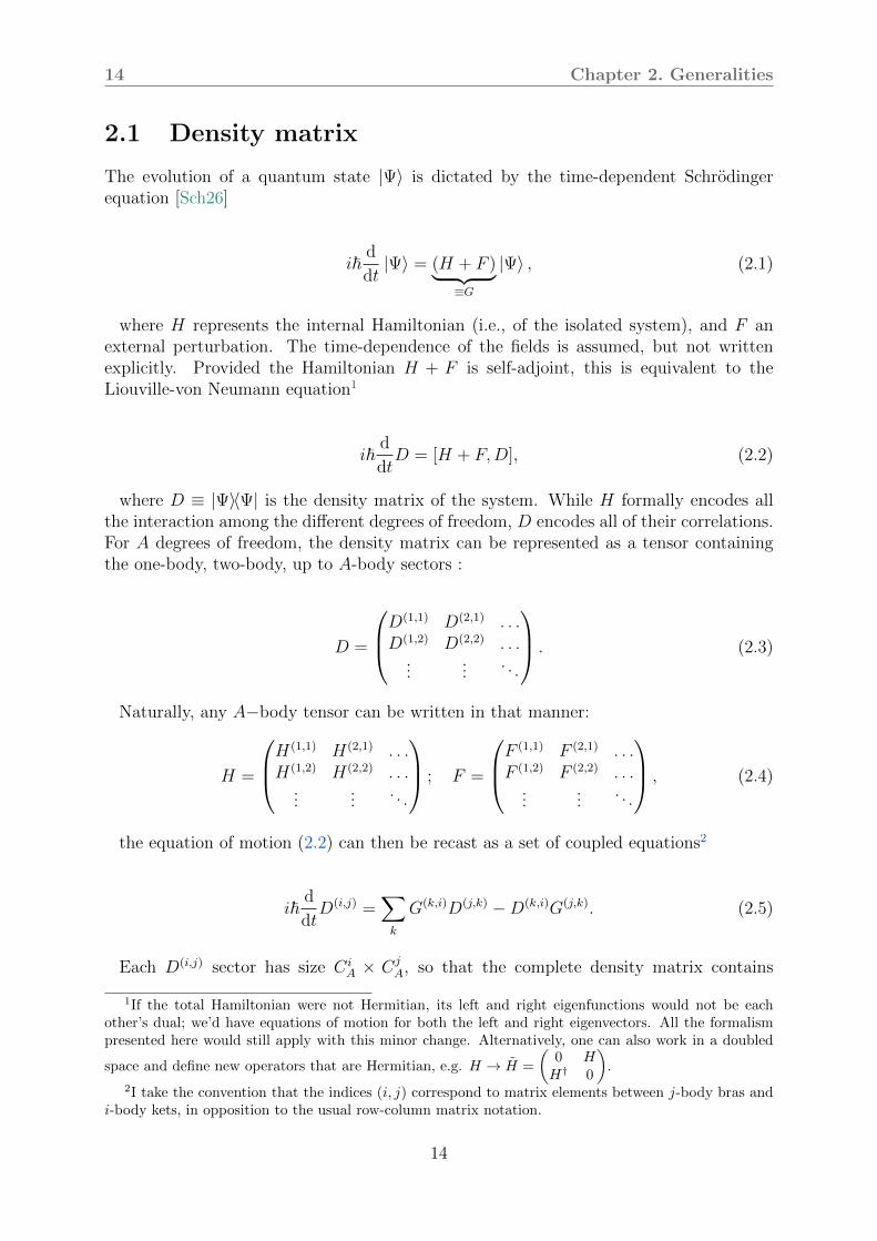
where D ≡ |Ψ⟩⟨Ψ| is the density matrix of the system. While H formally encodes allthe interaction among the different degrees of freedom, D encodes all of their correlations.For A degrees of freedom, the density matrix can be represented as a tensor containingthe one-body, two-body, up to A-body sectors :
D =
D(1,1) D(2,1) . . .D(1,2) D(2,2) . . .
......
. . .
. (2.3)
Naturally, any A−body tensor can be written in that manner:
H =
H(1,1) H(2,1) . . .H(1,2) H(2,2) . . .
......
. . .
; F =
F (1,1) F (2,1) . . .F (1,2) F (2,2) . . ....
.... . .
, (2.4)
the equation of motion (2.2) can then be recast as a set of coupled equations2
iℏd
dtD(i,j) =
∑k
G(k,i)D(j,k) −D(k,i)G(j,k). (2.5)
Each D(i,j) sector has size CiA × Cj
A, so that the complete density matrix contains
1If the total Hamiltonian were not Hermitian, its left and right eigenfunctions would not be eachother’s dual; we’d have equations of motion for both the left and right eigenvectors. All the formalismpresented here would still apply with this minor change. Alternatively, one can also work in a doubled
space and define new operators that are Hermitian, e.g. H → H =
(0 HH† 0
).
2I take the convention that the indices (i, j) correspond to matrix elements between j-body bras andi-body kets, in opposition to the usual row-column matrix notation.
14

Chapter 2. Generalities 15
(2A − 1)2 elements. Such an exponential growth of the Hilbert space with the number ofparticles quickly renders the exact equations of motion (2.1) and (2.2) intractable beyondthe few-body cases3. In order to tackle a wider range of systems, approximation schemeshave to be designed. The conceptually simplest one is to introduce a transformation overthe many-body space so as to recast as much of the system’s properties as possible ontothe few-body densities and discard the high-order terms. The most severe truncation isto retain only one-body degrees of freedom, in which case the Liouville-von Neumannequation reduces to its purely one-body sector:
iℏd
dtD(1,1) =
[G(1,1), D(1,1)
]. (2.6)
Nonetheless, such an abrupt restriction is in general not suited for a faithful description:for instance, a genuine Hamiltonian containing a kinetic term and a two-body interactionwill be degraded into a free Hamiltonian without further ado. In order to grasp as manycorrelations as possible within such a reduction, the density matrix is instead optimisedby imposing that the energy of the system be a variational minimum with respect to theone-body densities respecting a set of constraints on various observables. This leads tothe so-called time-dependent mean-field (TDMF) equations
iℏd
dtR = [G,R], (2.7)
with R and G the mean-field density matrix and total mean-field Hamiltonian, respec-tively. The general framework of the static mean-field theories, along with the specificHartree-Fock-Bogoliubov (HFB), will be briefly summarised in section 2.4.
2.2 Statistical ensemble
The study of many-body systems requires identifying the thermodynamical quantities ofinterest. Although all statistical ensembles are equivalent in the thermodynamic limit(N → ∞, V → ∞, N/V = cst), this is not the case for systems with a finite number ofdegrees of freedom, as the relative statistical fluctuations can be of sizeable importance[LL67b, §2]. The case of finite systems therefore demands a careful choice of the statisticalensemble. In this work, we impose that the thermodynamic variables T and µ, respec-tively corresponding to the temperature and chemical potential of the system, have somefixed value. The second fixes the average particle number. We consider therefore the sys-tem as a grand canonical ensemble. This choice permits the theory to incorporate statesthat do not display the correct number of particles into the description of the system; thatis, this ensemble allows including the particle number fluctuations of statistical nature.In addition, we may impose any kind of constraint; typically, geometric/shape constraintsmay be enforced through the expectation values QLM of the multipole moments of thedensity. It is also possible to fix a given value of the total linear or angular momenta P
3As a matter of illustration, the current state-of-the-art no-core shell model calculations can reachA ∼ 20 in the case of atomic nuclei, see e.g. [FN21; Dja+21].
15

16 Chapter 2. Generalities
and J by projecting to target values, the former constraint being crucial for the study ofself-bound systems such as atomic nuclei, since there is no external potential ensuring thelocalisation of the total wave function4. Consequently, self-bound systems are invariant bytranslation. As such, any densities that are identical up to a Galilean transformation areequally good reference states. In average, the total wave function is therefore completelydelocalised in space. Imposing a zero momentum condition forbids the system to wanderinside the coordinate space, thus forcing its localisation. Such shape and momentum con-straints allow targeting not only the (hopefully) global minimum of the potential energysurface spanned but any kind of state following the desired constraints5. In this work,only centre-of-mass (and eventually deformations) constraints are imposed, hence J willnever be forced onto a specific value, although this is allowed by the formalism developedin this thesis. The constraints are imposed by the method of Lagrange multipliers, writ-ten λLM for the multipolar moments and ωJ for the angular momenta. In that case, theconstrained states are obtained by minimising the grand potential
Ω = E − TS − µN −∑LM
λLMQLM − ωJ
√J(J + 1). (2.8)
The sum encodes the desired shape constraints. Once the (exact) density matrix Dof the system is known in some basis |n⟩ fulfilling the closure relation |n⟩⟨n| = I, thecalculation of any observable amounts to that of a trace:
⟨O⟩= ⟨Ψ|O|Ψ⟩ =
∑n
⟨Ψ|O|n⟩ ⟨n|Ψ⟩ =∑n
⟨n|DO|n⟩ = TrDO
. (2.9)
In particular,
E = TrDH
, (2.10)
N = TrDN
, (2.11)
S = TrD log D
, (2.12)
QLM = TrDQLM
. (2.13)
Other thermodynamic quantities can be calculated in the usual manner [LL67a, §14][LL67b, §5] [KG06, 1, A]. The ground state formally writes as the global minimumof (2.8)6 over the potential (hyper-)surface spanned by the possible eigenvectors (or,
4Note however that this full-glory projection is rather costly, as it formally requires integrating overthe set of all translated wave functions. Instead, we use the fact that the centre-of-mass motion isdecoupled from the motion of the nucleus in its intrinsic frame, which allows correcting the Hamiltonianby a one-plus-two-body term that imposing the zero-momentum condition.
5For simplicity, such constrained vacua will be referred to as ground states without distinction, keepingin mind that they may very well not be the vacuum corresponding to the global ground state but thoseof lowest energy fulfilling some constraints.
6For a time-dependent grand potential, the time-dependent ground state is the dense sequence of itsground state at each time, if we assume the adiabatic approximation.
16
Chapter 2. Generalities 17
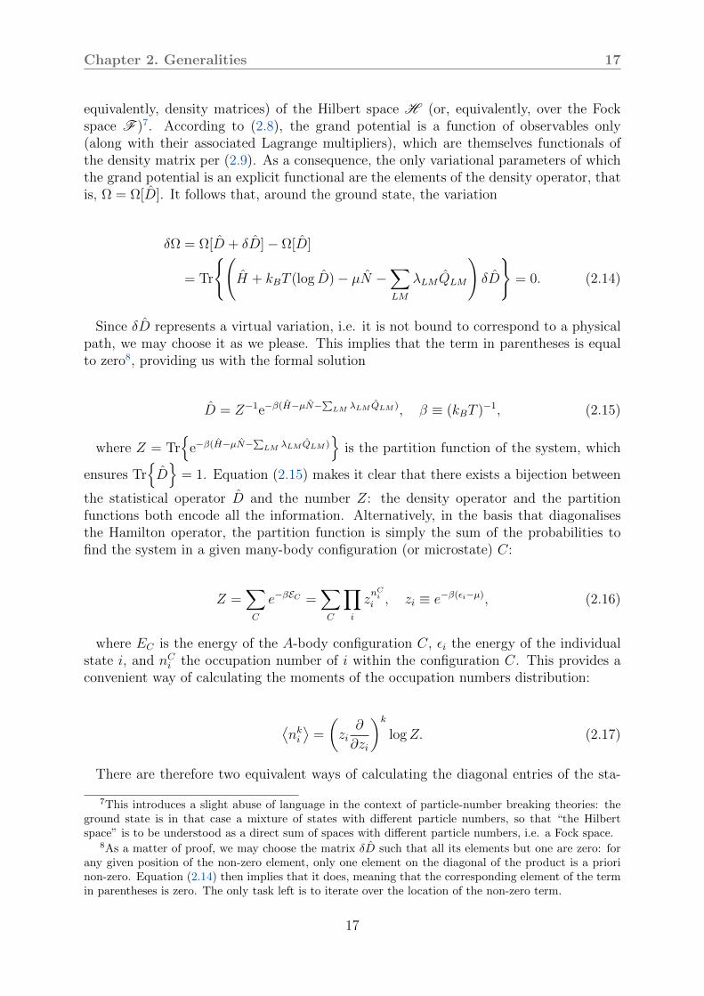
equivalently, density matrices) of the Hilbert space H (or, equivalently, over the Fockspace F )7. According to (2.8), the grand potential is a function of observables only(along with their associated Lagrange multipliers), which are themselves functionals ofthe density matrix per (2.9). As a consequence, the only variational parameters of whichthe grand potential is an explicit functional are the elements of the density operator, thatis, Ω = Ω[D]. It follows that, around the ground state, the variation
δΩ = Ω[D + δD]− Ω[D]
= Tr
(H + kBT (log D)− µN −
∑LM
λLMQLM
)δD
= 0. (2.14)
Since δD represents a virtual variation, i.e. it is not bound to correspond to a physicalpath, we may choose it as we please. This implies that the term in parentheses is equalto zero8, providing us with the formal solution
D = Z−1e−β(H−µN−∑
LM λLM QLM ), β ≡ (kBT )−1, (2.15)
where Z = Tre−β(H−µN−
∑LM λLM QLM )
is the partition function of the system, which
ensures TrD= 1. Equation (2.15) makes it clear that there exists a bijection between
the statistical operator D and the number Z: the density operator and the partitionfunctions both encode all the information. Alternatively, in the basis that diagonalisesthe Hamilton operator, the partition function is simply the sum of the probabilities tofind the system in a given many-body configuration (or microstate) C:
Z =∑C
e−βEC =∑C
∏i
znCi
i , zi ≡ e−β(ϵi−µ), (2.16)
where EC is the energy of the A-body configuration C, ϵi the energy of the individualstate i, and nC
i the occupation number of i within the configuration C. This provides aconvenient way of calculating the moments of the occupation numbers distribution:
⟨nki
⟩=
(zi
∂
∂zi
)k
logZ. (2.17)
There are therefore two equivalent ways of calculating the diagonal entries of the sta-
7This introduces a slight abuse of language in the context of particle-number breaking theories: theground state is in that case a mixture of states with different particle numbers, so that “the Hilbertspace” is to be understood as a direct sum of spaces with different particle numbers, i.e. a Fock space.
8As a matter of proof, we may choose the matrix δD such that all its elements but one are zero: forany given position of the non-zero element, only one element on the diagonal of the product is a priorinon-zero. Equation (2.14) then implies that it does, meaning that the corresponding element of the termin parentheses is zero. The only task left is to iterate over the location of the non-zero term.
17

18 Chapter 2. Generalities
tistical density matrix: using (2.15), or using (2.17) with k = 1. The average occupationnumbers are those of a Fermi-Dirac distribution
⟨ni⟩ =zi
1 + zi, (2.18)
whereas the thermal fluctuation of the particle numbers have variance
σ2i =
⟨n2i
⟩− ⟨ni⟩2 =
zi − z2i(1 + zi)2
. (2.19)
Not so surprisingly, the variance (2.19) is maximal for energies close to the temperature,namely σ2
max = 1/8 for Ei = kBT ln 3. That said, the relative thermal fluctuations, σ/ ⟨n⟩,as one could also expect, increase with the energy, as the orbitals are exponentially lessoccupied.
The solution (2.15) is, as is, not expressed in the basis that diagonalises H, whichmakes it impractical for the determination of D. A most convenient procedure is toexplicitly carry on the variations of δΩ, after the independent parameters have beenidentified. This machinery is deployed for the mean-field theories, as presented succinctlyin subsection 2.4.2. Whilst the other observables at play in (2.8) are system-independent,the energy requires a thorough analysis of the Hamiltonian, which is done in the nextsubsection.
2.3 Static Hamiltonian and some general properties
In real life, one may be interested in the response of a system initially in a state ofthermodynamic equilibrium (or not) in the absence of external field. Consequently, afirst step is to focus on obtaining the isolated eigenstates9. The Hamiltonian describinga many-body system writes in the most general form
H = T (1) + V (1, 2) +W (1, 2, 3) + . . . , (2.20)
where T contains all the one-body terms (typically consisting of the kinetic energy and,for self-bound (resp. externally bound) systems, of a one-body centre-of-mass correc-tion (resp. external potential)), V corresponds to the two-body interactions, and so on.Expliciting the indices of the individual degrees of freedom:
H =∑i
ti +1
2!
∑ij
vij +1
3!
∑ijk
wijk + . . . , (2.21)
or, in second-quantised form in an arbitrary basis spanning the whole one-body Hilbert
9Note that the present discussion trivially generalises to time-dependent Hamiltonians, e.g., one couldvery well study H(t), E(t), etc within the framework presented in this section.
18

Chapter 2. Generalities 19
space,
H =∑αβ
tαβb†αbβ +
1
(2!)2
∑αγβδ
vαγβδb†αb
†γbδbβ +
1
(3!)2
∑αβγδϵζ
wαγϵβδζb†αb
†γb
†ϵbζbδbβ + . . . ,
(2.22)
where the denominators appearing in (2.21) and (2.22) balance the over-countings due tothe sums running over all indices10.
Although the Hamiltonian describing A particles should in principle involve up to A-body interaction terms, the present work only considers vertices up to the three-bodyones. There is no system-independent justification why a many-body system can, eitherexactly or approximately (but with a good enough accuracy), be described in terms offew-body interactions.
Yet, a few arguments in favour of such low-rank Hamiltonians are the following:
- if the degrees of freedom are approximately independent (i.e., coupled weakly enough),we expect a “natural” hierarchy of the contributions. Loosely speaking, the expec-tation value ⟨O⟩ = ⟨O1−body⟩+ ⟨O2−body⟩+ ⟨O3−body⟩+ . . . of any relevant operatorO should obey ⟨Oi−body⟩ ≫
⟨O(i+1)−body
⟩≫ . . . for some small i.
- the interaction is not an observable. We therefore have the freedom to transform itthe way we fancy11, with the all-important constraint that all observables are unaf-fected by said transformation12. This is the idea underlying renormalisation group(RG) approaches [GL54a; GL54b; WK74], that have been shown capable of dras-tically improving the quality of the results obtained with truncated Hamiltonians[Her+17; Her+18; Her20].
- more practically, the matrix representation of a k−body operator in a generic basisis a Nk × Nk object13, which quickly grows out of the reach of the computationalresources a typical physicist has.
In particular, a small coupling constant14 and the Pauli principle15 both favour an ap-proximately independent particle picture: while the first one implies a strong hierarchyamong the k-body matrix elements, the second tends to disfavour scattering between theparticles by reducing the outgoing available phase space. It should nonetheless be notedthat small coupling constants do not guarantee the validity of the independent degreesof freedom picture, as combinatorics quickly render the contributions of high rank terms
10That is, one could do the substitutions 1k!
∑ij... →
∑i<j<... and
1(k!)2
∑α,β,... →
∑α<β<....
11That is, in a way that puts as much weight as possible on the lowest-rank terms.12More precisely, the observables should remain unchanged if the full initial Hamiltonian is kept. How-
ever, observables obtained from a truncated Hamiltonian do depend on the transformation. It is the verypurpose of the latter to render the contribution of high-rank terms as little as possible.
13This is worse than the combinatorial scaling of the previous section, since for practical applicationsthe wave functions are expanded on a basis which is not the basis spanned by the one-body eigenstates.
14As is the case for, e.g., electronic systems.15As is the case for fermionic systems. This includes composite bosons (e.g. Cooper pairs, α particles
to name a few) made of fermions, if the bosonic pairs still show substantial interaction.
19
20 Chapter 2. Generalities
prevalent16, see appendix B for an illustration.
When the Hamiltonian (2.22) is truncated at the three-body level, the energy of a(normalised) state |Ψ⟩ writes
E[|Ψ⟩] =∑αβ
tαβ⟨b†αbβ
⟩+
1
(2!)2
∑αγβδ
vαγβδ⟨b†αb
†γbδbβ
⟩+
1
(3!)2
∑αβγδϵζ
wαγϵβδζ
⟨b†αb
†γb
†ϵbζbδbβ
⟩, (2.23)
where the brackets ⟨.⟩ denote the expectation value with respect to |Ψ⟩. As already al-luded to, handling two- and higher-body densities is an exceedingly demanding task, whichwe want to avoid. For our salvation, the Wick theorem lets us recast such many-pointcorrelations functions into products of two-point ones, i.e. one-body densities [FW71, Ch.III.8] [BR86, Ch. IV] [Zee10, Ch. I.A.2].
2.3.1 Wick theorem
The expectation value of strings of creation and annihilation operators can be written asproducts of one-body densities by applying Wick’s theorem [Wic50; ES96] with respectto the yet-to-be-determined ground state |Ψ⟩. The theorem states that any product ofladder operators can be recast as a sum of pairs of such operators. It builds on the useof the normal-ordering of strings of operators, with the elementary contractions of twooperators (either creation or annihilation) Ai, Aj defined as
AiAj ≡ AiAj− :AiAj:, (2.24)
the dots denoting the normal ordering operation, which places all creation operatorsto the left. As Ai and Aj can be creation or annihilation operators, there exist foursuch elementary contractions. Owing to the usual commutation relations for bosons andfermions, three of these contractions vanish, the only remaining one being
AiA†j = δij. (2.25)
By induction, arbitrary strings of operators can be recast as a sum of products in-volving Wick-contracted and normal-ordered terms only. Such combinatorial expansionbeams when employed to calculate expectation values atop a reference state which is avacuum with respect to the annihilation operators. In that case, all strings involvingnormal-ordered terms vanish, and only the fully contracted term remains. The expecta-tion value of any strings becomes a product of expectation values of pairs of operators,which are tremendously more simple to handle. Since this is only true when the referencestate is annihilated by the lowering operators, the measure ⟨.⟩ corresponding to taking
16Typically, for A degrees of freedom, terms of order ∼ A/2 become outrageously dominant.
20

Chapter 2. Generalities 21
expectation values must be that of independent operators, i.e. be Gaussian17.
For fermions18, and after discarding non-fully contracted strings of operators (whichamounts to performing a mean-field approximation, as this only retains one-body densi-ties),
⟨b†αbβ
⟩≡ ρβα = δαβ −
⟨bβb
†α
⟩, (2.26)⟨
b†αb†β
⟩≡ κβα, (2.27)⟨
bαbβ⟩≡ καβ, (2.28)⟨
b†αb†γbδbβ
⟩= ρδγρβα − ρδαρβγ + κγακδβ, (2.29)⟨
b†αb†γb
†ϵbζbδbβ
⟩= ρζϵρδγρβα − ρζγρδϵρβα + ρζαρδϵρβγ (2.30)
− ρζϵρδαρβγ + ρζγρδαρβϵ − ρζαρδγρβϵ
+ ρζϵκγακδβ − ρζγκϵακδβ + ρζακϵγκδβ
− ρδϵκγακζβ + ρδγκϵακζβ − ρδακϵγκζβ
+ ρβϵκγακζδ − ρβγκϵακζδ + ρβακϵγκζδ.
More general considerations on the contractions of a string of creation and annihilationoperators can be made here, in order to gauge the recording complexity of generic ex-pectation values, and appreciate the relief brought by symmetrising the matrix elements.In the general setting, a string involving 2k operators can be contracted in (2k − 1)!!different ways. If anomalous contractions are not allowed, only b†b-type strings will resultin non-zero contributions, in which case there are k! different contractions. On the otherhand, Wick’s theorem (along with the use of anti-symmetrised interactions) reduces thenumber of interactions stemming from a k-body operator to ⌊k/2⌋+ 1 if anomalous con-tractions are allowed, and only 1 if not. This procedure thus reduces the doubly factorialbookkeeping down to a linear one.
2.3.2 Interaction symmetrisation
Depending on the spin of the degrees of freedom, the total many-body wave function isrequired to be either completely symmetric or antisymmetric under the exchange of anytwo particles. Introducing the operator Pij that swaps the particles i and j, a fermionicmany-body wave function must verify
−H︷ ︸︸ ︷H Pij |Ψ⟩︸ ︷︷ ︸
−|Ψ⟩
= −E |Ψ⟩ , (2.31)
so that the anti-symmetry can be cast into the Hamiltonian, and therefore into the
17In the language of path integrals, this means that the Lagrangian must only contain bilinears inthe operators (and their derivatives), which strongly suggests the use of mean-field approximations whendealing with many-body problems.
18As for bosons, all minus signs would become plusses.
21

22 Chapter 2. Generalities
interaction matrix elements. This symmetrisation of the interaction is very useful oncethe Wick theorem has been applied to the expectation value of H, as it allows transferringthe symmetry properties from the densities into the two- and three-body matrix elements.A properly anti-symmetrised interaction matrix elements arises from the following proce-dure. A generic k-body operator writes, in second-quantised form,
Ok−body =1
(k!)2
∑1,...,k1′,...,k′
u1,...,k,1′,...,k′b†1 . . . b
†kbk′ . . . b1′ . (2.32)
The k-body interaction vertex u(a), anti-symmetrised to the right (i.e.with respect topermutations of the k rightmost operators) can be built from an initial u through
u(a)1,...,k,1′,...,k′ ≡
∑P ′
(−1)πP′uP ′ (1,...,k,1′,...,k′)
=(1−
∑i,jall =
P ′
ij +∑i,j,kall =
P ′
ijP′
jk − . . .)u1,...,k,1′,...,k′ , (2.33)
where P ′denotes a permutation of the primed indices, and P ′ the set thereof. The
exponent πP ′ is the parity of the permutation19. For instance, the anti-symmetrisedfermionic two- and three-body interaction matrix elements read
v(a)ρραγβδ ≡ vαγβδ − vαγδβ, (2.34)
w(a)ρρραγϵβδζ ≡ wαγϵβδζ − wαβϵδγζ + wϵβαδγζ − wγβαδϵζ + wγβϵδαζ − wϵβγδαζ . (2.35)
The anti-symmetrised matrix elements generated by permuting indices to the rightare associated to contractions involving only b†b strings because this amounts to movingannihilation operators only. As for the remaining contractions, the form of the two- andthree-body matrix elements can be deduced by noting that the orderings to be involvedare, by construction, all the ones that do not contribute in producing the terms (2.34)-(2.35). For a k-body operator, there are (2k − 1)!! − k! such types of permutations.Alternatively, one can simply use the Wick-contracted densities (2.29)-(2.30) involvingpairing tensors. This yields:
v(a)κκαγβδ = vαγβδ, (2.36)
w(a)ρκκαγϵδβζ ≡ wαγϵβδζ − wαϵγβδζ + wγϵαβδζ − wαγϵβζδ
+ wαϵγβζδ − wγϵαβζδ + wαγϵδζβ − wαϵγδζβ + wγϵαδζβ. (2.37)
Using anti-symmetrised interactions allows us to recast the 21 different strings into only
19Naturally, this procedure can be applied to bosonic operators, with this time no parity (hence nominus signs) involved.
22
Chapter 2. Generalities 23
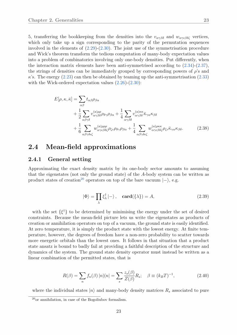
5, transferring the bookkeeping from the densities into the vαγβδ and wαγϵβδζ vertices,which only take up a sign corresponding to the parity of the permutation sequencesinvolved in the elements of (2.29)-(2.30). The joint use of the symmetrisation procedureand Wick’s theorem transform the tedious computation of many-body expectation valuesinto a problem of combinatorics involving only one-body densities. Put differently, whenthe interaction matrix elements have been anti-symmetrised according to (2.34)-(2.37),the strings of densities can be immediately grouped by corresponding powers of ρ’s andκ’s. The energy (2.23) can then be obtained by teaming up the anti-symmetrisation (2.33)with the Wick-ordered expectation values (2.26)-(2.30):
E[ρ, κ, κ] =∑αβ
tαβρβα
+1
2
∑αβγδ
v(a)ρραγβδρδγρβα +
1
4
∑αγβδ
v(a)κκαγβδ κγακβδ
+1
6
∑αβγδϵζ
w(a)ρρραγϵβδζρζϵρδγρβα +
1
4
∑αβγδϵζ
w(a)ρκκαγϵβδζρζϵκγακβδ. (2.38)
2.4 Mean-field approximations
2.4.1 General setting
Approximating the exact density matrix by its one-body sector amounts to assumingthat the eigenstates (not only the ground state) of the A-body system can be written asproduct states of creation20 operators on top of the bare vacuum |−⟩, e.g.
|Φ⟩ =∏λ
ξ†λ |−⟩ , card(λ) = A, (2.39)
with the set ξ† to be determined by minimising the energy under the set of desiredconstraints. Because the mean-field picture lets us write the eigenstates as products ofcreation or annihilation operators on top of a vacuum, the ground state is easily identified.At zero temperature, it is simply the product state with the lowest energy. At finite tem-perature, however, the degrees of freedom have a non-zero probability to scatter towardsmore energetic orbitals than the lowest ones. It follows in that situation that a productstate ansatz is bound to badly fail at providing a faithful description of the structure anddynamics of the system. The ground state density operator must instead be written as alinear combination of the permitted states, that is
R(β) =∑n
fn(β) |n⟩⟨n| =∑s
zs(β)
Z(β)Rs; β ≡ (kBT )
−1, (2.40)
where the individual states |n⟩ and many-body density matrices Rs associated to pure
20or annihilation, in case of the Bogoliubov formalism.
23
24 Chapter 2. Generalities
states implicitly depend on the inverse temperature β through the self-consistent solutionto the mean-field equation.
The fn and zs can be determined by a derivation21 entirely similar to that of section 2.2:
fn =1
eβEn + 1, zs = e−βEs , Z =
∑s
zs, (2.41)
with En the energy of the nth one-body eigenstate and Es the energy of the sth productstate. The fact that the fn are different from 0 or 1 (except at zero temperature), causesthat the thermal density R(β) cannot be associated to a pure state, but is rather astatistical mixture of different density operators. The most general (single-reference)finite temperature mean-field transformation, the one of Hartree-Fock-Bogoliubov (HFB),is recapitulated in the next subsection.
2.4.2 Hartree-Fock-Bogoliubov theory
The simplest mean-field theory, the Hartree-Fock approximation, assumes that the opti-mal creation (resp. annihilation) operators write as linear combinations of the creation(resp. annihilation) operators spanning a basis of the one-body Hilbert space, with thesymmetry that only operators of identical time-signature can mix. It is thus by con-struction unable to account for pairing correlations. In the presence of a pairing inter-action among the degrees of freedom, the single-particle states interact even if they donot have the same time signature. While the Bardeen-Cooper-Schrieffer (BCS) theory[Coo56; BCS57a; BCS57b] assumes that only time-reversed partners are explicitly cou-pled through a pairing field22, the most general way of constructing the new eigenstates isto express them as a linear combination of all the single particle ones, regardless of theirrelative quantum numbers. In the same spirit as the BCS theory defines new independentdegrees of freedom operators as a mixing of forward- and backward-propagating singleparticle ones, the HFB transformation [Bog47; Bog58; BTS58] defines quasi-particles23
on top of the HFB vacuum as linear combinations of all possible single-particle states,and is conventionally parametrised as
αµ =∑i
U∗iµci + V ∗
iµc†i , (2.42a)
ᆵ =
∑i
Viµci + Uiµc†i . (2.42b)
21One could also invoke the “heuristic” argument that R(β) being a state built with independent degreesof freedom, the ground state density immediately writes as a linear combination of the independent-particle densities, weighted by their Fermi-Dirac coefficients.
22Which is generally a reasonable assumption since these are the pairs of states with maximal spatialoverlap.
23One can make the distinction between occupied states (quasi-holes, or qh) and unoccupied states(quasi-particles, or qp). While it is customary to refer to both as qp, the discrimination will hopefullybe made scrupulously.
24
Chapter 2. Generalities 25
The matrices U and V encode the Bogoliubov transformation, and are to be obtainedby the minimisation of the mean-field grand potential. The product state of lowest energyis constructed as a vacuum with respect to the newly defined quasi-particle annihilationoperators (2.42a)-(2.42b):
αµ
∣∣ΦHFB⟩= 0 ⇒
∣∣ΦHFB⟩=∏λ
αλ |−⟩ . (2.43)
Special attention should be paid when defining the transformation, as many conventionscoexist [DFT84]. The prescription (2.42a)-(2.42b) for the transformations corresponds tothe so-called traditional representation of the Bogoliubov transformation. Eventually, theequations for the Russian convention will also be given in section 3.3. The transformationcan conveniently be represented in matrix form24:
B† ≡(U † V †
V T UT
);
(αα†
)= B†
(cc†
), (2.44)
defining the Bogoliubov matrix B. The inverse transformation is
(cc†
)= B
(αα†
); B =
(U V ∗
V U∗
);
ci =∑µ
Uµiαµ + V ∗µiα
†µ,
c†i =∑µ
Vµiαµ + U∗µiα
†µ.
(2.45)
Amounting to a mere linear transformation, the passage from the initial basis c†, cto the Bogoliubov basis α†, α must be achieved through a unitary transformation, i.e.,BB† = I = B†B. This ensures the preservation of the canonical anti-commutation rela-tions between the Bogoliubov operators:
αµ, α†ν =
∑ij
U∗iµVjνci, cj+ U∗
iµUjνci, c†j+ V ∗iµVjνc†i , cj+ V ∗
iµUjνc†i , c†j
=∑i
U∗iµUiν + V ∗
iµViν = δµν , (2.46)
αµ, αν =∑ij
U∗iµUjνci, cj+ U∗
iµVjνci, c†j+ V ∗iµUjνc†i , cj+ V ∗
iµVjνc†i , c†j
=∑i
U∗iµViν + V ∗
iµUiν = 0. (2.47)
This unitarity requirement can also be written in matrix form, yielding the two sets ofrelations
24Single-particle operators are not barred to ease the representation; one should see the c’s and c†’s asspanning both the time-forward and time-backward states here.
25

26 Chapter 2. Generalities
B†B = I : U †U + V †V = I, (2.48a)
U †V ∗ + V †U∗ = 0, (2.48b)
V TU + UTV = 0, (2.48c)
V TV ∗ + UTU∗ = I, (2.48d)
BB† = I : UU † + V ∗V T = I, (2.49a)
UV † + V ∗UT = 0, (2.49b)
V U † + U∗V T = 0, (2.49c)
V V † + U∗UT = I. (2.49d)
Since the transformation allows the mixing of all the states regardless of their behaviourunder symmetry operations (e.g. time reversal, parity, angular momentum, etc), the re-sulting wave functions do not possess well-defined quantum numbers, and, most notori-ously, the product state of lowest energy resulting from the application of the Rayleigh-Ritz method does not conserve the particle number. As an illustration, one has in generala non-zero pairing tensor:
κij ≡⟨c†ic
†j
⟩=∑µν
VµiVνj ⟨αµαν⟩+ VµiU∗νj
⟨αµα
†ν
⟩+ U∗
µiVνj
⟨ᆵαν
⟩+ U∗
µiU∗νj
⟨ᆵα
†ν
⟩.
(2.50)
Of the four expectation values, only the second and third can survive by virtue of theproduct state ansatz (2.43). As the independent degrees of freedom of the problem arethe quasi-particle operators α, α†, one has
⟨αµα
†ν
⟩= fµδµν and
⟨ᆵαν
⟩= (1 − fµ)δµν .
The generalised density (or Valatin) operator, that contains all the one-body densitycorrelations, then writes in its diagonal form
R(β) ≡(⟨
α†α⟩
⟨αα⟩⟨α†α†⟩ ⟨
αα†⟩) =
(f
1− f
); ⟨.⟩ =
⟨ΦHFB
∣∣.∣∣ΦHFB⟩, (2.51)
f and f being the Fermi-Dirac occupations for unbound and bound states, respectively.Naturally, a consequence of the fact that the eigenvalues of the HFB equation come in pairis that f = f ; the distinction is however maintained for bookkeeping purposes. Just like inthe BCS theory, the fact that particle-particle and hole-hole correlations can be non-zeroforces the doubling of the basis. Equivalently, this necessity can be seen directly fromthe form of the Bogoliubov transformation (2.42), which mixes creation and annihilationtogether25. Recalling the definitions (2.26)-(2.28) of the elementary contractions withrespect to the sought HFB vacuum, the densities in the c, c† basis write
ρ(β) = UfU † + V ∗(I − f)V T , (2.52a)
κ(β) = UfV † + V ∗(I − f)UT , (2.52b)
−κ(β) = V fU † + U∗(I − f)V T , (2.52c)
I − ρ(β) = V fV † + U∗(I − f)UT . (2.52d)
25One may also take the obverse viewpoint, saying that the HF theory is a very peculiar transformation,in which c’s and c†’s do not mix so that the density matrix is separable as a direct sum. The often enforcedtime-reversal symmetry and zero temperature regime then allow discarding half of the generalised densitymatrix.
26
Chapter 2. Generalities 27
The energy writes as in (2.38), with the minimisation of the grand potential to be carriedout within the space of one-body densities (2.52). Due to the canonical relations (2.46),not all the variational parameters are independent26. This can also be seen straight from(2.52) with the help of (2.48), (2.49):
(2.52) and f = f : ρ(β) = ρ∗(β), (2.53a)
c, c = 0 : κ(β) = −κT (β), (2.53b)
c†, c† = 0 : κ(β) = −κT (β). (2.53c)
In addition, anticipating that the Hamiltonian of the theory is Hermitian27, one knowsthat the U and V matrices can be made real, and the eigenvalues come by pairs of oppositesign (hence E = E, implying in turn f = f) due to the doubling of the basis. Equippedwith this, all densities become real, and can reach finer degrees of symmetries:
U, V real : ρT (β) = ρ(β), (2.54a)
ρT (β) = ρ(β), (2.54b)
κ(β) = κ(β). (2.54c)
These symmetries will be reviewed in greater detail in section 3.3. Rather than taking allof ρ, ρ, κ, κ, one can thus consider ρij, κij, ρij, κiji≤j as the complete and irreducible28
set of parameters with respect to which the energy is to be varied. One thus has
δE =∑i≤j
δE
δρijδρij +
δE
δρijδρij +
δE
δκij
δκij +δE
δκij
δκij. (2.55)
Then, on defining the mean and pairing fields according to
hνµ ≡ δE
δρµν, (2.56a)
hνµ ≡ δE
δρµν, (2.56b)
∆µν ≡ δE
δκµν
, (2.56c)
∆µν ≡ δE
δκµν
, (2.56d)
we may define the generalised Hamilton matrix such that δE = TrHδR: after iden-tifying the diagonal terms of HδR with those of (2.55), one obtains
26While the corresponding relations between the one-body densities are sometimes determined fromthe idempotency of the generalised density, at finite temperature the density operator is not longer asingle product state, so that this relation does no hold any more. Eventually, the Rk(β), k ∈ N form aconvex sequence, and have a fixed point only at T = 0. The idempotency can only be met in the productstates (of which the thermal density is a mixture), not in the thermal density itself.
27Which is natural since the system is closed, hence of unitary evolution.28Irreducibility is to be understood within the doubled basis: owing to the relations between barred
and non-barred densities, this set still contains redundancies.
27
28 Chapter 2. Generalities
H =
(h ∆
−∆ −h
), (2.57)
with the fields deriving from (2.38) writing29
hαβ = tαβ +∑γδ
v(a)ρραγβδρδγ +
1
2
∑γδϵζ
w(a)ρρραγϵβδζρζϵρδγ +
1
4
∑γδϵζ
w(a)ρκκαγϵβδζ κϵγκδζ , (2.58a)
∆αγ =1
2
∑γδ
v(a)κκαγβδ κβδ +
1
2
∑γδϵζ
w(a)ρκκαγϵβδζρζϵκβδ, (2.58b)
∆αγ =1
2
∑γδ
v(a)κκαγβδ κβδ +
1
2
∑γδϵζ
w(a)ρκκαγϵβδζρζϵκβδ, (2.58c)
hαβ = tαβ +∑γδ
v(a)ρραγβδ ρδγ +
1
2
∑γδϵζ
w(a)ρρραγϵβδζ ρζϵρδγ +
1
4
∑γδϵζ
w(a)ρκκαγϵβδζ κϵγκδζ . (2.58d)
Due to the hermicity of the HFB Hamiltonian, one has h† = h and ∆† = −∆, in consis-tency with the symmetries of the generalised density matrix. As a consequence of (2.53a),ones also has h∗ = h, while (2.54c) gives ∆ = ∆.
Since the energy is to be varied with certain constraints, one should express these in thedoubled basis as well in order to handle a single representation. The expectation valuesof generic one-body operators Q =
∑ij Q
ρijc
†icj + Qκ
ijcicj can be written in the doubledbasis thanks to the very same procedure, making use of the symmetries (2.53) and (2.54)
TrQρρ+ TrQκκ =1
2Tr
(Qρ Qκ
(Qκ)T (−Qρ)∗
)(ρ κ−κ I − ρ
)+
1
2TrQρ. (2.59)
It should be noted that Qρ being real and symmetric, using its complex conjugate isentirely conventional and due to using the relation (2.53a). It will be shown in section 3.3that the only choice consistent with complex matrix elements is to use the scalar transposeof Qρ. In our case, where the constraints are imposed solely for the particle numbers andmultipolar moments (whose operators only have components in the normal sector), theseexpressions reduce to the usual block-diagonal ones.
One finds the set of many-body states by minimising the grand potential (2.8), withthe additional constraint that the associated density operators Rp.s. must correspond toproduct states. This translates into the fact that one can find a set of idempotent densitymatrices Rp.s. solving the equation of motion. However, they only correspond to thepossible pure states that can be obtained, and the one of lowest energy identifies with theground state only in the T → 0 limit. In the T > 0 case, the ground state is a mixtureof these densities according to (2.15) (or equivalently, in the case of the FTHFB theory,
29Note that the indices β and γ are sometimes permuted in order to write ∆αβ rather than ∆αγ ; thisis a matter of convention.
28
Chapter 2. Generalities 29
using (2.52)). Thus, one only has to solve
δ
(E − µN − Λ(R2
p.s. −Rp.s.)−∑LM
λLM(QLM − qLM)
)= 0, (2.60)
where the indices LM run over the multipole moments we want to constrain to thevalues qLM . Solving this equation gives the product state of lowest energy, along with theeigenvectors of the constrained Hamiltonian. Recalling the expressions of the expectationvalues and using (2.59), one obtains by the very same argument as in section 2.2
H − µN − ΛRp.s. −Rp.s.Λ + Λ− 1
2
∑LM
λLMQLM = 0. (2.61)
This expression can be multiplied by Rp.s. separately to the left and to the right, thesubtraction of these two copies leading to the static HFB equation
[H − 1
2
∑LM
λLMQLM ,Rp.s.
]= 0. (2.62)
Once this equation has been solved, the thermal state R can be constructed from thedensity operatorRp.s. with the lowest energy using the Fermi-Dirac factors, or equivalentlyas a weighted sum over the whole set Rp.s..
2.5 Thermal phase transitions
Allowing the system to have non-zero temperatures opens a way to several phenomena.Naturally, one might expect from their everyday experience that the changes of a system’stemperature can trigger a plethora of effects, the most notable being the occurrence ofphase transitions30. In the case of interacting quantum systems, thermal scattering ofthe particles between the possible shells can lead to highly non-trivial rearrangements ofthe energy spectrum. More specifically, the pair condensate being produced by a (ratherweak) interaction between time-reversed partners, the competition between pairing andthermal effects is easily conceived to cause the breakup of pairs when the temperature isincreased. In the case of deformation, a restoration of the spherical symmetry is also tobe anticipated: a well-pronounced deformation marks that a set of corresponding orbitalsis occupied while states of higher energy are not. When the temperature is increased,the nucleons initially sitting on the deformed orbital also have significant probability tooccupy all the energetically close states, resulting in an averaging that smoothens thetotal deformations [BM75]32. The two following subsections concisely illustrate the two
30The complex problem of understanding how phase transitions can occur in finite systems is entirelyset aside; the reader may refer to [YL52; LY52], [Mai05]31and [CG08].
31Mind that the r.h.s. of his equation (2) should read κ∏N(V )
r=1
(1− z
zr
), without the log.
32Likewise, one could also expect a spherical to deformed transition in very small systems.
29
30 Chapter 2. Generalities
predicted behaviours.
2.5.1 Collapse of the pairing via thermal excitations
From the expression (2.52b), one sees with the help of (2.49) that the pairing correlationsshould fade out at high temperatures:
κij =∑k
V ∗ikU
Tkj(1− fk − fk) −→
β→00. (2.63)
That said, it leads to a pairing energy that appears smoothly vanishing, whereas it isknown that within mean-field theories like HFB and BCS, pairing does not survive beyonda critical temperature Tc at which the transition from the superfluid to the normal phaseoccurs [BCS57c]. The rapid collapse of the pairing tensor is therefore encoded in the Vand U amplitudes. While the sharp transition cannot be inferred directly from (2.69)alone, one can be convinced that, the pairing gap depending on the average occupationof the shells, a much faster collapse than the one predicted by a too quick observation of(2.63) should be expected. In addition, pairing is mostly a surface phenomenon. Albeitthis is not easy to see from the Bogoliubov transformation, this is clearer by using theBloch-Messiah-Zumino (BMZ) decomposition [BM62; Zum62] [RS80, Secs. 7.2, 7.3, App.E1] (and its generalisation [Dob00]):
(U † V †
V T UT
)=
(C†
CT
)(U † V †
V † U †
)︸ ︷︷ ︸
BCS-like
(D†
DT
)︸ ︷︷ ︸
HF-like
. (2.64)
Since this transformation is well-known, its features are only succinctly recapped here.The first step is a block-diagonal transformation of the single particle operators amongthemselves, that puts the normal density matrix and pairing tensor in their diagonalform33. This defines the so-called canonical basis. In the situation where pairing cor-relations are not described, this is equivalent to the Hartree-Fock transformation. TheHamiltonian transformed accordingly can thus be written as a collection of two by twomatrices:
Hcb =N⊕k
hcbk =
N⊕k
(ϵk − λ ∆k
−∆k −ϵk + λ
)= diag(hcb
1 , . . . , hcbN ), (2.65)
each block being diagonalised by a BCS-like transformation with squared amplitudesand eigenvalues
33Depending on the ordering of the c†, c operators, the pairing tensors can be made either diagonalor anti-diagonal.
30

Chapter 2. Generalities 31
v2k =1
2
(1− ϵk − λ√
(ϵk − λ)2 +∆2k
), (2.66)
u2k =
1
2
(1 +
ϵk − λ√(ϵk − λ)2 +∆2
k
), (2.67)
E±k = ±
√(ϵk − λ)2 +∆2
k. (2.68)
This second transformation thus takes the canonical basis to the BCS basis. The thirdrotation mixes the BCS quasiparticle operators among themselves, leading to the Bogoli-ubov basis. The BMZ theorem can thus be understood as a decomposition of the full HFBtransformation into a series of HF-like and BCS-like transformations, followed by a thirdone diagonalising the resulting Hamiltonian and density operator simultaneously. As thedensity matrix is diagonal in the canonical basis, it corresponds to the best independentparticle representation of the problem, hence it is convenient for a physical analysis. Forthe present discussion, we assume that the last transformation is trivial (C = I), so thatthe HFB transformation reduces to the HF-BCS one. In that case, the total energy writes
EBCStot =
∑k
(ϵk − λ)[v2k(1− fk) + (1− v2k)fk] + ∆kukvk(2fk − 1) ≡ EBCSnormal + EBCS
pair .
(2.69)
Remarking that 2ukvk = ∆k/EBCSk and eying (2.68), one sees that the effects of pairing
are localised around the Fermi surface, which is another argument in favour of a rapidcollapse of the pairing with the temperature, since the levels close to the Fermi energyare the most affected by the statistical distribution (2.41). This statement can be mademore quantitative by showing [BCS57c; Gor96] that the pairing abruptly vanishes abovea critical temperature TC
∆(T ) = ∆(0)
[1−
(T
TC
)m]1/2Θ(TC − T ), (2.70)
where the zero-temperature pairing gap ∆(0) is obtained by assuming the pairing inter-action to be constant within a small window around the Fermi energy. Typical expectedvalues for the critical temperature are about 0.5-0.6 times ∆(0).
2.5.2 Spherical symmetry restoration
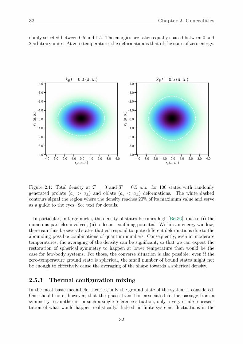
Like for the pairing transition, the evolution of the deformation with temperature isstrongly affected by the energy spectrum and the shape of the corresponding wave func-tion. At low temperature, the overall deformation is that of the lowest energy states. Asthe temperature increases, several states can be occupied with about similar probabilities,which results in an essentially spherical thermal state. Figure 2.1 considers 100 shells towhich are associated Woods-Saxon density profiles, with relative diffusenesses az, a⊥ ran-
31
32 Chapter 2. Generalities
domly selected between 0.5 and 1.5. The energies are taken equally spaced between 0 and2 arbitrary units. At zero temperature, the deformation is that of the state of zero energy.
-4.0 -3.0 -2.0 -1.0 0.0 1.0 2.0 3.0 4.0rz (a. u.)
-4.0
-3.0
-2.0
-1.0
0.0
1.0
2.0
3.0
4.0
r(a
.u.)
kBT = 0.0 (a. u.)
-4.0 -3.0 -2.0 -1.0 0.0 1.0 2.0 3.0 4.0rz (a. u.)
-4.0
-3.0
-2.0
-1.0
0.0
1.0
2.0
3.0
4.0
r(a
.u.)
kBT = 0.5 (a. u.)
Figure 2.1: Total density at T = 0 and T = 0.5 a.u. for 100 states with randomlygenerated prolate (az > a⊥) and oblate (az < a⊥) deformations. The white dashedcontours signal the region where the density reaches 20% of its maximum value and serveas a guide to the eyes. See text for details.
In particular, in large nuclei, the density of states becomes high [Bet36], due to (i) thenumerous particles involved, (ii) a deeper confining potential. Within an energy window,there can thus be several states that correspond to quite different deformations due to theabounding possible combinations of quantum numbers. Consequently, even at moderatetemperatures, the averaging of the density can be significant, so that we can expect therestoration of spherical symmetry to happen at lower temperature than would be thecase for few-body systems. For those, the converse situation is also possible: even if thezero-temperature ground state is spherical, the small number of bound states might notbe enough to effectively cause the averaging of the shape towards a spherical density.
2.5.3 Thermal configuration mixing
In the most basic mean-field theories, only the ground state of the system is considered.One should note, however, that the phase transition associated to the passage from asymmetry to another is, in such a single-reference situation, only a very crude represen-tation of what would happen realistically. Indeed, in finite systems, fluctuations in the
32
Chapter 2. Generalities 33
order parameters can be of sizeable importance. The corresponding energy surface canbe explored to a substantial extent. As a consequence, a more faithful description wouldinvolve mixing all the configurations of the surface obtained for a given temperature.Expectation values should therefore be calculated as a doubly averaged quantity: for anoperator O, labelling a point of the energy surface as q,
⟨⟨O⟩⟩ =
∫dq e−βF (q)⟨O⟩q∫dq e−βF (q)
, (2.71)
the first averaging being the usual tracing operation, ⟨O⟩q = TrOD(q)
, the second
the averaging over all configurations at a given temperature, and F the Helmholtz freeenergy. The results presented in chapters 4-5 only carry out the first averaging. Becausethe statistical weights of the configuration are exponentially decreasing functions of theinverse temperature, this approximation should be valid only at very low temperatures.In the case of phase transitions, the sharp collapse of the order parameter should not holdany more: close below (or above) the critical temperature, a fraction of the states withsignificant weight may be in a state fulfilling either symmetry, so that the sharp evolutionconcerning only the ground state is diluted in the thermal average. In particular, ithas been shown in [MER03b; MER03a] that including the thermal averaging smoothensthe evolution of the average deformation and pairing a great deal, and also that thediscrepancy between the single-reference and fully averaged results indeed increases withthe temperature. An interesting alternative is to include the particle number fluctuationdirectly into the FTHFB equations [DA03; Din06], which is shown to also make the phasetransition more gentle in the case of superfluidity.
2.6 Response theory
2.6.1 General aspects and points of view
Collective behaviours are an omnipresent property of strongly correlated systems. Inquantum mechanics, all excitations can be represented as picking one or several particle(s)in a given set of states, and placing them back on different orbitals. The overall differencein spin is integer34, and thus corresponds to bosonic excitations. This bosonic charac-ter can only provide an approximate representation for two reasons. First, for fermions,the Pauli principle constrains the permitted transitions, whereas a simple boson picturecannot account for it. Second, the raising and lowering of particles has consequences onthe whole structure of the ensemble, since the degrees of freedom interact. Therefore,in interacting theories, the promotion of a degree of freedom from one state to anothermodifies the levels of all the particles; consequently, a self-consistent theory of collectivemodes must break this bosonic approximation. When the reference state is obtained viaan approximation, e.g. within a mean-field theory, this inclusion of additional correlations
34Unless one has the somewhat curious idea of letting bosons transmute into fermions and vice versa,see e.g. [Pol88; Okn14].
33
34 Chapter 2. Generalities
changes the reference state, so that the ground state of the system with respect to theexcitations is not the mean-field state, but a more correlated one.
The collective features of a quantum system can be studied from two different points ofview:
- One may take an “external” (or extrinsic) look and send an external probe ontothe system in order to excite the collective eigenmodes that are consistent withthe selection rules of the ensemble probe+system. This standpoint is commonlyformalised as the response theory. As will be shown in subsection 3.4, this view canbe related to the “internal” one by extending the linear response into the complexplane and carrying on suitable contour integrations [Som83].
- Conversely, one may adopt an “internal” (or intrinsic) point of view by consideringthe system as truly isolated, and determine its collective states by diagonalising itsfull-fledged Hamiltonian, or an approximation thereof. The correspondence withthe “external” viewpoint is obtained by calculating the transition probability froman eigenmode to another under the action of a selected probe [RS80, Ch.8][PN66].
The two emblematic formulations of the external and internal perspectives are, respec-tively, the TDMF and the RPA.
2.6.2 Linear approximation
The linear response theory goes by the assumption that excitations of more than onedegree of freedom are largely sub-leading and can therefore be neglected. From the ex-perimental side, this supposes that the probe employed to excite the system is of smallenough intensity, and active for a timescale small enough to prevent non-linear effectsfrom building up, for instance through a heating up of the system [Som83]. The validityof the linear regime can thus be experimentally assessed in two different manners:
- by scaling up the intensity I of the probe, e.g. I → λI, with λ some scaling factor,
- by increasing the duration for which the probe is turned on, e.g. T → λT ,
the linear response regime resulting in the expectation values of the fluctuations ofany observable to scale accordingly, i.e. ⟨δO⟩ → λ ⟨δO⟩. In real-life experiments, it iscommonly assumed and verified that such non-linear effects are largely sub-leading withrespect to statistical fluctuations and device-based sources of non-linear behaviours. Fromthe theory side we can’t do wonders, except going beyond the linear approximation andchoosing the amplitude of F such that linear terms are dominant. To make the connec-tion with experiment, F can be chosen to match the amplitude of an actual probe. Theinclusion of non-linear type of fluctuations is usually realised within second RPA [Da 65;Yan87; GGC10; Gam+16; VGG18], a specific kind of extended RPA theories [LCA98;LCA99; Tse13; Sch+20] where up to two-phonons modes are considered.
While the characteristics of the probe plays a crucial role in the validity of the linearapproximation, the initial state of the system is naturally of considerable importance.
34

Chapter 2. Generalities 35
If the system is not in a local state of equilibrium, then an arbitrarily small probe candrive it away from its initial state towards a more stable one with an a priori very dif-ferent structure. Such an instability mathematically translates into a non-semi positivedefinite Hessian (often called the stability matrix), and therefore into complex eigenval-ues. It follows that detecting non-real collective eigenvalues invalidates the linear regime.Two techniques for determining the presence of such instabilities within the formalismdeveloped in this work will be given in subsection 3.8.
2.6.3 Formalisms survey
Given an initial state, collective motion on top of it can be addressed by a plethora oftechniques. Non-exhaustively, the equations describing small amplitude fluctuations canbe obtained by the following approaches:
- by the equation of motion method on double commutators [Row68; Yan87; Sch+20][RS80, Sec. 8.4],
- by the Dyson equation and similar methods [Dys49; Nam50; LS50; Sch51; SB51;HM52],
- by diagrammatic techniques [GB57],
- as a linearisation of the time-dependent equations of motion [Noz64, Ch. 2] [RS80,Sec. 8.5] [Som83] or Liouville-von Neumann equations,
- as the small amplitude limit of the full-fledged generator coordinate method (GCM)[JS64; BW68].
Note that these techniques can be used to go beyond the linear approximation, a prioriwithout encountering any critical dead-end, although at the cost of severe complexifica-tions of the formalisms.
Rowe’s equation of motion approach re-formulates quantal eigenvalue equations in termsof expectation values identities involving sets of commutators. While they can be derivedin a strictly exact manner, the evaluation of the commutators usually requires that ap-proximations be done. For the (Q)RPA, one has to assume the correlated ground state|(Q)RPA⟩ can be replaced by the mean-field one, |HF(B)⟩. This amounts to the quasi-boson approximation (QBA), where the excitations are assumed to be of purely bosoniccharacter.
The Dyson equation can be derived from several starting points, e.g. from time-dependent perturbation theory [Dys49] or from a variational principle [Sch51]. In thecontext of time-dependent oscillations, it can be used to determine the response functionof the system, or its linear component, by keeping only the first-order expansion of thetime-ordered propagator, as done in subsection 2.6.4.
Diagrammatically, the RPA resums ring-type density correlations only [SHS08; SHB13].Ladder diagrams are not included, which corresponds to the fact that the basic RPA does
35
36 Chapter 2. Generalities
not include short-range correlations. Beyond-RPA theories, such as the self-consistentRPA [Sch+20; DU20a; DU20b] aim at including such polarisation effects by self-consistentlycorrelating the reference state.
As for TDMF-type equations, the linear approximation is easily seen. Since the densityfluctuations are expected to be small, only terms linear in the oscillating densities areretained. The generic procedure will be established in chapter 3.
The last point states that the QRPA can be obtained from the GCM. This is perhapssurprising, because the GCM is in practice established as a large amplitude collectivemotion method over a selected set of few collective coordinates. On the other hand, theQRPA is a small amplitude theory that does not resort to such macroscopic variables.The key to this apparent paradox lies in that the derivation of [JS64] does not specify thecoordinates employed in the Hill-Wheeler-Griffith equation. One can thus take them tobe a complete set of many-particle many-hole coordinates (mpmh), which reduce in thesmall amplitudes limit to a 1p1h (or 2qp when superfluidity is included) expansion. Con-versely, one can consider a set of collective coordinates -and their canonical conjugates-sufficiently large and rich to approach the exact motion of the system. The small am-plitude limit then selects the 1p1h or 2qp components of these fluctuations, leading tothe QRPA. The standard implementations of the QRPA and the GCM thus go along twodifferent directions: the first belongs to the class of approaches building up correlations interms of mpmh excitations on top of a single reference state, whereas the second targets aresummation of the correlations through an approach where no excitations on top of themultiple reference states are considered explicitly. In this formulation as well, the QBAis performed.
A general observation is that in their simplest formulation, all of these approaches per-form the QBA, be it somewhat implicitly. While this is essentially an ad-hoc approxima-tion (although the mean-field picture strongly suggests it should be good), its successes,be it within quantum chemistry, atomic or nuclear physics, can be taken as a justificationto its approximate validity. That said, the formal mapping of the fermions pairs operatorsto bosonic ones is a well-studied problem. The map can be expressed as a series in theboson operators, two common prescriptions being of the Belyaev-Zelevinksii [BZ62] andof the Marumori [MYT64] types. This procedure is discussed in detail in [RS80, Ch.9],[AYG81; BC92], and references therein. In passing, it can be remarked that this boson-isation approach constitutes the foundation of models of interacting bosons [AI75; AI76;AI78; AI81].
Independently of these considerations, the general formalism of the linear response the-ory is reviewed in the next subsection, and will serve as a basis to establish the connectionbetween the FAM amplitudes and the eigenproperties of the system under scrutiny.
2.6.4 Elements of formalism
The solution to the Schrodinger equation (2.1) is formally given by the time-orderedexponential [FW71, Secs. 3.6, 3.8] [BR86] [Sak85, Sec 5.5] (ℏ will be set equal to one past
36

Chapter 2. Generalities 37
this equation)
U(t, t0) = T exp
− i
ℏ
∫ t
t0
dt1F (t1)
∼ I − i
ℏ
∫ t
t0
dt1F (t1)−O(
1
ℏ2
∫ t
t1
dt1
∫ t1
t0
dt2F (t1)F (t2)
). (2.72)
In this equation, t0 corresponds to the time at which the external probe F is switchedon, i.e., the evolution is free for t < t0. Keeping only the first order of the expansionconstitutes the linear response approximation. In that setting, the expectation value ofsome operator O with respect to the perturbed state is
⟨O(t)
⟩= ⟨HFB|U †(t, t0)O(t)U(t, t0)|HFB⟩
∼ ⟨HFB|O(t)|HFB⟩+ i ⟨HFB|∫ t
t0
dτ [FH(τ), OH(t)]|HFB⟩ (2.73)
= TrO(t)D0+ iTr
∫ t
t0
dτ [OH(t), FH(τ)]D0
≡⟨O(t)
⟩0+⟨δO(t)
⟩, (2.74)
with the correlated part⟨δO(t)
⟩becoming, after inserting two complete sets of unper-
turbed eigenstates |µ⟩, |ν⟩, using D0 = Z−1∑
λ e−βEλ |λ⟩⟨λ| and the cyclic property
of the trace
⟨δO(t)
⟩= iZ−1
∑µν
e−βEν∫ t
t0
dτ⟨ν|O(t)|µ⟩ ⟨µ|F (τ)|ν⟩ eiΩν
µ(t−τ)
−⟨ν|F (τ)|µ⟩ ⟨µ|O(t)|ν⟩ e−iΩνµ(t−τ)
, (2.75)
with the shorthand definition Ωνµ ≡ Eν − Eµ. If F is chosen as a one-body operator, Ων
µ
becomes a sum or difference of quasiparticles energies Eµ, Eν . Moreover, when consideringa one-body operator, e.g. F (τ) =
∑cd Fcd(τ)c
†ccd, and the density oscillations (so that
O =∑
ab Oabc†bca has no time dependence35), the density fluctuations are given by the
convolution product
δρab(t) =
∫ t
t0
dτ∑γδ
Rρabcd(t− τ)Fcd(τ) (2.76)
Rρabcd(t− τ) ≡ iZ−1
∑µν
e−βEν
⟨ν|c†bca|µ⟩ ⟨µ|c†ccd|ν⟩ e+iΩν
µ(t−τ)
−⟨ν|c†ccd|µ⟩ ⟨µ|c†bca|ν⟩ e−iΩνµ(t−τ)
θ(t− τ), (2.77)
35In the present case of densities, Oab = 1.
37
38 Chapter 2. Generalities
with the step function θ(t − τ) to ensure a causal response (i.e. R(t − τ) = 0 fort < τ). The object R is commonly named the response function36. Equation (2.76) canbe handled by inserting an exponential damping prior to taking its Fourier transform.This amounts to assuming the interaction is switched off adiabatically, so that it vanishesat large times. The convolution integral is then replaced by the matrix product
δρ(ω) = Rρ(ω)F (ω), (2.78)
where
Rρabcd(ω) = Z−1
∑µν
e−βEν
(⟨ν|c†bca|µ⟩ ⟨µ|c†ccd|ν⟩
Ωνµ + ω + iγ
− ⟨ν|c†ccd|µ⟩ ⟨µ|c†bca|ν⟩Ων
µ − ω − iγ
), (2.79)
which makes it clear that the introduction of the damping has the same effect as tiltingthe excitation frequency into the complex plane, i.e. ω → ω + iγ ≡ ωγ. This resultis essentially the Umezawa-Kamefuchi-Kallen-Lehmann spectral representation [UK51;Kal52; Leh54], and can also typically be obtained from Green’s functions theory (for apedagogical introduction see [BC17] and references therein, see also [Som20] for a morepractical overview). It is useful to remark that this result has been obtained in a non-perturbative way, and thus entirely encodes the linear component of the two-point (i.e.one-body) response of the system. Additionally, it shows that the response function canbe determined from the knowledge of the static structure only. Finally, within the one-body sector, the only approximation results from using as a reference the mean-field state.Had we used the exact ground state instead of the HFB, (2.79) would be the exact linear,one-body response function of the system. In case superfluidity is included, one can derivean equation of the form (2.78) for each type of density, and we can write
δR(ω) = R(ω)F (ω), (2.80)
where δR(ω) is to be understood as the vector (δρ, δκ, δκ, δρ). The extensions of thisderivation to both 2k-point expectation values and N th order in the expansion (2.72) aregiven in appendix D.
As can be seen from (2.78) and (2.80), if the operator F representing the probe is real(meaning that the norm of the probe’s wave function is conserved through time evolution– more precisely, a unitary evolution translates in the hermicity of the corresponding op-erator, which imply that it can be made to have real entries only–), then the imaginarypart of the response function determines the dissipative component of the density fluctu-ations. In that setting, the imaginary part of the oscillating density δR is therefore therelevant quantity to characterise the resonances of the system.
36Attention should be paid, however, since the response function can also refer to the strength functionS(F, ωγ).
38
Chapter 2. Generalities 39
In particular, the transition rate Γ(ω) for an excitation of frequency ω writes, fromsecond-order perturbation theory [Dir27][Sak85, Sec. 5.6]
Γ(ω) =2π
ℏZ−1
∑µν
|⟨ν|F |µ⟩|2e−βEµδ(ω − Ωνµ)︸ ︷︷ ︸
≡S(F,ω)
= −2
ℏImTr
F †δR(ω)
. (2.81)
In consistency with the introduction of the damping frequency γ, the strength functionS(F, ωγ) becomes
S(F, ωγ) = Z−1∑µν
e−βEµ
(|⟨ν|F |µ⟩|2Ων
µ − ωγ
+|⟨µ|F |ν⟩|2Ων
µ + ωγ
), (2.82)
the imaginary part of which exhibits a Lorentzian smearing of full width at half maxi-mum 2γ. Thus, introducing the complex frequency results in a spreading of the resonances.The relevance of using a finite value for γ will be addressed in section 3.9. The complex-valued function S(F, ωγ) thus defined can be recast as the non-smeared function S(F, ω)by writing the denominators as the sum of their principal values and Dirac distributions,then using l’Hospital’s rule.
It can be shown without much trouble [PN66, p. 132] that the competition betweenΓ(ω) and Γ(−ω) follows the principle of detailed balance
Γ(ω)
Γ(−ω)= eβω. (2.83)
In particular, this translates the fact that the decay rate Γ(−ω) must vanish when thetemperature goes to zero: de-excitations are not possible since the system is assumed tobe in a ground state.
Due to the probabilistic nature of the transition between states, it is also convenient toconsider the probability distribution for the system to jump from a state |µ⟩ to a state|ν⟩ under the action of the operator F and be left with an energy ω. This microscopicprobability writes
p(F, ω, µ, ν) ≡ δ(ω − Ωνµ)|⟨ν|F |µ⟩|2 e
−βEµ
Z. (2.84)
The statistical weight is included in the definition, since the states |µ⟩ implicitly de-pend on the temperature (and therefore, not including the weight could be confusing assomewhat concealing this fact). As an aside, it makes the definition of the momentsmore natural. The macroscopic probability that a transition occurs is obtained by sum-ming over all possible initial and final states. One can then obtain the moments of thisdistribution as
39

40 Chapter 2. Generalities
mk ≡∫
dω∑µν
ωkp(F, ω, µ, ν) = Z−1∑µν
(Ωνµ)
ke−βEµ|⟨ν|F |µ⟩|2. (2.85)
In case of “external” point of view theories like the linear response formalism [Som83]and the FAM, only the complex strength S(F, ωγ) can be calculated. The exact momentscan be recovered by applying Cauchy’s integral theorem to (2.82) around a contour Ccircling all the positive energy eigenmodes:
mk =1
2iπ
∮Cdωγω
kγS(F, ωγ). (2.86)
This complex-energy formulation of the sum rules has been successfully applied withinthe context of the FAM [Hin+15] at zero temperature, and (2.86) is valid at T ≥ 0.
The present approach to the linear response theory involves calculating the responsefunction. Being a four-indices object, this task is often very involved. In order to connectthe derivation of this section to the QRPA form of the theory, we follow [Som83], and putthe linear response equation under the following form:
C a b D
a† A B bT
b† B∗ A∗ aT
D∗ b∗ a∗ C∗
− ωγ
1
1−1
−1
W
X
Y
Z
=
F 11
F 20
F 02
F′11
, (2.87)
which can be reduced to the FTQRPA when the external operator F is set to zero andthe frequency of the probe ω are replaced by eigenfrequencies Ω of the isolated system.While we have in mind the prescription of [Som83] for the definition of the QRPA sub-matrices, the definition of [VM84] can also be employed. The choice of [Som83] leads toa Hermitian matrix, and thus more straightforwardly to the eigenmodes [Sch19, Ch. 7.4].
Equation (2.87) involving two qp excitations, the matrices A,B,C,D and a, b are repre-sented by four indices tensors, where one index tags one quasi-particle state. In the linearresponse formulation, finding the W,X, Y, Z amplitudes (2.87) amounts to solving a four-indices equation for each operator F and excitation frequency ω. The QRPA version isnot much more appealing: albeit only one equation has to be solved, it is an eigenvalueequation over the same very large configuration space. Both methods consider the matrixelements of the interaction as basic building blocks of the problem. Roughly speaking,the finite amplitude method replaces the costly handling of these matrix elements by thefields constructed from them, turning the question of determining the density responseinto a set of one-body problems.
As will be shown in the next section, the FAM is very close to the TDMF approach forthe description of collective modes. Very quickly, TDMF techniques proceed as follows:
40
Chapter 2. Generalities 41
- pick an excitation operator F (t);
- apply it to the system as a boost;
- solve the TDMF equations with sufficient accuracy;
- eventually, take the Fourier transform of ⟨F (t)⟩ to obtain the strength function.
One may then wonder what can be the advantages of the FAM. The FAM equations canbe solved for a small (typically, ∼ 100) number of frequencies for a given operator. Onthe opposite side, TDMF approaches follow the propagation in the time domain. Basicsignal processing considerations (namely the Nyquist-Shannon theorem, or equivalentlyHeisenberg’s uncertainty relation) tell us that the number of time values must be atleast twice the largest frequency of the signal (typical responses can reach ∼ 50 MeV),while the energy resolution is inversely proportional to the total propagation time. Thus,describing low-energy modes with good resolution requires substantially more time stepsthan higher energy ones, up to the point where typical TDHF calculations require abouta thousand points or more. In the FAM, as the grid spacing in the frequency domain isat the discretion of the user, one can freely adapt the energy range of interest and thecorresponding resolution. The detailed formalism of the FAM, including several technicalpoints, is the subject of the next chapter.
41


Chapter 3
Finite Amplitude MethodThis chapter details the formalism employed and developed during this thesis.Several formal properties of the equations are derived and discussed.
Contents3.1 Derivation . . . . . . . . . . . . . . . . . . . . . . . . . . . . . . . 443.2 Linearisation of the fields . . . . . . . . . . . . . . . . . . . . . . 47
3.2.1 Implicit linearisation . . . . . . . . . . . . . . . . . . . . . . . . 47
3.2.2 Explicit linearisation . . . . . . . . . . . . . . . . . . . . . . . . 48
3.3 Symmetries of the QFAM and HFB equations . . . . . . . . . 50
3.3.1 Density matrices . . . . . . . . . . . . . . . . . . . . . . . . . . 51
3.3.2 Dynamical fields . . . . . . . . . . . . . . . . . . . . . . . . . . 53
3.4 Connection with the QRPA . . . . . . . . . . . . . . . . . . . . 56
3.4.1 Eigenvectors and transition amplitudes . . . . . . . . . . . . . 56
3.4.2 Eigenvalues . . . . . . . . . . . . . . . . . . . . . . . . . . . . . 64
3.4.3 Eigenvalues and transition amplitudes from the moments . . . 66
3.4.4 Summary . . . . . . . . . . . . . . . . . . . . . . . . . . . . . . 67
3.5 Self-consistent dressing . . . . . . . . . . . . . . . . . . . . . . . 68
3.6 Nambu-Goldstone modes . . . . . . . . . . . . . . . . . . . . . . 683.6.1 Equations of motion for the NG modes . . . . . . . . . . . . . 68
3.6.2 NG modes removal . . . . . . . . . . . . . . . . . . . . . . . . . 693.7 Centre of mass . . . . . . . . . . . . . . . . . . . . . . . . . . . . 713.8 Unstable modes . . . . . . . . . . . . . . . . . . . . . . . . . . . 763.9 Resonance broadening . . . . . . . . . . . . . . . . . . . . . . . 78
3.10 QFAM in harmonic oscillator basis: selection rules . . . . . . 80
3.10.1 From the external probe . . . . . . . . . . . . . . . . . . . . . . 80
3.10.2 From the interaction . . . . . . . . . . . . . . . . . . . . . . . . 813.10.3 Quantum numbers of the oscillations . . . . . . . . . . . . . . . 82
43
44 Chapter 3. Finite Amplitude Method
3.1 Derivation
The usual derivations of the FAM equation of motion start from either the TDHF equa-tions [NIY07; INY09a; Sto+11; Lia+13] or from the TDHFB ones [Nik+13; Ney+20].One can however start from the full-fledged Liouville-von Neumann equation (2.2), whichreduces to TDMF in the case of a mean-field approximation. The derivation presentedfollows this route, thus proceeding in a different order than usual: the time-dependentequation of motion is first obtained, then reduced to the linearised mean-field approx-imation. Note that these derivations could also be carried out for the (quasi-)particleoperators instead of the density matrix, as done in [AN11]. For convenience, let us splitthe matrices into their static and time-dependent components, writing O(t) = O0+ δO(t)(and recalling that G(0) = H(0)):
0 =∑k
G(k,i)0 D
(j,k)0 −D
(k,i)0 G
(j,k)0 , (3.1)
iℏd
dtδD(i,j)(t) =
∑k
G
(k,i)0 δD(j,k) − δD(k,i)G
(j,k)0 + δG(k,i)D
(j,k)0 −D
(k,i)0 δG(j,k)
+∑k
δG(k,i)δD(j,k) − δD(k,i)δG(j,k)
. (3.2)
The first equation corresponds to the static solution, whereas the second describes time-dependent fluctuations. Since we want to study the response of the system as a functionof the probe’s energy, it is more convenient to take the Fourier transform of (3.2),
ℏωδD(i,j)(ω) =∑k
G
(k,i)0 δD(j,k)(ω)− δD(k,i)(ω)G
(j,k)0 + δG(k,i)(ω)D
(j,k)0 −D
(k,i)0 δG(j,k)(ω)
+∑k
(δG(k,i) ∗ δD(j,k)
)(ω)−
(δD(k,i) ∗ δG(j,k)
)(ω), (3.3)
where ∗ denotes the convolution product.
In the present work, we make the small amplitude approximation, that is, the hypothesisthat all the fluctuations are of much smaller amplitude than the corresponding staticquantities. Thus, only terms that are linear in the fluctuations are kept. In addition,owing to the mean-field approximation, only the (1, 1) sectors of the many-body tensorsare treated. In that case, the response of the system verifies the equation
ℏωδD(1,1)(ω) =[G
(1,1)0 , δD(1,1)(ω)
]+[δG(1,1)(ω), D
(1,1)0
]. (3.4)
With the specific notations introduced for the FTHFB approximation, D(1,1)0 = R0,
G(1,1)0 = H0, δD
(1,1) = δR and δG(1,1) = δH + F , leading to
ℏωδR(ω) = [H0, δR(ω)] + [δH(ω) + F(ω),R0]. (3.5)
44
Chapter 3. Finite Amplitude Method 45
The static matrices write in the quasiparticle basis
R0 =
(f
1− f
); H0 =
(E
−E
), (3.6)
whereas the oscillating fields are parametrised as
δR(ω) =
(W XY Z
); δH(ω) =
(H11 H20
H02 H′11
); F(ω) =
(F 11 F 20
F 02 F′11
). (3.7)
Plugging these expressions back into (3.4) leads, after solving for δR, to
Xµν(T ) = − H20µν + F 20
µν
Eµ + Eν − ωγ
(1− fν − fµ), (3.8a)
Yµν(T ) = − H02µν + F 02
µν
Eµ + Eν + ωγ
(1− fµ − fν), (3.8b)
Wµν(T ) = − H11µν + F 11
µν
Eµ − Eν − ωγ
(fν − fµ), (3.8c)
Zµν(T ) = − H′11µν + F
′11µν
Eµ − Eν + ωγ
(fν − fµ), (3.8d)
which reduce at T = 0 to only two equations:
Xµν = − H20µν + F 20
µν
Eµ + Eν − ωγ
(3.9a)
Yµν = − H02µν + F 02
µν
Eµ + Eν + ωγ
. (3.9b)
In this derivation, the coefficients fk have been thought of as Fermi-Dirac factors com-ing from the finite temperature. However, as their specific expressions are not neededthroughout the calculations, equations (3.8) can also be employed when the fk stem froma different mechanism than thermal excitations. In particular, it reduces to the zero-temperature expressions within the QFAM on top of the equal-filling approximation tothe HFB theory for nuclei with odd number of protons and/or neutrons [Ney+20]. Natu-rally, the equal-filling QFAM could also be extended to finite temperature, with this timethe coefficients fk encoding for both the Fermi-Dirac distribution and the fact that a stateis blocked.
Since the QFAM equations involve first order poles on the real axis, the frequency ωmust be tilted into the complex plane: ω → ωγ = ω + iγ. The corresponding strengthfunction writes as the expectation value of the response function with respect to theperturbed ground state:
45

46 Chapter 3. Finite Amplitude Method
S(F, ωγ) =⟨F †RF
⟩= Tr
F †δR
= Tr
F 11†W + F 02†Y + F 20†X + F
′11†Z, (3.10)
the imaginary part of which gives the smeared transition rate
dB(F, ω)
dω= − 1
πImTrF †δR
. (3.11)
The continuation of the excitation frequency into the complex plane introduces a Lorentziansmearing into the strength distribution:
dB(F, ω)
dω=
γ
π
∑µν
e−βEµ
(|⟨ν|F |µ⟩|2
(Ωνµ − ω)2 + γ2
− |⟨µ|F |ν⟩|2(Ων
µ + ω)2 + γ2
). (3.12)
As a consequence, the introduction of the imaginary frequency iγ here serves two pur-poses: (i) it regularises the otherwise divergent expressions (3.8), and (ii) it artificiallygives a width Γ = 2γ to the resonances of the response function, and as such, can emulatea part of their physical width that the theory is not able to account for.
Regardless of the physical considerations in terms of symmetries, temperature, parityof the particle number, etc, the procedure to solve the FAM equation can be summarisedin the diagram of figure 3.1.
Figure 3.1: Algorithm employed for the self-consistent solution of (3.8).
The procedure goes by picking an operator F with complex frequency ωγ, before cal-culating the transition fields and density self-consistently. The transformations betweencomputational and static quasiparticle bases are easily carried out. Once convergence hasbeen reached, the transition densities can be stored, and serve to calculate the strengthfunction. It will be shown in subsection 3.4 that these densities can be related to the
46

Chapter 3. Finite Amplitude Method 47
QRPA eigenvectors. The most complicated and time-consuming bit is the calculation ofthe fields1, which can only be done in the computational basis. The cornerstone of theFAM lies in the ability to calculate the linearised field δH facilely. Because the struc-ture of the associated fields is different from that of the static Hamiltonian, an in-depthpresentation is given in the next sections.
3.2 Linearisation of the fields
Formally, the transition fields are the first order derivatives of the mean-field:
δh = limη→0
(h[R + ηδR]− h[R])/η, (3.13)
δ∆ = limη→0
(∆[R + ηδR]−∆[R])/η, (3.14)
δ∆ = limη→0
(∆[R + ηδR]− ∆[R])/η, (3.15)
δh = limη→0
(h[R + ηδR]− h[R])/η. (3.16)
Two different ways of obtaining these are discussed below.
3.2.1 Implicit linearisation
In the original formulation of the FAM [NIY07] the fields are linearised by assuming thatthey are at least once-differentiable functions of the density matrices in a small regionabout the static solution. Eventually, one can make the stronger assumption that theycan be differentiated more than once, and obtain the usual finite difference formulae:
H[D0 ± ηδD] ≡ H± =∑k=0
(±ηδD)k
k!H
(k)0 , (3.17)
so that the even and odd derivatives can be zeroed out by adding or subtracting theforward and backward expansions:
H+ +H− = 2∑k=0
(ηδD)2k
(2k)!H
(2k)0 , (3.18)
H+ −H− = 2∑k=0
(ηδD)2k+1
(2k + 1)!H
(2k+1)0 . (3.19)
In particular, the first order derivative writes, using (3.17),
δH = H(1) =H+ −H0
η+ O
η→0(η), (3.20)
1But still, at a cost comparable with that of a HFB calculation
47

48 Chapter 3. Finite Amplitude Method
whilst using both the backward and forward expansions (3.19) gives the more accurate
δH = H(1) =H+ −H−
2η+ O
η→0(η2). (3.21)
In practice however, calculatingH is quite demanding, so that the less accurate but twicefaster first-order expression is employed in [NIY07; INY09a; Sto+11; Nik+13; Lia+13;AN11]2, while care is taken that η is chosen appropriately. Regarding the use of higher-order formulae, this not only increases the number of calculations to be realised numeri-cally, but also rests on the assumption that the potential energy surface does not possessany discontinuity in the neighbourhood explored by using the small parameter η. Thefirst point is only a dull matter of computational efficiency. The second, however, is crit-ical from a physical perspective, where discontinuities may very well happen, e.g. in thecase of phase transitions. All in all, sticking to a first-order, two points forward (3.20) orcentred (3.21) scheme seems to be the soundest choice.
This explicit finite-difference scheme, while relatively simple, suffers from the fact thatthe small expansion parameter η cannot be estimated a priori, so that practical calcula-tions must always resort to an ad-hoc value for it. The finite-difference technique has beenshown to be stable over about three orders of magnitude (typically η ∼ 10−5 to 10−8),regardless of the fact that η is fixed [Sto+11; AN11; Lia+13] or adjusted with respect tothe entries of the density fluctuations matrix in the quasi-particle basis [NIY07; INY09a].However, this introduces an additional parameter to be adjusted. This drawback can becircumvented by the explicit linearisation.
3.2.2 Explicit linearisation
An appealing alternative is to explicitly linearise the fields with respect to first-orderfluctuations of the density [KHN15; OKH16; SL17]. All non-linear terms are then fullyomitted. This procedure is particularly suited for ab initio theories, where we enjoy thefact that the fields write as polynomials of the normal and anomalous densities3. A field h(normal or pairing) produced by anti-symmetrised many-body interactions can be written,with full generality and sloppiness,
h =∑k=1
v(k)(ρ . . . ρ︸ ︷︷ ︸q times
κ . . . κ︸ ︷︷ ︸q′ times
), q + q′ = k − 1, (3.22)
so that its derivatives with respect to the densities are easy to calculate:
2It is to be noted that this article does not solve the FAM equations, but rather uses the FAM toconstruct the QRPA matrix.
3The application of the method to energy density functionals involving non-integer powers of thedensities (and more generally, to any kind of functional) poses no formal problem, although it requires amore attentive handling of the linearised fields in practical implementations.
48

Chapter 3. Finite Amplitude Method 49
δh ∼∑k=1
v(k)δ(ρ . . . ρ︸ ︷︷ ︸q times
κ . . . κ︸ ︷︷ ︸q′ times
) =∑k=1
v(k)(qρq−1κq′δρ+ q′ρqκq′−1δκ)
≡∑k=1
v(k)ρ δρ+ v(k)κ δκ, (3.23)
where the first equality comes from the (anti-)symmetry of the interaction vertices withrespect to swapping the particles.
Therefore, no matter how complicated the interaction, the fluctuation δh can alwaysbe calculated as coming from a collection of two-body effective interactions, after all thecontractions with respect to the static densities have been performed. Absorbing theconstant factor falling when differentiating the fields, one can further group the effectivevertices together, so that any k-body interaction can be represented exactly by either oneor three effective interactions, once the pre-contractions have been carried out.
With these considerations and the symmetries of the static densities (2.53)(2.54), onecan write down the expressions for the linearised fields arising from a three-body Hamil-tonian:
δhαβ =∑γδ
v(a)ρραγβδδρδγ +
∑γδϵζ
w(a)ρρραγϵβδζρζϵδρδγ +
1
4
∑γδϵζ
w(a)ρκκαγϵβδζ(κϵγδκδζ + κδζδκϵγ), (3.24)
δ∆αγ =1
2
∑βδ
v(a)κκαγβδ δκβδ +
1
2
∑βδϵζ
w(a)ρκκαγϵβδζ(ρζϵδκβδ + δρζϵκβδ), (3.25)
δ∆αγ =1
2
∑βδ
v(a)κκαγβδ δκβδ +
1
2
∑βδϵζ
w(a)ρκκαγϵβδζ(ρζϵδκβδ + δρζϵκβδ), (3.26)
δhαβ =∑γδ
v(a)ρραγβδδρδγ +
∑γδϵζ
w(a)ρρραγϵβδζ ρζϵδρδγ +
1
4
∑γδϵζ
w(a)ρκκαγϵβδζ(κϵγδκδζ + κδζδκϵγ). (3.27)
These expressions can be recast in a way that makes apparent the possibility to carryout the FAM as a problem involving only two-body effective interactions:
δhαβ =∑γδ
(v(a)ρραγβδ +
∑ϵζ
w(a)ρρραγϵβδζρζϵ
)δρδγ
+1
4
∑δζ
(∑γϵ
w(a)ρκκαγϵβδζ κϵγ
)δκδζ +
1
4
∑γϵ
(∑δζ
w(a)ρκκαγϵβδζκδζ
)δκϵγ, (3.28)
δ∆αγ =1
2
∑βδ
v(a)κκαγβδ δκβδ +
1
2
∑βδ
(∑ϵζ
w(a)ρκκαγϵβδζρζϵ
)δκβδ +
1
2
∑βδ
(∑ϵζ
w(a)ρκκαγϵβδζκβδ
)δρζϵ,
(3.29)
49

50 Chapter 3. Finite Amplitude Method
δ∆αγ =1
2
∑βδ
v(a)κκαγβδ δκβδ +
1
2
∑βδ
(∑ϵζ
w(a)ρκκαγϵβδζρζϵ
)δκβδ +
1
2
∑ϵζ
(∑βδ
w(a)ρκκαγϵβδζ κβδ
)δρζϵ,
(3.30)
δhαβ =∑γδ
(v(a)ρραγβδ +
∑ϵζ
w(a)ρρραγϵβδζ ρζϵ
)δρδγ
+1
4
∑δζ
(∑γϵ
w(a)ρκκαγϵβδζ κϵγ
)δκδζ +
1
4
∑γϵ
(∑δζ
w(a)ρκκαγϵβδζκδζ
)δκϵγ. (3.31)
Due to the small amplitude limit, the fields can now be evaluated directly from thetransition densities after carrying out their explicit linearisation, so that we can writeδH = H[δR] as in the static case.
3.3 Symmetries of the QFAM and HFB equations
As mentioned in section 2.4.2, the symmetries of the HFB equations depend on the chosenparametrisation for the Bogoliubov matrix. Some of them directly stem from the factthat the Hamiltonian is Hermitian. In the FAM, this symmetry is no longer presentdue to the analytic continuation of the transition amplitudes. This section recapitulatesthe symmetries of the HFB operators, and present the remaining symmetries of the FAMobjects. For completeness, the equations are given in both the Russian and the traditionalrepresentations. The useful notations and symmetries are given as:
Traditional
B =
(U V ∗
V U∗
), (3.32)
R =
(ρ +κ−κ I − ρ
), (3.33)
H =
(h +∆
−∆ −h
), (3.34)
Russian
B =
(U −VV U
), (3.35)
R =
(ρ ρ¯ρ I − ρ
), (3.36)
H =
(h h¯h −h
), (3.37)
ρ(β) = UfU † + V ∗(I − f)V T ,
κ(β) = UfV † + V ∗(I − f)UT ,
−κ(β) = V fU † + U∗(I − f)V T ,
I − ρ(β) = V fV † + U∗(I − f)UT ,
(3.38a)
(3.38b)
(3.38c)
(3.38d)
ρ(β) = UfU † + V (I − f)V †,
ρ(β) = UfV † − V (I − f)U †,
¯ρ(β) = V fU † − U(I − f)V †,
I − ρ(β) = V fV † + U(I − f)U †.
(3.39a)
(3.39b)
(3.39c)
(3.39d)
The anti-commutation relations imply the skew-symmetry of both pairing tensors inboth representations:
50

Chapter 3. Finite Amplitude Method 51
κ = −κT (3.40a)
κ = −κT (3.40b)
ρ = −ρT (3.41a)
¯ρ = − ¯ρT , (3.41b)
while the unitarity of the Bogoliubov transformation along with f = f yield
ρ = ρ∗ = ρT (3.42a)
κ = κ (3.42b)
ρ = ρ = ρ† (3.43a)
¯ρ = ρ† (3.43b)
At the FAM level, one has the following expressions:
δR =
(δρ δκ−δκ −δρ
)with
δρ = UWU † + V ∗Y U † + UXV T + V ∗ZV T
δκ = UWV † + V ∗Y V † + UXUT + V ∗ZUT
−δκ = VWU † + U∗Y U † + V XV T + U∗ZV T
−δρ = VWV † + U∗Y V † + V XUT + U∗ZUT
(3.44a)
(3.44b)
(3.44c)
(3.44d)
δH =
(H11 H20
H02 H′11
)with
H11 = +U †δhU − V †δ∆U + U †δ∆V − V †δhV
H20 = +U †δhV ∗ − V †δ∆V ∗ + U †δ∆U∗ − V †δhU∗
H02 = +V T δhU − UT δ∆U + V T δ∆V − UT δhV
H′11 = +V T δhV ∗ − UT δ∆V ∗ + V T δ∆U∗ − UT δhU∗
(3.45a)
(3.45b)
(3.45c)
(3.45d)
δR =
(δρ −δκ−δκ −δρ
)with
δρ = UWU † − V Y U † − UXV † + V ZV †
δρ = UWV † − V Y V † + UXU † − V ZU †
δ ¯ρ = VWU † + UY U † + V XV † − UZV †
−δρ = VWV † + UY V † + V XU † + UZU †
(3.46a)
(3.46b)
(3.46c)
(3.46d)
δH =
(H11 H20
H02 H′11
)with
H11 = +U †δhU + V †δ¯hU + U †δhV − V †δhV
H20 = −U †δhV − V †δ¯hV + U †δhU − V †δhU
H02 = −V †δhU + U †δ¯hU − V †δhV − U †δhV
H′11 = +V †δhV − U †δ¯hV − V †δhU − U †δhU.
(3.47a)
(3.47b)
(3.47c)
(3.47d)
3.3.1 Density matrices
We’d like to identify under which conditions the QFAM equations are invariant undertime-reversal symmetry: if both the ground state and the external operator are, we expectthat the symmetry is preserved by the QFAM. In particular, the RPA does preserve thesymmetry for even-even nuclei and a perturbation F (t) = F (−t), hence the QFAM shouldalso under the same conditions.
51
52 Chapter 3. Finite Amplitude Method
Symmetries of δρ
In both the Russian and the traditional convention, the ground state normal density isreal, hence (3.42a)-(3.43a) can be grouped as ρ = ρ = ρ∗ = ρT . As for δρ, the imaginarypart makes it impossible to verify all of these relations simultaneously; the correct onemust be identified with the help of (3.44) and (3.46). In both representations, the HFBHamiltonian is Hermitian, thus the eigenvectors (U, V ) can be made real 4, whereas thecomplex frequency ωγ = ω + iγ implies the following:
• X = X†;X = X∗
• Y = Y †;Y = Y ∗.
The only possibilities left are X ∝ XT and Y ∝ Y T , which tell us that the relation
δρ = δρT (3.48)
is the only correct one when complex matrices are involved. From there, we deduce:
X = −XT , (3.49a)
Y = −Y T , (3.49b)
X = XT , (3.50a)
Y = Y T . (3.50b)
As for W and Z, inspecting (3.46a)-(3.46d) and (3.44a)-(3.44d) tells us that W shouldbe related to Z. With the help of (3.48), we get to the same relation in both conventions:
W = −ZT . (3.51)
Symmetries of δκ and δκ
The symmetries of the pairing tensors still holds at the QFAM level: from (3.46b)-(3.46c)& (3.44b)-(3.44c) and the symmetries of U, V,X, Y,W,Z, one obtains that
δκ = −δκT , (3.52a)
δκ = −δκT , (3.52b)
δκ = +δκT , (3.53a)
δκ = +δκT . (3.53b)
The static pairing tensors being related through (3.40a) or (3.41a), we may expectsimilar relations to hold in the dynamic case. Since the U, V matrices can be madereal, the Hermitian conjugation can be replaced by a transpose. Yet, having an explicitlink between δκ and δκ as for the static case would require that X and Y are related,which is not possible since X has poles on R+ while those of Y lie on R−. Even in thecase X = Y = 0, one can quickly show using (3.44)-(3.46) that no connection can beestablished between δκ and δκ, for it would be incompatible with the relation (3.51).
4Note that this requirement is not necessary in the traditional representation (transpositions andconjugations balance each other out nicely), while it is mandatory in the mixed one in order to carry onthe present derivations
52
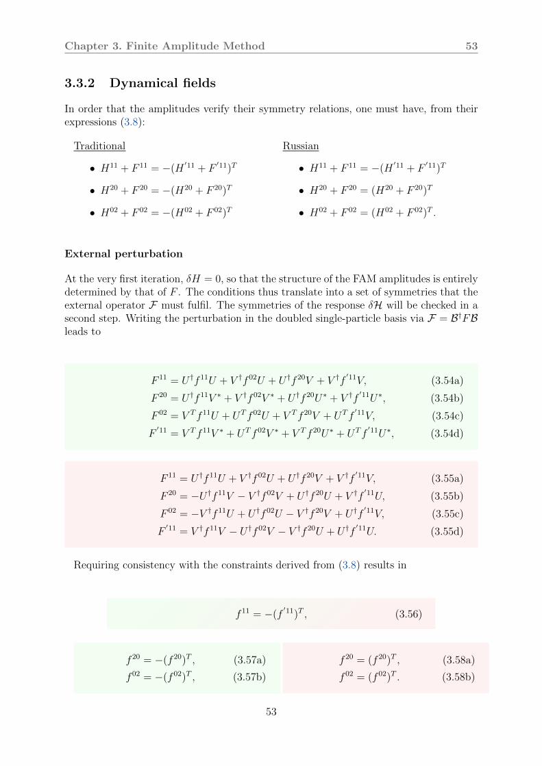
Chapter 3. Finite Amplitude Method 53
3.3.2 Dynamical fields
In order that the amplitudes verify their symmetry relations, one must have, from theirexpressions (3.8):
Traditional
• H11 + F 11 = −(H′11 + F
′11)T
• H20 + F 20 = −(H20 + F 20)T
• H02 + F 02 = −(H02 + F 02)T
Russian
• H11 + F 11 = −(H′11 + F
′11)T
• H20 + F 20 = (H20 + F 20)T
• H02 + F 02 = (H02 + F 02)T .
External perturbation
At the very first iteration, δH = 0, so that the structure of the FAM amplitudes is entirelydetermined by that of F . The conditions thus translate into a set of symmetries that theexternal operator F must fulfil. The symmetries of the response δH will be checked in asecond step. Writing the perturbation in the doubled single-particle basis via F = B†FBleads to
F 11 = U †f 11U + V †f 02U + U †f 20V + V †f′11V, (3.54a)
F 20 = U †f 11V ∗ + V †f 02V ∗ + U †f 20U∗ + V †f′11U∗, (3.54b)
F 02 = V Tf 11U + UTf 02U + V Tf 20V + UTf′11V, (3.54c)
F′11 = V Tf 11V ∗ + UTf 02V ∗ + V Tf 20U∗ + UTf
′11U∗, (3.54d)
F 11 = U †f 11U + V †f 02U + U †f 20V + V †f′11V, (3.55a)
F 20 = −U †f 11V − V †f 02V + U †f 20U + V †f′11U, (3.55b)
F 02 = −V †f 11U + U †f 02U − V †f 20V + U †f′11V, (3.55c)
F′11 = V †f 11V − U †f 02V − V †f 20U + U †f
′11U. (3.55d)
Requiring consistency with the constraints derived from (3.8) results in
f 11 = −(f′11)T , (3.56)
f 20 = −(f 20)T , (3.57a)
f 02 = −(f 02)T , (3.57b)
f 20 = (f 20)T , (3.58a)
f 02 = (f 02)T . (3.58b)
53

54 Chapter 3. Finite Amplitude Method
Internal fields
By the very same procedure, inspecting (3.45) and (3.47) lead to the following conditions:
Traditional
• δh = δhT
• δ∆ = −δ∆T
• δ∆ = −δ∆T
Russian
• δh = δhT
• δh = δhT
• δ¯h = δ¯hT
The fulfilment of these constraints is verified in detail in the following page for thetraditional convention. In case of the Russian convention, these requirements can onlybe met at the two-body level, as an undesired consequence of the static pairing tensorsbeing skew-symmetric ((3.41)) whereas the time-dependent are symmetric ((3.53))5. Thenormal and anomalous fields are thus inspected in the traditional representation only.They rely on the fact that the two- and three-body interactions are invariant under time-reversal (T ), symmetric under swapping the labels of two particles i& j (S(i, j)), andantisymmetric under particle exchange. Renaming of the dummy indices will be shownas well.
Normal fields
The three sums contributing to
δhαβ = δh(2)αβ + δh
(3)ραβ + δh
(3)καβ (3.59)
write
δh(2)αβ =
∑γδ
v(a)ρραγβδδρδγ
T=∑γδ
v(a)ρρ
δβγαδρδγ
S(1,2)=
∑γδ
v(a)ρρ
βδαγδρδγ
(3.48)=∑γδ
v(a)ρρ
βδαγδργδ
γ↔δ=∑γδ
v(a)ρρ
βγαδδρδγ = δh
(2)
βα, (3.60a)
δh(3)ραβ =
∑γδϵζ
w(a)ρρραγϵβδζρζϵδρδγ
T=∑γδϵζ
w(a)ρρρ
ζδβϵγαρζϵδρδγ
S(1,3)=
∑γδϵζ
w(a)ρρρ
βδζαγϵρζϵδρδγ
(3.48)=∑γδϵζ
w(a)ρρρ
βδζαγϵρϵζδργδ
γ↔δ=ϵ↔ζ
∑γδϵζ
w(a)ρρρ
βγϵαδζρζ ϵδρδγ = δh
(3)ρ
βα, (3.60b)
δh(3)καβ =
∑γδϵζ
w(a)ρκκαγϵβδζ(κδζδκϵγ + δκδζ κϵγ)
T=∑γδϵζ
w(a)ρκκ
ζδβϵγα(κδζδκϵγ + δκδζ κϵγ)
5One can however remark that the components of the pairing tensor being typically much smaller(say of order 1) than those of the normal density (which are, say, of order 0), these contributions withincorrect properties should be of order 3 for the normal field (versus 1 for the two-body component and2 for the δρ-dependent three-body), and of order 2 for the anomalous fields. The symmetry-breakingcontribution thus comes at next to leading order, so to speak.
54
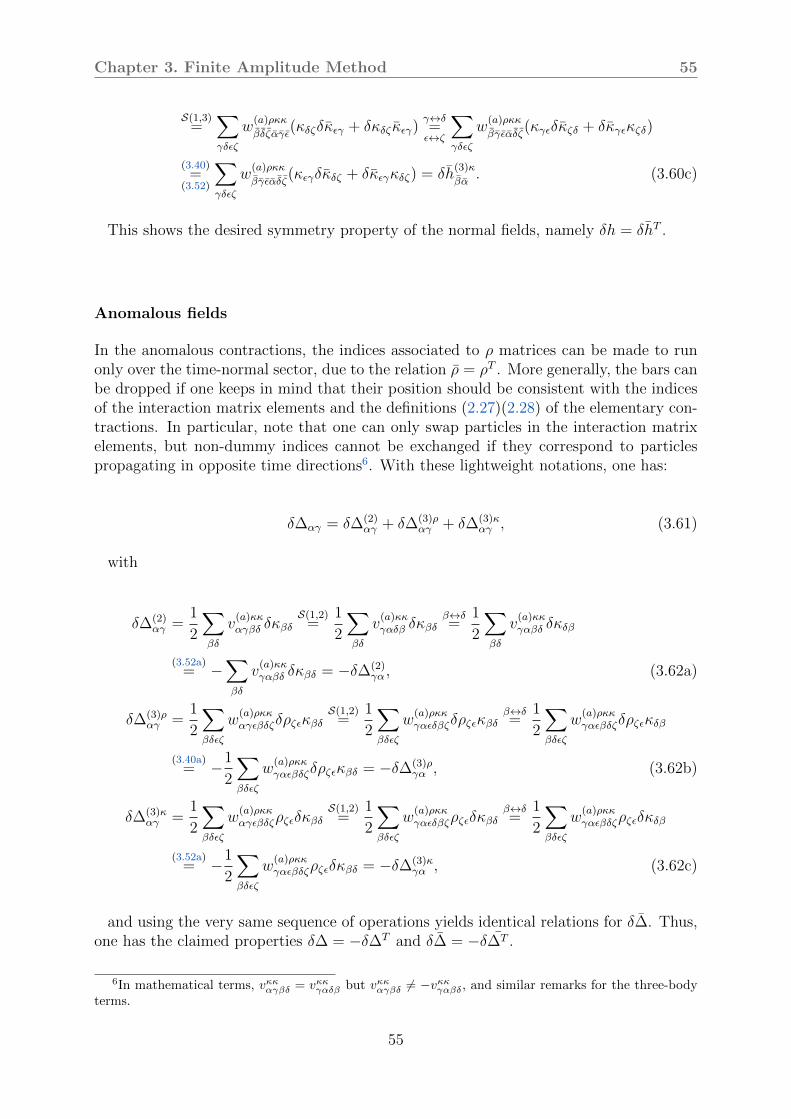
Chapter 3. Finite Amplitude Method 55
S(1,3)=
∑γδϵζ
w(a)ρκκ
βδζαγϵ(κδζδκϵγ + δκδζ κϵγ)
γ↔δ=ϵ↔ζ
∑γδϵζ
w(a)ρκκ
βγϵαδζ(κγϵδκζδ + δκγϵκζδ)
(3.40)=
(3.52)
∑γδϵζ
w(a)ρκκ
βγϵαδζ(κϵγδκδζ + δκϵγκδζ) = δh
(3)κ
βα. (3.60c)
This shows the desired symmetry property of the normal fields, namely δh = δhT .
Anomalous fields
In the anomalous contractions, the indices associated to ρ matrices can be made to runonly over the time-normal sector, due to the relation ρ = ρT . More generally, the bars canbe dropped if one keeps in mind that their position should be consistent with the indicesof the interaction matrix elements and the definitions (2.27)(2.28) of the elementary con-tractions. In particular, note that one can only swap particles in the interaction matrixelements, but non-dummy indices cannot be exchanged if they correspond to particlespropagating in opposite time directions6. With these lightweight notations, one has:
δ∆αγ = δ∆(2)αγ + δ∆(3)ρ
αγ + δ∆(3)καγ , (3.61)
with
δ∆(2)αγ =
1
2
∑βδ
v(a)κκαγβδ δκβδ
S(1,2)=
1
2
∑βδ
v(a)κκγαδβ δκβδ
β↔δ=
1
2
∑βδ
v(a)κκγαβδ δκδβ
(3.52a)= −
∑βδ
v(a)κκγαβδ δκβδ = −δ∆(2)
γα , (3.62a)
δ∆(3)ραγ =
1
2
∑βδϵζ
w(a)ρκκαγϵβδζδρζϵκβδ
S(1,2)=
1
2
∑βδϵζ
w(a)ρκκγαϵδβζδρζϵκβδ
β↔δ=
1
2
∑βδϵζ
w(a)ρκκγαϵβδζδρζϵκδβ
(3.40a)= −1
2
∑βδϵζ
w(a)ρκκγαϵβδζδρζϵκβδ = −δ∆(3)ρ
γα , (3.62b)
δ∆(3)καγ =
1
2
∑βδϵζ
w(a)ρκκαγϵβδζρζϵδκβδ
S(1,2)=
1
2
∑βδϵζ
w(a)ρκκγαϵδβζρζϵδκβδ
β↔δ=
1
2
∑βδϵζ
w(a)ρκκγαϵβδζρζϵδκδβ
(3.52a)= −1
2
∑βδϵζ
w(a)ρκκγαϵβδζρζϵδκβδ = −δ∆(3)κ
γα , (3.62c)
and using the very same sequence of operations yields identical relations for δ∆. Thus,one has the claimed properties δ∆ = −δ∆T and δ∆ = −δ∆T .
6In mathematical terms, vκκαγβδ = vκκγαδβ but vκκαγβδ = −vκκγαβδ, and similar remarks for the three-bodyterms.
55

56 Chapter 3. Finite Amplitude Method
3.4 Connection with the QRPA
In the QFAM formulation of the linear response theory, an excitation operator F is neededin order to calculate the strength function. The QFAM therefore belongs to the “externalpoint of view” theories. As mentioned in subsection 2.6.1, the “internal” vision (as re-alised by the QRPA theory), characterised by the knowledge of the collective eigenstates,can be recovered through integration along aptly chosen contours in the complex plane.This section generalises the work of [HKN13], showing the link between the QFAM andthe QRPA at finite temperature.
As discussed in section 2.6, the eigenmodes of a quantum system can be studied fromtwo different points of view. The usual setting of the QRPA involves diagonalising theHamiltonian, giving as a result the eigenvectors and eigenvalues. Since it does not call foran external probe, it can be labelled as an “internal point of view” description. Conversely,the FAM explicitly demands a probe in the form of the operator F , it is thus an “external”approach. The extension of the excitation frequency ω into the complex plane and theoccurrence of first order poles both in the FAM equations (3.8) and strength function(3.10) clearly hints that a contour integration should make the link between the FAM andthe QRPA.
3.4.1 Eigenvectors and transition amplitudes
The zero temperature QRPA equation writes(A BB∗ A∗
)(XY
)= Ω
(1
−1
)(XY
), (3.63)
where Ω is the diagonal matrix containing all the (positive and negative) eigenvalues.Due to the eigenvalues occurring in pairs, this equation can be doubled7:(
A BB∗ A∗
)(X λY µ
)=
(1
−1
)(X λY µ
)(Ω
−Ω
). (3.64)
The matrices λ, µ are the solutions of
AX +BY = ΩX
B∗Y + A∗X = −ΩY
Aλ+Bµ = −Ωλ
B∗λ+ A∗µ = Ωµ,
(3.65)
that is, after identifying the two last equations with the two firsts, λ = Y ∗ and µ = X∗.The procedure is exactly the same at finite temperature: one starts with the QRPAequation [Som83]
7The eigenvalues matrix occurring to the right of the eigenvectors one comes from identifying the“doubled” vectors as the negative Ω solutions.
56
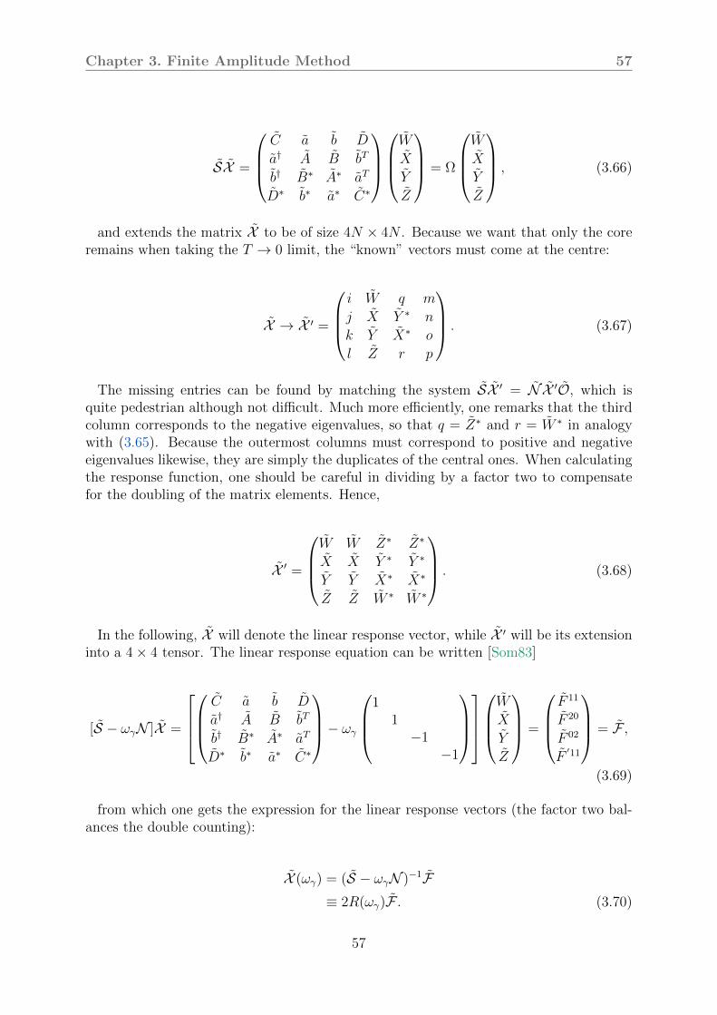
Chapter 3. Finite Amplitude Method 57
SX =
C a b D
a† A B bT
b† B∗ A∗ aT
D∗ b∗ a∗ C∗
W
X
Y
Z
= Ω
W
X
Y
Z
, (3.66)
and extends the matrix X to be of size 4N × 4N . Because we want that only the coreremains when taking the T → 0 limit, the “known” vectors must come at the centre:
X → X ′ =
i W q m
j X Y ∗ n
k Y X∗ o
l Z r p
. (3.67)
The missing entries can be found by matching the system SX ′ = N X ′O, which isquite pedestrian although not difficult. Much more efficiently, one remarks that the thirdcolumn corresponds to the negative eigenvalues, so that q = Z∗ and r = W ∗ in analogywith (3.65). Because the outermost columns must correspond to positive and negativeeigenvalues likewise, they are simply the duplicates of the central ones. When calculatingthe response function, one should be careful in dividing by a factor two to compensatefor the doubling of the matrix elements. Hence,
X ′ =
W W Z∗ Z∗
X X Y ∗ Y ∗
Y Y X∗ X∗
Z Z W ∗ W ∗
. (3.68)
In the following, X will denote the linear response vector, while X ′ will be its extensioninto a 4× 4 tensor. The linear response equation can be written [Som83]
[S − ωγN ]X =
C a b D
a† A B bT
b† B∗ A∗ aT
D∗ b∗ a∗ C∗
− ωγ
1
1−1
−1
W
X
Y
Z
=
F 11
F 20
F 02
F′11
= F ,
(3.69)
from which one gets the expression for the linear response vectors (the factor two bal-ances the double counting):
X (ωγ) = (S − ωγN )−1F≡ 2R(ωγ)F . (3.70)
57

58 Chapter 3. Finite Amplitude Method
The equation defines the response function as the matrix relating the external field tothe induced oscillation of the system. On the other hand, the QRPA equation is easilyseen to generalise as
SX ′ = NX ′O, (3.71)
where N = diag(1, 1,−1,−1) is the metric and O = diag(Ω1, . . . ,ΩN ,−Ω1, . . . ,−ΩN)is the matrix of eigenvalues. The orthonormalisation condition corresponds to8
X ′†NX ′ = N . (3.72)
Eq. (3.71) yields
S = NX ′OX ′−1, (3.73)
which, inserted in (3.70), produces
X (ωγ) = (NX ′OX ′−1 − ωγN )−1F= (NX ′OX ′−1 − ωγNX ′X ′−1)−1F= X ′(O − ωγI)−1X ′−1NF . (3.74)
Then, (3.72) gives9
NX ′ =(X ′†)−1
N ⇒ X ′−1N = NX ′†, (3.75)
therefore
X (ωγ) = X ′(O − ωγI)−1NX ′†F , (3.76)
showing the link between the linear response amplitudes (on the left-hand side) and theQRPA ones (on the right-hand side). The thermal response function (3.70) can now becalculated after remembering the necessary 1/2 factor:
R(ωγ) =1
2X ′(O − ωγI)−1NX ′† (3.77a)
8Note: this condition differs from the one of Hinohara [HKN13] but is the same as Sommermann[Som83]. While both are correct at zero temperature, the former is not valid for the thermal regime, asit gives, e.g., W †W − Z∗ZT instead of W †W +X†X − Y ∗Y T − Z∗ZT .
9The orthonormalisation of [HKN13] gives the same equation.
58

Chapter 3. Finite Amplitude Method 59
=1
2X ′
1
Ω−ωγ1
Ω−ωγ1
Ω+ωγ1
Ω+ωγ
W † X† Y † Z†
W † X† Y † Z†
ZT Y T XT W T
ZT Y T XT W T
=1
2
W W Z∗ Z∗
X X Y ∗ Y ∗
Y Y X∗ X∗
Z Z W ∗ W ∗
W †
Ω−ωγ
X†
Ω−ωγ
Y †
Ω−ωγ
Z†
Ω−ωγ
W †
Ω−ωγ
X†
Ω−ωγ
Y †
Ω−ωγ
Z†
Ω−ωγ
ZT
Ω+ωγ
Y T
Ω+ωγ
XT
Ω+ωγ
WT
Ω+ωγ
ZT
Ω+ωγ
Y T
Ω+ωγ
XT
Ω+ωγ
WT
Ω+ωγ
≡
R11 R12 R13 R14
R21 R22 R23 R24
R31 R32 R33 R34
R41 R42 R43 R44
. (3.77b)
The collection of blocks involved in (3.77b) are the matrices
R11 =∑i
W iW i,†
Ωi − ωγ
+Zi,∗Zi,T
Ωi + ωγ
, (3.78a)
R12 =∑i
W iX i,†
Ωi − ωγ
+Zi,∗Y i,T
Ωi + ωγ
, (3.78b)
R13 =∑i
W iY i,†
Ωi − ωγ
+Zi,∗X i,T
Ωi + ωγ
, (3.78c)
R14 =∑i
W iZi,†
Ωi − ωγ
+Zi,∗W i,T
Ωi + ωγ
, (3.78d)
R21 =∑i
X iW i,†
Ωi − ωγ
+Y i,∗Zi,T
Ωi + ωγ
, (3.78e)
R22 =∑i
X iX i,†
Ωi − ωγ
+Y i,∗Y i,T
Ωi + ωγ
, (3.78f)
R23 =∑i
X iY i,†
Ωi − ωγ
+Y i,∗X i,T
Ωi + ωγ
, (3.78g)
R24 =∑i
X iZi,†
Ωi − ωγ
+Y i,∗W i,T
Ωi + ωγ
, (3.78h)
R31 =∑i
Y iW i,†
Ωi − ωγ
+X i,∗Zi,T
Ωi + ωγ
, (3.78i)
R32 =∑i
Y iX i,†
Ωi − ωγ
+X i,∗Y i,T
Ωi + ωγ
, (3.78j)
R33 =∑i
Y iY i,†
Ωi − ωγ
+X i,∗X i,T
Ωi + ωγ
, (3.78k)
59

60 Chapter 3. Finite Amplitude Method
R34 =∑i
Y iZi,†
Ωi − ωγ
+X i,∗W i,T
Ωi + ωγ
, (3.78l)
R41 =∑i
ZiW i,†
Ωi − ωγ
+W i,∗Zi,T
Ωi + ωγ
, (3.78m)
R42 =∑i
ZiX i,†
Ωi − ωγ
+W i,∗Y i,T
Ωi + ωγ
, (3.78n)
R43 =∑i
ZiY i,†
Ωi − ωγ
+W i,∗X i,T
Ωi + ωγ
, (3.78o)
R44 =∑i
ZiZi,†
Ωi − ωγ
+W i,∗W i,T
Ωi + ωγ
. (3.78p)
One can recover the elements indexed by the four indices (µ, ν, µ′, ν ′) of each block bysubstitutions of the form W iW i,T → W i
µνWi,†µ′ν′ .
All of that mess can be conveniently written by defining the forward and backwardresponses:
R(ωγ) = R+(ωγ) +R−(ωγ), (3.79)
R+(ωγ) =∑i
1
Ωi − ωγ
W iW i,T W iX i,T W iY i,T W iZi,T
X iW i,T X iX i,T X iY i,T X iZi,T
Y iW i,T Y iX i,T Y iY i,T Y iZi,T
ZiW i,T ZiX i,T ZiY i,T ZiZi,T
, (3.80)
R−(ωγ) =∑i
1
Ωi + ωγ
Zi,∗Zi,T Zi,∗Y i,T Zi,∗X i,T Zi,∗W i,T
Y i,∗Zi,T Y i,∗Y i,T Y i,∗X i,T Y i,∗W i,T
X i,∗Zi,T X i,∗Y i,T X i,∗X i,T X i,∗W i,T
W i,∗Zi,T W i,∗Y i,T W i,∗X i,T W i,∗W i,T
. (3.81)
Thus,
X (ωγ) =R(ωγ)F (3.82)
=∑i
1
Ωi − ωγ
W i,∗
(W i,†F 11 + X i,†F 20 + Y i,†F 02 + Zi,†F
′11)
X i,∗(W i,†F 11 + X i,†F 20 + Y i,†F 02 + Zi,†F
′11)
Y i,∗(W i,†F 11 + X i,†F 20 + Y i,†F 02 + Zi,†F
′11)
Zi,∗(W i,†F 11 + X i,†F 20 + Y i,†F 02 + Zi,†F
′11)
60
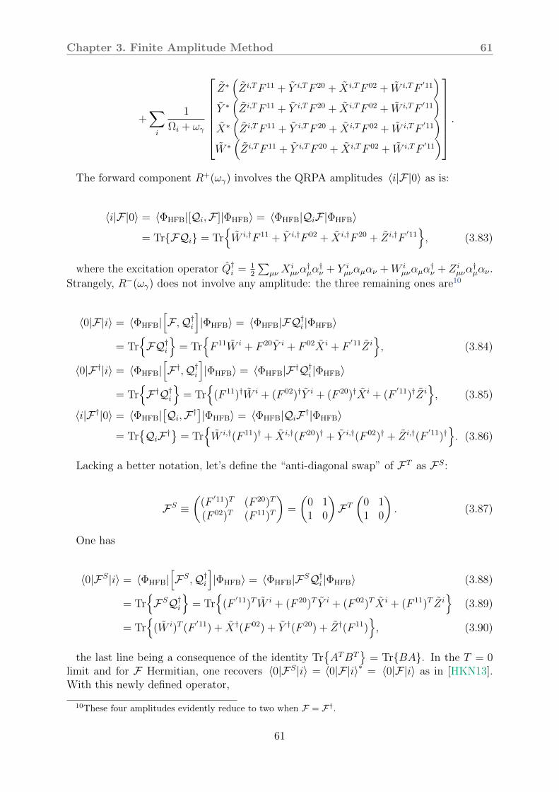
Chapter 3. Finite Amplitude Method 61
+∑i
1
Ωi + ωγ
Z∗(Zi,TF 11 + Y i,TF 20 + X i,TF 02 + W i,TF
′11)
Y ∗(Zi,TF 11 + Y i,TF 20 + X i,TF 02 + W i,TF
′11)
X∗(Zi,TF 11 + Y i,TF 20 + X i,TF 02 + W i,TF
′11)
W ∗(Zi,TF 11 + Y i,TF 20 + X i,TF 02 + W i,TF
′11)
.
The forward component R+(ωγ) involves the QRPA amplitudes ⟨i|F|0⟩ as is:
⟨i|F|0⟩ = ⟨ΦHFB|[Qi,F ]|ΦHFB⟩ = ⟨ΦHFB|QiF|ΦHFB⟩= TrFQi = Tr
W i,†F 11 + Y i,†F 02 + X i,†F 20 + Zi,†F
′11, (3.83)
where the excitation operator Q†i =
12
∑µν X
iµνα
†µα
†ν + Y i
µναµαν +W iµναµα
†ν + Zi
µνᆵαν .
Strangely, R−(ωγ) does not involve any amplitude: the three remaining ones are10
⟨0|F|i⟩ = ⟨ΦHFB|[F ,Q†
i
]|ΦHFB⟩ = ⟨ΦHFB|FQ†
i |ΦHFB⟩
= TrFQ†
i
= Tr
F 11W i + F 20Y i + F 02X i + F
′11Zi, (3.84)
⟨0|F †|i⟩ = ⟨ΦHFB|[F †,Q†
i
]|ΦHFB⟩ = ⟨ΦHFB|F †Q†
i |ΦHFB⟩
= TrF †Q†
i
= Tr
(F 11)†W i + (F 02)†Y i + (F 20)†X i + (F
′11)†Zi, (3.85)
⟨i|F †|0⟩ = ⟨ΦHFB|[Qi,F †]|ΦHFB⟩ = ⟨ΦHFB|QiF †|ΦHFB⟩
= TrQiF † = Tr
W i,†(F 11)† + X i,†(F 20)† + Y i,†(F 02)† + Zi,†(F
′11)†. (3.86)
Lacking a better notation, let’s define the “anti-diagonal swap” of FT as FS:
FS ≡((F
′11)T (F 20)T
(F 02)T (F 11)T
)=
(0 11 0
)FT
(0 11 0
). (3.87)
One has
⟨0|FS|i⟩ = ⟨ΦHFB|[FS,Q†
i
]|ΦHFB⟩ = ⟨ΦHFB|FSQ†
i |ΦHFB⟩ (3.88)
= TrFSQ†
i
= Tr
(F
′11)T W i + (F 20)T Y i + (F 02)T X i + (F 11)T Zi
(3.89)
= Tr(W i)T (F
′11) + X†(F 02) + Y †(F 20) + Z†(F 11), (3.90)
the last line being a consequence of the identity TrATBT
= TrBA. In the T = 0
limit and for F Hermitian, one recovers ⟨0|FS|i⟩ = ⟨0|F|i⟩∗ = ⟨0|F|i⟩ as in [HKN13].With this newly defined operator,
10These four amplitudes evidently reduce to two when F = F†.
61

62 Chapter 3. Finite Amplitude Method
Wµν(ωγ) = −∑i
W i
µν ⟨i|F|0⟩Ωi − ωγ
+Zi∗
µν ⟨0|FS|i⟩Ωi + ωγ
, (3.91a)
Xµν(ωγ) = −∑i
X i
µν ⟨i|F|0⟩Ωi − ωγ
+Y i∗µν ⟨0|FS|i⟩Ωi + ωγ
, (3.91b)
Yµν(ωγ) = −∑i
Y iµν ⟨i|F|0⟩Ωi − ωγ
+X i∗
µν ⟨0|FS|i⟩Ωi + ωγ
, (3.91c)
Zµν(ωγ) = −∑i
Zi
µν ⟨i|F|0⟩Ωi − ωγ
+W i∗
µν ⟨0|FS|i⟩Ωi + ωγ
. (3.91d)
From Cauchy’s integral theorem, one sees that integrating those equations around acontour C enclosing any number of poles yields
1
2iπ
∮CWµν(ωγ)dωγ =
∑i
W iµν ⟨i|F|0⟩ , (3.92a)
1
2iπ
∮CXµν(ωγ)dωγ =
∑i
X iµν ⟨i|F|0⟩ , (3.92b)
1
2iπ
∮CYµν(ωγ)dωγ =
∑i
Y iµν ⟨i|F|0⟩ , (3.92c)
1
2iπ
∮CZµν(ωγ)dωγ =
∑i
Ziµν ⟨i|F|0⟩ , (3.92d)
In the fortunate event where the contour circles exactly one pole, these reduce to theexpression of the eigenmatrices in terms of the FAM ones:
1
2iπ
∮Ci
Wµν(ωγ)dωγ = W iµν ⟨i|F|0⟩ , (3.93a)
1
2iπ
∮Ci
Xµν(ωγ)dωγ = X iµν ⟨i|F|0⟩ , (3.93b)
1
2iπ
∮Ci
Yµν(ωγ)dωγ = Y iµν ⟨i|F|0⟩ , (3.93c)
1
2iπ
∮Ci
Zµν(ωγ)dωγ = Ziµν ⟨i|F|0⟩ , (3.93d)
The QRPA amplitudes can then be found once the associated matrix elements ⟨i|F|0⟩are obtained. The requirement (3.72) that the eigenstates be orthonormal with respectto the metric N = diag(1, 1,−1,−1) translates as
62
Chapter 3. Finite Amplitude Method 63
δii′ = ⟨i′|N |i⟩ = ⟨0|Qi′NQ†i |0⟩ ; Q†
i =
W i
X i
Y i
Zi
. (3.94)
To make the indices match with the rest of the derivations (and most of the literature),it’s more convenient to explicitly stack the vectors, i.e. go back to the matrix notation:
δii′ = ⟨i′|N |i⟩ = TrQi′NQ†
i
; Q†
i =
(W i X i
Y i Zi
), N =
(1
−1
)(3.95)
= TrW i′,†W i + X i′,†X i − Y i′,†Y i − Zi′,†Zi
(3.96)
=∑µν
W i′∗µν W
iµν + X i′∗
µν Xiµν − Y i′∗
µν Yiµν − Zi′∗
µν Ziµν . (3.97)
It follows that the transition probability from the ground state to the ith excited statewrites
|⟨i|F|0⟩|2 = 1
4π2
∑µν
∣∣∣∣∮Ci
Wµν(ωγ)dωγ
∣∣∣∣2 + ∣∣∣∣∮Ci
Xµν(ωγ)dωγ
∣∣∣∣2−∣∣∣∣∮
Ci
Yµν(ωγ)dωγ
∣∣∣∣2 − ∣∣∣∣∮Ci
Zµν(ωγ)dωγ
∣∣∣∣2. (3.98)
(Remark that the contribution of the W and Z amplitudes should cancel each otherexactly, by (3.51)). Eq. (3.98) can be paired up with (3.93) to give forth the QRPAamplitudes:
W i′
µν =e−iθ
|⟨i′|F|0⟩|1
2iπ
∮Ci′
Wµν(ωγ)dωγ (3.99a)
X i′
µν =e−iθ
|⟨i′|F|0⟩|1
2iπ
∮Ci′
Xµν(ωγ)dωγ (3.99b)
Y i′
µν =e−iθ
|⟨i′|F|0⟩|1
2iπ
∮Ci′
Yµν(ωγ)dωγ (3.99c)
Zi′
µν =e−iθ
|⟨i′|F|0⟩|1
2iπ
∮Ci′
Zµν(ωγ)dωγ, (3.99d)
where the phase e+iθ = ⟨i|F|0⟩ /|⟨i|F|0⟩| cannot be determined, but can be chosenarbitrarily since it is common to all the eigenvectors11. Because the thermal factor of the
11Note that in practical calculations, one may choose it so that all the discrete amplitudes are real,since the eigenvectors of a positive definite matrix can be made real simultaneously.
63

64 Chapter 3. Finite Amplitude Method
QRPA and QFAM amplitudes are the same, all these equations (and most importantly,(3.93), (3.98) and (3.99)) also hold when removing the tildes.
3.4.2 Eigenvalues
Line by line, and after multiplying either by σµν ≡√
fν − fµ or by ηµν ≡√
1− fµ − fν ,(3.69) leads to
σµν
∑µ′<ν′
(Cµνµ′ν′ − ωγδµµ′δνν′)Wµ′ν′ + aµνµ′ν′Xµ′ν′ + bµνµ′ν′Yµ′ν′ + Dµνµ′ν′Zµ′ν′ = −σ2µνF
11µν
(3.100)
ηµν∑µ′<ν′
a†µνµ′ν′Wµ′ν′ + (Aµνµ′ν′ − ωγδµµ′δνν′)Xµ′ν′ + Bµνµ′ν′Yµ′ν′ + bTµνµ′ν′Zµ′ν′ = −η2µνF20µν
(3.101)
ηµν∑µ′<ν′
b†µνµ′ν′Wµ′ν′ + B∗µνµ′ν′Xµ′ν′ + (A∗
µνµ′ν′ + ωγδµµ′δνν′)Yµ′ν′ + aTµνµ′ν′Zµ′ν′ = −η2µνF02µν
(3.102)
σµν
∑µ′<ν′
D∗µνµ′ν′Wµ′ν′ + b∗µνµ′ν′Xµ′ν′ + a∗µνµ′ν′Yµ′ν′ + (C∗
µνµ′ν′ + ωγδµµ′δνν′)Zµ′ν′ = −σ2µνF
′11µν .
(3.103)
On the other hand, the QFAM equations read12
(Eµ − Eν − ωγ)Wµν(ωγ) +H11µν(fν − fµ) = −F 11
µν(fν − fµ) = −σ2µνF
11µν (3.104)
(Eµ + Eν − ωγ)Xµν(ωγ) +H20µν(1− fµ − fν) = −F 20
µν(1− fµ − fν) = −η2µνF20µν (3.105)
(Eµ + Eν + ωγ)Yµν(ωγ) +H02µν(1− fµ − fν) = −F 02
µν(1− fµ − fν) = −η2µνF02µν (3.106)
(Eµ − Eν + ωγ)Zµν(ωγ) +H′11µν (fν − fµ) = −F
′11µν (fν − fµ) = −σ2
µνF′11µν , (3.107)
so that (the dependence of the fields and amplitudes on ωγ has been omitted for legi-bility)
H11µν = σ−1
µν
∑µ′<ν′
[(Cµνµ′ν′ −
(ωγ +
Eµ − Eν − ωγ
σ2µν
)δµµ′δνν′
)Wµ′ν′ + aµνµ′ν′Xµ′ν′
+ bµνµ′ν′Yµ′ν′ + Dµνµ′ν′Zµ′ν′
](3.108a)
H20µν = η−1
µν
∑µ′<ν′
[a†µνµ′ν′Wµ′ν′ +
(Aµνµ′ν′ −
(ωγ +
Eµ + Eν − ωγ
η2µν
)δµµ′δνν′
)Xµ′ν′
12The bars correspond to matrix elements in the ⟨HFB|αα†|HFB⟩ sector; they are equal to their α†αpartners owing to the eigenvalues of the HFB equation coming by pairs of opposite sign. We have E = Eand f = f , but conserve the bars for bookkeeping.
64
Chapter 3. Finite Amplitude Method 65
+ Bµνµ′ν′Yµ′ν′ + bTµνµ′ν′Zµ′ν′
](3.108b)
H02µν = η−1
µν
∑µ′<ν′
[b†µνµ′ν′Wµ′ν′ + B∗
µνµ′ν′Xµ′ν′
+
(A∗
µνµ′ν′ +
(ωγ −
Eµ + Eν + ωγ
η2µν
)δµµ′δνν′
)Yµ′ν′ + aTµνµ′ν′Zµ′ν′
](3.108c)
H′11µν = σ−1
µν
∑µ′<ν′
[D∗
µνµ′ν′Wµ′ν′ + b∗µνµ′ν′Xµ′ν′
+ a∗µνµ′ν′Yµ′ν′ +
(C∗
µνµ′ν′ +
(ωγ −
Eµ − Eν + ωγ
σ2µν
)δµµ′δνν′
)Zµ′ν′
]. (3.108d)
These equations show that the FAM one-body fields can be directly linked to the QRPAtwo-body tensors and one-body eigenvectors. What’s more, as these expressions explicitlyinvolve the frequency of the perturbation, they provide a closed set of expression for theeigenfrequencies. Indeed, integrating (anti-clockwise) each of them around a contour Ccircling one or more poles, we obtain with the help of (3.93) and the QRPA equation(3.66)
∮CH11
µν(ωγ)dωγ =∑i′
∮Ci′
H11µν(ωγ)dωγ = 2iπσµν
∑i′
⟨i′|F|0⟩ W i′
µν(Ωi′ − (Eµ − Eν))
(3.109a)∮CH20
µν(ωγ)dωγ =∑i′
∮Ci′
H20µν(ωγ)dωγ = 2iπηµν
∑i′
⟨i′|F|0⟩ X i′
µν(Ωi′ − (Eµ + Eν))
(3.109b)∮CH02
µν(ωγ)dωγ =∑i′
∮Ci′
H02µν(ωγ)dωγ = 2iπηµν
∑i′
⟨i′|F|0⟩ Y i′
µν(−Ωi′ − (Eµ + Eν))
(3.109c)∮CH
′11µν (ωγ)dωγ =
∑i′
∮Ci′
H′11µν (ωγ)dωγ = 2iπσµν
∑i′
⟨i′|F|0⟩ Zi′
µν(−Ωi′ − (Eµ − Eν)).
(3.109d)
When the contour C goes around only one pole (collective or not), these expressionsreduce in the zero temperature limit to eqs. (25a)-(25b) of [HKN13]. Each pair (µ, ν) ofindices gives four different expressions for the frequency. However, these involve dividingby the matrix elements and amplitudes, yet both may be small. It would be great if thesum of the eigenvalues could be calculated without needing to identify all the poles. Thisis sadly not possible, due to the presence of the transition matrix elements. Our lastresort is to manage to locate the poles individually: in that case, the sum over i′ containsonly one term, and each frequency can be calculated by inverting (3.109). Due to theaforementioned potentially small denominators, it is safer to recast these equations as
65
66 Chapter 3. Finite Amplitude Method
2iπ ⟨i′|F|0⟩σµνWi′
µνΩi′ = (Eµ − Eν)2iπ ⟨i′|F|0⟩σµνWi′
µν +
∮Ci
H11µν(ωγ)dωγ (3.110a)
2iπ ⟨i′|F|0⟩ ηµνX i′
µνΩi′ = (Eµ + Eν)2iπ ⟨i′|F|0⟩ ηµνX i′
µν +
∮Ci
H20µν(ωγ)dωγ (3.110b)
−2iπ ⟨i′|F|0⟩ ηµν Y i′
µνΩi′ = (Eµ + Eν)2iπ ⟨i′|F|0⟩ ηµνY i′
µν +
∮Ci
H02µν(ωγ)dωγ (3.110c)
−2iπ ⟨i′|F|0⟩σµνZi′
µνΩi′ = (Eµ − Eν)2iπ ⟨i′|F|0⟩σµνZi′
µν +
∮Ci
H′11µν (ωγ)dωγ (3.110d)
and use (3.93) to obtain
W i′
µνΩi′ =1
⟨i′|F|0⟩
∮Ci
[(Eµ − Eν)Wµν(ωγ) + σ−1
µν H11µν(ωγ)
]dωγ (3.111a)
X i′
µνΩi′ =1
⟨i′|F|0⟩
∮Ci
[(Eµ + Eν)Xµν(ωγ) + η−1
µνH20µν(ωγ)
]dωγ (3.111b)
−Y i′
µνΩi′ =1
⟨i′|F|0⟩
∮Ci
[(Eµ + Eν)Yµν(ωγ) + η−1
µν H02µν(ωγ)
]dωγ (3.111c)
−Zi′
µνΩi′ =1
⟨i′|F|0⟩
∮Ci
[(Eµ − Eν)Zµν(ωγ) + σ−1
µν H′11µν (ωγ)
]dωγ. (3.111d)
With the help of the normalisation condition, we then have
Ω2i =
∑µ<ν
Ω2i (|W i
µν |2 + |X iµν |2 − |Y i
µν |2 − |Ziµν |2)
=1
4π2|⟨i|F|0⟩|2∑µ<ν
∣∣∣∣∮Ci
[(Eµ − Eν)Wµν(ωγ) + σ−1
µνH11µν(ωγ)
]dωγ
∣∣∣∣2+
∣∣∣∣∮Ci
[(Eµ + Eν)Xµν(ωγ) + η−1
µν H20µν(ωγ)
]dωγ
∣∣∣∣2−∣∣∣∣∮
Ci
[(Eµ + Eν)Yµν(ωγ) + η−1
µνH02µν(ωγ)
]dωγ
∣∣∣∣2−∣∣∣∣∮
Ci
[(Eµ − Eν)Zµν(ωγ) + σ−1
µνH′11µν (ωγ)
]dωγ
∣∣∣∣2, (3.112)
which allows us to calculate the energy Ωi once we have found a contour selecting thisfrequency only.
3.4.3 Eigenvalues and transition amplitudes from the moments
As shown in 2.6.4, integrating the smeared strength in the whole positive ω complex half-plane gives the moments of the strength distribution. More precisely, if a contour C goes
66
Chapter 3. Finite Amplitude Method 67
around some poles Ωµν of the strength function, one can obtain from (2.82), (2.85) and(2.86) that
mk(C) =1
2iπ
∮Cdωγω
kγS(F, ωγ) = Z−1
∑Ωµν∈C
Ωkµνe
−βEµ |⟨ν|F |µ⟩|2. (3.113)
In a situation where only one pole is enclosed by C (noted Ci for the occasion),
m0(Ci) = Z−1e−βEµ|⟨ν|F |µ⟩|2, (3.114a)
mk+k′(Ci)
mk(Ci)= Ωk′
µν , ∀ k, k′ ∈ Z. (3.114b)
Thus, if one is only interested in the thermal matrix elements (3.114a) and/or eigenval-ues (3.114b), only two partial moments of the strength need to be calculated.
3.4.4 Summary
Finally, the equations allowing the calculation of different interesting quantities are givenhere:
- eigenvectors: (3.99),
- eigenvalues: (3.112), (3.114b).
As of obtaining the transition matrix elements, there are two possibilities13 [HKN13]:
- by a contour integral of the FAM amplitudes (3.98),
- the thermally weighted squared matrix element can be found by (3.114a).
Note that only the latter is physically meaningful at T > 0, since it properly encodesthe statistical distribution of the initial state. Following [HKN13] again, we remark thatin case the chosen contour contains more than one pole, (3.112) and (3.114b) must givedifferent results: the first contains interferences between the enclosed modes due to squar-ing the matrix elements, whereas the second equation does not. This can in practice beemployed to determine whether the contour loops around a single pole or more than one.
Similarly, the integral (3.98) contains interferences. On the other hand, (3.114a) doesnot. The two techniques can thus be tested against each other, to discriminate theoccurrence of more than one pole. One could also think of using (3.99) to calculate(3.83), but the value of matrix element depends on the choice of the technique, henceit does contain contaminations or does not, depending on the technique. It should beremarked that this cross-validation is only possible at T = 0, unless the partition functionand energies Eµ of the many-body microstates are calculated as well.
13Calculating the trace (3.83) is not possible since the matrix element is needed to obtain the FAMamplitudes from (3.99).
67
68 Chapter 3. Finite Amplitude Method
3.5 Self-consistent dressing
At first glance, the propagators seem to always be the HFB ones. This turns out notto be the case when the dynamical fields are included, as they will implicitly dress thepropagators by self-consistently including RPA correlations. This can be illustrated byinspecting a simple two-level system (representing for instance a two-level system withtwo particles, in the presence of an oscillating electromagnetic field):
H0 =
(ϵ
−ϵ
); R0 =
(1
1
); F =
(f
f
); δH =
(vx
vy
); δR =
(x
y
).
(3.115)
Here, H0 and R0 are the unperturbed Hamiltonian and density matrix, F is the externalfield, δH and δR are the residual interaction and density fluctuations. The FAM equationsread
x = −f + vx
2ϵ− ω(3.116)
y = −f + vy
2ϵ+ ω. (3.117)
Solving for the amplitudes x and y yields first-order poles at ω = ±(2ϵ+v), which showsthat the poles are shifted due to the residual interaction. Note that the 2ϵ + v residualis reminiscent of the entries of the QRPA matrix Aµνµ′ν′ = (Eµ + Eν)δµµ′δνν′ + Vµνµ′ν′ : ifthe two-body interaction is diagonal in the two-body basis, the energy shifts are triviallyobtained due to their δµµ′δνν′ character.
3.6 Nambu-Goldstone modes
3.6.1 Equations of motion for the NG modes
Nambu-Goldstone (NG) modes correspond to zero-energy excitations restoring sponta-neously broken symmetries [Nam60; Gol61; GSW62]. For a system described by theHamiltonian H, the density matrix solves the Liouville-von Neumann equation
iD = [H,D]. (3.118)
Likewise, we have for mean-field theories
iR = [H,R] HFB, (3.119)
iρ = [h, ρ] HF. (3.120)
Since these have the same form as (3.118), the results of this subsection transposeto the mean-field theories with no problem. For some arbitrary Hermitian operator Pcorresponding to a transformation of magnitude α, the symmetry transformation of an
68
Chapter 3. Finite Amplitude Method 69
operator A is written as
A → A = eiαPAe−iα∗P †= eiαPAe−iαP . (3.121)
Spontaneous symmetry breaking occurs when H is invariant under the symmetry trans-formation S (that is, [H,S] = 0, or equivalently, H = H), but the density matrix is not.The Liouville equation remains unchanged by the transformation:
i ˜D = [H,D] = eiαP [H,D]e−iαP = eiαPHe−iαP eiαPDe−iαP −H ↔ D
=[H, D
]. (3.122)
The derivative of the transformed density matrix is
˙D =d
dt
(eiαPDe−iαP
)= i(αP + αP )eiαPDe−iαP + eiαP De−iαP − ieiαPD(αP + αP )e−iαP
= ˜D + i((αP + αP )eiαPDe−iαP − eiαPD(αP + αP )e−iαP
)= ˜D + iα
[P, D
]+ iα
[P , eiαPD
]e−iαP . (3.123)
If α and P are both independent of time, one finds that14
˙D = ˜D, (3.124)
yielding
i ˙D =[H, D
](3.125)
after recalling that P and H commute, hence H = H. Therefore, any solution of theLiouville-von Neumann equation transformed according to a continuous symmetry of thesystem is also a solution of the equation of motion.
3.6.2 NG modes removal
Since the transformed density matrices verify the transformed Liouville-von Neumannequation for the same Hamiltonian, they describe an equivalent state. The eigenvalues aretherefore identical to those of the original state. The resulting Nambu-Goldstone modesrelate elements of this manifold of states differing by zero-energy excitations through theapplication of the exponential map associated to the algebra describing the symmetry
14Which could have been seen by the following argument: if the generator of the transformation doesnot depend on time, the order between the transformation and the derivation does not matter, i.e.∀A,
[ddt , P
]A = PA+ PA− PA = 0.
69

70 Chapter 3. Finite Amplitude Method
operator.
One can measure the difference between two equivalent operators (in that case, densitymatrices) through the definition
∆DP ≡ (DP −D) = eiαPDe−iαP −D
∼ iα[P,D] (3.126)
from which, regardless of the magnitude α of the transformation, one defines
δDP ≡ α−1∆DP ∼ i[P,D]. (3.127)
It is no big deal to show that δDP is Hermitian if so does D (and being the groundstate density matrix, it does) and P 15:
δD†P = α−1∆D†
P = α−1(eiαPD†e−iαP −D†) = δDP . (3.128)
This forbids one to use the normalisation condition for the density fluctuations (3.72),since it requires these to be non-Hermitian (the hermicity of Qi ≡ QiN 1/2 follows fromthat of Qi and N ):
δii′ = ⟨i′|N |i⟩ = ⟨0|Qi′NQ†i |0⟩ = ⟨0|Qi′Q
†i |0⟩ = ⟨0|
[Qi′ , Q
†i
]|0⟩ = Tr
[Qi′ , Q
†i
]R0
.
(3.129)
Therefore, these modes cannot be separated from the physical ones using this orthogo-nality relation. Instead, we assume that the spurious densities contribute linearly to thecalculated density:
δDcalc = δDphys + δDspurious = δDphys +∑P
λP δDP +∑R
λRδDR, (3.130)
which is reasonable since the density fluctuations are expected to be small, hence cou-plings between NG modes and non-spurious ones should be second order terms. The or-thogonality of the spurious densities with the non-contaminated one, ⟨δDphysδDP,R⟩ = 0,can be recast under a commutator form:
⟨[δDphys, δDP ]⟩ = 0 =
⟨[δDcalc −
∑R
λRδDR, δDP
]⟩= ⟨[δDcalc, δDP ]⟩ −
∑R
λR ⟨[δDR, δDP ]⟩ , (3.131)
15This is also immediate from the first order expression in (3.127).
70

Chapter 3. Finite Amplitude Method 71
⟨[δDphys, δDR]⟩ = 0 =
⟨[δDcalc −
∑P
λP δDP , δDR
]⟩= ⟨[δDcalc, δDR]⟩ −
∑P
λP ⟨[δDP , δDR]⟩ . (3.132)
All the quantities in that last equation can be calculated from static operators and thecomputed transition density. One finds
λR =⟨[δDcalc, δDP ]⟩⟨[δDR, δDP ]⟩
, (3.133)
λP =⟨[δDcalc, δDR]⟩⟨[δDP , δDR]⟩
, (3.134)
which yield the final expression
δDphys = δDcalc −⟨[δDcalc, δDR]⟩⟨[δDP , δDR]⟩
i[P,D]− ⟨[δDcalc, δDP ]⟩⟨[δDR, δDP ]⟩
i[R,D]
= δDcalc −⟨[δDcalc, [R,D]]⟩⟨[[P,D], [R,D]]⟩ [P,D]− ⟨[δDcalc, [P,D]]⟩
⟨[[R,D], [P,D]]⟩ [R,D]. (3.135)
If there is more than one pair of operators that generate spurious modes, this subtrac-tion can be applied iteratively, provided the generators of the transformations commute.
In practise, the direction of symmetry breaking is entirely determined by the externaloperator Q: if it does not break a symmetry S, there will be no induced spurious densityin the direction in which S is broken. Therefore, the number of broken generators dependson the choice of Q. For instance, an operator of which the projection K along the r⊥ axisis zero cannot reach spurious states generated by rotation in the ⊥ direction (in otherwords, it does not break S⊥), so that one only has to subtract δDrz , δDpz from thecalculated density. Conversely, an operator depending only on the radial distance r⊥ doesnot break Sz but only S⊥.
3.7 Centre of mass
As mentioned in section 2.2, the centre of mass of a system that is not bound by an exter-nal field must be fixed by imposing explicitly that the total linear momentum vanishes:
P =A∑i
pi = 0, (3.136)
which is equivalent to
71
72 Chapter 3. Finite Amplitude Method
0 =P2
2M=
A∑i
p2i
2M+
A∑i =j
pi.pj
2M, (3.137)
M being the total mass. In the following, we assume that all masses are identical16.At the one-body level, one can simply subtract from each particle’s kinetic energy theaverage kinetic energy of the translation-invariant system:
T =p2
2m→(1− 1
A
)p2
2m, (3.138)
while an additional two-body interaction appears:
vc.o.m = −pi.pj
2Am. (3.139)
This understanding of the centre of mass contribution is only valid when the particlenumber A can take a single value. Indeed, mathematical correctness commands to writethe intrinsic momentum at the operator level. Is has been shown in detail [HR09] thattwo identical (at the operator level) representations of the kinetic operator may lead todifferent normal and anomalous fields. This possible discrepancy has been tracked downto idempotency of the generalised density matrix, owing to which the ρ and κ densitiesare related. The rest of this section summarises the findings of [HR09], and shows thatthe same conclusion hold for the linearised fields entering the FAM.
The kinetic operator can take the form either of a one-plus-two-body operator:
T(a)int = Tlab − Tc.o.m =
(I − A−1
)∑i
p2i
2m− A−1
2m
∑i =j
pi.pj, (3.140)
or a purely two-body term, corresponding to the relative kinetic energy of each pair:
T(b)int = A−1
∑i<j
(pi − pj)2
2m. (3.141)
While these two expressions are formally equivalent, the second leads to an ambiguityregarding whether the variation of the kinetic energy contributions in the normal or pairingchannel. It can be shown [HR09] that a specific prescription has to be taken to enforce theequality of the normal and pairing fields derived from either (3.140) or (3.141). In suchcase, since h(a) = h(b) and ∆(a) = ∆(b), the explicitly linearised terms entering the FAMequation are identical as well with either choice (a) or (b). Conversely, the conclusion of
16If one has different types of degrees of freedom (e.g. two for protons and neutrons), as many copiesof (3.137) -and the forthcoming equations- should be considered, since having one species with non-zerolinear momentum would signify it can drift away from the total origin of the coordinate frame. The factidentical particles are grouped together stems from their indistinguishability.
72
Chapter 3. Finite Amplitude Method 73
[HR09] is expected to hold at the FAM level as well: when no prescription is taken, (a)and (b) should lead to identical fields if and only if the total wave function is an eigenstateof the particle number operator. The rest of this section proves this statement. For theexpressions of the static mean-field, we refer the reader to [HR09] (Eqs. 23 and 31, 25and 32) once more. In the FAM, the first iteration can be initialised with δh = δ∆ = 017,hence the very first trial δρ and δκ are the same with both ways of calculating the fields.It is thus sufficient to examine whether the different fields given by (a) and (b) lead toidentical expressions once linearised. One finds
δh(a)kk′ =
∑qq′
(vkqk′q′ −
1
⟨A⟩m⟨kq|p1.p2|k′q′⟩
)δρq′q
, (3.142)
and
δh(b)kk′ =
∑qq′
(vkqk′q′ +
2
⟨A⟩m⟨kq|q212|k′q′⟩
)δρq′q
+1
⟨A⟩∑q
(tkqδρqk′ + tqk′δρkq) . (3.143)
The difference dhkk′ ≡ δh(b)kk′ − δh
(a)kk′ is
dhkk′ =1
⟨A⟩m∑qq′
⟨kq|(2q212 + p1.p2)|k′q′⟩ δρq′q
+1
⟨A⟩∑q
(tkqδρqk′ + tqk′δρkq) . (3.144)
Using the identity
2
m⟨kq|q212|k′q′⟩ = tkk′δqq′ − tkq′δqk′ + tqq′δkk′ − tqk′δkq′ −
1
m⟨kq|p1.p2|k′q′⟩ , (3.145)
we get
dhkk′ =1
⟨A⟩∑qq′
[(tkk′δqq′ − tkq′δqk′ + tqq′δkk′ − tqk′δkq′
− 1
m⟨kq|p1.p2|k′q′⟩) + 1
m⟨kq|p1.p2|k′q′⟩
]δρq′q
+1
⟨A⟩∑q
(tkqδρqk′ + tqk′δρkq)
17And the same for the barred fields.
73
74 Chapter 3. Finite Amplitude Method
=1
⟨A⟩
[tkk′∑q
δρqq −∑q′
tkq′δρq′k′ +∑qq′
tqq′δkk′δρq′q −∑q
tqk′δρkq
]
+1
⟨A⟩∑q
(tkqδρqk′ + tqk′δρkq)
=1
⟨A⟩
[tkk′∑q
δρqq + δkk′∑qq′
tqq′δρq′q
]
=1
⟨A⟩[tkk′ Trδρ+ δkk′ TrTδρ.] (3.146)
In the cases where the excitation couples elements having different angular momentaprojections (AMP), both traces vanish18. There can thus be no difference in the resultsobtained with these two prescription as far as these excitation modes are concerned.As for AMP non-conserving transitions, the first trace vanishes only for particle-numberdispersion-less theories19. Indeed,
Trδρ (3.44a)= Tr
UWU † + V ∗Y U † + UXV T + V ∗ZV T
(2.48a)=
(2.48b)TrV TU(X − Y ) +W − 2V †VW
; (3.147)
the second and third terms vanish at zero temperature, since W = 0 in this limit. Thefirst term involves V TU , which quite resembles the pairing tensor. Yet, the presence ofX does not allow applying the cyclic property. Instead, one can invert block-wise theBogoliubov matrix to show that U ∝ U † and V ∝ V †. The transformation being encodedin a real matrix, one immediately deduces Trδρ = 0 at zero temperature and for avanishinThe second part, however, is apparently not zero. It results in the normal fields being
“shifted”:
δh(b) = δh(a) + αI, α = ⟨A⟩−1TrTδρ. (3.148)
It follows that the generalised Hamiltonian becomes
δH(b) = δH(a) + α
(I
−I
). (3.149)
The shift transforms into the Bogoliubov basis as
(dH(11) dH(20)
dH(02) dH(′11)
)ρ
= dHρ = α
(U † V †
−V † U †
)(I
−I
)(U −VV U
)18Provided the matrix representation of the operators is consistently ordered, i.e. the basis states come
in the same order column-wise (from left to right) and row-wise (from top to bottom).19The cyclic property of the trace and the tracelessness of W -see (3.8c)- are employed)
74
Chapter 3. Finite Amplitude Method 75
= α
(U †U − V †V −U †V − V †U−V †U − U †V V †V − U †U
)= α
(ρ+ ρ− I κ+ κκ+ κ I − ρ− ρ
). (3.150)
Unfortunately, the shift results in non-zero changes in the perturbed fields. One maynote, however, that at the Hartree-Fock approximation, the (20) and (02) blocks remainunchanged. At T = 0, the diagonal blocks (11) and (′11) do not contribute to any ob-servable, as can be seen from (3.9) and (3.10). Altogether, we find that versions (a) and(b) of the centre of mass correction yield identical observables within the FAM. This isconsistent with the result obtained in [HR09] for the static fields. It has been numericallychecked that the two prescriptions yield the same strengths functions (up to machineprecision) for the double magic nucleus 16O at T = 0 for IS monopole, IV dipole and ISquadrupole excitations.
If the system is either thermally excited and/or superfluid, the above derivations showthat the two representations (3.140)-(3.141) do not lead to identical fields if one is notcareful. In that case, the simplest choice is to adopt the kinetic operator (3.140), whichdoes not require a specific prescription.
Finally, the pairing fields need not be examined, since the consistency is valid only fornon-superfluid systems. For completeness, the difference between the two pairing fieldswrites, in the very same manner,
d∆kk′ ≡ δ∆(b)kk′ − δ∆
(a)kk′
=1
⟨A⟩∑q
[tkqδκqk′ + t∗qk′δκkq
]+
1
⟨A⟩∑qq′
[tkqδk′q′ − tkq′δqk′ + tk′q′δkq − tk′k′δkq′ ] δκqq′
=1
⟨A⟩∑q
[tkqδκqk′ + t∗qk′δκkq
]+
1
⟨A⟩∑q
[tkqδκqk′ − tkqδκk′q + tk′qδκkq − tk′k′δκqk]
=2
⟨A⟩∑q
[tkqδκqk′ + t∗qk′δκkq
]− 1
⟨A⟩∑q
[tkqδκk′q + tk′k′δκqk] . (3.151)
Bonus: Coordinate space centre of mass correction
The zero-momentum condition writes
0 = K =A∑i
k ⇔ K2
2Am=
1
2Am
(∑i
k2i +
∑i =j
ki.kj
), (3.152)
75
76 Chapter 3. Finite Amplitude Method
viz., the correction has the same form as in a basis. This is evident, as (3.137) makes noreference to a particular basis whatsoever: the coordinate basis is simply a special one,where the basis “functions” are Dirac and form a mesh. The one-body contribution cansimply be subtracted, while the two-body is most easily calculated by Fourier transformingthe wave functions:
−⟨a|ka.kb
2Am|b⟩ = −
∫dk1dk2Φ
∗a(k1)
ka.kb
2AmΦb(k2), (3.153)
which seems rather involved for such a simple field. Among the infinitely many choicesfor the grid, it is smart to choose one such that multidimensional integrals like (3.153)can be carried out analytically. The obvious and standard choice is to employ a Cartesianmesh, for which the eigenfunctions are those of a particle in a box, that is, plane waves.Behold! The integrals in (3.153) suddenly become easy.
3.8 Unstable modes
Although the FAM formalism can always (why not?) be applied to obtain the linear re-sponse of a system to some given perturbation, the linear regime is expected only when thesystem undergoes small oscillations around the reference state. This means for instancethat the approach must fail when applied on top of a reference state which is unstablewith respect to the perturbation. As is known20, instabilities in the RPA response leadto imaginary eigenvalues. Complex QRPA eigenvalues thus constitute clear indicators ofthe breakdown of the linear approximation21. This section examines how and when it ispossible, from FAM calculations, to detect such poles that characterise the collapse of themethod’s validity.
Method 1: sum rules
The sum rules can be obtained [Hin+15] (see also (2.6.4)) by contour integration aroundthe Re(ω) > 0 half-plane. When performed around a contour C that does not circle allthe poles of the strength function, one may define the partial sum rules as
mk(C) =1
2iπ
∮Cdωγω
kγS(F, ωγ) = Z−1
∑Ων
µ∈C
(Ωνµ)
ke−βEµ |⟨ν|F |µ⟩|2. (3.154)
In particular,
20This can be checked in the simple case of a 2×2 RPA matrix
(a b
−b∗ −a∗
), which bears minus signs
as opposed to (2.87) to account for the metric, and thus deal with an eigenvalue equation instead of ageneralised one. It is a bit more involved to show that the stability of the ground state is related to thepositive-definiteness of the RPA matrix (2.87), this time with plus signs only.
21But the converse is not true: having real eigenvalues only by no means imply that the linear responseis a “good” approximation.
76

Chapter 3. Finite Amplitude Method 77
m1(C) = Z−1∑Ων
µ∈C
Ωνµe
−βEµ |⟨ν|F |µ⟩|2. (3.155)
Thus, the partial sum rules can be employed to check if any unstable mode is presentwithin a given contour C. Provided unstable eigenvalues do not come in conjugate pairs,the existence of such values can be characterised by a non-zero imaginary part of them1 sum rule. If they do come in pair (and with transition matrix elements of identicalnorm for the pair), as is the case with the RPA theory, a contour C going around allthe poles in the positive ω half-plane will always result in real moments mk. As such,an all-encompassing contour cannot be employed to detect complex-energy modes. Thisdownside is sidestepped by a simple ruse: rather than calculating the total sum rules, onerestricts the contour to one looping around the Γ ≥ 0 axis.
Method 2: sign of S
Another means of identifying the presence of complex energy eigenvalues comes from thestrength function: writing Ων
µ = Ωq + iΓq, e−βEµ|⟨ν|F |µ⟩|2 = M2
q and e−βEµ |⟨µ|F |ν⟩|2 =M2
−q,
ImS(F, ωγ) = −γ∑q>0
(M 2
q − M 2−q
)+∑q>0
Γq
(M 2
q + M 2−q
)(3.156)
M 2q ≡ M2
q
(Ωq − ω)2 + (Γq − γ)2; M 2
−q ≡M2
−q
(Ωq + ω)2 + (Γq + γ)2. (3.157)
When no complex-energy eigenmodes is present, the imaginary part of the strengthis always negative. Conversely, if the frequencies Γq are large enough, (3.156) becomespositive. Hence, a positive imaginary part of S always implies the instability of the systemwith respect to the perturbation. Equation (3.156) can be used to give the followingbounds:
Γmin < γ
∑q>0 M 2
q − M 2−q∑
q>0 M 2q + M 2
−q
ImS(F, ωγ) < 0, (3.158)
Γmax > γ
∑q>0 M 2
q − M 2−q∑
q>0 M 2q + M 2
−q
ImS(F, ωγ) > 0. (3.159)
More drastically, the strength is non-zero on the imaginary axes only when instabilitiesare present.
ImS(F, ωγ = iγ) = 0 ⇔ γ∑q>0
(M 2
q − M 2−q
)=∑q>0
Γq
(M 2
q + M 2−q
). (3.160)
This is shown in two steps. First, because the eigenvalues come in pair, Eq. (3.156)
77

78 Chapter 3. Finite Amplitude Method
becomes
ImS(F, ωγ = iγ) = −γ∑q>0
M2q −M2
−q
Ω2q + γ2
, if Γq = 0 for all q. (3.161)
For a Hermitian probe, F = F †, implying the matrix elements M2q and M2
−q are equal.Having no complex eigenvalues thus causes (3.161) to be equal to zero for imaginaryexcitation frequencies. Second, assuming there is at least one Γq = 0 (and F = F † forconsistency with the previous equation), there exist frequencies such that γ ≪ Ω2
q + Γ2q.
Expanding the denominators to second order and keeping terms up to γ3, one obtains byimposing ImS = 0 on the imaginary axis
−γ∑q>0Γq =0
M2q
(Ω2q + Γ2
q)2(γ2 − 2γΓq) =
∑q>0Γq =0
M2q
Ω2q + Γ2
q
(1 + γ2
1 + 4Γ2q
(Ω2q + Γ2
q)3
). (3.162)
Being a polynomial in γ, in only has a finite number of roots. Finding ImS = 0 alongthe imaginary axis thus gives a proof of the stability of the ground state with respect tothe perturbation.
3.9 Resonance broadening
The linear approximation at the heart of the theory implies that the excited states, re-gardless of their collective or individual character, do not couple to each other. As such,the theory is not able to give a width to the strength obtained from the eigenmodes.However, experimental measurements show that the resonances do possess a generallysizeable width. Besides those introduced by the measurement apparatus, the phenomenaresponsible for the broadening of the response spectra can be separated in two categories:
• On the one hand, several effects are due to the many-body character of the systemswe look at. Namely, we typically distinguish three phenomena [HW01, Ch. 1]:
– The coupling to excitations of richer nature, i.e. 2p2h/4qp, and higher. Tothese is associated a spreading width Γs;
– The coupling between collective and individual states, causing the fragmen-tation of the resonance through the opening of several decay channels. It ischaracterised by the so-called Landau damping, of width ΓL;
– The coupling to continuum states, to which can be associated an escape widthΓe. It is generally assumed to be much weaker than the two others for stablesystems. However, in systems containing few nucleons and/or close to insta-bility, coupling to continuum can be of sizeable importance.
• A Doppler broadening due to the thermal motion of the particles. While this effectis often overlooked, it gives a significant contribution to the spectral width at tem-peratures relevant for astrophysical processes. Figure 3.2 gives the relative thermal
78
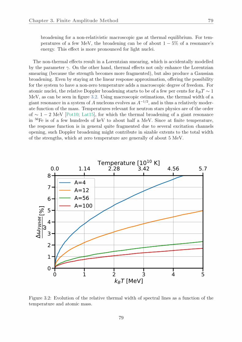
Chapter 3. Finite Amplitude Method 79
broadening for a non-relativistic macroscopic gas at thermal equilibrium. For tem-peratures of a few MeV, the broadening can be of about 1 − 5% of a resonance’senergy. This effect is more pronounced for light nuclei.
The non-thermal effects result in a Lorentzian smearing, which is accidentally modelledby the parameter γ. On the other hand, thermal effects not only enhance the Lorentziansmearing (because the strength becomes more fragmented), but also produce a Gaussianbroadening. Even by staying at the linear response approximation, offering the possibilityfor the system to have a non-zero temperature adds a macroscopic degree of freedom. Foratomic nuclei, the relative Doppler broadening starts to be of a few per cents for kBT ∼ 1MeV, as can be seen in figure 3.2. Using macroscopic estimations, the thermal width of agiant resonance in a system of A nucleons evolves as A−1/2, and is thus a relatively moder-ate function of the mass. Temperatures relevant for neutron stars physics are of the orderof ∼ 1 − 2 MeV [Pot10; Lat15], for which the thermal broadening of a giant resonancein 56Fe is of a few hundreds of keV to about half a MeV. Since at finite temperature,the response function is in general quite fragmented due to several excitation channelsopening, such Doppler broadening might contribute in sizable extents to the total widthof the strengths, which at zero temperature are generally of about 5 MeV.
0 1 2 3 4 5kBT [MeV]
0
1
2
3
4
5
6
7
8
FWH
M[%
]
A=4A=12A=56A=100
0.0 1.14 2.28 3.42 4.56 5.7Temperature [1010 K]
A=4A=12A=56A=100
Figure 3.2: Evolution of the relative thermal width of spectral lines as a function of thetemperature and atomic mass.
79

80 Chapter 3. Finite Amplitude Method
In the case of neutron stars, the interaction of the nuclei with their environment couldplay a considerable role [Pen+11; KMC00; KMC01], so that this model of isolated nucleiis by no means expected to be valid in presence of extremely high magnetic fields. Addi-tionally, it assumes all nuclei are perfectly thermalised, which may very well not be thecase in realistic situations, e.g. in the case of newly formed neutron stars, whose temper-ature drops by five to six orders of magnitude within a few years [Pot10; Lat15], althoughpairing correlations [For+10], electronic collisions and interaction with photons can sig-nificantly accelerate the cooling. Finally, since the structure of the nuclei is stronglyaffected by their temperature, thermal effects cannot be faithfully represented by theoverly simplistic form of a Gaussian spreading of the zero-temperature spectral function:strictly speaking, the effect of the temperature on nuclei in a macroscopic body shouldbe accounted for by drawing T from their temperature distribution, then summing theirresponses altogether to obtain the properly weighted average:
S(F, ωγ, Tbath) =
∫dTp(Tnucl = T | Tbath)S(F, ωγ, T ), (3.163)
p(Tnucl = T | Tbath) being the probability of finding a nucleus with temperature T withina bath at temperature Tbath
22.
For crude estimations of the thermal broadening of a particular resonance mode andnucleus, one can use the macroscopic formulae of [Cho97]. In particular, these tell us thatthe thermal broadening should be the most important in case of iso-vector quadrupoleoscillations. As for low-lying resonances, which in general are of single-particle character,the effect of temperature is expected to be much stronger, since the participant orbitalsare those with energy close to the Fermi energy.
3.10 QFAM in harmonic oscillator basis: selection
rules
3.10.1 From the external probe
A convenient approach to the treatment of collective excitations is to study the responseof the system to a probe of well-defined multipolarity. Indeed, a given multipolaritycomes along with its associated selection rules, so that one can, owing to the linearapproximation, decompose the total response of the system to any kind of perturbationas a sum over the different projections of the angular momentum:
F (ω) =∑J,K
K all =
cJK(ω)QJK S(F, ω) =∑J,K
K all =
cJK(ω)S(QJK , ω). (3.164)
This translates into the fact that for a given J , the different K = −J,−J +1, . . . , J can
22If the ensemble nuclei+bath is in statistical equilibrium and the nuclei form a gaseous state, onehas p(Tnucl = T | Tbath) equal to the Maxwell-Boltzmann distribution.
80
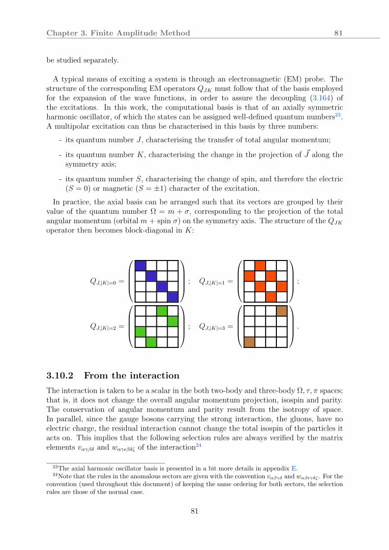
Chapter 3. Finite Amplitude Method 81
be studied separately.
A typical means of exciting a system is through an electromagnetic (EM) probe. Thestructure of the corresponding EM operators QJK must follow that of the basis employedfor the expansion of the wave functions, in order to assure the decoupling (3.164) ofthe excitations. In this work, the computational basis is that of an axially symmetricharmonic oscillator, of which the states can be assigned well-defined quantum numbers23.A multipolar excitation can thus be characterised in this basis by three numbers:
- its quantum number J , characterising the transfer of total angular momentum;
- its quantum number K, characterising the change in the projection of J along thesymmetry axis;
- its quantum number S, characterising the change of spin, and therefore the electric(S = 0) or magnetic (S = ±1) character of the excitation.
In practice, the axial basis can be arranged such that its vectors are grouped by theirvalue of the quantum number Ω = m + σ, corresponding to the projection of the totalangular momentum (orbital m + spin σ) on the symmetry axis. The structure of the QJK
operator then becomes block-diagonal in K:
QJ,|K|=0 =
; QJ,|K|=1 =
;
QJ,|K|=2 =
; QJ,|K|=3 =
.
3.10.2 From the interaction
The interaction is taken to be a scalar in the both two-body and three-body Ω, τ, π spaces;that is, it does not change the overall angular momentum projection, isospin and parity.The conservation of angular momentum and parity result from the isotropy of space.In parallel, since the gauge bosons carrying the strong interaction, the gluons, have noelectric charge, the residual interaction cannot change the total isospin of the particles itacts on. This implies that the following selection rules are always verified by the matrixelements vαγβδ and wαγϵβδζ of the interaction24
23The axial harmonic oscillator basis is presented in a bit more details in appendix E.24Note that the rules in the anomalous sectors are given with the convention vαβγδ and wαβϵγδζ . For the
convention (used throughout this document) of keeping the same ordering for both sectors, the selectionrules are those of the normal case.
81

82 Chapter 3. Finite Amplitude Method
Normal sectors
Ωα + Ωγ = Ωβ + Ωδ (3.165)
τα + τγ = τβ + τδ (3.166)
πα + πγ = πβ + πδ. (3.167)
Anomalous sectors
Ωα + Ωβ = Ωγ + Ωδ (3.168)
τα + τβ = τγ + τδ (3.169)
πα + πβ = πγ + πδ. (3.170)
Normal sectors
Ωα + Ωγ + Ωϵ = Ωβ + Ωδ + Ωζ (3.171)
τα + τγ + τϵ = τβ + τδ + τζ (3.172)
πα + πγ + πϵ = πβ + πδ + πζ . (3.173)
Anomalous sectors
Ωα + Ωβ + Ωϵ = Ωγ + Ωδ + Ωζ (3.174)
τα + τβ + τϵ = τγ + τδ + τζ (3.175)
πα + πβ + πϵ = πγ + πδ + πζ . (3.176)
This leads to some relationships between the structure of the density matrix and thefields. If we define K such that Ωδ = Ωγ +K (resp. Ωδ = Ωβ +K) in the normal (resp.anomalous) sector, (3.165) (resp. (3.168)) implies Ωα = Ωβ + K (resp. Ωα = Ωγ + K).Therefore, if the density matrix contains coupling between elements differing by K, sodo the h and ∆ fields. The isospin and parity being both invariant under time-reversal,the selections rules (3.166)-(3.167) & (3.169)-(3.170) are also valid in the time-reversedsectors with no sign to be introduced. In addition, the invariance of quantum mechanicsunder time-reversal implies that the inter-nucleons interactions are invariant under thissymmetry. Finally, the interaction must be the same if all the initial and final states areswapped consistently, as the indices labelling the states are evidently dummy. These twolast properties come in handy when calculating the fields, and are for instance put towork in the derivations of (3.60) and (3.62).
3.10.3 Quantum numbers of the oscillations
In usual mean-field calculations, the matrices representing the many-body interactionscan be brought to a form that is block-diagonal in the conserved quantum numbers25.The densities are mandated to have the same structure, and thus, so do the fields. Thesituation is slightly richer when a probe is included, since it is allowed to excurse outsidethe symmetry imposed to the unperturbed Hamiltonian, for which K = 0. It is easilyverified26 that the fields constructed by contracting the two- and three-body interactionswith the off-diagonal densities have the same quantum number K. Then, the FAM ampli-tudes (3.8) always display the same structure as the operator F(ω). Finally, transformingback to single-particle basis leads to transition densities non-zero only when they con-nect states with difference of the angular momentum projection of K. Altogether, thestructure of the external operator propagates to all of the FAM densities and fields.
25This can be achieved simply by arranging the basis vectors appropriately.26Sketching the operation as a block-wise product of two matrices does the trick.
82
Chapter 4
Application to thermal phasetransitions
This chapter presents a succinct study of phase transitions triggered by tem-perature. Although these phenomena are usually studied in heavy nuclei,which exhibit properties closer to the thermodynamic limit, the work of thischapter is centered around the mid-mass system 56Fe. The characteristic fea-tures of the phase transition can be well reproduced. The results are in goodqualitative agreement with those observed in heavy systems.
Contents4.1 Signatures of phase transitions . . . . . . . . . . . . . . . . . . 84
4.2 Motivation for studying 56Fe . . . . . . . . . . . . . . . . . . . . 85
4.3 Results . . . . . . . . . . . . . . . . . . . . . . . . . . . . . . . . . 854.3.1 Foreword: mean-field and expectations from ab initio interactions 85
4.3.2 Convergence with model space parameters and chiral order . . 87
4.3.3 Shape transition in 56Fe . . . . . . . . . . . . . . . . . . . . . . 94
83

84 Chapter 4. Application to thermal phase transitions
4.1 Signatures of phase transitions
Colloquially, a phase transition is defined by the sudden and drastic change in the struc-ture of the system. This is often realised by the different phases possessing differentsymmetries [Lan37][LL67b, Ch. 14]. Formally, the phase transition is identified with adiscontinuity in a derivative of the free energy F . The modern classification labels phasetransitions as discontinuous or continuous, depending on whether the entropy
S = −(∂F
∂T
)N,V
(4.1)
shows a discontinuity or not. The derivatives of the free energy are to be taken withrespect to the parameter that is varied, namely the temperature in the present case. Asthe transition corresponds to an abrupt modification of the system’s properties acrossthe different phases, at least one macroscopic observable must undergo identical changes.There exists therefore a quantity characterising, loosely speaking, the extent to which thehigh-symmetry phase is broken down to the low-symmetry one. These are the so-calledorder parameters. An intuitive example is the shape phase transition in finite systems.An axially deformed phase breaks SO(3) down to SU(2), and is identified by a non-zeroquadrupole moment β20. The transition from a spherical to a deformed phase thereforeoccurs as soon as β20 departs from zero. The high-energy phase typically has higher sym-metry than the low-energy one. This can be understood by arguing that at large energy,the degrees of freedom can explore a wider part of the parameter space, washing out theeffects of the small region corresponding to a particular subgroup of the overall symmetrygroup of the high-energy phase. The situation is similar for the pairing transition, whichbreaks the particle number symmetry at low energy; the pairs break up as the tempera-ture is increased, effectively restoring the U(1) symmetry.
A somewhat more rigorous definition is that different phase of the system are char-acterised by different symmetries or topologies, that are identified with the expectationvalues of symmetry operators, which commute with the Hamiltonian in one phase but notin another. This translates in an order parameter acquiring a non-zero expectation value,that can be used as a gauge of the extent to which the symmetry is broken. For instance,a superconducting phase involves a non-zero pair creation gap, whereas a normal phasecorresponds to disfavoured pair condensation. The corresponding order parameter is thepairing gap, or equivalently the pairing energy. Likewise, a deformed ground state is notinvariant under rotations, and thus exhibits one or more non-zero expectation values ofmultipolar moments.
In this chapter, we study the shape phase transition of the deformed nucleus 56Fe. Thelighter 46Ti and 44Ti display a step-like collapse of the deformation, and are thereforediscarded for this thermodynamically inclined analysis. Iron is found to exhibit an oblateshape. The evolution of the appropriate order parameter, namely the quadrupole defor-mation β20, is studied as a function of the temperature. This allows to identify the criticaltemperature TC and observe the behaviour of thermodynamical parameters deriving fromthe free energy. The convergence with respect to numerical parameters of the axial har-
84
Chapter 4. Application to thermal phase transitions 85
monic oscillator basis is studied, as well as the convergence as different orders in the chiralinteraction are included.
4.2 Motivation for studying 56Fe
A fine understanding of nuclear structure and reactions is required if one desires to accu-rately describe the giant resonances, and by such the origin and abundances of chemicalelements [Bur+57]. The whole nucleosynthesis can schematically be split into two parts,corresponding to the formation of light to mid-mass nuclei, and the generation of heavierones. From the appearance of light nuclei through the cooling down of the early universe,a gravitational collapse of protostellar clouds (composed of hydrogen in atomic or molecu-lar form, helium and, to a lesser extent, of nuclei up to carbon) may trigger thermonuclearfusion, and hence the genesis of stars. High pressure and temperature cause nuclear re-actions to abound. Illustratively, the combustion of hydrogen towards heavier nuclei is aseries of energetically favoured processes, up to iron and nickel. During the late stages ofstellar nucleosynthesis, the earlier-formed silicon nuclei capture alpha particles towards56Ni [Cla68, Ch. 7]. This nucleus undergoes beta-decay towards 56Co, which also convertsone of its protons to form 56Fe. Having one of the highest fractional binding energies ofthe whole nuclide chart [Few95], the chain stops here. This explains the abundance of ironin the universe [Cla68; LPG09; AG20] and its role as a starting point for the formation ofheavier nuclei through the s-process [Hil78; MC90; CT04] that occurs during the late lifeof stars with about one to eight solar masses [Boo06]. Knowing of the rates at which thesereactions occur is key to faithful prediction of nucleosynthetic processes. The status ofthis iron isotope as both an accumulation point of the silicon burning stage and a startingpoint for the nucleosynthesis of heavier elements calls for an in-depth understanding ofthe structure of its ground and excited states. The present chapter analyses and discussesthe effects of coupling to a thermal bath on the bulk properties of 56Fe.
4.3 Results
4.3.1 Foreword: mean-field and expectations from ab initio in-teractions
In case of a microscopic theory, the exact, many-body Schrodinger must in principle besolved. However, its exponentially increasing dimension with the number of degrees offreedom often makes such an approach a daunting task. As an alternative, we resort to aHartree-Fock-Bogoliubov mean field theory, including superfluidity (see subsection 2.4.2).Furthermore, we allow the breaking of the rotational SO(3) symmetry down to an axial(SU(2)) one, as a means of grasping additional correlations at a mild cost by letting thesystem explore a landscape of lesser symmetry. While breaking symmetries may seemcurious for finite systems, this approach can be phenomenologically justified. For defor-mation, several types of quantum systems (atoms, molecules and nuclei alike) do exhibitrotational bands, that can only exist in non-spherical bodies. In case of pairing inter-actions, the odd-even staggering effect signals an increase of binding energy for systemspossessing even numbers of nucleons. This suggested the possibility of pairing in atomic
85

86 Chapter 4. Application to thermal phase transitions
nuclei early on [BMP58]. It is important to note that on average, symmetries are preservedin finite systems: while frameworks allowing for their breaking are allowed and motivatedby empirical facts, the story must be complemented by a symmetry-restoration step in or-der to obtain eigenstates exhibiting the same symmetries as the Hamiltonian. Additionalcorrelations beyond the single-reference mean-field can be obtained by including mpmhcorrelations in a perturbative manner [Tic+16; Tic+18; TRD20] or not [DS15; Qiu+19;BD21], and carrying a projection onto the desired symmetries.
On the other side, interactions derived from an effective theory become less reliable asthe size of the system increases. Indeed, in order to maintain the connection to QCD,the low-energy constants must be adjusted on few-body data, and as such, the quality ofthe predictions degrades with increasing masses by lack of four-body (and higher) terms.The derivation and production of high-rank interactions is a highly involved endeavour[Her+13; Hup+13; Rot+14]. Extending the reach of ab initio methods to higher massesis a task currently being undertaken [Som+14; Her20]. It should be pointed out thatthe ab-initio interactions are known for providing differential quantities (e.g. nucleonicseparation energies) in better agreement with experiment than the integrated values suchas the total binding energies. Still, neither can rival the results obtained with phenomeno-logical interactions, that are adjusted over the whole nuclear chart, and thus yield moreaccurate results on average.
The results presented in this thesis thus rest on the arguable balance of tackling mid-mass systems. On the one hand, mean field approximations are not well-suited for lightsystems, where the contribution from individual particles with respect to the bulk canbe non-negligible. Alternatively, the use of ab initio interactions, adjusted on few-bodydata, becomes questionable for large numbers of particles, at least when using a simpleHFB framework. Despite this apparent flaw, we can stress two points. First, the relevantquantities for the study of temperature on FTHFB results are calculated as differencesor differentials, we can thus expect a correct quantitative behaviour even if the groundstate energy is shifted from the experimental values. In case of the FTFAM, simpleparticle-hole type excitations over a ground state are considered. The energy differencesbetween single-particle states being in general overestimated, we can expect the strengthsfunction obtained in the next chapter to overestimate the excitation energies, although thequalitative behaviour should be correct. On the other hand, the self-consistent solution ofthe FAM equation incorporates collective correlations, and as such contribute in correctingthe quasiparticle self-energies. Second, the improvement of “raw” FTHFB results is stillpossible by any of the previously mentioned techniques (provided they are formalised fornon-zero temperatures). Although our results on binding energies, radii, or deformationsare no match for those given by phenomenological interactions, they remain relevant asfirst steps towards the extension of usual mean-field-and-beyond techniques to the finitetemperature regime within an ab initio setting.
86
Chapter 4. Application to thermal phase transitions 87
4.3.2 Convergence with model space parameters and chiral or-der
The calculations performed here depend on several parameters: the frequency ℏΩ ofthe harmonic oscillator employed to construct the basis functions, the number of single-particle basis functions (characterised by the integer emax), the relative length of theoscillator in the radial and axial directions1, and the order in the chiral expansion, toname the most important. The axial and radial oscillator frequencies could be optimisedsimultaneously, but are always taken to be equal. The three first are essentially numericalparameters to be optimised in order to obtain the lowest energy, whereas the latter has aclear physical meaning and will be discussed in a following section.
The oscillator frequency controls the stiffness of the basis functions: a large (resp. small)frequency corresponds to narrow (resp. spread out) wave functions. In the ℏΩ → 0 limit,the wave functions become those of plane waves, for which achieving localisation can sen-sibly be conceived to be more difficult than when using a non-zero frequency. On theother hand, the ℏΩ → ∞ translates into basis function sharply localised around the cen-tre of the coordinate frame, so that the system can only be much more localised than itsground state shape within an otherwise identical model space. These two extreme casesshould thus lead to ground state energies far above the minimum of E(ℏΩ). A reasonablechoice for ℏΩ can be to have resulting eigenfunctions with a spatial extent close to theexpected (e.g. estimated from a hard-sphere formula) radius of the nucleus, although thedependence of the radius on the shell structure makes this guess usually land off the op-timal value. Taking ℏΩ according to a liquid drop formula, ℏΩ ∝ A−1/3, can nonethelessprovide a starting point for scanning a range of oscillator frequencies.
On the opposite side, increasing the size of the model space must unambiguously lead tolower ground state energies, all other parameters being equal. The emax → ∞ is obviouslyunreachable, as it would require infinitely many basis functions. Since the energy isexpected to converge smoothly with the size of the model space, one can instead studythe convergence by carrying calculations with a set of different values of emax. It shouldbe noted that the energy is the only quantity for which this monotonous convergenceis guaranteed, by the variational principle underlying the resolution of the equations ofmotion.
Interpolations in oscillator frequency
Assuming the shell structure of the nucleus under study is relatively independent of ℏΩ,one can presume that the energy does not vary too abruptly with the oscillator frequencyabout the optimal value. It is thus reasonable to suppose the energy to be a quadraticfunction of ℏΩ when close to the best frequency. This can be used to interpolate numeri-cally the optimal oscillator frequency, and obtain the corresponding energy, or an estimatethereof, straight from the polynomial regression.
1Because Ω is the geometric mean of the oscillator frequencies in the two directions, one can eithertake their ratio and Ω as the parameters of the basis, or the two oscillator lengths, both choices beingstrictly equivalent.
87
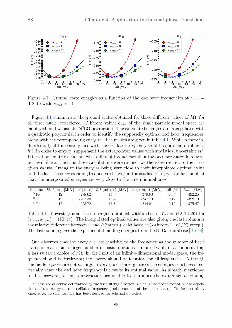
88 Chapter 4. Application to thermal phase transitions
10 12 14 16 18 20 22 [MeV]
280275270265260255250245240235230
E [M
eV]
56Feemax = 6emax = 8emax = 10
10 12 14 16 18 20 22 [MeV]
240
235
230
225
220
215
E [M
eV]
46Tiemax = 6emax = 8emax = 10
10 12 14 16 18 20 22 [MeV]
225
220
215
210
205
E [M
eV]
44Tiemax = 6emax = 8emax = 10
Figure 4.1: Ground state energies as a function of the oscillator frequencies at emax =6, 8, 10 with e3max = 14.
Figure 4.1 summarises the ground states obtained for three different values of ℏΩ, forall three nuclei considered. Different values emax of the single-particle model space areemployed, and we use the N3LO interaction. The calculated energies are interpolated witha quadratic polynomial in order to identify the supposedly optimal oscillator frequencies,along with the corresponding energies. The results are given in table 4.1. While a more in-depth study of the convergence with the oscillator frequency would require more values ofℏΩ, in order to employ supplement the extrapolated values with statistical uncertainties2.Interactions matrix elements with different frequencies than the ones presented here werenot available at the time these calculations were carried; we therefore restrict to the threegiven values. Owing to the energies being very close to their interpolated optimal valueand the fact the corresponding frequencies lie within the studied ones, we can be confidentthat the interpolated energies are very close to the true minimal ones.
Nucleus ℏΩ (best) [MeV] E [MeV] ℏΩ (interp.) [MeV] E (interp.) [MeV] diff (%) Eexp. [MeV]56Fe 12 -278.62 14.0 -279.60 0.35 -492.2646Ti 12 -237.30 13.4 -237.70 0.17 -398.1944Ti 12 -223.72 13.8 -224.01 0.15 -375.47
Table 4.1: Lowest ground state energies obtained within the set ℏΩ = (12, 16, 20) for(emax, e3max) = (10, 14). The interpolated optimal values are also given; the last column isthe relative difference between E and E(interp.), calculated as (E(interp.)−E)/E(interp.).The last column gives the experimental binding energies from the NuDat database [Bro08].
One observes that the energy is less sensitive to the frequency as the number of basisstates increases, as a larger number of basis functions is more flexible in accommodatinga less suitable choice of ℏΩ. In the limit of an infinite-dimensional model space, the fre-quency should be irrelevant; the energy should be identical for all frequencies. Althoughthe model spaces are not so large, a very good convergence of the energies is achieved, es-pecially when the oscillator frequency is close to its optimal value. As already mentionedin the foreword, ab initio interaction are unable to reproduce the experimental binding
2These are of course determined by the used fitting function, which is itself conditioned by the depen-dence of the energy on the oscillator frequency (and dimension of the model space). To the best of myknowledge, no such formula has been derived for schematic models.
88

Chapter 4. Application to thermal phase transitions 89
energies when only a single mean field is employed, as can be seen from the rightmostcolumn.
Although for all nuclei, the energy varies in less than 5% among the three frequenciesemployed at emax = 10, this does not guarantee the convergence of all observables. Theground state quadrupole deformations and radii are displayed in figures 4.2-4.3 in orderto verify whether these quantities vary in similar magnitude. While all three observabledepend on the nucleonic densities, it can be anticipated that they do not vary to similarextents with the spatial extension of the basis functions. The energy is a spatial integralinvolving the local parts of the densities and mean-fields. Since these typically resembleeach other (the density is higher in the regions where the potential is higher in absolutevalue), an overall quite reasonable variation of the energy with the basis frequency canbe expected. Conversely, the quadrupole moment is more directly sensitive to the den-sity distribution, as the corresponding operator, Q20, is not a functional of the densities.Changing the stiffness of the basis functions should have large consequences on the over-all shape of the system, resulting in deformations more strongly dependent on ℏΩ thatthe energy is. Finally, since the spatial matter density does not take particularly exoticshapes, but is instead rather constant (at around the saturation density ρ0 = 0.16 fm−3),we can presume the point-particle radii to vary fairly less than the deformations.
10 12 14 16 18 20 22 [MeV]
0.20
0.15
0.10
20
56Feemax = 6emax = 8emax = 10
10 12 14 16 18 20 22 [MeV]
0.100.050.000.050.100.150.200.250.30
20
46Ti
emax = 6emax = 8emax = 10
10 12 14 16 18 20 22 [MeV]
0.10
0.15
0.20
20
44Ti
emax = 6emax = 8emax = 10
Figure 4.2: Same as figure 4.1 for the quadrupole moments.
The quadrupole moments are found to exhibit a strong dependence on the frequencyof the basis. At emax = 8, their values at ℏΩ = 20 MeV are 20-40% off the ℏΩ = 12results, while the larger basis emax = 10 diminishes the discrepancies roughly by a factorof two. Although the energy also displays non-negligible dependence on the oscillatorfrequency, the β20 observable varies in much greater amounts. This hints that the studyof deformation-dependent observables (e.g. inertial masses, rotational and vibrationalspectra) requires a careful verification that the numerical parameters of the model spaceare optimised, even in cases where the energy does not vary too much. On the other hand,at emax = 10, the radii of all three nuclei are observed to vary within a few percents only,showing relative variations of the same order as the energies. Note that the trend in theevolution of β20 and R with ℏΩ can be understood on the basis that larger oscillator fre-quencies correspond to more squeezed basis functions, which yields smaller deformations
89
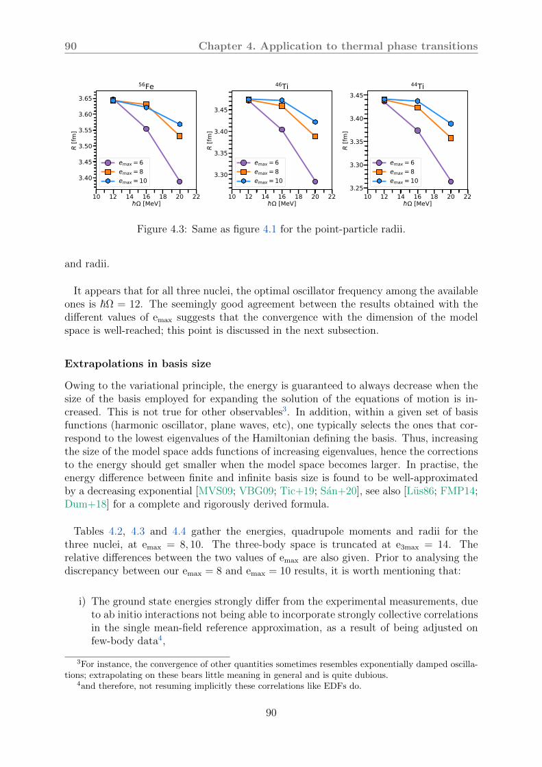
90 Chapter 4. Application to thermal phase transitions
10 12 14 16 18 20 22 [MeV]
3.40
3.45
3.50
3.55
3.60
3.65
R [fm
]56Fe
emax = 6emax = 8emax = 10
10 12 14 16 18 20 22 [MeV]
3.30
3.35
3.40
3.45
R [fm
]
46Ti
emax = 6emax = 8emax = 10
10 12 14 16 18 20 22 [MeV]
3.25
3.30
3.35
3.40
3.45
R [fm
]
44Ti
emax = 6emax = 8emax = 10
Figure 4.3: Same as figure 4.1 for the point-particle radii.
and radii.
It appears that for all three nuclei, the optimal oscillator frequency among the availableones is ℏΩ = 12. The seemingly good agreement between the results obtained with thedifferent values of emax suggests that the convergence with the dimension of the modelspace is well-reached; this point is discussed in the next subsection.
Extrapolations in basis size
Owing to the variational principle, the energy is guaranteed to always decrease when thesize of the basis employed for expanding the solution of the equations of motion is in-creased. This is not true for other observables3. In addition, within a given set of basisfunctions (harmonic oscillator, plane waves, etc), one typically selects the ones that cor-respond to the lowest eigenvalues of the Hamiltonian defining the basis. Thus, increasingthe size of the model space adds functions of increasing eigenvalues, hence the correctionsto the energy should get smaller when the model space becomes larger. In practise, theenergy difference between finite and infinite basis size is found to be well-approximatedby a decreasing exponential [MVS09; VBG09; Tic+19; San+20], see also [Lus86; FMP14;Dum+18] for a complete and rigorously derived formula.
Tables 4.2, 4.3 and 4.4 gather the energies, quadrupole moments and radii for thethree nuclei, at emax = 8, 10. The three-body space is truncated at e3max = 14. Therelative differences between the two values of emax are also given. Prior to analysing thediscrepancy between our emax = 8 and emax = 10 results, it is worth mentioning that:
i) The ground state energies strongly differ from the experimental measurements, dueto ab initio interactions not being able to incorporate strongly collective correlationsin the single mean-field reference approximation, as a result of being adjusted onfew-body data4,
3For instance, the convergence of other quantities sometimes resembles exponentially damped oscilla-tions; extrapolating on these bears little meaning in general and is quite dubious.
4and therefore, not resuming implicitly these correlations like EDFs do.
90
Chapter 4. Application to thermal phase transitions 91
ii) No experimental data for the ground state deformations being available, we resort tocomparing with the available EDF predictions of [BN20] and [HG07], and observe amismatch of the β20 values between EDF and ab initio results for 56Fe, and betweenall three calculations for 44Ti. Besides the fact that such masses touch on the vergeof the current ab initio interaction’s reach (at least within a single-reference HFBapproach), we note that 56Fe posses both oblate and prolate minima, the oblatebeing lower in our calculations. On the other hand, the softness of 44Ti, especiallytowards the prolate deformations, explains why we find such different quadrupolemoment.
E [MeV] β20 R [fm]emax = 8 -277.51 -0.2192 3.6313emax = 10 -278.62 -0.2187 3.6427diff. (%) 0.40 0.20 0.31
E [MeV] β20 R [fm]DD-PC1 -489.63 0.24 3.6931D1S -488.84 0.20 x
Table 4.2: Selected ground state observables for 56Fe at emax = 8 and 10 (left), and fullyconverged EDF results for a relativistic (DD-PC1) and a non-relativistic (D1S) functional(right). The three-body space is truncated at e3max = 14. The relative difference on anobservableX is calculated as |X(emax = 10)−X(emax = 8)/X(emax = 10)|, and is roundedup to two decimal places. The experimental charge radius is Rexp
ch = 3.7377 ± 0.0016 fm[AM13].
E [MeV] β20 R [fm]emax = 8 -236.92 0.2625 3.4591emax = 10 -237.30 0.2650 3.4742diff. (%) 0.16 0.94 0.43
E [MeV] β20 R [fm]DD-PC1 -397.11 0.24 3.5040D1S -396.04 0.20 x
Table 4.3: Same as table 4.2 for 46Ti. The experimental charge radius is Rexpch = 3.6070±
0.0022 fm [AM13].
E [MeV] β20 R [fm]emax = 8 -223.49 0.2329 3.4234emax = 10 -223.72 0.2304 3.4411diff. (%) 0.11 1.10 0.51
E [MeV] β20 R [fm]DD-PC1 -373.60 0.15 3.4478D1S -372.97 0.00 x
Table 4.4: Same as table 4.2 for 44Ti. The experimental charge radius is Rexpch = 3.6115±
0.0051 fm [AM13].
For all three systems, the macroscopic observables are quite well converged with respectto the basis sizes we use. This however holds only close to the optimal frequencies; seefigures 4.1, 4.2, 4.3 where the discrepancy between emax = 8 and emax = 10 reaches muchhigher levels for ℏΩ = 20. The fact all three observables are converged within roughly onepercent or less is a first hint that the model space (emax, e3max) = (10, 14) with ℏΩ = 14is large enough to describe the structure of the system. One can go a small step further,
91

92 Chapter 4. Application to thermal phase transitions
by applying the aforementioned extrapolation to apprehend the emax → ∞ limit. Theenergies are fitted with
E(emax, ℏΩ) = E∞(ℏΩ) + A(ℏΩ) exp−b(ℏΩ)emax , (4.2)
and, for a given nucleus, we call the best extrapolated value the energy minℏΩ=12,16,20
E∞(ℏΩ).
6 8 10 12eMax
280
270
260
250
240
230
220
E [M
eV]
56Fe= 12= 16= 20
6 8 10 12eMax
240
230
220
210E
[MeV
]
46Ti= 12= 16= 20
6 8 10 12eMax
225
220
215
210
205
200
195
E [M
eV]
44Ti= 12= 16= 20
Figure 4.4: Evolution of the ground state energies with emax. The dashed lines representthe fitted curves, and the grey lines denote the best extrapolated values. The model spaceused has e3max = 14.
56Fe 46Ti 44TiE(emax = 10) -278.62 -237.30 -223.72
E∞ -279.73 -238.95 -223.78diff. (%) 0.40 0.69 0.03
Table 4.5: Values and relative differences between the energies obtained at emax = 10 andtheir extrapolation. The results are given for ℏΩ = 12 MeV. The differences are calculatedas (E∞ − E(emax = 10))/E∞.
The corresponding values are given in figure 4.4, and the relative differences are listedin table 4.5. In all nuclei, the extrapolated values are astonishingly close to the finite-basisresults, which testifies once more that the convergence is well-attained. This conclusion isconsistent with the results of [Tic+19; Hop+21], that use the same potentials, regulatorand SRG evolution, with a slightly different adjustment of the coupling constants. How-ever, the obtention of different extrapolated values when using different frequencies signalsthat the extrapolation (4.2) does not exactly hold; it is rather a convenient and simpletool to gauge the convergence with emax, and can only be given a meaningful meaningwhen associated with covariances.
Convergence in the chiral expansion
The two previous parameters, while bearing a more or less pronounced physical meaning,can be classified as principally numerical. On the completely opposite side, how many
92
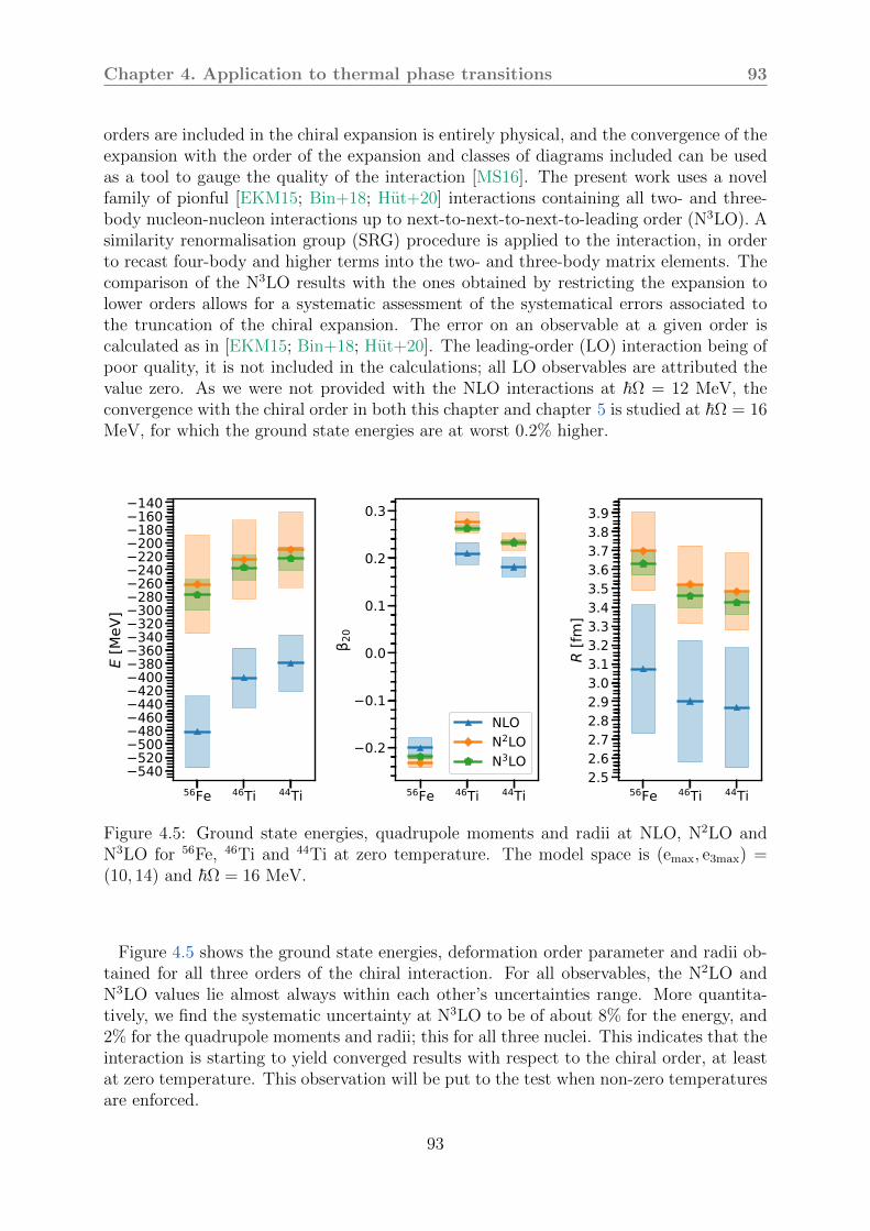
Chapter 4. Application to thermal phase transitions 93
orders are included in the chiral expansion is entirely physical, and the convergence of theexpansion with the order of the expansion and classes of diagrams included can be usedas a tool to gauge the quality of the interaction [MS16]. The present work uses a novelfamily of pionful [EKM15; Bin+18; Hut+20] interactions containing all two- and three-body nucleon-nucleon interactions up to next-to-next-to-next-to-leading order (N3LO). Asimilarity renormalisation group (SRG) procedure is applied to the interaction, in orderto recast four-body and higher terms into the two- and three-body matrix elements. Thecomparison of the N3LO results with the ones obtained by restricting the expansion tolower orders allows for a systematic assessment of the systematical errors associated tothe truncation of the chiral expansion. The error on an observable at a given order iscalculated as in [EKM15; Bin+18; Hut+20]. The leading-order (LO) interaction being ofpoor quality, it is not included in the calculations; all LO observables are attributed thevalue zero. As we were not provided with the NLO interactions at ℏΩ = 12 MeV, theconvergence with the chiral order in both this chapter and chapter 5 is studied at ℏΩ = 16MeV, for which the ground state energies are at worst 0.2% higher.
56Fe 46Ti 44Ti540520500480460440420400380360340320300280260240220200180160140
E [M
eV]
56Fe 46Ti 44Ti
0.2
0.1
0.0
0.1
0.2
0.3
20
NLON2LON3LO
56Fe 46Ti 44Ti2.52.62.72.82.93.03.13.23.33.43.53.63.73.83.9
R [fm
]
Figure 4.5: Ground state energies, quadrupole moments and radii at NLO, N2LO andN3LO for 56Fe, 46Ti and 44Ti at zero temperature. The model space is (emax, e3max) =(10, 14) and ℏΩ = 16 MeV.
Figure 4.5 shows the ground state energies, deformation order parameter and radii ob-tained for all three orders of the chiral interaction. For all observables, the N2LO andN3LO values lie almost always within each other’s uncertainties range. More quantita-tively, we find the systematic uncertainty at N3LO to be of about 8% for the energy, and2% for the quadrupole moments and radii; this for all three nuclei. This indicates that theinteraction is starting to yield converged results with respect to the chiral order, at leastat zero temperature. This observation will be put to the test when non-zero temperaturesare enforced.
93
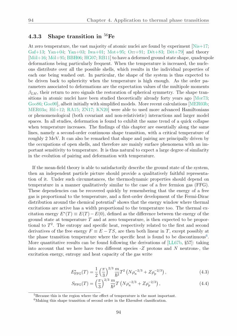
94 Chapter 4. Application to thermal phase transitions
4.3.3 Shape transition in 56Fe
At zero temperature, the vast majority of atomic nuclei are found by experiment [Nis+17;Gaf+13; Yan+04; Yan+03; Iwa+01; Mot+95; Orr+91; Det+83; Det+79] and theory[Mol+16; Mol+95; BBH06; HG07; RB11] to have a deformed ground state shape, quadrupoledeformations being particularly frequent. When the temperature is increased, the nucle-ons distribute over all the possible shells, which results in the individual properties ofeach one being washed out. In particular, the shape of the system is thus expected tobe driven back to sphericity when the temperature is high enough. As the order pa-rameters associated to deformations are the expectation values of the multipole momentsβLM , their return to zero signals the restoration of spherical symmetry. The shape tran-sitions in atomic nuclei have been studied theoretically already forty years ago [Mor73;Goo86; Goo90], albeit initially with simplified models. More recent calculations [MER03b;MER03a; Hil+12; RA15; ZN17; KN20] were able to used more advanced Hamiltoniansor phenomenological (both covariant and non-relativistic) interactions and larger modelspaces. In all studies, deformation is found to exhibit the same trend of a quick collapsewhen temperature increases. The findings of this chapter are essentially along the samelines, namely a second-order continuous shape transition, with a critical temperature ofroughly 2 MeV. It can also be remarked that shape and pairing are principally driven bythe occupations of open shells, and therefore are mainly surface phenomena with an im-portant sensitivity to temperature. It is thus natural to expect a large degree of similarityin the evolution of pairing and deformation with temperature.
If the mean-field theory is able to satisfactorily describe the ground state of the system,then an independent particle picture should provide a qualitatively faithful representa-tion of it. Under such circumstances, the thermodynamic properties should depend ontemperature in a manner qualitatively similar to the case of a free fermion gas (FFG).These dependencies can be recovered quickly by remembering that the energy of a freegas is proportional to the temperature, and a first-order development of the Fermi-Diracdistribution around the chemical potential5 shows that the energy window where thermalexcitations are active has a width proportional to the temperature too. The thermal ex-citation energy E∗(T ) ≡ E(T )−E(0), defined as the difference between the energy of theground state at temperature T and at zero temperature, is then expected to be propor-tional to T 2. The entropy and specific heat, respectively related to the first and secondderivatives of the free energy F ≡ E − TS, are then both linear in T , except possibly atthe phase transition temperature where the specific heat is found to be discontinuous6.More quantitative results can be found following the derivations of [LL67b, §57]: takinginto account that we here have two different species -Z protons and N neutrons-, theexcitation energy, entropy and heat capacity of the gas write
E∗FFG(T ) =
1
2
(π3
)2/3 mℏ2
T 2(Nρ−2/3
n + Zρ−2/3p
), (4.3)
SFFG(T ) =(π3
)2/3 mℏ2
T(Nρ−2/3
n + Zρ−2/3p
), (4.4)
5Because this is the region where the effect of temperature is the most important.6Making this shape transition of second order in the Ehrenfest classification.
94
Chapter 4. Application to thermal phase transitions 95
CFFG(T ) = SFFG(T ). (4.5)
In all numerical calculations, we take for the FFG ρn = ρp = ρ0/2, with the saturationdensity ρ0 = 0.16 fm−3; the same mass m = 939 MeV/c2 is used for protons and neu-trons. Finally, the evolution of the deformation in thermal mid-mass and heavy nucleican be understood on the basis of Landau’s theory of continuous phase transitions [Lan37].
A shape phase transition is observed in finite temperature calculations of the groundstate of the mid-mass nuclei 56Fe. The coordinate-space density of the ground state atdifferent temperatures is given in figure 4.6, to help visualising the restoration of sphericalsymmetry. The T = 0 and T = 1 MeV densities are almost identical, while the defor-mation is much less pronounced at T = 2 MeV already. The spherical symmetry is fullyrestored at T = 3 MeV. As mentioned in section 2.5, no thermal averaging is carried out,so that the symmetry restoration occurs sharply at a critical temperature Tc.
Figure 4.7 shows the excitation energy as a function of temperature, obtained with theNLO, N2LO and N3LO orders of the chiral interaction. Calculations are performed atℏΩ = 16 MeV, (emax, e3max) = (8, 14). The excitation energies exhibit the quadratic de-pendence estimated from the schematic model of independent fermions, and the nucleusis found to be bound up to T = 8.6 MeV with the N3LO interaction. The very goodagreement between the two last orders seems to indicate that the convergence of the zero-temperature observables, usually reached with the third and fourth orders in the chiralexpansion, also holds at finite temperature. This can be taken as a strong indicationthat the quality of these interactions is about the same for both occupied and unoccu-pied orbitals of the zero-temperature nucleus. The same conclusion can be drawn fromfigure 4.8, where the total entropy is represented. The excellent agreement among thetwo last orders clearly signals the onset of convergence.
The entropy is found to globally display the expected linear dependence, except at verysmall temperatures where thermal excitations occur with negligible probabilities. Thisdeviation from the Fermi gas-like behaviour occurs predominantly at low temperature be-cause this is the region where the structure effects, in particular the shell gaps, are mostsensitive to the individual properties of each orbital. At low temperatures, the entropy(and thus, the free energy, and all thermodynamical variables) is for the largest part de-termined by the states close to the Fermi energy7. The low-temperature regime shouldthus be the region where the deviations from a Fermi liquid model are the most important.As a side remark, the fact the free energy is, for finite systems, mostly a surface quantityat low temperature, and grows to become a bulk quantity at high temperature, could beused as a means of determining the degree of agreement between different interactionswhile using only macroscopic observables.
The static quadrupole moment β20(T) is shown on figure 4.9. The discrepancy be-tween N2LO and N3LO is slightly more pronounced away from the phase transition,albeit remaining of less than 5%. Including the systematic errors according to the for-
7To be more precise, by those with energy E such that βE < 1, owing to the rapid fall-off of the Fermidistribution away from E = 0.
95

96 Chapter 4. Application to thermal phase transitions
Figure 4.6: Total (protons+neutrons) ground state densities of 56Fe for four tempera-tures. The calculations are made at (emax, e3max) = (8, 14), ℏΩ = 12 MeV, with the N3LOinteraction. The black, blue and yellow contours signal the iso-density surfaces, whereρ = 0.08, 0.12 and 0.16 fm−3, respectively.
mulae of [EKM15; Bin+18; Hut+20], the critical temperature at N3LO is found to beTc = 2.46± 0.23 MeV. The large uncertainty is due to the NLO prediction at around 4.5MeV; the N2LO and N3LO values differ in only 80 keV. The deformation showing signifi-cant variations over the span of a few MeV, it can be concluded that realistic predictionsof astrophysical processes involving iron in high-temperature environments should signifi-cantly cannot be made using information about the zero-temperature structure only. Thisstatement is even to be given more credit by the fact we do not mix different configura-tions according to their statistical weight (see (2.71)). Remarking that the modification ofthe observables once the thermal averaging is carried out can be qualitatively understoodwith statistical arguments only, we can expect to observe similar changes in β20(T ) as theones found in [MER03b; MER03a], namely a steeper decrease of the deformation belowthe critical temperature than found with a single-thermal state calculation, and a more
96

Chapter 4. Application to thermal phase transitions 97
0 1 2 3 4 5 6kBT [MeV]
500
400
300
200
100
E [M
eV]
NLON2LON3LO
0 1 2 3 4 5 6kBT [MeV]
0
50
100
150
E* (
T) [M
eV]
NLON2LON3LOFFG
Figure 4.7: Ground state energy (left) and excitation energy (right) as a function oftemperature in 56Fe. The excitation energy of a two-components free fermion gas ofprotons and neutrons at saturation density is also represented as circles placed every 0.2MeV.
0 1 2 3 4 5 6kBT [MeV]
0
10
20
30
40
50
S
NLON2LON3LOFFG
Figure 4.8: Same as figure 4.7 for the total entropy.
gentle return to sphericity beyond.
The energy and entropy being continuous functions of the temperature across the phasetransition, so is the free energy. However, the specific heat, related to the second derivativeof F and defined as
97
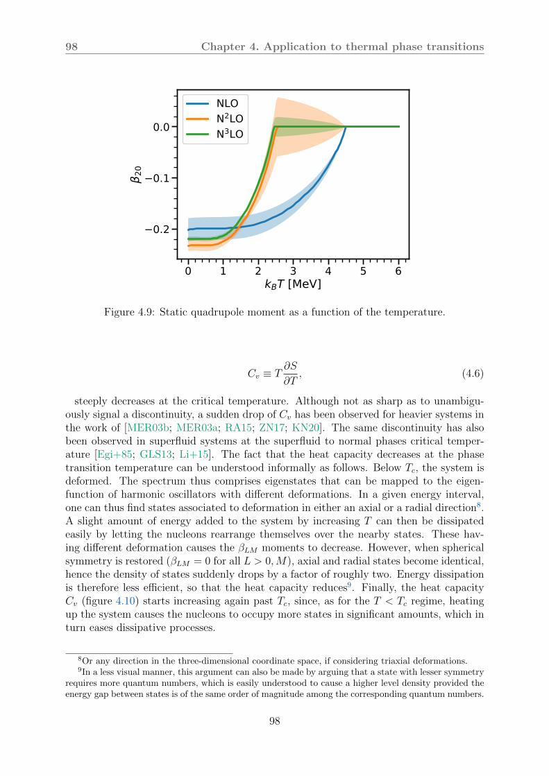
98 Chapter 4. Application to thermal phase transitions
0 1 2 3 4 5 6kBT [MeV]
0.2
0.1
0.020
NLON2LON3LO
Figure 4.9: Static quadrupole moment as a function of the temperature.
Cv ≡ T∂S
∂T, (4.6)
steeply decreases at the critical temperature. Although not as sharp as to unambigu-ously signal a discontinuity, a sudden drop of Cv has been observed for heavier systems inthe work of [MER03b; MER03a; RA15; ZN17; KN20]. The same discontinuity has alsobeen observed in superfluid systems at the superfluid to normal phases critical temper-ature [Egi+85; GLS13; Li+15]. The fact that the heat capacity decreases at the phasetransition temperature can be understood informally as follows. Below Tc, the system isdeformed. The spectrum thus comprises eigenstates that can be mapped to the eigen-function of harmonic oscillators with different deformations. In a given energy interval,one can thus find states associated to deformation in either an axial or a radial direction8.A slight amount of energy added to the system by increasing T can then be dissipatedeasily by letting the nucleons rearrange themselves over the nearby states. These hav-ing different deformation causes the βLM moments to decrease. However, when sphericalsymmetry is restored (βLM = 0 for all L > 0,M), axial and radial states become identical,hence the density of states suddenly drops by a factor of roughly two. Energy dissipationis therefore less efficient, so that the heat capacity reduces9. Finally, the heat capacityCv (figure 4.10) starts increasing again past Tc, since, as for the T < Tc regime, heatingup the system causes the nucleons to occupy more states in significant amounts, which inturn eases dissipative processes.
8Or any direction in the three-dimensional coordinate space, if considering triaxial deformations.9In a less visual manner, this argument can also be made by arguing that a state with lesser symmetry
requires more quantum numbers, which is easily understood to cause a higher level density provided theenergy gap between states is of the same order of magnitude among the corresponding quantum numbers.
98

Chapter 4. Application to thermal phase transitions 99
0 1 2 3 4 5 6kBT [MeV]
0
10
20
30
40
50
60
C v
NLON2LON3LOFFG
Figure 4.10: Same as figure 4.7 for the heat capacity. The derivatives are calculated usingfinite differences, for temperatures equally spaced of 0.01 MeV.
As a final remark, the energy, deformations and radii being bulk observables, they arenot so much sensitive to the details of the spectrum. At zero temperature, the good agree-ment between the last two orders can only be taken as an indicator that the interactionyields converged values for thermodynamic observables that are not driven by a specificregion of the spectrum. The maintaining of a good agreement between these differentorders at finite temperatures and for all the studied quantities allows more ambitiousstatements. The fact that the N2LO and N3LO results (not looking at the error bars, todiscard the poorly-converged NLO results from the discussion) remain almost identicalover the whole T = 0 − 6 MeV range brings the conclusion that these two interactionsnot only give converged bulk quantities at T = 0, but also at finite temperature, and thusremain of identical quality for the study of hot nuclei.
99


Chapter 5
Application to giant resonances
In this chapter, the finite amplitude method is put into operation to studygiant resonances in the mid-mass nuclei 56Fe, 46Ti and 44Ti. A strong de-pendence of the isovector dipole strength on the temperature is observed,characterised by a downwards shift of the resonance centroid when the sys-tems are heated up. The chapter starts by comparing the FAM results to thestandard RPA in the case of 16O, which, being spherical and non-superfluid,is currently within the reach of ab-initio RPA. As should be, the dependenceof the results on the parameters studied for the ground states calculations isalso scrutinised.
Contents5.1 Benchmark against standard RPA . . . . . . . . . . . . . . . . 103
5.2 Convergence aspects . . . . . . . . . . . . . . . . . . . . . . . . . 104
5.2.1 With the oscillator frequency . . . . . . . . . . . . . . . . . . . 106
5.2.2 With the basis size . . . . . . . . . . . . . . . . . . . . . . . . . 1105.2.3 With the chiral expansion . . . . . . . . . . . . . . . . . . . . . 111
5.2.4 Conclusion . . . . . . . . . . . . . . . . . . . . . . . . . . . . . 1135.3 Moments of the strength . . . . . . . . . . . . . . . . . . . . . . 114
5.4 Multipolar strengths of selected mid-mass nuclei at finitetemperature . . . . . . . . . . . . . . . . . . . . . . . . . . . . . . 117
5.5 Conclusion . . . . . . . . . . . . . . . . . . . . . . . . . . . . . . 126
101

102 Chapter 5. Application to giant resonances
The richness of collective features arising in quantum systems reveals the complex in-terplay between their microscopic constituents. In strongly correlated systems, excitedstates can be highly different from the ones built from simple particle-hole excitationson top of the ground state, owing to the self-consistent rearrangement occurring whenone (or several) particle(s) is (are) moved from an orbital to another. From a physicalperspective, the apparition of such collective resonances under the action of an externalfield can be understood from a self-consistent field picture. For simplicity, assume thesystem of interest to be at equilibrium, that is, static in its ground state. Then, apply apolarising field. This triggers the motion of each particle, so that the overall field oscillatesalong. Since the degrees of freedom interact, the motion of each one (or, equivalently,of the total field) affects the others’. These interferences can be one either side of thetwo extreme situations, i.e., destructive or constructive. The first case corresponds to anoverall cancellation of the oscillations, while the second results in a coherent oscillationof the surface at a single frequency. Thus, the emergence of collective modes in complexsystems can be seen as a consequence of non-linear interferences. In nuclear physics, theeigenstates of a system under a time-dependent field range from rather “simple” indi-vidual oscillations to excitations of the whole nuclear surface, passing through somehowmore exotic oscillations of nuclear clusters (typically by groups of α-particles) [ITH68;SHI72; Ito+14]. From the dynamical viewpoint, nuclear collisions can give rise to severaloutcomes, depending on the kinetic energies and impact parameter of the participantnuclei. A fine understanding of the structure of such resonances, in terms of degree ofcollectivity, evolution of correlations with temperature, etc, is of paramount importanceto accurately describe capture and decay processes, and as such, predict nucleosyntheticreactions in astrophysical sites. Indeed, the formation of heavy elements in astrophysicalenvironments typically happens through the capture of neutrons, followed by β− decaysto attain stable nuclei. Such environments also comprise extreme electromagnetic fields,that can strongly influence the structural properties of the nuclei. Knowing a nucleus’behaviour under the action of electromagnetic fields, or of adding or removing particles,thus gives keys to understanding the chemical elements’ abundances.
Among others, the so-called giant resonances correspond to coherent excitations of thesystem as a whole, and find their name in the large associated cross-sections. Experi-mentally, their occurrence in atomic nuclei at excitation energies typically twice or thricegreater than the typical nucleon separation energy signals the collective nature of thesemodes.
As a test-bench system for the applications of the FTQFAM machinery, we focus on themid-mass 56Fe nucleus. Being a starting point for the stellar nucleosynthesis of heavierelements, understanding its structure properties, among which the energies of its collec-tive resonances, is thus highly important for the study of such astrophysical processes.In particular, experiments have found an up-bend [Voi+04; Voi+06] in the low-energypart of the de-excitations strength functions for this nucleus, a feature also present in46Ti and 44Ti. Although the FAM describes the reverse process of excitation from theground state, emission and absorption can be related within the Brink-Axel (BA) hy-pothesis [Bri55; Axe62]. This assumption states that these two processes are obliviousto the detailed structure (in terms of absolute energies, spin, parity) of the initial and
102
Chapter 5. Application to giant resonances 103
final states, but only depend on the energy of the emitted or absorbed photons. The BAhypothesis has been demonstrated to be consistent within experimental uncertainties for56Fe [Voi+06; Lar+17; Jon+18], 46Ti [Gut+11] and 44Ti [Lar+12].
While these peaks are attributed to dipole excitations, their electric or magnetic na-ture is yet unclear [Gor+19]. Although the FTQFAM and FTQRPA are capable ofproducing strength functions for these modes [Paa+09; Yuk+14; Yuk+17; LW18; WL19;Yuk+19; LW19; LRW20; Yuk+20; Rav+20; LR21], phenomenological corrections areusually applied to improve the agreement with experimental data whenever the strengthfunctions serve as input ingredients for reaction models. This is due to the non-lineareffects mentioned in section 3.9. An approximate account may be supplied by a Fermiliquid correction, which gives the smearing width a quadratic temperature dependence[Bru+08; Yan+19]. Additionally, accounting for the Doppler broadening might be im-portant for macroscopic nuclear matter, e.g. in stellar bodies. All such corrections couldbe applied in the calculations of this chapter, but are not, so as to render the comparisonbetween the strength functions obtained at different temperatures more transparent.
In this chapter, we therefore study basic electric multipole excitations, and centre ourattention on the astrophysically relevant 56Fe, 46Ti, 44Ti nuclei. A first part is howeverdedicated to the benchmark results of the FAM against a spherical HF-RPA solution.
5.1 Benchmark against standard RPA
As discussed in chapter 3, the FAM and RPA should yield identical strength functions. Inthis first section, the implementation of the FAM is validated against RPA calculations forthe doubly-magic nucleus 16O. This serves as a benchmark of the FAM for non-superfluidnuclei only; ab initio matrix QRPA calculations including the three-body terms are notyet feasible. The implementation of the FAM is agnostic to the employed basis, in thesense that one can incorporate a FAM module on top of a static code without ever usingany explicit property of the computational basis; such task is left to the static code upto adequate (and tricky) modifications. Figure 5.1 displays the FAM strength function,along with the one obtained from RPA matrix elements with a Lorentzian smearing, asin (2.82). In these figures and the rest of the document, we use the compact notationSJK ≡ −π−1 ImS(QJK , ωγ).
For all three multipolarities, the RPA and FAM results agree up to four decimal placesat worst, which corresponds to the number of digits of the RPA matrix elements in thedata files. This set of calculations confirms the correctness of the FAM implementation.
103
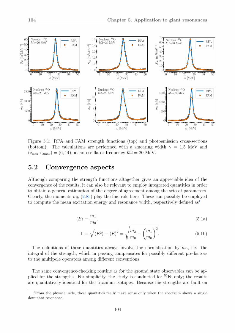
104 Chapter 5. Application to giant resonances
0 10 20 30 40 50ω [MeV]
0
10
20
30
40
50
60
S00
[fm
4M
eV−
1]
Nucleus: 16OhΩ=20 MeV
RPA
FAM
0 10 20 30 40 50ω [MeV]
0.0
0.1
0.2
0.3
0.4
0.5
S10
[fm
2M
eV−
1]
Nucleus: 16OhΩ=20 MeV
RPA
FAM
0 10 20 30 40 50ω [MeV]
0
10
20
30
40
50
60
70
S20
[fm
2M
eV−
1]
Nucleus: 16OhΩ=20 MeV
RPA
FAM
0 10 20 30 40 50ω [MeV]
0
500
1000
1500
σ00
[mb
]
Nucleus: 16OhΩ=20 MeV
RPA
FAM
0 10 20 30 40 50ω [MeV]
0
5
10
σ10
[mb
]Nucleus: 16OhΩ=20 MeV
RPA
FAM
0 10 20 30 40 50ω [MeV]
0
500
1000
1500
σ20
[mb
]
Nucleus: 16OhΩ=20 MeV
RPA
FAM
Figure 5.1: RPA and FAM strength functions (top) and photoemission cross-sections(bottom). The calculations are performed with a smearing width γ = 1.5 MeV and(emax, e3max) = (6, 14), at an oscillator frequency ℏΩ = 20 MeV.
5.2 Convergence aspects
Although comparing the strength functions altogether gives an appreciable idea of theconvergence of the results, it can also be relevant to employ integrated quantities in orderto obtain a general estimation of the degree of agreement among the sets of parameters.Clearly, the moments mk (2.85) play the fine role here. These can possibly be employedto compute the mean excitation energy and resonance width, respectively defined as1
⟨E⟩ ≡ m1
m0
, (5.1a)
Γ ≡√
⟨E2⟩ − ⟨E⟩2 =√
m2
m0
−(m1
m0
)2
. (5.1b)
The definitions of these quantities always involve the normalisation by m0, i.e. theintegral of the strength, which in passing compensates for possibly different pre-factorsto the multipole operators among different conventions.
The same convergence-checking routine as for the ground state observables can be ap-plied for the strengths. For simplicity, the study is conducted for 56Fe only; the resultsare qualitatively identical for the titanium isotopes. Because the strengths are built on
1From the physical side, these quantities really make sense only when the spectrum shows a singledominant resonance.
104

Chapter 5. Application to giant resonances 105
the ground states, we expect the differences in the results obtained with different param-eters and chiral orders to be magnified with respect to those observed in chapter 4. It isimportant to realise that the discrepancies can be evaluated in two manners, dependingon whether we want to focus on integrated quantities or on the difference at a given fre-quency. I thus define the errors on an integrated quantity X calculated at a parameter qas
∆(1)X [q] ≡ maxq′∈q
(∫ ∞
0
dωQ(q, q′)∣∣∣X [q](ω)−X [q′](ω)
∣∣∣) , (5.2)
∆(2)X [q] ≡∫ ∞
0
dωmaxq′∈q
(Q(q, q′)
∣∣∣X [q](ω)−X [q′](ω)∣∣∣) . (5.3)
In these definitions, the integrand ω is typically the energy, and for the specific purposeof the section, it corresponds to the frequency of the probe F . The set q represents theset of parameters we can vary: in our case, it is either the set of oscillator frequencies,of the size of single-particle basis, or of the chiral orders. The quantity X [q′](ω) is thestrength function calculated with the parameter q′ and at excitation frequency ω, andthe particular value q is the parameter with respect to which the error is calculated.The factor Q(q′) gives a weight to each difference, and should be motivated by physicalsense. Equation (5.2) corresponds to comparing the integrated quantities, whereas (5.3)integrates the function defined by the largest error at each ω, and thus we have ∆(2) > ∆(1).This is easier to see with loose notations:
∆(1)X ∼ max
(∣∣∣∣∫ dωx1(ω)
∣∣∣∣, ∣∣∣∣∫ dωx2(ω)
∣∣∣∣, . . .) (5.4)
∆(2)X ∼∫
dωmax (|x1(ω)|, |x2(ω)|, . . . ) . (5.5)
To illustrate, we may take X as the set of eigenvalues of the HFB equation, weightedby the density function. In that case (omitting the q, q′ exponents for clarity),
ω → E, (5.6)
X → Ei1
eβEi + 1δ(Ei − E), (5.7)
Q → 1, (5.8)
and the definition (5.2) corresponds to adding the absolute value of the differences foreach single particle eigenvalue (weighted by its occupation number),
∆(1)E[q] = maxq′∈q
∑i
∣∣∣∣∣ E[q]i
eE[q]i + 1
− E[q′]i
eE[q]i + 1
∣∣∣∣∣. (5.9)
Errors thus pile up, and the values obtained with different parameters q′ are compared
105

106 Chapter 5. Application to giant resonances
afterwards. Conversely, (5.3) always takes the worst of all:
∆(2)E[q] =∑i
maxq′∈q
∣∣∣∣∣ E[q]i
eE[q]i + 1
− E[q′]i
eE[q]i + 1
∣∣∣∣∣. (5.10)
The studies of [EKM15; Bin+18; Hut+20] use a formula derived from (5.2), where qis the N3LO, q′ are the lower orders, and Q is a power of 1/3. To obtain meaningfulcomparisons, we must adopt a formula compatible with (5.2). The simplest way being tocalculate the mk moments (and if need be, derive the values of (5.1) accordingly), errorsare defined as
∆m[q]k (F ) ≡ max
q′∈q
(Q(q, q′)
∣∣∣m[q]k (F )−m
[q′]k (F )
∣∣∣) , (5.11)
and we take the Q(q, q′) identically to the prescription of [EKM15; Bin+18; Hut+20] incase q, q′ are chiral orders, and equal to one otherwise. Note that comparing the strengthsat a given frequency can also provide quality information, and is in particular much moreconnected to what is measured experimentally, namely a number of counts as a functionof an energy. Whenever it is relevant for the discussion, the strength functions will bepresented with their error bars.
5.2.1 With the oscillator frequency
We saw in subsection 4.3.2 that all macroscopic observables bore a non-negligible depen-dence on the frequency ℏΩ of the harmonic oscillator basis. Larger variations, but on thesame order of magnitude, should be expected for the strength functions and derived quan-tities. Such affirmations are verified on figure 5.2, where the isoscalar monopole (ISM),isovector dipole (IVD) and isoscalar quadrupole (ISQ) electric responses of iron at threetemperatures are given.
On the qualitative aspects, the results obtained at all three values of the oscillator stiff-ness are altogether consistent. The monopole operator visibly has the most pronouncedℏΩ-dependence. A more quantitative view is given in figures 5.3-5.4-5.5, which reviewthe variations of the moments with the oscillator frequencies, for all three types of per-turbation. In most cases, the moments undergo variations of a few percents in case ofthe IVD and ISQ excitations, but eventually reach 20-30% for the monopole mode. Themean excitation energies, being calculated as the ratio of m1 and m0, exhibit a depen-dence roughly equal to the sum of the variations of these two moments. This translates in25% relative difference between the ℏΩ = 20 and ℏΩ = 12 MeV in case of the monopoleoperator, and about 9% (resp. 3%) for the dipole (resp. quadrupole). Except for thestrongly frequency-dependent S00 response, the variations are of the same order as thoseobserved for the energy and radii in the static HFB calculations. Overall, the qualityof the results obtained with suboptimal frequencies is deteriorated as compared with thestatic case. In the particular case of the monopole mode, the large error calls for a preciseadjustment of ℏΩ at the HFB level. In all cases, the variations do not suffer great changes
106
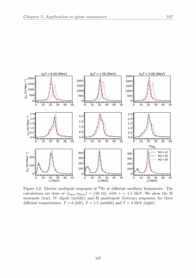
Chapter 5. Application to giant resonances 107
0 10 20 30 40 500
500
1000
1500
2000
S 00 [
fm4 M
eV1 ]
kBT = 0.00 [MeV]
0 10 20 30 40 500
500100015002000
kBT = 1.50 [MeV]
0 10 20 30 40 500
5001000150020002500
kBT = 3.00 [MeV]
0 10 20 30 40 500.00.51.01.52.02.5
S 10 [
fm2 M
eV1 ]
0 10 20 30 40 500.00.51.01.52.0
0 10 20 30 40 500.00.51.01.52.02.5
0 10 20 30 40 50 [MeV]
0
100
200
S 20 [
fm2 M
eV1 ]
0 10 20 30 40 50 [MeV]
0100200300400
0 10 20 30 40 50 [MeV]
0100200300400
56Fe= 12= 16= 20
Figure 5.2: Electric multipole responses of 56Fe at different oscillator frequencies. Thecalculations are done at (emax, e3max) = (10, 14), with γ = 1.5 MeV. We show the ISmonopole (top), IV dipole (middle) and IS quadrupole (bottom) responses, for threedifferent temperatures: T = 0 (left), T = 1.5 (middle) and T = 3 MeV (right).
107

108 Chapter 5. Application to giant resonances
when the system is hot.
12 16 20
0.6
0.8
1.0
1.2
m2/m
2(k B
T=
0,=
12)
12 16 20
0.7
0.8
0.9
1.0
m1/m
1(k B
T=
0,=
12)
12 16 200.80
0.85
0.90
0.95
1.00
1.05
m0/m
0(k B
T=
0,=
12)
12 16 20 [MeV]
0.98
0.99
1.00
1.01
1.02
m1/m
1(k B
T=
0,=
12)
12 16 20 [MeV]
1.00
1.05
1.10
1.15
m2/m
2(k B
T=
0,=
12)
12 16 20 [MeV]
21.022.023.024.025.026.0
E [M
eV]
56Fe0.00 MeV1.50 MeV3.00 MeV
Figure 5.3: Normalised moments of the Q00 strength function for 56Fe. The normalisationis applied with respect to the kBT = 0 MeV, ℏΩ = 12 MeV values. The bottom-rightsubplot represents the mean excitation energy calculated as in (5.1a). The calculationsare performed with the model space (emax, e3max) = (10, 14) and use a smearing γ = 1.5MeV.
As for the mean energy of the resonances, we find it to be almost independent of thetemperature for the monopole operator, and to change in approximately one MeV for thequadrupole excitation. For the former, this can be interpreted by the compressibility ofnuclear matter undergoing only small changes with the temperature. In the Q20 case,⟨E⟩ is lowest at kBT = 1.5 MeV, because deformation is still present, and excitations arefacilitated by the finite temperature. Beyond Tc, ⟨E⟩ increases past its zero-temperaturevalue, as a consequence of the restoration of spherical symmetry. Conversely, the giantdipole resonance shows a strong T− dependence, dropping from several MeVs within thetemperature range scanned. This is mainly due to the low-ω part of the strengths, whichis more sensitive to temperature. In case of the S10 strength, which visibly undergoesthe largest variations via the onset of low-energy resonances at around 10 MeV (and to alesser extent, smaller resonances beyond 30 MeV), the differences between the observablescalculated using ℏΩ = 12 MeV and ℏΩ = 20 MeV grow to ten percents. Finally, at agiven frequency and in all cases, the ratios between the strengths can grow several or-ders of magnitudes. This stems from the fact that the single-particle energies are slightlydifferent between the set of parameters, which result in the energy of the peaks beingshifted. The sharp increase of the strength around the resonances aggravates this differ-ence. This observation shows the importance of comparing more meaningful quantities,namely integrated ones.
108
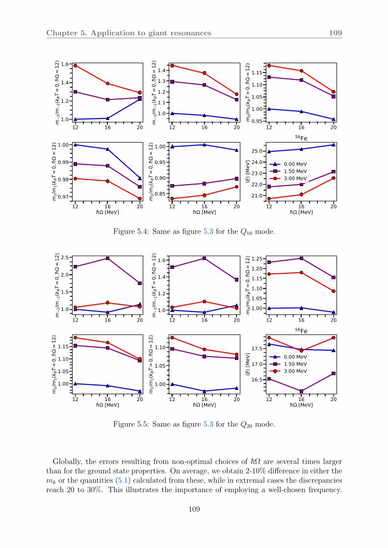
Chapter 5. Application to giant resonances 109
12 16 201.0
1.2
1.4
1.6m
2/m2(
k BT
=0,
=12
)
12 16 20
1.0
1.1
1.2
1.3
1.4
m1/m
1(k B
T=
0,=
12)
12 16 200.95
1.00
1.05
1.10
1.15
m0/m
0(k B
T=
0,=
12)
12 16 20 [MeV]
0.97
0.98
0.99
1.00
m1/m
1(k B
T=
0,=
12)
12 16 20 [MeV]
0.85
0.90
0.95
1.00m
2/m2(
k BT
=0,
=12
)
12 16 20 [MeV]
21.0
22.0
23.0
24.0
25.0
E [M
eV]
56Fe
0.00 MeV1.50 MeV3.00 MeV
Figure 5.4: Same as figure 5.3 for the Q10 mode.
12 16 20
1.0
1.5
2.0
2.5
m2/m
2(k B
T=
0,=
12)
12 16 201.0
1.2
1.4
1.6
m1/m
1(k B
T=
0,=
12)
12 16 20
1.001.051.101.151.201.25
m0/m
0(k B
T=
0,=
12)
12 16 20 [MeV]
1.00
1.05
1.10
1.15
m1/m
1(k B
T=
0,=
12)
12 16 20 [MeV]
1.00
1.05
1.10
m2/m
2(k B
T=
0,=
12)
12 16 20 [MeV]
16.5
17.0
17.5
E [M
eV]
56Fe
0.00 MeV1.50 MeV3.00 MeV
Figure 5.5: Same as figure 5.3 for the Q20 mode.
Globally, the errors resulting from non-optimal choices of ℏΩ are several times largerthan for the ground state properties. On average, we obtain 2-10% difference in either themk or the quantities (5.1) calculated from these, while in extremal cases the discrepanciesreach 20 to 30%. This illustrates the importance of employing a well-chosen frequency.
109

110 Chapter 5. Application to giant resonances
Unless great caution has been taken in determining the one giving the lowest groundstate energy, the predicted moments vary strongly. This harsh conclusion can howeverbe balanced by the observation that the overall shape of the strengths remains similaracross the choices of ℏΩ, and we still obtain very close moments whenever the frequencyis sufficiently close to its optimal value.
5.2.2 With the basis size
0 10 20 30 40 500
500
1000
1500
2000
S 00 [
fm4 M
eV1 ]
kBT = 0.00 [MeV]
0 10 20 30 40 500
500
1000
1500
2000
kBT = 1.50 [MeV]
0 10 20 30 40 500
500
1000
1500
2000
kBT = 3.00 [MeV]
0 10 20 30 40 500.0
0.5
1.0
1.5
2.0
2.5
S 10 [
fm2 M
eV1 ]
0 10 20 30 40 500.0
0.5
1.0
1.5
2.0
0 10 20 30 40 500.0
0.5
1.0
1.5
2.0
2.5
0 10 20 30 40 50 [MeV]
0
100
200
S 20 [
fm2 M
eV1 ]
0 10 20 30 40 50 [MeV]
0
100
200
300
400
0 10 20 30 40 50 [MeV]
0
100
200
300
400
50056Fe
emax = 6emax = 8emax = 10
Figure 5.6: Multipole responses of 56Fe at emax = 6 (dashed), emax = 8 (dash-dotted) andemax = 10 (full). All calculations use a model space of e3max = 14 and ℏΩ = 12 MeV; thesmearing width γ = 1.5 MeV.
In subsection 4.3.2, a good convergence of the bulk quantities with the size of the single-particle space was found. The corrections brought by increasing the parameter emax from8 to 10 were of about one percent. In figure 5.6, we show the strength functions obtainedat the three values of emax used throughout this chapter. We place the model space in itsoptimal frequency, ℏΩ = 12 MeV, and fold the strength function with γ = 1.5 MeV.
In all cases, the difference between emax = 8 and emax = 10 is faint. For the dipoleand quadrupole modes, it rarely goes beyond 3% for all mk with k ranging from -3to 3, and remains less than 6%. The disagreement is on average slightly higher for
110

Chapter 5. Application to giant resonances 111
4 3 2 1 0 1 2 3 41.001.021.04
k(Q00
)kBT = 0.00 [MeV]
4 3 2 1 0 1 2 3 4
1.00
1.02
kBT = 1.50 [MeV]
4 3 2 1 0 1 2 3 40.9751.0001.025
kBT = 3.00 [MeV]
4 3 2 1 0 1 2 3 41.0
1.1
k(Q10
)
4 3 2 1 0 1 2 3 41.0
1.1
4 3 2 1 0 1 2 3 41.0
1.1
4 3 2 1 0 1 2 3 4k
0.98
0.99
1.00
k(Q20
)
4 3 2 1 0 1 2 3 4k
0.98
0.99
1.00
4 3 2 1 0 1 2 3 4k
0.9850.9900.995
56Fe
Figure 5.7: Ratios between the moments calculated at emax = 8 and emax = 10. Thedefinition ηk ≡ mk(emax = 8)/mk(emax = 10) serves as a shorthand. The calculations arecarried out with ℏΩ = 12 MeV, e3max = 14, and the smoothing γ = 1.5 MeV.
the monopole mode, albeit remaining under 6% as well. The good convergence of thestrengths, concluded by visual inspection of figure 5.6, can be given a more numericalflavour by representing the ratios between the moments calculated within different modelspaces. These are traced in figure 5.7 in the case of 56Fe. The moments are calculated bydirect integration along the R+ axis. As always, the results for 46−44Ti follow the sametrends and are in the same ranges. The increase of the errors with larger k originatesfrom the different strengths being marginally different at high energy (cf. (3.113))). Asfor k < 0 moments, which are more sensitive to the low-ω strength, the ratios ηk arealways close to one. This is due to the low-energy part of the strength converging fasterwith the size of the model space than the high-energy region, since the latter requiresmore energetic quasiparticles, and therefore larger basis sizes. The dust settles down inthe same path as for subsection 5.2.1: the error due to finite values of emax is substantiallyhigher than it was for the HFB calculations, but can be considered kept under reasonableranges.
5.2.3 With the chiral expansion
We saw in subsection 4.3.2 that using the second to fourth chiral orders lets us establisherror bars on the observables, yielding around 10% uncertainty on the three analysedground state quantities. Moreover, the preservation of such uncertainties when the tem-perature is increased let use anticipate that the convergence in the chiral order remainsvalid at non-zero temperatures.
As the interactions are pre-processed through a normal-ordering, we verify that the
111

112 Chapter 5. Application to giant resonances
0 10 20 30 40 500
500
1000
1500
S 00 [
fm4 M
eV1 ]
56Fe
0 10 20 30 40 500
500
1000
150046Ti
0 10 20 30 40 500
500
1000
150044Ti
0 10 20 30 40 50
0
2
S 10 [
fm2 M
eV1 ]
0 10 20 30 40 500
2
4
0 10 20 30 40 50
0
2
4
0 10 20 30 40 50 [MeV]
0
200
400
S 20 [
fm2 M
eV1 ]
0 10 20 30 40 50 [MeV]
0
200
400
0 10 20 30 40 50 [MeV]
0
200
400 NLON2LON3LO
Figure 5.8: Zero-temperature multipolar responses of 56Fe, 46Ti, 44Ti, obtained with thethree available orders in the chiral interaction. The error bars are represented as shadedareas. The calculations are carried out at (emax, e3max) = (10, 14), ℏΩ = 16 MeV andemploy a smearing γ = 1.5 MeV.
similitude of the N3LO and N2LO strengths is present for all three studied nuclei onfigure 5.8. Because the moments vary across several orders of magnitude for different val-ues of k, they are normalised with respect to the N3LO ones on figure 5.9. The systematicuncertainties are calculated according to (5.3). Repeating the drills of this section, wefind that uncertainty bars associated to the N3LO are within 5-10% relative difference.The NLO moments are systematically far away from the better-quality results, due to thelarge differences in the strength functions. The NLO peaks always lie at larger energies, aconsequence of the single-particle spectrum being more gapped. The corresponding inte-grated strengths are however always smaller, and both observations explain the accidentalresult mLO
k /mN3LOk ∼ 1 for k around two. For all, the N2LO and N3LO moments differ in
at most 10%, and are thus in acceptable (although not excellent) agreement. They onlybecome significant either at small or at large k, owing to small differences in the low- orhigh-energy strengths.
As mentioned in the beginning of this section, it is also useful and instructing to com-pare the N3LO strengths and their uncertainty bars for a single frequency. We find thatthe uncertainty always represent less than 10% of the strength when close to the reso-nances. The only dramatic increases are found when ω is close to a NLO peak. Thisgood agreement in the results obtained with the two last orders was already observed inthe FTHFB calculations. However, the propagators are dressed by the RPA self-energyduring the solution of the FTQFAM equation, which can be expected to further magnifydifferences in the qp spectra between different orders in the chiral expansion. The strong
112

Chapter 5. Application to giant resonances 113
Figure 5.9: Some zero-temperature moments of the strength functions calculated with theNLO (blue triangles), N2LO (orange diamonds) and N3LO (green pentagons), normalisedwith respect to the N3LO values. The calculations use (emax, e3max) = (10, 14), ℏΩ = 16MeV and γ = 1.5 MeV. The left, centre and right columns correspond to 56Fe, 46Ti and44Ti, respectively.
resemblance between the N2LO and N3LO strengths functions seems to consolidate thatthe interaction is well-converged.
5.2.4 Conclusion
All parameters analysed for the convergence of the FTHFB calculations of chapter 4 arefound to produce amplified errors at the FTQFAM level. In particular, the choice of theoptimal oscillator frequency plays a crucial role within the model spaces studied. Theinfluence of ℏΩ on the energy of the GMR shows that tuning this parameter is of greatimportance for the study of GMR-related quantities, such as the compressibility of nuclearmatter.
Regarding the size of the model space, we find already well-converged strength func-tions (and corresponding moments) at emax = 6. The difference with the much largeremax = 10 case is of less than 10% at worst for the monopole excitations. We can there-fore conclude that these basis sizes are appropriate for a description of giant resonances
113
114 Chapter 5. Application to giant resonances
with this interaction and for stable nuclei of such masses. The convergence with thesize of the three-body space, characterised by e3max, could not be studied in detail. Thepossibility that sizeable corrections are brought by increasing e3max towards higher valuescannot be dismissed. Nonetheless, calculations of ground state properties in sd−shellnuclei using the same or close by interactions have been shown to be well converged ate3max = 14 [Dik+15; Jan+16; Her20] for shell-model approaches, and the bulk propertiesof the ground states of stable heavier nuclei (A ≳ 100) were shown to change in aboutfive percents when increasing e3max from 14 to values yielding convergence [Miy+21]. Al-though the three present nuclei lie in between in protons and neutrons numbers, we canexpect the modifications engendered by lifting e3max to higher values do not change toomuch the predicted observables.
Lastly, we observe a reasonable convergence of the RPA moments with the number ofchiral orders, with roughly 10% relative uncertainty. This stays consistent with the un-certainties obtained for the ground state calculations. While these errors are not largeenough to prevent us from extracting meaningful physical information, higher-orders ormore evolved interactions would in the future be very relevant, as a back-of-the-enveloppecalculation based on the excellent agreement between N2LO and N3LO lets us foreseethat each additional chiral order would reduce the uncertainties by a factor Q = 1/3.
5.3 Moments of the strength
If one is specifically interested in quantities related to the moments of the strength func-tion S(F, ω), such as the average excitation energy, the width of the strength, etc, it ispossible to use (3.113) around a contour circling all the QRPA poles.
Whenever the cross-section is strongly peaked around one collective frequency, the in-tegrated quantities (5.1a) and (5.1b) can constitute good substitutes to the full strengthfunction. From the theoretical side, it is interesting to study whether the contour integra-tion method can serve as shortcut to obtain the moments mk with good accuracy. From[Hin+15], we expect a fast convergence of the moments with the number of integrationpoints, so that a couple dozens of nodes should already yield results converged within afew percents.
Tables 5.1-5.2-5.3 give the benchmark results for 16O. The results of the contour in-tegration are compared with the exact results obtained from matrix RPA calculations,and with the appropriate integrals of the FAM strengths on the real ω axis. The contouris composed of four portions (figure 5.10), and is automatically adjusted to enclose allthe poles, by imposing a large radius equal to three times the maximum qp energy2; theradius of the small semicircle is chosen as the minimum between 500 keV3 and half the
2Without the RPA self-energy, the highest-energy pole lies at two times max (Eqp), hence taking a50% larger radius should certainly enclose all the RPA poles.
3If no spurious modes are present, one can let the contour get arbitrarily close to ωγ = 0. A smallbut finite radius is kept as a middle-ground, to avoid bad surprises in case the removal of the NG suffersfrom numerical noise.
114

Chapter 5. Application to giant resonances 115
Figure 5.10: Contour in the (ω, γ) plane employed for numerically integrating the mk
moments. The contour is composed of two semicircles A1 and A2, and two segments I1and I2. It is oriented counter-clockwise to match the signs of all contour integral formulaegiven in this thesis. Figure taken from [Hin+15].
smallest qp energy4.
The spacing between the different integration nodes is adjusted such that each portioncontains a number of points proportional to its arc length. The line integrals are calculatedby the trapezoid rule. Note that applying Richardson’s extrapolation [RG11; RG27](interestingly, see [Huy54b; Huy54c; Huy54a; Huy54d], and also [Bre09] and referencestherein) to a series of points whose number grow as 2k in an attempt to further improve theconvergence produces slight but unpredictable instabilities, so that it is safer in practiceto keep an eye on the results obtained at each order when carrying it out. Additionally,it can be verified from (2.82) that S(F, ωγ) possesses the two symmetries
ImS(F, ω + iγ) = − ImS(F, ω − iγ), (5.12)
ReS(F, ω + iγ) = +ReS(F, ω − iγ); (5.13)
these two can be employed to avoid calculating the strength along either of I1 or I2,which provides a ∼ 25% speed-up.
A rather fast convergence is observed for all considered moments and multipolarities,except for the k = 2 moment. From the imaginary part of the calculated values, whichshould be zero in the exact limit, the error due to the integration method and the nu-merical noise can be estimated to be less than 10−5 relative to the values given in tables5.1, 5.2, 5.3. The source of the important error on m2 could not be tracked down; it
4Again, without the self-consistent rearrangement, the pole is located at twice the smallest qp energy.If the RPA self-energy is large compared with min (Eqp), this contour may miss some poles.
115
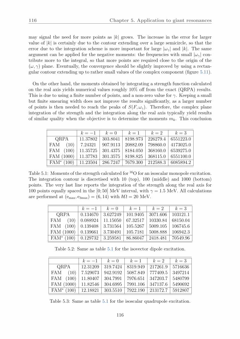
116 Chapter 5. Application to giant resonances
may signal the need for more points as |k| grows. The increase in the error for largervalue of |k| is certainly due to the contour extending over a large semicircle, so that theerror due to the integration scheme is more important for large |ωγ| and |k|. The sameargument can be applied for the negative moments: the frequencies with small |ωγ| con-tribute more to the integral, so that more points are required close to the origin of the(ω, γ) plane. Eventually, the convergence should be slightly improved by using a rectan-gular contour extending up to rather small values of the complex component (figure 5.11).
On the other hand, the moments obtained by integrating a strength function calculatedon the real axis yields numerical values roughly 10% off from the exact (QRPA) results.This is due to using a finite number of points, and a non-zero value for γ. Keeping a smallbut finite smearing width does not improve the results significantly, as a larger numberof points is then needed to reach the peaks of S(F, ωγ). Therefore, the complex planeintegration of the strength and the integration along the real axis typically yield resultsof similar quality when the objective is to determine the moments mk. This conclusion
k = −1 k = 0 k = 1 k = 2 k = 3QRPA 11.37802 303.8041 8198.973 226279.4 6551223.0
FAM (10) 7.24321 907.9113 20882.09 798860.0 4173025.0FAM (100) 11.35725 301.4375 8184.050 368160.0 6539275.0FAM (1000) 11.37783 301.3575 8198.825 368115.0 6551100.0FAM∗ (100) 11.23504 286.7247 7679.300 212588.3 6085894.2
Table 5.1: Moments of the strength calculated for 16O for an isoscalar monopole excitation.The integration contour is discretised with 10 (top), 100 (middle) and 1000 (bottom)points. The very last line reports the integration of the strength along the real axis for100 points equally spaced in the [0; 50] MeV interval, with γ = 1.5 MeV. All calculationsare performed at (emax, e3max) = (6, 14) with ℏΩ = 20 MeV.
k = −1 k = 0 k = 1 k = 2 k = 3QRPA 0.134670 3.627249 101.9405 3071.606 103121.1
FAM (10) 0.088924 11.15050 67.32517 10330.84 68150.04FAM (100) 0.139408 3.731564 105.5267 5009.105 106745.6FAM (1000) 0.139661 3.730491 105.7181 5008.888 106942.3FAM∗ (100) 0.129732 3.259581 86.86047 2418.481 70549.96
Table 5.2: Same as table 5.1 for the isovector dipole excitation.
k = −1 k = 0 k = 1 k = 2 k = 3QRPA 12.31209 319.7424 8319.949 217261.9 5716636
FAM (10) 7.529073 942.9192 5087.849 777409.5 3497214FAM (100) 11.80407 304.7991 7976.651 347203.7 5480799FAM (1000) 11.82546 304.6995 7991.106 347137.6 5490692FAM∗ (100) 12.18821 303.5510 7922.190 213172.7 5912807
Table 5.3: Same as table 5.1 for the isoscalar quadrupole excitation.
116
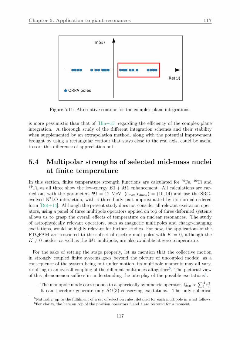
Chapter 5. Application to giant resonances 117
Im( )
Re( )
QRPA poles
Figure 5.11: Alternative contour for the complex-plane integrations.
is more pessimistic than that of [Hin+15] regarding the efficiency of the complex-planeintegration. A thorough study of the different integration schemes and their stabilitywhen supplemented by an extrapolation method, along with the potential improvementbrought by using a rectangular contour that stays close to the real axis, could be usefulto sort this difference of appreciation out.
5.4 Multipolar strengths of selected mid-mass nuclei
at finite temperature
In this section, finite temperature strength functions are calculated for 56Fe, 46Ti and44Ti, as all three show the low-energy E1 + M1 enhancement. All calculations are car-ried out with the parameters ℏΩ = 12 MeV, (emax, e3max) = (10, 14) and use the SRG-evolved N3LO interaction, with a three-body part approximated by its normal-orderedform [Rot+14]. Although the present study does not consider all relevant excitation oper-ators, using a panel of three multipole operators applied on top of three deformed systemsallows us to grasp the overall effects of temperature on nuclear resonances. The studyof astrophysically relevant operators, such as magnetic multipoles and charge-changingexcitations, would be highly relevant for further studies. For now, the applications of theFTQFAM are restricted to the subset of electric multipoles with K = 0, although theK = 0 modes, as well as the M1 multipole, are also available at zero temperature.
For the sake of setting the stage properly, let us mention that the collective motionin strongly coupled finite systems goes beyond the picture of uncoupled modes: as aconsequence of the system being put under motion, its multipole moments may all vary,resulting in an overall coupling of the different multipoles altogether5. The pictorial viewof this phenomenon suffices in understanding the interplay of the possible excitations6:
- The monopole mode corresponds to a spherically symmetric operator, Q00 ∝∑A
i r2i .It can therefore generate only SO(3)-conserving excitations. The only spherical
5Naturally, up to the fulfilment of a set of selection rules, detailed for each multipole in what follows.6For clarity, the hats on top of the position operators r and z are restored for a moment.
117

118 Chapter 5. Application to giant resonances
harmonic exhibiting this symmetry being Q00 itself, monopole excitations do notcontain any other modes.
- The isovector dipole corresponds to protons and neutrons vibrating against eachother, i.e. QIV
10 ∝ NA
∑Zi zi − Z
A
∑Ni zi. This mode a priori modifies the radius of
the system, as well as its deformation. It can therefore trigger both monopole andquadrupole motion. Because it breaks both spherical and parity symmetries, it cancouple to any other QJK as well.
- The quadrupole operator Q20 ∝∑A
i 3z2i − r2⊥,i, as well as modes of higher multipo-larity, induce non-spherical oscillations. The even-J ones do not break the paritysymmetry, and therefore they do not contain odd-J oscillations. Conversely, theparity-breaking, odd-J modes may also contain parity-conserving vibrations.
For the modes we restrict this study on, we thus expect to observe an intrusion ofmonopole modes in dipole and quadrupole oscillations, and a presence of quadrupolemodes in the dipole strengths.
Like observed in other studies [Paa+09; Niu+09; Yuk+14; Yuk+17; LW18; WL19;Yuk+19; LW19; LRW20; Yuk+20; Rav+20; LR21], the strengths appreciably depend onthe temperature in general. These evolutions are explained by two mechanisms. First,the positive energy qp states become occupied, so less energy is required to take theground state to an excited one. This shifts towards low-ω the large peaks that alreadyexist at T = 0. Second, the (positive and negative) low-energy qp states have occupationssignificantly differing from zero or one, resulting in the W and Z amplitudes becomingof increasing importance. Transitions among qps that do not cross the Fermi energy arenow permitted, which causes resonances mainly at low excitation frequencies, withoutdiscarding the possibility of important contributions at higher energies.
While these effects do not appear to be very pronounced for the monopole modes, tracedin figure 5.12, we note however the disappearing of the low-energy strength in the Ti nu-clei. A feeble resonance is visible on the low-energy monopole in Fe as well, but its veryweak magnitude with respect to the GMR, and the dependence on ℏΩ that is not yetcompletely washed out within a model space of (emax, e3max) = (10, 14), do not allow forunambiguous conclusions. In all cases, the GMR becomes slightly narrower and higher asthe temperature increases; this is visibly a consequence of two neighbouring resonancesmerging. The average excitation energy is globally found to increase with temperature(figure 5.13), due to (i) the collapse of the small resonances below 10 MeV, already com-plete at T = 1.5 MeV, and (ii) the drift of the main peak, and (iii) the enhancement of asecondary peak past the location of the GMR.
A rather similar conclusion is drawn for the isoscalar quadrupole (figure 5.14), in whichthe energy of the GQR is not so much affected by the temperature. We note however thatthe strength of the giant resonance in 56Fe becomes quickly doubles, due to different peaksstacking at approximately 20 MeV. For all three nuclei, the effects are more importantat low energies (ω < 10 MeV), as usual. In this region, the strengths are quenched by afactor of two. This is tentatively attributed to the diminution of the occupation numbers
118
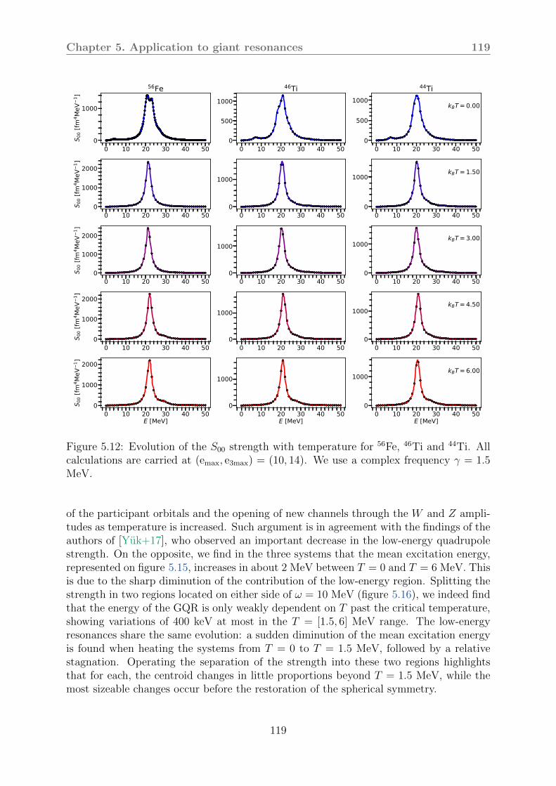
Chapter 5. Application to giant resonances 119
0 10 20 30 40 500
1000
S 00 [
fm4 M
eV1 ]
56Fe
0 10 20 30 40 500
500
1000
46Ti
0 10 20 30 40 500
500
1000kBT = 0.00
44Ti
0 10 20 30 40 500
1000
2000
S 00 [
fm4 M
eV1 ]
0 10 20 30 40 500
1000
0 10 20 30 40 500
1000kBT = 1.50
0 10 20 30 40 500
1000
2000
S 00 [
fm4 M
eV1 ]
0 10 20 30 40 500
1000
0 10 20 30 40 500
1000kBT = 3.00
0 10 20 30 40 500
1000
2000
S 00 [
fm4 M
eV1 ]
0 10 20 30 40 500
1000
0 10 20 30 40 500
1000kBT = 4.50
0 10 20 30 40 50E [MeV]
0
1000
2000
S 00 [
fm4 M
eV1 ]
0 10 20 30 40 50E [MeV]
0
1000
0 10 20 30 40 50E [MeV]
0
1000kBT = 6.00
Figure 5.12: Evolution of the S00 strength with temperature for 56Fe, 46Ti and 44Ti. Allcalculations are carried at (emax, e3max) = (10, 14). We use a complex frequency γ = 1.5MeV.
of the participant orbitals and the opening of new channels through the W and Z ampli-tudes as temperature is increased. Such argument is in agreement with the findings of theauthors of [Yuk+17], who observed an important decrease in the low-energy quadrupolestrength. On the opposite, we find in the three systems that the mean excitation energy,represented on figure 5.15, increases in about 2 MeV between T = 0 and T = 6 MeV. Thisis due to the sharp diminution of the contribution of the low-energy region. Splitting thestrength in two regions located on either side of ω = 10 MeV (figure 5.16), we indeed findthat the energy of the GQR is only weakly dependent on T past the critical temperature,showing variations of 400 keV at most in the T = [1.5, 6] MeV range. The low-energyresonances share the same evolution: a sudden diminution of the mean excitation energyis found when heating the systems from T = 0 to T = 1.5 MeV, followed by a relativestagnation. Operating the separation of the strength into these two regions highlightsthat for each, the centroid changes in little proportions beyond T = 1.5 MeV, while themost sizeable changes occur before the restoration of the spherical symmetry.
119

120 Chapter 5. Application to giant resonances
0.00 1.50 3.00 4.50 6.00kBT [MeV]
21.0
21.5
22.0
22.5E
[MeV
]
Q00
56Fe46Ti44Ti
Figure 5.13: Evolution of the mean excitation energy with the temperature, for a isoscalarmonopole probe.
Finally, the evolution of the GDR, plotted in figure 5.17 is clearer. Between T = 0and T = 1.5 MeV, the maxima of the dipole strengths are shifted of several MeVs. Thiscan be understood from the schematic models of Goldhaber and Teller (GT) [GT48] andSteinwedel, Jensen and Jensen (SJJ) [SJJ50]. The GT model assimilates the GDR as amotion of protons and neutrons fluids against each other, as two spheres attached by aspring whose stiffness is related to the GDR frequency. The model of SJJ implements theGDR as a volume-conserving motion, in which protons and neutrons oscillate betweentwo hemispheres. Both predict a centroid energy decreasing with the radius R, like R− 1
2
(GT) or R−1 (SJJ). The two models were initially derived assuming spherical nuclearshapes; they can however be readily generalised to vibrations of deformed systems alongone of their symmetry axis. For axial shapes, we can consider ellipsoids defined by theradial and axial lengths R⊥ and Rz. In the Q10 vibrations, motion takes place alongthe z direction. With respect to the GDR centroids given by the spherical formulae, wecan therefore expect the values to be lowered for prolate systems, and raised for oblateones. These considerations are consistent with the observed evolution of the strength infigure 5.17, where the oblate Fe nucleus sees its mean excitation energy shifted down-wards when heated to T = 1.5 MeV, where the static deformation is reduced down toapproximately 80% of its zero-temperature value. As the shift is essentially absent athigher temperatures -in particular, between T = 1.5 and T = 3 MeV, where the sphericalsymmetry is being fully restored-, the decline of β2 does not seem to entirely explain
120
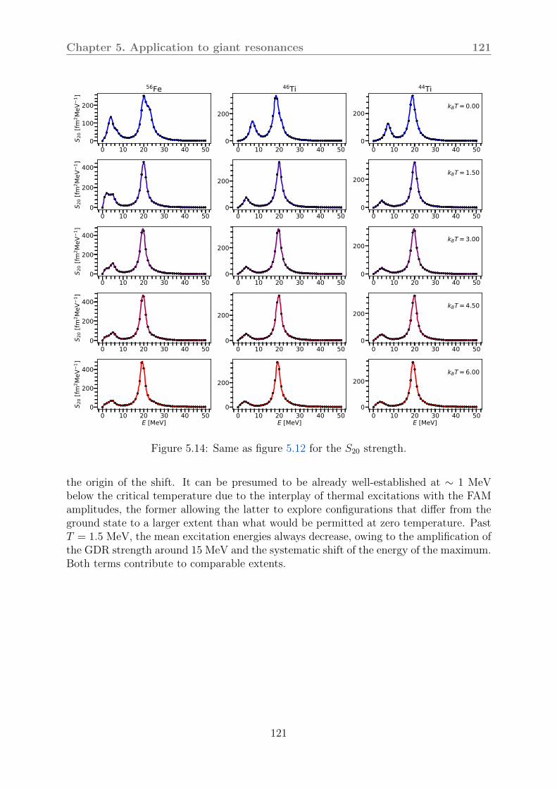
Chapter 5. Application to giant resonances 121
0 10 20 30 40 500
100
200
S 20 [
fm2 M
eV1 ]
56Fe
0 10 20 30 40 500
200
46Ti
0 10 20 30 40 500
200kBT = 0.00
44Ti
0 10 20 30 40 500
200
400
S 20 [
fm2 M
eV1 ]
0 10 20 30 40 500
200
0 10 20 30 40 500
200kBT = 1.50
0 10 20 30 40 500
200
400
S 20 [
fm2 M
eV1 ]
0 10 20 30 40 500
200
0 10 20 30 40 500
200kBT = 3.00
0 10 20 30 40 500
200
400
S 20 [
fm2 M
eV1 ]
0 10 20 30 40 500
200
0 10 20 30 40 500
200kBT = 4.50
0 10 20 30 40 50E [MeV]
0
200
400
S 20 [
fm2 M
eV1 ]
0 10 20 30 40 50E [MeV]
0
200
0 10 20 30 40 50E [MeV]
0
200kBT = 6.00
Figure 5.14: Same as figure 5.12 for the S20 strength.
the origin of the shift. It can be presumed to be already well-established at ∼ 1 MeVbelow the critical temperature due to the interplay of thermal excitations with the FAMamplitudes, the former allowing the latter to explore configurations that differ from theground state to a larger extent than what would be permitted at zero temperature. PastT = 1.5 MeV, the mean excitation energies always decrease, owing to the amplification ofthe GDR strength around 15 MeV and the systematic shift of the energy of the maximum.Both terms contribute to comparable extents.
121

122 Chapter 5. Application to giant resonances
0.00 1.50 3.00 4.50 6.00kBT [MeV]
16.0
16.5
17.0
17.5
18.0
18.5
E [M
eV]
Q20
56Fe46Ti44Ti
Figure 5.15: Same as figure 5.13 for an isoscalar quadrupole probe.
122
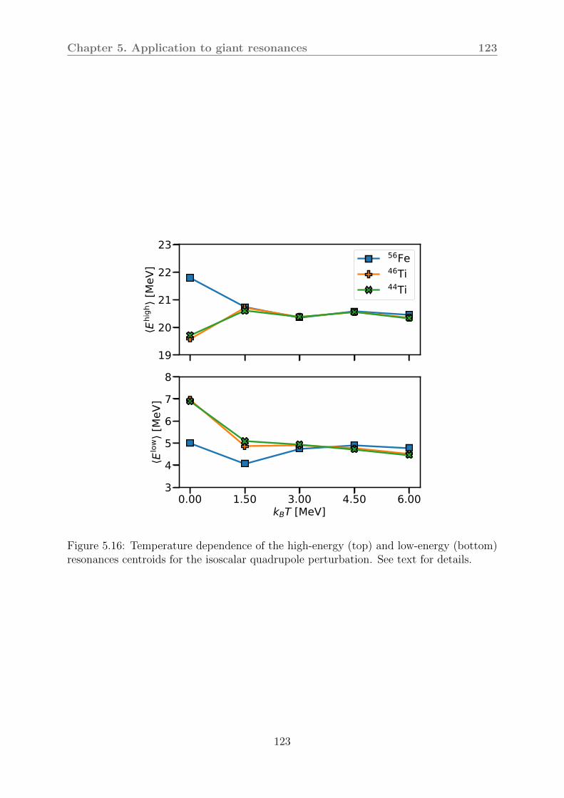
Chapter 5. Application to giant resonances 123
19
20
21
22
23
Ehigh
[MeV
]
56Fe46Ti44Ti
0.00 1.50 3.00 4.50 6.00kBT [MeV]
345678
Elow
[MeV
]
Figure 5.16: Temperature dependence of the high-energy (top) and low-energy (bottom)resonances centroids for the isoscalar quadrupole perturbation. See text for details.
123
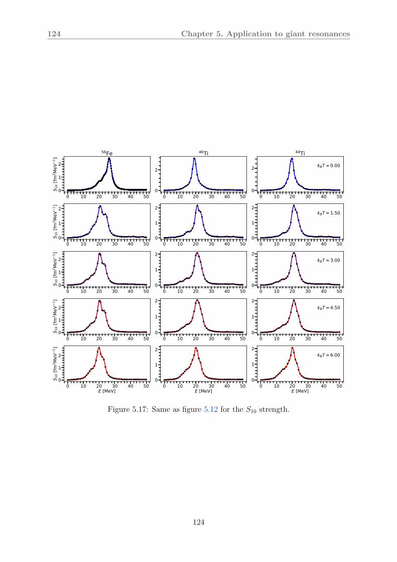
124 Chapter 5. Application to giant resonances
0 10 20 30 40 500
1
2
S 10 [
fm2 M
eV1 ]
56Fe
0 10 20 30 40 500
2
46Ti
0 10 20 30 40 500
2 kBT = 0.00
44Ti
0 10 20 30 40 500
1
2
S 10 [
fm2 M
eV1 ]
0 10 20 30 40 500
1
2
0 10 20 30 40 500
1
2kBT = 1.50
0 10 20 30 40 500
1
2
S 10 [
fm2 M
eV1 ]
0 10 20 30 40 500
1
2
0 10 20 30 40 500
1
2kBT = 3.00
0 10 20 30 40 500
1
2
S 10 [
fm2 M
eV1 ]
0 10 20 30 40 500
1
2
0 10 20 30 40 500
1
2kBT = 4.50
0 10 20 30 40 50E [MeV]
0
1
2
S 10 [
fm2 M
eV1 ]
0 10 20 30 40 50E [MeV]
0
1
2
0 10 20 30 40 50E [MeV]
0
1
2kBT = 6.00
Figure 5.17: Same as figure 5.12 for the S10 strength.
124

Chapter 5. Application to giant resonances 125
0.00 1.50 3.00 4.50 6.00kBT [MeV]
20
21
22
23
24
25
E [M
eV]
Q1056Fe46Ti44Ti
Figure 5.18: Same as figure 5.13 for an isovector dipole probe.
125

126 Chapter 5. Application to giant resonances
5.5 Conclusion
The thermal evolution of the most frequently studied multipolarities have been analysedfor a restricted set of oblate and prolate nuclei, and the qualitative features are in con-cordance with the ones predicted by schematic models. Although we do not observethe low-energy enhancement of the dipole strength functions, a strong evolution of theIVGDR with temperature is found. This section is concluded by pointing out possiblemechanisms that could generate the low-energy up-bend in the studied nuclei. First, the∝ T 2 contribution to the width γ could contribute to some extent to producing a widepeak at low energy if the number of RPA eigenstates is very large and located in a smallenergy window: these several small peaks would overlap, resulting in an amplified strengthwithin a narrow energy interval. The resulting broad resonance however appears ratherflat; this mechanism thus cannot by itself explain the increase of the strength function.
Second, although the story is not complete already at the level of the 2qp excitations –the FAM is applied on top of a single-reference, symmetry-unrestored ground state, whichmay very well possess a spectrum too distant from reality–, we can speculate that higher-order thermal effect play a role. Indeed, four quasi-particle effects should enter the stageby contributing to the 4qp amplitudes as (see appendix D)
X 4qpijkl (ωγ) ∼
1
Ei + Ej + Ek + El − ωγ
, (5.14)
and should thus result in eigenstates at energies more or less close to Ei+Ej+Ek+El7.
In opposition, thermal excitations mix positive- and negative-energy qps (see the W andZ amplitudes in (3.8)), so that contributions of the form of
W4qpijkl(ωγ) ∼
1
Ei + Ej − Ek − El − ωγ
(5.15)
and the likes are also possible. Now, some of these terms do contribute at low energy,contrarily to amplitudes like (5.14) which should reasonably be located beyond four timesthe smallest qp energy. A low-energy enhancement of the strength function can thereforebe speculated for higher-order RPA and FAM, at non-zero temperature only. Finally,as the present work uses an ab initio interaction and a single HFB vacuum that doesbreak the SO(3) and U(1) symmetries, a significant amount of correlations is not yetincluded. The extension of the method towards the inclusion of higher-order excitationsis an obvious direction. In parallel, the restoration of symmetries, either before or duringthe FAM step, should improve the quality of the description.
7It should be clear that this is only an estimation, as the effects of the self-consistent rearrangementcannot be gauged in this order-of-magnitude calculation.
126
Chapter 6
Conclusion and perspectives
Incidently, this work presents the first finite temperature calculations for deformed andsuperfluid nuclei when the interaction derives from an effective theory of quantum chro-modynamics at low energy. Prior to this work, ab initio calculations of strength functionshad to be restricted to zero-temperature systems and spherical nuclei, while only the su-perfluid regime could be addressed1. Rather than a feat of exceptional intelligence andskill from the author of this thesis, such a fact is entirely a merit of the method’s originalproponents [NIY07].
In the present work, we have extended the formalism of the FAM to systems writing asstatistical mixtures, opening in particular the door to studies of systems in thermal baths.Different aspects of the formalism have been studied in detail, and the connection of thenewly developed FTQFAM with the standard FTQRPA has been shown. A first studypresented in the thesis concerns the evolution of the HFB ground states with tempera-ture; general features of phase transitions have been observed and analysed. In particular,the critical temperature is within the range of those found in heavier systems with phe-nomenological interactions. A second study focused on applications of the FTQFAM toaxially-symmetric electric transitions. The results coincide with the trends in the evolu-tion of the strength functions that can be expected from schematic models. Both chapterscontain a careful analysis of the convergence of the calculation with respect to numericaland physical parameters; and the FAM has been benchmarked scrupulously against exist-ing RPA calculations. Owing to the efficiency and transversality of the method, it shouldprovide a useful tool and a fruitful avenue for previously out-of-reach ab initio studies ofmultipolar response in strongly coupled quantum systems.
Possible future extensions of the work done in this thesis abound. On a “short”timescale, spectroscopic information on the structure of the resonances could be got byprojecting the transition densities on well-defined quantum numbers. Another importantperspective would be to open up the study to odd-mass and odd-odd systems, e.g. throughthe blocking technique mentioned in section 3.12 or by treating the last single nucleon(s)
1This is only true in the context of an ab initio interaction; full glory calculations using phenomeno-logical interactions have been around for quite a few years.
2The explicit treatment of the last nucleon requires the explicit breaking of time-reversal symmetry inthe HFB reference state, which is quite some work to implement. Using the equal-filling approximation[PR08] allows one to simplify the problem.
127

128 Chapter 6. Conclusion and perspectives
exactly. At the FAM level, the inclusion of more exotic operators can be realised, in orderto study charge-changing transitions such as single [Mus+14] or double beta-decay. Al-though available, the magnetic transitions have not been studied in detailed in this thesiseither. On longer terms, the formalism can certainly be adapted to projection techniques,many-particle-many-hole expansions and perhaps a mixing of both. The ground stateon top of which the FAM is applied could be further correlated: one could adapt theself-consistent RPA to the FAM (e.g. by recovering the RPA eigenvectors), recasting thecorrelation obtained through the “vertical” expansion on top of a single reference state.It should also be possible to mix the vertical and horizontal techniques by using a groundstate obtained via a multi-reference approach such as the GCM.
Another appealing direction is the possibility to carry out FAM calculations with re-stored symmetries. It is tempting to say that projecting the reference state before solvingthe FAM equation identifies with a variation after projection (VAP), while projecting aset of FAM solutions obtained on top of symmetry-breaking ground states constitutes aprojection after variation (PAV). The VAP approach requires no formal extension of theFAM formalism, whereas the PAV calls for a procedure of symmetry restoration for theFAM solutions, tentatively entirely analogous to the ones of static HFB solution [SR00;Sim10; SY14; SH17].
Along the line of [Hin15; WHN21], the systematic evolution of inertial masses whencalculated over potential energy surfaces according to HFB, cranked RPA (i.e., non-self-consistent QFAM) and self-consistent QFAM3 could constitute a useful study of the im-portance of the residual interaction, e.g., along dynamical paths with or without includingrotational correlations, which can be addressed in an extension of the FAM to a collectiveHamiltonian.
Finally, a more in-depth study of the giant resonances in astrophysically pertinent nucleicould be carried out by adding the Hamiltonian with terms corresponding to electromag-netic fields of magnitude similar to what is speculated to occur in neutron stars andsupernovae.
3Those last two steps can respectively be understood as including the residual static, then dynamiccorrelations.
128

Appendix A
Producing ab initio nuclearinteractions
A.1 Quantum chromodynamics and chiral effective
field theory
In principle, the description of any nuclear system can be done solely by solving themany-body problem starting from the Lagrangian density of quantum chromodynamics(QCD)1. QCD is a non-Abelian gauge theory of interacting fermions (quarks) and bosons(gluons), with a Lagrangian density that writes [MS16]
LQCD = L = q(iγµDµ −M)q − 1
4Ga
µνGµνa . (A.1)
The gauge group of QCD being SU(Nc), there are Nc quarks and N2c − 1 gluons.
Experimental data on the hadron spectrum indicate that Nc = 3, resulting in three quarkfields and eight gluons fields. In (A.1):
- q represents the vector of quark fields and q its Hermitian conjugate,
- γµ the Dirac matrices,
- Dµ the covariant derivative, written in terms of the usual derivative ∂µ, the gluonfields Aa
µ and the associated generators ta:
Dµ = ∂µ − igAaµta, (A.2)
with g the coupling constant of the theory,
- M is the mass matrix of the quarks:
Mqq′ = mqδqq′ , (A.3)
1Quantum electrodynamics (QED) must be included as well. Being perturbative, it constitutes the“easy” part of the problem, and is therefore omitted from the present appendix.
129

130 Chapter A. Producing ab initio nuclear interactions
- Gaµν is the gluon field tensor, and contains an Abelian term, plus one that depends
on the structure constants fabc2:
Gaµν = ∂µG
aµ − ∂νG
aµ + gfabcG
bµG
cν . (A.4)
The last term is, when at play in (A.1), responsible for the three and four gluonsvertices.
Owing to the large value of the QCD coupling constant g in the low-energy regime, thespectrum of the theory cannot be determined by perturbative means. This renders any at-tempt to calculate analytically the properties of nuclear systems extraordinarily difficult,be it in an approximate (but systematically improvable) manner. The alternative pathof effective theories exploits chiral perturbation theory, which core ideas are condensed inthe following lines.
Following [NJ61; MS16], one can define the left- and right-handed quark fields as
qL ≡ 1− γ52
q, (A.5)
qR ≡ 1 + γ52
q, (A.6)
and obtain that the Lagrangian (A.1) mixes left and right quarks only through the massterm. The massless part of the QCD Lagrangian, L0
QCD, is on the other hand invariantunder rotations of the quark fields (they are identical, up to their colour charge), resultingin the so-called chiral symmetry. This symmetry is however spontaneously broken3, givingrise to Nc = 3 massless Nambu-Goldstone (NG) bosons. In reality, quarks have masses,and the symmetry breaking of SU(Nc)L × SU(Nc)R becomes explicit. The NG modesthus acquire a mass too. Due to these masses vanishing in the chiral limit, the effectiveLagrangian of QCD at energies Q < mNG is essentially driven by L0
QCD, which can be
understood as an interaction occurring at momenta√Q being, at first order, not energetic
enough to produce massive NG bosons, and thereby break the chiral symmetry in anexplicit manner. Virtual NG modes creation should however be included. The massesof the lightest NG bosons, the pions (mπ ∼ 135 MeV), are small with respect to thatof the nucleons (mN ∼ 939 MeV). This scale separation mπ/mN ∼ 0.14 < 1, lets usdefine an expansion parameter, resulting in the possibility to account for the finite massof quarks through a perturbative expansion. This yields the possibility to map, at lowenergy, the full QCD Lagrangian into one containing pion and nucleons only. In otherwords, starting from L0
QCD, a hierarchy of interactions in terms of number of participantsnaturally emerges:
LQCD → LEFT = Lππ + LπN + LNN + . . . (A.7)
The most intuitive picture of this chiral expansion is to regard above-threshold inter-
2Determined such that [ta, tb] = ifabctc.3That is, the vacuum expectation value of the quark condensate ⟨qq⟩ is non-zero.
130

Chapter A. Producing ab initio nuclear interactions 131
actions as multistep mechanisms. Since higher energy phenomena correspond to smallerreaction times, one can see the perturbative expansion as a delving towards faster in-teractions timescales. Alternatively, it can be interpreted as many one-pion exchangesas needed in order to reach the correct energy. All processes are therefore treated withrespect to a timescale 1/Λ, allowing one to classify the interactions. If the time betweensuccessive collisions is small, the full process can be treated as a single many-particlecollision. Above a certain energy threshold, different processes cannot be distinguishedand are treated as a whole. Figure A.1 sketches the emergence of many-body interactionsfrom binary processes, where a series of two-body interactions occurring within a timewindow τ < Λ−1 are not resolved independently, but grouped together and classified as athree-body interaction.
11’
1”
2
2’
3
3’
1 1”
2
2’3
3’τ < Λ−1
τ
t
x
Figure A.1: Schematic interpretation of an effective many-body interaction stemmingfrom two-body interactions.
Nuclear systems being characterised by their number of protons and neutrons, the pionsentering (A.7) can in a second step be integrated out, leaving only interactions betweennucleons:
LEFT = LNN + LNNN + . . . (A.8)
The two-, three-, four-nucleons interaction terms appear sequentially through the inclu-sion of higher orders in the chiral expansion. Figure A.2 illustrates the four first ordersand corresponding diagrams, along with the predicted phase shifts at different orders. Asthe EFT is a low-energy expansion, the agreement is very good at low incident energies,and progressively degrades as the kinetic energy increases.
While it could be expected that the thusly derived and adjusted many-nucleon potentialscan be readily employed for any calculation of nuclear structure, it is not so in practice.This is due to these interactions still involving strong couplings between low and highmomenta, making the calculated observable strongly sensitive to the size of the modelspace employed for practical calculations. In addition and loosely speaking, a k−bodyinteraction contributes to the energy of a A−body system in a combinatorial manner (seeappendix B). Both these problems can be circumvented to a large extent by evolvingthe potentials through a flow equation. A particular flavour of such evolution, the oneemployed by the Darmstadt group for computing the interaction matrix elements usedthroughout this thesis, is presented in the next section.
131
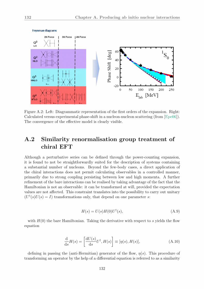
132 Chapter A. Producing ab initio nuclear interactions
Figure A.2: Left: Diagrammatic representation of the first orders of the expansion. Right:Calculated versus experimental phase-shift in a nucleon-nucleon scattering (from [Epe06]).The convergence of the effective model is clearly visible.
A.2 Similarity renormalisation group treatment of
chiral EFT
Although a perturbative series can be defined through the power-counting expansion,it is found to not be straightforwardly suited for the description of systems containinga substantial number of nucleons. Beyond the few-body cases, a direct application ofthe chiral interactions does not permit calculating observables in a controlled manner,primarily due to strong coupling persisting between low and high momenta. A furtherrefinement of the bare interactions can be realised by taking advantage of the fact that theHamiltonian is not an observable: it can be transformed at will, provided the expectationvalues are not affected. This constraint translates into the possibility to carry out unitary(U †(s)U(s) = I) transformations only, that depend on one parameter s:
H(s) = U(s)H(0)U †(s), (A.9)
with H(0) the bare Hamiltonian. Taking the derivative with respect to s yields the flowequation
d
dsH(s) =
[dU(s)
dsU †, H(s)
]≡ [η(s), H(s)], (A.10)
defining in passing the (anti-Hermitian) generator of the flow, η(s). This procedure oftransforming an operator by the help of a differential equation is referred to as a similarity
132
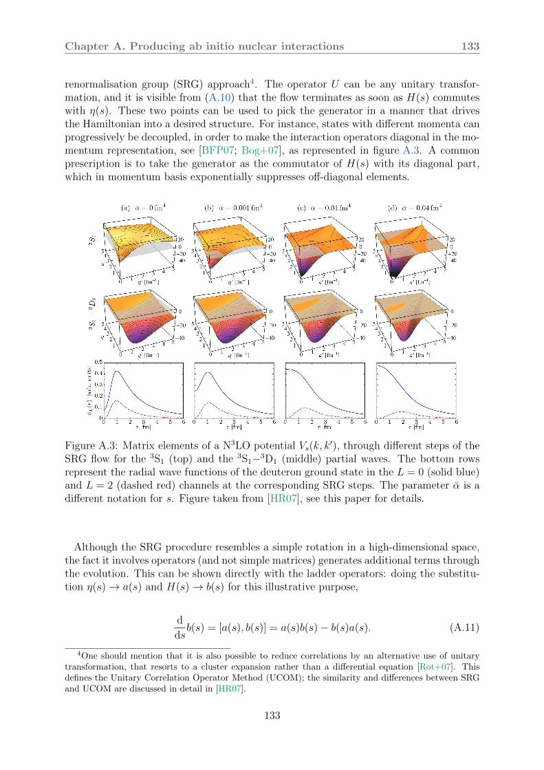
Chapter A. Producing ab initio nuclear interactions 133
renormalisation group (SRG) approach4. The operator U can be any unitary transfor-mation, and it is visible from (A.10) that the flow terminates as soon as H(s) commuteswith η(s). These two points can be used to pick the generator in a manner that drivesthe Hamiltonian into a desired structure. For instance, states with different momenta canprogressively be decoupled, in order to make the interaction operators diagonal in the mo-mentum representation, see [BFP07; Bog+07], as represented in figure A.3. A commonprescription is to take the generator as the commutator of H(s) with its diagonal part,which in momentum basis exponentially suppresses off-diagonal elements.
Figure A.3: Matrix elements of a N3LO potential Vs(k, k′), through different steps of the
SRG flow for the 3S1 (top) and the 3S1−3D1 (middle) partial waves. The bottom rowsrepresent the radial wave functions of the deuteron ground state in the L = 0 (solid blue)and L = 2 (dashed red) channels at the corresponding SRG steps. The parameter α is adifferent notation for s. Figure taken from [HR07], see this paper for details.
Although the SRG procedure resembles a simple rotation in a high-dimensional space,the fact it involves operators (and not simple matrices) generates additional terms throughthe evolution. This can be shown directly with the ladder operators: doing the substitu-tion η(s) → a(s) and H(s) → b(s) for this illustrative purpose,
d
dsb(s) = [a(s), b(s)] = a(s)b(s)− b(s)a(s). (A.11)
4One should mention that it is also possible to reduce correlations by an alternative use of unitarytransformation, that resorts to a cluster expansion rather than a differential equation [Rot+07]. Thisdefines the Unitary Correlation Operator Method (UCOM); the similarity and differences between SRGand UCOM are discussed in detail in [HR07].
133

134 Chapter A. Producing ab initio nuclear interactions
As the flow equation is usually integrated by time-slicing, (A.11) shows that the SRGevolution induces many-body terms regardless of the content of the initial Hamiltonian.Such terms greatly quickly render intractable the numerical integration of (A.10); four-body terms and higher are generally dismissed.
Ab initio nuclear interactions can thus be generated according to the following workflow:
- derive all Feynman diagrams of chiral EFT at a given order,
- adjust the associated low-energy constants to reproduce few-body experimentaldata,
- calculate the matrix elements of the chiral potentials in a given model space,
- evolve the resulting Hamiltonian through the flow equations (A.10).
The resulting interaction can in a second step used as input ingredients for the solutionof the many-body problem, e.g. through in-medium SRG, shell model calculations, or, asdone within this document, mean-field calculations. In all numerical calculations of thisthesis, we use unless specified otherwise the two- and three-body N3LO interactions of[EKM15], SRG-evolved up to the final value of the flow parameter λSRG = s−1/4 = 1.88fm−1 [Hut+20].
134

Appendix B
Effective theories ideas applied to anexactly solvable model
The production of the interactions for each order of an effective theory, and the determi-nation of the associated coupling constants, is a greatly arduous task. If the interactionsare organised in a sequence of many-body terms, the adjustment of the couplings canhowever be made in successive steps1. The effective approach is nonetheless expectedto break down when applied to increasing numbers of particles. This is illustrated infigures B.1-B.4, where a naive effective theory has been designed for a schematic systemof two N -fold degenerate shells, known as the Lipkin-Meshkov-Glick [LMG65]2 model. Itssimplest version is described by the Hamiltonian
H =ϵ
2
∑pσ
σa†pσapσ +V
2
∑pp′σ
a†pσa†p′σap′−σap−σ; p = shell index, σ = spin. (B.1)
The effective theory allows one to constructively obtain many-body interactions strengthsUk, by matching the sought coupling constants with the exact energies:
E(N) =N∑k=1
CkNUk ⇒ UN = E(N)−
N−1∑k=1
CkNUk. (B.2)
1Still, this is no easy game.2To be picky, it should be mentioned that equations (3.4)-(3.5) are half incorrect: one should instead
find
N = 6 :E
ϵ= ±
5 + 33
(V
ϵ
)2
± 4
[1 + 6
(V
ϵ
)2
+ 54
(V
ϵ
)4]1/2
1/2
, (LGM-3.4 top)
N = 8 :E
ϵ= 0,±
10 + 118
(V
ϵ
)2
± 6
[1− 2
(V
ϵ
)2
+ 225
(V
ϵ
)4]1/2
1/2
. (LGM-3.5 bottom)
135
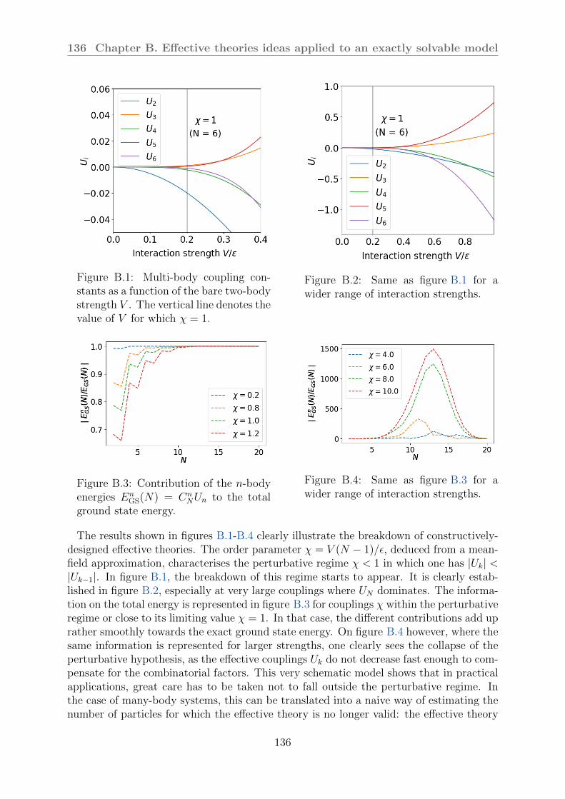
136 Chapter B. Effective theories ideas applied to an exactly solvable model
Figure B.1: Multi-body coupling con-stants as a function of the bare two-bodystrength V . The vertical line denotes thevalue of V for which χ = 1.
Figure B.2: Same as figure B.1 for awider range of interaction strengths. aaaa
Figure B.3: Contribution of the n-bodyenergies En
GS(N) = CnNUn to the total
ground state energy.
Figure B.4: Same as figure B.3 for awider range of interaction strengths. a
The results shown in figures B.1-B.4 clearly illustrate the breakdown of constructively-designed effective theories. The order parameter χ = V (N − 1)/ϵ, deduced from a mean-field approximation, characterises the perturbative regime χ < 1 in which one has |Uk| <|Uk−1|. In figure B.1, the breakdown of this regime starts to appear. It is clearly estab-lished in figure B.2, especially at very large couplings where UN dominates. The informa-tion on the total energy is represented in figure B.3 for couplings χ within the perturbativeregime or close to its limiting value χ = 1. In that case, the different contributions add uprather smoothly towards the exact ground state energy. On figure B.4 however, where thesame information is represented for larger strengths, one clearly sees the collapse of theperturbative hypothesis, as the effective couplings Uk do not decrease fast enough to com-pensate for the combinatorial factors. This very schematic model shows that in practicalapplications, great care has to be taken not to fall outside the perturbative regime. Inthe case of many-body systems, this can be translated into a naive way of estimating thenumber of particles for which the effective theory is no longer valid: the effective theory
136
Chapter B. Effective theories ideas applied to an exactly solvable model 137
is only legitimate for N such that
|Uk+q|Ck+qN < |Uk|Ck
N ∀k, q > 1. (B.3)
137

Appendix C
Sum rules from the static state
While the sum rules correspond to the different moments of the strength function (2.82),it is possible to obtain some of these from static quantities only. Looking at the quantitieswe have at hand before starting the RPA calculation, we find that only the HamiltonianH, the external operator F , the density matrix D and the set of single-particle operatorscan be used to obtain sum rules expressions. Additionally, we may introduce a parameterλ corresponding to the system constrained as H + λF , for which the ground state will bewritten |0λ⟩. Since we may want to have a general formula, the simplest way is to buildthe kth commutator on a nested scheme:
B(k) = [Xk . . . [X3[X1, X2]]. (C.1)
Within this constraint, it is clear that X1 = X2 (otherwise B(k) = 0). Additionally, thelast term of the k + 1th commutator must be H in order to obtain the last power of theenergy difference. Finally, as we need a second F operator in order to obtain squaredmatrix elements, we are led to the recurrence relation between the B(k):
B(0) ≡ F
B(1) ≡[H,B(0)
]B(k) ≡
[H,B(k−1)
]for k ≥ 1. (C.2)
Then,
⟨m|B(k)|n⟩ = ⟨m|HB(k−1)|n⟩ − ⟨m|B(k−1)H|n⟩= (Em − En) ⟨m|B(k−1)|n⟩= (Em − En)
k ⟨m|G|n⟩ , (C.3)
hence
⟨m|[F,B(k)
]|n⟩ =
∑l
⟨m|F |l⟩ ⟨l|B(k)|n⟩ − ⟨m|B(k)|l⟩ ⟨l|F |n⟩
138

Chapter C. Sum rules from the static state 139
taking m = n∑l
(1− (−1)k)(El − En)k ⟨n|F |l⟩ ⟨l|F |n⟩ . (C.4)
For F Hermitian, taking the sum over the n states weighted by their statistical factorleads to the odd-k sum rules:
1
2Tr[
G,B(k)]
=
0 k even
Z−1∑ln
e−βEn(El − En)k| ⟨n|F |l⟩|2 = mk(F ) k odd. (C.5)
A similar derivation can be made for the inverse energy-weighted sum rule (IEWSR):we write a perturbative expansion (the notations are hopefully self-evident)
⟨F ⟩λ = Tr
F
(D + λδD +
1
2!λ2δ2D
)+O(λ3)
. (C.6)
Recalling that δD = RF ((2.80)), we can take the derivative and obtain
1
2
d
dλ⟨0λ|F |0λ⟩
∣∣∣∣λ=0
= TrFδD = TrFRF. (C.7)
From the expression (2.79) of the response function, one identifies the right-hand sideterm with the IEWSR. This approach unfortunately cannot yield other moments: it wouldrequire getting powers of the response function R by taking higher derivative with respectto λ, which’d also make the operator F fall identically many times. Recollecting thedifferent pieces, one sees that the moments are related to expressions involving two timesthe operator F , whereas each response function must be matched with two of these. Onlym−1, involving a first derivative, can be obtained this way.
139

Appendix D
Higher-order responses
D.1 Linear responses
In this appendix, the linear response of k-body densities is derived. Starting from (2.74),the time-dependent part of the expectation value of an operator O is given as
⟨δO(t)⟩ = iTr
∫ t
t0
dτ [OH(t), FH(τ)]D0
. (D.1)
If both O and F are two-body operators, one ought to introduce closure relations overthe two-body Hilbert space in order to replace the propagators by their eigenvalues, thatis,
OH(t)FH(τ) =∑µνλσ
|µν⟩⟨µν| eiHtOS(t)e−iHt |λσ⟩⟨λσ| eiHτFS(τ)e
−iHτ
=∑µνλσ
eiΩµνλσt |µν⟩⟨µν|OS(t) |λσ⟩⟨λσ| eiΩ
λστFS(τ)e−iHτ , (D.2)
with the notation Ωaba′b′ ≡ Ea + Eb − Ea′ − Eb′ . Multiplying by the static density and
taking the trace in the two-body Hilbert space yields
⟨OH(t)FH(τ)⟩ =∑κι
fκfι∑µνλσ
⟨κι|µν⟩ ⟨µν| eiHtOS(t)e−iHt |λσ⟩⟨λσ| eiHτFS(τ)e
−iHτ |κι⟩
=∑µνλσ
fµfνeiΩµν
λσ(t−τ) ⟨µν|OS(t)|λσ⟩ ⟨λσ|FS(τ)|µν⟩ . (D.3)
In this expression, the fk are the Fermi-Dirac (or Bose-Einstein in case of bosons)factors. Using individual states rather than many-body eigenstates as done before greatlysimplifies the tracing, and is permitted since the trace can be taken in the eigenbasis ofthe density operator. If O has no explicit time-dependence in the Schrodinger picture(OS(t) = OS), (D.1) can be written as the sum of two convolutions, as done in (2.76).One obtains the two-body response function
140

Chapter D. Higher-order responses 141
Rραβγδϵζηθ
[O] =∑µνλσ
fµfνOαβγδ×[⟨µν|a†αa†βaγaδ|λσ⟩ ⟨λσ|a†ϵa†ζaηaθ|µν⟩
Ωµνλσ − ω − iΓ
−⟨µν|a†ϵa†ζaηaθ|λσ⟩ ⟨λσ|a†αa†βaγaδ|µν⟩
Ωµνλσ + ω + iΓ
]. (D.4)
Note that the separability of the matrix elements has not been assumed. This proceduregeneralises clearly to k-body operators (I write Aαβ...
γδ... for a†αa†β . . . aγaδ . . . to shorten the
expression):
Rρα1...αk,β1...βkζ1...ζk,ξ1...ξk
[O] =∑
µ1...µkλ1...λk
(k∏
j=1
fµj
)⟨α1 . . . αk|O|β1 . . . βk⟩×
[⟨µ1 . . . µk|Aα1...αk
βk...βk|λ1 . . . λk⟩ ⟨λ1 . . . λk|Aζ1...ζk
ξ1...ξk|µ1 . . . µk⟩
Ωµ1...µk
λ1...λk− ω − iΓ
−⟨µ1 . . . µk|Aζ1...ζk
ξ1...ξk|λ1 . . . λk⟩ ⟨λ1 . . . λk|Aα1...αk
βk...βk|µ1 . . . µk⟩
Ωµ1...µk
λ1...λk+ ω + iΓ
].
(D.5)
D.2 Non-linear responses
The time-dependent component of the expectation value of an operator O can be written,from (2.72), as a sum of commutators involving nested integrals. Focusing on termscontaining N such integrals, one has
⟨δO(τN)⟩ ∼ iN Tr
∫ τN
τN−1
dτN−1
∫ τN−1
τN−2
dτN−2· · ·∫ τ1
τ0
dτ0 e∑N−1
q=0 αq(τq+1−τq)F (τq)O(τN)
.
(D.6)
One can identify τN = t and τ0 = t0 to match the notations employed up to now.Likewise, the αq identify with the Ωµ1...µk
λ1...λkterms. Eventually, the notation can be made
more compact by writing either of
∫ τN
τN−1
dτN−1
∫ τN−1
τN−2
dτN−2· · ·∫ τ1
τ0
dτ0 ≡N−1∏q=0
∫ τq+1
τq
dτq ≡∫ τN
τ0
Dτ. (D.7)
The integrals in (D.6) can be written as a chain of convolutions, after inserting theappropriate step functions to account for the boundaries τq. One can then take theFourier transform of (D.6), which is now the product of the individual transforms. Prior
to this, exponential damping functions of the form e−∑N−1
q=0 Γqτq are introduced, in order
141

142 Chapter D. Higher-order responses
to translate the fact that the probe is switched off and must vanish at infinite times.This has the effect of removing terms that depend on the intermediate times τq =0,N ,which would otherwise make the result a rather messy sum of 2N terms1. The productof Fourier transforms then becomes a product of two-point functions, with the matrixelements correctly inserted in-between (the factor iN gets cancelled by the is coming fromthe integrals, as usual):
Rρ,[N ]αβγδ
(ω) ∼ Z−1∑
µ1...µNν1...νN
e−βEν
[(N∏q=1
⟨νq|a†βaα|µq⟩ ⟨µq|a†γaδ|νq⟩Ω
νqµq − ω − iΓ
)
−(
N∏q=1
⟨νq|a†γaδ|µq⟩ ⟨µq|a†βaα|νq⟩Ω
νqµq + ω + iΓ
)]. (D.8)
Altogether, this yields
δR[N ](ωγ) = R[N ](ωγ)F[N ](ωγ). (D.9)
If one so desires, the 2k-point non-linear response functions can be derived by combiningthe procedures of section D.1 and section D.2.
1To convince oneself of how unpleasant the situation becomes, the computation can be done for N = 2.Taking both τ2 and τ1 to infinity, as they should, lead to a second term that is an indefinite function ofτ2 and τ1. The infinite time limit is well-defined only if the integral converges, which is achieved by thedamping factor that makes the integrand decay exponentially toward zero.
142

Appendix E
Overview of the axial harmonicoscillator basis
In practical calculations, one has to choose a specific basis on which to expand the un-known wave functions. Two types of bases are commonly encountered. In the coordinate⊗ spin ⊗ isospin basis, the spatial component of the wave functions are calculated on a(usually Cartesian) mesh. While this method is fairly intuitive, it is often computation-ally expansive due to the large number of required grid points1, especially for non-localinteractions2.
On the other hand, the problem may be expanded on a basis with ’nice’ properties;most importantly, it is crucial to employ basis functions that allow us to avoid computinghigh-dimensional integrals. The choice of the basis is thus largely constrained by the formof the potential: for instance, a Gaussian measure makes Hermite polynomials orthogo-nal, so that they allow for an efficient evaluation of spatial integrals when the integrandinvolves a Gaussian potential. The second approach therefore uses eigenfunctions thatdisplay useful properties. The most commonly ones are those of harmonic oscillators3.
Because the eigenfunctions of all three types of oscillators span R3, any of them canbe used as the computational basis. However, wave functions possessing either spherical,axial or triaxial symmetry can naturally be well-approximated by basis functions display-ing the same symmetries, so that the choice of basis is essentially determined by the kindof expected wave functions. For nuclear systems, experimental data [Nis+17; Gaf+13;Yan+04; Yan+03; Iwa+01; Mot+95; Orr+91; Det+83; Det+79] show that the majorityof the ground states display features (e.g. rotational bands) that can only be interpretedby assuming the systems are deformed in their intrinsic frame. Most deformation beingessentially quadrupolar, an axial basis seems an appropriate choice. Note that this choiceis in general not guided by the shape of excited states -which themselves show a widevariety of geometries [ITH68; SHI72; Ito+14]-.
1Note however that it is possible to reduce the number of points by using non-Cartesian grids with adistribution of points adjusted to the problem considered [NY05; INY09b].
2In three dimensions for instance, it leads to 6-dimensional integrals for the two-body terms, versus 3for local interactions.
3The eigenfunctions of a Woods-Saxon potential are also sometimes used [ZMR03], although theydon’t allow for analytical evaluation of the integrals.
143
144 Chapter E. Overview of the axial harmonic oscillator basis
A particle of mass m inside a three-dimensional harmonic oscillator is described by theHamiltonian
H =p2
2m+
m
2(ω2
xx2 + ω2
yy2 + ω2
zz2), (E.1)
where ωx,y,z are the oscillator frequencies, and correspond to the stiffness of the os-cillator along the corresponding direction. The eigenfunctions of (E.1) are products ofGauss-Hermite polynomials, the angular part being described by the functions eimφ, wherem is the orbital quantum number.
An axial oscillator corresponds to the particular case ωx = ωy, so that
H =p2
2m+
m
2(ω2
⊥r2⊥ + ω2
zz2). (E.2)
The deformation can be characterised by the ratio q = ω⊥/ωz, while the geometric meanof the frequencies ω0 = (ω2
⊥ωz)1/3. Thus,
ω⊥ = ω0q1/3, (E.3)
ωz = ω0q−2/3, (E.4)
which is probably quite unimportant here. The eigenfunctions of (E.2) are productsof Gauss-Hermite polynomials (along the z direction) and generalised Gauss-Laguerrepolynomials (along the r⊥ direction). Lastly, when ωx = ωy = ωz, the harmonic oscillatorbecomes spherically symmetric:
H =p2
2m+
m
2ω2r2, (E.5)
the corresponding eigenfunctions being the Gauss-Laguerre polynomials in the radial di-rection, and spherical harmonics in the angular directions.
While the cylindrical oscillator seems a good compromise, it must be remarked thatonly the spherical oscillator possesses the correct asymptotic behaviour with respect to apotential going to zero at infinity. This can be critical when the surface properties playan important role, e.g. for halo and/or drip-line nuclei, as well as when coupling to thecontinuum effects become prominent, as can be the case for at high temperature and fordecaying systems.
The numerical code employed in this work is based on an axial basis, some propertiesof which are quickly reviewed here. In a cylindrical basis, the relevant quantum numberslabelling an eigenstate of an axial harmonic oscillator with different spin-isospin speciesare:
144

Chapter E. Overview of the axial harmonic oscillator basis 145
- m, the orbital quantum number;
- nz, the principal quantum number along the z axis, corresponding to the number ofnodes of the wave function in the z direction;
- n⊥, the principal quantum number perpendicular to the symmetry axis z, corre-sponding to the number of nodes of the wave function in the r⊥ direction;
- σ, the spin;
- τ , the isospin.
A state of the axial oscillator basis will therefore be written
|α⟩ ≡ |mαnzαn⊥ασατα⟩ ≡ |mανασατα⟩ ≡ |µασατα⟩ , (E.6)
introducing shorthand notations splitting the coordinate and internal spaces quantumnumbers |α⟩ = |µα⟩ ⊗ |σατα⟩. It can also be convenient to work with Ω = m + σ,projection of the total orbital momentum on the z-axis. The coordinate representationfor the ket |α⟩ form the basis of functions
Φα(r, σ, τ) ≡ ⟨rστ |α⟩ ,Φα(r) = (πb2⊥bz)
− 12ϕmα
n⊥α(η)ϕnzα
(ξ)eimαφ,
where variables have been switched to dimensionless ones through η ≡ r2⊥/b2⊥ and
ξ ≡ z/bz. Regarding the eigenfunctions of the harmonic oscillator, a few useful propertiesare recalled: first, their explicit expressions are
ϕn(ξ) ≡ N (⊥)n e−ξ2/2Hn(ξ) = eξ
2/2(−1)ndn
dξne−ξ2 Gauss-Hermite, (E.7a)
ϕmn (η) ≡ N (z)ηm/2e−η/2Lm
n (η) =1
n!
dn
dηn(e−ηηm+n
)Gauss-Laguerre, (E.7b)
with the normalisation constants N (⊥)n = (2nn!
√π)−1/2 and N (z) =
√n!
(n+m)!.
Second, they possess the following orthogonality and recurrence properties:Gauss-Hermite polynomials:
⋆
∫dξϕn(ξ)ϕm(ξ) = δm,n, (E.8a)
⋆ ϕn =
√2
nξϕn−1 −
√n− 1
nϕn−2, (E.8b)
⋆ ξϕn =
√n+ 1
2ϕn+1 +
√n
2ϕn−1, (E.8c)
⋆ ∂ξϕn =
√n
2ϕn−1 −
√n+ 1
2ϕn+1, (E.8d)
145

146 Chapter E. Overview of the axial harmonic oscillator basis
Generalised Gauss-Laguerre polynomials:
⋆
∫dηϕm
n (ξ)ϕmn′(ξ) = δn,n′ , (E.9a)
⋆√ηϕm
n =
√n+m+ 1ϕm+1
n −√nϕm+1
n−1√n+mϕm−1
n −√n+ 1ϕm−1
n+1
, (E.9b)
⋆m√ηϕmn =
√n+m+ 1ϕm+1
n +√n+ 1ϕm−1
n+1√n+mϕm−1
n −√nϕm+1
n−1
, (E.9c)
⋆ 2√η∂ηϕ
mn =
√n+ 1ϕm−1
n+1 −√nϕm+1
n−1√n+mϕm−1
n −√n+m+ 1ϕm+1
n
. (E.9d)
The matrix elements for contact or Gaussian interactions in axial symmetry are notgiven here for the sake of conciseness, but can be found in [You09].
146

Appendix F
Resume substantiel en francais
Introduction
Le probleme quantique a N corps est extremement complexe et nombre de phenomenesne peuvent etre compris finement que lorsque les correlations entre les degres de libertesont traitees de maniere satisfaisante. Ces correlations, resultant d’interactions au traversde differents canaux (de spin et d’isospin notamment), generent plethore de configura-tions, telles que des etats deformes et des phases superfluides. Cette phenomenologieest agrementee par la realisation de configurations plus exotiques : etats dits a halos oubulles, resonances geantes, agregats et bien d’autres. A titre d’illustration, on peut citerl’etat de Hoyle, un etat excite du carbone dans lequel les douze nucleons s’agencent entrois agregats de particules alpha.
Notamment, les proprietes des etats excites des noyaux atomiques jouent un role depremier plan dans la comprehension des processus de nucleosynthese ; le travail icipresente peut etre vu comme un pas dans cette direction. Deux difficultes principalesdoivent cependant etre adressees. Premierement, la nature des etats excites est tresdiverse, allant d’excitations elementaires d’une seule ou de quelques particules a desphenomenes de vibration tres collectifs, pour lesquels les correlations entre degres deliberte sont une composante primordiale. En second lieu, ces resonances couvrent unegamme d’energie s’etalant sur un a deux ordres de grandeur. A ce jour, le principalcadre theorique permettant de tenir compte de ces deux contraintes est l’approximationdes phases aleatoires ((Q)RPA), dans lequel les etats excites sont construits comme dessuperpositions coherentes de modes pour lesquels seules les correlations les plus simples(dites “une particule-un trou” ou “deux quasi-particules” dans le cas superfluide). Malgrecette approximation, la QRPA reste une approche en pratique tres couteuse ; la plupartdes applications restent donc relativement limitees quant aux classes de correlations (an-gulaires, superfluides...) traitees. Le travail presente dans ce document repose sur une re-formulation recente -la methode des amplitudes finies (FAM)- de la QRPA, qui permet enpratique de lever ces verrous. On utilise egalement une interaction effective entre nucleonsderivant de la theorie de l’interaction forte, la chromodynamique quantique (QCD). En susde ces nouveaux resultats, dans les milieux astrophysiques ou s’effectuent les differentesetapes de la nucleosynthese regnent des temperatures tres elevees (T ≳ 109K), de sorteque le couplage d’un systeme a son environnement thermique peut generer d’importantes
147

148 Chapter F. Resume substantiel en francais
modifications de la structure des etats fondamentaux et excites. Le travail de these tientcompte de ces couplages, en generalisant pour la premiere fois la FAM au cas ou le systemedoit etre decrit comme un ensemble statistique. On presente de premieres applicationsa la transition de phase deformee vers spherique sous l’effet de la temperature, ainsique de premieres applications a la description de resonances geantes dans des conditionspertinentes pour l’astrophysique.
Generalites
Ce chapitre introductif presente le cadre theorique de la description du probleme quan-tique a N corps. On s’attache a rester le plus general possible, de sorte que toutes lesidees et techniques resumees dans ce chapitre sont applicables aussi bien a la physiquedes atomes froids qu’a la matiere condensee, la chimie quantique ou la physique nucleaire.Les concepts principaux de la description quantique d’un systeme a N corps en termes demelange statistique de matrices de densite sont exposes. On recapitule ensuite les deuxtechniques principales employees pour simplifier la representation formelle du probleme, asavoir le theoreme de Wick et la procedure d’anti-symetrisation des chaınes d’operateursfermioniques. On presente ensuite l’approximation du champ moyen incluant la superflu-idite et le couplage a un bain thermique. Ce second aspect ouvre la possibilite de decrireles transitions de phase induites par les effets de temperature ; deux de celles-cis sontdiscutees schematiquement. Enfin, ce chapitre presente la theorie de la reponse et metl’accent sur son approximation lineaire, laquelle est rarement depassee en pratique.
Matrice de densite
On resume comment il est possible, a partir de l’equation de Schrodinger decrivant unefonction d’onde, d’arriver a l’equation de Liouville-von Neumann dependante du temps(TDLvN), qui porte sur l’evolution de la matrice de densite associee. Il est mentionne quele formalisme peut aisement etre vu comme decrivant une dynamique non hermitienne etdonc non unitaire, c’est-a-dire ne conservant pas la norme de la fonction d’onde, commec’est le cas dans les systemes ouverts. L’equation du mouvement de TDLvN est ensuiteseparee en differents secteurs, selon le nombre d’operateurs d’echelle presents dans lesfonctions d’onde “gauche” et “droite”.
Ensemble statistique
Schematiquement, des lors qu’un systeme quantique est en contact avec un milieu exterieurdont la temperature n’est pas tres inferieure a la difference d’energie entre la derniereorbitale occupee et la premiere orbitale vide de ce premier, les excitations thermiquesne sont pas negligeables et doivent donc etre incluses de maniere satisfaisante dans leformalisme. Cela est effectue en ecrivant l’etat thermique comme un melange de differentsetats produits. On rappelle egalement l’expression de quelques observables en termes detrace, ainsi la derivation des moments des nombres d’occupation moyens a partir de lafonction de partition.
148

Chapter F. Resume substantiel en francais 149
Hamiltonien statique et quelques proprietes generales
Dans cette partie, on considere un hamiltonien multicorps arbitraire, et montre quel’ecriture en seconde quantification amene tres rapidement a de severes limitations duesau nombre exponentiel de fonctions de correlations. On evoque que des transformationsde groupe de renormalisation par similarite permettent de transformer un hamiltonien aN corps quelconque en hamiltonien dans lequel les elements de matrice a un, deux, voiretrois corps sont largement predominants. Cela permet de rendre le probleme de recherchedes valeurs et vecteurs propres a la fois moins complexe et plus perturbatif. On donneenfin l’expression generale de l’energie totale lorsque l’hamiltonien est tronque de sorteque les termes a quatre corps et plus ne sont pas inclus. Une seconde etape de reductiond’information passe par la combinaison du theoreme de Wick avec la procedure d’anti-symetrisation des elements de matrice, ce qui permet de ne conserver que les densites a uncorps et non plus des determinants de Slater, la structure anti-symetrique de la fonctiond’onde a N corps etant absorbee dans les interactions a deux et trois corps.
Approximations de champ moyen
On presente la theorie dite de Hartree-Fock-Bogoliubov, qui par construction est l’approchede champ moyen la plus generale possible. On derive les expressions des densites normaleset anomales, ainsi que des champs associes, a temperature finie. Le principe variation-nel de minimisation de l’energie mene ensuite a l’equation non-lineaire permettant ladetermination de l’etat fondamental.
Transitions de phase thermiques
L’evolution des deux types de brisures de symetrie consideres dans cette these, a savoirde nombre de particules et de geometrie, est discutee avec la temperature. L’accent estmis sur les arguments physiques plutot que sur les details de derivation. On montre quel’appariement comme la deformation diminuent avec la temperature, et doivent chacundonner lieu a une transition de phase de second ordre. En dernier lieu, on montre quememe a basses temperatures, il est necessaire de considerer non plus un seul etat fonda-mental (sous la forme d’un melange statistique) mais bien l’ensemble des etats generespar le parametre d’ordre considere (couplage d’appariement ou bien deformation), tousetant occupes suivant une probabilite en exponentielle de leur energie libre. Bien que cetteseconde etape est trop chronophage pour etre effectuee, on pointe l’evolution attendue desparametres d’ordre.
Theorie de la reponse
Apres avoir discute des deux points de vue conceptuels a la theorie de la reponse, est dis-cute brievement des principaux points de depart formels menant aux equations associees,on derive l’equation de la reponse lineaire ainsi que des moments correspondants aux prob-abilites de transition. Ce chapitre s’acheve sur la remarque que la formulation habituelle,sous forme d’equation aux valeurs propres, etant un probleme dont la resolution se faiten une duree croissant comme le cube du nombre d’etats a une particule considere, cette
149
150 Chapter F. Resume substantiel en francais
approche est en pratique limitee aux systemes pour lesquels le nombre d’etats necessaireest assez faible.
Methode des amplitudes finies
La methode des amplitudes finies est une formulation equivalente a l’approche QRPAhabituelle. Elles different cependant en ce que la QRPA se resout comme une equation auxvaleurs propres generalisee, tandis que la FAM contourne ce probleme de haute dimensionen y substituant un ensemble de problemes plus simples, equivalents a ceux rencontresdans la determination de l’etat fondamental. Apres avoir presente une derivation desequations de la FAM, ce chapitre detaille plusieurs points techniques ayant trait a lamethode. On y discute notamment de la connexion de la FAM a la QRPA par le biaisd’integrales dans le plan complexe ; cela demontre que les deux methodes peuvent etrerendues strictement equivalentes. Il est egalement prouve quelques points importants pourla mise en branle de la methode, tels que la linearisation des champs moyens, ainsi que descontraintes de symetries des equations, plus delicates que celles rencontrees usuellementen raison de l’emploi de matrices de densite complexes. Differents points critiques pourle succes de la methode, tels que l’elimination des modes de Nambu-Goldstone ou lanecessite de fixer le centre de masse au travers d’une prescription a un-plus-deux corpssont presentes. Quelques criteres de determination d’instabilites du systeme vis-a-vis de laperturbation appliquee sont derives. On mentionne egalement les mecanismes physiquesa l’origine de l’elargissement des resonances, lequel n’est pas accessible dans la presentetheorie et est rajoute a la main. Enfin, on montre rapidement la maniere dont la structurede l’operateur generant les oscillations influe sur les nombres quantiques des fluctuationsde champs et densites.
Derivation
On presente ici une derivation des equations de la FAM a temperature finie, dans le casd’une theorie incluant l’appariement. Le choix est porte sur la derivation partant desequations de TDLvN, plus generales que l’equation HFB dependante du temps puisquen’etant pas restreinte au secteur a un corps. Quoiqu’elles s’ecrivent a priori dans desbases differentes, il est possible de transformer l’ensemble d’equations TDLvN dans labase HFB, de sorte que la derivation montree dans cette partie peut egalement fournirun point de depart a des theories au-dela de la FAM. Une methode de resolution desequations du mouvement est donnee.
Linearisation des champs
En general, les hamiltoniens de champ moyen dependent non-lineairement des densites.Cela est du a la presence de termes a trois corps, voire plus, ou alors, pour la plupart desinteractions phenomenologiques, a une dependance explicite des termes d’interaction adeux corps en la densite. Puisque la FAM s’attache a decrire des fluctuations au-dela duchamp moyen, les champs melangent densites statiques et dynamiques, de sorte que leurcalcul est plus complexe que celui des champs moyens statiques. Toutefois, il est possiblede calculer les champs oscillants induits d’une maniere analogue aux champs statiques, de
150

Chapter F. Resume substantiel en francais 151
sorte que seules les composantes lineaires de la reponse sont retenues. On parle alors delinearisation des champs induits. Cette sous-section discute des deux differentes manieresdont les champs dependants du temps peuvent etre linearises. Une premiere approcheest entierement numerique et repose sur une methode de differences finies ; on discuteles avantages et inconvenients de cette approche. La seconde methode, utilisee danscette these, consiste a separer le calcul des champs induits de la FAM en deux etapes: une etape de pre-contraction, qui permet de definir des interactions effectives pourles fluctuations, suivie d’une etape de calcul analogue a celle mise en place au niveaudu champ moyen statique. On donne les expressions des interactions effectives lorsquel’hamiltonien contient des termes a un, deux et trois corps.
Symetries des equations FAM et HFB
Ayant ete mentionne que les symetries presentes dans la FAM sont moindres que cellesrencontrees dans la theorie HFB, on s’attele a leur etude precise. On donne egalementles expressions des densites et champs statiques et induits, dans les deux conventions lesplus communement employees pour parametrer la transformation de Bogoliubov.
Connexion avec la QRPA
On montre comment la FAM peut etre reliee a la QRPA, c’est-a-dire comment les am-plitudes et fonction de force lineaires exactes peuvent etre calculees a partir de cellesobtenues via la FAM.
Habillage auto-coherent
Si les energies presentes au denominateur des equations FAM sont les energies statiquesdes etats propres, les poles de la fonction de reponse different des poles de la fonctionde reponse “nue”, en raison de l’habillage des propagateurs a un corps par le biais desoscillations de champ moyen. On montre ceci a l’aide d’un modele exactement soluble,clarifiant ainsi cet aspect d’apparence contre-intuitif.
Modes de Nambu-Goldstone
Les modes dits de Nambu-Goldstone sont des modes parasites lies a la brisure de symetrieautorisee pour l’etat de reference. Cette brisure genere un ensemble d’etats equivalentsa une (ou un ensemble de) phase(s) pres. Les differents etats de cette variete peuventetre atteints accidentellement lorsque l’on excite le systeme avec une sonde contenantles operateurs reliant ces differents etats. Il est alors necessaire de mettre en place uneprocedure de soustraction afin d’eliminer ces contributions non desiree. C’est ce qui estfait dans cette partie, en suivant la derivation de l’article [NIY07].
Centre de masse
Il a ete montre dans [HR09] que les deux manieres differentes de tenir compte de lafixation du centre de masse pour les systemes auto-lies, quoiqu’equivalentes au niveaudes operateurs, ne le sont plus lorsque l’on calcule des valeurs moyennes des lors que
151
152 Chapter F. Resume substantiel en francais
les densites d’appariement sont non-nulles. Cette derivation ayant ete effectuee pour lesetats statiques uniquement, il est de rigueur de verifier si le calcul du centre de massereste correct lorsque l’on tient compte des oscillations de densite. Il est montre que lesresultats obtenus pour les etats independants du temps se generalisent pour les etatsfluctuants consideres ici.
Modes instables
Lorsque le systeme est stable, c’est-a-dire lorsqu’il ne devie de son etat d’equilibre que pardes fluctuations du meme ordre de grandeur que l’intensite de la sonde, les energies detous les etats collectifs sont reelles. Dans le cas inverse, elles deviennent imaginaires. Ondonne ici quelques techniques permettant d’estimer si de tels modes sont presents sansavoir a les identifier precisement.
Elargissement des resonances
On discute ici des phenomenes a l’origine des largeurs finies des resonances collectives.Outre les habituels couplages d’etalement (couplage aux modes impliquant plus d’etatsparticipants), de Landau (couplage entre etats collectifs et individuels) et couplage auxetats non lies, on mentionne les effets cinetiques dus au couplage du systeme a un bainthermique.
QFAM en base d’oscillateur harmonique : regles de selection
Cette sous-section montre comment (i) les nombres quantiques de la sonde contraignent letype d’excitations pouvant avoir lieu, (ii) comment les contraintes imposees aux interac-tions a deux et trois corps se traduisent en regles de selection pour les champs et densitesdynamiques.
Applications aux transitions de phase thermiques
Ce premier chapitre de resultats s’attache a la description de l’etat fondamental du 56Fesur une gamme de temperatures similaire a celle rencontree dans les etoiles a neutrons. Ony observe une restauration abrupte de la phase spherique pour une temperature critiqueTc = 2.46 ± 0.23 MeV. L’evolution du parametre d’ordre encodant la deformation, enl’occurrence quadripolaire, peut etre comprise schematiquement dans le cas de la theoriede Landau des transitions de phase. L’etude plus detaillee des grandeurs thermody-namiques pertinentes ici (entropie et capacite calorifique) permet d’identifier une transi-tion de phase d’ordre deux, conformement a ce qui est observe dans d’autres approcheset des noyaux plus lourds. Il est a noter que cette etude physique est precedee d’uneanalyse de la convergence des resultats en fonction des parametres de la base (nombred’etats et raideur de l’oscillateur) sur laquelle les fonctions d’onde sont ecrites, ainsi quel’evolution desdits resultats lorsque differents ordres du developpement chiral a l’origine del’interaction effective sont inclus. On observe globalement une convergence bien etablie (del’ordre du pourcent) pour les parametres numeriques, tandis que la comparaison des ordresdeux a quatre de l’interaction chirale permet d’estimer produit une erreur systematique
152

Chapter F. Resume substantiel en francais 153
d’environ 10% sur les observables differentielles, cet ecart etant systematiquement du a ladifference entre les ordres deux et quatre ; l’accord entre les ordres trois et quatre etanttoujours bien meilleur. Les erreurs dues a l’interaction peuvent etre reduites de manierebien definie (via l’inclusion d’ordres superieurs) quoiqu’au prix d’efforts de travail formelet numerique hors de portee de ce travail de these.
Applications aux resonances geantes
Ce chapitre demarre par la validation de la methode face a des calculs RPA dans l’16O,spherique et non superfluide. La methode des amplitudes finies thermique est ensuiteappliquee a l’etude des modes collectifs electriques dans trois noyaux interessants pour leprocessus s, partiellement a l’origine des elements lourds dans la nature. Comme dans lechapitre precedent, on s’applique a verifier la convergence des calculs FAM. Ici encore,on trouve une convergence en voie d’etablissement, avec des erreurs de l’ordre de 10%pour chacun des trois parametres etudies : la frequence de l’oscillateur harmonique, lenombre de quanta de la base, ainsi que l’ordre chiral de l’interaction. Ensuite, on etudiela possibilite de calculer les moments de la fonction de reponse par integration de celle-cidans le plan complexe ; les resultats sont de qualite similaire a ceux obtenus par integrationsur l’axe reel positif de la fonction de reponse convoluee avec une distribution de Cauchy.Enfin, les resultats principaux de ce chapitre sont l’etude de l’evolution des fonctions dereponse a mesure que la temperature croıt. On trouve des variations plutot moderees, dontla tendance peut etre comprise par des modeles schematiques. Toutefois, l’augmentationde la fonction de reponse dipolaire a basse energie est assez remarquable, et pourraitlaisser presager d’une contribution de nature electrique a l’augmentation mesuree dansles trois systemes etudies. Il est cependant pointe que seules les perturbations le long del’axe de symetrie de la distribution de densite statique sont considerees ; il est tout a faitenvisageable que l’augmentation soit plus consequente dans des directions non axiales, oualors ne puisse s’observer qu’au-dessus d’etats de reference de symetrie moindre (c.-a-d.ne possedant aucun axe de symetrie). De meme, une etude des modes magnetiques M1 estnecessaire afin d’apporter des elements de reponse. Enfin, est mentionnee la possibiliteque ces resonances ne puissent etre decrites dans le cadre de l’approximation lineaireeffectuee, et on montre de maniere simplifiee comment des excitations plus complexespeuvent devenir preponderantes a basse energie dans des systemes chauds.
Conclusions et perspectives
Ce travail est conclu par le constat qu’il ouvre la voie a des etudes jusqu’alors hors deportee de l’approche usuelle a la description des resonances dans le cas d’une interactionderivant de la QCD. On note toutefois que l’etude complete des possibilites ouvertes parla FAM n’a pas ete realisee dans ce travail. La demonstration formelle que la methodedes amplitudes finies a temperature finie est equivalente a l’approche QRPA thermiqueetend la preuve a temperature nulle de [HKN13].
Differents modes d’excitation (echange de charge, d’isospin, operateurs de Gamow-Telleret de Fermi) ont ete omis, quoique le mode magnetique M1 soit deja a portee d’etude.
153
154 Chapter F. Resume substantiel en francais
L’inclusion de ces modes ouvrira l’acces a d’autres mecanismes, telles que la decroissanceβ, simple ou double, avec ou sans neutrinos.
Il est egalement remarque qu’un systeme fini devant respecter les symetries de l’hamiltonienle decrivant, une etape supplementaire de developpement serait de restaurer les symetriesbrisees par l’etat fondamental au niveau des solutions FAM, l’approche la plus directeetant a priori de se baser sur la formulation developpee dans [Sim10; SY14; SH17].
154

List of Figures
1.1 Zoom on the nuclear chart for N ≤ 16 and Z ≤ 10. Courtesy of W. Korten. 9
2.1 Total density at T = 0 and T = 0.5 a.u. for 100 states with randomlygenerated prolate (az > a⊥) and oblate (az < a⊥) deformations. The whitedashed contours signal the region where the density reaches 20% of itsmaximum value and serve as a guide to the eyes. See text for details. . . . 32
3.1 Algorithm employed for the self-consistent solution of (3.8). . . . . . . . . 46
3.2 Evolution of the relative thermal width of spectral lines as a function ofthe temperature and atomic mass. . . . . . . . . . . . . . . . . . . . . . . . 79
4.1 Ground state energies as a function of the oscillator frequencies at emax =6, 8, 10 with e3max = 14. . . . . . . . . . . . . . . . . . . . . . . . . . . . . 88
4.2 Same as figure 4.1 for the quadrupole moments. . . . . . . . . . . . . . . . 89
4.3 Same as figure 4.1 for the point-particle radii. . . . . . . . . . . . . . . . . 90
4.4 Evolution of the ground state energies with emax. The dashed lines representthe fitted curves, and the grey lines denote the best extrapolated values.The model space used has e3max = 14. . . . . . . . . . . . . . . . . . . . . . 92
4.5 Ground state energies, quadrupole moments and radii at NLO, N2LO andN3LO for 56Fe, 46Ti and 44Ti at zero temperature. The model space is(emax, e3max) = (10, 14) and ℏΩ = 16 MeV. . . . . . . . . . . . . . . . . . . 93
4.6 Total (protons+neutrons) ground state densities of 56Fe for four tempera-tures. The calculations are made at (emax, e3max) = (8, 14), ℏΩ = 12 MeV,with the N3LO interaction. The black, blue and yellow contours signal theiso-density surfaces, where ρ = 0.08, 0.12 and 0.16 fm−3, respectively. . . . 96
4.7 Ground state energy (left) and excitation energy (right) as a functionof temperature in 56Fe. The excitation energy of a two-components freefermion gas of protons and neutrons at saturation density is also repre-sented as circles placed every 0.2 MeV. . . . . . . . . . . . . . . . . . . . . 97
4.8 Same as figure 4.7 for the total entropy. . . . . . . . . . . . . . . . . . . . . 97
4.9 Static quadrupole moment as a function of the temperature. . . . . . . . . 98
4.10 Same as figure 4.7 for the heat capacity. The derivatives are calculatedusing finite differences, for temperatures equally spaced of 0.01 MeV. . . . 99
5.1 RPA and FAM strength functions (top) and photoemission cross-sections(bottom). The calculations are performed with a smearing width γ = 1.5MeV and (emax, e3max) = (6, 14), at an oscillator frequency ℏΩ = 20 MeV. . 104
155
156 LIST OF FIGURES
5.2 Electric multipole responses of 56Fe at different oscillator frequencies. Thecalculations are done at (emax, e3max) = (10, 14), with γ = 1.5 MeV. Weshow the IS monopole (top), IV dipole (middle) and IS quadrupole (bot-tom) responses, for three different temperatures: T = 0 (left), T = 1.5(middle) and T = 3 MeV (right). . . . . . . . . . . . . . . . . . . . . . . . 107
5.3 Normalised moments of the Q00 strength function for 56Fe. The normal-isation is applied with respect to the kBT = 0 MeV, ℏΩ = 12 MeV val-ues. The bottom-right subplot represents the mean excitation energy cal-culated as in (5.1a). The calculations are performed with the model space(emax, e3max) = (10, 14) and use a smearing γ = 1.5 MeV. . . . . . . . . . . 108
5.4 Same as figure 5.3 for the Q10 mode. . . . . . . . . . . . . . . . . . . . . . 109
5.5 Same as figure 5.3 for the Q20 mode. . . . . . . . . . . . . . . . . . . . . . 109
5.6 Multipole responses of 56Fe at emax = 6 (dashed), emax = 8 (dash-dotted)and emax = 10 (full). All calculations use a model space of e3max = 14 andℏΩ = 12 MeV; the smearing width γ = 1.5 MeV. . . . . . . . . . . . . . . . 110
5.7 Ratios between the moments calculated at emax = 8 and emax = 10. Thedefinition ηk ≡ mk(emax = 8)/mk(emax = 10) serves as a shorthand. Thecalculations are carried out with ℏΩ = 12 MeV, e3max = 14, and thesmoothing γ = 1.5 MeV. . . . . . . . . . . . . . . . . . . . . . . . . . . . . 111
5.8 Zero-temperature multipolar responses of 56Fe, 46Ti, 44Ti, obtained withthe three available orders in the chiral interaction. The error bars are rep-resented as shaded areas. The calculations are carried out at (emax, e3max) =(10, 14), ℏΩ = 16 MeV and employ a smearing γ = 1.5 MeV. . . . . . . . . 112
5.9 Some zero-temperature moments of the strength functions calculated withthe NLO (blue triangles), N2LO (orange diamonds) and N3LO (green pen-tagons), normalised with respect to the N3LO values. The calculations use(emax, e3max) = (10, 14), ℏΩ = 16 MeV and γ = 1.5 MeV. The left, centreand right columns correspond to 56Fe, 46Ti and 44Ti, respectively. . . . . . 113
5.10 Contour in the (ω, γ) plane employed for numerically integrating the mk
moments. The contour is composed of two semicircles A1 and A2, and twosegments I1 and I2. It is oriented counter-clockwise to match the signs ofall contour integral formulae given in this thesis. Figure taken from [Hin+15].115
5.11 Alternative contour for the complex-plane integrations. . . . . . . . . . . . 117
5.12 Evolution of the S00 strength with temperature for 56Fe, 46Ti and 44Ti.All calculations are carried at (emax, e3max) = (10, 14). We use a complexfrequency γ = 1.5 MeV. . . . . . . . . . . . . . . . . . . . . . . . . . . . . 119
5.13 Evolution of the mean excitation energy with the temperature, for a isoscalarmonopole probe. . . . . . . . . . . . . . . . . . . . . . . . . . . . . . . . . 120
5.14 Same as figure 5.12 for the S20 strength. . . . . . . . . . . . . . . . . . . . 121
5.15 Same as figure 5.13 for an isoscalar quadrupole probe. . . . . . . . . . . . . 122
5.16 Temperature dependence of the high-energy (top) and low-energy (bottom)resonances centroids for the isoscalar quadrupole perturbation. See text fordetails. . . . . . . . . . . . . . . . . . . . . . . . . . . . . . . . . . . . . . . 123
5.17 Same as figure 5.12 for the S10 strength. . . . . . . . . . . . . . . . . . . . 124
5.18 Same as figure 5.13 for an isovector dipole probe. . . . . . . . . . . . . . . 125
156

LIST OF FIGURES 157
A.1 Schematic interpretation of an effective many-body interaction stemmingfrom two-body interactions. . . . . . . . . . . . . . . . . . . . . . . . . . . 131
A.2 Left: Diagrammatic representation of the first orders of the expansion.Right: Calculated versus experimental phase-shift in a nucleon-nucleonscattering (from [Epe06]). The convergence of the effective model is clearlyvisible. . . . . . . . . . . . . . . . . . . . . . . . . . . . . . . . . . . . . . 132
A.3 Matrix elements of a N3LO potential Vs(k, k′), through different steps of the
SRG flow for the 3S1 (top) and the 3S1−3D1 (middle) partial waves. Thebottom rows represent the radial wave functions of the deuteron groundstate in the L = 0 (solid blue) and L = 2 (dashed red) channels at thecorresponding SRG steps. The parameter α is a different notation for s.Figure taken from [HR07], see this paper for details. . . . . . . . . . . . . . 133
B.1 Multi-body coupling constants as a function of the bare two-body strengthV . The vertical line denotes the value of V for which χ = 1. . . . . . . . . 136
B.2 Same as figure B.1 for a wider range of interaction strengths. aa aa . . . . 136B.3 Contribution of the n-body energies En
GS(N) = CnNUn to the total ground
state energy. . . . . . . . . . . . . . . . . . . . . . . . . . . . . . . . . . . . 136B.4 Same as figure B.3 for a wider range of interaction strengths. a . . . . . . 136
157

List of Tables
4.1 Lowest ground state energies obtained within the set ℏΩ = (12, 16, 20) for(emax, e3max) = (10, 14). The interpolated optimal values are also given; thelast column is the relative difference between E and E(interp.), calculatedas (E(interp.) − E)/E(interp.). The last column gives the experimentalbinding energies from the NuDat database [Bro08]. . . . . . . . . . . . . . 88
4.2 Selected ground state observables for 56Fe at emax = 8 and 10 (left),and fully converged EDF results for a relativistic (DD-PC1) and a non-relativistic (D1S) functional (right). The three-body space is truncatedat e3max = 14. The relative difference on an observable X is calculatedas |X(emax = 10)−X(emax = 8)/X(emax = 10)|, and is rounded up to twodecimal places. The experimental charge radius is Rexp
ch = 3.7377± 0.0016fm [AM13]. . . . . . . . . . . . . . . . . . . . . . . . . . . . . . . . . . . . 91
4.3 Same as table 4.2 for 46Ti. The experimental charge radius is Rexpch =
3.6070± 0.0022 fm [AM13]. . . . . . . . . . . . . . . . . . . . . . . . . . . 914.4 Same as table 4.2 for 44Ti. The experimental charge radius is Rexp
ch =3.6115± 0.0051 fm [AM13]. . . . . . . . . . . . . . . . . . . . . . . . . . . 91
4.5 Values and relative differences between the energies obtained at emax = 10and their extrapolation. The results are given for ℏΩ = 12 MeV. Thedifferences are calculated as (E∞ − E(emax = 10))/E∞. . . . . . . . . . . . 92
5.1 Moments of the strength calculated for 16O for an isoscalar monopole ex-citation. The integration contour is discretised with 10 (top), 100 (mid-dle) and 1000 (bottom) points. The very last line reports the integrationof the strength along the real axis for 100 points equally spaced in the[0; 50] MeV interval, with γ = 1.5 MeV. All calculations are performed at(emax, e3max) = (6, 14) with ℏΩ = 20 MeV. . . . . . . . . . . . . . . . . . . 116
5.2 Same as table 5.1 for the isovector dipole excitation. . . . . . . . . . . . . . 1165.3 Same as table 5.1 for the isoscalar quadrupole excitation. . . . . . . . . . . 116
159


Bibliography
[AM13] I. Angeli and K.P. Marinova. “Table of experimental nuclear ground statecharge radii: An update”. In: Atomic Data and Nuclear Data Tables 99.1(2013), pp. 69–95. issn: 0092-640X. doi: https://doi.org/10.1016/j.adt.2011.12.006 (cit. on p. 91).
[Aok+12] Sinya Aoki et al. Lattice QCD approach to Nuclear Physics. 2012. arXiv:1206.5088 [hep-lat] (cit. on p. 10).
[AI76] A Arima and F Iachello. “Interacting boson model of collective states I. Thevibrational limit”. In: Annals of Physics 99.2 (1976), pp. 253–317. issn: 0003-4916. doi: https://doi.org/10.1016/0003-4916(76)90097-X (cit. onp. 36).
[AI78] A Arima and F Iachello. “Interacting boson model of collective nuclear statesII. The rotational limit”. In: Annals of Physics 111.1 (1978), pp. 201–238.issn: 0003-4916. doi: https://doi.org/10.1016/0003-4916(78)90228-2(cit. on p. 36).
[AI81] A Arima and F Iachello. “The Interacting Boson Model”. In: Annual Reviewof Nuclear and Particle Science 31.1 (1981), pp. 75–105. doi: 10.1146/annurev.ns.31.120181.000451. eprint: https://doi.org/10.1146/annurev.ns.31.120181.000451 (cit. on p. 36).
[AI75] A. Arima and F. Iachello. “Collective Nuclear States as Representations ofa SU(6) Group”. In: Phys. Rev. Lett. 35 (16 Oct. 1975), pp. 1069–1072. doi:10.1103/PhysRevLett.35.1069 (cit. on pp. 9, 36).
[AYG81] Akito Arima, N. Yoshida, and Joseph N. Ginocchio. “A test of boson map-pings of fermion systems”. In: Physics Letters B 101.4 (1981), pp. 209–215.issn: 0370-2693. doi: https://doi.org/10.1016/0370-2693(81)90296-3(cit. on p. 36).
[AG20] M. Arnould and S. Goriely. “Astronuclear Physics: A tale of the atomicnuclei in the skies”. In: Progress in Particle and Nuclear Physics 112 (2020),p. 103766. issn: 0146-6410. doi: https://doi.org/10.1016/j.ppnp.2020.103766 (cit. on p. 85).
[AN11] Paolo Avogadro and Takashi Nakatsukasa. “Finite amplitude method for thequasiparticle random-phase approximation”. In: Phys. Rev. C 84 (1 July2011), p. 014314. doi: 10.1103/PhysRevC.84.014314 (cit. on pp. 11, 44,48).
161
162 BIBLIOGRAPHY
[Axe62] Peter Axel. “Electric Dipole Ground-State Transition Width Strength Func-tion and 7-Mev Photon Interactions”. In: Phys. Rev. 126 (2 Apr. 1962),pp. 671–683. doi: 10.1103/PhysRev.126.671 (cit. on p. 102).
[BD21] V. V. Baran and J. Dukelsky. “Variational theory combining number-projectedBCS and coupled-cluster doubles”. In: Physical Review C 103.5 (May 2021).issn: 2469-9993. doi: 10.1103/physrevc.103.054317 (cit. on p. 86).
[BC17] Carlo Barbieri and Arianna Carbone. “Self-Consistent Green’s Function Ap-proaches”. In:An Advanced Course in Computational Nuclear Physics: Bridg-ing the Scales from Quarks to Neutron Stars. Ed. by Morten Hjorth-Jensen,Maria Paola Lombardo, and Ubirajara van Kolck. Cham: Springer Interna-tional Publishing, 2017, pp. 571–644. isbn: 978-3-319-53336-0. doi: 10.1007/978-3-319-53336-0_11 (cit. on p. 38).
[BCS57a] J. Bardeen, L. N. Cooper, and J. R. Schrieffer. “Microscopic Theory of Su-perconductivity”. In: Phys. Rev. 106 (1 Apr. 1957), pp. 162–164. doi: 10.1103/PhysRev.106.162 (cit. on p. 24).
[BCS57b] J. Bardeen, L. N. Cooper, and J. R. Schrieffer. “Theory of Superconduc-tivity”. In: Phys. Rev. 108 (5 Dec. 1957), pp. 1175–1204. doi: 10.1103/PhysRev.108.1175 (cit. on p. 24).
[BCS57c] J. Bardeen, L. N. Cooper, and J. R. Schrieffer. “Theory of Superconduc-tivity”. In: Phys. Rev. 108 (5 Nov. 1957), pp. 1175–1204. doi: 10.1103/PhysRev.108.1175 (cit. on pp. 30, 31).
[BC92] D. Beaumel and Ph. Chomaz. “Anharmonicity in extended RPA”. In: Annalsof Physics 213.2 (1992), pp. 405–428. issn: 0003-4916. doi: https://doi.org/10.1016/0003-4916(92)90052-N (cit. on p. 36).
[BZ62] S.T. Beliaev and V.G. Zelevinsky. “Anharmonic effects of quadrupole oscil-lations of spherical nuclei”. In: Nuclear Physics 39 (1962), pp. 582–604. issn:0029-5582. doi: https://doi.org/10.1016/0029-5582(62)90416-9 (cit.on p. 36).
[BBH06] M. Bender, G. F. Bertsch, and P.-H. Heenen. “Global study of quadrupolecorrelation effects”. In: Phys. Rev. C 73 (3 Mar. 2006), p. 034322. doi: 10.1103/PhysRevC.73.034322 (cit. on p. 94).
[Bet36] H. A. Bethe. “An Attempt to Calculate the Number of Energy Levels of aHeavy Nucleus”. In: Phys. Rev. 50 (4 Aug. 1936), pp. 332–341. doi: 10.1103/PhysRev.50.332 (cit. on p. 32).
[Bin+18] S. Binder et al. “Few-nucleon and many-nucleon systems with semilocalcoordinate-space regularized chiral nucleon-nucleon forces”. In: Phys. Rev.C 98 (1 July 2018), p. 014002. doi: 10.1103/PhysRevC.98.014002 (cit. onpp. 93, 96, 106).
[BN20] A. Bjelcic and T. Niksic. “Implementation of the quasiparticle finite ampli-tude method within the relativistic self-consistent mean-field framework: Theprogram DIRQFAM”. In: Computer Physics Communications 253 (2020),p. 107184. issn: 0010-4655. doi: https://doi.org/10.1016/j.cpc.2020.107184 (cit. on p. 91).
162
BIBLIOGRAPHY 163
[BR86] J. P. Blaizot and G. Ripka. Quantum Theory of Finite Systems. Cambridge,Massachusetts: The MIT Press, 1986 (cit. on pp. 20, 36).
[BM62] Claude Bloch and Albert Messiah. “The canonical form of an antisymmetrictensor and its application to the theory of superconductivity”. In: NuclearPhysics 39 (1962), pp. 95–106. issn: 0029-5582. doi: https://doi.org/10.1016/0029-5582(62)90377-2 (cit. on p. 30).
[BFP07] S. K. Bogner, R. J. Furnstahl, and R. J. Perry. “Similarity renormalizationgroup for nucleon-nucleon interactions”. In: Physical Review C 75.6 (June2007). issn: 1089-490X. doi: 10.1103/physrevc.75.061001 (cit. on p. 133).
[Bog+07] S.K. Bogner et al. “Are low-energy nuclear observables sensitive to high-energy phase shifts?” In: Physics Letters B 649.5-6 (June 2007), pp. 488–493. issn: 0370-2693. doi: 10.1016/j.physletb.2007.04.048 (cit. onp. 133).
[Bog47] N. Bogoliubov. “On the theory of superfluidity”. In: J. Phys. (USSR) (1947)(cit. on p. 24).
[Bog58] N. N. Bogoljubov. “On a new method in the theory of superconductivity”.In: Nuovo Cimento 7 (1958), pp. 794–805. doi: https://doi.org/10.1007/BF02745585 (cit. on p. 24).
[BTS58] N. N. Bogoljubov, V. V. Tolmachov, and D. V. Sirkov. “A New Methodin the Theory of Superconductivity”. In: Fortschritte der Physik 6.11-12(1958), pp. 605–682. doi: https://doi.org/10.1002/prop.19580061102.eprint: https://onlinelibrary.wiley.com/doi/pdf/10.1002/prop.19580061102 (cit. on p. 24).
[BMP58] A. Bohr, B. R. Mottelson, and D. Pines. “Possible Analogy between the Ex-citation Spectra of Nuclei and Those of the Superconducting Metallic State”.In: Phys. Rev. 110 (4 May 1958), pp. 936–938. doi: 10.1103/PhysRev.110.936 (cit. on p. 86).
[BM53a] Aage Bohr and Ben R. Mottelson. “Interpretation of Isomeric Transitions ofElectric Quadrupole Type”. In: Phys. Rev. 89 (1 Jan. 1953), pp. 316–317.doi: 10.1103/PhysRev.89.316 (cit. on p. 9).
[BM53b] Aage Bohr and Ben R. Mottelson. “Rotational States in Even-Even Nuclei”.In: Phys. Rev. 90 (4 May 1953), pp. 717–719. doi: 10.1103/PhysRev.90.717.2 (cit. on p. 9).
[BM75] Aage Bohr and Ben R. Mottelson. Nuclear structure, volume II: Nucleardeformations. eng. New York Amsterdam: W.A. Benjamin, 1975. isbn: 0-8053-1016-9 (cit. on p. 29).
[Boo06] Arnold I. Boothroyd. “Heavy Elements in Stars”. In: Science 314.5806 (Dec.2006), pp. 1690–1691. doi: 10 . 1126 / science . 1136842. eprint: https ://www.science.org/doi/pdf/10.1126/science.1136842 (cit. on p. 85).
[Bre09] Claude Brezinski. “Some pioneers of extrapolation methods”. In: The Birthof Numerical Analysis. 2009, pp. 1–22. doi: 10 . 1142 / 9789812836267 _
0001. eprint: https://www.worldscientific.com/doi/pdf/10.1142/9789812836267_0001 (cit. on p. 115).
163
164 BIBLIOGRAPHY
[Bri55] D. M. Brink. “Some aspects of the interaction of light with matter”. PhDthesis. University of Oxford, 1955 (cit. on p. 102).
[BW68] D.M. Brink and A. Weiguny. “The generator coordinate theory of collectivemotion”. In: Nuclear Physics A 120.1 (1968), pp. 59–93. issn: 0375-9474.doi: https://doi.org/10.1016/0375-9474(68)90059-6 (cit. on p. 35).
[Bro08] National Nuclear Data Center Brookhaven National Laboratory. NuDat (Nu-clear Structure and Decay Data). Mar. 2008 (cit. on p. 88).
[Bru+08] G. M. Bruun et al. “Collisional Properties of a Polarized Fermi Gas withResonant Interactions”. In: Phys. Rev. Lett. 100 (24 June 2008), p. 240406.doi: 10.1103/PhysRevLett.100.240406 (cit. on p. 103).
[Bur+57] E. Margaret Burbidge et al. “Synthesis of the Elements in Stars”. In: Rev.Mod. Phys. 29 (4 Oct. 1957), pp. 547–650. doi: 10.1103/RevModPhys.29.547(cit. on p. 85).
[Cho97] P. Chomaz. “Collectives excitations in nuclei”. Ecole thematique. Lecture.Maubuisson, (France), du 8-13 septembre 1997 : 16eme session, France, Sept.1997 (cit. on p. 80).
[CG08] Philippe Chomaz and Francesca Gulminelli. “Phase Transitions in FiniteSystems using Information Theory”. In: AIP Conference Proceedings 970.1(2008), pp. 175–202. doi: 10 . 1063 / 1 . 2839119. eprint: https : / / aip .scitation.org/doi/pdf/10.1063/1.2839119 (cit. on p. 29).
[Cla68] Donald D. Clayton. Principles of stellar evolution and nucleosynthesis. TheUniversity of Chicago press, 1968 (cit. on p. 85).
[Coe15] Eduardo Antonio Coello Perez. “Effective field theory approach to collectivemotion in atomic nuclei.” PhD thesis. University of Tennessee, 2015 (cit. onp. 10).
[CP15] E. A. Coello Perez and T. Papenbrock. “Effective field theory for nuclearvibrations with quantified uncertainties”. In: Physical Review C 92.6 (Dec.2015). issn: 1089-490X. doi: 10.1103/physrevc.92.064309 (cit. on p. 10).
[CP16] E. A. Coello Perez and T. Papenbrock. “Effective field theory for vibrationsin odd-mass nuclei”. In: Physical Review C 94.5 (Nov. 2016). issn: 2469-9993.doi: 10.1103/physrevc.94.054316 (cit. on p. 10).
[Coo56] Leon N. Cooper. “Bound Electron Pairs in a Degenerate Fermi Gas”. In:Phys. Rev. 104 (4 Nov. 1956), pp. 1189–1190. doi: 10.1103/PhysRev.104.1189 (cit. on p. 24).
[CT04] John J. Cowan and Friedrich-Karl Thielemann. “R-Process Nucleosynthesisin Supernovae”. In: Physics Today 57.10 (2004), pp. 47–53. doi: 10.1063/1.1825268. eprint: https://doi.org/10.1063/1.1825268 (cit. on p. 85).
[Da 65] J. Da Providencia. “Variational approach to the many-body problem”. In:Nuclear Physics 61.1 (1965), pp. 87–96. issn: 0029-5582. doi: https://doi.org/10.1016/0029-5582(65)90937-5 (cit. on p. 34).
164

BIBLIOGRAPHY 165
[Det+79] C. Detraz et al. “Beta decay of 27−32Na and their descendants”. In: Phys.Rev. C 19 (1 Jan. 1979), pp. 164–176. doi: 10.1103/PhysRevC.19.164(cit. on pp. 94, 143).
[Det+83] C. Detraz et al. “Mapping of the onset of a new region of deformation: Themasses of 31Mg and 32Mg”. In: Nuclear Physics A 394.3 (1983), pp. 378–386.issn: 0375-9474. doi: https://doi.org/10.1016/0375-9474(83)90111-2(cit. on pp. 94, 143).
[Dik+15] E. Dikmen et al. “Ab initio effective interactions for sd-shell valence nucle-ons”. In: Phys. Rev. C 91 (6 June 2015), p. 064301. doi: 10.1103/PhysRevC.91.064301 (cit. on p. 114).
[Din06] Nguyen Dinh Dang. “Superfluid-normal phase transition in finite systemsand its effect on damping of hot giant resonances”. In: Collective Motion andPhase Transitions in Nuclear Systems. 2006, pp. 253–270. doi: 10.1142/9789812770417_0015 (cit. on p. 33).
[DA03] Nguyen Dinh Dang and Akito Arima. “Modified Hartree-Fock-Bogoliubovtheory at finite temperature”. In: Phys. Rev. C 68 (1 July 2003), p. 014318.doi: 10.1103/PhysRevC.68.014318 (cit. on p. 33).
[Dir27] P.A.M. Dirac. “The quantum theory of the emission and absorption of ra-diation”. In: Proc. R. Soc. Lond. A 114 (1927), pp. 243–265. doi: https://doi.org/10.1098/rspa.1927.0039 (cit. on p. 39).
[Dja+21] T. Djarv et al. “Ab initio calculations of electric dipole moments in lightnuclei”. In: (2021) (cit. on p. 15).
[Dob00] J. Dobaczewski. “Generalization of the Bloch-Messiah-Zumino theorem”. In:Phys. Rev. C 62 (1 May 2000), p. 017301. doi: 10.1103/PhysRevC.62.017301 (cit. on p. 30).
[DFT84] J. Dobaczewski, H. Flocard, and J. Treiner. “Hartree-Fock-Bogolyubov de-scription of nuclei near the neutron-drip line”. In: Nuclear Physics A 422.1(1984), pp. 103–139. issn: 0375-9474. doi: https://doi.org/10.1016/0375-9474(84)90433-0 (cit. on p. 25).
[DS15] T. Duguet and A. Signoracci. Symmetry broken and restored coupled-clustertheory. II. Global gauge symmetry and particle number. 2015. arXiv: 1512.02878 [nucl-th] (cit. on p. 86).
[Dum+18] E. F. Dumitrescu et al. “Cloud Quantum Computing of an Atomic Nu-cleus”. In: Phys. Rev. Lett. 120 (21 May 2018), p. 210501. doi: 10.1103/PhysRevLett.120.210501 (cit. on p. 90).
[DU20a] David Durel and Michael Urban. “Application of the renormalized random-phase approximation to polarized Fermi gases”. In: Phys. Rev. A 101 (1 Jan.2020), p. 013608. doi: 10.1103/PhysRevA.101.013608 (cit. on p. 36).
[DU20b] David Durel and Michael Urban. “BCS-BEC Crossover Effects and Pseu-dogap in Neutron Matter”. In: Universe 6.11 (2020). issn: 2218-1997. doi:10.3390/universe6110208 (cit. on p. 36).
165
166 BIBLIOGRAPHY
[Dys49] F. J. Dyson. “The S Matrix in Quantum Electrodynamics”. In: Phys. Rev.75 (11 June 1949), pp. 1736–1755. doi: 10.1103/PhysRev.75.1736 (cit. onp. 35).
[Egi+85] J.L. Egido et al. “On the validity of the mean field approach for the de-scription of pairing collapse in finite nuclei”. In: Physics Letters B 154.1(1985), pp. 1–5. issn: 0370-2693. doi: https://doi.org/10.1016/0370-2693(85)91555-2 (cit. on p. 98).
[Epe06] E. Epelbaum. “Four-nucleon force in chiral effective field theory”. In: PhysicsLetters B 639.5 (2006), pp. 456–461. issn: 0370-2693. doi: https://doi.org/10.1016/j.physletb.2006.06.046 (cit. on p. 132).
[EKM15] E. Epelbaum, H. Krebs, and U. -G. Meißner. “Improved chiral nucleon-nucleon potential up to next-to-next-to-next-to-leading order”. In: The Eu-ropean Physical Journal A 51 (May 2015), p. 53. issn: 1434-601X. doi: 10.1140/epja/i2015-15053-8 (cit. on pp. 93, 96, 106, 134).
[ES96] T.S Evans and D.A Steer. “Wick’s theorem at finite temperature”. In: Nu-clear Physics B 474.2 (1996), pp. 481–496. issn: 0550-3213. doi: https://doi.org/10.1016/0550-3213(96)00286-6 (cit. on p. 20).
[FW71] A. L. Fetter and J. D. Walecka. Quantum Theory of Many-Particle Systems.Boston: McGraw-Hill, 1971 (cit. on pp. 20, 36).
[Few95] M. P. Fewell. “The atomic nuclide with the highest mean binding energy”.In: American Journal of Physics 63.7 (1995), pp. 653–658. doi: 10.1119/1.17828. eprint: https://doi.org/10.1119/1.17828 (cit. on p. 85).
[For+10] M. Fortin et al. “Thermalization time and specific heat of the neutron starscrust”. In: Physical Review C 82.6 (Dec. 2010). issn: 1089-490X. doi: 10.1103/physrevc.82.065804 (cit. on p. 80).
[FN21] P. Froese and P. Navratil. “Ab initio calculations of electric dipole momentsin light nuclei”. In: (2021) (cit. on p. 15).
[FMP14] R. J. Furnstahl, S. N. More, and T. Papenbrock. “Systematic expansion forinfrared oscillator basis extrapolations”. In: Phys. Rev. C 89 (4 Apr. 2014),p. 044301. doi: 10.1103/PhysRevC.89.044301 (cit. on p. 90).
[Gaf+13] L. P. Gaffney et al. “Studies of pear-shaped nuclei using accelerated radioac-tive beams”. In: Nature 497.7448 (May 2013), pp. 199–204. issn: 1476-4687.doi: 10.1038/nature12073 (cit. on pp. 94, 143).
[GGC10] D. Gambacurta, M. Grasso, and F. Catara. “Collective nuclear excitationswith Skyrme-second random-phase approximation”. In: Phys. Rev. C 81 (5May 2010), p. 054312. doi: 10.1103/PhysRevC.81.054312 (cit. on p. 34).
[Gam+16] D. Gambacurta et al. “Nuclear excitations as coupled one and two random-phase-approximation modes”. In: Phys. Rev. C 93 (2 Feb. 2016), p. 024309.doi: 10.1103/PhysRevC.93.024309 (cit. on p. 34).
[GLS13] Danilo Gambacurta, Denis Lacroix, and N. Sandulescu. “Pairing and specificheat in hot nuclei”. In: Phys. Rev. C 88 (3 Sept. 2013), p. 034324. doi:10.1103/PhysRevC.88.034324 (cit. on p. 98).
166
BIBLIOGRAPHY 167
[GL54a] M. Gell-Mann and F. E. Low. “Quantum Electrodynamics at Small Dis-tances”. In: Phys. Rev. 95 (5 Sept. 1954), pp. 1300–1312. doi: 10.1103/PhysRev.95.1300 (cit. on p. 19).
[GL54b] M. Gell-Mann and F. E. Low. “Quantum Electrodynamics at Small Dis-tances”. In: Phys. Rev. 95 (5 Sept. 1954), pp. 1300–1312. doi: 10.1103/PhysRev.95.1300 (cit. on p. 19).
[GB57] Murray Gell-Mann and Keith A. Brueckner. “Correlation Energy of an Elec-tron Gas at High Density”. In: Phys. Rev. 106 (2 Apr. 1957), pp. 364–368.doi: 10.1103/PhysRev.106.364 (cit. on p. 35).
[GT48] M. Goldhaber and E. Teller. “On Nuclear Dipole Vibrations”. In: Phys. Rev.74 (9 Jan. 1948), pp. 1046–1049. doi: 10.1103/PhysRev.74.1046 (cit. onp. 120).
[Gol61] J. Goldstone. “Field theories with “Superconductor” solutions”. In: Il NuovoCimento (1955-1965) 19.1 (Jan. 1961), pp. 154–164. issn: 1827-6121. doi:10.1007/BF02812722 (cit. on p. 68).
[GSW62] Jeffrey Goldstone, Abdus Salam, and Steven Weinberg. “Broken Symme-tries”. In: Phys. Rev. 127 (3 Aug. 1962), pp. 965–970. doi: 10.1103/PhysRev.127.965 (cit. on p. 68).
[Goo90] A. L. Goodman. “Phase Transitions in Nuclei at Low Temperatures”. In:Phase Structure of Strongly Interacting Matter. Ed. by Jean Cleymans. Berlin,Heidelberg: Springer Berlin Heidelberg, 1990, pp. 26–52. isbn: 978-3-642-87821-3 (cit. on p. 94).
[Goo86] Alan L. Goodman. “Finite-temperature Hartree-Fock-Bogoliubov calcula-tions in rare earth nuclei”. In: Phys. Rev. C 34 (5 Nov. 1986), pp. 1942–1949. doi: 10.1103/PhysRevC.34.1942 (cit. on p. 94).
[Gor96] S. Goriely. “A new nuclear level density formula including shell and pair-ing correction in the light of a microscopic model calculation”. In: NuclearPhysics A 605.1 (1996), pp. 28–60. issn: 0375-9474. doi: https://doi.org/10.1016/0375-9474(96)00162-5 (cit. on p. 31).
[Gor+19] S. Goriely et al. “Reference database for photon strength functions”. In: TheEuropean Physical Journal A 55.10 (Oct. 2019), p. 172. issn: 1434-601X. doi:10.1140/epja/i2019-12840-1 (cit. on p. 103).
[Gut+11] M. Guttormsen et al. “Fermi’s golden rule applied to the γ decay in thequasicontinuum of 46Ti”. In: Physical Review C 83.1 (Jan. 2011). issn: 1089-490X. doi: 10.1103/physrevc.83.014312 (cit. on p. 103).
[HW01] Muhsin N. Harakeh and Adriaan van der Woude. Giant Resonances: Funda-mental High-Frequency Modes of Nuclear Excitation. Ed. by P. E. Hodgson.2001. isbn: 0-19-851733-5 (cit. on p. 78).
[HM52] Chushiro Hayashi and Yasuo Munakata. “On a Relativistic Integral Equationfor Bound States”. In: Progress of Theoretical Physics 7.5-6 (May 1952),pp. 481–516. issn: 0033-068X. doi: 10.1143/PTP.7.5.481. eprint: https://academic.oup.com/ptp/article-pdf/7/5-6/481/24072334/7-5-
481.pdf (cit. on p. 35).
167
168 BIBLIOGRAPHY
[HPR11] H. Hergert, P. Papakonstantinou, and R. Roth. “Quasiparticle random-phaseapproximation with interactions from the Similarity Renormalization Group”.In: Phys. Rev. C 83 (6 June 2011), p. 064317. doi: 10.1103/PhysRevC.83.064317 (cit. on p. 11).
[HR07] H. Hergert and R. Roth. “Unitary correlation operator method from a simi-larity renormalization group perspective”. In: Physical Review C 75.5 (May2007). issn: 1089-490X. doi: 10.1103/physrevc.75.051001 (cit. on p. 133).
[HR09] H. Hergert and R. Roth. “Treatment of the intrinsic Hamiltonian in particle-number nonconserving theories”. In: Physics Letters B 682.1 (2009), pp. 27–32. issn: 0370-2693. doi: https://doi.org/10.1016/j.physletb.2009.10.100 (cit. on pp. 72, 73, 75, 151).
[Her+13] H. Hergert et al. “In-medium similarity renormalization group with chiraltwo- plus three-nucleon interactions”. In: Physical Review C 87.3 (Mar. 2013).issn: 1089-490X. doi: 10.1103/physrevc.87.034307 (cit. on p. 86).
[Her+18] H. Hergert et al. “Nuclear Structure from the In-Medium Similarity Renor-malization Group”. In: Journal of Physics: Conference Series 1041 (June2018), p. 012007. doi: 10.1088/1742-6596/1041/1/012007 (cit. on p. 19).
[Her20] Heiko Hergert. “A Guided Tour of ab initio Nuclear Many-Body Theory”.In: Frontiers in Physics 8 (2020), p. 379. issn: 2296-424X. doi: 10.3389/fphy.2020.00379 (cit. on pp. 19, 86, 114).
[Her+17] Heiko Hergert et al. “In-Medium Similarity Renormalization Group Approachto the Nuclear Many-Body Problem”. In: An Advanced Course in Compu-tational Nuclear Physics: Bridging the Scales from Quarks to Neutron Stars.Ed. by Morten Hjorth-Jensen, Maria Paola Lombardo, and Ubirajara vanKolck. Cham: Springer International Publishing, 2017, pp. 477–570. isbn:978-3-319-53336-0. doi: 10.1007/978-3-319-53336-0_10 (cit. on p. 19).
[HG07] S. Hilaire and M. Girod. “The AMEDEE nuclear structure database”. In:EDP Sciences, 2007. doi: 10.1051/ndata:07709 (cit. on pp. 91, 94).
[Hil+12] S. Hilaire et al. “Temperature-dependent combinatorial level densities withthe D1M Gogny force”. In: Phys. Rev. C 86 (6 Dec. 2012), p. 064317. doi:10.1103/PhysRevC.86.064317 (cit. on p. 94).
[Hil78] Wolfgang Hillebrandt. “The rapid neutron-capture process and the synthesisof heavy and neutron-rich elements”. In: Space Science Reviews 21.6 (Apr.1978), pp. 639–702. issn: 1572-9672. doi: 10.1007/BF00186236 (cit. onp. 85).
[Hin15] Nobuo Hinohara. “Collective inertia of the Nambu-Goldstone mode fromlinear response theory”. In: Phys. Rev. C 92 (3 Sept. 2015), p. 034321. doi:10.1103/PhysRevC.92.034321 (cit. on p. 128).
[HKN13] Nobuo Hinohara, Markus Kortelainen, and Witold Nazarewicz. “Low-energycollective modes of deformed superfluid nuclei within the finite-amplitudemethod”. In: Phys. Rev. C 87 (6 June 2013), p. 064309. doi: 10.1103/PhysRevC.87.064309 (cit. on pp. 56, 58, 61, 65, 67, 153).
168
BIBLIOGRAPHY 169
[Hin+15] Nobuo Hinohara et al. “Complex-energy approach to sum rules within nucleardensity functional theory”. In: Phys. Rev. C 91 (4 Apr. 2015), p. 044323. doi:10.1103/PhysRevC.91.044323 (cit. on pp. 40, 76, 114, 115, 117).
[Hop+21] J. Hoppe et al. “Natural orbitals for many-body expansion methods”. In:Phys. Rev. C 103 (1 Jan. 2021), p. 014321. doi: 10.1103/PhysRevC.103.014321 (cit. on p. 92).
[Hoy54] F. Hoyle. “On Nuclear Reactions Occuring in Very Hot STARS.I. the Syn-thesis of Elements from Carbon to Nickel.” In: The Astrophysical JournalSupplement Series 1 (Sept. 1954), p. 121. doi: 10.1086/190005 (cit. onp. 9).
[Hup+13] Guillaume Hupin et al. “Ab initiomany-body calculations of nucleon-4Hescattering with three-nucleon forces”. In: Physical Review C 88.5 (Nov. 2013).issn: 1089-490X. doi: 10.1103/physrevc.88.054622 (cit. on p. 86).
[Hut+20] Thomas Huther et al. “Family of chiral two- plus three-nucleon interactionsfor accurate nuclear structure studies”. In: Physics Letters B 808 (2020),p. 135651. issn: 0370-2693. doi: https://doi.org/10.1016/j.physletb.2020.135651 (cit. on pp. 93, 96, 106, 134).
[Huy54a] Christiaan Huygens. “De Circuli Magnitudine Inventa”. In: De Circuli Mag-nitudine Inventa. Ed. by Christiaan Huygens. San Diego: Elsevier, 1654,pp. 1–44. isbn: 978-1-4933-0403-5. doi: https://doi.org/10.1016/B978-1-4933-0403-5.50003-9 (cit. on p. 115).
[Huy54b] “Front Matter”. In: De Circuli Magnitudine Inventa. Ed. by Christiaan Huy-gens. San Diego: Elsevier, 1654, p. ii. isbn: 978-1-4933-0403-5. doi: https://doi.org/10.1016/B978-1-4933-0403-5.50001-5 (cit. on p. 115).
[Huy54c] Christiaan Huygens. “Illustrium Quorundam Problematum Constructiones”.In: De Circuli Magnitudine Inventa. Ed. by Christiaan Huygens. San Diego:Elsevier, 1654, pp. 45–72. isbn: 978-1-4933-0403-5. doi: https://doi.org/10.1016/B978-1-4933-0403-5.50023-4 (cit. on p. 115).
[Huy54d] “PRÆFATIO”. In: De Circuli Magnitudine Inventa. Ed. by Christiaan Huy-gens. San Diego: Elsevier, 1654, pp. iv–ix. isbn: 978-1-4933-0403-5. doi:https://doi.org/10.1016/B978- 1- 4933- 0403- 5.50002- 7 (cit. onp. 115).
[ITH68] Kiyomi Ikeda, Noboru Takigawa, and Hisashi Horiuchi. “The SystematicStructure-Change into the Molecule-like Structures in the Self-Conjugate 4nNuclei”. In: Progress of Theoretical Physics Supplement E68 (July 1968),pp. 464–475. issn: 0375-9687. doi: 10.1143/PTPS.E68.464. eprint: https://academic.oup.com/ptps/article-pdf/doi/10.1143/PTPS.E68.464/
5216547/E68-464.pdf (cit. on pp. 102, 143).
[INY09a] Tsunenori Inakura, Takashi Nakatsukasa, and Kazuhiro Yabana. “Self-consistentcalculation of nuclear photoabsorption cross sections: Finite amplitude methodwith Skyrme functionals in the three-dimensional real space”. In: Phys. Rev.C 80 (4 Oct. 2009), p. 044301. doi: 10.1103/PhysRevC.80.044301 (cit. onpp. 44, 48).
169

170 BIBLIOGRAPHY
[INY09b] Tsunenori Inakura, Takashi Nakatsukasa, and Kazuhiro Yabana. “Self-consistentcalculation of nuclear photoabsorption cross sections: Finite amplitude methodwith Skyrme functionals in the three-dimensional real space”. In: PhysicalReview C 80.4 (Aug. 2009). issn: 1089-490X. doi: 10.1103/physrevc.80.044301 (cit. on p. 143).
[IAH07] N. Ishii, S. Aoki, and T. Hatsuda. “Nuclear Force from Lattice QCD”. In:Physical Review Letters 99.2 (July 2007). issn: 1079-7114. doi: 10.1103/physrevlett.99.022001 (cit. on p. 10).
[Ito+14] M Itoh et al. “Cluster structure of broad resonances near threshold in12Cand16O”. In: Journal of Physics: Conference Series 569 (Dec. 2014), p. 012009.doi: 10.1088/1742-6596/569/1/012009 (cit. on pp. 102, 143).
[Iwa+01] H. Iwasaki et al. “Large collectivity of 34Mg”. In: Physics Letters B 522.3(2001), pp. 227–232. issn: 0370-2693. doi: https://doi.org/10.1016/S0370-2693(01)01244-8 (cit. on pp. 94, 143).
[JS64] B. Jancovici and D.H. Schiff. “The collective vibrations of a many-fermionsystem”. In: Nuclear Physics 58 (1964), pp. 678–686. issn: 0029-5582. doi:https://doi.org/10.1016/0029-5582(64)90578-4 (cit. on pp. 35, 36).
[Jan+16] G. R. Jansen et al. “Open sd-shell nuclei from first principles”. In: Phys. Rev.C 94 (1 July 2016), p. 011301. doi: 10.1103/PhysRevC.94.011301 (cit. onp. 114).
[Jon+18] M. D. Jones et al. “Examination of the low-energy enhancement of the γ-ray strength function of 56Fe”. In: Physical Review C 97.2 (Feb. 2018). issn:2469-9993. doi: 10.1103/physrevc.97.024327 (cit. on p. 103).
[Kal52] Gunnar Kallen. “On the Definition of the Renormalization Constants inQuantum Electrodynamics”. In: Helvetica Physica Acta 25 (1952), pp. 417–434. doi: https://dx.doi.org/10.5169/seals-112316. eprint: https://www.e-periodica.ch/digbib/view?pid=hpa-001:1952:25::814 (cit.on p. 38).
[KG06] Joseph I Kapusta and Charles Gale. Finite-temperature field theory: prin-ciples and applications; 2nd ed. Cambridge monographs on mathematicalphysics. Cambridge: Cambridge Univ. Press, 2006. doi: 10.1017/CBO9780511535130(cit. on p. 16).
[KN20] Yu Kashiwaba and Takashi Nakatsukasa. “Coordinate-space solver for finite-temperature Hartree-Fock-Bogoliubov calculations using the shifted Krylovmethod”. In: Phys. Rev. C 101 (4 Apr. 2020), p. 045804. doi: 10.1103/PhysRevC.101.045804 (cit. on pp. 94, 98).
[Kol15] U. van Kolck. Few-Nucleon Systems in a Quirky World: Lattice Nuclei inEffective Field Theory. 2015. arXiv: 1505.06323 [nucl-th] (cit. on p. 10).
[KMC00] V. N. Kondratyev, T. Maruyama, and S. Chiba. “Shell Structure of Nucleiin Strong Magnetic Fields in Neutron Star Crusts”. In: Phys. Rev. Lett. 84(6 Feb. 2000), pp. 1086–1089. doi: 10.1103/PhysRevLett.84.1086 (cit. onp. 80).
170
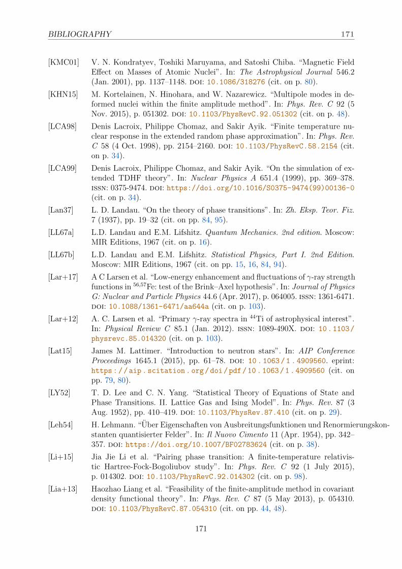
BIBLIOGRAPHY 171
[KMC01] V. N. Kondratyev, Toshiki Maruyama, and Satoshi Chiba. “Magnetic FieldEffect on Masses of Atomic Nuclei”. In: The Astrophysical Journal 546.2(Jan. 2001), pp. 1137–1148. doi: 10.1086/318276 (cit. on p. 80).
[KHN15] M. Kortelainen, N. Hinohara, and W. Nazarewicz. “Multipole modes in de-formed nuclei within the finite amplitude method”. In: Phys. Rev. C 92 (5Nov. 2015), p. 051302. doi: 10.1103/PhysRevC.92.051302 (cit. on p. 48).
[LCA98] Denis Lacroix, Philippe Chomaz, and Sakir Ayik. “Finite temperature nu-clear response in the extended random phase approximation”. In: Phys. Rev.C 58 (4 Oct. 1998), pp. 2154–2160. doi: 10.1103/PhysRevC.58.2154 (cit.on p. 34).
[LCA99] Denis Lacroix, Philippe Chomaz, and Sakir Ayik. “On the simulation of ex-tended TDHF theory”. In: Nuclear Physics A 651.4 (1999), pp. 369–378.issn: 0375-9474. doi: https://doi.org/10.1016/S0375-9474(99)00136-0(cit. on p. 34).
[Lan37] L. D. Landau. “On the theory of phase transitions”. In: Zh. Eksp. Teor. Fiz.7 (1937), pp. 19–32 (cit. on pp. 84, 95).
[LL67a] L.D. Landau and E.M. Lifshitz. Quantum Mechanics. 2nd edition. Moscow:MIR Editions, 1967 (cit. on p. 16).
[LL67b] L.D. Landau and E.M. Lifshitz. Statistical Physics, Part I. 2nd Edition.Moscow: MIR Editions, 1967 (cit. on pp. 15, 16, 84, 94).
[Lar+17] A C Larsen et al. “Low-energy enhancement and fluctuations of γ-ray strengthfunctions in 56,57Fe: test of the Brink–Axel hypothesis”. In: Journal of PhysicsG: Nuclear and Particle Physics 44.6 (Apr. 2017), p. 064005. issn: 1361-6471.doi: 10.1088/1361-6471/aa644a (cit. on p. 103).
[Lar+12] A. C. Larsen et al. “Primary γ-ray spectra in 44Ti of astrophysical interest”.In: Physical Review C 85.1 (Jan. 2012). issn: 1089-490X. doi: 10.1103/physrevc.85.014320 (cit. on p. 103).
[Lat15] James M. Lattimer. “Introduction to neutron stars”. In: AIP ConferenceProceedings 1645.1 (2015), pp. 61–78. doi: 10.1063/1.4909560. eprint:https://aip.scitation.org/doi/pdf/10.1063/1.4909560 (cit. onpp. 79, 80).
[LY52] T. D. Lee and C. N. Yang. “Statistical Theory of Equations of State andPhase Transitions. II. Lattice Gas and Ising Model”. In: Phys. Rev. 87 (3Aug. 1952), pp. 410–419. doi: 10.1103/PhysRev.87.410 (cit. on p. 29).
[Leh54] H. Lehmann. “Uber Eigenschaften von Ausbreitungsfunktionen und Renormierungskon-stanten quantisierter Felder”. In: Il Nuovo Cimento 11 (Apr. 1954), pp. 342–357. doi: https://doi.org/10.1007/BF02783624 (cit. on p. 38).
[Li+15] Jia Jie Li et al. “Pairing phase transition: A finite-temperature relativis-tic Hartree-Fock-Bogoliubov study”. In: Phys. Rev. C 92 (1 July 2015),p. 014302. doi: 10.1103/PhysRevC.92.014302 (cit. on p. 98).
[Lia+13] Haozhao Liang et al. “Feasibility of the finite-amplitude method in covariantdensity functional theory”. In: Phys. Rev. C 87 (5 May 2013), p. 054310.doi: 10.1103/PhysRevC.87.054310 (cit. on pp. 44, 48).
171
172 BIBLIOGRAPHY
[LMG65] H.J. Lipkin, N. Meshkov, and A.J. Glick. “Validity of many-body approxi-mation methods for a solvable model: (I). Exact solutions and perturbationtheory”. In: Nuclear Physics 62.2 (1965), pp. 188–198. issn: 0029-5582. doi:https://doi.org/10.1016/0029-5582(65)90862-X (cit. on p. 135).
[LS50] B. A. Lippmann and Julian Schwinger. “Variational Principles for ScatteringProcesses. I”. In: Phys. Rev. 79 (3 Aug. 1950), pp. 469–480. doi: 10.1103/PhysRev.79.469 (cit. on p. 35).
[LR21] Elena Litvinova and Caroline Robin. “Impact of complex many-body correla-tions on electron capture in thermally excited nuclei around Ni78”. In: Phys-ical Review C 103.2 (Feb. 2021). issn: 2469-9993. doi: 10.1103/physrevc.103.024326 (cit. on pp. 103, 118).
[LRW20] Elena Litvinova, Caroline Robin, and Herlik Wibowo. “Temperature depen-dence of nuclear spin-isospin response and beta decay in hot astrophysicalenvironments”. In: Physics Letters B 800 (Jan. 2020), p. 135134. issn: 0370-2693. doi: 10.1016/j.physletb.2019.135134 (cit. on pp. 103, 118).
[LW18] Elena Litvinova and Herlik Wibowo. “Finite-Temperature Relativistic Nu-clear Field Theory: An Application to the Dipole Response”. In: Physical Re-view Letters 121.8 (Aug. 2018). issn: 1079-7114. doi: 10.1103/physrevlett.121.082501 (cit. on pp. 103, 118).
[LW19] Elena Litvinova and Herlik Wibowo. “Nuclear response in a finite-temperaturerelativistic framework”. In: The European Physical Journal A 55.12 (Dec.2019). issn: 1434-601X. doi: 10.1140/epja/i2019-12771-9 (cit. on pp. 103,118).
[LPG09] K. Lodders, H. Palme, and H.-P. Gail. 4.4 Abundances of the elements inthe Solar System: Data sheet from Landolt-Bornstein - Group VI Astron-omy and Astrophysics · Volume 4B: “Solar System” in Springer Materials(https://doi.org/10.1007/978-3-540-88055-4 34). Ed. by J.E. Trumper. ac-cessed 2021-08-05. 2009. doi: 10.1007/978-3-540-88055-4_34 (cit. onp. 85).
[Lus86] M. Luscher. “Volume dependence of the energy spectrum in massive quantumfield theories”. In: Communications in Mathematical Physics 104 (2 June1986), pp. 177–206. doi: 10.1007/BF01211589 (cit. on p. 90).
[MS16] R Machleidt and F Sammarruca. “Chiral EFT based nuclear forces: achieve-ments and challenges”. In: Physica Scripta 91.8 (July 2016), p. 083007. doi:10.1088/0031-8949/91/8/083007 (cit. on pp. 10, 93, 129, 130).
[Mai05] Paul Mainwood. Phase Transitions in Finite Systems. 2005. eprint: http://philsci-archive.pitt.edu/8340/1/Phase_transitions_in_finite_
systems.pdf (cit. on p. 29).
[MVS09] P. Maris, J. P. Vary, and A. M. Shirokov. “Ab initio no-core full configurationcalculations of light nuclei”. In: Phys. Rev. C 79 (1 Jan. 2009), p. 014308.doi: 10.1103/PhysRevC.79.014308 (cit. on p. 90).
172
BIBLIOGRAPHY 173
[MER03a] V. Martin, J. L. Egido, and L. M. Robledo. “Publisher’s Note: Thermal shapefluctuation effects in the description of hot nuclei [Phys. Rev. C 68, 034327(2003)]”. In: Phys. Rev. C 68 (5 Nov. 2003), p. 059902. doi: 10.1103/PhysRevC.68.059902 (cit. on pp. 33, 94, 96, 98).
[MER03b] V. Martin, J. L. Egido, and L. M. Robledo. “Thermal shape fluctuationeffects in the description of hot nuclei”. In: Phys. Rev. C 68 (3 Sept. 2003),p. 034327. doi: 10.1103/PhysRevC.68.034327 (cit. on pp. 33, 94, 96, 98).
[MYT64] Toshio Marumori, Masatoshi Yamamura, and Akira Tokunaga. “On the “An-harmonic Effects” on the Collective Oscillations in Spherical Even Nuclei. I”.In: Progress of Theoretical Physics 31.6 (June 1964), pp. 1009–1025. issn:0033-068X. doi: 10.1143/PTP.31.1009. eprint: https://academic.oup.com/ptp/article- pdf/31/6/1009/5270097/31- 6- 1009.pdf (cit. onp. 36).
[MC90] G. J. Mathews and J. J. Cowan. “New insights into the astrophysical r-process”. In: Nature 345.6275 (June 1990), pp. 491–494. issn: 1476-4687.doi: 10.1038/345491a0 (cit. on p. 85).
[Miy+21] T. Miyagi et al. Converged ab initio calculations of heavy nuclei. 2021. arXiv:2104.04688 [nucl-th] (cit. on p. 114).
[Mol+95] P. Moller et al. “Nuclear Ground-State Masses and Deformations”. In: AtomicData and Nuclear Data Tables 59.2 (1995), pp. 185–381. issn: 0092-640X.doi: https://doi.org/10.1006/adnd.1995.1002 (cit. on p. 94).
[Mol+16] P. Moller et al. “Nuclear ground-state masses and deformations: FRDM(2012)”.In: Atomic Data and Nuclear Data Tables 109-110 (2016), pp. 1–204. issn:0092-640X. doi: https://doi.org/10.1016/j.adt.2015.10.002 (cit. onp. 94).
[Mor73] L.G. Moretto. “Finite temperature calculation of angular velocities and mo-ments of inertia in rotating nuclei”. In: Physics Letters B 44.6 (1973), pp. 494–496. issn: 0370-2693. doi: https://doi.org/10.1016/0370-2693(73)90006-3 (cit. on p. 94).
[Mot+95] T. Motobayashi et al. “Large deformation of the very neutron-rich nucleus32Mg from intermediate-energy Coulomb excitation”. In: Physics Letters B346.1 (1995), pp. 9–14. issn: 0370-2693. doi: https://doi.org/10.1016/0370-2693(95)00012-A (cit. on pp. 94, 143).
[Mus+14] M. T. Mustonen et al. “Finite-amplitude method for charge-changing tran-sitions in axially deformed nuclei”. In: Phys. Rev. C 90 (2 Aug. 2014),p. 024308. doi: 10.1103/PhysRevC.90.024308 (cit. on p. 128).
[NY05] T. Nakatsukasa and K. Yabana. “Unrestricted TDHF studies of nuclear re-sponse in the continuum”. In: The European Physical Journal A - Hadronsand Nuclei 25.1 (Sept. 2005), pp. 527–529. issn: 1434-601X. doi: 10.1140/epjad/i2005-06-052-x (cit. on p. 143).
173

174 BIBLIOGRAPHY
[NIY07] Takashi Nakatsukasa, Tsunenori Inakura, and Kazuhiro Yabana. “Finite am-plitude method for the solution of the random-phase approximation”. In:Phys. Rev. C 76 (2 Aug. 2007), p. 024318. doi: 10.1103/PhysRevC.76.024318 (cit. on pp. 11, 44, 47, 48, 127, 151).
[NJ61] Y. Nambu and G. Jona-Lasinio. “Dynamical Model of Elementary ParticlesBased on an Analogy with Superconductivity. II”. In: Phys. Rev. 124 (1 Oct.1961), pp. 246–254. doi: 10.1103/PhysRev.124.246 (cit. on p. 130).
[Nam50] Yoichiro Nambu. “Force Potentials in Quantum Field Theory”. In: Progressof Theoretical Physics 5.4 (July 1950), pp. 614–633. issn: 0033-068X. doi:10.1143/ptp/5.4.614. eprint: https://academic.oup.com/ptp/article-pdf/5/4/614/5430503/5-4-614.pdf (cit. on p. 35).
[Nam60] Yoichiro Nambu. “Quasi-Particles and Gauge Invariance in the Theory ofSuperconductivity”. In: Phys. Rev. 117 (3 Feb. 1960), pp. 648–663. doi: 10.1103/PhysRev.117.648 (cit. on p. 68).
[Ney+20] E. M. Ney et al. “Global description of β− decay with the axially deformedSkyrme finite-amplitude method: Extension to odd-mass and odd-odd nu-clei”. In: Phys. Rev. C 102 (3 Sept. 2020), p. 034326. doi: 10.1103/PhysRevC.102.034326 (cit. on pp. 44, 45).
[Nik+13] T. Niksic et al. “Implementation of the finite amplitude method for the rela-tivistic quasiparticle random-phase approximation”. In: Phys. Rev. C 88 (4Oct. 2013), p. 044327. doi: 10.1103/PhysRevC.88.044327 (cit. on pp. 44,48).
[Nis+17] H. Nishibata et al. “Shape coexistence in the N=19 neutron-rich nucleus 31Mgexplored by β − γ spectroscopy of spin-polarized 31Na”. In: Physics LettersB 767 (2017), pp. 81–85. issn: 0370-2693. doi: https://doi.org/10.1016/j.physletb.2017.01.049 (cit. on pp. 94, 143).
[Niu+09] Y.F. Niu et al. “Low-energy monopole and dipole response in nuclei at finitetemperature”. In: Physics Letters B 681.4 (Nov. 2009), pp. 315–319. issn:0370-2693. doi: 10.1016/j.physletb.2009.10.046 (cit. on p. 118).
[Noz64] P. Nozieres. Theory of interacting Fermi systems. New York: W.A. Benjamin,1964 (cit. on p. 35).
[OKH16] Tomohiro Oishi, Markus Kortelainen, and Nobuo Hinohara. “Finite ampli-tude method applied to the giant dipole resonance in heavy rare-earth nuclei”.In: Phys. Rev. C 93 (3 Mar. 2016), p. 034329. doi: 10.1103/PhysRevC.93.034329 (cit. on p. 48).
[Okn14] Andrzej Okninski. “On the Mechanism of Fermion-Boson Transformation”.In: International Journal of Theoretical Physics 53 (2014), pp. 2662–2667.doi: 10.1007/s10773-014-2062-4 (cit. on p. 33).
[Orr+91] N.A. Orr et al. “New mass measurements of neutron-rich nuclei near N=20”.In: Physics Letters B 258.1 (1991), pp. 29–34. issn: 0370-2693. doi: https://doi.org/10.1016/0370-2693(91)91203-8 (cit. on pp. 94, 143).
174
BIBLIOGRAPHY 175
[Paa+06] N. Paar et al. “Collective multipole excitations based on correlated realisticnucleon-nucleon interactions”. In: Phys. Rev. C 74 (1 July 2006), p. 014318.doi: 10.1103/PhysRevC.74.014318 (cit. on p. 11).
[Paa+09] N. Paar et al. “Calculation of stellar electron-capture cross sections on nucleibased on microscopic Skyrme functionals”. In: Phys. Rev. C 80 (5 Nov. 2009),p. 055801. doi: 10.1103/PhysRevC.80.055801 (cit. on pp. 103, 118).
[PW16] T Papenbrock and H A Weidenmuller. “Effective field theory for deformedatomic nuclei”. In: Physica Scripta 91.5 (Apr. 2016), p. 053004. issn: 1402-4896. doi: 10.1088/0031-8949/91/5/053004 (cit. on p. 10).
[PW14] T. Papenbrock and H. A. Weidenmuller. “Effective field theory for finitesystems with spontaneously broken symmetry”. In: Physical Review C 89.1(Jan. 2014). issn: 1089-490X. doi: 10.1103/physrevc.89.014334 (cit. onp. 10).
[Pen+11] D. Pena Arteaga et al. “Nuclear structure in strong magnetic fields: Nucleiin the crust of a magnetar”. In: Phys. Rev. C 84 (4 Oct. 2011), p. 045806.doi: 10.1103/PhysRevC.84.045806 (cit. on p. 80).
[PR08] Sara Perez-Martin and L. M. Robledo. “Microscopic justification of the equalfilling approximation”. In: Phys. Rev. C 78 (1 July 2008), p. 014304. doi:10.1103/PhysRevC.78.014304 (cit. on p. 127).
[PN66] David Pines and Philippe Nozieres. The theory of quantum liquids, volumeI: Normal Fermi liquids. eng. New York Amsterdam: W.A. Benjamin, 1966(cit. on pp. 34, 39).
[Pol88] A.M. Polyakov. “Fermi-Bose transmutations induced by gauge fields”. In:Modern Physics Letters A 03.03 (1988), pp. 325–328. doi: 10.1142/S0217732388000398.eprint: https://doi.org/10.1142/S0217732388000398 (cit. on p. 33).
[Pot10] Aleksandr Y Potekhin. “The physics of neutron stars”. In: Physics-Uspekhi53.12 (Dec. 2010), pp. 1235–1256. doi: 10.3367/ufne.0180.201012c.1279(cit. on pp. 79, 80).
[Qiu+19] Y. Qiu et al. “Particle-number projected Bogoliubov-coupled-cluster theory:Application to the pairing Hamiltonian”. In: Physical Review C 99.4 (Apr.2019). issn: 2469-9993. doi: 10.1103/physrevc.99.044301 (cit. on p. 86).
[Rai50] James Rainwater. “Nuclear Energy Level Argument for a Spheroidal Nu-clear Model”. In: Phys. Rev. 79 (3 Aug. 1950), pp. 432–434. doi: 10.1103/PhysRev.79.432 (cit. on p. 9).
[Rav+20] A. Ravli c et al. “Stellar electron-capture rates based on finite-temperaturerelativistic quasiparticle random-phase approximation”. In: Phys. Rev. C 102(6 Dec. 2020), p. 065804. doi: 10.1103/PhysRevC.102.065804 (cit. onpp. 103, 118).
[RA15] A. K. Rhine Kumar and P. Arumugam. “Thermal shape fluctuation modelstudy of the giant dipole resonance in 152Gd”. In: Phys. Rev. C 92 (4 Oct.2015), p. 044314. doi: 10.1103/PhysRevC.92.044314 (cit. on pp. 94, 98).
175

176 BIBLIOGRAPHY
[RG27] Lewis Fry Richardson and J. Arthur Gaunt. “VIII. The deferred approach tothe limit”. In: Philosophical Transactions of the Royal Society of London. Se-ries A, Containing Papers of a Mathematical or Physical Character 226.636-646 (1927), pp. 299–361. doi: 10.1098/rsta.1927.0008. eprint: https://royalsocietypublishing.org/doi/pdf/10.1098/rsta.1927.0008
(cit. on p. 115).
[RG11] Lewis Fry Richardson and Richard Tetley Glazebrook. “IX. The approxi-mate arithmetical solution by finite differences of physical problems involv-ing differential equations, with an application to the stresses in a masonrydam”. In: Philosophical Transactions of the Royal Society of London. Se-ries A, Containing Papers of a Mathematical or Physical Character 210.459-470 (1911), pp. 307–357. doi: 10.1098/rsta.1911.0009. eprint: https://royalsocietypublishing.org/doi/pdf/10.1098/rsta.1911.0009
(cit. on p. 115).
[RS80] P. Ring and P. Schuck. The nuclear many-body problem. New York: Springer-Verlag, 1980 (cit. on pp. 9, 30, 34, 35, 36).
[RB11] L. M. Robledo and G. F. Bertsch. “Global systematics of octupole excitationsin even-even nuclei”. In: Phys. Rev. C 84 (5 Nov. 2011), p. 054302. doi:10.1103/PhysRevC.84.054302 (cit. on p. 94).
[Rot+07] R. Roth et al. “Nuclear Structure in the UCOM Framework: From RealisticInteractions to Collective Excitations”. In: Nuclear Physics A 788.1-4 (May2007), pp. 12–19. issn: 0375-9474. doi: 10.1016/j.nuclphysa.2007.01.008(cit. on p. 133).
[Rot+14] Robert Roth et al. “Evolved chiral NN+3N Hamiltonians for ab initio nuclearstructure calculations”. In: Physical Review C 90.2 (Aug. 2014). issn: 1089-490X. doi: 10.1103/physrevc.90.024325 (cit. on pp. 86, 117).
[Row68] D. J. Rowe. “Equations-of-Motion Method and the Extended Shell Model”.In: Rev. Mod. Phys. 40 (1 Jan. 1968), pp. 153–166. doi: 10.1103/RevModPhys.40.153 (cit. on p. 35).
[Sak85] J. J. Sakurai. Modern Quantum Mechanics. 3rd ed. Cambridge UniversityPress, 1985. isbn: 0-8053-7501-5 (cit. on pp. 36, 39).
[SB51] E. E. Salpeter and H. A. Bethe. “A Relativistic Equation for Bound-StateProblems”. In: Phys. Rev. 84 (6 Dec. 1951), pp. 1232–1242. doi: 10.1103/PhysRev.84.1232 (cit. on p. 35).
[San+20] M. Sanchez Sanchez et al. “Improved description of light nuclei through chiraleffective field theory at leading order”. In: Phys. Rev. C 102 (2 Aug. 2020),p. 024324. doi: 10.1103/PhysRevC.102.024324 (cit. on p. 90).
[SH17] Guillaume Scamps and Yukio Hashimoto. “Transfer probabilities for thereactions 14,20O +20 O in terms of multiple time-dependent Hartree-Fock-Bogoliubov trajectories”. In: Phys. Rev. C 96 (3 Sept. 2017), p. 031602. doi:10.1103/PhysRevC.96.031602 (cit. on pp. 128, 154).
176
BIBLIOGRAPHY 177
[Sch26] E. Schrodinger. “An Undulatory Theory of the Mechanics of Atoms andMolecules”. In: Phys. Rev. 28 (6 Dec. 1926), pp. 1049–1070. doi: 10.1103/PhysRev.28.1049 (cit. on p. 14).
[Sch+20] P. Schuck et al. “Equation of Motion Method to strongly correlated Fermisystems and Extended RPA approaches”. In: (Sept. 2020). doi: arXiv:2009.00591 (cit. on pp. 34, 35, 36).
[Sch19] Nicolas Schunck, ed. Energy Density Functional Methods for Atomic Nuclei.2053-2563. IOP Publishing, 2019. isbn: 978-0-7503-1422-0. doi: 10.1088/2053-2563/aae0ed (cit. on p. 40).
[Sch51] Julian Schwinger. “On the Green’s functions of quantized fields. I”. In: Pro-ceedings of the National Academy of Sciences 37.7 (July 1951), pp. 452–455.issn: 0027-8424. doi: 10.1073/pnas.37.7.452. eprint: https://www.pnas.org/content/37/7/452.full.pdf (cit. on p. 35).
[SHB13] Gustavo E. Scuseria, Thomas M. Henderson, and Ireneusz W. Bulik. “Particle-particle and quasiparticle random phase approximations: Connections to cou-pled cluster theory”. In: The Journal of Chemical Physics 139.10 (2013),p. 104113. doi: 10.1063/1.4820557. eprint: https://doi.org/10.1063/1.4820557 (cit. on p. 35).
[SHS08] Gustavo E. Scuseria, Thomas M. Henderson, and Danny C. Sorensen. “Theground state correlation energy of the random phase approximation from aring coupled cluster doubles approach”. In: The Journal of Chemical Physics129.23 (2008), p. 231101. doi: 10.1063/1.3043729. eprint: https://doi.org/10.1063/1.3043729 (cit. on p. 35).
[SY14] Kazuyuki Sekizawa and Kazuhiro Yabana. “Particle-number projection methodin time-dependent Hartree-Fock theory: Properties of reaction products”. In:Phys. Rev. C 90 (6 Dec. 2014), p. 064614. doi: 10.1103/PhysRevC.90.064614 (cit. on pp. 128, 154).
[SR00] Javid A. Sheikh and Peter Ring. “Symmetry-projected Hartree–Fock–Bogoliubovequations”. In: Nuclear Physics A 665.1 (2000), pp. 71–91. issn: 0375-9474.doi: https://doi.org/10.1016/S0375-9474(99)00424-8 (cit. on p. 128).
[Sim10] Cedric Simenel. “Particle Transfer Reactions with the Time-Dependent Hartree-Fock Theory Using a Particle Number Projection Technique”. In: Phys. Rev.Lett. 105 (19 Nov. 2010), p. 192701. doi: 10.1103/PhysRevLett.105.192701(cit. on pp. 128, 154).
[Som+14] V. Soma et al. “Chiral two- and three-nucleon forces along medium-massisotope chains”. In: Physical Review C 89.6 (June 2014). issn: 1089-490X.doi: 10.1103/physrevc.89.061301 (cit. on p. 86).
[Som20] Vittorio Soma. “Self-Consistent Green’s Function Theory for Atomic Nuclei”.In: Frontiers in Physics 8 (2020), p. 340. issn: 2296-424X. doi: 10.3389/fphy.2020.00340 (cit. on p. 38).
177

178 BIBLIOGRAPHY
[Som83] H. Michael Sommermann. “Microscopic description of giant resonances inhighly excited nuclei”. In: Annals of Physics 151.1 (1983), pp. 163–203. issn:0003-4916. doi: https://doi.org/10.1016/0003-4916(83)90318-4 (cit.on pp. 34, 35, 40, 56, 57, 58).
[SJJ50] Helmut Steinwedel, J. Hans D. Jensen, and Peter Jensen. “Nuclear DipoleVibrations”. In: Phys. Rev. 79 (6 Sept. 1950), pp. 1019–1019. doi: 10.1103/PhysRev.79.1019 (cit. on p. 120).
[Sto+11] M. Stoitsov et al. “Monopole strength function of deformed superfluid nuclei”.In: Phys. Rev. C 84 (4 Oct. 2011), p. 041305. doi: 10.1103/PhysRevC.84.041305 (cit. on pp. 44, 48).
[SL17] Xuwei Sun and Dinghui Lu. “Implementation of a finite-amplitude methodin a relativistic meson-exchange model”. In: Phys. Rev. C 96 (2 Aug. 2017),p. 024614. doi: 10.1103/PhysRevC.96.024614 (cit. on p. 48).
[SHI72] Yasuyuki Suzuki, Hisashi Horiuchi, and Kiyomi Ikeda. “Study of α ChainStates through Their Decay Widths”. In: Progress of Theoretical Physics 47.5(May 1972), pp. 1517–1536. issn: 0033-068X. doi: 10.1143/PTP.47.1517.eprint: https://academic.oup.com/ptp/article- pdf/47/5/1517/5304507/47-5-1517.pdf (cit. on pp. 102, 143).
[Tic+18] A. Tichai et al. “Bogoliubov many-body perturbation theory for open-shellnuclei”. In: Physics Letters B 786 (Nov. 2018), pp. 195–200. issn: 0370-2693.doi: 10.1016/j.physletb.2018.09.044 (cit. on p. 86).
[TRD20] Alexander Tichai, Robert Roth, and Thomas Duguet. Many-body perturba-tion theories for finite nuclei. 2020. arXiv: 2001.10433 [nucl-th] (cit. onp. 86).
[Tic+16] Alexander Tichai et al. “Hartree–Fock many-body perturbation theory fornuclear ground-states”. In: Physics Letters B 756 (May 2016), pp. 283–288.issn: 0370-2693. doi: 10.1016/j.physletb.2016.03.029 (cit. on p. 86).
[Tic+19] Alexander Tichai et al. “Natural orbitals for ab initio no-core shell modelcalculations”. In: Phys. Rev. C 99 (3 Mar. 2019), p. 034321. doi: 10.1103/PhysRevC.99.034321 (cit. on pp. 90, 92).
[Tse13] V. I. Tselyaev. “Subtraction method and stability condition in extendedrandom-phase approximation theories”. In: Phys. Rev. C 88 (5 Nov. 2013),p. 054301. doi: 10.1103/PhysRevC.88.054301 (cit. on p. 34).
[UK51] Hiroomi Umezawa and Susumu Kamefuchi. “The Vacuum in Quantum Elec-trodynamics”. In: Progress of Theoretical Physics 6.4 (Aug. 1951), pp. 543–558. issn: 0033-068X. doi: 10 . 1143 / ptp / 6 . 4 . 543. eprint: https : / /academic.oup.com/ptp/article-pdf/6/4/543/5418774/6-4-543.pdf
(cit. on p. 38).
[VBG09] Sergey Vaintraub, Nir Barnea, and Doron Gazit. “6He β-decay rate and thesuppression of the axial constant in nuclear matter”. In: Phys. Rev. C 79 (6June 2009), p. 065501. doi: 10.1103/PhysRevC.79.065501 (cit. on p. 90).
178
BIBLIOGRAPHY 179
[VGG18] O. Vasseur, D. Gambacurta, and M. Grasso. “Systematic study of giantquadrupole resonances with the subtracted second random-phase approxi-mation: Beyond-mean-field centroids and fragmentation”. In: Phys. Rev. C98 (4 Oct. 2018), p. 044313. doi: 10.1103/PhysRevC.98.044313 (cit. onp. 34).
[VM84] D. Vautherin and N.Vinh Mau. “Temperature dependence of collective statesin the random-phase approximation”. In: Nuclear Physics A 422.1 (1984),pp. 140–156. issn: 0375-9474. doi: https://doi.org/10.1016/0375-9474(84)90434-2 (cit. on p. 40).
[Voi+04] A. Voinov et al. “Large Enhancement of Radiative Strength for Soft Tran-sitions in the Quasicontinuum”. In: Phys. Rev. Lett. 93 (14 Sept. 2004),p. 142504. doi: 10.1103/PhysRevLett.93.142504 (cit. on p. 102).
[Voi+06] A. V. Voinov et al. “Level density of 56Fe and low-energy enhancement ofγ-strength function”. In: Phys. Rev. C 74 (1 July 2006), p. 014314. doi:10.1103/PhysRevC.74.014314 (cit. on pp. 102, 103).
[WHN21] Kouhei Washiyama, Nobuo Hinohara, and Takashi Nakatsukasa. “Finite-amplitude method for collective inertia in spontaneous fission”. In: Phys.Rev. C 103 (1 Jan. 2021), p. 014306. doi: 10.1103/PhysRevC.103.014306(cit. on p. 128).
[Wei79] Steven Weinberg. “Phenomenological Lagrangians”. In: Physica A: StatisticalMechanics and its Applications 96.1 (1979), pp. 327–340. issn: 0378-4371.doi: https://doi.org/10.1016/0378-4371(79)90223-1 (cit. on p. 10).
[WL19] Herlik Wibowo and Elena Litvinova. “Nuclear dipole response in the finite-temperature relativistic time-blocking approximation”. In: Physical ReviewC 100.2 (Aug. 2019). issn: 2469-9993. doi: 10.1103/physrevc.100.024307(cit. on pp. 103, 118).
[Wic50] G. C. Wick. “The Evaluation of the Collision Matrix”. In: Phys. Rev. 80 (2Oct. 1950), pp. 268–272. doi: 10.1103/PhysRev.80.268 (cit. on p. 20).
[WK74] Kenneth G. Wilson and J. Kogut. “The renormalization group and the ϵexpansion”. In: Physics Reports 12.2 (1974), pp. 75–199. issn: 0370-1573.doi: https://doi.org/10.1016/0370-1573(74)90023-4 (cit. on p. 19).
[Yan+19] Zhenjie Yan et al. “Boiling a Unitary Fermi Liquid”. In: Phys. Rev. Lett. 122(9 Mar. 2019), p. 093401. doi: 10.1103/PhysRevLett.122.093401 (cit. onp. 103).
[Yan+03] Y. Yanagisawa et al. “The first excited state of 30Ne studied by proton in-elastic scattering in reversed kinematics”. In: Physics Letters B 566.1 (2003),pp. 84–89. issn: 0370-2693. doi: https : / / doi . org / 10 . 1016 / S0370 -2693(03)00802-5 (cit. on pp. 94, 143).
[Yan+04] Y. Yanagisawa et al. “The first excited state of 30Ne studied by proton in-elastic scattering in reversed kinematics”. In: Nuclear Physics A 734 (2004),pp. 374–377. issn: 0375-9474. doi: https://doi.org/10.1016/j.nuclphysa.2004.01.071 (cit. on pp. 94, 143).
179
180 BIBLIOGRAPHY
[YL52] C. N. Yang and T. D. Lee. “Statistical Theory of Equations of State andPhase Transitions. I. Theory of Condensation”. In: Phys. Rev. 87 (3 Aug.1952), pp. 404–409. doi: 10.1103/PhysRev.87.404 (cit. on p. 29).
[Yan87] Constantine Yannouleas. “Zero-temperature second random phase approx-imation and its formal properties”. In: Phys. Rev. C 35 (3 Mar. 1987),pp. 1159–1161. doi: 10.1103/PhysRevC.35.1159 (cit. on pp. 34, 35).
[You09] W. Younes. “Gaussian matrix elements in a cylindrical harmonic oscillatorbasis”. In: Computer Physics Communications 180.7 (July 2009), pp. 1013–1040. issn: 0010-4655. doi: 10.1016/j.cpc.2008.12.021 (cit. on p. 146).
[Yuk+14] E. Yuksel et al. “Effect of temperature on the effective mass and the neu-tron skin of nuclei”. In: The European Physical Journal A 50.10 (Oct. 2014),p. 160. issn: 1434-601X. doi: 10.1140/epja/i2014-14160-4 (cit. on pp. 103,118).
[Yuk+17] E. Yuksel et al. “Multipole excitations in hot nuclei within the finite temper-ature quasiparticle random phase approximation framework”. In: Phys. Rev.C 96 (2 Aug. 2017), p. 024303. doi: 10.1103/PhysRevC.96.024303 (cit. onpp. 103, 118, 119).
[Yuk+19] E. Yuksel et al. “Nuclear excitations within microscopic EDF approaches:Pairing and temperature effects on the dipole response”. In: The EuropeanPhysical Journal A 55.12 (Dec. 2019), p. 230. issn: 1434-601X. doi: 10.1140/epja/i2019-12918-8 (cit. on pp. 103, 118).
[Yuk+20] E. Yuksel et al. “Gamow-Teller excitations at finite temperature: Competi-tion between pairing and temperature effects”. In: Phys. Rev. C 101 (4 Apr.2020), p. 044305. doi: 10.1103/PhysRevC.101.044305 (cit. on pp. 103,118).
[Zee10] A. Zee. Quantum field theory in a nutshell (2nd edn). 2010. isbn: 978-0-691-14034-6. doi: 10.1088/0264-9381/28/8/089003 (cit. on p. 20).
[ZN17] W. Zhang and Y. F. Niu. “Shape transition with temperature of the pear-shaped nuclei in covariant density functional theory”. In: Phys. Rev. C 96 (5Nov. 2017), p. 054308. doi: 10.1103/PhysRevC.96.054308 (cit. on pp. 94,98).
[ZMR03] Shan-Gui Zhou, Jie Meng, and P. Ring. “Spherical relativistic Hartree theoryin a Woods-Saxon basis”. In: Physical Review C 68.3 (Sept. 2003). issn: 1089-490X. doi: 10.1103/physrevc.68.034323 (cit. on p. 143).
[Zum62] Bruno Zumino. “Normal Forms of Complex Matrices”. In: Journal of Mathe-matical Physics 3.5 (1962), pp. 1055–1057. doi: 10.1063/1.1724294. eprint:https://doi.org/10.1063/1.1724294 (cit. on p. 30).
180
Copyright © 2022 FDOKUMEN