arX

iv:0

906.

1463

v2 [

nucl

-th]

11

Sep

2009

Toward ab initio density functional theory for nuclei

J.E. Drut, R.J. Furnstahl, L. PlatterDepartment of Physics, Ohio State University, Columbus, OH 43210

September 16, 2018

Abstract

We survey approaches to nonrelativistic density functional theory (DFT) for nuclei usingprogress toward ab initio DFT for Coulomb systems as a guide. Ab initio DFT starts with a micro-scopic Hamiltonian and is naturally formulated using orbital-based functionals, which generalizethe conventional local-density-plus-gradients form. The orbitals satisfy single-particle equationswith multiplicative (local) potentials. The DFT functionals can be developed starting from inter-nucleon forces using wave-function based methods or by Legendre transform via effective actions.We describe known and unresolved issues for applying these formulations to the nuclear many-body problem and discuss how ab initio approaches can help improve empirical energy densityfunctionals.

Keywords: Density functional theory, nuclear structure, many-body perturbation theory

Contents

1 Introduction 21.1 Overview . . . . . . . . . . . . . . . . . . . . . . . . . . . . . . . . . . . . . . . . . . . . 21.2 Basic features/ingredients of DFT . . . . . . . . . . . . . . . . . . . . . . . . . . . . . . 31.3 Coulomb vs. nuclear DFT . . . . . . . . . . . . . . . . . . . . . . . . . . . . . . . . . . 81.4 Scope and plan of review . . . . . . . . . . . . . . . . . . . . . . . . . . . . . . . . . . . 10

2 Orbital-based DFT 112.1 Hartree-Fock in coordinate representation . . . . . . . . . . . . . . . . . . . . . . . . . 112.2 Motivation for orbital-dependent functionals . . . . . . . . . . . . . . . . . . . . . . . . 132.3 Derivation of the optimized effective potential . . . . . . . . . . . . . . . . . . . . . . . 172.4 OEP from total energy minimization or density invariance . . . . . . . . . . . . . . . . 192.5 Approximations . . . . . . . . . . . . . . . . . . . . . . . . . . . . . . . . . . . . . . . . 21

3 DFT and ab initio wave function methods 223.1 Goldstone many-body perturbation theory . . . . . . . . . . . . . . . . . . . . . . . . . 223.2 Improved perturbation theory . . . . . . . . . . . . . . . . . . . . . . . . . . . . . . . . 253.3 Low-momentum interactions . . . . . . . . . . . . . . . . . . . . . . . . . . . . . . . . . 283.4 Density matrix expansion . . . . . . . . . . . . . . . . . . . . . . . . . . . . . . . . . . 30

4 DFT as Legendre transform 384.1 Analogy to Legendre transform in thermodynamics . . . . . . . . . . . . . . . . . . . . 404.2 Effective actions for composite operators . . . . . . . . . . . . . . . . . . . . . . . . . . 424.3 EFT and power counting for functionals . . . . . . . . . . . . . . . . . . . . . . . . . . 464.4 Additional comments . . . . . . . . . . . . . . . . . . . . . . . . . . . . . . . . . . . . . 48

1

5 Topics for nuclear DFT 49

5.1 Pairing . . . . . . . . . . . . . . . . . . . . . . . . . . . . . . . . . . . . . . . . . . . . . 49

5.2 Broken symmetries . . . . . . . . . . . . . . . . . . . . . . . . . . . . . . . . . . . . . . 53

5.3 Single-particle energies . . . . . . . . . . . . . . . . . . . . . . . . . . . . . . . . . . . . 55

5.4 Improving empirical EDF’s . . . . . . . . . . . . . . . . . . . . . . . . . . . . . . . . . . 56

6 Summary and outlook 58

References 62

1 Introduction

1.1 Overview

Density functional theory (DFT) has been applied to the Coulomb many-body problem with greatphenomenological success in predicting properties of atoms, molecules, and solids [1, 2, 3, 4, 5, 6]. DFTcalculations are comparatively simple to implement yet often very accurate and have a computationalcost that makes them at present the only choice for systems with large numbers of electrons [7]. For thesesame reasons (with nucleons rather than electrons), large-scale collaborations of nuclear physicists in theSciDAC UNEDF [8, 9] (“Universal Nuclear Energy Density Functional”) and FIDIPRO [10] projects,as well as many other individuals, are working on further developing DFT for the nuclear many-bodyproblem. Questions in astrophysics and the advent of new experimental facilities to study nuclei atthe limits of existence, as well as societal needs, are driving multi-pronged efforts to calculate nuclearproperties and reactions across the full table of the nuclides more accurately and reliably than what iscurrently possible with existing energy density functional (EDF) methods (e.g., those based on Skyrme,Gogny, or relativistic mean-field functionals [11]).

A principal strategy is to exploit the substantial and ongoing progress in ab initio nuclear struc-ture calculations, which are primarily based on approximating the many-nucleon wave function. Thisprogress is the consequence of synergistic advances in the construction of internucleon interactions, inmethods to calculate properties of many-nucleon systems, and in the ability to effectively use grow-ing computational power [8]. Because these approaches will be limited in scope for the foreseeablefuture, a natural goal is to develop ab initio DFT for nuclei. In this context, “ab initio” is taken tomean a formalism based directly on a microscopic nuclear Hamiltonian that describes two-nucleon andfew-body scattering and bound-state observables, in analogy to calculations in quantum chemistry orcondensed matter physics that start from the Coulomb interaction. This contrasts with many nuclearEDF approaches [11] that fit a functional without relying on an explicit underlying Hamiltonian [12].Efforts to construct bridges between ab initio few-body calculations and the largely empirical nuclearEDF’s are bringing together diverse theorists and formal techniques using insights from other fields.The language and formalism differences are a barrier to progress. We hope to lessen this barrier withthis review by setting up ab initio DFT as an intermediary.

There are multiple possible paths to ab initio DFT and the optimal choice for describing nuclei isnot clear. In confronting the limitations of the most widely used conventional Coulomb DFT implemen-tations (such as so-called “generalized gradient approximation” or GGA functionals), condensed matterphysicists and quantum chemists have made extensive developments toward ab initio Coulomb DFTbased on wave-function methods. We would like to exploit these advances. This means understandingwhat can be borrowed directly for nuclei and where modifications are needed. At the same time, DFTbased on effective actions may suggest alternative approximations as well as connections to effectivefield theory (EFT). The goal of this review is to outline various strategies that are being adopted (or

2

may be explored soon), identify common features and challenges, and generally make them more acces-sible to the various communities of nuclear physicists attacking these problems. We restrict ourselvesto a definition of ab initio DFT that is consistent with usage in Coulomb systems (see Section 1.2)but which is a subset of the full range of efforts pointing toward non-empirical nuclear EDF (e.g., seeRefs. [13, 14, 15, 16]).

The focus on ab initio DFT does not mean we propose abandoning the successes of the empiricalEDF’s, which already achieve an accuracy for known nuclear masses that will be hard to reach directlywith ab initio functionals. Furthermore, it will only be possible in the near future to make ab initio

calculations of a limited subset of all nuclei. DFT was originally formulated and is still typicallydescribed in terms of existence proofs. These proofs imply that it is possible to find a functional (orfunctionals) that depends only explicitly on the density and which is minimized at the ground stateenergy with the ground state density. While these proofs are not constructive, they can be taken tojustify empirical nuclear EDF approaches. An important prong of the nuclear DFT effort seeks to makethe EDF’s less empirical and therefore more reliable for extrapolation to unmeasured nuclear propertiesby generalizing or constraining the functionals based on ab initio input. This can be done directlyusing constraints from accurate ab initio nuclear structure calculations (e.g., fitting the theoreticalneutron matter equation of state) but also through insights from ab initio DFT about the form andcharacteristics of the functionals.

1.2 Basic features/ingredients of DFT

Our discussion is based on the nuclear many-body problem formulated in terms of a nonrelativisticSchrodinger equation for protons and neutrons, with a Hamiltonian of the form

HN = T + V ≡ T + VNN + VNNN + . . . , (1)

where T is the kinetic energy and V is the sum of two- and three- and higher-body forces in a decreas-ing hierarchy, which is truncated at three-body forces in the most complete present-day calculations.(Effects from relativity and other degrees of freedom are absorbed into the potentials either explicitly orimplicitly.) Such Hamiltonians are derived in low-energy effective theories of quantum chromodynamics(QCD) with varying degrees of model dependence. The development of better Hamiltonians, and ofmany-body forces in particular, is an on-going enterprise [17]. We emphasize that “Hamiltonians” isplural because there is not a unique or even preferred form of the short-distance parts of the potentials(the longest-ranged part, pion exchange, does have a common, local form in almost all potentials).Contrast this with the electronic case, where the long-range Coulomb potential is for many systems theentire story.

For most of our discussion it is irrelevant whether the Hamiltonian being used results from a sys-tematic effective field theory (EFT) expansion [17] or a more phenomenological form [18], as long as itreproduces few-body observables. What is relevant is that the initial Hamiltonian can be transformed(e.g., with renormalization group methods) to maintain observables while making it more suitable forparticular many-body methods (see below). We argue that transformations to soften the potential willbe critical in making DFT a feasible framework for nuclei; that is, DFT implies an organization of themany-body problem that will not work well with all nuclear Hamiltonians.

We can classify microscopic nuclear structure methods into two broad categories, wave function andGreen’s function methods. In the former, one solves in some approximation the A-body Schrodingerequation for the A-body wave function Ψ(x1, · · · , xA), where xi is shorthand for all of the variablesof nucleon i (e.g., xi, spin, isospin). If the operators are known, this allows the calculation of anynuclear observable. Methods in this category include Green’s function1 and auxiliary field Monte Carlo

1Despite the name, GFMC is not a Green’s function method in the sense it is used here.

3

(GFMC/AFMC) [19, 20], no-core shell model (NCSM) [21], and coupled cluster (CC) [22, 23]. Thecomputational cost of such calculations rises rapidly with A. Nevertheless, most of the recent progressin ab initio nuclear structure physics has come from pushing these techniques to higher A [24, 21, 25].

Our ab initio DFT discussion will connect to wave-function based formulations that use a single-particle basis and can handle non-local interactions (e.g., NCSM and CC but not GFMC). In principle,

such a formulation solves the problem of finding the ground-state energy Egs of a given HN (for a

specified number of nucleons A) by minimizing 〈Ψ|HN |Ψ〉 over all normalized anti-symmetric A-particlewave functions [4]:

Egs = minΨ〈Ψ|HN |Ψ〉 . (2)

In practice, of course, the Hilbert space (i.e., the basis size) is finite and Egs is found approximately.(The calculation is also not variational in many cases, such as CC, but that is not an issue here.)

An alternative to working with the many-body wave function is density functional theory (DFT)[1, 4, 26], which as the name implies, has fermion densities as the fundamental “variables”. We willstart with DFT as it is typically introduced, citing a theorem of Hohenberg and Kohn (HK) [27]: Thereexists an energy functional Ev[ρ] of the density ρ(x),2 labeled by a (static) external potential vext(x)such that

Ev[ρ] = F [ρ] +

∫dx vext(x)ρ(x) , (3)

which is minimized at the ground-state energy Egs with the ground-state density ρgs(x). An exampleof vext is the electrostatic potential from ions in atoms and molecules, as in Eq. (30). The functional F ,often designated FHK in the literature, is independent of the external potential vext and has the sameform for any A. In this sense it is said to be universal . The HK theorem offers no help in constructingF , but is useful in that it gives a license to search for (or guess) approximate energy functionals. Thiswould serve as justification for nuclear EDF’s except for the disquieting feature that there is no vext forself-bound nuclei, which makes the meaning of Eq. (3) unclear.

A constrained search derivation [28] is a more illuminating alternative to the proof-by-contradictionapproach to DFT used by Hohenberg and Kohn. We start as before with the minimization in Eq. (2),adding an external potential, but now we separate the minimization into two steps [4]:

1. First minimize over all Ψ that yield a given density ρ(x):

minΨ→ρ〈Ψ|HN + Vext|Ψ〉 = min

Ψ→ρ〈Ψ|T + V |Ψ〉+

∫dx vext(x)ρ(x) , (4)

where V is the full internucleon interaction and Vext =∫dx vext(x)ρ(x). Define F [ρ] as the resulting

contribution of the first term:F [ρ] ≡ 〈Ψmin

ρ |T + V |Ψminρ 〉 . (5)

2. Then minimize over ρ(x):

E = minρEv[ρ] ≡ min

ρ

F [ρ] +

∫dx vext(x)ρ(x)

. (6)

where the external potential vext(x) is held fixed.

In principle one works at fixed A by introducing a chemical potential µ:

δF [ρ] +

∫dx vext(x)ρ(x)− µ

∫dx ρ(x)

= 0 , (7)

2As discussed below, we will have multiple densities in practice but considering the fermion density only suffices fornow.

4

which impliesδF [ρ]

δρ(x)+ vext(x) = µ . (8)

The chemical potential is adjusted until the density ρ resulting from solving Eq. (8) yields the desiredparticle number A. Or one minimizes only over ρ that satisfy

∫dx ρ(x) = A.

As noted by Kutzelnigg [29], the presentation of the HK theorem as an existence proof is oftenaccompanied by misleading statements such as “all information about a quantum mechanical groundstate is contained in its electron density ρ” or that “the energy is completely expressible in terms ofthe density alone.” These claims seem at odds with the observation that while the external potentialenergy is expressible in terms of ρ (if there is a vext), the kinetic energy is given in terms of the one-particle density matrix and interaction energies require two-particle and higher density matrices. Howdo we reconcile this? The key is that the usual wave-function treatment of the many-body problem asin Eq. (2) has in mind a single, fixed Hamiltonian. In that case, to make a variational calculation ofthe ground-state wave function Ψ, the energy E must be made stationary to variations in the relevantdensity matrices and not just the density. This corresponds to variations of the normalized A-bodywave function Ψ.

To understand DFT we should consider instead a family of Hamiltonians H [v], each characterizedby a potential v for which we know the corresponding ground state energy E[v]. We might ask, if weknow E[v], why not just evaluate at v = vext and avoid more complications? But if we do know E[v],then we can construct the functional Legendre transform [29],

− F [ρ] = minv

∫dx v(x)ρ(x)− E[v]

, (9)

where the minimization is over an appropriate domain of v (really the infimum or greatest lower bound)rather than just considering a fixed vext [29]. Thus we obtain the dependence of the internal energyon the density. This justifies the suggestive notation of Eq. (3): If v(x) is set to a constant, it actsas a chemical potential and the equation expresses a Legendre transform between two thermodynamicpotentials. (An expanded version of the thermodynamic analogy is given in Section 4.) If the Legendretransform is possible (see Ref. [30, 29]), we can also obtain with a second Legendre transformation that

E[v] = minρ

∫dx v(x)ρ(x) + F [ρ]

≡ min

ρ

Ev[ρ]

, (10)

which is the energy for fixed v expressed as a minimization over a trial set of densities. Thus wereproduce Eq. (6) and show the origin of the HK expression in Eq. (3).

This perspective shows that DFT and Eq. (3) are really in the spirit of the other major categoryof microscopic nuclear structure methods, namely Green’s functions. Instead of the many-body wavefunction, the Green’s function approach considers the response of the ground state to adding or removingparticles [31, 32, 33]. The underlying idea is that knowing the most general response of the ground state(or the partition function in the presence of the most general sources) gives a complete specification of themany-body problem. Observables such as the ground state energy, densities, single-particle excitations,and more can be expressed in terms of Green’s functions (with one-body operators needing the single-particle Green’s function, two-body operators generally needing the two-particle Green’s function, andso on). The special case considered here starts with the response of the energy to a “source” v(x),which is coupled to the density. Instead of non-local sources that individually create particles in oneplace and destroy them elsewhere, here the perturbation by the source is a local shift in the density.Because it is a more limited response than the usual Green’s functions, the corresponding observablesprobed are also limited, but include the ground-state energy. A natural mathematical framework forsuch responses and other Legendre transforms is the effective action formalism using path integrals. We

5

VHO

=⇒VKS

Figure 1: Kohn-Sham DFT for a vext = VHO harmonic trap. On the left is the interacting system andon the right the Kohn-Sham system. The density profile is the same in each.

give more details in Section 4 on how this works. (This perspective also shows that taking v = 0 is nota problem in principle; such sources are usually set equal to zero at the end, although in this case thereare related issues with self-bound systems such as nuclei.)

In practice, DFT is rarely implemented as a pure functional of the density, such as a generalizedThomas-Fermi functional, because no one has succeeded in constructing one that yields the desiredaccuracy (an immediate problem is finding an adequate functional of density only for the kinetic energy).Instead, the most successful procedure is to introduce single-particle orbitals that are used in whatappears to be an auxiliary problem, but which still leads to the minimization of the energy functionalfor the ground-state energy Egs and density ρgs. This is called Kohn-Sham (KS) DFT, and is illustratedschematically in Fig. 1 for fermions in a harmonic trap. The characteristic feature is that the interactingdensity for A fermions in the external potential vext is equal (by construction) to the non-interactingdensity in another single-particle potential. This is achieved by orbitals φi(x) in the local potentialvKS([ρ],x) ≡ vKS(x), which are solutions to

[−∇2/2m+ vKS(x)]φi(x) = εiφi(x) , (11)

and determine the density by

ρ(x) =∑

i

ni|φi(x)|2 =

A∑

i=1

|φi(x)|2 , (12)

where the sum is over the lowest A states with ni = θ(εF − εi) here. When we include pairing, thesum is generalized to be over all orbitals with appropriate occupation numbers (see Section 5.1). Themagic Kohn-Sham potential vKS([ρ],x) is in turn determined from δEv[ρ]/δρ(x) (see below). Thus theKohn-Sham orbitals depend on the potential, which depends on the density, which depends on theorbitals, so we must solve self-consistently (for example, by iterating until convergence). We will returnlater to address the meaning of the KS eigenvalues εi. The ground-state energy is Egs = Evext [ρgs].

We will define orbital-based density functional theory (DFT) broadly as any many-body methodbased on a local (“multiplicative”) background potential (what we called vKS above) used to calculatethe ground-state energy and density of inhomogeneous systems in the manner just described. That is,there will be a single-particle, non-interacting component of the problem that involves solving for orbitalswith a local (diagonal in coordinate space) potential. We will also require that there are no correctionsto the density obtained from these occupied orbitals (as in usual Kohn-Sham DFT). It is not obvious atthis point that this is a necessary feature, because it is not essential to the numerical simplicity or goodscaling behavior. We will see in later sections how it arises. This characterization of DFT can be realizedin seemingly very different approaches, such as a particular organization of (possibly resummed) many-body perturbation theory (MBPT) and effective actions for composite operators (based on functionalLegendre transformations). The DFT formalism is often said to be a mean-field approach because ofthe Kohn-Sham potential and this applies to our general definition as well. The point is that it is not a

6

mean-field approximation but an organization that takes a mean-field state as a reference state, whichif solved completely includes all many-body correlations. (The real issue is how much correlation isincluded in a given approximation to the exact functional.)

Energy

Functional

Orbitals and Occupation Numbers

Kohn-Sham Potentials

Schrödinger-Eqn. Solver

Figure 2: Generic self-consistency cycle for Kohn-Sham DFT. The energy functional takes orbital wavefunctions and eigenvalues (with occupation numbers) as inputs. The outputs are the local Kohn-Shampotentials from the functional derivative of the energy functional. These could be directly evaluated aswith a Skyrme or density matrix expansion functional, or solved from OEP equations.

Implementations of orbital-based DFT will have a self-consistency cycle of the form shown in Fig. 2.The code that solves the KS single-particle Schrodinger equations (“Schrodinger-Eqn. Solver”) can begeneric (if generalized to include pairing) because the same equations are solved for different energyfunctionals (only the potentials change). This part of the calculation is generally the key to the com-putational scaling because the cost goes up gently with A and it also means that we can adapt thewell-developed tools used for Skyrme calculations. The “Energy Functional” will be particular to theimplementation, ranging from simple function evaluation to solving complicated integral equations. Ifthe cost of evaluating this box, which includes calculating the functional derivative defining vKS, can bekept under control, the computational advantage will hold. (Conversely, in full calculations of orbital-based DFT, one has to consider seriously the computational scaling when comparing to alternativestrategies.) It is often the case that the energy functional is taken to be of the local or semi-local3 form:

E[ρi, τi, . . .] =

∫dx E(ρi(x), τi(x), . . .) , (13)

where we have allowed different types of densities such as the kinetic energy density τi and where depen-dence on gradients of the densities is also allowed. For example, the Skyrme functional in Eq. (101) hasthis structure. We emphasize that this is not a general form, but requires significant approximations tobe derived from a non-local orbital-based functional (such as by applying the density matrix expansion,see Section 3.4).

We also emphasize that the Kohn-Sham potentials vKS are always local no matter how non-local theenergy density becomes. This is different from some nuclear EDF approaches that feature finite-rangeeffective interactions in the form of a Hartree-Fock functional (e.g., Gogny), for which the single-particleequations have non-local exchange potentials [11]. While the locality of Kohn-Sham potentials easesthe computational burden, it is a constraint that may ultimately prove to be too limiting for nuclearenergy functionals [13, 16].

We can separate our subsequent discussion of ab initio DFT into two parts:

3“Semi-local” in this context means that the energy density at x depends only on the electron density and orbitals inan infinitesimal neighborhood of x [34]. So E has only a finite number of gradients.

7

1. Given an energy functional, what is the associated Kohn-Sham potential?

2. How do we construct an ab initio energy functional systematically?

The second question is more fundamental but the first one is more generic, so we begin with it inSection 2; two approaches to the second question are described in Sections 3 and 4. We stress thatKohn-Sham DFT, with orbitals, is in fact a natural development in each of these approaches, rather thansimply a “trick” to better approximate the kinetic energy. Further, we find that keeping the densitiesfixed entirely from the Kohn-Sham orbitals either follows as a consequence of the DFT minimizationconditions or can be used as an imposed condition to derive a functional. In our working definition ofDFT we allow complete freedom in defining the Kohn-Sham system, which permits more physics to beshifted into the potential (“mean field”), making the DFT functional more effective (e.g., a perturbativeexpansion will converge more rapidly). One way of doing this is to allow any local densities paired withcorresponding sources.

1.3 Coulomb vs. nuclear DFT

We will rely heavily on the progress made in ab initio DFT for Coulomb systems, but we shouldalways keep in mind the differences between Coulomb and nuclear many-body problems, which willintroduce substantial challenges. For most Coulomb applications, the Hamiltonian is well known andtakes a simple, two-body local form (that is, it is diagonal in coordinate representation and has nospin dependence). While in principle one could modify the interaction at short distances, e.g., withunitary transformations, the original local form is clearly preferred. Because the interaction is to goodapproximation 1/r, it does not make sense to transform it.

The 1/r potential follows in a straightforward manner from the underlying theory of quantumelectrodynamics (QED).4 A directly analogous ab initio calculation of the strong interaction would haveto start with the quark and gluon interactions of quantum chromodynamics (QCD). But because quarksand gluons are not efficient low-energy degrees of freedom because of confinement, low-energy effectivetheories of QCD are used to construct interactions between protons and neutrons. These interactionsmay be systematic (e.g., using EFT) or more phenomenological. But as effective interactions they arenot unique and transformations may result in forms more amenable to the DFT formulation.

The weak strength and long range of the Coulomb potential means that the binding energies of atomsand molecules are numerically dominated by the Hartree contribution [6]. This dominance would makethe problem simple except that while the exchange-correlation energy (what is beyond Hartree) is aoften a small fraction of the total binding energy of atoms, molecules, and solids, it is of the samesize as the chemical bonding or atomization energy [4]. Thus an accurate DFT functional for thiscontribution (called Exc) is essential and this is the principal challenge of Coulomb DFT, althoughthere are complications in certain electron systems (e.g., from pseudopotentials, relativity, etc.).

It might be supposed that the dominance of Hartree-Fock contributions to the energy, so that cor-relations are small corrections treatable in (possibly resummed) perturbation theory, is an importantreason why Coulomb DFT works so well. In contrast, for typical realistic NN interactions, correla-tions are much greater than the Hartree-Fock contribution! This may mean that DFT fails for theseHamiltonians. But we can use the possibility of modifying the interactions by renormalization groupmethods [35, 36] (and related methods [37, 38]) to change the “perturbativeness” of nuclei. There areseveral sources of nonperturbative physics for typical nucleon-nucleon interactions:5

1. Strong short-range repulsion (“hard-core” for short).

4If heavier atoms are being considered there will be in practice a more involved potential and possibly the need totreat the system fully relativistically.

5There is also pairing, which we consider separately.

8

2. Iterated tensor interactions (e.g., from pion exchange).

3. Near zero-energy bound states (e.g., the deuteron and near bound state in the 1S0 channel).

However, the first two sources depend on the resolution (i.e., the degree of coupling to high-energyphysics), and the third one is affected by Pauli blocking. Thus we can use the freedom of low-energytheories to simplify calculations by lowering the resolution, which softens the potential and makesthe nonperturbative nuclear physics more perturbative. That is, the convergence rate of perturbativeexpansions such as the Born series for free-space scattering or the in-medium sum of particle-particleladder diagrams improves at lower resolution. This is demonstrated using a quantitative measure of theconvergence in Ref. [39].

In general, transformations to low-resolution interactions that are compatible with the natural reso-lution scale of nuclear bound states make the nuclear problem look in some ways more like the Coulombproblem. Not entirely, of course, but generally much more perturbative with weaker tensor correlations.For example, Hartree-Fock plus second-order many-body perturbation theory may be well convergedfor the bulk energy of the uniform system [39, 40]. Residual issues include how to handle contributionsfrom mixing into the ground state of low-lying excitations in finite nuclei, which could require a nonper-turbative treatment. In addition, we might expect that such contributions to the energy functional aresignificantly non-local, which may be why empirical nuclear EDF’s (which are semi-local) have problemsincorporating this physics and typically rely on additional procedures to handle these corrections [41].Testing whether orbital-based DFT can accommodate this physics will be an important area for study.

The conventional DFT for Coulomb systems takes as its starting point precision calculations ofthe uniform electron gas. These are ab initio numerical calculations (e.g., using GFMC) combinedwith well-controlled analytic limits. This solid starting point for a local density approximation (LDA)is combined with constrained gradient terms to construct semi-local functionals (GGA) that are notmicroscopic but are also not fit to data.6 For any DFT, the uniform system is special, because E vs. ρis a limiting case for the functional that is an observable function. (In general, the functional evaluatedwith a density that is not at the minimum is not an observable, see Section 4.1.) At present, ab initio

nuclear calculations of the uniform system with equal numbers of protons and neutrons (“symmetricnuclear matter”) are much less controlled than the electron gas counterpart. As a result, present-daynuclear EDF’s are often purely empirical (e.g., most Skyrme interactions): a parametrized form hasconstants fit to properties such as binding energies and radii of a set of nuclei. Indeed, the moststringent constraints on the saturation properties of symmetric nuclear matter come from taking theuniform limit of the fitted EDF’s. Other nuclear EDF’s take guidance from the best possible nuclearmatter calculations but then fine tune to yield quantitatively accurate properties of finite nuclei (e.g.,see Refs. [44, 45] and references cited therein).

The calculation of nuclei also has features without direct parallel in the basic Coulomb systems,which complicates the formulation of DFT. Perhaps most apparent is the role of symmetries. Atomsand molecules can generally be treated in Born-Oppenheimer approximation, where the slow nucleardegrees of freedom provide an external (Coulomb) potential (this is vext!) for the fast electronic degreesof freedom. The basic Coulomb problem for DFT is to find the minimal energy given a configurationof nuclei, treated as fixed in space, and the related distribution of electrons (the density or, moregenerally, the spin densities). This external potential means that symmetries of the Hamiltonian suchas translational and rotational invariance are not realized in the physical ground state. In contrast,ordinary nuclei are self-bound and should reflect these symmetries.

But the nuclear Kohn-Sham potential vKS(x) breaks these symmetries, so that the system beingcalculated is an intrinsic “deformed” state. This is familiar from any mean-field based calculation

6These are called “non-empirical” [42, 43] because the additional parameters are determined by constraints ratherthan data; quantum chemists also construct empirical Kohn-Sham DFT functionals that are less microscopic.

9

of nuclei [46, 47]; in general, the organization of the problem about a mean-field inevitably breakssymmetries. Handling the restoration of symmetries is well known from a wave-function point of viewthrough the use of projection. How we should deal with it for ab initio DFT has only recently beenconsidered and may require significant developments [12, 48, 49]. The fact that nuclei are self-boundpresents not only practical problems but conceptual problems, because there is no external field in thecase of interest. In the face of symmetry breaking, is the Kohn-Sham approach even well defined?This issue has been considered by various authors recently and will be reviewed in Section 5.2. Thisis a situation where an alternative formulation, in this case using effective actions, lends a somewhatcomplementary interpretation that can suggest different ideas for approximation.

Bulk nuclear matter is superfluid and the treatment of pairing is found to be crucial in the accuratereproduction of experimental trends in finite nuclei by empirical energy density functionals. For Skyrme-type EDF’s, pairing has been accomodated by generalizing from zero-range Hartree-Fock equations(equivalent to Hartree) to zero-range Hartree-Fock-Bogoliubov equations [50], with empirical fits ofthe pairing parameters. This requires the inclusion of “anomalous” densities, which is not physicsthat arises for atoms and molecules, and the use of local anomalous potentials leads to divergences.Bulgac and collaborators [51, 52] have clarified the corresponding renormalization issues and developedprocedures that could be incorporated into ab initio orbital-based DFT (see Section 5.1). An alternativepath has been followed for Coulomb DFT applied to bulk supercondutivity, where non-local Kohn-Shampotentials avoid the new divergences. Similarly, nuclear EDF’s with finite-range pairing potentials (e.g.,Gogny) and recent non-empirical pairing based on low-momentum microscopic interactions in non-localform [15, 16] have natural high-momentum cutoffs. While we focus in this review on methods with localKohn-Sham potentials, we stress that the best way to incorporate pairing is an open question.

All of these features of nuclei impact the energy functional at the same level of accuracy as weare trying to achieve, so they cannot be ignored. This further motivates a multi-pronged attack to beable to have complementary calculations and to cross-check results, as well as the need to be open toalternatives to strict orbital-based DFT.

1.4 Scope and plan of review

Our target audience for this review spans several communities of nuclear physicists. Those who dowave-function based many-body theory, such as coupled cluster, are likely most familiar with secondquantization formalism and many-body perturbation theory (MBPT). The practitioners of effective fieldtheory, who often come from a particle physics background, are generally more fluent in the languageof path integrals and effective actions (although probably not in the form directly analogous to DFT).The users of EDF’s are experts in the language and techniques of mean-field approximations and brokensymmetries, dealing with pairing and the like. Rather than concentrate on only one of these formalisms,we consider both effective action and many-body perturbation theory perspectives as well as discusshow to make empirical approaches less empirical. We believe this will make each more understandable,help focus on the key issues, and suggest approximations and generalizations.

However, it is clear that a complete treatment of these various formalisms would require detailedreviews on each topic. Because of space limitations, our discussions will necessarily be rather schematic,but we will indicate where to find more details in the literature. Fortunately, there are many fine articlestargeted at the Coulomb many-body problem that can fill in details. We hope that our treatment herewill make these articles more accessible to a nuclear physics audience (or, more precisely, audiences).

Our intention is to provide a guide to possible pathways to improved DFT for nuclei based on the abinitio ideas that result in local Kohn-Sham potentials rather than to make an assessment of the currentstatus of alternative approaches. Therefore we provide limited details on the successes and problemswith present-day DFT (or EDF) for nuclei, except for pointers to the literature. We also omit varioustopics, including the many developments in covariant density functional theory, which builds upon the

10

phenomenologically successful relativistic mean-field calculations, time-dependent DFT, the superfluidlocal density approximation (SLDA), and efforts to analyze and improve EDF’s without reference to anunderlying Hamiltonian. At the end we return to provide brief perspectives on some of these topics.

The plan of the review is as follows. In Section 2, the formalism for orbital-based DFT is derivedseveral ways to help clarify its nature. We also present simplifying approximations that have provennotably effective in Coulomb applications. In Section 3, the connection to ab initio wave functionmethods is explored through conventional nuclear MBPT and an improved perturbation approach forCoulomb DFT. The critical role of low-momentum potentials to make MBPT for nuclei viable and howthis can be exploited in a semi-local expansion is also examined. The idea of DFT based on Legendretransformations as formulated using effective actions is reviewed in Section 4, with connections to effec-tive field theory (EFT) for DFT and conventional Green’s function methods. The issues of symmetrybreaking for self-bound systems, pairing, and single-particle energies are addressed in Section 5, alongwith an overview of efforts to make empirical nuclear EDF’s closer to ab initio. Section 6 summarizesour perspective on the paths to ab initio DFT and points out some alternative routes.

2 Orbital-based DFT

In this section, we introduce the general motivation for orbital-based DFT using the experience ofCoulomb systems as a guide and derive in several ways how to go from an energy functional to mul-tiplicative (local) Kohn-Sham potentials within the optimized effective potential (OEP) method. Werely heavily on the reviews by Engel, which appears in Ref. [4], and by Kummel and Kronik [53] (seealso Refs. [54, 6] and Kurth/Pittalis in Ref. [55]), but annotate the presentation with comments ondifferences expected for applications to nuclei. We defer discussion of the construction of appropriateenergy functionals to later sections. To provide a point of comparison for the OEP method, we startwith a brief review of the Hartree-Fock (HF) approximation in coordinate representation, which is thesimplest version of the wave-function microscopic approach. While the exchange-only OEP has closesimilarities to HF, there are important distinctions that persist when OEP includes correlations.

For simplicity, we present formulas as if the microscopic interactions were always finite-ranged butlocal (i.e., diagonal in coordinate representation), spin-isospin independent, and two-body only. Wecaution the reader that for the nuclear case we will have to deal with non-local forces and (at least) three-body forces, all with spin-isospin dependence (see Section 3.4 for examples of these generalizations).

2.1 Hartree-Fock in coordinate representation

The distinction between the usual wave-function description based on many-body perturbation theory(resummed or not) and orbital-based DFT is already evident with Hartree-Fock. As noted earlier, HFis a natural starting place for any Coulomb calculation and, with low-momentum interactions, the sameis now true for nuclei (although Hartree-Fock plus second-order may be a fairer comparison). Further,most nuclear EDF’s have been viewed at least originally as arising from Hartree-Fock calculations ofeffective interactions (which might be zero-ranged as with Skyrme or finite-ranged as with Gogny) [11].

Hartree-Fock is the simplest approximate realization of Eq. (2), with single Slater determinants oforbitals φi:

|ΨHF〉 −→ detφi(x), i = 1 · · ·A (14)

as the wave functions over which the energy is minimized. The spin-isospin dependence of the nuclearinteraction is critical to the physics but not to the structure of the equations, where it is a distraction. Soin order to keep the notation from getting cumbersome, through much of this review we let x representthe coordinate variable and, when relevant, also the spin-isospin indices. (Similarly,

∫dx includes a

summation over spin and isospin when relevant.)

11

The Hartree-Fock energy in coordinate representation for a local two-body potential V (x,y) in thepresence of an external potential is [47]

〈ΨHF|H|ΨHF〉 =

A∑

i=1

~2

2M

∫dx∇φ†

i · ∇φi+1

2

A∑

i,j=1

∫dx

∫dy |φi(x)|

2V (x,y)|φj(y)|2

−1

2

A∑

i,j=1

∫dx

∫dy φ†

i(x)φi(y)V (x,y)φ†j(y)φj(x) +

A∑

i=1

∫dy vext(y)|φj(y)|

2 , (15)

where the sums are over occupied states. Note that this energy functional of the orbitals is non-localin that there are integrals over x and y. The minimization of the energy is achieved by a variation ofEq. (15) with respect to the φi:

δ

δφ∗i (x)

(〈ΨHF|H|ΨHF〉 −

A∑

j=1

εj

∫dy |φj(y)|

2)= 0 , (16)

with the HF eigenvalues εj introduced as Lagrange multipliers to constrain the orbitals to be normalized.There are no other subsidiary conditions, such as imposed below in the OEP. The result is the familiarcoordinate-space equation for φi(x):

−~2

2M∇

2φi(x) +

A∑

j=1

∫dy V (x,y)φ∗

j(y)φj(y)φi(x)− φj(x)φi(y)

= εiφi(x) , (17)

or, after defining the local Hartree potential and the non-local exchange or Fock potential,

ΓH(x) ≡

∫dy V (x,y)

A∑

j=1

|φj(y)|2 =

∫dy V (x,y)ρ(y) (18)

ΓF(x) ≡ −V (x,y)A∑

j=1

φ∗j(y)φj(x) = −V (x,y)ρ(x,y) , (19)

we find the non-local Schrodinger equation:

−

~2

2M∇

2 + ΓH(x)φi(x) +

∫dyΓF(x,y)φi(y) = εiφi(x) . (20)

The equations for the Hartree-Fock orbitals are solved with the same self-consistency cycle as in Fig. 2.This is more involved than solving the Kohn-Sham equations (11) because of the non-local Fock poten-tial, but it is drastically simpler than solving for the full wave function. (A typical numerical solutionmethod is to introduce a basis, e.g. the harmonic oscillator basis, which reduces the calculation to astraightforward linear algebra problem.)

The coordinate-space HF equations become significantly more complicated with non-local NN po-tentials, such as the soft low-momentum NN potentials, and with three-body potentials. With non-localpotentials, even the Hartree piece is no longer a multiplicative potential. Indeed, working in coordinaterepresentation is not particularly natural in this case, which may raise questions about the appropri-ateness of the DFT focus on locality [56]. The treatment of non-local, momentum-space potentials atHF is outlined below in Section 3.4.

At the opposite extreme, if the interaction is taken to be zero ranged (contact interactions) so thatV (x,y) → V (x)δ(x − y), then the Hartree and Fock terms reduce to the same multiplicative form.

12

This is why “Skyrme-Hartree-Fock” is not only equivalent to a Hartree functional, but has the sameform as Kohn-Sham functionals that include correlations beyond exchange. This is also why a ladder ofapproximations leading to full orbital-based DFT (as described in Section 6) naturally involves Skyrmefunctionals on the lower rungs. (However, we emphasize that the microscopic functionals describedbelow do not assume zero-range interactions.)

Finally, we comment on the interpretation of orbital eigenvalues. The Kohn-Sham eigenvalues inEq. (11) appear to be analogs of the HF orbital energies in Eq. (20). The latter are well-definedapproximations to the separation energies:

EA+1α − EA

0 for α > A (particle) (21)

EA0 − E

A−1α for α ≤ A (hole) . (22)

The interpretation of the corresponding KS eigenvalues that appear in the orbital-based DFT treatmentis less clear, as there is no Koopman’s theorem to identify the difference of A+ 1 and A body ground-state energies with the eigenvalues [53]. However, Gorling [57] has shown that differences of Kohn-Sham eigenvalues are well-defined approximations to excitation energies. In addition, Janak’s theoremholds that the ionization potential equal to the chemical potential is given by the highest occupied KSeigenvalue [6]. (This follows in most cases simply from the large-distance fall-off of the physical densityas dictated by the contribution of the least bound particle, whose wave function falls off according toits energy.) The viability of a physical interpretation for the KS eigenvalues is an important topic fornuclear DFT and we return to it below.

2.2 Motivation for orbital-dependent functionals

The motivation given in the literature for orbital-dependent DFT functionals for Coulomb systems isbased on some characteristic failures of semi-local functionals as well as the need for greater accuracy insome applications. Both of these points are relevant to nuclear DFT, where EDF’s of the Skyrme typeare also semi-local and where greater accuracy is sought globally and greater reliability is sought forextrapolations. Before considering the motivation in more detail, we first review some of the standardCoulomb DFT formalism, indicating where our treatment for nuclei will differ. Following Engel [4], werestrict our discussion to non-relativistic, time-independent, spin-saturated systems; this is for simplicityand is not a limitation of the formalism.

The total energy functional is generally decomposed for Coulomb systems as (except that n istypically used for density instead of ρ; other details of the notation also vary in the literature)

Etot[ρ] = Ts[ρ] + Eext[ρ] + EH[ρ] + Exc[ρ] , (23)

where Ts is the KS kinetic energy, Eext is the external potential energy, EH is the Hartree energy,and Exc (“xc” stands for “exchange-correlation”) is defined to be everything that is left over; i.e., it isimplicitly defined by specifying the other pieces. (Note: We have omitted a piece describing the energyof the ions themselves.) For Coulomb systems with just a 1/r potential there are explicit expressionsin terms of KS orbitals for all but Exc, namely

Ts[ρ] = −1

2m

A∑

i=1

∫dxφ†

i(x)∇2φi(x) , (24)

Eext[ρ] =

∫dx vext(x) ρ(x) , (25)

EH[ρ] =1

2

∫dx

∫dy ρ(x)Vc(x,y)ρ(y) where Vc(x,y) =

e2

|x− y|. (26)

13

As before (and throughout this review), these orbitals satisfy

[−∇2

2m+ vKS(x)

]φi(x) = εiφi(x) , (27)

where the KS potential vKS(x) = δ(Eext +EH +Exc)/δρ(x).7 The signature features for ab initio DFT

(in our broad definition) is that vKS(x) appears multiplicatively in the KS equation and that the densityis given completely by summing up the occupied (defined as the energetically lowest here) KS states:

ρ(x) =∑

i

ni |φi(x)|2 . (28)

At finite temperature or when pairing is introduced, the sum will be extended to all orbitals withappropriate occupation numbers ni (see Section 5.1).

Given Eq. (23), the KS potential vKS(x) is the sum of three pieces,

vKS(x) = vext(x) + vH(x) + vxc(x) , (29)

where

vext(x) = −

Nion∑

α=1

Zαe2

|x− xα|, (30)

vH(x) =δEH[ρ]

δρ(x)= e2

∫dx′ ρ(x′)

|x− x′|, (31)

and

vxc(x) =δExc[ρ]

δρ(x). (32)

These formulas for vext(x) and vH(x) are particular to the Coulomb problem, but the structure of theseterms is more general, as is the expression of vxc(x) as a functional derivative.

Some comments about these formulas:

• While real nuclei usually do not have external potentials, it can be useful to theoretically putthe nucleus in a trap for comparisons of empirical functionals to ab initio calculations. However,the external potential should be viewed more generally as a source that is varied and then setto zero at the end, such as those used in field theory with path integrals. Therefore we canadd more general sources coupled to local densities, such as the kinetic energy, spin-orbit, andpairing densities found in Skyrme EDF theory and expect to have better energy functionals. Inthis case, we have a series of Kohn-Sham potentials, each equal to a functional derivative of thecorresponding density. We will see how this works explicitly for the kinetic energy and anomalous(pairing) densities in Sections 4.2 and 5.1, respectively.

• If a functional in the semi-local form of Eq. (13) is constructed (e.g., from a local density ap-proximation plus gradient corrections), then vxc can be evaluated trivially from Eq. (32) and theself-consistency cycle of Fig. 2 can be carried out directly. This is the form of Kohn-Sham DFTthat is most widely used (e.g., GGA and its variations for the Coulomb problem and Skyrme,SLDA, etc. for the nuclear problem).

• The success of Kohn-Sham compared to Thomas-Fermi (for which the kinetic energy is a functionalof the density) followed from the introduction of orbitals to treat the kinetic energy, with manifestimprovements such as the reproduction of oscillations from shell structure [26]. Thus, in this sense

7The KS potential, density, etc. are often denoted vs, ρs, and so on in the Coulomb DFT literature.

14

orbital-based functionals are already inevitable and making the potential energy orbital dependentis not a major step conceptually [4]. Note that the kinetic energy contribution here is just adefinition and, while a good approximation, it is not the many-body kinetic energy (which wouldbe expressed in terms of the full single-particle Green’s function or the one-body density matrix).The exchange-correlation part has to absorb the difference between these kinetic energies.

• For Coulomb systems the Hartree contribution is dominant and the Hartree energy functionaltakes a special form that depends explicitly on the density only. These are the reasons for singlingit out. For nuclear systems the Hartree piece is neither the dominant contribution nor simple ingeneral with low-momentum potentials, which are non-local and require integrals over quantitiesthat do not reduce to the density (e.g., the one-particle density matrix). So singling it out is notgenerally helpful. It is advantageous in some approximations such as the density matrix expansion(DME) to isolate the long-range part of the potential, which is local, and to treat this part of theHartree potential explicitly.

• The exchange part can also be singled out for Coulomb because of the possibility of a preciseformula in terms of the KS orbitals and the Coulomb potential. But isolating particular parts ofthe functional is not necessary, because

vH(x) + vxc(x) ≡ vHxc(x) =δ

δρ(x)

EH[ρ] + Exc[ρ]

≡δEHxc[ρ]

δρ(x), (33)

so all the interaction terms can simply be combined (and we use the “Hxc” subscript to indicatewhen this is done). This is the form we generally use for the application to nuclei.

As is well documented, the conventional Kohn-Sham DFT with semi-local functionals has beenextremely successful for Coulomb systems. However, there are failures and these help motivate thedevelopment of orbital-dependent functionals. It is not yet clear to what extent these failures haveanalogs for nuclear-based system, but we summarize the list of arguments (taken largely from Engel’sreview in Ref. [4]; look there for specific references) along with some speculations about nuclei:

• Heavy Elements. For heavy constituents (e.g., gold), the local density approximation (LDA)tends to work better than the generalized gradient approximation (GGA) and this is not at-tributable to relativistic effects. The suggestion is that GGA has trouble with higher angularmomentum (d and f). If this is a generic problem it would certainly be relevant for nuclei. Thefact that GGA is not a systematic improvement over LDA is also motivation for ab initio DFT— to develop a hierarchy of approximations that do systematically improve, as for the coupledcluster method [58, 59].

• Negative Ions. The fall-off of the Kohn-Sham potential does not have the 1/r asymptotic formneeded for negative ions and Rydberg states. The physical picture is that if one electron is faraway from the others, it should see the net charge of the remaining system of N −1 electrons andN protons. But because vH still always has the Coulomb repulsion of the far electron, it has to beremoved by vx, but this does not happen with LDA or GGA functionals. Engel emphasizes thatthe exchange functional needs to be rather non-local to cancel the self-interaction in the Hartreepotential [4]. For the nuclear case, the impact of the self-interaction problem was considered longago in Ref. [60] but only recently reconsidered along with the additional problem of self-pairingin Refs. [12, 48, 49].

• Dispersion Forces. Dispersion forces are a type of van der Waals force. The problem here is thelocality of the exchange-correlation functional. If two atoms are so separated such that there is no

15

overlap in the densities, then the density is the sum of the two atomic densities. But we expectvirtual dipole excitations leading to molecular bonding (this is called the London dispersion force).This does not work for LDA because the binding energy from the correlation functional is

Eb = ELDAc [ρA + ρB]− E

LDAc [ρA]− E

LDAc [ρB] , (34)

which vanishes because only regions with non-zero density contribute to the correlation energy(so the first term on the right side is the sum of the other two terms). The same result holds forGGA because the density only in the near vicinity of x contributes to the energy density at x. Sowe need non-locality for virtual excitations. Analogous issues for nuclei may arise from couplingto low-lying vibrations.

• Strongly Correlated Systems. Here there are failures for certain systems, such as some 3dtransition metal monoxides, which the LDA and GGA either predict are metallic when they areactually Mott insulators or else greatly underestimate the band gap. Indications are that theincorrect treatment of self-interaction correction is the problem (although this is not proven).

The self-interaction problem can be illustrated by considering the “exact exchange” functional Ex

of DFT, which is defined to be the Fock term as in Eq. (15) written with KS orbitals. So for a localpotential V (x,x′), this is simply

Ex ≡ −1

2

∑

kl

nknl

∫dx

∫dx′ φ†

k(x)φl(x)V (x,x′)φ†l (x

′)φk(x′) . (35)

This is not the usual HF exchange contribution, because while it agrees in form with Eq. (15), it doesnot have orbitals that satisfy the non-local HF equations. Just like the difference in the kinetic part,the difference between HF and KS exchange is absorbed into the correlation functional by construction.The functional Ex is a density functional in that the orbitals are uniquely determined by the density,but it is implicit in the density dependence. The more general EHxc[ρ] will also depend on the KSeigenvalues.

The form of Ex ensures exact cancellation of the self-interaction energy in EH [4]. Suppose we splitEx into two pieces according to whether or not k = l in the double sum. Then

Ex = −1

2

∑

k 6=l

nknl

∫dx

∫dx′ φ†

k(x)φl(x)V (x,x′)φ†

l (x′)φk(x

′)

−1

2

∑

k

nk

∫dx

∫dx′ φ†

k(x)φk(x)V (x,x′)φ†k(x

′)φk(x′) . (36)

Note that the integrand in the second term does not reduce to the product of densities because there isonly one k sum. However, this second term does cancel the corresponding part of the Hartree functionalif we rewrite the latter in a similar form:

EH =1

2

∑

k 6=l

nknl

∫dx

∫dx′ φ†

k(x)φk(x)V (x,x′)φ†l (x

′)φl(x′)

+1

2

∑

k

nk

∫dx

∫dx′ φ†

k(x)φk(x)V (x,x′)φ†k(x

′)φk(x′) . (37)

This cancellation is familiar from ordinary Hartree-Fock. But if Ex is expanded in semi-local form as inthe LDA or GGa for Coulomb systems or the DME for the nuclear case (see Sect. 3.4), this cancellationis lost.

16

Kummel and Kronik [53] emphasize the formal deficiencies that can lead to qualitative failures ofthe LDA and GGA predictions. These include not only the non-cancellation of self-interaction but thelack of a derivative discontinuity in Exc. The latter issue starts with the DFT definition of a chemicalpotential µ:

µ ≡δEtot[ρ]

δρ(x), (38)

which is position independent when evaluated at the ground-state density. Perdew et al. argued [61]that this chemical potential must have a discontinuity: if the integer number of electrons is approachedfrom below its absolute value should be the ionization potential while if from above it should equal theelectron affinity. The derivative discontinuities at integer particle numbers in general comes from boththe noninteracting kinetic energy and Exc. But the LDA and GGA Exc’s are continuous in the densityand its gradient, so there is no particle number discontinuity. Ref. [53] has more details on why this isan important issue for Coulomb DFT. We know of no investigation, however, into its impact on nuclearEDF’s.

In the end, a basic issue is that any full DFT energy functional must have non-localities and it maybe problematic for nuclear structure to expand in a semi-local functional [12, 48, 49]. The only way weknow to test this is by comparing such functionals derived from microscopic interactions (e.g., throughthe density matrix expansion, see Section 3.4) to a full orbital-based functional. A program to carryout such comparisons was recently initiated as part of the UNEDF project [8, 9].

2.3 Derivation of the optimized effective potential

The fundamental problem in extracting the Kohn-Sham potential is to calculate the functional derivativewith respect to the density as in Eq. (33). (More generally, we will need to take functional derivativeswith respect to other densities, such as the kinetic energy density and the anomalous density for pairingfor nuclear applications.) Starting from an ab initio energy functional, one way to proceed is anexpansion such as the density matrix expansion (DME), which results in functionals with the densitiesexplicit (see Section 3.4). In the absence of such approximations, the density is naturally explicit onlyin the Hartree energy functional (and in this case only for local interactions). Therefore, we need animplicit calculation of the derivatives [4].

The most direct procedure is to use the chain rule [4]. As reviewed in later sections, the energyfunctional can be built from the KS orbitals and eigenvalues (e.g., with Kohn-Sham MBPT as inSection 3), so we express the density derivative in terms of those. As an intermediate derivative wevary the KS potential vKS:

δExc[φk, εk]

δρ(x)=

∫dx′ δExc

δvKS(x′)

δvKS(x′)

δρ(x)

=

∫dx′ δvKS(x

′)

δρ(x)

∑

k

∫dx′′

[δφ†

k(x′′)

δvKS(x′)

δExc

δφ†k(x

′′)+ c.c.

]+

δεkδvKS(x′)

∂Exc

∂εk

. (39)

Note that in all of the expressions given here the sum over orbitals k is not restricted to occupied statesunless nk explicitly appears. (We assume filled shells here and refer the reader to the cited literature forthe case of unfilled shells.) Now we need to find the functional derivatives introduced in this expression.8

For the exchange functional defined in Eq. (35) with a local potential, we obtain

δEx

δφ†k(x

′)= −nk

∑

l

nl φl(x′)

∫dxφ†

l (x)φk(x)V (x,x′) , (40)

8In general one also needs to vary the occupation numbers, although this is not needed if there is fixed particlenumber [62].

17

and ∂Ex/∂εk = 0. The functional derivatives δφ†k/δvKS and δǫk/δvKS follow from simple first-order (non-

degenerate) perturbation theory with δvKS as the perturbation. That is, we treat the KS equation forthe orbitals just like in conventional quantum mechanics. So we start with the change in the eigenvalue:

δεk[δvKS] =

∫dx′ φ†

k(x′) δvKS(x

′)φk(x′) , (41)

which directly implies the functional derivative

δεkδvKS(x)

= φ†k(x)φk(x) . (42)

Similarly, for the wave function,

δφk(x) =∑

l 6=k

φl(x)

εk − εl

∫d3x′′ φ†

l (x′′)δvKS(x

′′)φk(x′′) , (43)

and

δφ†k(x) =

∑

l 6=k

∫d3x′′ φ†

k(x′′)δvKS(x

′′)φl(x′′)φ†l (x)

εk − εl, (44)

which imply the functional derivatives

δφk(x)

δvKS(x′)=∑

l 6=k

φl(x)φ†l (x

′)

εk − εlφk(x

′) = −Gk(x,x′)φk(x

′) , (45)

andδφ†

k(x)

δvKS(x′)= φ†

k(x′)∑

l 6=k

φl(x′)φ†

l (x)

εk − εl= −φ†

k(x′)Gk(x

′,x) , (46)

where (note the sign change in the denominator, which can differ in the literature)

Gk(x,x′) ≡

∑

l 6=k

φl(x)φ†l (x

′)

εl − εk. (47)

Note that to construct the Green’s function for every state requires explicit solutions for all the orbitals.Below we discuss approximations that avoid the complication of unoccupied orbitals.

To complete the chain rule we need to evaluate δvKS/δρ. To do so, we focus first on the inversefunction, which is the static response function of the KS system,

δρ(x)

δvKS(x′)= χs(x,x

′) = −∑

k

nk φ†k(x)Gk(x,x

′)φk(x′) + c.c. . (48)

This follows directly by applying our functional derivative formulas to the expression for ρ(x) in termsof orbitals. Note that only the terms with l unoccupied in Gk will contribute to χs, because those withl occupied will cancel (e.g., pick an l and a k and note that the complex conjugate term is the samebut with the opposite sign energy denominator).

By multiplying δExc/δρ(x) by χs and integrating over x, the OEP or OPM (optimized potentialmethod) integral equation is obtained:9

∫dx′ χs(x,x

′)vxc(x′) = Λxc(x) , (49)

9The names OEP and OPM are used in the literature by different authors to describe either this equation or moregenerally the orbital-based approach.

18

where

Λxc(x) =∑

k

−

∫dx′[φ†k(x)Gk(x,x

′)δExc

δφ†k(x

′)+ c.c.

]+ |φk(x)|

2∂Exc

∂εk

. (50)

This is a Fredholm integral equation of the first kind. Note that because Eqs. (49) and (50) are linearin Exc, we can consider separate equations for different pieces of Exc. It is common to introduce the“orbital shifts” [53]

ψ†k(x) ≡

∫dx′ φ†

k(x′)[uxc,k(x

′)− vxc(x′)]Gk(x

′,x) , (51)

where

uxc,k ≡1

φ†k(x

′)

δExc

δφk(x′s), (52)

so that we can write the OPM integral equation compactly as

∑

k

(ψ†k(x)φk(x) + c.c.) = 0 . (53)

In carrying out the self-consistency loop (Fig. 2), the solution for the orbitals when given a Kohn-Shampotential proceeds the same as always. Given the new orbitals and eigenvalues, we first find Gk(x,x

′)and uxc,k, and then the new KS potential by solving the OPM equation, and the loop repeats. Asdiscussed in Section 2.5, this is numerically difficult and comparatively inefficient, but there are alsogood approximations that simplify the solution significantly.

2.4 OEP from total energy minimization or density invariance

To get more insight into the physics of the OEP, we turn to the original derivation of the OPM integralequation, which is based on the minimization of the energy functional with respect to the density [4].Without explicit dependence on the density we do not know how to do that minimization, but theHohenberg-Kohn theorem that tells us that vKS and ρ are directly related. In particular, this impliesthat we can replace the minimization with respect to ρ by a minimization with respect to vKS (for fixedparticle number),

δEtot[φk, εk]

δvKS(x)= 0 . (54)

Now we apply the chain rule as before:

δEtot[φk, εk]

δvKS(x)=∑

k

∫dx′

[δφ†

k(x′)

δvKS(x)

δEtot

δφ†k(x

′)+ c.c.

]+

δεkδvKS(x′)

∂Exc

∂εk

. (55)

The functional derivatives of Etot with respect to the orbitals and eigenvalues are given by

δEtot

δφ†k(x)

= nk

[−∇2

2M+ vext(x) + vH(x)

]φk(x) +

δExc

δφ†k(x)

, (56)

∂Etot

∂εk=

∂Exc

∂εk, (57)

with the remaining derivatives given by previous expressions. The first term on the right side of Eq. (56)can be rewritten because φk(x) satisfies the KS orbital equation,

δEtot

δφ†k(x)

= nk [εk − vxc(x)]φk(x) +δExc

δφ†k(x)

. (58)

19

Plugging everything into Eq. (55) gives the minimization condition:

∑

k

∫dx′

φ†k(x)Gk(x,x

′)

[nkφk(x)(vxc − εk) +

δExc

δφ†k(x

′)

]+ c.c.

+∑

k

|φk(x)|2∂Exc

∂εk= 0 . (59)

Finally, the OPM integral equation is recovered after identifying χs(x,x′) and Λxc(x) and using

∫dxφ†

k(x)Gk(x,x′) =

∫dx′Gk(x,x

′)φ†k(x

′) = 0 . (60)

(Note that Eq. (60) means there will be complications with inverting χs.)If we just include the direct and exchange terms in the functional then Etot looks just like an

HF functional. The key difference is that the HF approach corresponds to a free (unconstrained)minimization of the total energy functional with respect to the φk and εk. But the minimization here isnot free; rather, the φk and εk have to satisfy the KS equations with a multiplicative potential. This is asubsidiary condition to the minimization of Etot, which is implemented by the OPM equation. Becausethis means the variational calculation is over a more limited set of states, the OEP applied to exchangeonly will always give a higher energy than Hartree-Fock [4].

The OPM equation can be derived yet another way, which is based on the point-by-point equivalenceof the KS and interacting densities [63, 64, 65]:

ρs(x)− ρ(x) = 0 . (61)

This is perhaps the least obvious feature of Kohn-Sham DFT. It might appear in the context of aperturbative expansion (see Section 3) to be simply a choice of the Kohn-Sham potential that makeshigher order corrections to the density vanish. However, in fact it implies the energy minimization that iscommon to all DFT applications, that is, that the KS exchange-correlation potential is the variationallybest local approximation to the exchange-correlation energy [64]. The basic demonstration starts withexpressing Eq. (61) in terms of traces over the KS and full single-particle Green’s functions evaluatedat equal times and the same coordinate arguments:

− iTrGs(xt,xt+)−G(xt,xt+) = 0 , (62)

where the Green’s functions are defined as usual as time-ordered products of the field operators in theKS or fully interacting ground states:

Gs(xt,x′t′) = −i〈ΦKS|Tψ(xt)ψ

†(x′t′)|ΦKS〉 (63)

G(xt,x′t′) = −i〈Ψ0|Tψ(xt)ψ†(x′t′)|Ψ0〉 . (64)

The specification t+ serves to order the field operators as ψ†ψ. The full Green’s function is related tothe KS Green’s function by a Dyson equation [using a four-vector notation x = (x, t)]:

G(x, x′) = Gs(x, x′) +

∫dy dy′Gs(x, y)

[ΣHxc(y, y

′)− δ(y − y′)vHxc(y)]G(y′, x′) , (65)

which follows from the separate Dyson equations for Gs and G by forming G−1 and G−1s and subtracting,

solving for G−1, and then taking the inverse [4]. Note that the Hartree parts of the irreducible self-energy ΣHxc(y, y

′) and the Kohn-Sham self-energy δ(y − y′)vHxc(y) cancel for local potentials, leavingthe difference of Σxc and vxc. This is known as the Sham-Schluter equation and is a nonlinear equationfor vxc, which can be shown to be equivalent to the OPM equation. We leave the details of showingthis equivalence to the references, but give a schematic demonstration in Section 4.

20

2.5 Approximations

While the preceding demonstrations illustrate formal constructions that suffice to carry out orbital-based DFT (given appropriate energy functionals), solving the equations can be numerically difficultand there are also efficiency issues. (For recent work on numerically stable methods to solve the OEPequations using Gaussian basis sets, see Refs. [59, 66].) In Coulomb applications, OPM calculations arefound to take one or two orders of magnitude longer than corresponding GGA calculations. The sourceof this inefficiency is the need for the Kohn-Sham Green’s function, which requires knowledge of all theunoccupied as well as occupied orbitals. An approximation (and subsequent variations) by Krieger, Liand Iafrate (KLI) [67] based on a closure approximation avoids this problem and seems in practice (forCoulomb cases) to be quite accurate, at least for the exchange part of the functional.

The key is to replace the energy denominator in the Green’s function by an averaged difference:

Gk(x,x′) ≈

∑

l 6=k

φl(x)φ†l (x

′)

∆ε=

1

∆ǫ[δ3(x− x′)− φk(x)φ

†k(x

′)] . (66)

Upon substituting into the OPM integral equation, one obtains

vxc(x) =1

2ρ(x)

∑

k

[φ†k(x)

δExc

δφ†k(x)

+ c.c.

]+ |φk(x)|

2

[∆vk −∆ǫ

∂Exc

∂εk

](67)

∆vk =

∫dx

nk|φk(x)|

2vxc(x)− φ†k(x)

∂Exc

∂εk

+ c.c. . (68)

Consistent with the closure approximation, the derivative ∂Exc/∂εk is neglected, which finally yields

vKLIxc (x) =

1

2ρ(x)

∑

k

[φ†k(x)

δExc

δφ†k(x)

+ c.c.

]+ |φk(x)|

2∆vKLIk

. (69)

Although vKLIxc appears on both sides, one can either iterate to self-consistency starting from (for exam-

ple) an LDA approximation to ∆vKLIk or recast these as a set of linear equations allowing ∆vKLI

k to bedetermined without knowing vKLI

xc .Results from representative calculations comparing OPM and KLI to LDA, GGA, and HF using

exchange-only functionals have been studied systematically and are summarized in Refs. [4] and [53].Note that in such comparisons the Hartree-Fock (HF) result serves as the “exact” answer. In mostcases, exchange-only OPM is found to be a very good approximation to HF, e.g., agreement at one partin 10−6 for the ground-state energies of heavy closed-subshell atoms. Because exchange-only OPM is amore restricted variational minimization than Hartree-Fock, the HF results must always be more boundthan OPM, but the small difference implies that the greater variational freedom for HF has little effectin practice. Furthermore, the KLI energies are very good approximations to the full OPM results; forthis same example the KLI–OPM difference is systematically about 1/3 that of HF–OPM. The KLIenergies are above OPM in all cases, as required because the full OPM energy is a minimum for localpotentials. The deviation for even the largest atom is still very small. The level of agreement can becalibrated by comparison to LDA and GGA results; the latter are much better than the former, butsometimes an order of magnitude worse than KLI and without a systematic sign.

Other approximations related to KLI but with improvements have been proposed. The CommonEnergy Denominator Approximation (CEDA) [68] and the Localized Hartree-Fock (LHF) approxima-tion [69] are the same as KLI except that only the energy differences for occupied-unoccupied pairsof states are approximated by an average, while the exact differences are kept for occupied-occupiedpairs. CEDA is invariant under unitary transformations of the occupied orbitals, which is a plus, but

21

in practice the results are similar to KLI [53]. Yet another approximation is the effective local potentialproposed by Staroverov et al. [70], which is efficient to implement numerically.

The good results that have been found using the KLI and similar approximations (for total energies)are encouraging because the corresponding potentials are far easier to calculate. KLI has been shown tobe a sort of mean-field approximation to the full OEP, which accounts for its success [53]. However, morework is needed on applications beyond exchange-only functionals. There are no calculations yet thatcompare these approximations (and more extreme approximations such as the density matrix expansion,see Section 3.4) for nuclear systems, so drawing conclusions on the prospects would be premature.

3 DFT and ab initio wave function methods

The development of accurate ab initio functionals for orbital-based DFT that go beyond exchange-only(what is called the “correlation functional”) for Coulomb systems is the subject of much recent activity.Progress is being made although it is still an open question whether the most ambitious accuracy goalscan be met (e.g., chemical accuracy). The extensive review by Kummel and Kronik [53] provides agood idea of the state of the art in 2008 but we note that there are subsequent and ongoing advances.

For the nuclear problem, the development of analogous ab initio functionals suitable for orbital-based DFT is still in its infancy. Thus our “review” in this section will mainly look toward the future,considering first how to formulate an exchange-correlation functional in MBPT, neglecting some seriousissues such as symmetry breaking. We then examine a specific implementation by Bartlett and collabo-rators for quantum chemistry that is based on requiring density invariance and which highlights how theconvergence of the perturbation expansion for the functional can be improved by shifting more physicsinto the Kohn-Sham potential. These developments are based on applying MBPT at low order, so wenext discuss how this is meaningful for nuclear interactions if they are transformed to low-momentumpotentials. Finally, we review recent and ongoing efforts to apply the density matrix expansion to makeab initio energy calculations by expanding functionals about the uniform system (asymmetric nuclearmatter). This also provides examples of how to deal with momentum space potentials, non-localities,and three-body forces, which will not be found in the Coulomb literature.

3.1 Goldstone many-body perturbation theory

A direct method to construct an orbital-based energy functional is to consider the Kohn-Sham potentialvKS(x) as defining the single-particle potential (typically called U(x) in the nuclear physics literature)that is used in Goldstone many-body perturbation theory (MBPT). This will give us a diagrammaticexpansion for the energy as a functional of U that will depend on KS orbitals and eigenvalues. There arevarious alternative ways to formulate MBPT. For example, in the Coulomb DFT literature a formalismfor perturbation theory based on coupling constant integration [1, 4] is typically used. Here we use theGoldstone formalism that historically led from “hard core” NN potentials to the hole-line expansion [71,72, 73], but the end result is basically the same. Note that “perturbation theory” does not excludeinfinite summations of diagrams in our functional, although we will argue in Section 3.3 that second-order perturbation theory is a good starting point for low-momentum nuclear interactions.

Our schematic discussion is compatible with the detailed, pedagogical expositions of the Goldstone-diagram expansion given in Refs. [71, 74, 32, 73]. We start with a division of the second-quantized,time-independent Hamiltonian:

H = H0 + H1 , (70)

where the separation is our choice. One might imagine taking H0 to be the kinetic energy plus the fixedexternal potential and H1 to be the interaction potential. Such a division will be invoked in Section 5.3when we discuss the connection to the perturbation expansion using Green’s functions. However, for

22

+ + +

+ + +

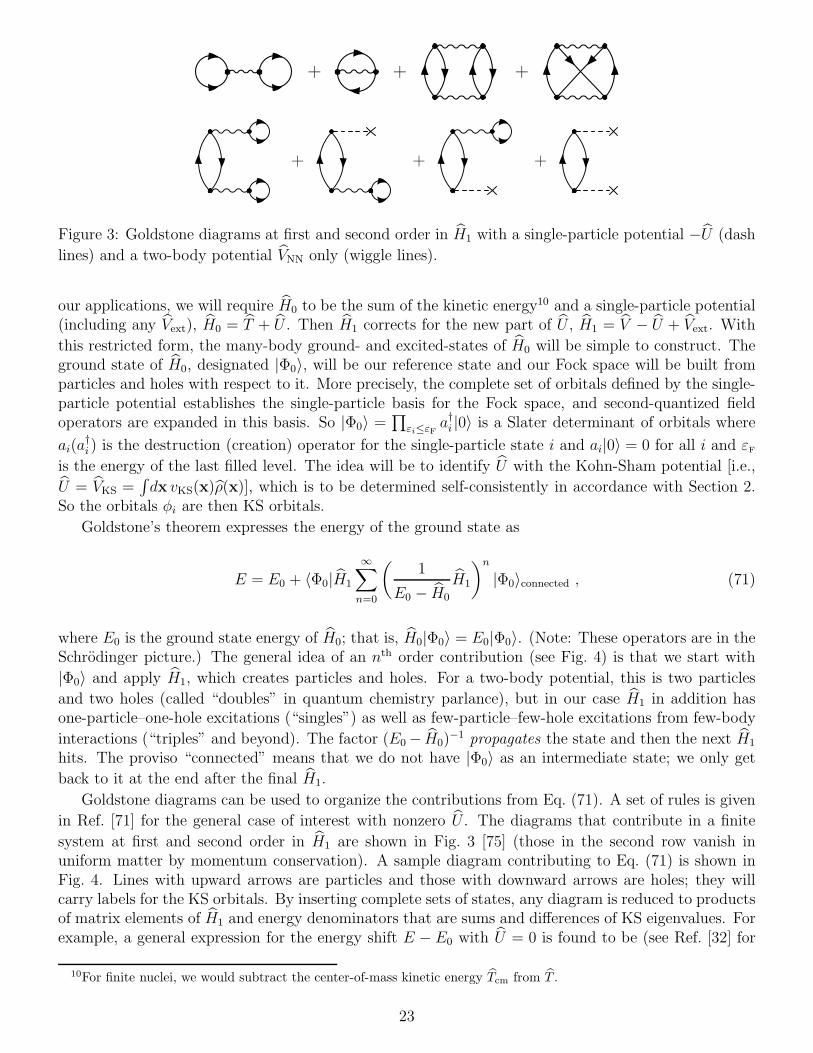
Figure 3: Goldstone diagrams at first and second order in H1 with a single-particle potential −U (dash

lines) and a two-body potential VNN only (wiggle lines).

our applications, we will require H0 to be the sum of the kinetic energy10 and a single-particle potential(including any Vext), H0 = T + U . Then H1 corrects for the new part of U , H1 = V − U + Vext. With

this restricted form, the many-body ground- and excited-states of H0 will be simple to construct. Theground state of H0, designated |Φ0〉, will be our reference state and our Fock space will be built fromparticles and holes with respect to it. More precisely, the complete set of orbitals defined by the single-particle potential establishes the single-particle basis for the Fock space, and second-quantized fieldoperators are expanded in this basis. So |Φ0〉 =

∏εi≤εF

a†i |0〉 is a Slater determinant of orbitals where

ai(a†i ) is the destruction (creation) operator for the single-particle state i and ai|0〉 = 0 for all i and εF

is the energy of the last filled level. The idea will be to identify U with the Kohn-Sham potential [i.e.,

U = VKS =∫dx vKS(x)ρ(x)], which is to be determined self-consistently in accordance with Section 2.

So the orbitals φi are then KS orbitals.

Goldstone’s theorem expresses the energy of the ground state as

E = E0 + 〈Φ0|H1

∞∑

n=0

(1

E0 − H0

H1

)n|Φ0〉connected , (71)

where E0 is the ground state energy of H0; that is, H0|Φ0〉 = E0|Φ0〉. (Note: These operators are in theSchrodinger picture.) The general idea of an nth order contribution (see Fig. 4) is that we start with

|Φ0〉 and apply H1, which creates particles and holes. For a two-body potential, this is two particles

and two holes (called “doubles” in quantum chemistry parlance), but in our case H1 in addition hasone-particle–one-hole excitations (“singles”) as well as few-particle–few-hole excitations from few-body

interactions (“triples” and beyond). The factor (E0− H0)−1 propagates the state and then the next H1

hits. The proviso “connected” means that we do not have |Φ0〉 as an intermediate state; we only get

back to it at the end after the final H1.

Goldstone diagrams can be used to organize the contributions from Eq. (71). A set of rules is given

in Ref. [71] for the general case of interest with nonzero U . The diagrams that contribute in a finite

system at first and second order in H1 are shown in Fig. 3 [75] (those in the second row vanish inuniform matter by momentum conservation). A sample diagram contributing to Eq. (71) is shown inFig. 4. Lines with upward arrows are particles and those with downward arrows are holes; they willcarry labels for the KS orbitals. By inserting complete sets of states, any diagram is reduced to productsof matrix elements of H1 and energy denominators that are sums and differences of KS eigenvalues. Forexample, a general expression for the energy shift E − E0 with U = 0 is found to be (see Ref. [32] for

10For finite nuclei, we would subtract the center-of-mass kinetic energy Tcm from T .

23

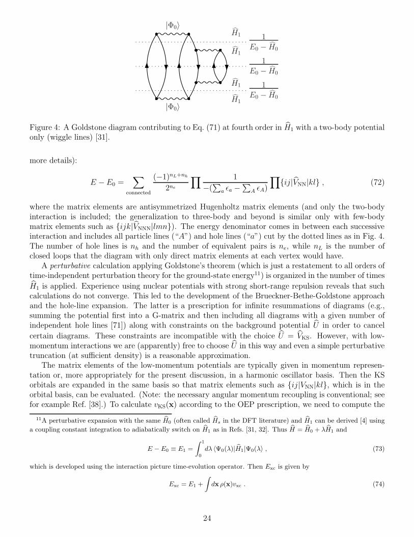
|Φ0〉

|Φ0〉

H1

H1

H1

H1

1

E0 −H0

1

E0 −H0

1

E0 −H0

Figure 4: A Goldstone diagram contributing to Eq. (71) at fourth order in H1 with a two-body potentialonly (wiggle lines) [31].

more details):

E −E0 =∑

connected

(−1)nL+nh

2ne

∏ 1

−(∑

a ǫa −∑

A ǫA)

∏ij|VNN|kl , (72)

where the matrix elements are antisymmetrized Hugenholtz matrix elements (and only the two-bodyinteraction is included; the generalization to three-body and beyond is similar only with few-bodymatrix elements such as ijk|VNNN|lmn). The energy denominator comes in between each successiveinteraction and includes all particle lines (“A”) and hole lines (“a”) cut by the dotted lines as in Fig. 4.The number of hole lines is nh and the number of equivalent pairs is ne, while nL is the number ofclosed loops that the diagram with only direct matrix elements at each vertex would have.

A perturbative calculation applying Goldstone’s theorem (which is just a restatement to all orders oftime-independent perturbation theory for the ground-state energy11) is organized in the number of times

H1 is applied. Experience using nuclear potentials with strong short-range repulsion reveals that suchcalculations do not converge. This led to the development of the Brueckner-Bethe-Goldstone approachand the hole-line expansion. The latter is a prescription for infinite resummations of diagrams (e.g.,summing the potential first into a G-matrix and then including all diagrams with a given number ofindependent hole lines [71]) along with constraints on the background potential U in order to cancel

certain diagrams. These constraints are incompatible with the choice U = VKS. However, with low-momentum interactions we are (apparently) free to choose U in this way and even a simple perturbativetruncation (at sufficient density) is a reasonable approximation.

The matrix elements of the low-momentum potentials are typically given in momentum represen-tation or, more appropriately for the present discussion, in a harmonic oscillator basis. Then the KSorbitals are expanded in the same basis so that matrix elements such as ij|VNN|kl, which is in theorbital basis, can be evaluated. (Note: the necessary angular momentum recoupling is conventional; seefor example Ref. [38].) To calculate vKS(x) according to the OEP prescription, we need to compute the

11A perturbative expansion with the same H0 (often called Hs in the DFT literature) and H1 can be derived [4] using

a coupling constant integration to adiabatically switch on H1 as in Refs. [31, 32]. Thus H = H0 + λH1 and

E − E0 ≡ E1 =

∫ 1

0

dλ 〈Ψ0(λ)|H1|Ψ0(λ〉 , (73)

which is developed using the interaction picture time-evolution operator. Then Exc is given by

Exc = E1 +

∫dx ρ(x)vxc . (74)

24

functional derivatives of EHxc [see Eq. (33)] with respect to the orbitals and eigenvalues. The eigenvaluesappear explicitly in the Goldstone expansion and the derivatives of the potential matrix elements canbe carried out using the basis expansion without having to evaluate the matrix elements in coordinatespace. For example, the two-body contribution from the Hartree-Fock terms is

δ

δφ∗i (x)

1

2

A∑

j,k=1

[〈jk|VNN|jk〉 − 〈jk|VNN|kj〉]

=

A∑

j,k=1

φk(x)[〈jk|VNN|ji〉 − 〈jk|VNN|ij〉] . (75)

If the matrix element integrals are written out in coordinate space for a local VNN(x,x′) and completeness

of the orbitals used to remove the sum over k, the corresponding part of Eq. (17) is reproduced.So we take [76]

H0 = Hs = T +

∫dx ρ(x)vKS(x) , (76)

where vKS = vext + vH + vxc ≡ vext + vHxc. The KS energy and density are

E0 = Es = Ts +

∫dx ρ(x)vKS(x) =

∑

i

niεi , (77)

ρ(x) = 〈Φ0|ρ(x)|Φ0〉 =∑

i

ni|φi(x)|2 ≡ ρKS(x) , (78)

which is the exact density according to the conditions (to be) imposed on vKS. (Note: ρ(x) = ψ†(x)ψ(x)

where the field operators are ψ†(x) =∑

i φ∗i (x)a

†i and ψ(x) =

∑i φi(x)a

†i .) Then we have

H1 = V −

∫dx ρ(x)vHxc(x) . (79)

At this point, we can carry out the Goldstone expansion to any order or with whatever infinite sum-mation we wish.

We note that because this expansion depends on vKS(x), it is a highly nonlinear functional equation,as EHxc depends on its own functional derivative. This is not in conflict with DFT because vHxc is adensity functional, so

EHxc = EH + Exc = E1 +

∫dx [vH(x) + vxc(x)]ρ(x) (80)

is an implicit functional. Furthermore, it is the same nonlinearity as in the OPM equation. A perturba-tive approach to solving for the functional derivative vHxc(x) = δEHxc[ρ]/δρ(x) leads to a linearizationof the OPM equation. This will correspond to the inversion method discussed in Section 4. The detailsof such a perturbative expansion and the nonperturbative resummation of ring diagrams (the randomphase approximation or RPA) is described by Engel (with references to the original literature) [4].

According to Engel the results for KS perturbation theory are not satisfactory. However, morerecent developments have shown promise by improving the perturbation theory. We have emphasizedthat with low-momentum potentials, U can be chosen freely to allow the DFT constraints to hold. Butthere is still freedom in defining it, which can be used to significantly improve perturbative convergencein the Coulomb problem. We consider this in the next section.

3.2 Improved perturbation theory

In this section, we summarize the basic features of the approach to ab initio DFT under developmentby Bartlett and collaborators [58, 59]. In Ref. [59] they explain their strategy, which is closely in line

25

with the highly successful coupled cluster approach to electronic systems. A key part of the formulationas well as its numerical execution is to use a finite basis set (which is almost always chosen to begaussians for finite systems in quantum chemistry so that all integrals can be done analytically). Aboveall, they emphasize that DFT should be formulated so that it converges in the limit of a full basis set,12

as obtained for wave function methods (cf. the partial hierarchy of CC approximations: MBPT(2) <CCSD < CCSD(T) < full CI). They contrast this precept with conventional DFT approaches suchas LDA or GGA or hybrid DFT (HDFT, which mixes semi-local GGA and non-local HF exchangefunctionals), which do not consistently predict better answers when applied in that order, even thoughthey are claimed to be better approximations. That is, there is no definite hierarchy.

The Bartlett construction follows most cleanly by requiring that corrections to the density beyondthe Kohn-Sham density, as calculated according to MBPT, must vanish. As noted in Section 2.4, thisis an alternate but equivalent prescription for orbital-based ab initio DFT. The Hamiltonian is split asin the last section into H = H0 + H1 using the Kohn-Sham potential to define the reference state. Wewill use |ΦKS〉 instead of |Φ0〉 to make this clear. The perturbative expansion for the energy is [58, 59]

E = E0 + E(1) + E(2) + · · · (81)

where (in quantum chemistry coupled cluster notation)

E0 = 〈ΦKS|H0|ΦKS〉 =∑

i

niεi , (82)

E(1) = 〈ΦKS|H1|ΦKS〉 , (83)

E(2) = 〈ΦKS|H1R0H1|ΦKS〉 , (84)

and so on. Here the operator R0 is

R0 = Q1

E0 − H0

Q , (85)

withQ =

∑|Φai 〉〈Φ

ai |+ |Φ

abij 〉〈Φ

abij |+ |Φ

abcijk〉〈Φ

abcijk|+ · · · , (86)

which are singles, doubles, and higher excitations with respect to the reference KS state (which is adeterminant). By convention, a, b, c are unoccupied and i, j, k are occupied in the KS state. We see

that this agrees with the Goldstone expansion from before, because Q ensures that only connectedcontributions are included (i.e., it is a complete set of states excluding |ΦKS〉).

Rather than use the functional derivative to calculate vKS, the condition that the density be un-changed from the Kohn-Sham density is used. For calculating the exchange-only KS potential Vx, thisimplies the density be unchanged to first order in perturbation theory. We expand the wave functionand the density:

|Ψ〉 = |ΦKS〉+ |Ψ(1)〉+ |Ψ(2)〉+ · · · , (87)

ρ = ρKS + ρ(1) + ρ(2) + · · · , (88)

where the density is computed from the expectation value of ρ(x) (note that Bartlett et al. write this

using δ, which is the same as ρ):

ρ(x) =〈Ψ|ρ(x)|Ψ〉

〈Ψ|Ψ〉. (89)

12The diagonalization of the Hamiltonian including all possible particle-hole excitations in a given basis set is called“full CI”. That solution is an upper bound to the exact energy and reproducing it using that same basis set is consideredto be an unambiguous measure of success in describing electron correlation [77].

26

So at leading order, we determine vx(x) such that ρ(1)(x) = 0. Thus

〈ΦKS|ρ(x)|Ψ(1)〉+ c.c. = 0 , (90)

where writing H|Ψ〉 = E|ψ〉 to this order gives

(E0 − H0)|Ψ(1)〉 = (H1 − E

(1))|ΦKS〉 (91)

and therefore|Ψ(1)〉 = R0(H1 −E

(1))|ΦKS〉 . (92)

Substituting for |Ψ(1)〉,

ρ(1) = 0 = 〈ΦKS|ρ(x)R0H1|ΦKS〉+ c.c. , (93)

and noting that at this order only single excitations contribute, we obtain

0 =∑

j,i,a

〈i|ρ(x)|a〉(aj|H1|ij − 〈a|VHx|i〉)/(εi − εa) + c.c.

= −∑

i,a

φ∗i (x)φa(x)(〈a|K|i〉+ 〈a|Vx|i〉)/(εi − εa) + c.c. . (94)

where we have used 〈Φai |E0 − H0|Φai 〉 = εi − εa. Here K is the conventional exchange (Fock) energy

operator V P12, where P12 is the particle-exchange operator.Note that we cannot choose 〈a|K|i〉 = −〈a|Vx|i〉 because Vx must be local. We can think of Eq. (94)

as the solution to a weighted least squares problem to replace the non-local K by the local Vx in thespace spanned by φ∗

i , φa [58]. This is a point-wise identity that can be written [with χs from Eq. (48)]

∫dx′ χs(x,x

′)[vx(x′) +K(x′)] = 0 , (95)

which agrees with the OEP equation in Section 2; that is, we have rederived the OEP equation withexchange only. Here

K(x)φj(x) =

∫dx′ ρ(x,x′)V (x,x′)φj(x

′) (96)

for a local potential with

ρ(x,x′) =∑

i

niφ∗i (x

′)φi(x) . (97)

Details on solving Eq. (95) in matrix form are given in Refs. [58, 59] with pointers to the literature.At second order, where the correlation potential first enters, one encounters issues with slow con-

vergence. Here we simply sketch the problem and proposed solution to give the flavor. Working tosecond-order MBPT, the second order energy is straightforward to write but naturally more complex.One insists that ρ(1) + ρ(2) = 0 and this defines V

(2)c consistent to this order. The problem is that the

perturbation H(1)1 − E

(1) = V − (VH + V(1)x )−E(1) (note: no Vc at this order) can have large, diagonal

contributions [59]:

〈ΦKS|ρ(x)|Φai 〉〈Φ

ai |(E0 − H0)

−1|Φai 〉〈Φai |H

(1) − E(1)|Φbi〉 (98)

= −[〈aj|V (1− P12)|bi〉 − δij〈a|K + Vx|b〉 − δab〈j|K + Vx|i〉

]φi(x)φ∗a(x)

εi − εa. (99)

Because we can have a = b and i = j, these are diagonal elements of K + Vx, which make H(1) a largerperturbation than usual [58, 59]. The remedy is to resum diagonal and near-diagonal one-particle terms

27

into H ′0 (this includes a rotation of the KS orbits so that off-diagonal terms in H ′

0 vanish). Most of theeffect from the resummation comes with the replacement of KS denominator energies εp (p is either aparticle or hole) with diagonal Fock matrix elements fpp, where

fpp = 〈p|f |p〉 = εp − 〈p|K + Vxc|p〉 . (100)

The details are beyond the scope of this review but can be found in Ref. [78] along with results.In summary, the key issue is that the freedom in how we split the Hamiltonian can be exploited to

improve convergence of the perturbation series without sacrificing the form of ab initio DFT. In particu-lar, rather than use the standard Kohn-Sham choice (called Gorling-Levy perturbation theory [79, 80]),

we shift as much physics as possible into H0. While far from a complete treatment, we hope we haveconveyed the flavor of the Bartlett approach. As a side note, Bartlett et al. claim that observationsmade for conventional DFT that orbital energies are meaningless (other than the least bound) aremostly because functionals and potentials were not accurate.

3.3 Low-momentum interactions

The last two sections illustrate how exchange-correlation functions can be constructed for Coulombsystems for which many-body perturbation theory is applicable. This is irrelevant for nuclear physicsunless we have similar control of MBPT. Here we highlight recent results that show that modern RGmethods can be used to obtain a convergent expansion of nuclear matter properties by evolving tolow-momentum interactions. There are various methods to achieve these interactions starting fromphenomenological or EFT potentials (e.g., see Refs. [37, 81, 36]), which for our purposes here areequivalent. We simply cite two proof-of-principle results and refer the reader to the literature.

First we consider the uniform system. Despite a decades-old emphasis on infinite nuclear matter,most advances in microscopic nuclear structure theory over the last decade have been through expand-ing the reach of few-body calculations. This has unambiguously established the quantitative role ofthree-nucleon forces (3NF) for light nuclei (A 6 12) [19, 20, 82, 22]. Until recently, few-body fitshave not sufficiently constrained 3NF contributions at higher density such that nuclear matter calcula-tions are predictive. Nuclear matter saturation is very delicate, with the binding energy resulting fromcancellations of much larger potential and kinetic energy contributions. When a quantitative reproduc-tion of empirical saturation properties has been obtained, it was imposed by hand through adjustingshort-range three-body forces (see, for example, Refs. [83, 84]).

Progress for controlled nuclear matter calculations has long been hindered by the difficulty of thenuclear many-body problem when conventional nuclear potentials are used. But recent calculations [40]overcome the hurdles by combining controlled starting Hamiltonians based on chiral effective field theory(EFT) [85, 86] with renormalization group (RG) methods [35, 87] to soften the short-range repulsionand short-range tensor components of the initial chiral interactions [88]. By doing so, the convergenceof many-body calculations is vastly accelerated [39, 89, 90].

Some key results are summarized in Fig. 5, which shows the energy per particle of symmetric matteras a function of Fermi momentum kF, or the density ρ = 2k3F/(3π

2). A grey square representing theempirical saturation point is shown in each of the nuclear matter figures. Its boundaries reflect the rangesof nuclear matter saturation properties predicted by phenomenological Skyrme energy functionals thatmost accurately reproduce properties of finite nuclei. The calculations of Fig. 5 start from the N3LOnucleon-nucleon (NN) potential (EM 500MeV) of Ref. [85]. This NN potential is RG-evolved to low-momentum interactions Vlow k with a smooth nexp = 4 regulator [87]. For each cutoff Λ, two couplingsthat determine the shorter-range parts of the N2LO 3NF [91, 92] are fit to the 3H binding energy andthe 4He matter radius [82] using exact Faddeev and Faddeev-Yakubovsky methods as in Ref. [93].

The Hartree-Fock results show that nuclear matter is bound even at this simplest level. A calcula-tion without approximations should be independent of the cutoffs, so the spread in Fig. 5 sets the scale

28

0.8 1.0 1.2 1.4 1.6

kF [fm

−1]

−20

−15

−10

−5

0

5

Ene

rgy/

nucl

eon

[MeV

] Λ = 1.8 fm−1

Λ = 2.0 fm−1

Λ = 2.2 fm−1

Λ = 2.8 fm−1

0.8 1.0 1.2 1.4 1.6

kF [fm

−1]

0.8 1.0 1.2 1.4 1.6

kF [fm

−1]

Hartree-Fock

Empiricalsaturationpoint 2nd order

Vlow k

NN from N3LO (500 MeV)

3NF fit to E3H and r4He

pp ladders

2.0 < Λ3NF

< 2.5 fm−1

Figure 5: Nuclear matter energy per particle as a function of Fermi momentum kF at the Hartree-Fock level (left) and including second-order (middle) and particle-particle-ladder contributions (right),based on evolved N3LO NN potentials and 3NF fit to E3H and r4He. Upper bounds to the theoreticaluncertainties are estimated by the NN (lines) and 3N (band) cutoff variations [40].

for omitted many-body contributions (more precisely, it sets a lower bound to omitted contributions).The second-order results show a dramatic narrowing of this spread, with predicted saturation consis-tent with the empirical range. The narrowing happens across the full density range. This is strongevidence that these encouraging results are not fortuitous. The particle-particle-ladder sum is littlechanged from second order except at the lowest densities shown. The latter is not surprising becauseat very low density the presence of a two-body bound state necessitates a nonperturbative summation.Similar results are obtained using flow equations to evolve Hamiltonians, which is called the SimilarityRenormalization Group (SRG) [94, 95, 36, 37] in nuclear physics.

The decrease in cutoff dependence in Fig. 5 with more complete approximations is necessary butnot sufficient to conclude that the calculations are under control. Indeed, approximations that areindependent of the cutoff will shift the answer but not widen the error band from cutoff variation. Thetheoretical errors arise from truncations in the initial chiral EFT Hamiltonian, the approximation of the3NF, and the many-body approximations. The 3NF approximation is particularly uncertain becauseit involves long-range contributions independent of the cutoff. Many-body corrections to the currentapproximations include higher-order terms in the hole-line expansion and particle-hole corrections. Anapproach such as coupled cluster theory that can perform a high-level resummation including long-rangecorrelations will ultimately be necessary for a robust validation.

These results, while not conclusive, open the door to ab-initio density functional theory (DFT) bothdirectly (as in the last sections) but also based on expanding about nuclear matter [96] (next section).This is analogous to the application of DFT in quantum chemistry and condensed matter starting withthe uniform electron gas in local-density approximations and adding constrained derivative corrections.Phenomenological energy functionals (such as Skyrme) for nuclei have impressive successes but lack a(quantitative) microscopic foundation based on nuclear forces and seem to have reached the limits ofimprovement with the current form of functionals [97, 98]. On the other hand, the theoretical errorsof the calculations in Fig. 5, while impressively small on the scale of the potential energy per particle,are far too large to be quantitatively competitive with existing functionals. However, there is thepossibility of fine tuning to heavy nuclei, of using EFT/RG to guide next-generation functional forms,and of benchmarking with ab-initio methods for low-momentum interactions. Overall, these results are

29

quite promising for a unified description of all nuclei and nuclear matter but much work is left to bedone.

Calculations of finite nuclei by another group using soft potentials further support the use of MBPT.Roth and collaborators have developed a method using designed unitary transformations to removeshort-range “hard core” and tensor correlations [99]. The approach is called the “Unitary CorrelationOperator Method” or UCOM. The result is a soft Hamiltonian that shares the favorable features ofthe RG-based potentials. They have also shown close parallels (and some distinctions) of UCOM tothe SRG approach [100, 101]. Using a UCOM NN potential, which is phase equivalent to a giveninitial Hamiltonian (in this case Argonne v18 [18]), they have calculated many nuclei (including heavynuclei such as 208Pb) in HF plus second- and third-order MBPT corrections. The energies and radiiobtained seem to be remarkably converged at second order with good systematics [38]. Preliminaryresults from supplementing the NN potential by a contact 3-body interaction with fitted strength arevery encouraging [102]. They have also examined corrections from particle-hole states in the RPA forclosed-shell nuclei; these are found to be relatively small corrections [103].

Thus MBPT appears to be a viable candidate for calculating a nuclear exchange-correlation func-tional. However, there are three important caveats. Detailed comparisons with a method that doeshigh-order resummations will be necessary before one can make robust conclusions. In this regard,converged calculations using soft potentials with coupled cluster and no-core-shell-model techniques arefeasible now in 16O including 3-body forces and soon13 in 40Ca (NN-only calculations for CC are possiblenow even for an unevolved chiral EFT potential [25]). Second, tests of MBPT have so far been largelylimited to spherical nuclei where pairing plays a small role. The final point to emphasize again is thatcorrections are relatively small, but not absolutely small and are large compared to the accuracy soughtfor functionals, so additional contributions must eventually be considered.

3.4 Density matrix expansion

While formally the construction of an ab initio DFT energy functional is well-defined based on a many-body perturbation expansion (resummed as needed) about a Kohn-Sham reference state, in practicethe feasibility of using KS potentials from such a functional beyond Hartree-Fock has only recentlybeen demonstrated. This is an ongoing area of research in quantum chemistry, with mixed results, andprogress in nuclear physics will require many further developments. A more immediate route to a DFTfunctional based on microscopic nuclear interactions is to make a quasi-local expansion of the energyin terms of various densities, so that functional derivatives needed to define Kohn-Sham potentialsare immediate. Of course, in doing so one sacrifices the full non-locality present in an orbital-basedfunctional. An example of such an expansion is the density matrix expansion (DME) introduced byNegele and Vautherin [104, 105], which we describe here in some detail.

The strategy is to follow a path that will be compatible with current nuclear DFT technology buttestable and systematically improvable. In this regard, the phenomenological nuclear energy densityfunctionals of the Skyrme form are a good starting point to build on the MBPT with low-momentuminteractions. Modern Skyrme functionals have been applied over a very wide range of nuclei, withquantitative success in reproducing properties of nuclear ground states and low-lying excitations [50,106, 11]. Nevertheless, a significant reduction of the current global and local errors is a major goal [9].One strategy is to improve the functional itself; the form of the basic Skyrme functional in use is very

13These calculations may require an approximation based on a normal-ordering truncation to treat the 3-body force [22],which has not been fully validated for these nuclei.

30

restricted, consisting of a sum of local powers of various nuclear densities, e.g., for N = Z nuclei [47]:

ESkyrme[ρ, τ,J] =

∫d3x

1

2Mτ +

3

8t0ρ

2 +1

16t3ρ

2+α +1

16(3t1 + 5t2)ρτ

+1

64(9t1 − 5t2)(∇ρ)2 −

3

4W0ρ∇ · J +

1

32(t1 − t2)J

2

, (101)

where the density ρ, the kinetic density τ , and the spin-orbit density J are expressed as sums oversingle-particle orbitals. (Expressions for the Skyrme functional including isovector and more generaldensities can be found in Ref. [107].) Fits to measured nuclear data have given to date only limitedconstraints on possible density and isospin dependencies and on the form of the spin-orbit interaction.Even qualitative insight into these properties from realistic microscopic calculations could be beneficialin improving the effectiveness of the energy density functional.

A theoretical connection of the Skyrme functional to free-space NN interactions was made long agoby Negele and Vautherin using the density matrix expansion (DME) [104, 105, 108], but there havebeen few subsequent microscopic developments. The DME originated as an expansion of the Hartree-Fock energy constructed using the nucleon-nucleon G matrix [104, 105], which was treated in a local(i.e., diagonal in coordinate representation) approximation. Recently the DME has been revisited forspin-saturated nuclei using non-local low-momentum interactions in momentum representation [96], forwhich G matrix summations are not needed because of the softening of the interaction (see Section 3.3).When applied to a Hartree-Fock energy functional, the DME yields an energy functional in the form ofa generalized Skyrme functional that is compatible with existing codes, by replacing Skyrme coefficientswith density-dependent functions. As in the original application, a key feature of the DME is that it isnot a pure short-distance expansion but includes resummations that treat long-range pion interactionscorrectly in a uniform system. However, we also caution that the Negele-Vautherin DME involvesprescriptions for the resummations without a corresponding power counting to justify them.

In essence, the DME maps the orbital-dependent expressions for contributions to the interactionenergy Eint of the type in Fig. 6(a) into a semi-local form, with explicit dependence on the local densitiesρ(R), τ(R), ∇2ρ(R), and so on. This greatly simplifies the determination of the Kohn-Sham potentialbecause the functional derivatives determining the KS potentials can be evaluated directly. The densitymatrix expansion (DME) for spin-saturated nuclei has been formulated for low-momentum interactionsand applied to a Hartree-Fock energy functional including both NN and NNN potentials in Ref. [96].The output is a set of functions of density that can replace density-independent parameters in standardSkyrme Hartree-Fock codes. Furthermore, the upgrade from Skyrme energy functional to DME energyfunctional can be carried out in stages. For example, the spin-orbit part and pairing can be kept inSkyrme form with the rest given by the DME. A further upgrade to orbital-based methods would onlymodify the same part of the code, although the increased computational load will be significant.

Here we outline how the density matrix expansion is carried out for a microscopic DFT at HF orderusing low-momentum (and non-local) two-body potentials. The relevant object we need to expand isEint, which is expressed in terms of the Kohn-Sham orbitals and eigenvalues that comprise the Kohn-Sham single-particle propagators as in Section 3.1. For Hartree-Fock contributions only the orbitalsenter. Higher-order contributions such as the ladder diagrams in the particle-particle channel can alsobe put approximately into the required form by averaging over the state dependence arising from theintermediate-state energy denominators (cf. the KLI approximation). Therefore, results presented herefor the Hartree-Fock contributions to the functional can be generalized to approximately include selectedhigher-order contributions. However, a framework for systematic improvement is yet to be developed.

Before considering the DME derivation and its application to non-local low-momentum interactions,it is useful to first derive in some detail the starting expression for EHF, the Hartree-Fock contributionto Eint. This introduces the basic notation and highlights the differences between most existing DME

31

studies, which are formulated with local interactions and in coordinate space throughout, and an ap-proach formulated in momentum space and geared towards non-local potentials. For a local potential,the distinction between the direct (Hartree) and exchange (Fock) contributions is significant, and isreflected in the conventional decomposition of the DFT energy functional for Coulomb systems, whichseparates out the Hartree piece. For a non-local potential, the distinction is blurred because the Hartreecontribution now involves the density matrix (as opposed to the density) and it is not useful to makethis separation when the range of the interaction is comparable to the non-locality.14 Consequently,throughout this section we work instead with an antisymmetrized interaction.

For a general (i.e., non-local) free-space two-body potential VNN, EHF is defined in terms of Kohn-Sham states [Eq. (11)] labeled by i and j,

EHF =1

2

A∑

ij

〈ij|VNN(1− P12)|ij〉 =1

2

A∑

ij

〈ij|V|ij〉 . (102)

The summation is over the occupied states and the antisymmetrized interaction V = VNN(1− P12) hasbeen introduced, with the exchange operator P12 equal to the product of operators for spin, isospin,and space exchange, P12 = PσPτPr. Note that the dependence of EHF on the Kohn-Sham potential isimplicit. By making repeated use of the completeness relation in space (r), spin (σ), and isospin (τ),

11 =∑

στ

∫dr|rστ〉〈rστ | , (103)

EHF can be written in terms of the coordinate space Kohn-Sham orbitals as

EHF =1

2

∑

ij

∑

στ

∫dr1

∫dr2

∫dr3

∫dr4 〈r1σ1τ1r2σ2τ2|V|r3σ3τ3r4σ4τ4〉

× φ∗i (r1σ1τ1)φi(r3σ3τ3)φ

∗j(r2σ2τ2)φj(r4σ4τ4) . (104)

From the definition of the Kohn-Sham density matrix,

ρ(r3σ3τ3, r1σ1τ1) =A∑

i

φ∗i (r1σ1τ1)φi(r3σ3τ3) , (105)

so Eq. (104) can be written as

EHF =1

2

∑

στ

∫dr1 · · ·

∫dr4 〈r1σ1τ1r2σ2τ2|V|r3σ3τ3r4σ4τ4〉ρ(r3σ3τ3, r1σ1τ1)ρ(r4σ4τ4, r2σ2τ4)

=1

2Tr1Tr2

∫dr1 · · ·

∫dr4 〈r1r2|V

1⊗2|r3r4〉ρ(1)(r3, r1)ρ

(2)(r4, r2) , (106)

where a matrix notation is used in the second equation and the traces denote summations over the spinand isospin indices for “particle 1” and “particle 2”. Hereafter we drop the superscripts on V and ρ

that indicate which space they act in as it will be clear from the context.Expanding the ρ matrices on Pauli spin and isospin matrices we have

ρ(r1, r2) =1

4[ρ0(r1, r2) + ρ1(r1, r2)τz + ~S0(r1, r2) · ~σ + ~S1(r1, r2) · ~στz] , (107)

where we have assumed the absence of charge-mixing in the single-particle states and the componentsare obtained by taking the relevant traces of ρ. From now on we consider only terms in the energy

32

r3

+∆/2RR + Σ/2

R - Σ/2

r4r1

r2

-∆/2

+∆/2

-∆/2r’/2

-r’/2r/2

-r/2

Figure 6: (a) Schematic diagram for approximations to Eint that can be expanded using the DME.(b) Coordinates appropriate for the DME applied to the Hartree-Fock potential energy with a non-localpotential.

functional arising from products of the scalar-isoscalar (ρ0) density matrices in Eq. (106), which arethe relevant terms for spin-saturated systems with N = Z. Because there will be no confusion, we willdrop the subscript “0” on the density matrices.

The first step is to switch to relative/center-of-mass (COM) coordinates (see Fig. 6). The free-spacetwo-nucleon potential is diagonal in the COM coordinate, so the starting point for the DME of thetwo-body Hartree-Fock contribution from a non-local interaction is

EHF =1

32

∫dR dr dr′ ρ(R+

r′

2,R+

r

2)ρ(R−

r′

2,R−

r

2)Trστ [〈r|V|r

′〉] , (108)

where V denotes the antisymmetrized interaction and the trace is defined as

Trστ [〈r|V|r′〉] ≡

∑

στ

〈rσ1τ1σ2τ2|V (1− P12)|r′σ1τ1σ2τ2〉 . (109)

The DME derivation of Negele and Vautherin (NV) [104] focuses on applications to local potentials,

which satisfy 〈r|V |r′〉 = δ(r − r′)〈r|V |r′〉. While the original NV work included coordinate-spaceformulas applicable for non-local interactions, for low-momentum potentials it is advantageous to revisitand extend the original derivation to a momentum-space formulation. (Note that Kaiser et al. haveshown how to use medium-insertions in momentum space in their application of the DME to chiralperturbation theory at finite density [109, 110, 111].)

For the momentum space formulation, we first rewrite the density matrices in Eq. (108) as

ρ(R± r′/2,R± r/2) = ρ(R± ±∆/2,R± ∓∆/2) , (110)

where the vectors appearing on the right-hand side are defined by (see Fig. 6)

R± = R±1

2Σ , Σ =

1

2(r′ + r) , ∆ =

1

2(r′ − r) . (111)

Introducing the Fourier transform of V in the momentum transfers conjugate to Σ and ∆,

q = k− k′ , p = k + k′ , (112)

(where k′, k correspond to relative momenta) gives

EHF =1

32

∫dR

∫dq dp

(2π)6F (R,q,p) Trστ [V(q,p)] ,

14However, it is useful to separate out the long-distance part of the potential, which is local, and treat its direct(Hartree) contribution exactly.

33

where we have defined

F (R,q,p) ≡

∫dΣ d∆ eiq·Σ eip·∆ ρ(R+ −∆/2,R+ +∆/2)ρ(R− +∆/2,R− −∆/2) , (113)

and

V(q,p) ≡ 8

∫dΣ d∆ e−iq·Σ e−ip·∆ 〈Σ−∆|V |Σ+∆〉 . (114)

The momenta q and p correspond to the momentum transfers for a local interaction in the direct andexchange channels. That is, the direct matrix element is a function of q and the exchange is a functionof p. In contrast, for a non-local interaction the direct and exchange matrix elements depend on bothq and p. This is the reason why we do not attempt to separate out the Hartree (direct) and Fock(exchange) contributions to EHF, as is commonly done for local interactions.

The trace of Eq. (114) can be written in a more convenient form for the application of low momentumNN interactions as a sum over partial wave matrix elements (see Ref. [96] for more complete definitions),

Trστ [V(q,p)] = 8π∑

lsj

′

(2j + 1)(2t+ 1)Pl(k · k′)〈klsjt|V |k′lsjt〉 , (115)

where the primed summation means that it is restricted to values where l+s+t is odd, with k = 12(p+q)

and k′ = 12(p − q). For simplicity we assume a charge-independent two-nucleon interaction, although

charge-dependence can easily be included.The expression Eq. (113) for EHF is written in terms of off-diagonal density matrices constructed from

the Kohn-Sham orbitals and so is an implicit functional of the density. To circumvent the applicationof the chain rule for the KS potentials, we apply Negele and Vautherin’s DME to EHF, resulting in anexpression of the form

EDME[ρ, τ,J] =

∫dR EDME(ρ(R), τ(R),J(R)) , (116)

with explicit dependence on the local quantities ρ(R), τ(R), and |∇ρ(R)|2 that we write for EHF as

EHF =

∫dR (A[ρ] +B[ρ]τ + C[ρ](∇ρ)2 + · · · ) . (117)

(We have suppressed terms that go beyond the present limited discussion; also, when N 6= Z these arefunctions of the isovector densities as well.) The goal is to find the coefficient functions in Eq. (117).The starting point of the DME is the formal identity [104]

ρ(R+ s/2,R− s/2) =∑

a

φ∗(R+ s/2)φ(R− s/2) =[es·(∇1−∇2)/2

∑

a

φ∗(R1)φ(R2)]R1=R2=R

, (118)

where ∇1 and ∇2 act on R1 and R1, respectively, and the result is evaluated at R1 = R1 = R. Weassume here that time-reversed orbitals are filled pairwise, so that the linear term of the exponentialexpansion vanishes. After applying a Bessel-function expansion (which is simply the usual plane-waveexpansion with real arguments), the angle-averaged density matrix takes the form

ρ(R+ s/2,R− s/2) =1

skF(R)

[∞∑

n=0

(4n+ 3)j2n+1(skF(R))Qn

((∇1 −∇2

2kF(R)

)2)]ρ(R1,R2) , (119)

where Q is related to the usual Legendre polynomial by Q(z2) = P2k+1(iz)/(iz) and an arbitrarymomentum scale kF(R) has been introduced. Equation (119) is independent of kF if all terms are kept,

34

but any truncation will give results depending on the particular choice for kF. The standard LDA choiceof Negele and Vautherin,

kF(R) = (3π2ρ(R)/2)1/3 , (120)

is used here. Alternative choices for kF(R) may better optimize the convergence of truncated expansionsof Eq. (119) and lead to a systematic power counting.

Following Negele and Vautherin, Eq. (119) is truncated to terms with n 6 1, which yields thefundamental equation of the DME,

ρ(R+s

2,R−

s

2) ≈ ρSL(kF(R)s) ρ(R) + s2g(kF(R)s)

[14∇2ρ(R)− τ(R) +

3

5kF(R)2ρ(R)

], (121)

whereρSL(x) ≡ 3j1(x)/x , g(x) ≡ 35j3(x)/2x

3 , (122)

and the kinetic energy density is τ(R) =∑

i |∇φi(R)|2. If a short-range interaction is folded with thedensity matrix, then a truncated Taylor series expansion of Eq. (121) in powers of s would be justifiedand would produce a quasi-local functional. But the local kF in the interior of a nucleus is typicallygreater than the pion mass mπ, so such an expansion would give a poor representation of the physicsof the long-range pion exchange interaction.

Instead, the DME is constructed as an expansion about the exact nuclear matter density matrix.Thus, Eq. (121) has the important feature that it reduces to the density matrix in the homogeneousnuclear matter limit, ρNM(R + s/2,R − s/2) = ρSL(kFs) ρ. As a result, the resummed expansion inEq. (121) does not distort the finite range physics, as the long-range one-pion-exchange contributionto nuclear matter is exactly reproduced and the finite-range physics is encoded as non-trivial (e.g.,non-monomial) density dependence in the resulting functional. The small parameters justifying thisexpansion emerge in the functionals as integrals over the inhomogeneities of the density. (See Section 4.3and Ref. [112] for examples of estimated contributions to a functional for a model problem.)

In the case of a local interaction, the Fock term is schematically given by WF ∼∫dR ds ρ2(R +

s/2,R−s/2)V (s), so a single application of Eq. (121) is sufficient to cast EHF into the desired form. Fora non-local interaction the calculation is more involved as two applications of the DME are required.There is arbitrariness in what is kept in higher orders of Σ2, which is used (following Negele andVautherin) to “reverse engineer” the expansion so that the exact nuclear matter limit is always exactlyreproduced by the leading term [104]. We emphasize that this is a prescription without establishedpower counting or error estimates; as shown in Ref. [96], different prescriptions can lead to significantchanges in nuclear observables. The end result for the product of two density matrices is [96]

ρ(R+r′

2,R+

r

2)ρ(R−

r′

2,R−

r

2) ≈ ρ2SL(kF∆)ρ2 +

1

2Σ2g(kFΣ)

(ρ∇2ρ ρSL(kF∆)j0(kF∆)

− |∇ρ|2[j20(kF∆) + j21(kF∆)])+ 2∆2g(kF∆)ρSL(kF∆)

(14ρ∇2ρ− ρ τ +

3

5k2Fρ

2). (123)

In the momentum space expression for EHF, it remains to evaluate the Fourier transforms defined inEq. (113) for the expanded density matrices in Eq. (123). Identifying the terms in Eq. (117) that givethe DME functionals A[ρ], B[ρ], and C[ρ], we have

A[ρ] =ρ2

16πk3F

∫ 2kF

0

p2dpTrστ [V(0,p)] (I1(p) +6

5I2(p)) , (124)

B[ρ] = −ρ

8πk5F

∫ 2kF

0

p2dpTrστ [V(0,p)] I2(p) , (125)

where Trστ [V(0,p)] is given by a simple sum of diagonal matrix elements in the different partial waves,

Trστ [V(0,p)] = 8π∑

lsj

′

(2j + 1)(2t+ 1) 〈p

2lsjt|V |

p

2lsjt〉 . (126)

35

The primed sum is over all channels for which l + s+ t is odd.In these expressions, the functions Ij(p) and Ij(q) are simple polynomials (and theta functions) in

the scaled momenta p ≡ p/kF and q ≡ q/kF:

I1(p) ≡

∫x2 dx j0(px) ρ

2SL(x) =

3π

32(16− 12p+ p3) θ(2− p) , (127)

I2(p) ≡

∫x4 dx j0(px) ρSL(x) g(x) = −

35π

128(p5 − 18p3 + 40p2 − 24p) θ(2− p) , (128)

I3(q) ≡

∫x4 dx j0(qx) g(x) = −

35π

8(5q2 − 3) θ(1− q) , (129)

I4(p) ≡

∫x2 dx j0(px) j0(x) ρSL(x) =

3π

8(2− p) θ(2− p) , (130)

I5(p) ≡

∫x2 dx j0(px)[j

20(x) + j21(x)] =

π

8p(4− p2) θ(2− p) . (131)

Note that the trivial angular dependence of Eqs. (127)–(131) is a consequence of the angle averagingthat is implicit with each application of the DME.

The contributions to EHF that have gradients of the local density take the form

EHF

∣∣|∇ρ|2

=

∫dR(C∇2ρ∇

2ρ(R) + C|∇ρ|2|∇ρ(R)|2). (132)

We can perform a partial integration on the∇2ρ terms to cast them into the canonical form proportionalto only |∇ρ|2; that is,

EHF

∣∣|∇ρ|2

=

∫dR |∇ρ(R)|2

[C|∇ρ|2 −

d

dρC∇2ρ

], (133)

so that

C[ρ] = C|∇ρ|2 −d

dρC∇2ρ . (134)

In practice it is efficient and accurate to calculate the derivative in Eq. (134) numerically rather thananalytically. The expressions for C|∇ρ|2 and C∇2ρ are

C|∇ρ|2 =1

32

∫dq dp

(2π)6(−8π2

k8FI3(q) I5(p)

)Trστ [V(q,p)] (135)

= −1

16π2k8F

∫ kF

0

q2dq

∫ 2kF

0

p2dp I3(q) I5(p) Vav(q, p) , (136)

C∇2ρ =ρ

32

∫dq dp

(2π)6( 1

k5F(2π)4δ3(q) I2(p) +

8π2

k8FI3(q) I4(p)

)Trστ [V(q,p)]

=ρ

32πk5F

∫ 2kF

0

p2dp I2(p) Trστ [V(0,p)]

+ρ

16π2k8F

∫ kF

0

q2dq

∫ 2kF

0

p2dp I3(q) I4(p) Vav(q, p) , (137)

where Vav(q, p) is the angle-averaged interaction,

Vav(q, p) ≡1

2

∫d(cos θ) Trστ [V(q,p)] , (138)

36

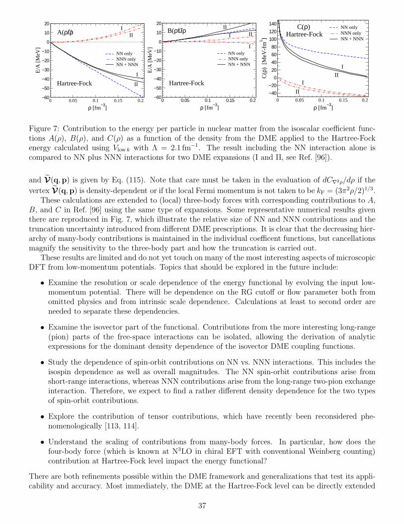
0 0.05 0.1 0.15 0.2

ρ [fm−3

]

−60

−50

−40

−30

−20

−10

0

10

20

E/A

[M

eV]

NN onlyNNN onlyNN + NNN

A(ρ)/ρ

Hartree-Fock

III

I

II

0 0.05 0.1 0.15 0.2ρ [fm

−3]

−60

−50

−40

−30

−20

−10

0

10

20

E/A

[M

eV]

NN onlyNNN onlyNN + NNN

B(ρ)τ/ρ

Hartree-Fock

IIIII

I

0 0.05 0.1 0.15 0.2

ρ [fm−3

]

−40−20

020406080

100120140

C(ρ

) [

MeV

-fm

5 ]

NN onlyNNN onlyNN + NNN

C(ρ)Hartree-Fock

I

III

II

Figure 7: Contribution to the energy per particle in nuclear matter from the isoscalar coefficient func-tions A(ρ), B(ρ), and C(ρ) as a function of the density from the DME applied to the Hartree-Fockenergy calculated using Vlow k with Λ = 2.1 fm−1. The result including the NN interaction alone iscompared to NN plus NNN interactions for two DME expansions (I and II, see Ref. [96]).

and V(q,p) is given by Eq. (115). Note that care must be taken in the evaluation of dC∇2ρ/dρ if the

vertex V(q,p) is density-dependent or if the local Fermi momentum is not taken to be kF = (3π2ρ/2)1/3.These calculations are extended to (local) three-body forces with corresponding contributions to A,

B, and C in Ref. [96] using the same type of expansions. Some representative numerical results giventhere are reproduced in Fig. 7, which illustrate the relative size of NN and NNN contributions and thetruncation uncertainty introduced from different DME prescriptions. It is clear that the decreasing hier-archy of many-body contributions is maintained in the individual coefficent functions, but cancellationsmagnify the sensitivity to the three-body part and how the truncation is carried out.

These results are limited and do not yet touch on many of the most interesting aspects of microscopicDFT from low-momentum potentials. Topics that should be explored in the future include:

• Examine the resolution or scale dependence of the energy functional by evolving the input low-momentum potential. There will be dependence on the RG cutoff or flow parameter both fromomitted physics and from intrinsic scale dependence. Calculations at least to second order areneeded to separate these dependencies.

• Examine the isovector part of the functional. Contributions from the more interesting long-range(pion) parts of the free-space interactions can be isolated, allowing the derivation of analyticexpressions for the dominant density dependence of the isovector DME coupling functions.

• Study the dependence of spin-orbit contributions on NN vs. NNN interactions. This includes theisospin dependence as well as overall magnitudes. The NN spin-orbit contributions arise fromshort-range interactions, whereas NNN contributions arise from the long-range two-pion exchangeinteraction. Therefore, we expect to find a rather different density dependence for the two typesof spin-orbit contributions.

• Explore the contribution of tensor contributions, which have recently been reconsidered phe-nomenologically [113, 114].

• Understand the scaling of contributions from many-body forces. In particular, how does thefour-body force (which is known at N3LO in chiral EFT with conventional Weinberg counting)contribution at Hartree-Fock level impact the energy functional?

There are both refinements possible within the DME framework and generalizations that test its appli-cability and accuracy. Most immediately, the DME at the Hartree-Fock level can be directly extended

37

to approximately include second-order (or full particle-particle ladder) contributions by using averagedenergies for the energy denominators.

In extending the first calculations from Ref. [96], the standard DME formalism from Negele andVautherin [104] will also need to be modified. This formalism has problems even beyond the truncationerrors from different DME prescriptions seen in Fig. 7, the most severe being that it provides anextremely poor description of the vector part of the density matrix. While the standard DME isreasonable at reproducing the scalar density matrices, even here the errors are sufficiently large thatthe disagreement with a full finite-range Hartree-Fock calculations can reach the MeV per particlelevel. Gebremariam and collaborators have traced both of these problems to an inadequate phasespace averaging (PSA) used in the previous DME approaches [115]. In the derivation of the DME, oneincorporates average information about the local momentum distribution into the approximation. TheNegele-Vautherin DME uses the phase space of infinite nuclear matter to perform this averaging forthe scalar part (and do not even average the vector part). However, the local momentum distributionin finite Fermi systems exhibits two striking differences from that of infinite homogeneous matter.First, mean-field calculations of nuclei show that the local momentum distribution exhibits a diffuseFermi surface that is especially pronounced in the nuclear surface [116]. Second, the local momentumdistribution is found to be anisotropic, with the deformation accentuated in the surface region of thefinite Fermi system [117].

Motivated by previous studies of the Wigner distribution function in nuclei, Gebremariam et al.calculate the quadrupole deformation of the local momentum distribution using wave functions for thatnucleus [115]. There are no free parameters. The improvements are substantial for the vector densitymatrices, typically reducing relative errors in integrated quantities by as much as an order of magnitudeacross many different isotope chains [115].

Future tests of the DME will include benchmarks against ab initio methods in the overlap region oflight-to-medium nuclei. Additional information is obtained from putting the nuclei in external fields,which can be added directly to the DFT/DME functional. Work is in progress on comparisons toboth coupled cluster and full configuration interaction calculations as part of the UNEDF project. Akey feature is that the same Hamiltonian will be used for the microscopic calculation and the DMEapproximation to the DFT. The freedom to adjust (or turn off) external fields as well as to vary otherparameters in the Hamiltonian permits detailed evaluations of the approximate functionals. In parallelthere will be refined nuclear matter calculations; power counting arguments from re-examining theBrueckner-Bethe-Goldstone approach in light of low-momentum potentials will provide a framework fororganizing higher-order contributions. These investigations should provide insight into how the energydensity functional can be fine tuned for greater accuracy in a manner consistent with power countingand EFT principles.

4 DFT as Legendre transform

In this section, we turn from MBPT in second quantization formalism to the formulation of DFT usingpath integrals for effective actions of composite operators. This can be an intimidating formalism ifunfamiliar but offers complementary advantages. For example:

• Effective actions are the natural theoretical framework for Legendre transforms [118, 119, 120],which is the underlying basis for DFT. These aspects tend to be hidden in the framework ofSection 3.

• The path integral construction of DFT is transparent, such as the role and usefulness of additionaldensities/sources. (As for implementation, we rapidly discover the same necessity to evaluatefunctional derivatives that was treated in Section 2.)

38

• Path integral effective actions are particularly suited for symmetry breaking, such as encounteredwith pairing. The renormalization issues in the latter case are manifest rather than hidden.

• Connections to effective field theory (EFT) and power counting can be more accessible.

• The path integral formulation puts the DFT construction in a broader perspective, which cansuggest connections and generalizations not apparent otherwise. For example, there are alternativeeffective actions using auxiliary fields or with a two-particle-irreducible nature. The latter maybe related to more general EDF constructions as proposed in Ref. [16].

• The quantization of gauge theories was greatly facilitated by Faddeev-Popov and BRST methodsusing path integrals; the same techniques offer alternative possibilities for implementing collectivecoordinates to restore symmetries broken by the mean-field organization of DFT [121, 122].

• The path integral formulation can suggest different types of nonperturbative approximations, suchas 1/N expansions, that might be needed for extensions beyond low-order nuclear MBPT (e.g.,to handle long-range correlations).

Space does not permit a detailed exposition of the path integral formulation of DFT. Furthermore, inthe short term the construction for nuclear DFT based on MBPT and the DME is probably cleanestin the formalism of Section 3. Therefore we focus on presenting the main ideas through analogy andschematic versions of the path integrals, and concentrate the EFT discussion on general issues such aspower counting for functionals.

As stressed in Section 1, microscopic DFT follows naturally from calculating the response of a many-body system to external sources, as in Green’s function methods, only with local, static sources thatcouple to densities rather than fundamental fields. (Time-dependent sources can be used for certainexcited states.) It is profitable to think in terms of a thermodynamic formulation of DFT, whichuses the effective action formalism [32] applied to composite operators to construct energy densityfunctionals [123, 124, 125]. The basic plan is to consider the zero temperature limit of the partitionfunction Z for the (finite) system of interest in the presence of external sources coupled to variousquantities of interest (such as the fermion density). We derive energy functionals of these quantities byLegendre transformations with respect to the sources [29]. These sources probe, in a variational sense,configurations near the ground state.

The work by Lieb [126] on the Hohenberg-Kohn theorem [27] establishes that the real issue forDFT is the existence of the Legendre transform F [ρ] of the ground state energy as a functional E[v]of the potential. The details involve sophisticated mathematics (e.g., convex-functional analysis) thatis not readily accessible; we recommend Ref. [29] by Kutzelnigg as a gateway to the mathematicallyrigorous literature behind DFT in terms of Legendre transformations.15 Fortunately, for our purposesthe familiarity of physicists with Legendre transforms in the context of thermodynamics is all we need.We highly recommend Ref. [26] as an elementary introduction to DFT that carries the analogy tothermodynamics through various simple examples.

Effective actions are a natural framework to implement Legendre transformations, motivate approx-imations not obvious in MBPT, and consider generalizations. One limitation of DFT is the exclusiverole of local potentials (sources) and densities, where locality is in reference to coordinate space. Kutzel-nigg points out that this is in contrast to many-body methods that introduce a finite basis in whichoperators are expanded, for which local operators have no privileged place. In this sense, density matrixfunctional theory, as proposed for nuclei in Ref. [16], seems more natural [29]. By looking at effectiveactions as a broader context, the limitations and problems of local sources are apparent, but also theopportunities for generalizations.

15There are important formal details [30], such as that we need E[v] to be concave to carry out the transform.

39

4.1 Analogy to Legendre transform in thermodynamics

We first preview DFT as an effective action [125] by recalling ordinary thermodynamics with N particlesas temperature T → 0. The thermodynamic potential is related to the grand canonical partitionfunction, with the chemical potential µ acting as a source to change N = 〈N〉,

Ω(µ) = −kT lnZ(µ) and N = −

(∂Ω

∂µ

)

TV

. (139)

Because Ω is convex, N is a monotonically increasing function of µ and we can invert to find µ(N) andapply a Legendre transform to obtain

F (N) = Ω(µ(N)) + µ(N)N . (140)

This is our (free) energy function of the particle number, which is analogous to the DFT energy func-tional of the density.16 Indeed, if we generalize to a spatially dependent chemical potential J(x), then

Z(µ) −→ Z[J(x)] and µN = µ

∫ψ†ψ −→

∫J(x)ψ†ψ(x) . (141)

Now Legendre transform from lnZ[J(x)] to Γ[ρ(x)], where ρ = 〈ψ†ψ〉J , and we have DFT with Γ simplyproportional to the energy functional! [Note that J(x)→ vext(x) to match our previous notation.]

The functional Γ is a type of effective action [125]. An effective action is generically the Legendretransform of a generating functional with an external source (or sources). For DFT, we use a source toadjust the density (cf. using an external applied magnetic field to adjust the magnetization in a spinsystem). Consider first the simplest case of a single external source J(x) coupled to the density operatorρ(x) ≡ ψ†(x)ψ(x) in the partition function

Z[J ] = e−W [J ] ∼ Tr e−β(bH+J bρ) ∼

∫D[ψ†]D[ψ] e−

R

[L+J ψ†ψ] , (142)

for which we can construct a (Euclidean) path integral representation with Lagrangian L [32]. (Note:because our treatment is schematic, for convenience we neglect normalization factors and take theinverse temperature β and the volume Ω equal to unity in the sequel.) The static density ρ(x) in thepresence of J(x) is

ρ(x) ≡ 〈ρ(x)〉J =δW [J ]

δJ(x), (143)

which we invert to find J [ρ] and then Legendre transform from J to ρ:

Γ[ρ] = −W [J ] +

∫dx J(x)ρ(x) , (144)

with

J(x) =δΓ[ρ]

δρ(x)−→

δΓ[ρ]

δρ(x)

∣∣∣∣ρgs(x)

= 0 . (145)

For static ρ(x), Γ[ρ] is proportional to the conventional Hohenberg-Kohn energy functional, which byEq. (145) is extremized at the ground state density ρgs(x) (and thermodynamic arguments establishthat it is a minimum [124]).17

16Because vext is typically given rather than eliminated, for a closer analogy we would also define Ωµ(N) ≡ F (N)−µN ,which depends explicitly on both N and µ. This gives the grand potential when minimized with respect to N [26].

17A Minkowski-space formulation of the effective action with time-dependent sources leads naturally to an RPA-likegeneralization of DFT that can be used to calculate properties of collective excitations.

40

Consider the partition function in the zero-temperature limit of a Hamiltonian with time-independentsource J(x) [120]:

H(J) = H +

∫J ψ†ψ . (146)

If the ground state is isolated (and bounded from below),

e−βbH = e−βE0

[|0〉〈0|+O

(e−β(E1−E0)

)]. (147)

As β →∞, Z[J ] yields the ground state of H(J) with energy E0(J):

E0(J) = limβ→∞

−1

βlogZ[J ] =

1

βW [J ] . (148)

Substitute and separate out the pieces:

E0(J) = 〈H(J)〉J = 〈H〉J +

∫J〈ψ†ψ〉J = 〈H〉J +

∫J ρ(J) . (149)

Rearranging, the expectation value of H in the ground state generated by J [ρ] is18

〈H〉J = E0(J)−

∫J ρ =

1

βΓ[ρ] . (150)

Now put it all together:

1

βΓ[ρ] = 〈H〉J

J→0−→ E0 and J(x) = −

δΓ[ρ]

δρ(x)

J→0−→

δΓ[ρ]

δρ(x)

∣∣∣∣ρgs(x)

= 0 . (151)

So for static ρ(x), Γ[ρ] is proportional to the DFT energy functional FHK. Furthermore, the true groundstate (with J = 0) is a variational minimum, so additional sources should be better than just one source

coupled to the density (as we will consider below).19 The simple, universal dependence on a non-zeroexternal potential v follows directly in this formalism:

Γv[ρ] =Wv[J ]−

∫J ρ =Wv=0[J + v]−

∫[(J + v)− v] ρ = Γv=0[ρ] +

∫v ρ . (152)

Thus allowing for non-zero vext is a trivial modification to Γ[ρ].There are a various paths to a DFT effective action:

1. The auxiliary field (Hubbard-Stratonovich) method [127, 128]: Couple ψ†ψ to an auxiliary fieldϕ, and eliminate all or part of (ψ†ψ)2. Add a source term Jϕ and perform a loop expansion aboutthe expectation value φ = 〈ϕ〉. A Kohn-Sham version uses the freedom of the expansion to requirethe density be unchanged at each order.

2. The inversion method [129, 124, 130, 131] yields a systematic Kohn-Sham DFT, based on an order-by-order expansion. For example, we can apply the EFT power counting for a dilute system.

3. Derive the functional with an RG approach [132]. This is briefly discussed in Section 6.

We will discuss here the inversion method, which connects most closely to the developments in Section 3.

18The functionals will change with resolution or field redefinitions; only stationary points are observables. This can beseen from Eq. (150), where Γ[ρ] is not the expectation value of H in an eigenstate unless J = J [ρgs].

19For the Minkowski-space version of this discussion, see Ref. [119].

41

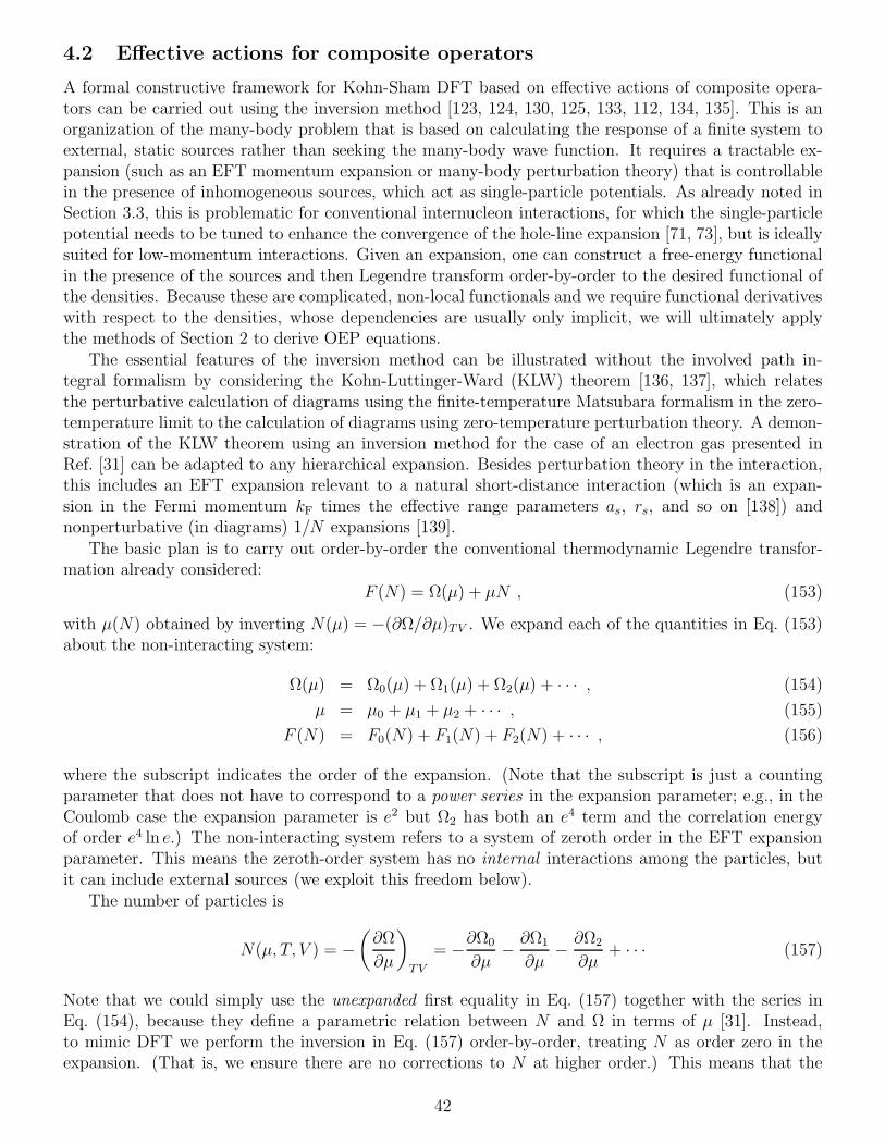
4.2 Effective actions for composite operators

A formal constructive framework for Kohn-Sham DFT based on effective actions of composite opera-tors can be carried out using the inversion method [123, 124, 130, 125, 133, 112, 134, 135]. This is anorganization of the many-body problem that is based on calculating the response of a finite system toexternal, static sources rather than seeking the many-body wave function. It requires a tractable ex-pansion (such as an EFT momentum expansion or many-body perturbation theory) that is controllablein the presence of inhomogeneous sources, which act as single-particle potentials. As already noted inSection 3.3, this is problematic for conventional internucleon interactions, for which the single-particlepotential needs to be tuned to enhance the convergence of the hole-line expansion [71, 73], but is ideallysuited for low-momentum interactions. Given an expansion, one can construct a free-energy functionalin the presence of the sources and then Legendre transform order-by-order to the desired functional ofthe densities. Because these are complicated, non-local functionals and we require functional derivativeswith respect to the densities, whose dependencies are usually only implicit, we will ultimately applythe methods of Section 2 to derive OEP equations.

The essential features of the inversion method can be illustrated without the involved path in-tegral formalism by considering the Kohn-Luttinger-Ward (KLW) theorem [136, 137], which relatesthe perturbative calculation of diagrams using the finite-temperature Matsubara formalism in the zero-temperature limit to the calculation of diagrams using zero-temperature perturbation theory. A demon-stration of the KLW theorem using an inversion method for the case of an electron gas presented inRef. [31] can be adapted to any hierarchical expansion. Besides perturbation theory in the interaction,this includes an EFT expansion relevant to a natural short-distance interaction (which is an expan-sion in the Fermi momentum kF times the effective range parameters as, rs, and so on [138]) andnonperturbative (in diagrams) 1/N expansions [139].

The basic plan is to carry out order-by-order the conventional thermodynamic Legendre transfor-mation already considered:

F (N) = Ω(µ) + µN , (153)

with µ(N) obtained by inverting N(µ) = −(∂Ω/∂µ)TV . We expand each of the quantities in Eq. (153)about the non-interacting system:

Ω(µ) = Ω0(µ) + Ω1(µ) + Ω2(µ) + · · · , (154)

µ = µ0 + µ1 + µ2 + · · · , (155)

F (N) = F0(N) + F1(N) + F2(N) + · · · , (156)

where the subscript indicates the order of the expansion. (Note that the subscript is just a countingparameter that does not have to correspond to a power series in the expansion parameter; e.g., in theCoulomb case the expansion parameter is e2 but Ω2 has both an e4 term and the correlation energyof order e4 ln e.) The non-interacting system refers to a system of zeroth order in the EFT expansionparameter. This means the zeroth-order system has no internal interactions among the particles, butit can include external sources (we exploit this freedom below).

The number of particles is

N(µ, T, V ) = −

(∂Ω

∂µ

)

TV

= −∂Ω0

∂µ−∂Ω1

∂µ−∂Ω2

∂µ+ · · · (157)

Note that we could simply use the unexpanded first equality in Eq. (157) together with the series inEq. (154), because they define a parametric relation between N and Ω in terms of µ [31]. Instead,to mimic DFT we perform the inversion in Eq. (157) order-by-order, treating N as order zero in theexpansion. (That is, we ensure there are no corrections to N at higher order.) This means that the

42

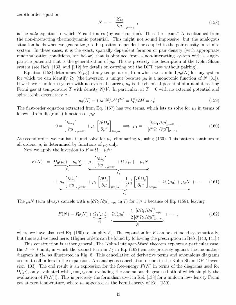
zeroth order equation,

N = −

[∂Ω0

∂µ

]

µ=µ0

, (158)

is the only equation to which N contributes (by construction). Thus the “exact” N is obtained fromthe non-interacting thermodynamic potential. This might not sound impressive, but the analogoussituation holds when we generalize µ to be position dependent or coupled to the pair density in a finitesystem. In these cases, it is the exact, spatially dependent fermion or pair density (with appropriaterenormalization conditions, see below) that is obtained from a non-interacting system with a single-particle potential that is the generalization of µ0. This is precisely the description of the Kohn-Shamsystem (see Refs. [133] and [112] for details on carrying out the DFT case without pairing).

Equation (158) determines N(µ0) at any temperature, from which we can find µ0(N) for any systemfor which we can identify Ω0 (the inversion is unique because µ0 is a monotonic function of N [31]).If we have a uniform system with no external sources, µ0 is the chemical potential of a noninteractingFermi gas at temperature T with density N/V . In particular, at T = 0 with no external potential andspin-isospin degeneracy ν,

µ0(N) = (6π2N/νV )2/3 ≡ k2F/2M ≡ ε0F. (159)

The first-order equation extracted from Eq. (157) has two terms, which lets us solve for µ1 in terms ofknown (from diagrams) functions of µ0:

0 =

[∂Ω1

∂µ

]

µ=µ0

+ µ1

[∂2Ω0

∂µ2

]

µ=µ0

=⇒ µ1 = −[∂Ω1/∂µ]µ=µ0[∂2Ω0/∂µ2]µ=µ0

. (160)

At second order, we can isolate and solve for µ2, eliminating µ1 using (160). This pattern continues toall orders: µi is determined by functions of µ0 only.

Now we apply the inversion to F = Ω + µN :

F (N) = Ω0(µ0) + µ0N︸ ︷︷ ︸F0

+ µ1

[∂Ω0

∂µ

]

µ=µ0

+ Ω1(µ0) + µ1N

︸ ︷︷ ︸F1

+ µ2

[∂Ω0

∂µ

]

µ=µ0

+ µ1

[∂Ω1

∂µ

]

µ=µ0

+1

2µ21

[∂2Ω0

∂µ2

]

µ=µ0

+ Ω2(µ0) + µ2N

︸ ︷︷ ︸F2

+ · · · (161)

The µiN term always cancels with µi[∂Ω0/∂µ]µ=µ0 in Fi for i ≥ 1 because of Eq. (158), leaving

F (N) = F0(N) + Ω1(µ0)︸ ︷︷ ︸F1

+Ω2(µ0)−1

2

[∂Ω1/∂µ]2µ=µ0

[∂2Ω0/∂µ2]µ=µ0︸ ︷︷ ︸F2

+ · · · , (162)

where we have also used Eq. (160) to simplify F2. The expansion for F can be extended systematically,but this is all we need here. (Higher orders can be found by following the prescription in Refs. [140, 141].)

This construction is rather general. The Kohn-Luttinger-Ward theorem explores a particular case,the T → 0 limit, in which the second term in F2 in Eq. (162) cancels precisely against the anomalousdiagram in Ω2, as illustrated in Fig. 8. This cancellation of derivative terms and anomalous diagramsoccurs to all orders in the expansion. An analogous cancellation occurs in the Kohn-Sham DFT inver-sion [133]. The end result is an expression for the free-energy F (N) in terms of the diagrams used forΩi(µ), only evaluated with µ = µ0 and excluding the anomalous diagrams (both of which simplify theevaluation of F (N)!). This is precisely the formalism used in Ref. [138] for a uniform low-density Fermigas at zero temperature, where µ0 appeared as the Fermi energy of Eq. (159).

43

+ + =

Figure 8: Cancellation of the anomalous diagram at NLO. The double lines represents the inverse of[∂2Ω0/∂µ

2]µ=µ0 in Eq. (162).

This procedure can be generalized rather directly [123, 124] to carry out the inversion from ρ[J ] toJ [ρ] needed for Eqs. (142)–(145). The idea again is to expand the relevant quantities in a hierarchy,here labeled by a counting parameter λ,

W [J, λ] = W0[J ] + λW1[J ] + λ2W2[J ] + · · · , (163)

J [ρ, λ] = J0[ρ] + λJ1[ρ] + λ2J2[ρ] + · · · , (164)

Γ[ρ, λ] = Γ0[ρ] + λΓ1[ρ] + λ2Γ2[ρ] + · · · , (165)

treating ρ as order unity (which is the same as requiring that there are no corrections to the zero-orderdensity), and match order by order in λ to determine the Ji’s and Γi’s. Zeroth order is a noninteractingsystem with potential J0(x):

Γ0[ρ] = −W0[J0] +

∫dx J0(x)ρ(x) (166)

and

ρ(x) =δW0[J0]

δJ0(x). (167)

Because ρ appears only at zeroth order, it is always specified from the non-interacting system accordingto Eq. (167); there are no corrections at higher order. This is the Kohn-Sham system with the same

density as the fully interacting system.

What we have done is use freedom to split J into J0 and J − J0, which is the analog of introducinga single-particle potential U and splitting the Hamiltonian according to H = (T + U) + (V − U), as

discussed in Section 3. Typically U is chosen to accelerate (or even allow) convergence of a many-bodyexpansion (e.g., the Bethe-Brueckner-Goldstone theory [71, 72, 73]). For DFT, we need to choose it toensure that the density is unchanged, order by order. Thus, we need the flexibility in the many-bodyexpansion to choose U without seriously degrading the convergence; such freedom is characteristic oflow-momentum interactions. (Note: If there is a non-zero external potential, it is simply included withJ0.)

The path integral defined by W0 (or Z0 actually) is a gaussian, which is equal to a functionaldeterminant that is evaluated by diagonalizingW0[J0]. To do so means to introduce Kohn-Sham orbitalsφi and eigenvalues εi,

[−∇2/2m− J0(x)]φi = εiφi (168)

so that

ρ(x) =

A∑

i=1

|φi(x)|2 . (169)

Then Z0 is the product and W0 is the sum of the εi’s. Thus in the path integral formalism, the Kohn-Sham system arises naturally as the zeroth-order approximation to the problem. The organization isbased on a saddlepoint evaluation about the system defined by J0 (which still must be specified) andsubsequent corrections.

The orbitals and eigenvalues are used to construct the Kohn-Sham Green’s functions, which areused as the propagator lines in calculations the diagrams generated by Wi[J0]. Finally, we find J0 for

44

the ground state by truncating the chain at Γimax,

J0 → W1 → Γ1 → J1 →W2 → Γ2 → · · · →Wimax→ Γimax

(170)

and completing the self-consistency loop that enforces J(x) = 0:

J0(x) = −imax∑

i>0

Ji(x) =imax∑

i>0

δΓi[ρ]

δρ(x)≡δΓint[ρ]

δρ(x). (171)

Note that the sum of the Γi’s is directly proportional to the desired energy functional. When transform-ing from Wi to Γi, there are additional diagrams that take into account the adjustment of the sourceto maintain the same density and also so-called anomalous diagrams (these are two-particle reducible).This is the most complicated part but corresponds directly to the extra terms in the KLW inversion[see Eqs. (161),(162) and Fig. 8]. A general discussion and Feynman rules for these diagrams are givenin Refs. [124, 130, 131, 133].

We emphasize that even though solving for Kohn-Sham orbitals makes the approach look like amean-field Hartree calculation, the approximation to the energy and density is only in the truncationof Eq. (171). It is a mean-field formalism in the sense of a conventional loop expansion, which isnonperturbative only in the background field while including further correlations perturbatively order-by-order in loops. The special feature of DFT is that the saddlepoint evaluation applies the conditionthat there are no corrections to the density. Once again, this is not ordinarily an appropriate expansionfor internucleon interactions; it is the special features of low-momentum interactions that make themsuitable.

To generalize the energy functional to accommodate additional densities such as τ and J (whichappear in the density matrix expansion for nuclei), we simply introduce an additional source coupled toeach density. Thus, to generate a DFT functional of the kinetic-energy density as well as the density,add η(x)∇ψ† · ∇ψ to the Lagrangian and Legendre transform to an effective action of ρ and τ [134]:

Γ[ρ, τ ] =W [J, η]−

∫dx J(x)ρ(x)−

∫dx η(x)τ(x) . (172)

The inversion method results in two Kohn-Sham potentials,

J0(x) =δΓint[ρ, τ ]

δρ(x)

∣∣∣∣τ

and η0(x) =δΓint[ρ, τ ]

δτ(x)

∣∣∣∣ρ

, (173)

where Γint ≡ Γ− Γ0. The Kohn-Sham equation is now [134]

[−∇

1

M∗(x)∇− J0(x)

]φi = εiφi , (174)

with an effective mass 1/2M∗(x) ≡ 1/2M−η0(x), just like in Skyrme HF (see also Ref. [142] for an earlyapplication to Coulomb systems). Generalizing to the spin-orbit or other densities (including pairing[143], see Section 5.1) proceeds analogously. We note that the variational nature of the effective actionimplies that adding sources will always improve the effectiveness of the energy functional.

The Feynman diagrams forWi will in general include multiple vertex points over which to integrate.Further, the dependence on the densities will not be explicit except when we have Hartree terms witha local potential (that is, a potential diagonal in coordinate representation). One way to proceed is tocalculate the Kohn-Sham potentials using a functional chain rule, e.g.,

J0(R) =δΓint[ρ]

δρ(R)=

∫dy

(δρ(R)

δJ0(y)

)−1δΓint[ρ]

δJ0(y), (175)

45

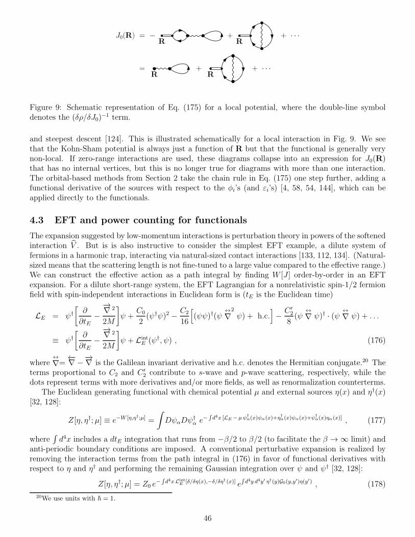
J0(R) = −R

+R

+ · · ·

=R

+R

+ · · ·

Figure 9: Schematic representation of Eq. (175) for a local potential, where the double-line symboldenotes the (δρ/δJ0)

−1 term.

and steepest descent [124]. This is illustrated schematically for a local interaction in Fig. 9. We seethat the Kohn-Sham potential is always just a function of R but that the functional is generally verynon-local. If zero-range interactions are used, these diagrams collapse into an expression for J0(R)that has no internal vertices, but this is no longer true for diagrams with more than one interaction.The orbital-based methods from Section 2 take the chain rule in Eq. (175) one step further, adding afunctional derivative of the sources with respect to the φi’s (and εi’s) [4, 58, 54, 144], which can beapplied directly to the functionals.

4.3 EFT and power counting for functionals

The expansion suggested by low-momentum interactions is perturbation theory in powers of the softenedinteraction V . But is is also instructive to consider the simplest EFT example, a dilute system offermions in a harmonic trap, interacting via natural-sized contact interactions [133, 112, 134]. (Natural-sized means that the scattering length is not fine-tuned to a large value compared to the effective range.)We can construct the effective action as a path integral by finding W [J ] order-by-order in an EFTexpansion. For a dilute short-range system, the EFT Lagrangian for a nonrelativistic spin-1/2 fermionfield with spin-independent interactions in Euclidean form is (tE is the Euclidean time)

LE = ψ†

[∂

∂tE−

−→∇ 2

2M

]ψ +

C0

2(ψ†ψ)2 −

C2

16

[(ψψ)†(ψ

↔

∇2

ψ) + h.c.]−C ′

2

8(ψ

↔

∇ ψ)† · (ψ↔

∇ ψ) + . . .

≡ ψ†

[∂

∂tE−

−→∇ 2

2M

]ψ + Lint

E (ψ†, ψ) , (176)

where↔

∇=←−∇ −

−→∇ is the Galilean invariant derivative and h.c. denotes the Hermitian conjugate.20 The

terms proportional to C2 and C ′2 contribute to s-wave and p-wave scattering, respectively, while the

dots represent terms with more derivatives and/or more fields, as well as renormalization counterterms.The Euclidean generating functional with chemical potential µ and external sources η(x) and η†(x)

[32, 128]:

Z[η, η†;µ] ≡ e−W [η,η†;µ] =

∫DψαDψ

†α e

−R

d4x [LE −µψ†α(x)ψα(x)+η

†α(x)ψα(x)+ψ

†α(x)ηα(x)] , (177)

where∫d4x includes a dtE integration that runs from −β/2 to β/2 (to facilitate the β →∞ limit) and

anti-periodic boundary conditions are imposed. A conventional perturbative expansion is realized byremoving the interaction terms from the path integral in (176) in favor of functional derivatives withrespect to η and η† and performing the remaining Gaussian integration over ψ and ψ† [32, 128]:

Z[η, η†;µ] = Z0 e−

R

d4xLintE

[δ/δη(x),−δ/δη† (x)] eR

d4y d4y′ η†(y)G0(y,y′)η(y′) , (178)

20We use units with ~ = 1.

46

where the spin indices are implicit and we have introduced the noninteracting partition function Z0.Explicit expressions for the Green’s function in coordinate and momentum space can be found inRef. [32]. The linked-cluster theorem [32] shows that the difference of the interacting and noninteractingthermodynamic potentials Ω and Ω0 is given by the sum of connected diagrams from the expansion ofZ, with the external sources η† and η set to zero at the end:

Ω(µ, T, V )− Ω0(µ, T, V ) =1

β(W [0, 0;µ]−W0[0, 0;µ]) . (179)

In evaluating the Feynman diagrams for W [J ] and new diagrams for Γ[ρ] order by order in theexpansion (e.g., EFT power counting), the source J0(x) is now the background field. This means thatpropagators (lines) in the background field J0(x) are

G0KS(x,x

′;ω) =∑

i

φi(x)φ∗i (x

′)

[θ(εi − εF)

ω − εi + iη+

θ(εF − εi)

ω − εi − iη

], (180)

where φi(x) satisfies:[−∇2

2M+ vext(x)− J0(x)

]φi(x) = εiφi(x) . (181)

For example, if we apply this prescription to the short-range LO contribution (i.e., Hartree-Fock), weobtain

W1[J0] =1

2ν(ν − 1)C0

∫d3x

∫ ∞

−∞

dω

2π

∫ ∞

−∞

dω′

2πG0

KS(x,x;ω)G0KS(x,x;ω

′)

= −1

2

(ν − 1)

νC0

∫d3x [ρJ0(x)]

2 , (182)

where ν is the spin-isospin degeneracy and

ρJ0(x) ≡ ν

εF∑

i

|φi(x)|2 . (183)

Expressions for the other Wi’s proceed directly from conventional Feynman rules using the new propa-gator.

Given W [J ] as an EFT expansion, we perform the Legendre transformation,

Γ[ρ] = W [J ]−

∫Jρ , (184)

by using the EFT power counting with the inversion method as described above, which gives us themeans to invert to find J [ρ] and to make an order-by-order inversion from W [J ] to Γ[ρ] [129, 124, 130].It proceeds by decomposing J(x) = J0(x) + JLO(x) + JNLO(x) + . . . as described earlier and fixing J0using

ρ(x) =δW0[J0]

δJ0(x)and J0(x)|ρ=ρgs =

δΓinteracting[ρ]

δρ(x)

∣∣∣∣ρ=ρgs

. (185)

Evaluating the functional derivatives is immediate if Γ is approximated so that the dependence on thedensity is explicit, as with the LDA or DME (see below). Otherwise we apply the OEP chain rule.

Consider the T = 0 local density approximation (LDA) for a dilute fermion gas with natural short-ranged interactions (meaning the scattering length a0 is comparable in magnitude to the effective ranger0 and the p-wave scattering length ap [138]). The energy density in the uniform system evaluates to:

E

V= ρ

k2F2M

[3

5+ (ν − 1)

2

3π(kFa0) + (ν − 1)

4

35π2(11− 2 ln 2)(kFa0)

2 (186)

+ (ν − 1)(0.076 + 0.057(ν − 3)

)(kFa0)

3 + (ν − 1)1

10π(kFr0)(kFa0)

2 + (ν + 1)1

5π(kFap)

3 + · · ·

].

47

0 1 2 3 4 5r/b

0

1

2

3

4

ρ(r/

b)

C0 = 0 (exact)

Kohn-Sham LOKohn-Sham NLO (LDA)Kohn-Sham NNLO (LDA)

E/A <kFa

s> <r

2>

1/2

6.75 -0.52 2.60

5.98 -0.58 2.35

6.25 -0.55 2.47

6.23 -0.55 2.46240 Fermions

spin up/downscattering length a

s = −0.16

Figure 10: Density profile of a dilute system of fermions in a trap [133].

where kFa0, kFr0, and kFap are expansion parameters with kF = (6π2ρ/ν)1/3. Using this relation toreplace kF everywhere by ρ(x), we directly obtain the LDA expression for Γ[ρ],

Γ[ρ] =

∫d3x

[TKS(x)+

1

2

(ν − 1)

ν

4πa0M

[ρ(x)]2 + d1a202M

[ρ(x)]7/3

+ d2 a30[ρ(x)]

8/3 + d3 a20 r0[ρ(x)]

8/3 + d4 a3p[ρ(x)]

8/3 + · · ·

]. (187)

The Kohn-Sham J0 according to the EFT expansion follows immediately in the LDA from (185):

J0(x) =

[−(ν − 1)

ν

4πa0M

ρ(x)− c1a202M

[ρ(x)]4/3 − c2 a30[ρ(x)]

5/3 − c3 a20 r0[ρ(x)]

5/3 − c4 a3p[ρ(x)]

5/3 + · · ·

].

(188)where the di’s and ci’s are given in Ref. [145]. Sample results at different EFT orders for a diluteFermi gas in a harmonic oscillator trap are shown in Fig. 10. Note the systematic convergence withsuccessive orders in the LDA average 〈kFas〉 (and as ≡ a0) for both the energy and density.

An important consequence of the systematic EFT approach is that we can also estimate individualterms in energy functionals. If we scale contributions to the energy per particle according to the averagedensity or 〈kF〉, we can make such estimates [133, 112]. This is shown in Fig. 11 for both the dilutetrapped fermions, which is under complete control, and for phenomenological energy functionals fornuclei, to which a postulated QCD power counting is applied [146, 147]. In both cases the estimates21

agree well with the actual numbers (sometimes overestimating the contribution because of accidentalcancellations), which means that truncation errors are understood. Understanding how such powercounting can emerge from the MBPT-based DFT for nuclei is an important problem for future study.

4.4 Additional comments

The perspective of Legendre transforms clarifies many DFT issues [29]. For example:

• The Legendre transform formulation adds mathematical rigor to DFT claims. For example, onefinds that a bijective mapping between v and ρ does not exist in general. However, it is notnecessary for there to be such a mapping to have a Legendre transform; only the uniqueness of ρgiven v is needed.

21The symbols with error bars are natural estimates with a factor of two spread in the order unity coefficient.

48

LO NLO NNLO0.01

0.1

1

ener

gy/p

artic

le

ν=4, as=+0.1, A=140

ν=4, as=-0.1, A=140

ν=2, as=+.16, A=330

Figure 11: Estimates for energy functionals for a dilute fermions in a harmonic trap (left) and forphenomenological energy functionals for nuclei (right).

• For non-degenerate states, it is true that the density is the functional derivative of the energywith respect to the external potential. But this is not actually needed and so is not a problem fordegenerate states; only the concavity of E[v] is necessary.

• DFT is only variational with respect to ρ if we have the exact functional (i.e., never). Once thereare approximations, it is no longer variational. This is not a cause for concern, as other successfulmany-body approaches such as coupled cluster are also not variational.

Additional useful comments on DFT and Legrendre transforms can be found in Ref. [29].

5 Topics for nuclear DFT

In this section, we consider various topics specifically relevant to implementations of DFT for nuclei.

5.1 Pairing

Pairing is an important feature of finite nuclei that is absent from isolated atoms and molecules. Itsinclusion in nuclear DFT based on microscopic interactions is a topic of much current activity. Whilethere is some work on superconductivity in a Coulomb DFT framework, it is based on using non-localsource terms to avoid divergences. The use of local densities for pairing is generally preferred for finitenuclei from a computational point of view. However, we note that recent results from hybrid EDFcalculations using low-momentum potentials at lowest order, which suggest that an accurate ab initio

DFT treatment of pairing is feasible [15], use non-local pairing fields. To use local pairing densities, weneed a consistent generalization of the Skyrme-Hartree-Fock-Bogoliubov approach [106]. In fact, onecan use functionals with local pairing fields as in phenomenological Skyrme functionals (that are basedon zero-range effective interactions) by properly renormalizing [52, 148].

Pairing is an example of spontaneous symmetry breaking, which is naturally accommodated in aneffective action framework [118, 119]. For example, consider testing for zero-field magnetization M in aspin system by introducing an external field H to break the rotational symmetry. Legendre transformthe Helmholtz free energy F (H):

invert M = −∂F (H)/∂H =⇒ Γ[M ] = F [H(M)] +MH(M) . (189)

Because H = ∂Γ/∂M −→ 0, we look for the stationary points of Γ to identify possible ground states,including whether the symmetry broken state is lowest. For pairing, the broken symmetry is a U(1)

49

[phase] symmetry for fermion number. We apply an external source that breaks the number symmetry,forcing ψψ to have an expectation value. Then we turn that source off and see whether the expectationvalue (condensate) persists. (Note: we will only have actual spontaneous symmetry breaking in aninfinite system.)

The textbook effective action treatment of pairing in condensed matter is to introduce a contactinteraction [127, 128]: g ψ†ψ†ψψ, and perform a Hubbard-Stratonovich transformation with an auxiliarypairing field ∆(x) coupled to ψ†ψ†, which eliminates the contact interaction. Then one constructs theone-particle-irreducible effective action Γ[∆] with ∆ = 〈∆〉, and looks for values for which δΓ/δ∆ = 0.To leading order in the loop expansion (which is a mean field approximation), this yields the BCSweak-coupling gap equation with gap ∆.

The natural alternative here is to use the inversion method for effective actions again [129, 124, 130].Thus we introduce another external current j(x), which is coupled to the fermion pair density ψψ inorder to explicitly break the phase symmetry. This is a natural generalization of normal-state Kohn-Sham DFT [51, 52, 149]. The generating functional has sources J, j coupled to the correspondingdensities [143]:

Z[J, j] = e−W [J,j] =

∫D(ψ†ψ) e−

R

d4x [L+J(x)ψ†αψα+j(x)(ψ

†↑ψ

†↓+ψ↓ψ↑)] . (190)

Densities are found by functional derivatives with respect to J and j:

ρ(x) ≡ 〈ψ†(x)ψ(x)〉J,j =δW [J, j]

δJ(x)

∣∣∣∣j

, (191)

and (note that κ is called φ in Ref. [143])

κ(x) ≡ 〈ψ†↑(x)ψ

†↓(x) + ψ↓(x)ψ↑(x)〉J,j =

δW [J, j]

δj(x)

∣∣∣∣J

. (192)

(The source j would in general be complex, but it is sufficient for our purposes to take it to be real.)The effective action Γ[ρ, κ] follows as in Section 4 by functional Legendre transformation:

Γ[ρ, κ] = W [J, j]−

∫d4x J(x)ρ(x)−

∫d4x j(x)κ(x) , (193)

and is proportional to the (free) energy functional E[ρ, κ]; at finite temperature, the proportionalityconstant is β. The sources are given by functional derivatives wrt ρ and κ:

δE[ρ, κ]

δρ(x)= J(x) and

δE[ρ, κ]

δκ(x)= j(x) . (194)

But the sources are zero in the ground state, so we determine the ground-state ρ(x) and κ(x) bystationarity:

δE[ρ, κ]

δρ(x)

∣∣∣∣ρ=ρgs,κ=κgs

=δE[ρ, κ]

δκ(x)

∣∣∣∣ρ=ρgs,κ=κgs

= 0 . (195)

This is Hohenberg-Kohn DFT extended to pairing!We need a method to carry out the Legendre transforms to get Kohn-Sham DFT; an obvious choice

is to apply the Kohn-Sham inversion method again, with order-by-order matching in the countingparameter λ. Once again,

diagrams =⇒ W [J, j, λ] = W0[J, j] + λW1[J, j] + λ2W2[J, j] + · · · (196)

assume =⇒ J [ρ, κ, λ] = J0[ρ, κ] + λJ1[ρ, κ] + λ2J2[ρ, κ] + · · · (197)

assume =⇒ j[ρ, κ, λ] = j0[ρ, κ] + λj1[ρ, κ] + λ2j2[ρ, κ] + · · · (198)

derive =⇒ Γ[ρ, κ, λ] = Γ0[ρ, κ] + λΓ1[ρ, κ] + λ2Γ2[ρ, κ] + · · · (199)

50

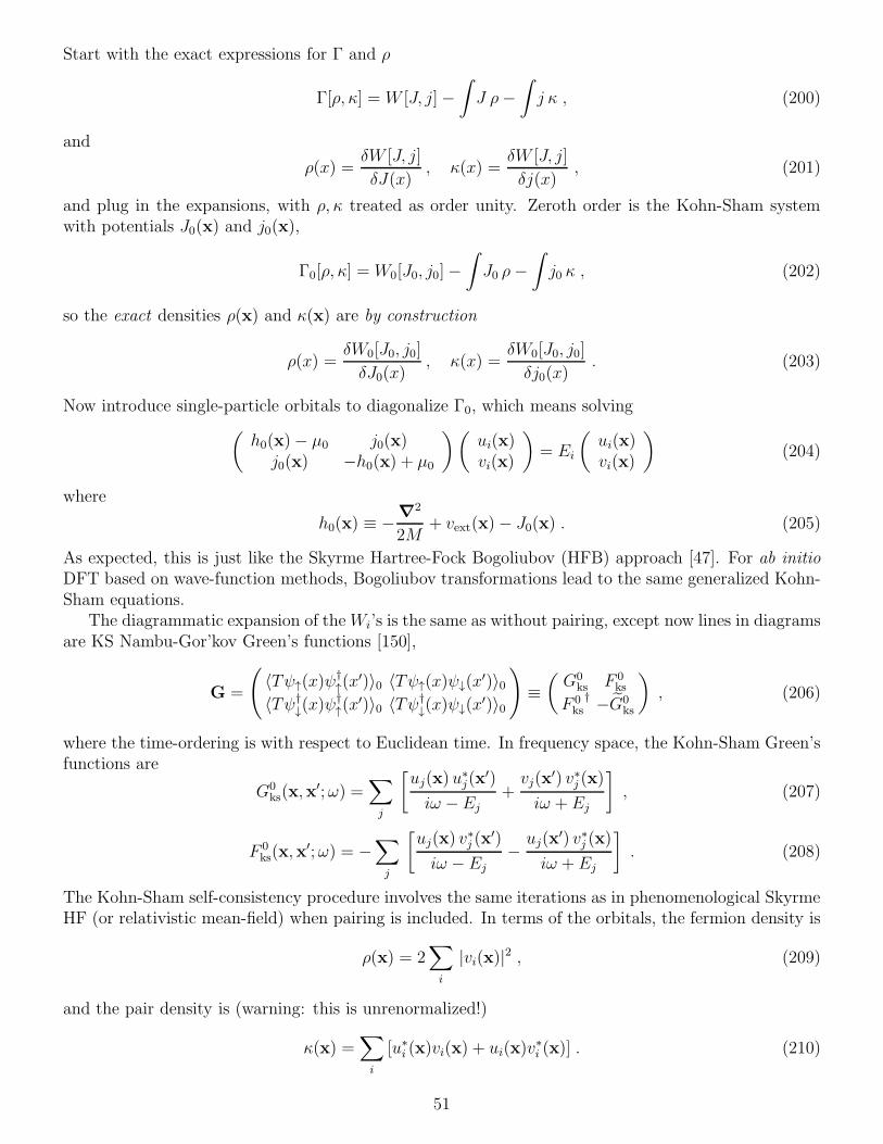
Start with the exact expressions for Γ and ρ

Γ[ρ, κ] = W [J, j]−

∫J ρ−

∫j κ , (200)

and

ρ(x) =δW [J, j]

δJ(x), κ(x) =

δW [J, j]

δj(x), (201)

and plug in the expansions, with ρ, κ treated as order unity. Zeroth order is the Kohn-Sham systemwith potentials J0(x) and j0(x),

Γ0[ρ, κ] =W0[J0, j0]−

∫J0 ρ−

∫j0 κ , (202)

so the exact densities ρ(x) and κ(x) are by construction

ρ(x) =δW0[J0, j0]

δJ0(x), κ(x) =

δW0[J0, j0]

δj0(x). (203)

Now introduce single-particle orbitals to diagonalize Γ0, which means solving(h0(x)− µ0 j0(x)j0(x) −h0(x) + µ0

)(ui(x)vi(x)

)= Ei

(ui(x)vi(x)

)(204)

where

h0(x) ≡ −∇2

2M+ vext(x)− J0(x) . (205)

As expected, this is just like the Skyrme Hartree-Fock Bogoliubov (HFB) approach [47]. For ab initio

DFT based on wave-function methods, Bogoliubov transformations lead to the same generalized Kohn-Sham equations.

The diagrammatic expansion of theWi’s is the same as without pairing, except now lines in diagramsare KS Nambu-Gor’kov Green’s functions [150],

G =

(〈Tψ↑(x)ψ

†↑(x

′)〉0 〈Tψ↑(x)ψ↓(x′)〉0

〈Tψ†↓(x)ψ

†↑(x

′)〉0 〈Tψ†↓(x)ψ↓(x

′)〉0

)≡

(G0

ks F 0ks

F 0ks

†−G0

ks

), (206)

where the time-ordering is with respect to Euclidean time. In frequency space, the Kohn-Sham Green’sfunctions are

G0ks(x,x

′;ω) =∑

j

[uj(x) u

∗j(x

′)

iω −Ej+vj(x

′) v∗j (x)

iω + Ej

], (207)

F 0ks(x,x

′;ω) = −∑

j

[uj(x) v

∗j (x

′)

iω − Ej−uj(x

′) v∗j (x)

iω + Ej

]. (208)

The Kohn-Sham self-consistency procedure involves the same iterations as in phenomenological SkyrmeHF (or relativistic mean-field) when pairing is included. In terms of the orbitals, the fermion density is

ρ(x) = 2∑

i

|vi(x)|2 , (209)

and the pair density is (warning: this is unrenormalized!)

κ(x) =∑

i

[u∗i (x)vi(x) + ui(x)v∗i (x)] . (210)

51

W [; j = +

j j

+

0.01 0.1 1 10 100Energy Cutoff

10-6

10-5

10-4

10-3

10-2

10-1

100

|φE

c− φ ∞

|/φ∞

subtract 1/εk

subtract P/(εk−µ

0)

µ0 = 1.

j0 = 0.1

2M = 1.

Figure 12: (a) Feynman diagram at second order in a perturbative expansion of W [µ, j] in j. (b) Con-verence of the integral for the pair density in the uniform system for two subtractions as a function ofan energy cutoff Ec in the integral.

The chemical potential µ0 is fixed by∫ρ(x) = A. Diagrams for Γ[ρ, κ] ∝ E0[ρ, κ] + Eint[ρ, κ] yield the

Kohn-sham potentials

J0(x)∣∣∣ρ=ρgs

=δEint[ρ, κ]

δρ(x)

∣∣∣∣ρ=ρgs

and j0(x)∣∣∣κ=κgs

=δEint[ρ, κ]

δκ(x)

∣∣∣∣κ=κgs

. (211)

So it appears that everything goes through smoothly as in the ab initio DFT without pairing.Potential problems arise, however, because the use of local composite operators leads to new ultra-

violet divergences even at the mean-field (Hartree-Fock) level when pairing is included. Divergencesat this order are not encountered when coupling an external source to the fermion density ψ†ψ, butappear now because the composite operators ψψ and ψ†ψ† need additional renormalization [151]. Thedivergences at leading order are symptomatic of generic problems identified long ago by Banks and Raby[152] that arise with effective potentials of local composite operators. (It was to avoid these divergencesin DFT that non-local sources were used in Refs. [153, 154].) These problems inhibited for many yearsthe use of effective actions of composite operators but more recently Verschelde et al. [155, 156, 157]and Miransky et al. [158, 159, 160] have revived their use for relativistic field theories. In Ref. [143],it was shown how to identify and renormalize up to NLO the EFT from Section 4.3 when pairing wasincluded.

The source of the divergences is found immediately when we try to carry out the DFT pairingcalculation even for a uniform dilute Fermi system. The generating functional with constant sources µand j for the EFT from Section 4.3 is:

e−W [µ,j] =

∫D(ψ†ψ) exp

−

∫d4x

[ψ†α(∂

∂τ−

∇ 2

2M− µ)ψα

+C0

2ψ†↑ψ

†↓ψ↓ψ↑ + j(ψ↑ψ↓ + ψ†

↓ψ†↑)]

+1

2ζ j2

](212)

(cf. adding an integration over an auxiliary field∫D(∆∗,∆) e

− 1|C0|

R

|∆|2, then shifting variables to elim-

inate ψ†↑ψ

†↓ψ↓ψ↑ for ∆∗ψ↑ψ↓). There are new divergences because of j, e.g., expand W to O(j2) [see

Fig. 12(a)], which has the same linear divergence found in 2-to-2 scattering. (Equivalently, in coordinatespace there is a 1/|r1 − r2| divergence in

∑i v

∗i (r1)ui(r2) as it becomes local with |r1 − r2| → 0.) To

renormalize, we add the counterterm 12ζ |j|2 to L (see [120]), which is additive to W (cf. |∆|2), so there

is no effect on scattering.

52

We can follow a less formal and more numerically suitable procedure to renormalize the pair (anoma-lous) density,

κ(x) =∑

i

[u∗i (x)vi(x) + ui(x)v∗i (x)] −→∞ , (213)

which diverges for contact interactions in a finite system. This is to use the renormalized expression forκ in the uniform system,

κ =

∫ kc d3k

(2π)3j0

(1√

(ǫ0k − µ0)2 + j20−

1

ǫ0k

)kc→∞−→ finite, (214)

which is cut off at momentum kc, and apply this in a local density approximation (i.e., Thomas-Fermi):

κ(x) = 2Ec∑

i

ui(x)vi(x)− j0(x)M kc(x)

2π2with Ec =

k2c (x)

2M+ J(x)− µ0 . (215)

This procedure was worked out by Bulgac and collaborators in Refs. [52, 51, 149, 161]. Convergence isvery slow as the energy cutoff Ec is increased, so Bulgac and Yu devised a different subtraction,

κ =

∫ kc d3k

(2π)3j0

(1√

(ǫ0k − µ0)2 + j20−

P

ǫ0k − µ0

)kc→∞−→ finite . (216)

A comparison of convergence in the uniform system for the two subtraction schemes (214) and (216) [seeFig. 12] shows dramatic improvement for the Bulgac/Yu subtraction. Bulgac et al. have demonstratedthat this works in finite systems [149] and it has been adopted for some Skyrme HFB implementations.

5.2 Broken symmetries

Ordinary nuclei are self-bound, which presents conceptual issues about whether Kohn-Sham DFT is welldefined and practical problems on how to deal with the consequences of symmetry breaking by the KSpotentials, which will not have all of the symmetries of the Hamiltonian [46].22 These broken symmetriesinclude the U(1) phase symmetry for fermion number and translational and rotational invariance. Whilerestoring broken symmetries is a topic well-explored for mean-field approximations [46, 47], it has onlyrecently been considered in a context relevant to ab initio DFT. Because no proven practical approachesare yet available, we simply point out the issues and current references.

The textbook discussions of how to restore mean-field broken symmetries tend to follow one of thesetwo related lines of discussion:

• States related by a unitary transformation U(α) corresponding to a broken symmetry are degen-erate:

|φα〉 = U(α)|φ〉 (217)

with |φ〉 a “deformed” state, implies

〈φα|HN |φα〉 = 〈φ|HN |φ〉 . (218)

The degeneracy can be removed by diagonalizing in the subspace spanned by the degeneratestates. The group parameter α for continuous groups can be considered a collective coordinate,which specifies the orientation in gauge space of the deformed state |φ〉. A general strategy is totransform from 3A particle coordinates into collective and internal coordinates [47].

22A state is one of broken symmetry if it does not have the quantum numbers of the eigenstates of the Hamiltonian(parity, particle number, angular momentum, linear momentum, isospin, and so on). Note that this does not mean itneeds to be invariant, just that it can be labeled by definite quantum numbers [46].

53

• In finite systems, broken symmetries arise only as a result of approximations. This usually hap-pens with variational calculations over trial wavefunctions that are too restricted; a mean-fieldapproximation is an example. The symmetry can be restored by using a linear superposition ofdegenerate states:

|ψ〉 =

∫dα f(α)|φα〉 , (219)

which when minimized with respect to the f(α)’s projects states of good symmetry [46]. (Becauseminimizing with respect to |φ〉 and with respect to f(α) do not commute, there are two types ofprojection. It is most accurate to project first and then find the best deformed state correspondingto a given quantum number.) For example, particle number projection for EDF’s is described inRefs. [162, 163].

When implemented, these approaches are sometimes considered to be beyond EDF, where there are onlydensities and not a wavefunction. From a different perspective, the restoration of broken symmetriesof GCM-type configuration mixings should be considered as a “multi-reference” extension of the usual“single-reference” EDF implementation (see Refs. [12, 48, 49]). What about ab initio DFT as we haveconsidered it?

For nuclear DFT, the conceptual question was highlighted by J. Engel [164], who pointed out thatthe ground state of a self-bound system, with a plane wave describing the center of mass, has a densitydistributed uniformly over space. Clearly this is not the density one wants to find from DFT, so thereis a question of how to proceed. There are two separate considerations: i) Does Kohn-Sham DFT existin a useful form for self-bound systems? ii) If so, how does one formulate and implement it? Engel andother authors have addressed this issue recently [164, 165, 166, 167, 168, 169], with a consensus thatHK existence proofs for DFT are still well founded, but for internal densities (meaning independentof the center-of-mass motion when considering broken translational symmetry).23 These authors alsopropose various schemes to carry out Kohn-Sham DFT that should be testable in the near future.

We have considered ab initio DFT from two viewpoints: MBPT using wave-function methods andeffective actions with path integrals. How are these symmetry issues dealt with in these approaches?Wave function methods have several related strategies for dealing with the “center of mass” (COM)problem:

1. Isolate the “internal” degrees of freedom, typically by introducing Jacobi coordinates. Then theobservables are by construction independent of the COM. This gets increasingly cumbersome withgreater numbers of particles.

2. Work in a harmonic-oscillator Slater determinant basis, for which the COM decouples, and intro-duce a potential for the COM that allows its contribution to be subtracted.

3. Work with the internal Hamiltonian (i.e., subtract the COM kinetic energy TCM) so that theCOM part factors and does not contribute to observables to good approximation (see in particularRef. [170] for coupled cluster calculations).

Versions of the first two possibilities are in fact among the ideas considered for DFT in Refs. [164, 165,166, 167, 168, 169].

For the effective action approach, the issue of broken symmetry is familiar from the study of soli-tons [171, 32], where it arises as the problem of dealing with zero modes when calculating quantumfluctuations. The methods found in the literature are similar to the textbook approaches cited above.One compelling approach for ab initio DFT in the effective action formalism uses the Fadeev-Popov

23In other contexts, such densities are called “intrinsic”, but this has a different meaning in the context of symmetrybreaking, so “internal” is typically used instead.

54

construction (or BRST invariance [121]) to introduce collective coordinates through ghost degrees offreedom. This is worked out to some degree by Calzetta and Hu for broken particle number symmetryin Ref. [122], but a concrete implementation appropriate for nuclei remains to be formulated.

Thus, while dealing with broken symmetries in the DFT of self-bound nuclei is a topic of activeinvestigation, the best way forward is not clear.

5.3 Single-particle energies

The only quantities obtained from Kohn-Sham DFT for ground states that are guaranteed to be thesame as those obtained from many-body wave function calculations (at an equivalent level of approxi-mation) are the total energies and the densities associated with the functionals.24 Of course, measurablequantities that can be expressed as the differences of ground state energies are also reliable. For nuclearapplications, one would like to establish a robust connection between KS eigenvalues and nuclear single-particle energies, but it is often observed that Kohn-Sham eigenvalues, except at the Fermi surface, arenot physical. On the other hand, Bartlett et al. claim that with a sufficiently rich Coulomb DFT func-tional, the KS orbital eigenvalues can be good approximations to removal (ionization) energies [58, 59].

We can understand how improved approximations can happen by considering how the full self-consistent one-particle Green’s function G, whose spectral density is physical, can be expressed in termsof the KS Green’s function GKS. We saw this earlier in the form of the Sham-Schluter equation, Eq. (65);here we consider an alternative functional integral derivation and a diagrammatic representation to makesome additional points. We add a non-local source ξ(x′, x) coupled to ψ(x)ψ†(x′) [we’re in Minkowskispace now with x = (x, t) so that we get real-time Green’s functions]:

Z[J, ξ] = eiW [J,ξ] =

∫DψDψ† ei

R

d4x [L+ J(x)ψ†(x)ψ(x) +R

d4x′ ψ(x)ξ(x,x′)ψ†(x′)] . (220)

Writing Γ[ρ, ξ] = Γ0[ρ, ξ] + Γint[ρ, ξ] and using functional properties of Legendre transforms,

G(x, x′) =δW

δξ

∣∣∣∣J

=δΓ

δξ

∣∣∣∣ρ

= Gks(x, x′) +Gks

[1i

δΓint

δGks+δΓint

δρ

]Gks , (221)

which is represented diagrammatically in Fig. 13 [134]. (Note that these are the reducible self-energieshere; so this is actually a rearranged Dyson-like equation that is equivalent to Eq. (65).)

G

=

G

ks

+

G

ks

G

ks

0

ks

+

G

ks

G

ks

Figure 13: Full Green’s function G in terms of the Kohn-Sham Green’s function Gks.

The Green’s functions G and Gks yield the same density by construction; that is, the Kohn-Shamdensity ρks(x) = −iνG

0KS(x, x

+) equals the full density ρ(x) = −iνG(x, x+). Here is a simple diagram-matic demonstration (the double line is minus the inverse of a single particle-hole ring):

x

=

x

+

x

+

x

=

x

24Note that these densities are not necessarily observables; e.g., the nuclear proton density is related to the measuredcharge density by a model dependent prescription, although this model dependence is generally considered to be negligible.

55

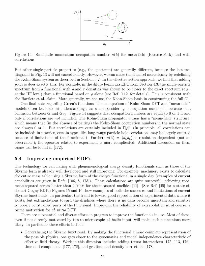
Fk k

n(k)

1

Figure 14: Schematic momentum occupation number n(k) for mean-field (Hartree-Fock) and withcorrelations.

But other single-particle properties (e.g., the spectrum) are generally different, because the last twodiagrams in Fig. 13 will not cancel exactly. However, we can make them cancel more closely by redefiningthe Kohn-Sham system as described in Section 3.2. In the effective action approach, we find that addingsources does exactly this. For example, in the dilute Fermi gas EFT from Section 4.3, the single-particlespectrum from a functional with ρ and τ densities was shown to be closer to the exact spectrum (e.g.,at the HF level) than a functional based on ρ alone (see Ref. [112] for details). This is consistent withthe Bartlett et al. claim. More generally, we can use the Kohn-Sham basis in constructing the full G.

One final note regarding Green’s functions. The comparison of Kohn-Sham DFT and “mean-field”models often leads to misunderstandings, as when considering “occupation numbers”, because of aconfusion between G and GKS. Figure 14 suggests that occupation numbers are equal to 0 or 1 if andonly if correlations are not included. The Kohn-Sham propagator always has a “mean-field” structure,which means that (in the absence of pairing) the Kohn-Sham occupation numbers in the normal stateare always 0 or 1. But correlations are certainly included in Γ[ρ]! (In principle, all correlations canbe included; in practice, certain types like long-range particle-hole correlations may be largely omittedbecause of limitations of the functional.) Further, n(k) = 〈a†kak〉 is resolution dependent (not anobservable!); the operator related to experiment is more complicated. Additional discussion on theseissues can be found in [172].

5.4 Improving empirical EDF’s

The technology for calculating with phenomenological energy density functionals such as those of theSkyrme form is already well developed and still improving. For example, machinery exists to calculatethe entire mass table using a Skyrme form of the energy functional in a single day (examples of currentcapabilities are given in Refs. [106, 8, 173]). These calculations are quite successful, achieving root-mean-squared errors better than 2 MeV for the measured nuclides [11]. (See Ref. [45] for a state-of-the-art Gogny EDF.) Figures 15 and 16 show examples of both the successes and limitations of currentSkyrme functionals. In particular, the trend is toward good reproduction of experimental data where itexists, but extrapolations toward the driplines where there is no data become uncertain and sensitiveto poorly constrained parts of the functional. Improving the reliability of extrapolation is, of course, aprime motivation for ab initio DFT.

There are substantial and diverse efforts in progress to improve the functionals in use. Most of these,even if not directly motivated by ties to microscopic ab initio input, will make such connections morelikely. In particular these efforts include:

• Generalizing the Skyrme functional. By making the functional a more complete representation ofthe possible physics, one gets closer to the systematics and model independence characteristic ofeffective field theory. Work in this direction includes adding tensor interactions [175, 113, 176],time-odd components [177, 178], and gradient and density corrections [178].

56

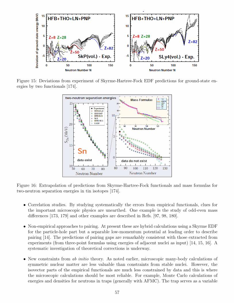
Figure 15: Deviations from experiment of Skyrme-Hartree-Fock EDF predictions for ground-state en-ergies by two functionals [174].

Figure 16: Extrapolation of predictions from Skyrme-Hartree-Fock functionals and mass formulas fortwo-neutron separation energies in tin isotopes [174].

• Correlation studies. By studying systematically the errors from empirical functionals, clues forthe important microscopic physics are unearthed. One example is the study of odd-even massdifferences [173, 179] and other examples are described in Refs. [97, 98, 180].

• Non-empirical approaches to pairing. At present these are hybrid calculations using a Skyrme EDFfor the particle-hole part but a separable low-momentum potential at leading order to describepairing [14]. The predictions of pairing gaps are remarkably consistent with those extracted fromexperiments (from three-point formulas using energies of adjacent nuclei as input) [14, 15, 16]. Asystematic investigation of theoretical corrections is underway.

• New constraints from ab initio theory. As noted earlier, microscopic many-body calculations ofsymmetric nuclear matter are less valuable than constraints from stable nuclei. However, theisovector parts of the empirical functionals are much less constrained by data and this is wherethe microscopic calculations should be most reliable. For example, Monte Carlo calculations ofenergies and densities for neutrons in traps (generally with AFMC). The trap serves as a variable

57

vext(x), so these calculations become benchmarks for testing or fitting empirical energy functionals.Note that constraints can be significantly more than realized by comparison to uniform neutronmatter. Such a program is being carried out with GFMC/AFMC and NCSM calculations as partof the UNEDF project [9].

• Development of EDF without explicit underlying Hamiltonians. The strategy and distinction ofEDF from DFT are described in Ref. [12], as well as challenges [13]. The insights gained andtechniques being developed [12, 48, 49] will carry over to ab initio DFT.

• Long-range correlations. With current EDF’s, the incorporation of long-range correlation effectsis handled separately from the functional calculations [11, 41]. The outlook for directly includingthis physics in an ab initio approach with OEP is unclear, but there are precedents in CoulombOEP (e.g., the Coulomb ring sum describing the high-density expansion of the electron gas canbe included).

• Merging a variant of the density matrix expansion (DME) and empirical functionals. The com-parison of the DME-I and DME-II curves in Fig. 7 gives us an estimate of the truncation errorin the expansion applied to the NNN terms because these prescriptions differ in the contributionsof higher-order terms in the expansion. Indeed, it has been verified that suppressing these termsby hand brings the predictions for the A and B coefficients into agreement [96]. The qualitativedifference for the NNN-only contribution to B is large, but the actual coefficient itself is small,so this should not be alarming. However, because the combination of A and B and the kineticenergy to obtain the nuclear matter energy per particle involves strong cancellations, the spreadin Fig. 7 is large on the scale of nuclear binding energies.

These differences motivate a generalization of the Negele-Vautherin DME following the discussionin Ref. [181]. In this approach, the expansion of the scalar density matrix takes the factorizedform

ρ(R+s

2,R−

s

2) =

∑

n

Πn(kFs)〈On(R)〉 , (222)

where

〈On(R)〉 = ρ(R), τ(R),∇2ρ(R), · · · , (223)

and kF is a momentum scale typically taken to be kF(R) as in Eq. (120). Similar expansions aremade for the other components of the density matrix. Input from finite nuclei can be used todetermine the Πn functions, which can be viewed as general resummations of the DME expansion.A program to merge these developments with empirical Skyrme functionals is underway [115].

Almost all of the major developments are only recently begun, so many new results can be expected inthe coming years.

6 Summary and outlook

The quest for an understanding of all nuclei based on microscopic few-body interactions among nucleonsis being attacked from multiple directions. In this review, we have considered ab initio density functionaltheory for nuclei, defined as DFT based on a realistic nuclear Hamiltonian (meaning one that accuratelyreproduces few-body data) and orbitals that satisfy equations with local Kohn-Sham potentials. This isan ambitious undertaking and one which will not be realized without significant further developments innuclear structure calculations. Nevertheless, the prospects are good for making microscopic connectionsto empirical functionals in the short term and building on them steadily.

58

We base this optimism in part on the successful advances in ab initio DFT for Coulomb-basedsystems by quantum chemists and condensed matter physicists. We believe nuclear physicists willprofit from greater attention paid to Coulomb DFT developments. At the same time, we recognizethat these advances have taken many years to realize and may not be readily transferred to the nucleardomain. Indeed, we have argued that strong analogies between Coulomb and nuclear systems are reallyonly apparent when one considers low-momentum interactions, so that the correlations induced by moreconventional (local or almost local) interactions are tamed from the outset. As one strives for greateraccuracy, the differences between atoms or molecules and nuclei are likely to become more significant.

Perdew and collaborators describe for Coulomb DFT a “Jacob’s Ladder” of increasingly sophisticated“nonempirical” functionals stretching toward the heaven of chemical accuracy. In Ref. [43], five rungsof the ladder are identified (see also [182]):

1. The local density approximation (LDA) with both spin densities ρ↑(x) and ρ↓(x) as ingredients(usually called LSDA).

2. The generalized gradient approximation (GGA), which adds dependence on ∇ρ↑(x) and ∇ρ↓(x)to the LSDA functional.

3. The meta-GGA adds dependence on (some subset of) ∇2ρ↑(x), ∇2ρ↓(x), τ↑(x), and τ↓(x). Note

that the kinetic energy densities are actually non-local functionals of the ordinary density, althoughonly semi-local functionals of the oocupied KS orbitals.

4. Hyper-GGA, which includes the exact exchange energy density calculated with the (occupied)orbitals.

5. Full orbital-based DFT, which in addition to exact exchange uses unoccupied orbitals. For ex-ample, this might include the random phase approximation (RPA) with Kohn-Sham orbitals toaddress long-range correlations.

An important aspect of the overall approach is “constraint satisfaction” as opposed to data fitting, whichis why the functionals are called nonempirical [182]. Climbing this ladder has been a decades-long effortby quantum chemists with much development in progress on the last rung.

We can imagine a corresponding ladder for nuclear DFT climbing toward a universal energy densityfunctional tied to microscopic nuclear Hamiltonians (and ultimately to QCD) that predicts knownnuclear properties more accurately than currently possible and robustly predicts unknown propertieswith plausible theoretical error estimates. The rungs might look like this:

1. Present-day Skyrme EDF’s, which are mostly empirical (i.e., fit to properties of selected medium-to-heavy nuclei), such as described in Ref. [11].

2. Generalized Skyrme interactions, with additional gradient and density dependences, with newconstraints from microscopic theory (e.g., neutron drops).

3. Functionals that merge the long-range parts of the microscopic NN and NNN interactions pre-scribed by chiral EFT, converted to semi-local form with a variant of the density matrix expansion(DME), with a Skyrme functional. The short-range parameters should be refit to nuclear proper-ties and theoretical constraints.

4. A complete functional based on a variant of DME applied to a low-momentum potential that isevolved from chiral EFT NN and NNN interactions.

5. Full orbital-based DFT based on low-momentum interactions.

59

This ladder is tied to our restriction to local Kohn-Sham potentials and so naturally builds on SkyrmeEDF’s. An alternative ladder could build on non-local potentials (e.g., on Gogny-type EDF’s) that arisefrom derivatives with respect to density matrices rather than densities; see Refs. [13, 16] for discussionsalong these lines. Just as in the Coulomb ladder, one hopes for monotonic improvements at each rung,but this may not always be the case. (Of course, rungs will shift or more will be added as progress ismade.)

Rather than climb slowly over the course of decades, nuclear physicists are trying to catch up rapidlyby attacking all of the higher rungs in parallel [8, 9, 10]. As described in Section 5.4, there are extensiveongoing efforts to explore the second rung, including more general density dependence and higher-ordergradients [9, 10], while projects on both rungs three and four have recently been started as part of theUNEDF project [8]. The last rung is in the exploratory stage with tests started in one dimension withnuclear-like interactions for both self-bound and trapped systems to explore the accuracy of the KLI(and related) approximations compared to a full OEP treatment of such systems and to establish thelimitations of semi-local expansions such as the DME.

While the last two rungs can be purely predictive if only few-body data is used to determine theinput Hamiltonian, it is likely that fine-tuning to heavier nuclei will be needed to reach the accuracygoals. This is because even the best ab initio nuclear structure calculations at present only achieveabout 1% accuracy in ground-state energies for a small fraction of the table of nuclides, while nuclearEDF’s such as Skyrme functionals easily surpass this over most of the table. Indeed, the comparativelyhigh accuracy of nuclear EDF may imply that a different organization of the problem (e.g., based on afinite-density effective field theory of nuclei) may be needed.

There are many important open questions to be addressed in the course of these projects (see alsoRef. [13]). Among them are those highlighted in Section 5 on symmetry breaking and restoration, single-particle levels, and pairing; these will be relevant for all rungs of the ladder. At the top of the ladderwe can ask: Which of the problems encountered in Coulomb DFT that motivate orbital-based func-tionals have analogs in nuclear DFT? E.g., what is the impact of self-interaction and missing derivativediscontinuities? Another class of open questions concerns the input Hamiltonian: For low-momentumpotentials, how accurate will many-body perturbation theory be? What corrections/summations willbe needed to reach the desired accuracy for nuclear DFT? Are four-body forces necessary? The list ofproblems yet to solve might be intimidating, especially given the many decades already spent attackingnuclear structure, but the coherence of the current effort and the dramatic advances of just the last fewyears give hope that they can be overcome.

We have taken a broad view at what ab initio density functional theory could be but our discussionhas been far from an exhaustive treatment. By focusing our discussion on orbital-based DFT fornonrelativistic Hamiltonians we have excluded various alternative paths to ab initio DFT. Here aresome of the other approaches that are relevant to the wider nuclear DFT effort:

• The perturbative in-medium results from low-momentum potentials suggest that an alternativeEFT power counting may be appropriate at nuclear matter densities. Kaiser and collaboratorshave proposed a perturbative chiral EFT approach to nuclear matter and then to finite nucleithrough an energy functional [183, 109, 111, 184, 185] (see also [186]). They consider Lagrangiansboth for nucleons and pions and for nucleons, pions, and ∆’s, and fit parameters to nuclearsaturation properties. They construct a loop expansion for the nuclear matter energy per particle,which leads to an energy expansion of the form

E(kF) =∞∑

n=2

knF fn(kF/mπ,∆/mπ) , [∆ =M∆ −MN ≈ 300MeV] (224)

where each fn is determined from a finite number of in-medium Feynman diagrams, which incorpo-rate the long-distance physics. All powers of kF/mπ and ∆/mπ are kept in the fn’s because these

60

ratios are not small quantities [187]. A semi-quantitative description of nuclear matter is foundeven with just the lowest two terms without ∆’s and adding ∆’s brings uniform improvement(e.g., in the neutron matter equation of state). There are open questions about power countingand convergence, but many promising avenues to pursue. By applying the DME in momentumspace to this expansion they derive a Skyrme-like energy functional for nuclei, which has also beenmerged with a treatment of strong scalar and vector mean fields. [109, 110, 111, 184, 185].

• The Superfluid Local Density Approximation (SLDA) and extensions developed by Bulgac andcollaborators [149, 188, 189, 190] have been applied with great success to systems of trapped coldfermionic atoms with large scattering lengths. The SLDA is an extension of DFT to superfluidsystem that uses a semi-local energy density with parameters determined by matching to numeri-cally accurate Monte Carlo simulations of uniform systems. Extensive further development of theSLDA for nuclear systems is in progress.

• We have noted that the Kohn-Sham DFT emphasis on locality in coordinate space is not so naturalin many-body formulations. In particular, the nuclear shell model is naturally considered in thespace of orbitals. Papenbrock has applied the Legendre transform formulation of DFT to energyfunctionals based on shell-model occupation numbers. That is, a functional of the density nowbecomes a function of the occupation numbers in the model space. He and his collaborators haveshown the usefulness of this in solvable models (the pairing Hamiltonian [191] and the three-levelLipkin model [56]). The functional is orbital-based and thus non-local in density. For applicationsto nuclei, the idea is to generalize the Duflo-Zuker mass formula [192, 193] to a functional ofoccupation numbers, with values determined from the minimization of the functional. With 10parameters, an RMS value of deviation for masses of about 2000 nuclei is just over 1MeV.

• Schwenk and Polonyi have proposed an alternative approach to ab initio but orbit-free DFT(i.e., not Kohn-Sham) using a clever renormalization group (RG) evolution [132]. The idea isto introduce an effective action for a nucleus with a low-momentum interaction included witha multiplicative factor λ and a confining background potential (e.g., a harmonic oscillator trap)with a factor (1 − λ). As λ flows from 0 to 1, the background potential is turned off and theinteractions, with associated many-body correlations, are turned on. This evolution is dictated byan RG equation in λ. Work is in progress to implement this approach for a realistic nucleus [194].

• There is a large body of work on covariant approaches to nuclear DFT, which cannot be adequatelysummarized here. Fortunately, there are many reviews that highlight DFT connections, includingRefs. [195, 196, 197, 147, 198, 199], to supplement our brief discussion. Covariant DFT invokes adifferent organization of the nuclear many-body problem that is particularly compelling becauseof the coupling of spin-orbit and central components dictated by relativity. In particular, thecharacteristic feature of relativistic approaches to nuclei is large isoscalar Lorentz scalar andvector mean fields, several hundred MeV in magnitude at nuclear densities, which cancel toprovide nuclear binding but add to produce spin-orbit splittings.

Relativistic mean-field models were originally motivated as the Hartree approximation to a morecomplete theory, but a more recent interpretation of the largely empirical functionals is as rela-tivistic versions of Kohn-Sham DFT [196]. The mean fields serve as local Kohn-Sham potentialsin Dirac equations for the orbitals. This picture is consistent with a microscopic derivation withinan effective action formulation as in Section 4 with sources coupled to each of the relativisticdensities or currents or to corresponding meson-like auxiliary fields [147] (this is in contrast toimplementations of relativistic electronic DFT for heavy atoms, which include only the vectorfour-current [4]). Application of a loop expansion with proper renormalization gives the possi-bility of a systematic microscopic expansion [200, 201]. Other ongoing efforts to provide more

61

ab initio aspects including a connection to free-space NN scattering derive relativistic EDF withdensity dependent meson-baryon vertex functionals, derived from the Dirac-Brueckner theory (seeRefs. [202, 203, 204] and references cited therein).

These more microscopic approaches do not at present have the close connection to few-body dataand to ab initio structure calculations of light nuclei that is possible with the non-relativisticapproaches we have considered. However, the wide phenomenological successes and complemen-tary nature of covariant nuclear DFT motivate further work toward incorporating additionalmicroscopic constraints. In the process, most of the challenges confronting nonrelativistic DFTdiscussed above are being attacked in parallel for covariant DFT. This includes the issues of real-istic pairing interactions [205, 206, 207], coupling to particle-hole vibrations [208], and symmetrybreaking/restoration [209, 210, 211].

Each of these avenues has the potential to make a significant impact on nuclear DFT.

Acknowledgments

We thank S. Bogner, T. Duguet, and A. Schwenk for useful discussions. This work was supportedin part by the National Science Foundation under Grant No. PHY–0653312 and the UNEDF SciDACCollaboration under DOE Grant DE-FC02-07ER41457.

References

[1] R.M. Dreizler and E. Gross, Density Functional Theory (Springer, Berlin, 1990).

[2] R.G. Parr and Y. Weitao, Density-Functional Theory of Atoms and Molecules (InternationalSeries of Monographs on Chemistry) (Oxford University Press, USA, 1994).

[3] W. Koch and M.C. Holthausen, A Chemist’s Guide to Density Functional Theory, 2nd Edition(Wiley-VCH, 2001).

[4] C. Fiolhais, F. Nogueira and M. Marques, editors, A Primer in Density Functional Theory(Springer, Berlin, 2003).

[5] R.M. Martin, Electronic Structure: Basic Theory and Practical Methods (Cambridge UniversityPress, 2004).

[6] J. Kohanoff, Electronic Structure Calculations for Solids and Molecules: Theory and Computa-tional Methods (Cambridge University Press, 2006).

[7] M. Head-Gordon and E. Artacho, Physics Today 61 (2008) 58.

[8] G.F. Bertsch, D.J. Dean and W. Nazarewicz, SciDAC Review 6 (2007) 42.

[9] UNEDF website, http://unedf.org.

[10] FIDIPRO website, https://www.jyu.fi/fysiikka/en/research/accelerator/fidipro.

[11] M. Bender, P.H. Heenen and P.G. Reinhard, Rev. Mod. Phys. 75 (2003) 121.

[12] D. Lacroix, T. Duguet and M. Bender, Phys. Rev. C 79 (2009) 044318.

[13] T. Duguet et al., (2006), arXiv:nucl-th/0606037.

62

[14] T. Duguet and T. Lesinski, Eur. Phys. J. ST 156 (2008) 207.

[15] K. Hebeler et al., (2009), arXiv:0904.3152.

[16] T. Duguet and T. Lesinski, (2009), arXiv:0907.1043.

[17] E. Epelbaum, H.W. Hammer and U.G. Meissner, (2008), arXiv:0811.1338.

[18] R.B. Wiringa, V.G.J. Stoks and R. Schiavilla, Phys. Rev. C51 (1995) 38.

[19] S.C. Pieper and R.B. Wiringa, Ann. Rev. Nucl. Part. Sci. 51 (2001) 53.

[20] S.C. Pieper, Nucl. Phys. A 751 (2005) 516.

[21] P. Navratil et al., (2009), arXiv:0904.0463.

[22] G. Hagen et al., Phys. Rev. C76 (2007) 034302.

[23] G. Hagen et al., Phys. Rev. C76 (2007) 044305.

[24] S.C. Pieper, (2007), arXiv:0711.1500.

[25] G. Hagen et al., Phys. Rev. Lett. 101 (2008) 092502.

[26] N. Argaman and G. Makov, Am. J. Phys. 68 (2000) 69.

[27] P. Hohenberg and W. Kohn, Phys. Rev. 136 (1964) B864.

[28] M. Levy, Phys. Rev. A26 (1982) 1200.

[29] W. Kutzelnigg, J. Mol. Struct. 768 (2006) 163.

[30] H. Eschrig, The Fundamentals of Density Functional Theory (Edition am Gutenbergplatz, Leipzig,2003).

[31] A.L. Fetter and J.D. Walecka, Quantum Many-Particle Systems (McGraw–Hill, New York, 1972).

[32] J.W. Negele and H. Orland, Quantum Many-Particle Systems (Addison-Wesley, Redwood City,CA, 1988).

[33] W.H. Dickhoff and D. Van Neck, Many-Body Theory Exposed!: Propagator Description of Quan-tum Mechanics in Many-Body Systems; 2nd ed. (World Scientific, Singapore, 2005).

[34] J.P. Perdew et al., Journal of Chemical Theory and Computation 5 (2009) 902.

[35] S.K. Bogner, T.T.S. Kuo and A. Schwenk, Phys. Rept. 386 (2003) 1.

[36] S.K. Bogner, R.J. Furnstahl and R.J. Perry, Phys. Rev. C 75 (2007) 061001.

[37] R. Roth et al., Phys. Rev. C 72 (2005) 034002.

[38] R. Roth et al., Phys. Rev. C 73 (2006) 044312.

[39] S.K. Bogner et al., Nucl. Phys. A 763 (2005) 59.

[40] S.K. Bogner et al., (2009), arXiv:0903.3366.

[41] M. Bender and P.H. Heenen, Eur. Phys. J. A25 (2005) 519.

63

[42] J.P. Perdew, Physical Review B 33 (1986) 8822.

[43] J. Perdew and S. Kurth, Density functionals for non-relativistic coulomb systems in the newcentury, A Primer in Density Functional Theory, pp. 1–55, Springer, 2003.

[44] F. Chappert, M. Girod and S. Hilaire, Phys. Lett. B668 (2008) 420.

[45] S. Goriely et al., Phys. Rev. Lett. 102 (2009) 242501.

[46] J.P. Blaizot and G. Ripka, Quantum Theory of Finite Systems (MIT Press, Cambridge, MA,1985).

[47] P. Ring and P. Schuck, The Nuclear Many-Body Problem (Springer, Berlin, 2005).

[48] M. Bender, T. Duguet and D. Lacroix, Phys. Rev. C 79 (2009) 044319.

[49] T. Duguet et al., Phys. Rev. C 79 (2009) 044320.

[50] J. Dobaczewski, W. Nazarewicz and P.G. Reinhard, Nucl. Phys. A 693 (2001) 361.

[51] A. Bulgac, Phys. Rev. C65 (2002) 051305.

[52] A. Bulgac and Y. Yu, Phys. Rev. Lett. 88 (2002) 042504.

[53] S. Kummel and L. Kronik, Rev. Mod. Phys. 80 (2008).

[54] A. Gorling, J. Chem. Phys. 123 (2005) 062203.

[55] J. Grotendorst, S. Blugel and D. Marx, editors, Computational Nanoscience: Do It Yourself! (,2006).

[56] M.G. Bertolli and T. Papenbrock, Phys. Rev. C78 (2008) 064310.

[57] A. Gorling, Phys. Rev. A 54 (1996) 3912.

[58] R.J. Bartlett, V.F. Lotrich and I.V. Schweigert, J. Chem. Phys. 123 (2005) 062205.

[59] R.J. Bartlett, I.V. Schweigert and V.F. Lotrich, J. Mol. Struct. THEOCHEM 771 (2006) 1.

[60] S. Stringari and D.M. Brink, Nucl. Phys. A304 (1978) 307.

[61] J.P. Perdew et al., Phys. Rev. Lett. 49 (1982) 1691.

[62] S. Kurth, C.R. Proetto and K. Capelle, Journal of Chemical Theory and Computation 5 (2009)693.

[63] L. Sham and M. Schluter, Phys. Rev. Lett. 51 (1983) 1888.

[64] M.E. Casida, Phys. Rev. A 51 (1995) 2005.

[65] S. Kummel and J.P. Perdew, Phys. Rev. B 68 (2003) 035103.

[66] A. Hesselmann et al., J. Chem. Phys. 127 (2007) 054102.

[67] J.B. Krieger, Y. Li and G.J. Iafrate, Phys. Lett. A 146 (1990) 256.

[68] O.V. Gritsenko and E.J. Baerends, Phys. Rev. A 64 (2001) 42506.

64

[69] F. Della Sala and A. Gorling, J. Chem. Phys. 115 (2001) 5718.

[70] V. Staroverov, G. Scuseria and E. Davidson, J. Chem. Phys. 125 (2006) 081104.

[71] B.D. Day, Rev. Mod. Phys. 39 (1967) 719.

[72] R. Rajaraman and H.A. Bethe, Rev. Mod. Phys. 39 (1967) 745.

[73] M. Baldo, editor, Nuclear Methods and the Nuclear Equation of State (World Scientific, Singa-pore, 1999).

[74] B.D. Day, Rev. Mod. Phys. 50 (1978) 495.

[75] R.L. Becker, A.D. MacKellar and B. Morris, Phys. Rev. 174 (1968) 1264.

[76] L. Sham, Phys. Rev. B 32 (1985) 3876.

[77] R.J. Bartlett and M. Musial, Reviews of Modern Physics 79 (2007) 291.

[78] R.J. Bartlett et al., J. Chem. Phys. 122 (2005) 0341045.

[79] A. Gorling and M. Levy, Phys. Rev. A 50 (1994) 196.

[80] A. Gorling and M. Levy, Int. J. Quantum Chem. 56 (1995) 385.

[81] S.K. Bogner and R.J. Furnstahl, Phys. Lett. B 639 (2006) 237.

[82] P. Navratil et al., Phys. Rev. Lett. 99 (2007) 042501.

[83] A. Akmal, V.R. Pandharipande and D.G. Ravenhall, Phys. Rev. C58 (1998) 1804.

[84] A. Lejeune, U. Lombardo and W. Zuo, Phys. Lett. B477 (2000) 45.

[85] D.R. Entem and R. Machleidt, Phys. Rev. C 68 (2003) 041001.

[86] E. Epelbaum, W. Glockle and U.G. Meissner, Nucl. Phys. A 747 (2005) 362.

[87] S.K. Bogner et al., Nucl. Phys. A 784 (2007) 79.

[88] S.K. Bogner et al., Nucl. Phys. A 773 (2006) 203.

[89] S.K. Bogner et al., Nucl. Phys. A801 (2008) 21.

[90] S. Bacca et al., (2009), arXiv:0902.1696.

[91] U. van Kolck, Phys. Rev. C 49 (1994) 2932.

[92] E. Epelbaum et al., Phys. Rev. C66 (2002) 064001.

[93] A. Nogga, S.K. Bogner and A. Schwenk, Phys. Rev. C 70 (2004) 061002.

[94] S.D. Glazek and K.G. Wilson, Phys. Rev. D48 (1993) 5863.

[95] F. Wegner, Ann. Phys. (Leipzig) 3 (1994) 77.

[96] S.K. Bogner, R.J. Furnstahl and L. Platter, Eur. Phys. J. A39 (2009) 219.

[97] G.F. Bertsch, B. Sabbey and M. Uusnakki, Phys. Rev. C71 (2005) 054311.

65

[98] M. Kortelainen et al., Phys. Rev. C77 (2008) 064307.

[99] R. Roth et al., Nucl. Phys. A 788 (2007) 12.

[100] H. Hergert and R. Roth, Phys. Rev. C75 (2007) 051001.

[101] R. Roth, S. Reinhardt and H. Hergert, Phys. Rev. C77 (2008) 064003.

[102] H. Hergert and R. Roth, private communication.

[103] C. Barbieri et al., (2006), arXiv:nucl-th/0608011.

[104] J.W. Negele and D. Vautherin, Phys. Rev. C 5 (1972) 1472.

[105] J.W. Negele and D. Vautherin, Phys. Rev. C 11 (1975) 1031.

[106] M.V. Stoitsov et al., Phys. Rev. C68 (2003) 054312.

[107] E. Perlinska et al., Phys. Rev. C69 (2004) 014316.

[108] F. Hofmann and H. Lenske, Phys. Rev. C57 (1998) 2281.

[109] N. Kaiser, S. Fritsch and W. Weise, Nucl. Phys. A 724 (2003) 47.

[110] N. Kaiser, Phys. Rev. C 68 (2003) 014323.

[111] S. Fritsch, N. Kaiser and W. Weise, Nucl. Phys. A 750 (2005) 259.

[112] A. Bhattacharyya and R.J. Furnstahl, Nucl. Phys. A 747 (2005) 268.

[113] T. Lesinski et al., Phys. Rev. C76 (2007) 014312.

[114] D.M. Brink and F. Stancu, Phys. Rev. C75 (2007) 064311.

[115] B. Gebremariam, S. Bogner and T. Duguet, in preparation.

[116] M. Durand, V.S. Ramamurthy and P. Schuck, Phys. Lett. B 113 (1982) 116.

[117] A. Bulgac and J.M. Thompson, Phys. Lett. B 383 (1996) 127.

[118] M.E. Peskin and D.V. Schroeder, An Introduction to Quantum Field Theory (Addison-Wesley,Reading, USA, 1995).

[119] S. Weinberg, The Quantum Theory of Fields: vol. II, Modern Applications (Cambridge UniversityPress, New York, 1996).

[120] J. Zinn-Justin, Quantum Field Theory and Critical Phenomena (Oxford University Press, NewYork, 2002).

[121] D.R. Bes and J. Kurchan, The Treatment of Collective Coordinates in Many-Body Systems(World Scientific, Singapore, 1990).

[122] E. Calzetta and B.L. Hu, (2005), arXiv:cond-mat/0508240.

[123] R. Fukuda et al., Prog. Theor. Phys. 92 (1994) 833.

[124] M. Valiev and G.W. Fernando, (1997), arXiv:cond-mat/9702247.

66

[125] J. Polonyi and K. Sailer, Phys. Rev. B 66 (2002) 155113.

[126] E.H. Lieb, Int. J. Quantum Chem. (1983) 243.

[127] N. Nagaosa, Quantum Field Theory in Condensed Matter Physics (Springer-Verlag, Berlin, 1999).

[128] M. Stone, The Physics of Quantum Fields (Springer-Verlag, Berlin, 2000).

[129] R. Fukuda et al., Prog. Theor. Phys. Suppl. 121 (1995) 1.

[130] M. Valiev and G.W. Fernando, Phys. Lett. A 227 (1997) 265.

[131] M. Rasamny, M. Valiev and G.W. Fernando, Phys. Rev. B58 (1998) 9700.

[132] A. Schwenk and J. Polonyi, (2004), arXiv:nucl-th/0403011.

[133] S.J. Puglia, A. Bhattacharyya and R.J. Furnstahl, Nucl. Phys. A 723 (2003) 145.

[134] A. Bhattacharyya and R.J. Furnstahl, Phys. Lett. B 607 (2005) 259.

[135] R.J. Furnstahl, J. Phys. G 31 (2005) S1357.

[136] W. Kohn and J.M. Luttinger, Phys. Rev. 118 (1960) 41.

[137] J.M. Luttinger and J.C. Ward, Phys. Rev. 118 (1960) 1417.

[138] H.W. Hammer and R.J. Furnstahl, Nucl. Phys. A 678 (2000) 277.

[139] R.J. Furnstahl and H.W. Hammer, Annals Phys. 302 (2002) 206.

[140] K. Okumura, Int. J. Mod. Phys. A 11 (1996) 65.

[141] S. Yokojima, Phys. Rev. D51 (1995) 2996.

[142] A. Bulgac, C. Lewenkopf and V. Mickrjukov, Phys. Rev. B 52 (1995) 16476.

[143] R.J. Furnstahl, H.W. Hammer and S.J. Puglia, Annals Phys. 322 (2007) 2703.

[144] E.J. Baerends and O.V. Gritsenko, J. Chem. Phys. 123 (2005) 062202.

[145] R.J. Furnstahl, (2007), arXiv:nucl-th/0702040.

[146] R.J. Furnstahl and J.C. Hackworth, Phys. Rev. C56 (1997) 2875.

[147] R.J. Furnstahl, Lect. Notes Phys. 641 (2004) 1.

[148] P.J. Borycki et al., Phys. Rev. C73 (2006) 044319.

[149] Y. Yu and A. Bulgac, Phys. Rev. Lett. 90 (2003) 222501.

[150] A.A. Abrikosov, L.P. Gorkov and I.E. Dzyaloshinski, Methods of Quantum Field Theory inStatistical Physics (Prentice-Hall, Englewood Cliffs, NJ, 1963).

[151] J. Collins, Renormalization (Cambridge University Press, New York, 1986).

[152] T. Banks and S. Raby, Phys. Rev. D 14 (1976) 2182.

[153] L. Oliveira, E. Gross and W. Kohn, Phys. Rev. Lett. 60 (1988) 2430.

67

[154] S. Kurth et al., Phys. Rev. Lett. 83 (1999) 2628.

[155] H. Verschelde, Phys. Lett. B 351 (1995) 242.

[156] H. Verschelde, S. Schelstraete and M. Vanderkelen, Phys. Lett. B 76 (1997) 161.

[157] K. Knecht and H. Verschelde, Phys. Rev. D 64 (2001) 085006.

[158] V.A. Miransky, Int. J. Mod. Phys. A8 (1993) 135.

[159] V.A. Miransky and K. Yamawaki, Phys. Rev. D55 (1997) 5051.

[160] V.P. Gusynin, V.A. Miransky and A.V. Shpagin, Phys. Rev. D58 (1998) 085023.

[161] Y. Yu and A. Bulgac, (2003), arXiv:nucl-th/0302007.

[162] M.V. Stoitsov et al., Phys. Rev. C76 (2007) 014308.

[163] J. Dobaczewski et al., Phys. Rev. C76 (2007) 054315.

[164] J. Engel, Phys. Rev. C75 (2007) 014306.

[165] B.G. Giraud, B.K. Jennings and B.R. Barrett, Phys. Rev. A78 (2008) 032507.

[166] N. Barnea, Phys. Rev. C76 (2007) 067302.

[167] B.G. Giraud, Phys. Rev. C77 (2008) 014311.

[168] B.G. Giraud, Phys. Rev. C78 (2008) 014307.

[169] J. Messud, M. Bender and E. Suraud, (2009), arXiv:0904.0162.

[170] G. Hagen, T. Papenbrock and D.J. Dean, (2009), arXiv:0905.3167.

[171] R. Rajaraman, Solitons and Instantons (North Holland, New York, 1982).

[172] R.J. Furnstahl and H.W. Hammer, Phys. Lett. B 531 (2002) 203.

[173] G.F. Bertsch et al., Phys. Rev. C79 (2009) 034306.

[174] W. Nazarewicz, private communication.

[175] B.A. Brown et al., Phys. Rev. C74 (2006) 061303.

[176] M. Zalewski et al., Phys. Rev. C77 (2008) 024316.

[177] J. Dobaczewski and J. Dudek, Phys. Rev. C52 (1995) 1827.

[178] B.G. Carlsson, J. Dobaczewski and M. Kortelainen, Phys. Rev. C78 (2008) 044326.

[179] W.A. Friedman and G.F. Bertsch, (2009), arXiv:0812.2006.

[180] J. Toivanen et al., Phys. Rev. C78 (2008) 034306.

[181] J. Dobaczewski, (2003), arXiv:nucl-th/0301069.

[182] J.P. Perdew et al., J. Chem. Phys. 123 (2005) 062201.

68

[183] N. Kaiser, S. Fritsch and W. Weise, Nucl. Phys. A 697 (2002) 255.

[184] P. Finelli et al., Nucl. Phys. A 770 (2006) 1.

[185] P. Finelli et al., Nucl. Phys. A 791 (2007) 57.

[186] M. Lutz, B. Friman and C. Appel, Phys. Lett. B 474 (2000) 7.

[187] N. Kaiser, M. Muhlbauer and W. Weise, Eur. Phys. J. A 31 (2007) 53.

[188] A. Bulgac and Y. Yu, Int. J. Mod. Phys. E13 (2004) 147.

[189] A. Bulgac, Phys. Rev. A76 (2007) 040502.

[190] A. Bulgac and M.M. Forbes, (2008), arXiv:0808.1436.

[191] T. Papenbrock and A. Bhattacharyya, Phys. Rev. C75 (2007) 014304.

[192] J. Duflo and A.P. Zuker, Phys. Rev. C52 (1995) 23.

[193] J. Duflo and A.P. Zuker, (1995), arXiv:nucl-th/9505011.

[194] J. Braun, J. Polonyi and A. Schwenk, in preparation.

[195] P. Ring, Prog. Part. Nucl. Phys. 37 (1996) 193.

[196] B.D. Serot and J.D. Walecka, Int. J. Mod. Phys. E 6 (1997) 515.

[197] R.J. Furnstahl and B.D. Serot, Comments Nucl. Part. Phys. 2 (2000) A23.

[198] D. Vretenar and W. Weise, Lect. Notes Phys. 641 (2004) 65.

[199] D. Vretenar, Eur. Phys. J. ST 156 (2008) 37.

[200] J. McIntire, Y. Hu and B.D. Serot, Nucl. Phys. A794 (2007) 166.

[201] Y. Hu, J. McIntire and B.D. Serot, Nucl. Phys. A794 (2007) 187.

[202] H. Lenske et al., Prepared for 11th International Conference on Nuclear Reaction Mechanisms,Varenna, Italy, 12-16 Jun 2006.

[203] H. Lenske et al., Prog. Part. Nucl. Phys. 59 (2007) 114.

[204] S. Hirose et al., Phys. Rev. C75 (2007) 024301.

[205] M. Serra and P. Ring, Phys. Rev. C65 (2002) 064324.

[206] Y. Tian, Z.y. Ma and P. Ring, Phys. Rev. C79 (2009) 064301.

[207] Y. Tian, Z.Y. Ma and P. Ring, Phys. Lett. B676 (2009) 44.

[208] E. Litvinova, P. Ring and V. Tselyaev, Phys. Rev. C75 (2007) 064308.

[209] J.A. Sheikh et al., Phys. Rev. C66 (2002) 044318.

[210] T. Niksic, D. Vretenar and P. Ring, Phys. Rev. C73 (2006) 034308.

[211] J.M. Yao et al., (2009), arXiv:0903.5027.

69