arX

iv:0

712.

1488

v1 [

cond

-mat

.mtr

l-sc

i] 1

0 D

ec 2

007

Magneto-optical properties of (Ga,Mn)As:

an ab–initio determination

Alessandro Stroppa

Faculty of Physics, University of Vienna,

and Center for Computational Materials Science,

Universitat Wien, Sensengasse 8/12, A-1090 Wien, Austria∗

Silvia Picozzi

Consiglio Nazionale delle Ricerche, Istituto Nazionale Fisica della Materia (CNR-INFM),

CASTI Regional Lab., 67010 Coppito (L’Aquila), Italy

Alessandra Continenza

CNISM - Dipartimento di Fisica,

Universita degli Studi dell’Aquila,

67010 Coppito (L’Aquila), Italy

MiYoung Kim

BK21 Frontier Physics Research Division,

Seoul National University, Seoul,

151-747 (Korea)

Arthur J. Freeman

Department of Physics and Astronomy,

Northwestern University, Evanston,

IL 60208 (U.S.A.)

(Dated: January 19, 2014)

1

Abstract

The magneto-optical properties of (Ga,Mn)As have been determined within density functional

theory using the highly precise full-potential linear augmented plane wave (FLAPW) method. A

detailed investigation of the electronic and magnetic properties in connection to the magneto-

optic effects is reported. The spectral features of the optical tensor in the 0-10 eV energy range

are analyzed in terms of the band structure and density of states and the essential role of the

dipole matrix elements is highlighted by means of Brillouin zone dissection. Using an explicit

representation of the Kerr angle in terms of real and imaginary parts of the tensor components, a

careful analysis of the Kerr spectra is also presented. The results of our study can be summarized

as follows: i) different types of interband transitions do contribute in shaping the conductivity

tensor; ii) the dipole matrix elements are important in obtaining the correct optical spectra; iii)

different regions in the irreducible Brillouin zone contribute to the conductivity very differently;

iv) a minimum in the Re σxx spectra can give rise to a large Kerr rotation angle in the same energy

region; and v) materials engineering via the magneto-optical Kerr effect is possible provided that

the electronic structure of the material can be tuned in such a way as to enhance the depth of the

minima of Re σxx.

∗Electronic address: alessandro.stroppa@univie.ac.at

2

I. INTRODUCTION

The magneto-optical Kerr effect (MOKE), discovered in 1877, [1] consists in the rotation

of the polarization plane of linearly polarized light with respect to that of the incident

light reflected from a magnetic solid surface. But only very recently has this property

become the subject of intense investigations. The reasons are twofold. First, one can

exploit this effect to read suitably magnetically stored information using optical means

in modern high density data storage technology, erasable video and audio disks (magneto-

optical disks).[2, 3, 4, 5, 6] Second, MOKE is now regarded as a powerful probe in many fields

of research, such as a microscopy for domain observation,[7] surface magnetism, magnetic

interlayer coupling in multilayers, plasma resonance effects in thin layers, and structural and

magnetic anisotropies.[8, 9] Magneto-optical measurements are also a valuable tool in the

study of the magnetic properties and electronic structure of magnetic materials. Further, it

is well known that optical reflection measurements can be used to determine the diagonal

elements of the dielectric tensor. However, the reflection spectra of many intermetallic

compounds do not show a pronounced fine structure and so the information on the electronic

structure obtained through reflection spectra is not very detailed. In contrast, the Kerr effect

shows a finer structure and gives important insights into the properties of transition-metal

and rare-earth compounds.[10, 11, 12]

In the last ten years, transition metal doped semiconductors have attracted considerable

attention in the field of spintronics,[13, 14, 15] where Ga1−xMnxAs is by far the most studied

material suitable for semiconductor-based spintronic devices.[16, 17, 18] Interestingly, the

giant magneto-optical effects observed in some of these systems are especially attractive for

optical applications.[19, 20, 21] For instance, optical isolators based on magnetic semicon-

ductors might be ideal components for high speed optical communication systems.[22] Fur-

thermore, magneto-optical measurements have been playing an important role in clarifying

the exchange interaction and the electronic structure of these ferromagnetic semiconductors,

as they provide very detailed information on the influence of broken time-reversal symmetry

in itinerant electron quasi-particle states.[22]

Despite the increasing role of magnetic semiconductors over the last years, and the exten-

sive studies available on their electronic and magnetic properties,[23, 24, 25, 26, 27, 28, 29]

only very recently have ab–initio calculations of their magneto-optical properties been

3

performed.[30, 31, 32] Weng et al. studied the electronic structure and polar magneto-optical

Kerr effect of transition metal chalcogenides, such as CrSe, CrTe, and VTe in zinc-blende

and wurtzite structures, by full-potential density-functional calculations[31], while in a fol-

lowing paper Weng et al. analyzed the magneto-optical response of Zn1−xCrxTe ordered

alloys. In Ref. 30, some of us investigated the magneto-optical properties of Ga1−xMnxAs

with highly precise first-principles density-functional FLAPW calculations in order to per-

form an accurate comparison with experiments, focusing on the effect of Mn concentration

and of the occupied sites.

The purpose of the present work is to go beyond the analysis presented in Ref. 30, by

performing an extensive study focused on the optical conductivity tensor as well as on the

Kerr spectra. Here we mainly focus on (Ga,Mn)As ferromagnetic semiconductors in the

high concentration limit by considering a 25% concentration of Mn substituting for Ga.

Although this can be considered as a rather unrealistic case due to the low solubility of

Mn in the host GaAs crystal, important aspects of the interplay between the underlying

electronic structure and the MO Kerr effect (MOKE) can be gained and then extended to

the low-concentration limit. We therefore studied the optical conductivity in connection

with the electronic structure. As analysis tools, we considered the density of states (DOS)

and band structure in order to elucidate the origin of the features of the optical spectra

in terms of electronic transitions. The origin of these features are further investigated by

performing an analysis of the electronic transitions throughout the Brillouin zone (k-space

dissection). In this way, the contributions coming from the different regions of the Brillouin

zone can be separated out and the role of the dipole matrix elements can be quantitatively

analyzed. Finally, in order to compare our results with available experiments, we considered

a more dilute case, namely x=6.25 % .

After the analysis of the optical properties, we turn our attention to the study of the

Kerr spectra. Our approach is based on a real representation of the Kerr angle. We show,

using such a representation, that useful analytical relations can be derived and can be used

to gain insights into the microscopic quantities that determine the magnitude and frequency

position of the main features in the Kerr rotation spectrum.

The work is organized as follows: in the next section, we briefly describe the theoretical

methods and provide computational details; in Sect. III, we review the electronic and

magnetic properties of Ga0.75Mn0.25As; Sect. IV is devoted to the analysis of the optical con-

4

ductivity tensor in terms of the band structure; in Sect. V we perform a full ~k-space analysis

in order to highlight the role of dipole matrix elements in shaping the optical spectra; in

Sect. VI, we analyze in detail the Kerr spectra; finally, in Sect. VII, we draw our conclusions.

II. THEORETICAL FRAMEWORK AND COMPUTATIONAL DETAILS

In this work, the Kohn-Sham equations are solved self-consistently, using the full–

potential linearized augmented plane wave (FLAPW) method.[33] We used the local

spin density approximation (LSDA) for the exchange-correlation functional, with the

parametrization of Hedin-Lundqvist.[34] The spin-orbit coupling (SOC) is essential to obtain

the orbital magnetic moment as well as the magneto-optical effects:[35, 36] in the evaluation

of the optical conductivity, the spin orbit effect is neglected in the self–consistent iterations

but is included in a second variational step.

The optical conductivity tensor is calculated according to the Kubo formula in the linear

response theory:[37, 38, 39]

σα,β(ω) =V e2

8π2~m2ω

∑

n,n′

∫d3~k < ~kn|pα|~kn

′

>< ~kn′ |pβ|~kn > f~kn

(1 − f~kn′ )δ(ǫ~kn

′ − ǫ~kn− ~ω)

(1)

where α, β=1, 2, 3; pα are components of the momentum operator, f~kn is the Fermi dis-

tribution function ensuring that only transitions from occupied to unoccupied states are

considered; |~kn > is the crystal wave function, corresponding to the Kohn-Sham eigenvalue

ǫ~kn with crystal momentum ~k; and the delta function warrants total energy conservation.

The above formula considers infinite lifetime of excited Bloch electronic states. In order

to take into account finite lifetime effects, we broadened the optical spectra by fixing the

interband relaxation time for excited states to 0.3 eV.

Equation 1 contains a double sum over all energy bands, which naturally splits into the

so-called interband contributions, i.e., n 6= n′

, and the intraband contributions, n = n′

, that

is:

σα,β = σinterαβ (ω) + σintra

α,β (ω) (2)

For the diagonal tensor components, both terms are important and should be considered

simultaneously. For metals (or half-metals), the intraband contribution to the diagonal

5

component of σ is usually described by the phenomenological expression according to the

Drude-Sommerfeld model:[40, 41]

σD(ω) =ω2

P

4π[( 1

τ1) − iω]

(3)

Within the Drude theory framework, the complex conductivity is fully characterized by

two parameters: the plasma frequency ωP and the relaxation rate γ1 = 1/τ1. The intraband

relaxation time, τ1, characterizes the scattering of charge carriers, which depends on the

amount of defects and therefore varies from sample to sample. Here we choose a fixed

value of 0.7 eV for γ1 in all our simulations. It is worth noting that this value does not

affect our discussion below, and, in any case, variations of its value between 0.2 and 0.7

eV, which include the usual variability range for γ1,[42] lead to a negligible effect on the

optical conductivity for energy values larger than 1 eV. The unscreened plasma frequency

is obtained integrating over the Fermi surface:

ω2

P,ii =8πe2

V

∑

kn,s

| < kns|pi|kns > |2δ(εkn − εF ) (4)

where V is the volume of the primitive cell, εF the Fermi energy, e the electron charge

and s is the spin. The calculated value of ωP is 2.42×1014 Hz (2.75 eV). The intraband

contribution to the off-diagonal optical conductivity is very small and is usually neglected

in the case of magnetically ordered materials.[43]

In the present work, we consider the Kerr effect in the so-called polar geometry, where

the magnetization vector is oriented perpendicular to the reflective surface and parallel to

the plane of incidence. In such a case, the Kerr rotation angle θk(ω) and its ellipticity ηk(ω)

can be obtained from the conductivity tensor as:

θk(ω) + iηk(ω) = − σxy(ω)

σxx(ω)√

1 + i(4π/ω)σxx(ω)(5)

.

Our study is based on the supercell approach where one of the Ga atoms in an 8-atom

cell of zinc-blende GaAs is replaced by a Mn atom, thus simulating an ordered alloy with an

x=25% Mn concentration. The lattice parameter is chosen equal to the experimental lattice

parameter of GaAs (5.65 A). For larger unit-cells, i.e. x = 6.25 %, we refer to the work of

Picozzi et al.,[30] where the pertinent computational and structural details are given.

6

As far as the other technical details are concerned, we used a wave-vector cutoff of the

basis set equal to Kmax=3.5 a.u. and an angular momentum expansion up to lmax = 8 for

both the potential and charge density. The muffin-tin radius, RMT , for Mn, Ga and As were

chosen equal to 2.1, 2.3, and 2.1 a.u., respectively. The relaxed internal atomic positions

were obtained by total-energy and atomic-force minimization using the Hellmann-Feynman

theorem[44] with residual forces below 0.015 eV/A. The sampling of the irreducible wedge

of the Brillouin zone (IBZ) was performed using the special k-point method.[45] In order

to speed up the convergence of the sampling, each eigenvalue is smeared with a Gaussian

function of width 0.03 eV . The ground-state electronic structure is calculated using a

4×4×4 cubic mesh. We checked that these computational parameters are accurate enough

to obtain total energies and magnetic moments within 10-15 meV/Mn and 0.01 µB (keeping

the muffin-tin radii fixed), respectively. On the other hand, in order to accurately compute

the optical conductivity, the k integration must be carefully taken care of. We investigated

its accuracy by varying the number of k points up to a (10,10,10) shell (35 k-points in the

IBZ): we get the Kerr rotation angle and ellipticity within a few hundredths of a degree

already using a (4,4,4) shell.

III. ELECTRONIC AND MAGNETIC PROPERTIES

Before discussing the magneto-optical (MO) properties, we consider in some detail the

electronic structure and the magnetic properties of Ga0.75Mn0.25As. Although shown and

discussed in several previous publications,[46, 47, 48, 49, 50, 51, 52, 53] we show them in

Fig. 1 and Fig. 2, as it is fundamental to have in mind a clear picture of the electronic and

magnetic properties of the compound considered. This is needed in order to consistently

follow the discussion of the optical conductivity tensor (see below), which is the main issue

of the present work. In particular, in Fig. 1 we show the spin polarized total density of

states (DOS) and the site angular momentum-projected DOS (PDOS) for Mn and nearest-

and next-nearest-neighboring atoms, that is As and Ga atoms, respectively. In Fig. 2, we

show the spin-polarized band structure (not including spin-orbit coupling), along the Γ-X-

M-Γ-R-M symmetry directions, for the majority (left) and minority (right) bands. Numbers

in round brackets label groups of bands (eventually degenerate) at the Γ point. Vertical

7

dashed lines denote the electronic transitions giving rise to spectral features in Re σxx (see

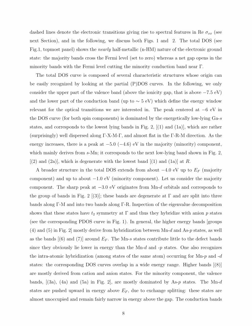
next Section), and in the following, we discuss both Figs. 1 and 2. The total DOS (see

Fig.1, topmost panel) shows the nearly half-metallic (n-HM) nature of the electronic ground

state: the majority bands cross the Fermi level (set to zero) whereas a net gap opens in the

minority bands with the Fermi level cutting the minority conduction band near Γ.

The total DOS curve is composed of several characteristic structures whose origin can

be easily recognized by looking at the partial (P)DOS curves. In the following, we only

consider the upper part of the valence band (above the ionicity gap, that is above −7.5 eV)

and the lower part of the conduction band (up to ∼ 5 eV) which define the energy window

relevant for the optical transitions we are interested in. The peak centered at −6 eV in

the DOS curve (for both spin components) is dominated by the energetically low-lying Ga-s

states, and corresponds to the lowest lying bands in Fig. 2, [(1) and (1a)], which are rather

(surprisingly) well dispersed along Γ-X-M-Γ, and almost flat in the Γ-R-M direction. As the

energy increases, there is a peak at −5.0 (−4.6) eV in the majority (minority) component,

which mainly derives from s-Mn; it corresponds to the next low-lying band shown in Fig. 2,

[(2) and (2a)], which is degenerate with the lowest band [(1) and (1a)] at R.

A broader structure in the total DOS extends from about −4.0 eV up to EF (majority

component) and up to about −1.0 eV (minority component). Let us consider the majority

component. The sharp peak at −3.0 eV originates from Mn-d orbitals and corresponds to

the group of bands in Fig. 2 [(3)]; these bands are degenerate at Γ and are split into three

bands along Γ-M and into two bands along Γ-R. Inspection of the eigenvalue decomposition

shows that these states have t2 symmetry at Γ and thus they hybridize with anion p states

(see the corresponding PDOS curve in Fig. 1). In general, the higher energy bands [groups

(4) and (5) in Fig. 2] mostly derive from hybridization between Mn-d and As-p states, as well

as the bands [(6) and (7)] around EF . The Mn-s states contribute little to the defect bands

since they obviously lie lower in energy than the Mn-d and -p states. One also recognizes

the intra-atomic hybridization (among states of the same atom) occurring for Mn-p and -d

states: the corresponding DOS curves overlap in a wide energy range. Higher bands [(8)]

are mostly derived from cation and anion states. For the minority component, the valence

bands, [(3a), (4a) and (5a) in Fig. 2], are mostly dominated by As-p states. The Mn-d

states are pushed upward in energy above EF , due to exchange splitting: these states are

almost unoccupied and remain fairly narrow in energy above the gap. The conduction bands

8

[(6a), (7a) and (8a)] are composed of Mn-d and -p states just above EF , while higher bands

[(9a)] mainly by Ga-s and As-p states. The same Mn-p,-d intra-atomic mixing is found in

the minority component above EF (the Mn-p and -d DOS are localized in the same energy

range).

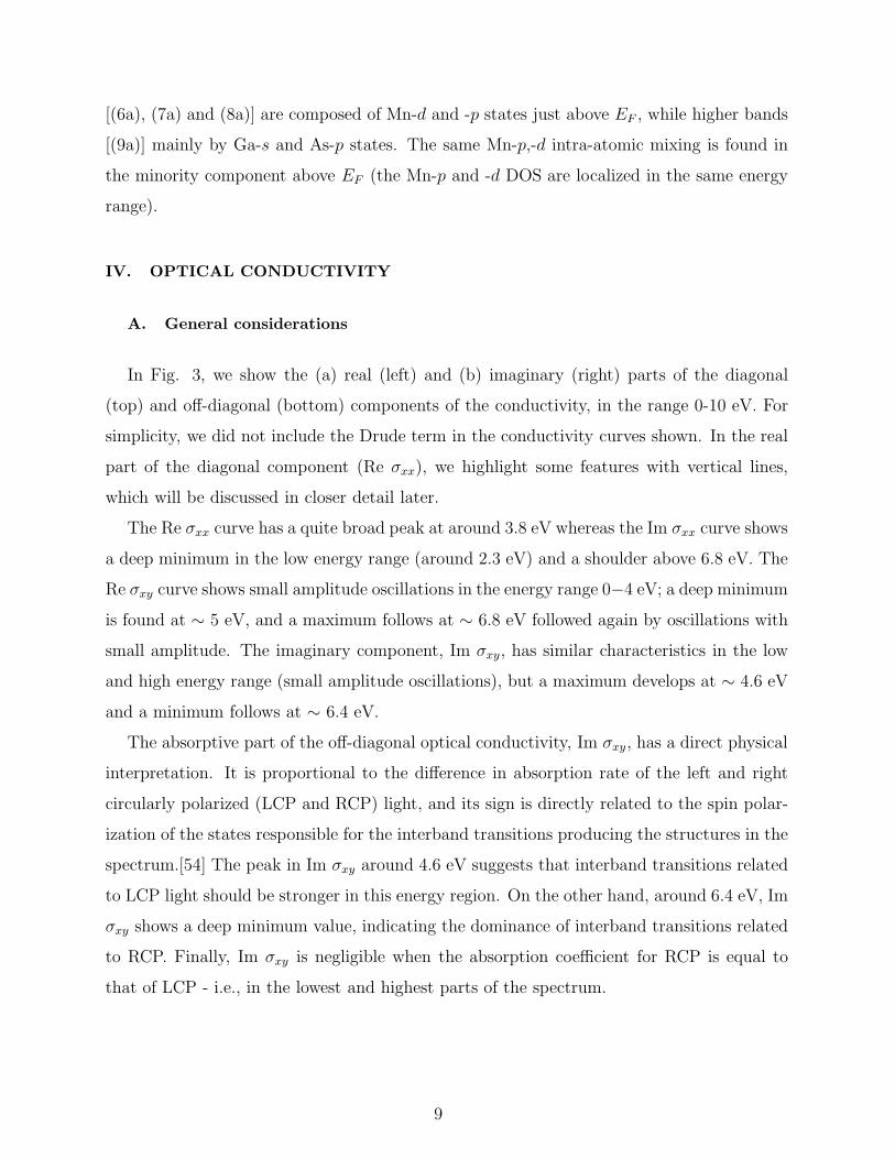
IV. OPTICAL CONDUCTIVITY

A. General considerations

In Fig. 3, we show the (a) real (left) and (b) imaginary (right) parts of the diagonal

(top) and off-diagonal (bottom) components of the conductivity, in the range 0-10 eV. For

simplicity, we did not include the Drude term in the conductivity curves shown. In the real

part of the diagonal component (Re σxx), we highlight some features with vertical lines,

which will be discussed in closer detail later.

The Re σxx curve has a quite broad peak at around 3.8 eV whereas the Im σxx curve shows

a deep minimum in the low energy range (around 2.3 eV) and a shoulder above 6.8 eV. The

Re σxy curve shows small amplitude oscillations in the energy range 0−4 eV; a deep minimum

is found at ∼ 5 eV, and a maximum follows at ∼ 6.8 eV followed again by oscillations with

small amplitude. The imaginary component, Im σxy, has similar characteristics in the low

and high energy range (small amplitude oscillations), but a maximum develops at ∼ 4.6 eV

and a minimum follows at ∼ 6.4 eV.

The absorptive part of the off-diagonal optical conductivity, Im σxy, has a direct physical

interpretation. It is proportional to the difference in absorption rate of the left and right

circularly polarized (LCP and RCP) light, and its sign is directly related to the spin polar-

ization of the states responsible for the interband transitions producing the structures in the

spectrum.[54] The peak in Im σxy around 4.6 eV suggests that interband transitions related

to LCP light should be stronger in this energy region. On the other hand, around 6.4 eV, Im

σxy shows a deep minimum value, indicating the dominance of interband transitions related

to RCP. Finally, Im σxy is negligible when the absorption coefficient for RCP is equal to

that of LCP - i.e., in the lowest and highest parts of the spectrum.

9

B. Analysis in terms of band structure

Since Re σxx is directly related to the density of states and transition probabilities,[54]

we investigate the calculated energy band structure in order to analyze the details of the

spectra. It has been known for quite some time that both the spin-orbit (SO) interaction and

the exchange splitting are needed to produce a non-zero Kerr effect.[35, 55, 56] Therefore,

a proper analysis should be performed considering the band structure with spin-orbit (SO)

included. However, we remark that the calculated band structure with SO (not shown here)

is quite similar to that formed by the superposition of the majority and minority spin bands

(without SO). This corresponds to a spin-orbit coupling interaction that is small compared

to the exchange splitting, so we can qualitatively consider the former as a perturbation

to the latter:[57] this allows us to restrict our discussion to the usual spin-polarized band

structure, thus neglecting the mixing of majority and minority spin components. In this

way, a decomposition with respect to each separate spin channel (spin up, down) can be

done; this decomposition is almost uniquely determined if the spin-orbit coupling is weak.

Inspection of the eigenvalue decomposition at Γ shows that the exchange-splitting of As-p

and Mn-degstates are ∼ 0.03 and 2.5 eV, respectively, whereas the spin-orbit splitting is ∼

0.02 and 0.002 eV, respectively. In this case, the main effect of the SO interaction is just to

remove some accidental and systematic degeneracies[58, 59, 60].

In Fig. 2, we can recognize three different contributions coming from the band structure

which build up the optical spectra: (a) close parallel bands crossing EF ; (b) bands which are

degenerate (or almost degenerate) at one point and then separate out, moving below and/or

above EF ; and (c) occupied/unoccupied bands which are almost parallel in a significant

part of the Brillouin zone.[61] The first type does contribute to the conductivity in the low

energy range and gives rise to bumps of interband transitions; the second type gives rise to

an almost constant amount of interband transitions with a distinct onset energy; the third

type gives rise to peaks at higher energies. In the following, we refer to bands although

a more appropriate discussion should be done in terms of constant eigenvalue surfaces in

reciprocal space.[62] However, the purpose of this section is to analyze on a qualitative level

the origin of the different structures in Re σxx. For this purpose, we highlight the relevant

electronic transitions (see Fig. 2) that give rise to the spectral features in the Re σxx curve

at 0.4, 1.1, 2.8 and 3.8 eV (see Fig. 3), respectively.

10

Re σxx is non-negligible already at rather low energies (as low as 0.5 eV, see Fig. 3). As

can be seen from Fig. 2, interband transitions are available at this energy due to bands which

are degenerate at some ~k points at energies slightly below (or above) EF and then separate

out, moving above EF [type (b) transitions]. For example, in the minority component, the

main contribution in this energy range comes from the two bands [(6a)] below EF , which

are degenerate at Γ and split along Γ-X and Γ-M. Incidentally, we note that the same bands

are responsible for the n-HM character of the (Ga,Mn)As compound. At very low energy,

the bands along Γ-M do contribute to the conductivity, whereas those along Γ-X do so at

higher energies.

Consider in detail the minority bands along Γ-X with energies just below EF [bands (6a)

at Γ, see Fig. 2]. A careful inspection of the eigenvalue decomposition into atomic-site-

projected wave functions shows that these bands have a prevalent d character but with a

non-negligible contribution from anion p as well as s cation states. Moving away from the

zone center, the d as well as p contributions increase in the higher energies of these bands,

while the s contribution decreases; the opposite occurs for the lower band. The d − p and

s− p mixing is crucial for the onset of the dipole transitions among these states at very low

excitation energies which otherwise would be forbidden by selection rules. Moving away from

Γ, their energy separation increases, as is typical for type (b); as the lower band crosses EF ,

the interband transitions stop contributing at an excitation energy around 0.40 eV. This

corresponds to the first flat region in Re σxx starting around 0.40 eV. Other electronic

transitions at 0.40 eV are shown in Fig. 2 with lines near the M point in the spin-up bands.

Upon further increase of the excitation energy, additional type (b) structures start con-

tributing, like the majority group of bands [(7)] above EF and degenerate at R which split

along R-Γ and R-M. In particular, along R-Γ, one band remains above EF , while the other

goes below. This causes an increase of Re σxx, at energies lower than 1.0 eV. In this energy

range, type (a) bands also contribute, like the almost parallel majority bands which cross

EF along Γ-M, and those crossing EF along Γ-X [all of them deriving from bands (6) and

(7)].

As the photon energy reaches ∼ 1.1 eV, several transitions are activated, accounting for

the bump in the conductivity. The transitions at 1.1 eV are shown with blue (dotted) lines

in Fig. 2. In the majority (minority) component, they are mainly localized near the R (Γ)

point [mostly type (c) transitions].

11

At ∼ 2.8 eV, we have a bump in the Re σxx (see Fig. 3), First, let’s consider the minority

component. The almost dispersionless occupied band around −1.0 eV [(5a)] is coupled to

the group of bands around 1.5 eV [(8a)]. These are type (c) transitions and they give rise

to the bump in Re σxx around 2.8 eV. The transitions which match the energy of 2.8 eV

are shown by red (dashed) lines in Fig. 2. In the majority component there is also a

contribution coming from the group of bands (5) and (7). As the photon energy increases,

Re σxx reaches its maximum value, at around 3.8 eV. There are several contributions to

this peak: they involve degenerate minority bands at high symmetry points, like the groups

of bands at Γ centered at −2.5 eV [(4a)] and 1.5 eV [(8a)] and at R with energies ∼−2.0 eV and 2.0 eV, respectively. In the majority components, more type (c) transitions

contribute to the maximum of Re σxx. They mainly involve groups of degenerate bands at

Γ (occupied/unoccupied) which split along Γ-M: they are not flat along this symmetry line

but are almost parallel near Γ. For instance, the highest of this group of bands [(5)] split

along Γ-M couples with the lowest of the group of bands [(8)].

As the photon energy increases, the lowest majority and minority energy bands between

−5 and −7 eV below EF come into play. The dispersion of the occupied as well as the unoc-

cupied bands involved in the transitions increases, and this correlates with the conductivity

decrease.

It can be useful to consider the role of the electrons with spin up and spin down in

shaping the spectra of Re σxx. Again, this can be done on a qualitative level only. In

fact, the dipole matrix elements enter quadratically in the calculation of the conductivity

(see Eq. 1) and interference effects can be lost by separating the spin-up or spin-down

contributions to the conductivity. Indeed, from Eq. 1, we have, for α=β=x and neglecting

the ~k index:

< n|px|n′

>< n′ |px|n >= | < n|px|n

′

> |2 (6)

where n includes the spin indices. Expressing the spin indices, and neglecting spin-flip

transitions[63, 64] we have:

| < n|px|n′

> |2 = |∑

ss′

pss′

x,nn′ |2 = |p↑↑

x,nn′ |2 + |p↓↓

x,nn′ |2 + 2Re(p↑↑

x,nn′p

↓↓∗

x,nn′ ) (7)

12

In Fig. 4, we show the two spin contributions to Re σxx, i.e. neglecting the last term

in Eq. 7, in the range 0-10 eV. Incidentally, we note that the sum of the two separate

contributions (which does not include the interference effects coming from the last term in

Eq. 7), not shown in Fig. 4, differs in some fine details from the curve shown in Fig. 3

(which naturally includes the interference effects). This confirms a posteriori that the loss

of interference effects due to neglecting the last term in Eq. 7 introduces a negligible error

and allows us to treat the two spin contributions to the conductivity separately. The two

curves are qualitatively similar, and they clearly show the origin of the bump at 2.8 eV and

the maximum at 3.8 eV: the former is mainly due to transitions involving minority while

the latter the majority spin bands. From Fig. 2 one could conclude that both the features

at 2.8 and 3.8 eV arise from minority spin band transitions: this is not exactly true due to

the role of the dipole matrix elements.

In the same Fig. 4, we also show the joint density of states (JDOS), which can be derived

from Eq. 1 by replacing the matrix elements with a constant factor set to 1 in our case.[54]

This quantity clearly highlights the role of the dipole matrix elements: as a matter of fact,

the JDOS does not show any relevant feature in the spectra stressing that the spectral

features observed occur primarily due to the very large matrix elements rather than to a

large joint density of states effect. On the same basis, the large shoulder above 6 eV in

the JDOS does not produce any peak in the conductivity spectra due to the small matrix

elements.

C. Comparison with experiments

Finally, we compare our calculations with some experimental results. For this purpose,

we consider a lower concentration x = 6.25% (1 Mn in a 32-atom cell) that is closer to

available experiments.[65, 66, 67] In Fig. 5 (a) we show the calculated real component of the

diagonal optical conductivity, Re σxx, as a function of the photon frequency, compared with

spectra obtained from experiments and model calculations [68] for Ga0.95Mn0.05As (at hole

concentration p ∼ 0.8 nm−3), in the [0.01-2] eV energy range. In this interval, our calculated

conductivity is of the order of 1-2·103 (ohm·cm)−1, i.e., remarkably larger (almost by an order

of magnitude) than the experimental values[65] but of the same order of magnitude as the

results of model calculations.[68] The disagreement with experiments may be fully explained

13

in terms of the suggested values of carrier concentration in the experimental samples: p ∼0.35 nm−3 for a Mn concentration on the order of ∼6%, with a degree of compensation on

the order of 70-80%.

In our systems, a pretty naive evaluation of the hole concentration can be obtained by

supposing that each Mn - with a nominal valence of +2 - substituting a Ga atom gives rise

to a hole; therefore, 1 Mn atom in a 32 atom cell produces a hole concentration of 1.38 nm−3.

It has been shown[68] that the hole concentration has a relevant influence on the optical

conductivity: for example, at very low energies (<0.01 eV) σxx ranged [68] from ∼ 1.5x102

to ∼ 3.5x103 (ohm·cm)−1 for hole concentrations varying from p ∼ 0.03 to 0.80 nm−3. These

values are very consistent with the range in which our conductivity falls. Looking at the

trend as a function of energy, our σxx spectrum is generally featureless, with the exception

of the minimum at 800-1000 meV - in remarkably close agreement with experimental as

well as model calculation results.[68] In the inset, we show the effect of including the Drude

contribution to the spectra in an extended energy range: as expected, only in the low

energy range (<∼ 1.5 eV) does the Drude term significantly contribute to the total spectra.

In particular, the above mentioned minimum is present in both total and interband-only

terms, but it is much more enhanced upon inclusion of the Drude term, therefore improving

the agreement with experiment.

The real and imaginary parts of the dielectric constant, ǫxx[69], are shown in Fig. 5 (b)

and (c), respectively, and compared with experimental ellipsometry measurements.[66] The

agreement is rather good, as far as the overall features are concerned. However, there is a

sizeable discrepancy in the energy position of peaks and valleys. This has probably to be

ascribed to the neglect of self–energy corrections or to the incorrect treatment of correlation

effects, resulting in an only partial description of the underlying electronic structure. In

order to improve the agreement with experiment, we used the so-called λ-fitting procedure,

suggested by Rhee et al. (see Ref. [70] for details), which is an oversimplified approach

to include a rescaling in the excitation energy spectrum, avoiding the complicated task of

properly evaluating self-energy effects. Using a value of λ ∼ −0.1 eV, both the real and

imaginary spectra were reasonably reproduced.

14

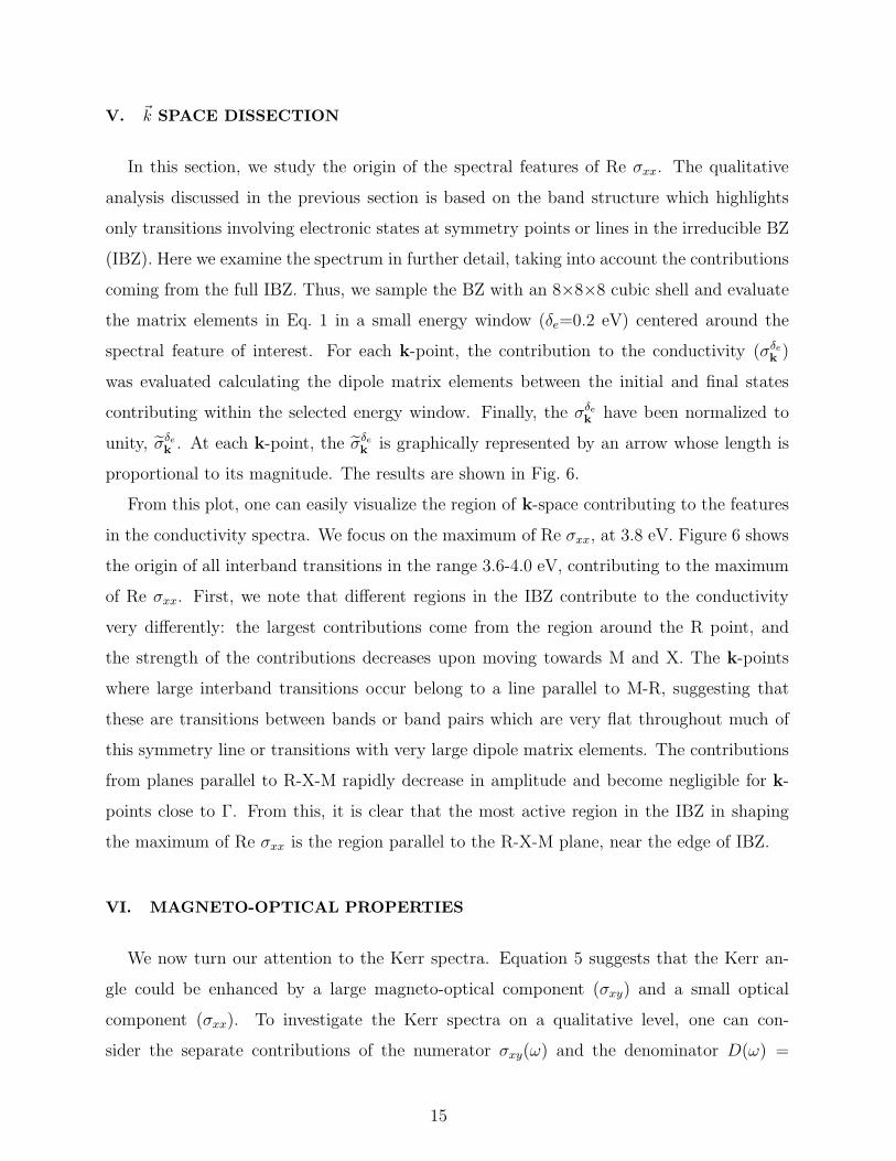
V. ~k SPACE DISSECTION

In this section, we study the origin of the spectral features of Re σxx. The qualitative

analysis discussed in the previous section is based on the band structure which highlights

only transitions involving electronic states at symmetry points or lines in the irreducible BZ

(IBZ). Here we examine the spectrum in further detail, taking into account the contributions

coming from the full IBZ. Thus, we sample the BZ with an 8×8×8 cubic shell and evaluate

the matrix elements in Eq. 1 in a small energy window (δe=0.2 eV) centered around the

spectral feature of interest. For each k-point, the contribution to the conductivity (σδe

k)

was evaluated calculating the dipole matrix elements between the initial and final states

contributing within the selected energy window. Finally, the σδe

khave been normalized to

unity, σδe

k. At each k-point, the σδe

kis graphically represented by an arrow whose length is

proportional to its magnitude. The results are shown in Fig. 6.

From this plot, one can easily visualize the region of k-space contributing to the features

in the conductivity spectra. We focus on the maximum of Re σxx, at 3.8 eV. Figure 6 shows

the origin of all interband transitions in the range 3.6-4.0 eV, contributing to the maximum

of Re σxx. First, we note that different regions in the IBZ contribute to the conductivity

very differently: the largest contributions come from the region around the R point, and

the strength of the contributions decreases upon moving towards M and X. The k-points

where large interband transitions occur belong to a line parallel to M-R, suggesting that

these are transitions between bands or band pairs which are very flat throughout much of

this symmetry line or transitions with very large dipole matrix elements. The contributions

from planes parallel to R-X-M rapidly decrease in amplitude and become negligible for k-

points close to Γ. From this, it is clear that the most active region in the IBZ in shaping

the maximum of Re σxx is the region parallel to the R-X-M plane, near the edge of IBZ.

VI. MAGNETO-OPTICAL PROPERTIES

We now turn our attention to the Kerr spectra. Equation 5 suggests that the Kerr an-

gle could be enhanced by a large magneto-optical component (σxy) and a small optical

component (σxx). To investigate the Kerr spectra on a qualitative level, one can con-

sider the separate contributions of the numerator σxy(ω) and the denominator D(ω) =

15

σxx(ω)√

1 + 4πω

σxx(ω). The corresponding features in the imaginary part of the spectra are

then correlated to those observed in the Kerr spectra. This analysis has been done in Ref. 30

by some of us, to which we refer the reader for further details. Incidentally, we note that our

spectrum (presented in Fig. 7, see below) is quite similar to those presented in Ref. [30] for

x = 6.25% and x = 12.5%. We can conclude that the main features of the Kerr spectra of

(Ga,Mn)As do not depend to a great extent on the Mn concentration, at least for the cases

considered: this further validates our choice to focus on the high concentration limit in this

study.

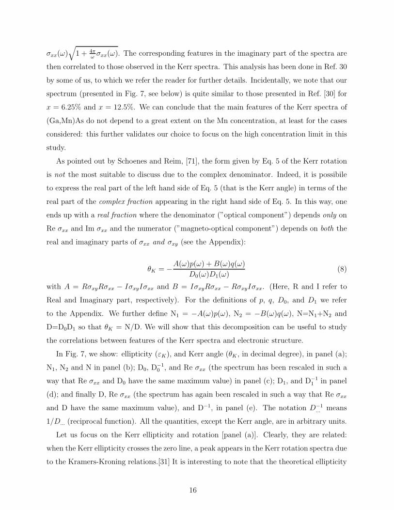
As pointed out by Schoenes and Reim, [71], the form given by Eq. 5 of the Kerr rotation

is not the most suitable to discuss due to the complex denominator. Indeed, it is possibile

to express the real part of the left hand side of Eq. 5 (that is the Kerr angle) in terms of the

real part of the complex fraction appearing in the right hand side of Eq. 5. In this way, one

ends up with a real fraction where the denominator (”optical component”) depends only on

Re σxx and Im σxx and the numerator (”magneto-optical component”) depends on both the

real and imaginary parts of σxx and σxy (see the Appendix):

θK = −A(ω)p(ω) + B(ω)q(ω)

D0(ω)D1(ω)(8)

with A = RσxyRσxx − IσxyIσxx and B = IσxyRσxx − RσxyIσxx. (Here, R and I refer to

Real and Imaginary part, respectively). For the definitions of p, q, D0, and D1 we refer

to the Appendix. We further define N1 = −A(ω)p(ω), N2 = −B(ω)q(ω), N=N1+N2 and

D=D0D1 so that θK = N/D. We will show that this decomposition can be useful to study

the correlations between features of the Kerr spectra and electronic structure.

In Fig. 7, we show: ellipticity (εK), and Kerr angle (θK , in decimal degree), in panel (a);

N1, N2 and N in panel (b); D0, D−1

0, and Re σxx (the spectrum has been rescaled in such a

way that Re σxx and D0 have the same maximum value) in panel (c); D1, and D−1

1in panel

(d); and finally D, Re σxx (the spectrum has again been rescaled in such a way that Re σxx

and D have the same maximum value), and D−1, in panel (e). The notation D−1

... means

1/D... (reciprocal function). All the quantities, except the Kerr angle, are in arbitrary units.

Let us focus on the Kerr ellipticity and rotation [panel (a)]. Clearly, they are related:

when the Kerr ellipticity crosses the zero line, a peak appears in the Kerr rotation spectra due

to the Kramers-Kroning relations.[31] It is interesting to note that the theoretical ellipticity

16

curve crosses/touches the zero axis a number of times, hence suggesting that the incident

linearly polarized light, at these frequencies, would stay as linearly polarized only. The

Kerr rotation is characterized by several spikes as well as sign reversals in the whole energy

window. In particular, there is a first magneto-optical resonance (0.56◦) at ~ω ∼ 0.2 eV

and other main peaks are located at ∼ 1, 2 and 6 eV. The arrows in the Kerr spectra mark

the main features (positive and negative). From Fig. 7 [panels (a),(b)], we see that the

shape of the Kerr spectra is mainly determined by N1 in the low energy range (0-3 eV),

by both N1 and N2 in the medium energy range (3-7 eV), and by N2 in the high energy

range (7-10 eV). Very interestingly, the overall spectral trend of the Kerr angle, such as

the peaks and sign reversal positions, are very close to that of the numerator N(ω) [panel

(b)], and only the relative heights of the spikes are different. As expected, the zero of N(ω)

fixes the zero in the Kerr spectra. We can draw the first conclusion: N(ω) determines the

overall trend of the Kerr spectra, and, in particular, the presence of maxima and minima.

We also stress that the analytic form of the numerator of the Kerr angle (see Eq. 8 and the

Appendix) entangles in a rather complicated way all the real and imaginary components of

the conductivity tensor: there is no simple guideline to link the trend of a part of the Kerr

spectra to the spectral trend of a specific (real or imaginary) tensor component in the same

energy range.

We now focus on the denominator D−1. First we write θK=N(ω)D−1(ω), so that D−1

plays the role of an enhancement factor. It is evident that both D0 and D1 are positive

definite, that is they never cross the zero line: the enhancement factor does not have any

”resonant” behavior. In Fig. 7 panel (c), we can see that, remarkably, the spectral trend of

D0 is very similar to Re σxx. We might therefore infer that D−1

0has large values whenever

Re σxx has its smallest ones. In our case, this happens when the photon energy approaches

∼ 0 eV. On the other hand, D1 [panel (d)] does not show any remarkable features, apart

from the maximum at very low energy. Considering that the reciprocal function D−1

0[panel

(c)] exhibits a maximum at ∼ 0 eV and strongly decreases with increasing energy, D−1

1has

a minimum at ∼ 0 eV and monotonically increases with energy. D−1

1is also featureless, in

almost the whole energy window. From panel (e), we see that D−1 has a large peak around ∼0.5 eV, then decreases very fast to an almost constant value, and slowly increases at energies

larger than ∼ 5 eV. Clearly, the shoulder of D−1 at low energy comes from the behavior of

D−1

0and D−1

1in the same energy range, whereas the increase of D−1 at high energy is mainly

17

due to the behavior of D−1

1in the corresponding energy range.

These results clearly explain the origin of the Kerr spike (0.56◦) at ∼ 0.2 eV. The nu-

merator determines the existence and location of the spikes: whether they give rise to a

strong Kerr angle follows entirely from the enhancement factor, D−1, which, in this case,

magnifies the peaks at low energy and suppresses those at higher energy. The importance

of D−1 is highlighted by again considering N(ω): we would expect large Kerr angle values

at higher energy (around 6 eV). However, the corresponding peaks are suppressed by the

D−1 factor. Hence, we are ready to conclude that the large Kerr peak at low energy has an

“optical” origin; the features at high energy have an MO origin (they follow the trend of the

numerator) but they do not result in large peaks due to the damped behavior of D−1 in this

same energy range. This confirms in a more transparent and direct way what was already

observed in Ref. [30] More important, the similar trend of D0(ω) (D) and Rσxx suggests

that the presence of minima in the Rσxx spectra may give rise to strong Kerr angles in the

same energy range. On the other hand, Rσxx is directly linked to the optical transitions,

that is to details of the electronic structure of the materials: this could have far reaching

consequences in magneto-optical Kerr effect engineering, provided that the electronic struc-

ture of the material can be tuned correctly in such a way as to enhance the features of the

Re σxx minima.

VII. CONCLUSION

We presented results of first-principles calculations of the magneto-optical properties of

(Ga,Mn)As within density functional theory aimed at investigating in great detail the role

of the electronic and magnetic properties in determining the magnetooptical behaviour of

the material. The spectral features of the optical tensor in the 0-10 eV energy range were

analyzed in terms of the band structure and density of states and the role of the dipole

matrix elements was highlighted in terms of Brillouin zone dissection.

We found that different types of interband transitions contribute in shaping the conduc-

tivity tensor. The dipole matrix elements play a key role greatly affecting the optical spectra

in the low as well as high energy ranges. Brillouin zone dissection reveals that different re-

gions in the Brillouin zone (not necessarily symmetry points or lines) can contribute very

differently in shaping the conductivity tensor; we find that the most active region in the IBZ

18

is around the R point.

Moreover, since the Kerr rotation spectrum is a result of a complex entanglement of real

and imaginary contrbutions, we presented a possible way to analyze the calculated Kerr

spectra in terms of a real representation of the Kerr angle. To the best of our knowledge,

this has not been used as an analysis tool in the past, although it is implicit in Eq. 5. Using

this representation, we have clearly elucidated the origin of the features of the Kerr spectra

and have highlighted the role of the minima of Re σxx which can possibly correlate with a

large Kerr angle (in our case, at low energies). Nevertheless, the results given above support

the conclusion that at present it is difficult to give simple rules for the occurrence of large

spectral features at specific laser-light frequencies. Indeed, both spin-orbit and exchange

splitting effects are entangled in N(ω), which determines the overall behavior of the Kerr

spectra and eventually the strength of the Kerr features. No simple rules can be given to

disentangle their effects on the absolute magnitude of the Kerr angle. On the other hand,

we found that part of the Kerr spectrum (in our case, the low energy range) is very sensitive

to the shape of Re σxx, which is very closely related to details of the band structure of the

materials.

While it is obvious that without a precise knowledge of the material band structure it is

not possible to make a priori predictions of the Kerr angle magnitude, it is also true that

a proper tuning of the band structure would allow one to consequently tune the magnitude

and location of spectral peaks through the D0 term, whose spectral behavior is very close

to Re σxx. However, further studies are needed in order to better elucidate how this proper

tuning of the underlying electronic structure can be achieved (i.e. by making use of alloying,

pressure, strain field) in order to enhance the minima of Re σxx. Therefore, we expect that

computational materials design can substantially contribute to magneto-optical Kerr effect

engineering in the future.

VIII. ACKNOWLEDGMENTS

One of the authors (A. Stroppa) thanks G. Kresse for useful comments and fruitful dis-

cussions; this work started during a stay at Dipartimento di Fisica Teorica, Universita degli

Studi di Trieste, Strada Costiera 11, I-34014 Trieste, Italy and INFM-CNR DEMOCRITOS

National Simulation Center, Trieste, Italy.

19

Work at Northwestern University was supported by the United States NSF (through its

MRSEC program at the Materials Research Center).

APPENDIX

Here we give an explicit representation of the complex Kerr angle (θk + iηk, Eq. 5) in the

form α+iβ, where α and β are real functions: the Kerr angle (θk) corresponds to α. To

this end, we need to calculate the square root of the complex number in the denominator of

Eq. 5. It can be helpful to make use of the following formula[72]: given√

a + ib = p + iq we

have

p =1√2

√√a2 + b2 + a q =

sgn(b)√2

√√a2 + b2 − a (9)

where sgn(b) is the sign of b. In our case,

√1 +

4πi

ωσxx =

√(1 − 4π

ωIσxx) + i

4π

ωRσxx

where R and I stand for real and imaginary part and a = 1 − 4πω

Iσxx, b = 4πω

Rσxx. By

definition, b is positive.

In order to get rid of the complex number in the denominator of Eq. 5, we multiply

numerator and denominator by σ∗xx(p − iq). After some algebra, we express:

θk + iηk = −(Ap + Bq) + i(Bp − Aq)

D0D1

(10)

Then the Kerr angle is:

θk = −(Ap + Bq)

D0D1

(11)

and the ellipticity is:

ηk =Aq − Bp

D0D1

(12)

where A = RσxyRσxx + IσxyIσxx, B = IσxyRσxx − RσxyIσxx, D0 = (Rσxx)2 + (Iσxx)

2 and

D1 =√

(1 − 8πω

)Iσxx + 16π2

ω2 D0

In this representation, an explicit analytic relation for the Kerr spike can be derived using

the Kramers-Kroning transformation: whenever the ellipticity vanishes, a spike in the Kerr

spectra appears.[31] Thus, imposing that ηk = 0, we derive an analytic relation for θk which

20

holds for the maximum or minimum in the Kerr spectra corresponding to zero ellipticity.

From ηk = 0, we have either (a) A = Bp

qor (b) B = Aq

pand using Eq. 11 we obtain:

θk = −Ap2 + q2

pD0D1

= −Bp2 + q2

qD0D1

(13)

A necessary condition to produce a Kerr spike is that AB

= p

q.

[1] J. Kerr, Philos. Mag. 3, 321 (1877).

[2] K. H. J. Buschow, P. G. van Engen, and R. Jongebreur, J. Magn. Mater. 38, 1 (1983).

[3] M. Hartmann, B. A. J. Jacobs, and J. J. M. Braat, Philips Tech. Rev. 42, 37 (1985).

[4] R. Waser, Nanoelectronics and Information Technology: Advanced Electronic Materials and

Novel Devices (Wiley, Weinheim, 2003).

[5] C. D. Mee and E. D. Daniel, Magnetic Recording (McGraw-Hill, New York, 1987).

[6] M. Mansuripur, The Physical Principles of Magneto-Optical Recording (Cambridge University

Press, New York, 1995).

[7] F. Schmidt, W. Rave, and A. Hubert, IEEE Trans. Magn. 21, 1596 (1985); D. A. Herman,

Jr., and B. E. Argyle, IEEE Trans. Magn. 22, 772 (1986).

[8] R. Q. Wu and A. J. Freeman, J. of Magn. Magn. Mat. 200, 498 (1999).

[9] S. D. Bader, E. R. Moog, and P. Grunberg, J. Magn. Magn. Mater. 53, L295 (1986).

[10] W. Reim, O. E. Huesser, J. Schoenes, E. Kaldis, P. Wachter, and K. Seiler, J. Appl. Phys.

55, 2155 (1984).

[11] J. L. Erskine and E. A. Stern, Phys. Rev. B 8, 1239 (1973).

[12] W. Reim and P. Wachter, Phys. Rev. Lett. 55, 871 (1985).

[13] H. Ohno, Science 281, 51 (1998), and references therein.

[14] Y. Ohno, D. K. Young, B. Beschoten, F. Matsukura, H. Ohno, and D. D. Awschalom, Nature

(London), 402, 790 (1999).

[15] H. Ohno, D. Chiba, F. Matsukura, T. Omiya, E. Abe, T. Dietl, Y. Ohno, and K. Ohtani,

Nature (London), 408, 944 (2000).

[16] H. Ohno, H. Munekata, T. Penney, S. von Molnar, and L. L. Chang, Phys. Rev. Lett. 68,

2664 (1992).

21

[17] H. Munekata, H. Ohno, S. von Molnar, A. Segmoller, L. L. Chang, and L. Esaki, Phys. Rev.

Lett. 63, 1849 (1989).

[18] H. Ohno, A. Shen, F. Matsukura, A. Oiwa, A. Endo, S. Katsumoto, and Y. Iye, Appl. Phys.

Lett. 69, 363 (1996).

[19] J. A. Gaj, R. R. Galazka, M. Nawrocki, Solid State Commun., 25, 193 (1978).

[20] A. E. Turner, R. L. Gunshor, S. Datta, Appl. Opt., 22, 3152 (1983).

[21] K. Onodera, T. Masumoto, M. Kimura, Electron. Lett., 30, 1954 (1994).

[22] S. Sugano and N. Kojima, Magneto-Optics (Berlin, Springer-Verlag, 2000).

[23] S. Sanvito, G. J. Theurich, and N. A. Hill, J. Supercond. 15, 85 (2002).

[24] G. Bouzerar, J. Kudrnovsky’, L. Bergqvist, P. Bruno, Phys. Rev. B 68, 081203 (R) (2003).

[25] P. Mahadevan, A. Zunger, Phys. Rev. B 68 075202 (2003).

[26] M. van Schilfgaarde and O. N. Mryasov, Phys. Rev. B 63 233205 (2001).

[27] L. Bergqvist, P. A. Korzhavyi, B. Sanyal, S. Mirbt, I. A. Abrikosov, L. Nordstrom, E. A.

Smirnova, P. Mohn, P. Svedlindh, and O. Eriksson, Phys. Rev. B 67 205201 (2003).

[28] L. M. Sandratskii, P. Bruno and J. Kudrnovsky’, Phys. Rev. B 69, 195203 (2004).

[29] A. B. Shick, J. Kudrnovsky, and V. Drchal, Phys. Rev. B 69, 125207 (2004).

[30] S. Picozzi, A. Continenza, M. Kim, A. J. Freeman, Phys. Rev. B 73, 235207 (2006).

[31] H. Weng, Y. Kawazoe, and J. Dong, Phys. Rev. B, 74, 85205 (2006).

[32] H. Weng, J. Dong, T. Fukumura, M. Kawasaki, and Y. Kawazoe, Phys. Rev. B, 74, 115201

(2006).

[33] E. Wimmer, H. Krakauer, M. Weinert and A. J. Freeman, Phys. Rev. B 24, 864 (1981); H.J.

F.Jansen and A. J. Freeman, Phys. Rev. B 30,561 (1984).

[34] L. Hedin and B. I. Lundqvist, J. Phys. C4, 2064 (1971).

[35] H. R. Hulme, Proc. R. Soc. (London) Ser. A 135, 237 (1932).

[36] C. Kittel, Phys. Rev. 83, A208 (1951).

[37] R. Kubo, J. Phys. Soc. Japan 12, 570 (1957).

[38] C. S. Wang and J. Callaway, Phys. Rev. B 9, 4897 (1974).

[39] M. Singh, C. S. Wang, and J. Callaway, Phys. Rev. B 11, 287 (1975).

[40] P. Drude, Phys. Z. 1 , 161 (1900).

[41] A. Sommerfeld and H. Bethe, Handbuch der Physik (Springer-Verlag, Berlin, 1933).

[42] A. P. Lenham and D. M. Treherne, in Optical and Electronic Structure of Metals and Alloys,

22

edited by F. Abels (North-Holland, Amsterdam, 1966).

[43] V. Antonov, B. Harmon and A. Yaresko, Electronic Structure and Magneto-Optical Properties

of Solids (Kluwer Academic, Dordrecht, 2004).

[44] R. P. Feynman, Phys. Rev. 56, 340 (1939).

[45] H. J. Monkhorst and J. D. Pack, Phys. Rev. B 13,5188 (1976).

[46] M. Jain, L. Kronik, J. R. Chelikowsky, V. V. Godlevsky, Phys. Rev. B 64, 245205 (2001).

[47] B. Sanyal and S. Mirbt, Journal of Magnetism and Magnetic Materials 290-291, 1408 (2005).

[48] E. Kulatov, H. Nakayama, H. Mariette, H. Ohta, and Y. A. Uspenskii Phys. Rev. B 66, 045203

(2002).

[49] H. Katayama-Yoshida and K. Sato, Physica B 327, 337 (2003).

[50] Y. J. Zhao, W. T. Geng, K. T. Park, and A. J. Freeman, Phys. Rev. B 64, 35207 (2001).

[51] M. Jain, L. Kronik, J. R. Chelikowsky, and V. V. Godlevsky, Phys. Rev. 64, 245205 (2001).

[52] S. H. Wei, X. G. Gong, G. M. Dalpian and S. H. Wei, Phys. Rev. B 71, 144409 (2005).

[53] R. Wu, Phys. Rev. Lett. 94, 207201 (2005).

[54] H. Ebert, Rep. Prog. Phys. 59, 1665 (1996).

[55] P. N. Argyres, Phys. Rev. 97, 334 (1955).

[56] J. L. Erskine, E. A. Stern, Phys. Rev. B 8, 1239 (1973).

[57] M. Singh, C. S. Wang, and J. Callaway, Phys. Rev. B 11, 287 (1975).

[58] In this framework, accidental degeneracy corresponds to an almost equal energy level for the

spin-up and spin-down states, i.e. a crossing of spin-up and spin-down curves at some k-

point in Fig. 2. The inclusion of spin-orbit coupling may lead to a repulsion of the crossing

majority and minority bands. On the other hand, systematic degeneracy corresponds to the

usual degeneracy imposed by all the transformations of the spatial symmetry group.

[59] B. R. Watts, J. Phys. C: Solid State. Phys. 6, 3605 (1973).

[60] G. B. Shaw, J. Phys. A.: Math., Nucl. Gen., 7, 1537 (1974).

[61] W. A. Harrison, Phys. Rev. 147, 467 (1966)

[62] H. Ehrenreich, H. R. Philip, and B. Segall, Phys. Rev. 132, 1918 (1963).

[63] Spin-flip transitions are allowed within the electric dipole approximation when spin-orbit cou-

pling is included, but are omitted in our work since their effect is negligible.

[64] D. K. Misemer, J. Magn. Magn. Mater. 12, 267 (1988).

[65] E. J. Singley, R. Kawakami, D. D. Awschalom and D. N. Basov, Phs. Rev. Lett. 89, 097203

23

(2002); E. J. Singley, K. S. Burch, R. Kawakami, J. Stephens, D. D. Awschalom and D. N.

Basov, Phys. Rev. B 68, 165204 (2003).

[66] K. S. Burch, J. Stephens, R. K. Kawakami, D. D. Awschalom, and D. N. Basov, Phys. Rev.

B.70, 205208 (2004).

[67] E. Kojima, R. Shimano, Y. Hashimoto, S. Katsumoto, Y. Iye, and M. Kuwata-Gonokami,

Phys. Rev. B 68, 193203 (2003).

[68] E. M. Hankiewicz, T. Jungwirth, T. Dietl, C. Timm and J. Sinova, Phys. Rev. 70, 245211

(2004).

[69] The dielectric constant and conductivity enter into a determination of the optical properties

of a solid in the combination: εαβ(ω) = δαβ + 4πiω

σαβ(ω).

[70] J. Y. Rhee, B. N. Harmon and D. W. Lynch, Phys. Rev. B 55, 4124 (1997).

[71] J. Schoenes and W. Reim, Phys. Rev. Lett. 60, 1988 (1988).

[72] S. Rabinowitz, Mathematics and Informatics Quarterly, 3, 54 (1993).

24

FIG. 1: Total and atomic- angular momentum- projected density of states (DOS) in Ga.75Mn.25As.

Positive and negative curves refer to spin-up and spin-down components, respectively. The Fermi

level is fixed at zero energy.

FIG. 2: (Color on line) Spin-polarized band structure for Ga.75Mn.25GAs along the symmetry lines

Γ-X-M-Γ-R-M in the irreducible BZ plotted without spin-orbit interaction for clarity: parts (a) and

(b) refer to spin-up (-down), respectively. The horizontal line marks the Fermi level (zero energy).

Numbers in round brackets at Γ label groups of bands discussed in the text. The vertical lines

indicate the different possible band to band transitions at 0.4, 1.1, 2.8, 3.8 eV within 0.1 eV (solid

black, dotted blue, dashed red and dot-dashed orange respectively). The labels for symmetry points

and lines are according to the standard group-theoretical notation of Bouckaert, Smoluchowski, and

Wigner. Spin-orbit effects are neglected.

25

FIG. 3: Calculated real (a) and imaginary (b) parts of diagonal and off-diagonal components of

the optical conductivity. The Drude term has not been included in the spectra. Vertical lines in

Re σxx indicate features discussed in the text.

FIG. 4: Selected contributions from spin-up (solid line) and spin-down (dashed line) transitions to

the total Re σxx spectra. The joint density of states (JDOS) is also reported, in arbitrary units.

FIG. 5: (a) Real part of the diagonal conductivity: our calculated spectrum (bold line) is compared

with the results of model calculations (dashed line) from Ref.[68] and experiments (dotted line)

from Ref.[65]. The inset in panel (a) shows the difference between the interband and the total

(interband + intraband) conductivity. Panels (b) and (c) show the calculated real and imaginary

parts of the dielectric constant, respectively, with (bold line) and without (dashed line) λ fitting.

Ellipsometry results from Ref.[66] are also shown (solid line).

FIG. 6: Prospective view of the irreducible wedge of Brillouin zone showing the origin of the

interband transitions at ∼ 3.8 eV. The length of the arrows shows the relative contributions to Re

σxx in the energy interval 3.6-4.0 eV (see Fig. 3). Increasing of the length of the arrows represents

an increasing contribution. See text for further details.

FIG. 7: (Color online) (a) Ellipticity and Kerr angle; the main features of the Kerr spectra are

indicated by arrows; (b) Different contributions to the numerator of the formula presented in

Sect. VI and the Appendix (arrows indicate the main spectral features); (c,d,e) decomposition

of the denominator (see text for details). Arbitrary units are used except for the Kerr angle (in

decimal degree). See text for details.

26

-4

0

4

8Totald Mn

-0.2

-0.1

0.0

0.1

0.2s Mnp Mn

-0.4

0.0

0.4 s Asp As

-8 -6 -4 -2 0 2 4

-0.4

0.0

0.4 s Gap Ga

DO

S(s

tate

s/eV

cel

l)

E-Ef (eV)

(a)

(b)

(c)

(d)

Fig. 1

27

Fig. 2

28

0

1

2

3

4

5

6

-3

-2

-1

0

1

2

3

4

0 1 2 3 4 5 6 7 8 9 10

-5

0

5

0 1 2 3 4 5 6 7 8 9 10

-6

-4

-2

0

2

4

6

Re[σxx

(ω)] Im[σxx

(ω)]

Re[σxy

(ω)] Im[σxy

(ω)]

(Ga1-x

Mnx)As, x=25 %

σ ij(1015

s-1

)

E(eV) E(eV)

1.1 eV

2.8 eV

3.8 eV

0.4 eV

(a) (b)

Fig. 3

29

0 1 2 3 4 5 6 7 8 9 100

1

2

3

4

5

JDOS (arbitrary units)updown

(Ga1-x

Mnx)As, x=25 %

Re[

σ xx(ω

)] (1

015 s

-1)

E (eV)

Fig. 4

30

1 2 3 4 5 6E (eV)

-20

-10

0

10

20

Re

ε xx

Expt. (Ref. 67)This workThis work + λ

1 2 3 4 5 6E (eV)

0

10

20

30

Im ε

xx

1E (eV)

103

104

σ xx

TotalInterband

0.01 0.1 1E (eV)

102

103

Re

σ xx (

ohm

-1cm

-1)

This workModel calc. (Ref. 69)Expt. (Ref. 66)(a)

(b) (c)

Fig. 5

31

Fig. 6

32

-0.6-0.4-0.20.00.2

ΘKε

K

-10-40

10-4

N1N2N

0

10-2 D0σ

xx

0

103

D-1

0

0

10

20

30D1

00.20.40.60.8

D1-1

0

102

D-1

0 2 4 6 8 100

0.04

0.08Dσ

xx

E(ev)

(a)

(b)

(c)

(d)

(e)

(Ga,Mn)As

(arb

. uni

ts)

Fig. 7

33